Essays on Private Equity

Giommetti, Nicola

Document VersionFinal published version

Publication date:2022

LicenseUnspecified

Citation for published version (APA):Giommetti, N. (2022). Essays on Private Equity. Copenhagen Business School [Phd]. PhD Series No. 03.2022

Link to publication in CBS Research Portal

General rightsCopyright and moral rights for the publications made accessible in the public portal are retained by the authors and/or other copyright ownersand it is a condition of accessing publications that users recognise and abide by the legal requirements associated with these rights.

Take down policyIf you believe that this document breaches copyright please contact us (research.lib@cbs.dk) providing details, and we will remove access tothe work immediately and investigate your claim.

Download date: 29. Oct. 2022

ESSAYS ON PRIVATE EQUITY

Nicola Giommetti

CBS PhD School PhD Series 03.2022

PhD Series 03.2022ESSAYS ON

PRIVATE EQUITY

COPENHAGEN BUSINESS SCHOOLSOLBJERG PLADS 3DK-2000 FREDERIKSBERGDANMARK

WWW.CBS.DK

ISSN 0906-6934

Print ISBN: 978-87-7568-059-7

Online ISBN: 978-87-7568-060-3

Essays on Private Equity

Nicola Giommetti

Supervisor: Steffen Andersen

CBS PhD SchoolCopenhagen Business School

1

Nicola GiommettiEssays on Private Equity

1st edition 2022 PhD Series 03.2022

© Nicola Giommetti

ISSN 0906-6934

Print ISBN: 978-87-7568-059-7Online ISBN: 978-87-7568-060-3

The CBS PhD School is an active and international research environment at Copenhagen Business School for PhD students working on theoretical and empirical research projects, including interdisciplinary ones, related to economics and the organisation and management of private businesses, as well as public and voluntary institutions, at business, industry and country level.

All rights reserved.No parts of this book may be reproduced or transmitted in any form or by any means, electronic or mechanical, including photocopying, recording, or by any information storage or retrieval system, without permission in writing from the publisher.

Acknowledgments

This thesis could not be possible without the support, advice, and encouragement of

those who helped me throughout the process. I owe them a great deal, probably more

than I can ever repay, and I would like to take this opportunity to say thank you.

First, I would like to thank Morten Sorensen, whose support as advisor and co-author

has been invaluable. Morten taught me most of what I know about research, and working

with him has been a privilege and a real pleasure. I will always be thankful for the effort

and time he has put towards my development as an economist.

I owe great thanks also to Steffen Andersen, who first introduced me to research work.

I was fortunate to assist Steffen in his projects during my Master’s studies, and that

experience convinced me to start a PhD in the first place. Steffen has supported and

helped me ever since, and I owe him a great deal.

I am grateful to Copenhagen Business School and the Department of Finance for sup-

porting my research and for providing a great working environment. I met many smart

and talented colleagues at the Department of Finance. I would like to thank especially

my co-author and friend, Rasmus Jørgensen, who shared with me much of the pain and

pleasure of writing a PhD thesis. Thanks also to Lena Jaroszek for the many refreshing

conversations about life and research.

Last but not least, I would like to thank my family for their unconditional love and

support throughout the years.

3

4

Abstract

This thesis concerns risk and performance of private equity funds. Private equity funds are

illiquid investments with mostly unobservable returns and with special institutional rules

distinguishing them from other assets typically considered in finance. This thesis studies

(i) how to risk-adjust the performance of private equity funds using data on cash flows

instead of returns, and (ii) how to optimally allocate capital between private equity and

publicly traded assets. It consists of three chapters which can be read independently.

The first chapter concerns risk adjustment of private equity cash flows. Recent liter-

ature has developed methods to risk-adjust private equity cash flows using stochastic

discount factors (SDFs). In this chapter, we find that those methods result in unrealistic

time discounting, which can generate implausible performance estimates. We propose

and evaluate a modified method which estimates a set of SDF parameters so that the

subjective term structure of interest rates is determined by market data. Our method

is based on a decomposition of private equity performance in a risk-neutral part and a

risk adjustment, and it keeps the risk-neutral part constant as we add or remove risk

factors from the SDF. We show that (i) our approach allows for economically meaning-

ful measurement and comparison of risk across models, (ii) existing methods estimate

implausible performance when time discounting is particularly degenerate, and (iii) our

approach results in lower variation of performance across funds.

The second and third chapters study optimal portfolio allocation with private equity

funds and publicly traded assets. In the second chapter, we study the portfolio problem

of an investor (or limited partner, LP) that invests in stocks, bonds, and private equity

funds. Stocks and bonds are liquid assets, while private equity is illiquid. The LP repeat-

edly commits capital to private equity funds. This capital is only gradually contributed

and eventually distributed back to the LP, requiring the LP to hold a liquidity buffer

for its uncalled commitments. We solve the problem numerically for LPs with different

5

risk aversion, and we find that optimal private equity allocation is not monotonically

declining in risk aversion, despite private equity being riskier than stocks. We investigate

the optimal dynamic investment strategy of two LPs at opposite ends of the risk aversion

spectrum, and we find two qualitatively different strategies with intuitive heuristics. Fur-

ther, we introduce a secondary market for private equity partnership interests to study

optimal trading in this market and implications for the LP’s optimal investments.

The third chapter considers a portfolio problem with private equity and several liquid

assets. This chapter focuses on average portfolio allocation over time, as opposed to

dynamic strategies generating that allocation, and derives an approximate closed-form

solution despite complex private equity dynamics. In this chapter, optimal portfolio al-

location is well approximated by static mean-variance optimization with margin require-

ments. Margin requirements are self-imposed by the investor, and because private equity

needs capital commitment, the investor assigns greater margin requirement to private

equity than liquid assets. Due to that greater margin requirement, the risky portfolio of

constrained investors can optimally underweight private equity relative to the tangency

portfolio, even when private equity has positive alpha and moderately high beta with

respect to liquid assets.

6

Abstract in Danish

Denne afhandling omhandler kapitalfondes risiko og afkast. Kapitalfonde foretager il-

likvide investeringer hvis afkast er vanskeligt at observere før fondene udløber og som

er underlagt særlige institutionelle regler hvilket adskiller dem fra de investeringer man

typisk undersøger i finansiel økonomi. Denne afhandling undersøger (i) hvordan man

risikojusterer kapitalfondes afkast ved hjælp af pengestrømsdata, og (ii) hvordan man

allokerer kapital optimalt mellem kapitalfonde og andre aktiver som noterede aktier og

obligationer. Afhandlingen består at tre kapitler der kan læses uafhængigt af hinan-

den.

Det første kapitel omhandler risikojustering af kapitalfondes pengestrømme. Tidligere

litteratur har udviklet metoder til at risikojustere kapitalfondes pengestrømme ved hjælp

af stokastiske diskonteringsfaktorer (SDF). I dette kapitel finder vi, at disse metoder

resulterer i en urealistisk diskontering af fremtidige pengestrømme, hvilket kan generere

urealistiske estimater. Vi fremsætter og evaluerer en modificeret metode, der estimerer et

sæt af SDF-parametre således at den subjektive rentekurve er bestemt af markedsdata.

Vores metode er baseret på en dekomponering af kapitalfondes performance i en risiko-

neutral del og en risikojustering, og metoden holder den risiko-neutrale del konstant, hvis

vi tilføjer eller fjerner risikofaktorer fra den stokastiske diskonteringsfaktor. Vi viser at (i)

vores metode foranlediger en økonomisk meningsfyldt måling og sammenligning af risiko

på tværs af modeller, (ii) vores metode er at foretrækker når diskontering af fremtidige

pengestrømme er særlig problematisk og (iii) vores metode resulterer i mindre variation

i afkast på tværs af fonde.

Det andet og tredje kapitel undersøger optimal porteføljeallokering mellem kapitalfonde

og noterede aktiver. I det andet kapital undersøger vi porteføljeproblemet for en investor

(eller limited partner, LP) der investerer i aktier, obligationer og kapitalfonde. Aktier

7

og obligationer er likvide aktiver, mens kapitalfonde er illikvide. LP’en giver løbende in-

vesteringstilsagn til kapitalfonde. Kapital trækkes gradvist og returneres til sidst, hvilket

kræver at LP’en holder en likviditetsreserve. Vi løser modellen numerisk for LP’er med

varierende grade af risikoaversion og finder, at den optimal allokering til kapitalfonde ikke

er monotont aftagende i risikoaversion på trods af, at kapitalfonde er mere risikofyldte

end aktier. Vi undersøger den optimale dynamiske investeringsstrategi for to LP’er, i

modsatte ender af risikoaversions spekteret, og finder to kvalitativt forskellige strategier

med intuitive heuristikker. Derudover introducerer vi et sekundært marked for partner-

skabsandel i kapitalfonde med henblik på at undersøge optimal handel i dette marked

samt implikationer for LP’ens optimale investeringer.

Det tredje kapitel undersøger et porteføljeproblem med kapitalfonde og adskillige likvide

aktiver. Dette kapitel fokuserer på porteføljeallokering over tid, i modsætning til de dy-

namiske strategier der genererer allokeringen, og udleder en approksimativ analytisk løs-

ning på lukket form på trods af de komplekse kapitalfonds dynamikker. I dette kapitel er

den optimal kapitalfonds allokering tilnærmelsesvist givet ved statisk middelværdi-varians

optimering med marginkrav, og marginkravet er opstår endogent som et resultat af inve-

storens optimalitetsbetingelser. Fordi kapitalfonde kræver investeringstilsagn, pålægger

investoren kapitalfonde større marginkrav end likvide aktiver. Som følge af det større

marginkrav er kapitalfonde undervægtet relativt til tangensporteføljen, selv hvis kapi-

talfonde udviser positiv risikojusteret afkast og et moderat beta med hensyn til likvide

aktiver.

8

Contents

Acknowledgments 3

Abstract 5

Abstract in Danish 7

1 Risk Adjustment of Private Equity Cash Flows 11

1.1 Risk adjustment of private equity cash flows . . . . . . . . . . . . . . . . . . 15

1.2 Stochastic discount factor . . . . . . . . . . . . . . . . . . . . . . . . . . . . 19

1.2.1 CAPM and long-term investors . . . . . . . . . . . . . . . . . . . . . 20

1.2.2 A model of discount rate news . . . . . . . . . . . . . . . . . . . . . . 21

1.3 Expected returns and discount rate news . . . . . . . . . . . . . . . . . . . . 22

1.3.1 Public market data . . . . . . . . . . . . . . . . . . . . . . . . . . . . 22

1.3.2 VAR estimation . . . . . . . . . . . . . . . . . . . . . . . . . . . . . . 23

1.4 Private equity performance . . . . . . . . . . . . . . . . . . . . . . . . . . . . 24

1.4.1 Funds data . . . . . . . . . . . . . . . . . . . . . . . . . . . . . . . . 24

1.4.2 Buyout . . . . . . . . . . . . . . . . . . . . . . . . . . . . . . . . . . . 26

1.4.3 Venture Capital . . . . . . . . . . . . . . . . . . . . . . . . . . . . . . 30

1.4.4 Generalist . . . . . . . . . . . . . . . . . . . . . . . . . . . . . . . . . 32

1.5 Robustness . . . . . . . . . . . . . . . . . . . . . . . . . . . . . . . . . . . . 33

1.5.1 Risk aversion . . . . . . . . . . . . . . . . . . . . . . . . . . . . . . . 33

1.5.2 Investor’s leverage . . . . . . . . . . . . . . . . . . . . . . . . . . . . 35

1.6 Conclusion . . . . . . . . . . . . . . . . . . . . . . . . . . . . . . . . . . . . . 36

Figures . . . . . . . . . . . . . . . . . . . . . . . . . . . . . . . . . . . . . . . 41

Tables . . . . . . . . . . . . . . . . . . . . . . . . . . . . . . . . . . . . . . . 49

Appendix . . . . . . . . . . . . . . . . . . . . . . . . . . . . . . . . . . . . . 58

2 Optimal Allocation to Private Equity 63

2.1 Model . . . . . . . . . . . . . . . . . . . . . . . . . . . . . . . . . . . . . . . 66

9

2.1.1 Preferences and Timing . . . . . . . . . . . . . . . . . . . . . . . . . 67

2.1.2 Linear fund dynamics . . . . . . . . . . . . . . . . . . . . . . . . . . . 69

2.1.3 Distributional assumptions and parameters . . . . . . . . . . . . . . . 75

2.1.4 Reduced portfolio problem . . . . . . . . . . . . . . . . . . . . . . . . 77

2.1.5 Liquidity constraint . . . . . . . . . . . . . . . . . . . . . . . . . . . . 78

2.2 Optimal allocation to private equity . . . . . . . . . . . . . . . . . . . . . . . 80

2.2.1 Value function . . . . . . . . . . . . . . . . . . . . . . . . . . . . . . . 84

2.2.2 Optimal new commitments . . . . . . . . . . . . . . . . . . . . . . . . 84

2.2.3 Optimal stock and bond allocation . . . . . . . . . . . . . . . . . . . 88

2.2.4 Optimal consumption . . . . . . . . . . . . . . . . . . . . . . . . . . . 92

2.3 Secondary market . . . . . . . . . . . . . . . . . . . . . . . . . . . . . . . . . 92

2.3.1 Gains from trade . . . . . . . . . . . . . . . . . . . . . . . . . . . . . 93

2.3.2 Insuring liquidity shocks . . . . . . . . . . . . . . . . . . . . . . . . . 95

2.4 Explicit management fees . . . . . . . . . . . . . . . . . . . . . . . . . . . . 98

2.4.1 Optimal allocation with explicit management fees . . . . . . . . . . . 102

2.5 Conclusion . . . . . . . . . . . . . . . . . . . . . . . . . . . . . . . . . . . . . 106

Appendix . . . . . . . . . . . . . . . . . . . . . . . . . . . . . . . . . . . . . 110

3 Private Equity with Leverage Aversion 133

3.1 Model . . . . . . . . . . . . . . . . . . . . . . . . . . . . . . . . . . . . . . . 136

3.1.1 Private equity . . . . . . . . . . . . . . . . . . . . . . . . . . . . . . . 136

3.1.2 Investor . . . . . . . . . . . . . . . . . . . . . . . . . . . . . . . . . . 138

3.1.3 Optimization problem . . . . . . . . . . . . . . . . . . . . . . . . . . 139

3.2 Private equity with leverage aversion . . . . . . . . . . . . . . . . . . . . . . 141

3.3 Optimal allocation . . . . . . . . . . . . . . . . . . . . . . . . . . . . . . . . 145

3.3.1 Reaching for yield . . . . . . . . . . . . . . . . . . . . . . . . . . . . . 146

3.3.2 Benchmarking private equity . . . . . . . . . . . . . . . . . . . . . . . 148

3.3.3 Numerical examples with two risky assets . . . . . . . . . . . . . . . 149

3.4 Dynamic objective . . . . . . . . . . . . . . . . . . . . . . . . . . . . . . . . 153

3.4.1 Idiosyncratic risk . . . . . . . . . . . . . . . . . . . . . . . . . . . . . 156

3.5 Conclusion . . . . . . . . . . . . . . . . . . . . . . . . . . . . . . . . . . . . . 160

Appendix . . . . . . . . . . . . . . . . . . . . . . . . . . . . . . . . . . . . . 165

10

Risk Adjustment of Private Equity Cash Flows

Nicola Giommetti Rasmus Jørgensen∗

Abstract

Existing stochastic discount factor methods for the valuation of private equity funds

result in unrealistic time discounting. We propose and evaluate a modified method.

Valuation has a risk-neutral component plus a risk adjustment, and we fix the risk-

neutral part by constraining the subjective term structure of interest rates with

market data. We show that (i) our approach allows for economically meaningful

measurement and comparison of risk across models, (ii) existing methods estimate

implausible performance when time discounting is particularly degenerate, and (iii)

our approach results in lower cross-sectional variation of performance.

∗Nicola Giommetti is from Copenhagen Business School (ngi.fi@cbs.dk) and Rasmus Jørgensen is fromCopenhagen Business School and ATP (rjo@atp.dk). We are grateful to the Private Equity ResearchConsortium (PERC) and the Insitute of Private Capital (IPC) for data access and support.

Chapter 1

11

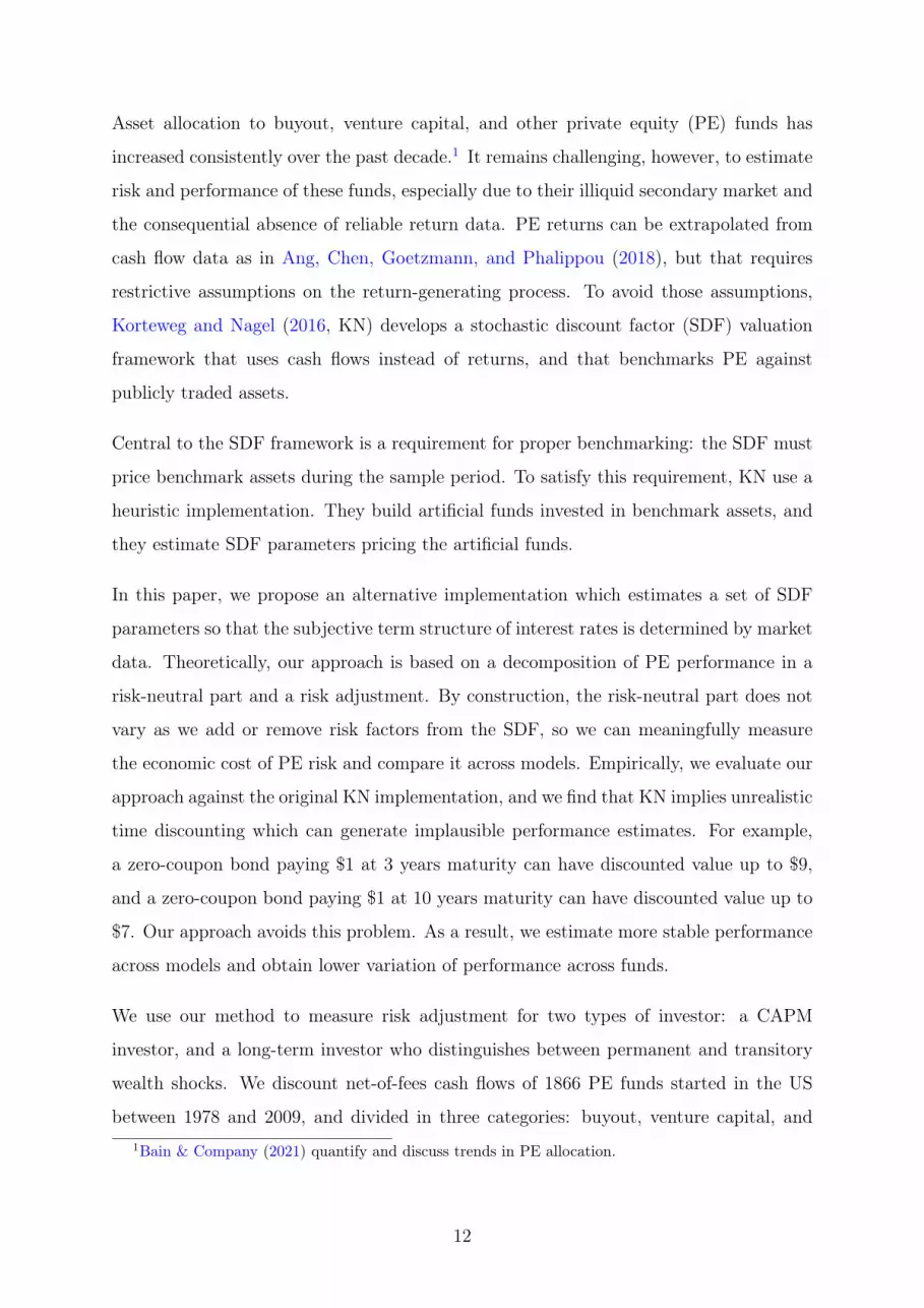
Asset allocation to buyout, venture capital, and other private equity (PE) funds has

increased consistently over the past decade.1 It remains challenging, however, to estimate

risk and performance of these funds, especially due to their illiquid secondary market and

the consequential absence of reliable return data. PE returns can be extrapolated from

cash flow data as in Ang, Chen, Goetzmann, and Phalippou (2018), but that requires

restrictive assumptions on the return-generating process. To avoid those assumptions,

Korteweg and Nagel (2016, KN) develops a stochastic discount factor (SDF) valuation

framework that uses cash flows instead of returns, and that benchmarks PE against

publicly traded assets.

Central to the SDF framework is a requirement for proper benchmarking: the SDF must

price benchmark assets during the sample period. To satisfy this requirement, KN use a

heuristic implementation. They build artificial funds invested in benchmark assets, and

they estimate SDF parameters pricing the artificial funds.

In this paper, we propose an alternative implementation which estimates a set of SDF

parameters so that the subjective term structure of interest rates is determined by market

data. Theoretically, our approach is based on a decomposition of PE performance in a

risk-neutral part and a risk adjustment. By construction, the risk-neutral part does not

vary as we add or remove risk factors from the SDF, so we can meaningfully measure

the economic cost of PE risk and compare it across models. Empirically, we evaluate our

approach against the original KN implementation, and we find that KN implies unrealistic

time discounting which can generate implausible performance estimates. For example,

a zero-coupon bond paying $1 at 3 years maturity can have discounted value up to $9,

and a zero-coupon bond paying $1 at 10 years maturity can have discounted value up to

$7. Our approach avoids this problem. As a result, we estimate more stable performance

across models and obtain lower variation of performance across funds.

We use our method to measure risk adjustment for two types of investor: a CAPM

investor, and a long-term investor who distinguishes between permanent and transitory

wealth shocks. We discount net-of-fees cash flows of 1866 PE funds started in the US

between 1978 and 2009, and divided in three categories: buyout, venture capital, and1Bain & Company (2021) quantify and discuss trends in PE allocation.

12

generalist.2 As benchmark assets, we use the S&P 500 total return index and the 3-

month T-bill. For the CAPM investor, buyout has generated 30 cents of NPV per dollar

of commitment, as opposed to 7 cents of venture capital and 21 cents of generalist.

Unsurprisingly, venture capital has the highest (absolute value of) risk adjustment, equal

to 65 cents per dollar of commitment and about twice as large compared to 31 cents

of buyout and 35 cents of generalist. Our long-term investor assigns similar NPVs; risk

adjustment is only marginally smaller, about 5 cents lower than CAPM across the three

categories.

Comparing our method with the KN implementation, we find the largest differences in

the buyout category. With CAPM, the risk-adjusted performance of buyout is similar

across the two methods, but performance components differ substantially. The KN imple-

mentation results in larger risk-neutral value which is then compensated by higher risk

adjustment. Further, the standard deviation of performance across funds is 142 cents

using KN, while it is 98 cents in our implementation. For the long-term investor, the

KN method shows very high buyout performance, up to 80 cents of NPV per dollar of

commitment, in contrast to 35 cents with our implementation. That very high NPV,

however, is not driven by lower risk adjustment; instead, it is driven by a large increase

in the risk-neutral value, which goes from 80 cents with CAPM up to 250 cents with the

long-term model. The standard deviation of performance in the long-term model goes

up to 925 cents with the KN implementation, while it remains stable at 105 cents with

our method.

We find smaller differences between the two implementations for the venture capital and

generalist categories. We consistently find, however, that our implementation implies a

more plausible subjective term structure of interest rates, resulting in lower cross-sectional

variation of performance and more stable NPV estimates across models.

With our implementation, we further decompose risk adjustment based on the timing of

cash flows during a fund’s life. For all three fund categories, cash flows have marginally

negative risk exposure in the first three years of operations, indicating weak pro-cyclicality

of contributions, and risk exposure becomes positive from the fourth year onwards. We2PE data is maintained by Burgiss, and it is one of the most comprehensive PE dataset available to

date.

13

find differences in the timing of risk across the three categories. For venture capital, the

largest risk adjustment is due to cash flows from year 4 to 7 and in contrast with year

9 to 11 for buyout. For generalist funds, risk adjustment is spread more homogeneously

between year 4 and 10.

An important weakness remaining in our approach is that our performance decomposition

does not provide clear guidance on how to estimate risk prices for proper benchmarking.

In practice, we restrict the SDF to price S&P 500 returns in the sample period at a

10-year horizon. This condition is heuristic, however, based on the typical horizon of

PE funds. To address this weakness, we study the robustness of our results by changing

the price of risk exogenously. We find only weak effects on risk adjustment and NPVs

of buyout and generalist funds. Their NPVs remain positive over a wide range of risk

prices. Venture capital, on the other hand, has higher risk exposure, and its valuation is

more sensitive to the price of risk.

This paper fits into a large literature studying the risk and return of PE investments.

Korteweg (2019) surveys that literature, and we build on a series of studies benchmarking

PE cash flows against publicly traded assets. In this context, a popular measure of risk-

adjusted performance is Kaplan and Schoar (2005)’s Public Market Equivalent (PME).

The PME discounts cash flows using the realized return on a portfolio of benchmark

assets. Sorensen and Jagannathan (2015) show that the PME fits into the SDF framework

as a special case of Rubinstein (1976)’s log-utility model. But the log-utility model does

not necessarily price benchmark assets, and in that case the PME applies the wrong risk

adjustment. To fix that issue, Korteweg and Nagel (2016) propose a generalized PME,

and we build on their work.3

Starting with Ljungqvist and Richardson (2003), several authors study the performance

of PE funds adjusting for different risk factors. Franzoni, Nowak, and Phalippou (2012)

along with Ang, Chen, Goetzmann, and Phalippou (2018) estimate some of the most

inclusive models considering Fama-French three factors, the liquidity factor of Pástor

and Stambaugh (2003), and in some cases also profitability and investment factors. With

our long-term investor, we introduce a new risk factor representing shocks to investment3Parallel effort by Gupta and Van Nieuwerburgh (2021) takes a different approach to benchmark PE.

They try to replicate funds’ cash flows with a large portfolio of synthetic dividend strips which is thenpriced with standard asset pricing techniques.

14

opportunities, or discount rate news, as in the intertemporal CAPM of Campbell (1993).

Closest to the spirit of our long-term investor is the work of Gredil, Sorensen, and Waller

(2020), who study PE performance using SDFs of leading consumption-based asset pricing

models.

1 Risk Adjustment of Private Equity Cash Flows

We measure the risk-adjusted performance of PE funds using the Generalized Public

Market Equivalent (GPME). In its most general form, the GPME of fund i is the sum of

fund’s cash flows, Ci,t, discounted with realized SDF:

GPMEi ≡H∑

h=0

Mt,t+hCi,t+h (1)

The term Mt,t+h denotes a multi-period SDF discounting cash flows from t + h to the

start of the fund. Time t is the date of the first cash flow of the fund, and it depends on

i despite the simplified notation. The letter H indicates the number of periods (quarters

in our case) from the first to last cash flow of the fund. As a convention, we let H be the

same across funds, and funds that are active for a lower number of periods have a series

of zero cash flows in the last part of their life.

Functional forms of the SDF are discussed in Section 2. They typically include at least

one risk factor and depend on a vector of parameters. Those parameters should be

estimated such that the SDF reflects realized returns on benchmark assets during the

sample period. This intuitive condition is necessary for proper benchmarking, but it is

unclear how it should be translated into formal statements. Korteweg and Nagel (2016)

propose a heuristic approach based on the construction of artificial funds that invest in

the benchmark assets. They then estimate parameters such that the NPV of those funds

is zero. In the rest of this section, we propose an alternative approach based on the

GPME decomposition which we are about to describe.4

Investing in a random fund gives E[GPMEi] as NPV, and it is useful to decompose this4A related but different decomposition is discussed by Boyer, Nadauld, Vorkink, and Weisbach (2021).

15

quantity in a typical asset pricing way:

E[GPMEi] =H∑

h=0

E[Mt,t+h]E[Ci,t+h]

︸ ︷︷ ︸risk-neutral value

+H∑

h=0

cov(Mt,t+h, Ci,t+h)

︸ ︷︷ ︸risk adjustment

(2)

As illustrated on the right-hand side of this expression, NPV is the sum of a risk-neutral

value and a risk adjustment. We make a simple consideration: by definition, the risk-

neutral value should be determined by cash flows and risk-free rates, and it should not

change as we add or remove risk factors from the SDF.

Further, a main objective of a benchmarking exercise like ours is to assess risk exposure

of PE to different risk factors. In general, the GPME does not allow direct measurement

of risk quantities, and we are left with indirect evidence based on the behavior of risk

adjustment (Jeffers, Lyu, and Posenau, 2021). As we add or remove risk factors from the

SDF, it is tempting to attribute differences in GPME to changes in risk adjustment, but

that interpretation is robust only when the risk-neutral value is fixed.

We fix the risk-neutral value using standard asset pricing conditions on risk-free assets.

We consider a $1 investment at time t in a risk-free asset paying Rft,t+h at time t+h. This

investment is priced by the SDF if Et[Mt,t+h] = 1/Rft,t+h. Take unconditional expectations

on both sides, we get the following condition:

E[Mt,t+h] = E

[1

Rft,t+h

](3)

Imposing this restriction for all horizons h from 1 to H, the risk-neutral value can be

rewritten without the SDF. Thus, risk-neutral value is determined by cash flows and risk-

free rates, and remains constant as we consider different SDFs, so our initial consideration

is satisfied.

Empirically, we wish to impose condition (3) to the SDF. However, the practical meaning

of the expectation operator inside that condition can be elusive. How does the population

condition translate into a sample condition?

To address this question, it is useful to consider the sample version of E[GPMEi]. We

16

call it simply GPME, and compute it as the mean of GPMEi across N funds in a sample:

GPME ≡ 1

N

N∑

i=1

H∑

h=0

Mt,t+hCi,t+h (4)

It is possible to decompose this quantity similarly to its population counterpart. For each

horizon h, we defineMh =1N

∑iMt,t+h as the average SDF and Ch =

1N

∑iCi,t+h as the

average cash flow across funds. With these definitions, we can write

GPME =H∑

h=0

MhCh +H∑

h=0

MhAh (5)

where Ah = 1N

∑i(Mt,t+h/Mh−1)(Ci,t+h−Ch) is the covariance between normalized SDF

and cash flows. In this decomposition, the risk-neutral value is∑H

h=0MhCh and the risk

adjustment is∑H

h=0MhAh. Fixing the risk-neutral value requires restrictions onMh, and

the expectation operator inside condition (3) must be implemented as a cross-sectional

mean. As a result, we impose the following sample condition on the SDF:

1

N

N∑

i=1

Mt,t+h =1

N

N∑

i=1

1

Rft,t+h

(6)

This expression must hold for horizons 1 to H, and it represents H moment conditions.

For large h, however, we do not observe all returns on benchmark assets.5 In that case,

we rescale N down to account for the missing observations.

In our GPME decomposition, risk adjustment is determined by risk prices inside the SDF,

and the decomposition does not provide clear guidance on how to identify the appropriate

risk prices. In this case, we use heuristic rules. For each benchmark asset, b, with risky

return Rbt,t+h, we impose the following condition:

1

N

N∑

i=1

Mt,t+hRbt,t+h = 1 (7)

This expression is the risky counterpart of the risk-free rate condition above. In our5Some funds in our data operate longer than 15 years, so that H > 60 quarters. However, we cannot

observe returns on benchmark assets at horizon h = 60 for funds started in 2009, for example, becausethat would require knowing returns realized in 2024.

17

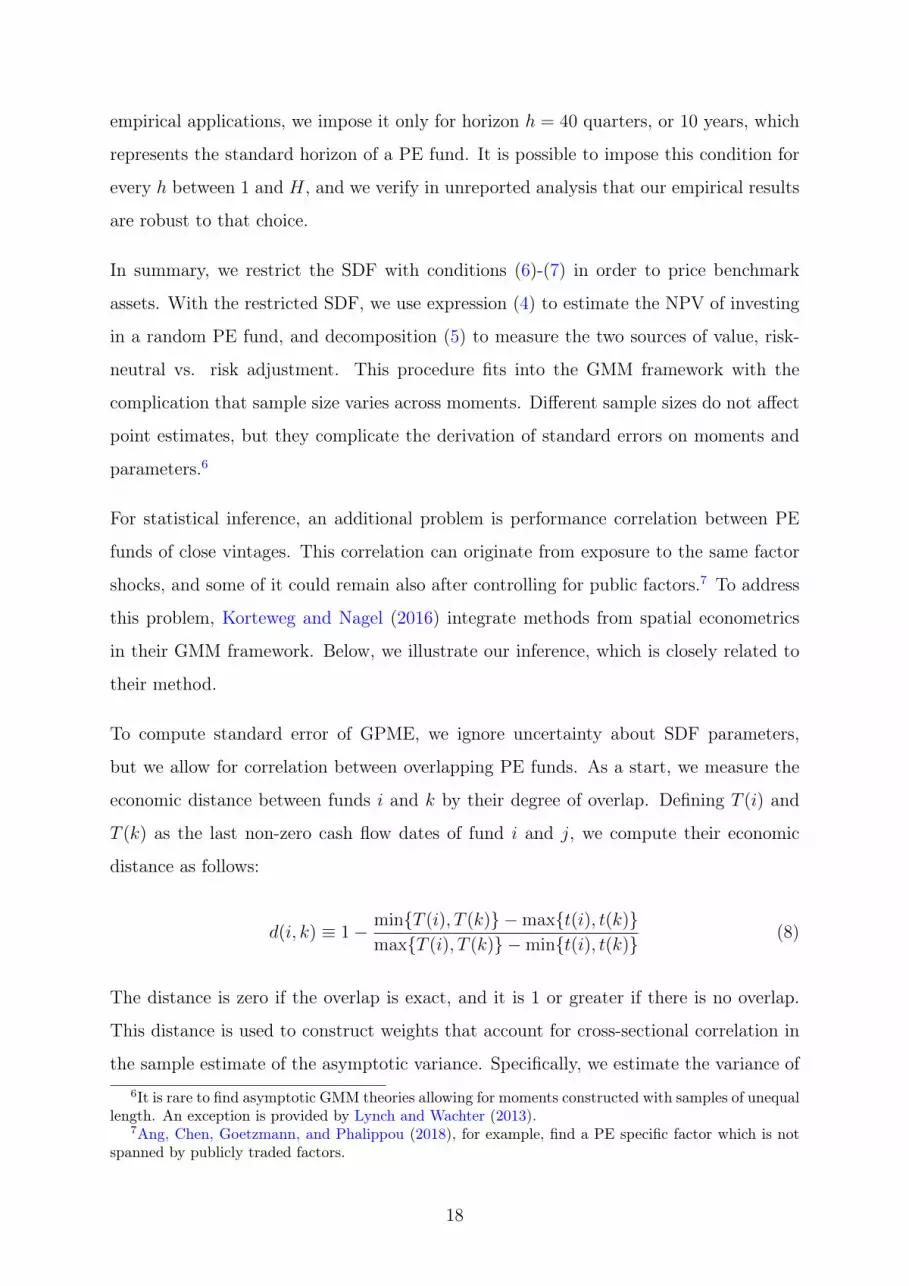
empirical applications, we impose it only for horizon h = 40 quarters, or 10 years, which

represents the standard horizon of a PE fund. It is possible to impose this condition for

every h between 1 and H, and we verify in unreported analysis that our empirical results

are robust to that choice.

In summary, we restrict the SDF with conditions (6)-(7) in order to price benchmark

assets. With the restricted SDF, we use expression (4) to estimate the NPV of investing

in a random PE fund, and decomposition (5) to measure the two sources of value, risk-

neutral vs. risk adjustment. This procedure fits into the GMM framework with the

complication that sample size varies across moments. Different sample sizes do not affect

point estimates, but they complicate the derivation of standard errors on moments and

parameters.6

For statistical inference, an additional problem is performance correlation between PE

funds of close vintages. This correlation can originate from exposure to the same factor

shocks, and some of it could remain also after controlling for public factors.7 To address

this problem, Korteweg and Nagel (2016) integrate methods from spatial econometrics

in their GMM framework. Below, we illustrate our inference, which is closely related to

their method.

To compute standard error of GPME, we ignore uncertainty about SDF parameters,

but we allow for correlation between overlapping PE funds. As a start, we measure the

economic distance between funds i and k by their degree of overlap. Defining T (i) and

T (k) as the last non-zero cash flow dates of fund i and j, we compute their economic

distance as follows:

d(i, k) ≡ 1− min{T (i), T (k)} −max{t(i), t(k)}max{T (i), T (k)} −min{t(i), t(k)} (8)

The distance is zero if the overlap is exact, and it is 1 or greater if there is no overlap.

This distance is used to construct weights that account for cross-sectional correlation in

the sample estimate of the asymptotic variance. Specifically, we estimate the variance of6It is rare to find asymptotic GMM theories allowing for moments constructed with samples of unequal

length. An exception is provided by Lynch and Wachter (2013).7Ang, Chen, Goetzmann, and Phalippou (2018), for example, find a PE specific factor which is not

spanned by publicly traded factors.

18

√N GPME as

v ≡ 1

N

N∑

i=1

N∑

k=1

max{1− d(i, k)/d, 0} uiuk (9)

where ui ≡ GPMEi − GPME. In the sum, each product uiuk is assigned a weight

between 0 and 1, and weights decrease with the distance between two funds. In our

empirical work, we set d = 2, and some non-overlapping pairs of funds still get positive

weight. The standard error of GPME is estimated as√v/N .

The resulting standard error ignores parameters uncertainty and can be interpreted con-

servatively as a lower bound. Our primary objective remains obtaining point estimates

of GPME that are as economically robust as possible.

2 Stochastic Discount Factor

We focus on applications with exponentially affine SDFs. To illustrate, consider the case

with a generic single factor f . The SDF can be written as follows:

Mt,t+h = exp (ah − γhft,t+h) (10)

In this expression, ah and γh indicate a pair of parameters per horizon, and γh can be

interpreted as the risk price of f at horizon h. In absence of other restrictions, this SDF

has a total of 2H parameters. Korteweg and Nagel (2016) restrict ah = ah and γh = γ,

so they work with only 2 parameters. We do not impose any functional form on ah. This

additional flexibility is necessary to satisfy moment conditions (6) and fix the subjective

term structure of interest rates with market data. We maintain the restriction on risk

prices, γh = γ, for two reasons. First, our main argument is about fixing the risk-neutral

value of GPME, which is not determined by risk prices, so we maintain this part of the

model as simple as possible. Second, we exploit this simplicity to study the robustness

of our empirical results with respect to risk prices.

The single-factor form of the SDF can easily be extended with additional factors and

corresponding risk prices. Below, we describe the form used in our empirical work.

19

2.1 CAPM and Long-Term Investors

We consider two risk factors. One factor is the log-return on the market, rmt,t+h =

ln(Rmt,t+h). The other factor is news about future expected returns on the market, of-

ten called discount rate (DR) news in the literature. DR news arriving between t and

t+ h is denoted NDRt,t+h, and is defined as follows:

NDRt,t+h ≡ (Et+h − Et)

∞∑

j=1

ρjrmt+h+j (11)

In this expression, ρ is an approximation constant just below 1, and the right-hand side

measures cumulative news between t and t+h about market returns from t+h onwards.

In a simple model with homoscedastic returns, this factor summarizes variation in invest-

ment opportunities, and positive news corresponds to better opportunities (Campbell,

1993).8

With the two risk factors, we construct the following SDF:

Mt,t+h = exp

(ah − ωγ rmt,t+h − ω(γ − 1)NDR

t,t+h

)(12)

This is a two-factor version of (10) with risk price ωγ for market return and ω(γ− 1) for

DR news. Appendix A connects this SDF with theory, and shows that the parameter γ

can be interpreted as the investor’s relative risk aversion, while ω is the portfolio weight

in the market, with 1 − ω being invested in the risk-free asset. Throughout our main

analysis and unless otherwise specified, we assume ω = 1 representing an investor fully

allocated to the market.

This SDF recognizes that the same realized market return implies different marginal

utility depending on expected returns. If expected returns are constant, NDRt,t+h is zero,

and the SDF simplifies to a single-factor CAPM model. If expected returns vary over

time, NDRt,t+h appears as an additional risk factor with positive risk price for investors with

γ > 1. These investors are particularly averse to portfolio losses arriving jointly with8Formally, ρ ≡ 1− exp(x) where x is the mean of the investor’s log consumption-wealth ratio. In our

empirical applications, one period corresponds to one quarter, and we set ρ = 0.951/4 corresponding toa mean consumption-wealth ratio of approximately 5% per year.

20

negative news about expected returns. These losses are permanent in the sense that they

are not compensated by higher expected returns, and a risk-averse, long-term investor

fears them in particular (Campbell and Vuolteenaho, 2004).

We compare GPME estimates obtained with different restrictions on (12). In one case,

we impose ah = 0 and γ = 1. These restrictions correspond to a log-utility investor and

result in the same SDF of Kaplan and Schoar (2005)’s PME. In addition to the log-utility

investor, we consider two other types, CAPM and long-term investors, differentiated

only by NDRt,t+h, which is zero with CAPM and estimated below for long-term investors.

The SDFs of these two investors require estimation of ah and γ, and we compare our

method with that of Korteweg and Nagel (2016). Since Korteweg and Nagel (2016)

impose ah = ah, we refer to their method as ‘single intercept’ and we refer to ours as

‘multiple intercepts’.

2.2 A Model of Discount Rate News

To estimate DR news, we follow a large literature starting with Campbell (1991) that

models expected market returns using vector autoregression (VAR).9 We assume that the

data are generated by a first-order VAR:

xt+1 = µ+Θxt + εt+1 (13)

In this expression, µ is aK×1 vector and Θ is aK×K matrix of parameters. Furthermore,

xt+1 is K × 1 vector of state variables with rmt+1 − rft+1 as first element, and εt+1 is a i.i.d

K × 1 vector of shocks with variance Σε.

In this model, DR news is a linear function of the shocks:

NDRt,t+1 = λεt+1 (14)

The vector of coefficients for DR news is defined as λ = ρe′Θ(I − ρΘ)−1, where I is

the identity matrix and e′ = (1, 0, 0, . . . , 0). Those coefficients measure the long-run9See for example Campbell (1991, 1993, 1996), Campbell and Vuolteenaho (2004), Lustig and

Van Nieuwerburgh (2006), Cochrane (2011).

21

sensitivity of expected returns to each element of xt.

Combining the VAR model with the definition of multi-period DR news from (11), we

obtain the following result:

NDRt,t+h = λεt+h + (λ− e′ρΘ) εt+h−1 +

(λ− e′ρΘ− e′ρ2Θ2

)εt+h−2 + . . .

. . .+ (λ− e′∑h−1

i=1 ρiΘi)εt+1 (15)

This equation expresses multi-period DR news in terms of observables, and it constitutes

the empirical specification of the risk factor. In section 3, we obtain two versions of this

factor by estimating two VAR models that differ in the choice of state variables.

3 Expected Returns and Discount Rate News

3.1 Public Market Data

The VAR vector xt contains data about publicly traded assets at a quarterly frequency

from 1950 to 2018. The first element of xt is the difference between the log-return on the

value-weighted S&P 500 and the log-return on quarterly T-bills. For this element, data

is taken from the Center of Research in Security Prices (CRSP). The remaining elements

of xt are candidate predictors of expected returns and DR news. We consider (1) the

log dividend-price ratio, (2) the term premium, (3) a credit spread of corporate bond

yields and (4) the value spread. The log dividend-price ratio, term premium, and credit

spread are constructed using data from Amit Goyal’s website. The log dividend-price

ratio is defined as the sum of the last 12 months dividends divided by the current price

of the S&P 500. Term premium is the difference between the annualized yield on 10-year

constant maturity Treasuries and the annualized quarterly T-bill yield. Credit spread is

the difference between the annualized yield on BAA-rated corporate bonds and AAA-

rated corporate bonds. For the value spread, we rely on data from Kenneth French’s

data library. We construct the value spread as the difference in log book-to-market ratio

of small-value and small-growth stock portfolios. These portfolios are generated from a

double sort on market capitalization and book-to-market ratio.

Table 1 reports summary statistics of public market data in our sample period. From

22

Panel A, the quarterly log equity premium is 1.6%, corresponding to 6.4% annualy, with

a quarterly standard deviation of 8%. Further, our candidate return predictors are highly

persistent, especially the log dividend-price ratio with autocorrelation coefficient of 0.982.

Panel B reports correlations between contemporaneous and lagged state variables. The

first column reports univariate correlations between one-period ahead excess market re-

turn (rmt − rft) and lagged predictors. Market return is positively correlated with lagged

dividend-price ratio, credit spread and term premium, and negatively correlated with

lagged value spread.

3.2 VAR Estimation

We estimate the VAR model using OLS at a quarterly frequency in the post-war period

from 1950 to 2018. We consider two different specifications: (1) a parsimonious speci-

fication including only the log dividend-price ratio as predictor and (2) a specification

including the full set of predictors.

Table 2 reports the two VAR estimations. Panel A reports the parsimonious DP specifi-

cation including only the dividend-price ratio, and Panel B reports the full specification.

Each row corresponds to an equation in the VAR. The first row of each panel corresponds

to the market return prediction equation. Standard errors are reported in brackets and

the last two columns report R2 and F-statistic for each forecasting equation. Panel A

shows that dividend-price ratio significantly predicts excess market returns with a coeffi-

cient of 0.025. The R2 is 2.8 percent and the F-statistic is statistically different from zero,

consistent with the dividend-price ratio and lagged market return jointly predicting excess

market returns. Panel B also includes the value spread, credit spread, and term premium

in the VAR. The first row shows that the lagged market return, dividend-price ratio and

term premium positively predict excess returns. The coefficients on the dividend-price

ratio and term premium are statistically significant at the five percent level. The value

spread and credit spread negatively predict market return, although the corresponding

coefficients are statistically insignificant.

Table 3 shows properties of one-period DR news, NDRt,t+1, implied by the two VAR estima-

tions. Panel A reports the vector of coefficients, λ, measuring the sensitivity of DR news

to each element of εt. The “DP only” column shows that shocks to the dividend-price ra-

23

tio are a significant determinant of DR news. The “Full VAR” column shows that shocks

to the dividend-price ratio and term premium are significant determinants of DR news

in the full VAR specification. These coefficients, however, do not represent a complete

picture of how much each variable affects DR news; they do not account for the fact

that elements of εt have different variances. We therefore decompose the unconditional

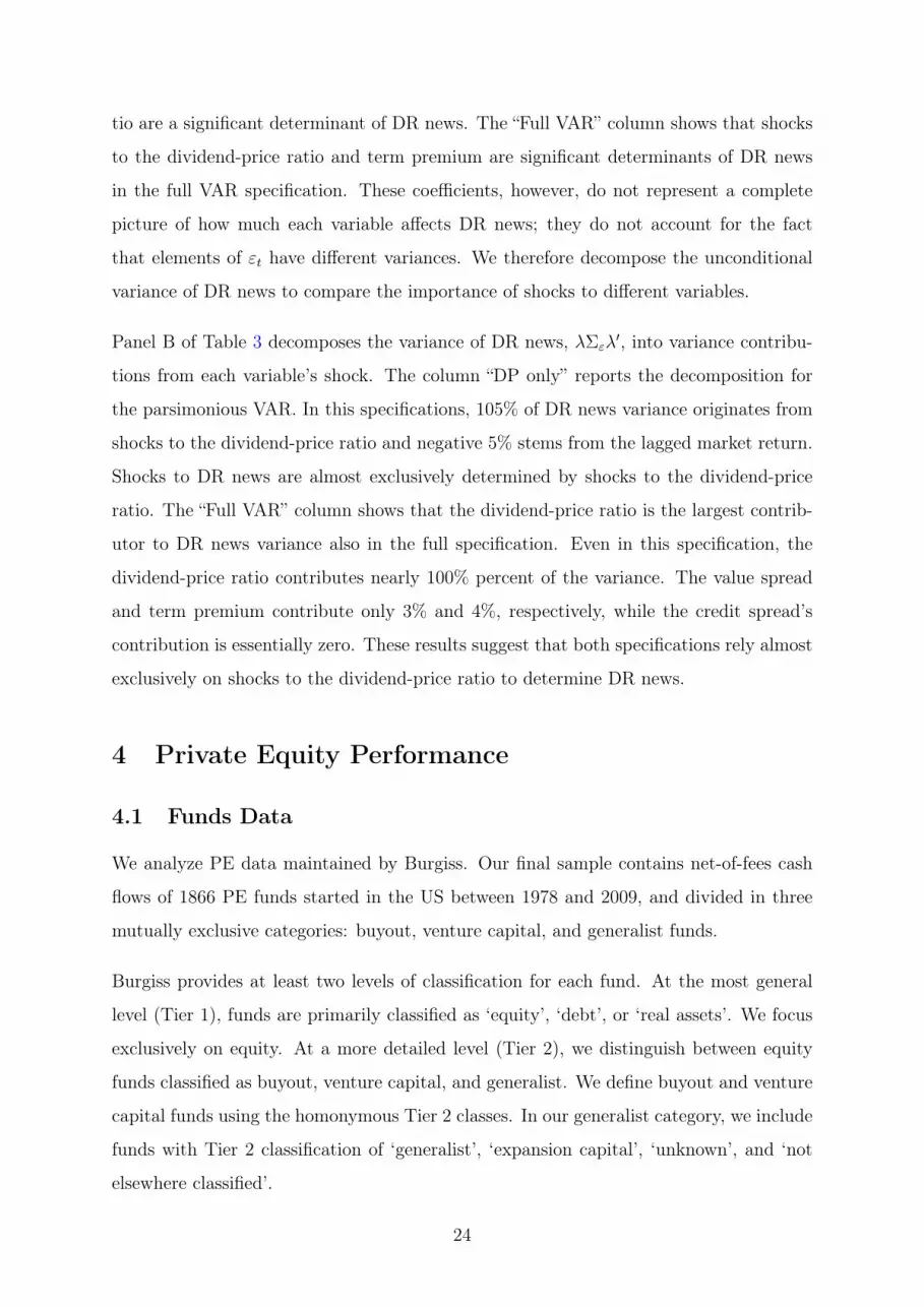
variance of DR news to compare the importance of shocks to different variables.

Panel B of Table 3 decomposes the variance of DR news, λΣελ′, into variance contribu-

tions from each variable’s shock. The column “DP only” reports the decomposition for

the parsimonious VAR. In this specifications, 105% of DR news variance originates from

shocks to the dividend-price ratio and negative 5% stems from the lagged market return.

Shocks to DR news are almost exclusively determined by shocks to the dividend-price

ratio. The “Full VAR” column shows that the dividend-price ratio is the largest contrib-

utor to DR news variance also in the full specification. Even in this specification, the

dividend-price ratio contributes nearly 100% percent of the variance. The value spread

and term premium contribute only 3% and 4%, respectively, while the credit spread’s

contribution is essentially zero. These results suggest that both specifications rely almost

exclusively on shocks to the dividend-price ratio to determine DR news.

4 Private Equity Performance

4.1 Funds Data

We analyze PE data maintained by Burgiss. Our final sample contains net-of-fees cash

flows of 1866 PE funds started in the US between 1978 and 2009, and divided in three

mutually exclusive categories: buyout, venture capital, and generalist funds.

Burgiss provides at least two levels of classification for each fund. At the most general

level (Tier 1), funds are primarily classified as ‘equity’, ‘debt’, or ‘real assets’. We focus

exclusively on equity. At a more detailed level (Tier 2), we distinguish between equity

funds classified as buyout, venture capital, and generalist. We define buyout and venture

capital funds using the homonymous Tier 2 classes. In our generalist category, we include

funds with Tier 2 classification of ‘generalist’, ‘expansion capital’, ‘unknown’, and ‘not

elsewhere classified’.

24

To obtain our final sample, we exclude funds with less than 5 million USD of commit-

ment from the raw data. We also exclude funds whose majority of investments are not

liquidated by 2019. For that, we impose two conditions. First, we only include funds of

vintage year 2009 or earlier. Second, among those funds, we exclude those with a ratio of

residual NAV over cumulative distributions larger than 50%. Finally, we normalize cash

flows and residual NAV by each fund’s commitment.

Figure 1 plots the aggregate sum of normalized contributions, distributions, and net

cash flows for the three fund categories over time. For all the categories, our sample

constitutes mostly of cash flows observed between 1995 and 2019. For venture capital, we

see uniquely large distributions in year 2000, corresponding to the dot-com bubble; those

distributions are almost 10 times larger than distributions and contributions observed at

any other time.

Table 4 summarizes our PE data. Panel A reports descriptive statistics and shows that the

sample consists of 652 buyout funds, 971 venture capital funds and 243 generalist funds.

The median (average) fund size is $421 ($1099) million for buyout, $126 ($222) million

for venture capital and $225 ($558) million for generalist funds. The average number

of years between the first and last buyout fund cash flow is 14.16 years, 15.52 years for

venture capital, and 14.42 years for generalist funds. The average number of cash flows

per fund is approximately 36 for buyout, 28 for venture capital and 33 for generalists.

The sample includes 311 unresolved buyout funds with an average NAV-to-Distributions

ratio of 0.10, 353 unresolved venture capital funds with NAV-to-Distributions ratio of

0.14, and 88 unresolved generalist funds with a NAV-to-Distributions ratio of 0.12.

Panel B of Table 4 reports Total Value to Paid-In ratios (TVPI) across vintage years.10

Across the three categories, TVPIs fluctuates over time and are typically higher for

earlier vintages. Furthermore, venture capital shows peculiarly high TVPIs between

1993 and 1996. These large multiples can be ascribed, at least in part, to funds of these

vintages deploying capital in the period leading up to the 2001 dot-com bubble and exiting

investments before 2001.10If there are less than five funds per vintage year, figures are omitted due to confidentiality.

25

4.2 Buyout

Table 5 reports GPME estimation for buyout funds. The first estimation corresponds to

“Log-Utility” and uses the inverse return on the market as SDF. The resulting GPME is a

reformulation of Kaplan and Schoar (2005)’s PME defined as the sum of discounted cash

flows rather than the ratio of discounted distributions over contributions. The log-utility

GPME is 0.20 and significantly different from zero at the one percent level; buyout funds

provide log-utility investors with 20 cents of abnormal profits per dollar of committed

capital.

Other than the log-utility model, Table 5 reports GPME estimation for CAPM and long-

term (LT) investors assuming they are fully invested in the market (ω = 100%). The

“Single Intercept” columns estimate only one intercept parameter a, with ah = ah, and

the estimations use the moment conditions of Korteweg and Nagel (2016). The “Multiple

Intercepts” columns use our method as described in Section 1, which does not impose

a functional restriction on ah and estimates multiple intercepts linking the subjective

term-structure of interest rates to market data.

4.2.1 Buyout Value for CAPM Investors

Table 5 shows a GPME of 0.28 for the CAPM SDF using a single intercept. The estimate

is statistically different from zero at the ten percent level. With multiple intercepts, The

GPME is 0.30 and statistically significant at the one percent level. These numbers are

close, and they imply that buyout funds provide CAPM investors with 28-30 cents of

NPV per dollar of committed capital. CAPM investors thus derive 8-10 cents more value

than log-utility investors from a marginal allocation to buyout funds.

Even though GPME estimates for CAPM investor are similar across the two methods,

we show below that the different restrictions placed on the single and multiple intercepts

specifications imply markedly different SDF properties. To further explore differences

between the two methods, Table 5 also reports the two GPME components from the

decomposition of Section 1. The first component is∑

hMhCh and corresponds to the risk-

neutral part of GPME. For each horizon, we take the average cash flow across funds and

discount it with the average SDF across funds. We then sum over horizons. The second

component is∑

hMhAh and corresponds to the total risk adjustment inside GPME.

26

For the CAPM investor, the risk-neutral component is 0.61 with multiple intercepts and

0.79 with a single intercept. Risk adjustment, instead, is -0.31 with multiple intercepts

and -0.51 with a single intercept. In this case, the single intercept specification achieves

similar GPME estimate by assigning higher risk-neutral value, but also more negative

risk adjustment, relative to the multiple intercepts case. Differences between the two

methods become more evident considering long-term investors below.

4.2.2 Buyout Value for Long-Term Investors

In Table 5, the “LT” columns report GPME estimations for long-term investors. In

particular, the “LT (DP)” columns use the VAR specification with only the dividend-

price ratio as return predictor to measure DR news. With a single intercept, the LT

(DP) investor assigns a GPME of 0.80 to buyout. This point estimate is considerably

higher relative to the CAPM investor, but it is not statistically significant due to the large

standard error. Further, a NPV of 80 cents per dollar of commitment is large enough to

appear economically implausible, and our decomposition shows that this GPME results

from summing a risk-neutral value of 2.50 with a risk adjustment of -1.69. Compared to

the CAPM, this large value is not generated by a change in risk adjustment. Instead, it

comes from a large increase of the risk-neutral component. With multiple intercepts, we

estimate a GPME of 0.35 for the LT (DP) investor. This point estimate is statistically

significant, and it is only marginally higher compared to CAPM. By construction, the

difference relative to CAPM is entirely due to risk adjustment.

The “LT (Full)” columns of Table 5 use DR news computed with the full VAR specifi-

cation which includes the dividend-price ratio, term premium, credit spread, and value

spread as return predictors. With single intercept, the resulting GPME is 0.41, although

not statistically significant, and substantially lower than 0.80 obtained in the LT (DP)

case. With multiple intercepts, GPME is 0.34, statistically significant at the one percent

level, and close to the 0.35 estimated in the LT (DP) case. While the single intercept

methodology suggests that the two VAR specifications result in DR news which generate

large GPME differences, the multiple intercepts method suggests similar GPME implica-

tions of the two VAR specifications. In Section 3, we show that both VAR estimations

generate DR news that vary almost exclusively from shocks to the dividend-price ratio,

suggesting that the full VAR might have similar dynamics to the parsimonious VAR.

27

Consistent with this interpretation, the multiple intercepts method estimates virtually

identical GPMEs for LT (DP) and LT (Full) investors.

4.2.3 Time Discounting of Buyout Funds

Figure 2 plots the average SDF across funds as a function of horizon. At each horizon

h, the average SDF measures the present value of one dollar paid for certain at that

horizon by all funds in the sample. The figure compares single intercept and multiple

intercepts specifications from Table 5. By construction, multiple intercepts estimations

using the same sample imply the same average SDF as a function of horizon. Single

intercept estimations impose less structure to the SDF, and the average SDF at each

horizon varies depending on the risk factors considered.

The figure shows unrealistic time discounting for the single intercept estimation with a

peculiar pattern of negative time discounting in the first 3 years, positive discounting

from year 4 to 8, and negative discounting again from year 8 to 11. This pattern is

qualitatively consistent across investors and it is quantitatively strongest for the LT (DP)

model, suggesting that the very large GPME estimate obtained with this model might

be due to this implausible time discounting pattern resulting from the single intercept

method.

With multiple intercepts, Figure 2 shows that time discounting is consistently positive

and stable across horizons, and this result corresponds to more stable GPME estimates

across models, as shown in Table 5. It also corresponds to lower variation of GPMEi

across funds, as we show below.

4.2.4 Cross-Sectional Variation of Performance

Table 6 summarizes the cross-sectional distribution of GPMEi resulting from the different

estimations. The table contains results for all three fund categories. We focus primarily

on buyout, and a similar discussion applies for venture capital and generalist funds studied

below. For each estimation, we report the mean of GPMEi, which corresponds to the

GPME estimates of Table 5. Below the mean, we report the standard deviation and

selected percentiles of the GPMEi distribution.

28

Differences in the distribution of GPMEi are interesting because the multiple intercepts

estimations, just like the single intercept ones, restrict the SDF using exclusively public

market data, and ignoring any information about PE cash flows. Thus, differences in

the GPMEi distribution are a result which is not imposed by construction. We find that

the multiple intercepts estimations imply consistently lower variation of GPMEi across

funds, relative to single intercept.

For buyout, the log-utility model generates the lowest standard deviation of of GPMEi,

equal to 0.64. The single intercept CAPM model implies a standard deviation of 1.42,

while the multiple intercepts CAPM model implies a standard deviation of 0.98. Thus, the

multiple intercepts model generates substantially lower standard deviation with CAPM,

even though the two models have similar mean (0.28 vs. 0.30). Further, the lower

standard deviation of the multiple intercepts CAPM model comes with less extreme

tail observations as indicated by the reported percentiles. For long-term investors, we see

qualitatively similar differences between the single intercept and multiple intercepts meth-

ods, with more extreme magnitudes. Especially for the LT (DP) investor, the GPMEi

standard deviation of the single intercept model is extremely high, 9.25, relative to 1.05

obtained with multiple intercepts model.

4.2.5 Components of Buyout Performance across Horizons

With multiple intercepts, we take the GPME decomposition one step further. Not only do

we decompose GPME in a risk-neutral part and a risk adjustment, but we also decompose

the risk-neutral part and the risk adjustment based on the contribution of each horizon.

To illustrate, we decompose the risk-neutral part as follows:

H∑

h=0

MhCh =M0C0 +4∑

h=1

MhCh +8∑

h=5

MhCh + · · ·+56∑

h=53

MhCh +H∑

h=57

MhCh (16)

These components correspond to values coming from year 0, year 1, year 2, . . . , year 14,

and year 15 or higher. A similar decomposition is done for risk adjustment.

Figure 3 plots the resulting GPME components against horizon for selected models with

multiple intercepts. The figure focuses on CAPM and LT (DP) models. By construction,

the risk-neutral component from each horizon (grey bars) is identical across models, and

29

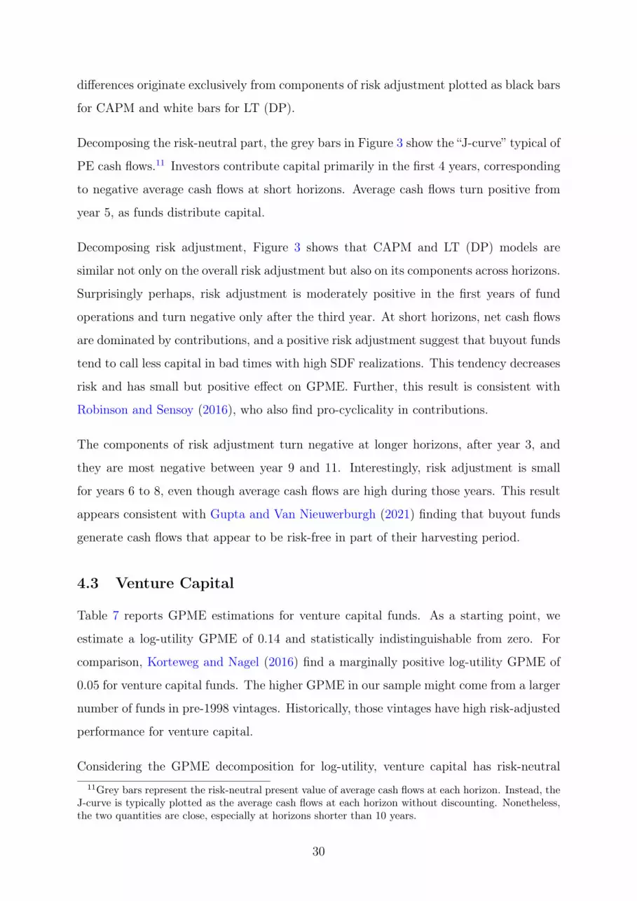
differences originate exclusively from components of risk adjustment plotted as black bars

for CAPM and white bars for LT (DP).

Decomposing the risk-neutral part, the grey bars in Figure 3 show the “J-curve” typical of

PE cash flows.11 Investors contribute capital primarily in the first 4 years, corresponding

to negative average cash flows at short horizons. Average cash flows turn positive from

year 5, as funds distribute capital.

Decomposing risk adjustment, Figure 3 shows that CAPM and LT (DP) models are

similar not only on the overall risk adjustment but also on its components across horizons.

Surprisingly perhaps, risk adjustment is moderately positive in the first years of fund

operations and turn negative only after the third year. At short horizons, net cash flows

are dominated by contributions, and a positive risk adjustment suggest that buyout funds

tend to call less capital in bad times with high SDF realizations. This tendency decreases

risk and has small but positive effect on GPME. Further, this result is consistent with

Robinson and Sensoy (2016), who also find pro-cyclicality in contributions.

The components of risk adjustment turn negative at longer horizons, after year 3, and

they are most negative between year 9 and 11. Interestingly, risk adjustment is small

for years 6 to 8, even though average cash flows are high during those years. This result

appears consistent with Gupta and Van Nieuwerburgh (2021) finding that buyout funds

generate cash flows that appear to be risk-free in part of their harvesting period.

4.3 Venture Capital

Table 7 reports GPME estimations for venture capital funds. As a starting point, we

estimate a log-utility GPME of 0.14 and statistically indistinguishable from zero. For

comparison, Korteweg and Nagel (2016) find a marginally positive log-utility GPME of

0.05 for venture capital funds. The higher GPME in our sample might come from a larger

number of funds in pre-1998 vintages. Historically, those vintages have high risk-adjusted

performance for venture capital.

Considering the GPME decomposition for log-utility, venture capital has risk-neutral11Grey bars represent the risk-neutral present value of average cash flows at each horizon. Instead, the

J-curve is typically plotted as the average cash flows at each horizon without discounting. Nonetheless,the two quantities are close, especially at horizons shorter than 10 years.

30

value of 0.48 and risk adjustment of -0.35. Compared to buyout, this risk adjustment

is considerably larger (-0.35 vs. -0.09). The log-utility model has constant risk price of

γ = 1 across samples, and differences in risk adjustment are entirely due to different

covariance between cash flows and market returns. Thus, higher risk adjustment for

venture capital suggests higher market exposure of venture capital’s cash flows relative

to buyout. Larger risk adjustment for venture capital is consistent with Driessen, Lin,

and Phalippou (2012), who estimate a market beta of 2.4 for venture capital and 1.3 for

buyout, and with Ang et al. (2018), who estimate a market beta 1.8 for venture capital

and 1.2 for buyout.

4.3.1 Venture Capital for CAPM and Long-Term Investors

In Table 7, the GPME estimate for the CAPM investor is -0.15 with single intercept

and 0.07 with multiple intercepts. Both methods indicate that CAPM implies lower

GPME relative to log-utility, and this qualitative difference is consistent with the findings

of Korteweg and Nagel (2016) in a smaller sample. The single intercept and multiple

intercepts methods disagree on the GPME sign and magnitude, however, and multiple

intercepts result in marginally positive GPME for venture capital.

Differences in GPME between single intercept and multiple intercepts can arise from

differences in the SDF intercepts, ah, but also from differences in the estimated risk

price, γ. Table 7 shows that CAPM’s risk price is 2.93 with single intercept and 2.03

with multiple intercepts. We show in Section 5.1 that differences in γ do not entirely

explain this GPME difference between the two methods, as the GPME of the CAPM

investor with multiple intercepts remain higher relative to single intercept even assuming

the same risk price of 2.93 for both models.

For the long-term investor, we observe qualitatively similar differences between single and

multiple intercepts. With single intercept, we estimate negative GPMEs of -0.19 for LT

(DP) and -0.08 for LT (Full). With multiple intercepts, we estimate positive GPMEs of

0.13 for LT (DP) and 0.15 for LT (Full). In Section 5.1, we also show that this difference

is not entirely explained by lower risk prices with multiple intercepts.

Comparing GPMEs between CAPM and long-term investors, we find that the long-term

investor assigns higher value to venture capital, relative to the CAPM investor, with mul-

31

tiple intercepts. GPME estimates with multiple intercepts under LT (DP) and LT (Full)

are almost double the GPME estimate under CAPM. Considering the single intercept

method, we find more stable performance across investors for venture capital relative to

buyout. To investigate this result, we plot the implied discounting of the different venture

capital estimations.

For venture capital, Figure 4 plots the cross-sectional average SDF as a function of hori-

zon. As we do for buyout, the figure distinguishes between multiple intercepts and the

three models with single intercept. This figure confirms that multiple intercepts imply a

more stable time discounting across horizons. The single intercept method implies quali-

tatively similar time discounting between buyout and venture capital estimations. With

venture capital, however, time discounting of the single intercept method does not vary

as widely across the three models.

4.3.2 Components of Venture Capital Performance across Horizons

Following the discussion of buyout results, we also decompose GPMEs by horizon for

venture capital. Figure 5 plots the decomposition for CAPM and LT (DP) models with

multiple intercepts. We focus on the decomposition of risk adjustment.

In the figure, risk adjustment varies similarly with horizon across the two models. For

both models, risk adjustment is marginally positive from year 0 to 2. This result suggests

that contributions tend to be slightly pro-cyclical, and it is similar to buyout funds

although quantitatively smaller. Starting from year 3, risk adjustment turns negative,

and it is most important between year 4 and 7. This result contrasts with buyout, whose

risk adjustment tends to be small especially in year 6 and 7. Distributions of venture

capital funds show substantially different risk across horizons, relative to buyout.

4.4 Generalist

Our analysis of generalist funds is similar to that of buyout and venture capital. Here we

provide an overview of the results.

Table 8 shows the results of our GPME estimations for generalist funds. With log-utility,

we estimate a statistically significant GPME of 0.16, which is lower relative to buyout

32

and marginally higher relative to venture capital. For CAPM and long-term investors,

we estimate consistently positive GPME with single intercept and multiple intercepts

methods. GPME estimates are higher and more stable across estimations with multiple

intercepts relative to single intercept.

Figure 6 shows differences in time discounting across methods plotting the average SDF

by horizons implied by the different estimations. Qualitatively, the figure shows results

similar to buyout and venture capital. With multiple intercepts, time discounting is

positive, constant across investors, and stable across horizons. With single intercept, we

observe time discounting being negative in the first 3 years, positive in the next 5 years,

and negative again in the next 3 years.

Figure 7 plots the risk-neutral value and risk adjustment components by horizon. From

year 0 to 2, the figure shows risk adjustment similar to the other fund categories and

consistent with contributions hedging some risk for PE investors. From year 3 onwards,

risk adjustment turns negative. Compared to the other categories, risk adjustment of

generalist fund can be attributed more homogeneously to cash flows received from year

4 to 10.

5 Robustness

In this section, we focus exclusively on the method with multiple intercepts, and we

explore the robustness of our results with respect to two parameters. First, we study

the sensitivity of GPME as we exogenously change risk aversion, γ. Second, we estimate

GPMEs for investors whose portfolio weight in the market is either ω = 50% or 200%, as

opposed to 100% in Section 4.

5.1 Risk Aversion

Our GPME decomposition does not provide clear guidance on how to estimate risk prices

for proper benchmarking of PE cash flows. As described in Section 1, our method iden-

tifies risk prices by constraining the SDF to price risky benchmark returns at a 10 year

horizon. This is a heuristic approach based on the typical horizon of PE funds, and we

study the sensitivity to this heuristic by changing risk prices exogenously. Specifically,

33

we change risk aversion, γ, since risk prices are primarily determined by this parameter

for our investors.

As we change risk aversion exogenously, we do not need to run new estimations. Instead,

the resulting GPME with multiple intercepts can be computed as follows:

GPME(γ) =H∑

h=1

(1

N

N∑

i=1

1

Rft,t+h

) (Ch + Ah(γ)

)(17)

To obtain this expression, we rewrite the GPME decomposition (5) using time discounting

restrictions: 1N

∑Ni=1Mt,t+h =

1N

∑Ni=1 1/R

ft,t+h. We use this notation to highlight that Ah

is the only term of GPME affected by risk prices. Further, Ah is the only term affected

by the SDF, but it does not depend on intercept parameters.12

Using expression (17), we compute GPMEs with risk aversion between 1 and 12 for

each type of investor in each fund category. Figure 8 plots the resulting GPMEs as a

function of γ. For each category, the three lines correspond to different investors. The

solid line represents CAPM, the dotted line represents LT (DP), and the dash-dotted

line represents LT (Full). Further, there are two circles over each line. The black circle

represents the combination of GPME and γ estimated for that investor with multiple

intercepts in Table 5, Table 7, or Table 8, depending on the category. For comparison,

the white circle corresponds to γ estimated with single intercept and GPME computed

with expression (17).

The top-left panel of Figure 8 shows results for buyout. For the CAPM investor, GPME

ranges from 0.5 to 0.1, it is monotonically decreasing in risk aversion, and it remains

positive even at risk aversion of 12. For long-term investors, the LT (DP) and LT (Full)

models imply approximately the same GPME across all levels of risk aversion. For these

investors, GPME ranges from 0.5 to 0.3, and it is non-monotonic in risk aversion. Overall,

we find robustly positive performance of buyout funds, and only moderate sensitivity to

risk prices.

The top-right panel of Figure 8 shows results for venture capital. As opposed to buyout,12To see why Ah does not depend on intercept parameters, recall that Ah = 1

N

∑i(Mt,t+h

/Mh −

1)(Ci,t+h − Ch) with Mh = 1N

∑i Mt,t+h. The SDF enters Ah only through its normalized form,

Mt,t+h

/Mh, and intercepts cancel out because of the normalization.

34

we find high sensitivity of venture capital’s GPME to risk prices. This sensitivity is

highest for the CAPM investor, whose GPME estimate goes from 0.35 to -0.25 as risk

aversion increases. For long-term investors, GPME shows marginally lower sensitivity,

ranging from 0.35 to -0.15. Across all investors, we find that venture capital’s GPME

is most sensitive to risk aversion in the range of risk aversion between 1 and 3, which

contains the three point estimates of γ with multiple intercepts from Table 7.

In the bottom panel of Figure 8, we report sensitivity results for generalist funds. Simi-

larly to buyout, the GPME of generalist funds display only moderate sensitivity to risk

prices, and it remains positive for all investors at all levels of risk aversion between 1 and

12. GPME ranges from 0.35 to 0.05 for the CAPM investor, and from 0.35 to 0.15 for

long-term investors.

Across investors and fund categories, we find tendency for GPME to decrease in risk

aversion, especially for risk aversion between 1 and 5, which is typically the most relevant

range. For buyout and generalist funds, we find quantitatively modest GPME sensitivity

to risk prices, and GPME remains positive across a wide range of risk aversion. For ven-

ture capital, instead, we find high sensitivity of GPME to risk prices, with positive GPME

for risk aversion below 2 and negative GPME for risk aversion above 3. Because of this

high sensitivity, venture capital seems the most problematic category to evaluate.

5.2 Investor Leverage

An additional way to compare CAPM and long-term investors is by looking at the effect of

investor’s leverage on GPME. A natural measure of leverage in our model is the portfolio

weight in the market, ω, and while we assume ω = 100% in most of the paper, here

we consider two different values representing a conservative investor with low leverage

(ω = 50%) and an aggressive investor with high leverage (ω = 200%).

After further inspection, SDF expression (12) presented in Section 2 suggests two consid-

erations about leverage. First, CAPM investors with different leverage assign the same

GPMEs. For those investors, ω enters the SDF only in the product ωγ that determines

market risk price, and it is a redundant parameter. For CAPM investors with higher lever-

age, our GPME estimation will mechanically result in proportionally lower risk aversion.

35

Second, long-term investors with different leverage can assign different GPMEs. For long-

term investors, ω affects the importance of market risk price, ωγ, relative DR news risk

price, ω(γ − 1). Since γ > γ − 1, risk from DR news is less important for aggressive

investors with large ω, and if DR news matters when evaluating PE, leverage can affect

GPMEs.

In Table 9, we report GPME estimations similar to the multiple intercepts part of Table 5,

Table 7, and Table 8, except that we do not assume ω = 100%. Instead, we assume

ω = 50% in first part of the table and ω = 200% in the second part. For CAPM

investors, the table confirms that leverage has no effect on GPME, and higher leverage

is mechanically offset by lower risk aversion. For long-term investors, we find some

differences in GPME across leverage. The conservative long-term investor assigns GPME

of 0.35 to buyout, 0.25 to generalist, and in the 0.15-0.20 range to venture capital. The

aggressive long-term investor, instead, assigns GPME of 0.33 to buyout, 0.22 to generalist,

and 0.07 to venture capital. Thus, the conservative investor assigns higher value to PE

across all three fund categories, and by construction, these differences are entirely due

to different risk adjustments. Quantitatively, however, these GPME differences across

leverage seem largely negligible at least for the case of buyout and generalist funds.

Overall, we estimate that all three fund categories provide positive values to both CAPM

investors and long-term investors across a wide range of leverage levels.

6 Conclusion

PE funds are illiquid investments whose true fundamental return is typically unobserv-

able. Since investment returns are unobservable, risk and performance cannot be esti-

mated with standard approaches, and the literature has developed methods to evaluate

these investments by discounting funds’ cash flows with SDFs. In this paper, we show

that existing SDF methods for the valuation of PE funds result in unrealistic time dis-

counting, which can generate implausible performance estimates. We propose a modified

method and compare it to existing ones.

Theoretically, our approach is based on a standard asset pricing decomposition of PE

performance in a risk-neutral part and a risk adjustment. We fix the risk-neutral part by

36

constraining the SDF such that the subjective term structure of interest rates is deter-

mined by market data. By construction, the risk-neutral part does not vary as we add

or remove risk factors from the SDF, so we can meaningfully measure the economic cost

of PE risk and compare it across models. Empirically, we evaluate our approach against

existing methods, and find that our approach results in more stable PE performance

across models and lower variation of performance across funds.

We use our method to measure PE performance and risk adjustment for two types of

investors: a CAPM investor, and a long-term investor who distinguishes between per-

manent and transitory wealth shocks. We discount net-of-fees cash flows of 1866 PE

funds started in the US between 1978 and 2009, and divided in three categories: buyout,

venture capital, and generalist. We find largely negligible differences between the two

investors, especially for buyout and generalist funds. Overall, we find positive perfor-

mance of buyout, generalist, and venture capital funds. For venture capital, however,

high risk exposure makes performance estimates particularly sensitive to estimated risk

prices.

Our performance decomposition does not provide clear guidance on how to estimate risk

prices for proper benchmarking of PE cash flows. Because of this, we rely on heuristic

SDF restrictions, and we study the sensitivity of performance estimates with respect to

risk prices. The open issue on the estimation of risk prices, among others, is left to future

research.

37

References

Ang, A., B. Chen, W. N. Goetzmann, and L. Phalippou (2018). Estimating private equity

returns from limited partner cash flows. The Journal of Finance 73 (4), 1751–1783.

Bain & Company (2021). Global private equity report. Technical Report.

Boyer, B., T. Nadauld, K. Vorkink, and M. Weisbach (2021). Discount rate risk in private

equity: Evidence from secondary market transactions. Working Paper.

Campbell, J. Y. (1991). A variance decomposition for stock returns. The Economic

Journal 101 (405), 157–179.

Campbell, J. Y. (1993). Intertemporal asset pricing without consumption data. American

Economic Review 83 (3), 487–512.

Campbell, J. Y. (1996). Understanding Risk and Return. Journal of Political Econ-

omy 104 (2), 298–345.

Campbell, J. Y. and L. M. Viceira (1999). Consumption and portfolio decisions when

expected returns are time varying. The Quarterly Journal of Economics 114 (2), 433–

495.

Campbell, J. Y. and T. Vuolteenaho (2004). Bad beta, good beta. The American Eco-

nomic Review 94 (5), 1249–1275.

Cochrane, J. H. (2011). Discount rates. The Journal of Finance 66 (4), 1047–1108.

Driessen, J., T.-C. Lin, and L. Phalippou (2012). A new method to estimate risk and

return of nontraded assets from cash flows: The case of private equity funds. The

Journal of Financial and Quantitative Analysis 47 (3), 511–535.

Epstein, L. G. and S. E. Zin (1989). Substitution, risk aversion, and the temporal behavior

of consumption and asset returns: A theoretical framework. Econometrica 57 (4), 937–

969.

Franzoni, F., E. Nowak, and L. Phalippou (2012). Private equity performance and liq-

uidity risk. The Journal of Finance 67 (6), 2341–2373.

38

Gredil, O., M. Sorensen, and W. Waller (2020). Evaluating private equity performance

using stochastic discount factors. Working Paper.

Gupta, A. and S. Van Nieuwerburgh (2021). Valuing private equity investments strip by

strip. Journal of Finance.

Jeffers, J., T. Lyu, and K. Posenau (2021). The risk and return of impact investing funds.

Working Paper.

Kaplan, S. N. and A. Schoar (2005). Private equity performance: Returns, persistence,

and capital flows. The Journal of Finance 60 (4), 1791–1823.

Korteweg, A. (2019). Risk adjustment in private equity returns. Annual Review of

Financial Economics 11 (1), 131–152.

Korteweg, A. and S. Nagel (2016). Risk-adjusting the returns to venture capital. The

Journal of Finance 71 (3), 1437–1470.

Ljungqvist, A. and M. Richardson (2003). The cash flow, return and risk characteristics

of private equity. Working Paper.

Lustig, H. and S. Van Nieuwerburgh (2006). The Returns on Human Capital: Good News

on Wall Street is Bad News on Main Street. The Review of Financial Studies 21 (5),

2097–2137.

Lynch, A. W. and J. A. Wachter (2013). Using samples of unequal length in generalized

method of moments estimation. The Journal of Financial and Quantitative Analy-

sis 48 (1), 277–307.

Pástor, L. and R. F. Stambaugh (2003). Liquidity risk and expected stock returns.

Journal of Political Economy 111 (3), 642 – 685.

Robinson, D. T. and B. A. Sensoy (2016). Cyclicality, performance measurement, and

cash flow liquidity in private equity. Journal of Financial Economics 122 (3), 521 –

543.

Rubinstein, M. (1976). The strong case for the generalized logarithmic utility model as

the premier model of financial markets. The Journal of Finance 31 (2), 551–571.

39

Sorensen, M. and R. Jagannathan (2015). The public market equivalent and private

equity performance. Financial Analysts Journal 71 (4), 43–50.

40

Figure 1

Aggregate Cash Flows

This figure plots aggregate (normalized) contributions, distributions, and net cash flows for the threefund categories. Buyout corresponds to the top-left, venture capital is in the top-right, and generalist atthe bottom. The blue area represents distributions, the red area represents contributions, and the solidline represents net cash flows. The grey shaded areas correspond to NBER recessions.

Buyout

-20

-10

0

10

20

30

Nor

mal

ized

Cas

h Fl

ows

($)

1980 1985 1990 1995 2000 2005 2010 2015 2020

Contributions Distributions Net Cash Flows

Venture Capital

-50

0

50

100

150

Nor

mal

ized

Cas

h Fl

ows

($)

1980 1985 1990 1995 2000 2005 2010 2015 2020

Contributions Distributions Net Cash Flows

Generalist

-5

0

5

10

15

20

Nor

mal

ized

Cas

h Fl

ows

($)

1980 1985 1990 1995 2000 2005 2010 2015 2020

Contributions Distributions Net Cash Flows

41

Figure 2

Time Discounting for Buyout

This figure plots average multi-period SDF,Mh = 1N

∑i Mt,t+h, across buyout funds every quarter. We

consider different SDFs resulting from the estimations of Table 5.

0

1

2

3

4

5

6

7

8

9

Aver

age

SDF

0 1 2 3 4 5 6 7 8 9 10 11 12 13 14 15Horizon (years)

Multiple Intercepts Single CAPMSingle LT(DP) Single LT(Full)

42

Figure 3

GPME Decomposition for Buyout

In this figure, we decompose GPMEs estimated in Table 5 for the CAPM and LT(DP) models withmultiple intercepts. Discounted Value of Avg. Cash Flow is C0 in year 0,

∑4h=1MhCh in year 1,∑4y

h=4y−3MhCh in year y between 2 and 14, and∑H

h=57MhCh in year 15. By construction, DiscountedValue of Avg. Cash Flow is the same across the two models. Discounted Value of Risk is 0 in year 0,∑4

h=1MhAh in year 1,∑4y

h=4y−3MhAh in year y between 2 and 14, and∑H

h=57MhAh in year 15.

-.2

-.1

0

.1

.2

Dis

coun

ted

Valu

e ($

)

0 1 2 3 4 5 6 7 8 9 10 11 12 13 14 15Horizon (years)

Avg. Cash Flow Risk CAPM Risk LT(DP)

43

Figure 4

Time Discounting for Venture Capital

This figure plots average multi-period SDF, Mh = 1N

∑i Mt,t+h, across venture capital funds every

quarter. We consider different SDFs resulting from the estimations of Table 7.

0.0

0.5

1.0

1.5

2.0

Aver

age

SDF

0 1 2 3 4 5 6 7 8 9 10 11 12 13 14 15Horizon (years)

Multiple Intercepts Single CAPMSingle LT(DP) Single LT(Full)

44

Figure 5

GPME Decomposition for Venture Capital

In this figure, we decompose GPMEs estimated in Table 7 for the Multiple Intercepts CAPM and LT(DP)models. The plot is constructed as in Figure 3.

-.2

-.1

0

.1

.2

Dis

coun

ted

Valu

e ($

)

0 1 2 3 4 5 6 7 8 9 10 11 12 13 14 15Horizon (years)

Avg. Cash Flow Risk CAPM Risk LT(DP)

45

Figure 6

Time Discounting for Generalist

This figure plots average multi-period SDF,Mh = 1N

∑i Mt,t+h, across generalist funds every quarter.

We consider different SDFs resulting from the estimations of Table 8.

0

1

2

3

4

5

Aver

age

SDF

0 1 2 3 4 5 6 7 8 9 10 11 12 13 14 15Horizon (years)

Multiple Intercepts Single CAPMSingle LT(DP) Single LT(Full)

46

Figure 7

GPME Decomposition for Generalist

In this figure, we decompose GPMEs estimated in Table 8 for the Multiple Intercepts CAPM and LT(DP)models. The plot is constructed as in Figure 3.

-.2

-.1

0

.1

.2

Dis

coun

ted

Valu

e ($

)

0 1 2 3 4 5 6 7 8 9 10 11 12 13 14 15Horizon (years)

Avg. Cash Flow Risk CAPM Risk LT(DP)

47

Figure 8

GPME Sensitivity to Risk Aversion Estimates

In this figure, we plot GPME for models with multiple intercepts using exogenous values of γ between1 and 12. For each category and for each model, we compute GPME as

∑h(

1N

∑i 1/R

ft,t+h) (Ch +

Ah), where Ah = 1N

∑i(Mt,t+h/Mh − 1)(Ci,t+h − Ch). The term Mt,t+h/Mh is computed as

exp(−γrmt,t+h)/1N

∑i exp(−γrmt,t+h) for CAPM and similarly with an additional risk factor for LT(DP)

and LT(Full). On each line, the black circle indicates the GPME estimate using γ from the correspondingmodel in Table 5 for buyout, Table 7 for venture capital, and Table 8 for generalist. The white circleindicates the GPME estimate using γ from the single intercept version of the model.

-.3-.2

-.10

.1.2

.3.4

.5G

PME

1 2 3 4 5 6 7 8 9 10 11 12Risk Aversion

CAPM LT(DP) LT(Full)

Buyout

-.3-.2

-.10

.1.2

.3.4

.5G

PME

1 2 3 4 5 6 7 8 9 10 11 12Risk Aversion

CAPM LT(DP) LT(Full)

Venture Capital

-.3-.2

-.10

.1.2

.3.4

.5G

PME

1 2 3 4 5 6 7 8 9 10 11 12Risk Aversion

CAPM LT(DP) LT(Full)

Generalist

48

Table 1Summary Statistics of VAR Variables

This table reports summary statistics of variables entering the full VAR model. Variables are computedquarterly from 1950 to 2018 for a total of 276 observations. The expression rm − rf indicates the excesslog-return on the S&P 500, DP is the logarithm of dividend yield on the S&P 500, V S is the difference inthe log book-to-market ratio of small-value and small-growth stocks, CS is the yield difference betweenBAA and AAA rated corporate bonds, and TERM is the yield difference between treasuries with 10-year and 3-month maturity. Panel A reports descriptive statistics. Panel B reports correlations betweencontemporaneous and lagged variables.

Panel A: Descriptive Statistics

Mean Std Min Max Autocorr.

rmt − rft 0.016 0.078 −0.311 0.192 0.099

DPt −3.536 0.424 −4.497 −2.624 0.982

V St 1.575 0.157 1.280 2.111 0.890

CSt 0.010 0.004 0.003 0.034 0.878

TERMt 0.017 0.014 −0.035 0.045 0.841

Panel B: Correlations

rmt − rft DPt V St CSt TERMt

rmt−1 − rft−1 0.099 −0.069 −0.017 −0.220 0.060

DPt−1 0.130 0.982 −0.439 0.159 −0.221

V St−1 −0.099 −0.429 0.890 0.030 0.326

CSt−1 0.022 0.144 0.060 0.878 0.321

TERMt−1 0.103 −0.273 0.283 0.171 0.841

49

Table 2VAR Estimation

This table reports the results of two VAR estimations. In Panel A, the VAR includes only the excesslog-return and the logarithm of dividend yield on the S&P 500. In Panel B, the VAR includes also thevalue spread, credit spread, and term premium as defined in Table 1 and in the main text. Variables arecomputed quarterly from 1950 to 2018 for a total of 276 observations. OLS Standard errors are reportedin parenthesis, and the symbols ∗∗∗, ∗∗, and ∗ indicate significance at 1%, 5%, and 10%.

Panel A: DP only

Constant rmt − rft DPt V St CSt TERMt R2

rmt+1 − rft+1 0.102∗∗∗ 0.107∗ 0.025∗∗ 0.028(0.039) (0.060) (0.011)

DPt+1 −0.084∗∗ −0.100 0.977∗∗∗ 0.965(0.040) (0.062) (0.011)

Panel B: Full VAR

Constant rmt − rft DPt V St CSt TERMt R2

rmt+1 − rft+1 0.162∗∗∗ 0.082 0.027∗∗ −0.040 −0.622 0.929∗∗ 0.051(0.055) (0.060) (0.012) (0.034) (1.118) (0.373)

DPt+1 −0.101∗ −0.085 0.975∗∗∗ 0.019 −0.705 −0.780∗∗ 0.966(0.056) (0.062) (0.013) (0.035) (1.153) (0.385)

V St+1 0.101∗∗ 0.064 −0.027∗∗ 0.868∗∗∗ 1.840∗ −0.240 0.798(0.051) (0.056) (0.012) (0.031) (1.039) (0.347)

CSt+1 0.001 −0.009∗∗∗ 0.000 0.000 0.875∗∗∗ −0.011 0.798(0.001) (0.002) (0.000) (0.001) (0.029) (0.010)

TERMt+1 −0.011∗∗ −0.004 0.000 0.006∗ 0.371∗∗∗ 0.789∗∗∗ 0.725(0.005) (0.006) (0.001) (0.003) (0.106) (0.036)

50

Table 3Discount Rate News

This table decomposes point estimates and variance of NDRt from the two VAR estimations of Table 2.

In Panel A, we report estimates of the vector λ such that NDRt = λεt where εt is the VAR error term.

The vector is λ = ρe′Θ(I − ρΘ)−1, where Θ is the matrix of VAR coefficients, I is the identity matrix,e is a column vector with 1 as first element and 0 elsewhere, and ρ = 0.951/4. In parentheses, we reportstandard errors calculated with delta method. Statistical significance is computed using the normaldistribution, and the symbols ∗∗∗, ∗∗, and ∗ indicate significance at 1%, 5%, and 10%. In Panel B,we decompose the variance of NDR

t expressed as λΣελ′. We report the vector of variance components

λ ◦ λΣε, where ◦ is the element-wise product. We also report components as percentages of the totalvariance.

Panel A: Long-Run CoefficientsDP only Full VAR

λ λ

rm − rf 0.039 0.046(0.027) (0.041)

DP 0.713∗∗∗ 0.782∗∗∗

(0.112) (0.139)

V S −0.110(0.097)

CS −4.869(3.843)

TERM 1.977∗∗∗

(0.747)

Panel B: Variance DecompositionDP only Full VAR

λ ◦ λΣε % λ ◦ λΣε %

rm − rf shock −0.00016 −5.4 −0.00019 −5.4

DP shock 0.00303 105.4 0.00343 99.2

V S shock 0.00011 3.0

CS shock −0.00002 −0.4

TERM shock 0.00013 3.6

Var(NDRt ) 0.00287 100.0 0.00345 100.0

51

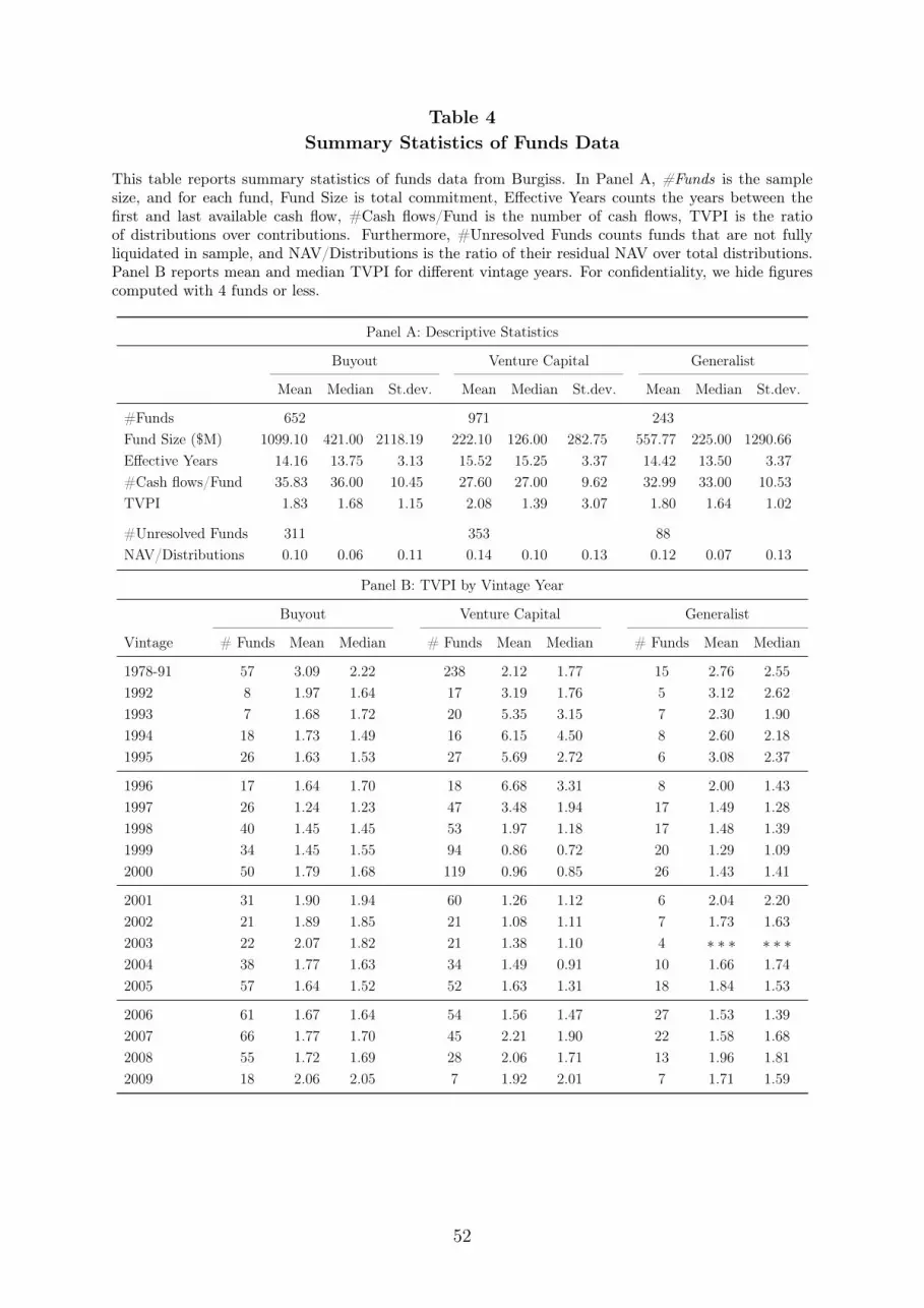
Table 4Summary Statistics of Funds Data

This table reports summary statistics of funds data from Burgiss. In Panel A, #Funds is the samplesize, and for each fund, Fund Size is total commitment, Effective Years counts the years between thefirst and last available cash flow, #Cash flows/Fund is the number of cash flows, TVPI is the ratioof distributions over contributions. Furthermore, #Unresolved Funds counts funds that are not fullyliquidated in sample, and NAV/Distributions is the ratio of their residual NAV over total distributions.Panel B reports mean and median TVPI for different vintage years. For confidentiality, we hide figurescomputed with 4 funds or less.

Panel A: Descriptive Statistics

Buyout Venture Capital Generalist

Mean Median St.dev. Mean Median St.dev. Mean Median St.dev.

#Funds 652 971 243

Fund Size ($M) 1099.10 421.00 2118.19 222.10 126.00 282.75 557.77 225.00 1290.66

Effective Years 14.16 13.75 3.13 15.52 15.25 3.37 14.42 13.50 3.37

#Cash flows/Fund 35.83 36.00 10.45 27.60 27.00 9.62 32.99 33.00 10.53

TVPI 1.83 1.68 1.15 2.08 1.39 3.07 1.80 1.64 1.02

#Unresolved Funds 311 353 88

NAV/Distributions 0.10 0.06 0.11 0.14 0.10 0.13 0.12 0.07 0.13

Panel B: TVPI by Vintage Year

Buyout Venture Capital Generalist

Vintage # Funds Mean Median # Funds Mean Median # Funds Mean Median

1978-91 57 3.09 2.22 238 2.12 1.77 15 2.76 2.55

1992 8 1.97 1.64 17 3.19 1.76 5 3.12 2.62

1993 7 1.68 1.72 20 5.35 3.15 7 2.30 1.90

1994 18 1.73 1.49 16 6.15 4.50 8 2.60 2.18

1995 26 1.63 1.53 27 5.69 2.72 6 3.08 2.37

1996 17 1.64 1.70 18 6.68 3.31 8 2.00 1.43

1997 26 1.24 1.23 47 3.48 1.94 17 1.49 1.28

1998 40 1.45 1.45 53 1.97 1.18 17 1.48 1.39

1999 34 1.45 1.55 94 0.86 0.72 20 1.29 1.09

2000 50 1.79 1.68 119 0.96 0.85 26 1.43 1.41

2001 31 1.90 1.94 60 1.26 1.12 6 2.04 2.20

2002 21 1.89 1.85 21 1.08 1.11 7 1.73 1.63

2003 22 2.07 1.82 21 1.38 1.10 4 ∗ ∗ ∗ ∗ ∗ ∗2004 38 1.77 1.63 34 1.49 0.91 10 1.66 1.74

2005 57 1.64 1.52 52 1.63 1.31 18 1.84 1.53

2006 61 1.67 1.64 54 1.56 1.47 27 1.53 1.39

2007 66 1.77 1.70 45 2.21 1.90 22 1.58 1.68

2008 55 1.72 1.69 28 2.06 1.71 13 1.96 1.81

2009 18 2.06 2.05 7 1.92 2.01 7 1.71 1.59

52

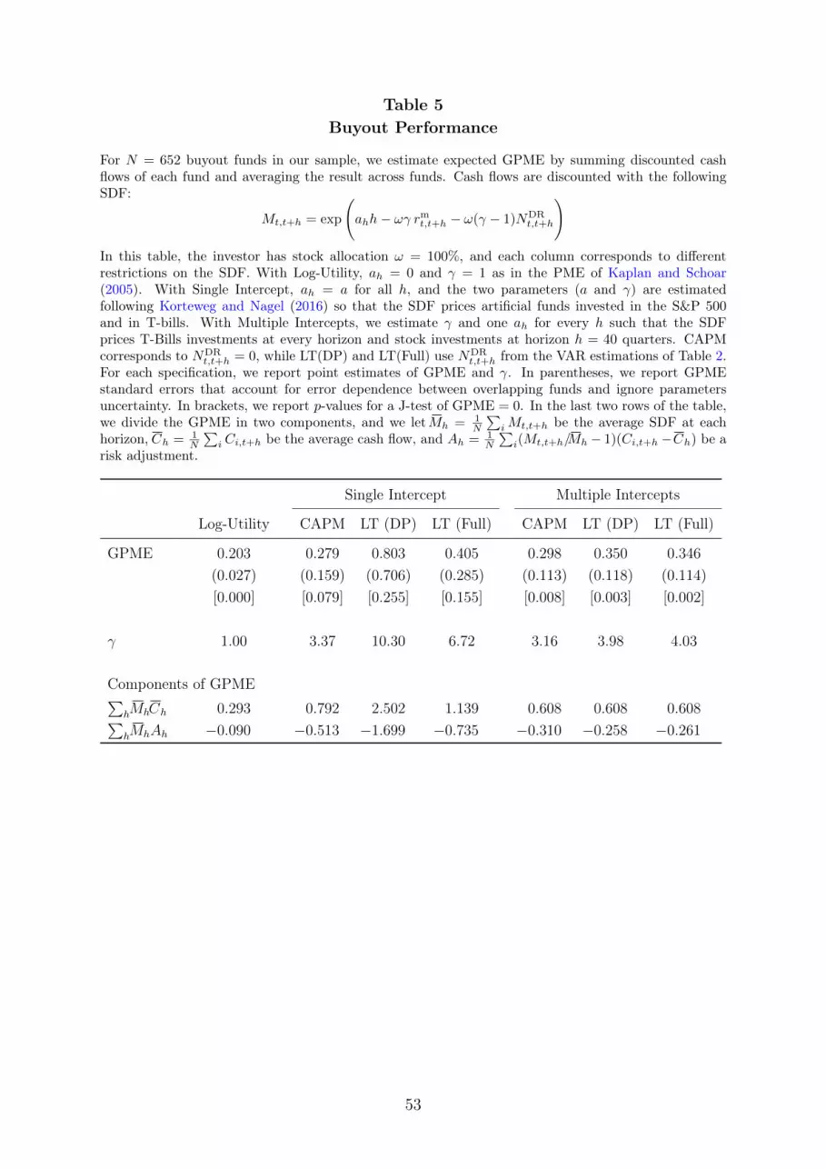
Table 5Buyout Performance

For N = 652 buyout funds in our sample, we estimate expected GPME by summing discounted cashflows of each fund and averaging the result across funds. Cash flows are discounted with the followingSDF:

Mt,t+h = exp

(ahh− ωγ rmt,t+h − ω(γ − 1)NDR

t,t+h

)

In this table, the investor has stock allocation ω = 100%, and each column corresponds to differentrestrictions on the SDF. With Log-Utility, ah = 0 and γ = 1 as in the PME of Kaplan and Schoar(2005). With Single Intercept, ah = a for all h, and the two parameters (a and γ) are estimatedfollowing Korteweg and Nagel (2016) so that the SDF prices artificial funds invested in the S&P 500and in T-bills. With Multiple Intercepts, we estimate γ and one ah for every h such that the SDFprices T-Bills investments at every horizon and stock investments at horizon h = 40 quarters. CAPMcorresponds to NDR

t,t+h = 0, while LT(DP) and LT(Full) use NDRt,t+h from the VAR estimations of Table 2.

For each specification, we report point estimates of GPME and γ. In parentheses, we report GPMEstandard errors that account for error dependence between overlapping funds and ignore parametersuncertainty. In brackets, we report p-values for a J-test of GPME = 0. In the last two rows of the table,we divide the GPME in two components, and we letMh = 1

N

∑i Mt,t+h be the average SDF at each

horizon, Ch = 1N

∑i Ci,t+h be the average cash flow, and Ah = 1

N

∑i(Mt,t+h/Mh − 1)(Ci,t+h −Ch) be a

risk adjustment.

Single Intercept Multiple Intercepts

Log-Utility CAPM LT (DP) LT (Full) CAPM LT (DP) LT (Full)

GPME 0.203 0.279 0.803 0.405 0.298 0.350 0.346

(0.027) (0.159) (0.706) (0.285) (0.113) (0.118) (0.114)

[0.000] [0.079] [0.255] [0.155] [0.008] [0.003] [0.002]

γ 1.00 3.37 10.30 6.72 3.16 3.98 4.03

Components of GPME∑

hMhCh 0.293 0.792 2.502 1.139 0.608 0.608 0.608∑hMhAh −0.090 −0.513 −1.699 −0.735 −0.310 −0.258 −0.261

53

Table 6GPME Distributions

The table reports mean, standard deviation, and selected percentiles of the GPME distribution forbuyout, venture capital, and generalist funds across different models. The models are estimated inTable 5, 7, and 8.

Single Intercept Multiple Intercepts

Log-Utility CAPM LT (DP) LT (Full) CAPM LT (DP) LT (Full)

Buyout (N = 652)

Mean 0.20 0.28 0.80 0.41 0.30 0.35 0.35

St.Dev. 0.64 1.42 9.25 2.99 0.98 1.05 1.04

Min −1.25 −4.15 −15.39 −5.86 −2.21 −1.60 −1.66

p10 −0.36 −0.83 −4.30 −1.65 −0.47 −0.48 −0.47

p25 −0.12 −0.38 −0.85 −0.56 −0.20 −0.23 −0.20

p50 0.13 −0.04 −0.17 −0.14 0.02 0.03 0.04

p75 0.44 0.59 0.61 0.69 0.51 0.61 0.58

p90 0.82 1.72 4.06 2.76 1.35 1.56 1.51

Max 10.89 13.98 165.94 42.62 8.78 8.32 8.66

Venture Capital (N = 971)

Mean 0.14 −0.15 −0.19 −0.08 0.07 0.13 0.15

St.Dev. 1.40 1.18 1.43 1.68 1.07 1.23 1.32

Min −1.14 −2.57 −3.21 −2.84 −1.50 −1.36 −1.40

p10 −0.67 −0.95 −1.12 −1.02 −0.66 −0.65 −0.65

p25 −0.44 −0.63 −0.68 −0.63 −0.42 −0.41 −0.41

p50 −0.19 −0.33 −0.37 −0.34 −0.16 −0.16 −0.15

p75 0.23 0.04 −0.04 0.03 0.26 0.30 0.31

p90 0.88 0.72 0.73 0.90 0.87 0.91 0.98

Max 15.13 16.47 20.42 24.55 15.51 17.31 17.46

Generalist (N = 243)

Mean 0.16 0.13 0.05 0.15 0.21 0.24 0.25

St.Dev. 0.52 1.01 2.28 1.58 0.75 0.79 0.79

Min −1.15 −2.72 −6.43 −3.75 −1.50 −1.47 −1.51

p10 −0.39 −0.72 −1.95 −1.08 −0.41 −0.46 −0.42

p25 −0.17 −0.44 −0.69 −0.51 −0.24 −0.24 −0.23

p50 0.06 −0.12 −0.24 −0.17 0.00 0.03 0.06

p75 0.44 0.42 0.34 0.40 0.46 0.51 0.53

p90 0.79 1.19 2.38 2.07 1.01 1.11 1.10

Max 2.63 6.11 11.52 8.94 4.15 4.01 4.20

54

Table 7Venture Capital Performance

We estimate expected GPME for N = 971 venture capital funds in our sample. The construction of thistable follows the description of Table 5 using the sample of venture capital funds.

Single Intercept Multiple Intercepts

Log-Utility CAPM LT (DP) LT (Full) CAPM LT (DP) LT (Full)

GPME 0.135 −0.150 −0.188 −0.077 0.073 0.126 0.151

(0.084) (0.067) (0.081) (0.101) (0.065) (0.078) (0.084)

[0.109] [0.026] [0.020] [0.447] [0.261] [0.108] [0.072]

γ 1.00 2.93 4.68 4.19 2.03 2.37 2.40

Components of GPME∑

hMhCh 0.484 0.910 0.903 0.892 0.725 0.725 0.725∑hMhAh −0.349 −1.060 −1.091 −0.969 −0.652 −0.599 −0.574

55

Table 8Generalist Performance

We estimate expected GPME for N = 243 generalist funds in our sample. The construction of this tablefollows the description of Table 5 using the sample of generalist funds.

Single Intercept Multiple Intercepts

Log-Utility CAPM LT (DP) LT (Full) CAPM LT (DP) LT (Full)

GPME 0.156 0.127 0.046 0.153 0.213 0.241 0.249

(0.023) (0.094) (0.173) (0.129) (0.069) (0.074) (0.071)

[0.000] [0.177] [0.791] [0.234] [0.002] [0.001] [0.000]

γ 1.00 3.05 7.49 5.43 2.53 3.14 3.19

Components of GPME∑

hMhCh 0.318 0.703 1.043 0.832 0.563 0.563 0.563∑hMhAh −0.162 −0.576 −0.998 −0.679 −0.350 −0.321 −0.313

56

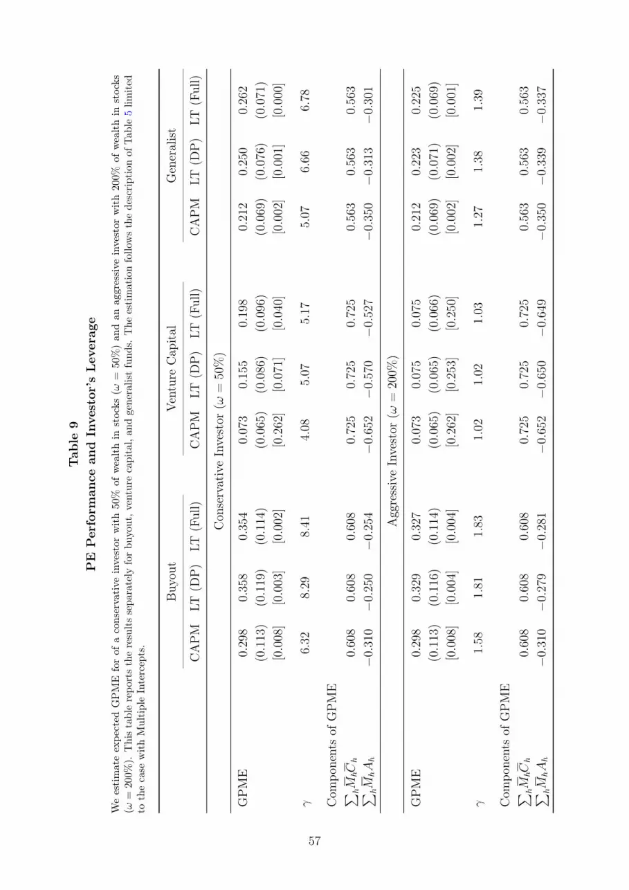
Tab

le9

PE

Per

form

ance

and

Inve

stor

’sLev

erag

e

We

esti

mat

eex

pect

edG

PM

Efo

rof

aco

nser

vati

vein

vest

orw

ith

50%

ofw

ealt

hin

stoc

ks(ω

=50%

)an

dan

aggr

essi

vein

vest

orw

ith

200%

ofw

ealt

hin

stoc

ks(ω

=20

0%).

Thi

sta

ble

repo

rts

the

resu

lts

sepa

rate

lyfo

rbu

yout

,ven

ture

capi

tal,

and

gene

ralis

tfu

nds.

The

esti

mat

ion

follo

ws

the

desc

ript

ion

ofTab

le5

limit

edto

the

case

wit

hM

ulti

ple

Inte

rcep

ts.

Buy

out

Ven

ture

Cap

ital

Gen

eral

ist

CA

PM

LT(D

P)

LT(F

ull)

CA

PM

LT(D

P)

LT(F

ull)

CA

PM

LT(D

P)

LT(F

ull)

Con

serv

ativ

eIn

vest

or(ω

=50%)

GP

ME

0.298

0.358

0.354

0.073

0.155

0.198

0.212

0.250

0.262

(0.113)

(0.119)

(0.114)

(0.065)

(0.086)

(0.096)

(0.069)

(0.076)

(0.071)

[0.008]

[0.003]

[0.002]

[0.262]

[0.071]

[0.040]

[0.002]

[0.001]

[0.000]

γ6.32

8.29

8.41

4.08

5.07

5.17

5.07

6.66

6.78

Com

pone

nts

ofG

PM

E∑

hM

hCh

0.608

0.608

0.608

0.725

0.725

0.725

0.563

0.563

0.563

∑hM

hAh

−0.310

−0.250

−0.254

−0.652

−0.570

−0.527

−0.350

−0.313

−0.301

Agg

ress

ive

Inve

stor

(ω=

200%

)

GP

ME

0.298

0.329

0.327

0.073

0.075

0.075

0.212

0.223

0.225

(0.113)

(0.116)

(0.114)

(0.065)

(0.065)

(0.066)

(0.069)

(0.071)

(0.069)

[0.008]

[0.004]

[0.004]

[0.262]

[0.253]

[0.250]

[0.002]

[0.002]

[0.001]

γ1.58

1.81

1.83

1.02

1.02

1.03

1.27

1.38

1.39

Com

pone

nts

ofG

PM

E∑

hM

hCh

0.608

0.608

0.608

0.725

0.725

0.725

0.563

0.563

0.563

∑hM

hAh

−0.310

−0.279

−0.281

−0.652

−0.650

−0.649

−0.350

−0.339

−0.337

57

A Theoretical Stochastic Discount Factor

In this section, we connect the long-term SDF from the main text to theory by deriving

its theoretical version. We use the setup of Campbell (1993) extending his results to price

payoffs received several periods in the future.

The investor has infinite-horizon Epstein-Zin preferences over consumption, and these

preferences correspond to the following generic form of SDF (Epstein and Zin, 1989):

M theoryt,t+1 = exp

(θ log δ − θ

ψ(ct+1 − ct)− (1− θ) rWt+1

)(A.1)

In this expression, ct is the natural logarithm of consumption, and rWt+1 is the log-return

on wealth. Greek letters indicate parameters with δ being the subjective discount factor,

ψ being the elasticity of intertemporal substitution, and θ = 1−γ1−1/ψ

, which depends on ψ

and relative risk aversion γ.

The budget constraint of the investor can be written as follows:

Wt+1 = (Wt − Ct)RWt+1 (A.2)

Wealth is Wt, while Ct = exp(ct) is consumption, and RWt+1 = exp(rWt+1) is the return on

wealth. Following Campbell (1993), we represent the investor’s budget constraint with

the following log-linear approximation:

wt+1 − wt = rWt+1 + k +

(1− 1

ρ

)(ct − wt) (A.3)

In this expression, wt is the logarithm of wealth, k and ρ are approximation constants.

A.1 Consumption

Assuming that second and higher moments of rWt+1 are constant over time, consumption

can be expressed as a function of returns. For that, we use two equations derived in

Campbell (1993) under the same set of assumptions. The first equation connects expected

58

consumption growth to expected return on wealth:

Et [ct+1 − ct] = ψEt[rWt+1

]+ ψ log(δ) +

1

2

1− γ

1− ψVart

(ct+1 − ct − ψrWt+1

)

︸ ︷︷ ︸constant

(A.4)

The second equation connects the unexpected component of consumption growth to the

unexpected component of rWt+1 and to discount rate (DR) news about investor’s wealth:

ct+1 − ct − Et [ct+1 − ct] = rWt+1 − Et[rWt+1

]+ (1− ψ) (Et+1 − Et)

∞∑

j=1

ρjrWt+1

︸ ︷︷ ︸NDR,W

t+1

(A.5)

Combining (A.4) with (A.5), we get the following expression for the logarithm of con-

sumption growth:

ct+1 − ct = rWt+1 + (1− ψ)NDR,Wt+1 − (1− ψ)Et

[rWt+1

]+ constant (A.6)

A.2 Return on Wealth

DR news on wealth, NDR,Wt+1 , can be expressed in terms of DR news on underlying assets.

For that, we specify a simple investment strategy for the investor. His portfolio is a

constant combination of two assets. One asset is risk-free, while the other is a market

index of public equities. The return on the risk-free asset is constant and its logarithm is

denoted rf . The return on the market is risky and its logarithm is denoted rmt . Expected

log-return on the market can vary over time, while its variance and higher moments

remain constant.

Following Campbell and Viceira (1999), log-returns on individual assets determine log-

return on wealth through the following approximate relation:

rWt+1 = ω(rmt+1 − rf

)+ rf +

1

2ω(1− ω)var

(rmt+1

)(A.7)

In this expression, ω is the constant portfolio weight in the market. Under our assump-

59

tions, this approximation implies:

NDR,Wt+1 = ωNDR

t+1 (A.8)

where NDRt+1 is one-period DR news on the market as defined in the main text.

A.3 Theoretical Long-Term SDF

To obtain the theoretical form of the long-term SDF, we substitute (A.6) and (A.7) inside

the SDF expression (A.1). As a result, we obtain the one-period theoretical version of

the long-term SDF:

M theoryt+1 = exp

(at − ωγ rmt+1 − ω(γ − 1)NDR

t+1

)(A.9)

with at = ω(γ − 1)Et [rm,t+1] + constant.

A.3.1 Two Periods

The product M theoryt+1 ×M theory

t+2 can be written as follows:

M theoryt,t+2 = exp

(a2,t − ωγ rmt,t+2 − ω(γ − 1)NDR

t,t+2

)(A.10)

This expression contains the following objects:

a2,t = ω(γ − 1)(Et[r

mt+1] + Et[r

mt+2])+ 2 · constant (A.11)

NDRt,t+2 = (Et+2 − Et)

∞∑

j=1

ρjrmt+2+j − (1− ρ)(Et+1 − Et)rmt+2

≈ (Et+2 − Et)∞∑

j=1

ρjrmt+2+j (A.12)

and the approximation of NDRt,t+2 is accurate for ρ close 1.

60

A.3.2 Many Periods

The product M theoryt+1 ×M theory

t+2 × · · · ×M theoryt+h can be written as follows:

M theoryt,t+h = exp

(ah,t − ωγ rmt,t+h − ω(γ − 1)NDR

t,t+h

)(A.13)

where

ah,t = ω(γ − 1)h∑

s=1

Et[rmt+s] + h · constant (A.14)

Furthermore, multi-period DR news is written as follows:

NDRt,t+h =

h∑

s=1

NDRt+s −

h−1∑

s=1

[(Et+s − Et+s−1)

h−s∑

j=1

rmt+s+j

](A.15)

=h∑

s=1

[(Et+s − Et+s−1)

∞∑

j=1

ρjrmt+s+j

]−

h−1∑

s=1

[(Et+s − Et+s−1)

h−s∑

j=1

rmt+s+j

]

=h∑

s=1

[(Et+s − Et+s−1)

∞∑

j=h−s+1

ρjrmt+s+j

]−

h−1∑

s=1

[(Et+s − Et+s−1)

h−s∑

j=1

(1− ρj)rmt+s+j

]

≈h∑

s=1

[(Et+s − Et+s−1)

∞∑

j=h−s+1

ρjrmt+s+j

]

=h∑

s=1

[(Et+s − Et+s−1)

∞∑

j=1

ρjrmt+h+j

]

= (Et+h − Et)∞∑

j=1

ρjrmt+h+j (A.16)

The approximation is accurate for ρ close to 1.

61

62

Optimal Allocation to Private Equity

Nicola Giommetti Morten Sorensen∗

Abstract

We study the portfolio problem of an investor (LP) that invests in stocks, bonds,

and private equity (PE) funds. The LP repeatedly commits capital to PE funds.

This capital is only gradually contributed and eventually distributed back to the

LP, requiring the LP to hold a liquidity buffer for its uncalled commitments. De-

spite being riskier, PE investments are not monotonically declining in risk aversion.

Instead, there are two qualitatively different investment strategies with intuitive

heuristics. We introduce a secondary market for PE partnership interests to study

optimal trading in this market and implications for the LP’s optimal investments.

∗The authors can be reached at Copenhagen Business School (ngi.fi@cbs.dk) and Tuck School ofBusiness (morten.sorensen@tuck.dartmouth.edu). We are grateful to Peter Cornelius and Tim Jenkinsonfor helpful suggestions and to Peter Feldhütter, Andrey Malenko, Mark Westerfield, and participants atCopenhagen Business School, Glion Institute Annual Private Equity Conference, LBS Private EquitySymposium, and Southern California Private Equity Conference for helpful discussion and comments.

Chapter 2

63

The number of US publicly traded companies is declining and an increasing amount

of capital is invested in private equity (PE) and other non-public assets.1 Typical PE

investors, so-called limited partners (LPs), are pension funds, sovereign wealth funds,

university endowments, and other institutional investors. Despite their increasing alloca-

tions to PE, it remains unclear how LPs should optimally manage their PE investments

as part of their broader portfolio allocations. We study this problem.

We introduce PE investments into a standard portfolio model. PE investments are risky,

illiquid, and long-term. They are risky because PE investments earn a risky return and

generate risky distributions to the LP. They are illiquid because the LP must hold them

to maturity, and the LP cannot liquidate (or collateralize) its PE investments to convert

them into current consumption, although this is relaxed in the extension with a secondary

market. They are long-term because the LP’s commitments are only gradually called and

invested into underlying private assets by PE funds, and the eventual distributions back

to the LP only arrive after a substantial time. Thus, the LP can only adjust its PE

exposure slowly, and it may need to hold a liquidity reserve to meet future capital calls

arising from its current uncalled commitments. A main contribution of our analysis is to

present a tractable model that captures these aspects of PE investments, particularly the

LP’s repeated capital commitments to an arbitrary number of PE funds, and to solve for

the LP’s optimal investment policies.

The particular nature of PE investments has interesting implications for the LP’s optimal

allocations and investment policies. Unsurprisingly, the illiquid and long-term nature of

PE investments can lead the LP to reduce its PE allocation relative to the first-best

allocation. Perhaps more surprisingly, the optimal PE allocation is not monotonically

decreasing in the LP’s risk aversion. With reasonable parameter values, the LP’s PE

allocation is largely constant, and a more risk averse LP may, in fact, choose a higher PE

allocation than a less risk averse LP. In contrast, risk aversion significantly affects the

LP’s allocations to traded stocks and bonds.

Depending on risk aversion, there are two distinct investment strategies. A conservative

LP, with higher risk aversion (in our specification, a relative risk aversion of γ = 3),1Doidge, Karolyi, and Stulz (2017) discuss the declining number of listed companies, and Bain &

Company (2019) show the increasing allocations to alternative investments.

64

holds relatively more liquid reserves of stocks and bonds than illiquid PE investments.

This LP tends to be unconstrained and to remain close to an interior optimum, leaving

it largely unaffected by the illiquid and long-term nature of PE investments. In response

to a positive shock to the net asset value (NAV) of its PE investments, the conservative

LP reduces new PE commitments to gradually rebalance its portfolio back towards the

interior optimum, basically treating PE investments as another traded stock. In contrast,

an aggressive LP with lower risk aversion (γ = 1) faces a binding liquidity constraint. It

would prefer greater PE exposure, but larger PE commitments would require a greater

liquidity reserve, which is costly. In response to a positive shock to the NAV of its PE

investments, the aggressive LP does not rebalance its portfolio, and instead it enjoys a

temporary increase in its PE exposure without a corresponding increase in its liquidity

reserve.

We extend the model with a secondary market where LPs can trade PE partnership

interests to investigate two effects: First, an aggressive LP assigns higher valuations

to mature PE funds than a conservative LP. Mature funds provide PE exposure with

relatively less liquidity requirements, which is valuable for a constrained LP, and there

are gains from trade when conservative LPs can sell partnership interests in mature

PE funds to aggressive LPs. Second, the presence of a secondary market where an LP

can liquidate its PE investments relaxes its liquidity constraint. In times of stress an

LP may choose to liquidate a fraction of its PE investments, even at a discount. And

knowing that this liquidity is available, ex-post, allows the LP to hold a more aggressive

allocation, ex-ante. We quantify these effects and find that the gains from a single trade,

while positive, are modest. However, a secondary market that provides liquidity in times

of stress substantially affects the aggressive LP’s optimal investments even though the

LP only rarely actually transacts in this market.

A large literature investigates the portfolio and asset pricing implications of illiquidity

in general, and we do not attempt to summarize this literature. Our analysis is in the

spirit of Longstaff (2001) who uses numerical methods to study a portfolio problem with

illiquid assets that can only be traded in limited amounts.

In the context of PE specifically, Ang, Papanikolaou, and Westerfield (2014) analyze an

investor’s optimal investments with an illiquid asset that can only be rebalanced infre-

65

quently, at Poisson arrival times, to capture a situation where the investor must search

for a counterparty. They find that this form of illiquidity increases the investor’s effective

risk aversion. Our analysis does not capture the arrival of trading opportunities. Instead,

we focus on the ongoing commitments and long-term dynamics of PE investments, which

have distinct implications. For example, in our model, LPs with higher risk aversion are

unaffected by the illiquidity of PE investments, and it does not increase their effective

risk aversion. Sorensen, Wang, and Yang (2014) model an LP that rebalances stocks and

bonds while holding an illiquid asset to maturity in order to analyze the costs of the

unspanned risks of the illiquid asset, taking the investment in the illiquid asset as given.

Bollen and Sensoy (2020) extend this analysis with a secondary market for partnership

interests. Dimmock, Wang, and Yang (2019) evaluate the “endowment model” used by

some institutions that invest in alternative assets with lock-up periods. Phalippou and

Westerfield (2014) study commitment risk for an investor in one, two, or an infinite num-

ber of PE funds using a Markov switching model to capture the state of the economy.

Finally, there is an extensive literature about the risks and returns of PE investments,

and Korteweg (2019) surveys this literature.

1 Model

We extend a standard portfolio model with illiquid PE investments that work as follows.

Each period (in our specification, each year) a limited partner (LP) decides how much

capital to commit to new PE funds. This capital is not immediately invested, however.

Instead, it is gradually contributed to (or drawn down or called by) the PE funds over a

period of several years. When capital is contributed (or drawn or called), it is paid by the

LP to the PE funds, which invest the capital in underlying private assets (typically, equity

stakes in portfolio companies). After holding these private assets for an extended period,

typically several years, the private assets are sold (exited) by the PE funds. The proceeds

from these sales, net of the PE funds’ fees (management fees and carried interest), are

paid out (distributed) to the LP.

The LP thus maintains a stock of uncalled commitments (drawdown obligations) rep-

resenting the capital that the LP has already committed but that has not yet been

contributed to the PE funds. These uncalled commitments are gradually called by the

66

PE funds and then invested in underlying private assets. The LP’s PE exposure arises

from its claim to the future distributions from the currently held private assets, and the

NAV is the value of this claim, which constitutes the LP’s illiquid wealth.2 Each period

the LP can decide to commit additional capital to new PE funds and increase its stock

of uncalled commitments. Once committed, however, the LP cannot decide to reduce its

uncalled commitments. Uncalled commitments only decline gradually, as capital is called

and invested by the PE funds.

PE funds are only open for new commitments at inception and typically have ten-year

lives, although funds are routinely extended. New PE funds are continuously raised, and

LPs diversify their PE investments both across different contemporaneous funds and over

time by committing capital to new funds on an ongoing basis, resulting in a diversified

portfolio of staggered PE fund commitments. In this case, distributions received from

earlier fund commitments, when available, can pay contributions to later commitments,

and our model is consistent with this practice.

1.1 Preferences and Timing

The analysis is based on a standard, discrete-time, infinite-horizon, partial-equilibrium,

portfolio model with i.i.d. returns and an LP with power utility (CRRA) preferences:

Et

[ ∞∑

s=t

δs−tC1−γs

1− γ

](1)

The LP’s consumption is Ct, its time preference is δ, and γ is its relative risk aver-

sion.

Like Ang et al. (2014) we assume a relative risk aversion greater than or equal to one,

γ ≥ 1, implying an elasticity of intertemporal substitution less than or equal to one. The

LP has negative infinite utility in states with zero consumption. The LP is “bankrupt”

when it is unable to consume, and the LP will avoid such states at all costs.3 Below, we

emphasize the results for an LP with γ = 1, which we call an aggressive LP, and for an

LP with γ = 3, which we call a conservative LP.2The NAV, denoted Pt below, is the price that PE investments would trade at, if they were traded.

In the liquid model introduced below, we allow for such trades.3Maurin, Robinson, and Stromberg (2020) and Banal-Estañol, Ippolito, and Vicente (2017) formally

model LPs’ liquidity constraints, distortions when LPs can default, and the penalties for defaulting.

67

Total wealth (Wt),illiquid wealth (Pt),

uncalled commitments (Kt)

t LP consumes (Ct),allocates to stocks (St),

to bonds (Bt), makes newPE commitments (Nt)

Returns realized(RF, RS,t+1, RP,t+1)

Contributions (It+1),distributions (Dt+1)

paid

t+ 1

Figure 1: Timing of events during the period from time t to time t+ 1.

The timing of the model is illustrated in Figure 1. At time t, the LP has total wealth

Wt, illiquid wealth Pt, and uncalled commitments Kt. After observing these three state

variables, the LP consumes and invests. The LP consumes Ct out of its liquid wealth,

Wt−Pt. Its remaining liquid wealth, Wt−Pt−Ct, is allocated to traded stocks, St, and

bonds, Bt:

Bt = Wt − Pt − Ct − St (2)

The LP decides the amount of capital to commit to new PE funds, Nt. New PE com-

mitments increase the LP’s total stock of uncalled commitments, Nt +Kt, but they do

not directly affect the LP’s wealth or budget constraint in the period when they are

made.

After the LP has consumed and made its portfolio decisions, returns are realized and

contributions and distributions are paid. In practice, returns, contributions, and dis-

tributions are earned and paid throughout the period. For simplicity, we assume that

returns are realized first and then contributions and distributions are paid. This assump-

tion emphasizes the long-term nature of PE investments, because new PE commitments

cannot be contributed and provide PE exposure to the LP in the period when they are

made. Rather, new PE commitments are contributed and invested in private assets with

at least a one-period lag.

Conventionally, returns earned from time t to t+ 1 have subscript t+ 1, and the returns

to stocks and PE investments during this period are denoted RS,t+1 and RP,t+1, respec-

tively. Bonds earn the risk-free rate, RF. All returns are gross returns. Correspondingly,

distributions and contributions paid from time t to t + 1 are denoted Dt+1 and It+1,

68

respectively. The LP pays contributions, It+1, out of its liquid wealth to the PE funds

who invest them in private assets. Distributions, Dt+1, are paid from the PE funds to

the LP as liquid wealth.

The three state variables update as follows. The LP’s uncalled commitments, Kt, increase

by the amount of new PE commitments, Nt, and decrease by the amount contributed,

It+1:

Kt+1 = Kt +Nt − It+1 (3)

The NAV of the PE investments, Pt, earns the risky return, RP,t+1, and then it increases by

the amount contributed to the PE funds, It+1, and it decreases by the amount distributed

from the PE funds, Dt+1:

Pt+1 = RP,t+1Pt + It+1 −Dt+1 (4)

The LP’s end-of-period wealth, Wt+1, is the combined value of its PE investments, stocks,

and bonds. Contributions and distributions made during the period do not affect the end-

of-period wealth since they only reallocate wealth between liquid and illiquid investments:

Wt+1 = RP,t+1Pt +RS,t+1St +RF(Wt − Pt − Ct − St) (5)

1.2 Linear Fund Dynamics

In practice, an LP invests in many PE funds, each with its own amounts of uncalled

commitments, contributions, distributions, and NAVs. Modeling each fund separately,

however, is difficult due to the resulting high-dimensional state space and the curse of

dimensionality in dynamic programming. Motivated by Takahashi and Alexander (2002),

we assume linear fund dynamics where each fund’s contributions and distributions are

linear in the fund’s uncalled commitments and NAV.4 An implication of linear fund

dynamics is that the LP’s aggregate contributions and distributions across all its PE

funds are linear in the aggregate uncalled commitments and aggregate NAV. Aggregate4Our model simplifies Takahashi and Alexander (2002) in two ways. Their contribution rate varies

over time, and our rate is fixed by λN and λK. Moreover, our distribution rate is fixed by λD, and theirdistribution rate approaches 100% as the fund winds down.

69

uncalled commitments and aggregate NAV are therefore sufficient statistics for the LP’s

portfolio of PE investments, in an arbitrary number of PE funds, which reduces the

state space to three dimensions (two, in the normalized problem below) and avoids the

numerical difficulties that arise when specifying each fund separately.

Formally, let PE funds be indexed by u, and let the set of PE funds that the LP has

a partnership interest in at time t, including the new PE funds that the LP commits

capital to at time t, be denoted Ut.5 In practice, multiple LPs invest in a PE fund,

and the uncalled commitments, contributions, distributions, and NAVs defined below

represent the LP’s share of each fund.

In its first year, contributions to a new fund u are the fraction λN of the fund’s newly

committed capital, Nu,t:

Iu,t+1 = λNNu,t (6)

In subsequent years, contributions are the fraction, λK, of the fund’s remaining uncalled

commitments, Ku,t:

Iu,t+1 = λKKu,t (7)

Since Nt =∑

u∈UtNu,t is the LP’s aggregate new PE commitments, and Kt =

∑u∈Ut

Ku,t

is the aggregate existing commitments, the LP’s aggregate contributions, It+1, are:

It+1 =∑

u∈Ut

Iu,t+1 = λNNt + λKKt (8)

Hence, aggregate contributions, It, are linear in aggregate new commitments, Nt, and ag-

gregate existing commitments, Kt. Our model allows for different intensities of contribu-

tions for new and existing commitments, but in our baseline specification λN = λK = 30%

for simplicity.6

Distributions are modeled similarly. Fund u’s distributions, Du,t+1, are the fraction, λD,5When fund u has a ten-year life, the LP has a partnership interest in this fund starting the year of

the LP’s initial commitment and extending through the following nine years until the fund terminates.Note also that a new PE fund, u, that the LP commits capital to at time t starts out with zero NAV, soPu,t = 0.

6For comparison, Takahashi and Alexander (2002) consider a contribution rate of 25% when the fundis one year old, 33.3% when it is two years old, and 50% after that.

70

of fund u’s NAV, which is Ru,t+1Pu,t, where Ru,t+1 is fund u’s gross return, so:

Du,t+1 = λDRu,t+1Pu,t (9)

The LP’s aggregate distributions across all its PE funds is denoted Dt+1 and equals:

Dt+1 =∑

u∈Ut

Du,t+1 = λDRP,t+1Pt (10)

Here, Pt =∑

u∈UtPu,t is the LP’s aggregate NAV, and RP,t+1 =

∑u∈Ut

Ru,t+1Pu,t

Ptis the

value-weighted average return of the LP’s PE funds. In our specification, the intensity

of distributions is λD = 40% of the fund’s remaining NAV. Even though distributions

are a deterministic fraction of the NAV, the fund’s NAV is stochastic, because private

assets earn risky returns, and the LP receives a risky flow of distributions from its PE

investments.

The above derivations are important for the generality of our analysis. In the general

problem, the LP invests in an arbitrary number of contemporaneous and staggered PE

funds, but specifying each fund individually is intractable, as mentioned. The above

discussions shows, however, that linear fund dynamics imply that the aggregate NAV

and aggregate uncalled commitments are sufficient statistics for the LP’s portfolio of PE

investments. Hence, the solution to the LP’s general problem can be found by solving

a reduced problem with a more tractable state space. Without loss of generality, we

therefore focus on the LP’s reduced problem below.7

A limitation of linear fund dynamics is that PE funds never completely end, as also

discussed by Takahashi and Alexander (2002). In practice, PE funds have ten-year lives,

although these lives are routinely extended.8 In our specification the remaining economic7An additional detail of the specification is how the idiosyncratic risk of the value-weighted PE return,

RP, depends on the LP’s PE investments, P . Here, we assume that the LP has partnership interests ina diversified number of PE funds, and that changes in the amount of the LP’s PE investments arise fromproportional changes in the stakes in these funds, leaving the idiosyncratic risk constant. Alternatively,changes in the LP’s PE investments can be associated with changes in the number of PE funds, in whichcase a lower amount of PE investments would be associated with an increase in the idiosyncratic riskof RP due to less diversification. In principle, our model can accommodate a dependency between theidiosyncratic risk of RP and P , although we have not pursued this extension. Robinson and Sensoy(2016) find that most of the volatility in PE investments can be diversified.

8In their analysis of long-term PE performance, Gupta and Van Nieuwerburgh (2020) report that itis common for PE funds to have activity fifteen years after inception.

71

value in the PE funds’ later years is minimal, mitigating this limitation of the linear fund

dynamics. Specifically, 83.2% of a fund’s committed capital is contributed during its first

five years, and 97.2% is contributed after ten years. Moreover, in steady state, the LP

holds a balanced portfolio of younger and older PE funds, and specification errors in the

dynamics will largely average out across the funds when aggregating their contributions

and distributions.9

Management fees are implicit in this setup. In practice, PE funds charge annual man-

agement fees of 0.5%–2% of the total committed capital, which means that this capital is

contributed by the LP to the PE funds, but this capital is not used to acquire underlying

private assets. Below, we extend our model to explicit management fees, but in most of

the analysis management fees are implicit, and the contributed capital, It, is the com-

bined amount invested in underlying private assets and paid in management fees. In this

case, the NAV, Pt, includes the value of management fees, and the PE return, RP,t, is net

of both management fees and carried interest.10 An advantage of implicit management

fees is that the analysis of illiquidity is more transparent, because the optimal allocations

can be compared to the first-best benchmark when PE is liquid and freely traded. With

liquid PE there is no notion of committed capital, however, and the liquid model does

not accommodate explicit management fees. Another advantage of implicit management

fees is that the return to PE investments, RP,t, is the return net of both management fees

and carried interest, which is the return that is typically reported in empirical studies.

In Section 4, we model management fees explicitly, which requires a reinterpretation of

the contributed capital, It, the NAV, Pt, and the PE return, RP,t. The main finding is

that the optimal policies are largely similar with implicit and explicit management fees

and that this modeling choice is not critical for our results.9To illustrate this averaging, assume that PE funds live for three periods, and let the dynamics of

contributions be specified by λ0, λ1, and λ2, which are the relative amounts of a fund’s total committedcapital that is contributed during each period. All committed capital is eventually contributed, soλ0+λ1+λ2 = 1. A diversified LP with an equal amount, κ, committed to funds at each of the three ageshas aggregate contributions of λ0κ+ λ1κ+ λ2κ = κ. It follows that regardless of the specification of thedynamics, i.e., the particular choice of λ, the resulting amount of aggregate contributions is unaffected.

10Actual accounting for management fees can be complicated. PE funds with deal-by-deal carry,sometimes known as the US Market Standard, typically attribute management fees to individual dealsand gross up the valuations of these deals with the attributed management fees. Another PE fundcompensation structure, sometimes known as the UK Market Standard, has the general partner borrowingthe amounts that correspond to the fees and repaying these amounts out of a priority share of the fund’sprofits, which is consistent with our model of implicit management fees.

72

The implied dynamics of capital calls and distributions are shown in Figures 2 to 5,

which show impulse responses of an initial $100 PE commitment in year 0, followed by

no further commitments. Figure 2 shows annual capital calls. In year one, $30 is called

(λN = 30% times N0 = $100). In year two, $21 is called (λK = 30% times K1 = $70). In

the following years, corresponding declining amounts of capital are called.

●

●

●

●

●

●

●

●

●

●●

● ● ● ● ●

Contributions following $100 commitment

Years

Dol

lars

0 1 2 3 4 5 6 7 8 9 10 11 12 13 14 15

0

10

20

30

Figure 2: Impulse response function of contributions following a $100 commitment in year 0.

Figure 3 shows the dynamics of distributions. Distributions depend on NAVs, which are

risky, and the figure shows average distributions along with the 5th and 95th percentiles

(distributional assumptions are provided below). The largest annual distributions arrive

three to five years after the initial commitment, reflecting the long-term nature of PE

investments.

Figure 4 shows the cumulative net cash flow, i.e., cumulative distributions minus cumula-

tive contributions. The cumulative cash flow exhibits the well-known “J-curve” dynamics,

where it is initially negative, meaning that the LP initially contributes more capital than

it receives. With average cash flows the LP breaks even around year six, and then the

cumulative cash flow becomes positive and converges to its final value as the fund winds

down. The average cumulative net cash flow from an initial $100 investment is around

$50, implying an average multiple (TVPI or MOIC) around 1.5.

Figure 5 shows the dynamics of the fund’s NAV. Interestingly, $100 of initial commitments

73

Distributions following $100 commitment

Years

Dol

lars

0 1 2 3 4 5 6 7 8 9 10 11 12 13 14 15

0

10

20

30

40

● ●

●

●●

●

●

●

●

●

●

●

●

●●

●

● Mean5th−95th percentiles

Figure 3: Impulse response function of distributions following a $100 commitment in year 0. The solidline shows average annual distributions. The dashed lines show the 95th and 5th percentiles of thedistribution of annual distributions.

Cumulative cash flows following $100 commitment

Years

Dol

lars

0 1 2 3 4 5 6 7 8 9 10 11 12 13 14 15

−50

0

50

100

150

200

●

●

●●

●

●

●

●

●

●●

●●

● ● ●

● Mean5th−95th percentiles

Figure 4: Impulse response function of cumulative net cash flows, the sum of past and current net cashflows, following a $100 commitment in year 0. The solid line shows average cumulative cash flows. Thedashed lines show the 95th and 5th percentiles.

74

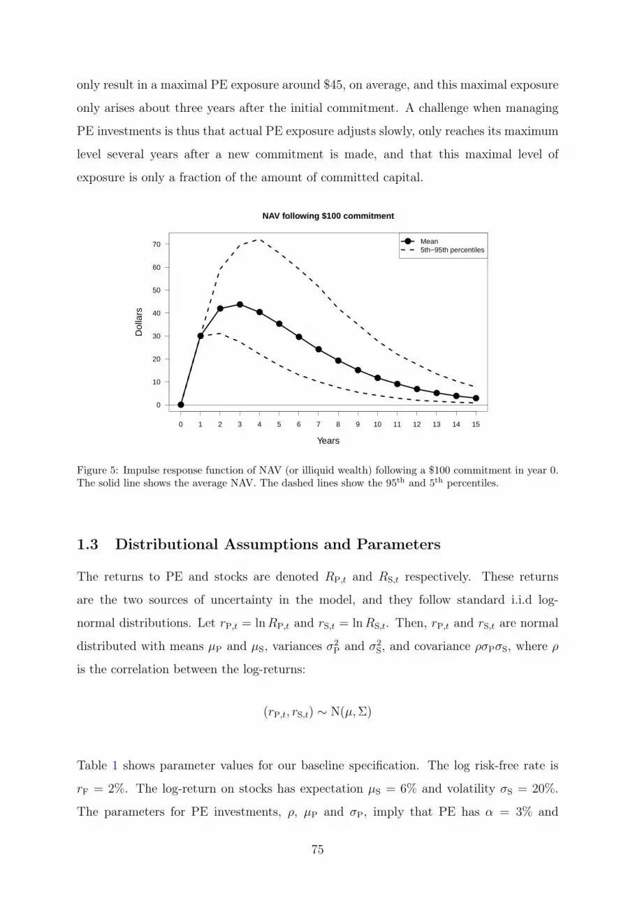
only result in a maximal PE exposure around $45, on average, and this maximal exposure

only arises about three years after the initial commitment. A challenge when managing

PE investments is thus that actual PE exposure adjusts slowly, only reaches its maximum

level several years after a new commitment is made, and that this maximal level of

exposure is only a fraction of the amount of committed capital.

NAV following $100 commitment

Years

Dol

lars

0 1 2 3 4 5 6 7 8 9 10 11 12 13 14 15

0

10

20

30

40

50

60

70

●

●

●

●

●

●

●

●

●

●

●

●

●

●●

●

● Mean5th−95th percentiles

Figure 5: Impulse response function of NAV (or illiquid wealth) following a $100 commitment in year 0.The solid line shows the average NAV. The dashed lines show the 95th and 5th percentiles.

1.3 Distributional Assumptions and Parameters

The returns to PE and stocks are denoted RP,t and RS,t respectively. These returns

are the two sources of uncertainty in the model, and they follow standard i.i.d log-

normal distributions. Let rP,t = lnRP,t and rS,t = lnRS,t. Then, rP,t and rS,t are normal

distributed with means µP and µS, variances σ2P and σ2

S, and covariance ρσPσS, where ρ

is the correlation between the log-returns:

(rP,t, rS,t) ∼ N(µ,Σ)

Table 1 shows parameter values for our baseline specification. The log risk-free rate is

rF = 2%. The log-return on stocks has expectation µS = 6% and volatility σS = 20%.

The parameters for PE investments, ρ, µP and σP, imply that PE has α = 3% and

75

β = 1.6, as defined by the log-linear CAPM:

ln E[RP]− rF = α + β (ln E[RS]− rF) (11)

with β = ρσP/σS.

Our parameters differ slightly from those in Ang et al. (2014), who assume a risk-free

rate of 4%, expected log-return on stocks of 12%, and volatility of 15%. To isolate

the effect of illiquidity, Ang et al. (2014) choose ρ, µP, and σP so PE investments have

the same risk and return as the stock market. In our specification, PE investments are

positively correlated with stocks, are more volatile than stocks, and have a positive alpha.

For robustness we also solve the model for other specifications of alpha, beta, and the

idiosyncratic risk, as reported in Appendix C.

Table 1: This table reports parameter values used as inputs of the model. It also includes importantstatistics that are implied by those parameter values.

Parameter/Statistic Expression ValueDraw-downs of new commitments λN 30%Draw-downs of older commitments λK 30%Distribution intensity λD 40%

Log of risk-free rate rF 2%Expected log-return to stocks µS 6%Expected log-return to PE µP 6.6%Volatility of log-return to stocks σS 20%Volatility of log-return to PE σP 40%Alpha of PE α 3%Beta of PE β 1.6

Subjective discount factor δ 95%

Implied:Log of expected return to stocks ln E[RS] 8%Log of expected return to PE ln E[RP] 14.6%Sharpe ratio of stocks (ln E[RS]− rF) /σS 0.3Sharpe ratio of PE (ln E[RP]− rF) /σP 0.315Correlation of log-returns to stocks and PE ρ 0.8

76

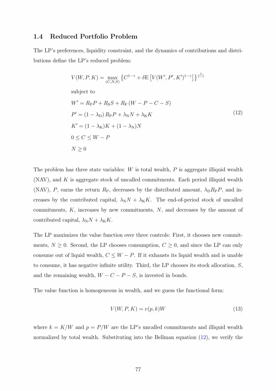
1.4 Reduced Portfolio Problem

The LP’s preferences, liquidity constraint, and the dynamics of contributions and distri-

butions define the LP’s reduced problem:

V (W,P,K) = max(C,N,S)

{C1−γ + δE

[V (W ′, P ′, K ′)1−γ

]} 11−γ

subject to

W ′ = RPP +RSS +RF (W − P − C − S)

P ′ = (1− λD)RPP + λNN + λKK

K ′ = (1− λK)K + (1− λN)N

0 ≤ C ≤ W − P

N ≥ 0

(12)

The problem has three state variables: W is total wealth, P is aggregate illiquid wealth

(NAV), and K is aggregate stock of uncalled commitments. Each period illiquid wealth

(NAV), P , earns the return RP, decreases by the distributed amount, λDRPP , and in-

creases by the contributed capital, λNN + λKK. The end-of-period stock of uncalled

commitments, K, increases by new commitments, N , and decreases by the amount of

contributed capital, λNN + λKK.

The LP maximizes the value function over three controls: First, it chooses new commit-

ments, N ≥ 0. Second, the LP chooses consumption, C ≥ 0, and since the LP can only

consume out of liquid wealth, C ≤ W − P . If it exhausts its liquid wealth and is unable

to consume, it has negative infinite utility. Third, the LP chooses its stock allocation, S,

and the remaining wealth, W − C − P − S, is invested in bonds.

The value function is homogeneous in wealth, and we guess the functional form:

V (W,P,K) = v(p, k)W (13)

where k = K/W and p = P/W are the LP’s uncalled commitments and illiquid wealth

normalized by total wealth. Substituting into the Bellman equation (12), we verify the

77

guess for v(k, p) solving the normalized problem:

v(p, k) = max(c,n,ωS)

{c1−γ + δE

[[(1− c)RWv(p

′, k′)]1−γ]} 1

1−γ

subject to

RW = ωP(RP −RF) + ωS(RS −RF) +RF

p′ =[(1− λD)RPp+ λNn+ λKk

]/[(1− c)RW

]

k′ =[k + n− λNn− λKk

]/[(1− c)RW

]

0 ≤ c ≤ 1− p

n ≥ 0

(14)

The normalized control variables are c = C/W , s = S/W , and n = N/W . Furthermore,

it is convenient to define the portfolio weight ωS = S/(W − C), ωP = P/(W − C), and

ωB = 1−ωS −ωP. These portfolio weights are normalized by the LP’s post-consumption

wealth in order to sum to one.11

1.5 Liquidity Constraint

The LP ensures that there is zero probability that it exhausts its liquid wealth, or,

equivalently, that its illiquid wealth, P , exceeds its total wealth, W . Since p = P/W , the

optimal policy satisfies the liquidity constraint:

Prob(p > 1) = 0 (15)

This liquidity constraint is the main friction in our analysis. One immediate implication of

the constraint and the unbounded support of the log-returns to stocks and PE investments

is that the LP wants to hold a liquidity reserve of safe assets, in our case risk-free bonds, at

least as large as its total stock of uncalled commitments. Another immediate implication

of the liquidity constraint is that the LP will not leverage its allocations to stocks and PE

by holding a negative amount of bonds, because a large negative shock then leaves the LP

with insufficient liquid wealth. Moreover, the LP will not short stocks, because a large

positive shock then exhausts its liquid wealth. As in Longstaff (2001), the LP optimally11Below, the optimal consumption ratio, c, is 4%–5% with minimal variation. Hence, the LP’s PE

allocation is approximately ωP ≈ 1/0.95× p.

78

acts as if subject to no-leverage and no-shorting constraints although these constraints

are not explicitly imposed.

This liquidity constraint, however, is not straightforward to evaluate empirically. In

practice LPs hold reserves in a variety of assets (the bonds in our model can be interpreted

as a general reserve asset). Moreover, LPs hold other illiquid assets—such as direct

investments in private companies, real estate, and natural resources—which have their

own liquidity requirements and implications for the LP’s liquidity reserve. Hence, a

simple comparison of an LP’s bond holdings to its stock of uncalled commitments may

not be an adequate test of the liquidity constraint. One case where this comparison

is meaningful is for the Return-Enhanced Investment Grade Notes (REIGNs) issued by

KKR in 2019. These long-term notes have payouts backed by investments in PE funds as

their sole illiquid asset, and they have a liquidity reserve expressly to cover the uncalled

commitments of these PE funds. Consistent with our liquidity constraint, the policy for

REIGNs states that “... the Liquidity Reserve is required to equal the sum of all scheduled

fixed coupon payments on the Notes and all future drawdown obligations.” (Kroll Bond

Rating Agency, 2019).

Proposition 1 (proof in Internet Appendix) shows the dynamic implications of the liq-

uidity constraint. In the dynamic model the LP may need to hold a reserve of bonds,

depending on its new and existing commitments, to ensure that it can make current and

future contributions, and the proposition captures this effect.

Proposition 1. Any optimal strategy satisfies the following inequality:

Bt ≥ aKKt + aNNt (16)

The coefficients aK and aN are given by:

aK =λK

λK +RF − 1aN =

λKRF

+ λN

(1− 1

RF

)

λK +RF − 1

Proposition 1 gives the required liquidity reserve that ensures that the LP can be certain

to meet future contributions. The reserve is linear in the LP’s new and existing commit-

79

ments, with the coefficients, aK and aN, both between zero and one. Economically, the

proposition captures the appreciation of the liquidity reserve due to the bonds earning

the risk-free rate, which relaxes the liquidity constraint. Both aK and aN are decreasing

in RF, and they attain their maximal values, aK = aN = 1, when RF = 1. In this case,

the risk free rate is zero, and the required liquidity reserve is simply Bt ≥ Kt + Nt.

Faster capital calls increase the size of the required liquidity reserve, because the reserve

has less time to appreciate before it is needed to fund contributions. Hence, aK and aN

increase in λK, and aN increases in λN. Similarly, aN − aK has the same sign as λN − λK,

because when new commitments are called faster than existing commitments, the new

commitments have less time to appreciate and therefore require a larger reserve. Finally,

the liquidity reserve is independent of the rate of distributions, λD, because distributions

are risky, and the LP cannot rely on them to pay future contributions.

2 Optimal Allocation to Private Equity

We use a standard value-function iteration algorithm (Ljungqvist and Sargent, 2018) to

solve the Bellman equation of the normalized problem in equation (14) for different levels

of risk aversion. We simulate the model 1000 times for initial convergence (“burn-in”)

followed by 10,000 simulations to recover the joint distribution of returns, state variables,

and choice variables. Appendix A describes the details of the numerical procedure. Panel

A of Table 2 shows the resulting distributions of the state variables, choice variables, and

portfolio returns. For comparison, Panels B and C also show the solutions to the liquid

model and the model with a secondary market, discussed below.

The average allocations are shown in Figure 6. Unsurprisingly, LPs with higher risk

aversion choose smaller stock allocations and larger bond allocations. Perhaps more

surprisingly, the optimal PE allocation is not monotonically decreasing with risk aversion.

It follows an inverse-U shape and largely remains in the range of 15%–25%. To illustrate,

the conservative LP, with γ = 3, has an average PE allocation of ωP = 16.2%, and

its new capital commitments are n = 5.3%, on average, bringing the total amount of

uncalled commitments of n + k = 17.5% each period. The aggressive LP, with γ = 1,

has a PE allocation of ωP = 23.6%, new commitments of n = 7.6%, and total uncalled

commitments of n + k = 25.9%, on average, each period. Their liquid holdings differ

80

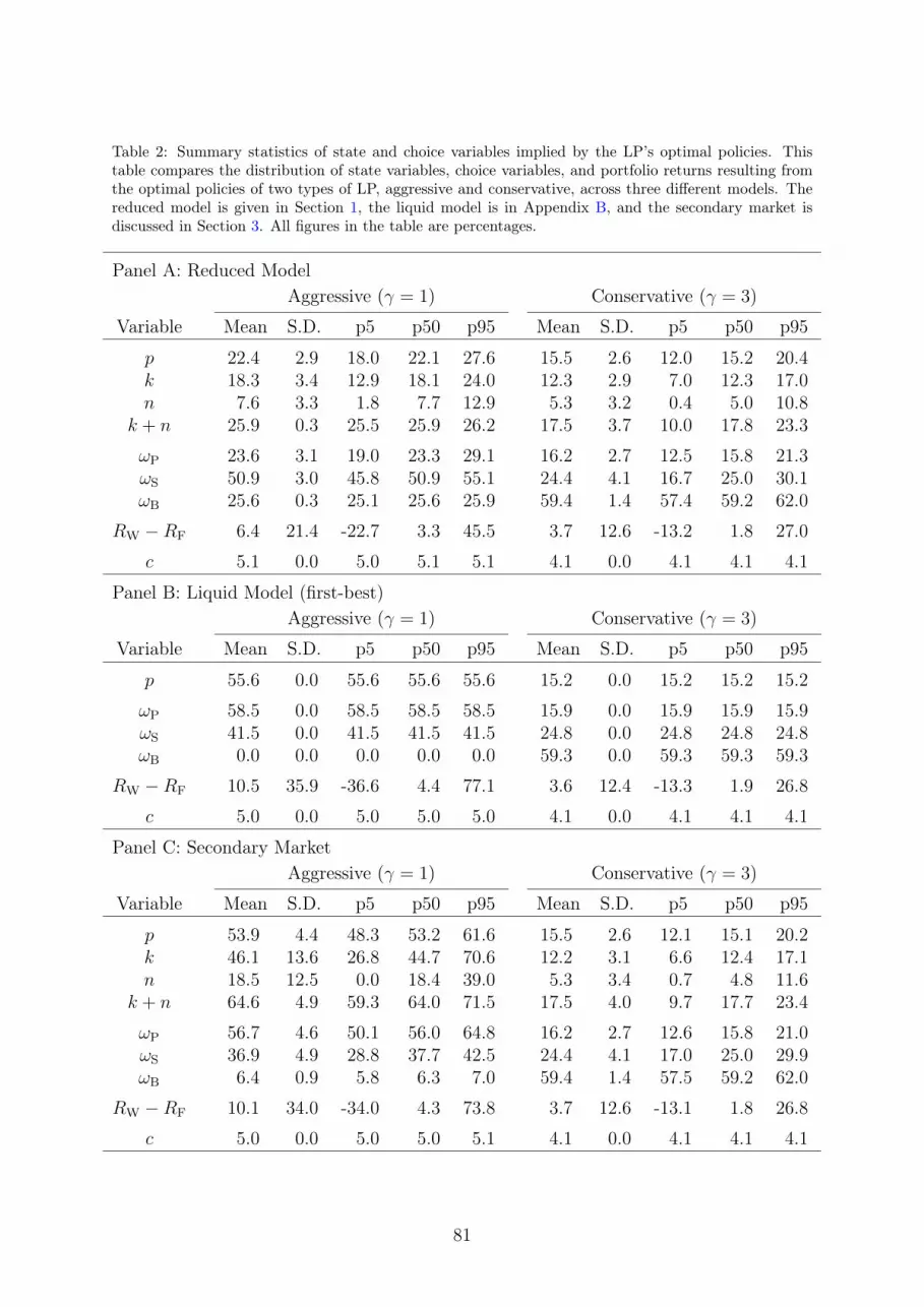
Table 2: Summary statistics of state and choice variables implied by the LP’s optimal policies. Thistable compares the distribution of state variables, choice variables, and portfolio returns resulting fromthe optimal policies of two types of LP, aggressive and conservative, across three different models. Thereduced model is given in Section 1, the liquid model is in Appendix B, and the secondary market isdiscussed in Section 3. All figures in the table are percentages.

Panel A: Reduced ModelAggressive (γ = 1) Conservative (γ = 3)

Variable Mean S.D. p5 p50 p95 Mean S.D. p5 p50 p95

p 22.4 2.9 18.0 22.1 27.6 15.5 2.6 12.0 15.2 20.4k 18.3 3.4 12.9 18.1 24.0 12.3 2.9 7.0 12.3 17.0n 7.6 3.3 1.8 7.7 12.9 5.3 3.2 0.4 5.0 10.8

k + n 25.9 0.3 25.5 25.9 26.2 17.5 3.7 10.0 17.8 23.3

ωP 23.6 3.1 19.0 23.3 29.1 16.2 2.7 12.5 15.8 21.3ωS 50.9 3.0 45.8 50.9 55.1 24.4 4.1 16.7 25.0 30.1ωB 25.6 0.3 25.1 25.6 25.9 59.4 1.4 57.4 59.2 62.0

RW −RF 6.4 21.4 -22.7 3.3 45.5 3.7 12.6 -13.2 1.8 27.0

c 5.1 0.0 5.0 5.1 5.1 4.1 0.0 4.1 4.1 4.1

Panel B: Liquid Model (first-best)Aggressive (γ = 1) Conservative (γ = 3)

Variable Mean S.D. p5 p50 p95 Mean S.D. p5 p50 p95

p 55.6 0.0 55.6 55.6 55.6 15.2 0.0 15.2 15.2 15.2

ωP 58.5 0.0 58.5 58.5 58.5 15.9 0.0 15.9 15.9 15.9ωS 41.5 0.0 41.5 41.5 41.5 24.8 0.0 24.8 24.8 24.8ωB 0.0 0.0 0.0 0.0 0.0 59.3 0.0 59.3 59.3 59.3

RW −RF 10.5 35.9 -36.6 4.4 77.1 3.6 12.4 -13.3 1.9 26.8

c 5.0 0.0 5.0 5.0 5.0 4.1 0.0 4.1 4.1 4.1

Panel C: Secondary MarketAggressive (γ = 1) Conservative (γ = 3)

Variable Mean S.D. p5 p50 p95 Mean S.D. p5 p50 p95

p 53.9 4.4 48.3 53.2 61.6 15.5 2.6 12.1 15.1 20.2k 46.1 13.6 26.8 44.7 70.6 12.2 3.1 6.6 12.4 17.1n 18.5 12.5 0.0 18.4 39.0 5.3 3.4 0.7 4.8 11.6

k + n 64.6 4.9 59.3 64.0 71.5 17.5 4.0 9.7 17.7 23.4

ωP 56.7 4.6 50.1 56.0 64.8 16.2 2.7 12.6 15.8 21.0ωS 36.9 4.9 28.8 37.7 42.5 24.4 4.1 17.0 25.0 29.9ωB 6.4 0.9 5.8 6.3 7.0 59.4 1.4 57.5 59.2 62.0

RW −RF 10.1 34.0 -34.0 4.3 73.8 3.7 12.6 -13.1 1.8 26.8

c 5.0 0.0 5.0 5.0 5.1 4.1 0.0 4.1 4.1 4.1

81

more substantially. The conservative LP, on average, holds wS = 24.4% in stocks and

ωB = 59.4% in bonds. The aggressive LP holds ωS = 50.9% in stocks, almost twice

as much as the conservative LP, and it holds only ωB = 25.6% in bonds. Despite PE

investments being substantially more risky than both stocks and bonds, the PE allocation

is much less sensitive to the LP’s risk aversion.

1.0 1.5 2.0 2.5 3.0

Risk aversion

0%

20%

40%

60%

80%

Por

tfolio

wei

ghts

Private EquityStocksBonds

Figure 6: Average portfolio weights resulting from the model. This figure plots the average allocation ofLPs solving our investment problem where PE is illiquid and requires commitment. Average allocationsare computed in three steps. First, we solve numerically the Bellman equation (14). At any point in thestate space, that solution provides the corresponding portfolio weights in stocks ω∗

S = s∗/(1 − c∗) andPE ω∗

P = p/(1− c∗), while 1− ω∗S − ω∗

P is the risk-free allocation. Second, we simulate the evolution ofthose variables under optimal strategies. Third, we compute their averages. This procedure is repeatedfor relative risk aversion γ ∈ {1, 1.1, 1.2, . . . , 2.9, 3}.

These allocations can be compared to the first-best allocations, which are the optimal

allocations if PE were liquid and could be freely traded at a price equal to the NAV,

effectively making PE investments another traded stock. This liquid model is standard,

it is described in Appendix B, and the optimal allocations are given in Panel B of Table 2

and shown in Figure 7. The LP’s PE allocation now declines in risk aversion, as expected.

Moreover, for more risk averse LP’s, the first-best allocations from the liquid model

largely coincide with the allocations with illiquid PE investments. To illustrate, for the

conservative LP the average PE allocation is ωP = 16.2% which effectively equals its

first-best allocation of ωP = 15.9%. Intuitively, the liquidity constraint tends to be slack

for more risk averse LPs, and they can effectively ignore the illiquidity of PE investments

in their portfolio allocations.

82

In contrast, for less risk averse LPs the liquidity constraint tends to bind, and these LPs

allocate substantially less capital to PE and substantially more to bonds than their first-

best allocations. For the aggressive LP, the average PE allocation is ωP = 23.6% and its

first-best allocation is ωP = 58.5%.

1.0 1.5 2.0 2.5 3.0

Risk aversion

0%

20%

40%

60%

80%

Por

tfolio

wei

ghts

Private EquityStocksBonds

Figure 7: Optimal portfolio weights with liquid PE. This figure plots the optimal portfolio weightsof investors operating in perfectly liquid markets. Optimal portfolio weights in stocks and PE arerespectively ωS and ωP solving Bellman equation (B.2). The residual weight goes to risk-free bonds.Markets are perfectly liquid because PE can be traded freely like stocks and bonds. We consider investorswith relative risk aversion coefficient γ ∈ {1, 1.1, 1.2, . . . , 2.9, 3}.

Because the conservative LP’s portfolio is largely unaffected by the illiquidity of PE

investments, its returns are also largely unaffected, and it earns an average return of

3.7% both with illiquid and liquid PE investments. In contrast, the aggressive LP earns

an average return of just 6.4% with illiquid PE investments, which is substantially below

the 10.6% average return this LP would earn from its first-best allocation.

These allocations and returns are calculated for the baseline specification where PE has

a beta of 1.6 and an alpha of 3%. We solve the model for other specifications, and

Appendix C shows the optimal allocations and policies. A consistent finding across these

specifications is that PE allocations are less sensitive to the LP’s risk aversion than the

allocations to stocks and bonds, despite PE being substantially more risky.

83

2.1 Value Function

Figure 8 shows the LP’s normalized value function, v(p, k), as a function of the two

normalized state variables: illiquid wealth as a fraction of total wealth, p = P/W , and

uncalled commitments as a fraction of total wealth, k = K/W . Returns are risky and

transitions in the state space are stochastic. In Figure 8 the state space is divided into

cells with sides of 2%, and the shading indicates how frequently each cell is visited during

the simulations. Cells that are never visited are blank. Cells that are visited at least

once (and less than 10%) are increasingly darker. A single cell is visited in more than

10% of the simulations, which is when then conservative LP holds 14% < p < 16% and

12% < k < 14%, and it is shaded black.

For both the aggressive (γ = 1) and the conservative LP (γ = 3) the value function is

decreasing in uncalled commitments, k, when uncalled commitments increases above the

shaded area of the state space. This follows naturally from the first-order condition for

k, because an LP can freely commit additional capital to PE, and the LP will continue

to commit new capital as long as the value function is increasing.

Importantly, in Figure 8 the value function increases in illiquid wealth, p, for the aggres-

sive LP (γ = 1), but it decreases in p for the conservative LP (γ = 3), above the shaded

part of the state space. An aggressive LP would prefer to increase its PE exposure, but

the binding liquidity constraint makes it costly to commit additional capital because it

also requires an increase in the LP’s liquidity reserve. In contrast, the conservative LP’s

liquidity constraint tends to be slack, and its portfolio moves around an interior optimum.

Its first-best bond allocation exceeds the amount needed for its liquidity reserve, and it

can freely commit additional capital to PE until it reaches its first-best allocation, given

by the liquid model.

2.2 Optimal New Commitments

The aggressive and conservative LPs have different optimal policies for new PE commit-

ments, as illustrated in Figure 9. A conservative LP (γ = 3) tends to be close to an

interior optimum, and in response to a positive shock to the NAV of its PE investments

this LP reduces its new PE commitments to rebalance its PE exposure back towards the

84

a. Aggressive (γ = 1)

k

p

Val

ue 0%

30%

70%

0% 30%70% 100%

0.75

0.80

0.85

0.90

0.95

1.00

1.05

b. Conservative (γ = 3)

k

p

Val

ue 0%

30%

70%

0% 30%70% 100%

0.75

0.80

0.85

0.90

0.95

1.00

1.05

Figure 8: Value function per unit of wealth. This figure compares the value function v(p, k) of thenormalized Bellman equation (14) for investors with low risk-aversion (γ = 1) and investors with high risk-aversion (γ = 3). In the figure, each function is rescaled and expressed in units of value at (p, k) = (0, 0).That is, we plot v(p, k)/v(0, 0) for the two types of investors. We only display functional values abovea certain threshold, which is 0.75 for the low risk-aversion case and 0.7 for the high risk-aversion case.The length of each axis is kept constant across the two cases, so the shapes of the functions are directlycomparable. The shade on the surface of the function indicates how often investors reach a certain areaof the state space. Darker areas indicate states that are reached more often. Shades are constructedusing a Monte Carlo simulation where investors behave optimally.

85

interior optimum. In contrast, an aggressive LP prefers a greater PE exposure but it

cannot commit additional capital due to the binding liquidity constraint. The aggressive

LP therefore does not reduce its new PE commitments in response to a positive shock to

the NAV of its existing PE investments. Instead, it enjoys a temporary increase in its PE

exposure, and it continues to make new commitments at the same maximally sustainable

rate, as seen in Figure 9.

a. Aggressive (γ = 1)

k

p

New

com

mitm

ent

0%

30%

70%

0% 30%70% 100%

0%

10%

20%

30%

40%

b. Conservative (γ = 3)

k

p

New

com

mitm

ent

0%

30%

70%

0% 30%70% 100%

0%

10%

20%

30%

40%

Figure 9: Optimal new commitment. This figure compares optimal commitment strategy for investorswith low risk-aversion (γ = 1) and investors with high risk-aversion (γ = 3). For each type, the plotsshow optimal new commitment as a share of wealth n∗(p, k) obtained solving the Bellman equation (14).The shade on the surface of the function indicates how often investors reach a certain area of the statespace. Darker areas indicate states that are reached more often. Shades are constructed using a MonteCarlo simulation where investors behave optimally.

Figure 9 shows that the optimal policies for new PE commitments consist of multiple

segments, each of which appears to be close to linear. The shading shows, however, that

the state mostly moves on a single such segment, although it occasionally drops to the

bottom segment with zero new commitments. In Table 2 the aggressive LP’s average

(standard deviation) of new commitments, n, is 7.6% (3.3%) (and n equals zero for 0.5%

of the simulations). For the conservative LP, n is 5.3% (3.2%) (and n equals zero for

1.5% of the simulations).

Since the state remains mostly on a single linear segment, we can locally approximate the

optimal policy by regressing the optimal new commitments, n∗(p, k), on the two normal-

ized state variables. Table 3 shows that regressions with and without an interaction term

86

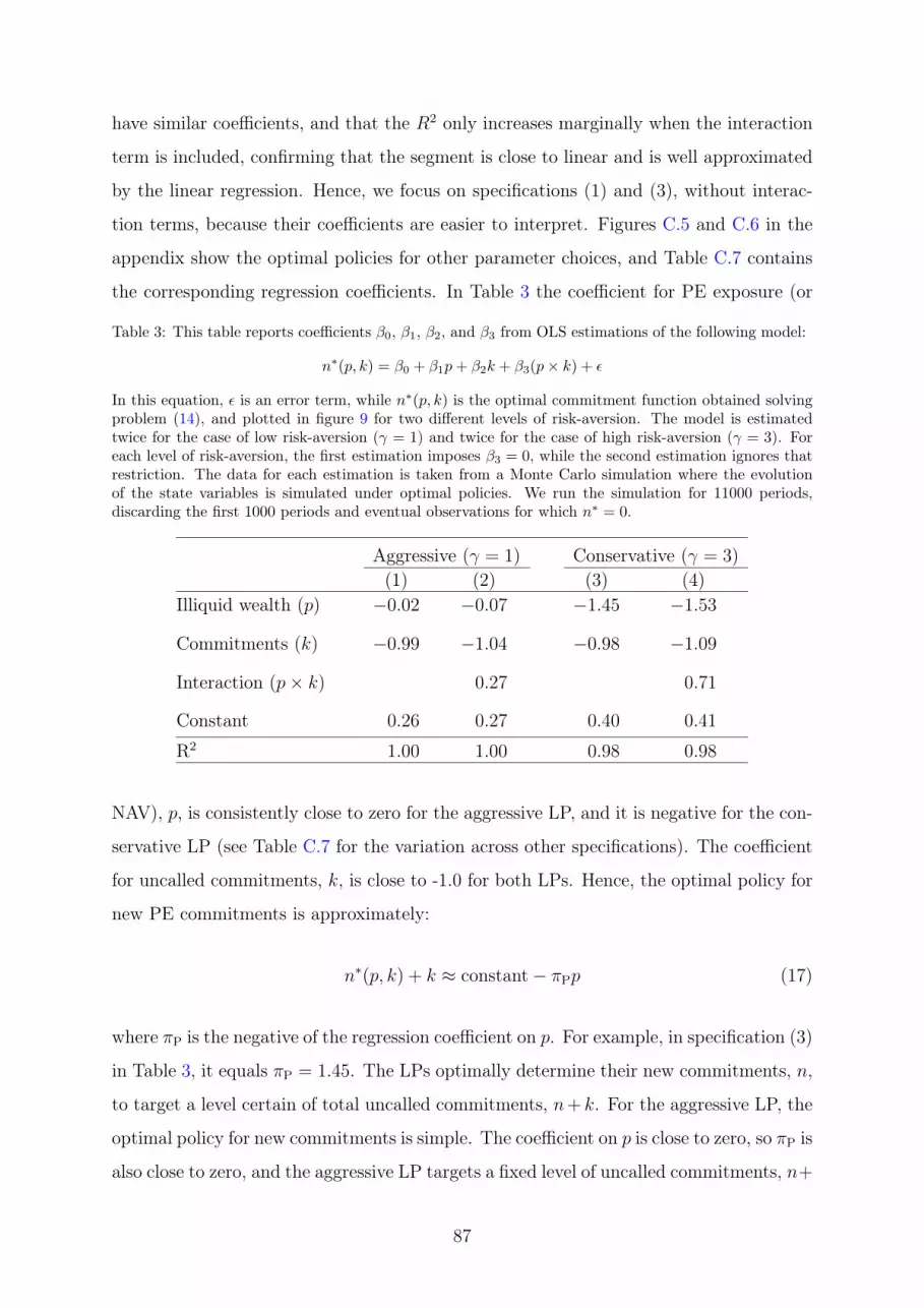
have similar coefficients, and that the R2 only increases marginally when the interaction

term is included, confirming that the segment is close to linear and is well approximated

by the linear regression. Hence, we focus on specifications (1) and (3), without interac-

tion terms, because their coefficients are easier to interpret. Figures C.5 and C.6 in the

appendix show the optimal policies for other parameter choices, and Table C.7 contains

the corresponding regression coefficients. In Table 3 the coefficient for PE exposure (or

Table 3: This table reports coefficients β0, β1, β2, and β3 from OLS estimations of the following model:

n∗(p, k) = β0 + β1p+ β2k + β3(p× k) + ϵ

In this equation, ϵ is an error term, while n∗(p, k) is the optimal commitment function obtained solvingproblem (14), and plotted in figure 9 for two different levels of risk-aversion. The model is estimatedtwice for the case of low risk-aversion (γ = 1) and twice for the case of high risk-aversion (γ = 3). Foreach level of risk-aversion, the first estimation imposes β3 = 0, while the second estimation ignores thatrestriction. The data for each estimation is taken from a Monte Carlo simulation where the evolutionof the state variables is simulated under optimal policies. We run the simulation for 11000 periods,discarding the first 1000 periods and eventual observations for which n∗ = 0.

Aggressive (γ = 1) Conservative (γ = 3)(1) (2) (3) (4)

Illiquid wealth (p) −0.02 −0.07 −1.45 −1.53

Commitments (k) −0.99 −1.04 −0.98 −1.09

Interaction (p× k) 0.27 0.71

Constant 0.26 0.27 0.40 0.41

R2 1.00 1.00 0.98 0.98

NAV), p, is consistently close to zero for the aggressive LP, and it is negative for the con-

servative LP (see Table C.7 for the variation across other specifications). The coefficient

for uncalled commitments, k, is close to -1.0 for both LPs. Hence, the optimal policy for

new PE commitments is approximately:

n∗(p, k) + k ≈ constant − πPp (17)

where πP is the negative of the regression coefficient on p. For example, in specification (3)

in Table 3, it equals πP = 1.45. The LPs optimally determine their new commitments, n,

to target a level certain of total uncalled commitments, n+ k. For the aggressive LP, the

optimal policy for new commitments is simple. The coefficient on p is close to zero, so πP is

also close to zero, and the aggressive LP targets a fixed level of uncalled commitments, n+

87

k ≈ constant, regardless of the performance of its other investments. For the conservative

LP, the coefficient πP is positive, and this LP optimally reduces the target level of uncalled

commitments in response to a positive shock its PE investments.

2.3 Optimal Stock and Bond Allocations

a. Aggressive (γ = 1)

k

p

Sto

ck a

lloca

tion

0%

30%

70%

0% 30%70% 100%

0%

20%

40%

60%

80%

b. Conservative (γ = 3)

k

p

Sto

ck a

lloca

tion

0%

30%

70%

0% 30%70% 100%

0%

20%

40%

60%

80%

Figure 10: Optimal stock allocation. This figure compares optimal stock allocation for investors withlow risk-aversion (γ = 1) and investors with high risk-aversion (γ = 3). For each type, the plots showoptimal portfolio weight in stocks ω∗

S(p, k) obtained solving the Bellman equation (14). The shade onthe surface of the function indicates how often investors reach a certain area of the state space. Darkerareas indicate states that are reached more often. Shades are constructed using a Monte Carlo simulationwhere investors behave optimally.

Figure 10 shows optimal stock allocations as functions of the state variables: illiquid

wealth, p, and uncalled commitments, k. Table 2 shows that the aggressive LP’s average

(standard deviation) stock allocation is ωS = 50.9% (3.0%), its average bond allocation

is ωB = 25.6% (0.3%), and its average PE allocation is ωP = 23.6% (3.1%). For the

conservative LP, the average stock allocation is 24.4% (4.1%), average bond allocation is

59.4% (1.4%), and average PE allocation is 16.2% (2.7%). Table 4 shows the coefficients

from a regression of the optimal stock allocation on the state variables in the shaded part

of the state space. As above, the optimal allocation is well approximated by a linear

regression, and we focus on specifications (1) and (3) without interaction terms.

In Table 4, the coefficients on uncalled commitments, k, are close to zero, and the LPs’

optimal stock allocations are largely unaffected by their aggregate uncalled PE commit-

88

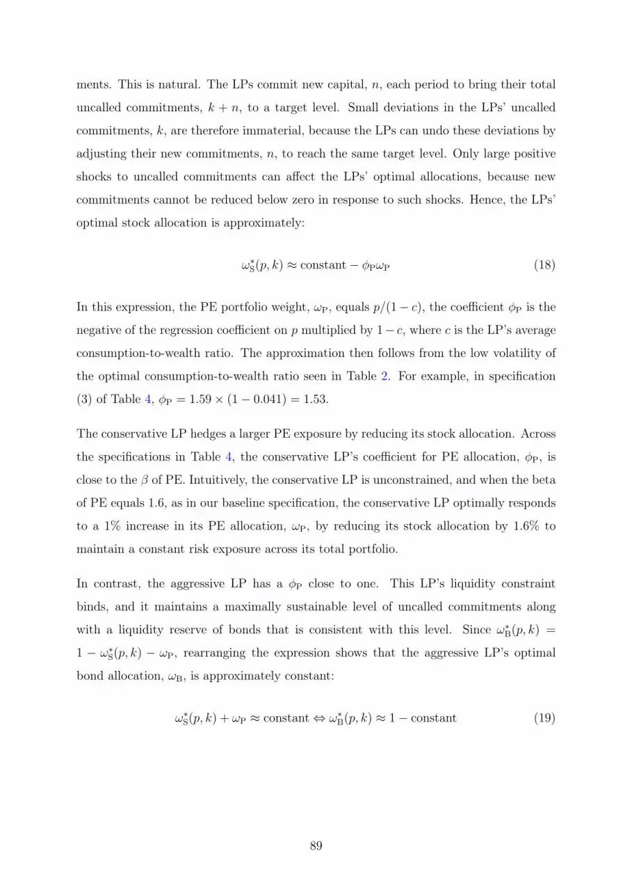
ments. This is natural. The LPs commit new capital, n, each period to bring their total

uncalled commitments, k + n, to a target level. Small deviations in the LPs’ uncalled

commitments, k, are therefore immaterial, because the LPs can undo these deviations by

adjusting their new commitments, n, to reach the same target level. Only large positive

shocks to uncalled commitments can affect the LPs’ optimal allocations, because new

commitments cannot be reduced below zero in response to such shocks. Hence, the LPs’

optimal stock allocation is approximately:

ω∗S(p, k) ≈ constant − ϕPωP (18)

In this expression, the PE portfolio weight, ωP, equals p/(1− c), the coefficient ϕP is the

negative of the regression coefficient on p multiplied by 1− c, where c is the LP’s average

consumption-to-wealth ratio. The approximation then follows from the low volatility of

the optimal consumption-to-wealth ratio seen in Table 2. For example, in specification

(3) of Table 4, ϕP = 1.59× (1− 0.041) = 1.53.

The conservative LP hedges a larger PE exposure by reducing its stock allocation. Across

the specifications in Table 4, the conservative LP’s coefficient for PE allocation, ϕP, is

close to the β of PE. Intuitively, the conservative LP is unconstrained, and when the beta

of PE equals 1.6, as in our baseline specification, the conservative LP optimally responds

to a 1% increase in its PE allocation, ωP, by reducing its stock allocation by 1.6% to

maintain a constant risk exposure across its total portfolio.

In contrast, the aggressive LP has a ϕP close to one. This LP’s liquidity constraint

binds, and it maintains a maximally sustainable level of uncalled commitments along

with a liquidity reserve of bonds that is consistent with this level. Since ω∗B(p, k) =

1 − ω∗S(p, k) − ωP, rearranging the expression shows that the aggressive LP’s optimal

bond allocation, ωB, is approximately constant:

ω∗S(p, k) + ωP ≈ constant ⇔ ω∗

B(p, k) ≈ 1− constant (19)

89

Table 4: This table reports coefficients β0, β1, β2, and β3 from OLS estimations of the following model:

ω∗S(p, k) = β0 + β1p+ β2k + β3(p× k) + ϵ

In this equation, ϵ is an error term, while ω∗S(p, k) is the optimal stock allocation obtained solving

problem (14), and plotted in figure 10 for two different levels of risk-aversion. The model is estimatedtwice for the case of low risk-aversion (γ = 1) and twice for the case of high risk-aversion (γ = 3). Foreach level of risk-aversion, the first estimation imposes β3 = 0, while the second estimation ignores thatrestriction. The data for each estimation is taken from a Monte Carlo simulation where the evolutionof the state variables is simulated under optimal policies. We run the simulation for 11000 periods,discarding the first 1000 periods and eventual observations for which ω∗

S = 0.

Aggressive (γ = 1) Conservative (γ = 3)(1) (2) (3) (4)

Illiquid wealth (p) −1.04 −1.01 −1.59 −1.56

Commitments (k) −0.03 0.00 0.00 0.05

Interaction (p× k) −0.13 −0.31

Constant 0.75 0.74 0.49 0.49

R2 0.99 0.99 1.00 1.00

Table 5: This table reports coefficients β0, β1, β2, and β3 from OLS estimations of the following model:

ω∗B(p, k) = β0 + β1p+ β2k + β3(p× k) + ϵ

In this equation, ϵ is an error term, while ω∗B(p, k) = 1−ω∗

S(p, k)−ω∗P(p, k) is the optimal bond allocation

obtained solving problem (14), and plotted in figure 11 for two different levels of risk-aversion. The modelis estimated twice for the case of low risk-aversion (γ = 1) and twice for the case of high risk-aversion(γ = 3). For each level of risk-aversion, the first estimation imposes β3 = 0, while the second estimationignores that restriction. The data for each estimation is taken from a Monte Carlo simulation where theevolution of the state variables is simulated under optimal policies. We run the simulation for 11000periods, discarding the first 1000 periods and eventual observations for which ω∗

S = 0.

Aggressive (γ = 1) Conservative (γ = 3)(1) (2) (3) (4)

Illiquid wealth (p) −0.02 −0.04 0.55 0.52

Commitments (k) 0.03 0.00 0.00 −0.05

Interaction (p× k) 0.13 0.31

Constant 0.25 0.26 0.51 0.51

R2 0.15 0.16 1.00 1.00

90

a. Aggressive (γ = 1)

k

p

Bon

d al

loca

tion

0%

30%

70%

0% 30%70% 100%

0%

20%

40%

60%

80%

100%

b. Conservative (γ = 3)

k

p

Bon

d al

loca

tion

0%

30%

70%

0% 30%70% 100%

0%

20%

40%

60%

80%

100%

c. Aggressive (γ = 1, rotated)

k

p

Bon

d al

loca

tion

0%

30%

70%

100%

0%

30%

70%100%

0%

20%

40%

60%

80%

100%

d. Conservative (γ = 3, rotated)

k

p

Bon

d al

loca

tion

0%

30%

70%

100%

0%

30%

70%100%

0%

20%

40%

60%

80%

100%

Figure 11: Optimal bond allocation. This figure compares optimal bond allocation for investors with lowrisk-aversion (γ = 1) and investors with high risk-aversion (γ = 3). For each type, the plots show optimalportfolio weight in bonds ω∗

B(p, k) = 1− ω∗S(p, k)− ω∗

P(p, k) obtained solving the Bellman equation (14).The shade on the surface of the function indicates how often investors reach a certain area of the statespace. Darker areas indicate states that are reached more often. Shades are constructed using a MonteCarlo simulation where investors behave optimally. The two plots at the bottom of the figure are rotatedversions of those at the top.

91

2.4 Optimal Consumption

Figure 12 shows optimal consumption for the conservative and aggressive LPs. A standard

result for the liquid model with i.i.d. shocks and CRRA preferences is that optimal

consumption is a constant fraction of total wealth. Figure 12 confirms that with illiquid

PE investments the optimal consumption rate remains close to constant in the shaded

part of the state space. The aggressive LP’s average (standard deviation) consumption

ratio, c, is 5.1% (0.020%), and the conservative LP’s is 4.1% (0.001%). Brown, Dimmock,

Kang, and Weisbenner (2014) study the payout policies of university endowments and

report typical payout rates of 4%–6%, which is consistent with the optimal consumption

rate in our model.

a. Aggressive (γ = 1)

k

p

Con

sum

ptio

n 0%

30%

70%

0% 30%70% 100%

3.0%

3.5%

4.0%

4.5%

5.0%

b. Conservative (γ = 3)

k

p

Con

sum

ptio

n 0%

30%

70%

0% 30%70% 100%

3.0%

3.5%

4.0%

4.5%

5.0%

Figure 12: Optimal consumption as a fraction of wealth. This figure compares optimal consumptionstrategy for investors with low risk-aversion (γ = 1) and investors with high risk-aversion (γ = 3). Foreach type, the plots show optimal consumption to wealth ratio c∗(p, k) obtained solving the Bellmanequation (14). The shade on the surface of the function indicates how often investors reach a certainarea of the state space. Darker areas indicate states that are reached more often. Shades are constructedusing a Monte Carlo simulation where investors behave optimally.

3 Secondary Market

We now introduce a secondary market for PE investments where LPs can trade partner-

ship interests in PE fund.12 This creates two effects: First, there are gains from trade12The secondary market for partnership interests is distinct from the market where PE funds trade

underlying private assets, typically by buying and selling equity stakes in portfolio companies, which is

92

when unconstrained LPs can sell partnership interests in mature PE funds to constrained

LPs. Mature PE funds are partly invested, with positive NAVs and fewer uncalled com-

mitments, allowing a constrained LP to increase its PE exposure with a relatively smaller

increase in its liquidity needs. Second, following a negative shock to the value of its liquid

investments, a stressed LP may decide to liquidate a fraction of its PE investments, even

at a discount, to raise liquidity. Moreover, access to liquidity, ex-post, relaxes the LP’s

liquidity constraint, ex-ante, allowing it to hold more risky allocations.

3.1 Gains from Trade

An aggressive constrained LP assigns a higher valuation to a mature PE fund than a

conservative unconstrained LP. The aggressive LP prefers greater PE exposure, but it

faces a binding liquidity constraint, and a mature fund provides PE exposure with a

relatively smaller amount of uncalled commitments. In contrast, a conservative LP assigns

no special value to mature PE funds compared to simply committing additional capital

to new PE funds, even though these new commitments imply a higher level of uncalled

commitments.

To quantify the gains from trade, Table 6 shows the effects of a transfer of PE investments

from a conservative to an aggressive LP. In this calculation, the two LPs have the same

amounts of wealth, so the transfer represents the same percentage change in their PE

investments. The transfer is compensated by a payment of liquid wealth that leaves both

LPs’ total wealth unchanged. The two LPs start with the average levels of NAV, p, and

uncalled commitments, k, that are implied by their respective optimal investment policies.

For the conservative LP, these levels are pC = 15.5% and kC = 12.3% (see Table 2). For

the aggressive LP, they are pA = 22.4% and kA = 18.3%. The transaction transfers an

amount of NAV, denoted ∆p, and an amount of uncalled commitments, denoted ∆k,

from the conservative to the aggressive LP. The aggressive LP pays ∆p of liquid wealth

to the conservative LP, leaving their total wealths unchanged. After the transaction,

the aggressive LP’s NAV is pA + ∆p, and its uncalled commitments are kA + ∆k. The

conservative LP has pC −∆p and kC −∆k.

also called a “secondary market.” Bollen and Sensoy (2020) model valuation with a secondary marketfor partnership interests. Hege and Nuti (2011), Albuquerque, Cassel, Phalippou, and Schroth (2018),and Nadauld, Sensoy, Vorkink, and Weisbach (2018) report empirical evidence of pricing and discountsfor secondary transactions in the secondary market for partnership interests.

93

Table 6 reports normalized value functions, v(p, k), for different levels of ∆p and ∆k. The

first column of Table 6 shows the initial values, v(p, k), before the transaction, i.e., with

∆p = ∆k = 0%. The following columns show the effects of transacting PE funds with

decreasing maturities, corresponding to increasing amounts of uncalled commitments, ∆k,

and decreasing amounts of NAV, ∆p. Table 6 shows the two value functions and their

sum. An increase in the sum implies that the transfer increases the two LPs’ aggregate

utility.

Even when the value function for the conservative LP declines, as long as the sum in-

creases, there exists an additional transfer of liquid wealth that leaves both LPs strictly

better off.

Table 6 shows that the conservative LP is largely unaffected by the transaction. This LP

is unconstrained, with an excess liquidity reserve, and it compensates for the reduction

in p by increasing its new commitments to rebuild its PE exposure. In the short term, it

also increases its stock allocation to rebalance its risk exposure. The transfer of PE funds

therefore leaves the conservative LP with only a minor and temporary deviation from its

optimal risk exposures, and its value function remains effectively unchanged.

In contrast, the transaction benefits the aggressive LP by temporarily increasing its PE

exposure. The benefit is larger for a more mature fund, with greater NAV and less

uncalled commitments. The benefit declines for younger funds, and a transaction of just

uncalled commitments, ∆p = 0%, does not benefit the aggressive LP.

In Table 6 the greatest increase in total valuations is 0.402%, and the gains from a single

transaction are therefore modest. The gains are larger when the LPs transact repeatedly.

Anticipating such repeated transactions, however, an unconstrained LP would increase

its PE commitments to have extra PE funds to sell to a constrained LP, as these PE funds

mature. In turn, a constrained LP would reduce its own commitments to new funds and

instead manage its PE exposure by acquiring mature PE funds from an unconstrained LP,

further relaxing its liquidity constraint. Formally, analyzing such strategic interactions

among LPs is interesting, but it is well beyond the scope of this paper.

94

Table 6: This table quantifies the net welfare gains from a single transfer of PE partnership interests of(∆p,∆k) from a conservative to an aggressive LP. The two LPs start with the same amounts of wealthand the average levels of p and k that are implied by their optimal investment policies.

∆p No 10% 8% 5% 2% 0%∆k trade 0% 2% 5% 8% 10%

vA(pA +∆p, kA +∆k) .0624 .0629 .0628 .0627 .0625 .0624vC(pC −∆p, kC −∆k) .0372 .0371 .0372 .0372 .0372 .0372vA + vC .0996 .1000 .0999 .0998 .0997 .0996

Gains from Trade 0.000% 0.402% 0.331% 0.221% 0.090% 0.000%

3.2 Insuring Liquidity Shocks

A secondary market for partnership interests can also insure LPs against liquidity shocks.

To quantify this effect, we extend the model to allow the LP to sell, but not buy, a

fraction of its PE investments each period. The extension is summarized below, and more

details are in Appendix D. In practice, an LP must sell its currently held PE funds, with

their actual mix of NAV and uncalled commitments. We capture this mix by restricting

the LP to sell NAV and uncalled commitments in the same proportions as in the LP’s

current PE investments. Each period, t, the LP can liquidate a fraction, 0 ≤ ft ≤ 1,

of its PE investments. When ft = 0 the LP does not transact in the secondary market.

When ft > 0 the sale of PE investments reduces the LP’s NAV by ftPt and reduces

the uncalled commitments by ftKt. The fraction ft is an additional choice variable in

the LP’s problem. It is convenient to model the transaction using the non-normalized

NAV, Pt, and non-normalized uncalled commitments, Kt (rather than the normalized pt

and kt). Due to the discounts, described below, the LP’s total wealth decreases when it

transacts in the secondary market, complicating the resulting changes in the normalized

state variables.

Liquidating PE investments at times of stress is costly, and they are liquidated at a

discount, which represents a transfer of wealth from the selling to the buying LPs.13 We

take this discount as given. LPs that provide liquidity must be relatively unconstrained.

Albuquerque et al. (2018) report that buying LPs are mostly pension funds, endowments,

and banks, which are arguably relatively conservative and unconstrained investors. As13Because the discount is a transfer between the transacting LPs, it is not relevant for the analysis of

gains from trade in the previous section.

95

shown above, unconstrained LPs have lower valuations of mature funds than constrained

LPs, which would naturally creates a discount for stressed sales of PE investments in the

secondary market.

The discount has two parts. The LP sells ftPt of NAV in return for (1−ψP)ftPt of liquid

wealth, where ψP ≥ 0 is the discount to NAV. The sale also reduces the LP’s uncalled

commitments by ftKt, which costs the LP ψKftKt, where ψK ≥ 0 is the cost of disposing

of uncalled commitments. In practice, reported discounts for secondary transactions

are typically (one minus) the transaction price divided by the NAV, which confounds

these two parts of the discount. Empirically disentangling the two parts would require

comparing transactions of, otherwise similar, funds with relatively more and less uncalled

commitments.

In terms of timing, we assume that the LP transacts in the secondary market after

contributions and distributions are paid and before new commitments are made. Uncalled

commitments are now the sum of the LP’s remaining existing commitments, (1− ft)Kt,

and its new commitments, Nt. The LP’s illiquid wealth is the remaining NAV, (1−ft)Pt.End-of-period wealth is now also net of the discount for transacting in the secondary

market, ft (ψPPt + ψKKt).

In our baseline specification, ψK = 5% and ψP = 20%. Nadauld et al. (2018) report

average discounts to NAV from 9.0% to 13.8% (although, they do not separate the part

of the discount due to uncalled commitments). Since our transactions occur at times of

liquidity stress, we assume higher than average discounts. Higher discounts are also a

conservative choice, giving a lower bound on the effects of a secondary market. Below,

we find that it allows the aggressive LP to effectively return to its first-best allocations,

and smaller discounts would only strengthen this finding.

The Bellman equation of the extended model is given in Appendix D. We solve the Bell-

man equation using the numerical methods from the original model (see Appendix A

for details), and Proposition 2 generalizes the liquidity constraint with a secondary mar-

ket.

Proposition 2. Suppose that the LP can sell PE interests in the secondary market with

96

liquidity costs ψP and ψK both between 0 and 1. Suppose also that λN = λK. Then, any

optimal strategy satisfies the following inequality at all times:

Bt ≥ aSM

((1− ft)Kt +Nt

)

In this expression, Bt is savings in bonds, and the coefficient aSM is defined as follows:

aSM =ψK(1− λK) + ψPλK

RF

Proof in Internet Appendix.

In Proposition 2, with the secondary market, Bt equals Wt−Ct−St−Pt+ft(1−ψP)Pt−ftψKKt. When ψK and ψP are less than one, which is natural, the coefficient aSM is below

the coefficient aK from proposition 1. Intuitively, aSM is increasing in ψK and ψP, and

the effect of λK on aSM depends on the relative magnitudes of ψK and ψP.

Figure 13 shows the optimal allocations with a secondary market, and we compare these

allocations to the optimal allocations without a secondary market, in Figure 6, and to

the first-best allocations in Figure 7. The conservative LP has similar allocations in all

three figures, because this LP already effectively holds its first-best allocation even when

PE is illiquid.

In contrast, the secondary market allows the aggressive LP to hold allocations substan-

tially closer to the first-best. Its average NAV increases from ωP = 23.6% without a

secondary market to ωP = 56.7% with a secondary market (first-best ωP = 58.5%). Its

stock allocation changes from ωS = 50.9% without a secondary market to ωS = 36.9%

(first-best ωS = 41.5%). And its bond allocation changes from ωB = 25.6% without a

secondary market to ωB = 6.4% (first-best ωB = 0.0%).

The positive allocation of 6.4% to bonds may be surprising, given that the aggressive

LP’s first-best bond allocation is zero. After a decline in the values of stocks and PE

investments, the aggressive LP’s PE investments consist of relatively more uncalled com-

mitments, Kt, than NAV, Pt. Therefore, the discount to uncalled commitments becomes

97

relatively more important, making it more costly for the aggressive LP to raise liquid

wealth in the secondary market, net of this discount. In this situation, the LP can be

unable to fund its contributions forcing it to sell its PE investments, at a discount, but

with a low NAV this sale effectively requires the LP to pay a buyer to accept the LP’s

unfunded liabilities, and the bond reserve allows the LP make this payment and remain

solvent.

The value functions with a secondary market are shown in Figure 14. The aggressive

LP is now also close to the interior optimum, and its liquidity constraint tends to be

slack. The secondary market, through its insurance function, increases the aggressive

LP’s utility by 11%.

Figure 15 shows optimal policies for trading in the secondary market, f ∗(p, k). As above,

the state space is divided into cells, and the shading indicates how frequently a cell is

visited during the simulations.14 Cells that are not visited during the simulations are

blank. Figure 15 shows that the conservative LP does not transact in the secondary

market. The aggressive LP sometimes, albeit rarely, liquidates a positive fraction of its

PE investments in response to a negative shock to its liquid wealth, which corresponds

to a positive shock to the normalized state variables, p and k.

The Internet Appendix reports optimal allocations and policies for additional specifica-

tions. The results are robust. In general, the conservative LP is unaffected by the intro-

duction of a secondary market. The aggressive LP benefits from the secondary market’s

insurance function, which allows the aggressive LP to approach its first-best allocation,

even when the secondary market is characterized by relatively large discounts.

4 Explicit Management Fees

Up to now the management fees that are charged by PE funds have been implicit in the

analysis. Annual fees are typically set to 0.5%–2% of a PE fund’s total committed capital,

and these fees often decline as the fund matures, either due to an explicit reduction in

the percentage fee or due to a change in basis from committed to invested capital (see14With a secondary market, the LPs visit a larger part of the state space, and we increase the size of

the cells to 5% times 5% to reduce the computational workload.

98

1.0 1.5 2.0 2.5 3.0

Risk aversion

0%

20%

40%

60%

80%P

ortfo

lio w

eigh

tsPrivate EquityStocksBonds

Figure 13: Average portfolio weights with secondary market. This figure plots the average allocation ofLPs solving the extended model with secondary market. Average allocations are computed in three steps.First, we solve numerically the Bellman equation of the extended model (see appendix D). At any point inthe state space, that solution provides the corresponding portfolio weights in stocks, private equity, andrisk-free bonds. Second, we simulate the evolution of those portfolio weights under optimal strategies.Third, we compute their averages. This procedure is repeated for risk-aversion γ ∈ {1, 1.1, 1.2, . . . , 2.9, 3}.

a. Aggressive (γ = 1)

k

p

Val

ue

0%

50%

100%

0%50%

100% 150%

0.650.700.750.800.850.900.95

1.00

1.05

b. Conservative (γ = 3)

k

p

Val

ue

0%

50%

100%

0%50%

100% 150%

0.650.700.750.800.850.900.95

1.00

1.05

Figure 14: Value function with secondary market. This figure compares the value function of investorswith low risk-aversion (γ = 1) and investors with high risk-aversion (γ = 3) from the model withsecondary market. In the figure, each function is rescaled and expressed in units of value at (p, k) = (0, 0).The shade on the surface of the function indicates how often investors reach a certain area of the statespace. Darker areas indicate states that are reached more often. Shades are constructed using a MonteCarlo simulation where investors behave optimally.

99

a. Aggressive (γ = 1)

k

p

Sec

onda

ry s

ales

0%

50%

100%

0%50%

100% 150%

0%10%20%30%40%50%60%

70%

80%

b. Conservative (γ = 3)

k

p

Sec

onda

ry s

ales

0%

50%

100%

0%50%

100% 150%

0%10%20%30%40%50%60%

70%

80%

c. Aggressive (γ = 1, rotated)

k

p

Sec

onda

ry s

ales

0%

50%

100%

150%

0%50%100%

150% 0%

10%20%30%40%50%60%

70%

80%

d. Conservative (γ = 3, rotated)

k

p

Sec

onda

ry s

ales

0%

50%

100%

150%

0%50%100%

150% 0%

10%20%30%40%50%60%

70%

80%

Figure 15: Optimal sales in the secondary market. This figure compares the optimal share f of PEinvestments sold in the secondary market at different points in the state space by investors with lowrisk-aversion (γ = 1) and investors with high risk-aversion (γ = 3). The shade on the surface of thefunction indicates how often investors reach a certain area of the state space. Darker areas indicate statesthat are reached more often. Shades are constructed using a Monte Carlo simulation where investorsbehave optimally. The two plots at the bottom of the figure are rotated versions of those at the top.

100

Metrick and Yasuda, 2010). Implicit management fees are convenient, because the liquid

model does not have a notion of committed capital, and it cannot accommodate explicit

management fees. So a benefit of implicit fees is that the optimal allocations can be

compared directly to the first-best allocations from the liquid model. Below, we extend

the model to explicit management fees. The main finding is that, with the appropriate

reinterpretation of the state variables and the returns, the optimal solution is largely

unaffected and the specification of these fees is not critical for the analysis.

In practice, management fees are specified as fraction of the fund’s committed capital,

and these fees are paid to the PE firm, acting as a general partner in the fund, to cover

the PE firm’s ongoing expenses and to compensate it for managing the fund. This capital

is contributed by the LP to the PE fund, but it is not used to acquire private assets. As

a simple illustration, a PE fund with $100 of total committed capital, a ten-year life, and

annual management fees of 1.5% of its total committed capital charges $1.50 annually

in management fees. Over ten years, these fees add up to $15, leaving $85 to invest in

private assets. Every time the LP contributes $1 to the PE fund, the fund charges $0.15

in fees. In the model the aggregate management fee can thus be specified as a proportion,

θ = 15%, of the contributed capital. When the LP contributes I to the PE funds, then

(1− θ)I is invested in private assets and the PE funds receive θI in fees.

Considering a single PE fund, this specification implies that the management fees are not

constant over the fund’s life. The fee is instead proportional to the contributed capital

each period, as illustrated in Figure 2. We prefer this specification for three reasons. First,

it is tractable and simple to implement in the model. Second, in practice, management

fees tend to decline as a fund matures, which is consistent with this specification (Metrick

and Yasuda, 2010). Third, only aggregate management fees are relevant for the LP’s

problem. Even if actual fees for younger funds are slightly lower than specified (and

actual fees for mature funds are slightly higher) these differences average out in steady

state when the LP’s portfolio contains a balanced mix of younger and older PE funds

(see footnote 9 at page for a similar argument).

Explicit fees require a reinterpretation of the state variables and the return to PE invest-

ments. Aggregate uncalled commitments, Kt, and Nt, still include the amount reserved

for management fees, but the aggregate NAV, Pt, is now net of management fees. The

101

return to PE investments, RP,t, is now gross of management fees, and total wealth, Wt,

is now net of the management fees paid at time t. The transition equations for Pt+1 and

Wt+1, corresponding to equations (4) and (5), become:

Pt+1 = RP,t+1Pt + (1− θ)It+1 −Dt+1 (20)

and

Wt+1 = RP,t+1Pt +RS,t+1St +RF(Wt − Pt − Ct − St)− θIt+1 (21)

Proposition 1 applies unchanged, and the normalized Bellman equation for the reduced

problem with explicit management fees is:

v(p, k) = max(c,n,ωS)

{c1−γ + δE

[[((1− c)RW − θ(λNn+ λKk)

)v(p′, k′)

]1−γ]} 11−γ

subject to

RW = ωPRP + ωSRS + (1− ωP − ωS)RF

p′ =[(1− λD)RPp+ (1− θ)(λNn+ λKk)

]/[(1− c)RW − θ(λNn+ λKk)

]

k′ =[(1− λK)k + (1− λN)n

]/[(1− c)RW − θ(λNn+ λKk)

]

0 ≤ c ≤ 1− p

n ≥ 0

(22)

We solve the model using the same numerical methods as before (see Appendix A for

details). As discussed above, we use θ = 15% as the rate of management fees. For the

other parameters, except for α and µP, we use the values from the baseline specification.

The PE return is now gross of management fees, and it needs to be increased accordingly.

We set α = 9% and µP = 12.6% to approximate the same allocations for the conservative

LP.

4.1 Optimal Allocation with Explicit Management Fees

The optimal allocations with explicit management fees are in Figure 16. These allocations

are almost identical to those with implicit fees, in Figure 6. As a function of risk aversion,

the PE allocation starts to decline and the bond allocation starts to increase slightly

102

earlier with explicit fees than with implicit fees, but the differences are minimal.

1.0 1.5 2.0 2.5 3.0

Risk aversion

0%

20%

40%

60%

80%

Por

tfolio

wei

ghts

Private EquityStocksBonds

Figure 16: Average portfolio weights with explicit management fees. This figure plots the averageallocation of LPs solving the model with explicit management fees. Average allocations are computedin three steps. First, we solve numerically the Bellman equation of the model with management fees(see expression (22)). At any point in the state space, that solution provides the corresponding portfolioweights in stocks, private equity, and risk-free bonds. Second, we simulate the evolution of those portfolioweights under optimal strategies. Third, we compute their averages. This procedure is repeated for risk-aversion γ ∈ {1, 1.1, 1.2, . . . , 2.9, 3}.

Figure 17 shows the value functions, v(p, k), with explicit management fees. These value

functions, however, are no longer comparable to the value functions with implicit fees,

from Figure 8. In Figure 17, the conservative LP’s value function is upward sloping in p in

the shaded part of the state space, but this slope does not mean that the conservative LP

is constrained, because the state variable p is now net of management fees and the value

function, v(p, k), is normalized by the LP’s wealth. An increase in p, holding everything

else equal, therefore reflects an increase in the LP’s PE exposure without paying the

management fees associated with this increase, which would obviously benefit the LP,

but which is not feasible. These complications when interpreting the value function with

explicit management fees are avoided when management fees are implicit.

Figure 18 shows the optimal policies for new PE commitments with explicit management

fees. These policies are indistinguishable from the policies with implicit fees, in Figure 9.

Table 7 confirms that the coefficients in the linear approximation of the optimal policy

are also similar to coefficients with implicit fees, in Table 3. Overall, the optimal policies

103

a. Aggressive (γ = 1)

k

p

Val

ue 0%

30%

70%

0% 30%70% 100%

0.75

0.85

0.95

1.05

1.15

b. Conservative (γ = 3)

k

p

Val

ue 0%

30%

70%

0% 30%70% 100%

0.75

0.85

0.95

1.05

1.15

Figure 17: Value function with explicit management fees. This figure compares the value function ofinvestors with low risk-aversion (γ = 1) and investors with high risk-aversion (γ = 3) from the modelwith explicit management fees. In the figure, each function is rescaled and expressed in units of valueat (p, k) = (0, 0). The shade on the surface of the function indicates how often investors reach a certainarea of the state space. Darker areas indicate states that are reached more often. Shades are constructedusing a Monte Carlo simulation where investors behave optimally.

and allocations with explicit and implicit management fees are almost identical, and the

choice between these two specifications of management fees does not appear to matter

for our results.

a. Aggressive (γ = 1)

k

p

New

com

mitm

ent

0%

30%

70%

0% 30%70% 100%

0%

10%

20%

30%

40%

b. Conservative (γ = 3)

k

p

New

com

mitm

ent

0%

30%

70%

0% 30%70% 100%

0%

10%

20%

30%

40%

Figure 18: Optimal commitment with explicit management fees.

104

Table 7: Optimal commitment with explicit management fees.

Aggressive (γ = 1) Conservative (γ = 3)(1) (2) (3) (4)

Illiquid Wealth −0.10 0.09 −1.84 −1.99

Commitment −0.98 −0.73 −0.90 −1.11

Interaction −1.15 1.77

Constant 0.27 0.23 0.36 0.38

R2 0.99 0.99 0.98 0.98

Figure 18 and Table 4 confirm that the optimal stock allocation with explicit fees is

similar to the allocation with implicit fees, and that the coefficients in the regressions are

similar, especially for the specifications without interaction terms.

a. Aggressive (γ = 1)

k

p

Sto

ck a

lloca

tion

0%

30%

70%

0% 30%70% 100%

0%

20%

40%

60%

80%

100%

b. Conservative (γ = 3)

k

p

Sto

ck a

lloca

tion

0%

30%

70%

0% 30%70% 100%

0%

20%

40%

60%

80%

100%

Figure 19: Optimal stock allocation with explicit management fees.

Table 8: Optimal stock allocation with explicit management fees.

Aggressive (γ = 1) Conservative (γ = 3)(1) (2) (3) (4)

Illiquid Wealth −0.97 −1.17 −1.79 −1.76

Commitment −0.03 −0.28 0.00 0.05

Interaction 1.21 −0.38

Constant 0.73 0.78 0.49 0.49

R2 0.99 0.99 1.00 1.00

105

5 Conclusion

We present the first formal analysis of an LP’s investment problem with ongoing com-

mitments to an arbitrary number of private equity (PE) funds. Our model captures

three aspects of PE investments: they are risky, illiquid, and long-term investments. PE

investments are risky because they earn an uncertain return. They are illiquid because

after committing capital to PE funds, the LP must hold this investment to maturity, and

the LP cannot liquidate (or collateralize) its PE investments to convert them into current

consumption, although this is relaxed somewhat with a secondary market. PE invest-

ments are long-term because the LP’s committed capital is not immediately invested into

private assets. Rather, the LP maintains a stock of uncalled commitments, which are

gradually contributed to the PE funds, and the LP’s need to pay future contributions

creates the main liquidity friction in our analysis. We show that linear fund dynamics

substantially simplify the problem, because the LP’s aggregate uncalled commitments

and aggregate uncalled NAV become summary statistics for the LP’s entire portfolio of

PE investment in the LP’s problem.

Depending on the LP’s risk aversion, we find two distinct investment strategies. A con-

servative LP with a high risk aversion (here, a relative risk aversion of γ = 3) is uncon-

strained. It’s first best portfolio allocation places a sufficient amount of capital in safe

assets, and the LP’s liquidity constraint is not binding. The LP is close to its first-best

interior optimum, and it effectively treats PE investing as another traded stock. In re-

sponse to a positive shock to the value of its PE investments it reduces its allocation to

traded stocks, and it reduces commitments to new PE funds to rebalance and return to

the optimal portfolio.

In contrast, an aggressive LP with a lower risk aversion (γ = 1) faces a binding liquidity

constraint. The aggressive LP does not rebalance its portfolio to maintain constant risk

exposures. It has a substantially larger allocation to the risk free asset and a lower

allocation to stocks than its first-best allocation. Each period it determines the amount

of new commitments to target a given level of total uncalled commitments.

We extend the analysis with a secondary market for PE partnership interests and an-

alyze two effects. There are gains from trade when mature PE funds are traded from

106

unconstrained to constrained LPs, because mature funds provide greater PE exposure

relative to the required liquidity reserve. Moreover, a secondary market can insure a con-

strained LP against negative shocks to the value of its liquid investments by providing

liquidity, ex-post, to the stressed LP. In turn, anticipating that it will be able to liquidate

its PE investments, an aggressive LP will hold a greater PE allocation, ex-ante. In our

specification, the gains from a single trade are economically small. In contrast, insuring

the aggressive LP from liquidity shocks has a large effect, and it effectively allows the

aggressive LP to hold its first-best portfolio.

Our model also allows for different specifications of management fees, which slightly

affects the interpretation of the state variables and the return to PE investments (either

net or gross of management fees). Most of our analysis assumes implicit management

fees, because the resulting portfolio allocations can be compared directly to the first-best

allocations from a liquid model. Another benefit of implicit fees is that the PE return

in the model is net of fees, which is easier to calibrate because this is the return that is

usually reported in industry studies and empirical research. We also analyze the model

with explicit management fees, but after the appropriate adjustments, the solution and

optimal policies are very similar, and this modeling choice appears unimportant for our

analysis.

107

References

Albuquerque, R. A., J. Cassel, L. Phalippou, and E. J. Schroth (2018). Liquidity provision

in the secondary market for private equity fund stakes. Working Paper.

Ang, A., D. Papanikolaou, and M. M. Westerfield (2014). Portfolio choice with illiquid

assets. Management Science 60 (11), 2737–2761.

Bain & Company (2019). Global private equity report. Technical Report.

Banal-Estañol, A., F. Ippolito, and S. Vicente (2017). Default penalties in private equity

partnerships. Working Paper.

Bollen, N. P. and B. A. Sensoy (2020). How much for a haircut? Illiquidity, secondary

markets, and the value of private equity. Working Paper.

Brown, J. R., S. G. Dimmock, J.-K. Kang, and S. J. Weisbenner (2014). How university

endowments respond to financial market shocks: Evidence and implications. American

Economic Review 104 (3), 931–62.

Dimmock, S. G., N. Wang, and J. Yang (2019). The endowment model and modern

portfolio theory. Working Paper.

Doidge, C., G. A. Karolyi, and R. M. Stulz (2017). The U.S. listing gap. Journal of

Financial Economics 123 (3), 464 – 487.

Gupta, A. and S. Van Nieuwerburgh (2020). Valuing private equity investments strip by

strip. Working Paper.

Hege, U. and A. Nuti (2011). The private equity secondaries market during the financial

crisis and the “valuation gap”. The Journal of Private Equity 14 (3), 42–54.

Korteweg, A. (2019). Risk adjustment in private equity returns. Annual Review of

Financial Economics 11 (1), 131–152.

Kroll Bond Rating Agency (2019). KKR Return-Enhanced Investment Grade Note

(REIGN). Fund Rating Report.

108

Ljungqvist, L. and T. Sargent (2018). Recursive Macroeconomic Theory (4 ed.). The

MIT Press.

Longstaff, F. A. (2001). Optimal portfolio choice and the valuation of illiquid securities.

Review of Financial Studies 14 (2), 407–431.

Maurin, V., D. Robinson, and P. Stromberg (2020). A theory of liquidity in private

equity. Working Paper.

Metrick, A. and A. Yasuda (2010). The economics of private equity funds. The Review

of Financial Studies 23 (6), 2303.

Nadauld, T. D., B. A. Sensoy, K. Vorkink, and M. S. Weisbach (2018). The liquidity cost

of private equity investments: Evidence from secondary market transactions. Journal

of Financial Economics 132 (3), 158 – 181.

Phalippou, L. and M. M. Westerfield (2014). Capital commitment and illiquidity risks in

private equity. Working Paper.

Robinson, D. T. and B. A. Sensoy (2016). Cyclicality, performance measurement, and

cash flow liquidity in private equity. Journal of Financial Economics 122 (3), 521 –

543.

Samuelson, P. A. (1969). Lifetime portfolio selection by dynamic stochastic programming.

Review of Economics and Statistics 51 (3), 239–46.

Sorensen, M., N. Wang, and J. Yang (2014). Valuing private equity. The Review of

Financial Studies 27 (7), 1977–2021.

Takahashi, D. and S. Alexander (2002). Illiquid alternative asset fund modeling. The

Journal of Portfolio Management 28 (2), 90–100.

109

A Numerical Methods

In this section, we describe the numerical procedure used to solve the portfolio problems

in the main text. We take the reduced model as a working example.

We use a standard value function iteration algorithm to solve the following problem:

v(p, k) = max(c,n,ωS)

{c1−γ + δE

[[(1− c)RWv(k

′, p′)]1−γ]} 1

1−γ

subject to

RW = ωPRP + ωSRS + (1− ωP − ωS)RF

p′ =[(1− λD)RPp+ λNn+ λKk

]/[(1− c)RW

]

k′ =[k + n− λNn− λKk

]/[(1− c)RW

]

0 ≤ c ≤ max{1− p, 0}

n ≥ 0

(A.1)

The value function of this problem is not smooth, so we use robust numerical methods,

such as linear interpolation and discretization of choice variables, which are described

below. We also exploit the inequality in Proposition 1, normalized by post-consumption

wealth:

1− ωS − ωP ≥ aKk/(1− c) + aNn/(1− c)

The coefficients aK and aN are given in Proposition 1. Numerically, at each point in

the state space, we ignore any combination of choice variables that does not satisfy this

constraint.

In our value function iteration algorithm, we represent the state space with a grid of (p, k)

values with 51 × 51 points, which are evenly distributed over the unit square [0, 1]2. In

each dimension, the distance between one point and the next is 2%.

We start the algorithm with a guess for the value function that is constant across all grid

points, and which equals the constant value vL of the case with perfect market liquidity

(see section B of this appendix).

In each iteration, we solve the constrained maximization problem to obtain the optimal

policies and the resulting value at every point of the grid. This generates an updated

110

guess for the value function that replaces the initial one. With the new guess, a new

iteration begins, and the procedure is repeated until convergence. Specifically, we stop the

algorithm when the absolute difference between the current and the new value function,

at each point of the grid, becomes lower than vL × 10−4.

To calculate expectations, we need to integrate with respect to the risky returns, rP =

ln(RP) and rS = ln(RS), and interpolate the value function v(k′, p′). We use linear

interpolation to evaluate this function with arguments outside the (k, p) grid. We use

Gauss-Hermite quadrature to integrate with respect to the risky returns. We employ 3

quadrature points for each risky asset, resulting into a total of 9 quadrature points.

From iteration 1 to 9, we represent the choice set with a grid made of 8×201×101 points

in the (c, ωS, n) space.15 At each (k, p) in the discretized state space, we select from

that grid the point that maximizes the objective function while satisfying proposition 1.

Then, at the beginning of iteration 10, we build new grids for the choice set that allow

us to refine the solution. Specifically, for each (k, p) in the discretized state space, we

build a new grid in the (c, ωS, n) space, which covers a smaller area while being finer

than the starting grid. Importantly, the center of these new grids are the optimal choices

obtained from iteration 9. We maintain these new grids until iteration 20, when we refine

them further using the same idea. After this second refinement, we let the algorithm

run unchanged for 10 more simulations. Finally, starting from iteration 30, we apply a

standard policy iteration procedure in order to speed up convergence.

The algorithm is implemented in R. It takes about 5 minutes to solve the model on a

standard computer running Linux.

A.1 Monte Carlo Simulation

Every time we solve the model, the solution is then used in a Monte Carlo simulation. In

the simulation, we consider a LP starting without any PE interests (k1 = 0 and p1 = 0).

The LP employs optimal strategies as it transitions randomly in the state space depending

on risky returns which are drawn from their lognormal distribution. The simulation lasts

for 11000 periods, and we discard the first 1000 periods to ensure that our assumption15In particular, we use the vector (0.0001, 0.01, 0.02, . . . , 0.07) for c, (0, 0.005, 0.01, 0.015, . . . , 1) for ωS,

and (0, 0.005, 0.01, 0.015, . . . , 0.5) for n.

111

about initial PE interests, k1 and p1, does not affect the results. For the remaining 10000

periods, we save the realization of state variables, choice variables, and returns. These

data are then used to compute properties of the marginal and joint distribution of those

variables. We use those data, for example, to obtain average portfolio allocations, and

also to compute how likely is the investor to visit a certain area of the state space.

112

B Liquid Model

We consider a simple liquid model where the LP can buy and sell private assets directly,

instead of having to make initial commitments that are gradually called and eventually

distributed. In this liquid model, PE is effectively another liquid stock. The model

with two stocks is standard, and it has been studied since, at least, Samuelson (1969).

Nevertheless, this liquid model provides a useful baseline.

Total wealth, W , is the only state variable of this model, and the Bellman equation is as

follows:VL(W ) = max

(c,ωP,ωS)

{(cW )1−γ + δE

[VL(W

′)1−γ]} 1

1−γ

subject to

RW = ωPRP + ωSRS + (1− ωP − ωS)RF,

W ′ = W (1− c)RW

0 ≤ c ≤ 1

(B.1)

In this expression, c is the consumption-to-wealth ratio, while ωP and ωS are portfolio

weights in PE and stocks, respectively. It is convenient to state explicitly the return to

LP’s total wealth, RW, even though this return is i.i.d and not a state variable.

Since the LP cannot consume more resources than what it owns, it is unable to consume in

states with zero wealth. Those states, however, are infinitely painful for LPs with γ ≥ 1,

who will then make sure to never run out of wealth. To that end, the LP maintains

a positive allocation to risk-free bonds, and does not short sell any risky asset. The

resulting constraints (i.e. ωP + ωS ≤ 1, ωP ≥ 0, and ωS ≥ 0) are introduced explicitly as

we normalize and solve the liquid model.

The liquid model is homogeneous in wealth, and the value function is VL(W ) = WvL

113

where vL is a positive constant that solves the normalized problem:

vL = max(c,ωP,ωS)

{c1−γ + δE

[[vL(1− c)RW]1−γ

]} 11−γ

subject to

RW = ωPRP + ωSRS + (1− ωP − ωS)RF

0 ≤ c ≤ 1

ωP + ωS ≤ 1

(B.2)

We solve this normalized problem numerically for 21 evenly distributed values of γ ∈ [1, 3].

Figure 7 in the main text shows the resulting optimal portfolio allocations for different

values of the LP’s relative risk aversion, γ. Naturally, when the LP’s relative risk aversion

increases, the optimal allocations to PE and stocks decline, and the bond allocation

increases. Conversely, as relative risk aversion decreases, the LP first reduces its bond

allocation to zero. Due to the no-leverage constraint in the model, the LP cannot reduce

its bond allocation below zero, and to keep increasing its PE allocation, the LP reduces

its stock allocation. The LP’s choice between PE and stocks depends on their relative

risks and returns. In the current parametrization, PE is more attractive than stocks, and

a less risk averse LP prefers to increase its PE allocation at the cost of a lower stock

allocation.

114

C Other Specifications of PE Performance

The baseline specification of the reduced model is reported in Table 1 of the main text.

In that specification, PE performance is characterized by α = 3%, β = 1.6, ρ = 0.8, and

σP = 40%. In this section, we compare the solution of the reduced model under different

assumptions about PE performance. We consider the following parameter values:

α ∈ (1%, 3%, 5%)

β ∈ (1.2, 1.6, 1.8)

ρ = 0.8 or σP = 40%

All other parameters remain constant at their baseline level. We obtain 18 (= 3× 3× 2)

specifications of PE performance, which are reduced to 15 after eliminating duplicates.

In particular, there are only 5 unique combinations of β, ρ, and σP:

β ρ σP

1.2 0.8 30%1.2 0.6 40%1.6 0.8 40%1.8 0.8 45%1.8 0.9 40%

These 5 combinations and the 3 possible values of α result into 15 unique cases.

We report output in the following order:

1. Average portfolio weights resulting from optimal policies (plots, p. )

2. Optimal portfolio weights in the Liquid Model (plots, p. )

3. Value function (plots, p. -)

4. Optimal new commitment (plots at p. - and tables at p. )

5. Optimal stock allocation (plots at p. - and tables at p. )

6. Optimal consumption-to-wealth ratio (plots, p. -)

115

In the figures of this section, the middle column of Panel A is identical to that of Panel

B, and the center of each panel corresponds to the baseline specification in Table 1 of the

main text. In the tables of Figure C.7 (p. ) and Figure C.10 (p. ), empty columns are

shown when average PE uncalled commitments are less than 3% of wealth. In Figure C.10,

empty columns are shown also when average portfolio weight in stocks is 3% or less.

116

Figure C.1: Average portfolio weights resulting from optimal policies

Panel A: σP = 40%

αααβββ 1.2 1.6 1.8

1%

1.0 1.5 2.0 2.5 3.0

Risk aversion

0%

20%

40%

60%

80%

100%

Por

tfolio

wei

ghts

Private EquityStocksBonds

1.0 1.5 2.0 2.5 3.0

Risk aversion

0%

20%

40%

60%

80%

100%

Por

tfolio

wei

ghts

Private EquityStocksBonds

1.0 1.5 2.0 2.5 3.0

Risk aversion

0%

20%

40%

60%

80%

100%

Por

tfolio

wei

ghts

Private EquityStocksBonds

3%

1.0 1.5 2.0 2.5 3.0

Risk aversion

0%

20%

40%

60%

80%

100%

Por

tfolio

wei

ghts

Private EquityStocksBonds

1.0 1.5 2.0 2.5 3.0

Risk aversion

0%

20%

40%

60%

80%

100%

Por

tfolio

wei

ghts

Private EquityStocksBonds

1.0 1.5 2.0 2.5 3.0

Risk aversion

0%

20%

40%

60%

80%

100%

Por

tfolio

wei

ghts

Private EquityStocksBonds

5%

1.0 1.5 2.0 2.5 3.0

Risk aversion

0%

20%

40%

60%

80%

100%

Por

tfolio

wei

ghts

Private EquityStocksBonds

1.0 1.5 2.0 2.5 3.0

Risk aversion

0%

20%

40%

60%

80%

100%

Por

tfolio

wei

ghts

Private EquityStocksBonds

1.0 1.5 2.0 2.5 3.0

Risk aversion

0%

20%

40%

60%

80%

100%

Por

tfolio

wei

ghts

Private EquityStocksBonds

Panel B: ρ = 0.8

αααβββ 1.2 1.6 1.8

1%

1.0 1.5 2.0 2.5 3.0

Risk aversion

0%

20%

40%

60%

80%

100%

Por

tfolio

wei

ghts

Private EquityStocksBonds

1.0 1.5 2.0 2.5 3.0

Risk aversion

0%

20%

40%

60%

80%

100%

Por

tfolio

wei

ghts

Private EquityStocksBonds

1.0 1.5 2.0 2.5 3.0

Risk aversion

0%

20%

40%

60%

80%

100%

Por

tfolio

wei

ghts

Private EquityStocksBonds

3%

1.0 1.5 2.0 2.5 3.0

Risk aversion

0%

20%

40%

60%

80%

100%

Por

tfolio

wei

ghts

Private EquityStocksBonds

1.0 1.5 2.0 2.5 3.0

Risk aversion

0%

20%

40%

60%

80%

100%

Por

tfolio

wei

ghts

Private EquityStocksBonds

1.0 1.5 2.0 2.5 3.0

Risk aversion

0%

20%

40%

60%

80%

100%

Por

tfolio

wei

ghts

Private EquityStocksBonds

5%

1.0 1.5 2.0 2.5 3.0

Risk aversion

0%

20%

40%

60%

80%

100%

Por

tfolio

wei

ghts

Private EquityStocksBonds

1.0 1.5 2.0 2.5 3.0

Risk aversion

0%

20%

40%

60%

80%

100%

Por

tfolio

wei

ghts

Private EquityStocksBonds

1.0 1.5 2.0 2.5 3.0

Risk aversion

0%

20%

40%

60%

80%

100%

Por

tfolio

wei

ghts

Private EquityStocksBonds

117

Figure C.2: Optimal portfolio weights in the Liquid Model

Panel A: σP = 40%

αααβββ 1.2 1.6 1.8

1%

1.0 1.5 2.0 2.5 3.0

Risk aversion

0%

20%

40%

60%

80%

100%

Por

tfolio

wei

ghts

Private EquityStocksBonds

1.0 1.5 2.0 2.5 3.0

Risk aversion

0%

20%

40%

60%

80%

100%

Por

tfolio

wei

ghts

Private EquityStocksBonds

1.0 1.5 2.0 2.5 3.0

Risk aversion

0%

20%

40%

60%

80%

100%

Por

tfolio

wei

ghts

Private EquityStocksBonds

3%

1.0 1.5 2.0 2.5 3.0

Risk aversion

0%

20%

40%

60%

80%

100%

Por

tfolio

wei

ghts

Private EquityStocksBonds

1.0 1.5 2.0 2.5 3.0

Risk aversion

0%

20%

40%

60%

80%

100%

Por

tfolio

wei

ghts

Private EquityStocksBonds

1.0 1.5 2.0 2.5 3.0

Risk aversion

0%

20%

40%

60%

80%

100%

Por

tfolio

wei

ghts

Private EquityStocksBonds

5%

1.0 1.5 2.0 2.5 3.0

Risk aversion

0%

20%

40%

60%

80%

100%

Por

tfolio

wei

ghts

Private EquityStocksBonds

1.0 1.5 2.0 2.5 3.0

Risk aversion

0%

20%

40%

60%

80%

100%

Por

tfolio

wei

ghts

Private EquityStocksBonds

1.0 1.5 2.0 2.5 3.0

Risk aversion

0%

20%

40%

60%

80%

100%

Por

tfolio

wei

ghts

Private EquityStocksBonds

Panel B: ρ = 0.8

αααβββ 1.2 1.6 1.8

1%

1.0 1.5 2.0 2.5 3.0

Risk aversion

0%

20%

40%

60%

80%

100%

Por

tfolio

wei

ghts

Private EquityStocksBonds

1.0 1.5 2.0 2.5 3.0

Risk aversion

0%

20%

40%

60%

80%

100%

Por

tfolio

wei

ghts

Private EquityStocksBonds

1.0 1.5 2.0 2.5 3.0

Risk aversion

0%

20%

40%

60%

80%

100%

Por

tfolio

wei

ghts

Private EquityStocksBonds

3%

1.0 1.5 2.0 2.5 3.0

Risk aversion

0%

20%

40%

60%

80%

100%

Por

tfolio

wei

ghts

Private EquityStocksBonds

1.0 1.5 2.0 2.5 3.0

Risk aversion

0%

20%

40%

60%

80%

100%

Por

tfolio

wei

ghts

Private EquityStocksBonds

1.0 1.5 2.0 2.5 3.0

Risk aversion

0%

20%

40%

60%

80%

100%

Por

tfolio

wei

ghts

Private EquityStocksBonds

5%

1.0 1.5 2.0 2.5 3.0

Risk aversion

0%

20%

40%

60%

80%

100%

Por

tfolio

wei

ghts

Private EquityStocksBonds

1.0 1.5 2.0 2.5 3.0

Risk aversion

0%

20%

40%

60%

80%

100%

Por

tfolio

wei

ghts

Private EquityStocksBonds

1.0 1.5 2.0 2.5 3.0

Risk aversion

0%

20%

40%

60%

80%

100%

Por

tfolio

wei

ghts

Private EquityStocksBonds

118

Figure C.3: Value function of aggressive LP (γ = 1)

Panel A: σP = 40%

αααβββ 1.2 1.6 1.8

1%k

p

Val

ue 0%

30%

70%

0% 30%70% 100%

0.800.85

0.90

0.95

1.00

1.05

1.10

k

p

Val

ue 0%

30%

70%

0% 30%70% 100%

0.800.85

0.90

0.95

1.00

1.05

1.10

k

p

Val

ue 0%

30%

70%

0% 30%70% 100%

0.800.85

0.90

0.95

1.00

1.05

1.10

3%k

p

Val

ue 0%

30%

70%

0% 30%70% 100%

0.800.85

0.90

0.95

1.00

1.05

1.10

k

p

Val

ue 0%

30%

70%

0% 30%70% 100%

0.800.85

0.90

0.95

1.00

1.05

1.10

k

p

Val

ue 0%

30%

70%

0% 30%70% 100%

0.800.85

0.90

0.95

1.00

1.05

1.10

5%k

p

Val

ue 0%

30%

70%

0% 30%70% 100%

0.800.85

0.90

0.95

1.00

1.05

1.10

k

p

Val

ue 0%

30%

70%

0% 30%70% 100%

0.800.85

0.90

0.95

1.00

1.05

1.10

k

pV

alue 0%

30%

70%

0% 30%70% 100%

0.800.85

0.90

0.95

1.00

1.05

1.10

Panel B: ρ = 0.8

αααβββ 1.2 1.6 1.8

1%k

p

Val

ue 0%

30%

70%

0% 30%70% 100%

0.800.85

0.90

0.95

1.00

1.05

1.10

k

p

Val

ue 0%

30%

70%

0% 30%70% 100%

0.800.85

0.90

0.95

1.00

1.05

1.10

k

p

Val

ue 0%

30%

70%

0% 30%70% 100%

0.800.85

0.90

0.95

1.00

1.05

1.10

3%k

p

Val

ue 0%

30%

70%

0% 30%70% 100%

0.800.85

0.90

0.95

1.00

1.05

1.10

k

p

Val

ue 0%

30%

70%

0% 30%70% 100%

0.800.85

0.90

0.95

1.00

1.05

1.10

k

p

Val

ue 0%

30%

70%

0% 30%70% 100%

0.800.85

0.90

0.95

1.00

1.05

1.10

5%k

p

Val

ue 0%

30%

70%

0% 30%70% 100%

0.800.85

0.90

0.95

1.00

1.05

1.10

k

p

Val

ue 0%

30%

70%

0% 30%70% 100%

0.800.85

0.90

0.95

1.00

1.05

1.10

k

p

Val

ue 0%

30%

70%

0% 30%70% 100%

0.800.85

0.90

0.95

1.00

1.05

1.10

119

Figure C.4: Value function of conservative LP (γ = 3)

Panel A: σP = 40%

αααβββ 1.2 1.6 1.8

1%k

p

Val

ue 0%

30%

70%

0% 30%70% 100%

0.800.85

0.90

0.95

1.00

1.05

1.10

k

p

Val

ue 0%

30%

70%

0% 30%70% 100%

0.800.85

0.90

0.95

1.00

1.05

1.10

k

p

Val

ue 0%

30%

70%

0% 30%70% 100%

0.800.85

0.90

0.95

1.00

1.05

1.10

3%k

p

Val

ue 0%

30%

70%

0% 30%70% 100%

0.800.85

0.90

0.95

1.00

1.05

1.10

k

p

Val

ue 0%

30%

70%

0% 30%70% 100%

0.800.85

0.90

0.95

1.00

1.05

1.10

k

p

Val

ue 0%

30%

70%

0% 30%70% 100%

0.800.85

0.90

0.95

1.00

1.05

1.10

5%k

p

Val

ue 0%

30%

70%

0% 30%70% 100%

0.800.85

0.90

0.95

1.00

1.05

1.10

k

p

Val

ue 0%

30%

70%

0% 30%70% 100%

0.800.85

0.90

0.95

1.00

1.05

1.10

k

pV

alue 0%

30%

70%

0% 30%70% 100%

0.800.85

0.90

0.95

1.00

1.05

1.10

Panel B: ρ = 0.8

αααβββ 1.2 1.6 1.8

1%k

p

Val

ue 0%

30%

70%

0% 30%70% 100%

0.800.85

0.90

0.95

1.00

1.05

1.10

k

p

Val

ue 0%

30%

70%

0% 30%70% 100%

0.800.85

0.90

0.95

1.00

1.05

1.10

k

p

Val

ue 0%

30%

70%

0% 30%70% 100%

0.800.85

0.90

0.95

1.00

1.05

1.10

3%k

p

Val

ue 0%

30%

70%

0% 30%70% 100%

0.800.85

0.90

0.95

1.00

1.05

1.10

k

p

Val

ue 0%

30%

70%

0% 30%70% 100%

0.800.85

0.90

0.95

1.00

1.05

1.10

k

p

Val

ue 0%

30%

70%

0% 30%70% 100%

0.800.85

0.90

0.95

1.00

1.05

1.10

5%k

p

Val

ue 0%

30%

70%

0% 30%70% 100%

0.800.85

0.90

0.95

1.00

1.05

1.10

k

p

Val

ue 0%

30%

70%

0% 30%70% 100%

0.800.85

0.90

0.95

1.00

1.05

1.10

k

p

Val

ue 0%

30%

70%

0% 30%70% 100%

0.800.85

0.90

0.95

1.00

1.05

1.10

120

Figure C.5: New commitment of aggressive LP (γ = 1)

Panel A: σP = 40%

αααβββ 1.2 1.6 1.8

1%zerocommitment

zerocommitment

k

p

New

com

mitm

ent

0%

30%

70%

0% 30%70% 100%

0%10%20%30%40%50%60%

70%

80%

3%k

p

New

com

mitm

ent

0%

30%

70%

0% 30%70% 100%

0%10%20%30%40%50%60%

70%

80%

k

p

New

com

mitm

ent

0%

30%

70%

0% 30%70% 100%

0%10%20%30%40%50%60%

70%

80%

k

p

New

com

mitm

ent

0%

30%

70%

0% 30%70% 100%

0%10%20%30%40%50%60%

70%

80%

5%k

p

New

com

mitm

ent

0%

30%

70%

0% 30%70% 100%

0%10%20%30%40%50%60%

70%

80%

k

p

New

com

mitm

ent

0%

30%

70%

0% 30%70% 100%

0%10%20%30%40%50%60%

70%

80%

k

pN

ew c

omm

itmen

t

0%

30%

70%

0% 30%70% 100%

0%10%20%30%40%50%60%

70%

80%

Panel B: ρ = 0.8

αααβββ 1.2 1.6 1.8

1%zerocommitment

zerocommitment

k

p

New

com

mitm

ent

0%

30%

70%

0% 30%70% 100%

0%10%20%30%40%50%60%

70%

80%

3%k

p

New

com

mitm

ent

0%

30%

70%

0% 30%70% 100%

0%10%20%30%40%50%60%

70%

80%

k

p

New

com

mitm

ent

0%

30%

70%

0% 30%70% 100%

0%10%20%30%40%50%60%

70%

80%

k

p

New

com

mitm

ent

0%

30%

70%

0% 30%70% 100%

0%10%20%30%40%50%60%

70%

80%

5%k

p

New

com

mitm

ent

0%

30%

70%

0% 30%70% 100%

0%10%20%30%40%50%60%

70%

80%

k

p

New

com

mitm

ent

0%

30%

70%

0% 30%70% 100%

0%10%20%30%40%50%60%

70%

80%

k

p

New

com

mitm

ent

0%

30%

70%

0% 30%70% 100%

0%10%20%30%40%50%60%

70%

80%

121

Figure C.6: New commitment of conservative LP (γ = 3)

Panel A: σP = 40%

αααβββ 1.2 1.6 1.8

1%k

p

New

com

mitm

ent

0%

30%

70%

0% 30%70% 100%

0%10%20%30%40%50%60%

70%

80%

k

p

New

com

mitm

ent

0%

30%

70%

0% 30%70% 100%

0%10%20%30%40%50%60%

70%

80%

k

p

New

com

mitm

ent

0%

30%

70%

0% 30%70% 100%

0%10%20%30%40%50%60%

70%

80%

3%k

p

New

com

mitm

ent

0%

30%

70%

0% 30%70% 100%

0%10%20%30%40%50%60%

70%

80%

k

p

New

com

mitm

ent

0%

30%

70%

0% 30%70% 100%

0%10%20%30%40%50%60%

70%

80%

k

p

New

com

mitm

ent

0%

30%

70%

0% 30%70% 100%

0%10%20%30%40%50%60%

70%

80%

5%k

p

New

com

mitm

ent

0%

30%

70%

0% 30%70% 100%

0%10%20%30%40%50%60%

70%

80%

k

p

New

com

mitm

ent

0%

30%

70%

0% 30%70% 100%

0%10%20%30%40%50%60%

70%

80%

k

pN

ew c

omm

itmen

t

0%

30%

70%

0% 30%70% 100%

0%10%20%30%40%50%60%

70%

80%

Panel B: ρ = 0.8

αααβββ 1.2 1.6 1.8

1%k

p

New

com

mitm

ent

0%

30%

70%

0% 30%70% 100%

0%10%20%30%40%50%60%

70%

80%

k

p

New

com

mitm

ent

0%

30%

70%

0% 30%70% 100%

0%10%20%30%40%50%60%

70%

80%

k

p

New

com

mitm

ent

0%

30%

70%

0% 30%70% 100%

0%10%20%30%40%50%60%

70%

80%

3%k

p

New

com

mitm

ent

0%

30%

70%

0% 30%70% 100%

0%10%20%30%40%50%60%

70%

80%

k

p

New

com

mitm

ent

0%

30%

70%

0% 30%70% 100%

0%10%20%30%40%50%60%

70%

80%

k

p

New

com

mitm

ent

0%

30%

70%

0% 30%70% 100%

0%10%20%30%40%50%60%

70%

80%

5%k

p

New

com

mitm

ent

0%

30%

70%

0% 30%70% 100%

0%10%20%30%40%50%60%

70%

80%

k

p

New

com

mitm

ent

0%

30%

70%

0% 30%70% 100%

0%10%20%30%40%50%60%

70%

80%

k

p

New

com

mitm

ent

0%

30%

70%

0% 30%70% 100%

0%10%20%30%40%50%60%

70%

80%

122

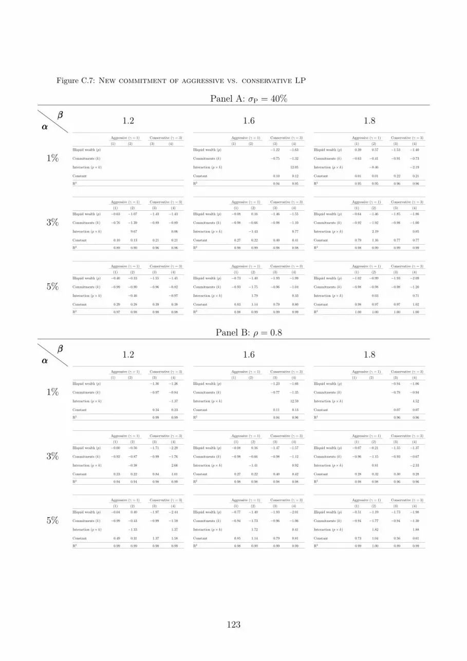
Figure C.7: New commitment of aggressive vs. conservative LP

Panel A: σP = 40%

αααβββ 1.2 1.6 1.8

1%

Aggressive (γ = 1) Conservative (γ = 3)

(1) (2) (3) (4)

Illiquid wealth (p)

Commitments (k)

Interaction (p× k)

Constant

R2

Aggressive (γ = 1) Conservative (γ = 3)

(1) (2) (3) (4)

Illiquid wealth (p) −1.22 −1.63

Commitments (k) −0.75 −1.32

Interaction (p× k) 12.05

Constant 0.10 0.12

R2 0.94 0.95

Aggressive (γ = 1) Conservative (γ = 3)

(1) (2) (3) (4)

Illiquid wealth (p) 0.39 0.57 −1.53 −1.40

Commitments (k) −0.63 −0.41 −0.91 −0.73

Interaction (p× k) −8.46 −2.19

Constant 0.01 0.01 0.22 0.21

R2 0.95 0.95 0.96 0.96

3%

Aggressive (γ = 1) Conservative (γ = 3)

(1) (2) (3) (4)

Illiquid wealth (p) −0.63 −1.07 −1.43 −1.43

Commitments (k) −0.76 −1.39 −0.89 −0.89

Interaction (p× k) 9.67 0.06

Constant 0.10 0.13 0.21 0.21

R2 0.89 0.90 0.96 0.96

Aggressive (γ = 1) Conservative (γ = 3)

(1) (2) (3) (4)

Illiquid wealth (p) −0.08 0.16 −1.46 −1.55

Commitments (k) −0.98 −0.66 −0.98 −1.10

Interaction (p× k) −1.43 0.77

Constant 0.27 0.22 0.40 0.41

R2 0.98 0.99 0.98 0.98

Aggressive (γ = 1) Conservative (γ = 3)

(1) (2) (3) (4)

Illiquid wealth (p) −0.64 −1.46 −1.85 −1.86

Commitments (k) −0.92 −1.92 −0.98 −1.00

Interaction (p× k) 2.19 0.05

Constant 0.79 1.16 0.77 0.77

R2 0.98 0.99 0.99 0.99

5%

Aggressive (γ = 1) Conservative (γ = 3)

(1) (2) (3) (4)

Illiquid wealth (p) −0.40 −0.33 −1.55 −1.45

Commitments (k) −0.99 −0.90 −0.96 −0.82

Interaction (p× k) −0.46 −0.97

Constant 0.29 0.28 0.39 0.38

R2 0.97 0.98 0.98 0.98

Aggressive (γ = 1) Conservative (γ = 3)

(1) (2) (3) (4)

Illiquid wealth (p) −0.73 −1.40 −1.93 −1.99

Commitments (k) −0.93 −1.75 −0.96 −1.04

Interaction (p× k) 1.79 0.33

Constant 0.83 1.14 0.79 0.80

R2 0.98 0.99 0.99 0.99

Aggressive (γ = 1) Conservative (γ = 3)

(1) (2) (3) (4)

Illiquid wealth (p) −1.02 −0.99 −1.93 −2.09

Commitments (k) −0.98 −0.98 −0.98 −1.20

Interaction (p× k) 0.03 0.71

Constant 0.98 0.97 0.97 1.02

R2 1.00 1.00 1.00 1.00

Panel B: ρ = 0.8

αααβββ 1.2 1.6 1.8

1%

Aggressive (γ = 1) Conservative (γ = 3)

(1) (2) (3) (4)

Illiquid wealth (p) −1.36 −1.26

Commitments (k) −0.97 −0.84

Interaction (p× k) −1.37

Constant 0.24 0.23

R2 0.99 0.99

Aggressive (γ = 1) Conservative (γ = 3)

(1) (2) (3) (4)

Illiquid wealth (p) −1.23 −1.66

Commitments (k) −0.77 −1.35

Interaction (p× k) 12.59

Constant 0.11 0.13

R2 0.94 0.96

Aggressive (γ = 1) Conservative (γ = 3)

(1) (2) (3) (4)

Illiquid wealth (p) −0.94 −1.06

Commitments (k) −0.78 −0.94

Interaction (p× k) 4.52

Constant 0.07 0.07

R2 0.96 0.96

3%

Aggressive (γ = 1) Conservative (γ = 3)

(1) (2) (3) (4)

Illiquid wealth (p) −0.60 −0.56 −1.71 −2.29

Commitments (k) −0.92 −0.87 −0.99 −1.76

Interaction (p× k) −0.38 2.66

Constant 0.23 0.22 0.84 1.01

R2 0.94 0.94 0.98 0.99

Aggressive (γ = 1) Conservative (γ = 3)

(1) (2) (3) (4)

Illiquid wealth (p) −0.08 0.16 −1.47 −1.57

Commitments (k) −0.98 −0.66 −0.98 −1.12

Interaction (p× k) −1.41 0.92

Constant 0.27 0.22 0.40 0.42

R2 0.98 0.98 0.98 0.98

Aggressive (γ = 1) Conservative (γ = 3)

(1) (2) (3) (4)

Illiquid wealth (p) −0.07 −0.21 −1.55 −1.37

Commitments (k) −0.96 −1.15 −0.93 −0.67

Interaction (p× k) 0.81 −2.33

Constant 0.28 0.32 0.30 0.28

R2 0.98 0.98 0.96 0.96

5%

Aggressive (γ = 1) Conservative (γ = 3)

(1) (2) (3) (4)

Illiquid wealth (p) −0.04 0.40 −1.97 −2.44

Commitments (k) −0.99 −0.43 −0.99 −1.59

Interaction (p× k) −1.33 1.37

Constant 0.49 0.31 1.37 1.58

R2 0.99 0.99 0.98 0.99

Aggressive (γ = 1) Conservative (γ = 3)

(1) (2) (3) (4)

Illiquid wealth (p) −0.77 −1.40 −1.93 −2.01

Commitments (k) −0.94 −1.73 −0.96 −1.06

Interaction (p× k) 1.72 0.41

Constant 0.85 1.14 0.79 0.81

R2 0.98 0.99 0.99 0.99

Aggressive (γ = 1) Conservative (γ = 3)

(1) (2) (3) (4)

Illiquid wealth (p) −0.51 −1.19 −1.73 −1.98

Commitments (k) −0.94 −1.77 −0.94 −1.30

Interaction (p× k) 1.82 1.88

Constant 0.73 1.04 0.56 0.61

R2 0.99 1.00 0.99 0.99

123

Figure C.8: Stock allocation of aggressive LP (γ = 1)

Panel A: σP = 40%

αααβββ 1.2 1.6 1.8

1%k

p

Sto

ck a

lloca

tion

0%

30%

70%

0% 30%70% 100%

0% 10% 20% 30% 40% 50% 60% 70% 80% 90%

100%

k

p

Sto

ck a

lloca

tion

0%

30%

70%

0% 30%70% 100%

0% 10% 20% 30% 40% 50% 60% 70% 80% 90%

100%

k

p

Sto

ck a

lloca

tion

0%

30%

70%

0% 30%70% 100%

0% 10% 20% 30% 40% 50% 60% 70% 80% 90%

100%

3%k

p

Sto

ck a

lloca

tion

0%

30%

70%

0% 30%70% 100%

0% 10% 20% 30% 40% 50% 60% 70% 80% 90%

100%

k

p

Sto

ck a

lloca

tion

0%

30%

70%

0% 30%70% 100%

0% 10% 20% 30% 40% 50% 60% 70% 80% 90%

100%

k

p

Sto

ck a

lloca

tion

0%

30%

70%

0% 30%70% 100%

0% 10% 20% 30% 40% 50% 60% 70% 80% 90%

100%

5%k

p

Sto

ck a

lloca

tion

0%

30%

70%

0% 30%70% 100%

0% 10% 20% 30% 40% 50% 60% 70% 80% 90%

100%

k

p

Sto

ck a

lloca

tion

0%

30%

70%

0% 30%70% 100%

0% 10% 20% 30% 40% 50% 60% 70% 80% 90%

100%

k

pS

tock

allo

catio

n

0%

30%

70%

0% 30%70% 100%

0% 10% 20% 30% 40% 50% 60% 70% 80% 90%

100%

Panel B: ρ = 0.8

αααβββ 1.2 1.6 1.8

1%k

p

Sto

ck a

lloca

tion

0%

30%

70%

0% 30%70% 100%

0% 10% 20% 30% 40% 50% 60% 70% 80% 90%

100%

k

p

Sto

ck a

lloca

tion

0%

30%

70%

0% 30%70% 100%

0% 10% 20% 30% 40% 50% 60% 70% 80% 90%

100%

k

p

Sto

ck a

lloca

tion

0%

30%

70%

0% 30%70% 100%

0% 10% 20% 30% 40% 50% 60% 70% 80% 90%

100%

3%k

p

Sto

ck a

lloca

tion

0%

30%

70%

0% 30%70% 100%

0% 10% 20% 30% 40% 50% 60% 70% 80% 90%

100%

k

p

Sto

ck a

lloca

tion

0%

30%

70%

0% 30%70% 100%

0% 10% 20% 30% 40% 50% 60% 70% 80% 90%

100%

k

p

Sto

ck a

lloca

tion

0%

30%

70%

0% 30%70% 100%

0% 10% 20% 30% 40% 50% 60% 70% 80% 90%

100%

5%k

p

Sto

ck a

lloca

tion

0%

30%

70%

0% 30%70% 100%

0% 10% 20% 30% 40% 50% 60% 70% 80% 90%

100%

k

p

Sto

ck a

lloca

tion

0%

30%

70%

0% 30%70% 100%

0% 10% 20% 30% 40% 50% 60% 70% 80% 90%

100%

k

p

Sto

ck a

lloca

tion

0%

30%

70%

0% 30%70% 100%

0% 10% 20% 30% 40% 50% 60% 70% 80% 90%

100%

124

Figure C.9: Stock allocation of conservative LP (γ = 3)

Panel A: σP = 40%

αααβββ 1.2 1.6 1.8

1%k

p

Sto

ck a

lloca

tion

0%

30%

70%

0% 30%70% 100%

0% 10% 20% 30% 40% 50% 60% 70% 80% 90%

100%

k

p

Sto

ck a

lloca

tion

0%

30%

70%

0% 30%70% 100%

0% 10% 20% 30% 40% 50% 60% 70% 80% 90%

100%

k

p

Sto

ck a

lloca

tion

0%

30%

70%

0% 30%70% 100%

0% 10% 20% 30% 40% 50% 60% 70% 80% 90%

100%

3%k

p

Sto

ck a

lloca

tion

0%

30%

70%

0% 30%70% 100%

0% 10% 20% 30% 40% 50% 60% 70% 80% 90%

100%

k

p

Sto

ck a

lloca

tion

0%

30%

70%

0% 30%70% 100%

0% 10% 20% 30% 40% 50% 60% 70% 80% 90%

100%

k

p

Sto

ck a

lloca

tion

0%

30%

70%

0% 30%70% 100%

0% 10% 20% 30% 40% 50% 60% 70% 80% 90%

100%

5%k

p

Sto

ck a

lloca

tion

0%

30%

70%

0% 30%70% 100%

0% 10% 20% 30% 40% 50% 60% 70% 80% 90%

100%

k

p

Sto

ck a

lloca

tion

0%

30%

70%

0% 30%70% 100%

0% 10% 20% 30% 40% 50% 60% 70% 80% 90%

100%

k

pS

tock

allo

catio

n

0%

30%

70%

0% 30%70% 100%

0% 10% 20% 30% 40% 50% 60% 70% 80% 90%

100%

Panel B: ρ = 0.8

αααβββ 1.2 1.6 1.8

1%k

p

Sto

ck a

lloca

tion

0%

30%

70%

0% 30%70% 100%

0% 10% 20% 30% 40% 50% 60% 70% 80% 90%

100%

k

p

Sto

ck a

lloca

tion

0%

30%

70%

0% 30%70% 100%

0% 10% 20% 30% 40% 50% 60% 70% 80% 90%

100%

k

p

Sto

ck a

lloca

tion

0%

30%

70%

0% 30%70% 100%

0% 10% 20% 30% 40% 50% 60% 70% 80% 90%

100%

3%k

p

Sto

ck a

lloca

tion

0%

30%

70%

0% 30%70% 100%

0% 10% 20% 30% 40% 50% 60% 70% 80% 90%

100%

k

p

Sto

ck a

lloca

tion

0%

30%

70%

0% 30%70% 100%

0% 10% 20% 30% 40% 50% 60% 70% 80% 90%

100%

k

p

Sto

ck a

lloca

tion

0%

30%

70%

0% 30%70% 100%

0% 10% 20% 30% 40% 50% 60% 70% 80% 90%

100%

5%k

p

Sto

ck a

lloca

tion

0%

30%

70%

0% 30%70% 100%

0% 10% 20% 30% 40% 50% 60% 70% 80% 90%

100%

k

p

Sto

ck a

lloca

tion

0%

30%

70%

0% 30%70% 100%

0% 10% 20% 30% 40% 50% 60% 70% 80% 90%

100%

k

p

Sto

ck a

lloca

tion

0%

30%

70%

0% 30%70% 100%

0% 10% 20% 30% 40% 50% 60% 70% 80% 90%

100%

125

Figure C.10: Stock allocation of aggressive vs. conservative LP

Panel A: σP = 40%

αααβββ 1.2 1.6 1.8

1%

Aggressive (γ = 1) Conservative (γ = 3)

(1) (2) (3) (4)

Illiquid wealth (p) −1.24 −1.22

Commitments (k) −0.00 0.04

Interaction (p× k) −1.31

Constant 0.50 0.50

R2 1.00 1.00

Aggressive (γ = 1) Conservative (γ = 3)

(1) (2) (3) (4)

Illiquid wealth (p) −1.65 −1.64

Commitments (k) 0.00 0.01

Interaction (p× k) −0.21

Constant 0.50 0.50

R2 1.00 1.00

Aggressive (γ = 1) Conservative (γ = 3)

(1) (2) (3) (4)

Illiquid wealth (p) −1.44 −1.60 −1.85 −1.84

Commitments (k) −0.37 −0.57 0.00 0.01

Interaction (p× k) 7.46 −0.12

Constant 0.99 0.99 0.50 0.50

R2 0.99 0.99 1.00 1.00

3%

Aggressive (γ = 1) Conservative (γ = 3)

(1) (2) (3) (4)

Illiquid wealth (p) −0.46 0.04 −1.21 −1.19

Commitments (k) −0.25 0.45 −0.00 0.02

Interaction (p× k) −10.69 −0.32

Constant 0.90 0.87 0.50 0.50

R2 0.72 0.77 1.00 1.00

Aggressive (γ = 1) Conservative (γ = 3)

(1) (2) (3) (4)

Illiquid wealth (p) −0.98 −1.24 −1.59 −1.57

Commitments (k) −0.03 −0.36 −0.00 0.02

Interaction (p× k) 1.51 −0.16

Constant 0.73 0.79 0.49 0.49

R2 0.98 0.98 1.00 1.00

Aggressive (γ = 1) Conservative (γ = 3)

(1) (2) (3) (4)

Illiquid wealth (p) −1.68 −1.58

Commitments (k) −0.01 0.11

Interaction (p× k) −0.51

Constant 0.46 0.44

R2 0.99 0.99

5%

Aggressive (γ = 1) Conservative (γ = 3)

(1) (2) (3) (4)

Illiquid wealth (p) −0.67 −0.72 −1.19 −1.16

Commitments (k) −0.03 −0.10 −0.00 0.04

Interaction (p× k) 0.40 −0.27

Constant 0.72 0.73 0.49 0.49

R2 0.96 0.96 1.00 1.00

Aggressive (γ = 1) Conservative (γ = 3)

(1) (2) (3) (4)

Illiquid wealth (p) −1.52 −1.40

Commitments (k) −0.01 0.15

Interaction (p× k) −0.61

Constant 0.47 0.44

R2 1.00 1.00

Aggressive (γ = 1) Conservative (γ = 3)

(1) (2) (3) (4)

Illiquid wealth (p)

Commitments (k)

Interaction (p× k)

Constant

R2

Panel B: ρ = 0.8

αααβββ 1.2 1.6 1.8

1%

Aggressive (γ = 1) Conservative (γ = 3)

(1) (2) (3) (4)

Illiquid wealth (p) −1.23 −1.20

Commitments (k) −0.00 0.04

Interaction (p× k) −0.47

Constant 0.50 0.50

R2 1.00 1.00

Aggressive (γ = 1) Conservative (γ = 3)

(1) (2) (3) (4)

Illiquid wealth (p) −1.65 −1.64

Commitments (k) 0.00 0.01

Interaction (p× k) −0.18

Constant 0.50 0.50

R2 1.00 1.00

Aggressive (γ = 1) Conservative (γ = 3)

(1) (2) (3) (4)

Illiquid wealth (p) −1.19 −1.24 −1.82 −1.78

Commitments (k) −0.34 −0.42 0.00 0.06

Interaction (p× k) 5.00 −1.53

Constant 0.99 0.99 0.50 0.50

R2 0.99 0.99 1.00 1.00

3%

Aggressive (γ = 1) Conservative (γ = 3)

(1) (2) (3) (4)

Illiquid wealth (p) −0.48 −0.41 −1.22 −1.20

Commitments (k) −0.09 0.01 0.00 0.02

Interaction (p× k) −0.69 −0.08

Constant 0.78 0.77 0.49 0.49

R2 0.64 0.64 1.00 1.00

Aggressive (γ = 1) Conservative (γ = 3)

(1) (2) (3) (4)

Illiquid wealth (p) −0.98 −1.24 −1.59 −1.57

Commitments (k) −0.03 −0.36 −0.00 0.03

Interaction (p× k) 1.47 −0.18

Constant 0.74 0.79 0.49 0.49

R2 0.97 0.98 1.00 1.00

Aggressive (γ = 1) Conservative (γ = 3)

(1) (2) (3) (4)

Illiquid wealth (p) −1.00 −0.91 −1.78 −1.74

Commitments (k) −0.06 0.06 −0.00 0.06

Interaction (p× k) −0.52 −0.53

Constant 0.73 0.70 0.49 0.49

R2 0.97 0.97 1.00 1.00

5%

Aggressive (γ = 1) Conservative (γ = 3)

(1) (2) (3) (4)

Illiquid wealth (p) −1.02 −1.45

Commitments (k) −0.01 −0.56

Interaction (p× k) 1.30

Constant 0.51 0.69

R2 0.96 0.97

Aggressive (γ = 1) Conservative (γ = 3)

(1) (2) (3) (4)

Illiquid wealth (p) −1.52 −1.40

Commitments (k) −0.01 0.15

Interaction (p× k) −0.64

Constant 0.47 0.44

R2 1.00 1.00

Aggressive (γ = 1) Conservative (γ = 3)

(1) (2) (3) (4)

Illiquid wealth (p) −1.74 −1.71

Commitments (k) −0.00 0.03

Interaction (p× k) −0.18

Constant 0.48 0.48

R2 1.00 1.00

126

Figure C.11: Consumption of aggressive LP (γ = 1)

Panel A: σP = 40%

αααβββ 1.2 1.6 1.8

1%k

p

Con

sum

ptio

n 0%

30%

70%

0% 30%70% 100%

2.5%

3.0%

3.5%

4.0%

4.5%

5.0%

5.5%

k

p

Con

sum

ptio

n 0%

30%

70%

0% 30%70% 100%

2.5%

3.0%

3.5%

4.0%

4.5%

5.0%

5.5%

k

p

Con

sum

ptio

n 0%

30%

70%

0% 30%70% 100%

2.5%

3.0%

3.5%

4.0%

4.5%

5.0%

5.5%

3%k

p

Con

sum

ptio

n 0%

30%

70%

0% 30%70% 100%

2.5%

3.0%

3.5%

4.0%

4.5%

5.0%

5.5%

k

p

Con

sum

ptio

n 0%

30%

70%

0% 30%70% 100%

2.5%

3.0%

3.5%

4.0%

4.5%

5.0%

5.5%

k

p

Con

sum

ptio

n 0%

30%

70%

0% 30%70% 100%

2.5%

3.0%

3.5%

4.0%

4.5%

5.0%

5.5%

5%k

p

Con

sum

ptio

n 0%

30%

70%

0% 30%70% 100%

2.5%

3.0%

3.5%

4.0%

4.5%

5.0%

5.5%

k

p

Con

sum

ptio

n 0%

30%

70%

0% 30%70% 100%

2.5%

3.0%

3.5%

4.0%

4.5%

5.0%

5.5%

k

pC

onsu

mpt

ion 0%

30%

70%

0% 30%70% 100%

2.5%

3.0%

3.5%

4.0%

4.5%

5.0%

5.5%

Panel B: ρ = 0.8

αααβββ 1.2 1.6 1.8

1%k

p

Con

sum

ptio

n 0%

30%

70%

0% 30%70% 100%

2.5%

3.0%

3.5%

4.0%

4.5%

5.0%

5.5%

k

p

Con

sum

ptio

n 0%

30%

70%

0% 30%70% 100%

2.5%

3.0%

3.5%

4.0%

4.5%

5.0%

5.5%

k

p

Con

sum

ptio

n 0%

30%

70%

0% 30%70% 100%

2.5%

3.0%

3.5%

4.0%

4.5%

5.0%

5.5%

3%k

p

Con

sum

ptio

n 0%

30%

70%

0% 30%70% 100%

2.5%

3.0%

3.5%

4.0%

4.5%

5.0%

5.5%

k

p

Con

sum

ptio

n 0%

30%

70%

0% 30%70% 100%

2.5%

3.0%

3.5%

4.0%

4.5%

5.0%

5.5%

k

p

Con

sum

ptio

n 0%

30%

70%

0% 30%70% 100%

2.5%

3.0%

3.5%

4.0%

4.5%

5.0%

5.5%

5%k

p

Con

sum

ptio

n 0%

30%

70%

0% 30%70% 100%

2.5%

3.0%

3.5%

4.0%

4.5%

5.0%

5.5%

k

p

Con

sum

ptio

n 0%

30%

70%

0% 30%70% 100%

2.5%

3.0%

3.5%

4.0%

4.5%

5.0%

5.5%

k

p

Con

sum

ptio

n 0%

30%

70%

0% 30%70% 100%

2.5%

3.0%

3.5%

4.0%

4.5%

5.0%

5.5%

127

Figure C.12: Consumption of conservative LP (γ = 3)

Panel A: σP = 40%

αααβββ 1.2 1.6 1.8

1%k

p

Con

sum

ptio

n 0%

30%

70%

0% 30%70% 100%

2.5%

3.0%

3.5%

4.0%

4.5%

5.0%

5.5%

k

p

Con

sum

ptio

n 0%

30%

70%

0% 30%70% 100%

2.5%

3.0%

3.5%

4.0%

4.5%

5.0%

5.5%

k

p

Con

sum

ptio

n 0%

30%

70%

0% 30%70% 100%

2.5%

3.0%

3.5%

4.0%

4.5%

5.0%

5.5%

3%k

p

Con

sum

ptio

n 0%

30%

70%

0% 30%70% 100%

2.5%

3.0%

3.5%

4.0%

4.5%

5.0%

5.5%

k

p

Con

sum

ptio

n 0%

30%

70%

0% 30%70% 100%

2.5%

3.0%

3.5%

4.0%

4.5%

5.0%

5.5%

k

p

Con

sum

ptio

n 0%

30%

70%

0% 30%70% 100%

2.5%

3.0%

3.5%

4.0%

4.5%

5.0%

5.5%

5%k

p

Con

sum

ptio

n 0%

30%

70%

0% 30%70% 100%

2.5%

3.0%

3.5%

4.0%

4.5%

5.0%

5.5%

k

p

Con

sum

ptio

n 0%

30%

70%

0% 30%70% 100%

2.5%

3.0%

3.5%

4.0%

4.5%

5.0%

5.5%

k

pC

onsu

mpt

ion 0%

30%

70%

0% 30%70% 100%

2.5%

3.0%

3.5%

4.0%

4.5%

5.0%

5.5%

Panel B: ρ = 0.8

αααβββ 1.2 1.6 1.8

1%k

p

Con

sum

ptio

n 0%

30%

70%

0% 30%70% 100%

2.5%

3.0%

3.5%

4.0%

4.5%

5.0%

5.5%

k

p

Con

sum

ptio

n 0%

30%

70%

0% 30%70% 100%

2.5%

3.0%

3.5%

4.0%

4.5%

5.0%

5.5%

k

p

Con

sum

ptio

n 0%

30%

70%

0% 30%70% 100%

2.5%

3.0%

3.5%

4.0%

4.5%

5.0%

5.5%

3%k

p

Con

sum

ptio

n 0%

30%

70%

0% 30%70% 100%

2.5%

3.0%

3.5%

4.0%

4.5%

5.0%

5.5%

k

p

Con

sum

ptio

n 0%

30%

70%

0% 30%70% 100%

2.5%

3.0%

3.5%

4.0%

4.5%

5.0%

5.5%

k

p

Con

sum

ptio

n 0%

30%

70%

0% 30%70% 100%

2.5%

3.0%

3.5%

4.0%

4.5%

5.0%

5.5%

5%k

p

Con

sum

ptio

n 0%

30%

70%

0% 30%70% 100%

2.5%

3.0%

3.5%

4.0%

4.5%

5.0%

5.5%

k

p

Con

sum

ptio

n 0%

30%

70%

0% 30%70% 100%

2.5%

3.0%

3.5%

4.0%

4.5%

5.0%

5.5%

k

p

Con

sum

ptio

n 0%

30%

70%

0% 30%70% 100%

2.5%

3.0%

3.5%

4.0%

4.5%

5.0%

5.5%

128

D Model with Secondary Market

The Bellman equation with a secondary market is given by the following expression:

V (W,P,K) = max(C,N,S,f)

{C1−γ + δE

[V (W ′, P ′, K ′)1−γ

]} 11−γ

subject to

W ′ = RPP (1− f) +RSS +RF (W − C − P (1− f)− S − f(ψPP + ψKK))

P ′ = (1− λD)RP(1− f)P + λNN + λK(1− f)K

K ′ = (1− λK)(1− f)K + (1− λN)N

0 ≤ C ≤ W − P (1− f)− f(ψPP + ψKK)

N ≥ 0

(D.1)

Variables and parameters in this expression are defined in the main text. Normalized by

wealth, the Bellman equation with a secondary market becomes:

v(p, k) = max(c,n,ωS,f)

{c1−γ + δE

[[(1− c− f(ψPp+ ψKk)

)RWv(p

′, k′)]1−γ]} 1

1−γ

subject to

RW = ωPRP + ωSRS + (1− ωP − ωS)RF

p′ =[(1− λD)RP(1− f)p+ λNn+ λK(1− f)k

]/[(1− c− f(ψPp+ ψKk))RW

]

k′ =[(1− λK)(1− f)k + (1− λN)n

]/[(1− c− f(ψPp+ ψKk))RW

]

0 ≤ c ≤ 1− p(1− f)− f(ψPp+ ψKk)

n ≥ 0

(D.2)

In this expression, the portfolio weights in PE and stocks are defined respectively as

ωP = P (1− f)/[W −C − f(ψPP + ψKK)] and ωS = S

/[W −C − f(ψPP + ψKK)]. The

remaining variables are defined in the main text.

We solve the normalized problem numerically using an algorithm similar to the one

described in Appendix A, and the rest of this section reports output from that solution.

We plot optimal policies for new commitment, stock allocation, and consumption. We

also include regression tables measuring the local sensitivity of optimal policies to the

129

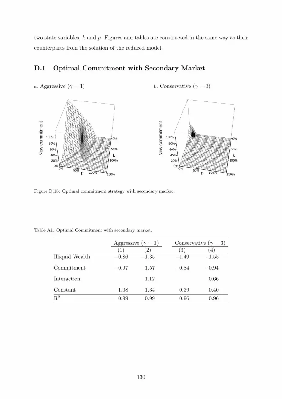
two state variables, k and p. Figures and tables are constructed in the same way as their

counterparts from the solution of the reduced model.

D.1 Optimal Commitment with Secondary Market

a. Aggressive (γ = 1)

k

p

New

com

mitm

ent

0%

50%

100%

0%50%

100% 150%

0%

20%

40%

60%

80%

100%

b. Conservative (γ = 3)

k

p

New

com

mitm

ent

0%

50%

100%

0%50%

100% 150%

0%

20%

40%

60%

80%

100%

Figure D.13: Optimal commitment strategy with secondary market.

Table A1: Optimal Commitment with secondary market.

Aggressive (γ = 1) Conservative (γ = 3)(1) (2) (3) (4)

Illiquid Wealth −0.86 −1.35 −1.49 −1.55

Commitment −0.97 −1.57 −0.84 −0.94

Interaction 1.12 0.66

Constant 1.08 1.34 0.39 0.40

R2 0.99 0.99 0.96 0.96

130

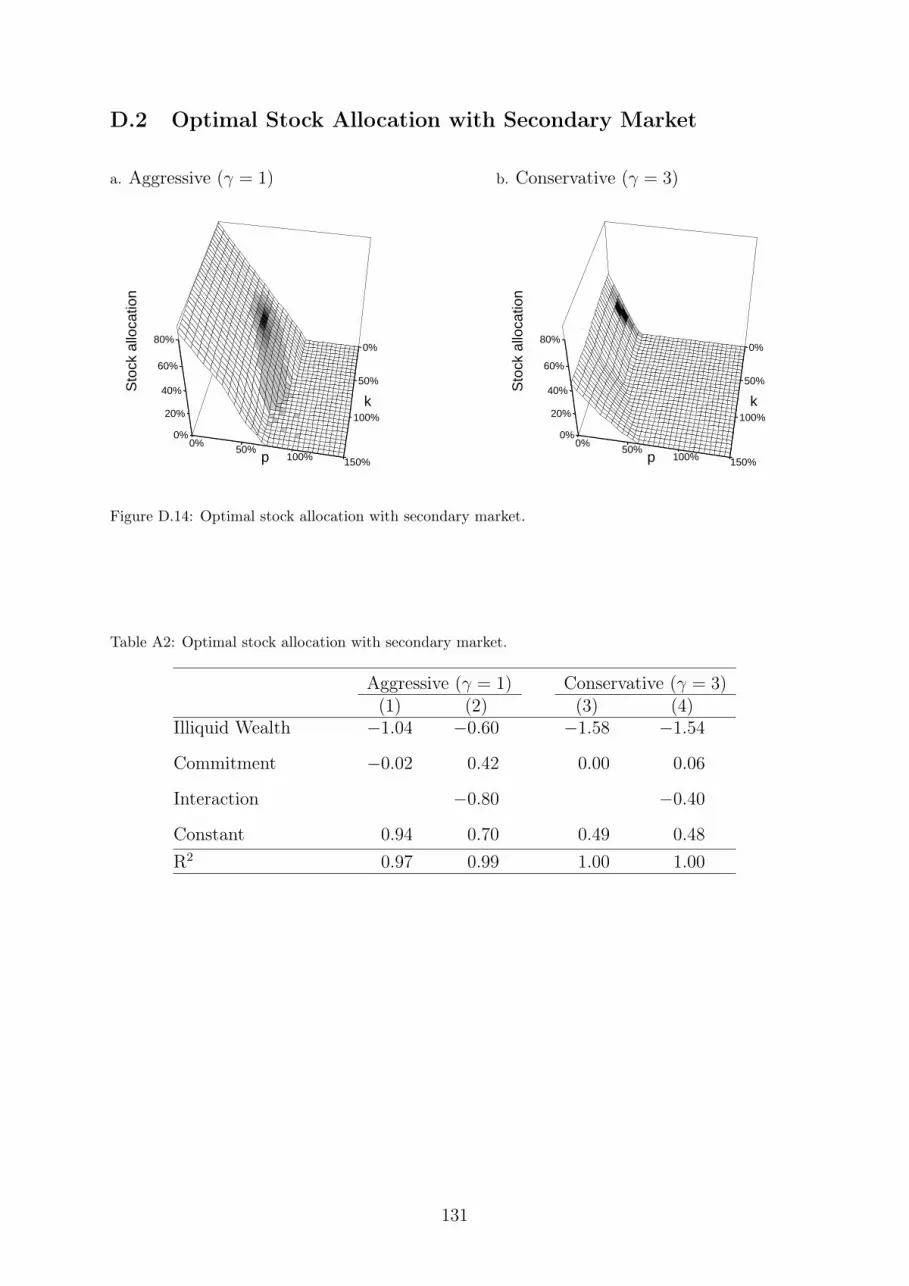
D.2 Optimal Stock Allocation with Secondary Market

a. Aggressive (γ = 1)

k

p

Sto

ck a

lloca

tion

0%

50%

100%

0%50%

100% 150%

0%

20%

40%

60%

80%

b. Conservative (γ = 3)

k

p

Sto

ck a

lloca

tion

0%

50%

100%

0%50%

100% 150%

0%

20%

40%

60%

80%

Figure D.14: Optimal stock allocation with secondary market.

Table A2: Optimal stock allocation with secondary market.

Aggressive (γ = 1) Conservative (γ = 3)(1) (2) (3) (4)

Illiquid Wealth −1.04 −0.60 −1.58 −1.54

Commitment −0.02 0.42 0.00 0.06

Interaction −0.80 −0.40

Constant 0.94 0.70 0.49 0.48

R2 0.97 0.99 1.00 1.00

131

D.3 Optimal Consumption with Secondary Market

a. Aggressive (γ = 1)

k

p

Con

sum

ptio

n

0%

50%

100%

0%50%

100% 150%

2.0%

2.5%

3.0%

3.5%

4.0%

4.5%

5.0%

b. Conservative (γ = 3)

k

p

Con

sum

ptio

n

0%

50%

100%

0%50%

100% 150%

2.0%

2.5%

3.0%

3.5%

4.0%

4.5%

5.0%

Figure D.15: Optimal consumption-to-wealth ratio with secondary market.

132

Private Equity with Leverage Aversion

Nicola Giommetti∗

Abstract

I study optimal portfolio allocation with private equity (PE) and several liquid as-

sets. PE requires capital commitment which is gradually contributed and eventually

distributed back to the investor. Optimal portfolio allocation is well approximated

by static mean-variance optimization with self-imposed margin requirements. Due

to capital commitment, the investor assigns greater margin requirement to PE than

liquid assets, and the risky portfolio of a constrained investor can optimally under-

weight PE relative to the tangency portfolio, even when PE has positive alpha and

moderately high beta with respect to liquid assets.

∗I am grateful to Morten Sorensen for helpful suggestions and support throughout this project, and toPeter Feldhütter, Rasmus Jørgensen, Andrey Malenko, Kasper Meisner Nielsen, and seminar participantsat Copenhagen Business School and LBS Private Equity Symposium for helpful discussion and comments.The author can be reached at Copenhagen Business School (ngi.fi@cbs.dk).

Chapter 3

133

Limited partnerships in private equity (PE) funds are risky long-term investments with

special institutional rules distinguishing them from other assets typically considered in

finance. PE investors become limited partners (LPs) by committing capital at the start

of the partnership. This capital is not immediately contributed to the fund, however,

and fund managers are given large discretion on the timing of contributions. LPs cannot

easily divest their initial commitment. They must typically ensure to cover contributions

as the fund requests them, and later wait for capital distributions as the fund liquidates

its underlying investments.

By the end of 2020, almost $10 trillion were allocated to PE and other private market

funds under those institutional rules.1 Little is known, however, about the effect of

those rules on optimal portfolio allocation of LPs. To address that question, this paper

studies the normative implications of a portfolio problem with explicit modeling of the

PE commitment mechanism.

I introduce PE in a mean-variance portfolio model with several liquid assets. As in Giom-

metti and Sorensen (2021), PE funds require capital commitment from the investor, and

they gradually call and invest that commitment in underlying private assets. These as-

sets appreciate at a risky rate until they are gradually liquidated, and the resulting value

is distributed to the investor. PE investments cannot be sold or collateralized, and the

investor must hold them to maturity. A main contribution of my analysis is to derive a

closed-form solution consistent with the result in Giommetti and Sorensen (2021) that

optimal PE allocation is not monotonically declining in risk aversion, despite the high

risk of PE.

I compare two versions of the model. In the main version, the investor has static mean-

variance objective over the return to his average portfolio allocation over time. The

investor ignores time variation of portfolio weights, provided that there is always some

liquid wealth available. Despite the dynamic PE mechanism, optimal average portfolio

allocation is the solution to a static mean-variance problem with margin requirements as-

signed endogenously by the investor. Liquid risky assets have a margin of 1, while PE has

greater margin, typically above 2. This greater margin is due primarily to commitments,

since the investor maintains a liquidity reserve in risk-free bonds which is proportional to1See Preqin dataset and Gourier, Phalippou, and Westerfield (2021) about this figure.

134

commitments. With plausible parameter values, greater PE margin tend to discourage

constrained investors; despite the high risk and return of PE, constrained investors un-

derweight PE and overweight liquid risky assets relative to the tangency portfolio.

In a second version of the model, the investor has dynamic mean-variance objective over

the return to his current and future portfolio allocations. This version is arguably more

realistic, but it cannot be reduced to a static problem. Instead, I solve it numerically for

five different specifications of parameter values and for several levels of risk aversion, then

I compare the resulting average portfolio allocations with those from the main model. I

find similar results across the two models. Portfolio allocations are virtually identical for

unconstrained investors, while they differ marginally for constrained investors. The main

model tend to overestimate the optimal PE allocation of constrained investors relative

to the more realistic version. The difference remains small, however, with limited and

usystematic variation across specifications.

A large literature studies portfolio and asset pricing implications of trading and financing

frictions. Within that broad literature, my results are related to the work of Frazzini

and Pedersen (2014), who study portfolio theory and asset pricing implications of ex-

ogenous margin constraints. Assuming margins to be constant across assets, they find

that constrained investors overweight assets with high market beta relative to uncon-

strained investors, and equilibrium alpha is positive for assets with low beta. Among PE,

buyout funds are known to undertake levered investments in low-beta firms, an activity

that generates valuable high-beta assets for constrained investors in the model of Frazz-

ini and Pedersen (2014). In my model, however, margins are endogenous and investors

assign high margin requirement to PE funds because of commitment. The high margin

requirement can discourage constrained investors from investing heavily in PE, despite

its positive alpha and moderately high beta.

Several authors study investment implications specific to PE illiquidity. Giommetti and

Sorensen (2021) solve numerically a dynamic portfolio model with stocks, bonds, and

illiquid PE. They find that stocks and bonds allocation are sensitive to risk aversion,

while PE allocation is approximately flat across investors. I obtain the same result in

a closed-form solution highlighting the main mechanism. Sorensen, Wang, and Yang

(2014) develop a subjective valuation model assigning a long-lasting illiquid asset to an

135

investor who can freely trade stocks and bonds. In their model, the investor demands

a liquidity premium for PE only if its return is not fully spanned by stocks. Similarly,

my results rely on PE having some idiosyncratic risk. In my model, idiosyncratic risk

has the main role of generating situations in which the investor could remain without

liquid wealth. Bollen and Sensoy (2020) extend the subjective valution approach with a

secondary market for partnership interests. Gourier, Phalippou, and Westerfield (2021)

study commitment risk with a single PE fund and show that commitment risk reduces

PE allocation significantly. I find capital commitment to be essential also for my results;

if the investor could buy (but not sell) PE directly, PE would have the same margin of

liquid assets. Finally, Ang, Papanikolaou, and Westerfield (2014) and Dimmock, Wang,

and Yang (2019) model illiquidity of PE and alternative assets more broadly.

1 Model

I consider a discrete time model with one risk-free bond and A + 1 risky assets a ∈{0, 1, . . . , A}. The risk-free bond appreciates at constant rate 1 + rF , while risky assets

grow at random rates 1 + ra,t. These random rates are collected in the vector rt =

{r0,t, r1,t, . . . , rN,t} and 1+ rt is i.i.d log-normal with expected value 1+µ and covariance

matrix Σ. All assets are freely tradeable except for a = 0, which denotes PE.

1.1 Private Equity

PE represents an investment in a diversified portfolio of PE funds. It is illiquid as there

is no market where to transact PE directly, but it is possible to invest in PE by becoming

a LP in PE funds. As a LP, the investor must be willing to commit capital to PE funds

at the start of their life. Committed capital remains in the hands of the LP until it is

gradually called (or drawn down) by the funds. The LP loses control of capital once it is

called, and it regains control only when funds decide to liquidate some of their underlying

investments and pay the realized value, net of fees, to the LP. I formalize this process

using the setup of Giommetti and Sorensen (2021).

Let Kt represent the amount of capital which is committed to PE funds before period t,

and which has yet to be called. I refer to this variable as uncalled commitments. At the

end of each period, uncalled commitments can be incremented taking new commitments

136

Nt, resulting in total commitments equal to Kt+Nt. Then, a constant share λC of those

total commitments is called and invested by PE funds in the next period. The updated

amount of uncalled commitments is given by:

Kt+1 = (Kt +Nt)− λC(Kt +Nt) (1)

The quantity λC(Kt + Nt) is a capital call, and it represents a cash flow from the LP

to PE funds. This expression for capital call at t + 1 implies that new commitments

affect capital calls with a 1-year delay. Capital calls, however, are immediately used for

underlying PE investments, so capital calls in a given period become part of illiquid PE

wealth, or net asset value (NAV), at the end of that period.

To illustrate the evolution of NAV, let Pt be the dollar amount of NAV at the end of

period t. This variable grows with the PE return r0,t, increases with capital calls, and

decreases because PE funds liquidate a share λD of underlying investments each period.

These three effects correspond to three components in the evolution of NAV:

Pt+1 = Pt(1 + r0,t+1) + λC(Kt +Nt)− λDPt(1 + r0,t+1) (2)

Random fluctuations in value move NAV from Pt at the end of one period to Pt(1+r0,t+1)

at the beginning of the next. At that point, two things happen contemporaneously:

there is a capital call equal to λC(Kt +Nt) and a distribution equal to λDPt(1 + r0,t+1).

The distribution is a cash flow from PE funds to the LP generated by the liquidation

of underlying investments. This cash flow represents the last stage of the investment

process.

To summarize, each time the LP makes a new commitment, it agrees to endure two

waiting periods. First, the LP must wait for commitment to be invested. Commitment is

invested gradually with capital calls that compel the LP to allocate capital to PE funds.

After capital is called, its value starts growing at the PE return, so the LP obtains PE

exposure. However, before it can dispose of that value, the LP must wait for PE funds

to sell the underlying investments and distribute the corresponding value. Distributions,

like capital calls, are made gradually over time.

137

1.2 Investor

I consider an investor whose preferences have two components: (i) a mean-variance ob-

jective function which ignores liquidity concerns, and (ii) a constraint which ensures that

the investor does not exhaust liquid wealth. I describe these two components in that

order, then I introduce the budget constraint.

For the objective function, a key variable is the average portfolio allocation. Specifically,

let ωt = {ω0,t, ω1,t, . . . , ωA,t} be the vector of portfolio weights in risky assets at time t.

The average portfolio allocation is then defined as the vector of mean portfolio weights,

ω = E[ωt]. With this definition, the objective function can be written as

ω′ (µ− rF )−γ

2ω′Σω (3)

where µ − rF is the vector of expected excess returns, Σ is the covariance matrix of

returns, and γ is risk aversion. This objective function is determined by the mean-

variance characteristics of the average portfolio allocation, so it is a static objective and

it is unaffected by variation of portfolio weights over time. I use this assumption for

tractability, and I consider a dynamic objective function in section 4. Furthermore,

Appendix A shows that a sufficient condition for this objective function to rank average

allocations similarly to a dynamic objective is that most variation in PE return be spanned

by liquid assets.

The second component of preferences is a constraint on liquid wealth. Specifically, let Wt

be the investor’s total wealth, so that Wt − Pt quantifies his liquid wealth. The investor

imposes the following constraint:

Prob(Wt − Pt ≤ 0

)= 0 (4)

Liquid wealth must always remain positive. This constraint is introduced exogenously

based on Giommetti and Sorensen (2021), who show that the same constraint arises

in a model with similar investment opportunities and power utility over consumption.

Although outside of my model, the economic intuition behind the constraint is that the

investor needs to maintain a positive amount of liquid wealth because the NAV of PE

investments is not immediately disposable, and the investor has recurring expenses that

138

might be costly or even impossible to delay.

I do not model any of the expenses that the investor might have in reality. In particular,

I assume that the investor does not consume anything, and while this is a simplification,

results would be virtually unchanged if I assumed a constant consumption-to-wealth ratio.

Without consumption, wealth grows according to the following budget constraint:

Wt+1 = Wt

[1 + rF + ω′

t(rt+1 − rF )]

(5)

In this expression, rt+1 − rF is the vector of excess returns on risky assets, and the term

inside square brackets is the gross return on wealth at time t + 1. Accordingly, the net

return on wealth is defined as follows:

rW,t+1 = rF + ω′t(rt+1 − rF ) (6)

1.3 Optimization Problem

The investor’s preferences, the budget constrant, and the dynamics of commitments and

NAV define the optimization problem. The investor has a static objective function, and

it might be intuitive that he should optimize over the set of average allocations. For-

mally, however, the liquidity constraint (4) forces the investor to optimize over dynamic

strategies to determine the set of feasible average allocations.

The investor chooses (i) a dynamic allocation strategy ωa,t = ωa(ω0,t, Kt) in liquid risky

assets a = 0 and (ii) a dynamic commitment strategy Nt = N(ω0,t, Kt) that maxi-

139

mizeω′ (µ− rF )−

γ

2ω′Σω

subject to

Prob(Wt − Pt ≤ 0

)= 0

Pt+1 = Pt(1− λD)(1 + r0,t+1) + λC(Kt +Nt)

Kt+1 = (1− λC)(Kt +Nt)

Wt+1 = Wt(1 + rW,t+1)

rW,t+1 = rF + ω′t(rt+1 − rF )

Nt ≥ 0

(7)

The investor can condition his strategy on three state variables: Wt is total wealth, Pt

is the NAV of his illiquid wealth, and Kt is uncalled commitments. Each period, the

evolution of these state variables is determined as follows. Wealth grows with portfolio

return, rW,t+1. NAV grows with PE return, r0,t+1, decreases with distributions, λDPt(1+

r0,t+1), and increases with capital calls, λC(Kt +Nt). Uncalled commitments increase at

the end of the period with new commitments, Nt, and decrease next period with capital

calls λC(Kt +Nt).

The last constraint of the problem explicitly prevents the investor to take negative new

commitments. Relaxing this constraint would allow the investor to default on uncalled

commitments, so to reduce future capital calls. In practice, the investor can potentially

default on commitments, but that is very costly both in terms of reputation with PE

funds and in terms of contractual punishments (Banal-Estañol, Ippolito, and Vicente,

2017).

A simplification can be obtained normalizing the constraints by wealth so that the level

of wealth disappears entirely from the problem. To write the normalized constraints,

it is useful to define nt = Nt/Wt and kt = Kt/Wt as the fraction of new and uncalled

commitments over wealth, and ω0,t as the portfolio weight in PE. With those definitions,

the normalized problem can be stated as follows. The investor chooses (i) a dynamic

allocation strategy ωa,t = ωa(ω0,t, kt) in liquid risky assets a = 0 and (ii) a dynamic

140

commitment strategy nt = n(ω0,t, kt) that maximize

ω′ (µ− rF )−γ

2ω′Σω

subject to

Prob(1− ω0,t ≤ 0

)= 0

ω0,t+1 = [ω0,tRP,t+1 + λC(kt + nt)− λDω0,tRP,t+1]/(1 + rW,t+1)

kt+1 = [(kt + nt)− λC(kt + nt)]/(1 + rW,t+1)

rW,t+1 = rF + ω′t(rt+1 − rF )

nt ≥ 0

(8)

Notice that this is not a standard dynamic programming problem, and the optimal dy-

namic strategy is not guaranteed to be unique. Specifically, there is an infinite number of

dynamic strategies that achieve the same average allocation, and the investor is indiffer-

ent between any two strategies that achieve the same average allocation while satisfying

the liquidity constraint. Instead of solving for the set of optimal dynamic strategies, I

show how to simplify the constraints so that the problem can be reformulated as static

mean-variance optimization with leverage aversion, and the choice variable becomes ω.

Using that reformulation, I solve for the optimal average allocation, which is unique.

2 Private Equity with Leverage Aversion

To derive a fully static version of the problem, I start by considering the liquidity con-

straint:

Prob(1− ω0,t ≤ 0

)= 0 (9)

With log-normally distributed returns, Giommetti and Sorensen (2021) show that this

constraint can be replaced with two types of dynamic inequalities. First, the investor does

not short-sell risky assets because large positive returns could otherwise exhaust his liquid

wealth. For simplicity, I assume that short-selling constraints do not bind.2 Second, the

investor maintains a liquidity reserve in risk-free bonds that is sufficiently large to meet2Short-selling constraints on average portfolio allocations do not bind in any of the examples I discuss

below.

141

future capital calls even if all risky assets were to lose their entire value. I focus on this

second condition, which corresponds to the following dynamic constraint:

1− ω′t1 ≥ λC

λC + rF(kt + nt) (10)

In this expression, 1 indicates a vector of ones, and the left-hand side represents the

current portfolio weight in bonds. The right-hand side quantifies the minimum reserve of

bonds required by the investor. This reserve is proportional to total commitments, and

the constant of proportionality can be written as

λCλC + rF

=∞∑

s=1

Is(1 + rF )s

(11)

where the terms Is = (1−λC)s−1λC represent the future stream of capital calls generated

by 1 unit of commitment. For a positive risk-free rate rF , the constant of proportionality

is lower than 1, and the minimum reserve of bonds is lower than total commitments

because commitments are called gradually with intensity λC , and the reserve has time to

appreciate before being possibly used up.

From a dynamic perspective, constraint (10) imposes a trade-off between present exposure

to risky assets (including PE) and future exposure to PE. This trade-off is a consequence

of the liquidity constraint and the commitment mechanism of PE. The investor dislikes

having no liquid wealth, and commitments represent a future obligation to invest in

illiquid PE. The investor reconciliates this obligation with his liquidity preferences by

making sure to always have enough liquid wealth to satisfy the obligation. This objective

is achieved by maintaining a safe reserve of bonds.

From a static perspective, taking expectations on both sides of (10), the constraint im-

poses a trade-off between average exposure to risky assets, including PE, and average

commitments. At the same time, average commitments are strictly related to the aver-

age portfolio weight in PE, and after accounting for this relationship, the static version

of (10) becomes exclusively about portfolio weights. To show that, I first formalize the

relationship between average commitments and average portfolio weight in PE.

Intuitively, if the investor increases average commitments, average PE allocation increases

too. Formally, that can be seen from problem (8) by taking expectations on both sides

142

of the constraint about ω0,t+1. Appendix B follows this approach to derive the following

proposition.

Proposition 1. Average PE allocation can be expressed approximately as a linear func-

tion of average commitments:

k + n = L ω0 (12)

In this expression, k = E[kt] and n = E[nt] are average uncalled and new commitment,

and

L =λD(1 + µ0) + µW − µ0

λC(13)

where µW = E[rW,t] is the expected return on wealth, and µ0 is the expected return to PE.

Proposition 1 quantifies the average commitments needed to maintain a given average

allocation to PE. The relationship between average commitments and average PE allo-

cation is determined by the coefficient L, which depends on the liquidity of PE (λC and

λD) and on expected returns (µW and µ0).

PE liquidity has contrasting effects on L. The coefficient decreases with respect to λC ,

when commitments are called faster, and it increases with respect to λD, when invest-

ments are liquidated faster. I explain these two effects in order. First, if funds call less

commitments each period, it takes more commitments to maintain capital calls and PE

allocation at the same average level. Second, if more investments are liquidated each pe-

riod, it takes larger capital calls to maintain the same average PE allocation. To increase

average capital calls, the investor must increase average commitments.

Asset returns affect the coefficient L in two intuitive ways. First, L decreases with

the expected return to PE, µ0. If the value of PE investments grows faster, it takes

smaller capital calls to maintain a constant average PE allocation, and smaller capital

calls correspond to less commitments on average. Second, L increases with the expected

return on wealth, µW . To understand this effect, recall that the portfolio weight in PE

is the ratio of NAV over wealth. If wealth grows faster, NAV must also grow faster to

143

maintain the same PE allocation. For NAV to grow faster, larger capital calls are needed,

and they are obtained increasing average commitments.

The two conditions (10) and (12) can be combined to characterize the set of feasible

average allocations implied by the constraints of problem (8). The result is shown in the

following proposition.

Proposition 2. The set of feasible average allocations in problem (8) can be expressed

as margin requirements on risky assets:

m0ω0 +A∑

a=1

ωa ≤ 1 (14)

The margin requirement for PE is given by:

m0 = 1 +λD(1 + µ0) + (µW − µ0)

λC + rF(15)

This proposition determines the endogenous margin requirements consistent with liquid-

ity constraint (9). An important characteristic of those margin requirements is that PE

has higher margin than liquid assets. Liquid assets require margin of 1, while PE requires

margin m0 > 1, and the difference is entirely due to the fact that PE allocation can be

obtained only through commitments. Commitments and capital calls are not directly

affected by asset returns, and periods of low returns deplete wealth, pushing the investor

towards illiquid states. To avoid excessive illiquidity, the investor saves m0 − 1 dollars in

bonds for every dollar of PE allocation.

Notice that the margin m0 is not fully exogenous with respect to the other terms of

constraint (14). In particular, m0 depends on the expected return on wealth, which is

affected by the average portfolio weights, ω. With realistic parameter values, however,

portfolio weights have negligible effect on m0, and I return to this point below with a

numerical example.

Using Proposition 2, it is possible to find the optimal average allocation from problem (8)

by solving a simpler static problem. In the static version of the problem, the investor

144

chooses average allocation in risky assets, ω, to maximize

ω (µ− rF )−γ

2ω′Σω

subject to

m0ω0 +A∑

a=1

ωa ≤ 1

(16)

where m0 is given in Proposition 2.

This is a familiar problem of mean-variance optimization with margin constraints. Com-

pared to problem (8), this version is simpler in at least two ways. Not only it is static, but

it also works directly with PE allocation, bypassing commitment. In the context of public

equities, a similar problem was first studied by Black (1972) and more recently extended

by Frazzini and Pedersen (2014). Importantly, I do not impose exogenous margins, and

the margin requirement of PE is endogenously higher than that of liquid assets.

3 Optimal Allocation

To find the optimal average allocation, it suffices to take the first-order condition of

problem (16). I define m = (m0 1 1 · · · 1)′ as the column vector of margin requirements,

and the optimal allocation can be expressed as follows:

ω∗ =1

γΣ−1(µ− rF − ψm) (17)

The Lagrange multiplier ψ ≥ 0 measures the impact of margin requirements.

Risk aversion is the only parameter differentiating constrained and unconstrained in-

vestors. Specifically, there exists risk aversion γ such that investors with γ > γ are

unconstrained, while investors with γ < γ are constrained. Unconstrained investors have

ψ = 0, and they achieve their first-best allocation despite the margin requirements. They

hold a combination of bonds and the tangency portfolio, which is the portfolio of risky

assets with highest Sharpe ratio. Constrained investors have ψ > 0 and their first-best

allocation violates margin requirements. As a result, constrained investors ‘reach for

yield’, meaning that they overweight assets with high expected returns and low margin

145

requirements. This strategy allows constrained investors to increase the expected return

of their portfolio while also satisfying the margin constraint. A main drawback of this

strategy, compared to the first-best, is that the resulting portfolio of risky assets achieves

a lower Sharpe ratio.

3.1 Reaching for Yield

An interesting question is whether constrained investors overweight or underweight PE

in their portfolio of risky assets relative to the tangency portfolio. Intuitively, is private

equity a good or bad asset to reach for yield? To answer this question, it is useful to

define two portfolios.

A relevant portfolio is the combination of liquid risky assets that minimize the variance

of return, or the liquid minimum variance portfolio for short. To define this portfolio, I

partition the covariance matrix of retuns as follows:

Σ =

σ2

0 σ0A

σ′0A ΣA

(18)

With a slight abuse of notation, ΣA indicates the covariance matrix of liquid risky assets,

σ20 indicates the variance of PE, and σ0A represents the row vector of covariances between

PE and liquid risky assets. The liquid minimum variance portfolio is defined by the

following vector of A+ 1 weights:

ωLMV =

(0

1′Σ−1A

1′Σ−1A 1

)(19)

where 1 is a column vector of ones.

A second relevant portfolio is the hedging portfolio, meaning the portfolio of liquid risky

assets that is most correlated with PE. To define this portfolio, let B = Σ−1A σ′

0A be the

vector of coefficients from a multivariate regression of PE return on the returns to liquid

risky assets. Ignoring a constant, the regression corresponds to

r0,t = B′rA,t + εt (20)

where rA,t is the vector of returns on liquid risky assets and εt is the idiosyncratic error

146

term. The hedging portfolio has weights that are proportional to B:

ωHDG =

(0

B′

B′1

)(21)

Furthermore, notice from (20) that the beta of PE with respect to this portfolio is B′1,

the sum of all elements of B.

Using the liquid minimum variance and hedging portfolios, Proposition 3 (proof in Ap-

pendix B) provides a necessary and sufficient condition for PE allocation to increase

disproportionately more than other risky assets as risk aversion decreases and margin

constraints become more binding.

Proposition 3. For γ < γ, the derivative of ω∗0/(ω

∗0 + ω∗

1 + . . . + ω∗A) with respect to γ

is negative if and only if the following condition is satisfied:

µ0 − rF > B′1(µHDG − rF ) + (m0 −B′1)(µLMV − rF ) (22)

The terms µHDG and µLMV are expected returns on the hedging and liquid minimum

variance portfolios.

At the margin, constrained investors compare PE with an alternative investment oppor-

tunity that requires the same amount of capital. Each unit of PE requires m0 units of

capital, and the alternative constitutes of purchasing B′1 units of the hedging portfolio

and m0−B′1 units of the liquid minimum variance portfolio. The expected excess return

of this alternative is:

B′1(µHDG − rF ) + (m0 −B′1)(µLMV − rF ) (23)

As risk aversion decreases, margin constraints become more binding, and the investor

substitutes the investment with lower expected return in favor of the other. PE is a

preferred asset to reach for yield only if its expected return is higher than (23). The

condition is satisfied if PE has a sufficiently high alpha and beta with respect to the

hedging portfolio, and ifm0 is sufficiently low. The expected return of the liquid minimum

variance portfolio has ambiguous effect.

147

A special case is when there is only one liquid risky asset. In that case, the liquid risky

asset constitutes the entirety of the hedging and liquid minimum variance portfolios.

Condition (22) simplifies as follows:

µ0 − rF > m0(µ1 − rF ) (24)

If expected excess return to PE is higher than m0 times the expected excess return on

the liquid risky asset, the risky portfolio of constrained investors overweights PE relative

to the tangency portfolio.

3.2 Benchmarking Private Equity

Studies such as Phalippou (2014) and Stafford (2021) argue that PE should be bench-

marked against leveraged portfolios of public equities most correlated with it. A refor-

mulation of the claim is that PE should be benchmarked against the hedging portfolio

leveraged B′1 times. This claim is correct for unconstrained investors, and to see why,

expression (17) can be used to write the optimal PE allocation as follows:

ω∗0 =

1

γvar(εt)[µ0 − rF −B′1(µHDG − rF ) + ψ(B′1−m0)] (25)

The term εt is the idiosyncratic component of PE return with respect to the hedging

portfolio, as defined in equation (20). Unconstrained investors have ψ = 0, and they invest

in PE only if it has positive alpha with respect to the hedging portfolio. Constrained

investors, however, have ψ > 0 and they might want to invest in PE even if it has negative

alpha with respect to the hedging portfolio, provided that B′1 > m0.

Alternatively, several studies including Kaplan and Schoar (2005) and Harris et al. (2014)

benchmark PE against the S&P500 and other stock market indices. This approach is

simpler but also more difficult to justify. It is valid for unconstrained investors if liquid

markets satisfy CAPM. In that case, it is possible to show that (µ0−rF )−B′1(µHDG−rF )would also be the alpha of PE with respect to the market portfolio of liquid assets. In

absence of pricing restrictions, however, more assumptions are needed to justify this ap-

proach. For unconstrained investors, this approach remains valid assuming that liquid

risky assets are pooled in a single portfolio which becomes the benchmark. This assump-

148

tion effectively restricts the hedging portfolio to equal the stock index, and investors

solve problem (16) with a risk-free bond, PE, and the index. The resulting optimal PE

allocation is:

ω∗0 =

1

γvar(εt)[µ0 − rF − b1(µ1 − rF ) + ψ(b1 −m0)] (26)

The term µ1 indicates the expected return of the index, and b1 is the beta of PE with

respect to the index. This expression is a special case of (25), and unconstrained investors

choose positive PE allocation only if PE has positive alpha with respect to the index.

For proper benchmarking, the index must be leveraged b1 times. Constrained investors

have positive Lagrange multiplier, and if b1 is sufficiently large and m0 sufficiently low,

they invest a positive amount in PE even if it has negative alpha with respect to the

index.

3.3 Numerical Example with Two Risky Assets

To illustrate the intuition of the model, it is useful to consider a numerical example in

which investors can choose between a risk-free bond, PE, and a liquid risky asset such as

a portfolio of stocks.

Table 1 reports the parameter values used in the numerical example. For the liquidity

of PE, I use call intensity λC = 30% and distribution intensity λD = 40%. These values

are used also by Giommetti and Sorensen (2021), who show that this specification can

generate plausible dynamics of PE cash flows. Stocks have expected return µ1 = 8% and

volatility σ1 = 20%, while the risk-free rate is rF = 2%, resulting in a Sharpe ratio of 0.3.

The values of µ0, σ0, and ρ imply that PE has α = 2.4% and β = 1.6, as defined by the

following CAPM:

µ0 − rF = α + β(µ1 − rF ) (27)

with β = ρσ0σ1. The specification of Table 1 is similar to that of Giommetti and Sorensen

(2021) with the main difference being that PE has lower alpha compared to their 3%.

Figure 1 plots in Panel A the set of average allocations (ω0, ω1) satisfying the margin

constraint of problem (16). It compares the case of fully liquid PE, implying m0 = 1,

with the case in which PE is illiquid and requires commitment. In this second case, m0

is taken from Proposition 2. The triangle delimited by the solid line contains feasible

149

Table 1: Parameter values. This table reports parameter values used in the numerical example with tworisky assets. It also includes important statistics that are implied by those parameter values.

Parameter/Statistic Expression ValueCapital call intensity λC 30%Distribution intensity λD 40%

Risk-free rate rF 2%Expected return to stocks µ1 8%Expected return to PE µ0 14%Volatility of stocks σ1 20%Volatility of PE σ0 40%Correlation of stocks and PE ρ 0.8

Implied:Sharpe ratio of stocks (µ1 − rF ) /σ0 0.3Sharpe ratio of PE (µ0 − rF ) /σ1 0.3Alpha of PE α 2.4%Beta of PE β 1.6

allocations with liquid PE, and the shaded area contains feasible allocations when PE

requires commitment. With liquid PE, the investor faces only a no-leverage constraint,

and any feasible allocation has positive portfolio weights satisfying ω0 + ω1 ≤ 1. The

illiquidity of PE reduces substantially the set of feasible allocations. With commitment,

the maximum PE allocation is lower than 50% and it would require the investor to hold

the rest of wealth in bonds.

In Panel A of Figure 1, the shaded area is not an exact triangle. Its diagonal edge is not

exactly a straight line, and Panel B plots the slope of that edge as a function of ω0. This

slope corresponds to the value of PE margin m0 at the corresponding (ω0, ω1) points, and

the diagonal edge of the shaded area in Panel A is the set of points where the margin

constraint is binding and m0 is most relevant. Ranging from 2.220 to 2.235, PE margin

is large and varies with (ω0, ω1) through the expected return on wealth, µW , but that

variation is negligible.

It remains unclear whether differences in feasible allocations between liquid PE and com-

mitment can generate large differences in portfolio allocation. The answer depends on

preferences and returns. Below, I show that commitment has large effects on the optimal

PE and stocks allocation of investors with risk aversion of 1, for example.

Figure 2 illustrates the numerical example in the space of expected returns and volatility.

150

0.0 0.2 0.4 0.6 0.8 1.0

0.0

0.2

0.4

0.6

0.8

1.0

Panel A: Feasible Allocations

PE weight ω0

Sto

cks

wei

ght ω

1

Liquid PECommitment

0.0 0.1 0.2 0.3 0.4

2.220

2.225

2.230

2.235

Panel B: PE Margin

PE weight ω0

mar

gin

m0

Figure 1: Feasible allocations and PE margin. This figure plots feasible allocations (Panel A) and PEmargin as function of PE allocation (Panel B) with parameter values from Table 1. Panel A distinguishesthe case with liquid PE from the case with commitment. Panel B plots the values of m0(ω0, ω1), as givenby (15), along the diagonal edge of the shaded area from Panel A.

In the figure, the dashed line is the constrained efficient frontier with liquid PE, and the

solid black line is the constrained efficient frontier with commitment. The solid line is

always below the dashed line since the investor is more constrained (i.e. m0 > 1) when

PE requires commitment. In this example, the expected return to PE is not high enough

to satisfy condition (24), so private equity is not a preferred asset to reach for yield, and

the solid line ends with a portfolio fully invested in stocks.

I consider an investor with risk aversion γ = 1 whose indifference curves are represented

with gray lines in Figure 2. If PE were liquid and m0 = 1, this investor would optimally

allocate 50% in PE and 50% in stocks. In that case, PE would be a preferred asset to

reach for yield, and as a response to the leverage constraint, the investor would optimally

tilt its risky portfolio towards PE relative to the 33% PE allocation of the tangency

portfolio. With commitment, instead, the investor responds to the margin constraint by

tilting his risky allocation towards stocks. His optimal portfolio invests 16% in PE, 65%

stocks, and 19% in bonds.

Figure 3 plots the optimal portfolio weights of investors with risk aversion between 1

and 3, and Table 2 reports their numeric value for a subset of risk aversion. With risk

aversion of 3, the margin constraint does not bind, and the investor holds 42% of wealth

151

0.20 0.25 0.30 0.35 0.40

0.08

0.10

0.12

0.14

Volatility of return

Exp

ecte

d re

turn

PE

Stocks

Tangency(ω0,ω1) = (0.33,0.67)

Optimum with liquid PE(ω0,ω1) = (0.50,0.50)

Optimum with commitment(ω0,ω1) = (0.16,0.65)

Efficient frontier with liquid PEEfficient frontier with commitmentIndifference curves for γ = 1

Figure 2: Efficient frontier and optimal allocation. This figure illustrates the solution to problem (16)with PE, stocks, and bonds in the space of expected returns and volatility. Using parameters values fromTable 1, the figure plots efficient frontier with liquid PE and m0 = 1 (dashed line), efficient frontier withcommitment and m0 given by (15) (solid line), and indifference curves for investors with risk aversionγ = 1 (gray lines).

in the tangency portfolio. The optimal allocation constitutes of 14% PE, 28% stocks, and

58% bonds. As risk aversion decreases, investors decrease their holdings of bonds and

invest more in the tangency portfolio until the margin constraint starts binding. At that

point, because of the large margin requirement of PE, investors prefer to increase their

stocks allocation at the expense of PE. As a result, PE allocation is approximately flat

across risk aversion with only a 2% difference between risk aversion of 1 and 3. Instead,

investors differ mainly in their allocation to liquid assets, and with risk aversion of 1 they

allocate an additional 37% of wealth in stocks compared to risk aversion of 3.

Table 2: Optimal average allocations. This table reports optimal average allocations solving staticproblem (16) for a subset of risk aversions between 1 and 3. Parameters are taken from Table 1 andm0 is computed with (15). PE allocation is indicated with ω0, stocks allocation is denoted ω1, andωF = 1− ω0 − ω1 represents bonds allocation. Percentages are rounded to the nearest integer.

Risk aversion

1.0 1.4 1.8 2.2 2.6 3.0ω0 16% 21% 23% 19% 16% 14%ω1 65% 53% 46% 38% 32% 28%ωF 19% 26% 31% 43% 52% 58%

152

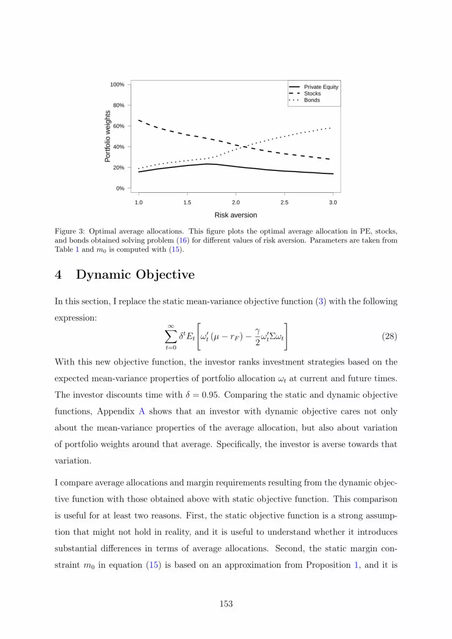
1.0 1.5 2.0 2.5 3.0

Risk aversion

0%

20%

40%

60%

80%

100%

Por

tfolio

wei

ghts

Private EquityStocksBonds

Figure 3: Optimal average allocations. This figure plots the optimal average allocation in PE, stocks,and bonds obtained solving problem (16) for different values of risk aversion. Parameters are taken fromTable 1 and m0 is computed with (15).

4 Dynamic Objective

In this section, I replace the static mean-variance objective function (3) with the following

expression:∞∑

t=0

δtEt

[ω′t (µ− rF )−

γ

2ω′tΣωt

](28)

With this new objective function, the investor ranks investment strategies based on the

expected mean-variance properties of portfolio allocation ωt at current and future times.

The investor discounts time with δ = 0.95. Comparing the static and dynamic objective

functions, Appendix A shows that an investor with dynamic objective cares not only

about the mean-variance properties of the average allocation, but also about variation

of portfolio weights around that average. Specifically, the investor is averse towards that

variation.

I compare average allocations and margin requirements resulting from the dynamic objec-

tive function with those obtained above with static objective function. This comparison

is useful for at least two reasons. First, the static objective function is a strong assump-

tion that might not hold in reality, and it is useful to understand whether it introduces

substantial differences in terms of average allocations. Second, the static margin con-

straint m0 in equation (15) is based on an approximation from Proposition 1, and it is

153

useful to assess its accuracy by comparing m0 to the exact counterpart in a fully dynamic

model.

With dynamic objective, the problem can be expressed in the form of Bellman equation.

I restrict my attention to the case with only one liquid risky asset representing a portfolio

of stocks. The investor chooses (i) a dynamic stocks allocation strategy ω1,t = ω1(ω0,t, kt)

and (ii) a dynamic commitment strategy nt = n(ω0,t, kt) solving the following prob-

lem:V (ω0,t, nt) = max

(nt,ω1,t)

{ω′t (µ− rF )−

γ

2ω′tΣωt + δEt[V (ω0,t+1, nt+1)]

}

subject to

Prob(1− ω0,t ≤ 0

)= 0

ω0,t+1 = [ω0,tRP,t+1 + λC(kt + nt)− λDω0,tRP,t+1]/(1 + rW,t+1)

kt+1 = [(kt + nt)− λC(kt + nt)]/(1 + rW,t+1)

rW,t+1 = rF + ω′t(rt+1 − rF )

nt ≥ 0

(29)

The constraints of this Bellman equation remain unchanged from problem (8), but the

new preferences do not allow a fully static reformulation of the problem as it was possible

earlier with static objective. Instead, we must find optimal dynamic strategies.

I solve the Bellman equation numerically using the value-function iteration algorithm

outlined in Giommetti and Sorensen (2021). I use parameter values from Table 1 as a

baseline specification, and I consider investors with risk aversion between 1 and 3. For

each investor, the solution is used to simulate the model and obtain the joint stationary

distribution of returns, state variables, and choice variables at the optimum.

Appendix C reports the value function, optimal stocks allocation, and optimal commit-

ment strategy for investors at opposite ends of the risk aversion spectrum, with γ = 1

and γ = 3. The optimal investment strategies of this problem are similar to those in

Giommetti and Sorensen (2021) despite differences with their setup and especially differ-

ent preferences compared to their assumption of power utility over consumption. As a

result, average allocations are also qualitatively similar.

Average allocations resulting from the simulations are shown in Figure 4 as a function

154

of risk aversion, and Table 3 reports the corresponding numerical values for a subset of

risk aversion. These average allocations are also qualitatively similar to those with static

objective in the numerical example of Section 3.3. Average PE allocation is approximately

flat across risk aversion and investors vary primarily their allocation to stocks and bonds.

As risk aversion decreases, investors increase their stocks allocation and decrease their

bonds allocation. Quantitatively, average portfolio allocations are also close to those

with static objective. For example, an investor with dynamic objective and risk aversion

of 3 has average PE allocation of 14%, stocks allocation of 28%, and bonds allocation

of 58%. These numbers are identical to their counterparts with static objective. A

similar comparison shows some differences at low risk aversion, but numbers remain

close. Compared to the case with static objective, an investor with risk aversion of 1 and

dynamic objective holds more stocks (72% vs. 65%) and less PE (12% vs. 16%).

Table 3: Average allocations with dynamic objective function. This table reports the average allocationsresulting from problem (29) for a subset of different risk aversions between 1 and 3. Parameters are takenfrom Table 1. PE allocation is indicated with ω0, stocks allocation is denoted ω1, and ωF = 1− ω0 − ω1

represents bonds allocation. Percentages are rounded to the nearest integer.

Risk aversion

1.0 1.4 1.8 2.2 2.6 3.0ω0 12% 18% 23% 18% 16% 14%ω1 72% 60% 46% 39% 32% 28%ωF 16% 22% 31% 43% 52% 58%

1.0 1.5 2.0 2.5 3.0

Risk aversion

Por

tfolio

wei

ghts

0%

20%

40%

60%

80%

100% Private EquityStocksBonds

Figure 4: Average allocation with dynamic objective function. This figure plots average portfolio weightsin PE, stocks, and bonds resulting from the optimal strategy of Bellman equation (29) for different levelsof risk aversion. Parameters values are taken from Table 1.

155

Next, I use the solution of the model with dynamic objective to study the accuracy of

the static margin constraint m0 given in equation (15). To compute PE margin in the

dynamic model, I use inequality (10) which determines the minimum liquidity reserve in

proportion to commitment. I rewrite that inequality as follows:

1−A∑

i=1

ωi,t ≥(1 +

λCλC + rF

kt + ntω0,t

)ω0,t (30)

This condition must hold every period also with dynamic objective, and based on that,

I compute PE margin averaging the following expression over time:

1 +λC

λC + rF

kt + ntω0,t

(31)

I plot the resulting quantity in Figure 5 as a function of risk aversion and I compare

it to the margin m0 derived in the static model. PE margin from the static model is

approximately 2.2 and almost constant with respect to risk aversion. PE margin from the

dynamic model is between 2.2 and 2.3, also approximately constant across risk aversion.

The two margins are quantitatively close to each other, indicating that m0 from the static

model provides an accurate measure of the average margin requirement implicit in the

dynamic model. Furthermore, the two margins are closest when it matters most, for

investors with low risk aversion that are more likely to be constrained.

4.1 Idiosyncratic Risk

Appendix A finds that the static and dynamic objective functions should result in similar

average allocations when the idiosyncratic risk of PE is small. To investigate robustness

of the static model with respect to idiosyncratic risk, I compare the two models using

four different specifications other than the baseline. Table 4 reports the parameter values

that differ across the specifications. The table reports also the resulting variance of

idiosyncratic risk, and CAPM α and β of PE.

The variance of idiosyncratic risk varies with PE volatility and with the correlation be-

tween PE and stocks:

var(εt) = (1− ρ2)σ20 (32)

156

1.0 1.5 2.0 2.5 3.0

1.8

2.0

2.2

2.4

2.6

2.8

3.0

Risk aversion

PE

mar

gin

Static modelDynamic model

Figure 5: PE margin in the static vs dynamic model. This figure compares PE margin of the static modelwith the average margin implicit in the dynamic model. The line with white triangles represents m0

from equation (15) at the average portfolio allocation solving problem (16) with risk aversion between1 and 3. The line with black squares represents the average over time of expression (31) for investorsfollowing dynamic investment strategies that solve problem (29).

To study the effect of each variable separately, I increase var(εt) relative to its baseline

value of 0.0576 by increasing σ0 in two specifications and decreasing ρ in two others. I

consider alternative σ0 of 45% and 50%, and alternative ρ of 0.7 and 0.6.

Other than idiosyncratic risk, a change in ρ and σ0 affects several statistics influencing

optimal PE allocation. I control for these additional effects by modifying the expected

return to PE. Across specifications, I change µ0 to fix the average PE allocation of un-

constrained investors in the static model. Specifically, I set

µ0 = γω∗0 var(εt) + rF + β(µ1 − rF ) (33)

where γω∗0 ≈ 0.41 is risk aversion times the optimal PE allocation of unconstrained

investors in the baseline specification of the static model. Across specifications, this

choice of µ0 fixes the demand for PE in absence of frictions.

Appendix C reports the value function and optimal strategies with dynamic objective for

all the specifications and for investors with risk aversion of 1 and 3. Figure 6 compares

average allocations with static and dynamic objective function across specifications. For

each specification, I compare the left-hand plot (static objective) with the right-hand plot

(dynamic objective). For risk aversion above 2, investors are unconstrained and the two

157

Table 4: Alternative model specifications. This table reports alternative specifications used to comparesolutions with static and dynamic objective function. The left-hand side of the table reports parametervalues that differ across specifications. It ignores parameters that remain constant from Table 1. Theright-hand side of the table reports implied variance of idiosyncratic PE risk, and CAPM alpha and betaof PE with respect to stocks.

Parameters ImplicationsSpecification ρ σ0 µ0 var(εt) α β

baseline 0.8 40% 14.00% 0.0576 2.40% 1.6σ + 0.8 45% 15.80% 0.0729 3.00% 1.8σ ++ 0.8 50% 17.75% 0.0900 3.75% 2.0ρ− 0.7 40% 13.80% 0.0816 3.40% 1.4ρ−− 0.6 40% 13.40% 0.1024 4.20% 1.2

objective functions result in approximately the same average allocation across all spec-

ifications. Idiosyncratic risk does not seem to affect unconstrained investors differently

between static and dynamic objective. For risk aversion below 2, average allocations

remain qualitatively similar across objectives for all specifications. However, there is a

tendency for investors with low risk aversion to invest more in PE with static than dy-

namic objective. Furthermore, since these investors tend to be constrained, more PE

implies less stocks and more bonds. This result is consistent with the baseline specifica-

tion, and I now study whether it varies quantitatively with idiosyncratic risk.

In Table 5, I focus on investors with risk aversion of 1 and report their average portfolio

allocations for every specification. The table distinguishes between static and dynamic

objective, and reports also average portfolio weights with static objective as a propor-

tion of the corresponding weight with dynamic objective. For PE, that proportion varies

between 1.13 and 1.30 depending on the specification. However, it does not seem sys-

tematically related to the variance of idiosyncratic risk. As σ0 increases, the proportion

goes from 1.27 in the baseline to 1.13 in specification σ+ and 1.30 in specification σ++.

As ρ decreases from the baseline, the proportion remains approximately constant at 1.28

in specification ρ − and decreases to 1.20 in specification ρ − −. Overall, for investors

with risk aversion of 1, the portfolio in PE with static objective is higher than the cor-

responding weight with dynamic objective, and the proportion between the two weights

has limited and seemingly unsystematic variation across specifications.

Figure 7 compares PE margin between static and dynamic models in the four alternative

specifications. The figure confirms results from the baseline. The margin m0 from the

158

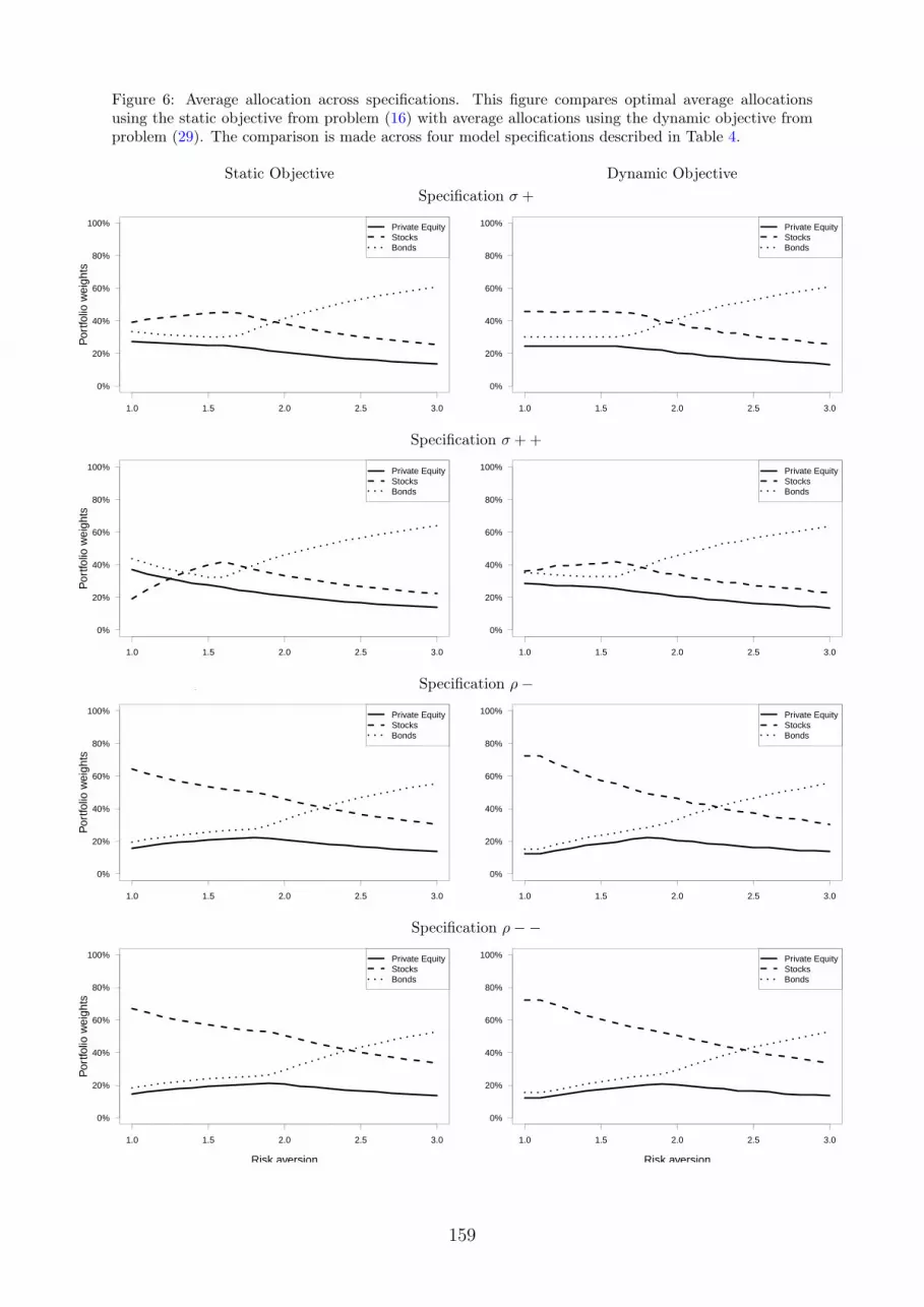
Figure 6: Average allocation across specifications. This figure compares optimal average allocationsusing the static objective from problem (16) with average allocations using the dynamic objective fromproblem (29). The comparison is made across four model specifications described in Table 4.

Static Objective Dynamic ObjectiveSpecification σ +

1.0 1.5 2.0 2.5 3.0

Risk aversion

0%

20%

40%

60%

80%

100%

Por

tfolio

wei

ghts

Private EquityStocksBonds

1.0 1.5 2.0 2.5 3.0

Risk aversion

0%

20%

40%

60%

80%

100% Private EquityStocksBonds

Specification σ ++

1.0 1.5 2.0 2.5 3.0

Risk aversion

0%

20%

40%

60%

80%

100%

Por

tfolio

wei

ghts

Private EquityStocksBonds

1.0 1.5 2.0 2.5 3.0

Risk aversion

0%

20%

40%

60%

80%

100% Private EquityStocksBonds

Specification ρ−

1.0 1.5 2.0 2.5 3.0

Optimal Allocation across Risk Aversion

Risk aversion

0%

20%

40%

60%

80%

100%

Por

tfolio

wei

ghts

Private EquityStocksBonds

1.0 1.5 2.0 2.5 3.0

Risk aversion

0%

20%

40%

60%

80%

100% Private EquityStocksBonds

Specification ρ−−

1.0 1.5 2.0 2.5 3.0

Optimal Allocation across Risk Aversion

Risk aversion

0%

20%

40%

60%

80%

100%

Por

tfolio

wei

ghts

Private EquityStocksBonds

1.0 1.5 2.0 2.5 3.0

Risk aversion

0%

20%

40%

60%

80%

100% Private EquityStocksBonds

159

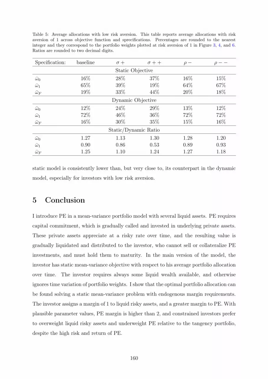
Table 5: Average allocations with low risk aversion. This table reports average allocations with riskaversion of 1 across objective function and sprecifications. Percentages are rounded to the nearestinteger and they correspond to the portfolio weights plotted at risk aversion of 1 in Figure 3, 4, and 6.Ratios are rounded to two decimal digits.

Specification: baseline σ + σ ++ ρ− ρ−−Static Objective

ω0 16% 28% 37% 16% 15%ω1 65% 39% 19% 64% 67%ωF 19% 33% 44% 20% 18%

Dynamic Objectiveω0 12% 24% 29% 13% 12%ω1 72% 46% 36% 72% 72%ωF 16% 30% 35% 15% 16%

Static/Dynamic Ratioω0 1.27 1.13 1.30 1.28 1.20ω1 0.90 0.86 0.53 0.89 0.93ωF 1.25 1.10 1.24 1.27 1.18

static model is consistently lower than, but very close to, its counterpart in the dynamic

model, especially for investors with low risk aversion.

5 Conclusion

I introduce PE in a mean-variance portfolio model with several liquid assets. PE requires

capital commitment, which is gradually called and invested in underlying private assets.

These private assets appreciate at a risky rate over time, and the resulting value is

gradually liquidated and distributed to the investor, who cannot sell or collateralize PE

investments, and must hold them to maturity. In the main version of the model, the

investor has static mean-variance objective with respect to his average portfolio allocation

over time. The investor requires always some liquid wealth available, and otherwise

ignores time variation of portfolio weights. I show that the optimal portfolio allocation can

be found solving a static mean-variance problem with endogenous margin requirements.

The investor assigns a margin of 1 to liquid risky assets, and a greater margin to PE. With

plausible parameter values, PE margin is higher than 2, and constrained investors prefer

to overweight liquid risky assets and underweight PE relative to the tangency portfolio,

despite the high risk and return of PE.

160

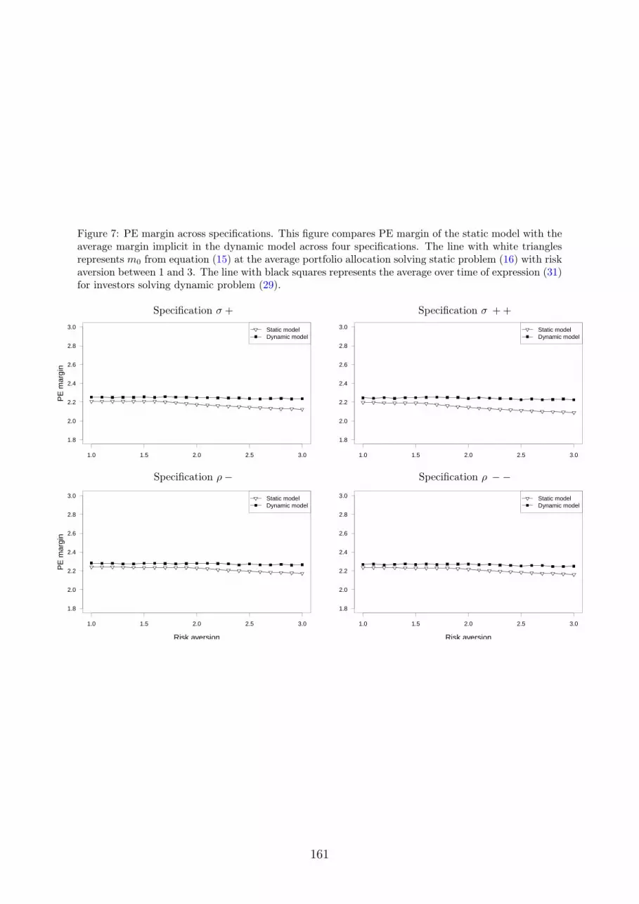
Figure 7: PE margin across specifications. This figure compares PE margin of the static model with theaverage margin implicit in the dynamic model across four specifications. The line with white trianglesrepresents m0 from equation (15) at the average portfolio allocation solving static problem (16) with riskaversion between 1 and 3. The line with black squares represents the average over time of expression (31)for investors solving dynamic problem (29).

Specification σ + Specification σ ++

1.0 1.5 2.0 2.5 3.0

1.8

2.0

2.2

2.4

2.6

2.8

3.0

Risk aversion

PE

mar

gin

Static modelDynamic model

1.0 1.5 2.0 2.5 3.0

1.8

2.0

2.2

2.4

2.6

2.8

3.0

Risk aversion

Static modelDynamic model

Specification ρ− Specification ρ −−

1.0 1.5 2.0 2.5 3.0

1.8

2.0

2.2

2.4

2.6

2.8

3.0

Risk aversion

PE

mar

gin

Static modelDynamic model

1.0 1.5 2.0 2.5 3.0

1.8

2.0

2.2

2.4

2.6

2.8

3.0

Risk aversion

Static modelDynamic model

161

I investigate the robustness of my results in a second version of the model assuming that

the investor has dynamic mean-variance objective on the return to his current and future

portfolio allocation. This second version cannot be reduced to a static problem. Instead,

I solve it numerically for five different specifications, and I compare the resulting average

portfolio allocations with those from the main model. I find similar results across the

two models. Portfolio allocations are virtually identical for unconstrained investors, while

they differ marginally for constrained investors. The main model tend to overestimate

the optimal PE allocation of constrained investors relative to the more realistic version.

The difference remains small, however, with limited and unsystematic variation across

specifications.

162

References

Ang, A., D. Papanikolaou, and M. M. Westerfield (2014). Portfolio choice with illiquid

assets. Management Science 60 (11), 2737–2761.

Banal-Estañol, A., F. Ippolito, and S. Vicente (2017). Default penalties in private equity

partnerships. Working Paper.

Black, F. (1972). Capital market equilibrium with restricted borrowing. The Journal of

Business 45 (3), 444–55.

Bollen, N. P. and B. A. Sensoy (2020). How much for a haircut? Illiquidity, secondary

markets, and the value of private equity. Working Paper.

Collin-Dufresne, P., K. Daniel, and M. Sağlam (2020). Liquidity regimes and optimal

dynamic asset allocation. Journal of Financial Economics 136 (2), 379–406.

Dimmock, S. G., N. Wang, and J. Yang (2019). The endowment model and modern

portfolio theory. Working Paper.

Frazzini, A. and L. H. Pedersen (2014). Betting against beta. Journal of Financial

Economics 111 (1), 1–25.

Giommetti, N. and M. Sorensen (2021). Optimal allocation to private equity. Working

Paper.

Gourier, E., L. Phalippou, and M. M. Westerfield (2021). Capital commitment. Working

Paper.

Harris, R. S., T. Jenkinson, and S. N. Kaplan (2014). Private equity performance: What

do we know? The Journal of Finance 69 (5), 1851–1882.

Kaplan, S. N. and A. Schoar (2005). Private equity performance: Returns, persistence,

and capital flows. The Journal of Finance 60 (4), 1791–1823.

Phalippou, L. (2014, 03). Performance of Buyout Funds Revisited? Review of Fi-

nance 18 (1), 189–218.

Sorensen, M., N. Wang, and J. Yang (2014). Valuing private equity. The Review of

Financial Studies 27 (7), 1977–2021.

163

Stafford, E. (2021). Replicating private equity with value investing, homemade leverage,

and hold-to-maturity accounting. Working Paper.

164

A Objective Function

In this appendix, I study the static objective function in relation to a more standard

dynamic mean-variance objective function. The starting point is the objective function

from the main text:

ω (µ− rF )−γ

2ω′Σω (A.1)

Under i.i.d. returns, and for a subjective discount factor δ ∈ (0, 1), it is possible to show

that the expression in (A.1) is proportional and economically equivalent, to the following

expression:

∞∑

t=0

δtE

[ω′t (µ− rF )−

γ

2ω′tΣωt

]

︸ ︷︷ ︸expected mean-variance

+∞∑

t=0

δt E

[γ

2(ωt − ω)′Σ(ωt − ω)

]

︸ ︷︷ ︸scaled variance of portfolio weights

(A.2)

This expression shows that the objective function (A.1) can be understood as the sum

of two components. The first component corresponds to the expected value of dynamic

mean-variance objective with constant relative risk aversion. Similar objective functions

are commonly used in the literature (e.g. Collin-Dufresne, Daniel, and Sağlam, 2020).

The second component is proportional to the variance of portfolio weights scaled through

the covariance matrix of returns. Formally, this component simplifies the objective func-

tion because it makes the investor risk-neutral toward variation in portfolio weights. Be-

cause of this second component, the objective function (A.1) deviates from the expected

value of standard dynamic mean-variance objective.

Below, I show that portfolio weights in liquid assets can be rebalanced such that, as PE

risk becomes more spanned by liquid assets, variation in portfolio weights becomes an

increasingly negligible source of risk. Thus, as PE becomes more spanned, the objective

function in (A.1) approximates the dynamic mean-variance objective in ranking average

portfolio allocations.

The argument starts with the exact relationship between the expected value of dynamic

165

mean-variance objective and the objective function used in the main model:

∞∑

t=0

δtE

[ω′t (µ− rF )−

γ

2ω′tΣωt

]=

∞∑

t=0

δt

(ω′ (µ− rF )−

γ

2ω′Σω

)

− γ

2

∞∑

t=0

δtE

[(ωt − ω)′Σ(ωt − ω)

](A.3)

Consider an investor whose objective function is the left-hand side of this expression.

The expression shows that this investor cares about two things: (i) the mean-variance

characteristics of his average allocation, which is the objective function used in the main

text, and (ii) variation of portfolio weights around that average allocation. This second

component constitutes the difference between this hypothetical investor and the ojective

function of the main model.

Proceeding with the argument, I take an exogenous sequence of PE portfolio weights

{ω0,t}∞t=0, and consider the following linear strategy for investing in liquid assets a =0:

ωa,t = ca − baω0,t (A.4)

The intercepts ca remain unrestricted throughout the argument, and the investor could

use them to maximize the first term on the right-hand side of (A.3). I find the vector

B = {b1, . . . , bA} that minimizes the scaled variance of portfolio weights, which is the

second term on the right-hand side of (A.3).

It is useful to introduce the following partitioning of the covariance matrix of returns:

Σ =

σ2

0 σ0A

σ′0A ΣA

(A.5)

In this expression, σ20 is the variance of PE return, σ0A is the covariance vector between

PE and liquid assets, and ΣA is the covariance matrix of liquid assets. Using definition

(A.5) and the linear strategy (A.4), it is possible to derive the following expression:

E

[(ωt − ω)′Σ(ωt − ω)

]= var(ω0,t)

1

−B

′ σ2

0 σ0A

σ′0A ΣA

1

−B

(A.6)

This formula expresses the scaled variance of portfolio weights in terms of the variance of

166

PE allocation and in terms of the rebalancing coefficients, B. I minimize the right-hand

side of this expression with respect to B taking the first order condition:

B = Σ−1A σ′

0A (A.7)

Considering ω0,t as exogenous, B minimizes the scaled variation of portfolio weights

among linear rebalancing strategies. Notice that B is also the vector of coefficients from

a multivariate regression of PE returns on the returns to liquid assets.

Substituting (A.7) inside (A.6) it is possible to find the resulting scaled variance of port-

folio weights:

var(ω0,t)[σ20 − σ0AΣ

−1A σ′

0A

](A.8)

The term in square brackets is the amount of variance that remains unexplained after

regressing PE return on the returns to liquid assets. In other words, it is the idiosyncratic

variance of PE, and when that is small, PE return is more spanned by liquid assets.

In summary, if PE return is more spanned by liquid assets, the investor can set the second

term on the right-hand side of (A.3) closer to zero without restricting his ability to affect

the average portfolio allocation; that is, without restricting his ability to maximize the

first term on the right-hand side of (A.3). Therefore, as PE becomes more spanned, the

second term on the right-hand side of (A.3) has increasingly negligible effect on optimal

average allocation, and the objective value from the main text approximates the expected

value of dynamic mean-variance objective.

I conclude with a discussion of the main assumptions and possible shortcomings of this

argument. First, throughout the argument I have assumed that the variance of ω0,t is

exogenous to the rebalancing strategy. This assumption is violated since the rebalancing

strategy determines the variance of wealth, which affects the variance of ω0,t. Relaxing

this assumption, the argument remains valid under the weak condition that the variance of

ω0,t does not diverge towards infinity as idiosyncratic PE volatility approaches zero.

A second and perhaps more important shortcoming of the argument is that it focuses

exclusively on the objective function of the model and ignores the constraint on liquid

wealth. In particular, since the evolution of ω0,t is endogenous to the rebalacing strategy,

it is possible that the suggested strategy with B violates the liquidity constraint imposed

167

by the investor:

Prob(1− ω0,t ≤ 0

)= 0 (A.9)

Ignoring this constraint, the argument can make use of a larger set of strategies. At

the same time, however, I restrict my attention to linear rebalancing strategies, and

even assuming that the proposed linear strategy fails to satisfy the liquidity constraint,

there could be non linear strategies that accomplish the same goals while satisfying that

constraint.

168

B Proofs

This appendix contains the derivations of Proposition 1 and Proposition 3. The derivation

of Proposition 2 is described in the main text.

B.1 Proposition 1

This proposition uses the law of motion of ω0,t from problem (8) to derive a relationship

between average commitments and average PE allocation. The law of motion can be

written as follows:

(1 + rW,t+1)ω0,t+1 = ω0,tRP,t+1 + λC(kt + nt)− λDω0,tRP,t+1 (B.1)

In the left-hand side, it is useful to linearize rW,t+1ω0,t+1 around the point rW,t+1 = µW

and ω0,t+1 = ω0. The linearization results into the following expression:

rW,t+1ω0,t+1 ≈ ω0,t+1µW + ω0(rW,t+1 − µW ) (B.2)

Replacing this approximation in the left-hand side of (B.1), and taking unconditional

expectations on both sides, I get the following result:

ω0(1 + µW ) = ω0(1− λD)(1 + µP ) + (k + n)λC (B.3)

It is sufficient to rearrange this expression to obtain the result of the proposition.

B.2 Proposition 3

The optimal portfolio allocation of the static portfolio problem is

ω∗ =1

γΣ−1(µ− rF − ψm) (B.4)

The elements of ω∗ are all proportional to γ, and the fraction of any two elements depends

on risk aversion indirectly through ψ. Similarly, the fraction ω∗0/(ω

∗0 + ω∗

1 + . . . + ω∗A)

depends on risk aversion only through ψ. Furhtermore, ω∗0/(ω

∗0 + ω∗

1 + . . .+ ω∗A) increases

with ψ if and only if ω∗0/(ω

∗1 + . . .+ ω∗

A) also increases with ψ.

169

Using expression (B.4) and blockwise matrix inversion, the fraction ω∗0/(ω

∗1 + . . . + ω∗

A)

can be written as follows:

ω∗0

ω∗1 + . . .+ ω∗

A

=v0(µ0 − rF )− σ0A

σ20vA(µA − rF )− ψ(v0m0 − σ0A

σ20vA1)

1′[−Σ−1

A σ′0Av0(µ0 − rF ) + vA(µA − rF ) + ψ(Σ−1

A σ′0Av0m0 − vA1)

]

(B.5)

In this expression, µA and ΣA indicate the vector of expected returns and covariance

matrix of risky assets except PE. Similarly, µ0 and σ20 indicate the expected return and

variance of PE, while σ0A is a row vector of covariances between PE and the other assets.

Furthermore, 1 indicates an A-dimensional column vector of ones, and the terms v0 and

vA are defined as follows:

v0 =(σ20 − σ0AΣ

−1A σ′

0A

)−1 (B.6)

vA =

(ΣA − σ′

0Aσ0A1

σ20

)−1

= Σ−1A + Σ−1

A σ′0Av0σ0AΣ

−1A (B.7)

Since ψ decreases with γ, the derivative of ω∗0/(ω

∗1 + . . . + ω∗

A) with respect to γ has to

opposite sign of the derivative ω∗0/(ω

∗1 + . . .+ ω∗

A) with respect to ψ. With basic algebra,

it is possible to show that the latter derivative is independent of ψ and has the same sign

of the following expression:

− v0m01′vA(µA − rF ) +

σ0Aσ20

vA11′(vA(µA − rF )− Σ−1

A σA0v0(µ0 − rF ))

+ 1′Σ−1A σA0v0m0

σ0Aσ20

vA(µA − rF ) + 1′vA1(v0(µ0 − rF )−

σ0Aσ20

vA(µA − rF ))

This expression can be simplified as follows:

1′Σ−1A 1[(µ0 − rF )− σ0AΣ

−1A (µA − rF )]− [m0 − 1′Σ−1

A σ′0A]1

′Σ−1A (µA − rF ) (B.8)

Using the definition of B, and dividing this expression by 1′Σ−1A 1, which is a positive

term, I find that the derivative of ω∗0/(ω

∗1 + . . .+ ω∗

A) with respect to ψ has the same sign

of the following expression:

(µ0 − rF )− 1′B

(B′

1′B− 1′Σ−1

A

1′Σ−1A 1

)(µA − rF )−m0

1′Σ−1A

1′Σ−1A 1

(µA − rF )

Thus, this expression has the opposite sign of the derivative of ω∗0/(ω

∗1 + . . . + ω∗

A) with

170

respect to γ. This is the result in the proposition.

Finally, it is possible to generalize the result with a generic vector mA of margin require-

ments for liquid risky assets. Under this assumption, the derivative of ω∗0/(ω

∗1 + . . .+ ω

∗A)

with respect to ψ has the same sign of

(µ0 − rF )−m′AB

(1′B

m′AB

B′

1′B− 1′Σ−1

A 1

1′Σ−1A mA

1′Σ−1A

1′Σ−1A 1

)(µA − rF )−m0

1′Σ−1A 1

1′Σ−1A mA

1′Σ−1A

1′Σ−1A 1

(µA − rF )

171

C Supplementary Output with Dynamic Objective

This section reports the value function and optimal strategies solving problem (29) for

every specification considered in the main text. To save space, I report only the solution

for two types of investor, with risk aversion of 1 and 3, which I call ‘Aggressive’ and

‘Conservative’. For the baseline specification, I also estimate and report a linear approxi-

mation of the optimal strategies on the area of the state space that is reached more often

by the investor.

C.1 Baseline Specification

(a) Aggressive (γ = 1)

k

ω0

Val

ue 0%

30%

70%

0% 30%70% 100%

0.800.85

0.90

0.95

1.00

1.05

1.10

(b) Conservative (γ = 3)

k

ω0

Val

ue 0%

30%

70%

0% 30%70% 100%

0.800.85

0.90

0.95

1.00

1.05

1.10

Figure C.8: Value function with dynamic objective function. This figure compares the value functionV (ω0, k) of Bellman equation (29) for investors with low risk-aversion (γ = 1) and investors with highrisk-aversion (γ = 3). Each function is rescaled and expressed in units of value at (ω0, k) = (0, 0), so I plotv(p, k)/v(0, 0) for the two types of investors. I only display functional values above a certain threshold,which is 0.75 for the low risk-aversion case and 0.7 for the high risk-aversion case. The shade on thesurface of the function indicates how often investors reach a certain area of the state space. Darker areasindicate states that are reached more often. Shades are constructed using a Monte Carlo simulationwhere investors behave optimally.

172

(a) Aggressive (γ = 1)

k

ω0

New

com

mitm

ent

0%

30%

70%

0% 30%70% 100%

0%10%20%30%40%50%60%

70%

80%

(b) Conservative (γ = 3)

k

ω0

New

com

mitm

ent

0%

30%

70%

0% 30%70% 100%

0%10%20%30%40%50%60%

70%

80%

Figure C.9: Optimal commitment with dynamic objective function. This figure reports optimal com-mitment strategy with dynamic objective for investors with low risk-aversion (γ = 1) and investors withhigh risk-aversion (γ = 3). For each type, the plots show optimal new commitment n∗(ω0, k) resultingfrom Bellman equation (29) with baseline specification given in Table 1. The shade on the surface of thefunction indicates how often investors reach a certain area of the state space. Darker areas indicate statesthat are reached more often. Shades are constructed using a Monte Carlo simulation where investorsbehave optimally.

Table A1: Local slope of the optimal commitment strategy. This table reports coefficients β0, β1, β2,and β3 from OLS estimations of the following model:

n∗(ω0, k) = β0 + β1ω0 + β2k + β3(ω0 × k) + ϵ

In this equation, ϵ is an error term, while n∗(ω0, k) is the optimal commitment function plotted inFigure C.9 for two different levels of risk-aversion. The model is estimated twice for the case of lowrisk-aversion (γ = 1) and twice for the case of high risk-aversion (γ = 3). For each level of risk-aversion,the first estimation imposes β3 = 0, while the second estimation ignores that restriction. The data foreach estimation is taken from a Monte Carlo simulation where the evolution of the state variables issimulated under optimal policies.

γ = 1 γ = 3

(1) (2) (3) (4)PE allocation (ω0) 0.17 0.40 −1.89 −2.16

Commitment (k) −0.95 −0.69 −0.93 −1.25

Interaction (ω0 × k) −2.09 0.46

Constant 0.14 0.11 0.43 0.46

R2 0.96 0.96 0.99 0.99

173

(a) Aggressive (γ = 1)

k

ω0

Sto

ck a

lloca

tion

0%

30%

70%

0% 30%70% 100%

0% 10% 20% 30% 40% 50% 60% 70% 80% 90%

100%

(b) Conservative (γ = 3)

k

ω0

Sto

ck a

lloca

tion

0%

30%

70%

0% 30%70% 100%

0% 10% 20% 30% 40% 50% 60% 70% 80% 90%

100%

Figure C.10: Optimal stocks allocation with dynamic objective function. This figure reports optimalstocks allocation with dynamic objective for investors with low risk-aversion (γ = 1) and investors withhigh risk-aversion (γ = 3). For each type, the plots show optimal stocks allocation ω∗

1(ω0, k) resultingfrom Bellman equation (29) with baseline specification given in Table 1. The shade on the surface of thefunction is constructed as in Figure C.9.

Table A2: Local slope of optimal stocks allocation. This table reports coefficients β0, β1, β2, and β3

from OLS estimations of the following model:

ω∗1(ω0, k) = β0 + β1ω0 + β2k + β3(ω0 × k) + ϵ

In this equation, ϵ is an error term, while ω∗1(ω0, k) is the optimal stocks allocation plotted in Figure C.10

for two different levels of risk-aversion. The model is estimated as in Table A1.

γ = 1 γ = 3

(1) (2) (3) (4)PE allocation (ω0) −1.17 −1.48 −1.64 −1.78

Commitment (k) −0.13 −0.47 0.02 −0.15

Interaction (ω0 × k) 2.81 1.21

Constant 0.88 0.92 0.51 0.52

R2 0.95 0.95 1.00 1.00

C.2 Alternative Specifications

174

Figure C.11: Value function with dynamic objective and different parameter specifications. This figureplots the value function V (ω0, k) of Bellman equation (29) for two types of investors (aggressive andconservative) across four different specifications described in Table 4 of the main text.

Aggressive Investor (γ = 1)Specification σ + Specification σ ++

k

ω0

Val

ue 0%

30%

70%

0% 30%70% 100%

0.800.85

0.90

0.95

1.00

1.05

1.10

k

ω0

Val

ue 0%

30%

70%

0% 30%70% 100%

0.800.85

0.90

0.95

1.00

1.05

1.10

Specification ρ− Specification ρ−−

k

ω0

Val

ue 0%

30%

70%

0% 30%70% 100%

0.800.85

0.90

0.95

1.00

1.05

1.10

k

ω0

Val

ue 0%

30%

70%

0% 30%70% 100%

0.800.85

0.90

0.95

1.00

1.05

1.10

Conservative Investor (γ = 3)Specification σ + Specification σ ++

k

ω0

Val

ue 0%

30%

70%

0% 30%70% 100%

0.800.85

0.90

0.95

1.00

1.05

1.10

k

ω0

Val

ue 0%

30%

70%

0% 30%70% 100%

0.800.85

0.90

0.95

1.00

1.05

1.10

Specification ρ− Specification ρ−−

k

ω0

Val

ue 0%

30%

70%

0% 30%70% 100%

0.800.85

0.90

0.95

1.00

1.05

1.10

k

ω0

Val

ue 0%

30%

70%

0% 30%70% 100%

0.800.85

0.90

0.95

1.00

1.05

1.10

175

Figure C.12: Optimal commitment strategy with dynamic objective and different parameter specifica-tions. This figure plots optimal new commitment n∗(ω0, k) of Bellman equation (29) for two types ofinvestors (aggressive and conservative) across four different specifications described in Table 4 of themain text.

Aggressive Investor (γ = 1)Specification σ + Specification σ ++

k

ω0

New

com

mitm

ent

0%

30%

70%

0% 30%70% 100%

0%10%20%30%40%50%60%

70%

80%

k

ω0

New

com

mitm

ent

0%

30%

70%

0% 30%70% 100%

0%10%20%30%40%50%60%

70%

80%

Specification ρ− Specification ρ−−

k

ω0

New

com

mitm

ent

0%

30%

70%

0% 30%70% 100%

0%10%20%30%40%50%60%

70%

80%

k

ω0

New

com

mitm

ent

0%

30%

70%

0% 30%70% 100%

0%10%20%30%40%50%60%

70%

80%

Conservative Investor (γ = 3)Specification σ + Specification σ ++

k

ω0

New

com

mitm

ent

0%

30%

70%

0% 30%70% 100%

0%10%20%30%40%50%60%

70%

80%

k

ω0

New

com

mitm

ent

0%

30%

70%

0% 30%70% 100%

0%10%20%30%40%50%60%

70%

80%

Specification ρ− Specification ρ−−

k

ω0

New

com

mitm

ent

0%

30%

70%

0% 30%70% 100%

0%10%20%30%40%50%60%

70%

80%

k

ω0

New

com

mitm

ent

0%

30%

70%

0% 30%70% 100%

0%10%20%30%40%50%60%

70%

80%

176

Figure C.13: Optimal stocks allocation with dynamic objective and different parameter specifications.This figure plots optimal stocks allocation ω∗

1(ω0, k) of Bellman equation (29) for two types of investors(aggressive and conservative) across four different specifications described in Table 4 of the main text.

Aggressive Investor (γ = 1)Specification σ + Specification σ ++

k

ω0

Sto

ck a

lloca

tion

0%

30%

70%

0% 30%70% 100%

0% 10% 20% 30% 40% 50% 60% 70% 80% 90%

100%

k

ω0

Sto

ck a

lloca

tion

0%

30%

70%

0% 30%70% 100%

0% 10% 20% 30% 40% 50% 60% 70% 80% 90%

100%

Specification ρ− Specification ρ−−

k

ω0

Sto

ck a

lloca

tion

0%

30%

70%

0% 30%70% 100%

0% 10% 20% 30% 40% 50% 60% 70% 80% 90%

100%

k

ω0

Sto

ck a

lloca

tion

0%

30%

70%

0% 30%70% 100%

0% 10% 20% 30% 40% 50% 60% 70% 80% 90%

100%

Conservative Investor (γ = 3)Specification σ + Specification σ ++

k

ω0

Sto

ck a

lloca

tion

0%

30%

70%

0% 30%70% 100%

0% 10% 20% 30% 40% 50% 60% 70% 80% 90%

100%

k

ω0

Sto

ck a

lloca

tion

0%

30%

70%

0% 30%70% 100%

0% 10% 20% 30% 40% 50% 60% 70% 80% 90%

100%

Specification ρ− Specification ρ−−

k

ω0

Sto

ck a

lloca

tion

0%

30%

70%

0% 30%70% 100%

0% 10% 20% 30% 40% 50% 60% 70% 80% 90%

100%

k

ω0

Sto

ck a

lloca

tion

0%

30%

70%

0% 30%70% 100%

0% 10% 20% 30% 40% 50% 60% 70% 80% 90%

100%

177

TITLER I PH.D.SERIEN:

20041. Martin Grieger

Internet-based Electronic Marketplacesand Supply Chain Management

2. Thomas BasbøllLIKENESSA Philosophical Investigation

3. Morten KnudsenBeslutningens vaklenEn systemteoretisk analyse of mo-derniseringen af et amtskommunaltsundhedsvæsen 1980-2000

4. Lars Bo JeppesenOrganizing Consumer InnovationA product development strategy thatis based on online communities andallows some firms to benefit from adistributed process of innovation byconsumers

5. Barbara DragstedSEGMENTATION IN TRANSLATIONAND TRANSLATION MEMORYSYSTEMSAn empirical investigation of cognitivesegmentation and effects of integra-ting a TM system into the translationprocess

6. Jeanet HardisSociale partnerskaberEt socialkonstruktivistisk casestudieaf partnerskabsaktørers virkeligheds-opfattelse mellem identitet oglegitimitet

7. Henriette Hallberg ThygesenSystem Dynamics in Action

8. Carsten Mejer PlathStrategisk Økonomistyring

9. Annemette KjærgaardKnowledge Management as InternalCorporate Venturing

– a Field Study of the Rise and Fall of aBottom-Up Process

10. Knut Arne HovdalDe profesjonelle i endringNorsk ph.d., ej til salg gennemSamfundslitteratur

11. Søren JeppesenEnvironmental Practices and GreeningStrategies in Small ManufacturingEnterprises in South Africa– A Critical Realist Approach

12. Lars Frode FrederiksenIndustriel forskningsledelse– på sporet af mønstre og samarbejdei danske forskningsintensive virksom-heder

13. Martin Jes IversenThe Governance of GN Great Nordic– in an age of strategic and structuraltransitions 1939-1988

14. Lars Pynt AndersenThe Rhetorical Strategies of Danish TVAdvertisingA study of the first fifteen years withspecial emphasis on genre and irony

15. Jakob RasmussenBusiness Perspectives on E-learning

16. Sof ThraneThe Social and Economic Dynamicsof Networks– a Weberian Analysis of ThreeFormalised Horizontal Networks

17. Lene NielsenEngaging Personas and NarrativeScenarios – a study on how a user-

centered approach influenced the perception of the design process in the e-business group at AstraZeneca

18. S.J ValstadOrganisationsidentitetNorsk ph.d., ej til salg gennemSamfundslitteratur

19. Thomas Lyse HansenSix Essays on Pricing and Weather riskin Energy Markets

20. Sabine MadsenEmerging Methods – An InterpretiveStudy of ISD Methods in Practice

21. Evis SinaniThe Impact of Foreign Direct Inve-stment on Efficiency, ProductivityGrowth and Trade: An Empirical Inve-stigation

22. Bent Meier SørensenMaking Events Work Or,How to Multiply Your Crisis

23. Pernille SchnoorBrand EthosOm troværdige brand- ogvirksomhedsidentiteter i et retorisk ogdiskursteoretisk perspektiv

24. Sidsel FabechVon welchem Österreich ist hier dieRede?Diskursive forhandlinger og magt-kampe mellem rivaliserende nationaleidentitetskonstruktioner i østrigskepressediskurser

25. Klavs Odgaard ChristensenSprogpolitik og identitetsdannelse iflersprogede forbundsstaterEt komparativt studie af Schweiz ogCanada

26. Dana B. MinbaevaHuman Resource Practices andKnowledge Transfer in MultinationalCorporations

27. Holger HøjlundMarkedets politiske fornuftEt studie af velfærdens organisering iperioden 1990-2003

28. Christine Mølgaard FrandsenA.s erfaringOm mellemværendets praktik i en

transformation af mennesket og subjektiviteten

29. Sine Nørholm JustThe Constitution of Meaning– A Meaningful Constitution?Legitimacy, identity, and public opinionin the debate on the future of Europe

20051. Claus J. Varnes

Managing product innovation throughrules – The role of formal and structu-red methods in product development

2. Helle Hedegaard HeinMellem konflikt og konsensus– Dialogudvikling på hospitalsklinikker

3. Axel RosenøCustomer Value Driven Product Inno-vation – A Study of Market Learning inNew Product Development

4. Søren Buhl PedersenMaking spaceAn outline of place branding

5. Camilla Funck EllehaveDifferences that MatterAn analysis of practices of gender andorganizing in contemporary work-places

6. Rigmor Madeleine LondStyring af kommunale forvaltninger

7. Mette Aagaard AndreassenSupply Chain versus Supply ChainBenchmarking as a Means toManaging Supply Chains

8. Caroline Aggestam-PontoppidanFrom an idea to a standardThe UN and the global governance ofaccountants’ competence

9. Norsk ph.d.

10. Vivienne Heng Ker-niAn Experimental Field Study on the

Effectiveness of Grocer Media Advertising

Measuring Ad Recall and Recognition, Purchase Intentions and Short-Term Sales

11. Allan MortensenEssays on the Pricing of CorporateBonds and Credit Derivatives

12. Remo Stefano ChiariFigure che fanno conoscereItinerario sull’idea del valore cognitivoe espressivo della metafora e di altritropi da Aristotele e da Vico fino alcognitivismo contemporaneo

13. Anders McIlquham-SchmidtStrategic Planning and CorporatePerformanceAn integrative research review and ameta-analysis of the strategic planningand corporate performance literaturefrom 1956 to 2003

14. Jens GeersbroThe TDF – PMI CaseMaking Sense of the Dynamics ofBusiness Relationships and Networks

15 Mette AndersenCorporate Social Responsibility inGlobal Supply ChainsUnderstanding the uniqueness of firmbehaviour

16. Eva BoxenbaumInstitutional Genesis: Micro – DynamicFoundations of Institutional Change

17. Peter Lund-ThomsenCapacity Development, EnvironmentalJustice NGOs, and Governance: TheCase of South Africa

18. Signe JarlovKonstruktioner af offentlig ledelse

19. Lars Stæhr JensenVocabulary Knowledge and ListeningComprehension in English as a ForeignLanguage

An empirical study employing data elicited from Danish EFL learners

20. Christian NielsenEssays on Business ReportingProduction and consumption ofstrategic information in the market forinformation

21. Marianne Thejls FischerEgos and Ethics of ManagementConsultants

22. Annie Bekke KjærPerformance management i Proces-

innovation – belyst i et social-konstruktivistiskperspektiv

23. Suzanne Dee PedersenGENTAGELSENS METAMORFOSEOm organisering af den kreative gøreni den kunstneriske arbejdspraksis

24. Benedikte Dorte RosenbrinkRevenue ManagementØkonomiske, konkurrencemæssige &organisatoriske konsekvenser

25. Thomas Riise JohansenWritten Accounts and Verbal AccountsThe Danish Case of Accounting andAccountability to Employees

26. Ann Fogelgren-PedersenThe Mobile Internet: Pioneering Users’Adoption Decisions

27. Birgitte RasmussenLedelse i fællesskab – de tillidsvalgtesfornyende rolle

28. Gitte Thit NielsenRemerger– skabende ledelseskræfter i fusion ogopkøb

29. Carmine GioiaA MICROECONOMETRIC ANALYSIS OFMERGERS AND ACQUISITIONS

30. Ole HinzDen effektive forandringsleder: pilot,pædagog eller politiker?Et studie i arbejdslederes meningstil-skrivninger i forbindelse med vellykketgennemførelse af ledelsesinitieredeforandringsprojekter

31. Kjell-Åge GotvassliEt praksisbasert perspektiv på dynami-skelæringsnettverk i toppidrettenNorsk ph.d., ej til salg gennemSamfundslitteratur

32. Henriette Langstrup NielsenLinking HealthcareAn inquiry into the changing perfor-

mances of web-based technology for asthma monitoring

33. Karin Tweddell LevinsenVirtuel UddannelsespraksisMaster i IKT og Læring – et casestudiei hvordan proaktiv proceshåndteringkan forbedre praksis i virtuelle lærings-miljøer

34. Anika LiversageFinding a PathLabour Market Life Stories ofImmigrant Professionals

35. Kasper Elmquist JørgensenStudier i samspillet mellem stat og erhvervsliv i Danmark under1. verdenskrig

36. Finn JanningA DIFFERENT STORYSeduction, Conquest and Discovery

37. Patricia Ann PlackettStrategic Management of the RadicalInnovation ProcessLeveraging Social Capital for MarketUncertainty Management

20061. Christian Vintergaard

Early Phases of Corporate Venturing

2. Niels Rom-PoulsenEssays in Computational Finance

3. Tina Brandt HusmanOrganisational Capabilities,Competitive Advantage & Project-Based OrganisationsThe Case of Advertising and CreativeGood Production

4. Mette Rosenkrands JohansenPractice at the top– how top managers mobilise and usenon-financial performance measures

5. Eva ParumCorporate governance som strategiskkommunikations- og ledelsesværktøj

6. Susan Aagaard PetersenCulture’s Influence on PerformanceManagement: The Case of a DanishCompany in China

7. Thomas Nicolai PedersenThe Discursive Constitution of Organi-zational Governance – Between unityand differentiationThe Case of the governance ofenvironmental risks by World Bankenvironmental staff

8. Cynthia SelinVolatile Visions: Transactons inAnticipatory Knowledge

9. Jesper BanghøjFinancial Accounting Information and Compensation in Danish Companies

10. Mikkel Lucas OverbyStrategic Alliances in Emerging High-Tech Markets: What’s the Differenceand does it Matter?

11. Tine AageExternal Information Acquisition ofIndustrial Districts and the Impact ofDifferent Knowledge Creation Dimen-sions

A case study of the Fashion and Design Branch of the Industrial District of Montebelluna, NE Italy

12. Mikkel FlyverbomMaking the Global Information SocietyGovernableOn the Governmentality of Multi-Stakeholder Networks

13. Anette GrønningPersonen bagTilstedevær i e-mail som inter-aktionsform mellem kunde og med-arbejder i dansk forsikringskontekst

14. Jørn HelderOne Company – One Language?The NN-case

15. Lars Bjerregaard MikkelsenDiffering perceptions of customervalueDevelopment and application of a toolfor mapping perceptions of customervalue at both ends of customer-suppli-er dyads in industrial markets

16. Lise GranerudExploring LearningTechnological learning within smallmanufacturers in South Africa

17. Esben Rahbek PedersenBetween Hopes and Realities:Reflections on the Promises andPractices of Corporate SocialResponsibility (CSR)

18. Ramona SamsonThe Cultural Integration Model andEuropean Transformation.The Case of Romania

20071. Jakob Vestergaard

Discipline in The Global EconomyPanopticism and the Post-WashingtonConsensus

2. Heidi Lund HansenSpaces for learning and workingA qualitative study of change of work,management, vehicles of power andsocial practices in open offices

3. Sudhanshu RaiExploring the internal dynamics ofsoftware development teams duringuser analysisA tension enabled InstitutionalizationModel; ”Where process becomes theobjective”

4. Norsk ph.d.Ej til salg gennem Samfundslitteratur

5. Serden OzcanEXPLORING HETEROGENEITY INORGANIZATIONAL ACTIONS ANDOUTCOMESA Behavioural Perspective

6. Kim Sundtoft HaldInter-organizational PerformanceMeasurement and Management inAction– An Ethnography on the Constructionof Management, Identity andRelationships

7. Tobias LindebergEvaluative TechnologiesQuality and the Multiplicity ofPerformance

8. Merete Wedell-WedellsborgDen globale soldatIdentitetsdannelse og identitetsledelsei multinationale militære organisatio-ner

9. Lars FrederiksenOpen Innovation Business ModelsInnovation in firm-hosted online usercommunities and inter-firm projectventures in the music industry– A collection of essays

10. Jonas GabrielsenRetorisk toposlære – fra statisk ’sted’til persuasiv aktivitet

11. Christian Moldt-JørgensenFra meningsløs til meningsfuldevaluering.Anvendelsen af studentertilfredsheds-

målinger på de korte og mellemlange videregående uddannelser set fra et

psykodynamisk systemperspektiv

12. Ping GaoExtending the application ofactor-network theoryCases of innovation in the tele-

communications industry

13. Peter MejlbyFrihed og fængsel, en del af densamme drøm?Et phronetisk baseret casestudie affrigørelsens og kontrollens sam-eksistens i værdibaseret ledelse!

14. Kristina BirchStatistical Modelling in Marketing

15. Signe PoulsenSense and sensibility:The language of emotional appeals ininsurance marketing

16. Anders Bjerre TrolleEssays on derivatives pricing and dyna-mic asset allocation

17. Peter FeldhütterEmpirical Studies of Bond and CreditMarkets

18. Jens Henrik Eggert ChristensenDefault and Recovery Risk Modelingand Estimation

19. Maria Theresa LarsenAcademic Enterprise: A New Missionfor Universities or a Contradiction inTerms?Four papers on the long-term impli-cations of increasing industry involve-ment and commercialization in acade-mia

20. Morten WellendorfPostimplementering af teknologi i den offentlige forvaltningAnalyser af en organisations konti-nuerlige arbejde med informations-teknologi

21. Ekaterina MhaannaConcept Relations for TerminologicalProcess Analysis

22. Stefan Ring ThorbjørnsenForsvaret i forandringEt studie i officerers kapabiliteter un-der påvirkning af omverdenens foran-dringspres mod øget styring og læring

23. Christa Breum AmhøjDet selvskabte medlemskab om ma-nagementstaten, dens styringstekno-logier og indbyggere

24. Karoline BromoseBetween Technological Turbulence andOperational Stability– An empirical case study of corporateventuring in TDC

25. Susanne JustesenNavigating the Paradoxes of Diversityin Innovation Practice– A Longitudinal study of six verydifferent innovation processes – inpractice

26. Luise Noring HenlerConceptualising successful supplychain partnerships– Viewing supply chain partnershipsfrom an organisational culture per-spective

27. Mark MauKampen om telefonenDet danske telefonvæsen under dentyske besættelse 1940-45

28. Jakob HalskovThe semiautomatic expansion ofexisting terminological ontologiesusing knowledge patterns discovered

on the WWW – an implementation and evaluation

29. Gergana KolevaEuropean Policy Instruments BeyondNetworks and Structure: The Innova-tive Medicines Initiative

30. Christian Geisler AsmussenGlobal Strategy and InternationalDiversity: A Double-Edged Sword?

31. Christina Holm-PetersenStolthed og fordomKultur- og identitetsarbejde ved ska-belsen af en ny sengeafdeling gennemfusion

32. Hans Peter OlsenHybrid Governance of StandardizedStatesCauses and Contours of the GlobalRegulation of Government Auditing

33. Lars Bøge SørensenRisk Management in the Supply Chain

34. Peter AagaardDet unikkes dynamikkerDe institutionelle mulighedsbetingel-ser bag den individuelle udforskning iprofessionelt og frivilligt arbejde

35. Yun Mi AntoriniBrand Community InnovationAn Intrinsic Case Study of the AdultFans of LEGO Community

36. Joachim Lynggaard BollLabor Related Corporate Social Perfor-mance in DenmarkOrganizational and Institutional Per-spectives

20081. Frederik Christian Vinten

Essays on Private Equity

2. Jesper ClementVisual Influence of Packaging Designon In-Store Buying Decisions

3. Marius Brostrøm KousgaardTid til kvalitetsmåling?– Studier af indrulleringsprocesser iforbindelse med introduktionen afkliniske kvalitetsdatabaser i speciallæ-gepraksissektoren

4. Irene Skovgaard SmithManagement Consulting in ActionValue creation and ambiguity inclient-consultant relations

5. Anders RomManagement accounting and inte-grated information systemsHow to exploit the potential for ma-nagement accounting of informationtechnology

6. Marina CandiAesthetic Design as an Element ofService Innovation in New Technology-based Firms

7. Morten SchnackTeknologi og tværfaglighed– en analyse af diskussionen omkringindførelse af EPJ på en hospitalsafde-ling

8. Helene Balslev ClausenJuntos pero no revueltos – un estudiosobre emigrantes norteamericanos enun pueblo mexicano

9. Lise JustesenKunsten at skrive revisionsrapporter.En beretning om forvaltningsrevisio-nens beretninger

10. Michael E. HansenThe politics of corporate responsibility:CSR and the governance of child laborand core labor rights in the 1990s

11. Anne RoepstorffHoldning for handling – en etnologiskundersøgelse af Virksomheders SocialeAnsvar/CSR

12. Claus BajlumEssays on Credit Risk andCredit Derivatives

13. Anders BojesenThe Performative Power of Competen-ce – an Inquiry into Subjectivity andSocial Technologies at Work

14. Satu ReijonenGreen and FragileA Study on Markets and the NaturalEnvironment

15. Ilduara BustaCorporate Governance in BankingA European Study

16. Kristian Anders HvassA Boolean Analysis Predicting IndustryChange: Innovation, Imitation & Busi-ness ModelsThe Winning Hybrid: A case study ofisomorphism in the airline industry

17. Trine PaludanDe uvidende og de udviklingsparateIdentitet som mulighed og restriktionblandt fabriksarbejdere på det aftaylo-riserede fabriksgulv

18. Kristian JakobsenForeign market entry in transition eco-nomies: Entry timing and mode choice

19. Jakob ElmingSyntactic reordering in statistical ma-chine translation

20. Lars Brømsøe TermansenRegional Computable General Equili-brium Models for DenmarkThree papers laying the foundation forregional CGE models with agglomera-tion characteristics

21. Mia ReinholtThe Motivational Foundations ofKnowledge Sharing

22. Frederikke Krogh-MeibomThe Co-Evolution of Institutions andTechnology– A Neo-Institutional Understanding ofChange Processes within the BusinessPress – the Case Study of FinancialTimes

23. Peter D. Ørberg JensenOFFSHORING OF ADVANCED ANDHIGH-VALUE TECHNICAL SERVICES:ANTECEDENTS, PROCESS DYNAMICSAND FIRMLEVEL IMPACTS

24. Pham Thi Song HanhFunctional Upgrading, RelationalCapability and Export Performance ofVietnamese Wood Furniture Producers

25. Mads VangkildeWhy wait?An Exploration of first-mover advanta-ges among Danish e-grocers through aresource perspective

26. Hubert Buch-HansenRethinking the History of EuropeanLevel Merger ControlA Critical Political Economy Perspective

20091. Vivian Lindhardsen

From Independent Ratings to Commu-nal Ratings: A Study of CWA Raters’Decision-Making Behaviours

2. Guðrið WeihePublic-Private Partnerships: Meaningand Practice

3. Chris NøkkentvedEnabling Supply Networks with Colla-borative Information InfrastructuresAn Empirical Investigation of BusinessModel Innovation in Supplier Relation-ship Management

4. Sara Louise MuhrWound, Interrupted – On the Vulner-ability of Diversity Management

5. Christine SestoftForbrugeradfærd i et Stats- og Livs-formsteoretisk perspektiv

6. Michael PedersenTune in, Breakdown, and Reboot: Onthe production of the stress-fit self-managing employee

7. Salla LutzPosition and Reposition in Networks– Exemplified by the Transformation ofthe Danish Pine Furniture Manu-

facturers

8. Jens ForssbæckEssays on market discipline incommercial and central banking

9. Tine MurphySense from Silence – A Basis for Orga-nised ActionHow do Sensemaking Processes withMinimal Sharing Relate to the Repro-duction of Organised Action?

10. Sara Malou StrandvadInspirations for a new sociology of art:A sociomaterial study of developmentprocesses in the Danish film industry

11. Nicolaas MoutonOn the evolution of social scientificmetaphors:A cognitive-historical enquiry into thedivergent trajectories of the idea thatcollective entities – states and societies,cities and corporations – are biologicalorganisms.

12. Lars Andreas KnutsenMobile Data Services:Shaping of user engagements

13. Nikolaos Theodoros KorfiatisInformation Exchange and BehaviorA Multi-method Inquiry on OnlineCommunities

14. Jens AlbækForestillinger om kvalitet og tværfaglig-hed på sygehuse– skabelse af forestillinger i læge- ogplejegrupperne angående relevans afnye idéer om kvalitetsudvikling gen-nem tolkningsprocesser

15. Maja LotzThe Business of Co-Creation – and theCo-Creation of Business

16. Gitte P. JakobsenNarrative Construction of Leader Iden-tity in a Leader Development ProgramContext

17. Dorte Hermansen”Living the brand” som en brandorien-teret dialogisk praxis:Om udvikling af medarbejdernesbrandorienterede dømmekraft

18. Aseem KinraSupply Chain (logistics) EnvironmentalComplexity

19. Michael NøragerHow to manage SMEs through thetransformation from non innovative toinnovative?

20. Kristin WallevikCorporate Governance in Family FirmsThe Norwegian Maritime Sector

21. Bo Hansen HansenBeyond the ProcessEnriching Software Process Improve-ment with Knowledge Management

22. Annemette Skot-HansenFranske adjektivisk afledte adverbier,der tager præpositionssyntagmer ind-ledt med præpositionen à som argu-menterEn valensgrammatisk undersøgelse

23. Line Gry KnudsenCollaborative R&D CapabilitiesIn Search of Micro-Foundations

24. Christian ScheuerEmployers meet employeesEssays on sorting and globalization

25. Rasmus JohnsenThe Great Health of MelancholyA Study of the Pathologies of Perfor-mativity

26. Ha Thi Van PhamInternationalization, CompetitivenessEnhancement and Export Performanceof Emerging Market Firms:Evidence from Vietnam

27. Henriette BalieuKontrolbegrebets betydning for kausa-tivalternationen i spanskEn kognitiv-typologisk analyse

20101. Yen Tran

Organizing Innovationin TurbulentFashion MarketFour papers on how fashion firms crea-te and appropriate innovation value

2. Anders Raastrup KristensenMetaphysical LabourFlexibility, Performance and Commit-ment in Work-Life Management

3. Margrét Sigrún SigurdardottirDependently independentCo-existence of institutional logics inthe recorded music industry

4. Ásta Dis ÓladóttirInternationalization from a small do-mestic base:An empirical analysis of Economics andManagement

5. Christine SecherE-deltagelse i praksis – politikernes ogforvaltningens medkonstruktion ogkonsekvenserne heraf

6. Marianne Stang VålandWhat we talk about when we talkabout space:

End User Participation between Proces-ses of Organizational and Architectural Design

7. Rex DegnegaardStrategic Change ManagementChange Management Challenges inthe Danish Police Reform

8. Ulrik Schultz BrixVærdi i rekruttering – den sikre beslut-ningEn pragmatisk analyse af perceptionog synliggørelse af værdi i rekrutte-rings- og udvælgelsesarbejdet

9. Jan Ole SimiläKontraktsledelseRelasjonen mellom virksomhetsledelseog kontraktshåndtering, belyst via firenorske virksomheter

10. Susanne Boch WaldorffEmerging Organizations: In betweenlocal translation, institutional logicsand discourse

11. Brian KanePerformance TalkNext Generation Management ofOrganizational Performance

12. Lars OhnemusBrand Thrust: Strategic Branding andShareholder ValueAn Empirical Reconciliation of twoCritical Concepts

13. Jesper SchlamovitzHåndtering af usikkerhed i film- ogbyggeprojekter

14. Tommy Moesby-JensenDet faktiske livs forbindtlighedFørsokratisk informeret, ny-aristoteliskτηθος-tænkning hos Martin Heidegger

15. Christian FichTwo Nations Divided by CommonValuesFrench National Habitus and theRejection of American Power

16. Peter BeyerProcesser, sammenhængskraftog fleksibilitetEt empirisk casestudie af omstillings-forløb i fire virksomheder

17. Adam BuchhornMarkets of Good IntentionsConstructing and OrganizingBiogas Markets Amid Fragilityand Controversy

18. Cecilie K. Moesby-JensenSocial læring og fælles praksisEt mixed method studie, der belyserlæringskonsekvenser af et lederkursusfor et praksisfællesskab af offentligemellemledere

19. Heidi BoyeFødevarer og sundhed i sen- modernismen– En indsigt i hyggefænomenet ogde relaterede fødevarepraksisser

20. Kristine Munkgård PedersenFlygtige forbindelser og midlertidigemobiliseringerOm kulturel produktion på RoskildeFestival

21. Oliver Jacob WeberCauses of Intercompany Harmony inBusiness Markets – An Empirical Inve-stigation from a Dyad Perspective

22. Susanne EkmanAuthority and AutonomyParadoxes of Modern KnowledgeWork

23. Anette Frey LarsenKvalitetsledelse på danske hospitaler– Ledelsernes indflydelse på introduk-tion og vedligeholdelse af kvalitetsstra-tegier i det danske sundhedsvæsen

24. Toyoko SatoPerformativity and Discourse: JapaneseAdvertisements on the Aesthetic Edu-cation of Desire

25. Kenneth Brinch JensenIdentifying the Last Planner SystemLean management in the constructionindustry

26. Javier BusquetsOrchestrating Network Behaviorfor Innovation

27. Luke PateyThe Power of Resistance: India’s Na-tional Oil Company and InternationalActivism in Sudan

28. Mette VedelValue Creation in Triadic Business Rela-tionships. Interaction, Interconnectionand Position

29. Kristian TørningKnowledge Management Systems inPractice – A Work Place Study

30. Qingxin ShiAn Empirical Study of Thinking AloudUsability Testing from a CulturalPerspective

31. Tanja Juul ChristiansenCorporate blogging: Medarbejdereskommunikative handlekraft

32. Malgorzata CiesielskaHybrid Organisations.A study of the Open Source – businesssetting

33. Jens Dick-NielsenThree Essays on Corporate BondMarket Liquidity

34. Sabrina SpeiermannModstandens PolitikKampagnestyring i Velfærdsstaten.En diskussion af trafikkampagners sty-ringspotentiale

35. Julie UldamFickle Commitment. Fostering politicalengagement in 'the flighty world ofonline activism’

36. Annegrete Juul NielsenTraveling technologies andtransformations in health care

37. Athur Mühlen-SchulteOrganising DevelopmentPower and Organisational Reform inthe United Nations DevelopmentProgramme

38. Louise Rygaard JonasBranding på butiksgulvetEt case-studie af kultur- og identitets-arbejdet i Kvickly

20111. Stefan Fraenkel

Key Success Factors for Sales ForceReadiness during New Product LaunchA Study of Product Launches in theSwedish Pharmaceutical Industry

2. Christian Plesner RossingInternational Transfer Pricing in Theoryand Practice

3. Tobias Dam HedeSamtalekunst og ledelsesdisciplin– en analyse af coachingsdiskursensgenealogi og governmentality

4. Kim PetterssonEssays on Audit Quality, Auditor Choi-ce, and Equity Valuation

5. Henrik MerkelsenThe expert-lay controversy in riskresearch and management. Effects ofinstitutional distances. Studies of riskdefinitions, perceptions, managementand communication

6. Simon S. TorpEmployee Stock Ownership:Effect on Strategic Management andPerformance

7. Mie HarderInternal Antecedents of ManagementInnovation

8. Ole Helby PetersenPublic-Private Partnerships: Policy andRegulation – With Comparative andMulti-level Case Studies from Denmarkand Ireland

9. Morten Krogh Petersen’Good’ Outcomes. Handling Multipli-city in Government Communication

10. Kristian Tangsgaard HvelplundAllocation of cognitive resources intranslation - an eye-tracking and key-logging study

11. Moshe YonatanyThe Internationalization Process ofDigital Service Providers

12. Anne VestergaardDistance and SufferingHumanitarian Discourse in the age ofMediatization

13. Thorsten MikkelsenPersonligsheds indflydelse på forret-ningsrelationer

14. Jane Thostrup JagdHvorfor fortsætter fusionsbølgen ud-over ”the tipping point”?– en empirisk analyse af informationog kognitioner om fusioner

15. Gregory GimpelValue-driven Adoption and Consump-tion of Technology: UnderstandingTechnology Decision Making

16. Thomas Stengade SønderskovDen nye mulighedSocial innovation i en forretningsmæs-sig kontekst

17. Jeppe ChristoffersenDonor supported strategic alliances indeveloping countries

18. Vibeke Vad BaunsgaardDominant Ideological Modes ofRationality: Cross functional

integration in the process of product innovation

19. Throstur Olaf SigurjonssonGovernance Failure and Icelands’sFinancial Collapse

20. Allan Sall Tang AndersenEssays on the modeling of risks ininterest-rate and infl ation markets

21. Heidi TscherningMobile Devices in Social Contexts

22. Birgitte Gorm HansenAdapting in the Knowledge Economy Lateral Strategies for Scientists andThose Who Study Them

23. Kristina Vaarst AndersenOptimal Levels of Embeddedness The Contingent Value of NetworkedCollaboration

24. Justine Grønbæk PorsNoisy Management A History of Danish School Governingfrom 1970-2010

25. Stefan Linder Micro-foundations of StrategicEntrepreneurship Essays on Autonomous Strategic Action

26. Xin Li Toward an Integrative Framework ofNational CompetitivenessAn application to China

27. Rune Thorbjørn ClausenVærdifuld arkitektur Et eksplorativt studie af bygningersrolle i virksomheders værdiskabelse

28. Monica Viken Markedsundersøkelser som bevis ivaremerke- og markedsføringsrett

29. Christian Wymann Tattooing The Economic and Artistic Constitutionof a Social Phenomenon

30. Sanne FrandsenProductive Incoherence A Case Study of Branding andIdentity Struggles in a Low-PrestigeOrganization

31. Mads Stenbo NielsenEssays on Correlation Modelling

32. Ivan HäuserFølelse og sprog Etablering af en ekspressiv kategori,eksemplifi ceret på russisk

33. Sebastian SchwenenSecurity of Supply in Electricity Markets

20121. Peter Holm Andreasen

The Dynamics of ProcurementManagement- A Complexity Approach

2. Martin Haulrich Data-Driven Bitext DependencyParsing and Alignment

3. Line Kirkegaard Konsulenten i den anden nat En undersøgelse af det intensearbejdsliv

4. Tonny Stenheim Decision usefulness of goodwillunder IFRS

5. Morten Lind Larsen Produktivitet, vækst og velfærd Industrirådet og efterkrigstidensDanmark 1945 - 1958

6. Petter Berg Cartel Damages and Cost Asymmetries

7. Lynn KahleExperiential Discourse in Marketing A methodical inquiry into practiceand theory

8. Anne Roelsgaard Obling Management of Emotionsin Accelerated Medical Relationships

9. Thomas Frandsen Managing Modularity ofService Processes Architecture

10. Carina Christine Skovmøller CSR som noget særligt Et casestudie om styring og menings-skabelse i relation til CSR ud fra enintern optik

11. Michael Tell Fradragsbeskæring af selskabersfi nansieringsudgifter En skatteretlig analyse af SEL §§ 11,11B og 11C

12. Morten Holm Customer Profi tability MeasurementModels Their Merits and Sophisticationacross Contexts

13. Katja Joo Dyppel Beskatning af derivaterEn analyse af dansk skatteret

14. Esben Anton Schultz Essays in Labor EconomicsEvidence from Danish Micro Data

15. Carina Risvig Hansen ”Contracts not covered, or not fullycovered, by the Public Sector Directive”

16. Anja Svejgaard PorsIværksættelse af kommunikation - patientfi gurer i hospitalets strategiskekommunikation

17. Frans Bévort Making sense of management withlogics An ethnographic study of accountantswho become managers

18. René Kallestrup The Dynamics of Bank and SovereignCredit Risk

19. Brett Crawford Revisiting the Phenomenon of Interestsin Organizational Institutionalism The Case of U.S. Chambers ofCommerce

20. Mario Daniele Amore Essays on Empirical Corporate Finance

21. Arne Stjernholm Madsen The evolution of innovation strategy Studied in the context of medicaldevice activities at the pharmaceuticalcompany Novo Nordisk A/S in theperiod 1980-2008

22. Jacob Holm Hansen Is Social Integration Necessary forCorporate Branding? A study of corporate brandingstrategies at Novo Nordisk

23. Stuart Webber Corporate Profi t Shifting and theMultinational Enterprise

24. Helene Ratner Promises of Refl exivity Managing and ResearchingInclusive Schools

25. Therese Strand The Owners and the Power: Insightsfrom Annual General Meetings

26. Robert Gavin Strand In Praise of Corporate SocialResponsibility Bureaucracy

27. Nina SormunenAuditor’s going-concern reporting Reporting decision and content of thereport

28. John Bang Mathiasen Learning within a product developmentworking practice: - an understanding anchoredin pragmatism

29. Philip Holst Riis Understanding Role-Oriented EnterpriseSystems: From Vendors to Customers

30. Marie Lisa DacanaySocial Enterprises and the Poor Enhancing Social Entrepreneurship andStakeholder Theory

31. Fumiko Kano Glückstad Bridging Remote Cultures: Cross-lingualconcept mapping based on theinformation receiver’s prior-knowledge

32. Henrik Barslund Fosse Empirical Essays in International Trade

33. Peter Alexander Albrecht Foundational hybridity and itsreproductionSecurity sector reform in Sierra Leone

34. Maja RosenstockCSR - hvor svært kan det være? Kulturanalytisk casestudie omudfordringer og dilemmaer med atforankre Coops CSR-strategi

35. Jeanette RasmussenTweens, medier og forbrug Et studie af 10-12 årige danske børnsbrug af internettet, opfattelse og for-ståelse af markedsføring og forbrug

36. Ib Tunby Gulbrandsen ‘This page is not intended for aUS Audience’ A fi ve-act spectacle on onlinecommunication, collaboration& organization.

37. Kasper Aalling Teilmann Interactive Approaches toRural Development

38. Mette Mogensen The Organization(s) of Well-beingand Productivity (Re)assembling work in the Danish Post

39. Søren Friis Møller From Disinterestedness to Engagement Towards Relational Leadership In theCultural Sector

40. Nico Peter Berhausen Management Control, Innovation andStrategic Objectives – Interactions andConvergence in Product DevelopmentNetworks

41. Balder OnarheimCreativity under Constraints Creativity as Balancing‘Constrainedness’

42. Haoyong ZhouEssays on Family Firms

43. Elisabeth Naima MikkelsenMaking sense of organisational confl ict An empirical study of enacted sense-making in everyday confl ict at work

20131. Jacob Lyngsie

Entrepreneurship in an OrganizationalContext

2. Signe Groth-BrodersenFra ledelse til selvet En socialpsykologisk analyse afforholdet imellem selvledelse, ledelseog stress i det moderne arbejdsliv

3. Nis Høyrup Christensen Shaping Markets: A NeoinstitutionalAnalysis of the EmergingOrganizational Field of RenewableEnergy in China

4. Christian Edelvold BergAs a matter of size THE IMPORTANCE OF CRITICALMASS AND THE CONSEQUENCES OFSCARCITY FOR TELEVISION MARKETS

5. Christine D. Isakson Coworker Infl uence and Labor MobilityEssays on Turnover, Entrepreneurshipand Location Choice in the DanishMaritime Industry

6. Niels Joseph Jerne Lennon Accounting Qualities in PracticeRhizomatic stories of representationalfaithfulness, decision making andcontrol

7. Shannon O’DonnellMaking Ensemble Possible How special groups organize forcollaborative creativity in conditionsof spatial variability and distance

8. Robert W. D. Veitch Access Decisions in aPartly-Digital WorldComparing Digital Piracy and LegalModes for Film and Music

9. Marie MathiesenMaking Strategy WorkAn Organizational Ethnography

10. Arisa SholloThe role of business intelligence inorganizational decision-making

11. Mia Kaspersen The construction of social andenvironmental reporting

12. Marcus Møller LarsenThe organizational design of offshoring

13. Mette Ohm RørdamEU Law on Food NamingThe prohibition against misleadingnames in an internal market context

14. Hans Peter RasmussenGIV EN GED!Kan giver-idealtyper forklare støttetil velgørenhed og understøtterelationsopbygning?

15. Ruben SchachtenhaufenFonetisk reduktion i dansk

16. Peter Koerver SchmidtDansk CFC-beskatning I et internationalt og komparativtperspektiv

17. Morten FroholdtStrategi i den offentlige sektorEn kortlægning af styringsmæssigkontekst, strategisk tilgang, samtanvendte redskaber og teknologier forudvalgte danske statslige styrelser

18. Annette Camilla SjørupCognitive effort in metaphor translationAn eye-tracking and key-logging study

19. Tamara Stucchi The Internationalizationof Emerging Market Firms:A Context-Specifi c Study

20. Thomas Lopdrup-Hjorth“Let’s Go Outside”:The Value of Co-Creation

21. Ana Ala ovskaGenre and Autonomy in CulturalProductionThe case of travel guidebookproduction

22. Marius Gudmand-Høyer Stemningssindssygdommenes historiei det 19. århundrede Omtydningen af melankolien ogmanien som bipolære stemningslidelseri dansk sammenhæng under hensyn tildannelsen af det moderne følelseslivsrelative autonomi. En problematiserings- og erfarings-analytisk undersøgelse

23. Lichen Alex YuFabricating an S&OP Process Circulating References and Mattersof Concern

24. Esben AlfortThe Expression of a NeedUnderstanding search

25. Trine PallesenAssembling Markets for Wind PowerAn Inquiry into the Making ofMarket Devices

26. Anders Koed MadsenWeb-VisionsRepurposing digital traces to organizesocial attention

27. Lærke Højgaard ChristiansenBREWING ORGANIZATIONALRESPONSES TO INSTITUTIONAL LOGICS

28. Tommy Kjær LassenEGENTLIG SELVLEDELSE En ledelsesfi losofi sk afhandling omselvledelsens paradoksale dynamik ogeksistentielle engagement

29. Morten RossingLocal Adaption and Meaning Creationin Performance Appraisal

30. Søren Obed MadsenLederen som oversætterEt oversættelsesteoretisk perspektivpå strategisk arbejde

31. Thomas HøgenhavenOpen Government CommunitiesDoes Design Affect Participation?

32. Kirstine Zinck PedersenFailsafe Organizing?A Pragmatic Stance on Patient Safety

33. Anne PetersenHverdagslogikker i psykiatrisk arbejdeEn institutionsetnografi sk undersøgelseaf hverdagen i psykiatriskeorganisationer

34. Didde Maria HumleFortællinger om arbejde

35. Mark Holst-MikkelsenStrategieksekvering i praksis– barrierer og muligheder!

36. Malek MaaloufSustaining leanStrategies for dealing withorganizational paradoxes

37. Nicolaj Tofte BrennecheSystemic Innovation In The MakingThe Social Productivity ofCartographic Crisis and Transitionsin the Case of SEEIT

38. Morten GyllingThe Structure of DiscourseA Corpus-Based Cross-Linguistic Study

39. Binzhang YANGUrban Green Spaces for Quality Life - Case Study: the landscapearchitecture for people in Copenhagen

40. Michael Friis PedersenFinance and Organization:The Implications for Whole FarmRisk Management

41. Even FallanIssues on supply and demand forenvironmental accounting information

42. Ather NawazWebsite user experienceA cross-cultural study of the relationbetween users´ cognitive style, contextof use, and information architectureof local websites

43. Karin BeukelThe Determinants for CreatingValuable Inventions

44. Arjan MarkusExternal Knowledge Sourcingand Firm InnovationEssays on the Micro-Foundationsof Firms’ Search for Innovation

20141. Solon Moreira

Four Essays on Technology Licensingand Firm Innovation

2. Karin Strzeletz IvertsenPartnership Drift in InnovationProcessesA study of the Think City electriccar development

3. Kathrine Hoffmann PiiResponsibility Flows in Patient-centredPrevention

4. Jane Bjørn VedelManaging Strategic ResearchAn empirical analysis ofscience-industry collaboration in apharmaceutical company

5. Martin GyllingProcessuel strategi i organisationerMonografi om dobbeltheden itænkning af strategi, dels somvidensfelt i organisationsteori, delssom kunstnerisk tilgang til at skabei erhvervsmæssig innovation

6. Linne Marie LauesenCorporate Social Responsibilityin the Water Sector:How Material Practices and theirSymbolic and Physical Meanings Forma Colonising Logic

7. Maggie Qiuzhu MeiLEARNING TO INNOVATE:The role of ambidexterity, standard,and decision process

8. Inger Høedt-RasmussenDeveloping Identity for LawyersTowards Sustainable Lawyering

9. Sebastian FuxEssays on Return Predictability andTerm Structure Modelling

10. Thorbjørn N. M. Lund-PoulsenEssays on Value Based Management

11. Oana Brindusa AlbuTransparency in Organizing:A Performative Approach

12. Lena OlaisonEntrepreneurship at the limits

13. Hanne SørumDRESSED FOR WEB SUCCESS? An Empirical Study of Website Qualityin the Public Sector

14. Lasse Folke HenriksenKnowing networksHow experts shape transnationalgovernance

15. Maria HalbingerEntrepreneurial IndividualsEmpirical Investigations intoEntrepreneurial Activities ofHackers and Makers

16. Robert SpliidKapitalfondenes metoderog kompetencer

17. Christiane StellingPublic-private partnerships & the need,development and managementof trustingA processual and embeddedexploration

18. Marta GasparinManagement of design as a translationprocess

19. Kåre MobergAssessing the Impact ofEntrepreneurship EducationFrom ABC to PhD

20. Alexander ColeDistant neighborsCollective learning beyond the cluster

21. Martin Møller Boje RasmussenIs Competitiveness a Question ofBeing Alike?How the United Kingdom, Germanyand Denmark Came to Competethrough their Knowledge Regimesfrom 1993 to 2007

22. Anders Ravn SørensenStudies in central bank legitimacy,currency and national identityFour cases from Danish monetaryhistory

23. Nina Bellak Can Language be Managed inInternational Business?Insights into Language Choice from aCase Study of Danish and AustrianMultinational Corporations (MNCs)

24. Rikke Kristine NielsenGlobal Mindset as ManagerialMeta-competence and OrganizationalCapability: Boundary-crossingLeadership Cooperation in the MNCThe Case of ‘Group Mindset’ inSolar A/S.

25. Rasmus Koss HartmannUser Innovation inside governmentTowards a critically performativefoundation for inquiry

26. Kristian Gylling Olesen Flertydig og emergerende ledelse ifolkeskolen Et aktør-netværksteoretisk ledelses-studie af politiske evalueringsreformersbetydning for ledelse i den danskefolkeskole

27. Troels Riis Larsen Kampen om Danmarks omdømme1945-2010Omdømmearbejde og omdømmepolitik

28. Klaus Majgaard Jagten på autenticitet i offentlig styring

29. Ming Hua LiInstitutional Transition andOrganizational Diversity:Differentiated internationalizationstrategies of emerging marketstate-owned enterprises

30. Sofi e Blinkenberg FederspielIT, organisation og digitalisering:Institutionelt arbejde i den kommunaledigitaliseringsproces

31. Elvi WeinreichHvilke offentlige ledere er der brug fornår velfærdstænkningen fl ytter sig– er Diplomuddannelsens lederprofi lsvaret?

32. Ellen Mølgaard KorsagerSelf-conception and image of contextin the growth of the fi rm– A Penrosian History of FiberlineComposites

33. Else Skjold The Daily Selection

34. Marie Louise Conradsen The Cancer Centre That Never WasThe Organisation of Danish CancerResearch 1949-1992

35. Virgilio Failla Three Essays on the Dynamics ofEntrepreneurs in the Labor Market

36. Nicky NedergaardBrand-Based Innovation Relational Perspectives on Brand Logicsand Design Innovation Strategies andImplementation

37. Mads Gjedsted NielsenEssays in Real Estate Finance

38. Kristin Martina Brandl Process Perspectives onService Offshoring

39. Mia Rosa Koss HartmannIn the gray zoneWith police in making spacefor creativity

40. Karen Ingerslev Healthcare Innovation underThe Microscope Framing Boundaries of WickedProblems

41. Tim Neerup Themsen Risk Management in large Danishpublic capital investment programmes

20151. Jakob Ion Wille

Film som design Design af levende billeder ifi lm og tv-serier

2. Christiane MossinInterzones of Law and Metaphysics Hierarchies, Logics and Foundationsof Social Order seen through the Prismof EU Social Rights

3. Thomas Tøth TRUSTWORTHINESS: ENABLINGGLOBAL COLLABORATION An Ethnographic Study of Trust,Distance, Control, Culture andBoundary Spanning within OffshoreOutsourcing of IT Services

4. Steven HøjlundEvaluation Use in Evaluation Systems –The Case of the European Commission

5. Julia Kirch KirkegaardAMBIGUOUS WINDS OF CHANGE – ORFIGHTING AGAINST WINDMILLS INCHINESE WIND POWERA CONSTRUCTIVIST INQUIRY INTOCHINA’S PRAGMATICS OF GREENMARKETISATION MAPPINGCONTROVERSIES OVER A POTENTIALTURN TO QUALITY IN CHINESE WINDPOWER

6. Michelle Carol Antero A Multi-case Analysis of theDevelopment of Enterprise ResourcePlanning Systems (ERP) BusinessPractices

Morten Friis-OlivariusThe Associative Nature of Creativity

7. Mathew AbrahamNew Cooperativism: A study of emerging producerorganisations in India

8. Stine HedegaardSustainability-Focused Identity: Identitywork performed to manage, negotiateand resolve barriers and tensions thatarise in the process of constructing organizational identity in a sustainabilitycontext

9. Cecilie GlerupOrganizing Science in Society – theconduct and justifi cation of resposibleresearch

10. Allan Salling PedersenImplementering af ITIL® IT-governance- når best practice konfl ikter medkulturen Løsning af implementerings-

problemer gennem anvendelse af kendte CSF i et aktionsforskningsforløb.

11. Nihat MisirA Real Options Approach toDetermining Power Prices

12. Mamdouh MedhatMEASURING AND PRICING THE RISKOF CORPORATE FAILURES

13. Rina HansenToward a Digital Strategy forOmnichannel Retailing

14. Eva PallesenIn the rhythm of welfare creation A relational processual investigationmoving beyond the conceptual horizonof welfare management

15. Gouya HarirchiIn Search of Opportunities: ThreeEssays on Global Linkages for Innovation

16. Lotte HolckEmbedded Diversity: A criticalethnographic study of the structuraltensions of organizing diversity

17. Jose Daniel BalarezoLearning through Scenario Planning

18. Louise Pram Nielsen Knowledge dissemination based onterminological ontologies. Using eyetracking to further user interfacedesign.

19. Sofi e Dam PUBLIC-PRIVATE PARTNERSHIPS FORINNOVATION AND SUSTAINABILITYTRANSFORMATION An embedded, comparative case studyof municipal waste management inEngland and Denmark

20. Ulrik Hartmyer Christiansen Follwoing the Content of Reported RiskAcross the Organization

21. Guro Refsum Sanden Language strategies in multinationalcorporations. A cross-sector studyof fi nancial service companies andmanufacturing companies.

22. Linn Gevoll Designing performance managementfor operational level - A closer look on the role of designchoices in framing coordination andmotivation

23. Frederik Larsen Objects and Social Actions– on Second-hand Valuation Practices

24. Thorhildur Hansdottir Jetzek The Sustainable Value of OpenGovernment Data Uncovering the Generative Mechanismsof Open Data through a MixedMethods Approach

25. Gustav Toppenberg Innovation-based M&A – Technological-IntegrationChallenges – The Case ofDigital-Technology Companies

26. Mie Plotnikof Challenges of CollaborativeGovernance An Organizational Discourse Studyof Public Managers’ Struggleswith Collaboration across theDaycare Area

27. Christian Garmann Johnsen Who Are the Post-Bureaucrats? A Philosophical Examination of theCreative Manager, the Authentic Leaderand the Entrepreneur

28. Jacob Brogaard-Kay Constituting Performance Management A fi eld study of a pharmaceuticalcompany

29. Rasmus Ploug Jenle Engineering Markets for Control:Integrating Wind Power into the DanishElectricity System

30. Morten Lindholst Complex Business Negotiation:Understanding Preparation andPlanning

31. Morten GryningsTRUST AND TRANSPARENCY FROM ANALIGNMENT PERSPECTIVE

32. Peter Andreas Norn Byregimer og styringsevne: Politisklederskab af store byudviklingsprojekter

33. Milan Miric Essays on Competition, Innovation andFirm Strategy in Digital Markets

34. Sanne K. HjordrupThe Value of Talent Management Rethinking practice, problems andpossibilities

35. Johanna SaxStrategic Risk Management – Analyzing Antecedents andContingencies for Value Creation

36. Pernille RydénStrategic Cognition of Social Media

37. Mimmi SjöklintThe Measurable Me- The Infl uence of Self-tracking on theUser Experience

38. Juan Ignacio StariccoTowards a Fair Global EconomicRegime? A critical assessment of FairTrade through the examination of theArgentinean wine industry

39. Marie Henriette MadsenEmerging and temporary connectionsin Quality work

40. Yangfeng CAOToward a Process Framework ofBusiness Model Innovation in theGlobal ContextEntrepreneurship-Enabled DynamicCapability of Medium-SizedMultinational Enterprises

41. Carsten Scheibye Enactment of the Organizational CostStructure in Value Chain Confi gurationA Contribution to Strategic CostManagement

20161. Signe Sofi e Dyrby

Enterprise Social Media at Work

2. Dorte Boesby Dahl The making of the public parkingattendant Dirt, aesthetics and inclusion in publicservice work

3. Verena Girschik Realizing Corporate ResponsibilityPositioning and Framing in NascentInstitutional Change

4. Anders Ørding Olsen IN SEARCH OF SOLUTIONS Inertia, Knowledge Sources and Diver-sity in Collaborative Problem-solving

5. Pernille Steen Pedersen Udkast til et nyt copingbegreb En kvalifi kation af ledelsesmulighederfor at forebygge sygefravær vedpsykiske problemer.

6. Kerli Kant Hvass Weaving a Path from Waste to Value:Exploring fashion industry businessmodels and the circular economy

7. Kasper Lindskow Exploring Digital News PublishingBusiness Models – a productionnetwork approach

8. Mikkel Mouritz Marfelt The chameleon workforce:Assembling and negotiating thecontent of a workforce

9. Marianne BertelsenAesthetic encounters Rethinking autonomy, space & timein today’s world of art

10. Louise Hauberg WilhelmsenEU PERSPECTIVES ON INTERNATIONALCOMMERCIAL ARBITRATION

11. Abid Hussain On the Design, Development andUse of the Social Data Analytics Tool(SODATO): Design Propositions,Patterns, and Principles for BigSocial Data Analytics

12. Mark Bruun Essays on Earnings Predictability

13. Tor Bøe-LillegravenBUSINESS PARADOXES, BLACK BOXES,AND BIG DATA: BEYONDORGANIZATIONAL AMBIDEXTERITY

14. Hadis Khonsary-Atighi ECONOMIC DETERMINANTS OFDOMESTIC INVESTMENT IN AN OIL-BASED ECONOMY: THE CASE OF IRAN(1965-2010)

15. Maj Lervad Grasten Rule of Law or Rule by Lawyers?On the Politics of Translation in GlobalGovernance

16. Lene Granzau Juel-JacobsenSUPERMARKEDETS MODUS OPERANDI– en hverdagssociologisk undersøgelseaf forholdet mellem rum og handlenog understøtte relationsopbygning?

17. Christine Thalsgård HenriquesIn search of entrepreneurial learning– Towards a relational perspective onincubating practices?

18. Patrick BennettEssays in Education, Crime, and JobDisplacement

19. Søren KorsgaardPayments and Central Bank Policy

20. Marie Kruse Skibsted Empirical Essays in Economics ofEducation and Labor

21. Elizabeth Benedict Christensen The Constantly Contingent Sense ofBelonging of the 1.5 GenerationUndocumented Youth

An Everyday Perspective

22. Lasse J. Jessen Essays on Discounting Behavior andGambling Behavior

23. Kalle Johannes RoseNår stifterviljen dør…Et retsøkonomisk bidrag til 200 årsjuridisk konfl ikt om ejendomsretten

24. Andreas Søeborg KirkedalDanish Stød and Automatic SpeechRecognition

25. Ida Lunde JørgensenInstitutions and Legitimations inFinance for the Arts

26. Olga Rykov IbsenAn empirical cross-linguistic study ofdirectives: A semiotic approach to thesentence forms chosen by British,Danish and Russian speakers in nativeand ELF contexts

27. Desi VolkerUnderstanding Interest Rate Volatility

28. Angeli Elizabeth WellerPractice at the Boundaries of BusinessEthics & Corporate Social Responsibility

29. Ida Danneskiold-SamsøeLevende læring i kunstneriskeorganisationerEn undersøgelse af læringsprocessermellem projekt og organisation påAarhus Teater

30. Leif Christensen Quality of information – The role ofinternal controls and materiality

31. Olga Zarzecka Tie Content in Professional Networks

32. Henrik MahnckeDe store gaver - Filantropiens gensidighedsrelationer iteori og praksis

33. Carsten Lund Pedersen Using the Collective Wisdom ofFrontline Employees in Strategic IssueManagement

34. Yun Liu Essays on Market Design

35. Denitsa Hazarbassanova Blagoeva The Internationalisation of Service Firms

36. Manya Jaura Lind Capability development in an off-shoring context: How, why and bywhom

37. Luis R. Boscán F. Essays on the Design of Contracts andMarkets for Power System Flexibility

38. Andreas Philipp DistelCapabilities for Strategic Adaptation: Micro-Foundations, OrganizationalConditions, and PerformanceImplications

39. Lavinia Bleoca The Usefulness of Innovation andIntellectual Capital in BusinessPerformance: The Financial Effects ofKnowledge Management vs. Disclosure

40. Henrik Jensen Economic Organization and ImperfectManagerial Knowledge: A Study of theRole of Managerial Meta-Knowledgein the Management of DistributedKnowledge

41. Stine MosekjærThe Understanding of English EmotionWords by Chinese and JapaneseSpeakers of English as a Lingua FrancaAn Empirical Study

42. Hallur Tor SigurdarsonThe Ministry of Desire - Anxiety andentrepreneurship in a bureaucracy

43. Kätlin PulkMaking Time While Being in TimeA study of the temporality oforganizational processes

44. Valeria GiacominContextualizing the cluster Palm oil inSoutheast Asia in global perspective(1880s–1970s)

45. Jeanette Willert Managers’ use of multipleManagement Control Systems: The role and interplay of managementcontrol systems and companyperformance

46. Mads Vestergaard Jensen Financial Frictions: Implications for EarlyOption Exercise and Realized Volatility

47. Mikael Reimer JensenInterbank Markets and Frictions

48. Benjamin FaigenEssays on Employee Ownership

49. Adela MicheaEnacting Business Models An Ethnographic Study of an EmergingBusiness Model Innovation within theFrame of a Manufacturing Company.

50. Iben Sandal Stjerne Transcending organization intemporary systems Aesthetics’ organizing work andemployment in Creative Industries

51. Simon KroghAnticipating Organizational Change

52. Sarah NetterExploring the Sharing Economy

53. Lene Tolstrup Christensen State-owned enterprises as institutionalmarket actors in the marketization ofpublic service provision: A comparative case study of Danishand Swedish passenger rail 1990–2015

54. Kyoung(Kay) Sun ParkThree Essays on Financial Economics

20171. Mari Bjerck

Apparel at work. Work uniforms andwomen in male-dominated manualoccupations.

2. Christoph H. Flöthmann Who Manages Our Supply Chains? Backgrounds, Competencies andContributions of Human Resources inSupply Chain Management

3. Aleksandra Anna RzeznikEssays in Empirical Asset Pricing

4. Claes BäckmanEssays on Housing Markets

5. Kirsti Reitan Andersen Stabilizing Sustainabilityin the Textile and Fashion Industry

6. Kira HoffmannCost Behavior: An Empirical Analysisof Determinants and Consequencesof Asymmetries

7. Tobin HanspalEssays in Household Finance

8. Nina LangeCorrelation in Energy Markets

9. Anjum FayyazDonor Interventions and SMENetworking in Industrial Clusters inPunjab Province, Pakistan

10. Magnus Paulsen Hansen Trying the unemployed. Justifi ca-tion and critique, emancipation andcoercion towards the ‘active society’.A study of contemporary reforms inFrance and Denmark

11. Sameer Azizi Corporate Social Responsibility inAfghanistan – a critical case study of the mobiletelecommunications industry

12. Malene Myhre The internationalization of small andmedium-sized enterprises:A qualitative study

13. Thomas Presskorn-Thygesen The Signifi cance of Normativity – Studies in Post-Kantian Philosophy andSocial Theory

14. Federico Clementi Essays on multinational production andinternational trade

15. Lara Anne Hale Experimental Standards in SustainabilityTransitions: Insights from the BuildingSector

16. Richard Pucci Accounting for Financial Instruments inan Uncertain World Controversies in IFRS in the Aftermathof the 2008 Financial Crisis

17. Sarah Maria Denta Kommunale offentlige privatepartnerskaberRegulering I skyggen af Farumsagen

18. Christian Östlund Design for e-training

19. Amalie Martinus Hauge Organizing Valuations – a pragmaticinquiry

20. Tim Holst Celik Tension-fi lled Governance? Exploringthe Emergence, Consolidation andReconfi guration of Legitimatory andFiscal State-crafting

21. Christian Bason Leading Public Design: How managersengage with design to transform publicgovernance

22. Davide Tomio Essays on Arbitrage and MarketLiquidity

23. Simone Stæhr Financial Analysts’ Forecasts Behavioral Aspects and the Impact ofPersonal Characteristics

24. Mikkel Godt Gregersen Management Control, IntrinsicMotivation and Creativity– How Can They Coexist

25. Kristjan Johannes Suse Jespersen Advancing the Payments for EcosystemService Discourse Through InstitutionalTheory

26. Kristian Bondo Hansen Crowds and Speculation: A study ofcrowd phenomena in the U.S. fi nancialmarkets 1890 to 1940

27. Lars Balslev Actors and practices – An institutionalstudy on management accountingchange in Air Greenland

28. Sven Klingler Essays on Asset Pricing withFinancial Frictions

29. Klement Ahrensbach RasmussenBusiness Model InnovationThe Role of Organizational Design

30. Giulio Zichella Entrepreneurial Cognition.Three essays on entrepreneurialbehavior and cognition under riskand uncertainty

31. Richard Ledborg Hansen En forkærlighed til det eksister-ende – mellemlederens oplevelse afforandringsmodstand i organisatoriskeforandringer

32. Vilhelm Stefan HolstingMilitært chefvirke: Kritik ogretfærdiggørelse mellem politik ogprofession

33. Thomas JensenShipping Information Pipeline: An information infrastructure toimprove international containerizedshipping

34. Dzmitry BartalevichDo economic theories inform policy? Analysis of the infl uence of the ChicagoSchool on European Union competitionpolicy

35. Kristian Roed Nielsen Crowdfunding for Sustainability: Astudy on the potential of reward-basedcrowdfunding in supporting sustainableentrepreneurship

36. Emil Husted There is always an alternative: A studyof control and commitment in politicalorganization

37. Anders Ludvig Sevelsted Interpreting Bonds and Boundaries ofObligation. A genealogy of the emer-gence and development of Protestantvoluntary social work in Denmark asshown through the cases of the Co-penhagen Home Mission and the BlueCross (1850 – 1950)

38. Niklas KohlEssays on Stock Issuance

39. Maya Christiane Flensborg Jensen BOUNDARIES OFPROFESSIONALIZATION AT WORK An ethnography-inspired study of careworkers’ dilemmas at the margin

40. Andreas Kamstrup Crowdsourcing and the ArchitecturalCompetition as OrganisationalTechnologies

41. Louise Lyngfeldt Gorm Hansen Triggering Earthquakes in Science,Politics and Chinese Hydropower- A Controversy Study

2018

34. Maitane Elorriaga-Rubio The behavioral foundations of strategic decision-making: A contextual perspective

35. Roddy Walker Leadership Development as Organisational Rehabilitation: Shaping Middle-Managers as Double Agents

36. Jinsun Bae Producing Garments for Global Markets Corporate social responsibility (CSR) in Myanmar’s export garment industry 2011–2015

37. Queralt Prat-i-Pubill Axiological knowledge in a knowledge driven world. Considerations for organizations.

38. Pia Mølgaard Essays on Corporate Loans and Credit Risk

39. Marzia Aricò Service Design as a Transformative Force: Introduction and Adoption in an Organizational Context

40. Christian Dyrlund Wåhlin- Jacobsen Constructing change initiatives in workplace voice activities Studies from a social interaction perspective

41. Peter Kalum Schou Institutional Logics in Entrepreneurial Ventures: How Competing Logics arise and shape organizational processes and outcomes during scale-up

42. Per Henriksen Enterprise Risk Management Rationaler og paradokser i en moderne ledelsesteknologi

43. Maximilian Schellmann The Politics of Organizing Refugee Camps

44. Jacob Halvas Bjerre Excluding the Jews: The Aryanization of Danish- German Trade and German Anti-Jewish Policy in Denmark 1937-1943

45. Ida Schrøder Hybridising accounting and caring: A symmetrical study of how costs and needs are connected in Danish child protection work

46. Katrine Kunst Electronic Word of Behavior: Transforming digital traces of consumer behaviors into communicative content in product design

47. Viktor Avlonitis Essays on the role of modularity in management: Towards a unified perspective of modular and integral design

48. Anne Sofie Fischer Negotiating Spaces of Everyday Politics: -An ethnographic study of organizing for social transformation for women in urban poverty, Delhi, India

2019

1. Shihan Du ESSAYS IN EMPIRICAL STUDIES BASED ON ADMINISTRATIVE LABOUR MARKET DATA

2. Mart Laatsit Policy learning in innovation policy: A comparative analysis of European Union member states

3. Peter J. Wynne Proactively Building Capabilities for the Post-Acquisition Integration of Information Systems

4. Kalina S. Staykova Generative Mechanisms for Digital Platform Ecosystem Evolution

5. Ieva Linkeviciute Essays on the Demand-Side Management in Electricity Markets

6. Jonatan Echebarria Fernández Jurisdiction and Arbitration Agreements in Contracts for the Carriage of Goods by Sea – Limitations on Party Autonomy

7. Louise Thorn Bøttkjær Votes for sale. Essays on clientelism in new democracies.

8. Ditte Vilstrup Holm The Poetics of Participation: the organizing of participation in contemporary art

9. Philip Rosenbaum Essays in Labor Markets – Gender, Fertility and Education

10. Mia Olsen Mobile Betalinger - Succesfaktorer og Adfærdsmæssige Konsekvenser

11. Adrián Luis Mérida Gutiérrez Entrepreneurial Careers: Determinants, Trajectories, and Outcomes

12. Frederik Regli Essays on Crude Oil Tanker Markets

13. Cancan Wang Becoming Adaptive through Social Media: Transforming Governance and Organizational Form in Collaborative E-government

14. Lena Lindbjerg Sperling Economic and Cultural Development: Empirical Studies of Micro-level Data

15. Xia Zhang Obligation, face and facework: An empirical study of the communi- cative act of cancellation of an obligation by Chinese, Danish and British business professionals in both L1 and ELF contexts

16. Stefan Kirkegaard Sløk-Madsen Entrepreneurial Judgment and Commercialization

17. Erin Leitheiser The Comparative Dynamics of Private Governance The case of the Bangladesh Ready- Made Garment Industry

18. Lone Christensen STRATEGIIMPLEMENTERING: STYRINGSBESTRÆBELSER, IDENTITET OG AFFEKT

19. Thomas Kjær Poulsen Essays on Asset Pricing with Financial Frictions

20. Maria Lundberg Trust and self-trust in leadership iden- tity constructions: A qualitative explo- ration of narrative ecology in the dis- cursive aftermath of heroic discourse

21. Tina Joanes Sufficiency for sustainability Determinants and strategies for reducing clothing consumption

22. Benjamin Johannes Flesch Social Set Visualizer (SoSeVi): Design, Development and Evaluation of a Visual Analytics Tool for Computational Set Analysis of Big Social Data

23. Henriette Sophia Groskopff Tvede Schleimann Creating innovation through collaboration – Partnering in the maritime sector

24. Kristian Steensen Nielsen The Role of Self-Regulation in Environmental Behavior Change

25. Lydia L. Jørgensen Moving Organizational Atmospheres

26. Theodor Lucian Vladasel Embracing Heterogeneity: Essays in Entrepreneurship and Human Capital

27. Seidi Suurmets Contextual Effects in Consumer Research: An Investigation of Consumer Information Processing and Behavior via the Applicati on of Eye-tracking Methodology

28. Marie Sundby Palle Nickelsen Reformer mellem integritet og innovation: Reform af reformens form i den danske centraladministration fra 1920 til 2019

29. Vibeke Kristine Scheller The temporal organizing of same-day discharge: A tempography of a Cardiac Day Unit

30. Qian Sun Adopting Artificial Intelligence in Healthcare in the Digital Age: Perceived Challenges, Frame Incongruence, and Social Power

31. Dorthe Thorning Mejlhede Artful change agency and organizing for innovation – the case of a Nordic fintech cooperative

32. Benjamin Christoffersen Corporate Default Models: Empirical Evidence and Methodical Contributions

33. Filipe Antonio Bonito Vieira Essays on Pensions and Fiscal Sustainability

34. Morten Nicklas Bigler Jensen Earnings Management in Private Firms: An Empirical Analysis of Determinants and Consequences of Earnings Management in Private Firms

2020

1. Christian Hendriksen Inside the Blue Box: Explaining industry influence in the International Maritime Organization

2. Vasileios Kosmas Environmental and social issues in global supply chains: Emission reduction in the maritime transport industry and maritime search and rescue operational response to migration

3. Thorben Peter Simonsen The spatial organization of psychiatric practice: A situated inquiry into ‘healing architecture’

4. Signe Bruskin The infinite storm: An ethnographic study of organizational change in a bank

5. Rasmus Corlin Christensen Politics and Professionals: Transnational Struggles to Change International Taxation

6. Robert Lorenz Törmer The Architectural Enablement of a Digital Platform Strategy

7. Anna Kirkebæk Johansson Gosovic Ethics as Practice: An ethnographic study of business ethics in a multi- national biopharmaceutical company

8. Frank Meier Making up leaders in leadership development

9. Kai Basner Servitization at work: On proliferation and containment

10. Anestis Keremis Anti-corruption in action: How is anti- corruption practiced in multinational companies?

11. Marie Larsen Ryberg Governing Interdisciolinarity: Stakes and translations of interdisciplinarity in Danish high school education.

12. Jannick Friis Christensen Queering organisation(s): Norm-critical orientations to organising and researching diversity

13. Thorsteinn Sigurdur Sveinsson Essays on Macroeconomic Implications of Demographic Change

14. Catherine Casler Reconstruction in strategy and organization: For a pragmatic stance

15. Luisa Murphy Revisiting the standard organization of multi-stakeholder initiatives (MSIs): The case of a meta-MSI in Southeast Asia

16. Friedrich Bergmann Essays on International Trade

17. Nicholas Haagensen European Legal Networks in Crisis: The Legal Construction of Economic Policy

18. Charlotte Biil Samskabelse med en sommerfugle- model: Hybrid ret i forbindelse med et partnerskabsprojekt mellem 100 selvejende daginstitutioner, deres paraplyorganisation, tre kommuner og CBS

19. Andreas Dimmelmeier The Role of Economic Ideas in Sustainable Finance: From Paradigms to Policy

20. Maibrith Kempka Jensen Ledelse og autoritet i interaktion - En interaktionsbaseret undersøgelse af autoritet i ledelse i praksis

21. Thomas Burø LAND OF LIGHT: Assembling the Ecology of Culture in Odsherred 2000-2018

22. Prins Marcus Valiant Lantz Timely Emotion: The Rhetorical Framing of Strategic Decision Making

23. Thorbjørn Vittenhof Fejerskov Fra værdi til invitationer - offentlig værdiskabelse gennem affekt, potentialitet og begivenhed

24. Lea Acre Foverskov Demographic Change and Employ- ment: Path dependencies and institutional logics in the European Commission

25. Anirudh Agrawal A Doctoral Dissertation

26. Julie Marx Households in the housing market

27. Hadar Gafni Alternative Digital Methods of Providing Entrepreneurial Finance

28. Mathilde Hjerrild Carlsen Ledelse af engagementer: En undersøgelse af samarbejde mellem folkeskoler og virksomheder i Danmark

29. Suen Wang Essays on the Gendered Origins and Implications of Social Policies in the Developing World

30. Stine Hald Larsen The Story of the Relative: A Systems- Theoretical Analysis of the Role of the Relative in Danish Eldercare Policy from 1930 to 2020

31. Christian Casper Hofma Immersive technologies and organizational routines: When head-mounted displays meet organizational routines

32. Jonathan Feddersen The temporal emergence of social relations: An event-based perspective of organising

33. Nageswaran Vaidyanathan ENRICHING RETAIL CUSTOMER EXPERIENCE USING AUGMENTED REALITY

2021

1. Vanya Rusinova The Determinants of Firms’ Engagement in Corporate Social Responsibility: Evidence from Natural Experiments

2. Lívia Lopes Barakat Knowledge management mechanisms at MNCs: The enhancing effect of absorptive capacity and its effects on performance and innovation

3. Søren Bundgaard Brøgger Essays on Modern Derivatives Markets

4. Martin Friis Nielsen Consuming Memory: Towards a conceptu- alization of social media platforms as organizational technologies of consumption

05. Fei Liu Emergent Technology Use in Consumer Decision Journeys: A Process-as-Propensity Approach

06. Jakob Rømer Barfod Ledelse i militære højrisikoteams

07. Elham Shafiei Gol Creative Crowdwork Arrangements

08. Árni Jóhan Petersen Collective Imaginary as (Residual) Fantasy: A Case Study of the Faroese Oil Bonanza

09. Søren Bering “Manufacturing, Forward Integration and Governance Strategy”

10. Lars Oehler Technological Change and the Decom- position of Innovation: Choices and Consequences for Latecomer Firm Upgrading: The Case of China’s Wind Energy Sector

11. Lise Dahl Arvedsen Leadership in interaction in a virtual context: A study of the role of leadership processes in a complex context, and how such processes are accomplished in practice

12. Jacob Emil Jeppesen Essays on Knowledge networks, scientific impact and new knowledge adoption

13. Kasper Ingeman Beck Essays on Chinese State-Owned Enterprises: Reform, Corporate Governance and Subnational Diversity

14. Sönnich Dahl Sönnichsen Exploring the interface between public demand and private supply for implemen- tation of circular economy principles

15. Benjamin Knox Essays on Financial Markets and Monetary Policy

16. Anita Eskesen Essays on Utility Regulation: Evaluating Negotiation-Based Approaches inthe Context of Danish Utility Regulation

17. Agnes Guenther Essays on Firm Strategy and Human Capital

18. Sophie Marie Cappelen Walking on Eggshells: The balancing act of temporal work in a setting of culinary change

19. Manar Saleh Alnamlah About Gender Gaps in Entrepreneurial Finance

20. Kirsten Tangaa Nielsen Essays on the Value of CEOs and Directors

21. Renée Ridgway Re:search - the Personalised Subject vs. the Anonymous User

22. Codrina Ana Maria Lauth IMPACT Industrial Hackathons: Findings from a longitudinal case study on short-term vs long-term IMPACT imple- mentations from industrial hackathons within Grundfos

23. Wolf-Hendrik Uhlbach Scientist Mobility: Essays on knowledge production and innovation

24. Tomaz Sedej Blockchain technology and inter-organiza- tional relationships

25. Lasse Bundgaard Public Private Innovation Partnerships: Creating Public Value & Scaling Up Sustainable City Solutions

26. Dimitra Makri Andersen Walking through Temporal Walls: Rethinking NGO Organizing for Sus- tainability through a Temporal Lens on NGO-Business Partnerships

27. Louise Fjord Kjærsgaard Allocation of the Right to Tax Income from Digital Products and Services: A legal analysis of international tax treaty law

28. Sara Dahlman Marginal alternativity: Organizing for sustainable investing

29. Henrik Gundelach Performance determinants: An Investigation of the Relationship between Resources, Experience and Performance in Challenging Business Environments

30. Tom Wraight Confronting the Developmental State: American Trade Policy in the Neoliberal Era

31. Mathias Fjællegaard Jensen Essays on Gender and Skills in the Labour Market

32. Daniel Lundgaard Using Social Media to Discuss Global Challenges: Case Studies of the Climate Change Debate on Twitter

33. Jonas Sveistrup Søgaard Designs for Accounting Information Systems using Distributed Ledger Technology

34. Sarosh Asad CEO narcissism and board compo- sition:Implicationsforfirmstrategy and performance

35. Johann Ole Willers Experts and Markets in Cybersecurity OnDefinitionalPowerandthe Organization of Cyber Risks

36. Alexander Kronies Opportunities and Risks in Alternative Investments

37. Niels Fuglsang The Politics of Economic Models: An inquiry into the possibilities and limits concerning the rise of macroeconomic forecasting models and what this means for policymaking

38. David Howoldt Policy Instruments and Policy Mixes for Innovation: Analysing Their Relation to Grand Challenges, Entrepreneurship and Innovation Capability with Natural Language Processing and Latent Variable Methods

2022

01. Ditte Thøgersen Managing Public Innovation on the Frontline

02. Rasmus Jørgensen Essays on Empirical Asset Pricing and Private Equity

03. Nicola Giommetti Essays on Private Equity

TITLER I ATV PH.D.-SERIEN

19921. Niels Kornum

Servicesamkørsel – organisation, øko-nomi og planlægningsmetode

19952. Verner Worm

Nordiske virksomheder i KinaKulturspecifi kke interaktionsrelationerved nordiske virksomhedsetableringer iKina

19993. Mogens Bjerre

Key Account Management of ComplexStrategic RelationshipsAn Empirical Study of the Fast MovingConsumer Goods Industry

20004. Lotte Darsø

Innovation in the Making Interaction Research with heteroge-neous Groups of Knowledge Workerscreating new Knowledge and newLeads

20015. Peter Hobolt Jensen

Managing Strategic Design Identities The case of the Lego Developer Net-work

20026. Peter Lohmann

The Deleuzian Other of OrganizationalChange – Moving Perspectives of theHuman

7. Anne Marie Jess HansenTo lead from a distance: The dynamic interplay between strategy and strate-gizing – A case study of the strategicmanagement process

20038. Lotte Henriksen

Videndeling – om organisatoriske og ledelsesmæs-sige udfordringer ved videndeling ipraksis

9. Niels Christian Nickelsen Arrangements of Knowing: Coordi-nating Procedures Tools and Bodies inIndustrial Production – a case study ofthe collective making of new products

200510. Carsten Ørts Hansen

Konstruktion af ledelsesteknologier ogeffektivitet

TITLER I DBA PH.D.-SERIEN

20071. Peter Kastrup-Misir

Endeavoring to Understand MarketOrientation – and the concomitantco-mutation of the researched, there searcher, the research itself and thetruth

20091. Torkild Leo Thellefsen

Fundamental Signs and Signifi canceeffectsA Semeiotic outline of FundamentalSigns, Signifi cance-effects, KnowledgeProfi ling and their use in KnowledgeOrganization and Branding

2. Daniel RonzaniWhen Bits Learn to Walk Don’t MakeThem Trip. Technological Innovationand the Role of Regulation by Lawin Information Systems Research: theCase of Radio Frequency Identifi cation(RFID)

20101. Alexander Carnera

Magten over livet og livet som magtStudier i den biopolitiske ambivalens