using logic programming for formal specification and validation of data models

101

Research

Using logic programming for formal specification and validation of data models

Richard G. Ramirez Decision and Information Systems, Arizona State University,

Tempe, AZ 85287, USA

Joobin Choobineh Business Analysis and Research, Texas A&M University, College

Station, TX 77843, USA

Ronald Dattero Computer Information Systems, Florida Atlantic Unruersity, Boca

Raron, FL USA

Mathematical specifications of data models provide formal means to prove the correctness of the models. Such specifications may be used as prototypes to determined the result of transactions on a database. This paper describes the use of logic programming to mechanize the axiomatization of a proposed extension to the relational data model. The extended model is defined using a many-sorted algebra termed DRE-algebra. The DRE-algebra is then directly implemented in PRO- LOG. The implementation helps in verifying the correctness of the DRE-algebra and is used as an early prototype to investi- gate design decisions.

Keywork Databases, Data Models, Logic Programming, De- rived Relations, Database Views, Formal Specifications.

Richard G. Ramirez is an Assistant Professor of Information Systems at Arizona State University. He holds a Ph.D. from Texas A&M University. His current research interests are in object oriented databases and model management systems. Richard is a member of the Association for Com- puting Machinery (ACM), IEEE Computer Society, and the Institute of Management Science (TIMS).

North-Holland Information & Management 19 (1990) 101-112

Introduction

The use of a mathematical formalism to define data types and programming language constructs has been advocated by many researchers [1,2,3,4,5]. The advantages of such formalism are: (1) that new data types or operations can be specified independent of any implementation and (2) the specifications can be tested for “completeness” - that every possible input has a precisely-defined output. The first allows the user or designer to concentrate on the intended effects of the oper-

Joobin Cboobineh received the Ph.D. Degree in management information systems from the University of Arizona, Tucson in 1985. He is an Assistant Professor in the Department of Business Analysis and Research, College of Business Administration, Texas A&M University. Prior to join- ing the faculty at Texas A&M, he was Research Associate in the Department of Management Information Systems at the University of Arizona. His research interests include conceptual

data modeling, integration of data and mathematical models, application of artificial intelligence techniques to data base design process, and expert database systems. The results of his research have been published in IEEE Transactions on Soft- ware Engineering, Database Engineering, Decisron Support Sys- tems, Information Systems, Management Information Systems, and numerous conference proceedings. Dr. Choobineh is a member of the Association for Computing Machinery (ACM), IEEE Computer Society, The Institute of Management Sci- ence. and Decision Sciences Institute.

Ronald Dattero is an Associate Profes- sor of Computer Information Systems at Florida Atlantic University. He received his Ph.D. from Purdue Univer- sity. His research interests are in the areas of decision support systems, database management, artificial intelligence, expert systems, and management science. He is a member of the American Association for Artificial Intelligence (AAAI), Decision Scien- ces Institute (DSI), Institute of In- dustrial Engineers (IIE), Operations

Research Society of America (ORSA), and The Institute of Management Sciences (TIMS).

037%7206/90/$03.50 0 1990 - Elsevier Science Publishers B.V. (North-Holland)

102 Research Information & Management

ations without concern for their physical implementation. For example, a stack may be implemented as a linked list or as an array, but the choice is (or should be) irrelevant to the understanding of the POP/PUSH operations. The second provides mathematical procedures for de- termining whether a set of operations is capable of producing a result for any of the possible inputs, thus guaranteeing that the system will always produce the desired result and will not “crash” during the actual running of a program.

However, final specifications are not without problems. One, as Furtado [5] points out, is “the unwillingness of researchers to divulge their goals in less than rigorous terminology” - probably referring to the difficulty non-mathematically trained users frequently have in understanding the literature dealing with formal specifications. Another, perhaps related, problem is that even after formal specifications have been attained, the proposed structure must be implemented and its results validated against a number of axioms. Usu- ally, even if these do not look imposing to the average programmer, they still require very careful manipulation to verify behavior. Moreover, changes to the original specification require changes in the formal specification and then verifying the correspondence between the implementation and the formalism again. Thus, having a formal specification does not imply that the user’s problem has been solved, but only that a solution, perhaps incorrect, has been formally defined.

A good alternative would be to verify the behavior of the system described by the formalism mechanically. In other words, find a way to store the formalism without change (other than syntax, perhaps) and then observe its behavior for specific transactions mechanically. This use of formalism has been presented by some authors [6,7]. Unfor- tunately, most of these papers suffer from the problem exposed by Furtado: there are simply too difficult to read and do not present a guide for a typical programmer.

This paper introduces the formalization of derived relations with exceptions (DREs) as DRE- algebras and describes a clear methodology for the formalization and prototyping of data models. PROLOG is used to directly implement and test the axioms in DRE-algebras. DREs allow database views to be treated as logic rules and permit exceptions to them. In addition, DREs implement

and extend the hypothetical relations developed by Woodfill and Stonebraker [8]. Also, DREs can be easily implemented by extending the SQL database language [9].

We describe the extension of views to DREs. DRE-algebras and their axiomatization are introduced. We describe the use of PROLOG for testing the axiom set, and a discussion of the advantages and disadvantages of this methodology.

Extending Views to Derived Relations with Excep- tions

Here we present a brief description of derived relations with exceptions (DRE). More detailed descriptions are made in Ramirez [lo] and Ramirez et al. [ll].

Conventional Views

In relational databases, data are stored as base tables or views. A base table is physically stored in the database. A view, or derived relation, is obtained by defining a sequence of operations on one or more base tables or views [12]. Relational algebra defines the operations (selection, projection, join, and others) that can be applied to relations. Relational database management systems (DBMS) include extra-relational operators such as aggregate and arithmetic functions (SUM, COUNT, and AVERAGE, for example).

Procedurally, we assume that a view is retrieved as in Figure I. The “view predicate” selects tuples (rows) from the source relation and thus defines a subset. The “transformation rule” maps the subset

I S source relation I

Fig. 1. The Process to Obtain a View or Derived Relation.

Information & Management

into another table by eliminating some attributes (columns, by projection), or by computing aggregate functions such as SUM or AVERAGE.

In general, Figure 1 applies to all views, as it can be shown that every (valid) expression constructed from an arbitrary number of Cartesian products, joins, selections and projections can always be transformed into a standard form consist- ing of a Cartesian product followed first by a selection, and then by a final projection [13]. The Cartesian product defines a single relation (the “source” relation) while the selection operations

define a subset of the source relation, and finally,

the projections define a “transformation rule”.

This model does not limit the transformation rule

to projections only: it allows for sort or aggregate

operators such as SUM and AVERAGE. This can be related to the SELECT statement

in the SQL language [12]. The SELECT statement has the general form (optional clauses shown in brackets):

Clause parameters General function

SELECT list of attributes projection, functions FROM one or more relations Cartesian product [WHERE “ view predicate”] selection [GROUP BY list of grouping attributes grouping [HAVING predicate on aggregates]] [ORDER BY sort attributes] ordering

The FROM clause defines a relation or Carte- sian product of relations as the source relation from which the final result will be obtained. The crossproduct is a binary operation. The WHERE clause defines a subset of that relation. The SELECT, GROUP BY, HAVING, ORDER BY, as well as any functions specified in the SELECT, WHERE or HAVING clauses are unary functions applied to the source relation.

To define a view, the SELECT statement (without the ORDER BY and a few other clauses such as UNION) is used to define the query associated to the view name, or equivalently the procedure to retrieve the view.

Derived Relations with Exceptions

Figure 2 extends the process to obtain views shown in Figure 1 to allow for exceptions to the “view predicate”. Three types of exceptions are allowed: (1) internal inclusions are tuples in S that do not satisfy the view predicate but must be

R. G. Ramrez et al. / Logic Programmrng 103

Fig. 2. The Process to Obtain Derived Relations tions.

with Excep-

included in the process, (2) omissions are tuples in S that do satisfy the view predicate but must be removed from the process, and (3) external inclusions are tuples that do not exist in S but are added to the DRE after the entire selection and transformation has taken place.

DREs have multiple uses. One is to represent constraints and classification rules with exceptions. For example, a constraint might specify “course CS-692 Database Seminar is open only to Ph.D. CS students”, and yet exceptional M.Sc. or Ph.D. students from other majors may be allowed. In business, a classification rule such as “discount 20% off all products with no movement during the last 2 months” may be modified to account for seasonal products or special conditions. In these cases, the view definition represents the rule, and exceptions must be handled individually, as “it is oflen neither feasible to anticipate, nor desirable to capture all possible situations in the world” [14]. Note that these exceptions do not invalidate the rule but instead complement it.

A more subtle application of DREs is to provide “ virtual” or “hypothetical” updating. Treat- ing a tuple as an omission has the same effect in the DRE as physically deleting the same tuple from S. By treating it as an omission, no changes need be made to the original relation S. In “what-


if” analysis, where a few tuples may be changed for exploratory studies, hypothetical relations and DREs avoid the copying of entire relations and thus reduce redundant storage of data.

The Formalization of Derived Relations with Ex-

ceptions

A formal definition of database operations provides independence from any language or implementation and uses mathematical proofs that guarantee valid and consistent results for the proposed operations. Naturally, the first decision in obtaining a formal definition is to decide on the mathematical formalism to be used. We chose to use many-sorted algebras with equational axioms. In this section, we explain some concepts of many-sorted algebras and describe their use in defining derived relations with exceptions.

In formalizing DREs, it was necessary to augment the relational algebra with the new operations and semantics. Problems exist, however, with the formalism used by Codd [15]. This specification has been criticized for lack of well defined semantics. Colombetti et al., for example, point out the unclear semantics of the original definition. In that, relations are sets of n-tuples, each has a key and it is illegal to have two n-tuples with the same key-value in the same relation. The union of two relations is defined as the set union of the two sets of n-tuples. But, “what happens if one desires to perform the union of two relations containing two tuples (one for each relation) with the same key value? In this operation illegal? If it is legal, how is the resulting operation defined?”

[71. Our solution was to add a set of axioms that

precisely define the behavior of each operation. In the same way as in number algebra, where an axiom such as n*l = n says that any number times 1 equals the same number, the axioms in a DRE- algebra state that a tuple with key K cannot be inserted if a tuple with the same key already exists.

In addition, the process of defining a data model is not a monolithic one step process. On the contrary, the result of each operation has to be defined under many different situations, some re- quiring design decisions. For example, should a delete-tuple-from-dre be treated as a delete-from-

source-relation or as an include-omission. To allow experimentation, it is desirable to have an axiomatization that is easy to understand, modify, and implement on a computer. Therefore, our axioms have the form of simple equations with some conditioned by if-then-else structures. This form has the advantage of being quite natural to programmers and yet supported by the mathematical formalisms.

Many-Sorted Algebras

Many-sorted algebras are necessary when the operations involve elements of different types. In a single-sort algebra, such as numeric algebra, an operation like addition takes two numbers and produces another number (of the same type). In a many-sorted algebra, an operation in a relational database may take a tuple and a relation (two different sorts) and produce another relation, while another may return a tuple.

The properties of operations in an algebra are determined by a set of axioms such as the distri- bution rule: x*(y + z) = (x*y) + (x*z). In general, the axioms cannot be stated arbitrarily and must be statements that do not include disjunc- tions or negations [16]. The reason for this restric- tion is a mathematically sophisticated proof that relates algebras defined using this type of axioms [17] to a so-called “initial algebra” with the desirable property that “those and only those things are true of the algebra which are logical implica- tions of the axioms”. It is this property that allows us to verify the validity of an operation using the set of axioms.

Typically, algebraic axioms take the form of equations, although other forms are found [18]. One such form includes the use of a condition as in

p = if q then r else s,

that indicates that p = r if q is true, but p = s if q is false. This conditional form can be transformed to simple equations if the operator ifthenelse is added to the algebra, resulting in the equation p = ifthenelse(q,r,s).

In the same way that the ifthenelse is a syntactical “trick” that allows the use of conditional without changing the form of the axioms, some forms of negation may be specified. Specifically, assume that three values “a”, “b”, and “c” exist

Information & Management R. G. Ranker et al. / Logic Programming 105

for a variable, then NOT “a” is equivalent to “b” OR “c”. In addition, this disjunction can be avoided by simply repeating the axiom for “b” and “c” while keeping everything else constant.

The set of axioms defines the behavior of all operations in the algebra. Whether enough operations and axioms have been defined is left to the designer. There are, however, mathematical proofs that can be applied to the axiom set to determine if it has some desirable properties. One such property is called sufficiently-completeness, which means, informally, that all its operations have exactly defined behavior [19].

Another desirable property is to be able to compare different expressions to determine whether they yield the same result. This allows translation of queries (i.e., a sequence of operations) to more efficient forms. For example, the sequence insert (A), then delete (A), then insert (B). This comparison can be accomplished by reducing all expression first to a “canonical” or simpler form. This is related to the idea of “traces” or “states” [20] that are expressions defining the status or condition of the database at a given point in time. Alternatively, the trace or state can be interpreted as the sequence of operations lead- ing to the current state or condition. For example, the status of the database after the previous example can be stated as “contains B” or as “insert (B) was executed.”

DRE-Algebras

A DRE-algebra is an algebra (S, OP) with axiomatic specification E, such that: S is the set of types or sorts {tuple, key, d-tuple,

dset, indicator, boolean}. OP is the set of operations shown in Table 1,

including a distinguished operation called the “view predicate” or “rule” which maps tuples to the boolean set.

E is the set of axioms shown in Table 2.

The sorts of a DRE are named after their elements. For example, the boolean sort is the set of boolean values. The sets of a DRE are the sets of elements defined as follows: tuple = elements of the form (a,, a2 ,..., ak,

akcl,. ..,a,,), where each a,, 1 > i G n represents a value taken from a set A, called the domain of a,. A dis-

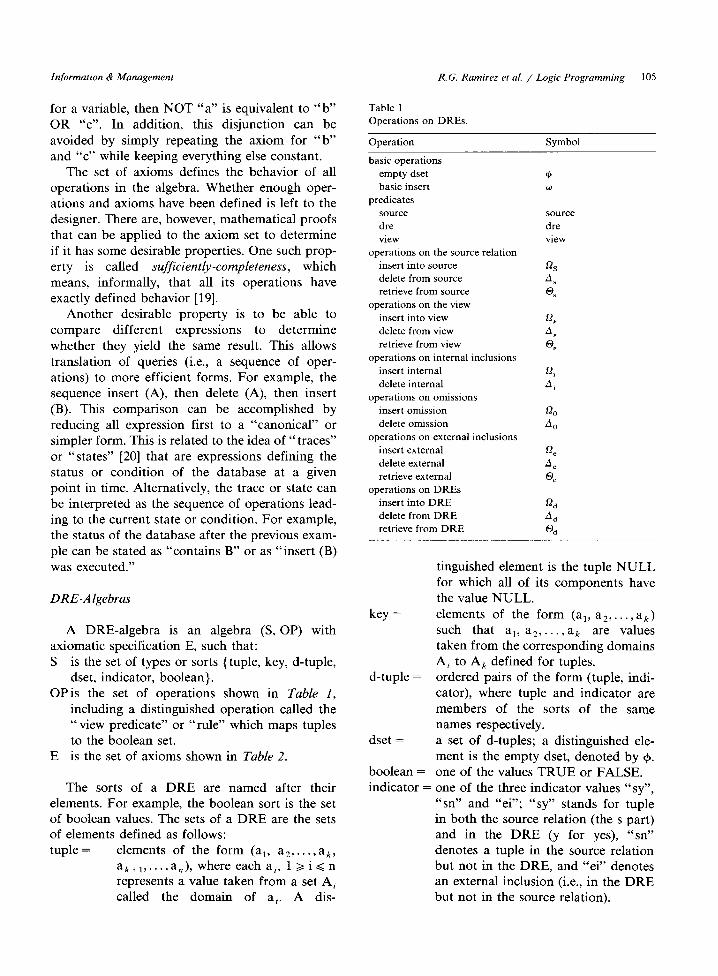
Table 1 Operations on DREs.

Operation Symbol

basic operations empty dset basic insert

predicates source

view operations on the source relation

insert into source delete from source retrieve from source

operations on the view insert into view delete from view retrieve from view

operations on internal inclusions insert internal delete internal

operations on omissions insert omission delete omission

operations on external inclusions insert external delete external retrieve external

operations on DREs insert into DRE delete from DRE retrieve from DRE

dre view

tinguished element is the tuple NULL for which all of its components have the value NULL.

key = elements of the form (a,, a2,. . . ,a,) such that a,, a2,. . .,ak are values taken from the corresponding domains A, to A, defined for tuples.

d-tuple = ordered pairs of the form (tuple, indicator), where tuple and indicator are members of the sorts of the same names respectively.

dset = a set of d-tuples; a distinguished element is the empty dset, denoted by +.

boolean = one of the values TRUE or FALSE. indicator = one of the three indicator values “sy”,

“sn” and “ei”; “sy” stands for tuple in both the source relation (the s part) and in the DRE (y for yes), “sn” denotes a tuple in the source relation but not in the DRE, and “ei” denotes an external inclusion (i.e., in the DRE but not in the source relation).

106 Research

Table 2

Axioms of DRE-Algebras

Notation: K, A, I, and D as well as K’, A’, and I’ are variables.

K represents a key value, K.A denotes a tuple with key K and

non-key attributes A. D represents a relation (dsets), and I (for

indicator) is one of the values “sn”, “sy”, and “ei”.

1 w(K.A.1, w(K’.A’.I’, D)) =

w(K’.A’.I’, w(K.A.1, D))

source(K.A.sy) = TRUE

source(K.A.sn)= TRUE

source(K.A.ei) = FALSE

9

10

11

12

13

14

dre(K.A.sy) = TRUE

dre(K.A.sn) = FALSE

dre(K.A.ei) = TRUE

Q,(K.A, @J) = if view(K.A)

then w(K.A.sy, I$)

else w(K.A.sn, +)

D,(K.A, w(K’.A’.I’, D)) =

ifK=K

then if source(K’.A’.I’)

then w(K.A.1’. D)

else O,(K.A, D)

else w(K’.A’.I’, B,(K.A,D))

A,(K> +) = 0

A,(K, o(K’.A’.I’, D)) =

if K = K’ & source(K’,A’.I’)

then A,(K, D)

else w(K’.A’.I’, A,(K, D))

O,(K, +) = NULL

O,(K, w(K’.A’.I’, D)) =

if K = K’ & source(K’.A’.I’)

then K’.A’

else O,(K, D)

Q,(K.A, +) = if view(K.A)

then o(K.A.sy, +)

else $I

15 O,(K.A, o(K’.A’.I’, D)) =

ifK=K

then if source(K’.A’.I’)

then o(K’.A’.I’, D)

else Q,(K.A, D)

else w(K’.A’.I’, O,(K.A, D))

16

17

A,(K. +) = $J

A,(K, w(K’.A’.I’, D)) = if K = K’ & view(K’.A’) & source(K’.A’.I’)

then A,(K, D) else w(K’.A’.I’, A,(K, D))

18 O,(K, $I) = NULL


Table 2 (continued)

19

20

21

22

23

24

25

26

27

28

29

30

31

32

33

34

O,(K, w(K’.A’.I’, D)) =

if K = K’ & Source(K’.A’.I’) & view(K’.A’)

then K’.A’

else O,(K, D)

Q,(K> +) = 9

O,(K, w(K’.A’.I’, D)) =

if K = K’ & source(K’.A’.I’)

then w(K’.A’.sy, D)

else w(K’.A’.I’, O,(K, D))

A,(K, 9) = +

A,(K, w(K’.A’.I’, D)) =

ifK=K

then if source(K’.A’.I’) and view(K’.A’)

then Ai(K, D)

else w(K’.A’.sn, D)


Q,(K.A, $I) = w(K.A.ny, 9)

D,(K. A, w(K’.A’.I’, D)) =

ifK=K

then w(K’.A’.I’, D)

else w(K’.A’.I’, Q,(K.A, D)

A,(K> +) = 9

A,(K, w(K’.A’.I’, D)) =

if K = K’ & dre(K’.A’.I’) & NOT source(K.A.1’)

then A,(K, D)


@,(K> 9) = +

O,(K, w(K’.A’.I’, D)) =

if K = K’ & dre (K’.A’.I’) & NOT source(K’.A’.I’)

then K’.A

else O,(K, D)

G,(K, +) = +J

&(K, w(K’.A’.I’, D)) = if K = K’ & source(K’.A’.I’)

then w(K’.A’.sn, D)

else w(K’.A’.I’, O,(K, D))

A&K, 9) = +

A,(K, w(K’.A’.I’, D)) =

ifK=K

then if source(K’.A’.I’) and view(K’.A’)

then w(K’.A’.sy, D)

else w(K’.A’.I’, D)


Q,(K.A. $J) = if view(K.A)

then w(K.A.sy, $J) else w(K.A.ei, $J)

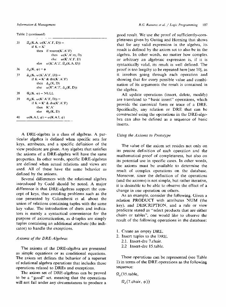
Informdon & Management R.G. Ramirez et al. / L.ogic Progmmming 107

Table 2 (continued) good result. We use the proof of sufficiently-completeness given by Guttag and Horning that shows that for any valid expression in the algebra, its result is defined by the axiom set to also be in the algebra. In other words, no matter how complex or arbitrary an algebraic expression is, if it is syntactically valid, its result is well defined. The proof is too lengthy to be repeated here [see lo], as it involves going through each operation and showing that for every possible value and combi- nation of its arguments the result is contained in the algebra.

35

36

37

38

39

40

D,(K.A, w(K’.A’.I’, D)) = ifK=K

then if source(K’.A’.I’) then w(K’.A’.sy, D) else w(K’.A’.I’, D)

else w(K’.A’.I’, Q,(K.A, D))

A,(K> +) = +J

A,(K, w(K’.A’.I’, D)) = if K = K’ & dre(K’.A’.I’)

then A,(K, D) else w(K’.A’.I’, A,(K, D))

O,(K, +) = NULL

Od(K, w(K’.A’.I’, D)) = if K = K’ & dre(K’.A’.I’)

then K’.A else Q,(K, D)

w(K.A.1, +) = w(K.A.1, +)

A DRE-algebra is a class of algebras. A par- ticular algebra is defined when specific sets for keys, attributes, and a specific definition of the view predicate are given. Any algebra that satisfies the axioms of a DRE-algebra will have the same properties. In other words, specific DRE-algebras are defined when actual relations and views are used. All of these have the same behavior as defined by the axioms.

Several differences with the relational algebra introduced by Codd should be noted. A major difference is that DRE-algebras support the con- cept of keys, thus avoiding problems such as the one presented by Colombetti et al. about the union of relations containing tuples with the same key value. The introduction of dsets and indicators is merely a syntactical convenience for the purpose of axiomatization, as d-tuples are simply tuples containing an additional attribute (the indicator) to handle the exceptions.

Axioms of the DRE-Algebras

The axioms of the DRE-algebra are presented as simple equations or as conditional equations. The axiom set defines the behavior of a superset of relational algebra operations that includes those operations related to DREs and exceptions.

The axiom set of DRE-algebras can be proved to be a “good” set, meaning that the operations will not fail under any circumstances to produce a

All update operations (insert, delete, modify) are translated to “basic insert” operations, which provide the canonical form or trace of a DRE. Specifically, any relation or DRE that can be constructed using the operations in the DRE-algebra can also be defined as a sequence of basic inserts.

Using the Axioms to Prototype

The value of the axiom set resides not only on its precise definition of each operation and the mathematical proof of completeness, but also on its potential use in specific cases. In other words, the axioms must be available to determine the result of complex operations on the database. Moreover, since the definition of the operations (and the axioms) is not simple, but rather iterative, it is desirable to be able to observe the effect of a change in one operation on others.

As an example, consider the following. Given a relation PRODUCT with attributes NUM (the key), and DESCRIPTION, and a rule or view predicate stated as “select products that are either chairs or tables”, one would like to observe the result of the following operations in the database:

1. Create an empty DRE. 2. Insert tuples to the DRE.

2.1. Insert-dre 7.chair. 2.2 Insert-dre 15.table.

These operations can be represented (see Table 1) in terms of the DRE operations as the following sequence:

9,(15.table,

52, (7.chair, +))


Consider the first insertion. According to Axiom 34, inserting a tuple K.A (K = 7, A = chair in the example) into an empty DRE is the same as the basic insert o(K.A.sy, +) if the view predicate is satisfied, and the same as w(K.A.ei, +) when it is not satisfied. In simple words, one of the constants “sy” or “ei” is added to the tuple depend- ing on the result of evaluating the view predicate. In the example, the view predicate is satisfied in both cases. The above expression thus becomes equivalent to:

w (15 .table.sy,

w (7.chair.sy, +))

This expression defines the state of the DRE after the intended operations. It also defines an equivalent form for the original expression.

An example Using the Axioms

The following shows the effect of internal inclusions as well as the retrieval operation on a DRE. First, it demonstrates that a tuple in the source relation that does not satisfy the view predicate will not be retrieved by an operation on the DRE (since it is not included in it). Second, it shows how an internal inclusion forces the pres- ence of the same tuple in the DRE. Consider the following sequence of operations:

@,(9,

9,(9.desk,

D,(S.chair, +)))

By Axioms 8 and 9, the insert-source operations (a,) can be reformulated as basic inserts, and the sequence is converted into the following algebraic expression:

Q,(9,

w(9.desk.sn,

w(5.chair.sy, cp)))

Axiom 39 applies to the sequence 0,(9, w(9.desk.sn _)). Although the keys are the same, the tuple 9.desk.sn (a d-tuple, formally speaking) does not satisfy the view predicate and is not included in the DRE (Axiom 6). Therefore, the ELSE part of the axiom reduces the original expression to:

Q,(9,

w (5.chair.sy, +))

which in turn is reduced to 0,(9, +) by Axiom 38, and the value returned is NULL.

Consider now the original sequence to which an internal inclusion has been added:

@*(9,

fi, (91

9,(9.desk,

Gn, (5 chair, +I>))

The sequence can be reexpressed in terms of the basic insert by using Axiom 9, resulting in the following algebraic expression.

@,(9,

52i(9,

w(9.desk.sn,

o (5.chair.sy, G))))

Using Axiom 21, the insert internal inclusion modifies the previous basic insert with the same key, and the expression is transformed into:

@,(9,

w(9.desk.sy,

w (5.chair.sy, +)))

and by Axiom 39, the retrieval-dre operation (0,) returns the tuple 9.desk, as intended by the internal inclusion superseding the view predicate.

It must be stressed that the axiomatization defines the semantics of the operations but not their implementation. In the example, the constants “sn” and “sy” are used as indicators appended to tuples. No implication is made that this is an appropriate form for implementation. In fact, our proposal for implementation under the SQL language does not make use of such indicators.

Implementation

We now discuss the use of PROLOG to provide mechanical testing of the axiom set, as well as define an initial prototype.

An ideal implementation environment is one which can accept the axioms in their original form and without changes. PROLOG comes very close to this goal although it does require changes that are not obvious. In addition, PROLOG does not

Information & Management R. G. Ramirez et al. / Logic Programming 109

require any coding to use the axioms in testing, as it provides a simple theorem prover.

The term “implementation” must be placed in the correct perspective. Our purpose was not to take the axioms and directly augment a DBMS. Rather, our purpose was to take the axioms and observe what went on during the execution of the statements. At the definition stage of a data model, it is not enough to simply define the expected results of an operation, but it is also necessary to observe the process followed by the system in dealing with a sequence of operations.

The Appendix contains a partial listing of the

PROLOG program that implements the axiom set of Table 2. The PROLOG syntax used is the classical Edinburgh syntax [21]. Names written with capital letters denote variables, while lower- case is used for constants. Our implementation was made using Arity PROLOG on an IBM AT. A previous implementation used PROLOG II on a standard IBM PC. Some PROLOG implementa- tions, such as Micro-PROLOG or Borland’s Turbo PROLOG, may not have the capabilities for this implementation, as it requires the substitution of variables for nested lists of arbitrary depth.

Conversion of Axioms to PROLOG Statements

Consider Axiom 1, that specifies that tuples in a relation (i.e., a set) hold no specific order. In other words, it specifies that inserting a tuple with key K after a tuple with they K’ is the same as inserting K’ after K. The axiom, from Table 2, is as follows: 1 w(K.A.1, w(K’.A’.I’, D)) =

o(K’.A’.I’, o(K.A.1, D)) This axiom is translated into the PROLOG

predicate “ insert”, which takes 3 arguments. The first specifies a tuple to be inserted, the second the relation or DRE (a dset, formally speaking) into which the tuple is inserted, and the third will contain the PROLOG output. Thus, Axiom 1 becomes the PROLOG clause:

insert( [K,A,i], insert([KP,AP,IP], Y) :-

insert( [KP,AP,IP], insert( [K,A,I], Y))).

Consider another example. Axiom 34 specifies that inserting a tuple into a (empty) DRE is equivalent to either (a) inserting a tuple into the source relation if it satisfies the view predicate, or

(b) an insertion as an external inclusion if it does not satisfy the view predicate. Axiom 34 is defined as: 34 %(K.A, +) =

if view (K.A) then w(K.A.sy, +) else w(K.A.ei, +)

and results in the following two PROLOG statements:

insert_dre([K,A], [I, insert([K,A,sy], [I))

:- view([K,A]),!.

inserttdre([K,A], [I, insert([K,A,ei], [I).

The use of the cut (!) operator prevents PROLOG from using the second statement in cases where the first statement has already been satisfied.

Use of PROLOG to Prototype

To observe the behavior of PROLOG prototyping the implementation of DREs, consider the statement derived from Axiom 1, and assume that it is the only statement in the PROLOG program. A user could then type the following goal:

insert( [ 15, table, sy],

insert([7, chair, sy], [I), X),

where (1) the first argument [15, table, sy] is the last tuple to be inserted, (2) the second argument is insert ([7, chair, sy], [I) (the relation formed by the tuple [7, chair, sy] and the empty relation) and (3) X (the third argument) gives the output which would be:

insert([7, chair, sy], insert[l5, table, sy], [I).

An Example Using PROLOG

A more complex example shows the use of PROLOG for a sequence of operations. It is our experience that persons not very familiar with PROLOG have difficulty creating a chain of re-’ sults. This is more evident when a chain of sym-’ bols rather than actual values are used.

Consider the sequence of operations of the previous section:

@,(9,

Qn,(9.desk,

Q,(S.chair, +)))

110 Reseurch Information & Management

Renaming the operations according to the PROLOG syntax, and using the empty list [] for 9, we have

retrieve_dre(9,

insert _ source( [ 9, desk],

insert _ source( [ 5, chair], [I)))

This statement must be rewritten as a sequence of operations, the result of one being fed to the next. In this expression, the order of operations is to execute insert_source([5, chair], [I), and to the result of this operation, apply inserttsource ([9, desk], and finally, execute the retrieve operation. Consider the first operation and feed it to the PROLOG program as follows:

insert _ source( [ 5 chair], [ 1, X) .

A third parameter, X, has been added to the statement, to receive the result from PROLOG. The answer from PROLOG is:

X = insert([5,chair,sy], [I).

Now, to observe the result of the first two operations, type:

insert._source([5,chair], [I, X),

insert_source([9, desk], X, Y).

PROLOG will execute the statements sequen- tially while keeping the intermediate result. The statement before the second insert -source is exactly the same statement used before and the result is stored in X. The second has also three arguments: the new ous result, and Y, PROLOG program

X = insert( [ S,chair,

Y = insert( [ 5 chair,

tuple, X containing the previ- to store the new result. The will give the following result:

syl7 [I).

sy] , insert( [ 9,desk,sn], [ 1)

The result given in Y is a series of basic inserts corresponding to the database created by the operations. The tuple inserted first appears as the last from Axiom 1 (order is not important). The PROLOG effect is to reverse the order.

The final result of the entire algebraic expression is obtained by:

insert source( [ 5 chair] ,[] ,X) ,

insert source( [ 9, desk] ,X,Y) ,

retrieveedre(9,Y,Z).

and the result from PROLOG is:

X = insert( [ S,chair, sy] , [I)

Y = insert( [ S,chair, sy], insert( [9,desk,sn], [I)

Z = [9,desk]

Discussion

We present here some of our experience from implementing the data model as a set of axioms in logic programming.

Advuntages of the Prototyping Approach Using

PROLOG

An intermediate advantage is the discipline en- forced by using an executable specification. As every programmer has discovered, any abstract or informal specification must be subject to detailed analysis in order to be implemented. It is simply not possible to transform the specification to PROLOG (or any other language) if some functions or variables are not completely and precisely defined.

Our initial attempts and later success at using PROLOG for the axiom sets provided useful ex- periences. For example, it became obvious that output, such as that from an actual DBMS, was not sufficient for full understanding of the data model and axiom set, particularly when several axioms or operations participated. This led to the need and understanding of formal traces and canonical forms. Second, it changed the formula- tion of axioms from a theoretical exercise to a practical and interesting task with immediate feedback. Without this, the algebraic method of defining a data model would have been only an excercise in theory.

The use of the executable specification encour- ages experimentation. Since the cost of verifying the behavior of a new axiom is small, many tests can be made. In our case, the semantics of some special cases were subject of discussion and the test with actual data helped understand the problem and decide on the best choice. One such problem occurred with (Axiom 35) the insertion of a tuple K.A into a DRE, when a tuple K.A’ with the same key value already exists in the source relation but not in the DRE. The existence tuple is

Informatron & Management R.G. Ramrrer et al. / Logic Programming 111

“hidden” from the DRE user before update. Our choice was to “ unhide” K.A’ and make it “ visible” to the DRE without considering the potential in- consistencies between A and A’. Alternative choices would have been to reject the insertion in cases where A was not identical to A’, or to replace A’ by A.

Disudvantages

The first and simplest disadvantage is the need to change notation when implementing. It is a relatively simple matter to change from an axiom to a PROLOG statement, but nevertheless some experience with PROLOG is required, and the solution is not always obvious to novice PROLOG programmers. We hope that our examples help new users.

Another disadvantage is the need to guarantee that the overall PROLOG program remains the same as the overall set of axioms. When much experimentation has been made, changes to the program may not be reflected in the axiom set. Only by discipline could we maintain a match between axioms and program. No statement other than an axiom was allowed in our program. At all times we were able to put the axiom set and the PROLOG translation side by side and compare their correspondence.

Summary

The advantages of algebraic specifications of data models are: (1) implementation independence with clear and precise semantics, and (2) formal proofs to verify completeness. Among the problems for practical use of algebraic specifications are the mathematically oriented and rigorous terminology used in works dealing with the subject, as well as the difficulty in translating the finished algebraic system into executable pro- grams.

A new construct for extending the relational data model (derived relations with exceptions) is explained and formally defined in this paper. Using this new construct, we have shown the basic tools for algebraic definitions in a non-mathematical manner. We have also shown the use of PRO- LOG in implementing the resulting axiom sets,

References

[l] C.A.R. Hoare, Proofs of Correctness of Data Representa-

tions, Acta Informatica, Vol. 1, pp. 272-281, 1972.

[2] J.A. Goguen, J.W. Thatcher, and E.G. Wagner (1978), An

Initial Algebra Approach to the Specification, Cor-

rectness, and Implementation of Abstract Data Types, in

R.T. Yeh (Ed.) (1978), Current Trends In Programming

Methodology, Vol. IV, Data Structuring, Prentice-Hall, En-

112

[I81

[I91

WI

VI

Research

J.C. Cleaveland, An Introduction to Data Types, Addison- Wesley, Reading, MA, 1986.

J. Martin, Data Types and Data Structures, Prentice-Hall

International, Englewood Cliffs, NJ, 1986.

P.A.S. Veloso, and A.L. Furtado, Stepwise Construction

of Algebraic Specifications, in Advances in Database The-

ory, Vol. 2, by H. Gallaire, J. Minker, and J.M. Nicolas, Plenum Press, New York, 1984.

W.F. Clocksin, and C.S. Mellish. Programming in PRO-

LOG, Springer-Verlag, Berlin, West Germany, 1981.

Appendix PROLOG Program Implementing Axioms ’

the DRE

PROGRAM DRE AXIOMS Implements the axiom set to define Derived Relations

with Exceptions (DREs).

PROLOG syntax is Clocksin-Mellish, the program was

run using ARITY-PROLOG on an IBM AT*/

Axioms Numbers correspond to Table 2 in Text */

General Notes 1. K and A are values for the new tuple,

KP and AP are values for the previous tuple.

F (flag) defines the indicator.

2. The values for the indicator are (sy, sn, ei},

sy = in source and in dre (view or internal inclusion)

sn = in source but no in dre (no view or omission)

ei = external inclusion and of course in dre*/

view is a distinguished predicate changed for each applica-

tion */

view([ _,D]) :-member(D,[chair. table]).

sample dre: typing ‘sample(X).’ gives an example */

sample(X) :- insert([7,chair,sy], [], DO),

insert([5,desk,sn],DO, Dl),

insert([lO,chair,sy], Dl, D2),

X=D2.

AXIOM 1: defines the BASK INSERT all DRE’s are built as series of insert’s insert takes 3

arguments:

(1) [key, attributes, flag] or [K, D, F]

(2) a DRE

(3) returns a DRE (dset) */

insert([K,D,F], [], insert([K,D,F], [I)).

insert([K,D,F], insert([KP,DP,FP], Y),

insert([KP,DP,FP], insert([K,D,F], Y))).

/’

/*

/*

/*

/*


predicates: AXIOMS 2-7 */

source([ ~, _,sy]). source([ _, _,sn]). source([ _ , _ ,ei]) : - fail.

dre([ + -,sy]). dre([ _, -,sn]) :-fail.

dre([ -, -.ei]). AXIOM 8: Insert into the source relation when the rela-

tion is empty */

insert- source([K,D], [], insert([K,D,sy], [I)) :-

view([K,D]), !.

insert_ source([K,D], [], insert([K,D,sn], [I)),

AXIOM 9: Insert into the source relation when the rela-

tion is non-empty.

The test K = K’ is made automatically by variable unifica- tion.

The cut makes sure that there is no backtracking for

clauses that already applied, as choices are

mutually exclusive

The first statement ignores can an insertion if the key

already exists in the source relation.

The next two statements define the inner ELSE. The

insert-source is converted to a basic-insert,

and the indicator depends on whether the new tuple satisfies the view or not.

The fourth statement represents the outer ELSE in the

axiom, and ignores the tuple K’.A’ if the

keys do not match (outer ELSE). */

insert _ source([K,D], insert([K,DP,F], DRE),

insert([K,DP,F], DRE)):-source([K,DP,F]), !.

insert- source([K,D], insert([K,DP,F], DRE),

insert([k,D,sy], DRE))

:- view((K,D]), !.

insert- source([K,D], insert((K,DP,F],DRE),

insert([K,D,sn], DRE)) :- !.

insert source([K,D], insert([KP,DP,F], DRE),

insert([KP,DP,F], Y))

:-insert- source([K,D], DRE, Y).

AXIOM 10: Delete from source relation when it is empty

*/ delete- source(K,[],[]). AXIOM 11: Delete from source relation when it is not

empty */ delete- source(K, insert([K,D,F], DRE), DRE)

:-source([K,D,F), !.

delete_ source(K, insert([KP,D,F], DRE),

insert([KP,D,F], Y))

; - delete- source(K, DRE, Y).

using logic programming for formal specification and validation of data models

Documents