USE OF CRITICAL CHAIN SCHEDULING TO INCREASE AIRCRAFT

AVAILABILITY

THESIS

Daniel. D. Mattioda, Captain, USAF

AFlT/GLM/ENS/02-11

DEPARTMENT OF THE AIR FORCE AIR UNIVERSITY

AIR FORCE INSTITUTE OF TECHNOLOGY

Wright-Patterson Air Force Base, Ohio

APPROVED FOR PUBLIC RELEASE; DISTRIBUTION UNLIMITED

The views expressed in this thesis are those of the author and do not refleet the offieial poliey or position of the United States Air Force, Department of Defense, or the U. S. Government.

AFlT/GLM/ENS/02-11

USE OF CRITICAL CHAIN SCHEDULING TO INCREASE AIRCRAFT

AVAILABILITY

THESIS

Presented to the Faeulty

Department of Operational Scienees

Graduate Sehool of Engineering and Management

Air Foree Institute of Teehnology

Air University

Air Edueation and Training Command

In Partial Fulfillment of the Requirements for the

Degree of Master of Seienee in Logistics Management

Daniel D. Mattioda, B.S.

Captain, USAF

March 2002

APPROVED FOR PUBLIC RELEASE; DISTRIBUTION UNLIMITED

AFlT/GLM/ENS/02-11

USE OF CRITICAL CHAIN SCHEDULING TO INCREASE AIRCRAFT

AVAILABILITY

Daniel D. Mattioda, BS Captain, USAF

Approved:

/s/_ _ Stephen M. Swartz, Maj. USAF (Advisor) Date Assistant Professor of Logisties Management Department of Operational Seienees

/s/_ _ Stanley E. Griffis, Maj. USAF (Reader) Date Assistant Professor of Logisties Management Department of Operational Seienees

Acknowledgements

1 would like to thank my beautiful wife for all her support and inspiration she has

given me during these last 18 months. Her smiling face and words of wisdom made the

sun come up every morning. To my wonderful sons, I spent too much time away and

missed too much of your life—Dad is coming home!

1 would like to express sincere gratitude to my advisors, Major Stephen Swartz,

and Major Stanley Griffis whose guidance and support were needed and appreciated. 1

learned a tremendous amount during this research. 1 would also like to thank Kent

Mueller, Col USAF (Ret), whose sponsorship made this research possible. 1 am greatly

indebted to MSgt Floyd Faddy and his ISO maintenance team at Hurlburt Field, Florida,

whose diligence in obtaining data for my thesis was unrelenting.

To all the foreign officers in my class, your ability and skills are humbling. It has

been a pleasure to be in the same class as you. Ft Col di Risio (Argentinean Air Force),

you are a leader among leaders. It has been an honor and privilege to work with you.

To my fellow American officers, thanks for all your support. 1 couldn’t have done it

without you. Special thanks to Captains Heinz Huester, Ben Skipper, Craig Punches,

Todd Bertulis, and Fieutenant Rob Overstreet.

Special recognition needs to be given to Ms. Janice Farr. Her attention to detail

and assistance in formatting this thesis were invaluable to its completion.

Daniel D. Mattioda

Table of Contents

Page

Acknowledgements.v

List of Figures.ix

List of Tables.x

Abstract.xi

I. Introduction.1

Background.1 Problem Statement.6 Research Questions.6 Research Methodology.7 Assumptions.7 Scope/Limitations.10 Summary.10

II. Literature Review.11

Introduction.11 Isochronal Inspection Process.12

Project.15 Project Management.16 Critical Path Method.16 Theory of Constraints.23

Critical Chain.26 Safety Time.27 Wasted Safety Time.28 Critical Chain Safety Buffers.30 Determination of Buffer Size (Newbold, 2001: 93).34 Management Use of Buffers.35 Task Duration.37 Slack.37

Single verses Multi-Project Implementation.37 Critical Chain and the ISO Process.38 Summary.40

VI

III. Methodology.42

Introduction.42 Data Collection.42

Activity Parameters.44 Description of Variables.45 Calculations of Probabilistic Task Durations.46 Microsoft Project 2000©.49 Measures of Performance.51 Experimental Manipulation.52 Conclusion.52

IV. Results.53

Introduction.53

Critical Path and Critical Chain Estimations.53 Simulation Results.54

Friedman Fr Test.55 Friedman Fr Test Results.56 Model Durations.57 Aircraft Availability and Scheduling Error.57 Critical Path Results.59 Critical Chain Lower Estimate Results.60 Critical Chain Upper Estimate Results.61 Primary Research and Investigative Questions.62 Conclusion.67

V. Conclusions and Recommendations.68

Introduction.68

Findings.69 Overall Findings.73 Additional Findings.73 Managerial Implications.74 Limitations.75 Future Research.76 Summary of Findings.77

Appendix A. ISO Task Information.78

Appendix B. ISO Work Breakdown Structure.80

Appendix C. ISO Manning Requirements.82

Appendix D. Simulation Values.83

vii

Appendix E. Simulation Results.91

Appendix F. Shapiro - Wilk W Test.92

Appendix G. Friedman Fr Test Results.92

Appendix Ft. Simulation Results Ascending Order.94

Appendix 1. CP Aircraft Availability Lost and Aircraft Scheduling Lost.95

Appendix J. CC Aircraft Availability Lost and Aircraft Scheduling Lost.96

Appendix K. CPI WBS.98

Appendix L. CP2 WBS.99

Appendix M. CPS WBS.100

AppendixN. CCl WBS.101

Appendix O. CC2 WBS.102

Appendix P. CCS WBS.lOS

Appendix Q. Current ISO Shift Schedule.104

Appendix R. Reduced ISO Shift Schedule.105

Appendix S. Surge ISO Shift Schedule.106

Bibliography.107

Vita.no

viii

List of Figures Page

Figure 1. Work Card 1-050.9

Figure 2. Work Card 1-003.13

Figure 3. Work Card 1-050.14

F igure 4. Proj ect N etwork.17

Figure 5. Dependency.18

Figure 6. Project Network.20

Figure 7. Critical Path.22

Figures. Critical Path.25

Figure 9. Critical Chain.27

Figure 10. Padding of Individual Tasks.28

Figure 11. Sequential Tasks.29

Figure 12. Parallel Tasks.30

Figure 13. Padding of Individual Tasks.31

Figure 14. Project Buffer.31

Figure 15. Feeding Buffer.32

Figure 16. Resource Buffer.33

Figure 17. Critical Chain Schedule.33

Figure 18. Standard Beta Distribution.47

Figure 19. Model Distributions.54

Figure 20. Model Means.56

Figure 21. Aircraft Availability and Aircraft Scheduling Loss.58

IX

List of Tables

Page

Table 1. Activities for Project.20

Table 2. CPM vs. CC.37

Table 3. WBS Information.44

Table 4. Shift Hours.46

Table 5. Beta A and B Values.49

Table 6. Experimental Design.52

Table 7. Critical Path and Critical Chain ISO Durations (Estimated).53

Table 8. Shapiro-Wilk W Test for Normality.55

Table 9. Model Duration Comparison.57

Table 10. CP Aircraft Scheduling.59

Table 11. CC Aircraft Scheduling Using Lower Estimate.60

Table 12. CC Aircraft Scheduling Using Upper Estimate.61

Table 13. CP Durations.63

Table 14. CC Durations.65

Table 15. CC to CP Comparison.66

Table 16. CP Results.70

Table 17. CC Lower Estimation Results.71

Table 18. CC Upper Estimation Results.72

Abstract

United States Air Force Special Operations Command (AFSOC) has a minimal

number of aircraft at its disposal. As a result, the aircraft are considered high demand,

low-density (small number in Air Force inventory) weapon systems. Any chance to

increase aircraft availability would greatly enhance the capability of AFSOC.

Isochronal maintenance (ISO) conducted once every 365 days (per AFl for C- 130

aircraft) provides the best opportunity to increase aircraft availability by improving the

scheduling of tasks and accurately estimating the inspection duration. Scheduled

maintenance portrays the characteristics of projects, therefore, this thesis proposed that

Critieal Chain (CC) seheduling, a projeet management teehnique, could provide an

improved ISO sehedule redueing aireraft downtime.

The ISO inspeetion proeess was modeled three ways (1) existing proeess, (2) task

eonstraints removed, and (3) task and resouree eonstraints removed. 100 simulated

aireraft inspeetions took plaee in eaeh model. The simulated duration times were

eompared to estimates provided by the use of Critieal Path and Critical Chain scheduling

teehniques.

Critieal Chain seheduling teehniques did not directly increase aircraft availability.

However, Critieal Chain seheduling did identify the potential for increasing aircraft

availability by removing poliey and seheduling eonstraints.

XI

USE OF CRITICAL CHAIN SCHEDULING TO INCREASE AIRCRAFT

AVAILABILITY

L Introduction

Background

The United States Speeial Operations Command (USSOCOM) tasks the United

States Air Foree Speeial Operations Command (AFSOC) with providing speeial

operations aireraft at a moments notice to all comers of the globe. Due to its special

mission characteristics and the resulting uniqueness of the aircraft, AFSOC has a minimal

number of aircraft at its disposal. There are 11 MC-130Hs, 8 AC-130Hs and 13 AC-

130Us permanently assigned to the 16th Special Operations Wing (SOW) at Hurlburt

Field, Florida. The 16 SOW is the only active duty United States Air Force (USAF)

special operations wing in the continental United States (CONUS). The AC-130s in use

by AFSOC are the only gun ships in the USAF inventory. As a result, the aircraft of the

16 SOW are considered high demand, low-density (small number in Air Force inventory)

weapon systems.

From 1 August 2000 to 31 July 2001, the above-mentioned aircraft were deployed

a total of 891 aircraft days to 146 temporary duty (TDY) locations. These TDYs

included joint exercises with the United States Army, Navy, and Marine Corps, along

with training scenarios with foreign military units and real-world operational taskings.

1

In order to meet those operational requirements, the aircraft are routinely

inspected to ensure airworthiness. These inspections, along with their associated

maintenance, reduce the availability of an already critical asset. Any chance to increase

aircraft availability would greatly enhance the capability of AFSOC.

There are two basic ways to increase overall aircraft availability. The first is to

increase the number of aircraft by additional purchases. At a time of decreasing defense

spending, purchasing more special operations force (SOF) aircraft, in particular MC-

130Hs, AC-130Hs, and AC-130Us, is not a consideration. The second way is to

minimize aircraft down time. It is this method of increasing availability that this thesis

will investigate.

Aircraft down time is a result of either of two circumstances: unscheduled or

scheduled maintenance. Unscheduled maintenance occurs when the aircraft breaks due

to unforeseen aircraft equipment malfunctions and/or improper maintenance practices.

Unscheduled maintenance cannot be planned for in advance, and as such, does not

provide a viable opportunity to decrease downtime. Scheduled maintenance, on the other

hand, can be planned for in advance.

Scheduled maintenance encompasses the routine servicing of aircraft and

scheduled aircraft inspections. Routine servicing of the aircraft occurs at predetermined

points during the maintenance cycle. Examples of servicing would be refueling the

aircraft, filling the liquid oxygen (LOX) converters, and checking the engine oil levels

and aircraft hydraulic reservoirs for the correct fluid levels and adding fluid if required.

This type of scheduled maintenance is simple, and most tasks are completed in a minimal

amount of time. Trying to complete these tasks faster raises safety issues and may not

2

provide much room for improvement. The correct sequencing of these tasks, however,

could provide room for improvement, although the correct management of, or

improvement upon scheduled inspections appears to offer greater potential.

Scheduled inspections are very complex, involving many tasks with multiple sub

tasks. It is this area where efficient scheduling of resources (personnel and equipment)

can reap the greatest benefits, most importantly reduced downtime, thereby increasing

aircraft availability.

The Isochronal Inspection (ISO) is a thorough inspection of the aircraft, which

occurs every 365 days on all C-130 type aircraft. They are divided into two different

categories of inspections called “Minor” and “Major.” There are 3 minor inspections

numbered 1, 2 and 3 while the major inspection is number 4. Inspections 1 and 3 closely

resemble each other (with 3 being a more thorough inspection). Likewise, 2 and 4 are

similar in content. However, inspection number 4 is the most thorough and labor

intensive of the four inspections. The minor and major inspection requirements are

contained in the 1C-130A-6WC-15 work card deck. A work card details the inspection

requirements for a certain area of the aircraft as well as the qualifications of the mechanic

who performs the inspection, the number of mechanics required, and the estimated time

to complete the inspection. A more thorough description of the minor and major

inspections will be conducted in chapter 2. These four inspections constitute one

complete maintenance cycle. Each inspection is accomplished by performing specific

parts of the complete minor and major inspection in conjunction with other inspections.

Prior to 1999, ISO maintenance on SOF-130 aircraft took 10 days. An initiative

was taken in the fall of 1999 to evaluate the isochronal inspection process and use

3

Microsoft Project 98© to define the critical path. Once the critical path was defined, the

workforce shifted focus from doing work with available resources (personnel, in

particular) to completing work in a set order that focused on the critical path. ISO

maintenance time decreased 10 percent to 9 days. Inspections, time changes (equipment

that is replaced after a certain amount of flight, operating, or calendar time) and any

relevant time compliance technical orders (TCTOs) are accomplished, when possible,

while the aircraft is in ISO.

At this time, the work cards were reviewed and “scrubbed” for relevancy and

accuracy by ISO supervision and maintenance personnel. This “scrub” evaluated the

inspection package for work that might not be strictly necessary. Any task that was not

required or unable to be performed due to deletion of an engineering based requirement

was deleted. An example is the wing leading-edge engine bleed air duct sensor

inspection. Initially these sensors were required to be inspected during the ISO once the

wing leading edges were removed. A design change to the wing resulted in the leading

edges only being removed at depot, but the engine bleed air duct sensor inspection was

still required during the ISO. ISO technicians submitted a technical order change for the

sensor inspection because the leading edges were no longer being removed. The C-130

aircraft engineers at Warner Robins AFB agreed, and the sensor inspection was removed

from the work cards and now is accomplished in coordination with the leading edge

removal at depot. The deletion of this inspection saved 8 man-hours of maintenance time

per aircraft.

Another problem area, which was investigated, was the scheduling of ISO

technicians. ISO technicians are the individuals who work on the aircraft during the

4

inspection. These technicians are made up of the following career fields: aircraft crew

chiefs, electrical and environmental, pneudraulic, engine, structural repair, and avionics

specialists. These technicians were scheduled according to how much work was required

in their individual area and by how to accomplish that work as fast as possible. Their

schedule was based on a two-shift operation, with day shift working from 0700-1600 and

swing shift from 1500-2300. This work schedule did not take into account the overall

workload itself After the study, technicians were scheduled when they were needed in

an effort to best optimize the entire ISO process. To ensure better coordination among

technicians, a shift coordinator assumed new responsibilities. The shift coordinators

ensured that one specialist was not holding up the work of another specialist. An

example in the ISO process occurred when the eleetricians were accomplishing their

electrical power eheeks. These eheeks kept the fuel cell specialists from completing their

fuel/water sereen inspeetions. Even though the eleetricians were ahead of schedule in

their area, by preventing the fuel eell speeialists from completing their work they were

not optimizing the overall process. The shift coordinator stepped in and had the

electricians suspend their power checks allowing fuel cell technicians to continue their

work. This oversight allows for optimization of the whole ISO process and not just one

shop’s individual area.

With the identification of the critical path and the comect allocation of resources,

the ISO time was reduced allowing greater aircraft availability. The saving of 1 day per

aircraft in ISO resulted in an increase in aircraft availability of 32 aircraft days (0.25

percent increase). A small amount, but significant in light of the high demand for the

aircraft. Any increase in aircraft availability for AFSOC’s high-demand, low-density

5

aircraft fleet is a pivotal factor in mission accomplishment. This 0.25 percent increase is

a starting point, but can it get better? The objective of this research is to apply the

recently developed project management techniques of “Critical Chain” scheduling to the

ISO process in an effort to achieve further improvements.

Problem Statement

Aircraft availability is essential to AFSOC in order to meet mission requirements.

Increasing the number of aircraft or reducing existing aircraft down time can increase

aircraft availability. Increasing the number of aircraft is not a viable option due to budget

constraints. Reducing aircraft down time is a viable alternative. Reducing the ISO flow

time may reap the largest aircraft availability gains. Can the current ISO flow be

improved upon to reduce aircraft downtime or is the current ISO the best it can be with

the allocated resources?

Research Questions

Reducing ISO flow time is key to reducing aircraft down time thus increasing

aircraft availability. The primary research question is “Can the use of Critical Chain

scheduling reduce the ISO flow time?” In order to answer the primary research

question, the following subordinate investigative questions must be answered:

1. What are the key differences between Critical Path and Critical Chain methods?

2. What are the results of applying a Critical Path analysis to the ISO project?

3. Are there opportunities for improving the ISO schedule (from the current schedule) using Critical Path?

4. What are the results of applying a Critical Chain analysis to the ISO project?

6

5. Are there opportunities for improving the ISO schedule (from the current schedule) using Critical Chain?

6. Are there differences in schedule performance for the ISO project between Critical Chain and Critical Path methods?

Research Methodology

The methodology used in this thesis will consist of a two-level investigation.

First, an examination of the current ISO process will be conducted to determine the

existing critical path. Once the critical path is identified, the second level of investigation

will begin. This level will apply the principles of critical chain scheduling techniques

and evaluate the results in reducing the project duration. Prioritized recommendations

will be made with their associated duration improvements.

Assumptions

The following assumptions are used throughout this work. For the purpose of this

study, no additional work is incorporated into the ISO process. Once the ISO process

begins the inspection is not interrupted or postponed. Work continues until the inspection

is complete.

This study assumes that weather is not a factor in the ISO process. Weather is

another issue that stops the ISO process. Hurlburt Field, located on the Gulf of Mexico,

is subject to hurricanes from June until November. If a hurricane develops and results in

the evacuation of the base, the ISO process could be interrupted. Normally, every

opportunity is provided to finish the ISO before the hurricane hits land. The aircraft is

then evacuated to a safe haven, usually Ft. Campbell, Kentucky. Flowever, sometimes

hurricanes develop faster than expected, and the ISO inspection is not completed and the

7

aircraft must remain at Hurlburt. The ISO is conducted in Eason hangar and is totally

enclosed from the weather. This hangar provides the aircraft protection from the

environment, but workers are released from duty to weather the hurricane with their

families. This causes a delay in the ISO process.

For this study, the aircraft is assumed available to enter the process at the applicable

time with all prerequisite tasks accomplished. Every attempt is made to have the aircraft

available to start the ISO process at the required time. However, certain circumstances

arise that cause the aircraft to be late. Off-station taskings, where the aircraft is TDY and

breaks and can’t return to home station, increases the duration of off station missions.

These instances are extremely rare.

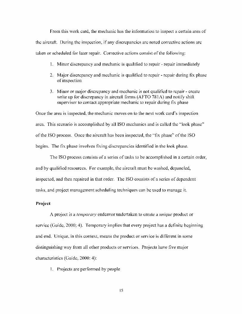
Individual task duration times are assumed to be accurate from the times posted on

the work cards in the “Card Time” block. This time, with the information from the “Type

Mech Rqd” and “Mech No.” blocks is the average time a mechanic should take to

complete all the work on that specific work card. For example, Figure 1 is a work card

from the ISO inspection work deck. The “Type Mech Rqd” is an APG (Airplane

General), commonly referred to as a crewchief. The “Mech No.” is 1, and the “Card

Time” is 1:14, which means 1 hour and 14 minutes. This states that the average time to

complete this work card by one qualified crew chief is 1 hour and 14 minutes.

Experience, training, and condition of aircraft are factors that can either increase or

decrease the task duration time. Interviews conducted with the 16th Equipment

Maintenance Squadron ISO dock chief, ISO shift coordinator, and ISO technicians

determined that the task duration times on the work cards are pessimistic times.

According to them, the actual task duration times are 25 to 50 percent less than shown on

8

the card. Using the documented task times would result in a pessimistic scenario. If

improvements are shown with this study, then actual improvements should be even

better. Actual improvement times should be an area for further research. It is assumed

that while the exact amount of improvement could not be determined at this time, the

research results should indicate the relative magnitude of the changes.

WORK AREA(S)

6R

TYPE MECH REQ.

APG

MECH NO.

1

CARD TIME

1;14

PUBLICATION NUMBER

T.O. 1C-130A-6WC-15

CHANGE NO.

1

MAN MIN

WORK AREA

WORK UNIT CODE ELECTRICAL POWER

INSPECTION REQUIREMENTS

CARD NO.

1-050

AFT FUSELAGE - INTERNAL

1. OBSERVE ZONE lAW THE ZONAL OBSERVATION CARD

005 6R 11 250 2. WITH FOAM INSULATION REMOVED FROM CARGO DOOR. INSPECT STRUCTURE FOR CORROSION: 1701 (REINSTALLATION OF FOAM INSULATION IS A LOCAL OPTION) IN ATC AIRCRAFT WITH LESS THAN 4900 AIRFRAME HOURS

002

010

010

6R

6R

6R

005 6R

001

001

6R

6R

CARD NO.

1-050

11 340

14 000

14 000

14 000

45 100

45 1F0

WORK AREA(S)

6R

3. EMERGENCY EXIT FOR POSITVE LOCKING (932)

4. FLIGHT CONTROL CABLES FOR CONDITION, lAWT.O. 1C-130H-2-00-GE-00-1.

5. ELEVATOR AND RUDDER BOOST PACKS AND DIVERTER PANELS FOR LEAKS (381) AND SECURITY (730),

6. RUDDER AND ELEVATOR PUSH-PULL RTODS FOR SECURITY (105) AND BROKEN (070). LOOSE OR MISSING (105) JO BOLTS,

7. AUXILIARY HYDRAULIC SERVICE CENTER FOR EVIDENCE OF LEAKS (387)

8. AUXILIARY HYDRAULIC RESERVOR FOR SERVICING (WITH RAMP CLOSED) (525) (APPROXIMATELY 1 INCH FROM TOP OF SIGHT GAGE ON MDS PRIOR AF 85-1361) 0 PSI FULL MARK ON AF 85-1361 AND SUBSEQUENT MDS) IF SERVICING IS REQUIRED REFER TO TO. 1C-130A-2-12JG-10-2

TYPE MECH REQ. MECH NO. CARD TIME PUBLICATION NUMBER CHANGE NO.

APG 1 1:14 T.O, 1C-130A-6WC-15 15 MAY 00 1

Figure 1. Work Card 1-050

It is assumed that the mechanic performing the inspection is qualified to perform

the task. Specialist skill requirements are required for each task. Work card 1-050 (Fig.

1) shows the “Type of Mech”, but does not state the skill level. Qualified means a 3, 5,

or 7-level who has been trained on the task required by the work card and that training is

properly documented in the individuals Air Force Form 623 (On-The-Job Training

Record). This record is the official documentation of technical training that an individual

is qualified to perform and/or is being trained to accomplish.

A final assumption is the availability of support equipment and replacement parts.

For this initial research, the ideal situation is assumed. Equipment and supplies are

9

readily available when requested. There is no delay between the time of request and

when the equipment or supply arrives or the time is minimum that it does not disrupt the

ISO process.

Scope/Limitations

This thesis deals with only the SOF-130 ISO inspection process at Hurlburt Field.

The specific recommendations provided by this research will have limited applicability.

The SOF-130s stationed at Flurlburt are a different mission design series than the C-130s

stationed at Little Rock or Pope AFBs, which leads to different inspection requirements.

However, while the specific results are not widely applicable, the process used in the

inquiry could be applied successfully in similar circumstances.

Summary

In the preceding pages, the current situation at AFSOC was described as it relates

to their high demand, low-density aircraft. The current ISO process resulting from the

initial critical path analysis was described. The research and investigative questions were

presented, as well as the assumptions, scope and limitations. In Chapter 2, a review of

the relevant literature will be presented. Key issues will be addressed, to include

treatment of the ISO process under the principles of project management, and the

principles of the Theory of Constraint’s “Critical Chain” application.

10

11. Literature Review

Introduction

Military aircraft frequently encounter stresses and activities that are not normally

assoeiated with eivilian aireraft. The SOF-130 type aireraft are no exception. These 130s

do not eneounter high gravity turns like the F-15 and F-16 fighters or fly at high attitudes

sueh as the U-2, but nonetheless are exposed to exceptional stresses on a day-to-day

basis. The AC-130s’ 105mm eannon used to destroy ground targets provides a

tremendous amount of stress to the rear of the aircraft each time it is fired. On the AC-

130H models, this stress is direeted at a 25-year old airframe that has seen action in every

military eonfrontation sinee the late stages of Vietnam. The newer AC-130Us are

nearing 10 years old and beginning to show signs of stress. An example of this stress is

minor wing eraeks found on the trailing edge of the AC-130 wings due to the

repercussions from the firing of the 105mm cannon (Ferrell, 2001).

The MC-BOHs are another fixed wing aircraft assigned to the 16 SOW at

Hurlburt Field. Their mission is to provide infiltration, exfiltration and resupply of

special operations forces and equipment in hostile or denied territory. Secondary

missions include psychological operations (MC-130E/H, 2001). Normal operations for

MC-130H aircraft include landings on unimproved runways and low-level flights. These

two situations are extremely stressful on the aircraft, just like the 105mm firings for the

AC-130s. In order to keep the aircraft flying and able to perform their missions, the ISO

proeess is important in the identification and correction of discrepancies in order to

sustain the aireraft in a mission capable posture.

11

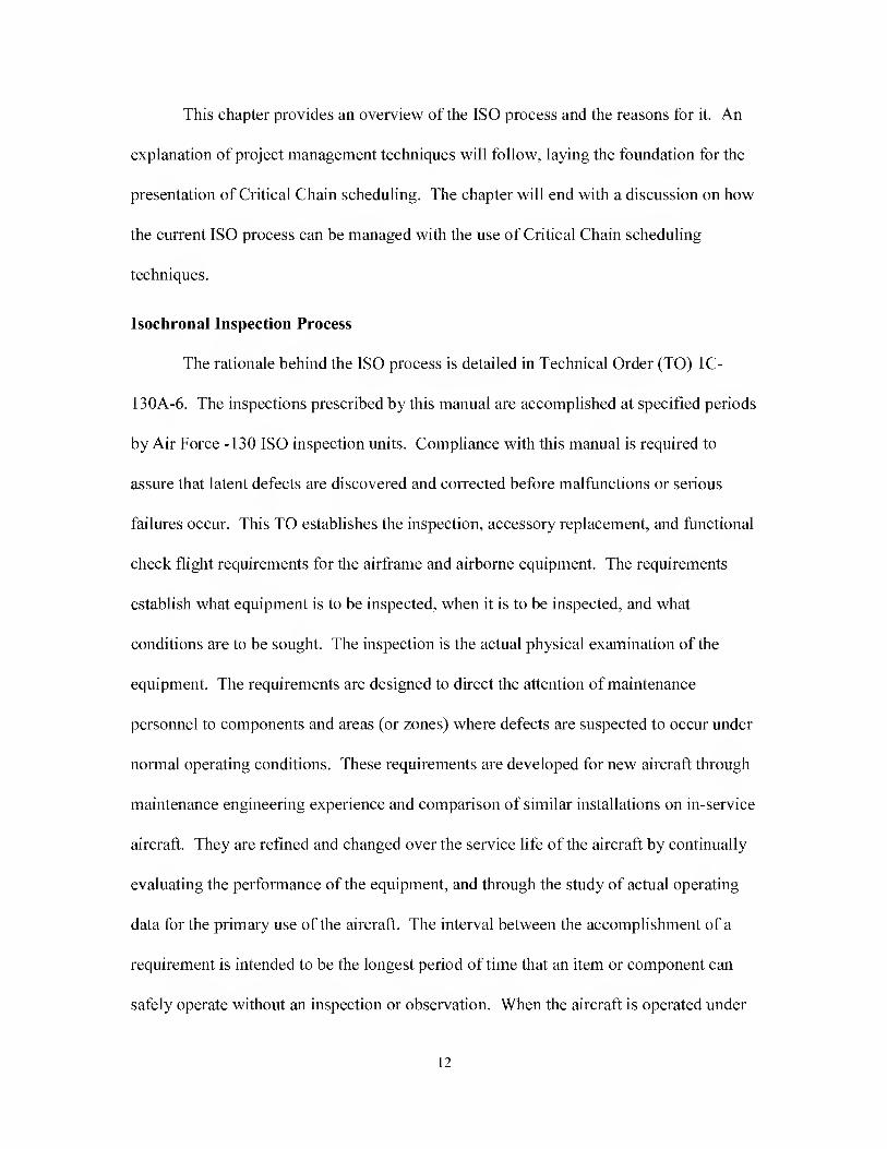
This chapter provides an overview of the ISO process and the reasons for it. An

explanation of project management techniques will follow, laying the foundation for the

presentation of Critical Chain scheduling. The chapter will end with a discussion on how

the current ISO process can be managed with the use of Critical Chain scheduling

techniques.

Isochronal Inspection Process

The rationale behind the ISO process is detailed in Technical Order (TO) IC-

130A-6. The inspections prescribed by this manual are accomplished at specified periods

by Air Force -130 ISO inspection units. Compliance with this manual is required to

assure that latent defects are discovered and corrected before malfunctions or serious

failures occur. This TO establishes the inspection, accessory replacement, and functional

check flight requirements for the airframe and airborne equipment. The requirements

establish what equipment is to be inspeeted, when it is to be inspected, and what

conditions are to be sought. The inspeetion is the actual physical examination of the

equipment. The requirements are designed to direct the attention of maintenance

personnel to components and areas (or zones) where defects are suspected to occur under

normal operating conditions. These requirements are developed for new aircraft through

maintenance engineering experience and comparison of similar installations on in-service

aircraft. They are refined and changed over the service life of the aircraft by continually

evaluating the performance of the equipment, and through the study of actual operating

data for the primary use of the aircraft. The interval between the accomplishment of a

requirement is intended to be the longest period of time that an item or component can

safely operate without an inspection or observation. When the aircraft is operated under

12

conditions other than its primary purpose the inspection requirements are adjusted

accordingly. These requirements and inspection intervals are the maximum and should

not be exceeded. Local conditions (type of missions, special utilization, geographical

locations, etc.) may dictate more or less frequent inspection.

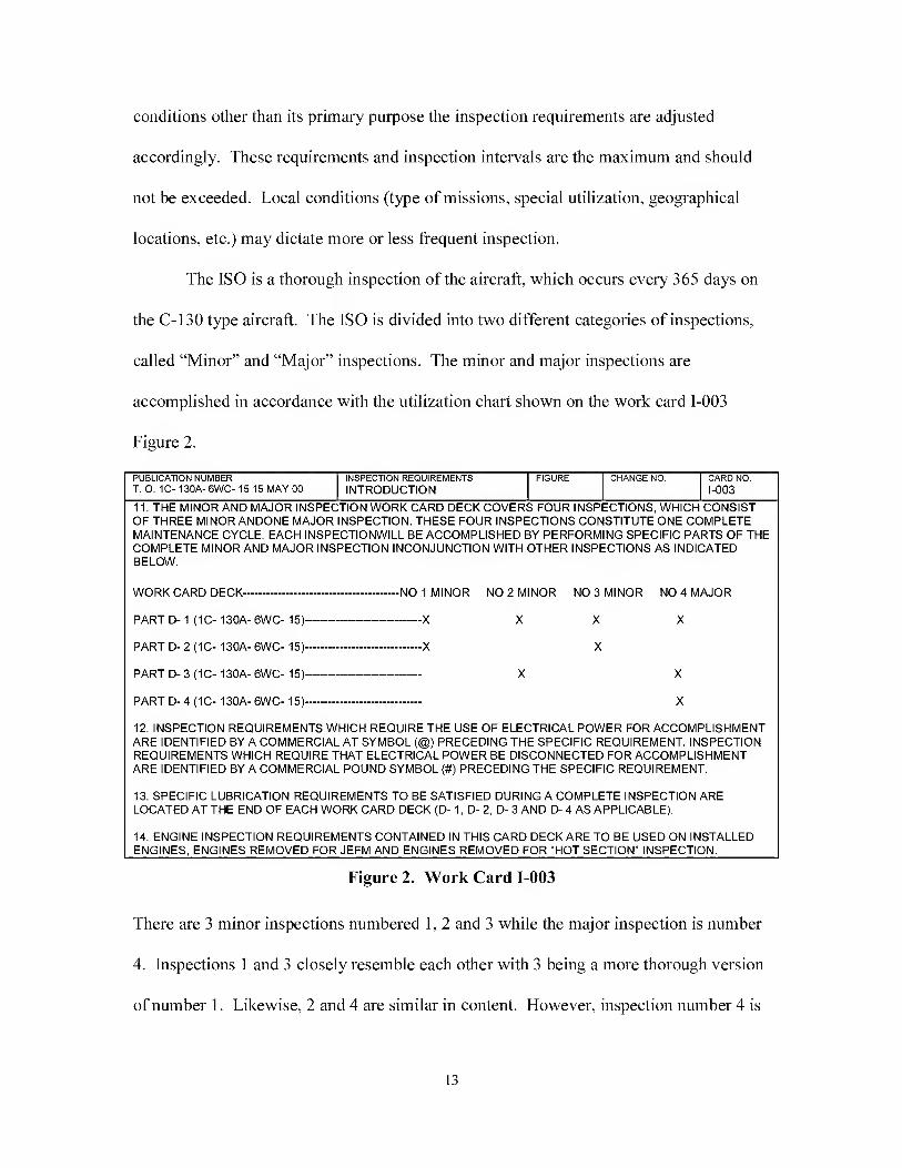
The ISO is a thorough inspection of the aircraft, which occurs every 365 days on

the C-130 type aircraft. The ISO is divided into two different categories of inspections,

called “Minor” and “Major” inspections. The minor and major inspections are

accomplished in accordance with the utilization chart shown on the work card 1-003

Figure 2.

PUBLICATION NUMBER INSPECTION REQUIREMENTS FIGURE CHANGE NO. CARD NO. T. 0. 1C- 130A-6WC-15 15 MAY 00 INTRODUCTION 1-003

11. THE MINOR AND MAJOR INSPECTION WORK CARD DECK COVERS FOUR INSPECTIONS, WHICH CONSIST OF THREE MINOR ANDONE MAJOR INSPECTION. THESE FOUR INSPECTIONS CONSTITUTE ONE COMPLETE MAINTENANCE CYCLE. EACH INSPECTIONWILL BE ACCOMPLISHED BY PERFORMING SPECIFIC PARTS OF THE COMPLETE MINOR AND MAJOR INSPECTION INCONJUNCTION WITH OTHER INSPECTIONS AS INDICATED BELOW.

WORK CARD DECK-NO 1 MINOR NO 2 MINOR NO 3 MINOR NO 4 MAJOR

PART D-1 (1C- 130A- 6WC- 15)-X XXX

PART D- 2 (1C- 130A- 6WC- 15)-X X

PARTD-3(1C-130A-6WC-15)- X X

PART D- 4 (1C- 130A- 6WC- 15)- X

12. INSPECTION REQUIREMENTS WHICH REQUIRE THE USE OF ELECTRICAL POWER FOR ACCOMPLISHMENT ARE IDENTIFIED BY A COMMERCIAL AT SYMBOL (@) PRECEDING THE SPECIFIC REQUIREMENT. INSPECTION REQUIREMENTS WHICH REQUIRE THAT ELECTRICAL POWER BE DISCONNECTED FOR ACCOMPLISHMENT ARE IDENTIFIED BY A COMMERCIAL POUND SYMBOL (#) PRECEDING THE SPECIFIC REQUIREMENT.

13. SPECIFIC LUBRICATION REQUIREMENTS TQ BE SATISFIED DURING A CQMPLETE INSPECTIQN ARE LOCATED AT THE END OF EACH WORK CARD DECK (D-1. D- 2, D- 3 AND D- 4 AS APPLICABLE).

14. ENGINE INSPECTION REQUIREMENTS CQNTAINED IN THIS CARD DECK ARE TQ BE USED QN INSTALLED ENGINES, ENGINES REMOVED FOR JEFM AND ENGINES REMQVED FQR “HQTSECTIQN" INSPECTION._

Figure 2. Work Card 1-003

There are 3 minor inspections numbered 1, 2 and 3 while the major inspection is number

4. Inspections 1 and 3 closely resemble each other with 3 being a more thorough version

of number 1. Likewise, 2 and 4 are similar in content. However, inspection number 4 is

13

the most thorough and labor intensive of the four inspections. The minor and major

inspection requirements are contained in the 1C-130A-6WC-15 work card deck. These

four inspections constitute one complete maintenance cycle. Each inspection is

accomplished by performing specific parts of the minor and major inspection in

conjunction with other inspections.

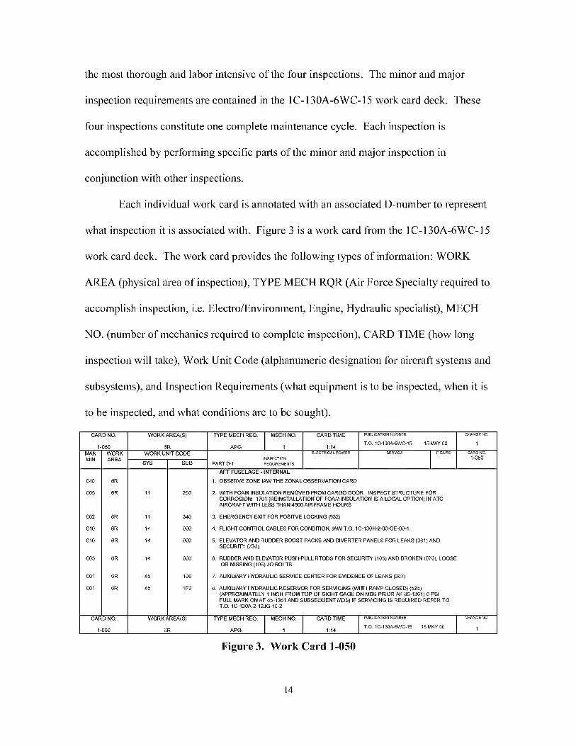
Each individual work card is annotated with an associated D-number to represent

what inspection it is associated with. Figure 3 is a work card from the 1C-130A-6WC-15

work card deck. The work card provides the following types of information: WORK

AREA (physical area of inspection), TYPE MECH RQR (Air Force Specialty required to

accomplish inspection, i.e. Electro/Environment, Engine, Hydraulic specialist), MECH

NO. (number of mechanics required to complete inspection), CARD TIME (how long

inspection will take). Work Unit Code (alphanumeric designation for aircraft systems and

subsystems), and Inspection Requirements (what equipment is to be inspected, when it is

to be inspected, and what conditions are to be sought).

CARD NO.

1-050

WORKAREA(S}

6R

TYPE MECH REQ.

APG

MECH NO.

1

CARD TIME

1:14

PUBLICATION NUMBER

T.O, 1C-130A-6WC-15

CHANGE NO.

1

MAN WORK MIN AREA

WORK UNIT CODE ELEOTRICAL POWER

INSPECTION REQUIREMENTS

CARD NO.

1-050

AFT FUSELAGE - INTERNAL

1. OBSERVE ZONE lAWTHE ZONAL OBSERVATION CARD

005 6R 11 250 2. WITH FOAM INSULATION REMOVED FROM CARGO DOOR. INSPECT STRUCTURE FOR CORROSION: 1701 (REINSTALLATION OF FOAM INSULATION IS A LOCAL OPTION) IN ATC AIRCRAFT WITH LESS THAN 4900 AIRFRAME HOURS

002 6R

010 6R

11

14

340 3. EMERGENCY EXIT FOR POSITVE LOCKING (932)

000 4. FLIGHT CONTROL CABLES FOR CONDITION. lAWT.O. 1C-130H-2-00-GE-00-1.

010 6R

005 6R

001

001

6R

6R

CARD NO.

1-050

14

14

45

000

000

100

5. ELEVATOR AND RUDDER BOOST PACKS AND DIVERTER PANELS FOR LEAKS (381) AND SECURITY (730).

6. RUDDER AND ELEVATOR PUSH-PULL RTODS FOR SECURITY (105) AND BROKEN (070), LOOSE OR MISSING (105) JO BOLTS.

7. AUXILIARY HYDRAULIC SERVICE CENTER FOR EVIDENCE OF LEAKS (387)

45 1F0 8. AUXILIARY HYDRAULIC RESERVOR FOR SERVICING (WITH RAMP CLOSED) (525) (APPROXIMATELY 1 INCH FROM TOP OF SIGHT GAGE ON MDS PRIOR AF 85-1361) 0 PS! FULL MARK ON AF 85-1361 AND SUBSEQUENT MDS) IF SERVICING IS REQUIRED REFER TO TO. 1C-130A-2-12JG-10-2

WORK AREA(S) TYPE MECH REQ. MECH NO. CARD TIME PUBLICATION NUMBER CHANGE NO.

6R APG 1:14 T.O, 1C-130A-6WC-15 15 MAY 00

Figure 3. Work Card 1-050

14

From this work card, the mechanic has the information to inspect a certain area of

the aircraft. During the inspection, if any discrepancies are noted corrective actions are

taken or scheduled for later repair. Corrective actions consist of the following:

1. Minor discrepancy and mechanic is qualified to repair - repair immediately

2. Major discrepancy and mechanic is qualified to repair - repair during fix phase of inspection

3. Minor or major discrepancy and mechanic is not qualified to repair - create write up for discrepancy in aircraft forms (AFTO 781 A) and notify shift supervisor to contact appropriate mechanic to repair during fix phase

Once the area is inspected, the mechanic moves on to the next work card’s inspection

area. This scenario is accomplished by all ISO mechanics and is called the “look phase”

of the ISO process. Once the aircraft has been inspected, the “fix phase” of the ISO

begins. The fix phase involves fixing discrepancies identified in the look phase.

The ISO process consists of a series of tasks to be accomplished in a certain order,

and by qualified resources. For example, the aircraft must be washed, depaneled,

inspected, and then repaired in that order. The ISO consists of a series of dependent

tasks, and project management scheduling techniques can be used to manage it.

Project

A project is a temporary endeavor undertaken to create a unique product or

service (Guide, 2000; 4). Temporary implies that every project has a definite beginning

and end. Unique, in this context, means the product or service is different in some

distinguishing way from all other products or services. Projects have five major

characteristics (Guide, 2000: 4):

1. Projects are performed by people

15

2. People are from different organizational and functional lines

3. Projects are constrained by limited resources

4. Projects are planned, executed, and controlled

5. Projects have a well-defined objective

Projects are undertaken at all levels of an organization. They can involve one or more

individuals and their duration can range from a few weeks to more than 5 years (Guide,

1996: 4). With such a wide range of attributes, new forms of project organization and

new practices of management have evolved. Project management is a result of this

evolution.

Project Management

Project management in business and industry is defined as managing and

directing time, material, personnel, and costs to complete a particular project in an

orderly, economical manner; and to meet established objectives in time, dollars, and

technical results (Spinner, 1992: 2). Another definition for project management is “the

application of knowledge, skills, tools, and techniques to project activities to meet project

requirements” (Guide, 2000; 1). Meeting project requirements is the ultimate goal of

project management for both definitions. In order to meet project requirements,

numerous project management techniques have developed. One such technique is the

Critical Path Method (CPM).

Critical Path Method

The Critical Path Method was developed in 1957 by a team of engineers and

mathematicians from Du Pont and the Sperry Rand Corporation as a management control

16

system (Horowitz, 1967: 5). CPM was used successfully at Du Pont for scheduling

complicated design, construction, and plant maintenance projects. CPM is one

methodical system for planning, scheduling, and controlling a project.

Projects are made up of individual tasks. One way these tasks, and the

relationships between them, can be shown is in a graph called a network. The network

shows the order in which the tasks must be completed; which tasks are sequential and

which can be accomplished in parallel.

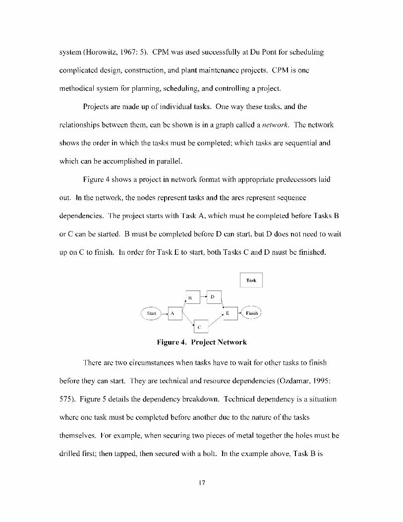
Figure 4 shows a project in network format with appropriate predecessors laid

out. In the network, the nodes represent tasks and the arcs represent sequence

dependencies. The project starts with Task A, which must be completed before Tasks B

or C can be started. B must be completed before D ean start, but D does not need to wait

up on C to finish. In order for Task E to start, both Tasks C and D must be finished.

Figure 4. Project Network

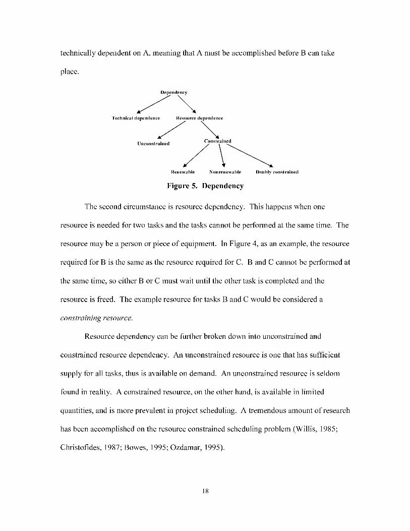
There are two cireumstanees when tasks have to wait for other tasks to finish

before they can start. They are teehnieal and resouree dependencies (Ozdamar, 1995:

575). Figure 5 details the dependeney breakdown. Technical dependency is a situation

where one task must be completed before another due to the nature of the tasks

themselves. For example, when securing two pieces of metal together the holes must be

drilled first; then tapped, then secured with a bolt. In the example above. Task B is

17

technically dependent on A, meaning that A must be accomplished before B can take

place.

Dependency

Figure 5. Dependency

The second circumstance is resource dependency. This happens when one

resource is needed for two tasks and the tasks cannot be performed at the same time. The

resource may be a person or pieee of equipment. In Figure 4, as an example, the resource

required for B is the same as the resouree required for C. B and C cannot be performed at

the same time, so either B or C must wait until the other task is completed and the

resouree is freed. The example resouree for tasks B and C would be considered a

constraining resource.

Resource dependeney ean be further broken down into unconstrained and

constrained resource dependeney. An uneonstrained resource is one that has sufficient

supply for all tasks, thus is available on demand. An unconstrained resource is seldom

found in reality. A constrained resouree, on the other hand, is available in limited

quantities, and is more prevalent in projeet seheduling. A tremendous amount of research

has been accomplished on the resouree constrained scheduling problem (Willis, 1985;

Christo Tides, 1987; Bowes, 1995; Ozdamar, 1995).

18

Constrained resources are further divided into renewable, nonrenewable, and

doubly constrained. A renewable constrained resource is constrained on a period-by-

period basis. For example, labor is used every day and limited on a daily basis

(Ozdamar, 1995: 575). A nonrenewable constrained resource is constrained on a project

basis. Materials and budget are examples when their total consumption over the duration

of the project is limited (Ozdamar, 1995: 575). A doubly constrained resource is

simultaneously constrained on a period and project basis.

Once the tasks and technical dependencies are established, project total duration

can be computed. It is important to note that the project’s total time is not the sum of all

the individual tasks because some operations can be completed in parallel. In fact, a

limited number of tasks control the project completion time. These tasks are called

critical operations and form a path through the network called the critical path.

Evaluation of these tasks form the basis of the Critical Path Method (Horowitz, 1967: 5).

Critical Path Method (CPM) is the most commonly used project management tool

in industry (Newbold, 1998: 54). Many industries use CPM to plan projects such as the

installation of tooling, building and designing operations for facilities and machinery,

construction projects, administrative programs, and maintenance operations (Spinner,

1992: 3). Its application is so broad as to be useful for any series of actions that, when

combined, form a complete program having a start and finish.

CPM determines the start and finish dates for individual activities in a project. A

result of this method is the identification of a critical path, or the unbroken series of

activities, which determine the start and the end of the project. A delay in the starting or

completion time of any critical path activity results in a delay in the overall project

19

completion time. Because of their importance for completing the project, critical path

activities receive top priority in the allocation of resources and managerial effort.

The example previously provided in Figure 4 is shown again in Figure 6. This

network is now expanded to include task duration times in Table 1. The following terms

used in CPM and this example are defined as:

Duration - length of time to complete the task

ES (Early Start) - earliest possible time that an activity can be started

EF (Early Finish) - earliest possible time that an activity can be completed

LS (Eate Start) - latest allowable time that an activity can be started without delaying the completion of the project

LF (Eate Finish) - latest allowable time that an activity can be completed without delaying the completion of the project

Predecessor tasks - tasks that need to be completed before another is started

Successor tasks - tasks that immediately follow a predecessor task

Task - activity being performed

Te - total time for completion of project

Table 1. Activities for Project

Task Predecessor Duration (weeks)

A 3

B A 4

C A 3

D B 1

E C,D 2

Task

Figure 6. Project Network

20

Once the task durations are known, the ES/EF and LS/LF times can be calculated for

each task. The CPM method calculates ES/EF and LS/LF times in two separate passes

through the network, a forward pass to determine ES/EF times and a backward pass to

determine LS/LF times. ES times are determined by using the formula ES =

(Nicholas, 2001: 208). Task A has no predecessor, so it can start at time 0. EF times are

determined by EF = ES + duration (Nicholas, 2001: 208). Task A takes 3 weeks to

complete, thus, the EF for Task A is 3. Tasks B and C can start once Task A is

completed, so their ES times are 3. This method is followed for each of the remaining

tasks, except for Task E. Task E has two predecessor tasks (C and D). Task C’s EF is 6,

but Task D’s EF is 8. In order for Task E to start. Tasks C and D must both be

completed, therefore, the earliest Task E can start is when the latter of Tasks C and D

finish. Task E’s ES is therefore 8. Once the forward pass through the project is

completed the entire project time {Te) can be determined. Also at this time the project’s

critical path can be determined. A project’s critical path is the longest path through the

network from origin node to terminal node (Nicholas, 2001: 205). In this case, the Te is

10 weeks and the critical path is ABDE. As stated before, any increase of time on tasks

ABDE will increase the time of the entire project. Figure 7 depicts the critical path.

Now a backward pass can be completed to determine the LS/LF times for each task.

The finish time of 10 weeks will be used as the starting point to perform a

backward pass to determine LS/LF. EF is calculated by LF = (Nicholas, 2001:

209). The LF for Task E is 10, since it does not have a successor. LS is calculated by

LS = LF - duration (Nicholas, 2001: 209). Task E’s duration is 2 weeks, so Task E’s LS

21

is 8. The LF for tasks C and D are determined by the LS of Task E. Therefore, Tasks C

and D’s LF is 8. Task A has two successors. When a task has two or more successors,

the successor with the earliest LS will be used to determine the predecessors LF. In this

case Task B’s LS is 3 compared to Task C’s 5. Therefore Task A’s LF is 3. The ES/EF

and LS/LF times for each task are annotated above their respective tasks in Fig. 7.

212 CP: ABDE= 10

Figure 7. Critical Path

Once the ES/EF and LS/LF times are determined. Total Slack (TS) and Free Slack

(FS) can be determined. Total slack (TS) is the difference between LS and LS

{TS = LS -ES) or LF and LF (75' = LF - EF) for an activity. It is the amount of time

between when a task must take place and can take place without affecting the project

finish date (Nicholas, 2001: 210). TS is shown under the respective activities in Fig 7.

The tasks with 0 total slack are the tasks on the critical path. In the example, they are A,

B, D, and E.

Free slack (FS) is the amount of time a task can be delayed without affecting the

early start of the activity immediately following. It is computed by the difference

between the EF and the earliest ES time of its successor {FS = - EF)

(Nicholas, 2001: 211). In the current example only Task C has FS. It can be delayed up

22

to 2 weeks and will not interfere with the start of Task E. With the above technique the

CP is determined, but that is not always enough to complete projects on time and under

budget.

Even with modem information and communication technology, most project

managers run into problems completing projects on time and within budget, while

fulfdling the customer’s needs of cost, schedule and performance. These challenges are

related more to management in general, than to any issue related to scheduling in

particular. The following are two government examples illustrating the difficulty in

meeting project goals.

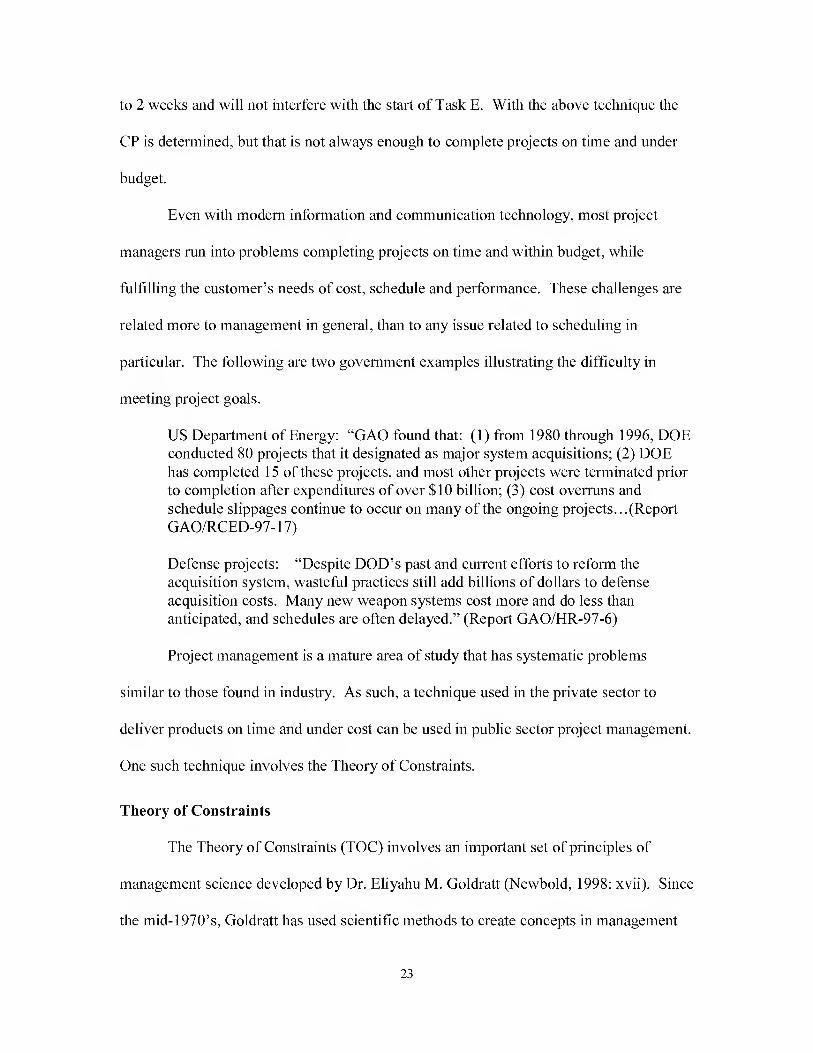
US Department of Energy: “GAO found that: (1) from 1980 through 1996, DOE conducted 80 projects that it designated as major system acquisitions; (2) DOE has completed 15 of these projeets, and most other projects were terminated prior to completion after expenditures of over $10 billion; (3) cost overmns and schedule slippages continue to oeeur on many of the ongoing projects.. .(Report GAO/RCED-97-17)

Defense projeets: “Despite DOD’s past and eurrent efforts to reform the acquisition system, wasteful praetiees still add billions of dollars to defense acquisition costs. Many new weapon systems cost more and do less than anticipated, and schedules are often delayed.” (Report GAO/HR-97-6)

Project management is a mature area of study that has systematic problems

similar to those found in industry. As such, a technique used in the private sector to

deliver products on time and under cost can be used in public sector project management.

One such technique involves the Theory of Constraints.

Theory of Constraints

The Theory of Constraints (TOC) involves an important set of principles of

management science developed by Dr. Eliyahu M. Goldratt (Newbold, 1998: xvii). Since

the mid-1970’s, Goldratt has used scientific methods to create concepts in management

23

which have proven to be of great value to industry (Newbold, 1998: xvii). These

methods have been used in the general and manufacturing management area,

manufacturing information technology environment, day-to-day managing skills, and

even in project management areas (Newbold, 1998: xvii). Goldratt’s first book. The

Goal, revolutionized manufacturing by describing how TOC could be applied to the

factory floor (Cook, 1998: 12). “TOC is a common sense management philosophy where

a person must find the constraint of the system and then concentrate effort on elevating

the capacity of the constraint” (Cook, 1998: 12). The following is an example of TOC in

use.

The Orman Grubb Company, a small manufacturer of wood furniture, used TOC to evaluate their inventory strategy, ultimately reducing inventory, which lowered overall eosts and led to inereased sales (20 - 100%) and an improved financial picture (Orman, 2001).

TOC focuses on increasing or optimizing the performance of processes that

involve a series of interdependent steps. Instead of breaking the process down into

individual steps and then improving the effieieney of each step, TOC focuses the

manager’s efforts on the bottlenecks, or constraints, that keep the process from improved

performance (Elton, 1998: 153). With TOC, the bottlenecks are scheduled to maximize

their throughput. Throughput is the rate at which a system generates money through

sales of its products or services while adhering to promised completion dates.

Application of TOC involves the following steps (Goldratt, 1990: 5 - 6):

1. Identify the system constraints - also at this time the constraints must be prioritized according to their impact on the goal

2. Decide how to exploit the constraints

3. Subordinate everything else to the above decision

24

4. Elevate the system’s constraints

5. If in the previous steps a constraint has been broken, go back to step 1

These steps need to be repeated because constraints can change over time.

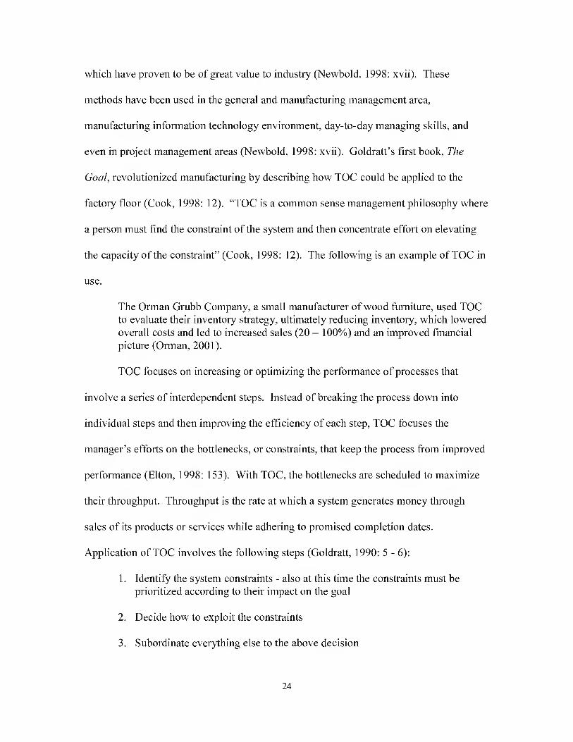
For projects, the constraint is represented by the tasks on the critical path. Our

example is shown again in Figure 8 with the CP (ABDE) bolded.

Figure 8. Critical Path

No matter how fast tasks are completed, the project cannot be completed faster

than the sum of the processing times of the critical path tasks. Goldratt identified a

second constraint to processes that managers often overlook: scarce resources needed by

tasks not only on and off the critical path but by other projects (Goldratt, 1997; 85).

Previously, scarce resources were considered finite and available at levels below the

quantity needed to complete the project in the minimal amount of time (Swartz, 1999:

14). Consider again that the same resource that accomplishes Task B is also required for

Task C. If there is only one unit of this resource, it would be unable to perform Task B

and C simultaneously as the unconstrained CPM schedule would require. There are a

variety of methods and options for how to deal with resource constraints. Once such

approach to the scheduling of scarce (constrained) resources in the beginning of CPM is

Critical Chain scheduling.

25

Critical Chain

The Critical Chain (CC) is that set of tasks which determines overall project

duration, taking into account both precedence and resource dependencies (Newbold,

1998; 57). It refers to a combination of the critical path and the scarce resources that

together constitute the constraints than need to be managed. CC has also been used in

project management with outstanding results. Below are two examples.

Lord Corporation, a developer of vibration and noise control systems for the industrial and aerospace markets used CC scheduling in its Information Services Division. The results were a capacity increase of 60%, cycle time improvement of 100%, two projects completed early, five on-time with no additional resources, and operating costs have remained the same. (Lord, 2001)

Harris Corporation's Mountaintop, PA. semiconductor plant applied CC scheduling in the development of their new wafer fabrication plant. For a project of this size, including the design and erection of the building, installation of equipment, hiring and training of employees, and ramp-up to 90% of designed production rate typically took an average of 54 months. From project kick-off to selling product produced in the new plant, the use of CC reduced the time to 13 months. (Harris, 2001)

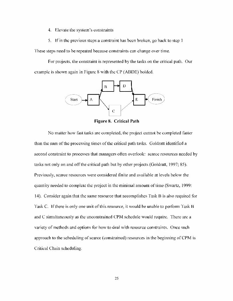
Once the constrained resources are determined, the CC tasks can be determined.

In our sample project, the CP was ABDE. However, there is only one unit of resource for

Tasks B and C. CPM states that B would get the resource first and then C would be

accomplished after B was finished. Under CPM, E could start as early as week 8, but due

to the constrained resource, C cannot start until week 7 and does not finish until week 10.

Therefore, E cannot start until week 10. The project now takes 12 weeks to complete and

the CC is ABCE. Figure 9 shows the CC with dummy arcs (bolded dashed lines) inserted

to represent how the CC differs from the CP. A major difference between CP and CC is

the topic of safety time, which will be discussed next.

26

ESIEF 317 718

CC: ABCE

Figure 9. Critical Chain

Safety Time

Most project schedules have implicit safety time built into each task estimate.

Individuals will tend to over-estimate the time to complete a task. By adding a “pad” to

the task time, the individual tries to ensure that their task will be completed on-time; this

added pad time represents protection against the schedule being disrupted by a delay in a

single task. This makes the individual look good to management. Second, managers

appreciate inflated task times because it gives them maneuvering room when bidding on

contracts. Managers know the times are inflated so if a potential customer wants a

shorter project duration, the manager assumes that he or she is able to give it to them to

increase the chance of winning the contract. Initially, padding individual task times

sounds like a good idea, but actually it is not. A problem with leaving padding in each

task estimate (Figure 10), is that the safety time is often wasted at the beginning of the

task period. One problem is that individuals can become concerned only with their tasks,

rather than the overall project because, they view the overall project as management’s

responsibility. By padding each task, the safety thought to be there is easily wasted.

There are three ways in which this safety, or buffer, is typically wasted (Cook, 1998: 14).

27

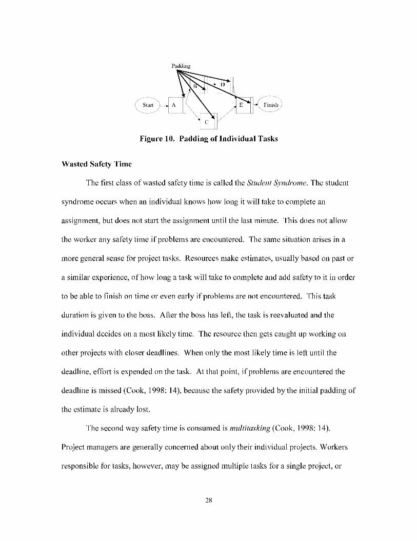
Padding

Figure 10. Padding of Individual Tasks

Wasted Safety Time

The first class of wasted safety time is called the Student Syndrome. The student

syndrome occurs when an individual knows how long it will take to complete an

assignment, but does not start the assignment until the last minute. This does not allow

the worker any safety time if problems are encountered. The same situation arises in a

more general sense for project tasks. Resources make estimates, usually based on past or

a similar experience, of how long a task will take to complete and add safety to it in order

to be able to finish on time or even early if problems are not encountered. This task

duration is given to the boss. After the boss has left, the task is reevaluated and the

individual decides on a most likely time. The resource then gets caught up working on

other projects with closer deadlines. When only the most likely time is left until the

deadline, effort is expended on the task. At that point, if problems are encountered the

deadline is missed (Cook, 1998: 14), because the safety provided by the initial padding of

the estimate is already lost.

The second way safety time is consumed is multitasking (Cook, 1998: 14).

Project managers are generally concerned about only their individual projects. Workers

responsible for tasks, however, may be assigned multiple tasks for a single project, or

28

worse yet they may be assigned multiple tasks across multiple projects. The priorities of

tasks by workers can change over time. This causes resources to work on one project or

task for a short amount of time, then jump to another and so forth. This movement from

one task to another increases individual task times, as workers need time to set up and

become familiar with the tasks again. This increase in task time has the effect of

reducing the safety buffer.

The third and final way in which safety time is wasted has to do with the

schedule’s structure (Cook, 1998: 15). Because tasks can have necessary predecessors or

are dependent on shared resources; in many circumstances delays are passed on, while

gains may not. There are two cases where this is present: sequential tasks and parallel

tasks.

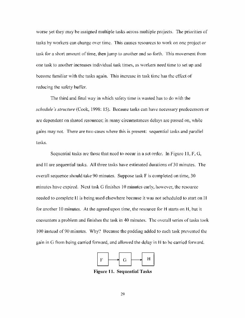
Sequential tasks are those that need to occur in a set order. In Figure 11, F, G,

and H are sequential tasks. All three tasks have estimated durations of 30 minutes. The

overall sequence should take 90 minutes. Suppose task F is completed on time, 30

minutes have expired. Next task G finishes 10 minutes early, however, the resource

needed to complete FI is being used elsewhere because it was not scheduled to start on H

for another 10 minutes. At the agreed upon time, the resource for H starts on H, but it

encounters a problem and finishes the task in 40 minutes. The overall series of tasks took

100 instead of 90 minutes. Why? Because the padding added to each task prevented the

gain in G from being carried forward, and allowed the delay in H to be carried forward.

Figure 11. Sequential Tasks

29

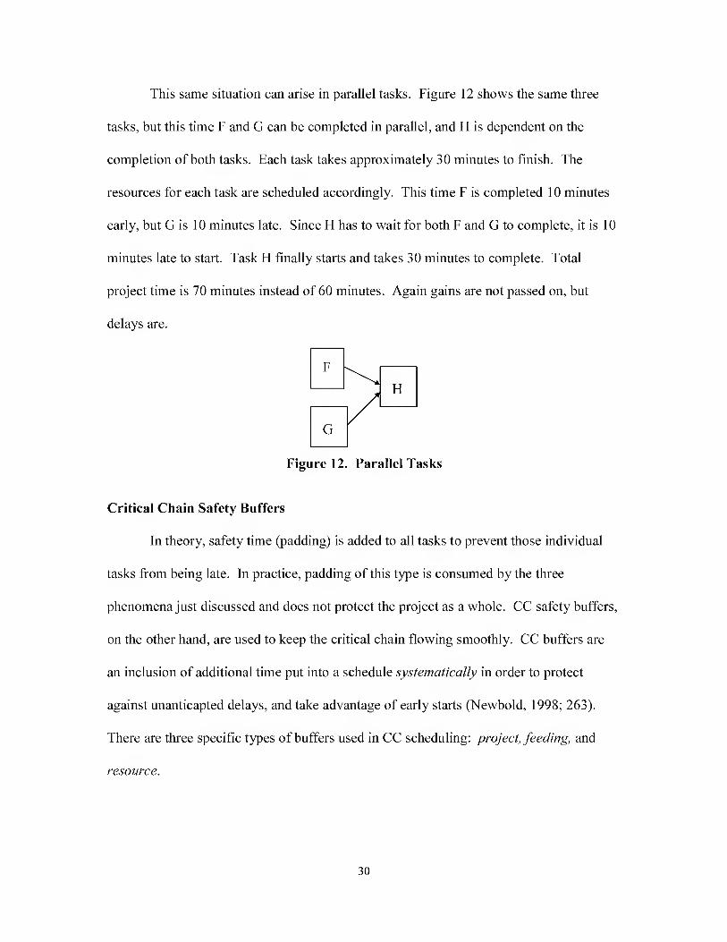
This same situation can arise in parallel tasks. Figure 12 shows the same three

tasks, but this time F and G can be completed in parallel, and FI is dependent on the

completion of both tasks. Each task takes approximately 30 minutes to finish. The

resources for each task are scheduled accordingly. This time F is completed 10 minutes

early, but G is 10 minutes late. Since Ft has to wait for both F and G to complete, it is 10

minutes late to start. Task Ft finally starts and takes 30 minutes to complete. Total

project time is 70 minutes instead of 60 minutes. Again gains are not passed on, but

delays are.

Figure 12. Parallel Tasks

Critical Chain Safety Buffers

In theory, safety time (padding) is added to all tasks to prevent those individual

tasks from being late. In practice, padding of this type is consumed by the three

phenomena just discussed and does not protect the project as a whole. CC safety buffers,

on the other hand, are used to keep the critical chain flowing smoothly. CC buffers are

an inclusion of additional time put into a schedule systematically in order to protect

against unanticapted delays, and take advantage of early starts (Newbold, 1998; 263).

There are three specific types of buffers used in CC scheduling: project, feeding, and

resource.

30

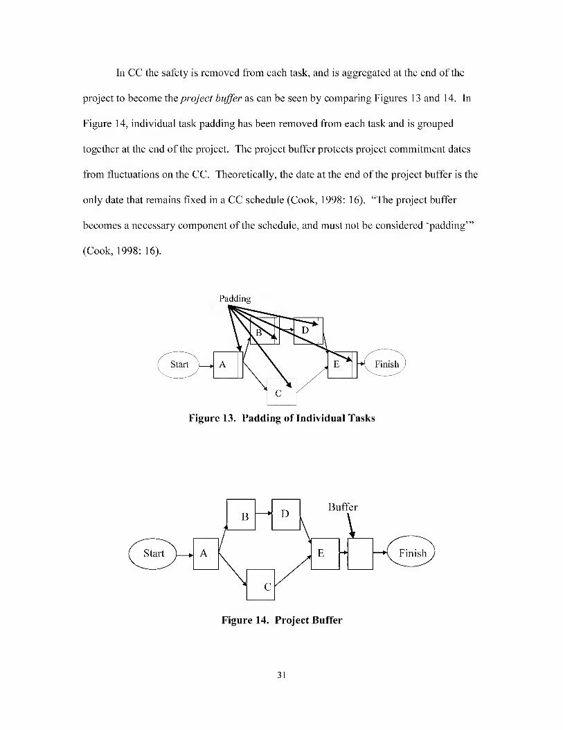
In CC the safety is removed from each task, and is aggregated at the end of the

project to become the project buffer as can be seen by comparing Figures 13 and 14. In

Figure 14, individual task padding has been removed from each task and is grouped

together at the end of the project. The project buffer protects project commitment dates

from fluctuations on the CC. Theoretically, the date at the end of the project buffer is the

only date that remains fixed in a CC schedule (Cook, 1998: 16). “The project buffer

becomes a necessary component of the schedule, and must not be considered ‘padding’”

(Cook, 1998: 16).

Padding

Figure 13. Padding of Individual Tasks

B D Buffer

Start )—J A Finish

Figure 14. Project Buffer

31

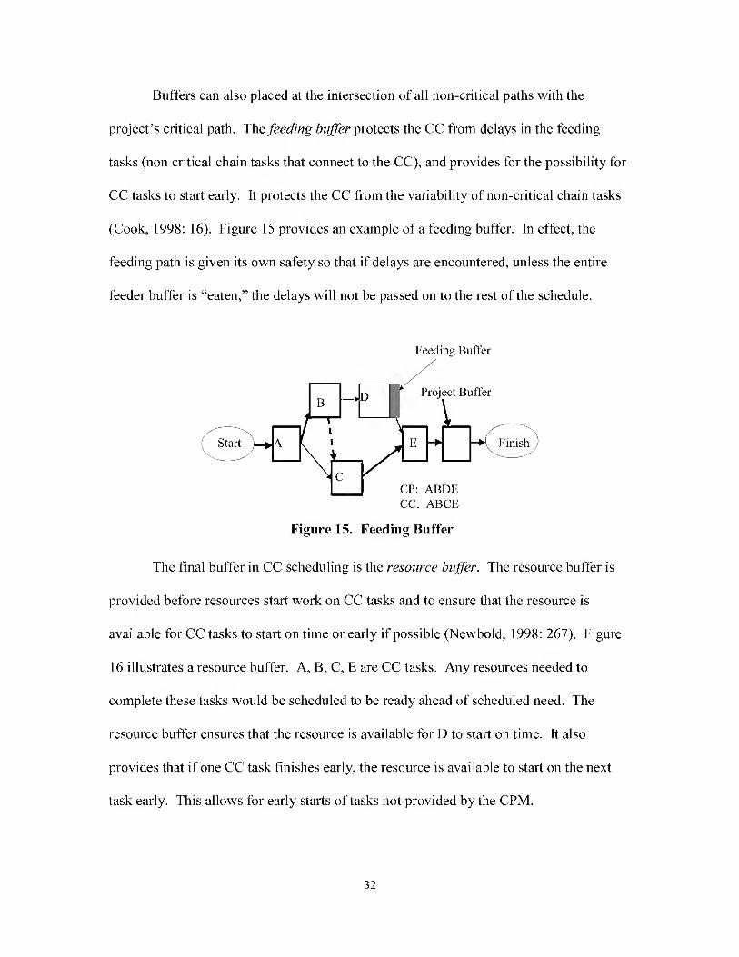
Buffers can also placed at the intersection of all non-critical paths with the

project’s critical path. The feeding buffer protects the CC from delays in the feeding

tasks (non critical chain tasks that connect to the CC), and provides for the possibility for

CC tasks to start early. It protects the CC from the variability of non-critical chain tasks

(Cook, 1998: 16). Figure 15 provides an example of a feeding buffer. In effect, the

feeding path is given its own safety so that if delays are encountered, unless the entire

feeder buffer is “eaten,” the delays will not be passed on to the rest of the schedule.

Feeding Buffer

CC: ABCE

Figure 15. Feeding Buffer

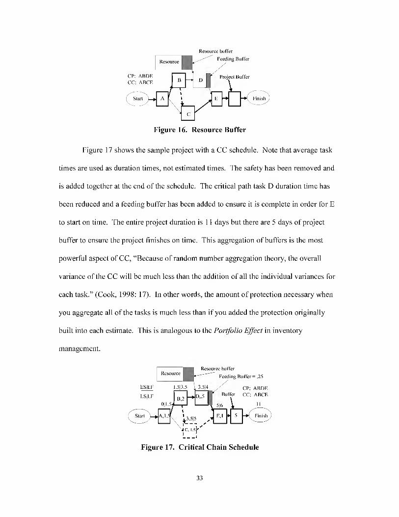
The final buffer in CC scheduling is the resource buffer. The resource buffer is

provided before resources start work on CC tasks and to ensure that the resource is

available for CC tasks to start on time or early if possible (Newbold, 1998: 267). Figure

16 illustrates a resource buffer. A, B, C, E are CC tasks. Any resources needed to

complete these tasks would be scheduled to be ready ahead of scheduled need. The

resource buffer ensures that the resource is available for D to start on time. It also

provides that if one CC task finishes early, the resource is available to start on the next

task early. This allows for early starts of tasks not provided by the CPM.

32

Resource buffer

Figure 16. Resource Buffer

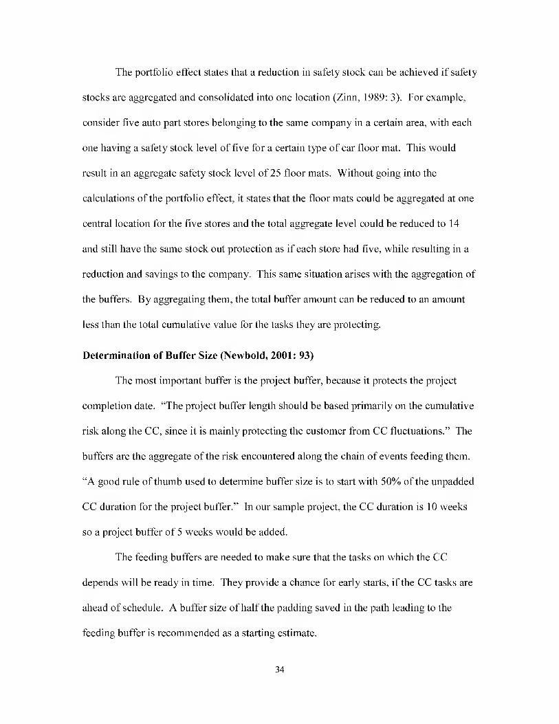
Figure 17 shows the sample project with a CC schedule. Note that average task

times are used as duration times, not estimated times. The safety has been removed and

is added together at the end of the schedule. The critical path task D duration time has

been reduced and a feeding buffer has been added to ensure it is complete in order for E

to start on time. The entire project duration is 11 days but there are 5 days of project

buffer to ensure the project finishes on time. This aggregation of buffers is the most

powerful aspect of CC, “Because of random number aggregation theory, the overall

variance of the CC will be much less than the addition of all the individual variances for

each task.” (Cook, 1998: 17). In other words, the amount of protection necessary when

you aggregate all of the tasks is much less than if you added the protection originally

built into each estimate. This is analogous to the Portfolio Effect in inventory

management.

Figure 17. Critical Chain Schedule

33

The portfolio effect states that a reduction in safety stock can be achieved if safety

stocks are aggregated and consolidated into one location (Zinn, 1989: 3). For example,

consider five auto part stores belonging to the same company in a certain area, with each

one having a safety stock level of five for a certain type of car floor mat. This would

result in an aggregate safety stock level of 25 floor mats. Without going into the

calculations of the portfolio effect, it states that the floor mats could be aggregated at one

central location for the five stores and the total aggregate level could be reduced to 14

and still have the same stock out protection as if each store had five, while resulting in a

reduction and savings to the company. This same situation arises with the aggregation of

the buffers. By aggregating them, the total buffer amount can be reduced to an amount

less than the total cumulative value for the tasks they are protecting.

Determination of Buffer Size (Newbold, 2001: 93)

The most important buffer is the project buffer, because it protects the project

completion date. “The project buffer length should be based primarily on the cumulative

risk along the CC, since it is mainly protecting the customer from CC fluctuations.” The

buffers are the aggregate of the risk encountered along the chain of events feeding them.

“A good rule of thumb used to determine buffer size is to start with 50% of the unpadded

CC duration for the project buffer.” In our sample project, the CC duration is 10 weeks

so a project buffer of 5 weeks would be added.

The feeding buffers are needed to make sure that the tasks on which the CC

depends will be ready in time. They provide a chance for early starts, if the CC tasks are

ahead of schedule. A buffer size of half the padding saved in the path leading to the

feeding buffer is recommended as a starting estimate.

34

Resource buffers are strictly “wakeup calls”. The resources can be notified and

made ready at appropriate times before they are needed, based on how the CC schedule is

going. If the CC tasks are experiencing delays, the resource allocation can be postponed.

If the CC tasks are being accomplished faster than scheduled, the resource allocation can

be advanced.

Management Use of Buffers

The aggregation of buffers allows individuals to take advantage of early finishes

and deal effectively with late finishes. Most project managers worry that a dynamic

schedule will become unmanageable, and thus opt for the “simpler” approach of trying to

lock down the schedule by assigning due dates. The Critical Chain schedule does not

become unmanageable beeause only the Critieal Chain tasks must remain buffered.

Unless there are major varianees to the sehedule, feeder paths remain set.

The last major distinetion of CC is the way in which the schedule is managed.

The resource buffers allow a projeet team to remain aware of the status of the CC. These

buffers are a form of communieation between the sehedule keeper and the rest of the

team (Cook, 1998: 18). The schedule keeper will get task updates from all resources

currently working on tasks as the schedule progresses. The resources merely need to

report how many workdays remain until their task is complete. When a predecessor CC

resource reports to have 5 days remaining, the schedule keeper informs the successor they

have approximately 5 days until they are on the CC (Cook, 1998: 18). This is a dynamic

countdown for the successor. If the predecessor reported 2 days later that he or she hit a

glitch and still had 5 days remaining, this would be passed on to the successor. This

35

allows CC resources to plan their work schedules and keep other project managers aware

of their pending CC status.

Management controls the project by monitoring the status of the buffers (Cook,

1998: 18). This allows them to highlight the tasks that need immediate attention. A

typical project will have numerous feeder buffers. The feeder buffer is protecting the

feeder path with the highest probability of delaying the CC. Thus, management can focus

attention on the feeder paths with the most depleted buffers. Of course, the CC tasks

themselves by definition are always considered crucial.

The buffers help management to act proactively. Buffer management highlights

potential problems much earlier than they would ordinarily be discovered using typical

project management teehniques.

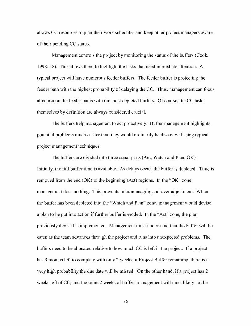
The buffers are divided into three equal parts (Act, Watch and Plan, OK).

Initially, the full buffer time is available. As delays oecur, the buffer is depleted. Time is

removed from the end (OK) to the beginning (Aet) regions. In the “OK” zone

management does nothing. This prevents mieromanaging and over adjustment. When

the buffer has been depleted into the “Watch and Plan” zone, management would devise

a plan to be put into action if further buffer is eroded. In the “Act” zone, the plan

previously devised is implemented. Management must understand that the buffer will be

eaten as the team advances through the project and runs into unexpected problems. The

buffers need to be allocated relative to how much CC is left in the project. If a project

has 9 months left to complete with only 2 weeks of Project Buffer remaining, there is a

very high probability the due date will be missed. On the other hand, if a project has 2

weeks left of CC, and the same 2 weeks of buffer, management will most likely not be

36

very concerned. Management monitors the buffers relative to how much CC or feeder

branch remains, and the rate of buffer consumption (Cook, 1998: 19).

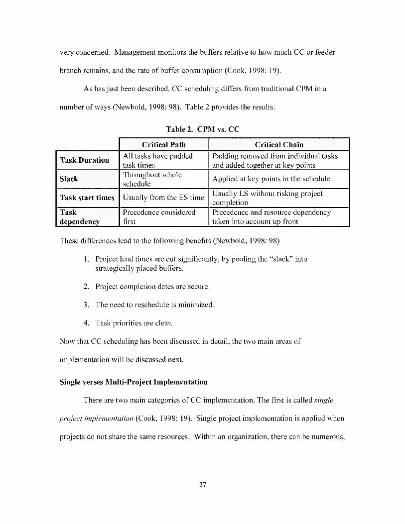
As has just been described, CC scheduling differs from traditional CPM in a

number of ways (Newbold, 1998: 98). Table 2 provides the results.

Table!. CPM vs. CC

Critical Path Critical Chain

Task Duration All tasks have padded task times

Padding removed from individual tasks and added together at key points

Slack Throughout whole schedule

Applied at key points in the schedule

Task start times Usually from the ES time Usually LS without risking project completion

Task

dependency

Precedence considered first

Precedence and resource dependency taken into account up front

These differences lead to the following benefits (Newbold, 1998: 98)

1. Project lead times are cut significantly, by pooling the “slack” into strategically placed buffers.

2. Project completion dates are secure.

3. The need to reschedule is minimized.

4. Task priorities are clear.

Now that CC scheduling has been discussed in detail, the two main areas of

implementation will be discussed next.

Single verses Multi-Project Implementation

There are two main categories of CC implementation. The first is called single

project implementation (Cook, 1998: 19). Single project implementation is applied when

projects do not share the same resources. Within an organization, there can be numerous.

37

single CC projects. As long as each project is assigned its own resources, independent

from all other projects, it can be managed as an independent project.

The second category is called multi-project implementation. Multi-project

implementation applies when there is multiple simultaneous projects and resources are

shared across projects (Cook, 1998: 20). It is more difficult to schedule resources across

multiple projects because there is no clear decision method when deciding which project

to give priority when allocating a constrained resource.

This thesis will concern itself with single project management because that

closely describes the environment of the ISO aircraft inspection. The individuals

(resources) assigned to the ISO act exclusively on the ISO projects.

Critical Chain and the ISO Process

The SOF-130 ISO process is a project management problem, set in a maintenance

environment. The project has a definite start and end date, and there are a limited number

of ISO mechanics (resources) assigned to the project from different organizations. There

is a clear objective to provide a fully mission capable aircraft to the flight line. With

these project characteristics, project management techniques can be used to optimize the

scheduling of resources to improve the process. The goal would be to complete the

inspection in no more than the currently allotted 9 days, and sooner if possible.

Identification of the CC would give maintenance supervision the ability to monitor tasks

that could delay the completion of the ISO and also allow them to adjust resources to

meet the completion date. By identifying the CC, supervision would be able to identify

those critical tasks and determine where future improvements can be made.

38

Current Implementation

Two current applications of Critical Path theory in maintenance are the Periodic

Depot Maintenance Scheduling System (PDMSS) and the allocation of resources during

C-5 depot maintenance.

The C-130 depot at Warner Robins Air Force Base uses PDMSS. This system is

maintained and updated by personnel under government contract with the Robbins Gioia

Company. PDMSS is a visual scheduling tool that shows the current status of an aircraft

moving through depot maintenance. When an aircraft enters the depot process, all tasks

required for that aircraft during the depot maintenance process are input into PDMSS.

PDMSS flows out the tasks in a Gantt type chart. As maintenance personnel accomplish

the tasks, the PDMSS is updated with eompleted tasks. PDMSS then compares

scheduled eompletion of tasks with aetual eompletion of tasks. The output is a horizontal

bar ehart identifying if an aireraft is behind or ahead of schedule by different colored

horizontal bars. The horizontal bars represent the tasks to be performed during the depot

and the length of the task. Green bars identify ahead or on schedule while red denotes

behind schedule. It also illustrates the amount of time the aircraft is ahead or behind

schedule. However, at the time of this thesis, there are problems with PDMSS. One

problem relates to how it determines the status of the aircraft. An incomplete 5-minute

subtask of a 150-hour task, will show the aircraft being 150 hours behind schedule,

instead of 5 minutes. Another problem is resource allocation. PDMSS currently does not

provide supervisors with a method to show how resources affect the aircraft schedule.

Robbins Gioia personnel are currently working on these two problems with a hope of

corrections in the future.

39

Another well-known application of Critical Path theory is in use at the C-5 depot,

also at Warner Robins AFB. Over a period of 5 years, the C-5 depot repair has extended

from the 200 - 250 day range to over 300 days. The increase in time was due to an

increase in extensive engine pylon repairs and deterioration of the aft tie box fitting on

the horizontal stabilizer. Maintenance personnel determined these tasks were along the

CP and looked at ways to shorten their duration. Technology and industrial support

workers stepped in to manufacture new parts before the aircraft arrived, which allowed

the replacement of defective parts in record time. The last two C-5A-models were

completed in 286 days, and the last C-5B-model was completed in 191 days. In this

example. Critical Path identification of the engine pylon and aft tie box repair tasks and

their resulting improvements led to a decrease in depot time of the C-5 aircraft.

Summary

This chapter presented the importance of the ISO process to aircraft airworthiness.

The ISO process was described, including the 4 different phases (3 minor and 1 major

inspections), which make up a complete inspection cycle. The ISO consists of a complex

set of tasks, completed either in parallel or sequentially. The ISO has a definite start and

end with technicians from different organizations completing the inspections, and finally

there is a clear ISO objective: to complete a set of tasks, resulting in a fully mission

capable aircraft, in a minimal amount of time. These aspects of the ISO are also

characteristics of projects. As such, project management techniques appear to be suitable

to the ISO environment.

One such project management technique is the Critical Path Method developed by

Du Pont in 1958. CPM determines which sequential tasks take the longest amount of

40

time and focuses management attention on those tasks. However, the CPM assumption

of unconstrained resources does not hold and is unrealistic in practice.

Goldratt’s Critical Chain view of the resource constrained project scheduling

problem points out that not only should managers consider the critical tasks, they need to

take resource contention into account “up front” when determining the critical path, and

schedule them correctly. This resulted in the Critical Chain method.

In the next chapter, the ISO process’s CP and CC will be developed. Once the

critical chain is identified, a CC scheduling package will be applied to the ISO to

determine if improvements to the critical chain can be accomplished. The CP and CC

versions of the process will be compared and the results presented in Chapter 4. The last

chapter will summarize the researeh results and explore the managerial implications of

the findings.

41

111. Methodology

Introduction

The purpose of this chapter is to discuss the framework for the analysis conducted

in this research effort. The methods used in this study and their relevance will be

provided, setting the stage for the presentation of the results. First, the sources of the data

and the methods of retrieval used will be introduced. The parameters of the analysis will

be discussed next, followed by a description of the variables (resources and work

schedules). Calculations of task durations using the Beta distribution will follow, which

will lead into a discussion of Microsoft Project 2000© as the model driver with the

resulting three different models. A description of the CP and CC project duration

estimations will follow. The chapter ends with a discussion of total project duration time

{Te) as the measure of performance and the experimental manipulations.

Data Collection

Data was collected for this study by reviewing the 1C-130A-6WC-15 work cards,

and by interviewing the following individuals from the 16th Equipment Maintenance

Squadron Isochronal inspection section: dock chief, shift supervisors, floor chiefs, and

wing chiefs.

The dock chief is in charge of the entire ISO process, including all personnel,

equipment and materials used in the ISO. The dock chief is the single point of contact for

ISO related issues. The shift supervisors support the dock chief, and control the

maintenance, equipment, and personnel on their respective work shifts. The ISO runs a

two-shift operation with an additional weekend duty crew; therefore, there are three shift

42

supervisors. The floor chiefs report to the shift supervisors and are primarily responsible

for maintenance on the aircraft. The wing chief, sometimes called the area chief, is in

charge of maintenance on a certain section of the aircraft, such as the left or right wing,

nose section, or tail section.

The interviews were conducted primarily to validate the WC information. They

consisted of a short explanation of the research area, followed by a listing of what

information was required. The following information was requested:

1. A listing of tasks accomplished during the ISO in order of occurrence.

2. Type of mechanic required for each task along with the number required.

3. The number of mechanic’s available during each day of the ISO.

4. Task start points.

5. Task duration.

6. Required task predecessors.

Appendix A shows the results of the data collection provided by the dock chief.

The tasks were categorized by which tasks were currently accomplished each day of the

ISO and by each AFSC. This aggregation of the work cards tasks for the ISO process by

AFSC and date, according to the dock chief, is the easiest for a description the ISO

process.

The dock chief, shift supervisor, floor chief and wing chief determined scheduled

task durations. The durations are the aggregated amount of time that one maintenance

person accomplishes work in their AFSC on the ISO aircraft during the duty day.

Additionally, the resource column of the task depicts which maintenance personnel is

performing the task and how many workers of that kind are required to perform that task

43

in the time allotted in the duration column. For example, using the data provided in

Table 3, nine ISO APG (dayshift) personnel are required to (inspect) and lubricate the

aircraft. The task should take 8 hours with nine individuals working on the task. The

nine personnel required are denoted by the 900% in the resources block.

Table 3. WBS Information

WBS Task Duration Resources

4.1 Look/Lube phase (APG dayshift) 8 hrs ISO APG (dayshift)[900%]

Activity Parameters

The activity parameters for this study include the type of work tasks performed

during the ISO, along with their associated maintenance personnel required, task duration

and task predecessors. The work performed is shown in the task column of the work

breakdown structure (WBS) in Appendix B. The WBS includes the task, duration,

resources and predecessors. This information is required for programming critical path

or critical chain problems.

The last parameter is the task predecessor. As stated in Chapter 2, certain tasks

have predecessors that must be accomplished before they can take place. The ISO tasks

are the same. The dock chief provided the predecessor alignment of tasks. Some of the

predecessor tasks are apparent, such as “Tow aircraft to ISO hangar. Task 2.3”, before

“Jack aircraft. Task 3.1” can be accomplished. Other predecessor arrangements are not

as apparent, such as “Engine performance runs. Task 9.1” must be completed before

“Fuel cell fix phase. Task 9.2” can be started. There are also extenuating circumstances

where the predecessor arrangement can change. For example, if, in the previous

example, a fuel cell discrepancy is a safety problem and the aircraft engines cannot be

44

started until the fuel cell problem is corrected, then the task dependency would change.

For the purpose of this study, the general task predecessor-successor relationships were

used. The general relationship was determined by the experience and knowledge of the

ISO maintenance technicians, which cannot be over emphasized.

Description of Variables

There are two types of variables: independent and dependent. Independent

variables cause, influence, or affect outcomes, while dependent variables, as the name

implies, are dependent on the independent variables; they are the outcomes or results of

the influence of the independent variables (Creswell, 1994: 63).

The independent variables for this study are the resources (maintenance

personnel) involved in the ISO proeess. There are a total of 11 different types of

maintenanee personnel and 1 government eontraet erew (aircraft wash) involved in the

ISO proeess. Appendix C lists eaeh type of maintenanee person, with their assoeiated Air

Foree Speeialty Code (AFSC), authorized manning level, and current manning levels.

Eaeh AFSC is required in different amounts and at different times during the ISO.

Certain AFSCs are broken down further by their duty sehedule, (such as personnel who

work on the weekends); known as weekend duty personnel, or by their duty location

(such as flight line or ISO) APG.

The other independent variable used in this study is the work schedule. The work

schedule is the work time for the maintenanee personnel involved in the ISO. The work

schedule is broken down into two further areas: shift hours and days off. Shift hours are

the working time of the ISO maintenance personnel for any workday. Days off are the

45

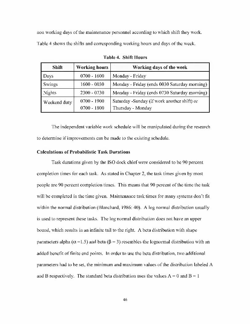
non working days of the maintenance personnel according to which shift they work.

Table 4 shows the shifts and corresponding working hours and days of the week.

Table 4. Shift Hours

Shift Working hours Working days of the week

Days 0700 - 1600 Monday - Friday

Swings 1600 - 0030 Monday - Friday (ends 0030 Saturday morning)

Nights 2300 - 0730 Monday - Friday (ends 0730 Saturday morning)

Weekend duty 0700 - 1900

0700 - 1800

Saturday -Sunday (if work another shift) or

Thursday - Monday

The independent variable work schedule will be manipulated during the research

to determine if improvements can be made to the existing schedule.

Calculations of Probabilistic Task Durations

Task durations given by the ISO dock chief were considered to be 90 percent

completion times for each task. As stated in Chapter 2, the task times given by most

people are 90 percent completion times. This means that 90 percent of the time the task

will be completed in the time given. Maintenance task times for many systems don’t fit

within the normal distribution (Blanchard, 1986: 40). A log normal distribution usually

is used to represent these tasks. The log normal distribution does not have an upper

bound, which results in an infinite tail to the right. A beta distribution with shape

parameters alpha (a =1.5) and beta (P = 3) resembles the lognormal distribution with an

added benefit of finite end points. In order to use the beta distribution, two additional

parameters had to be set, the minimum and maximum values of the distribution labeled A

and B respectively. The standard beta distribution uses the values A = 0 and B = 1

46

(Devore, 2000: 183). These four values resulted in the following standard Beta

distribution (1.5, 3, 0,1) Figure 18.

Figure 18. Standard Beta Distribution

Using the standard beta distribution with a = 1.5 and P = 3, Mathcad’spbeta

(x,sl,s2) (si = a, s2 = P) function was used to calculate the x value which results in a 90

percent cumulative probability. Cumulative probability distribution gives the probability

that a random variable (x) will take on a value less than or equal to a specified value.

These are obtained by simply integrating (or summing when appropriate) the

corresponding probability density over an appropriate range (Mathcad, 1999: 164). In

this case, when x = .62 of the standard Beta (Range 0 - 1) a 90 percent cumulative

probability was returned. Once x = .62 value was determined, new A and B values could

be calculated for each of the different task times. Of the 75 different tasks, 13 different

durations were used. Using the 13 basic task durations, the stochastic P(1.5, 3)

distribution was derived as follows. First, since the A and B values are the upper and

lower limits of the beta distribution, an arbitrary determination was made that the spread

between the A and B values would be 50 percent of the original task duration for each

47

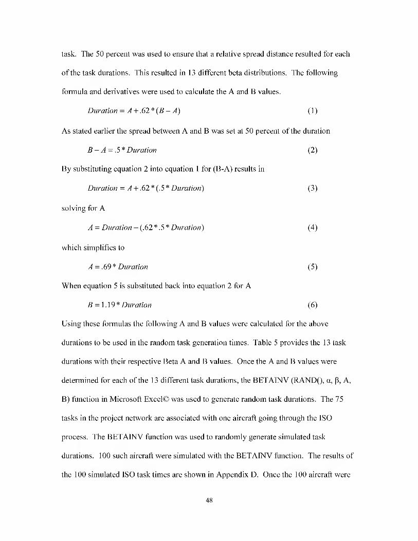
task. The 50 percent was used to ensure that a relative spread distance resulted for each

of the task durations. This resulted in 13 different beta distributions. The following

formula and derivatives were used to calculate the A and B values.

Duration = A +.62* {B - A) (1)

As stated earlier the spread between A and B was set at 50 percent of the duration

B — A = .5* Duration (2)

By substituting equation 2 into equation 1 for (B-A) results in

Duration = ^ + .62 * (.5 * Duration) (3)

solving for A

A = Duration — (.62 * .5 * Duration) (4)

which simplifies to

A = .69* Duration (5)

When equation 5 is substituted back into equation 2 for A

5 = 1.19* Duration (6)

Using these formulas the following A and B values were calculated for the above

durations to be used in the random task generation times. Table 5 provides the 13 task

durations with their respective Beta A and B values. Once the A and B values were

determined for each of the 13 different task durations, the BETAINV (RAND(), a, (3, A,

B) function in Microsoft Excel© was used to generate random task durations. The 75

tasks in the project network are associated with one aircraft going through the ISO

process. The BETAINV function was used to randomly generate simulated task

durations. 100 such aircraft were simulated with the BETAINV function. The results of

the 100 simulated ISO task times are shown in Appendix D. Once the 100 aircraft were

48

simulated, the task durations for each aircraft were input into Microsoft Project 2000© to

determine how long the simulated aircraft were in the ISO process.

Table 5. Beta A and B Values

Durations (hours) A value B value

0.75 0.52 0.89

1.00 0.69 1.19

1.5 1.04 1.79

2.00 1.38 2.38

3.00 2.07 3.57

4.00 2.76 4.76

6.00 4.14 7.14

7.00 4.83 8.33

7.5 5.18 8.93

8.00 5.52 9.52

12.00 8.28 14.28

16.00 11.04 19.04

21.00 14.49 24.99

Microsoft Project 2000©

The first step in programming the model is to input the tasks under each day of

the ISO. For example, Day 1 of the ISO will be the main task, with all tasks

accomplished during that day as subtasks. This procedure was completed for each day of

the ISO process. Once the task was loaded into Microsoft Project 2000© (MSP2000), the

task duration and predecessors were then loaded. Finally, the resources for each task

were input.

The matching of resources to tasks is a three-step process. First, the resources

(maintenance personnel) need to be added with their respective, current manning levels.

Once this was accomplished their individual work schedules could be added. The work

schedule is the time during the day each resource is available to perform work. Finally,

49

the resource is added to the task with the numbers required to perform that task in the

allotted time (duration).

The original task durations provided by the ISO dock chief were used to set the

baseline model for the experiment. Appendix B shows the initial Microsoft Project

2000© scenario Model (Ml). Ml reflects the current ISO process with one exception.

All work for each day of the ISO is continuous. This is different than what the dock chief

provided. For example, the dock chief stated that 8 hours of ISO APG work is conducted

on dayshift and 8 hours conducted on swing shift resulting in 16 hours of work conducted

in a 24-hour period by ISO APG. The ISO APG are scheduled to work 9 hours on days

and swings. This results in 18 hours of work availability. For the Ml model, this work

availability is nullified by the not earlier than (NET) restriction put on tasks. Even

though ISO APG tasks are completed before the shift ends new work is restricted from

starting until the next day.

Model 2 (M2) was developed with the NET constraints removed. Therefore tasks

could be started as soon as resources were available to accomplish the tasks. The only

constraints in M2 are the availability of the resources.

Model 3 (M3) was developed as an ideal model in which all constraints are

removed. Resources are available 24 hours a day, 7 days a week. Tasks are started as

soon as preceding tasks are accomplished.

Once the three models were built, Microsoft Project 2000© was used to calculate

the project duration and identify the critical tasks for each model.

In order to determine a difference between CP and CC scheduling, ProChain

Version 5.0© was used to calculate the critical chain project duration for the above three

50

models. The Critical Chain versions took the original task durations and reduced them 50

percent. Following standard Critical Chain procedures, the CC was then calculated and a

project buffer that was 50 percent of the project duration was inserted. The project buffer

was placed at the end of the critical chain tasks to protect the project. Each of the feeding

tasks had a feeding buffer inserted which was 50 percent of the length of the feeding

tasks it was protecting. A 2-hour resource buffer was added for each of the resources

currently not in use.

With this procedure, CC estimated durations for the three models were obtained.

The estimations along with the CP estimations for the models were compared against the

100 simulated durations to determine benefits or drawbacks from using CP and CC

scheduling.

Measures of Performance

The primary measure of performance for this research is total project duration

(Je). Te is measured in hours. A 24-hour clock will be used. Te is measured from the

first hour/date of the ISO (ISO start) to the time/date when all required ISO maintenance

is complete (ISO end). For example, if ISO start was at 0700 on Friday, 9 November

2001 and all ISO maintenance is complete (ISO end) at 2400 on Saturday, 17 November

2001, then Te equals 209 hours. Te will be affected by No Earlier Than (NET) task start

constraint and the work schedule of personnel. By removing NET and or increasing or

decreasing the shift schedule of workers, Te should change.

51

Experimental Manipulation

This study will identify the impact of ISO scheduling using the CP and the CC

method by comparing the 100 simulated ISO durations {Te) in each of the models to the

estimated duration times provided by the CP and CC scheduling techniques for the

respective models. The results will be viewed in the areas of aircraft availability lost

(aircraft available for use, but not scheduled because ISO was completed before

scheduled time) and aircraft scheduling lost (aircraft was scheduled to be ready and it

was not). Table 6 provides visual representation of the experimental design.

Table 6. Experimental Design

Models Te \ Scheduling Technique Estimated Te: Ml M2 M3

Critical Path X X X

Critical Chain X X X

Conclusion

In this chapter, the methods used in this study were described. First, the sources

of the data used and the methods of retrieval employed were introduced. The parameters

of the analysis were discussed, followed by a description of the variables (resources and

work schedules). Calculations of task durations using the Beta distribution were

described, which led into a discussion of Microsoft Project 2000© as the model driver

with the resulting three different models. The CP and CC estimations for project duration

followed. Finally, total project duration time {Te) as the measure of performance was

discussed. The chapter ended with a discussion of the experimental manipulation.

Chapter 4 will present the experimental results.

52

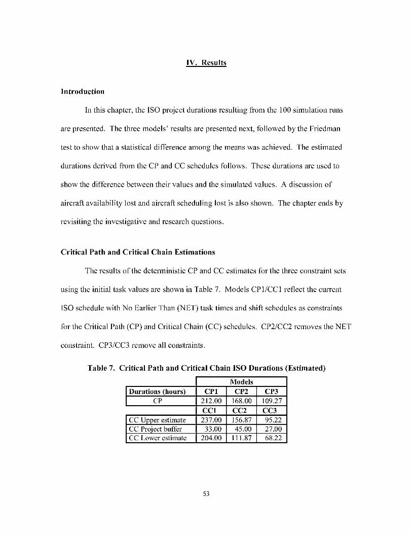
IV. Results

Introduction

In this chapter, the ISO project durations resulting from the 100 simulation runs

are presented. The three models’ results are presented next, followed by the Friedman

test to show that a statistieal difference among the means was achieved. The estimated

durations derived from the CP and CC schedules follows. These durations are used to

show the differenee between their values and the simulated values. A discussion of

aircraft availability lost and aircraft scheduling lost is also shown. The chapter ends by

revisiting the investigative and research questions.

Critical Path and Critical Chain Estimations

The results of the deterministic CP and CC estimates for the three constraint sets

using the initial task values are shown in Table 7. Models CPl/CCl reflect the current

ISO schedule with No Earlier Than (NET) task times and shift schedules as constraints

for the Critical Path (CP) and Critical Chain (CC) schedules. CP2/CC2 removes the NET

constraint. CP3/CC3 remove all constraints.

Table 7. Critical Path and Critical Chain ISO Durations (Estimated)

Models 1

Durations (hours) CPI CP2 CP3 CP 212.00 168.00 109.27

CCl CC2 CC3 1 CC Upper estimate 237.00 156.87 95.22

33.00 45.00 27.00 1 CC Lower estimate 204.00 111.87 68.22

53

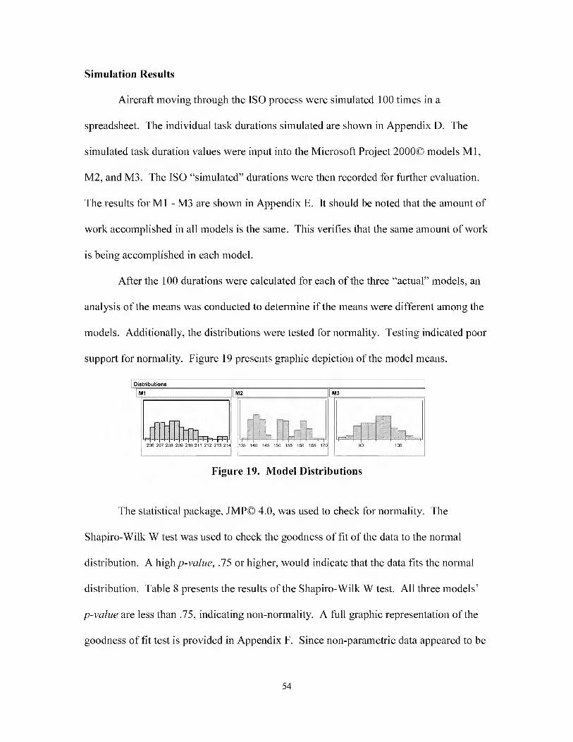
Simulation Results

Aircraft moving through the ISO process were simulated 100 times in a

spreadsheet. The individual task durations simulated are shown in Appendix D. The

simulated task duration values were input into the Microsoft Project 2000© models Ml,

M2, and M3. The ISO “simulated” durations were then reeorded for further evaluation.

The results for Ml - M3 are shown in Appendix E. It should be noted that the amount of

work aeeomplished in all models is the same. This verifies that the same amount of work

is being aeeomplished in eaeh model.

After the 100 durations were ealculated for each of the three “aetual” models, an

analysis of the means was eondueted to determine if the means were different among the

models. Additionally, the distributions were tested for normality. Testing indieated poor

support for normality. Figure 19 presents graphic depiction of the model means.

Figure 19. Model Distributions

The statistical package, JMP© 4.0, was used to check for normality. The

Shapiro-Wilk W test was used to check the goodness of fit of the data to the normal

distribution. A high p-value, .75 or higher, would indicate that the data fits the normal

distribution. Table 8 presents the results of the Shapiro-Wilk W test. All three models’

p-value are less than .75, indicating non-normality. A full graphic representation of the

goodness of fit test is provided in Appendix F. Since non-parametric data appeared to be

54

present and a statistical verification of the difference of means was required, the

Friedman test was conducted.

Table 8. Shapiro-Wilk W Test for Normality

Models 1

Ml M2 M3

p-value .0001 <.0001 .6609

Friedman Fr Test

To show a statistical difference in means between the different models, the

Friedman {Fr) test was used. The Fr test compares p probability distributions when the

normality and equal variance cannot be assumed (McClave, 1988: 973). The following

assumptions are made in order to use the Fr test:

1. The treatments are randomly assigned to experimental units within blocks.

2. Either the number of blocks (Zi) or the number of treatments {p) should exceed

5 for the ehi-squared (% ) approximation to be adequate.

3. The p probability distributions from which the samples within each block are drawn are eontinuous.

The hypotheses for the Fr test are:

Flo: The probability distributions for thep treatments are identical. Fla: At least two of the probability distributions differ in location.

The test statistic is:

12

bpip +1) ^ (7)

where

b = Number of blocks p = Number of treatments Rj = Rank sum of theyth treatments, where the rank of each measurement is computed relative to its position within its own block

55

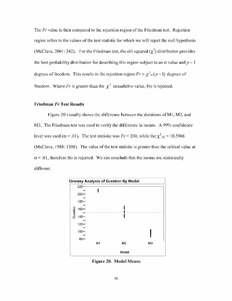
The Fr value is then compared to the rejection region of the Friedman test. Rejection

region refers to the values of the test statistic for which we will reject the null hypothesis

(McClave, 2001: 342). For the Friedman test, the chi squared (% ) distribution provides

the best probability distribution for describing this region subject to an a value and p-\

degrees of freedom. This results in the rejection region Fr > x^a {p -1) degrees of

freedom. Where Fr is greater than the x^ cumulative value, Ho is rejected.

Friedman Fr Test Results

Figure 20 visually shows the difference between the durations of Ml, M2, and

M3. The Friedman test was used to verify the difference in means. A 99% confidence

level was used (a = .01). The test statistic was Fr = 200, while the % .oi = 10.5966

(McClave, 1988: 1208). The value of the test statistic is greater than the critical value at

a = .01, therefore Ho is rejected. We can conclude that the means are statistically

different.

Oneway Analysis of Duration By Model 220- 200

180

1 160 2 Q 140

120

100

80

Figure 20. Model Means

Ml M2

Model

M3

56

Model Durations

The 100 simulated ISO durations were ranked in ascending order for each model

(Appendix H). A minimum, mean, and maximum duration was recorded for each. These

durations were compared to the estimated durations obtained from the CP and CC

models. Table 9 provides an overview of the results.

Table 9. Model Duration Comparison

Models

Durations (hours) Ml M2 M3

Min 205.67 137.13 84.78

Mean 208.65 149.93 94.64

Max 213.69 167.80 104.95

CP estimate 212.00 168.00 109.27

CC lower estimate 204.00 111.87 68.22

CC upper estimate 237.00 156.87 95.22

Aircraft Availability and Scbeduling Error

The two scheduling methods were also compared on the basis of completion time

percentile, aircraft availability lost, and aircraft scheduling lost. Completion time

percentile is the percentile of times that the estimated duration falls in the range of the

ranked ordered simulated times for that model. Aircraft availability lost is the amount of

time that an aircraft could have been used for mission accomplishment, but was not used

because it was not planned to be ready. Aircraft scheduling lost occurs when an aircraft

is scheduled to be ready and it is not. Each of the three measures will be described in

detail below.

Before proceeding with an examination of the data, an explanation of how the

completion time percentile was calculated is required. The estimated duration for a

particular model (CPl/CCl, CP2/CC2, CP3/CC3) was compared to the ascending rank

57

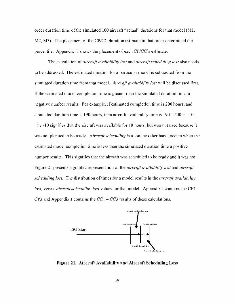
order duration time of the simulated 100 aircraft “actual” durations for that model (Ml,

M2, M3). The placement of the CP/CC duration estimate in that order determined the

percentile. Appendix H shows the placement of each CP/CC’s estimate.

The calculation of aircraft availability lost and aircraft scheduling lost also needs

to be addressed. The estimated duration for a particular model is subtracted from the

simulated duration time from that model. Aircraft availability lost will be discussed first.

If the estimated model completion time is greater than the simulated duration time, a

negative number results. For example, if estimated completion time is 200 hours, and

simulated duration time is 190 hours, then aircraft availability time is 190 - 200 == -10.

The -10 signifies that the aircraft was available for 10 hours, but was not used because it

was not planned to be ready. Aircraft scheduling lost, on the other hand, occurs when the

estimated model completion time is less than the simulated duration time a positive

number results. This signifies that the aircraft was scheduled to be ready and it was not.

Figure 21 presents a graphic representation of the aircraft availability lost and aircraft

scheduling lost. The distribution of times for a model results in the aircraft availability

lost, versus aircraft scheduling lost values for that model. Appendix I contains the CPI -

CP3 and Appendix J contains the CC1 - CC3 results of these calculations.

ISO Start

Figure 21. Aircraft Availability and Aircraft Scheduling Loss

Aircraft scheduling loss

58

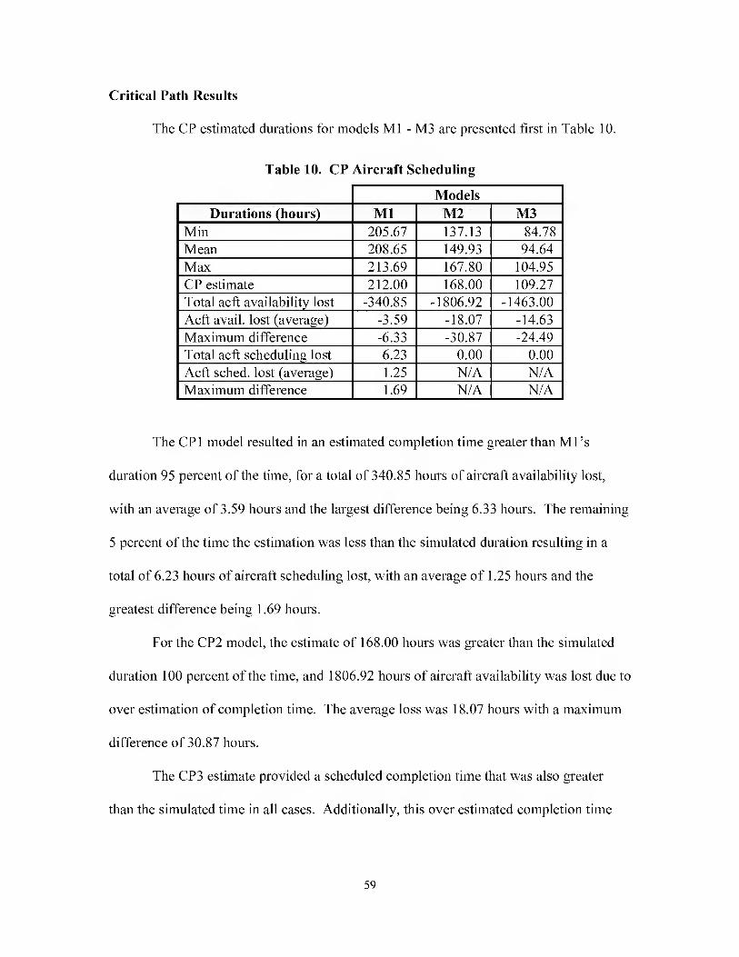
Critical Path Results

The CP estimated durations for models Ml - M3 are presented first in Table 10.

Table 10. CP Aircraft Scheduling

Models 1

Durations (hours) Ml M2 M3

Min 205.67 137.13 84.78

Mean 208.65 149.93 94.64

Max 213.69 167.80 104.95

CP estimate 212.00 168.00 109.27

Total acft availability lost -340.85 -1806.92 -1463.00

Acft avail, lost (average) -3.59 -18.07 -14.63

Maximum difference -6.33 -30.87 -24.49

Total acft scheduling lost 6.23 0.00 0.00

Acft sched. lost (average) 1.25 N/A N/A

Maximum difference 1.69 N/A N/A

The CPI model resulted in an estimated completion time greater than Ml’s

duration 95 percent of the time, for a total of 340.85 hours of aircraft availability lost,

with an average of 3.59 hours and the largest difference being 6.33 hours. The remaining

5 percent of the time the estimation was less than the simulated duration resulting in a

total of 6.23 hours of aircraft scheduling lost, with an average of 1.25 hours and the

greatest difference being 1.69 hours.

For the CP2 model, the estimate of 168.00 hours was greater than the simulated

duration 100 percent of the time, and 1806.92 hours of aircraft availability was lost due to

over estimation of completion time. The average loss was 18.07 hours with a maximum

difference of 30.87 hours.

The CP3 estimate provided a scheduled completion time that was also greater

than the simulated time in all cases. Additionally, this over estimated completion time

59

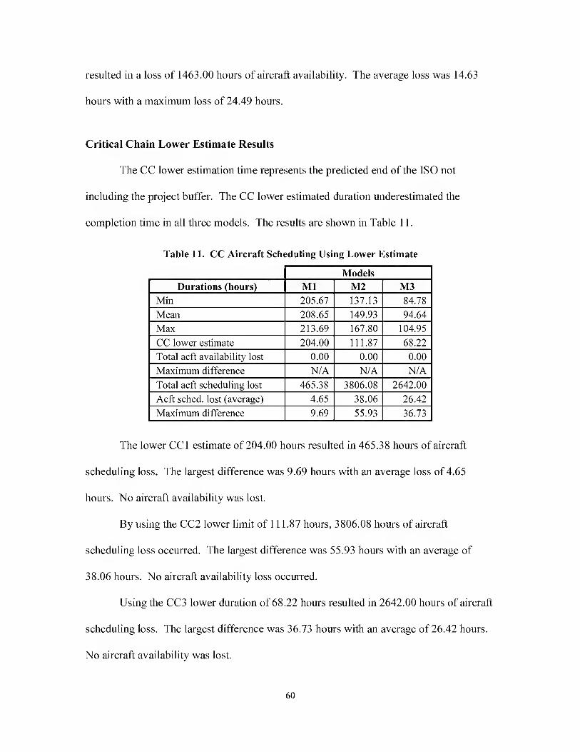
resulted in a loss of 1463.00 hours of aircraft availability. The average loss was 14.63

hours with a maximum loss of 24.49 hours.

Critical Chain Lower Estimate Results

The CC lower estimation time represents the predicted end of the ISO not

including the project buffer. The CC lower estimated duration underestimated the

completion time in all three models. The results are shown in Table 11.

Table 11. CC Aircraft Scheduling Using Lower Estimate

Models 1

Durations (hours) Ml M2 M3

Min 205.67 137.13 84.78

Mean 208.65 149.93 94.64

Max 213.69 167.80 104.95

CC lower estimate 204.00 111.87 68.22

Total aeft availability lost 0.00 0.00 0.00

Maximum differenee N/A N/A N/A

Total aeft seheduling lost 465.38 3806.08 2642.00

Aeft sehed. lost (average) 4.65 38.06 26.42

Maximum difference 9.69 55.93 36.73

The lower CCl estimate of 204.00 hours resulted in 465.38 hours of aircraft

scheduling loss. The largest difference was 9.69 hours with an average loss of 4.65

hours. No aircraft availability was lost.

By using the CC2 lower limit of 111.87 hours, 3806.08 hours of aircraft

scheduling loss occurred. The largest difference was 55.93 hours with an average of

38.06 hours. No aircraft availability loss occurred.

Using the CC3 lower duration of 68.22 hours resulted in 2642.00 hours of aircraft

scheduling loss. The largest difference was 36.73 hours with an average of 26.42 hours.

No aircraft availability was lost.

60

Critical Chain Upper Estimate Results

The CC upper estimate includes the project buffer. Table 12 shows these results.

Table 12, CC Aircraft Scheduling Using Upper Estimate

Models 1

Durations (hours) Ml M2 M3

Min 205.67 137.13 84.78

Mean 208.65 149.93 94.64

Max 213.69 167.80 104.95

CC upper estimation 237.00 156.87 95.22

Total acft availability lost -825.39 -200.54

Acft avail, lost (average) -28.35 -11.31 -3.86

Maximum difference -31.33 -19.74 -10.44

Total acft scheduling lost 0.00 134.46 142.54

Acft sched. lost (average) N/A 4.98 2.97

Maximum difference N/A 10.93 9.73

For CCl, the upper estimate of 237.00 hours always overestimated the completion

time. This resulted in 2834.62 hours of aircraft availability lost, with 31.33 hours as the

largest difference and an average of 28.35 hours. No aircraft scheduling loss occurred.

The CC2 upper estimate of 156.87 hours overestimated completion time 74

percent of the time. This resulted in 825.39 hours of aircraft availability lost. The

underestimation (26 percent of the time) resulted in 134.46 hours of aircraft scheduling

lost. The maximum differences were 19.74 hours and 10.93 hours respectively with the

corresponding averages of 11.31 hours and 4.98 hours.

By using the CC3 upper estimate of 95.22 hours, the duration was overestimated

52 percent of the time. This resulted in 200.54 hours of aircraft availability lost. Forty-

eight percent of the time, the duration was underestimated resulting in 142.54 hours of

61

aircraft scheduling loss. The maximum differences were 10.44 and 9.73 hours

respectively with an average loss of 3.86 and 2.97 hours.

Primary Research and Investigative Questions

The primary research question for this thesis was “Can the use of Critical Chain

scheduling reduce the ISO flow time?” In order to answer the primary research

question, the following subordinate investigative questions were answered.

The first investigative question “What are the key differences between Critical

Path and Critical Chain methods?'^ was addressed in Chapter 2. Two key differences

are, the scheduling of scarce (constrained) resources explicitly in the beginning of the

scheduling process by CC, and the removal of safety time from individual tasks and their

aggregation into specific project buffers. The first buffer occurs at the end of the project

in what is known as the project buffer. Safety time is also added at the end of all feeding

tasks in what are called the feeding buffers. Resource buffers are also added to schedule

the availability of resources that are not currently working on the critical chain activities.

The second investigative question, “What are the results of applying a Critical

Path analysis to the ISO project?'' is examined by the identification of the critical path

activities of the ISO, and the formulation of the three CP models. The complete work

breakdown structures (WBS) for these three versions of the CP are shown in Appendices

K - M. Asterisks (*) highlight the critical path activities.

There are only three critical path tasks in the CPI model as a result of the No

Earlier Than (NET) constraints. These tasks take place on the last day of the ISO. There

62

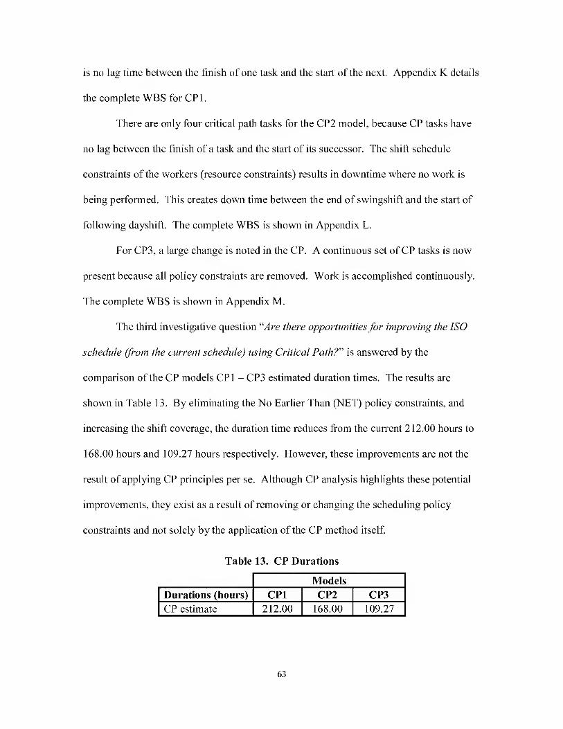
is no lag time between the finish of one task and the start of the next. Appendix K details

the complete WBS for CPI.

There are only four critical path tasks for the CP2 model, because CP tasks have

no lag between the finish of a task and the start of its successor. The shift schedule

constraints of the workers (resource constraints) results in downtime where no work is

being performed. This creates down time between the end of swingshift and the start of

following dayshift. The complete WBS is shown in Appendix L.

For CPS, a large change is noted in the CP. A continuous set of CP tasks is now

present because all policy constraints are removed. Work is accomplished continuously.

The complete WBS is shown in Appendix M.

The third investigative question “Are there opportunities for improving the ISO

schedule (from the current schedule) using Critical Path?'"’ is answered by the

comparison of the CP models CPI - CPS estimated duration times. The results are

shown in Table IS. By eliminating the No Earlier Than (NET) policy constraints, and

increasing the shift coverage, the duration time reduces from the current 212.00 hours to

168.00 hours and 109.27 hours respectively. However, these improvements are not the

result of applying CP principles per se. Although CP analysis highlights these potential

improvements, they exist as a result of removing or changing the scheduling policy

constraints and not solely by the application of the CP method itself

Table 13. CP Durations

Models 1

Durations (hours) CPI CP2 CP3

CP estimate 212.00 168.00 109.27

63

The fourth investigative question ‘’’’What are the results of applying a Critical

Chain analysis to the ISO project?" is answered by examining the CC versions of the

models. The complete WBSs are shown in Appendices M - O. Asterisks (*) highlight

the critical chain activities. In order for the CCl model to replicate the current ISO

process with certain tasks starting on specified days, No Later Than (NLT) constraints

had to be added to the model. This is due to the process of CC scheduling tasks from

their Late Finish (LF) time. If the NLT constraints were not added, all tasks would

adhere to the NET constraint, by starting at the project’s LF. This model behavior,

coupled with the reduction of task durations by 50 percent, would result in half the

allotted time for the ISO. The NLT constraint for each day resulted in each individual

day having its own CC. Appendix N details the WBS for the CCl model.

For the CC2 model, the NET (and subsequent NLT) constraints were removed.

This resulted in seven CC tasks. These seven tasks occurred on the last day of the ISO as

would be expected, since the shift schedule constraints allows a gap between the finish of

one task and the start of the subsequent tasks on the next day. There is down time

between the end of swingshift and the start of following dayshift. The complete WBS is

shown in Appendix O.

For CC3, a large change is noted in the CC. A continuous set of CC tasks is now

identified because all constraints have been removed. Work is accomplished

continuously. The complete WBS is shown in Appendix P.

The fifth investigative question there opportunities for improving the ISO

schedule (from the current schedule) using Critical Chain?" can be answered by a

comparison of the CC estimations compared to the current duration of 212.00 hours.

64

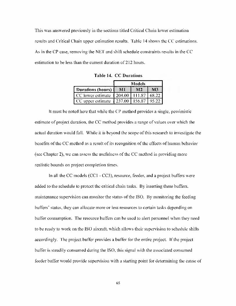
This was answered previously in the sections titled Critical Chain lower estimation

results and Critical Chain upper estimation results. Table 14 shows the CC estimations.

As in the CP case, removing the NET and shift schedule constraints results in the CC

estimation to be less than the current duration of 212 hours.

Table 14. CC Durations

Models 1 Durations (hours) Ml M2 M3 CC lower estimate 204.00 111.87 68.22

CC upper estimate 237.00 156.87 95.22

It must be noted here that while the CP method provides a single, pessimistic

estimate of project duration, the CC method provides a range of values over which the

actual duration would fall. While it is beyond the seope of this research to investigate the

benefits of the CC method as a result of its reeognition of the effects of human behavior

(see Chapter 2), we ean assess the usefulness of the CC method in providing more

realistie bounds on projeet eompletion times.

In all the CC models (CCl - CCS), resource, feeder, and a project buffers were

added to the schedule to protect the critical chain tasks. By inserting these buffers,

maintenance supervision can monitor the status of the ISO. By monitoring the feeding

buffers’ status, they can allocate more or less resources to certain tasks depending on

buffer consumption. The resource buffers can be used to alert personnel when they need

to be ready to work on the ISO aircraft, which allows their supervision to schedule shifts

accordingly. The project buffer provides a buffer for the entire project. If the project

buffer is steadily consumed during the ISO, this signal with the associated consumed

feeder buffer would provide supervision with a starting point for determining the cause of

65

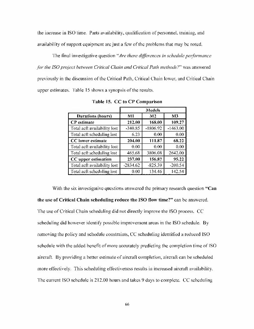
the increase in ISO time. Parts availability, qualification of personnel, training, and

availability of support equipment are just a few of the problems that may be noted.

The final investigative question “Are there differences in schedule performance

for the ISO project between Critical Chain and Critical Path methods?'’’ was answered

previously in the discussion of the Critical Path, Critical Chain lower, and Critical Chain

upper estimates. Table 15 shows a synopsis of the results.

Table 15. CC to CP Comparison

Models 1

Durations (hours) Ml M2 M3

CP estimate 212.00 168.00 109.27

Total acft availability lost -340.85 -1806.92 -1463.00

Total acft scheduling lost 6.23 0.00 0.00

CC lower estimate 204.00 111.87 68.22

Total acft availability lost 0.00 0.00 0.00

Total acft scheduling lost 465.68 3806.08 2642.00

CC upper estimation 237.00 156.87 95.22

Total acft availability lost -2834.62 -825.39 -200.54

Total acft scheduling lost 0.00 134.46 142.54

With the six investigative questions answered the primary research question “Can

the use of Critical Chain scheduling reduce the ISO flow time?” can be answered.

The use of Critical Chain scheduling did not directly improve the ISO process. CC

scheduling did however identify possible improvement areas in the ISO schedule. By

removing the policy and schedule constraints, CC scheduling identified a reduced ISO

schedule with the added benefit of more accurately predicting the completion time of ISO

aircraft. By providing a better estimate of aircraft completion, aircraft can be scheduled

more effectively. This scheduling effectiveness results in increased aircraft availability.

The current ISO schedule is 212.00 hours and takes 9 days to complete. CC scheduling

66

showed that by removing the NET and shift schedule constraints the ISO could be

decreased to 95.22 hours; a reduction of nearly 55 percent. This CC ISO takes 3 days to

complete and provided the most accurate approximation of completion time for aircraft

scheduling purposes. Additional benefits are the adding of resource, feeding and project

buffers to the schedule. These buffers provide the buffer at key points in the schedule

and can be used by supervision to monitor the ISO process. Further discussion will be

presented in the Chapter 5 when managerial considerations are presented.

Conclusion

In this chapter the results of the ISO project simulations were presented. The

Friedman Fr test was used to verify that the means were statistically different. The

estimated durations derived from the CP and CC sehedules were presented. These times

were used to show the differenee between their values and the simulated values. A

discussion of aircraft availability lost and aircraft scheduling lost which occurred by

using the estimated eompletion times of the CP and CC models compared to the actual

simulation results followed. The chapter ended with the answering of the investigative

and primary research questions. In Chapter 5, the management implications will be

addressed along with recommendations for further research.

67

V. Conclusions and Recommendations

Introduction

Chapter 1 provided the foundation for this thesis with a discussion of the United

States Air Force Special Operations Command (AFSOC) high demand, low-density

weapon systems (AC-130H, AC-130U, MC-130H aircraft) belonging to the 16th Special

Operations Wing (SOW) stationed at Hurlburt Field, Florida. Due to their limited

numbers, aircraft availability is a key issue. Reducing aircraft downtime by improved

scheduling during the -130 Isochronal inspection process (ISO) was the center of this

thesis. By reducing aircraft downtime, increased aircraft availability could result without

purchasing more aircraft.

Chapter 2 detailed the current ISO process and how it can be viewed as a project

because it consists of a complex set of tasks, completed either in parallel or sequentially,

with a definite start and end, with technicians from different organizations completing the

inspections. These aspects of the ISO are also characteristics of projects, and the ISO

process can be modeled as a directed, acyclic network. As such, project management

techniques appeared to be suitable to the ISO environment. The chapter ended with the

evolution of project management from Critical Path Methodology (CPM) to Critical

Chain (CC) scheduling.

Chapter 3 provided a discussion of the methodology used in this thesis. The

gathering of data started the chapter, followed by the development of the three Microsoft

Project 2000 models (Ml - M3). Ml represents the current situation. M2 removed the

Not Earlier Than (NET) constraint, and M3 removed the shift schedule constraint. Next,

68

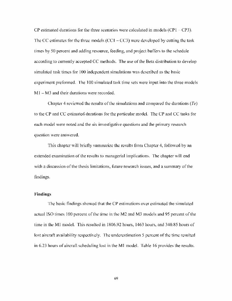
CP estimated durations for the three scenarios were calculated in models (CPI - CP3).

The CC estimates for the three models (CCl - CCS) were developed by cutting the task

times by 50 percent and adding resource, feeding, and project buffers to the schedule

according to currently accepted CC methods. The use of the Beta distribution to develop

simulated task times for 100 independent simulations was described as the basic

experiment preformed. The 100 simulated task time sets were input into the three models

Ml - MS and their durations were recorded.

Chapter 4 reviewed the results of the simulations and compared the durations {Te)

to the CP and CC estimated durations for the particular model. The CP and CC tasks for

each model were noted and the six investigative questions and the primary research

question were answered.

This ehapter will briefly summarize the results from Chapter 4, followed by an

extended examination of the results to managerial implications. The chapter will end

with a discussion of the thesis limitations, future research issues, and a summary of the

findings.

Findings

The basic findings showed that the CP estimations over estimated the simulated

actual ISO times 100 percent of the time in the M2 and MS models and 95 percent of the

time in the Ml model. This resulted in 1806.92 hours, 146S hours, and S40.85 hours of

lost aircraft availability respectively. The underestimation 5 percent of the time resulted

in 6.2S hours of aircraft scheduling lost in the Ml model. Table 16 provides the results.

69

Table 16. CP Results

Models 1

Durations (hours) Ml M2 M3

CP estimate 212.00 168.00 109.27

Total acft availability lost -340.85 -1806.92 -1463.00

Total acft scheduling lost 6.23 0.00 0.00

An argument could be made that, while not captured by the model, a scheduled

completion time would hardly ever be improved upon. In other words, if the CP model

established a completion time and that time was published as a deadline, human nature

would dictate the entire time would be used to complete the ISO. The phenomenon is

called Parkinson’s Law named after its originator Professor Cyril Northcote Parkinson.

Professor Parkinson stated that work will expand to fill the time allotted (Parkinson,

2001). Parkinson’s Law, coupled with the student syndrome (Chapter 2), suggests that

workers will not start a task early, even when possible. This results in project

completions that are never earlier than scheduled. This in turn results in no room for

error or the ability to overcome problems if they arise at the end of the ISO.

This leads to the larger issue of the aircraft availability lost. With the current

situation, 340.85 hours of aircraft availability was lost. If the duration estimate times

were more accurately scheduled, aircraft availability would increase. By allowing the

ISO schedule to take longer than it might normally have, more work (non engineering

based inspections) gets added to the ISO, personnel are tasked to complete other details,

and possibly manning reductions might take place. Aircraft availability lost will be

further discussed with the CC estimates next.

70

The use of CC scheduling resulted in two durations for each model, a lower

estimation and an upper estimation (project buffer included). Using the lower estimation

resulted in 0 hours of lost aircraft availability, because the estimate was always less than

the 100 simulated durations all three models. This underestimation of duration produced

465.68, 3806.08, and 2642.00 hours of aircraft scheduling loss in the Ml, M2, and M3

models respectively. The results are shown in Table 17.

Table 17. CC Lower Estimation Results

Models 1

Durations (hours) Ml M2 M3

CC lower estimate 204.00 111.87 68.22

Total acft availability lost 0.00 0.00 0.00

Total acft scheduling lost 465.68 3806.08 2642.00

Using the CC lower estimation would result in a risk of scheduling the aircraft

when it is not ready. This can cause cancelled training and real-world missions, poor

relations with the operational side of the wing, and, most importantly, tremendously low

aircraft scheduling effectiveness. Scheduling effectiveness is used as one of the key

metrics on aircraft performance briefed up the chain of command. Providing such a low

estimate may seem like a good approach at first, but has serious complications. In order

to try to meet the reduced schedule, maintenance may suffer, morale will be reduced, and

ultimately a poor quality product would be the result. As stated in Chapter 2 (on the

discussion of CC scheduling) the lower estimate should not be used to determine the

project duration. The CC upper estimate (project buffer included) is the only estimate

that stays fixed and should be used for scheduling purposes. The CC upper estimate will

be discussed next.

71

Using the upper CC estimation resulted in 2834.62 hours of aircraft availability

lost in the Ml model, 825.39 hours in M2, and 200.54 hours in M3. Aircraft scheduling

loss occurred in two models with the upper CC estimation resulting in 134.46, and 142.54

hours for M2 and M3 respectively. Table 18 shows the upper CC estimation results.

Using the CC upper estimate results in both overestimation and underestimation of the

completion time of the ISO depending on the scenario involved. However, the difference

is less than the CP duration, except in the Ml model.

Table 18. CC Upper Estimation Results

Models 1

Durations (hours) Ml M2 M3

CC lower estimate 237.00 156.87 95.22

Total acft availability lost -2834.62 -825.39 -200.54

Total acft scheduling lost 0.00 134.46 142.54

There is a tradeoff between underestimating and overestimating the completion

time. By underestimating, supervision forces workers to cut safety time out of their

tasks, workers have to work harder and faster, training of new personnel might suffer,

and ultimately, the quality of the end product suffers and scheduling effectiveness is

decreased. However, overestimating the duration results in workers that have scheduled

idleness, there is no pressure to make their process better, proficiency might be lost, job

satisfaction is lowered because tasks are not demanding, and ultimately, the end product

may suffer. Additionally, aircraft availability is lost.

In a perfect world, the exact duration of the ISO would be known in advance, and

the aircraft and workers could be scheduled accordingly. In reality, this is far from the

case. Choices must be made between scheduling early (and assuming the risk of

72

lateness), and scheduling later (and assuming the inefficiencies of idleness). A “middle

ground” would provide the benefits of increasing aircraft availability without increasing

the risk of aircraft scheduling loss.

Overall Findings

The current ISO schedule is 212 hours and takes 9 days to complete. The use of

CC scheduling did not improve upon the current schedule except for removing slack from

each task and aggregating it at key points in the ISO schedule.

Under the current ISO conditions (constraints of Not Earlier Than and shift

schedules intact), the CP estimated duration provides the best approximation of

completion time, as the CC method provides no advantage under these types of

constraints. If no changes are made to the eurrent ISO proeess, the CP method is

suffieient to manage the ISO work.

Additional Findings

CP and CC scheduling analysis highlighted the opportunity that by removing the

NET and shift schedule eonstraints the ISO eould be decreased to 95.22 hours; increasing

aircraft availability 116.78 hours per aireraft. The CCS ISO takes 3 days to complete and

provided the most accurate approximation of eompletion time for aircraft scheduling

purposes.

When only the NET constraint is removed, the CC upper estimation provided the

best duration approximation. Aircraft availability was increased 55.13 hours per aircraft

over the current schedule used by the ISO.

73

As stated previously, the best-case scenario (in terms of rapid project completion)

occurs when both constraints are removed. Under these conditions, the CC upper

estimation resulted in only 200.54 hours of lost aircraft availability over 100 simulated

aircraft. This accurate prediction results in an 86 percent increase in aircraft availability

over the CP estimate. When an aircraft schedule is built to take advantage of this early

finish schedule, 142.54 hours of aircraft scheduling loss occurred but the largest duration

was only 9.73 hours. This could be avoided entirely by simply modifying the project

buffer following the CC implementation methodology.

Managerial Implications

The use of CC scheduling results in the largest increase in aircraft availability,

when time eonstraints are removed from the projeet. If a situation arose that required the

ISO faeility to inerease its output, the CC sehedule would provide the best approximation

of duration time and the most aeeurate way to sehedule aircraft to maximize aircraft

availability. The eurrent 9-day (212 hour) ISO eould be reduced to a 5-day (156.87 hour)

schedule or if a surge was required a 3-day, 3-shift sehedule could be used to complete

the ISO in approximately 95.22 hours.

In order to determine the number of personnel and their work times for each

schedule, the current schedule was compared against the CC2 and CC3 proposed

schedules. The shift schedules are shown in Appendices Q, R and S.

Appendix Q shows the current work schedule. The schedule shows that the

majority of the work occurs on days 4 - 7 of the ISO. This is when the greatest number

of workers are scheduled.

74

The reduced ISO schedule (Appendix R) is the result of the NET constraint being

removed. The schedule is reduced to 5 days. The current manning situation will be able

to accomplish the 5-day schedule with no additional personnel. The majority of the work

is on days 2 and 3 of the ISO.

The surge ISO schedule, which could be used in a wartime situation or any time

that requires an increase in aircraft availability, is shown in Appendix S. This schedule

takes 3 days and would require an additional shift of workers, except for ISO engine

personnel, which would require two additional shifts. Fifty percent of the work is

accomplished on day 2 of the ISO. Current manning levels would have to be assessed to

determine feasibility. The benefit of increasing aircraft availability would have to be

weighted against current manning levels. If additional manning was not available, the

reduction in capability in certain areas, due to the movement of personnel from those

areas to the ISO, would have to investigated compared to the increase in aircraft

availability. Even though the ISO duration could be reduced, other tasks that affect the

ISO may be increased because manning is not available, thus increasing the ISO duration.

A global optimum of increasing aircraft availability needs to be addressed.

Limitations

This thesis is limited by the accuracy of the data provided by the 16 EMS ISO

inspection section. The initial task times provided are the basis for this thesis. Inaccurate

task times, availability of personnel, qualifications of personnel to perform required

work, and availability of required equipment and supplies have an affect on the results.

75

Another limitation is in the duration times of the simulated aircraft. Studies

showed that the lognormal distribution closely resembles maintenance tasks times. The

Beta distribution, with aforementioned parameters, was used because it resembles the

lognormal distribution and has the added benefit of upper and lower limits. The values of

90 percent duration time for the initial values, the selected alpha, beta, A and B values for

the Beta distribution will have an affect on the outcome. The extent of the effect is not

known at this time and is an area for future research.

Future Research

Further research needs to be conducted into the realistic value of the estimated

durations of the models by the CP and CC schedules. Actual ISO inspection times could

be referenced for each ISO and than compared to the estimated times.

The ISO process at Hurlburt could be used as a field test by actually removing the

NET and shift schedule constraints and comparing the actual ISO durations to the

estimated times.

The procedures used to determine the CP and CC schedules for this thesis could

be used on other military aircraft inspection processes to determine if improvements

could be made to aircraft availability.

Additionally, the relevance of CC scheduling techniques should be investigated in

other areas of aircraft maintenance, like the generation of aircraft for daily flying or

deployment, off equipment maintenance actions to include repair and replacement of line

or shop replaceable units. Any major project that could be modeled as a directed, acyclic

network of tasks is worthy of investigation using the principles of CC scheduling.

76

This same technique could be investigated at the depot level. The C-130 depot

inspection takes nearly 180 days. Reducing depot inspection time could provide

additional aircraft availability far in excess of that available at organizational level.

Finally, since this thesis has shown that there is slack in the ISO schedule , the

addition of depot tasks could be investigated. Incorporating depot tasks could reduce the

amount of work that has to be accomplished at the depot, reducing downtime.

Summary of Findings

From the start of this thesis, the main objective was to determine if CC scheduling

could increase aircraft availability. This thesis showed that CC scheduling could not by

itself improve upon the existing ISO proeess, without adjusting policy constraints. It did

however show that by removing poliey eonstraints the ISO could be reduced increasing

aireraft availability, and additionally more aeeurate estimations of the ISO duration

would be possible further inereasing aireraft availability.

Finally, the manning eonsiderations for a 3-day sehedule needs to be addressed in

the area of global optimum for inereasing aireraft availability instead of local optimums.

77

Appendix A. ISO Task Information

Pre ISO Prep (Friday) Depanel aircraft for ISO wash (2 Flightline APG); Duration (2 hours); Predecessor (none)

Pre ISO Prep (Saturday) Tow aircraft to Wash rack (7 Flightline APG); Duration (45 minutes); Predecessor (depanel)

Wash aircraft (5 Contractors); Duration (8 hours); Predecessor (depanel)

Tow aircraft to ISO hangar (7 Flightline APG); Duration (45 minutes); Predecessor (wash complete,

defueled)

Day One (Sunday) Jack aircraft (7 ISO-APG); Duration (1.5 hours); Predecessor (aircraft defueled, washed)

Set up stands (7 ISO-APG & 4 Eng-ISO); Duration (45 minutes); Predecessor (aircraft on jacks)

Depanel aircraft (7 ISO-APG & 4 eng-ISO); Duration (3 hours); Predecessor (stand setup)

Critical engine inspection (4 ISO-Eng); Duration (8 hours); Predecessor (engines depane led)

Day Two (Monday) ISO-APG (dayshift) look/lube phase (9 ISO-APG); Duration (8 hours); Predecessor (aircraft depaneled)

ISO-APG (swingshift) look/lube phase (8 ISO-APG); Duration (8 hours); Predecessor (aircraft depaneled)

ISO-Eng (dayshift only) look phase (10 ISO- Eng); Duration (8 hours); Predecessor (engine depaneled)

WEAPONS look phase (2 inspectors); Duration (21 hours days/swings); Predecessor (none)

COM-NAV look phase (2 inspectors); Duration (16 hours days/swings); Predecessors (elect power)

ELECTRICS look phase (2 inspectors) Duration (16 hours days/swings); Predecessor (elect power)

EW look phase (3 inspectors); Duration (6 hours); Predecessor (aircraft depanel)

FIYDRAULICS look phase (5 inspectors); Duration (16 hours days/swings); Predecessor (aircraft

depaneled, power)

SENSORS look phase (3 inspectors); Duration (6 hours); Predecessor (power)

CORROSION look phase (2 inspectors); Duration (7 hours); Predecessor (aircraft depaneled)

GUIDANCE CONTROL look phase (2 inspectors); Duration (7 hours); Predecessor (aircraft power)

FUEL CELL look phase (1 inspector); Duration (1 hour); Predecessor (aircraft power, depaneled)

NDI look phase (2 inspectors); duration (6 hours); Predecessor (aircraft depaneled)

Day Three (Tuesday) ISO-APG (dayshift) lube/fix phase (9 ISO-APG); Duration (8 hours); Predecessor (look complete)

ISO-APG (swingshift) lube/fix phase (8 ISO-APG); Duration (8 hours); Predecessor (look complete)

ISO-Eng (dayshift only) fix phase (8 ISO-Eng); Duration (8 hours); Predecessor (elect power off)

WEAPONS fix phase (2 inspectors); Duration (8 hours); Predecessor (look complete)

COM-NAV fix phase (4/3 inspectors); Duration (12 hours days/swings); Predecessor (look complete)

ELECTRICS fix phase (2 inspectors); Duration (7,5 hours); Predecessor (look complete, no power)

EW fix phase (2 inspectors); Duration (8 hours); Predecessor (look complete)

FIYDRAULICS fix phase (2 inspectors); Duration (7.5 hours); Predecessor (look complete)

SENSORS fix phase (2 inspectors); Duration (8 hours); Predecessor (look complete)

CORROSION fix phase (2 inspectors); Duration (8 hours)’ Predecessor (look complete)

GUIDANCE CONTROL fix phase (2 inspectors); Duration (8 hours); Predecessor (look complete)

NDI fix phase (2 inspectors); Duration (8 hours); Predecessor (look complete)

Day Four (Wednesday) ISO-APG (dayshift) fix phase (9 ISO-APG); Duration (8 hours); Predecessor (look complete)

ISO-APG (swings) fix phase (8 ISO-APG); Duration (8 hours); Predecessor (look complete

ISO-Eng (dayshift only) fix phase (8 ISO-Eng); Duration (8 hours); Predecessor (look complete)

WEAPONS fix phase (2 inspectors); Duration (8 hours); Predecessor (look complete)

78

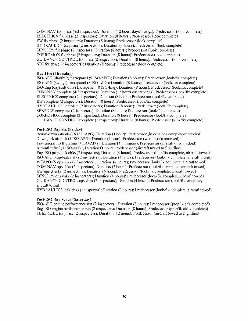
COM-NAV fix phase (4/3 inspectors); Duration (12 hours days/swings); Predecessor (look complete)

ELECTRICS fix phase (2 inspectors); Duration (8 hours); Predecessor (look complete)

EW fix phase (2 inspectors); Duration (8 hours); Predecessor (look complete)

HYDRAULICS fix phase (2 inspectors); Duration (8 hours); Predecessor (look complete)

SENSORS fix phase (2 inspectors); Duration (8 hours); Predecessor (look complete)

CORROSION fix phase (2 inspectors); Duration (8 hours)’ Predecessor (look complete)

GUIDANCE CONTROL fix phase (2 inspectors); Duration (8 hours); Predecessor (look complete)

NDI fix phase (2 inspectors); Duration (8 hours); Predecessor (look complete)

Day Five (Thursday)

ISO-APG (dayshift) fix/repanel (9 ISO-APG); Duration (8 hours); Predecessor (look/fix complete)

ISO-APG (swings) fix/repanel (8 ISO-APG); Duration (8 hours); Predecessor (look/fix complete)

ISO-Eng (dayshift only) fix/repanel (8 ISO-Eng); Duration (8 hours); Predecessor (look/fix complete)

COM-NAV complete (4/3 inspectors); Duration (12 hours days/swings); Predecessor (look/fix complete)

ELECTRICS complete (2 inspectors); Duration (8 hours); Predecessor (look/fix complete)

EW complete (2 inspectors); Duration (8 hours); Predecessor (look/fix complete)

HYDRAULICS complete (2 inspectors); Duration (8 hours); Predecessor (look/fix complete)

SENSORS complete (2 inspectors); Duration (8 hours); Predecessor (look/fix complete)

CORROSION complete (2 inspectors); Duration (8 hours)’ Predecessor (look/fix complete)

GUIDANCE CONTROL complete (2 inspectors); Duration (8 hours); Predecessor (look/fix complete)

Post-ISO Day Six (Friday)

Remove workstands (16 ISO-APG); Duration (1 hour); Predecessor (inspections complete/repaneled)

Down jack aircraft (7 ISO-APG); Duration (1 hour); Predecessor (workstands removed)

Tow aircraft to tlightline (7 ISO-APG); Duration (45 minutes); Predecessor (aircraft down jacked)

Aircraft refuel (3 ISO-APG); Duration (1 hour); Predecessor (aircraft towed to flightline)

Eng-ISO prop/leak chks (2 inspectors); Duration (4 hours); Predecessor (look/fix complete, aircraft towed)

ISO-APG prop/leak chks (2 inspectors); Duration (4 hours); Predecessor (look/fix complete, aircraft towed)

WEAPONS ops chks (2 inspectors); Duration (4 hours); Predecessor (look/fix complete, aircraft towed)

COM-NAV ops chks (2 inspectors); Duration (2 hours); Predecessor (look/fix complete, aircraft towed)

EW ops checks (2 inspectors); Duration (6 hours); Predecessor (look/fix complete, aircraft towed)

SENSORS ops chks (2 inspectors); Duration (4 hours); Predecessor (look/fix complete, aircraft towed)

GUIDANCE CONTROL ops chks (2 inspectors); Duration (4 hours); Predecessor (look/fix complete,

aircraft towed)

HYDRAULICS leak chks (1 inspector); Duration (2 hours); Predecessor (look/fix complete, aircraft towed)

Post-ISO Day Seven (Saturday)

ISO-APG engine performance run (2 inspectors); Duration (8 hours); Predecessor (prop/lk chk completed)

Eng-ISO engine performance run (2 inspectors); Duration (8 hours); Predecessor (prop/lk chk completed)

FUEL CELL fix phase (2 inspectors); Duration (12 hours); Predecessor (aircraft towed to flightline)

79

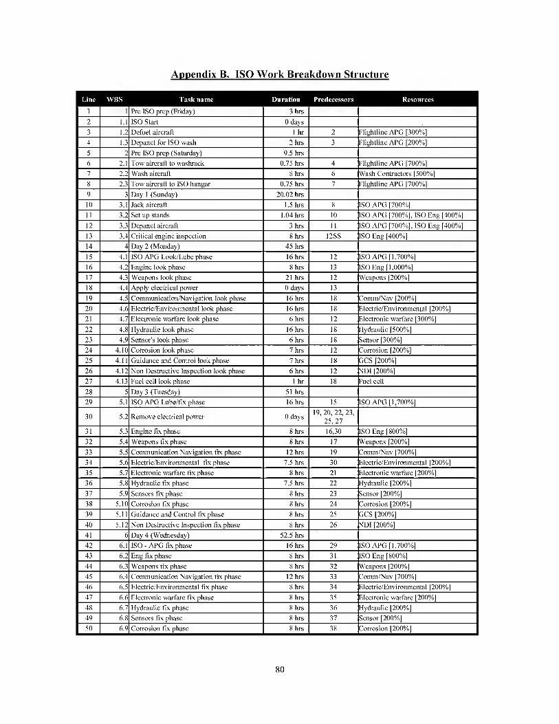
AoDendix B, ISO Work Breakdown Structure

Task name Duration Predecessors

Pre ISO prep (Friday) 3 hrs

ISO Start 0 days

Defuel aircraft 1 hr

Depanel for ISO wash 2 hrs

Pre ISO prep (Saturday) 9.5 hrs

Tow aircraft to washrack 0.75 hrs

Wash aircraft 8 hrs

Tow aircraft to ISO hangar 0.75 hrs

Day 1 (Sunday) 20.02 hrs

Jack aircraft 1.5 hrs

Set up stands 1.04 hrs

Depanel aircraft 3 hrs

Critical engine inspection 8 hrs

Day 2 (Monday) 45 hrs

ISO APG Look/Lube phase 16 hrs

Engine look phase 8 hrs

Weapons look phase 21 hrs

Apply electrical power 0 days

Communication/Navigation look phase 16 hrs

Electric/Environmental look phase 16 hrs

Electronic warfare look phase 6 hrs

Hydraulic look phase 16 hrs

Sensor's look phase 6 hrs

Corrosion look phase 7 hrs

Guidance and Control look phase 7 hrs

Non Destructive Inspection look phase 6 hrs

Fuel cell look phase 1 hr

Day 3 (Tuesday) 51 hrs

ISO APG Lube/fix phase 16 hrs

Remove electrical power 0 days

Engine fix phase 8 hrs

Weapons fix phase 8 hrs

Communication Navigation fix phase 12 hrs

Electric/Environmental fix phase 7.5 hrs

Electronic warfare fix phase 8 hrs

Hydraulic fix phase 7.5 hrs

Sensors fix phase 8 hrs

Corrosion fix phase 8 hrs

Guidance and Control fix phase 8 hrs

Non Destructive Inspection fix phase 8 hrs

Day 4 (Wednesday) 52.5 hrs

ISO - APG fix phase 16 hrs

Eng fix phase 8 hrs

Weapons fix phase 8 hrs

Communication Navigation fix phase 12 hrs

Electric/Environmental fix phase 8 hrs

Electronic warfare fix phase 8 hrs

Hydraulic fix phase 8 hrs

Sensors fix phase 8 hrs

Corrosion fix phase 8 hrs

Flightline APG [300%]

iFlightline APG [200%]

15

19, 20, 22, 23, 25, 27

16,30

17

19

30

21

22

23

24

25

26

Flightline APG [700%]

Wash Contractors [500%]

Flightline APG [700%]

ISO APG [700%]

ISO APG [700%], ISO Eng [400%]

ISO APG [700%], ISO Eng [400%]

|IS0 Eng [400%]

ISO APG [1,700%]

ISO Eng [1,000%]

[Weapons [200%]

3omm/Nav [200%]

Electric/Environmental [200%]

Electronic warfare [300%]

Hydraulic [500%]

[Sensor [300%]

;’orrosion [200%]

:iCS [200%]

DI [200%]

Fuel cell

ISO Eng [800%]

Weapons [200%]

2omm/Nav [700%]

Electric/Environmental [200%]

Electronic warfare [200%]

Hydraulic [200%]

>nsor [200%]

Corrosion [200%]

:SCS [200%]

,D1 [200%]

ISO APG [1,700%]

ISO Eng [800%]

Weapons [200%]

:omm/Nav [700%]

Electric/Environmental [200%

Electronic warfare [200%

Hydraulic [200%]

Sensor [200%]

:orrosion [200%]

80

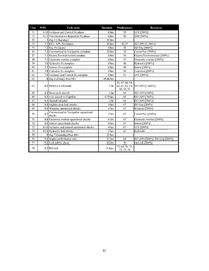
Line WBS Task name Duration Predecessors Resources

51 6.10 Guidance and Control fix pha.se 8 hrs 39 GCS [200%]

52 6.11 Non De.structive Inspection fix phase 8 hrs 40 NDl [200%]

53 7 Day 5 (Thursday) 55 hrs

54 7.1 ISO - APG fix/repanel 16 hrs 42,27 ISO APG [1,700%]

55 7.2 Eng fix/repanel 8 hrs 43 ISO Eng [800%]

56 7.3 Communication Navigation complete 12 hrs 45 Comm/Nav [700%]

57 7.4 Electric/Environmental complete 8 hrs 46 Electric/Environmental [200%]

58 7.5 Electronic warfare complete 8 hrs 47 Electronic warfare [200%]

59 7.6 Hydraulic fix complete 8 hrs 48 Hydraulic [200%]

7.7 Sensors fix complete 8 hrs 49 Sensor [200%]

61 7.8 Corrosion fix complete 8 hrs 50 Corrosion [200%]

62 7.9 Guidance and Control fix complete 8 hrs 51 GCS [200%]

63 8 Day 6 (Friday) Post ISO 19.48 hrs

64 8.1 Remove work.stands 1 hr 55, 57, 58, 59, 60,61,62, 54,

56, 44, 52 ISO APG [1,600%]

65 8.2 Down jack aircraft 1 hr 64 ISO APG [700%]

66 8.3 Tow aircraft to flightline 0.75 hrs 65 ISO APG [700%]

67 8.4 Aircraft refueled 1 hr 66 ISO APG [300%]

68 8.5 Engines prop leak checks 4 hrs 67 ISO Eng [200%]

69 8.6 Weapons operational checks 4 hrs 67 Weapons [200%]

70 8.7 Communication Navigation operational checks

2 hrs 67 Comm/Nav [200%]

71 8.8 Electronic warfare operational checks 6 hrs 67 Electronic warfare [200%]

72 8.9 Sensors operational checks 4 hrs 67 Sensor [200%]

73 8.10 Guidance and control operational checks 4 hrs 67 GCS [200%]

74 8.11 Hydraulic leak checks 2 hrs 67 Hydraulic

75 9 Day 7 (Saturday) Post ISO 23 hrs

76 9.1 Engine performance runs 11 hrs 68 ISO APG [200%], ISO Eng [200%]

77 mg Fuel cell fix pha.sc 12 hrs 76 Fuel cell [200%]

78 9.3 ISO end 0 days 77, 69, 70,71,

72, 73, 74

81

Appendix C. ISO Manning Requirements

AFSC Name Authorized Manning

Level

Current Manning

Level

2A5X1J Airplane General (Crew Chief) 17 17

2A6X1B Engines 10 10

2A6X6 Electric/Environmental 2 2

2A1X7 Electronic Warfare 2 2

2A6X5 Hydraulic 5 5

2A1X1 Sensors 2 2

Corrosion 2 2

2A4X1 Guidance and Control (GCS) 2 2

2A7X2 Nondestructive Inspection (NDI) 2 2

Fuel Cell 2 2

2A1X3 Communication/Navigation

(Comm/Nav)

7 7

Weapons 2 2

N/A Aircraft Wash Crew (Contractor) 5 5

2A7X3 Aircraft Structural Maintenance See Corrosion See Corrosion

82

AoDendix D. Simulation Values

83

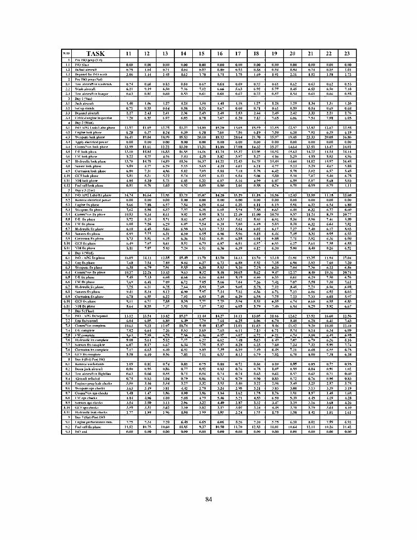
84

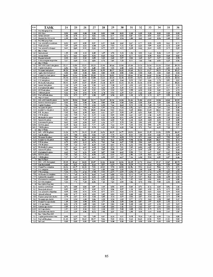
85

86

87

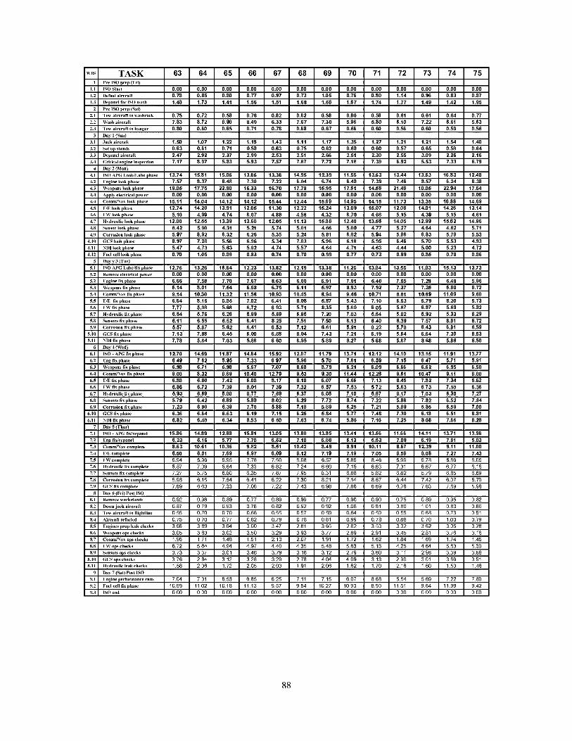
88

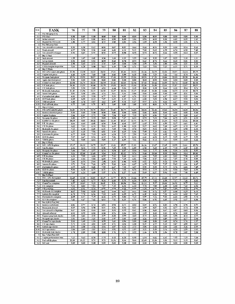
89

90

AoDendix E. Simulation Results

Simulation Ml M2 M3 Work Simulation Ml M2 M3 Work

1 211.90 144.00 100.22 2145.65 SI 208.24 144.10 94.58 2071.83 2 209.27 141.42 97.74 2156.73 52 208.36 150.58 93.29 2143.42

3 209.52 140.92 89.17 2019.72 53 206.19 160.78 95.01 2070.68

4 208.46 144.10 92.21 2129.17 54 206.56 142.46 87.09 2081.32 5 207.77 142.38 90.78 2099.95 55 208.34 139.55 86.60 2019.72

6 207.38 139.30 90.53 2100.52 56 208.95 152.32 97.17 2191.00

7 206.76 141.99 88.20 2074.88 57 211.53 154.20 102.13 2167.02

8 209.77 151.94 100.83 2170.83 58 207.58 139.03 94.26 2093.47

9 206.91 159.86 95.29 2109.03 59 211.42 153.09 92.20 2061.43 10 207.22 151.36 89.72 2116.77 60 210.14 146.15 97.05 2165.38

11 208.70 140.20 95.24 2161.42 61 206.33 161.79 92.75 2143.48

12 206.25 159.94 93.83 2163.12 62 210.40 145.70 91.73 2075.02

13 207.30 160.09 94.21 2130.68 63 207.93 142.88 95.91 2115.83

14 210.10 163.02 97.31 2189.87 64 209.30 162.45 98.23 2202.03

15 206.69 159.80 93.53 2081.53 65 207.14 142.41 97.27 2149.53

16 210.46 152.55 97.36 2182.62 66 208.64 144.08 96.26 2192.67

17 209.98 145.15 97.15 2195.87 67 206.23 159.56 91.72 2169.15 18 213.28 144.50 103.88 2106.42 68 206.82 137.98 93.21 2077.48 19 207.88 143.69 85.61 2024.33 69 210.07 152.98 91.95 2057.63 20 207.31 161.25 95.78 2075.55 70 209.14 152.43 87.88 2047.73 21 212.35 143.58 102.91 2093.48 71 206.87 138.51 88.30 2088.58 22 209.34 152.64 90.96 2095.93 72 208.10 143.73 96.42 2067.27

23 208.93 161.09 96.44 2202.05 73 206.98 139.26 94.43 2123.27 24 209.79 152.31 94.39 2141.75 74 210.79 162.94 100.59 2186.07

25 208.33 160.53 94.81 2068.02 75 207.98 140.01 90.26 2084.42

26 208.94 140.06 98.12 2065.28 76 211.14 153.91 98.27 2140.77 27 207.07 138.33 90.95 2095.25 77 208.99 163.25 94.89 2170.32

28 137.13 2095.00 78 206.89 142.85 84.78 2017.22

29 RiiaCT 137.86 wgnBil 2116.95 79 208.23 163.80 95.74 2091.25

30 RildKa 160.56 MEHtSfl 2109.70 80 208.74 152.97 96.98 2172.28

31 206.30 142.03 95.30 2147.98 81 209.73 151.77 99.40 2176.73

32 207.54 159.57 92.40 2163.48 82 205.67 140.72 94.73 2168.82 33 210.70 164.21 98.35 2171.12 83 210.64 165.46 99.68 2188.68

34 207.36 138.42 92.40 2113.77 84 213.50 155.01 101.34 2115.38

35 208.47 140.18 92.94 2105.53 85 207.72 143.15 95.10 2076.15

36 207.52 161.65 97.75 2223.52 86 206.12 140.38 95.41 2151.72

37 206.86 138.11 89.03 2050.03 87 207.29 140.77 91.08 2110.17

38 209.36 151.61 96.84 2134.32 88 207.05 151.21 91.09 2081.22

39 208.53 144.41 89.21 2060.55 89 207.12 140.07 90.40 2108.23

40 210.59 152.73 96.07 2122.60 90 213.41 155.12 100.28 2135.03

41 209.27 144.56 95.83 2140.27 91 207.00 150.26 97.91 2021.13

42 210.98 164.31 99.30 2194.23 92 210.34 159.68 95.63 2174.12

43 209.58 150.91 101.46 2121.98 93 208.16 160.66 97.01 2186.35

44 210.88 154.78 97.77 2175.63 94 207.57 154.54 96.30 2140.17 45 208.37 139.19 90.82 2065.42 95 208.55 137.69 89.42 2047.52

46 208.37 150.45 93.70 2111.77 96 210.33 163.36 100.80 2070.83

47 206.23 141.81 88.01 2044.27 97 209.19 153.20 91.96 2105.80

48 208.84 151.51 93.62 2094.25 98 208.71 161.06 89.07 2062.27

49 206.75 138.11 88.47 2040.67 99 213.69 167.80 104.95 2253.93 50 208.70 161.48 99.27 2082.37 100 209.32 153.84 98.52 2201.53

91

Appendix F. Shai

Distributions

M1

M2

M3

9

Normal{208.654,1.800891 pjttGCl NormsI

Goodness-of-Fit Test

Shapiro-Wilk W Test

W Prob<W

0.936889 0.0001

-Normal(149.931,8.89819 Fitted Normai

Goodness-of-Fit Test

Shapiro-Wilk W Test

W Prob<W

0.896559 <.0001

Normal(94.64,4.23768 Fitted Normai

Goodness-of-Fit Test

Shapiro-Wilk W Test

W Prob<W

0.982517 0.6609

93

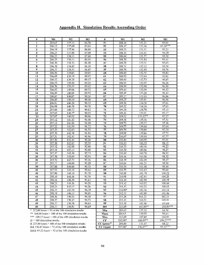
Appendix H. Simulation Results Ascending Order

# Ml M2 M3 # Ml M2 M3

1 205.67 137.13 84.78 51 208.46 151.21 95.01

2 206.12 137.69 85.61 52 208.47 151.36 95.10“*

3 206.19 137.86 86.60 53 208.53 151.51 95.24

4 206.23 137.98 87.09 54 208.55 151.61 95.29

5 206.23 138.11 87.88 55 208.64 151.77 95.30

6 206.25 138.11 88.01 56 208.70 151.94 95.41

7 206.30 138.33 88.20 57 208.70 152.31 95.63

8 206.30 138.42 88.30 58 208.71 152.32 95.74

9 206.33 138.51 88.47 59 208.74 152.43 95.78

10 206.56 139.03 89.03 60 208.84 152.55 95.83

11 206.69 139.19 89.07 61 208.93 152.64 95.91

12 206.72 139.26 89.17 62 208.94 152.73 96.07

13 206.75 139.30 89.21 63 208.95 152.97 96.26

14 206.76 139.55 89.42 64 208.99 152.98 96.30

15 206.82 140.01 89.72 65 209.14 153.09 96.42

16 206.86 140.06 89.92 66 209.19 153.20 96.44

17 206.87 140.07 90.26 67 209.27 153.84 96.84

18 206.89 140.18 90.40 68 209.27 153.91 96.98

19 206.91 140.20 90.53 69 209.30 154.20 97.01

20 206.98 140.38 90.78 70 209.32 154.54 97.05

21 207.00 140.72 90.82 71 209.34 154.78 97.15

22 207.05 140.77 90.95 72 209.36 155.01 97.17

'23 207.07 140.92 90.96 73 209.52 155.12“ 97.27

24 207.12 141.42 91.08 74 209.58 159.56 97.31

25 207.14 141.81 91.09 75 209.73 159.57 97.36

26 207.22 141.99 91.72 76 209.77 159.68 97.64

27 207.29 142.03 91.73 77 209.79 159.80 97.74

28 207.30 142.38 91.95 78 209.98 159.86 97.75

29 207.31 142.41 91.96 79 210.07 159.94 97.77

30 207.36 142.46 92.20 80 210.10 160.09 97.91

31 207.38 142.85 92.21 81 210.14 160.53 98.12

32 207.52 142.88 92.40 82 210.33 160.56 98.23

33 207.54 143.15 92.40 83 210.34 160.66 98.27

34 207.57 143.58 92.75 84 210.40 160.78 98.35

35 207.58 143.69 92.94 85 210.46 161.06 98.52

36 207.72 143.73 93.21 86 210.59 161.09 99.27

37 207.77 144.00 93.29 87 210.64 161.25 99.30

38 207.88 144.08 93.53 88 210.70 161.48 99.40

39 207.93 144.10 93.62 89 210.79 161.65 99.68

40 207.98 144.10 93.70 90 210.88 161.79 100.22

41 208.10 144.41 93.70 91 210.98 162.45 100.28

42 208.16 144.50 93.83 92 211.14 162.94 100.59

43 208.23 144.56 94.21 93 211.42 163.02 100.80

44 208.24 145.15 94.26 94 211.53 163.25 100.83

45 208.33 145.70 94.39 95 211.90* 163.36 101.34

46 208.34 146.15 94.43 96 212.35 163.80 101.46

47 208.36 150.26 94.58 97 213.28 164.21 102.13

48 208.37 150.45 94.73 98 213.41 164.31 102.91

49 208.37 150.58 94.81 99 213.50 165.46 103.88

50 208.37 150.91 94.89 100 213.69 167.80** 104.95***

* 212.00 hours > 95 of the 100 simulation results

** 168.00 hours > 100 of the 100 simulation results

*** 109.27 hours > 100 of the 100 simulation results

@ < 100 simulation results

& 237.00 hours > 100 of the 100 simulation results

&& 156.87 hours > 73 of the 100 simulation results

Min 205.67 137.13 84.78

Mean 208.65 149.93 94.64

Max 213.69 167.80 104.95

CP 212.00* 168.00** 109.27***

CC Lower* 204.00 111.87 68.22

CC Upper 237.00* 156.87“ 95.22***

&&& 95.22 hours > 52 of the 100 simulation results

94

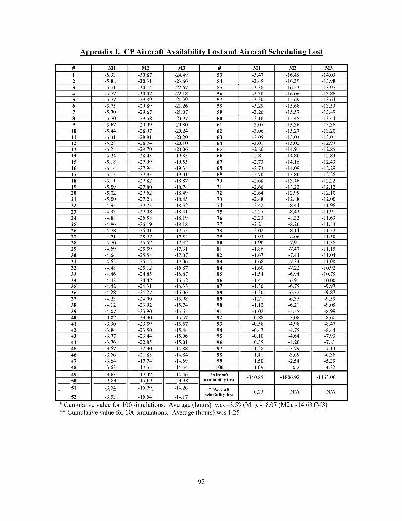
Appendix 1. CP Aircraft Availability Lost and Aircraft Scheduling Lost

# Ml M2 M3 # Ml M2 M3

1 -6.33 -30.87 -24.49 S3 -3.47 -16.49 -14.03 2 -5.88 -30.31 -23.66 54 -3.45 -16.39 -13.98 3 -5.81 -30.14 -22.67 55 -3.36 -16.23 -13.97 4 -5.77 -30.02 -22.18 56 -3.30 -16.06 -13.86 5 -5.77 -29.89 -21.39 57 -3.30 -15.69 -13.64 6 -5.75 -29.89 -21.26 58 -3.29 -15.68 -13.53 7 -5.70 -29.67 -21.07 59 -3.26 -15.57 -13.49 8 -5.70 -29.58 -20.97 60 -3.16 -15.45 -13.44 9 -5.67 -29.49 -20.80 61 -3.07 -15.36 -13.36 10 -5.44 -28.97 -20.24 62 -3.06 -15.27 -13.20 11 -5.31 -28.81 -20.20 63 -3.05 -15.03 -13.01 12 -5.28 -28.74 -20.10 64 -3.01 -15.02 -12.97 13 -5.25 -28.70 -20.06 65 -2.86 -14.91 -12.85 14 -5.24 -28.45 -19.85 66 -2.81 -14.80 -12.83 15 -5.18 -27.99 -19.55 67 -2.73 -14.16 -12.43 16 -5.14 -27.94 -19.35 68 -2.73 -14.09 -12.29 17 -5.13 -27.93 -19.01 69 -2.70 -13.80 -12.26 18 -5.11 -27.82 -18.87 70 -2.68 -13.46 -12.22 19 -5.09 -27.80 -18.74 71 -2.66 -13.22 -12.12 20 -5.02 -27.62 -18.49 72 -2.64 -12.99 -12.10 21 -5.00 -27.28 -18.45 73 -2.48 -12.88 -12.00 22 -4.95 -27.23 -18.32 74 -2.42 -8.44 -11.96 23 -4.93 -27.08 -18.31 75 -2.27 -8.43 -11.91 24 -4.88 -26.58 -18.19 76 -2.23 -8.32 -11.63 25 -4.86 -26.19 -18.18 77 -2.21 -8.20 -11.53 26 -4.78 -26.01 -17.55 78 -2.02 00

-11.52 27 -4.71 -25.97 -17.54 79 -1.93 -8.06 -11.50 28 -4.70 -25.62 -17.32 80 -1.90 -7.91 -11.36 29 -4.69 -25.59 -17.31 81 -1.86 -7.47 -11.15 30 -4.64 -25.54 -17.07 82 -1.67 -7.44 -11.04 31 -4.62 -25.15 -17.06 83 -1.66 -7.34 -11.00 32 -4.48 -25.12 -16.87 84 -1.60 -7.22 -10.92 33 -4.46 -24.85 -16.87 85 -1.54 -6.94 -10.75 34 -4.43 -24.42 -16.52 86 -1.41 -6.91 -10.00 35 -4.42 -24.31 -16.33 87 -1.36 -6.75 -9.97 36 -4.28 -24.27 -16.06 88 -1.30 -6.52 -9.87 37 -4.23 -24.00 -15.98 89 -1.21 -6.35 -9.59 38 -4.12 -23.92 -15.74 90 -1.12 -6.21 -9.05 39 -4.07 -23.90 -15.65 91 -1.02 -5.55 -8.99 40 -4.02 -23.90 -15.57 92 -0.86 -5.06 -8.68 41 -3.90 -23.59 -15.57 93 -0.58 -4.98 -8.47 42 -3.84 -23.50 -15.44 94 -0.47 -4.75 -8.44 43 -3.77 -23.44 -15.06 95 -0.10 -4.64 -7.93 44 -3.76 -22.85 -15.01 96 0.35 -4.20 -7.81 45 -3.67 -22.30 -14.88 97 1.28 -3.79 -7.14 46 -3.66 -21.85 -14.84 98 1.41 -3.69 -6.36 47 -3.64 -17.74 -14.69 99 1.50 -2.54 -5.39 48 -3.63 -17.55 -14.54 100 1.69 -0.2 -4.32

49 -3.63 -17.42 -14.46 *Aircraff availability lost -340.85 -1806.92 -1463.00

50 -3.63 -17.09 -14.38

51 -3.54 -16.79 -14.26 **Aircraft scheduling lost 6.23 N/A N/A

52 -3.53 -16.64 -14.17

* Cumulative value for 100 simulations. Average (hours) was-3.59 (Ml), -18.07 (M2), -14.63 (M3) ** Cumulative value for 100 simulations. Average (hours) was 1.25

95

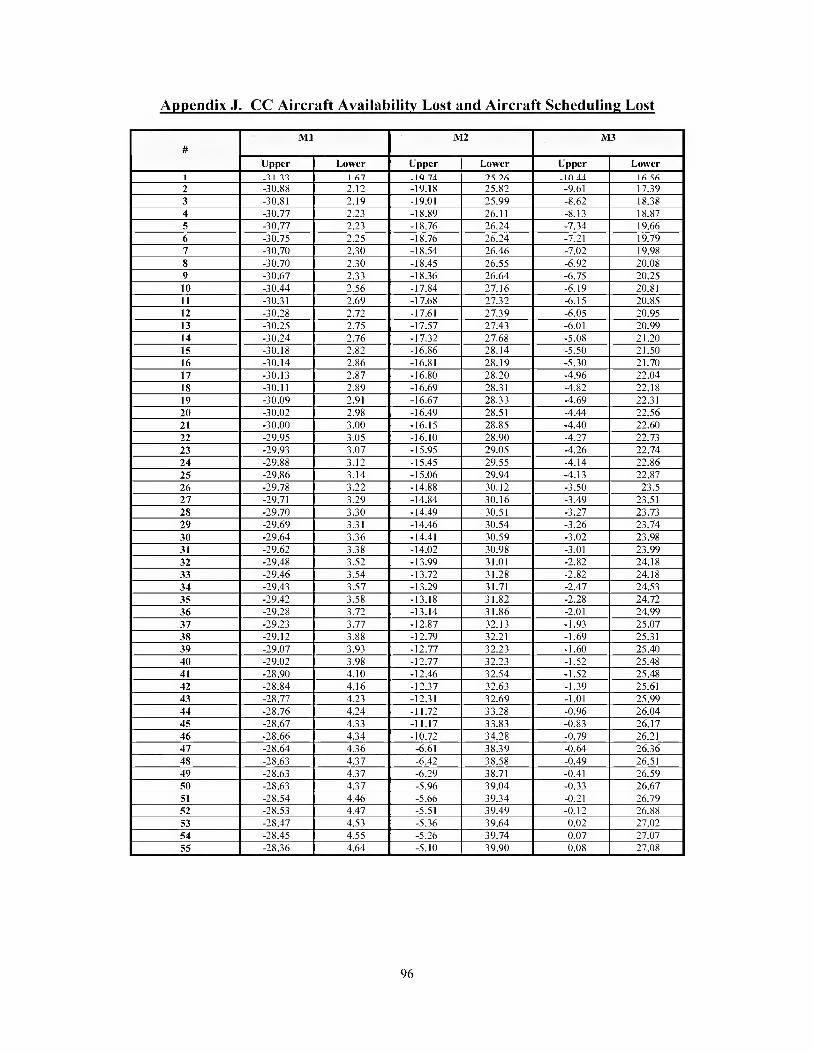
AoDendix J. CC Aircraft Availabilitv Lost and Aircraft Scheduling Lost

Ml M2 M3 #

Upper Lower Upper Lower Upper Lower

1 -'tl 1 fn -IQ 74 -in 44

2 -30.88 2.12 -19.18 25.82 -9.61 17.39

3 -30.81 2.19 -19.01 25.99 -8.62 18.38

4 -30.77 2.23 -18.89 26.11 -8.13 18.87

5 -30.77 2.23 -18.76 26.24 -7.34 19.66

6 -30.75 2.25 -18.76 26.24 -7.21 19.79

7 -30.70 2.30 -18.54 26.46 -7.02 19.98

8 -30.70 2.30 -18.45 26.55 -6.92 20.08

9 -30.67 2.33 -18.36 26.64 -6.75 20.25

10 -30.44 2.56 -17.84 27.16 -6.19 20.81

11 -30.31 2.69 -17.68 27.32 -6.15 20.85

12 -30.28 2.72 -17.61 27.39 -6.05 20.95

13 -30.25 2.75 -17.57 27.43 -6.01 20.99

14 -30.24 2.76 -17.32 27.68 -5.08 21.20

15 -30.18 2.82 -16.86 28.14 -5.50 21.50

16 -30.14 2.86 -16.81 28.19 -5.30 21.70

17 -30.13 2.87 -16.80 28.20 -4.96 22.04

18 -30.11 2.89 -16.69 28.31 -4.82 22.18

19 -30.09 2.91 -16.67 28.33 -4.69 22.31

20 -30.02 2.98 -16.49 28.51 -4.44 22.56

21 -30.00 3.00 -16.15 28.85 -4.40 22.60

22 -29.95 3.05 -16.10 28.90 -4.27 22.73

23 -29.93 3.07 -15.95 29.05 -4.26 22.74

24 -29.88 3.12 -15.45 29.55 -4.14 22.86

25 -29.86 3.14 -15.06 29.94 -4.13 22.87

26 -29.78 3.22 -14.88 30.12 23.5

27 -29.71 3.29 -14.84 30.16 -3.49 23.51

28 -29.70 3.30 -14.49 30.51 -3.27 23.73

29 -29.69 3.31 -14.46 30.54 -3.26 23.74

30 -29.64 3.36 -14.41 30.59 -3.02 23.98

31 -29.62 3.38 -14.02 30.98 -3.01 23.99

32 -29.48 3.52 -13.99 31.01 -2.82 24.18

33 -29.46 3.54 -13.72 31.28 -2.82 24.18

34 -29.43 3.57 -13.29 31.71 -2.47 24.53

35 -29.42 3.58 -13.18 31.82 -2.28 24.72

36 -29.28 3.72 -13.14 31.86 -2.01 24.99

37 -29.23 3.77 -12.87 32.13 -1.93 25.07

38 -29.12 3.88 -12.79 32.21 -1.69 25.31

39 -29.07 3.93 -12.77 32.23 -1.60 25.40

40 -29.02 3.98 -12.77 32.23 -1.52 25.48

41 -28.90 4.10 -12.46 32.54 -1.52 25.48

42 -28.84 4.16 -12.37 32.63 -1.39 25.61

43 -28.77 4.23 -12.31 32.69 -1.01 25.99

44 -28.76 4.24 -11.72 33.28 -0.96 26.04

45 -28.67 4.33 -11.17 33.83 -0.83 26.17

46 -28.66 4.34 -10.72 34.28 -0.79 26.21

47 -28.64 4.36 -6.61 38.39 -0.64 26.36

48 -28.63 4.37 -6.42 38.58 -0.49 26.51

49 -28.63 4.37 -6.29 38.71 -0.41 26.59

50 -28.63 4.37 -5.96 39.04 -0.33 26.67

51 -28.54 4.46 -5.66 39.34 -0.21 26.79

52 -28.53 4.47 -5.51 39.49 -0.12 26.88

53 -28.47 4.53 -5.36 39.64 0.02 27.02

54 -28.45 4.55 -5.26 39.74 0.07 27.07

55 -28.36 4.64 -5.10 39.90 0.08 27.08

96

#

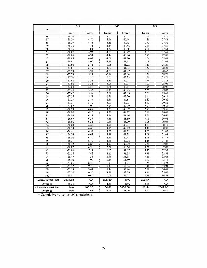
Ml M2 M3

Upper Lower Upper Lower Upper Lower

-9k 90 4 70 -4 09 40 07 0 10 97 10

57 -28.30 4.70 -4.56 40.44 0.41 27.41

58 -28.29 4.71 -4.55 40.45 0.52 27.52

59 -28.26 4.74 -4.44 40.56 0.56 27.56

60 -28.16 4.84 -4.32 40.68 0.61 27.61

61 -28.07 4.93 -4.23 40.77 0.69 27.69

62 -28.06 4.94 -4.14 40.86 0.85 27.85

63 -28.05 4.95 -3.90 41.10 1.04 28.04

64 -28.01 4.99 -3.89 41.11 1.08 28.08

65 -27.86 5.14 -3.78 41.22 1.20 28.20

66 -27.81 5.19 -3.67 41.33 1.22 28.22

67 -27.73 5.27 -3.03 41.97 1.62 28.62

68 -27.73 5.27 -2.96 42.04 1.76 28.76

69 -27.70 5.30 -2.67 42.33 1.79 28.79

70 -27.68 5.32 -2.33 42.67 1.83 28.83

71 -27.66 5.34 -2.09 42.91 1.93 28.93

72 -27.64 5.36 -1.86 43.14 1.95 28.95

73 -27.48 5.52 -1.75 43.25 2.05 29.05

74 -27.42 5.58 2.69 47.69 2.09 29.09

75 -27.27 5.73 2.70 47.70 2.14 29.14

76 -27.23 5.77 2.81 47.81 2.42 29.42

77 -27.21 5.79 2.93 47.93 2.52 29.52

78 -27.02 5.98 2.99 47.99 2.53 29.53

79 -26.93 6.07 3.07 48.07 2.55 29.55

80 -26.90 6.10 3.22 48.22 2.69 29.69

81 -26.86 6.14 3.66 48.66 2.90 29.90

82 -26.67 6.33 3.69 48.69 3.01 30.01

83 -26.66 6.34 3.79 48.79 3.05 30.05

84 -26.60 6.40 3.91 48.91 3.13 30.13

85 -26.54 6.46 4.19 49.19 3.30 30.30

86 -26.41 6.59 4.22 49.22 4.05 31.05

87 -26.36 6.64 4.38 49.38 4.08 31.08

88 -26.30 6.70 4.61 49.61 4.18 31.18

89 -26.21 6.79 4.78 49.78 4.46 31.46

90 -26.12 6.88 4.92 49.92 5.00 32.00

91 -26.02 6.98 5.58 50.58 5.06 32.06

92 -25.86 7.14 6.07 51.07 5.37 32.37

93 -25.58 7.42 6.15 51.15 5.58 32.58

94 -25.47 7.53 6.38 51.38 5.61 32.61

95 -25.10 6.49 51.49 6.12 33.12

96 -24.65 8.35 6.93 51.93 6.24 33.24

97 -23.72 9.28 7.34 52.34 6.91 33.91

98 -23.59 9.41 7.44 52.44 7.69 34.69

99 -23.50 9.50 8.59 53.59 8.66 35.66

100 -23.31 9.69 10.93 55.93 9.73 36.73

-2834.62 N/A N/A -200.54 N/A

Average -28.35 N/A -11.31 N/A -3.86 N/A

*Aircraft schecl. lost N/A 465.38 134.46 142.54 2642.00

Average N/A 4.65 4.98 38.06 1 2.97 26.42

* Cumulative value for 100 simulations.

97

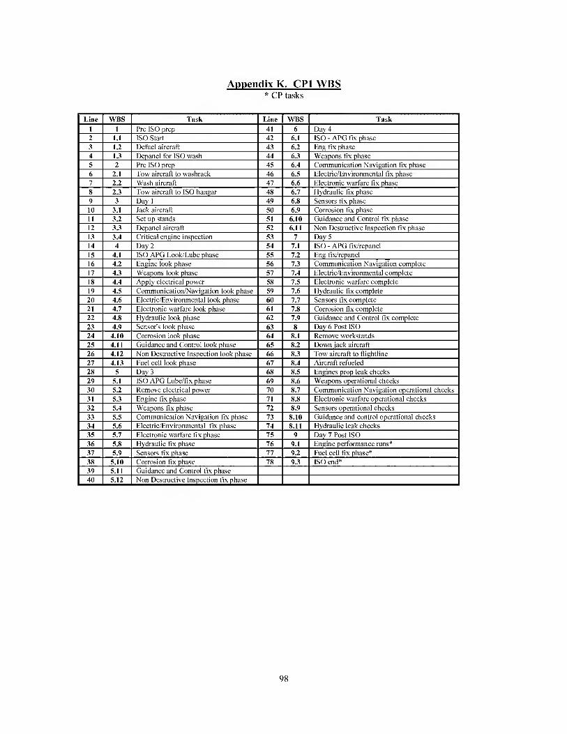
Appendix K. CPI WBS * CP tasks

Line WBS Line WBS Task Task

1 1 Pre ISO prep 41 6 Day 4 2 1.1 ISO Start 42 6.1 ISO - APG fix phase 3 1.2 Defuel aireraft 6.2 Eng fix phase

4 1.3 Depanel for ISO wash 44 6.3 Weapons fix phase 5 2 Pre ISO prep 45 6.4 Communication Navigation fix phase

6 2.1 Tow aircraft to washrack 46 6.5 Electric/Environmental fix phase 7 2.2 Wash aircraft 47 6.6 Electronic warfare fix phase 8 2.3 Tow aircraft to ISO hangar 48 6.7 Hydraulic fix phase 9 3 Day I 49 6.8 Sensors fix phase 10 3.1 Jack aircraft 6.9 Corrosion fix phase

11 3.2 Set up stands 51 6.10 Guidance and Control fix phase 12 3.3 Depanel aircraft 52 6.11 Non Destructive Inspection fix phase

3.4 Critical engine inspection 7 Day 5 14 4 Day 2 1 54 1 7.1 ISO - APG fix/repanel 15 4.1 ISO APG Look/Lube phase 7.2 Eng fix/repanel 16 4.2 56 7.3 Communication Navigation complete 17 4.3 57 7.4 Electric/Environmental complete 18 4.4 Apply electrical power 58 7.5 Electronic warfare complete

19 4.5 Communication/Navigation look phase 59 7.6 Hydraulic fix complete

20 4.6 Electric/Environmental look phase 7.7 Sensors fix complete

mm 4.7 Electronic warfare look phase 61 7.8 Corrosion fix complete 4.8 Hydraulic look phase 62 7.9 Guidance and Control fix complete

4.9 Sensor's look phase 63 8 Day 6 Post ISO

mm 4.10 Corrosion look phase 64 8.1 Remove workstands

ra 4.11 Guidance and Control look phase 65 8.2 Down jack aircraft

26 4.12 Non Destructive Inspection look phase 8.3 Tow aircraft to flightline

27 4.13 Fuel cell look phase 67 8.4 Aircraft refueled

28 5 Day 3 68 8.5 Engines prop leak checks

29 5.1 ISO APG Lubc/fix phase 69 8.6 Weapons operational checks

mm 5.2 Remove electrical power 70 8.7 Communication Navigation operational cheeks

mm 5.3 Engine fix phase 71 8.8 Electronic warfare operational cheeks

KS 5.4 72 8.9 Sensors operational checks 5.5 Communication Navigation fix phase mm 8.10 Guidance and control operational checks 5.6 Electric/Environmental fix phase 74 8.11 Hydraulic leak checks

35 5.7 Electronic warfare fix phase 75 9 Day 7 Post ISO 36 5.8 Hydraulic fix phase 76 9.1 Engine performance runs* 37 5.9 Sensors fix phase 77 9.2 Fuel cell fix phase* 38 5.10 Corrosion fix phase 78 9.3 ISO end* 39 5.11 Guidance and Control fix phase 40 5.12 Non Destructive Inspection fix phase

98

Appendix L. CP2 WBS * CP tasks

Line WBS Task WBS Task

1 1 Pre ISO prep 41 6 2 1.1 ISO Start 42 6.1 ISO - APG fix phase 3 1.2 Defuel aircraft 43 6.2 Eng fix phase

4 1.3 Depanel for ISO wash 44 6.3 Weapons fix phase 5 2 Pre ISO prep 45 6.4 Communication Navigation fix phase

6 2.1 Tow aircraft to washrack 46 6.5 Electric/Environmental fix phase 7 2.2 Wash aircraft 47 6.6 Electronic warfare fix phase 8 2.3 Tow aircraft to ISO hangar 48 6.7 Hydraulic fix phase 9 3 49 6.8 Sensors fix phase 10 3.1 Jack aircraft 6.9 Corrosion fix phase 11 3.2 Set up stands 51 6.10 Guidance and Control fix phase 12 3.3 Depanel aircraft 52 6.11 Non Destructive Inspection fix phase

13 3.4 Critical engine inspection 53 7

bei 4 54 7.1 ISO - APG fix/repanel 15 4.1 ISO APG Look/Lube phase 55 7.2 Eng fix/repanel 16 4.2 Engine look phase 56 7.3 Communication Navigation complete 17 4.3 Weapons look phase 57 7.4 Electric/Environmental complete 18 4.4 Apply electrical power 58 7.5 Electronic warfare complete 19 4.5 Communication/Navigation look phase 59 7.6 Hydraulic fix complete 20 4.6 Electric/Environmental look phase 60 7.7 Sensors fix complete 21 4.7 Electronic warfare look phase 61 7.8 Corrosion fix complete

4.8 Hydraulic look phase 7.9 Guidance and Control fix complete

23 4.9 Sensor's look phase 63 8 Post ISO 24 4.10 Corrosion look phase 64 8.1 Remove workstands

25 4.11 Guidance and Control look phase 65 8.2 Down jack aircraft

26 4.12 Non Destructive Inspection look phase 66 8.3 Tow aircraft to flightline

4.13 Fuel cell look phase 67 8.4 Aircraft refueled* 5 Ba 8.5 Engines prop leak checks

1291 5.1 ISO APG Lube/flx phase 1 69 1 8.6 Weapons operational checks

mm 5.2 Remove electrical power 8.7 Communication Navigation operational checks

l 31 5.3 8.8 Electronic warfare operational checks

Ka 5.4 8.9 Sensors operational checks

5.5 mm 8.10 Guidance and control operational checks

1 34 5.6 Electric/Environmental fix phase 74 8.11 Hydraulic leak checks 5.7 Electronic warfare fix phase 75 9 Post ISO

36 5.8 Hydraulic fix phase 76 9.1 Engine performance runs* 37 5.9 Sensors fix phase 77 9.2 Fuel cell fix phase*

38 5.10 Corrosion fix phase 78 9.3 ISO end* 39 5.11 Guidance and Control fix phase 40 5.12 Non Destructive Inspection fix phase

99

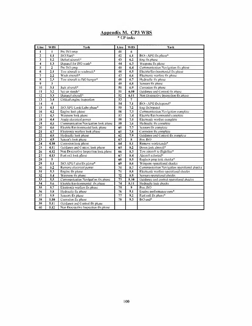
Appendix M. CP3 WBS * CP tasks

Line WBS Task WBS Task

1 1 Pre ISO prep 41 6 2 1.1 ISO Start* 42 6.1 ISO - APG fix phase* 3 1.2 Defuel aircraft* 43 6.2 Eng fix phase

4 1.3 Depanel for ISO wash* 44 6.3 Weapons fix phase 5 2 Pre ISO prep 45 6.4 Communication Navigation fix phase

6 2.1 Tow aircraft to washrack* 46 6.5 Electric/Environmental fix phase 7 2.2 Wash aircraft* 47 6.6 Electronic warfare fix phase 8 2.3 Tow aircraft to ISO hangar* 48 6.7 Hydraulic fix phase 9 3 49 6.8 Sensors fix phase 10 3.1 Jack aircraft* 6.9 Corrosion fix phase 11 3.2 Set up stands* 51 6.10 Guidance and Control fix phase 12 3.3 Depanel aircraft* 52 6.11 Non Destructive Inspection fix phase

13 3.4 Critical engine inspection 53 7

bei 4 54 7.1 ISO - APG fix/repanel* 15 4.1 ISO APG Look/Lube phase* 55 7.2 Eng fix/repanel 16 4.2 Engine look phase 56 7.3 Communication Navigation complete 17 4.3 Weapons look phase 57 7.4 Electric/Environmental complete 18 4.4 Apply electrical power 58 7.5 Electronic warfare complete 19 4.5 Communication/Navigation look phase 59 7.6 Hydraulic fix complete 20 4.6 Electric/Environmental look phase 60 7.7 Sensors fix complete 21 4.7 Electronic warfare look phase 61 7.8 Corrosion fix complete

4.8 Hydraulic look phase 7.9 Guidance and Control fix complete

23 4.9 Sensor's look phase 63 8 Post ISO 24 4.10 Corrosion look phase 64 8.1 Remove workstands*

25 4.11 Guidance and Control look phase 65 8.2 Down jack aircraft*

26 4.12 Non Destructive Inspection look phase 66 8.3 Tow aircraft to flightline*

4.13 Fuel cell look phase 67 8.4 Aircraft refueled* 5 68 8.5 Engines prop leak checks*

1291 5.1 ISO APG Lube/flx phase* 69 8.6 Weapons operational checks

mm 5.2 Remove electrical power KEMi 8.7 Communication Navigation operational checks

l 31 5.3 warn 8.8 Electronic warfare operational checks

Ka 5.4 \ 72 1 8.9 Sensors operational checks

5.5 mm 8.10 Guidance and control operational checks

1 34 5.6 Electric/Environmental fix phase 74 8.11 Hydraulic leak checks 5.7 Electronic warfare fix phase 75 9 Post ISO

36 5.8 Hydraulic fix phase 76 9.1 Engine performance runs* 37 5.9 Sensors fix phase 77 9.2 Fuel cell fix phase*

38 5.10 Corrosion fix phase 78 9.3 ISO end* 39 5.11 Guidance and Control fix phase 40 5.12 Non Destructive Inspection fix phase

100

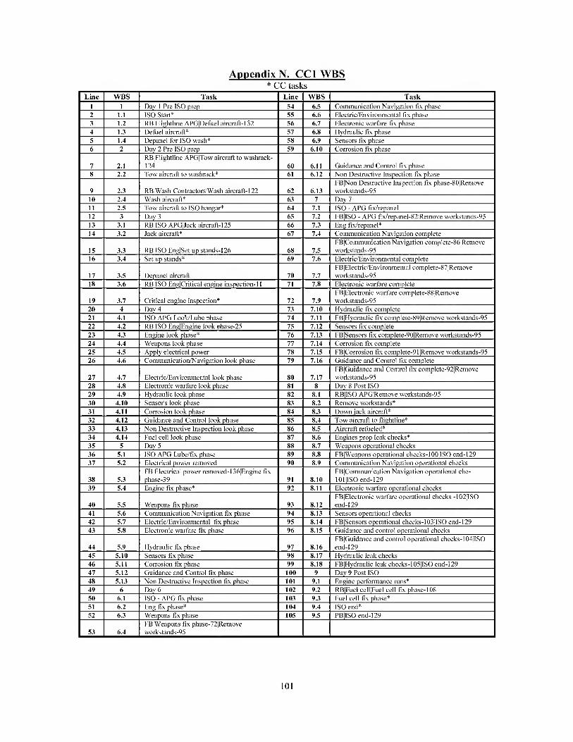
ADoendix N. CCl WBS * CC tasks

ISO Start* RBIFlightline APGiDefuel aircraft-132 Defuel aircraft*

Day 2 Pre ISO prep RB|Flightline APGjTow aircraft to washrack- 124 Tow aircraft to washrack*

RBIWash ContractorsIWash aircraft-122 Wash aircraft* Tow aircraft to ISO hanaar* Dav3 RBIISO APGIJack aircraft-125 Jack aircraft*

RBIISO EnalSet up stands-126 Set up stands*

Depanel aircraft RBIISO EnalCritical engine inspection-11

Critical engine inspection* Day 4 ISO APG Look/Lube phase RBIISO EndEngine look phase-25

Weapons look phase Apply electrical power Communication/Navigation look phase

Electric/Environmental look phase Electronic warfare look phase Hydraulic look phase Sensor's look phase Corrosion look phase Guidance and Control look phase Non Destructive Inspection look phase Fuel cell look phase Day 5 ISO APG Lube/fix phase Electrical power removed FBjElectrical power removed-136|Engine fix hase-39

Weapons fix phase Communication Navigation fix phase Electric/Environmental fix phase Electronic warfare fix phase

Hydraulic fix phase Sensors fix phase Corrosion fix phase Guidance and Control fix phase Non Destructive Inspection fix phase Day 6

Task

Communication Navigation fix phase Electric/Environmental fix phase Electronic warfare fix phase Hydraulic fix phase Sensors fix phase Corrosion fix phase

Guidance and Control fix phase Non Destructive Inspection fix phase FBjNon Destructive Inspection fix phase-80|Remove

6.13 workstands-95 Day 7

FBIISO - APG fix/repanel-82|Remove workstands-95

Communication Navigation complete FBjCommunication Navigation complete-86jRemove workstands-95 Electric/Environmental complete FB|Electric/Environmental complete-87|Remove workstands-95 Electronic warfare complete FB|Electronic warfare complete-88jRemove workstands-95 Hydraulic fix complete FBIHv'draulic fix complete-89|Remove workstands-95 Sensors fix complete FBISensors fix complete-90|Remove workstands-95 Corrosion fix complete FBICorrosion fix complete-91 IRemove workstands-95 Guidance and Control fix complete FB|Guidance and Control fix complete-92|Remove workstands-95 Day 8 Post ISO RBIISO APG|Remove workstands-95 Remove workstands* Down lack aircraft* Tow aircraft to flightline* Aircraft refueled* Engines prop leak checks* Weapons operational checks FBIWeapons operational checks-100|ISO end-129 Communication Navigation operational checks FBjCommunication Navigation operational che- lOllISO end-129 Electronic warfare operational checks FBjElectronic warfare operational checks -102jlSO end-129 Sensors operational checks FBISensore operational checks-103iISO end-129 Guidance and control operational checks FBjGuldance and control operational checks-104jISO end-129 Hydraulic leak checks FBIHvdraulic leak checks-105jlSO end-129 Day 9 Post ISO Engine performance runs*

ISO end* PBIISO end-129

FBjWeapons fix phase-72|Remove workstands-95

101

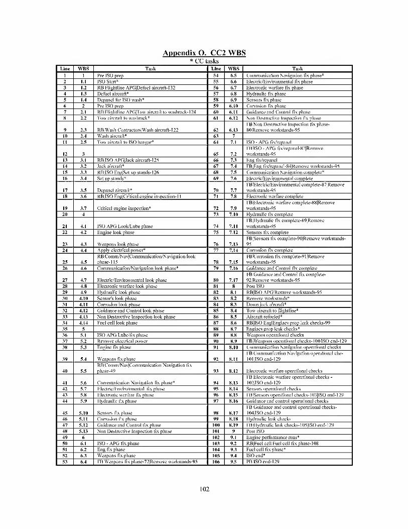
AouendixO. CO WBS * CC tasks

so Start*

RBlFlightline APGIDefuel aircraft-132

Defuel aircraft*

Depanel for ISO wash*

RBlFliahtline APGITow aircraft to washrack-124

Tow aircraft to washrack*

RBlWash ContractorsIWash aircraft-122

Wash aircraft*

Tow aircraft to ISO hangar*

RBIISO APGIJack aircraft-125

Jack aircraft*

RBIISO EnalSet up stands-126

Set up stands*

Depanel aircraft*

RBIISO EnalCritical engine inspection-11

Critical endue inspection*

ISO APG Look/Lube phase

iMaiiatiCTaiSlIlifr

Weapons look phase

Apply electrical power*

RB|Comm/NavjCommunication/Navigation look

phase-115

Communication/Naviaation look phase*

Electric/Environmental look phase

Electronic warfare look phase

Hydraulic look phase

Sensor's look phase

Corrosion look phase

Guidance and Control look phase

Non Destructive Inspection look phase

Fuel cell look phase_

ISO APG Lube/fix phase_

Remove electrical power_

Engine fix phase_

Weapons fix phase_

RB|Comm/Nav|Communication Navigation fix

phase-49_

Communication Navigation fix phase*

Electric/Environmental fix phase

Electronic warfare fix phase

Hydraulic fix phase_

Sensors fix phase

Corrosion fix phase

Guidance and Control fix phase

Non Destructive Inspection fix phase_

SO - APG Fix phase_

Eng fix phase_

Weapons fix phase_

FB|Weapons Fix phase-721Remove wQrkstands-95

Task

Communication Navigation fix phase*

Electric/Environmental fix phase

Electronic warfare fix phase

Hydraulic fix phase

Corrosion fix phase

Guidance and Control fix phase

Non Destructive Inspection fix phase

FBjNon Destructive Inspection fix phase-

SOlRemove workstands-95

ISO - APG fix/repanel

FBjISO-APG fix/repanel-82jRemove

workstands-95

FBIEng fix/repanel-84iRemove workstands-95

Communication Navigation complete*

Electric/Environmental complete

FB|Electric/Environmental complete-87|Remove

workstands-95

Electronic warfare complete

FBjElectronic warfare complete-88|Remove

workstands-95

Hydraulic fix complete

FBjHydraulic fix complete-89|Remove

workstands-95

Sensors fix complete

FBlSensors fix complete-901Remove workstands-

95

Corrosion fix complete

FB|Corrosion fix complete-91|Remove

workstands-95

Guidance and Control fix complete

FBlGuidance and Control fix complete-

92|Remove workstands-95

Post ISO

RBIISO APGIRemove workstands-95

Remove workstands*

Down lack aircraft*

Tow aircraft to flightline*

Aircraft refueled*

RB|lSO EnglEngmes prop leak checks-99_

Engines prop leak checks*_

Weapons operational checks_

FB|Weapons operational checks-100|ISO end-129

Communication Navigation operational checks

FBjCommunication Navigation operational che-

lOlllSO end-129

Electronic warfare operational checks_

FB|Electronic warfare operational checks -

102I1SO end-129

Sensors operational checks

FBlSensors operational checks-1031ISO end-129

Guidance and control operational checks_

FBjGuidance and control operational checks-

104I1SO end-129

Hydraulic leak checks

FBIHydraulic leak checks-105|ISO end-129

Post ISO

Engine performance runs*_

RB|Fuel cell|Fuel cell fix phase-108_

Fuel cell fix phase*_

ISO end*

PBIISO end-129

102

Appendix P. CC3 WBS * CC tasks

ISO Start*

RB|FIightline APGjPefuel aircraft-132_

Defuel aircraft*

Depanel for ISO wash*_

RBjFlightline APGjTow aircraft to washrack-

124

2.2 Tow aircraft to washrack*

RBIWash ContractorsIWash aircraft-122

Wash aircraft*

Tow aircraft to ISO hanaar*

RB|ISO APGIJack aircraft-125

3.2 Jack aircraft*

RB|ISO EngISet up stands-126

Set up stands*

Depanel aircraft*

3.6 Critical engine inspection

RBIISO APGIISO APG Look/Lube phase-14

ISO APG Look/Lube phase*

Engine look phase

Weapons look phase

Apply electrical power

Communication/Navigation look phase

Electric/Environmental look phase

Electronic warfare look phase

Hydraulic look phase

Sensor's look phase

Corrosion look phase

Guidance and Control look phase

Non Destructiye Inspection look phase

Fuel cell look phase

FBIFuel cell look phase-35|lSO - APG

fix/repanel-82

ISO APG Lube/fix phase*_

Remove electrical power_

Engine fix phase_

Weapons fix phase

Communication Navigation fix phase

Electric/Environmental fix phase_

Electronic warfare fix phase_

Hydraulic fix phase

Sensors fix phase

Corrosion fix phase_

Guidance and Control fix phase_

Non Destructive Inspection fix phase

ISO - APG fix phase*_

Eng fix phase_

Weapons fix phase_

FBjWeapons fix phase-72|Remove

workstands-95

Task

Communication Navigation fix phase

Electric/Environmental fix phase

Electronic warfare fix phase_

Hydraulic fix phase_

Sensors fix phase_

Corrosion fix phase

Guidance and Control fix phase

FB|Non Destructive Inspection fix phase-80|Remove

6.13 workstands-95

ISO - APG fix/repanel*_

Eng fix/repanel

FB|Eng fix/repanel-84|Remove workstands-95_

Communication Navigation complete_

FB|Communication Navigation complete-86jRemove

workstands-95

Electric/Environmental complete_

FB|Electric/Environmental complete-87|Remove

workstands-95

Electronic warfare complete_

FB|Electronic warfare complete-88jRemove workstands-

95

Hydraulic fix complete

FBIHvdraulic fix complete-89|Remove workstands-95

Sensors fix complete

FBISensors fix complete-90|Remove workstands-95

Corrosion fix complete

FBICorrosion fix complete-9I |Remove workstands-95

Guidance and Control fix complete

FB|Guidance and Control fix compIete-92|Remove

workstands-95

Remove workstands*

Down jack aircraft*

Tow aircraft to flightline*

Aircraft refueled*

RB|ISO EnglEnmnes prop leak checks-99

Engines prop leak checks*_

Weapons operational checks_

FB|Weapons operational checks-100[ISO end-129_

Communication Navigation operational checks_

FB|Communication Navigation operational che-101|ISO

end-129

Electronic warfare operational checks_

FB|Electronic warfare operational checks -102jlSO end-

129

Sensors operational checks

FBISensors operational checks-103|ISO end-129_

Guidance and control operational checks_

FB|Guidance and control operational checks-104jISO

end-129

Hydraulic leak checks

FB|Hydraulic leak checks-105jlSO end-129_

Post ISO

Engine performance runs*_

RB|Fuel cell|Fuel cell fix phase-108_

Fuel cell fix phase*_

SO end*

PBIISO end-129

Mid

shif

t S

win

gsh

ift

Day

shif

t

AoDendix O. Current ISO Shift Schedule

Specialist

FL APG

Wash contractor

ISO APG

ISO Eng

E/E

EW

Hyd

Sensors

Corrosion

GCS

NDI

FC

CN

Number of Specialists Needed (Current Dayl Day2 Day3 Day4 DayS Day 6 Day? DayS Day9 Day 10

17 17 17

10 8 8

2 2 2

3 2 2

5 2 2

3 2 2

2 2 2

2 2 2

2 2 2

FL APG

Wash contractor

ISO APG 17 17 17 17

E/E

EW

Hvd

Sensors

Corrosion

GCS

NDI

FC

CN

28 24 24 24

FL APG

Wash contractor

ISO APG

ISO Eng

E/E

EW

Hyd

Sensors

Corrosion

GCS

NDI

FC

CN

Weapons_

Aggregate Current 19 19 81 72 72 68 31 10

Total

0 I 379

104

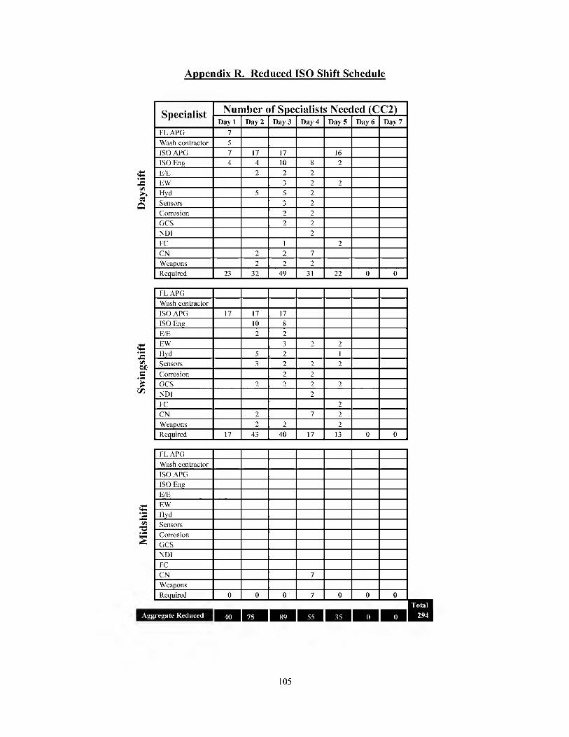
105

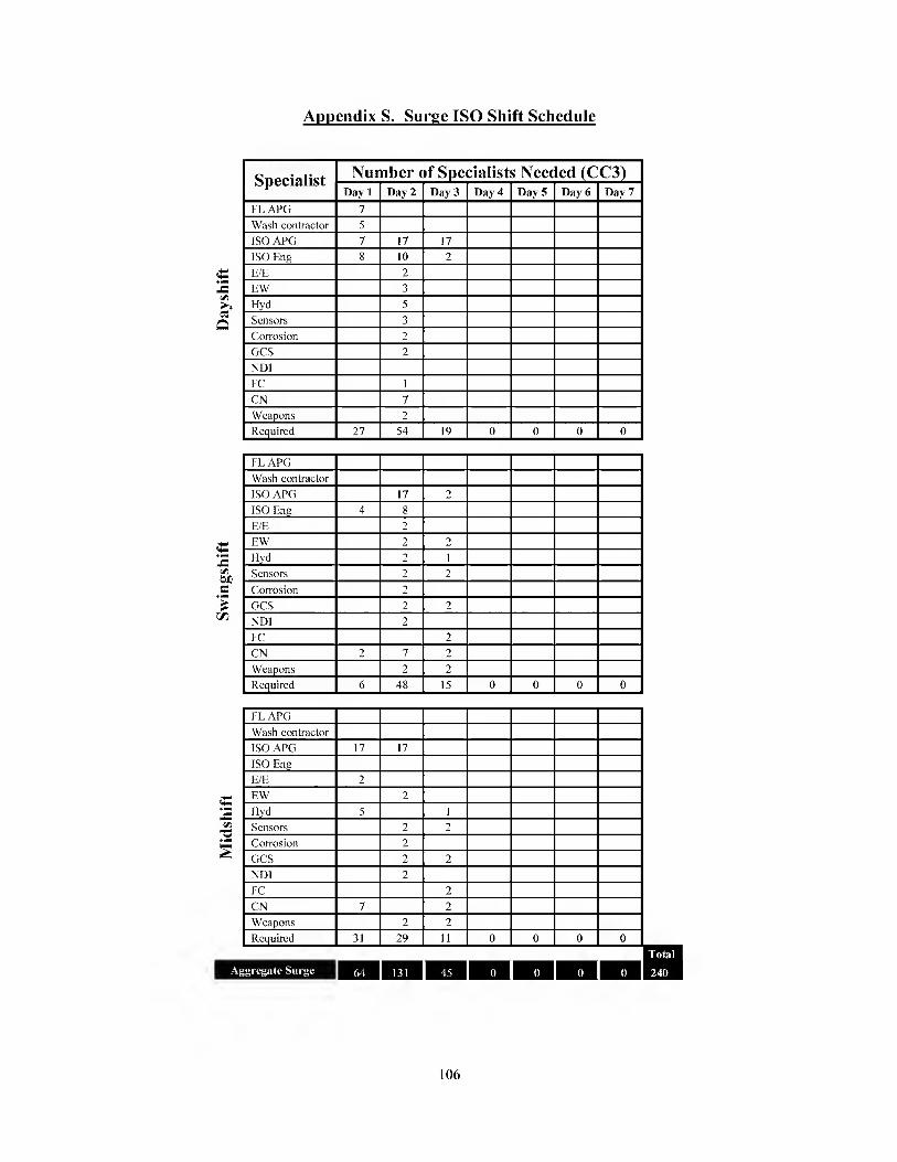
Appendix S. Surge ISO Shift Schedule

Specialist Number of Specialists Need led(CC3) 1 Dayl Day 2 Day 3 Day 4 Days Day 6 Day?

FL APG 7

Wash contractor 5

ISO APG 7 17 17

ISO Eng 8 10 2

E/E 2

EW 3

Hyd 5

Sensors 3

Corrosion 2

GCS 2

NDI

FC 1

CN 7

2

27 54 19 0 0 0 0

Q

FL APG

Wash contractor

ISO APG 17 2

ISO Eng 4 8

E/E 2

EW 2 2

Hyd 2 1

Sensors 2 2

Corrosion 2

GCS 2 2

NDI 2

FC 2

CN 2 7 2

2 2

6 48 15 0 0 0 0

tfi

"C

FL APG

Wash contractor

ISO APG 17 17

ISO Eng

E/E 2

EW 2

Hyd 5 1

Sensors 2 2

Corrosion 2

GCS 2 2

NDI 2

FC 2

CN 7 2

Weapons 2 2

31 29 11 0 0 0 0

mm mm mm mm Total

1 Aggregate Surge 240

106

Bibliography

Blanchard, Benjamin S. Logistics Engineering and Management. Englewood Cliffs NJ. Prentice-Hall. 1986

Bowers, J. "Criticality in Resource Constrained Networks." Journal of the Operational Research Society. 46: 80-91 (December 1995).

Christofides, N., R. Alvarez-Valdes, and J. Tamarit. "Project Scheduling with Resource Constraints: A Branch and Bound Approach." European Journal of Operational Research. 29: 262-273 (Jun 1987).

Cook, Stephen C. Applying Critical Chain to Improve the Management of Uncertainty in Projects. MS thesis, Sloan School of Management and the Department of Electrical Engineering and Computer Science, Massachusetts Institute of Technology, 1998.

Creswell, John W. Research Design Qualitative &Quantitative Approaches. Thousand Oaks CA. SAGE Publications, Inc. 1994.

Devore, Jay L. Probability and Statistics For Engineering and the Sciences. Pacific Grove CA. Brooks/Cole. 2000.

Elton, Jeffrey and Justin Roe. “Bringing Discipline to Project Management,” Harvard Business Review, 16: 153-160 (March/April 1998).

Evers, Philip T. The Impact of Transhipments on Safety Stock Requirements. Journal of Business Logistics, 17: 109-133,) (1996).

Ferrell, Jeffrey. Structural Maintenance Technician, USAF, Hurlburt Field FL. Personal

Correspondence. 5 November 2001.

Goldratt, Eliyahu M. and Jeff Cox. The Goal. Great Barrington, Massachusetts: North River Press, 1984.

Goldratt, Eliyahu M. What is This Thing Called Theory of Constraints and How Should It Be Implemented?. Great Barrington MA: North River Press, 1990.

Goldratt, Eliyahu M. Critical Chain. Great Barrington MA: North River Press, 1997.

“Guide to the Project Management Body of Knowledge”. Newton Square PA: Project Management Institute, Inc., 1996.

107

“Guide to the Project Management Body of Knowledge”. Newton Square PA: Project Management Institute, Inc., 2000.

Harris Semiconductor. Avraham Y. Goldratt Institute, n.pag. http://www.goldratt.com/ harriserp.htm 20 November 2001.

Ho, C. An Examination of a Distribution Resource Planning Problem: DRP System Nervousness Journal of Business Logistics, v. 13, n. 2,125-149, (1992).

Horowitz, Joseph. Critical Path Scheduling. New York: The Ronald Press Company,

1967.

Kahneman, Slovic, and Tversky, “Jugdement Under Uncertainty”. Cambridge University Press, 1982.

Krajewski, Lee J. and Larry P. Ritzman. Operations Management: Strategy and Analysis. Reading MA: Addison-Wesley Publishing Company, Inc. 1999.

Kolisch, R., A. Sprecher, and A. Drexl. Characterization and Generation of a General Class of Resource-Constrained Project Scheduling Problems Management Science, v. 41, n. 10, 1693-1703, (Oct 1995).

Lord Corporation: Multi Project Management. Avraham Y. Goldratt Institute, n.pag. http://www.goldratt.com/lord.htm. 20 November 2001.

Mathcad2000 User’s Guide. Cambridge MA. Mathsoft Inc. 1999.

McClave, James T. and P. George Benson. Statistics for Business and Economics. San Francisco. Dellen Publishing Company. 1988.

McClave, James. T and others. Statistics For Business and Economics. Upper Saddle River NJ. Prentice-Hall, Inc. 2001.

“MC-130E/H Combat Talon 1/11” Air Force Aircraft Fact Sheet, n. pag. http://www.af mil/news/factsheets/MC_130E_H_Combat_Talon_l_lLhtml. 25 October 2001.

Newbold, Robert C. Project Management in the Fast Lane; Applying the Theory of Constraints. Boca Raton FE: St Eucie Press, 1998.

Nicholas, John M. Project Management for Business and Technology: Principles and Practice. Upper Saddle River NJ: Prentice Hall, 2001.

108

Office of the Inspector General. “Additional Information Related to Improvements Needed in the Department of Transportation.” http://www.dot.gov/oig/statements/attach.html. 25 October 2001.

Oguz, O., and H. Bala. A Comparative Study Of Computational Procedures For The Resource Constrained Project Scheduling Problem European Journal of Operational Research, v. 72, i. 2. 406-416, (Jan 1994).

Orman Grubb Furniture. Avraham Y. Goldratt Institute, n.pag. http://www.goldratt.com/onnan.htm. 20 November 2001.

Ozdamar, L., and G. Ulusoy. A Survey On The Resource-Constrained Project Scheduling Problem HE Transactions. 574-586, (Oct 1995).

Parkinson, Cyril Northcote. Parkinson’s Law. n.page. http://www.heretical.com/miscella/parkinsl.html. (7 Feb. 1995).

Spinner, Pete M. Elements of Project Management, Plan, Schedule & Control. Englewood Cliffs NJ: Prentice Hall, 1992.

Swartz, Stephen M. The Effects of Variability and Disruption of Project Stability, Duration, and Net Present Value. Miehigan State University, East Lansing Ml. September 1999.

Tallon, William J. The Impact of Inventory Centralization on Aggregate Safety Stock: The Variable Supply Lead Time Case. Journal of Business Logistics, 14: 185- 203 (1993).

TOC in Colombia, Venezuela and Costa Rica: From The Goal to the Desirable Future. The TOC Times, n.pag. http://www.goldratt.com/toctimes/september2001.html #award. 20 November 2001a.

U.S Government Accounting Office. “Information Management and Technology.” Document GAO/HR-97-9, 1997.

Willis, R. "Critical Path Analysis and Resource Constrained Project Scheduling- Theory and Practice." European Journal of Operational Research, 21: 149-155 (1985).

Zinn, Walter, Michael Levy, Donald J. Bowersox. Measuring the Effect of Inventory

Centralization/Decentralization on Aggregate Safety Stock: The "Square Root Law” Revisited. Journal of Business Logistics, 10: 1-14 (1989).

109

Vita

Captain Mattioda graduated from South Vermillion High Sehool in Clinton,

Indiana and enlisted in the Air Foree in June 1985. After earning Honor Graduate awards

at basic training and technical school, he was assigned to Bergstrom AFB, Texas. During

the next 12.5 years, he attained the rank of Master Sergeant with assignments at Nellis

AFB, Nevada, where he was a member of the USAF Air Demonstration Squadron

(THUNDERBIRDS); Incirlik AB, Turkey; and Grand Forks AFB, North Dakota.

During his enlisted career, he received four Commendation medals and the John

Levitow award at NCO Prepatory School, Distinguished Graduate honors from the NCO

Leadership course and the USAFE NCO Academy.

Capt Mattioda earned an Associate Degree in Aircraft Accessory Systems

Technology from the Community College of the Air Force in 1990 and a Bachelors of

Science degree (with Dean’s List honors) in Professional Aeronautics from Embry Riddle

Aeronautical University in July 1997. In February 1998, he graduated from USAF

Officer Training School (OTS) earning Distinguished and Honor Graduate awards.

He was assigned to Hurlburt Field, Florida after OTS. Capt Mattioda attended

Aircraft Maintenance Officer Course and graduated in September 1998 with the Honor

Graduate award. While at Hurlburt Field, he was decorated with his fifth Commendation

medal and was the 16 AGS and 16 LG CGO of the Year and Lance P. Sijan award

winner. In August 2000, he entered the Graduate School of Engineering and

Management, Air Force Institute of Technology. Capt Mattioda is married and has three

sons.

no

REPORT DOCUMENTATION PAGE Form Approved OMB No. 074-0188

The public reporting burden for this collection of information is estimated to average 1 hour per response, including the time for reviewing instructions, searching existing data sources, gathering and maintaining the data needed, and completing and reviewing the collection of infonmation. Send comments regarding this burden estimate or any other aspect of the collection of information, including suggestions for reducing this burden to Department of Defense, Washington Headquarters Services, Directorate for Information Operations and Reports (0704-0188), 1215 Jefferson Davis Highway, Suite 1204, Arlington, VA 22202-4302. Respondents should be aware that notwithstanding any other provision of law, no person shall be subject to an penalty for failing to comply with a collection of information if it does not display a currently valid OMB control number. PLEASE DO NOT RETURN YOUR FORM TO THE ABOVE ADDRESS.

1. REPORT DATE (DD-MM-YYYY) 2. REPORT TYPE

20-03-2002 Master’s Thesis 4. TITLE AND SUBTITLE

USE OF CRITICAL CHAIN SCHEDULING TO INCREASE AIRCRAFT AVAILABILITY

3. DATES COVERED (From - To)

1 Mar 2001 -20 Mar 2002

5a. CONTRACT NUMBER

5b. GRANT NUMBER

6. AUTHOR(S)

Mattioda, Daniel D., Capt, USAF

7. PERFORMING ORGANIZATION NAMES(S) AND ADDRESS(S)

Air Force Institute of Technology Graduate School of Engineering and Management (AFIT/EN) 2950 P Street, Building 640, WPAFB OH 45433-8865

9. SPONSORING/MONITORING AGENCY NAME(S) AND ADDRESS(ES)

Kent A. Mueller, Colonel, USAF, Director of Logistics Air Force Special Operations Command (AFSOC) 100 Bartley St, Hurlburt Fid FL 32544 (850) 884 2371 e-mail: Kent.Muller@hurlburt.afmil

5c. PROGRAM ELEMENT NUMBER

5d. PROJECT NUMBER

5e. TASK NUMBER

5f. WORK UNIT NUMBER

8. PERFORMING ORGANIZATION REPORT NUMBER

AFIT/GLM/ENS/02-11

10. SPONSOR/MONITOR’S ACRONYM(S)

11. SPONSOR/MONITOR’S REPORT NUMBER(S)

12. DISTRIBUTION/AVAILABILITY STATEMENT

APPROVED FOR PUBLIC RELEASE; DISTRIBUTION UNLIMITED. 13. SUPPLEMENTARY NOTES

14. ABSTRACT

United States Air Foree Speeial Operations Command (AFSOC) has a minimal number of aircraft at its disposal. As a result, the

aircraft are considered high demand, low-density (small number in Air Force inventory) weapon systems. Any chance to increase

aircraft availability would greatly enhance the capability of AFSOC.

Isochronal maintenance (ISO) conducted once every 365 days (per AFI for C- 130 aircraft) provides the best opportunity to

increase aircraft availability by improving the scheduling of tasks and accurately estimating the inspection duration. Scheduled

maintenance portrays the characteristics of projects, therefore, this thesis proposed that Critical Chain (CC) scheduling, a project

management technique, could provide an improved ISO schedule reducing aircraft downtime.

The ISO inspection process was modeled three ways (1) existing process, (2) task constraints removed, and (3) task and resource

constraints removed. 100 simulated aircraft inspections took place in each model. The simulated duration times were compared to

estimates provided by the use of Critical Path and Critical Chain scheduling techniques.

Critical Chain scheduling techniques did not directly Increase aircraft availability. However, Critical Chain scheduling did

identify the potential for increasing aircraft availability by removing policy and scheduling constraints. 15. SUBJECT TERMS

16. SECURITY CLASSIFICATION OF: 17. LIMITATION OF 18. NUMBER 19a. NAME OF RESPONSIBLE PERSON ABSTRACT OF Maj Stephen M. Swartz

a. REPORT

u b. ABSTRACT

u c. THIS PAGE

u uu PAGES

122 19b. TELEPHONE NUMBER (Include area code)

(937) 255-6565, ext 4284

Stephen.Swartz(5),afit.af.edu Standard Form 298 (Rev. 8-98) Prescribed by ANSI Std. Z39-18