updated lagrangian formulation for corrected smooth particle hydrodynamics
TRANSCRIPT
February 2, 2006 21:52 WSPC/INSTRUCTION FILE HVB˙ws-ijcm
International Journal of Computational Methodsc© World Scientific Publishing Company
UPDATED LAGRANGIAN FORMULATION FOR CORRECTEDSMOOTH PARTICLE HYDRODYNAMICS
ANTONIO HUERTA, YOLANDA VIDAL
Departament de Matematica Aplicada III, Laboratori de Calcul Numeric (LaCaN),Universitat Politecnica de Catalunya,
Jordi Girona 1, Barcelona, E-08034,Spain{antonio.huerta,yolanda.vidal}@upc.es
http://<www-lacan.upc.es>
JAVIER BONET
Civil and Computational Engineering Center (C2EC),University of Wales Swansea
Singleton Park, Swansea, SA2 8PP, United [email protected]
Received (Day Month Year)Revised (Day Month Year)
Smooth Particle Hydrodynamics (SPH) are,in general, more robust than finite elementsfor large distortion problems. Nevertheless, updating the reference configuration may benecessary in some problems involving extremely large distortions. If a standard updatedformulation is implemented in SPH zero energy modes are activated and spoil the so-lution. It is important to note that the updated Lagrangian does not present tensioninstability but only zero energy modes. Here an stabilization technique is incorporatedto the updated formulation to obtain an improved method without mechanisms.
Keywords: Corrected SPH; total Lagrangian formulation; large deformations.
1. INTRODUCTION
In its original form Smooth Particle Hydrodynamics (SPH) had several weak points,described in detail by Swegle et al. [1995] and Belytschko et al. [2000]. These prob-lems consisted, among others, on lack of consistency, tension instability and thepresence of zero energy modes in the numeric solution.
The correction of SPH in order to reproduce polynomials in finite domains aswell as passing the patch test has been an area of intensive work. Some of thesecontributions, without being exhaustive, are discussed in this paper. See [Liu et al.(2003)] for a detailed discussion on reproducibility of SPH methods or [Huerta et al.(2004)] for a general review of meshfree methods. Johnson and Beissel developed thenormalized smoothing method [Johnson and Beissel (1996); Johnson et al. (1996)]obtaining linear consistency. Chen et al. [1999] introduce a corrected kernel by
1
February 2, 2006 21:52 WSPC/INSTRUCTION FILE HVB˙ws-ijcm
2 A. Huerta, Y. Vidal and J. Bonet
invoking a Taylor series expansion. Bonet and Kulasegaram [2000] developed theCorrected Smooth Particle Hydrodynamics (CSPH) method that allows to obtainlinear consistency in the interpolation of the function and in the interpolation ofthe gradient. Consistency is achieved introducing corrections in the kernel functionsand in their derivatives.
The classical SPH formulation defining a fixed support in the laboratory for eachparticle and thus recomputing neighbors at each time-step (i.e. updated neighborsearch) that will be called here Eulerian formulation presents tension instability,see for instance [Monaghan (1982)]. Nevertheless, Bonet and Kulasegaram [2001]show that a (total) Lagrangian formulation removes this instability. It is importantto note however that zero energy modes still remain in the Lagrangian formula-tion. Without tension instability, a SPH Lagrangian formulation presents seriousadvantages compared to finite elements. For instance, Libersky et al. [1993] appliedsuccessfully the Lagrangian SPH code to high strain problems, Johnson et al. [1993]incorporated the SPH algorithm into a standard Lagrangian code such as EPIC andStellingwerf and Wingate [1993] as well as Johnson et al. [1996] used SPH for impactproblems. Nevertheless, in problems with severe distortions a Lagrangian formula-tion will still require updates of the reference configuration. When such updates areincorporated zero energy modes are more likely to be activated. When few updatesare performed during the computation the induced errors may remain unnoticed.But when updates are performed frequently the solution is completely spoilt, be-cause zero energy modes are excited and they produce spurious oscillations. Theobjective of this paper is to develop an updated Lagrangian formulation that cancarry out updates of the reference configuration without suffering from spuriousmodes.
The problem of zero energy modes is still open. In the literature two types ofsolutions are used: dissipate spurious modes (conceptually similar to the techniquesused in finite elements for hourglass control [Flanagan and Belytschko (1981)]) or analternative discretization that does not evaluate the variables and their derivativesat the same points. For example, Gray et al. [2001] precluded the instability intro-ducing an artificial stress (but that introduces also small errors in the solution) andRandles and Libersky [2000] used different sets of particles to interpolate differentfields generating the denominated stress points. Here, for computational efficiency,particles are the only information carrying points.
First, the total Lagrangian CSPH formulation is revised for large strains dynamicproblems and a numerical example is performed. Then, in section 3 the standardupdated Lagrangian formulation is recalled and analyzed to show its drawbacks inSPH. Finally in section 4 a stabilized updated Lagrangian formulation is proposedand its performance is assessed both in a simple one-dimensional synthetic exampleand in a numerical benchmark test extremely sensible to zero energy modes.
February 2, 2006 21:52 WSPC/INSTRUCTION FILE HVB˙ws-ijcm
Updated Lagrangian formulation for CSPH 3
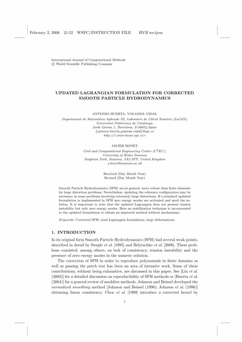
x = ϕ(X, t)
F(X, t)X
x
dX
dx
Fig. 1. Movement of a deformable body.
2. TOTALLY LAGRANGIAN CSPH
2.1. Continuum equations
Consider the three-dimensional continuum shown in Figure 1 undergoing a givenmotion defined by a mapping ϕ between initial and current positions as,
x = ϕ(X, t).
The deformation gradient F, defined as
F =∂x
∂X, (1)
is a quantity of interest in the study of large deformations because it is presentin all those equations that relate magnitudes in the initial configuration with theircorresponding ones in the final configuration. The volume change of the continuumcan be obtained in terms of the Jacobian
J = detF =dV
dV 0,
where dV 0 and dV represent the initial and current element volumes. The Cauchyequation (balance of momentum equation) for the deformable body reads
∇· σ + ζf = ζa, (2)
where ζ is the material density, a is the acceleration, f is external force per unit ofvolume and σ is the Cauchy stress tensor. Recall that,
P = JσF−T ,
where P is the first Piola-Kirchhoff tensor.
February 2, 2006 21:52 WSPC/INSTRUCTION FILE HVB˙ws-ijcm
4 A. Huerta, Y. Vidal and J. Bonet
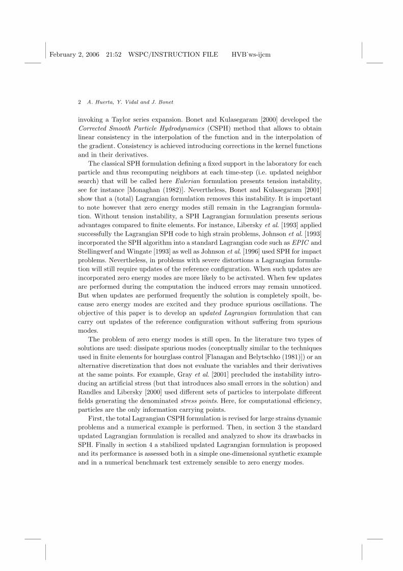
u(x)
φ((x-x )/ρ)
x
i
iρ
Fig. 2. Reproducing kernel.
2.2. CSPH approximation
Here some basic notions on CSPH will be recalled. The earliest mesh-free methodis the SPH method [Lucy (1977)]. The method is based on a simple property of theDirac delta function δ(x),
u(x) =∫
δ(x− y)u(y)dy,
where u(x) is the function to be approximated. The key idea is to replace the Diracdelta function by a kernel or weight function Cρ φ
((x − y)/ρ
)positive, even and
compact supported, see Figure 2,
u(x) ' uρ(x) :=∫
Cρφ(x− y
ρ
)u(y)dy, (3)
where ρ is called the dilation parameter, which is usually the support radius of thekernel function, and Cρ is a normalization constant such that∫
Cρφ(x− y
ρ
)dy = 1,
i.e. constant functions are exactly interpolated. Therefore, as ρ tends to zero thekernel function approaches the Dirac delta function, and consequently,
limρ→0
uρ(x) = u(x).
In order to develop a computational technique, it is necessary to evaluate theintegration in equation (3) in a discrete manner to give
u(x) ' uρ(x) ' uρ(x) :=∑
i
Vi Cρφ(x− xi
ρ
)u(xi), (4)
February 2, 2006 21:52 WSPC/INSTRUCTION FILE HVB˙ws-ijcm
Updated Lagrangian formulation for CSPH 5
where xi and Vi are the points and weights of the numerical quadrature. Usuallythe quadrature points are called particles and the weights are called volumes.
It is possible to re-write equation (4) in terms of standard shape function as
u(x) ' uρ(x) :=∑
i
Ni(x)u(xi), Ni(x) = ViCρφ(x− xi
ρ
). (5)
As a result of point integration in equation (4), the consistency conditions areno longer satisfied exactly. Bonet and Kulasegaram [2000] present a corrected SPHapproximation (CSPH) to preclude these difficulties. The foregoing is a brief reviewof the three main corrections introduced by Bonet and coworkers.
First, the discrepancy in the numerically integrated consistency conditions iseliminated by a kernel correction. As proposed by Liu et al. [1995], Cρ is selectedby enforcing linear consistency conditions now given by a point-wise integration as,
∑
i
Vi Cρφ(x− xi
ρ
)= 1,
∑
i
Vi(x− xi)Cρφ(x− xi
ρ
)= 0. (6)
These equations lead to,
Cρ = α(x)(1 + β(x) · (x− xi)
)(7)
where
α(x) =(∑
i
Vi φ(x− xi
ρ
)(1 + β(x) · (x− xi)
))−1
,
and
β(x) =(∑
i
Vi φ(x− xi
ρ
)(x− xi) (x− xi)T
)−1 ∑
i
Vi(xi − x)φ(x− xi
ρ
).
The use of this type of correction ensures that linear functions are perfectly inter-polated and their gradients are exactly obtained. A possible way of simplifying thecalculation is by using constant, rather than linear, correction. This is equivalentto taking β(x) = 0 in equation (7). However, gradient evaluation using the aboveexpressions is expensive, both in computer memory and time consuming.
Second, the gradient functions are directly amended to ensure that the gradientof a general constant or linear function is correctly evaluated. The corrected gradientis defined as
∇uρ(x) =∑
i
Vi
(u(xi)− u(x)
)∇φ(x− xi
ρ
),
where
∇φ(x− xi
ρ
)= L(x)∇φ
(x− xi
ρ
). (8)
It is clear that equation (8) will ensure that the gradient of a constant function van-ishes. The correction matrix L(x) is obtained after imposing the linear consistency
February 2, 2006 21:52 WSPC/INSTRUCTION FILE HVB˙ws-ijcm
6 A. Huerta, Y. Vidal and J. Bonet
condition, namely∑
i
Vi ∇φ(x− xi
ρ
)xT
i = I.
This equation enables the explicit evaluation of the correction term as,
L(x) =(∑
i
Vi ∇φ(x− xi
ρ
)(xi − x)T
)−1
.
This corrected gradient, proposed by Bonet and coworkers, is similar to the Renor-malized Meshless Derivative (RMD) proposed in [Randles and Libersky (1996);Krongauz and Belytschko (1997); Vila (1999)].
2.3. Lagrangian CSPH
This section will recall the basics ideas and the notation of the Lagrangian CSPHformulation. The details and the development of this formulation can be found in[Bonet and Kulasegaram (2001)].
Let us consider a discretized body using SPH particles. The mapping ϕ betweeninitial and current positions can be approximated using SPH approximation as,
xj = ϕ(Xj , t) =∑
k
Vk Cρφ
(Xj −Xk
ρ
)xk.
The deformation gradient, defined in (1), can now be evaluated at a given particlej in terms of the current positions computing the gradient of the previous equation,as
Fj = ∇0ϕ =∑
k
xk GTk (Xj), (9)
where ∇0 indicates the gradient respect to the initial configuration, xk is the currentposition of particle k and where the vectors G contain the corrected kernel gradientsat the initial configuration, that is,
Gk(Xj) = Vk∇0φ
(Xj −Xk
ρ
),
where ∇0 is a “corrected” gradient to ensure linear completeness as shown in (8).Once the expression of the deformation gradient is determined the internal forces
can be computed using the first Piola-Kirchhoff tensor, P. Thus, the variation ofinternal forces in a Lagrangian CSPH formulation in the reference configurationare:
δwint =∫
V 0P : δFdV 0 '
∑
j
V 0j Pj : δFj . (10)
The variation of the virtual deformation gradient emerges from equation (9) as
δFj =∑
k
δvk GTk (Xj),
February 2, 2006 21:52 WSPC/INSTRUCTION FILE HVB˙ws-ijcm
Updated Lagrangian formulation for CSPH 7
which after substitution into (10) leads to the expression of the internal virtual work
δwint '∑
j
V 0j Pj :
(∑
k
δvk GTk (Xj)
)=
∑
k
δvk ·(∑
j
V 0j Pj Gk(Xj)
).
With this expression the vector of internal forces corresponding to a certain particlei can be identified as
Ti =∑
j
V 0j Pj Gi(Xj). (11)
It is important to observe that in (11) the kernel derivatives, Gi(Xj), are fixedin the reference configuration and therefore they do not depend on the currentpositions of the particles. This bears that corrections are only calculated at thebeginning reducing the computational cost.
2.4. Numerical Example: cylinder bending test with a hyperelastic
material
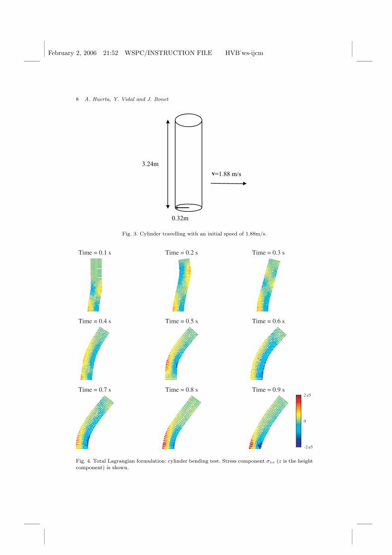
In order to illustrate the ability and limitations of Lagrangian CSPH formulationa benchmark example is proposed. This example, which is very sensible to insta-bilities, consists in the simulation of a three-dimensional problem with large defor-mations using a hyperelastic material. This example was also solved in [Bonet andKulasegaram (2001)]. Let’s consider a nearly incompressible neo-Hookean cylindertravelling with an initial speed of 1.88m/s, see Figure 3, which is suddenly fixedat its base. Homogeneous Dirichlet boundary conditions are directly imposed tothe coefficients, which is standard in SPH, because the characteristic radius of thesupport of the kernel function is small. For larger values of ρ other alternatives maybe implemented [Fernandez-Mendez and Huerta (2004)]. The initial radius is 0.32mand the length 3.24m. The shear modulus is taken as 0.3571MN/m2 and the bulkmodulus is 1.67MN/m2.
The results obtained using a Lagrangian CSPH formulation can be seen in Figure10. The bar oscillates from initial position to maximum deformation and then backto initial position as expected. The stress component σzz is shown where z is theheight component. The cylinder deformation is simulated with good results even inthe presence of high tension.
3. STANDARD UPDATED LAGRANGIAN
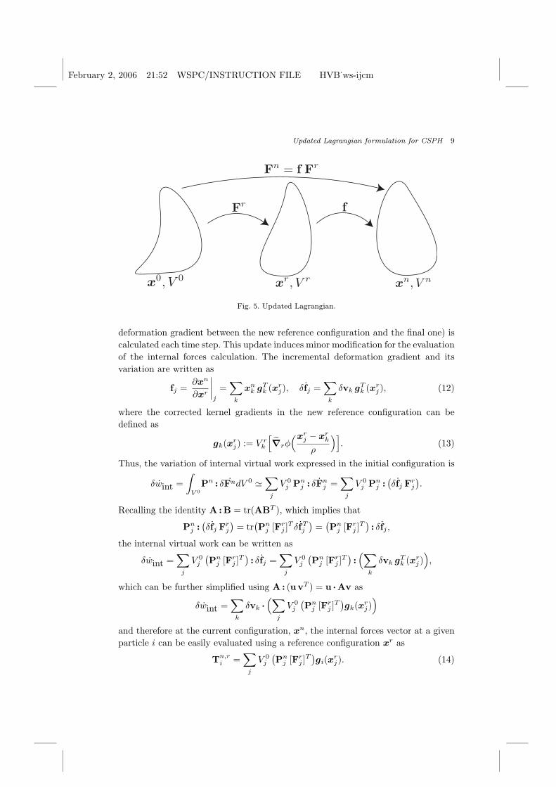
The updated Lagrangian formulation consists of a multiplicative incremental ap-proach as illustrated in Figure 5. The intermediate configuration xr will be the newreference configuration for the next time steps. This means that a new neighborsearch must be done in this configuration, xr, and that corrections of the kerneland its derivatives must be recalculated.
It is important to observe that the deformation gradient Fr is stored as aninternal state variable and only the incremental deformation gradient, f , (i.e. the
February 2, 2006 21:52 WSPC/INSTRUCTION FILE HVB˙ws-ijcm
8 A. Huerta, Y. Vidal and J. Bonet
v=1.88 m/s
0.32m
3.24m
Fig. 3. Cylinder travelling with an initial speed of 1.88m/s.
Time = 0.1 s Time = 0.2 s Time = 0.3 s
Time = 0.4 s Time = 0.5 s Time = 0.6 s
Time = 0.7 s Time = 0.8 s Time = 0.9 s
-2.e5
0
2.e5
Fig. 4. Total Lagrangian formulation: cylinder bending test. Stress component σzz (z is the heightcomponent) is shown.
February 2, 2006 21:52 WSPC/INSTRUCTION FILE HVB˙ws-ijcm
Updated Lagrangian formulation for CSPH 9
Fn
= f Fr
Fr
f
x0, V 0
xr, V r
xn, V n
Fig. 5. Updated Lagrangian.
deformation gradient between the new reference configuration and the final one) iscalculated each time step. This update induces minor modification for the evaluationof the internal forces calculation. The incremental deformation gradient and itsvariation are written as
fj =∂xn
∂xr
∣∣∣∣j
=∑
k
xnk gT
k (xrj), δfj =
∑
k
δvk gTk (xr
j), (12)
where the corrected kernel gradients in the new reference configuration can bedefined as
gk(xrj) := V r
k
[∇rφ
(xrj − xr
k
ρ
)]. (13)
Thus, the variation of internal virtual work expressed in the initial configuration is
δwint =∫
V 0Pn : δFndV 0 '
∑
j
V 0j Pn
j : δFnj =
∑
j
V 0j Pn
j :(δfj Fr
j
).
Recalling the identity A:B = tr(ABT ), which implies that
Pnj :
(δfj Fr
j
)= tr
(Pn
j [Frj ]
T δfTj
)=
(Pn
j [Frj ]
T): δfj ,
the internal virtual work can be written as
δwint =∑
j
V 0j
(Pn
j [Frj ]
T): δfj =
∑
j
V 0j
(Pn
j [Frj ]
T):(∑
k
δvk gTk (xr
j)),
which can be further simplified using A: (uvT ) = u ·Av as
δwint =∑
k
δvk ·(∑
j
V 0j
(Pn
j [Frj ]
T)gk(xr
j))
and therefore at the current configuration, xn, the internal forces vector at a givenparticle i can be easily evaluated using a reference configuration xr as
Tn,ri =
∑
j
V 0j
(Pn
j [Frj ]
T)gi(xr
j). (14)
February 2, 2006 21:52 WSPC/INSTRUCTION FILE HVB˙ws-ijcm
10 A. Huerta, Y. Vidal and J. Bonet
h
φ(x − xr
i
ρ
)
xr
i−2 xr
i−1xr
ixr
i+1 xr
i+2
xi−2 xi−1 xi xi+1 xi+2
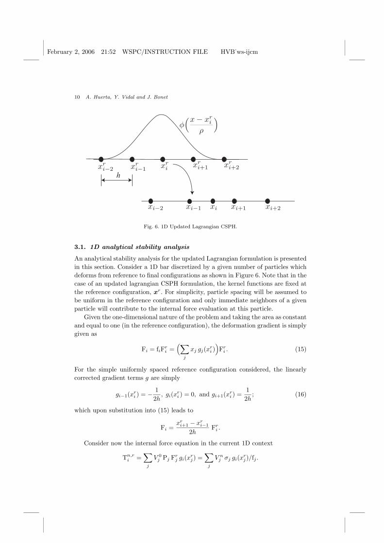
Fig. 6. 1D Updated Lagrangian CSPH.
3.1. 1D analytical stability analysis
An analytical stability analysis for the updated Lagrangian formulation is presentedin this section. Consider a 1D bar discretized by a given number of particles whichdeforms from reference to final configurations as shown in Figure 6. Note that in thecase of an updated lagrangian CSPH formulation, the kernel functions are fixed atthe reference configuration, xr. For simplicity, particle spacing will be assumed tobe uniform in the reference configuration and only immediate neighbors of a givenparticle will contribute to the internal force evaluation at this particle.
Given the one-dimensional nature of the problem and taking the area as constantand equal to one (in the reference configuration), the deformation gradient is simplygiven as
Fi = fiFri =
(∑
j
xj gj(xri )
)Fr
i . (15)
For the simple uniformly spaced reference configuration considered, the linearlycorrected gradient terms g are simply
gi−1(xri ) = − 1
2h, gi(xr
i ) = 0, and gi+1(xri ) =
12h
; (16)
which upon substitution into (15) leads to
Fi =xr
i+1 − xri−1
2hFr
i .
Consider now the internal force equation in the current 1D context
Tn,ri =
∑
j
V 0j Pj Fr
j gi(xrj) =
∑
j
V nj σj gi(xr
j)/fj .
February 2, 2006 21:52 WSPC/INSTRUCTION FILE HVB˙ws-ijcm
Updated Lagrangian formulation for CSPH 11
Using this identity together with (16) for the gradient functions enables the internalforce at point i to be obtained as
Ti =(V n
i−1 σi−1
fi−1− V n
i+1 σi+1
fi+1
)/2h.
The internal force vector is only a function of the current nodal positions via thestress values. Using the linear constitutive relationship, σi = κ(Ji − 1), the tangentstiffness matrix terms are now easily evaluated to give
Ki,i =V nκ
(xi − xi−2)2+
V nκ
(xi+2 − xi)2,
Ki,i+1 = Ki,i−1 = 0,
Ki,i+2 =−V nκ
(xi+2 − xi)2, and Ki,i−2 =
−V nκ
(xi − xi−2)2.
Finally a simple calculation shows that the eigenvalue associated to the alter-nating eigenvector (−1)i now vanishes as
∑
j
Kij(−1)j = 0.
The above equation implies that this alternating mode is a mechanism instead of amode with a possible negative eigenvalue as happens in the Eulerian formulation,see [Bonet and Kulasegaram (2001)]. Consequently, the algorithm should be stablebut, in the absence of artificial viscosity, undamped oscillations may emerge duringthe computations.
3.2. Numerical examples
3.2.1. One-dimensional example
The previous section has proven the existence of mechanisms in the updated La-grangian formulation. This was also proven for the total Lagrangian formulation in[Bonet and Kulasegaram (2001)]). Next, a 1D numerical test is performed in orderto verify whether in these formulations the mechanisms are activated or not.
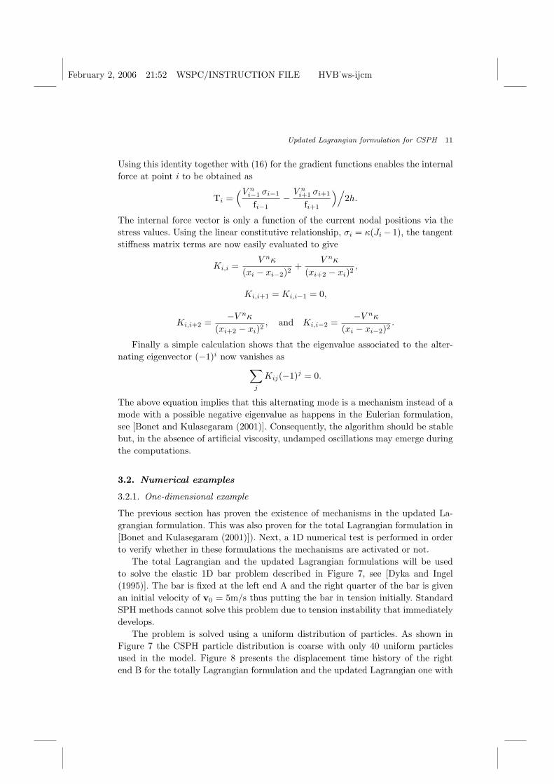
The total Lagrangian and the updated Lagrangian formulations will be usedto solve the elastic 1D bar problem described in Figure 7, see [Dyka and Ingel(1995)]. The bar is fixed at the left end A and the right quarter of the bar is givenan initial velocity of v0 = 5m/s thus putting the bar in tension initially. StandardSPH methods cannot solve this problem due to tension instability that immediatelydevelops.
The problem is solved using a uniform distribution of particles. As shown inFigure 7 the CSPH particle distribution is coarse with only 40 uniform particlesused in the model. Figure 8 presents the displacement time history of the rightend B for the totally Lagrangian formulation and the updated Lagrangian one with
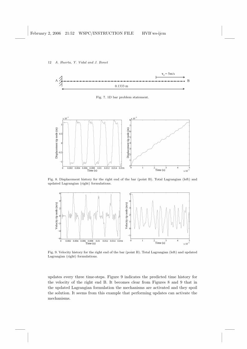
February 2, 2006 21:52 WSPC/INSTRUCTION FILE HVB˙ws-ijcm
12 A. Huerta, Y. Vidal and J. Bonet
0.1333 m
A B
v = 5m/s0
Fig. 7. 1D bar problem statement.
0 0.002 0.004 0.006 0.008 0.01 0.012 0.014 0.016
−1
−0.5
0
0.5
1
x 10−3
Time (s)
Dis
plac
emen
t tip
nod
e (m
)
0 1 2 3 4 5
x 10−3
0
1
2
3
4
5
6
7
8x 10
−3
Time (s)
Dis
plac
emen
t tip
nod
e (m
)
Fig. 8. Displacement history for the right end of the bar (point B). Total Lagrangian (left) andupdated Lagrangian (right) formulations.
0 0.002 0.004 0.006 0.008 0.01 0.012 0.014 0.016−6
−4
−2
0
2
4
6
Time (s)
Vel
ocity
tip
node
(m
/s)
0 1 2 3 4 5
x 10−3
−1
0
1
2
3
4
5
Time (s)
Vel
ocity
tip
node
(m
/s)
Fig. 9. Velocity history for the right end of the bar (point B). Total Lagrangian (left) and updatedLagrangian (right) formulations.
updates every three time-steps. Figure 9 indicates the predicted time history forthe velocity of the right end B. It becomes clear from Figures 8 and 9 that inthe updated Lagrangian formulation the mechanisms are activated and they spoilthe solution. It seems from this example that performing updates can activate themechanisms.
February 2, 2006 21:52 WSPC/INSTRUCTION FILE HVB˙ws-ijcm
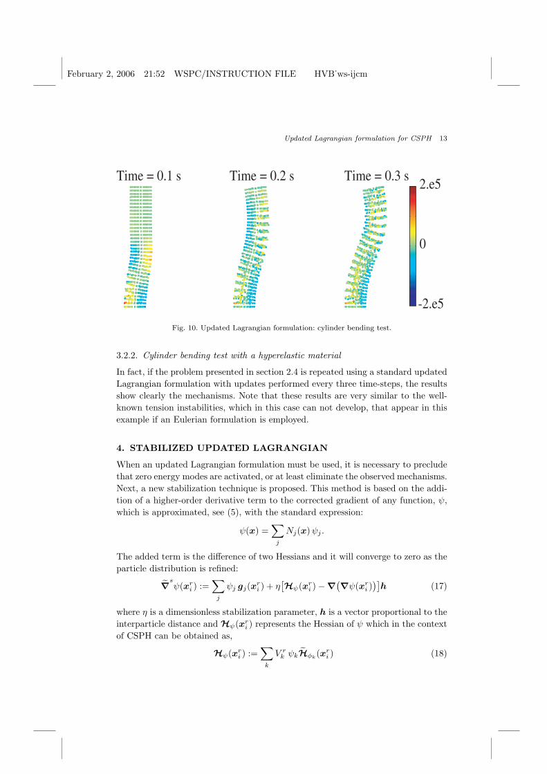
Updated Lagrangian formulation for CSPH 13
Time = 0.1 s Time = 0.2 s Time = 0.3 s
-2.e5
0
2.e5
Fig. 10. Updated Lagrangian formulation: cylinder bending test.
3.2.2. Cylinder bending test with a hyperelastic material
In fact, if the problem presented in section 2.4 is repeated using a standard updatedLagrangian formulation with updates performed every three time-steps, the resultsshow clearly the mechanisms. Note that these results are very similar to the well-known tension instabilities, which in this case can not develop, that appear in thisexample if an Eulerian formulation is employed.
4. STABILIZED UPDATED LAGRANGIAN
When an updated Lagrangian formulation must be used, it is necessary to precludethat zero energy modes are activated, or at least eliminate the observed mechanisms.Next, a new stabilization technique is proposed. This method is based on the addi-tion of a higher-order derivative term to the corrected gradient of any function, ψ,which is approximated, see (5), with the standard expression:
ψ(x) =∑
j
Nj(x)ψj .
The added term is the difference of two Hessians and it will converge to zero as theparticle distribution is refined:
∇sψ(xr
i ) :=∑
j
ψj gj(xri ) + η
[Hψ(xri )−∇(∇ψ(xr
i ))]
h (17)
where η is a dimensionless stabilization parameter, h is a vector proportional to theinterparticle distance and Hψ(xr
i ) represents the Hessian of ψ which in the contextof CSPH can be obtained as,
Hψ(xri ) :=
∑
k
V rk ψkHφk
(xri ) (18)
February 2, 2006 21:52 WSPC/INSTRUCTION FILE HVB˙ws-ijcm
14 A. Huerta, Y. Vidal and J. Bonet
where Hφkis the linearly corrected Hessian kernel. To obtain linear reproducibility,
Hφkis corrected by means of two terms, namely a matrix B(x) and a third order
tensor A(x) as,
Hφk(xr
i ) = Hφk(xr
i ) + δikB(xri ) + A(xr
i ) · (xri − xr
k),
where Hφk(xr
i ) is the Hessian of the kernel function φ, that is,
Hφk(x) = ∇
(∇φ
(x− xk
ρ
)),
which has an explicit known expression once the kernel φ is defined. Correctionterms B and A are determined enforcing that constant and linear functions musthave null Hessian, that is,∑
k
V rk Hφk
(xri ) = 0 and
∑
k
V rk Hφk
(xri ) xr
k = 0.
These reproducibility conditions determine the expressions for B(x) and A(x),namely
A(x) =[∑
k
V rk Hφk
(x) (xrk − x)T
][∑
k
V rk (xr
k − x) (xrk − x)T
]−1
B(x) =1
V ri
[−
∑
k
V rk Hφk
(x) + V rk A(x) · (xr
k − x)].
Equation (17) can be rewritten using the definition of the Hessian, equation (18),and the gradient, equation (13), as∑
k
ψk gsk(x) =
∑
k
ψk gk(x) + η
[∑
k
V rk ψkHφk
(x)−∑
k
ψk
(∑
l
gk(xrl ) · gT
l (x))]
h.
Hence gsk(x) can be written as:
gsk(x) = gk(x) + η
[V r
k Hφk(x)−
(∑
l
gk(xrl ) gT
l (x))]
h, (19)
which is the expression that must be introduced, for instance, in (14) to evaluatethe internal forces. Equation (19) represents the complete form for the correctedgradient of the kernel, it includes the correction (for reproducibility in the discretesetting —nodal integration—) and stabilization.
4.1. Numerical examples
4.1.1. One-dimensional test
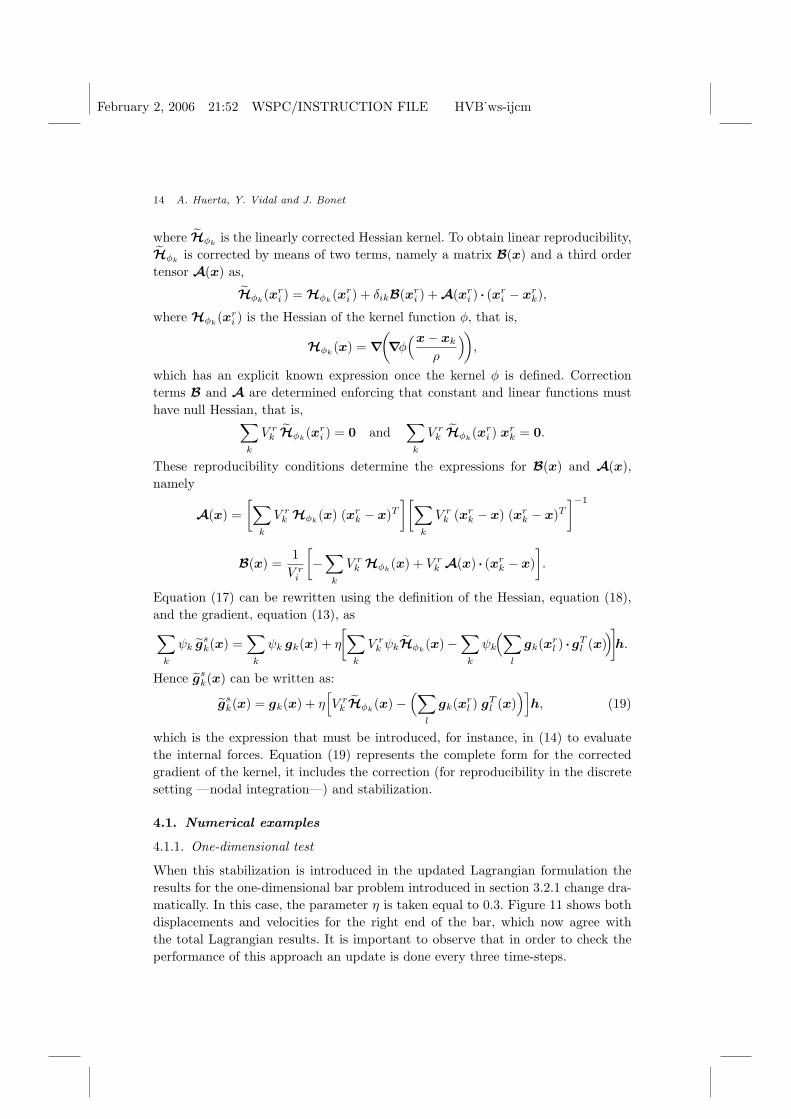
When this stabilization is introduced in the updated Lagrangian formulation theresults for the one-dimensional bar problem introduced in section 3.2.1 change dra-matically. In this case, the parameter η is taken equal to 0.3. Figure 11 shows bothdisplacements and velocities for the right end of the bar, which now agree withthe total Lagrangian results. It is important to observe that in order to check theperformance of this approach an update is done every three time-steps.
February 2, 2006 21:52 WSPC/INSTRUCTION FILE HVB˙ws-ijcm
Updated Lagrangian formulation for CSPH 15
0 0.002 0.004 0.006 0.008 0.01 0.012 0.014 0.016
−1
−0.5
0
0.5
1
x 10−3
Time (s)
Dis
plac
emen
t tip
nod
e (m
)
0 0.002 0.004 0.006 0.008 0.01 0.012 0.014 0.016−6
−4
−2
0
2
4
6
Time (s)
Vel
ocity
tip
node
(m
/s)
Fig. 11. Displacement (left) and velocity (right) history for the right end of the bar using Hessian’sdifference stabilization.
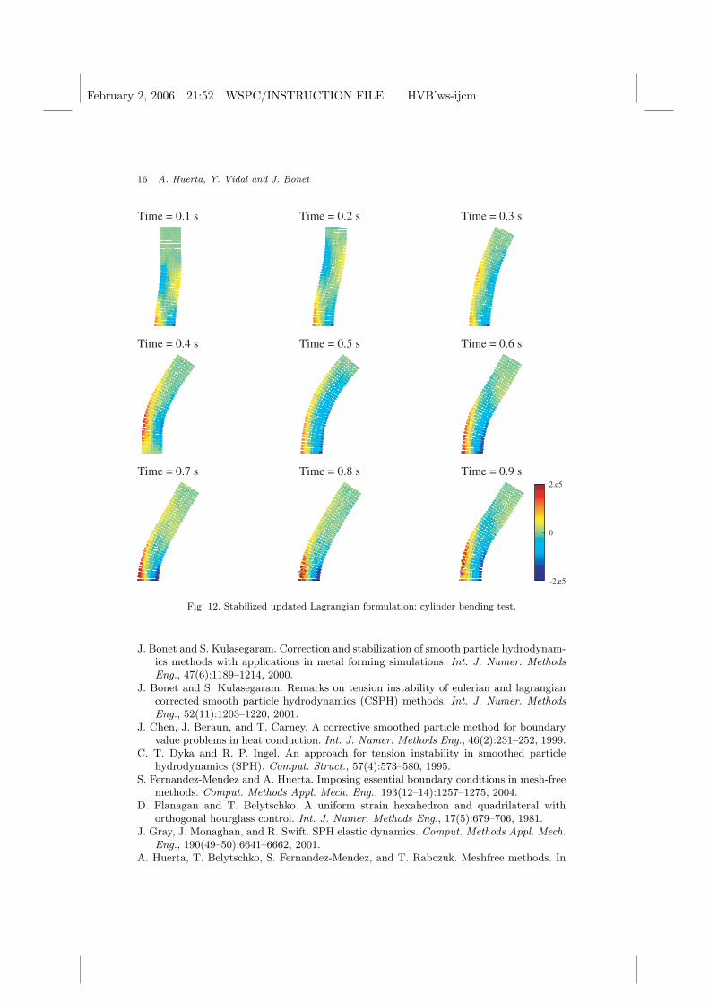
4.1.2. Cylinder bending test with a hyperelastic material
The oscillating bar presented in section 2.4 is solved using an updated Lagrangianstabilized formulation. These test is particularly demanding for both tension in-stability (not present in any updated formulation) and spurious mechanisms, thatmust be suppressed with the stabilization. Moreover, in order to further evaluatethe performance of the stabilization updates are activated every three time-steps inorder to ensure updates are not activating any mechanisms. Results for η = 1.5 canbe seen in Figure 12. Time t = 0.9s is achieved with 8633 time steps. Thus, 2877updates have been performed. Good results similar to the ones obtained with theLagrangian formulation are obtained.
5. CONCLUSIONS
In this paper an updated Lagrangian stabilized formulation has been proposed. Itsbehavior has been tested in a simple one-dimensional synthetic example and in anumerical benchmark test extremely sensible to tensile instability or zero energymodes. The stabilized updated Lagrangian formulation behaves similarly to thetotal Lagrangian formulation but can encompass problems involving large distor-tions using updates for the neighbors. Updates are only performed when needed;thus, in practice, the updated formulation has a low computational cost comparedto the total Lagrangian one. Moreover, numerical examples show that even foran unreasonable number of updates —inducing, in practice, to a formulation whereneighbors a recomputed almost at each time-step— zero (or negative) energy modesare precluded.
References
T. Belytschko, Y. Guo, W. K. Liu, and S. P. Xiao. A unified stability analysis of meshlessparticle methods. Internat. J. Numer. Methods Engrg., 48(9):1359–1400, 2000.
February 2, 2006 21:52 WSPC/INSTRUCTION FILE HVB˙ws-ijcm
16 A. Huerta, Y. Vidal and J. Bonet
Time = 0.1 s Time = 0.2 s Time = 0.3 s
Time = 0.4 s Time = 0.5 s Time = 0.6 s
Time = 0.7 s Time = 0.8 s Time = 0.9 s
-2.e5
0
2.e5
Fig. 12. Stabilized updated Lagrangian formulation: cylinder bending test.
J. Bonet and S. Kulasegaram. Correction and stabilization of smooth particle hydrodynam-ics methods with applications in metal forming simulations. Int. J. Numer. MethodsEng., 47(6):1189–1214, 2000.
J. Bonet and S. Kulasegaram. Remarks on tension instability of eulerian and lagrangiancorrected smooth particle hydrodynamics (CSPH) methods. Int. J. Numer. MethodsEng., 52(11):1203–1220, 2001.
J. Chen, J. Beraun, and T. Carney. A corrective smoothed particle method for boundaryvalue problems in heat conduction. Int. J. Numer. Methods Eng., 46(2):231–252, 1999.
C. T. Dyka and R. P. Ingel. An approach for tension instability in smoothed particlehydrodynamics (SPH). Comput. Struct., 57(4):573–580, 1995.
S. Fernandez-Mendez and A. Huerta. Imposing essential boundary conditions in mesh-freemethods. Comput. Methods Appl. Mech. Eng., 193(12–14):1257–1275, 2004.
D. Flanagan and T. Belytschko. A uniform strain hexahedron and quadrilateral withorthogonal hourglass control. Int. J. Numer. Methods Eng., 17(5):679–706, 1981.
J. Gray, J. Monaghan, and R. Swift. SPH elastic dynamics. Comput. Methods Appl. Mech.Eng., 190(49–50):6641–6662, 2001.
A. Huerta, T. Belytschko, S. Fernandez-Mendez, and T. Rabczuk. Meshfree methods. In
February 2, 2006 21:52 WSPC/INSTRUCTION FILE HVB˙ws-ijcm
Updated Lagrangian formulation for CSPH 17
E. Stein, R. de Borst, and T. J. R. Hughes, editors, Encyclopedia of ComputationalMechanics, volume 1 Fundamentals, chapter 10, pages 279–309. John Wiley & Sons,Ltd., Chichester, 2004.
G. R. Johnson and S. R. Beissel. Normalized smoothing functions for SPH impact com-putations. Int. J. Numer. Methods Eng., 39(16):2725–2741, 1996.
G. R. Johnson, E. H. Petersen, and R. A. Stryk. Incorporation of an SPH option into theEPIC code for a wide-range of high-velocity impact computations. Int. J. Impact Eng.,14(1–4):385–394, 1993.
G. R. Johnson, R. A. Stryk, and S. R. Beissel. SPH for high velocity impact computations.Comput. Methods Appl. Mech. Eng., 139(1-4):347–373, 1996.
Y. Krongauz and T. Belytschko. Consistent pseudo-derivatives in meshless methods. Com-put. Methods Appl. Mech. Eng., 146(3-4):371–386, 1997.
L. Libersky, A. Petscheck, T. Carney, J. Hipp, and F. Allahdadi. High strain lagrangianhydrodynamics. J. Comput. Phys., 109(1):67–75, 1993.
M. B. Liu, G. R. Liu, and K. Y. Lam. Constructing smoothing functions in smoothedparticle hydrodynamics with applications. J. Comput. Appl. Math., 155(2):263–284,2003.
W. K. Liu, S. Jun, and Y. F. Zhang. Reproducing kernel particle methods. Int. J. Numer.Methods Fluids, 20(8–9):1081–1106, 1995.
L. Lucy. Numerical approach to testing of the fission hypothesis. Astron. J., 82(12):1013–1024, 1977.
J. J. Monaghan. Why particle methods work. SIAM J. Sci. Stat. Comput., 3(4):422–433,1982.
P. W. Randles and L. D. Libersky. Normalized SPH with stress points. Int. J. Numer.Methods Eng., 48(10):1445–1462, 1996.
P. W. Randles and L. D. Libersky. Smoothed particle hydrodynamics: some recent im-provements and applications. Comput. Methods Appl. Mech. Eng., 139(1–4):375–408,1996.
R. Stellingwerf and C. Wingate. Impact modeling with Smooth Particle Hydrodynamics.Int. J. Impact Eng., 14(1–4):707–718, 1993.
J. W. Swegle, D. L. Hicks, and S. W. Attaway. Smoothed particle hydrodynamics stabilityanalysis. J. Comput. Phys., 116(1):123–134, 1995.
J. P. Vila. On particle weighted methods and smooth particle hydrodynamics. Math. Mod-els Methods Appl. Sci., 9(2):161–209, 1999.