unsteady flow simulations over variable topography without

INTERNATIONAL JOURNAL FOR NUMERICAL METHODS IN FLUIDSInt. J. Numer. Meth. Fluids 2000; 00:1–6 Prepared using fldauth.cls [Version: 2002/09/18 v1.01]

Unsteady Flow Simulations Over Variable Topography withoutRiemann Solvers

C. Zoppou1, S. G. Roberts1,∗, A. I. Delis2 and J. Sampson3

1 Department of Mathematics, Mathematical Sciences Institute, Australian National University, Canberra,ACT 0200, Australia

2 Department of Science, Division of Mathematics, Technical University of Crete, University Campus, 71409Chania, Crete, Greece

3 Mathematics Discipline, Faculty of Engineering and Industrial Sciences, Swinburne University ofTechnology, Hawthorn, Victoria, 3122, Australia

SUMMARY

A number of efficient and accurate algorithms exist for solving the homogeneous shallow water waveequations. Source terms which account for the influence of bathymetry and frictional forces aregenerally added to the homogeneous equations. There are a number of schemes which include thesource terms in the underlying numerical algorithm, such as the relaxation scheme and extensions tothe staggered central scheme present in this paper. These schemes also have the advantage that thestructure of the solution does not need to be known, nor is knowledge of the exact or approximatesolution to the Riemann problem required. These numerical schemes are used to simulate unsteadyflow in a canal with a parabolic shaped longitudinal bed profile and linear friction, for which analyticalsolutions have been derived by the last author. This is an example of a new class of one- and two-dimensional analytical solutions to the shallow water wave equations with bathymetry and friction.The attractive feature of these analytical solutions is that they are simple to evaluate.

The second-order relaxation and staggered central schemes are capable of simulating unsteadyflows in a channel with variable topography without requiring that knowledge of the structure ofthe solution is known in detail. However, their formal accuracy is reduced for problems involvingthe wetting and drying process. This is demonstrated by simulating unsteady flow in a channel withvariable bathymetry, friction and with a moving interface between the wet and dry region for which ananalytical solution to the shallow water wave equation is derived. The analytical solution can be usedto enhance the treatment of the wetting and drying process in these and other numerical schemes andto effectively compare the performance of other numerical schemes. Copyright c© 2000 John Wiley& Sons, Ltd.

key words: shallow water wave equations; central scheme; relaxation scheme; unsteady flows;

analytical solution; source terms

∗Correspondence to: Department of Mathematics, Mathematical Sciences Institute, Australian NationalUniversity, Canberra, ACT 0200, Australia

Received -

Copyright c© 2000 John Wiley & Sons, Ltd. Revised -

2 C. ZOPPOU ET AL.

1. Introduction

The governing equations for one-dimensional unsteady flow in a wide open channel can bewritten in non-homogeneous conservative form as

∂U

∂t+

∂F (U)

∂x= S(U) (1)

in which

U =

[

huh

]

, F (U) =

uh

u2h +gh2

2

and S(U) =

0

−gh

(

dzb

dx+ Sf

)

(2)

where, g is the acceleration due to gravity, h is the water depth, u is the cross-sectional averageflow velocity, zb is the elevation of the bed above some arbitrary horizontal datum, z = zb+h isthe elevation of the water surface above the horizontal datum, Sf is the friction slope, expressedby the Manning equation; Sf = η2u|u|/h4/3, where η is the Manning resistance coefficient,and t is the time. These equations are considered sufficiently accurate for the simulation ofunsteady flow in open channels, where the flow is predominately along the length of the channelin the x-direction. When S = 0 these equations are homogeneous, hyperbolic when h > 0,becoming parabolic when h = 0.

The solution of the one-dimensional problem is the foundation of many two-dimensionalmodels, such as models based on the finite volume scheme. Therefore, investigating thebehaviour and the accuracy of numerical schemes used to solve the one-dimensional problemis relevant to higher dimensional problems as well. Extending the analysis to two-dimensionalproblems is not in the scope of this current work but is under investigation.

There are numerous schemes that are capable of accurately solving the homogeneousform of the governing equations, see Erduran et al. [15] and Zoppou and Roberts [40].Amongst the most popular are Osher’s P [14], Roe [31], HLL [18], upwind [4] [34], weightedaverage flux [16] [37], piecewise parabolic [10], essentially non-oscillatory [29], space-timeconservative [8], relaxation [3][11][12][13][33], and central [28] schemes.

The solution of the homogeneous equations in shock-capturing methods generally involvesthe solution of the initial value problem (1) with discontinuous data

U(x = 0, t) =

{

UL if x < 0UR if x > 0

,

where, UL and UR are the states to the left and right respectively of the discontinuity at x = 0,known as the Riemann problem. Generally, the solution of the Riemann problem requiresdetailed knowledge of the underlying structure of the equations, i.e. does it degenerate intoa solution of a family of shocks, rarefaction waves or a combination of shock and rarefactionwaves. For the one-dimensional shallow water wave equations there must be a rarefaction waveor two waves which can be any combination of shock and rarefaction waves. For the wetting todrying process the hyperbolic system of equations revert to a parabolic system and this casemust be considered explicitly as part of the Reimann problem.

Knowledge of the shock speed and their strength requires a detailed understanding ofthe structure of the solution. This is the situation for the exact and approximate Riemannsolvers such as the HLL [18] and weighted average flux schemes [16] [37], piecewise parabolic

Copyright c© 2000 John Wiley & Sons, Ltd. Int. J. Numer. Meth. Fluids 2000; 00:1–6Prepared using fldauth.cls

UNSTEADY FLOW SIMULATIONS WITHOUT RIEMANN SOLVERS 3

method [10], Osher’s P -scheme [14], Roe’s scheme [31], essentially non-oscillatory [29] andupwind schemes [4] [34].

There are classes of numerical schemes that do not require a detailed understanding of theunderlying structure of the solution. Amongst these include the central schemes describedby Nessyahu and Tadmor [28] and others [19] [23] [25] [26]; the kinetic scheme described byXu [39], Audusse et al. [2] and Perthame and Simeoni [30]; the relaxation scheme described byJin and Xin [22] and Caflisch et al. [5] and used by Aral et al. [1], Delis and Katsaounis [11][12]and Delis and Papoglou [13]; Boltzman based models, see Ghidaoui et al. [17]; and the space-time conservation element scheme developed by Chang [8] and used by Molls and Molls [27].These schemes represent promising strategies that compliment schemes that solve the Riemannproblem.

Avoiding the solution of a Riemann problem can significantly simplify large scale engineeringproblems as well as avoiding the calculation of complicated Jacobian matrices for complexfluxes, such as two phase flow, pollutant and sediment transport problems (see, for exampleDelis and Katsaounis [12] and Delis and Papoglou [13]).

An extension to the central scheme developed by Nessyahu and Tadmor [28] and therelaxation scheme described by Delis and Katsaounis [11] are used to solve the shallow waterwave equations containing source terms. The major feature of these schemes is that they avoidthe solution of the time consuming Riemann problem, only requiring the specification of theflux F (U). They are capable of simulating unsteady flows in channels with variable topographyand the wetting and drying process is handled automatically. This is demonstrated using ananalytical solution to the shallow water wave equations describing unsteady flow in a canalwith a parabolic shaped longitudinal bed and linear friction. The analytical solution is from anew class of analytical solution to the shallow water wave equations. This class compliments asmall group of analytical solutions to the non-linear shallow water wave equations that can befound in the literature, which involve a bed slope. This is the only class of analytical solutionsthat involves both bed slope and friction, albeit linear friction.

In Section 2 the central scheme of Nessyahu and Tadmor is described. This is followed bya description of the relaxation scheme of Delis and Katsaounis in Section 3. In Section 4,one example of a new class of analytical solutions of the shallow water wave equations withbed slope and linear friction is derived. The central and relaxation schemes are used to solvethe unsteady flow problem for which the analytical solution was derived in Section 4. Theperformance of these schemes is discussed in Section 5.

2. Central Schemes

Following the work of Nessyahu and Tadmor [28], a family of fully-discrete, high resolutionRiemann-solver free schemes have been developed. This staggered second-order in both spaceand time scheme, has been extended to more general non-staggered second-order schemesby Kurganov and Levy [23] and to third- and fourth-order accurate schemes by Liu andTadmor [26], Levy et al. [24], Jiang et al. [19], and to non-homogeneous equations by Liottaet al. [25].

The staggered central scheme is developed by integrating (1) over a computational cell


4 C. ZOPPOU ET AL.

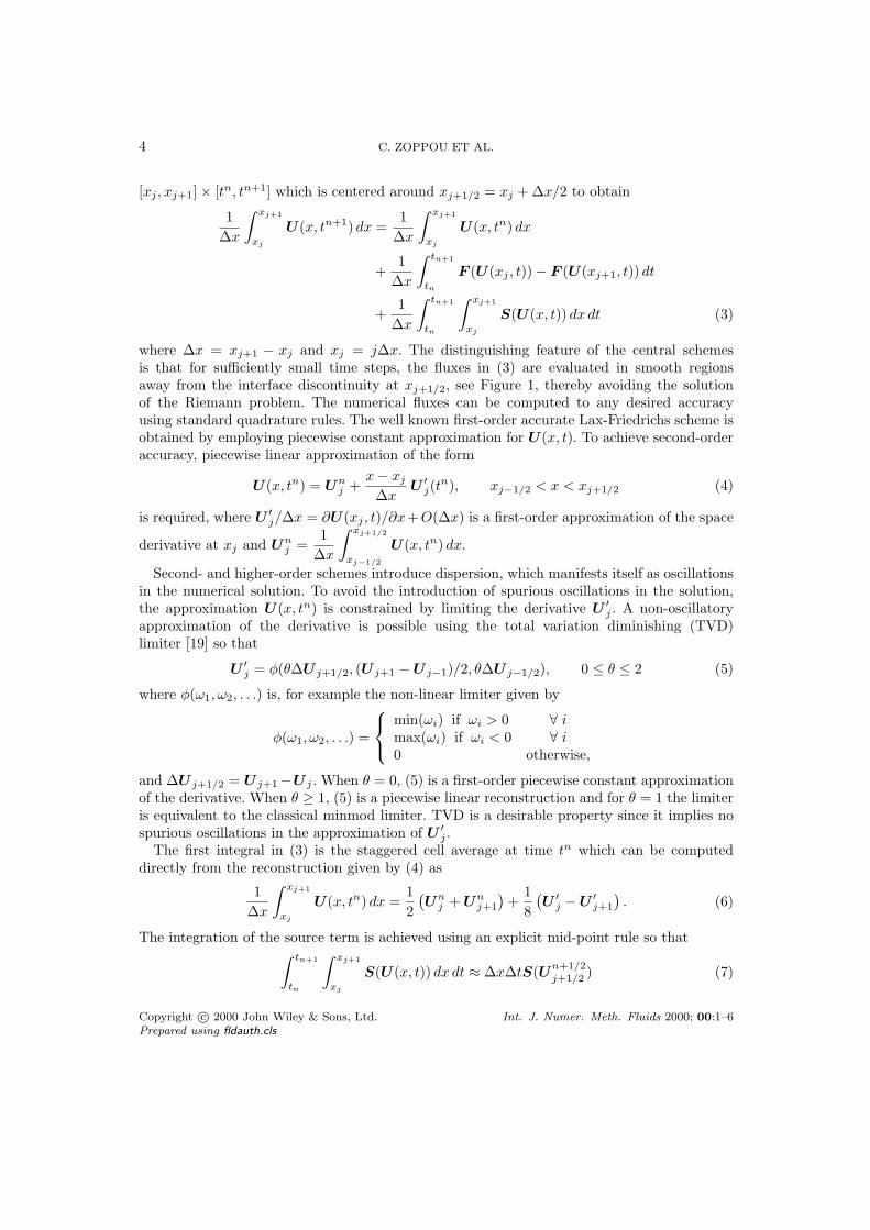
[xj , xj+1] × [tn, tn+1] which is centered around xj+1/2 = xj + ∆x/2 to obtain

1

∆x

∫ xj+1

xj

U(x, tn+1) dx =1

∆x

∫ xj+1

xj

U(x, tn) dx

+1

∆x

∫ tn+1

tn

F (U(xj , t)) − F (U(xj+1, t)) dt

+1

∆x

∫ tn+1

tn

∫ xj+1

xj

S(U(x, t)) dx dt (3)

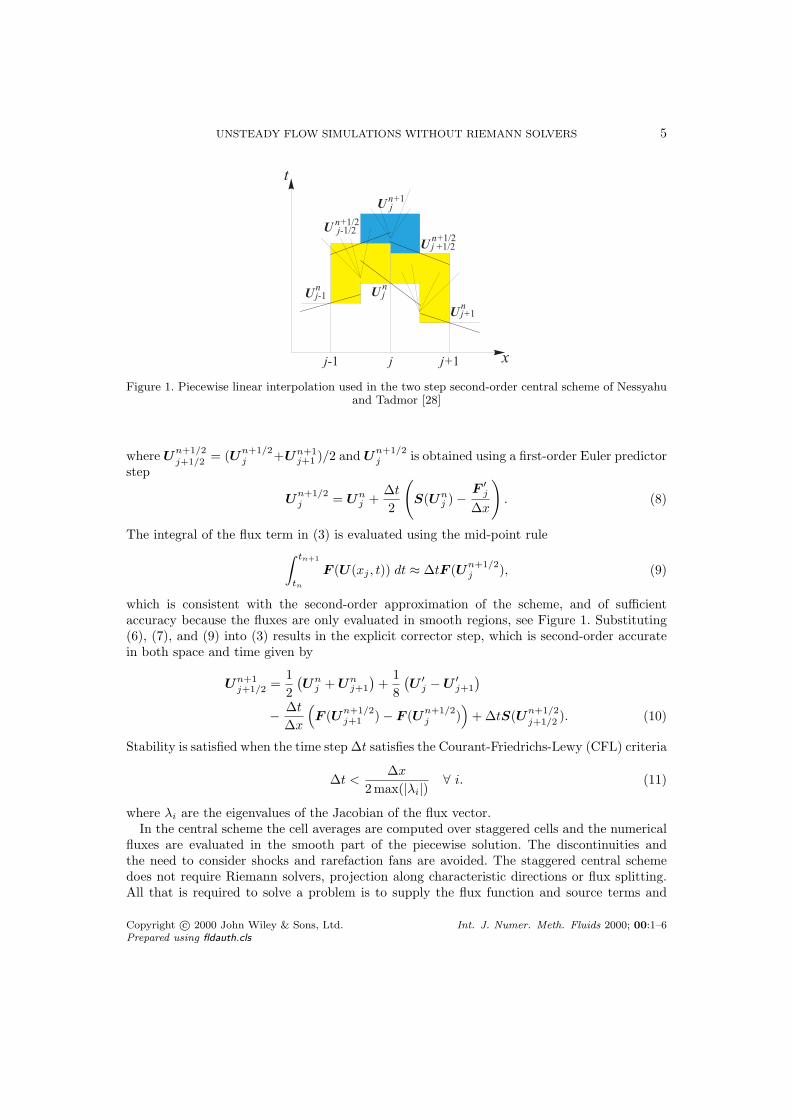
where ∆x = xj+1 − xj and xj = j∆x. The distinguishing feature of the central schemesis that for sufficiently small time steps, the fluxes in (3) are evaluated in smooth regionsaway from the interface discontinuity at xj+1/2, see Figure 1, thereby avoiding the solutionof the Riemann problem. The numerical fluxes can be computed to any desired accuracyusing standard quadrature rules. The well known first-order accurate Lax-Friedrichs scheme isobtained by employing piecewise constant approximation for U(x, t). To achieve second-orderaccuracy, piecewise linear approximation of the form

U(x, tn) = Unj +

x − xj

∆xU

′

j(tn), xj−1/2 < x < xj+1/2 (4)

is required, where U′

j/∆x = ∂U(xj , t)/∂x+O(∆x) is a first-order approximation of the space

derivative at xj and Unj =

1

∆x

∫ xj+1/2

xj−1/2

U(x, tn) dx.

Second- and higher-order schemes introduce dispersion, which manifests itself as oscillationsin the numerical solution. To avoid the introduction of spurious oscillations in the solution,the approximation U(x, tn) is constrained by limiting the derivative U

′

j . A non-oscillatoryapproximation of the derivative is possible using the total variation diminishing (TVD)limiter [19] so that

U′

j = φ(θ∆U j+1/2, (U j+1 − U j−1)/2, θ∆U j−1/2), 0 ≤ θ ≤ 2 (5)

where φ(ω1, ω2, . . .) is, for example the non-linear limiter given by

φ(ω1, ω2, . . .) =

min(ωi) if ωi > 0 ∀ imax(ωi) if ωi < 0 ∀ i0 otherwise,

and ∆U j+1/2 = U j+1−U j . When θ = 0, (5) is a first-order piecewise constant approximationof the derivative. When θ ≥ 1, (5) is a piecewise linear reconstruction and for θ = 1 the limiteris equivalent to the classical minmod limiter. TVD is a desirable property since it implies nospurious oscillations in the approximation of U

′

j .The first integral in (3) is the staggered cell average at time tn which can be computed

directly from the reconstruction given by (4) as

1

∆x

∫ xj+1

xj

U(x, tn) dx =1

2

(

Unj + U

nj+1

)

+1

8

(

U′

j − U′

j+1

)

. (6)

The integration of the source term is achieved using an explicit mid-point rule so that∫ tn+1

tn

∫ xj+1

xj

S(U(x, t)) dx dt ≈ ∆x∆tS(Un+1/2j+1/2 ) (7)



Figure 1. Piecewise linear interpolation used in the two step second-order central scheme of Nessyahuand Tadmor [28]

where Un+1/2j+1/2 = (U

n+1/2j +U

n+1j+1 )/2 and U

n+1/2j is obtained using a first-order Euler predictor

step

Un+1/2j = U

nj +

∆t

2

(

S(Unj ) −

F′

j

∆x

)

. (8)

The integral of the flux term in (3) is evaluated using the mid-point rule

∫ tn+1

tn

F (U(xj , t)) dt ≈ ∆tF (Un+1/2j ), (9)

which is consistent with the second-order approximation of the scheme, and of sufficientaccuracy because the fluxes are only evaluated in smooth regions, see Figure 1. Substituting(6), (7), and (9) into (3) results in the explicit corrector step, which is second-order accuratein both space and time given by

Un+1j+1/2 =

1

2

(

Unj + U

nj+1

)

+1

8

(

U′

j − U′

j+1

)

− ∆t

∆x

(

F (Un+1/2j+1 ) − F (U

n+1/2j )

)

+ ∆tS(Un+1/2j+1/2 ). (10)

Stability is satisfied when the time step ∆t satisfies the Courant-Friedrichs-Lewy (CFL) criteria

∆t <∆x

2max(|λi|)∀ i. (11)

where λi are the eigenvalues of the Jacobian of the flux vector.In the central scheme the cell averages are computed over staggered cells and the numerical

fluxes are evaluated in the smooth part of the piecewise solution. The discontinuities andthe need to consider shocks and rarefaction fans are avoided. The staggered central schemedoes not require Riemann solvers, projection along characteristic directions or flux splitting.All that is required to solve a problem is to supply the flux function and source terms and


6 C. ZOPPOU ET AL.

to estimate the characteristic speeds so that the Courant-Friedrichs-Lewy stability condition,(11) is satisfied.

A single evolution of the solution over the time step ∆t on the original grid is obtained asa sequence of two intermediate steps over ∆t/2 on the staggered grid, see Figure 1.

3. Relaxation Scheme

Following Jin and Xin [22], the original equations (1) are written as an enlarged system ofequations with linear advection of the form

∂U

∂t+

∂V

∂x= S(U), (12a)

∂V

∂t+ C

2 ∂U

∂x= −1

ε(V − F (U)) , (12b)

by introducing a new variable V , where, ε > 0 is the relaxation time, C2 is a positive diagonal

matrix with components c2i , which are to be chosen.

When ε ≪ 1, the relaxation system, given by (12) is an approximation of the originalconservation law, given by (1). The original conservation law has been replaced by a linearhyperbolic system with a relaxation source term where V → F (U) rapidly as ε → 0+.Therefore, for sufficiently small ε solving (12) can also provide a reasonable approximationto the original non-linear conservation laws.

The stability of the relaxation scheme can be established by expanding equations (12) usingthe Chapman-Enskog expansion. Retaining only first-order terms in ε, in the Chapman-Enskogexpansion, the relaxation equations are approximated by the advective-diffusion equation

∂U

∂t+

∂

∂x

(

F (U) − ε∂F (U)

∂US(U)

)

= S(U) + ε∂

∂x

([

C2 −

(

∂F (U)

∂U

)2]

∂U

∂x

)

.

Stability of the scheme is ensured if it is dissipative, which is achieved if the sub-characteristic

condition

C2 −

(

∂F (U)

∂U

)2

≥ 0. (13)

Therefore, it is only necessary to choose sufficiently large C to produce the desired dissipativescheme. There is no need for characteristic decomposition. It is however, desirable to selectvalues for C that satisfy the equality in (13) to avoid the introduction of excessive diffusion inthe numerical scheme. Ideally, estimates of C can be based on estimates of the characteristicspeed for the problem considered. For the one-dimensional problem, every eigenvalue, λi of∂F (U)/∂U should satisfies |λ| ≤ cmax, where cmax = max(ci) ∀ i thereby ensuring that thecharacteristic speeds of the hyperbolic part of (12) are larger than the characteristic speeds ofthe original problem. A necessary condition to ensure stability of the scheme.

The relaxation system (12) has two Riemann invariants along characteristic with slopesgiven by

V ±CU . (14)



Therefore, (12) retains the hyperbolic characteristics of the original equations, as long as theci’s are chosen large enough.

Adopting the method of lines, where the space and time discretizations are treatedseparately, then a semi-discrete approximation to (12) can be written as

dU j

dt+ Dx(V j) = Sj (15a)

dV j

dt+ C

2Dx(U j) = −1

ε(V j − F (U j)) (15b)

where

Dx(W j) =1

∆x

(

W j+1/2 − W j−1/2

)

. (15c)

What remains is the evaluation of flux terms in (15). Any approximation of the numericalflux should be consistent with the accuracy of the time integration employed to evolve (15).Therefore, a second-order approximation of the flux terms is required. The MUSCL (MonotoneUpwind-centered Schemes for Conservation Laws) [38] piecewise linear interpolation is appliedto the kth component of the Riemann invariants (14) to give

(V + ckU)j+1/2 = (V + ckU)j +∆xσ+

j

2(16a)

(V − ckU)j+1/2 = (V − ckU)j+1 −∆xσ−

j+1

2(16b)

where the slopes of v ± cku, σ±

j are determined using a slope limiter to avoid introducingspurious extrema in the solution. The slope

σ±

j =1

∆x(V j+1 ± ckU j+1 − V j ∓ ckU j)φ(θ±j )

where

θ±j =V j ± ckU j − V j−1 ∓ ckU j−1

V j+1 ± ckU j+1 − V j ∓ ckU j

and φ(θ±j ) is a suitable slope limiter function. From (16)

U j+1/2 =1

2(U j + U j+1) −

1

2ck(V j+1 − V j) +

∆x

4ck(σ+

j + σ−

j+1)

V j+1/2 =1

2(V j + V j+1) −

ck

2(U j+1 − U j) +

∆x

4(σ+

j − σ−

j+1)

which are required in (15) to complete the semi-discrete relaxation scheme.A fully discrete relaxation scheme is developed by employing a second-order total variational

diminishing (TVD) Runge-Kutta splitting scheme described by Jin [21] to perform the timeintegration.

Given Un,V n then U

n+1,V n+1 can be computed using a splitting strategy which treatsthe stiff source term 1

ε (V − F (U)) implicitly in steps (17b) and (17f) and the other sourceand convection terms explicitly in alternating steps, so that (see, Caflisch et al. [5] and Delis


8 C. ZOPPOU ET AL.

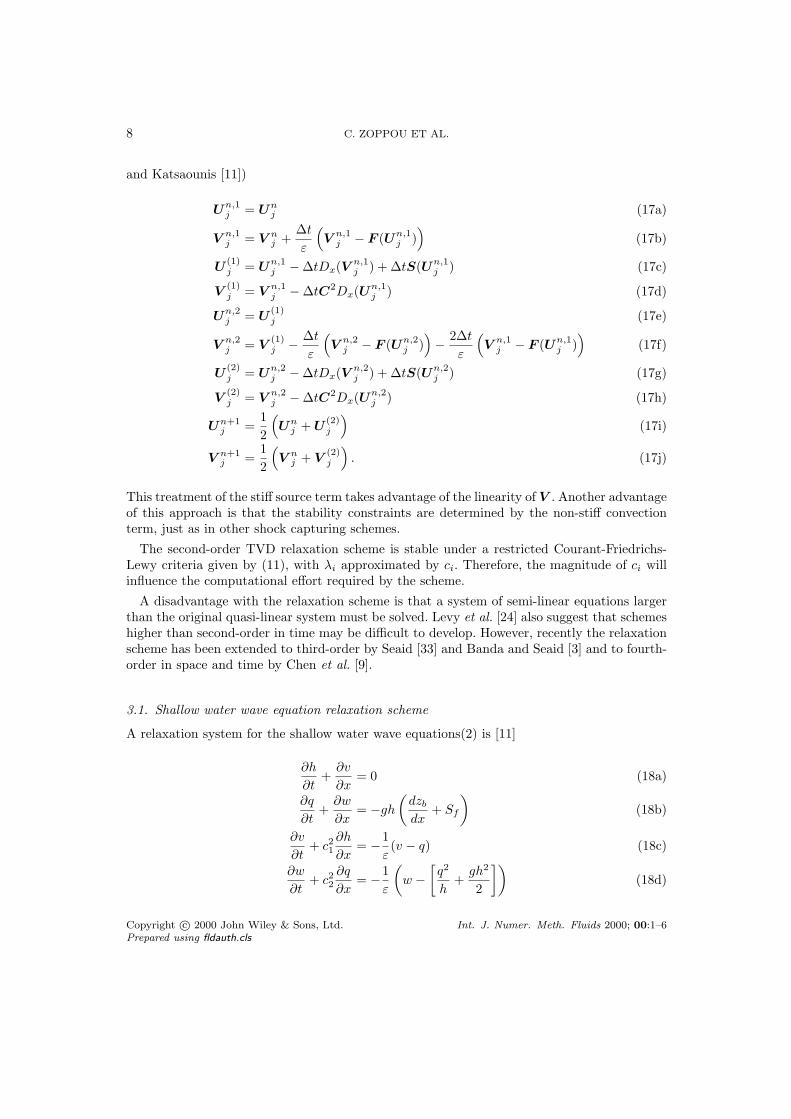
and Katsaounis [11])

Un,1j = U

nj (17a)

Vn,1j = V

nj +

∆t

ε

(

Vn,1j − F (Un,1

j ))

(17b)

U(1)j = U

n,1j − ∆tDx(V n,1

j ) + ∆tS(Un,1j ) (17c)

V(1)j = V

n,1j − ∆tC2Dx(Un,1

j ) (17d)

Un,2j = U

(1)j (17e)

Vn,2j = V

(1)j − ∆t

ε

(

Vn,2j − F (Un,2

j ))

− 2∆t

ε

(

Vn,1j − F (Un,1

j ))

(17f)

U(2)j = U

n,2j − ∆tDx(V n,2

j ) + ∆tS(Un,2j ) (17g)

V(2)j = V

n,2j − ∆tC2Dx(Un,2

j ) (17h)

Un+1j =

1

2

(

Unj + U

(2)j

)

(17i)

Vn+1j =

1

2

(

Vnj + V

(2)j

)

. (17j)

This treatment of the stiff source term takes advantage of the linearity of V . Another advantageof this approach is that the stability constraints are determined by the non-stiff convectionterm, just as in other shock capturing schemes.

The second-order TVD relaxation scheme is stable under a restricted Courant-Friedrichs-Lewy criteria given by (11), with λi approximated by ci. Therefore, the magnitude of ci willinfluence the computational effort required by the scheme.

A disadvantage with the relaxation scheme is that a system of semi-linear equations largerthan the original quasi-linear system must be solved. Levy et al. [24] also suggest that schemeshigher than second-order in time may be difficult to develop. However, recently the relaxationscheme has been extended to third-order by Seaid [33] and Banda and Seaid [3] and to fourth-order in space and time by Chen et al. [9].

3.1. Shallow water wave equation relaxation scheme

A relaxation system for the shallow water wave equations(2) is [11]

∂h

∂t+

∂v

∂x= 0 (18a)

∂q

∂t+

∂w

∂x= −gh

(

dzb

dx+ Sf

)

(18b)

∂v

∂t+ c2

1

∂h

∂x= −1

ε(v − q) (18c)

∂w

∂t+ c2

2

∂q

∂x= −1

ε

(

w −[

q2

h+

gh2

2

])

(18d)



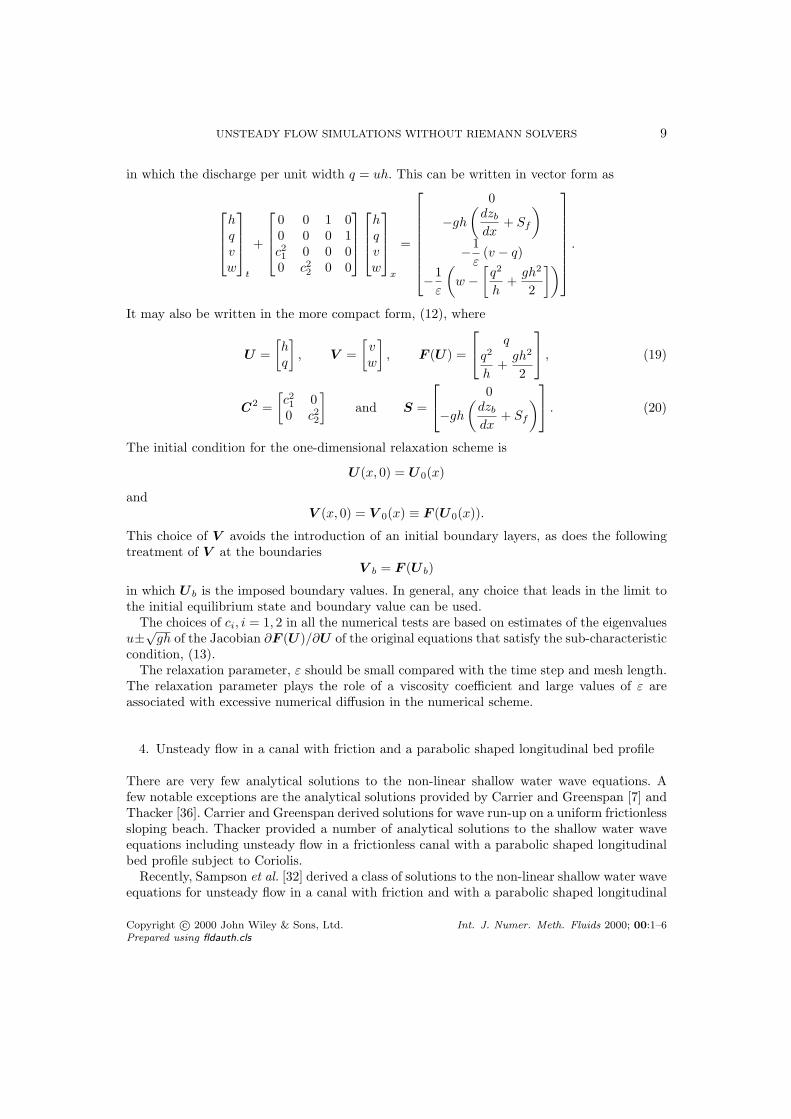
in which the discharge per unit width q = uh. This can be written in vector form as

hqvw

t

+

0 0 1 00 0 0 1c21 0 0 00 c2

2 0 0

hqvw

x

=

0

−gh

(

dzb

dx+ Sf

)

−1

ε(v − q)

−1

ε

(

w −[

q2

h+

gh2

2

])

.

It may also be written in the more compact form, (12), where

U =

[

hq

]

, V =

[

vw

]

, F (U) =

qq2

h+

gh2

2

, (19)

C2 =

[

c21 00 c2

2

]

and S =

0

−gh

(

dzb

dx+ Sf

)

. (20)

The initial condition for the one-dimensional relaxation scheme is

U(x, 0) = U0(x)

andV (x, 0) = V 0(x) ≡ F (U0(x)).

This choice of V avoids the introduction of an initial boundary layers, as does the followingtreatment of V at the boundaries

V b = F (U b)

in which U b is the imposed boundary values. In general, any choice that leads in the limit tothe initial equilibrium state and boundary value can be used.

The choices of ci, i = 1, 2 in all the numerical tests are based on estimates of the eigenvaluesu±

√gh of the Jacobian ∂F (U)/∂U of the original equations that satisfy the sub-characteristic

condition, (13).The relaxation parameter, ε should be small compared with the time step and mesh length.

The relaxation parameter plays the role of a viscosity coefficient and large values of ε areassociated with excessive numerical diffusion in the numerical scheme.

4. Unsteady flow in a canal with friction and a parabolic shaped longitudinal bed profile

There are very few analytical solutions to the non-linear shallow water wave equations. Afew notable exceptions are the analytical solutions provided by Carrier and Greenspan [7] andThacker [36]. Carrier and Greenspan derived solutions for wave run-up on a uniform frictionlesssloping beach. Thacker provided a number of analytical solutions to the shallow water waveequations including unsteady flow in a frictionless canal with a parabolic shaped longitudinalbed profile subject to Coriolis.

Recently, Sampson et al. [32] derived a class of solutions to the non-linear shallow water waveequations for unsteady flow in a canal with friction and with a parabolic shaped longitudinal


10 C. ZOPPOU ET AL.

bed profile. The approach used by Sampson et al. [32] is similar to that used by Thacker [36].In the latter case, the initially stagnant water oscillates backward and forward in the canalunabated. In Sampson et al. [32], because friction is present, the oscillating water surfacedampens with time, becoming stagnant with a horizontal water surface. In both cases thelongitudinal profile of the water surface does not change, it remains a plane.

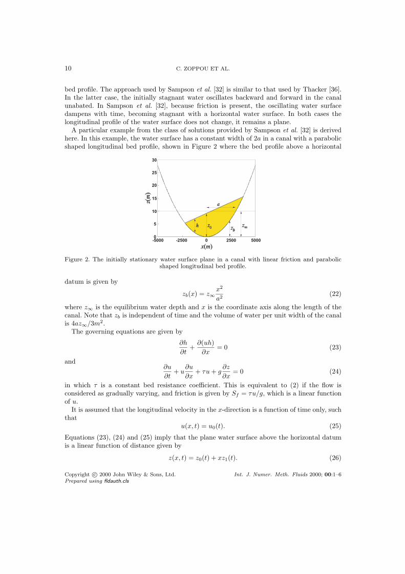
A particular example from the class of solutions provided by Sampson et al. [32] is derivedhere. In this example, the water surface has a constant width of 2a in a canal with a parabolicshaped longitudinal bed profile, shown in Figure 2 where the bed profile above a horizontal

30

25

20

15

10

5

0-5000 -2500 0 2500 5000

x m( )

zm(

)

a

h zb

z0

z¥

Figure 2. The initially stationary water surface plane in a canal with linear friction and parabolicshaped longitudinal bed profile.

datum is given by

zb(x) = z∞x2

a2(22)

where z∞ is the equilibrium water depth and x is the coordinate axis along the length of thecanal. Note that zb is independent of time and the volume of water per unit width of the canalis 4az∞/3m2.

The governing equations are given by

∂h

∂t+

∂(uh)

∂x= 0 (23)

and∂u

∂t+ u

∂u

∂x+ τu + g

∂z

∂x= 0 (24)

in which τ is a constant bed resistance coefficient. This is equivalent to (2) if the flow isconsidered as gradually varying, and friction is given by Sf = τu/g, which is a linear functionof u.

It is assumed that the longitudinal velocity in the x-direction is a function of time only, suchthat

u(x, t) = u0(t). (25)

Equations (23), (24) and (25) imply that the plane water surface above the horizontal datumis a linear function of distance given by

z(x, t) = z0(t) + xz1(t). (26)



The variables z0 and z1 are determined from boundary conditions imposed on the problem. Interms of water depth, (26) becomes

h(x, t) = z0(t) + xz1(t) − z∞x2

a2. (27)

Substituting (25) and (27) into (23) gives(

dz0

dt+ u0z1

)

+

(

dz1

dt− 2u0z∞

a2

)

x = 0. (28)

Equating the time-varying coefficients of the linearly independent terms 1 and x respectively,then

dz0

dt+ u0z1 = 0 (29)

anddz1

dt− 2u0z∞

a2= 0. (30)

There are two equations in the three unknown functions, u0, z0 and z1. The third equation isobtained by substituting (25) and (26) into (24), giving

du0

dt+ τu0 + gz1 = 0. (31)

First note that u0 can be eliminated from equations (29) and (30) to obtain a relationshipbetween z0 and z1, namely

dz0

dt+

d

dt

(

a2

4z∞z21

)

= 0.

Indeed, this can be integrated to obtain

z0 = z∞ − a2

4z∞z21 (32)

where the constant of integration follows from the fact that as t → ∞, z1(t) → 0, andz0(t) → z∞.

Differentiating (31) and eliminating dz1/dt between this equation and (30) results in asecond-order ordinary differential equation in u0 given by

d2u0

dt2+ τ

du0

dt+

2gz∞a2

u0 = 0. (33)

The solution to this equation involves the solution of the auxiliary equation

β2 + τβ +2gz∞

a2= 0

which has the roots

β =−τ ±

√

τ2 − p2

2

in which p is defined as

p =

√

8gz∞a2

.


12 C. ZOPPOU ET AL.

There are three possible solutions for β. These are when τ < p, τ > p and τ = p. Only thesolution for τ < p is provided here, the other solutions can be found in Sampson et al. [34].

If τ < p, then the general solution to (33) is

u0(t) = exp

(

−τt

2

)

(A cos(st) + B sin(st)) . (34)

where

s =

√

p2 − τ2

2.

Choosing u0(0) = 0, then from (34), A = 0 so that

u0(t) = B exp

(

−τt

2

)

sin(st). (35)

The velocity of the fluid in the canal exhibits an exponentially damped oscillatory behaviourwith time and as t → ∞, u0(t) → 0. This result is substituted into (31) to obtain the followingsolution for z1(t)

z1(t) = −exp

(

−τt

2

)

g

(

Bs cos(st) +τB

2sin(st)

)

. (36)

Substituting (32) and (36) into (26), the water surface elevation above the horizontal watersurface is given by

z(x, t) = z∞ − a2

4z∞z21(t) + xz1(t) (37)

= z∞ +a2B2 exp (−τt)

8g2z∞

(

−sτ sin(2st) +

[

τ2

4− s2

]

cos(2st)

)

− B2 exp(−τt)

4g− 1

g

(

exp

(

−τt

2

)[

Bs cos(st) +τB

2sin(st)

])

x.

As t → ∞, u0(t) → 0 and z(x, t) → z∞, the water surface becomes horizontal and still.The location of the shoreline occurs where z = zb, i.e. where

z∞ − a2

4z∞z21(t) + xz1(t) =

z∞a2

x2.

This is a quadratic equation in terms of the location of the shoreline x, given by

(

x − a2

2z∞z1(t)

)2

= a2.

which provides the following explicit solution for the position of the shoreline

x =a2 exp(−τt

2)

2gz∞

(

−Bs cos(st) − Bτ

2sin(st)

)

± a.

The shoreline oscillates backwards and forwards in the canal reaching equilibrium with x = ±aat t → ∞.



For example, the evolution of the water surface from t = 0s to 3,400s, in increments of200s defined by the analytical solution, (37) is shown in Figure 3. In this example, the canalwith a parabolic longitudinal bed profile, defined by (22), is 10,000m in length, has a frictioncoefficient, τ = 0.001s−1. The body of water in the canal has a top width of 2a = 6,000m, amaximum depth z∞ = 10m and B = 5ms−1 in (35), which defines the velocity of the waterbody. The volume of water per unit width of the canal is 4 × 104m2.

The unsteady flow in the canal maintains a plane water surface for all time. The variationin the water depth h at x = 0m with time is shown in Figure 4. There is an exponentialdecay in the oscillatory behaviour of the water depth with a rapid convergence to steady statecondition by t = 5,000s. The uniform velocity of the fluid body is shown in Figure 5 andthe location of the shoreline in the negative x-plane is shown in Figure 6. The oscillatorybehaviour of the velocity of the fluid body and the location of the shoreline also dampens withtime, eventually the fluid becomes stagnant with a horizontal water surface. The surface widthof the water body is always 6,000m and the shoreline is located at ±3,000m when the waterbody is stationary.

This is one example of an important class of analytical solutions to the shallow water waveequations that can be used to test numerical schemes for the solution of the non-linear shallowwater wave equations with source terms. Unlike other solutions to the non-linear shallow waterwave equations, these analytical solutions are very simple to evaluate and they can be extendedto unsteady flow in parabolic and elliptic basins.

5. Evaluation of the schemes

The above analytical solution is used to demonstrate the utility of the modified central andrelaxation schemes. The canal is 10,000m long and is divided into 500 segments, each 20min length. In both numerical schemes the minmod (θ = 1) limiter is used in (5) and thecomputational time step ∆t is calculated to satisfy the Courant-Friedrichs-Lewy criteria. Inthe; (a) modified staggered central scheme, CFL = 0.5 and the source term is treated explicitlyusing (8), and (b) relaxation scheme, c1 = c2 = 10ms−1, CFL = 0.25 and ε = 1 × 10−6.

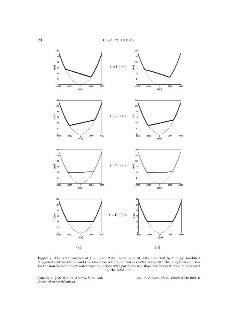
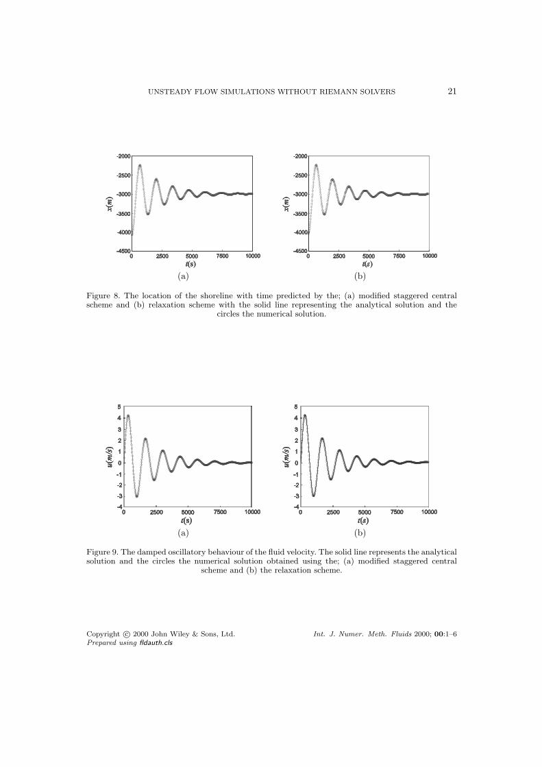
In Figure 7, the predicted and analytical water depth of the oscillating water surfacein a channel with a parabolic longitudinal bed profile and linear friction at timet = 1,400, 2,000, 5,000 and 10,000s is shown. The analytical solution and the numericalsolution are indistinguishable after four cycles. The wetting and drying process is capturedby the numerical scheme which required no modification to simulate this process. This isconfirmed by the excellent reproduction of the location of the shoreline, in the negative x-plane shown in Figure 8 for both schemes. The shoreline in the numerical scheme is identifiedas the location where the water depth is just greater than 1×10−4m. Both schemes are capableof accurately simulating the wetting and drying process as well as the location of the movingshoreline as the body of water inundates and recedes along the canal.

The uniform velocity of the oscillating fluid exhibits the same damped exponential behaviouras the analytical solution, see, Figure 9. The phase is also accurately predicted by the numericalscheme and both numerical schemes converge to the correct steady state solution. The flow isstagnant with a horizontal water surface.

The volume of water per unit width in the canal at t = 10,000s was also compared with theinitial volume in the canal. Within machine precision, both numerical schemes conserve the


14 C. ZOPPOU ET AL.

volume of water in the canal.

5.1. Convergance rates of the schemes

Since the analytical solution, (37) is a solution to a smooth problem, it can be used to establishthe formal convergence rate of a numerical scheme.

Theoretically, the central and relaxation schemes are considered as second-order schemes.This will be confirmed by comparing the simulated solution with the analytical solutionfor unsteady flow in a canal where a = 3,000m, τ = 0.001s−1, the maximum water depthz∞ = 10m and B = 5ms−1.

The difference between the analytical and predicted solution is calculated using the non-dimensional L1 norm given, for example the water depth h by

L1 =

∑ki=1 |hi − h(xi)|∑k

i=1 |h(xi)|at all the computational nodes, i = 1, . . . , k, at the end of the simulation, when t =1,000s,where hi is the simulated water depth at xi, and h(xi) is the corresponding analytical waterdepth.

Each scheme was used to perform a number of simulations of the same problem, but in eachsimulation the computational domain was subdivided into a different number of segments, kof equal size. The size of the segments range between ∆x = 0.1 to 50m. The computationaltime step chosen for each simulation was determined using

∆t =0.2∆x√

gz∞

which is proportional to ∆x and satisfies the CFL crtieria.In the modified staggered central scheme, θ = 1.5 in (5) and the source term is treated

explicitly using (8). For this smooth problem θ in (5) has no effect on the results, providedθ ≥ 1. For the relaxation scheme, c1 = c2 = 10ms−1, θ = 1 in (5) and ε = 1 × 10−11.Preliminary test reveal the accuracy of the relaxation scheme is insensitive to the relaxationparameter, ε. It is recommended that it should be chosen so that it is at least the same orderas the accuracy of the scheme, otherwise the full accuracy of the scheme will not be realised(see, Banda and Seaid [3] for a discussion on the selection of the relaxation parameters). Theanalytical solution is used to establish the initial and boundary conditions for the numericalschemes. In addition, there is no special treatment of the wetting and drying process.

The convergence rate for the staggered central and relaxation schemes is shown in Figures10(a) and 11(a) respectively for a canal which has a length of 10,000m. Both schemes do notexhibit second-order convergence. This slight deterioration in their theoretical convergencerate is attributable to the naive treatment of boundary between the body of water and thebed of the canal.

To establish the formal convergence rate of the schemes, the analytical problem has beenmodified slightly. In this case the canal has been truncated. The behaviour of the water body inthe central 2,000m of the canal only is simulated. Restricting the computation to this portionof the canal avoids the moving interface between the water body and the canal bed. At theextremity of the truncated canal the analytical solution is used as the boundary condition inthe models.



The convergence rate of both schemes are illustrated in Figures 10(b) and 11(b) forthe truncated canal. For this smooth problem, both schemes exhibit second-order rate ofconvergence. Compared to the simulation of the flow in the full canal, there is a significantimprovement in the overall accuracy of the numerical scheme, by two orders of magnitudein the L1 norm for both the water depth and velocity. Similar results were also obtained forthe second-order non-staggered central scheme proposed by Jiang et al. [20] and Jiang andTadmor [19].

Although both schemes are shown to be second-order accurate, the relaxation scheme is morediffusive than the staggered central scheme. In addition, for the full canal example, the rateof convergence for the relaxation scheme is lower than that for the staggered central scheme.

6. Conclusions

Two schemes, the modified staggered central and the relaxation schemes have beendemonstrated for the solution of the shallow water wave equation containing source terms.Both schemes avoid the intricate and time-consuming computation of the eigensystem of theproblem, required for the solution of the Riemman problem by other well known numericalschemes. They also incorporate source terms in the underlying numerical scheme. There is noneed to resort to operator splitting [35]. Therefore, they are highly suited for solving the shallowwater wave equation with source terms that represent, for example, complicated topographyand frictional resistance.

Unlike the one-dimensional case, no explicit Riemann solvers yet exist for two-dimensionalproblems. For two-dimensional problems a splitting strategy is employed where the one-dimensional Riemann problem is solved in one dimension at a time. These Riemman-free solverstherefore, can play a major role in the solution of the two-dimensional problem. In addition,these schemes are particularly suitable for complex systems in which little information on thephysical structure of the solution is available. This is certainly the case in the simulation ofsediment transport in unsteady flow [6]. In addition, it is not necessary to identify and treatthe wetting and drying process, where the system of equations become parabolic as a separateproblem.

Despite the lack of any specific physical input beyond the maximum local speeds, both themodified central scheme and relaxation schemes provide accurate simulation of unsteady flowsand the wetting and drying process. This was demonstrated using an example from a newclass of analytical solutions for unsteady flow in a canal with a parabolic shaped longitudinalbed profile and linear friction.

Because the relaxation scheme involves the solution of an enlarged system of equations, itis less efficient than the central scheme. It is also not as accurate as the central scheme. Bothschemes are shown to be second-order accurate. However, there is a slight deterioration in theconvergence rate of both schemes and a significant degradation in accuracy due to the naivetreatment of the wetting and drying process.

The analytical solution has been shown to be useful in objectively comparing theperformance of different numerical schemes and it can be used to develop more accuratetreatment of the wetting and drying process.


16 C. ZOPPOU ET AL.

REFERENCES

1. Aral MM, Zhang L, Jin S. Application of relaxation scheme to wave-propagation simulation in open-channelnetworks, Journal of Hydraulic Engineering American Society of Civil Engineers 1998;124(11):1125-1133.[3]

2. Audusse E, Bristeau MO, Perthame B. Kinetic schemes for Saint-Venant equations with source terms onunstructured grids. Institut National de Recherche en Informatique et en Automatique, INRIA, France,Report No. 3989 2000. p. 44. [3]

3. Banda, MK, Seaid M. Higher-order relaxation schemes for hyperbolic system of conservation laws. Journalof Numerical Mathematics. 2005;13(3):171-196. [2, 8, 14]

4. Bermudez A, Vazquez ME. Upwind methods for hyperbolic conservation laws with source terms.Computers and Fluids 1994;23(8):1049-1071. [2, 3]

5. Caflisch, RE, Jin S, Russo G. Uniformly accurate schemes for hyperbolic systems with relaxation. Societyfor Industrial and Applied Mathematics Journal for Numerical Analysis 1997;34(1):246-281. [3, 7]

6. Caleffi V, Valiani A, Bernini A. High-order balanced CWENO scheme for movable bed shallow waterequations. Advances in Water Resources 2007:30(4):730-741. [15]

7. Carrier GF, Greenspan HP. Water waves of finite amplitude on a sloping beach. Journal of FluidMechnanics 1958;4(1):97-109. [9]

8. Chang SC. The method of space-time conservation element and solution element: A new approach forsolving the Navier-Stokes and Euler equations. Journal of Computational Physics 1995;119(2):295-324.[2, 3]

9. Chen JZ, Shin, ZK. Application of fourth-order relaxation scheme to hyperbolic systems of conservationlaws. Acta Mechanica Sinica 2006;22(1):84-92. [8]

10. Colella P, Woodward P. The piecewise-parabolic method (PPM) for gas dynamical simulations. Journalof Computational Physics 1984;54(1):174-201. [2, 3]

11. Delis AI, Katsaounis Th. Relaxation schemes for the shallow water equation. International Journal forNumerical Methods in Fluids 2003;41(7):695-719. [2, 3, 8]

12. Delis AI, Katsaounis Th. A generalized relaxation method for transport and diffusion of pollutant modelsin shallow water. Computer Methods in Applied Mathematics 2004;4(4):410-430. [2, 3]

13. Delis AI. Papoglou, I. Relaxation approximation to bed-load sediment transport. Journal of Computationaland Applied Mathematics 2008;213(2):521-546. [2, 3]

14. Enquist B, Osher S. One sided difference approximations for nonlinear conservation laws. Mathematics ofComputation 1981;36(154):321-351. [2, 3]

15. Erduran KS, Kutija V, Hewett CJM. Performance of finite volume solutions to the shallow water equationswith shock-capturing schemes. International Journal for Numerical Methods in Fluids 2002;40(10):1237-1273. [2]

16. Fraccarollo L, Toro EF. Experimental and numerical assessment of the shallow water model for two-dimensional dam-break type. Journal of Computational Physics 1995;33(6):843-864. [2]

17. Ghidaoui MS, Deng JQ, Gray WG, Xu K. A Boltzmann based model for open channel flows. InternationalJournal for Numerical Methods in Fluids 2001;35(4):449-494. [3]

18. Harten A, Lax P, van Leer A. On upstream differencing and Godunov-type scheme for hyperbolicconservation laws. Society for Industrial and Applied Mathematics Review 1983;25(1):35-61. [2]

19. Jiang GS, Tadmor E. Nonoscillatory central scheme for multidimensional hyperbolic conservation laws.Society for Industrial and Applied Mathematics Journal on Scientific Computing 1998;19(6);1892-1917.[3, 4, 15]

20. Jiang GS, Levy D, Lin CT, Osher S, Tadmor E. High-resolution nonoscillatory central scheme withnonstaggered grids for hyperbolic conservation laws. Society for Industrial and Applied MathematicsJournal on Numerical Analysis 1998;35(6):2147-2168. [15]

21. Jin S. Runge-Kutta methods for hyperbolic conservation laws with stiff relaxation terms. Journal ofComputational Physics 1995;122(1):51-67. [7]

22. Jin S, Xin Z. The relaxation scheme for systems of conservation laws in arbitrary space dimensions.Communications on Pure and Applied Mathematics 1995;48(3):235-276. [3, 6]

23. Kurganov A, Levy D. A third-order semi-discrete central scheme for conservation laws and convection-diffusion equations. Society for Industrial and Applied Mathematics Journal on Scientific Computing2000;22(4):1461-1488. [3]

24. Levy D, Puppo G, Russo G. Central WENO schemes for hyperbolic systems of conservation laws.Mathematical Modelling and Numerical Analysis 1999;33(3):547-571. [3, 8]

25. Liotta SF, Romano V, Russo G. Central Schemes for Balance Laws of Relaxation type. Society forIndustrial and Applied Mathematics Journal on Numerical Analysis 2000;38(4):1337-1356. [3]

26. Liu XD, Tadmor E. Third order nonoscillatory central scheme for hyperbolic conservation laws. NumerischeMathematik 1998;79(3);397-425. [3]



27. Molls T, Molls F. Space-time conservation method applied to Saint Venant equations. Journal of HydraulicEngineering American Society of Civil Engineers 1998;124(6):605-614. [3]

28. Nessyahu H, Tadmor E. Non-oscillatory central differencing for hyperbolic conservation laws. Journal ofComputational Physics 1990;87(2):408-463. [2, 3, 5]

29. Nujic M. Efficient implementation of non-oscillatory schemes for the computation of free surface flows.Journal of Hydraulic Research 1995;33(1):100-111. [2, 3]

30. Perthame B, Simeoni C. A kinetic scheme for the Saint-Venant system with source term. CALCOLO2001;38(4):201-231. [3]

31. Roe PL. Approximate Riemann solvers, parameter vectors, and difference schemes. Journal ofComputational Physics 1981;43(2):357-372. [2, 3]

32. Sampson J, Easton A, Singh M. Moving boundary shallow water flow in parabolic canals. School ofMathematical Sciences, Swinburne University of Technology, Melbourne, Australia, Unpublished Report,2003. p. 5p. [9, 10]

33. Seaid M. Non-oscillatory relaxation methods for the shallow-water equations in one and two spacedimensions. International Journal for Numerical Methods in Fluids 2004;46(5):457-484. [2, 8]

34. Steger JL, Warming RF. Flux vector splitting of the inviscid gas dynamic equation with application tofinite-difference methods. Journal of Computational Physics 1981;40(2):263-293. [2, 3, 12]

35. Strang, G. On the Construction and Comparison of Finite Difference Schemes. Society for Industrial andApplied Mathematics Journal for Numerical Analysis 1968;5(3):506-517. [15]

36. Thacker WC. Some exact solutions to the nonlinear shallow-water wave equations. Journal of FluidMechanics 1981;107:499-508. [9, 10]

37. Toro EF. A weighted average flux method for hyperbolic conservation laws. Proceedings of the RoyalSociety Series A, 1989;423:401-418. [2]

38. van Leer B. Towards the ultimate conservative difference scheme, V. A second-order sequel to Godunov’smethod. Journal of Computational Physics 1979;32(1):101-136. [7]

39. Xu K. A well-balanced gas-kinetic scheme for the shallow-water equations with source terms. Journal ofComputational Physics 2002;178(2):533-562. [3]

40. Zoppou C, Roberts S. Explicit schemes for dam-break simulations. Journal of Hydraulic EngineeringAmerican Society of Civil Engineers 2003;129(1):11-34. [2]


18 C. ZOPPOU ET AL.

z z z

z z z

z z z

z z z

z z z

z z z

Figure 3. The evolution of the solution from t = 0s to 3,400s, in increments of 200s from left to rightwith the top left hand figure depicting the solution at t = 0s, to the non-linear shallow water wave

equation in a canal with a parabolic shaped bed profile and linear friction.



2500

8.5

9.0

9.5

10.0

10.5

0 5000 100007500

hm(

)

t s( )

Figure 4. The water depth an observer at x = 0m would observe in the canal for the problem shownin Figure 3.

2500

-5

-2

-1

1

3

5

0 5000 100007500

um

/s(

)

t s( )

-4

-3

0

2

4

Figure 5. The velocity of the fluid as it oscillates in the canal for the problem shown in Figure 3.

2500

-1500

-4500

-4000

-3500

-3000

-2500

-2000

0 5000 100007500

xm(

)

t s( )

Figure 6. The location of the shoreline in the negative x-axis as the water oscillates in the canal forthe problem shown in Figure 3.


20 C. ZOPPOU ET AL.

-2500

30

0

5

10

15

20

25

-5000 0 50002500

z(

)m

x m( )

t =1,400s

-2500

30

0

5

10

15

20

25

-5000 0 50002500

z(

)m

x m( )

-2500

30

0

5

10

15

20

25

-5000 0 50002500

z(

)m

x m( )

t =2,000s

-2500

30

0

5

10

15

20

25

-5000 0 50002500

z(

)m

x m( )

-2500

30

0

5

10

15

20

25

-5000 0 50002500

z(

)m

x m( )

t =5,000s

-2500

30

0

5

10

15

20

25

-5000 0 50002500

z(

)m

x m( )

-2500

30

0

5

10

15

20

25

-5000 0 50002500

z(

)m

x m( )

t =10,000s

-2500

30

0

5

10

15

20

25

-5000 0 50002500

z(

)m

x m( )

(a) (b)

Figure 7. The water surface at t = 1,400, 2,000, 5,000 and 10, 000s predicted by the; (a) modifiedstaggered central scheme and (b) relaxation scheme, shown as circles along with the analytical solutionfor the non-linear shallow water wave equations with parabolic bed slope and linear friction represented

by the solid line.



2500

-4500

-4000

-3500

-3000

-2500

-2000

0 5000 100007500

xm(

)

t s( )

(a) (b)

Figure 8. The location of the shoreline with time predicted by the; (a) modified staggered centralscheme and (b) relaxation scheme with the solid line representing the analytical solution and the

circles the numerical solution.

2500

-4

-1

1

3

5

0 5000 100007500

um

/s(

)

t s( )

-3

-2

0

2

4

(a) (b)

Figure 9. The damped oscillatory behaviour of the fluid velocity. The solid line represents the analyticalsolution and the circles the numerical solution obtained using the; (a) modified staggered central

scheme and (b) the relaxation scheme.


22 C. ZOPPOU ET AL.

Log x( )D10

Log

L()

10

1

1

2

-90-1 1 2

-7

-5

-3

-1

h

u

Log x( )D10

Log

L()

10

1

1

2

-110-1 1 2

-9

-7

-5

-3

h

u

(a) (b)

Figure 10. Convergence rate for the staggered central scheme applied to the; (a) full canal, and (b)truncated canal with a parabolic longitudinal bed profile and linear friction.

Log x( )D10

Log

L()

10

1

1

2

-90-1 1 2

-7

-5

-3

-1

h

u

Log x( )D10

Log

L()

10

1

1

2

-110-1 1 2

-9

-7

-5

-3

h

u

(a) (b)

Figure 11. Convergence rate for the relaxation scheme applied to the; (a) full canal, and (b) truncatedcanal with a parabolic longitudinal bed profile and linear friction.


unsteady flow simulations over variable topography without

Documents