Old Dominion University Old Dominion University

ODU Digital Commons ODU Digital Commons

Physics Faculty Publications Physics

2021

Unpolarized Gluon Distribution in the Nucleon From Lattice Unpolarized Gluon Distribution in the Nucleon From Lattice

Quantum Chromodynamics Quantum Chromodynamics

Tanjib Khan

Raza Sabbir Sufian

Joseph Karpie

Christopher J. Monahan

Colin Egerer

See next page for additional authors

Follow this and additional works at: https://digitalcommons.odu.edu/physics_fac_pubs

Part of the Elementary Particles and Fields and String Theory Commons, Nuclear Commons, and the

Quantum Physics Commons

Original Publication Citation Original Publication Citation Khan, T., Sufian, R. S., Karpie, J., Monahan, C. J., Egerer, C., Joo, B., et al. (2021). Unpolarized gluon distribution in the nucleon from lattice quantum chromodynamics. Physical Review D, 104(9), 1-19, Article 094516. https://doi.org/10.1103/PhysRevD.104.094516

This Article is brought to you for free and open access by the Physics at ODU Digital Commons. It has been accepted for inclusion in Physics Faculty Publications by an authorized administrator of ODU Digital Commons. For more information, please contact digitalcommons@odu.edu.

Authors Authors Tanjib Khan, Raza Sabbir Sufian, Joseph Karpie, Christopher J. Monahan, Colin Egerer, Bálint Joó, Wayne Morris, Kostas Orginos, Anatoly Radyushkin, David G. Richards, Eloy Romero, Savvas Zafeiropoulos, and On behalf of the HadStruc Collaboration

This article is available at ODU Digital Commons: https://digitalcommons.odu.edu/physics_fac_pubs/554

Unpolarized gluon distribution in the nucleon from latticequantum chromodynamics

Tanjib Khan ,1 Raza Sabbir Sufian ,1,2 Joseph Karpie,3 Christopher J. Monahan,1,2 Colin Egerer,1,2 Bálint Joó,4

WayneMorris,5,2 Kostas Orginos,1,2 Anatoly Radyushkin,5,2 David G. Richards,2 Eloy Romero,2 and Savvas Zafeiropoulos6

(On behalf of the HadStruc Collaboration)

1Department of Physics, William and Mary, Williamsburg, Virginia 23185, USA2Thomas Jefferson National Accelerator Facility, Newport News, Virginia 23606, USA3Department of Physics, Columbia University, New York City, New York 10027, USA

4Oak Ridge National Laboratory, Oak Ridge, Tennessee 37831, USA5Department of Physics, Old Dominion University, Norfolk, Virginia 23529, USA

6Aix Marseille Univ, Universite de Toulon, CNRS, CPT, Marseille, France

(Received 10 August 2021; accepted 15 October 2021; published 29 November 2021)

In this study, we present a determination of the unpolarized gluon Ioffe-time distribution in the nucleonfrom a first principles lattice quantum chromodynamics calculation. We carry out the lattice calculation ona 323 × 64 ensemble with a pion mass of 358 MeV and lattice spacing of 0.094 fm. We construct thenucleon interpolating fields using the distillation technique, flow the gauge fields using the gradient flow,and solve the summed generalized eigenvalue problem to determine the gluonic matrix elements.Combining these techniques allows us to provide a statistically well-controlled Ioffe-time distributionand unpolarized gluon parton distribution function. We obtain the flow time independent reduced Ioffe-time pseudodistribution and calculate the light-cone Ioffe-time distribution and unpolarized gluondistribution function in the MS scheme at μ ¼ 2 GeV, neglecting the mixing of the gluon operator withthe quark singlet sector. Finally, we compare our results to phenomenological determinations.

DOI: 10.1103/PhysRevD.104.094516

I. INTRODUCTION

Gluons, which carry color charge and serve as themediator bosons of the strong interaction, play a key rolein the nucleon’s mass and spin. Confinement in quantumchromodynamics (QCD) ensures that no free quarks orgluons have been observed, so analyses of hadrons involv-ing high energy scattering rely on QCD factorization [1].Factorization separates the perturbatively calculable hard-scattering quark and gluon dynamics from the nonpertur-bative collinear dynamics, described by parton distributionfunctions (PDFs) of the relevant hadrons.There are long-standing efforts to conduct global analy-

ses [2–6] of data from available deep inelastic scattering(DIS) and related hard scattering processes to explore thenature of the PDFs. It is essential to have a clear and preciseunderstanding of the gluon PDF in order to calculate the

cross section for Higgs boson production [7] and jetproduction [8] at the Large Hadron Collider (LHC) andJ=ψ photo production [9] at Jefferson Lab. Future colliders,such as the Electron Ion Collider (EIC) [10–12], which is tobe built at Brookhaven National Lab, and the Electron IonCollider in China (EicC) [13], are expected to make asignificant impact on the precision of the gluon PDFs.While the precision of the extracted gluon distributionxgðxÞ has been improved over the last decade, severalissues remain unresolved; for example, the suppression inthe momentum fraction region 0.1 < x < 0.4when ATLASand CMS jet data are included [3] and how to obtain a moreprecise determination of gðxÞ are subjects of ongoingefforts.The determination of PDFs from lattice QCD is of

particular theoretical interest to directly explore the non-perturbative sector of QCD from the first principles. Toachieve this goal, there have been several proposals for theextraction of the x-dependent hadron structure from latticeQCD calculations, such as the path-integral formulation ofthe deep-inelastic scattering hadronic tensor [14], theoperator product expansion [15], quasi-PDFs [16,17],pseudo-PDFs [18], and lattice cross sections [19,20].

Published by the American Physical Society under the terms ofthe Creative Commons Attribution 4.0 International license.Further distribution of this work must maintain attribution tothe author(s) and the published article’s title, journal citation,and DOI. Funded by SCOAP3.

PHYSICAL REVIEW D 104, 094516 (2021)

2470-0010=2021=104(9)=094516(19) 094516-1 Published by the American Physical Society

Lattice QCD is formulated in Euclidean space, so thebilocal light-cone correlators that are necessary to extractthe PDFs cannot be evaluated directly because they requireoperators containing fields at lightlike separations, z2 ¼ 0,which cannot exist in Euclidean space. The quasi-PDFframework [16] circumvents this drawback by calculatingmatrix elements associated with equal time and purelyspacelike field separations with hadron states at nonzeromomentum, pz. The corresponding quasi-PDFs can bematched to the light-cone PDFs when the hadron momen-tum is large, by applying the Large Momentum EffectiveTheory (LaMET) [17]. These calculation techniques havebeen explored extensively in numerical lattice calculations.(For recent reviews, see Refs. [21,22] and the referencestherein.)There have been significant achievements in lattice QCD

calculations of x-dependent hadron structure: the nucleonvalence quark distribution using pseudo-PDFs [23], thecalculation of the pion valence distribution using the latticecross section, quasi-PDF and pseudo-PDF frameworks[24–28], the kaon PDF calculation using the quasi-PDFformalism [29], nucleon unpolarized and helicity distribu-tions within quasi-PDF formalism [30–32], the unpolarizedand helicity GPD calculation of the proton [33], and thequasi-TMD calculation in the pion [34]. However, there arefewer lattice calculations of gluon distribution functionsthan that of quark distributions. Lattice calculations includethe gluon momentum fraction [35,36], the gluon contribu-tion to the nucleon spin [37], gluon gravitational formfactors of the nucleon and the pion [38]. Recently, therehave been attempts to calculate gluon PDFs in the nucleon[39,40] and in the pion [41].In this work, we apply the pseudo-PDF approach [18] to

extract the gluon PDF in the nucleon. We calculate theIoffe-time pseudodistribution function (pseudo-ITD),Mðν; z2Þ [18,42,43], where the Ioffe-time [44] is a dimen-sionless quantity that describes the length of time that theDIS probe interacts with the nucleon in units of the inversehadron mass. The related pseudo-PDF, Pðx; z2Þ can bedetermined from the Fourier transform of the pseudo-ITD.The pseudo-PDF and the pseudo-ITD are the Lorentzinvariant generalizations of the PDF and of the Ioffe-timedistribution function (ITD) [45] to nonzero separations,z2 > 0, respectively. In renormalizable theories, thepseudo-PDF has a logarithmic divergence at small zseparations that corresponds to the DGLAP evolution ofthe PDF. The pseudo-PDF and the pseudo-ITD can befactorized into the PDF and perturbatively calculablekernels, similar to the factorization framework for exper-imental cross sections. There have been a number of latticecalculations implementing the pseudo-PDF method [46–51]. Our calculation applies the reduced pseudo-ITDapproach, in which the multiplicative UV renormalizationfactors are canceled by constructing a ratio of the relevantmatrix elements [48]. This ratio, the reduced pseudo-ITD,

removes the Wilson-line related divergences, as well asvarious other systematic errors. We determine the gluonPDF from the reduced pseudo-ITD through the shortdistance factorization (SDF).The unpolarized gluon PDF must be extracted from our

lattice results by inverting the convolution that relates thePDF to the lattice matrix elements. We have access to alimited number of discrete and noisy values of the matrixelement on the lattice, so this inversion problem is ill-posed. A number of techniques have been proposed toovercome this inverse problem [52], such as discreteFourier transform, the Backus-Gilbert method [51,52],the Bayes-Gauss-Fourier transform [30], adapting phenom-enologically motivated functional forms [24], and finallythe application of neural networks [53,54], which providemore flexible parametrizations of the PDFs. Here, weparametrize the reduced pseudo-ITD using Jacobi poly-nomials [23,55]. We vary the parametrization of the latticematrix elements to incorporate different correction termsand to compare multiple functional forms for the gluonPDF to study the parametrization dependence.The rest of this paper is organized as follows. In Sec. II,

we first identify the matrix elements needed to calculate theunpolarized gluon parton distribution, construct thereduced pseudo-ITD from the matrix elements, and layout the position-space matching that relates the reducedpseudo-ITD to the light-cone ITD. In Sec. III, we describethe construction of the gluonic currents associated with thematrix elements and the nucleon two-point correlators.Section IV contains the details of our lattice setup. InSec. V, we demonstrate the consistency of the nucleon two-point correlators by extracting the energy spectra.Section VI describes the methodology we implement tocalculate the reduced pseudo-ITD from the three-pointcorrelators. In Sec. VII, we extract the gluon PDF from thereduced pseudo-ITD and compare our results with thephenomenological distributions. Section VIII contains ourconcluding remarks.

II. THEORETICAL BACKGROUND OF GLUONPSEUDODISTRIBUTIONS

A. Matrix elements

To access the unpolarized gluon PDF, we calculate thematrix elements of a spin-averaged nucleon for operatorscomposed of two gluon fields connected by a Wilson line,which have the general form,

Mμα;λβðz; pÞ≡ hpjGμαðzÞW½z; 0�Gλβð0Þjpi: ð1Þ

Here, zμ is the separation between the gluon-fields, pμ is thefour-momentum of the nucleon, W½z; 0� is the standardstraight-line Wilson line in the adjoint representation,

TANJIB KHAN et al. PHYS. REV. D 104, 094516 (2021)

094516-2

W½x;y� ¼P exp

�igs

Z1

0

dηðx−yÞμ× Aμðηxþð1−ηÞyÞ�;

ð2Þ

for the gauge field Aμ, where P indicates that the integral ispath ordered. The matrix elements can be decomposed intoinvariant amplitudes, Mpp, Mzz, Mzp, Mpz, Mppzz, andMgg using the four-vectors, pμ and zμ, and the metrictensor gμν [56]. These amplitudes are functions of theinvariant interval z2 and the Ioffe-time p · z≡ −ν [44].The light-cone gluon distribution is obtained from

gαβMþα;βþðz−; pÞ ¼ −2p2þMppðν; 0Þ; ð3Þ

where z is taken in the light-cone “minus” direction,z ¼ z−, and pþ is the momentum in the light-cone “plus”direction. The PDF is determined by the Mpp amplitude,

−Mppðν; 0Þ ¼1

2

Z1

−1dxe−ixνxgðxÞ: ð4Þ

The density of the momentum carried by the gluons,GðxÞ ¼ xgðxÞ is the natural quantity in this definition of thegluon PDF, rather than gðxÞ. The field-strength tensor Gμα

is antisymmetric with respect to its indices and g−− ¼ 0, sothe left-hand side of Eq. (3) reduces to a summation overthe transverse indices i; j ¼ x, y, perpendicular to thedirection of separation between the two gluon fields.The matrix element Mti;it decomposes into the invariantamplitudes [56],

Mti;it ¼ 2p20Mpp þ 2Mgg; ð5Þ

where Mgg is a contamination term. The matrix element,

Mji;ij ¼ hpjGjiðzÞW½z; 0�Gijð0Þjpi ¼ −2Mgg; ð6Þ

cancels the contamination term from Mti;it [56]. Thus, theproper combination of the matrix elements to extract thetwist-2 invariant amplitude, Mpp is

Mti;it þMji;ij ¼ 2p20Mpp: ð7Þ

For spatially separated fields, the gauge link operator hasextra ultraviolet divergences not present for lightlikeseparated fields. The combination of matrix elementsMti;it is multiplicatively renormalizable [57]. And, becauseof the antisymmetry of the gluon fields, the combinationMji;ij can be written as

Mji;ij ¼ 2hpjGyxðzÞW½z; 0�Gxyð0Þjpi; ð8Þ

which contains only one set of indices fμα; λβg, makingexplicit the fact that this matrix element is multiplicatively

renormalizable, too [58]. Furthermore, bothMti;it andMji;ij

have the same one-loop UV anomalous dimension [56],making the whole combination in Eq. (7) multiplicativelyrenormalizable at the one-loop level, at least.

B. Reduced matrix elements

Similar to spacelike separations, the extended gluonoperator has additional link-related ultraviolet (UV)divergences, which are multiplicatively renormaliz-able [59–61]. These UV divergences can be canceledby taking appropriate ratios. We combine the matrixelements from Eq. (7), which we denote by Mðν; z2Þfor the rest of the paper, and take the ratio [46] of thecombination to its rest-frame value, keeping the separationsame. This ratio cancels out the ν-independent UV factorZðz2=a2Þ, making the ratio UV-finite. The kinematicfactors remaining in the ratio can be removed by takingthe ratio of the nonzero separation to the zero separationmatrix elements, at fixed Ioffe-time, in both the numeratorand denominator [48].The resulting reduced matrix element, the reduced

pseudo-ITD, can be written as

Mðν; z2Þ ¼�

Mðν; z2ÞMðν; 0Þjz¼0

���Mð0; z2Þjp¼0

Mð0; 0Þjp¼0;z¼0

�: ð9Þ

Taking the ratio, we also eliminate z2-dependent, butν-independent, nonperturbative factors thatMðν; z2; Þ maycontain. The residual polynomial “higher twist” depend-ence on z2, if visible, should be explicitly fitted in order toseparate it from the twist-2 contribution.

C. Position-space matching

The reduced pseudo-ITD has a logarithmic z2 depend-ence. We relate the reduced pseudo-ITD, Mðν; z2Þ to thegluon and singlet quark light-cone ITDs Igðν; μ2Þ andISðν; μ2Þ in the MS scheme through the short distancefactorization relationship with z2 as the hard scale. Here,Igðν; μ2Þ is related to the gluon PDF, gðx; μ2Þ by

Igðν; μ2Þ ¼1

2

Z1

−1dxeixνxgðx; μ2Þ: ð10Þ

The product xgðx; μ2Þ is an even function of x, so the realpart of Igðν; μ2Þ is given by the cosine transform ofxgðx; μ2Þ, while its imaginary part vanishes. Neglectingthe higher twist terms of Mzz, Mzp, Mpz, Mppzz, andkeeping just theMpp term, the one-loop matching relationis [56,62],

UNPOLARIZED GLUON DISTRIBUTION IN THE NUCLEON … PHYS. REV. D 104, 094516 (2021)

094516-3

Mðν; z2Þ ¼ Igðν; μ2ÞIgð0; μ2Þ

−αsNc

2π

Z1

0

duIgðuν; μ2ÞIgð0; μ2Þ

×

�ln

�z2μ2e2γE

4

�BggðuÞ þ 4

�uþ lnðuÞ

u

�þ

þ 2

3½1 − u3�þ

�−αsCF

2πln

�z2μ2e2γE

4

�

×Z

1

0

dwISðwν; μ2ÞIgð0; μ2Þ

BgqðwÞ: ð11Þ

The singlet quark Ioffe-time distribution ISðν; μ2Þ is relatedto the singlet quark distribution, summed over quarkflavors. The Altarelli-Parisi kernel, BggðuÞ, is given by

BggðuÞ ¼ 2

�ð1 − uuÞ21 − u

�þ; ð12Þ

and the quark-gluon mixing kernel is given by

BgqðwÞ ¼ ½1þ ð1 − wÞ2�þ; ð13Þ

where the plus-prescription is

Z1

0

du½fðuÞ�þgðuÞ ¼Z

1

0

dufðuÞ½gðuÞ − gð1Þ�; ð14Þ

and u≡ ð1 − uÞ. Here, γE is the EulerMascheroni constant,andCF is the quadratic Casimir operator in the fundamentalrepresentation. Determining the singlet quark Ioffe-timedistribution requires evaluation of the disconnected dia-grams, which involves the computationally demandingcalculation of the trace of the all-to-all quark propagator[63], but contributes only a little to the matching. Weneglect quark-gluon mixing in this calculation and imple-ment the matching relation,

Mðν; z2Þ ¼ Igðν; μ2ÞIgð0; μ2Þ

−αsNc

2π

Z1

0

duIgðuν; μ2ÞIgð0; μ2Þ

×

�ln

�z2μ2e2γE

4

�BggðuÞ þ 4

�uþ lnðuÞ

u

�þ

þ 2

3½1 − u3�þ

�: ð15Þ

III. COMPUTATIONAL FRAMEWORK

A. Gluonic current calculation

The gluonic currents, inserted into the nucleon tocalculate the matrix elements, are not connected to thenucleon state by any quark propagator, so the currents arelargely decoupled from the nucleon part of the calculationitself. As a result, on the lattice, we can calculate thegluonic currents and the nucleon two-point correlators

separately and combine them together to obtain thethree-point correlators from which we extract the matrixelements. On the lattice, the gluonic current can be writtenwith the Wilson line in the fundamental representation as

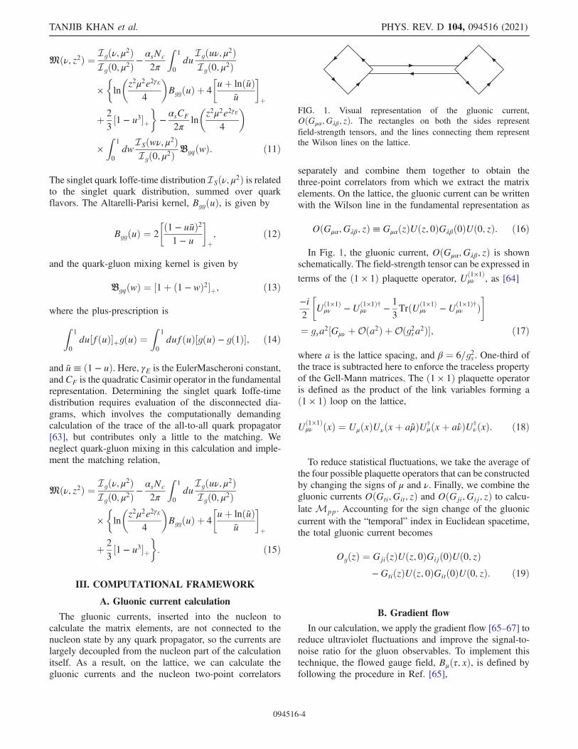
OðGμα; Gλβ; zÞ≡ GμαðzÞUðz; 0ÞGλβð0ÞUð0; zÞ: ð16Þ

In Fig. 1, the gluonic current, OðGμα; Gλβ; zÞ is shownschematically. The field-strength tensor can be expressed in

terms of the ð1 × 1Þ plaquette operator, Uð1×1Þμν , as [64]

−i2

�Uð1×1Þ

μν −Uð1×1Þ†μν −

1

3TrðUð1×1Þ

μν −Uð1×1Þ†μν Þ

�¼ gsa2½Gμν þOða2Þ þOðg2sa2Þ�; ð17Þ

where a is the lattice spacing, and β ¼ 6=g2s . One-third ofthe trace is subtracted here to enforce the traceless propertyof the Gell-Mann matrices. The ð1 × 1Þ plaquette operatoris defined as the product of the link variables forming að1 × 1Þ loop on the lattice,

Uð1×1Þμν ðxÞ ¼ UμðxÞUνðxþ aμÞU†

μðxþ aνÞU†νðxÞ: ð18Þ

To reduce statistical fluctuations, we take the average ofthe four possible plaquette operators that can be constructedby changing the signs of μ and ν. Finally, we combine thegluonic currents OðGti; Git; zÞ and OðGji; Gij; zÞ to calcu-late Mpp. Accounting for the sign change of the gluoniccurrent with the “temporal” index in Euclidean spacetime,the total gluonic current becomes

OgðzÞ ¼ GjiðzÞUðz; 0ÞGijð0ÞUð0; zÞ−GtiðzÞUðz; 0ÞGitð0ÞUð0; zÞ: ð19Þ

B. Gradient flow

In our calculation, we apply the gradient flow [65–67] toreduce ultraviolet fluctuations and improve the signal-to-noise ratio for the gluon observables. To implement thistechnique, the flowed gauge field, Bμðτ; xÞ, is defined byfollowing the procedure in Ref. [65],

FIG. 1. Visual representation of the gluonic current,OðGμα; Gλβ; zÞ. The rectangles on both the sides representfield-strength tensors, and the lines connecting them representthe Wilson lines on the lattice.

TANJIB KHAN et al. PHYS. REV. D 104, 094516 (2021)

094516-4

_Bμ ¼ DνGνμ; Dμ ¼ ∂μ þ ½Bμ; ·�;Gμν ¼ ∂μBν − ∂νBμ þ ½Bμ; Bν�; ð20Þ

where the flowed gauge field is subjected to the boundarycondition Bμðτ ¼ 0; xÞ ¼ AμðxÞ. Here, τ is the flow time,and we abbreviate differentiation with respect to τ by a dot.The flow equation of the gauge field is a diffusion equationand the evolution operator in the momentum space acts asan UV regulator for τ > 0. As a result, the gradient flowexponentially suppresses the UV field fluctuations, whichcorresponds to smearing out the original degrees of free-dom in coordinate space. The operators constructed usingflowed gauge fields with positive flow time enter into therelevant theories at length scales of ∼

ffiffiffiffiffi8τ

p.

On the lattice, the gradient flow is implemented bydefining the flowed link variable, Vμðτ; xÞ as [65]

_Vμðτ; xÞ ¼ −g20f∂x;μSðVμðτ; xÞÞgVμðτ; xÞ; ð21Þ

where g0 is the bare coupling, SðVμðτ; xÞÞ is the flowedaction, Vμðτ ¼ 0; xÞ has the boundary condition of beingequal to the link variable, UμðxÞ, and ∂x;μ stands for thenatural SU(3)-valued differential operator with respect toVμðτ; xÞ. The action, SðVμðτ; xÞÞ is a monotonicallydecreasing function of τ, and the gradient flow correspondsto a continuous stout-link smearing procedure [68].Weuse unimprovedWilson flow and calculate the gluonic

currents with flow times from τ ¼ a2 to τ ¼ 3.8a2. Weconstruct the double ratio of Eq. (9) using the flowed matrixelements, which further reduces UV fluctuations and sup-presses the flow time dependence. The residual τ-depend-ence is removed by fitting the flowed reduced matrixelements to an appropriate functional form, which, in turn,gives us the reduced pseudo-ITD at zero flow time.

C. Nucleon two-point correlator

We calculate the nucleon two-point correlators byapplying interpolators at the source time slice and the sinktime slice on the lattice. We apply distillation [69], a low-rank approximation to the gauge-covariant Jacobi-smearing

kernel, Jσ;nσ ðtÞ ¼ ð1þ σ∇2ðtÞnσ

Þnσ [70]. The tunable parame-ters fσ; nσg ensure that, in the large iteration limit, thekernel approaches that of a spherically symmetricGaussian. The quark fields are smeared using the distil-lation smearing kernel,

▫xyðtÞ ¼XND

k¼1

νðkÞx ðtÞ νðkÞ†y ðtÞ≡ VDðtÞV†DðtÞ; ð22Þ

where VDðtÞ is a ðNc × Nx × Ny × NzÞ × ND matrix,where Nc is the dimension of the color space, Nx, Ny,Nz are the extents of the lattice in the three spatialdirections, and ND is the dimension of the distillation

space. The kth column of VDðtÞ, νðkÞx ðtÞ is the ktheigenvector of the second-order three-dimensional differ-ential operator, ∇2, evaluated on the background of thespatial gauge fields of time slice t, once the eigenvectorshave been sorted by the ascending order of the eigenval-ues. Now, applying the distillation smearing kernel fromEq. (22) on the quark fields and inserting the outer-product decomposition of the kernel ▫ðtÞ, the two-pointcorrelator for the nucleon can be written as

hON;iðmÞON;jðnÞi¼ΦðpqrÞ

i;αβγ ðtmÞ½Pppαα ðtm; tnÞPqq

ββðtm; tnÞPrr

γγðtm; tnÞ−Ppp

αα ðtm; tnÞPqrβγðtm;tnÞPrq

γβðtm; tnÞ�Φðp q rÞ�

j;α β γðtnÞ; ð23Þ

where

ΦðpqrÞi;αβγ ðtÞ¼ϵabcSi;αβγðΓ1iν

ðpÞÞaðΓ2iνðqÞÞbðΓ3iν

ðrÞÞcðtÞ; ð24Þ

and

Pppαα ðtm; tnÞ ¼ νðpÞ†ðtmÞD−1

ααðtm; tnÞνðpÞðtnÞ: ð25Þ

Here, ΦiðtÞ andPðtm; tnÞ are referred to as elementals andperambulators, respectively; D is the lattice representa-tion of the Dirac operator; α, α, β, β, γ, γ are the spinindices; a, b, c are the color indices. TheΦiðtÞ encodes thestructure of the interpolating operator as well as has awell-defined momentum, while Pðtm; tnÞ encodes thepropagation of the quarks and does not have any explicitmomentum projection. Elementals can be decomposedinto terms that act only within coordinate and color space,like Γ, and only within spin space, like Sαβγ .We adopt distillation for two reasons. First, the computa-

tionally demanding parallel transporters of the theory, theperambulators, depend only on the gauge field, and not onthe interpolators. Therefore, we can calculate the peram-bulators on an ensemble of gauge fields once and then reusethem for an extended basis of interpolators, thus reducingthe computational cost to a great extent. This extendedbasis of interpolators is the key to perform a successfulsummed generalized eigenvalue problem (sGEVP) analysis[71], enabling us to attain a clear signal for the ground statenucleon.Second, distillation admits a momentum projection both

at the source interpolating operator and at the sinkinterpolating operator, in contrast to the more usuallyadopted methods. Thus, for the gluonic three-point func-tions computed here, we are able to impose momentumprojection at all three time slices, ensuring the mostcomplete possible sampling of the lattice. Moreover, thelow-lying spectra of the nucleon can be faithfully capturedwith a relatively small number of distillation eigenvectors[72], thus lowering the cost of the calculation further. The

UNPOLARIZED GLUON DISTRIBUTION IN THE NUCLEON … PHYS. REV. D 104, 094516 (2021)

094516-5

expectation is that ND should scale as the physical volume,and the cost of computing the corresponding correlationfunctions scales as N4

D for the case of the nucleon. In thiscalculation, we employed ND ¼ 64 eigenvectors. Theefficacy of distillation for the calculation of nucleoncharges was demonstrated in Ref. [73] and subsequentlyextended to the case of the nucleon in motion [74].Recently, the unpolarized, isovector PDF of the nucleonhas been computed using the same ensemble within thedistillation framework [55].

D. Interpolators

The lattice regulator explicitly breaks the continuumSO(3) rotational symmetry, so the associated symmetrygroup reduces to the double-cover octahedral group,OD

h forthe nucleon at rest. Although there are six irreduciblerepresentations (irreps.) available in OD

h , we focus on G1g,because the states with continuum spin 1

2, such as the

ground state nucleon, are subduced onto this irrep. Here,the subscript g stands for positive parity. At nonzero spatialmomenta, the OD

h group breaks into further little groupsdepending on the direction of the boost. We consider boostsonly along the z direction, so the associated little group isthe order-16 dicyclic group or Dic4.To calculate the low-lying spectra of the nucleon, we

include interpolators with zero orbital angular momentum,which have the largest overlaps with the ground state of thenucleon. For the lowest excited states, we include inter-polators with gauge-covariant derivatives acting on thequark fields to capture the effect of the nonzero angularmomenta between the quarks [75]. All these interpolatorsare “nonrelativistic” in the sense that they feature only theupper components of the Dirac spinors. We also include theinterpolators that have derivatives of second order and formcombinations corresponding to the commutation of twogauge-covariant derivatives acting on the same quark field.These interpolators, also referred to as hybrid interpolators[76], vanish in the absence of a gauge-field and correspondto the chromomagnetic components of the gluonic field-strength tensor. We tabulate our choice of interpolators forthe nucleon at rest as the first row in Table I, usingthe spectroscopic notation of X2Sþ1LπJP where X is thenucleon, N; S is the Dirac spin; L ¼ S; P;D;… is theorbital angular momentum; π ¼ S;M or A is the permu-tation symmetry of the derivatives; J is the total angularmomentum; and P is the parity. For the construction of thethree-point correlators needed for the unpolarized distri-butions, we take the sum of the spin ¼ þ 1

2and spin ¼ − 1

2

nucleon two-point correlators.For the case of the correlation functions at nonzero

spatial momentum, parity is no longer a good quantumnumber, and further operators are classified according totheir helicity. We therefore include operators correspondingboth to higher spin and to negative parity in our basis within

the little group Dic4. We choose the direction of momentato be in the same direction of the polarization to ensurelongitudinal polarization. We access the unpolarized gluonPDF by taking the sum of helicity ¼ þ 1

2and helicity ¼ − 1

2

nucleon two-point correlators. The basis of interpolators istabulated as the second row in Table I.

E. Momentum smearing

To access a wide range of Ioffe-times, we perform thelattice calculation at multiple spatial momenta. On thelattice, the spatialmomentum is discretized and expressed as

p ¼ 2πlaL

: ð26Þ

Here,L ¼ 32, is the spatial extent of the lattice. Forp, wherel > 3, we enhance the overlap of the interpolators onto thelowest-lying states in motion by applying momentumsmearing [77]. We follow the procedure introduced in[74] and add a phase to the distillation eigenvectors forhigher momenta to preserve translational invariance, whichis essential for the projection onto the states of definitemomenta. The “phased” distillation eigenvector becomes

νðkÞx ðz; tÞ ¼ eiζ·zνðkÞx ðz; tÞ: ð27ÞIt is sufficient to modify the previously computed

eigenvectors to perform calculation at the higher latticemomenta, though the perambulators and the elementalsneed to be recalculated with these “phased” eigenvectors.For our calculation, choosing

ζ ¼ 2 ·2π

Lz ð28Þ

gives the momentum smearing needed for boosts upto p ¼ 6 × 2π

aL.

IV. LATTICE DETAILS

We perform our calculation on an isotropic ensemblewith (2þ 1) dynamical flavors of clover Wilson fermionswith stout-link smearing [68] of the gauge fields and a tree-level tadpole-improved Symanzik gauge action, with

TABLE I. Nucleon interpolators used in the calculation. Theinterpolators with asterisk (*) on them are hybrid in nature.

Spatial momentum Interpolators

p ¼ 0 N2SS12þ, N2SM1

2þ, N4DM

12þ

N2PA12þ, N4P�

M12þ, N2P�

M12þ,

p ≠ 0 N2PM12−, N2PM

32−, N4PM

12−,

N4PM32−, N4PM

52−, N2SS12

þ,

N2SM12þ, N2P�

M12þ, N4P�

M12þ

TANJIB KHAN et al. PHYS. REV. D 104, 094516 (2021)

094516-6

approximate lattice spacing, a ∼ 0.094 fm and pion mass,Mπ ∼ 358 MeV, generated by the JLab/W&M collabora-tion [78]. The rational hybrid Monte Carlo (RHMC)algorithm [79] is used to carry out the updates. One iterationof four-dimensional stout smearing with the weight ρ ¼0.125 for the staples is used in the fermion action. After stoutsmearing, the tadpole-improved tree-level clover coefficient,CSW , is very close to the nonperturbative value. This isconfirmed using the Schrödinger functional method fordetermining the clover coefficient nonperturbatively [78].The tuning of the strange quark mass is done by first settingthe quantity, ð2M2

Kþ −M2π0Þ=M2

Ω− equal to its physical value0.1678. This quantity is independent of the light quarkmasses to the lowest order in χPT, depending only on thestrange quark mass [80]. So, it can be tuned in the SU(3)symmetric limit. The resulting value of the strange quarkmass is then kept fixed as the light quark masses aredecreased in the (2þ 1) flavor theory to their physical values.We use 64 temporal sources over 349 gauge configura-

tions, with each configuration separated by 10 HMCtrajectories. The two light quark flavors, u and d, aretaken to be degenerate, and the lattice spacing wasdetermined using the w0 scale [81]. We summarize theparameters of the ensemble in Table II.

V. VARIATIONAL ANALYSIS

To check whether the two-point correlators give us theexpected results, we investigate the associated principalcorrelators and extract the energy spectra by performing avariational analysis for the nucleon at rest in the G1gchannel and for all the boosted frames in the Dic4 littlegroup with the interpolators in Table I. This fittingprocedure is discussed in detail in [72,73,75]. We onlysummarize the procedure here. We solve the GEVP ofEq. (A9) over a range of t0. We then define optimalinterpolators, in the variational sense, for the energyeigenstates, jni through

Pi u

inON;i. Here, ON;i are the

interpolators used in the calculation, and uin are the weightsof these interpolators that define the optimal interpolator.The energy associated with each state jni is obtained byfitting its principal correlator according to

λnðt; t0Þ ¼ ð1 − AnÞe−Enðt−t0Þ þ Ane−E0nðt−t0Þ: ð29Þ

In our fitting procedure, we aim to ensure that theprincipal correlators are dominated by the leading expo-nential. Thus, in each of our fits, we choose t0 such that weobtain an acceptable χ2=d:o:f:, that the value of An is small,

typically less than 0.1, and that, for each principal corre-lator, λnðt; t0Þ, the subleading energy E0

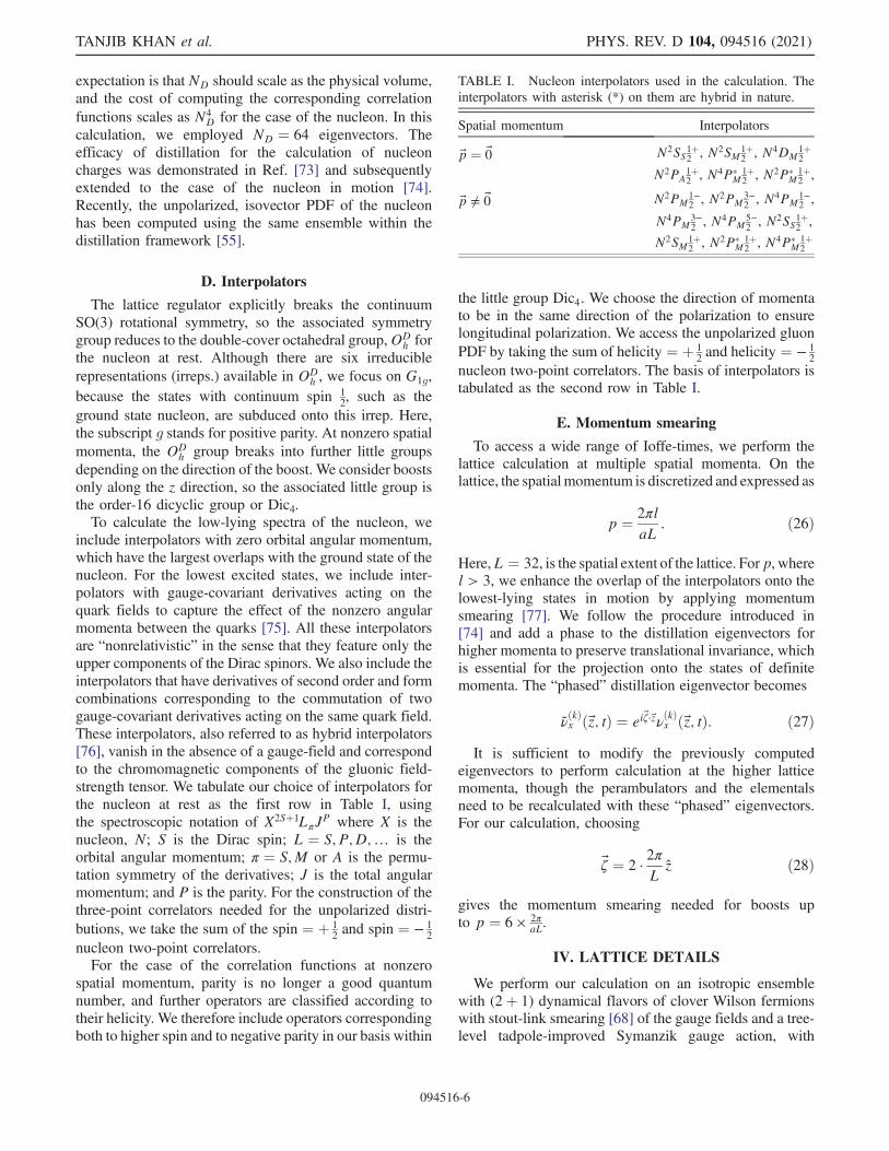
n is larger than thanthe leading energies for all the principal correlators. Thisindicates that the matrix of two-point correlators is, to alarge degree, saturated by the lowest-lying states.In Figs. 2 and 3, we show fits to the leading principal

correlators for the nucleon subduced onto the little group,Dic4 for p¼ 2× 2π

aL¼ 0.82GeV, and p¼6× 2πaL¼2.46GeV,

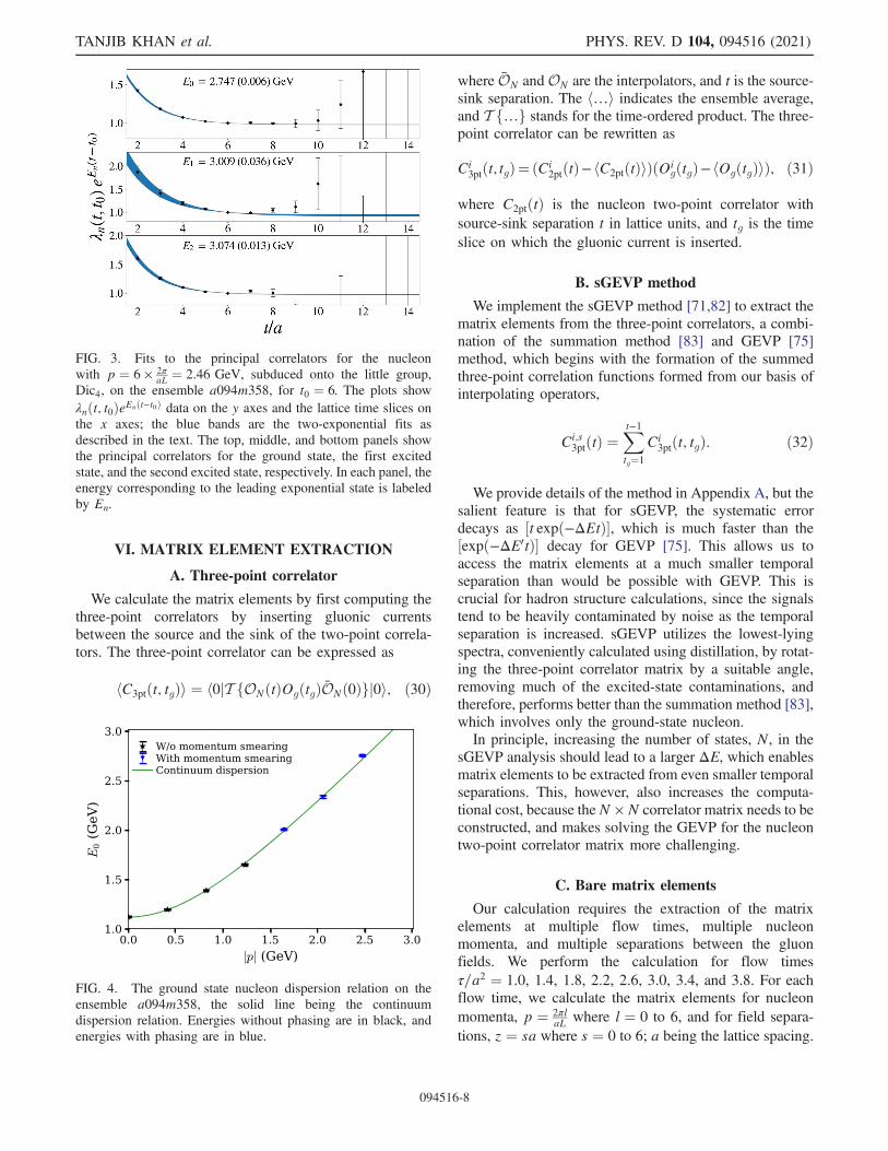
respectively. For each panel, the blue band is thereconstruction from the fitted parameters. The approachof the plateaux close to unity at large times is indicative ofthe small value of An in the fits and the small contributionof the other states to each principal correlator.In Fig. 4, we plot the ground state nucleon energies

extracted using the variational analysis with respect to thespatial momentum, together with the expectations from thecontinuum dispersion relation.Figure 4 shows that for lower momenta, the

unphased ground state nucleon energies are in excellentagreement with the continuum dispersion relation. Atp ¼ 3 × 2π

aL ¼ 1.23 GeV, the ground state energy startsto deviate, but from p ¼ 4 × 2π

aL ¼ 1.64 GeV, after phasing,the ground state energy starts to align with the continuumdispersion curve, indicating that adding a phase to thedistillation eigenvectors with ζ ¼ 2 2π

L resulted in a signifi-cant increase in the overlap of the interpolators onto thelowest-lying states in motion.

TABLE II. The parameters of the ensemble used in this work.Here, Ncfg is the number of gauge configurations.

ID a (fm) Mπ (MeV) L3 × Nt Ncfg Nsrcs

a094m358 0.094(1) 358(3) 323 × 64 349 64

FIG. 2. Fits to the principal correlators for the nucleon with forp ¼ 2 × 2π

aL ¼ 0.82 GeV, subduced onto the little group, Dic4, onthe ensemble a094m358, for t0 ¼ 5. The plots showλnðt; t0ÞeEnðt−t0Þ data on the y axes and the lattice time sliceson the x axes; the blue bands are the two-exponential fits asdescribed in the text. The top, middle, and bottom panels showthe principal correlators for the ground state, the first excitedstate, and the second excited state, respectively. In each panel, theenergy corresponding to the leading exponential state is labeledby En.

UNPOLARIZED GLUON DISTRIBUTION IN THE NUCLEON … PHYS. REV. D 104, 094516 (2021)

094516-7

1.2 Eo = 1.387 (0 .002) GeV

1.0 ,-._ ,2 2 4 6 8 10 12 14 I 1.50 -;J E1 = 1.867 (0.007) GeV

~ 1.25

,,-.. ./2 1.00 .....;' ',_/

2 4 6 8 10 12 14 ~ 1.50 E2 = 1.927 (0.006) GeV

1.25

1.00 I I

2 4 6 8 10 12 14

t/a

VI. MATRIX ELEMENT EXTRACTION

A. Three-point correlator

We calculate the matrix elements by first computing thethree-point correlators by inserting gluonic currentsbetween the source and the sink of the two-point correla-tors. The three-point correlator can be expressed as

hC3ptðt; tgÞi ¼ h0jT fONðtÞOgðtgÞONð0Þgj0i; ð30Þ

where ON andON are the interpolators, and t is the source-sink separation. The h…i indicates the ensemble average,and T f…g stands for the time-ordered product. The three-point correlator can be rewritten as

Ci3ptðt; tgÞ¼ ðCi

2ptðtÞ− hC2ptðtÞiÞðOigðtgÞ− hOgðtgÞiÞ; ð31Þ

where C2ptðtÞ is the nucleon two-point correlator withsource-sink separation t in lattice units, and tg is the timeslice on which the gluonic current is inserted.

B. sGEVP method

We implement the sGEVP method [71,82] to extract thematrix elements from the three-point correlators, a combi-nation of the summation method [83] and GEVP [75]method, which begins with the formation of the summedthree-point correlation functions formed from our basis ofinterpolating operators,

Ci;s3ptðtÞ ¼

Xt−1tg¼1

Ci3ptðt; tgÞ: ð32Þ

We provide details of the method in Appendix A, but thesalient feature is that for sGEVP, the systematic errordecays as ½t expð−ΔEtÞ�, which is much faster than the½expð−ΔE0tÞ� decay for GEVP [75]. This allows us toaccess the matrix elements at a much smaller temporalseparation than would be possible with GEVP. This iscrucial for hadron structure calculations, since the signalstend to be heavily contaminated by noise as the temporalseparation is increased. sGEVP utilizes the lowest-lyingspectra, conveniently calculated using distillation, by rotat-ing the three-point correlator matrix by a suitable angle,removing much of the excited-state contaminations, andtherefore, performs better than the summation method [83],which involves only the ground-state nucleon.In principle, increasing the number of states, N, in the

sGEVP analysis should lead to a larger ΔE, which enablesmatrix elements to be extracted from even smaller temporalseparations. This, however, also increases the computa-tional cost, because theN × N correlator matrix needs to beconstructed, and makes solving the GEVP for the nucleontwo-point correlator matrix more challenging.

C. Bare matrix elements

Our calculation requires the extraction of the matrixelements at multiple flow times, multiple nucleonmomenta, and multiple separations between the gluonfields. We perform the calculation for flow timesτ=a2 ¼ 1.0, 1.4, 1.8, 2.2, 2.6, 3.0, 3.4, and 3.8. For eachflow time, we calculate the matrix elements for nucleonmomenta, p ¼ 2πl

aL where l ¼ 0 to 6, and for field separa-tions, z ¼ sa where s ¼ 0 to 6; a being the lattice spacing.

FIG. 3. Fits to the principal correlators for the nucleonwith p ¼ 6 × 2π

aL ¼ 2.46 GeV, subduced onto the little group,Dic4, on the ensemble a094m358, for t0 ¼ 6. The plots showλnðt; t0ÞeEnðt−t0Þ data on the y axes and the lattice time slices onthe x axes; the blue bands are the two-exponential fits asdescribed in the text. The top, middle, and bottom panels showthe principal correlators for the ground state, the first excitedstate, and the second excited state, respectively. In each panel, theenergy corresponding to the leading exponential state is labeledby En.

FIG. 4. The ground state nucleon dispersion relation on theensemble a094m358, the solid line being the continuumdispersion relation. Energies without phasing are in black, andenergies with phasing are in blue.

TANJIB KHAN et al. PHYS. REV. D 104, 094516 (2021)

094516-8

1.5 Eo = 2.747 (0.006) GeV

1.0

I 4 6 8 10 12 14 -~ 2.0

~ 1.5

.a I ,._;' 1.0 ~

E1 = 3.009 (0.036) GeV

I "-;_;: 2 0 2 4 6 8 10 12 14 "' : :t'-:;~' 074 (0:13) :-1-,v j -l-+-1111

2 4 6 8 10 12 14

t/a

3.0-----------------~~

2.5

1.5

f W/o momentum smearing I With momentum smearing

- Continuum dispersion

l .0+----r-----.-----.----~-----r----, 0.0 0.5 1.0 1.5 2.0 2.5 3.0

IPI (GeV)

We construct the effective matrix element, Meffðt; z; p; τÞfor each flow time, nucleon momentum, and fieldseparation, using the formulation described in Appendix A,and fit the matrix elements using the functional form inEq. (A12), which can be written in simplified notation andarguments as

MeffðtÞ ¼ Aþ Bt expð−ΔEtÞ: ð33Þ

Here, A is the matrix element we wish to extract. Toperform the fit of Eq. (33) for a particular nucleonmomentum, p, we first fit the matrix element for z ¼ 0using a Bayesian analysis and determine the correspondingfitted value of the parameter, ΔE. As the hadronic spectrumis determined by the two-point correlators, we use the valueof ΔE obtained from the fit to the matrix element for z ¼ 0as the prior for our subsequent fits to the matrix elementsfor z > 0 at that particular nucleon momentum. We set theprior width of ΔE for z > 0 to be three times larger thanthe uncertainty in ΔE and allow for random priors inXMBF [84]. The priors are chosen randomly from normaldistributions with the given prior widths. We perform asimultaneous and correlated fit to the matrix elements forz ¼ f1; 2; 3; 4; 5; 6g × a ¼ 0.094, 0.188 fm, 0.282 fm,0.376 fm, 0.470 fm, 0.564 fm, respectively,

MeffðtÞi ¼ Ai þ Bit expð−ΔEtÞ; ð34Þ

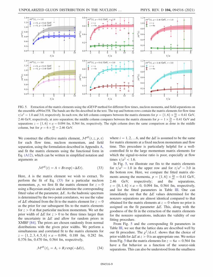
where i ¼ 1; 2;…6, and the ΔE is assumed to be the samefor matrix elements at a fixed nucleon momentum and flowtime. This procedure is particularly helpful for a well-controlled fit to the large momentum matrix elements forwhich the signal-to-noise ratio is poor, especially at flowtimes τ=a2 < 1.6.In Fig. 5, we illustrate our fits to the matrix elements

for τ=a2 ¼ 1.0 in the upper row and for τ=a2 ¼ 3.0 inthe bottom row. Here, we compare the fitted matrix ele-ments among the momenta, p ¼ f1; 6g × 2π

aL ¼ 0.41 GeV,2.46 GeV, respectively; and the separations,z ¼ f0; 1; 6g × a ¼ 0, 0.094 fm, 0.564 fm, respectively,and list the fitted parameters in Table III. One canimmediately see that the ΔE values determined for thenonzero separations are almost identical compared to thatobtained for the matrix elements at z ¼ 0 where no prior isassigned on the fit parameter ΔE. This, along with thegoodness of the fit in the extraction of the matrix elementsfor the nonzero separations, indicates the validity of ourfitting procedure.From Fig. 5 and the corresponding fit parameters in

Table III, we see that the lattice data are described well byour fit procedure. The χ2=d:o:f: shows that the choice ofprior width forΔE at z > 0 is an appropriate one. We noticefrom Fig. 5 that the matrix elements for z ¼ 6a ¼ 0.564 fmhave a flat behavior as a function of the source-sinkseparations. This can also be understood from the smallness

FIG. 5. Extraction of the matrix elements using the sGEVPmethod for different flow times, nucleon momenta, and field separations onthe ensemble a094m358. The bands are the fits described in the text. The top and bottom rows contain the matrix elements for flow timeτ=a2 ¼ 1.0 and 3.0, respectively. In each row, the left column compares between the matrix elements for p ¼ f1; 6g × 2π

aL ¼ 0.41 GeV,2.46 GeV, respectively, at zero separation; the middle column compares between the matrix elements for p ¼ 1 × 2π

aL ¼ 0.41 GeV andseparations z ¼ f1; 6g × a ¼ 0.094 fm, 0.564 fm, respectively. The right column does the same comparison as done in the middlecolumn, but for p ¼ 6 × 2π

aL ¼ 2.46 GeV.

UNPOLARIZED GLUON DISTRIBUTION IN THE NUCLEON … PHYS. REV. D 104, 094516 (2021)

094516-9

1.4 0.8 M'rr(t), p = 0.41 GeV, r = l.0

1.2 M'ff(t), p = 2.46 GeV, r = 1.0

1.2 I z = a 1.0 I z=a

0.6 I z = 6a I z=6a 1.0

0.8

so.a ~ ~ ii 0.4 0.6 ~ 0.6 ~ ~

0.4 0.4 0.2

0.2 0.2

0.0 0.0 0.0 2 4 6 8 10 2 4 6 8 10 12 2 4 6 8

t/a t/a t/a

1.4 0.8 1.2 M 'ff(t), T=3.0 M'ff(t), p = 0.41 GeV, r =3.0 M'rr(t), p = 2.46 GeV, r = 3.0

1.2 I z=0, p=0.41 GeV I z = a 1.0 I z = a I z=0, p=2.46 GeV 0.6 I z=6a I z=6a

1.0 0.8

so.a ~ i ii 0.4 0.6 ~ 0.6 ~ ~

0.4 0.4 0.2

0.2 0.2

0.0 0.0 0.0 2 4 6 8 10 2 4 6 8 10 12 2 4 6 8

t/a t/a t /a

of B-parameters listed in Table III, with relatively largeruncertainties.The nucleon two-point correlators have quite good

signal-to-noise ratios up to the source-sink separation t ¼9a ¼ 0.846 fm at p ¼ 6 × 2π

aL ¼ 2.46 GeV, as can be seenfrom Fig. 3. Figure 5 shows, however, that the matrixelements almost lose any statistical signal around source-sink separation t ¼ 6a ¼ 0.564 fm, which is expected asthe nucleon momentum increases. As shown in Ref. [85],the optimized interpolators reduce the excited-state con-tributions allowing us to start the fit at significantly earliersource-sink separations. In support of this, we indeed seefrom Fig. 5 that the matrix elements for p ¼ 1 × 2π

aL ¼0.41 GeV reach a plateau around the source-sink separa-tion, t ¼ 4a ¼ 0.376 fm.We note that lattice QCD calculations of the gluonic

observables are, in general, much noisier than quark matrixelements. Measures of the goodness of the fits do notnecessarily reflect all the systematic uncertainties in ourextractions of the fit parameters A, B, andΔE. However, byusing N interpolators within a variational approach, we arebetter able to sample the Hilbert space in a particular irrep.in finite volume. This has been proven successful innucleon structure calculation in [73]. The crucial insightis that projecting to the definite finite volume states via thevariational solutions allows us to take advantage of theorthogonality of the states in the Hilbert space [82]. Thereare clearly residual excited states present as constructingthe ideal basis is unrealistic. However, a significantimprovement is achieved by incorporating a moderatenumber of interpolators and applying distillation, one ofthe most computationally cost-effective methods for imple-menting a large number of interpolators. Therefore, byadding multiple interpolators, we have attempted to

systematically improve the determination of A, B, andΔE in this calculation. Further investigation with largerstatistics will be necessary for complete estimate of all thesystematic uncertainties associated with excited-state con-tamination at large nucleon momenta.

D. Reduced matrix elements and zero flow timeextrapolation

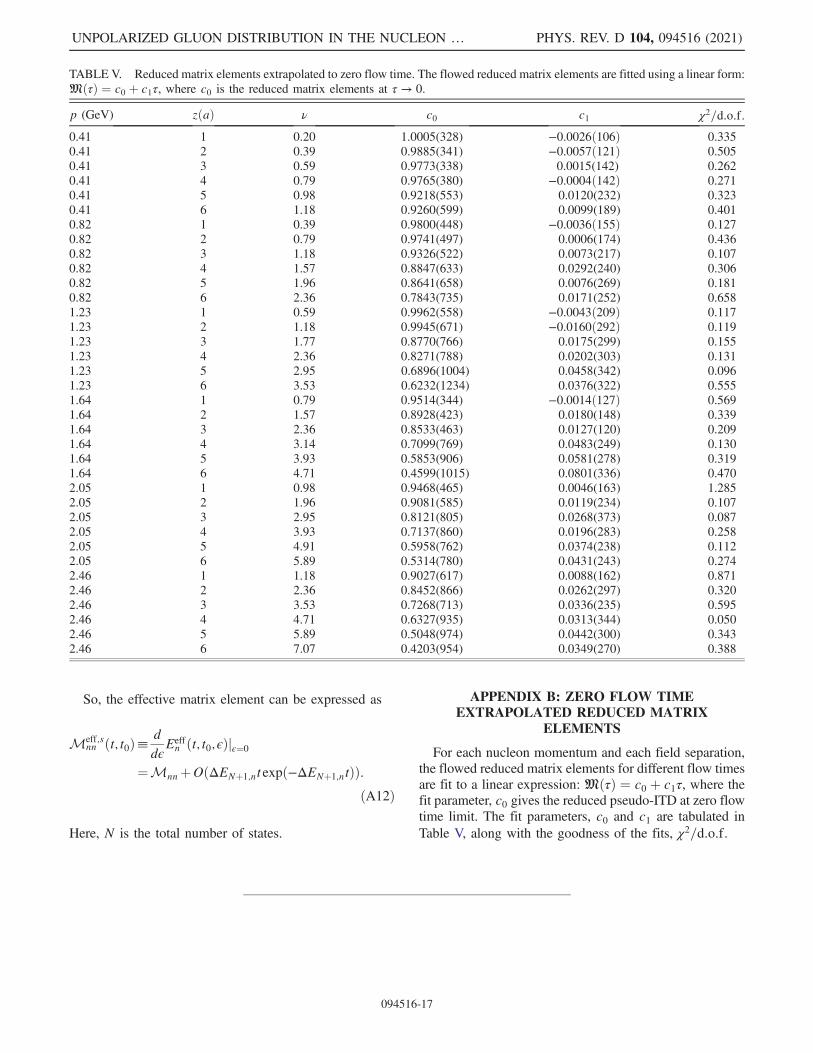
From the bare matrix elements, we calculate the reducedmatrix elements using the double ratio in Eq. (9) fordifferent flow times, nucleon momenta, and field separa-tions. We present the reduced matrix elements for fourdifferent values of τ=a2 in Fig. 6. We expect the higher twistcontributions, discretization effects, and flow time depend-ence to be minimized through this double ratio.From the reduced matrix elements at different flow

times, we calculate the reduced pseudo-ITD distributionby extrapolating to zero flow time. At fixed values of thefield separation, z, and nucleon momentum, p, we findthat the τ-dependence is best fit by a linear form,MðτÞ ¼ c0 þ c1τ, which we use to determine the reducedpseudo-ITD matrix elements for the subsequent analyses.The values of the fitted parameters are tabulated inAppendix B. Out of 36 different fits, we present sixexamples of such extrapolation in Fig. 7, and for allextrapolations, we find χ2=d:o:f: < 1.0. Finally, we presentthe reduced pseudo-ITD in the zero flow time limitin Fig. 8.

VII. DETERMINATION OF GLUON PDF ANDCOMPARISON WITH PHENOMENOLOGICAL

DISTRIBUTION

Determining PDFs from lattice calculations involvesthe challenge of how best to extract a continuousdistribution from the discrete lattice data, compoundedby a limited number of data points due to a finite range offield separations and hadron momenta and therefore,a finite range of ν. By performing a phenomenologicalanalysis of the NNPDF unpolarized gluon PDF [4], it hasbeen found in Ref. [86] that a ν-range that is muchlarger than the present calculation or any available latticeQCD determination of the gluon ITD [40,41], is neces-sary to determine the gluon distribution in the entire xregion from the ITD data. Therefore, we do not expect aproper determination of the gluon distribution in theentire x region, especially in the small-x domain.However, given our lattice data in a limited region,namely ν ∈ ½0; 7.07�, we extract the gluon PDF fromthe reduced pseudo-ITD using the Jacobi polynomialparametrization proposed in Ref. [23]. The details of thisprocedure are presented in Refs. [23,55]; here, we startwith the simplest form for the PDF containing thematching kernel and the leading PDF behavior, whichwe label as [2-param (Q)]

TABLE III. The fitted parameters and the goodness of the fitsfor the matrix elements shown in Fig. 5. For a particular flow timeand nucleon momentum, we first fit the matrix elements at z ¼ 0;the information regarding the fit parameter ΔE from this fit isused to set the prior for ΔE in a simultaneous correlated fit for thematrix elements of all the nonzero separations.

τ=a2p

(GeV) zðaÞ ν A B ΔE χ2=d:o:f:

1.0 0.41 0 0.00 0.62(4) −2.69ð79Þ 1.41(18) 0.531.0 0.41 1 0.20 0.60(3) −2.35ð50Þ 1.40(13) 0.771.0 0.41 6 1.18 0.13(2) −0.14ð7Þ 1.40(13) 0.771.0 2.46 0 0.00 0.94(12) −2.56ð83Þ 1.15(25) 0.621.0 2.46 1 1.18 0.85(8) −2.23ð28Þ 1.22(12) 0.291.0 2.46 6 7.07 0.09(2) 0.07(13) 1.22(12) 0.293.0 0.41 0 0.00 0.62(4) −1.80ð13Þ 1.03(5) 0.353.0 0.41 1 0.20 0.60(2) −1.68ð8Þ 1.02(4) 0.313.0 0.41 6 1.18 0.19(1) −0.39ð4Þ 1.02(4) 0.313.0 2.46 0 0.00 0.91(11) −2.16ð20Þ 0.91(10) 0.293.0 2.46 1 1.18 0.83(7) −1.90ð17Þ 0.93(7) 0.223.0 2.46 6 7.07 0.18(3) −0.28ð13Þ 0.93(7) 0.22

TANJIB KHAN et al. PHYS. REV. D 104, 094516 (2021)

094516-10

FIG. 7. Reduced matrix elements,MðτÞ extrapolated to τ → 0 limit for different nucleon momenta and different field separations. Thefunctional form used to fit the reduced matrix elements isMðτÞ ¼ c0 þ c1τ. The top-left panel shows the fit for p ¼ 1 × 2π

aL ¼ 0.41 GeVand z ¼ a ¼ 0.094 fm. The top-middle panel shows the fit for p ¼ 2 × 2π

aL ¼ 0.82 GeV and z ¼ 2a ¼ 0.188 fm. The top-right panelshows the fit for p ¼ 2 × 2π

aL ¼ 0.82 GeV and z ¼ 6a ¼ 0.564 fm. The bottom-left panel shows the fit for p ¼ 4 × 2πaL ¼ 1.64 GeV and

z ¼ 6a ¼ 0.564 fm. The bottom-middle panel shows the fit for p ¼ 5 × 2πaL ¼ 2.05 GeV and z ¼ 4a ¼ 0.376 fm. The bottom-right

panel shows the fit for p ¼ 6 × 2πaL ¼ 2.46 GeV and z ¼ a ¼ 0.094 fm.

FIG. 6. The reduced matrix elements, Mðν; z2Þ with respect to the Ioffe-time for different flow times. The top-left, top-right, bottom-left, bottom-right panels have the reduced matrix elements for τ ¼ 1.0, 1.8, 2.6, 3.4 in lattice units, respectively.

UNPOLARIZED GLUON DISTRIBUTION IN THE NUCLEON … PHYS. REV. D 104, 094516 (2021)

094516-11

1.2 1.2 T= l.0 T= l.8

1.0

11tHf i!f I 1.0

' lfhf Itf I 0.8 jl I jl

0.8

jI I l jl ~

l ~

I "' "' "' "' ~ 0 .6 ~ 0.6

I ~ ! z = a I ~ ! z = a f z =2a f z = 2a 0.4 t z = 3a

0.4 t z = 3a I z =4a I z =4a

0.2 ! z=5a 0.2 ! z=5a I z=6a I z=6a

0.0 0.0 0 .0 1.0 2 .0 3 .0 4 .0 5.0 6 .0 7 .0 0 .0 1.0 2 .0 3.0 4.0 5.0 6 .0 7 .0

lJ lJ

1.2 1.2 7= 2.6 T= 3.4

1.0 ·ll!U H! I 1.0 H!iIJ Hi I 0.8 fi ll H

0.8 Hi I ti ~ I ~

! "' "' I "' I "' ;:,." 0 .6 ;:;- 0.6

~ ! z = a ~ ! z =a

0.4 f z=2a 0.4 f z=2a t z = 3a t z = 3a I z = 4a I z =4a

0.2 ! z = 5a 0.2 ! z = 5a I z=6a I z=6a

0.0 0.0 0 .0 1.0 2 .0 3.0 4.0 5.0 6.0 7.0 0.0 1.0 2.0 3.0 4.0 5.0 6 .0 7.0

lJ lJ

I.I I.I f !n('t) lp= 0.82GeV, z= 2a

I.I ! rol(t) lp- 0.41GeV, z - a ! 2Jl(•t) lp- 0.82GeV, z - 6a

l!Jl(<)= eo+c,T Fit - !lll(<l = eo +c1r Fit - l!Jl(<)= eo+c,T Fit 1.0

1.0 0.9

E E E ii 1.0 ii ii 0.8

0.9

0.7

0 .9 0 .8 0 .6 0 1.0 2.0 3 .0 4 .0 0 1.0 2.0 3 .0 4 .0 0 1.0 2.0 3 .0 4 .0

r/a' r/a' r/a'

1.0 1.0 I.I ! l!Jl(<)l, - 1.64GeV. , _ ,. ! IDl(t) lp- 2.0SGeV, z - 4a ! rol(t ) lp- 2.46GeV, z - a

0.9 l!Jl(<)= eo+c,T Fit l!Jl(<)= eo+c1T Fit i l!Jl(<) = eo C1T Fit 0.9

IM$J=r=i 1.0

0.8

I E 0 .1 0.8

E E ii 0.6 ii [

ii 0.9

0.7

0 .5 0.8 0.6

0.4

0 .3 0 .5 0.7 0 1.0 2.0 3 .0 4 .0 0 1.0 2.0 3 .0 4 .0 0 1.0 2.0 3 .0 4 .0

r/a' r/a' r/a'

Mðν; z2Þ ¼Z

1

0

dxKðxν; μ2z2Þ xαð1 − xÞβBðαþ 1; β þ 1Þ : ð35Þ

Here, Kðxν; μ2z2Þ is the matching kernel that factorizesthe reduced pseudo-ITD directly to the gluon PDF andthe beta function, Bða; bÞ ¼ R

10 r

a−1ð1 − rÞb−1dr. Toassess our fit model, and the associated systematicuncertainties, we add terms to the model. We considerthe effect of adding one transformed Jacobi polynomialto the functional form of the PDF and label this model[3-param (Q)],

Mðν;z2Þ¼Z

1

0

dxKðxν;μ2z2Þxαð1−xÞβ

×

�1

Bðαþ1;βþ1Þþdðα;βÞ1 Jðα;βÞ1 ðxÞ�: ð36Þ

Finally, we consider a model that we denote [2-paramðQÞ þ P1] for which we add a nuisance term to capturepossible Oða=jzjÞ effects. This nuisance term can beparametrized by a transformed Jacobi polynomial [23],

Mðν;z2Þ¼Z

1

0

dxKðxν;μ2z2Þ xαð1−xÞβBðαþ1;βþ1Þþ

�ajzj�P1ðνÞ;

ð37Þ

where

P1ðνÞ ¼ pðα;βÞ1

Z1

0

dx cosðνxÞxαð1 − xÞβJðα;βÞ1 ðxÞ: ð38Þ

The transformed Jacobi polynomials, Jðα;βÞn ðxÞ aredefined as

Jðα;βÞn ðxÞ ¼Xnj¼0

ωðα;βÞn;j xj; ð39Þ

with

ωðα;βÞn;j ¼

�n

j

�ð−1Þjn!

Γðαþnþ1ÞΓðαþβþnþ jþ1ÞΓðαþβþnþ1ÞΓðαþ jþ1Þ :

ð40Þ

Here, ΓðnÞ is the Gamma function. The orthogonalityrelation for these transformed Jacobi polynomials becomesZ

1

0

dxxαð1 − xÞβJðα;βÞn ðxÞJðα;βÞm ðxÞ ¼ Nðα;βÞn δn;m; ð41Þ

where

Nðα;βÞn ¼ 1

2nþαþβþ1

Γðαþnþ1ÞΓðβþnþ1Þn!Γðαþβþnþ1Þ : ð42Þ

The transformed Jacobi polynomials form a complete basisof functions in the interval [0,1], making it possible toparametrize the PDF.We use Bayesian analysis to extract the PDF from the

reduced pseudo-ITD. We denote the set of fit parameters,which includes the exponents α, β, and the linear coef-ficients of the Jacobi series for the PDF and additionalterms, by θ. Bayes’ theorem gives the posterior distribution,P½θjM; I�, which describes the probability distribution of agiven set of parameters being the true parameters for agiven set of data, Mðν; z2Þ, and prior information, I, as

P½θjM; I� ¼ P½Mjθ�P½θjI�P½MjI� : ð43Þ

Here, P½Mjθ� is the probability distribution of the data for agiven set of model parameters. The prior distribution,which describes the probability distribution of a set ofparameters given some previously held information, isP½θjI�, and P½MjI� is the marginal likelihood or evidencethat describes the probability that the data are correct giventhe previously held information.In our parametrization, the PDF is dominated by the

leading behavior xαð1 − xÞβ, and the other terms should besmall corrections to this. Therefore, in the [3-param (Q)]

model, our prior for the PDF model parameter, dðα;βÞ1 isgiven by a normal distribution, with a mean and width of d0and σd, respectively. Similarly, in the [2-param ðQÞ þ P1]model, we expect the parameter for the additional P1 termto be a small correction to the dominant PDF and use anormal distribution as a prior. The mean and width of thedistribution are given by e0 and σe.Guided by phenomenological fits of PDFs, we set α and

β to be positive, and their prior distributions are set to belog-normal distributions,

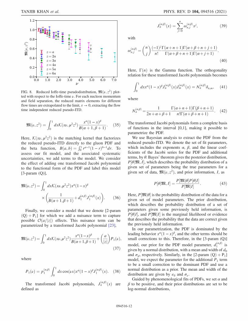
FIG. 8. Reduced Ioffe-time pseudodistribution, Mðν; z2Þ plot-ted with respect to the Ioffe-time ν. For each nucleon momentumand field separation, the reduced matrix elements for differentflow times are extrapolated to the limit, τ → 0, extracting the flowtime independent reduced pseudo-ITD.

TANJIB KHAN et al. PHYS. REV. D 104, 094516 (2021)

094516-12

1.2-r----------------,

I o.o-~------~-------.-----'

0.0 1.0 2.0 3.0 4.0 5.0 6.0 7.0 l/

Pðx; μl; σ; x0Þ ¼1

ðx − x0Þσffiffiffiffiffiffi2π

p e−½logðx−x0Þ−μl�2=2σ2 ; ð44Þ

where μl is the mean and σ2 the variance of the distributionof logðx − x0Þ, and x0 is the lower bound of the log-normaldistributions. The most likely parameters of the model arefound by maximizing the posterior distribution. This isperformed by minimizing the negative log of the posteriordistribution,

L2 ¼ −2 logðP½θjM; I�Þ þ C; ð45Þ

where C is the normalization of the posterior, which isindependent of the model parameters.In Fig. 9, we compare the light-cone ITDs obtained from

these three models. Adding more terms to the functionalform of the PDF or adding more nuisance terms does notimprove the quality of the fits, and the limited Ioffe-timerange does not allow us to add an arbitrary number ofparameters to the fit models. Figure 9 demonstrates that theITDs do not differ among the three models, and theresulting PDFs remain quantitatively the same. We listthe L2=d:o:f: and χ2=d:o:f: of the models in Table IV andfind no significant change. The χ2=d:o:f: and L2=d:o:f:values are also in the acceptable range, and their proximityshows that the prior distributions on the PDF parameters do

not have a significant effect on the fit. Therefore, for ourfollowing discussion, we focus on the [2-param (Q)] model.In Fig. 10, the reduced pseudo-ITD calculated is shown

for different separations, z, along with its fitted bandsobtained from the [2-param (Q)] model. In Fig. 11, we plotthe light-cone Ioffe-time distribution with the lattice datamodified by the matching kernel from the short distancefactorization. SDF removes the logarithmic z2 dependenceof the reduced pseudo-ITD and introduces the μ2 depend-ence on the light-cone Ioffe-time distribution. This effectcan be observed in Fig. 11, where after applying thematching kernel, the lattice data points with different fieldseparations shift upward, depending on their field separa-tions, and the data points fall on a regular light-cone Ioffe-time distribution for all z2. In previous pseudo-PDFcalculations, such as the pion valence quark distributiondetermination [49], the PDF moments extracted by imple-menting SDF show the logarithmic z2 dependence removedfor z up to 1 fm. Similar results can be found in [47], wherethe moments of quark distribution in the nucleon calculated

FIG. 9. Comparison among light-cone Ioffe-time distributions calculated using Jacobi polynomial parametrization and thecorresponding xgðxÞ distributions at 2 GeV in the MS-scheme.

TABLE IV. The L2=d:o:f: and the χ2=d:o:f: of different modelsused to perform Jacobi polynomial parametrization of the latticereduced pseudo-ITD to calculate the gluon PDF.

Model L2=d:o:f: χ2=d:o:f:

2-param (Q) 1.07 0.813-param (Q) 1.11 0.822-param ðQÞ þ P1 1.04 0.77 FIG. 10. Lattice reduced pseudo-ITD shown along with their

reconstructed fitted bands calculated for the model: 2-param (Q).

UNPOLARIZED GLUON DISTRIBUTION IN THE NUCLEON … PHYS. REV. D 104, 094516 (2021)

094516-13

1.0 ..------ 2 - param(Q) -- 3 - param(Q)

2 - param(Q) + P1

0.4.J...---------~-~--~--,-' 0 1.0 2.0 3.0 4.0 5.0 6.0 7.0

V

8.0----------------~

7.0

6.0

5.0

3.0

2.0

1.0

2-param(Q) -- 3-param(Q)

2 - param(Q) + P1

o.oL ____ __:~ ~ - ..--- -~------.l

~

"' N

::.'

0 0.2

0.8

0.4 0.6 0.8 1.0 X

'i 0.6 - z =a - z =2a

I - z= 3a 0.4 - z =4a

- z = 5a z =6a

0.2 J...._---~-~-~----~-~ 0.0 1.0 2.0 3.0 4.0 5.0 6.0 7.0

V

through SDF are found to be independent of a logarithmicz2 effect for z as large as 0.93 fm. On the other hand, if SDFbreaks down, we should see a nonpolynomial z2 depend-ence in the lattice data, especially for large z2. We do notsee such behavior within the current statistics. Instead, thelattice data, after modification by the matching kernel, alignwith the light-cone Ioffe-time distribution band, includingthe large z2 data points, indicating that SDF is quitesuccessful in extracting the Ioffe-time distribution.In Fig. 12, we present the unpolarized gluon PDF (cyan

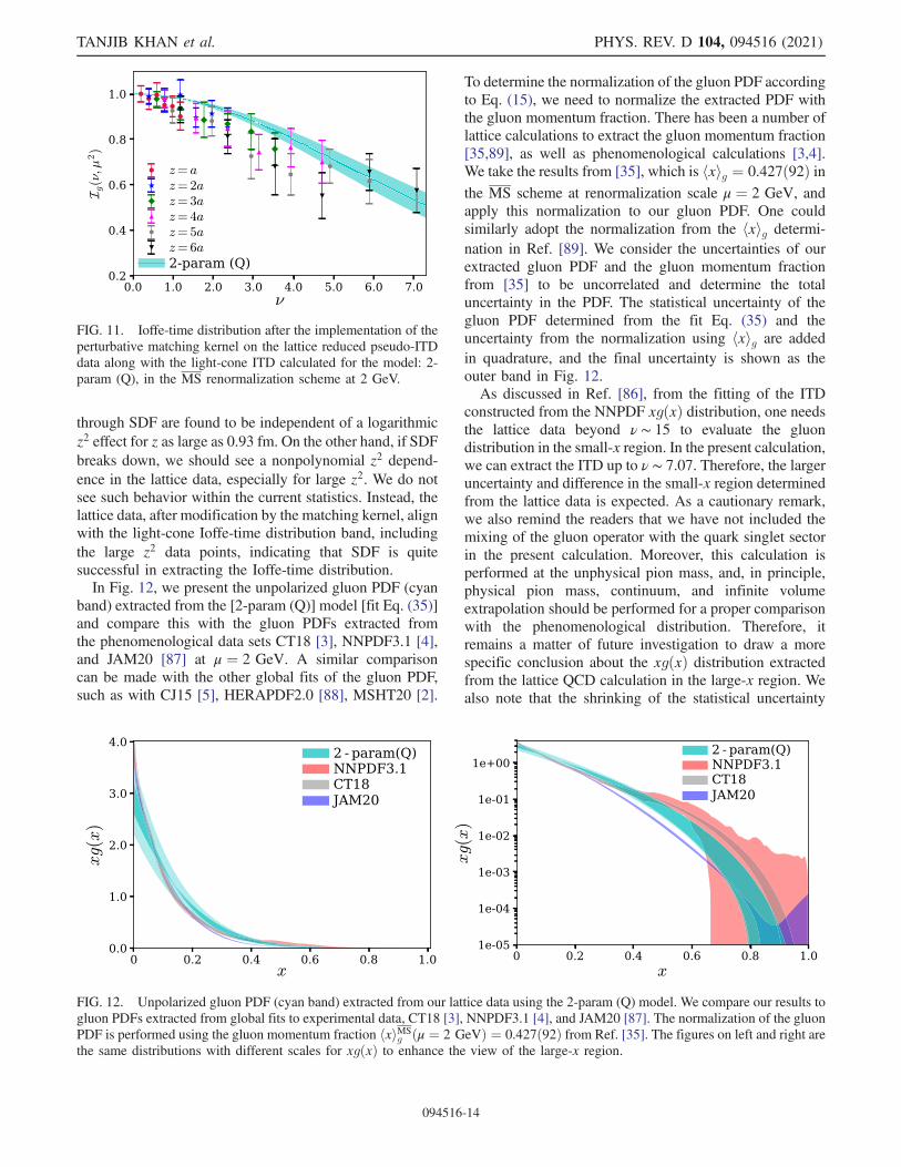
band) extracted from the [2-param (Q)] model [fit Eq. (35)]and compare this with the gluon PDFs extracted fromthe phenomenological data sets CT18 [3], NNPDF3.1 [4],and JAM20 [87] at μ ¼ 2 GeV. A similar comparisoncan be made with the other global fits of the gluon PDF,such as with CJ15 [5], HERAPDF2.0 [88], MSHT20 [2].

To determine the normalization of the gluon PDF accordingto Eq. (15), we need to normalize the extracted PDF withthe gluon momentum fraction. There has been a number oflattice calculations to extract the gluon momentum fraction[35,89], as well as phenomenological calculations [3,4].We take the results from [35], which is hxig ¼ 0.427ð92Þ inthe MS scheme at renormalization scale μ ¼ 2 GeV, andapply this normalization to our gluon PDF. One couldsimilarly adopt the normalization from the hxig determi-nation in Ref. [89]. We consider the uncertainties of ourextracted gluon PDF and the gluon momentum fractionfrom [35] to be uncorrelated and determine the totaluncertainty in the PDF. The statistical uncertainty of thegluon PDF determined from the fit Eq. (35) and theuncertainty from the normalization using hxig are addedin quadrature, and the final uncertainty is shown as theouter band in Fig. 12.As discussed in Ref. [86], from the fitting of the ITD

constructed from the NNPDF xgðxÞ distribution, one needsthe lattice data beyond ν ∼ 15 to evaluate the gluondistribution in the small-x region. In the present calculation,we can extract the ITD up to ν ∼ 7.07. Therefore, the largeruncertainty and difference in the small-x region determinedfrom the lattice data is expected. As a cautionary remark,we also remind the readers that we have not included themixing of the gluon operator with the quark singlet sectorin the present calculation. Moreover, this calculation isperformed at the unphysical pion mass, and, in principle,physical pion mass, continuum, and infinite volumeextrapolation should be performed for a proper comparisonwith the phenomenological distribution. Therefore, itremains a matter of future investigation to draw a morespecific conclusion about the xgðxÞ distribution extractedfrom the lattice QCD calculation in the large-x region. Wealso note that the shrinking of the statistical uncertainty

FIG. 11. Ioffe-time distribution after the implementation of theperturbative matching kernel on the lattice reduced pseudo-ITDdata along with the light-cone ITD calculated for the model: 2-param (Q), in the MS renormalization scheme at 2 GeV.

FIG. 12. Unpolarized gluon PDF (cyan band) extracted from our lattice data using the 2-param (Q) model. We compare our results togluon PDFs extracted from global fits to experimental data, CT18 [3], NNPDF3.1 [4], and JAM20 [87]. The normalization of the gluonPDF is performed using the gluon momentum fraction hxiMS

g ðμ ¼ 2 GeVÞ ¼ 0.427ð92Þ from Ref. [35]. The figures on left and right arethe same distributions with different scales for xgðxÞ to enhance the view of the large-x region.

TANJIB KHAN et al. PHYS. REV. D 104, 094516 (2021)

094516-14

1.0

0.8

0.4

! z=a I z=2a ! z=3a I z=4a I z=5a I z=6a

2-param (Q) 0.2+----.-----.------r--~--~---_...J

0.0 1.0 2.0 3.0 4.0 5.0 6.0 7.0

4.0.,-------------------- 2 - param(Q) - NNPDF3.1

3.0 - CT18 - JAM20

1.0

0.2 0.4 0.6 0.8 1.0 X

- 2-param(Q) le+00 - NNPDF3.1

- CT18 le-01 - JAM20

le-03

le-04

le-05+-----.------.-------r-__L_~-­O 0.2 0.4 0.6 0.8 1.0

X

band in the PDF near x ∼ 0.15 results from the correlationof the PDF fit parameters. This feature has also been seen inprevious works [28,40,49,51].However, within these limitations, we find the large-x

distribution is in reasonable agreement with the global fitsof xgðxÞ distribution, as can be seen from Fig. 12. The valueof β ¼ 5.85ð72Þ determined in this calculation is sta-tistically in good agreement with the leading ð1 − xÞβbehavior obtained in Ref. [86] from the fit to theNNPDF3.1 gluon distribution and a recent phenomeno-logical calculation [90]. The ISðν; μ2Þ distribution, whichwe have not included in the present work, is expected tohave an increasingly larger effect as ν increases and isexpected to have an observable effect in the small-x gluondistribution. However, in the present lattice calculation atheavier up- and down-quark masses, one expects the singletdistribution to increase at a slower rate compared to thephenomenological singlet distribution, therefore having asmaller effect on the Ioffe-time distribution in the0 ≤ ν ≤ 7.07-range.

VIII. CONCLUSION AND OUTLOOK

In this paper, we present the unpolarized gluon partondistribution using the pseudo-PDF approach. We employthe distillation technique, combined with momentumsmearing in our lattice. Distillation allows us not only toimprove the sampling of the lattice but also to construct thenucleon two-point correlators with an extended basis ofinterpolators, which is necessary for the implementation ofthe sGEVP method. By using momentum smearing,momentum as high as 2.46 GeV is achieved. ThesGEVP method combines the features of the summationmethod and GEVP technique, suppressing the excited-statecontributions to the matrix elements significantly. Gradientflow reduces the UV fluctuations from the flowed matrixelements. The combination of these techniques enables usto control the signal-to-noise issues to a great extent. Thereduced pseudo-ITD is calculated from the flowed reducedmatrix elements by fitting the τ-dependence using a linearform and extrapolating to τ → 0 limit. Using the Jacobipolynomial parametrization, the gluon parton distribution isextracted directly from the reduced pseudo-ITD. Althoughsystematics like higher-twist contributions, lattice spacingerrors, infinite volume effects, unphysical pion mass effectsare not refined from the parton distribution, and quark-gluon mixing is excluded from the calculation, the resultantITD has a well-regulated signal-to-noise ratio. The gluonPDF extracted is remarkably consistent with that extractedfrom the phenomenological distributions. Future endeavorsinclude performing the calculation with a larger number ofgauge configurations on the same ensemble and alsoperforming a lattice calculation of the gluon momentumfraction, which will enable us to address the systematicuncertainties more completely along with better statistics.Incorporating the quark-gluon mixing to the calculation is

another task we are aiming to undertake. When all thesystematic uncertainties are properly quantified and themixing with the isoscalar quark PDF is included, the latticecalculations will help constrain the gluon PDF at large-x,where the PDF is less constrained by experimental data.

ACKNOWLEDGMENTS

We would like to thank all the members of the HadStruccollaboration for fruitful and stimulating exchanges. T. K.and R. S. S. acknowledge Luka Leskovec and ArchanaRadhakrishnan for offering their generous help, whichgreatly assisted this research. T. K. is support in part bythe Center for Nuclear Femtography Grants No. C2-2020-FEMT-006, C2019-FEMT-002-05. T. K., R. S. S., andK. O. are supported by U.S. DOE Grant No. DE-FG02-04ER41302. A. R. and W.M. are also supported by U.S.DOE Grant No. DE-FG02-97ER41028. J. K. is supportedby U.S. DOE Grant No. DE-SC0011941. This work issupported by the U.S. Department of Energy, Office ofScience, Office of Nuclear Physics under Contract No. DE-AC05-06OR23177. Computations for this work werecarried out in part on facilities of the USQCDCollaboration, which are funded by the Office ofScience of the U.S. Department of Energy. This workwas performed in part using computing facilities at TheCollege of William and Mary, which were provided bycontributions from the National Science Foundation (MRIgrant PHY-1626177), and the Commonwealth of VirginiaEquipment Trust Fund. This work used the ExtremeScience and Engineering Discovery Environment(XSEDE), which is supported by National ScienceFoundation Grant No. ACI-1548562. Specifically, it usedthe Bridges system, which is supported by NSF GrantNo. ACI-1445606, at the Pittsburgh SupercomputingCenter (PSC) [91]. In addition, this work used resourcesat NERSC, a DOE Office of Science User Facilitysupported by the Office of Science of the U.S.Department of Energy under Contract No. DE-AC02-05CH11231, as well as resources of the Oak RidgeLeadership Computing Facility at the Oak RidgeNational Laboratory, which is supported by the Office ofScience of the U.S. Department of Energy under ContractNo. DE-AC05-00OR22725. The software codes Chroma

[92], QUDA [93,94], and QPhiX [95] were used in our work.The authors acknowledge support from the U.S.Department of Energy, Office of Science, Office ofAdvanced Scientific Computing Research and Office ofNuclear Physics, Scientific Discovery through AdvancedComputing (SciDAC) program, and of the U.S. Departmentof Energy Exascale Computing Project. The authors alsoacknowledge the Texas Advanced Computing Center(TACC) at The University of Texas at Austin for providingHPC resources, like Frontera computing system [96] thathas contributed to the research results reported within thispaper. We acknowledge PRACE (Partnership for Advanced

UNPOLARIZED GLUON DISTRIBUTION IN THE NUCLEON … PHYS. REV. D 104, 094516 (2021)

094516-15

Computing in Europe) for awarding us access to the highperformance computing system Marconi100 at CINECA(Consorzio Interuniversitario per il Calcolo AutomaticodellItalia Nord-orientale) under the Grant No. Pra21-5389.JLAB-THY-21-3469.

APPENDIX A: IMPLEMENT OF sGEVP

In sGEVP [71,82] method, the summation method [83]and GEVP method [75] are combined together. In order toachieve that, we construct the summed three-point corre-lator by summing over the three-point correlators that havethe same source-sink separations, but gluonic currentsinserted at different time slices between the source andsink. From the sum, to avoid contact contributions, weexclude the three-point correlators that have gluonic cur-rents inserted at the source time slice or sink time slicethemselves. We construct the summed three-point correla-tors for different interpolator combinations at the sourceand the sink,

Cs3ptðtsrc; tsnkÞ ¼

Xðtsnk−1Þtg¼ðtsrcþ1Þ

C2ptðtsrc; tsnkÞOgðtgÞ: ðA1Þ

Here, tsrc and tsnk are the lattice time slices where thesource and the sink are, respectively. The label “s” standsfor summed. To implement the sGEVP, consider two sets ofinterpolators,

OiðtÞ ¼ OðAÞi ðtÞ; i ¼ 1…N:

OiþNðtÞ ¼ OðBÞi ðtÞ; i ¼ 1…N: ðA2Þ

Expanding the path integral to first order in ϵ, thecombined 2N × 2N matrix of the two-point correlatorsfrom these interpolators, Cijðt; ϵÞ ¼ hOiðtÞO†

jð0Þi, can bewritten in the simple block structure,

Cðt; ϵÞ ¼"C2ptðtÞ ϵCs

3ptðtÞϵCs†

3ptðtÞ C2ptðtÞ

#þOðϵ2Þ: ðA3Þ

Here, we set CðAÞ ¼ CðBÞ ¼ C2pt. The 2N × 2N GEVPequation,

Cðt; ϵÞρnðt; t0; ϵÞ ¼ λnðt; t0; ϵÞCðt0; ϵÞρnðt; t0; ϵÞ; ðA4Þ

can be rewritten into its components,

½C2ptðtÞ � ϵCs3ptðtÞ�u�n ðt; t0; ϵÞ

¼ λ�n ðt; t0; ϵÞ½C2ptðt0Þ � ϵCs3ptðt0Þ�u�n ðt; t0; ϵÞ; ðA5Þ

where

ρ�n ¼ 1ffiffiffi2

p�

u�n�u�n

�: ðA6Þ

Taking the small ϵ limit, we can treat the summedthree-point correlators as a perturbation. By expanding theGEVP equation in ϵ, we can write the effective matrixelement as [71],

Meff;snn ðt; t0Þ¼−∂t

�jðun; ½Cs3ptðtÞλ−1n ðt; t0Þ−Cs

3ptðt0Þ�unÞjðun;C2ptðt0ÞunÞ

�:

ðA7Þ

Here,

ðun; C2ptðt0ÞunÞ≡ u†nðC2ptðt0ÞunÞ; ðA8Þ

and n is the index of the interpolator. In the small ϵ limit, unand λnðt; t0Þ are the generalized eigenvector and theprincipal correlator of the generalized eigenvalue problemfor the two-point correlator matrix,

C2ptðtÞunðt; t0Þ ¼ λnðt; t0ÞC2ptðt0Þunðt; t0Þ: ðA9Þ

The generalized eigenvector, un, satisfies the orthogon-ality condition:

u†n0 ðt; t0ÞC2ptðt0Þunðt; t0Þ ¼ δn;n0 : ðA10Þ

In GEVP, we rotate the two-point correlator matrixto be diagonal in the generalized eigenvectorspace, eliminating the excited-state contributions signifi-cantly. In sGEVP, we rotate the summed three-pointcorrelator matrix with the same angle by which the two-point correlator matrix is rotated to be diagonal. Thisrotation suppresses the excited-state contributions in thesummed three-point correlators, too. As the orthogon-ality of the generalized eigenvectors are defined withrespect to t ¼ t0, the ratio of the C3ptðtÞ matrix to theprincipal correlator matrix λðt; t0Þ is ill-defined at t ¼ t0.We subtract C3ptðt0Þ from the ratio for all t to avoidthis issue.To extract the matrix element from Meff;s

nn ðt; t0Þ, werecall from the degenerate perturbation theory that thematrix element is the first derivative of the energy withrespect to the perturbation taken in the ϵ → 0 limit. Now,the effective energy is given in terms of the principalcorrelator [97],

Eeffn ðt; t0; ϵÞ ¼ −∂t logðλnðt; t0; ϵÞÞ: ðA11Þ

TANJIB KHAN et al. PHYS. REV. D 104, 094516 (2021)

094516-16

So, the effective matrix element can be expressed as

Meff;snn ðt; t0Þ≡ d

dϵEeffn ðt; t0;ϵÞjϵ¼0

¼MnnþOðΔENþ1;ntexpð−ΔENþ1;ntÞÞ:ðA12Þ

Here, N is the total number of states.

APPENDIX B: ZERO FLOW TIMEEXTRAPOLATED REDUCED MATRIX

ELEMENTS

For each nucleon momentum and each field separation,the flowed reduced matrix elements for different flow timesare fit to a linear expression: MðτÞ ¼ c0 þ c1τ, where thefit parameter, c0 gives the reduced pseudo-ITD at zero flowtime limit. The fit parameters, c0 and c1 are tabulated inTable V, along with the goodness of the fits, χ2=d:o:f:

TABLE V. Reduced matrix elements extrapolated to zero flow time. The flowed reduced matrix elements are fitted using a linear form:MðτÞ ¼ c0 þ c1τ, where c0 is the reduced matrix elements at τ → 0.

p (GeV) zðaÞ ν c0 c1 χ2=d:o:f:

0.41 1 0.20 1.0005(328) −0.0026ð106Þ 0.3350.41 2 0.39 0.9885(341) −0.0057ð121Þ 0.5050.41 3 0.59 0.9773(338) 0.0015(142) 0.2620.41 4 0.79 0.9765(380) −0.0004ð142Þ 0.2710.41 5 0.98 0.9218(553) 0.0120(232) 0.3230.41 6 1.18 0.9260(599) 0.0099(189) 0.4010.82 1 0.39 0.9800(448) −0.0036ð155Þ 0.1270.82 2 0.79 0.9741(497) 0.0006(174) 0.4360.82 3 1.18 0.9326(522) 0.0073(217) 0.1070.82 4 1.57 0.8847(633) 0.0292(240) 0.3060.82 5 1.96 0.8641(658) 0.0076(269) 0.1810.82 6 2.36 0.7843(735) 0.0171(252) 0.6581.23 1 0.59 0.9962(558) −0.0043ð209Þ 0.1171.23 2 1.18 0.9945(671) −0.0160ð292Þ 0.1191.23 3 1.77 0.8770(766) 0.0175(299) 0.1551.23 4 2.36 0.8271(788) 0.0202(303) 0.1311.23 5 2.95 0.6896(1004) 0.0458(342) 0.0961.23 6 3.53 0.6232(1234) 0.0376(322) 0.5551.64 1 0.79 0.9514(344) −0.0014ð127Þ 0.5691.64 2 1.57 0.8928(423) 0.0180(148) 0.3391.64 3 2.36 0.8533(463) 0.0127(120) 0.2091.64 4 3.14 0.7099(769) 0.0483(249) 0.1301.64 5 3.93 0.5853(906) 0.0581(278) 0.3191.64 6 4.71 0.4599(1015) 0.0801(336) 0.4702.05 1 0.98 0.9468(465) 0.0046(163) 1.2852.05 2 1.96 0.9081(585) 0.0119(234) 0.1072.05 3 2.95 0.8121(805) 0.0268(373) 0.0872.05 4 3.93 0.7137(860) 0.0196(283) 0.2582.05 5 4.91 0.5958(762) 0.0374(238) 0.1122.05 6 5.89 0.5314(780) 0.0431(243) 0.2742.46 1 1.18 0.9027(617) 0.0088(162) 0.8712.46 2 2.36 0.8452(866) 0.0262(297) 0.3202.46 3 3.53 0.7268(713) 0.0336(235) 0.5952.46 4 4.71 0.6327(935) 0.0313(344) 0.0502.46 5 5.89 0.5048(974) 0.0442(300) 0.3432.46 6 7.07 0.4203(954) 0.0349(270) 0.388

UNPOLARIZED GLUON DISTRIBUTION IN THE NUCLEON … PHYS. REV. D 104, 094516 (2021)

094516-17

[1] J. C. Collins, D. E. Soper, and G. F. Sterman, Adv. Ser. Dir.High Energy Phys. 5, 1 (1989).

[2] S. Bailey, T. Cridge, L. A. Harland-Lang, A. D. Martin, andR. S. Thorne, Eur. Phys. J. C 81, 341 (2021).

[3] T.-J. Hou et al., Phys. Rev. D 103, 014013 (2021).[4] R. D. Ball et al. (NNPDF Collaboration), Eur. Phys. J. C 77,

663 (2017).[5] A. Accardi, L. T. Brady, W. Melnitchouk, J. F. Owens, and

N. Sato, Phys. Rev. D 93, 114017 (2016).[6] S. Dulat, T.-J. Hou, J. Gao, M. Guzzi, J. Huston, P.

Nadolsky, J. Pumplin, C. Schmidt, D. Stump, and C. P.Yuan, Phys. Rev. D 93, 033006 (2016).

[7] S. Chatrchyan et al. (CMS Collaboration), Science 338,1569 (2012).

[8] R. Kogler et al., Rev. Mod. Phys. 91, 045003 (2019).[9] Albayrak et al., Jefferson Lab PAC 39 Proposal,

PR12.12.001 (2012).[10] A. Accardi et al., Eur. Phys. J. A 52, 268 (2016).[11] A. C. Aguilar et al., Eur. Phys. J. A 55, 190 (2019).[12] R. Abdul Khalek et al., arXiv:2103.05419.[13] D. P. Anderle et al., Front. Phys. (Beijing) 16, 64701 (2021).[14] K.-F. Liu and S.-J. Dong, Phys. Rev. Lett. 72, 1790 (1994).[15] W. Detmold and C. J. D. Lin, Phys. Rev. D 73, 014501

(2006).[16] X. Ji, Phys. Rev. Lett. 110, 262002 (2013).[17] X. Ji, Sci. China Phys. Mech. Astron. 57, 1407 (2014).[18] A. V. Radyushkin, Phys. Rev. D 96, 034025 (2017).[19] Y.-Q. Ma and J.-W. Qiu, Phys. Rev. D 98, 074021 (2018).[20] Y.-Q. Ma and J.-W. Qiu, Phys. Rev. Lett. 120, 022003

(2018).[21] M. Constantinou et al., Prog. Part. Nucl. Phys. 121, 103908

(2021).[22] K. Cichy and M. Constantinou, Adv. High Energy Phys.

2019, 3036904 (2019).[23] J. Karpie, K. Orginos, A. Radyushkin, and S. Zafeiropoulos,

arXiv:2105.13313.[24] R. S. Sufian, C. Egerer, J. Karpie, R. G. Edwards, B. Joó,

Y.-Q. Ma, K. Orginos, J.-W. Qiu, and D. G. Richards, Phys.Rev. D 102, 054508 (2020).

[25] R. S. Sufian, J. Karpie, C. Egerer, K. Orginos, J.-W. Qiu,and D. G. Richards, Phys. Rev. D 99, 074507 (2019).

[26] K. Zhang, Y.-Y. Li, Y.-K. Huo, P. Sun, and Y.-B. Yang,Phys. Rev. D 104, 074501 (2021).

[27] T. Izubuchi, L. Jin, C. Kallidonis, N. Karthik, S. Mukherjee,P. Petreczky, C. Shugert, and S. Syritsyn, Phys. Rev. D 100,034516 (2019).

[28] X. Gao, L. Jin, C. Kallidonis, N. Karthik, S. Mukherjee, P.Petreczky, C. Shugert, S. Syritsyn, and Y. Zhao, Phys. Rev.D 102, 094513 (2020).

[29] H.-W. Lin, J.-W. Chen, Z. Fan, J.-H. Zhang, and R. Zhang,Phys. Rev. D 103, 014516 (2021).

[30] C. Alexandrou, K. Cichy, M. Constantinou, J. R. Green, K.Hadjiyiannakou, K. Jansen, F. Manigrasso, A. Scapellato,and F. Steffens, Phys. Rev. D 103, 094512 (2021).

[31] C. Alexandrou, M. Constantinou, K. Hadjiyiannakou, K.Jansen, and F. Manigrasso, Phys. Rev. Lett. 126, 102003(2021).

[32] Z. Fan, X. Gao, R. Li, H.-W. Lin, N. Karthik, S. Mukherjee,P. Petreczky, S. Syritsyn, Y.-B. Yang, and R. Zhang, Phys.Rev. D 102, 074504 (2020).

[33] C. Alexandrou, K. Cichy, M. Constantinou, K.Hadjiyiannakou, K. Jansen, A. Scapellato, and F. Steffens,Phys. Rev. Lett. 125, 262001 (2020).

[34] Q.-A. Zhang et al. (Lattice Parton Collaboration), Phys.Rev. Lett. 125, 192001 (2020).

[35] C. Alexandrou, S. Bacchio, M. Constantinou, J. Finkenrath,K.Hadjiyiannakou,K. Jansen, G.Koutsou,H. Panagopoulos,and G. Spanoudes, Phys. Rev. D 101, 094513 (2020).

[36] Y.-B. Yang, J. Liang, Y.-J. Bi, Y. Chen, T. Draper, K.-F. Liu,and Z. Liu, Phys. Rev. Lett. 121, 212001 (2018).

[37] C. Alexandrou, M. Constantinou, K. Hadjiyiannakou, K.Jansen, C. Kallidonis, G. Koutsou, A. Vaquero Aviles-Casco, and C. Wiese, Phys. Rev. Lett. 119, 142002 (2017).

[38] P. E. Shanahan and W. Detmold, Phys. Rev. D 99, 014511(2019).

[39] Z.-Y. Fan, Y.-B. Yang, A. Anthony, H.-W. Lin, and K.-F.Liu, Phys. Rev. Lett. 121, 242001 (2018).

[40] Z. Fan, R. Zhang, and H.-W. Lin, Int. J. Mod. Phys. A 36,2150080 (2021).

[41] Z. Fan and H.-W. Lin, arXiv:2104.06372.[42] A. V. Radyushkin, Phys. Lett. B 781, 433 (2018).[43] A. Radyushkin, Phys. Rev. D 98, 014019 (2018).[44] B. L. Ioffe, Phys. Lett. 30B, 123 (1969).[45] V. Braun, P. Gornicki, and L. Mankiewicz, Phys. Rev. D 51,

6036 (1995).[46] K. Orginos, A. Radyushkin, J. Karpie, and S. Zafeiropoulos,

Phys. Rev. D 96, 094503 (2017).[47] J. Karpie, K. Orginos, and S. Zafeiropoulos, J. High Energy

Phys. 11 (2018) 178.[48] B. Joó, J. Karpie, K. Orginos, A. Radyushkin, D.

Richards, and S. Zafeiropoulos, J. High Energy Phys. 12(2019) 081.

[49] B. Joó, J. Karpie, K. Orginos, A. V. Radyushkin, D. G.Richards, R. S. Sufian, and S. Zafeiropoulos, Phys. Rev. D100, 114512 (2019).

[50] B. Joó, J. Karpie, K. Orginos, A. V. Radyushkin, D. G.Richards, and S. Zafeiropoulos, Phys. Rev. Lett. 125,232003 (2020).

[51] M. Bhat, K. Cichy, M. Constantinou, and A. Scapellato,Phys. Rev. D 103, 034510 (2021).

[52] J. Karpie, K. Orginos, A. Rothkopf, and S. Zafeiropoulos, J.High Energy Phys. 04 (2019) 057.

[53] K. Cichy, L. Del Debbio, and T. Giani, J. High Energy Phys.10 (2019) 137.

[54] L. Del Debbio, T. Giani, J. Karpie, K. Orginos, A.Radyushkin, and S. Zafeiropoulos, J. High Energy Phys.02 (2021) 138.

[55] C. Egerer, R. G. Edwards, C. Kallidonis, K. Orginos,A. V. Radyushkin, D. G. Richards, E. Romero, and S.Zafeiropoulos, arXiv:2107.05199.

[56] I. Balitsky, W. Morris, and A. Radyushkin, Phys. Lett. B808, 135621 (2020).

[57] J.-H. Zhang, X. Ji, A. Schäfer, W. Wang, and S. Zhao, Phys.Rev. Lett. 122, 142001 (2019).

[58] Z.-Y. Li, Y.-Q. Ma, and J.-W. Qiu, Phys. Rev. Lett. 122,062002 (2019).

[59] T. Izubuchi, X. Ji, L. Jin, I. W. Stewart, and Y. Zhao, Phys.Rev. D 98, 056004 (2018).

[60] X. Ji, J.-H. Zhang, and Y. Zhao, Phys. Rev. Lett. 120,112001 (2018).

TANJIB KHAN et al. PHYS. REV. D 104, 094516 (2021)

094516-18

[61] J. Green, K. Jansen, and F. Steffens, Phys. Rev. Lett. 121,022004 (2018).

[62] I. Balitsky, W. Morris, and A. Radyushkin, in Proceedingsof the 28th International Workshop on Deep InelasticScattering and Related Subjects (2021), arXiv:2106.01916.

[63] A. S. Gambhir, A. Stathopoulos, K. Orginos, B. Yoon, R.Gupta, and S. Syritsyn, Proc. Sci. LATTICE2016 (2016)265.

[64] S. O. Bilson-Thompson, D. B. Leinweber, and A. G.Williams, Ann. Phys. (Amsterdam) 304, 1 (2003).

[65] M. Lüscher, J. High Energy Phys. 08 (2010) 071; 03 (2014)092(E).

[66] M. Luscher and P. Weisz, J. High Energy Phys. 02 (2011)051.

[67] M. Luscher, J. High Energy Phys. 04 (2013) 123.[68] C. Morningstar and M. J. Peardon, Phys. Rev. D 69, 054501

(2004).[69] M. Peardon, J. Bulava, J. Foley, C. Morningstar, J. Dudek,

R. G. Edwards, B. Joo, H.-W. Lin, D. G. Richards, and K. J.Juge (Hadron Spectrum Collaboration), Phys. Rev. D 80,054506 (2009).

[70] C. R. Allton et al. (UKQCD Collaboration), Phys. Rev. D47, 5128 (1993).

[71] J. Bulava, M. Donnellan, and R. Sommer, J. High EnergyPhys. 01 (2012) 140.

[72] T. Khan, D. Richards, and F. Winter, Phys. Rev. D 104,034503 (2021).

[73] C. Egerer, D. Richards, and F. Winter, Phys. Rev. D 99,034506 (2019).

[74] C. Egerer, R. G. Edwards, K. Orginos, and D. G. Richards,Phys. Rev. D 103, 034502 (2021).

[75] R. G. Edwards, J. J. Dudek, D. G. Richards, and S. J.Wallace, Phys. Rev. D 84, 074508 (2011).

[76] J. J. Dudek and R. G. Edwards, Phys. Rev. D 85, 054016(2012).

[77] G. S. Bali, B. Lang, B. U. Musch, and A. Schäfer, Phys.Rev. D 93, 094515 (2016).

[78] R. Edwards, B. Joó, K. Orginos, D. Richards, and F.Winter, U.S. 2þ 1 flavor clover lattice generation program(unpublished).

[79] S. Duane, A. D. Kennedy, B. J. Pendleton, and D. Roweth,Phys. Lett. B 195, 216 (1987).

[80] H.-W. Lin et al. (Hadron Spectrum Collaboration), Phys.Rev. D 79, 034502 (2009).

[81] S. t. Borsanyi, J. High Energy Phys. 09 (2012) 010.[82] B. Blossier, M. Della Morte, G. von Hippel, T. Mendes, and

R. Sommer, J. High Energy Phys. 04 (2009) 094.[83] C. Bouchard, C. C. Chang, T. Kurth, K. Orginos, and A.

Walker-Loud, Phys. Rev. D 96, 014504 (2017).[84] S. Meinel, http://www.stefanmeinel.com/software/XMBF/

XMBF 2.40.[85] J. J. Dudek, R. G. Edwards, and C. E. Thomas, Phys. Rev. D

86, 034031 (2012).[86] R. S. Sufian, T. Liu, and A. Paul, Phys. Rev. D 103, 036007

(2021).[87] E. Moffat, W. Melnitchouk, T. Rogers, and N. Sato, Phys.

Rev. D 104, 016015 (2021).[88] H. Abramowicz et al. (H1, ZEUS Collaborations), Eur.

Phys. J. C 75, 580 (2015).[89] Y.-B. Yang, M. Gong, J. Liang, H.-W. Lin, K.-F. Liu, D.

Pefkou, and P. Shanahan, Phys. Rev. D 98, 074506 (2018).[90] G. F. de Teramond, H. G. Dosch, T. Liu, R. S. Sufian, S. J.

Brodsky, and A. Deur, arXiv:2107.01231.[91] J. Towns, T. Cockerill, M. Dahan, I. Foster, K. Gaither, A.

Grimshaw, V. Hazlewood, S. Lathrop, D. Lifka, G. D.Peterson, R. Roskies, J. Scott, and N. Wilkins-Diehr,Comput. Sci. Eng. 16, 62 (2014).

[92] R. G. Edwards and B. Joo (SciDAC, LHPC, UKQCDCollaborations), Nucl. Phys. B, Proc. Suppl. 140, 832(2005).

[93] M. A. Clark, R. Babich, K. Barros, R. C. Brower, and C.Rebbi, Comput. Phys. Commun. 181, 1517 (2010).

[94] R. Babich, M. A. Clark, and B. Joo, in Proceedings of theSC 10 (Supercomputing 2010) (IEEE, New York, 2010),arXiv:1011.0024.

[95] B. Joó, D. D. Kalamkar, T. Kurth, K. Vaidyanathan, and A.Walden, High Performance Computing: ISC High Perfor-mance 2016 International Workshops, ExaComm, E-MuCoCoS, HPC-IODC, IXPUG, IWOPH, P3MA, VHPC,WOPSSS, Frankfurt, Germany, 2016, Revised SelectedPapers (Springer International Publishing, Cham, 2016),pp. 415–427.

[96] D. Stanzione, J. West, R. T. Evans, T. Minyard, O. Ghattas,and D. K. Panda, in Practice and Experience in AdvancedResearch Computing, PEARC’20 (Association for Comput-ing Machinery, New York, NY, 2020), pp. 106–111.

[97] M. Luscher and U. Wolff, Nucl. Phys. B339, 222 (1990).

UNPOLARIZED GLUON DISTRIBUTION IN THE NUCLEON … PHYS. REV. D 104, 094516 (2021)

094516-19