arX

iv:1

405.

3506

v1 [

hep-

ph]

14

May

201

4

A new method for determining the quark-gluon vertex

A. C. Aguilar,1 D. Binosi,2 D. Ibanez,2 and J. Papavassiliou3

1University of Campinas - UNICAMP,

Institute of Physics “Gleb Wataghin”

13083-859 Campinas, SP, Brazil

2European Centre for Theoretical Studies in Nuclear Physics

and Related Areas (ECT*) and Fondazione Bruno Kessler,

Villa Tambosi, Strada delle Tabarelle 286, I-38123 Villazzano (Trento) Italy

3Department of Theoretical Physics and IFIC, University of Valencia and CSIC,

E-46100, Valencia, Spain

Abstract

We present a novel nonperturbative approach for calculating the form factors of the quark-gluon

vertex, in a general covariant gauge. The key ingredient of this method is the exact all-order relation

connecting the conventional quark-gluon vertex with the corresponding vertex of the background

field method, which is Abelian-like. When this latter relation is combined with the standard gauge

technique, supplemented by a crucial set of transverse Ward identities, it allows the approximate

determination of the nonperturbative behavior of all twelve form factors comprising the quark-

gluon vertex, for arbitrary values of the momenta. The actual implementation of this procedure is

carried out in the Landau gauge, in order to make contact with the results of lattice simulations

performed in this particular gauge. The most demanding technical aspect involves the calculation

of certain (fully-dressed) auxiliary three-point functions, using lattice data as input for the gluon

propagators appearing in their diagrammatic expansion. The numerical evaluation of the relevant

form factors in three special kinematical configurations (soft gluon and quark symmetric limit, zero

quark momentum) is carried out in detail, finding rather good agreement with the available lattice

data. Most notably, a concrete mechanism is proposed for explaining the puzzling divergence of

one of these form factors observed in lattice simulations.

PACS numbers: 12.38.Aw, 12.38.Lg, 14.70.Dj

1

I. INTRODUCTION

The fundamental vertex that controls the interaction between quarks and gluons is con-

sidered as one of the most important quantities in QCD [1, 2], and a great deal of effort

has been devoted to the unraveling of its structure and dynamics. In fact, its nonpertur-

bative properties are essential to a variety of subtle mechanisms of paramount theoretical

and phenomenological relevance. Indeed, the quark-gluon vertex, which will be denoted by

Γaµ(q, r, p), has a vital impact on the dynamics responsible for the breaking of chiral sym-

metry and the subsequent generation of constituent quark masses [3–7], and contributes

crucially to the formation of the bound states that compose the physical spectrum of the

theory [8–13].

Despite its physical importance, to date the nonperturbative behavior of this special

vertex is still only partially known, mainly due to a variety of serious technical difficulties1.

In particular, its rich tensorial structure leads to a considerable proliferation of form factors,

which, in addition, depend on three kinematic variables (e.g., the modulo of two momenta,

say q and r, and their relative angle). As a result, only few (quenched) lattice simulations

(in the Landau gauge and on modest lattice sizes) have been performed [17–20], and for

a limited number of simple kinematic configurations. The situation in the continuum is

also particularly cumbersome; indeed, the treatment of this vertex in the context of the

Schwinger-Dyson equations (SDEs) requires a variety of approximations and truncations,

and even so, one must deal, at least in principle, with an extended system of coupled

integral equations (one for each form factor).

There is an additional issue that complicates the extraction of pertinent nonperturbative

information on the quark-gluon vertex by means of traditional methods, which will be of

central importance in what follows. Specifically, in the linear covariant (Rξ) gauges, Γaµ

satisfies a non-linear Slavnov-Taylor identity (STI), imposed by the Becchi-Rouet-Stora-

Tyutin (BRST) symmetry of the theory. This STI is akin to the QED Ward identity (WI)

qµΓµ(q, r, p) = S−1e (r)− S−1

e (p), which relates the photon-electron vertex with the electron

propagator Se, but it is substantially more complicated, because it involves, in addition to

1 In perturbation theory, a complete study has been carried out at the one-loop level in arbitrary gauges,

dimensions and kinematics [14], whereas at the two- and three-loop order only partial results for specific

gauges and kinematics exist [15, 16].

2

the quark propagator S, contributions from the ghost-sector of the theory (most notably,

the so-called “ghost-quark” kernel). This fact limits considerably the possibility of devising

a “gauge technique” inspired Ansatz [21–24] for the longitudinal part of Γaµ(q, r, p). Indeed,

whereas in an Abelian context the longitudinal part of the vertex is expressed exclusively in

terms of the Dirac components comprising S such that the WI is automatically satisfied, in

the case of the STI the corresponding longitudinal part receives contributions from additional

(poorly known) auxiliary functions and their partial derivatives.

The applicability of the gauge technique, however, presents an additional difficulty, which

although intrinsic to this method, acquires its more acute form in a non-Abelian context.

Indeed, as is well-known, the gauge technique leaves the “transverse” (automatically con-

served) part of any vertex (Abelian or non-Abelian) undetermined. The amelioration of this

shortcoming has received considerable attention in the literature, especially for the case of

the photon-electron vertex, which constitutes the prototype for any type of such study [25–

28]. Particularly interesting in this context is the discovery of the so-called “transverse Ward

identities” (TWIs) [29–33], which involve the curl of the vertex, ∂µΓν··· − ∂νΓµ···, and can

therefore be used, at least in principle, to constrain the transverse parts. The problem is

that, unlike WIs, these TWIs are coupled identities, mixing vector and axial terms, and

contain non local terms, in the form of gauge-field-dependent line integrals [33]. However,

as was shown in [34], the induced coupling between TWIs can in fact be disentangled, and

the corresponding identity for the vector vertex explicitly solved. Thus an Abelian photon-

electron vertex satisfying the corresponding WI and TWI could be constructed for the first

time [34]. However, the extension of these results to the non-Abelian sector remains an open

issue. In what follows, for the sake of brevity, we will refer to the framework obtained when

the standard gauge technique (applied to Abelian WIs) is supplemented by the TWIs as the

“improved gauge technique” (IGT).

The main conclusion of the above considerations is that, whereas the IGT constitutes

a rather powerful approach for Abelian theories, its usefulness for non-Abelian vertices is

rather limited. It would be clearly most interesting if one could transfer some of the above

techniques to a theory like QCD, and in particular, to the quark-gluon vertex. What we

propose in the present work is precisely this: express the conventional quark-gluon vertex

as a deviation from an “Abelian-like” quark-gluon vertex, use the technology derived from

the IGT to fix this latter vertex, and then compute (in an approximate way) the difference

3

between these two vertices.

The field theoretic framework that enables the realization of the procedure outlined above

is the PT-BFM scheme [35–37], which is obtained through the combination of the pinch

technique (PT) [38–43] with the background field method (BFM) [44]. Since within the

BFM the gluon is split into a quantum (Q) and a background (A) part, two kinds of vertices

appear: vertices (Γ) that have Q external lines only (which correspond to the vertices

appearing in the conventional formulation of the theory) and vertices (Γ) that have A (or

mixed) external lines. Now, interestingly enough, while the former satisfy the usual STIs, the

latter obey Abelian-like WIs. In addition, a special kind of identities, known as “background

quantum identities”(BQIs) [45, 46], relate the two types of vertices (Γ and Γ) by means of

auxiliary ghost Green’s functions. For the specific cases of the quark-gluon vertices the

corresponding BQI [37] reads schematically [for the detailed dependence on the momenta,

see Eq. (2.15)]

Γµ = [gνµ + Λνµ]Γν + S−1Kµ +KµS

−1,

where Λ and K are special two- and three-point functions, respectively, the origin of which

can be ultimately related to the antiBRST symmetry of the theory2.

In the present work, the above BQI will be exploited in order to obtain nontrivial infor-

mation on all twelve form factors of the vertex Γµ. Specifically, the main conceptual steps

of the approach may be summarized as follows. (i ) Since the vertex Γµ satisfies a QED-like

WI, it will be reconstructed using the IGT, following the exact procedure and assumptions

(minimal Ansatz) of [34]. (ii ) The two form factors comprising Λνµ are known to a high

degree of accuracy, because they are related to the dressing function of the ghost propagator

by an exact relation. Since the latter has been obtained in large volume lattice simulations,

as well as computed through SDEs, this part of the calculation is under control. (iii ) The

form of the quark propagator S is obtained from the solution of the corresponding quark gap

equation. (iv ) The functions Kµ and Kµ constitute the least known ingredient of this entire

construction, and must be computed using their diagrammatic expansion, within a feasible

approximation scheme. In particular, we employ a version of the “one-loop dressed” ap-

proximation, where the relevant Feynman graphs are evaluated using as input fully dressed

2 The antiBRST symmetry transformations can be obtained from the BRST ones by exchanging the role

of the ghost and antighost fields.

4

propagators (obtained from lattice simulations) and bare vertices.

The general procedure outlined above, and developed in the main body of the paper,

is valid in the context of the linear covariant (Rξ) gauges gauges, for any value of the

gauge-fixing parameter ξ. However, in what follows we will specialize to the particular

case of ξ = 0, namely the Landau gauge. The main reason for this choice is the fact

that the lattice simulations of [17–20] are performed in the Landau gauge; therefore, the

comparison of our results with the lattice is only possible in this particular gauge. An

additional advantage of this choice is the fact that the main nonperturbative ingredient

entering in our diagrammatic calculations, namely the gluon propagator, has been simulated

very accurately in this gauge [47, 48], and will be used as an input (see Sec. V).

The paper is organized as follows. In Sec. II we set up the theoretical framework, and

review all the relevant identities (WI, STI, TWI and BQI) satisfied by Γ and Γ. In Sec. III

we present the main result of our study. Specifically, the detailed implementation of the

procedure outlined above [points (i )–(iv )] furnishes closed expressions for all twelve form

factors comprising Γ in a standard tensorial basis, and for arbitrary values of the physical

momenta. Next, in Sec. IV, we specialize our results to the case of three simple kinematic

configurations, and derive expressions for the corresponding form factors. Two of these

cases (the “soft gluon” and the “symmetric” limits) have already been simulated on the

lattice [17, 18], while the third (denominated the “zero quark momentum”) constitutes a

genuine prediction of our method. In Sec. V we carry out the numerical evaluation of

the expressions derived in the previous section, and then compare with the aforementioned

lattice results. The coincidence with the lattice results is rather good in most cases. In fact,

due to the special structure of the expressions employed, we are able to suggest a possible

mechanism that would make one of the “soft gluon” form factors diverge at the origin, as

observed on the lattice; this particular feature has been rather puzzling, and quite resilient

to a variety of approaches. Finally, in Sec.VI we present our discussion and conclusions.

The article ends with two Appendices, where certain technical details are reported.

II. THEORETICAL FRAMEWORK

As already mentioned, within the PT-BFM framework one distinguishes between two

quark-gluon vertices, depending on the nature of the incoming gluon. Specifically, the ver-

5

Qaµ

p2p1

q

ψ ψ

iΓaµ(q, p2,−p1) =

Aaµ

p2p1

q

ψ ψ

iΓaµ(q, p2,−p1) =

FIG. 1: The conventional and background quark-gluon vertex with the momenta routing used

throughout the text.

tex formed by a quantum gluon (Q) entering into a ψψ pair corresponds to the conventional

vertex known for the linear renormalizable (Rξ) gauges, to be denoted by Γaµ; the corre-

sponding three-point function with a background gluon (A) entering represents instead the

PT-BFM vertex and will be denoted by Γaµ. Choosing the flow of the momenta such that

p1 = q + p2, we then define (see Fig. 1)

iΓaµ(q, p2,−p1) = igtaΓµ(q, p2,−p1); iΓa

µ(q, p2,−p1) = igtaΓµ(q, p2,−p1), (2.1)

where the hermitian and traceless generators ta of the fundamental SU(3) representation are

given by ta = λa/2, with λa the Gell-Mann matrices. Notice that Γµ and Γµ coincide only

at tree-level, where one has Γ(0)µ = Γ

(0)µ = γµ.

A. Slavnov-Taylor and (background) Ward identities

One of the most important differences between the two vertices just introduced is that,

as a consequence of the background gauge invariance, Γµ obeys a QED-like WI, instead of

the standard STI satisfied by Γµ [44]. Specifically, one finds

qµΓµ(q, p2,−p1) = S−1(p1)− S−1(p2), (2.2)

where S−1(p) is the inverse of the full quark propagator, with

S−1(p) = A(p2) /p−B(p2), (2.3)

and A(p2) and B(p2) the propagator’s Dirac vector and scalar components, respectively.

On the other hand, for the conventional vertex one has

qµΓµ(q, p2,−p1) = F (q2)[S−1(p1)H(q, p2,−p1)−H(−q, p1,−p2)S−1(p2)

], (2.4)

6

p2p1

r

s

s

r

Ha(q, p2,−p1) = −gta +

Ha(−q, p1,−p2) = gta +

q

q

a

a

p1

p2

FIG. 2: The ghost kernels H and H appearing in the STI satisfied by the quark vertex Γµ. The

composite operators ψcs and ψcs have the tree-level expressions −gta and gta respectively.

where F (q2) denotes the ghost dressing function, which is related to the full ghost propagator

D(q2) through

D(q2) =F (q2)

q2, (2.5)

whereas the functions Ha = −gtaH and Ha= gtaH correspond to the so-called quark-ghost

kernel, and are shown in Fig. 2. It should be stressed that H and H are not independent, but

are related by “conjugation”; specifically, to obtain one from the other, we need to perform

the following operations: (i ) exchange −p1 with p2; (ii ) reverse the sign of all external

momenta; (iii ) take the hermitian conjugate of the resulting amplitude.

Notice that the quark-ghost kernel admits the general decomposition [14]

H(q, p2,−p1) = X0I+X1p/1 +X2p/2 +X3σµνpµ1p

ν2, (2.6)

where Xi = Xi(q2, p22, p

21), and

3 σµν = 12[γµ, γν ]. The decomposition of H is then dictated by

3 Note the difference between σµν and the usually defined σµν = i2[γµ, γν ].

7

the aforementioned conjugation operations, yielding

H(−q, p1,−p2) = X0I+X2p/1 +X1p/2 +X3σµνpµ1p

ν2, (2.7)

where now Xi = Xi(q2, p21, p

22). At tree-level, one clearly has X

(0)0 = X

(0)

0 = 1, with the

remaining form factors vanishing.

B. Transverse Ward identity

In addition to the usual WI (2.2) and STI (2.4) specifying the divergence of the quark-

gluon vertex ∂µΓµ, there exists a set of less familiar identities called transverse Ward iden-

tities (TWIs) [29–34] that gives information on the curl of the vertex, ∂µΓν − ∂νΓµ.

Specifically, let us consider the simplified context of an Abelian gauge theory in which a

fermion is coupled to a gauge boson through a vector vertex Γµ and an axial-vector vertex

ΓA

µ; then the TWIs for these latter vertices read [34]

qµΓν(q, p2,−p1)− qνΓµ(q, p2,−p1) = i[S−1(p2)σµν − σµνS−1(p1)] + 2imΓµν(q, p2,−p1)

+ tλǫλµνρΓρA(q, p2,−p1) + AV

µν(q, p2,−p1),

qµΓA

ν (q, p2,−p1)− qνΓA

µ(q, p2,−p1) = i[S−1(p2)σ5µν − σ5

µνS−1(p1)]

+ tλǫλµνρΓρ(q, p2,−p1) + V A

µν(q, p2,−p1). (2.8)

In the equations above we have set t = p1 + p2 and σ5µν = γ5σµν ; in addition, ǫλµνρ is the

totally antisymmetric Levi-Civita tensor, while Γµν , AV

µν , and VA

µν represent non-local tensor

vertices that appear in this type of identities4.

As Eq. (2.8) above shows, the TWIs couple the vector and the axial-vector vertices;

however, following the procedure outlined in [34], one can disentangle the two vertices,

obtaining an identity that involves only one of the two. To do so, let us define the tensorial

projectors

P µνi =

1

2ǫαµνβθiαqβ, i = 1, 2; θ1α = tα, θ2α = γα. (2.9)

Then, due to the antisymmetry of the Levi-Civita tensor, it is easy to realize that both

tensors annihilate the l.h.s. of the second equation in (2.8); for the vector vertex that we

4 See, e.g., [49–51] for the perturbative one-loop calculations of some of these quantities.

8

are interested in, one then gets the two identities

[tµθiµqρ − (q·t)θiρ]Γρ(q, p2,−p1) = P µνi {i[S−1(p2)σ

5µν − σ5

µνS−1(p1)] + V A

µν(q, p2,−p1)}, (2.10)

which, when used in conjunction with the WI (2.2), determine the complete set of form

factors characterizing the vertex Γµ.

C. Background-quantum identity

All the identities described so far (WIs, STIs and TWIs) are the expression at the quan-

tum level of the original BRST symmetry of the SU(N) Yang-Mills action. However, this

action can be also rendered invariant under a less known symmetry that goes under the name

of antiBRST [52–54]. Then, in [55] it was shown that the requirement that a SU(N) Yang-

Mills action (gauge fixed in an Rξ gauge) is invariant under both the BRST as well as the

corresponding antiBRST symmetry, automatically implies that the theory is quantized in

the (Rξ) background field method (BFM) gauge [44]. As an expression of antiBRST invari-

ance, a new set of identities appear, called background quantum identities (BQIs) [45, 46],

which relate the conventional and PT-BFM vertices.

To obtain the BQI for the quark-gluon vertex, let us first introduce the auxiliary two-point

function

Λµν(q) = −ig2CA

∫

k

∆σµ(k)D(q − k)Hνσ(−q, q − k, k)

= gµνG(q2) +

qµqνq2

L(q2), (2.11)

where CA represents the Casimir eigenvalue of the adjoint representation [CA = N for

SU(N)], d = 4− ǫ is the space-time dimension, and we have introduced the integral measure∫k= µǫ

∫ddk/(2π)d, with µ the ’t Hooft mass. Finally, Hµν is the so called ghost-gluon

scattering kernel, whereas ∆µν(q) is the gluon propagator, which in the Landau gauge reads

i∆µν(q) = −iPµν(q)∆(q2), Pµν(q) = gµν − qµqν/q2. (2.12)

In addition, in this gauge, the form factors G(q2) and L(q2) are related to the ghost dressing

function F (q2) by the all-order relation [56, 57]

F−1(q2) = 1 +G(q2) + L(q2). (2.13)

9

p1

p2 q

q

p2p1

p2

q

k

a, µ

b, ρ

c, σ

r

s

r′

s′

s

r

c, σ

b, ρ

a, µ

s′

r′ r

s

a, µ

b, ρ

c, σ

=

=p1

+ · · ·

ψi

q

k

p1

p2

a, µ

c, σ

b, ρ

sr

+ · · ·

iKaµ(q, p2,−p1) =

iKaµ(−q, p1,−p2) =

FIG. 3: The auxiliary functions Kµ and Kµ appearing in the BQI relating the conventional quark

vertex Γµ with the PT-BFM vertex Γµ. The composite operator involving Acσ c

s (with external

indices a, µ) has the tree-level expression gfascgµσ . For later convenience we also show the one-

loop dressed approximation of the two functions.

Since in four dimensions L(0) = 0 and L(q2) ≪ G(q2) [57], Eq. (2.13) is usually replaced by

the approximate identity

F−1(q2) ≈ 1 +G(q2). (2.14)

Notice, however, that, given the subtle nature of the problem at hand, and in order to not

distort possible cancellations, we will refrain from using Eq. (2.14) in the general derivation

of the form factors of Γµ, employing instead the exact Eq. (2.13).

The BQI of interest reads [37]

Γµ(q, p2,−p1) =

[gνµ

(1 +G(q2)

)+qµq

ν

q2L(q2)

]Γν(q, p2,−p1)

− S−1(p1)Kµ(q, p2,−p1)−Kµ(−q, p1,−p2)S−1(p2), (2.15)

where the special functions Kµ and Kµ are given in Fig. 3; notice that, as happens for H

10

and H, K and K are related by conjugation. At this point one may appreciate what has

been already announced in the introduction, namely that the BQI is qualitatively different

from the WI (2.2) or the STI (2.4), since it does not involve the divergence of the vertices.

Therefore, at least in principle, all form factors of the quark-gluon vertex can be determined

by “solving” it.

Let us now contract Eq. (2.15) by qµ, using simultaneously Eqs. (2.2) and (2.4), as well as

the identity (2.13); it is relatively straightforward to establish that the self-consistency of all

aforementioned equations imposes an additional relation between the functions H and K.

One obtains then

H(q, p2,−p1) = 1 + qµKµ(q, p2,−p1), (2.16)

as well as the conjugated identity

H(−q, p1,−p2) = 1− qµKµ(−q, p1,−p2). (2.17)

Eqs. (2.16) and (2.17) ensure that when the BQI (2.15) is contracted with the gluon mo-

mentum q it is compatible with both the WI of the background vertex and the STI of the

conventional vertex. They are nothing but a consequence of the so-called local antighost

equation associated to the antiBRST symmetry [55].

Coming back to the BQI (2.15), we observe that the term proportional to L triggers the

STI (2.4); thus, using the relations (2.16) and (2.17), one can write the BQI in its final form

as

G(q2)Γµ(q, p2,−p1) = Γµ(q, p2,−p1) + S−1(p1)Qµ(q, p2,−p1) +Qµ(−q, p1,−p2)S−1(p2),

(2.18)

where G(q2) = 1 +G(q2), and we have defined

Qµ(q, p2,−p1) = Kµ(q, p2,−p1)−qµq2L(q2)F (q2) [1 + qρKρ(q, p2,−p1)] , (2.19)

and its conjugated expression

Qµ(−q, p1,−p2) = Kµ(−q, p1,−p2) +qµq2L(q2)F (q2)

[1− qρKρ(−q, p1,−p2)

]. (2.20)

The functional identities derived in this section are summarized in Table I, together with

the symmetries they originate from.

11

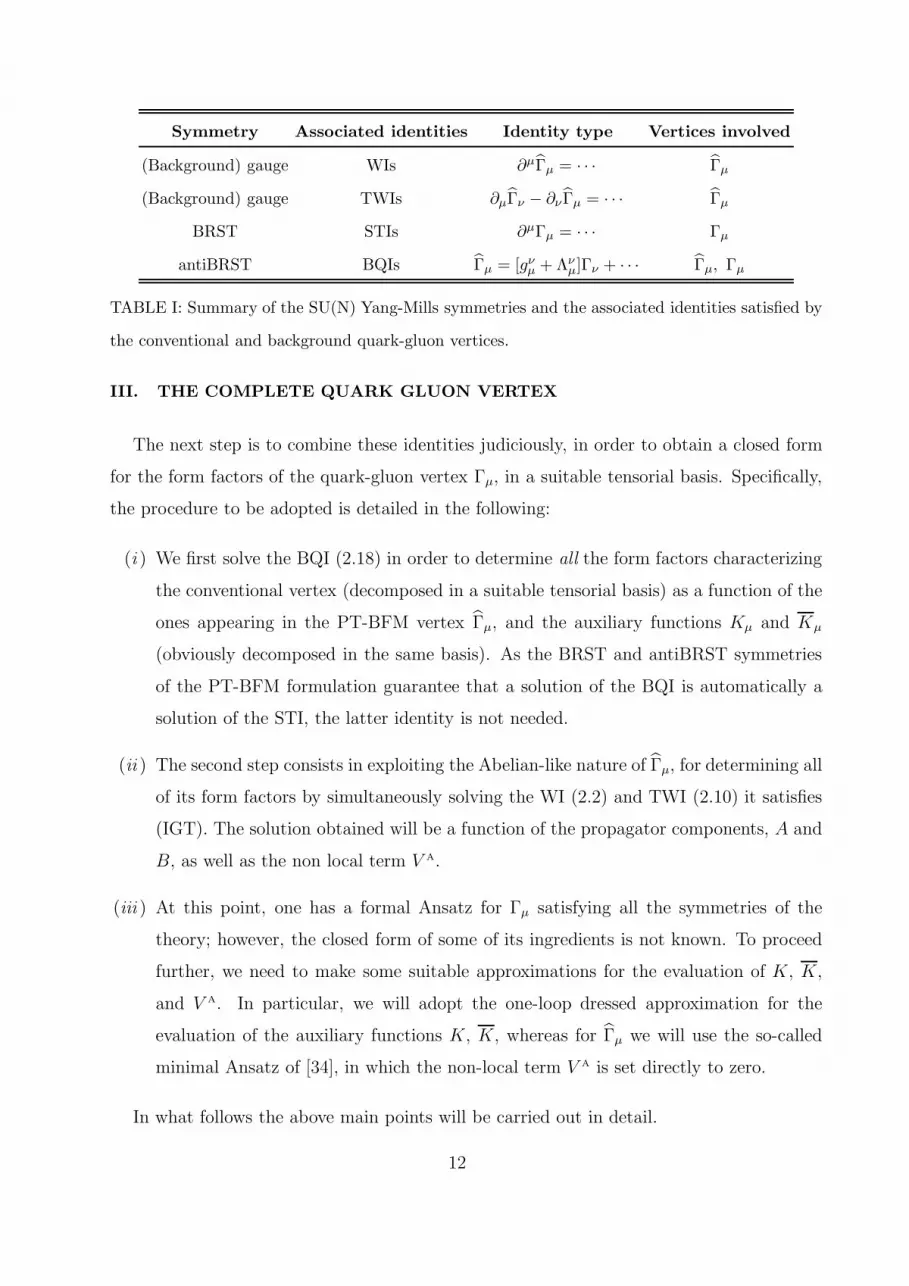
Symmetry Associated identities Identity type Vertices involved

(Background) gauge WIs ∂µΓµ = · · · Γµ

(Background) gauge TWIs ∂µΓν − ∂νΓµ = · · · Γµ

BRST STIs ∂µΓµ = · · · Γµ

antiBRST BQIs Γµ = [gνµ + Λνµ]Γν + · · · Γµ, Γµ

TABLE I: Summary of the SU(N) Yang-Mills symmetries and the associated identities satisfied by

the conventional and background quark-gluon vertices.

III. THE COMPLETE QUARK GLUON VERTEX

The next step is to combine these identities judiciously, in order to obtain a closed form

for the form factors of the quark-gluon vertex Γµ, in a suitable tensorial basis. Specifically,

the procedure to be adopted is detailed in the following:

(i ) We first solve the BQI (2.18) in order to determine all the form factors characterizing

the conventional vertex (decomposed in a suitable tensorial basis) as a function of the

ones appearing in the PT-BFM vertex Γµ, and the auxiliary functions Kµ and Kµ

(obviously decomposed in the same basis). As the BRST and antiBRST symmetries

of the PT-BFM formulation guarantee that a solution of the BQI is automatically a

solution of the STI, the latter identity is not needed.

(ii ) The second step consists in exploiting the Abelian-like nature of Γµ, for determining all

of its form factors by simultaneously solving the WI (2.2) and TWI (2.10) it satisfies

(IGT). The solution obtained will be a function of the propagator components, A and

B, as well as the non local term V A.

(iii ) At this point, one has a formal Ansatz for Γµ satisfying all the symmetries of the

theory; however, the closed form of some of its ingredients is not known. To proceed

further, we need to make some suitable approximations for the evaluation of K, K,

and V A. In particular, we will adopt the one-loop dressed approximation for the

evaluation of the auxiliary functions K, K, whereas for Γµ we will use the so-called

minimal Ansatz of [34], in which the non-local term V A is set directly to zero.

In what follows the above main points will be carried out in detail.

12

A. Tensorial bases

The procedure outlined above requires the definition of a tensorial basis, in order to

project out the twelve different components of the vertices and auxiliary functions. Given

the properties of the functions Kµ and Kµ under conjugation, it is natural to employ bases

whose components possess simple transformation properties under this operation.

It turns out that there are (at least) two suitable candidates, which we briefly describe

below.

1. Transverse/longitudinal basis

The T+L basis separates the possible contributions to a vector quantity into (four) lon-

gitudinal and (eight) transverse form factors. Thus, in the T+L basis all vector quantities

are decomposed according to [14]

fµ(q, p2,−p1) =4∑

i=1

fL

i (q2, p22, p

21)L

µi (q, p2,−p1) +

8∑

i=1

f T

i (q2, p22, p

21)T

µi (q, p2,−p1), (3.1)

where the longitudinal basis vectors read (remember that t = p1 + p2)

Lµ1 = γµ; Lµ

2 = t/tµ; Lµ3 = tµ; Lµ

4 = σµνtν ; (3.2)

while for the transverse basis vectors we have instead

T µ1 = pµ2 (p1 · q)− pµ1 (p2 · q); T µ

2 = T µ1 t/;

T µ3 = q2γµ − qµq/; T µ

4 = T µ1 σνλp

ν1p

λ2 ;

T µ5 = σµνqν ; T µ

6 = γµ(q ·t)− tµq/;

T µ7 = −1

2(q ·t)Lµ

4 − tµσνλpν1p

λ2 ; T µ

8 = γµσνλpν1p

λ2 + pµ2p/1 − pµ1p/2. (3.3)

It is then relatively straightforward to prove that under conjugation one has the properties

Lµ

i = Lµi , i = 1, 2, 3; L

µ

4 = −Lµ4 ;

Tµ

i = T µi , i = 1, 2, 3, 4, 5, 7, 8; T

µ

6 = −T µ6 , (3.4)

where Lµi = Lµ

i (q, p2,−p1) and Lµ

i = Lµ

i (−q, p1,−p2) and similarly for the T tensors.

13

2. Naive conjugated basis

A second convenient possibility is the NC basis, which is obtained by minimally modifying

the naive basis of [14] in order to avoid mixing of different tensors under conjugation.

In this basis the decomposition of a generic vector fµ is given by

fµ(q, p2,−p1) =12∑

i=1

fi(q2, p22, p

21)C

µi (q, p2,−p1), (3.5)

with

Cµ1 = γµ; Cµ

2 = pµ2 ; Cµ3 = pµ1 ; Cµ

4 = σµν p

ν2;

Cµ5 = σµ

ν pν1 ; Cµ

6 = pµ2p/2; Cµ7 = pµ2p/1; Cµ

8 = pµ1p/2;

Cµ9 = pµ1p/1; Cµ

10 = pµ2p/1p/2; Cµ11 = pµ1p/1p/2; Cµ

12 =1

2(γµp/1p/2 + p/1p/2γ

µ) . (3.6)

Then, under conjugation one has the following properties

Cµ

1 = Cµ1 ; C

µ

2 = Cµ3 ; C

µ

3 = Cµ2 ; C

µ

4 = −Cµ5 ; C

µ

5 = −Cµ4 ; C

µ

6 = Cµ9 ;

Cµ

7 = Cµ8 ; C

µ

8 = Cµ7 ; C

µ

9 = Cµ6 ; C

µ

10 = Cµ11; C

µ

11 = Cµ10; C

µ

12 = Cµ12, (3.7)

where Cµi = Cµ

i (q, p2,−p1) and Cµ

i = Cµ

i (−q, p1,−p2).The relations between the form factors in the T+L and NC bases are given in Appendix A.

B. The IGT implementation

In this subsection we implement the IGT, namely we present the general solution of the

WI and the TWI, in the T+L basis.

1. Ward identity

For the vertex Γµ the “solution” of the WI (2.2) immediately yields for the longitudinal

form factors [58] the expressions

ΓL

1 =A1 + A2

2; ΓL

2 =A1 − A2

2(q ·t) ; ΓL

3 = −B1 − B2

q ·t ; ΓL

4 = 0, (3.8)

where we have defined Ai = A(p2i ) and Bi = B(p2i ). It is then elementary to verify that the

resulting “longitudinal” vertex satisfies indeed the WI of (2.2).

14

2. Transverse Ward identity

Equations (2.10) can be used to determine the remaining (transverse) form factors of Γµ.

In the T+L basis Eq. (2.10) yields

(q ·t)θµi ΓT

µ = [tρθiρqµ − (q ·t)θµi ] ΓL

µ − iP µνi [S−1(p2)σ

5µν − σ5

µνS−1(p1)]− P µν

i V A

µν . (3.9)

Next, introducing the parametrization

P µνi V A

µν = V A

i1 + V A

i2p/1 + V A

i3p/2 + V A

i4 σµνpµ1p

ν2, (3.10)

we obtain for the transverse form factors the general expressions

ΓT

1 = − 1

2r(q ·t)VA

11,

ΓT

2 = − 1

8r(q ·t) [3(VA

12 + V A

13)− 2V A

21] ,

ΓT

3 =A1 − A2

2(q ·t) +1

16r(q ·t){[3t2 − 4(t·p1)]V A

12 + [3t2 − 4(t·p2)]V A

13 − 2t2V A

21

},

ΓT

4 =1

4r(q ·t)2 {2VA

11 − 3(q ·t)V A

14 − 2(t·p1)V A

22 − 2(t·p2)V A

23} ,

ΓT

5 = −B1 −B2

q ·t − 1

8r(q ·t) {(q ·t)VA

11 + 2r(V A

14 + V A

22 − V A

23)} ,

ΓT

6 =1

16r(q ·t) {[4(q ·p1)− 3(q ·t)]V A

12 + [4(q ·p2)− 3(q ·t)]V A

13 + 2(q ·t)V A

21} ,

ΓT

7 =1

4r(q ·t)2{q2V A

11 − 2r(V A

22 + V A

23)},

ΓT

8 =A1 − A2

q ·t − 1

4r(q ·t) {(q ·p1)VA

12 + (q ·p2)V A

13 + rV A

24} , (3.11)

where we have set r = r(p1, p2) = p21p22 − (p1 ·p2)2.

By setting all the V A

ij to zero one obtains a minimal Ansatz for the PT-BFM vertex that

is compatible with both the WI and the TWI; in this case one finds only three non zero

transverse components, namely [34]

ΓT

3 =A1 − A2

2(q ·t) ; ΓT

5 = −B1 − B2

q ·t ; ΓT

8 = −A1 − A2

q ·t . (3.12)

15

C. General solution for arbitrary momenta

The closed form of the non-Abelian vertex Γµ, can be finally obtained by solving the

BQI (2.18). Using the results (3.8) we obtain for the longitudinal form factors (T+L basis)

GqΓL

1 =[1− L(q2)F (q2)

]{ΓL

1 + A1

[1

2(q ·t)KL

3 − (p1 ·t)KL

4

]− B1K

L

1

+A2

[−1

2(q ·t)KL

3 + (p2 ·t)KL

4

]− B2K

L

1

},

GqΓL

2 =[1− L(q2)F (q2)

]{ΓL

2 + A1

[1

2KL

3 +p1 ·qq ·t K

L

4

]− B1K

L

2

+A2

[1

2K

L

3 −p2 ·qq ·t K

L

4

]−B2K

L

2

},

GqΓL

3 =[1− L(q2)F (q2)

]{ΓL

3 + A1

[p1 ·qq ·t K

L

1 + (p1 ·t)KL

2

]− B1K

L

3

+A2

[p2 ·qq ·t K

L

1 + (p2 ·t)KL

2

]− B2K

L

3

},

GqΓL

4 =[1− L(q2)F (q2)

]{A1

2[−KL

1 + (q ·t)KL

2 ]− B1KL

4

+A2

2

[K

L

1 + (q ·t)KL

2

]−B2K

L

4

}, (3.13)

while, for the transverse form factors we get

GqΓT

1 = ΓT

1 + A1

[− 1

q ·tKL

1 + (p1 ·t)KT

2 +KT

3 −KT

6

]− B1K

T

1

+ A2

[1

q ·tKL

1 + (p2 ·t)KT

2 +KT

3 +KT

6

]− B2K

T

1

+2

q2L(q2)F (q2)

{A1

[p1 ·qq ·t K

L

1 + (p1 ·t)KL

2

]− B1K

L

3+

+ A2

[p2 ·qq ·t K

L

1 + (p2 ·t)KL

2

]− B2K

L

3 −B1 − B2

q ·t

}

GqΓT

2 = ΓT

2 + A1

[− 1

q ·tKL

4 +1

2KT

1 +1

2(p1 ·q)KT

4 − 1

2KT

7

]−B1K

T

2

+ A2

[− 1

q ·tKL

4 +1

2K

T

1 − 1

2(p2 ·q)K

T

4 − 1

2K

T

7

]−B2K

T

2

+2

q2L(q2)F (q2)

{A1

[1

2KL

3 +p1 ·qq ·t K

L

4

]− B1K

L

2+

+ A2

[1

2K

L

3 −p2 ·qq ·t K

L

4

]− B2K

L

2 +A1 −A2

2(q ·t)

},

16

GqΓT

3 = ΓT

3 +A1

2

[1

2(q ·t)KT

1 − 1

2(p1 ·t)(q ·t)KT

4 −KT

5

]− B1K

T

3

+A2

2

[−1

2(q ·t)KT

1 +1

2(p2 ·t)(q ·t)K

T

4 −KT

5

]− B2K

T

3

+1

q2L(q2)F (q2)

{A1

[1

2(q ·t)KL

3 − (p1 ·t)KL

4

]−B1K

L

1

+ A2

[−1

2(q ·t)KL

3 + (p2 ·t)KL

4

]−B2K

L

1 +1

2(A1 + A2)

},

GqΓT

4 = ΓT

4 + A1

[KT

2 − 2

q ·tKT

3 +1

q ·tKT

8

]− B1K

T

4 + A2

[K

T

2 +2

q ·tKT

3 − 1

q ·tKT

8

]− B2K

T

4

+4

q2(q ·t)L(q2)F (q2)

{A1

2[−KL

1 + (q ·t)KL

2 ]− B1KL

4 +A2

2

[K

L

1 + (q ·t)KL

2

]− B2K

L

4

},

GqΓT

5 = ΓT

5 +A1

2

[−KL

1 − q2KT

3 − (q ·t)KT

6 − (p1 ·t)KT

8

]− B1K

T

5

+A2

2

[−KL

1 − q2KT

3 − (q ·t)KT

6 − (p2 ·t)KT

8

]− B2K

T

5 ,

GqΓT

6 = ΓT

6 +A1

2

[−KL

3 − q2

2KT

1 +q2

2(p1 ·t)KT

4 −KT

5 − (p1 ·t)KT

7

]−B1K

T

6

+A2

2

[K

L

3 +q2

2K

T

1 −q2

2(p2 ·t)K

T

4 +KT

5 + (p2 ·t)KT

7

]− B2K

T

6 ,

GqΓT

7 = ΓT

7 + A1

[−KL

2 − q2

q ·tKT

3 −KT

6 +p1 ·qq ·t K

T

8

]− B1K

T

7

+ A2

[−KL

2 +q2

q ·tKT

3 +KT

6 +p2 ·qq ·t K

T

8

]− B2K

T

7

+2

q ·tL(q2)F (q2)

{A1

2[−KL

1 + (q ·t)KL

2 ]− B1KL

4 +A2

2

[K

L

1 + (q ·t)KL

2

]− B2K

L

4

},

GqΓT

8 = ΓT

8 + A1

[KL

4 −KT

5 +1

2(q ·t)KT

7

]−B1K

T

8 + A2

[−KL

4 −KT

5 − 1

2(q ·t)KT

7

]−B2K

T

8 .

(3.14)

In the formulas above,

Gq = 1 +G(q2); KT,L

i = KT,L

i (q2, p22, p21); K

T,L

i = KT,L

i (q2, p21, p22). (3.15)

As far as the longitudinal terms are concerned, it should be noticed that the form

of Eq. (3.13) is dictated by the required compatibility between the STI and the BQI. Indeed,

using Eq. (2.13) we get the relation 1−L(q2)F (q2) = GqF (q2), so that the Gq simplifies and

one is left with the result we would have obtained starting directly from the STI (2.4) after

using Eqs. (2.16) and (2.17) to trade the form factors appearing in the H and H for the ones

appearing in K and K. This is not the case for the transverse form factors, where indeed

no such pattern is found.

17

IV. SOME SPECIAL KINEMATIC LIMITS

Here we specialize the general solution reported in the previous section to the two kine-

matic configurations that have been simulated on the lattice [17, 18], corresponding to the

soft gluon limit p1 → p2 (or q → 0) and the symmetric limit p1 → −p2. A third interesting

limit in which the quark momenta p2 is set to zero, will be also discussed.

A. Soft-gluon limit

The solution of the BQI in this limit can be obtained by letting p1 → p2 in the general

solution presented in Eqs. (3.13) and (3.14). Although several of the expressions appearing

there seem singular in this limit, it should be noticed that this is not the case. The reason

is that whenever p1 → ±p2, the form factors KL,T

i and KL,T

i also coincide (up to a sign);

indeed, the conjugation properties (3.4) gives the relations

KL

i (q2, p21, p

22) = KL

i (q2, p21, p

22) i = 1, 2, 3; K

L

4(q2, p21, p

22) = −KL

4 (q2, p21, p

22)

KT

i (q2, p21, p

22) = KT

i (q2, p21, p

22) i = 1, 2, 3, 4, 5, 7, 8; K

T

6 (q2, p21, p

22) = −KL

6 (q2, p21, p

22).

(4.1)

As a result, all potentially divergent terms cancel out and one is left with a well defined

result. In particular, since the limit p1 → p2 also implies that q → 0, all the transverse

tensor structures (3.3) vanish identically. The vertex is therefore purely longitudinal, and

after setting p1 = p2 = p, one finds that the Lµi vectors reduce to

Lµ1 = γµ; Lµ

2 = 4p/pµ; Lµ3 = 2pµ; Lµ

4 = 2σµνpν . (4.2)

Redefining the basis vectors so that they are simply given by {γµ, p/pµ, pµ, σµνpν} with cor-

responding form factors {Γ1,Γ2,Γ3,Γ4} and {K1, K2, K3, K4}, one obtains the results

F−10 Γ1 = A

(1− 2p2K4

)− 2BK1,

F−10 Γ2 = 2A′ + 2A (K3 +K4)− 2BK2,

F−10 Γ3 = −2B′ + 2A

(K1 + p2K2

)− 2BK3,

Γ4 = 0, (4.3)

where F−10 = F−1(0), A = A(p2), B = B(p2), Ki = Ki(p

2), and a prime denotes derivative

with respect to p2.

18

We conclude this subsection by noticing that in the soft gluon limit the identities (2.16)

and (2.17) yield an all-order constraint on the form of H and H. To see this, let us observe

that the Taylor expansion of a function f(q, p2,−p1) when q → 0, and p1 = p2 = p reads

f(q, p2,−p1) = f(0, p,−p) + qµ∂

∂qµf(q, p2,−p1)

∣∣∣∣q=0

+O(q2), (4.4)

where the (possible) Lorentz structure of the function f has been suppressed. Specializing

this result to the identities (2.16), one obtains the (all-order) conditions

H(0, p,−p) = 1 =⇒ X1(0, p2, p2) = −X2(0, p

2, p2); X0(0, p2, p2) = 1, (4.5)

where we have used the form factor decomposition of Eq. (2.6). Clearly, an equivalent result

holds for H and its corresponding form factors.

B. Symmetric limit

The symmetric limit, in which p1 → −p2, is subtler than the previous case. The relations

listed in Eq. (4.1) remain valid also in this limit, thus leading to a finite result for the expres-

sions (3.13) and (3.14); nevertheless, one finds that only one longitudinal basis tensor (3.2)

and two transverse tensors (3.3) survive in this limit, namely

Lµ1 = γµ; T µ

3 = 4(p2γµ − pµp/

); T µ

5 = −2σµνpν . (4.6)

However, as in the previous case, there are in principle four independent tensors in the basis:

we are clearly missing pµ.

Thus, we arrive to the conclusion that in the T+L basis the symmetric limit is singular,

and one cannot get the results by taking directly this limit in the general solution (3.13)

and (3.14). The way to proceed is instead the following: (i ) first, use the relations (A3) be-

fore taking any limit to get the general solution in the naive conjugated basis; (ii ) next, take

the symmetric limit of this solution, given that this basis is well behaved in this limit, giving

rise to the four independent tensors needed; (iii ) go back to the T+L basis using Eqs. (A1)

and (A2).

Following this procedure, and redefining the basis vectors to be, as in the previous

19

limit, {γµ, p/pµ, pµ, σµνpν}, one obtains the results

G2pΓ1 = Γ1 + 2p2AK4 − 2BK1,

G2pΓ2 = Γ2 − 2A (K3 +K4)− 2BK2 −1

p2L2pF2p

[A(1− 2p2K3

)− 2B

(K1 + p2K2

)]

G2pΓ3 = Γ3,

G2pΓ4 = Γ4 + 2AK1 − 2BK4, (4.7)

where A = A(p2), B = B(p2) and

G2p = 1 +G(4p2); F2p = F (4p2); L2p = L(4p2). (4.8)

Within this basis, the solution of the WI and TWI (3.8) and (3.11) gives the relations

Γ1 + p2Γ2 = A; Γ3 = 0; Γ4 = 2B′ (4.9)

and therefore one gets the final results

F−12p

(Γ1 + p2Γ2

)= A

(1− 2p2K3

)− 2B

(K1 + p2K2

),

Γ3 = 0,

G2pΓ4 = 2B′ + 2AK1 − 2BK4. (4.10)

As the above results clearly show, in the naive conjugated basis it is not possible to disen-

tangle the form factors Γ1 and Γ2. This, however, can be achieved by going back to the T+L

basis {γµ, pµ, p2γµ−p/pµ, σµνpν} in which the corresponding form factors {ΓL

1 ,ΓL

3 ,ΓT

3 ,ΓT

5} can

be obtained from the previous ones through the relations

ΓL

1 = Γ1 + p2Γ2; ΓL

3 = Γ3; ΓT

3 = −Γ2; ΓT

5 = Γ4, (4.11)

and similarly for {KL

1 , KL

3 , KT

3 , KT

5 }; one then obtains 5

F−12p ΓL

1 = A− 2p2AKL

3 − 2BKL

1 ,

ΓL

3 = 0,

G2pΓT

3 = 2A′ + 2A

[(1− L2pF2p)K

L

3 +KT

5 +1

2p2L2pF2p

]− 2B

[KT

3 +1

p2L2pF2pK

L

1

],

G2pΓT

5 = 2B′ + 2A(KL

1 + p2KT

3

)− 2BKT

5 . (4.12)

5 We notice that the terms proportional to KL

3 are precisely those that one would miss by taking directly

the symmetric limit of the T+L solution (3.13) and (3.14).

20

However, on the lattice in the Landau gauge and for a momentum configuration other

than the soft gluon, what they have measured is only the combination P νµΓν , that is

P νµ (p)Γν = P ν

µ (p)γν(ΓL

1 + p2ΓT

3 ) + σµνpνΓT

5 , (4.13)

yielding

G2p(ΓL

1 + p2ΓT

3 ) = 2p2A′ + A(1 + 2p2KT

5 )− 2B(KL

1 + p2KT

3 ),

G2pΓT

5 = 2B′ + 2A(KL

1 + p2KT

3

)− 2BKT

5 . (4.14)

Evidently, the multiplication of ΓT

3 by p2 removes the potentially IR divergent terms; thus,

one expects the corresponding form factor measured on the lattice to be finite.

C. Zero quark momentum

We now set to zero the quark momentum p2, so that q = p1 = p. This limit is well

defined in any of the two bases introduced earlier, and the corresponding form factors can

be obtained directly form our general solution (3.13) and (3.14). However, the form fac-

tors KL,T

i (p2, 0, p2) and KL,T

i (p2, p2, 0) do not coincide anymore, and need to be evaluated

separately. Defining the basis tensors to be {γµ, pµ, p2γµ− p/pµ, σµνpν} with the correspond-

ing form factors {ΓL

1 ,ΓL

3 ,ΓT

3 ,ΓT

5}, {KL

1 , KL

3 , KT

3 , KT

5 }, and {KL

1 , KL

3 , KT

3 , KT

5}, we obtain the

following results

F−1ΓL

1 = A(1 + p2KL

3 )−BKL

1 − B0KL

1 ,

F−1ΓL

3 = − 1

p2(B −B0) + AKL

1 −BKL

3 − B0KL

3 ,

GΓT

3 = −A(KL

3 +KT

5 )−BKT

3 −B0KT

3 +1

p2LpFp

[A(1 + p2KL

3 )− BKL

1 −B0KL

1

],

GΓT

5 = − 1

p2(B −B0)− A(KL

1 + p2KT

3 )−BKT

5 − B0KT

5 , (4.15)

with the usual definitions A = A(p2), B = B(p2), as well as B0 = B(0).

On the lattice one focuses on the projected vertex (4.13), for which one has the two form

factors

G(ΓL

1 + p2ΓT

3 ) = A(1− p2KT

5 )−B(KL

1 + p2KT

3 )− B0(KL

1 + p2KT

3 ),

GΓT

5 = − 1

p2(B − B0)− A(KL

1 + p2KT

3 )−BKT

5 − B0KT

5 . (4.16)

21

V. NUMERICAL RESULTS AND COMPARISON WITH LATTICE DATA

In this section we carry out a numerical study of the form factors of the quark-gluon

vertex in the various kinematical limits studied in the previous section.

A. The one-loop dressed approximation for the auxiliary functions

As a first step in our numerical study, we need to identify a suitable approximation for

the functions Kµ and Kµ in order to determine the corresponding form factors Ki and Ki,

which ultimately characterize the quark-gluon vertex. In what follows we will use the one-

loop dressed approximation (see Fig. 3), in which the propagators are fully dressed while

vertices are retained at tree-level (see Fig. 3 again). This yields the following expressions

Kµ(q, p2,−p1) =i

2g2CA

∫

k

S(k + p2)γνPµν(k)∆(k2)D(k − q),

Kµ(−q, p1,−p2) =i

2g2CA

∫

k

γνS(p1 − k)Pµν(k)∆(k2)D(k − q). (5.1)

It turns out that the best and most expeditious strategy for projecting out the various

components of this function is to use the naive conjugated basis, eventually passing to the

T+L basis using the formulas (A1) and (A2). For general values of the pi momenta the

calculation is carried out in Appendix B; here we will study the limiting cases singled out

in the previous section (notice that, in the case of the soft gluon and symmetric limit, one

cannot obtain the corresponding results as a direct limit of the general results).

1. Soft-gluon and symmetric limit

In the limit p1 → ±p2 one can concentrate on the calculation of Kµ only, as in this case

K and K coincide. Thus, we start by writing

Kµ(p) =i

2g2CA

∫

k

(k/+ p/) γνPµν(k)RA(k, p) +

i

2g2CA

∫

k

γνPµν(k)RB(k, p), (5.2)

where we have defined

Rf (k, p) =f(k + p)∆(k2)

A2(k + p)(k + p)2 −B2(k + p)D(k, p), (5.3)

22

and

D(k, p) =

D(k), soft gluon limit;

D(k + 2p), quark symmetric limit.(5.4)

We next introduce the integrals

If0 (p) =i

2g2CA

∫

k

Rf(k, p),

Ifµ(p) =i

2g2CA

∫

k

kµRf (k, p) = If1 (p

2)pµ,

Ifµν(p) =i

2g2CA

∫

k

kµkνk2

Rf(k, p) = Jf1 (p

2)gµν + Jf2 (p

2)pµpν , (5.5)

with, correspondingly,

If1 (p2) =

pµ

p2Ifµ(p); Jf

1 (p2) =

1

3P µν(p)Ifµν(p); Jf

2 (p2) =

1

3p2

(4pµpν

p2− gµν

)Ifµν(p). (5.6)

Notice that not all these form factors are independent, since one has the constraint

4Jf1 (p

2) = If0 (p2)− p2Jf

2 (p2). (5.7)

Writing finally

Kµ(p) = γµK1(p2) + p/pµK2(p

2) + pµK3(p2) + σµνp

νK4(p2), (5.8)

we obtain the results

K1(p2) = IB

0 (p2)− JB

1 (p2) =

i

6g2CA

∫

k

[2 +

(k ·p)2k2p2

]RB(k, p),

K2(p2) = −JB

2 (p2) =

i

6p2g2CA

∫

k

[1− 4

(k ·p)2k2p2

]RB(k, p),

K3(p2) = 3JA

1 (p2) =

i

2g2CA

∫

k

[1− (k ·p)2

k2p2

]RA(k, p),

K4(p2) = −IA

0 (p2)− IA

1 (p2) + JA

1 (p2) = − i

6g2CA

∫

k

[2 + 3

(k ·p)p2

+(k ·p)2k2p2

]RA(k, p). (5.9)

Notice the 1/p2 factor multiplying the K2(p2) function; we will return to this important

point shortly.

2. Zero quark momentum

In this case one has to consider both K and K, as when p2 = 0 the two functions do not

coincide. For Kµ, after defining

Rf (k, p) =f(k2)∆(k2)D(k + p)

A2(k2)k2 − B2(k2), (5.10)

23

one finds thatK3(p2) = 0, K1 andK2 are given in Eq. (5.9) with RB obtained from Eq. (5.10)

above, and finally

K4(p2) = IA

1 (p2) =

i

2g2CA

∫

k

(k ·p)p2

RA(k, p). (5.11)

For Kµ one has instead

Rf (k, p) =f(k + p)∆(k2)D(k + p)

A2(k + p)(k + p)2 −B2(k + p), (5.12)

and one gets for the Ki the corresponding results of Eq. (5.9) for Ki, in which Rf is replaced

by the expression above and K4 gets an extra minus sign.

B. Passing to the Euclidean space

In order to pass from Minkowskian to Euclidean space, let us define

γ0 → γE

4 ; γj → iγE

j ; k0 → ikE

4 ; kj → −kE

j . (5.13)

Then, with the signature of the Minkowski metric being (+,−,−,−), one has the replace-

ment rules

d4k → id4kE; k/→ ik/E; k · q → −kE · qE; k2 → −k2

E. (5.14)

On the one hand, these rules are enough to convert to their Euclidean counterparts scalar

expressions; specifically one has

AE(p2E) = A(−p2); BE(p

2E) = B(−p2);

FE(p2E) = F (−p2); ∆E(p

2E) = −∆(−p2);

KE

1,3,4(p2E) = K1,3,4(−p2); KE

2 (p2E) = −K2(−p2);

KE

1,3,4(p2E) = K1,3,4(−p2); K

E

2(p2E) = −K2(−p2). (5.15)

On the other hand, they are not sufficient to specify how to proceed in the case of a

four-vector quantity like the quark-gluon vertex; to accomplish the conversion, we follow the

prescription of [18]. Specificaly, first we form a Minkowski scalar by contracting Γµ with

γµ, and then we demand that the resulting expression be identical to the one obtained if we

had started directly from the Euclidean expression, and had assumed that all the Euclidean

form factors are equal to the corresponding Minkowski ones evaluated at negative momenta,

Γi(q2E, p22E, p

21E) = Γi(−q2,−p22,−p21). (5.16)

24

In the kinematic configurations of interest, which involves only one momentum scale p,

this prescription yields the NC tensor basis {γE

µ, ipE

µ,−p/EpE

µ, iσE

µνpE

ν} or the T+L basis

{γE

µ, ipE

µ,−p2EγE

µ + p/EpE

µ, iσE

µνpE

ν}.Finally, integrals will be performed using the following spherical coordinates:

x = p2; y = k2; z = (k + p)2 = x+ y + 2√xy cos θ;

∫

kE

=1

(2π)3

∫ π

0

dθ sin2 θ

∫∞

0

dy y, (5.17)

Equipped with these expressions we can convert all quantities appearing in the previous

section into Euclidean quantities and, once numerically evaluated, directly compare them

with the one obtained in the lattice study of [18].

C. Numerical results

In this subsection we carry out the numerical evaluation of the various relevant quantities

introduced so far, and we compare our results with the lattice data on the quark-gluon vertex.

1. Ingredients

For the evaluation of the one-loop dressed scalar functions Ki we need the following

ingredients : (i ) the gluon propagator ∆, (ii ) the ghost dressing function F , (iii ) the value

of the strong coupling, at the relevant renormalization scale, µ. Specifically, since the lattice

data on the quark-gluon vertex have been renormalized at µ = 2.0 GeV [18], this particular

scale will serve as our reference, and all quantities will be renormalized, for consistency, at

this particular point. (iv ) the Dirac vector and scalar components of the quark propagator,

A and B, respectively. In what follows we explain briefly how the above ingredients are

obtained.

(i ) As in a variety of previous works (e.g., [6, 59–61]), we use for the gluon propagator ∆

directly the SU(3) lattice data of [48]. As has been explained in detail in the literature

cited above, an excellent, physically motivated fit of the lattice data (renormalized at

µ = 4.3 GeV, the last available point in the ultraviolet tail of the gluon propagator),

is given by

∆−1(q2) =M2(q2) + q2[1 +

13CAg21

96π2ln

(q2 + ρ1M

2(q2)

µ2

)], (5.18)

25

0

1

2

3

4

5

0.001 0.01 0.1 1 10 100

µ=2.0 [GeV], β=5.70 V=644

V=724

V=804

Fit

q2 [GeV2]

∆(q

2)[G

eV−2]

FIG. 4: (color online). The functional fit given in Eq. (5.18) to the SU(3) gluon propagator. Lattice

data are taken from [48] and renormalized at µ = 2.0 GeV.

where

M2(q2) =m4

0

q2 + ρ2m20

. (5.19)

Notice that in the above expression, the finiteness of ∆−1(q2) is assured by the presence

of the function M2(q2), which forces the value of ∆−1(0) =M2(0) = m20/ρ2. The best

fit obtained with this functional form corresponds to settingm0 = 520 MeV, g21 = 5.68,

ρ1 = 8.55 and ρ2 = 1.91.

Of course, since we want our results renormalized at µ = 2.0 GeV instead of µ = 4.3

GeV, the curve of Eq. (5.18) must be rescaled by a multiplicative factor. This factor

can be obtained from the standard relation

∆(q2, µ2) =∆(q2, ν2)

µ2∆(µ2, ν2), (5.20)

which allows one to convert a set of points renormalized at ν to the corresponding set

renormalized at µ. In our case ν = 4.3 GeV and µ = 2.0 GeV, and ∆(µ2, ν2) ≈ 0.384

GeV−2, so that the multiplicative factor is [µ2∆(µ2, ν2)]−1 ≈ 0.652 . The corresponding

fit is shown in Fig. 4.

(ii ),(iii ) The ghost dressing function F is determined by solving the corresponding ghost gap

equation. For the fully dressed ghost-gluon vertex entering in it we use the expres-

sions obtained in [62]. Then, the strong coupling α(µ2) is simultaneously fixed by

demanding that the solution obtained for F matches the SU(3) lattice results of [48].

26

0.5

1

1.5

2

2.5

0.01 0.1 1 10 100

µ=2.0 [GeV], β=5.70 V=644

V=804

SDE, α(µ)=0.45

0

0.2

0.4

0.6

0.8

1

1.2

0.01 0.1 1 10 100

1+G(q2)L(q2)

q2 [GeV2] q2 [GeV2]

F(q

2)

1+G(q

2),L(q

2)

FIG. 5: (color online). Left: The Landau gauge ghost dressing function F obtained as a solution

of the ghost gap equation for α = 0.45 using as input the lattice gluon propagator. Right: The

decomposition of the (inverse) ghost dressing function into its 1 +G (blue, dashed-dotted) and L

(orange, dashed) components. Lattice data are taken from [48].

The best match is achieved for α = 0.45 at µ = 2.0 GeV, as shown in the left panel

of Fig. 5. From now on α will be kept fixed at this particular value. The (inverse)

ghost dressing function can be further separated in its 1 + G and L components that

appears in Eq. (2.13). This is done by solving the SDEs they satisfy [57], and the

corresponding results are shown in the right panel of the same figure.

(iv ) With the ∆ and F we have just determined, one can evaluate the vector and scalar

components of the quark propagator. This is achieved by solving the quark gap equa-

tion described in [6] with a Curtis-Pennington quark-gluon vertex [26], and a bare

quark mass fixed at 115 MeV, which is the value employed in the lattice simulations

of [18]. The results obtained for the quark wavefunction Z = 1/A and mass M = B/A

are shown in Fig. 6.

At this point we have all the ingredients and shall proceed to determine the Ki and Ki

auxiliary functions, and subsequently the vertex form factors for the various kinematical

limits introduced before.

27

0.84

0.86

0.88

0.9

0.92

0.94

0.96

0.98

1

0.01 0.1 1 10 100 0.1

0.15

0.2

0.25

0.3

0.35

0.4

0.45

0.5

0.01 0.1 1 10 100

p2 [GeV2] p2 [GeV2]

Z(p

2)

M(p

2)[G

eV]

FIG. 6: (color online). The quark wave-function (left), and mass (right), obtained from the solution

of the quark gap equation for a current mass m0 = 115 MeV and αs(µ) = 0.45.

2. Soft-gluon limit

In Fig. 7 we plot the functions Ki in the soft gluon limit Eq. (5.9), obtained using ∆, F ,

Z and M determined before.

It is then immediate to construct the Euclidean version of the soft gluon limit form

factors (4.3). Specifically, in Fig. 8 we plot the form factors

λ1(p) = ΓE

1(pE); λ3(p) = −1

2ΓE

3(pE), (5.21)

and compare them with the lattice data of [18], obtaining a rather satisfactory agreement.

-0.3

-0.2

-0.1

0

0.1

0.2

0.3

0.4

0.001 0.01 0.1 1 10 100

K1(p2)K2(p2)K3(p2)K4(p2)

p2 [GeV2]

Ki(p2)

FIG. 7: (color online). The auxiliary functions Ki evaluated in the soft gluon limit.

28

0.8

1

1.2

1.4

1.6

1.8

2

0 0.5 1 1.5 2 2.5 3 3.5

Lattice, β=6.0, V=163x48BQI

-0.5

-0.4

-0.3

-0.2

-0.1

0

0.1

0.2

0.3

0 0.5 1 1.5 2 2.5 3 3.5 4

Lattice, β=6.0, V=163x48BQI

p [GeV] p [GeV]

λ1(p)

pλ3(p)

FIG. 8: (color online). The soft gluon form factors λ1 (left) and pλ3 (right). Lattice data in this

and all the following plots are taken from [18].

However, in the case of the form factor

λ2(p) =1

4ΓE

2(pE), (5.22)

we observe a fundamental qualitative discrepancy with respect to the lattice data; in partic-

ular, as Fig. 9 shows, we obtain a finite form factor, while the lattice shows an IR divergence

as p2 → 0.

This discrepancy seems common to all attempts to evaluate the quark-vertex form factors

from a purely SDE approach (see for example [63, 64]). In what follows we will offer a

plausible explanation for its origin, at least within our framework.

0.01

0.1

1

10

0 0.5 1 1.5 2 2.5 3 3.5

Lattice, β=6.0, V=163x48BQI

p [GeV]

λ2(p)[G

eV−2]

FIG. 9: (color online). The form factor λ2 and the corresponding lattice data.

29

To begin with, recall that in the soft gluon limit the transverse parts of the vertex are

not active; thus, the expressions (4.3) are exact, and any divergence can only manifest itself

in the auxiliary functions Ki. Specifically, Eq. (4.3) shows that in λ2 only the functions Ki

with i = 2, 3, 4 appear. In general, however, K3 should not develop a IR divergence, since

this would render IR divergent also λ3, and we know from the lattice that this form factor

is finite (see Fig. 8). On the other hand, both K2 and K4 could in principle have an IR

divergence, as long as they diverge at most as 1/p2, given that they both appear in λ1 and

λ3 multiplied by a factor p2.

To analyze what happens in the p → 0 limit of these two functions, let us observe that

in the soft gluon limit the function Rf of Eq. (5.3) can be written as

Rf (k, p) = ∆(k2)D(k2)g(k + p); g(k + p) =f(k + p)

A2(k + p)(k + p)2 − B2(k + p). (5.23)

The function g can be next expanded around p = 0 according to

g(k + p) = g(k2) + 2(k ·p)g′(k2) + p2g′(k2) + 2(k ·p)2g′′(k2) +O(p3), (5.24)

where the primes denote derivatives w.r.t. k2. All functions appearing in the above expansion

of g are well behaved in the IR, and we will assume the same about their derivatives.

One may then establish that the K4 in Eq. (5.9) is regular as p → 0; indeed, the only

possible divergence may come from the zeroth order term in (5.24). This term, however,

vanishes, since it is proportional to the integral of (k ·p)g(k2)/p2, which is an odd function

of the integration angle θ in the interval [0, π]. In the case of K2, the presence of the

prefactor 1/p2 implies that one has to consider both the zeroth and the first order term

in the expansion (5.24). Again, however, they both vanish: the linear term in p for the

same reason as before (odd in θ) , while the zeroth order term due to the vanishing of the

corresponding angular integral, namely6

∫ π

0

dθ sin2 θ(1− 4 cos2 θ) = 0. (5.25)

As a result, the one-loop dressed K2 and K4 in the soft gluon limit both saturate to a

constant in the IR, as Fig. 7 shows.

6 Note that if Eq. (5.9) are worked out in d space-time dimensions, one has the factor (1 − d cos2 θ); thus,

the result of Eq. (5.25) is particular to d = 4.

30

-0.4

-0.3

-0.2

-0.1

0

0.1

0.2

0.3

0.4

0.001 0.01 0.1 1 10 100

K1(p2)K2(p2)K3(p2)K4(p2)

0.8

1

1.2

1.4

1.6

1.8

2

0 0.5 1 1.5 2 2.5 3 3.5

Lattice, β=6.0, V=163x48BQI, b=0BQI, b=-0.5

0.01

0.1

1

10

0 0.5 1 1.5 2 2.5 3 3.5

Lattice, β=6.0, V=163x48BQI, b=0BQI, b=-0.5

-0.5

-0.4

-0.3

-0.2

-0.1

0

0.1

0.2

0.3

0 0.5 1 1.5 2 2.5 3 3.5 4

Lattice, β=6.0, V=163x48BQI, b=0BQI, b=-0.5

p2 [GeV2] p [GeV]

p [GeV] p [GeV]

Ki(p

2)

λ1(p)

λ2(p)[G

eV−2]

pλ3(p)

FIG. 10: (color online). The auxiliary functions Ki evaluated in the soft gluon limit with a

fermion vertex cos2 θγµ. When comparing with the results obtained for the tree-level vertex γµ

(gray curves) one notice that K2 becomes IR divergent, whereas the remaining Ki are suppressed.

In the remaining panels we show the soft gluon form factors obtained when using the vertex

γµ(1 + b cos2 θ) for the representative value b = −0.5; one obtains a divergent λ2, affecting only

modestly λ1 and leaving λ3 practically invariant.

Evidently, the finiteness of the form factor K2 in the soft gluon limit originates from

the conspiracy of two independent facts: (i ) The IR finiteness of the expanded function g,

which implies that the O(p2) terms in Eq. (5.24) will give rise to an IR convergent integral.

Instead, in the symmetric and zero quark momentum limits, the function to be expanded

involves always the IR divergent ghost propagator, and therefore K2 will be IR divergent

in both cases (see Figs 11 and 15). (ii ) The vanishing of the angular integral (5.25) (in 4

space-time dimensions).

31

-0.6

-0.4

-0.2

0

0.2

0.4

0.001 0.01 0.1 1 10 100

K1(p2)K2(p2)K3(p2)K4(p2)

p [GeV]

Ki(p)

FIG. 11: (color online). The auxiliary functions Ki evaluated in the symmetric gluon limit when

an extra angular dependence of the type b cos2 θ is added to the tree-level vertex γν .

Now, the presence of the integral (5.25) can be traced back to the one-loop dressed

approximation we have used to evaluate the functions Ki, where the fermion vertex was

kept at tree-level. In that sense, the obtained finiteness of K2 is accidental, being really an

artefact of our particular implementation of the one-loop dressed approximation. Actually,

if one were to include some additional angular dependence to this vertex (which will happen

anyway when quantum corrections are added), the cancellation (5.25) would be unavoidably

distorted, and one would end up with an IR divergent K2 ∼ 1/p2.

This fact is shown in Fig. 10, where the tree-level vertex γµ has been replaced by

γµ(1 + b cos2 θ). One observes that K2 becomes indeed IR divergent as soon as b 6= 0,

while all remaining Ki are only modestly affected by the presence of b. The resulting form

factors for the representative value b = −1/2 are shown in the same figure: λ2 develops a

1/p2 IR divergence, while λ1 and λ3 are marginally modified.

3. Symmetric limit

Let us now turn our attention to the symmetric limit. According to our previous discus-

sion, in this limit we expect a divergent K2 and a finite K4, as indeed shown in Fig. 11.

We next proceed to plot (Fig. 12) the form factors

λ′1(p) = ΓLE

1 (pE)− p2EΓTE

3 (pE); τ5(p) =1

2ΓTE

5 (pE), (5.26)

32

0.5

1

1.5

2

2.5

0 1 2 3 4 5 6

Lattice, β=6.0, V=163x48BQI0.8*BQI

0.001

0.01

0.1

1

10

0 1 2 3 4 5 6 7

Lattice, β=6.0, V=163x48BQI3*BQI

2p [GeV] 2p [GeV]

λ′ 1(p)

τ 5(p)[G

eV−1]

FIG. 12: (color online). The symmetric limit form factors λ′1 and τ5 compared with the corre-

sponding lattice data. The grey curves are obtained through simple rescaling of the blue ones.

which are measured on the lattice in the symmetric limit. As Eq. (4.14) shows, these form

factors do not explicitly involve the divergent term K2, and therefore are finite. For both of

them the overall shape of the lattice data is accurately described; however, the strength of

the two components is inverted, since we get a higher λ′1 and a lower τ5. Quite interestingly,

a simple rescaling of each form factor (through multiplication by a numerical constant) leads

to a very good overlap with the lattice data, as the gray curves demonstrate.

Our analysis is not limited to the projected form factors (5.26), as we can study also all

the three non-zero form factors (4.12) in this limit, similarly to what we have done in the

soft gluon limit. Specifically, on the basis of Eq. (4.12) one expects that ΓL

1 and ΓT

5 are finite

0.5

1

1.5

2

2.5

3

0.1 1 10 0

0.2

0.4

0.6

0.8

1

1.2

0.1 1 10

p [GeV] p [GeV]

ΓLE

1(p)

ΓTE

5(p)[G

eV−1]

FIG. 13: (color online). The symmetric form factors ΓL

1 (left) and ΓT

5 (right).

33

-70

-60

-50

-40

-30

-20

-10

0

0.1 1 10

p [GeV]

ΓTE

3(p)[G

eV−2]

FIG. 14: (color online). The divergent form factor ΓT3 in the symmetric limit.

(Fig. 13), as they involve only the combination p2K2 through the term KL

1 ; however, ΓT

3 has

two divergent pieces (Fig. 14), both proportional to the combination L2p/p2 reading7 [57]

1

p2L2p ∼

1

p2

∫

k

[1− d

(k · p)2k2p2

]∆(k)D(k + 2p) ∼

p2→0

1

p. (5.27)

4. Zero quark momentum

The case of the zero quark momentum constitutes a “prediction”, given that there are

no lattice data available for this particular momentum configuration.

In this specific case, the degeneracy between the Ki and Ki functions is broken, and one

has to study them separately. In addition, one will have both K2 and K2 divergent in this

case, even though the (projected) form factors λ′1 and τ5, introduced in Eq. (5.26), will still

be finite, as the only combination that enters in their definition (4.16) is KL

1 = K1 + p2K2.

In Fig. 15 we plot the auxiliary functions Ki and K i, while in Fig. 16 we plot the form

factors defined in Eq. (5.26), which, in principle, could be simulated on the lattice. Finally,

in Fig. 17, we present all form factors; notice in particular the (negative) divergence expected

for the term ΓTE

3 .

7 In the SDE for the function L, the ghost-gluon vertex has been approximated by its tree-level value;

however, the dressing of this vertex is not expected to alter the above argument

34

-0.7

-0.6

-0.5

-0.4

-0.3

-0.2

-0.1

0

0.1

0.2

0.01 0.1 1 10 100

K1(p2)K2(p2)K4(p2)

-0.6

-0.4

-0.2

0

0.2

0.4

0.01 0.1 1 10 100

K1(p2)K2(p2)K3(p2)K4(p2)

p2 [GeV2] p2 [GeV2]

Ki(p

2)

Ki(p

2)

FIG. 15: (color online). The auxiliary functions Ki (left) and Ki (right) evaluated in the zero

quark momentum configuration.

VI. DISCUSSION AND CONCLUSIONS

In this article we have presented a novel method for determining the nonperturbative

quark-gluon vertex, which constitutes a crucial ingredient for a variety of theoretical and

phenomenological studies. Our method is particular to the PT-BFM scheme, and relies

heavily on the BQI relating Γµ and Γµ. The TWIs are of paramount importance in this

approach, because they provide nontrivial information on the transverse part of Γµ (and

eventually of Γµ).

1

1.2

1.4

1.6

1.8

2

2.2

2.4

0 0.5 1 1.5 2 2.5 3-1

-0.8

-0.6

-0.4

-0.2

0

0 0.5 1 1.5 2 2.5 3

p [GeV] p [GeV]

λ′ 1(p)

τ 5(p)[G

eV−1]

FIG. 16: (color online). The form factors λ′1 (left) and τ5 (right) in the quark zero momentum

configuration.

35

1

1.5

2

2.5

0 0.5 1 1.5 2 2.5 3

0

1

2

3

4

0 0.5 1 1.5 2 2.5 3

-10

-8

-6

-4

-2

0

0 0.5 1 1.5 2 2.5 3

p [GeV] p [GeV]

p [GeV]

ΓLE

1(p)

ΓLE

3(p)[G

eV−1]

ΓT

E

3(p)[G

eV−2]

FIG. 17: (color online). The form factors ΓLE

1 , ΓLE

3 and ΓTE

3 evaluated in the zero quark momentum

configuration.

One important difference of this method compared to the standard SDE approach is that

it takes full advantage of the rich amount of information originating from the fundamental

underlying symmetries, before actually computing (fully-dressed) Feynman diagrams. In

particular, both the BRST and antiBRST symmetries are properly exploited, by appealing

to a set of crucial identities (WIs ,STIs, BQIs), in order to obtain nontrivial information

for all form-factors, already at the first level of approximation. The actual calculation

of diagrams is then reduced to the auxiliary three-point functions, which have a simpler

structure compared to the standard SDE expansion. Note in particular that, at the level of

approximation that we work, the three-gluon vertex, a known source of technical complexity,

does not enter at all. On the other hand, a major downside of this method is that the minimal

Ansatz employed at the level of the TWI may be hard to improve upon, given the nonlocal

36

nature of the omitted terms.

The main external ingredient used in the calculation of the three-point function Kµ is

the nonperturbative gluon propagator ∆(q2), which has been taken from the lattice. On

the other hand, the ghost dressing function F (q2) and the Dirac components of the quark

propagator (A(p2) and B(p2)) are obtained from the solution of the corresponding SDEs. To

be sure, a completely self-contained analysis ought to include the dynamical determination

of ∆(q2) from its own SDE; however, this task is beyond our present powers, mainly due to

the poor knowledge of one of the ingredients of this SDE, namely the fully dressed four-gluon

vertex of the PT-BFM.

Even though the numerical analysis presented here appears to be in rather good agreement

with the known lattice simulations, it is clear that we are far from having performed an

exhaustive numerical study of the theoretical quark-gluon vertex solutions found. Indeed, in

order to do that, one should solve the system composed by Eqs. (3.13) and (3.14) allowing

the momenta p1 and p2 to be general, and using an iterative procedure of which the one-

loop dressed approximation used here represents the first step. After the iterative solution

becomes stable, one would then project to the various momenta configurations (soft gluon,

symmetric, zero quark momentum) studied here and, at that point, possibly compare to

the lattice. As this procedure is expected to distort the accidental angular cancellations

taking place for the one-loop dressed K2, one expects to find directly the 1/p2 divergence

seen on the lattice in the soft gluon limit. In addition, as mentioned above, one should also

be able to assess the quality of the minimal Ansatz of [34], which was readily assumed for

the transverse form factors of the background quark-gluon vertex Γ. We hope to address

some of these points in the near future.

It would be certainly interesting to apply the results obtained here, and in particular

the general solution presented in Sec. III C, to phenomenologically relevant situations. In

particular, the quark-gluon vertex is an essential ingredient of the Bethe-Salpeter kernel

that appears in the calculations of the hadronic spectrum by means of integral equations

[8, 12, 13]. Since, in this case, some of the momenta entering into the vertex are inte-

grated over, one would have to develop the tools that allow the computation of the form

factors Eqs. (3.13) and (3.14) for arbitrary momentum configurations. A preliminary step

in this direction is already reported in Appendix B; however, additional theoretical work is

required, since, depending on the external kinematics, the integration momenta of the rele-

37

vant Bethe-Salpeter equations are known to pass from the Euclidean to the Minkowski space,

see e.g., [3, 65]. It would be interesting to explore the possibilities that the present approach

may offer for accomplishing this challenging endeavor.

Acknowledgments

The research of J. P. is supported by the Spanish MEYC under grant FPA2011-23596.

The work of A. C. A is supported by the National Council for Scientific and Technological

Development - CNPq under the grant 306537/2012-5 and project 473260/2012-3, and by

Sao Paulo Research Foundation - FAPESP through the project 2012/15643-1.

Appendix A: Relations between the NC and T+L bases

The form factors of the T + L basis are related to those of the naive conjugate basis

through the relations [14],

fL

1 = f1 −1

2(p2 ·q)(f6 − f7)−

1

2(p1 ·q)(f8 − f9) + (p1 ·p2)f12,

fL

2 =1

2(q ·t) [(p2 ·q)(f6 + f7) + (p1 ·q)(f8 + f9)] ,

fL

3 =1

q ·t {(p2 ·q) [f2 + (p1 ·p2)f10] + (p1 ·q) [f3 + (p1 ·p2)f11]} ,

fL

4 =1

2[f4 + f5 + (p2 ·q)f10 + (p1 ·q)f11] , (A1)

and

f T

1 =1

q ·t [f2 − f3 + (p1 ·p2)(f10 − f11)] ,

f T

2 =1

2(q ·t) [f6 + f7 − f8 − f9] ,

f T

3 = −1

4[f6 − f7 − f8 + f9] ,

f T

4 =1

q ·t [f10 − f11] ,

f T

5 = −1

2[f4 − f5] ,

f T

6 =1

4[f6 − f7 + f8 − f9] ,

38

f T

7 = − 1

q ·t [(p2 ·q)f10 + (p1 ·q)f11] ,

f T

8 = f12. (A2)

Conversely one has

f1 = fL

1 + q2f T

3 + (q ·t)f T

6 − (p1 ·p2)f T

8 ,

f2 = fL

3 + (p1 ·q)f T

1 − (p1 ·p2)(p1 ·q)f T

4 + (p1 ·p2)f T

7 ,

f3 = fL

3 − (p2 ·q)f T

1 + (p1 ·p2)(p2 ·q)f T

4 + (p1 ·p2)f T

7 ,

f4 = fL

4 − f T

5 +1

2(q ·t)f T

7 ,

f5 = fL

4 + f T

5 +1

2(q ·t)f T

7 ,

f6 = fL

2 + (p1 ·q)f T

2 − f T

3 + f T

6 ,

f7 = fL

2 + (p1 ·q)f T

2 + f T

3 − f T

6 ,

f8 = fL

2 − (p2 ·q)f T

2 + f T

3 + f T

6 ,

f9 = fL

2 − (p2 ·q)f T

2 − f T

3 − f T

6 ,

f10 = (p1 ·q)f T

4 − f T

7 ,

f11 = −(p2 ·q)f T

4 − f T

7 ,

f12 = f T

8 . (A3)

Appendix B: One-loop dressed integrals for general momenta

In the case of arbitrary momenta p1 and p2, we split the one-loop dressed function Kµ

according to

Kµ(q, p2,−p1) =i

2g2CA

∫

k

(/k + /p2)γνP µ

ν (k)RA(k, p1, p2)

︸ ︷︷ ︸K

µ1(p1,p2)

+i

2g2CA

∫

k

γνP µν (k)R

B(k, p1, p2)

︸ ︷︷ ︸K

µ2(p1,p2)

.

(B1)

The objective is then to project out the above integrals such that they become expressed

in terms of the tensors appearing in the naive conjugated basis. If we start with the integral

Kµ1 , since one has

(/k + /p2)γνP µ

ν (k) = /p2γµ + /kγµ − kµ

k2[k · (k + p2)]−

kµ

k2σρνp

ρ2k

ν , (B2)

39

one may reorganize this integral in the form

Kµ1 (p1, p2) =

4∑

i=1

Jµi (p1, p2), (B3)

with

Jµ1 (p1, p2) = /p2γ

µ

∫

k

RA(k, p1, p2); Jµ2 (p1, p2) =

∫

k

/kγµRA(k, p1, p2);

Jµ3 (p1, p2) = −

∫

k

kµ

k2[k · (k + p2)]R

A(k, p1, p2); Jµ4 (p1, p2) = −σρνpρ2

∫

k

kµkν

k2RA(k, p1, p2).

(B4)

It is then straightforward to show that

Jµ1 = IA1 (C

µ2 − Cµ

4 ),

Jµ2 =

1

r

{[p21I

A

2 − (p1 ·p2)IA

3 ](Cµ2 − Cµ

4 ) + [p22IA

3 − (p1 ·p2)IA

2

](Cµ

3 − Cµ5 )},

Jµ3 = −1

r

{[p21(I

A

2 + IA

5 )− (p1 ·p2)(IA

3 + IA

4 )]Cµ

2

+[p22(I

A

3 + IA

4 )− (p1 · p2)(IA

2 + IA

5 )]Cµ

3

},

Jµ4 =

MA

2rCµ

4 +1

r

[p22I

A

1 − IA

5 − 3p222rMA

][Cµ

11 − (p1 ·p2)Cµ3 ]

+1

r

[(p1 ·p2)IA

1 − IA

4 − 3(p1 ·p2)2r

MA

][(p1 ·p2)Cµ

2 − Cµ10] , (B5)

where we have set

If1 (p1, p2) =

∫

k

Rf (k, p1, p2); If2 (p1, p2) =

∫

k

(k ·p2)Rf (k, p1, p2),

If3 (p1, p2) =

∫

k

(k ·p1)Rf(k, p1, p2); If4 (p1, p2) =

∫

k

(k ·p1)(k ·p2)k2

Rf(k, p1, p2),

If5 (p1, p2) =

∫

k

(k ·p2)2k2

Rfk, p1, p2); If6 (p1, p2) =

∫

k

(k ·p1)2k2

Rf (k, p1, p2),

Mf (p1, p2) = rIf1 + 2(p1 ·p2)If4 − p21If5 − p22I

f6 . (B6)

For the integral Kµ2 we may instead write

Kµ2 (p1, p2) = Jµ

5 (p1, p2) + Jµ6 (p1, p2), (B7)

with

Jµ5 (p1, p2) = γµ

∫

k

RB(k, p1, p2); Jµ6 (p1, p2) = −γν

∫

k

kµkν

k2RB(k, p1, p2). (B8)

40

It is then immediate to show that

Jµ5 = IB

1 Cµ1 ,

Jµ6 = −M

B

2rCµ

1 +1

r

[(p1 ·p2)IB

1 − IB

4 − 3(p1 ·p2)2r

MB

](Cµ

7 + Cµ8 )

+1

r

[3p212rMB + IB

6 − p21IB

1

]Cµ

6 +1

r

[3p222rMB + IB

5 − p22IB

1

]Cµ

9 . (B9)

Using the results above one can therefore recover all the twelve form factors characterizing

Kµ in the NC basis; the corresponding expressions in the T+L basis can be obtained by

using Eqs. (A1) and (A2).

[1] W. J. Marciano and H. Pagels, Phys. Rept. 36, 137 (1978).

[2] P. Pascual and R. Tarrach, Lect. Notes Phys. 194, 1 (1984).

[3] P. Maris and C. D. Roberts, Int.J.Mod.Phys. E12, 297 (2003).

[4] C. D. Roberts and A. G. Williams, Prog. Part. Nucl. Phys. 33, 477 (1994).

[5] C. S. Fischer and R. Alkofer, Phys.Rev. D67, 094020 (2003).

[6] A. Aguilar and J. Papavassiliou, Phys.Rev. D83, 014013 (2011).

[7] I. C. Cloet and C. D. Roberts (2013), 1310.2651.

[8] P. Maris and P. C. Tandy, Phys.Rev. C60, 055214 (1999).

[9] A. Bender, W. Detmold, C. Roberts, and A. W. Thomas, Phys.Rev. C65, 065203 (2002).

[10] M. Bhagwat, A. Holl, A. Krassnigg, C. Roberts, and P. Tandy, Phys.Rev. C70, 035205 (2004).

[11] A. Holl, A. Krassnigg, and C. Roberts, Nucl.Phys.Proc.Suppl. 141, 47 (2005).

[12] L. Chang and C. D. Roberts, Phys.Rev.Lett. 103, 081601 (2009).

[13] R. Williams (2014), 1404.2545.

[14] A. I. Davydychev, P. Osland, and L. Saks, Phys. Rev. D63, 014022 (2001).

[15] K. Chetyrkin and T. Seidensticker, Phys.Lett. B495, 74 (2000).

[16] K. Chetyrkin and A. Retey (2000).

[17] J. Skullerud, P. O. Bowman, and A. Kizilersu, pp. 270–272 (2002).

[18] J. I. Skullerud, P. O. Bowman, A. Kizilersu, D. B. Leinweber, and A. G. Williams, JHEP

0304, 047 (2003).

41

[19] J.-I. Skullerud, P. O. Bowman, A. Kizilersu, D. B. Leinweber, and A. G. Williams,

Nucl.Phys.Proc.Suppl. 141, 244 (2005).

[20] H.-W. Lin, Phys.Rev. D73, 094511 (2006).

[21] A. Salam, Phys. Rev. 130, 1287 (1963).

[22] A. Salam and R. Delbourgo, Phys. Rev. 135, B1398 (1964).

[23] R. Delbourgo and P. C. West, J. Phys. A10, 1049 (1977).

[24] R. Delbourgo and P. C. West, Phys. Lett. B72, 96 (1977).

[25] J. E. King, Phys. Rev. D27, 1821 (1983).

[26] D. C. Curtis and M. R. Pennington, Phys. Rev. D42, 4165 (1990).

[27] A. Bashir, A. Kizilersu, and M. R. Pennington, Phys. Rev. D57, 1242 (1998).

[28] A. Kizilersu and M. Pennington, Phys.Rev. D79, 125020 (2009).

[29] Y. Takahashi, Canonical quantization and generalized Ward relations: Foundation of nonper-

turbative approach eralized Ward relations: Foundation of nonperturbative approach (Print-

85-0421 (Alberta), 1985).

[30] K.-I. Kondo, Int.J.Mod.Phys. A12, 5651 (1997).

[31] H.-X. He, F. Khanna, and Y. Takahashi, Phys.Lett. B480, 222 (2000).

[32] H.-X. He, Commun.Theor.Phys. 46, 109 (2006).

[33] H.-X. He, Int.J.Mod.Phys. A22, 2119 (2007).

[34] S.-X. Qin, L. Chang, Y.-X. Liu, C. D. Roberts, and S. M. Schmidt, Phys.Lett. B722, 384

(2013).

[35] A. C. Aguilar and J. Papavassiliou, JHEP 12, 012 (2006).

[36] D. Binosi and J. Papavassiliou, Phys.Rev. D77, 061702 (2008).

[37] D. Binosi and J. Papavassiliou, JHEP 0811, 063 (2008).

[38] J. M. Cornwall, Phys. Rev. D26, 1453 (1982).

[39] J. M. Cornwall and J. Papavassiliou, Phys. Rev. D40, 3474 (1989).

[40] A. Pilaftsis, Nucl. Phys. B487, 467 (1997).

[41] D. Binosi and J. Papavassiliou, Phys. Rev. D66, 111901(R) (2002).

[42] D. Binosi and J. Papavassiliou, J.Phys.G G30, 203 (2004).

[43] D. Binosi and J. Papavassiliou, Phys.Rept. 479, 1 (2009).

[44] L. F. Abbott, Nucl. Phys. B185, 189 (1981).

[45] P. A. Grassi, T. Hurth, and M. Steinhauser, Annals Phys. 288, 197 (2001).

42

[46] D. Binosi and J. Papavassiliou, Phys.Rev. D66, 025024 (2002).n

[47] I. L. Bogolubsky, E. M. Ilgenfritz, M. Muller-Preussker, and A. Sternbeck (2007).

[48] I. Bogolubsky, E. Ilgenfritz, M. Muller-Preussker, and A. Sternbeck, Phys.Lett. B676, 69

(2009).

[49] H.-x. He (2002), hep-th/0202013.

[50] M. Pennington and R. Williams, J.Phys. G32, 2219 (2006).

[51] H.-X. He and F. Khanna, Int.J.Mod.Phys. A21, 2541 (2006).

[52] G. Curci and R. Ferrari, Nuovo Cim. A32, 151 (1976).

[53] I. Ojima, Prog.Theor.Phys. 64, 625 (1980).

[54] L. Baulieu and J. Thierry-Mieg, Nucl.Phys. B197, 477 (1982).

[55] D. Binosi and A. Quadri, Phys.Rev. D88, 085036 (2013).

[56] P. A. Grassi, T. Hurth, and A. Quadri, Phys. Rev. D70, 105014 (2004).

[57] A. Aguilar, D. Binosi, and J. Papavassiliou, JHEP 0911, 066 (2009).

[58] J. S. Ball and T.-W. Chiu, Phys.Rev. D22, 2542 (1980).

[59] A. Aguilar, D. Binosi, and J. Papavassiliou, Phys.Rev. D84, 085026 (2011).

[60] A. Aguilar, D. Binosi, and J. Papavassiliou, JHEP 1007, 002 (2010).

[61] A. Aguilar, D. Binosi, and J. Papavassiliou, JHEP 1201, 050 (2012).

[62] A. Aguilar, D. Ibanez, and J. Papavassiliou, Phys.Rev. D87, 114020 (2013).

[63] M. Bhagwat and P. Tandy, Phys.Rev. D70, 094039 (2004).

[64] F. J. Llanes-Estrada, C. S. Fischer, and R. Alkofer, Nucl.Phys.Proc.Suppl. 152, 43 (2006).

[65] J. Meyers and E. S. Swanson, Phys.Rev. D87, 036009 (2013).

43