evolution of the spin of the nucleon
TRANSCRIPT
arX
iv:h
ep-p
h/94
1228
7v1
13
Dec
199
4
NIKHEF-94-P9
NPL-1110
hep-ph/9412287
Evolution of the spin of the nucleon
P.J. Mulders ∗
National Institute for Nuclear Physics and High Energy Physics (NIKHEF).
P.O. Box 41882, NL-1009 DB Amsterdam, The Netherlands
Email address: [email protected]
S.J. Pollock
University of Colorado, Boulder CO, USA 80303
Email address: [email protected]
Abstract
We compare momentum sum rules from unpolarized electroproduction and
the spin sum rule for g1 in polarized electroproduction, and their Q2 evolution
in the framework of the operator product expansion. Second order effects in
αs are included. We show that in comparing the evolution of the spin sum
rule with the momentum sum rule one is not overly sensitive to using first or
second order, even when going to the extreme low Q2 limit in which gluons
carry no momentum. Our results show that in that limit there is no need to
include any contribution of strange quarks.
∗Also at the Department of Physics and Astronomy, Free University, Amsterdam
1

I. INTRODUCTION
Deep inelastic scattering (DIS) is an important tool for studying the structure of hadrons.
Through sum rules the experiments provide values of specific quark and gluon operator
matrix elements. The framework for this is the operator product expansion (OPE) [1].
Experimentally measurable sum rules are expressed as the product of matrix elements and
coefficient functions. Examples are the momentum sum rules measured in unpolarized deep
inelastic scattering and the Bjorken sum rule [2] and Ellis-Jaffe sum rule [3] in polarized
deep inelastic scattering [4]. Initial measurements of the latter, showing deviations from
the Ellis-Jaffe prediction, have been interpreted as an indication of a surprisingly small
contribution of the quark spin to the nucleon spin [5]. One of the points relevant for the
interpretation is the scale dependence of the matrix elements and the coefficient functions,
which can be calculated in perturbation theory. The QCD corrections to the Bjorken sum
rule up to order α3s have now been calculated in leading twist [6–8], and the higher twist
corrections have been estimated [9]. Recently, the order α2s corrections to the Ellis-Jaffe
sum rule in leading twist and massless quark approximation have been completed as well
[8]. These corrections provide powerful means to further study the Q2 evolution of the spin
structure of the nucleon.
For matrix elements that have no scale dependence deep inelastic measurements imme-
diately provide us with interpretable results that occasionally can be compared with other
experimental measurements in a completely different domain, e.g. the Bjorken sum rule. It
is well known [5] that the singlet part of the first moment of the spin structure function g1
is not of this type and has an anomalous Q2 evolution. It is also well known [10] that the
leading term in αs in the axial anomalous dimension vanishes, and for this reason some au-
thors dismiss this Q2 evolution as insignificant. Roughly speaking, corrections to the singlet
first moment arising from the anomalous dimension can be argued to behave like αs log Q2,
and hence appear approximately Q2 independent. In an earlier paper, [11] we argued that
comparing momentum sum rules from unpolarized electroproduction and the spin sum rule
2
for g1, including their Q2 evolution, showed that DIS spin measurements are consistent with
a low energy valence quark picture, where the valence quarks carry a substantial part of the
spin of the proton, namely of the order of GA/(5/3) ≈ 0.75. In this paper, we extend our
earlier calculations to fully include the next higher order QCD corrections in leading twist.
In this way we are able to get a feeling for the sensitivity to the use of first and second order
in the evolution of the spin sum rule. We also consider the possible effects of a strange quark
threshold at very low momentum scales. With the results of more recent experiments we
can give an estimate of the “spin carried by quarks”.
II. FORMALISM
A. The momentum sum rules
As a typical example of an (unpolarized) “quark momentum sum rule”, the second
moment of F2 is given by
∫ 1
0dxF2(x, Q2)=
nf∑
i=1
e2i
∫
x[qi(x, Q2) + q̄i(x, Q2)] dx
=nf∑
i=1
e2i ǫi(Q
2) =nf∑
i=1
e2i ǫ
NSi (Q2) + 〈e2〉Σ2(Q
2), (1)
where qi(x, Q2) is the quark distribution function and ǫi = ǫi(Q2) is the momentum fraction
carried by quarks and antiquarks of flavor i (nf is the number of flavors), which is separated
into nonsinglet (NS) and singlet contributions. The quantity Σ2 ≡∑
i ǫi is the total mo-
mentum fraction carried by the (valence+sea) quarks, which can be expressed as the matrix
element of the quark part of the energy momentum tensor. The quantity ǫNSi ≡ ǫi−Σ2/nf is
the nonsinglet part of the second moment for flavor i, and 〈e2〉 is the average quark charge.
There is no unique way to define parton distributions beyond leading order, but we follow
Buras’ [12] conventions, including renormalization in the MS scheme. This results in the
following formulae for the (unpolarized) momentum sum rules, including next to leading
order corrections [13]. For the (nonsinglet) valence quark momentum sum rule
3
V2 =nf∑
i=1
∫ 1
0x[qi(x, Q2) − q̄i(x, Q2)] dx (2)
the evolution is given by
V2(Q2) = exp
(
−∫ αs(Q2)
αs(Q20)
dα′γNS(α′)
2β(α′)
)
V2(Q20), (3)
with the anomalous dimension given by
γNS(αs) = γNS0
(
αs4π
)
+ γNS1
(
αs4π
)2
+ · · · , (4)
with γNS0 = 64/9 and γNS1 = 96.6584 − 6.32 nf . The beta function governs the behavior of
the strong coupling constant,
µ2 dαsdµ2
= β(αs) = −β0α2s
4π− β1
α3s
16π2− · · · , (5)
with β0 = 11 − 2 nf/3, β1 = 102 − 38 nf/3.
The leading order (LO) solution for the strong coupling constant is
4π
β0αs(Q2)− log(Q2) = invariant, (6)
while the next to leading order (NLO) is
4π
β0αs(Q2)− log(Q2) −
β1
β20
log
(
1 +β2
0
β1
4π
β0αs(Q2)
)
= invariant. (7)
We use these expressions to calculate the running coupling constant, i.e. we make no further
expansion.
The leading order solution for the valence quark momentum sum rule V2(Q2) using only
the leading term in the γ-function reads
V2(Q2) =
(
αs(Q2)
αs(Q20)
)
γNS02β0
V2(Q20). (8)
The next to leading order result reads
V2(Q2) =
(
αs(Q2)
αs(Q20)
)
γNS02β0
(
4πβ0 + β1αs(Q2)
4πβ0 + β1αs(Q20)
)
β0γNS1 −β1γNS
02β0β1
V2(Q20). (9)
4
The NLO solution can be rewritten [12] as the LO solution times a polynomial in αs. This
is the result which we will refer to as truncated NLO. It reads
V2(Q2) = V2(Q0)
2[
αs(Q2)/αs(Q
20)]d
(2)NS
(
1 +αs(Q
2) − αs(Q20)
4πZNS
)
, (10)
where the values for d(2)NS and ZNS can be found in Table I.
For the singlet part the second moment of the distribution function for quarks, Σ2(Q2),
mixes with the second moment of the gluon distribution, G2(Q2). One has, however, Σ2(Q
2)
+ G2(Q2) = 1, which makes it possible to write the evolution as
G2(Q2) = MS(αs(Q
2))
[
G2(Q20) +
∫ αs(Q2)
αs(Q20)
dα′γqq(α
′)
2β(α′)MS(α′)
]
, (11)
with
MS(αs) = exp
(
−∫ αs
αs(Q20)
dα′(γqq(α
′) + γGG(α′)
2β(α′)
)
. (12)
Here γqq(αs) and γGG(αs) are elements of the singlet anomalous dimension matrix, expanded
in αs in the same way as the nonsinglet anomalous dimension function. For the second
moment the anomalous dimensions obey γqq = −γGq and γGG = −γqG. The expansion
coefficients are γqq,0 = 64/9, γqq,1 = 96.6584 − 10.2716 nf , γGG,0 = 4 nf/3 and γGG,1 =
15.0864 nf .
The solution for the function MS(αs), appearing in the evolution of the singlet quark
momentum sum rule is in leading order given by
MS(αs) =
(
αsαs(Q2
0)
)
(γqq,0+γGG,0)
2β0
, (13)
The NLO solution for MS(αs) is given by
MS(αs) =
(
αsαs(Q2
0)
)
(γqq,0+γGG,0)
2β0
(
4πβ0 + β1αs(Q2)
4πβ0 + β1αs(Q20)
)
β0(γqq,1+γGG,1)−β1(γqq,0+γGG,0)
2β0β1
. (14)
This leads to the following LO solution for G2,
G2(Q2) =
γqq,0γqq,0 + γGG,0
+
(
αsαs(Q2
0)
)
(γqq,0+γGG,0)
2β0
[
G2(Q20) −
γqq,0γqq,0 + γGG,0
]
. (15)
5

For the NLO solution we do not have an analytic expression, but using the result for MS
a numerical solution is easily obtained. The truncated NLO result is given by the coupled
equations
Σ2(Q2) = [ (1 − α̃)Σ2(Q
20) − α̃ G2(Q
20)]
[
αs(Q2)
αs(Q20)
]d(2)+(
1 +αs(Q
2) − αs(Q20)
4πZ+
)
+α̃
1 +
αs(Q20)
4π
[
αs(Q2)
αs(Q20)
]d(2)+
−α(Q2)
4π
Kψ
, (16)
G2(Q2) = [−(1 − α̃) Σ2(Q
20) + α̃ G2(Q
20)]
[
αs(Q2)
αs(Q20)
]d(2)+(
1 +αs(Q
2) − αs(Q20)
4πZ+
)
+(1 − α̃)
1 +
αs(Q20)
4π
[
αs(Q2)
αs(Q20)
]d(2)+
−α(Q2)
4π
KG
. (17)
The d’s are the relevant anomalous dimensions for this moment, here evaluated to first order.
Higher order corrections come from the Z’s and K’s, which are (Q2 independent) coefficients
tabulated in table I. Note also that conservation of momentum requires Σ2(Q2)+G2(Q
2) = 1,
which the above moments satisfy due to the relation between α̃, KG, and Kψ.
B. The singlet spin sum rule
The singlet piece of the first moment of g1 has recently been computed to next to lead-
ing order in αs [8]. This includes both the singlet coefficient function CS, as well as the
anomalous dimension, γS of the singlet axial current in the MS scheme, using dimensional
regularization. In the adopted normalization, this yields for the sum rule expressed in terms
of the singlet axial matrix element
ΓS1 (Q2) =∫ 1
0gS1 (x, Q2)dx = CS(αs(Q
2)) ∆Σ(Q2), (18)
with
∆Σ(µ2)sσ = 〈p, s|J5σ|p, s〉 = 〈p, s|
nf∑
i=1
q̄iγσγ5qi|p, s〉 ≡ (∆u + ∆d + ∆s + · · ·)sσ, (19)
the quantity sometimes interpreted as the spin carried on the quarks. The coefficient function
is given by
6
CS(αs) = 1 − αs/π + α2s/π
2 (−4.5833 + 1.16248 nf) . (20)
Not included in the sum rule for g1 in Eq. 18 are higher twist contributions. The matrix
element in Eq. 18 is scale dependent,
∆Σ(Q2) = exp
(
−∫ αs(Q2)
αs(Q20)
dα′γS(α′)
2β(α′)
)
∆Σ(Q20), (21)
governed by the anomalous dimension, which with our normalization is
γS(αs) = γS1
(
αs4π
)2
+ γS2
(
αs4π
)3
+ · · · (22)
with γS1 = 16 nf and γS2 = 314.67 nf − 3.556 n2f .
The LO solution for the singlet axial charge ∆Σ reads
∆Σ(Q2) = exp
(
γS18πβ0
(αs(Q2) − αs(Q
20))
)
∆Σ(Q20), (23)
while the NLO solution reads
∆Σ(Q2) =
(
4πβ0 + β1αs(Q2)
4πβ0 + β1αs(Q20)
)
β1γS1 −β0γS
22β2
1exp
(
γS28πβ1
(αs(Q2) − αs(Q
20))
)
∆Σ(Q20). (24)
Finally, the truncated NLO solution for ∆Σ is
∆Σ(Q2) =(
1 +γS1
8πβ0(αs(Q
2) − αs(Q20)) +
(
β0γS2 − β1γ
S1
64π2β20
)
(α2s(Q
2) − α2s(Q
20))
+(γS1 )2
128π2β20
(αs(Q2) − αs(Q
20))
2)
∆Σ(Q20). (25)
Experimental results are mostly given for ∆Σ(Q2), which is obtained from the exper-
imental sum rule by explicitly factoring out the coefficient function CS(αs(Q2), but not
factoring out the Q2 dependence in the matrix element, given in Eq. 21. Note that CS(Q2)
differs at second order and beyond from the analogous function CNS(Q2),
CNS(αs) = 1 − αs/π + α2s/π
2 (−4.5833 + nf/3) . (26)
which appears in the Bjorken sum rule. Being nonsinglet, the Bjorken sum rule has no
analogous anomalous dimension correction.
7
III. RESULTS
In our previous work [11], we proposed fixing a quark model scale, Q20, where e.g.
G2(Q20) = 0, and/or V2(Q
20) = 1. This can be obtained by evolving from experimental
values at high Q2 [15]. The spin sum rule was considered in the same way, with a starting
point ∆Σ(Q20) taken from a quark model value, and then evolved up to Q2 relevant to DIS
experiments. In the bag model the estimate for ∆Σ(Q20) ≈ 0.65 [11], the reduction from
unity coming from the lower components of the (relativistic) quark spinors, the same source
which reduces the axial charge in the bag model from its nominal value of 5/3.
The most important improvement of the results of [11] is the inclusion of the effects of
corrections in the next order in αs. This of course does not justify the use of perturbation
theory in the domain where we are using it, going to rather large values of the strong
coupling constant, αs ∼ 2. On the other hand, we can get some feeling for the convergence
or nonconvergence of our approach by comparing first and second order evolution for the
various moments.
It is well-known that for the running coupling constant the difference between the first
and second order results is large when one looks at the functional dependence of αs on Q2.
Similarly the evolution of the moments as a function of αs can also be strongly dependent
on the order. Evolving down from αs(M2Z) = 0.117 [4,14], and the starting value G2(4
GeV2) = 0.44 [15], using LO order equations, gives G2 = 0 when αs = 1.80. Using NLO
order equations gives G2 = 0 when αs = 1.79. Much larger is the difference for the valence
momentum sum rule. Here one finds that starting from V2(4 GeV2) = 0.40, using LO order
equations, gives V2 = 1 when αs = 2.77. Using NLO order equations gives V2 = 1 when
αs = 2.21.
When we plot moments against each other as done in Fig 1, we notice that the NLO
calculations (dashed line) do not exhibit a drastically different behavior as compared to the
LO calculations (solid). When we show NLO calculations, the dashed line shows the exact
solution to the evolution equations. The dotted line shows the NLO truncated expansions
8
in αs given in Eqs 10, 16 and 17. The dot-dashed line is the same truncated expansion,
but any terms involving higher order corrections in αs are evaluated using the leading order
expression for αs, as suggested in ref [12]. Comparison of the dotted, dot-dashed and solid
line indicate typical uncertainties in the NLO result. The differences between them is one
order in αs higher.
The same comparison of LO (solid) and three approximations for the NLO results can
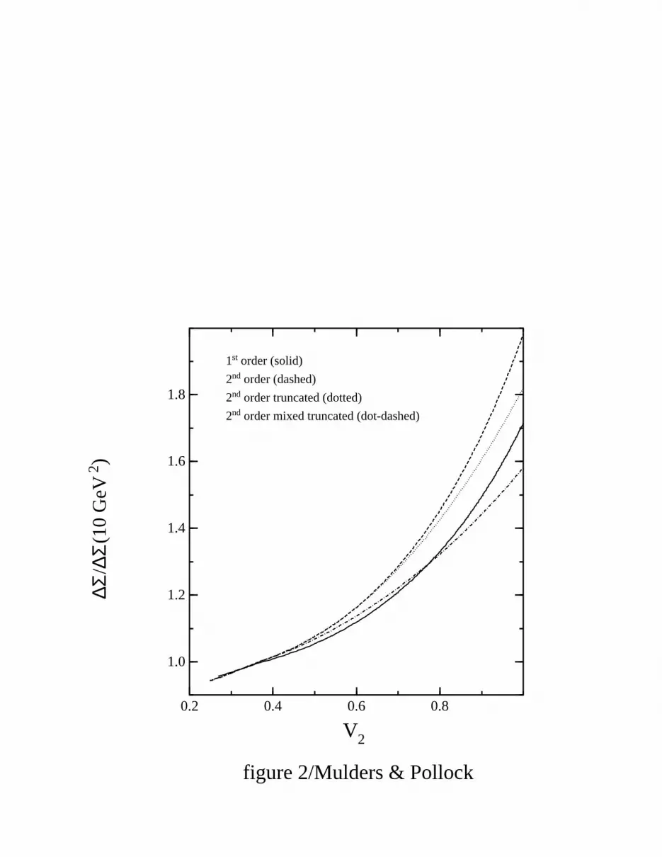
be seen in Figs 2 and 3, which show ∆Σ plotted against V2 and G2 respectively. For the spin
sum rule, we have compared our results with ∆Σ(Q2exp = 10 GeV2) because we note from
Eq. (21) that the results remain proportional to the starting value at all Q2. This makes it
easy to consider any scenario, e.g. starting from a world average such as ∆Σ(4 GeV2) = 0.31
[14] or starting from a low-energy value [11].
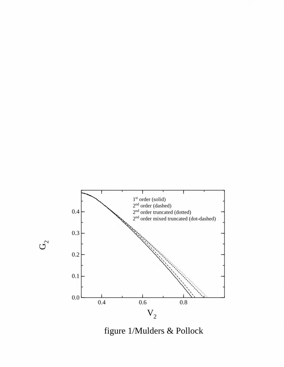
In Fig. 1, αs is increasing down and to the right. There is no single value of Q20 where
both V2 = 1 and G2 = 0, in either LO or NLO perturbation theory. In both cases G2 vanishes
earlier (at higher Q2), which is consistent with an intuitive picture that at the quark model
scale, meson-cloud effects result in some residual qq̄ sea. Note that if one plots e.g. V2 vs αs,
there is a stronger dependence on the order of perturbation theory used, as the evolution of
αs is itself highly modified at these low Q2. It is encouraging that when these observables
are plotted against one another, the trends are similar. Furthermore, varying the value of
αS(M2Z) within current experimental limits (e.g. using values ranging from 0.11 to 0.12) has
negligible effect on these curves.
In Fig. 2, we show the relative value of the singlet axial matrix element ∆Σ versus V2,
normalized to the value at Q2exp = 10 GeV2, the characteristic scale of the SMC experiment.
The right edge corresponds to a value of Q20 where V2(Q
20) = 1. We see that ∆Σ(Q2
0)/∆Σ(10)
increases from about 1.71 (LO) to 1.98 (NLO). This increase of the NLO evolution is, unlike
that in Fig. 1, sensitive to the value of αs(M2Z). Increasing the value of αs(M
2Z) by 5%, gives
ratios of 1.83 (LO) and 2.21 (NLO).
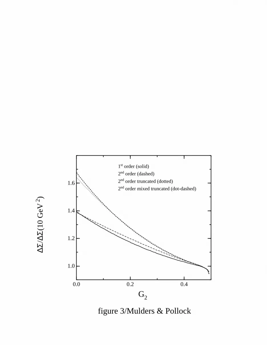
In Fig. 3, ∆Σ is plotted against G2, again normalized to its value at Q2exp = 10
GeV2. Evolving from 10 GeV2 to Q20, this time fixed from G2(Q
20) = 0, gives for the
9

ratio ∆Σ(Q20)/∆Σ(Q2
exp) values of 1.39 (LO) to 1.68 (NLO). The ratios are smaller than in
Fig. 2, because G2 = 0 corresponds to a value of V2 < 1. Again a 5% larger value of αs(M2Z)
results in somewhat larger ratios, 1.45 (LO) and 1.85 (NLO). The persistent enhancement
of ∆Σ at the low-energy scale, also in NLO, suggest that a valence picture with ∆Σ of the
order of 0.5 - 0.8 is consistent with the experimental result in DIS of the order of 0.3 - 0.5.
Clearly, the scale dependence cannot be neglected in interpreting the results in deep inelastic
experiments.
The evolution from Q2 = 1 GeV2 to 10 GeV2 is presumably more reliably in the pertur-
bative regime, and in this case we find a ratio ∆Σ(1)/∆Σ(10) of 1.031 (LO), or 1.068 (NLO)
when αs(M2Z) = 0.117. Especially here, we note a sensitivity to αs(M
2Z). Taking its value to
be 5% higher, the ratios becomes 1.040 (LO) and 1.110 (NLO). The modification of the ac-
tual singlet moment ΓS1 , which includes CS(Q2) as well, shows a decrease for ΓS1 when going
to lower momenta, the ratios being ΓS1 (1)/ΓS1 (10) = 0.980 (LO) and 0.956 (NLO). (Taking
αs(M2Z) 5% higher gives 0.973 (LO) and 0.921 (NLO).) Although fairly small in this region,
the contribution to the evolution from the anomalous dimension clearly can and should be
taken into account, and goes beyond the standard QCD effect arising purely from CS(Q2),
which is sometimes all that is taken into account. Note furthermore that in ΓS1 (Q2), higher
twist contributions proportional to 1/Q2 could contribute. These have not been included in
the above estimate for ΓS1 , which refers purely to the twist two part.
Another point that deserves discussion is the inclusion of the effects of the strangeness
threshold. If one considers the KK threshold, i.e. Q2 ≈ 1 GeV2, as an appropriate value,
a large part of the evolution down to Q20 involves nf = 2. If the strangeness content of
the nucleon has not become zero, the decoupling of strangeness from the evolution leads to
ambiguities in the treatment. It would require a global analysis, which takes carefully into
account existing inequalities such as ∆s(x) ≤ s(x) and the consequences for the moments.
The evolution equations with nf = 2 instead of nf = 3 in general tend to somewhat slow
down the increase of ∆Σ at lower momentum scales.
Finally, if we assume that (i) ∆Σ(Q20) = 0.65 as an appropriate value at the low mo-
10

mentum scale, e.g. from an effective low energy model [11], and (ii) pQCD continues to
work down to low Q2, and (iii) the asymptotic values of the nonsinglet combinations of the
axial matrix elements are known from weak decays, ∆u−∆d = 1.257 and (from low energy
hyperon decays) ∆u + ∆d − 2∆s = 0.58 ± 0.05, then we are able to calculate at any scale
the axial matrix elements for each of the quark flavors. The values at Q20 (corresponding to
G2 = 0), 1 and 10 GeV2 are given in Table II. Assuming three active flavors at Q20 gives
a positive value for ∆s. In this case we have the possibility to incorporate the strangeness
threshold in a natural way, using only two active flavors to evolve ∆Σ down to 0.58, then
continuing with three active flavors. The numbers in this scenario for NLO are given in Ta-
ble II. The strangeness threshold required is Q2s = 0.286 GeV2. We note that decoupling of
the strange quarks in the momentum sumrule at this same threshold implies that at 4 GeV2
the momentum carried by the strange antiquarks as compared to nonstrange antiquarks is
2 s2/(u2 + d2) = 0.57.
In conclusion, using NLO equations, a very satisfactory picture is obtained running all the
way from a low-energy-scale proton without gluons but with some nonstrange sea, acquiring
nonzero values for strangeness matrix elements only starting at the strangeness threshold
which is slightly above the scale where G2 = 0. We have analyzed the errors arising from an
uncertainty in the strong coupling constant αs(MZ) = 0.117± 0.005 and those coming from
an uncertainty in the octet axial charge, 0.58 ± 0.05. These are indicated in Table II. Note
that the results for ∆u and ∆d are not sensitive to the octet axial charge if this is taken
to coincide with the strangeness threshold. Using these results and including second order
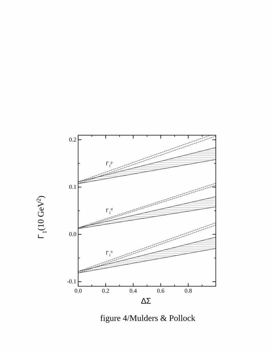
QCD corrections everywhere, we find that
Γp1(10 GeV2)= (0.109 ± 0.002) + (0.062 ± 0.007 ± 0.009)∆Σ(Q20)
= 0.149 ± 0.006 ± 0.006, (27)
Γn1 (10 GeV2)= (−0.080 ± 0.001) + (0.062 ± 0.007 ± 0.009)∆Σ(Q20)
= −0.040 ± 0.003 ± 0.006, (28)
Γd1(10 GeV2)≡ 0.5(Γp1 + Γn1 )(1 − 1.5 ωD)
11
= (0.013 ± 0.001) + (0.056 ± 0.006 ± 0.008)∆Σ(Q20)
= 0.049 ± 0.004 ± 0.005 (29)
(using the usual D-state admixture of 6% in the latter). The first error in each term arises
from our assumed uncertainties in αs(MZ) and from the octet part of the sum rule, here
added in quadrature. The second error bar (if shown) comes from our estimate of the
prescription dependence associated with evolving ∆Σ from 10 GeV2 to Q20. This includes
e.g. differences in truncation schemes (see Figs. 2 and 3), choice of s-quark threshold
mechanism, and determination of Q20 from V2 = 1 rather than G2 = 0. These have all been
discussed above. We conservatively estimate ∆Σ(Q20)/∆Σ(10) = 1.65 ± 0.25, and the final
numbers above correspond to this choice, with ∆Σ(Q20) = 0.65. The relations between the
experimental sum rules and the ”spin carried by the quarks”, i.e. ∆Σ(Q20) are illustrated in
Fig. 4.
IV. CONCLUSIONS
In this paper we have investigated the extent to which measurements of the spin sum
rule at high energies should be interpreted, in view of the role of their scale dependence. We
have investigated the spin sum rule together with the momentum sum rules in a systematic
way, extending our earlier results that used purely leading order evolution to results that
use next to leading order evolution. This has become possible in part due to the recent
work of Larin [8]. We have estimated uncertainties arising from scheme dependence and
higher order QCD effects in the evolution, by using several truncation prescriptions. Our
results indicate that many qualitative features present in the leading order remain the same.
Quantitative differences show up, but do not upset the picture. In particular, we have
considered momentum sum rules for valence quarks and gluons compared with one another
or spin sum rules compared with the momentum sum rules. In general, we have not made
any interpretation of the relative gluonic contribution to the results for the singlet moment,
which helps avoid obvious scheme-dependent assumptions. (see, e.g. reference [16], which
12
shows that the gluon contribution is zero in certain renormalization schemes). We are simply
using the operator product expansion for the moments of interest, at next to leading order.
The results for evolution from 1 GeV2 to 10 GeV2 are quite reliable, and the fractional
change evolving down to Q20 is apparently reasonably stable to next to leading order cor-
rections too. Of course, the moderate sensitivity in going from first to second order is no
proof of the reliability of the perturbative expansion. We have noted that while the sensi-
tivity to using first or second order is moderate, the sensitivity to the value of αs(Mz) is
quite strong. We find that the inclusion of a strangeness threshold is not very important
for the rate of evolution. Much more important is the fact that there is a large change in
∆Σ running from 10 GeV2 to a low-momentum scale Q20, large enough that it can easily
reach a point where ∆Σ = ∆u + ∆d− 2∆s, i.e. ∆s = 0, a natural point for the strangeness
threshold. We have made this more explicit by starting with a value [11] of ∆Σ(Q20) = 0.65,
although any assumption that one can estimate ∆Σ(Q20) from a low energy nucleon model
is very clearly subject to debate. This scenario implies that at present there is no reason to
require an anomalously large strange contribution in the proton at a low-momentum scale.
Of course, independent measurements of the strangeness content at this scale (e.g. from
elastic neutrino - nucleon scattering) are important to confirm this.
V. ACKNOWLEDGMENTS
This work is supported in part (S.J.P) by U. S. Department of Energy grant DOE-
DE-FG0393DR-40774 and in part (P.J.M.) by the foundation for Fundamental Research of
Matter (FOM) and the National Organization for Scientific Research (NWO). SJP acknowl-
edges the support of a Sloan Foundation Fellowship.
13

REFERENCES
[1] K.G Wilson, Phys. Rev D10 (1974) 2445
[2] J.D. Bjorken, Phys. Rev. 148 (1966) 1467; Phys. Rev. D1 (1970) 1376.
[3] J. Ellis, R.L. Jaffe, Phys. Rev. D9 (1974) 1444; D10 (1974) 1669
[4] EMC: J. Ashman et al., Phys. Lett. B206 (1988) 364; Nucl. Phys. B328 (1989) 1; SLAC
E-80: M.J. Alguard et al., Phys. Rev. Lett. 37 (1976) 1261; ibid. 41 (1978) 70; SLAC
E-130: G. Baum et al., Phys. Rev. Lett. 51 (1983) 1135; SLAC E142: D.L. Anothony
et al., Phys. Rev. Lett. 71 (1993) 959; SMC: B. Adeva et al., Phys. Lett. B302 (1993)
533, Phys. Lett B329 (1994) 399
[5] see e.g. R.G. Roberts, The structure of the proton, deep inelastic scattering, Cambridge
University Press 1990; G. Altarelli and G.C. Ross, Phys. Lett B212 (1988) 391; R.D.
Carlitz, J.C. Collins and A.H. Mueller, Phys. Lett. B214 (1988) 229.
[6] D.J. Gross and F. Wilczek, Phys. Rev. Lett. 30 (1973) 1343; H.D. Politzer, Phys. Rev.
Lett. 30 (1973) 1346; W. Caswell, Phys. Rev. Lett 33 (1974) 244; D.R.T. Jones, Nuc.
Phys. B75 (1974) 531; O.V. Tarasov, A.A. Vladimirov, A. Yu. Zharkov, Phys. Lett.
B93 (1980) 429;
[7] S.A. Larin and J.A.M. Vermaseren, Phys. Lett. B303 (1993) 334
[8] S.A. Larin and J.A.M. Vermaseren, Phys. Lett. B259(1991) 345; S.A. Larin, Phys. Lett.
B303 (1993) 113; S.A. Larin, CERN-TH.7208/94 (1994)
[9] I.I. Balitsky, V.M. Braun and A.V. Kolesnichenko, Phys. Lett. B242 (1990) 245; B318
(1993) 648(E); J. Ellis and M. Karliner, Phys. Lett. B313 (1993) 131
[10] J. Kodaira et al., Nucl Phys B159 (1979) 99; J. Kodaira, Nucl. Phys B165 (1980) 129
[11] J. Kunz, P.J. Mulders and S. Pollock, Phys. Lett B222 (1989) 481
[12] A.J. Buras, Rev. Mod. Phys. 52 (1980) 199
14

[13] E.G. Floratos, D.A. Ross and C.T. Sachrajda, Nucl. Phys. B129 (1977) 66 and B139
(1977) 545 (E); E.G. Floratos, D.A. Ross and C.T. Sachrajda, Nucl. Phys. B152 (1979)
493.
[14] J. Ellis and M. Karliner, CERN preprint CERN-TH-7324/94
[15] A.D. Martin, R.G. Roberts, and W.J. Stirling, Phys. Rev. D47 (1993) 867
[16] U. Ellwanger, Phys Lett. B259 (1991) 469
15
FIGURES
FIG. 1. Plot of G2 vs V2. Solid (dashed) curve shows first(second) order calculations. We
started from experimental values [15] at roughly 4 GeV2 and evolve downwards. Dotted curve is
2nd order, but truncated. Dash-dotted is again 2nd order, truncated, but with αs in all higher
order terms replaced with its leading order expression.
FIG. 2. Same as Fig. 1, but plotting ∆Σ/∆Σ(Q20) versus V2. Curves are labeled as before.
FIG. 3. Same as Fig. 3, but plotting ∆Σ/∆Σ(Q20) versus G2.
FIG. 4. Experimental sum rules as a function of the spin carried by the quarks, ∆Σ(Q20),
including uncertainties from αs, octet axial charge, and scheme dependence are given by the shaded
areas. The areas enclosed by the dashed lines are the results as a function of ∆Σ(10 GeV2).
16

TABLES
TABLE I. Numerical values [12,13] used for the various parameters appearing in the truncated
next to leading order solutions for the momentum sum rules, Eqs 10 through 17.
nf α̃ d(2)NS d
(2)+ Z+ ZNS Kψ KG
2 0.2727 0.3678 0.5058 1.486 1.428 0.4544 -0.1704
3 0.36 0.3951 0.6173 1.783 1.507 2.121 -1.193
4 0.4286 0.4267 0.7467 2.355 1.654 5.895 -4.421
5 0.4839 0.4638 0.8986 3.341 1.904 22.604 -21.191
TABLE II. Values for the axial matrix elements of the quarks using a starting value of ∆Σ(Q20)
= 0.65 at the scale where G2(Q20) = 0 using NLO results and a strangeness threshold at the point
where ∆s = 0. The errors refer to uncertainties in αs(MZ) = 0.117 ± 0.005, and in the octet axial
charge, 0.58 ± 0.05 (underlined errors).
Q2 [GeV2] ∆u ∆d ∆s ∆Σ
Q20 0.954 -0.304 - 0.650
Q2s = 0.3 ∓ 0.1 0.919 ± 0.025 -0.339 ± 0.025 0.00 0.580 ± 0.05
1 0.873 ∓ 0.01 -0.384 ∓ 0.01 -0.045 ∓ 0.01 ∓ 0.025 0.445 ∓ 0.03 ∓ 0.025
4 0.866 ∓ 0.01 -0.391 ∓ 0.01 -0.052 ∓ 0.01 ∓ 0.025 0.423 ∓ 0.03 ∓ 0.025
10 0.864 ∓ 0.01 -0.393 ∓ 0.01 -0.055 ∓ 0.01 ∓ 0.025 0.417 ∓ 0.03 ∓ 0.025
17

This figure "fig1-1.png" is available in "png" format from:
http://arXiv.org/ps/hep-ph/9412287v1
0.4 0.6 0.80.0
0.1
0.2
0.3
0.4
V2
G2
figure 1/Mulders & Pollock
1st order (solid) 2nd order (dashed) 2nd order truncated (dotted) 2nd order mixed truncated (dot-dashed)
This figure "fig1-2.png" is available in "png" format from:
http://arXiv.org/ps/hep-ph/9412287v1
0.2 0.4 0.6 0.8
1.0
1.2
1.4
1.6
1.8
V2
∆Σ/∆
Σ(1
0 G
eV2 )
figure 2/Mulders & Pollock
1st order (solid)
2nd order (dashed)
2nd order truncated (dotted)
2nd order mixed truncated (dot-dashed)

This figure "fig1-3.png" is available in "png" format from:
http://arXiv.org/ps/hep-ph/9412287v1
0.0 0.2 0.4
1.0
1.2
1.4
1.6
G2
∆Σ/∆
Σ(1
0 G
eV2 )
figure 3/Mulders & Pollock
1st order (solid)
2nd order (dashed)
2nd order truncated (dotted)
2nd order mixed truncated (dot-dashed)

This figure "fig1-4.png" is available in "png" format from:
http://arXiv.org/ps/hep-ph/9412287v1
0.0 0.2 0.4 0.6 0.8
-0.1
0.0
0.1
0.2
∆Σ
Γ 1(10
GeV
2 )
figure 4/Mulders & Pollock
Γ1p
Γ1d
Γ1n