UNIVERSITÀ DI PISA

Facoltà di Ingegneria Dipartimento di Ingegneria Civile e Industriale

Corso di Laurea Magistrale in Ingegneria Aerospaziale

TESI DI LAUREA

MODEL – BASED BRAKING PERFORMANCE PREDICTION

RELATORI Prof. Eugenio DENTI Ing. Andrea GIOVANNINI Prof. Gianpietro DI RITO

Candidato

Leonardo PINO

ANNO ACCADEMICO 2015 - 2016

2

ACKNOWLEDGEMENTS

I am not sure of when precisely my passion for aviation began, maybe when I was a kid

building airplane models in the attic during rainy days. I grew up with this passion and

managed to make it real when I started studying aerospace engineering six years ago, and

finally crowned my ambition to work on airplanes thanks to this internship. If I look back to

the dawn of this internship I cannot realise how fast these six months ran out and how much

it enriched my personal and professional life. I learned things that I could not imagine

learning at university lectures, and gained knowledge and lessons from high skilled

colleagues which I never mastered from any engineering book.

There are many people I would like to express my gratitude to, first of all my Airbus tutor

Andrea Giovannini who saw some potentialities in me since we first spoke during my

telephone interview, and who has been a spiritual guide during the internship, always

believing in the work I was doing. It is thanks to him if I was selected and given this

opportunity.

I would like to thank the whole EGV aircraft performance department for being my family

for six months, even the people I just had a chat with sometimes to relieve me of the work

between one simulation and the following, but in particular Julien Delbove for the

fundamental help on software’s issues and OSMA training, Catherine Wisler for flight tests

documentation, Kasidit Leoviriyakit for general aircraft performance explanations and Mattia

Padulo for the sensitivity analyses suggestions.

A precious help came from some flight physics EGY colleagues: Pamphile Roy for ALADYN

support, Florian Troude for GRM clarifications, and most of all Matthieu Miot who suffered

my numerous questions and introduced me to the world of aircraft dynamics modelling and

simulation, being critical to the development of this work.

I learned a lot about the anti – skid system thanks to the colleagues in Filton UK in the

landing gear department EL, many thanks to Andy Bird for the long telephone calls during

which I understood the real issues faced by a big aircraft manufacturing company like

Airbus, who has been a mentor and became more than just a colleague; to David Reid for the

technical conversations and to Christophe Rougelot who proposed this internship and has

3

always believed in cross team collaboration and strengths sharing to produce a higher level

technology.

Many thanks to the University of Pisa, the Aerospace Engineering department and my tutor

teacher Eugenio Denti for having enabled this ambitious experience.

My love and appreciation goes to my girlfriend Ilaria who has followed me step by step,

supported me during the hard times, alleviated the shock of living in another country and

rejoiced for my achievements.

Finally my family.

My brother Francesco with his passion for aircraft models and aviation which he handed to

me, my sister Lucia who has always given me golden life lessons, my mum Rita and my dad

Giovanni who grew me up like I am and constantly encouraged me to be determined and

follow my dreams and ambitions. I will never thank you enough for everything you did for

me.

4

ABSTRACT

This paper describes the activities carried out during a six months internship at Airbus

Operations S.A.S. aiming the investigation of model – based braking performance prediction.

The conception of physical models to represent the dynamics of an aircraft is a basic step to

predict its performance. The braking performance prediction is a key subject when coming to

prove evidence to airliners that the object aircraft is capable of operating on a certain runway,

and its modelling needs to be sufficiently accurate to gain approval from the applicable

aviation authority. The following work provides with the definition of the mathematical and

physical reasoning behind the braking performance, the description of the projects promoted

within Airbus to develop a state-of-the-art anti – skid braking platform, and the analysis and

tuning of the latest developed model, through the software tool OSMA (Outil de Simulation

des Mouvements Avion) witnessing its application to a new level of realistic accuracy for

simulation.

Keywords: Aircraft performance, braking performance, anti – skid system, modelling and

simulation.

5

Contents

1. INTRODUCTION 8

2. TECHNICAL BACKGROUND 9

2.1 REGULATIONS 9

2.2 LANDING 9

2.3 REJECTED TAKE-OFF 11

3. THE BRAKING PERFORMANCE 13

3.1 DRY RUNWAY FRICTION 14

3.2 WET RUNWAY FRICTION 15

3.3 BRAKING FORCE LIMITATION 17

3.3.1 Torque Limitation 18

3.3.2 Anti-Skid Limitation 20

3.3.3 Sum up of braking limitations 22

3.4 FRICTION COEFFICIENT AS A FUNCTION OF THE SLIP RATIO 24

4. THE ANTI-SKID REGULATION LOOP 25

4.1 ROLE OF THE ANTI-SKID SYSTEM 25

4.2 ANTI-SKID SYSTEM CONFIGURATION 26

4.3 ANTI-SKID SYSTEM OPERATION 27

4.4 ANTI-SKID SYSTEM PERFORMANCE 29

4.4.1 Stopping distance efficiency 30

4.4.2 Friction coefficient efficiency 30

4.4.3 Wheel slip efficiency 31

5. INTERNSHIP GOAL 33

5.1 TAPAS 33

5.2 "EGV" ETAMU IDENTIFICATION PROCESS 33

6

5.3 "EL" PLATFORM 34

5.4 THE SHARED PLATFORM 35

5.5 THE RESULTS 37

5.6 INTERNSHIP GOALS: INITIAL DEFINITION AND UPDATE 39

6. SIMULATION & MODELLING WITHIN OSMA SOUPLE ENVIRONMENT 41

6.1 OSMA GENERAL DESCRIPTION AND FUNCTIONS 41

6.2 CREATING THE SCENARIO AND ENVOI FILE 42

6.2.1 The Trim (“Balance”) 43

6.2.2 The Time-History 44

6.2.3 The Hold (“Maintain”) 45

6.3 RTO SCENARIO ‒ SIMPLIFIED BRAKING MODEL 45

6.3.1 Weight Sensitivity 50

6.4 RTO SCENARIO ‒ REALISTIC BRAKING MODEL 52

6.5 THE GRM ADJUSTMENTS 63

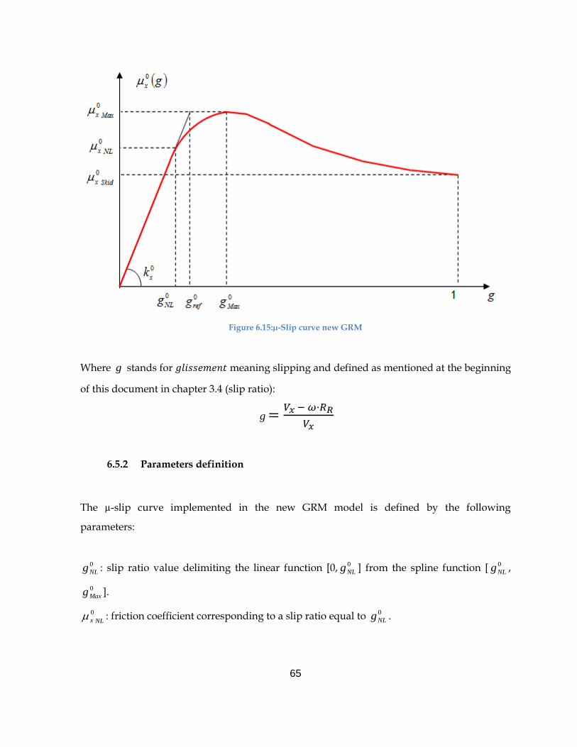
6.5.1 The longitudinal µ - Slip curve in the new GRM model 63

6.5.2 Parameters definition 65

6.6 FIRST ATTEMPT TUNING 66

6.6.1 µ - slip characteristics sensitivity analysis 68

6.6.2 Shaping of Maxx

0 72

6.6.3 Shaping of the Max brake torque 79

6.7 MANUAL BALANCED SHAPING OF Maxx

0 AND 𝑴𝒂𝒙 𝑩𝒓𝒂𝒌𝒆 𝑻𝒐𝒓𝒒𝒖𝒆 –

FINAL TUNING 86

6.7.1 The ultimate Maxx

0 86

6.7.2 The ultimate 𝑴𝒂𝒙 𝑩𝒓𝒂𝒌𝒆 𝑻𝒐𝒓𝒒𝒖𝒆 92

6.8 FURTHER SENSITIVITY ANALYSIS 100

7

6.8.1 First Phase Sensitivity 100

6.8.2 Second Phase Sensitivity 113

7. CONCLUSIONS 116

7.1 REVIEW 116

7.2 FUTURE WORK 118

8

1. INTRODUCTION

This Master Thesis work is the result of a six months internship at Airbus Operations S.A.S,

aiming at improving some of the models used to assess the aircraft braking performance.

Within Airbus engineering, the group is divided into several departments and sub-

departments. The one I have been working with is labelled EGVX standing for aircraft

performance modelling and identification. The aircraft performance department EGV is

responsible for providing the high and low speed performance data for the Airbus fleet of

aircraft. Low speed performance principally refers to the aircraft during take-off and landing.

The department provides the electronic aircraft flight manuals which allow a pilot to

calculate the take-off and landing distances for the aircraft as a function of different aircraft

configurations and different environmental conditions such as airport density altitude,

runway slope, winds etc… This information is supplied in accordance with the certification

rules as written by the applicable aviation authority. The applicable aviation authority for

aircraft certification is the authority for the country where the aircraft is manufactured. In

Europe, the applicable aviation authority is the European Aviation Safety Agency (EASA)

while for the United States it is the Federal Aviation Authority (FAA).

In order to provide the take-off and landing distances for all conditions, Airbus relies on

aircraft performance modelling that has been validated by flight tests and certified by the

aviation authorities.

The braking performances are tightly dependent on the characteristics of the braking system

which is mounted on the main landing gears of the aircraft. This system is developed in

Filton by the landing gear department EL, and the technical specifications defined by EL are

then handled to an external manufacturer (e.g. Messier Bugatti Dowty). It is then evident that

the prediction of its performances needed for the certification before the first flight of a new

aircraft, and for the airliners’ support once the aircraft is on duty, is a really hard task because

of the several development steps and different stakeholders involved. Every department with

its skills is specialised on a certain step of the development process and uses softwares and

tools specifically created for the different tasks, so that the final success is affected by the

good interaction between many factors.

9

In order to better understand, investigate and find a matching point in this arduous

interdisciplinary work, this internship work was proposed. As we will come to see, the focus

of the internship project shifted over time with the realities of modelling the aircraft braking.

2. TECHNICAL BACKGROUND

In the following chapter we will specify the most meaningful definitions for landing and

rejected take off (RTO) runway lengths, used during the computation of the performance

parameters.

These requirements are based on airworthiness rules and dispatch conditions.

2.1 REGULATIONS

The two main phases for which the braking performance prediction is needed are the

Landing phase and the Rejected Take-Off (RTO). On a lower level of importance are the Taxi

phase when the aircraft operates at low speed moving on the ground between the airport

facilities, and the Pre-Take-Off phase when the pilot is acting a full brake pedal push until the

maximum take-off thrust power is reached and then releases them to start accelerating. It

must be proved that the predicted performance meets the authority’s requirements in term of

landing/RTO stopping distance.

2.2 LANDING

The first distance we describe for the landing is the Actual Landing Distance (ALD). During

the certification of the aircraft the ALD is demonstrated as the distance between a point at

50ft above the runway threshold to the point where the aircraft comes to a complete stop.

This distance must be determined for standard temperatures at each weight, altitude and

wind for which the aircraft is approved for operation. This distance is certified and published

in the Aircraft Flight Manual (AFM) for dry runways. The next set of regulations must be

followed by the airline company that wishes to operate the airplane. Known as the OPS

regulations, they define the Required Landing Distance (RLD). Before an aircraft departs on a

10

commercial flight, the company must calculate the aircraft RLD, taking into account a

prediction of the environmental conditions likely to be encountered upon arrival at the

destination. The RLD must be less than the Landing Distance Available (LDA) i.e. the length

of usable runway. If this condition is not satisfied, the aircraft is prohibited to depart.

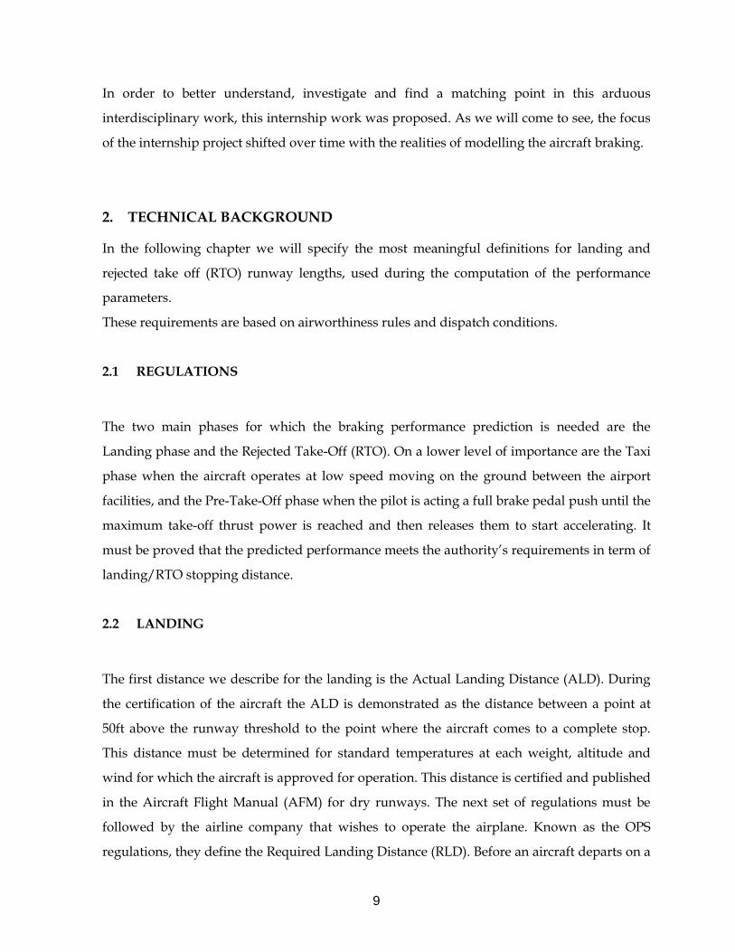
The landing sequence as defined for certified performance computations goes through the

following steps:

Pass through 50 ft above the runway

Main Landing Gear touch-down

Braking about 1 second after the touchdown

Lift-dumpers (or Ground Spoilers) deflection

Thrust Reverser deployment (when applicable, e.g. wet runways)

Computation of the landing distance on dry runway:

From 50ft to touchdown : Aerial phase

From touch down to full stop : Ground phase

Actual Landing Distance (ALDdry) = [Aerial phase + Ground phase]

Required Landing Distance (RLDdry) = (ALDdry / 0.6) ≤ LDA

Figure 2.1: Actual Landing Distance

11

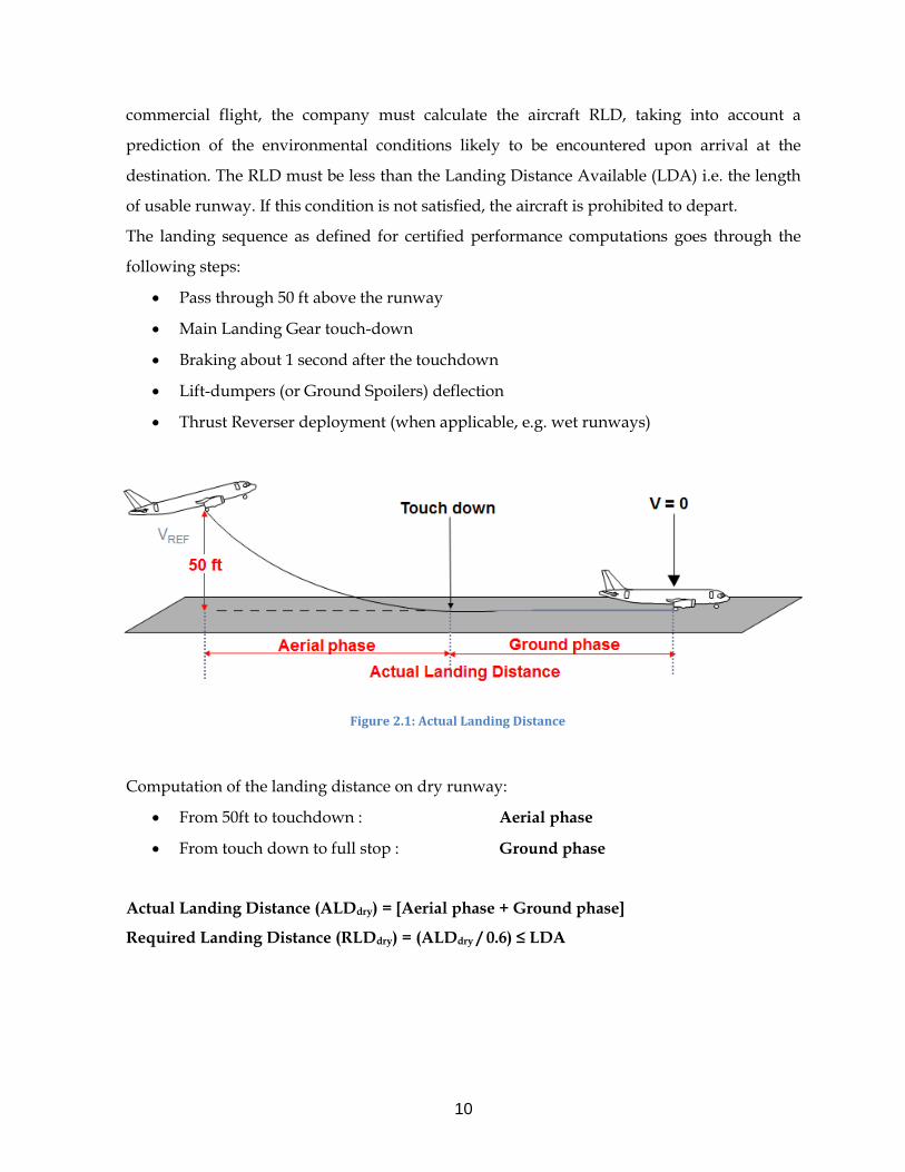
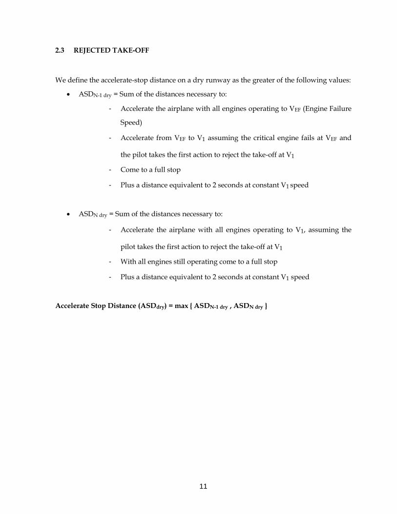
2.3 REJECTED TAKE-OFF

We define the accelerate-stop distance on a dry runway as the greater of the following values:

ASDN-1 dry = Sum of the distances necessary to:

- Accelerate the airplane with all engines operating to VEF (Engine Failure

Speed)

- Accelerate from VEF to V1 assuming the critical engine fails at VEF and

the pilot takes the first action to reject the take-off at V1

- Come to a full stop

- Plus a distance equivalent to 2 seconds at constant V1 speed

ASDN dry = Sum of the distances necessary to:

- Accelerate the airplane with all engines operating to V1, assuming the

pilot takes the first action to reject the take-off at V1

- With all engines still operating come to a full stop

- Plus a distance equivalent to 2 seconds at constant V1 speed

Accelerate Stop Distance (ASDdry) = max { ASDN-1 dry , ASDN dry }

12

Figure 2.2: Accelerate Stop Distance

13

3. THE BRAKING PERFORMANCE

As stated by the regulations, the aircraft manufacturer must provide the ALD and ASD for all

weights, aircraft configurations and environmental conditions. The number of possible

variations makes it unfeasible to flight test all the cases. Thus the manufacturer relies on a

mathematical model of the aircraft performance that is validated with flight test and certified

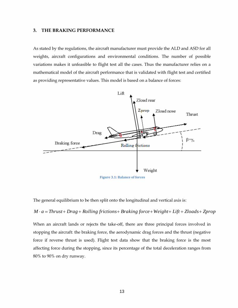
as providing representative values. This model is based on a balance of forces:

The general equilibrium to be then split onto the longitudinal and vertical axis is:

When an aircraft lands or rejects the take-off, there are three principal forces involved in

stopping the aircraft: the braking force, the aerodynamic drag forces and the thrust (negative

force if reverse thrust is used). Flight test data show that the braking force is the most

affecting force during the stopping, since its percentage of the total deceleration ranges from

80% to 90% on dry runway.

ZpropZloadsLiftWeightforceBrakingfrictionsRollingDragThrustaM

Figure 3.1: Balance of forces

14

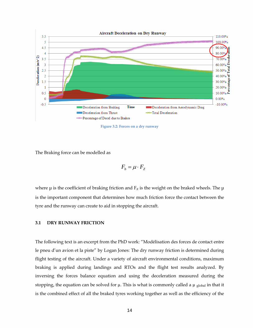
Figure 3.2: Forces on a dry runway

The Braking force can be modelled as

where μ is the coefficient of braking friction and Fz is the weight on the braked wheels. The μ

is the important component that determines how much friction force the contact between the

tyre and the runway can create to aid in stopping the aircraft.

3.1 DRY RUNWAY FRICTION

The following text is an excerpt from the PhD work: “Modélisation des forces de contact entre

le pneu d’un avion et la piste” by Logan Jones: The dry runway friction is determined during

flight testing of the aircraft. Under a variety of aircraft environmental conditions, maximum

braking is applied during landings and RTOs and the flight test results analyzed. By

inversing the forces balance equation and using the deceleration measured during the

stopping, the equation can be solved for µ. This is what is commonly called a µ global in that it

is the combined effect of all the braked tyres working together as well as the efficiency of the

Zb FF

15

anti-skid system η which regulates the brake pressure to obtain the maximum friction force, it

can then be expressed as η· µ or ETAMU. Using the combined results of several flight tests,

an average ETAMUdry is obtained which is used in the aircraft model for determining the

stopping distances for all conditions.

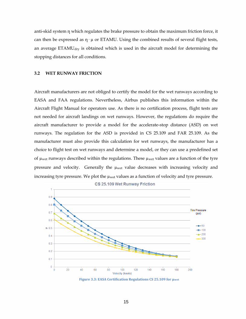
3.2 WET RUNWAY FRICTION

Aircraft manufacturers are not obliged to certify the model for the wet runways according to

EASA and FAA regulations. Nevertheless, Airbus publishes this information within the

Aircraft Flight Manual for operators use. As there is no certification process, flight tests are

not needed for aircraft landings on wet runways. However, the regulations do require the

aircraft manufacturer to provide a model for the accelerate-stop distance (ASD) on wet

runways. The regulation for the ASD is provided in CS 25.109 and FAR 25.109. As the

manufacturer must also provide this calculation for wet runways, the manufacturer has a

choice to flight test on wet runways and determine a model, or they can use a predefined set

of µwet runways described within the regulations. These µwet values are a function of the tyre

pressure and velocity. Generally the µwet value decreases with increasing velocity and

increasing tyre pressure. We plot the µwet values as a function of velocity and tyre pressure.

Figure 3.3: EASA Certification Regulations CS 25.109 for µwet

16

The µ values are described as the maximum possible coefficients of friction. The

manufacturer must then determine experimentally the efficiency of the anti-skid system on

the aircraft. The final result is that the manufacturer determines the efficiency, ηwet, of the

system and multiplies this ηwet value by the µwet value as defined by the certification

regulations (See Table) to determine the effective friction value, µeffective wet, to be used in the

aircraft model.

Table 1: µwet as defined by the EASA Certification Regulations in CS 25.109

Tyre Pressure (psi) µwet

50 µ = -0.0350(V/100)3 + 0.306(V/100)2 – 0.851(V/100) + 0.883

100 µ = -0.0437(V/100)3 + 0.320(V/100)2 – 0.805(V/100) + 0.804

200 µ = -0.0331(V/100)3 + 0.252(V/100)2 – 0.658(V/100) + 0.692

300 µ = -0.0401(V/100)3 + 0.263(V/100)2 – 0.611(V/100) + 0.614

The values cited are the ones used to calculate the ASD defined by the EASA Certification

Regulations in CS 25.109 plotted above.

wetwetwetweteffective ETAMU

17

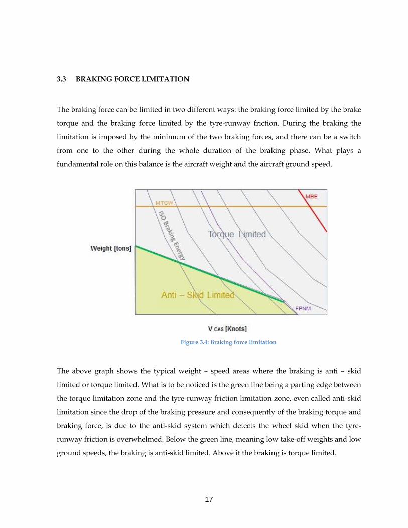
3.3 BRAKING FORCE LIMITATION

The braking force can be limited in two different ways: the braking force limited by the brake

torque and the braking force limited by the tyre-runway friction. During the braking the

limitation is imposed by the minimum of the two braking forces, and there can be a switch

from one to the other during the whole duration of the braking phase. What plays a

fundamental role on this balance is the aircraft weight and the aircraft ground speed.

Figure 3.4: Braking force limitation

The above graph shows the typical weight – speed areas where the braking is anti – skid

limited or torque limited. What is to be noticed is the green line being a parting edge between

the torque limitation zone and the tyre-runway friction limitation zone, even called anti-skid

limitation since the drop of the braking pressure and consequently of the braking torque and

braking force, is due to the anti-skid system which detects the wheel skid when the tyre-

runway friction is overwhelmed. Below the green line, meaning low take-off weights and low

ground speeds, the braking is anti-skid limited. Above it the braking is torque limited.

18

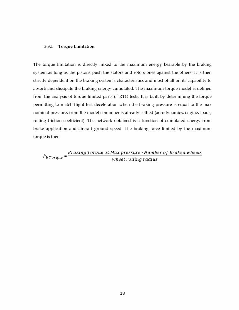
3.3.1 Torque Limitation

The torque limitation is directly linked to the maximum energy bearable by the braking

system as long as the pistons push the stators and rotors ones against the others. It is then

strictly dependent on the braking system’s characteristics and most of all on its capability to

absorb and dissipate the braking energy cumulated. The maximum torque model is defined

from the analysis of torque limited parts of RTO tests. It is built by determining the torque

permitting to match flight test deceleration when the braking pressure is equal to the max

nominal pressure, from the model components already settled (aerodynamics, engine, loads,

rolling friction coefficient). The network obtained is a function of cumulated energy from

brake application and aircraft ground speed. The braking force limited by the maximum

torque is then

𝐹𝑏 𝑇𝑜𝑟𝑞𝑢𝑒 = 𝐵𝑟𝑎𝑘𝑖𝑛𝑔 𝑇𝑜𝑟𝑞𝑢𝑒 𝑎𝑡 𝑀𝑎𝑥 𝑝𝑟𝑒𝑠𝑠𝑢𝑟𝑒 · 𝑁𝑢𝑚𝑏𝑒𝑟 𝑜𝑓 𝑏𝑟𝑎𝑘𝑒𝑑 𝑤ℎ𝑒𝑒𝑙𝑠

𝑤ℎ𝑒𝑒𝑙 𝑟𝑜𝑙𝑙𝑖𝑛𝑔 𝑟𝑎𝑑𝑖𝑢𝑠

19

Figure 3.5: Torque model & torque evolution vs ground speed

The black and purple curves represent the braking torque history for two fully torque limited

flight tests, respectively the High Energy Rejected Take-Off (HERTO) testing the maximum

braking energy up to 110.5 MJ/wheel and the Maximum Energy Rejected Take-Off (MERTO)

testing it up to 130.7 MJ/wheel.

20

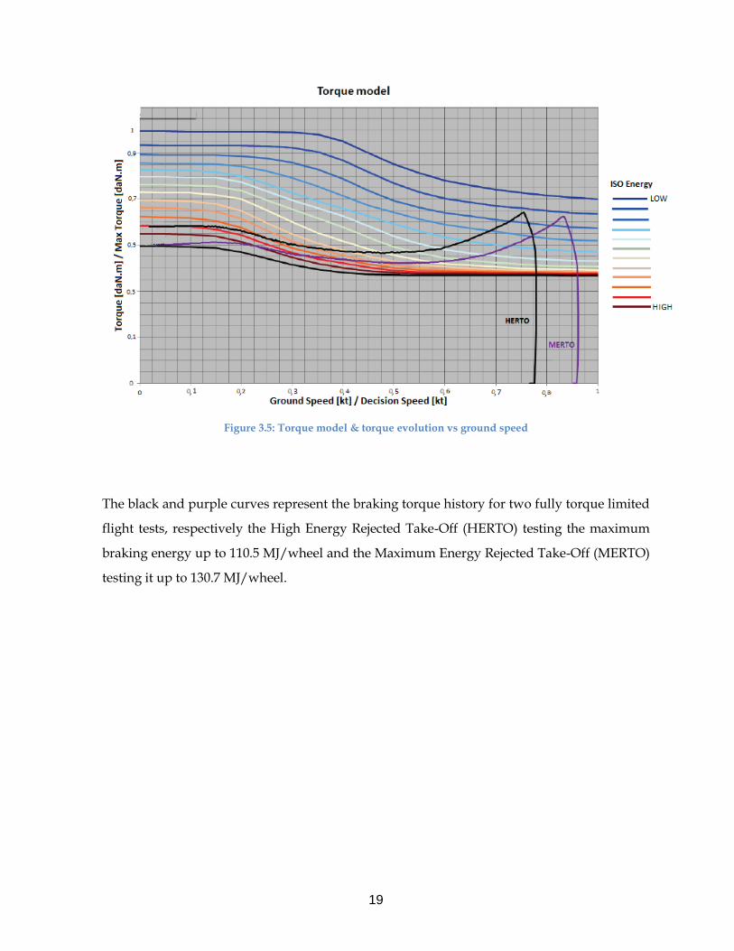
Figure 3.6: Torque limited braking force

As we can see in the above graph, for the two braking forces functions of the time passed

since the aircraft reached the decision speed V1, the torque limited braking force is the

minimum of the two and thus the resulting braking force.

3.3.2 Anti-Skid Limitation

The anti-skid limitation depends basically on the maximum coefficient of friction existing in

the contact patch between the tyre and the runway. It is called anti-skid limitation because it

is the target of the anti-skid system to modulate the pressure sent to the brakes in order to

produce a friction coefficient μ close to the maximum friction coefficient µmax. Since the µmax

is not constant but it is function of the runway state (dry, wet, contaminated), the type of tyre

and in second order the coating of the runway, then the maximum anti-skid limited braking

force depends on all these variables, as well as on the Braking and Steering Control Unit

(BSCU) which is the calculus unit of the anti-skid system. The maximum braking force on

21

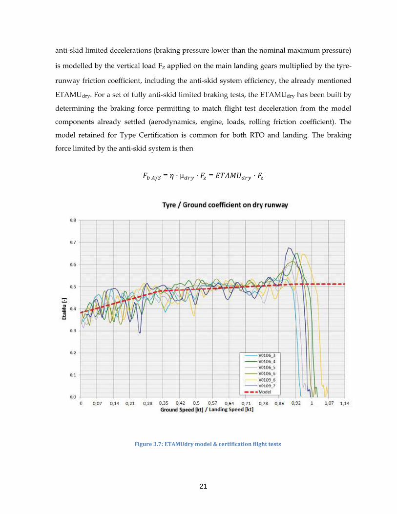
anti-skid limited decelerations (braking pressure lower than the nominal maximum pressure)

is modelled by the vertical load Fz applied on the main landing gears multiplied by the tyre-

runway friction coefficient, including the anti-skid system efficiency, the already mentioned

ETAMUdry. For a set of fully anti-skid limited braking tests, the ETAMUdry has been built by

determining the braking force permitting to match flight test deceleration from the model

components already settled (aerodynamics, engine, loads, rolling friction coefficient). The

model retained for Type Certification is common for both RTO and landing. The braking

force limited by the anti-skid system is then

𝐹𝑏 𝐴/𝑆 = 𝜂 · µ𝑑𝑟𝑦 · 𝐹𝑧 = 𝐸𝑇𝐴𝑀𝑈𝑑𝑟𝑦 · 𝐹𝑧

Figure 3.7: ETAMUdry model & certification flight tests

22

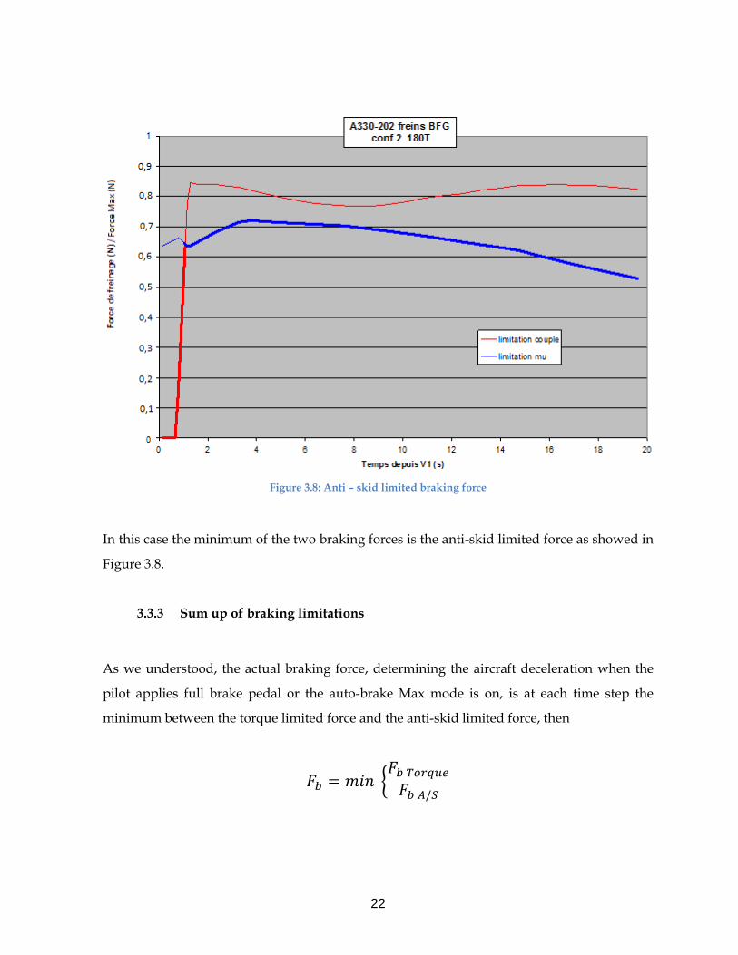
Figure 3.8: Anti – skid limited braking force

In this case the minimum of the two braking forces is the anti-skid limited force as showed in

Figure 3.8.

3.3.3 Sum up of braking limitations

As we understood, the actual braking force, determining the aircraft deceleration when the

pilot applies full brake pedal or the auto-brake Max mode is on, is at each time step the

minimum between the torque limited force and the anti-skid limited force, then

𝐹𝑏 = 𝑚𝑖𝑛 {𝐹𝑏 𝑇𝑜𝑟𝑞𝑢𝑒

𝐹𝑏 𝐴/𝑆

23

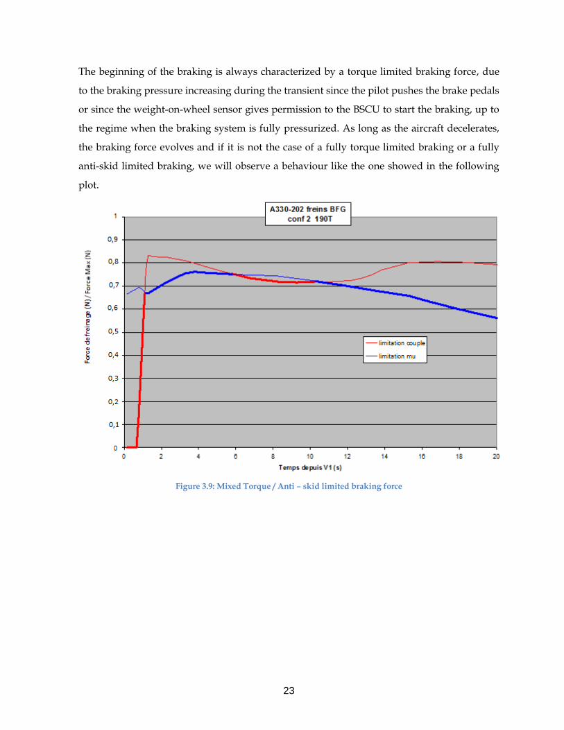
The beginning of the braking is always characterized by a torque limited braking force, due

to the braking pressure increasing during the transient since the pilot pushes the brake pedals

or since the weight-on-wheel sensor gives permission to the BSCU to start the braking, up to

the regime when the braking system is fully pressurized. As long as the aircraft decelerates,

the braking force evolves and if it is not the case of a fully torque limited braking or a fully

anti-skid limited braking, we will observe a behaviour like the one showed in the following

plot.

Figure 3.9: Mixed Torque / Anti – skid limited braking force

24

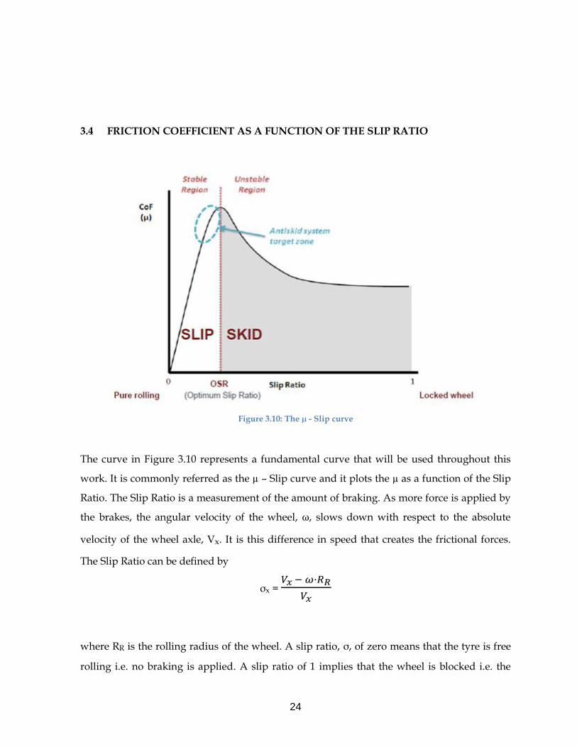
3.4 FRICTION COEFFICIENT AS A FUNCTION OF THE SLIP RATIO

Figure 3.10: The µ - Slip curve

The curve in Figure 3.10 represents a fundamental curve that will be used throughout this

work. It is commonly referred as the µ – Slip curve and it plots the µ as a function of the Slip

Ratio. The Slip Ratio is a measurement of the amount of braking. As more force is applied by

the brakes, the angular velocity of the wheel, ω, slows down with respect to the absolute

velocity of the wheel axle, Vx. It is this difference in speed that creates the frictional forces.

The Slip Ratio can be defined by

σx = 𝑉𝑥 − 𝜔·𝑅𝑅

𝑉𝑥

where RR is the rolling radius of the wheel. A slip ratio, σ, of zero means that the tyre is free

rolling i.e. no braking is applied. A slip ratio of 1 implies that the wheel is blocked i.e. the

25

angular velocity is zero and the tyre is purely sliding with a velocity Vx. The form of this

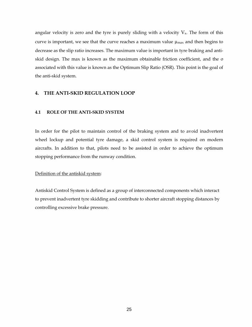
curve is important, we see that the curve reaches a maximum value µmax and then begins to

decrease as the slip ratio increases. The maximum value is important in tyre braking and anti-

skid design. The max is known as the maximum obtainable friction coefficient, and the σ

associated with this value is known as the Optimum Slip Ratio (OSR). This point is the goal of

the anti-skid system.

4. THE ANTI-SKID REGULATION LOOP

4.1 ROLE OF THE ANTI-SKID SYSTEM

In order for the pilot to maintain control of the braking system and to avoid inadvertent

wheel lockup and potential tyre damage, a skid control system is required on modern

aircrafts. In addition to that, pilots need to be assisted in order to achieve the optimum

stopping performance from the runway condition.

Definition of the antiskid system:

Antiskid Control System is defined as a group of interconnected components which interact

to prevent inadvertent tyre skidding and contribute to shorter aircraft stopping distances by

controlling excessive brake pressure.

26

4.2 ANTI-SKID SYSTEM CONFIGURATION

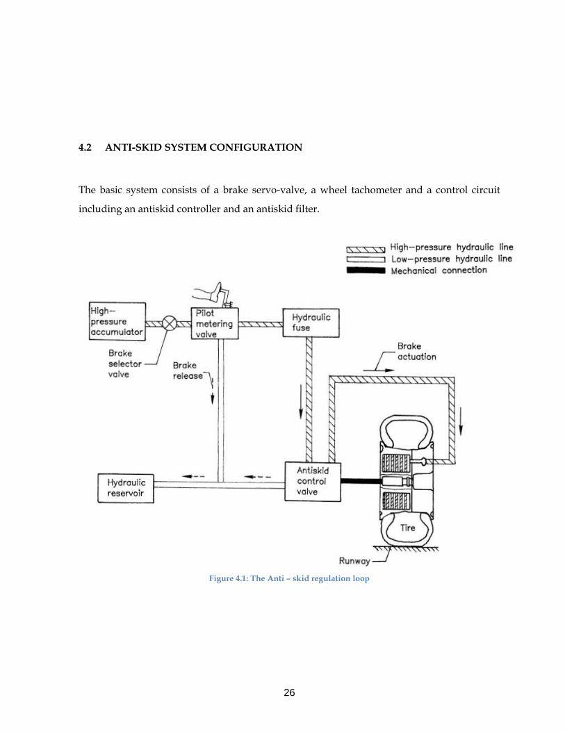
The basic system consists of a brake servo-valve, a wheel tachometer and a control circuit

including an antiskid controller and an antiskid filter.

Figure 4.1: The Anti – skid regulation loop

27

The tachometer provides a frequency signal function of the wheel rotation speed which is

converted into an analogic value (rad/s) by the braking control system. Then, it is converted

into a longitudinal velocity (m/s) using an estimation of the rolling radius (constant value).

Based on the input wheel speed information, the controller determines if the wheel is going

to skid.

Antiskid command is generated by the antiskid filter and removed from the braking

command. The signal is then supplied to the brake servo-valve which regulates brake

pressure in a manner proportional to the current, releasing pressure when a skid is detected

and reapplying it when the wheel recovers.

The antiskid system can be individual or paired wheel control. With the former, each braked

wheel is controlled by a separate servo-valve whereas with the latter, two braked wheels are

controlled together by the same servo-valve (only using the highest antiskid current of the

two wheels).

4.3 ANTI-SKID SYSTEM OPERATION

Fundamentally, the antiskid system provides anti-lock wheel protection to the aircraft braked

wheels by limiting the commanded brake pressure to levels compatible with optimum

aircraft deceleration, while preventing excessive wheel skidding. It is required to cope with

touchdown dynamics, varying vertical loads and gear dynamics (such as gear walk, shimmy

and pitching moments).

Typical operation is as follows:

Before braking is applied, wheels are generally in free rolling configuration. Considering the

rolling friction forces as negligible, we can say that the wheels longitudinal velocity is the

same as the aircraft ground velocity.

The pilot then applies braking either by selecting the automatic braking mode or by applying

force to the brake pedals. This results in an increase in pressure in the brakes. As the pressure

28

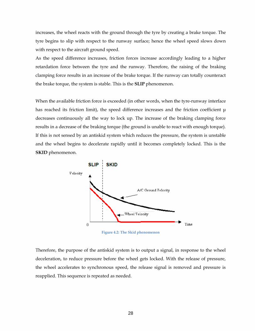
increases, the wheel reacts with the ground through the tyre by creating a brake torque. The

tyre begins to slip with respect to the runway surface; hence the wheel speed slows down

with respect to the aircraft ground speed.

As the speed difference increases, friction forces increase accordingly leading to a higher

retardation force between the tyre and the runway. Therefore, the raising of the braking

clamping force results in an increase of the brake torque. If the runway can totally counteract

the brake torque, the system is stable. This is the SLIP phenomenon.

When the available friction force is exceeded (in other words, when the tyre-runway interface

has reached its friction limit), the speed difference increases and the friction coefficient μ

decreases continuously all the way to lock up. The increase of the braking clamping force

results in a decrease of the braking torque (the ground is unable to react with enough torque).

If this is not sensed by an antiskid system which reduces the pressure, the system is unstable

and the wheel begins to decelerate rapidly until it becomes completely locked. This is the

SKID phenomenon.

Figure 4.2: The Skid phenomenon

Therefore, the purpose of the antiskid system is to output a signal, in response to the wheel

deceleration, to reduce pressure before the wheel gets locked. With the release of pressure,

the wheel accelerates to synchronous speed, the release signal is removed and pressure is

reapplied. This sequence is repeated as needed.

29

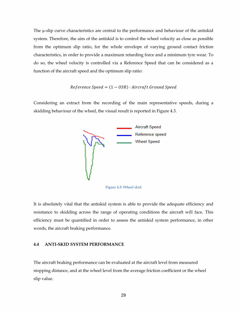
The µ-slip curve characteristics are central to the performance and behaviour of the antiskid

system. Therefore, the aim of the antiskid is to control the wheel velocity as close as possible

from the optimum slip ratio, for the whole envelope of varying ground contact friction

characteristics, in order to provide a maximum retarding force and a minimum tyre wear. To

do so, the wheel velocity is controlled via a Reference Speed that can be considered as a

function of the aircraft speed and the optimum slip ratio:

𝑅𝑒𝑓𝑒𝑟𝑒𝑛𝑐𝑒 𝑆𝑝𝑒𝑒𝑑 = (1 − 𝑂𝑆𝑅) · 𝐴𝑖𝑟𝑐𝑟𝑎𝑓𝑡 𝐺𝑟𝑜𝑢𝑛𝑑 𝑆𝑝𝑒𝑒𝑑

Considering an extract from the recording of the main representative speeds, during a

skidding behaviour of the wheel, the visual result is reported in Figure 4.3.

Figure 4.3: Wheel skid

It is absolutely vital that the antiskid system is able to provide the adequate efficiency and

resistance to skidding across the range of operating conditions the aircraft will face. This

efficiency must be quantified in order to assess the antiskid system performance, in other

words, the aircraft braking performance.

4.4 ANTI-SKID SYSTEM PERFORMANCE

The aircraft braking performance can be evaluated at the aircraft level from measured

stopping distance, and at the wheel level from the average friction coefficient or the wheel

slip value.

30

4.4.1 Stopping distance efficiency

The stopping distance efficiency is the ratio of the minimum distance required by the aircraft

to stop and the actual distance required to stop:

𝑆𝑡𝑜𝑝𝑝𝑖𝑛𝑔 𝐷𝑖𝑠𝑡𝑎𝑛𝑐𝑒 𝐸𝑓𝑓𝑖𝑐𝑖𝑒𝑛𝑐𝑦 =𝑂𝑝𝑡 𝐷𝑖𝑠𝑡𝑎𝑛𝑐𝑒

𝐴𝐿𝐷· 100

With,

𝑂𝑝𝑡 𝑑𝑖𝑠𝑡𝑎𝑛𝑐𝑒 = 𝑚𝑖𝑛𝑖𝑚𝑢𝑚 𝑎𝑖𝑟𝑐𝑟𝑎𝑓𝑡 𝑠𝑡𝑜𝑝𝑝𝑖𝑛𝑔 𝑑𝑖𝑠𝑡𝑎𝑛𝑐𝑒

This value is obtained by conducting a simulated stop with the friction force held equal to the

maximum available friction coefficient multiplied by the instantaneous vertical load.

And,

𝐴𝐿𝐷 = 𝐴𝑐𝑡𝑢𝑎𝑙 𝐿𝑎𝑛𝑑𝑖𝑛𝑔 𝐷𝑖𝑠𝑡𝑎𝑛𝑐𝑒

already mentioned above.

4.4.2 Friction coefficient efficiency

This parameter is computed by taking into account the maximum friction coefficient and the

actual friction coefficient available from the runway, in particular it is the ratio

𝜂𝐴/𝑆 = µ𝐴𝑐ℎ𝑖𝑒𝑣𝑒𝑑(𝑡)

µ𝑀𝑎𝑥(𝑡)

The actual friction 𝜇𝐴𝑐ℎ𝑖𝑒𝑣𝑒𝑑 is calculated by dividing the braking force by the vertical load on

the braked wheels. The braking force is obtained by dividing the recorded brake torque by a

constant rolling radius value. The maximum friction 𝜇𝑀𝑎𝑥 is evaluated using the same

31

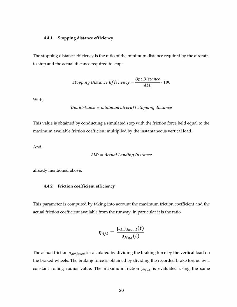
calculation but using the torque peak history instead of the actual recorded torque. Peaks of

brake torques are detected using peak-to-peak algorithms and are linked together to

determine the torque peak history:

Figure 4.4: Torque peak history

The 𝜇𝑀𝑎𝑥 is easier to determine on wet runways where the antiskid activity is high, thus

torque peaks are clearly distinct from the torque history. On dry runways, it is much more

difficult to extract the peak history, and most of the time, the evaluation of the average

maximum friction coefficient is not very accurate. This is the reason why the comparison of

the antiskid efficiency between dry and wet runways is very sensitive. However, if used

cautiously, the method can be a good way of evaluating qualitatively two different antiskid

systems.

4.4.3 Wheel slip efficiency

The wheel slip efficiency is determined by comparing the actual wheel slip ratio measured

during the stop to the optimum slip ratio available. Since the wheel slip varies significantly

during the stop, the accuracy of the wheel speed recording sample rate must be very high to

correctly determine the actual and optimal slip during the stop.

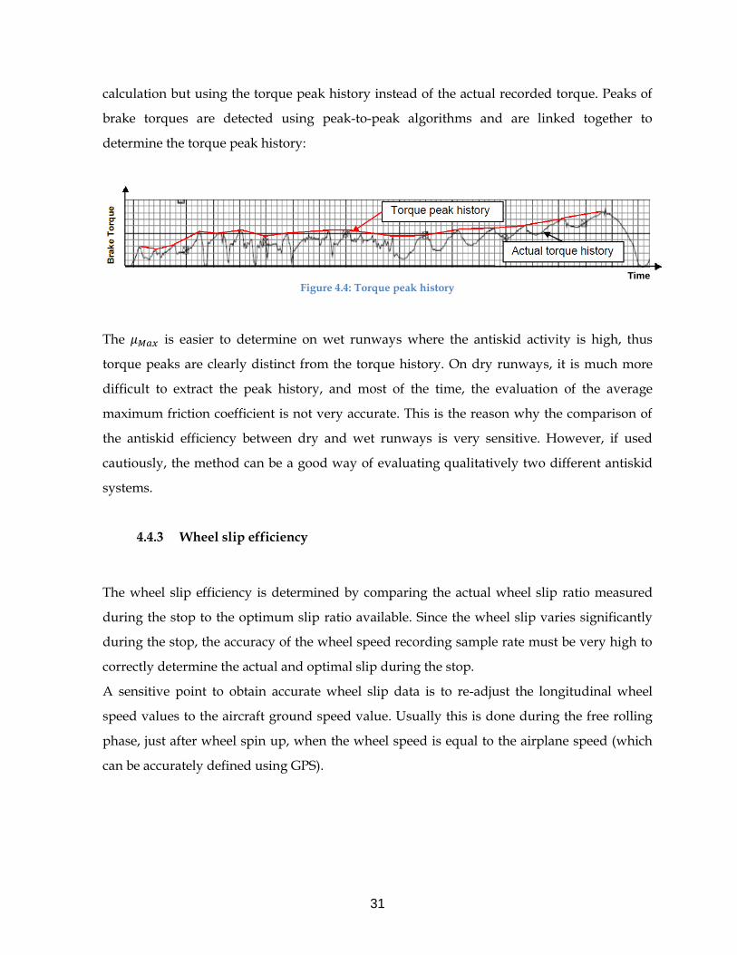
A sensitive point to obtain accurate wheel slip data is to re-adjust the longitudinal wheel

speed values to the aircraft ground speed value. Usually this is done during the free rolling

phase, just after wheel spin up, when the wheel speed is equal to the airplane speed (which

can be accurately defined using GPS).

Time

32

Figure 4.5: Adjustment of the wheel speed to ground speed

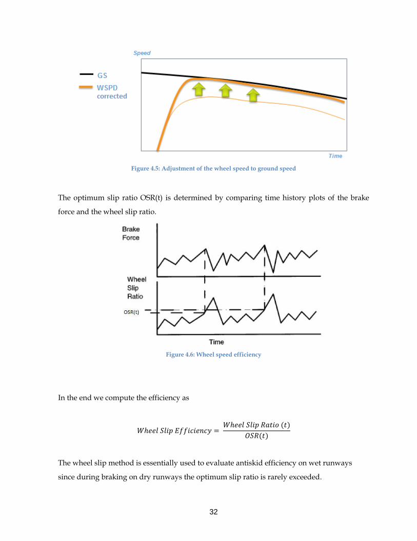
The optimum slip ratio OSR(t) is determined by comparing time history plots of the brake

force and the wheel slip ratio.

Figure 4.6: Wheel speed efficiency

In the end we compute the efficiency as

𝑊ℎ𝑒𝑒𝑙 𝑆𝑙𝑖𝑝 𝐸𝑓𝑓𝑖𝑐𝑖𝑒𝑛𝑐𝑦 = 𝑊ℎ𝑒𝑒𝑙 𝑆𝑙𝑖𝑝 𝑅𝑎𝑡𝑖𝑜 (𝑡)

𝑂𝑆𝑅(𝑡)

The wheel slip method is essentially used to evaluate antiskid efficiency on wet runways

since during braking on dry runways the optimum slip ratio is rarely exceeded.

33

5. INTERNSHIP GOAL

5.1 TAPAS

The Transnational Aircraft Performance & Anti-Skid (TAPAS) project is an initiative carried

on in 2011/2012, whose target was to align the work done on the anti-skid system by

different Airbus departments in France and UK: EGV (Aircraft Performance), ELYB (Braking

& Steering Control Systems), and ELID (Landing Gear Design Analysis).

There is a common need between them to predict the braking performance before flight test,

developing a simulation platform sufficiently advanced which gives output values close to

the real behaviour of the braking. This way, before the real aircraft actually flies, the anti-skid

system designer can converge on an acceptable system tuning (by virtual testing), and the

performance engineer can have a good estimation of the ETAMU curves for performance

calculation. Furthermore, only a few flight tests would be needed to complete anti-skid

tuning and refine, validate and certify the ETAMU model, since the improved simulation

platform would predict the braking performance within a close margin.

The most important parameter to predict is the ETAMU previously mentioned, since it is

fundamental to compute the braking force and consequently provide the stopping distance

predicted.

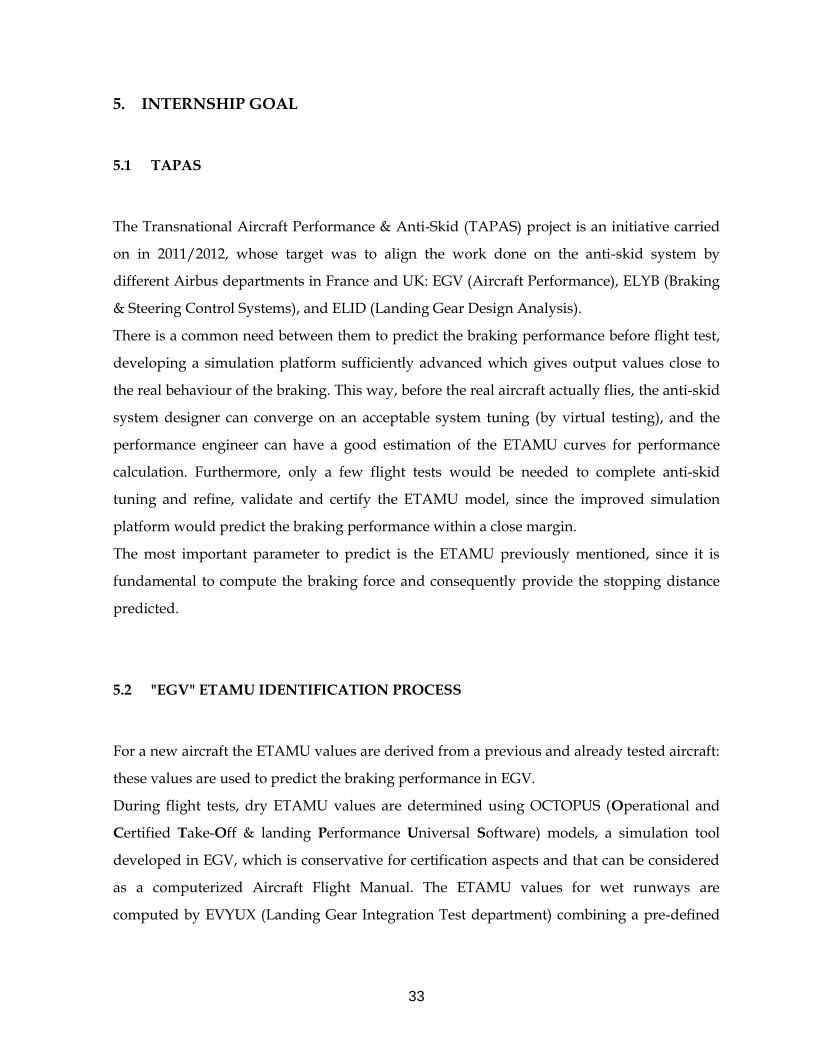
5.2 "EGV" ETAMU IDENTIFICATION PROCESS

For a new aircraft the ETAMU values are derived from a previous and already tested aircraft:

these values are used to predict the braking performance in EGV.

During flight tests, dry ETAMU values are determined using OCTOPUS (Operational and

Certified Take-Off & landing Performance Universal Software) models, a simulation tool

developed in EGV, which is conservative for certification aspects and that can be considered

as a computerized Aircraft Flight Manual. The ETAMU values for wet runways are

computed by EVYUX (Landing Gear Integration Test department) combining a pre-defined

34

optimum slip ratio for the anti-skid efficiency η, and the friction values from ESDU

(Engineering Sciences Data Unit) guidelines (CS 25.109/FAR 25.109).

Figure 5.1: OCTOPUS software scheme

5.3 "EL" PLATFORM

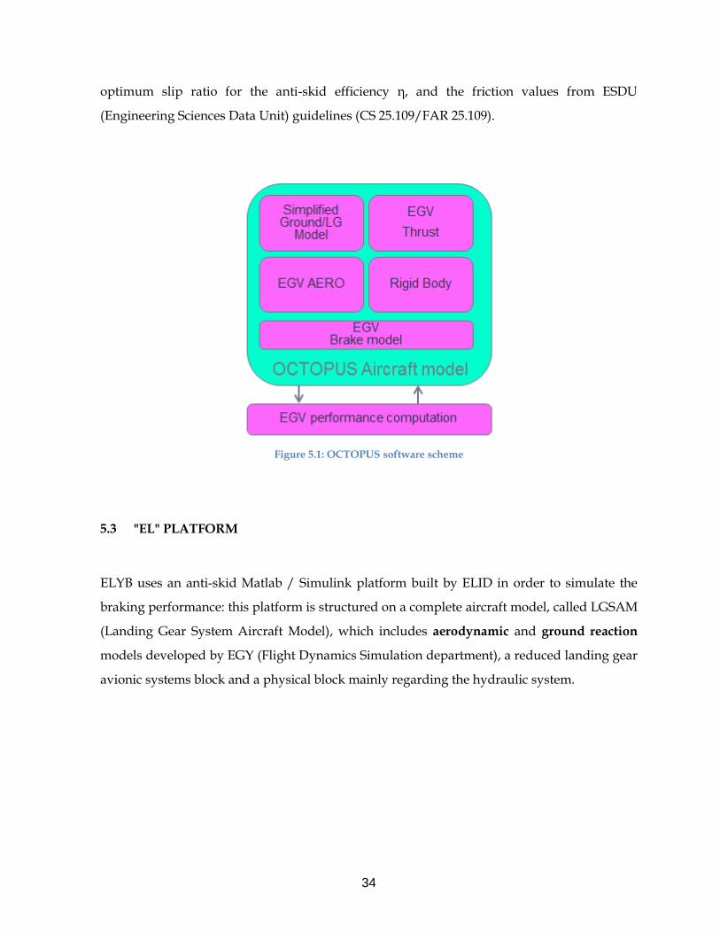
ELYB uses an anti-skid Matlab / Simulink platform built by ELID in order to simulate the

braking performance: this platform is structured on a complete aircraft model, called LGSAM

(Landing Gear System Aircraft Model), which includes aerodynamic and ground reaction

models developed by EGY (Flight Dynamics Simulation department), a reduced landing gear

avionic systems block and a physical block mainly regarding the hydraulic system.

35

Figure 5.2: ELY Matlab / Simulink anti – skid platform

Given the differences mentioned above between EG and EL processes and tools, the aim of

TAPAS was to develop a joint EGV/ELY/ELI platform overwhelming the weaknesses of one

department with the strengths of the others, and create a communication environment

around the tool.

5.4 THE SHARED PLATFORM

TAPAS has been developed onto two platforms: A350 model and A380 model. To make these

changes EGV has provided ELID with the aerodynamic and engine models, which have then

been integrated into the simulation platform by ELID. ELYB was then able to run the model

and extract the correct friction curve μ-slip; this was done by comparing the A380 flight test

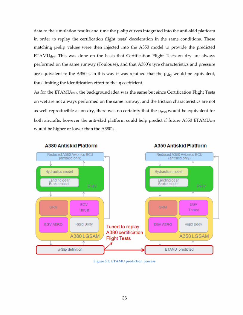
36

data to the simulation results and tune the μ-slip curves integrated into the anti-skid platform

in order to replay the certification flight tests’ deceleration in the same conditions. These

matching μ-slip values were then injected into the A350 model to provide the predicted

ETAMUdry. This was done on the basis that Certification Flight Tests on dry are always

performed on the same runway (Toulouse), and that A380’s tyre characteristics and pressure

are equivalent to the A350’s, in this way it was retained that the μdry would be equivalent,

thus limiting the identification effort to the η coefficient.

As for the ETAMUwet, the background idea was the same but since Certification Flight Tests

on wet are not always performed on the same runway, and the friction characteristics are not

as well reproducible as on dry, there was no certainty that the μwet would be equivalent for

both aircrafts; however the anti-skid platform could help predict if future A350 ETAMUwet

would be higher or lower than the A380’s.

Figure 5.3: ETAMU prediction process

37

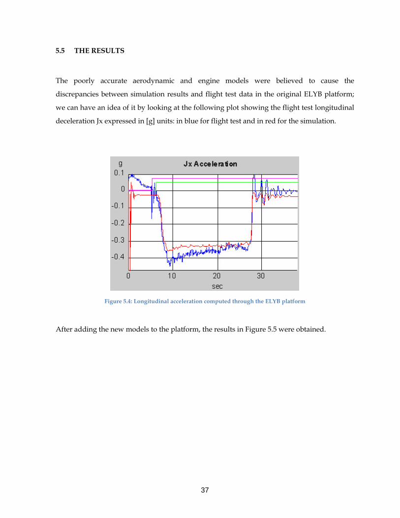
5.5 THE RESULTS

The poorly accurate aerodynamic and engine models were believed to cause the

discrepancies between simulation results and flight test data in the original ELYB platform;

we can have an idea of it by looking at the following plot showing the flight test longitudinal

deceleration Jx expressed in [g] units: in blue for flight test and in red for the simulation.

Figure 5.4: Longitudinal acceleration computed through the ELYB platform

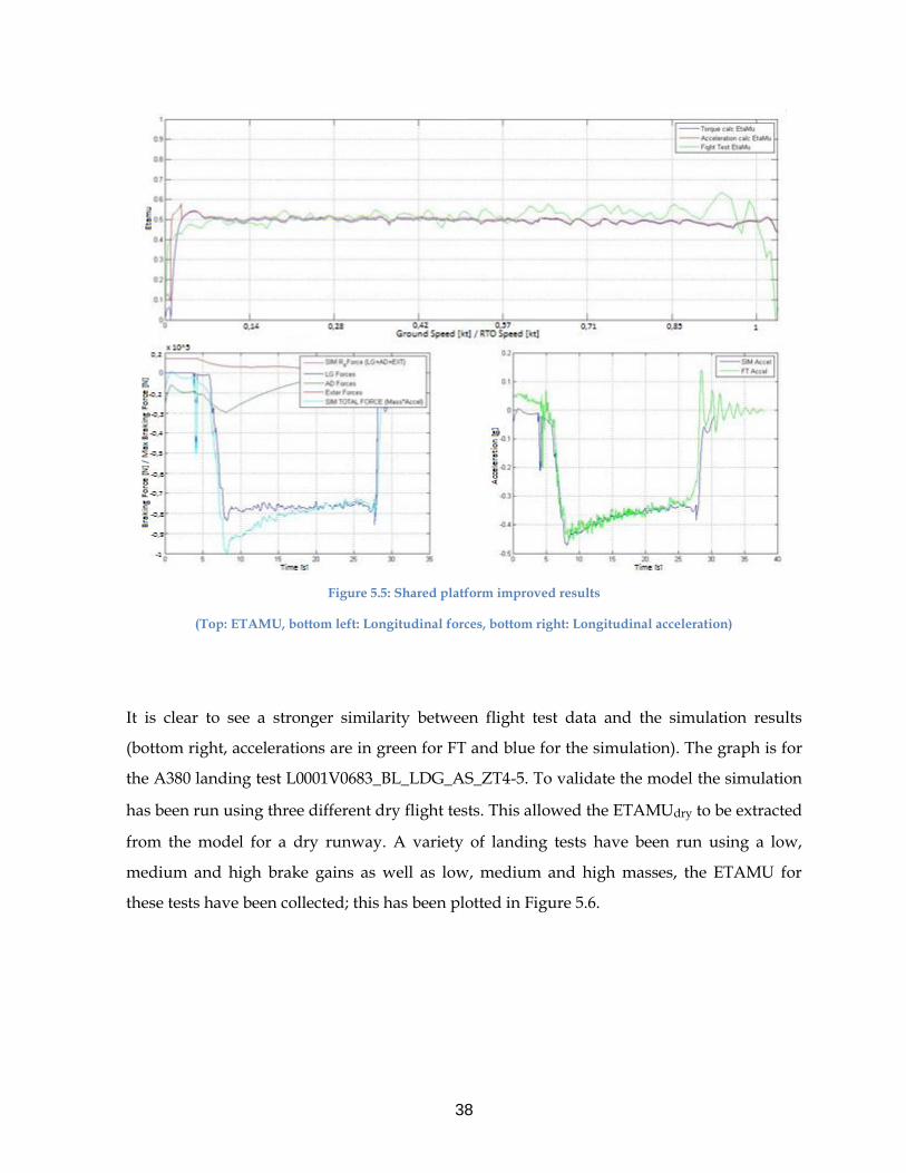
After adding the new models to the platform, the results in Figure 5.5 were obtained.

38

Figure 5.5: Shared platform improved results

(Top: ETAMU, bottom left: Longitudinal forces, bottom right: Longitudinal acceleration)

It is clear to see a stronger similarity between flight test data and the simulation results

(bottom right, accelerations are in green for FT and blue for the simulation). The graph is for

the A380 landing test L0001V0683_BL_LDG_AS_ZT4-5. To validate the model the simulation

has been run using three different dry flight tests. This allowed the ETAMUdry to be extracted

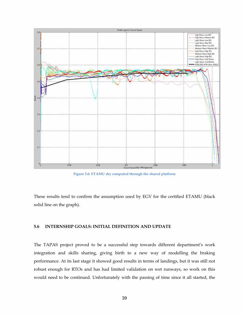
from the model for a dry runway. A variety of landing tests have been run using a low,

medium and high brake gains as well as low, medium and high masses, the ETAMU for

these tests have been collected; this has been plotted in Figure 5.6.

39

Figure 5.6: ETAMU dry computed through the shared platform

These results tend to confirm the assumption used by EGV for the certified ETAMU (black

solid line on the graph).

5.6 INTERNSHIP GOALS: INITIAL DEFINITION AND UPDATE

The TAPAS project proved to be a successful step towards different department’s work

integration and skills sharing, giving birth to a new way of modelling the braking

performance. At its last stage it showed good results in terms of landings, but it was still not

robust enough for RTOs and has had limited validation on wet runways, so work on this

would need to be continued. Unfortunately with the passing of time since it all started, the

40

working priorities for the different stakeholders switched direction and everything was left

behind.

The first aim of this internship was then to give a new life to TAPAS gathering the

knowledge produced and testing it to be a precious source to improve the braking

performance prediction. What is now different from when it was launched, is the availability

of the A350-900 certification flight tests to be taken as important comparison basis to the

platform results, and possibly make some steps forward in the development of the future

A350-1000, adapting the model to the new aircraft’s characteristics.

A great effort was made during the first month of this internship into retrieving the Matlab /

Simulink anti-skid shared platform, trying to get all the needed files back together and

investigate the issues encountered, always supported by ELYB and ELID whose specialists

developed the platform itself. Unfortunately we realised that it would be a very long and

digging work into the corporate folders where the files left behind where scattered.

The constraints of the internship’s limited period and the huge working load of ELYB / ELID

in other several projects marked the decision to redefine the shape and the target of this

work, in order to manage to achieve some concrete results by the end of the Internship. This

happened mainly thanks to brainstorming with colleagues working in the Research &

Technology field inside EGVX, proposing to investigate the potentialities of another

modelling & simulation software: OSMA Souple, standing for Outil de Simulation des

Mouvements Avion, developed and used by the flight dynamics simulation department

EGY. From that moment on, the focus of the internship shifted gradually into the modelling

of the anti-skid braking performance identified through OSMA.

41

6. SIMULATION & MODELLING WITHIN OSMA SOUPLE ENVIRONMENT

6.1 OSMA GENERAL DESCRIPTION AND FUNCTIONS

OSMA Souple is a tool used to model the flight loop of an aircraft by integrating the

calculation models used by OSMA, SIMPA, CHARADE, OCASIME or other tools. This tool is

compatible with the whole family of Airbus fleet.

Its main functionalities are:

- execute trim (“balance”) simulations, f (t) temporal simulations, chaining of the two, and

sweeps

- execute linear simulations and reconstruction of forces

- apply holds (“maintains”) to certain simulation parameters (fixed parameter)

- apply inputs to the parameters during the simulation

- do manoeuvres during the simulations

- generate outputs with various formats

- convert the OSMA, SIMPA or CHARADE scenario files to OSMA SOUPLE format

It operates in batch mode meaning that there is no interaction with the user during execution,

and by means of other HMI (Human Machine Interface) applications like SALIMA, OSMA

ATELIER and ELSA.

The user supplies the input data required in the form of two main files, an “envoi” file and a

“scenario” file: the envoi file includes all the technical information necessary to OSMA to

know which file is the simulation file, the error file, the report file, the output file and their

path, together with the list of models describing the whole Aircraft model, their True/False

activation flag and the version of each one, as an example:

AER;V5_18.1;true;a359v5_18p12; (Aerodynamics model, Active)

ATM;V4_7.0;true; (Atmosphere model, Active)

42

BSC;V5_6.9;false;;;;5.2.0 (Braking & Steering Control unit model, Not active)

…

The scenario file is the script describing the simulation with its trim and temporal phases, its

parameters and its input values, as well as the aircraft model and characteristics. The envoi

file is launched and the scenario file automatically read; the simulation is then started.

After execution, an output file containing the results of the simulation(s) and a report of the

execution of the simulation(s) can be recovered.

6.2 CREATING THE SCENARIO AND ENVOI FILE

Both the scenario and the envoi file have to be written in xml format. The xml files have a tree

structure. Each branch is identified by a keyword and can have attributes to which the user

assigns a value and sub-branches. A branch is declared as follows:

<BRANCH1 attribute1="value1" attribute2="value2" >

<SUB-BRANCH1 attribute3="value3"/>

<SUB-BRANCH2 attribute4="value4"/>

</BRANCH1>

A branch which has no sub-branches can also be declared as follows:

<BRANCH1 attribute1="value1" attribute2="value2" />

The first line of the envoi file contains the inclusion of the osma_souple_envoi.dtd file:

< !DOCTYPE SESSION SYSTEM "osma_souple_envoi.dtd">

As for the envoi file, the first line of the scenario file must be the inclusion of the

osma_souple_scenario.dtd file:

< !DOCTYPE SESSION SYSTEM "osma_souple_scenario.dtd">

43

6.2.1 The Trim (“Balance”)

During the trim phase, the user sets some parameters to define the aircraft’s position and

attitude, and the models compute the values of the other necessary parameters.

Example: the user wants to simulate an aircraft in level flight, with a CAS of 300kts. During

the trim phase the models will search for the thrust value necessary to have a level flight at

300kts. The result of the trim phase is exact if the cost is lower than ε (10-8 by default).

6.2.1.1 Trim Codes

Trim codes indicate what parameters the user has set, each code corresponding to certain

aliases. Codes are classified by categories. Only one code per category can be used at a time.

There are appropriate tables that list the categories and some common codes for initialization

in flight.

The easiest way to create a scenario with the right trim codes is to edit a similar existing

scenario. If it is not possible, the following example explains what to do.

Example: The user wants to create a scenario with an aircraft at 30000ft, descending with a

slope of -3° and with a CAS of 300kts.

It is necessary to choose the most appropriate trim code in each category.

Trajectory: no turn is expected; therefore general is the best code. P1, Q1, R1 have to

be defined if the user wants them to be different from 0 (their default value).

Drag: the user has to choose on what kind of drag curve the aircraft will be initialized.

Since he is working in CAS, iso_vc is a good choice. The user has to define VC

(=300kts), and if it is different from 0 he can define DVC.

Speed: The user has to choose which parameter will determine the thrust. Since he

wants the aircraft to descend with a fixed slope, pente is the best choice. The alias

GAMASOL has to be set to -3°.

Pitch: The user does not know what the position of the THS should be in this case. The

best code is therefore dqequi, to impose an equivalent pitch stick, and in normal law

44

the position of the THS will be determined automatically. The user can leave

DQEQUI and IHDQEQUI at their default values.

Lateral: The user does not have a preference for the lateral state of the aircraft.

rholongi is a good code in this case since it covers many parameters. If all the

associated aliases are left at their default values, the aircraft will be initialized with no

sideslip and no roll, at a route (RHO) towards the north.

Stick: If the user does not have any particular requirements for the stick position, he

doesn’t have to use one of the relative codes.

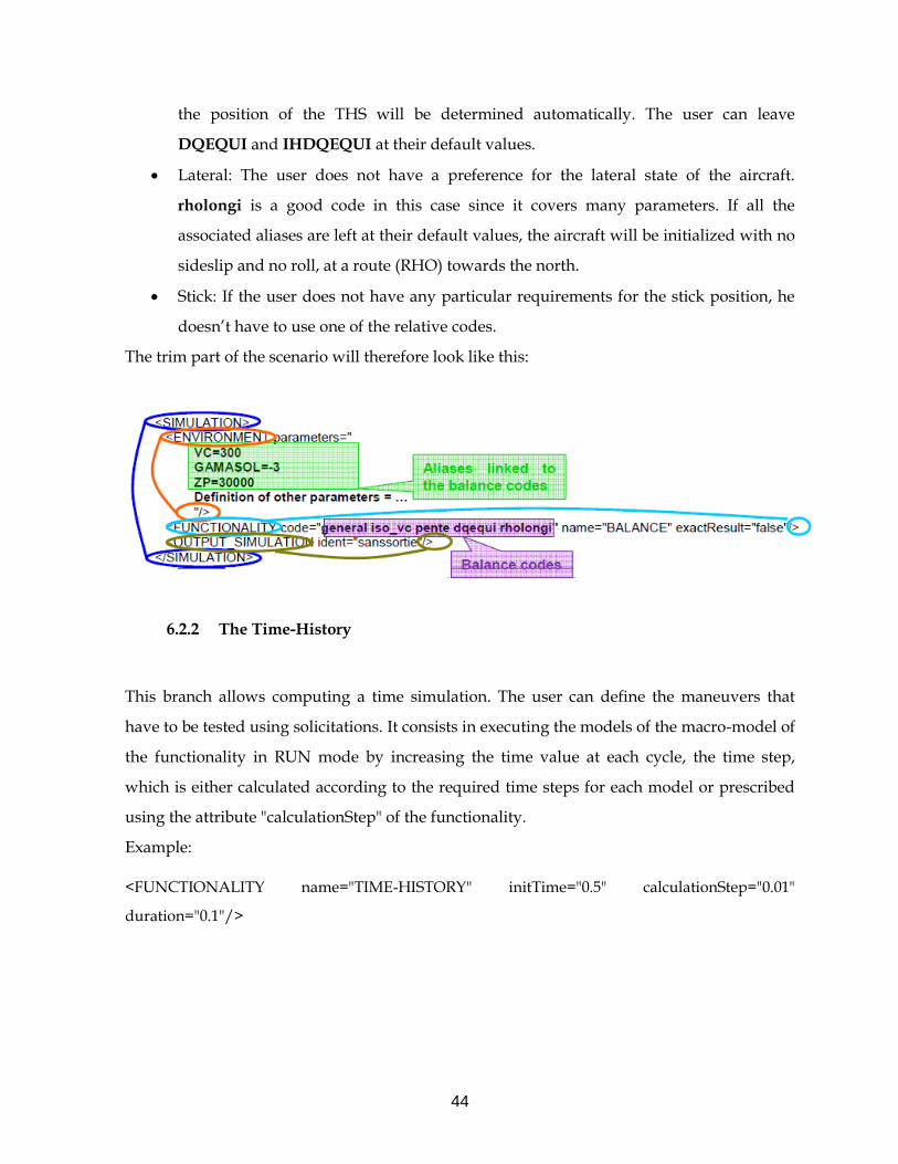
The trim part of the scenario will therefore look like this:

6.2.2 The Time-History

This branch allows computing a time simulation. The user can define the maneuvers that

have to be tested using solicitations. It consists in executing the models of the macro-model of

the functionality in RUN mode by increasing the time value at each cycle, the time step,

which is either calculated according to the required time steps for each model or prescribed

using the attribute "calculationStep" of the functionality.

Example: <FUNCTIONALITY name="TIME-HISTORY" initTime="0.5" calculationStep="0.01"

duration="0.1"/>

45

6.2.3 The Hold (“Maintain”)

This is another temporal functionality with monitoring of the “order” parameter(s) by

estimating other parameters. As for the "TIME-HISTORY" functionality, the functionality

"MAINTAIN" executes the models of its macro-model in RUN mode and increments, at each

cycle, the time value. Moreover, it performs a special processing operation for the estimation

of the parameters per cycle. At the beginning of a cycle, it calculates all target orders and

deduces an increment value for each estimation parameter with a gain matrix:

Increment = (order – target order) X gain

Increment, order and target order are vectors. These increments are added to the common

values of the associated estimation parameters, at the beginning of a cycle for pure entries

and after execution of the model calculating them for the others. In order to use this

functionality, not only the simulation duration is necessary, but also the list of the associated

“order” parameters and estimations as well as the gains linking them.

6.3 RTO SCENARIO ‒ SIMPLIFIED BRAKING MODEL

The first simulation model I worked on is a RTO scenario which was provided by a colleague

specialist in OSMA. The characteristics of the model are the following:

Aircraft model: A350-900

Engine model: TRENTX84

Weight: 250 tons

XG = 22% (Position of the CG along the longitudinal X aircraft axis, in % of the Mean

Aerodynamic Cord)

CONF = 4 (OSMA value) (Corresponding to CONF = 3, meaning a “Take-Off”

flaps/slats configuration)

46

DQT = -2 deg (Elevator tail plane deflection)

ZTP = 17 bar (Zero Torque Pressure = hydraulic system brake pressure when brakes

not activated)

TSAC = 105.5 deg TOGA (Thrust lever deflection angle )

These are part of the so called “ENVIRONMENT parameters” listed in the scenario file, the

most characterizing ones, since the others are just logical setting parameters.

After reading the environment parameters, OSMA executes the BALANCE functionality,

computing the equilibrium of the forces for the aircraft starting from the known imposed

parameters, the arguments of the balance.

The second step of the simulation is the TIME-HISTORY functionality or temporal

simulation:

Table 2: Temporal evolution of the inputs

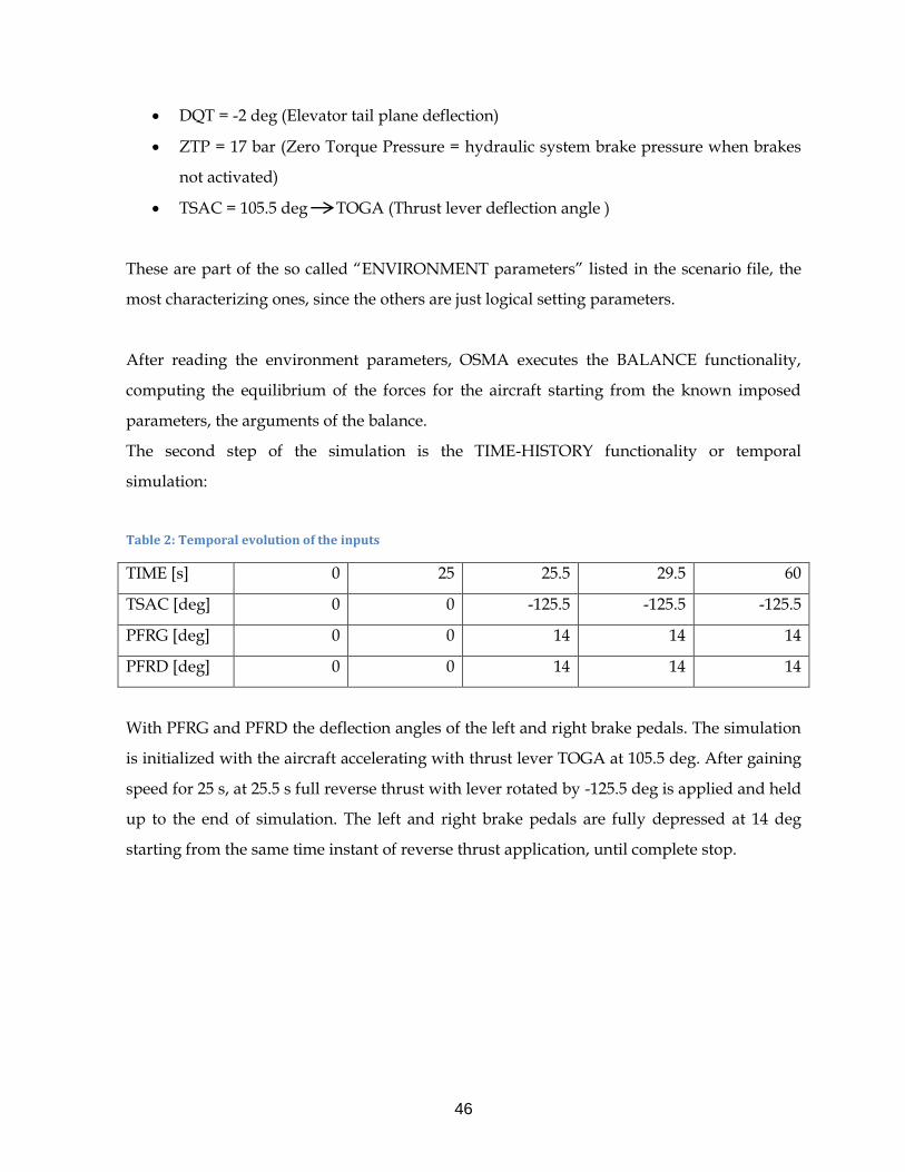
TIME [s] 0 25 25.5 29.5 60

TSAC [deg] 0 0 -125.5 -125.5 -125.5

PFRG [deg] 0 0 14 14 14

PFRD [deg] 0 0 14 14 14

With PFRG and PFRD the deflection angles of the left and right brake pedals. The simulation

is initialized with the aircraft accelerating with thrust lever TOGA at 105.5 deg. After gaining

speed for 25 s, at 25.5 s full reverse thrust with lever rotated by -125.5 deg is applied and held

up to the end of simulation. The left and right brake pedals are fully depressed at 14 deg

starting from the same time instant of reverse thrust application, until complete stop.

47

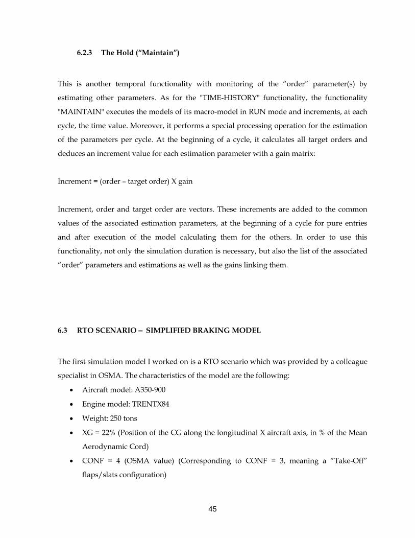
Figure 6.1: Simplified model. Pilot commands

The plots of the most characteristic output parameters will show why this simulation gives as

a result only a simplified braking model.

(1) => ENGINE 1 (2) => ENGINE 2

48

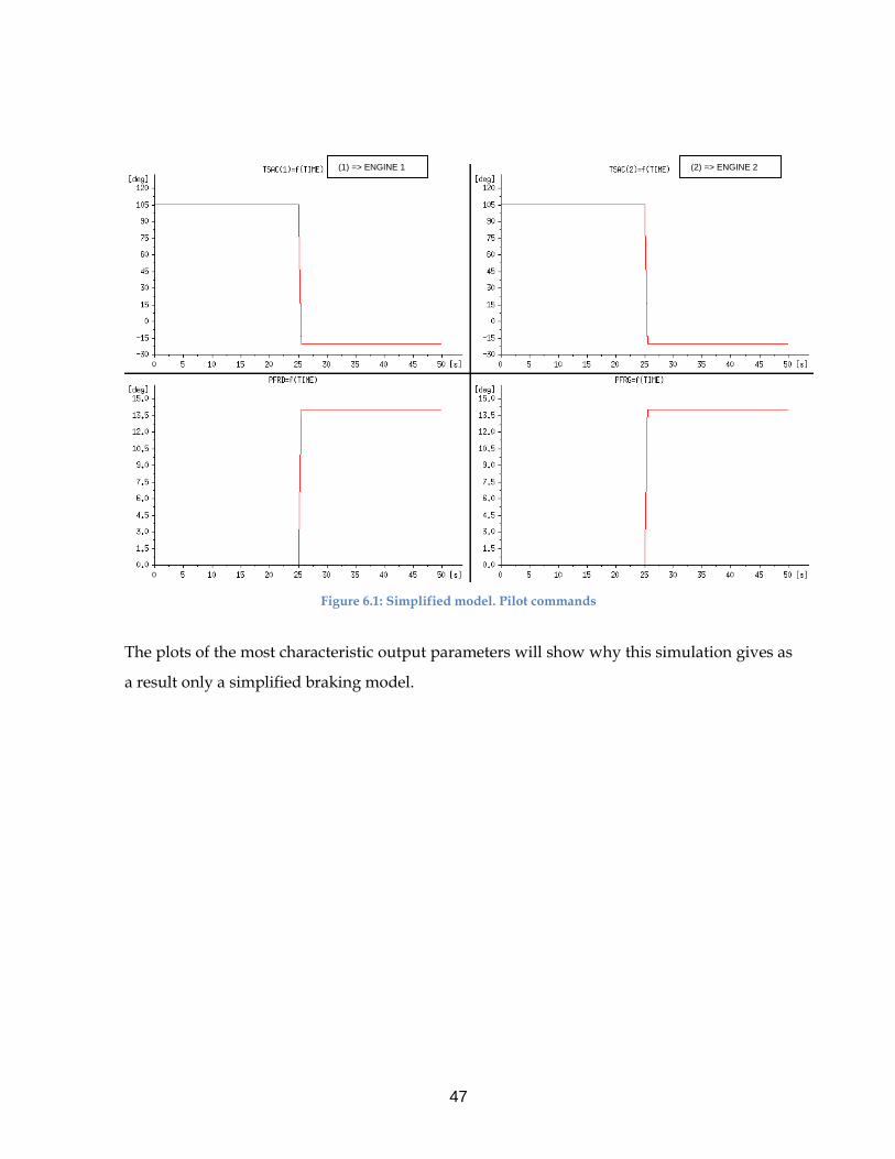
Figure 6.2: Simplified model. Most meaningful simulation outputs

As long as the aircraft accelerates, ground speed, wheel tangential speed and CG longitudinal

displacement (displacement along X runway axis) increase as it should be. At the time of

reverse thrust and brake pedals application the effective brake pressure increases rapidly as

well as the brake torque and longitudinal brake force (ground reaction on the tyre along X

runway axis). As it was previously explained the anti-skid activity should result in a peaked

braking pressure and torque history and by side, in the typical drops in wheel speed due to

the beginning of locking of the wheel itself. Here below in Figure 6.3 there is a sample RTO

flight test compared to the simulation, to show what we have just explained.

GROUND SPEED / MAX GROUND SPEED

BRAKE TORQUE / MAX BRAKE TORQUE

Longitudinal Brake Force / Max Force

EFFECTIVE BRAKE PRESSURE / MAX PRESSURE

WHEEL SPEED / MAX WHEEL SPEED

CG Longitudinal DISPLACEMENT / Max CG DISPLACEMENT

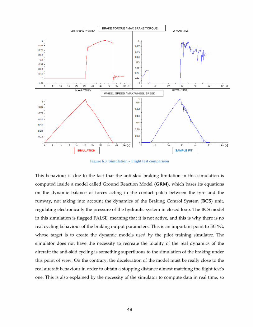
49

Figure 6.3: Simulation – Flight test comparison

This behaviour is due to the fact that the anti-skid braking limitation in this simulation is

computed inside a model called Ground Reaction Model (GRM), which bases its equations

on the dynamic balance of forces acting in the contact patch between the tyre and the

runway, not taking into account the dynamics of the Braking Control System (BCS) unit,

regulating electronically the pressure of the hydraulic system in closed loop. The BCS model

in this simulation is flagged FALSE, meaning that it is not active, and this is why there is no

real cycling behaviour of the braking output parameters. This is an important point to EGYG,

whose target is to create the dynamic models used by the pilot training simulator. The

simulator does not have the necessity to recreate the totality of the real dynamics of the

aircraft: the anti-skid cycling is something superfluous to the simulation of the braking under

this point of view. On the contrary, the deceleration of the model must be really close to the

real aircraft behaviour in order to obtain a stopping distance almost matching the flight test’s

one. This is also explained by the necessity of the simulator to compute data in real time, so

BRAKE TORQUE / MAX BRAKE TORQUE

WHEEL SPEED / MAX WHEEL SPEED

SIMULATION SAMPLE F/T

50

really fast and in accordance to the computer’s calculus capability, meaning that the less the

data the faster the computation and the real time feasibility.

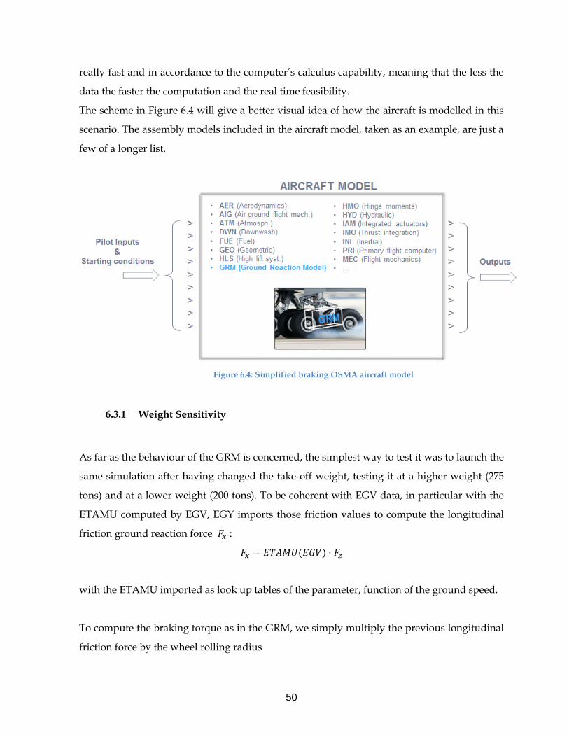
The scheme in Figure 6.4 will give a better visual idea of how the aircraft is modelled in this

scenario. The assembly models included in the aircraft model, taken as an example, are just a

few of a longer list.

Figure 6.4: Simplified braking OSMA aircraft model

6.3.1 Weight Sensitivity

As far as the behaviour of the GRM is concerned, the simplest way to test it was to launch the

same simulation after having changed the take-off weight, testing it at a higher weight (275

tons) and at a lower weight (200 tons). To be coherent with EGV data, in particular with the

ETAMU computed by EGV, EGY imports those friction values to compute the longitudinal

friction ground reaction force 𝐹𝑥 :

𝐹𝑥 = 𝐸𝑇𝐴𝑀𝑈(𝐸𝐺𝑉) · 𝐹𝑧

with the ETAMU imported as look up tables of the parameter, function of the ground speed.

To compute the braking torque as in the GRM, we simply multiply the previous longitudinal

friction force by the wheel rolling radius

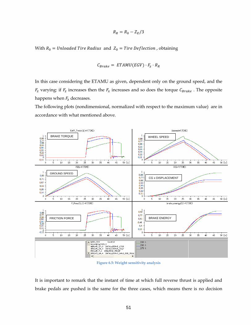
51

𝑅𝑅 = 𝑅0 − 𝑍𝐸/3

With 𝑅0 = 𝑈𝑛𝑙𝑜𝑎𝑑𝑒𝑑 𝑇𝑖𝑟𝑒 𝑅𝑎𝑑𝑖𝑢𝑠 and 𝑍0 = 𝑇𝑖𝑟𝑒 𝐷𝑒𝑓𝑙𝑒𝑐𝑡𝑖𝑜𝑛 , obtaining

𝐶𝐵𝑟𝑎𝑘𝑒 = 𝐸𝑇𝐴𝑀𝑈(𝐸𝐺𝑉) · 𝐹𝑧 · 𝑅𝑅

In this case considering the ETAMU as given, dependent only on the ground speed, and the

𝐹𝑧 varying: if 𝐹𝑧 increases then the 𝐹𝑥 increases and so does the torque 𝐶𝐵𝑟𝑎𝑘𝑒 . The opposite

happens when 𝐹𝑧 decreases.

The following plots (nondimensional, normalized with respect to the maximum value) are in

accordance with what mentioned above.

Figure 6.5: Weight sensitivity analysis

It is important to remark that the instant of time at which full reverse thrust is applied and

brake pedals are pushed is the same for the three cases, which means there is no decision

BRAKE TORQUE

GROUND SPEED

FRICTION FORCE

WHEEL SPEED

CG x DISPLACEMENT

BRAKE ENERGY

52

speed 𝑉1 recomputation. At first it might seem senseless since for a given runway length (let

us consider a fictitious fixed runway length for this simulation) if the take-off weight

increases, the 𝑉1 should increase, but in this case it was not taken into consideration since we

only wanted to test the equations behind the GRM.

In accordance with the reasoning above, the plots show that the lighter the aircraft, the higher

the ground speed and the wheel tangential speed reached at the instant of braking. As soon

as the braking phase starts, the anti-skid limitation (expressed through the ETAMU) compels

the maximum friction force and braking torque to decrease with the decreasing take-off

weight. The time needed to stop the aircraft increases and so do the stopping distance and the

total braking energy.

6.4 RTO SCENARIO ‒ REALISTIC BRAKING MODEL

As soon as the will to investigate the OSMA capability to model the anti-skid braking was

confirmed, I decided to focus on demonstrating whether the OSMA anti-skid platform could

really be a valid substitute to the shared Matlab / Simulink anti-skid platform developed

with the TAPAS project. Indeed, on the long term the aim is to find a common software

between EL, EGY and EGV, whose roles are, respectively, to design the system, to create the

physical dynamic models and to predict its performance. This would permanently solve the

computational discrepancies and communicational misunderstandings due to the usage of

different needs-targeted softwares. Furthermore, this approach is consistent with the MUSE-

PERFO project already in progress.

That is why I continued my studies on a more complex RTO scenario, again handled by the

EGYG GRM specialist. The big difference with the previous one is the fact that it is based on a

real RTO flight test. Thanks to a software called ALADYN used for flight test data treatment

(identification, validation, documentation, etc…) it is possible to create an OSMA simulation

model, including all the necessary files (especially ‘envoi’ and ‘scenario’), where the aircraft

settings and pilot commands recorded during flight test are reproduced exactly into the

scenario. In this way the simulation’s outputs can be tested and compared directly with the

flight test data, and we are able to tune the model in order to better match the real aircraft

behaviour.

53

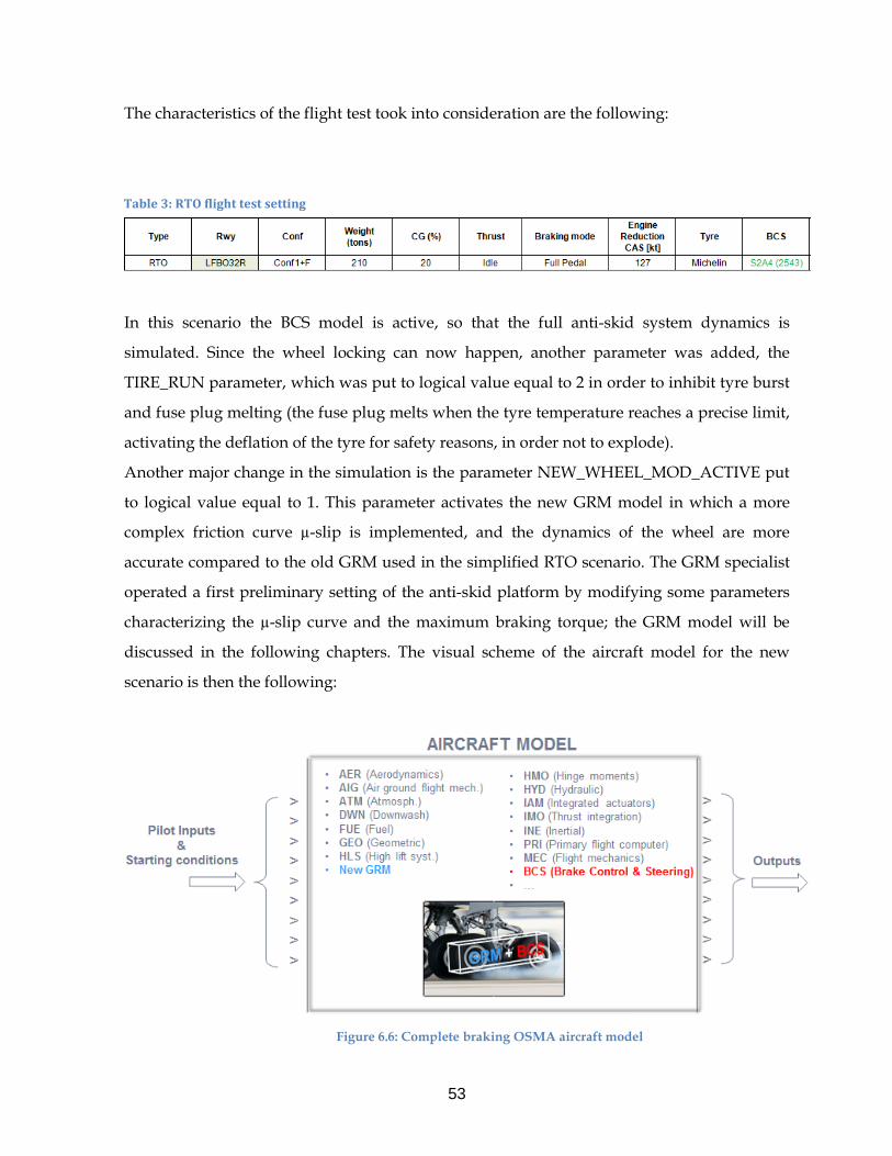
The characteristics of the flight test took into consideration are the following:

In this scenario the BCS model is active, so that the full anti-skid system dynamics is

simulated. Since the wheel locking can now happen, another parameter was added, the

TIRE_RUN parameter, which was put to logical value equal to 2 in order to inhibit tyre burst

and fuse plug melting (the fuse plug melts when the tyre temperature reaches a precise limit,

activating the deflation of the tyre for safety reasons, in order not to explode).

Another major change in the simulation is the parameter NEW_WHEEL_MOD_ACTIVE put

to logical value equal to 1. This parameter activates the new GRM model in which a more

complex friction curve µ-slip is implemented, and the dynamics of the wheel are more

accurate compared to the old GRM used in the simplified RTO scenario. The GRM specialist

operated a first preliminary setting of the anti-skid platform by modifying some parameters

characterizing the µ-slip curve and the maximum braking torque; the GRM model will be

discussed in the following chapters. The visual scheme of the aircraft model for the new

scenario is then the following:

Figure 6.6: Complete braking OSMA aircraft model

Table 3: RTO flight test setting

54

Below are attached the plots of the commands and of the most significant output parameters

to identify the braking performance, in red the simulation results and in blue the flight test

results. Some of them are per wheel parameters (8 braked wheels for the main landing gear, 4

right and 4 left), some others are global parameters.

The comparison between the two will be analyzed afterwards (nondimensional plots,

normalized with respect to the maximum value).

55

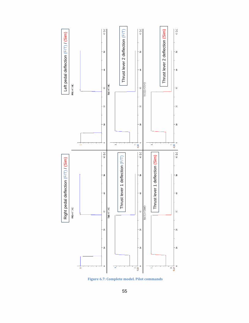
Figure 6.7: Complete model. Pilot commands

Thru

st le

ver

1 d

eflection

(F

/T)

Thru

st le

ver

2 d

eflection

(F

/T)

Thru

st le

ver

1 d

eflection

(S

im)

Thru

st le

ver

2 d

eflection

(S

im)

Rig

ht pe

da

l deflectio

n (

F/T

) / (S

im)

Left

ped

al deflection (

F/T

) / (S

im)

56

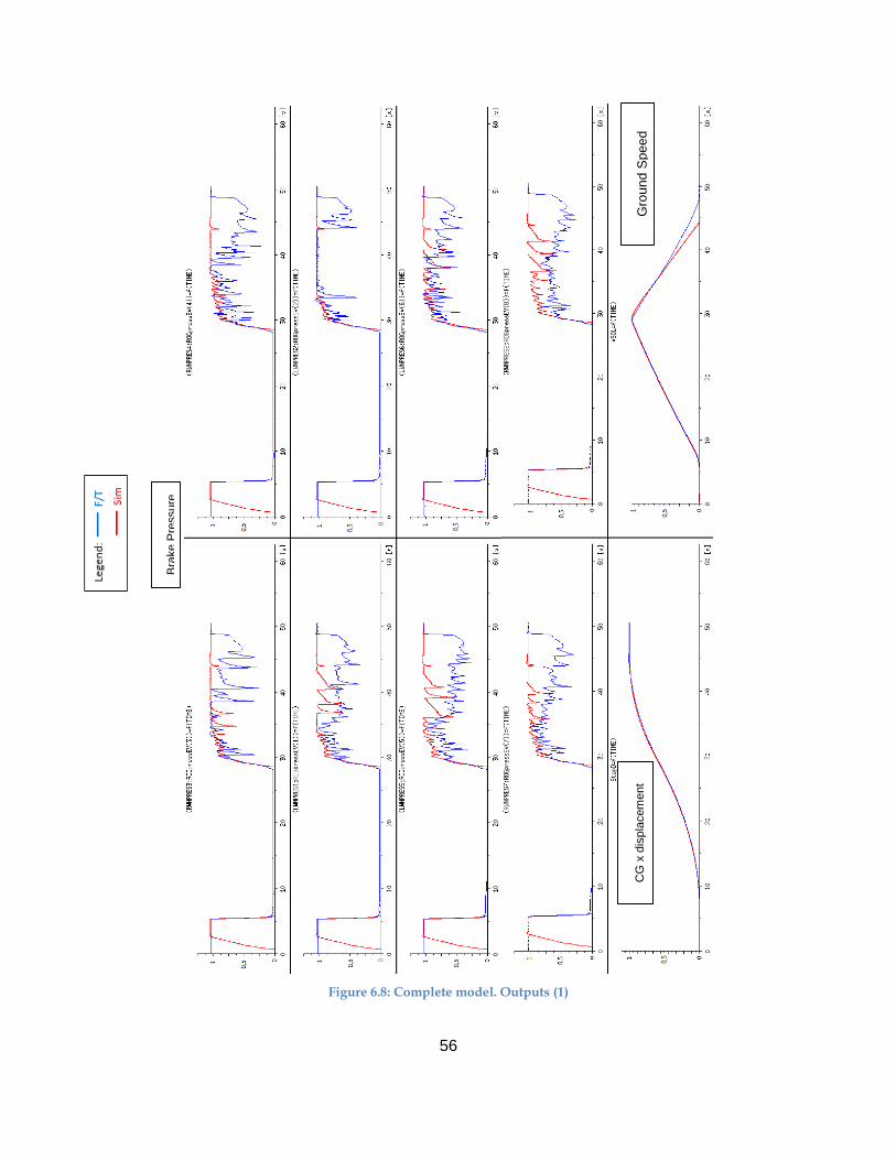
Figure 6.8: Complete model. Outputs (1)

Bra

ke P

ressure

CG

x d

ispla

cem

ent

Gro

un

d S

pe

ed

57

Figure 6.9: Complete model. Outputs (2)

Whee

l S

pe

ed

Torq

ue

58

Figure 6.10: Complete model. Outputs (3)

Slip

Ra

tio

Fx

Loa

d o

n L

+R

gea

rs

Z L

oad F

acto

r E

TA

MU

59

Figure 6.11: Complete model. Outputs (4)

Energ

y

60

As mentioned before the simulated pilot commands are the same as in flight test, as it

emerges from the PFRG and PFRD perfectly matching, as well as TSA1/TSAC(1),

TSA2/TSAC(2), brake pedals deflection and thrust levers deflection. Let us now consider the

outputs in order of showing:

Effective braking pressure [ROGpressEV(1-8) –

LWNPRES(1,2,5,6)/RWNPRES(3,4,7,8)]

We are interested in the braking phase (from 30 s up to the stop); for almost all the wheels, in

the first 5 seconds the cycling of the anti-skid is well simulated. As the braking evolves, the

general trend is less accurate since there are many skids in the flight test not detected in the

simulation.

Stopping Distance [StopD]

The displacement of the CG for the simulation matches almost perfectly the flight test; the

final stopping distance has a gap of 35m, 1371m for flight test against 1336m for the

simulation.

Ground Speed [VSOL]

The two signals are almost identical for the acceleration phase, and then from the instant of

braking, as it happened for the pressure, only the first 5 seconds of the simulation show a

good behaviour. After that, it decreases with a steeper slope and stops the aircraft 3 – 4 s

before the flight test.

Wheel spin speed [ROGgw(1-8) – TACHY(1-8)]

For all the 8 wheels the simulation proves its capability to detect the dropping in wheel

speed, even though not exactly happening at the same instants as the flight test. The gradient

for the simulation increases, following the ground speed trend and stopping the wheels

before compared to flight test.

Effective braking torque [ROGgtrqef(1-8) – LWTQ(1,2,5,6)/RWTQ(3,4,7,8)]

Focusing on the braking phase time range, the torque behaves for the 8 wheels like it did for

the pressure since it is directly linked to it. We notice in general less skid detection and in

average a higher mean level for the simulation.

Longitudinal load factor [NX1 – NX1Sim]

61

The acceleration is well represented; the deceleration is good for 4 – 5 s then the simulation

diverges to higher values.

Global R+L landing gears longitudinal friction braking force [RFX1_kN – WGFX]

The simulation diverges from the beginning of the braking phase to higher values.

Vertical load on L+R landing gears [LoadLRgear – TotLRLoad]

The simulation follows the mean value of the flight test parameter. Not all the oscillations of

the flight test are reproduced even due to the unevenness of the runway not considered in the

scenario.

ETAMU [ROGmuXmean – MuXmean]

As for the friction force, the simulation diverges to higher values along the braking.

Vertical load factor [NZ1]

It evolves exactly as the load factor mentioned above.

Slip ratio [ROGslipR(1-8) – SlipR(1-8)filtr]

It confirms what we analyzed for the wheel spin speed; the skids are well detected, especially

in the first phase of braking, even though not corresponding to the flight test instants. There

is lack of detection in the second phase.

Braking energy cumulated [ROGbEnergy(1-8) –

LWNRGY(1,2,5,6)/RWNRGY(3,4,7,8)]

The behaviour changes depending on the wheel, for some the discrepancy is higher, for

others is lower. The global trend is good.

Considering the totality of the parameters listed, it is possible to identify a global trend for

the simulation: the numbers of wheel skids detected for all the 8 wheels is lower than for the

flight test. This leads to a lower anti-skid activity bringing to longer time intervals during

which braking pressure is held at the maximum value and braking torque to higher levels

than flight test. The brakes clamp the disks for a longer time and develop a higher torque, so

the braking force is higher and diverges. This explains the aircraft stopping in less time, less

space, and the cumulated energy for most of the wheels being higher.

62

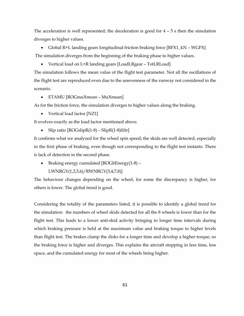
We already pointed out the importance of the ETAMU curve to assess the braking

performance prediction, and from now on we will consider it as the main mean of

comparison between the flight test and the simulation. For this first attempt of tuning the

result is showed in Figure 6.12:

Figure 6.12: ETAMU first adjustment

In blue is the flight test, in red is the simulation, with the corresponding interpolation 2nd

order polynomial curves, in green the certified A350-900 curve.

To conclude, the simulation is not perfectly matching the flight test, but we were able to

demonstrate that through the OSMA scenarios it is possible to have a higher level of accuracy

and reality that was never tested before; what is more, the setting done on the model to

63

obtain these results was brief and not too much studied, meaning that it has great

potentialities if a focused tuning is made.

6.5 THE GRM ADJUSTMENTS

As I previously mentioned, the real braking scenario is characterized by the modification of

some GRM parameters in addition to the activation of the BCS model and new GRM model,

in particular some µ-slip curve parameters and the maximum braking torque. To understand

those changes we need to have a look before at the µ-slip curve implemented in the new

GRM.

6.5.1 The longitudinal µ - Slip curve in the new GRM model

We will stay focused on the longitudinal friction characteristics of the contact between tyre

and runway, as we have been doing since the beginning of this document, so not analyzing

the drifting events (β), but still being aware that they exist, they are modelled in the GRM,

and there are coupling effects between the longitudinal and lateral friction parameters. The

following scheme will make it clear.

Figure 6.13: Tyre-runway reference system & characteristics

64

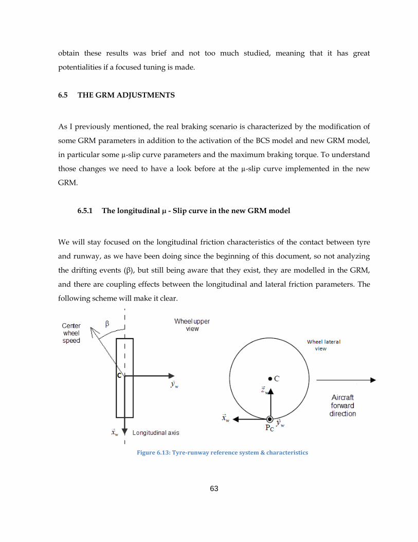
The change from the old to the new GRM that is of interest for us is the modelling of the

longitudinal µ-slip curve, which was previously parametrized in a very simple manner with

two linear functions for both the increasing and decreasing side, and now it is a more

complex spline function for the decreasing and upper increasing zone, preceded by a linear

function for the lower increasing zone.

Figure 6.14: µ-Slip curve old GRM

65

Figure 6.15:µ-Slip curve new GRM

Where g stands for 𝑔𝑙𝑖𝑠𝑠𝑒𝑚𝑒𝑛𝑡 meaning slipping and defined as mentioned at the beginning

of this document in chapter 3.4 (slip ratio):

g =𝑉𝑥 − 𝜔·𝑅𝑅

𝑉𝑥

6.5.2 Parameters definition

The µ-slip curve implemented in the new GRM model is defined by the following

parameters:

0

NLg : slip ratio value delimiting the linear function [0, 0

NLg ] from the spline function [ 0

NLg ,

0

Maxg ].

NLx

0 : friction coefficient corresponding to a slip ratio equal to 0

NLg .

66

0

xk : slope of the linear increasing zone of the function gx

0 expressed as 0

0

0

NL

NLx

xg

k

.

0

refg : slip ratio corresponding to Maxx

0 if the increasing zone was only linear, so

0

0

0

x

Maxx

refk

g

.

There are two more parameters used to define the linear and spline zones of the increasing

side of the gx

0 curve:

0

NLx : ratio between NLx

0 and the maximum friction coefficient Maxx

0 , so Maxx

NLx

NLx 0

0

0

.

Maxg

0 : ratio between 0

refg and the optimum slip ratio 0

Maxg , so 0

0

0

Max

ref

Maxgg

g .

6.6 FIRST ATTEMPT TUNING

The parameters involved in the first tuning of the model and that remained part of the

adjustment during the whole tuning process are:Maxx

0 , 0

NLx , Maxg

0 , 0

xk , VxA (related to

the function driving the decreasing part of the bell-shaped curve) , 𝑀𝑎𝑥 𝐵𝑟𝑎𝑘𝑒 𝑇𝑜𝑟𝑞𝑢𝑒.

The last one was already introduced when the torque limitation model was described;

anyway it is the torque permitting to match flight test deceleration when the braking pressure

is equal to the max nominal pressure. These parameters have been changed from the original

values implemented in the GRM through an adjustment file. They are not constant values but

are function of the ground speed, the normal force on the landing gear, the index describing

the configuration of the landing gear and the braking energy. In particular, the

correspondence between parameters and their labels in the GRM is:

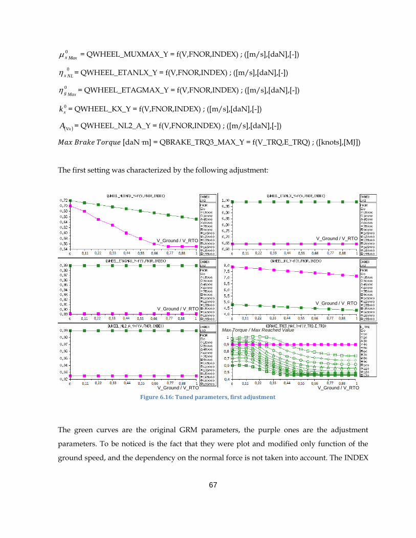
67

Maxx

0 = QWHEEL_MUXMAX_Y = f(V,FNOR,INDEX) ; ([m/s],[daN],[-])

0

NLx = QWHEEL_ETANLX_Y = f(V,FNOR,INDEX) ; ([m/s],[daN],[-])

Maxg

0 = QWHEEL_ETAGMAX_Y = f(V,FNOR,INDEX) ; ([m/s],[daN],[-])

0

xk = QWHEEL_KX_Y = f(V,FNOR,INDEX) ; ([m/s],[daN],[-])

VxA = QWHEEL_NL2_A_Y = f(V,FNOR,INDEX) ; ([m/s],[daN],[-])

𝑀𝑎𝑥 𝐵𝑟𝑎𝑘𝑒 𝑇𝑜𝑟𝑞𝑢𝑒 [daN·m] = QBRAKE_TRQ3_MAX_Y = f(V_TRQ,E_TRQ) ; ([knots],[MJ])

The first setting was characterized by the following adjustment:

The green curves are the original GRM parameters, the purple ones are the adjustment

parameters. To be noticed is the fact that they were plot and modified only function of the

ground speed, and the dependency on the normal force is not taken into account. The INDEX

Max Torque / Max Reached Value

Figure 6.16: Tuned parameters, first adjustment

V_Ground / V_RTO V_Ground / V_RTO

V_Ground / V_RTO V_Ground / V_RTO

V_Ground / V_RTO V_Ground / V_RTO

68

= 102 describes the main landing gears. As for 𝑀𝑎𝑥 𝐵𝑟𝑎𝑘𝑒 𝑇𝑜𝑟𝑞𝑢𝑒, it is clear that it faced the

most significant change from the original shape because it was just set constant to 90% of the

maximum value independently from ground speed and braking energy. It might seem brutal

but it was needed to make the anti-skid system show some cycling and we must also consider

that the original model is valid only for fully torque limited cases, which is not the case of our

flight test, so this parameter needs to have a different shape still to be determined.

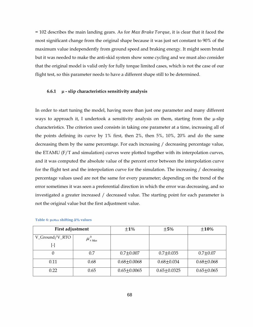
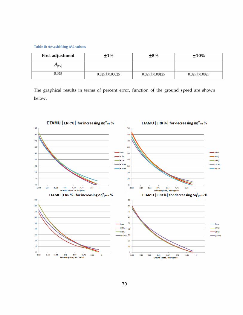
6.6.1 µ - slip characteristics sensitivity analysis

In order to start tuning the model, having more than just one parameter and many different

ways to approach it, I undertook a sensitivity analysis on them, starting from the µ-slip

characteristics. The criterion used consists in taking one parameter at a time, increasing all of

the points defining its curve by 1% first, then 2%, then 5%, 10%, 20% and do the same

decreasing them by the same percentage. For each increasing / decreasing percentage value,

the ETAMU (F/T and simulation) curves were plotted together with its interpolation curves,

and it was computed the absolute value of the percent error between the interpolation curve

for the flight test and the interpolation curve for the simulation. The increasing / decreasing

percentage values used are not the same for every parameter; depending on the trend of the

error sometimes it was seen a preferential direction in which the error was decreasing, and so

investigated a greater increased / decreased value. The starting point for each parameter is

not the original value but the first adjustment value.

Table 4: µxMax shifting ∆% values

First adjustment ±𝟏% ±𝟓% ±𝟏𝟎%

V_Ground/V_RTO

[-] Maxx

0

0 0.7 0.7±0.007 0.7±0.035 0.7±0.07

0.11 0.68 0.68±0.0068 0.68±0.034 0.68±0.068

0.22 0.65 0.65±0.0065 0.65±0.0325 0.65±0.065

69

0.33 0.63 0.63±0.0063 0.63±0.0315 0.63±0.063

0.44 0.6 0.6±0.006 0.6±0.03 0.6±0.06

0.55 0.58 0.58±0.0058 0.58±0.029 0.58±0.058

0.66 0.56 0.56±0.0056 0.56±0.028 0.56±0.056

0.77 0.55 0.55±0.0055 0.55±0.0275 0.55±0.055

0.88 0.55 0.55±0.0055 0.55±0. 0275 0.55±0.055

1 0.55 0.55±0.0055 0.55±0. 0275 0.55±0.055

Table 5: ηxNL shifting ∆% values

First adjustment ±𝟏% ±𝟓% ±𝟏𝟎% ±𝟐𝟎%

0

NLx

Original curve points · 0.65 Original curve

points · 0.65±0.0065

Original curve

points ·

0.65±0.0325

Original curve

points ·

0.65±0.065

Original curve

points · 0.65±0.13

Table 6: ηgMax shifting ∆% values

First adjustment ±𝟏% ±𝟓% ±𝟏𝟎%

Maxg

0

Original curve points · 0.9 Original curve points ·

0.65±0.009

Original curve points ·

0.65±0.045

Original curve points ·

0.65±0.09

Table 7: Kx shifting ∆% values

First adjustment ±𝟏% ±𝟐% ±𝟓% ±𝟏𝟎% −𝟐𝟎%

0

xk

Original curve points ·

1.646

Original curve

points ·

0.65±0.01646

Original curve

points ·

0.65±0.03292

Original curve

points ·

0.65±0.0823

Original curve

points ·

0.65±0.1646

Original curve

points ·

0.65−0.3292

70

Table 8: A(Vx) shifting ∆% values

First adjustment ±𝟏% ±𝟓% ±𝟏𝟎%

VxA

0.025 0.025±0.00025 0.025±0.00125 0.025±0.0025

The graphical results in terms of percent error, function of the ground speed are shown

below.

71

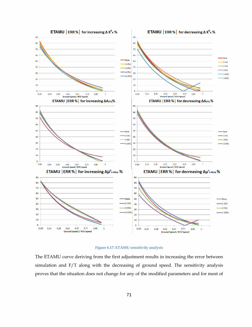
Figure 6.17: ETAMU sensitivity analysis

The ETAMU curve deriving from the first adjustment results in increasing the error between

simulation and F/T along with the decreasing of ground speed. The sensitivity analysis

proves that the situation does not change for any of the modified parameters and for most of

72

them the maximum error at zero ground speed remains between 80% and 70%. The only

better result involves a decreasing of 10% forMaxx

0 , showing a final error lower than 60%.

What is more interesting is the nonlinear behaviour between the increasing / decreasing of

one parameter and its error: if we take for example0

NLx , at high speeds the error is

decreasing in this order: -10%, -5%, Base, -1%, -20%, and the criterion changes as long as the

aircraft decelerates. Again, the only parameter behaving almost linearly as far as the error is

concerned is Maxx

0 which proves an increasing error with the increasing of its ∆ and vice

versa. For this reason I decided to investigate more on the shaping of the Maxx

0 curve,

focusing on the evolution of the ETAMU as the ∆Maxx

0 decreases.

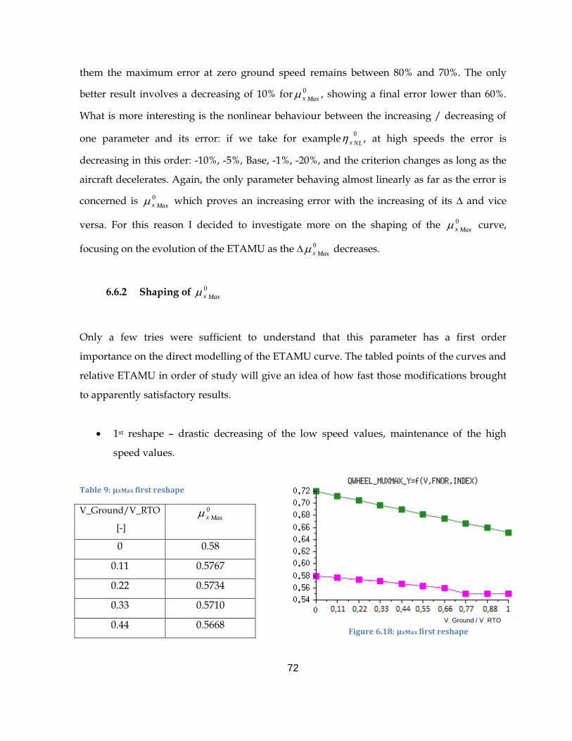
6.6.2 Shaping of Maxx

0

Only a few tries were sufficient to understand that this parameter has a first order

importance on the direct modelling of the ETAMU curve. The tabled points of the curves and

relative ETAMU in order of study will give an idea of how fast those modifications brought

to apparently satisfactory results.

1st reshape – drastic decreasing of the low speed values, maintenance of the high

speed values.

Table 9: µxMax first reshape

V_Ground/V_RTO

[-] Maxx

0

0 0.58

0.11 0.5767

0.22 0.5734

0.33 0.5710

0.44 0.5668 Figure 6.18: µxMax first reshape

V_Ground / V_RTO

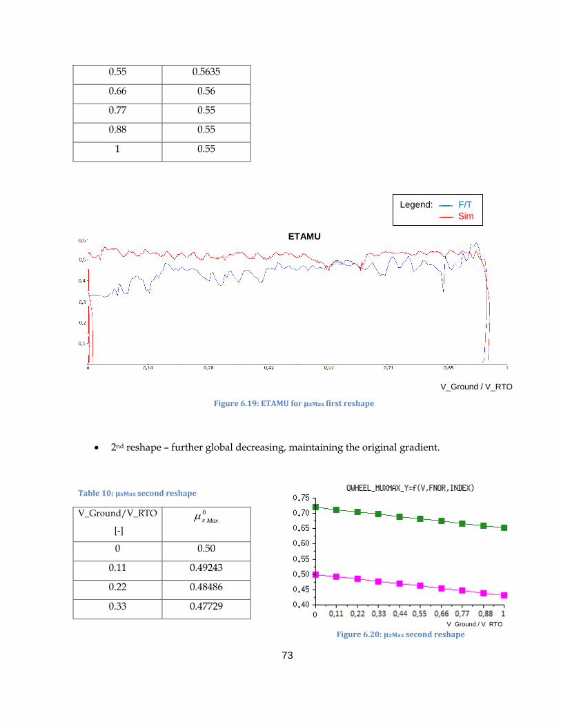
73

0.55 0.5635

0.66 0.56

0.77 0.55

0.88 0.55

1 0.55

2nd reshape – further global decreasing, maintaining the original gradient.

Table 10: µxMax second reshape

V_Ground/V_RTO

[-] Maxx

0

0 0.50

0.11 0.49243

0.22 0.48486

0.33 0.47729

V_Ground / V_RTO

Figure 6.20: µxMax second reshape

V_Ground / V_RTO

Legend: F/T

Sim

Figure 6.19: ETAMU for µxMax first reshape

ETAMU

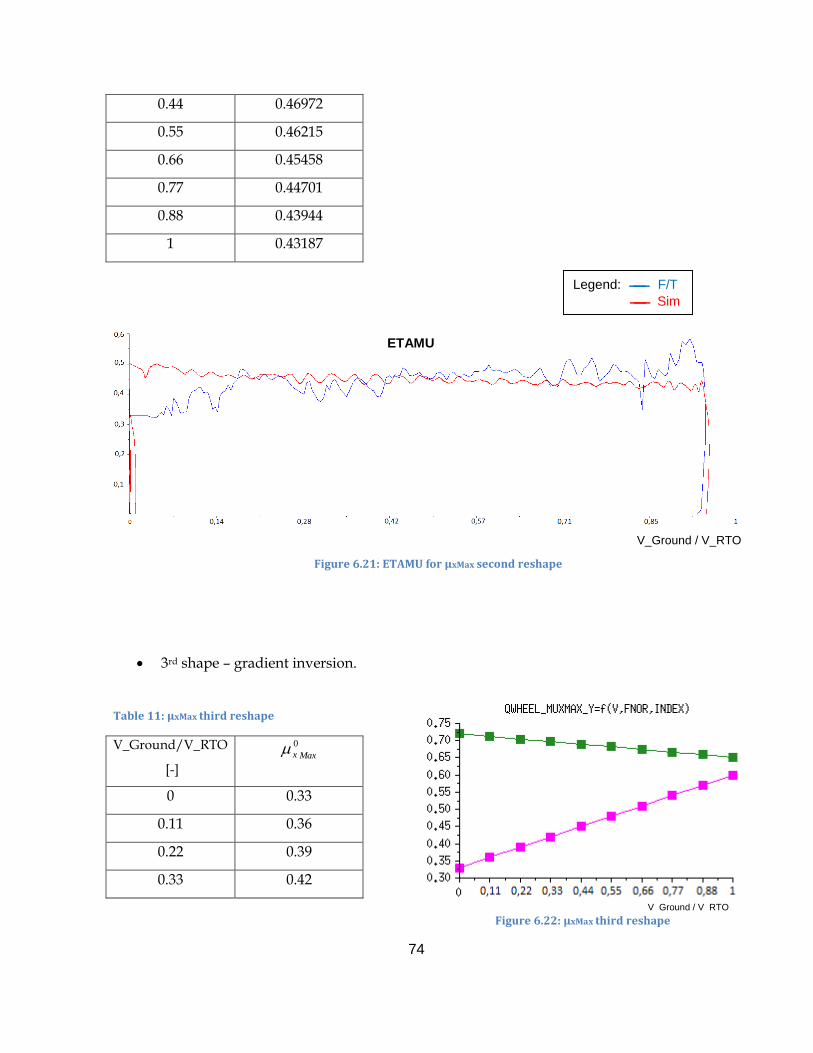
74

0.44 0.46972

0.55 0.46215

0.66 0.45458

0.77 0.44701

0.88 0.43944

1 0.43187

3rd shape – gradient inversion.

Table 11: µxMax third reshape

V_Ground/V_RTO

[-] Maxx

0

0 0.33

0.11 0.36

0.22 0.39

0.33 0.42

Figure 6.21: ETAMU for µxMax second reshape

Figure 6.22: µxMax third reshape V_Ground / V_RTO

Legend: F/T

Sim

ETAMU

V_Ground / V_RTO

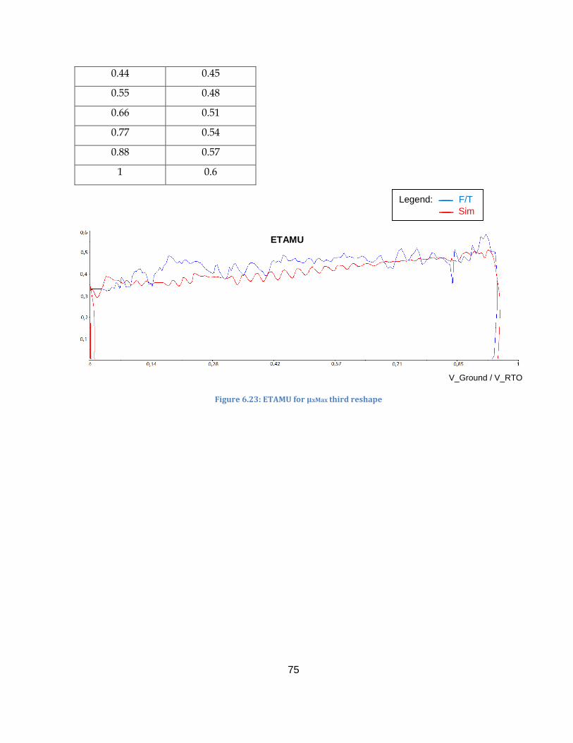
75

0.44 0.45

0.55 0.48

0.66 0.51

0.77 0.54

0.88 0.57

1 0.6

Figure 6.23: ETAMU for µxMax third reshape

ETAMU

Legend: F/T

Sim

V_Ground / V_RTO

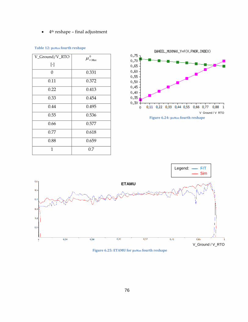
76

4th reshape – final adjustment

Table 12: µxMax fourth reshape

V_Ground/V_RTO

[-] Maxx

0

0 0.331

0.11 0.372

0.22 0.413

0.33 0.454

0.44 0.495

0.55 0.536

0.66 0.577

0.77 0.618

0.88 0.659

1 0.7

Figure 6.24: µxMax fourth reshape

V_Ground / V_RTO

Figure 6.25: ETAMU for µxMax fourth reshape

Legend: F/T

Sim

ETAMU

V_Ground / V_RTO

77

6.6.2.1 Analysis of the results

The shaping of the Maxx

0 resulted very effective in tuning the model to match the ETAMU, as

it is evident from the only 4 necessary steps. The 1st and 2nd reshape showed a typical trend of

the ETAMU as if the η was almost equal to 1 and the curve was following closely the Maxx

0

target of the anti-skid system. This brought me to switch the gradient in the 3rd reshape,

making it resemble the F/T ETAMU curve and fix the max and min values to the F/T

ETAMU max and min. The 4th reshape is only a final adjustment to fix the excessive lowering

of the simulation curve compared to F/T, and it proved a satisfactory matching.

Unfortunately the freedom in modelling physical parameters is constrained by the limits of

the real physical behaviours, and the gaining of good results can easily obfuscate those limits.

The study of tribology, the science studying the interactions between two surfaces in contact

and relative motion, has widely demonstrated that the static coefficient of friction µs is higher

than the dynamic coefficient of friction µd. We will take it as a fact and not investigate it since

it is not the aim of this thesis. What is evident in the 3rd and 4th shapings is that this law is not

respected because if we consider theMaxx

0 from high speeds to rest, it can be seen as a µ

shifting from dynamic to static that needs to increase. In those cases on the contrary it

decreases, meaning that it is not following its physical behaviour.

By doing this, practically the maximum friction force that can be produced in the contact

patch between the tyre and the runway is limited from the outside as long as the aircraft

decelerates: the ground longitudinal friction force should then match as good as the ETAMU

does, but the braking pressure will be wrongly limited in order to develop less braking

torque to prevent from skidding as long as the frictional characteristics degrade with speed.

Since the task of the anti-skid system is producing a slip ratio as close as possible to the

optimum slip ratio 0

Maxg (so generating a friction coefficient as close as possible to the

maximum Maxx

0 ), and since are valid in the GRM the relations (after manipulation of the

already described equations):

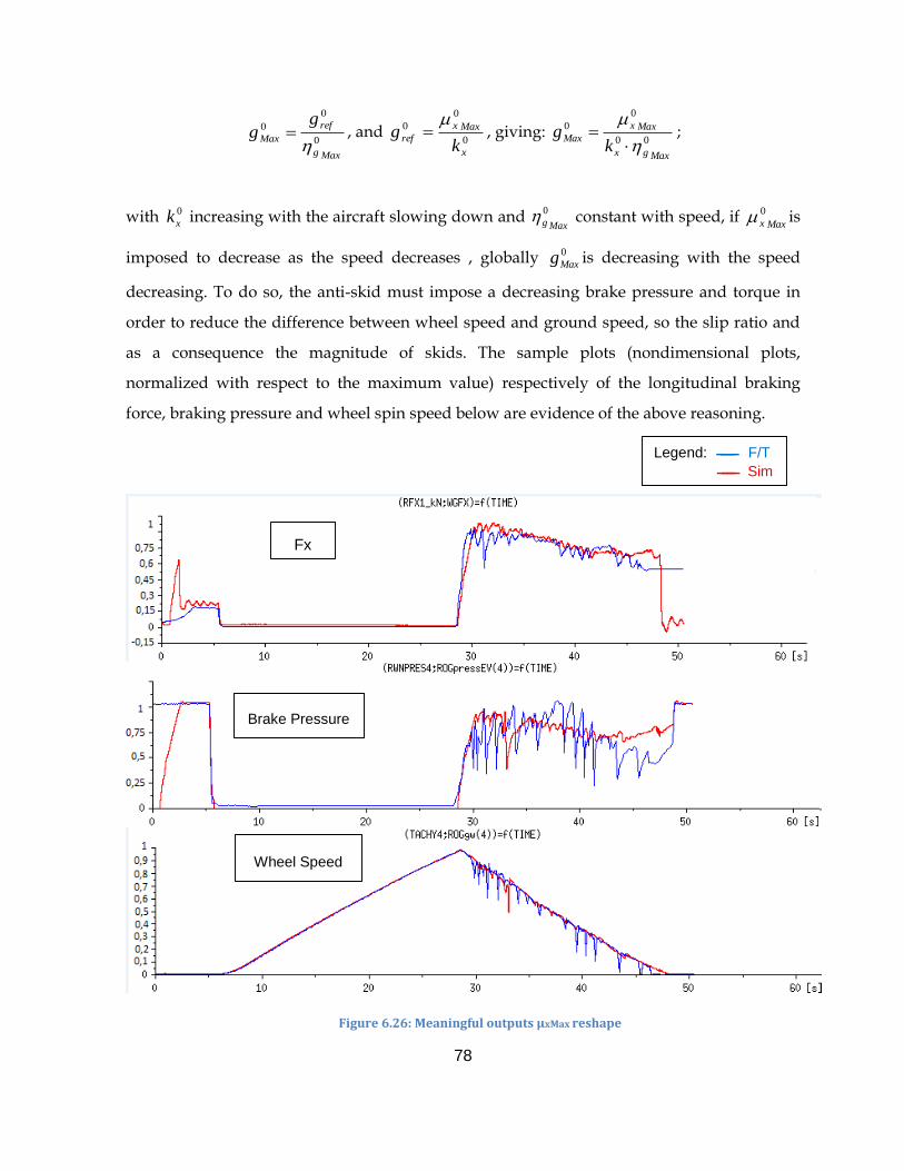
78

Maxg

ref

Max

gg

0

0

0

, and

0

0

0

x

Maxx

refk

g

, giving:

Maxgx

Maxx

Maxk

g00

0

0

;

with 0

xk increasing with the aircraft slowing down and Maxg

0 constant with speed, if Maxx

0 is

imposed to decrease as the speed decreases , globally 0

Maxg is decreasing with the speed

decreasing. To do so, the anti-skid must impose a decreasing brake pressure and torque in

order to reduce the difference between wheel speed and ground speed, so the slip ratio and

as a consequence the magnitude of skids. The sample plots (nondimensional plots,

normalized with respect to the maximum value) respectively of the longitudinal braking

force, braking pressure and wheel spin speed below are evidence of the above reasoning.

Legend: F/T

Sim

Figure 6.26: Meaningful outputs µxMax reshape

Fx

Brake Pressure

Wheel Speed

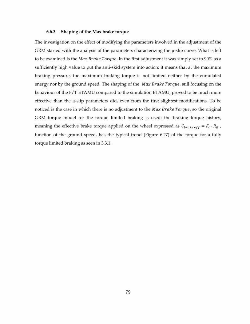
79

6.6.3 Shaping of the Max brake torque

The investigation on the effect of modifying the parameters involved in the adjustment of the

GRM started with the analysis of the parameters characterizing the µ-slip curve. What is left

to be examined is the 𝑀𝑎𝑥 𝐵𝑟𝑎𝑘𝑒 𝑇𝑜𝑟𝑞𝑢𝑒. In the first adjustment it was simply set to 90% as a

sufficiently high value to put the anti-skid system into action: it means that at the maximum

braking pressure, the maximum braking torque is not limited neither by the cumulated

energy nor by the ground speed. The shaping of the 𝑀𝑎𝑥 𝐵𝑟𝑎𝑘𝑒 𝑇𝑜𝑟𝑞𝑢𝑒, still focusing on the

behaviour of the F/T ETAMU compared to the simulation ETAMU, proved to be much more

effective than the µ-slip parameters did, even from the first slightest modifications. To be

noticed is the case in which there is no adjustment to the 𝑀𝑎𝑥 𝐵𝑟𝑎𝑘𝑒 𝑇𝑜𝑟𝑞𝑢𝑒, so the original

GRM torque model for the torque limited braking is used: the braking torque history,

meaning the effective brake torque applied on the wheel expressed as 𝐶𝑏𝑟𝑎𝑘𝑒 𝑒𝑓𝑓 = 𝐹𝑥 · 𝑅𝑅 ,

function of the ground speed, has the typical trend (Figure 6.27) of the torque for a fully

torque limited braking as seen in 3.3.1.

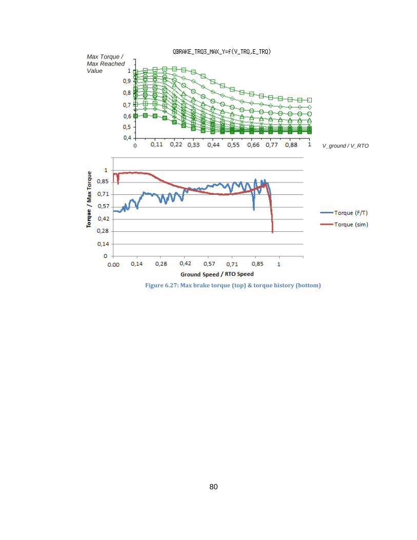
80

V_ground / V_RTO

Max Torque / Max Reached Value

Figure 6.27: Max brake torque (top) & torque history (bottom)

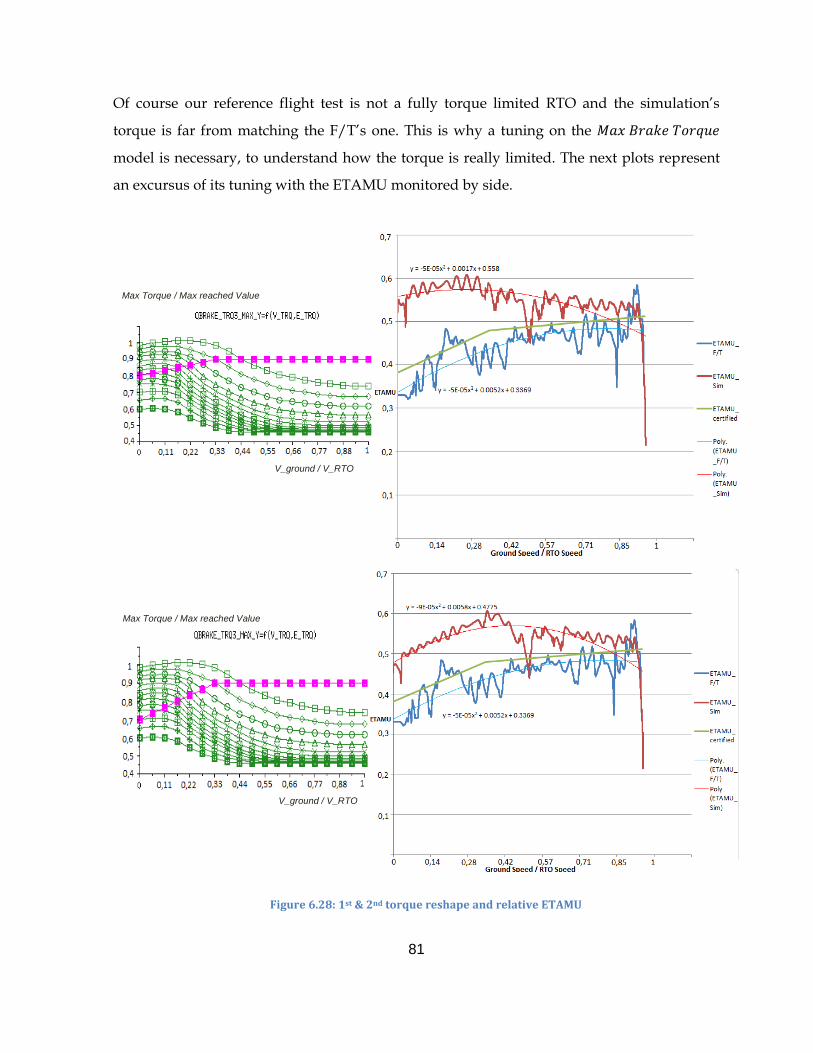
81

Of course our reference flight test is not a fully torque limited RTO and the simulation’s

torque is far from matching the F/T’s one. This is why a tuning on the 𝑀𝑎𝑥 𝐵𝑟𝑎𝑘𝑒 𝑇𝑜𝑟𝑞𝑢𝑒

model is necessary, to understand how the torque is really limited. The next plots represent

an excursus of its tuning with the ETAMU monitored by side.

Figure 6.28: 1st & 2nd torque reshape and relative ETAMU

V_ground / V_RTO

Max Torque / Max reached Value

Max Torque / Max reached Value

V_ground / V_RTO

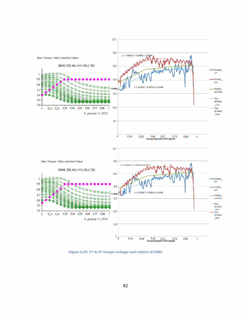
82

Figure 6.29: 3rd & 4th torque reshape and relative ETAMU

Max Torque / Max reached Value

V_ground / V_RTO

Max Torque / Max reached Value

V_ground / V_RTO

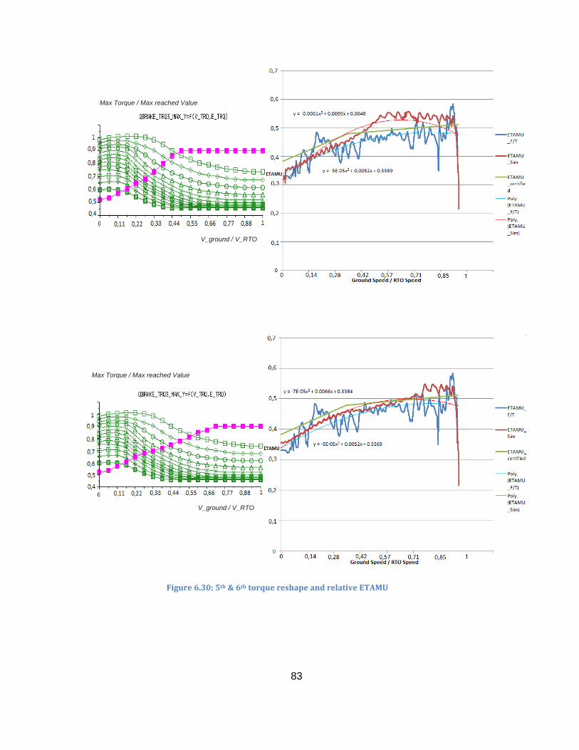
83

Figure 6.30: 5th & 6th torque reshape and relative ETAMU

Max Torque / Max reached Value

V_ground / V_RTO

Max Torque / Max reached Value

V_ground / V_RTO

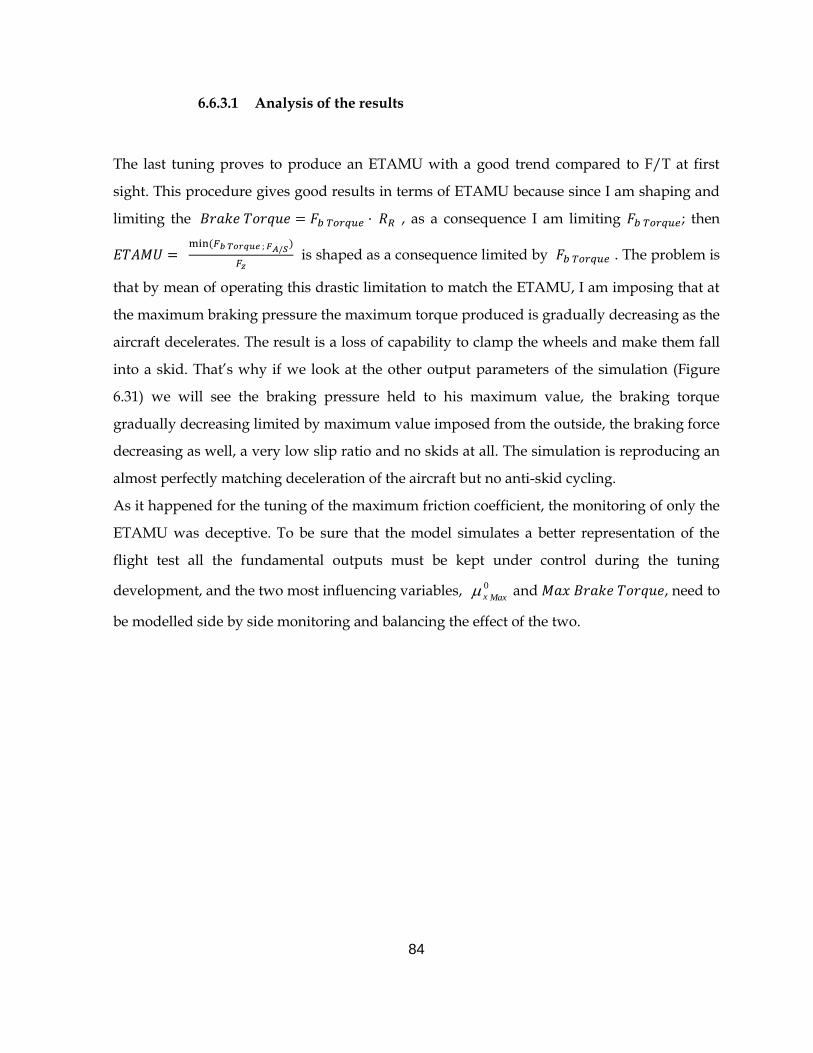
84

6.6.3.1 Analysis of the results

The last tuning proves to produce an ETAMU with a good trend compared to F/T at first

sight. This procedure gives good results in terms of ETAMU because since I am shaping and

limiting the 𝐵𝑟𝑎𝑘𝑒 𝑇𝑜𝑟𝑞𝑢𝑒 = 𝐹𝑏 𝑇𝑜𝑟𝑞𝑢𝑒 · 𝑅𝑅 , as a consequence I am limiting 𝐹𝑏 𝑇𝑜𝑟𝑞𝑢𝑒; then

𝐸𝑇𝐴𝑀𝑈 = min (𝐹𝑏 𝑇𝑜𝑟𝑞𝑢𝑒 ; 𝐹𝐴/𝑆

)

𝐹𝑧 is shaped as a consequence limited by 𝐹𝑏 𝑇𝑜𝑟𝑞𝑢𝑒 . The problem is

that by mean of operating this drastic limitation to match the ETAMU, I am imposing that at

the maximum braking pressure the maximum torque produced is gradually decreasing as the

aircraft decelerates. The result is a loss of capability to clamp the wheels and make them fall

into a skid. That’s why if we look at the other output parameters of the simulation (Figure

6.31) we will see the braking pressure held to his maximum value, the braking torque

gradually decreasing limited by maximum value imposed from the outside, the braking force

decreasing as well, a very low slip ratio and no skids at all. The simulation is reproducing an

almost perfectly matching deceleration of the aircraft but no anti-skid cycling.

As it happened for the tuning of the maximum friction coefficient, the monitoring of only the

ETAMU was deceptive. To be sure that the model simulates a better representation of the

flight test all the fundamental outputs must be kept under control during the tuning

development, and the two most influencing variables, Maxx

0 and 𝑀𝑎𝑥 𝐵𝑟𝑎𝑘𝑒 𝑇𝑜𝑟𝑞𝑢𝑒, need to

be modelled side by side monitoring and balancing the effect of the two.

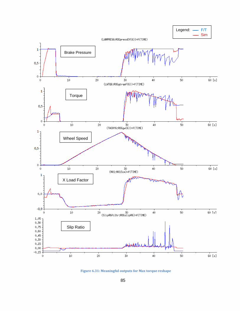
85

Figure 6.31: Meaningful outputs for Max torque reshape

Wheel Speed

Brake Pressure

Torque

X Load Factor

Slip Ratio

Legend: F/T

Sim

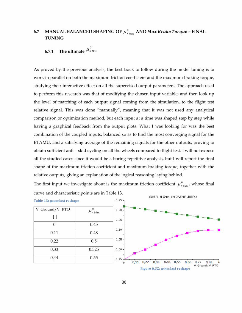
86

6.7 MANUAL BALANCED SHAPING OF Maxx

0 AND 𝑴𝒂𝒙 𝑩𝒓𝒂𝒌𝒆 𝑻𝒐𝒓𝒒𝒖𝒆 – FINAL

TUNING

6.7.1 The ultimate Maxx

0

As proved by the previous analysis, the best track to follow during the model tuning is to

work in parallel on both the maximum friction coefficient and the maximum braking torque,

studying their interactive effect on all the supervised output parameters. The approach used

to perform this research was that of modifying the chosen input variable, and then look up

the level of matching of each output signal coming from the simulation, to the flight test

relative signal. This was done “manually”, meaning that it was not used any analytical

comparison or optimization method, but each input at a time was shaped step by step while

having a graphical feedback from the output plots. What I was looking for was the best

combination of the coupled inputs, balanced so as to find the most converging signal for the

ETAMU, and a satisfying average of the remaining signals for the other outputs, proving to

obtain sufficient anti – skid cycling on all the wheels compared to flight test. I will not expose

all the studied cases since it would be a boring repetitive analysis, but I will report the final

shape of the maximum friction coefficient and maximum braking torque, together with the

relative outputs, giving an explanation of the logical reasoning laying behind.

The first input we investigate about is the maximum friction coefficient Maxx

0 , whose final

curve and characteristic points are in Table 13.

Table 13: µxMax last reshape

V_Ground/V_RTO

[-] Maxx

0

0 0.45

0,11 0.48

0,22 0.5

0,33 0.525

0,44 0.55

Figure 6.32: µxMax last reshape V_Ground / V_RTO

87

0,55 0.57

0,66 0.584

0,77 0.595

0,88 0.599

1 0.6

If we consider what was previously stated during the shaping of this parameter, about the

tests made with positive gradients of the curve, the first thing that can be realized is that it

looks having a non-physical behaviour because the friction coefficient, if interpreted as

switching gradually from dynamic to static, should increase, exactly the opposite of what

showed above.

However, when speaking of physical or non-physical behaviours, it is necessary to take into

account all the possible interactions between the different phenomena playing an effective

role on the modification of a parameter.

What was lately investigated and assumed are the effects of the rising temperature and

exciting frequency on the frictional characteristics of two sliding surfaces when one of the

two is rubber. These results were taken from the PhD work “Modelisation des forces de

contact entre le pneu d’un avion et la piste” by Logan Jones, a very accurate analysis on the

forces generated in the contact patch between tyre and runway. The relative paragraph states:

“The third law of friction states that kinetic friction is independent of the sliding speed.

However for rubber sliding on a rough surface this law does not generally hold true due to

the effects of temperature and exciting frequency”…”rubber’s mechanical properties change

as function of frequency and temperature due to viscoelastic effects. When rubber is sliding

on a rough surface, the asperities generate an exciting frequency in the rubber. This exciting

frequency has the effect of increasing the mechanical strength (shear modulus and Young’s

modulus). This increase in stiffness results in the tyre sinking less into the surface asperities

for a given vertical load, thus decreasing the real area of contact and consequently the friction

force. Inversely, as the rubber experiences prolonged sliding, the temperature of the rubber

increases due to the frictional forces generating heat. Material Science demonstrated that as

88

the temperature increases, rubber experiences a decrease in mechanical strength which, by

the same mechanism as above, results in an increase in the frictional force.

To summarize, if temperature effects were not taken into account, an increase of velocity

would result in a decrease in the coefficient of sliding friction due to the exciting frequency

effects. However, due to the associated temperature rise in the rubber due to friction, this

effect is partially neutralized. Consequently, in real world conditions, the effect of velocity on

the coefficient of friction is often small due to these two competing effects.”

The above analysis can be applied to our study case with some precisions: when the author

speaks of “increase of velocity” he intends an increase of sliding velocity, meaning in our case

𝑉𝑥 − 𝜔 · 𝑅𝑅 , and as a consequence since the slip ratio is σx = 𝑉𝑥 − 𝜔·𝑅𝑅

𝑉𝑥 , it is translated in

increase of slip ratio. In our flight test the slip ratio increases and reaches high values in the

final part of the braking, that is to say with the decreasing of the ground speed.

Second thing is that he’s reporting the results of laboratory tests on rubber specimens sliding

on rough surfaces, considering frequency and thermal solicitations. The friction of a braked

aircraft wheel is driven by more complex dynamics.

What is more, the maximum friction coefficient we are considering is an average value of all

the eight braked wheels, being sensitive to the different temporal behaviours of each tyre,

and thus globally it is possible to have an increase or decrease of friction coefficient with an

increasing sliding velocity depending on how many braked tyres are more high frequency

excited and how many are more high temperature excited.

The Maxx

0 shaped decreases with the decreasing of the ground speed so with the increasing

of the sliding velocity, so the hypothesis we make to justify its final shape is that globally the

effect of the exciting frequency is predominant.

Something interesting that is in favour of that shape, is the fact that the anti – skid system for

the A350-900 is auto-adaptive, that is to say that it tries to keep the 0

x as close as possible to

the maximum value Maxx

0 to maximize the braking performance, meaning that its target is

to maintain an anti – skid efficiency ETA ≅ 1. This implies that ETAMU ≅ 1· MU = Maxx

0 , so

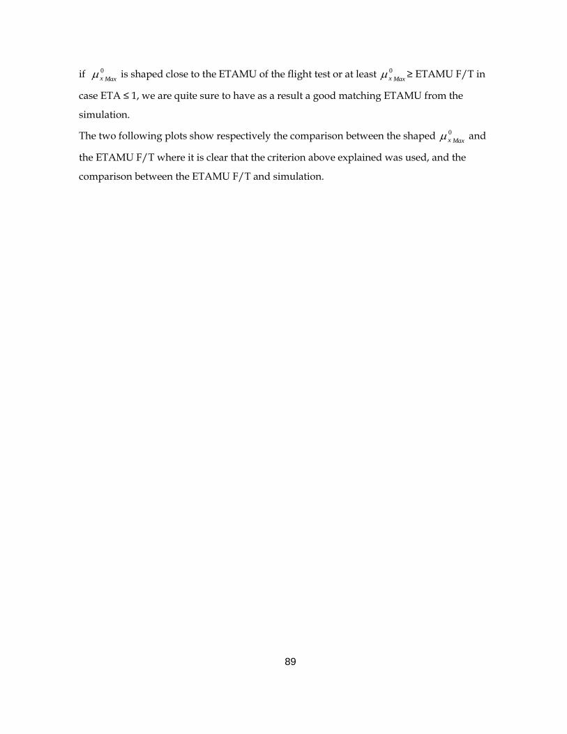
89

if Maxx

0 is shaped close to the ETAMU of the flight test or at least Maxx

0 ≥ ETAMU F/T in

case ETA ≤ 1, we are quite sure to have as a result a good matching ETAMU from the

simulation.

The two following plots show respectively the comparison between the shaped Maxx

0 and

the ETAMU F/T where it is clear that the criterion above explained was used, and the

comparison between the ETAMU F/T and simulation.

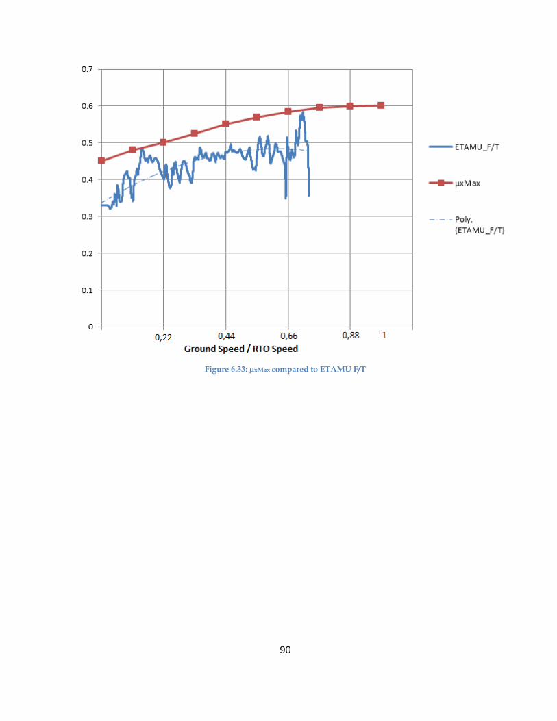
90

Figure 6.33: µxMax compared to ETAMU F/T

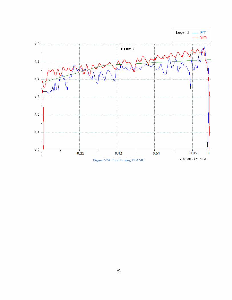
91

Figure 6.34: Final tuning ETAMU

V_Ground / V_RTO

ETAMU

Legend: F/T

Sim

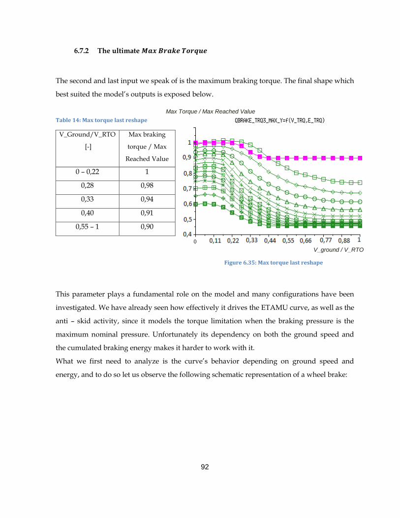
92

6.7.2 The ultimate 𝑴𝒂𝒙 𝑩𝒓𝒂𝒌𝒆 𝑻𝒐𝒓𝒒𝒖𝒆

The second and last input we speak of is the maximum braking torque. The final shape which

best suited the model’s outputs is exposed below.

Table 14: Max torque last reshape

V_Ground/V_RTO

[-]

Max braking

torque / Max

Reached Value

0 – 0,22 1

0,28 0,98

0,33 0,94

0,40 0,91

0,55 – 1 0,90

This parameter plays a fundamental role on the model and many configurations have been

investigated. We have already seen how effectively it drives the ETAMU curve, as well as the

anti – skid activity, since it models the torque limitation when the braking pressure is the

maximum nominal pressure. Unfortunately its dependency on both the ground speed and

the cumulated braking energy makes it harder to work with it.

What we first need to analyze is the curve’s behavior depending on ground speed and

energy, and to do so let us observe the following schematic representation of a wheel brake:

Figure 6.35: Max torque last reshape

V_ground / V_RTO

Max Torque / Max Reached Value

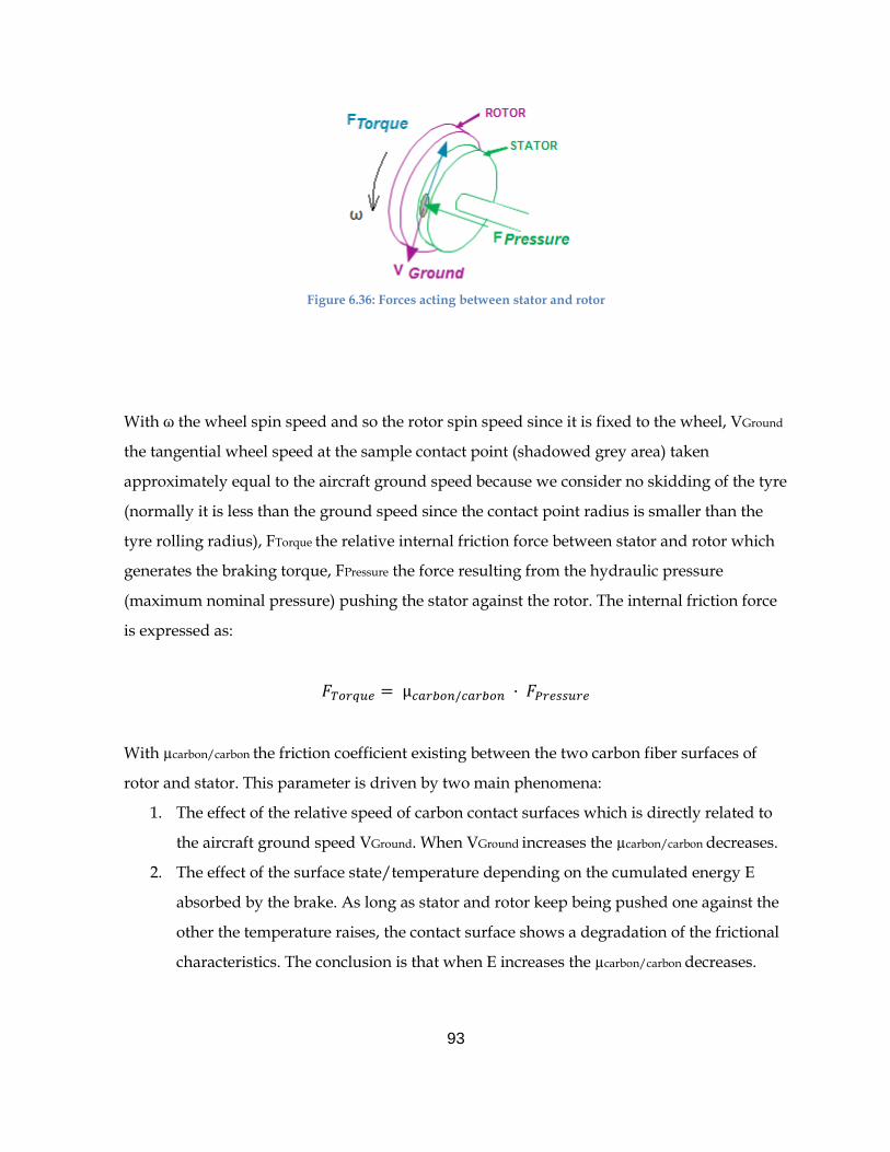
93

Figure 6.36: Forces acting between stator and rotor

With ω the wheel spin speed and so the rotor spin speed since it is fixed to the wheel, VGround

the tangential wheel speed at the sample contact point (shadowed grey area) taken

approximately equal to the aircraft ground speed because we consider no skidding of the tyre

(normally it is less than the ground speed since the contact point radius is smaller than the

tyre rolling radius), FTorque the relative internal friction force between stator and rotor which

generates the braking torque, FPressure the force resulting from the hydraulic pressure

(maximum nominal pressure) pushing the stator against the rotor. The internal friction force

is expressed as:

𝐹𝑇𝑜𝑟𝑞𝑢𝑒 = µ𝑐𝑎𝑟𝑏𝑜𝑛/𝑐𝑎𝑟𝑏𝑜𝑛 · 𝐹𝑃𝑟𝑒𝑠𝑠𝑢𝑟𝑒

With µcarbon/carbon the friction coefficient existing between the two carbon fiber surfaces of

rotor and stator. This parameter is driven by two main phenomena:

1. The effect of the relative speed of carbon contact surfaces which is directly related to

the aircraft ground speed VGround. When VGround increases the µcarbon/carbon decreases.

2. The effect of the surface state/temperature depending on the cumulated energy E

absorbed by the brake. As long as stator and rotor keep being pushed one against the

other the temperature raises, the contact surface shows a degradation of the frictional

characteristics. The conclusion is that when E increases the µcarbon/carbon decreases.

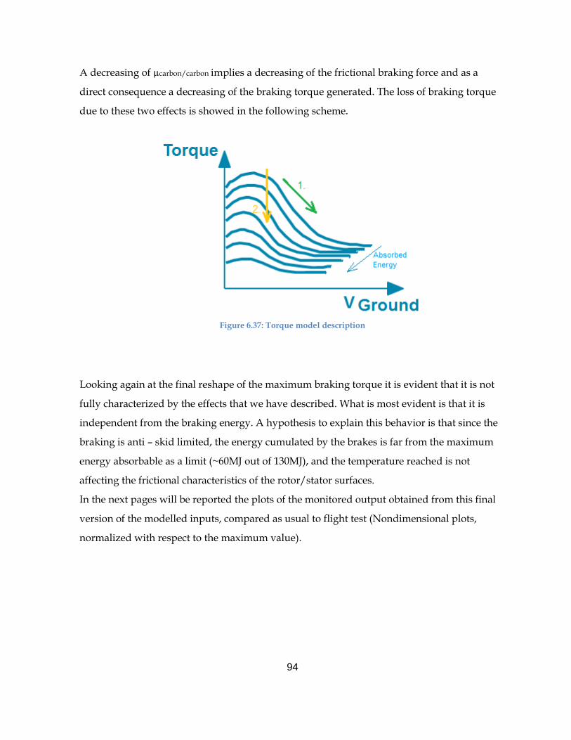
94

A decreasing of µcarbon/carbon implies a decreasing of the frictional braking force and as a

direct consequence a decreasing of the braking torque generated. The loss of braking torque

due to these two effects is showed in the following scheme.

Figure 6.37: Torque model description

Looking again at the final reshape of the maximum braking torque it is evident that it is not

fully characterized by the effects that we have described. What is most evident is that it is

independent from the braking energy. A hypothesis to explain this behavior is that since the

braking is anti – skid limited, the energy cumulated by the brakes is far from the maximum

energy absorbable as a limit (~60MJ out of 130MJ), and the temperature reached is not

affecting the frictional characteristics of the rotor/stator surfaces.

In the next pages will be reported the plots of the monitored output obtained from this final

version of the modelled inputs, compared as usual to flight test (Nondimensional plots,

normalized with respect to the maximum value).

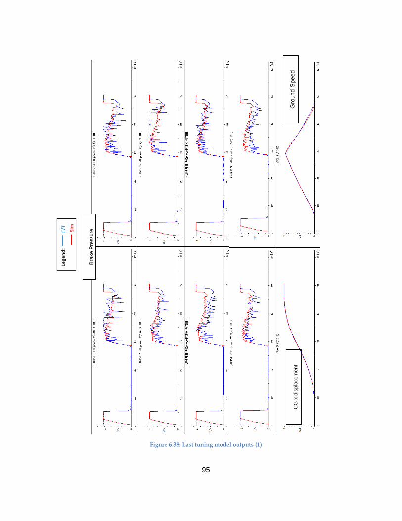
95

Figure 6.38: Last tuning model outputs (1)

Bra

ke P

ressure

CG

x d

ispla

cem

ent

Gro

un

d S

pe

ed

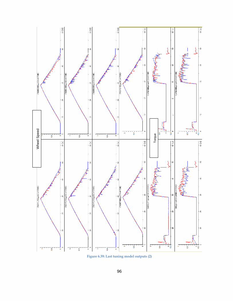
96

Figure 6.39: Last tuning model outputs (2)

Whee

l S

pe

ed

To

rque

97

Figure 6.40: Last tuning model outputs (3)

Slip

Ratio

Fx

Lo

ad

on

L+

R g

ea

rs

Z L

oad F

acto

r

X L

oad F

acto

r

ET

AM

U

98

Figure 6.41: Last tuning model outputs (4)

Energ

y

99

Figure 6.42: Last tuning model outputs (5)

To

rque H

isto

ry

V_Ground

V_

gro

und

/ V

_R

TO

100

6.8 FURTHER SENSITIVITY ANALYSIS

In order to flatten the track for future studies and tunings of the OSMA anti – skid platform

another tests campaign was performed to understand which of the parameters involved in

the GRM adjustment has a greater impact on the model, and which of the monitored output

is mainly affected. The difference with the previously reported sensitivity analysis consists in

taking into account all the simulated outputs and not only the ETAMU, allowing us to have a

wider control of the platform’s evolution.

The analysis has been characterized by two phases, for both of them the initial configuration

is the reference simulation with all the input parameters of the GRM adjustment set to the

value they had in the most satisfactory simulation, the one described in chapter 6.7.

6.8.1 First Phase Sensitivity

Starting from this adjustment, the first phase consisted in choosing for each input two

symmetrical values in the neighborhood of the central starting value, one being a ∆%

decreased and the other being the same ∆% but increased, we will call them respectively Left

(L) ∆% and Right (R) ∆%. The simulation was launched for both the extremes, while all the

other inputs were maintained constant to the starting values, and the results tabulated in

spreadsheet files. It has been created a Matlab script whose target was to:

Load each of the eight monitored outputs for the reference simulation, the L ∆%

simulation, the R ∆% simulation and the flight test: eight column vectors all with a

length of 101000 cells, describing the time history of each output during the 50.5

seconds of the braking phase, considering a simulation clock of 0.0005s.

Cut each vector using a time window going from 35s to 40s, where the braking phase

is concentrated, in order to focus the analysis of each output on the mentioned time

frame of interest.

Compute a polynomial of the 3rd order for each vector, describing the signal

smoothed from the skid cycles.

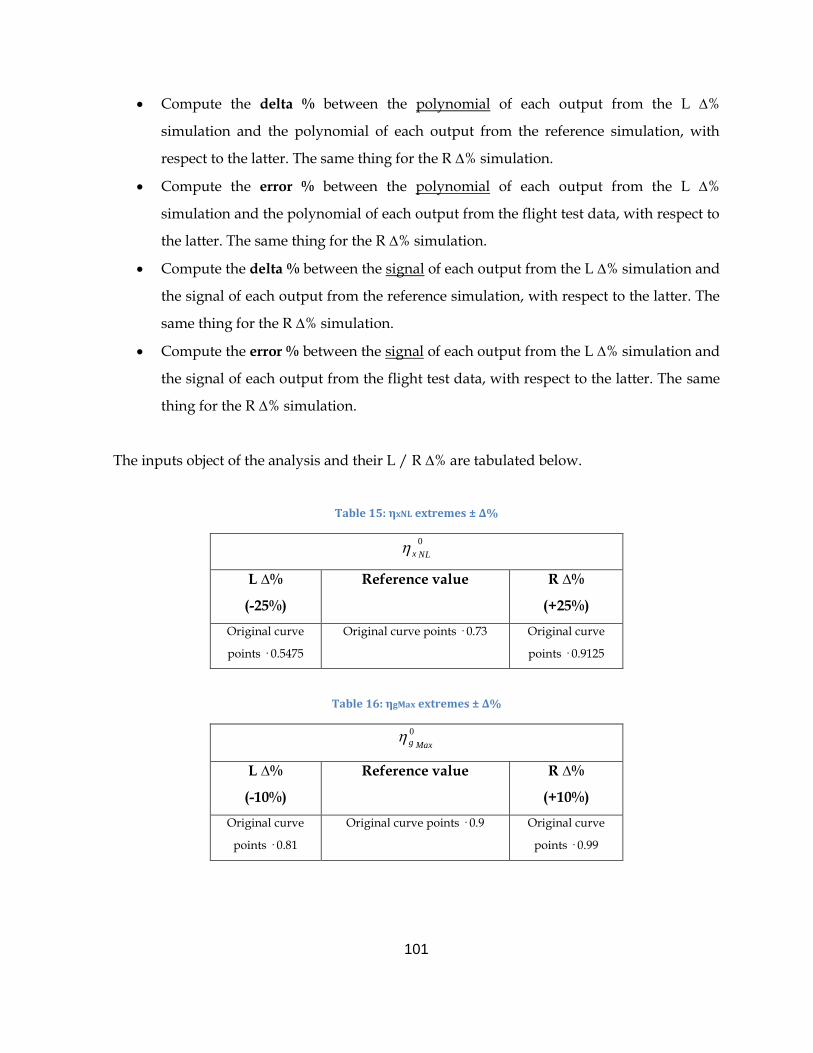
101

Compute the delta % between the polynomial of each output from the L ∆%

simulation and the polynomial of each output from the reference simulation, with

respect to the latter. The same thing for the R ∆% simulation.

Compute the error % between the polynomial of each output from the L ∆%

simulation and the polynomial of each output from the flight test data, with respect to

the latter. The same thing for the R ∆% simulation.

Compute the delta % between the signal of each output from the L ∆% simulation and

the signal of each output from the reference simulation, with respect to the latter. The

same thing for the R ∆% simulation.

Compute the error % between the signal of each output from the L ∆% simulation and

the signal of each output from the flight test data, with respect to the latter. The same

thing for the R ∆% simulation.

The inputs object of the analysis and their L / R ∆% are tabulated below.

Table 15: ηxNL extremes ± ∆%

0

NLx

L ∆%

(-25%)

Reference value R ∆%

(+25%)

Original curve

points · 0.5475

Original curve points · 0.73 Original curve

points · 0.9125

Table 16: ηgMax extremes ± ∆%

Maxg

0

L ∆%

(-10%)

Reference value R ∆%

(+10%)

Original curve

points · 0.81

Original curve points · 0.9 Original curve

points · 0.99

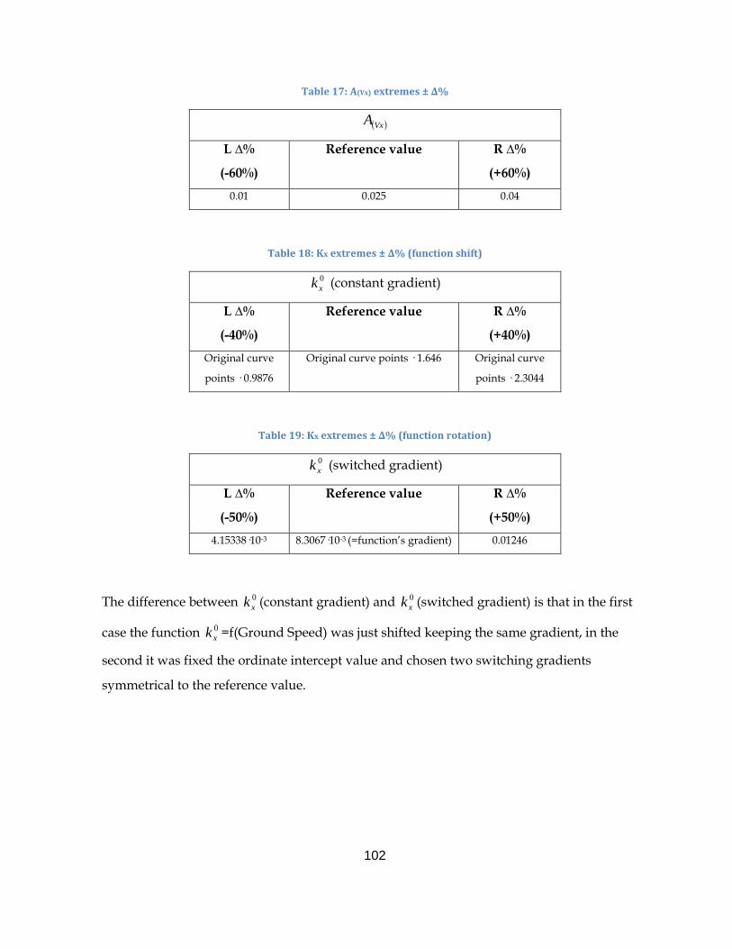
102

Table 17: A(Vx) extremes ± ∆%

VxA

L ∆%

(-60%)

Reference value R ∆%

(+60%)

0.01 0.025 0.04

Table 18: Kx extremes ± ∆% (function shift)

0

xk (constant gradient)

L ∆%

(-40%)

Reference value R ∆%

(+40%)

Original curve

points · 0.9876

Original curve points · 1.646 Original curve

points · 2.3044

Table 19: Kx extremes ± ∆% (function rotation)

0

xk (switched gradient)

L ∆%

(-50%)

Reference value R ∆%

(+50%)

4.15338·10-3 8.3067·10-3 (=function’s gradient) 0.01246

The difference between 0

xk (constant gradient) and 0

xk (switched gradient) is that in the first

case the function 0

xk =f(Ground Speed) was just shifted keeping the same gradient, in the

second it was fixed the ordinate intercept value and chosen two switching gradients

symmetrical to the reference value.

103

Figure 6.43: Kx analysis

The example plots of the above mentioned calculation will clarify the process, the input taken

as example is VxA . Note: index (1) and (2) in the legend correspond respectively to the

output coming from a L ∆% and from a R ∆% of the input.

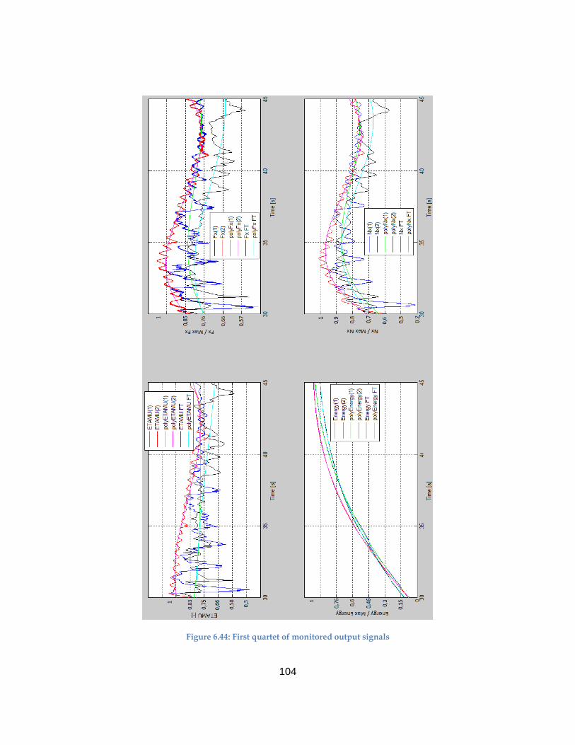
104

Figure 6.44: First quartet of monitored output signals

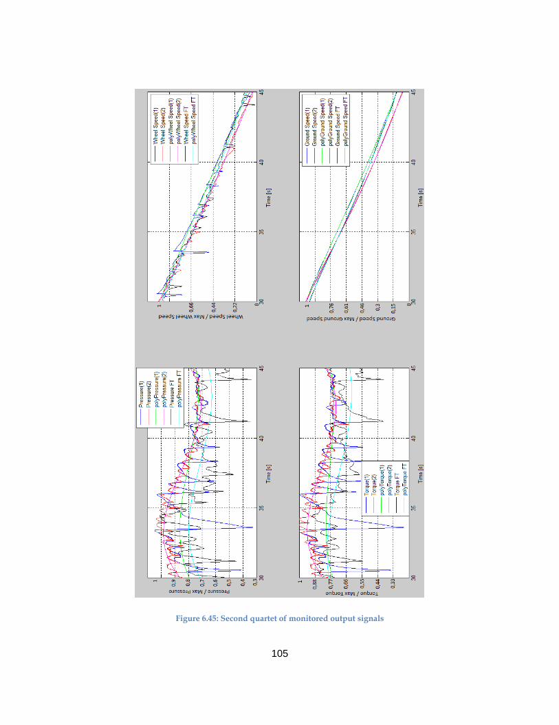
105

Figure 6.45: Second quartet of monitored output signals

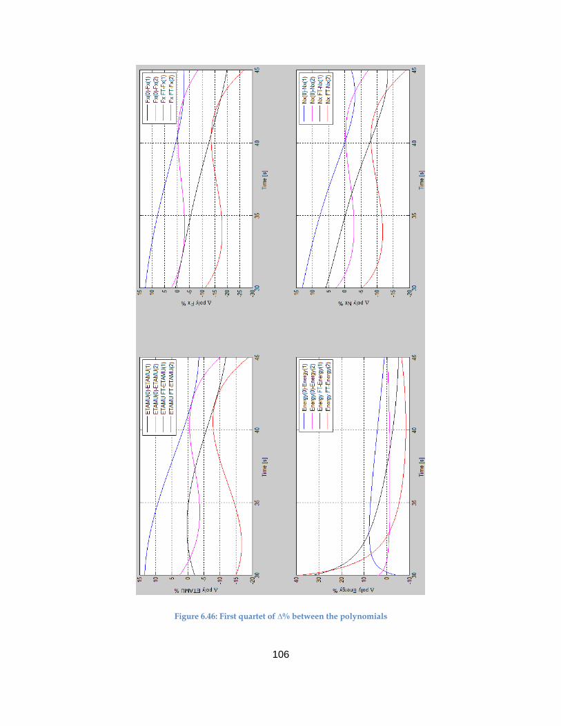
106

Figure 6.46: First quartet of ∆% between the polynomials

107

Figure 6.47: Second quartet of ∆% between the polynomials

108

Figure 6.48: First quartet of ∆% between the signals

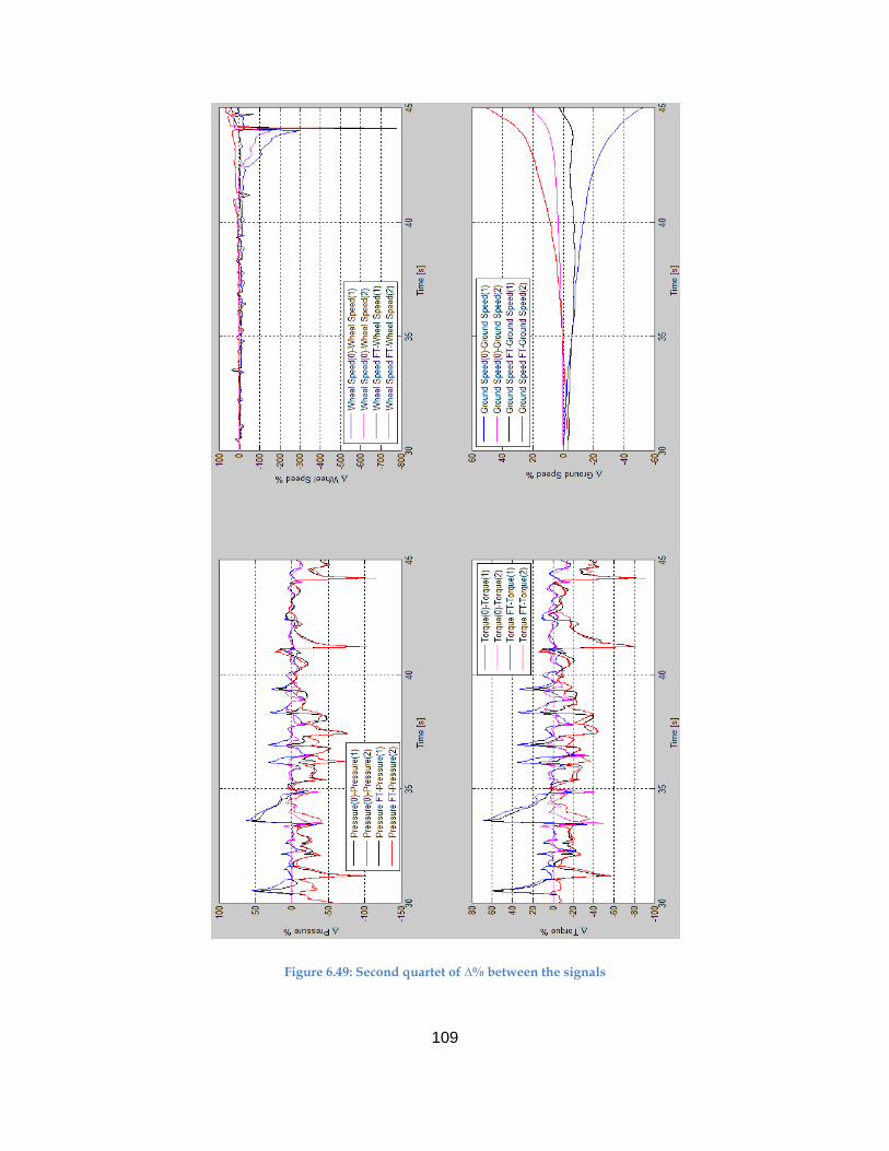
109

Figure 6.49: Second quartet of ∆% between the signals

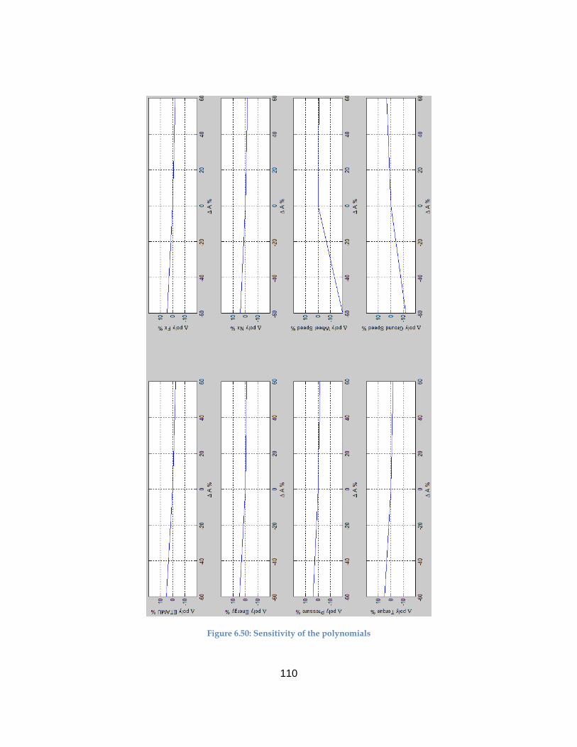
110

Figure 6.50: Sensitivity of the polynomials

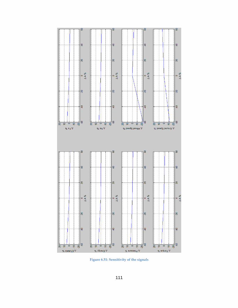
111

Figure 6.51: Sensitivity of the signals

112

The last two figures are the most meaningful because they show the average percent

variation of one output with respect to its reference value, corresponding to the two extremes

R / L ∆% of the input. The sensitivity of the output to the input is just the slope of the straight

line. What is more important is the information we gain from the sign: we can read if the

output increases or decrease respectively with an increasing or decreasing input % variation.

The ordinate always has its maximum corresponding to the maximum delta % among all the

outputs, so that we have an immediate understanding of the relative sensitivity of all the

other outputs.

Taking into account both the average delta % of the polynomials as well as of the cycling

signals, we manage to analyze how the trend of the signal evolves with the variation of the

input, but also how the skids react to this variation. We can observe that the cycling signals

are characterized by a delta only slightly greater than the polynomials, and they keep the

same order of magnitude (the order from the less sensitive output to the more sensitive one is

the same for the polynomials and for the cycling signals), meaning that the skids are only

mildly modified (variation of peaks magnitude or temporal shift of the peak). This happens

for all the inputs studied.

In order to have an idea of the global sensitivity of the model to all the studied input

parameters, the main question is: among all the input variations, which of them causes in

average the greatest outputs variation? To answer, what was done is: for a given parameter

was calculated the average ∆% among all the outputs, for the L ∆% and again for the R ∆%.

This was repeated for all the inputs. The histogram of the results shows that the model is

globally most sensitive to a L ∆% of the input VxA which corresponds to a decreasing of

VxA by 60%.

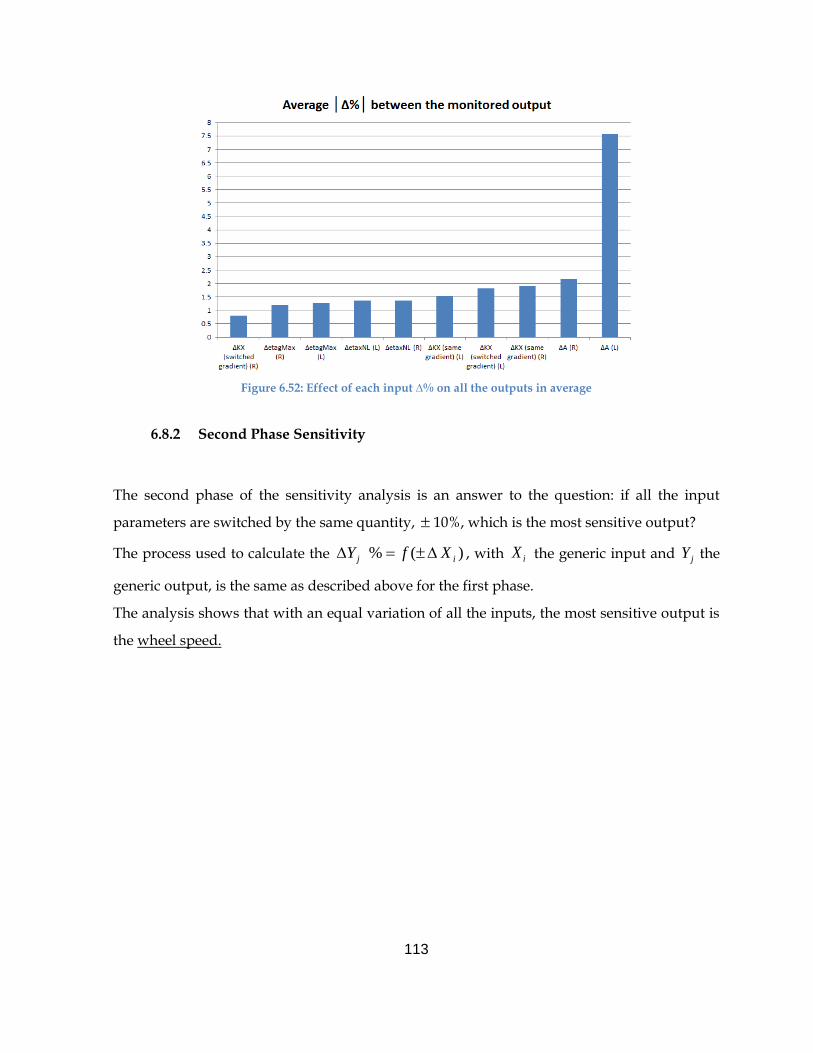
113

Figure 6.52: Effect of each input ∆% on all the outputs in average

6.8.2 Second Phase Sensitivity

The second phase of the sensitivity analysis is an answer to the question: if all the input

parameters are switched by the same quantity, 10%, which is the most sensitive output?

The process used to calculate the )(% ij XfY , with iX the generic input and jY the

generic output, is the same as described above for the first phase.

The analysis shows that with an equal variation of all the inputs, the most sensitive output is

the wheel speed.

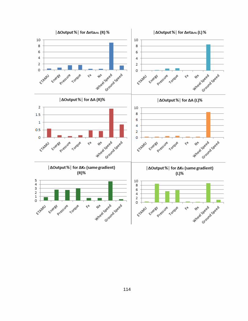
114

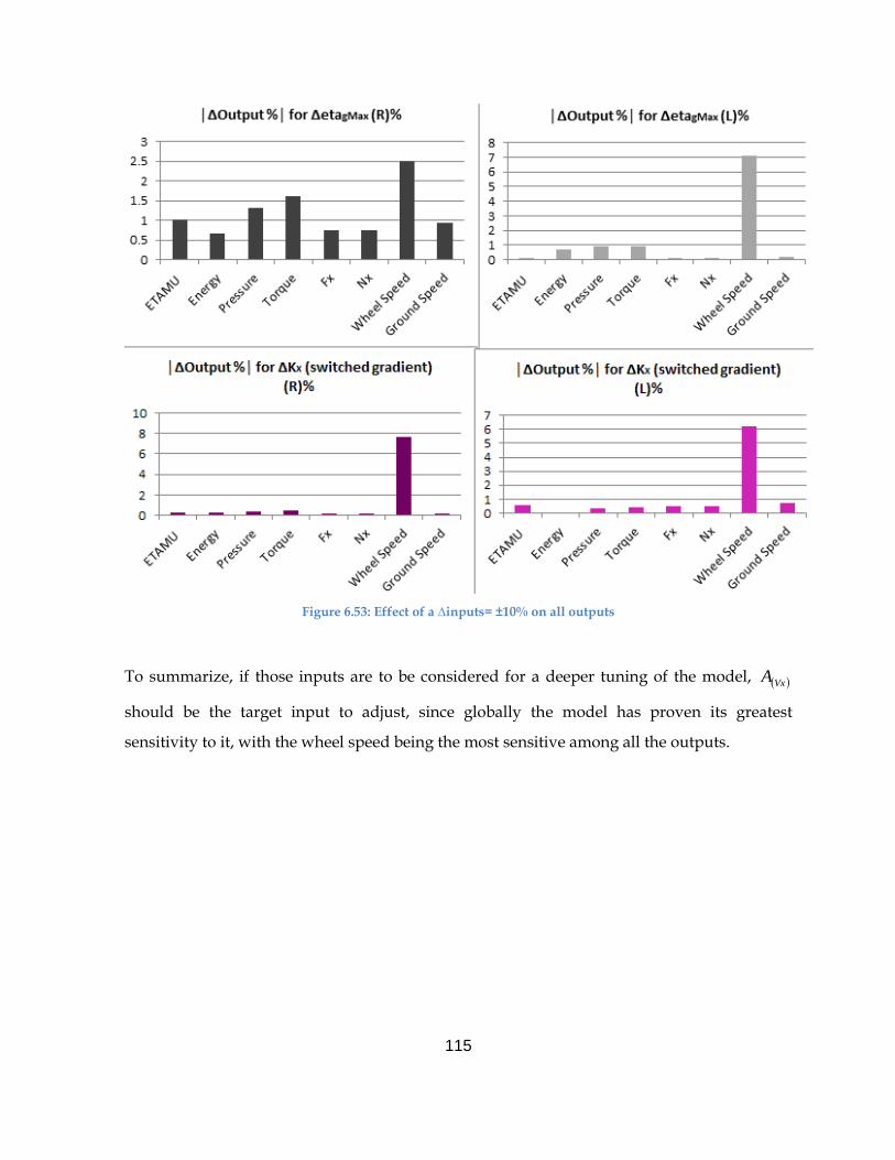
115

Figure 6.53: Effect of a ∆inputs= ±10% on all outputs

To summarize, if those inputs are to be considered for a deeper tuning of the model, VxA

should be the target input to adjust, since globally the model has proven its greatest

sensitivity to it, with the wheel speed being the most sensitive among all the outputs.

116

7. CONCLUSIONS

7.1 REVIEW

This thesis work has focused as a central subject on the modelling of the braking performance

for a commercial aircraft. The regulations about the reference landing distances and

accelerate stop distances are the main constraints for a commercial aircraft manufacturer

company like Airbus, which needs to develop robust and reliable mathematical models to

predict the performance of the aircraft on ground, and certify them to be formally included in

the AFM (Aircraft Flight Manual).

These models take into account the forces and moments determining the trim of the aircraft

during the ground phases of a mission. What emerges from flight tests is that among all the

forces playing a role in the total deceleration, the most effective is the braking force generated

by the braking system installed on the landing gears.

The braking force is a function of the friction coefficient existing in the contact patch between

each tyre and the runway, and of the vertical load on the braked wheels. The latter depends

on the balance between the weight and the aerodynamic forces acting on the aircraft, and its

modelling relies on the accuracy of the calculation of the aerodynamic forces. Normally the

aerodynamic model is not a weak point in predicting the braking force, what is critical is the

friction coefficient and more precisely the global friction coefficient called ETAMU, consisting

of the anti-skid system’s efficiency ETA and the friction coefficient MU.

This parameter is fundamental in the prediction of the braking force and as a consequence of

the stopping distance, and the methods used to compute it are different for a dry or a wet

runway. We showed how the braking force is limited: by the maximum braking torque

generated by the brakes, due to the maximum energy bearable, or by the anti-skid system

which is ceil limited by the maximum friction coefficient, function of the runway state, the

tyre characteristics, the ground speed, the BCSU (Braking & Steering Control Unit). A core

variable giving a measure of the magnitude of the braking is the slip ratio, and the µ-slip

curve representing the dependency of the friction coefficient by the slip ratio itself.

117

The central part of the thesis introduces the TAPAS project, an internal Airbus initiative

proposed to create a common anti-skid Matlab / Simulink platform between all the teams

involved in the development of the anti-skid system, which has been the working target of

the internship during the first months.

Despite the great efforts made in retrieving the four years leftover work, collaborating with

the colleagues in Filton UK, designers of the anti-skid system, the internship’s work on it

gave as a result only the acknowledgment of the platform’s logic, architecture and reasoning

behind, limited to the results already obtained when it was operative.

The six months’ time constraint of the internship then overwhelmed the initial target, and led

to a redefinition of its task, made possible by the recent availability of a freshly developed

anti-skid platform produced by the flight physics department EGY. The platform is based on

the OSMA tool (Outil de Simulation des Mouvements Avion) used in EGY to create

simulation scenarios for the pilot training simulator.

The core work of the thesis is then centred on the analyses and simulations performed with

OSMA.

At first we report an explanation of the structure of an OSMA scenario describing which can

be the inputs and outputs of the simulation, and the models included in the tool’s database

used to reproduce the dynamics of all the aircraft’s integrated systems.

The first case study is then a rejected take-off scenario characterised by a simplified braking

because the Brake Control & Steering model (BCS) is not active. The main character of the

simulation is the Ground Reaction Model (GRM) which includes the entirety of the equations

driving the dynamics of the landing gears, shock absorbers, braking system, tyres and

frictional characteristics of the contact. The GRM though is not capable of simulating the real

anti-skid cycling dynamics.

After getting acquainted with the tool, having used this first scenario as a test bench, the

thesis gets deep into the latest developed capabilities of the braking simulation, with a

realistic rejected take-off scenario.

This time the inputs of the scenario, both the pilot commands and the starting conditions, are

coming from a RTO flight test data injected, so all the actions linked to the pilot commands

are driven precisely as it happened during flight test: from the control of the engines to the

118

deflection of all the aerodynamic surfaces. Additionally, the BCS is active and the outputs

show the typical anti-skid cycling. This simulation is considered to be the first of its kind

since it was demonstrated that OSMA has the capabilities of reproducing the anti-skid

activity for a braking scenario, and this happened also thanks to a first brief adjustment made

by an EGY colleague who is GRM modeller, to some parameters, especially µ-slip curve and

brake torque parameters.

The thesis work developed naturally following the tuning of these parameters, targeted to a

better match of flight test data, mostly focusing on the ETAMU to guarantee that the braking

performance is well predicted, but also making sure that the anti-skid cycling was evident

and satisfactory. The tuning was preceded and followed by a sensitivity analysis of the model

to its parameters in order to focus on the most effective modifications among all the

adjustments. The first in pre-tuning phase was targeting this thesis work, the second in post-

tuning phase to smoothen the track to those who will improve this work.

7.2 FUTURE WORK

The thesis work has provided with the baseline to perform a braking simulation taking into

account the complete anti-skid dynamics of the braking system into a simulation tool that has

always been used to predict the braking performance at a higher level. The tuning of the

frictional and torque characteristics has proved to fit the RTO flight test subject of the

analysis. The future work of this project will aim at continuing investigating and studying the

tuning of the model, in particular intended to:

1. Continuing a deeper and more accurate sensitivity analysis of the model to the

already studied input parameters, enlarging it to all the other variables describing the

µ-slip curve implemented in the GRM or which are supposed to have an impact on

the simulation.

2. Starting from the most affecting parameters, improve the tuning to have a better

representation of the flight test object of this work.

119

3. Validate the tuning with a sufficient number of flight tests, and prove it to be a robust

modelling.

4. Build a process through which computing the µ-slip curve from flight test data and

create a representative µ-slip curve to be implemented into the GRM.

5. Study the torque model and understand how it could be modified to satisfy the anti-

skid limited cases.

6. Investigate more the response of rubber’s frictional characteristics to the excitation

frequency and to rising temperatures. Take into consideration the adding of these

effects to the GRM to drive a more realistic evolution of the µ-slip curve.

120

BIBLIOGRAPHY

[1] Airbus Customer Services. Getting to grips with aircraft performance. Blagnac: Flight

Operations Support & Line Assistance, 2002.

[2] Logan Jones. Modélisation des forces de contact entre le pneu d’un avion et la piste.

Doctorat de l’Université de Toulouse, ISAE – Airbus, 2012.

[3] S. Picaut. Antiskid system principles. Technical report L32D08017874, Airbus, 2008.

[4] M. Miot. Response to LISA. Technical report L00RP0703121, Airbus, 2007.

[5] EGVTV3. A350 Certification Document. Technical report V060RP1400629, Airbus, 2014.

[6] M. Miot. Spécification nouveau modèle roue GRM. Technical report AI-ECM090881, Airbus,

2013.

[7] P. Scantamburlo. OSMA Souple v4.9 User’s manual. Technical report X03UG0600506,

Airbus, 2015.

[8] John A. Tanner, Sandy M. Stubbs and Eunice G. Smith. Behavior of Aircraft Antiskid

Braking Systems on Dry and Wet' -Runway Surfaces, Hydromechanically Controlled

System. NASA Technical Paper, August 1981.