unit 12 advanced features of microsoft excel

Advanced Features ofMicrosoft Excel

207

UNIT 12 ADVANCED FEATURES OFMICROSOFT EXCEL

Structure12.1 Introduction

12.2 Using Formulas, Functions and Macros12.2.1 Entering Formulas

12.2.2 Entering Date and Time Formulas

12.2.3 Converting Formulas to Values

12.2.4 Inserting Range Names in Formulas

12.3 Entering Functions12.3.1 Entering Function Manually

12.3.2 Paste Function

12.3.3 Editing Functions

12.4 Macros12.4.1 Creating and Storing Macros

12.4.2 Running a Macro

12.5 Printing Worksheet Data12.5.1 Printing an Area

12.5.2 Defining and Deleting a Print Area

12.5.3 Printing Worksheets

12.5.4 Inserting and Removing Page Break

12.5.5 Modifying Page Setup

12.6 Creating Headers and Footers12.6.1 Using Built-in Headers and Footers

12.6.2 Custom Headers and Footers

12.7 Protecting Data Within Workbooks12.7.1 Password to Open a File

12.7.2 Password to Modify a File

12.7.3 Creating the Backup Option

12.7.4 Removing Protection and Modification Passwords

12.7.5 Workbook Level Protection

12.7.6 Protection and Security at Worksheet Level

12.7.7 Cell Protection

12.8 Sharing Data With Other Applications12.8.1 Inserting Pictures into Worksheets

12.8.2 Inserting or Linking to a Worksheet

12.8.3 Embedding an Excel Object in Another Application

12.9 Working With Data Forms Using Lists12.9.1 Adding Records with Data Forms

12.9.2 Deleting Records with Data forms

12.9.3 Finding Records with Data Form

12.9.4 Sorting Data in a List

12.9.5 Filtering Data in a List

12.9.6 Using the Autofilter

12.9.7 Setting Custom Categories

12.10 Pivot Tables

12.11 Let Us Sum Up

12.12 Check Your Progress Exercise

12.13 Answers to Check Your Progress Exercise

208

UnderstandingComputer Applications 12.1 INTRODUCTION

In this unit we will introduce several advanced features of Microsoft Excel. These arerelated to using formulas, functions and macros, creating headers and footers in theworksheet, protecting data within the worksheet, inserting picture into worksheet etc.One feature which we use quite often in MS Excel is MACRO. Macros automatefragmentally performed tasks by changing them into a set of keystrokes that are storedor recorded and are assigned a control key. Whenever the specified control key is used,the entire operation is performed automatically. You can have macros for formattingworksheet, report generation and so on.

Objectives

After going through this unit, you will be able to:

� use formula, function within the worksheet,

� edit functions,

� define macros,

� print worksheet data,

� create headers and footers,

� protect data within workbooks, and

� share data with other applications.

12.2 USING FORMULAS, FUNCTIONS ANDMACROS

In this section we will study about how to enter formulas, enter date and time formulas,converting formulas to values, inserting range name in formulas. So let us get started.

12.2.1 Entering Formulas

Formulas provide the power while analyzing and creating functioning spreadsheet systemsin Excel. Various numeric calculations can be very conveniently accomplished by the useof formulas. You can also manipulate text and lookup values in tables.

Formulas can be created in following ways:

(i) To enter a formula manually into a cell, the steps are:

1. Select the cell in which you want to enter the formula.

2. Enter the formula you want preceded by an equal to (=) sign.

When you press the Enter key, the resulting value would be displayed in the specifiedcell.

(ii) You can point to cells rather than typing cell references in the formula. It hastensthe tasks of formula creation as well as reduces the chances of errors. To build aformula by pointing, the steps are:

1. Select the cells in which you want the formula.

2. Type the equal to (=) sign to start the formula.

3. Click on the cells with the reference that is required in the formula.

4. Optionally, enter an arithmetic operator, such as, +, -, *, / or %, or a comparisonoperator such as <, > = or text operator like the ampersand (&).


209

5. Click on the next cell that you want to include in the formula.

6. Click on the check box in the formula entry.

The arithmetic operators used in formulas for addition, subtraction, multiplication, division,+, -, *, / are used respectively. In addition, exponent (^), percentage (%), text operator(&) and comparison operators like =, <, >, <=, >= are used in formulas.

Most errors occur when the arithmetic operators are not in the proper order of precedence.Negative (–), Percentage (%), Exponential (^), Multiplication and Division (* and /),Addition and subtraction (+ and –), joining Text (&), Comparison operators (=,<,>,<=,>=,<>)

i) Is the order of precedence.

Two examples are discussed hereunder:

14+9*5

In this example, multiplication would be performed before addition.

70/2*5

Order of precedence in the example states that multiplication and division operators areat the same level. Since the division operator is prior to multiplication, seventy would firstbe divided by two and then the result of the division would be multiplied by five.

12.2.2 Entering Date and Time Formulas

You can create formulas to calculate values by using dates and time. For excel to recognizedate and time that you enter in the formula, you need to specify it in the correct format.You need to enclose the entry in double quotation marks. Excel would then give therequired result. To find out the difference of two dates, the format is : = “12/4/”-“4/4”.Excel would return the value 244 days. An example to calculate hours difference is =HOUR (“4:30:00− “3:30:00”). This would display the result 1. # VALUE! is an errormessage displayed by Excel when it cannot recognize a date or time.

12.2.3 Converting Formulas to Values

Most of the times when you create a formula, you would only want to view its result andnot the formula, which is normally displayed on the formula bar. In such a situation, youcan convert the formula to its actual value. To convert a single formula to a value, thesteps are:

1. Select the cell that contain the formula.

2. Double-click on the cell or press the F2 function key.

3. Press the F9 function key.

Excel now shows only the result and not the formula.

Debugging Formulas

While entering formulas, it is possible that you might make errors. In such situations,Excel displays an error value list that enables you to debug your formulas.

Working with Range Names

Name is an identifier that represents a cell or a range. You can define names to representdata in formulas that are easier to use and understand. For example, =Sum(Marks). Todefine a name, the steps are:

Check box

210

UnderstandingComputer Applications

1. Select the cell or range of cells you want to name.

2. Click on the Name Box located at the left end of the formula bar.

3. Enter the name you want to give to the selected range and press ENTER.

To name a range using the other method, the steps are here under:

1. Select the cell range which has to be named.

2. Select the Name option from Insert menu.

3. Select the Define option from the Name submenu.

The Define name dialog box gets invoked as shown in Figure 12.1.

4. Type a name in the Name in workbook text box. There should be no space in rangednames. The first character of a range name should be a letter or underline.

5. Click on the OK button.

12.2.4 Inserting Range Names in Formulas

You can insert a name into the formula. The steps are:

1. Create a formula that can use the name and type the (=) equal to symbol in a cell.

2. Select the Name option from the Insert menu.

3. Select the Paste option from the Name submenu.

The Paste Name dialog box gets invoked.

1. In the Paste Name drop-down list, select the name you want to insert.


3. Enter the rest of the formula and press Enter.

For example, to sum the marks of 25 students, enter the marks of the 25 students in 25contiguous cells. Give a name to the range of cells namely Marks. Enter the formula=SUM(in a cell. Select the name option from the Insert menu. Select the Paste optionfrom the Name submenu. The formula in the cell now becomes =SUM(Marks). Alwayscomplete the formula by adding the closed brackets. Press the Enter key. This shows youthe sum of the marks of the 25 students.

Deleting Range Names

If you change the contents of the range, you may want to change the range name also, ordelete the name if it is no longer suitable for the contents that it contains. To delete aname, the steps are:

1. Select the Name option from the Insert menu.

2. Select the Define option from the Name submenu.

Figure 12.1: Define Name dialog box


211

3. The Define Name dialog box gets invoked.

4. In the Name in workbook drop-down list, select the range name you want todelete.

5. Click on the Delete button.


12.3 ENTERING FUNCTIONSExcel functions help in performing simple to complex arithmetic calculations. There are200 built-in functions or predefined formulas that enable you to create formulas for awide range of application including business, scientific and engineering applications.

Functions can be entered in the following ways:

� Entering function Manually

� With the help of the Paste Function

12.3.1 Entering Function Manually

(i) To enter a function in the active cell, type the equal to (=) sign, followed by an openparentheses. You can then specify the cell range you want the function to use andcomplete the function with closed parentheses; for example, =SUM(A2:A8).

(ii) You can use the AutoSum button for quick calculations that involves addition ofnumbers. This button is located on the standard toolbar. To use this feature ofExcel, follow these steps:

1. Select a cell adjacent to the range you want to sum.

2. Click on the AutoSum button

Excel automatically inserts the SUM function and selects the cells in the columnabove the selected cell.

3. You can also highlight the cell range (including a blank cell in which you want thetotal) that you want to sum and then click on the AutoSum button.

Excel automatically calculates the total and displays it.

12.3.2 Paste Function

The Paste Function feature is a convenient way of applying functions to the formulas forcalculations. To use this feature, the steps are:

1. Select the Paste Function button from on the standard toolbar or select the Functionoption from the Insert menu. The Paste Function window is displayed in Figure 12.2.

Figure 12.2: Paste Function Window

212


2. The Function Category list displays the built-in functions of Excel.

3. Select the function that is required by clicking on it and click on the OK button. Aformula palette drops down which prompts you to enter the required arguments asshown in Figure in 12.3.

4. Enter the arguments in the display area or click on the cell reference button to go tothe worksheet to select the cells.

5. Click again on the cell reference button to come back to the same formula palette.

6. Press Enter or click on the OK button.

12.3.3 Editing Functions

Functions also require editing. To modify functions in a formula, the steps are:

1. Select the cell that contains the function which you want to edit.

2. Select the Function option from the Insert menu.

The formula palette is displayed.

1. You can change any of the specified arguments as required.


You can even edit a function by changing the formula entry in the cell. To do so, thesteps are:

1. Select the cell that contains the formula which has to be edited.

2. Click on the formula bar or double-click on the cell.

3. Change the arguments as required.

4. Press Enter or click on the check mark button on the formula bar.

12.4 MACROS

Macros automate frequently performed tasks by changing them into a set of keystrokesthat are stored or recorded and are assigned a control key. Whenever the specifiedcontrol key is used, the entire operation is performed automatically. You can have macrosfor formatting worksheets, report generations and so on. This feature is time saving,flexible and very powerful.

12.4.1 Creating and Storing Macros

You can create a macro in a number of ways. To create a macro, you should have yourprogram in the macro record mode. This can be done by:

Cell reference is specified here

Figure 12.3: Formula Palette


213

1. Selecting the Record New Macro option from the Tools menu as shown in Figure12.4. A Record Macro dialog box gets invoked.

Macro recorder is a tool that translates your actions in Visual Basic Applications (VBA)macro. It works like a tape recorder – when you turn it on, it records everything you do.Later you can run the macro and all the previously performed actions are repeated.

You can name your macro in the Record macro dialog box as shown below. The namethat you specify should not contain spaces or other punctuation marks, but it can containunderscores.

You can assign a shortcut key for the macro that you want to record.

You can specify the letter for your shortcut key and use it in conjunction with Ctrl to runthe macro. The latter can be in lower or upper case; for example, you can assign theCtrl + r shortcut key combinations for a macro that is recorded for generating reports.

You can store macros in the Store macro in text box. The options available are:

l Personal Macro Workbook – which has the name PERSONAL.XLS. This workbookopens and is hidden automatically everytime you start Excel.

l This Workbook – which stores the macro in the active workbook.

l The New Workbook – which stores/records the macro in a new workbook that iscreated.

2. You can click on the OK button and the macro recording processing begins.

3. You can then perform the actions that you want to record. It is a good practice tosave your workbook and the recorded macro that it contains before running themacro.

Figure 12.4: Record Macro Dialog Box

214


Once you have completed all the necessary actions for storing/recording macros,you can click on the stop button as shown in Figure below.

You can also select the Stop Recording option from Macro submenu within theTools menu option.

12.4.2 Running a Macro

You can run a macro in different ways. You can select the Run option from the dialog boxor use the shortcut key that you have assigned to your macro. Given below is an exampleto create a macro.

You can record a macro that can create the given worksheet, by following the steps:

1. Select the Macro from the Tools menu.

2. Select the Record New Macro option from the Macro submenu.

The Record Macro dialog box gets invoked as shown in Figure 12.5

3. Give a name to the macro that you want to record and assign m as a shortcut key.

4. Click on OK.

5. In the Excel worksheet, type the Name, Product, Varieties,Total.

6. Type in the rest of the data shown in the sample worksheet.

7. Click on the Stop button, to end the recording process.

8. Clear the data that you have copied on your worksheet.

9. Run the macro by pressing Ctrl+m.

The entire worksheet would be created again for you.

12.5 PRINTING WORKSHEET DATA

Excel offers you various printing options for your worksheets. It enables you to have apreview of worksheet data with the aid of the Print Preview option. You can set margins,fonts, headers and footers to enhance your worksheets.

12.5.1 Printing an Area

By default, Excel prints the current worksheet when the Print command is selected fromthe File menu. However, if you require a particular area of the worksheet to be printed,then you are offered this facility also. To do so, you can follow these steps:

Figure 12.5: Record Macro dialog box


215

1. Select the range that you want to print.

2. Select the Print option from the File menu.

The Print dialog box gets invoked as shown in Figure 12.6.

3. In the Print What section of the dialog box, choose the Selection option.

4. Select the OK option to complete the procedure.

12.5.2 Defining and Deleting a Print Area

There may be situations where you need to print the same range repeatedly. To avoidthe tedium of specifying the same range for printing several times, you can convenientlydefine range as the print area.

To define the print area, you can follow these steps:

1. Select the area you want to specify.

2. Select the Print Area option from the File menu.

3. Select the Set Print Area from the Print Area submenu as shown in Figure 12.7.

4. Select the Print option from the File menu.


6. You can select Clear Print Area when you want to remove the defined Print Area.

Figure 12.6: Print Dialog Box

Figure 12.7: Print Area Window

216


12.5.3 Printing Worksheets

Worksheets can be very conveniently printed by the use of the Print command that sendsyour worksheet pages to the printer immediately.

To print worksheets, the steps are:

1. Select the Print option from the File menu. This invokes the Print dialog box.

This dialog box is very similar as you used in the MS-Word Print dialog box. Theonly difference is the three extra – buttons which are given below:

Selection – prints selected cells.

Active sheet(s) – prints only selected worksheets.

Entire Workbook – prints open workbook.

Device Options : controls the print quality and allows you to adjust Printer memorytracking (this affects how the driver tracks printer memory usage).

12.5.4 Inserting and Removing Page Break

Whenever a print area is defined, Excel automatically inserts page break into theworksheet. Page break gets displayed in the form of dashed lines. If the page breaks arenot according to your choice, you can insert the page breaks yourself. There are twotypes of page breaks that you can insert:

• Vertical page breaks, and

• Horizontal page breaks.

Inserting Vertical Page break

To insert a vertical page break, the steps are:

1. Click on the heading of the column to the right of text where you want your pagebreak. The column gets highlighted.

2. Select the Page Break option from the Insert menu.

Inserting a Horizontal Page Break

To insert a horizontal page break, the steps are:

1. Click on the heading of the row below where you want your page break to beinserted.

2. Select the Page Break option from the Insert menu.

3. You can select the Remove Page Break option from the Insert menu to remove allpage breaks.

You can also select the Page Break Preview from View menu. Page breaks are displayedon the screen in thick blue lines while page numbers are displayed in large grey text. Tomake changes in page breaks, place your mouse pointer on the page break and, when itturns into a double-headed arrow, drag the line to the new position. To get back to thenormal view, select the normal option from the view menu.

12.5.5 Modifying Page Setup

The Page settings can be setup by using the Page Setup command. This help you tocontrol the basic layout of the printed pages, change the margins, text alignment and setthe print titles.


217

Setting Print Titles

You can set print titles so that information about column, row headings get displayed oneach page in the printout.

To create print titles, the steps are:

1. Select the Page Setup option from File menu. The Page Setup dialog box will openas shown in Figure 12.8.

2. Select the Sheet tab from the Page Setup dialog box.

3. If you want to define titles across the top of each page, select the Rows to repeatat top box. If you want to define titles down the left side of each page, select thecolumn to repeat at left box.


Removing Print Titles

You can remove the print titles by following the steps here under:

1. Select the Page Setup option from the File menu.

2. Select the Header/Footer tab as shown in Figure 12.9.

3. Click on the arrow next to the Header box.

4. Select a header from the drop-down list.

5. Select the data that you want to use as footer from the list.


12.6 CREATING HEADERS AND FOOTERSYou can format headers and footers by selecting the Header/Footer tab available on thePage Setup dialog box. Headers are printed at the top of every page and they arecommonly used for report titles, chapter names, company names, and so on. Footers aremainly used for specifying page numbers, or total number of pages, and are printed at thebottom of each page. There are a variety of built-in headers and footers from which youcan select or define your own headers and footers.

12.6.1 Using Built-in Headers and Footers

To use the built-in headers and footers, the steps are:

1. Select the Page Setup option from File menu.

2. Select the Header/Footer tab as shown in Figure 12.9.

Figure 12.8: Page Setup Dialog Box

218


3. Click on the arrow next to the Header box.4. Select a header from the drop-down list.5. Select the data that you want to use as footer from the list.6. Click on the OK button.

12.6.2 Custom Headers and Footers

To define your own headers and footers, the steps are:

1. Select the Page Setup option from the File menu.

2. Select the Header/Footer tab.

3. Select the Custom Header option to display the Header dialog box as shown inFigure 12.10.

This dialog box has three text boxes – left section, center section and right section.These text boxes allow you to justify the text of your headers and footers. Data can beleft-aligned, centered or right-aligned. The buttons that are displayed above the text boxesare used to insert the codes. The Date code, for example, inserts the current date. Toapply text formatting to the header or footer information, click on the Font button todisplay the Font dialog box. The buttons on the Custom headers and their functions arelisted in the table which is given below:

Button Function

Font Format Invokes the font dialog box

Page Number Inserts the page number

Total pages Inserts the total number of pages

Current date Inserts the current date

Current time Inserts the current time

Worksheet name Inserts the name of the active sheet

Figure 12.9: Page Setup Dialog Box

Figure 12.10: Changing column width


219

12.7 PROTECTING DATA WITHIN WORKBOOKSProtection against loss or corruption of worksheet data has always been a matter ofgreat concern. This important issue has been dexterously dealt by Excel. There areseveral levels of protection that can be applied to a workbook.

12.7.1 Password to Open a File

The top-most level of protection is set at the file level, which offers several protectionoptions. In this level of protecting data:

� User needs to enter a password to open the file.

� You can make your files read-only so that the data is not deleted or altered byaccident or intention.

To apply a password for protecting files, the steps are:

1. Select the Save As option from the File menu. The Save As dialog box gets invokedas shown in Figure 12.11 (a):

2. Click on the Options button. The Save Option dialog box gets invoked as shown inFigure 12.11 (b).

3. Enter the password you want to use for the file in the Password to open area ofthe Save Options dialog box. This invokes the Confirm Password dialog box displayedin Figure 12.11 (c).

4. Re-enter the password to proceed in the Confirm Password dialog box and clickon the OK button. The Save As dialog box is displayed again.

Figure 12.11 (a) : Save As Option in File Menu

Figure 12.11 (b) : Save Option Dialog Box

Figure 12.11 (C) : Confirm Password Dialog Box

220


5. Click on the Save button in the Save AS dialog box.

6. If the Replace Existing File dialog box gets invoked, then click on Yes to implementpassword protection.

12.7.2 Password to Modify a File

The password that is set is to open or access the workbook. This password is used onworkbooks that contain vital information that needs to be kept confidential and protectedfrom getting corrupted. This option only allows a user to open the file. To save modificationsto a file, you can set a password that a user can enter to save the changes.

Entering a password in the password to modify text box in the Save Options dialog boxpermits a user to open a workbook in the read-only mode. The user can view andmanipulate data but cannot save the changes made to the workbook without the knowledgeof the password.

Setting the Read-Only Option

The Save Options dialog box contains a read-only recommendation option which you canactivate so as to make your workbooks read-only.

12.7.3 Creating the Backup Option

The Save Options dialog box has an option for creating backups.

When activated, it creates backups because the Always create backup setting has beenapplied. Every time the file is saved, Excel creates a backup. You can open this backupfile when the original file is corrupted. Backup files are saved as backups of the filename.They have an extension .XLS and reside in the same folder as the original file.

12.7.4 Removing Protection and Modification Passwords

To remove the password protection from a file, the steps are:

1. Open the workbook that has the password for itself.

2. Select the Save As option from the File menu.

3. Click on the Options button.

Clear the password(s)

Asterisks will get displayed when there is a password.

4. Click on the OK button. The Save Options dialog box closes.

5. Now click on the save option to save the file.

6. Click on Yes when the Replace Existing File dialog box gets invoked.

There are three other levels of protection with workbooks that maintain data security atthe

� Workbook level.

� Worksheet level.

� Object (cells and graphical objects) level.

12.7.5 Workbook Level Protection

A user can be restricted to use or change the workbook data even when the user has theaccess to it. To implement security at the workbook level, the steps are:


221

1. Select the Protection option from the Tools menu.

2. Select the Protect Workbook option from the Protection submenu.

The Protect Workbook dialog box is involved as shown in Figure 12.12.

The Protect Workbook dialog box enlists certain options. These are:

• Structure - prevents changes made to worksheet structure. Deleting, inserting,renaming, copying, moving, hiding or unhiding sheet is prevented.

• Windows – checks changes made to workbook windows. Windows control buttonis hidden and its window functions are deactivated.

• Password (optional) – is for optional passwords which can be upto 255 characters,including special characters, and is case-sensitive.

12.7.6 Protection and Security at Worksheet Level

You may want to prevent users from changing the contents of a particular worksheet,which is to say, you may want a user to make changes to one worksheet but not to theothers. You can follow these steps to do so:

1. Select the Protection option from the Tools menu.

2. Select the Protect Sheet option from the Protection submenu.The Protect Sheetdialog box gets invoked as shown in figure 12.13.

The dialog box offers several options. These options allows a user to protect a sheet atvarious levels.

• Contents - protects cells and chart items in a worksheet.

• Objects – protects graphic objects on a worksheet.

• Scenarios – prevents changes to scenario definition.

• Password (Optional) – is case-sensitive and can contain 255 characters, whichcan include special characters.

Figure 12.12 : Protect Workbook Dialog Box

Figure 12.13: Protect Sheet Dialog Box

222


HIDING SHEET: You can also hide all or part of the sheet. For this, you can select theFormat, Sheet and Hide options to a hide a worksheet. Unhide the worksheet by selectingFormat, Sheet and Unhide. If the workbook structure is protected, then the Hide and theUnhide options fail to work. To overcome this, you should first hide the sheets and thenprotect the workbook structure. Then unprotect the workbook to unhide the screen.

You can hide rows and columns by selecting the Tools, Row Hide and Format, ColumnHide options, respectively. If you choose Tools, Protection, Protect Sheet command,then it becomes all the more difficult for the user to unhide the rows and columns.

12.7.7 Cell Protection

Cell protection is sometimes required to keep data in cells secure even when the entireworksheet in which it resides has been worked on by other users.

You can protect the cells by following the steps:

1. Select the Cells options from the Format menu. The Format Cells dialog box getsinvoked as shown in Figure 12.14.

2. Select the Protection tab.

There are two options available in the dialog box. These are:

Locked – this option does not allow the cells to be changed once the sheet is protected.

Hidden – this option hides the formulas once the sheet is protected.

12.8 SHARING DATA WITH OTHER APPLICATIONSExcel allows you to link worksheets to a non-Excel document. This is facilitated by usingthe Dynamic Data Exchange (DDE) and Object Linking and Embedding (OLE) utilities,which are a part a Windows application. Using this feature, you can embed in MSPowerPoint as MS Word document, an Excel worksheet, chart and so on. This capabilityalso exists in other applications, such as Access, Word and Excel.

Using OLE, you can embed or link documents.

� You can embed a document from another application into an Excel worksheet. Theembedded application appears as an object which can be moved and resized. Editingthe contents of the object is possible by double-clicking on it.

� In a link between two files, the information from the source document isinserted into the destination document. As a result of the link, whenever there is achange in the source document, the data in the destination document is automaticallyupdated.

Figure 12.14 : Format Calls Dialog Box


223

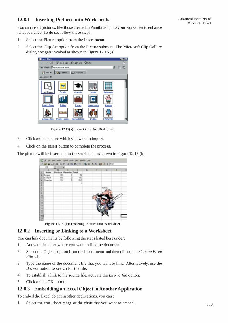
12.8.1 Inserting Pictures into Worksheets

You can insert pictures, like those created in Paintbrush, into your worksheet to enhanceits appearance. To do so, follow these steps:

1. Select the Picture option from the Insert menu.

2. Select the Clip Art option from the Picture submenu.The Microsoft Clip Gallerydialog box gets invoked as shown in Figure 12.15 (a).

3. Click on the picture which you want to import.

4. Click on the Insert button to complete the process.

The picture will be inserted into the worksheet as shown in Figure 12.15 (b).

12.8.2 Inserting or Linking to a WorksheetYou can link documents by following the steps listed here under:

1. Activate the sheet where you want to link the document.

2. Select the Objects option from the Insert menu and then click on the Create FromFile tab.

3. Type the name of the document file that you want to link. Alternatively, use theBrowse button to search for the file.

4. To establish a link to the source file, activate the Link to file option.


12.8.3 Embedding an Excel Object in Another ApplicationTo embed the Excel object in other applications, you can :

1. Select the worksheet range or the chart that you want to embed.

Figure 12.15(a): Insert Clip Art Dialog Box

Figure 12.15 (b): Inserting Picture into Worksheet

224


2. Select the Copy option from the Edit menu.

3. Start the other application.

4. Open the document in which you want to embed the Excel object.

5. Select the Paste Special option from the Edit menu. Select the Paste Link from thePaste Special dialog box and then click on the OK button.

12.9 WORKING WITH DATA FORMS USING LISTSA list is data stored in worksheet cells. Columns in a list represent a category and determinethe type of information required for each entry in the list. Each row in the list is a record.Records is a list that can be entered and edited by a user with the aid of the data formsthat Excel provides. A data form is a dialog box that is used to simplify the tasks ofentering data, deleting entries and finding specific cell entries. A sample list created inExcel worksheet is shown in Figure 12.16. The columns in this list are considered asFields and the rows are treated as Records.

12.9.1 Adding Records with Data Forms

To add new records to the list, using the data forms, the steps are:

1. Select the Form option from the Data menu.

At the left side of the form are labels of the fields in the list and the text boxes that showsthe entries for the records. At the right side of the form are buttons that help to performspecific operation in the list as shown in Figure 12.17.

12.9.2 Deleting Records With Data Forms

Records can also be deleted from the list with the help of the data forms. When you usethe data forms to delete records, you are able to delete only one record at a time.

To delete the records, the steps are:

1. Select the Form option from the Data menu. This opens up the data form for thecurrent list.

Figure 12.16 : Sample Excel worksheet

Figure 12.17 : Adding Recods With Data Forms

ScrollBar


225

2. Scroll to the record that you want to delete.

3. Click on the delete button. A message box gets invoked which prompts you toconfirm the deletion.

4. Confirm the record from the list, or click on Cancel to cancel the deletion.

The records below the deleted records gets renumbered automatically.

12.9.3 Finding Records with Data Form

You can use the data form to find particular records in a list. You can view only onerecord at a time when you use the data form. To search for records, the steps are:

1. Select the Form option from the Data menu.

This opens the data form for the current list.

2. Click on the Criteria button. The window displayed is illustrated in Figure 12.18.

3. Select a text box and enter the criteria that you want to search. For example, marksin Maths.

4. Select the Find Next button after you have entered the criteria. If no matches arefound, Excel beeps. Select the Find Previous button if you want to search backwardsin the list to find a match.

5. Select the Close button to clear the dialog box.

12.9.4 Sorting Data in a ListSorting helps to arrange the data entries in a systematic order. You can sort a data baseor a list by a single or multiple fields in ascending or descending order.

Sorting by a Single Field

To sort a list or a database by a single field, you can:

1. Select any one cell within the database range.

2. Select the sort option from the Data menu. The Sort dialog box gets invoked asshow in Figure 12.19.

Figure 12.18 : Finding Records with data form

Figure 12.19 : Sort Dialog Box

226


3. Select the field you want to sort from the Sort by drop-down list.

4. Use the Options buttons to specify the ascending or descending order, or use thebuttons available on the standard toolbar.

5. Excel tries to determine if the database has a header row (field names), and sets theHeader row or No Header row setting accordingly in the My list has area.Override this setting, if necessary.

6. Click on the OK button to sort the list.

Sorting by Multiple Fields

There may be situations where you need to sort a database by multiple fields. For example,in students records list of database, you need to sort the records by the Name, and then bythe Total from the highest to the lowest. To do so, the steps are:

1. Select a cell inside the database.

2. Select the Sort option from the Data menu.

3. Select the Product field from the Sort by drop-down list, and select the Ascendingorder option and specify the Amount field in the Then by deop-down list in theDescending order.


Your data would be sorted accordingly (refer to Figure 12.20).

12.9.5 Filtering Data in a List

Filters allow you to work with selected rows of information in any list, including a list thatyou have organized as the database. This implies that you can display only those databaserecords that meet your criteria. For example:

You want to send out certificates to academic proficiency to all those students who haveacquired more than 75% marks in their annual examinations. For this, you can filter thedata base so that only the records with more than 75% and above marks are displayed.

12.9.6 Using the Autofilter

AutoFilter is a special filter that filters records from the worksheet databases with thehelp of a single command. It makes the filtering task very easy and quick. With AutoFilter,you can also specify complex filtering criteria. To filter records by using the AutoFilter,the steps are:

1. Select any cell in the database.

2. Select the Filter option from the Data menu.

3. Select the AutoFilter option from the Filter submenu.

Figure 12.20 : Sorting by Multiple Field


227

Drop-down controls are placed on the top of each field name as shown in figure below.

4. Click on a drop-down control to apply a filter to the field.

The resultant list shows all the unique data entries in the column along with several otheroptions as shown in Figure 12.21 (a).

You can use the drop-down menu lists for other fields to apply additional filters to yourdatabase. A record must match all the selections that you make in the drop-down list.Excel immediately hides all those records that do not match the criteria. There are threeoptions that you can use for special purposes:

• Choose(All) – to cancel the filter defined for the current column (filters in othercolumns remain in effect).

• Choose (Top 10) – to apply criteria based on the values in the cells of the currentcolumns; for example, you can display the top ten records based on their cell values.

• Choose (Custom) – this is to apply complex criteria to your database.

If you select the Top 10 AutoFilter option from the drop-down list, as shown in Figure12.21 (b) then the Top 10 AutoFilter dialog box gets displayed.

Once you apply the option to your data, then the data gets filtered and gets displayed inthe required format as shown in Figure 12.21 (c)

Figure 12.21 (a) : Using theAutofiller

Figure 12.21 (b) : Top 10 Auto Filter Dialog Box

Figure 12.21 : Data Display Using Auto Filter

228


12.9.7 Setting Custom CategoriesYou can define a Custom AutoFilter when the data you want to filter meets the specifiedcriteria. To apply a customized criteria to a database, the steps are:

1. Select a cell in the database.

2. Select the Filter option from the Data menu.

3. Select the AutoFilter option from the Filter submenu. Drop-down arrows gets displayedon the top of each field in the database.

4. Click on the arrow next to any field name and select the custom entry.

The Custom AutoFilter dialog box gets invoked as shown in Figure12.22 (a). It hasfour boxes in which you can specify one or two criteria to apply to the currentcolumn. Each criteria consists of a condition and data item.

5. Click on the arrow next to the first box. Select one of the operators from the resultinglist. These include conditions such as Equals, Does not equal, Is greater than, Isless than, and so on.

6. Click on the arrow of the next box. A drop-down list is displayed. In this list thereare all unique data entries in the current column.

7. Select an entry (to complete the criteria) which you want to compare or enter thedata yourself in the text box.

8. You can repeat the last three steps to specify another criteria in the second row ofthe text boxes.

If you specify another criteria, then select either the And or the Or option button toconnect the two criteria.

1. Click on the OK button to apply the custom criteria.

Excel hides all records that do not match the criteria. For example, if you want therecord for which the Name is Yashpal, then you can specify the conditions accordingly inthe custom AutoFilter as shown in Figure 12.22 (b).

The result of this condition is displayed by Excel which hides all those records that do notmatch the criteria.

Figure 12.22 (a) : Custom Auto Filter Dialog Box

Figure 12.22 (b) : Custom Auto Filter—Specifying Conditions


229

12.10 PIVOT TABLESPivot tables enable you to easily summarize and compare data in a list.

They are called pivot tables because you can change their layout by rearranging orpivoting the row and column headings quickly and conveniently. You can use pivot tablesto create summaries of large amounts of data. You can summarize and rearrange dataspecifically for charts with the help of pivot tables. Whenever the pivot tables change,the chart based on those pivot tables also change. You can also use them for in-depthdata analysis or creating reports.

Using the Pivot Table Wizard

A pivot table can be created with the aid of the Pivot Table Wizard. To use the wizard,the steps are:

1. Select the Pivot table Report option from the Data menu.

Step 1 of the Pivot Table Wizard dialog box gets invoked as shown in Figure 12.23 (a).

1. Enter the data that you want to use in the pivot table.

2. Select the Microsoft Excel list or database when using worksheet data.

You can create a pivot table from other sources of data, from another pivot table, databasefrom other applications.

1. Click on the Next button.

Step 2 of the Pivot Table Wizard gets invoked as shown in Figure 12.23 (b):

2. Type the range address that is to be specified in the range text box.


Step 3 of the Pivot Table Wizard gets invoked as shown in Figure 12.23 (c):

Figure 12.23 (a) : Pivot Table Wizard Dialog Box

Figure 12.23 (b) : Step 2 Pivot Table Wizard Dialog Box

Figure 12.23 (c) : Step 3 Pivot Table Wizard Dialog Box

230



5. Indicate whether you want to place the pivot table in a New worksheet or an ExistingWorksheet.

6. Select the Options button for more options.

7. You can enter Format and Data options according to your requirements.

8. Click on the Finish button.

The Pivot Table Wizard displays the results in a table on the worksheet [refer toFigure 12.23 (d)].

12.11 LET US SUM UP

In this Unit, we learnt about various advanced features of Microsoft Excel. You wouldrecall, we read that:

� a list is a table of data stored in a worksheet. The top row of the list contains labelsidentifying the contents of each column, and the rest of the rows under these headingsor labels contains data. It can also be thought of as a database table.

� databases are modified and maintained by typing directly in to a worksheet. Whenyou require a more structured way of performing data entry, you can use Excel’sbuilt-in forms. A data form shows one record at a time. It can be used to add newrecords and edit existing records.

� sorting arranges data in a list or database in ascending or descending order.

� filtering helps you to extract all those records that match your criteria.

12.12 CHECK YOUR PROGRESS EXERCISE

1. Create a custom number format to display the cell values in thousands.

2. Create a list with column headings as Names, Class, Marks, Percentage andGrade and add some records to it.

Add some more records to it using the data forms.

Sort the list on Name and then by Marks.

Figure 12.23 (d) : Pivot Table Options Dialog Box


231

Use the AutoFilter to get the top ten marks of the students.

Summarize the worksheet list by using the pivot table, and create subtotals andgrand total.

3. Copy and paste a range of cells using the AutoFill handle. Find out the differencein the results when the mouse pointer is positioned at the edge of the block of cellsand dragged, and when the lower right corner is dragged.

4. Create a worksheet in which column A has the label Roll-no, column B has thelabel Names, Column C has the label Marks and Column D has the labelpercentage.

Put in the required data for the respective columns in twenty rows for all columnsexcept for the roll number.

Enter the roll numbers for all twenty students in the format r1, r2, r3,….r20 byusing the Fill, Series command from the Edit menu.

Enter the marks of every student in the Marks column.

Calculate the percentage of each student, presuming that the marks are given outof a total of 500. Complete the task by entering the percentage formula manuallyfor the first five students and then use the Edit formula feature for the next fifteenstudents.

Calculate the Grand Total.

Calculate the Average

Rename the sheet as RESULT

Cut and Paste the students name, marks in another sheet which should be namedas REPORT.

5. Create a table with Column A labeled as Item Name, Column B as Item No.,Column C as Price and Column D as Comments. Fill in the rows with appropriatecell entries. Now do the following:

Customize the price field to display the amount in thousands 2,233 format.

Increase the column width by using the menu bar.

Increase the row height by using the mouse.

Align the data vertically to position the contents on top.

Fill in cell D1 with an entry “This product is not available and the supplier should beinformed about it’’.

Rotate the item names.

Change the font of Cell A1 to make it bold and underlined.

Add to your worksheet graphic objects and fill it with a title Sales Report.

Now create a chart by using the Chart Wizard (use a pie chart) and use the ColumnA and C as its axis.

6. Create a range of 15 values and name it as Test. Find out the maximum value fromthe text range, by using the range name in the formula.

7. Create a worksheet with column B containing 20 numeric values under the headingPrice. Column A

232


Should have 20 item numbers in the format 101, 102 till 120.

Now create a formula to add all the values by specifying the cell references throughpointing.

Perform the same operation by using the AutoSum button.

Use the Paste Function feature and determine:

The number of entries

The maximum value

The minimum value

The average of all the twenty values

Search the cell value for item number 119 by using the Natural Language formula.

Create a bar chart using the values in the in column A as x-axis and use the valuesof column B as y-axis. Give a title name to the chart as Rate Chart.

Record a macro to copy the contents of column A to column C (after recording themacro remove the contents of column C and then run the macro).

8. i) Create a worksheet with a bar chart showing Book # against No. available.Add headings as bar chart showing Book # against number of books issuedshowing Books in Demand.

A Sample worksheet is given below:

ii) Previous this worksheet.

iii) Adjust the margins (on the Print Preview screen) to centralize the chartsheetvertically.

iv) Copy a part of your worksheet data to MS Word in a document namedcombination.

v) Create this Word document called Combination and save it in Excel worksheetas an icon.

vi) Select an area of the Libmast worksheet data area and set it as a print area.Print two copies of it.

9. Create your own page footers which should specify the page numbers in the formatA.1, A.2, and so on.

10. What option would you use to align the text both left and right? Which option wouldbe suitable to center text across multiple lines?

11. Create a worksheet with data in four pages and send only the first two pages forprinting.

12.13 ANSWERS TO CHECK YOUR PROGRESSEXERCISE

1) Select a cell and make a numeric entry. Select the Cells option from the Formatmenu. Select the Numbers tab from the Format Cell dialog box. Select the customCategory and enter #,### in the type box. Click on the OK button. Now your cellvalues would appear as 3,456.

2) No model answer. Do it yourself. This is practice exercise.


233

3) Dragging the edge of the block moves the block of data to another location while thelower right corner has the AutoFill handle (a solid cross) which copies data to an adjacentcell.

4) No model answer. This is practice exercise.

5) No model answer. This is a practice exercise.

6) Enter the 15 values in the First 15 rows of column A. Select the cell range. Select thename option from the Insert menu. Select the Define option from the Name submenu. Inthe Define Name dialog box enter the name you want to give to the range in the Name inWorkbook text box. Select a cell in which you want the formula. Type =MAX (in thecell). Select the name option from the Insert menu. Select the Paste option from theName submenu. In the Paste Name dialog box select the name Test that gets displayedin the past name text box. Click on the OK button. The formula now contains the rangename. Complete the formula by typing the closed brackets. Press Enter and the resultwill be shown in the cell.



9) Select the Page Setup option from the File menu. Click on the Custom footer. Click onthe Center section on the Footer dialog box. Type A, and click on the Page numberbutton. Click on the OK button.

10) Use the justify option of the horizontal alignment. Use the option Center Across Selectionfor centering text across multiple columns.

There are various options available for vertical alignment also. These are:

Top: Position contents at the top of the cell.

Center: Centers contents vertically within a cell.

Bottom: Position contents at the bottom of the cell.

Justify: Justifies lines vertically from top to bottom and automatically wraps the text.

To position contents at the bottom of the cell, which option would you select from thevertical alignment options?

11) Select the print option from the file menu. In the print dialog box, specify pages 1 to 2 inthe print range section.

unit 12 advanced features of microsoft excel

Documents