Sensors 2011, 11, 2035-2055; doi:10.3390/s110202035OPEN ACCESS

sensorsISSN 1424-8220

www.mdpi.com/journal/sensors

Article

Ultra Wide-Band Localization and SLAM: A ComparativeStudy for Mobile Robot NavigationMarcelo J. Segura, Fernando A. Auat Cheein ?, Juan M. Toibero, Vicente Mut andRicardo Carelli

Instituto de Automatica, National University of San Juan, Av. Libertador Gral. San Martin 1109 Oeste,J5400ARL San Juan, Argentina

? Author to whom correspondence should be addressed; E-Mail: fauat@inaut.unsj.edu.ar;Tel.: +54-264-4213303; Fax: +54-264-4213672.

Received: 10 December 2010; in revised form: 26 January 2011 / Accepted: 28 January 2011 /Published: 10 February 2011

Abstract: In this work, a comparative study between an Ultra Wide-Band (UWB)localization system and a Simultaneous Localization and Mapping (SLAM) algorithm ispresented. Due to its high bandwidth and short pulses length, UWB potentially allowsgreat accuracy in range measurements based on Time of Arrival (TOA) estimation. SLAMalgorithms recursively estimates the map of an environment and the pose (position andorientation) of a mobile robot within that environment. The comparative study presentedhere involves the performance analysis of implementing in parallel an UWB localizationbased system and a SLAM algorithm on a mobile robot navigating within an environment.Real time results as well as error analysis are also shown in this work.

Keywords: ultra wide-band; SLAM; mobile robots

1. Introduction

This article addresses the experimental comparison analysis between an ultra wide-band localizationsystem (UWB) and a SLAM (Simultaneous Localization and Mapping) algorithm.

Indoor location systems have some problems such as the ability to locate objects exactly. This canbe caused by a number of factors depending on the system being used. Each system has its advantagesand its drawbacks. Some can provide a high degree of accuracy but are not suitable for manufacturing

Sensors 2011, 11 2036

businesses, as they do not perform well in these conditions partly due to interference caused by othermachinery. Cost is another factor as some localization systems can be very expensive to implement.Scalability is also another issue that requires investigation. However in order to evaluate these systemswe must look at how the different systems operate, as well as their advantages and disadvantages. UltraWide Band technologies are often described as the next generation of real time location positioningsystems. In the world today industry is becoming more competitive and any technology that can providea competitive edge is welcome.

Industrial mobile robots, stock control and logistics in warehouses, mobility assistance forhandicapped people or patient monitoring in hospitals are some scenarios that require accurate positionestimation in indoor environments. Sensors based on ultrasound, lasers, cameras and Radio Frequencysignals (RF) are often used for these applications. Radio Frequency sensors have a wide range of usage asthe electromagnetic waves propagate through most typical environments. Impulse-based ultra widebandtransceivers offer accurate ranging with low cost. However, one of the most significant obstacles inaccurate ranging and positioning is the non-line of sight (NLOS) problem, which occurs in shadowedenvironments where a signal that propagates with a clear line of sight (LOS) may not be available. Thereare different wireless technologies, like WiFi [1], ZigBee [2], ultrasound [3], and others narrow band RFsystems that have been proposed for indoor localization. Generally, these localization systems are basedon low cost and low power sensors that measure received power or time of arrival. In the comparativestudy of Clarke et al. [4], it is shown that UWB is one of the best candidates for low cost accurateindoor localization. Commercial systems that use UWB sensors for indoor asset tracking are alreadyavailable. For example, Zebra Enterprise Solutions [5] utilize time-difference-of-arrival (TDOA), andUbisense [6] use a combination of TDOA and angle-of-arrival (AOA). The specified real-time accuracyof these systems is sub-15 cm with indoor operating ranges of over 50 m to 100 m.

In a previous work, a Mobile Robot Self-Localization systems using UWB technology wasintroduced [7]. The typical approach of commercial indoor localization systems consists of multiplebase stations (BS) that receive an UWB signal from the tag to be localized. The received signals areprocessed by a central control unit or by the BS to finally estimate the tag or mobile robot position. Inthe mentioned work, a new approach for mobile robot localization was developed and it is implementedin this comparative study.

The SLAM algorithm applied on a mobile robot recursively estimates the pose—localization andorientation—of the vehicle and the elements of the environment—called map—while reducing errorsassociated with the estimation process [8,9]. Several algorithms have been proposed as solutions tothe SLAM problem. The most widely used by the scientific community is the Extended Kalman filter(EKF) [8,10–12] solution and its derived filters, such as the Unscented Kalman filter (UKF) [12] andthe Extended Information filter (EIF) [13,14]. In these filters, the SLAM system state, composed bythe robot’s pose and the map of the environment, is modeled as a Gaussian random variable. Otherssolutions has also been implemented to solve the SLAM problem with high success, such as the case ofthe Particle filter (PF) [15], the Graph-SLAM [16] and the FastSLAM presented in [12].

Different SLAM algorithms solutions are presented to solve one or several issues associated withthe SLAM process, such as the time consuming processing, the accuracy of the map, the successfulclosure of the loop, the integration of the SLAM algorithm with control laws to drive the vehicle motion

Sensors 2011, 11 2037

and the modeling of different environments (dynamic, highly dynamic, static, structured, unstructured,etc.) [9,12]. Thus, for example, the EKF-SLAM presented in [10] extracted maps lines from structuredenvironments, whereas [17] works on environments with point-based features (parameterized as rangeand bearing). The EKF has also been used in vision-based SLAM. Despite the easy implementation ofthe EKF-SLAM, its correction part demands high computation resources. To solve this, the EIF is usedinstead of the EKF [12].

In this article, an experimental comparison between the UWB localization method and the SLAMalgorithm is performed. The UWB localization system and the SLAM algorithm are implemented inparallel on a mobile robot. The SLAM algorithm is implemented on an Extended Kalman filter (EKF)and extracts corners and lines —associated with walls—from the environment.

The comparison analysis involves the pros and cons of both methods when implemented on the mobilerobot platform for navigation purposes. The experimental analysis includes covariances estimationevolution, accuracy of the localization methods, portability and feasibility of the SLAM and the UWBsystem, and error analysis. Finally, a comparative table is presented showing the advantages anddisadvantages of both techniques presented in this work.

The article is organized as follows: Section 2 shows the general system implemented in this work;Section 3 introduces the UWB localization system; Section 4 presents the SLAM algorithm, the mobilerobot and the map’s features model used in this work; Section 5 shows the experimental results ofcarrying out parallel experimentations of the UWB localization system and the SLAM algorithm.Section 6 concludes.

2. General System Architecture

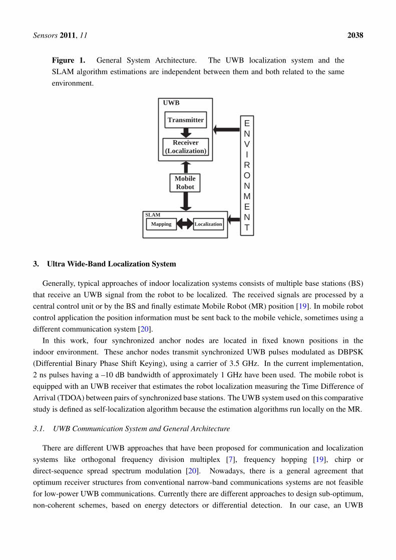
The system architecture of the comparative study between the UWB localization system and theSLAM algorithm is shown in Figure 1. Both localization systems (UWB and SLAM) are implementedin parallel and their localization estimations are independent from each other.

Given that the mobile robot has two independent localization systems implemented on it, thenavigation of the vehicle should not rely on any of them [18] in order to avoid contradictory drivingcommands. Thus, the mobile robot motion is controlled by hand-joystick. This way, the mobile robotnavigates within the same environment, following the same path for both localization methods.

The UWB localization system transmitters are located within the environments whereas the UWBlocalization system receiver is located on the mobile robot (see Figure 1). This scenario will be explainedin detail in Section 3. On the other hand, the SLAM algorithm depends only on the exteroceptivesensors [18] of the mobile robot. UWB localization system estimates the position of the robot whereasthe SLAM algorithm estimates both the position and the orientation of the mobile robot while it isnavigating within the environment.

The following sections will show in detail each block of Figure 1.

Sensors 2011, 11 2038

Figure 1. General System Architecture. The UWB localization system and theSLAM algorithm estimations are independent between them and both related to the sameenvironment.

ENVIRONMENT

MobileRobot

LocalizationMapping

SLAM

Transmitter

Receiver(Localization)

UWB

3. Ultra Wide-Band Localization System

Generally, typical approaches of indoor localization systems consists of multiple base stations (BS)that receive an UWB signal from the robot to be localized. The received signals are processed by acentral control unit or by the BS and finally estimate Mobile Robot (MR) position [19]. In mobile robotcontrol application the position information must be sent back to the mobile vehicle, sometimes using adifferent communication system [20].

In this work, four synchronized anchor nodes are located in fixed known positions in theindoor environment. These anchor nodes transmit synchronized UWB pulses modulated as DBPSK(Differential Binary Phase Shift Keying), using a carrier of 3.5 GHz. In the current implementation,2 ns pulses having a –10 dB bandwidth of approximately 1 GHz have been used. The mobile robot isequipped with an UWB receiver that estimates the robot localization measuring the Time Difference ofArrival (TDOA) between pairs of synchronized base stations. The UWB system used on this comparativestudy is defined as self-localization algorithm because the estimation algorithms run locally on the MR.

3.1. UWB Communication System and General Architecture

There are different UWB approaches that have been proposed for communication and localizationsystems like orthogonal frequency division multiplex [7], frequency hopping [19], chirp ordirect-sequence spread spectrum modulation [20]. Nowadays, there is a general agreement thatoptimum receiver structures from conventional narrow-band communications systems are not feasiblefor low-power UWB communications. Currently there are different approaches to design sub-optimum,non-coherent schemes, based on energy detectors or differential detection. In our case, an UWB

Sensors 2011, 11 2039

non-coherent system based on differential detection was implemented due to its simplicity androbustness, also because it allows to develop implementations with small power consumption.

The modulated Differential Binary Phase Shift Keying (DBPSK) signal in a complex form can bewritten as:

s(t) =√Eb

+∞∑k=−∞

(2b(k)− 1)p(t− kTf ) (1)

In (1), b(k) = b(k)⊕

b(k − 1), b(k) ∈ {0, 1}.⊕

is the logical or operator, b(k) are the differentialencoded pulses, and p(t) is the selected pulse shape (Eb is the bit energy). An IR-UWB system transmitseach information symbol over a time interval of Ts seconds, which consists ofNf frames of length Tf andthe resulted symbol length is Ts = Nf× Tf . In each frame, a short pulse p(t) of Tp = 2ns is transmittedwith the selected shape.

The mobile robot must identify multiple signals that come from different base stations. In order todifferentiate each BS, Direct Sequence (DS) Gold spreading codes are differentially encoded prior tothe modulation. The code length 7, which is the smallest Gold code, was implemented for reducingacquisition and processing time. It is worth noting that better accuracy could be achieved if longer codeswere implemented. If the base stations transmit at the same time, inter-pulse interference takes place,hence a simple time division multiple access (TDMA) was implemented. The final DS-UWB DBPSKtransmitted signal can be written as:

xu(t) =√Eb

+∞∑k=−∞

(2b(k)− 1)p(t− kTf − uTs) (2)

In (2), xu(t) is the transmitted signal by the base station BSu, u = 0, 1, ..., NBS − 1 and NBS is thenumber of base stations, in our case NBS = 4. The UWB transmitter use an RF switch to distribute thecorresponding signal to each antenna.

Regarding the receiver, differential demodulation is necessary to compare the phase of the previouspulse with the phase of the current pulse. To do this, the delay needs to be as large as the frame time Tf .The receiver accuracy is related with the capacity to make a precise delay. Since it is difficult to makean accurate analog delay, the authors used the concept of Software Defined Radio (SDR), in which theanalog to digital converter (ADC) is placed as close as possible to the antenna.

3.2. UWB Localization Algorithm

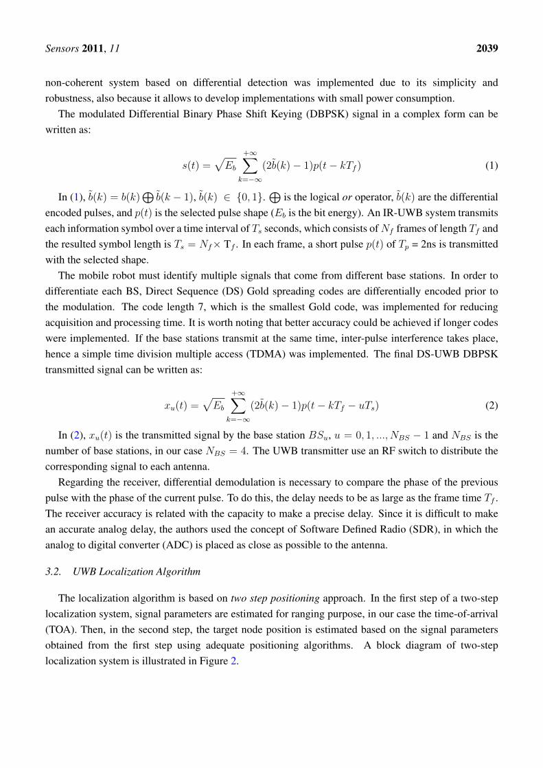
The localization algorithm is based on two step positioning approach. In the first step of a two-steplocalization system, signal parameters are estimated for ranging purpose, in our case the time-of-arrival(TOA). Then, in the second step, the target node position is estimated based on the signal parametersobtained from the first step using adequate positioning algorithms. A block diagram of two-steplocalization system is illustrated in Figure 2.

Sensors 2011, 11 2040

Figure 2. Two step localization scheme.

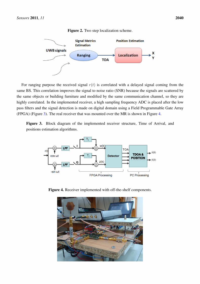
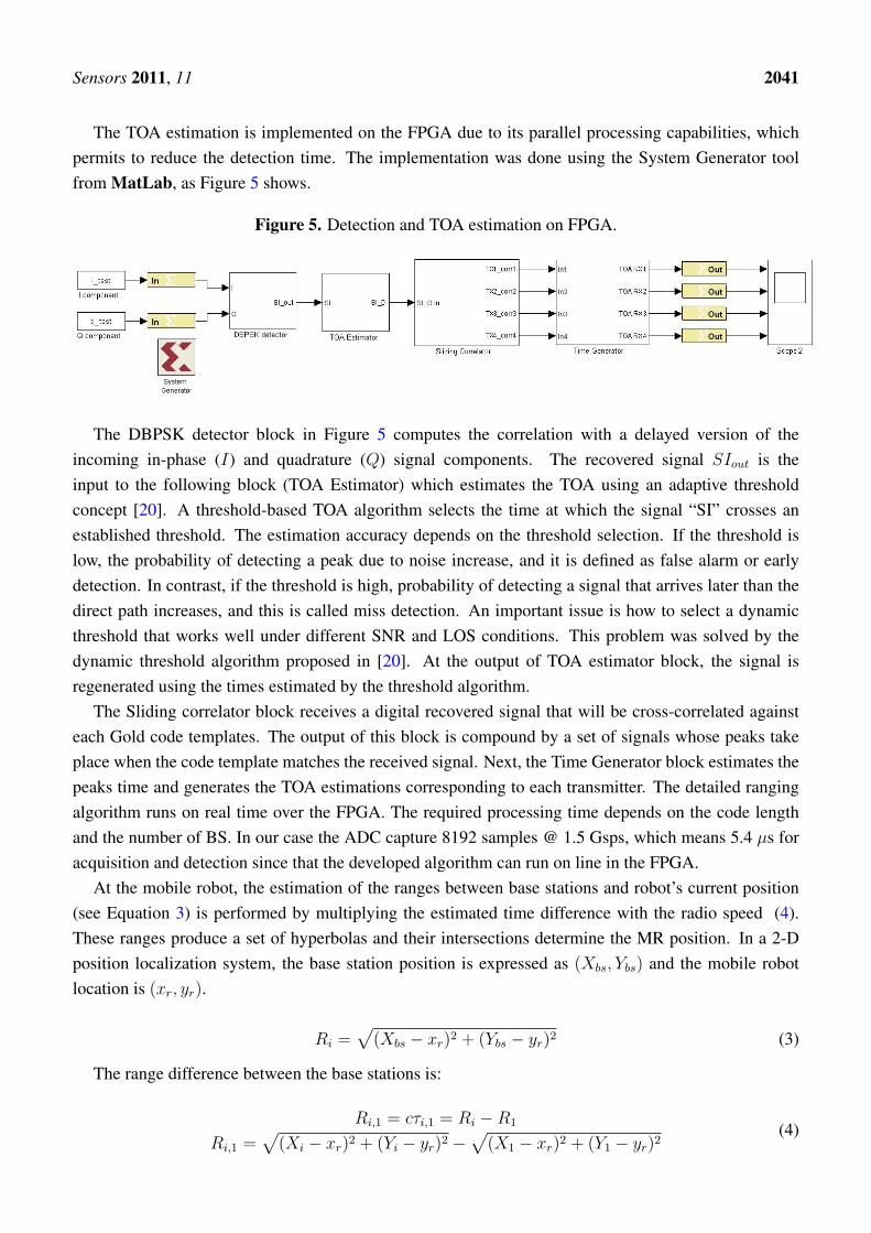
For ranging purpose the received signal r(t) is correlated with a delayed signal coming from thesame BS. This correlation improves the signal to noise ratio (SNR) because the signals are scattered bythe same objects or building furniture and modified by the same communication channel, so they arehighly correlated. In the implemented receiver, a high sampling frequency ADC is placed after the lowpass filters and the signal detection is made on digital domain using a Field Programmable Gate Array(FPGA) (Figure 3). The real receiver that was mounted over the MR is shown in Figure 4.

Figure 3. Block diagram of the implemented receiver structure, Time of Arrival, andpositions estimation algorithms.

Figure 4. Receiver implemented with off-the-shelf components.

Sensors 2011, 11 2041

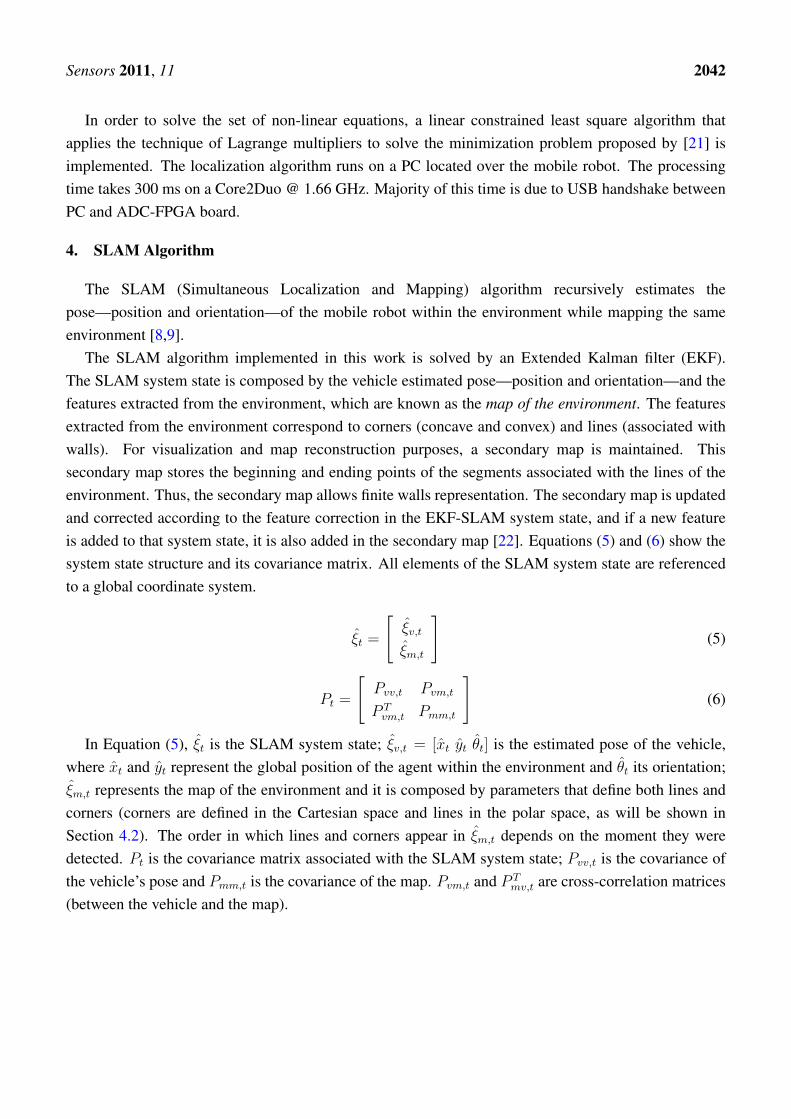
The TOA estimation is implemented on the FPGA due to its parallel processing capabilities, whichpermits to reduce the detection time. The implementation was done using the System Generator toolfrom MatLab, as Figure 5 shows.

Figure 5. Detection and TOA estimation on FPGA.

The DBPSK detector block in Figure 5 computes the correlation with a delayed version of theincoming in-phase (I) and quadrature (Q) signal components. The recovered signal SIout is theinput to the following block (TOA Estimator) which estimates the TOA using an adaptive thresholdconcept [20]. A threshold-based TOA algorithm selects the time at which the signal “SI” crosses anestablished threshold. The estimation accuracy depends on the threshold selection. If the threshold islow, the probability of detecting a peak due to noise increase, and it is defined as false alarm or earlydetection. In contrast, if the threshold is high, probability of detecting a signal that arrives later than thedirect path increases, and this is called miss detection. An important issue is how to select a dynamicthreshold that works well under different SNR and LOS conditions. This problem was solved by thedynamic threshold algorithm proposed in [20]. At the output of TOA estimator block, the signal isregenerated using the times estimated by the threshold algorithm.

The Sliding correlator block receives a digital recovered signal that will be cross-correlated againsteach Gold code templates. The output of this block is compound by a set of signals whose peaks takeplace when the code template matches the received signal. Next, the Time Generator block estimates thepeaks time and generates the TOA estimations corresponding to each transmitter. The detailed rangingalgorithm runs on real time over the FPGA. The required processing time depends on the code lengthand the number of BS. In our case the ADC capture 8192 samples @ 1.5 Gsps, which means 5.4 µs foracquisition and detection since that the developed algorithm can run on line in the FPGA.

At the mobile robot, the estimation of the ranges between base stations and robot’s current position(see Equation 3) is performed by multiplying the estimated time difference with the radio speed (4).These ranges produce a set of hyperbolas and their intersections determine the MR position. In a 2-Dposition localization system, the base station position is expressed as (Xbs, Ybs) and the mobile robotlocation is (xr, yr).

Ri =√

(Xbs − xr)2 + (Ybs − yr)2 (3)

The range difference between the base stations is:

Ri,1 = cτi,1 = Ri −R1

Ri,1 =√

(Xi − xr)2 + (Yi − yr)2 −√

(X1 − xr)2 + (Y1 − yr)2(4)

Sensors 2011, 11 2042

In order to solve the set of non-linear equations, a linear constrained least square algorithm thatapplies the technique of Lagrange multipliers to solve the minimization problem proposed by [21] isimplemented. The localization algorithm runs on a PC located over the mobile robot. The processingtime takes 300 ms on a Core2Duo @ 1.66 GHz. Majority of this time is due to USB handshake betweenPC and ADC-FPGA board.

4. SLAM Algorithm

The SLAM (Simultaneous Localization and Mapping) algorithm recursively estimates thepose—position and orientation—of the mobile robot within the environment while mapping the sameenvironment [8,9].

The SLAM algorithm implemented in this work is solved by an Extended Kalman filter (EKF).The SLAM system state is composed by the vehicle estimated pose—position and orientation—and thefeatures extracted from the environment, which are known as the map of the environment. The featuresextracted from the environment correspond to corners (concave and convex) and lines (associated withwalls). For visualization and map reconstruction purposes, a secondary map is maintained. Thissecondary map stores the beginning and ending points of the segments associated with the lines of theenvironment. Thus, the secondary map allows finite walls representation. The secondary map is updatedand corrected according to the feature correction in the EKF-SLAM system state, and if a new featureis added to that system state, it is also added in the secondary map [22]. Equations (5) and (6) show thesystem state structure and its covariance matrix. All elements of the SLAM system state are referencedto a global coordinate system.

ξt =

[ξv,t

ξm,t

](5)

Pt =

[Pvv,t Pvm,t

P Tvm,t Pmm,t

](6)

In Equation (5), ξt is the SLAM system state; ξv,t = [xt yt θt] is the estimated pose of the vehicle,where xt and yt represent the global position of the agent within the environment and θt its orientation;ξm,t represents the map of the environment and it is composed by parameters that define both lines andcorners (corners are defined in the Cartesian space and lines in the polar space, as will be shown inSection 4.2). The order in which lines and corners appear in ξm,t depends on the moment they weredetected. Pt is the covariance matrix associated with the SLAM system state; Pvv,t is the covariance ofthe vehicle’s pose and Pmm,t is the covariance of the map. Pvm,t and P T

mv,t are cross-correlation matrices(between the vehicle and the map).

Sensors 2011, 11 2043

The covariance matrix initialization techniques and the EKF definition can be found in [8,9]. TheEKF is represented in Equation (7). All variables involved in the estimation process are considered asGaussian random variables.

ξ−t = f(ξt, ut)

P−t = AtPt−1ATt +WtQt−1W

Tt

Kt = P−t HTt (HtP

−t H

Tt +Rt)

−1

ξt = ξ−t +Kt(zt − h(ξ−t ))

Pt = (I −KtHt)P−t .

(7)

In Equation (7), ξ−t is the predicted state of the system at time t; ut is the input control commandsand ξt is the corrected state at time t; f describes the motion of the elements of ξ. P−t and Pt are thepredicted and corrected covariance matrices respectively at time t; At is the Jacobian of f with respect tothe SLAM system state and Qt is the covariance matrix of the noise associated to the process, whereasWt is its Jacobian matrix; Kt is the Kalman gain at time t; Ht is the Jacobian matrix of the measurementmodel (h) and Rt is the covariance matrix of the actual measurement(zt). The term (zt − h(ξ−t )) iscalled the innovation vector [12] and takes place when the data association procedure has reached anappropriate matching between the observed feature and the predicted one (h(ξ−t )). Both the processmodel (f ) and the observation model are non-linear expressions. Further information concerning theEKF-SLAM can be found in [22].

In this work, the sequential EKF was implemented in order to reduce computational costs. Thesequential EKF-SLAM is based on the iterative calculation of the correction stage (SLAM system stateand covariance matrix) for each feature with correct association, see [12]. The prediction stage remainsas stated in Equation (7).

The general form of the correction stage of the classical sequential EKF-SLAM algorithm [12] issummarized in the algorithm shown in Algorithm 1. Sentences (3) to (9) describe the for loop of thecorrection stage of the algorithm. For every feature with correct association (sentence (2)), the for loopis executed. Sentence (4) shows the Kalman gain calculation; sentence (5) is the correction of the SLAMsystem state, whereas sentence (6) is the correction of the covariance matrix of the SLAM algorithm. Insentence (7), the current feature is deleted from the set of features with correct association (Mt). In thenext iteration, the next predicted SLAM system state and covariance matrix are the last corrected SLAMsystem state and covariance matrix respectively, as noted in sentence (8).

Further information concerning the EKF-SLAM implemented in this work can be found in [23].

4.1. Mobile Robot

The mobile robot used during the experimentation is a Pioneer 3AT built by ActivMedia. The Pioneer3AT is an unicycle like non-holonomic mobile robot. The vehicle has a range sensor laser, built bySICK, incorporated on it that acquires 181 measurements between 0 and 180 degrees in a range of 32 m.

Sensors 2011, 11 2044

Algorithm 1 Algorithm of the correction stage of the Sequential EKF-SLAM.1: Let Nt be set of the observed features2: Let Mt ⊆ Nt be the set of features with correct association3: for j = 1 to #Mt do4: Kt,j = P−t,jH

Tt,j(Ht,jP

−t,jH

Tt,j +Rt,j)

−1

5: ξt,j = ξ−t,j +Kt,j(zj − h(ξ−t,j))

6: Pt,j = (I −Kt,jHt,j))P−t,j

7: Mt,j = Mt,j − {zj}8: P−t,j := Pt,j; ξ−t,j = ξt,j

9: end for

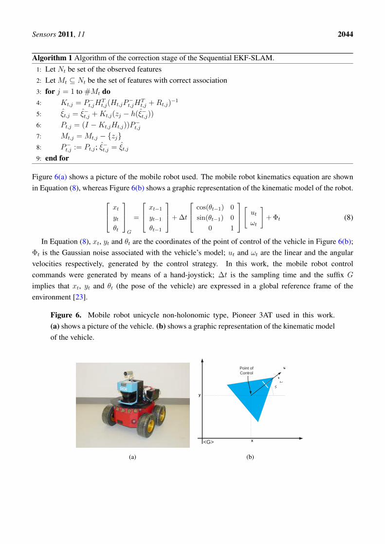
Figure 6(a) shows a picture of the mobile robot used. The mobile robot kinematics equation are shownin Equation (8), whereas Figure 6(b) shows a graphic representation of the kinematic model of the robot. xt

yt

θt

G

=

xt−1

yt−1

θt−1

+ ∆t

cos(θt−1) 0

sin(θt−1) 0

0 1

[ut

ωt

]+ Φt (8)

In Equation (8), xt, yt and θt are the coordinates of the point of control of the vehicle in Figure 6(b);Φt is the Gaussian noise associated with the vehicle’s model; ut and ωt are the linear and the angularvelocities respectively, generated by the control strategy. In this work, the mobile robot controlcommands were generated by means of a hand-joystick; ∆t is the sampling time and the suffix G

implies that xt, yt and θt (the pose of the vehicle) are expressed in a global reference frame of theenvironment [23].

Figure 6. Mobile robot unicycle non-holonomic type, Pioneer 3AT used in this work.(a) shows a picture of the vehicle. (b) shows a graphic representation of the kinematic modelof the vehicle.

(a)

x

y

Point ofControl

<G>

(b)

Sensors 2011, 11 2045

4.2. Features of the Environment

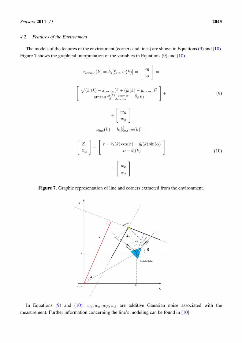
The models of the features of the environment (corners and lines) are shown in Equations (9) and (10).Figure 7 shows the graphical interpretation of the variables in Equations (9) and (10).

zcorner(k) = hi[ξv,t, w(k)] =

[zR

zβ

]=

[ √(xt(k)− xcorner)2 + (yt(k)− ycorner)2

arctan yt(k)−ycorner

xt−xcorner− θt(k)

]+

+

[wR

wβ

](9)

zline(k) = hi[ξv,t, w(k)] =

[Zρ

Zα

]=

[r − xt(k) cos(α)− yt(k) sin(α)

α− θt(k)

]

+

[wρ

wα

](10)

Figure 7. Graphic representation of line and corners extracted from the environment.

X

Y

Corner

Xrobo

t

Yrobot

xcorn

erycorner

<v>

Mobile Robot

<G>x

y

In Equations (9) and (10), wρ, wα, wR, wβ are additive Gaussian noise associated with themeasurement. Further information concerning the line’s modeling can be found in [10].

Sensors 2011, 11 2046

5. Experimental Results

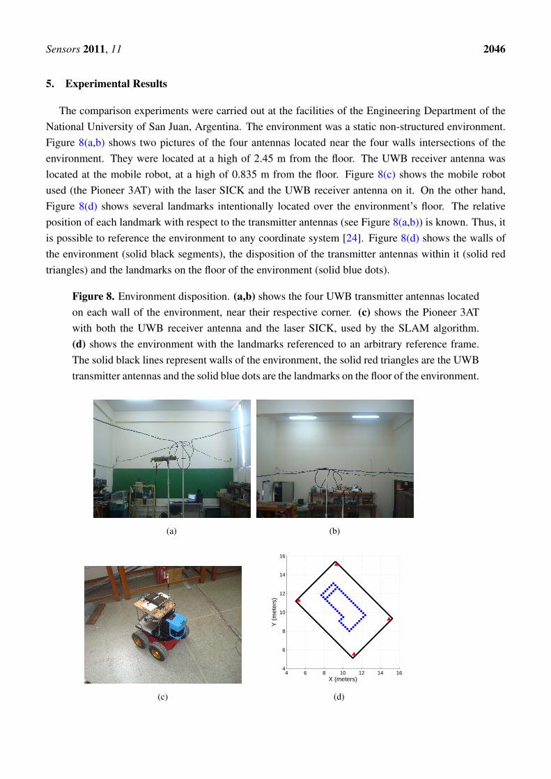
The comparison experiments were carried out at the facilities of the Engineering Department of theNational University of San Juan, Argentina. The environment was a static non-structured environment.Figure 8(a,b) shows two pictures of the four antennas located near the four walls intersections of theenvironment. They were located at a high of 2.45 m from the floor. The UWB receiver antenna waslocated at the mobile robot, at a high of 0.835 m from the floor. Figure 8(c) shows the mobile robotused (the Pioneer 3AT) with the laser SICK and the UWB receiver antenna on it. On the other hand,Figure 8(d) shows several landmarks intentionally located over the environment’s floor. The relativeposition of each landmark with respect to the transmitter antennas (see Figure 8(a,b)) is known. Thus, itis possible to reference the environment to any coordinate system [24]. Figure 8(d) shows the walls ofthe environment (solid black segments), the disposition of the transmitter antennas within it (solid redtriangles) and the landmarks on the floor of the environment (solid blue dots).

Figure 8. Environment disposition. (a,b) shows the four UWB transmitter antennas locatedon each wall of the environment, near their respective corner. (c) shows the Pioneer 3ATwith both the UWB receiver antenna and the laser SICK, used by the SLAM algorithm.(d) shows the environment with the landmarks referenced to an arbitrary reference frame.The solid black lines represent walls of the environment, the solid red triangles are the UWBtransmitter antennas and the solid blue dots are the landmarks on the floor of the environment.

(a) (b)

(c)

4 6 8 10 12 14 164

6

8

10

12

14

16

X (meters)

Y (

met

ers)

(d)

Sensors 2011, 11 2047

5.1. UWB Localization

In order to determine the performance of the localization systems shown in Figure 1, the mobile robotis positioned at [x y]T = [10.5 8.2]T meters within the environment shown in Figure 8(d).

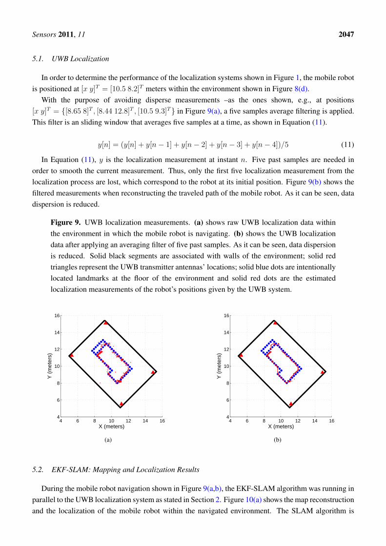
With the purpose of avoiding disperse measurements –as the ones shown, e.g., at positions[x y]T = {[8.65 8]T , [8.44 12.8]T , [10.5 9.3]T} in Figure 9(a), a five samples average filtering is applied.This filter is an sliding window that averages five samples at a time, as shown in Equation (11).

y[n] = (y[n] + y[n− 1] + y[n− 2] + y[n− 3] + y[n− 4])/5 (11)

In Equation (11), y is the localization measurement at instant n. Five past samples are needed inorder to smooth the current measurement. Thus, only the first five localization measurement from thelocalization process are lost, which correspond to the robot at its initial position. Figure 9(b) shows thefiltered measurements when reconstructing the traveled path of the mobile robot. As it can be seen, datadispersion is reduced.

Figure 9. UWB localization measurements. (a) shows raw UWB localization data withinthe environment in which the mobile robot is navigating. (b) shows the UWB localizationdata after applying an averaging filter of five past samples. As it can be seen, data dispersionis reduced. Solid black segments are associated with walls of the environment; solid redtriangles represent the UWB transmitter antennas’ locations; solid blue dots are intentionallylocated landmarks at the floor of the environment and solid red dots are the estimatedlocalization measurements of the robot’s positions given by the UWB system.

4 6 8 10 12 14 164

6

8

10

12

14

16

X (meters)

Y (

met

ers)

(a)

4 6 8 10 12 14 164

6

8

10

12

14

16

X (meters)

Y (

met

ers)

(b)

5.2. EKF-SLAM: Mapping and Localization Results

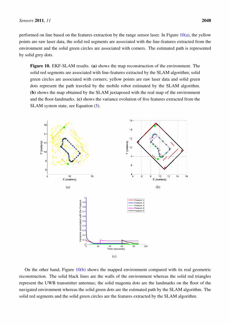
During the mobile robot navigation shown in Figure 9(a,b), the EKF-SLAM algorithm was running inparallel to the UWB localization system as stated in Section 2. Figure 10(a) shows the map reconstructionand the localization of the mobile robot within the navigated environment. The SLAM algorithm is

Sensors 2011, 11 2048

performed on line based on the features extraction by the range sensor laser. In Figure 10(a), the yellowpoints are raw laser data, the solid red segments are associated with the line-features extracted from theenvironment and the solid green circles are associated with corners. The estimated path is representedby solid grey dots.

Figure 10. EKF-SLAM results. (a) shows the map reconstruction of the environment. Thesolid red segments are associated with line-features extracted by the SLAM algorithm; solidgreen circles are associated with corners; yellow points are raw laser data and solid greendots represent the path traveled by the mobile robot estimated by the SLAM algorithm.(b) shows the map obtained by the SLAM juxtaposed with the real map of the environmentand the floor-landmarks. (c) shows the variance evolution of five features extracted from theSLAM system state, see Equation (5).

(a) (b)

0 20 40 60 80 1000

0.1

0.2

0.3

0.4

0.5

0.6

0.7

0.8

0.9

1

Time (seconds)

Var

ianc

e as

soci

ated

with

the

Fea

ture Feature 1

Feature 2Feature 3Feature 4Feature 5

(c)

On the other hand, Figure 10(b) shows the mapped environment compared with its real geometricreconstruction. The solid black lines are the walls of the environment whereas the solid red trianglesrepresent the UWB transmitter antennas; the solid magenta dots are the landmarks on the floor of thenavigated environment whereas the solid green dots are the estimated path by the SLAM algorithm. Thesolid red segments and the solid green circles are the features extracted by the SLAM algorithm.

Sensors 2011, 11 2049

Figure 10(c) shows the variance evolution associated with five features extracted from theenvironment by the SLAM algorithm. As it can be seen, the variance of the features gradually decreasesas established in [23,25], proving that the SLAM algorithm has consistently estimated the map of theenvironment after closing the loop (re-observation of the first extracted features [12]).

5.3. UWB vs. EKF-SLAM: Discussion

As stated in Section 2, the UWB localization system and the SLAM algorithm were implementedin parallel. Thus, the UWB localization and the SLAM estimation were performed during the samepath traveled by the mobile robot. The SLAM maximum sampling time was 0.2 s whereas the UWBlocalization method sampling time was 0.3 s. In this section the advantages and disadvantages of bothlocalization methods will be shown.

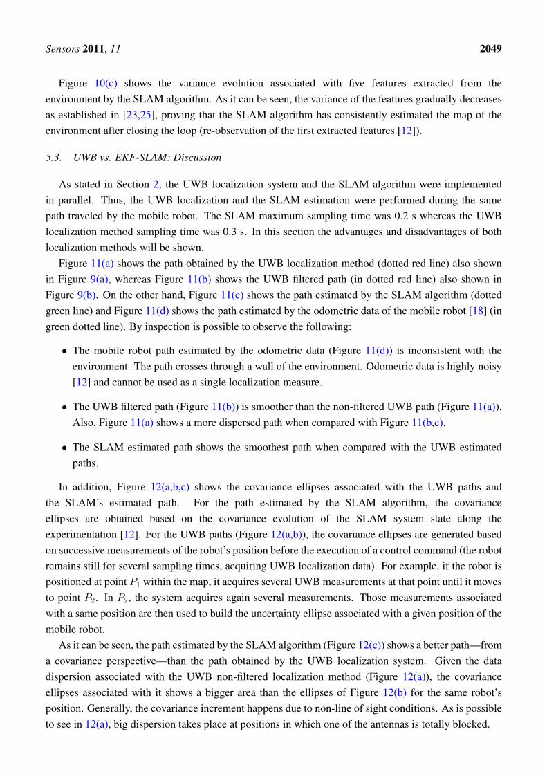
Figure 11(a) shows the path obtained by the UWB localization method (dotted red line) also shownin Figure 9(a), whereas Figure 11(b) shows the UWB filtered path (in dotted red line) also shown inFigure 9(b). On the other hand, Figure 11(c) shows the path estimated by the SLAM algorithm (dottedgreen line) and Figure 11(d) shows the path estimated by the odometric data of the mobile robot [18] (ingreen dotted line). By inspection is possible to observe the following:

• The mobile robot path estimated by the odometric data (Figure 11(d)) is inconsistent with theenvironment. The path crosses through a wall of the environment. Odometric data is highly noisy[12] and cannot be used as a single localization measure.

• The UWB filtered path (Figure 11(b)) is smoother than the non-filtered UWB path (Figure 11(a)).Also, Figure 11(a) shows a more dispersed path when compared with Figure 11(b,c).

• The SLAM estimated path shows the smoothest path when compared with the UWB estimatedpaths.

In addition, Figure 12(a,b,c) shows the covariance ellipses associated with the UWB paths andthe SLAM’s estimated path. For the path estimated by the SLAM algorithm, the covarianceellipses are obtained based on the covariance evolution of the SLAM system state along theexperimentation [12]. For the UWB paths (Figure 12(a,b)), the covariance ellipses are generated basedon successive measurements of the robot’s position before the execution of a control command (the robotremains still for several sampling times, acquiring UWB localization data). For example, if the robot ispositioned at point P1 within the map, it acquires several UWB measurements at that point until it movesto point P2. In P2, the system acquires again several measurements. Those measurements associatedwith a same position are then used to build the uncertainty ellipse associated with a given position of themobile robot.

As it can be seen, the path estimated by the SLAM algorithm (Figure 12(c)) shows a better path—froma covariance perspective—than the path obtained by the UWB localization system. Given the datadispersion associated with the UWB non-filtered localization method (Figure 12(a)), the covarianceellipses associated with it shows a bigger area than the ellipses of Figure 12(b) for the same robot’sposition. Generally, the covariance increment happens due to non-line of sight conditions. As is possibleto see in 12(a), big dispersion takes place at positions in which one of the antennas is totally blocked.

Sensors 2011, 11 2050

Figure 11. Path estimated by the localization system. (a) shows the path obtained by theUWB localization system without filtering data; (b) shows the path generated by the UWBlocalization system applying the filtering criterion shown in Equation (11). In both figures,the dotted red line is the path estimated by the UWB localization system. (c) shows thepath estimated by the SLAM algorithm (dotted green line) and (d) shows the path estimatedby the odometric data of the mobile robot. As it can be seen, the odometric data becomesinconsistent with the environment information.

4 6 8 10 12 14 164

6

8

10

12

14

16

X (meters)

Y (

met

ers)

(a)

4 6 8 10 12 14 164

6

8

10

12

14

16

X (meters)

Y (

met

ers)

(b)

(c) (d)

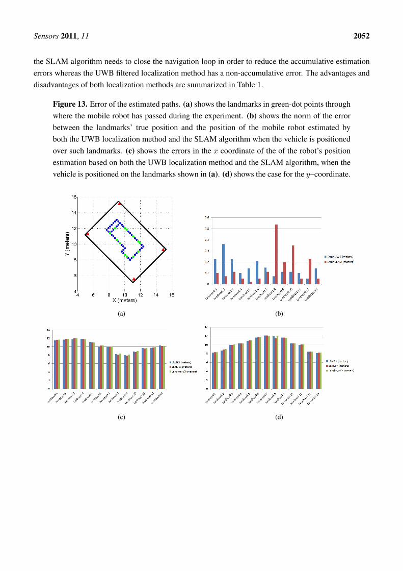
Finally, the paths obtained by the UWB filtered localization system and the SLAM algorithm arecompared with the landmarks located on the floor of the environment. As stated in Section 5, the positionof the landmarks within the environment is previously known. The landmarks over which the mobilerobot has passed are also known (they are shown in green-dot points in Figure 13(a)). Thus, Figure 13(b)shows the norm of the error between the landmarks’ true localization within the environment (shown inFigure 13(a)) and both the UWB localization estimation and the SLAM algorithm mobile robot’ poseestimation. Figure 13(c) and 13(d) show the error of the estimated position of the mobile robot basedon both the UWB localization method and the SLAM algorithm for each coordinate. The estimationerrors shown in Figure 13(c) and 13(d) are compared with respect to the true landmark position within

Sensors 2011, 11 2051

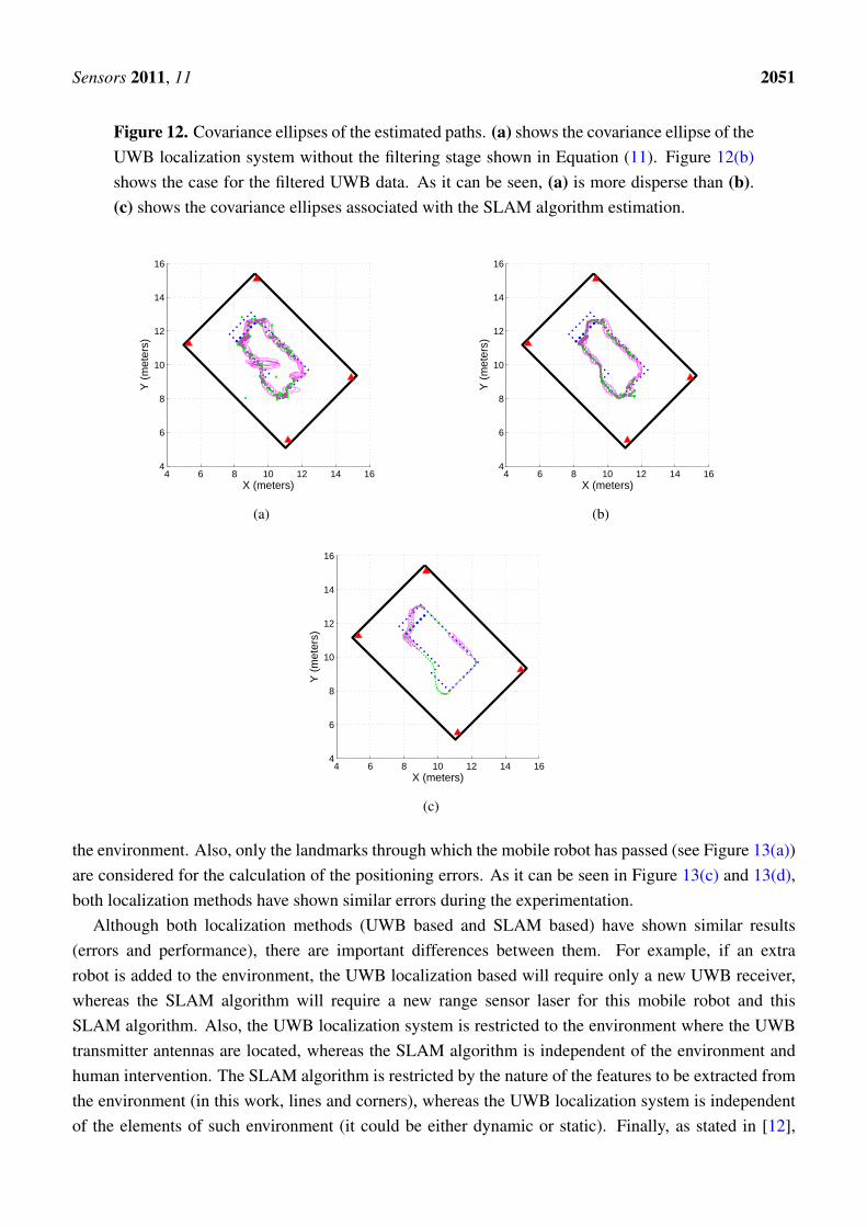
Figure 12. Covariance ellipses of the estimated paths. (a) shows the covariance ellipse of theUWB localization system without the filtering stage shown in Equation (11). Figure 12(b)shows the case for the filtered UWB data. As it can be seen, (a) is more disperse than (b).(c) shows the covariance ellipses associated with the SLAM algorithm estimation.

4 6 8 10 12 14 164

6

8

10

12

14

16

X (meters)

Y (

met

ers)

(a)

4 6 8 10 12 14 164

6

8

10

12

14

16

X (meters)Y

(m

eter

s)

(b)

4 6 8 10 12 14 164

6

8

10

12

14

16

X (meters)

Y (

met

ers)

(c)

the environment. Also, only the landmarks through which the mobile robot has passed (see Figure 13(a))are considered for the calculation of the positioning errors. As it can be seen in Figure 13(c) and 13(d),both localization methods have shown similar errors during the experimentation.

Although both localization methods (UWB based and SLAM based) have shown similar results(errors and performance), there are important differences between them. For example, if an extrarobot is added to the environment, the UWB localization based will require only a new UWB receiver,whereas the SLAM algorithm will require a new range sensor laser for this mobile robot and thisSLAM algorithm. Also, the UWB localization system is restricted to the environment where the UWBtransmitter antennas are located, whereas the SLAM algorithm is independent of the environment andhuman intervention. The SLAM algorithm is restricted by the nature of the features to be extracted fromthe environment (in this work, lines and corners), whereas the UWB localization system is independentof the elements of such environment (it could be either dynamic or static). Finally, as stated in [12],

Sensors 2011, 11 2052

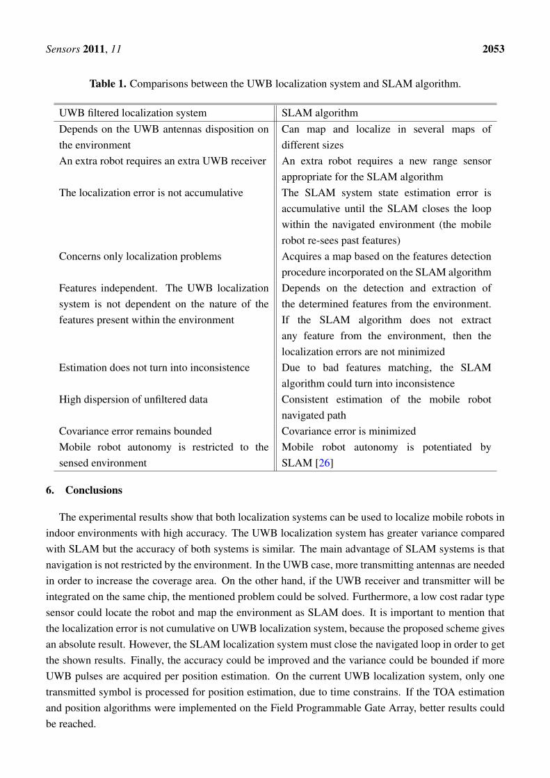
the SLAM algorithm needs to close the navigation loop in order to reduce the accumulative estimationerrors whereas the UWB filtered localization method has a non-accumulative error. The advantages anddisadvantages of both localization methods are summarized in Table 1.

Figure 13. Error of the estimated paths. (a) shows the landmarks in green-dot points throughwhere the mobile robot has passed during the experiment. (b) shows the norm of the errorbetween the landmarks’ true position and the position of the mobile robot estimated byboth the UWB localization method and the SLAM algorithm when the vehicle is positionedover such landmarks. (c) shows the errors in the x coordinate of the of the robot’s positionestimation based on both the UWB localization method and the SLAM algorithm, when thevehicle is positioned on the landmarks shown in (a). (d) shows the case for the y–coordinate.

(a) (b)

(c) (d)

Sensors 2011, 11 2053

Table 1. Comparisons between the UWB localization system and SLAM algorithm.

UWB filtered localization system SLAM algorithmDepends on the UWB antennas disposition onthe environment

Can map and localize in several maps ofdifferent sizes

An extra robot requires an extra UWB receiver An extra robot requires a new range sensorappropriate for the SLAM algorithm

The localization error is not accumulative The SLAM system state estimation error isaccumulative until the SLAM closes the loopwithin the navigated environment (the mobilerobot re-sees past features)

Concerns only localization problems Acquires a map based on the features detectionprocedure incorporated on the SLAM algorithm

Features independent. The UWB localizationsystem is not dependent on the nature of thefeatures present within the environment

Depends on the detection and extraction ofthe determined features from the environment.If the SLAM algorithm does not extractany feature from the environment, then thelocalization errors are not minimized

Estimation does not turn into inconsistence Due to bad features matching, the SLAMalgorithm could turn into inconsistence

High dispersion of unfiltered data Consistent estimation of the mobile robotnavigated path

Covariance error remains bounded Covariance error is minimizedMobile robot autonomy is restricted to thesensed environment

Mobile robot autonomy is potentiated bySLAM [26]

6. Conclusions

The experimental results show that both localization systems can be used to localize mobile robots inindoor environments with high accuracy. The UWB localization system has greater variance comparedwith SLAM but the accuracy of both systems is similar. The main advantage of SLAM systems is thatnavigation is not restricted by the environment. In the UWB case, more transmitting antennas are neededin order to increase the coverage area. On the other hand, if the UWB receiver and transmitter will beintegrated on the same chip, the mentioned problem could be solved. Furthermore, a low cost radar typesensor could locate the robot and map the environment as SLAM does. It is important to mention thatthe localization error is not cumulative on UWB localization system, because the proposed scheme givesan absolute result. However, the SLAM localization system must close the navigated loop in order to getthe shown results. Finally, the accuracy could be improved and the variance could be bounded if moreUWB pulses are acquired per position estimation. On the current UWB localization system, only onetransmitted symbol is processed for position estimation, due to time constrains. If the TOA estimationand position algorithms were implemented on the Field Programmable Gate Array, better results couldbe reached.

Sensors 2011, 11 2054

Acknowledgements

The authors would like to thank to the CONICET-Argentina, to the National University of San Juan,San Juan, Argentina and to National Instruments, for partially funding this research.

References

1. Ladd, A.M.; Bekris, E.K.E.; Rudys, A.P.; Wallach, D.S.; Kavraki, L.E. On the feasibility of usingwireless Ethernet for indoor localization. IEEE T. Robotic Autom. 2004, 20, 555-559.

2. Blumenthal, J.; Grossmann, R.; Golatowski, F.; Timmermann, D. Weighted centroid localizationin Zigbee-based sensor networks. In Proceedings of IEEE International Symposium on IntelligentSignal, Alcala de Henares, Spain, 3–5 October 2007; pp. 1-6.

3. Priyantha, N.; Chakraborty, A.; Balakrishnan, H. The cricket location-support system. InProceedings of Annual ACM International Conference on Mobile Computing and Networking(MOBICOM), Boston, MA, USA, 6–11 August 2000.

4. Clarke, D.; Park, A. Active-RFID system accuracy and its implications for clinical applications.In Proceedings of IEEE Symposium Computer-Based Medical Systems, Salt Lake City, UT, USA,5 July 2006; pp. 21-26,

5. Zebra Enterprise Solutions. Oakland, CA, USA. Available online:http://zes.zebra.com/technologies/location/ultra-wideband.jsp/(accessed on 30 January 2011).

6. Ubisense, Cambridge, CB4 1DL. UK. Available online: http://www.ubisense.net/en/products/precise-real-time-location.html (accessed on 29 January 2011).

7. Segura, M. J.; Mut, V.; Patio, H. Mobile robot self-localization system using IR-UWB sensor inindoor environments. In Proceedings of IEEE International Workshop on Robotic and SensorsEnvironments, Lecco, Italy, 6–7 November 2009, pp. 29-34.

8. Durrant-Whyte, H.; Bailey, T. Simultaneous Localization and Mapping (SLAM): Part I EssentialAlgorithms. IEEE Robot. Autom. Mag. 2006, 13, 99-108.

9. Durrant-Whyte, H.; Bailey, T. Simultaneous Localization and Mapping (SLAM): Part II State ofthe Art. IEEE Robot. Autom. Mag. 2006, 13, 108-117.

10. Garulli, A.; Giannitrapani, A.; Rossi, A.; Vicino, A. Mobile robot SLAM for line-basedenvironment representation. In Proceedings of IEEE Conference on Decision and Control, Seville,Spain, 12–15 December 2005; pp. 2041-2046.

11. Tamjidi, A.; Taghirad, H.D.; Aghamohammadi, A. On the consistency of EKF-SLAM: Focusingon the observation models. In Proceedings of IEEE International Conference on IntelligentRobots and Systems (IROS), Saint Louis, MO, USA, 11–15 October 2009; pp. 2083-2088,

12. Thrun, S; burgard, W; Fox, D. Probabilistic Robotics; MIT Press: Cambridge, MA, USA, 2005.13. Cadena, C.; Neira, J. SLAM in O(log n) with the Combined Kalman—Information filter. In

Proceedings of IEEE International Conference on Intelligent Robots and Systems (IROS), SaintLouis, MO, USA, 11–15 October 2009; pp. 2069-2076.

14. Yufeng, L.; Thrun, S. Results for outdoor-SLAM using sparse extended information filters.In Proceedings of IEEE International Conference on Robotics and Automation (ICRA), Taipei,Taiwan, 14–19 September 2003; pp. 1227-1233.

Sensors 2011, 11 2055

15. Nosan, K.; Beom-Hee L.; Yokoi, K. Result representation of Rao-Blackwellized particle filteringfor SLAM. In Proceedings of International Conference on Control, Automation and Systems,Seoul, Korea, 14–17 October 2008; pp. 698-703.

16. Guo, R.; Sun, F.; Yua, J. ICP based on Polar Point Matching with application to Graph-SLAM. InProceedings of International Conference on Mechatronics and Automation, Changchun, China,9–12 August 2009; pp. 1122-1127.

17. Bailey, T.; Nieto, J.; Guivant, J.; Stevens, M.; Nebot, E. Consistency of the EKF-SLAMAlgorithm. In Proceedings of IEEE International Conference on Intelligent Robots and Systems(IROS), Beijing, China, 9–15 October 2006; pp. 562-3568.

18. Siegwart, R.; Nourbakhsh, I. Autonomous Mobile Robots; MIT Press: Cambridge, MA, USA,2004.

19. Krishnan, S.; Sharma, P.; Guoping, Z.;Woon, H. A UWB based localization system forindoor robot navigation ultra-wideband. In Proceedings of IEEE International Conference onUltra-Wideband, Singapore, 24–26 September 2007; pp. 77-82.

20. Schroeder J.; Galler, S.; Kyamakya, K. A low-cost experimental ultra-wideband positioningsystem. In Proceedings of IEEE International Conference on Ultra-Wideband, Zurich,Switzerland, 5–8 September 2005; pp. 632-637.

21. Public Safety Communication Europe, D.4.1.1. Public Report EUROPCOM (EmergencyUltrawideband Radio for Positioning and Communications), Summery of the SystemArchitecture, Issue 1, Project no. 004154, June 2006.

22. Auat Cheein, F.; De la Cruz, C.; Carelli, R.; Bastos Filho, T. F. Solution to a door crossingproblem for an autonomous wheelchair. In Proceedings of IEEE/RSJ International Conferenceon Intelligent Robots and Systems, Saint Louis, MO, USA, 2009; pp. 4931-4936.

23. Auat Cheein, F.; Scaglia, G.; di Sciascio, F.; Carelli, R. Feature selection criteria for real timeEKF-SLAM algorithm. Int. J. Adv. Rob. Syst. 2009, 6, 229-238.

24. Arkin, R.C. Behavior-based Robotics; MIT Press: Cambridge, MA, USA, 1998.25. Dissanayake, G.; Newman, P.; Clark, S.; Durrant-Whyte, H. F.; Csorba, M. A solution to the

simultaneous localisation and map building (SLAM) problem. IEEE T. Robotic Autom. 2001, 17,229-241.

26. Choset, H.; Lynch, K.; Hutchinson, S.; Kantor, G.; Burgard, W.; Kavraki, L.; Thrun, S. Principlesof Robot Motion: Theory, Algorithms and Implementations; MIT Press: Cambridge, MA, USA,2005.

c© 2011 by the authors; licensee MDPI, Basel, Switzerland. This article is an open access articledistributed under the terms and conditions of the Creative Commons Attribution license(http://creativecommons.org/licenses/by/3.0/.)