map fusion based on a multi-map slam framework

Map fusion based on a multi-map SLAMframework

François Chanier, Paul Checchin, Christophe Blanc, and Laurent Trassoudaine

Abstract This paper presents a method for fusing two maps of an environment:one estimated with an application of the Simultaneous Localization and Mapping(SLAM) concept and the other one known a priori by a vehicle. The goal of suchan application is double: first, to estimate the vehicle pose in this known map and,second, to constrain the map estimate with the known map using an implementationof the local maps fusion approach and a heterogeneous mapping of the environment.This article shows how a priori knowledge available in the form of a map can befused within an EKF-SLAM framework to obtain more accuracy on the vehicleposes and map estimates. Simulation and experimental results are given to showthese improvements.

1 INTRODUCTION

The Simultaneous Localization and Mapping (SLAM) problem corresponds to theability of a robot to build a map of its environment while localizing itself in thatmap. Since the seminal paper [15], the understanding of the Extended Kalman Filter(EKF) approach to the SLAM problem made real progress [7][1]. Many researchersunderlined the problem of filter consistency [9] [3] and improved it with multi-mapsolutions [14] [5] [13]. Other difficulties were addressed like data association [12]and computational burden [8].

Generally, in such applications, both the trajectory of the vehicle and the locationof the landmarks are estimated online without the need for any a priori knowledge oflocation [1]. However, we choose to use absolute data in a form of an a priori mapin a SLAM application. This information fusion is done to improve the EKF-SLAM

F. Chanier · P. Checchin · C. Blanc · L. TrassoudaineLAboratoire des Sciences et Matériaux pour l’Electronique et d’AutomatiqueUniversité de Clermont-Ferrand, 24, avenue des Landais, 63177 Aubière cedex, Francee-mail: [email protected]

1

2 François Chanier, Paul Checchin, Christophe Blanc, and Laurent Trassoudaine

estimates. Few SLAM applications use available information on the environment.One example is described in [11]. Lee et al. suggest a path-constrained SLAM so-lution using a priori information in the form of a digital road map.

Furthermore, such map fusion approaches can answer questions about solvingthe problem of observability in SLAM systems. This property is important, and isrelated to the problem of consistency. A lower limit on the estimated error can onlybe guaranteed if the designed state (vehicle and map) is completely observable. In[10], a demonstration proves that EKF-SLAM formulation is not fully observablewithout absolute information. In other words, SLAM approaches, with on boardexteroceptive and proprioceptive sensors which provide relative measurements bet-ween the moving vehicle and the observed landmarks, give only partially observableestimates and fail to yield the absolute robot pose and feature positions in the globalcoordinates.

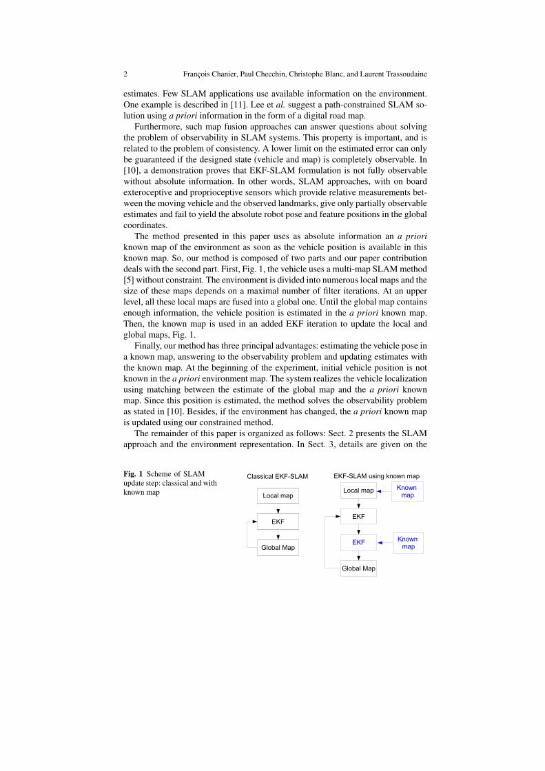
The method presented in this paper uses as absolute information an a prioriknown map of the environment as soon as the vehicle position is available in thisknown map. So, our method is composed of two parts and our paper contributiondeals with the second part. First, Fig. 1, the vehicle uses a multi-map SLAM method[5] without constraint. The environment is divided into numerous local maps and thesize of these maps depends on a maximal number of filter iterations. At an upperlevel, all these local maps are fused into a global one. Until the global map containsenough information, the vehicle position is estimated in the a priori known map.Then, the known map is used in an added EKF iteration to update the local andglobal maps, Fig. 1.

Finally, our method has three principal advantages: estimating the vehicle pose ina known map, answering to the observability problem and updating estimates withthe known map. At the beginning of the experiment, initial vehicle position is notknown in the a priori environment map. The system realizes the vehicle localizationusing matching between the estimate of the global map and the a priori knownmap. Since this position is estimated, the method solves the observability problemas stated in [10]. Besides, if the environment has changed, the a priori known mapis updated using our constrained method.

The remainder of this paper is organized as follows: Sect. 2 presents the SLAMapproach and the environment representation. In Sect. 3, details are given on the

Fig. 1 Scheme of SLAMupdate step: classical and withknown map

Map fusion based on a multi-map SLAM framework 3

update stage with the known map and more especially the algorithm used to findvehicle position in the a priori map. In Sect. 4, simulation and experimental resultsunderline the improvement with regard to the estimated vehicle path and mappedfeatures. They also show the consistency of the fusion approach.

2 SLAM APPROACH DESCRIPTION

In this section, the SLAM part of our method is based on the Robotcentric mapjoining approach [5]. This SLAM approach is chosen because it is reliable, see theresults presented in [5]. Indeed, if the vehicle pose in the a priori known map cannot be estimated early in the experiment, the environment mapping has to remainconsistent without being constrained, until the estimated map provides enough in-formation to determine this vehicle pose, see Sect. 3.2.

2.1 Robotcentric map joining approach

As reported in [5], the Robotcentric map joining approach consists in building asequence of consecutive uncorrelated local maps and joining them together in afull correlated map. This technique limits the number of update steps for each localmap, thus, limiting both feature location uncertainties and the effects of linearizationerrors [3]. This section introduces the different formulations of local and globalmaps used in the presented approach.

2.1.1 Local maps

Each local map is represented with a Robotcentric approach. Features, XRFi

withi = {1 · · ·n}, are referenced to a frame attached to the vehicle R. The local referenceWlocal is included as a non-observable feature in the stochastic state vector, Xlocal :

Xlocal =[

XRWlocal

XRF1· · · XR

Fn

]T(1)

with the associated covariance matrix Clocal .

2.1.2 Global Map

Each local map is joined in a global map represented by the same robotcentric ap-proach. Features, XWlocal

Giwith i = {1 · · ·m}, are referenced to the current local frame

Wlocal and the global reference is Wglobal . The global vector state is written as:


Xglobal =[

XWlocalWglobal

XWlocalG1

· · · XWlocalGm

]T(2)

with the associated covariance matrix Cglobal .To update the global map, the local map vector Xlocal is joined in Xglobal . It is

supposed that these local maps are not correlated. The vector state is written as:

Xsystem =[

Xglobal Xlocal]T (3)

with the associated covariance matrix:

Csystem =

[

Cglobal 00 Clocal

]

(4)

Innovation calculation (distance between local and global associated features),used in EKF update step, is done in local map frame. The nonlinear observationfunction, hk that formulates global feature coordinates in local map frame, is givenby:

Z = hk(Xsystem) =XRFk⊕XR

Wlocal⊕XWlocal

Gk= 0 (5)

The Jacobian matrix is given by:

Hk =[

0 HGk 0 HR 0 HFk 0]

(6)

with HGk is the Jacobian of hk with respect to XRGk

, HR is the Jacobian of hk withrespect to XR

Rgand HFk is equal to identity matrix as covariance matrix associated to

the measurement (local map feature) is null.In the last step, named composition, vehicle and feature poses in the global map

are updated with respect to the vector XRWlocal

.

2.2 Heterogeneous mapping

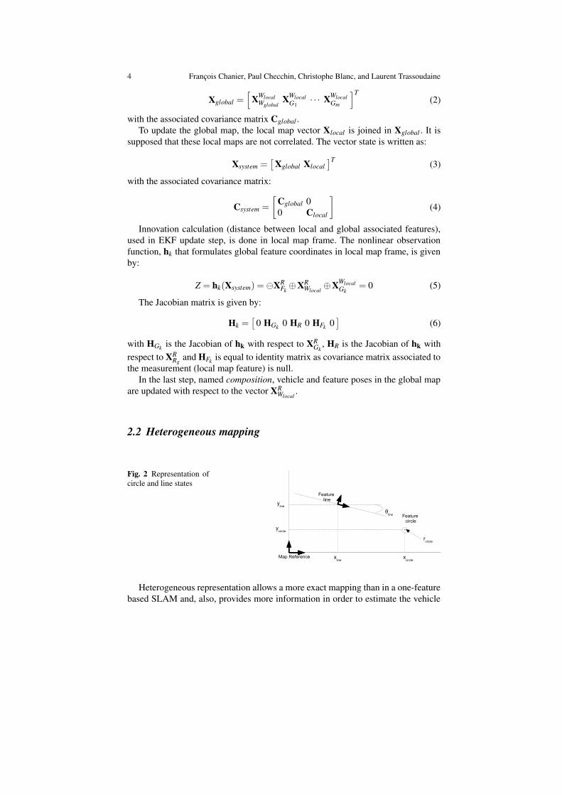
Fig. 2 Representation ofcircle and line states

Heterogeneous representation allows a more exact mapping than in a one-featurebased SLAM and, also, provides more information in order to estimate the vehicle


position in the known map, Sect. 3.2. Two geometric feature types, line and circle,are used to represent the environment in two dimensions and are shown in Fig. 2.

2.2.1 Line

The SPmap model [6] is used to represent line features. The state vector is writtenas:

Xline =[

xline yline θline]T (7)

The states, xline and yline, are the Cartesian coordinates of line frame and θline re-presents the orientation of this frame in the map reference, see Fig. 2. Only angularand lateral displacements are used in EKF update step. The other parameter xline isused to improve data association step with ambiguous matching (parallel walls forexample).

2.2.2 Circle

Circle features are represented by:

Xcircle =[

xcircle ycircle rcircle]T (8)

The states, xcircle and ycircle, are the Cartesian coordinates of circle center and rcircleis the radius, see Fig. 2. The estimation of these parameters is based on a Levenberg-Marquardt algorithm, see [16].

In this heterogeneous mapping concept, the general form of state vectors of thelocal and the global maps, respectively Xlocal and Xglobal , is:

Xmap =[

Xline Xcircle]T (9)

3 UPDATE SLAM WITH KNOWN MAP

In this section, the part of our method where the EKF-SLAM estimates are cons-trained by the knowledge of an a priori map of the environment is presented, Fig. 1.It corresponds to the contribution to the approach presented in Sect. 2.1.

3.1 Known map description

Known map is composed of line and circle features, as presented in Sect. 2.2. Thismap is composed of l features. The state vector is written as:


Xknown =[

XWknownE1

· · · XWknownEl

]T(10)

If this map is perfectly known, for example obtained from blueprints of building,map uncertainty is null. However, for the presented experiments in Sect. 4, featureposes are measured with a differential GPS sensor. The sensor standard deviation isaround 5 centimeters. This uncertainty is translated in the known map by the matrixCknown:

Cknown =

σ 2 0. . .

0 σ 2

(11)

with σ deviations on the feature states. Six different variables are defined:

• σxl , σyl and σθl for line type features,• σxc , σyc and σrc for circle type features.

3.2 Geometric transformation determination

Fig. 3 Geometric transforma-tion between the global mapand the known map

Combined constraint data association (CCDA), presented in [2], is used to de-termine geometric transformation between the references of the global map, Wglobal

and the known map Wknown, see Fig. 3. The vector XWglobalWknown

, equation (12), representsthe a priori map reference pose, Wknown, in the global map.

XWglobalWknown

=[

xknown yknown θknown]T (12)

xknown et yknown are the Cartesian coordinates and θknown is the orientation.To calculate XWglobal

Wknown, two steps are necessary: matching global map with a prio-

ri map features and finding the position and the orientation of the a priori mapreference, Wknown, in the global map.


First, CCDA algorithm performs batch-validation gating by constructing andsearching a correspondence graph. The different features of a map are representedby a graph where each node is a feature and each edge is an invariant relationshipbetween two features. Three different relationships are used by CCDA: between twolines, between two circles and between a circle and a line. These relationships onlyuse center coordinates for circles and angular and lateral displacements for lines.

Having generated two feature graphs with the relationships, one for the globalmap and the other one for the known map, a correspondence graph is created. Thenodes of this graph represent all the possible pairings of the different features ofboth maps. An algorithm, used in [2], searches the maximum clique. If the clique islong enough, it means that there are enough feature pairings (more than three), thevector XWglobal

Wknownand the covariance matrix CWglobal

Wknownare estimated.

3.3 Update step with known map

3.3.1 Insertion of the translation vector in local and global map vectors

The vector XWglobalWknown

specified in Sect. 3.2, is now referenced to the frame attached tothe vehicle Wlocal:

XWlocalWknown

= XWlocalWglobal

⊕XWglobalWknown

(13)

XWlocalWknown

is included in the global map state vector (2) as a non observable feature. Itsestimate can be improved during the update steps of the EKF filter:

Xglobal =[

XWlocalWknown

XWlocalWglobal

XWlocalF1

· · · XWlocalFm

]T(14)

The covariance matrix associated with the new vector Xglobal is given by:

Cglobal = G×

[

CWglobalWknown

00 Cglobal

]

×GT (15)

with

G =

[

Jg JXglobal

0 I

]

(16)

and Jg is the Jacobian of equation (13) with respect to XWglobalWknown

, JXglobal is the Jacobianof equation (13) with respect to Xglobal and I is equal to identity matrix.

The XWlocalWknown

is also included in each local map state vector. As these maps are

initialized at the position of XWlocalWglobal

, the vector XRWknown

can be initialized by the last

value of XWlocalWknown

. The vector Xlocal is now given by:


Xlocal =[

XWlocalWknown

XWlocalWlocal

]T(17)

XWlocalWlocal

is equal to zero. It is supposed that the vector XRWknown

is uncorrelated withthe initial vehicle pose in the local map. The initial values of the uncertainties onvehicle states are null. So, the associated covariance matrix Xlocal is initialized with:

Clocal =

[

CWlocalWknown

00 0

]

(18)

With this translation vector, states of local and global maps can be updated withthe known map using equations presented in the next part. Moreover, the estimateof this vector is improved at each algorithm iteration.

3.3.2 Update of local maps and global map with known map

This update is realized at every step after the update of local maps. To update thelocal map, the vector Xknown is joined in the vector Xlocal :

Xsystem =[

Xlocal Xknown]T (19)

Feature positions are estimated, once the data association step is done, with thesame formulation introduced in [5]. However, the observation equation (5) has to bechanged to introduce the translation (13):

Z = hk(Xsystem) =XWlocalFk

⊕XWlocalWknown

⊕XWknownEk

= 0 (20)

The Jacobian matrix is given by:

Hk =[

Hknown 0 HFk 0 HEk 0]

(21)

with Hknown is the Jacobian of hk with respect to XWlocalWknown

, HFk is the Jacobian of hk

with respect to XWlocalFk

and HEk is equal to identity matrix.

3.3.3 Update of the translation vector

Vector XWlocalWknown

is estimated using both the global and local map vectors. When alocal map is joined to the global map, this vector is updated with the observationequation given by:

XRWknown

= hknown(XRWlocal

,XWlocalWknown

)+wknown (22)

with wknown, Gaussian noise and the observation function hknown defined by:


XRWknown

= XRWlocal

⊕XWlocalWknown

(23)

the corresponding Jacobian matrix is given by:

Hknown =[

Hglobalknown 0 Hlocal

known HR 0]

(24)

with HglobalWknown

the Jacobian of hknown with respect to XWlocalWknown

, HR Jacobian of hknown

with respect to XRWlocal

(vector equal to XRWlocal

) and HlocalWknown

the identity matrix.

3.3.4 SLAM constrained by a known map algorithm

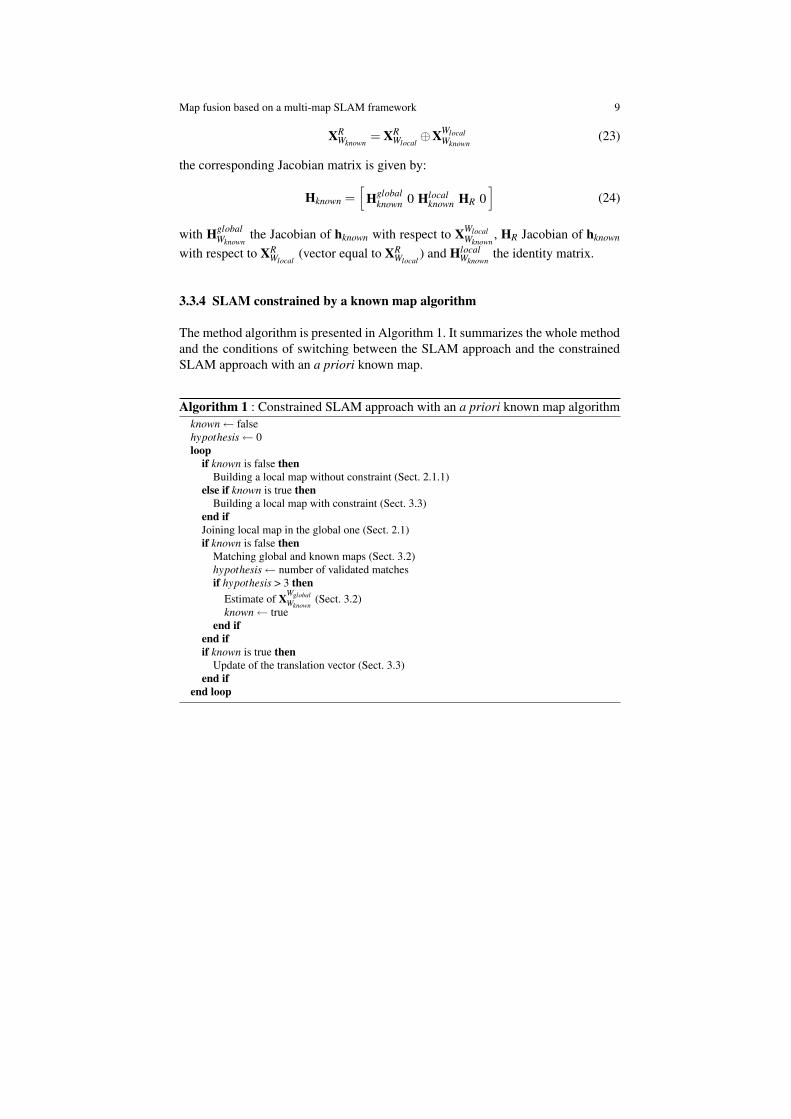
The method algorithm is presented in Algorithm 1. It summarizes the whole methodand the conditions of switching between the SLAM approach and the constrainedSLAM approach with an a priori known map.

Algorithm 1 : Constrained SLAM approach with an a priori known map algorithmknown← falsehypothesis← 0loop

if known is false thenBuilding a local map without constraint (Sect. 2.1.1)

else if known is true thenBuilding a local map with constraint (Sect. 3.3)

end ifJoining local map in the global one (Sect. 2.1)if known is false then

Matching global and known maps (Sect. 3.2)hypothesis← number of validated matchesif hypothesis > 3 then

Estimate of XWglobalWknown

(Sect. 3.2)known← true

end ifend ifif known is true then

Update of the translation vector (Sect. 3.3)end if

end loop


4 SIMULATION AND EXPERIMENTAL RESULTS

4.1 Consistency definition

As ground-truth is available with simulation and experimental data (differentialGPS) for the vehicle states, a statistical test for filter consistency can be carriedout on the Normalized Estimation Error Squared (NEES):

d = (XWglobalWlocal

− X̂WglobalWlocal

)T (PWglobalWlocal

)−1(XWglobalWlocal

− X̂WglobalWlocal

) (25)

As it is defined in [4], the filter results are consistent if:

d ≤ χ2do f ,1−α (26)

where χ2do f ,1−α is a threshold obtained from the χ2 distribution with 3 degrees of

freedom and a significance level equal to 0.05.

4.2 Simulation results

−100 −80 −60 −40 −20 0 20 40 60 80−80

−60

−40

−20

0

20

40

60

80

100

x [m]

y [m

]

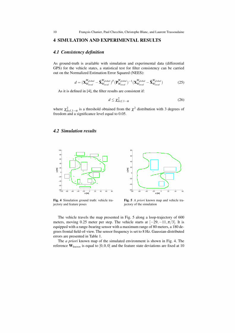
Fig. 4 Simulation ground truth: vehicle tra-jectory and feature poses

−80 −60 −40 −20 0 20 40 60−60

−40

−20

0

20

40

60

80

x [m]

y [m

]

Fig. 5 A priori known map and vehicle tra-jectory of the simulation

The vehicle travels the map presented in Fig. 5 along a loop-trajectory of 600meters, moving 0.25 meter per step. The vehicle starts at [−29,−11,π/3]. It isequipped with a range-bearing sensor with a maximum range of 80 meters, a 180 de-grees frontal field-of-view. The sensor frequency is set to 8 Hz. Gaussian-distributederrors are presented in Table 1.

The a priori known map of the simulated environment is shown in Fig. 4. Thereference Wknown is equal to [0,0,0] and the feature state deviations are fixed at 10


centimeters for coordinates, 10 centimeters for circle radiuses and 0.05 radians forline angles.

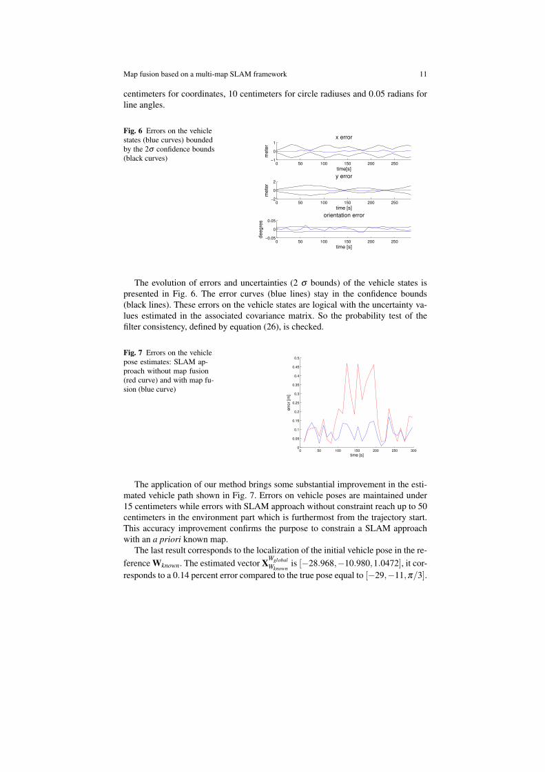
Fig. 6 Errors on the vehiclestates (blue curves) boundedby the 2σ confidence bounds(black curves)

0 50 100 150 200 250−1

0

1

time[s]

met

er

x error

0 50 100 150 200 250−2

0

2

time [s]

met

er

y error

0 50 100 150 200 250−0.05

0

0.05

time [s]

deeg

res

orientation error

The evolution of errors and uncertainties (2 σ bounds) of the vehicle states ispresented in Fig. 6. The error curves (blue lines) stay in the confidence bounds(black lines). These errors on the vehicle states are logical with the uncertainty va-lues estimated in the associated covariance matrix. So the probability test of thefilter consistency, defined by equation (26), is checked.

Fig. 7 Errors on the vehiclepose estimates: SLAM ap-proach without map fusion(red curve) and with map fu-sion (blue curve)

0 50 100 150 200 250 3000

0.05

0.1

0.15

0.2

0.25

0.3

0.35

0.4

0.45

0.5

time [s]

erro

r [m

]

The application of our method brings some substantial improvement in the esti-mated vehicle path shown in Fig. 7. Errors on vehicle poses are maintained under15 centimeters while errors with SLAM approach without constraint reach up to 50centimeters in the environment part which is furthermost from the trajectory start.This accuracy improvement confirms the purpose to constrain a SLAM approachwith an a priori known map.

The last result corresponds to the localization of the initial vehicle pose in the re-ference Wknown. The estimated vector XWglobal

Wknownis [−28.968,−10.980,1.0472], it cor-

responds to a 0.14 percent error compared to the true pose equal to [−29,−11,π/3].


This error on the vehicle pose estimates proves that our method is accurate in a lo-calization context.

4.3 Experimental results

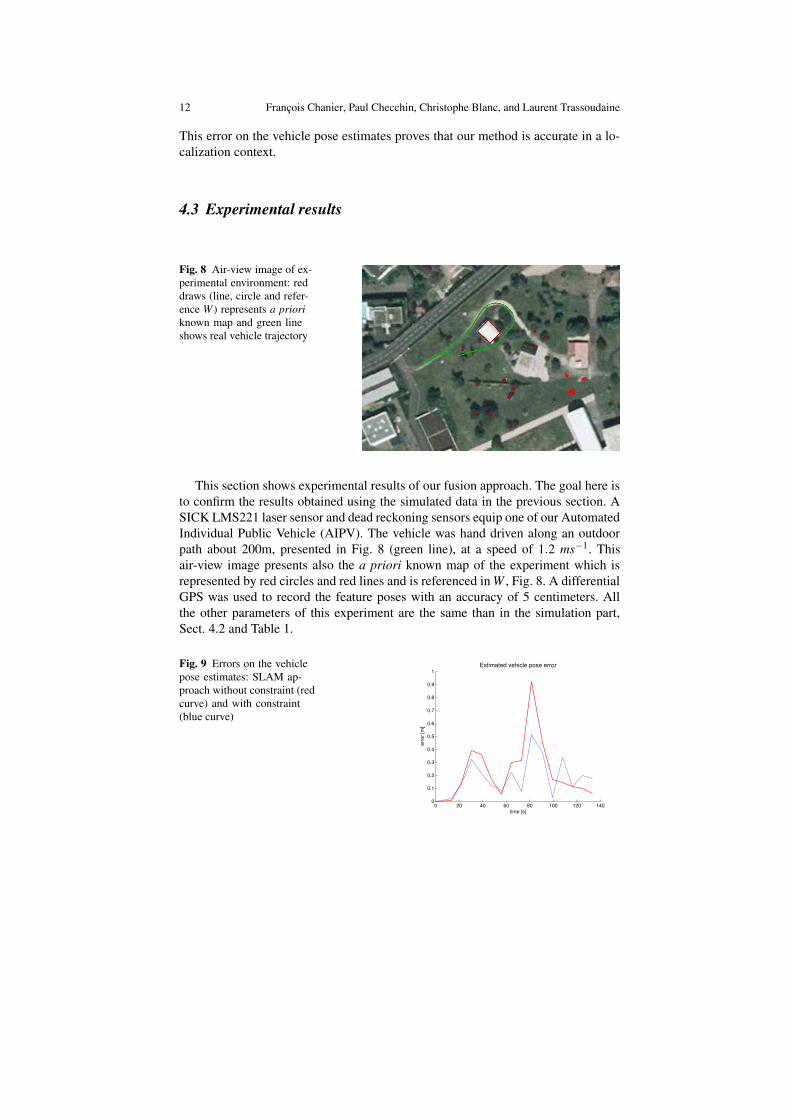
Fig. 8 Air-view image of ex-perimental environment: reddraws (line, circle and refer-ence W ) represents a prioriknown map and green lineshows real vehicle trajectory

This section shows experimental results of our fusion approach. The goal here isto confirm the results obtained using the simulated data in the previous section. ASICK LMS221 laser sensor and dead reckoning sensors equip one of our AutomatedIndividual Public Vehicle (AIPV). The vehicle was hand driven along an outdoorpath about 200m, presented in Fig. 8 (green line), at a speed of 1.2 ms−1. Thisair-view image presents also the a priori known map of the experiment which isrepresented by red circles and red lines and is referenced in W , Fig. 8. A differentialGPS was used to record the feature poses with an accuracy of 5 centimeters. Allthe other parameters of this experiment are the same than in the simulation part,Sect. 4.2 and Table 1.

Fig. 9 Errors on the vehiclepose estimates: SLAM ap-proach without constraint (redcurve) and with constraint(blue curve)

0 20 40 60 80 100 120 1400

0.1

0.2

0.3

0.4

0.5

0.6

0.7

0.8

0.9

1

time [s]

erro

r [m

]

Estimated vehicle pose error


A quantitative evaluation of the accuracy of our EKF-SLAM approach with orwithout map fusion is done studying the evolution of the error on the vehicle pose,Fig. 8. First, these results correspond to the simulation results and confirm the im-provement carried by the map fusion. Errors with our approach are maintained at alower level than with the classical SLAM approach. The difference with simulationresults on error amplitude can be explained by the fact that the floor is not flat in thisenvironment.

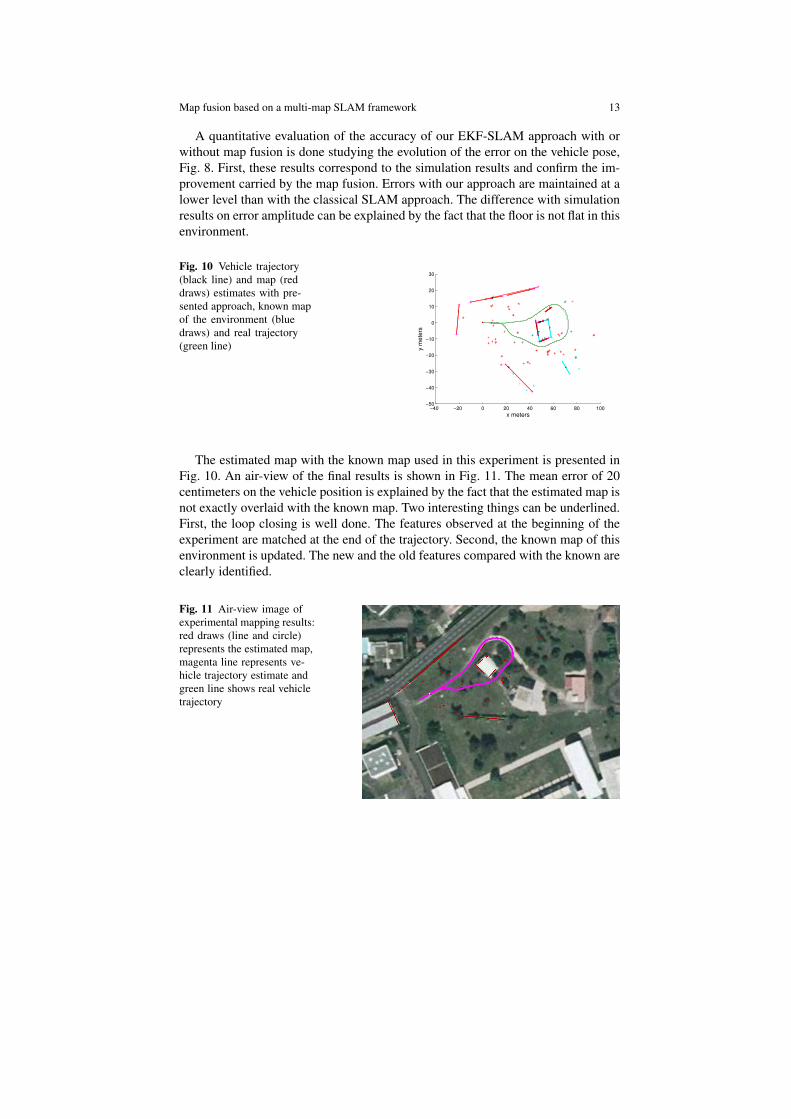
Fig. 10 Vehicle trajectory(black line) and map (reddraws) estimates with pre-sented approach, known mapof the environment (bluedraws) and real trajectory(green line)

−40 −20 0 20 40 60 80 100−50

−40

−30

−20

−10

0

10

20

30

x metersy

met

ers

The estimated map with the known map used in this experiment is presented inFig. 10. An air-view of the final results is shown in Fig. 11. The mean error of 20centimeters on the vehicle position is explained by the fact that the estimated map isnot exactly overlaid with the known map. Two interesting things can be underlined.First, the loop closing is well done. The features observed at the beginning of theexperiment are matched at the end of the trajectory. Second, the known map of thisenvironment is updated. The new and the old features compared with the known areclearly identified.

Fig. 11 Air-view image ofexperimental mapping results:red draws (line and circle)represents the estimated map,magenta line represents ve-hicle trajectory estimate andgreen line shows real vehicletrajectory


Table 1 Range-bearing and control standard deviations

Sensor Variable units Standard deviation value

Telemeter range σρ m 0.05Telemeter bearing σβ rad π/720Vehicle velocity σv ms−1 0.10Vehicle heading angle σϕ rad π/360

5 CONCLUSION

In this paper, a fusion between an a priori known map and an estimated map in amulti-map SLAM framework is presented. The simulation and experimental resultsprove that this fusion increases the estimate accuracy of vehicle pose and map com-pared to a classical SLAM approach. Our approach allows to use available map ofthe visited environment and to update these information. A direct application of ourmethod is to detect changes on a known map of any place without GPS system.

References

1. Bailey, T., Durrant-Whyte, H.: Simultaneous Localisation and Mapping (SLAM) : Part II Stateof the Art. IEEE Robotics and Automation Magazine 13(3), 108–117 (2006)

2. Bailey, T., Nebot, E., Rosenblatt, J., Durrant-Whyte, H.: Data Association for Mobile RobotNavigation: A Graph Theoretic Approach. In: Proceedings, IEEE International Conference onRobotics and Automation, vol. 3, pp. 2512–2517. Washington, US (2000)

3. Bailey, T., Nieto, J., Guivant, J., Stevens, M., Nebot, E.: Consistency of the EKF-SLAM Al-gorithm. In: Proceedings, IEEE/RSJ International Conference on Robots and Systems, pp.3562–3568. Beijing, China (2006)

4. Bar-Shalom, Y., Li, X., Kirubarajan, T.: Estimation with Applications to Tracking and Navi-gation. J. Wiley and Sons, Inc.

5. Castellanos, J., Martinez-Cantin, R., Tardos, J., Neira, J.: Robocentric map joining: Improvingthe consistency of EKF-SLAM. Robotics and Autonomous Systems 55(1), 21–29 (2007)

6. Castellanos, J., Montiel, J., Neira, J., Tardos, J.: The SPmap: A probabilistic framework forsimultaneous localization and map building. IEEE Transactions on Robotics and Automation15(5), 948–953 (1999)

7. Durrant-Whyte, H., Bailey, T.: Simultaneous Localisation and Mapping (SLAM) : Part I TheEssential Algorithms. IEEE Robotics and Automation Magazine 13(2), 99–110 (2006)

8. Guivant, J., Nebot, E.: Optimization of the Simultaneous Localization and Map-building Algo-rithm for Real-Time Implementation. IEEE Transactions on Robotics and Automation 17(3),242–257 (2001)

9. Julier, S., Uhlmann, K.: A Counter Example to the Theory of Simultaneous Localization andMap Building. In: Proceedings, IEEE International Conference on Robotics and Automation,vol. 4. Seoul, Korea (2001)

10. Lee, K., Wijesoma, W., Guzman, J.: On the Observability and Observability Analysis ofSLAM. In: Proceedings, IEEE/RSJ International Conference on Intelligent Robots and Sys-tems, pp. 3569–3574. Beijing, China (2006)


11. Lee, K., Wijesoma, W., Guzman, J.: A constrained SLAM approach to robust and accuratelocalisation of autonomous ground vehicles. Robotics and Autonomous Systems 55(7), 527–540 (2007)

12. Neira, J., Tardos, J.: Data Association in Stochastic Mapping Using the Joint CompatibilityTest. IEEE Transactions on Robotics and Automation 17(6), 890–897 (2001)

13. Paz, L., Jensfelt, P., Tardos, J., Neira, J.: EKF SLAM updates in O(n) with Divide and ConquerSLAM. In: Proceedings, IEEE Conference on Robotics and Automation, pp. 1657–1663.Roma, Italy (2007)

14. Rodriguez-Losada, D., Matia, F., Jimenez, A.: Local Maps Fusion for Real Time Multiro-bot Indoor Simultaneous Localization and Mapping. In: Proceedings, IEEE Conference onRobotics and Automation, New Orleans, U.S., vol. 2, pp. 1308–1313 (2004)

15. Smith, R., Self, M., Cheeseman, P.: Estimating Uncertain Spatial Relationships in Robotics.In: Proceedings, 2nd workshop on Uncertainty in Artificial Intelligence (AAAI), pp. 1–21(1986)

16. Triggs, B., McLauchlan, P., Hartley, R., Fitzgibbon, A.: Bundle Adjustment – A Modern Syn-thesis. In: W. Triggs, A. Zisserman, R. Szeliski (eds.) Vision Algorithms: Theory and Practice,LNCS, pp. 298–375. Springer Verlag (2000)

map fusion based on a multi-map slam framework

Documents