tribological analysis of injection cams lubrication in ... - diva

TRIBOLOGICAL ANALYSIS OF

INJECTION CAMS LUBRICATION IN ORDER TO REDUCE

FRICTION & WEAR

av Julien Claret-Tournier •••• 2007 06 21

Handledare : M. Frederic Cabanettes Examinator : Pr. Bengt-Göran Rosén

Ett examensarbete utfört enligt kraven för Högskolan i Halmstad

Abstract

Engine development is now driven by cost, performance, governmental regulations andcustomer demands. Several of the requirements have tribological associations. Tribo-logical improvements which consist in lowering friction and improving wear resistance inengines, will play a major role to increase reliability and life cycle.

The components studied here are parts of the valvetrain mechanism of heavy-dutyDiesel engines. The injection cam is one of the most problematic parts of the camshaft,as it is subjected to high pressures from the fuel injector. Lubrication is of significantimportance in the prevention of cam failure caused by wear. However, the satisfactorylubrication of the cam and roller contact has proved to be one of the most difficult tribo-logical design challenges to take up.

For a lubricated contact, the degree of separation between surfaces has a very stronginfluence on the type and amount of wear. This degree of separation is termed as specificfilm thickness ; its value provides a measure of the severity of asperities interaction in thelubricated contact.

In this report, attention is drawn on the evaluation of oil film thickness in the cam-rollercontact, in order to predict regimes of lubrication and thus to identify the probable wearzones of the injection cam. Then, confrontation with experimental results is performed(observation of worn cam surfaces). Future work to achieve is to discover the influenceof the different parameters on oil film thickness, by performing a multivariate analysis.The next step will focus on modelling the wear of injection cams, and finally establishingquantified correlations between wear and specific film thickness.

3

Acknowledgements

I want to thank all the people who helped me to carry out this final-year-project and soto go trough this experience in Sweden. My thanks go to the following persons :

Pr. Bengt-Goran Rosen for his warm welcome to the University of Halmstad, hiskindness, and for his confidence on me to carry out this project.

Mr. Frederic Cabanettes, who helped me to follow-up my project, for his suggestionsand comments, and the time he dedicated me always in a good mood.

Mr. Zlate Dimkovski, Peter Larsson, Par-Johan Loof and Mathias Pettersson, ourcolleagues, for their help and their company.

Mr. Stefan Rosen from Toponova AB for his instructions and guidance in performingoptimal measurements on the profilometer.

Mrs. Li Xiao and Mr. Johan Mohlin respectively from Volvo Powertrain Corporationand Finnveden Powertrain AB, for their cooperation and all the meaningful data theyprovided me, which helped to carry out my project successfully.

To finish, big up to all the exchange students from all over the world I met duringthis period, who made this human experience unforgettable. Thank you for this awesomesemester.

5

Contents

1 Work Environment 111.1 The city of Halmstad . . . . . . . . . . . . . . . . . . . . . . . . . . . . . . 111.2 The university of Halmstad . . . . . . . . . . . . . . . . . . . . . . . . . . 111.3 The Functional Surfaces Research Group . . . . . . . . . . . . . . . . . . . 121.4 Volvo Powertrain . . . . . . . . . . . . . . . . . . . . . . . . . . . . . . . . 13

2 Aim of the project 152.1 Background . . . . . . . . . . . . . . . . . . . . . . . . . . . . . . . . . . . 152.2 Purpose . . . . . . . . . . . . . . . . . . . . . . . . . . . . . . . . . . . . . 172.3 Description of the valvetrain mechanism . . . . . . . . . . . . . . . . . . . 18

3 Introduction to tribology : friction, wear & lubrication 193.1 Tribology . . . . . . . . . . . . . . . . . . . . . . . . . . . . . . . . . . . . 19

3.1.1 The tribological contact . . . . . . . . . . . . . . . . . . . . . . . . 203.1.2 The concept of third body . . . . . . . . . . . . . . . . . . . . . . . 20

3.2 Friction . . . . . . . . . . . . . . . . . . . . . . . . . . . . . . . . . . . . . 213.3 Wear . . . . . . . . . . . . . . . . . . . . . . . . . . . . . . . . . . . . . . . 223.4 Lubrication . . . . . . . . . . . . . . . . . . . . . . . . . . . . . . . . . . . 23

3.4.1 Viscosity . . . . . . . . . . . . . . . . . . . . . . . . . . . . . . . . . 233.4.2 Regimes of lubrication . . . . . . . . . . . . . . . . . . . . . . . . . 243.4.3 Conformal and non-conformal surfaces . . . . . . . . . . . . . . . . 26

4 Analysis of oil film behavior in the cam-roller contact 274.1 Physical explanation of EHL-contact . . . . . . . . . . . . . . . . . . . . . 284.2 EHL film thickness model for elliptical contacts . . . . . . . . . . . . . . . 294.3 Evolution of the parameters over one revolution of the camshaft . . . . . . 33

4.3.1 Radius of curvature of the cam . . . . . . . . . . . . . . . . . . . . 334.3.2 Entraining velocity . . . . . . . . . . . . . . . . . . . . . . . . . . . 364.3.3 Normal load at the contact . . . . . . . . . . . . . . . . . . . . . . . 394.3.4 r.m.s roughness of the cam . . . . . . . . . . . . . . . . . . . . . . . 404.3.5 Constant parameters . . . . . . . . . . . . . . . . . . . . . . . . . . 42

4.4 Thermal correction of film thickness . . . . . . . . . . . . . . . . . . . . . . 424.4.1 Thermal correction factor . . . . . . . . . . . . . . . . . . . . . . . 424.4.2 Maximum Hertzian pressure . . . . . . . . . . . . . . . . . . . . . . 434.4.3 Thermal correction values - Discussion . . . . . . . . . . . . . . . . 45

4.5 Numerical results . . . . . . . . . . . . . . . . . . . . . . . . . . . . . . . . 464.6 Confrontation with experimental results . . . . . . . . . . . . . . . . . . . 49

7

4.6.1 Cam follower test equipment . . . . . . . . . . . . . . . . . . . . . . 494.6.2 Specific film thickness results . . . . . . . . . . . . . . . . . . . . . 504.6.3 Observation of worn cams - Discussion . . . . . . . . . . . . . . . . 51

5 Future work 535.1 Multivariate analysis . . . . . . . . . . . . . . . . . . . . . . . . . . . . . . 535.2 Wear modelling . . . . . . . . . . . . . . . . . . . . . . . . . . . . . . . . . 54

6 Conclusion 556.1 Technical conclusions . . . . . . . . . . . . . . . . . . . . . . . . . . . . . . 556.2 Personal conclusion . . . . . . . . . . . . . . . . . . . . . . . . . . . . . . . 56

Appendices i

A Classification of wear iA.1 Adhesive wear . . . . . . . . . . . . . . . . . . . . . . . . . . . . . . . . . . iA.2 Abrasive wear . . . . . . . . . . . . . . . . . . . . . . . . . . . . . . . . . . iA.3 Surface fatigue . . . . . . . . . . . . . . . . . . . . . . . . . . . . . . . . . iiA.4 Corrosive wear (+ fretting) . . . . . . . . . . . . . . . . . . . . . . . . . . . iiA.5 Erosion - Cavitation . . . . . . . . . . . . . . . . . . . . . . . . . . . . . . iv

B Physical explanation of the Stribeck curve v

C Follower motion characteristics vii

References x

Nomenclature

A kinematic parameter

A = 2 · (u2−u1)(u2+u1)

b semi-length of contact b along thex axis, m

b =√

8·w·Rx

π·L·E′

Br Brinkman number

Br =(− ∂η

∂T

)· u2

K≈ β·η0·u2

K

CT dimensionless thermal correctionfactor

E ′ effective modulus of elasticity, Pa

E ′ = 2 ·(

1−ν21

E1+

1−ν22

E2

)−1

Ei modulus of elasticity of the mate-rial i, Pa

F tangential force exerted by fric-tion, N

G dimensionless material parameterG = α · E ′

h0 central film thickness, µmhmin minimum film thickness, µmK thermal conductivity of the lubri-

cant, W/m ·◦ Ck dimensionless form parameter

k = 1.0339 ·(

Ry

Rx

)2/π

L length of contact along the y axis,m

m1 i slope of the straight line(Pi−1Pi+1)

m2 i slope of the line carried by thevector −→u resulting i

m2 i = −1m3 i

m3 i slope of the straight line (OPi)N rotational speed, rpsp pressure distribution, Pa

p = p0 ·√

1− y2

b2

p0 maximum Hertzian pressure, Pa

p = p0 ·√

1− y2

b2

P specific load, PaRp i distance from the cam rotation

axis O to the point Pi, mRqi r.m.s roughness of the contacting

surfaces, µmRx effective radius in the rolling di-

rection x, m1

Rx= 1

rx1+ 1

rx2

Ry effective radius in the orthogonaldirection y, m1

Ry= 1

ry1+ 1

ry2

rx,y radii of curvature of cam (1) androller (2), in the rolling and or-thogonal directions, m

S slip between the two surfacesS = u1−u2

u1

U dimensionless speed parameterU = η0·u

E′·Rx

u entraining velocity in the rollingdirection, m/su = 1

2(u1 + u2)

∆u sliding velocity between the twosurfaces, m/s∆u = |u1 − u2|

ui surface velocity of the two sur-faces, m/s

ucam i camshaft rotational speed at thepoint Pi, m/sucam i = uresulting i · cos θi

uresulting i cam resulting speed at the pointPi, m/suresulting i = Rpi

· ωcam

uroller i roller tangential speed at thepoint Pi, m/suroller i = ucam i · (1− S)

9

W dimensionless load parameterW = w

E′·R2x

y follower displacement, m•y follower velocity, m/s••y follower acceleration, m/s2

•••y follower jerk, m/s3

α pressure-viscosity coefficient atoperating temperature, Pa−1

β temperature-viscosity coefficient,1/◦C

δ total deformation of the contact-ing bodies, µm

δ = b2

Rx

η dynamic viscosity, Pa · sη0 oil dynamic viscosity at p = 0 and

operating temperature, Pa · sλ specific film thickness

λ = hmin√Rq2

1+Rq22

µ coefficient of frictionν kinematic viscosity, m2/s

ν = ηρ

νi Poisson’s ratio of the material iωcam camshaft rotational speedρ fluid density, kg/m3

ρ(x) radius of curvature of a profile, m

ρ(x) =(1+f ′(x)2)

3/2

|f ′′(x)|σ composite surface roughness of

the surfaces, µm

σ =√

Rq21 + Rq

22

τ shear stress, Paτ = η ∂u

∂y

θi angle formed between −→u resulting i

and −→u cam i, degucam i = uresulting i · cos θi

∂u∂y

velocity gradient, or strain rate,s−1

List of Figures

1.1 Map of Sweden - Location of Halmstad . . . . . . . . . . . . . . . . . . . . 121.2 Halmstad university buildings . . . . . . . . . . . . . . . . . . . . . . . . . 13

2.1 The development of governmental regulations for NOx and particle emissions 162.2 Energy and mechanical losses distribution in an internal combustion engine 162.3 Volvo D12 truck Diesel engine with parts of the valvetrain mechanism en-

larged . . . . . . . . . . . . . . . . . . . . . . . . . . . . . . . . . . . . . . 172.4 Illustration of the valvetrain mechanism . . . . . . . . . . . . . . . . . . . 18

3.1 Main elements of the tribological contact . . . . . . . . . . . . . . . . . . . 203.2 Representation of the numerical contact when a stable layer of third body

is obtained . . . . . . . . . . . . . . . . . . . . . . . . . . . . . . . . . . . . 213.3 Solid rubbing on a plan : creation of a frictional force F . . . . . . . . . . . 223.4 Main forms of damages . . . . . . . . . . . . . . . . . . . . . . . . . . . . . 223.5 Laminar shear of fluid between 2 plates . . . . . . . . . . . . . . . . . . . . 243.6 The Stribeck diagram identifying the regimes of lubrication as convention-

ally associated with specific lubricated engine components . . . . . . . . . 253.7 Contacts where a lubricating film separates the surfaces in relative motion 26

4.1 2D model-geometry of a deformed EHL-contact . . . . . . . . . . . . . . . 284.2 Contact is made of a central region where thickness h0 is constant, and a

horseshoe-shaped constriction of minimum thickness hmin . . . . . . . . . . 294.3 Schematic illustration of the theoretical EHL model used in this work . . . 324.4 Cam profile and its distinct regions . . . . . . . . . . . . . . . . . . . . . . 334.5 Radius of curvature of a profile . . . . . . . . . . . . . . . . . . . . . . . . 344.6 Calculated radius of curvature, plotted in polar coordinate . . . . . . . . . 354.7 Calculated radius of curvature, plotted in Cartesian coordinate . . . . . . . 354.8 Geometry of two loaded cylinders rotating around their fixed centre . . . . 364.9 8 periods moving averaged slip measurements, and roller acceleration curve 374.10 Schematic representation of the tangential and resulting speeds at the point

Pi . . . . . . . . . . . . . . . . . . . . . . . . . . . . . . . . . . . . . . . . 384.11 Resulting and tangential speeds of both cam and roller, subplotted with

the entraining velocity u . . . . . . . . . . . . . . . . . . . . . . . . . . . . 394.12 Normal force on roller, at an engine speed of 1800 rpm and maximum

injection force . . . . . . . . . . . . . . . . . . . . . . . . . . . . . . . . . . 404.13 8 measured points of the injection cam . . . . . . . . . . . . . . . . . . . . 404.14 Measured cam r.m.s roughness, subplotted with radius of curvature and jerk 414.15 Pressure distribution between two parallel cylinders . . . . . . . . . . . . . 44

11

4.16 Semi-length of contact b and maximum Hertzian pressure p0 as a functionof cam angle . . . . . . . . . . . . . . . . . . . . . . . . . . . . . . . . . . . 45

4.17 Thermal correction factor CT values, subplotted with the entraining andsliding velocities . . . . . . . . . . . . . . . . . . . . . . . . . . . . . . . . . 46

4.18 Minimum and central film thicknesses, subplotted wih the specific filmthickness . . . . . . . . . . . . . . . . . . . . . . . . . . . . . . . . . . . . . 47

4.19 Specific film thickness, subplotted with the ratio h0/hmin and the totaldeformation . . . . . . . . . . . . . . . . . . . . . . . . . . . . . . . . . . . 48

4.20 Photo of the test equipment, the top cover being removed . . . . . . . . . . 494.21 Comparison of specific film thickness of an unworn and a worn cam . . . . 504.22 Wear observations on the first injection cam . . . . . . . . . . . . . . . . . 52

5.1 Control loop showing the interdependence between function, manufacturingand characterization, the three essentials for producing complex surfaces . 53

A.1 Adhesive wear . . . . . . . . . . . . . . . . . . . . . . . . . . . . . . . . . . iA.2 Abrasive wear . . . . . . . . . . . . . . . . . . . . . . . . . . . . . . . . . . iiA.3 Surface fatigue . . . . . . . . . . . . . . . . . . . . . . . . . . . . . . . . . iiA.4 Abrasion and reformation of a passive oxide film in a corrosive environment iiiA.5 Mechanisms of fretting wear . . . . . . . . . . . . . . . . . . . . . . . . . . iiiA.6 Principle of erosion . . . . . . . . . . . . . . . . . . . . . . . . . . . . . . . ivA.7 Mechanisms of cavitation wear . . . . . . . . . . . . . . . . . . . . . . . . . iv

B.1 A Stribeck curve, showing the effects of Hersey number η·NP

on frictioncoefficient . . . . . . . . . . . . . . . . . . . . . . . . . . . . . . . . . . . . vi

C.1 Follower motion curves, during one revolution of the camshaft at a constantspeed of 900 rpm . . . . . . . . . . . . . . . . . . . . . . . . . . . . . . . . ix

Chapter 1

Work Environment

Contents

1.1 The city of Halmstad

1.2 The university of Halmstad

1.3 The Functional Surfaces Research Group

1.4 Volvo Powertrain

1.1 The city of Halmstad

Halmstad is located on the Swedish west coast, 150 km north of Malmo and 150 km southof Goteborg (see Fig. 1.1). Halmstad is a port, university, industrial center and summerresort. Manufactures include textiles, engineering, brewing, paper and shipbuilding iscarried on.

The city itself has a population of 56 000 (2005) and is the seat of Halmstad Mu-nicipality, which includes the region around the city and has 89 000 inhabitants (2006),but there are always many more people around. Tourists, businessmen, members of thearmed forces, and students make sure that entertainment and culture prosper all the yearround.

Chartered in 1307, Halmstad was an important fortified city of Denmark before beingconquered by Sweden in 1645. Halmstad celebrates its 700-year anniversary this year.

1.2 The university of Halmstad

The university of Halmstad is a medium sized university which recently celebrated its20th anniversary as an independent institution of higher education with its own vice-chancellor. The first courses in tertiary education began in 1973.

13

14 Chap. 1: Work Environment

Figure 1.1: Map of Sweden - Location of Halmstad

At present the university has some 40 degree programmes, 7000 students and 500 em-ployees, regrouped in 5 fields of education : Department of Humanities, Department ofTeacher Education, School of Business and Engineering, School of Information Science,Computer and Electrical Engineering and School of Social and Health Sciences. Most ofthe study programmes lead to either a Bachelor’s or Master’s degree.

The university has also well-developed research environments, most with a uniquenational or international profile. Research at Halmstad university is made up of 27 pro-fessors, 16 readers and 91 research students.

1.3 The Functional Surfaces Research Group

I have performed my internship within the Functional Surfaces Research Group, leadedby Pr. Bengt-Goran Rosen. The research in this group has the aim to produce surfaces100% ”tailor-made” for specified purposes. Whether a dental implant will last 5 or 50years or if our cars and trucks will be able to reduce their petrol consumption or if amobile phone will have a high-quality texture appearance are topics addressed within thescope of the research group’s work.

The research has a wide application range. General methods within research areas,such as signals analysis, statistics, physical metrology, and quantitative topography char-acterisation can be applied to support engineering applications.

1.4 Volvo Powertrain 15

Figure 1.2: Halmstad university buildings

The applications vary from the automotive industry with manufacturing of low fuel-consumption engines, silent gear boxes, and complex car body panels, to manufacturing ofdental implant surfaces and characterisation of artificial hip joint-implants for improvedfunction and long product life. Focus for the research is to analyse surface topographyand texture to enable detailed modelling of manufacturing and function of general surfaceapplications.

The two main application areas, Automotive and Biotech, are organized in projectareas ; engine cylinder-liner and piston interactions, transmission surfaces as valvetraincomponents, car body panel surfaces, and dental implant surfaces. Common for theautomotive applications is the endeavour towards friction and wear control.

1.4 Volvo Powertrain

I have carried out my final year project in collaboration with Volvo Powertrain, one ofthe world’s biggest manufacturer of heavy-duty 9-18 liters Diesel engines.

Volvo Powertrain is the Volvo Group Strategic Center for powertrain issues. Thescope covers complete powertrain systems, components such as engines, transmissionsand driven axles.

Volvo Powertrain has operations in Sweden, France and North and South America.The Business Unit incorporates powertrain development and manufacturing activitiesrepresenting approximately 8 500 employees around the world.

Chapter 2

Aim of the project

Contents

2.1 Background

2.2 Purpose

2.3 Description of the valvetrainmechanism

2.1 Background

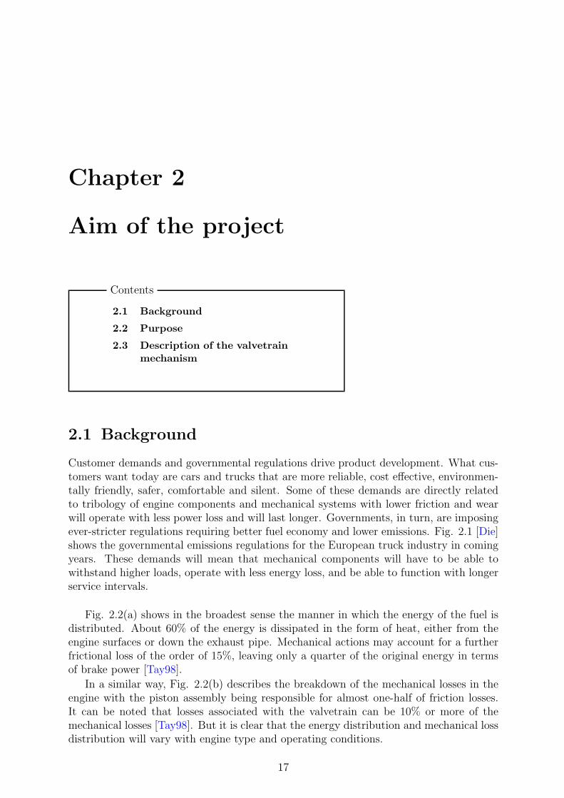
Customer demands and governmental regulations drive product development. What cus-tomers want today are cars and trucks that are more reliable, cost effective, environmen-tally friendly, safer, comfortable and silent. Some of these demands are directly relatedto tribology of engine components and mechanical systems with lower friction and wearwill operate with less power loss and will last longer. Governments, in turn, are imposingever-stricter regulations requiring better fuel economy and lower emissions. Fig. 2.1 [Die]shows the governmental emissions regulations for the European truck industry in comingyears. These demands will mean that mechanical components will have to be able towithstand higher loads, operate with less energy loss, and be able to function with longerservice intervals.

Fig. 2.2(a) shows in the broadest sense the manner in which the energy of the fuel isdistributed. About 60% of the energy is dissipated in the form of heat, either from theengine surfaces or down the exhaust pipe. Mechanical actions may account for a furtherfrictional loss of the order of 15%, leaving only a quarter of the original energy in termsof brake power [Tay98].

In a similar way, Fig. 2.2(b) describes the breakdown of the mechanical losses in theengine with the piston assembly being responsible for almost one-half of friction losses.It can be noted that losses associated with the valvetrain can be 10% or more of themechanical losses [Tay98]. But it is clear that the energy distribution and mechanical lossdistribution will vary with engine type and operating conditions.

17

18 Chap. 2: Aim of the project

Figure 2.1: The development of governmental regulations for NOx and particle emissions

Tribological improvements which consist in lowering friction and improving wear re-sistance in engines will play a major role in future developments. Several solutions areavailable to reduce friction and improve the wear resistance of surfaces. Examples areimprovements in lubrication, better design from a tribological point of view (roughness,contact mechanics, surface coatings) and surface hardening to improve material properties.

(a) Fuel energy distribution (b) Mechanical losses distribution

Figure 2.2: Energy and mechanical losses distribution in an internal combustion engine

2.2 Purpose 19

2.2 Purpose

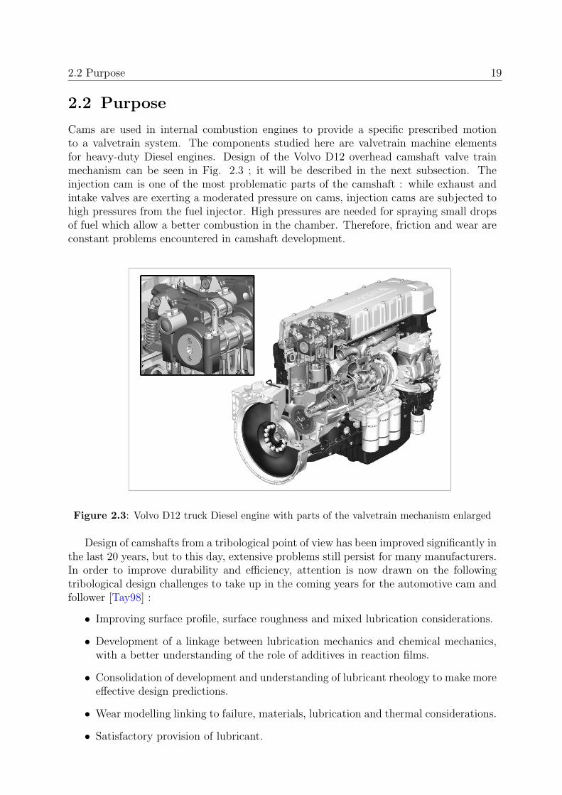
Cams are used in internal combustion engines to provide a specific prescribed motionto a valvetrain system. The components studied here are valvetrain machine elementsfor heavy-duty Diesel engines. Design of the Volvo D12 overhead camshaft valve trainmechanism can be seen in Fig. 2.3 ; it will be described in the next subsection. Theinjection cam is one of the most problematic parts of the camshaft : while exhaust andintake valves are exerting a moderated pressure on cams, injection cams are subjected tohigh pressures from the fuel injector. High pressures are needed for spraying small dropsof fuel which allow a better combustion in the chamber. Therefore, friction and wear areconstant problems encountered in camshaft development.

Figure 2.3: Volvo D12 truck Diesel engine with parts of the valvetrain mechanism enlarged

Design of camshafts from a tribological point of view has been improved significantly inthe last 20 years, but to this day, extensive problems still persist for many manufacturers.In order to improve durability and efficiency, attention is now drawn on the followingtribological design challenges to take up in the coming years for the automotive cam andfollower [Tay98] :

• Improving surface profile, surface roughness and mixed lubrication considerations.

• Development of a linkage between lubrication mechanics and chemical mechanics,with a better understanding of the role of additives in reaction films.

• Consolidation of development and understanding of lubricant rheology to make moreeffective design predictions.

• Wear modelling linking to failure, materials, lubrication and thermal considerations.

• Satisfactory provision of lubricant.

20 Chap. 2: Aim of the project

The satisfactory lubrication of the cam and follower contact in internal combustion en-gines has proved to be the most difficult of all the tribological components. The primaryfunction of the lubricant is to separate contacting surfaces, thus preventing metal-to-metal contact and premature cam failure. In cam operation, elastohydrodynamic lubri-cation films are generated which reduce interaction of the contacting surfaces. For thesetribomechanical elements, numerous methods have been developed to calculate the thick-ness of these films.

The purpose of this work is to investigate the behavior of the oil film in the cam androller contact, in order to predict regimes of lubrication and thus to identify the probablewear zones of the injection cam. Confrontation with experimental results will also bedone. Future work to achieve is to discover the influence of the different parameters on oilfilm thickness, by performing a multivariate analysis. The next step will focus on mod-elling the wear of injection cams, and finally establishing quantified correlations betweenwear and oil film thickness.

The outline of this report is structured as follows :

• Chapter 3 gives basic notions of tribology, friction, wear and lubrication, and de-scribes accurately the different regimes of lubrication,

• Chapter 4 is focused on the tribological study of the cam-roller contact, i.e theevaluation of oil film thickness from elastohydrodynamic film theory,

• Chapter 5 is about the prospects to investigate in the framework of my MSc work.

2.3 Description of the valvetrain mechanism

The camshaft’s function in an engine is to open and close the valves. Its design results invalves being opened and closed at a controlled rate of speed as well as at a precise time inrelation to piston position. The Volvo D12 valvetrain mechanism is composed of a rockerarm with a roller follower, used to open and shut the intake and exhaust valves and alsoto pump up the pressure in the Diesel injector placed between the intake and exhaustrocker arms (see Fig. 2.4).

Figure 2.4: Illustration of the valvetrain mechanism

Chapter 3

Introduction to tribology : friction,wear & lubrication

Contents

3.1 Tribology

3.1.1 The tribological contact

3.1.2 The concept of third body

3.2 Friction

3.3 Wear

3.4 Lubrication

3.4.1 Viscosity

3.4.2 Regimes of lubrication

3.4.3 Conformal and non-conformal surfaces

3.1 Tribology

Tribology is the science of interacting surfaces in relative motion and the word originatesfrom the Greek word ”tribos” which means ”rubbing”. The science includes sub-areassuch as friction, wear and lubrication.

Friction is the resistance to bodies moving against each other and is always presentwhen bodies are in motion. Friction can either be dry or viscous and in the former casewe make a distinction between static and dynamic friction ; and in the latter case frictiondevelops due to molecular forces between adjacent fluid layers.

Wear is a destructive process where surface material is removed from one or both ofthe two bodies in relative motion.

Finally, lubrication is a way of controlling both friction and wear. Lubricants can beeither solid or fluid type, and their main purpose is to reduce the friction and protect thesurfaces against wear. The work presented in this report deals with fluid film lubrication.

21

22 Chap. 3: Introduction to tribology : friction, wear & lubrication

3.1.1 The tribological contact

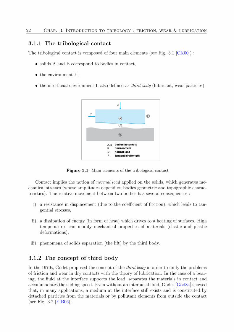
The tribological contact is composed of four main elements (see Fig. 3.1 [CK00]) :

• solids A and B correspond to bodies in contact,

• the environment E,

• the interfacial environment I, also defined as third body (lubricant, wear particles).

Figure 3.1: Main elements of the tribological contact

Contact implies the notion of normal load applied on the solids, which generates me-chanical stresses (whose amplitudes depend on bodies geometric and topographic charac-teristics). The relative movement between two bodies has several consequences :

i). a resistance in displacement (due to the coefficient of friction), which leads to tan-gential stresses,

ii). a dissipation of energy (in form of heat) which drives to a heating of surfaces. Hightemperatures can modify mechanical properties of materials (elastic and plasticdeformations),

iii). phenomena of solids separation (the lift) by the third body.

3.1.2 The concept of third body

In the 1970s, Godet proposed the concept of the third body in order to unify the problemsof friction and wear in dry contacts with the theory of lubrication. In the case of a bear-ing, the fluid at the interface supports the load, separates the materials in contact andaccommodates the sliding speed. Even without an interfacial fluid, Godet [God84] showedthat, in many applications, a medium at the interface still exists and is constituted bydetached particles from the materials or by pollutant elements from outside the contact(see Fig. 3.2 [FIB06]).

3.2 Friction 23

Figure 3.2: Representation of the numerical contact when a stable layer of third body isobtained

3.2 Friction

The force known as friction may be defined as the resistance encountered by one body inmoving over another. It is always exerted in the direction opposite to the movement (forkinetic friction) or the potential movement (for static friction) between two surfaces incontact. It is not a fundamental force, as it is made up of electromagnetic forces betweenatoms (interfacial connections, adhesive force). When contacting surfaces move relativelyto each other, the friction between the two objects converts kinetic energy into thermalenergy (heat).

Static friction occurs when the two bodies are not moving relatively to each other. Itcorresponds to the initial force to get an object moving. Rolling friction is classified understatic friction, because there is no relative velocity at the contact.

Kinetic (or dynamic) friction occurs when two bodies are moving relative to each otherand rub together. It corresponds to the force necessary to keep the motion at constantspeed (ex : sliding friction, fluid friction).

According to the Coulomb model, the coefficient of friction is a dimensionless scalarvalue which describes the ratio between the frictional force F and the normal load P (seeFig. 3.3) :

µ =F

P(3.1)

where µ is the coefficient of friction, P is the normal force exerted between the surfaces(here : P = body weight) and F is the tangential force exerted by friction.

In the laws of sliding friction, the frictional force is proportional to the normal load,and is independent from the apparent area and sliding velocity. In rolling contact, thefrictional force inversely proportional to the radius of the rolling element and is lower forsmoother surfaces.


Figure 3.3: Solid rubbing on a plan : creation of a frictional force F

3.3 Wear

Wear is a consequence of friction. It is a process in which interaction of surfaces of a solidwith the working environment results in the dimensional and functional loss of the solid,with or without loss of material (see Fig. 3.4 [KC00]).

Considering a tribological approach based on the nature of phenomena at the originof the damages, we can distinguish 5 main wear processes 1 :

• adhesive wear,

• abrasive wear,

• surface fatigue,

• corrosive wear (+ fretting),

• erosion / cavitation.

These five processes of wear can be found in an engine group. The valvetrain compo-nents are mainly affected by adhesive wear and surface fatigue.

Figure 3.4: Main forms of damages

1The 5 wear processes are detailed in Appendix A.

3.4 Lubrication 25

3.4 Lubrication

Fluid film lubrication occurs when opposing bearings surfaces are completely separatedby a lubricant film. A lubricant is any substance that reduces friction and wear andprovides smooth running and a satisfactory life for machine elements. Lubricants alsoallow to transfer heat, carry away contaminants and debris, transmit power, and preventcorrosion.

Most lubricants are liquids (such as mineral oils, synthetic esters, silicone fluids), butthey may be solids (such as PTFE) for use in dry bearings (ex : aeronautic), greases foruse in rolling-element bearings, or gases (such as air) for use in gas bearings [Ham94].Typically, lubricants contain 90% base oil (most often petroleum fractions, called mineraloils) and less than 10% additives (such as antioxidants, corrosion and rust inhibitors,anti-foaming...).

The physical and chemical interactions between the lubricant and the lubricating sur-faces must be understood in order to provide the machine elements with satisfactory life.First, we shall give a definition of the most important property of an oil for lubricatingpurposes : its viscosity. Then, the four lubrication regimes will be described, followed bya brief discussion about conformal and non-conformal surfaces.

3.4.1 Viscosity

The friction between surfaces which are completely separated (no asperity contact) is dueonly to the internal friction of the liquid, namely, its viscosity. The viscosity of a fluidmay be associated with its resistance to flow ; it is a measure of the resistance of a fluidto deform under shear stress [Ham94].

i). The dynamic viscosity η expresses the relationship between the shear stress τ andthe velocity gradient ∂u

∂y.

τ = η∂u

∂y(3.2)

ii). The kinematic viscosity ν characterises the ratio of the viscous force to the inertialforce (function of the fluid density ρ) :

ν =η

ρ(3.3)

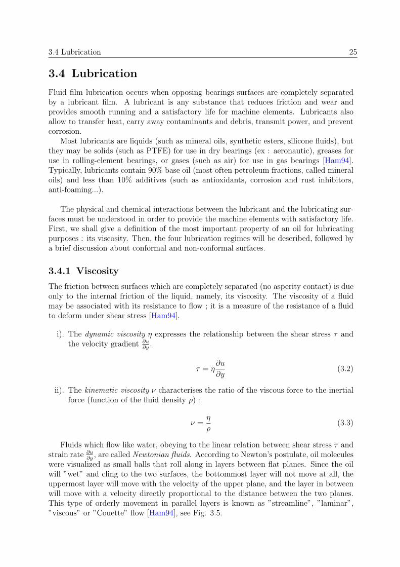
Fluids which flow like water, obeying to the linear relation between shear stress τ andstrain rate ∂u

∂y, are called Newtonian fluids. According to Newton’s postulate, oil molecules

were visualized as small balls that roll along in layers between flat planes. Since the oilwill ”wet” and cling to the two surfaces, the bottommost layer will not move at all, theuppermost layer will move with the velocity of the upper plane, and the layer in betweenwill move with a velocity directly proportional to the distance between the two planes.This type of orderly movement in parallel layers is known as ”streamline”, ”laminar”,”viscous” or ”Couette” flow [Ham94], see Fig. 3.5.


Figure 3.5: Laminar shear of fluid between 2 plates

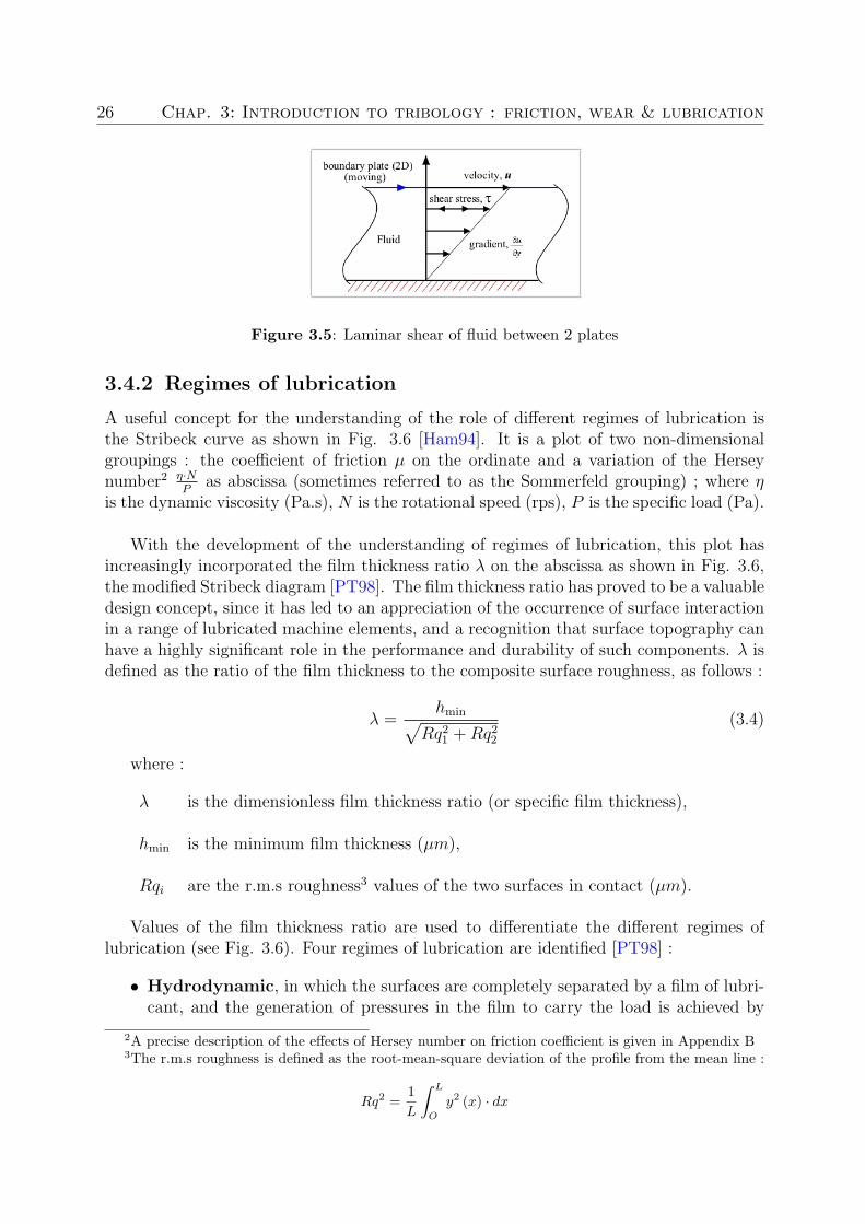
3.4.2 Regimes of lubrication

A useful concept for the understanding of the role of different regimes of lubrication isthe Stribeck curve as shown in Fig. 3.6 [Ham94]. It is a plot of two non-dimensionalgroupings : the coefficient of friction µ on the ordinate and a variation of the Herseynumber2 η·N

Pas abscissa (sometimes referred to as the Sommerfeld grouping) ; where η

is the dynamic viscosity (Pa.s), N is the rotational speed (rps), P is the specific load (Pa).

With the development of the understanding of regimes of lubrication, this plot hasincreasingly incorporated the film thickness ratio λ on the abscissa as shown in Fig. 3.6,the modified Stribeck diagram [PT98]. The film thickness ratio has proved to be a valuabledesign concept, since it has led to an appreciation of the occurrence of surface interactionin a range of lubricated machine elements, and a recognition that surface topography canhave a highly significant role in the performance and durability of such components. λ isdefined as the ratio of the film thickness to the composite surface roughness, as follows :

λ =hmin√

Rq21 + Rq2

2

(3.4)

where :

λ is the dimensionless film thickness ratio (or specific film thickness),

hmin is the minimum film thickness (µm),

Rqi are the r.m.s roughness3 values of the two surfaces in contact (µm).

Values of the film thickness ratio are used to differentiate the different regimes oflubrication (see Fig. 3.6). Four regimes of lubrication are identified [PT98] :

• Hydrodynamic, in which the surfaces are completely separated by a film of lubri-cant, and the generation of pressures in the film to carry the load is achieved by

2A precise description of the effects of Hersey number on friction coefficient is given in Appendix B3The r.m.s roughness is defined as the root-mean-square deviation of the profile from the mean line :

Rq2 =1L

∫ L

O

y2 (x) · dx

3.4 Lubrication 27

hydrodynamic action, in which the dynamic viscosity of the lubricant is the primelubricant characteristic. In this regime, friction is generated by shearing of the oil.

• Elastohydrodynamic, in which the surfaces are also in theory separated, butthe contact is much more concentrated, the films are thinner and other physicalphenomena (elastic distortion of the surfaces and the effect of pressure on dynamicviscosity) are influential. The work presented in this report deals exclusively withcontacts that operate in this regime.

• Mixed, in which a lubricated contact experiences some degree of asperity contactbetween surfaces and the overall behavioral characteristics and load capacity aredefined by both (elasto)hydrodynamic and boundary (see below) influences. Loadis supported both by the oil film (via the phenomenon of hydrodynamic lift) andthe contacts between surface asperities.

• Boundary, in which the surfaces are in normal contact with behavior characterizedby the chemical (and physical) actions of thin films of molecular proportions. Inthe most severe conditions (low speed, critical viscosity, high loads), metal-to-metalcontacts lead to a fast deterioration of surfaces.

Figure 3.6: The Stribeck diagram identifying the regimes of lubrication as conventionallyassociated with specific lubricated engine components

The regimes of lubrication conventionally associated with the piston rings, cam-followerand engine bearings of an automobile are shown in Fig. 3.6. These components rely upondifferent modes of lubrication for satisfactory performance and indeed each may encountermore than one form of lubrication during a cycle. This reflects the challenges that face thedesigner in improving operational characteristics, in response to legal and other pressureson emissions control and energy efficiency.


3.4.3 Conformal and non-conformal surfaces

Conformal surfaces fit thightly into each other with a high degree of geometrical con-formity, so that the load is carried over a relatively large area. The load-carrying surfacearea remains essentially constant while the load is increased. Fluid film journal bearings(see Fig. 3.7(a)) and slider bearings have conformal surfaces. Hydrodynamic lubrication iscommonly attributed to conformal surfaces ; the bearing pressure is generated in the highviscosity fluid due to the motion of the surfaces and the geometrical converging wedgecreated by the inclination of the surfaces. The film thickness is usually larger than 1µm and the pressure rarely exceeds 10 MPa. Further, the pressure is normally not highenough to deform the surfaces elastically [Alm04].

Non-conformal surfaces do not geometrically conform to each other well and havesmall lubrication areas (nominally line or point contact), see Fig. 3.7(b). The lubricationarea enlarges with increasing load but is still small in comparison with the lubricationarea of conformal surfaces. Typical components that operate in this region are the contactbetween gear teeth, between a cam and its follower, or between a ball and its track in aball bearing. The local pressures in the contact zone will generally be much higher thanthose encountered in hydrodynamic lubrication ; they typically range up to several GPafor steel components. The lubricating fluid film is normally less than 1 µm. Under theseconditions, elastic deformation of the solid surfaces plays an important role, as does thepressure-viscosity effects of the lubricant. Lubrication in these circumstances is known aselastohydrodynamic [Hut92].

(a) Conformal contact (b) Non-conformal contact

Figure 3.7: Contacts where a lubricating film separates the surfaces in relative motion

Chapter 4

Analysis of oil film behavior in thecam-roller contact

Contents

4.1 Physical explanation of EHL-contact

4.2 EHL film thickness model for elliptical contacts

4.3 Evolution of the parameters over one revolution of the camshaft

4.3.1 Radius of curvature of the cam

4.3.2 Entraining velocity

4.3.3 Normal load at the contact

4.3.4 r.m.s roughness of the cam

4.3.5 Constant parameters

4.4 Thermal correction of film thickness

4.4.1 Thermal correction factor

4.4.2 Maximum Hertzian pressure

4.4.3 Thermal correction values - Discussion

4.5 Numerical results

4.6 Confrontation with experimental results

4.6.1 Cam follower test equipment

4.6.2 Specific film thickness results

4.6.3 Observation of worn cams - Discussion

Lubrication is of significant importance in the prevention of cams from tribologicalprocesses and wear which cause failure. Many tribomechanical systems such as cams havecontacting surfaces that do not conform to each other very well. The full magnitude of theload must then be carried by a very small contact area. The lubrication of the contactingsurfaces of cams involves a complex technology. Contact loads on the contacting surfaces

29

30 Chap. 4: Analysis of oil film behavior in the cam-roller contact

of these tribomechanical systems tend to deform the material in the contact zone. Even ifthe loads are high, there is usually a thin film of lubricant between the contacting surfaces,so called an elastohydrodynamic film (EHL). The behavior of such films is complicatedbecause their formation depends on mutually dependent factors : tribological propertiesof the lubricant and deformation of the contact zone.

4.1 Physical explanation of EHL-contact

In order to explain the physics in an EHL-contact, a simplified geometry is shown inFig. 4.1. The geometry is 2D and is only the central part of the geometry shown inFig. 3.7(b). The fluid film interacts with the moving surfaces through adhesive forcesbetween surfaces and the adjacent fluid layers ; i.e. the fluid adheres to the surfaces.Two main forces are created in the fluid film with a highly viscous fluid, the viscous andpressure forces. The movement between the fluid layers creates viscous forces and theseare balanced by pressure forces [Alm04].

Figure 4.1: 2D model-geometry of a deformed EHL-contact

At the inlet of the EHL-contact, a geometrical wedge is formed by the convergingsurfaces. The fluid is dragged into the converging wedge due to the viscous forces, andin order to enforce mass conservation some of the fluid has to be pushed back by thepressure forces.

The pressure in the fluid is increased during the passage through the inlet region, aswell as the pressure-dependent variables, such as viscosity and density. At some stage thepressure is high enough to deform the surfaces elastically. When this occurs, the geomet-rical converging wedge disappears and the fluid is transported through the central regionof the contact. The oil film thickness in this region is called central film thickness h0. Afeature of EHL-contacts is that the central region has an almost constant film thickness,apart from a small curvature due to compressibility effects.

Another interesting feature of EHL-contacts is the characteristic pressure peak occur-ing close to the exit region, see Fig. 4.1. In this region, the pressure will drop rapidlydue to the diverging surfaces where the fluid cavitates. The decrease in pressure resultsin smaller elastic deformations and a constriction of the surfaces close to the outlet. The

4.2 EHL film thickness model for elliptical contacts 31

same effect applies once again ; i.e a geometrical wedge is created at the outlet. A partof the fluid is pushed back in order to enforce mass conservation, and a pressure peak iscreated at the position of the exit constriction, where the minimum film thickness hmin

can be found.

Thus, formation of an EHL film is the combination of three main effects : (1) formationof an hydrodynamic film (due to the pressure generated by the oil wedge mechanism), (2)elastic deformation of the two surfaces, and (3) increase of oil viscosity with respect topressure (piezoviscosity effect, also called pressure-viscosity index).

4.2 EHL film thickness model for elliptical contacts

According to experimental results of literature ([Ham94], [Geo00]), high loaded EHL-contacts are assumed to be elliptical, as shown in Fig. 4.2.

(a) EHL-contact shape visualizedby optical interferometry

(b) Schematic illustrationof EHL-contact

Figure 4.2: Contact is made of a central region where thickness h0 is constant, and a horseshoe-shaped constriction of minimum thickness hmin

In the 1970s, Hamrock and Dowson [HD76] [BD81] published a series of articles givinga numerical analysis of the elastohydrodynamic lubrication. Several equations have beenindependently derived by various investigations for predicting EHL minimum and centralfilm thicknesses.

Theoretical investigation of EHL involves solving Reynolds equation1 while takingaccount of the variation of lubricant viscosity with pressure, and allowing for the elastic

1The differential equation governing the pressure distribution in fluid film lubrication is known as the”Reynolds equation” (Reynolds, 1886). For time-invariant conditions while neglecting side leakage forEHL, the appropriate Reynolds equation is :

d

dx

(ρ · h3

η

dp

dx

)= 12 · ud (ρ · h)

dx

The Reynolds equation is derived in two different ways, from the Navier-Stokes and continuity equations,and directly from the principle of mass conservation.


distortion of the bounding surfaces caused by the hydrodynamically generated pressuredistribution.

Assumptions of the model are the following : isothermal flow, newtonian, piezoviscousand incompressible lubricant, fully flooded lubrication, hard elastic materials. Thirty-fourcases were used to generate the minimum film thickness hmin and central film thicknessh0 formulas for EHL elliptical conjunctions :

hmin = 3.63 ·Rx · U0.68 ·G0.49 ·W−0.073 ·(1− e−0.68·k) (4.1)

h0 = 2.69 ·Rx · U0.67 ·G0.53 ·W−0.067 ·(1− 0.61 · e−0.73·k) (4.2)

where U , G, W and k are dimensionless groupings defined as follows :

U is the dimensionless speed parameter :

U =η0 · u

E ′ ·Rx

(4.3)

G is the dimensionless material parameter :

G = α · E ′ (4.4)

W is the dimensionless load parameter :

W =w

E ′ ·R2x

(4.5)

k is the dimensionless form parameter (ellipticity parameter) :

k = 1.0339 ·(

Ry

Rx

)2/π

(4.6)

The variables used in this EHL model for elliptical conjunctions are :

Rx effective radius in the rolling direction x, m

1

Rx

=1

rx1

+1

rx2

(4.7)

4.2 EHL film thickness model for elliptical contacts 33

Ry effective radius in the orthogonal direction y, m

1

Ry

=1

ry1

+1

ry2

(4.8)

rx,y radii of curvature of cam (1) and roller (2), in the rolling and orthogonal directions, m

E ′ effective modulus of elasticity, Pa

E ′ = 2 ·(

1− ν21

E1

+1− ν2

2

E2

)−1

(4.9)

Ei modulus of elasticity of the material i, Pa

νi Poisson’s ratio of the material i

u entraining velocity in the rolling direction, m/s

u =1

2(u1 + u2) (4.10)

ui surface velocity of the cam and roller follower, m/s

η0 oil dynamic viscosity at p = 0 and operating temperature, Pa.s

α pressure-viscosity coefficient at operating temperature, Pa−1, such as :

η (p) = η (p0) · eα·(p−p0) (4.11)

w normal load at the contact, N

The minimum oil film thickness, together with the surface roughness, determines whenfull fluid film lubrication begins to break down. The expression of the specific film thick-ness λ introduced in Section 3.4.2 is reminded below :

λ =hmin

σ=

hmin√Rq

21 + Rq

22

(4.12)

where σ =√

Rq21 + Rq

22 is the composite surface roughness of the surfaces (also called

roughness standard deviation). The specific film thickness λ is used to describe the rangeof values for the lubrication regimes ; its value provides a measure of how likely, and howsevere, asperity interactions will be in lubricated sliding [Hut92] :


• for λ > 3, a full fluid film separates the two surfaces, asperity contact is negligibleand both friction and wear should be low. However, many non-conformal contactsin machine components operate with λ < 3.

• the regime 1 < λ < 3 is termed partial EHL, or mixed EHL ; under these conditionssome contact between asperities occurs.

• at λ = 1, the film thickness is of the same size as the contacting asperities. This isoften considered to be the border between the boundary lubricated regime and themixed lubricated regime.

• for λ < 1, no real lubricant film can develop and there is significant asperity contact,resulting in high friction. At extremely high loads or low sliding speeds, increasinglysurface severe damage can occur on sliding (adhesive wear), and the behavior of thesystem depends critically on the properties of boundary lubricants, if present.

A schematic picture of the theoretical model used is given in Fig. 4.3.

Figure 4.3: Schematic illustration of the theoretical EHL model used in this work

The minimum and central film thicknesses developed above are not only useful fordesign purposes but also provides convenient means of assessing the influence of vari-ous parameters on the EHL film thickness. According to literature [Ham94], comparisonbetween theoretical and experimental film thicknesses show a quite good accuracy of pre-dicted film thicknesses, between 10% and 20% of accuracy.

The next paragraph will focus on the evolution of the parameters of the model duringone revolution of the camshaft. Then, numerical results will be discussed, and adjustmentswill be made to the model, in order to take into account thermal effects on the value ofoil film thickness.

4.3 Evolution of the parameters over one revolution of the camshaft 35

4.3 Evolution of the parameters over one revolution

of the camshaft

While some parameters of the model can be assumed to be constant during one revolutionof the camshaft (discussed in Section 4.3.5), many parameters are variable and must becalculated as a function of cam angle :

i). the radius of curvature of the cam rx1 in the rolling direction is a function of thecam profile,

ii). the entraining velocity u depends both on cam and roller peripheral speeds,

iii). the normal load at the contact w is directly linked to the injection pressure, whichis a function of cam angle.

iv). measurements of r.m.s roughnesses on a brand-new machined camshaft have shownthat Rq is dependent on the cam angle.

4.3.1 Radius of curvature of the cam

The notion of radius of curvature is directly linked to the cam profile2, which is obtainedwith the principle of ”inversion” : the cam is considered as the fixed member and thefollower is then moved to its proper position (same relative motion). The cam profile isthus the enveloppe of the follower profile as the follower is positionned around the cam.Volvo D12 injection cam profile and its distinct regions are shown in Fig. 4.4.

Figure 4.4: Cam profile and its distinct regions

The shape of a curve at any point depends on the rate of change of direction calledcurvature. We can construct for each point of the curve a tangent circle whose curvature

2Cam profile also provides crucial information – for design considerations – about follower motioncharacteristics ; see Appendix C.


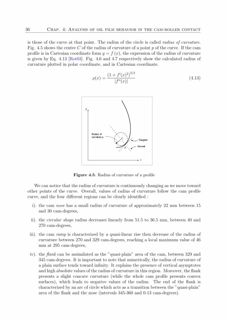
is those of the curve at that point. The radius of the circle is called radius of curvature.Fig. 4.5 shows the centre C of the radius of curvature of a point p of the curve. If the camprofile is in Cartesian coordinate form y = f (x), the expression of the radius of curvatureis given by Eq. 4.13 [Rot03]. Fig. 4.6 and 4.7 respectively show the calculated radius ofcurvature plotted in polar coordinate, and in Cartesian coordinate.

ρ(x) =(1 + f ′(x)2)

3/2

|f ′′(x)|(4.13)

Figure 4.5: Radius of curvature of a profile

We can notice that the radius of curvature is continuously changing as we move towardother points of the curve. Overall, values of radius of curvature follow the cam profilecurve, and the four different regions can be clearly identified :

i). the cam nose has a small radius of curvature of approximately 22 mm between 15and 30 cam-degrees,

ii). the circular shape radius decreases linearly from 51.5 to 36.5 mm, between 40 and270 cam-degrees,

iii). the cam ramp is characterized by a quasi-linear rise then decrease of the radius ofcurvature between 270 and 329 cam-degrees, reaching a local maximum value of 46mm at 295 cam-degrees,

iv). the flank can be assimilated as the ”quasi-plain” area of the cam, between 329 and345 cam-degrees. It is important to note that numerically, the radius of curvature ofa plain surface tends toward infinity. It explains the presence of vertical asymptotesand high absolute values of the radius of curvature in this region. Moreover, the flankpresents a slight concave curvature (while the whole cam profile presents convexsurfaces), which leads to negative values of the radius. The end of the flank ischaracterized by an arc of circle which acts as a transition between the ”quasi-plain”area of the flank and the nose (intervals 345-360 and 0-13 cam-degrees).


Figure 4.6: Calculated radius of curvature, plotted in polar coordinate

Figure 4.7: Calculated radius of curvature, plotted in Cartesian coordinate


4.3.2 Entraining velocity

a/ Slip measurement

Velocities of both cam and roller can be easily visualized as the contact between twocylinders or discs rotating at the appropriate speeds to give the correct combination ofrolling and sliding contact. Fig. 4.8 shows two cylinders 1 and 2 of radii R1 and R2

rotating around their fixed centres in opposite directions and in the presence of a viscousfluid. Their peripheral speeds through the line of contact are u1 and u2 respectively. Inthis case, u2 > u1, but the directions of both are such as to draw the viscous fluid intothe gap between them, thus the entraining velocity u, which must be incorporated intothe film thickness model, is given by [Wil05] :

u =1

2(u1 + u2) (4.14)

This is also known as the rolling velocity. In our example, because u1 does not equalu2 there is also an element of relative sliding velocity between the two surfaces. Thissliding velocity is equal to :

∆u = |u1 − u2| (4.15)

The slip is defined as the relative difference between cam and roller velocities, asfollows :

S =u1 − u2

u1

=ucam − uroller

ucam

(4.16)

Figure 4.8: Geometry of two loaded cylinders rotating around their fixed centre


A method for slip analysis between the camshaft and the roller of a Volvo D12 enginewas developed at Finnveden Powertrain AB, using high-speed camera [Mal06]. Slip wasmeasured for an engine speed of 1800 rpm (i.e. camshaft speed of 900 rpm) at themaximal injection force. Moving averaged results are plotted in Fig. 4.9, and comparedwith acceleration.

Figure 4.9: 8 periods moving averaged slip measurements, and roller acceleration curve

By observing simultaneously the two curves, it can be noticed that the slip curvefollows interesting trends. When the acceleration keeps constant values, the slip oscil-lates around zero. But when acceleration varies suddenly, peaks can be observed quasi-instantaneously in the slip curve. This is particularly obvious between 330 and 345 cam-degrees, where roller acceleration rises suddenly. This leads to a negative value of the slip,down to -0.13 (meaning that roller speed is 1.13 times higher than cam speed). The effectof roller decceleration on slip between 15 and 40 cam-degrees is less marked. Moreover,two areas where slip is subjected to strong variations remain difficult to explain, 60 to 90cam-degrees, and 230-270 cam-degrees. Thus, it seems evident that the phenomenon ofslip also depends on other parameters.

b/ Calculation of velocities

In order to obtain the entraining velocity u, it is necessary :

i). first, to calculate the cam tangential speed ucam,

ii). then, to find out the roller tangential speed uroller using the expression of slip.


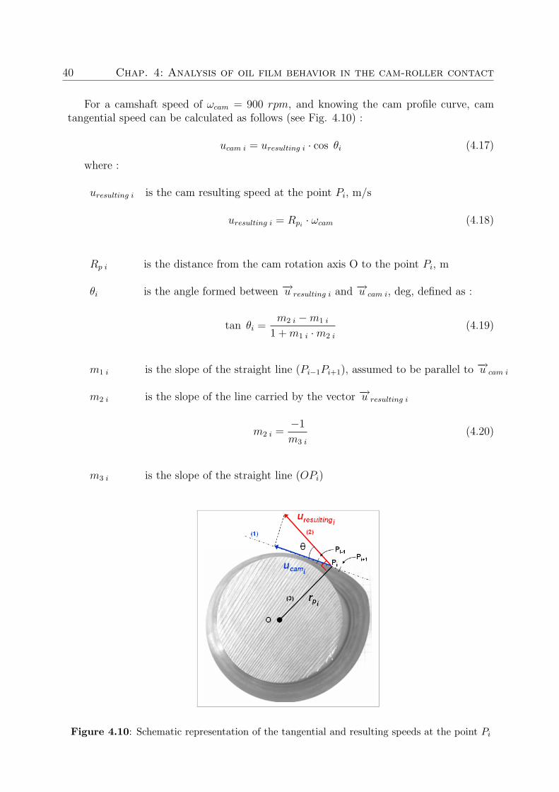
For a camshaft speed of ωcam = 900 rpm, and knowing the cam profile curve, camtangential speed can be calculated as follows (see Fig. 4.10) :

ucam i = uresulting i · cos θi (4.17)

where :

uresulting i is the cam resulting speed at the point Pi, m/s

uresulting i = Rpi· ωcam (4.18)

Rp i is the distance from the cam rotation axis O to the point Pi, m

θi is the angle formed between −→u resulting i and −→u cam i, deg, defined as :

tan θi =m2 i −m1 i

1 + m1 i ·m2 i

(4.19)

m1 i is the slope of the straight line (Pi−1Pi+1), assumed to be parallel to −→u cam i

m2 i is the slope of the line carried by the vector −→u resulting i

m2 i =−1

m3 i

(4.20)

m3 i is the slope of the straight line (OPi)

Figure 4.10: Schematic representation of the tangential and resulting speeds at the point Pi


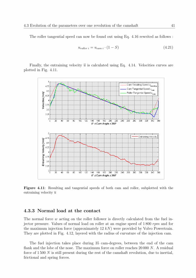
The roller tangential speed can now be found out using Eq. 4.16 rewrited as follows :

uroller i = ucam i · (1− S) (4.21)

Finally, the entraining velocity u is calculated using Eq. 4.14. Velocities curves areplotted in Fig. 4.11.

Figure 4.11: Resulting and tangential speeds of both cam and roller, subplotted with theentraining velocity u

4.3.3 Normal load at the contact

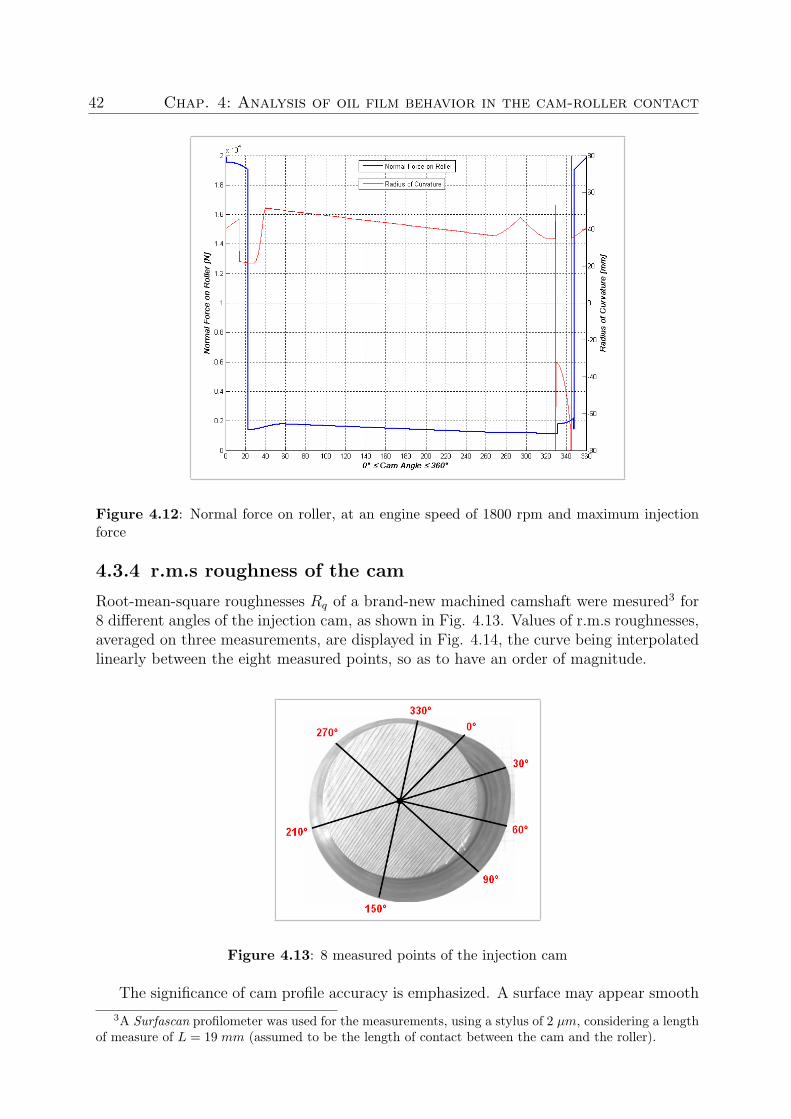
The normal force w acting on the roller follower is directly calculated from the fuel in-jector pressure. Values of normal load on roller at an engine speed of 1 800 rpm and forthe maximum injection force (approximately 12 kN) were provided by Volvo Powertrain.They are plotted in Fig. 4.12, layered with the radius of curvature of the injection cam.

The fuel injection takes place during 35 cam-degrees, between the end of the camflank and the lobe of the nose. The maximum force on roller reaches 20 000 N . A residualforce of 1 500 N is still present during the rest of the camshaft revolution, due to inertial,frictional and spring forces.


Figure 4.12: Normal force on roller, at an engine speed of 1800 rpm and maximum injectionforce

4.3.4 r.m.s roughness of the cam

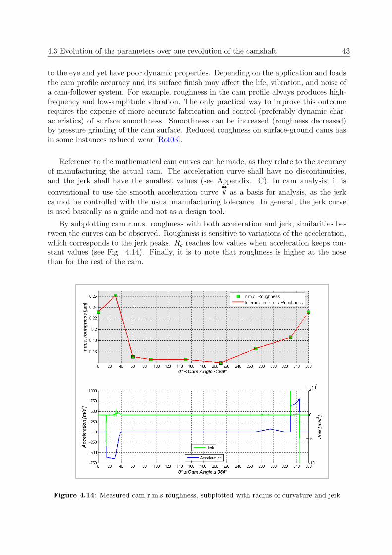
Root-mean-square roughnesses Rq of a brand-new machined camshaft were mesured3 for8 different angles of the injection cam, as shown in Fig. 4.13. Values of r.m.s roughnesses,averaged on three measurements, are displayed in Fig. 4.14, the curve being interpolatedlinearly between the eight measured points, so as to have an order of magnitude.

Figure 4.13: 8 measured points of the injection cam

The significance of cam profile accuracy is emphasized. A surface may appear smooth

3A Surfascan profilometer was used for the measurements, using a stylus of 2 µm, considering a lengthof measure of L = 19 mm (assumed to be the length of contact between the cam and the roller).


to the eye and yet have poor dynamic properties. Depending on the application and loadsthe cam profile accuracy and its surface finish may affect the life, vibration, and noise ofa cam-follower system. For example, roughness in the cam profile always produces high-frequency and low-amplitude vibration. The only practical way to improve this outcomerequires the expense of more accurate fabrication and control (preferably dynamic char-acteristics) of surface smoothness. Smoothness can be increased (roughness decreased)by pressure grinding of the cam surface. Reduced roughness on surface-ground cams hasin some instances reduced wear [Rot03].

Reference to the mathematical cam curves can be made, as they relate to the accuracyof manufacturing the actual cam. The acceleration curve shall have no discontinuities,and the jerk shall have the smallest values (see Appendix. C). In cam analysis, it is

conventional to use the smooth acceleration curve••y as a basis for analysis, as the jerk

cannot be controlled with the usual manufacturing tolerance. In general, the jerk curveis used basically as a guide and not as a design tool.

By subplotting cam r.m.s. roughness with both acceleration and jerk, similarities be-tween the curves can be observed. Roughness is sensitive to variations of the acceleration,which corresponds to the jerk peaks. Rq reaches low values when acceleration keeps con-stant values (see Fig. 4.14). Finally, it is to note that roughness is higher at the nosethan for the rest of the cam.

Figure 4.14: Measured cam r.m.s roughness, subplotted with radius of curvature and jerk


4.3.5 Constant parameters

Table 4.3.5 gives the values of the parameters which are assumed to be constant duringone revolution of the camshaft. They can be grouped in three categories : geometry ofthe two contacting surfaces, elastic characteristics of the materials, and oil properties. Itis to note that the subscripts 1 and 2 refer respectively to the cam and to the roller.

Geometry of the two contacting surfaces :

Rx 2 = 22.5 mmRy 1 = Ry 2 = 5 000 mm (→∞)Rq 2 = 0.18 µm

Elastic characteristics of materials :

E1 = E2 = 210 000 Mpaν1 = ν2 = 0.3

Oil properties :

η0 = 0.01207 Pa.s at 100 ◦Cα = 1.5 · 10−8 Pa−1

β = 0.056 ◦C−1

K = 0.137 W/m · ◦C

Table 4.1: Constant parameters of the model

4.4 Thermal correction of film thickness

4.4.1 Thermal correction factor

In most engineering applications, especially for high loaded contacts such as the cam-roller contact, it is not realistic to assume isothermal conditions. In fact, the lubricantis strongly heated due to the high shearing at the inlet of the contact. Such heating willlower the viscosity and the film thickness will decrease in comparison to the isothermalcase. A thermal correction factor CT is defined as follows :

hmin, thermal = CT · hmin, isothermal (4.22)

The film thickness reduction due to viscous heating of the lubricant at the conjunctioninlet was examined by Cheng (1967) and by Sheu and Wilson (1982). These data wereconsolidated by Gupta et al. (1991) to give the following integrated empirical formula for

4.4 Thermal correction of film thickness 45

calculating the percentage of film thickness reduction due to inlet heating, or the thermalcorrection factor CT [Ham94] :

CT =1− 13.2 · (pm/E ′) ·Br0.42

1 + 0.213 · (1 + 2.323 · A0.83) ·Br0.64(4.23)

where Br and A are dimensionless groupings defined as follows :

Br is a thermal parameter (Brinkman number) :

Br =

(− ∂η

∂T

)· u2

K≈ β · η0 · u2

K(4.24)

A is a kinematic parameter :

A = 2 · (u2 − u1)

(u2 + u1)(4.25)

and

p0 is the maximum Hertzian pressure, Pa

β is the temperature-viscosity coefficient, 1/◦C, defined from :

η = η0 · e−β·(T−TO) (4.26)

K is the thermal conductivity of the lubricant, W/m ·◦ C

The following subsection is about the evaluation of the maximum Hertz pressure p0

at the contact, as it is a required variable. Then, values of the thermal correction factorCT will be discussed.

4.4.2 Maximum Hertzian pressure

The contact between cam and roller is simplified by assuming two parallel cylinders incontact. According to the Hertz theory [Fla00], the shape of the contact between camand roller is rectangular of width 2b and length L, and the pressure distribution p, ischaracterized by a semi-ellipse (see Fig. 4.15).

Values of the pressure distribution p and the maximum pressure p0 can be calculatedby knowing the load, radius of the cylinders, and the elastic properties of the materials :

p = p0 ·√

1− y2

b2(4.27)


where the maximum pressure p0 along the load axis x is given by :

po =

√w · E ′

2 · π · L ·Rx

=2 · w

π · b · L(4.28)

and the semi-length of contact b along the x axis is defined by :

b =

√8 · w ·Rx

π · L · E ′ (4.29)

Figure 4.15: Pressure distribution between two parallel cylinders

The Hertzian method has two limitations which are worth being mentioned : the bod-ies are assumed to have elastic and isotropic material behavior, and the length of contactL in the orthogonal direction has to be very large in comparison with their radii, whichis not the case for the cam and roller follower configuration. But literature agrees to saythat these formulas are precise enough to estimate maximum Hertzian pressures in thecam and roller.

Using results developed in Section 4.3, the maximum Hertzian pressure can be cal-culated as a function of cam angle. The contact length L in the orthogonal direction yis assumed to be constant and equal to L = 19 mm. The results are displayed in Fig. 4.16.

The maximum pressure occurs between the flank and the nose. This result is due toa combination of highest loads and smallest radii (see Fig. 4.12), so that pressure risesbecause the same load is distributed on a narrower contact area. The contact lengthfollows an interesting trend, reaching a peak at the flank (about 330 cam-degrees), wherethe radius of curvature tends towards infinity (plain surface). Moreover, it can be seenthat the contact area (equal to the product b · L) increases significantly with the load.

4.4 Thermal correction of film thickness 47

Figure 4.16: Semi-length of contact b and maximum Hertzian pressure p0 as a function of camangle

4.4.3 Thermal correction values - Discussion

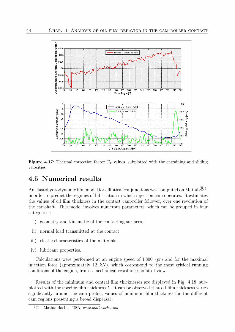
Using the results developed in previous subsection, the thermal correction factor CT canbe calculated as a function of cam angle using Eq. 4.23. Results are plotted in Fig. 4.17.

It can be observed that thermal correction of the oil film thickness is not negligible,CT varying from 0.73 to 0.87.

It can also be seen that the thermal correction factor CT is very sensitive to theentraining (or rolling) and sliding velocities. The thermal correction of film thicknessincreases (i.e. value of CT decreases) when velocities (both rolling and sliding) rise. Oilfilm thickness is then reduced due to an increased shearing at the inlet of the contact.Moreover, Fig. 4.17 shows that film thickness is much more sensitive to sliding than toentraining velocity4. Thus, sliding motion causes more heating (consequence of shearing)than rolling motion.

4The following inegality can be established by observing the curves plotted in Fig. 4.17 :

d CT

d (∆u)>>

d CT

d u

where u is the rolling velocity, and ∆u is the sliding velocity.


Figure 4.17: Thermal correction factor CT values, subplotted with the entraining and slidingvelocities

4.5 Numerical results

An elastohydrodynamic film model for elliptical conjunctions was computed on Matlab R©5,in order to predict the regimes of lubrication in which injection cam operates. It estimatesthe values of oil film thickness in the contact cam-roller follower, over one revolution ofthe camshaft. This model involves numerous parameters, which can be grouped in fourcategories :

i). geometry and kinematic of the contacting surfaces,

ii). normal load transmitted at the contact,

iii). elastic characteristics of the materials,

iv). lubricant properties.

Calculations were performed at an engine speed of 1 800 rpm and for the maximalinjection force (approximately 12 kN), which correspond to the most critical runningconditions of the engine, from a mechanical-resistance point of view.

Results of the minimum and central film thicknesses are displayed in Fig. 4.18, sub-plotted with the specific film thickness λ. It can be observed that oil film thickness variessignificantly around the cam profile, values of minimum film thickness for the differentcam regions presenting a broad dispersal :

5The Mathworks Inc. USA, www.mathworks.com

4.5 Numerical results 49

• around 0.2 µm for the nose, with a local minima of 0.15 µm just before the nose’slobe,

• a linear decrease from 0.25 µm to 0.2 µm for the circular shape,

• a constant value of 0.2 µm for the ramp,

• a local peak of 0.43 µm for the ”quasi-plain” part of the flank, followed by a rapiddrop to 0.15 µm.

It can be noticed that the central film thickness h0 is about 1.25 times higher thanthe minimum film thickness hmin (confer the h0/hmin ratio, Fig. 4.19).

Figure 4.18: Minimum and central film thicknesses, subplotted wih the specific film thickness

The specific film thickness λ is a valuable design concept, as it is used to describe therange of values for the lubrication regimes. Since λ < 3 for the whole profile, the camnever operates under a full fluid film and asperities contacts play an important role inboth friction and wear.

• Cam nose and the end of the flank (after the ”quasi-plain” surface) appear to be themost critical areas of the profile in terms of lubrication : the specific film thicknessλ is lower than 1 for the intervals [ 0 ; 60 ] and [ 345 ; 360 ] cam-degrees. The oil filmis thinner than the surface asperities, so that the surfaces are in continuous metal-to-metal contact, i.e boundary lubrication. Under such conditions, deformation will


occur on the rolling surfaces. This statement can be sensed by plotting the ratioh0/hmin, which defines the ratio between the central region of the contact andthe exit constriction thicknesses. It can also be verified by calculating the totaldeformation of the contacting bodies (see Fig. 4.19), according to Hertz theory[Geo00] :

δ =b2

Rx

(4.30)

Figure 4.19: Specific film thickness, subplotted with the ratio h0/hmin and the total defor-mation

• The circular shape and the ramp operate between λ = 0.8 and 1, which means thatthe film thickness is of the same size as the contacting asperities. This is oftenconsidered to be the border between the boundary lubricated regime and the mixedEHL regime, even if the transition between the two regimes is not sharp.

• The ”quasi-plain” area of the flank operates between λ = 1 and 1.6, i.e mixed-EHL– also termed as ”effective” boundary-lubrication condition – in which significantasperity contact occurs.

These values provide a measure of the severity of asperities interaction in the lubricatedcontact, and enable us to predict the probable wear zones of the injection cam.

However, it has been shown that surface roughness significantly decreases during thefirst 20 minutes of the engine running-in – due to surface polishing – and then stabilizes

4.6 Confrontation with experimental results 51

for longer operation [Ols06]6. Thus, when attempting to foresee cam wear, it is morerealistic to appreciate the regimes of lubrication by taking into account polished surfaces.Results of specific film thicknesses considering polished surfaces will be interpreted in thefollowing subsection.

4.6 Confrontation with experimental results

Tests were performed on a valvetrain equipment in order to observe the evolution ofsurfaces during running. The camshaft was driven during 160 hours at different speeds.The experimental equipment is described below ; then, specific film thickness takinginto account worn surface roughnesses will be presented. Finally, comparison betweencalculations and cam surface observations will be made.

4.6.1 Cam follower test equipment

The cam follower test equipment located in Finnveden Powertrain AB was designed on acylinder head of a Volvo D12 Diesel engine (see Fig. 4.20). The camshaft is placed overthe inlet and outlet valves. At the front, the camshaft is driven by an electric motor. Thelubricant is heated up to about 110 ◦C, and circulated through the normal lubricationsystem.

In the same way, fuel is going through the original system : fuel is injected withoutcombustion in the chamber and then recycled. The original engine control unit is used andis connected to the Diesel injectors, making it possible to adjust the timing of the openingand closing of the injectors so that different loads can be simulated. The equipment canbe run for long periods and at speeds covering the normal engine speed range.

Figure 4.20: Photo of the test equipment, the top cover being removed

6According to [Ols06], there is no distinguish difference between the cam surface samples that hadbeen run 20 minutes or those which had been run for 2000 minutes.


4.6.2 Specific film thickness results

Running-in is a process that affects the film parameter. This process allows wear to occurso that the mating surfaces can adjust to each other to provide smooth running. This typeof wear may be viewed as beneficial. The film parameter will increase with running-in,since the composite surface roughness σ will decrease. According to [Ham94], running-inalso has a significant effect on the shape of the asperities that is not captured by the com-posite surface roughness. With running-in, the peaks of the asperities in contact becomeflattened.

Root-mean-square roughnesses Rq of an injection cam were mesured after a 160-hourrunnning (about 107 cycles). Rq values are approximately 5 times lower than those of anunworn cam, the range of values being 0.04-0.065 µm. Measured r.m.s roughness of theroller is 0.16 µm for the whole roller profile (while it was 0.18 µm for the unworn roller).Specific film thicknesses of the worn cam are displayed in Fig. 4.21.

Figure 4.21: Comparison of specific film thickness of an unworn and a worn cam

The specific film thickness λ can be applied as an indicator of rolling element perfor-mance and service life :

• Cam nose and the end of the flank remain at λ < 1, i.e in boundary lubricatedconditions, for the intervals [ 0 ; 22 ] and [ 348 ; 360 ] cam-degrees. No real lubricantfilm can develop and the surfaces are in continuous metal-to-metal contact, result-ing in high friction. According to literature [Rot03], wear can be 20 times moreimportant than for λ > 3.

4.6 Confrontation with experimental results 53

• The circular shape and the ramp operate between λ = 1.2 and 1.4. It indicatesan ”effective” boundary-lubrication condition in which significant asperity contactoccurs. According to [Rot03], surface distress will exist for 1 < λ < 1.5, accompaniedby superficial surface pitting with about 4 times more wear than λ > 3.

• The ”quasi-plain” area of the flank operates between λ = 1.6 and 2.6, termed aspartial EHL or mixed EHL regime. Under these conditions, some contacts betweenasperities occurs. A thicker film develops due to the plain surface, favouring thephenomenon of hydrodynamic lift. Load is partially supported by the oil film andthe contacts between surface asperities. For 1.5 < λ < 3, some surface polishingcan occur with eventual surface failure by subsurface pitting fatigue with about 1.5times more wear than λ > 3 [Rot03].

4.6.3 Observation of worn cams - Discussion

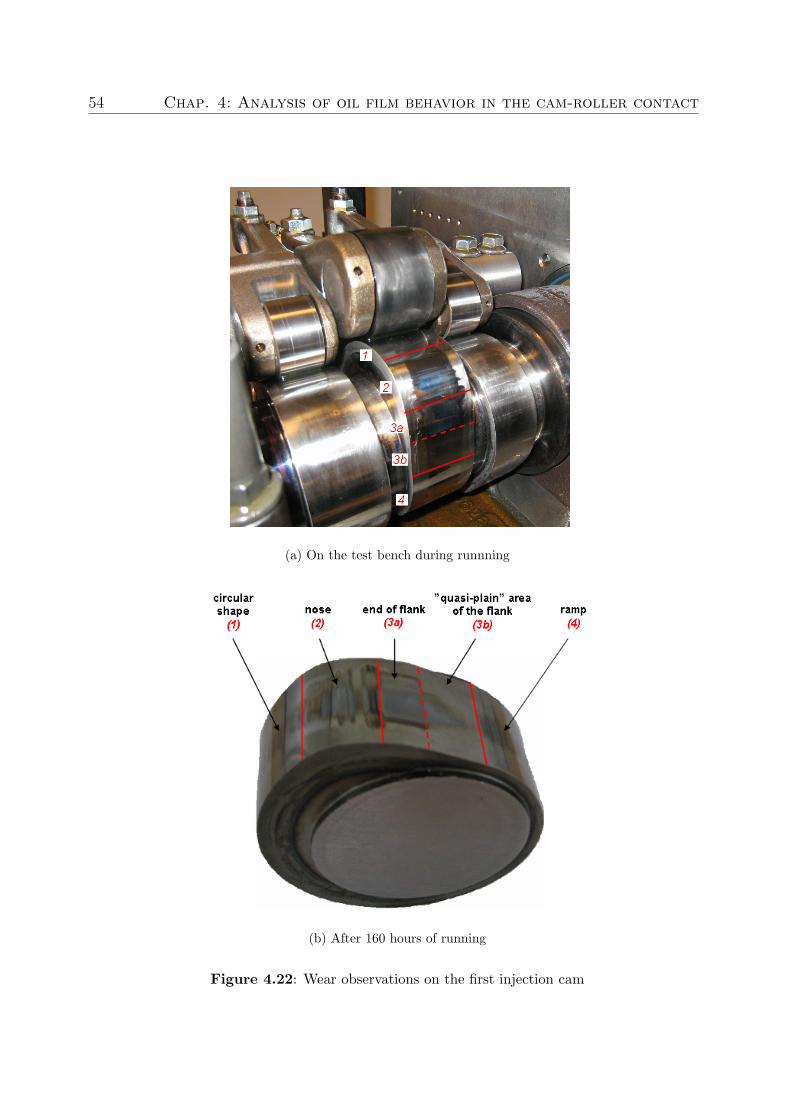
According to the predicted regimes of lubrication, we can expect the end of the flank andthe nose to be more affected by wear than the rest of the cam profile. This statement isconfirmed by visual observations of worn cam surface after running, as Fig. 4.22 shows :

• The nose is characterized by the widest wear track of the cam. In fact, these area isaffected by the biggest deformations, implying an increased area of contact betweencam and roller. Furthermore, fluctuation of the contact width can be observed –caused by vibrations and contact pressure variations – as well as bumping marks,due to roller bouncing.

• The end of the flank is subjected to a strong surface glazing (or polishing) of constantwidth.

• The ”quasi-plain” area of the flank only presents slight glazing traces, as expectedin the mixed EHL regime.

• Both circular shape and ramp present numerous bumping marks, and a relativelynarrow wear track.

Observations of worn cam surface after running show a quite good concordance be-tween predicted regimes of lubrication (combined with expected wear) and experimentalresults. However, the model itself is not sufficient to explain all the forms of wear observedon a cam. For example, it doesn’t incorporate the phenomenon of interactions betweencams, which causes roller bouncing that creates bumping marks on the cam surface.

But this model remains of great interest to appreciate the impact of design parameterson oil film thickness and operating regimes of lubrication. Nevertheless, it is to note thatthe model is not only composed of design parameters (i.e parameters controlled by thedesigner) but also incorporates required functions of the cam-roller mechanism, such asthe sliding velocity and therefore the slip. Indeed, slip is not a controlled parameter as itis a result of the tribo-contact. Thus, slip cannot be imposed as an initial condition ; itsvalue can only be obtained through measurements on the test equipment.


(a) On the test bench during runnning

(b) After 160 hours of running

Figure 4.22: Wear observations on the first injection cam

Chapter 5

Future work

Contents

5.1 Multivariate analysis

5.2 Wear modelling

5.1 Multivariate analysis

Surface engineering includes establishing a series of specifications. The designer has todecide on a number of parameters that will meet the functional demands on the finishedproduct in regard to friction, wear resistance, lubrication, and so on. These parametersthen have to be translated by the planning engineer into machining parameters in orderto produce a surface with the desired properties. Finally, quality control should be able tomeasure the surface and verify that the manufacturing is in agreement with the demandsspecified by the designer.

A control loop suggested by Stout and Davis [SD84] is shown in Fig. 5.1. It showsthe interdependence between the required functional behavior of the surface, its manu-facturing, and the characterization of its design parameters. This work will particularlyfocus on the dependence between characterization and function. Correlation with themanufacturing process parameters is beyond the scope of this study.

Figure 5.1: Control loop showing the interdependence between function, manufacturing andcharacterization, the three essentials for producing complex surfaces

55

56 Chap. 5: Future work

Required functions for the cam-roller follower mechanism are a low wear rate (i.e a longlife cycle), low frictional losses, low sliding and efficiency in terms of engine performance.Oil film thickness can also be interpreted as a function, since the operating lubricationregime directly impacts both friction and wear of the contacting surfaces.

By performing a multivariate analysis1, the aim of this study will be to determine :

i). the influence of design parameters on the EHL-film thickness,

ii). correlations between the different parameters.

This goal could be achieved by performing a principal component analysis (PCA) usingthe software SIMCA-P2, which attempts to determine a smaller set of synthetic variablesthat could explain the original set.

5.2 Wear modelling

In the previous chapter, the predicted specific film thickness λ has proved to be a mean-ingful indicator of the probable wear zones of the cam. The upcoming step of this projectwill consist in modelling the wear generated at the contact cam-roller. A general modelproposed by [HBA96] for the micro-scale wear between rough surfaces caused by asperitieswill be used. The model is derived from the Archard’s wear equation and based on theprinciple of ”single point observation”. It considers what a single point on a contactingsurface is going through when interacting asperities of the opposite surface pass the point.

The objective of this last study is to find numerical correlations between the predictedspecific film thickness and the simulated wear of the cam. A further step would be tocompare simulations with wear measurements.

1Multivariate analysis comprises a set of techniques which involves observation and analysis of morethan one variable at the same time. In design and analysis, the tehcnique is used to perform trend-studies accross multiple dimensions while taking into account the effects of all variables on the responsesof interest.

2Umetrics, Sweden. www.umetrics.com

Chapter 6

Conclusion

Contents

6.1 Technical conclusions

6.2 Personal conclusion

6.1 Technical conclusions

For a lubricated contact, the degree of separation between surfaces has a very stronginfluence on the type and amount of wear. This degree of separation is termed as specificfilm thickness ; its value provides a measure of the severity of asperities interaction in thelubricated contact. In the cam-roller contact, the surfaces do not geometrically conformto each other very well ; they are subjected to high contact pressures and elastic defor-mations. Lubrication in those circumstances is known as elastohydrodynamic.

The purpose of this work was to evaluate the oil film thickness from elastohydrody-namic film theory. A fluid film model for elliptical conjuctions – established by Hamrockand Dowson – was computed on Matlab R©, in order to predict regimes of lubricationand thus to identify the probable wear zones of the injection cam. This model involvesnumerous parameters, which can be grouped in four categories :

i). geometry and kinematic of the contacting surfaces,

ii). normal load transmitted at the contact,

iii). elastic characteristics of the materials,

iv). lubricant properties.

Calculations showed that cam nose and the end of the flank are the most critical areasof the profile in terms of lubrication : they operate in boundary lubricated conditionswhich implie continuous metal-to-metal contacts, resulting in high friction. A more im-portant wear is expected in this zone than in the rest of the cam profile. Circular shape

57

58 Chap. 6: Conclusion

and ramp both operate around the border between boundary and mixed EHL regimes,in which significant asperity contact still occurs. The ”quasi-plain” area of the flank op-erates in the mixed EHL regime, in which load is supported both by the oil film and thecontacts between surface asperities.

Furthermore, observations of worn cam surface after running have shown a quite goodconcordance between predicted regimes of lubrication (combined with expected wear) andexperimental results.

In the framework of my MSc Research work, attention will be drawn on the depen-dence between design parameters characterization and required functional behavior of thesurface. By performing a multivariate analysis, the sudy will aim at determining the influ-ence of design parameters on the EHL-film thickness, as well as establishing correlationsbetween the different parameters.

The final stage of this project will consist in modelling the wear generated at thecam-roller contact, and then finding numerical correlations between the predicted specificfilm thickness and the simulated wear.

6.2 Personal conclusion

I have performed my final-year-project within the Functional Surfaces Research Group ofthe University of Halmstad, Sweden. This experience in a foreign country was rewardingat several levels.

At the educational level, this work period in a laboratory was the opportunity to dis-cover a new field, the Research, quite different from the industry. I familiarized myselfwith tribology, which made me aware of the importance of surfaces characterization inmany fields and the potential of this often unrecognized science.

The project I have carried out was connected with engine development ; it gave mea completing approach to my previous placements performed in the automotive industry.Alltogether, these three work experiences gave me the incentive to become a powertrainengineer. In that purpose, I will undertake applied-graduate-studies in Powertrain Engi-neering at the IFP School of Petroleum and Engines in Paris, in alternation with trainingperiods in a research institute, l’Institut Francais du Petrole.

At the human level, this period in Sweden was beneficial both culturally and linguis-tically. It was a chance to discover Sweden as well as Scandinavian countries. Moreover, Ihave spent five months with exchange students from all over the world. This melting-potof people and cultures was fulfilling from a human point of view. This once-in-a-lifetimeexperience will remain unforgettable, and I am convinced that it will provide me a greatasset to work in an international environment.

Appendices

59

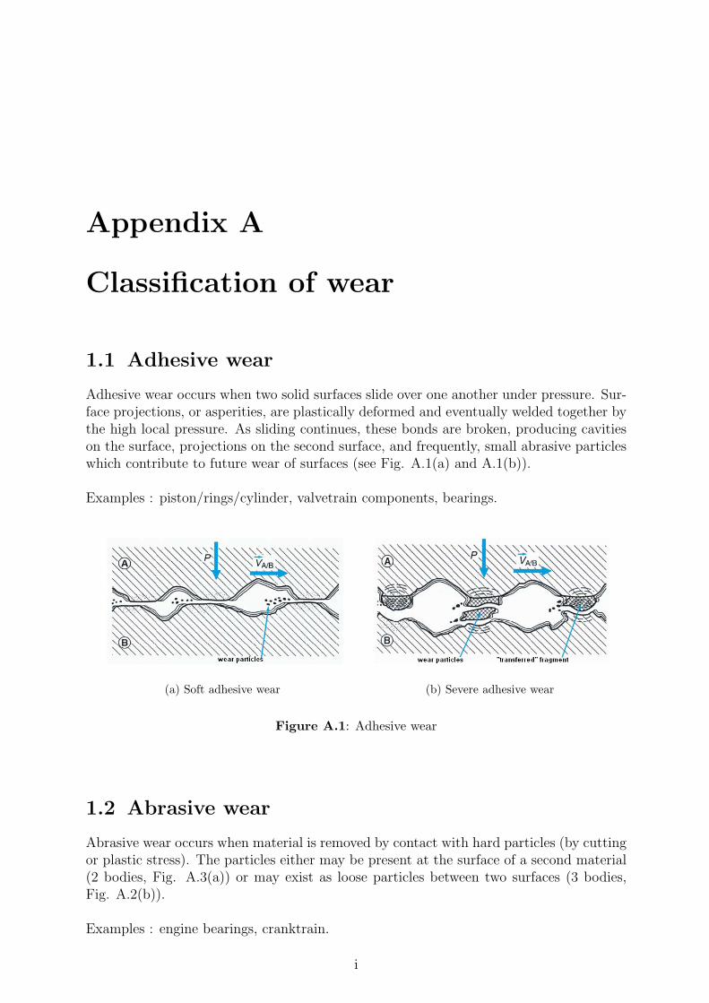
Appendix A

Classification of wear

1.1 Adhesive wear

Adhesive wear occurs when two solid surfaces slide over one another under pressure. Sur-face projections, or asperities, are plastically deformed and eventually welded together bythe high local pressure. As sliding continues, these bonds are broken, producing cavitieson the surface, projections on the second surface, and frequently, small abrasive particleswhich contribute to future wear of surfaces (see Fig. A.1(a) and A.1(b)).

Examples : piston/rings/cylinder, valvetrain components, bearings.

(a) Soft adhesive wear (b) Severe adhesive wear

Figure A.1: Adhesive wear

1.2 Abrasive wear

Abrasive wear occurs when material is removed by contact with hard particles (by cuttingor plastic stress). The particles either may be present at the surface of a second material(2 bodies, Fig. A.3(a)) or may exist as loose particles between two surfaces (3 bodies,Fig. A.2(b)).

Examples : engine bearings, cranktrain.

i

ii Chap. A: Classification of wear

(a) Abrasion with 2 bodies (b) Abrasion with 3 bodies

Figure A.2: Abrasive wear

1.3 Surface fatigue

Surface fatigue is a process by which the surface of a material is weakened by cyclicloading. It appears mainly by a surface cracking (surface cracks, Fig. A.3(a).a) or in anunder layer (delamination cracks, Fig. A.3(a).b), which both lead to the formation ofwear particles, in the form of scales or pitting (see Fig. A.3(b)).

Examples : gears, cam / roller.

(a) Ignition areas of fatigue cracks (b) Phenomenon ofpitting : formation ofcracks

Figure A.3: Surface fatigue

1.4 Corrosive wear (+ fretting)

Corrosive wear is a loss of material due to chemical reactions between rubbing surfaceand its environment (combustion gases, water...). Electrons of metal reacting with wateror oxygen lead to the formation of an oxide layer on surfaces environment by chemicalattack of a chemical agent. Then, oxide layer is removed by the simultaneous or successiveaction of :

A.4 Corrosive wear (+ fretting) iii

• the chemical attack of aggressive agent,

• the friction with an abrasive particule (see Fig. A.4).

Examples : cylinder liner, engine bearings.

Figure A.4: Abrasion and reformation of a passive oxide film in a corrosive environment

Fretting wear (or fretting corrosion) occurs when two surfaces in contact are subjectto very weak amplitude movements (vibrations, microglidings).

• Adhesive phenomena lead to wear particles in the contact, which are not evacuated.

• These particles stay there, accumulate and oxidize themselves.

• Then, these oxides cause a surface deterioration by abrasion, possibly aggravatedby fatigue cracks (see Fig. A.5).

Examples : fixing screws, gear box rods.

Figure A.5: Mechanisms of fretting wear

iv Chap. A: Classification of wear

1.5 Erosion - Cavitation

Erosion / cavitation is defined as the progressive loss of material on the surface of a solidby a fluid loaded with particles. We can distinguish the erosion by abrasive particles andthe erosion by cavitation :

i). In hard particle erosion, 3 main mechanisms can occur : abrasion, surface fatigueand contact cracking. It leads to the creation of impacts and scores on surfaces (seeFig. A.6).

Figure A.6: Principle of erosion

ii). Cavitation corresponds to a superficial wear of the material under the influence ofshock waves due to the implosion of vapor bubbles. It can lead to the formation ofscales and cavities (see Fig. A.7).

Examples : cooling circuit / oil circuit.

Figure A.7: Mechanisms of cavitation wear

Appendix B

Physical explanation of the Stribeckcurve

Four lubrication regimes were described : hydrodynamic, elastohydrodynamic, mixed andboundary. There are most clearly demonstrated through a Stribeck curve. The ordinatein Fig. B.1 is the coefficient of friction under steady state conditions. The abscissa inFig. B.1 is the Hersey dimensionless number, and is given as :

η ·NP

(B.1)

where :

• η is the dynamic viscosity (Pa.s),

• N is the rotational speed (rps),

• P is the specific load (Pa).

A high Hersey number usually means a relatively thick lubricant film, whereas a smallnumber results in a very thin film.

i). At an extremely low Hersey number, no real lubricant film can develop and thereis significant asperity contact, resulting in high friction. This high friction value ispersistent with increasing Hersey number until a first threshold value is reached.This represents the dominance of boundary lubrication in determining load transferand friction between surfaces.

ii). As the Hersey number increases, a noticeable and rapid decrease in friction valuesis observed. This is explained by in increasing lubricant film thickness and sharedload between the surface asperities and the pressurized liquid lubricant present inthe conjunction. In this mixed regime, widely varying friction values can be mea-sured and are strongly dependent on operating conditions.

v

vi Chap. B: Physical explanation of the Stribeck curve

iii). With a further increase in Hersey number, friction reaches a lower plateau value,corresponding to the onset of hydrodynamic lubrication. At this point, the surfacesare effectively separated by the liquid lubricant, and asperity contact has negligibleeffect on load support and friction.

Figure B.1 shows a slight increase in friction with respect to Hersey number in thehydrodynamic regime. It can be attributed to increased redundant work in the lu-bricant or to increases in shear strength, but these are seen to be relatively minoreffects.

iv). A furher distinction is often made between elastohydrodynamic and full film lubri-cation in a Stribeck curve. This is useful for some bearing types, gears or cams,but it should be recognized that conformal surfaces do not encounter for elastohy-drodynamic lubrication. Therefore, this regime may or may not be identified in theStribeck curve, depending on the source [Ham94].

Figure B.1: A Stribeck curve, showing the effects of Hersey number η·NP on friction coefficient

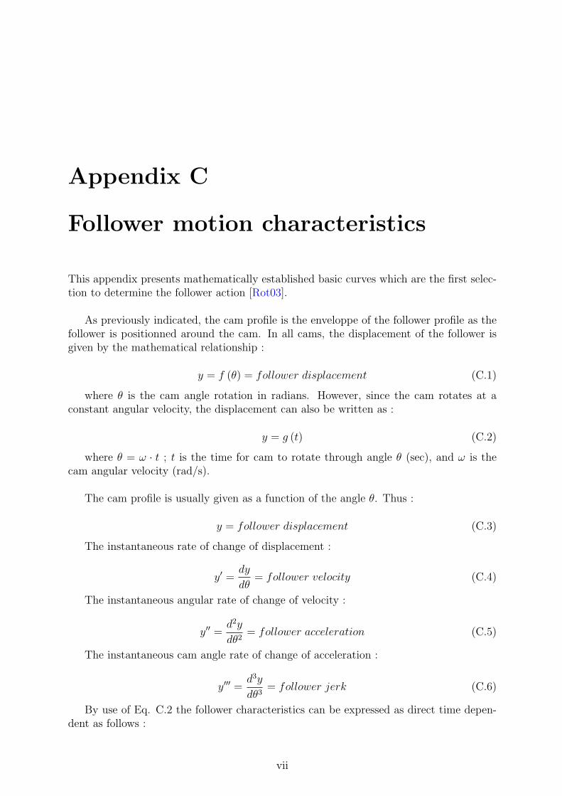
Appendix C

Follower motion characteristics

This appendix presents mathematically established basic curves which are the first selec-tion to determine the follower action [Rot03].

As previously indicated, the cam profile is the enveloppe of the follower profile as thefollower is positionned around the cam. In all cams, the displacement of the follower isgiven by the mathematical relationship :

y = f (θ) = follower displacement (C.1)

where θ is the cam angle rotation in radians. However, since the cam rotates at aconstant angular velocity, the displacement can also be written as :

y = g (t) (C.2)

where θ = ω · t ; t is the time for cam to rotate through angle θ (sec), and ω is thecam angular velocity (rad/s).

The cam profile is usually given as a function of the angle θ. Thus :

y = follower displacement (C.3)

The instantaneous rate of change of displacement :

y′ =dy

dθ= follower velocity (C.4)

The instantaneous angular rate of change of velocity :

y′′ =d2y

dθ2= follower acceleration (C.5)

The instantaneous cam angle rate of change of acceleration :

y′′′ =d3y

dθ3= follower jerk (C.6)

By use of Eq. C.2 the follower characteristics can be expressed as direct time depen-dent as follows :

vii

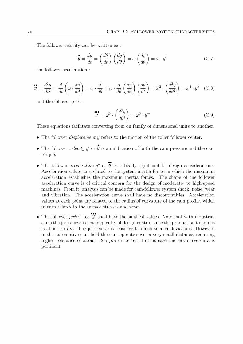
viii Chap. C: Follower motion characteristics

The follower velocity can be written as :

•y =

dy

dt=

(dθ

dt

) (dy

dθ

)= ω

(dy

dθ

)= ω · y′ (C.7)

the follower acceleration :

••y =

d2y

dt2=

d

dt

(ω · dy

dθ

)= ω · d

dθ= ω · d

dθ

(dy

dθ

) (dθ

dt

)= ω2 ·

(d2y

dθ2

)= ω2 · y′′ (C.8)

and the follower jerk :

•••y = ω3 ·

(d3y

dθ3

)= ω3 · y′′′ (C.9)

These equations facilitate converting from on family of dimensional units to another.

• The follower displacement y refers to the motion of the roller follower center.

• The follower velocity y′ or•y is an indication of both the cam pressure and the cam

torque.

• The follower acceleration y′′ or••y is critically significant for design considerations.

Acceleration values are related to the system inertia forces in which the maximumacceleration establishes the maximum inertia forces. The shape of the followeracceleration curve is of critical concern for the design of moderate- to high-speedmachines. From it, analysis can be made for cam-follower system shock, noise, wearand vibration. The acceleration curve shall have no discontinuities. Accelerationvalues at each point are related to the radius of curvature of the cam profile, whichin turn relates to the surface stresses and wear.

• The follower jerk y′′′ or•••y shall have the smallest values. Note that with industrial

cams the jerk curve is not frequently of design control since the production toleranceis about 25 µm. The jerk curve is sensitive to much smaller deviations. However,in the automotive cam field the cam operates over a very small distance, requiringhigher tolerance of about ±2.5 µm or better. In this case the jerk curve data ispertinent.

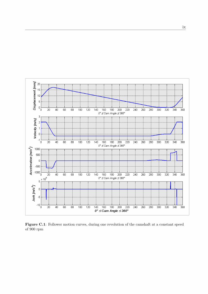
ix

Figure C.1: Follower motion curves, during one revolution of the camshaft at a constant speedof 900 rpm

Bibliography

[Alm04] T. Almqvist. Computational Fluid Dynamics in Theoretical Simulations of Elas-tohydrodynamic Lubrication. PhD thesis, Lulea University of Technology, 2004.26, 28

[BD81] B.J.Hamrock and D. Dowson. Ball bearing lubrication, the elastohydrodynamicsof elliptical contacts. John Willey and Sons, New York, 1981. 29

[CK00] M. Cartier and P. Kapsa. Usure des contacts mecaniques - Elements de tri-bologie. Techniques de l’Ingenieur, traite Genie Mecanique, BM 5 066, 2000.20

[Die] DieselNet. http://www.dieselnet.com/standards/eu/hd.html. 15

[FIB06] N. Fillot, I. Iordanoff, and Y. Berthier. Modelling third body flows with adiscrete element method - a tool for understanding wear with adhesive particles.Tribology International, 40:973–981, 2006. 20

[Fla00] L. Flamand. Fatigue des surfaces. Techniques de l’Ingenieur, traite GenieMecanique, BM 5 055, 2000. 43

[Geo00] J.M. Georges. Frottement, usure et lubrification - La tribologie ou sciences dessurfaces. CNRS Editions, 2000. 29, 48

[God84] M. Godet. The third body approach : a mechanical view of wear. Wear,52:100–437, 1984. 20

[Ham94] B.J. Hamrock. Fundamentals of Fluid Film Lubrication. McGraw-Hill, 1994.23, 24, 29, 32, 43, 50, vi

[HBA96] A.B-J. Hugnell, S. Bjorklund, and S. Andersson. Simulation of the mild wearin a cam-follower contact with follower rotation. Wear, 199:202–210, 1996. 54

[HD76] B.J. Hamrock and D. Dowson. Isothermal elasthohydrodynamic lubrication ofpoint contacts - part 1 : theoretical formulations. ASME Journal of lubricationtechnology, 98:223–229, 1976. 29

[Hut92] I.M. Hutchings. Tribology - Friction and Wear of Engineering Materials. But-terworth Heinemann, 1992. 26, 31

[KC00] P. Kapsa and M. Cartier. Usure des contacts mecaniques - manifestation del’usure. Techniques de l’Ingenieur, traite Genie Mecanique, BM 5 067, 2000. 22

xi

xii BIBLIOGRAPHY

[LBC03] P. Lindholm, S. Bjorklund, and M. Calvo Cortes. Characterisation of wear ona cam follower system in a diesel engine. Elsevier Wear, 254:1199–1207, 2003.

[Lin04] P. Lindholm. Wear resistant low friction coatings for engine components. PhDthesis, KTH Royal Institute of Technology, Stockholm, 2004.

[Mal06] A. Malmkvist. Method development for slip measurement on valve train, VolvoD12. PhD thesis, Chalmers University of Technology, 2006. 37

[Ols06] M. Olsson. Diesel Engnine Cam and Roller Follower Tribology. PhD thesis,Lund Institute of Technology, 2006. 49

[PT98] M. Priest and C.M. Taylor. Automobile engine tribology - approaching thesurface. Elsevier Wear, 241:193–203, 1998. 24

[Rot03] H.A. Rothbart. Cam Design Handbook. McGraw-Hill, 2003. 34, 41, 50, 51, vii

[SD84] K.J. Stout and E.J. Davis. Surface topography of cylinder bores - the relation-ship between manufacture, characterization and function. Wear, 95:111–125,1984. 53

[Tay98] C.M. Taylor. Automobile engine tribology - design considerations for efficiencyand durability. Elsevier Wear, 221:1–8, 1998. 15, 17

[Wil05] J. Williams. Engineering Tribology. Cambridge University Press, 2005. 36

tribological analysis of injection cams lubrication in ... - diva

Documents