arX

iv:1

105.

4151

v1 [

cs.N

I] 1

9 M

ay 2

011

Towards Realistic Vehicular Network Modeling UsingPlanet-scale Public Webcams

Gautam S. Thakur‡§ Pan Hui‡ Hamed Ketabdar‡ Ahmed Helmy§

§CISE, University of Florida, Gainesville, ‡Deutsche Telekom Laboratories, Berlin

gsthakur@cise.ufl.edu, pan.hui@telekom.de, hamed.ketabdar@telekom.de, helmy@cise.ufl.edu

ABSTRACTRealistic modeling of vehicular mobility has been particu-larly challenging due to a lack of large libraries of mea-surements in the research community. In this paper we in-troduce a novel method for large-scale monitoring, analy-sis, and identification of spatio-temporal models for vehic-ular mobility using the freely available online webcams incities across the globe. We collect vehicular mobility tracesfrom 2,700 traffic webcams in 10 different cities for severalmonths and generate a mobility dataset of 7.5 Terabytes con-sisting of 125 million of images. To the best of our knowl-edge, this is the largest data set ever used in such study.To process and analyze this data, we propose an efficientand scalable algorithm to estimate traffic density based onbackground image subtraction. Initial results show that atleast 82% of individual cameras with less than 5% devia-tion from four cities follow Loglogistic distribution and also94% cameras from Toronto follow gamma distribution. Theaggregate results from each city also demonstrate that Log-Logistic and gamma distribution pass the KS-test with 95%confidence. Furthermore, many of the camera traces exhibitlong range dependence, with self-similarity evident in theaggregates of traffic (per city). We believe our novel datacollection method and dataset provide a much needed con-tribution to the research community for realistic modelingofvehicular networks and mobility.

1. INTRODUCTIONResearch in the area of vehicular networks has in-

creased dramatically in recent years. With the prolifer-ation of mobile networking technologies and their inte-gration with the automobile industry, various forms ofvehicular networks are being realized. These networksinclude vehicle-to-vehicle, vehicle-to-roadside, and vehicle-to-roadside-to-vehicle architectures. Realistic model-ing, simulation and informed design of such networksface several challenges, mainly due to the lack of large-scale community-wide libraries of vehicular data mea-surement, and representative models of vehicular mo-bility.Earlier studies in this area have clearly established

a direct link between vehicular density distribution andthe performance [16, 3] of vehicular networks primitivesand mechanisms, including broadcast and geocast pro-tocols[1]. Although good initial efforts have been ex-erted to capture realistic vehicular density distributions,such efforts were limited by availability of sensed vehic-ular data[20]. Hence, there is a real need to conductvehicular density modeling using larger scale and morecomprehensive data sets. Furthermore, commonly usedassumptions, such as exponential distribution[19] of ve-hicular inter-arrival times[1], have been used to derivemany theories and conduct several analyses, the validityof which bears further investigation.In this study, we provide a novel framework for the

systematic monitoring, measurement, analysis and mod-eling of vehicular density distributions at a large scale.To avoid the limitations of sensed vehicular data, weinstead utilize the existing global infrastructure of tensof thousands of video cameras providing a continuousstream of street images from dozens of cities around theworld. Millions of images captured from publicly avail-able traffic web cameras are processed using a noveldensity estimation algorithm, to help investigate andunderstand the traffic patterns of cities and major high-ways. Our algorithm employs simple, scalable, and ef-fective background subtraction techniques to processthe images and build an extensive library of spatio-temporal vehicular density data.As a first step toward realistic vehicular network mod-

eling, we aim to provide a comprehensive view of thefundamental statistical characteristics of the vehiculartraffic density exhibited by the data from four majorcities over 45 days. Two main sets of statistical anal-yses are conducted. The first includes an investigationof the best-fit distribution for the arrival process usingvarious cameras and aggregate city data, while the sec-ond is a study of the long range dependence (LRD) andself-similarity observed in the data. Our early analysisshow two main results: i) the empirical distribution ofvehicular densities in most of the cameras and cities fol-low ‘log-logistic’ and ‘gamma’ distributions. ii) Consis-

1

tently, the data showed a high degree of self-similarityover orders of magnitude of time scales, in all citiesand for many cameras. This suggests a long-range-dependent process governing the vehicular arrival pro-cess in many realistic scenarios. Such result is in sharpcontrast to the assumptions of memoryless processescommonly used for vehicular mobility.The contributions of this work are manifold. (i) To

the best of our knowledge, we provide by far the largestand most extensive library of vehicular density data,based on processing of millions of images obtained fromten main cities and thousands of cameras. This ad-dresses a severe shortage of such data sets in the com-munity. The library will be made available to the re-search community in the future. (ii) We propose afast algorithm for traffic density estimation to efficientlyprocess millions of image files. (iii) We establish log-logistic and gamma distributions as the most suitablefits for the vehicular density distribution and provideearly evidence of self-similarity exhibited by the trafficat various time scales.The rest of the document is outlined as follows. Sec-

tion 2 discusses related work. In Section 3, we dis-cuss our vehicular dataset. In Section 4, we discussour background subtraction algorithm, and detectionand removal of outliers. Statistical analysis of measure-ments and modeling is illustrated in Section 5. Finallywe conclude our paper in Section 6 and give insight intothe future work.

2. RELATED WORKLarge scale mobility datasets are very important for

the mobile network and computing research community,but collecting them is even more challenging and usu-ally expensive [8]. In this paper, we propose an inex-pensive method to collect global scale vehicular mobilitytraces using thousands of freely available webcams thatprovide continuous and fine-grained monitoring of thevehicular traffic.Existing studies in transportation sciences focus on

improving road traffic and use of structural engineer-ing methods to resolve issues of congestion, evacuation,and mitigation plans. Initial work[5] mainly focusedon developing infrastructure for movement of vehicleson roads and bridges. However, in the recent times[7]much focus has been given to the use of sensor data.The later helps to engineer better traffic conditions, en-suring safety and management of traffic. For example,inductive loop detectors are equipped to monitor trafficflows. However, the availability of the data generatedfrom these sensors is not readily available to the gen-eral public. Second, studies[4] do not necessarily focuson vehicular networks, traffic modeling, and character-ization. In spite of data availability problems, surpris-ingly there is a large deployment of publicly available

online web cameras, which can be used to monitoringand modeling traffic. In our work, we take advantage ofthese free webcams. To our knowledge we are the firstto identify the power and usability of these free web cam-eras for the purpose of modeling and characterizing thetraffic across globe.Simulation tools like CORSIM[7] and VISSIM[11] are

geared to model specific scenarios for planning futuretraffic conditions on a micro-mobility and small scalelevel. In this work, we focus on the aspect of macro-mobility to model vehicular movements in form of flowdensities to analyze traffic on huge scale. From a net-working perspective, mobility models[4, 14] and routing[21] techniques investigate how mobility impact the per-formance of routing protocols [2]. If the mobility modelis unrealistic then routing performance is questionable.So, we need models inspired from real data sets. Byway of this work, we believe a comprehensive set of pa-rameters can be extracted to develop such models.In a recent work, Bai et. al [1] analyzed spatio-

temporal variations in vehicular traffic from the purposeof inter-vehicle communications. Data collected fromrealistic scenarios shows the effectiveness of exponen-tial model for highway vehicle traffic. On the same line,quantitative characteristics of vehicle arrival pattern onhighways is studied in [13]. By using real highway trafficdata, the study examines the existence of self-similaritycharacteristics on vehicle arrival data and finds thattime headway of vehicles on the highways follows theheavy-tailed distribution. These findings enrich trafficmodeling, but carried out on very small sample of dataand mainly localized to one or two locations. In ourstudy, we use 45 days of vehicular imagery data fromfour cities to model traffic and characterize the densitydistribution.A principle activity related to our work is image pro-

cessing and efficient retrieval of traffic information fromthese images. Many studies[5] have been carried outthat look into aspects of both background subtraction[15,17] and object detection[10]. In former methods[6], dif-ference in the current and reference frame is used toidentify objects. In detection approaches[18], learningthe object features (shape, size etc.) are used to detectand classify them. In our work, we are using a tem-poral methods for background subtraction to calculatea relative numerical value instead of counting cars. Inour work we find background subtraction is much fasterthan object detection, which is discussed in detail inlater section.

2

Table 1: Global Webcam DatasetsCity # of Cameras Duration Interval Records Database Size

Bangalore 160 30/Nov/10 - 01/Mar/11 180 sec 2.8 million 357 GBBeaufort 70 30/Nov/10 - 01/Mar/11 30 sec. 24.2 million 1150 GB

Connecticut 120 21/Nov/10- 20/Jan/11 20 sec. 7.2 million 435 GBGeorgia 777 30/Nov/10 - 02/Feb/11 60 sec. 32 million 1400 GBLondon 182 11/Oct/10 - 22/Nov/10 60 sec. 1 million 201 GB

London(BBC) 723 30/Nov/10 - 01/Mar/11 60 sec. 20 million 1050 GBNew york 160 20/Oct/10 - 13/Jan/11 15 sec. 26 million 1200 GBSeattle 121 30/Nov/10 - 01/Mar/11 60 sec. 8.2 million 600 GBSydney 67 11/Oct/10 - 05/Dec/10 30 sec. 2.0 million 350 GBToronto 89 21/Nov/10 - 20/Jan/11 30 sec. 1.8 million 325 GB

Washington 240 30/Nov/10 - 01/Mar/11 60 sec. 5 million 400 GBTotal 2709 - - 125.2 million 7468 GB

Figure 1: Infrastructure for measurement col-lection

(a) London (b) Sydney

Figure 2: Traffic cameras in London and Sydney. The

red dots show the location of cameras deployed.

3. DATA COLLECTIONThere are thousands, if not millions, of outdoor cam-

eras currently connected to the Internet, which are placedby governments, companies, conservation societies, na-tional parks, universities, and private citizens. Out-door webcams are usually mounted on a roadside pole

with easy accessibility, installation and maintenance,and they have seen enormous applications not only inadaptive traffic control and information systems, butalso in monitoring the weather conditions, advertisingthe beauty of a particular beach or mountain, or provid-ing a view of animal or plant life at a particular location.We view the connected global network of webcams as ahighly versatile platform, enabling an untapped poten-tial to monitor global trends, or changes, in the flow ofthe city, and providing large-scale data to realisticallymodel vehicular, or even human, mobility.In this section, we introduce the methodology for the

data collection and give a high level statistics of thedata traces. We collect vehicular mobility traces usingthe online webcam crawled by our crawler. A majorityof these webcams are deployed by the Department ofTransportations (DoT) in each city. They are used toprovide real time information about road traffic condi-tions to general public via online traffic web cameras.These web cameras are basically installed on traffic sig-nal poles facing towards the roads of some prominentintersections throughout city and highways. At regularinterval of time, these camera captures still pictures ofon-going road traffic and send them in form of feeds tothe DoTs media server. For the purpose of this study,we chose 10 cities with large number of webcam cover-age and took the permission from concerned DoTs tocollect these vehicular imagery data for several months.We cover cities in North America, Europe, Asia, andAustralia. In Fig.-1, we show our experimental infras-tructure to download and maintain the image data.Since these cameras provide better imagery during thedaytime, we limit our study to download and analyzethem only during such hours. On average, we down-load 15 Gigabytes of imagery data per day from over4700 traffic web cameras, with a overall dataset of 6.5Terabytes and containing around 120 millions images.Table-1 shows the high level statistics of datasets wecollected. Each city has a different number of deployed

3

cameras and a different interval time to capture images.For example, cameras for the city of Sydney capture im-ages at an interval of one minute while for the state ofconnecticut the interval time between two consecutivesnapshots is only 20 seconds. The wide spread geo-graphical deployment of these cameras covering majorsections of city and highways. Fig.-2 give an example ofthe camera deployments in the city of London and Syd-ney by mapping the Global Positioning System (GPS)location of the cameras to Google maps. The area cov-ered by the cameras in London is 950km2 and that inSydney is 1500km2. Hence, we believe our study willbe comprehensive and will reflect major trends in trafficmovement of cities.

4. ALGORITHM TO EXTRACT TRAFFICDENSITIES

We aim to estimate traffic density on roads consid-ering the number of vehicles or pedestrians crossingthe road. We have a sequence of images (I1(x, y) +I2(x, y)...+Iz(x, y)) captured by webcams. Consideringour problem, we have to be able to separate informa-tion we need, e.g. number of vehicles and pedestriansfrom the back ground image which is normally road andbuildings around. The main factor that can distinguishbetween vehicles and background image (road, build-ings) is the fact that the vehicles are not in a stationarysituation for a long period of time, however the background is stationary. The solution for the problem thenseems to be applying a sort of high pass filtering overa sequence of images captured by a webcam over time.The high pass filter removes the stationary part of theimages (road, buildings, etc.), and keeps the movingcomponents (mainly vehicles). In order to implementsuch a high pass filter, we subtract result of a low passfilter over a sequence of images, from each still image.This is practically equal to implementing a high passfilter over sequence of images. In order to obtain lowpass filtering effect, we run a moving average filter overa time sequence of images obtained from one webcam.The duration of moving average filter can be adjusted inan adhoc way. The moving average filter is simply im-plemented by averaging over intensity map for severalimages in a certain duration. At the output of mov-ing average filter, the intensity of each pixel is obtainedby averaging intensity of corresponding pixels in the in-terval. The output of the moving average filter (lowpass filter) is normally the required background image,which is still image of street and buildings. Therefore,subtracting each image from the output of low pass fil-ter, gives us the moving components (e.g. vehicles).This is in fact the high pass component of the imageover time.Having the high pass component of the image, the ve-

hicles are highlighted from background. One may then

use regular object detection techniques to identify andcount number of vehicles in the high pass filtered im-age. However, applying such techniques may requireheavy load of computation, and in the same time it canbe unnecessary. As an alternative, we simply countingnumber of active pixels (pixels with a value higher thana certain threshold). Such a process can be much fasterthan detecting and counting objects in an image. Inthe same time, it can be much more effective, becausewe are looking for the percentage of the street (road)which is covered by vehicles (as an indicator of howcrowded is the street), rather than number of vehicles.Number of vehicles can not be necessarily a good indi-cator of crowdedness, as a long vehicle may introducemore traffic than a small one. Secondly, it overcomesthe issues that object detection algorithm face in con-ditions of severe congestions. One of them is visibilityof boundary contours used to separate objects from oneanother. In contrary, counting number of active pixelscan indicate what percentage of the road is covered, nomatter how many vehicles are in the road.Said that, consider an image can be represented as

I(x, y) = L(x, y) + T (x, y) +N(x, y)

where I(x, y) is the captured image, L(x, y) is ourlow pass filter and T (x, y) and N(x, y) are respectivelythe traffic and associated noise with the images. In firststep, we generate a low pass filter using the aforemen-tioned technique of moving average. Initially, we aver-age a give data pixel with its right and left neighbors.For the purpose of this study, we kept the number of itsneighbors z = 100. The averaging results in the removalof dominant trends. These dominant trends are T (x, y)and N(x, y). This low pass filter remains constant forone camera,

L(x, y) = (I1(x, y) + I2(x, y)...+ Iz(x, y))/z

To get the traffic density associated with an imagewe subtract the low pass filter and set a threshold (τ)to reject a resulted pixel value below it so as to reducethe effect of noise (shadows etc.) N(x, y). In summary,

I′

(x, y) = I(x, y)− L(x, y)

Such that I′

(x, y) > τ . Later, we convert the image

to grayscale I′′

(x, y) and sum the pixels to get the trafficdensity (d).

d =

m∑

x=0

n∑

y=0

I′′

(x, y)

Outliers Detection and Removal

An important aspect of collecting images on such a largescale requires automated processes to manage and ex-tract useful information. As mentioned, different cam-eras have different refreshing rate, we have to contin-uously download images at a specific time-interval for

4

0 2000 4000 6000 8000 10000 12000 14000 160000

10000

20000

30000

40000

Image Count

Tra

ffic

Den

siti

es

5000

10000

15000

20000

25000

30000

35000

Outliers

(a) Outliers Present

0 2000 4000 6000 8000 10000 12000 14000 160000

2000

4000

6000

8000

10000

Image Count

Tra

ffic

Den

siti

es

2000

4000

6000

8000

(b) Outliers Removed

Figure 3: Outliers detection and removal. (a)Outliers detection by encircling them (b) Fac-tual traffic density distribution.

each camera. To ensure that we are not missing evena single traffic snapshot, we keep our download time-interval a little shorter than the camera refreshing rate.However, this results in few duplicate images that wefilter out as a first step towards outliers detection andremoval. Normally, the downloaded data set containimages, which are the snapshot of vehicular traffic onthe roads. But in many instances, the images are cor-rupted with zero sized or with extraneous bytes (noise).Next, if the camera instrument is non-functional or hasmechanical errors, the traffic monitoring server replacescurrent traffic snapshot with error notification image.The challenge here is to detect all such errors and

remove them before modeling and statistical analysis.The analysis become more complex as we do not knowthe kind of distribution underlying and hence any statis-tical techniques that rely on some distribution (boxplotetc) cannot be used. We used semi-supervised learningand data mining to overcome the challenges of outliersdetection and removal in millions of traffic images.In our case, we treat data set X containing all types

of images as X = {xi, x2, x3, ..., xn}. Later on we di-vide this set into two parts: the data points in Xl ={x1, x2, x3, ..., xl}mapped to labels in Yl = {y1, y2, y3, ..., yl}.The provided input features includes but not limited toimage size, color depths, multi-channel color arrays andimage segmentation stderrs for detecting outliers. Thesecond part contains points with unknown labels repre-sented as

Xu = {xl+1, xl+2, xl+3, ..., xl+u}

such that u >> l. The already known and learnedlabeled point are later used to find cluster boundariesand assigning class to each cluster.In this case, we used low density separation assump-

tion that help to cut the dataset into clusters. Theidentified clusters are separated out as outliers, whichare mostly distant from the regular traffic density data.In Fig-3, we compare the results of detecting and re-moving the outliers.

(a) d = 2023, 0.28 (b) d = 5400, 0.55 (c) d = 9230, 0.93

Figure 4: A series of pictures for same inter-section but varying [(a)low/(b)medium/(c)high]traffic intensities. This variation is captured bydensity parameter d. The first values is the re-sult of background subtraction and later is thenormalized value.

Figure 5: Traffic arrival process on hourly basisfor 45 days. A regular pattern of high trafficintensity during morning and evening hours isevident.

5. TOWARD REALISTIC VEHICULAR NET-WORK MODELING

As a first step toward realistic modeling of vehicu-lar communication network, we focus on two studies oftraffic arrival process in this paper: modeling the den-sities (d) against well known probability distributionsand analyzing the typical traffic burstiness using self-similarity analysis. The objective of this study thushelp to understand the underlying statistical patternsand model the arrival processes. The models are se-lected based on their applicability in every day statisti-cal analysis and by several iterations of modeling thatshowed the traffic closely follow (less deviation) one ormore of the discussed probability distributions. Due topage limit and as early study, in this section we willonly present results from 4 represented cities (London,Sydney, Toronto, and Connecticut) with in total 458cameras and 12 million images. An important and un-derlying fact about the traffic densities is the approxi-mation to relative traffic on the roads. This assumptionis different from counting cars using loop detectors orother sensors. As shown in the Fig.-4, we depict threetraffic scenarios of varying intensities from low to fully

5

0 0.1 0.2 0.3 0.4 0.5 0.6 0.7 0.8 0.9 1.00

0.2

0.4

0.6

0.8

1

Data

CD

F (

CI 9

5%) Connecticut Traffic

ExponentialGammaLog−LogisticNormalWeibull

(a) Connecticut

0 0.1 0.2 0.3 0.4 0.5 0.6 0.7 0.8 0.9 1.00

0.2

0.4

0.6

0.8

1

Data

CD

F (

CI 9

5%) London Traffic

ExponentialGammaLog−LogisticNormalWeibull

(b) London

0 0.1 0.2 0.3 0.4 0.5 0.6 0.7 0.8 0.9 1.00

0.2

0.4

0.6

0.8

1

Data

CD

F (

CI 9

5%) Sydney Traffic

ExponentialGammaLog−LogisticNormalWeibull

(c) Sydney

0 0.1 0.2 0.3 0.4 0.5 0.6 0.7 0.8 0.9 1.00

0.2

0.4

0.6

0.8

1

Data

CD

F (

CI 9

5%)

TorontoExponentialGammaLog−LogisticNormalWeibull

(d) Toronto

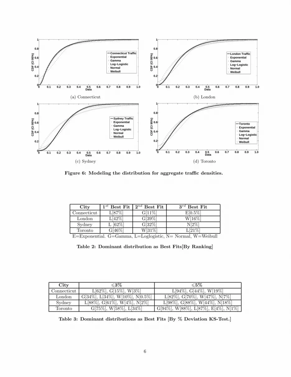
Figure 6: Modeling the distribution for aggregate traffic densities.

City 1st Best Fit 2nd Best Fit 3rd Best FitConnecticut L[87%] G[11%] E[0.5%]London L[42%] G[39%] W[16%]Sydney L [62%] G[32%] N[2%]Toronto G[46%] W[31%] L[21%]

E=Exponential. G=Gamma, L=Loglogistic, N= Normal, W=Weibull

Table 2: Dominant distribution as Best Fits[By Ranking]

City 63% 65%Connecticut L[62%], G[15%], W[3%] L[94%], G[44%], W[19%]London G[34%], L[34%], W[10%], N[0.5%] L[82%], G[70%], W[47%], N[7%]Sydney L[88%], G[61%], W[4%], N[2%] L[98%], G[88%], W[44%], N[18%]Toronto G[75%], W[58%], L[34%] G[94%], W[88%], L[87%], E[4%], N[1%]

Table 3: Dominant distributions as Best Fits [By % Deviation KS-Test.]

6

0 0.1 0.2 0.3 0.4 0.5 0.6 0.7 0.8 0.9 1.00

0.2

0.4

0.6

0.8

1

Data

CD

F (

CI 9

5%)

Connecticut TrafficExponentialGammaLoglogisticNormalWeibull

(a) Connecticut(L)

0 0.1 0.2 0.3 0.4 0.5 0.6 0.7 0.8 0.9 1.00

0.2

0.4

0.6

0.8

1

Data

CD

F (

CI 9

5%)

Connecticut TrafficExponentialGammaLoglogisticNormalWeibull

(b) Connecticut(M)

0 0.1 0.2 0.3 0.4 0.5 0.6 0.7 0.8 0.9 1.00

0.2

0.4

0.6

0.8

1

Data

CD

F (

CI 9

5%)

Connecticut TrafficExponentialGammaLoglogisticNormalWeibull

(c) Connecticut(H)

0 0.1 0.2 0.3 0.4 0.5 0.6 0.7 0.8 0.9 1.00

0.2

0.4

0.6

0.8

1

Data

CD

F (

CI 9

5%)

London TrafficExponentialGammaLoglogisticNormalWeibull

(d) London(L)

0 0.1 0.2 0.3 0.4 0.4 0.6 0.7 0.8 0.9 1.00

0.2

0.4

0.6

0.8

1

Data

CD

F (

CI 9

5%)

London TrafficExponentialGammaLoglogisticNormalWeibull

(e) London(M)

0 0.1 0.2 0.3 0.4 0.5 0.6 0.7 0.8 0.9 1.00

0.2

0.4

0.6

0.8

1

Data

CD

F (

CI 9

5%)

London TrafficExponentialGammaLoglogisticNormalWeibull

(f) London(H)

0 0.1 0.2 0.3 0.4 0.5 0.6 0.7 0.8 0.9 1.00

0.2

0.4

0.6

0.8

1

Data

CD

F (

CI 9

5%)

Sydney TrafficExponentialGammaLoglogisticNormalWeibull

(g) Sydney(L)

0 0.1 0.2 0.3 0.4 0.5 0.6 0.7 0.8 0.9 1.00

0.2

0.4

0.6

0.8

1

Data

CD

F (

CI 9

5%)

Sydney TrafficExponentialGammaLoglogisticNormalWeibull

(h) Sydney(M)

0 0.1 0.2 0.3 0.4 0.5 0.6 0.7 0.8 0.9 1.00

0.2

0.4

0.6

0.8

1

Data

CD

F (

CI 9

5%)

Sydney TrafficExponentialGammaLoglogisticNormalWeibull

(i) Sydney(H)

0 0.1 0.2 0.3 0.4 0.5 0.6 0.7 0.8 0.9 1.00

0.2

0.4

0.6

0.8

1

Data

CD

F (

CI 9

5%)

Toronto TrafficExponentialGammaLoglogisticNormalWeibull

(j) Toronto(L)

0 0.1 0.2 0.3 0.4 0.5 0.6 0.7 0.8 0.9 1.00

0.2

0.4

0.6

0.8

1

Data

CD

F (

CI 9

5%)

Toronto TrafficExponentialGammaLoglogisticNormalWeibull

(k) Toronto(M)

0 0.1 0.2 0.3 0.4 0.5 0.6 0.7 0.8 0.9 1.00

0.2

0.4

0.6

0.8

1

Data

CD

F (

CI 9

5%)

Toronto TrafficExponentialGammaLoglogisticNormalWeibull

(l) Toront(H)

Figure 7: Cumulative plot for three varying traffic intensities captured per city. The individual flows are characterized by theLow(L), Medium(M) and High(H) traffic intensities.

7

congested intersection for the same camera as capturedby the density parameter (d).

Exponential Gamma Loglogistic Normal Weibull0

20

40

60

80

100

Distribution Model

Avg

. % [

1st B

est

Fit

]

<3%: 49%<5%: 89%

<3%: 0.6%<5%: 5.9%

<3%: 17%<5%: 70%

<3%: 42%<5%: 70%

<3%: 0%<5%: 0.9%

Figure 8: The percentage of distribution thatcover cameras from all four cities. The values inthe box show percentage deviation error fromempirical data.

5.1 Traffic Flow CharacterizationIn order to investigate the nature of traffic we take

a holistic approach to systematically extract individualand aggregate flows of the traffic densities from the im-ages. Each individual flow constitutes a distribution oftraffic densities that demonstrate the flow of traffic asviewed from an individual camera. This helps us to bet-ter understand traffic intensity at a microscopic level ofeach intersection. The aggregate traffic combines theflows from all the camera in timely ordered fashion.The main advantage from analyzing aggregate trafficis to understand the emergent properties and helps tomodel and profile the city and make intelligent guessesabout different city based on this aggregate.On analyzing the traffic, an important activity to fac-

torize the granularity of traffic for various purpose. Forexample, hourly patterns provides a good estimate onthe nature of congestions during morning and eveningtimes which otherwise flow at individual density levelmay not depict. On the other hand, the finer granular-ity helps to understand sudden spikes in the traffic flowand congestion mitigation plan. In this work, we chooseto look into all these patterns by modeling flows againstwell known probability distributions. Fig 5 gives an ex-ample of the traffic density on hourly basis for one of thecamera in Sydney. We can observe that there is in gen-eral high traffic density during the peak hours and lowtraffic density between 10am and 2pm (off peak time)which provides positive confirmation that our algorithmcan effectively detect traffics.Fig. 7 shows the cumulative density function of the

traffic for three individual cameras in each city, withlow, medium and high average traffic. We can see thattraffic at individual cameras can vary a lot, but in gen-eral Log-Logistic, Gamma and Weibull distribution cancapture some of the key features of the data. Log-

logistic is the best approximation for the individualcamera traffics in all the four cities, and we furthershows the detail statistics of the fitting in Table-2 thatbest fits, which had shown least order of deviation againstKS-test.In Table-3, we measure the deviation from empirical

data and sample the camera at 3% and 5% error levels.In Fig.-8, results show the average dominance of eachof four distribution. We find that even on individualaggregation level, the loglogistic distribution providesa good estimate for empirical data. As evident, Loglo-gistic and Gamma closely matches the empirical datadistribution.Finally, Fig. 6 shows the cumulative statistics for the

aggregated traffic for each city. We can observe that dif-ferent cities have different aggregated traffic, for exam-ple we can see that London in general has more trafficthan Connecticut.

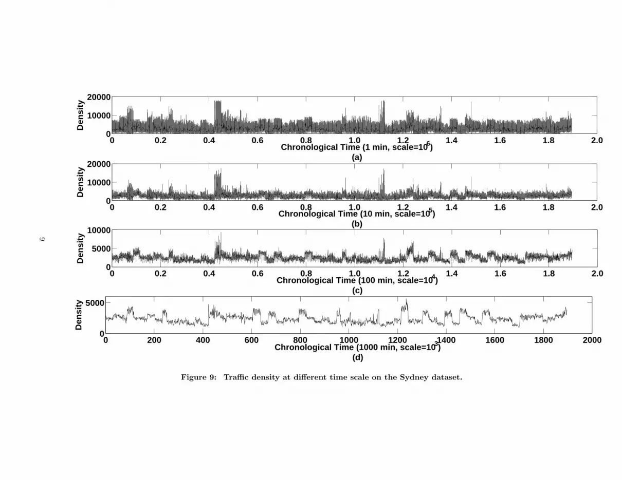
5.2 Long Range DependenceIn [9, 12], authors demonstrate the existence of long

range dependence and self-similar nature of ethernettraffic, which has serious implications on the designand analysis of computer networks. Inspired by thisstudy on the arrival process of ethernet packets in wirednetworks, we also characterize the nature of vehiculartraffic and investigate long range dependence. Self-similarity means that aggregate traffic statistics showlong range dependence and the correlation decays lessthan exponential. In Fig-9(a-d), we show time seriesplots for four different chronological resolution of inter-vals for the city of Sydney. Initially, we plotted with atime interval unit of one minute. The subsequent plotscome from their previous plots but with one less or-der of resolution of time interval. A significant burstis omni-present from finer to most abstract time reso-lutions. We also observed this behavior in other citiesand we will further investigate in the future work byusing different type of Hurst estimation[10].

6. CONCLUSION AND FUTURE WORKIn this paper we introduced a novel method to collect

large-scale vehicular network datasets using the alwaysavailable online traffic webcams. These webcams are al-ready deployed by governments, companies, or privateand hence it is an inexpensive way for data collection.They provide 24 hours monitoring on the data collectionpoints and have refresh rate as high as seconds, which isvery desirable for fine grained data collection. We col-lected 7.5 TB of vehicular image data from more than4,500 cameras distributed in 10 cites over 4 continents.We believe these large amount of data will be very im-portant for mobile network researchers to understandthe dynamics of the global cities and as a key step torealistic model vehicular communication networks. Our

8

0 0.2 0.4 0.6 0.8 1.0 1.2 1.4 1.6 1.8 2.00

10000

20000

Chronological Time (1 min, scale=106)(a)

Den

sity

0 0.2 0.4 0.6 0.8 1.0 1.2 1.4 1.6 1.8 2.00

10000

20000

Chronological Time (10 min, scale=105)(b)

Den

sity

0 0.2 0.4 0.6 0.8 1.0 1.2 1.4 1.6 1.8 2.00

5000

10000

Chronological Time (100 min, scale=104)(c)

Den

sity

0 200 400 600 800 1000 1200 1400 1600 1800 20000

5000

Chronological Time (1000 min, scale=103)(d)

Den

sity

Figure 9: Traffic density at different time scale on the Sydney dataset.

9

results strongly suggest a revisit to the general case ofexponential pattern as modeling distribution for the ve-hicular traffic. Finally, the implication of long rangedependence indicate the effect of traffic on the infras-tructure of road networks.

AcknowledgmentWe are thankful to Georgios Smaragdakis, Harold ChiLiu, Maria Gonzalez Garcia, Ranjan Pal and Shiva Sun-daram for their insightful comments.

7. REFERENCES

[1] F. Bai and B. Krishnamachari. Spatio-temporalvariations of vehicle traffic in vanets: facts andimplications. In Proceedings of the sixth ACMinternational workshop on VehiculArInterNETworking, VANET ’09, pages 43–52, NewYork, NY, USA, 2009. ACM.

[2] F. Bai, N. Sadagopan, and A. Helmy. Important:A framework to systematically analyze the impactof mobility on performance of routing protocolsfor adhoc networks. In INFOCOM, 2003.

[3] L. Briesemeister, L. Schafers, and G. Hommel.Disseminating messages among highly mobilehosts based on inter-vehicle communication. InIntelligent Vehicles Symposium, 2000. IV 2000.Proceedings of the IEEE, pages 522 –527, 2000.

[4] V. Bychkovsky, B. Hull, A. K. Miu,H. Balakrishnan, and S. Madden. A MeasurementStudy of Vehicular Internet Access Using In SituWi-Fi Networks. In 12th ACM MOBICOM Conf.,Los Angeles, CA, September 2006.

[5] R. E. Chandler, R. Herman, and E. W. Montroll.Traffic dynamics: Studies in car following.OPERATIONS RESEARCH, 6(2):165–184, 1958.

[6] A. Elgammal, D. Harwood, and L. Davis.Non-parametric model for backgroundsubtraction. In D. Vernon, editor, ComputerVision ECCV 2000, volume 1843 of LectureNotes in Computer Science, pages 751–767.Springer Berlin / Heidelberg, 2000.

[7] A. Halati, H. Lieu, and S. Walker.CORSIM-corridor traffic simulation model. InProceedings of the Traffic Congestion and TrafficSafety in the 21st Century Conference, pages570–576, 1997.

[8] P. Hui, R. Mortier, M. Piorkowski, T. Henderson,and J. Crowcroft. Planet-scale human mobilitymeasurement. In Proceedings of the 2nd ACMInternational Workshop on Hot Topics inPlanet-scale Measurement, HotPlanet ’10, pages1:1–1:5, New York, NY, USA, 2010. ACM.

[9] W. E. Leland, M. S. Taqqu, W. Willinger, andD. V. Wilson. On the self-similar nature of

ethernet traffic (extended version). IEEE/ACMTrans. Netw., 2:1–15, February 1994.

[10] R. Lienhart and J. Maydt. An extended set ofhaar-like features for rapid object detection. InImage Processing. 2002. Proceedings. 2002International Conference on, volume 1, pagesI–900 – I–903 vol.1, 2002.

[11] N. E. Lownes and R. B. Machemehl. Vissim: amulti-parameter sensitivity analysis. InProceedings of the 38th conference on Wintersimulation, WSC ’06, pages 1406–1413. WinterSimulation Conference, 2006.

[12] B. Mandelbrot and J. W. Van Ness. FractionalBrownian Motions, Fractional Noises andApplications. SIAM Review, 10(4):422–437, 1968.

[13] Q. Meng and H. L. Khoo. Self-similarcharacteristics of vehicle arrival pattern onhighways. Journal of Transportation Engineering,135(11):864–872, 2009.

[14] J. Ott and D. Kutscher. Drive-thru internet: Ieee802.11b for ”automobile” users. In INFOCOM2004. Twenty-third AnnualJoint Conference of theIEEE Computer and Communications Societies,volume 1, pages 4 vol. (xxxv+2866), march 2004.

[15] M. Piccardi. Background subtraction techniques:a review. In Systems, Man and Cybernetics, 2004IEEE International Conference on, volume 4,pages 3099 – 3104 vol.4, oct. 2004.

[16] J. Singh, N. Bambos, B. Srinivasan, andD. Clawin. Wireless lan performance under variedstress conditions in vehicular traffic scenarios. InVehicular Technology Conference, 2002.Proceedings. VTC 2002-Fall. 2002 IEEE 56th,volume 2, pages 743 – 747 vol.2, 2002.

[17] C. Stauffer and W. Grimson. Adaptivebackground mixture models for real-time tracking.In Computer Vision and Pattern Recognition,1999. IEEE Computer Society Conference on.,volume 2, pages 2 vol. (xxiii+637+663), 1999.

[18] Z. Sun, G. Bebis, and R. Miller. On-road vehicledetection: A review. IEEE Transactions onPattern Analysis and Machine Intelligence,28:694–711, 2006.

[19] N. Wisitpongphan, F. Bai, P. Mudalige,V. Sadekar, and O. Tonguz. Routing in sparsevehicular ad hoc wireless networks. Selected Areasin Communications, IEEE Journal on, 25(8):1538–1556, oct. 2007.

[20] J. Yeo, D. Kotz, and T. Henderson. Crawdad: acommunity resource for archiving wireless data atdartmouth. SIGCOMM Comput. Commun. Rev.,36:21–22, April 2006.

[21] X. Zhang, J. Kurose, B. N. Levine, D. Towsley,and H. Zhang. Study of a bus-baseddisruption-tolerant network: mobility modeling

10

and impact on routing. In Proceedings of the 13thannual ACM international conference on Mobilecomputing and networking, MobiCom ’07, pages195–206, New York, NY, USA, 2007. ACM.

11