wave-absorbing vehicular platoon controller
TRANSCRIPT
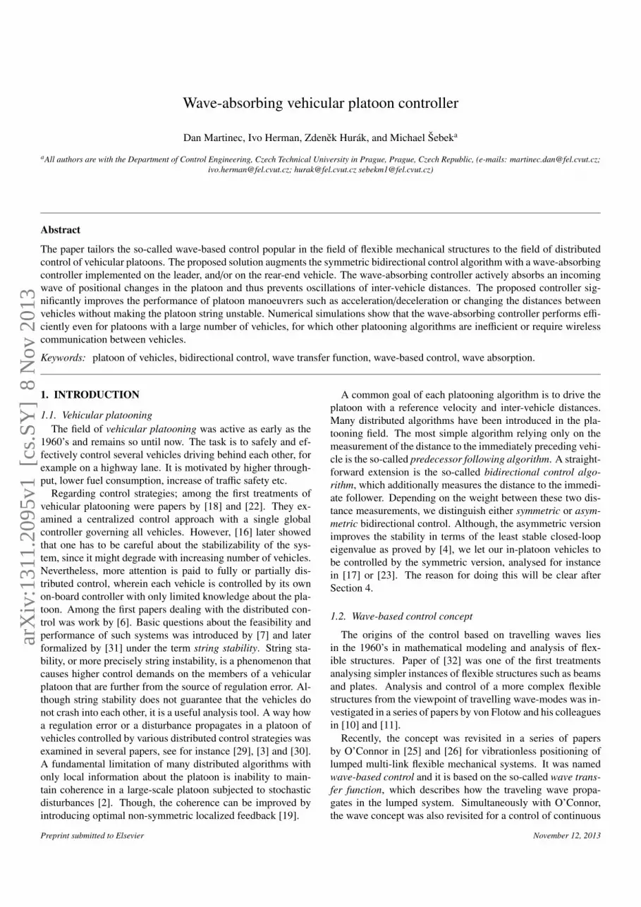
Wave-absorbing vehicular platoon controller
Dan Martinec, Ivo Herman, Zdenek Hurak, and Michael Sebeka
aAll authors are with the Department of Control Engineering, Czech Technical University in Prague, Prague, Czech Republic, (e-mails: [email protected];[email protected]; [email protected] [email protected])
Abstract
The paper tailors the so-called wave-based control popular in the field of flexible mechanical structures to the field of distributedcontrol of vehicular platoons. The proposed solution augments the symmetric bidirectional control algorithm with a wave-absorbingcontroller implemented on the leader, and/or on the rear-end vehicle. The wave-absorbing controller actively absorbs an incomingwave of positional changes in the platoon and thus prevents oscillations of inter-vehicle distances. The proposed controller sig-nificantly improves the performance of platoon manoeuvrers such as acceleration/deceleration or changing the distances betweenvehicles without making the platoon string unstable. Numerical simulations show that the wave-absorbing controller performs effi-ciently even for platoons with a large number of vehicles, for which other platooning algorithms are inefficient or require wirelesscommunication between vehicles.
Keywords: platoon of vehicles, bidirectional control, wave transfer function, wave-based control, wave absorption.
1. INTRODUCTION
1.1. Vehicular platooningThe field of vehicular platooning was active as early as the
1960’s and remains so until now. The task is to safely and ef-fectively control several vehicles driving behind each other, forexample on a highway lane. It is motivated by higher through-put, lower fuel consumption, increase of traffic safety etc.
Regarding control strategies; among the first treatments ofvehicular platooning were papers by [18] and [22]. They ex-amined a centralized control approach with a single globalcontroller governing all vehicles. However, [16] later showedthat one has to be careful about the stabilizability of the sys-tem, since it might degrade with increasing number of vehicles.Nevertheless, more attention is paid to fully or partially dis-tributed control, wherein each vehicle is controlled by its ownon-board controller with only limited knowledge about the pla-toon. Among the first papers dealing with the distributed con-trol was work by [6]. Basic questions about the feasibility andperformance of such systems was introduced by [7] and laterformalized by [31] under the term string stability. String sta-bility, or more precisely string instability, is a phenomenon thatcauses higher control demands on the members of a vehicularplatoon that are further from the source of regulation error. Al-though string stability does not guarantee that the vehicles donot crash into each other, it is a useful analysis tool. A way howa regulation error or a disturbance propagates in a platoon ofvehicles controlled by various distributed control strategies wasexamined in several papers, see for instance [29], [3] and [30].A fundamental limitation of many distributed algorithms withonly local information about the platoon is inability to main-tain coherence in a large-scale platoon subjected to stochasticdisturbances [2]. Though, the coherence can be improved byintroducing optimal non-symmetric localized feedback [19].
A common goal of each platooning algorithm is to drive theplatoon with a reference velocity and inter-vehicle distances.Many distributed algorithms have been introduced in the pla-tooning field. The most simple algorithm relying only on themeasurement of the distance to the immediately preceding vehi-cle is the so-called predecessor following algorithm. A straight-forward extension is the so-called bidirectional control algo-rithm, which additionally measures the distance to the immedi-ate follower. Depending on the weight between these two dis-tance measurements, we distinguish either symmetric or asym-metric bidirectional control. Although, the asymmetric versionimproves the stability in terms of the least stable closed-loopeigenvalue as proved by [4], we let our in-platoon vehicles tobe controlled by the symmetric version, analysed for instancein [17] or [23]. The reason for doing this will be clear afterSection 4.
1.2. Wave-based control concept
The origins of the control based on travelling waves liesin the 1960’s in mathematical modeling and analysis of flex-ible structures. Paper of [32] was one of the first treatmentsanalysing simpler instances of flexible structures such as beamsand plates. Analysis and control of a more complex flexiblestructures from the viewpoint of travelling wave-modes was in-vestigated in a series of papers by von Flotow and his colleaguesin [10] and [11].
Recently, the concept was revisited in a series of papersby O’Connor in [25] and [26] for vibrationless positioning oflumped multi-link flexible mechanical systems. It was namedwave-based control and it is based on the so-called wave trans-fer function, which describes how the traveling wave propa-gates in the lumped system. Simultaneously with O’Connor,the wave concept was also revisited for a control of continuous
Preprint submitted to Elsevier November 12, 2013
arX
iv:1
311.
2095
v1 [
cs.S
Y]
8 N
ov 2
013

flexible structures by [13] under the name absolute vibrationsuppression. It relies on the transfer function as well, though inthis case, the time delay plays a key role. Surprisingly, it wasshown by the joint paper of the last two mentioned authors in[28], that both the wave-based control and the absolute vibra-tion suppression are just a feedback version of the input shapingcontrol. It was also shown that the wave-based control can begeneralized even for continuous flexible systems, e.g. a steelrod, and then it coincides with the absolute vibration suppres-sion.
The key idea of the wave-based control is to generate a waveat the actuated front end of the interconnected system and letit propagate to the opposite end of the system, where it reflectsand returns back to the front-end actuator. When it reaches thefront again, it is absorbed by the front-end actuator by means ofthe wave transfer function. A both interesting and troublesomeproperty of the wave transfer function is the presence of thesquare root of polynomial in the function. This makes its im-plementation in the time domain very challenging. To be ableto run numerical simulations, we therefore introduce a conver-gent recursive algorithm that approximates the wave transferfunction for an arbitrary dynamics of the local system.
There are other viewpoints on the wave-based control. Onewas introduced by [27] in terms of the characteristic impedancefor a mass-spring system. Other possible viewpoint introduced[24] for wave control of ladder electric networks.
1.3. Objective of the paperIn this paper, a finite one-dimensional platoon of vehicles
moving in a highway lane is considered. Each individual vehi-cle in the platoon is locally controlled by a bidirectional con-troller, which plays the role of string-damper connection in me-chanical structures and hence enables a wave to propagate backand forth. One or both of the platoon ends are controlled bythe wave-absorbing controller allowing active absorption of thetraveling wave. The similarity of bidirectional control with con-tinuous wave equation was described in [14]
The key objective of the paper is to generalize the principleof the wave-based control used in the field of mechanics for ve-hicular platooning control in such a way that the distances be-tween vehicles are additionally considered. In this regard, thepresented concept offers a symmetric version of bidirectionalcontrol enhanced by the feedback control of one or both platoonends. Thus, it significantly decreases long transient oscillationsduring platoon manoeuvres such as acceleration/deceleration orchanging the distances between vehicles. In addition, the papercontributes the following: a) It generalizes the wave transferfunction description for the arbitrary dynamics of the local sys-tem, b) it offers the convergent recursive algorithm that approx-imates the wave transfer function, c) it presents an alternativeway of deriving the wave transfer function using a continuedfraction approach, and d) it provides a mathematical derivationof the transfer functions describing reflections on the platoonends.
The paper is structured as follows. Section 2 gives a math-ematical model of the vehicle. Section 3 describes the wavetransfer function as a requisite tool for the wave description.
A mathematical description of wave reflections on forced andfree ends is given in Section 4. Section 5 introduces the wave-absorbing controller as an addon for the bidirectional control.The new controllers are analyzed by numerical simulations insection 6. The necessary mathematical derivations are given inthe three appendices.
2. LOCAL CONTROL OF THE PLATOON VEHICLES
A vehicle in a platoon indexed by n is in the Laplace domainmodelled as
Xn(s) = P(s)Un(s), (1)
where s is the Laplace variable, Xn(s) is a position of the nth ve-hicle in the Laplace domain, P(s) represents the transfer func-tion of system dynamics and Un(s) is the system input which isgenerated by the local controller of the vehicle specified in thefollowing.
Except for the leader indexed n = 0 and the rear-end vehi-cle, each vehicle in the platoon is equipped with a symmetricbidirectional controller C(s) with the task of equalizing the dis-tances to its immediate predecessor and successor, giving
Un(s) = C(s)(Dn−1(s) − Dn(s)), (2)
where Dn(s) is the distance between vehicles indexed by n andn + 1, hence Dn(s) = Xn(s) − Xn+1(s). Substituting (2) into(1) yields the resulting model of the in-platoon vehicle with thebidirectional control for the inter-vehicle distances,
Xn(s) = P(s)C(s)(Xn−1(s) − 2Xn(s) + Xn+1(s)). (3)
Using the notation,
α(s) =1
P(s)C(s)+ 2, (4)
equation (3) is thus rewritten as
Xn(s) =1α(s)
(Xn−1 + Xn+1). (5)
The vehicle at the rear end of the platoon is driven by the prede-cessor following algorithm and is supposed to equalize the dis-tance to its immediate predecessor and reference distance Dref,
XN(s) =1
α(s) − 1(XN−1(s) − Dref(s)), (6)
where XN(s) is the position of the last vehicle in the platoon.To carry out numerical simulations, we will use the model
that is often used in theoretical studies. The vehicle is de-scribed by a double integrator model with a simple (linear)model of friction, ξ, and controlled by a PI controller. Hence,P(s) = 1/(s2 + ξs) and C(s) = (kps + ki)(s), where kp and ki areproportional and integral gains of the PI controller, respectively.Such a model was also used in experimental studies in [21].
2
3. WAVE TRANSFER FUNCTION
The bidirectional property of locally controlled systemscauses any change in the movement of the leading vehicle topropagate through the platoon as a wave up to the last vehicle.To describe this wave, we need to find out how the position ofa vehicle is influenced by the position of its immediate neigh-bours. For a moment, let us assume that the length of the pla-toon is infinite, so that there is no platoon end where the wavecan reflect. A generalization for platoon with a one platoon end,i.e. a semi-infinite platoon, is done in the next section.
3.1. Mathematical model of the wave transfer functionFollowing the standard arguments for wave equation found
for instance in [1], the solution to the wave equation can be de-composed into two components: An(s) and Bn(s) (also calledwave variables in the literature), which represent two wavespropagating along a platoon in the forward and backward di-rections, respectively.
To find a transfer function describing the wave propagation,we are searching for two linearly independent recurrence re-lations that satisfy (5). We first recursively apply (5) and (6)with Dref(s) = 0, for a platoon with an increasing number ofvehicles. The transfer function for a platoon with two vehi-cles is A1/A0 = (α − 1)−1, for a platoon with three vehicles isA1/A0 =
(α − (α − 1)−1
)−1, for a platoon with four vehicles is
A1/A0 =
(α −
(α − (α − 1)−1
)−1)−1
and so on. Continuing re-cursively, A1/A0 is expressed by the continued fraction
A1
A0=
1
α −1
α −1
α −1. . .
. (7)
The continued-fraction expansion of a square root is given by[15] √
z2 + y = z +y
2z +y
2z +y
2z +y. . .
. (8)
Letting the number of vehicles approach infinity, the right-handsides of (7) and (8) are equal, provided that y = −1 and z = α/2.Hence,
A1
A0=α
2−
12
√α2 − 4. (9)
Likewise, the transfer function A2/A1 can be expressed from (5)and (6) for n = 2 as
αA1 = A0 + A2. (10)
Substituting for A0 from the previous recursive step (9) gives
αA1 = A1
(α
2+
12
√α2 − 4
)+ A2, (11)
which provides
A2
A1=α
2−
12
√α2 − 4. (12)
Continuing recursively, we can find that the transfer functionAn+1/An is again equal to (9) or (12). We can conclude that thetransfer function from the nth to (n + 1)th vehicle is the samefor each vehicle, and is equal to
G1(s) =α
2−
12
√α2 − 4. (13)
Analogously, the second linearly independent recurrence re-lation of (5) and (6) is searched for by their recursive applica-tion with a decreasing index of vehicles. After similar algebraicmanipulations as for An, we find
Bn
Bn−1= α −
1
α −1
α −1
α −1. . .
. (14)
Letting the number of vehicles approach infinity, the right-handsides of (14) and (8) are equal provided that y = −1 and z =
α/2. Hence,Bn
Bn−1=α
2+
12
√α2 − 4. (15)
The transfer function from nth to (n − 1)th vehicle is the samefor each vehicle, and is equal to
G2(s) =α
2+
12
√α2 − 4. (16)
The resulting model of the vehicular platoon with an infinitenumber of vehicles is therefore described as follows:
Xn = An + Bn, (17)An+1 = G1An, (18)
Bn = G2Bn−1, (19)
G1 = G−12 , (20)
where (20) follows from the multiplication of (13) and (16).Equations (18)-(19) express the rheological property of the pla-toon, that is, they define the form of how these two compo-nents propagate through the platoon. Equation (20) expressesthe principle of reciprocity, that is, if A(s) propagates with thehelp of G1(s) to higher indexes of vehicles, then B(s) propa-gates with the help of G1(s) to lower indexes of vehicles. Thefunction G1(s) is hereafter referred to as the wave transfer func-tion.
It should be noted that if there is a boundary in the system,e.g., if the length of platoon is finite, where the rheology prop-erty for wave propagation changes abruptly, the principles mustbe supplemented by boundary conditions. We discuss this casein the following section.
3

3.2. Verification of the wave transfer functionWe now outline an alternative way to derive the wave transfer
function. Let the model of the vehicular platoon (17)-(20) holdand now search for the transfer functions G1(s) and G2(s) thatsatisfy these four equations. Substituting (17) into (5) yields
α(An + Bn) = An−1 + Bn−1 + An+1 + Bn+1, (21)
which, in view of (18) and (19), is
α(s) = G1(s) + G2(s). (22)
We can substitute either for G1(s) or G2(s) from (20). Eitherpossibility leads to the same quadratic equation (m = 1, 2),
G2m(s) − α(s)Gm(s) + 1 = 0, (23)
with two linearly independent solutions,
Gm(s) =α
2∓
12
√α2 − 4. (24)
Let G1(s) be chosen as the solution with the negative sign infront of the square root. Then (20) only allows G2(s) to bethe solution with the positive sign in front of the square root.Hence, G1(s) and G2(s) are identical to those derived in theprevious section. The quadratic equation (23) can be employedas a starting model for the positioning of multi-link flexible me-chanical systems [25].
3.3. Approximation of the wave transfer functionIt will be shown later in the paper that to be able to implement
the wave-absorbing controller advertised at the beginning of thepaper, we need to find the impulse response of the wave transferfunction, i.e. the inverse Laplace transform of G1(s). Due to thepresence of the square root in the function it is very challengingto find exact impulse response of G1(s). However, we can ap-proximate the impulse response with a finite impulse response(FIR) filter. Therefore, we first approximate the wave transferfunction in the Laplace domain, then transform this approxi-mate form to the time domain and finally truncate and samplethe approximate impulse response to obtain FIR filter coeffi-cients.
The square root function in (24) can be approximated by var-ious ways, e.g., Newton’s method, the binomial theorem, orcontinued fraction expansion (7). We employ the last optionsince it guarantees the convergence of iterative approximationsand is applicable to an arbitrary dynamics of the local systemwith a generalized parameter α(s) as in (4). The recursive for-mula (7) immediately provides the iterative approximation ofG1(s),
Gl1(s) =
1α(s) −Gl−1
1 (s), (25)
where l = 1, 2, . . ., and the initial value G01(s) = 1. The approxi-
mate Gl1(s) can be transformed to the time domain by Matlab or
Mathematica. Our experience with the inverse Laplace solversfor the Fractional Calculus invlap [8], weeks [33] and nilt [5] inMatlab is that, while they were not capable of performing the
inverse Laplace transform of (24) due to the square root func-tion, they carried out the inverse Laplace transform of Gl
1(s)without complications since (25) is a rational function.
The approximate Gl1(s) can interpreted as follows. Equation
(25) represents the transfer function from the position of theleader to the position of the first follower in a platoon of l ve-hicles. Increasing the number of iterations (25) means that thelength of a platoon grows and the effect of the rear-end vehi-cle on G1(s) weakens. The approximation of G1(s) thereforesuccessively improves. Figs. 1 and 2 show the Bode charac-teristics Gl
1(s) and the associated impulse responses for variousnumber of iterations, respectively. Increasing the numbers of it-erations makes the peak in the Bode characteristic sharper, morelocalized and moves it towards lower frequencies, eventuallydisappearing entirely. The basic characteristic of the impulseresponse is fitted after a few iterations while small differencesoccur at longer times. To obtain the FIR filter coefficients, wetruncate the approximate impulse response at a few seconds andsample it with an appropriate frequency. In our numerical sim-ulations it was sufficient to stop the iterative procedure after 20iterations, to truncate the impulse response at 15 seconds andsample it at a frequency of 100 Hz.
10−2
10−1
100
101
−30
−20
−10
0
10
Frequency [rad/s]
Mag
nitu
de [d
B]
Approx. G1 − 5 iter.
Approx. G1 − 10 iter.
Approx. G1 − 20 iter.
Approx. G1 − 30 iter.
Figure 1: The Bode characteristics of G1(s) approximations after several itera-tions by (25) for kp = ki = ξ = 4.
4. REFLECTION OF THE WAVE ON PLATOON ENDS
To be able to design a wave-absorbing controller for the pla-toon end, we first need to mathematically describe the wavereflection.
In the previous section an infinite platoon is considered,whereas here we assume a semi-infinite platoon having one endthat is either externally controlled (forced end) or allowed tomove freely (free end). When a wave propagates along a pla-toon and reaches its free end, it is reflected with the same polar-ity, i.e., the same sign of amplitude, but with the opposite polar-ity at the fixed/forced end. This phenomenon, known from ba-sic wave physics [12], is discussed in the following in terms ofthe wave transfer function. The necessary mathematical deriva-tions are given in Appendix A and B.
4
0 5 10 15 20−0.2
0
0.2
0.4
0.6
0.8
Time [s]
Impu
lse
resp
onse
[−]
Approx. G1 − 5 iter.
Approx. G1 − 10 iter.
Approx. G1 − 20 iter.
Approx. G1 − 30 iter.
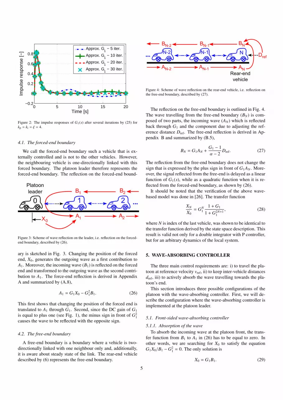
Figure 2: The impulse responses of G1(s) after several iterations by (25) forkp = ki = ξ = 4.
4.1. The forced-end boundary
We call the forced-end boundary such a vehicle that is ex-ternally controlled and is not to the other vehicles. However,the neighbouring vehicle is one-directionally linked with thisforced boundary. The platoon leader therefore represents theforced-end boundary. The reflection on the forced-end bound-
0 1 2
X0
Platoon
leader B1
B2
A1
A2
Figure 3: Scheme of wave reflection on the leader, i.e. reflection on the forced-end boundary, described by (26).
ary is sketched in Fig. 3. Changing the position of the forcedend, X0, generates the outgoing wave as a first contribution toA1. Moreover, the incoming wave (B1) is reflected on the forcedend and transformed to the outgoing wave as the second contri-bution to A1. The force-end reflection is derived in AppendixA and summarized by (A.8),
A1 = G1X0 −G21B1. (26)
This first shows that changing the position of the forced end istranslated to A1 through G1. Second, since the DC gain of G1is equal to plus one (see Fig. 1), the minus sign in front of G2
1causes the wave to be reflected with the opposite sign.
4.2. The free-end boundary
A free-end boundary is a boundary where a vehicle is two-directionally linked with one neighbour only and, additionally,it is aware about steady state of the link. The rear-end vehicledescribed by (6) represents the free-end boundary.
N-1
BN
AN
BN-1
AN-1
Rear-end
vehicle
Dref
NN-2
BN-2
AN-2
Figure 4: Scheme of wave reflection on the rear-end vehicle, i.e. reflection onthe free-end boundary, described by (27).
The reflection on the free-end boundary is outlined in Fig. 4.The wave travelling from the free-end boundary (BN) is com-posed of two parts, the incoming wave (AN) which is reflectedback through G1 and the component due to adjusting the ref-erence distance Dref. The free-end reflection is derived in Ap-pendix B and summarized by (B.5),
BN = G1AN +G1 − 1α − 2
Dref. (27)
The reflection from the free-end boundary does not change thesign that is expressed by the plus sign in front of G1AN . More-over, the signal reflected from the free-end is delayed as a linearfunction of G1(s), while as a quadratic function when it is re-flected from the forced-end boundary, as shown by (26).
It should be noted that the verification of the above wave-based model was done in [26]. The transfer function
XN
X0= GN
11 + G1
1 + G2N+11
, (28)
where N is index of the last vehicle, was shown to be identical tothe transfer function derived by the state space description. Thisresult is valid not only for a double integrator with P controller,but for an arbitrary dynamics of the local system.
5. WAVE-ABSORBING CONTROLLER
The three main control requirements are: i) to travel the pla-toon at reference velocity vref, ii) to keep inter-vehicle distancesdref, iii) to actively absorb the wave travelling towards the pla-toon’s end.
This section introduces three possible configurations of theplatoon with the wave-absorbing controller. First, we will de-scribe the configuration where the wave-absorbing controller isimplemented at the platoon leader.
5.1. Front-sided wave-absorbing controller
5.1.1. Absorption of the waveTo absorb the incoming wave at the platoon front, the trans-
fer function from B1 to A1 in (26) has to be equal to zero. Inother words, we are searching for X0 to satisfy the equationG1X0/B1 −G2
1 = 0. The only solution is
X0 = G1B1. (29)
5

To be consistent with the model (17)-(20), we denote B0 =
G1B1 and A0 = X0 − B0, then (26) is expressed as A1 =
G1X0 −G1B0 = G1A0. Summarizing this yields the wave com-ponents of the leader
B0 = G1X1 −G21A0, (30)
A0 = X0 − B0. (31)
This means that if one component of the position of the leaderis equal to B0, then the leader absorbs the incoming wave. Wecan imagine that if the leader is pushed/pulled by its followers,thus it manoeuvres like one of the in-platoon vehicles.
5.1.2. Acceleration to the reference velocityThe previous algorithm actively absorbs the incoming wave
to the platoon leader. To change the platoon’s velocity and inter-vehicle distances are other tasks that need to be solved.
To accelerate the platoon, we need to add an exter-nal/reference input, Xref, for the leader. This changes (29) toX0 = B0 + Xref. The rear-end vehicle represents the free-endboundary, therefore, B0 is expressed by the combination of (18),(19), (26) and (30) as B0 = G2N+1
1 Xref. This leads the transferfunction from Xref to X0 to be
X0
Xref= 1 + G2N+1
1 . (32)
Fig. 1 showed that the DC gain of G1 is equal to one, therefore,the DC gain of (1 + G2N+1
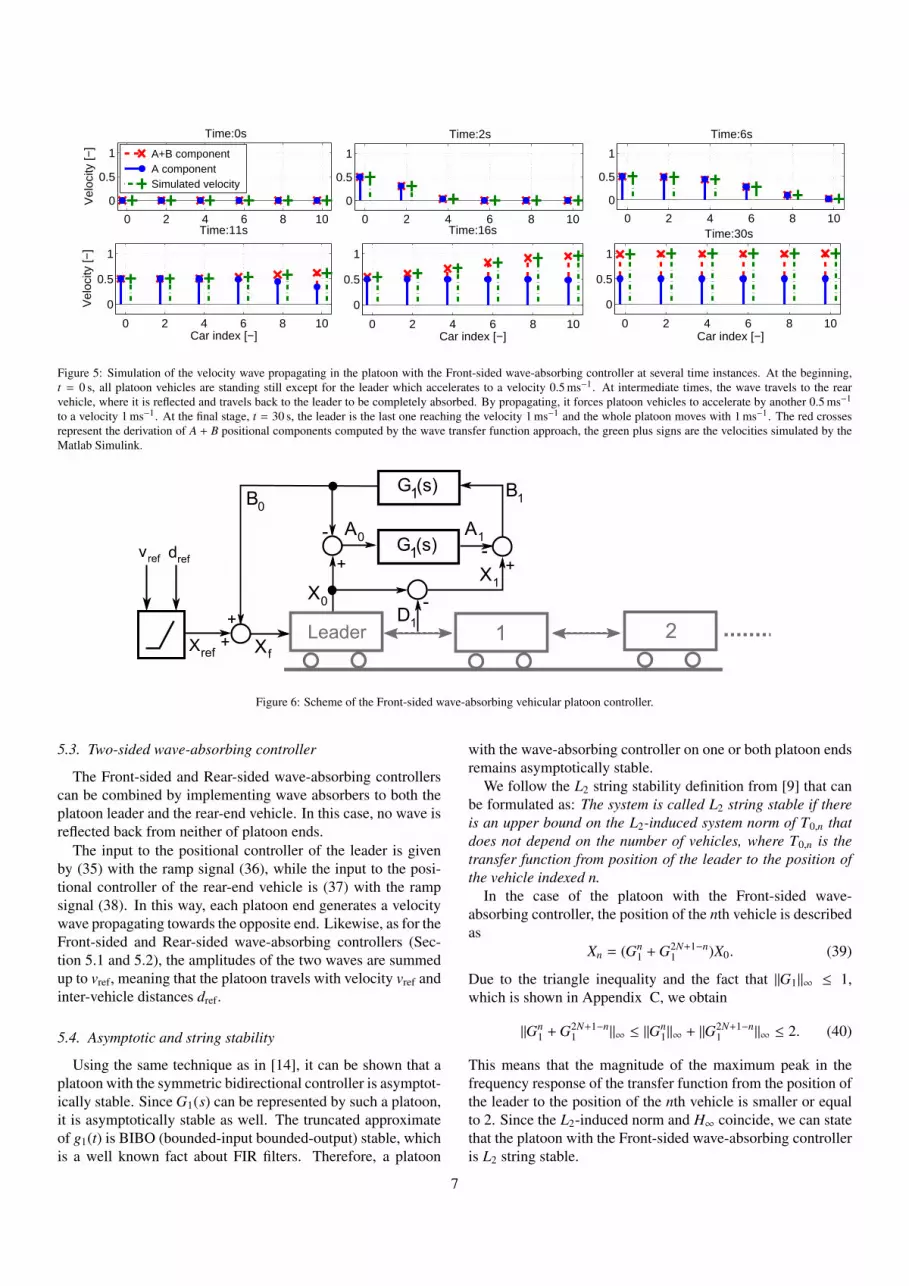
1 ) is equal to two. This means that toaccelerate the platoon to reference velocity vref, the leader has tobe commanded to accelerate to velocity vref/2 at the beginningof the manoeuver, as shown in Fig. 5.
Fig. 5 additionally shows an independent validation of thewave transfer function approach. The derivation of the sum ofA + B velocity components (red crosses) of the wave travellingthrough the platoon are compared against the velocities simu-lated by the Matlab Simulink (green plus signs). We can seean agreement between the wave-transfer-function-derived andindependently-simulated velocities.
5.1.3. Changing of the inter-vehicle distancesIncreasing the inter-vehicle distances poses a more difficult
task than merely accelerating the platoon. The reason is thatthe rear-end vehicle reacts to the change of reference distancedref by acceleration/deceleration. This creates a velocity wavepropagating towards the leader who absorbs it by changing itsvelocity. This means, however, that when all vehicles reachthe desired inter-vehicle distance dref, the whole platoon travelswith a new velocity different from the original. Only by anadditional action of the leader, see the next paragraph, will theoriginal velocity be reestablished.
Although the platoon has a finite number of vehicles, it be-haves like a semi-infinite platoon because no wave reflects fromthe platoon leader, who is equipped with the wave absorber.Since (27) holds for a semi-infinite platoon, it can be now usedto determine the transfer function from Dref to velocity of theleader, V0(s), that is
V0
Dref= GN
1s(G1 − 1)α − 2
. (33)
The DC gain of (33) reads as
κf = lims→0
(GN
1s(G1 − 1)α − 2
). (34)
In the case where the reference distance is changed and theleader does not accelerate, the velocity of the platoon changesby (κfdref). This means that the platoon slows down or evenmoves backwards. To compensate for this undesirable veloc-ity change, the leader is commanded to accelerate to the ve-locity (−κfdref)/2. The platoon will consequently travel withthe original velocity, hence compensating for the accelera-tion/deceleration of the rear-end vehicle.
The DC gain of (33) for the PI controller case is equal to(−
√ki/ξ).
5.1.4. Overall control of the leaderLet us now assume that the leader has a positional controller
with input Xf. Summarizing preceding subsections yields theresulting control law of the leader,
Xf(s) = Xref(s) + B0(s), (35)
From the above discussion, Xref(s) must be represented by aramp signal with slope w0,
w0 =12
(vref − κfdref) , (36)
to ensure that the platoon travels with a reference velocity vrefand inter-vehicle distances dref. In case of the PI controller,w0 =
(vref +
√ki/ξdref
)/2. The Front-sided wave-absorbing
controller is summarized in Fig. 6.
5.2. Rear-sided wave-absorbing controllerInstead of placing the wave-absorbing controller at the pla-
toon’s front, it can be placed at the platoon’s rear. In thiscase, the platoon has one leader in the front and one wave-absorbing controller at the rear. However, the absence of thepredecessor follower in the platoon has an important conse-quence. Any velocity change of the leader, V0(s), causes achange in the distance to the first follower, D1(s), as shownin (A.10). Consequently, all other distances between vehiclesare changed. This negative effect is to be compensated by anacceleration/deceleration of the rear-end vehicle. We denote κrto be the DC gain of the transfer function from V0(s) to D1(s).
Having specified the DC gain, a certain reference signalneeds to be sent to the platoon end to set up a desired inter-vehicle distance dref. The input to the positional controller ofthe rear-end vehicle, Xr(s), is expressed, analogous to (35), as
Xr(s) = Xref,rear(s) + G1(s)AN−1(s), (37)
where Xref,rear(s) is a reference ramp signal with slope wr,
wr =12
(vref − κrdref) . (38)
In other words, the platoon leader drives the platoon to travelwith velocity vref, while the rear-end vehicle makes the platoontravel with inter-vehicle distances dref. For the PI controller caseκr = ki/ξ.
6
0 2 4 6 8 10
0
0.5
1
Time:0s
Vel
ocity
[−]
0 2 4 6 8 10
0
0.5
1
Time:2s
0 2 4 6 8 10
0
0.5
1
Time:6s
0 2 4 6 8 10
0
0.5
1
Time:11s
Car index [−]
Vel
ocity
[−]
0 2 4 6 8 10
0
0.5
1
Time:16s
Car index [−]0 2 4 6 8 10
0
0.5
1
Time:30s
Car index [−]
A+B componentA componentSimulated velocity
Figure 5: Simulation of the velocity wave propagating in the platoon with the Front-sided wave-absorbing controller at several time instances. At the beginning,t = 0 s, all platoon vehicles are standing still except for the leader which accelerates to a velocity 0.5 ms−1. At intermediate times, the wave travels to the rearvehicle, where it is reflected and travels back to the leader to be completely absorbed. By propagating, it forces platoon vehicles to accelerate by another 0.5 ms−1
to a velocity 1 ms−1. At the final stage, t = 30 s, the leader is the last one reaching the velocity 1 ms−1 and the whole platoon moves with 1 ms−1. The red crossesrepresent the derivation of A + B positional components computed by the wave transfer function approach, the green plus signs are the velocities simulated by theMatlab Simulink.
1
+
- A0
G (s)1d
ref
2Leader
G (s)1
+
+
+-
Xref
X0
X1
A1
B1B
0
Xf
vref
D1
-
Figure 6: Scheme of the Front-sided wave-absorbing vehicular platoon controller.
5.3. Two-sided wave-absorbing controller
The Front-sided and Rear-sided wave-absorbing controllerscan be combined by implementing wave absorbers to both theplatoon leader and the rear-end vehicle. In this case, no wave isreflected back from neither of platoon ends.
The input to the positional controller of the leader is givenby (35) with the ramp signal (36), while the input to the posi-tional controller of the rear-end vehicle is (37) with the rampsignal (38). In this way, each platoon end generates a velocitywave propagating towards the opposite end. Likewise, as for theFront-sided and Rear-sided wave-absorbing controllers (Sec-tion 5.1 and 5.2), the amplitudes of the two waves are summedup to vref, meaning that the platoon travels with velocity vref andinter-vehicle distances dref.
5.4. Asymptotic and string stability
Using the same technique as in [14], it can be shown that aplatoon with the symmetric bidirectional controller is asymptot-ically stable. Since G1(s) can be represented by such a platoon,it is asymptotically stable as well. The truncated approximateof g1(t) is BIBO (bounded-input bounded-output) stable, whichis a well known fact about FIR filters. Therefore, a platoon
with the wave-absorbing controller on one or both platoon endsremains asymptotically stable.
We follow the L2 string stability definition from [9] that canbe formulated as: The system is called L2 string stable if thereis an upper bound on the L2-induced system norm of T0,n thatdoes not depend on the number of vehicles, where T0,n is thetransfer function from position of the leader to the position ofthe vehicle indexed n.
In the case of the platoon with the Front-sided wave-absorbing controller, the position of the nth vehicle is describedas
Xn = (Gn1 + G2N+1−n
1 )X0. (39)
Due to the triangle inequality and the fact that ||G1||∞ ≤ 1,which is shown in Appendix C, we obtain
||Gn1 + G2N+1−n
1 ||∞ ≤ ||Gn1||∞ + ||G2N+1−n
1 ||∞ ≤ 2. (40)
This means that the magnitude of the maximum peak in thefrequency response of the transfer function from the position ofthe leader to the position of the nth vehicle is smaller or equalto 2. Since the L2-induced norm and H∞ coincide, we can statethat the platoon with the Front-sided wave-absorbing controlleris L2 string stable.
7

The position of the nth vehicle with an absorber placed at therear-end vehicle is
Xn = Gn1X0 + (GN−n
1 −GN+n1 )XN . (41)
We apply the same idea and state that H∞ norm of both Gn1 and
(GN−n1 −GN+n
1 ) are bounded regardless of the number of vehicles.Therefore, the platoon with the Rear-sided wave-absorbing con-trol is L2 string stable.
The position of the nth vehicle in a platoon with absorbers onboth ends is expressed as
Xn = Gn1X0 + GN−n
1 XN , (42)
which immediately shows that the platoon with the Two-sidedwave-absorbing controller is L2 string stable as well.
6. NUMERICAL SIMULATIONS
We consider the linear friction of our system to be ξ = 4 andsearch for the parameters of the PI controller such that oscil-lations of the impulse response of G1(s) are minimized. Theparameters kp = ki = 4 satisfy this requirement. All numericalsimulations are run for a platoon of 50 vehicles to demonstratethat the wave-absorbing controllers are capable of controllinglarge platoons.
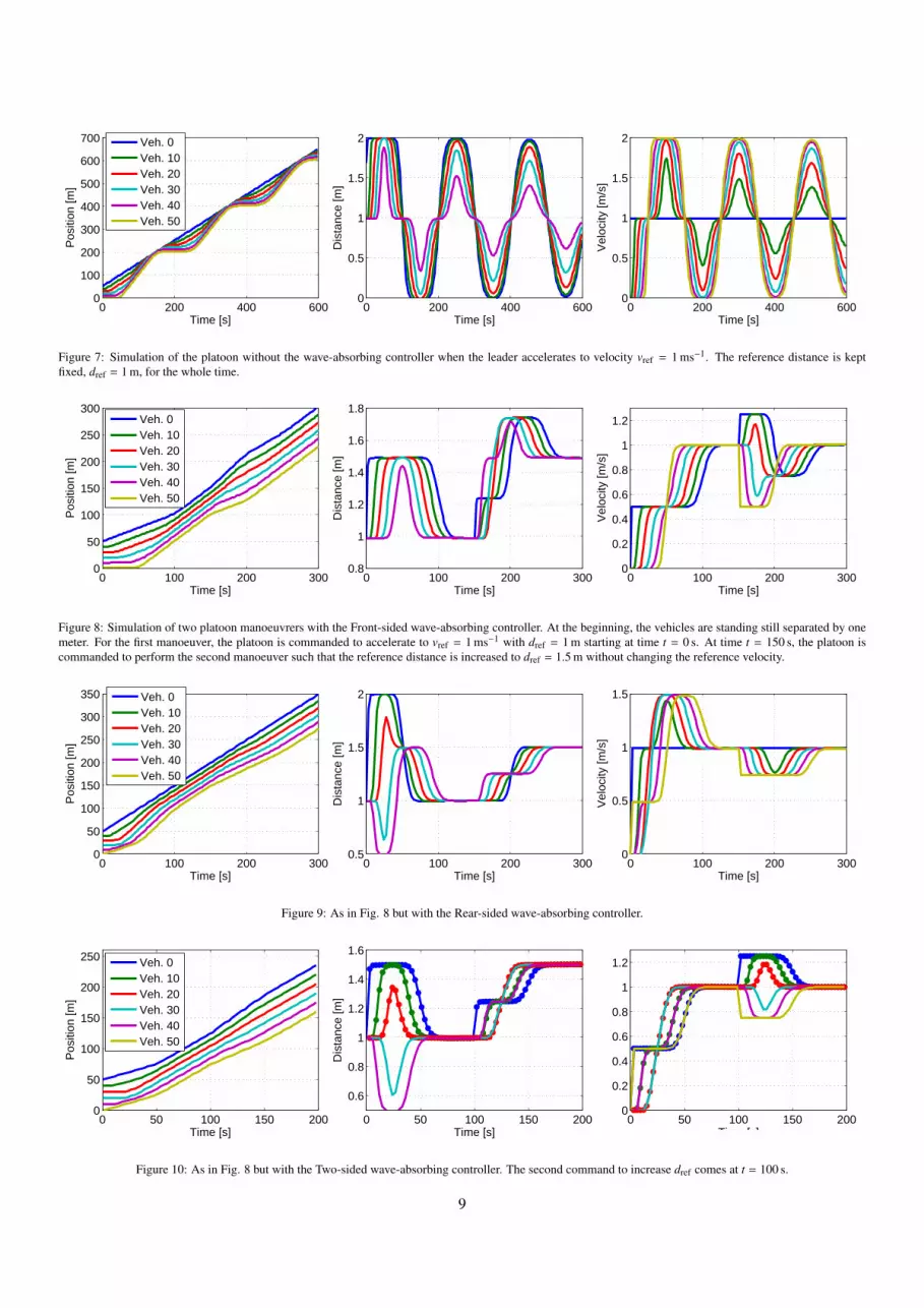
To demonstrate the advantages of the wave-absorbing con-trollers, we will compare their performance against a pure bidi-rectional control without any wave-absorbing controller. Thismeans that the leader travels with a constant velocity vref forthe whole time of the simulation. Fig. 7 shows outcomes ofnumerical simulation when the leader without wave-absorbingcontroller increases its velocity. We can see significant limi-tations of the bidirectional control. The oscillatory behaviourin the movement of the platoon is caused by numerous wavereflections from both platoon ends. Eventually, the platoon set-tles at a desired velocity after many velocity oscillations. Theseoscillations not only significantly prolong the settling time, butthey could lead to accidents within the platoon.
The performance of the Front-sided wave-absorbing con-troller during two platoon manoeuvrers is shown in Fig. 8. Inthe first 150 s manoeuver, the platoon accelerates (not neces-sarily from zero velocity) to reach a desired velocity. In com-parison with the pure bidirectional control, see Fig. 7, the set-tling time is now significantly shorter. Moreover, under somecircumstances, it can be guaranteed that vehicles do not crashinto each other during the platoon acceleration. In fact, the dis-tances between vehicles are increased at the beginning of theacceleration as suggested by (A.10) and shown in the middlepanel of the Fig. 8. However, the distances may undershoot theinitial inter-vehicles distances in the second part of the accel-eration manoeuver. If the impulse response of the wave trans-fer function is tuned such that it does not undershoot the zerovalue, then the distances between vehicles can not become lessthan the initial inter-vehicle distances. In the opposite case (notshown here), where the platoon travels with a constant veloc-ity and starts to decelerate, the distances between vehicles aretemporarily decreased and a collision may occur.
At time t = 150 s in Fig. 8, the platoon is commanded toperform the second manoeuver such that the reference distanceis increased, but the reference velocity is kept unchanged. Therear-end vehicle reacts to this command at the same time asthe leader since it is controlled by the reference distance that isnow changing. However, the end vehicles differ in action; theleader accelerates, while the rear-end vehicle decelerates. Thisbehaviour creates an undesirable overshoot in distances.
A numerical simulation of the two manoeuvrers for the pla-toon controlled by the Rear-sided wave-absorbing controller isshown in Fig. 9. During the acceleration manoeuver the inter-vehicle distances between vehicles closer to the rear end aretemporarily decreased while those for vehicles near the leaderare temporarily increased. During the changing-distance ma-noeuver, on the other hand, no overshoot in distances occurs.
In Fig. 10, the acceleration and changing-distance manoeu-vrers carried out for the one-sided wave-absorbing controllersare now performed for the two-sided wave-absorbing controller.Since both platoon ends are fully controlled, the settling time isonly half of that for the one-sided wave-absorbing controllers.The middle panel in Fig. 10 shows that there is no overshootin distances during the second manoeuver. On the other hand,there is no guarantee that the vehicles will not collide duringthe acceleration manoeuver.
6.1. Evaluation of the performance
We now evaluate the performance of the acceleration ma-noeuver described in the previous section with the help of themean squared error (MSE) criterion,
MSE =1
N + 1
N∑n=0
1T
T∑t=0
(vref(t) − vn(t))2, (43)
where T is the simulation time (in our case T = 500 s), vref(t)is the reference velocity of the platoon at time t and vn(t) is theactual velocity of the nth vehicle at time t.
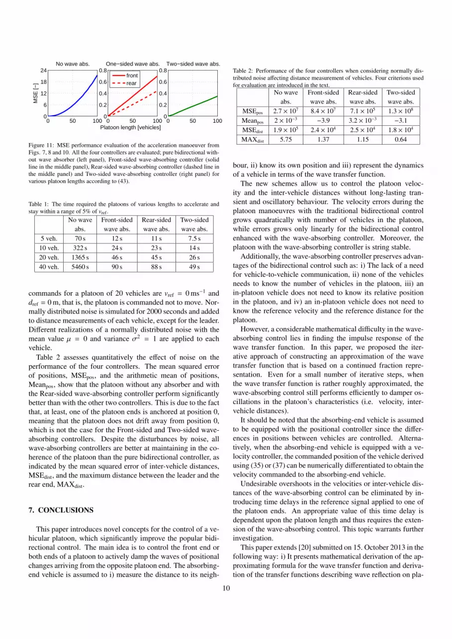
The comparison in performance of the four controllers forvarious platoon lengths is depicted in Fig. 11. We can see thatthe MSE increases linearly for all wave-absorbing controllers,but quadratically for the pure bidirectional control without waveabsorber. Moreover, a linear increase in MSE for the Two-sidedcontroller is only about half of that for the Front-sided con-troller. The linear increase of MSE for the Rear-sided controllerlies between these two cases. Evidently, the wave-absorbingcontroller qualitatively improves the performance of the bidi-rectional control.
The settling time of the acceleration manoeuver arising fromthe four types of controllers are compared in Table 1. We cansee that the settling time increases quadratically with the pla-toon length for a platoon without wave-absorbing controller,but approximately linearly for a platoon with wave-absorbingcontrollers.
6.2. Effect of noise in the platoon
This subsection examines the performance of the four con-trollers when noise is present in the system. The reference
8
0 200 400 6000
100
200
300
400
500
600
700
Time [s]
Pos
ition
[m]
Veh. 0Veh. 10Veh. 20Veh. 30Veh. 40Veh. 50
0 200 400 6000
0.5
1
1.5
2
Time [s]D
ista
nce
[m]
0 200 400 6000
0.5
1
1.5
2
Time [s]
Vel
ocity
[m/s
]
Figure 7: Simulation of the platoon without the wave-absorbing controller when the leader accelerates to velocity vref = 1 ms−1. The reference distance is keptfixed, dref = 1 m, for the whole time.
0 100 200 3000
50
100
150
200
250
300
Time [s]
Pos
ition
[m]
0 100 200 3000.8
1
1.2
1.4
1.6
1.8
Time [s]
Dis
tanc
e [m
]
0 100 200 3000
0.2
0.4
0.6
0.8
1
1.2
Time [s]V
eloc
ity [m
/s]
Veh. 0Veh. 10Veh. 20Veh. 30Veh. 40Veh. 50
Figure 8: Simulation of two platoon manoeuvrers with the Front-sided wave-absorbing controller. At the beginning, the vehicles are standing still separated by onemeter. For the first manoeuver, the platoon is commanded to accelerate to vref = 1 ms−1 with dref = 1 m starting at time t = 0 s. At time t = 150 s, the platoon iscommanded to perform the second manoeuver such that the reference distance is increased to dref = 1.5 m without changing the reference velocity.
0 100 200 3000
50
100
150
200
250
300
350
Time [s]
Pos
ition
[m]
Veh. 0Veh. 10Veh. 20Veh. 30Veh. 40Veh. 50
0 100 200 3000.5
1
1.5
2
Time [s]
Dis
tanc
e [m
]
0 100 200 3000
0.5
1
1.5
Time [s]
Vel
ocity
[m/s
]
Figure 9: As in Fig. 8 but with the Rear-sided wave-absorbing controller.
0 50 100 150 2000
50
100
150
200
250
Time [s]
Pos
ition
[m]
Veh. 0Veh. 10Veh. 20Veh. 30Veh. 40Veh. 50
0 50 100 150 200
0.6
0.8
1
1.2
1.4
1.6
Time [s]
Dis
tanc
e [m
]
0 50 100 150 2000
0.2
0.4
0.6
0.8
1
1.2
Time [s]
Figure 10: As in Fig. 8 but with the Two-sided wave-absorbing controller. The second command to increase dref comes at t = 100 s.
9
0 50 1000
6
12
18
24No wave abs.
MS
E [−
]
0 50 1000
0.2
0.4
0.6
0.8One−sided wave abs.
frontrear
0 50 1000
0.2
0.4
0.6
0.8Two−sided wave abs.
Platoon length [vehicles]
Figure 11: MSE performance evaluation of the acceleration manoeuver fromFigs. 7, 8 and 10. All the four controllers are evaluated; pure bidirectional with-out wave absorber (left panel), Front-sided wave-absorbing controller (solidline in the middle panel), Rear-sided wave-absorbing controller (dashed line inthe middle panel) and Two-sided wave-absorbing controller (right panel) forvarious platoon lengths according to (43).
Table 1: The time required the platoons of various lengths to accelerate andstay within a range of 5% of vref.
No wave Front-sided Rear-sided Two-sidedabs. wave abs. wave abs. wave abs.
5 veh. 70 s 12 s 11 s 7.5 s10 veh. 322 s 24 s 23 s 14 s20 veh. 1365 s 46 s 45 s 26 s40 veh. 5460 s 90 s 88 s 49 s
commands for a platoon of 20 vehicles are vref = 0 ms−1 anddref = 0 m, that is, the platoon is commanded not to move. Nor-mally distributed noise is simulated for 2000 seconds and addedto distance measurements of each vehicle, except for the leader.Different realizations of a normally distributed noise with themean value µ = 0 and variance σ2 = 1 are applied to eachvehicle.
Table 2 assesses quantitatively the effect of noise on theperformance of the four controllers. The mean squared errorof positions, MSEpos, and the arithmetic mean of positions,Meanpos, show that the platoon without any absorber and withthe Rear-sided wave-absorbing controller perform significantlybetter than with the other two controllers. This is due to the factthat, at least, one of the platoon ends is anchored at position 0,meaning that the platoon does not drift away from position 0,which is not the case for the Front-sided and Two-sided wave-absorbing controllers. Despite the disturbances by noise, allwave-absorbing controllers are better at maintaining in the co-herence of the platoon than the pure bidirectional controller, asindicated by the mean squared error of inter-vehicle distances,MSEdist, and the maximum distance between the leader and therear end, MAXdist.
7. CONCLUSIONS
This paper introduces novel concepts for the control of a ve-hicular platoon, which significantly improve the popular bidi-rectional control. The main idea is to control the front end orboth ends of a platoon to actively damp the waves of positionalchanges arriving from the opposite platoon end. The absorbing-end vehicle is assumed to i) measure the distance to its neigh-
Table 2: Performance of the four controllers when considering normally dis-tributed noise affecting distance measurement of vehicles. Four criterions usedfor evaluation are introduced in the text.
No wave Front-sided Rear-sided Two-sidedabs. wave abs. wave abs. wave abs.
MSEpos 2.7 × 10⁷ 8.4 × 10⁷ 7.1 × 10⁵ 1.3 × 10⁸
Meanpos 2 × 10⁻³ −3.9 3.2 × 10⁻³ −3.1MSEdist 1.9 × 10⁵ 2.4 × 10⁴ 2.5 × 10⁴ 1.8 × 10⁴
MAXdist 5.75 1.37 1.15 0.64
bour, ii) know its own position and iii) represent the dynamicsof a vehicle in terms of the wave transfer function.
The new schemes allow us to control the platoon veloc-ity and the inter-vehicle distances without long-lasting tran-sient and oscillatory behaviour. The velocity errors during theplatoon manoeuvres with the traditional bidirectional controlgrows quadratically with number of vehicles in the platoon,while errors grows only linearly for the bidirectional controlenhanced with the wave-absorbing controller. Moreover, theplatoon with the wave-absorbing controller is string stable.
Additionally, the wave-absorbing controller preserves advan-tages of the bidirectional control such as: i) The lack of a needfor vehicle-to-vehicle communication, ii) none of the vehiclesneeds to know the number of vehicles in the platoon, iii) anin-platoon vehicle does not need to know its relative positionin the platoon, and iv) an in-platoon vehicle does not need toknow the reference velocity and the reference distance for theplatoon.
However, a considerable mathematical difficulty in the wave-absorbing control lies in finding the impulse response of thewave transfer function. In this paper, we proposed the iter-ative approach of constructing an approximation of the wavetransfer function that is based on a continued fraction repre-sentation. Even for a small number of iterative steps, whenthe wave transfer function is rather roughly approximated, thewave-absorbing control still performs efficiently to damper os-cillations in the platoon’s characteristics (i.e. velocity, inter-vehicle distances).
It should be noted that the absorbing-end vehicle is assumedto be equipped with the positional controller since the differ-ences in positions between vehicles are controlled. Alterna-tively, when the absorbing-end vehicle is equipped with a ve-locity controller, the commanded position of the vehicle derivedusing (35) or (37) can be numerically differentiated to obtain thevelocity commanded to the absorbing-end vehicle.
Undesirable overshoots in the velocities or inter-vehicle dis-tances of the wave-absorbing control can be eliminated by in-troducing time delays in the reference signal applied to one ofthe platoon ends. An appropriate value of this time delay isdependent upon the platoon length and thus requires the exten-sion of the wave-absorbing control. This topic warrants furtherinvestigation.
This paper extends [20] submitted on 15. October 2013 in thefollowing way: i) It presents mathematical derivation of the ap-proximating formula for the wave transfer function and deriva-tion of the transfer functions describing wave reflection on pla-
10

toon ends, ii) it generalizes the result from double integratormodel with linear friction and PI controller for an arbitrary localsystem dynamics, iii) it introduces two additional modificationsof the wave-absorbing controller for the vehicular platoon, iv)it analyses asymptotic and string stability of a platoon with thewave-absorbing controller and v) it more thoroughly evaluatesperformance of the wave-absorbing controller.
8. ACKNOWLEDGEMENTS
This work was supported by Grant Agency of the Czech Re-public within the project GACR P103-12-1794.
The authors thank Kevin Fleming for his comments on themanuscript.
Appendix A. Reflection on a forced-end boundary
In this appendix, we derive the formula describing the re-flection of a wave on a forced-end boundary that is defined inSection 4.1.
We first combine (17)-(19) to obtain
Xn+1 = G1An + G2Bn, (A.1)Xn−1 = G2An + G1Bn. (A.2)
Equation (5) specified for the first vehicle behind the platoonleader is therefore
αX1 = X0 + X2. (A.3)
Substituting (17) for X1 and (A.1) for X2 yields
α(A1 + B1) = X0 + G1A1 + G2B1, (A.4)
which can be reformulated as
A1 =1
α −G1X0 +
G2 − α
α −G1B1. (A.5)
The term in front of B1 can be arranged as
G2 − α
α −G1=−α2 + 1
2
√α2 − 4
α2 + 1
2
√α2 − 4
= −G1
G2= −G2
1, (A.6)
where the principle of reciprocity from (20) has been applied.Similarly, the term in front of X0 is expressed as
1α −G1
=1
α2 + 1
2
√α2 − 4
=1
G2= G1. (A.7)
Finally, we haveA1 = G1X0 −G2
1B1. (A.8)
The wave-based platoon control in Section 5.3 requires oneto specify the way how the velocity of the leader V0(s) influ-ences the distance to the first follower D1(s), D1(s) = X0(s) −X1(s). Assuming a semi-infinite platoon, equation (9) givesX1(s) = G1(s)X0(s). Hence,
D1(s) = X0(s) −G1(s)X0(s) =1s
(1 −G1(s))V0(s), (A.9)
In other words, the transfer function from velocity V0(s) to dis-tance D1(s) is
D1(s)V0(s)
=1s
(1 −G1(s)). (A.10)
Appendix B. Reflection on a free-end boundary
In this appendix, we derive the formula describing the reflec-tion of a wave on a free-end boundary that is defined in Section4.2.
Substituting (17) and (A.2) into (6) yields
(AN + BN)(α − 1) = G2AN + G1BN − Dref, (B.1)
which, after rearranging, gives
BN =G2 − α + 1α − 1 −G1
AN −1
α − 1 −G1Dref, (B.2)
where
G2 − α + 1α − 1 −G1
=1 − α
2 + 12
√α2 − 4
−1 + α2 + 1
2
√α2 − 4
=
α − α2
2 −√α2 − 4 + α
2
√α2 − 4
2 − α=
2 − α2 − α
G1 = G1. (B.3)
Similarly,
1α − 1 −G1
= G11
G2 − α + 1=(
α
2−
12
√α2 − 4
)1 − α
2 + 12
√α2 − 4(
1 − α2
)2− 1
4 (α2 − 4)=
G1 − 12 − α
. (B.4)
Hence, (B.2) is
BN = G1AN +G1 − 1α − 2
Dref. (B.5)
Appendix C. PROOF OF ||G1(s)||∞ ≤ 1
We will show that ||G2(s)||∞ ≥ 1. Then (20) implies that||G1(s)||∞ ≤ 1. To inspect the amplification and phase shift onfrequency ω, we substitute ω for s in the definition of G2(s)in (16), where is the imaginary unit, and obtain the complexnumber z2 in the polar form,
z2 = r2 exp( ϕ2). (C.1)
Similarly as in (16), we can separate z2 into two parts,
z2 =12
z +12√
zs, (C.2)
where
z = α( ω) = r exp( ϕ),
zs = z2 − 4 = rs exp( ϕs). (C.3)
The magnitude rs is given by
rs = (r2 cos(2ϕ) − 4)2 + (r2 sin(2ϕ))2
= r4 + 8r2 + 16 − 16r2 cos2 ϕ. (C.4)
11

with magnitude r2 then expressed as
r2 =
[14
(r2 + rs + 2r
√rs
(cos
ϕs
2cosϕ + sin
ϕs
2sinϕ
))] 12
=
[14
(r2 + rs + 2r
√rs cos
(ϕ −
ϕs
2
))] 12
. (C.5)
The minimum of rs over all possible phases is for ϕ = kπ, k ∈ Z,and is equal to
min(rs) =√
r4 − 8r2 + 16 = |r2 − 4| =
4 − r2 if 0 ≤ r ≤ 2r2 − 4 if r > 2
(C.6)Therefore,
14
(r2 + rs) ≥ 1. (C.7)
In the next step, we will show that |ϕ − ϕs/2| ≤ π/2 whichmeans that cos (ϕ − ϕs/2) is nonnegative. It is known fact thatthe sum of two complex numbers with phases δ1 and δ2, whereδ1 ≤ δ2 and δ1, δ2 ∈ [−π, π) , yields a complex number with thephase δ ∈ [−π, π), that is
δ ∈ [δ1, δ2] if |δ1 − δ2| < π, (C.8)δ ∈ [δ2, δ1] if |δ1 − δ2| > π, (C.9)
δ = δ1 or δ = δ2 if |δ1 − δ2| = π. (C.10)
This implies that
|δ − δ2| ≤ π ∧ |δ1 − δ| ≤ π. (C.11)
The phase ϕs calculated from (C.3) is ϕs = 2ϕ − θ, where|θ| ≤ π according to (C.11). Then,∣∣∣∣∣ϕ − ϕs
2
∣∣∣∣∣ =
∣∣∣∣∣ϕ − ϕ +12θ
∣∣∣∣∣ =12|θ| ≤
12π. (C.12)
Therefore,cos
(ϕ −
ϕs
2
)≥ 0 (C.13)
and (C.5) gives,r2 ≥ 1. (C.14)
This means that the amplification of G2(s) for all frequencies isgreater or equal to one. Since G1(s) = G2(s)−1 (20), it meansthat the amplification of G1(s) on all frequencies is less than orequal to one, hence ||G1(s)||∞ ≤ 1.
References
[1] N. H. Asmar, Partial Differential Equations with Fourier Series andBoundary Value Problems, 2nd ed., Pearson Prentice Hall, New Jersey,2004.
[2] B. Bamieh, M. R. Jovanovic, P. Mitra, S. Patterson, Coherence in Large-Scale Networks: Dimension-Dependent Limitations of Local Feedback,IEEE Transactions on Automatic Control 57 (9) (2012) 2235–2249.
[3] P. Barooah, J. Hespanha, Error amplification and disturbance propagationin vehicle strings with decentralized linear control, in: 44th IEEE Confer-ence on Decision and Control, No. theorem 3, 2005, pp. 4964–4969.
[4] P. Barooah, P. Mehta, J. Hespanha, Mistuning-Based Control Designto Improve Closed-Loop Stability Margin of Vehicular Platoons, IEEETransactions on Automatic Control 54 (9) (2009) 2100–2113.
[5] L. Brancik, Programs for fast numerical inversion of Laplace transformsin MATLAB language environment, Conference MATLAB (1999) 27–39.
[6] K.-c. Chu, Decentralized control of high-speed vehicular strings, Trans-portation Science 8 (4) (1974) 361–384.
[7] R. Cosgriff, The asymptotic approach to traffic dynamics, IEEE Transac-tions on Systems Science and Cybernetics (4) (1969) 361–368.
[8] F. R. de Hoog, J. H. Knight, A. N. Stokes, An Improved Method forNumerical Inversion of Laplace Transforms, SIAM Journal on Scientificand Statistical Computing 3 (3) (1982) 357–366.
[9] J. Eyre, D. Yanakiev, I. Kanellakopoulos, A Simplified Framework forString Stability Analysis of Automated Vehicles∗, Vehicle System Dy-namics.
[10] A. H. Flotow, Disturbance propagation in structural networks, Journal ofSound and Vibration 106 (3) (1986) 433–450.
[11] A. H. V. Flotow, Traveling wave control for large spacecraft structures,Journal of Guidance Control and Dynamics 9 (4) (1986) 462–468.
[12] A. P. French, Vibration’s and Waves, M.I.T. introductory physics series,CBS Publishers & Distributors, 2003.
[13] Y. Halevi, Control of Flexible Structures Governed by the Wave Equa-tion Using Infinite Dimensional Transfer Functions, Journal of DynamicSystems, Measurement, and Control 127 (4) (2005) 579.
[14] I. Herman, D. Martinec, Z. Hurak, M. Sebek, PDdE-based analysis ofvehicular platoons with spatio-temporal decoupling, in: Proceedings of4th IFAC Workshop on Distributed Estimation and Control in NetworkedSystems (NecSys), Koblenz, Germany, 2013, pp. 144–151.
[15] W. B. Jones, W. J. Thron, Continued Fractions: Analytic Theory and Ap-plications, Encyclopedia of Mathematics and its Applications, CambridgeUniversity Press, 1984.
[16] M. Jovanovic, B. Bamieh, On the ill-posedness of certain vehicular pla-toon control problems, IEEE Transactions on Automatic Control 50 (9)(2005) 1307–1321.
[17] I. Lestas, G. Vinnicombe, Scalability in heterogeneous vehicle platoons,2007 American Control Conference (M) (2007) 4678–4683.
[18] W. Levine, M. Athans, On the optimal error regulation of a string of mov-ing vehicles, Automatic Control, IEEE Transactions on.
[19] F. Lin, M. Fardad, M. R. Jovanovic, Optimal Control of Vehicular For-mations With Nearest Neighbor Interactions, IEEE Transactions on Au-tomatic Control 57 (9) (2012) 2203–2218.
[20] D. Martinec, I. Herman, Z. Hurak, M. Sebek, Augmentation of a bidirec-tional platooning controller by wave absorption at the leader, in: (Submit-ted to the) 3th European Control Conference, 2014.
[21] D. Martinec, M. Sebek, Z. Hurak, Vehicular platooning experiments withracing slot cars, 2012 IEEE International Conference on Control Appli-cations (2012) 166–171.
[22] S. Melzer, B. Kuo, A closed-form solution for the optimal error regulationof a string of moving vehicles, IEEE Transactions on Automatic Control16 (1) (1971) 50–52.
[23] R. H. Middleton, J. H. Braslavsky, String Instability in Classes of LinearTime Invariant Formation Control With Limited Communication Range,IEEE Transactions on Automatic Control 55 (7) (2010) 1519–1530.
[24] K. Nagase, H. Ojima, Y. Hayakawa, Wave-based Analysis and Wave Con-trol of Ladder Networks, 44th IEEE Conference on Decision and Control(2005) 5298–5303.
[25] W. J. O’Connor, Wave-echo control of lumped flexible systems, Journalof Sound and Vibration 298 (4-5) (2006) 1001–1018.
[26] W. J. O’Connor, Wave-Based Analysis and Control of Lump-ModeledFlexible Robots, IEEE Transactions on Robotics 23 (2) (2007) 342–352.
[27] H. Ojima, K. Nagase, Y. Hayakawa, Wave-based analysis and wave con-trol of damped mass-spring systems, 40th IEEE Conference on Decisionand Control 8 (December) (2001) 2574–2579.
[28] I. Peled, W. O’Connor, Y. Halevi, On the relationship between wave basedcontrol, absolute vibration suppression and input shaping, MechanicalSystems and Signal Processing (2012) 1–11.
[29] P. Seiler, A. Pant, K. Hedrick, Disturbance Propagation in Vehicle Strings,IEEE Transactions on Automatic Control 49 (10) (2004) 1835–1841.
[30] E. Shaw, J. K. Hedrick, Controller design for string stable heterogeneousvehicle strings, in: 46th IEEE Conference on Decision and Control, IEEE,2007, pp. 2868–2875.
[31] D. Swaroop, J. Hedrick, String stability of interconnected systems, IEEETransactions on Automatic Control 41 (3) (1996) 349–357.
12

[32] D. R. Vaughan, Application of Distributed Parameter Concepts to Dy-namic Analysis and Control of Bending Vibrations, Journal of Basic En-gineering 90 (2) (1968) 157–166.
[33] W. Weeks, Numerical inversion of Laplace transforms using Laguerrefunctions, Journal of the ACM (JACM).
13