Technische Universität MünchenInstitut für Energietechnik

Professur für Thermofluiddynamik

Analysis and Low-Order Modeling of Interactions

between Acoustics, Hydrodynamics and Premixed

Flames

Thomas Steinbacher

Vollständiger Abdruck der von der Fakultät für Maschinenwesen derTechnischen Universität München zur Erlangung des akademischen Gradeseines

DOKTOR – INGENIEURS

genehmigten Dissertation.

Vorsitzender:Prof. Dr.-Ing. Hartmut Spliethoff

Prüfer der Dissertation:Prof. Wolfgang Polifke, Ph.D.Prof. Matthew Juniper, Ph.D.,University of Cambridge, UK

Die Dissertation wurde am 29.04.2019 bei der Technischen Universität Müncheneingereicht und durch die Fakultät für Maschinenwesen am 24.07.2019angenommen.

Kurzfassung

Die vorliegende Dissertationsschrift untersucht die Wechselwirkung zwischenAkustik und mager vorgemischten Flammen. Im Fokus stehen hierbei die ther-moakustischen Eigenschaften von Brennerflammen, welche gemeinhin durch dieFlammen-Transfer-Funktion (FTF), also die lineare Antwort der globalen Wärme-freisetzungsrate auf akustische Störungen, beschrieben werden. Ausgangspunktaller Untersuchungen ist die Feststellung, dass das in der Literatur vorherrschendephysikalische Verständnis des vorliegenden Problems von den etablierten Erkennt-nissen zur Dynamik dünner Flammen abweicht. Während letztere hauptsächlich aufflammenintrinsischen hydrodynamischen und thermodiffusiven Prozessen beruhen,dreht sich die Theorie akustisch angeregter Flammen hauptsächlich um experimentellbeobachtete konvektiv transportierte Geschwindigkeitsstörungen, welche mit derFlamme wechselwirken. Das Ziel der vorliegenden Arbeit ist es daher, beide Be-trachtungesweisen zu vereinen und dabei die wichtigsten Mechanismen der Akustik-Flammen-Interaktion herauszuarbeiten. Zu diesem Zweck wird eine neues Konzeptzur niedrigdimensionalen Modellierung entwickelt, mit dessen Hilfe bestimmte, klardefinierte Aspekte der zugrunde liegenden Dynamik getrennt untersucht werdenkönnen. Detaillierte numerische Rechnungen dienen zu dessen Validierung und bi-eten zudem aufschlussreiche Einblicke in die physikalischen Vorgänge. Die damitdurchgeführte Analysen beschränken sich auf Schachtflammen. Zwei Arten derAkustik-Flammen-Strömungsinteraktion konnten identifiziert werden: (i) PrimäreWechselwirkungen, welche ausschließlich unmittelbare Auswirkungen akustischerStörungen einschließen, und (ii) sekundäre Wechselwirkungen, welche flammenin-trinsische Prozesse umfassen, die im Wesentlichen auf einer Kopplung zwischen Hy-drodynamik und Flammendynamik beruhen. Ein Ergebnis der durchgeführten Unter-suchungen ist es, dass das rotationsfreie akustische Feld in erster Linie die Regionam Flammenfuß beeinflusst, während von der Akustik erzeugte abgelöste Wirbelso gut wie nicht mit der Flamme interagieren. Die daraus resultierenden primärenAuslenkungen der stationären Flammenfront sind anschließend hydrodynamischenMechanismen ausgesetzt, welche aufgrund des verbrennungsinduzierten Dichte-sprungs zu deren Anwachsen führen. Zusätzlich dazu bilden sich in der Umgebungprimärer Störungen weitere, sekundäre aus. Beide Phänomene zusammen führenzu einer Amplitudenverstärkung der zugehörigen FTF, die Werte von Eins deutlichübersteigen kann. In Übereinstimmung mit der Literatur, konnte das Auftreten dergenannten konvektiv transportierten Geschwindigkeitsstörungen auf eine Kopplungzwischen Hydrodynamik und Flammendynamik zurückgeführt werden. Basierendauf theoretischen Untersuchungen zur Auswirkung der Flammengeometrie auf dielineare Flammenantwort, wird abschließend eine Methode vorgeschlagen, die es er-möglicht, die für Schachtflammen gewonnenen Erkenntnisse auch auf andere Flam-mengeometrien wie Bunsen- oder Keilflammen, zu übertragen.

iii

Abstract

This doctoral thesis analyses interactions between acoustics and lean premixed flamesfrom a thermoacoustic point of view. Special focus is put on the linear response ofthe global heat release rate of burner-stabilized laminar flames to acoustic perturba-tions, commonly expressed by the flame transfer function (FTF). The starting pointof all investigations is the inconsistency between (i) the prevailing notion of the un-derlying physical mechanisms of the problem at hand and (ii) first principle-baseddescriptions of the dynamics of thin flames. While the latter are essentially based onhydrodynamic and thermal-diffusive modes of flame propagation, the former revolvearound the empirical concept of acoustically triggered convected velocity perturba-tions interacting with the flame. This work strives to bring together both perceptionsand, in doing so, aims to identify the skeletal processes governing acoustics-flameinteractions. To this end, a first principle-based low order modeling framework isdeveloped, which allows to separately investigate well-defined aspects of the un-derlying dynamics. High fidelity numerical simulations provide instructive valida-tion data. Focusing on Slit flames, two types of acoustics-flame-flow interactions areidentified: (i) Primary interactions, which involve only immediate effects of acousticperturbations on the flame, and (ii) secondary interactions, which cover flame in-trinsic processes essentially depending on a hydrodynamic flame-flow feedback. Itis found that the irrotational acoustic field predominantly interacts with the flamebase region, while vortex shedding has almost no impact. The acoustically triggeredprimary flame displacements are subject to mechanisms of flame-flow feedback pro-voked by the change in density across the flame sheets. These mechanisms lead totheir convective growth as well as to the formation of secondary displacements, whichaltogether results in FTF peak gain values significantly exceeding unity. Furthermore,in agreement with the literature, flame-flow feedback is found to be responsible forthe mentioned convected velocity perturbations. By analyzing consequences of flamegeometry for the acoustic response, a simple way is suggested how to transfer theresults found for Slit flames to the more widespread Bunsen and Wedge flame con-figurations.

v

Acknowledgements

The research project, which finally led to the completion of the thesis at hand, wouldnot have been successful without the support and encouragement of so many helpfuland great people. There is, of course, Prof. Polifke who gave me the unique oppor-tunity to do scientific research without imposing too many obligations to predefinedresearch projects — that has been a great chance, but also kind of a challenge. Thenthere is this remarkable research group of which I could be part of. Everyone has beenso helpful and, many times, instructive and fruitful discussion sparked. Furthermore,I have to thank all of the students I supervised, I learned more from them and theirwork than they might be aware of. And — last but not least — I am deeply indebtedto my wife Sofi, my parents and my two sisters.

Thank you!

vii

Wesentliche Teile der vorliegenden Dissertationsschrift wurden vom Autor bereitsauf Konferenzen vorgetragen oder als Konferenz und Zeitschriftenbeiträge veröf-fentlicht [1, 2]. Alle Vorveröffentlichungen sind entsprechend der gültigen Promo-tionsordnung ordnungsgemäß gemeldet. Sie sind deshalb nicht zwangsläufig im De-tail einzeln referenziert. Vielmehr wurde bei der Referenzierung eigener Vorveröf-fentlichungen Wert auf Verständlichkeit und inhaltlichen Bezug gelegt.

Major parts of the present thesis have been presented by the author at conferences,and published in conference proceedings or journal papers [1, 2]. All of the author’sprior publications are registered according to the valid doctoral regulations. In the in-terest of clarity and comprehensibility of presentation, not all of the prior publicationsare explicitly cited throughout the present work.

viii

Contents

Contents xi

Nomenclature xvii

Introduction 1

I Literature Review on Acoustics-Flame Interactions 9

1 Dynamics of Thin Flame Sheets 11

1.1 Scope . . . . . . . . . . . . . . . . . . . . . . . . . . . . . . . . . . . . 12

1.1.1 Definition of the Term “Thin Flame” . . . . . . . . . . . . . . 12

1.1.2 Historical Background . . . . . . . . . . . . . . . . . . . . . . 15

1.2 Mechanisms Governing Flame Propagation . . . . . . . . . . . . . . . 21

1.2.1 Propagation Normal to Itself . . . . . . . . . . . . . . . . . . . 22

1.2.2 Thermal-Diffusive . . . . . . . . . . . . . . . . . . . . . . . . . 24

1.2.3 Hydrodynamic . . . . . . . . . . . . . . . . . . . . . . . . . . . 27

1.2.4 Advection of Perturbations at Inclined Flames . . . . . . . . . 31

1.3 Low-Order Models . . . . . . . . . . . . . . . . . . . . . . . . . . . . . 33

1.3.1 Level-Set or G-Equation Approach . . . . . . . . . . . . . . . 34

1.3.2 1D Linearized Flame Dynamics . . . . . . . . . . . . . . . . . 35

1.4 Summary . . . . . . . . . . . . . . . . . . . . . . . . . . . . . . . . . . 38

2 Acoustic Response of Burner-Stabilized Flames 41

2.1 Problem Definition . . . . . . . . . . . . . . . . . . . . . . . . . . . . . 42

2.2 Acoustics-Flame Interactions . . . . . . . . . . . . . . . . . . . . . . . 43

2.2.1 Freely Propagating Flame Sheet . . . . . . . . . . . . . . . . . 43

2.2.2 Burner-Stabilized Flame . . . . . . . . . . . . . . . . . . . . . 44

2.2.3 Global Heat Release Rate Dynamics . . . . . . . . . . . . . . 49

2.3 Low-Order Models . . . . . . . . . . . . . . . . . . . . . . . . . . . . . 52

2.4 Summary . . . . . . . . . . . . . . . . . . . . . . . . . . . . . . . . . . 55

ix

CONTENTS

II Analysis of Acoustics-Flame Interactions of Slit Flames 57

3 Flow-Decomposition Based Modeling Framework 59

3.1 Helmholtz Decomposition . . . . . . . . . . . . . . . . . . . . . . . . . 603.2 Problem Formulation and Governing Equations . . . . . . . . . . . . 623.3 Conformal Mapping Technique . . . . . . . . . . . . . . . . . . . . . . 66

3.3.1 Schwarz-Christoffel Mapping . . . . . . . . . . . . . . . . . . 663.3.2 Flow-Field Singularities . . . . . . . . . . . . . . . . . . . . . 673.3.3 Kutta Condition . . . . . . . . . . . . . . . . . . . . . . . . . . 69

3.4 Summary . . . . . . . . . . . . . . . . . . . . . . . . . . . . . . . . . . 76

4 Primary Interactions 77

4.1 Test Case Setups . . . . . . . . . . . . . . . . . . . . . . . . . . . . . . 784.2 Irrotational and Vortical Response Analysis . . . . . . . . . . . . . . . 79

4.2.1 Harmonic Forcing . . . . . . . . . . . . . . . . . . . . . . . . . 804.2.2 Impulse Forcing . . . . . . . . . . . . . . . . . . . . . . . . . . 814.2.3 Discussion . . . . . . . . . . . . . . . . . . . . . . . . . . . . . 84

4.3 Summary and Conclusions . . . . . . . . . . . . . . . . . . . . . . . . 86

5 Secondary Interactions 89

5.1 Flame Response Revisited in the Light of Flame-Flow Feedback . . . 915.1.1 High Fidelity CFD/SI Data . . . . . . . . . . . . . . . . . . . . 915.1.2 Convective Velocity Model . . . . . . . . . . . . . . . . . . . . 94

5.2 Modeling of Flame-Flow Feedback . . . . . . . . . . . . . . . . . . . 965.2.1 Jump Conditions Across a Flame Sheet . . . . . . . . . . . . . 975.2.2 Modeling of Flame Generated Vorticity . . . . . . . . . . . . 995.2.3 Modeling of Geometrical Focusing . . . . . . . . . . . . . . . 102

5.3 Analysis of the Impact of Flame-Flow Feedback . . . . . . . . . . . . 1065.3.1 Flame Generated Vorticity . . . . . . . . . . . . . . . . . . . . 1085.3.2 Irrotational Flame-Flow Feedback . . . . . . . . . . . . . . . . 112

5.4 Summary and Conclusions . . . . . . . . . . . . . . . . . . . . . . . . 116

III Generalization to Other Burner Configurations 119

6 Consequences of Flame Geometry 121

6.1 Test Case Setups . . . . . . . . . . . . . . . . . . . . . . . . . . . . . . 1236.2 Integral Heat-Release . . . . . . . . . . . . . . . . . . . . . . . . . . . 1256.3 Physics Based Illustration of the Heat Release Dynamics . . . . . . . 1336.4 Incompressible-Convective FTF Models . . . . . . . . . . . . . . . . . 1376.5 Geometry-Dependent Analysis of the Incompressible-Convective

Model . . . . . . . . . . . . . . . . . . . . . . . . . . . . . . . . . . . . 1416.6 Validation of Flame Response Models . . . . . . . . . . . . . . . . . . 1456.7 Summary and Conclusions . . . . . . . . . . . . . . . . . . . . . . . . 153

x

CONTENTS

Summary and Conclusions 155

Appendix A Numerical Response Analysis 161

A.1 Test Case Setups . . . . . . . . . . . . . . . . . . . . . . . . . . . . . . 161A.2 CFD/SI Method . . . . . . . . . . . . . . . . . . . . . . . . . . . . . . . 162

A.2.1 Incompressible Numerical Simulations . . . . . . . . . . . . . 162A.2.2 System Identification . . . . . . . . . . . . . . . . . . . . . . . 163A.2.3 Goodness of the Identified Model . . . . . . . . . . . . . . . . 167

A.3 Time vs. Frequency Domain Based Response Analysis . . . . . . . . 173A.4 Computation of Flame Normal Displacements . . . . . . . . . . . . . 175

Appendix B Impact of the Anchoring Wall Temperature 177

Appendix C Flame Transfer Functions 181

C.1 Convective Incompressible FTFs with Gaussian Kernel . . . . . . . . 181C.2 Flame Base Velocity Forcing . . . . . . . . . . . . . . . . . . . . . . . 183

Appendices

List of Figures 191

List of Tables 193

Bibliography 215

xi

CONTENTS

xii

Nomenclature

Acronyms

BIBO Bounded-Input Bounded Output

CFD Computational Fluid Dynamics

DIC Incompressible-Convective Velocity Model with Dirac Kernel, see Sec. 6.4

FBD Flame Base Displacement Model, see Eq. 4.2

FIR Finite Impulse Response, see Sec. A.2.2

FR Frequency Response

FTF Flame Transfer Function

GIC Incompressible-Convective Velocity Model with Gaussian Kernel, seeSec. 6.4

IC Incompressible-Convective Velocity Model, see Sec. 2.3

IR Impulse Response

LOM Low-Order Model

LTI Linear Time Invariant

MS equation Michelson-Sivashinsky equation

PA system Public address system comprising microphones, amplifiers and loud-speakers

SI System Identification

SNR Signal-to-Noise Ratio

Modifiers

(.)′ Fluctuating quantity

xiii

CONTENTS

(.)∗ Non-dimensional quantity

(.)F Quantity in flame aligned coordinates

(.)L Quantity in laboratory coordinates

(.)con Quantity concerning a conical configuration (Wedge or Bunsen)

(.)ref Quantity at a reference position

(.)slit Quantity concerning a slit configuration

(.)∥ Component parallel to the mean flame front

(.)⊥ Component perpendicular to the mean flame front

(.)b Quantity of the burned flow

(.)i Component of a vector quantity in the i -th direction

(.)u Quantity of the unburned flow

(.)Λ Quantity concerning a (Conical) Bunsen configuration

(.)V Quantity Concerning a (Conical) Wedge configuration

[∗]bu Change of a quantity across the flame: ∗b −∗u , see Eq. (1.7)

(.) Mean flow quantity

(.) Complex conjugate

Non-Dimensional Numbers

α∗ Non-dimensional flame angle α∗ = sin(α) = s0L/u1, see Sec. 1.2.4.

αM Reduced Markstein number, see Sec. 1.1.2

Cr Confinement ratio Cr = Ri /Ra

e Inverse expansion ratio e = ρb/ρu

E Non-dimensional increase of specific volume E = ρu/ρb −1

e Expansion ratio e = ρu/ρb

f ∗ Strouhal number (non-dimensional frequency) with f ∗ = f τr

He Helmholtz number, see Eq. (3.3)

Ka Karlovitz number, see Eq. (1.12)

Le Lewis number, see Eq. (1.5)

xiv

CONTENTS

Ma Markstein number, see Eqs. (1.9) and (1.11)

Pe Péclet number, see Eq. (1.4)

r Non-dimensional rod radius r = Rr /Ra

Re Reynolds number

Ze Zeldovich number, see Eq. (1.6)

Symbols

A f Flame surface area [m2]

α Flame angle, see Fig. 1.13 [rad]

βx/ξ Angle defining a vortex panel in the physical/image domain, see Fig. 3.6

cp Specific heat capacity for constant pressure [Jkg−1K−1]

δD Thickness of the preheat zone, see Sec. 1.1.1 [m]

δ(.) Dirac Delta function

δR Thickness of the reaction sheet, see Sec. 1.1.1 [m]

δth Thermal diffusivity [m2 s−1]

δY Mass diffusivity of species Y [m2 s−1]

Ea Activation energy of a chemical reaction [J]

ǫ A small number ǫ≪ 1

η Flame front displacement in laboratory coordinates, see Fig. 1.13 [m]

f Temporal frequency [s−1]

F (ω) Frequency response function, see Eqs. (2.1) or (A.2)

fg Geometrical factor, fg = 1 (Slit) and fg = 1/2 (Conical)

f ∗O Strouhal number of the oscillatory feature of the IR, see Eq. (6.23)

G G-field of the Level-Set method, see Sec. 1.3

G(.) General kernel function of the convective flow perturbation: 1st antiderivative

g (.) General kernel function of the convective flow perturbation

Γ Circulation, see Eq. (5.18) [m2 s−1]

xv

CONTENTS

Γ(.) General kernel function of the convective flow perturbation: 2nd antideriva-tive

γx/ξ Vortex sheet strength in the physical/image domain, see Eqs. (3.27) and (3.28)[ms−1]

h(t ) Impulse response function, see Eq. (2.3)

H f Axial length (height) of the mean flame front, see Fig. 6.4 [m]

hi Impulse response coefficients, see Eq. (A.1)

i Complex unit or (summation) index

K Flow perturbation convection speed relative to the mean flow speed K =uc /u1, see Eqs. (6.17) and (6.18)

κ f Local flame front mean curvature, see Eqs. (1.8) or (1.25) [m−1]

κs Flame stretch, see Eq. (1.10) [m−1]

λ Wave length [m] or thermal conductivity [Wm−1K−1]

L f Length of the mean flame front, see Fig. 1.13 [m]

l f (t ) Length of the perturbed flame front with ref. to Fig. 6.4 [m]

lM Markstein length, see Eq. (1.8) [m]

n f Vector normal to the flame front, see Eqs. (5.2) or (1.21) [m]

ν Kinematic viscosity [m2 s−1]

ω Angular frequency [rads−1] or vorticity [s−1]

Ω0 Darrieus-Landau parameter , see Eq. (1.18)

p Pressure [Pa]

φ Equivalence ratio [-] or flow potential m2 s−1, see Eq. (3.1)

ψ Flow vector potential m2 s−1, see Eq. (3.2)

Q Heat-release rate [W]

Ra Outlet half-diameter, see Fig. 6.1 [m]

r f Local flame front radius, see Fig. 6.4 [s]

Rg Gas constant [JK−1]

ρ Density [kgm−3]

xvi

CONTENTS

Ri Inlet half-diameter, see Fig. 6.1 [m]

Rr Rod radius, see Fig. 6.1 [m]

s Parametrization of the (perturbed) flame front, see Fig. 6.4 [m]

σ Standard deviation of the gaussian kernel function [s] or temporal growth rate[rads−1]

sL Flame speed [ms−1]

s0L Unstretched flame speed [ms−1]

T Temperature [K]

t Time [s]

τ Time delay [s]

τc Characteristic flame time scale of convection in the convective velocity FTFmodels, see Eq. (6.22) [s]

τr Characteristic flame time scale of restoration, see Eq. (6.21) [s]

τt Flame transition time t f = δD /sL used to non-dimensionalize growth rates,see Sec. (5.1.1) [s]

TBP Temperature of the combustion chamber back plate, see Fig. 6.1 [K]

t f Vector parallel to the flame front, see Eq. (5.2) [m]

θ(.) Heaviside Step function

u Flow velocity [ms−1]

uc Flow perturbation convection speed along the mean flame frontuc = K u1/cos(α), see Tab. 6.1 [ms−1]

Uedge Velocity evaluated right at the edge of separation including a Kutta condition[ms−1]

k Wave number [radm−1]

x Coordinate [m]

ξ Flame front displacement in flame coordinates, see Fig. 1.13 [m] or coordi-nate in the complex plane, see Sec. 3.3.1

yY Mass fraction of species Y

xvii

CONTENTS

xviii

Introduction

Simplicity is a great virtue but it requires hard work to achieve it and

education to appreciate it. And to make matters worse: complexity sells

better.

– Edsger Wybe Dijkstra

Turbulent combustion is complex and of high technical relevance and, as a conse-quence, increasingly attracts the attention of scientific research. Laminar combustion,on the other hand, is apparently simple and of less technical relevance; accordingly,the number of fundamental studies published in this field is receding, particularlyin industry-funded research projects. Yet, most of the low-order modeling conceptsused to capture the dynamics of turbulent flames are derived from laminar theory.This means, blind spots in laminar theory propagate to gaps of knowledge in turbu-lent combustion and hence might hinder a more fundamental understanding as wellas the development of new modeling frameworks. Ultimately, the development ofhighly relevant technical innovations might be delayed by just some missing insightsat the very foundations of knowledge. As will be shown in the course of this the-sis, there are indeed significant blind spots concerning the specific topic of laminaracoustic-flame interactions in a thermoacoustic context. Motivated by this realization,this work is devoted to contribute to their illumination.

The Thermoacoustic Problem

Why are interactions between acoustics and lean premixed flames important at all?This question will be answered in the following relying on three examples: (i) LordRayleigh’s early and fundamental studies of a Rijke tube, (ii) the extravagant SaturnV program and (iii) modern gas turbine combustors. A common feature of these threeexamples is that they are all prone to instabilities driven by thermoacoustic effects,which may lead to high amplitude oscillations. Due to the fact that these oscillationsmanifest themselves as pressure fluctuations that may lead to severe sound emis-sions or even to system failure, they are usually undesired. Consequently, this sectionspeaks of the thermoacoustic problem when referring to these kind of instabilities.

1

CONTENTS

(a) (b) (c)

Figure 1: (a): Sketch of a Rijke tube. (b): Rocketdyne F-1 engines of the Saturn Vrocket with Wernher von Braun standing in front of it (taken from [9],Chap. 3.2). (c): Injector plate of the Rocketdyne F-1 engine (taken from[10]).

A literal definition of the field of thermoacoustics would include all acoustic phenom-ena in a gaseous medium that rely either on diffusive effects or entropy variations [3].Following Rott [3], however, a more restrictive definition shall be adopted here thatemphasizes one essential thermoacoustic phenomenon, namely the maintenance ofaerial vibrations by heat, as put by Rayleigh [4]. This definition shall be clarified inthe following by use of one of the most famous thermoacoustic experimental setups,the Rijke tube [5–7].

A sketch of such a device is provided in Fig. 1a. It consists of a vertical tube, where ametallic wire mesh (or wire gauze) is mounted somewhere in its lower half. By plac-ing a Bunsen burner right beneath its lower end, the wire mesh is heated. Removingthe burner, astonishingly, an enervating high-pitched sound appears, which slowly de-cays over time. Lord Rayleigh was the first to provide an adequate explanation of thisphenomenon. According to him, the key ingredient responsible for the sound genera-tion is the right phasing between pressure fluctuations and heat transfer from the wireto the flow: Only if heat is added to the fluid at the moment of greatest condensationor taken from it at the moment of greatest rarefaction, a self-sustained oscillation candevelop, which manifest itself as a clearly audible sound [8]. The phasing is essen-tially defined by the acoustic properties of the tube and by the dynamics as well asthe location of the heat source.

One of the most illustrative examples of the drastic consequences and difficulties re-lated to thermoacoustic phenomena is taken from the endeavor of the USA to bring aman to the moon. Such a mission requires the possibility to cope with high payloads,since a lot of equipment has to be brought into earth orbit. For that reason, the NASAdeveloped the Saturn V rocket. Its first stage was equipped with five RocketdyneF-1 engines, each providing a thrust of at least 6672 kN [11], whose impressive di-mensions are illustrated in Fig. 1b. One important problem encountered during their

2

CONTENTS

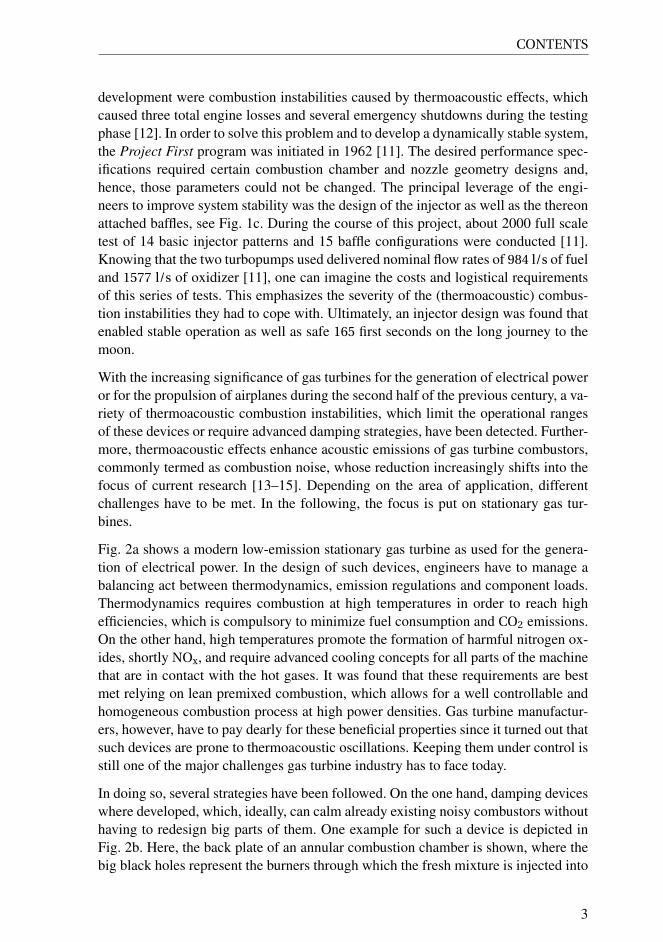
development were combustion instabilities caused by thermoacoustic effects, whichcaused three total engine losses and several emergency shutdowns during the testingphase [12]. In order to solve this problem and to develop a dynamically stable system,the Project First program was initiated in 1962 [11]. The desired performance spec-ifications required certain combustion chamber and nozzle geometry designs and,hence, those parameters could not be changed. The principal leverage of the engi-neers to improve system stability was the design of the injector as well as the thereonattached baffles, see Fig. 1c. During the course of this project, about 2000 full scaletest of 14 basic injector patterns and 15 baffle configurations were conducted [11].Knowing that the two turbopumps used delivered nominal flow rates of 984 l/s of fueland 1577 l/s of oxidizer [11], one can imagine the costs and logistical requirementsof this series of tests. This emphasizes the severity of the (thermoacoustic) combus-tion instabilities they had to cope with. Ultimately, an injector design was found thatenabled stable operation as well as safe 165 first seconds on the long journey to themoon.

With the increasing significance of gas turbines for the generation of electrical poweror for the propulsion of airplanes during the second half of the previous century, a va-riety of thermoacoustic combustion instabilities, which limit the operational rangesof these devices or require advanced damping strategies, have been detected. Further-more, thermoacoustic effects enhance acoustic emissions of gas turbine combustors,commonly termed as combustion noise, whose reduction increasingly shifts into thefocus of current research [13–15]. Depending on the area of application, differentchallenges have to be met. In the following, the focus is put on stationary gas tur-bines.

Fig. 2a shows a modern low-emission stationary gas turbine as used for the genera-tion of electrical power. In the design of such devices, engineers have to manage abalancing act between thermodynamics, emission regulations and component loads.Thermodynamics requires combustion at high temperatures in order to reach highefficiencies, which is compulsory to minimize fuel consumption and CO2 emissions.On the other hand, high temperatures promote the formation of harmful nitrogen ox-ides, shortly NOx, and require advanced cooling concepts for all parts of the machinethat are in contact with the hot gases. It was found that these requirements are bestmet relying on lean premixed combustion, which allows for a well controllable andhomogeneous combustion process at high power densities. Gas turbine manufactur-ers, however, have to pay dearly for these beneficial properties since it turned out thatsuch devices are prone to thermoacoustic oscillations. Keeping them under control isstill one of the major challenges gas turbine industry has to face today.

In doing so, several strategies have been followed. On the one hand, damping deviceswhere developed, which, ideally, can calm already existing noisy combustors withouthaving to redesign big parts of them. One example for such a device is depicted inFig. 2b. Here, the back plate of an annular combustion chamber is shown, where thebig black holes represent the burners through which the fresh mixture is injected into

3

CONTENTS

(a)

(b)

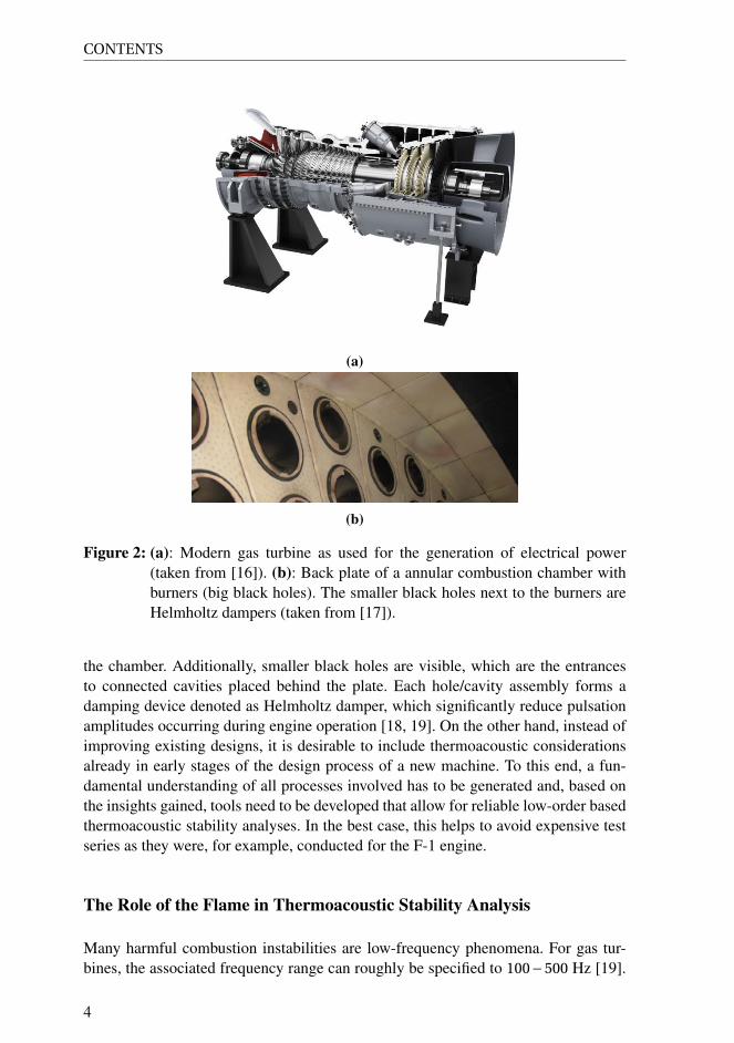
Figure 2: (a): Modern gas turbine as used for the generation of electrical power(taken from [16]). (b): Back plate of a annular combustion chamber withburners (big black holes). The smaller black holes next to the burners areHelmholtz dampers (taken from [17]).

the chamber. Additionally, smaller black holes are visible, which are the entrancesto connected cavities placed behind the plate. Each hole/cavity assembly forms adamping device denoted as Helmholtz damper, which significantly reduce pulsationamplitudes occurring during engine operation [18, 19]. On the other hand, instead ofimproving existing designs, it is desirable to include thermoacoustic considerationsalready in early stages of the design process of a new machine. To this end, a fun-damental understanding of all processes involved has to be generated and, based onthe insights gained, tools need to be developed that allow for reliable low-order basedthermoacoustic stability analyses. In the best case, this helps to avoid expensive testseries as they were, for example, conducted for the F-1 engine.

The Role of the Flame in Thermoacoustic Stability Analysis

Many harmful combustion instabilities are low-frequency phenomena. For gas tur-bines, the associated frequency range can roughly be specified to 100−500 Hz [19].

4

CONTENTS

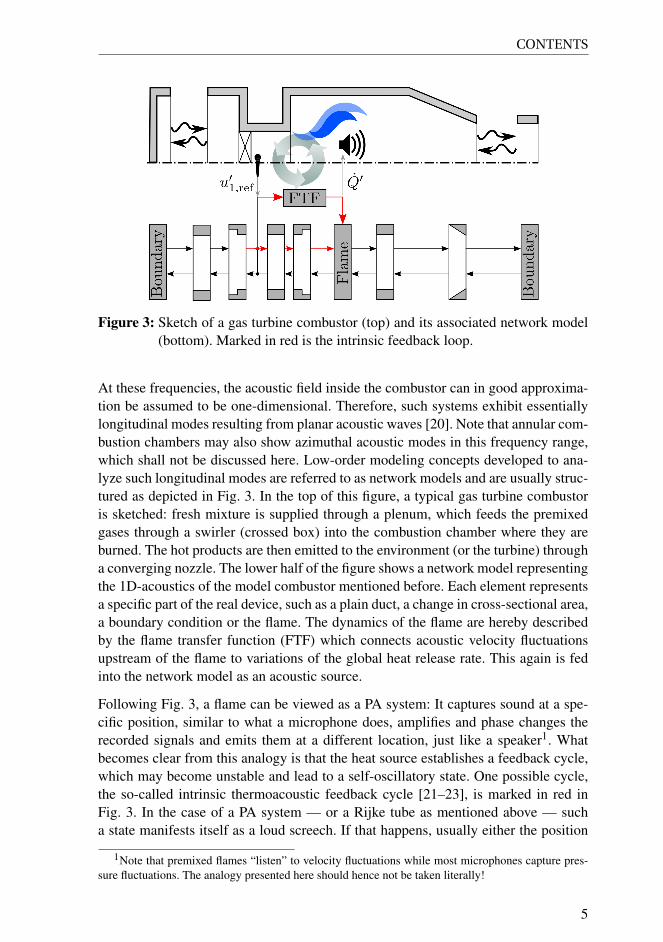
Figure 3: Sketch of a gas turbine combustor (top) and its associated network model(bottom). Marked in red is the intrinsic feedback loop.

At these frequencies, the acoustic field inside the combustor can in good approxima-tion be assumed to be one-dimensional. Therefore, such systems exhibit essentiallylongitudinal modes resulting from planar acoustic waves [20]. Note that annular com-bustion chambers may also show azimuthal acoustic modes in this frequency range,which shall not be discussed here. Low-order modeling concepts developed to ana-lyze such longitudinal modes are referred to as network models and are usually struc-tured as depicted in Fig. 3. In the top of this figure, a typical gas turbine combustoris sketched: fresh mixture is supplied through a plenum, which feeds the premixedgases through a swirler (crossed box) into the combustion chamber where they areburned. The hot products are then emitted to the environment (or the turbine) througha converging nozzle. The lower half of the figure shows a network model representingthe 1D-acoustics of the model combustor mentioned before. Each element representsa specific part of the real device, such as a plain duct, a change in cross-sectional area,a boundary condition or the flame. The dynamics of the flame are hereby describedby the flame transfer function (FTF) which connects acoustic velocity fluctuationsupstream of the flame to variations of the global heat release rate. This again is fedinto the network model as an acoustic source.

Following Fig. 3, a flame can be viewed as a PA system: It captures sound at a spe-cific position, similar to what a microphone does, amplifies and phase changes therecorded signals and emits them at a different location, just like a speaker1. Whatbecomes clear from this analogy is that the heat source establishes a feedback cycle,which may become unstable and lead to a self-oscillatory state. One possible cycle,the so-called intrinsic thermoacoustic feedback cycle [21–23], is marked in red inFig. 3. In the case of a PA system — or a Rijke tube as mentioned above — sucha state manifests itself as a loud screech. If that happens, usually either the position

1Note that premixed flames “listen” to velocity fluctuations while most microphones capture pres-sure fluctuations. The analogy presented here should hence not be taken literally!

5

CONTENTS

of the microphone is changed or the gain of the amplifier is reduced in order to getrid of this perturbing sound. In the case of a gas turbine combustor, consequences ofa developed self-oscillatory state are more severe and might — in the worst case —even lead to system failure, similar to what has been shown above for the F-1 rocketengine. The main leverage for counteracting such a state is the FTF, which can, forexample, be modified by changing the mass flux or the air-to-fuel ratio.

Since the flame is the driving force of a combustion instability, understanding itsdynamics is crucial. Having powerful low-order models at hand that allow adequatepredictions of the flame dynamics would significantly enhance stability predictions,particularly in early stages of the design process of a full combustor or a dampingsystem. To this end, a profound understanding of interactions between acoustics anda flame needs to be established. This is not an easy task, considering that even aRijke tube, where a heated mesh instead of a flame acts as a heat source, exhibitsnon trivial behavior [24, 25]. Although there are many studies that have already dealtwith this topic, the flame response to acoustic perturbations is not yet adequatelyunderstood - even for the simple case of a Bunsen flame and low forcing amplitudes(linear regime). Thus, it seems to be a good idea to focus on these setups first beforeadvancing to even more complex, turbulent flames, as used in gas turbine combustors.

Objective and Outline of the Thesis

The ultimate goal of this work is to advance the understanding and modeling of theresponse of burner-stabilized laminar flames to acoustic perturbations. The behav-ior of the global heat release rate is of particular interest, since its fluctuations areproportional to the sound generated by a flame, which is an important quantity inthermoacoustic analysis. To this end, instructive low-order models shall be devel-oped and extended, which allow to bring order into the analysis of acoustics-flameinteractions.

In the field of thermoacoustics, there is a lack of first principle-based, low-order mod-eling concepts for the linear flame response expressed by the flame transfer function(FTF), see Fig. 3. As will be detailed in the course of this work, the most wide-spread models all rely on the assumption of convective velocity perturbations, whichis based on experimental observations instead of a rigorous derivation starting fromfirst principles. Although they allow for reasonable FTF predictions relying on em-pirical parameters (they are useful . . . ), they are not suitable for the analysis of theunderlying physical mechanisms (. . . but not instructive).

Based on this realization, this thesis starts with a review of the literature on the dy-namics of laminar flames. A lot has been achieved in this field, however, only a rathersmall fraction of the gathered knowledge has made its way to the field of thermoa-coustics. A similar statement can be made concerning the field of aero-acoustics,which deals with the generation and attenuation of acoustic energy in flows without

6

CONTENTS

chemical reactions. Elaborate models for the transient acoustic field inside a con-finement or the process of vortex shedding have been developed here, which wouldqualify as candidates for low-order descriptions of the velocity field in the vicin-ity of an acoustically perturbed anchored flame. Again, rather few concepts made itto the field of thermoacoustics. This thesis tries to account for the inherently inter-disciplinary nature of thermoacoustics and strives to bring together knowledge andmethods from the fields of laminar premixed combustion and aero-acoustics.

The work is split into three parts:

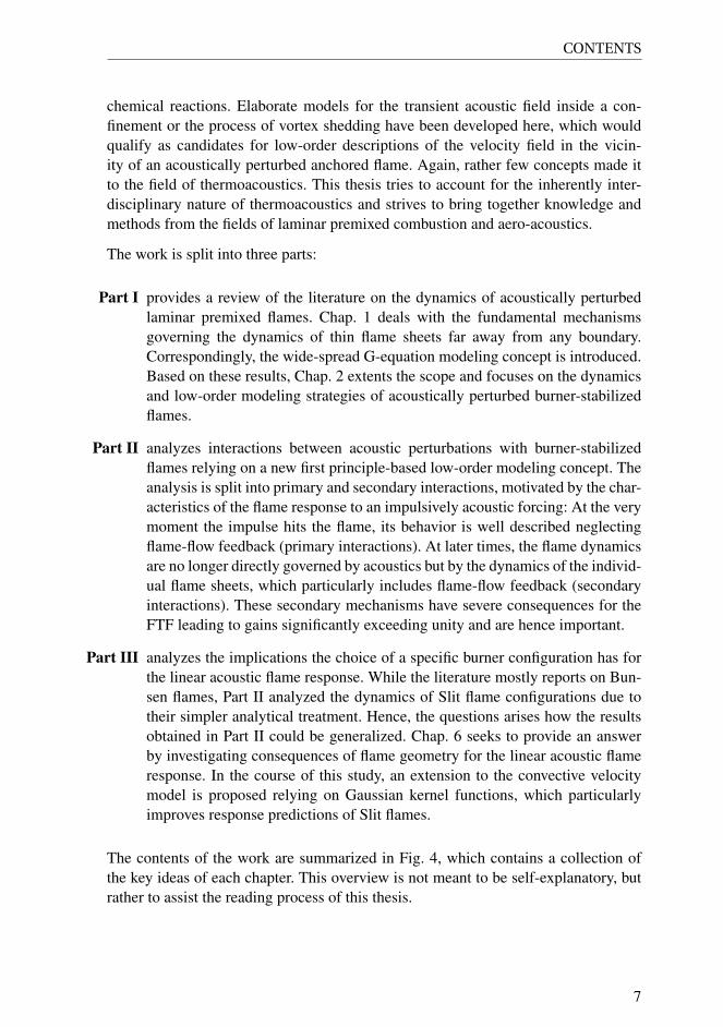
Part I provides a review of the literature on the dynamics of acoustically perturbedlaminar premixed flames. Chap. 1 deals with the fundamental mechanismsgoverning the dynamics of thin flame sheets far away from any boundary.Correspondingly, the wide-spread G-equation modeling concept is introduced.Based on these results, Chap. 2 extents the scope and focuses on the dynamicsand low-order modeling strategies of acoustically perturbed burner-stabilizedflames.

Part II analyzes interactions between acoustic perturbations with burner-stabilizedflames relying on a new first principle-based low-order modeling concept. Theanalysis is split into primary and secondary interactions, motivated by the char-acteristics of the flame response to an impulsively acoustic forcing: At the verymoment the impulse hits the flame, its behavior is well described neglectingflame-flow feedback (primary interactions). At later times, the flame dynamicsare no longer directly governed by acoustics but by the dynamics of the individ-ual flame sheets, which particularly includes flame-flow feedback (secondaryinteractions). These secondary mechanisms have severe consequences for theFTF leading to gains significantly exceeding unity and are hence important.

Part III analyzes the implications the choice of a specific burner configuration has forthe linear acoustic flame response. While the literature mostly reports on Bun-sen flames, Part II analyzed the dynamics of Slit flame configurations due totheir simpler analytical treatment. Hence, the questions arises how the resultsobtained in Part II could be generalized. Chap. 6 seeks to provide an answerby investigating consequences of flame geometry for the linear acoustic flameresponse. In the course of this study, an extension to the convective velocitymodel is proposed relying on Gaussian kernel functions, which particularlyimproves response predictions of Slit flames.

The contents of the work are summarized in Fig. 4, which contains a collection ofthe key ideas of each chapter. This overview is not meant to be self-explanatory, butrather to assist the reading process of this thesis.

7

CONTENTS

Figure 4: Contents of the thesis in a nutshell.

8

Part I

Literature Review on

Acoustics-Flame Interactions

This thesis seeks to analyze and model interactions between acousticsand laminar lean premixed flames. A well-established method to effi-ciently assess the dynamics of such flames avoiding the need to dealwith chemical reactions relies on a kinematic description: the usuallythin flame sheets are viewed as gasdynamic discontinuities that prop-agate normal to themselves with a characteristic speed. Their dynam-ics are hereby governed by consequences of density changes across theflame sheets as well as by dependencies of the flame speed on various ge-ometrical and mixture properties. This approach became state-of-the-artand, thus, the literature review provided in this Part of the thesis revolvesaround this key concept.

Chap. 1 introduces the fundamental dynamics of freely propagatingflame sheets. Four canonical mechanisms are identified and explicatedthat govern flame propagation. Most low-order modeling concepts arebased on the so-called G-equation approach, which is subsequently dis-cussed. Relying on these ideas, Chap. 2 then moves on to the more re-alistic setups of burner-stabilized flames. Here, driven by the thermoa-coustics focus of this work, their interactions with acoustic perturbationsare emphasized. The phenomenological convective velocity model is in-troduced, which is, combined with the G-equation framework, the state-of-the-art low-order model of such systems.

9

1 Dynamics of Thin Flame Sheets

A literature review on the dynamics of thin flame sheets far away

from any boundary is provided, ranging from (i) a discussion on

the internal flame structure, over (ii) an outline of four important

canonical mechanisms of flame propagation to (iii) associated low-

order modeling concepts.

Premixed laminar flame fronts are often assumed to be thin with respect to a charac-teristic length of the considered problem, such as the overall flame length or a per-turbation wave length. This approximation allows for a purely kinematic treatmentof their spatio-temporal behavior avoiding detailed considerations of flame-internalchemical and transport processes that govern the combustion process. A descriptionof the complete dynamics boils down to an expression for the flame propagationvelocity as well as jump conditions, connecting macroscopic properties of the fluidup- and downstream of the flame. This simplified treatment enables analytical stud-ies on the dynamics of planar flame sheets and allows to identify the physical keymechanisms. Hence, it constitutes one of the central concepts when dealing with thedynamics of premixed flame fronts.

Accordingly, this chapter introduces the relevant findings and observations requiredto understand the key motivations and theoretical concepts associated to this idea.For the sake of clearness, this chapter is limited to the study of freely propagatingthin flame sheets far away from any boundary. Burner-stabilized flames are only in-troduced in the subsequent chapter as an extension to the theory introduced here.

Sec. 1.1 specifies the term “thin” in the context of a lean methane-air flame and pro-vides a historical review of important experiments and theoretical achievements inthe field. Subsequently, the four main governing mechanisms for the dynamics oflean methane-air flame sheets are summarized in Sec 1.2. Finally, Sec 1.3 introducesthe G-equation or level-set method as well as a 1D linearized advection-diffusionequation, which are both widely used modeling approach in order to efficiently cap-ture the dynamics of flame sheets.

11

Dynamics of Thin Flame Sheets

1.1 Scope

The overview presented in the following clarifies when a flame front is consideredto be “thin” and how the analysis of such flames evolved, starting from the earlyworks of Darrieus [26] and Landau [27]. This section is not strictly limited to find-ings directly related to the main topic of this thesis, but rather seeks to provide amore comprehensive view. Readers who are only interested in the main mechanismsgoverning the dynamics of flame sheets, may skip this section for now and directlycontinue with Sec 1.2.

1.1.1 Definition of the Term “Thin Flame”

The overall combustion process of lean methane-oxygen mixtures to carbon dioxideand water involves tens of chemical sub-reactions and the formation of hundredsof intermediate species. Peters and Williams [28] systematically reduced these forsufficiently high pressures and temperatures to only three global reactions that involvesix species:

CH4 +O2 → CO+H2 +H2O (1.1)

CO+H2OCO2 +H2 (1.2)

O2 +2H2 → 2H2O. (1.3)

Fig. 1.1 illustrates the inner structure of such an adiabatic, lean methane-air flame ofequivalence ratio φ= 0.81. Three characteristic layers are identified [28, 31]: (i) Aninert convective-diffusive layer of thickness δD where the fresh mixture is preheatedand methane molecules are transported towards the reaction zone. (ii) A thin reactionlayer of extension δR where methane CH4 and oxygen O2 react to carbon monoxideCO, hydrogen H2 and water H2O, as expressed by Reaction (1.1). (iii) A secondreaction layer of thickness δO where hydrogen and carbon monoxide are oxidized tocarbon dioxide and water, see Reactions (1.2) and (1.3).

The reaction zone can be visualized by the heat release rate q , which is a conse-quence of the transformation of chemically stored enthalpy of the products to sen-sible enthalpy via the three global exothermic oxidation reactions. The heat releaserate is plotted in Fig. 1.1 and it is apparent that the reaction layer associated with theglobal Reaction (1.1) has a much thinner spatial extension than the one of the sec-ondary oxidation zone associated with the global Reactions (1.2) and (1.3). This isreflected by different activation energies, which are significantly higher for the globalReaction (1.1) than for the Reaction (1.2). The latter is also known as the moderatelyexothermic water-gas shift reaction [32] and, compared to Reaction (1.1), only addsa secondary contribution to the total heat release rate. It, however, leads to the for-mation of hydrogen that is finally oxidized by Reaction (1.3). All in all, due to the

1Computed with Cantera [29] using the GRI-Mech 3.0 reaction mechanism [30]

12

1.1 Scope

Figure 1.1: Internal structure of a lean methane-air flame of equivalence ratio φ =0.8. All curves are normalized by their maximum value.

dominance of Reaction (1.1), the combustion of methane-air mixtures is essentiallya very localized process.

Based on the insight that this also holds for a variety of mixtures, where the combus-tion process is confined to a layer that is thin compared to a global length scale —such as the burner mouth diameter – flames are often approximated as gas dynamicdiscontinuities, i. e. surfaces separating cold reactants from hot products [26, 27, 33–35]. Far away from this discontinuity, fluid composition, temperature and densityare essentially constant. The dynamics of the flame sheet is governed by a localconsumption speed, which defines a propagation velocity of the flame normal to it-self and relative to the fresh mixture, quantified by the flame speed. This speed is amanifestation of chemical reactions and transport processes in the reaction and theconvective-diffusive layer, respectively [34–37].

Models that regard a flame as a discontinuity are specifically designed to capture thespatio-temporal dynamics of a reacting flow, while the formation of pollutants or anyother chemical property of the combustion process are neglected. In order to retrievea closed formulation of such flow problems, a flame speed and jump conditions, con-necting up- and downstream flow quantities, need to be specified at the surface repre-senting the flame. They were derived from first principles by use of matched asymp-totic expansion methods, which exploit the fact that flames exhibit length scales ofdifferent order. Each scale has its own characteristic properties, which allows to dropspecific terms from the full set of governing equations. By asymptotically matchingthe results of the individual length scales, a macroscopic description of the internalprocesses could be derived, which essentially boils down to an expression for thedesired flame speed and the jump conditions, see e. g. [28, 34, 35, 37–41].

13

Dynamics of Thin Flame Sheets

In order to apply these matched asymptotic expansion methods, characteristic lengthscales associated with the available internal layers need to be found. Based on them,non-dimensional parameters are defined that are used to derive the respective govern-ing equation for each layer. In the case of premixed combustion, the relative thicknessof the convective-diffusive boundary layer δD , see Fig. 1.1, is quantified by a Pécletnumber

Pe= L

δD, (1.4)

which relates a typical length scale of the macroscopic (or outer) flow problem L, toa length scale of the microscopic (or inner) advection-diffusion problem. Here, theouter problem may be characterized by the burner diameter or the perturbation wavelength of interest and the inner problem by a diffusion length δD = D/sL , where sL

is the flame speed and D either the thermal diffusivity D th or the mass diffusivity ofthe deficient species relative to the fresh mixture DY [37, 41, 42]. Both diffusivitiesare related by the Lewis number

Le = D th

DY, (1.5)

where the thermal diffusivity is defined by D th =λ/(ρcp ) with the thermal conduc-tivity λ, the density ρ and the specific heat capacity for constant pressure cp , allevaluated for the fresh mixture. If D th = DY and thus Le= 1 holds, the thermal andthe species boundary layer are identical. Otherwise, one of them outweighs the other.Lean methane-air flames, as considered in this thesis, typically have Lewis numbersvery close unity, which is also reflected in the similar boundary layer thicknesses ofCH4 and temperature ahead of the reaction zone shown in Fig. 1.1. Hence, the Lewisnumber quantifies the coupling of species transport and energy equation, similarly asthe Prandtl number does it for momentum and energy. For the Le≈ 1 case, typicallythe thermal, instead of the mass, diffusion length scale δD = D th/sL is used in orderto quantify the extension of the preheat layer.

The thickness of the reaction layer δR is related to the Zeldovich number

Ze= Ea

Rg Tb

Tb −Tu

Tb(1.6)

with the activation energy of the global chemical reaction Ea , the gas constant Rg andthe temperatures of the unburned and burned fluid Tu and Tb , respectively [43]. Highactivation energies, and hence Ze≫ 1, lead to thin reaction layers [35].

Using these definitions, the spatial extension of the convective-diffusive layeris of order δD =O

(Pe−1

)and the one of the two reaction zones of order

δR/O =O(Pe−1Ze−1

)[35, 37]. For the flame configurations considered in this the-

sis (lean methane-air mixtures at φ ≈ 0.8 and burner inlet radii of Ri = 5 mm ), weretrieve a Péclet number of the order O (100). Hence, all flames can safely be consid-ered as thin flame sheets.

14

1.1 Scope

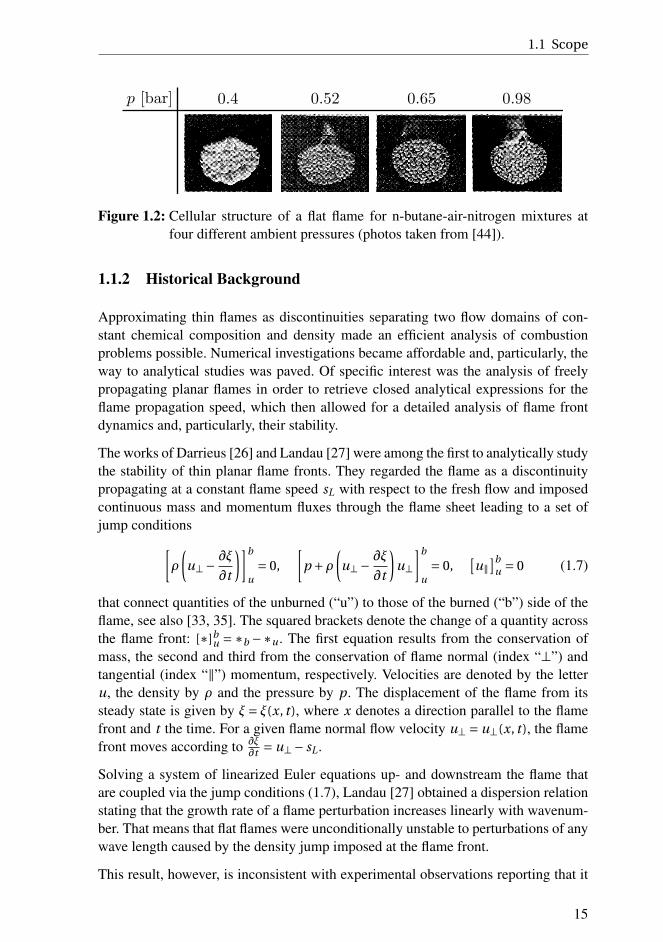
Figure 1.2: Cellular structure of a flat flame for n-butane-air-nitrogen mixtures atfour different ambient pressures (photos taken from [44]).

1.1.2 Historical Background

Approximating thin flames as discontinuities separating two flow domains of con-stant chemical composition and density made an efficient analysis of combustionproblems possible. Numerical investigations became affordable and, particularly, theway to analytical studies was paved. Of specific interest was the analysis of freelypropagating planar flames in order to retrieve closed analytical expressions for theflame propagation speed, which then allowed for a detailed analysis of flame frontdynamics and, particularly, their stability.

The works of Darrieus [26] and Landau [27] were among the first to analytically studythe stability of thin planar flame fronts. They regarded the flame as a discontinuitypropagating at a constant flame speed sL with respect to the fresh flow and imposedcontinuous mass and momentum fluxes through the flame sheet leading to a set ofjump conditions

[ρ

(u⊥− ∂ξ

∂t

)]b

u

= 0,

[p +ρ

(u⊥− ∂ξ

∂t

)u⊥

]b

u

= 0,[u∥

]bu = 0 (1.7)

that connect quantities of the unburned (“u”) to those of the burned (“b”) side of theflame, see also [33, 35]. The squared brackets denote the change of a quantity acrossthe flame front: [∗]b

u =∗b −∗u . The first equation results from the conservation ofmass, the second and third from the conservation of flame normal (index “⊥”) andtangential (index “∥”) momentum, respectively. Velocities are denoted by the letteru, the density by ρ and the pressure by p. The displacement of the flame from itssteady state is given by ξ= ξ(x, t ), where x denotes a direction parallel to the flamefront and t the time. For a given flame normal flow velocity u⊥ = u⊥(x, t ), the flamefront moves according to ∂ξ

∂t= u⊥− sL .

Solving a system of linearized Euler equations up- and downstream the flame thatare coupled via the jump conditions (1.7), Landau [27] obtained a dispersion relationstating that the growth rate of a flame perturbation increases linearly with wavenum-ber. That means that flat flames were unconditionally unstable to perturbations of anywave length caused by the density jump imposed at the flame front.

This result, however, is inconsistent with experimental observations reporting that it

15

Dynamics of Thin Flame Sheets

is indeed possible to stabilize flat planar flames, see e. g. [44–47]. Further, it is in con-flict with observations made by Markstein [44], who showed that a flat flame developscellular structures whose averaged cell size decreases with rising ambient pressure,see Fig. 1.2. While the theory of Landau [27] predicts a linear increase of growthrate with the wave number, the experimental results of Markstein [44] reported apressure dependent uniform cell size, which suggests the existence of a pressure de-pendent maximum growth rate at a wave number approximately corresponding to theobserved cell sizes (approximately since the observed cellular structures are alreadyaffected by non-linear processes, see [48]).

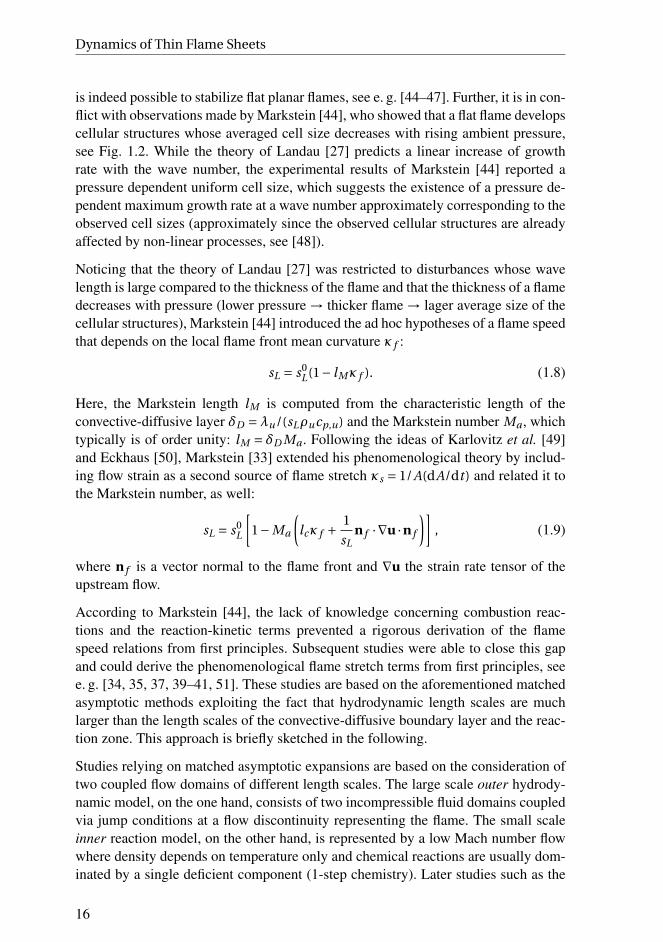
Noticing that the theory of Landau [27] was restricted to disturbances whose wavelength is large compared to the thickness of the flame and that the thickness of a flamedecreases with pressure (lower pressure → thicker flame → lager average size of thecellular structures), Markstein [44] introduced the ad hoc hypotheses of a flame speedthat depends on the local flame front mean curvature κ f :

sL = s0L(1− lMκ f ). (1.8)

Here, the Markstein length lM is computed from the characteristic length of theconvective-diffusive layer δD =λu/(sLρucp,u) and the Markstein number Ma , whichtypically is of order unity: lM = δD Ma . Following the ideas of Karlovitz et al. [49]and Eckhaus [50], Markstein [33] extended his phenomenological theory by includ-ing flow strain as a second source of flame stretch κs = 1/A(dA/dt ) and related it tothe Markstein number, as well:

sL = s0L

[1−Ma

(lcκ f +

1

sLn f ·∇u ·n f

)], (1.9)

where n f is a vector normal to the flame front and ∇u the strain rate tensor of theupstream flow.

According to Markstein [44], the lack of knowledge concerning combustion reac-tions and the reaction-kinetic terms prevented a rigorous derivation of the flamespeed relations from first principles. Subsequent studies were able to close this gapand could derive the phenomenological flame stretch terms from first principles, seee. g. [34, 35, 37, 39–41, 51]. These studies are based on the aforementioned matchedasymptotic methods exploiting the fact that hydrodynamic length scales are muchlarger than the length scales of the convective-diffusive boundary layer and the reac-tion zone. This approach is briefly sketched in the following.

Studies relying on matched asymptotic expansions are based on the consideration oftwo coupled flow domains of different length scales. The large scale outer hydrody-namic model, on the one hand, consists of two incompressible fluid domains coupledvia jump conditions at a flow discontinuity representing the flame. The small scaleinner reaction model, on the other hand, is represented by a low Mach number flowwhere density depends on temperature only and chemical reactions are usually dom-inated by a single deficient component (1-step chemistry). Later studies such as the

16

1.1 Scope

one by Matalon et al. [41] included a 2-step mechanism allowing for considerationof mixtures whose composition varies from rich to lean conditions. The outer andthe inner models are matched by assuming that their solutions have to coincide faraway from the flame, which results in expressions for the flame speed and the jumpconditions. Flame speed relations, as well as the definition of the Markstein number,generally depend on the exact location of the discontinuity with respect to the innerflame structure [37, 41, 52–54]. By constraining the mass flux of the outer solution tobe continuous at the discontinuity, Class et al. [37] naturally fixed the position of theflame and, thus, the expressions for the flame speed as well as the Markstein number.

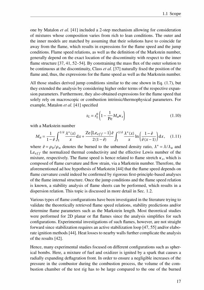
All those studies derived jump conditions similar to the one shown in Eq. (1.7), butthey extended the analysis by considering higher order terms of the respective expan-sion parameters. Furthermore, they also obtained expressions for the flame speed thatsolely rely on macroscopic or combustion intrinsic/thermophysical parameters. Forexample, Matalon et al. [41] specified

sL = s0L

(1− 1

PeMaκs

)(1.10)

with a Markstein number

Ma = 1

1− e

∫1/e

1

λ∗(x)

xdx +

Ze(Lee f f −1

)e

2(1− e)

∫1/e

1

λ∗(x)

xln

(1− e

e (x −1)

)dx , (1.11)

where e = ρb/ρu denotes the burned to the unburned density ratio, λ∗ =λ/λu andLee f f the normalized thermal conductivity and the effective Lewis number of themixture, respectively. The flame speed is hence related to flame stretch κs , which iscomposed of flame curvature and flow strain, via a Markstein number. Therefore, theaforementioned ad hoc hypothesis of Markstein [44] that the flame speed depends onflame curvature could indeed be confirmed by rigorous first-principle-based analysesof the flame internal structure. Once the jump conditions and the flame speed relationis known, a stability analysis of flame sheets can be performed, which results in adispersion relation. This topic is discussed in more detail in Sec. 1.2.

Various types of flame configurations have been investigated in the literature trying tovalidate the theoretically retrieved flame speed relations, stability predictions and/ordetermine flame parameters such as the Markstein length. Most theoretical studieswere performed for 2D planar or flat flames since the analysis simplifies for suchconfigurations. Experimental investigations of such flames, however, are not straightforward since stabilization requires an active stabilization loop [47, 55] and/or elabo-rate ignition methods [44]. Heat losses to nearby walls further complicate the analysisof the results [42].

Hence, many experimental studies focused on different configurations such as spher-ical bombs. Here, a mixture of fuel and oxidizer is ignited by a spark that causes aradially expanding deflagration front. In order to ensure a negligible increases of thepressure in the combustor during the combustion process, the volume of the com-bustion chamber of the test rig has to be large compared to the one of the burned

17

Dynamics of Thin Flame Sheets

Figure 1.3: Snapshots of spherically expanding stoichiometric propane/air flames(spherical bombs) for three different ambient pressures at a Lewis num-ber close to unity. The snapshots compare instants in time of the samenon-dimensional stretch rate, defined by the Karlovitz number Ka (snap-shots are taken from [62]).

mixture. Advantages of such test rigs are the relatively simple adjustment of exper-imental parameters such as pressure and temperature of the mixture, the absence ofinitial turbulence in the unburned fluid and a well defined and uniformly distributedflame stretch [56, 57]. In particular, the latter property qualifies these configurationsfor measurements of Markstein numbers and laminar flame speeds [58–61], as wellas for the assessment of flame front instabilities.

Fig. 1.3, for example, shows experimental results of Kwon et al. [62]. They investi-gated the development of spherically expanding stoichiometric propane/air flame atthree ambient pressures. By variation of pressure, they changed the flame thickness(higher pressure → thinner flames), while all other parameters influencing flame sta-bility were kept approximately constant. The higher the ambient pressure and, thus,the thinner the flame, the less stable the expanding flame front becomes: Similarlyto the experimental results of Markstein [44] shown in Fig. 1.2, a lower pressure in-creases stability and successively less “cracks” – indicating the formation of growingcellular structures – are visible in Fig 1.3 comparing the 10 bar, 5 bar and the 2 barseries of snapshots.

Finally, aerodynamically anchored flames such as Bunsen or Slit flames constituteanother important flame configuration of high technical relevance. Since for suchflames local displacements are convected downstream, flame instabilities cause spa-tially growing displacements, as depicted in experiments carried out by Searby et al.

[63] and reproduced in Fig 1.4. Several studies have analyzed such configurations andfound that, besides the advection of flame front displacements and the existence of

18

1.1 Scope

Figure 1.4: Snapshot of an aerodynamically anchored and inclined richpropane/air/oxygen flame whose base is displaced by a vibratingflame holder (taken from [63]).

a flame anchoring and tip, the dynamics of anchored and inclined flames essentiallycorresponds to the one of the planar counterpart, i. e. the same instability mechanismsare present [45, 64–66]. Such type of flames are investigated within the scope of thisthesis. Formally, they will only be introduced in the following chapter.

Having solved the linear stability problem of planar flames for many canonical con-figurations, the next step was to assess the process of non-linear saturation. For thispurpose, on the one hand, Navier-Stokes based simulations treating the flame as agas dynamic discontinuity [67–70] have been performed. On the other, a low-orderweakly non-linear flame model, known as the Michelson-Sivashinsky (MS) equa-tion, has been introduced [38, 48, 71]. It has been proven to be a valuable tool forthe prediction of the onset of hydrodynamic instabilities and their fully non-lineardevelopment [67]. The dynamics of the MS equation on a finite domain of width L

is controlled by a reduced Markstein number αM = lM /(ρu/ρb −1)L. For sufficientlysmall values of this parameter, short wave length flame front displacements perpet-ually coalesce forming bigger and bigger structures until, eventually, a stable singlepeak solution is reached [72]. This process is illustrated in Fig. 1.5 where a randomlyperturbed flame sheet (top line) develops into a stable cusp (bottom line), which con-tinues to propagate at a constant speed [67].

Instabilities, such as the ones described above, are responsible for many crucial andpractically relevant flow phenomena and often result in characteristic large-scale co-herent structures. There are, for example, the widely known Kelvin-Helmholtz in-stability or the Tollmien–Schlichting waves. Both lead to the formation of flow fea-tures that have several important consequences for technical applications, such aspipe flows or the flow around airplane wings. Accordingly, stability considerationshave made their way to the analysis of flames in a thermoacoustic context, as well.Here, technically relevant setups often rely on swirl-stabilized turbulent flames. Oneimportant feature of these flames is a precessing vortex core that responds to acous-tics and significantly interacts with the combustion process [73–75], another the oc-currence of a so-called vortex breakdown [76–78]. Both mechanisms are related toflow field instabilities and essentially determine the flame response to acoustic per-turbations. Exploiting this principal finding, Oberleithner et al. [79] and Oberleithner

19

Dynamics of Thin Flame Sheets

Figure 1.5: Temporal evolution of a randomly perturbed flame sheet according to theMS equation for αM = 0.005. Several snapshots of the same flame frontat different times are shown, where time progresses from the top to thebottom line (taken from [67]).

and Paschereit [80] developed a method that is capable to adequately predict the fre-quency and amplitude dependent flame response based on a linear stability analysisof the underlying mean flow. It can hence be concluded that the understanding andconsideration of the relevant instability mechanisms constitutes one important pre-requisite in order to correctly interpret and model the complex flow behavior of bothlaminar and turbulent flames.

The dynamics and stability of thin flame fronts has historically been classified ac-cording to a variety of non-dimensional numbers. The Markstein number has alreadybeen mentioned above and quantifies the effect of stretch (curvature and flow strain)onto the flame speed. It usually is of order O (1), and large positive Markstein num-bers indicate stable flames. Note that its definition depends on the assumed location ofthe gas dynamic discontinuity representing the flame with respect to the inner flamestructure. Often it is assumed that it coincides with the reaction layer, see e. g. [52].A second important number is the Lewis number Le, which relates the thermal to themass diffusivity of the deficient species relative to the mixture [81]. The experimentaldata shown in Fig. 1.3 was obtained at unity Lewis number. The fact that thermal andmass diffusion are approximately equal prevents the occurrence of thermo-diffusiveand pulsating instabilities. The former will be discussed in Sec. 1.2.2. Another impor-tant non-dimensional number is the Karlovitz number, which quantifies flame stretch:

Ka =2δ f

s0L

R f

dR

d t, (1.12)

20

1.2 Mechanisms Governing Flame Propagation

where R f is the flame radius, t the time, δ f the flame thickness and s0L the unstretched

flame speed. The snapshots of the spherical bombs shown in Fig. 1.3 are taken at dis-tinct Karlovitz numbers for all three pressure levels. As mentioned above, stretchedflames are less prone to develop instabilities than unstretched ones. An expandingspherical flame increases its radius and, hence, the flame front is exposed to suc-cessively decreasing stretch. By comparing snapshots of constant Ka, the effect ofdifferent pressure dependent stretch levels on stability can be eliminated.

Finally, flames usually propagate in the gravitational field of the earth. For flameswhose associated flow direction points upwards (heavy unburned mixture belowlight burned products), gravity tends to stabilize perturbations of long wave lengths[82, 83]. The impact of gravity relative to the flame speed is given by a Froude num-ber Fr = s2

L/(gδ f ) with the gravitational acceleration g . As pointed out by Searby andClavin [82], for a given mixture there exists a critical value of the Froude number Frc

below which planar flames are unconditionally stable. The wave length of the pertur-bations that become unstable at Frc is large compared to the flame thickness [82]. Theeffect of gravity together with the effect of flame curvature explains why it is possi-ble to experimentally implement stable planar flame fronts [44, 82]. Flames with aflow streaming downwards (light burned products below heavy unburned mixture)are destabilized by the Rayleigh-Taylor instability [84].

1.2 Mechanisms Governing Flame Propagation

In the previous section it was shown that the representation of a flame as a propa-gating discontinuity connecting the unburned with the burned flow domain by meansof jump conditions provides an efficient tool for understanding and modeling thedynamics of thin flame sheets. First principle-based expressions for the propagationspeed as well as jump conditions could be derived by means of matched asymp-totic expansion techniques. While the latter ensure the conservation of mass, normaland tangential momentum across the flame, the former emerges as a consequenceof chemical kinetics combined with the energy and species transport. One importantoutcome of this kind of analysis is that the local flame speed depends on flame stretch,i. e. flame curvature and flow strain.

Coupling two incompressible flow domains of different densities using aforemen-tioned jump conditions and flame speed relations results in an powerful frameworkfor the analysis of the dynamics of thin flame sheets. Its main advantage consistsin the fact that the chemical details of the combustion process need no longer to beconsidered and, thus, the focus is shifted to macroscopic quantities, such as the flamespeed or the flame shape. This method consequently brings order into the complexfield of flame propagation and allows to differentiate between well-defined intuitivelyaccessible governing mechanisms.

The within the scope of this thesis four most important mechanisms are discussed in

21

Dynamics of Thin Flame Sheets

the following. Each one is in a first step formally introduced and subsequently its im-plications are illustrated by analyzing how it affects the dynamics of a perturbed flamesheet. Section 1.2.1 deals with the most elementary mechanism of flame propagation,namely the fact that flame sheets propagate normal to themselves. Section 1.2.2 an-alyzes thermal-diffusive mechanisms that address implications of the flame speedrelation onto flame sheet propagation. This is followed by an analysis of hydrody-namic mechanisms, which arise as soon as two flow domains of different densitiesare coupled via jump conditions. Finally, Sec. 1.2.4 deals with flame sheets that areinclined with respect to the mean flow field, e. g. by anchoring them. Here, in addi-tion to the former mechanisms, the advection of flame front perturbations becomesimportant.

1.2.1 Propagation Normal to Itself

1D simulations, as the one shown in Fig. 1.1, reveal that a (thin) reaction zone propa-gates into the domain of the fresh mixture at a certain speed. The velocity of the meanflow field far upstream of the flame that is required to maintain the flame front at afixed position is referred to as the flame speed sL in the following. Note that, theoret-ically, also other definitions of sL are possible, such as the flow speed far downstreamof the reaction zone. Since the properties of the fresh mixture are the ones that are setby an experimentalist or at a numerical simulation, it is convenient to define sL withrespect to them.

Knowing how a 1D flame propagates, we are now interested in the transient behaviorof a flame sheet, where each point on this sheet propagates at a constant speed sL .Without loss of generality, we approach this problem by assuming a 2D sheet thathas at a time t0 the shape as depicted by the black line in Fig. 1.6a. Since a point ofthat line propagates at a speed sL , its position at a time t0 +∆t has to be somewhereon a circle of radius ∆t sL drawn around the current position. This has to hold for eachpoint on the black line and, therefore, the flame front position at t0 +∆t can only begiven by the upstream envelope of all circles, depicted by the red line in Fig. 1.6a.From this consideration, which is also known as Huygens’s principle, it naturallyevolves that a flame propagates normal to itself.

One important consequence of this mechanism is the formation of cusps, which areperturbations of the flame front of discontinuous slope. Following Huygens’s prin-ciple, it can be shown that such non-smooth flame shapes develop from an initiallysmooth flame front, which is concavely bent towards the fresh fuel mixture [85].Since flame fronts propagate normal to themselves, the position of the flame sheet atlater times can be estimated by rays drawn normal to the current flame front position,see Fig. 1.6a ( ). These rays will eventually intersect and, hence, one side of theinitially smooth flame wrinkle propagates into the opposing front, which leads to thegeneration of cusps and to a propagation of the tip of the wrinkle in the directionof the unburned gases with a speed faster than the flame speed [86]. This process is

22

1.2 Mechanisms Governing Flame Propagation

(a) (b)

Figure 1.6: Illustration of Huygens’s Principle (1.6a), which explains the formationof cusps from an initially smooth flame front (1.6b).

illustrated for four instants in time in Fig. 1.6b (blue arrow). On the contrary, convexparts of a flame sheet will expand and heal themselves from eventual cusps [86].

It is interesting to note that the formation of cusps constitutes a non-linear mecha-nism that leads to saturation of high amplitude perturbations, particularly for highwave numbers. Further, it is not symmetric since convex displacements are smoothedout, while concave ones form sharp edges. Hence, as pointed out by Sivashinsky[38], Landau [27] eliminated a major stabilizing mechanism by linearizing all of theequations. This argument partly resolves Landau’s paradoxical prediction of uncon-ditionally unstable flame fronts. This becomes more clear when considering the factthat Clanet and Searby [55] were the first to experimentally measure and visualizethe growth of planar flame front perturbations due to the Darrieus-Landau instabilityas late as 1998. All previous studies on planar flames only measured cellular struc-tures that were already non-linearly saturated and, hence, subjected to the mechanismdescribed above.

This thesis is devoted to the study of the linear response of acoustically perturbedflames. The non-linear mechanism described above leads to the formation of verycharacteristic flame shapes that exhibit sharp edges at concave and smooth frontsat convex parts of a flame sheet. Hence, it provides a simple tool to estimate if theresponse of a flame is still in the linear regime or if non-linear processes have alreadystarted to become significant.

23

Dynamics of Thin Flame Sheets

1.2.2 Thermal-Diffusive

So far it was assumed that all points of a flame sheet propagate at a constantspeed. Theory, however, predicts that this speed depends on the local flame stretchκs = 1/A(dA/dt ), i. e. the normalized rate of change of the local flame surface area.Flame stretch has its origin in flame curvature and flow strain. Since the related pro-cesses are governed by thermal as well as mass diffusion of a deficient species, theirconsequences for the flame dynamics are attributed to the so-called thermal-diffusive(or also thermodiffusive) mechanism.

The decisive parameter for this mechanism is the Lewis number, which relates thethermal to the mass diffusivity of the deficient species1. It allows to distinguish be-tween several distinct regimes of flame propagation: The first consists of mixtureswhose mass diffusivity of the deficient component with respect to the mixture is sig-nificantly higher than the thermal one. Those flame fronts exhibit thermal-diffusiveinstabilities that cause strongly corrugated flame surfaces. One example for such mix-tures are lean hydrogen-air flames, e. g., Le≈ 0.4 for φ= 0.6 [87]. The second regimeis defined by mixtures with a Lewis number close to one, such as lean methane-airflames (Le≈ 1 [88]), as considered in this work. Conditions with Le> 1 are usuallyobserved in lean mixtures of heavy fuels (e. g. propane/air [88]) or rich mixtures oflight fuels, as well as for combustion in porous media (blocked mass and enhancedthermal diffusion) or for solid propellants [89]. These high Lewis number flamesshow a third type of instability not considered in this work, the so-called pulsatinginstability. It is expected to occur for Ze(Le−1)& 10 and is — since it results from athermal-diffusive mechanism — affected (enhanced) by flame stretch [48, 90–93].

In order to suppress hydrodynamic mechanisms, which will only be discussed in thenext section, it is assumed that the density of the flow does not change across theflame. That way consequences of thermal-diffusive mechanisms can efficiently bestudied. In order to maintain chemical reactions inside a flame, on the one hand, heathas to diffuse from the reaction zone into the fresh mixture and, in doing so, preheatit to a temperature where the (fast) combustion processes can take place. On the otherhand, the deficient component is diffusively transported from the unburned mixture tothe reaction zone — i. e. methane molecules in the case of a lean methane-air flame.Both diffusive processes together with the kinetics of the reaction define a laminarunstretched flame speed, which depends on temperature, pressure and equivalenceratio of the fresh gases, see e. g. [94].

If now the flame front is perturbed as illustrated in Fig. 1.7, from a geometrical pointof view, the heat released at regions that are convex towards the fresh mixture has toheat up more cool reactants than in concave ones. Hence, more heat is carried away

1Later studies relying on a matched asymptotic expansion technique analyzed a two-step instead ofa one-step chemical scheme, see Matalon et al. [41]. They introduced an effective Lewis number, whichis a weighted sum of the Lewis numbers of the individual species. This extension of the theory shall notbe considered here.

24

1.2 Mechanisms Governing Flame Propagation

Figure 1.7: Illustration of the thermal-diffusive flame instability mechanism. Tem-perature fluxes are marked in red, mass fluxes of the deficient species inblue.

from the reaction zone in convex regions, which therefore cool down and propagateat lower speeds than the unperturbed flame. On the contrary, heat accumulates in con-cave regions, an effect that increases the local flame speed. Since the flow speed isconstant everywhere (we presently assume constant density across the flame front!),perturbations of the flame sheet will be damped by this mechanism. At the same time,however, mass diffusion of the deficient component is enhanced in convex and atten-uated in concave regions for analogous reasons as explicated above for temperature.This increases the flame speed in convex and decreases it in concave regions and,therefore, has exactly the reverse effect of temperature diffusion: flame sheet pertur-bations are further amplified. Depending on the Lewis number either one or the othermechanism dominates. At a critical Lewis number Le0

c,TDboth effects cancel each

other and the flame sheet is marginally stable, that is (small) perturbations neithergrow (unstable) nor do they asymptotically decay (stable). An increase of mass —or decrease in heat — diffusivity leads to Le<Le0

c,TDand, therefore, to an unstable

flame sheet. Conversely, a reduction of mass — or increase in heat — diffusivitycauses Le>Le0

c,TDand, thus, a stable flame sheet.

This phenomenon was analytically analyzed for flows of constant density bySivashinsky [90]. Assuming an inviscid flow up- and downstream the flame sheet,a dispersion relation

σ = D th

[Ze

2(1−Le)−1

]k2

︸ ︷︷ ︸long−wave disturbances

− 4D thδ2D k4

︸ ︷︷ ︸short−wave correction

(1.13)

was derived relating a growth rate σ to a wave vector k. Harmonic perturbations of theflame sheet develop in time according to exp(σt + i kx1). Thus, positive growth ratescorrespond to unstable, negative ones to asymptotically stable regimes. A growth rateof zero corresponds to a marginally stable flame sheet. Neglecting the correction term

25

Dynamics of Thin Flame Sheets

(a) growth rate over wave number (b) growth rate over wave length

Figure 1.8: Dispersion relation of Eq. (1.13) for the thermal-diffusive instabilitymechanism plotted over non-dimensional wave number (1.8a) and wavelength (1.8b) for several Lewis numbers Le ∈ [0.5,1]. The one forLe0

c,TD≈ 0.7 is highlighted in red ( ). Additionally, for the two shown

extreme Lewis numbers dispersion relations neglecting the short-wavenumber correction term are plotted ( ).

in Eq. (1.13), one can compute a critical Lewis number Le0c,TD

= 1−2Ze−1 for whichthe growth rate is at maximum zero, i. e. σ ≤ 0,∀k. The short-wave correction inEq. (1.13) accounts for the fact that perturbations with a wave length that is of theorder of the preheat zone thickness δD are damped by diffusion since boundary layersof two adjacent flame wrinkles overlap and merge.

Using Eq. (1.13), dispersion relations such as the one shown in Fig. 1.8 are retrieved.Fig. 1.8a shows the growth rate over the non-dimensional wave number k∗ = kδD

and Fig. 1.8b the one over the non-dimensional wave length λ∗ =λ/δD . By using theflame thickness δD as reference length, it is recognized that wave lengths of the orderO (δD ) are damped (i. e. the growth rate is negative) for all Lewis numbers shown. Thedispersion relation corresponding to the critical Lewis number Le0

c,TDis highlighted

in red ( ). Dispersion relations of higher and lower Lewis number, respectively, areshown by the gray lines (darker shades correspond to lower Le). The blue dashed line( ) corresponds to the two extreme Le cases neglecting the short-wave correctionterm.

The critical Lewis number evaluates to Le0c,TD

. 0.8 for lean methane-air mixtures.Since such flames have Lewis numbers of approximately unity, thermal-diffusivemechanisms do not lead to a growth of flame front perturbations, but rather dampenexisting ones. Hence, they stabilize a flame front by damping existing disturbances,which is especially important when considering that hydrodynamic mechanisms re-sulting from a change of density across the flame always have a destabilizing effect.They counteract each other, as will be shown in the following section.

26

1.2 Mechanisms Governing Flame Propagation

(a) (b)

Figure 1.9: (a): Since the flow across the flame front is accelerated in flame normaldirection, velocity vectors are bend towards the flame normal directiondownstream a flame. (b): Illustration of contracting (red) and expand-ing (blue) flow tubes due to a displaced flame front, which explain theoccurrence of the Darrieus-Landau instability.

1.2.3 Hydrodynamic

As discussed in Sec. 1.1, according to the seminal work of Darrieus [26] and Landau[27], a change in density across the flame sheet destabilizes planar flames for per-turbation wave lengths that are much longer than the flame thickness. In honor of itstwo discoverers, this instability is referred to as the Darrieus-Landau (DL) instabil-ity in the literature. The intensity of this mechanism is proportional to the prevailingdensity change across the flame sheet, which is quantified by the non-dimensionalincrease of specific volume

E = ρu

ρb−1. (1.14)

The first term in this expression is also referred to as the expansion ratio e = ρu/ρb .Since all flames covered in this thesis produce a significant change in density ofE ≈ 5.7, it can be expected that the DL mechanism plays an important role for theirdynamics.

Before assessing the problem analytically, a qualitative description shall be provided.A planar, perturbed flame front stabilized in a uniform flow, as shown in Fig. 1.9bis assumed. Due to the density jump across the flame front, the upstream flow uu isaccelerated in flame normal direction, as illustrated in Fig. 1.9a. The tangential com-ponent stays constant. This leads to a bending of the flow vector towards the localflame normal direction. Consequently, in regions where the flame front is concavetowards the fresh mixture, the flow tubes are contracted, while they expand in con-

27

Dynamics of Thin Flame Sheets

vex ones. This is illustrated in Fig. 1.9b by red (contraction) and blue (expansion)flow tubes. Assuming that the flame speed is not affected by stretch, in red regions,the local flow speed will outweigh the flame speed and the flame front is transportedfurther downstream. This will lead to an increase in amplitude of the flame displace-ment. In blue regions, the reduced flow speed will lead to an upstream propagationof the flame front, which also increases the displacement amplitude. Hence, flamessheets imposing a density jump are prone to a hydrodynamic kind of instability. Thismechanism will be assessed analytically in the following.

Assuming inviscid Eulerian flow equations up- and downstream of the flame

∂u j

∂x j= 0 (1.15)

∂ui

∂t+u j

∂ui

∂x j=− 1

ρ

∂p

∂xi, (1.16)

inserting harmonic perturbations of the form exp(σt + i kx1 ±kx 2) for all flow statesand coupling both domains by use of the jump conditions of Eq. (1.7), one retrievesa dispersion relation

σ=Ω0sLk (1.17)

with the Darrieus-Landau parameter

Ω0 =p

e3 +e2 −e −e

e +1. (1.18)

This is the classical result obtained by Landau [27] and Darrieus [26] and predicts thatflame sheets are unconditionally unstable to perturbations of all wave lengths, sinceΩ0 ≥ 0. In particular, the growth rate linearly increases with k and, thus, shorter wavelengths are more amplified than longer ones. Based on this result, one would expectthat planar flames always develop high frequency oscillations that rapidly grow inamplitude until non-linear effects lead to saturation [42].

It was already mentioned in Sec. 1.1.2 that such a behavior could not be observedexperimentally. Instead, planar flames form a cellular structure of a certain wave-length, which suggests the existence of a maximum growth rate at this wave length(or close to it, since the amplitude of the observed cellular flame structure is finiteand, therefore, non-linear effects have already lead to a saturation). Markstein sug-gested a phenomenological correction by relating the flame speed to the local flamesheet curvature multiplied by a factor lM , see Eq. (1.8). This factor is called the Mark-stein length and is of the order of the thickness of the convective-diffusive layer ofa flame. It lumps the effects of various transport processes inside the flame as wellas those concerning the kinetics of the chemical reaction into one single parameter.Physically, flame stretching effects result from interactions of the external hydrody-namic field and the inner flame structure, which leads to convective fluxes along theflame redistributing heat and species. This affects the local reaction rates and thus the

28

1.2 Mechanisms Governing Flame Propagation

flame speed [42]. According to Zeldovich et al. [42], introduction of a curvature de-pendent flame speed is analogous to the introduction of a stabilizing surface tensionat the flame front.

The solution of Darrieus and Landau is asymptotically valid for Péclet numberPe= L/δD approaching infinity. Hence, the Darrieus-Landau model is a proper ap-proximation in the limit of very long wave lengths. Stated differently, expanding allstate variables using the small parameter 1/Pe, it is the zeroth order approximation ofthe flow problem. The extension of Markstein is then a first order correction of thatmodel in the limiting case of high activation energies of the global reaction [42]. It isinteresting to note that this first order correction only affects the flame speed and notthe jump conditions of Eq. (1.7). This can be explained by the strong dependency ofthe flame speed to temperature for high activation energy global reactions [42].

Later studies could derive expressions for the flame speed from first principles usingmatched asymptotic expansion methods. They included also effects of terms that areof first or higher order in 1/Pe and considered different Lewis and Zeldovich num-bers. Since these theories capture effects of diffusive and convective fluxes along theflame front and, hence, flame stretch related effects, those studies do not strictly sep-arate thermal-diffusive and hydrodynamic mechanisms. Indeed, they capture the neteffect of both mechanisms. Particularly, Frankel and Sivashinsky [95] and Pelce andClavin [40] derived a dispersion relation accounting for hydrodynamic effects as wellas for heat conduction and mass diffusion:

σ=Ω0sLk −Ω1D thk2 (1.19)

with

Ω1 =e(1− e)2 − e ln(e) (2Ω0 +1+ e)− e(1+Ω0)(e +Ω0)Ze(1−Le)

∫E0

ln(1+x)x

dx

2(1− e) [e + (1+ e)Ω0],

(1.20)where e = ρb/ρu denotes the inverse of the expansion ratio. Viscosity, responsible fordiffusion of momentum and quantified by the Prandtl number in the non-dimensionalframework, was found to have only a secondary effect on flame stability and, thusdoes not show up here [48, 95]. This is surprising, since it usually is of the sameorder of magnitude as thermal and mass diffusivity. And, indeed, the more recentstudy of Matalon [83] showed that, if viscosity is allowed to vary across the flamesheet, it has an effect on flame stability which is equal to the one imposed by otherdiffusive processes. Its impact is proportional to the Prandtl number and always hasa stabilizing effect.

For Ω1 > 0 the flame is thermo-diffusively stable and vice versa for Ω1 < 0. Basedon this criterion, one can derive a critical Lewis number for which Ω1 = 0 holds. ForE = 0 this coincides with the critical Lewis number Le0

c,TDderived in Sec. 1.2.2. It is

interesting to note that the critical Lewis number Lec,TD computed from Eq. (1.20) de-creases for increasing E , see Fig. 1.10 (top). Hence, gas expansion effects extend the

29

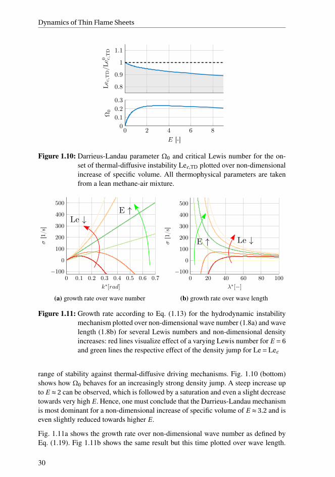
Dynamics of Thin Flame Sheets

0.8

0.9

1

1.1

Lec,T

D/Le0 c,T

D

0 2 4 6 80

0.1

0.2

0.3

E [-]

Ω0

Figure 1.10: Darrieus-Landau parameter Ω0 and critical Lewis number for the on-set of thermal-diffusive instability Lec,TD plotted over non-dimensionalincrease of specific volume. All thermophysical parameters are takenfrom a lean methane-air mixture.

(a) growth rate over wave number (b) growth rate over wave length

Figure 1.11: Growth rate according to Eq. (1.13) for the hydrodynamic instabilitymechanism plotted over non-dimensional wave number (1.8a) and wavelength (1.8b) for several Lewis numbers and non-dimensional densityincreases: red lines visualize effect of a varying Lewis number for E = 6

and green lines the respective effect of the density jump for Le=Lec

range of stability against thermal-diffusive driving mechanisms. Fig. 1.10 (bottom)shows how Ω0 behaves for an increasingly strong density jump. A steep increase upto E ≈ 2 can be observed, which is followed by a saturation and even a slight decreasetowards very high E . Hence, one must conclude that the Darrieus-Landau mechanismis most dominant for a non-dimensional increase of specific volume of E ≈ 3.2 and iseven slightly reduced towards higher E .

Fig. 1.11a shows the growth rate over non-dimensional wave number as defined byEq. (1.19). Fig 1.11b shows the same result but this time plotted over wave length.

30

1.2 Mechanisms Governing Flame Propagation

The green lines visualize the impact of the strength of the density jump alone, sincefor each E exactly the corresponding critical Lewis number Lec,TD is chosen. A highernon-dimensional increase of specific volume hence leads to a steeper slope of thedispersion relation plotted over k∗, which however saturates around E ≈ 3 and thenslightly decreases. The slope directly follows the trend of Ω0 shown in Fig. 1.10(bottom). The red lines visualize how Lewis number affects the dispersion relation fora fixed non-dimensional increase of specific volume of E = 6. Lewis numbers largerthan the critical one, lead to parabolic dispersion relations, which intersect the zerogrowth rate line at a critical wave number. Further, they exhibit a certain wave numberof maximum growth. Decreasing the Lewis number below its critical value leads toa superposition of thermal-diffusive and hydrodynamic instability mechanisms and,therefore, to a dispersion relation of increasing slope for k∗ →∞.

Summarizing, all flame fronts are subject to a destabilizing hydrodynamic mecha-nism since combustion is associated with exothermic reactions, which always lead toan increase in specific volume. Depending on the Lewis number, thermal-diffusivemechanisms may either stabilize a flame front (Le > Le0

c,TD) or further destabilize

it (Le < Le0c,TD

). The stabilizing effect of this mechanism increases with expansionratio.

1.2.4 Advection of Perturbations at Inclined Flames

So far only freely propagating flame sheets far away from any boundary were ana-lyzed. Such flames are however of no relevance for thermoacoustically driven com-bustion instabilities, since they allow not for continuous operation. Therefor, theflame sheet has to be anchored such that it stays at a fixed position. One exampleof such a device is a Bunsen burner, where the flame is anchored at the burner rim.In this chapter, any additional effects of the anchoring shall be excluded from theanalysis and only the behavior of the flame sheet far away from this point shall beof interest. It should be noted that the advection of perturbations along an inclinedflame sheet is ultimately only a consequence of the fact that flames propagate normalto themselves and the imposed anchoring of the flame. Nevertheless, it constitutesan important mechanisms, which is not obvious. Therefore, it is treated as a distinctmechanism here.

Fig. 1.12 shows a sketch of such a flame sheet. The fresh gases stream along thevertical x1 axis by a mean flow velocity u1 until they eventually reach the flame sheetthat burns at a constant speed s0

L . From geometrical considerations, the angle betweenflame the sheet and the velocity u1 is computed as α∗ = sin(α) = s0

L/u1, with thenon-dimensional flame angle α∗. At α∗ = 1 the flame speed equals the flow velocityand the flame propagates normal to the fresh flow. For 0 <α∗ < 1, the flame sheetpropagates slower than the flow field and hence it can only be stabilized at an angleα< 90. One important consequence of such an inclination is that perturbations of theflame front are advected downstream by a velocity u∥ = u1 cos(α), which is the to the

31

Dynamics of Thin Flame Sheets

Figure 1.12: Sketch of an anchored and perturbed flame sheet that is inclined by anangle α with respect to the flow velocity of the fresh mixture.

mean flame sheet projected flow velocity u1 [45, 65]. In terms of the non-dimensionalflame angle it writes u∥ = u1

√1− (α∗)2.

In summary, the main property of inclined flames is that perturbations of the flamesheet are advected along the mean flame front at a velocity u∥. How does this interferewith the three other mechanisms explicated in Secs. 1.2.1–1.2.3? Let us for nowassume that all of the so far mentioned mechanisms are simply superimposed. Then,flame front displacements of growing amplitude — either driven by a hydrodynamicor a thermal-diffusive mechanism — would be advected downstream along the meanflame front by a velocity u∥. Consequently, the originally absolutely unstable flamesheet is now convectively unstable and the growth of flame wrinkles becomes a spatial— instead of a temporal — phenomenon [66, 96].

One might now wonder if the preceding assumption of a perturbation growth ratethat is invariant to changes in the flame angle α was too naive. In this regard, Petersenand Emmons [45] experimentally showed that inclined flames indeed exhibit a spatialgrowth of flame front perturbations that could be associated with the Darrieus-Landaumechanism. They found that, depending on the equivalence ratio, stable or unstableflame sheets could be established. The unstable cases are split into two groups: Thosethat develop growing flame displacements at a natural frequency without any forcingand those that are stable, but show growing disturbances when the anchoring positionis displaced harmonically at a certain frequency. Assuming that the observed natu-ral frequency approximately corresponds to the wave number where the dispersionrelation predicts a maximum growth rate, it is possible to compute a correspond-ing Markstein length, see Fig. 1.11a for a qualitative example of such a dispersionrelation. A second method to estimate the Markstein length relies on data gatheredfrom the setup with a forced flame anchoring. By assuming that the lowest forc-ing frequency, where the flame sheet does not respond, corresponds to the criticalwave number (zero growth rate) of the dispersion relation, a Markstein length can becomputed. Both methods yielded similar results, which cross-validates the individual

32

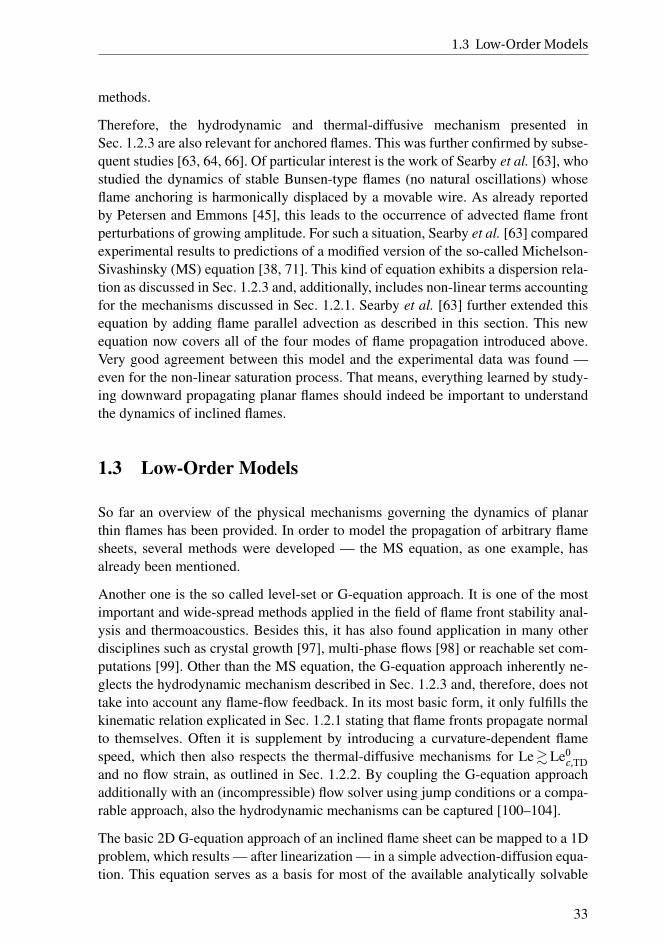
1.3 Low-Order Models

methods.

Therefore, the hydrodynamic and thermal-diffusive mechanism presented inSec. 1.2.3 are also relevant for anchored flames. This was further confirmed by subse-quent studies [63, 64, 66]. Of particular interest is the work of Searby et al. [63], whostudied the dynamics of stable Bunsen-type flames (no natural oscillations) whoseflame anchoring is harmonically displaced by a movable wire. As already reportedby Petersen and Emmons [45], this leads to the occurrence of advected flame frontperturbations of growing amplitude. For such a situation, Searby et al. [63] comparedexperimental results to predictions of a modified version of the so-called Michelson-Sivashinsky (MS) equation [38, 71]. This kind of equation exhibits a dispersion rela-tion as discussed in Sec. 1.2.3 and, additionally, includes non-linear terms accountingfor the mechanisms discussed in Sec. 1.2.1. Searby et al. [63] further extended thisequation by adding flame parallel advection as described in this section. This newequation now covers all of the four modes of flame propagation introduced above.Very good agreement between this model and the experimental data was found —even for the non-linear saturation process. That means, everything learned by study-ing downward propagating planar flames should indeed be important to understandthe dynamics of inclined flames.

1.3 Low-Order Models

So far an overview of the physical mechanisms governing the dynamics of planarthin flames has been provided. In order to model the propagation of arbitrary flamesheets, several methods were developed — the MS equation, as one example, hasalready been mentioned.

Another one is the so called level-set or G-equation approach. It is one of the mostimportant and wide-spread methods applied in the field of flame front stability anal-ysis and thermoacoustics. Besides this, it has also found application in many otherdisciplines such as crystal growth [97], multi-phase flows [98] or reachable set com-putations [99]. Other than the MS equation, the G-equation approach inherently ne-glects the hydrodynamic mechanism described in Sec. 1.2.3 and, therefore, does nottake into account any flame-flow feedback. In its most basic form, it only fulfills thekinematic relation explicated in Sec. 1.2.1 stating that flame fronts propagate normalto themselves. Often it is supplement by introducing a curvature-dependent flamespeed, which then also respects the thermal-diffusive mechanisms for Le&Le0

c,TD

and no flow strain, as outlined in Sec. 1.2.2. By coupling the G-equation approachadditionally with an (incompressible) flow solver using jump conditions or a compa-rable approach, also the hydrodynamic mechanisms can be captured [100–104].

The basic 2D G-equation approach of an inclined flame sheet can be mapped to a 1Dproblem, which results — after linearization — in a simple advection-diffusion equa-tion. This equation serves as a basis for most of the available analytically solvable

33

Dynamics of Thin Flame Sheets

low-order models of acoustically perturbed flame fronts. Just like the G-equation,it only captures the basic kinematics of a flame sheet, including advection and acurvature-dependent flame speed. It is important to note that it specifically excludesany flame-flow feedback and, hence, the hydrodynamic mechanism of Sec. 1.2.3.

In the following, firstly the level-set or G-equation approach is introduced inSec. 1.3.1, before the aforementioned 1D advection-diffusion equation is derivedfrom it in Sec. 1.3.2.

1.3.1 Level-Set or G-Equation Approach

Based on the early works of Darrieus [26] and Landau [27], Markstein [33] was thefirst to introduce a partial differential equation (PDE) in space and time to modelthe dynamics of a scalar field whose zero iso-line is identified with the gas dynamicdiscontinuity representing the flame front. The PDE he provided represents the flameas a front that propagates normal to itself at a velocity sL with respect to a given un-burned flow field just ahead of it. To the best knowledge of the author, Williams [105]was the first to use the letter “G” as representation for said scalar field. Presumablysince then, the governing PDE is also known as the G-equation. It should be pointedout that the G-field itself has no physical meaning and is just a tool to track the flamefront.

As already mentioned, the flame front is represented by the iso-line/-surfaceG(xi , t ) = 0. Regions of G < 0 represent the unburned mixture and those of G > 0

burned products. The flame normal direction, pointing towards the hot products, iscomputed from

n f ,i =∂G

∂xi/

öG

∂x j

∂G

∂x j(1.21)

using the Einstein summation convention. The total derivative of the G-field has tosatisfy

dG

d t= ∂G

∂t+ ∂G

∂xi

d xi

d t= 0. (1.22)

in order to ensure that G stays zero everywhere at the flame front. FollowingSec. 1.2.1, flames propagate normal to themselves and, hence, each point on the flamesheet moves relatively to the cold flow field uu,i ahead of it according to

d xi

d t= uu,i −n f ,i sL . (1.23)

Combining Eqs. (1.21)–(1.23) one obtains the final version of the G-equation

∂G

∂t+uu,i

∂G

∂xi= sL

öG

∂x j

∂G

∂x j. (1.24)

34

1.3 Low-Order Models

The non-linearity in this equation results from the fact that the front propagates nor-mal to itself and that there exist only two distinct states, burned (G > 0) and unburned(G < 0), see Sec. 1.2.1 for more details.

As discussed in Sec. 1.2.2, the flame speed of thin flames depends on the local cur-vature of the flame sheet κ f , which is computed from the G-field by taking the diver-gence of the normalized gradient (i. e. the flame normal vector)

κ f =− ∂

∂xi

∂G∂xi√∂G∂x j

∂G∂x j

, (1.25)

see e. g. Smereka [106]. Using the curvature dependent definition of the flame speedof Eq. (1.8) together with Eq. (1.25) and inserting both to the G-equation (1.24) oneobtains

∂G

∂t+ui

∂G

∂xi= s0

L

(1− lMκ f

)√

∂G

∂x j

∂G

∂x j. (1.26)

Here, flow strain was neglected and, thus, curvature is assumed to be the only sourceof flame stretch. It becomes apparent that consideration of a curvature dependentflame speed adds a diffusion term (Laplacian) with diffusion coefficient s0

llM to the

governing equation of a flame sheet. Hence, flame curvature effectively reduces steepgradients of the G-field and, for example, ensures the round tip of a Bunsen flame byincreasing the flame speed at this strongly curved flame region.

Concerning the simulation of anchored flames, problems arise at points where flamesare aerodynamically anchored and significant heat losses are present, e. g. at Bunsenflames. Those quenching effects change the inner structure of the flame and, on ahydrodynamical scale, the flame speed. This is especially important when a realisticflow solver is coupled with a G-equation approach. Due to friction, flow velocitydecreases to zero right at the boundary. If the flame speed is not adjusted in thisregion, i. e. by considering quenching and/or curvature effects, the flame would flashback in the boundary layer of the flow and, hence, cannot be stabilized. While somestudies implemented these quenching effects using empirical correlations [107, 108],others artificially fixed the G-field at the burner mouth using a Dirichlet boundarycondition [100–102, 109].

1.3.2 1D Linearized Flame Dynamics

As already mentioned above, practical combustion systems often rely on aerodynam-ically stabilized flames whose fronts are inclined by an angle α with respect to thebulk flow velocity of the fresh mixture far away from the flame. The dynamics of suchflames can be assessed best by mapping the G-equation to a 1D coordinate system by

35

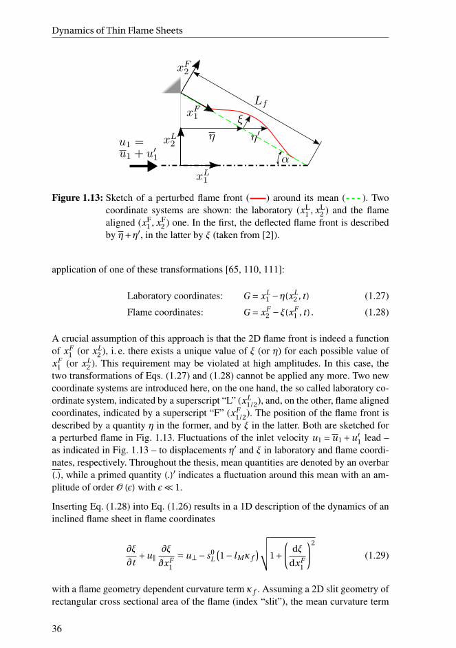
Dynamics of Thin Flame Sheets

Figure 1.13: Sketch of a perturbed flame front ( ) around its mean ( ). Twocoordinate systems are shown: the laboratory (xL

1 , xL2 ) and the flame

aligned (xF1 , xF

2 ) one. In the first, the deflected flame front is describedby η+η′, in the latter by ξ (taken from [2]).

application of one of these transformations [65, 110, 111]:

Laboratory coordinates: G = xL1 −η(xL

2 , t ) (1.27)

Flame coordinates: G = xF2 −ξ(xF

1 , t ) . (1.28)

A crucial assumption of this approach is that the 2D flame front is indeed a functionof xF

1 (or xL2 ), i. e. there exists a unique value of ξ (or η) for each possible value of

xF1 (or xL

2 ). This requirement may be violated at high amplitudes. In this case, thetwo transformations of Eqs. (1.27) and (1.28) cannot be applied any more. Two newcoordinate systems are introduced here, on the one hand, the so called laboratory co-ordinate system, indicated by a superscript “L” (xL

1/2), and, on the other, flame aligned

coordinates, indicated by a superscript “F” (xF1/2

). The position of the flame front isdescribed by a quantity η in the former, and by ξ in the latter. Both are sketched fora perturbed flame in Fig. 1.13. Fluctuations of the inlet velocity u1 = u1 +u′

1 lead –as indicated in Fig. 1.13 – to displacements η′ and ξ in laboratory and flame coordi-nates, respectively. Throughout the thesis, mean quantities are denoted by an overbar(.), while a primed quantity (.)′ indicates a fluctuation around this mean with an am-plitude of order O (ǫ) with ǫ≪ 1.

Inserting Eq. (1.28) into Eq. (1.26) results in a 1D description of the dynamics of aninclined flame sheet in flame coordinates

∂ξ

∂t+u∥

∂ξ

∂xF1

= u⊥− s0L

(1− lMκ f

)√√√√1+

(dξ

dxF1

)2

(1.29)

with a flame geometry dependent curvature term κ f . Assuming a 2D slit geometry ofrectangular cross sectional area of the flame (index “slit”), the mean curvature term

36

1.3 Low-Order Models

writes

κ f ,slit =

∂2ξ

∂xF1

2

√1+

(dξ

dxF1

)2−

(∂ξ

∂xF1

)2 ∂2ξ

∂xF1

2

(1+

(dξ

dxF1

)2)3/2

, (1.30)

[112, 113]. It should be noted that the second term of this equation only adds a O(ǫ3

)

contribution to Eq. (1.29) and may hence be dropped for small flame front displace-ments. Similarly, for such conditions, the square root term in the denominator wouldasymptote to 1+O (ǫ) and may be approximated as unity. For conical flames of cir-cular cross sectional flame area, additionally, an azimuthal curvature contributiondepending on the local flame radius r f has to be considered. Neglecting the secondas well as the square root term of Eq. (1.30), it writes

κ f ,con = 1

2

(1

r f+ ∂2ξ

∂xF1

2

), (1.31)

where the index “con” denotes a conical flame [114]. In the following the differencesbetween Slit and Conical flames are neglected and only the curvature relation for Slitflames is considered. Assuming fluctuations of the state variables u1 and ξ of orderO (ǫ) and neglecting all second order terms in ǫ, a linear PDE

∂ξ

∂t+u∥

∂ξ

∂xF1

= u′⊥+ lM s0

L

∂2ξ

∂xF1

2(1.32)

is retrieved. A relation sL = u⊥ was applied, taking into account the fact that, in steadystate, the flame normal flow velocity is exactly balanced by the laminar flame speed.Due to its simplicity, this advection-diffusion equation is well suited for analyticaltreatment [65, 111, 115]. Neglecting flame curvature effects (lM ≡ 0), the resultingnon-homogeneous advection equation is solved by integration of the flame-normalvelocity perturbations

ξ(xF1 , t ) = 1

u∥

∫xF1

0u′⊥

(xF

1 , t −xF

1 − xF1

u∥

)dxF

1 +ξ

(0, t −

xF1

u∥

). (1.33)

The second term on the right-hand side of this equation considers perturbations atthe flame anchoring (xF

1 = 0). Hence, perturbations of the flame base would reach theflame tip at a time τr = L f /u∥, where L f denotes the steady state flame length, seeFig. 1.13. This quantity is known as the characteristic time of restoration [116].

Expressing Eq. (1.32) in laboratory coordinates by use of Eq. (1.27) again assuminglM ≡ 0, one obtains

∂η′

∂t−cos(α)sin(α)u1

∂η′

∂xL2

= 1

sin(α)

[sin(α)u′

1 +cos(α)u′2

]−

s′Lsin(α)

. (1.34)

Inserting the relations η′ = ξ/sin(α) and d xL2 = −sin(α)d xF

1 (Wedge flames: “+”)into this equation, transforms the equation in flame aligned coordinates, as shown in

37

Dynamics of Thin Flame Sheets

Eq. (1.32). Since, for small perturbations, both descriptions are equivalent, it is fa-vorable to use flame aligned coordinates for modeling the flame front dynamics sincehere the equation becomes more compact. As will be shown in Sec. 6.2, however, theuse of a coordinate system other than the flame aligned one can be advantageous forevaluating flame surface integrals, due to a simpler treatment at the boundaries.

Eq. (1.32) holds for slit and conical configurations. It has, however, to be noted that,just like in the aforementioned G-equation approach, flow strain as well as flame-flow-flame feedback resulting from exothermic effects were neglected. Both wouldact quantitatively different for the two flame geometries. Another consequence offlame geometry concerns flame curvature: Due to their azimuthal curvature, coni-cal flames are generally exposed to higher flame stretch than slit flames, compareEq. (1.30) for Slit and Eq. (1.31) for conical flames. The maximum stretch due toazimuthal curvature is imposed at the flame tip for Bunsen flames and at the flameanchoring for Wedge flames, since there the respective local flame radius r f reachesa minimum. It follows that advected flame front perturbations are exposed to increas-ingly stronger stretch rates for Bunsen flames, which should lead to smoother flameshapes towards the tip compared to Slit flames. This mollifying effect impacts alsothe generation of flame pockets at the flame tip (pinch off) [104]. For Wedge configu-rations it is the other way round: flame stretch decreases while a flame perturbation isadvected along the flame front, which make it more prone to the formation of cusps.

1.4 Summary

In this chapter, the available literature on the dynamics of thin flame sheets far awayfrom any boundary was reviewed. The general idea concerning the analysis of suchflames is based on the fact that these flames can be viewed as propagating discon-tinuities separating two coupled flow domains of different densities, namely the do-main of the fresh mixture and the domain of the burned products. Based on matchedasymptotic expansion techniques, a propagation speed of the discontinuity (flamespeed) and jump conditions connecting the two flow domains could be derived fromfirst principles. This specific way of describing thin flame sheets shifts the focusaway from details of the combustion process to macroscopic properties such as flamespeed, flame shape and acceleration/deceleration of the underlying flow field.

Four mechanisms governing the dynamics of thin flame sheets could be identified: (i)the propagation of a flame sheet normal to itself, (ii) thermal-diffusive mechanismsinteracting with the propagation speed of a flame front, (iii) hydrodynamic featuresmainly affecting the surrounding flow field and (iv) the downstream advection offlame perturbations along the flame sheet for inclined flames (neglecting the dynam-ics close to the anchoring point). Finally, the wide-spread G-equation approach wasintroduced in its 2D non-linear as well as in its 1D linearized form. It was pointed outthat it only captures the kinematics of a flame front, but inherently neglects flame-

38

1.4 Summary

flow feedback, i. e. hydrodynamic mechanisms. This is a substantial shortcoming ofthis method, as will be shown in the course of this thesis.

39

Dynamics of Thin Flame Sheets

40

2 Acoustic Response of

Burner-Stabilized Flames

A literature review on interactions between acoustics and burner-

stabilized premixed flames is provided, which builds upon the con-

cepts outlined in the previous section. Additionally, the notion of

convected velocity perturbations is introduced, around which most

theoretical predictions of the acoustic flame response evolve.

Chapter. 1 discussed the dynamics of flame sheets far away from any boundary. Fourdifferent governing mechanisms were identified, which allowed to break down theoverall flame dynamics into their canonical components. This realization lays thefoundations for the analyses of acoustically perturbed burner-stabilized flames, whichwill be conducted in this chapter. Such configurations introduce essentially two newfeatures, that is (i) a burner where the flame is anchored/stabilized and enclosed and(ii) acoustic perturbations interacting with the flame. Furthermore, not only the flameshape but also the change of the global heat release rate will now be an output quan-tity of interest. Due to these features and requirements, the low-order modeling con-cepts introduced in the previous chapter need to be extended in order to cope withthermoacoustically relevant setups.

Burner-stabilized flames consist of multiple flame sheets of finite extension that areusually anchored by a separation-induced low-speed region close to a wall. Addi-tionally, they might be confined by a casing and exposed to nonconstant upstreamflow profiles. It becomes clear that the rather idealized flame dynamics described inChap. 1 might be enriched by additional phenomena such as flame-wall or flame-flame interactions. Furthermore, the mean state of a flame is no longer trivial andmight significantly impact the dynamics of the overall system. Finally, the exis-tence of acoustic perturbations introduces further complications. The individual flamesheets of the overall flame are now externally forced, which introduces completelynew dynamic features. Therefore, the acoustic field inside the respective burner con-figuration needs to be studied and acoustic-flame sheet interactions have to be con-sidered.

Knowing how a flame reacts to acoustic fluctuations is only half the story when deal-ing with thermoacoustic interactions. The other half concerns the generation of acous-tic perturbations by the flame itself. It can be shown that acoustically compact flamesact as a monopole-like source of sound whose strength is proportional to fluctua-

41

Acoustic Response of Burner-Stabilized Flames

(a) Bunsen (conical Λ) (b) Slit (c) Wedge (conical V)

Figure 2.1: Investigated flame geometries (taken from [2]).

tions of their global heat release rate. Consequently, the dynamics of the overall heatrelease rate is an important feature that has to be discussed in this section, as well.

This chapter is structured as follows: Sec. 2.1 provides a definition of the class ofproblems that are tackled by this thesis, i. e. the analyzed burner configurations andfuel-oxidizer mixtures are defined. Secs. 2.2 and 2.3 then provide a literature reviewon the dynamics and low-order modeling concepts of acoustically perturbed flames,respectively.

2.1 Problem Definition

In this thesis laminar lean methane-air flames of different equivalence ratios are ana-lyzed that are operated far away from the region of lean extinction. They all exhibitLewis numbers close to unity and are hence thermal-diffusively stable. Furthermore,they can in good approximation be assumed to be thin for all analyzed setups, aspointed out in Sec. 1.1.1. The initial temperature of the fresh mixture is always keptconstant (300 K).

The geometrical details of all investigated burners shall resemble a backward fac-ing step configuration, which allows for an efficient anchoring of the flame in thelow-speed region induced by the separating flow field. Depending on the specific ge-ometrical details of the burner, the boundary and initial conditions, flames of severaldifferent geometrical shapes can be stabilized. Three of the most important ones areshown in Fig. 2.1: The Bunsen, the Slit and the Wedge flame. The three illustrationsimmediately point out that flame sheets of realistic burner setups are not necessarilyplanar and may also intersect. Furthermore, interactions with combustor walls, e. g.at the anchoring position, imposes new dynamics via quenching, viscous effects andflow separation. Due to advection, any flame front perturbation will eventually reachthe flame tip, where it might lead to a pinch-off of burning bubbles of fresh mixture.All of these effects complicate the analysis by adding new dynamic features. Theirrespective significance for the process of interest, however, might not necessarily behigh. Figuring out what is important and what not is one major goal of this work. Inorder to reduce complexity, this work mainly focuses on Slit configurations.

The combustion region of all of the considered flame configurations shall be limitedby lateral constraints. This respects the fact that in technical applications flames are

42

2.2 Acoustics-Flame Interactions

Figure 2.2: Unconfined (left) vs. confined (right) flame.

usually confined in order to use the sensible enthalpy of the hot products or to shieldthe combustion process from the environment. Fig. 2.2 compares the jet of hot gasesof an open flame to the one of a confined flame. It becomes clear that a sufficientlynarrow confinement might alter the mean flow field by accelerating the burned gasesand, in doing so, also the acoustic flame response.

Finally, all configurations are exposed to acoustic perturbations whose minimumwave length shall be much longer than the height of the respective flame. This limita-tion demands that all flames are acoustically compact, i. e. they are exposed to acous-tic pressure or velocity perturbations that are in-phase everywhere along the flamesheets. Furthermore, under such conditions perturbed flames can be approximated asmonopole-like sources of sound.

2.2 Acoustics-Flame Interactions

The analysis of the dynamics of acoustically perturbed flame configurations, as de-scribed in Sec. 2.1, requires some extensions of the theory of freely propagating flamesheets presented in Chap. 1. A literature review on what has been achieved so far isprovided in the proceeding section.

Sec. 2.2.1 provides fundamental insights into how flame sheets, as introduced inChap. 1, respond to acoustic perturbations. These fundamental studies are followedby a review of the literature concerning acoustically perturbed Bunsen flames inSec. 2.2.2. Here, the focus is put on the shape and the dynamics of acoustically trig-gered flame front displacements. Section 2.2.3 then provides an overview on howthese displacements are connected to variations of the global heat release rate. Crucialthermoacoustic concepts, such as the flame transfer function and its representationsin the frequency and time domain are introduced.

2.2.1 Freely Propagating Flame Sheet

In a first step, the interaction of acoustic perturbations with an freely propagatingplanar flame sheet is analyzed, which should provide guidance on how to deal withthe more complex problem of a burner stabilized flame. For all cases studied here,the flame thickness is much smaller than the wave length of any relevant acoustic

43

Acoustic Response of Burner-Stabilized Flames

perturbation (≤ O(103

)Hz). Therefore, we can rely on the flame sheet assumptions

introduced in Chap. 1 when assessing acoustics-flame interactions [117]. Accordingto theoretical studies, for the frequency range that is relevant when considering com-bustion instabilities, the flame speed is supposed to depend on the acoustic forcing[118, 119], i. e. sL is thought to be a function of the acoustic field. This fact, however,requires further rigorous experimental validation [117] and is, for the sake of simplic-ity, usually neglected in thermoacoustic studies. The validity of this simplification formany setups of practical relevance is supported by experimental and numerical stud-ies, such as the one of Baillot et al. [120] or Michaels and Ghoniem [121], whichleads to the conclusion that the impact of acoustics on the flame speed is indeedrather weak.

It is also commonly assumed that premixed flames predominantly respond to ve-locity perturbations and almost completely ignore changes in pressure [117]. Thus,the flame speed is basically not affected by acoustics. Based on these realizations, itcan be concluded that acoustic velocity fluctuations essentially displace a flame frontand, in doing so, alter its shape. This may trigger dynamical processes governed bythe four mechanisms identified in Chap. 1.

A fundamental study analysing details of acoustic-flame interactions has been per-formed by Lieuwen [122] for the case of a planar downward propagating flame ofinfinite extension that is hit by a planar acoustic wave at an angle of incidence θ: De-pending on the angle θ, acoustic waves are transmitted and reflected at different ratiosat the flame front. As known from optics, when a disturbance travels from a mediumof lower to one of higher propagation speed, there exists a “cut-off” angle dependingon the density ratio across the flame, where the incident wave is fully reflected at theflame front. This only happens for upstream and never for downstream acoustic ex-citation. Furthermore, baroclinic production of vorticity at the flame front acts as anacoustic damping mechanism. These results indicate that flame front displacementscaused by acoustic perturbations affect the surrounding flow field, for example, byintroducing vortical structures. And, indeed, such features are also observed in thevicinity of burner-stabilized flames, as will be shown in the course of this thesis.

2.2.2 Burner-Stabilized Flame

Acoustics-flame interactions are significantly more complex for burner stabilizedflames than for freely propagating flame sheets. Although acoustic velocity fluctu-ations mainly displace a flame, see the previous section, their spatial shape, flame-wall and flame-flame interactions add some important burner-configuration depen-dent peculiarities. In the following a brief overview of the most important findings isprovided. In the first part, the various modes of interactions of acoustic perturbationswith flames are covered. Knowing how flame displacements are generated, the reviewfocuses in a second part on the response of a flame to these perturbations. Interest-ingly, the literature revolves around the notion of convected velocity perturbations

44

2.2 Acoustics-Flame Interactions

instead of the four canonical mechanisms introduced in Sec. 1.2, which motivates theanalysis conducted in this thesis.

Acoustic Interactions with Burner-Stabilized Flames

Based on the fact that flames are usually stabilized in the vicinity of sharp edgeswhere acoustics triggers the shedding of vortices [123–126], it is natural to struc-ture a review on acoustic interactions with burner-stabilized flames according to adecomposition of acoustic perturbations into a potential (irrotational) and a vortical(solenoidal) contribution. This decomposition accounts for the respective nature ofthe individual flow modes [127] and allows for their separate analysis.

Investigations of the vortical part of the acoustic perturbation field, on the one hand,have not drawn too much attention in the literature. One reason for this might be thatperturbed flame sheets generate a reasonable amount of vorticity by themselves [128–130], which makes it hard to isolate effects of acoustically triggered vortex shedding.Schlimpert et al. [104] tried to overcome this problem by neglecting flame-inducedgas expansion in their numerical model, which suppresses the generation of distract-ing flame generated vorticity. In doing so, however, they at the same time removeddilatation effects, which significantly dampen the vortical flow component and bendthe mean flow shear layer away from the flame. Hence, interactions of separating vor-tices with the flame were overestimated compared to realistic conditions. Accordingto their analysis, at proper levels of gas expansion and far away from the region oflean extinction, only interactions between the flame base region and shed vorticityremain.

On the other hand, the potential acoustic velocity field in a backward-facing stepcombustor, as depicted in Fig. 2.2 (right), was closer analyzed in a series of numericalinvestigations by Lieuwen [131] as well as Lee and Lieuwen [132]. They found thatthe acoustic velocity field interacting with the flame front is essentially 2-dimensionalwith a maximum close to the flame anchoring position, even for acoustically compactflames. Since evaluation of the flame response using such a model did — unexpect-edly — not yield significant improvements compared to a 1-dimensional descriptionof the velocity field, this study has not drawn too much attention. Their principalfinding was later experimentally confirmed by Kornilov et al. [133] who did, how-ever, not explicitly mention the connection to the previous study of Lee and Lieuwen[132]. Kornilov et al. [133] forced a Bunsen flame, one time by moving the anchoringtransversally in and out and, one time by imposing acoustic velocity perturbations.Both kinds of excitation resulted in very similar velocity fields, which are visualizedin Fig. 2.3. The authors further evaluated the transfer functions from the forcing tothe globally integrated heat release rate for both sets of experiments and found thatthey also agreed reasonably well. Hence, they indirectly confirmed the findings ofLee and Lieuwen [132] that acoustics interacts predominantly with the flame baseregion.

45

Acoustic Response of Burner-Stabilized Flames

Figure 2.3: TiO2 smoke trace flow field visualization of two Bunsen flame forced at200 Hz, one time by transversal movements of the flame holder at whichthe flame is anchored (left) and one time by acoustic excitation (right)(images are taken from Kornilov et al. [133], Figs. 5 and 6).

In summary, (i) the impact of acoustically triggered vorticity on a flame is still unclearand (ii) the potential part of the acoustic velocity field predominantly interacts withthe flame base region. It has to be emphasized that, although this review follows saidflow decomposition approach, many of the studies mentioned remained side notes inthe body of literature on acoustics-flame interactions or they did not explicitly followsuch a decomposition-based mindset. Due to the fact, however, that this work is goingto revisit such a mindset, the concept of flow decomposition was granted a prominentposition in this review.

Flame Response to Acoustically Generated Displacements

As explicated in Sec. 1.2.4, one essential dynamical feature of burner-stabilized in-clined flames is the advection of flame front perturbations. In this regard, Cuquel[134] published an instructive experimental investigation of acoustically forcedflames. Fig. 2.4 shows four snapshots that were taken at equidistant phases at a fre-quency of 80 Hz. In accordance with the studies reviewed above, acoustic interactionsdisplace the flame close to the burner mouth. This creates flame wrinkles, which areconvected along the flame front until they reach the flame tip. In Fig. 2.4, two ofthese wrinkles are marked by a red and a green line, respectively. In each successivesnapshot, they move by an approximately constant distance and are hence advecteddownstream by a fixed velocity.

At this point it should be emphasized that the flame is anchored at the burner, i. e. anysudden displacement of the anchoring exerted by acoustic perturbations will eventu-ally be counteracted such that after some time the flame has returned to its originalsteady state position. The information of the restored flame anchoring will — just likeany flame front displacement — be advected along the front and will reach the flametip after a time τr . Accordingly, Blumenthal et al. [116] named this period of time thecharacteristic time of restoration. It should, however, be noted that this time scales ischaracteristic for the advection of any flame front feature, not just the restoration. Inthat sense it should rather be called the characteristic time of advection.

46

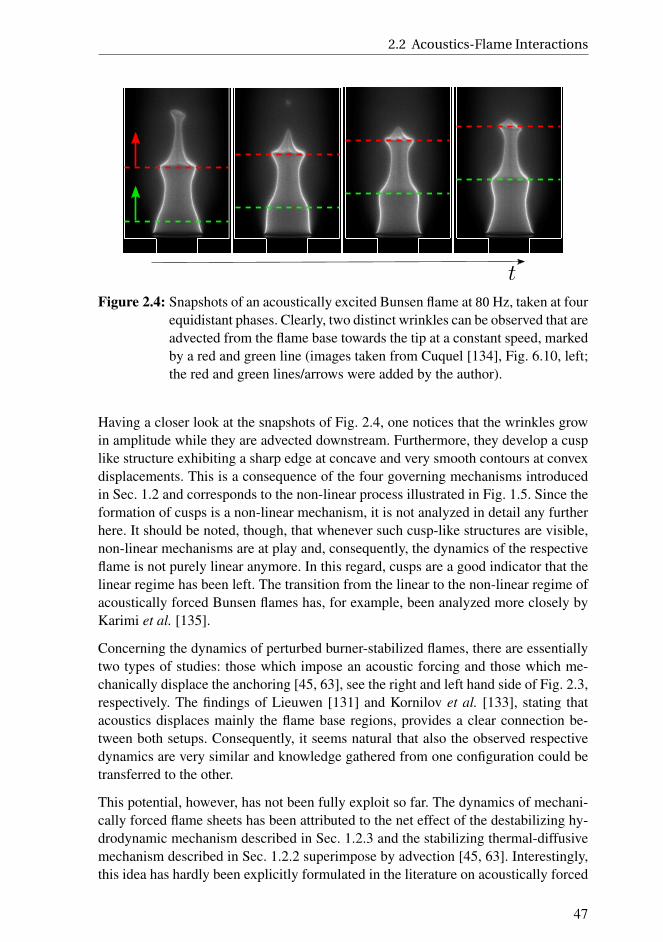
2.2 Acoustics-Flame Interactions

Figure 2.4: Snapshots of an acoustically excited Bunsen flame at 80 Hz, taken at fourequidistant phases. Clearly, two distinct wrinkles can be observed that areadvected from the flame base towards the tip at a constant speed, markedby a red and green line (images taken from Cuquel [134], Fig. 6.10, left;the red and green lines/arrows were added by the author).

Having a closer look at the snapshots of Fig. 2.4, one notices that the wrinkles growin amplitude while they are advected downstream. Furthermore, they develop a cusplike structure exhibiting a sharp edge at concave and very smooth contours at convexdisplacements. This is a consequence of the four governing mechanisms introducedin Sec. 1.2 and corresponds to the non-linear process illustrated in Fig. 1.5. Since theformation of cusps is a non-linear mechanism, it is not analyzed in detail any furtherhere. It should be noted, though, that whenever such cusp-like structures are visible,non-linear mechanisms are at play and, consequently, the dynamics of the respectiveflame is not purely linear anymore. In this regard, cusps are a good indicator that thelinear regime has been left. The transition from the linear to the non-linear regime ofacoustically forced Bunsen flames has, for example, been analyzed more closely byKarimi et al. [135].

Concerning the dynamics of perturbed burner-stabilized flames, there are essentiallytwo types of studies: those which impose an acoustic forcing and those which me-chanically displace the anchoring [45, 63], see the right and left hand side of Fig. 2.3,respectively. The findings of Lieuwen [131] and Kornilov et al. [133], stating thatacoustics displaces mainly the flame base regions, provides a clear connection be-tween both setups. Consequently, it seems natural that also the observed respectivedynamics are very similar and knowledge gathered from one configuration could betransferred to the other.

This potential, however, has not been fully exploit so far. The dynamics of mechani-cally forced flame sheets has been attributed to the net effect of the destabilizing hy-drodynamic mechanism described in Sec. 1.2.3 and the stabilizing thermal-diffusivemechanism described in Sec. 1.2.2 superimpose by advection [45, 63]. Interestingly,this idea has hardly been explicitly formulated in the literature on acoustically forced

47

Acoustic Response of Burner-Stabilized Flames

Figure 2.5: Snapshots of a G-equation-based simulation of an acoustically excitedBunsen flame at 120 Hz relying on the convective incompressible veloc-ity model introduced by Baillot et al. [120], taken at three equidistantphases. Colors denote the imposed axial velocity fluctuations u′

1 and thegreen and red horizontal lines tag two maxima of the underlying velocityfield visualizing their axial convection (note: other than in Fig. 2.4, herethe lines tag axially transported velocity fluctuations not flame wrinkles).

flames. Instead, here the analysis has taken a very different way, centered aroundpurely kinematic observations of the flow field. Baillot et al. [120] experimentallydetected axially convected velocity perturbations just upstream of an acoustically per-turbed flame inside the volume enclosed by the flame sheets and the burner mouth.They explained these observations by both hydrodynamic interactions of the wrin-kled flame front with the upstream flow field and the effect of gas expansion acrossthe flame. In principle, this hypothesis was later confirmed by studies of Birbaudet al. [136] and Blanchard et al. [129].

The important point, however, of the study of Baillot et al. [120] is that it couldretrieve a good match between experimentally measured perturbed flame sheets andthose obtained from a G-equation-based model only if axially convected velocity per-turbations upstream of the flame were introduced, resembling the ones that have beenmeasured. Fig. 2.5 depicts three successive snapshots of such a G-equation-basedsimulation, which illustrates the model of axially convected velocity perturbationsand the resulting flame shapes.

Such a convective velocity model results in a linearly decreasing phase of theassociated FTF (see next section), which was confirmed by subsequent studies[111, 137, 138]. Hence, Candel wrote in his 2013 review paper “This behavior [thelinearly decreasing phase] is the signature of perturbations convected by the flow of-

ten revealing the presence of large structures conveyed by the flow and impinging the

flame” (Candel et al. [139], p. 98). In this specific case he was referring to a burner-stabilized Wedge flame that is clearly subjected to vortical structures shed from theburner rim. The notion of this statement, however, was generalized for all types of

48

2.2 Acoustics-Flame Interactions

flames and it became state-of-the-art that acoustically excited premixed (Bunsen)flames are subject to convected velocity perturbations [140]. The contradictory pointhere is that Birbaud et al. [136] and Blanchard et al. [129] as well as even Baillotet al. [120] found that these perturbations are a consequence rather than a source offlame front wrinkles. Therefore, the assumption of convected velocity perturbationsseems to violate causality (they cannot be source and consequence at the same time)[1, 2]. This point has not explicitly been adressed so far and will be clarified in thecourse of this work.

In summary, the most important mechanisms governing the linear response of in-clined flame fronts to acoustic perturbations have been discussed:

1. Acoustics displaces predominantly the flame base region

2. Flame displacements are advected downstream by a constant speed resultingin a characteristic time of restoration τr

3. Flame intrinsic instability mechanisms act on flame displacements, whichmight lead to their growth in amplitude

4. Acoustically perturbed flames exhibit axially convected velocity perturbationsupstream of the flame sheets

What is missing in this overview are features concerning the flame tip (pinch-off)and the anchoring (quenching, vortex shedding). They are, however, either essen-tially non-linear in nature, of secondary importance or beyond the scope of this work.Furthermore, there is a strong dependency of the flame response on the respectiveburner configuration. One important point here concerns the confinement of the com-bustion region [141–144], another the boundary conditions of walls adjacent to theflame sheet [121, 145–149]. Also the burner size is important [150] as well as itsgeometry [151–153].

2.2.3 Global Heat Release Rate Dynamics

This thesis is devoted to the study of flames in the context of thermoacoustic systems,where the flame constitutes one specific sub-system. Therefore, the input/output re-lation of interest of the flame module needs to quantify the sound that is produced byan acoustically perturbed flame. In the regime of acoustically compactness, temporalfluctuations of the global heat release act like an acoustic monopole whose dynamicsis directly proportional to the normalized fluctuation of the global heat release rateof the flame [22, 154]. In the linear regime, the mentioned input/output relation isestablished by the flame transfer function (FTF)

Q ′

Q= F (ω)

u′ref

uref. (2.1)

49

Acoustic Response of Burner-Stabilized Flames

It relates velocity fluctuations at a reference position u′ref

to variations of the globalheat release rate. For perfectly premixed flames, a relation

Q ′

Q=

A′f

A f

+∫

s′LdA f∫

sLdA f

(2.2)

holds, which connects fluctuations of the global heat release rate Q ′ to fluctuations ofthe flame surface area A′

fand the mean surface integrated flame speed s′L [117, 155].

For perfectly premixed flames, as discussed here, the latter term is usually neglectedand essentially becomes important at higher frequencies [112, 113].

The thermoacoustic response of premixed flames is the consequence of a great va-riety of physical mechanisms including everything that has so far been mentionedin this and the previous chapter: hydrodynamic mechanisms leading to the growth offlame front perturbations, thermal-diffusive processes stabilizing the front, non-linearmechanisms leading to the formation of cusps, quenching effects at walls and flame-flame interactions at the flame tip. This section now deals with the final step, which— following Eq. (2.2) — essentially comprises the computation of the flame sur-face area for a given displaced flame front. While this may sound trivial, it has somenon-straightforward consequences, especially concerning flame geometry. This willbe examined in greater detail in Chap. 6. For the remainder of this section, sometechnical details concerning the representation of the linear flame response will bediscussed.

A frequency domain representation of the linear response of a laminar Bunsen typeflame is depicted in Fig. 2.6. The left half of that figure (a+b) depicts the frequencyresponse in terms of gain and phase, while the right half (c+d) shows the rather un-typical representations in terms of a polar plot and a plot of the real and the imaginarypart of the FTF over frequency. Note that the gain has a logarithmic scale in Fig. 2.6(a) and (c). These — sometimes also double logarithmic scales — are adopted fromthe field of control theory, where this particular choice of scaling allows a simpleidentification of the corner frequencies, i. e. frequencies above which a signal is at-tenuated instead of being passed through by the system (in the case of a low passfilter). These frequencies are also known as cut-off frequencies.

Another illustration of the linear flame response is the impulse response (IR), whichis shown in Fig. 2.7 (left half). It can be considered as the time domain equivalentto the frequency response (FR) (Fig. 2.7; right half) and relates the heat release rateto fluctuations of a reference velocity via temporal convolution (denoted by the ”∗“-operator):

Q ′

Q= h(t )∗

u′ref

uref. (2.3)

The axes of Fig. 2.7 have a linear scaling improving the presentation of the low fre-quency behavior compared to the previously shown logarithmic scale, which usuallyhas a gain and a Strouhal number of order O (1). The behavior of the gain for values

50

2.2 Acoustics-Flame Interactions

Figure 2.6: Representation of a typical linear flame response of a Bunsen flame in thefrequency domain (frequency response) in terms of (a) gain, (b) phase,(c) polar plot with phase determining the angle and gain the radius and(d) real and imaginary part plotted over frequency (taken from Kornilov[156], Fig. 3.1).

lower than O (1) is of little practical interest. Similarly, from a thermoacoustical pointof view, predominantly the flame dynamics at Strouhal numbers of order O (1) is im-portant. Therefore, in this thesis all frequency response plots exhibit linearly scaledaxes.

Characteristic features of the FTF of perfectly premixed laminar flames are (i) a lowfrequency limit ( f → 0) of unity [157], (ii) an essentially linear decay of phase and(iii) a low-pass behavior featuring reoccurring minima followed by local maxima.The IR of such flames shows a more or less constant positive response that is fol-lowed by some strongly damped oscillations. It should however be noted that thischaracteristic strongly depends on the considered flame geometry, as will be shownin Chap. 6. Keeping the geometry fixed, the responses of several flames are rathersimilar. Introducing a non-dimensional frequency, a so-called Strouhal number, us-ing the characteristic time of restoration f ∗ = f τr , Ducruix et al. [158] found thatplotting the responses of the global heat release rate of harmonically forced Bunsenflames of different inclination angles over such a Strouhal number causes the individ-ual curves to collapse on each other. Hence, in this work most representations of flame

51

Acoustic Response of Burner-Stabilized Flames

0

0.5

1

Magnitude

0 2 4 6

-16π

-8π

0

f∗ [-]

Phase

0 0.5 1 1.5

−2

−1

0

1

t∗ [-]

h∗

Figure 2.7: Representation of a typical linear flame response of a Bunsen flame inthe time domain as impulse response (left) and in the frequency domainas frequency response (right).

responses are either plotted over such a Strouhal number or over a non-dimensionaltime t∗ = t/τr .

2.3 Low-Order Models

The dynamics of acoustically perturbed burner-stabilized flames is more complexthan the one of freely propagating flame sheets, see the discussion above. Therefore,a less rigorous analysis of the respective dynamics has been conducted for such con-figurations — mostly due to complexities introduced by the flame anchoring and tipas well as by the acoustic forcing. Probably due to these difficulties, mostly phe-nomenological models were developed that enabled decent low-order predictions ofthe global heat release dynamics of acoustically perturbed flames, however, obscuredthe analysis of the underlying physical processes, since they are not rigorously de-rived from first principles.

Early studies on the global flame response to acoustic perturbations boiled the com-plete flame dynamics down to a time lag τ and an interaction index n [159]. Thisrather simplistic model became to be known in the literature as the n-τ model. Itcorrectly captures the experimentally observed linear decrease of the FTF phase,however, predicts a frequency independent gain of value n. This is a severe over-simplification of the observed low-pass filtering behavior of flames, which was latertaken into account by a semi-empirical model developed by Merk [160]. He describedthe flame front by use of a first order low-pass filter that provided an improved gainprediction at the cost of a poorer phase behavior, which now saturates at −π/2. Sugi-

52

2.3 Low-Order Models

moto and Matsui [64] developed a model based on growing convected perturbations,which suffers from the same problem.

Later studies focused on capturing the actual flame front kinematics by use of a G-equation based approach that inherently neglects flame-flow feedback, see Sec. 1.3.One of the first to capture the dynamics of inclined flames using such a (1D lin-earized) approach were Boyer and Quinard [65]. They imposed an uniform in-phasevelocity forcing

u′1 = A exp(iωt ) , u′

2 = 0 (2.4)

of amplitude A and angular forcing frequency ω, which harmonically displaces thewhole flame sheet and found advected flame displacements that propagate inside sta-tionary envelops. A laboratory coordinate system, as illustrated in Fig. 1.13, is usedin this representation. This model will be referred to as the uniform velocity modelin the following. By adding an additional growth term σξ to the 1D G-equation, theyartificially included otherwise neglected consequences of flame-flow feedback. Thegrowth rate σ that matched their experiments best, however, was significantly smallerthan the one computed from dispersion relations of planar freely propagating flames.They attributed this discrepancy to a confinement related stretching of the flame incombination with a strong sensitivity of the underlying dispersion relation to stretcheffects.

Baillot et al. [120] assessed the dynamics of acoustically excited Bunsen flamesexperimentally and analytically. They also relied on the 1D linearized G-equationframework used by Boyer and Quinard [65], however, they dismissed the growthterm. As already pointed out in Sec. 2.2.2, they measured velocity fluctuations ofthe fresh mixture inside the region just downstream of the edge where the flameis anchored, one time without flame (“cold case”) and one time with flame (“hotcase”). They observed axially propagating velocity perturbations inside this zonewith a speed close to the mean flow velocity for both cases, which they attributedto vortex shedding for the cold and to the upstream influence of the perturbed flamefront for the hot case. Motivated by this observation, they imposed axially convectedvelocity perturbations

u′1 = A exp

(i kxL

1

), u′

2 =−i kxL

2

2A exp

(i kxL

1

)(2.5)

fulfilling continuity for an axisymmetric frame of reference to their 1D linearizedG-equation framework. Here, k =ω/u1 denotes the wave vector of the forcing. Verygood agreement between experimentally measured and the modeled transient flameshapes was found. This velocity model is – in accordance with the literature [161] –called the “incompressible convective” model. Results of a G-equation based simu-lation relying on such a velocity model (with u′

2 ≡ 0) are shown in Fig. 2.5.

The first to derive an analytical expression for the FTF using the G-equation frame-work were Fleifil et al. [115]. Based on the observation that acoustic wave lengths

53

Acoustic Response of Burner-Stabilized Flames

in the frequency range of interest are long compared to the flame height, they as-sumed an uniform in-phase forcing of the flame sheet by the velocity field, as alreadyapplied by Boyer and Quinard [65]. Neglecting variations in flame speed along theflame sheet, they exploit the fact that for perfectly premixed flames the heat releaserate is proportional to the instantaneous flame surface area, see Eq. (2.2). Based onthis assumption, they could derive an equation for the linearized heat release ratefluctuations by evaluation of the instantaneous flame surface area from a displacedflame front. The resulting FTF showed the desired low-pass behavior, however, thephase saturated at −π/2 — just as in the model by Merk [160]. Particularly for lowfrequencies it provided some useful predictions, though. Ducruix et al. [158] thengeneralized the model of Fleifil et al. [115] for arbitrary flame angles by introductionof a reduced frequency or Strouhal number ω∗.

Schuller et al. [137] revisited the convective velocity model proposed by Baillot et al.

[120], extended it by imposing an axial decay of the convected waves and combinedit with the approach of Fleifil et al. [115]. This led to an improved description of theFTF phase, which now resembles that of a system of constant time delay and, hence,does not saturate at −π/2. Schuller et al. [137], however, could only numericallyevaluate the model and were not able to provide analytical expressions. In a succeed-ing publication, Schuller et al. [111] simplified this velocity model by neglecting theaxial decay and the lateral velocity component satisfying continuity, which led to ananalytically solvable problem. Later, Preetham et al. [138] and Cuquel et al. [161]seized on the original idea of Baillot et al. [120] of the incompressible convectivevelocity model and were able to provide analytical solutions using again the frame-work of Fleifil et al. [115]. They, however, discarded the axial decay of the velocityperturbation imposed by Schuller et al. [137]. Their model overpredicts the gain athigh frequencies, but provides good estimates of the phase.

The incompressible convective model, became the predominant low-order model foracoustically induced flow-flame interactions. Since Schuller et al. [137] introducedit to the field of thermoacoustics, it has been used (with slight modifications) for agreat variety of studies. For example, it was used to study non-linear thermoacousticoscillations [162, 163], the dynamics of bluff-body stabilized flames subjected tolongitudinal acoustic forcing [138, 164, 165], the non-linear behavior of the flameresponse for high amplitude forcing [109, 166, 167] or to study the impact of stretchand exothermicity on the flame response [104, 112, 113, 142]. This model hencebecame state of the art, however, as already indicated in Sec. 2.2.2, a discussionon the physical justification of the imposed axially convected velocity perturbationarose.

Finally, it should be mentioned that linear models can equally be evaluated in fre-quency and time domain. In the formulations mentioned above, harmonic velocityforcing was assumed, which leads to a description of the response behavior in fre-quency domain when combined with the 1D linearized G-equation framework, seeSchuller et al. [111] or Preetham et al. [138]. Blumenthal et al. [116] assumed a unit

54

2.4 Summary

impulse forcing of the flame following a Dirac distribution δ(t ). For such a forcing,the incompressible convective velocity model of Eq. (2.5) transforms to

u′1 = δ

(t −

xL1

u1

), u′

2 =xL

2

2u1δ′

(t −

xL1

u1

)(2.6)

for the two velocity components. Combined with the G-equation formalism, such aforcing leads to a time domain representation of the linear response behavior, whichcan be transformed to frequency domain. Similarly, any frequency domain represen-tation can be mapped to the time domain. One significant advantage of the time do-main perspective regards the improved identification of causalities, see Appendix A.3for more details. A second related advantage concerns the clear separation and char-acterization of physical processes: Following Blumenthal et al. [116], an impulsiveforcing results in two clearly separated processes, an axially moving source of flamefront displacement and a process that restores the original flame front. Each of theseprocesses can be associated with a characteristic time scale, which allows for a nat-ural definition of a Strouhal number, for example. Conversely, in frequency domain,one has to deal with the fact that the observable flame front displacement at a certainlocation is the superposition of past displacements provoked anywhere upstream ofthat point, which complicates the analysis.

2.4 Summary

In this chapter the body of literature concerning the dynamics of acoustically per-turbed burner-stabilized flames was reviewed from an thermoacoustic point of view.In a first step, the problem under consideration was specified by imposing constraintson the burner geometry and the mixture properties. The literature on acoustics-flameinteractions was analyzed, starting with freely propagating flame sheets and thenmoving on to burner-stabilized flames. Subsequently, available low-order modelingconcepts were reviewed, which are mostly based on a 1D linearized G-equation ap-proach that is excited by convected velocity perturbations.

One important outcome of this chapter is that not only low-order modeling strategiesbut also a significant part of the notion of the dynamics of acoustically perturbedflames relies on the concept of convected velocity perturbations. This concept, how-ever is paradoxical: On the one hand, it is assumed that the flame front is locallydisplaced by axially convected velocity perturbations, on the other, it is stated thatthese perturbations are a consequence of flame front wrinkling. Obviously, one ofthese contradictory findings needs to be wrong. Interestingly, studies on flames whoseanchoring is displaced mechanically exhibit a very similar dynamics as acousticallyperturbed flames, since both ways of forcing essentially act at the flame base region.Nevertheless, the analysis of the mechanically forced configurations does not relyon convected velocity perturbations, but rather on the fundamentals introduced inChap. 1. This should provide some hints how to resolve the paradox described above.

55

Acoustic Response of Burner-Stabilized Flames

56

Part II

Analysis of Acoustics-Flame

Interactions of Slit Flames

So far, a review of the fundamental principles and modeling strategiesregarding the acoustic response of premixed laminar flames has beenprovided. A variety of phenomena have been identified that need to beorganized in a clear way. For that reason, Chaps. 1 and 2 presented theanalysis of acoustically burner-stabilized flames as a continuation andextension of the studies on freely propagating flame sheets. This allowsfor a clear separation of the relevant canonical governing mechanisms,similar to how it has already been done for the case of flames whoseanchoring is displaced mechanically [45, 63].

Contrary to the underlying idea of the structure of Part I, in the fieldof thermoacoustics, the understanding and modeling of acoustically per-turbed burner-stabilized flames is essentially based on the notion of con-vected velocity perturbations. In order to provide a new perspective onthe topic and to resolve the paradox consequences of the assumption ofsuch convected perturbations, this Part of the thesis focuses rather on thedynamics of the acoustic field and the flame sheet than on the kinemat-ics of the flow field upstream of the combustion zone. Therefore, Chap. 3presents a new first principle-based low-order modeling approach. Basedon it, Chap. 4 analyzes the interactions of acoustic perturbations with theflame sheet neglecting flame-flow feedback. Finally, Chap. 5 investigatesthe consequences of such a feedback from the flame onto the flow.

Parts of Chaps. 3 and 4 have already been published, see Steinbacher et al.

[1]. Compared to this publication, significant changes have been applied:Essentially, the underlying modeling concept is introduced in more detail,now having a wider scope, and a Kutta condition is applied. Consequently,also the discussion and analysis of the results is updated. Nevertheless,the general statements and results of the original publication remain un-changed.

57

3 Flow-Decomposition Based Modeling

Framework

A new low-order modeling framework for the interaction of acous-

tics with premixed flames is introduced. It relies on a Helmholtz

decomposition combined with a flow-field representation based on

flow-field singularities and a conformal mapping technique. The vis-

cous mechanism of vortex shedding is included by use of a Kutta

condition.

Low-order modeling approaches naturally require a simplification strategy that isoften based on a decomposition of the overall problem into several simpler onesaccording to a predefined criterion. In this work, a Helmholtz-Decomposition basedapproach is chosen, which splits the flow into two contributions: an irrotational partthat obeys to a flow potential, and a solenoidal or vortical part that identically satisfiescontinuity. The former is again split into a constant density and a flow expansion partthat takes the combustion related density changes and the therewith accompaniedacceleration of the flow into account. In doing so, it is easy to switch-off feedback ofthe flame onto the flow, as will be done in Chap. 4 to analyze primary acoustic-flameinteractions. On the other hand, it also allows for a rather straight forward analysis ofconsequences of flame-flow feedback, which will be discussed in Chap. 5.

Decomposing the flow field into irrotational and solenoidal parts simplifies the flowproblem by imposing some structure. For the purpose of allowing for a low-ordertreatment, however, some more simplifications are required. Hence, a slightly com-pressible 2D (slit) flow of an ideal fluid is assumed. In doing so, the overall flow-fieldcan be constructed from a number of flow-field singularities, i. e. point sources andvortices. Applying a conformal mapping technique accounting for the boundary con-ditions, the rather complex dynamics of the overall system boils down to a numberof less complex canonical problems. Special focus is put on the implementation ofa Kutta condition, which accounts for viscous effects in the vicinity of sharp edges.A Slit flame configuration is choosen since it allows for a significantly simpler ana-lytical treatment than conical ones. It will be explained in Chap. 6 how to relate theobtained results to other flame geometries.

Sec. 3.1 introduces the general idea of the chosen modeling approach that is basedon the well-known Helmholtz-Decomposition. Based on this idea, acoustics-flame-flow interactions are analyzed and three perturbation flow modes are identified. In

59

Flow-Decomposition Based Modeling Framework

Sec. 3.2, the considered problem is explicated in detail and the associated govern-ing equations are derived. Sec. 3.3 introduces a low-order method for solving theposed problem relying on a finite number of flow field singularities combined with aconformal mapping technique and a Kutta condition adopted from aero-acoustics.

3.1 Helmholtz Decomposition

Any vector field u can be decomposed into an irrotational ui and a vortical uω part.While the former is defined as the gradient of a potential φ

ui =∇φ , (3.1)

the latter is computed from the curl of a vector potential ψ

uω =∇×ψ , (3.2)

where ∇= ∂/∂xi denotes the nabla operator and “×” the cross-product. In doing so,the divergence of the overall field u = ui +uω solely depends on ui , since ∇·u =∇2φ,and the curl of it solely on uω, since ∇×u =−∇2ψ. Here, “ ·” indicates a scalarproduct and ∇2 = ∂2/(∂xi∂xi ) the Laplace operator. This approach is known as theHelmholtz Theorem or Helmholtz Decomposition [168, 169].

Why is this theorem useful for the analysis of acoustically perturbed flames? Themain reason for this is based on the fact that irrotational and vortical flow componentsexhibit very different characteristics and properties, which help to bring some orderinto the complex field of acoustics-flame-flow interactions. The flow field of irrota-tional disturbances depends at every instant in time solely on the prevailing boundaryconditions, such as the pressure at the in- and outlet, while the one of vortical pertur-bations is capable of showing transient phenomena not instantaneously governed bythe boundaries. Lord Kelvin reflected this fact in his definition of a vortex as “... a

portion of fluid having any motion that it could not acquire by fluid pressure transmit-

ted through itself from its boundary” (Thomson [170], p. 225(§20)). It should be keptin mind that here the term vortex is used in order to describe the angular velocity ofa point in continuous space, which would nowadays be rather referred to as vorticity.It is defined as the curl of the velocity field, i. e. ω=∇×u.

Another important property was found by Chu and Kovasznay [127] who showedthat three modes of fluid motion can be identified: sound, vorticity and entropy. Faraway from any boundary, they hardly interact with each other, such that any givenvorticity or entropy perturbation is convected as a frozen pattern. This agrees withthe findings of Helmholtz [168] stating that simple vortical structures are rather stableand stay well separated in space while they are transported by the local flow velocity.In this chapter, only the sound and vorticity flow mode shall be considered since ouranalysis is limited to perfectly premixed flames that should, particularly in the limit of

60

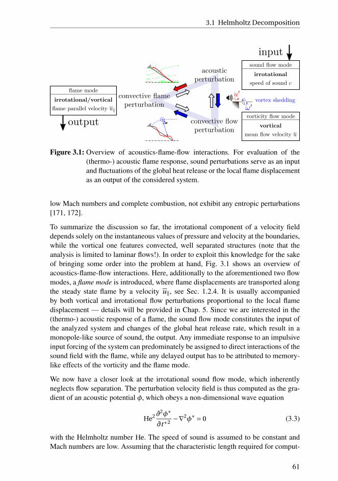
3.1 Helmholtz Decomposition

Figure 3.1: Overview of acoustics-flame-flow interactions. For evaluation of the(thermo-) acoustic flame response, sound perturbations serve as an inputand fluctuations of the global heat release or the local flame displacementas an output of the considered system.

low Mach numbers and complete combustion, not exhibit any entropic perturbations[171, 172].

To summarize the discussion so far, the irrotational component of a velocity fielddepends solely on the instantaneous values of pressure and velocity at the boundaries,while the vortical one features convected, well separated structures (note that theanalysis is limited to laminar flows!). In order to exploit this knowledge for the sakeof bringing some order into the problem at hand, Fig. 3.1 shows an overview ofacoustics-flame-flow interactions. Here, additionally to the aforementioned two flowmodes, a flame mode is introduced, where flame displacements are transported alongthe steady state flame by a velocity u∥, see Sec. 1.2.4. It is usually accompaniedby both vortical and irrotational flow perturbations proportional to the local flamedisplacement — details will be provided in Chap. 5. Since we are interested in the(thermo-) acoustic response of a flame, the sound flow mode constitutes the input ofthe analyzed system and changes of the global heat release rate, which result in amonopole-like source of sound, the output. Any immediate response to an impulsiveinput forcing of the system can predominately be assigned to direct interactions of thesound field with the flame, while any delayed output has to be attributed to memory-like effects of the vorticity and the flame mode.

We now have a closer look at the irrotational sound flow mode, which inherentlyneglects flow separation. The perturbation velocity field is thus computed as the gra-dient of an acoustic potential φ, which obeys a non-dimensional wave equation

He2 ∂2φ∗

∂t∗2−∇2φ∗ = 0 (3.3)

with the Helmholtz number He. The speed of sound is assumed to be constant andMach numbers are low. Assuming that the characteristic length required for comput-

61

Flow-Decomposition Based Modeling Framework

ing He is the length of the flame, we can express the Helmholtz number as a productof the Mach number Ma and the Strouhal number, i. e. He = Ma f ∗. Strouhal num-bers of interest for FTFs are at maximum of the order O (10), see Chap. 4, and Machnumbers of order O

(10−2

). Hence, He can be considered to be of maximum order

O(10−1

), which allows to safely drop the time dependent term in Eq. (3.3) for fur-

ther analysis. The domain of interest is hence acoustically compact, which simplifiesEq. (3.3) to the now dimensional equation

∇2φ= 0. (3.4)

Consequently, the acoustic flow mode is governed by a Laplace equation and in thefollowing we refer to the low Helmholtz number regime as the regime of compactacoustics.

Having discussed the properties of a Helmholtz decomposition and having introducedan overview of the relevant interactions governing the flame response in Fig. 3.1, thefield is set to explicate the modeling approach pursued In this chapter as well as tointroduce the investigated test case setups, which will be provided in the next twosections.

3.2 Problem Formulation and Governing Equations

A symmetric configuration as depicted in Fig. 3.2 shall be considered, where aSlit type flame is stabilized above a jet of perfectly premixed lean air-fuel mix-ture and excited by upstream velocity perturbations whose bulk value is given byu′

1,blk(t ) = 1/Ri

∫Ri

0 u′1(x2, t )dx2. Assuming a high activation energy of the global

chemical reaction and a Lewis number of about unity, the overall flow problem is splitinto a large-scale hydrodynamic and a thin, quasi-1D combustion zone, see Chap. 1.

A low Mach number macroscopic flow is assumed, which is regarded to be slightly

compressible in the sense that density is only affected by the combustion process[100, 173]. Furthermore, the analysis shall be restricted to a 2D ideal fluid (zero vis-cosity, thermal and mass diffusivity) without any volume or body forces. Viscouseffects will be incorporated by use of a Kutta conditions. This results in a flow prob-lem that is governed by

∇·u =− 1

ρ

Dρ

Dt(3.5)

Du

Dt=− 1

ρ∇p , (3.6)

where D(.)/Dt = ∂(.)/∂t +u ·∇(.) is the material derivative and u, ρ and p denoteflow velocity, density and pressure, respectively.

The density-gradient dependent source term on the right-hand side of continuityEq. (3.5) vanishes everywhere but in the immediate vicinity of the flame front. Here

62

3.2 Problem Formulation and Governing Equations

Figure 3.2: A Slit type flame is stabilized above a stream of unburned mixture (“u”)with a bulk flow velocity u1,blk and subjected to upstream bulk veloc-ity perturbations u′

1,blk. The flame propagates normal to itself by a flame

front curvature κ dependent speed sL and acts as a volume source ofstrength m. Two coordinate systems are used, namely laboratory coor-dinates (x1, x2) and flame aligned coordinates (x∥, x⊥) where x⊥ pointsalong the local flame normal direction towards the burned gas (“b”).

it acts as a source of volume, which leads to a volume production per unit length ofthe flame of m = E sL [173, 174], where E = ρu/ρb −1 denotes the non-dimensionaldensity increase and the indices “u” and “b” indicate a quantity of the unburned andburned flow, respectively. Introducing a kernel D(x⊥) capturing the spatial distribu-tion of the volume production along the flame normal direction x⊥, see Fig. 3.2,Eq. (3.5) can be rewritten as

∇·u = mD(d

(x, x f

))(3.7)

with∫∞−∞ D(x)dx = 1 and d

(x, x f

)denoting the distance from a point x to the flame

front x f .

Taking the curl of the momentum Equation (3.6) leads to a transport equation forvorticity ω

Dω

Dt= 1

ρ2

(∇ρ×∇p

). (3.8)

Here, the dilatation term −ω (∇·u) was neglected since it only is non-zero right atthe flame front and the unburned flow field is assumed to be free of vorticity. Further-more, Matalon et al. [41] argued that contributions of this term are negligible acrossthe flame sheet. Thus, for 2D inviscid flows, the dominant source term of the vortic-ity transport equation is the baroclinic tourque, which arises from a misalignment of

63

Flow-Decomposition Based Modeling Framework

Figure 3.3: Illustration of a parcel of fluid exhibiting a horizontal gradient in densityρ (∝ shade of gray) that is exposed to a vertical gradient in pressure p

leading to a force F accelerating the parcel. Due to the density gradient,the center of gravity of the fluid parcel (red line) is shifted away from thegeometrical center (black line) and, hence, the parcel of fluid would startto rotate in counter-clockwise direction.

the pressure and density gradients, see Fig. 3.3. For a detailed and rather completedescription of how vorticity interacts with a flame sheet, it is referred to the works ofHayes [175] and Berndt [176]. We eliminate the pressure term in Eq. (3.8) by use ofEq. (3.6) and obtain

Dω

Dt= 1

ρ

(Du

Dt× ∇ρ

ρ

)(3.9)

[177]. From the left-hand side of this equation it becomes clear that, in the absence ofany density gradient ∇ρ, vorticity is transported like a massless particle. The move-ment of any hypothetical point vortex whose spatial position may be defined by xω isgoverned by

d xω

d t= u (xω) (3.10)

with u (xω) being the flow velocity right at the vortex position.

Using Eqs. (3.7) and (3.9), the flow problem depicted in Fig. 3.2 is solved by de-composing the flow field u into two irrotational parts uc and ue , where the formeris caused by a pressure difference between in- and outlet of the domain initiatingthe volume flux through the combustor. The latter captures effects of the volume ex-pansion across the flame. Further, a vortical part uω is introduced that represents therotational parts of the flow field. In summary, the decomposition is written as

u = uc +ue +uω , (3.11)

see [100, 128, 173, 178]. While the irrotational components each have a potentialuc/e =∇φc/e , the vortical component depends on a stream function via uω =∇×ψω.Application of these relations, together with continuity Equation (3.7) and the de-

64

3.2 Problem Formulation and Governing Equations

composition of Eq. (3.11) results in the three Poisson equations

∇2φc = 2V (t )

Riδ(x1 −x1,EF) (3.12)

∇2φe = mD(d

(x, x f

))(3.13)

∇2ψω =−ω (3.14)

with the Laplace operator ∇2 = ∂2/(∂xi∂xi ). Note that uc is subject to a line source at

x1,EF =−∞, which generates a volume flux V (t ) =[

u1,blk +u′1,blk

]Ri∆x3 through the

combustor that is driven by a potential (or pressure) gradient between x1 =−∞ andx1 =+∞. All boundaries shall be impermeable and the axial velocity gradients shallvanish far up- and downstream the flame: ∂u/∂x1|±∞ = 0. Note that Eq. (3.12) con-stitutes the non-homogeneous equivalent to the Laplace Eq. (3.4), which was derivedfrom the acoustic wave equation.

The dynamics of the flame sheet is captured by the G-equation approach, as expli-cated in Sec. 1.3. The G-field, so far, has no other physical meaning than the fact thatits zero iso-line represents the instantaneous position of the flame front. Therefore,we are in principle free to define it to any spatial function as long as the position ofthe zero iso-line remains untouched (excluding numerical issues). For the problemat hand, it is beneficial to define G to be a signed distance function, i. e. its value ata position G(x) represents the distance from this point to the flame front located atG(x f ) = 0. This property allows for a straight forward evaluation of the argument ofthe function D(x) in Eq. (3.13) as d

(x, x f

)≡G(x). The G-equation writes

DG

Dt= s0

L

(1+ lM∇· ∇G

||∇G||

)||∇G|| . (3.15)

and, consequently, its dynamics depends on the underlying flow field as well as onthe local, stretch dependent flame speed. Here, only flame stretch related to flamecurvature is considered, whose importance is quantified by the Markstein length lM ,which is a length of the order of the flame thickness. Inserting G = x⊥−ξ(x∥, t ) intoEq. (3.15) and linearizing the resulting expression with respect to ξ leads to a 1Ddescription of the flame front in flame aligned coordinates

∂ξ

∂t+u∥

∂ξ

∂x∥= u′

⊥+ lM s0L

∂2ξ

∂x2∥

(3.16)

where u∥ denotes the mean flow velocity in flame-parallel direction.

Eq. (3.9) together with Eqs. (3.12)-(3.14) and (3.15) define the flow problem. Ad-ditionally, in the case of E > 0, a volume production kernel D has to be defined.One major difficulty in solving this problem constitutes the impermeability boundaryconditions together with the non-trivial considered geometry (backward facing stepcombustor), another the trailing edge where the flow separates. In this work, we ad-dress the former issue by use of a Schwarz-Christoffel mapping technique and thelatter by application of a Kutta condition at the trailing edge. Both are introduced inthe following.

65

Flow-Decomposition Based Modeling Framework

(a) Physical domain (b) Image domain

Figure 3.4: Illustration of the Schwarz-Christoffel mapping (not to scale). Meanflame position ( ) and straight lines radiating from the origin of theimage domain ( ), each in the physical and the image domain. Fur-ther, a point vortex, as well as its mirror vortex in the image domain, aredrawn at the shear layer.

3.3 Conformal Mapping Technique

The problem formulated in Sec. 3.2 has already — in similar form — been solvednumerically by several studies, see for example the works of Pindera and Talbot [173]and Rhee et al. [100]. In this thesis, however, a low-order formulation is desired.Therefore, the chosen solution approach is essentially based on three points: (1) Theimpermeability boundary conditions are satisfied by use of a Schwarz-Christoffelmapping technique, (2) the flow field is decomposed into a finite set of flow fieldsingularities, i. e. point sources and point vortices, and the flame front dynamics iscaptured by a 1D linearized G-equation approach as shown in Eq. (3.16) and (3) inorder to avoid infinitely high velocities at the anchoring point, a Kutta condition isemployed. These approaches are one by one explicated in the following.

3.3.1 Schwarz-Christoffel Mapping

The Poisson Eqs. (3.12)–(3.14) are solved on the geometry of interest by use of aSchwarz-Christoffel mapping technique. The inner of the physical flow domain ismapped to the imaginary positive half of a complex image domain. By doing so, theflow problem is split into a mapping problem simplifying and unifying the boundaryconditions and a canonical flow problem in the image domain. Schwarz-Christoffelmappings are conformal mappings, i. e. they locally preserve angles and orienta-tions [179]. These kind of transformations are complex valued functions of the formξ= f (x) that rotate and scale line elements in the approximate vicinity of a point x0 byan angle arg

[d f (x0)/dx

]and a factor

∣∣d f (x0)/dx∣∣, respectively. From this property it

follows that solutions of Laplace’s equation in the image domain are also solutions ofLaplace’s equation in the physical domain, see Howe [180] (Sec. 3.5). Consequently,such a mapping can be applied to solve the given set of Eqs. (3.12)-(3.14).

66

3.3 Conformal Mapping Technique

The coordinate system used to describe the combustor shown in Fig. 3.2 is illustratedin Fig. 3.4. Due to symmetry, we limit ourselves to only one half of the domain.Complex variables are used to describe the 2D problem: Coordinates in the physicaldomain are represented by x = x1 + i x2 where x1 denotes the axial and x2 the spatialdirection, perpendicular to the first. Accordingly, velocities are expressed by u =u1 + i u2. In the image domain, the complex variable ξ= ξ1 + i ξ2 is used to specifylocation.

All corners of the flow domain are named by capital letters (A to E) and are mappedto points on the real axis of the image domain. At edge A, the feed channel opens intothe combustion chamber. This edge is mapped to ξ= 1. Points E and F are located atx1 =−∞ in the physical domain and are mapped to ξ = 0 in the image domain. Themapping is defined by

x(ξ) = Ra

π

[cosh−1

(2C 2

r ξ−1−C 2r

1−C 2r

)−Cr cosh−1

((1+C 2

r )ξ−2

(1−C 2r )ξ

)](3.17)

with the confinement ratio Cr = Ri /Ra [179]. This mapping can only be inverted nu-merically, therefore, evaluation of ξ(x) requires the application of a numerical rootfinding algorithm.

The complex conjugate, denoted by (.), of the velocity in the physical domain iscomputed by application of the chain rule

u(x) = dφ (ξ(x))

dξ

dξ(x)

d x. (3.18)

The first term in this equation is the derivative of the flow potential φ with respect tothe image domain coordinate ξ, the second the first derivative of the mapping withrespect to the physical coordinate x. The latter writes for the combustor geometry

dξ(x)

d x=π

ξ(x)

Ra

[ξ(x)−C−2

r

ξ(x)−1

] 12

. (3.19)

Using these relations, we are able to compute the velocity field in the physical domaindue to any potential φ(ξ) given in the image domain. Knowing that any point sourceor vortex maps to its counterpart in the image domain by conserving its strength —i. e. volume production and circulation, respectively — and vice versa, we are able todefine a potential field as the superposition of several point sources and vortices. Bymapping these points to the image domain, Eq. (3.18) can be used in order to computethe associated physical velocity field that complies with the boundary conditions.This process is explicated in more detail in the following section.

3.3.2 Flow-Field Singularities

The solution of a Poisson equation ∇2φ= c together with a set of boundary condi-tions and a Dirac Delta function as non-homogeneous part c = δ(x − x ′) is known as

67

Flow-Decomposition Based Modeling Framework

the Green’s function G(x, x ′) of this problem. Here, the Dirac Delta function con-

stitutes a point source whose 2D-spatial position is given by x ′ = (x ′1, x ′

2). Knowingthe respective Green’s function, the solution of the Poisson equation for an arbitrarynon-homogeneous part c(x) is computed as the spatial convolution of the Green’sfunction with a given c(x). Simplifying the problem by assuming free-space bound-ary conditions, i. e. the potential φ asymptots to zero at infinity, a so-called free-spaceGreen’s function

G(x, x ′)= 1

2πln

[√(x1 −x ′

1

)2 +(x2 −x ′

2

)2]

(3.20)

emerges. By mapping the non-homogeneous part of a Poisson equation to the imagedomain, a solution that is conform with the impermeability boundary conditions atthe walls is easily constructed by solely relying on free-space Green’s functions. Thissimplifies the analysis and will be explicated in the following.

First of all, we need to constitute that there are two types of non-homogeneousfunctions, which are volume sources and vortices, see Eqs. (3.12)–(3.14). ApplyingGreen’s Function (3.20) in the image domain (complex coordinate ξ), the complexconjugate of the irrotational velocity component due to a point source of strength S

at position ξ′ becomes

uc/e (ξ, t ) = S

2π

1

ξ−ξ′. (3.21)

Similarly, we get for the solenoidal (vortical) velocity due to a point vortex of strengthΓ at the same position

uω(ξ, t ) =−iΓ

2π

1

ξ−ξ′. (3.22)

In the image domain, all walls are mapped to the real axis. Therefore, in order to fulfillthe impermeability boundary conditions at all walls, mirror sources of equal strengthS are placed in the lower half of the complex plane by mirroring the source locationsat the real axis. This simply corresponds to computing the complex conjugate ofthe original source position ξ′. Equivalently, mirror vortices of opposite strength areintroduced. In doing so, velocity components normal to the real axis vanish and thevolume flux through all walls is zero. This is illustrated in Fig. 3.5 for a single vortex.

In the proposed model, the vortical part of the overall perturbation velocity field isapproximated by a finite number of N point vortices of strengths ∆Γ

′n , which results

in an expression for the velocity in the image domain of

uω(ξ, t ) =− i

2π

N∑

n=1

∆Γ′n

ξ′n − ξ′n(ξ−ξ′n)(ξ− ξ′n)

, (3.23)

where mirror vortices of opposite circulation have been placed at the complex conju-gate coordinates ξ′n of all vortices.

The potential part of the perturbation velocity field that drives the volume fluxthrough the combustor can be computed by placing a source of strength

S(t ) = 2u′1(t )Ri (3.24)

68

3.3 Conformal Mapping Technique

(a) Physical domain (b) Image domain

Figure 3.5: Illustration of how impermeability boundary conditions are met by useof a mirror vortex (not to scale): the wall normal velocity componentof the original vortex of strength ∆Γ

′ (green) is canceled by its mirrorcounterpart (pink) such that the resulting velocity (red) is parallel to thewalls in the image (3.5b) as well as in the physical domain (3.5a). Here,the shear layer and the flame front are shown as blue dashed and reddotted lines, respectively.

at ξEF = 0 since all points of x1 →−∞ are mapped to a single point in the imagedomain (EF). Following Eq. (3.21), the complex conjugate of the associated velocityfield is computed in the image domain as

uc (ξ, t ) = S(t )

2πξ. (3.25)

Resulting stream lines are shown in green in Fig. 3.4, one time in the image and onetime in the physical domain.

3.3.3 Kutta Condition

Following Eqs. (3.18) and (3.19), the flow field of the combustor geometry exhibitsa O

((ξ−1)−1/2

)singularity at edge A, which results from the fact that, in reality, a

viscous flow cannot follow the abrupt 90 turn of the wall contour, since this wouldrequire an infinitely high pressure gradient. The lack of such high gradients leads tothe separation of the flow and vorticity, originally bound in the wall boundary layer,is shed into the inner region of the flow domain. In the modeling framework adoptedhere, this singularity is removed by employing a Kutta condition. Its application re-covers a finite-valued velocity at the edge, which can only be ensured by demanding

dφ

dξ

∣∣∣∣ξ=1

!= 0, (3.26)

69

Flow-Decomposition Based Modeling Framework

see Eq. (3.18). In order to meet this condition, vorticity is introduced in the vicinityof edge A, which implies the formation of a thin shear layer. It should be pointedout that in the case of an anchored flame, getting rid of the singularity is compulsorysince otherwise the infinitely high velocity at the anchoring would lead to unbounddisplacement amplitudes at this point.

Concerning the validity of a Kutta condition, at least some qualitative statements canbe found in the literature. Crighton [181] published an extensive review article on theKutta condition in unsteady flows stating that “within restricted parameter ranges,

only those ‘outer’ potential flows that satisfy a Kutta condition are, in general, com-

patible (in the matched asymptotic expansion sense) with an acceptable multilay-

ered ‘inner’ viscous structure” (Crighton [181], p.412). Williams [182] made a morecautious statement in a review article on aeroacoustics: “There is no proof that the

solution obtained through the matched-expansion scheme is, in fact, a solution of

the real problem — but it usually is [. . . ]” (Williams [182], p.449). Generally, inthe field of aero-acoustics, application of a Kutta condition is considered to be anacceptable principle for modeling flows around sharp edges [183, 184]. The resultscomputed in this chapter compare well with the CFD/SI data and hence confirm theaforementioned assertions, as will be shown below. Nevertheless, it should be kept inmind that a Kutta condition does not naturally appear when simplifying the govern-ing equations of a viscid flow but rather has to be viewed as an ad hoc hypothesis thatallows to incorporate viscous effects into an inherently inviscid flow description.

In the literature, several methods have been proposed in order to implement a Kuttacondition. A method relying on a single vortex ensuring a finite valued velocity at asharp edge of a acoustically excited flow of zero mean flow was first developed byBrown and Michael [185, 186]. It was adopted by several later studies, e. g., [187,188]. The idea of this approach is that during both the positive and negative part ofa forcing cycle, shed vorticity accumulates in a single vortex, which represents therolled up shear layer.

A more advanced method is the single panel method [124, 189–191], which intro-duces a vortex sheet (the panel) of length Hx and constant strength γx that is attachedto the trailing edge. The strength and length of this sheet depend on the instantaneousflow field and are set such that the edge singularity is removed. At each time step,the circulation confined to the sheet is condensed into one point vortex and advectedby the local flow velocity. The work presented in this chapter relies on such a singlepanel method.

The shape of the vortex panel is defined by two geometrical parameters: Its length Hξ

and its angle with respect to the real axis βξ, both measured in the image domain asillustrated in Fig. 3.6. Ideally, the strength of the vortex sheet in the physical domain

γx (x) = dΓ(x)

d x(3.27)

is constant, where Γ=∫

A ωdS is the circulation, defined as the integral of vorticity ω

70

3.3 Conformal Mapping Technique

Figure 3.6: Flow field according to source at ξ= 0 and a Kutta panel (green), shownfor the whole combustor (top). Additionall, a close up view of the Kuttapanel is shown in the physical (bottom left) and the image domain (bot-tom right), with Cr = 0.4, Hξ = 2.1 and βξ =π/3.

over an area A. We, therefore, need to define the panel strength in the image domainγξ(ξ) such that it maps back to a constant distribution in the physical domain γx (x).Following the chain rule, we get

γx = γξdξ

d x(3.28)

and, hence, we would have to impose a distribution of γξ ∝ dx/dξ in the image do-main in order to get a constant value in the physical domain. We call this the idealdistribution of vorticity in the following. The flow field corresponding to such a dis-tribution, however, could not be solved analytically (by the author of this thesis).Therefore, a simplified distribution

γξ(ξ′) = c1

√ξ′−1

ξ′(3.29)

is used, where ξ′ parametrizes the vortex sheet and c1 its strength. Fig.3.7 compares

the ideal vorticity distribution of dx/dξ, i. e. γξ = c1

[sξ/(ξ−C−2

r )]1/2

/ξ ( ) withthe approximation according to Eq. (3.29) ( and ). Here, sξ and sx denote thepanel aligned coordinates in the image and the physical domain, respectively. It be-comes clear that the approximation is a good model in the limit of short panel lengthsand low confinement ratios. Note that the Cr = 0.4 and Hx /Ri = 0.4 case corresponds

71

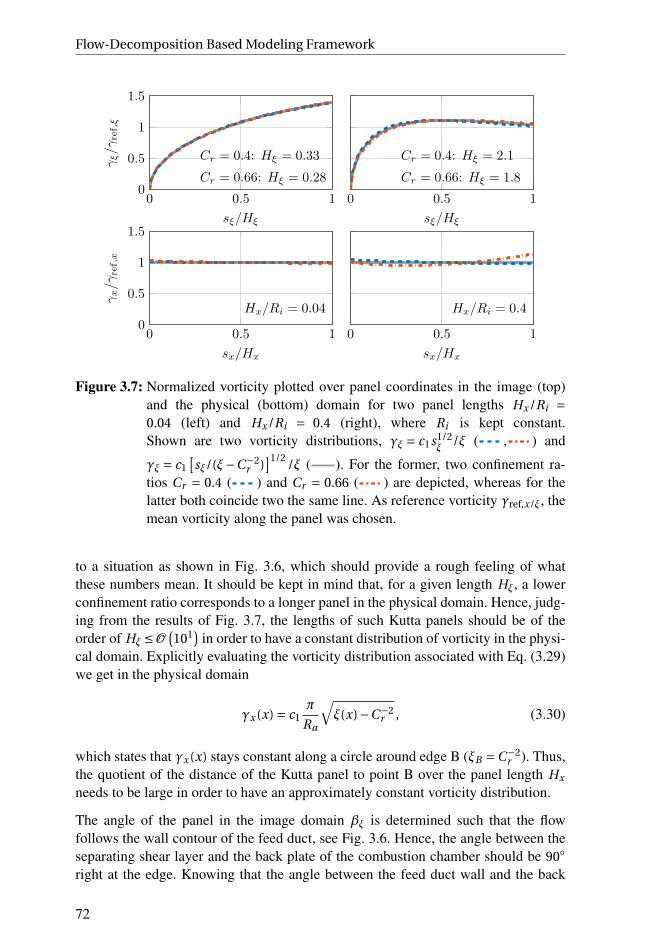
Flow-Decomposition Based Modeling Framework

0 0.5 10

0.5

1

1.5

Cr = 0.4: Hξ = 0.33

Cr = 0.66: Hξ = 0.28

sξ/Hξ

γξ/γ

ref,ξ

0 0.5 10

0.5

1

1.5

Hx/Ri = 0.04

sx/Hx

γx/γ

ref,x

0 0.5 1

Cr = 0.4: Hξ = 2.1

Cr = 0.66: Hξ = 1.8

sξ/Hξ

0 0.5 1

Hx/Ri = 0.4

sx/Hx

Figure 3.7: Normalized vorticity plotted over panel coordinates in the image (top)and the physical (bottom) domain for two panel lengths Hx /Ri =0.04 (left) and Hx /Ri = 0.4 (right), where Ri is kept constant.Shown are two vorticity distributions, γξ = c1s1/2

ξ/ξ ( , ) and

γξ = c1

[sξ/(ξ−C−2

r )]1/2

/ξ ( ). For the former, two confinement ra-tios Cr = 0.4 ( ) and Cr = 0.66 ( ) are depicted, whereas for thelatter both coincide two the same line. As reference vorticity γref,x/ξ, themean vorticity along the panel was chosen.

to a situation as shown in Fig. 3.6, which should provide a rough feeling of whatthese numbers mean. It should be kept in mind that, for a given length Hξ, a lowerconfinement ratio corresponds to a longer panel in the physical domain. Hence, judg-ing from the results of Fig. 3.7, the lengths of such Kutta panels should be of theorder of Hξ ≤O

(101

)in order to have a constant distribution of vorticity in the physi-

cal domain. Explicitly evaluating the vorticity distribution associated with Eq. (3.29)we get in the physical domain

γx (x) = c1π

Ra

√ξ(x)−C−2

r , (3.30)

which states that γx (x) stays constant along a circle around edge B (ξB =C−2r ). Thus,

the quotient of the distance of the Kutta panel to point B over the panel length Hx

needs to be large in order to have an approximately constant vorticity distribution.

The angle of the panel in the image domain βξ is determined such that the flowfollows the wall contour of the feed duct, see Fig. 3.6. Hence, the angle between theseparating shear layer and the back plate of the combustion chamber should be 90

right at the edge. Knowing that the angle between the feed duct wall and the back

72

3.3 Conformal Mapping Technique

Figure 3.8: Sketch of the Kutta panel (upper) and its mirror counterpart (lower) inthe image domain. The starting point of the Kutta panel is named ξA andits ending ξB .

plate is 270, which corresponds to an angle of 180 in the image domain, the desired90 angle corresponds to βξ = 60 or, in radians, βξ =π/3. It will be shown belowthat this angle is indeed a special one, since imposing such an angle, the velocityright beneath the point where the panel is attached vanishes.

We now evaluate, for a given velocity field, the respective panel strength c1 that satis-fies the Kutta condition. This requires the evaluation of the velocity field imposed bythe Kutta panel. In doing so, we firstly need to evaluate the gradient of the potentialφp associated with the panel in the image domain. Assuming a vorticity distributionaccording to Eq. (3.29) we need to evaluate an integral

dφp

dξ=− i

2π

ξB∫

ξA

c1

pξ′−1

ξ′

ξ−ξ′dξ′ , (3.31)

where all relevant quantities are sketched in Fig. 3.8. Solving this integral, we get

dφp,up

dξ= i

π

c1

(ξ−1)exp(−iβξ)+1

[arctan

(√Hξ

)

−√

(1−ξ)exp(−iβξ)arctan

(√Hξ

(1−ξ)exp(−iβξ)

)]exp(−iβξ) . (3.32)

Here, the index “up” signifies that only the potential of the original Kutta panelis respected, which is found in the upper half of the image domain as depicted inFig. 3.8. The solution for the associated mirror panel, placed in the lower half of thecomplex plane (index “low”), is the same as the one given by Eq. (3.32), but with anegative sign and a negative angle βξ. Accordingly, it writes

dφp,low

dξ= − i

π

c1

(ξ−1)exp(iβξ)+1

[arctan

(√Hξ

)

−√

(1−ξ)exp(iβξ)arctan

(√Hξ

(1−ξ)exp(iβξ)

)]exp(iβξ) . (3.33)

73

Flow-Decomposition Based Modeling Framework

The superposition of both results in the overall expression for the panel, namelydφp /dξ.

Equations (3.32) and (3.33) can now be used in order to compute the strength of thevortex sheet c1 (including the mirror panel!). From Condition (3.26) we know thatthe gradient of the overall potential needs to vanish at edge A (ξ= 1). Assuming thepotential resulting from a superposition of all flow field singularities (vortices andsources) except the Kutta panel may be denoted as φΣ, this condition translates to

dφp

dξ

∣∣∣∣ξ→1

=− dφΣ

dξ

∣∣∣∣ξ=1

. (3.34)

Combining Eqs. (3.32)–(3.34) and solving for c1 leads to

c1 =− dφΣ

dξ

∣∣∣∣ξ=1

π

2arctan(√

Hξ

)sin(βξ)

. (3.35)

Using these relations and following Eq. (3.18), we can compute the complex conju-gate of the resulting flow velocity in the physical domain as

u(x) = dξ

d x

[dφΣ

dξ+

dφp

dξ

]

= dξ

d x

[dφΣ

dξ+

dφp,up

dξ+

dφp,low

dξ

]. (3.36)

This expression respects the Kutta panel as well as its mirror counterpart plus theimpact of all other flow field singularities. We now evaluate the right-hand and left-hand limits (with respect to the real part of ξ) of the velocity fields at the separationpoint A and get

u+ = limξ→1+

u (x(ξ)) =π

Ra

√1−C−2

r

dφΣ

dξ

∣∣∣∣ξ=1

πcos(

32βξ

)

2arctan(√

Hξ

)sin(βξ)

(3.37)

and

u− = limξ→1−

u (x(ξ)) =− π

Ra

√1−C−2

r

dφΣ

dξ

∣∣∣∣ξ=1

iπsin(

32βξ

)

2arctan(√

Hξ

)sin(βξ)

, (3.38)

respectively. If we insert βξ =π/3, the right-hand limit of Eq. (3.37) simplifies tou+ = 0 and the left-hand one of Eq. (3.38) to

u− =− π

Ra

√1−C−2

r

dφΣ

dξ

∣∣∣∣ξ=1

iπ

2arctan(√

Hξ

)sin

(π3

) . (3.39)

This reflects the fact that the left-hand limit constitutes the jet velocity at the sepa-rating edge, while the right-hand limit evaluates the flow velocity at the side of therecirculation bubble, see Fig. 3.6. From Eq. (3.39) it becomes clear that, at edge A,

74

3.3 Conformal Mapping Technique

Figure 3.9: Summary of all computations that need to be performed during one timestep when considering a Kutta condition.

multiplication of the local velocity dφΣ/dξ∣∣ξ=1 with the complex unit i bends the

flow by 90, which leads to the desired separation.

For the sake of completeness, it should be mentioned that one of the major difficultiesencountered during the derivation of the Kutta condition concerns branch cuts, whichare curves across which the resulting flow field is discontinuous. In this regard aKutta panel is such a branch cut. Hence it has to be ensured that the branch cutsassociated with the Kutta panels used do not exceed their desired lengths and, indoing so, impose spurious discontinuities. In the implementation presented here, thisproperty has been verified.

Finally, it is explicated how the methods described above are used in order to numer-ically simulate the process of vortex shedding. An overview of all required compu-tations is provided in Fig. 3.9. First of all, in each time step the length of the vortex

75

Flow-Decomposition Based Modeling Framework

sheets Hξ needs to be computed, which is done by assuming a transport velocityof the vorticity bound in the separating shear layer of Uedge = (u++ u−)/2. Multi-plication of this velocity with the time step length ∆t results in the panel length inthe physical domain Hx . Note that in the proposed acoustic LOM, an approximationUedge = ublk/2 is used, which avoids the evaluation of a mean flow state. This ap-proach implicitly assumes a block flow profile in the feed channel and zero velocityin the recirculation zone. Subsequently, Hξ is numerically evaluated as the root of

Hξ∫

0

∣∣∣∣d x

(sξ(t )

)

dξ

∣∣∣∣dt −Hx = 0, (3.40)

where a parametrization sξ(t ) = 1+exp(iβξ)t of the curve representing the Kuttapanel is used (note that, here, t denotes the parametrization parameter not thetime). Based on this length, the Kutta condition can be applied according toEqs. (3.35),(3.32), (3.33) and (3.36). The total circulation of the resulting panel isthen provided by

Γ′p =

∫Hξ

0c1

pt∣∣1+exp(iβξ)t

∣∣dt . (3.41)

After each time step, this integral is numerically evaluated employing the trapezoidalrule and its respective value of Γ′

p propagated to a new point vortex, which is placedat end of the vortex panel from which it resulted.

3.4 Summary

In this chapter, a low-order modeling approach for the dynamics of acoustically per-turbed burner-stabilized 2D flames was derived. It is essentially based on first prin-ciples and relies on the assumption of an inviscid, slightly compressible flow whosedensity is solely affected by the combustion process. Imposing a Helmholtz decom-position, three velocity components need to be modeled: (i) an irrotational field re-lated to the pressure difference between in- and outlet of the domain, (ii) a secondirrotational field associated to the volume flux generated by the flame and (iii) asolenoidal velocity field containing all vortical contributions. It is assumed that vor-ticity is only generated by the flame sheet as well as by a Kutta condition capturingthe shedding of vorticity at sharp edges.

Relying on a conformal mapping technique and a finite number of flow field singular-ities, the overall problem could be split into several canonical problems. This clarifiesthe solution process and allows to simply switch certain physical mechanisms on andoff in order to evaluate their individual contributions. This approach will be appliedto the case of a 2D Slit flame in the following.

76

4 Primary Interactions

Based on a rigorous analysis neglecting flame-flow feedback and

relying on methods presented in Chap. 3, it is found that predomi-

nantly irrotational velocity perturbations interact with a flame hav-

ing maximum impact at the base region, while the impact of shed

vorticity is negligible. A significant discrepancy between the mod-

eled response and high fidelity CFD data is observed, which is at-

tributed to flame-flow feedback — a mechanism neglected in this

chapter.

The basic idea of this chapter is to take a first step towards the identification and mod-eling of the skeletal processes governing acoustics-flame interactions. To this end,flame-flow feedback as well as thermal-diffusive mechanisms shall be neglected andonly the remaining interactions of acoustics with the flame shall be analyzed. Morespecifically, the modeling approach introduced in the previous chapter shall be ex-ploited in order to resolve the paradoxical finding concerning the convective velocitymodel explained in Chap. 2. This model assumes that acoustically excited premixed(Bunsen) flames are subject to convected velocity perturbations, which are responsi-ble for the observed wrinkling of the flame front. Several studies, however, demon-strated that these convected perturbations are rather a consequence than a source offlame front wrinkles, caused by a feedback of the flame on the flow. Therefore, the as-sumption of convected velocity perturbations seems to violate causality (they cannotbe source and consequence at the same time). In this chapter, it shall be investigatedif vortex shedding imposes significant levels of convected velocity perturbations ontothe flame front. If that is the case, causality may at least partly be respected by con-vective velocity models.

From an analytical point of view, it has to be noted that acoustic perturbations propa-gate at the speed of sound and, consequently, a convective flow perturbation cannot beassigned to the acoustic flow mode. Thus, an acoustic-to-hydrodynamic mode conver-sion is required in order to generate perturbations that are transported with the localflow velocity. Following Fig. 3.1, one possible candidate for such a mode conversionmechanism is the process of flow separation, which can happen at sharp corners, e. g.at a backward-facing step or bluff body flame holder. At the separation point, vor-ticity, originally confined to the wall boundary layers, is shed into the interior of theflow domain. Transient (acoustic) forcing of a separating flow leads to unsteady gen-eration and shedding of vorticity[124, 190, 192]. Vortical structures that are advected

77

Primary Interactions

downstream by the flow represent an acoustic damping mechanism [123] and may —more important in the context of this study — interact with the flame front. Using a2D compressible flow solver, which allowed to artificially modify the gas expansion,Schlimpert et al. [104] showed for an unconfined flame that vortical structures sig-nificantly affect the flame front in the case of negligible gas expansion. With realisticgas expansion, however, the influence of shed vorticity is substantial only right at theflame base.

In this Chapter the issue of flow-flame interactions is revisited by decomposing theacoustic velocity disturbance into an irrotational potential and a solenoidal vorticalfield and analyzing how both interact with the flame. For this purpose, the modelingframework introduced in Chap. 3 is adopted and applied to the analysis of acoustic-flow-flame interactions at a duct singularity. Of particular interest is an assessment ofthe impact of shed vorticity on the flame front and if and how it contributes to the con-vective nature of the FTF. In order to suppress the occurrence of vortical structuresdue to flame-flow feedback, we neglect exothermicity/gas expansion in the pertur-bations. This assumption is in line with the assumptions of the convective velocitymodel. The mean flow field, required to compute vortex advection, is neverthelessretrieved from exothermic numerical simulations.

In this chapter, the effect of gas expansion is explicitly excluded from the analysis,i. e. E = 0. Thus, due to m = 0, Eq. (3.13) drops from the analysis and the baroclinictourque source term vanishes, which eliminates the right-hand side of Eq. (3.9). Inthe remaining problem, the only source of vorticity is vortex shedding. To simplifythe analysis, curvature (stretch) effects are neglected and hence lM ≡ 0.

Sec. 4.1 introduces the specific test case setups as well as the high-fidelity CFD re-sults, which serve as validation cases of the developed model. The resulting low-ordermodel is then analyzed and compared to high fidelity CFD data in terms of flamesheet and global heat release dynamics in Sec. 4.2.

4.1 Test Case Setups

The modeling framework derived in this chapter is applied to a backward facingstep combustor, as shown in Fig. 4.1. Configurations of two different confinementratios Cr = Ri /Ra of Cr = 0.4 (upper half) and Cr = 0.66 (bottom half) are analyzed,with Ri denoting the feed channel and Ra the combustion chamber half width. Thecoloring represents the steady state velocity field resulting from a 2D incompressibleCFD simulation with a reduced chemical kinetic 2-step mechanism (2S-CM2) asdescribed in Appendix. A. The area of maximum heat release is shown in green colorin Fig. 4.1 ( ). An estimate of the shear layer position ( ) as well as the steadystate flame front of length L f , as predicted by the 1D linearized G-equation approachintroduced in Sec. 1.3.2 (lM ≡ 0), ( ) are indicated. Note, that other than for conicalconfigurations [144], the confinement ratio does not impact the flame height of 2D

78

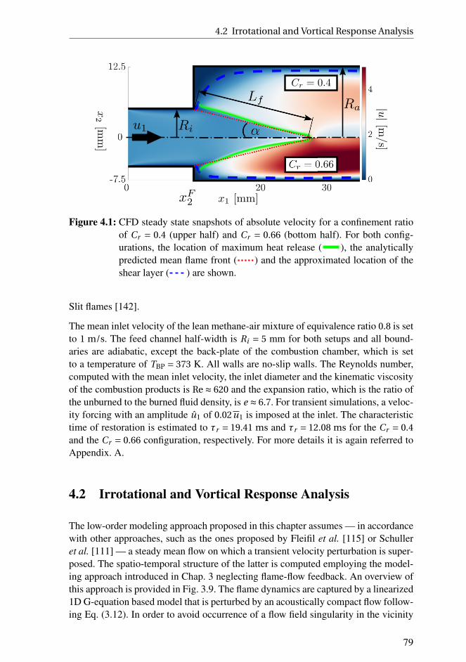
4.2 Irrotational and Vortical Response Analysis

Figure 4.1: CFD steady state snapshots of absolute velocity for a confinement ratioof Cr = 0.4 (upper half) and Cr = 0.66 (bottom half). For both config-urations, the location of maximum heat release ( ), the analyticallypredicted mean flame front ( ) and the approximated location of theshear layer ( ) are shown.

Slit flames [142].

The mean inlet velocity of the lean methane-air mixture of equivalence ratio 0.8 is setto 1 m/s. The feed channel half-width is Ri = 5 mm for both setups and all bound-aries are adiabatic, except the back-plate of the combustion chamber, which is setto a temperature of TBP = 373 K. All walls are no-slip walls. The Reynolds number,computed with the mean inlet velocity, the inlet diameter and the kinematic viscosityof the combustion products is Re ≈ 620 and the expansion ratio, which is the ratio ofthe unburned to the burned fluid density, is e ≈ 6.7. For transient simulations, a veloc-ity forcing with an amplitude u1 of 0.02u1 is imposed at the inlet. The characteristictime of restoration is estimated to τr = 19.41 ms and τr = 12.08 ms for the Cr = 0.4

and the Cr = 0.66 configuration, respectively. For more details it is again referred toAppendix. A.

4.2 Irrotational and Vortical Response Analysis

The low-order modeling approach proposed in this chapter assumes — in accordancewith other approaches, such as the ones proposed by Fleifil et al. [115] or Schulleret al. [111] — a steady mean flow on which a transient velocity perturbation is super-posed. The spatio-temporal structure of the latter is computed employing the model-ing approach introduced in Chap. 3 neglecting flame-flow feedback. An overview ofthis approach is provided in Fig. 3.9. The flame dynamics are captured by a linearized1D G-equation based model that is perturbed by an acoustically compact flow follow-ing Eq. (3.12). In order to avoid occurrence of a flow field singularity in the vicinity

79

Primary Interactions

of the flame anchoring point and for the sake of capturing the effect of vortex shed-ding, a Kutta condition is applied. The mean flow is characterized by a constant axialvelocity ublk and a constant flame speed sL , which in combination lead to the forma-tion of an inclined steady state flame front. The position of the mean flow shear layeris taken from the high-fidelity CFD simulations described in Sec. 4.1. The transportvelocity for vorticity along this line is set to the fixed value of ublk/2 [126].

The spatial shape of the velocity perturbation associated with the regime of compactacoustics depends on the confinement ratio Cr . This can be seen from the definitionof the resulting velocity field provided in Eq. (3.18) and the herein occurring mappingprovided by Eq. (3.17). Hence, in this section, the responses of two flame configu-rations of different confinement ratios are analyzed and the results are compared toCFD/SI data, see Appendix. A.

For this purpose, the two test cases introduced in Sec. 4.1 are simulated. In a firststep, simulations under harmonic velocity forcing are conducted and analyzed inSec. 4.2.1. Realizing that vortex shedding is negligible, the impulse response is com-puted in Sec. 4.2.2 relying solely on the irrotational velocity component. This re-quires some non-trivial considerations caused by the Kutta condition. In a final step,in Sec. 4.2.3, analyzes the gathered response data and compares it to CFD/SI results.

4.2.1 Harmonic Forcing

Harmonic forcing of the bulk flow velocity provokes irrotational flow field perturba-tions and, at edge A, the shedding of vorticity. A Kutta panel attached to this edgeensures that the flow field remains finite and leaves the trailing edge tangentially tothe wall contour. In each time step, the vorticity bound by this panel is condensed intoa point vortex that is placed right at the panel end. This vortex then becomes part ofthe vortical flow field and is advected along the mean flow shear layer by a velocityublk/2, whose coordinates are estimated from the CFD data, see Fig. 4.1 ( ).

Forcing the Cr = 0.4 configuration harmonically at a frequency of 80 Hz and an am-plitude of 2% ublk results in a response as depicted in Fig. 4.2. Here, four snapshotsat different phases of the forcing signal are shown. The upper half of each snapshotvisualizes the resulting vortical and the lower half the corresponding irrotational per-turbation velocity field. The flame front displacements provoked by the latter ( )are significantly larger than the vortical ones. Hence, it seems that shed vorticityhardly contributes to the response of the flame and could safely be neglected. Thespatial shape of the irrotational perturbation can be deduced from the green arrowsshown in Fig. 4.2, which illustrate the flame normal velocity perturbations. Accord-ing to them, acoustic perturbations mainly displace the flame base region, while theflame tip is hardly affected.

In the literature, a common approach to approximate the amount of vorticity shed

80

4.2 Irrotational and Vortical Response Analysis

Figure 4.2: LOM predictions of a harmonically forced flame configuration (at 80 Hzand an amplitude of 2% ublk) for a confinement ratio of Cr = 0.4. Shownare four consecutive snapshots taken at phases from 0 to 270 with re-spect of the forcing signal. The upper half of each snapshot shows thevortical flow component, where the color along the shear layer corre-sponds to the strength of the vorticity fluctuations. The lower half showsthe respective irrotational flow component. The flame normal velocity,scaled by a factor of 4, is illustrated by green arrows (upper+lower half).The shown flame front displacements are scaled by a factor of 7 ( ).

during a time interval ∆t is to evaluate the linearized relation

∆Γ′(t ) = ublk

∫t+∆t

tu′

1( t )d t , (4.1)

which provides an estimate of the created total circulation of the separating vortexsheet [126, 193]. This formula has been used by Steinbacher et al. [1] in order toquantify the effects of the free shear layer onto the flame front. Fig. 4.3 comparesthe resulting strength of the vortex sheet of this approach ( ) to the one caused bythe aforementioned Kutta condition ( ). For Cr = 0.4, the amplitude of vorticityfluctuations caused by the Kutta condition is more than twice as large as the onecomputed by Eq. (4.1). Nevertheless, both studies — the one of Steinbacher et al. [1]and the one presented here — agree that vortex shedding has only a negligible impacton the flame response. Having a look at the Cr = 0.66 configuration, both ways ofcomputing the shed vorticity almost coincide. Therefore, it seems that predictions ofEq. (4.1) agree better with results of the Kutta condition in cases where the flow isless two-dimensional, which is the case if the confinement is getting more narrow(Cr → 1).

4.2.2 Impulse Forcing

The finding that vorticity shed from the burner mouth has only a negligible impacton the flame response shall now be exploited: It allows to evaluate the impulse re-sponse (IR) solely based on the irrotational part of the perturbation velocity field.

81

Primary Interactions

0 π 2π 3π 4π 5π 6π

−2

−1

0

1

2

phase forcing signal [rad]

nor

mal

ized

amplitu

de

[-]

Cr = 0.4

0 π 2π 3π 4π 5π 6π

phase forcing signal [rad]

Cr = 0.66

Figure 4.3: Comparison of vorticity distribution resulting from vortex shedding dueto a Kutta condition ( ) and the linear approximation of Eq. (4.1)( ) for three forcing cycles at 80 Hz and two confinement ratios.

To this end, an impulsive forcing u′blk

= ǫδ(t ) of amplitude ǫ is applied to the com-bustor and the resulting instantaneous flame displacement is computed from therespective irrotational velocity perturbation by evaluation of the temporal integralξ(x∥) =

∫∞0 u′

⊥(x∥)dt . Application of a Kutta panel, however, leads to a situationswhere u′

⊥(x∥) depends on the panel length, which is computed from the local trans-port velocity (u++ u−)/2 multiplied by the temporal width of the impulse forcing ∆t .Assuming a harmonic forcing signal, vorticity is continuously shed from the burnermouth. That means, the panel length Hx is well defined in each time step and con-tinuously varies over time. In the case of an impulsive signal, however, the resultingpanel length Hx depends on both the amplitude of the forcing and the width of theimpulse signal. This is a problem since in the linear limit, the impulse response mapsto a certain frequency response and vice versa. Having a significant dependency ofthe response to the forcing amplitude ǫ, this property is no longer ensured as will beshown in the following.

Fig. 4.4 analyzes for two confinement ratios how the flame normal velocity perturba-tion depends on the length of the vortex panel. For this purpose, an impulsive velocityforcing is applied and the resulting flame normal velocity is measured for differentpanel lengths right at the moment when the impulse hits the flame. A rather strongimpact of the panel length on the resulting velocity can be observed: the shorter thepanel gets, the higher and more localized the peak velocity becomes. Thus, an impul-sive forcing using a very narrow impulse perturbation or a very low amplitude wouldboth lead to a short Kutta panel and, therefore, to a flame displacement that is verylocalized at the flame holder. The opposite holds for a wide impulse perturbation ora high velocity amplitude. In consequence, this means that the IR is rather sensitiveto the specific kind of forcing signal, which is an unfavorable property.

In order to compute an estimate of the IR that robustly captures the linear dynamicsof the system in the inviscid limit, an empirical approach is chosen: the panel length

82

4.2 Irrotational and Vortical Response Analysis

0 0.1 0.2 0.30

1

2

xF1 /Lf [-]

u′ ⊥/u

[-]

Cr = 0.4

0 2 4 60

2

4

6

8

x1 [mm]

x2

[mm

]

0 0.1 0.2 0.3

xF1 /Lf [-]

Cr = 0.66

0 2 4 6

x1 [mm]

Figure 4.4: Top: Flame normal velocity resulting from a constant mean flow and aKutta condition evaluated for four panel lengths, Hξ ( ), Hξ/2 ( ),Hξ/4 ( ) and Hξ/8 ( ) plotted over normalized flame coordinate.In accordance with Fig. 3.7, Hξ is set to 2.1 for Cr = 0.4 and to 1.8 forCr = 0.66. Lower: Visualization of the associated panel shapes, wherethe end of each panel is marked by a vertical line. Additionally, the flamefront is shown ( ).

is set to a value such that the frequency response computed from the resulting IR cor-responds best to predictions using harmonic forcing. The associated panels fulfillingthis requirement best are plotted in Fig. 4.4 for the two investigated confinement ra-tios ( ). Panels of these lengths have already been studied in Sec. 3.3.3. Using theassociated flame normal velocity perturbations resulting from such panel lengths, theflame displacement right at the moment when the impulse hits the flame (t∗ = 0) iscomputed and plotted in Fig. 4.5. The shown curves are normalized by the displace-ment amplitude ξ =

∫t0 u′

1d t . Indeed, good agreement between the LOM ( ) andthe CFD/SI data ( ) is found for t∗ = 0 for both confinement ratios. Details on theprocessing of the CFD results are provided in Appendix. A.4.

Due to the fact that the resulting flame front has the shape of a triangle at t∗ = 0, aso-called flame base displacement (FBD) model is introduced:

ξ(x∥, t ) = 2sin(α)ǫ

fb

[Θ

(x∥− tu∥

)−θ

(x∥− tu∥− fbL f

)][1−

x∥− tu∥L f fb

](4.2)

where fb measures the length of the triangle relative to the flame length L f and u∥ theflame-parallel component of the mean flow velocity ublk. The height of the triangleresults from conservation of the global volume flux of the perturbation. All the vol-ume provided by the velocity forcing at the inlet is pushed through the mean flame

83

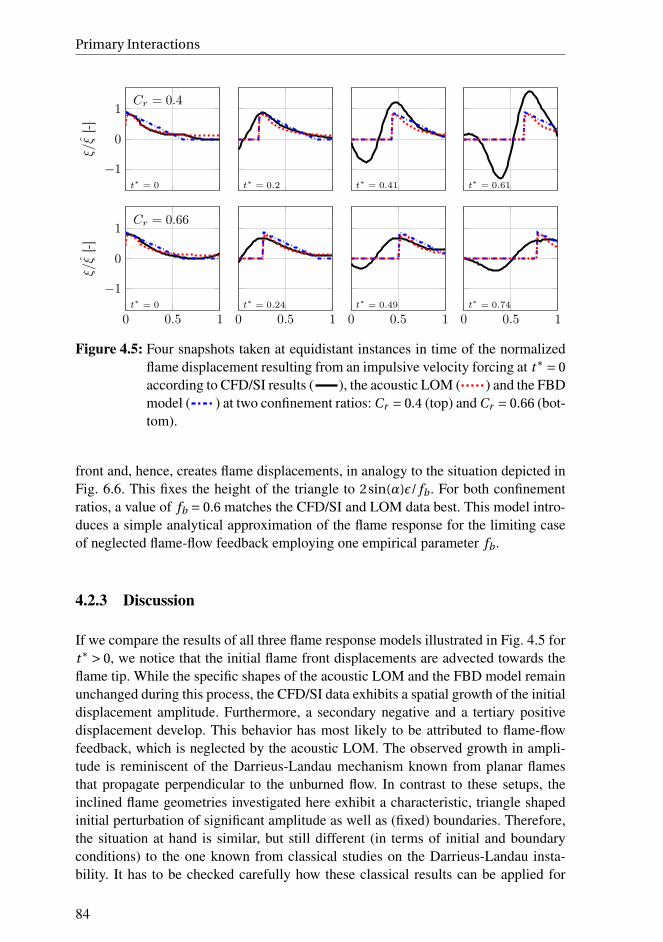
Primary Interactions

−1

0

1Cr = 0.4

t∗ = 0

ξ/ξ

[-]

t∗ = 0.2 t∗ = 0.41 t∗ = 0.61

0 0.5 1

−1

0

1Cr = 0.66

t∗ = 0

ξ/ξ

[-]

0 0.5 1

t∗ = 0.24

0 0.5 1

t∗ = 0.49

0 0.5 1

t∗ = 0.74

Figure 4.5: Four snapshots taken at equidistant instances in time of the normalizedflame displacement resulting from an impulsive velocity forcing at t∗ = 0

according to CFD/SI results ( ), the acoustic LOM ( ) and the FBDmodel ( ) at two confinement ratios: Cr = 0.4 (top) and Cr = 0.66 (bot-tom).

front and, hence, creates flame displacements, in analogy to the situation depicted inFig. 6.6. This fixes the height of the triangle to 2sin(α)ǫ/ fb . For both confinementratios, a value of fb = 0.6 matches the CFD/SI and LOM data best. This model intro-duces a simple analytical approximation of the flame response for the limiting caseof neglected flame-flow feedback employing one empirical parameter fb .

4.2.3 Discussion

If we compare the results of all three flame response models illustrated in Fig. 4.5 fort∗ > 0, we notice that the initial flame front displacements are advected towards theflame tip. While the specific shapes of the acoustic LOM and the FBD model remainunchanged during this process, the CFD/SI data exhibits a spatial growth of the initialdisplacement amplitude. Furthermore, a secondary negative and a tertiary positivedisplacement develop. This behavior has most likely to be attributed to flame-flowfeedback, which is neglected by the acoustic LOM. The observed growth in ampli-tude is reminiscent of the Darrieus-Landau mechanism known from planar flamesthat propagate perpendicular to the unburned flow. In contrast to these setups, theinclined flame geometries investigated here exhibit a characteristic, triangle shapedinitial perturbation of significant amplitude as well as (fixed) boundaries. Therefore,the situation at hand is similar, but still different (in terms of initial and boundaryconditions) to the one known from classical studies on the Darrieus-Landau insta-bility. It has to be checked carefully how these classical results can be applied for

84

4.2 Irrotational and Vortical Response Analysis

0

1

2

3

Magnitude

0 1 2 3 4

-12π

-8π

-4π

0

f∗ [-]

Phase

0 0.5 1 1.5 2

−6

−3

0

3

6

t∗ [-]

h∗

(a) Cr = 0.4

0

0.5

1

1.5

Magnitude

0 1 2 3 4

-12π

-6π

0

f∗ [-]

Phase

0 0.5 1 1.5 2

−2

−1

0

1

2

3

t∗ [-]

h∗

(b) Cr = 0.66

Figure 4.6: IR and FR in terms of gain and phase for Cr = 0.4 (left) and Cr = 0.66

(right). Shown are results from CFD ( ), the FBD model for fb = 0.6

( ) and the acoustic LOM ( ). Additionally, results from harmonicforcing of the acoustic LOM are included, split into irrotational ( ) anda vortical ( ) contributions.

Bunsen-type flames, which will be analyzed in more detail in Chap. 5.

Comparing the transient behavior of the Cr = 0.4 to the Cr = 0.66 setup, a weakergrowth of the initially caused flame displacements can be observed for the latter.It seems that the presence of a confinement delimits the possible displacement am-plitudes. Based on the analysis presented in this chapter, which neglects flame-flowfeedback, the detailed mechanisms responsible for this behavior cannot be analyzed,though. In Fig. 4.5 it can be seen that the resulting non-dimensional initial displace-ments as well as the velocity of convection match the CFD data very well.

Based on the results shown in Fig. 4.6, flame-flow feedback is supposed to have a ma-jor impact onto the response of the global heat release rate. One of the most prominentdiscrepancies constitutes the damped oscillatory behavior of the IR predicted by theCFD/SI data ( ), especially for the wide confinement case (Cr = 0.4). Here, theacoustic LOM only captures the first peak of this curve, significantly underestimat-ing the amplitude. The subsequent positive and negative peaks are not captured atall. In the frequency domain, the damped oscillatory behavior manifests itself as avery high peak gain value at a Strouhal number approximately corresponding to theoscillation frequency. The acoustic LOM, on the other hand, results in a frequencyresponse resembling the gain behavior of a first-order low-pass filter. The almost lin-early decaying phase is captured well by all models.

85

Primary Interactions

The agreement between the acoustic LOM and the CFD/SI data is better for the nar-row confinement configuration (Cr = 0.66). Here, the first peak of the IR is capturedreasonably well. In contrast to the Cr = 0.4 case, the IR exhibits a relatively high levelaround t∗ = 0, which cannot be observed in the CFD/SI data. Hence, the initial dis-placement at the flame tip is overpredicted, which is also seen in Fig. 4.5. The IR ofthe Cr = 0.66 setup shows less pronounced peaks and, thus, the associated FR showsa reduced peak gain value compared to the Cr = 0.4 case.

Fig. 4.6 decomposes the frequency response of the acoustic LOM into its irrotational( ) and vortical ( ) contributions. The individual frequency response data is gainedfrom harmonic simulations, as depicted in Fig. 4.2. The fact that the former matchesthe results gained from the impulsively forced configuration ( ), very well cross-validates both approaches. The weak response of the vortical contribution confirmsthe finding that vortex shedding can be safely neglected.

Finally, an analytical prediction of the response of the FBD model introduced inEq. (4.2) is provided. Its impulse response writes

h∗FBD(t ) = t∗−1+ fb

2 f 2b

[Θ(t∗−1+ fb)−Θ(t∗−1)

](4.3)

with the Heaviside Theta function Θ(t ). The associated FR can be mapped to fre-quency domain by use of Tab. C.2. Following Fig. 4.6, this model captures the over-all trend of the acoustic LOM model well. Due to the fact that flame-flow feedbackhas such an important influence onto the flame response, it can only be used to esti-mate the cut-off frequency or the phase behavior, but not the gain around a Strouhalnumber of approximately unity. In this regard it is much simpler to evaluate than thepresented acoustic LOM, while it still captures the essential effects.

4.3 Summary and Conclusions

The response of laminar premixed flames stabilized at a backward-facing step to ve-locity perturbations was scrutinized. One goal was to test the hypothesis that shedvorticity contributes to the so-called convective velocity perturbations, which arean important, widely-used element of low-order flame response models. Analyticalmethods from aero-acoustics were combined with a flow decomposition approach toquantify the respective contributions of the irrotational and the vortical parts of thedisturbance velocity field to the overall flame transfer function (FTF). The completeset of equations derived in Chap. 3 capturing the flow field dynamics of acousticallyperturbed flames was used, however, exothermic effects, in particular the effect offlame displacement and wrinkling on the upstream velocity, were neglected in thisstudy.

For the cases considered — a Slit flame geometry with a Péclet number of Pe= 223,an expansion ratio of e ≈ 6.7 and confinement ratios Cr = 0.4 and 0.66 — the ir-

86

4.3 Summary and Conclusions

rotational part was shown to dominate the flame displacement, which is most pro-nounced at and near the flame anchoring point. Correspondingly, a flame base dis-placement (FBD) model was proposed, which captures the early part of the impulseresponse well, particularly for high confinement ratios. Discrepancies for later timesand for low confinement ratios were attributed to exothermic flame-flow-flame feed-back mechanisms not taken into account by the low-order modeling approach. Forthe configurations investigated, vortex shedding is found to only have a negligibleimpact on the flame response.

The main findings of the present analysis are:

1. Vortex shedding due to an oscillatory flow in the vicinity of a sharp corner isfound to have only negligible impact on the flame response.

2. Hence, the shedding of vorticity was ruled out as a possible candidate to phys-ically justify the assumption of convected velocity perturbations as a source offlame wrinkling. Consequently, one must conclude that models based on thisassumption do not faithfully represent acoustics-flame-flow interactions.

3. The irrotational part of an acoustic perturbation essentially interacts with theflame base region, which is captured by an analytical model proposed in thisstudy, namely, the FBD model.

Flame-flow feedback is supposed to have a substantial impact on the flame response,particularly, at Strouhal numbers of order O (1). It might lead to rather high and dis-tinct peaks in the gain of an FTF, particularly, for high confinement ratios. This willbe analyzed in more detail in the next chapter.

87

Primary Interactions

88

5 Secondary Interactions

The previously introduced low-order modeling framework is ex-

tended such that it can cope with two important types of flame-flow

feedback: (i) vortical flame-flow feedback resulting from flame gen-

erated vorticity and (ii) irrotational flame-flow feedback resulting

from a flame normal acceleration of the flow across a flame sheet.

Both contribute to the convective growth of flame sheet disturbances

and account for the appearance of FTF gain values exceeding unity

as well as convected velocity perturbations upstream a perturbed

flame.

In the previous chapter, interactions of acoustic perturbations and burner-stabilizedSlit flames were analyzed in the limit of negligible flame-flow feedback (no gas ex-pansion) and flame stretch (constant flame speed). While the latter is expected todampen flame front displacements (Le>Lec,TD), flame-flow feedback leads to con-vective growth of flame perturbations (e > 1). Consequently, the observed significantdiscrepancy between the low-order model developed in the previous chapter and highfidelity CFD data was attributed to flame-flow feedback. This hypothesis shall be an-alyzed in more detail in the following.

In order to clarify the discussion, we want to agree upon the terminology first. Theterm “secondary interactions” has already been specified before and refers to phe-nomena/flame displacements, which are not directly caused by acoustic perturba-tions, but by incompressible flame intrinsic processes. It can be distinguished mosteasily between primary and secondary interactions for the case of impulsively forcedflames, since any change in flame shape occurring after an acoustic impulse has hitthe flame (t > 0) is subsumed as a secondary interaction (except advection). In prin-ciple, all phenomena discussed in Chap. 1 governing the dynamics of a flame sheetare potentially important here. It was observed in the previous chapter by inspectinghigh fidelity CFD data that the primary displacement, caused by acoustics, grows inamplitude and, additionally, secondary displacements develop. Such a growth is thesignature of a hydrodynamic mechanism, described in Sec. 1.2.3, which is sometimesalso referred to as the Darrieus-Landau mechanism. It arises due to interactions ofthe flow field with the flame sheet, captured by a set of jump conditions. It is drivenby the change in specific volume across the flame, i. e. it is a consequence of gasexpansion. Hence, this phenomenon relies on flame-flow feedback.

89

Secondary Interactions

The role of flame-flow feedback for the (linear) response has already been pointedout by some previous studies. Already Baillot et al. [120] attributed the occurrenceof convected flow perturbations upstream a wrinkled flame front to the “retroactive

hydrodynamic effects of the flame on the flow of the unburned gases” (Baillot et al.

[120], p. 164). This was later confirmed by Birbaud et al. [136], who conducted aseries of demonstrative experiments. Blanchard et al. [129] numerically showed thata perturbed flame sheet acts as a vortex sheet whose upstream influence contributesto the formation of axially convected velocity perturbations. They related this phe-nomenon to the Darrieus-Landau mechanisms. The relevance of this hydrodynamicmechanism for the flame response of perturbed burner-stabilized flames was furtherconfirmed by the studies of Hemchandra [103] and Schlimpert et al. [104]. Both re-ported a strong impact of hydrodynamic mechanisms leading to the spatial growth offlame front perturbations. Hemchandra [103] conjectured that this mechanism maybe responsible for the occurrence of high FTF gains exceeding unity.

Flow instabilities often trigger the development of large coherent structures. In conse-quence, characteristic flow features develop, which have important consequences fortechnical applications. Oberleithner et al. [79] as well as Oberleithner and Paschereit[80] found for swirl-stabilized flames that the gain of the flame response scaleswith stability properties of the respective shear layers. According to these studies, aKelvin–Helmholtz-type hydrodynamic instability triggered by acoustic perturbationsleads to the formation of large scale coherent structures that interact with the flameand, thus, provoke fluctuations of the global heat release rate. Similar to flames, shearlayers (or vortex sheets) can be idealized as discontinuities. While flame related dis-continuities exhibit jumps in normal and tangential velocity, shear layers only showchanges in tangential velocity. In their most idealized versions, both entities are un-conditionally (convectively) unstable [180, 194] and may hence both contribute tothe formation of coherent structures that may impact the flame response. Hence, theDarrieus-Landau mechanisms or instability should be analyzed in more detail andclearly demarcated from shear layer instabilities. As a first step, flame-flow feedbackrelated mechanism will be analyzed for laminar flames in this chapter.

Although thermal-diffusive mechanisms might have a crucial impact on secondaryacoustics-flame interactions, as well, the following discussion focuses on the hy-drodynamic ones. They are the drivers for all observable secondary phenomena,while thermal-diffusive mechanisms only exert a damping influence (assuming leanmethane-air flames). It can already be anticipated that a consideration of drivingmechanisms will create a need for damping and, therefore, displacement amplitudesare likely to be overestimated if damping mechanisms are neglected. It will be shownin the course of this chapter that this expectation is true indeed, however, this point isbeyond the scope of this work and shall be left for succeeding studies. This chapterstrives to take one step forward towards a comprehensive understanding of the flamedynamics by assessing mechanisms that provoke the convective growth of flame frontperturbations. These mechanisms are expected to be associated with flame-flow feed-back.

90

5.1 Flame Response Revisited in the Light of Flame-Flow Feedback

In a first step, Sec. 5.1 revisits flame response predictions from high fidelity CFDsimulations as well as from low-order models relying on convected velocity pertur-bations in the light of flame-flow feedback. Section 5.2 then shows how flame-flowfeedback is integrated into the modeling framework introduced in Chap. 3. Finally,Sec. 5.3 discusses and analyzes flame response predictions computed with this newframework and compares them to high fidelity CFD simulations.

5.1 Flame Response Revisited in the Light of Flame-Flow

Feedback

As already discussed in Chap. 2, the understanding and modeling of interactions be-tween acoustics and burner stabilized flames often relies on the notion of convectedvelocity perturbations. Conversely, in the case of flames whose anchoring is mechan-ically displaced, it essentially follows the concepts of flame-sheet dynamics outlinedin Chap. 1. Based on this point of view, flame-flow feedback — namely the hydro-dynamic mechanism explicated in Sec. 1.2.3 — is not explicitly considered in theanalysis of acoustically perturbed flames. Nevertheless, it is implicitly contained inthe models since, according to the literature [120, 129, 136], the observed convectedperturbations are supposed to be induced by the upstream influence of a wrinkledflame. In the following, the response of acoustically perturbed flames is revisited fo-cusing on consequences of flame-flow feedback. The goal is to provide links betweenthe notion of convected velocity perturbations and the dynamics of flames driven bygas expansion.

To this end, high fidelity CFD data is evaluated in Sec. 5.1.1. Special focus is puton how the impulse response is linked to the flame sheet dynamics and how strongthe expected effects of flame-flow feedback are. This provides further evidence forthe conjecture made in Chap. 4, which states that the oscillatory nature of the IRand the high gain values are caused by gas expansion driven flame-flow feedback.Subsequently, the convective velocity model is revisited in Sec. 5.1.2 and analyzed inthe light of these findings.

5.1.1 High Fidelity CFD/SI Data

The snapshots shown in Fig. 4.5 ( ), which are taken from high fidelity CFD data,clearly indicate convectively growing flame displacements amplitudes. Furthermore,three distinct positive and negative peaks emerge in the final snapshot, although —following the analysis of Chap. 4 — acoustics caused only one of them directly (theone at t∗ = 0). Consequently, the other peaks have to be caused by flame sheet in-trinsic mechanisms. Flame-flow feedback due to exothermic gas expansion is onepromising candidate for such a mechanism, since it was explicitly neglected in thelow-order modeling approach analyzed in the previous chapter, see Fig. 4.5 ( ).

91

Secondary Interactions

Figure 5.1: Top: Impulse responses for the Cr = 0.4 ( ) configuration depictedin Fig. 4.1 (but with TBP = 700 K). Instants in time corresponding toone of the snapshots shown in the bottom blot are marked by verticallines. Bottom: Consecutive snapshots of the normalized flame-normalflame front displacement caused by an impulsive acoustic forcing of aflame setup with Cr = 0.4 ( ). Depicted are five instants in time, wheret1 matches the time the acoustic impulse hits the flame. Primary andsecondary peaks in flame shape are marked by colored dots.

It is shown in Appendix. A.3 that the global heat release signal of a flame subjectedto an impulsive forcing (Fig. 4.5; ) coincides well with the IR identified frombroad band data for all analyzed setups (Fig. 4.6; ). Consequently, the analysisof the flow field and flame dynamics resulting from an impulsive forcing providesvaluable physical insights into the linear flame dynamics. In order to relate the flamedisplacement data with the respective IR, it is necessary to know how the global heatrelease rate is linked to flame sheet displacements. As will be detailed in Chap. 6, inthe limit of stiffly anchored Slit flames, the linear dynamics of the global heat releaserate depends only on the displacement of the flame tip. That means, the heat releaserate stays constant as long as the flame tip is not perturbed.

Exploiting this relation, Fig. 5.1 compares the IR of the Slit flame configuration tothe associated flame front displacements1. At the very moment the acoustic impulsehits the flame (t = 0), the flame front is displaced in the previously described triangle-like manner and a primary displacement peak is formed. At this time, the IR of theglobal heat release rate h∗ shows no signal since the flame tip was not displaced.

1The data shown corresponds to the same setup as discussed in Chap. 4, only the temperature ofthe anchoring wall is changed to TBP = 700 K. As discussed in App. B, this hardly affects the overallcharacteristics of the flame response, which allows to directly compare both setups.

92

5.1 Flame Response Revisited in the Light of Flame-Flow Feedback

0 0.25 0.5 0.75 1

-4

0

4σ ≈ −1.22 1

s

xF1 /Lf

ξ/ξ

Cr = 0.66

0 0.25 0.5 0.75 1

σ ≈ 86.9 1

s

xF1 /Lf

Cr = 0.40

0 0.25 0.5 0.75 1

σ ≈ 1221

s

xF1 /Lf

Cr = 0.17

Figure 5.2: Normalized flame displacements shown for three confinement ratios cor-responding to the cases shown in Fig. 5.1. Additionally, a case withCr = 0.17 is added. The thick black line signifies the displacement im-mediately caused by an impulsive velocity forcing of the flame and thegray lines its subsequent spatio-temporal development. The primary pos-itive displacement peak is tracked and marked in each time step ( ).Similarly, the positive and negative secondary peaks are tracked ( ).An exponential function is fitted to the spatial trace of the primary peak( ) and from it a temporal growth rate σ is computed.

Only around t3 (Cr = 0.4; ) the heat release rate starts to increases, which corre-sponds to the time the initially created primary displacement reaches xF

1 /L f = 1. Ac-cordingly, the subsequent negative secondary displacements causes the heat releaseto decrease to negative values at t4. We note that (i) the convective growth of flamefront displacements directly leads to higher peak values of the associated IR and (ii)the presence of the numerous positive and negative displacement peaks of decreasingamplitude is responsible for the damped oscillatory IR behavior. Those two observa-tions are supposed to be caused by flame-flow feedback and shall be quantified in thefollowing.

To this end, the spatial growth of the convected displacement peaks is evaluated.Fig. 5.2 combines several snapshots of the displaced flame front at different instantsin time in one single plot (thick black line for t∗ = 0 and gray lines for t∗ > 0). Ad-ditionally, for each snapshot, the maximum of the primary displacement — causedby acoustics at t∗ = 0 — is marked by a green circle ( ). The subsequently devel-oping first two positive and negative secondary peaks are marked by orange circles( ). Due to the fact that all of these maxima are convected downstream towardsthe flame tip at xF

1 /L f = 1, their traces form lines of growing amplitude. Assumingthis growth is governed by linear dynamics (no sharp edges in concave regions!) andthe initial shape approximately resembles a sine (see particularly the shapes at t ≥ t2

in Fig. 5.1), the growth should be exponential. Fitting an exponential function to thedistribution of the primary peaks, a spatial growth rate σx is computed. In order toavoid to capture anchoring and tip related effects, points close to one of these twoexceptional points are excluded from the respective data sets. By use of the advection

93

Secondary Interactions

velocity u∥, these spatial growth rates can be converted to temporal ones via σ=σx u∥[63, 66].

Before the results of this kind of analysis are discussed, it should be emphasized thatimpulsively forced data is used here. Such kind of analysis, however, is usually per-formed based on harmonically forced data, see for example Truffaut and Searby [66].Assuming that harmonic forcing also results in harmonic flame sheet perturbationsof a single wave number, growth rates can be evaluated for each wave number sep-arately. Repeating this for several frequencies, samples of the underlying dispersionrelation are computed. Imposing an impulsive acoustic forcing excites perturbationsof several wave numbers at the same time, see the triangle-shaped initial displace-ment shown in Fig. 5.1. Subsequently, each excited wave number perturbation willindependently grow in amplitude at a rate given by the underlying dispersion relation(we assume we are still in the linear regime). This means that the flame displace-ments shown in Fig. 5.1 are a superposition of all of these individual perturbations.Therefore, the computed overall growth rate can not directly be related to frequency-specific growth rates of the associated dispersion relation. Nevertheless, the displace-ments resembles a sine-like shape already in the second snapshot (t2). Therefore, itis possible to get, at least, a rough idea of the order of magnitude of the maximallyexpected growth rates from impulsively forced data. In the scope of this section, thisshall be sufficient.

Evaluating the temporal growth rates σ for three confinement ratios in Fig. 5.1, it isfound that they strongly depend on confinement ratio. While the growth of displace-ments is suppressed at the narrowest confinement, it reaches a value of about 120 1/s

for Cr = 0.17. In order to put this number into perspective, it is non-dimensionalizedby the flame transition time τt = δD /sL to στt = 0.038. Truffaut and Searby [66] ex-perimentally determined non-dimensional growth rates between approximately 0.03

and 0.09 for rich propane-air flames stabilized at a harmonically displaced rod, seeFig. 1.4. The order of magnitude of their results is hence the same as the ones ob-tained here. Further, Truffaut and Searby [66] attributed the observed growth to theDarrieus-Landau mechanism, which is denoted as the hydrodynamic mechanism inChap. 1. This provides evidence that similar, flame-flow feedback related processesare at work for the configurations studied in this thesis. For future studies it shouldbe kept in mind that displacement amplitude growth rates may significantly be influ-enced by lateral constraints of the flow, such as a confinement.

5.1.2 Convective Velocity Model

If flame-flow feedback really has the decisive impact on the flame dynamics as as-serted above, why is it possible that G-equation based approaches relying on convec-tive velocity models, which do not explicitly account for flame-flow feedback, arecapable of correctly reproducing essential aspects of the dynamics of acousticallyperturbed flames? The answer is that they implicitly do, which is analyzed in the

94

5.1 Flame Response Revisited in the Light of Flame-Flow Feedback

Figure 5.3: Normalized flame front displacements as predicted by the uniform (top)and the incompressible convective (middle and bottom) velocity modelfor a harmonic velocity forcing at a Strouhal number of ω∗ = 5 (top andmiddle) and one of ω∗ = 20 (bottom).

following.

Having a closer look at the convective velocity model of Eq. (2.5), one recognizesthat this model indeed leads to a spatial growth of flame front displacements. This isillustrated in Fig. 5.3, which shows the response of a flame front exposed to harmonicvelocity forcing at a fixed frequency according to the 1D linearized G-equation ap-proach introduced in Sec. 1.3.2. Three response predictions are shown for two veloc-ity models and two Strouhal numbers. While, for a Strouhal number of 5, the uniformvelocity model of Eq. (2.4) (Fig. 5.3, top) shows a constant amplitude of the wrin-kled flame surface, the incompressible convective velocity model (Fig. 5.3, middle)exhibits a clear spatial growth of the respective flame front displacements. Hence,the convected velocity perturbation mimics the effects of flame-flow feedback, whichexplains their agreement with experimental data.

At a Strouhal number of 20, however, the spatial distribution of displacement am-plitudes grows only up to xF

1 /L f & 0.5 and subsequently decreases again. Overall,a low frequency modulation on top of a high frequency oscillation becomes visible(Fig. 5.3, bottom), which is also known as a beat. This might explain the decreas-ing predictive capabilities of such models at high frequencies, which was reportedby Cuquel et al. [161]. But even at sufficiently low frequencies, the model deviatesfrom a realistic behavior. Theoretically, it is possible to evaluate spatial growth ratesrelying on a convective velocity model by post-processing displacement predictionsas the one shown in Fig. 5.3, middle. Doing this for several forcing frequencies, thiswill eventually result in a dispersion relation that, ideally, coincides at low frequen-cies with the realistic flame sheet behavior. If that is true, we can expect that the con-vective velocity predicts the actual acoustic flame response very well. The study ofKashinath et al. [167], however, suggests that convective velocity models do not cap-ture the real physical behavior. In this work, the authors fitted the convection speedof the velocity perturbations to high fidelity CFD data and found a significant de-pendency of this speed to frequency. Knowing that this speed influences the resultinggrowth rates, their study indicates that the dispersion relation naturally resulting from

95

Secondary Interactions

a convective model does not agree with the one of the underlying physical process,but requires a non straight forward fitting procedure.

It can be concluded that models relying on convected velocity perturbation mimicthe flame-flow feedback related spatial growth of displacement amplitudes, however,only up to a certain frequency. Furthermore, the associated (theoretical) dispersionrelation of these kind of models does in general not reproduce the real physical be-havior.

5.2 Modeling of Flame-Flow Feedback

The previous section pointed out the importance of flame-flow feedback by analyzinghigh fidelity CFD data. Furthermore, hints of such a feedback were found in theconvective velocity model, which is commonly applied in G-equation based modelingapproaches. Motivated by these findings, the goal of this section is to integrate flame-flow feedback into the modeling framework introduced in Chap. 3 such that it can beused to analyze its impact on the linear flame response.

According to the concepts outlined in Chap. 1, flame-flow feedback is a hydrody-namic mechanism related to density changes across the flame sheet. It necessarilyresults in the unconditional growth of flame front displacements, if it is not stabilizedby thermal-diffusive mechanisms [44]. Following the analysis of Darrieus and Lan-dau, in the framework of gasdynamic discontinuities, this growth emerges from thejump conditions of mass and momentum across the flame. Hence, it can be expectedthat analyzing these conditions in more detail contributes to the understanding of thebasic mechanisms at play.

Having done this, it should be possible to integrate gas expansion into the existingmodeling framework of Chap. 3. It explicitly appears at two positions, (i) as volumesource in the gas expansion related flow component ue of Eq. (3.13) and (ii) in form ofa density gradient in the baroclinic source term of the vorticity transport equation, i. e.Eq. (3.9). The modeling concept proposed in this section concerning point (i) relieson the specification of a volume production kernel. This kernel function distributesthe volume produced by the flame in space and serves as a source to the gas expansionrelated flow field component ue . Based on a study conducted by Zimmermann [195],a Gaussian kernel function will be introduced. Concerning the modeling concept forthe baroclinic source term, see point (ii), it will be shown that a candidate for such aconcept can be derived from the analysis of the jump conditions.

Following these ideas, Sec. 5.2.1 derives and analyzes a set of jump conditions,including and excluding flame stretch effects, respectively. Based on these results,Sec. 5.2.2 introduces a concept for how flame generated (baroclinic) vorticity can beincluded into the modeling framework. Finally, a kinematic modeling approach ofgas expansion is introduced in Sec. 5.2.3.

96

5.2 Modeling of Flame-Flow Feedback

5.2.1 Jump Conditions Across a Flame Sheet

In the subsequent analysis it is assumed that the fluxes of mass and momentumthrough the flame front are constant, i. e. the fluxes of mass, normal and tangentialmomentum are conserved across the flame sheet

[m]bu = 0, [p +mui ni ]b

u = 0, [mui ti ]bu = 0, (5.1)

where ui , ni and ti denote the i -th component of the flow velocity, the local flamenormal and flame tangential vectors, respectively. Further, the Einstein summationconvention is employed and m = ui ni −∂ξ∂t denotes the local mass flux across theflame sheet. This essentially follows the original ideas of Landau [27] and Markstein[44], who derived the set of jump conditions shown in Eq. (1.7). All of the relationsshown below are derived from the formulation of the fluxes as they are stated inEq. (5.1). They are evaluated right at the mean flame position, which is, per definition,fixed in space and time. This simplification imposes an error that scales with thedisplacement amplitude and the inverse of the perturbations wave length.

A flame aligned coordinate system [x1, x2] as depicted in Fig. 1.9b is assumed. Themean flow field in which a freely propagating flame sheet is stabilized points towardsthe positive x2-direction. Application of the jump conditions Eq. (5.1) requires thecomputation of the velocity components tangential and normal to the flame front.The linear analysis presented in the following shall be limited to perturbation wavelengths λ that are long compared to the convective-diffusive length scale δD in orderto avoid the occurrence of significant levels of flame stretch and to not trigger sig-nificant 2D effects. Mathematically, this fact is reflected by limiting the analysis tolarge Péclet numbers Pe= δD /λ. Furthermore, flame displacement amplitudes shallbe small, that is ξ≪λ. We assume ξ=O (ǫ), where ǫ may be a small quantity, suchthat all terms O

(ǫ2

)are negligible. Accordingly, they are dropped in the following

analysis. Developing all quantities in powers of Pe−1 shifts perturbations that exhibita short wave length compared to the flame thickness to higher order terms in the ex-pansion parameter. Based on this expansion, only zeroth order terms are consideredin the following. Using this method, the flame normal and tangential vectors resultingfrom the perturbed flame are given by

n f =[n f ,1,n f ,2

]=

[− ∂ξ

∂x1,1

]+O

(Pe−1

)and t f =

[t f ,1, t f ,2

]=

[1,

∂ξ

∂x1

]+O

(Pe−1

),

(5.2)respectively.

A perturbed flame sheet goes along with perturbations of all other flow vari-ables, that is velocity and pressure. Assuming a flow field of the fresh mixtureuu = [u′

u,1,uu,2 +u′u,2]+O

(Pe−1

), the flame normal and tangential velocity compo-

nents just upstream of the flame sheet can be computed from n f ,i uu,i and t f ,i uu,i ,which results in

uu,⊥ = uu,2 +u′u,2 +O

(Pe−1

)and uu,∥ = uu,2

∂ξ

∂x1+u′

u,1 +O(Pe−1

), (5.3)

97

Secondary Interactions

respectively. Using these equations together with Eq. (5.1), we get for the mean quan-tities

[u2

]bu = s0

LE (5.4)[p

]bu = −(s0

L)2ρuE (5.5)[u1

]bu = 0, (5.6)

where the assumption of a stationary flame front of the unperturbed flow requiresuu,2 = s0

L and E = ρu/ρb −1 denotes the non-dimensional increase of specific volume.Hence, across the flame front the flow is accelerated by a factor e = (E +1) in x2-direction and the static pressure decreases by a term (s0

L)2ρuE . Application of thejump conditions for the perturbed flow field results in

[u′

2

]bu = E

(u′

u,2 −∂ξ

∂t

)+O

(Pe−1

)(5.7)

[p ′]b

u = −2ρu s0L

[u′

2

]bu +O

(Pe−1

)(5.8)

[u′

1

]bu = −s0

LE∂ξ

∂x1+O

(Pe−1

), (5.9)

while the equation governing the kinematics of the flame sheet sL = uu,⊥−∂ξ/∂t

leads to

u′u,2 −

∂ξ

∂t= sL −uu,2 +O

(Pe−1

). (5.10)

Neglecting Flame Stretch

When Landau [27] assessed the stability of planar flames, he assumed a constantflame speed sL = s0

L +O(Pe−1

)and, thus, neglected stretch effects. Note that this as-

sumption is perfectly in line with the neglect of terms that are of higher than zerothorder in 1/Pe. Inserting the constant flame speed assumption into Eqs. (5.7)–(5.9),the jump conditions write

[u′

2

]bu =O

(Pe−1

),

[p ′]b

u =O(Pe−1

)and

[u′

1

]bu =−s0

LE∂ξ

∂x1+O

(Pe−1

).

(5.11)From Eq. (5.10) it follows that the flame front moves in response to upstream velocityperturbations according to ∂ξ/∂t = u′

u,2 +O(Pe−1

). While pressure and flame-normal

velocity fluctuations are continuous across the flame, flame-tangential velocity per-turbations change, as stated by Eq. (5.11).

Considering Flame Stretch

Now consequences of flame stretch shall be investigated by including terms up toO

(Pe−1

)to the analysis. As already mentioned in Sec. 1.2.3, in the limiting case of

98

5.2 Modeling of Flame-Flow Feedback

high activation energies of the global reaction, this shall only add a new stretch de-pendent term to the flame speed relation, while the jump conditions Eqs. (5.7)–(5.9)remain the same. This approximation is in line with the phenomenological stretch-related correction of Markstein [44] and justified by the strong dependency of theflame speed to temperature in the case of a high activation energy of the global reac-tion [42].

Assuming that the Markstein number for flow strain and flame curvature is the same,the equation for the flame speed writes

sL = s0L (1− lMκs) (5.12)

with the Markstein length lM and the flame stretch κs . Using this relation togetherwith Eq. (5.10) we get

u′u,2 −

∂ξ

∂t=−lMκs . (5.13)

This extended relation of the flame sheet kinematics is now inserted to the jumpconditions Eqs. (5.7)–(5.9) and we obtain

[u′

2

]bu = −E lMκs (5.14)

[p ′]b

u = −2ρu s0L

[u′

2

]bu (5.15)

[u′

1

]bu = −s0

LE∂ξ

∂x1. (5.16)

While the jump conditions (5.16) for the tangential velocity u′1 remain unchanged

compared to the case without flame stretch, the other two now contain flame stretchrelated quantities. These new terms reflect the fact that changes in the flame speedaffect the local volume production per unit length m = E sL of the flame sheet, seeEq. (3.7). Hence, concave parts of the flame now produce more volume since theflame propagation speed is increased here, and vice versa for convex parts.

A stretch dependent flame speed, as expressed in Eq.(5.13), is one of the most impor-tant mechanisms that dampens flame front displacements by imposing flame speedvariation in convex/concave regions. Following the analysis conducted in Sec. 1.3.2,it has a diffusion-like effect on the flame dynamics. Consequently, sharp displace-ments are smeared in space.

5.2.2 Modeling of Flame Generated Vorticity

Based on the jump conditions derived in the previous section, a model for the pro-duction of vorticity by a perturbed flame sheet shall now be deduced. To this end, thejump in the tangential velocity component of Eqs. (5.9) or (5.16) is revisited, sinceit quantifies the amount of vorticity generated across the flame sheet. This can beshown by computing the circulation around a closed surface as depicted in Fig. 5.4.

99

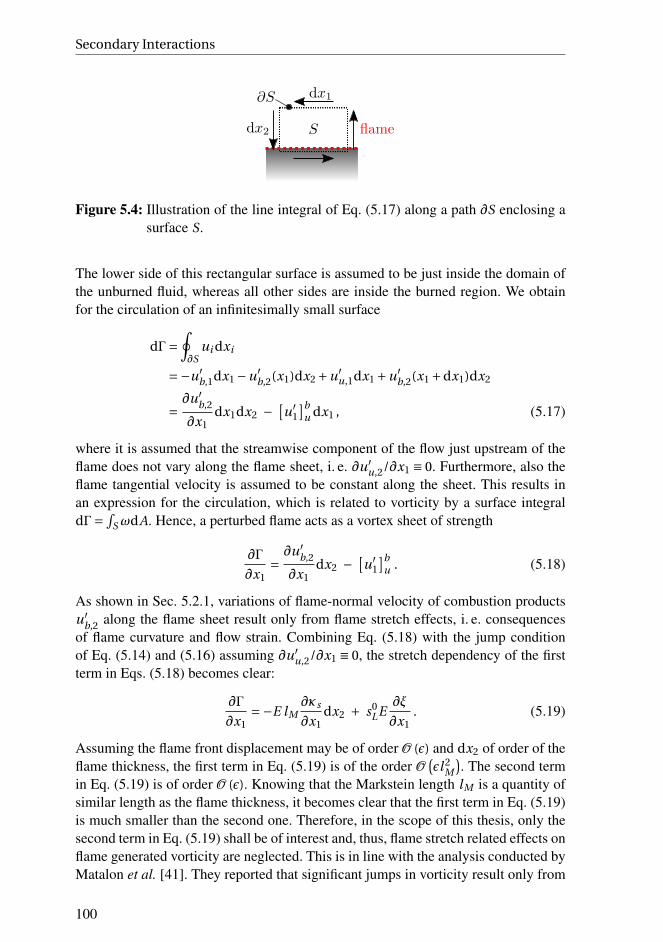
Secondary Interactions

Figure 5.4: Illustration of the line integral of Eq. (5.17) along a path ∂S enclosing asurface S.

The lower side of this rectangular surface is assumed to be just inside the domain ofthe unburned fluid, whereas all other sides are inside the burned region. We obtainfor the circulation of an infinitesimally small surface

dΓ=∮

∂Sui dxi

=−u′b,1dx1 −u′

b,2(x1)dx2 +u′u,1dx1 +u′

b,2(x1 +dx1)dx2

=∂u′

b,2

∂x1dx1dx2 −

[u′

1

]bu dx1 , (5.17)

where it is assumed that the streamwise component of the flow just upstream of theflame does not vary along the flame sheet, i. e. ∂u′

u,2/∂x1 ≡ 0. Furthermore, also theflame tangential velocity is assumed to be constant along the sheet. This results inan expression for the circulation, which is related to vorticity by a surface integraldΓ=

∫S ωdA. Hence, a perturbed flame acts as a vortex sheet of strength

∂Γ

∂x1=

∂u′b,2

∂x1dx2 −

[u′

1

]bu . (5.18)

As shown in Sec. 5.2.1, variations of flame-normal velocity of combustion productsu′

b,2along the flame sheet result only from flame stretch effects, i. e. consequences

of flame curvature and flow strain. Combining Eq. (5.18) with the jump conditionof Eq. (5.14) and (5.16) assuming ∂u′

u,2/∂x1 ≡ 0, the stretch dependency of the firstterm in Eqs. (5.18) becomes clear:

∂Γ

∂x1=−E lM

∂κs

∂x1dx2 + s0

LE∂ξ

∂x1. (5.19)

Assuming the flame front displacement may be of order O (ǫ) and dx2 of order of theflame thickness, the first term in Eq. (5.19) is of the order O

(ǫl 2

M

). The second term

in Eq. (5.19) is of order O (ǫ). Knowing that the Markstein length lM is a quantity ofsimilar length as the flame thickness, it becomes clear that the first term in Eq. (5.19)is much smaller than the second one. Therefore, in the scope of this thesis, only thesecond term in Eq. (5.19) shall be of interest and, thus, flame stretch related effects onflame generated vorticity are neglected. This is in line with the analysis conducted byMatalon et al. [41]. They reported that significant jumps in vorticity result only from

100

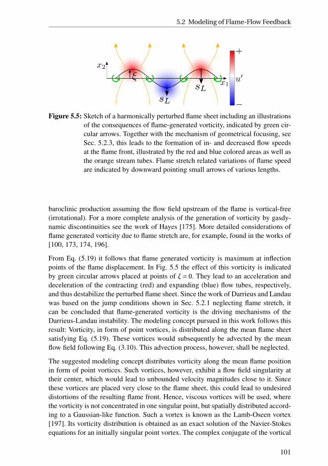
5.2 Modeling of Flame-Flow Feedback

Figure 5.5: Sketch of a harmonically perturbed flame sheet including an illustrationsof the consequences of flame-generated vorticity, indicated by green cir-cular arrows. Together with the mechanism of geometrical focusing, seeSec. 5.2.3, this leads to the formation of in- and decreased flow speedsat the flame front, illustrated by the red and blue colored areas as well asthe orange stream tubes. Flame stretch related variations of flame speedare indicated by downward pointing small arrows of various lengths.

baroclinic production assuming the flow field upstream of the flame is vortical-free(irrotational). For a more complete analysis of the generation of vorticity by gasdy-namic discontinuities see the work of Hayes [175]. More detailed considerations offlame generated vorticity due to flame stretch are, for example, found in the works of[100, 173, 174, 196].

From Eq. (5.19) it follows that flame generated vorticity is maximum at inflectionpoints of the flame displacement. In Fig. 5.5 the effect of this vorticity is indicatedby green circular arrows placed at points of ξ= 0. They lead to an acceleration anddeceleration of the contracting (red) and expanding (blue) flow tubes, respectively,and thus destabilize the perturbed flame sheet. Since the work of Darrieus and Landauwas based on the jump conditions shown in Sec. 5.2.1 neglecting flame stretch, itcan be concluded that flame-generated vorticity is the driving mechanisms of theDarrieus-Landau instability. The modeling concept pursued in this work follows thisresult: Vorticity, in form of point vortices, is distributed along the mean flame sheetsatisfying Eq. (5.19). These vortices would subsequently be advected by the meanflow field following Eq. (3.10). This advection process, however, shall be neglected.

The suggested modeling concept distributes vorticity along the mean flame positionin form of point vortices. Such vortices, however, exhibit a flow field singularity attheir center, which would lead to unbounded velocity magnitudes close to it. Sincethese vortices are placed very close to the flame sheet, this could lead to undesireddistortions of the resulting flame front. Hence, viscous vortices will be used, wherethe vorticity is not concentrated in one singular point, but spatially distributed accord-ing to a Gaussian-like function. Such a vortex is known as the Lamb-Oseen vortex[197]. Its vorticity distribution is obtained as an exact solution of the Navier-Stokesequations for an initially singular point vortex. The complex conjugate of the vortical

101

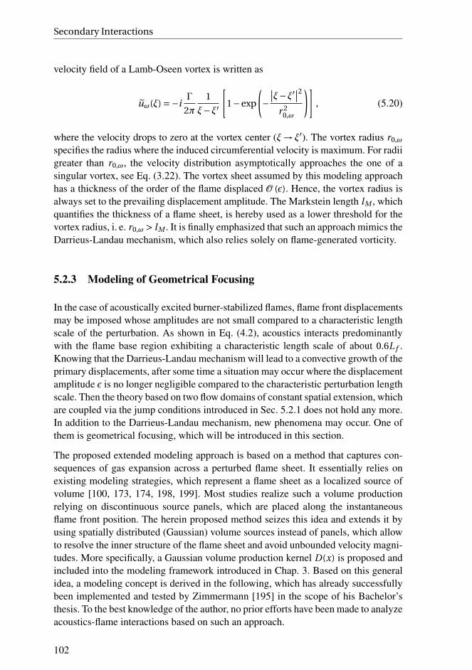
Secondary Interactions

velocity field of a Lamb-Oseen vortex is written as

uω(ξ) =−iΓ

2π

1

ξ−ξ′

[1−exp

(−

∣∣ξ−ξ′∣∣2

r 20,ω

)], (5.20)

where the velocity drops to zero at the vortex center (ξ→ ξ′). The vortex radius r0,ω

specifies the radius where the induced circumferential velocity is maximum. For radiigreater than r0,ω, the velocity distribution asymptotically approaches the one of asingular vortex, see Eq. (3.22). The vortex sheet assumed by this modeling approachhas a thickness of the order of the flame displaced O (ǫ). Hence, the vortex radius isalways set to the prevailing displacement amplitude. The Markstein length lM , whichquantifies the thickness of a flame sheet, is hereby used as a lower threshold for thevortex radius, i. e. r0,ω > lM . It is finally emphasized that such an approach mimics theDarrieus-Landau mechanism, which also relies solely on flame-generated vorticity.

5.2.3 Modeling of Geometrical Focusing

In the case of acoustically excited burner-stabilized flames, flame front displacementsmay be imposed whose amplitudes are not small compared to a characteristic lengthscale of the perturbation. As shown in Eq. (4.2), acoustics interacts predominantlywith the flame base region exhibiting a characteristic length scale of about 0.6L f .Knowing that the Darrieus-Landau mechanism will lead to a convective growth of theprimary displacements, after some time a situation may occur where the displacementamplitude ǫ is no longer negligible compared to the characteristic perturbation lengthscale. Then the theory based on two flow domains of constant spatial extension, whichare coupled via the jump conditions introduced in Sec. 5.2.1 does not hold any more.In addition to the Darrieus-Landau mechanism, new phenomena may occur. One ofthem is geometrical focusing, which will be introduced in this section.

The proposed extended modeling approach is based on a method that captures con-sequences of gas expansion across a perturbed flame sheet. It essentially relies onexisting modeling strategies, which represent a flame sheet as a localized source ofvolume [100, 173, 174, 198, 199]. Most studies realize such a volume productionrelying on discontinuous source panels, which are placed along the instantaneousflame front position. The herein proposed method seizes this idea and extends it byusing spatially distributed (Gaussian) volume sources instead of panels, which allowto resolve the inner structure of the flame sheet and avoid unbounded velocity magni-tudes. More specifically, a Gaussian volume production kernel D(x) is proposed andincluded into the modeling framework introduced in Chap. 3. Based on this generalidea, a modeling concept is derived in the following, which has already successfullybeen implemented and tested by Zimmermann [195] in the scope of his Bachelor’sthesis. To the best knowledge of the author, no prior efforts have been made to analyzeacoustics-flame interactions based on such an approach.

102

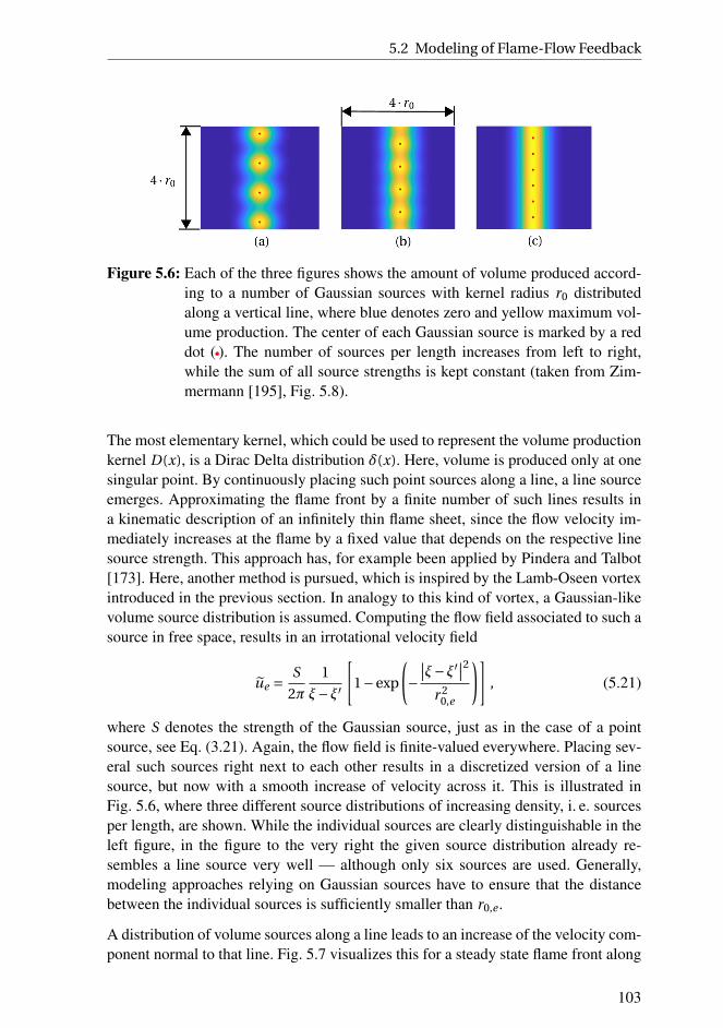
5.2 Modeling of Flame-Flow Feedback

Figure 5.6: Each of the three figures shows the amount of volume produced accord-ing to a number of Gaussian sources with kernel radius r0 distributedalong a vertical line, where blue denotes zero and yellow maximum vol-ume production. The center of each Gaussian source is marked by a reddot ( ). The number of sources per length increases from left to right,while the sum of all source strengths is kept constant (taken from Zim-mermann [195], Fig. 5.8).

The most elementary kernel, which could be used to represent the volume productionkernel D(x), is a Dirac Delta distribution δ(x). Here, volume is produced only at onesingular point. By continuously placing such point sources along a line, a line sourceemerges. Approximating the flame front by a finite number of such lines results ina kinematic description of an infinitely thin flame sheet, since the flow velocity im-mediately increases at the flame by a fixed value that depends on the respective linesource strength. This approach has, for example been applied by Pindera and Talbot[173]. Here, another method is pursued, which is inspired by the Lamb-Oseen vortexintroduced in the previous section. In analogy to this kind of vortex, a Gaussian-likevolume source distribution is assumed. Computing the flow field associated to such asource in free space, results in an irrotational velocity field

ue =S

2π

1

ξ−ξ′

[1−exp

(−

∣∣ξ−ξ′∣∣2

r 20,e

)], (5.21)

where S denotes the strength of the Gaussian source, just as in the case of a pointsource, see Eq. (3.21). Again, the flow field is finite-valued everywhere. Placing sev-eral such sources right next to each other results in a discretized version of a linesource, but now with a smooth increase of velocity across it. This is illustrated inFig. 5.6, where three different source distributions of increasing density, i. e. sourcesper length, are shown. While the individual sources are clearly distinguishable in theleft figure, in the figure to the very right the given source distribution already re-sembles a line source very well — although only six sources are used. Generally,modeling approaches relying on Gaussian sources have to ensure that the distancebetween the individual sources is sufficiently smaller than r0,e .

A distribution of volume sources along a line leads to an increase of the velocity com-ponent normal to that line. Fig. 5.7 visualizes this for a steady state flame front along

103

Secondary Interactions

Figure 5.7: Left: Magnitude of flow velocity evaluated along three stream lines (seeright plot) plotted over the axial coordinate x1. The theoretical veloci-ties far up- and downstream of the flame are marked by horizontal blackdashed lines. Right: Steady state flow field for Cr = 0.4. The flame front(green) is represented by a number of Gaussian sources of kernel ra-dius r0. The three stream lines (gray lines) referenced in the left plot aremarked by corresponding line styles.

Figure 5.8: Left: Axial velocity of a channel flow including a vertical flame sheet(methane-air, φ= 0.8) represented by Gaussian sources with kernel ra-dius r0 ( ). Right: Flame normal velocity evaluated along the pink lineshown in the left plot (pink line) compared to results of a 1D simulationemploying detailed chemical mechanism (red dashed line). The Gaussiansources are placed at x1 = 0 and have a kernel radius of r0,e = 0.53 mm(taken from Zimmermann [195], Fig. 5.6).

which Gaussian volume source of strength S and radius r0,e are distributed. Plottingthe absolute velocity along three selected stream lines illustrates the acceleration ofthe flow across the flame sheet. Therefore, r0,e has to be chosen such that the flamenormal velocity induced by the Gaussian sources optimally resembles the behaviorimposed by a realistic combustion zone. In order to archive this, 1D simulations ofa steady flame are conducted employing a detailed chemical reaction scheme. Re-

104

5.2 Modeling of Flame-Flow Feedback

sults are compared to the fields relying on Gaussian sources in Fig. 5.81. The left plotof this figure shows a straight flame stabilized inside a duct, along which Gaussiansources are uniformly distributed. The plot on the right hand side of Fig. 5.8 showsthe flame normal velocity inside the duct evaluated along the pink horizontal lineshown in the left plot (pink line). Additionally, results of the detailed 1D simulationsare shown (red dashed line). Both curves coincide very well and only deviate on thedownstream side of the flame sheet, where the secondary reaction layer is placed, seeSec. 1.1.1. All in all, for the given value of r0,e , very good agreement between bothcombustion models is found.

The velocity fields depicted in Figs. 5.7 and 5.8 are retrieved by placing a num-ber of Gaussian sources of kernel radius r0,e = 0.53 mm along a given steady stateflame front and placing a source of strength S = 2u1,blkRi at x1 =−∞ (correspondsto ξ = 0 in the image domain). A Kutta condition is employed at the trailing edgefor the setup shown in Fig. 5.7. Besides this, the only difference in the computationsinvolved to create both figures is the choice of the respective Schwarz-Christoffelmapping (see Zimmermann [195] for details). Considering the fact that the Gaussiansources should impact the flow velocity down- and upstream of the flame, it may besurprising that the velocity far upstream of the flame asymptotes to u1,blk while it ap-proaches Cr Eu1,blk on the downstream side. This point can be clarified as follows: Asshown in Fig. 3.4, the Gaussian sources are placed in the image domain along an arcstarting from ξ= 1 and extending to negative values of ξ1. Impermeability boundaryconditions demand an second arc of sources mirrored at the real axis. These two arcsenclose the flow domain upstream of the flame, where the flow field contributionsof the individual Gaussian sources mostly annihilate each other. Considering a ductflame, the superimposed contributions of all sources even perfectly vanish on the up-stream side of the flame. This is a consequence of the fact that here the flame frontmaps to a sphere around the origin in the image domain, which is symmetric withrespect to the imaginary and the real axes. For the burner-stabilized flame of Fig. 5.7,the arc shown in Fig. 3.4 is only symmetric with respect to the real axis. In conse-quence, a slightly negative flow upstream of the flame is induced by the Gaussiansources, which however is negligible as illustrated in Fig. 5.7 (the absolute velocitiesalmost approach 1 for x1 →−∞).

Representing a flame front by a number of Gaussian sources, leads to an uncondi-tional growth of flame front displacements, as will be shown in the next section.Hence, together with the destabilizing effect of flame-generated baroclinc vorticity,discussed in Sec. 5.2.2, two hydrodynamic mechanisms of flame-flow feedback arefound — a vortical and an irrotational one. The former has already been covered inthe discussion above. The latter can be understood by considering a perturbed flamesheet, as depicted in Fig. 5.9. The combustion process imposes a volume productiononto the flow, which is an irrotational effect, and which can be captured by distribut-ing sources along the flame sheet. This imposes, on the one hand, a discontinuity in

1Computed with Cantera [29] using the GRI-Mech 3.0 reaction mechanism [30]

105

Secondary Interactions

Figure 5.9: Illustration of the perturbed flow field imposed by a displaced flamesheet, which is represented by a number of Gaussian volume sources.The overall effect of these sources leads to a geometrical focusing of theflow, i. e. an acceleration of the flow in the vicinity of concave and a de-celeration in the vicinity of convex parts of the flame, amplifying alreadyexistent flame perturbations.

flame normal velocity across the flame. On the other hand, additionally the flow fieldin the vicinity of the flame is modified. This is illustrated in Fig. 5.9: Three sourcesplaced at the inflection points of the perturbed flame sheet are exemplarily highlighted(gray). Each imposes a velocity field that points away from the center of the respec-tive source. Overall, this results in an increase of flow velocity in the vicinity of themaxima of the displaced flame sheet and, vice versa, a decrease at the minima. Alto-gether, this results in an accelerated flow at concave and a decelerated flow at convexparts of the flow field. Due to this dependency on flame shape, this process is referredto as geometrical focusing in the following. Just like the Darrieus-Landau mechanismrelying on flame-generated vorticity, geometrical focusing amplifies flame perturba-tions and constitutes a hydrodynamic flame-flow feedback mechanism. It essentiallyrelies on movements of the mean flame shape and is, hence, not accounted for if twocoupled flow domains of constant boundaries are assessed, as it is assumed in thescope of Darrieus-Landau’s problem discussed in Sec. 1.2.3.

For the sake of completeness, it should be mentioned that geometrical focusing alsoleads to the occurrence of spatially varying tangential velocity perturbations, associ-ated with flow strain. Their consideration, however, is explicitly neglected here.

5.3 Analysis of the Impact of Flame-Flow Feedback

The modeling framework introduced in Chap. 3 supplemented with the approachesoutlined in this chapter shall now be applied to the flame configurations analyzedin Chap. 4 (primary interactions). Since vortex shedding was found to only have anegligible impact on the flame response, it is excluded from the analysis presented inthe following.

106

5.3 Analysis of the Impact of Flame-Flow Feedback

Parameter ValueExpansion ratio e 6.68Flame speed s0

L 0.2686 m/s

Flame thickness δD 83.95 µmMarkstein number Ma 4Gaussian source kernel radius r0,e 0.53 mm

Table 5.1: Flame parameters used for the computations of this chapter.

An overview of the flame parameters used for the computations of this chapter isprovided in Tab. 5.1. The values for e, sL and δD are retrieved from 1D simulationsof lean methane-air flames at φ= 0.8 relying on the software Cantera [29] employingthe GRI-Mech 3.0 reaction mechanism [30]. The flame thickness is estimated by adiffusion length δD = D th/sL , where D th denotes the thermal diffusivity. FollowingEq. (5.12), the definition of the stretched flame speed depends on the Markstein lengthlM , which is computed from δD and the Markstein number Ma via lM = δD Ma .

Following Matalon et al. [41], methane-air mixtures exhibit Markstein numbersroughly between 3 and 4. As mentioned in the introduction of this chapter, we shouldexpect an overprediction of displacement amplitudes when including flame-flowfeedback into the modeling approach, since only driving and no damping mechanismsare considered. Damping mechanisms are usually associated with flame stretch. In themodeling approach proposed here, only consequences of curvature-related stretch forthe flame speed are considered. Flow strain as well as stretch generated vorticity areneglected, which might significantly underestimate the damping, as indicated by thestudy of Pindera and Talbot [174]. Hence, in the scope of this thesis only a qualita-tive analysis of flame-flow feedback mechanisms is possible and therefore, in a firstapproximation, a Markstein number of 4 is assumed. Following Fig. 5.8, the kernelradius of all Gaussian sources is fixed to r0,e = 0.53 mm.

Based on these assumptions, the model relying on the 1D linear representation of theflame dynamics of Eq. (3.16), a Schwarz-Christoffel mapping, a representation of theflow field by a finite number of flow field singularities and a Kutta condition is readyto be solved. Exactly the same setup as discussed in Chap. 4 is analyzed, but thistime flame-flow feedback is included. Concerning the numerical details, Eq. (3.16)is integrated in time relying on an explicit Euler method together with a first-orderupwind discretization scheme for the advection and a second-order central schemefor the diffusion term. The flame sheet is discretized using 100 sample points andthe time step width is set such that a mesh Fourier number of lM s0

L∆t/∆x2 ≈ 0.05

is achieved [200]. In each time step, Lamb-Oseen vortices are distributed along themean flame position (one vortex per sampling point), with their respective strengthbeing computed from Eq. (5.16). Furthermore, Gaussian sources of kernel radiusr0,ω are placed along the instantaneous flame front, with a density of 10 sources permillimeter. Their strengths depend on the local flame speed, on the expansion ratio

107

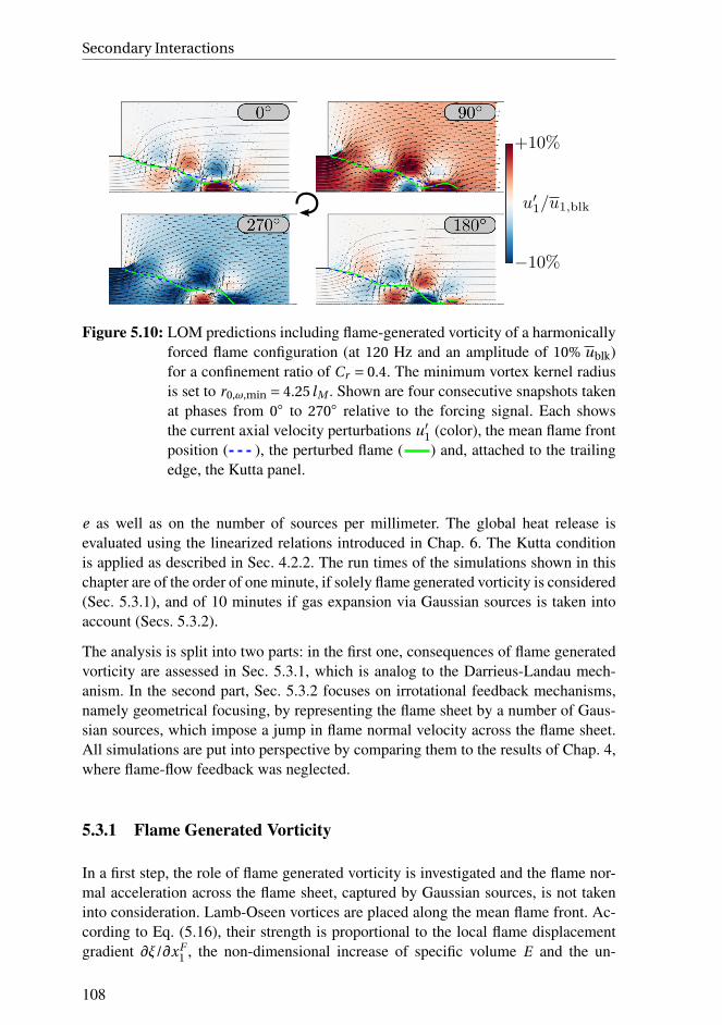
Secondary Interactions

Figure 5.10: LOM predictions including flame-generated vorticity of a harmonicallyforced flame configuration (at 120 Hz and an amplitude of 10% ublk)for a confinement ratio of Cr = 0.4. The minimum vortex kernel radiusis set to r0,ω,min = 4.25 lM . Shown are four consecutive snapshots takenat phases from 0 to 270 relative to the forcing signal. Each showsthe current axial velocity perturbations u′

1 (color), the mean flame frontposition ( ), the perturbed flame ( ) and, attached to the trailingedge, the Kutta panel.

e as well as on the number of sources per millimeter. The global heat release isevaluated using the linearized relations introduced in Chap. 6. The Kutta conditionis applied as described in Sec. 4.2.2. The run times of the simulations shown in thischapter are of the order of one minute, if solely flame generated vorticity is considered(Sec. 5.3.1), and of 10 minutes if gas expansion via Gaussian sources is taken intoaccount (Secs. 5.3.2).

The analysis is split into two parts: in the first one, consequences of flame generatedvorticity are assessed in Sec. 5.3.1, which is analog to the Darrieus-Landau mech-anism. In the second part, Sec. 5.3.2 focuses on irrotational feedback mechanisms,namely geometrical focusing, by representing the flame sheet by a number of Gaus-sian sources, which impose a jump in flame normal velocity across the flame sheet.All simulations are put into perspective by comparing them to the results of Chap. 4,where flame-flow feedback was neglected.

5.3.1 Flame Generated Vorticity

In a first step, the role of flame generated vorticity is investigated and the flame nor-mal acceleration across the flame sheet, captured by Gaussian sources, is not takeninto consideration. Lamb-Oseen vortices are placed along the mean flame front. Ac-cording to Eq. (5.16), their strength is proportional to the local flame displacementgradient ∂ξ/∂xF

1 , the non-dimensional increase of specific volume E and the un-

108

5.3 Analysis of the Impact of Flame-Flow Feedback

Figure 5.11: Results of a simulation as described in Fig. 5.10, but for a confinementratio of Cr = 0.66.

stretched flame speed s0L . Since vorticity is generated all along the perturbed flame

sheet with maxima at the inflection points of ξ, its spatial distribution is modeled byLamb-Oseen vortices whose kernel radii are set to the current maximum displacementamplitude. Furthermore, a minimum radius of r0,ω,min = 4.25 lM is assumed in orderto avoid an overprediction of the imposed vortical velocity perturbations at the flamesheet. Applying such a definition for r0,ω,min ensures that the order of magnitudeof the kernel radius cannot become smaller than the flame thickness. Nevertheless,r0,ω,min has to be regarded as an empirical parameter whose value is not rigorously de-rived from first principles. Unfortunately, it significantly affects the computed flameresponse, as will be shown below.

Figs. 5.10 and 5.11 show four snapshots of harmonically forced simulations of thismodel at Cr = 0.4 and Cr = 0.66, respectively. It is evident that consideration of flamegenerated vorticity leads indeed to a convective growth of flame front perturbations:right at the anchoring, hardly any flame displacement is visible, whereas the flametip oscillates with significant amplitude. Comparing the results of both confinementratios, we observe that the wave length and maximum displacement amplitude ofthe resulting flame front perturbations varies: A more narrow confinement seems topromote perturbations of longer wave lengths and lower displacement amplitudes.Furthermore, a considerable impact of the flame sheet on the flow of premixture isobservable for both setups. Positive and negative axial velocity perturbations prop-agate from the flame base region to its tip, similar as reported by Blanchard et al.

[129]. It has, however, to be noted that, other than claimed by Blanchard et al. [129],the vortical component of flame-flow feedback does most probably not fully explainthe observed convected velocity perturbations, since the irrotational component has asignificant impact, as well, which will be shown in Sec. 5.3.2.

Imposing an impulsive forcing, results in a response as depicted in 5.12. As expected,the response with and without flame-flow feedback agree at t∗ = 0 and then increas-ingly deviate from each other. Similar to the CFD data, negative and positive sec-ondary peaks develop and subsequently grow in amplitude while they are advectedtowards the flame tip. The most apparent deviation between the LOM ( ) and

109

Secondary Interactions

−1

0

1Cr = 0.4

t∗ = 0

ξ/ξ

[-]

t∗ = 0.2 t∗ = 0.41 t∗ = 0.61

0 0.5 1

−1

0

1Cr = 0.66

t∗ = 0

ξ/ξ

[-]

0 0.5 1

t∗ = 0.24

0 0.5 1

t∗ = 0.49

0 0.5 1

t∗ = 0.74

Figure 5.12: Four snapshots taken at equidistant instances in time of the normal-ized flame displacement resulting from an impulsive velocity forcingat t∗ = 0 taken from CFD/SI results ( ), the acoustic LOM exclud-ing flame-flow feedback ( ) and the acoustic LOM including flame-generated vorticity with r0,ω,min = 4.25 lM ( ) at two confinementratios: Cr = 0.4 (top) and Cr = 0.66 (bottom).

the CFD data ( ) is the position where the negative and positive peaks develop,which is slightly too far downstream in the low-order representation. Furthermore,the responses predicted by the LOM is stronger than the respective CFD counterpart.Overall, the Cr = 0.4 low-order predictions match the respective CFD results betterthan the Cr = 0.66 ones. The damping behavior, presumably imposed by the presenceof a rather narrow confinement, seems to be underpredicted for the Cr = 0.66 setup.Nevertheless, a — compared to the acoustic LOM — improved agreement can beobserved for both configurations.

This improved agreement is also reflected by the corresponding impulse and fre-quency response data of the global heat release rate, which is shown in Fig. 5.13.At Cr = 0.4, CFD/SI ( ) and LOM ( ) predictions agree well, only small de-viations in phase/gain and the impulse response are observable. At Cr = 0.66, theacoustic LOM correctly captures the oscillatory behavior of the IR, however, the re-sponse deviates significantly from the CFD/SI data around t∗ = 0, see Fig. 5.13b.Accordingly, the corresponding FTF gain curves are qualitatively different. The dras-tic reduction of the peak gain value of the Cr = 0.66 setup (compared to Cr = 0.4),can also be found in the acoustic LOM data ( ). All in all, the suggested low ordermodeling strategy results in reasonable response predictions, even at Cr = 0.66.

Interpreting the results of the acoustic LOM including flame generated vorticity, itshould be kept in mind that they are based on an empirical parameter r0,ω,min. Eval-uating the flame responses for 10% lower and larger values of r0,ω,min results in the

110

5.3 Analysis of the Impact of Flame-Flow Feedback

1

3

Magnitude

0 1 2 3 4

-12π

-8π

-4π

0

f∗ [-]

Phase

0 1 2

−8

−4

0

4

8

t∗ [-]

h∗

(a) Cr = 0.4

0

1

Magnitude

0 1 2 3 4

-12π

-8π

-4π

0

f∗ [-]

Phase

0 1 2

−1.5

0

1.5

3

t∗ [-]

h∗

(b) Cr = 0.66

Figure 5.13: IR and FR in terms of gain and phase at Cr = 0.4 and Cr = 0.66 aspredicted by CFD/SI ( ) as well as by the acoustic LOM with( ) and without ( ) consideration of flame-generated vorticity(r0,ω,min = 4.25lM ).

responses visualized in Figs. 5.14a and 5.14b, respectively. A reduction of the min-imum kernel radius leads to higher velocity amplitudes and, thus, to an increase ofthe FTF gain. Exactly the opposite behavior can be observed when the radius is in-creased. We have to recognize that the low-order predictions are rather sensitive tovariations in r0,ω,min. That means that the quantitatively good agreement with the ref-erence CFD/SI data is the result of a parameter tuning, i. e. finding an optimal valuefor r0,ω,min. Nevertheless, the fact that the model shows reasonable results for bothconfinement ratios and, additionally, leads to qualitatively correct response predic-tions indicates that flame generated vorticity may indeed be one important drivingmechanism resulting from flame flow feedback.

The rather simplistic treatment of flame generated vorticity proposed in this sectionresulted in valuable insights in consequences of flame-flow feedback. Its impact onthe FTF could be shown to lead to gains exceeding unity. Furthermore, the findingsof Blanchard et al. [129] could be corroborated stating that a perturbed flame sheetacts as a vortex sheet whose upstream influence is responsible for the observed con-vected velocity perturbations. The present analysis contains the empirical parameterr0,ω,min and it was shown that response predictions are quite sensitive to its exactvalue. Therefore, all results presented in this section are qualitative in nature. Quanti-tatively good agreement between LOM and CFD/SI data could be achieved by tuningr0,ω,min. Future studies could refine the analysis of flame-generated vorticity by im-plementation of more detailed vorticity source terms, for example, relying on the

111

Secondary Interactions

1

3

Magnitude

0 1 2 3 4

-12π

-8π

-4π

0

f∗ [-]

Phase

0 1 2

−8

−4

0

4

8

t∗ [-]

h∗

(a) r0,ω,min = 90% 4.25lM

1

3

Magnitude

0 1 2 3 4

-12π

-8π

-4π

0

f∗ [-]

Phase

0 1 2

−8

−4

0

4

8

t∗ [-]

h∗

(b) r0,ω,min = 110% 4.25lM

Figure 5.14: IR and FR in terms of gain and phase at Cr = 0.4 as predicted by CFD/SI( ) as well as by the acoustic LOM with ( ) and without ( )consideration of flame-generated vorticity. Shown are results for twominimum vortex kernel radii r0,ω,min.

work of Hayes [175]. This might possibly enable a quantitative assessment of thevortical component of flame-flow feedback.

5.3.2 Irrotational Flame-Flow Feedback

A flame usually imposes a significant change in density on a flow, which is causedby exothermic reactions releasing reasonable amounts of sensible enthalpy. Such adensity change is accompanied by an expansion and, thus, an acceleration of theflow across the flame zone. This process is captured by means of Gaussian sources,which are placed along the perturbed flame sheet and, hence, provoke a jump inflame normal velocity. Their kernel radii r0,e are adjusted in order to optimally matcha realistic velocity profile through the flame front, see Fig. 5.8.

Applying this technique, the problem arises that the steady state position of the flameis a priori unknown, since the presence of a confinement together with an combustion-induced expanding flow alters the steady state flow field and, hence, also the corre-sponding flame shape [142, 144]. This circumstance would require the computationof the steady state in a first step, before the displacement dynamics could be eval-uated in a second. Employing a 2D non-linear G-equation solver combined with arepresentation of the flame by Gaussian sources, the steady state solution was com-puted by Zimmermann [195]. Since this requires the availability of another solver as

112

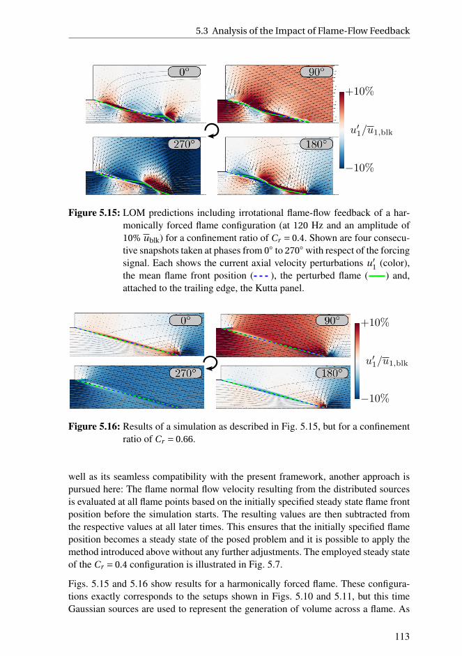
5.3 Analysis of the Impact of Flame-Flow Feedback

Figure 5.15: LOM predictions including irrotational flame-flow feedback of a har-monically forced flame configuration (at 120 Hz and an amplitude of10% ublk) for a confinement ratio of Cr = 0.4. Shown are four consecu-tive snapshots taken at phases from 0 to 270 with respect of the forcingsignal. Each shows the current axial velocity perturbations u′

1 (color),the mean flame front position ( ), the perturbed flame ( ) and,attached to the trailing edge, the Kutta panel.

Figure 5.16: Results of a simulation as described in Fig. 5.15, but for a confinementratio of Cr = 0.66.

well as its seamless compatibility with the present framework, another approach ispursued here: The flame normal flow velocity resulting from the distributed sourcesis evaluated at all flame points based on the initially specified steady state flame frontposition before the simulation starts. The resulting values are then subtracted fromthe respective values at all later times. This ensures that the initially specified flameposition becomes a steady state of the posed problem and it is possible to apply themethod introduced above without any further adjustments. The employed steady stateof the Cr = 0.4 configuration is illustrated in Fig. 5.7.

Figs. 5.15 and 5.16 show results for a harmonically forced flame. These configura-tions exactly corresponds to the setups shown in Figs. 5.10 and 5.11, but this timeGaussian sources are used to represent the generation of volume across a flame. As

113

Secondary Interactions

(a)

40 60 80

−0.1

0

0.1

t [ms]

fluct

uat

ion

(b)

Figure 5.17: (a): Illustration of the dipole-like flow structure in the vicinity of a per-turbed duct flame, which results from an acceleration of flame-normalvelocity across a flame sheet (geometrical focusing). (b): Fluctuation ofthe global heat release rate for a harmonic velocity forcing at 120 Hzat an amplitude of 10%u1,blk( ) for Cr = 0.4, resulting from simu-lations respecting flame-generated vorticity ( ), see Fig. 5.10, andirrotational gas expansion ( ), see Fig. 5.15.

in the vortical case, the displacement amplitude convectively increases towards theflame tip. Due to the now significantly larger wave lengths of the imposed flame sheetperturbations, this fact is harder to recognize. The Cr = 0.66 case shows hardly anyspatial variations of the local displacement phase and only a rather small convectivegrowth in perturbation amplitude. When interpreting the u′

1 field, it should be con-sidered that the deep red and deep blue parts right at the flame front are caused by thefact that the flame sheet moves: if the flame propagates into the fresh mixture, the ve-locity at points placed inside the originally unburned flow will be strongly increasedcompared to the steady state and, vice versa, if the flame is pushed into burned parts.Hence, consequences of the sources for the flow field become only apparent furtheraway from the flame sheet.

Respecting this fact, it is interesting to note that also the irrotational part of theflame-flow feedback imposes distinct convected velocity perturbations upstream ofthe flame, at least for Cr = 0.4. Dipole-like irrotational perturbations are imposedonto the surrounding flow field, which is shown for the case of a perturbed duct flamein Fig. 5.17a2: regions where the displacement shows local maxima (concave parts)behave as sources on the burned and as sinks on the unburned side of the flame sheet.For regions at local minima (convex parts), it is the other way round. In consequence,the overall perturbation flow field might appear vortical, while it is irrotational in re-ality. This complicates a visual analysis of the flow field in the vicinity of perturbedflames. Based on these findings, it has to be concluded that the description of Blan-

2The computation of this figure employs exactly the same framework as the ones of Figs. 5.15 and5.16, however, a different Schwarz-Christoffel mapping was applied in order to cope with the depictedduct geometry, see Zimmermann [195] for details.

114

5.3 Analysis of the Impact of Flame-Flow Feedback

0 0.5 1

−1

0

1

2Cr = 0.4

t∗ = 0

ξ/ξ

[-]

0 0.5 1

t∗ = 0.20 0.5 1

t∗ = 0.410 0.5 1

t∗ = 0.61

Figure 5.18: Four snapshots taken at equidistant instances in time of the normal-ized flame displacement resulting from an impulsive velocity forcing att∗ = 0 taken from CFD/SI results ( ), the acoustic LOM excludingflame-flow feedback ( ) and the acoustic LOM including irrotationalgas expansion ( ) at a confinement ratio of Cr = 0.4.

chard et al. [129] is incomplete: a perturbed flame sheet is more than just a vortexsheet of varying strength.

One important difference between the setup respecting flame-generated vorticity andthe setup respecting irrotational gas expansion is that at Cr = 0.4 the latter exhibits aclearly non-linear output behavior of the global heat release, even for small ampli-tudes of the input velocity. The time series data of the global heat release rate asso-ciated with the simulations shown in Fig. 5.10 and 5.15 are depicted in Fig. 5.17b.While the vortical output data ( ) is sinusoidal, the irrotational output ( ) showsa drop of the global heat release signal every time a maximum is reached. Such a be-havior is non-linear in nature and can be associated with the dynamics of the flametip. Once a positive flame front perturbation reaches the flame tip, this will eventuallylead to a pinch-off of a bubble of unburned fluid. When this bubble is burned, a rapidchange in the global heat release rate is provoked. This process is not faithfully cap-tured by the model at hand, nevertheless, qualitatively something similar happens:A positive flame displacement is usually followed by a negative one. In flame coor-dinates, this might lead to the occurrence of negative displacements exceeding thesymmetry line at x2 = 0. This, of course, is not possible and the numerical algorithmdisregards portions of the flame sheet that are outside the flow domain, i. e. x2 < 0.That means, the heat release drops overproportionally fast, which manifests itself asthe observed rapid drop of the global heat release rate. Regarding the simulations thatrespect only flame generated vorticity, vortices are distributed along the mean flame

position and not the displaced one, and hence also displacements with x2 < 0 whereallowed. This results in the good-natured output of this model. At Cr = 0.66 all forcedsimulations exhibited an essentially harmonic output signal at the forcing frequency(not shown), which shows that the presence of a confinement significantly dampensthe impact of flame-flow feedback, particularly its irrotational component.

The observed convective growth of displacement amplitudes resulting from an im-

115

Secondary Interactions

pulsive velocity forcing is significantly stronger for the irrotational gas expansionmodel than for the model that respects only flame-generated vorticity. The result-ing flame displacements of the former model are depicted in Fig. 5.18. Already atthe second snapshot (t∗ = 0.2) very high displacement amplitudes have formed. Theysubsequently grow even further in amplitude and, additionally, a variety of secondarydisplacements develop. This emphasizes the point made in the introduction of thischapter: capturing mainly mechanisms that are responsible for a growth of flame frontperturbations will most probably result in an overprediction of displacement ampli-tudes. This could possible be fixed by including damping mechanisms. In the studyshown here, consequences of flame curvature were respected, however, the resultsclearly suggest that this is not sufficient. An appropriate consideration of dampingmechanisms is out of the scope of this work and should be analyzed in future studies.

Finally, it should be pointed out that a joint analysis of both flame-flow feedbackmechanisms, i. e. the irrotational and the vortical one, results in even higher dis-placement amplitudes than the ones shown here (not shown). Therefore, such a com-bined study is only instructive once damping mechanisms are adequately includedinto the modeling framework. This situation is very similar to what happened to theworks of Darrieus [26] and Landau [27]: since their model included only drivingmechanisms leading to the unconditional growth of flame front perturbations, it waslater complemented by Markstein [44] introducing the empirical assumption of acurvature-dependent flame speed. Concerning the present modeling approach, sim-ilarly, it turned out that there is a significant lack of damping mechanism in orderto achieve quantitative agreement with CFD/SI data. Therefore, in addition to thecurvature dependency of the flame speed, other mechanisms need to be assessed.

5.4 Summary and Conclusions

In this chapter, consequences of flame-flow feedback for the acoustic flame responsewere modeled and analyzed. A vortical and an irrotational mechanism resulting fromgas expansion were found to be the driving forces that govern secondary acoustics-flame interactions. While the former is known as the Darrieus-Landau mechanismrelying on flame-generated vorticity, the latter results from a geometrical focusingof accelerating effects of a perturbed flame sheet and has, so far, not been analyzedin the context of acoustics-flame interactions. Based on these two mechanisms, per-turbed flames act as vortex sheets of varying strength (flame-generated vorticity) aswell as sheets of advected dipoles (irrotational gas expansion), which explains theoccurrence of convected velocity perturbations upstream of the flame. Furthermore,both mechanisms lead to the formation of secondary convectively growing displace-ments causing FTF peak gain values that significantly exceed unity — just like it waspredicted by the CFD/SI results. The presence of a narrow confinement significantlyimpacts the consequence of flame-flow feedback, leading to flame front displace-ments of longer wave lengths and lower amplitudes. Accordingly, the maximum FTF

116

5.4 Summary and Conclusions

peak gain values are reduced.

Qualitatively, mechanisms that could explain the discrepancies observed in Chap. 4were found and promising modeling strategies were proposed. Contrary to the MSequation, as used by Searby et al. [63], the modeling framework proposed here al-lows to capture confinement induced consequence for the flame response. Relying onthis new modeling approach, it was found that the previously neglected irrotationalconsequences of gas expansion led to an unphysically fast growth of flame front dis-placements, such that the response dynamics left the linear regime. It is conjecturedthat this growth is in reality limited by some damping mechanisms, which were notincluded in the present study. Their investigation should be subject of future research,which then might also allows for quantitative assessments of the flame dynamics.Furthermore, relying on the works of Oberleithner et al. [79] and Oberleithner andPaschereit [80], it would be interesting to analyze the role of flame-flow feedbackdriven instability mechanisms for technically relevant configurations, in analogy toshear layer instabilities.

The main findings of the present analysis are:

1. Compact acoustics imposes irrotational flow perturbations, which predomi-nantly displace the flame base region.

2. These primary flame front displacements are advected downstream by themean flow and are exposed to mechanisms of flame-flow feedback along theirway to the flame tip.

3. This feedback leads to the convective growth of displacement amplitudes and,additionally, creates new secondary flame front perturbations.

4. These secondary perturbations lead to an oscillatory behavior of the impulseresponse (IR) of the global heat release rate. This, in turn, creates a pronouncedpeak in the gain of the associated frequency response at a frequency close tothe oscillation frequency of the IR.

5. For the flame configuration at hand, two mechanisms of flame-flow feedbackwere identified: (i) the Darrieus-Landau mechanism relying on flame generatedvorticity and (ii) geometrical focusing resulting from a flame-normal accelera-tion of the flow across a perturbed flame sheet.

6. Both mechanisms lead to the convective growth of flame front perturbationsand impose convected velocity perturbations upstream of the flame front.

117

Secondary Interactions

118

Part III

Generalization to Other Burner

Configurations

The analysis conducted so far analyzed Slit flame setups. Most exper-imental and theoretical studies, however, report on Bunsen flames. Inorder to provide a connection of both configurations, the impact of flamegeometry onto the acoustic flame response shall be investigated in thefollowing. For the sake of completeness, also Wedge flames are consid-ered. The results should provide guidance how to generalize the findingsmade for Slit flame configurations as well as how to interpret data ob-tained using arbitrary flame configurations.

Major parts of Chap. 6 have already been published, see Steinbacher et al.

[2]. Compared to this publication, Sec. 6.3 is newly added and some minorchanges have been applied (wording, grammar).

119

6 Consequences of Flame Geometry

Flame geometry (Slit, Wedge or Bunsen) determines how flame

front displacements translate to global heat release rate fluctu-

ations, which defines geometry-specific response characteristics.

Low-order models relying on a Gaussian kernel function are able

to adequately capture the FTFs of all three geometries.

Various types of laminar flame configurations are used in academia and technical ap-plications, which often exhibit very different response characteristics [146, 153, 201].Three of the most prominent geometries are depicted in Fig. 2.1: Bunsen, Wedge (orV-) and Slit flames. Most theoretical studies on analytical FTF models are concernedwith Bunsen and Wedge flames [31, 113, 138, 202], while only very few deal with Slitflames [112, 142, 203]. One reason for this might be that the latter are technically lessrelevant. Particularly for academic studies, however, Slit flames are very interestingdue to the simpler analytical treatment of the governing equations [112, 132, 148],see also the works presented in Part II of this thesis.

To date, no study has strictly and comprehensively analyzed the differences in thelinear flame response that result from flame geometry. Schuller et al. [111] and Blu-menthal et al. [116] compared analytical response predictions of Wedge and Bunsenflames, but did not include Slit flames. Schuller et al. [111] provided validation datafrom experiments solely for the Bunsen configuration. Durox et al. [152] comparedexperimental response results of Bunsen, Wedge and M-flames, where the last one isa hybrid of the first two types of flames. They focused on the nonlinear behavior ofthe frequency response for increasing forcing amplitude levels and did not comparemeasurements to analytical predictions. Other studies assessing the consequences offlame geometry examined the production of combustion noise of turbulent Slit andBunsen flames. Kotake and Takamoto [151] experimentally investigated the impactof the nozzle shape (or burner mouth shape) on the acoustic power of the associatedcombustion noise for constant cross-sectional areas. They found that for lean con-ditions, rectangular nozzles (“slits”) produce significantly higher levels of acousticpower than square and circular (Bunsen) shapes. A similar conclusion was drawnfrom numerical results by Pausch et al. [153], who additionally found that Slit burn-ers exhibit a lower peak frequency than Bunsen type ones. Further, they located theposition of maximum heat-release of the rectangular flame at its tip, while it is abit further upstream for the Bunsen flame. Neither study analyzed the correspondingFTFs. Due to this lack of comprehensive studies on consequences of flame geometry

121

Consequences of Flame Geometry

for the respective FTFs, a literature review for each of the three investigated configu-rations is provided in the following.

For Bunsen type flames, results for both experimentally determined and theoreticallymodeled FTFs are readily available, see e. g. [111, 115, 133, 144, 145, 158, 204–206].Low-order models based on the so-called convective or incompressible-convectivevelocity model agree reasonably well with experimental data, see Sec. 2.2.1 (Low-Order Models) for details.

To the best knowledge of the author, there is a lack of literature regarding FTF anal-ysis and models for laminar Slit flames that are validated against experimental orhigh fidelity numerical data. On the one hand, several theoretical studies develop andinvestigate analytical models for the FTF of Slit flames [112, 138, 142, 207], how-ever, none of them compares results to experimental/high fidelity numerical data. Onthe other hand, experimental and/or numerical investigations reporting on measuredFTFs of Slit flames [147–149, 208–210] do not compare their measurements to ana-lytical predictions. Only Duchaine et al. [146] presented an empirical model for thephase of Slit and Bunsen FTFs and compared it to experimental data, finding that theeffective time lag of a Bunsen flame is about half the value of a Slit configuration.Further, Kornilov et al. [209] visually compare measured gain and phase values ofa Bunsen and Slit setup, which shows a significantly higher gain — even exceedingunity — of the Slit flame. But again no model was developed and validated againstthis data.

Finally, there is a group of studies that compared analytically predicted instantaneousflame front positions of harmonically perturbed Slit flames to experimental or highfidelity numerical data, however, they did not evaluate transfer functions of the globalheat-release rate [104, 164, 165, 211, 212]. All of them rely on a G-equation basedapproach where the speed of a convective velocity perturbation was fitted in order toachieve good agreement of the resulting perturbed flame front with the comparisondata. From the good match in terms of flame front position, a very similar behavior ofthe corresponding global heat-release dynamics at the considered forcing frequencycan be inferred. However, since the responses were only computed at a few forcingfrequencies, it is not possible to deduce an FTF from those studies.

There are several experimental studies reporting measured FTFs of Wedge flames,e. g., [152, 201, 213], but they are all lacking a comparison to theoretical predictions.The studies performed by Schuller et al. [111] and Blumenthal et al. [116] developanalytical FTF models for Bunsen and Wedge flames, but compare only the responseof the Bunsen type setup to experimental data. Finally, Schuller [214] developed amodeling approach, which was validated against experimental data. At the same time,however, he mentions the difficulties in deriving an analytical model for such burnerstabilized Wedge flames, which essentially arises from a strong interaction of theflame with vortical structures shed from the burner mouth [202]. Other Wedge typeflames found in the literature are swirl stabilized flames, which depend on variations

122

6.1 Test Case Setups

of the turbulent burning velocity, axially convected velocity disturbances, as well ason convected swirl waves [79, 215–217]. Modeling of the FTF requires an adequatedescription of all those effects. This complicates the analysis and shifts the focusaway from geometrical consequences.

The study presented in the following aims to generate a more profound understandingof the consequences of flame geometry by comparing analytical FTF predictions ofSlit, Wedge and Bunsen type flames to each other and analyzing the origin of the dis-crepancies found. For the first time, Slit and Wedge flame FTF predictions resultingfrom high fidelity computational fluid dynamics (CFD) simulations are compared toanalytical model predictions. The unique feature of the Wedge flame setup consid-ered in our study is that it is not dominated by vortex-flame interaction, as it is thecase for a burner stabilized flame [202], since no burner mouth is involved. Therefore,a clean validation basis for analytical models is provided for all three geometries. Itis found that the widespread G-equation framework, combined with a convective ve-locity model, is not able to adequately predict the flame response of Slit flames. Inorder to overcome this limitation, an extension of the well-known velocity models isintroduced, which relies on a Gaussian kernel function in order to add some temporaldispersion to the transfer function model.

The analysis is structured as follows: In Sec. 6.1 the three test case setups are intro-duced, which are used to validate the theoretical models. For each flame configura-tion steady-state and transient numerical simulations are performed and the respec-tive flame transfer function are identified from broad-band input/output data usingmeans of system identification (SI). The overall heat-release rate, evaluated as theintegral over the flame surface, plays a crucial role in the analysis of flame geometry-related response differences. Peculiarities of the various flame configurations on theone hand, and of the coordinate system on the other hand are detailed in Sec. 6.2.The here gained mathematical expressions are elucidated by descriptive physical rea-soning based on a model that solely relies on displacements of the flame anchoringin Sec. 6.3. In Sec. 6.4, incompressible-convective velocity models with Dirac andGaussian kernel functions are introduced, respectively for all flame configurationsconsidered. Properties of the Dirac kernel based models are discussed in Sec. 6.5and, in particular, the flame geometry-related differences in the flame response areexplicated. Finally, in Sec. 6.6 FTF predictions of the various velocity models arevalidated against CFD data, as well as against experimental data taken from the liter-ature.

6.1 Test Case Setups

Transient and steady state numerical simulations employing well-established meansof computational fluid dynamics of three flame configurations are performed andserve as a validation basis, see Appendix A.2.1 for details. Using input-output time

123

Consequences of Flame Geometry

(a) Bunsen (conical Λ)

(b) Wedge (conical V)

(c) Slit

Figure 6.1: CFD steady state snapshots of absolute velocity for the three investigatedflame test cases of different flame geometries. For all configurations, thelocation of maximum heat release (green) and the analytically predictedmean flame front ( ) are shown (taken from [2]).

series data resulting from broad-band forced simulations, FTFs are identified bymeans of system identification (SI) employing a finite impulse response (FIR) modelas described in Appendix A.2.2.

Three setups are considered and the respective steady state solutions are depictedin Fig. 6.1. All setups are chosen to be as simple as possible in order to serve asa clean reference that exhibits any geometry-related characteristics in a clear man-ner. Further, the mechanisms governing the flame response to acoustic perturbationsshould be similar for all cases, i. e. similar Reynolds numbers and negligible interac-tion with vortical structures shed from the burner mouth for the Wedge configuration[1, 104, 201]. This shedding process is suppressed by adding a straight lateral wallconstraining the flame, see Fig. 6.1b. Note that all configurations exhibit a smallrecirculation zone since the flow cannot follow the sharp edge at the inlet to thecombustion chamber. Following Chap. 4, however, acoustically triggered sheddingof vorticity from this edge has only a negligible impact on the linear flame response.

For the Slit and Bunsen setups, a feed duct and combustion chamber with a half-diameter of Ri = 5 mm and Ra = 12.5 mm are used, respectively (Fig. 6.1). The

124

6.2 Integral Heat-Release

Wedge flame setup has the same feed duct height of 5 mm as the other two casesand a rod radius of Rr = 3.5 mm, which results in a combustion chamber radius ofRa = 8.5 mm. At the inlet, a uniform flow profile of axial velocity u1 = 1 m/s with atemperature of 300 K is imposed for all setups. Further, zero pressure gradients at theinlet and a fixed pressure are assumed, as well as a zero axial velocity gradient at theoutlet. No swirl of the flow is imposed. All walls are set to be adiabatic, except fromthe feed duct wall, which is set to a fixed temperature of 300 K, and the combustionchamber back plate, which is set to TBP = 700 K. This configuration correspond to aReynolds number of Re = 620, which is computed with the mean inlet velocity, thefeed duct diameter and the kinematic viscosity of the fresh mixture.

6.2 Integral Heat-Release

For all three geometrical configurations considered, the integral heat-release rate isproportional to the respective flame surface area A f (t ) =

∫A dS. Hence, evaluation of

surface area fluctuations A′f

(t ) = A f (t )− A f of a perturbed flame up to contributionsof order O (ǫ) allows to retain the flame geometry specific heat-release dynamics. Thisleads to qualitatively very different results for the three flame geometries, as shownin the following.

One assumption made in this analysis is that the flame is stiffly anchored at its base,i. e. this point is not allowed to move. This assumption is justified by the fact that theimpulse response for Slit flames shows no signal around t = 0, see Sec. 6.6. If theflame base would move, a displacement would directly lead to a fluctuation of theheat-release rate1. A second assumption is that all flames considered are symmetric,i. e. it is sufficient to analyze only one half of the flame front, see Fig. 1.13. A pointon the flame front at the symmetry axis consequently fluctuates in axial direction,which is best captured using laboratory coordinates and the flame front displacementη′. These two assumptions are important, since they define the possible directionsof movement of the flame boundaries (tip and anchoring), which is crucial for theevaluation of the linearized surface area, as will be shown below.

For the computation of the FTF a variety of coordinate systems have already beenadopted in the literature, see e. g. [111, 112, 115]. However, to date no study hascomprehensively scrutinized the derivations of the flame surface area with respect tothe coordinate systems used, nor have the geometry dependent peculiarities ever beenpointed out explicitly. Indeed, a technical note by Humphrey et al. [218] provides ev-idence that this issue deserves more attention: They reported that the expression for

1Purely flame normal displacements of the flame-anchoring would also not cause any O (ǫ) fluctu-ations of the flame surface area, see discussion on Fig. 6.3 below. Hence, strictly speaking, it is notpossible to infer from a zero response at t = 0 of the Slit IR that the flame base is actually stiffly an-chored — it could also be displaced normally. In the 1D linearized G-equation framework, however, theimplications for the modeling are the same in both cases and, hence, it is decided to proclaim the morestraight forward assumption of a stiffly anchored flame.

125

Consequences of Flame Geometry

Figure 6.2: Illustration of the dependency of the change of the flame line segmentlength dS′ = dS −dS on the displacements dη′

iand dη′

i+1up to O (ǫ)

contributions. For conical flames, also the radii r and r of the geometricalcenters of the line segments are important. The region of the unburnedfluid is filled in gray.

the linearized flame surface area of a Slit flame seems to depend on the coordinatesystem used. To resolve this counterintuitive finding, Humphrey et al. [218] proposedto use frequency dependent integration limits, which result in coordinate system spe-cific correction terms. In this section, this issue is revisited and it is sought to providea more intuitive understanding by not limiting our analysis to the frequency domain.Further, a more global context is provided by considering three technically relevantflame geometries.

The geometrical analysis starts by focusing on a single 1D line segment dS of a flamefront, see Fig. 6.2. The notation used in the following is illustrated in Fig. 1.13, whereη′ denotes the axial displacement of the flame front using laboratory coordinates. Itis displaced by η′

iat node i and η′

i+1at node i +1 with reference to the corresponding

steady-state line segment dS. Hence, we write the length of the displaced segment,using the Pythagorean theorem, up to the leading order in the axial displacement as

dS =√(

d xL2

)2 +(ηi+1 +η′

i+1−ηi −η′

i

)2

=

√√√√1+(

dη

d xL2

)2

d xL2

︸ ︷︷ ︸dS

+dη

d xL2

dη′

√1+

(dη

d xL2

)2+O

((dη′)2

)

︸ ︷︷ ︸dS′

(6.1)

with the difference of the steady-state axial distances dη= ηi+1 −ηi and the transientdistances dη′ = η′

i+1−η′

i, as well as the lateral distance d xL

2 . The second line resultsfrom a Taylor series development of the term in the first line around dη′ = 0. The firstterm in Eq. (6.1) denotes the length of the steady-state line segment and the second

126

6.2 Integral Heat-Release

Figure 6.3: Displaced flame segment in flame aligned (blue) and laboratory (red)coordinates.

its change due to η′i /i+1

. By applying the trigonometric relation cot(α) = dη/d xL2 , the

linearized variation of the line segment length is transformed to

dS′ = d s′i +d s′i+1 = cos(α)(η′i+1 −η′i

). (6.2)

From this expression it can directly be deduced that up to the first order in dη′ thechange of the line segment depends on the flame parallel (xF

1 -) component of thedisplacements ds′

i /i+1, see Fig. 6.2. The elongation d s′

i+1counts positive, while d s′

i

contributes with a negative sign.

As pointed out in Sec. 1.3.2, for small displacements, the perturbed flame front canequivalently be described in flame aligned and laboratory coordinates. In order toanalyze the consequences of a change of the coordinate system for the computation ofthe linearized surface area fluctuations, again a single displaced flame segment shallbe analyzed (Fig. 6.3, red). Node i may be fixed and node i +1 be axially displacedby η′

i+1. Following Eq. (6.2), this would result in a linearized change of the segment

length of dS′ = cos(α)η′i+1

. Transforming this situation to flame aligned coordinatesby application of a relation ξi+1 = η′

i+1sin(α) results in the segment shown in blue.

However, the linearized change of the resulting segment length

dSF =√(

dxF1

)2 +dξ2

= dxF1︸︷︷︸

dSF

+O(dξ2

)︸ ︷︷ ︸

dS′F

(6.3)

vanishes to leading order since the displacement ξi+1 has no component parallel tothe mean flame front. Hence, paradoxically, a displacement η′

i+1only imposes a

change of the linearized line segment length in laboratory coordinates, and not inflame aligned coordinates.

This can be resolved by realizing that the aforementioned transformation from η′ toξ is incomplete: In order to equivalently describe the axially displaced flame front

127

Consequences of Flame Geometry

(Fig. 6.3, red) using flame aligned coordinates, the displacement ξi+1 = η′i

sin(α)

should not be applied at node i +1, but at a position shifted by a distance ds′i+1

further to the right (Fig. 6.3, orange). Vice versa, in order to describe a normally dis-placed flame front (Fig. 6.3, blue) using laboratory coordinates, the respective nodei +1 for η′

i+1would have to be shifted to the left by ds′

i+1. In doing so, the first order

change of the segment length stays the same in both coordinate systems.

Therefore, it is concluded that — other than for the flame dynamics described byEq. (1.32) — a transformation of the coordinate system has non-trivial implicationsregarding the evaluation of the linearized change of the flame length and, thus, alsothe respective flame surface area. Depending on the given behavior of the flame,possible elongations or shortenings of the flame length not covered by the chosencoordinate system have to be accounted for correctly. Adding contributions of flamemovement not parallel to one of the employed coordinates is equivalent to imposingvarying integration limits when evaluating the flame surface integral. Other than pro-posed by Humphrey et al. [218], terms resulting from such varying limits should notbe regarded as correction terms since they are a mathematical necessity for solvinga well defined problem. This will be explicated in the following for the individualflame geometries.

Slit Flames

The flame surface area of Slit flames (index “slit”) is given by an integral

A f ,slit(t ) =∆x3

∫l f (t )

0ds , (6.4)

where l f (t ) is the length of the displaced flame surface profile line and ∆x3 the ex-tension of the flame in xL

3 direction. Using laboratory coordinates, the arc length ds

(Fig. 6.4) is expressed as ds =√

1+(dη/dxL

2

)2dxL

2 , see Eq. (6.1). Linearization re-sults in a surface area fluctuation

A′f ,slit(t ) =−cos(α)∆x3

∫Ri

0

∂η′

∂xL2

dxL2

=∆x3 cos(α)η′ (0, t ) , (6.5)

where the anchoring boundary condition η′∣∣

xL2=Ri

= 0 has been applied and Ri is thebase half-diameter of the flame. This leads to the result that surface area fluctuationsof stiffly anchored Slit flames, to leading order, only result from movements of theflame tip.

As stated above, in flame aligned coordinates a varying upper integration limit has tobe considered for evaluation of the flame surface integral. Inserting the corresponding

128

6.2 Integral Heat-Release

Figure 6.4: Geometric measures required for the computation of the flame surfacearea of Bunsen flames.

arc length, see Eq (6.3), and integration limits, the respective surface integral becomes

A f ,slit(t ) =∆x3

∫L f +∆L f (t )

0

√√√√1+(∂ξ

∂xF1

)2

︸ ︷︷ ︸=1+O(ǫ2)

dxF1

=∆x3

[∫L f

0d xF

1 +∫L f +∆L f (t )

L f

dxF1 +O

(ǫ2

)], (6.6)

with the elongation/shortening of the flame length ∆L f (t ) (Fig. 6.4). The first term inEq.(6.6) denotes the mean flame surface area, the second one the contribution due tothe elongation of the flame. As illustrated in Fig. 6.3, the flame tip contribution is ofthe same order as ξ and has, thus, to be considered for the linear analysis.

The variation of the flame length ∆L f (t ) has to be determined from the flamenormal displacement ξ in order to close the flame aligned modeling approach.From Fig. 6.3 we recall the relation between ξ and η′ at the flame tip:ξ(L f , t ) = η′(0, t )sin(α). Using this relation, we compute the variation of the flamelength, which corresponds to an elongation d s′

i+1= cos(α)η′

i+1in Fig. 6.3. Hence,

we get ∆L f (t ) = ξ(L f , t

)cos(α)/sin(α), which, with use of Eq. (6.6), results in an

expression for the surface area fluctuation

A′f ,slit(t ) = ∆x3

tan(α)ξ(L f , t

)(6.7)

that is equivalent to Eq. (6.5). The only coordinate system that does not require avarying upper integration limit is the laboratory one, which is therefore consideredto be the most natural one for the flame surface area integral for the configurationconsidered (symmetric, stiffly anchored Slit flame).

129

Consequences of Flame Geometry

Bunsen Flames

For conical flames in general (index “con”) we have to consider the radius r of thegeometrical center of a line segment. Using the steady-state flame segment radius r ,we retrieve A′

con = 2πr dS′ for the change in flame surface area of one single flameelement, see Fig. 6.2. The flame surface integral is written as

A f ,con(t ) = 2π

∫l f (t )

0r f (s, t )ds (6.8)

where s is the parametrization of the flame front profile, l f (t ) its transient lengthand r f (s, t ) its local radius, see Fig. 6.4. For Bunsen flames (index “Λ”), using flamealigned coordinates, with a decomposition into mean and fluctuating quantities, thisresults in an expression

A f ,Λ(t ) = 2π

∫L f +∆L f (t )

0

[Ri −xF

1 sin(α)+ξcos(α)]

dxF1 . (6.9)

Here, L f is the mean flame length, ∆L f (t ) its transient variation in flame coordinatesand Ri the flame base radius. As in the Slit flame case, the upper integration limit istime dependent: Wrinkles reaching the flame tip impose a change in flame height H f

and, hence, also in the upper integration limit, which is required to capture this effect,see Fig. 6.4. For Bunsen flames, this additional transient contribution to the flamesurface area, however, does not contribute to the linear approximation of the flamesurface area fluctuation. An increase of the flame height by ∆H f (t ) =∆L f (t )/cos(α)

would add the surface of a cone with both base radius and height of order O (ǫ). There-fore, the lateral surface area of this cone is of the order O

(ǫ2

)and is thus neglected

in linear considerations for anchored flames:

A′f ,Λ(t ) = 2πcos(α)

∫L f

0ξdxF

1 . (6.10)

Hence, the global linearized flame surface fluctuation is computed from the integralof the displacements.

Wedge Flames

Wedge flames (index “V”) are conical flames, as well. Hence, the surface integralof Eq.(6.8) also holds for them and, using a flame aligned coordinate system anda corresponding parametrization of the local flame radius r f (s, t ), we retrieve thelinearized flame surface area

A f ,V (t ) = 2π

∫L f +∆L f (t )

0

[Rr +xF

1 sin(α)−ξcos(α)]

dxF1

= A f ,V +2π

[Ra∆L f (t )−cos(α)

∫L f

0ξd xF

1

], (6.11)

130

6.2 Integral Heat-Release

Figure 6.5: Geometric measures required for the computation of the flame surfacearea of Wedge flames.

which results with ∆L f (t ) = ξ(L f , t )/tan(α) in a surface area fluctuation

A′f ,V (t ) = 2πcos(α)

[Ra

sin(α)ξ(L f , t

)−

∫L f

0ξdxF

1

]. (6.12)

Similar to the Slit case, fluctuations in the flame height add or subtract the surfaceof a cone with a base radius of the order of the maximum flame radius Ra and aheight of the order O (ǫ), see Fig. 6.5. In total, the flame tip movement ∆H f (t ) wouldadd a O (ǫRa) contribution to the flame surface area fluctuations, which is significant.As a result, the linearized surface fluctuations of stiffly anchored Wedge flames isexpressed as the (negative) integral of the deflection from the mean, plus the flametip movement.

131

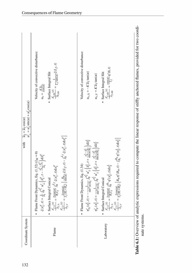
Consequences of Flame Geometry

Coo

rdin

ate

Sys

tem

wit

hu∥=

u1

co

s(α

)

u′ ⊥=

u′ 1

sin

(α)+

u′ 2

co

s(α

)

Fla

me

•F

lam

eF

ront

Dyn

amic

s,E

q.(1

.32)

(lM

=0)

ξ(x

F 1,t

)=

1 u∥

∫ xF 1

0u′ ⊥

( xF 1

,t−

xF 1−

xF 1

u∥

) dx

F 1

•S

urfa

ceIn

tegr

alC

onic

alA′ f

,Λ(t

)

Af

,Λ=

2c

os(α

)R

iL

f

∫ Lf

0ξ

(xF 1

,t)d

xF 1

A′ f

,V(t

)

Af

,V=

2c

os(α

)L

f(R

r+R

a)

[R

asi

n(α

)ξ

(Lf

,t)−

∫ Lf

0ξ

(xF 1

,t)d

xF 1

]

Vel

ocit

yof

conv

ecti

vedi

stur

banc

e:

uc=

Ku

1c

os(α

)

•S

urfa

ceIn

tegr

alS

lit

A′ f,

slit

(t)

Af,

slit

=1

Lf

tan

(α)ξ

(Lf

,t)

Lab

orat

ory

•F

lam

eF

ront

Dyn

amic

s,E

q.(1

.34)

η′ Λ

(xL 2

,t)=−

1si

n2

(α)u

∥

∫ xL 2

0u′ ⊥

( xL 2

,t+

xL 2−

xL 2

sin

(α)u

∥

) dx

L 2

η′ V

(xL 2

,t)=

1si

n2

(α)u

∥

∫ xL 2

0u′ ⊥

( xL 2

,t+

xL 2−

xL 2

sin

(α)u

∥

) dx

L 2

•S

urfa

ceIn

tegr

alC

onic

alA′ f

,Λ(t

)

Af

,Λ=

2c

os(α

)R

iL

f

∫ Ri

0η′ (x

L 2,t

)dx

L 2

A′ f

,V(t

)

Af

,V=

2c

os(α

)L

f(R

r+R

a)

[ Raη′ (R

a,t

)−∫ R

a

Rrη′ (x

L 2,t

)dx

L 2

]

Vel

ocit

yof

conv

ecti

vedi

stur

banc

e:

uc

,Λ=−K

u1

tan

(α)

uc

,V=

Ku

1ta

n(α

)

•S

urfa

ceIn

tegr

alS

lit

A′ f

,sli

t(t)

Af

,sli

t=

co

s(α

)L

fη′ (0

,t)

Tab

le6.1

:O

verv

iew

ofan

alyt

icex

pres

sion

sre

quir

edto

com

pute

the

line

arre

spon

seof

stif

fly

anch

ored

flam

es,p

rovi

ded

for

two

coor

di-

nate

syst

ems.

132

6.3 Physics Based Illustration of the Heat Release Dynamics

Figure 6.6: Illustration of a thought experiment: A Bunsen-type flame shall be sup-plied with an extra amount of fresh fluid Ve (green) by means of an im-pulsive velocity forcing u′

1, which shall lead to a displacement of theflame base region.

It is concluded that the computation of the linearized flame surface area fluctuationrequires a consideration of the possible flame movements at the boundaries for all ge-ometrical configurations. A coordinate system should be chosen that allows a properdescription of this movement, otherwise, the elongation/shortening of the flame ne-cessitates varying integration limits. This procedure is in particular important for Slitand Wedge flames, where the flame tip adds a leading order contribution to the lin-earized fluctuation of the flame surface area. All formulas concerning the flame frontand the integral heat-release are summarized in Tab. 6.1 for the three geometries andthe two coordinate systems considered. Also expressions for the convection speed,required for the convective velocity models, are provided in this table. They will beexplained in detail in Sec. 6.4.

6.3 Physics Based Illustration of the Heat Release Dynam-

ics

So far, formulas for flame surface area fluctuations up to contributions of order O (ǫ)

have been derived mathematically for three flame geometries. In this section, theseformulas shall be elucidated by physical reasoning based on a model that solely relieson displacements of the flame anchoring. Instead of assessing variations in the flamesurface area, changes of the volume of unburned fluid upstream of the flame shall beconsidered [219, 220]. This concept allows for a descriptive and simple way to graspthe mathematical results of the previous section.

Let us set up a thought experiment: a stationary Bunsen-type flame shall be suppliedwith an extra amount of fresh mixture of the volume Ve by impulsively increasing theinflow velocity for a short amount of time. Since this process shall happen very fast,the flame cannot immediately consume this extra volume of premixture and, thus,it shall solely lead to a very narrow displacement of the flame front at its anchoringposition, as illustrated in Fig. 6.6. Effects of non-linear flame propagation (Huygens’sPrinciple; see Fig. 1.6) and flame stretch shall be neglected, which means that thisnewly created flame pocket is advected downstream without changing its shape, aspredicted by Eq. (1.32) for lM ≡ 0. Note, that this does not faithfully represent what

133

Consequences of Flame Geometry

(a) Slit (b) Bunsen (c) Wedge

Figure 6.7: Sketch of an advected flame pocket, which is generated by an impulsivedeflection of the flame base, shown for three flame configurations (seeFig. 6.6). Assuming a Dirac impulse forcing, the flame is displaced onlyat one point (indicated in blue), while a Gaussian impulse would imposea smooth flame displacement as visualized here.

would happen in reality, but let us disregard this fact for a moment in order to createa simple model that helps to understand geometry related differences of the flameresponse.

The flame shapes resulting from such a forcing are plotted for all three flame geome-tries in Fig. 6.7. For all cases, a small pocket of unburned fluid is formed (positionI), which is advected along the flame front with the velocity u∥ such that it reachespositions II and III at subsequent times. The extra fluid, trapped in the pocket, willlead to an increase of the global heat release rate of the flame at the very moment itis burned. Since all of the initially supplied extra volume Ve is conserved, the globalheat release rate does not change with respect to the steady state at t = 0. We willsee in the following that the process of how the pocket is burned depends strongly onflame geometry.

Firstly a Slit type flame, as depicted in Fig. 6.7a, is analyzed. Here, the volume ofunburned fluid inside the pocket remains constant during the advection process. Therate at which fuel is burned by the flame is the same as in the steady state case and isnot affected by the presence of the described pocket. Hence, the integral heat releaserate remains constant for all pocket positions I, II and III. Once the pocket reaches theflame tip, however, the volume of fluid trapped inside the pocket is consumed since itcannot be advected any further. In real flames this might lead to pinch-off effects oran elongation of the flame front. In any case, the pocket is burned and the integral heatrelease rate of the flame is increased at the moment when the displacement reachesthe flame tip. This agrees with the mathematical result of Sec. 6.2, which states thatQ ′ is proportional to movements of the flame tip.

The situation is different for Bunsen flames, see Fig. 6.7b. While the pocket is ad-vected, its radial position r is reduced and, hence, the trapped volume of fluid isconstantly depleted along the way from position I to III. Thus, volume Ve is con-tinuously reduced, which leads to an increase of the heat release rate compared tothe steady state. Once the pocket reaches the flame tip (at r → 0), all of the fluid hasbeen consumed and the heat release rate returns to the steady state value. This cor-

134

6.3 Physics Based Illustration of the Heat Release Dynamics

responds to the finding made in Sec. 6.2 that Q ′ is proportional to the integral of theinstantaneous flame front displacements.

If we, finally, assume a Wedge flame, we have a situation as illustrated in Fig. 6.7c.Position I now is at a small and III at a large radius. The initially created pocket,therefore, gathers more and more unburned fluid while it is advected downstream.Due to mass conservation, this has to lead to a reduction of the global heat releaserate compared to the steady state, since the flame stores more and more premixtureinstead of burning it. This is exactly the inverse behavior of a Bunsen flame andexplains the negative sign of the integral in Eq. (6.12), which is positive for Bunsenflames. When the growing pocket ultimately reaches the flame tip, all of the gatheredfluid is burned all of a sudden, similarly to Slit flames.

The described behavior is now assessed analytically. Therefore, an unit impulse ve-locity forcing at the flame base u′

⊥ = aδ(xF1 )δ(t ) is assumed, which leads to an in-

finitely thin pocket of unburned gas (see blue line/dot in Fig. 6.7) which is advectedalong the mean flame front according to

ξ(xF

1 , t)= a

u∥δ

(t −

xF1

u∥

)(6.13)

with the Dirac delta function δ(t ) and the geometry dependent amplitude a. Allthe volume of the impulsively supplied unburned fluid Ve is now condensed to onepoint. The amplitude a is chosen such, that all of the extra volume flux provided atthe inlet of the domain (Index “i”) is displacing the flame and hence is conserved:∫

A faδ(xF

1 )dS =∫

Aiu′

1dS. Therefore, we get a = Ri for Slit flames, a = Ri /2 for Bun-

sen Flame and a = Rr /2(1/r 2 −1) for Wedge flames, with the non-dimensional rodradius r = Rr /Ra . By integrating Eq. (1.32) (lM = 0) and applying a flame base move-ment as described above as a boundary condition, a transfer function connecting thenormalized upstream velocity perturbation u′

1 and the normalized flame surface areafluctuation is evaluated:

Fδ(ω) = A′(ω)/A

u′1(ω)/u1

(6.14)

The impulse responses resulting from this approach are provided in Appendix C.2for all three geometries.

Fδ(ω) can be viewed as an FTF where the velocity perturbation is imposed only atthe flame base. Therefore, it shares some basic properties with conventional FTFs,for example, that it has a low-frequency limit of unity [157]. The resulting responsefunctions are plotted for all three flames in Fig. 6.8, on the left hand side in timedomain (impulse response hδ) and on the right in frequency domain in terms of gainand phase. All quantities are non-dimensionalized by the characteristic flame time:h∗δ= hδτr , t∗ = t/τr and f ∗ = f τr . For Wedge flames, a non-dimensional rod ra-

dius of r = 0.5 is assumed. It should be noted that the IRs of the Slit and the Wedgeconfiguration both contain a Dirac delta function. The strength of such a δ-function

135

Consequences of Flame Geometry

0

0.51

1.52

2.5

Magnitude

0 1 2 3

-4π

-2π

0

f∗ [-]

Phase

0 0.5 1

−2

−1

0

1

2

t∗ [-]

h∗

δ

Figure 6.8: Transfer function in terms of impulse response hδ and frequency re-sponse Fδ from flame base velocity perturbations to heat release shownfor three flame configurations: Slit ( , impulses as ), Bunsen ( )and Wedge flames ( , impulses as ). The phase curves correspond-ing to a fixed time delay of τr ( ) and the one corresponding to τr /2

( ) are added to the phase plots. For Wedge flames a non-dimensionalrod radius of r = 0.5 is assumed.

is characterized by its integral and it is hence decided to plot this integral value inall IR visualizations. That means, for example, that the yellow square in Fig. 6.8 ( )represents a 2δ(t∗−1) contribution.

The impulse response (IR) of the Slit flame ( , impulses as ) only consists of aDirac impulse at t∗ = 1, which is exactly the time it takes for a flame front perturba-tion to be advected from the base to the tip. Since a very localized response in timedomain leads to a very spread out response in frequency domain (and vice versa), thegain of Slit flames is unity for all frequencies, see also Tab. C.2 in Appendix C.1. Thephase linearly decays, as it is expected for systems with a single, constant time delayτr .

A Bunsen flame ( ) spreads the response in time, as it continuously burns the sup-plied pocket of fluid. This leads to a constant positive value of the IR until t∗ = 1,where the pocket has reached the flame tip. Consequently, the gain of the associatedfrequency response (FR) drops to zero at that frequency whose period fits the charac-teristic flame time, which is f = 1/τr . Up to a Strouhal number of f ∗ = 1, the phasedecays with a constant slope which corresponds to that of a system with a fixed timedelay τr /2. This delay is defined by the geometrical center of the IR. At multiples off ∗ = 1 the phase jumps by π since the gain drops to zero. The smearing of the heatrelease fluctuation in time leads to a, compared to Slit flames, reduced cut-off fre-

136

6.4 Incompressible-Convective FTF Models

quency of the corresponding transfer function. Mathematically, this can be explainedby the low-pass filter behavior of an integrator (∝ 1/ω).

Finally, a Wedge flame ( , impulses as ) increases the initially supplied pocketof fresh fluid and, hence, shows a negative response in the time domain up to t∗ = 1.At the time the pocket reaches the tip, all of the accumulated and excitation suppliedpremixture is burned at once and leads to a strong impulse at t∗ = 1. The magnitude ofthis impulse is higher than the one of the Slit flame, since the fluid pocket grew in sizealong its way to the flame tip. Hence, Wedge flames have two intrinsic time scales,τr from the impulse and τr /2 from the integration. Through interference effects thisleads to recurring peaks in the gain [116]. In particular at high frequencies, the phaseis dominated by the characteristic flame time τr .

Using the example of a (infinitely narrow) pocket of fluid, which is advected from theflame base to the tip, it was possible to intuitively confirm the analytical results fromSec. 6.2. Further, some fundamental consequences of different flame geometries onthe flame response in frequency and time domain could be illustrated. One exampleare the different time lags of Bunsen and Slit flames (τr /2 vs. τr ), which lead to dif-ferent slopes in the transfer function phase. This is in accordance with the findingsby Duchaine et al. [146], which leads to the conclusion that even such a simple flameresponse model as the one described here correctly predicts some features of realisticFTFs. In the next section we derive analytical predictions for the FTF for all configu-rations, using the most widespread velocity models from the literature, and comparethe results to CFD/SI data, see Sec. 6.1, as well as to measurement data from the liter-ature. It will be shown that the respective results, although being more complex, willqualitatively be very similar to those retained by the aforementioned simple model.

6.4 Incompressible-Convective FTF Models

Integration of Eq. (1.32) (lM = 0) requires a model for the flame normal velocityperturbation u′

⊥. State of the art models, which allow the analytical evaluation of theFTF, are based on axially advected flow perturbations emanating from the flame base,see Sec. 2.2.1 (Low-Order Models). The two most common ones are the “convectivevelocity model” [111, 116] and the “incompressible-convective velocity model” [138,161]. The flow field of the former consists of axial flow perturbations, which aretransported with mean flow velocity u1 and lead to the generation of wrinkles atthe momentary location of the perturbation along the flame. The flow field of thelatter introduces a matching lateral flow perturbation to fulfill continuity equation.Using the Einstein summation convention, the incompressibility condition reads for

137

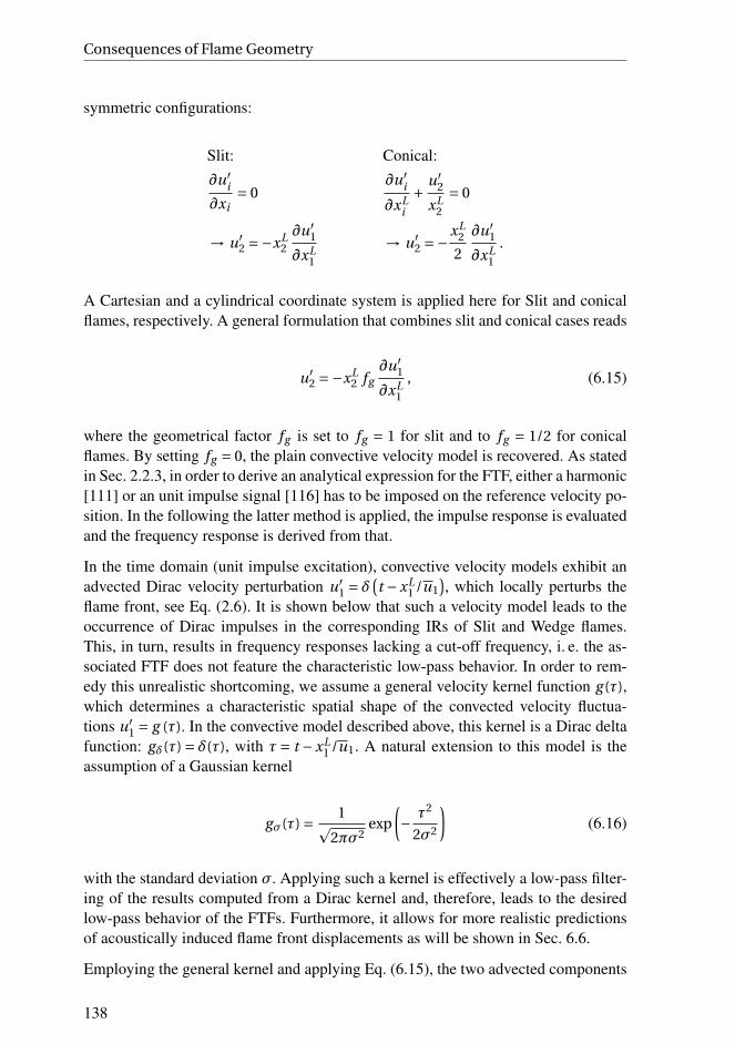
Consequences of Flame Geometry

symmetric configurations:

Slit: Conical:

∂u′i

∂xi= 0

∂u′i

∂xLi

+u′

2

xL2

= 0

→ u′2 =−xL

2

∂u′1

∂xL1

→ u′2 =−

xL2

2

∂u′1

∂xL1

.

A Cartesian and a cylindrical coordinate system is applied here for Slit and conicalflames, respectively. A general formulation that combines slit and conical cases reads

u′2 =−xL

2 fg

∂u′1

∂xL1

, (6.15)

where the geometrical factor fg is set to fg = 1 for slit and to fg = 1/2 for conicalflames. By setting fg = 0, the plain convective velocity model is recovered. As statedin Sec. 2.2.3, in order to derive an analytical expression for the FTF, either a harmonic[111] or an unit impulse signal [116] has to be imposed on the reference velocity po-sition. In the following the latter method is applied, the impulse response is evaluatedand the frequency response is derived from that.

In the time domain (unit impulse excitation), convective velocity models exhibit anadvected Dirac velocity perturbation u′

1 = δ(t −xL

1 /u1

), which locally perturbs the

flame front, see Eq. (2.6). It is shown below that such a velocity model leads to theoccurrence of Dirac impulses in the corresponding IRs of Slit and Wedge flames.This, in turn, results in frequency responses lacking a cut-off frequency, i. e. the as-sociated FTF does not feature the characteristic low-pass behavior. In order to rem-edy this unrealistic shortcoming, we assume a general velocity kernel function g (τ),which determines a characteristic spatial shape of the convected velocity fluctua-tions u′

1 = g (τ). In the convective model described above, this kernel is a Dirac deltafunction: gδ(τ) = δ(τ), with τ= t −xL

1 /u1. A natural extension to this model is theassumption of a Gaussian kernel

gσ(τ) = 1p

2πσ2exp

(− τ2

2σ2

)(6.16)

with the standard deviation σ. Applying such a kernel is effectively a low-pass filter-ing of the results computed from a Dirac kernel and, therefore, leads to the desiredlow-pass behavior of the FTFs. Furthermore, it allows for more realistic predictionsof acoustically induced flame front displacements as will be shown in Sec. 6.6.

Employing the general kernel and applying Eq. (6.15), the two advected components

138

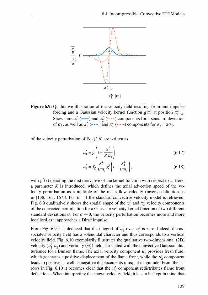
6.4 Incompressible-Convective FTF Models

xL1,ref

0

xL1 [m]

u′ 1/2

[m/s]

Figure 6.9: Qualitative illustration of the velocity field resulting from unit impulseforcing and a Gaussian velocity kernel function g (τ) at position xL

1,ref.

Shown are xL1 ( ) and xL

2 ( ) components for a standard deviationof σ1, as well as xL

1 ( ) and xL2 ( ) components for σ2 = 2σ1.

of the velocity perturbation of Eq. (2.6) are written as

u′1 = g

(t −

xL1

K u1

)(6.17)

u′2 = fg

xL2

K u1g ′

(t −

xL1

K u1

), (6.18)

with g ′(τ) denoting the first derivative of the kernel function with respect to τ. Here,a parameter K is introduced, which defines the axial advection speed of the ve-locity perturbation as a multiple of the mean flow velocity (inverse definition asin [138, 163, 167]). For K = 1 the standard convective velocity model is retrieved.Fig. 6.9 qualitatively shows the spatial shape of the xL

1 and xL2 velocity components

of the convected perturbation for a Gaussian velocity kernel function of two differentstandard deviations σ. For σ→ 0, the velocity perturbation becomes more and morelocalized as it approaches a Dirac impulse.

From Fig. 6.9 it is deduced that the integral of u′2 over xL

1 is zero. Indeed, the as-sociated velocity field has a solenoidal character and thus corresponds to a vorticalvelocity field. Fig. 6.10 exemplarily illustrates the qualitative two-dimensional (2D)velocity (u′

1,u′2) and vorticity (ω′

3) field associated with the convective Gaussian dis-turbance for a Bunsen flame. The axial velocity component u′

1 provides fresh fluid,which generates a positive displacement of the flame front, while the u′

2 componentleads to positive as well as negative displacements of equal magnitude. From the ar-rows in Fig. 6.10 it becomes clear that the u′

2 component redistributes flame frontdeflections. When interpreting the shown velocity field, it has to be kept in mind that

139

Consequences of Flame Geometry

Figure 6.10: Snapshot of the velocity and vorticity field resulting from unit impulseresponse forcing and a Gaussian velocity kernel for a Bunsen flame.Shown are the two velocity components u′

1 (top left), u′2 (top right)

and the correspond xL3 vorticity component ω′

3 (bottom), all of themnormalized by their maximum absolute value.

only the velocity right at the mean flame front interacts with the flame. The spatio-temporal structure far away from the flame is not important and should, hence, not bemisinterpreted as a strange kind of shear layer vortex.

In order to derive analytical expressions for the IRs of all three configurations, wefirstly evaluate the flame normal velocity perturbation associated with Eqs. (6.17)and (6.18), which is

u′⊥,Λ/slit =g

[t −

xF1

L fτc

]sin(α)+

fg τc

Ri −xF1 sin(α)

L fg ′

[t −

xF1

L fτc

](6.19)

140

6.5 Geometry-Dependent Analysis of the Incompressible-Convective Model

for Slit and Bunsen flames and

u′⊥,V =g

[t −

xF1

L fτc

]sin(α)+

fg τc

R0 +xF1 sin(α)

L fg ′

[t −

xF1

L fτc

](6.20)

for Wedge flames. A second characteristic time τc is introduced here, which denotesthe time it takes for an axially advected velocity perturbation to be transported fromthe flame base to its tip. This introduces the velocity of the convective disturbance inflame coordinates uc , which is provided for both coordinate systems in Tab. 6.1. Thecharacteristic flame times τr and τc are related to flame speed, the flame angle andthe feed duct half-diameter by

τr =Ri

sL cos(α), (6.21)

τc =cos2(α)

Kτr , (6.22)

where the relation cos2(α) = 1− s2L/u2

1 could be applied to estimate the flame angle.For Wedge flames, a length Ri = Ra −Rr has to be used in Eq. (6.21). Using the de-scribed perturbation velocity field, analytical expressions for the IRs of all three flamegeometries are derived by solving Eq. (1.32) (lM = 0) and, subsequently, Eq. (2.3)for the unit impulse response h(t ) using the flame surface integrals summarized inTab. 6.1. Results are provided in Appendix C.1 and are functions of τr and τc only(ignoring fg and possible kernel parameters). The FTF of Wedge flames has the non-dimensional rod radius r = Rr /Ra as a third parameter. All FTFs are derived in termsof a general kernel g and are hence ready to be used with arbitrary functions.

We introduce the abbreviation DIC for the Dirac kernel based incompressible-convective velocity model and GIC for the Gaussian kernel based counterpart. TheGIC model relies on the two additional empirical parameters K and σ, which needto be fitted to experimental observations. As will be shown later, K is primarily usedto modify the frequency of maximum gain and σ to set the cut-off frequency of theFTF.

6.5 Geometry-Dependent Analysis of the Incompressible-

Convective Model

Above, the incompressible-convective velocity models for three flame configurationswere introduced. We now want to analyze the DIC model for all geometries in orderto gain some insights into the respective flame responses. To date, expressions ofthe DIC model have solely been evaluated for Bunsen flames. While Cuquel [134]

141

Consequences of Flame Geometry

0

1

2

Magnitude

0 2 4 6

-8π

-4π

0

f∗ [-]

Phase

0 0.5 1−2

−1

0

1

2

3

4

t∗ [-]

h∗

Figure 6.11: FTF predictions of the DIC model for α=π/4 and K = 1 in terms ofimpulse response h(t ) (left) and frequency response F (ω) (right) shownfor three flame configurations: Slit ( , impulses as ), Bunsen ( )and Wedge flames ( , impulses as ). The phase decay correspond-ing to a fixed time delay of τr ( ) and the one corresponding toτr /2 ( ) are added to the phase plots. For Wedge flames a non-dimensional rod radius of r = 0.5 is assumed.

analyzed them in time and frequency domain, Preetham et al. [138] and Orchiniand Juniper [163] focused only on frequency domain representations. The followingdiscussion seeks to close this gap in the literature.

FTF predictions of the DIC model for α=π/4 and K = 1 are shown in Fig. 6.11for all three flame geometries. For Wedge flames, a non-dimensional rod radius ofr = 0.5 is assumed. The IRs are shown on the left-hand side of this figure and theassociated FRs, in terms of magnitude and phase, on the right. All quantities arenon-dimensionalized by the characteristic flame time: h∗ = hτr , t∗ = t/τr and f ∗ =f τr . The IRs of the Slit and the Wedge flame contain Dirac delta functions. Thiskind of function (strictly speaking distribution) is characterized by its integral andit is hence decided to indicate this integral value in all IR visualizations whenever aDirac Impulse is present. That means, for example, that the blue circle in Fig. 6.11represents a −δ(t∗−1) contribution. Since the integral of this expression is −1, thecircle indicates this value in the graphical representation of the IR at t∗ = 1.

The respective behavior of the FTF for the various geometries becomes more clearwhen analyzing the transient flame front deflection ξ(xF

1 , t ) caused by an impulseforcing. An illustration of a snapshot is shown in Fig. 6.12a for Slit and Bunsen and in

142

6.5 Geometry-Dependent Analysis of the Incompressible-Convective Model

(a) Bunsen and Slit flames (b) Wedge flames

Figure 6.12: Illustration of the displaced flame front deflection ξ(xF

1 , t)

of the DICmodel for an impulse velocity perturbation. Shown are two flanks,which propagate with the velocity ur (restoration) and uc (convectiveflow disturbance), and two impulses I and II both propagating with thevelocity of the respective flank.

Fig. 6.12b for Wedge flames. As expound by Blumenthal et al. [116] for the plain con-vective velocity model, two flanks are formed (see Fig. 6.12), which delimit a pocketof unburned gas. This pocket grows in extent, since the downstream flank propagateswith a higher velocity than the upstream one (uc > ur ). In case of the incompressible-convective velocity model, additionally, two flame front displacements of the shapeof a Dirac impulse are formed (see Fig. 6.12), which are not present in the plain con-vective velocity model and also propagate along the flame front. They result from thelateral, solenoidal velocity component of the convected perturbation. In agreementwith Fig. 6.12 we refer to those impulses as Impulse I and Impulse II. Their propa-gation speed equals the speed of the adjacent flank, i. e. uc for impulse II and ur forimpulse I.

First let us consider a Bunsen flame. Here, Impulse I forms a negative flame frontdisplacement and its amplitude stays constant while it is advected downstream withur , see Fig. 6.12a. Impulse II constitutes a positive displacement and its amplitudedecreases when advected downstream by the velocity uc , until it reaches zero right atthe flame tip. According to Sec. 6.2, the linearized flame surface area fluctuation ofa Bunsen flame depends on the integral of the instantaneous flame front deflections.Hence, advected Dirac impulses are transformed to Heaviside Step functions in timewhen evaluating the IR, see Appendix C.1. Consequently, the IR of a Bunsen flamesdoes not show any Dirac Impulses as depicted in Fig. 6.13a. Impulse I adds a constantnegative contribution to the overall IR ( ), while Impulse II adds an decreasing,positive value to the overall IR, which disappears at t∗ = 0.5, i. e. in dimensionaltime at t = τc ( ). The specific nature of the Bunsen flame heat-release dynamics(integral of ξ) leads to a dispersion of the flame response in time. This, in turn, goesalong with a relatively low cut-off frequency of the associated FTF, see Fig. 6.11( ). This can be explained by the fact that integration imposes a 1/ω behavior in

143

Consequences of Flame Geometry

0 0.5 1

−1

0

1

2

3

t∗ [-]

h∗

(a) Bunsen flame

0 0.5 1

−1

0

1

2

3

4

t∗ [-]h∗

(b) Slit flame

0 0.5 1

−2

−1

0

1

2

t∗ [-]

h∗

(c) Wedge flame

Figure 6.13: Impulse responses of the three different flame configurations. Shownare the overall IR ( , impulses as ), as well as the contributions ofthe flanks ( ), Impulse I ( , impulses as ) and Impulse II ( ,impulses as ) of ξ

(xF

1 , t)

to the overall IR. Parameters are the same asthose described in Fig. 6.11.

frequency domain, see Tab. C.2 in Appendix C.1: The integral of a Dirac impulse isthe Heaviside step function and, consequently, the amplitude of the one-sided Fouriertransform of the latter shows an 1/ω behavior while it is unity for the former.

The situation is very different when a Slit flame is considered. The instantaneousflame front displacement according to the DIC model is qualitatively the same as fora Bunsen flame, see Fig. 6.12a. However, since the flame surface area fluctuation ofSlit flames depends to leading order only on the flame tip movement, see Sec. 6.2,Dirac impulses in ξ lead to the appearance of Dirac impulses in the IR. More specif-ically, as shown in Fig. 6.13b, Impulse I adds a negative Dirac impulse at t∗ = 1 (indimensional time at t = τr ). Impulse II has no impact as it vanishes at the flame tip.The negative impulse at t∗ = 1 leads to an FR gain tending to unity instead of zerofor f →∞, see Fig. 6.11 ( ). All in all, the response of a Slit flame constitutesa time delayed, direct effect of flame front perturbations. No spatial integration offlame displacements, as in the Bunsen case, is present, which leads to an FR lackinga low-pass filtering behavior.

The global heat-release rate of Bunsen flames responds to the integral of a flamefront perturbation, while Slit flames react to flame front deflections directly oncethey reach the flame tip. Bunsen flames are, in consequence, a more sedate source ofsound than Slit flames for a given flame front perturbation. This fact might, besidesother effect such as flame curvature or burner-plenum acoustics, contribute to thelower sound pressure levels of combustion noise produced by turbulent Bunsen typeflames compared to Slit ones, as reported by Kotake and Takamoto [151] and Pauschet al. [153].

144

6.6 Validation of Flame Response Models

In terms of response characteristics, Wedge flames are in some aspects similar to Slitflames and in others more close to Bunsen flames. A snapshot of the resulting flamefront deflection due to an impulse velocity forcing is shown in Fig. 6.12b. Again,two flanks appear, which are advected downstream. Impulse I depends on the non-dimensional rod radius r and has a constant, non-zero value for r > 0. Contrary toBunsen and Slit flames, Impulse II now increases in amplitude while it is advecteddownstream. Consequently, both impulses lead to the occurrence of Dirac impulsesin the IR of Wedge flames, see Fig. 6.13c. Thus, the gain of the corresponding FRnever reaches zero and shows several recurring peaks of high magnitude, similar to aSlit configuration, see Fig. 6.11 ( ). While the phase of a Slit flame decays with aconstant slope, which corresponds to the one of a system with a fixed time delay τr ,the phase of a Bunsen flames decays with a slope corresponding to a time delay τr /2.The phase of a Wedge flame with α=π/4 behaves similar to the one of a Bunsenflame, as depicted in Fig. 6.11. For longer flames (α ↓) the phase of a Wedge flamewould approach the one of a Slit flame (not shown).

The response of Wedge flames integrates flame front perturbations and also directlyresponds to them once they reach the flame tip. In that sense they are a hybrid ofSlit and Bunsen flames. Since, however, their flame front deflection according to theDIC model is different to that of Bunsen and Slit flames, see Fig. 6.12, they are nota pure hybrid and additionally bring some individual response characteristics, suchas the presence of pronounced positive and negative contributions in their IR. Asexplicated by Blumenthal et al. [116], this is a necessary condition for the occurrenceof peak gain values exceeding unity. Indeed, the gain shown in Fig. 6.11 affirms thisstatement.

In this section it is illustrated that each of the three considered flame configurationshas its own peculiar response characteristics. As will be shown in the following, theincompressible-convective velocity model is able to predict frequency and impulseresponses, which qualitatively and also quantitatively agree with CFD and experi-mental data, if a Gaussian instead of a Dirac kernel is used. In doing so, the Diracimpulses, appearing in the IRs of Slit and Wedge flames, are transformed to Gaussianimpulses. This corresponds to a dispersion in time and, hence, to a decreased cut-offfrequency, which brings the desired low-pass behavior of the predicted FTFs.

6.6 Validation of Flame Response Models

Figs. 6.14, 6.15 and 6.16 visualize FTFs identified from the CFD simulations in-troduced in Sec. 6.1 for all three flame configurations ( ). Additionally, predic-tions from the convective and the incompressible-convective velocity model (DICand GIC) are shown. The free parameters τr , τc and r are computed according toEqs. (6.21) and (6.22) using the physical and geometrical quantities introduced inSec. 6.1 and a laminar flame speed of sL = 0.278 m/s. Due to confinement effects

145

Consequences of Flame Geometry

0

1

2

3

Magnitude

0 2 4 6

-12π

-6π

0

f∗ [-]

Phase

0 0.5 1 1.5−12

−8

−4

0

4

8

12

t∗ [-]

h∗

Figure 6.14: Comparison of FTF predictions for Slit flames visualized in time (left)and frequency domain (right) from CFD/SI data ( ), as well as fromthe plain convective ( ) and the incompressible-convective velocitymodel using a Dirac ( , impulses as ) and a Gaussian kernel withσ= 1.2 ms and K = 1.3 ( ) for τr = 18.7 ms.

(see e. g. [144]), we have to adjust τr for the Slit and the Wedge setup compared tothe results provided by Eq. (6.21) in order to match the CFD/SI data. This correctionis applied by fitting the reduced order models to the CFD/SI IR data such that the po-sition of the first negative part of the IRs coincide. Confinement effects are negligiblefor the Bunsen flame setup. The respectively values of τr are provided in the figurecaptions of the FTF data.

Concerning the empirical parameters of the GIC model, for the Bunsen and the Slitresults presented here, we chose σ = 1.2 ms and K = 1.3 in order to match the CFDdata. For the Wedge case, K = 1.3 could be applied as well, however, we use an in-creased standard deviation of σ= 1.9 ms. This results in a non-dimensionalized stan-dard deviation σ∗ =σ/τr of σ∗ ≈ 0.064 for the Slit and Bunsen setup and σ∗ ≈ 0.142

for Wedge case. Hence, at least for the three cases discussed here, some universalityof these parameter values can be assumed.

By evaluating the FTF for both a Dirac and a Gaussian kernel, the importance ofthe dispersion in time, which was mentioned in Sec. 6.4, becomes apparent. Wedgeand Slit flames have Dirac impulses in their DIC model based predictions, see ( ,impulses as ) in Figs. 6.14 and 6.16. The corresponding FR gain curves oscillatewithout decaying to zero, which does not reflect the observed low-pass filtering be-havior of flames. Introducing a Gaussian kernel, the Dirac impulses of the DIC based

146

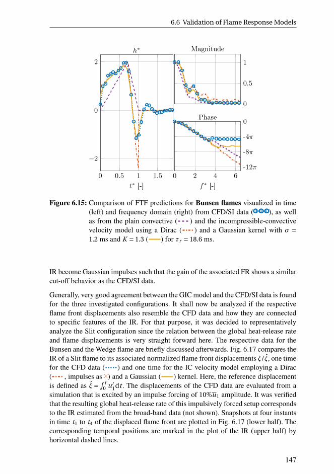
6.6 Validation of Flame Response Models

0

0.5

1

Magnitude

0 2 4 6

-12π

-8π

-4π

0

f∗ [-]

Phase

0 0.5 1 1.5

−2

0

2

t∗ [-]

h∗

Figure 6.15: Comparison of FTF predictions for Bunsen flames visualized in time(left) and frequency domain (right) from CFD/SI data ( ), as wellas from the plain convective ( ) and the incompressible-convectivevelocity model using a Dirac ( ) and a Gaussian kernel with σ =1.2 ms and K = 1.3 ( ) for τr = 18.6 ms.

IR become Gaussian impulses such that the gain of the associated FR shows a similarcut-off behavior as the CFD/SI data.

Generally, very good agreement between the GIC model and the CFD/SI data is foundfor the three investigated configurations. It shall now be analyzed if the respectiveflame front displacements also resemble the CFD data and how they are connectedto specific features of the IR. For that purpose, it was decided to representativelyanalyze the Slit configuration since the relation between the global heat-release rateand flame displacements is very straight forward here. The respective data for theBunsen and the Wedge flame are briefly discussed afterwards. Fig. 6.17 compares theIR of a Slit flame to its associated normalized flame front displacements ξ/ξ, one timefor the CFD data ( ) and one time for the IC velocity model employing a Dirac( , impulses as ) and a Gaussian ( ) kernel. Here, the reference displacementis defined as ξ=

∫t0 u′

1dt . The displacements of the CFD data are evaluated from asimulation that is excited by an impulse forcing of 10%u1 amplitude. It was verifiedthat the resulting global heat-release rate of this impulsively forced setup correspondsto the IR estimated from the broad-band data (not shown). Snapshots at four instantsin time t1 to t4 of the displaced flame front are plotted in Fig. 6.17 (lower half). Thecorresponding temporal positions are marked in the plot of the IR (upper half) byhorizontal dashed lines.

147

Consequences of Flame Geometry

0

1

2

3

4

Magnitude

0 1 2 3 4

-8π

-4π

0

f∗ [-]

Phase

0 0.5 1 1.5

−4

−2

0

2

4

6

t∗ [-]

h∗

Figure 6.16: Comparison of FTF predictions for Wedge flames visualized in time(left) and frequency domain (right) from CFD/SI data ( ), as wellas from the plain convective ( ) and the incompressible-convectivevelocity model using a Dirac ( , impulses as ) and a Gaussian ker-nel with σ= 1.9 ms and K = 1.3 ( ) for τr = 13.3 ms.

0 0.5 1

−2

0

2

t1

xF1 /Lf [-]

ξ/ξ

[-]

0 0.5 1

t2

xF1 /Lf [-]

0 0.5 1

t3

xF1 /Lf [-]

0 0.5 1

t4

xF1 /Lf [-]

0 1 2

t1 t2 t3 t4

t∗ [-]

h∗

[-]

Figure 6.17: Comparison of IR (top) and the corresponding normalized flame frontdisplacement ξ/ξ of the Slit configuration resulting from an impulseforcing at four instants in time, shown for the CFD/SI data ( ) as wellas for the incompressible-convective velocity model employing a Dirac( , impulses as ) and a Gaussian ( ) kernel, see also Fig. 6.14.Compare to Fig. 6.12a for clarification.

At time t1 = 0 the impulsive velocity forcing hits the flame and both the CFD dataand the GIC model show displacements in the approximate vicinity of the flame base

148

6.6 Validation of Flame Response Models

0 0.5 1

−2

0

2

t1

xF1 /Lf [-]

ξ/ξ

[-]

0 0.5 1

t2

xF1 /Lf [-]

0 0.5 1

t3

xF1 /Lf [-]

0 0.5 1

t4

xF1 /Lf [-]

0 1

t1 t2 t3 t4

t∗ [-]

h∗

[-]

Figure 6.18: Comparison of IR (top) and the corresponding normalized flame frontdisplacement ξ/ξ of the Bunsen configuration resulting from an impulseforcing at four instants in time, shown for the CFD/SI data ( ) as wellas for the incompressible-convective velocity model employing a Dirac( , impulses as ) and a Gaussian ( ) kernel, see also Fig. 6.15.Compare to Fig. 6.12a for clarification.

region. This is in accordance with the findings of Chap. 4 relating this to the impact ofthe potential part of the acoustic perturbation. The flame tip stays unaffected and thusthe corresponding IR exhibits no response at t1. The CFD data now shows that whilethis initial displacement is convected downstream it grows in amplitude and smaller,secondary negative and positive displacements develop. Each time a displacementreaches the flame tip, a response of the global heat-release is provoked, see t3 and t4.Having a look at the corresponding GIC and DIC data, it is apparent that displace-ment amplitudes are overpredicted until they reach the flame tip, where they matchthe CFD results reasonably well. Knowing that the global heat-release rate of Slitflames depends solely on flame tip movements, it becomes clear that the matching ofamplitudes at the tip region is the crucial property that determines the quality of theassociated IR prediction.

Figs. 6.18 and 6.19 show the corresponding results for a Bunsen and Wedge config-uration, respectively. Again it can bee seen that although flame displacements pre-dicted by CFD and the GIC model do not perfectly match, the IRs of the globalheat-release agree well. The GIC model is able to qualitatively capture the dynam-ics of an impulsively perturbed flame front. For harmonic forcing Baillot et al. [120]reported good agreement between experiment and the DIC model in terms of flameshapes. Since the GIC model improves response predictions compared to the DICmodel, it can be conjectured that the GIC model should further improve that alreadygood match.

It is interesting to note that while Slit and Bunsen configurations exhibit flame frontdisplacements that grow in amplitude, the ones for Wedge flames show a decayingbehavior (Fig. 6.19, ). The reason for this is unclear. Further, the initial displace-ments at t = 0 are very similar for all three configurations, which means that, qual-

149

Consequences of Flame Geometry

0 0.5 1

−0.50

0.51

t1

xF1 /Lf [-]

ξ/ξ

[-]

0 0.5 1

t2

xF1 /Lf [-]

0 0.5 1

t3

xF1 /Lf [-]

0 0.5 1

t4

xF1 /Lf [-]

0 1

t1 t2 t3 t4

t∗ [-]

h∗

[-]

Figure 6.19: Comparison of IR (top) and the corresponding normalized flame frontdisplacement ξ/ξ of the Wedge configuration resulting from an impulseforcing at four instants in time, shown for the CFD/SI data ( ) as wellas for the incompressible-convective velocity model employing a Dirac( , impulses as ) and a Gaussian ( ) kernel, see also Fig. 6.16.Compare to Fig. 6.12b for clarification.

itatively, the results presented in Chap. 4 seem not to be limited to Slit flames butare rather universal. Finally, the deviation of displacements of the DIC from the GICmodel for Slit and Wedge configurations illustrates the importance of the Gaussianimpulses for the overall response characteristics.

Comparing predictions of the flame front displacements shown in Fig. 6.17 from theDIC ( , impulses as ) and the GIC ( ) model, one realizes that the Gaussiankernel disperses unphysical, very localized Dirac displacements of the DIC modelin space. Such a dispersion might be related to effects of flame stretch, particularlycurvature, as well as to the finite width of the initial flame displacements of the CFDdata at t1, which is an essentially inviscid effect [1].

As a consequence of the oscillatory displaced flame front, Slit flames show a decay-ing oscillatory IR with alternating positive and negative contributions of decreasingamplitude, see Figs. 6.14 and 6.17. The GIC model captures the first period of thissignal and then immediately decays to zero. The negative part of the predicted IR iscaused by the u′

2 component of the velocity model, see Eq. (6.18), which correspondsto a vortical velocity field, as described in Sec. 6.4. It is hence deduced that, In theproposed models, the first negative minimum (the second for Wedge flames) of allIRs is caused by vortical structures.

Slit flames show a very high peak gain value, which is not at all predicted by theplain convective velocity model, see Fig. 6.14 ( ). For the other two geometries,this model agrees reasonably well with the CFD/SI data. It correctly predicts the cut-off behavior of Bunsen flames and only misses to capture the reoccurring maxima inthe gain for f ∗ > 1.5, as depicted in Fig. 6.15. For Wedge flames, Fig. 6.16 shows thatthe gain exceeding unity at f ∗ ≈ 1.3 is qualitatively captured, however, the maximum

150

6.6 Validation of Flame Response Models

gain value is underestimated. The most important feature added by the DIC model,compared to the convective one, is the occurrence of impulses in the IR ( ). Slitflames show one negative impulse at t∗ = 1, right at the position of the first minimumof the IR. Wedge flames have two of them, a negative one at t∗ = 1 and a positive oneat t∗ = τc /τr , both at positions of local extreme values of the IR.

Having a closer look at the IRs, it is found that the time scale defined by τr −τc playsan important role. As already pointed out by Blumenthal et al. [116], the differencebetween the restorative and the convective time defines the frequency of maximumgain for (sharp) Wedge flames. The IRs of all three flame configurations show oscil-lations of decaying amplitude. They are most prominent for the Slit and the Wedgeconfiguration, see Figs. 6.14 and 6.16. The width of half a period of these oscillationsvery well agrees with the time τr −τc . The corresponding oscillation frequency isapproximated by a Strouhal number

f ∗O = τr

2(τr −τc )= 1

2(1− cos2(α)

K

) , (6.23)

which is f ∗O ≈ 1.7 for all shown cases. Around this frequency the Slit and the Bunsen

flame show a local maximum in the gain of their FR. The peak value of the Wedgeflame is shifted to a lower Strouhal number of about 1.1.

As stated by Eq. (6.23), the frequency of maximum gain depends on K and, hence,provides a physically motivated criterion to estimate this parameter. It is thereforepresumed that the width of the Gaussian kernel function, set by the standard devi-ation σ, determines the cut-off frequency of the FTF and the parameter K fixes thefrequency of maximum gain. Physically, the value of the first might be connected todiffusive processes and the one of the latter to (baroclinic) generation of vorticity.

This finding is exploited in order to compare the proposed models to data from theliterature. Since Wedge setups comparable to the ones described here could not befound (i. e. no swirl and no influence of vortex shedding), only Bunsen and Slit con-figurations are used. Information about the experimental data is provided in Tab. 6.2.Fig. 6.20 shows the adopted frequency responses (FR), as well as the fitted FTF pre-dictions of the GIC models. For each data set, a frequency is identified where thegain has a local maximum and Eq. (6.23) is used to compute an associated value forK . The values of cos2(α), which is according to Eq. (6.22) required to compute τc ,and τr are estimated from the cited references. The standard deviation σ is then ad-justed until the cut-off frequency of the GIC model agrees sufficiently well with theexperimental data. All fit parameters are provided in Tab. 6.2.

Since all Bunsen setups show a very similar trend, only one single model ( f ∗O ≈ 1.85)

was fitted. On the contrary, the FR of Slit flames has a high variance and is stronglyaffected by τr : the maximum gain value and the cut-off frequency rise with increas-ing τr . Accordingly, the non-dimensional frequency f ∗

O shifts from 0.9 over 2.4 to4.4. Since the GIC model consistently overpredicts the gain for low frequencies, it is

151

Consequences of Flame Geometry

Source Fit Parameter τr Fig. 6.20

Bun

sen

[156](Fig. 3.6,

2 m/s)

K = 1.33

σ= 1.2 mscos2(α) = 0.97

14.8 ms

[134](Fig. 3.8)

– 26.1 ms

[134](Fig. 6.12,0.396 g/s)

– 31.7 ms

Sli

t

[148](Fig. 7,T50h)

K = 2.1

σ= 1.45 mscos2(α) = 0.95

12.50 ms

[149](CBB)

K = 1.18

σ= 1.9 mscos2(α) = 0.94

38.3 ms

[149](UBB)

K = 1.04

σ= 1.9 mscos2(α) = 0.92

46.6 ms

Table 6.2: Summary of experimental data adopted from the literature, see Fig. 6.20.

0

0.5

1

Mag

nit

ude

0 1 2 3 4 5 6

-8π

-4π

0

f∗ [-]

Phas

e

(a) Bunsen

0

2

4

Mag

nit

ude

0 2 4 6 8 10 12

-18π

-12π

-6π

0

f∗ [-]

Phas

e

(b) Slit

Figure 6.20: Experimental frequency response data of selected conical (a) and a slitflames (b) adopted from the literature (see Tab. 6.2). Additionally, pre-dictions of the GIC model are shown (black lines). The phase corre-sponding to a fixed time delay of τr ( ) and τr /2 ( ) is indicatedin the phase plots.

concluded that it is lacking some damping mechanisms, which are present in exper-iments. Besides this, it is able to capture both gain and phase sufficiently well. Thisis remarkable considering the fact that in particular for Slit flames, the convective aswell as the DIC model lead to very inaccurate FTF predictions, see also Fig. 6.14.

Finally, it should be pointed out that the phase of all Bunsen FTFs coincides with theone of a system with a constant time delay τr /2, while Slit flames resemble a systemof time delay τr , see Fig. 6.20. This result corresponds to the findings of Duchaine

152

6.7 Summary and Conclusions

et al. [146] and is captured correctly by both of the convective velocity models (DICand GIC), see Sec. 6.5.

6.7 Summary and Conclusions

This chapter analyzed the consequences of flame geometry for the linear flame re-sponse, namely the flame transfer function (FTF). This was done by following a wellestablished, G-equation based modeling approach and analyzing it with respect togeometry-related differences of Slit, Bunsen and Wedge type flame configurations.The process of how a wrinkled flame front leads to fluctuations in the global heat-release was identified as the key mechanism, which distinguishes the response ofeach flame. Therefore, the flame surface integral was analyzed in detail and analyt-ical expressions for stiffly anchored, symmetric flames were derived. By extendingthe well-known incompressible-convective velocity model with a Gaussian Kernel,analytical FTF expressions were derived, which very well coincide with FTF predic-tions from numerical simulations for all three considered flame configurations. Thederived models rely on two empirical parameters, namely the standard deviation ofthe Gaussian kernel and the advection velocity of the convective flow perturbationrelative to the mean flow velocity. By relating the latter parameter to the frequencyof maximum gain and the first to the cut-off frequency of the FTF, it was possible toprovide good predictions of gain and phase of experimentally determined FTFs takenfrom the literature.

The main finding of the present analysis are:

1. The integral heat-release of Bunsen flames is proportional to the integral of theflame front displacement, the flame tip movement is negligible. Consequently,heat-release rate fluctuations induced by a displaced flame front are dispersedin time, which leads to a relatively low cut-off frequency, such that the FTFs ofBunsen flames look always quite similar when plotted over Strouhal number.The phase of the FTF is dominated by half the time of restoration τr /2.

2. The integral heat-release of Slit flames is proportional to the flame tip move-ment. Therefore, flame front displacements directly affect the heat-release rateonce they reach the tip. Compared to Bunsen flames, this leads to an increasedcut-off frequency and, hence, to a higher response variance of Slit flame setups.Slit frequency responses show a high maximum gain value, which increaseswith the time of restoration τr . The heat-release of Slit flames responds timedelayed to flame front perturbations, which leads to an FTF phase dominatedby the characteristic flame time of restoration τr .

3. The integral heat-release of Wedge flames is proportional to the flame tipmovement and the integral of the flame front displacement. Their impulse re-sponse shows significant positive and negative parts, which lead to gain values

153

Consequences of Flame Geometry

exceeding unity. The phase behaves similar to the phase of a Bunsen flame andapproaches the behavior of a Slit flame for long flames.

4. The impulse responses of all flame configurations, identified from CFD data,show a strongly damped oscillatory behavior, which leads to a local maximumin the FTF gain close to the oscillation frequency. In the proposed modelingframework, this frequency could be related to the difference in the time ofrestoration and the one of distortion, τr −τc . This dependency can be exploitedin order to compute the two empirical parameters of the proposed Gaussianincompressible-convective (GIC) velocity model.

5. For surface integration, it is important to choose a coordinate system that ac-counts for the possible flame movements at the boundaries. Otherwise, variableintegration limits are required.

Based on these results, the findings of Part II, which are based on Slit flames, can betransferred to Bunsen and Wedge geometries. Since the flame sheet dynamics essen-tially remains the same for all discussed configurations, differences emerge mainlyfrom how flame shape translates to heat release. These integrals could simply be im-plemented into the low-order modeling framework suggested in Part II, which wouldallow for an approximation of the respective response characteristics.

154

Summary and Conclusions

This doctoral thesis analyzed the linear acoustic response of laminar premixedBunsen-type flames primarily relying on first-principle-based, low-order modelingapproaches. A literature review on the dynamics of laminar flames and interactionsbetween acoustics and burner-stabilized flames laid the foundation for all subse-quently performed investigations and provided guidance for the identification of rele-vant physical mechanisms determining the response characteristics. While, in the lit-erature, the understanding of the dynamics of burner-stabilized flames whose anchor-ing is mechanically displaced, is based on the concepts of the Darrieus-Landau insta-bility and thermal-diffusive mechanisms, the interpretation evolves around the notionof convected velocity perturbations in the case of acoustically perturbed flames. Thisis particularly surprising knowing that their dynamics should in fact be very similar,since acoustics predominately displaces the flame base region in both cases.

Motivated by this realization, a first principles-based incompressible low-order mod-eling framework was introduced, relying on methods adopted from aero-acoustics:the flow field is represented by a number of flow-field singularities combined witha conformal mapping technique and a Kutta condition. In a first step, flame-flowfeedback was neglected and primary acoustics-flame interactions were assessed. Itwas found that consequences of shed vorticity for the flame response are negligibleand that the irrotational part of the acoustic perturbations displaces essentially theflame base region. Hence, convective sources of flame displacement, as assumed bystate-of-the-art low-order modeling approaches in the limit of negligible flame-flowfeedback, could not be identified. Comparing low-order predictions to high fidelityCFD data, it could be shown that the resulting flame front displacements match onlywell right at the moment when the acoustic impulse hits the flame.

At later times, secondary mechanisms come into play, causing secondary displace-ments as well as the convective growth of displacement amplitudes. These effectscould be associated with flame-flow feedback which essentially has two contribu-tions: (i) a vortical one relying on flame-generated vorticity and (ii) an irrotationalone relying on a flame-normal acceleration of the flow across a flame sheet togetherwith a flame displacement-induced geometrical focusing. While the former mecha-nism causes a perturbed flame sheet to behave like a vortex sheet of varying strength,the far field of the latter resembles the one of advected dipoles. The upstream in-

155

Consequences of Flame Geometry

fluence of each of these two mechanisms onto the unburned flow induces convectedvelocity perturbations. This explains observations reported by previous experimentalstudies. Concerning the linear response of the global heat release, it could be shownthat both mechanisms of flame-flow feedback lead to the occurrence of peak FTFgain values significantly exceeding unity.

All those investigations were performed for Slit flame configurations; the literature,however, mostly reports on Bunsen flames. Therefore, in the final part of this thesis,consequences of flame geometry — namely of Slit, Bunsen and Wedge configurations— for the acoustic response were analyzed. It was found that the process of how awrinkled flame front leads to fluctuations in the global heat-release constitutes thekey mechanism that distinguishes the responses of different flame geometries. Byextending the well-known incompressible-convective velocity model with a GaussianKernel, analytical FTF expressions were derived, which coincide very well with FTFpredictions from numerical simulations for all three considered flame geometries.

The main achievements of this work can be summarized to:

• The linear thermoacoustic response (FTF) of a laminar premixed flame isessentially governed by hydrodynamic mechanisms that lead to (i) primaryacoustically induced perturbations acting predominantly at the flame base and(ii) flame-flow feedback interacting with these primary flame front displace-ments while they are convected downstream.

• Flame-flow feedback has vortical and irrotational contributions and is respon-sible for FTF peak gain values significantly exceeding unity. Further it explainsthe observations of convected velocity perturbations upstream a wrinkled flamesheet.

• G-equation-based low-order models are usually based on the ad hoc assump-tion of convected velocity perturbations. They only implicitly include con-sequences of flame-flow feedback and, thus, do not faithfully represent thecausality of the underlying flow physics.

• Flame geometry significantly impacts the dynamics of the global heat releaserate, while the respective flame sheet dynamics remains essentially unchanged.Each geometry has its own unique response characteristics.

Based on the analysis performed in this thesis, some questions still remain open and,additionally, some new issues have been raised. One important point that requiresfurther investigations concerns the quantitative analysis of flame-flow feedback: Itis still unclear whether the irrotational or the vortical component is more important,although the computed data suggests the former. Furthermore, the prevailing mech-anisms that impose a damping of flame front perturbations and their respective con-sequences for the flame response still need to be assessed. Based on these results,the introduced low-order modeling framework could then possibly be extended such

156

6.7 Summary and Conclusions

that it allows for quantitative FTF predictions. Another point of interest concerns theobserved oscillatory behavior of the impulse response of the global heat release rate.It would be of high value to explain the underlying mechanism in detail and pro-vide an estimate of the oscillation frequency. This is of particular interest knowingthat this frequency is closely related to the frequency where the FTF gain exhibits itsmaximum. A detailed analysis of the flame anchoring dynamics might assist theseefforts.

From a global point of view, the main outcome of this thesis is that modeling of theflame response in a thermoacoustic context should be driven by first-principle basedanalyses in future studies. It was shown in this work that one of the currently mostwide-spread low-order models, the so-called convective velocity model, relies at itscore on an ad hoc hypothesis that does not faithfully respect causality. While thismay be acceptable for preliminary and academic studies on the global thermoacous-tic behavior of a system, it prevents detailed analyses of acoustic-flame interactions.Particularly the flame-flow feedback driven high gains of the flame transfer functionfound for Slit flames provide strong hints that a more rigorous analysis would also beof high technical relevance. Furthermore, knowing that the flame is the main sourceof non-linearity in thermoacoustic systems, improved flame models would allow tocompute amplitudes of non-linear self-sustained oscillations and thereby would en-able more detailed stability predictions of combustors. The theoretical fundamentalsrequired to this end have already been laid in other fields of research. A first step wasconducted in this work to bring this knowledge into the field of thermoacoustics.

157

Consequences of Flame Geometry

158

Appendices

159

A Numerical Response Analysis

Throughout this work numerical data is used for validation purposes or to provideguidance on identification of the essential underlying physical mechanisms regard-ing acoustics-flame interactions. This high-fidelity data is computed using numericalsimulations employing a 2-step chemical reaction scheme combined with means ofsystem identification. In order to efficiently extract information from this numericalsimulations, various forcing signals and post-processing methods are applied. Detailson all of these points are provided in the following.

First of all, Sec. A.1 introduces the setups of the analyzed flame configurations. Then,Sec. A.2 outlines the applied CFD/SI method using illustrative and representative ex-amples. An excursion on the various different ways of representing and analyzing thelinear flame response, with special focus on causality, will be provided in Sec. A.3.Finally, it is described in Sec. A.4 how flame front displacements are computed fromCFD field data, which is specifically important for post-processing simulations ofimpulsively perturbed flames.

A.1 Test Case Setups

In this thesis, premixed laminar premixed flames, as sketched in Fig. 2.1, are investi-gated. In order to reduce complexity, only lean methane-air flames of an equivalenceratio of φ= 0.8 are considered, which all have Lewis numbers of approximately unityand an expansion ratio of e ≈ 6.7. All assessed flame configurations are anchored bya separation induced low-speed region. Considering confined flames, all setups can— based on their cross-sectional view — be idealized as backward-facing step com-bustors, see Fig. A.1. A length Ri defines the half-width of the inlet or feed duct and alength Ra the half-width of the combustion chamber. For axisymmetric (conical) con-figurations, these two lengths define the respective radii. For Wedge configurations,additionally, a central rod of radius Rr is added. A stream of fresh premixed reac-tants enters the domain at a bulk flow velocity u1, temperature Ti n = 300 K, ambientpressure and equivalence ratio φ.

Depending on the temperature boundary as well as the initial condition, either aWedge or a Bunsen flame establishes. In order to reduce complexity, all walls areassumed to be adiabatic. There are two exceptions: (1) the walls of the feed duct,which are set to a temperature of TF = 300 K in order to avoid a flushing back of the

161

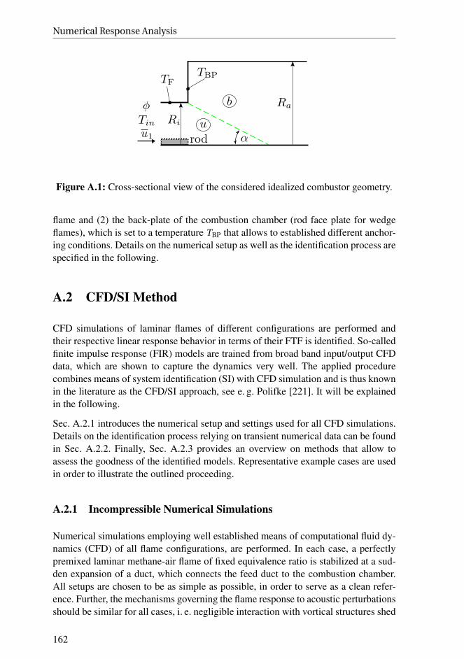
Numerical Response Analysis

Figure A.1: Cross-sectional view of the considered idealized combustor geometry.

flame and (2) the back-plate of the combustion chamber (rod face plate for wedgeflames), which is set to a temperature TBP that allows to established different anchor-ing conditions. Details on the numerical setup as well as the identification process arespecified in the following.

A.2 CFD/SI Method

CFD simulations of laminar flames of different configurations are performed andtheir respective linear response behavior in terms of their FTF is identified. So-calledfinite impulse response (FIR) models are trained from broad band input/output CFDdata, which are shown to capture the dynamics very well. The applied procedurecombines means of system identification (SI) with CFD simulation and is thus knownin the literature as the CFD/SI approach, see e. g. Polifke [221]. It will be explainedin the following.

Sec. A.2.1 introduces the numerical setup and settings used for all CFD simulations.Details on the identification process relying on transient numerical data can be foundin Sec. A.2.2. Finally, Sec. A.2.3 provides an overview on methods that allow toassess the goodness of the identified models. Representative example cases are usedin order to illustrate the outlined proceeding.

A.2.1 Incompressible Numerical Simulations

Numerical simulations employing well established means of computational fluid dy-namics (CFD) of all flame configurations, are performed. In each case, a perfectlypremixed laminar methane-air flame of fixed equivalence ratio is stabilized at a sud-den expansion of a duct, which connects the feed duct to the combustion chamber.All setups are chosen to be as simple as possible, in order to serve as a clean refer-ence. Further, the mechanisms governing the flame response to acoustic perturbationsshould be similar for all cases, i. e. negligible interaction with vortical structures shed

162

A.2 CFD/SI Method

from the burner mouth for the Wedge configuration [1, 104, 201]. Here, this shed-ding process is suppressed by adding a straight lateral wall constraining the flame,see Fig. 6.1b.

All setups can be considered to be acoustically compact up to the respective cut-offfrequency of the FTF. Since such flames hardly respond to acoustic pressure fluctu-ations, their acoustic response can numerically be evaluated by imposing (upstream)velocity perturbations applying an incompressible (low-Mach number) method, seee. g. [222]. In doing so, possible thermoacoustic instabilities are avoided and bound-ary conditions are simplified. The open source software OpenFOAM [223] is em-ployed. Chemical reactions are respected by adopting the reduced chemical kinetic2-step mechanism (2S-CM2) proposed by Bibrzycki et al. [224]. Schmidt numbersfor all six considered species are set according to Duchaine et al. [146]. This solversetup has been used successfully in previous studies for transient and steady state sim-ulations [1, 2, 172, 225]. A 2D uniform structured rectangular grid with a cell densityof 40cells/mm2 and a slight increase of the axial cell width towards the boundariesafter the flame region is adopted for all cases.

Steady state solutions for three exemplary setups are shown in Fig. 6.1. The colordenotes absolute velocity and the region of maximum heat release is plotted in green.Additionally, the analytically predicted mean flame front (see Sec. 2.2.1) is included( ). For all setups, the steady state solutions show an accelerating flow with aseparating shear layer. Flow velocities of the burned gases are highest for the Wedgeand lowest for the Bunsen case. Also, the shear layer is least pronounced for theWedge case compared to the two other setups.

A.2.2 System Identification

In the following it is explained how a flame response model is fitted to transientCFD input/output data such that it represents the underlying linear dynamics. Forthis purpose, a black-box approach is chosen. The resulting model is then used toevaluate and analyze the respective impulse and frequency responses of the simulatedflames. All means of system identification described below are explicated in muchmore detail in the books by Ljung [226], Keesman [227] or Tangirala [228].

In a first step, a model structure has to be chosen that adequately represents the sys-tem of interest. Hence, the investigated flame system needs to be characterized. Indoing so, it can be constituted that the structure and parameters of all consideredcombustors usually do not vary over time and are, therefore, time invariant. Further-more, since the desired flame model is used in a network model in order to assesslinear stability, it has to be inherently linear. Conceptually, the input and output ofa the flame response is constructed such that its transfer behavior reflects causal-

ity, i. e. that all outputs only depend on past and present inputs. The idea of a flametransfer function (FTF) representing a flame in an acoustic network model usually as-

163

Numerical Response Analysis

Figure A.2: Assumed model structure of the flame system: An input signal u ismapped to an output y by the system F . The measured output ym isadditionally influenced by white noise e.

sumes bounded-input bounded-output (BIBO) stability of the flame element, see e. g.Subramanian et al. [229]. Finally, the response of an impulsively perturbed flame isassumed to decay quickly, which is equivalent to the assumption of a high dampingrate. For these reasons, a causal and BIBO stable linear time invariant (LTI) modelstructure is required.

As depicted in Fig. A.2, such systems – in the following denoted as F – are assumedto transform an input signal u to an output signal y . The measured signal ym thatconstitutes the available output time series data is then the superposition of the de-terministic system output y and an erratic signal e, which is in a first approximationassumed to exhibit white noise characteristics. The ratio of the power of the signalsy and e is called the signal-to-noise ratio (SNR) and determines the available infor-mation in the output data: A signal ym,1 whose SNR is higher than that of a signalym,2 contains more information1 for a given signal length, which allows for identifi-cation of less ambiguous input-output models [230]. It should be mentioned that thedetailed characteristics of the erratic signal e (white or colored noise) is not impor-tant for the flame setups considered here due to the obtained very high SNR for allconducted simulations, which is a consequence of the prevailing laminar conditions.That means, e can be neglected and, to good approximation, a relation ym ≈ y holds.

All system properties of F described above are met by a so-called finite impulseresponse (FIR) model. It is discrete in time and relates the in- and output signals byconvolution of the input u with an impulse response h

y[n] = h0u[n]+h1u[n −1]+·· ·+hN u[n −N ]

=N∑

i=0

hi u[n − i ] . (A.1)

Here, y[n] denotes the input signal at a time step n ∈N and hi the i -th impulse re-sponse coefficient. Such a model consists of N +1 finite valued coefficients hi and is,consequently, inherently BIBO stable since

∑∞k=0

|hk | <∞ holds [231]. Causality isreflected by the fact that hi ≡ 0,∀i < 0, which explains why the sum in Eq. (A.1) onlystarts at i = 0. FIR models are a subset of LTI models, since their output is computedby the convolution of an impulse response with an input signal, which is a linear op-eration. The frequency response associated with a given FIR model is computed from

1White noise, as one limiting case, does not contain any information

164

A.2 CFD/SI Method

Figure A.3: Illustration of the CFD/SI approach applied to identify a FIR model us-ing broad band input/output CFD data. The “∗”-operator denotes tem-poral convolution.

the z-transform of the impulse response

F (ω) =N∑

i=0

hi exp(−iωi∆t ) (A.2)

with the imaginary unit i (not to confuse with the summation index i ), the samplingtime of the FIR coefficients ∆t and the real valued angular frequency ω.

One known general disadvantage of FIR models is the high number of coefficients,which have to be identified, particularly for weakly damped systems having a poleclose to the unit circle [232]. However, as stated above, all flames show sufficientdamping such that the available time series data allows for good estimates of allrequired FIR coefficients. FIR models are fairly robust against noise e, more specif-ically, Gaussian white noise of zero mean [232]. For systems with a rather low SNRthat are exposed to non Gaussian white noise or for systems that are less damped,other model structures, such as ARX or Box-Jenkins type models, have to be applied,see for example [233, 234]. All in all, FIR models fulfill all demanded requirementsof an appropriate model structure and are, thus, an appropriate choice for the type ofsystems encountered in this thesis.

Determining the FIR coefficients hi based on available data is referred to as the actualprocess of system identification. The associated process is illustrated in Fig. A.3:In a first step, transient CFD simulations are performed, where the inlet velocity isexcited around its mean, i. e. u1(t ) = u1 +u′

1(t ). The amplitude of these fluctuationsis set to 2−5% of the mean velocity in order to not trigger non-linear effects but,at the same time, to achieve an adequate SNR. The input signal u ( ) used foridentification is the normalized velocity fluctuation at the domain inlet u′

1(t )/u1 and

the output signal ym the normalized heat release rate fluctuation Q ′/Q integratedover the whole domain ( ). Feeding the FIR model with the same input data asthe CFD simulation results in a model output y ( ) according to Eq. (A.1). Now,those values of the FIR coefficients hi are searched, which minimize the quadratic

165

Numerical Response Analysis

error between the CFD output time series ym ( ) and the model output y ( ),formally written as

θ = argminθ

1

M

M∑

j=1

(ym

[j]− y

[j |θ

])2, (A.3)

where θ = hi denotes the solution vector containing all FIR coefficients. Hence, com-putation of the optimal parameters θ requires the solution of a linear least squaresproblem and, therefore, it has to be ensured that the number of sampling instantsM is significantly higher than the number of FIR coefficients N +1. For such linearmodels, the predicted model output can be written in terms of a multiplication of aninput matrix Φ and the solution vector y =Φθ. Using this definition, the linear leastsquares problem formulated above leads to a set of linear equations whose solutionis the desired optimal parameter vector θ:

ΦTΦθ =Φ

T ym . (A.4)

Essentially, four free parameters exist that determine the quality of the resulting fit:(1) The type of input signal u, (2) the length of the input/output time series, (3) thenumber of FIR coefficients N +1 and (4) the sampling interval of the IR ∆t . Thesepoints are discussed one after another in the following.

In order to ensure identifiability, the system input needs to excite all frequencies ofinterest. Otherwise, the information available in the input/output data is not sufficientfor identifying a response model. For example, if the input time series data resem-bles a sine of only one distinct frequency, no information about the response to otherfrequencies is available in the input/output data set [230]. In order to obtain infor-mation on as many frequencies as possible at reasonable computational costs, it hasbeen shown to be advantageous to use a broad band input signal that excites severalfrequencies at once [221, 235, 236]. The lower bound of the frequency content ofsuch a signal is limited by the length of the signal and the upper bound by the sam-pling time (Nyquist frequency). Practically, the upper bound has to be set well beyondthe expected cut-off frequency of the FTF. Decreasing the lower bound is expensive,since longer time series data requires longer simulations. One way of improving thelow-frequency accuracy at ω→ 0 is to use a step input signal: The new steady statethat develops after the input velocity has been rapidly increased (step forcing) definesthe zero frequency response at very high accuracy (neglecting noise). In the case ofperfectly premixed flames its value is unity [157]. All models shown in this thesis areidentified by use of a broad band input signal as proposed by Föller and Polifke [235]and correctly capture this low frequency behavior.

Determining the optimal number of FIR coefficients N + 1 and sampling time ∆t

for a given setup, is an iterative and rather intuitive process. The goal is to use asfew coefficients as possible by, at the same time, retaining a good representationof the system behavior. This avoids overfitting and reduces the required time series

166

A.2 CFD/SI Method

length, since only a minimal number of parameters need to be estimated. A heuristicapproach to finding these two parameters starts with a small number of coefficientsand a sampling time that is related to a characteristic time of the flame, which couldbe the time of restoration τr . A reasonable initial guess would be to use N +1 = 15

coefficients that are separated by a sampling time of ∆t = 2τr /N , since the expectedIR is known to have a length of the order of τr . For this specific choice of parameters,the goodness of the resulting fit has to be evaluated and based on that, N and ∆t

have to be adjusted. This has to be repeated until a satisfactory model is retained.Although, in principle, it might be possible to develop an algorithm that managesthis iterative process, two points should be kept in mind: (1) Similar flames requiresimilar parameters and (2) finding an adequate model is a rather fast process sinceestimation of the fit parameters is computationally relatively cheap and only two freeparameters are available. Hence, due to efficiency, the author decided to rather relyon his intuition than to develop an algorithm.

Efficiently adjusting the two FIR parameters requires some basic understanding of thephysics as well as the identification process. Tools that allow to judge the goodnessof a specific fit are discussed in the following.

A.2.3 Goodness of the Identified Model

While – as shown above – the process of determining the optimal set of FIR parame-ters N and ∆t is a rather intuitive and iterative process, assessment of the goodness ofthe results follows well-defined processes. Several established methods exist, whichare introduced in the following. Representative examples from the flame responsedata presented in this chapter are provided for the sake of illustration.

Generally, a good fit captures all of the deterministic part of ym that depends (here:linearly) on the input u and filters out the noise e. Given a specific data set, it shallprovide the corresponding parameter vector θ that represents most likely the real sys-tem behavior. At the same time, overfitting the given data set, i. e. capturing featuresby the deterministic model that rely on probabilistic processes, shall be avoided 1. Inthis thesis, three points are checked:

1. Check of plausibility

2. Quantification of the uncertainties of the parameter vector θ

3. Quantification of how well the deterministic linear process is captured by thefitted model

4. Demonstration that the model does not suffer from overfitting

1In a low-noise environment overfitting is not a severe problem, nevertheless, it should be kept inmind.

167

Numerical Response Analysis

0 0.5 1 1.5 2 2.5

−8

−4

0

4

8

t∗ [-]

h∗

[-]

(a) Slit

0 0.5 1 1.5

−1

−0.5

0

0.5

1

1.5

t∗ [-]

h∗

[-]

(b) Bunsen

Figure A.4: Visualization of two representative FIR models, one for a Slit flameA.4a and one for a Bunsen flame A.4b configuration (φ= 0.8, Re= 650,TBP = 700, see Fig. 6.1). Shown are the identified FIR coefficient ( ) thatare connected by lines ( ) and the associated 3σ confidence intervals(gray area, framed by ).

All of them are discussed in the following.

Plausibility

First of all, prior knowledge of the expected response model should be exploited.That is, the resulting transfer function can, e. g., be compared to available low-ordermodels in terms of cut-off frequency, low frequency limit (should be unity), excessof gain or phase decay. Furthermore, characteristics of the IR, such as the time delayor the overall shape (decay to zero, rather smooth), can be checked.

Fig. A.4 shows the FIR coefficients resulting from identification of a Slit and a Bun-sen flame configuration. Both are smooth functions of time t∗ and their character-istics compare well to reduced order model predictions (see Chap. 6). Evaluation ofthe associated frequency response would result in a low-frequency limit of unity (notshown) and the IR decays to zero after a time that is of the order of τr . Hence, theresult shown can be considered to plausibly represent the system dynamics.

Uncertainty Quantification

Confidence intervals of the parameter vector θ can be constructed that allow to quan-tify the uncertainties of the fit with respect to the length and the SNR of the underly-ing time series data. The shorter the available time series and the higher the SNR, theless information is contained in a given data set, which will result in a more uncertainidentification of the parameter vector θ. While experimental data suffers essentiallyfrom rather low SNRs, the critical issue for CFD is the length of the available time

168

A.2 CFD/SI Method

series data, since transient CFD simulations usually require a significant amount ofcomputational resources. For all performed simulations of laminar flames, the SNR isvery high and time series of a length of about 10τr have been proven to be sufficient.

In order to quantify uncertainties resulting from noisy finite length time series data,the covariance matrix of the identified model parameters is employed:

Cov(θ)=

σ200 σ2

01 · · · σ20N

σ210 σ2

11

......

. . .

σ2N 0 · · · σ2

N N

(A.5)

where σ2i j= E

[(θi −θi

)(θ j −θ j

)]denotes the covariance of two parameters θi and

θ j with the estimated parameter vector θ and the expected (or “true”) value of thatparameter vector θ. Bias errors (i. e. limM→∞ E

[θ]6= θ) shall be excluded here. The

diagonal elements of the matrix contain the variances of each parameter and the off-diagonal elements the covariances of each pair of parameters. Assuming the covari-ance matrix is known and the estimated parameters follow a normal distribution,confidence intervals can be constructed:

E[θi

]∈

[θi −3σi i , θi +3σi i

](with 99.73% confidence) . (A.6)

Here a 3σ confidence interval is assumed, which states that, based on the provideddata, there is only a 0.27% chance that θi is outside of that interval.

Usually, the covariance matrix is a priori unknown and, hence, needs to be estimatedfrom the data provided, as well. It can be shown that it is given by

ˆCov(θ)= λ0

[Φ

TΦ

]−1(A.7)

where λ0 denotes the (estimated) variance of the residuals ǫ= ym − y[

j |θ]

and ΦTΦ

the matrix of the linear regressor defined in Eq. (A.4) [237]. The former needs to beestimated from the data by

λ0 =1

M − (N +1)

M∑

j=1

(ym

[j]− y

[j |θ

])2. (A.8)

Knowing that the SNR of a signal is computed by the quotient of the variance ofthe signal over the variance of the noise, it now becomes clear that the confidenceintervals scale with the SNR.

Fig. A.4 depicts the 3σ confidence intervals resulting from identification of the shownFIR coefficients. They are very small in both cases and, thus, the shown coefficientsθi = hi very likely represent the actual underlying dynamics of the system. All othersetups discussed in this thesis exhibit similarly small confidence intervals. Therefore,visualizations of confidence intervals are omitted for all IR and FR plots. In order tofurther clarify the presentation by leaving out unnecessary information, throughoutthe thesis, impulse responses are shown as line plots ( ) and leave out a visualiza-tion of the FIR coefficients ( ).

169

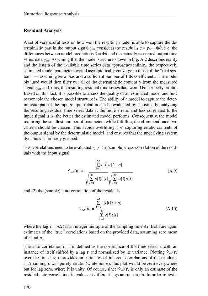
Numerical Response Analysis

Residual Analysis

A set of very useful tests on how well the resulting model is able to capture the de-terministic part in the output signal ym considers the residuals ǫ= ym −Φθ, i. e. thedifferences between model predictions y =Φθ and the actually measured output timeseries data ym . Assuming that the model structure shown in Fig. A.2 describes realityand the length of the available time series data approaches infinity, the respectivelyestimated model parameters would asymptotically converge to those of the “real sys-tem” — assuming zero bias and a sufficient number of FIR coefficients. The modelobtained would then filter out all of the deterministic content y from the measuredsignal ym and, thus, the resulting residual time series data would be perfectly erratic.Based on this fact, it is possible to assess the quality of an estimated model and howreasonable the chosen model structure is. The ability of a model to capture the deter-ministic part of the input/output relation can be evaluated by statistically analyzingthe resulting residual time series data ǫ: the more erratic and less correlated to theinput signal it is, the better the estimated model performs. Consequently, the modelrequiring the smallest number of parameters while fulfilling the aforementioned twocriteria should be chosen. This avoids overfitting, i. e. capturing erratic contents ofthe output signal by the deterministic model, and ensures that the underlying systemdynamics is properly grasped.

Two correlations need to be evaluated: (1) The (sample) cross-correlation of the resid-uals with the input signal

γue [n] =

M∑i=1

ǫ[i ]u[i +n]

√M∑

i=1ǫ[i ]ǫ[i ]

√M∑

i=1u[i ]u[i ]

(A.9)

and (2) the (sample) auto-correlation of the residuals

γee [n] =

M∑i=1

ǫ[i ]ǫ[i +n]

M∑i=1

ǫ[i ]ǫ[i ]

(A.10)

where the lag τ= n∆t is an integer multiple of the sampling time ∆t . Both are againestimates of the “true” correlations based on the provided data, assuming zero meanof ǫ and u.

The auto-correlation of ǫ is defined as the covariance of the time series ǫ with aninstance of itself shifted by a lag τ and normalized by its variance. Plotting γee (τ)

over the time lag τ provides an estimates of inherent correlations of the residualsǫ. Assuming ǫ was purely erratic (white noise), this plot would be zero everywherebut for lag zero, where it is unity. Of course, since γee (τ) is only an estimate of theresidual auto-correlation, its values at different lags are uncertain. In order to test a

170

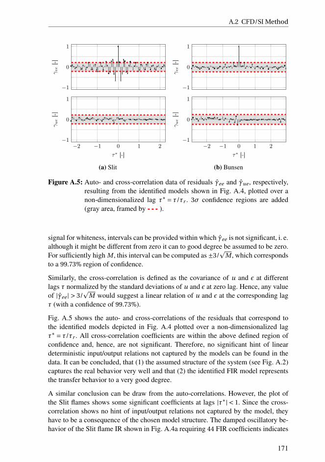
A.2 CFD/SI Method

−1

0

1

γee

[-]

−2 −1 0 1 2

−1

0

1

τ∗ [-]

γue

[-]

(a) Slit

−1

0

1

γee

[-]

−2 −1 0 1 2

−1

0

1

τ∗ [-]

γue

[-]

(b) Bunsen

Figure A.5: Auto- and cross-correlation data of residuals γee and γue , respectively,resulting from the identified models shown in Fig. A.4, plotted over anon-dimensionalized lag τ∗ = τ/τr . 3σ confidence regions are added(gray area, framed by ).

signal for whiteness, intervals can be provided within which γee is not significant, i. e.although it might be different from zero it can to good degree be assumed to be zero.For sufficiently high M , this interval can be computed as ±3/

pM , which corresponds

to a 99.73% region of confidence.

Similarly, the cross-correlation is defined as the covariance of u and ǫ at differentlags τ normalized by the standard deviations of u and ǫ at zero lag. Hence, any valueof |γee | > 3/

pM would suggest a linear relation of u and ǫ at the corresponding lag

τ (with a confidence of 99.73%).

Fig. A.5 shows the auto- and cross-correlations of the residuals that correspond tothe identified models depicted in Fig. A.4 plotted over a non-dimensionalized lagτ∗ = τ/τr . All cross-correlation coefficients are within the above defined region ofconfidence and, hence, are not significant. Therefore, no significant hint of lineardeterministic input/output relations not captured by the models can be found in thedata. It can be concluded, that (1) the assumed structure of the system (see Fig. A.2)captures the real behavior very well and that (2) the identified FIR model representsthe transfer behavior to a very good degree.

A similar conclusion can be draw from the auto-correlations. However, the plot ofthe Slit flames shows some significant coefficients at lags |τ∗| < 1. Since the cross-correlation shows no hint of input/output relations not captured by the model, theyhave to be a consequence of the chosen model structure. The damped oscillatory be-havior of the Slit flame IR shown in Fig. A.4a requiring 44 FIR coefficients indicates

171

Numerical Response Analysis

an autoregressive behavior of the system, i. e. the present output of the system doesnot only depend on past and present inputs but also on past outputs. Using a systemstructure that allows for such autoregressive interactions, such as an ARX model,could reduce the required number of model parameters. At the same time, also theerratic part e would be subjected to the autoregressive system behavior and, hence,its contribution to ym would be colored instead of white. It has been shown by So-vardi [238] (Sec. 4.2.5) that for such situations, application of an ARX model wouldindeed lead to a reduction of the residual auto-correlation. It was checked by the au-thor of this thesis that this also holds for the Slit flame case discussed here. However,although the auto-correlation of ǫ exhibits strong hints that the underlying signal isnot white, its relevance for the time series data is very minor due to the fact that theamplitude of ǫ is several orders of magnitude smaller than that of ym . This will beillustrated in the following section where the model output is compared with the CFDdata output using a test data set. For that reason, it can be concluded that the chosenFIR model performs very well for both types of flames.

Comparison with Test Data Set

It is a common practice in regression analysis to split the available time series datainto a training and a test data set. The first is used in order to identify the modelparameters θ, the second to evaluate the predictive quality of the model on a statisti-cally independent data set. Usually the distance between the model predictions ( ;Fig. A.3) and the CFD output ( ; Fig. A.3) is measured in terms of a norm, alsoknown as the fit value:

FIT = 100

1−

√M∑

i=1

(ym[i ]− y[i ]

)2

√M∑

i=1

(ym[i ]− ym,mean

)2

% (A.11)

where y denotes the model output, ym the CFD time series and ym,mean its meanvalue [239, 240].

Computing the model output for a test data set of the two identified models shownin Fig. A.4 ( ) results in the time series shown in Fig. A.6. Very good agreementwith the CFD data output ym ( ) is found and results in fit values of 93.87% and95.8% for the slit and the Bunsen type configuration, respectively. Since the test dataset is independent from the trainings data set, it can be concluded that both modelsare not overfitted to the trainings data.

172

A.3 Time vs. Frequency Domain Based Response Analysis

0 5 10 15

-1

0

1

t∗ [-]

y[-]

(a) Slit

0 5 10 15

-0.5

0

0.5

t∗ [-]

y[-]

(b) Bunsen

Figure A.6: Model ( ) and CFD ( ) output time series for the identified modelsshown in Fig. A.4 for a test data set, plotted over non-dimensionalizedtime t∗ = τ/τr . Fit values are 93.87% and 95.8% for the slit and the Bun-sen type configuration, respectively.

A.3 Time vs. Frequency Domain Based Response Analysis

Besides CFD/SI methods relying on broad band data, there are also other methods toestimate the IR of a flame configuration. A simple direct approach relies on an impul-sively excited flame using a input signal u resembling a Dirac impulse. For example,a Gaussian impulse of small variance and sufficiently low amplitude (to not triggernon-linear effects) can be used as input signal. The normalized associated response ofthe global heat release then provides an estimate of the IR. Such a procedure has onesignificant advantage: It allows for a direct and rather simple analysis of the transientCFD field data and, thus, the physical processes that determine the system behav-ior. Without use of further computationally expensive statistical evaluations, such apost-processing of the data is not possible for broad band excitation.

The reason behind this property is that an impulsive forcing constitutes the optimalinput signal for analyzing causalities. Analyzing transient CFD data subjected to har-monic forcing, for example, might lead to identification of coherent (flow) structuresthat have a strong impact on the respective flame response. However, it is not easy toreveal causal relations, since in a fully established oscillatory state, as it is inherentlyassumed in frequency domain representations, one cannot distinguish between causeand effect. This can be improved by using broad band forcing, however, as statedabove, elaborate and computational expensive computations are required in order toreveal spatially resolved causal relations. Application of an impulsive forcing allowsto identify causalities by just naively inspecting the transient CFD field data: anychange in a certain snapshot has to be directly related to information present in thepreceding snapshots.

This advantage is payed for by, compared to broad band based methods, less robustresponse predictions that are caused by the reduced amount of data and, hence, in-

173

Numerical Response Analysis

0 0.5 1 1.5 2

−8

−4

0

4

8

t∗ [-]

h∗

[-]

(a) Slit

0 0.5 1 1.5−1

0

1

t∗ [-]

h∗

[-]

(b) Bunsen

0 0.5 1 1.5 2 2.5 3

−4

−2

0

2

4

t∗ [-]

h∗

[-]

(c) Wedge

Figure A.7: Comparison of IR predictions resulting from impulsive forcing ( )as well as from the CFD/SI approach ( ) for three representative se-tups (one for each flame geometry). All simulations were performed ata maximum perturbation velocity amplitude of 2%u1. For the slit caseadditionally a simulation at 10% amplitude was performed ( ).

formation: the total length of usable time series data equals exactly one times theIR length. Furthermore, confidence intervals as well as quality measures quantifyingthe resulting model (residual analysis) cannot be specified without further consider-ations. Hence, in order to get both good estimates of the (linear) response behaviorand the possibility to analyze physical causalities, one has to jointly analyze broadband and impulsively forced systems. It should be noted that the evaluation of thelatter is usually only informative for systems exhibiting very low noise levels, suchas laminar flames. Processing LES simulations of turbulent flames, the turbulent fluc-tuations will contaminate the output time series data of a step or impulse forcing andcannot be correlated out (using a single simulation).

Applying such a joint analysis, it has to be ensured that the impulsively forced sys-tems exhibits the same linear response as the model identified from broad band data.If that is the case, non-linearities or noise related effects most probably can be ruledout to contaminate the CFD data. Fig. A.7 compares IR predictions resulting froman impulsive forcing ( ) to the ones from the CFD/SI approach ( ) for threerepresentative setups. All setups were forced by a narrow Gaussian impulse with anamplitude of 2% of the bulk flow velocity u1, see Appendix A.4 for more details.For the Slit setup additionally a forcing with 10% forcing amplitude is shown ( ),which still exhibits the same transfer behavior as the two other cases.

Overall, very good agreement can be found for all three configurations. Only theBunsen case in Fig. A.7b shows a minor discrepancy at t∗ ≈ 1.3 but also here theoverall IR is captured very well. This result allows to safely analyze impulsivelyforced CFD data and draw conclusion regarding the physics that governs the linearresponse. This fact is exploited in Parts II and III by analyzing the transient behaviorof flame normal displacements.

174

A.4 Computation of Flame Normal Displacements

0 0.5 1 1.5 2

−8

−4

0

4

8

12

t∗ [-]

h∗

[-]

Figure A.8: IR predictions resulting from impulsive forcing of a Slit flame shownfor four amplitudes: 10% ( ), 20% ( ), 40% ( ) and 60% ( )with respect to u1.

Fig. A.8 analyses the amplitude dependence of a Slit flame in more detail. It showsthat the linear behavior is to a good degree preserved up to amplitudes of 20%. Onlyat 40% amplitude non-linear effects significantly kick in and effect the response. Asshown in Chap. 6, Slit flames exhibited the strongest response of all three investigatedflames. Therefore, it can be expected that Bunsen and Wedge flames should stay inthe linear regime for even higher forcing amplitudes.

A.4 Computation of Flame Normal Displacements

−1.5 0 1.50

0.5

1

t [ms]

am

plitu

de

[-]

(a)

Hf/2 Hf0

Ri

xL1

xL 2

(b)

Figure A.9: (a): Signal of normalized amplitude used for impulsive forcings con-ducted in this thesis. (b): Flame shape computed from an CH4-isoline ofa CFD data snapshot including its normals.

The transient behavior of flame normal displacements of impulsively excited flamesis discussed in several sections of this thesis, see for example Fig. 5.1 (middle). De-tails on the computation and post-processing of theses results are provided in thefollowing. Background information on the motivation for such a kind of analysis is

175

Numerical Response Analysis

provided in Sec. A.3.

The forcing signal employed for all impulsively forced simulations is illustrated inFig. A.9a. It exhibits a normalized amplitude, which has yet to be scaled by the levelof forcing, e. g. by ǫ= 2%u1. Its shape is described by

f (t ) = exp

(− (t − t0)2

σ

), (A.12)

where t0 denotes the time at which the impulse forcing has to be applied andσ= 5e −7 the width of the Gaussian-like distribution. The temporal integral definesa reference displacement ξ=

∫∞0 ǫ f (t )dt .

Having performed the impulsively forced transient numerical simulations, snapshotsat several instants in time are taken and CH4-isolines extracted. The respective CH4

values are chosen such that the resulting isoline adequately captures the spatial distri-bution of the heat release. The first snapshot corresponds to a time before the forcingis applied (t < t0) and is defined to represent the unperturbed steady state solution.For this snapshot, flame normals are evaluated. An exemplary result is sketched inFig. A.9b. Having done this, flame normal deviations from the steady state are eval-uated for all subsequent snapshots. Finally, the resulting flame normal displacementsfrom the steady state flame are normalized by the aforementioned reference displace-ment ξ in order to ensure comparability with other simulations or with LOM predic-tions.

176

B Impact of the Anchoring Wall

Temperature

Some of the shown CFD/SI results shown in this work were conducted at differenttemperatures of the wall above which the flame is anchored, denoted as TBP. Theliterature provides evidence that this temperature has a crucial impact on the associ-ated acoustic flame response [121, 148, 149, 241, 242]. Therefore, its consequencesfor the FTF of the investigated flame configurations are assessed in the following.In order to specify wall temperatures, a non-dimensional quantity T ∗

BP= TBP/Tad is

introduced relating the temperature of a wall TBP to the adiabatic flame temperatureTad. Adiabatic walls hence have a non-dimensional temperature of unity.

Figs. B.1 and B.2 show steady state and acoustic response data of three Slit and Bun-sen flames, respectively, anchored above a back-plate exhibiting different temperatureboundary conditions: (1) adiabatic walls, (2) TBP = 700 K and (3) TBP = 373 K. Theseboundaries were chosen as limiting cases of the range of possible (uncooled) walltemperatures. The study of Kornilov et al. [209] specified the prevailing wall tem-perature of a Slit flame setup to 373−423 K. This serves as an estimate of the lowerthreshold of possible temperatures and, hence, TBP = 373 K defines a first samplingpoint. According to Mejia et al. [149], the temperature of their cylindrical bluff bodycould reach temperatures up to 700 K. Since around temperatures of 750−800 K thebackplate would start to radiate light in the visible wavelengths (“incandescence”),which is not reported from experimental studies, a temperature of TBP = 700 K waschosen to define the upper limit of temperatures of interest. The adiabatic chase wasadded primarily because of academic interests. Such configurations define the limit-ing cases where the flame is anchored directly at the trailing edge.

All shown frequency and impulse response data are non-dimensionalized by use ofthe characteristic time of restoration τr . It is determined here by demanding that allIRs have to coincide at t∗ = 1. This exploits the fact that all IRs are qualitativelyvery similar and that the main difference can be related to a scaling of the frequencyand time scales of the FR and IR representations, respectively. In order to effectivelyvisualize the behavior of the characteristic time of restoration, relative changes of thetime of restoration

∆τ∗r =τr −τr,ref

τr,ref(B.1)

are plotted in Figs. B.1 and B.2. Hereby, the characteristic time of the configurationsexhibiting the minimal τr serves as the reference time τr,ref.

177

Impact of the Anchoring Wall Temperature

Figure B.1: Effect of temperature of the back-plate TBP on on the FTF (left) and themean flow field (right) for Slit flame configurations at Re= 650, φ= 0.8

and Cr = 0.4. Close-up views of the steady state flame anchoring areprovided for each setup (middle and lower row, right half).

Figure B.2: Effect of temperature of the back-plate TBP on on the FTF (left) andthe mean flow field (right) for Bunsen flame configurations at Re= 650,φ= 0.8 and Cr = 0.4. Close-up views of the steady state flame anchoringare provided for each setup (middle and lower row, right half).

From the data shown it becomes clear that variations of the wall temperature mainlylead to variations of τr , while the qualitative behavior of the IR/FR representationsare essentially maintained. This directly translates to a significant change of the FTFphase of the three setups, when plotted over dimensional frequency. It is hence con-cluded that variations of the wall temperature right at the flame anchoring predomi-

178

nantly lead to significant changes in the phase of the corresponding FTF and only torather weak changes of the gain. While all analyzed data provides evidence that τr

increases with rising TBP, the gain does not behave as regularly and can show bothhigher and lower amplitudes. On the detailed mechanisms that are responsible forthis behavior can only be speculated. From the data provided, it seems that cooledwalls lead to a low speed region upstream of the flame base, which might lead to anincrease of τr . All in all, comparing FR/IR representations of different TBP in non-dimensionalized form, it can in a first approximation be assumed that their overallshape remain unchanged and predominantly the respective τr varies.

179

Impact of the Anchoring Wall Temperature

180

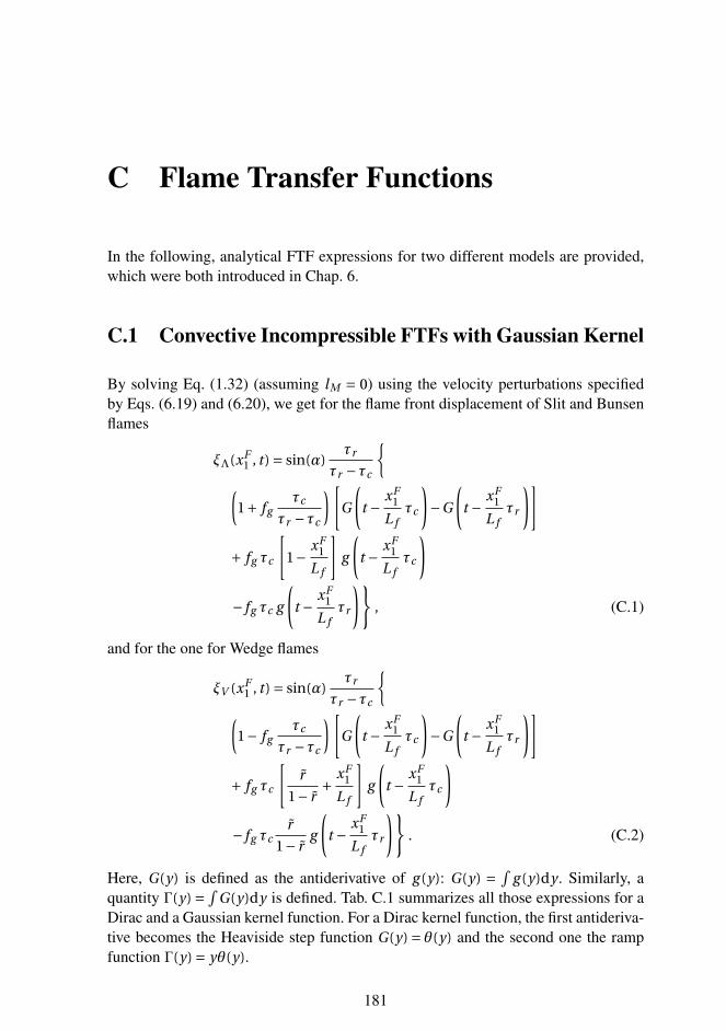
C Flame Transfer Functions

In the following, analytical FTF expressions for two different models are provided,which were both introduced in Chap. 6.

C.1 Convective Incompressible FTFs with Gaussian Kernel

By solving Eq. (1.32) (assuming lM = 0) using the velocity perturbations specifiedby Eqs. (6.19) and (6.20), we get for the flame front displacement of Slit and Bunsenflames

ξΛ(xF1 , t ) = sin(α)

τr

τr −τc

(1+ fg

τc

τr −τc

) [G

(t −

xF1

L fτc

)−G

(t −

xF1

L fτr

)]

+ fg τc

[1−

xF1

L f

]g

(t −

xF1

L fτc

)

− fg τc g

(t −

xF1

L fτr

), (C.1)

and for the one for Wedge flames

ξV (xF1 , t ) = sin(α)

τr

τr −τc

(1− fg

τc

τr −τc

) [G

(t −

xF1

L fτc

)−G

(t −

xF1

L fτr

)]

+ fg τc

[r

1− r+

xF1

L f

]g

(t −

xF1

L fτc

)

− fg τcr

1− rg

(t −

xF1

L fτr

). (C.2)

Here, G(y) is defined as the antiderivative of g (y): G(y) =∫

g (y)dy . Similarly, aquantity Γ(y) =

∫G(y)dy is defined. Tab. C.1 summarizes all those expressions for a

Dirac and a Gaussian kernel function. For a Dirac kernel function, the first antideriva-tive becomes the Heaviside step function G(y) = θ(y) and the second one the rampfunction Γ(y) = yθ(y).

181

Flame Transfer Functions

Function Dirac Kernel Gaussian Kernel

g (y) δ(y) 1p2πσ2

exp

(− y2

2σ2

)

G(y) θ(y) 12 erf

(yp2σ2

)

Γ(y) y θ(y)y2 erf

(yp2σ2

)+ σp

2πexp

(− y2

2σ2

)

Table C.1: Overview of the two Dirac and the Gaussian kernel functions and theirantiderivatives.

These displacements are used to evaluate the integral flame surface area fluctuationA′, according to the formulas provided in Sec. 6.2. From that, the impulse responseis computed as

h(t ) = A′

Au1 , (C.3)

which yields for slit flames

hslit =1

τr −τc

(1+ fg

τc

τr −τc

) [G (t −τc )−G (t −τr )

]

− fg τc g (t −τr )

. (C.4)

For Bunsen flames we retrieve

hcon,Λ = 2

τr −τc

(1+ fg

τc

τr −τc

)[1

τr

[Γ (t −τr )−Γ (t )

]

− 1

τc

[Γ (t −τc )−Γ (t )

]]

+ fg

[G (t )+

1

τc

[Γ (t −τc )−Γ (t )

]]

+ fgτc

τr

[G (t −τr )−G (t )

](C.5)

182

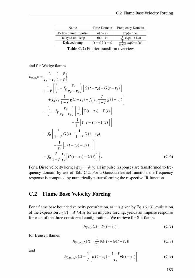
C.2 Flame Base Velocity Forcing

Name Time Domain Frequency Domain

Delayed unit impulse δ(t −τ) exp(−τ i ω)

Delayed unit step θ(t −τ) 1i ω exp(−τ i ω)

Delayed ramp (t −τ)θ(t −τ) 1(i ω)2 exp(−τ i ω)

Table C.2: Fourier transform overview.

and for Wedge flames

hcon,V = 2

τr −τc

1− r

1+ r

1

1− r

[(1− fg

τc

τr −τc

) [G (t −τc )−G (t −τr )

]

+ fg τc1

1− rg (t −τc )− fg τc

r

1− rg (t −τr )

]

−(1− fg

τc

τr −τc

) [1

τr

[Γ (t −τr )−Γ (t )

]

− 1

τc

[Γ (t −τc )−Γ (t )

]]

− fg

[r

1− rG (t )−

1

1− rG (t −τc )

− 1

τc

[Γ (t −τc )−Γ (t )

]]

− fgr

1− r

τc

τr

[G (t −τr )−G (t )

]. (C.6)

For a Dirac velocity kernel g (y) = δ(y) all impulse responses are transformed to fre-quency domain by use of Tab. C.2. For a Gaussian kernel function, the frequencyresponse is computed by numerically z-transforming the respective IR function.

C.2 Flame Base Velocity Forcing

For a flame base bounded velocity perturbation, as it is given by Eq. (6.13), evaluationof the expression hδ(t ) = A′/Au1 for an impulse forcing, yields an impulse responsefor each of the three considered configurations. We retrieve for Slit flames

hδ,slit(t ) = δ (t −τr ) , (C.7)

for Bunsen flames

hδ,con,Λ(t ) = 1

τr[Θ(t )−Θ(t −τr )] (C.8)

and

hδ,con,V (t ) = 1

r

[δ (t −τr )−

1− r

τrΘ(t −τr )

](C.9)

183

Flame Transfer Functions

for Wedge flames. The corresponding frequency responses Fδ are computed by useof Tab. C.2 provided in Appendix C.1.

184

List of Figures

1 Sketch of a Rjike tube, photo of the Rocketdyne F-1 engines of theSaturn V rocket as well as of its injector plate. . . . . . . . . . . . . . 2

2 Illustration of a modern gas turbine combustor and photo taken insidean annular combustion chamber. . . . . . . . . . . . . . . . . . . . . . 4

3 Sketch of a gas turbine combustor (top) and its associated networkmodel (bottom). . . . . . . . . . . . . . . . . . . . . . . . . . . . . . . . 5

4 Contents of the thesis in a nutshell. . . . . . . . . . . . . . . . . . . . . 8

1.1 Internal structure of a lean methane-air flame of equivalence ratioφ= 0.8. . . . . . . . . . . . . . . . . . . . . . . . . . . . . . . . . . . . 13

1.2 Cellular structure of a flat flame for n-butane-air-nitrogen mixtures atfour different ambient pressures. . . . . . . . . . . . . . . . . . . . . . 15

1.3 Snapshots of spherically expanding stoichiometric propane/airflames (spherical bombs) for three different ambient pressures at aLewis number close to unity. . . . . . . . . . . . . . . . . . . . . . . . 18

1.4 Snapshot of an aerodynamically anchored and inclined richpropane/air/oxygen flame whose base is displaced by a vibratingflame holder. . . . . . . . . . . . . . . . . . . . . . . . . . . . . . . . . 19

1.5 Temporal evolution of a randomly perturbed flame sheet according tothe MS equation. . . . . . . . . . . . . . . . . . . . . . . . . . . . . . . 20

1.6 Illustration of Huygens’s Principle, which explains the formation ofcusps from an initially smooth flame front. . . . . . . . . . . . . . . . 23

1.7 Illustration of the thermal-diffusive flame instability mechanism. . . . 25

1.8 Dispersion relation of Eq. (1.13) for the thermal-diffusive instabilitymechanism. . . . . . . . . . . . . . . . . . . . . . . . . . . . . . . . . . 26

185

LIST OF FIGURES

1.9 Illustration of contracting (red) and expanding (blue) flow tubesdue to a displaced flame front, which explain the occurrence of theDarrieus-Landau instability. . . . . . . . . . . . . . . . . . . . . . . . . 27

1.10 Darrieus-Landau parameter Ω0 and critical Lewis number for theonset of thermal-diffusive instability Lec,TD plotted over non-dimensional increase of specific volume. . . . . . . . . . . . . . . . . 30

1.11 Growth rate according to Eq. (1.13) for the hydrodynamic instabilitymechanism plotted for several Lewis numbers and non-dimensionaldensity increases. . . . . . . . . . . . . . . . . . . . . . . . . . . . . . . 30

1.13 Sketch of a perturbed flame front around its mean using laboratoryand flame aligned coordinates. . . . . . . . . . . . . . . . . . . . . . . 36

2.1 Investigated flame geometries (taken from [2]). . . . . . . . . . . . . . 42

2.2 Unconfined (left) vs. confined (right) flame. . . . . . . . . . . . . . . . 43

2.3 TiO2 smoke trace flow field visualization of two Bunsen flame forcedat 200 Hz, one time by transversal movements of the flame holder atwhich the flame is anchored (left) and one time by acoustic excitation(right). . . . . . . . . . . . . . . . . . . . . . . . . . . . . . . . . . . . . 46

2.4 Snapshots of an acoustically excited Bunsen flame at 80 Hz, taken atfour equidistant phases. . . . . . . . . . . . . . . . . . . . . . . . . . . 47

2.5 Snapshots of a G-equation-based simulation of an acoustically ex-cited Bunsen flame at 120 Hz relying on the convective incompress-ible velocity model, taken at three equidistant phases. . . . . . . . . . 48

2.6 Representation of a typical linear flame response of a Bunsen flamein the frequency domain (frequency response) in terms of (a) gain,(b) phase, (c) polar plot with phase determining the angle and gainthe radius and (d) real and imaginary part plotted over frequency. . . 51

2.7 Representation of a typical linear flame response of a Bunsen flamein the time domain as impulse response (left) and in the frequencydomain as frequency response (right). . . . . . . . . . . . . . . . . . . 52

3.1 Overview of acoustics-flame-flow interactions. . . . . . . . . . . . . . 61

3.2 Sketch of the investigated Slit flame setup. . . . . . . . . . . . . . . . 63

3.3 Illustration of the baroclinic generation of vorticity for a single parcelof fluid. . . . . . . . . . . . . . . . . . . . . . . . . . . . . . . . . . . . 64

3.4 Illustration of the Schwarz-Christoffel mapping. . . . . . . . . . . . . 66

186

LIST OF FIGURES

3.5 Illustration of how impermeability boundary conditions are met byuse of a mirror vortex. . . . . . . . . . . . . . . . . . . . . . . . . . . . 69

3.6 Flow field according to source at ξ = 0 and a Kutta panel includingclose up views of this panel in the physical and the image domain. . . 71

3.7 Normalized vorticity plotted over panel coordinates in the image andthe physical domain for two panel lengths, two vorticity distributionsand two confinement ratios. . . . . . . . . . . . . . . . . . . . . . . . . 72

3.8 Sketch of the Kutta panel and its mirror counterpart in the imagedomain. . . . . . . . . . . . . . . . . . . . . . . . . . . . . . . . . . . . 73

3.9 Summary of all computations that need to be performed during onetime step when considering a Kutta condition. . . . . . . . . . . . . . 75

4.1 CFD steady state snapshots of absolute velocity for a confinementratio of Cr = 0.4 and Cr = 0.66. . . . . . . . . . . . . . . . . . . . . . . 79

4.2 Four consecutive snapshots taken from LOM predictions of a har-monically forced flame configuration excluding flame-flow feedback,split into vortical and irrotational flow components. . . . . . . . . . . 81

4.3 Comparison of vorticity distribution resulting from vortex sheddingdue to a Kutta condition and a linear approximation for two confine-ment ratios. . . . . . . . . . . . . . . . . . . . . . . . . . . . . . . . . . 82

4.4 Visualization of the flame normal velocity resulting from a constantmean flow and a Kutta condition evaluated for four panel lengths aswell as of the associated panel shapes. . . . . . . . . . . . . . . . . . . 83

4.5 Four snapshots taken at equidistant instances in time of the normal-ized flame displacement resulting from an impulsive velocity forc-ing according to CFD/SI results, the proposed acoustic LOM and theFBD model at two confinement ratios. . . . . . . . . . . . . . . . . . . 84

4.6 IR and FR in terms of gain and phase for Cr = 0.4 and Cr = 0.66 aspredicted by CFD/SI, the FBD model and the proposed acoustic LOM. 85

5.1 Impulse responses for the Cr = 0.4 configuration depicted in Fig. 4.1as well as the corresponding consecutive snapshots of the normalizedflame-normal flame front displacement. . . . . . . . . . . . . . . . . . 92

5.2 Normalized flame displacements shown for three confinement ratioscorresponding to the cases shown in Fig. 5.1 where exponential func-tions are fitted to the spatial traces of the primary and secondary peaks. 93

187

LIST OF FIGURES

5.3 Normalized flame front displacements as predicted by the uniform(top) and the incompressible convective (middle and bottom) velocitymodel for a harmonic velocity forcing. . . . . . . . . . . . . . . . . . . 95

5.4 Illustration of the line integral of Eq. (5.17) along a path ∂S enclosinga surface S. . . . . . . . . . . . . . . . . . . . . . . . . . . . . . . . . . 100

5.5 Sketch of a harmonically perturbed flame sheet including an illustra-tions of the consequences of flame-generated vorticity. . . . . . . . . 101

5.6 Three figures showing the amount of volume produced according toan increasing number of Gaussian sources. . . . . . . . . . . . . . . . 103

5.7 Steady state flow field with the flame front being represented by anumber of Gaussian sources. Additionally, the magnitude of the flowvelocity is plotted along three selected stream lines. . . . . . . . . . . 104

5.8 Axial flow profile of a channel flow including a vertical flame sheetrepresented by Gaussian sources compared to results of a 1D simula-tion employing detailed chemical mechanism. . . . . . . . . . . . . . 104

5.9 Illustration of the perturbed flow field imposed by a displaced flamesheet, which is represented by a number of Gaussian volume sourcesleading to a geometrical focusing of the flow, which amplifies alreadyexistent flame perturbations. . . . . . . . . . . . . . . . . . . . . . . . . 106

5.10 LOM predictions including flame-generated vorticity of a harmon-ically forced flame configuration (at 120 Hz and an amplitude of10% ublk) for a confinement ratio of Cr = 0.4. . . . . . . . . . . . . . . 108

5.11 LOM predictions including flame-generated vorticity of a harmon-ically forced flame configuration (at 120 Hz and an amplitude of10% ublk) for a confinement ratio of Cr = 0.66. . . . . . . . . . . . . . 109

5.12 Four snapshots taken at equidistant instances in time of the normal-ized flame displacement resulting from an impulsive velocity forcingtaken from CFD/SI results as well as from the acoustic LOM with andwithout flame-flow feedback resulting from flame generated vorticityat two confinement ratios. . . . . . . . . . . . . . . . . . . . . . . . . . 110

5.13 IR and FR in terms of gain and phase at Cr = 0.4 and Cr = 0.66 as pre-dicted by CFD/SI as well as by the acoustic LOM with and withoutconsideration of flame-generated vorticity. . . . . . . . . . . . . . . . 111

5.14 IR and FR in terms of gain and phase at Cr = 0.4 as predicted byCFD/SI as well as by the acoustic LOM with and without considera-tion of flame-generated vorticity. Shown are results for two minimumvortex kernel radii r0,ω,min. . . . . . . . . . . . . . . . . . . . . . . . . 112

188

LIST OF FIGURES

5.15 LOM predictions including irrotational flame-flow feedback of a har-monically forced flame configuration (at 120 Hz and an amplitude of10% ublk) for a confinement ratio of Cr = 0.4. . . . . . . . . . . . . . . 113

5.16 LOM predictions including irrotational flame-flow feedback of a har-monically forced flame configuration (at 120 Hz and an amplitude of10% ublk) for a confinement ratio of Cr = 0.66. . . . . . . . . . . . . . 113

5.17 Illustration of the dipole-like flow structure in the vicinity of a per-turbed duct flame as well as fluctuation of the global heat release ratefor a harmonic velocity forcing at 120 Hz resulting from simulationsrespecting flame-generated vorticity and irrotational gas expansion. . 114

5.18 Four snapshots taken at equidistant instances in time of the normal-ized flame displacement resulting from an impulsive velocity forcingtaken from CFD/SI results as well as from the acoustic LOM with andwithout flame-flow feedback resulting from irrotational gas expansion. 115

6.1 CFD steady state snapshots of absolute velocity for the three investi-gated flame test cases of different flame geometries. . . . . . . . . . . 124

6.2 Illustration of the dependency of the change of the flame line segmentlength dS′ = dS −dS on the displacements dη′

iand dη′

i+1up to O (ǫ)

contributions. . . . . . . . . . . . . . . . . . . . . . . . . . . . . . . . . 126

6.3 Displaced flame segment in flame aligned and laboratory coordinates. 127

6.4 Geometric measures required for the computation of the flame sur-face area of Bunsen flames. . . . . . . . . . . . . . . . . . . . . . . . . 129

6.5 Geometric measures required for the computation of the flame sur-face area of Wedge flames. . . . . . . . . . . . . . . . . . . . . . . . . 131

6.6 Thought experiment illustrating the results of the linearized surfaceintegrals. . . . . . . . . . . . . . . . . . . . . . . . . . . . . . . . . . . . 133

6.7 Sketch of an advected flame pocket, which is generated by an impul-sive deflection of the flame base, shown for three flame configurations. 134

6.8 Transfer function in terms of impulse response hδ and frequencyresponse Fδ from flame base velocity perturbations to heat releaseshown for three flame configurations. . . . . . . . . . . . . . . . . . . 136

6.9 Qualitative illustration of the velocity field resulting from unit im-pulse forcing and a Gaussian velocity kernel function g (τ). . . . . . . 139

6.10 Snapshot of the velocity and vorticity field resulting from unit im-pulse response forcing and a Gaussian velocity kernel. . . . . . . . . 140

189

LIST OF FIGURES

6.11 FTF predictions of the DIC model in terms of impulse response h(t )

and frequency response F (ω) shown for three flame configurations. . 142

6.12 Illustration of the displaced flame front deflection ξ(xF

1 , t)

of the DICmodel for an impulse velocity perturbation. . . . . . . . . . . . . . . . 143

6.13 Impulse responses of the three different flame configurations. . . . . 144

6.14 Comparison of FTF predictions for Slit flames visualized in time andfrequency domain from CFD/SI data, the DIC, the GCI and the plainconvective velocity models. . . . . . . . . . . . . . . . . . . . . . . . . 146

6.15 Comparison of FTF predictions for Bunsen flames visualized in timeand frequency domain from CFD/SI data, the DIC, the GCI and theplain convective velocity models. . . . . . . . . . . . . . . . . . . . . . 147

6.16 Comparison of FTF predictions for Wedge flames visualized in timeand frequency domain from CFD/SI data, the DIC, the GCI and theplain convective velocity models. . . . . . . . . . . . . . . . . . . . . . 148

6.17 Comparison of IR and the corresponding normalized flame front dis-placement ξ/ξ of the Slit configuration resulting from an impulseforcing at four instants in time, shown for the CFD/SI data as wellas the DCI/GCI models. . . . . . . . . . . . . . . . . . . . . . . . . . . 148

6.18 Comparison of IR and the corresponding normalized flame front dis-placement ξ/ξ of the Bunsen configuration resulting from an impulseforcing at four instants in time, shown for the CFD/SI data as well asthe DCI/GCI models. . . . . . . . . . . . . . . . . . . . . . . . . . . . . 149

6.19 Comparison of IR and the corresponding normalized flame front dis-placement ξ/ξ of the Wedge configuration resulting from an impulseforcing at four instants in time, shown for the CFD/SI data as well asthe DCI/GCI models. . . . . . . . . . . . . . . . . . . . . . . . . . . . . 150

6.20 Experimental frequency response data of selected conical and a slitflames adopted from the literature compared to GCI predictions. . . . 152

A.1 Cross-sectional view of the considered idealized combustor geometry. 162

A.2 Assumed model structure of the flame system. . . . . . . . . . . . . . 164

A.3 Illustration of the CFD/SI approach applied to identify a FIR modelusing broad band input/output CFD data. . . . . . . . . . . . . . . . . 165

A.4 Visualization of FIR coefficients and confidence intervals for two rep-resentative FIR models (Slit and Bunsen). . . . . . . . . . . . . . . . . 168

190

LIST OF FIGURES

A.5 Auto- and cross-correlation data of residuals resulting from the iden-tified models. . . . . . . . . . . . . . . . . . . . . . . . . . . . . . . . . 171

A.6 Model and CFD output time series for two identified models using atest data set. . . . . . . . . . . . . . . . . . . . . . . . . . . . . . . . . . 173

A.7 Comparison of IR predictions resulting from impulsive forcing aswell as from the CFD/SI approach for three representative setups. . . 174

A.8 IR predictions resulting from impulsive forcing of a Slit flame shownfor four amplitudes. . . . . . . . . . . . . . . . . . . . . . . . . . . . . 175

A.9 Signal of normalized amplitude used for impulsive forcings con-ducted in this thesis and flame shape computed from an CH4-isolineof a CFD data snapshot. . . . . . . . . . . . . . . . . . . . . . . . . . . 175

B.1 Effect of temperature of the back-plate TBP on on the FTF and themean flow field of a Slit flame (close-up views of the steady stateflame anchoring). . . . . . . . . . . . . . . . . . . . . . . . . . . . . . . 178

B.2 Effect of temperature of the back-plate TBP on on the FTF and themean flow field of a Bunsen flame (close-up views of the steady stateflame anchoring). . . . . . . . . . . . . . . . . . . . . . . . . . . . . . . 178

191

LIST OF FIGURES

192

List of Tables

5.1 Flame parameters used for the computations of this chapter. . . . . . 107

6.1 Overview of analytic expressions required to compute the linear re-sponse of stiffly anchored flames, provided for two coordinate systems.132

6.2 Summary of experimental data adopted from the literature, seeFig. 6.20. . . . . . . . . . . . . . . . . . . . . . . . . . . . . . . . . . . 152

C.1 Overview of the two Dirac and the Gaussian kernel functions andtheir antiderivatives. . . . . . . . . . . . . . . . . . . . . . . . . . . . . 182

C.2 Fourier transform overview. . . . . . . . . . . . . . . . . . . . . . . . . 183

193

LIST OF TABLES

194

Bibliography

[1] T. Steinbacher, A. Albayrak, A. Ghani, and W. Polifke. Response of Pre-mixed Flames to Irrotational and Vortical Velocity Fields Generated byAcoustic Perturbations. Proc. Combust. Inst., 37(4):5367–5375, 2019. doi:10.1016/j.proci.2018.07.041.

[2] T. Steinbacher, A. Albayrak, A. Ghani, and W. Polifke. Consequences ofFlame Geometry for the Acoustic Response of Premixed Flames. Combust.

Flame, 199:411–428, 2019. doi: 10.1016/j.combustflame.2018.10.039.

[3] N. Rott. Thermoacoustics. Adv. Appl. Mech., bf20:135–175, 1980. doi:10.1016/S0065-2156(08)70233-3.

[4] L. Rayleigh. The Theory of Sound. Macmillan, London, 1896. ISBN 0-486-60292-3.

[5] P. L. Rijke. Notiz über eine neue Art, die in einer an beiden Enden offenenRöhre enthaltene Luft in Schwingungen zu versetzen. Ann. Phys., 183(6):339–343, 1859. doi: 10.1002/andp.18591830616.

[6] Feldman. Review of the Literature om Rijke Thermoacoustic Phenomena. J.

Sound Vib., 7:83–89, 1968.

[7] G. Bisio and G. Rubatto. Sondhauss and Rijke Oscillations – ThermodynamicAnalysis, Possible Applications and Analogies. Energy, 24(2):117–131, 1999.doi: 10.1016/S0360-5442(98)00090-5.

[8] J. W. S. Rayleigh. The Explanation of Certain Acoustical Phenomena. Nature,18:319–321, 1878. doi: 10.1038/018319a0.

[9] E. M. Cortright. Apollo Expeditions to the Moon. https://history.nasa.gov/SP-350/cover.html, 2018.

[10] R. Kraemer and V. Wheelock. Rocketdyne: Powering Humans into Space.Library of Flight. American Institute of Aeronautics and Astronautics, Inc.,2005. ISBN 978-1-56347-754-6.

195

BIBLIOGRAPHY

[11] J. C. Oefelein and V. Yang. Comprehensive Review of Liquid-Propellant Com-bustion Instabilities in F-1 Engines. J. Propuls. Power, 9(5):657–677, 1993.doi: 10.2514/3.23674.

[12] S. C. Fisher and S. A. Rahman. Apollo Rocket Propulsion Development. TheNASA History Series. National Aeronautics and Space Administration, Wash-ington, DC, 2009.

[13] A. P. Dowling and Y. Mahmoudi. Combustion Noise. Proc. Combust. Inst., 35(1):65–100, 2015. doi: 10.1016/j.proci.2014.08.016.

[14] A. S. Morgans and I. Duran. Entropy Noise: A Review of Theory, Progressand Challenges. Int. J. Spray Combust. Dyn., 8(4):285–298, 2016. doi:10.1177/1756827716651791.

[15] M. Ihme. Combustion and Engine-Core Noise. Annu. Rev. Fluid Mech., 49(1), 2017. doi: 10.1146/annurev-fluid-122414-034542.

[16] Siemens.com. Sgt5-9000hl (567 Mw) Heavy-Duty Gas Tur-bine. https://www.siemens.com/us/en/home/products/energy/power-generation/gas-turbines/sgt5-9000hl.html, 2018.

[17] ge.com. GT13E2 EV-Alpha Burner | GE Power.https://www.ge.com/power/services/gas-turbines/upgrades/gt13e2-ev-alpha-burner, 2018.

[18] M. R. Bothien, N. Noiray, and B. Schuermans. A Novel Damping De-vice for Broadband Attenuation of Low-Frequency Combustion Pulsationsin Gas Turbines. J. Eng. Gas Turbines Power, 136(4):041504, 2013. doi:10.1115/1.4025761.

[19] M. R. Bothien, D. A. Pennell, M. Zajadatz, and K. Döbbeling. On Key Fea-tures of the Aev Burner Engine Implementation for Operational Flexibility.In Volume 1B: Combustion, Fuels and Emissions, page V01BT04A051, SanAntonio, Texas, USA, 2013. ASME. doi: 10.1115/GT2013-95693.

[20] T. Poinsot. Prediction and Control of Combustion Instabilites in Real Engines.Proc. Combust. Inst., 36:1–28, 2017. doi: 10.1016/j.proci.2016.05.007.

[21] M. Hoeijmakers, V. Kornilov, I. Lopez Arteaga, P. de Goey, and H. Nijmeijer.Intrinsic Instability of Flame-Acoustic Coupling. Combust. Flame, 161(11):2860–2867, 2014. doi: 10.1016/j.combustflame.2014.05.009.

[22] S. Bomberg, T. Emmert, and W. Polifke. Thermal Versus Acoustic Response ofVelocity Sensitive Premixed Flames. Proc. Combust. Inst., 35(3):3185–3192,2015. doi: 10.1016/j.proci.2014.07.032.

196

BIBLIOGRAPHY

[23] T. Emmert, S. Bomberg, S. Jaensch, and W. Polifke. Acoustic and IntrinsicThermoacoustic Modes of a Premixed Combustor. Proc. Combust. Inst., 36(3):3835–3842, 2017. doi: 10.1016/j.proci.2016.08.002.

[24] M. J. Lighthill. The Response of Laminar Skin Friction and Heat Transfer toFluctuations in the Stream Velocity. Proc. R. Soc. Lond., A 224:1–23, 1954.doi: 10.1098/rspa.1954.0137.

[25] A. Witte and W. Polifke. Dynamics of Unsteady Heat Transfer in PulsatingFlow Across a Cylinder. Int J Heat Mass Transf., 109(C):1111–1131, 2017.doi: 10.1016/j.ijheatmasstransfer.2017.02.072.

[26] G. Darrieus. Propagation d’un Front de Flamme. In La Technique Moderne

and Le Congr és de Mechanique Appliqu ée, Paris, France, 1938. Unpublishedwork; presented 1938 at La Technique Moderne (Paris) and in 1945 at Congrèsde Mécanique Appliquée (Paris).

[27] L. Landau. On the Theory of Slow Combusiton. Acta Physicochim. URSS, 19(1):403–411, 1944. doi: 10.1016/B978-0-08-092523-3.50044-7.

[28] N. Peters and F. A. Williams. The Asymptotic Structure of StoichiometricMethane-Air Flames. Combust. Flame, 68:185–207, 1987. doi: 10.1016/0010-2180(87)90057-5.

[29] D. G. Goodwin, H. K. Moffat, and R. L. Speth. Cantera: An Object-OrientedSoftware Toolkit for Chemical Kinetics, Thermodynamics, and Transport Pro-cesses. http://www.cantera.org, 2016. Version 2.2.1.

[30] G. P. Smith, D. M. Golden, M. Frenklach, N. W. Moriarty, B. Eit-eneer, M. Goldenberg, C. T. Bowman, R. K. Hanson, S. Song,W. C. Gardiner Jr., V. V. Lissianski, and Z. Qin. GRI-Mech 3.0.http://www.me.berkeley.edu/gri_mech, 2016.

[31] L. de Goey, J. van Oijen, V. Kornilov, and J. ten Thije Boonkkamp. Propa-gation, Dynamics and Control of Laminar Premixed Flames. Proc. Combust.

Inst., 33:863–886, 2011. doi: 10.1016/j.proci.2010.09.006.

[32] B. Smith R J, M. Loganathan, and M. S. Shantha. A Review of the Wa-ter Gas Shift Reaction Kinetics. Int. J. Chem. React. Eng., 8(1), 2010. doi:10.2202/1542-6580.2238.

[33] G. Markstein. Nonsteady Flame Propagation. Pergamon Press, New York, 1edition, 1964. ISBN 978-1-4832-2162-5.

[34] G. I. Sivashinsky. On a Distorted Flame Front as a Hydrodynamic Discon-tinuity. Acta Astronautica, 3(11–12):889–918, 1976. doi: 10.1016/0094-5765(76)90001-1.

197

BIBLIOGRAPHY

[35] M. Matalon and B. J. Matkowsky. Flames as Gas Dynamic Discontinuities. J.

Fluid Mech., 124:239–259, 1982. doi: 10.1017/S0022112082002481.

[36] Y. B. Zeldovich, G. I. Barenblatt, V. B. Librovich, and G. M. Makhviladze.The Mathematical Theory of Combustion and Explosions. Plenum Publishing,Moscow, USSR, 1985.

[37] A. G. Class, B. J. Matkowsky, and a. Y. Klimenko. A Unified Model ofFlames as Gasdynamic Discontinuities. J. Fluid Mech., 491:11–49, 2003. doi:10.1017/S002211200300507X.

[38] G. I. Sivashinsky. Nonlinear Analysis of Hydrodynamic Instability in LaminarFlames—I. Derivation of Basic Equations. Acta Astronautica, 4(11–12):1177–1206, 1977. doi: 10.1016/0094-5765(77)90096-0.

[39] P. Clavin and F. A. Williams. Effects of Molecular Diffusion and of ThermalExpansion on the Structure and Dynamics of Premixed Flames in TurbulentFlows of Large Scale and Low Intensity. J. Fluid Mech., 116:251–282, 1982.doi: 10.1017/S0022112082000457.

[40] P. Pelce and P. Clavin. Influence of Hydrodynamics and Diffusion Upon theStability Limits of Laminar Premixed Flames. J. Fluid Mech., 124:219–237,1982. doi: 10.1017/S002211208200247X.

[41] M. Matalon, C. Cui, and J. K. Bechtold. Hydrodynamic Theory of Pre-mixed Flames: Effects of Stoichiometry, Variable Transport Coefficients andArbitrary Reaction Orders. J. Fluid Mech., 487:179–210, 2003. doi:10.1017/S0022112003004683.

[42] Y. B. Zeldovich, G. I. Barenblatt, V. B. Librovich, and G. M. Makhviladze.Chapter 6.3: Hydrodynamic Instability of Flames. In The Mathematical

Theory of Combustion and Explosions, pages 487–539. Plenum Publishing,Moscow, USSR, 1985.

[43] F. A. Williams. 9.2 Inherent Oscillations of Burning Solids. In Combustion

Theory. Addison-Wesley Publishing Company, Menlo Park, California, 2ndedition, 1985. ISBN 0-8053-9801-5.

[44] G. H. Markstein. Experimental and Theoretical Studies of Flame-Front Sta-bility. J. Aeronaut. Sci., 18(3):199–209, 1951. doi: 10.2514/8.1900.

[45] R. E. Petersen and H. W. Emmons. Stability of Laminar Flames. Phys. Fluids,4(4):456–464, 1961. doi: 10.1063/1.1706349.

[46] I. Miller. A High-Pressure Premixed Flat-Flame Burner for Chemical ProcessStudies. NASA Tech. Pap. 1318, 1978.

[47] G. Searby and J. Quinard. Direct and Indirect Measurement of MarksteinNumbers of Premixed Flames. Combust Flame, 82:298–311, 1990.

198

BIBLIOGRAPHY

[48] G. I. Sivashinsky. Instabilities, Pattern Formation, and Turbulence inFlames. Annu. Rev. Fluid Mech., 15(1):179–199, 1983. doi: 10.1146/an-nurev.fl.15.010183.001143.

[49] B. Karlovitz, D. W. Denniston, D. H. Knappschaefer, and F. E. Wells. Studieson Turbulent Flames. 4th Symp. Int. Combust., (KARL53):613–620, 1953.

[50] W. Eckhaus. Theory of Flame-Front Stability. J. Fluid Mech., 10(1):80–100,1961. doi: 10.1017/S0022112061000081.

[51] P. Clavin and P. Garcia-Ybarra. The Influence of the Temperature Depen-dence of Diffusivities on the Dynamics of Flame Fronts. J. Phys. Théorique

Appliquée, 2(2):245–263, 1983.

[52] J. Bechtold and M. Matalon. The Dependence of the Markstein Length on Sto-ichiometry. Combust. Flame, 127(1-2):1906–1913, 2001. doi: 10.1016/S0010-2180(01)00297-8.

[53] G. K. Giannakopoulos, A. Gatzoulis, C. E. Frouzakis, M. Matalon, and A. G.Tomboulides. Consistent Definitions of “flame Displacement Speed” and“markstein Length” for Premixed Flame Propagation. Combustion and Flame,2014. doi: 10.1016/j.combustflame.2014.10.015.

[54] G. Giannakopoulos, M. Matalon, C. Frouzakis, and A. Tomboulides. The Cur-vature Markstein Length and the Definition of Flame Displacement Speed forStationary Spherical Flames. Proc. Combust. Inst., 35(1):737–743, 2015. doi:10.1016/j.proci.2014.07.049.

[55] C. Clanet and G. Searby. First Experimental Study of the Darrieus-LandauInstability. Phys. Rev. Lett., 80(17):3867–3870, 1998. doi: 10.1103/Phys-RevLett.80.3867.

[56] G. Dixon-Lewis. Structure of laminar flames. Symp. Int. Combust., 23(1):305–324, 1991. doi: 10.1016/S0082-0784(06)80274-2.

[57] D. Bradley, P. H. Gaskell, and X. J. Gu. Burning Velocities, MarksteinLengths, and Flame Quenching for Spherical Methane-Air Flames: A Compu-tational Study. Combust. Flame, 104(1–2):176–198, 1996. doi: 10.1016/0010-2180(95)00115-8.

[58] L.-K. Tseng, M. Ismail, and G. Faeth. Laminar Burning Velocities and Mark-stein Numbers of Hydrocarbon/Air Flames. Combust. Flame, 95:410–426,1993.

[59] D. Bradley, R. A. Hicks, M. Lawes, C. G. W. Sheppard, and R. Woolley. TheMeasurement of Laminar Burning Velocities and Markstein Numbers for Iso-Octane-Air and Iso-Octane-N-Heptane-Air Mixtures at Elevated Temperaturesand Pressures in an Explosion Bomb. Combust. Flame, 115(1-2):126–144,1998. doi: 10.1016/S0010-2180(97)00349-0.

199

BIBLIOGRAPHY

[60] X. J. Gu, M. Z. Haq, M. Lawes, and R. Woolley. Laminar burning velocityand Markstein lengths of methane–air mixtures. Combustion and Flame, 121(1–2):41–58, 2000. doi: 10.1016/S0010-2180(99)00142-X.

[61] G. Wang, Y. Li, W. Yuan, Y. Wang, Z. Zhou, Y. Liu, and J. Cai. Investigationon Laminar Flame Propagation of N -Butanol/Air and N -Butanol/O 2 /HeMixtures at Pressures up to 20 Atm. Combust. Flame, 191:368–380, 2018.doi: 10.1016/j.combustflame.2018.01.025.

[62] O. C. Kwon, G. Rozenchan, and C. K. Law. Cellular Instabilities andSelf-Acceleration of Outwardly Propagating Spherical Flames. Proceedings

of the Combustion Institute, 29(2):1775–1783, 2002. doi: 10.1016/S1540-7489(02)80215-2.

[63] G. Searby, J.-M. Truffaut, and G. Joulin. Comparison of Experiments and aNonlinear Model Equation for Spatially Developing Flame Instability. Phys.

Fluids, 13(11):3270–3276, 2001. doi: 10.1063/1.1407815.

[64] T. Sugimoto and Y. Matsui. An Experimental Study on the Dynamic Behaviorof Premixed Laminar Flames. Symposium (International) on Combustion, 19(1):245–250, 1982. doi: 10.1016/S0082-0784(82)80194-X.

[65] L. Boyer and J. Quinard. On the Dynamics of Anchored Flames. Combust.

Flame, 82(1):51–65, 1990. doi: 10.1016/0010-2180(90)90077-5.

[66] J.-M. Truffaut and G. Searby. Experimental Study of the Darrieus-Landau Instability on an Inverted-V Flame, and Measurement of the Mark-stein Number. Combust. Sci. Technol., 149(1-6):35–52, 1999. doi:10.1080/00102209908952098.

[67] Y. Rastigejev and M. Matalon. Nonlinear Evolution of HydrodynamicallyUnstable Premixed Flames. J. Fluid Mech., 554:371–392, 2006. doi:10.1017/S0022112005008098.

[68] Y. Rastigejev and M. Matalon. Numerical Simulation of Flames as Gas-Dynamic Discontinuities. Combust. Theory Model., 10(3):459–481, 2006. doi:10.1080/13647830500463502.

[69] F. Creta and M. Matalon. Propagation of Wrinkled Turbulent Flames in theContext of Hydrodynamic Theory. J. Fluid Mech., 680:225–264, 2011. doi:10.1017/jfm.2011.157.

[70] F. Creta and M. Matalon. Strain Rate Effects on the Nonlinear Development ofHydrodynamically Unstable Flames. Proceedings of the Combustion Institute,33(1):1087–1094, 2011. doi: 10.1016/j.proci.2010.06.029.

[71] D. M. Michelson and G. I. Sivashinsky. Nonlinear Analysis of HydrodynamicInstability in Laminar Flames—Ii. Numerical Experiments. Acta Astronautica,4(11–12):1207–1221, 1977. doi: 10.1016/0094-5765(77)90097-2.

200

BIBLIOGRAPHY

[72] M. Matalon. Flame dynamics. Proceedings of the Combustion Institute, 32(1):57–82, 2009. doi: 10.1016/j.proci.2008.08.002.

[73] S. Candel, D. Durox, T. Schuller, J. F. Bourgouin, and J. P. Moeck. Dynam-ics of Swirling Flames. Annu. Rev. Fluid Mech., 46(1):147–173, 2014. doi:10.1146/annurev-fluid-010313-141300.

[74] K. Oberleithner, M. Stöhr, S. H. Im, C. M. Arndt, and A. M. Steinberg. For-mation and Flame-Induced Suppression of the Precessing Vortex Core in aSwirl Combustor: Experiments and Linear Stability Analysis. Combustion and

Flame, 162(8):3100–3114, 2015. doi: 10.1016/j.combustflame.2015.02.015.

[75] A. Ghani, T. Poinsot, L. Gicquel, and J.-D. Müller. LES Study of TransverseAcoustic Instabilities in a Swirled Kerosene/Air Combustion Chamber. Flow

Turbulence Combust, 96(1):207–226, 2016. doi: 10.1007/s10494-015-9654-9.

[76] T. B. Benjamin. Theory of the Vortex Breakdown Phenomenon. J. Fluid

Mech., 14(04):593, 1962. doi: 10.1017/S0022112062001482.

[77] K. Oberleithner, M. Sieber, C. N. Nayeri, C. O. Paschereit, C. Petz, H. C.Hege, B. R. Noack, and I. Wygnanski. Three-Dimensional Coherent Struc-tures in a Swirling Jet Undergoing Vortex Breakdown: Stability Analysis andEmpirical Mode Construction. J. Fluid Mech., 679:383–414, 2011. doi:10.1017/jfm.2011.141.

[78] M. C. Jones, K. Hourigan, and M. C. Thompson. A Study of the Geometryand Parameter Dependence of Vortex Breakdown. Phys. Fluids 1994-Present,27(4):044102, 2015. doi: 10.1063/1.4916352.

[79] K. Oberleithner, S. Schimek, and C. O. Paschereit. Shear Flow Instabilities inSwirl-Stabilized Combustors and Their Impact on the Amplitude DependentFlame Response: A Linear Stability Analysis. Combust. Flame, 162(1):86 –99, 2015. doi: 10.1016/j.combustflame.2014.07.012.

[80] K. Oberleithner and C. O. Paschereit. Modeling Flame Describing Func-tions Based on Hydrodynamic Linear Stability Analysis. In ASME Turbo

Expo 2016: Turbomachinery Technical Conference and Exposition, pageV04BT04A009. ASME, 2016. doi: 10.1115/GT2016-57316.

[81] C. Sun, C. Sung, L. He, and C. Law. Dynamics of Weakly Stretched Flames:Quantitative Description and Extraction of Global Flame Parameters. Com-

bust. Flame, 118(1-2):108–128, 1999. doi: 10.1016/S0010-2180(98)00137-0.

[82] G. Searby and P. Clavin. Weakly Turbulent, Wrinkled Flames in PremixedGases. Combust. Sci. Technol., 46(3-6):167–193, 1986.

[83] M. Matalon. Intrinsic Flame Instabilities in Premixed and Nonpremixed Com-bustion. Annu. Rev. Fluid Mech., 39(1):163–191, 2007. doi: 10.1146/an-nurev.fluid.38.050304.092153.

201

BIBLIOGRAPHY

[84] V. V. Bychkov and M. A. Liberman. Dynamics and Stability of PremixedFlames. Phys. Rep., page 123, 2000. doi: 10.1016/S0370-1573(99)00081-2.

[85] J. A. Sethian. Curvature and the Evolution of Fronts. Commun.Math. Phys.,101(4):487–499, 1985. doi: 10.1007/BF01210742.

[86] Y. B. Zeldovich, G. I. Barenblatt, V. B. Librovich, and G. M. Makhviladze.Chapter 1.2: Self Accelerating Chemical Reactions and Critical Phenomena -Explosions and Self-Ignition. Semenov’s Theory. In The Mathematical Theory

of Combustion and Explosions, pages 36–74. Plenum Publishing, Moscow,USSR, 1985.

[87] N. Bouvet, F. Halter, C. Chauveau, and Y. Yoon. On the Effective Lewis Num-ber Formulations for Lean Hydrogen/Hydrocarbon/Air Mixtures. Int. J. Hy-

drog. Energy, 38(14):5949–5960, 2013. doi: 10.1016/j.ijhydene.2013.02.098.

[88] P. Tromans and R. Furzeland. An Analysis of Lewis Number and Flow Effectson the Ignition of Premixed Gases. Symp. Int. Combust., 21(1):1891–1897,1988. doi: 10.1016/S0082-0784(88)80425-9.

[89] F. A. Williams. Turbulent Combustion. In The Mathematics of Combustion,pages 97–131. edited by John D. Buckmaster, University of Illinois, Urbana,Illinois, 1985.

[90] G. I. Sivashinsky. Diffusional-Thermal Theory of Cellular Flames. Combust.

Sci. Technol., 15(3-4):137–145, 1977. doi: 10.1080/00102207708946779.

[91] E. Christiansen and C. Law. Pulsating Instability and Extinction ofStretched Premixed Flames. Proc. Combust. Inst., 29(1):61–68, 2002. doi:10.1016/S1540-7489(02)80012-8.

[92] C. Sung, A. Makino, and C. Law. On Stretch-Affected Pulsating Instability inRich Hydrogen/Air Flames: Asymptotic Analysis and Computation. Combust.

Flame, 128(4):422–434, 2002. doi: 10.1016/S0010-2180(01)00361-3.

[93] I. Brailovsky, P. V. Gordon, L. Kagan, and G. Sivashinsky. Diffusive-Thermal Instabilities in Premixed Flames: Stepwise Ignition-Temperature Kinetics. Combust. Flame, 162(5):2077–2086, 2015. doi:10.1016/j.combustflame.2015.01.006.

[94] T. Poinsot and D. Veynante. Theoretical and Numerical Combustion. RTEdwards, Inc., 2005.

[95] M. L. Frankel and G. I. Sivashinsky. The Effect of Viscosity on HydrodynamicStability of a Plane Flame Front. Combust. Sci. Technol., 29(3-6):207–224,1982. doi: 10.1080/00102208208923598.

202

BIBLIOGRAPHY

[96] P. Garcia-Ybarra and R. Borghi. Stability of an Oblique Flame FrontModel. Dyn. React. Syst. Part Flames Config. Part II Model. Het-

erog. Combust. Prog. Astronaut. Aeronaut., pages 296–319, 1986. doi:10.2514/5.9781600865794.0296.0319.

[97] J. A. Sethian. Numerical Methods for Propagating Fronts. In P. Concus andR. Finn, editors, Variational Methods for Free Surface Interfaces, pages 155–164. Springer New York, 1987. ISBN 978-1-4612-9101-5 978-1-4612-4656-5.

[98] E. Olsson and G. Kreiss. A Conservative Level Set Method for Two PhaseFlow. Journal of Computational Physics, 210(1):225–246, 2005. doi:10.1016/j.jcp.2005.04.007.

[99] I. M. Mitchell and Y. Susuki. Level Set Methods for Computing ReachableSets of Hybrid Systems with Differential Algebraic Equation Dynamics. InM. Egerstedt and B. Mishra, editors, Hybrid Systems: Computation and Con-

trol, volume 4981, pages 630–633. Springer Berlin Heidelberg, Berlin, Hei-delberg, 2008. doi: 10.1007/978-3-540-78929-1_51.

[100] C. W. Rhee, L. Talbot, and J. A. Sethian. Dynamical Behaviour of a Pre-mixed Turbulent Open V-Flame. J. Fluid Mech., 300:87–115, 1995. doi:10.1017/S0022112095003624.

[101] P. Preetham. Modeling the Response of Premixed Flames to Flow Distur-

bances. PhD Thesis, Georgia Institute of Technology, 2007.

[102] D. Hartmann, M. Meinke, and W. Schröder. A Level-Set Based Adaptive-GridMethod for Premixed Combustion. Combustion and Flame, 158(7):1318–1339, 2011. doi: 10.1016/j.combustflame.2010.11.007.

[103] S. Hemchandra. Premixed Flame Response to Equivalence Ratio Fluc-tuations: Comparison Between Reduced Order Modeling and DetailedComputations. Combust. Flame, 159(12):3530–3543, 2012. doi:10.1016/j.combustflame.2012.08.003.

[104] S. Schlimpert, S. Hemchandra, M. Meinke, and W. Schröder. HydrodynamicInstability and Shear Layer Effect on the Response of an Acoustically Ex-cited Laminar Premixed Flame. Combust. Flame, pages 1–23, 2014. doi:10.1016/j.combustflame.2014.08.001.

[105] F. A. Williams. 5.3 The Unimolecular Decomposition Flame with Newis Num-ber of Unity. In Combustion Theory, pages 143–165. Addison-Wesley Pub-lishing Company, Menlo Park, California, 2nd edition, 1985. ISBN 0-8053-9801-5.

[106] P. Smereka. Semi-Implicit Level Set Methods for Curvature and Surface Dif-fusion Motion. J. Sci. Comput., 19(1):439–456, 2003.

203

BIBLIOGRAPHY

[107] I. Waugh. Methods for Analysis of Nonlinear Thermoacoustic Systems. PhDthesis, University of Cambridge, Department of Engineering, 2013.

[108] M. Blanchard. Linear and Nonlinear Dynamics of Laminar Premixed Flames

Submitted to Flow Oscillations. PhD thesis, Ecole Centrale Paris, Paris,France, 2015.

[109] S. Schlimpert, M. Meinke, and W. Schröder. Nonlinear Analysis of an Acous-tically Excited Laminar Premixed Flame. Combustion and Flame, 163:337–357, 2016. doi: 10.1016/j.combustflame.2015.09.035.

[110] A. R. Kerstein, W. T. Ashurst, and F. A. Williams. Field Equation for InterfacePropagation in an Unsteady Homogeneous Flow Field. Phys. Rev. A, 37(7):2728–2731, 1988. doi: 10.1103/PhysRevA.37.2728.

[111] T. Schuller, D. Durox, and S. Candel. A Unified Model for the Predic-tion of Laminar Flame Transfer Functions: Comparisons Between Conicaland V-Flame Dynamics. Combust. Flame, 134(1,2):21–34, 2003. doi:10.1016/S0010-2180(03)00042-7.

[112] H. Y. Wang, C. K. Law, and T. Lieuwen. Linear Response of Stretch-AffectedPremixed Flames to Flow Oscillations. Combust. Flame, 156(4):889–895,2009. doi: 10.1016/j.combustflame.2009.01.012.

[113] Preetham, S. K. Thumuluru, T. Lieuwen, and H. Santosh. Linear Response ofLaminar Premixed Flames to Flow Oscillations: Unsteady Stretch Effects. J.

Propuls. Power, 26(3):524–532, 2010. doi: 10.2514/1.41559.

[114] Wolfram|Alpha. Wolfram Alpha LLC.http://mathworld.wolfram.com/MeanCurvature.html, 2016.

[115] A. Fleifil, A. M. Annaswamy, Z. A. Ghoneim, and A. F. Ghoniem. Responseof a Laminar Premixed Flame to Flow Oscillations: A Kinematic Model andThermoacoustic Instability Results. Combust. and Flame, 106:487–510, 1996.doi: 10.1016/0010-2180(96)00049-1.

[116] R. S. Blumenthal, P. Subramanian, R. Sujith, and W. Polifke. Novel Perspec-tives on the Dynamics of Premixed Flames. Combust. Flame, 160(7):1215–1224, 2013. doi: 10.1016/j.combustflame.2013.02.005.

[117] T. Lieuwen. Modeling Premixed Combustion - Acoustic Wave Interactions: AReview. J. Propuls. Power, 19(5):765–781, 2003. doi: 10.2514/2.6193.

[118] A. C. McIntosh. The Linearised Response of the Mass Burning Rate of aPremixed Flame to Rapid Pressure Changes. Combust. Sci. Technol., 91(4):329–346, 1993. doi: 10.1080/00102209308907652.

204

BIBLIOGRAPHY

[119] A. C. McIntosh. Deflagration Fronts and Compressibility. Philos. Trans.

R. Soc. Lond. Math. Phys. Eng. Sci., 357(1764):3523–3538, 1999. doi:10.1098/rsta.1999.0507.

[120] F. Baillot, D. Durox, and R. Prud’homme. Experimental and Theoretical Studyof a Premixed Vibrating Flame. Combust. Flame, 88(2):149–168, 1992. doi:10.1016/0010-2180(92)90049-U.

[121] D. Michaels and A. F. Ghoniem. Leading Edge Dynamics of Lean PremixedFlames Stabilized on a Bluff Body. Combustion and Flame, 191:39–52, 2018.doi: 10.1016/j.combustflame.2017.12.020.

[122] T. Lieuwen. Theoretical investigation of unsteady flow interactions witha premixed planar flame. J. Fluid Mech., 435:289–303, 2001. doi:10.1017/S0022112001003780.

[123] D. W. Bechert. Sound Absorption Caused by Vorticity Shedding, Demon-strated with a Jet Flow. J. Sound Vib., 70(3):389–405, 1980. doi:10.1016/0022-460X(80)90307-7.

[124] M. C. A. M. Peters and A. Hirschberg. Acoustically Induced Periodic VortexShedding At Sharp Edged Open Channel Ends: Simple Vortex Models. J.

Sound Vib., 161(2):281–299, 1993. doi: 10.1006/jsvi.1993.1072.

[125] P. Durrieu, G. Hofmans, G. Ajello, R. Boot, Y. Auregan, A. Hirschberg, andM. C. A. M. Peters. Quasisteady Aero-Acoustic Response of Orifices. J.

Acoust. Soc. Am., 110(4):1859–1872, 2001.

[126] A. Hirschberg and H. Hoeijmakers. Comments on the Low Frequency Radia-tion Impedance of a Duct Exhausting a Hot Gas. J. Acoust. Soc. Am., 136(2):EL84–EL89, 2014. doi: 10.1121/1.4885540.

[127] B. T. Chu and L. S. G. Kovasznay. Non-Linear Interactions in a ViscousHeat-Conducting Compressible Gas. J. Fluid Mech., 3:495–514, 1957. doi:10.1017/S0022112058000148.

[128] P. G. Mehta and M. C. Soteriou. Combustion Heat Release Effects on the Dy-namics of Bluff Body Stabilized Premixed Reacting Flows. In 41st Aerospace

Sciences Meeting and Exhibit, 2003.

[129] M. Blanchard, T. Schuller, D. Sipp, and P. J. Schmid. Response Analysisof a Laminar Premixed M-Flame to Flow Perturbations Using a LinearizedCompressible Navier-Stokes Solver. Phys. Fluids, 27(4):043602, 2015. doi:10.1063/1.4918672.

[130] D. Michaels and A. F. Ghoniem. Impact of the Bluff-Body Material onthe Flame Leading Edge Structure and Flame–Flow Interaction of Pre-mixed Ch4/Air Flames. Combustion and Flame, 172:62–78, 2016. doi:10.1016/j.combustflame.2016.07.007.

205

BIBLIOGRAPHY

[131] T. Lieuwen. Analysis of Flame-Acoustic Wave Interactions using BoundaryElement Methods. Proceedings of the 2000 Meeting of the Eastern State Sec-tion of the Combustion Institute, 2000.

[132] D. Lee and T. Lieuwen. Premixed Flame Kinematics in a Longitudinal Acous-tic Field. J. Propuls. Power, 19(5):837–846, 2003. doi: 10.2514/2.6173.

[133] V. N. Kornilov, K. R. A. M. Schreel, and L. P. H. de Goey. Ex-perimental Assessment of the Acoustic Response of Laminar PremixedBunsen Flames. Proc. Combust. Inst., 31(1):1239–1246, 2007. doi:10.1016/j.proci.2006.07.079.

[134] A. Cuquel. Dynamics and Nonlinear Thermo-Acoustic Stability Analysis of

Premixed Conical Flames. PhD Thesis, Ecole Centrale Paris, Paris, France,2013.

[135] N. Karimi, M. J. Brear, S.-H. Jin, and J. P. Monty. Linear and Non-LinearForced Response of a Conical, Ducted, Laminar Premixed Flame. Combust.

Flame, 156(11):2201–2212, 2009. doi: 10.1016/j.combustflame.2009.06.027.

[136] A. Birbaud, D. Durox, and S. Candel. Upstream Flow Dynamics of a Lam-inar Premixed Conical Flame Submitted to Acoustic Modulations. Combust.

Flame, 146(3):541–552, 2006. doi: 10.1016/j.combustflame.2006.05.001.

[137] T. Schuller, S. Ducruix, D. Durox, and S. Candel. Modeling Tools for thePrediction of Premixed Flame Transfer Functions. Proc. Combust. Inst., 29(1):107–113, 2002.

[138] Preetham, S. Hemchandra, and T. Lieuwen. Dynamics of Laminar PremixedFlames Forced by Harmonic Velocity Disturbances. J. Propuls. Power, 24(6):1390–1402, 2008. doi: 10.2514/1.35432.

[139] S. Candel, D. Durox, T. Schuller, N. Darabiha, L. Hakim, and T. Schmitt.Advances in Combustion and Propulsion Applications. Eur. J. Mech. BFluids,40:87 – 106, 2013. doi: 10.1016/j.euromechflu.2013.01.002.

[140] S. Candel. Combustion Dynamics and Control: Progress and Challenges. Proc.

Combust. Inst., 29(1):1–28, 2002.

[141] T. Poinsot and S. M. Candel. A Nonlinear Model for Ducted Flame Combus-tion Instabilities. Combust Sci Tech, 61:121–153, 1988.

[142] P. Mehta, M. Soteriou, and A. Banaszuk. Impact of Exothermicity on Steadyand Linearized Response of a Premixed Ducted Flame. Combust. Flame, 141(4):392–405, 2005. doi: 10.1016/j.combustflame.2005.01.012.

[143] M. J. Remie, M. F. G. Cremers, K. R. A. M. Schreel, and L. P. H. de Goey.Flame Jet Properties of Bunsen-Type Flames. Combust. Flame, 147(3):163–170, 2006. doi: 10.1016/j.combustflame.2006.09.003.

206

BIBLIOGRAPHY

[144] A. Cuquel, D. Durox, and T. Schuller. Scaling the Flame Transfer Function ofConfined Premixed Conical Flames. Proc. Combust. Inst., 34(1):1007–1014,2013. doi: 10.1016/j.proci.2012.06.056.

[145] H. M. Altay, S. Park, D. Wu, D. Wee, A. M. Annaswamy, and A. F.Ghoniem. Modeling the Dynamic Response of a Laminar Perforated-PlateStabilized Flame. Proc. Combust. Inst., 32(1):1359 – 1366, 2009. doi:10.1016/j.proci.2008.06.099.

[146] F. Duchaine, F. Boudy, D. Durox, and T. Poinsot. Sensitivity Analysis ofTransfer Functions of Laminar Flames. Combust. Flame, 158(12):2384–2394,2011. doi: 10.1016/j.combustflame.2011.05.013.

[147] K. Kedia, H. Altay, and A. Ghoniem. Impact of Flame-Wall Interaction on Pre-mixed Flame Dynamics and Transfer Function Characteristics. Proc. Combust.

Inst., 33(1):1113–1120, 2011. doi: 10.1016/j.proci.2010.06.132.

[148] D. Mejia, L. Selle, R. Bazile, and T. Poinsot. Wall-Temperature Effects onFlame Response to Acoustic Oscillations. Proc. Combust. Inst., 35(3):3201–3208, 2015. doi: 10.1016/j.proci.2014.07.015.

[149] D. Mejia, M. M. Brebion, A. Ghani, T. Kaiser, F. Duchaine, L. Selle, andT. Poinsot. Influence of Flame-Holder Temperature on the Acoustic FlameTransfer Functions of a Laminar Flame. Combust. Flame, 188(2):5–12, 2018.doi: doi.org/10.1016/j.combustflame.2017.09.016.

[150] R. Gaudron, M. Gatti, C. Mirat, and T. Schuller. Analysis of the TransferFunction of Large and Small Premixed Laminar Conical Flames. In ASME

Turbo Expo 2017: Turbomachinery Technical Conference and Exposition,volume 4A, page V04AT04A079, Charlotte, NC, USA, 2017. ASME. doi:10.1115/GT2017-64231.

[151] S. Kotake and K. Takamoto. Combustion Noise: Effects of the Shape and Sizeof Burner Nozzle. J. Sound Vib., 112(2):345–354, 1987. doi: 10.1016/S0022-460X(87)80201-8.

[152] D. Durox, T. Schuller, N. Noiray, and S. Candel. Experimental Analysis ofNonlinear Flame Transfer Functions for Different Flame Geometries. Proc.

Combust. Inst., 32(1):1391 – 1398, 2009. doi: 10.1016/j.proci.2008.06.204.

[153] K. Pausch, S. S. Herff, S. Schlimpert, M. H. Meinke, and W. Schroeder. Acous-tic Flame Response of a Round and a Slot Burner. In 23rd AIAA/CEAS

Aeroacoustics Conference, AIAA AVIATION Forum. AIAA, 2017. doi:10.2514/6.2017-3360.

[154] B. T. Chu. On the Generation of Pressure Waves at a Plane Flame Front. In 4th

Symposium (International) on Combustion, volume 4, pages 603–612, Cam-

207

BIBLIOGRAPHY

bridge, Massachusetts, USA, 1953. Combustion Institute. doi: 10.1016/S0082-0784(53)80081-0.

[155] P. Clavin. Premixed Combustion and Gas Dynamics. Ann Rev Fluid Mech,26:321–352, 1994.

[156] V. Kornilov. Experimental Research of Acoustically Perturbed Bunsen Flames.PhD Thesis, Technische Universiteit Eindhoven, Eindhoven, Netherlands,2007.

[157] W. Polifke and C. J. Lawn. On the Low-Frequency Limit of FlameTransfer Functions. Combust. Flame, 151(3):437–451, 2007. doi:10.1016/j.combustflame.2007.07.005.

[158] S. Ducruix, D. Durox, and S. Candel. Theoretical and Experimental Determi-nations of the Transfer Function of a Premixed Laminar Flame. Proc. Com-

bust. Inst., 28(1):765–773, 2000. doi: 10.1016/S0082-0784(00)80279-9.

[159] L. Crocco. Aspects of Combustion Stability in Liquid Propellant Rocket Mo-tors Part1: Fundamentals. Low frequency instability with monopropellants. J.

Am. Rocket Soc., 21(6):163–178, 1951. doi: 10.2514/8.4393.

[160] H. J. Merk. An Analysis of Unstable Combustion of Premixed Gases. Symp.

Int. Combust., 6(1):500 – 512, 1957. doi: http://dx.doi.org/10.1016/S0082-0784(57)80067-8.

[161] A. Cuquel, D. Durox, and T. Schuller. Theoretical and Experimental Determi-nation of the Flame Transfer Function of Confined Premixed Conical Flames.In 7th Mediterranean Combustion Symposium, Chia Laguna, Cagliari, Sar-dinia, Italy, 2011.

[162] K. Kashinath, S. Hemchandra, and M. P. Juniper. Nonlinear Phenomena inThermoacoustic Systems With Premixed Flames. J. Eng. Gas Turbines Power,135(6):061502, 2013. doi: 10.1115/1.4023305.

[163] A. Orchini and M. P. Juniper. Linear Stability and Adjoint Sensitivity Analysisof Thermoacoustic Networks with Premixed Flames. Combust. Flame, 165:97–108, 2016. doi: 10.1016/j.combustflame.2015.10.011.

[164] S. Shanbhogue, D.-H. Shin, S. Hemchandra, D. Plaks, and T. Lieuwen.Flame Sheet Dynamics of Bluff-Body Stabilized Flames During Longitudi-nal Acoustic Forcing. Proc. Combust. Inst., 32(2):1787–1794, 2009. doi:10.1016/j.proci.2008.06.034.

[165] D.-H. Shin, D. V. Plaks, T. Lieuwen, U. M. Mondragon, C. T. Brown, andV. G. McDonell. Dynamics of a Longitudinally Forced, Bluff Body StabilizedFlame. J. Propuls. Power, 27(1):105–116, 2011. doi: 10.2514/1.48056.

208

BIBLIOGRAPHY

[166] Preetham and T. Lieuwen. Nonlinear Flame-Flow Transfer Function Calcu-lations: Flow Disturbance Celerity Effects. In 40 Th AIAA/ASME/SAE/ASEE

Joint Propulsion Conference & Exhibit, 40th AIAA/ASME/AE/ASEE JointPropulsion Conference, Fort Lauderdale, Florida, 2004. AIAA.

[167] K. Kashinath, S. Hemchandra, and M. P. Juniper. Nonlinear Thermoacousticsof Ducted Premixed Flames: The Influence of Perturbation Convection Speed.Combust. Flame, 160(12):2856–2865, 2013.

[168] H. Helmholtz. Über Integrale der hydrodynamischen Gleichungen, welcheden Wirbelbewegungen entsprechen. J. Für Reine Angew. Math., 55:25–55,1858. ISSN 0075-4102; 1435-5345/e.

[169] H. Bhatia, G. Norgard, V. Pascucci, and P.-T. Bremer. The Helmholtz-HodgeDecomposition: A Survey. IEEE Trans. Vis. Comput. Graph., 19(8):1386–1404, 2013. doi: 10.1109/TVCG.2012.316.

[170] W. Thomson. VI.—On Vortex Motion. Earth Environ. Sci. Trans. R. Soc.

Edinb., 25(1):217–260, 1868/ed. doi: 10.1017/S0080456800028179.

[171] L. Strobio Chen, S. Bomberg, and W. Polifke. Propagation and Generation ofAcoustic and Entropy Waves Across a Moving Flame Front. Combust. Flame,166:170–180, 2016. doi: 10.1016/j.combustflame.2016.01.015.

[172] T. Steinbacher, M. Meindl, and W. Polifke. Modeling the Generation of Tem-perature Inhomogeneities by a Premixed Flame. Int. J. Spray Combust. Dyn.,10(2):111–130, 2018. doi: 10.1177/1756827717738139.

[173] M.-Z. Pindera and L. Talbot. Some Fluid Dynamic Considerations in theModeling of Flames. Combustion and Flame, 73(2):111–125, 1988. doi:10.1016/0010-2180(88)90041-7.

[174] M. Z. Pindera and L. Talbot. Flame Induced Vorticity: Effects of Stretch.Symposium (International) on Combustion, 21(1):1357–1366, 1988. doi:10.1016/S0082-0784(88)80367-9.

[175] W. D. Hayes. The Vorticity Jump Across a Gasdynamic Discontinuity. J. Fluid

Mech., 2(6):595–600, 1957. doi: 10.1017/S0022112057000403.

[176] S. B. Berndt. The Vorticity Jump Across a Flow Discontinuity. J. Fluid Mech.,26(3):433–436, 1966. doi: 10.1017/S0022112066001319.

[177] M. C. Soteriou and A. F. Ghoniem. The Vorticity Dynamics of an Exothermic,Spatially Developing, Forced, Reacting Shear Layer. In Symposium (Inter-

national) on Combustion, volume 25, pages 1265–1272. Elsevier, 1994. doi:10.1016/S0082-0784(06)80767-8.

209

BIBLIOGRAPHY

[178] R. Erickson, M. Soteriou, and P. Mehta. The Influence of Temperature Ratio onthe Dynamics of Bluff Body Stabilized Flames. In 44th AIAA Aerospace Sci-

ences Meeting and Exhibit, Reno, Nevada, 2006. American Institute of Aero-nautics and Astronautics. doi: 10.2514/6.2006-753.

[179] J. W. Brown and R. V. Churchill. Complex Variables and Applications. Brownand Churchill Series. McGraw-Hill Higher Education, Boston, 8th ed edition,2009. ISBN 978-0-07-305194-9 0-07-305194-2.

[180] M. S. Howe. Hydrodynamics and Sound. Cambridge University Press, Cam-bridge ; New York, 2007. ISBN 0-521-86862-9.

[181] D. G. Crighton. The Kutta Condition in Unsteady Flow. Annu. Rev. Fluid

Mech., 17(1):411–445, 1985. doi: 10.1146/annurev.fl.17.010185.002211.

[182] J. E. F. Williams. Aeroacoustics. Annu. Rev. Fluid Mech., 9(1):447–468, 1977.doi: 10.1146/annurev.fl.09.010177.002311.

[183] S. W. Rienstra. Edge Influence on the Response of Shear Layers to Acoustic

Forcing. PhD thesis, 1979.

[184] S. W. Rienstra and A. Hirschberg. An Introduction to Acoustics. TechnicalReport IWDE 92-06, Eindhoven University of Technology, 2015.

[185] C. E. Brown and W. J. Michael. Effect of Leading-Edge Separation onthe Lift of a Delta Wing. J. Aeronaut. Sci., 21(10):690–706, 1954. doi:10.2514/8.3180.

[186] C. E. Brown and W. H. Michael. On Slender Delta Wings with Leading-EdgeSeparation. Report 3430, Washington, 1955.

[187] M. S. Howe. Contributions to the Theory of Aerodynamic Sound, with Appli-cation to Excess Jet Noise and the Theory of the Flute. J. Fluid Mech., 71(04):625–673, 1975. doi: 10.1017/S0022112075002777.

[188] M. S. Howe. Emendation of the Brown and Michael Equation, with Applica-tion to Sound Generation by Vortex Motion Near a Half-Plane. J. Fluid Mech.,329:89–101, 1996. doi: 10.1017/S002211209600883X.

[189] D. I. Pullin. The Large-Scale Structure of Unsteady Self-SimilarRolled-up Vortex Sheets. J. Fluid Mech., 88(3):401–430, 1978. doi:10.1017/S0022112078002189.

[190] J. H. M. Disselhorst and L. V. Wijngaarden. Flow in the Exit of Open PipesDuring Acoustic Resonance. J. Fluid Mech., 99(02):293–319, 1980. doi:10.1017/S0022112080000626.

[191] H. W. M. Hoeijmakers. Computational Aerodynamics of Ordered Vortex

Flows. PhD thesis, 1989.

210

BIBLIOGRAPHY

[192] R. R. Clements. An Inviscid Model of Two-Dimensional Vortex Shedding. J.

Fluid Mech., 57(2):321–336, 1973. doi: 10.1017/S0022112073001187.

[193] P. A. Nelson, N. A. Halliwell, and P. E. Doak. Fluid Dynamics of a FlowExcited Resonance, Part II: Flow Acoustic Interaction. J. Sound Vib., 91(3):375–402, 1983.

[194] A. G. Class, B. J. Matkowsky, and A. Y. Klimenko. Stability of PlanarFlames as Gasdynamic Discontinuities. J. Fluid Mech., 491:51–63, 2003. doi:10.1017/S0022112003005081.

[195] A. Zimmermann. Modeling the Influence of Gas Expansion on the Linear

Response of Laminar Premixed Flames. PhD thesis, Technische UniversitätMünchen, München, 2018.

[196] W. M. T. Ashurst, G. I. Sivashinsky, and V. Yakhot. Flame Front Propagationin Nonsteady Hydrodynamic Fields. Combust. Sci. Technol., 62(4-6):273–284,1988. doi: 10.1080/00102208808924013.

[197] P. G. Saffman. Vortex Dynamics. Cambridge Univ. Press, Cambridge, 1995.

[198] W. T. Ashurst. Vortex Simulation of Unsteady Wrinkled Lami-nar Flames. Combust. Sci. Technol., 52(4-6):325–351, 1987. doi:10.1080/00102208708952582.

[199] B. I. Choi and H. D. Shin. Flame/Flow Interaction in Oscillat-ing Flow Field. Combust. Sci. Technol., 159(1):87–107, 2000. doi:10.1080/00102200008935778.

[200] H. P. Langtangen and S. Linge. 3.1 an Explicit Method for the 1D DiffusionEquation. In Finite Difference Computing with PDEs: A Modern Software

Approach, number 16 in Texts in Computational Science and Engineering.Springer Open, Cham, Switzerland, 2017. ISBN 978-3-319-55456-3.

[201] D. Durox, T. Schuller, and S. Candel. Combustion Dynamics of In-verted Conical Flames. Proc. Combust. Inst., 30(2):1717–1724, 2005. doi:10.1016/j.proci.2004.08.067.

[202] T. Schuller, D. Durox, A. Cuquel, P. Palies, J. Moeck, and S. Candel. Model-ing the Response of Premixed Flame Transfer Functions – Key Elements andExperimental Proofs. In 50th AIAA Aerospace Sciences Meeting Including the

New Horizons Forum and Aerospace Exposition, Nashville, Tennessee, 2012.AIAA. doi: 10.2514/6.2012-985.

[203] L. J. Humphrey, V. S. Acharya, D.-H. Shin, and T. C. Lieuwen. Modeling theResponse of Turbulent Flames to Harmonic Forcing. Combust. Sci. Technol.,189(2):187–212, 2017. doi: 10.1080/00102202.2016.1202245.

211

BIBLIOGRAPHY

[204] A. P. Dowling. A Kinematic Model of a Ducted Flame. J. Fluid Mech., 394:51–72, 1999. doi: 10.1017/S0022112099005686.

[205] N. Karimi. Response of a Conical, Laminar Premixed Flame to Low Ampli-tude Acoustic Forcing – a Comparison Between Experiment and KinematicTheories. Energy, 78:490–500, 2014. doi: 10.1016/j.energy.2014.10.036.

[206] R. Gaudron, M. Gatti, C. Mirat, and T. Schuller. Impact of the Injector Sizeon the Transfer Functions of Premixed Laminar Conical Flames. Combust.

Flame, 179:138–153, 2017. doi: 10.1016/j.combustflame.2017.01.022.

[207] Shreekrishna and T. Lieuwen. High Frequency Premixed Flame Response toAcoustic Perturbations. In 47th AIAA Aerospace Sciences Meeting, Orlando,Florida, 2009.

[208] N. Noiray, D. Durox, T. Schuller, and S. Candel. Passive Control of Combus-tion Instabilities Involving Premixed Flames Anchored on Perforated Plates.Proc. Combust. Inst., 31(1):1283–1290, 2007.

[209] V. N. Kornilov, R. Rook, J. H. M. ten Thije Boonkkamp, and L. P. H. deGoey. Experimental and Numerical Investigation of the Acoustic Responseof Multi-Slit Bunsen Burners. Combust. Flame, 156(10):1957 – 1970, 2009.doi: 10.1016/j.combustflame.2009.07.017.

[210] N. Hosseini, V. N. Kornilov, O. J. Teerling, I. Lopez Arteaga, and P. de Goey.Evaluating Thermoacoustic Properties of Heating Appliances Considering theBurner and Heat Exchanger as Acoustically Active Elements. Combustion and

Flame, 191:486–495, 2018. doi: 10.1016/j.combustflame.2018.01.030.

[211] V. Acharya, B. Emerson, U. Mondragon, D.-H. Shin, C. Brown, V. McDonell,and T. Lieuwen. Velocity and Flame Wrinkling Characteristics of a Trans-versely Forced, Bluff-Body Stabilized Flame, Part II: Flame Response Mod-eling and Comparison with Measurements. Combust. Sci. Technol., 185(7):1077–1097, 2013. doi: 10.1080/00102202.2013.777715.

[212] B. Emerson, U. Mondragon, V. Acharya, D.-H. Shin, C. Brown, V. Mc-Donell, and T. Lieuwen. Velocity and Flame Wrinkling Characteristics ofa Transversely Forced, Bluff-Body Stabilized Flame, Part I: Experimentsand Data Analysis. Combust. Sci. Technol., 185(7):1056–1076, 2013. doi:10.1080/00102202.2013.777714.

[213] A. L. Birbaud, D. Durox, S. Ducruix, and S. Candel. Dynamics ofConfined Premixed Flames Submitted to Upstream Acoustic Modulations.Proceedings of the Combustion Institute, 31(1):1257–1265, 2007. doi:10.1016/j.proci.2006.07.122.

[214] T. Schuller. Mécanismes de Couplage Dans Les Interactions Acoustique-

Combustion. PhD Thesis, Ecole Centrale Paris, Paris, France, 2003.

212

BIBLIOGRAPHY

[215] T. Komarek and W. Polifke. Impact of Swirl Fluctuations on the Flame Re-sponse of a Perfectly Premixed Swirl Burner. J. Eng. Gas Turbines Power,132(6):061503, 2010. doi: 10.1115/1.4000127.

[216] P. Palies, T. Schuller, D. Durox, and S. Candel. Modeling of Premixed SwirlingFlames Transfer Functions. Proc. Combust. Inst., 33(2):2967 – 2974, 2011.doi: http://dx.doi.org/10.1016/j.proci.2010.06.059.

[217] F. Di Sabatino, T. F. Guiberti, W. R. Boyette, W. L. Roberts, J. P. Moeck,and D. A. Lacoste. Effect of Pressure on the Transfer Functions of PremixedMethane and Propane Swirl Flames. Combustion and Flame, 193:272–282,2018. doi: 10.1016/j.combustflame.2018.03.011.

[218] L. Humphrey, V. Acharya, D.-H. Shin, and T. Lieuwen. Coordinate Systemsand Integration Limits for Global Flame Transfer Function Calculations. Int. J.

Spray Combust. Dyn., 6(4):411–416, 2014. doi: 10.1260/1756-8277.6.4.411.

[219] P. L. Blackshear. Driving Standing Waves by Heat Addition. Proc Combust

Inst, 4(1):553–566, 1953. doi: 10.1016/S0082-0784(53)80077-9.

[220] A. Dowling and G. Bloxsidge. Reheat Buzz- an Acoustically Driven Combus-tion Instability. In 9th Aeroacoustics Conference, Williamsburg, VA, 1984.American Institute of Aeronautics and Astronautics. doi: 10.2514/6.1984-2321.

[221] W. Polifke. Black-Box System Identification for Reduced OrderModel Construction. Ann. Nucl. Energy, 67C:109–128, 2014. doi:10.1016/j.anucene.2013.10.037.

[222] A. Majda and K. G. Lamb. Simplified Equations for Low Mach NumberCombustion with Strong Heat Release. In A. Friedman, W. Miller, P. C. Fife,A. Liñán, and F. Williams, editors, Dynamical Issues in Combustion Theory,volume 35, pages 167–211. Springer New York, New York, NY, 1991. ISBN978-1-4612-0947-8.

[223] The OpenFOAM Foundation. OpenFOAM 2.3.1. https://openfoam.org/, 2017.

[224] J. Bibrzycki, T. Poinsot, and A. Zajdel. Investigation of Laminar Flame Speedof CH4/N2/O2 and CH4/CO2/O2 Mixtures Using Reduced Chemical KineticMechanisms. Arch. Combust., 30(4):287–296, 2010.

[225] S. Jaensch, M. Merk, E. Gopalakrishnan, S. Bomberg, T. Emmert, R. Su-jith, and W. Polifke. Hybrid CFD/Low-Order Modeling of Nonlinear Ther-moacoustic Oscillations. Proc. Combust. Inst., 36(3):3827–3834, 2017. doi:10.1016/j.proci.2016.08.006.

[226] L. Ljung. System Identification: Theory for the User. Prentice Hall PTR, NewJersey, 2nd edition, 1999. ISBN 0-13-656695-2.

213

BIBLIOGRAPHY

[227] K. J. Keesman. Time-invariant System Identification. In System Identifica-

tion, Advanced Textbooks in Control and Signal Processing, pages 59–167.Springer London, London, 2011. ISBN 978-0-85729-521-7.

[228] A. K. Tangirala. Principles of System Identification: Theory and Practice.CRC Press, Boca Raton, FL, 2014. ISBN 978-1-4398-9602-0.

[229] P. Subramanian, R. S. Blumenthal, R. Sujith, and W. Polifke. Dis-tributed Time Lag Response Functions for the Modelling of Combus-tion Dynamics. Combust. Theory Model., 19(2):223–237, 2015. doi:10.1080/13647830.2014.1001438.

[230] A. K. Tangirala. Part III.13: Goodness of Estimators. In Principles of System

Identification: Theory and Practice, pages 317–349. CRC Press, Boca Raton,FL, 2014. ISBN 978-1-4398-9602-0.

[231] A. K. Tangirala. Part I.4: Models for Discrete-Time LTI Systems. In Principles

of System Identification: Theory and Practice, pages 68–108. CRC Press, BocaRaton, FL, 2014. ISBN 978-1-4398-9602-0.

[232] L. Ljung. Appendix II: Some Statistical Techniques for Linear Regressions.In System Identification: Theory for the User, pages 543–564. Prentice HallPTR, New Jersey, 2nd edition, 1999. ISBN 0-13-656695-2.

[233] C. Sovardi, S. Jaensch, and W. Polifke. Concurrent Identification ofAero-acoustic Scattering and Noise Sources at a Flow Duct Singularityin low Mach Number Flow. J Sound Vib., 377:90–105, 2016. doi:10.1016/j.jsv.2016.05.025.

[234] M. Merk, S. Jaensch, C. Silva, and W. Polifke. Simultaneous Identification ofTransfer Functions and Combustion Noise of a Turbulent Flame. J Sound Vib.,422:432–452, 2018. doi: 10.1016/j.jsv.2018.02.040.

[235] S. Föller and W. Polifke. Advances in Identification Techniques for Aero-Acoustic Scattering Coefficients from Large Eddy Simulation. In 18th Inter-

national Congress on Sound and Vibration (ICSV18), volume 4, pages 3122–3129, Rio de Janeiro, Brazil, 2011.

[236] S. Jaensch, M. Merk, T. Emmert, and W. Polifke. Identification ofFlame Transfer Functions in the Presence of Intrinsic Thermoacoustic Feed-back and Noise. Combust. Theory Model., 22(3):613–634, 2018. doi:10.1080/13647830.2018.1443517.

[237] L. Ljung. Chap. 4: Models of Linear Time-Invariant Systems. In System

Identification: Theory for the User, pages 79–139. Prentice Hall PTR, NewJersey, 2nd edition, 1999. ISBN 0-13-656695-2.

214

BIBLIOGRAPHY

[238] C. Sovardi. Identification of Sound Sources in Duct Singularities. Ph.D. The-sis, TU München, Garching, Germany, 2016.

[239] D. Moriasi, J. G. Arnold, M. W. van Liew, R. L. Bingner, R. D. Harmel, andT. L. Veith. Model Evaluation Guidelines for Systematic Quantification ofAccuracy in Watershed Simulations. Trans. ASABE, 50(3):885–900, 2007.doi: 10.13031/2013.23153.

[240] H. Muroi and S. Adachi. Model Validation Criteria for System Identifi-cation in Time Domain. IFAC-PapersOnLine, 48(28):86–91, 2015. doi:10.1016/j.ifacol.2015.12.105.

[241] A. Cuquel, D. Durox, and T. Schuller. Impact of Flame Base Dy-namics on the Non-Linear Frequency Response of Conical Flames.Comptes Rendus Mécanique, 341(1–2):171 – 180, 2013. doi:http://dx.doi.org/10.1016/j.crme.2012.11.004.

[242] M. M. Brebion, D. Mejia, P. Xavier, F. Duchaine, B. Bedat, L. Selle,and T. Poinsot. Joint Experimental and Numerical Study of the In-fluence of Flame Holder Temperature on the Stabilization of a LaminarMethane Flame on a Cylinder. Combust. Flame, 172:153–161, 2016. doi:10.1016/j.combustflame.2016.06.025.

215