The University of York Department of Computer Science

Submitted in part fulfilment for the degree of BEng.

3D Reconstruction of Scenes from

multiple Photos

Tom SF Haines

17th March 2005

Supervisor: Dr. Richard Wilson

Number of words = 17322, as counted by wc -w.This includes the body of the report but none of the appendices.

Abstract

3D reconstruction is the creation of recognisable virtual 3D scenes directly fromreality, without the need for an artist. It is a commercial reality, for example[1, 2, 3], however the services these and other companies provide are not cheap1

due to the specialist hardware requirement and the limited market that followsfrom the price. Research now focuses on 3D reconstruction with cheap com-modity hardware under difficult conditions, as opposed to complex sensors andcontrolled conditions. Systems capable of working within such constraints haveemerged[5]. This project attempts to produce such a system.

1Direct Dimensions[1] products are based on specialist hardware, which starts at $10000 andreaches $150000, before software and training is taken into account[4].

4

Contents

1 Introduction 9

1.1 Overview . . . . . . . . . . . . . . . . . . . . . . . . . . . . . . . . . 91.2 Motivation . . . . . . . . . . . . . . . . . . . . . . . . . . . . . . . . 101.3 Structure . . . . . . . . . . . . . . . . . . . . . . . . . . . . . . . . . 11

2 Concepts 13

2.1 2D & 3D Representation . . . . . . . . . . . . . . . . . . . . . . . . 132.2 Image Processing . . . . . . . . . . . . . . . . . . . . . . . . . . . . 142.3 Geometry . . . . . . . . . . . . . . . . . . . . . . . . . . . . . . . . . 152.4 Sensors . . . . . . . . . . . . . . . . . . . . . . . . . . . . . . . . . . 182.5 The Camera . . . . . . . . . . . . . . . . . . . . . . . . . . . . . . . 202.6 Imaging Errors . . . . . . . . . . . . . . . . . . . . . . . . . . . . . 232.7 Epipolar Geometry . . . . . . . . . . . . . . . . . . . . . . . . . . . 242.8 Sumary . . . . . . . . . . . . . . . . . . . . . . . . . . . . . . . . . . 26

3 Proccessing Models 27

3.1 Overview . . . . . . . . . . . . . . . . . . . . . . . . . . . . . . . . . 273.2 Camera Callibration . . . . . . . . . . . . . . . . . . . . . . . . . . 283.3 Depth Determination . . . . . . . . . . . . . . . . . . . . . . . . . . 293.4 Registration . . . . . . . . . . . . . . . . . . . . . . . . . . . . . . . 313.5 Material Application . . . . . . . . . . . . . . . . . . . . . . . . . . 323.6 Final Model . . . . . . . . . . . . . . . . . . . . . . . . . . . . . . . 323.7 Other Methods . . . . . . . . . . . . . . . . . . . . . . . . . . . . . 33

4 Design 35

4.1 Development Process . . . . . . . . . . . . . . . . . . . . . . . . . . 354.2 Requirements . . . . . . . . . . . . . . . . . . . . . . . . . . . . . . 364.3 The Framework . . . . . . . . . . . . . . . . . . . . . . . . . . . . . 384.4 The Algorithms . . . . . . . . . . . . . . . . . . . . . . . . . . . . . 43

5 System Evaluation 51

5.1 Validation . . . . . . . . . . . . . . . . . . . . . . . . . . . . . . . . 515.2 Capability . . . . . . . . . . . . . . . . . . . . . . . . . . . . . . . . 57

5

Contents

6 Conclusion 59

6.1 Review . . . . . . . . . . . . . . . . . . . . . . . . . . . . . . . . . . 596.2 Further Work . . . . . . . . . . . . . . . . . . . . . . . . . . . . . . 61

A Aegle Structure 71

A.1 Overview . . . . . . . . . . . . . . . . . . . . . . . . . . . . . . . . . 71A.2 Cross-Cutting Concerns . . . . . . . . . . . . . . . . . . . . . . . . 71A.3 The Document Object Model . . . . . . . . . . . . . . . . . . . . . 73A.4 The Single Variable Type . . . . . . . . . . . . . . . . . . . . . . . . 74A.5 The Core . . . . . . . . . . . . . . . . . . . . . . . . . . . . . . . . . 76A.6 Variable Types . . . . . . . . . . . . . . . . . . . . . . . . . . . . . . 77A.7 Module Implementation . . . . . . . . . . . . . . . . . . . . . . . . 80

B Aegle Operations 85

B.1 Embedded . . . . . . . . . . . . . . . . . . . . . . . . . . . . . . . . 85B.2 var . . . . . . . . . . . . . . . . . . . . . . . . . . . . . . . . . . . . 85B.3 image.io . . . . . . . . . . . . . . . . . . . . . . . . . . . . . . . . . 86B.4 math.matrix . . . . . . . . . . . . . . . . . . . . . . . . . . . . . . . 87B.5 stats . . . . . . . . . . . . . . . . . . . . . . . . . . . . . . . . . . . . 89B.6 image . . . . . . . . . . . . . . . . . . . . . . . . . . . . . . . . . . . 90B.7 image.filter . . . . . . . . . . . . . . . . . . . . . . . . . . . . . . . . 91B.8 stereo . . . . . . . . . . . . . . . . . . . . . . . . . . . . . . . . . . . 92B.9 3d . . . . . . . . . . . . . . . . . . . . . . . . . . . . . . . . . . . . . 97B.10 3d.view . . . . . . . . . . . . . . . . . . . . . . . . . . . . . . . . . . 98B.11 features . . . . . . . . . . . . . . . . . . . . . . . . . . . . . . . . . . 99B.12 camera . . . . . . . . . . . . . . . . . . . . . . . . . . . . . . . . . . 102B.13 intrinsic . . . . . . . . . . . . . . . . . . . . . . . . . . . . . . . . . . 104B.14 registration . . . . . . . . . . . . . . . . . . . . . . . . . . . . . . . . 105

C Testing 109

C.1 XML Parsing . . . . . . . . . . . . . . . . . . . . . . . . . . . . . . . 109C.2 Framework . . . . . . . . . . . . . . . . . . . . . . . . . . . . . . . . 110C.3 Increment 1 . . . . . . . . . . . . . . . . . . . . . . . . . . . . . . . 112C.4 Increment 2 . . . . . . . . . . . . . . . . . . . . . . . . . . . . . . . 116C.5 Matching Limits Test . . . . . . . . . . . . . . . . . . . . . . . . . . 120

6

List of Figures

2.1 Projective Geometry Point & Line . . . . . . . . . . . . . . . . . . . 172.2 Laser Scanner & Apple . . . . . . . . . . . . . . . . . . . . . . . . . 202.3 Camera . . . . . . . . . . . . . . . . . . . . . . . . . . . . . . . . . . 202.4 Pinhole Camera . . . . . . . . . . . . . . . . . . . . . . . . . . . . . 212.5 Barrel Distortion . . . . . . . . . . . . . . . . . . . . . . . . . . . . . 242.6 The Epipolar arrangment . . . . . . . . . . . . . . . . . . . . . . . 24

3.1 2D to 3D Data Flow . . . . . . . . . . . . . . . . . . . . . . . . . . . 273.2 Rectified Image Pair . . . . . . . . . . . . . . . . . . . . . . . . . . . 303.3 Registration . . . . . . . . . . . . . . . . . . . . . . . . . . . . . . . 31

4.1 Incremental Development . . . . . . . . . . . . . . . . . . . . . . . 354.2 Incremental Development Variation . . . . . . . . . . . . . . . . . 364.3 Example of Scripting language . . . . . . . . . . . . . . . . . . . . 414.4 Data Flow Diagram for Iteration 1 . . . . . . . . . . . . . . . . . . 444.5 Data Flow Diagram for Iteration 2 . . . . . . . . . . . . . . . . . . 464.6 Intrinsic Camera Calibration Data Flow . . . . . . . . . . . . . . . 494.7 Camera Calibration Target . . . . . . . . . . . . . . . . . . . . . . . 49

5.1 Stereo Pairs . . . . . . . . . . . . . . . . . . . . . . . . . . . . . . . . 535.2 Correspondence Results 1 . . . . . . . . . . . . . . . . . . . . . . . 545.3 Correspondence Results 2 . . . . . . . . . . . . . . . . . . . . . . . 555.4 Angles Comparison . . . . . . . . . . . . . . . . . . . . . . . . . . . 575.5 Graph of matches against angle . . . . . . . . . . . . . . . . . . . . 58

6.1 Final Result . . . . . . . . . . . . . . . . . . . . . . . . . . . . . . . 60

A.1 UML Class Diagram of Basic Types . . . . . . . . . . . . . . . . . . 73A.2 UML Class Diagram of the DOM . . . . . . . . . . . . . . . . . . . 82A.3 UML Class Diagram of the SVT . . . . . . . . . . . . . . . . . . . . 83A.4 UML Class Diagram of the Core . . . . . . . . . . . . . . . . . . . 84

7

List of Figures

8

1 Introduction

This section provides an overview of the project, followed by the motivationsbehind the project and then the structure of this document as a whole.

1.1 Overview

3D reconstruction from various types of input is a long standing problem incomputer vision. Under controlled circumstances the problem is manageablethough by no means perfect, and as such current research is focused on remov-ing the constraints of current solutions. A few common constraints as they applyto particular techniques follow:

• Known background. One of the most reliable classes of solution, spacecarving, distinguishes between the foreground and the background, usingmany such classified views to carve the shape of the viewed object. Thisrequires that the background be identifiable, such as a blue screen or abackground plate taken before the object was introduced.

• Transparency and Reflections. Efforts have gone into managing sceneswith these properties[6], however most current systems fail on encounter-ing either, so its best to avoid such scenes. This unfortunately covers themajority of real world objects.

• Known sensors. To create a proper Euclidean reconstruction using inputfrom cameras you need to know the properties of the cameras, otherwisethe returned geometry will be distorted. This used to involve long andcomplex processes, but can now be done with little effort[7], and can evenbe done from the scene being captured[8].

• Controlled light. Some systems work out the shape of a scene based onlight, so called shape from shading, for this to work details about the lightsources usually have to be known. This is often done by controlling thelighting, in a studio for example.

• Scene constraints. If properties about the scene in question are known thework required to model them can be considerably reduced. For instance,if the scene is made up of only cuboid structures then only flat surfaces atright angles to each other need be considered.

9

1 Introduction

The most advanced 3D reconstruction device we know of is are own eyes1, so theultimate goal is to match and then surpass this2. Such technology is still far away.It is possible however to work within the many constraints and limitations ofcurrent technology to create a system that can be casually3 used to model a widevariety of scenes.

The biggest issue facing current systems is reliability/robustness. Most algo-rithms have countless failure scenarios and when they do work the output oftenboth transfers the noise in the input and adds mistakes of its own, so each partof the system has to cope with large numbers of errors, sometimes over half ofthe data. Many of these errors survive to the final output (Even if detected anddeleted, leaving holes.) making the data useless for most practical purposes.

1.2 Motivation

In the media rich world we live in today 3D models sourced from reality havecountless uses, to name a few

• Military training simulations4.

• Interfaces5.

• TV/Film Special Effects6.

• Computer Games7.

In all of the above fields 3D models are created by artists and 3D scanners whenthey can afford it. The ability to reliably create 3D models using cheap digi-tal cameras would be invaluable, especially in the amateur equivalents of thesefields. It is unrealistic to expect to produce such a system with current technol-ogy within the time constraints of this project, but the aim is to get as close aspossible.

1Or to be precise, our eyes in combination with our brain and our ability to actively direct oureyes with the muscles in our neck.

2It is prudent to note that whilst we as humans understand the scene before us in a 3D sense,we do not have a 3D model such as we are aiming to achieve, without specifically thinkingabout it at any rate. We, as humans, also understand the scene in front of us at a high level,whilst a 3D model is only an understanding of shape and colour.

3By casually I mean without planning, such as booking a blue screen or setting up specialistlighting. It is not intended to imply the task being easy or reliable.

4http://www.breakawayfederal.com/5http://javadesktop.org/articles/LookingGlass/index.html6http://ilm.com/,http://www.pixar.com/7http://www.half-life2.com/,http://doom3.com/

10

1.3 Structure

1.3 Structure

This document is divided up as follows:

• Chapter 2 Concepts covers the physical, geometrical and mathematical prin-ciples the project is built on. This includes various formula required by thesystem that do not warrant detailed discussion.

• Chapter 3 Proccessing Models discusses the types of algorithm and howthey can be combined to produce a working system.

• Chapter 4 Design covers the design of the implemented system.

• Chapter 5 System Evaluation covers standard testing of the code and find-ing the limits of the system i.e. where it fails.

• Chapter 6 Conclusion briefly summarises the system and discusses both itsfailings and potential further work.

• Appendix A Aegle Structure covers the system implementation in detail.

• Appendix B Aegle Operations covers the implemented algorithms and howto use them.

• Appendix C Testing contains the scripts and results of testing that are notincluded in the main body.

11

1 Introduction

12

2 Concepts

This chapter is a review of the many concepts on which this project is based. Itcovers many disparate subjects and by nature lacks the structure of latter chap-ters.

2.1 2D & 3D Representation

This section discusses ways of representing 2D and 3D data, being as they arethe respective input and output data types of this project.

2D images on a computer have two representations:

• Pixel based. Pixels (Picture Elements) are individual samples of the ’value’of a particular position, typically on a square grid. In a typical colour dig-ital image this will be the three components; Red, Green and Blue [RGB].Pixel based storage has to be used for sampled data, such as that capturedby a digital camera.

• Vector based. Vector based graphics are stored as a sequence of mathemat-ically constructed primitives. For instance, a line segment can be stored asa pair of position vectors indicating endpoints, whilst a circle can be storedas a position vector for its centre and a radius.

in turn, both representations extend to 3D:

• Voxel based. The extension from 2D pixels to 3D voxels (Volume Ele-ments) simply involves redefining the sampling pattern to cover three di-mensions instead of two. It is often useful to visualise such an arrangementas 2D images stacked in the Z dimension.

• Vector based. The coordinate system has to work in three dimensions;extra primitives are usually provided to represent solids. For instance,a sphere could be represented as a position vector and radius. The low-est common denominator of 3D representation, which is almost invariablysupported, is a triangle mesh. This is a set of triangles, each representedby three position vectors for the corners.

Ultimately 3D output from the system must be in a tightly constrained vectorformat due to the limitations of 3D rendering hardware. (That is presuming acustom renderer is not written. Time constraints forbid this here.) Algorithms

13

2 Concepts

can produce data in many formats, including less constrained geometric primi-tives from those which can be rendered, in such cases the data needs to be con-verted to the required format for rendering. For instance the Marching Cubes[9]algorithm would need to be applied if voxels were the output. Once the datais in the right format problems can be encountered if too much data is presentfor the hardware to cope with, so data reduction becomes an issue. Generallyvector based representations are preferred for 3D data, for many reasons thatultimately come down to the ability to view 3D data from many positions, soconsiderably more information is needed to maintain correctness in all views.The memory consumption of any reasonable sized voxel field soon becomesprohibitive, and unlike images where a single colour value is enough 3D datarequires material information so it can change according to the viewing parame-ters.

2.2 Image Processing

This section covers a select set of image processing techniques that are used bythis project.

2.2.1 Corners

An edge is where a transition occurs in an image. Edge detectors attempt tofind such transitions; these usually occur at the boundaries of objects, shadowsand regions of texture. A common approach is to find the zero crossings of thesecond derivative of the image. A corner can be defined as where two edgesmeet/cross.

There are many corner detectors, a popular one is the Harris corner detector[10],which calculates a corner response function for each pixel as

R = det M − ktrace(M)2 (2.1)

where k = 0.04 and

M = ∑W

[ δIδxδIδy

] [ δIδx

δIδy

]w(x, y) (2.2)

The sum is over a window around the pixel in question, where w(x, y) is aweighting function over the window, suggested as a Gaussian kernel with sd =0.7 by [5]. A corner is found at every local maximum of this function, this pro-duces too many to work with so they have to be pruned. Pruning can be doneby selecting the corners with the largest response.

2.2.2 Normalised Cross Correlation

Normalised Cross Correlation[11] [NCC] returns the similarity of two windowsof pixels. For our purposes high similarity between two windows centred on

14

2.3 Geometry

corners gives an indication that the corners match. It is given as

S = ∑W (I(x, y)− I)(J(x, y)− J)w(x, y)√∑W

[(I(x, y)− I)w(x, y)

]2∑W

[(J(x, y)− J)w(x, y)

]2(2.3)

where I = 1w ∑W I(x, y), J = 1

w ∑W J(x, y), I(x, y) is the value of a pixel fromwindow 1 and J(x, y) is the value of a pixel from window 2. w(x, y) is a weight-ing function.

2.3 Geometry

The first part of this section covers the use of vectors and matrices with respectto Euclidean geometry as a motivation for homogeneous coordinates, the follow-ing part. Projective geometry is covered in the third part, as the basis for mostof the systems formula.

2.3.1 Vectors & Matrices

A 2-dimensional vector, X =[

xy

]is used to represent a particular location, with

respect to O =[

00

], the origin. As a matter of notational convenience this is also

written as [ x y ]T. For 3D the obvious extension applies, [ x y z ]T.A matrix can represent a transformation, X ′ = TX where X ′ is the trans-

formed point, X.

X ′ =[

s 00 s

]X (2.4)

X ′ =[

cos(θ) −sin(θ)sin(θ) cos(θ)

]X (2.5)

Equation 2.4 is a scaling with respect to the origin, where s is a scaling factor;Equation 2.5 is a rotation around the origin (Counter-clockwise) of θ radians.There are other transformations, such as shears not mentioned here. The sametransformations naturally extend to 3D. A sequence of these transformationscan be composed together into a single matrix by multiplication, however thereis one transformation missing, translation. Equation 2.6 achieves a translationof [ u v ]T, but it does this using addition, and cannot be composed with othertransformations.

X ′ = X +[

uv

](2.6)

15

2 Concepts

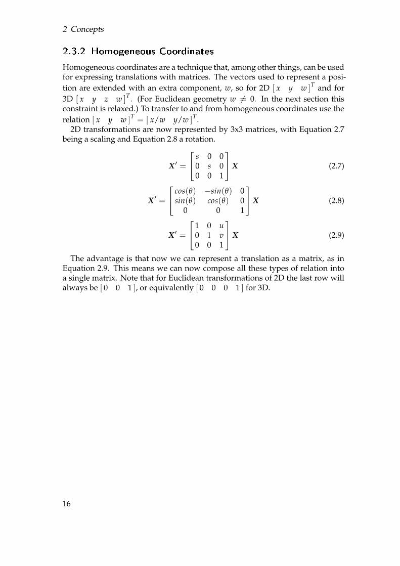
2.3.2 Homogeneous Coordinates

Homogeneous coordinates are a technique that, among other things, can be usedfor expressing translations with matrices. The vectors used to represent a posi-tion are extended with an extra component, w, so for 2D [ x y w ]T and for3D [ x y z w ]T. (For Euclidean geometry w 6= 0. In the next section thisconstraint is relaxed.) To transfer to and from homogeneous coordinates use therelation [ x y w ]T = [ x/w y/w ]T.

2D transformations are now represented by 3x3 matrices, with Equation 2.7being a scaling and Equation 2.8 a rotation.

X ′ =

s 0 00 s 00 0 1

X (2.7)

X ′ =

cos(θ) −sin(θ) 0sin(θ) cos(θ) 0

0 0 1

X (2.8)

X ′ =

1 0 u0 1 v0 0 1

X (2.9)

The advantage is that now we can represent a translation as a matrix, as inEquation 2.9. This means we can now compose all these types of relation intoa single matrix. Note that for Euclidean transformations of 2D the last row willalways be [ 0 0 1 ], or equivalently [ 0 0 0 1 ] for 3D.

16

2.3 Geometry

2.3.3 Projective Geometry

This section is based on [12, 5], due to the complexity of projective geometry thisis a light tour at best, for more details see the references.

Projective geometry is fundamentally different from Euclidean geometry, hav-ing one different axiom. They share the first four axioms1, but the fifth is differ-ent. For Euclidean geometry the 5th axiom implies that there can be parallel linesthat never intersect, for projective geometry it states that all lines intersect. Theconsequences of this are many, but the important consequence of using projec-tive geometry is in regards to the transformations. Euclidean geometry allowsonly rotation and translation transforms whilst projective additionally allowsscaling, shear and perspective transformations2. This affects what can be con-sidered invariant under transformation in these geometries, under projectivegeometry very little survives an arbitrary transformation, in fact only incidence(If two objects occupy the same space before the transform they will do so afterit.) and the cross-ratio invariant[12]. Under Euclidean geometry almost every-thing survives - distances, angles, parallelism.

w = 1

Y

W

P

LX

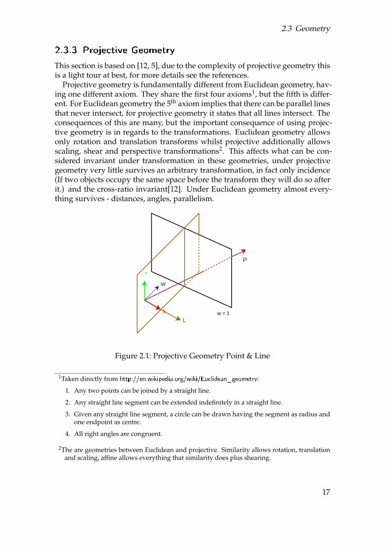
Figure 2.1: Projective Geometry Point & Line

1Taken directly from http://en.wikipedia.org/wiki/Euclidean_geometry:

1. Any two points can be joined by a straight line.

2. Any straight line segment can be extended indefinitely in a straight line.

3. Given any straight line segment, a circle can be drawn having the segment as radius andone endpoint as centre.

4. All right angles are congruent.

2The are geometries between Euclidean and projective. Similarity allows rotation, translationand scaling, affine allows everything that similarity does plus shearing.

17

2 Concepts

For practical purposes projective geometry is represented using homogeneouscoordinates. For 2D you can visualise the homogeneous coordinates as beingvectors in 3D space with w as the extra dimension. Where a point vector inter-cepts the plane w = 1 is the point in Euclidean space. Figure 2.1 demonstratesthis with line P. A consequence of this is that equality is with a scale factor, i.e.∀α, α 6= 0 ⇒ [ x y w ]T = [ αx αy αw ]T. A line is represented by a plane,its position in Euclidean space being where it intercepts the w = 1 plane. Theplane is represented by a vector perpendicular to the plane, so it has the samerepresentation as a point, [ x y w ]T, as indicated by L in Figure 2.1. Equalitywith a scale factor also applies to lines. Transformations are again representedby matrices as in subsection 2.3.2, however the last row can now be any arbitraryvalue for projective transforms. Transformation matrices are also equal with ascale factor.

Projective Geometry limits what can be calculated, as things like angles anddistance no longer mean anything. Given points as Xn = [ x y w ]T then theline Ln = [ x y w ]T that passes through two of them is L = [X1]x X2 where[X1]x indicates the cross product3. The reverse also holds, given two lines thenX = [L1]x L2 where X is the point of intersection for the two lines. A line andpoint intersect if PT L = 0. Points at infinity are represented by vectors withw = 0, there is also a line at infinity, L = [ 0, 0, α ]T , α 6= 0.

2.4 Sensors

To build a model of reality within a computer one first has to obtain informationabout that reality. A non-exhaustive list of relevant sensors follows:

• Human input. As obvious as it is to state, a human can act as a sensorand input data into a computer. Human beings have an extremely goodsense of the 3D world, but not a very good sense of how to transfer thisinformation into a computer. In addition, such work is time consuming,tedious and expensive to pay for4.

One can view the activity of getting a computer to automatically producea 3D reconstruction as one of automation, of removing the human beingfrom the loop. Total removal is not yet possible, if only because a humanhas to operate the sensors used instead, but some tasks still lend them-selves to human involvement. Examples of such tasks are providing one

3Given a vector V = [ v1 v2 v3 ]T then [V ]x =

0 −v3 v2v3 0 −v1−v2 v1 0

. If written as [A]x B for

two vectors A and B then this is the cross product of the two vectors.4In most subject areas pointing out that humans make mistakes is traditionally done here. How-

ever, from the results obtained they are models of perfection compared to what can currentlybe achieved in computer vision.

18

2.4 Sensors

shot values, such as the real world distance between two points to scalea model; or providing approximate initial data for refinement by the com-puter, such as the spatial relationship between two sensor readings. Thekey area where human involvement is vital however is where there are cur-rently no algorithms or the algorithms that exist are of limited capability.An example of this is in deciding which sensor readings are related; thattwo images of the same object are of the same object, and that two imagesof different objects are not.

• Cameras. Cameras project the 3D world onto a 2D plane and record thisprojection, thereby losing any depth information. The vast majority of cam-eras available capture what we as humans perceive. Cameras can be con-structed to capture most forms of light radiation however, for instance tocapture x-rays in a hospital. Video cameras are a form of camera that cap-tures many frames at regular intervals, to create the illusion of movementwhen played back. Technical details on cameras are given in the next sec-tion, 2.5.

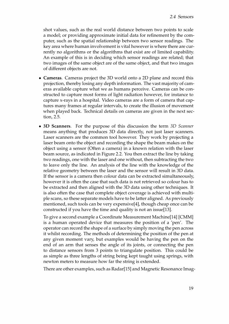
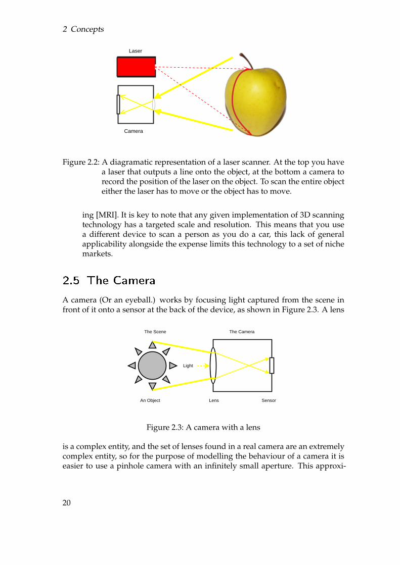
• 3D Scanners. For the purpose of this discussion the term 3D Scannermeans anything that produces 3D data directly, not just laser scanners.Laser scanners are the common tool however. They work by projecting alaser beam onto the object and recording the shape the beam makes on theobject using a sensor (Often a camera) in a known relation with the laserbeam source, as indicated in Figure 2.2. You then extract the line by takingtwo readings, one with the laser and one without, then subtracting the twoto leave only the line. An analysis of the line with the knowledge of therelative geometry between the laser and the sensor will result in 3D data.If the sensor is a camera then colour data can be extracted simultaneously,however it is often the case that such data is not retrieved so colour has tobe extracted and then aligned with the 3D data using other techniques. Itis also often the case that complete object coverage is achieved with multi-ple scans, so these separate models have to be latter aligned. As previouslymentioned, such tools can be very expensive[4], though cheap once can beconstructed if you have the time and quality is not an issue[13].

To give a second example a Coordinate Measurement Machine[14] [CMM]is a human operated device that measures the position of a ’pen’. Theoperator can record the shape of a surface by simply moving the pen acrossit whilst recording. The methods of determining the position of the pen atany given moment vary, but examples would be having the pen on theend of an arm that senses the angle of its joints, or connecting the pento distance sensors from 3 points to triangulate position. This could beas simple as three lengths of string being kept taught using springs, withnewton meters to measure how far the string is extended.

There are other examples, such as Radar[15] and Magnetic Resonance Imag-

19

2 Concepts

Laser

Camera

Figure 2.2: A diagramatic representation of a laser scanner. At the top you havea laser that outputs a line onto the object, at the bottom a camera torecord the position of the laser on the object. To scan the entire objecteither the laser has to move or the object has to move.

ing [MRI]. It is key to note that any given implementation of 3D scanningtechnology has a targeted scale and resolution. This means that you usea different device to scan a person as you do a car, this lack of generalapplicability alongside the expense limits this technology to a set of nichemarkets.

2.5 The Camera

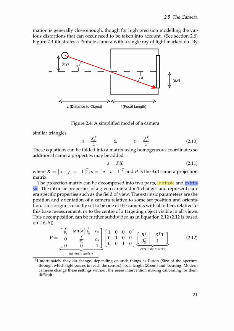
A camera (Or an eyeball.) works by focusing light captured from the scene infront of it onto a sensor at the back of the device, as shown in Figure 2.3. A lens

The CameraThe Scene

An Object

Light

Lens Sensor

Figure 2.3: A camera with a lens

is a complex entity, and the set of lenses found in a real camera are an extremelycomplex entity, so for the purpose of modelling the behaviour of a camera it iseasier to use a pinhole camera with an infinitely small aperture. This approxi-

20

2.5 The Camera

mation is generally close enough, though for high precision modelling the var-ious distortions that can occur need to be taken into account. (See section 2.6)Figure 2.4 illustrates a Pinhole camera with a single ray of light marked on. By

(x,y)

(u,v)

z (Distance to Object) f (Focal Length)

a

a

Figure 2.4: A simplified model of a camera

similar triangles

u =x fz

& v =y fz

(2.10)

These equations can be folded into a matrix using homogeneous coordinates soadditional camera properties may be added

s = PX (2.11)

where X = [ x y z 1 ]T, s = [ u v 1 ]T and P is the 3x4 camera projectionmatrix.

The projection matrix can be decomposed into two parts, intrinsic and extrin-sic. The intrinsic properties of a given camera don’t change5 and represent cam-era specific properties such as the field of view. The extrinsic parameters are theposition and orientation of a camera relative to some set position and orienta-tion. This origin is usually set to be one of the cameras with all others relative tothis base measurement, or to the centre of a targeting object visible in all views.This decomposition can be further subdivided as in Equation 2.12 (2.12 is basedon [16, 5]).

P =

f

Pxtan(α) f

Pycx

0 fPy

cy

0 0 1

︸ ︷︷ ︸

intrinsic matrix

1 0 0 00 1 0 00 0 1 0

[RT −RTT0T

3 1

]︸ ︷︷ ︸

extrinsic matrix

(2.12)

5Unfortunately they do change, depending on such things as F-stop (Size of the aperturethrough which light passes to reach the sensor.), focal length (Zoom) and focusing. Moderncameras change these settings without the users intervention making calibrating for themdifficult.

21

2 Concepts

The intrinsic matrix is constructed from several parameters, f is the focallength of the camera (i.e. 28mm, 35mm.), Px and Py are the dimensions of thepixels6, α is the angular skew whilst cx and cy form the principal point. The prin-cipal point is the centre of the sensor, in theory this is aligned with the centre ofthe aperture, so if the image is parametrized as [-1,1]x[-1,1] should be [ 0 0 ]T.Similarly, the pixels should be perfectly square therefore the skew should be 0.You can calculate a cameras intrinsic matrix from the manufacturers providedspecifications, but this does not produce a useful result as workmanship is notperfect and most of the parameters used only make true sense for a pin holecamera, so the manufacturer provides approximate parameters anyway.

The extrinsic matrix is constructed from a rotation (R) and a translation (T)from the origin to the camera. The projection matrix must contain the inverse,which can be constructed as in Equation 2.12. Given pairs of world coordinatesand projected coordinates it is possible to calculate the projection matrix of acamera using SVD.[17, p. 455]8 If the projection matrix is represented as

P =

p11 p12 p13 p14p21 p22 p23 p24p31 p32 p33 p34

(2.13)

then for any given match, X = [ x y z 1 ]T, s = [ u v 1 ]T

[x y z 1 0 0 0 0 −ux −uy −uz −u0 0 0 0 x y z 1 −vx −vy −vz −v

] p11p12...

p33p34

= 0 (2.14)

As P has 11 degrees of freedom (4x3 homogeneous matrix minus one for equal-ity with a scaling factor.) 6 matches can be used to find the projection matrix

6This is the size of a pixel in real-world units. Approximately calculated by taking the size ofthe CCD7and dividing by the number of pixels in each dimension. (This is wrong becausenot all of the CCDs area is used.)

7A digital camera uses a Charged Coupling Device [CCD] to detect light, its equivalent to thefilm in an analog camera.

8Singular Value Decomposition[18] [SVD] decomposes a mxn matrix A such that A = UDV T

where U is a mxn (m > n) matrix, V is a nxn matrix and D is a nxn diagonal matrix. Both Uand V have orthogonal columns such that UUT = VV T = I. It works for any given matrix,including non-invertible once.

22

2.6 Imaging Errors

using SVD9

Given the projection matrices Pn =

PT1

PT2

PT3

of two or more cameras and sn =

[ u v 1 ]T where a single point X = [ x y z w ]T projects onto each of themyou can obtain X using[19]

[uPT

3 − PT1

vPT3 − PT

2

] xyzw

= 0 (2.15)

for each camera and solving with SVD. X has four degrees of freedom so at leasttwo views are required.

2.6 Imaging Errors

There are two types of error caused by the imaging process worth considering;noise from the sensor and distortion from the lens(es).

Noise comes from many sources[20], for practical purposes however it is in-variably modelled as a Gaussian distribution around the true value of a givensensor reading.

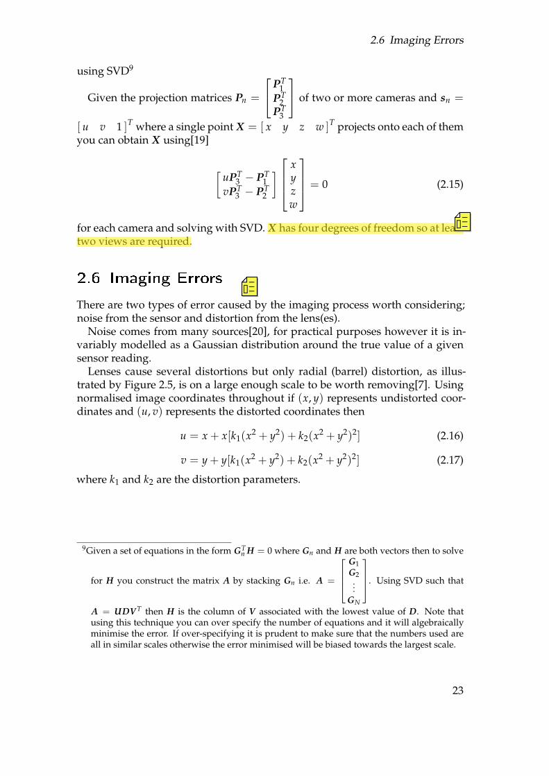
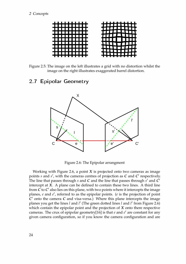
Lenses cause several distortions but only radial (barrel) distortion, as illus-trated by Figure 2.5, is on a large enough scale to be worth removing[7]. Usingnormalised image coordinates throughout if (x, y) represents undistorted coor-dinates and (u, v) represents the distorted coordinates then

u = x + x[k1(x2 + y2) + k2(x2 + y2)2] (2.16)

v = y + y[k1(x2 + y2) + k2(x2 + y2)2] (2.17)

where k1 and k2 are the distortion parameters.

9Given a set of equations in the form GTn H = 0 where Gn and H are both vectors then to solve

for H you construct the matrix A by stacking Gn i.e. A =

G1G2...

GN

. Using SVD such that

A = UDV T then H is the column of V associated with the lowest value of D. Note thatusing this technique you can over specify the number of equations and it will algebraicallyminimise the error. If over-specifying it is prudent to make sure that the numbers used areall in similar scales otherwise the error minimised will be biased towards the largest scale.

23

2 Concepts

Figure 2.5: The image on the left illustrates a grid with no distortion whilst theimage on the right illustrates exaggerated barrel distortion.

2.7 Epipolar Geometry

X

ss’

e e’C C’

l

l’

Figure 2.6: The Epipolar arrangment

Working with Figure 2.6, a point X is projected onto two cameras as imagepoints s and s′, with the cameras centres of projection as C and C′ respectively.The line that passes through s and C and the line that passes through s′ and C′

intercept at X. A plane can be defined to contain these two lines. A third linefrom C to C′ also lies on this plane, with two points where it intercepts the imageplanes, e and e′, referred to as the epipolar points. (e is the projection of pointC′ onto the camera C and visa-versa.) Where this plane intercepts the imageplanes you get the lines l and l′ (The green dotted lines l and l′ from Figure 2.6)which contain the epipolar point and the projection of X onto there respectivecameras. The crux of epipolar geometry[16] is that e and e′ are constant for anygiven camera configuration, so if you know the camera configuration and are

24

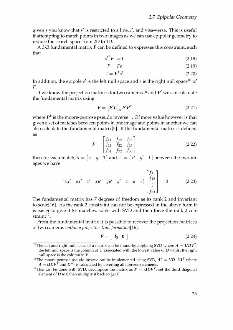
2.7 Epipolar Geometry

given s you know that s′ is restricted to a line, l′, and visa-versa. This is usefulif attempting to match points in two images as we can use epipolar geometry toreduce the search space from 2D to 1D.

A 3x3 fundamental matrix F can be defined to expresses this constraint, suchthat

s′TFs = 0 (2.18)

l′ = Fs (2.19)

l = FTs′ (2.20)

In addition, the epipole e′ is the left null space and e is the right null space10 ofF.

If we know the projection matrices for two cameras P and P′ we can calculatethe fundamental matrix using

F =[P′C

]x P′P† (2.21)

where P† is the moore-penrose pseudo inverse11. Of more value however is thatgiven a set of matches between points in one image and points in another we canalso calculate the fundamental matrix[5]. If the fundamental matrix is definedas

F =

f11 f12 f13f21 f22 f23f31 f32 f33

(2.22)

then for each match, s = [ x y 1 ] and s′ = [ x′ y′ 1 ] between the two im-ages we have

[ xx′ yx′ x′ xy′ yy′ y′ x y 1 ]

f11f12...

f33

= 0 (2.23)

The fundamental matrix has 7 degrees of freedom as its rank 2 and invariantto scale[16]. As the rank 2 constraint can not be expressed in the above form itis easier to give it 8+ matches, solve with SVD and then force the rank 2 con-straint12.

From the fundamental matrix it is possible to recover the projection matricesof two cameras within a projective transformation[16].

P =[

I3 0]

(2.24)

10The left and right null space of a matrix can be found by applying SVD where A = UDV T ,the left null space is the column of U associated with the lowest value of D whilst the rightnull space is the column in V.

11The moore-penrose pseudo inverse can be implemented using SVD, A† = V D−1UT whereA = UDV T and D−1 is calculated by inverting all non-zero elements.

12This can be done with SVD, decompose the matrix as F = UDV T , set the third diagonalelement of D to 0 then multiply it back to get F.

25

2 Concepts

P′ =[

[e′]x F e′]

(2.25)

Transforming the resulting matrices to the correct transforms then requires fur-ther information. Alternatively, if you have the intrinsic parameters for the cam-eras you can calculate the projective transformations directly via the essentialmatrix.

The essential matrix is identical to the fundamental matrix except it uses nor-malised coordinates, which have had the intrinsic matrix applied i.e. s0 = K−1swhere K is the intrinsic matrix. A consequence of this is

E = [T ]x R (2.26)

where E is the essential matrix, T is the translation between the cameras and Ris the rotation between them. The essential matrix can be calculated using theintrinsic matrices as13

E = K′TFK (2.27)

and then decomposed into the rotation and translation parts by decomposing Eusing SVD as E = UDV T then

[T ]x = URzDUT (2.28)

R = URTz V T (2.29)

where Rz =

0 −1 01 0 00 0 1

or Rz =

0 1 0−1 0 00 0 −1

[21]. The projection matrices

can then be reconstructed as

P = K

1 0 0 00 1 0 00 0 1 0

(2.30)

P′ = K′ [ RT −RTT]

(2.31)

Note that scale can not be recovered.

2.8 Sumary

The previous sections have covered many of the algorithms used by this sys-tem. Specifically, NCC and the Harris corner detector given in section 2.2, Equa-tion 2.15 is used to calculate 3D coordinates given image coordinates, Equa-tion 2.23 to calculate the fundamental matrix and Equations 2.24 to 2.31 to cal-culate the projection matrices. The rest of this chapter has been concerned withthe basis for the system and background to the following chapters.

13The SVD of E = UDV T should have D =

α 0 00 α 00 0 0

. This should be enforced with α =

(D11 + D22)/2 before multiplying back to get E.

26

3 Proccessing Models

3.1 Overview

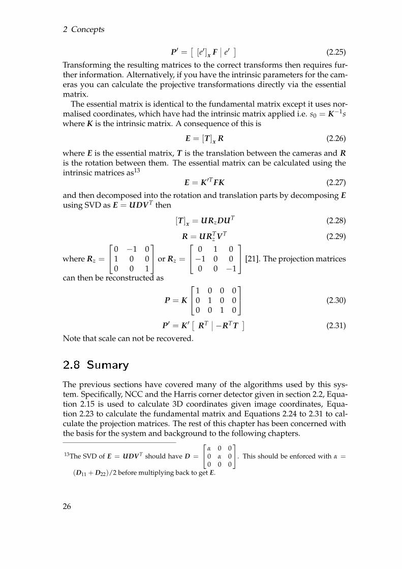
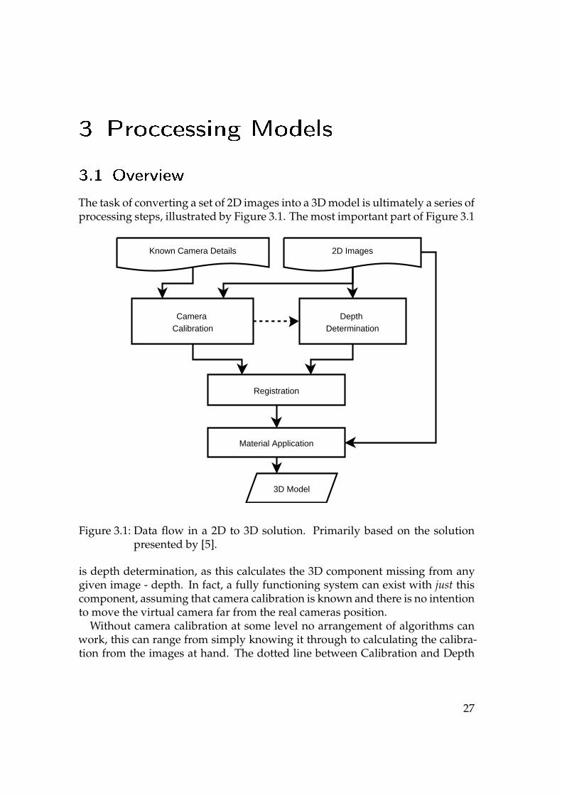
The task of converting a set of 2D images into a 3D model is ultimately a series ofprocessing steps, illustrated by Figure 3.1. The most important part of Figure 3.1

Known Camera Details 2D Images

Camera Calibration

Depth Determination

Registration

Material Application

3D Model

Figure 3.1: Data flow in a 2D to 3D solution. Primarily based on the solutionpresented by [5].

is depth determination, as this calculates the 3D component missing from anygiven image - depth. In fact, a fully functioning system can exist with just thiscomponent, assuming that camera calibration is known and there is no intentionto move the virtual camera far from the real cameras position.

Without camera calibration at some level no arrangement of algorithms canwork, this can range from simply knowing it through to calculating the calibra-tion from the images at hand. The dotted line between Calibration and Depth

27

3 Proccessing Models

Determination represents that the camera calibration is usually required to deter-mine depth, for instance steropsis requires that the epipolar geometry be known.

Once you have multiple depth maps you have to combine them to create afinal mesh, this is the process of registration1. This uses camera calibration toidentify where the many meshes created by depth maps can be joined togetherto create a larger mesh that stands up to observation from more than one angle.

By the stage of Material Application you have a complete 3D mesh, whichmay be the final goal, but usually you will want to apply the colour from theoriginal photographs to the mesh. This can range from projecting the imagesonto the mesh arbitrarily, through methods of merging the textures for super-resolution2 and ultimately to subdividing the mesh by material and inferringdetails about those materials, such as specular and diffuse properties.

The following sections cover each part of Figure 3.1 in turn, with a final sectionon other methods.

3.2 Camera Callibration

There are three common scenarios when it comes to camera calibration; knownconfiguration, off-line configuration and self calibration. In all cases we are aim-ing to obtain the projection matrices of the cameras. For the following list itis assumed that multiple cameras are involved, if one camera is involved thenonly the intrinsic parameters need be recovered; this can be done using an off-line technique.

Known configuration simply means both the rotation and translation betweencameras and the intrinsic matrices for cameras, and therefore their projectionmatrices, are known. This usually happens with a stereo rig where two camerasare fixed with no rotation and a translation perpendicular to there shared direc-tion between them. If constructing a stereo rig the intrinsic parameters will beunknown and can be found using an off-line technique.

Off-line calibration is done in two stages, intrinsic parameters then extrinsicparameters. The first stage involves photographing a target with known para-meters then using techniques depending on the type of target to determine theintrinsic parameters. Examples of this would be [7, 22]. The second stage is doneon-line by finding matches between scene points, calculating the fundamentalmatrix and reconstructing the projection using the fundamental and intrinsicmatrices. (See section 2.7) Off-line calibration can also be done on-line if there isa target to use in the scene, either put there or manually measured.

1Registration also refers to the post-processing of separately gathered depth maps and colourmaps to line them up, often as a consequence of using a 3D scanner.

2Super resolution is the technique of merging photos of the same object from multiple anglesat low resolution to create a higher resolution texture of that object resulting in more visibledetail.

28

3.3 Depth Determination

Self-calibration generally involves finding the fundamental matrix and recon-structing the projection matrices within a projective translation using the tech-niques discussed in section 2.7. The Projective Reconstruction Theorem[19] statesthat there is a transformation H such that

X2 = HX1 P2 = P1H−1 P′2 = P′

1H−1 (3.1)

there are many possible H but only one results in the correct reconstruction. Find-ing the correct H involves applying scene constraints, such as parallel lines, an-gles between lines or known vertex positions. With three or more images self-calibration can be done with just the images at hand, using techniques such asthe Kruppa equations[8].

3.3 Depth Determination

Excluding direct methods such as 3D scanners (2.4) depth can be determined foran image either by using just that image or multiple images.

3.3.1 Single Image

Generally, calculating depth from a single image is an ill-posed problem[17, p.447], but by applying extra constraints it can be done. If the scene is constructedof known objects then those objects can be found and 3D geometry already ob-tained matched to the scene[23]. Such techniques are limited by the fact thatonly known objects can be reconstructed.

Visual cues can be used to provide the necessary information, such as focus,light and texture. If you can determine how far in/out of focus a point in an im-age is (A defocus operator[24].) then using a detailed camera model depth canbe determined. There are numerous constraints on this technique, such as the de-tailed knowledge of the camera required and its dependence on a small depthof field. By modelling light and how it results in the particular pixel colourssurface normals can be determined[25], this requires known lighting. Surfacenormals can also be discovered by examining how a regular texture deformswith the shape of an object. Both these techniques produce needle maps (A rep-resentation of surface orientation3.) from which shape can be reconstructed.

3.3.2 Multiple Images

Stereopsis, using multiple images to calculate depth, is a well defined problemwhen compared to working with single images. The correspondence problem,that of finding matches between two images so the positions of the matchedelements can then be triangulated in 3D space is at the core of this. There are

3http://www.bmva.ac.uk/bmvc/1997/papers/094/node1.html

29

3 Proccessing Models

two main categories of the correspondence problem, sparse and dense. Sparsecan be further divided into wide and short baseline.

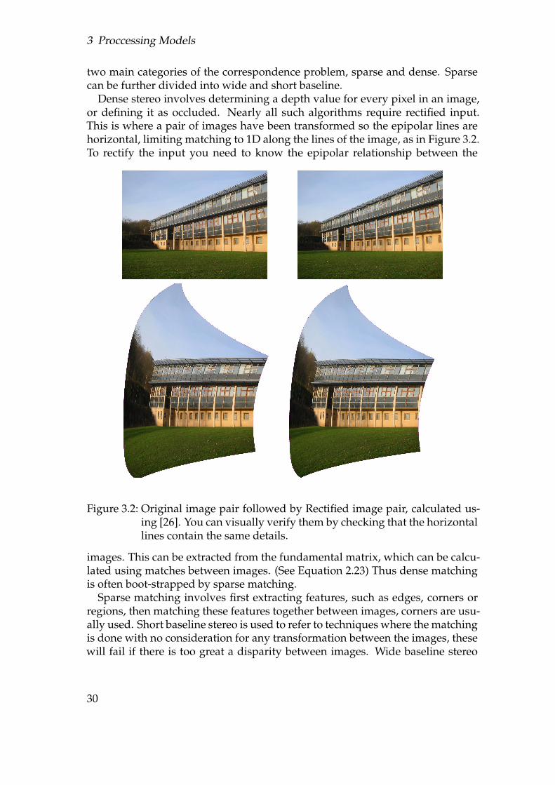
Dense stereo involves determining a depth value for every pixel in an image,or defining it as occluded. Nearly all such algorithms require rectified input.This is where a pair of images have been transformed so the epipolar lines arehorizontal, limiting matching to 1D along the lines of the image, as in Figure 3.2.To rectify the input you need to know the epipolar relationship between the

Figure 3.2: Original image pair followed by Rectified image pair, calculated us-ing [26]. You can visually verify them by checking that the horizontallines contain the same details.

images. This can be extracted from the fundamental matrix, which can be calcu-lated using matches between images. (See Equation 2.23) Thus dense matchingis often boot-strapped by sparse matching.

Sparse matching involves first extracting features, such as edges, corners orregions, then matching these features together between images, corners are usu-ally used. Short baseline stereo is used to refer to techniques where the matchingis done with no consideration for any transformation between the images, thesewill fail if there is too great a disparity between images. Wide baseline stereo

30

3.4 Registration

algorithms are designed specifically for the task and can cope with angles be-tween views of 60◦ plus[27]. If used for depth determination sparse matchingcomes with the disadvantage that the sparse depth values have to be interpo-lated between features.

Once the correspondence of an image has been obtained a 3D mesh can thenbe produced, by calculating depth and projecting out of the camera. See Equa-tion 2.15, which does this directly from correspondences.

3.4 Registration

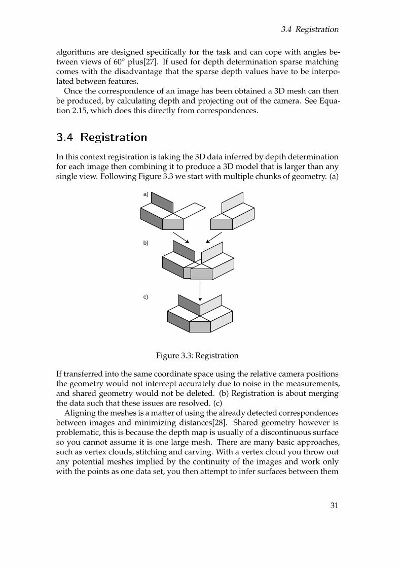
In this context registration is taking the 3D data inferred by depth determinationfor each image then combining it to produce a 3D model that is larger than anysingle view. Following Figure 3.3 we start with multiple chunks of geometry. (a)

a)

b)

c)

Figure 3.3: Registration

If transferred into the same coordinate space using the relative camera positionsthe geometry would not intercept accurately due to noise in the measurements,and shared geometry would not be deleted. (b) Registration is about mergingthe data such that these issues are resolved. (c)

Aligning the meshes is a matter of using the already detected correspondencesbetween images and minimizing distances[28]. Shared geometry however isproblematic, this is because the depth map is usually of a discontinuous surfaceso you cannot assume it is one large mesh. There are many basic approaches,such as vertex clouds, stitching and carving. With a vertex cloud you throw outany potential meshes implied by the continuity of the images and work onlywith the points as one data set, you then attempt to infer surfaces between them

31

3 Proccessing Models

from scratch. With stitching you segment the image to create a set of continuoussurfaces, these are then stitched together. With carving you use the depth mapsas definitions of empty space and consider everything else as solid, you thencarve away the depth maps data from the solid space.

3.5 Material Application

At its simplest applying a material to the 3D model is applying a colour texture,this can be done by simply mapping the original images onto the parts of the 3Dmodel created by those images. When multiple images map to the same sectionof geometry one of the images can be chosen arbitrarily to take priority or theycan be blended. If blending is done it is often weighted in favour of images fromcameras closer to the geometry and image projections closer to being flat to thegeometry. Beyond this simple technique many others exist, such as:

• View Dependent Texture Mapping is blending the images depending onthe viewing angle, such that images taken from a similar angle to the viewertake priority. This can be very effective as details too small to be capturedby the 3D model can obtain a sense of depth on account of being renderedfrom the correct direction.

• Super resolution, for example [29], involves combining the images to cre-ate a higher resolution image.

• Material parameter modelling is going beyond simple colour and measur-ing the details that define how a material changes colour depending onviewing angle and viewing conditions. This requires many, many samplesof the material and is impractical in a real world scene as controlled light-ing is usually required. The many samples required can be obtained bysegmenting the model by material, so you get many samples from manydirections for each material.

3.6 Final Model

Once a final a 3D model with materials has been created it will then need post-processing. Noise is a substantial problem and needs to be minimised, this canbe done using various statistical techniques to detect and smooth or delete out-liers. Standard signal processing can be applied to meshes[30], alternatively out-lier detection can be based on detecting significant deviation from neighbouringstatistical properties. Once noise is removed holes then need to be filled in, in-terpolation techniques can be applied. For real time rendering model simplifica-tion and conversion to the correct format is often required. If detailed materialinformation has been obtained a specific renderer will be required to visualiseit.

32

3.7 Other Methods

3.7 Other Methods

This section contains a list of alternative system arrangements which do not fitwithin the above data flow model.

3.7.1 Homo-Sapian

It may seem strange to include the humble human being in a list of systems,however reality is that the human being is the best system available for this task.This particular algorithm can be applied to all parts of the problem, and givena 3D modelling package, a tape measure and time (And probably money.) willsolve the entire problem with a high degree of accuracy. (Assuming the object(s)in question are of a suitable scale.)

On a more practical note, solutions that automate the process but allow a hu-man to add there own input and correct the computers mistakes are inevitablymore successful than systems that work alone, and form the most robust sys-tems that can be currently created. (An example would be [31], a technique usedin modern films4.) The issues with implementing such a system are non-trivialhowever, as interfaces5 and work flow becomes an issue6.

Despite being the best solution, due to the time constraints human interac-tion with the process will no longer be considered as even a partially completesolution that has interactivity is unachievable in the time available.

3.7.2 Space Carving

The principal behind space carving is to take a large solid space and then foreach view of the object calculate the outline of the object and carve away theparts that are outside the outline. If done from enough views this creates anaccurate model of the object. This requires that views can be captured fromall angles of the object and that the object is not concave. It also requires thatthe object can be distinguished from the background to find its outline, whichusually requires the background be known, limiting such solutions to studioenvironments. Whilst limited in its capability the simplicity of this techniquemakes it very reliable.

4http://www.debevec.org/Campanile/5Such interfaces are complete 3D modelling interfaces with extra functionality. An examination

of any popular 3D modelling tool (Such as Maya, http://www.alias.com.) shows that manyman years have gone into its design and implementation.

6The direct consequence of work flow being an issue is that algorithms that take more than afew seconds become inappropriate. In consequence the computer becomes less of a contrib-utor as simpler algorithms are used.

33

3 Proccessing Models

3.7.3 Image Based Rendering

Image Based Rendering7 never constructs a model of the scene, instead it di-rectly constructs new views of the scene from the images. The motivation be-hind this is that a 3D model is usually constructed to be rendered back as anotherview of the scene, so you have the computer vision pipeline followed by a ren-dering pipeline. Instead of this the two pipelines can be merged and customisedfor the task. This comes with the advantage of producing a very realistic resultas it works directly from real world data, it is also independent of scene complex-ity and can capture details that model based techniques lose. It does howeverlimit the output to non-realtime behaviour as it can not use standard real-timerendering pipelines. It also requires many parts of the standard pipeline and itis of greater complexity to implement.

7http://homepages.inf.ed.ac.uk/rbf/CVonline/LOCAL_COPIES/LIVATINO2/MainApprRVVS/node1.html

34

4 Design

Four sections follow, the first explains the development process, the second therequirements of the system. The final two sections are the designs for the frame-work (This is explained in the relevant section. To summarise a framework hasbeen used to abstract between data flow and data processing.) and algorithmsrespectively.

4.1 Development Process

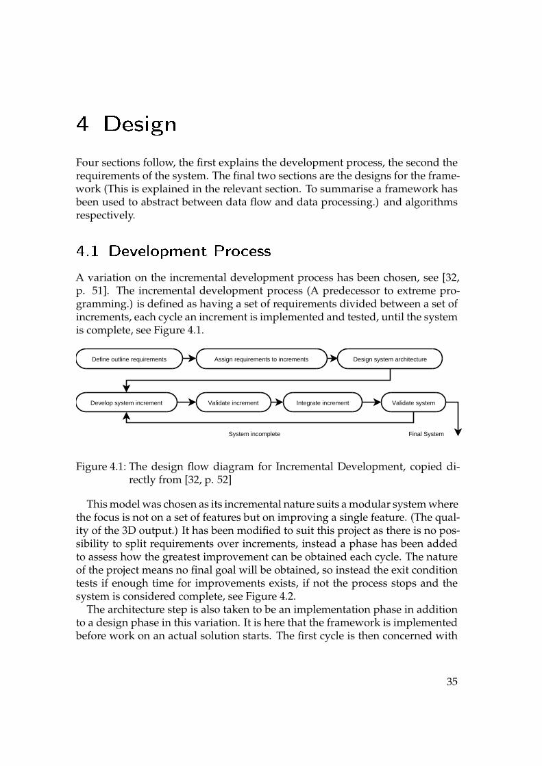
A variation on the incremental development process has been chosen, see [32,p. 51]. The incremental development process (A predecessor to extreme pro-gramming.) is defined as having a set of requirements divided between a set ofincrements, each cycle an increment is implemented and tested, until the systemis complete, see Figure 4.1.

Define outline requirements Assign requirements to increments Design system architecture

Develop system increment Validate increment Integrate increment Validate system

System incomplete Final System

Figure 4.1: The design flow diagram for Incremental Development, copied di-rectly from [32, p. 52]

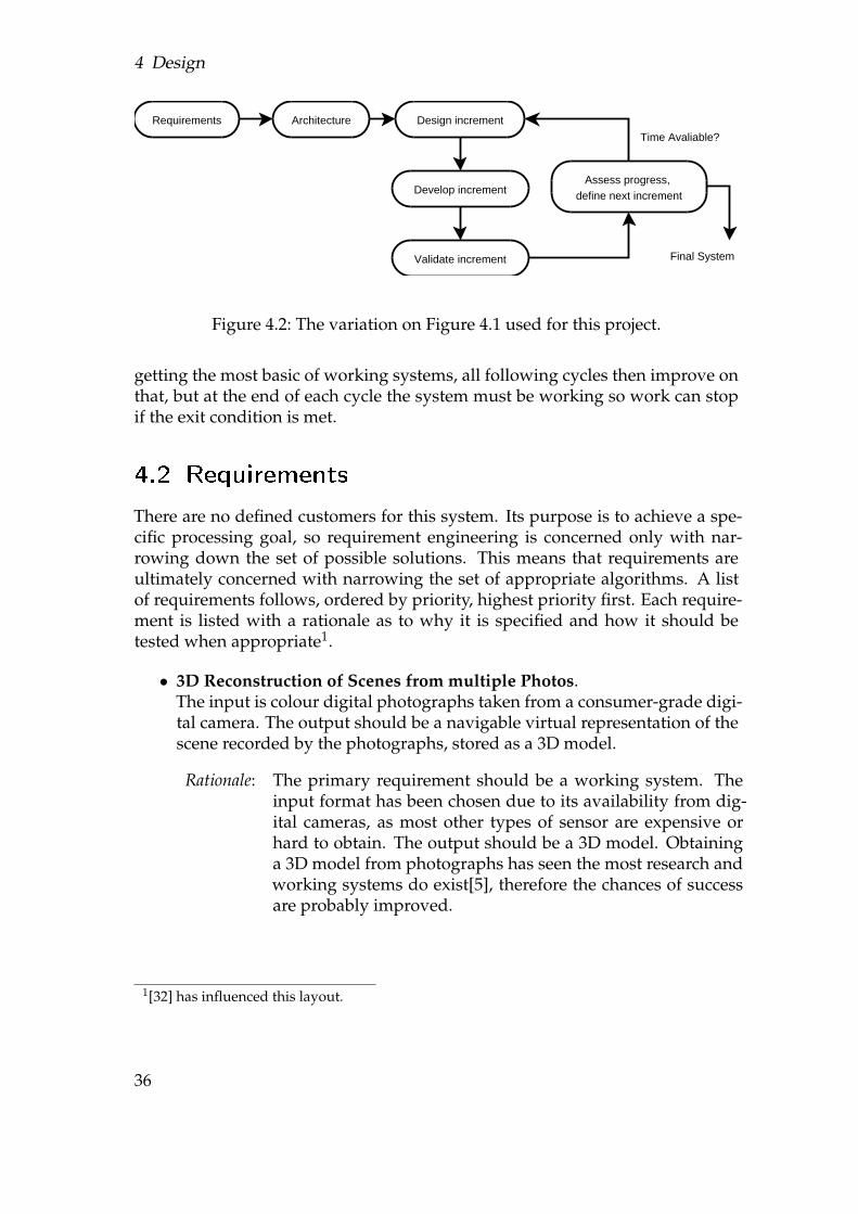
This model was chosen as its incremental nature suits a modular system wherethe focus is not on a set of features but on improving a single feature. (The qual-ity of the 3D output.) It has been modified to suit this project as there is no pos-sibility to split requirements over increments, instead a phase has been addedto assess how the greatest improvement can be obtained each cycle. The natureof the project means no final goal will be obtained, so instead the exit conditiontests if enough time for improvements exists, if not the process stops and thesystem is considered complete, see Figure 4.2.

The architecture step is also taken to be an implementation phase in additionto a design phase in this variation. It is here that the framework is implementedbefore work on an actual solution starts. The first cycle is then concerned with

35

4 Design

Requirements Design increment

Develop increment

Validate increment

Assess progress, define next increment

Final System

Time Avaliable?

Architecture

Figure 4.2: The variation on Figure 4.1 used for this project.

getting the most basic of working systems, all following cycles then improve onthat, but at the end of each cycle the system must be working so work can stopif the exit condition is met.

4.2 Requirements

There are no defined customers for this system. Its purpose is to achieve a spe-cific processing goal, so requirement engineering is concerned only with nar-rowing down the set of possible solutions. This means that requirements areultimately concerned with narrowing the set of appropriate algorithms. A listof requirements follows, ordered by priority, highest priority first. Each require-ment is listed with a rationale as to why it is specified and how it should betested when appropriate1.

• 3D Reconstruction of Scenes from multiple Photos.The input is colour digital photographs taken from a consumer-grade digi-tal camera. The output should be a navigable virtual representation of thescene recorded by the photographs, stored as a 3D model.

Rationale: The primary requirement should be a working system. Theinput format has been chosen due to its availability from dig-ital cameras, as most other types of sensor are expensive orhard to obtain. The output should be a 3D model. Obtaininga 3D model from photographs has seen the most research andworking systems do exist[5], therefore the chances of successare probably improved.

1[32] has influenced this layout.

36

4.2 Requirements

Testing: Comparison of the output of the system with the results of thebest available vision system, a pair of human eyes. A quanti-tative analysis is not possible as the actual 3D models for cap-tured scenes are unknown.

• Casual Capture.This implies that capturing the scene does not require special arrange-ments, such as a blue screen or specific lighting.

Rationale: This is a follow on from the input being captured using aconsumer-grade digital camera. By stating that the systemmust not apply such constraints in theory if developmentof the system was perpetual it should never reach the pointwhere improvements would require a rewrite.

Testing: If a constraint exists which fails this then it fails. Success is un-defined however as there can always be constraints assumedwithout the realisation that they have been assumed.

• Minimization of Scene Constraints.Current solutions fail on many types of scene. Whilst it is unrealistic to beattempting to obtain state of the art capability there should be a preferencetowards robust and reliable algorithms.

Rationale: Every capturing constraint reduces the number of scenes thatcan be processed by the system. Whilst some constraints cannot be removed, for instance that the scene is static, there is noreason to not minimise constraints where possible within thetime available.

Testing: As the requirement states no specific constraints testing cannot be quantitavely done. However, measurements can bemade of the system limits and of what causes it to fail.

• Automatic Processing.The system should be automatic, in that human interaction with the sys-tem is to be avoided.

Rationale: See subsection 3.7.1.Testing: None required. Note that this constraint has been broken for

intrinsic camera calibration (4.4.3) due to time constraints.

• Performance is not a priority.Once a module is working time will not be spent making it run faster.Memory usage is also to be ignored, unless its more than the hardwareavailable can manage.

37

4 Design

Rationale: The time constraints on the project mean certain parts are go-ing to have to take second place. Performance is an obviouscandidate for this as its going to be slow anyway. Spendingconsiderable time to take 10% off an hour of unattended proc-cessing is not justifiable.

Testing: -

• High Modularity.Any one part of the system should be replaceable, adding new featuresshould involve minimal effort.

Rationale: In the interest of current and future expandability a systemshould be modular. This should allow algorithms to bechanged, or even base elements so it could be ported to runon a grid for instance.

Testing: -

• Development using C++ under Windowstm.The system will be coded using C++ to run on the Windowstm platform,though an effort has been made to abstract all system calls. (See section A.2)

Rationale: This is justified as it is the arrangement for which the mostexperience is available, therefore a certain class of problem areunlikely to occur.

Testing: -

4.3 The Framework

Following on from the idea of treating 2D to 3D as a sequence of processing steps(chapter 3) the design has been split into two parts. The framework providesa script-driven environment, modular structure (Using dynamically linked li-braries. [DLLs]) and a general purpose data type for inter-algorithm communi-cation. The algorithms are a collection of modules that plug into the framework.Essentially the framework abstracts data flow from the algorithm implementa-tions and allows changes to the data flow without recompilation. The other de-sign possibility was to not have a framework, and to hard code the connectionsbetween algorithms. The advantages of a framework over none are:

• Modular Development. This allows algorithms to be developed withoutconsideration for the rest of the system. Algorithms that are not perform-ing as expected can be swapped out without any changes other than imple-menting the replacement. Also, the system proposed keeps the algorithms

38

4.3 The Framework

in dynamic libraries that can be separately compiled2.

• Scripted Execution. This allows the data flow to be arbitrarily edited. Al-gorithms can be swapped out without recompilation, or compared side byside. By having multiple script files with one executable it saves on com-piling a different executable for each task the system might do. It also actsas an interface, so instead of the system asking for input it can be typedinto the script file. This reduces development complexity and eliminatesbabysitting of the program. It also provides a form of precise documenta-tion.

• Single Variable Type. [SVT] With only one data type available time doesnot need to be spent designing, implementing and debugging each datastructure required. It also allows a script to save itself in an arbitrary statewithout developing savers/loaders for each data type. This is useful whendeveloping modules far into the system, as you can run the system up tojust before where you are working, save the state then load it in each timeyou run your new code instead if running it up to that point.3

and the disadvantages are:

• Development time. The time available is the primary restriction. Imple-menting a framework consumes time which could be spent on algorithms.Ultimately I believe that it will save time however, as many of the advan-tages mentioned above will reduce total work.

• Single Variable Type. [SVT] The design of this data type has to be perfect,otherwise it will be unable to pass all the types of data required betweenalgorithms. Even then, having only one data type can involve passingdata inefficiently and using nasty hacks to bypass design shortcomings.The data types passed between algorithms in this system are reasonablyconsistent however (Images and matrices), so this should not be an issue.

• Speed. On execution the system has to load and parse a script, it also hasto load in modules. Once running the inefficiency of a single data typewill slow things down. It is probably safe to say that such time delays areneglible in comparison with the algorithms that are run however.

Based on the above list the advantages of a framework are considered to out-weigh the disadvantages, especially as the flexibility provided can be of greatuse when working within a short time span. Possible design alternatives for the

2To give an indication of the advantage this provides a complete compilation of the systemat the end of development took 1:07 minutes, whilst recompilation after changing a singlealgorithm was 7 seconds.

3Stereo correspondence algorithms can take hours to run. Development of algorithms that runafterwards would be tedious without saving the results.

39

4 Design

framework itself are listed in the following list, with reasons as to why theseoptions were not taken:

• Multiple Variable Types. Instead of having a single variable type to con-tain all possible data types multiple types could be developed for eachtype of data required. This comes with the disadvantage of extended de-velopment to implement them. As the algorithms are modular the datatypes would sensibly then need to be modular, this would need an ad-vanced saving/loading scheme with an object factory etc. The advantageis data structures that precisely match the requirements of algorithms. Theextended development does not seem to justify this minimal advantage.

• Extra Variable Types. As a less extreme variant of the above a set of non-modular variable types could be provided. Whilst simple to implement itshard to find extra types that compliment the SVT as defined, see subsec-tion 4.3.2.

• Non-Modular Development. Instead of developing each set of algorithmsin separate DLLs they could all be compiled into a single executable. Thismakes compilation easier, and means dependencies are going to be less ofan issue, but at the expense of compilation time. Ultimately compilationis done with greater frequency than makefile updates, so time should besaved by using DLLs.

The design now follows in terms of its interfaces, not its implementation, forthe details of the implementation see Appendix A. It has two interfaces, thescripting language interface used by users of the system and covered in the firstsub-section and the module interface for algorithms, i.e. the SVT, covered in thesecond section.

4.3.1 Scripting

Each algorithm takes a set of inputs and then produces a set of outputs, theseinputs and outputs all being SVTs. The SVT is suitable for large data structures,but not for single numbers and other such details that are needed to define howan algorithm behaves. For this purpose extra details need to be passed intoalgorithms, though no requirement exists to pass them back out again or editthem within a script. To call an algorithm then requires the following data:

• Algorithm Identifier.

• A set of input SVTs.

• A set of output SVTs.

• Configuration data.

40

4.3 The Framework

Any given script file is a sequence of algorithm calls, the nature of the processingmeans that no program control constructs (loops, ifs etc.) are needed. Variabletypes could either be declared or created on first use. If created on first useno scoping could exist, scoping provides advantages in that variables can bedeleted when they go out of scope4 instead of at the end of the program, alsoscripts written separately can be combined even if variable names clash. Thismeans that variable declarations and a hierarchy structure are required.

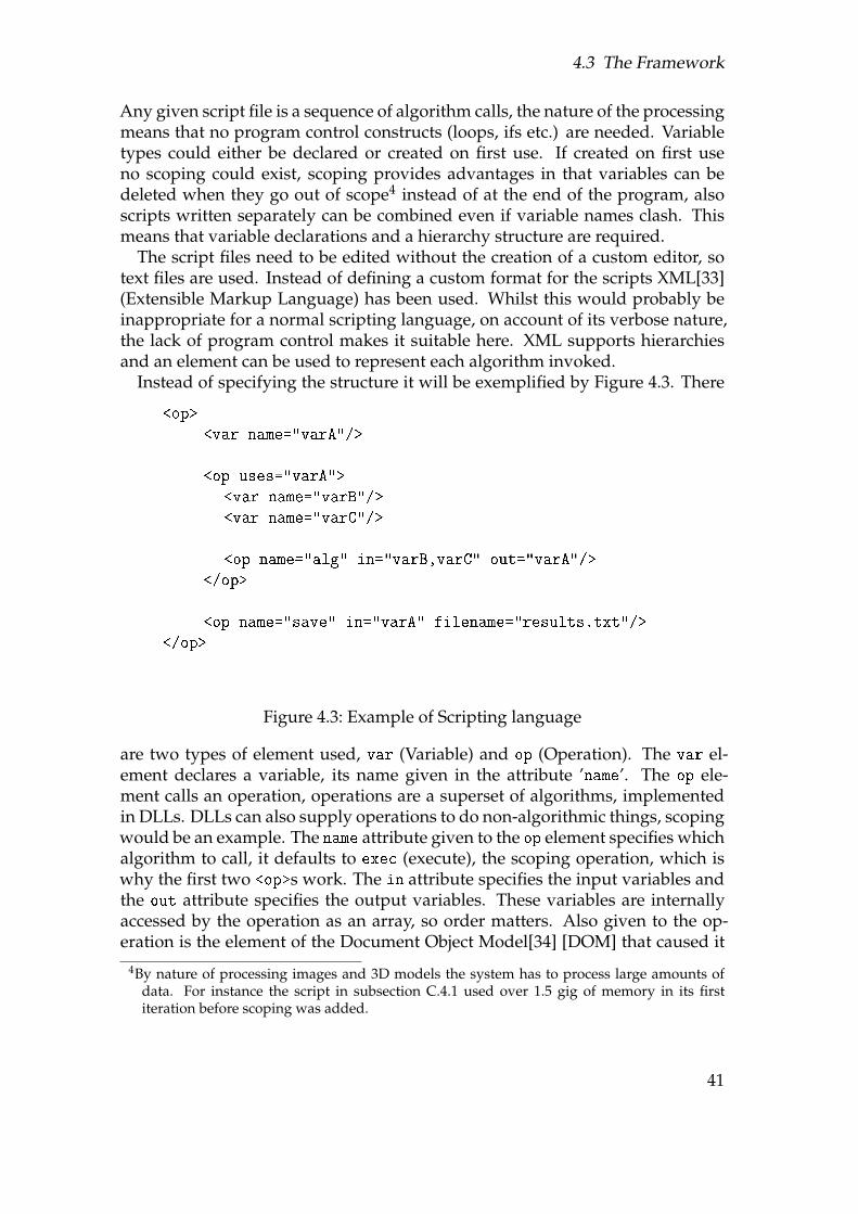
The script files need to be edited without the creation of a custom editor, sotext files are used. Instead of defining a custom format for the scripts XML[33](Extensible Markup Language) has been used. Whilst this would probably beinappropriate for a normal scripting language, on account of its verbose nature,the lack of program control makes it suitable here. XML supports hierarchiesand an element can be used to represent each algorithm invoked.

Instead of specifying the structure it will be exemplified by Figure 4.3. There

<op>

<var name="varA"/>

<op uses="varA">

<var name="varB"/>

<var name="varC"/>

<op name="alg" in="varB,varC" out="varA"/>

</op>

<op name="save" in="varA" filename="results.txt"/>

</op>

Figure 4.3: Example of Scripting language

are two types of element used, var (Variable) and op (Operation). The var el-ement declares a variable, its name given in the attribute ’name’. The op ele-ment calls an operation, operations are a superset of algorithms, implementedin DLLs. DLLs can also supply operations to do non-algorithmic things, scopingwould be an example. The name attribute given to the op element specifies whichalgorithm to call, it defaults to exec (execute), the scoping operation, which iswhy the first two <op>s work. The in attribute specifies the input variables andthe out attribute specifies the output variables. These variables are internallyaccessed by the operation as an array, so order matters. Also given to the op-eration is the element of the Document Object Model[34] [DOM] that caused it

4By nature of processing images and 3D models the system has to process large amounts ofdata. For instance the script in subsection C.4.1 used over 1.5 gig of memory in its firstiteration before scoping was added.

41

4 Design

to be executed. This allows the operation to access any arbitrary parameters inthat element, such at the filename attribute given to the save operation in theexample. With some exceptions operations are named using a hierarchy, start-ing with the module name. For instance, ’math.matrix.mult’ is the name of anoperation in ’math_matrix.dll’, which multiplies two matrices together.

This scripting language was chosen for its simplicity, both to implement andto explain. It was also chosen for its potential expandability, as whilst not re-quired or even desirable operations could be written to implement loops, func-tions etc. All alternatives would be harder to explain and/or implement, exceptin regards to the scripting language. For instance a C style one could be chosen,however XML comes with the associated DOM. This defines the data structuresfor storing XML, so no design needs to be produced for that part of the system.

The final part of the user interface is the resulting program, which runs fromthe command line with a script file, it then loads the script, parses into a DOMand executes the root operation.

4.3.2 Single Variable Type

The SVT has to store many arrangements of data, so it must be structured togeneralise all these possibilities. Structures it will have to store include:

• Images. These are represented as 2D arrays of colours or grey scale values.

• Depth Maps. Images with depth values associated with each pixel.

• Matrices. These are represented as 2D arrays of real values.

• 3D Models. One of many representations is a set of objects including:

– Images, identical to above, used to texture the model.

– Vertices, a 1D array of positions, normals and texture coordinates.

– Triangles, a 1D array of three indices to vertices.

The structure of the first three generalises to a n dimensional array of fields,where fields are integers, reals etc. The 3D model contains several of these com-bined to create its structure. This implies a hierarchy of nodes, where leaf nodescontain n dimensional arrays of specific data items. The SVT has been definedto match this model.

There are two types of node, branch nodes and leaf nodes. The branch nodescontain both branch and leaf nodes and exist to construct a hierarchy. The rootnode of a SVT is always a branch. The leaf nodes are n dimensional arrays offields. There is an enum of field types, each of which has a defined type andtherefore size. Any given element in the array can only have one of each fieldtype. (Multiple are not required.) All this data is exposed by a set of accessors,see section A.4. See section A.6 for a list of variable types expressed using this

42

4.4 The Algorithms

system. Various helper methods and an iterator class are provided, as otherwisethey would be duplicated within many operations. Every node is assigned atype, this has no actual bearing except that each type has a set of requirementsassociated with it, so type checking is not about checking that a SVT containsthe right number of dimensions and fields but that its type is equal to the oneexpected. A hierarchy of types was considered, so you could have a RGB imageas a sub-type of image for instance, but considered too complicated for limitedadvantage.

There are alternate designs, such as

• The fields within each element of the leaf array could be defined on a perelement basis instead of a per leaf basis.

• It could be implemented as a sparse array.

• Fields could be generalised, so arbitrary fields could be inserted into thearrays.

• In addition to the array structure each node could also have a set of prop-erties in ’token=value’ form, to store arbitrary meta-data about the data inthe node.

None of these alternatives confer any real advantage or provide features thatare actually required, the solution proposed is considered the best solution asit is the simplest solution that provides all functionality and pushes no workinto the algorithm implementations. (i.e. the leaf type could simply be a blockof memory, but then each algorithm would have to index that block itself andwould be doing work that should be centralised.)

4.4 The Algorithms

On account of the development process the algorithms have been split into asequence of increments, the first increment is designed to get a bare minimumworking system, all further increments were then designed to improve on it.

4.4.1 Increment 1, Stereo Correspondence

As previously covered in section 3.1 a working system can exist with just depthdetermination, for this reason the first iteration is to implement this. Specifically,stereo correspondence is the method used. This approach has been taken as itbest matches the casual capture requirement, in that all other techniques requirespecialist tools or specific environments to work. Of all the possible solutionsit also has had both the most research and success. As validation is requiredthe iteration also requires enough supporting functionality to get the images

43

4 Design

Stereo Correspondence

Correspondence to 3D model

3D Model

Left Image Right Image

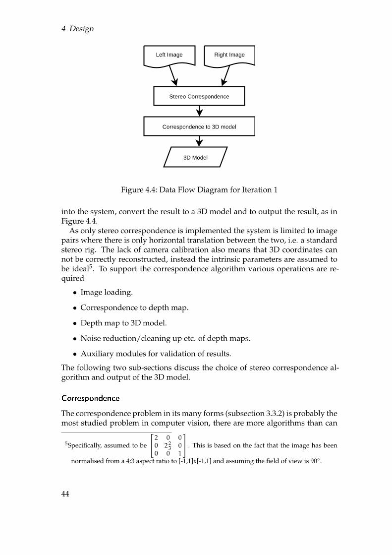
Figure 4.4: Data Flow Diagram for Iteration 1

into the system, convert the result to a 3D model and to output the result, as inFigure 4.4.

As only stereo correspondence is implemented the system is limited to imagepairs where there is only horizontal translation between the two, i.e. a standardstereo rig. The lack of camera calibration also means that 3D coordinates cannot be correctly reconstructed, instead the intrinsic parameters are assumed tobe ideal5. To support the correspondence algorithm various operations are re-quired

• Image loading.

• Correspondence to depth map.

• Depth map to 3D model.

• Noise reduction/cleaning up etc. of depth maps.

• Auxiliary modules for validation of results.

The following two sub-sections discuss the choice of stereo correspondence al-gorithm and output of the 3D model.

Correspondence

The correspondence problem in its many forms (subsection 3.3.2) is probably themost studied problem in computer vision, there are more algorithms than can

5Specifically, assumed to be

2 0 00 2 2

3 00 0 1

. This is based on the fact that the image has been

normalised from a 4:3 aspect ratio to [-1,1]x[-1,1] and assuming the field of view is 90◦.

44

4.4 The Algorithms

be sensibly reviewed. A good start is [35], a league table of stereo algorithmsby accuracy. However, the top algorithms are complicated, and would take toolong to implement. For instance, second place on the list[36] requires an under-standing of four of its references before it can be implemented.

Instead A Maximum Likelihood Stereo Algorithm[37] was used for the followingreasons

• It is used by [5], a working solution, so it should be good enough for thetask in question.

• It is relatively simple, understanding and implementing it within the timeavailable is a reasonable undertaking.

• There are improvements to the base algorithm[38, 39, 5], so it can be im-proved to the standard required.

The base variant of this algorithm uses dynamic programming on maximumlikelihood derived costs of either matching features or marking them as oc-cluded. It assumes monotonic ordering6. The base algorithm uses the luminancevalue of individual pixels as its features. Many variations of this algorithmwere implemented, see section B.8, and extensive testing was done, see subsec-tion 5.1.2.

Model Output

Once a 3D model is produced it needs to be viewed. There are two ways to viewa model, either save it in a standard file format and open it in an external vieweror develop a viewer specifically for the task. Initially the first of these optionswas presumed to require the least amount of work, however an investigationof free model viewers showed a limited set of supported file formats, and ofthese formats documentation on them was limited. Of the formats that couldbe implemented several could not store the required data, the remaining fewwould of taken considerable time to get working. It was therefore decided thatimplementing a viewer would be easier, as OpenGL7 is a known quantity.

The viewer was designed to be both simple and quick to implement. It is im-plemented as an operation, which is given the 3D model SVT defined in A.6.2,it then shows a window with the model in and pauses execution of the scripttill the window is closed. Browsing the model consists of dollying around a cen-tre point in the scene by dragging with the LMB, panning when using the RMBand zooming with the mouse wheel. The centre point can be altered using thekeyboard. This is a clone of the interface design common among 3D programs8

6∀i, j, u, v • matched(xi, yj) ∧ u > 0 ∧ v > 0 ⇒ ¬matched(xi+u, yj−v) where xi is an indexedpixel in one image and yj is an indexed pixel in the other.

7tm, http://opengl.org8Such as Blender (http://www.blender3d.org) or Maya (http://www.alias.com).

45

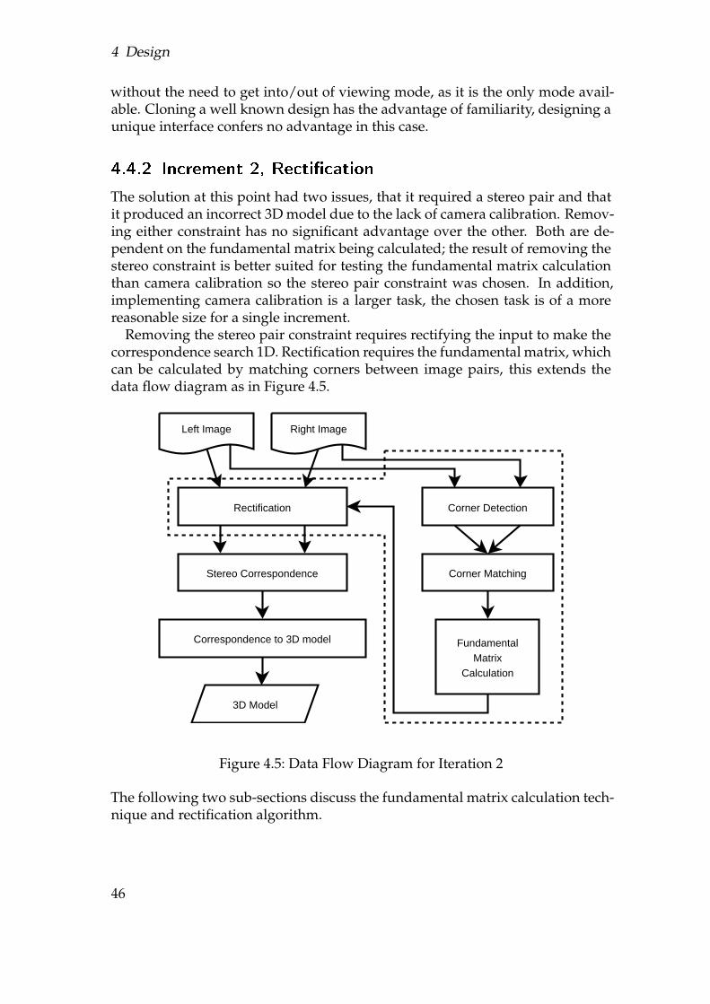
4 Design

without the need to get into/out of viewing mode, as it is the only mode avail-able. Cloning a well known design has the advantage of familiarity, designing aunique interface confers no advantage in this case.

4.4.2 Increment 2, Recti�cation

The solution at this point had two issues, that it required a stereo pair and thatit produced an incorrect 3D model due to the lack of camera calibration. Remov-ing either constraint has no significant advantage over the other. Both are de-pendent on the fundamental matrix being calculated; the result of removing thestereo constraint is better suited for testing the fundamental matrix calculationthan camera calibration so the stereo pair constraint was chosen. In addition,implementing camera calibration is a larger task, the chosen task is of a morereasonable size for a single increment.

Removing the stereo pair constraint requires rectifying the input to make thecorrespondence search 1D. Rectification requires the fundamental matrix, whichcan be calculated by matching corners between image pairs, this extends thedata flow diagram as in Figure 4.5.

Stereo Correspondence

Correspondence to 3D model

3D Model

Left Image Right Image

Rectification Corner Detection

Corner Matching

FundamentalMatrix

Calculation

Figure 4.5: Data Flow Diagram for Iteration 2

The following two sub-sections discuss the fundamental matrix calculation tech-nique and rectification algorithm.

46

4.4 The Algorithms

Fundamental Matrix Calculation

Given a set of constraints between the two images the fundamental matrix canbe calculated, these constraints are usually in the form of matches between cor-ners so Equation 2.23 can be used. Corners have to first be found, the Harriscorner detector (See 2.2.1) is used for this purpose. The Harris detector hasbeen chosen as it produces the lowest rate of errors according to [40]. Match-ing corners is then done using NCC. More advanced methods that are capableof handling large disparities between images exist (i.e. [27]), however the restof the system will not become robust enough to manage such scenes in the timeavailable so there is little point in implementing anything more advanced.

The matching process just mentioned produces a sparse set of correspondencesbetween two images. This set contains errors however, so SVD can not be di-rectly used to calculate the fundamental matrix from them, instead a methodknown as RANSAC is used. Random Sample Consensus[41] [RANSAC] workson any model fitting problem where a large number of outliers are present. Itrepeatedly selects a random subset of the samples from which it constructs themodel, it then checks how many other samples fit the model selected, these arethat models inliers. After doing this many times the correct model is consideredto be the one which obtained the most inliers. For our purposes this means

• Repeat until the probability of having the correct solution is high enough.

– Select 8 matches randomly.

– Calculate the fundamental matrix using those 8 matches.

– Iterate all matches and count how many of them fit the epipolar geom-etry specified by the fundamental matrix. This is done by checkingthat the distance from the epipolar line calculated from one point iswithin a threshold of the other point of a proposed match.

• Use SVD on all the inliers selected by the iteration that got the most inliersand calculate the final fundamental matrix.

Recti�cation

Three rectification algorithms were examined, one representative of the tradi-tional solution[42] and two more recent solutions[43, 26]. Pollefeys[26] pointsout that traditional solutions fail under forward motion, (When the epipole is inthe image.) and whilst there is little between Polar Rectification[26] and Cylin-drical Rectification[43] Pollefeys claims his is easier to implement. ThereforePollefeys algorithm was chosen.

47

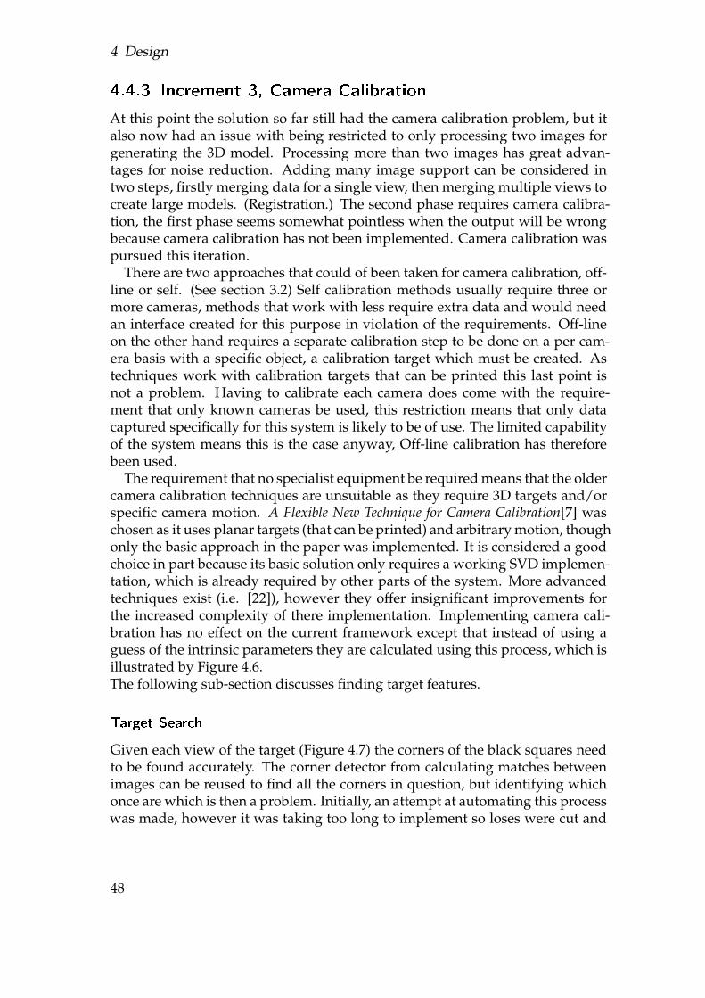
4 Design

4.4.3 Increment 3, Camera Calibration

At this point the solution so far still had the camera calibration problem, but italso now had an issue with being restricted to only processing two images forgenerating the 3D model. Processing more than two images has great advan-tages for noise reduction. Adding many image support can be considered intwo steps, firstly merging data for a single view, then merging multiple views tocreate large models. (Registration.) The second phase requires camera calibra-tion, the first phase seems somewhat pointless when the output will be wrongbecause camera calibration has not been implemented. Camera calibration waspursued this iteration.

There are two approaches that could of been taken for camera calibration, off-line or self. (See section 3.2) Self calibration methods usually require three ormore cameras, methods that work with less require extra data and would needan interface created for this purpose in violation of the requirements. Off-lineon the other hand requires a separate calibration step to be done on a per cam-era basis with a specific object, a calibration target which must be created. Astechniques work with calibration targets that can be printed this last point isnot a problem. Having to calibrate each camera does come with the require-ment that only known cameras be used, this restriction means that only datacaptured specifically for this system is likely to be of use. The limited capabilityof the system means this is the case anyway, Off-line calibration has thereforebeen used.

The requirement that no specialist equipment be required means that the oldercamera calibration techniques are unsuitable as they require 3D targets and/orspecific camera motion. A Flexible New Technique for Camera Calibration[7] waschosen as it uses planar targets (that can be printed) and arbitrary motion, thoughonly the basic approach in the paper was implemented. It is considered a goodchoice in part because its basic solution only requires a working SVD implemen-tation, which is already required by other parts of the system. More advancedtechniques exist (i.e. [22]), however they offer insignificant improvements forthe increased complexity of there implementation. Implementing camera cali-bration has no effect on the current framework except that instead of using aguess of the intrinsic parameters they are calculated using this process, which isillustrated by Figure 4.6.The following sub-section discusses finding target features.

Target Search

Given each view of the target (Figure 4.7) the corners of the black squares needto be found accurately. The corner detector from calculating matches betweenimages can be reused to find all the corners in question, but identifying whichonce are which is then a problem. Initially, an attempt at automating this processwas made, however it was taking too long to implement so loses were cut and

48

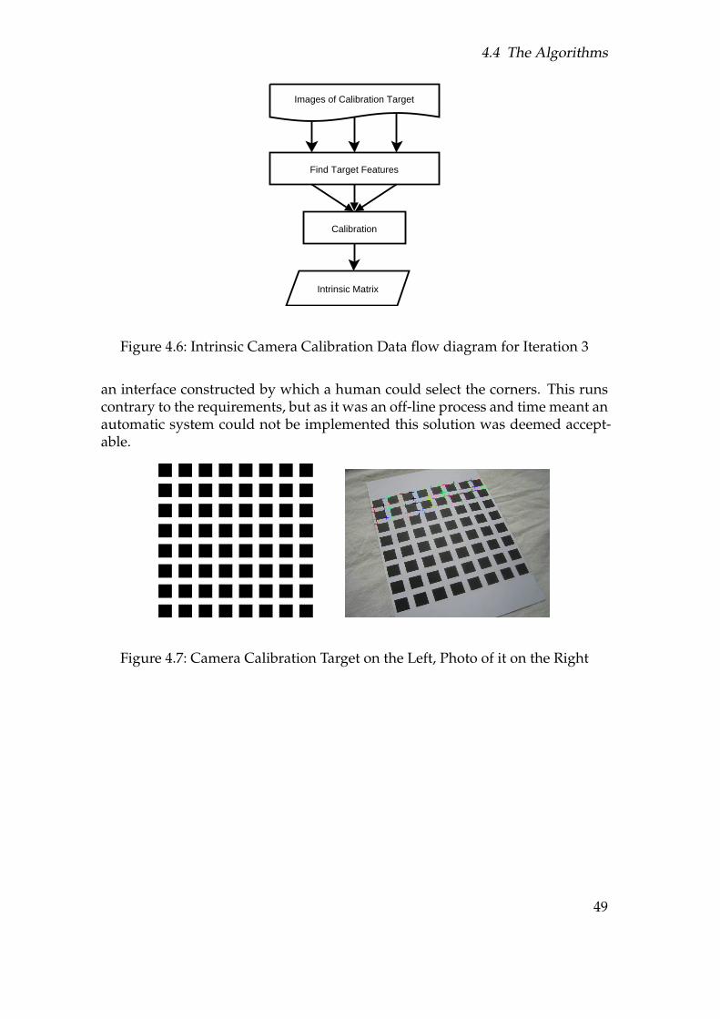
4.4 The Algorithms

Images of Calibration Target

Find Target Features

Intrinsic Matrix

Calibration

Figure 4.6: Intrinsic Camera Calibration Data flow diagram for Iteration 3

an interface constructed by which a human could select the corners. This runscontrary to the requirements, but as it was an off-line process and time meant anautomatic system could not be implemented this solution was deemed accept-able.

Figure 4.7: Camera Calibration Target on the Left, Photo of it on the Right

49

4 Design

50

5 System Evaluation

This chapter has been divided into two, the first section focuses on validatingthat the implementation is correct at each stage, the second focuses on determin-ing the limits of the system as an assessment of how it handles the requirements.

5.1 Validation

This section contains a sub-section for validating each step of the implementa-tion, in line with the design process.

5.1.1 Framework

Minimal testing was done of the framework on the grounds that it was goingto be tested every time it was run for the rest of development. The frameworkloads an XML file into a DOM and then runs the operations specified by theDOM; these two steps were tested separately. XML parsing was tested with aseries of XML files known to be either correct or not, see section C.1. All correctfiles parsed correctly, all bad files showed error messages, except for test 3 whichignored the erroneous data and test 9 which ignored the second root node. Theseproblems were ignored as they are not major. Note that this test only covers afew errors and is by no means thorough.

To test that the framework could load modules and execute operations withinthem modules were needed, so var.dll and image_io.dll were implemented,see sections B.2 and B.3 respectively for details. A variety of scripts were thenrun, see section C.2. The tests have the following purposes:

• 1: Runs both of the built in operations, testing that operations in generalwork and both the operations in question work.

• 2: Declares a variable to test SVTs and uses external algorithms to testmodule loading. Consequently tests image loading and saving.

• 3: Tests scope.

• 4: Tests variable saving and loading.

All tests produce there expected results, which also shows that the modules inquestion work.

51

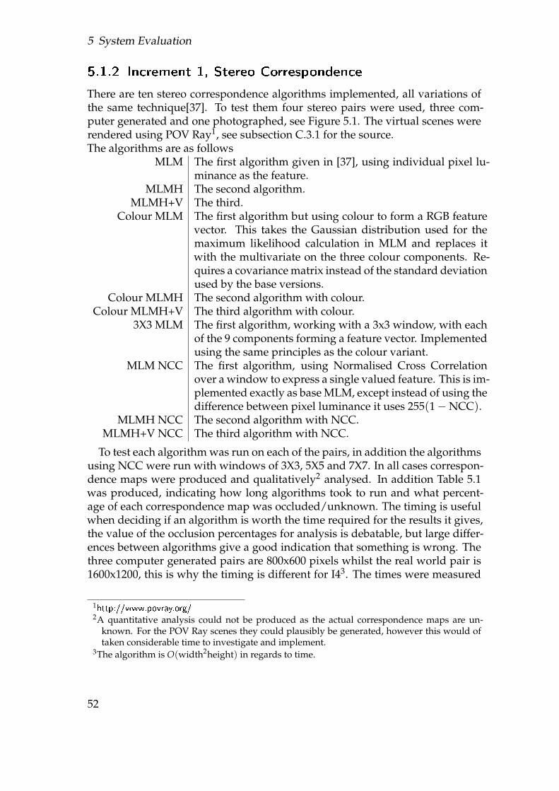
5 System Evaluation

5.1.2 Increment 1, Stereo Correspondence

There are ten stereo correspondence algorithms implemented, all variations ofthe same technique[37]. To test them four stereo pairs were used, three com-puter generated and one photographed, see Figure 5.1. The virtual scenes wererendered using POV Ray1, see subsection C.3.1 for the source.The algorithms are as follows

MLM The first algorithm given in [37], using individual pixel lu-minance as the feature.

MLMH The second algorithm.MLMH+V The third.

Colour MLM The first algorithm but using colour to form a RGB featurevector. This takes the Gaussian distribution used for themaximum likelihood calculation in MLM and replaces itwith the multivariate on the three colour components. Re-quires a covariance matrix instead of the standard deviationused by the base versions.

Colour MLMH The second algorithm with colour.Colour MLMH+V The third algorithm with colour.

3X3 MLM The first algorithm, working with a 3x3 window, with eachof the 9 components forming a feature vector. Implementedusing the same principles as the colour variant.

MLM NCC The first algorithm, using Normalised Cross Correlationover a window to express a single valued feature. This is im-plemented exactly as base MLM, except instead of using thedifference between pixel luminance it uses 255(1−NCC).

MLMH NCC The second algorithm with NCC.MLMH+V NCC The third algorithm with NCC.

To test each algorithm was run on each of the pairs, in addition the algorithmsusing NCC were run with windows of 3X3, 5X5 and 7X7. In all cases correspon-dence maps were produced and qualitatively2 analysed. In addition Table 5.1was produced, indicating how long algorithms took to run and what percent-age of each correspondence map was occluded/unknown. The timing is usefulwhen deciding if an algorithm is worth the time required for the results it gives,the value of the occlusion percentages for analysis is debatable, but large differ-ences between algorithms give a good indication that something is wrong. Thethree computer generated pairs are 800x600 pixels whilst the real world pair is1600x1200, this is why the timing is different for I43. The times were measured

1http://www.povray.org/2A quantitative analysis could not be produced as the actual correspondence maps are un-

known. For the POV Ray scenes they could plausibly be generated, however this would oftaken considerable time to investigate and implement.

3The algorithm is O(width2height) in regards to time.

52

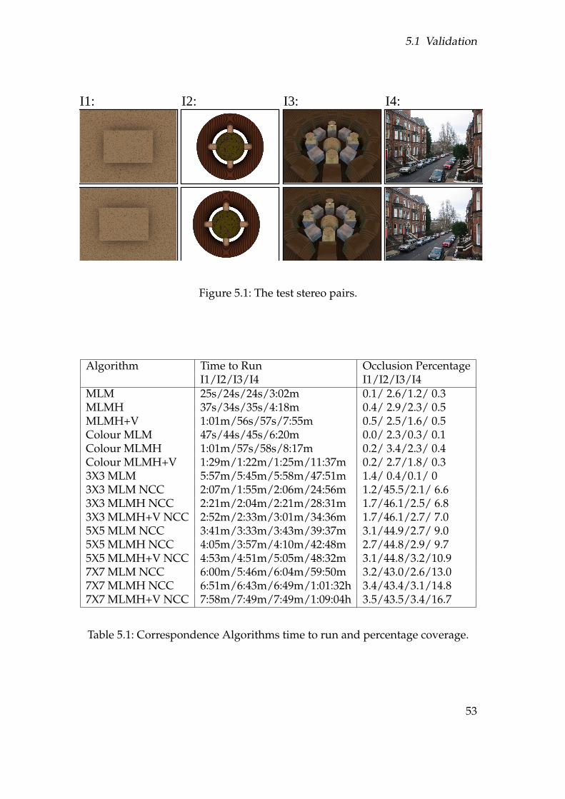
5.1 Validation

I1: I2: I3: I4:

Figure 5.1: The test stereo pairs.

Algorithm Time to Run Occlusion PercentageI1/I2/I3/I4 I1/I2/I3/I4

MLM 25s/24s/24s/3:02m 0.1/ 2.6/1.2/ 0.3MLMH 37s/34s/35s/4:18m 0.4/ 2.9/2.3/ 0.5MLMH+V 1:01m/56s/57s/7:55m 0.5/ 2.5/1.6/ 0.5Colour MLM 47s/44s/45s/6:20m 0.0/ 2.3/0.3/ 0.1Colour MLMH 1:01m/57s/58s/8:17m 0.2/ 3.4/2.3/ 0.4Colour MLMH+V 1:29m/1:22m/1:25m/11:37m 0.2/ 2.7/1.8/ 0.33X3 MLM 5:57m/5:45m/5:58m/47:51m 1.4/ 0.4/0.1/ 03X3 MLM NCC 2:07m/1:55m/2:06m/24:56m 1.2/45.5/2.1/ 6.63X3 MLMH NCC 2:21m/2:04m/2:21m/28:31m 1.7/46.1/2.5/ 6.83X3 MLMH+V NCC 2:52m/2:33m/3:01m/34:36m 1.7/46.1/2.7/ 7.05X5 MLM NCC 3:41m/3:33m/3:43m/39:37m 3.1/44.9/2.7/ 9.05X5 MLMH NCC 4:05m/3:57m/4:10m/42:48m 2.7/44.8/2.9/ 9.75X5 MLMH+V NCC 4:53m/4:51m/5:05m/48:32m 3.1/44.8/3.2/10.97X7 MLM NCC 6:00m/5:46m/6:04m/59:50m 3.2/43.0/2.6/13.07X7 MLMH NCC 6:51m/6:43m/6:49m/1:01:32h 3.4/43.4/3.1/14.87X7 MLMH+V NCC 7:58m/7:49m/7:49m/1:09:04h 3.5/43.5/3.4/16.7

Table 5.1: Correspondence Algorithms time to run and percentage coverage.

53

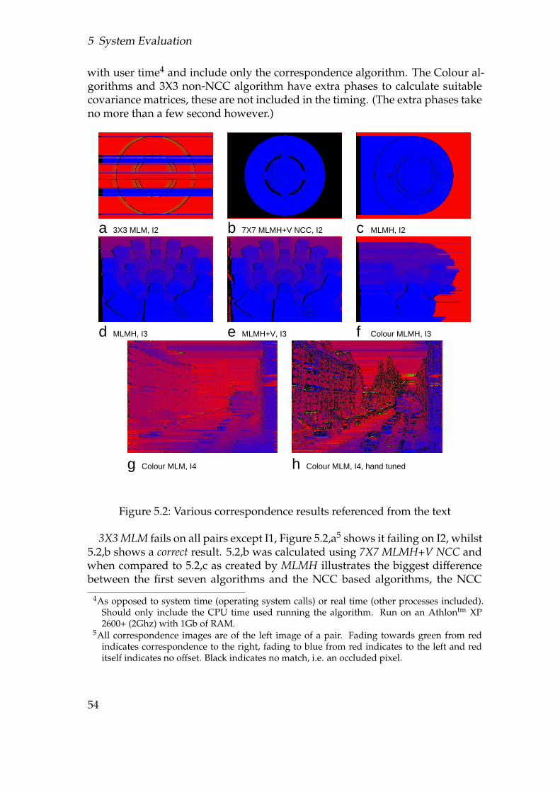
5 System Evaluation

with user time4 and include only the correspondence algorithm. The Colour al-gorithms and 3X3 non-NCC algorithm have extra phases to calculate suitablecovariance matrices, these are not included in the timing. (The extra phases takeno more than a few second however.)

cba

fed

hg

3X3 MLM, I2 7X7 MLMH+V NCC, I2 MLMH, I2

MLMH, I3 MLMH+V, I3 Colour MLMH, I3

Colour MLM, I4 Colour MLM, I4, hand tuned

Figure 5.2: Various correspondence results referenced from the text

3X3 MLM fails on all pairs except I1, Figure 5.2,a5 shows it failing on I2, whilst5.2,b shows a correct result. 5.2,b was calculated using 7X7 MLMH+V NCC andwhen compared to 5.2,c as created by MLMH illustrates the biggest differencebetween the first seven algorithms and the NCC based algorithms, the NCC

4As opposed to system time (operating system calls) or real time (other processes included).Should only include the CPU time used running the algorithm. Run on an Athlontm XP2600+ (2Ghz) with 1Gb of RAM.

5All correspondence images are of the left image of a pair. Fading towards green from redindicates correspondence to the right, fading to blue from red indicates to the left and reditself indicates no offset. Black indicates no match, i.e. an occluded pixel.

54

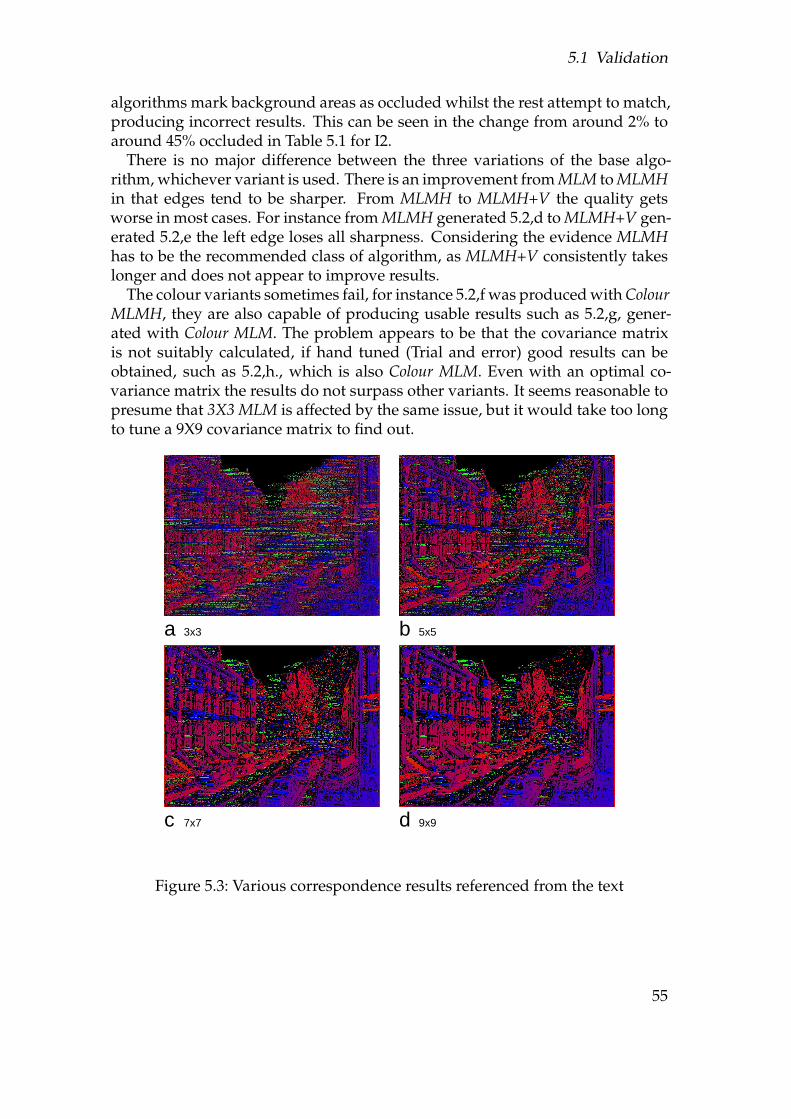
5.1 Validation

algorithms mark background areas as occluded whilst the rest attempt to match,producing incorrect results. This can be seen in the change from around 2% toaround 45% occluded in Table 5.1 for I2.

There is no major difference between the three variations of the base algo-rithm, whichever variant is used. There is an improvement from MLM to MLMHin that edges tend to be sharper. From MLMH to MLMH+V the quality getsworse in most cases. For instance from MLMH generated 5.2,d to MLMH+V gen-erated 5.2,e the left edge loses all sharpness. Considering the evidence MLMHhas to be the recommended class of algorithm, as MLMH+V consistently takeslonger and does not appear to improve results.

The colour variants sometimes fail, for instance 5.2,f was produced with ColourMLMH, they are also capable of producing usable results such as 5.2,g, gener-ated with Colour MLM. The problem appears to be that the covariance matrixis not suitably calculated, if hand tuned (Trial and error) good results can beobtained, such as 5.2,h., which is also Colour MLM. Even with an optimal co-variance matrix the results do not surpass other variants. It seems reasonable topresume that 3X3 MLM is affected by the same issue, but it would take too longto tune a 9X9 covariance matrix to find out.

c

ba

d

3x3 5x5

7x7 9x9

Figure 5.3: Various correspondence results referenced from the text

55

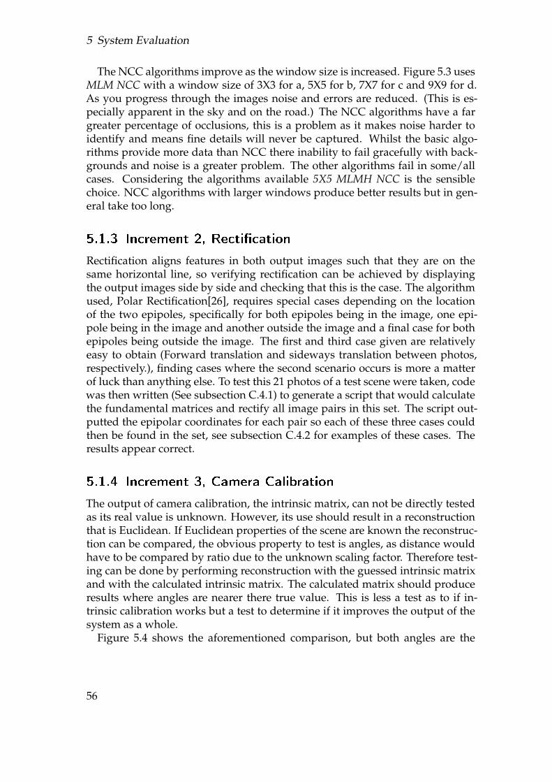
5 System Evaluation

The NCC algorithms improve as the window size is increased. Figure 5.3 usesMLM NCC with a window size of 3X3 for a, 5X5 for b, 7X7 for c and 9X9 for d.As you progress through the images noise and errors are reduced. (This is es-pecially apparent in the sky and on the road.) The NCC algorithms have a fargreater percentage of occlusions, this is a problem as it makes noise harder toidentify and means fine details will never be captured. Whilst the basic algo-rithms provide more data than NCC there inability to fail gracefully with back-grounds and noise is a greater problem. The other algorithms fail in some/allcases. Considering the algorithms available 5X5 MLMH NCC is the sensiblechoice. NCC algorithms with larger windows produce better results but in gen-eral take too long.

5.1.3 Increment 2, Recti�cation

Rectification aligns features in both output images such that they are on thesame horizontal line, so verifying rectification can be achieved by displayingthe output images side by side and checking that this is the case. The algorithmused, Polar Rectification[26], requires special cases depending on the locationof the two epipoles, specifically for both epipoles being in the image, one epi-pole being in the image and another outside the image and a final case for bothepipoles being outside the image. The first and third case given are relativelyeasy to obtain (Forward translation and sideways translation between photos,respectively.), finding cases where the second scenario occurs is more a matterof luck than anything else. To test this 21 photos of a test scene were taken, codewas then written (See subsection C.4.1) to generate a script that would calculatethe fundamental matrices and rectify all image pairs in this set. The script out-putted the epipolar coordinates for each pair so each of these three cases couldthen be found in the set, see subsection C.4.2 for examples of these cases. Theresults appear correct.

5.1.4 Increment 3, Camera Calibration

The output of camera calibration, the intrinsic matrix, can not be directly testedas its real value is unknown. However, its use should result in a reconstructionthat is Euclidean. If Euclidean properties of the scene are known the reconstruc-tion can be compared, the obvious property to test is angles, as distance wouldhave to be compared by ratio due to the unknown scaling factor. Therefore test-ing can be done by performing reconstruction with the guessed intrinsic matrixand with the calculated intrinsic matrix. The calculated matrix should produceresults where angles are nearer there true value. This is less a test as to if in-trinsic calibration works but a test to determine if it improves the output of thesystem as a whole.

Figure 5.4 shows the aforementioned comparison, but both angles are the

56

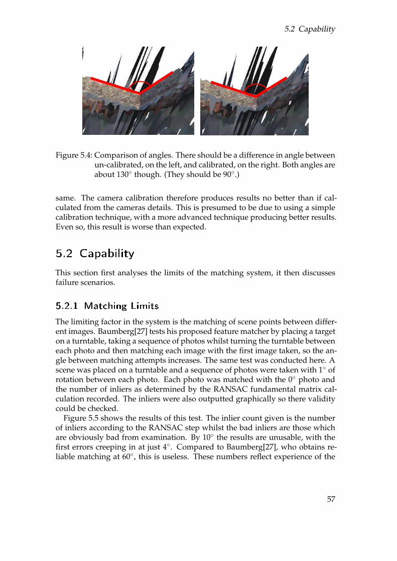
5.2 Capability

Figure 5.4: Comparison of angles. There should be a difference in angle betweenun-calibrated, on the left, and calibrated, on the right. Both angles areabout 130◦ though. (They should be 90◦.)

same. The camera calibration therefore produces results no better than if cal-culated from the cameras details. This is presumed to be due to using a simplecalibration technique, with a more advanced technique producing better results.Even so, this result is worse than expected.

5.2 Capability

This section first analyses the limits of the matching system, it then discussesfailure scenarios.

5.2.1 Matching Limits

The limiting factor in the system is the matching of scene points between differ-ent images. Baumberg[27] tests his proposed feature matcher by placing a targeton a turntable, taking a sequence of photos whilst turning the turntable betweeneach photo and then matching each image with the first image taken, so the an-gle between matching attempts increases. The same test was conducted here. Ascene was placed on a turntable and a sequence of photos were taken with 1◦ ofrotation between each photo. Each photo was matched with the 0◦ photo andthe number of inliers as determined by the RANSAC fundamental matrix cal-culation recorded. The inliers were also outputted graphically so there validitycould be checked.

Figure 5.5 shows the results of this test. The inlier count given is the numberof inliers according to the RANSAC step whilst the bad inliers are those whichare obviously bad from examination. By 10◦ the results are unusable, with thefirst errors creeping in at just 4◦. Compared to Baumberg[27], who obtains re-liable matching at 60◦, this is useless. These numbers reflect experience of the

57

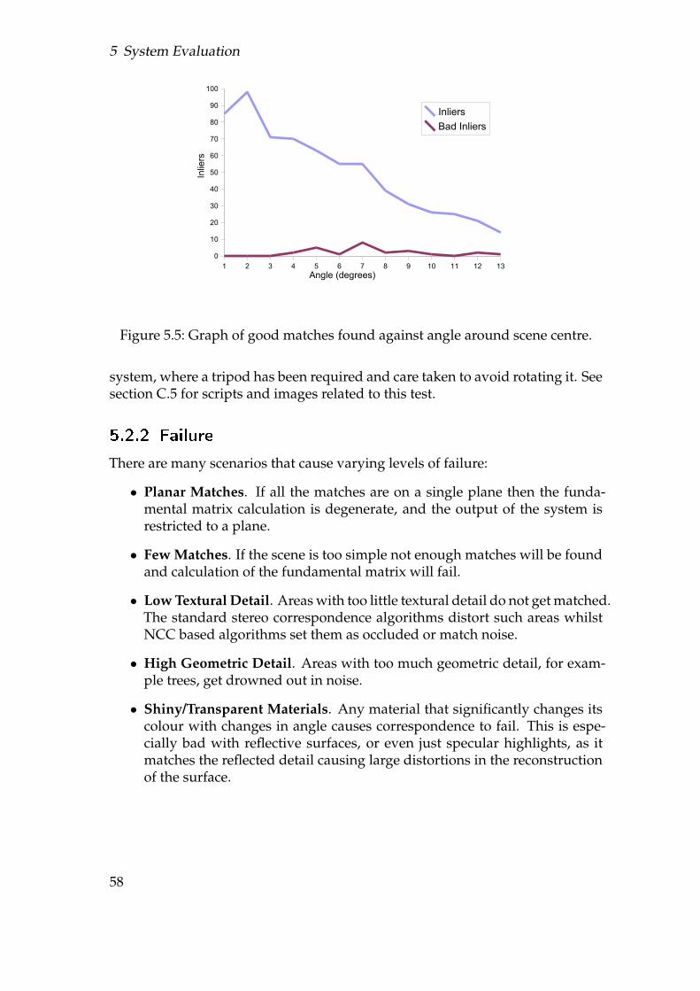
5 System Evaluation

1 2 3 4 5 6 7 8 9 10 11 12 130

10

20

30

40

50

60

70

80

90

100

InliersBad Inliers

Angle (degrees)

Inlie

rs

Figure 5.5: Graph of good matches found against angle around scene centre.

system, where a tripod has been required and care taken to avoid rotating it. Seesection C.5 for scripts and images related to this test.

5.2.2 Failure

There are many scenarios that cause varying levels of failure:

• Planar Matches. If all the matches are on a single plane then the funda-mental matrix calculation is degenerate, and the output of the system isrestricted to a plane.

• Few Matches. If the scene is too simple not enough matches will be foundand calculation of the fundamental matrix will fail.

• Low Textural Detail. Areas with too little textural detail do not get matched.The standard stereo correspondence algorithms distort such areas whilstNCC based algorithms set them as occluded or match noise.

• High Geometric Detail. Areas with too much geometric detail, for exam-ple trees, get drowned out in noise.

• Shiny/Transparent Materials. Any material that significantly changes itscolour with changes in angle causes correspondence to fail. This is espe-cially bad with reflective surfaces, or even just specular highlights, as itmatches the reflected detail causing large distortions in the reconstructionof the surface.

58

6 Conclusion

This section is divided into two, a critical review of what has been achieved andthen a review of what could be obtained with further work, specifically with aneye to resolving the issues raised by the critical review.

6.1 Review

The system implemented follows Figure 4.5, each step has been verified to workindividually and all the steps work as a group to successfully produced 3D mod-els based on photographs. However, the scenes for which it will do this are lim-ited and the quality of the output is poor. Figure 6.1 is the best output obtained,it has no real-world use due to the noise, failure to handle shiny objects andthe limited range that can be obtained with only two photographs. Whilst notevident in the figure it also suffers from a projective distortion as the intrinsicmatrix is not perfect (The virtual angle between the two walls of the house isabout 130◦.) and the walls suffer from noise close up. The following is a sum-mary of problems observed throughout the results (with no consideration as toif the problems given can be solved)

• Noise. The noise produced by correspondence makes the models unus-able. A heavy averaging filter has to be applied to reduce it to the levelsseen in Figure 6.1, so all small details are lost.

• Pairs Only. The system will only take two images as input, this restrictsthe output range to that which is visible in both images. It also providesonly one sample of each points position when multiple would assist noisereduction.

• Poor Matching. The matching algorithm is incapable of handling any realchange in the angle between photos and can not manage much translationeither. It is directly responsible for most failures due to it only matchingcorners on a single plane or making too many mistakes. This limits cap-turing to scenes with plenty of matchable objects, which generally meansinorganic with lots of texturing information. The photos also have to betaken from almost the same angle, which can be hard to do without a tri-pod.

• Shiny and Transparent Surfaces. Surfaces that do not look roughly thesame from every angle fail to match, causing dramatic distortions such as

59

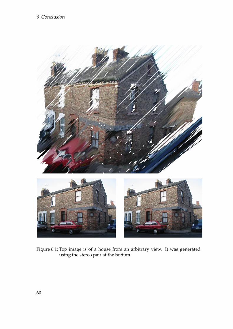
6 Conclusion

Figure 6.1: Top image is of a house from an arbitrary view. It was generatedusing the stereo pair at the bottom.

60

6.2 Further Work

the cars and windows in Figure 6.1. In addition, untextured surfaces tendto be distorted as there is nothing to match.

• Distortion. The intrinsic camera calibration is not very accurate, and thelack of compensation for barrel distortion does not help either. This resultsin a reconstruction that is wrong by a projective transformation, so anglesand lengths are meaningless.

• Materials. Currently the photo is simply projected onto the model, noeffort is made to merge multiple photos or calculate material properties.Renderings are therefore incorrectly coloured.

• Movement. The scene must remain static between photos.

Whilst the capability of the solution is limited the framework has proved tobe a versatile tool, supporting modular development, fast experimentation andextensive testing.

6.2 Further Work

There are several improvements that can be made to the system by simply swap-ping out current algorithms and using better once:

• Better matching. The limiting factor of the current solution is matching,therefore the first piece of further work is to improve this part of the sys-tem. An algorithm such as [27] would be suggested as it can express thesame interface as the current matching algorithm and be swapped in withno effort beyond implementation. It claims to work with angles of sepa-ration between photos of 60◦ plus, with such flexibility multiple imagesbecomes a sensible proposition.

• Multiple images. Support for multiple images comes in two phases. Thefirst is to merge multiple correspondence maps between one view and sev-eral others to generate a single depth map. This should reduce noise tomanageable levels as multiple samples will now exist for each point anda higher percentage of the image should be matched. The second step isto add registration, to combine multiple depth maps into 3D models thatcover an area larger than any one photograph. With these two improve-ments the first three issues listed in section 6.1 should be resolved.

• Correct Calibration. Improvements can be made to the intrinsic cameracalibration to reduce distortion, the obvious approach would be to imple-ment the more advanced methods from the paper used[7]. Whilst thiswould improve the results off-line calibration does not sit well with an au-tomated system. Once three or more images become involved self-calibration

61

6 Conclusion

using a technique such as the Kruppa equations[8] becomes an option andwould remove the off-line calibration step altogether. This should not onlybe more convenient but it should produce better results1.

• Improved Correspondence. The current stereo correspondence algorithmsare slow and unreliable, they were chosen primarily due to time constraints.Implementing a better one, such as any from [35], would improve the sys-tem. A faster one would also be recommended, as with multiple imagesbeing matched 42 minutes per pair becomes unreasonable.

• Automated Pairing. The current system requires the user to indicate whichpairs of images should be matched. Automating this is possible[44].

• Materials. The system has focused on producing the correct shape, not onthe correct material for that shape. There are many approaches that can betaken, as discussed in section 3.5. The result of using any should be a morerealistic and more convincing rendering.

• Compression. The framework currently saves SVTs to disk without anycompression, this results in enormous files2. Compressing them wouldsave considerable disk space, especially as the above improvements wouldrequire the system to handle more data than at present.

Once the current system is both reliable enough and flexible enough in regardsto its current functionality further improvements can be considered:

• Managing Motion. Whilst the problem of solving with motion betweencaptured photos of a scene is ill-posed there is the possibility of domain-specific solutions. A possible approach is to know which objects will causeproblems, find them, and remove them. For instance, if attempting tocapture a town centre finding and removing people from the images be-fore calculating correspondence. This would necessitate correspondencealgorithms that can manage such gaps. If the objects are to be kept thenmatching a known 3D model to the images then using that model insteadof calculating from the data can be done. There is then the possibility ofusing the outlines of shadows generated by these known objects to assistwith determining geometry.

• Inverse Lighting. If material data is suitably captured then determiningthe positions of light sources should be theoretically possible. This canpotentially lead to correctly integrating foreign 3D models into the data.

1This is because the intrinsic matrix changes as the camera adjusts to the scene in front of it.(See section 2.5) The calibration target will probably be shot up close to fill the shot whilstreal scenes will be shot at a distance, so whilst the intrinsic matrix is likely to be consistentwithin these two sets its unlikely to remain the same between them.

2The directory containing all the testing data has over 5 gigabytes in it.

62

6.2 Further Work

• Instancing. Once a 3D model has been obtained you will typically wantto create arbitrary renderings of it. Finding and instancing duplicate ob-jects, materials and textures would improve the response of a real-timerenderer. The details that make each object unique could then be option-ally rendered depending on resources available, or removed to save space.Each instanced thing would then have multiple instances, combining theseinstances could improve the quality of the generic thing.

• Object Replacement. Detecting and replacing known objects with para-metrised representations could be done. (Similar to above.) Such para-metrised objects might include extra details, details that do not actuallyexist, animations, interactivity or other features to improve a virtual repre-sentation. This could potentially cover non-solid continuous objects, suchas water.

• Safe Viewing. Most models of real world data will have gaps. Lettingusers see the gaps in the model would be unacceptable; a means of calcu-lating the safe areas for a user to be in would be required. In addition thiswould provide a diagnostic, for finding gaps in the model so data can becaptured to fill them. This could also cover detail, so the user can not gettoo close to low detail objects. The automatic generation of a sky sphere3

to fill in the background would be required for completeness.

• Simplification. Once a 3D model is produced simplification will be re-quired in most cases, especially for real-time rendering purposes. Whilstsimplifying 3D models is a well understood area the metrics used are gen-eral, for a navigable virtual environment different metrics might be opti-mal. For instance, if an aviator is to collide with the model then removingcertain smaller concave shapes would be advantageous to avoid the avia-tor getting stuck in/on them.

• Non-visual Material Properties. In addition to detecting the visual prop-erties of materials other properties exist that could be determined usingpattern recognition. For instance, detecting that a surface is wood allowsfor a realistic footstep sound when walking on it within a virtual environ-ment. Such information could also assist in deciding which objects shouldbe solid to the aviator, so the floor should be solid but bushes are usuallynot, as you can get stuck on there irregular shape.

3A rendering of objects at a distance where perspective is no longer an issue, rendered as anunmoving sphere around the user.

63

6 Conclusion

Beyond the improvements mentioned so far if rewrites of large parts of thesystem were an option then the following could be considered:

• Interface. The current system is suitable only for people who can use XMLand have an understanding of how the system works. Putting an interfaceon top of such a system could open it to a larger number of users. Thiscould be done by adding extra hooks into the framework to keep the inter-face as a separate module.

• Human Interaction. As stated in subsection 3.7.1 this would be advanta-geous to correct the mistakes of the algorithms.

• Distributed Computing. In addition to swapping in faster algorithmsbringing more CPU cycles to task would be advantageous. By changingthe framework appropriately but maintaining the interface this could bedone without rewriting any of the algorithms.

64

Bibliography

[1] Direct dimensions (company). http://www.directdimensions.com/prod_scan.htm. Last accessed: 13th October 2004.

[2] Eyetronics. Shapesnatcher (product). http://www.eyetronics.com/products/shapesnatcher.php. Last accessed: 13th October 2004.

[3] 3D Scanners. Modelmaker (product). http://www.3dscanners.com/. Lastaccessed: 13th October 2004.

[4] Direct Dimensions. Direct dimensions 2004 product catalog. http://www.directdimensions.com/pdfs/ProductCat_W2004.pdf. Last accessed: 13th Octo-ber 2004.

[5] Marc Pollefeys. Visual 3d modeling from images. http://www.cs.unc.edu/%7Emarc/tutorial.pdf. Last accessed: 13th October 2004.

[6] Richard Szeliski Yanghai Tsin, Sing Bing Kang. Stereo matching with re-flections and translucency. IEEE Conference on Computer Vision & PatternRecognition, pages 702–709, 2003.

[7] Zhengyou Zhang. A flexible new technique for camera calibration. http://research.microsoft.com/~zhang/Papers/TR98-71.pdf (Last Accessed: 2nd Feb-ruary 2005).

[8] Q.-T. Luong O.D. Faugeras and S.J. Maybank. Camera self-calibration: The-ory and experiments. Lecture Notes in Computer Science, Vol. 558; EuropeanConference on Computer Vision, pages 321–334, 1992.

[9] A high resolution 3d surface construction algorithm. http://www.cs.technion.ac.il/~u_shani/cs236807-S2/lectures-students/Marching%20Cubes.pdf. Last accessed: 13th February 2005.

[10] Chris Harris & Mike Stephens. A combined corner and edge detector. Pro-ceedings of The Fourth Alvey Vision Conference, pages 147–151, 1988. http://www.csse.uwa.edu.au/~pk/Research/MatlabFns/Spatial/Docs/Harris (Last Ac-cessed: 9th February 2005).

[11] J. P. Lewis. Fast normalized cross-correlation. 1995. http://www.idiom.com/~zilla/Work/nvisionInterface/nip.html (Last Accessed: 9th February 2005).

65

Bibliography

[12] Stan Birchfield. An introduction to projective geometry (for computer vi-sion). http://robotics.stanford.edu/~birch/projective/projective.pdf. Last ac-cessed: 20th January 2005.

[13] Ethan Gold. Building a homemade laser line scanner. http://www.thaumaturgy.net/~etgold/scanner/. Last accessed: 10th February 2005.

[14] Faro platinum arm (product). http://www.directdimensions.com/pdfs/DDI%20-%20FARO%20Platinum%20Arm.pdf. Last accessed: 10th February 2005.

[15] Qinetiq. Passive millimetre wave systems (technology). http://www.qinetiq.com/home/core_skills/sensors_and_electronics/optronics/mmw_systems.html.Last accessed: 10th Feburary 2005.

[16] Ramani Duraiswami. Epipolar geometry and the fundamental matrix. http://www.umiacs.umd.edu/~ramani/cmsc828d/lecture27.pdf. Last accessed: 24th

January 2005.

[17] Roger Boyle Milan Sonka, Vaclav Hlavac. Image Processing, Analysis, andMachine Vision. PWS Publishing, 1999.

[18] Numerical Recipes in C: The Art of Scientific Computing, chapter 2.6. Cam-bridge University Press, 1988. http://www.library.cornell.edu/nr/bookcpdf/c2-6.pdf Last accessed: 25th February 2005.

[19] Daniel DeMenthon. Reconstruction from multiple views. http://www.umiacs.umd.edu/~ramani/cmsc828d/lecture28.pdf. Last accessed: 24th Janu-ary 2005.

[20] Richard Wilson. http://www-course.cs.york.ac.uk/cvi/slides/cvi3.pdf. Last ac-cessed: 25th February 2005.

[21] Jana Kosecka. Two-view geometry. http://cs.gmu.edu/~kosecka/lect4.ppt.Last accessed: 15th March 2005.

[22] Paulo R. S. Mendonca Kwan-Yee K. Wong and Roberto Cipolla. Cameracalibration from symmetry. ftp://swr-ftp.eng.cam.ac.uk/pub/reports/wong_ima00.pdf (Last Accessed: 11th February 2005).

[23] Christian Perwass Bodo Rosenhahn and Gerald Sommer. Foundationsabout 2d-3d pose estimation. http://homepages.inf.ed.ac.uk/rbf/CVonline/LOCAL_COPIES/ROSENHAHN1/CVOnlinePose.html (Last Accessed: 26st

February 2005).

[24] John Ens and Peter Lawrence. An investigation of methods for determin-ing depth from focus. IEEE Transactions on Pattern Analysis and MachineIntelligence, Vol. 15, No. 2, pages 97–107, 1993.

66

Bibliography

[25] P.L.Worthington and E.R. Hancock. Coarse view synthesis using shape-from-shading. Pattern Recognition 36, pages 439–449, 2003. http://www-users.cs.york.ac.uk/~erh/rae/cvs.pdf (Last Accessed: 17th March 2005).

[26] Reinhard Koch Marc Pollefeys and Luc Van Gool. A simple and efficientrectification method for general motion. 7th International Conference on Com-puter Vision, pages 496–501, 1999.

[27] Adam Baumberg. Reliable feature matching across widely separated views.IEEE Proceedings on Computer Vision & Pattern Recognition Vol. 1, pages 774–781, 2000.

[28] S. J. Cunnington and A. J. Stoddart. N-view point set registration: Acomparison. http://www.ee.surrey.ac.uk/Research/VSSP/3DVision/virtuous/Publications/cunnington-bmvc99.pdf (Last Accessed: 21st February 2005).

[29] Richard Szeliski Heung-Yeung Shum Lifeng Wang, Sing Bing Kang. Opti-mal texture map reconstruction from multiple views. IEEE Conference onComputer Vision & Pattern Recognition, Vol. 1, pages 347–354, 2001.

[30] Peter Schroder Igor Guskov, Wim Sweldens. Multiresolution signal process-ing for meshes. Computer Graphics Proceedings, Annual Conference Series,pages 325–334, 1999.

[31] Jitendra Malik Paul E. Debevec, Camillo J. Taylor. Modeling and render-ing architecture from photographs: A hybrid geometry- and image-basedapproach. Computer Graphics Proceedings, Annual Conference Series, pages11–20, 1996.

[32] Ian Sommerville. Software Engineering. Addison Wesley, 2001.

[33] Worldwide Web Consortium. Extensible markup language. http://www.w3.org/XML/. Last accessed: 2nd March 2005.

[34] Worldwide Web Consortium. Document object model. http://www.w3.org/DOM/. Last accessed: 2nd March 2005.

[35] Daniel Scharstein and Richard Szeliski. http://bj.middlebury.edu/~schar/stereo/web/results.php. Last accessed: 3rd March 2005.

[36] George Chen Li Hong. Segment-based stereo matching using graph cuts.IEEE Conference on Computer Vision & Pattern Recognition, Vol. 1, pages 74–81, 2004.

[37] Satish B. Rao Ingemar J. Cox, Sunita L. Hingorani and Bruce M. Maggs. Amaximum likelihood stereo algorithm. Computer Vision and Image Under-standing, Vol. 63, No. 3, pages 542–567, 1996.

67

Bibliography

[38] Lutz Falkenhagen. Hierarchical block-based disparity estimation consid-ering neighbourhood constraints. IEEE Workshop On Multimedia SignalProcessing, 1997.

[39] Lutz Falkenhagen. Depth estimation from stereoscopic image pairs assum-ing piecewise continuos surfaces. Image Processing for Broadcast and VideoProduction, pages 115–127, 1994.

[40] Robert D. Dony Wenxin Wang. Evaluation of image corner detectorsfor hardware implementation. http://www.soe.uoguelph.ca/web�les/rdony/pubs/WangCCECE04.pdf (Last Accessed: 13th December 2004).

[41] Robert B. Fisher. The ransac (random sample consensus) algorithm. http://homepages.inf.ed.ac.uk/rbf/CVonline/LOCAL_COPIES/FISHER/RANSAC/.Last accessed: 5nd March 2005.

[42] Nicholas Ayache and Charles Hansen. Rectification of images for binocularand trinocular stereovision. 9th International Conference on Pattern Recogni-tion, pages 11–16, 1988.

[43] Ingemar J. Cox Sebastien Roy, Jean Meunier. Cylindrical rectification tominimize epipolar distortion. IEEE Conference on Computer Vision & PatternRecognition, pages 393–399, 1997.

[44] David Lowe. Distinctive image features from scale-invariant keypoints. In-ternational Journal of Computer Vision, pages 91–110, 2004. http://www.cs.ubc.ca/~lowe/papers/ijcv04-abs.html (Last Accessed: 15th March 2005).

[45] Mark Priestley. Practical Object-Oriented Design with UML. Mc Graw Hill,1996.

68

Appendices

69

A Aegle1 Structure

A.1 Overview

This section follows on from section 4.3 by detailing exactly how the frameworkis implemented. It first covers cross cutting issues such as the types and datastructures used throughout, then it follows the design structure, detailing theDOM, the single variable type and the module interface in turn. Finally it liststhe standardised variable types and how to implement new modules for thesystem.

UML[45] has been used to provide a diagrammatic representation of the sys-tems under discussion due to it being a well known notation. (This is not toimply that UML has been used as a serious design tool, the system was not com-plicated enough to warrant that level of formality.) I have assumed knowledgeof C and theoretical Object Oriented Programming for this section. (C++ wouldbe of greater use.) Attempts have been made to explain more obscure techniqueswhen they arise.

A.2 Cross-Cutting Concerns

Any system has a set of cross-cutting concerns in its implementation, detailedhere as a series of bullet points:

• All classes are preceded with AE to make sure there names are unlikelyto clash with any other system it is integrated with. namespaces were notused as a matter of preference.

• A consequence of using dynamically linked code under Windowstm is thatany memory declared in a module must be deleted by that module. To fa-cilitate this two functions AEmalloc and AEfree plus a base class AEbase

(See Figure A.1) are exported from the executable with which all modulesstatically link. All memory is then allocated and freed within the executa-bles heap, circumventing the problem.

1The codename given to the framework, as a consequence all classes etc. in the system aregiven the prefix AE. The source is from Greek mythology, where it is a name shared by severalgods. In this particular instance it references one of the Heliades, a daughter of Helios theSun God. It means ’light, radiance, glory’.

71

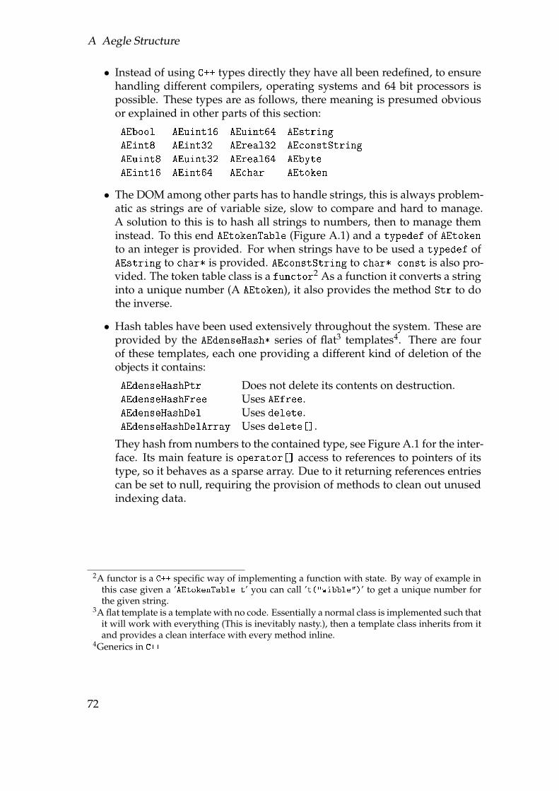
A Aegle Structure

• Instead of using C++ types directly they have all been redefined, to ensurehandling different compilers, operating systems and 64 bit processors ispossible. These types are as follows, there meaning is presumed obviousor explained in other parts of this section:

AEbool AEuint16 AEuint64 AEstring

AEint8 AEint32 AEreal32 AEconstString

AEuint8 AEuint32 AEreal64 AEbyte

AEint16 AEint64 AEchar AEtoken

• The DOM among other parts has to handle strings, this is always problem-atic as strings are of variable size, slow to compare and hard to manage.A solution to this is to hash all strings to numbers, then to manage theminstead. To this end AEtokenTable (Figure A.1) and a typedef of AEtokento an integer is provided. For when strings have to be used a typedef ofAEstring to char* is provided. AEconstString to char* const is also pro-vided. The token table class is a functor2 As a function it converts a stringinto a unique number (A AEtoken), it also provides the method Str to dothe inverse.

• Hash tables have been used extensively throughout the system. These areprovided by the AEdenseHash* series of flat3 templates4. There are fourof these templates, each one providing a different kind of deletion of theobjects it contains:

AEdenseHashPtr Does not delete its contents on destruction.AEdenseHashFree Uses AEfree.AEdenseHashDel Uses delete.AEdenseHashDelArray Uses delete[].

They hash from numbers to the contained type, see Figure A.1 for the inter-face. Its main feature is operator[] access to references to pointers of itstype, so it behaves as a sparse array. Due to it returning references entriescan be set to null, requiring the provision of methods to clean out unusedindexing data.

2A functor is a C++ specific way of implementing a function with state. By way of example inthis case given a ’AEtokenTable t’ you can call ’t("wibble")’ to get a unique number forthe given string.

3A flat template is a template with no code. Essentially a normal class is implemented such thatit will work with everything (This is inevitably nasty.), then a template class inherits from itand provides a clean interface with every method inline.

4Generics in C++

72

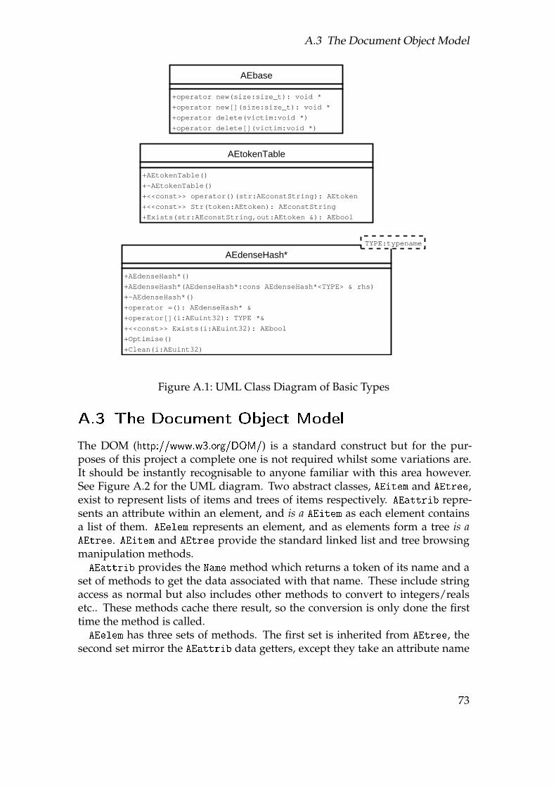
A.3 The Document Object Model

AEbase

+operator new(size:size_t): void *

+operator new[](size:size_t): void *

+operator delete(victim:void *)

+operator delete[](victim:void *)

AEtokenTable

+AEtokenTable()

+~AEtokenTable()

+<<const>> operator()(str:AEconstString): AEtoken

+<<const>> Str(token:AEtoken): AEconstString

+Exists(str:AEconstString,out:AEtoken &): AEbool

AEdenseHash*

+AEdenseHash*()

+AEdenseHash*(AEdenseHash*:cons AEdenseHash*<TYPE> & rhs)

+~AEdenseHash*()

+operator =(): AEdenseHash* &

+operator[](i:AEuint32): TYPE *&

+<<const>> Exists(i:AEuint32): AEbool

+Optimise()

+Clean(i:AEuint32)

TYPE:typename

Figure A.1: UML Class Diagram of Basic Types

A.3 The Document Object Model

The DOM (http://www.w3.org/DOM/) is a standard construct but for the pur-poses of this project a complete one is not required whilst some variations are.It should be instantly recognisable to anyone familiar with this area however.See Figure A.2 for the UML diagram. Two abstract classes, AEitem and AEtree,exist to represent lists of items and trees of items respectively. AEattrib repre-sents an attribute within an element, and is a AEitem as each element containsa list of them. AEelem represents an element, and as elements form a tree is aAEtree. AEitem and AEtree provide the standard linked list and tree browsingmanipulation methods.AEattrib provides the Name method which returns a token of its name and a

set of methods to get the data associated with that name. These include stringaccess as normal but also includes other methods to convert to integers/realsetc.. These methods cache there result, so the conversion is only done the firsttime the method is called.AEelem has three sets of methods. The first set is inherited from AEtree, the

second set mirror the AEattrib data getters, except they take an attribute name

73

A Aegle Structure

token for which attribute of that element to access and a default value for ifthe attribute does not exist. The final pair of methods allow accessing of sub-elements of the element by name, with indexing for if multiple sub-elementsexist with the same name. To load the XML file two functions are also provided:AEelem * ParseXML(AEstring xml,AEtokenTable & tokTab);

AEelem * LoadXML(AEstring filename,AEtokenTable & tokTab);

They construct a DOM from there input, respectively a null terminated stringand a file name to be loaded and parsed.

A.4 The Single Variable Type

The SVT is a hierarchy of nodes, with leaf nodes that contain data. It is madeof three classes, AEnode which represents any node in the hierarchy and thenthe two types of node that can exist, AEbranch and AEleaf. See Figure A.3 forthe UML. As the SVT is constructed/de-constructed by modules AEnode inheritsfrom AEbase.AEnode is virtual (Abstract in UML terminology.) and provides methods to

indicate if its a branch or a leaf. As both branches and leaves have types it pro-vides methods for getting and setting type, it also provides a recursive Clone()

method for duplicating parts of a hierarchy. AEbranch and AEleaf inherit fromthis and implement there own versions of these methods.AEbranch contains a list of AEnodes. This list can be numerically accessed us-

ing operator[] and edited using Add(...),Del(...) and Remove(...) meth-ods. (Del(...) removes the AEnode from the data structure and then deletes it,Remove(...) only removes it so it can be Add(...)ed again.) It also providesmethods (Del(...) & Get(...)) to index by type. In addition Read(...) andWrite(...) methods are provided so the SVT object can be saved and loadedto/from disk. (A constructor is also provided to construct the object from disk.)

One of the properties of AEleaf is that once constructed its data can be changedbut its meta-data can not. Due to the quantity of meta-data associated with eachAEleaf a support class, AEleafDesc is provided to be passed into the constructorof AEleaf and define its structure. It provides the following public variables:

74

A.4 The Single Variable Type

.type The node type, see section A.6.

.dims How many dimensions it has. A list would be one, animage two and a voxel field three for instance.

.size[] This is a pointer to an array of AEint32, each elementbeing the size of that dimension. (The array must con-tain .dims valid entries.) On construction it points toan array of three AEint32’s contained in this structure.In the event that more dimensions are needed it mustbe set to point to a different array, of which it is theclass users responsibility to free.

.fields[] An array of booleans indexed by field type. For thestructure to include a particular field set the relevantvalue to true, otherwise leave it as false.

On construction a AEleafDesc has the entire .fields[] array set to false, soyou only have to set to true the fields required.

For AEleaf three constructors are provided, the primary one that uses AEleafDesca copy constructor and a constructor to load in a saved AEleaf. A Save(...)

method is also provided to store the data in the first place. (Load(...) doesnot make sense, as a AEleafs structure can not be modified after construction.)A set of methods are provided to then get the AEleaf structure, including ex-tracting a AEleafDesc object so it can be edited and used to construct similarAEleafs. The data area provided allows overrun up to a certain limit, changedby MinBorder(...). The postcondition of calling this is that you can be the givenvalue outside the limits of the data without causing problems. The Get*(...)

methods form the bulk of the interface and all return pointers to data, so you canedit the data as well as read it. Each of the methods in this set has two properties,of which every combination is provided; the first property is the dimensionalityof the access - there are special once for 1D, 2D and 3D to cover the majority ofaccesses, there is also nD accessors for if more dimensions are required or analgorithm that works within multiple dimension counts is implemented. Thesecond property is the return type of the pointer, which can be void*, AEbyte*,AEint32*, AEuint32* or AEreal32*. In addition to the standard methods thereare also a set of specialist methods, for very particular situations, all of whichwere implemented as needed:

75

A Aegle Structure

.Grab(...) Given another AEleaf with the same dimensionalitythis copies all shared fields from that AEleaf into thisone.

.Set(...) Given a field and some data this sets every instance ofthat field in the structure to that data.

.MallocField(...) This is given a specific field, it then mallocs a tightlypacked array of all the data in that field from the struc-ture and returns it.

.Fetch(...) This performs similarly to .Grab(...), except it onlyworks on a single passed in field.

.Line(...) Limited to 2D data sets only, sets the value of a passedfield along a line to passed data. Exists specifically fordrawing lines on images.

In addition to the interface provided by AEleaf a further support class exists,AEiter. This iterates all the entries in the AEleaf it is constructed with. It isdesigned to be constructed and then used in the formdo {

...

} while (iter.Next());

Where .Next() moves to the next item and returns true, unless its the last item inwhich case it returns to the start of the data and returns false. It provides similar.Get*(...) methods to AEleaf except without coordinates being required. Italso provides offset Gets in 1D and 2D, to get at the item above or to the left forinstance.

A.5 The Core

AEcore, see Figure A.4, unifies all the aforementioned classes to create the sys-tem as a whole. A single one is constructed within the executable and providesall services to loaded in modules and executes the script. Its parts are as follows:

• Token Hashing. The AEcore class inherits from AEtokenTable, so that itprovides all the token services that various parts of the system require.

• Module loading. This consists of three methods. AddOp(...) registersan operation with the system, giving it the relevant method and namewith which its referenced. The core maintains a list of all registered oper-ations so when asked to execute a XML chunk it can. The second methodis LoadModule(...), this is given the name of a dynamically linked li-brary, it then links in that library and calls its handle function, whichthen calls the AddOp(...) method to register all the operations it contains.LoadModules() looks in the working directory, finds all dynamically linkedlibraries and calls LoadModule(...) on them.

76

A.6 Variable Types

• Execution. Two methods are provided to execute the scripting language,ExecOp(...) is given a DOM element, it expects a <op .../> element andmanages scope automatically. Exec(...) is given a DOM element, thedetails of which do not matter, it loops through all sub-elements in orderand executes each in turn, including handling <var .../> elements. Bothof these methods return true on error, indicating either an unrecognisedelement, operation or an operation indicating that an error happened.

• Scope. The scripting language structure requires scoping of variables, thisis provided by two methods, PushScope() and PopScope(). To managewhich variables go into and out of the current scope the method Link()

explicitly generates a variable in the current scope that aliases a variablein the previous scope.

• Variables. SVT’s can be created and named using the NewVar(...) method,once created they can be obtained by name using Var(...), noting thatyou can only access variables either created in the current scope or linkedfrom a previous scope. A newly created SVT is a empty AEbranch with itstype set to Tnone.

• Operation Parameters. To assist with passing parameters into and out ofoperations two sets of arrays are provided, an array of in variables and anarray of out parameters, both of which are pushed/popped by the stack,the methods Set/Get In/Out Param(...) are the interface for this func-tionality.

• Logging. A single method, Msg(...) is provided that outputs any textgiven to it so the user can see it. It uses the printf interface.

Using this interface executing an Aegle script consists of loading the relevantscript into a DOM, creating a AEcore and calling its LoadMethods() method, thenfinally calling ExecOp(...) on the root element of the loaded DOM.

A.6 Variable Types

The SVT by its nature allows for arbitrary data structures. Passing data betweenoperations however requires standard data structures to be defined. To this enda standard list of fields is defined and a standard list of SVT types that coversall arrangements of data passed around. This is also advantageous for errorchecking, as any structure of a particular type can have certain assumption madeabout its structure instead of every operation having to check all details. Listsfor both follow:

77

A Aegle Structure

A.6.1 Fields

Fbyte A simple AEbyte, for storing arbitrary data.Fflag A set of 8 flags in a AEbyte, for masks and the like.Fcount A AEuint32 counter, for histograms.Fvalue An arbitrary AEreal32, main use as components of a

matrix.Findex1 An index to a 1 dimension/position structure.

1*AEuint32. (Used for texture indices.)Findex2 An index to a 2 dimension/position structure.

2*AEuint32. (Used for edges indices.)Findex3 An index to a 3 dimension/position structure.

3*AEuint32. (Used for indexed triangles.)Findex4 An index to a 4 dimension/position structure.

4*AEuint32. (Used for indexed quads)FcolourL Luminescence component, AEbyte, for greyscale im-

ages.FcolourRGB 3 AEbytes, RGB.

FcolourA An alpha/transparency component, to complimentthe colour spaces, AEbyte.

Flength A AEreal32 length.FposX,FposY,FposZ,FposW The components of a X, Y, Z, W position vector,

AEreal32s.FdirX,FdirY,FdirZ,FdirW The components of a X, Y, Z, W direction vector. Used

for normals among other purposes, AEreal32s.FtexS,FtexT,FtexU Components of a S, T, U texture coordinate,

AEreal32s.FangH,FangP,FangB Components of a H, P, B angle using AEreal32s. (Anti-

clockwise, radians)

A.6.2 Types

Basic Types

• Tnone. Used on construction of nodes, no other purpose.

• Tarray. An array of other types. (AEbranch only)

Leaf Types

• Tmatrix. A matrix, must be 2D and only contain field Fvalue.

• TimageL. A greyscale image. Is required to be 2D, with FcolourL set. Op-tionally FcolourA can be included if an alpha map is required, Flength canbe included for a depth map and Fflag can indicate a mask, with any bitsset indicating membership.

78

A.6 Variable Types

• TimageRGB. Similar to TimageL except its for colour images, only differenceis it requires FcolouRGB instead of FcolourA. The same optional fields ap-ply.

• Tdepth. A depth map, consists only of the Flength field in a 2D structure.No optional fields.

• Tstencil. A mask, a set of Fflag fields in a 2D arrangement. Having anybits set in Fflag indicates membership.

• ToffsetImage. A 2D structure containing fields FposX and FposY. This isthe output of a stereo correspondence algorithm and maps each pixel inthe structure to its correspondence, indexed by the fields. Pixels with nocorresponding pixel have both there fields set to negative numbers.

• TvoxelL. A 3D TimageL.

• TvoxelRGB. A 3D TimageRGB.

• Tvolume. A 3D Tmask.

• Thistogram. A 1D set of Fcount, representing the sum of instances of arange of cases.

• TshapedTexture. An image (2D) with 3D coordinates associated with eachpixel as well as colour. Requires a 3D coordinate and colour, can also havea Fflag to indicate coordinate validity. Specifically created to supersededepth maps, as latter iterations of the code generate 3D coordinates di-rectly from correspondences.

3D model

A 3D model consists of a set of leafs inside a branch with type Tmodel3D. Inaddition to the below listed leaf types images can also be included as textures. A3D model consists of a set of textures, vertices, edges (Line segments), trianglesand quads. Any image or voxel type included in the branch is a texture to bereferenced by the geometry, indexed with 0 being the first one within the branch.

• Tpoints3D. This is a 1D array of vertices. It requires a position consisting ofFdirX, FdirY and FdirZ, optionally FdirW. It can also contain the Fdir set asa normal for that vertex, the Ftex set for texture coordinates and any of thethree colour field types for per vertex colour/transparency. These verticesare then indexed by other parts of the 3D model, the indices start at 0 withmultiple Tpoints3D being appended together to create the complete set inthe order they are stored in the branch. The next type, TpointsExtra3D, isalso included in that array.

79

A Aegle Structure

• TpointsExtra3D. The extra points type also adds vertices, it however de-fines them in terms of vertices already defined via the required Findex1

field it has, overriding them with the same optional fields as Tpoints3D.The reason for this is it allows you to define one vertex with multiplenormals/texture coordinates/colours assigned to it such that a rendererknows they are the same vertex and can optimise accordingly.

• Tedges3D. This is a 1D array of Findex2 that indexes vertices to define thestart and end of each edge. It can also have a colour associated with it tooverride anything set for the vertices. Edges can not be textured.

• Ttris3D. This defines a 1D list of primitives, each with a Findex3 to defineits three corners. It can also have a Findex1 to indicate it should be texturedwith the texture of that index, colour information to colour it and the Fdir

set to flat shade it with a given normal.

• Tquads3D. Identical to Ttris3D except it uses the Findex4 field instead toindicate four vertices.

A 3D model can be explicitly rendered as either a point field, a set of edges ora set of primitives.

A.7 Module Implementation

To add an operation to Aegle involves creating a module with that operation(and usually others) in it. An operation is a function with the following proto-type:AEGLE_FUNC AEbool MyOperation(AEcore & core,AEelem & self);

When an operation is called it is given the core object as its interface to the sys-tem, and self, the DOM element that caused this operation to be called. It shouldreturn false if everything is ok or true if something goes wrong5. Operationsusually all take the same sequence of steps:

• Read and validate the variables passed in to and out of the operation.(in="" and out="" in the element self, using the Get/Set In/Out Param()

core methods.)

• Uses self to get specific parameters to control the execution of the opera-tion.

• Loops all data passed in via the in SVTs and processes it, adding outputdata to the out SVTs.

5Standard C++ throw/catch were avoided as I have no experience of using them within dy-namically linked libraries, and could not risk the potential time lost if it proved problematic.

80

A.7 Module Implementation

• Returns false on success, or uses core.Msg to give a reason for failure andreturns true.

The operations need to be compiled into a dll, with a handle function:AEGLE_FUNC void OnAegleLoad(AEcore & core)

{

core.AddOp(core("MyModule.MyOperation"),MyOperation);

...

}

Aegle will then automatically load the dll if its put into the working directoryand you can use the operation in a script file with the XML fragment<op name="MyModule.MyOperation" in="..." out="..." .../>

81

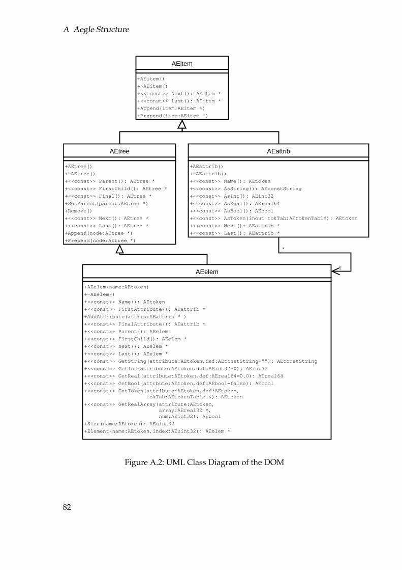
A Aegle Structure

AEitem

+AEitem()

+~AEitem()

+<<const>> Next(): AEitem *

+<<const>> Last(): AEitem *

+Append(item:AEitem *)

+Prepend(item:AEitem *)

AEtree

+AEtree()

+~AEtree()

+<<const>> Parent(): AEtree *

+<<const>> FirstChild(): AEtree *

+<<const>> Final(): AEtree *

+SetParent(parent:AEtree *)

+Remove()

+<<const>> Next(): AEtree *

+<<const>> Last(): AEtree *

+Append(node:AEtree *)

+Prepend(node:AEtree *)

AEattrib

+AEattrib()

+~AEattrib()

+<<const>> Name(): AEtoken

+<<const>> AsString(): AEconstString

+<<const>> AsInt(): AEint32

+<<const>> AsReal(): AEreal64

+<<const>> AsBool(): AEbool

+<<const>> AsToken(inout tokTab:AEtokenTable): AEtoken

+<<const>> Next(): AEattrib *

+<<const>> Last(): AEattrib *

AEelem

+AEelem(name:AEtoken)

+~AEelem()

+<<const>> Name(): AEtoken

+<<const>> FirstAttribute(): AEattrib *

+AddAttribute(attrib:AEattrib * )

+<<const>> FinalAttribute(): AEattrib *

+<<const>> Parent(): AEelem

+<<const>> FirstChild(): AEelem *

+<<const>> Next(): AEelem *

+<<const>> Last(): AEelem *

+<<const>> GetString(attribute:AEtoken,def:AEconstString=""): AEconstString

+<<const>> GetInt(attribute:AEtoken,def:AEint32=0): AEint32

+<<const>> GetReal(attribute:AEtoken,def:AEreal64=0.0): AEreal64

+<<const>> GetBool(attrbute:AEtoken,def:AEbool=false): AEbool

+<<const>> GetToken(attribute:AEtoken,def:AEtoken, tokTab:AEtokenTable &): AEtoken

+<<const>> GetRealArray(attribute:AEtoken, array:AEreal32 *, num:AEint32): AEbool

+Size(name:AEtoken): AEuint32

+Element(name:AEtoken,index:AEuint32): AEelem *

1

*

Figure A.2: UML Class Diagram of the DOM

82

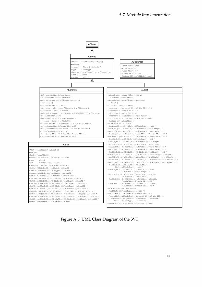
A.7 Module Implementation

AEbase

AEnode

+AEnode(type:AEnodeType=Tnode)

+~AEnode()

+<<const>> Clone(): AEnode *

+Type(): AEnodeType

+Type(newType:AEnodeType): AEnodeType

+Leaf(): AEbool

+Branch(): AEbool

AEbranch

+AEbranch(t:AEnodeType=Tnode)

+AEbranch(rhs:const AEbranch &)

+AEbranch(hand:AEint32,Read:AEioFunc)

+~AEbranch()

+<<const>> Leaf(): AEbool

+operator =(rhs:const AEbranch &): AEbranch &

+<<const>> Clone(): AEnode *

+Add(node:AEnode *,index:AEuint32=0xFFFFFFFF): AEuint32

+Del(index:AEuint32)

+Remove(index:AEuint32): AEnode *

+<<const>> Count(): AEuint32

+<<const>> operator[](index:AEuint32): AEnode &

+Count(type:AEnodeType): AEuint32

+Get(type:AEnodeType,index:AEuint32): AEnode *

+Transfer(from:AEbranch &)

+Save(hand:AEint32,Write:AEioFunc): AEbool

+Load(hand:AEint32,Read:AEioFunc)

AEleafDesc

+type: AEnodeType

+dims: AEint32

+size: AEint32 *

+sizes: AEint32 [3]

+fields: AEbool[AEfieldCount]

AEleaf

+AEleaf(desc:const AEleafDesc &)

+AEleaf(rhs:const AEleaf &)

+AEleaf(hand:AEint32,Read:AEioFunc)

+~AEleaf()

+<<const>> Leaf(): AEbool

+operator =(rhs:const AEleaf &): AEleaf &

+<<const>> Clone(): AEleaf *

+<<const>> Dims(): AEuint32

+<<const>> Size(dim:AEuint32): AEuint32

+<<const>> Has(field:AEfieldType): AEbool

+GetDesc(out:AEleafDesc &)

+MinBorder(bs:AEint32)

+Get(pos:AEint32 *,field:AEfieldType): void *

+GetByte(pos:AEint32 *,field:AEfieldType): AEbyte *

+GetInt32(pos:AEint32 *,field:AEfieldType): AEint32 *

+GetUint32(pos:AEint32 *,field:AEfieldType): AEuint32 *

+GetReal32(pos:AEint32 *,field:AEfieldType): AEreal32 *

+Get1D(d1:AEint32,field:AEfieldType): void *

+Get1Dbyte(d1:AEint32,field:AEfieldType): AEbyte *

+Get1Dint32(d1:AEint32,field:AEfieldType): AEint32 *

+Get1Duint32(d1:AEint32,field:AEfieldType): AEuint32 *

+Get1Dreal32(d1:AEint32,field:AEfieldType): AEreal32 *

+Get2D(d1:AEint32,d2:AEint32,field:AEfieldType): void *

+Get2Dbyte(d1:AEint32,d2:AEint32,field:AEfieldType): AEbyte *

+Get2Dint32(d1:AEint32,d2:AEint32,field:AEfieldType): AEint32 *

+Get2Duint32(d1:AEint32,d2:AEint32,field:AEfieldType): AEuint32 *

+Get2Dreal32(d1:AEint32,d2:AEint32,field:AEfieldType): AEreal32 *

+Get3D(d1:AEint32,d2:AEint32,d3:AEint32, field:AEfieldType): void *

+Get3Dbyte(d1:AEint32,d2:AEint32,d3:AEint32, field:AEfieldType): AEbyte *

+Get3Dint32(d1:AEint32,d2:AEint32,d3:AEint32, field:AEfieldType): AEint32 *

+Get3Duint32(d1:AEint32,d2:AEint32,d3:AEint32, field:AEfieldType): AEuint32 *

+Get3Dreal32(d1:AEint32,d2:AEint32,d3:AEint32, field:AEfieldType): AEreal32 *

+Grab(rhs:AEleaf &): AEbool

+Set(field:AEfieldType,data:void *)

+MallocField(field:AEfieldType): AEbyte *

+Fetch(field:AEfieldType,rhs:const AEleaf &): AEbool

+Line(x1:AEint32,y1:AEint32,x2:AEint32,y2:AEint32, field:AEfieldType,data:void *)

+Save(hand:AEint32,Write:AEioFunc): AEbool

AEiter

+AEiter(leaf:const AEleaf &)

+~AEiter()

+SetPos(pos:AEint32 *)

+<<const>> Pos(dim:AEuint32): AEint32

+Next(): AEbool

+Get(field:AEfieldType): void *

+GetByte(field:AEfieldType): AEbyte *

+GetInt32(field:AEfieldType): AEint32

+GetUint32(field:AEfieldType): AEuint32 *

+GetReal32(field:AEfieldType): AEreal32 *

+Get1D(d1:AEint32,field:AEfieldType): void *

+Get1Dbyte(d1:AEint32,field:AEfieldType): AEbyte *

+Get1Dint32(d1:AEint32,field:AEfieldType): AEint32 *

+Get1Duint32(d1:AEint32,field:AEfieldType): AEuint32 *

+Get1Dreal32(d1:AEint32,field:AEfieldType): AEreal32 *

+Get2D(d1:AEint32,d2:AEint32,field:AEfieldType): void *

+Get2Dbyte(d1:AEint32,d2:AEint32,field:AEfieldType): AEbyte *

+Get2Dint32(d1:AEint32,d2:AEint32,field:AEfieldType): AEint32 *

+Get2Duint32(d1:AEint32,d2:AEint32,field:AEfieldType): AEuint32 *

+Get2Dreal32(d1:AEint32,d2:AEint32,field:AEfieldType): AEreal32 *

+Fetch(rhs:AEiter &,field:AEfieldType)

Figure A.3: UML Class Diagram of the SVT

83

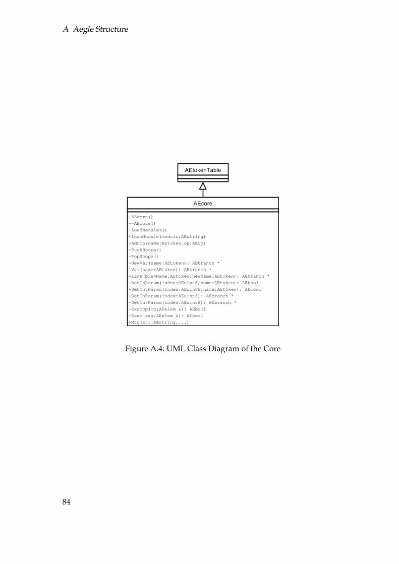
A Aegle Structure

AEcore

+AEcore()

+~AEcore()

+LoadModules()

+LoadModule(module:AEstring)

+AddOp(name:AEtoken,op:AEop)

+PushScope()

+PopScope()

+NewVar(name:AEtoken): AEbranch *

+Var(name:AEtoken): AEbranch *

+Link(prevName:AEtoken,newName:AEtoken): AEbranch *

+SetInParam(index:AEuint8,name:AEtoken): AEbool

+SetOutParam(index:AEuint8,name:AEtoken): AEbool

+GetInParam(index:AEuint8): AEbranch *

+GetOutParam(index:AEuint8): AEbranch *

+ExecOp(op:AEelem &): AEbool

+Exec(seq:AEelem &): AEbool

+Msg(str:AEstring,...)

AEtokenTable

Figure A.4: UML Class Diagram of the Core

84

B Aegle Operations

The following chapter details all operations that have been implemented, subdi-vided by package.

B.1 Embedded

These three operations are integrated into the Aegle executable as there basicfunctionality.

exec:<op name="exec" uses="...">

<!� Variables & Operations �>

</op>

This executes the operations contained within inside a new scope.uses: This contains a comma separated list of variables to import

into the scope, as external variables are not implicitly avail-able.

time:This is identical to exec, but it also times how long the operations within take

and prints it out to the console.

msg:<op name="msg" msg="Hello World!"/>

Prints a message to the console.msg: The message to be printed.

B.2 var

This module contains general purpose operations, that work on all variables.

var.copy:<op name="var.copy" in="from" out="to"/>

85

B Aegle Operations

Copies a variable into another variable, overwriting the contents of the to vari-able.in[0]: The variable to be copied.out[0]: The variable to be overwritten.

var.append:<op name="var.append" in="from" out="to"/>

Clones the root nodes children of from and appends them to the end of the rootnode of to.in[0]: The variable to be copied.out[0]: The variable to be merged into.

var.save:<op name="var.save" in="var" filename="file"/>

Serialises a variable into a file so it can be latter loaded.in[0]: The SVT to save.filename: The file the SVT will be saved into.

var.load:<op name="var.load" out="var" filename="file"/>

Loads a file putting the SVT it contains into the given variable.out[0]: The variable to load into.filename: The file the SVT will be loaded from.

B.3 image.io

This module provides two methods, one to load images and another to save im-ages. Uses Developers Image Library1 and will load/save most image formats.When saving it decides the type based on the extension.

1http://openil.sourceforge.net/

86

B.4 math.matrix

image.io.load:<op name="image.io.load" out="loaded">

<file value="image.jpg"/> <!� Repeatable �>

</op>

Loads image files, is given a list of images which it loads into the root of theout variable. The images loaded will be colour or greyscale depending on thefile format, and will have alpha channels if the file does.out[0]: The variable to load into.file: Each file element loads a file, the name given by the value at-

tribute.

image.io.save:<op name="image.io.save" in="images">

<file value="image.jpg" index="0"/> <!� Repeatable �>

</op>

Saves given images, as the given data can contain multiple image leafs this op-eration is designed to be able to save multiple files.in[0]: The variable to save from.file: Each file element saves a file, the name given by the value at-

tribute and the index giving which file in the set to save.

B.4 math.matrix

This section provides some matrix manipulation operations.

math.matrix.identity:<op name="math.matrix.identity" out="matrix" width="4"

height="4"/>

Creates an identity matrix.out[0]: The output matrix.width: The width of the output matrix.height: The height of the output matrix.

math.matrix.transform:<op name="math.matrix.transform" in="in" out="out">

<rotate h="180" p="90" b="0"/>

<offset x="10" y="5" z="0"/>

<scale x="2" y="2" z="2"/>

</op>

87

B Aegle Operations

This applies transforms to a 4x4 matrix, in the order given.in[0]: (Optional) Matrix to transform. If omitted it starts from an

identity matrix.out[0]: Output matrix.<rotate>: Does a HPB rotation.<offset>: Does a translation.<scale>: Does a scaling.

math.matrix.add:<op name="math.matrix.add" in="in1,in2" out="out"/>

Calculates out = in1 + in2.in[0]: First matrix.in[1]: Second matrix.out[0]: Resultant matrix.

math.matrix.sub:<op name="math.matrix.sub" in="in1,in2" out="out"/>

Calculates out = in1 - in2.in[0]: First matrix.in[1]: Second matrix.out[0]: Resultant matrix.

math.matrix.mult:<op name="math.matrix.mult" in="in1,in2" out="out"/>

Calculates out = in1 * in2.in[0]: First matrix.in[1]: Second matrix.out[0]: Resultant matrix.

math.matrix.transpose:<op name="math.matrix.transpose" in="in" out="out"/>

Calculates the transpose of a matrix.in[0]: Input matrix.out[0]: Output matrix.

88

B.5 stats

math.matrix.inverse:<op name="math.matrix.inverse" in="in" out="out"/>

Calculates the inverse of a matrix.in[0]: Input matrix.out[0]: Output matrix.

math.matrix.shrink:<op name="math.matrix.shrink" in="in" out="out" width="5"

height="3"/>

Shrinks a matrix to make it smaller, useful for trimming data matrices.in[0]: Input matrix.out[0]: Output matrix.width: (Optional) Width to set the matrix to, will not make it larger

and if omitted its width is not changed.height: (Optional) Height to set the matrix to, will not make it larger

and if omitted its height is not changed.

math.matrix.save:<op name="math.matrix.save" in="matrix" filename="out.csv"/>

Saves a matrix to a comma separated file.in[0]: Input matrix.filename: File matrix is saved to.

math.matrix.load:<op name="math.matrix.load" out="matrix" filename="out.csv"/>

Loads a matrix from a comma separated file.out[0]: Output matrix.filename: File matrix is loaded from.

B.5 stats

A set of operations to determine the covariance matrices required by certain ver-sions of the stereo algorithms.

89

B Aegle Operations

stats.covariance.imageRGB:<op name="stats.covariance.imageRGB" in="image1,image2,..."

out="matrix"/>

Takes a selection of RGB images as inputs and calculates a covariance matrixon the 3 colour components, making a 3x3 matrix.in[n]: Input images to be sampled.out[0]: Resulting 3x3 matrix.

stats.covariance.imageRGB.diff:<op name="stats.covariance.imageRGB.diff" in="image1,image2"

out="matrix"/>

Calculates the covariance of the differences between two RGB images.in[0]: Input colour image 1.in[1]: Input colour image 2.out[0]: Resulting 3x3 matrix.

stats.covariance.imageArea33.diff:<op name="stats.covariance.imageArea33.diff" in="image1,image2"

out="matrix"/>

Calculates the covariance of the differences between 3x3 areas of the given greyscaleimages.in[0]: Input greyscale image 1.in[1]: Input greyscale image 2.out[0]: Resulting 9x9 matrix.

B.6 image

Some miscalaneous image operations.

image.set.depth:<op name="image.set.depth" in="image,depth" out="merged"/>

Takes an image and a depth map and merges them to produce an image withdepthin[0]: Input image map, either colour or greyscale.in[1]: Input depth map. Must be the same size as the image map.

90

B.7 image.filter

out[0]: Resulting Timage* width depth data..

image.from.depth:<op name="image.from.depth" in="depth" out="image"/>

Generates an image from a depth map, sets nearby objects to blue then fadesto red as they get further away and then to green as they get further still.in[0]: Input depth map.out[0]: Resulting image.

B.7 image.�lter

Filters for images, for filtering them prior to other processing, such as Gaussianblurs before correspondence matching.

image.filter.grey:<op name="image.filter.grey" in="colour" out="grey"/>

Converts a colour image into a greyscale image. If its already greyscale it justcopies it.in[0]: Input image.out[0]: Output image.

image.filter.colour:<op name="image.filter.colour" in="grey" out="colour"/>

Converts a greyscale image into a colour image. If its already colour it just copiesit.in[0]: Input image.out[0]: Output image.

image.filter.convolve:<op name="image.filter.convolve" in="in" out="out">

<kernel width="3" height="3" data="0,1,0,1,2,1,0,1,0"

scale="1.0"/>

</op>

This applies a sequence of convolutions to the input. The kernels are normalised

91

B Aegle Operations

and then multiplied by the given scale. Works on all image channels available,including alpha.in[0]: Input image.out[0]: Output image.<kernel>: Multiple kernels can listed, each has a window (Sizes must be

odd) defined and factors for that window, plus the scale value.

image.filter.gaussian:<op name="image.filter.gaussian" in="in" out="out" sd="3.2"/>

Applies a Gaussian blur to the input image.in[0]: Input image.out[0]: Output image.sd: The standard deviation of the blue, in pixels.

image.filter.threshold:<op name="image.filter.threshold" in="in" out="out" min="0"

max="255"/>

Not really a threshold unless min==max, sets any pixel less than or equal tomin to 0 and any pixel greater than or equal to max to 255.in[0]: Input greyscale image.out[0]: Output greyscale image.min: Any value equal to or less than this is set to 0.max: Any value equal to or greater than this is set to 255.

B.8 stereo

This module contains two sets of algorithms, the major set is dense correspon-dence algorithms, of which there are many variations on the maximum Like-lihood Stereo Algorithm[37]. There are also a set of algorithms to render outthe resulting correspondence maps, to generate depth maps from the data andto then visualise them. Some noise reduction operations are also provided fordepth maps.

stereo.basic.MLM:<op name="stereo.basic.MLM" in="left,right"

out="offsetLeft,offsetRight" sd="2.0" fov="1.5707963267948966"

pd="0.9"/>

This impliments the first algorithm given in [37], it takes a left and right greyscale

92

B.8 stereo

image (TimageL) and outputs a pair of correspondence maps, of type ToffsetImage.The default parameters given are the default parameters taken from the paper.

in[0]: The left greyscale image.in[1]: The right greyscale image.out[0]: The left output correspondence map.out[1]: The right output correspondence map.sd: The standard deviation of the Gaussian noise that is consid-

ered to be in the image.fov: The field of view of the image, in radians. Defaults to 90◦

pd: Percentage of the image that is not occluded, i.e. 1− pd shouldbe the percentage of pixels that are not visible in the other im-age.

stereo.basic.MLMH:This is identical to stereo.basic.MLM except it implements the second algo-

rithm of the paper

stereo.basic.MLMHV:This is identical to stereo.basic.MLM except it implements the third algo-

rithm of the paper

stereo.colour.MLM:<op name="stereo.colour.MLM" in="left,right,covar"

out="offsetLeft,offsetRight" sd="2.0" fov="1.5707963267948966"

pd="0.9"/>

This implements a variation on the basic MLM algorithm by using colour.in[0]: The left colour image.in[1]: The right colour image.in[2]: The covariance matrix that relates the three colour compo-

nents.out[0]: The left output correspondence map.out[1]: The right output correspondence map.sd: The standard deviation of the Gaussian noise that is consid-

ered to be in the image.fov: The field of view of the image, in radians. Defaults to 90◦

pd: Percentage of the image that is not occluded, i.e. 1− pd shouldbe the percentage of pixels that are not visible in the other im-age.

stereo.colour.MLMH:This is identical to stereo.colour.MLM except it implements the second algo-

rithm of the paper

93

B Aegle Operations

stereo.colour.MLMHV:This is identical to stereo.colour.MLM except it implements the third algo-

rithm of the paper

stereo.area33.MLM:<op name="stereo.area33.MLM" in="left,right,covar"

out="offsetLeft,offsetRight" sd="2.0" fov="1.5707963267948966"

pd="0.9"/>

This applies the same expansion that stereo.colour.MLM applies, but by increas-ing it to use a 3x3 window.in[0]: The left greyscale image.in[1]: The right greyscale image.in[2]: The 9x9 covariance matrix that relates the nine pixels inside

the window.out[0]: The left output correspondence map.out[1]: The right output correspondence map.sd: The standard deviation of the Gaussian noise that is consid-

ered to be in the image.fov: The field of view of the image, in radians. Defaults to 90◦

pd: Percentage of the image that is not occluded, i.e. 1− pd shouldbe the percentage of pixels that are not visible in the other im-age.

stereo.basic.MLM.NCC:<op name="stereo.basic.MLM.NCC" in="left,right"

out="offsetLeft,offsetRight" area="2" sd="2.0"

fov="1.5707963267948966" pd="0.9"/>

This achieves the same effect as stereo.area33.MLM but instead of extendingthe MLM algorithm to do area it uses the basic MLM algorithm on values calcu-lated using Normalised Cross Correlation.in[0]: The left greyscale image.in[1]: The right greyscale image.out[0]: The left output correspondence map.out[1]: The right output correspondence map.area: Defines the window size for the Normalised Cross Correlation,

as (2area + 1) square.sd: The standard deviation of the Gaussian noise that is consid-

ered to be in the image.fov: The field of view of the image, in radians. Defaults to 90◦

94

B.8 stereo

pd: Percentage of the image that is not occluded, i.e. 1− pd shouldbe the percentage of pixels that are not visible in the other im-age.

stereo.basic.MLMH.NCC:This is identical to stereo.basic.MLM.NCC except it implements the second al-

gorithm of the paper

stereo.basic.MLMHV.NCC:This is identical to stereo.basic.MLM.NCC except it implements the third al-

gorithm of the paper

stereo.depth:<op name="stereo.depth" in="offset1,offset2,proj1,proj2"

out="depth"/>

This calculates a depth map from an offset pair and there projection matrices,outputting it as depth for image1.in[0]: Offset map for camera 1in[1]: Offset map for camera 2in[2]: Projection matrix for camera 1in[3]: Projection matrix camera 2out[0]: Depth map, Tdepth. Note that it has no colour information

and needs to be merged with the relevant image if required.

stereo.depth.extrema:<op name="stereo.depth.extrema" in="in" out="out" sd="2.0"/>

This calculates the mean and standard deviation of the entire input depth map,it then sets any values outside of sd multiplied by the standard deviation fromthe mean to unknown. This removes extreme values.in[0]: Input depth mapout[0]: Output depth mapsd: A multiplier to indicate sensitivity.

stereo.depth.norm:<op name="stereo.depth.norm" in="in" out="out" norm="100"

min="-1" max="100"/>

This scales a depth map so the given depth is the greatest, it then restricts valuesto a given range. (This is useful for pushing objects that get too close to the cam-era away and scaling different sized scenes so they are equally navigable withthe visualisation tools.)

95

B Aegle Operations

in[0]: Input depth mapout[0]: Output depth mapnorm: The values are scaled such that this is the maximum depth.min: All values less than this value after the scaling are set to this

value.max: All values greater than this value after the scaling are set to

this value.

stereo.depth.outlier:<op name="stereo.depth.outlier" in="in" out="out" size="1"

factor="1.0"/>

This attempts to remove outlier points from a given depth map. It calculatesthe mean and standard deviation of the window with and without the pixelin question. If the gap between the means of this calculation is greater thanthe standard deviation multiplied by factor then it is an outlier and set to un-known. Any point that dose not have at least 3 neighbours in the window isalso set to unknown. This algorithm is over zealous, after running it a Gaussianblur should then be run to fill in the holes.in[0]: Input depth mapout[0]: Output depth mapsize: The window size is (2size + 1).factor: The scalar factor that decides how sensitive the algorithm is.

stereo.depth.blur:<op name="stereo.depth.blur" in="in" out="out" sd="0.0"

unsd="4.0"/>

This applies a Gaussian blue to a depth map. The Gaussian blur only includesvalues that are set, unknown depth values are ignored. A different standarddeviation can be used when the central pixel is known than when it is not. If astandard deviation value is set to 0 it dose not apply that particular one, so bydefault this calculates unknown depth values as Gaussian weighted averages ofthere surrounding area but does not affect known values.in[0]: Input depth mapout[0]: Output depth mapsd: Standard deviation used for the blur when applied to known

depth values.unsd: Standard deviation used for the blur when applied to un-

known depth values.

stereo.chess:

96

B.9 3d

<op name="stereo.chess" in="offset" out="image"/>

This generates an image from a correspondence map, where it renders a chessboard distorted by the correspondence map, as a means of visualising a corre-spondence map.in[0]: Offset mapout[0]: Output colour image

stereo.hoffset:<op name="stereo.hoffset" in="offset" out="image" range="24"/>

This renders an offset map to an image indicating its horizontal offset. Pixelswith no offset are red, they fade towards blue for it heading left and green forit heading right. Unknown correspondences (Occlusions, noise) are renderedblack.in[0]: Offset mapout[0]: Output colour imagerange: Maximum offset before it reaches he maximum colour and is

clamped.

B.9 3d

This provides two methods, for generating 3D data from depth maps and shapedtextures.

3d.from.depth.mesh:<op name="3d.from.depth.mesh" in="depth,proj" out="model"

scale="32"/>

This converts a depth map into a textured mesh, constructed from quads.in[0]: This is the depth map, it should include colour information.in[1]: A 4x3 projection matrix for the camera, should be calculated

from normalised coordinates. ([-1,-1]x[1,1])out[0]: The output 3D model.scale: The length of the sides of quads in pixels.

3d.from.shaped.mesh:<op name="3d.from.shaped.mesh" in="shaped" out="model"

scale="32"/>

97

B Aegle Operations

This converts a shaped texture into a textured mesh, constructed from quads.in[0]: The shaped texture to use.out[0]: The output 3D model.scale: The length of the sides of quads in pixels.

B.10 3d.view

This provides visualisation capabilities, as either a point cloud or a texturedmesh, using OpenGL.

Both windows use the same interface, it uses the concept of a scene centre,which the camera moves in relation to and always looks at.

• Dragging with the LMB dollies around the scene centre.

• Dragging with the RMB pans the scene, moving the scene centre in theplane perpendicular to the cameras direction.

• The mouse wheel moves in and out from the centre point.

• Q and A move the scene centre on the X axis.

• W and S move the scene centre on the Y axis.

• E and D move the scene centre on the Z axis.

• G toggles the rendering of a X-Z grid.

• O toggles the rendering of an origin.

• B toggles the background colour between black and white. (Black is easieron the eyes, white is suitable for output into this document.)

• R resets the camera to the centre of the world looking down the negative Zaxis.

• T sets the camera to look straight down.

• C toggles backface culling on and off.

• F toggles if clockwise faces are backfacing or anti-clockwise faces.

• P toggles between perspective rendering and orthographic rendering.

98

B.11 features

3d.view.points:<op name="3d.view.points" in="model"/>

Opens a window to display a point cloud.in[0]: The 3D model to display

3d.view.mesh:<op name="3d.view.mesh" in="model"/>

Opens a window to display a textured polygon soup.in[0]: The 3D model to display

B.11 features

The features library contains corner detectors and corner matchers, to find matchesbetween images that are probably the same point in space.

features.corner.harris:<op name="features.corner.harris" in="image" out="points"

k="0.04" sd="0.7" border="3"/>

This implements a harris corner detector[10]. It takes as input a greyscale im-age and outputs a list of 2D points. In addition to an array of points representedas a FposX and FposY it outputs them in sorted order, with the strongest pointfirst and the weakest last, so the list can be clipped down to a manageable sizesensibly.in[0]: The image to detect corners in.out[0]: An array of corners.k: This is the k value from the algorithm, should probably be left

as 0.04.sd: Standard deviation of the Gaussian kernel used by the algo-

rithm.border: A border in pixels around the image that is ignored, due to the

problems borders produce.

features.render.corner:<op name="features.render.corner" in="points,image" out="image"

colour="R" type="P"/>

This renders the given corners onto the given image and outputs it, for verifi-cation.

99

B Aegle Operations

in[0]: The points to be renderedin[1]: The image to render onto.out[0]: The image with the points rendered onto it.colour: This field can contain ’R’, ’G’ or ’B’, as the colour to render the

corners as.type: This can be either ’P’ to render points or ’C’ to render crosses.

features.prune.count:<op name="features.prune.count" in="lots" out="less"

count="1000"/>

This prunes points by simply clipping the list to the given length.in[0]: The point array before being clipped.out[0]: The point array after being clipped.count: Maximum number of corners to be left after clipping.

features.prune.area:<op name="features.prune.area" in="lots,image" out="less"

divx="32" divy="24" count="4" max="8000"/>

This prunes points but instead of having a global count for each square it di-vides the image up into squares and has a local count for each one, to stop thecorners being crowded around the highest contrast features of the image.in[0]: The point array before being clipped.in[1]: The image, so it knows its dimensions and can divide up ac-

cordingly.out[0]: The point array after being clipped.divx: How many divisions to have on the x axis.divy: How many divisions to have on the y axis.count: Maximum number of corners to be left in each square after

clipping.max: Maximum number of corners down the given array to con-

sider, to stop squares in the image that contain no useful con-tent from being filled with corners.

features.match.ncc:<op name="features.match.ncc" in="corner1,image1,corner2,image2"

out="matrix" area="3" max="0.1"/>

This produces a similarity matrix between two images corners using NormalisedCross Correlation to compare windows around the corners.in[0]: The corners for image 1.

100

B.11 features

in[1]: Image 1in[2]: The corners for image 2.in[3]: Image 2out[0]: Similarity matrix.area: The NCC is done over a window of (2area + 1).max: This defines the maximum distance between two pixels before

they are not matched, in terms of a fraction of the image.

features.select.basic:<op name="features.select.basic" in="corner1,corner2,sim_matrix"

out="matrix" cutoff="0.9"/>

Given a similarity matrix this produces a data matrix of selected corner pairsthat are probably matched. It works by considering any two corners matched ifthe NCC between them is greater than either corner with any other corner.in[0]: The corners for image 1.in[1]: The corners for image 2.in[3]: The similarity matrixout[0]: Data matrix of corner pairs. Each row reads as a match of

(image1.x,image1.y,image2.x,image2.y).cutoff : Any NCC less than this value is considered to be a mismatch.

features.select.advanced:<op name="features.select.advanced" in="corner1,corner2,sim_matrix"

out="matrix" cutoff="0.9" slice="0.9" set="1.1" iter="3"/>

Identical to features.select.basic except instead of using the distance cut-offset in features.match.ncc it works out an optimum match distance to reducethe number of outliers that get through. It does iter iterations, each iterationit gets all the matches within the current distance (Starts as the width of the im-age.) and generates a histogram of distances between them. It then takes thefirst slice fraction of the inliers and sets the distance to set multiplied by thelargest distance in this set. The matches selected in the final iteration are output.in[0]: The corners for image 1.in[1]: The corners for image 2.in[3]: The similarity matrixout[0]: Data matrix of corner pairs. Each row reads as a match of

(image1.x,image1.y,image2.x,image2.y).cutoff : Any NCC less than this value is considered to be a mismatch.slice: Fraction of matches considered to probably be inliers.set: A multiplier used by the algorithm.iter: How many iterations of refinement to do.

101

B Aegle Operations

features.render.match:<op name="features.render.match" in="data_matrix,image1,image2"

out="image"/>

This renders matches between two images in such a way they can be checked. Itrenders image1 to the red channel, image2 to the blue channel and then drawsgreen lines between the matches.in[0]: Data matrix of the matches.in[1]: Image 1, greyscale.in[2]: Image 2, greyscale.out[0]: The rendered image.

B.12 camera

The camera module is concerned with calculating the fundamental matrix andrectification. It also provides lots of validation operations.

camera.ext.match.fun:<op name="camera.ext.match.fun" in="match,image1,image2"

out="fun[,valid]" cutoff="1.0" cert="0.95" max="1000000"

refine="2"/>

It takes a data matrix of matches and outputs the fundamental matrix. It usesthe RANSAC solution of trying a random set of 8 matches and generating a fun-damental matrix from it. It then uses the epipolar constraint to define whichpoints are inliers and which are outliers. This is done a number of times and thepoints defined as inliers for the largest set are ultimately then chosen as the cor-rect point set. The fundamental matrix is then calculated for all of these inliersto produce the final fundamental matrix which is output.in[0]: Data matrix of the matches.in[1]: Image 1, simply for its dimensions so the matches can be nor-

malised.in[2]: Image 2, again for its dimensions.out[0]: The 3x3 fundamental matrix.out[1]: (Optional) The data matrix passed in but only with the corners

defined as inliers by this process.cutoff : The distance a point can be from the epipolar line in pixels

for it to be considered as on the epipolar line and therefore amatch.

cert: The chance of having the correct solution, it keeps running tillit is this sure it has the correct answer.

102

B.12 camera

max: The max number of runs through, in case its chances of successsimply aren’t increasing fast enough.

refine: The number of refinement stages to have after the RANSACprocess is over.

camera.rectify.polar:<op name="camera.rectify.polar" in="image1,image2,funmat"

out="rect1,rect2"/>

This implements polar rectification[26]. Saves the information required to de-rectify in the output so the de-rectification algorithm is simple.in[0]: Image 1.in[1]: Image 2.in[2]: 3x3 fundamental matrix.out[0]: Rectified version of image 1.out[1]: Rectified version of image 2.

camera.derectify:<op name="camera.derectify" in="image1,rect1,rect2,corr1"

out="corr_out"/>

This de-rectifies rectified correspondence data.in[0]: Image 1.in[1]: Rectified image 1.in[2]: Rectified image 2.in[3]: Rectified Correspondences for image 1out[0]: De-rectified version of correspondences for image 1.

camera.render.epilines:<op name="camera.render.epilines" in="image,funmat,match"

out="image" transpose="false"/>

This takes the given image and renders the epipolar lines associated with thepoints in match onto it using the given fundamental matrix, for validation.in[0]: Image.in[1]: 3x3 fundamental matrix.in[2]: Match array.out[0]: Image with epipolar lines rendered onto it.transpose: If the fundamental matrix goes from this image to another

then set transpose to false, if its from another to this settrasnpose to true.

103

B Aegle Operations

camera.projection.gen:<op name="camera.projection.gen" in="int1,fun,int2"

out="proj1,proj2"/>

Given the intrinsic matrices for two cameras and the fundamental matrix be-tween two views this generates the projection matrices of teh two views assum-ing that the first view is at the origin.in[0]: Intrinsic matrix for the first view.in[1]: 3x3 fundamental matrix.in[2]: Intrinsic matrix for the second view.out[0]: Projection matrix for the first view.out[1]: Projection matrix for the second view.

camera.match.cloud:<op name="camera.match.cloud" in="proj1,proj2,image1,image2,matches"

out="model"/>

Given the projection matrices and images of two views it then converts a setof matches between the two views into a point cloud. Used for testing purposes.in[0]: Projection matrix for the first view.in[1]: Projection matrix for the second view.in[2]: Image 1.in[3]: Image 2.in[4]: Data matrix of matches.out[0]: 3D model of vertices.

B.13 intrinsic

The intrinsic module provides tools to obtain a cameras intrinsic parameters.intrinsic.select.squares:

<op name="intrinsic.select.squares" in="image,corners"

out="squares"/>

This is given an image and corners on it. It provides an interface by whichthe user can select the corners of a calibration grid, working through the grid inreading order, it snaps selected corners to the given list of detected corners, sothe user does not have to be accurate. The interface is LMB to place next point,RMB jumps closest point to where you click to where you click, to correct mis-takes. Note that the moment you place the last point the interface exits. Thecorners are colour coded such that you will know if you miss a corner/doubleclick.in[0]: The image to select corners for.

104

B.14 registration

in[1]: The computer detected corners.out[0]: List of corners that make up the calibration grid.

intrinsic.select.squares:<op name="intrinsic.select.squares" in="image,corners"

out="image"/>

This renders the result of intrinsic.select.squares to an image for verifica-tion.in[0]: The image to render to.in[1]: The corners to render.out[0]: The output image with the calibration grid on.

intrinsic.homography.squares:<op name="intrinsic.homography.squares" in="image,squares"

out="matrix,[render]"/>

This calculates the homography required to get from the 3D coordinates of thepoints on the square calibration grid to the image points. Essentially it worksout the projection matrix based on us having a known set of points. The passedin image is just to normalise the image coordinates.in[0]: The image, just for normalising the coordinates.in[1]: The corners that make up the calibration grid.out[0]: 3x3 homography matrix.out[1]: (Optional.) If given it renders the matched calibration target

to the given image, for seeing what the error is.

intrinsic.calc:<op name="intrinsic.calc" in="homographys" out="intrinsic"/>

Given a set of homographies this calculates an intrinsic matrix, at least threemust be provided. (Use var.append to construct the input.)in[0]: An array of homographys.out[0]: A 3x3 intrinsic matrix.

B.14 registration

This section was ultimately meant to contain registration algorithms, but dueto time constraints instead it contains a set of algorithms to manage shaped tex-

105

B Aegle Operations

tures.

registration.correspondence.to.3D:<op name="registration.correspondence.to.3D"

in="image1,offset1,offset2,proj1,proj2" out="shaped"/>

This generates a shaped texture for an image given correspondence maps andother details.in[0]: Image to texture the shaped texture.in[1]: Offset map from view 1 to view 2.in[2]: Offset map from view 2 to view 1.in[3]: Projection matrix for view 1.in[4]: Projection matrix for view 2.out[0]: A shaped texture.

registration.clean.border:<op name="registration.clean.border" in="in" out="out"

border="10"/>

This removes a border of pixels around the edge of a shaped texture as thereusually wrong.in[0]: Input shaped texture.out[0]: Output shaped texture.border: Border to cull.

registration.clean.average:<op name="registration.clean.average" in="in,proj" out="out"

average="40.0"/>

This scales a shaped texture such that the average distance from the camera isas given, for visualisation.in[0]: Input shaped texture.in[1]: Projection matrix, so it knows where the centre of the camera

is.out[0]: Output shaped texture.average: Average distance for parts of the shaped texture to be from the

camera.

registration.clean.merge:<op name="registration.clean.merge" in="in" out="out" area="4"

mult="2.0" cutoff="50"/>

This removes noise from shaped textures, and if given several merges them to

106

B.14 registration

assist with noise reduction. For each shaped texture it takes an average andstandard deviation of a window, and points outside mult times the standard de-viation are declared as outliers. If there are at least cut-off inliers the value isthen set to the average of the windows excluding the outliers. It then mergesshaped textures using a kalman filter.in[0]: Input shaped texture.in[1]: Projection matrix, so it knows where the centre of the camera

is.out[0]: Output shaped texture.average: Average distance for parts of the shaped texture to be from the

camera.

107

B Aegle Operations

108

C Testing

C.1 XML Parsing

C.1.1 Correct �les

ok1.xml:

<a/>

ok2.xml:

<elem attrib="a"/>

ok3.xml:

<elem attrib="12345">

</elem>

ok4.xml:

<elem>

<!� A coment �>

Some text

</elem>ok5.xml:

<elem

attrib="12345">

Some text

<turnip b="9876"/>

Some more text

<turnip>

Text

<cabbage size="5.6"/>

</turnip>

</elem>

109

C Testing

C.1.2 Incorrect �les

bad1.xml: bad2.xml:

<elem>

bad3.xml:

Outside

<elem/>

bad4.xml:

<elem/

bad5.xml:

elem/>

bad6.xml:

<elem attrib/>

bad7.xml:

<elem attrib="/>

bad8.xml:

<elem>

hello<world

</elem>

bad9.xml:

<rootone/>

<roottwo/>

bad10.xml:

<elem>

<!� Not closed

<var attrib="mouse"/>

</elem>

C.2 Framework

script1.xml:<op>

<op name="msg" msg="Hello World!"/>

</op>

script2.xml:<op>

<var name="image"/>

<op name="image.io.load" out="image">

<file value="test.jpg"/>

</op>

<op name="image.io.save" in="image">

<file value="out1.jpg"/>

</op> </op>

script3.xml:

110

C.2 Framework

<op>

<var name="image"/>

<op uses="image">

<var name="local"/>

<op name="image.io.load" out="local">

<file value="test.jpg"/>

</op>

<op name="var.copy" in="local" out="image"/>

</op>

<op name="image.io.save" in="image">

<file value="out2.jpg"/>

</op>

</op>

script4.1.xml:<op>

<var name="image"/>

<op name="image.io.load" out="image">

<file value="test.jpg"/>

</op>

<op name="var.save" in="image" filename="store.var"/>

</op>

script4.2.xml:<op>

<var name="image"/>

<op name="var.load" out="image" filename="store.var"/>

<op name="image.io.save" in="image">

<file value="out3.jpg"/>

</op>

</op>

111

C Testing

C.3 Increment 1

C.3.1 POV Ray Scripts

This section gives the POV ray source used to render the CG test scenes. (UsingPOV Ray’s radiosity renderer, at 800x600.) They all start with the following:

#include "colors.inc"

#include "textures.inc"

#include "rad_def.inc"

global_settings

{

radiosity

{

Rad_Settings(Radiosity_Final,false,false)

}

}

Each scene gives two camera settings, first for the left then second for theright.I1, ’Planes’:

camera

{

location <0.0, 10, 0>

look_at <0.0, 0, 0>

}

camera

{

location <0.5, 10, 0>

look_at <0.5, 0, 0>

}

plane

{

<0, 1, 0>, 0

texture {Cork}

finish {ambient 0.0}

}

box

{

<-3, 1,-2>,<3,1.1,2>

112

C.3 Increment 1

texture {Cork}

finish {ambient 0.0}

}

sky_sphere

{

pigment {colour White}

}

I2, ’Curves’:

camera

{

location <0.0, 10, 0>

look_at <0.0, 0, 0>

}

camera

{

location <0.5, 10, 0>

look_at <0.5, 0, 0>

}

sphere

{

<0, 0, 0>, 2

texture

{

Rusty_Iron

finish {phong 1 ambient 0.0}

}

}

torus

{

3.5, 1

pigment {DMFDarkOak}

finish {ambient 0.0}

}

#declare i = 0;

#while (i<4)

torus

{

0.7, 0.4

113

C Testing

rotate x*90

translate <2,0,0>

rotate y*90*i

texture {DMFWood6}

finish {ambient 0.0}

}

#declare i = i+1;

#end

sky_sphere

{

pigment {colour White}

}

I3, ’Objects’:

camera

{

location <-0.25, 6, 5>

look_at <-0.25, 0, 0>

}

camera

{

location <0.0, 6, 5>

look_at <0.0, 0, 0>

}

plane

{

<0, 1, 0>, 0

texture {DMFLightOak}

finish {ambient 0.0}

}

#declare i = 0;

#while (i<8)

box

{

<-0.5,0,-0.5>,<0.5,1,0.5>

texture {PinkAlabaster}

finish {ambient 0.0}

translate <2,0,0>

rotate y*45*i

}

114

C.3 Increment 1

#declare i = i+1;

#end

#declare i = 0;

#while (i<12)

box

{

<-0.5,0,-0.5>,<0.5,2,0.5>

texture {DMFLightOak}

finish {ambient 0.0}

translate <3.5,0,0>

rotate y*30*i

}

#declare i = i+1;

#end

#declare i = 0;

#while (i<4)

lathe

{

cubic_spline

8,

<0.1,0>, <0.1,0>, <0.1,0.4>, <0.15,0.45>,

<0.4,0.6>, <0.15,0.75>, <0.0,0.8> <0.0,0.8>

texture {Cork}

finish {ambient 0.0}

translate <2,1,0>

rotate y*90*i

}

sphere

{

<2, 1.5, 0>, 0.2

texture {Gold_Metal}

finish {ambient 16}

rotate y*90*i

}

#declare i = i+1;

#end

torus

{

20, 1

pigment {rgb <57/255,126/255,175/255>}

finish {ambient 100.0}

115

C Testing

translate <0,1,0>

}

sphere

{

<0, 0, 0>, 1

texture {Cork}

finish {ambient 0.0}

}

sky_sphere

{

pigment {colour White}

}

C.4 Increment 2

C.4.1 Recti�cation Script

The following code uses PHP1, a scripting language that usually runs on webservers to generate http pages, but is equally good at anything where text outputis the goal.

<?

echo("<op>\n");

$imageCount = 21;

for ($i=1;$i<=$imageCount;$i++)

{

echo("\t<var name=\"i$i\"/>\n");

echo("\t<op name=\"image.io.load\" out=\"i$i\">

<file value=\"$i.jpg\"/></op>\n");

echo("\t<var name=\"i$i"."g\"/>\n");

echo("\t<op name=\"image.filter.grey\" in=\"i$i\"

out=\"i$i"."g\"/>\n");

echo("\t<var name=\"i$i"."cm\"/>\n");

echo("\t<op name=\"features.corner.harris\" in=\"i$i"."g\"

out=\"i$i"."cm\" sd=\"0.7\" border=\"3\" res=\"1\"/>\n");

echo("\t<var name=\"i$i"."c\"/>\n");

echo("\t<op name=\"features.prune.area\" in=\"i$i"."cm,i$i"."g\"

out=\"i$i"."c\" divx=\"32\" divy=\"24\" count=\"4\"

1http://www.php.net/

116

C.4 Increment 2

max=\"8000\"/>\n");

echo("\n");

}

for ($i=1;$i<=$imageCount;$i++)

{

for ($j=$i+1;$j<=$imageCount;$j++)

{

echo("\t\t<op name=\"msg\" msg=\"$i-$j...\"/>\n");

echo("\t<op uses=\"i$i,i$i"."c,i$i"."g,i$j,i$j"."c,i$j"."g\">\n");

echo("\t\t<var name=\"ncc\"/>\n");

echo("\t\t<op name=\"features.match.ncc\"

in=\"i$i"."c,i$i"."g,i$j"."c,i$j"."g\" out=\"ncc\"

area=\"3\" res=\"1\" max=\"0.1\"/>\n");

echo("\t\t<var name=\"mat\"/>\n");

echo("\t\t<op name=\"features.select.advanced\"

in=\"i$i"."c,i$j"."c,ncc\" out=\"mat\" cutoff=\"0.9\"

slice=\"0.9\" set=\"1.1\" iter=\"10\"/>\n");

echo("\t\t<var name=\"fun\"/>\n");

echo("\t\t<op name=\"camera.ext.match.fun\" in=\"mat,i$i,i$j\"

out=\"fun\" cutoff=\"0.5\" cert=\"0.95\" max=\"10000\"

refine=\"2\"/>\n");

echo("\t\t<var name=\"rect-a\"/>\n");

echo("\t\t<var name=\"rect-b\"/>\n");

echo("\t\t<op name=\"camera.rectify.polar\" in=\"i$i,i$j,fun\"

out=\"rect-a,rect-b\"/>\n");

echo("\t\t<op name=\"image.io.save\" in=\"rect-a\">

<file value=\"rect$i-$j-a.jpg\"/></op>\n");

echo("\t\t<op name=\"image.io.save\" in=\"rect-b\">

<file value=\"rect$i-$j-b.jpg\"/></op>\n");

echo("\t</op>\n");

}

}

echo("</op>\n");

?>

C.4.2 Recti�cation Special Cases

Each of the below tests is arranged with the source pair at the top then the recti-fied pair below them. The top left image is the same in all cases.

117

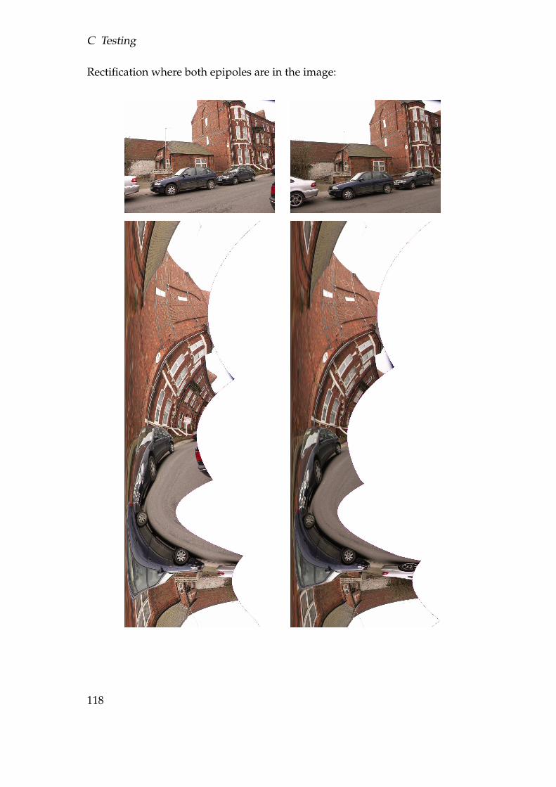
C Testing

Rectification where both epipoles are in the image:

118

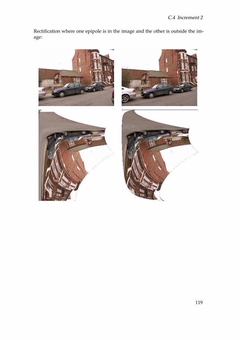
C.4 Increment 2

Rectification where one epipole is in the image and the other is outside the im-age:

119

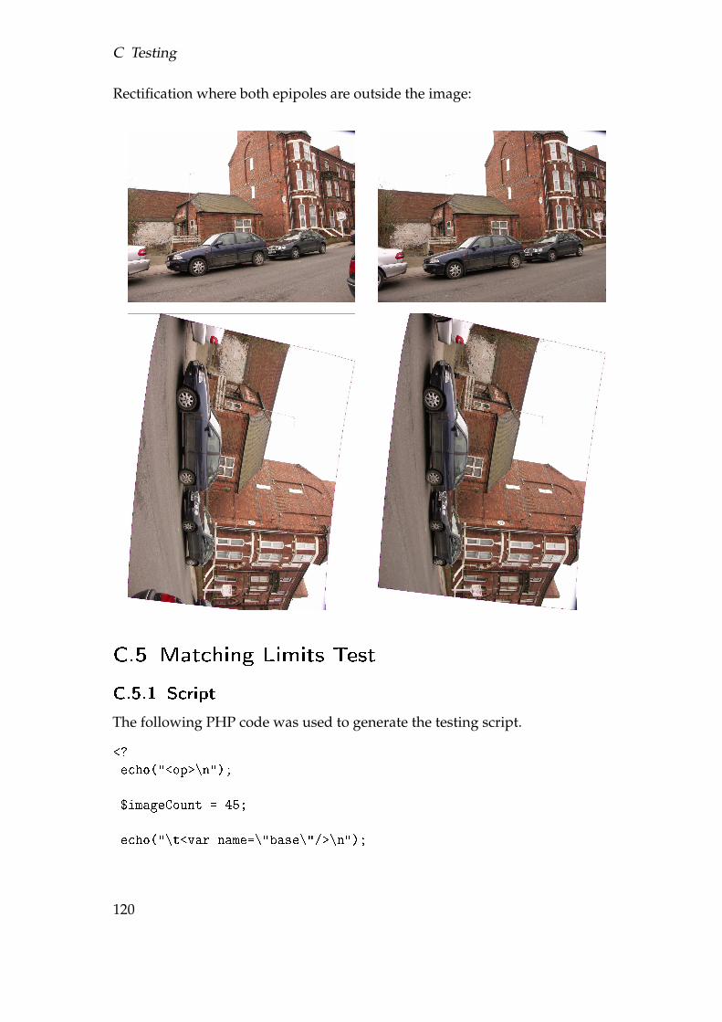
C Testing

Rectification where both epipoles are outside the image:

C.5 Matching Limits Test

C.5.1 Script

The following PHP code was used to generate the testing script.

<?

echo("<op>\n");

$imageCount = 45;

echo("\t<var name=\"base\"/>\n");

120

C.5 Matching Limits Test

echo("\t<op name=\"image.io.load\" out=\"base\">

<file value=\"0.jpg\"/></op>\n");

echo("\t<var name=\"base-grey\"/>\n");

echo("\t<op name=\"image.filter.grey\" in=\"base\"

out=\"base-grey\"/>\n");

echo("\t<var name=\"base-cm\"/>\n");

echo("\t<op name=\"features.corner.harris\" in=\"base-grey\"

out=\"base-cm\" sd=\"0.7\" border=\"3\" res=\"1\"/>\n");

echo("\t<var name=\"base-c\"/>\n");

echo("\t<op name=\"features.prune.area\" in=\"base-cm,base-grey\"

out=\"base-c\" divx=\"32\" divy=\"24\" count=\"4\"

max=\"8000\"/>\n");

echo("\n");

for ($i=1;$i<=$imageCount;$i++)

{

echo("\t<op uses=\"base-grey,base-c\">\n");

echo("\t\t<var name=\"img\"/>\n");

echo("\t\t<op name=\"image.io.load\" out=\"img\">

<file value=\"$i.jpg\"/></op>\n");

echo("\t\t<var name=\"img-grey\"/>\n");

echo("\t\t<op name=\"image.filter.grey\" in=\"img\"

out=\"img-grey\"/>\n");

echo("\t\t<var name=\"img-cm\"/>\n");

echo("\t\t<op name=\"features.corner.harris\" in=\"img-grey\"

out=\"img-cm\" sd=\"0.7\" border=\"3\" res=\"1\"/>\n");

echo("\t\t<var name=\"img-c\"/>\n");

echo("\t\t<op name=\"features.prune.area\" in=\"img-cm,img-grey\"

out=\"img-c\" divx=\"32\" divy=\"24\" count=\"4\"

max=\"8000\"/>\n");

echo("\n");

echo("\t\t<op name=\"msg\" msg=\"$i...\"/>\n");

echo("\n");

echo("\t\t<var name=\"ncc\"/>\n");

echo("\t\t<op name=\"features.match.ncc\"

in=\"base-c,base-grey,img-c,img-grey\" out=\"ncc\"

area=\"3\" res=\"1\" max=\"0.1\"/>\n");

echo("\t\t<var name=\"mat\"/>\n");

echo("\t\t<op name=\"features.select.advanced\" in=\"base-c,img-c,ncc\"

out=\"mat\" cutoff=\"0.9\" slice=\"0.9\" set=\"1.1\" iter=\"10\"/>\n");

echo("\t\t<var name=\"fun\"/>\n");

121

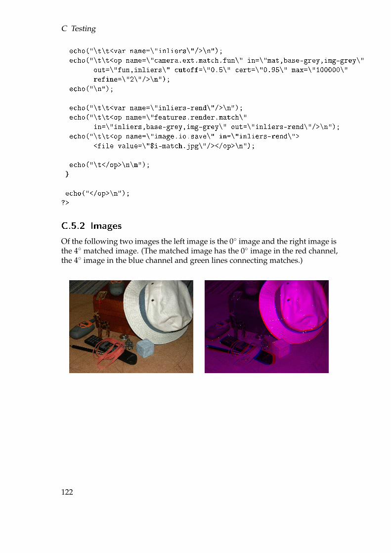
C Testing

echo("\t\t<var name=\"inliers\"/>\n");

echo("\t\t<op name=\"camera.ext.match.fun\" in=\"mat,base-grey,img-grey\"

out=\"fun,inliers\" cutoff=\"0.5\" cert=\"0.95\" max=\"100000\"

refine=\"2\"/>\n");

echo("\n");

echo("\t\t<var name=\"inliers-rend\"/>\n");

echo("\t\t<op name=\"features.render.match\"

in=\"inliers,base-grey,img-grey\" out=\"inliers-rend\"/>\n");

echo("\t\t<op name=\"image.io.save\" in=\"inliers-rend\">

<file value=\"$i-match.jpg\"/></op>\n");

echo("\t</op>\n\n");

}

echo("</op>\n");

?>

C.5.2 Images

Of the following two images the left image is the 0◦ image and the right image isthe 4◦ matched image. (The matched image has the 0◦ image in the red channel,the 4◦ image in the blue channel and green lines connecting matches.)

122