the statistics of supersonic isothermal turbulence

THE STATISTICS OF SUPERSONIC ISOTHERMAL TURBULENCE

Alexei G. Kritsuk,1Michael L. Norman, Paolo Padoan, and Rick Wagner

Department of Physics and Center for Astrophysics and Space Sciences, University of California, San Diego, 9500 Gilman Drive,

La Jolla, CA 92093-0424; [email protected], [email protected], [email protected]

Received 2006 December 11; accepted 2007 April 27

ABSTRACT

We present results of large-scale three-dimensional simulations of supersonic Euler turbulence with the piece-wise parabolic method and multiple grid resolutions up to 20483 points. Our numerical experiments describe non-magnetized driven turbulent flows with an isothermal equation of state and an rms Mach number of 6. We discussnumerical resolution issues and demonstrate convergence, in a statistical sense, of the inertial range dynamics insimulations on grids larger than 5123 points. The simulations allowed us to measure the absolute velocity scalingexponents for the first time. The inertial range velocity scaling in this strongly compressible regime deviates sub-stantially from the incompressible Kolmogorov laws. The slope of the velocity power spectrum, for instance, is�1.95 compared to�5/3 in the incompressible case. The exponent of the third-order velocity structure function is1.28, while in incompressible turbulence it is known to be unity. We propose a natural extension of Kolmogorov’sphenomenology that takes into account compressibility by mixing the velocity and density statistics and preservesthe Kolmogorov scaling of the power spectrum and structure functions of the density-weighted velocity v � �1=3u.The low-order statistics of v appear to be invariant with respect to changes in the Mach number. For instance, atMach 6 the slope of the power spectrum of v is�1.69, and the exponent of the third-order structure function of v isunity. We also directly measure the mass dimension of the ‘‘fractal’’ density distribution in the inertial subrange,Dm � 2:4, which is similar to the observed fractal dimension of molecular clouds and agrees well with the cascadephenomenology.

Subject headinggs: hydrodynamics — instabilities — ISM: structure — methods: numerical — turbulence

Online material: color figures

1. INTRODUCTION

Understanding the nature of supersonic turbulence is of fun-damental importance in both astrophysics and aeronautical engi-neering. In the interstellar medium (ISM), highly compressibleturbulence is believed to control star formation in densemolecularclouds (Padoan & Nordlund 2002). In radiation-driven outflowsfrom carbon-dominant Wolf-Rayet stars, supersonic turbulencecreates highly clumpy structure that is stochastically variableon a very short timescale (e.g., Acker et al. 2002). Finally, awhole class of more terrestrial applications deals with the dragand stability of projectiles traveling through the air at hyper-sonic speeds.

Molecular clouds have an extremely inhomogeneous structure,and the intensity of their internal motions corresponds to an rmsMach number of order 20. Larson (1981) has demonstrated thatwithin the range of scales from 0.1 to 100 pc, the gas density andthe velocity dispersion tightly correlate with the cloud size.2 Sup-ported by other independent observational facts indicating scaleinvariance, these relationships are often interpreted in termsof supersonic turbulence with characteristic Reynolds numbersRe � 108 (Elmegreen & Scalo 2004). Within a wide range ofdensities above 103 cm�3, the gas temperature remains close to�10 K, since the thermal equilibration time at these densities isshorter than a typical hydrodynamic (HD) timescale. Thus, an

isothermal equation of state can be used as a reasonable ap-proximation. Self-gravity, magnetic fields, chemistry, cooling,and heating, as well as radiative transfer, should ultimately beaccounted for in turbulent models of molecular clouds. How-ever, since highly compressible turbulence still remains an un-solved problem even in the absence of magnetic fields, our mainfocus here is specifically on the more tractable HD aspects of theproblem.Magnetic fields are important for the general ISM dynamics

and, particularly, for the star formation process. Observations ofmolecular clouds are consistent with the presence of super-Alfvenic turbulence (Padoan et al. 2004a), and thus, the averagemagnetic field strength may be much smaller than required tosupport the clouds against the gravitational collapse (Padoan &Nordlund 1997, 1999). Even weak fields, however, have the po-tential to modify the properties of supersonic turbulent flowsthrough the effects of magnetic tension and magnetic pressureand introduce small-scale anisotropies. Magnetic tension tendsto stabilize hydrodynamically unstable postshock shear layers(Miura & Pritchett 1982; Keppens et al. 1999; Ryu et al. 2000;Baty et al. 2003). The shock jump conditions modified by mag-netic pressure result in substantially different predictions for theinitial mass function of stars forming in nonmagnetic and mag-netized cases via turbulent fragmentation (Padoan et al. 2007).Remarkably, although not surprisingly (e.g., Armi & Flament1985), the impact of magnetic field on the low-order statistics ofsuper-Alfvenic turbulence appears to be rather limited. At a gridresolution of 10243 points, the slopes of the power spectra in oursimulations show stronger sensitivity to the numerical diffusivityof the scheme of choice than to the presence of the magnetic field(Padoan et al. 2007). The similarity of nonmagnetized andweakly

A

1 Also at: Sobolev Astronomical Institute, St. Petersburg State University,St. Petersburg, Russia.

2 For an earlier version of what is now known as Larson’s relations, seeKaplan & Pronik (1953) and also see Brunt (2003) for the latest results on thevelocity dispersionYcloud size relation.

416

The Astrophysical Journal, 665:416Y431, 2007 August 10

# 2007. The American Astronomical Society. All rights reserved. Printed in U.S.A.

magnetized turbulence will allow us to compare our HD resultswith those from super-Alfvenic magnetohydrodynamic (MHD)simulations where equivalent pure HD simulations are not avail-able in the literature.

Numerical simulations of decaying supersonic HD turbulencewith the piecewise parabolic method (PPM) in two dimensionswere pioneered by Passot et al. (1988)3 and then followed up withhigh-resolution two- and three-dimensional simulations by Porteret al. (1992a, 1992b, 1994, 1998). Sytine et al. (2000) comparedthe results of PPM Euler computations with PPM Navier-Stokesresults and showed that the Euler simulations agree well with thehigh-Re limit attained in the Navier-Stokes models. The conver-gence in a statistical sense as well as the direct comparison ofstructures in configuration space indicate the ability of PPM toaccurately simulate turbulent flows over a wide range of scales.More recently, Porter et al. (2002) discussed measures of inter-mittency in simulated driven transonic flows at Mach numbers ofthe order unity on grids of up to 5123 points. Porter et al. (1999)review the results of these numerical studies, focusing on theorigin and evolution of turbulent structures in physical spaceas well as on scaling laws for two-point structure functions. Oneof the important results of this fundamental work is the demon-stration of the compatibility of a Kolmogorov-type (Kolmogorov1941a, hereafter K41) spectrum with a mild gas compressibilityat transonic Mach numbers.

Since most of the computations discussed above assume aperfect gas equation of state with the ratios of specific heat � ¼7/5 or 5/3 and Mach numbers generally below 2, the questionremains whether this result will still hold for near isothermalconditions and hypersonic Mach numbers characteristic of denseparts of star-forming molecular clouds where the gas compress-ibility is much higher. What kind of coherent structures shouldone expect to see in highly supersonic turbulence? Do low-orderstatistics of turbulence follow the K41 predictions closely in thisregime? How can the statistical diagnostics traditionally used instudies of incompressible turbulence be extended to reconstructthe energy cascade properties in supersonic flows? How can wemeasure the intrinsic intermittency of supersonic turbulence?Many of these and similar questions can only be addressed withnumerical simulations of sufficiently high resolution. The inter-pretation of astronomical data from new surveys of the cold ISMand dust in the Milky Way by the Spitzer and Herschel SpaceObservatory satellites requires more detailed knowledge of thesebasic properties of supersonic turbulence.

In this paper we report the results from large-scale numer-ical simulations of driven supersonic isothermal turbulence atMach 6 with PPM and grid resolutions up to 20483 points. Thepaper is organized as follows. Section 2 contains the details ofthe simulations’ setup and describes the input parameters. Thestatistical diagnostics, including power spectra of the velocity,the kinetic energy, and the density, and velocity structure func-tions, together with a discussion of turbulent structures andtheir fractal dimension are presented in x 3. In x 3.9 we com-bine the scaling laws determined in our numerical experimentsto verify a simple compressible cascade model proposed byFleck (1996). We also introduce a new variable v � �1=3u thatcontrols the energy transfer rate through the compressible cas-cade. We then summarize the results and discuss possible ways tovalidate our numerical model with astrophysical observations inxx 4 and 5.

2. METHODOLOGY

We use PPM implemented in the Enzo code4 to solve the Eulerequations for the gas density � and the velocity u with a constantexternal acceleration term F,

@t�þ: = (�u) ¼ 0; ð1Þ

@tuþ u = :u ¼ �:�=�þ F; ð2Þ

in a periodic box of linear size L ¼ 1 starting with an initially uni-form density distribution �(x; t ¼ 0) ¼ �0(x) � 1 and assumingthe sound speed c � 1. The equations that were actually numer-ically integrated were written in a conventional form of conser-vation laws for the mass, momentum, and total energy that is lesscompact, but nearly equivalent to equations (1) and (2), since inpractice we mimic the isothermal equation of state by setting thespecific heat ratio in the ideal gas equation of state very close tounity, � ¼ 1:001.

The simulations were initialized on grids of 2563 or 5123 pointswith a random velocity field u(x; t ¼ 0) ¼ u0(x) / F that con-tains only large-scale power within the range of wavenumbersk /kmin2½1; 2�, where kmin ¼ 2�, and that corresponds to the rmsMach numberM ¼ 6. The dynamical time is hereafter definedas td � L/(2M).

2.1. Uniform Grid Simulation at 10243

Our major production run is performed on a grid of 10243

points that allowed us to resolve a portion of the uncontaminatedinertial range sufficient to get a first approximation for the low-order scaling exponents. We started the simulation at a lowerresolution of 5123 points and evolved the flow from the initialconditions for five dynamical times to stir up the gas in the box.Then we doubled the resolution and evolved the simulation foranother 5td on a grid of 10243 points.

The time-average statisticswere computed using 170 snapshotsevenly spaced in time over the final segment of 4td . (We allowedone dynamical time for flow relaxation at high resolution, sothat it could reach a statistical steady state after regridding.) Weused the full set of 170 snapshots to derive the density statistics,since the density field displays a very high degree of intermittency.This gave us a very large statistical sample, e.g., 2 ; 1011 measure-ments were available to determine the probability density function(PDF) of the gas density discussed in x 3.2. The time-averagepower spectra discussed in xx 3.3, 3.5, 3.6, and 3.9 are also basedon the full data set. The velocity structure functions presented inx 3.4 are derived from a sample of 20% of the snapshots coveringthe same period of 4td . The corresponding two-point PDFs ofvelocity differences were built on (2Y4) ; 109 pairs per snapshoteach, depending on the pair separation.

2.2. AMR Simulations

The adaptive mesh refinement (AMR) simulations with effec-tive resolution of 20483 points were also initialized by evolvingthe flow on the root grid of 5123 points for six dynamical times.Then one level of refinement by a factor of 4 was added in bothcases that covers on average 50% of the domain volume. Thegrid is refined to better resolve strong shocks and to captureHD instabilities in the layers of strong shear. We use the nativeshock-detection algorithm of PPM, and we flag for refinementthose zones that are associated with shocks with density jumps in

3 See a review on compressible turbulence by Pouquet et al. (1991) for ref-erences to earlier works. 4 See http://lca.ucsd.edu/.

SIMULATIONS OF SUPERSONIC TURBULENCE 417

excess of 2. We also track shear layers using the Frobenius normk@iuj(1� �ij)kF (see also Kritsuk et al. 2006). This second re-finement criterion adds about 20% more flagged zones thatwould be left unrefined if only the refinement on shocks wereused. The simulations were continued with AMR for only 1:2td ,which allows enough time for relaxation of the flow at high res-olution, but does not allow us to perform time-averaging overmany statistically independent snapshots. Therefore, we use thedata from AMR simulations mostly to compare the quality of in-stantaneous statistical quantities from simulations with adaptiveand nonadaptive meshes.

2.3. Random Forcing

The initial velocity field is used, after an appropriate renorm-alization, as a steady random force (acceleration) to keep the to-tal kinetic energy within the box on an approximately constantlevel during the simulations. The force we applied is isotropicin terms of the total specific kinetic energy per dimension,u20; x ¼ u2

0; y ¼ u20; z, but its solenoidal (: = u0;S � 0) and dilata-

tional (: < u0;D � 0) components are anisotropic, since one ofthe three directions is dominated by the large-scale compressionalmodes, while the other two aremostly solenoidal. The distributionof the total specific kinetic energy

E � 1

2

ZVu2 dV ¼ ES þ ED ð3Þ

between the solenoidal ES and dilatational ED components issuch that �0 � E0;S /E0 � 0:6. The forcing field is helical, butthe mean helicity is very low, h0

2Th20, where the helicity h isdefined as

h � u = : < u: ð4Þ

Note that in compressible flows with an isothermal equation ofstate the mean helicity is conserved, as in the incompressiblecase, since the Ertel’s potential vorticity is identically zero(Gaffet 1985).

3. RESULTS

In this sectionwe start with a general quantitative description ofour simulated turbulent flows and then derive their time-averagestatistical properties. We end upwith assembling the pieces of this

statistical picture in a context of a simple cascade model thatextends the Kolmogorov phenomenology of incompressible tur-bulence into the compressible regime.

3.1. Time-Evolution of Global Variables

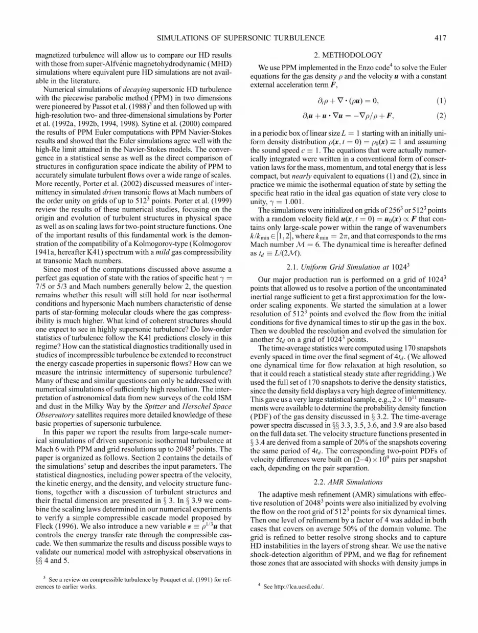
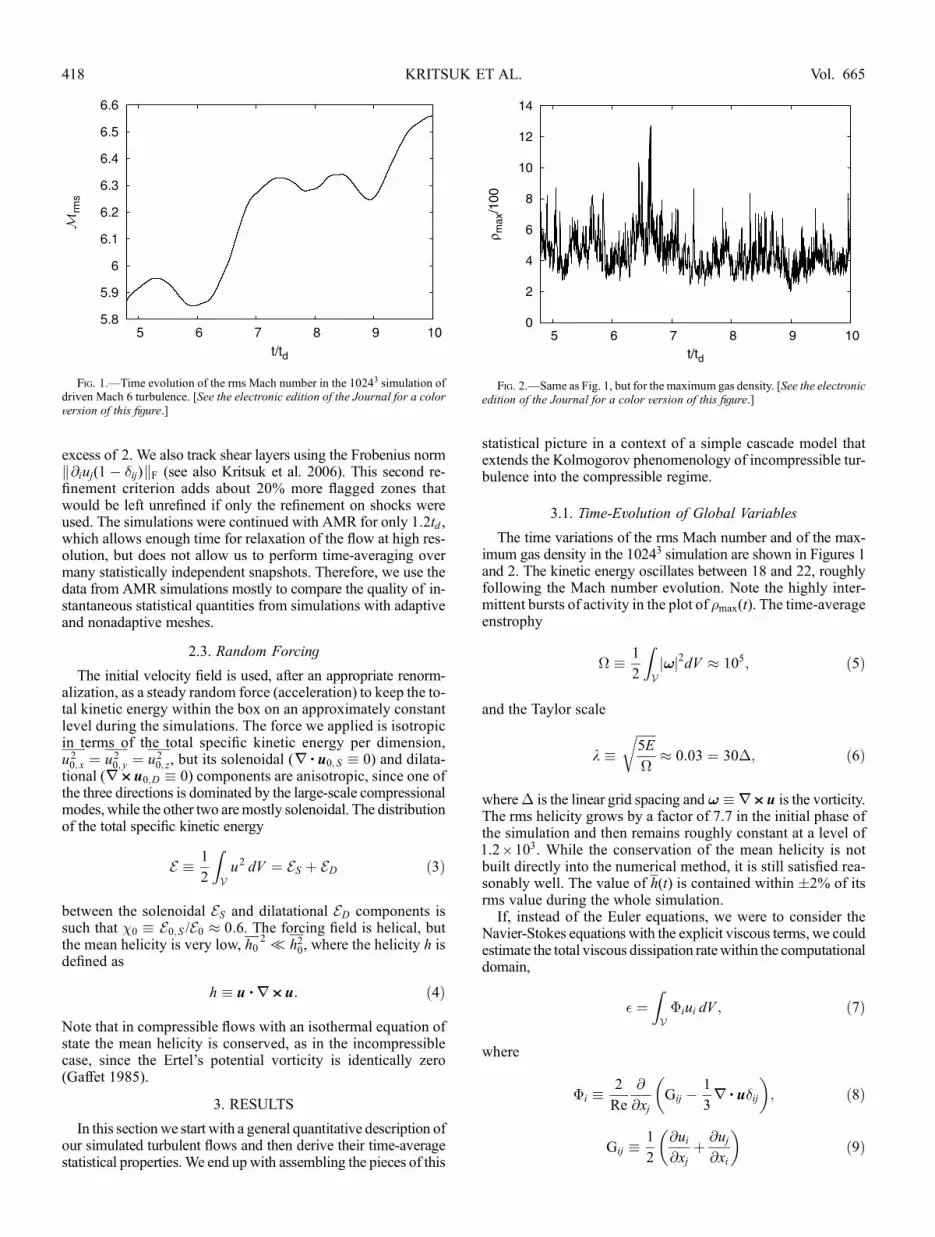
The time variations of the rms Mach number and of the max-imum gas density in the 10243 simulation are shown in Figures 1and 2. The kinetic energy oscillates between 18 and 22, roughlyfollowing the Mach number evolution. Note the highly inter-mittent bursts of activity in the plot of �max(t). The time-averageenstrophy

� � 1

2

ZVwj j2dV � 105; ð5Þ

and the Taylor scale

k �ffiffiffiffiffiffi5E

�

r� 0:03 ¼ 30�; ð6Þ

where� is the linear grid spacing andw � : < u is the vorticity.The rms helicity grows by a factor of 7.7 in the initial phase ofthe simulation and then remains roughly constant at a level of1:2 ; 103. While the conservation of the mean helicity is notbuilt directly into the numerical method, it is still satisfied rea-sonably well. The value of h(t) is contained within �2% of itsrms value during the whole simulation.If, instead of the Euler equations, we were to consider the

Navier-Stokes equations with the explicit viscous terms, we couldestimate the total viscous dissipation ratewithin the computationaldomain,

� ¼ZV�iui dV ; ð7Þ

where

�i �2

Re

@

@xjGij �

1

3: = u�ij

� �; ð8Þ

Gij �1

2

@ui@xj

þ @uj@xi

� �ð9Þ

Fig. 1.—Time evolution of the rms Mach number in the 10243 simulation ofdriven Mach 6 turbulence. [See the electronic edition of the Journal for a colorversion of this figure.]

Fig. 2.—Same as Fig. 1, but for the maximum gas density. [See the electronicedition of the Journal for a color version of this figure.]

KRITSUK ET AL.418 Vol. 665

is the symmetric rate-of-strain tensor, and the integration is doneover the volume of the domain V ¼ 1. Using vector identities,%can be rewritten through the vorticityw and the dilatation: = u as

% ¼ � 1

Re: < w� 4

3:: = u

� �; ð10Þ

and, by partial integration in equation (7),

� ¼ � 1

Rej: < uj2

D Eþ 4

3j: = uj2

D E� �; ð11Þ

where the two terms on the right-hand side of equation (11) de-scribe the mean dissipation rate due to solenoidal and dilatationalvelocities, respectively, � ¼ �S þ �D.

In our Euler simulations, the role of viscous dissipation isplayed by the numerical diffusivity of PPM. This numerical dis-sipation does not necessarily have the same or similar functionalform as the one used in the Navier-Stokes equations. It is stillinstructive, however, to get a flavor of the numerical dissipationrate by studying the properties of the vorticity and dilatation. Theso-called small-scale compressive ratio (Kida & Orszag 1990,1992),

rcs �j: = uj2

D Ej: = uj2

D Eþ j: < uj2D E ; ð12Þ

represents the relative importance of the dilatational componentat small scales. The time-average rcs � 0:28. Themean fraction ofthe dissipation rate that depends solely on the solenoidal velocitycomponent �S /� � 0:65. Even though the two-dimensional shockfronts are dominating the geometry of the density distribution inthe dissipation range (see x 3.8), the dissipation rate itself isdominated by the solenoidal velocity component that tracks cor-rugated shocks due to vortex stretching in the associated strongshear flows.

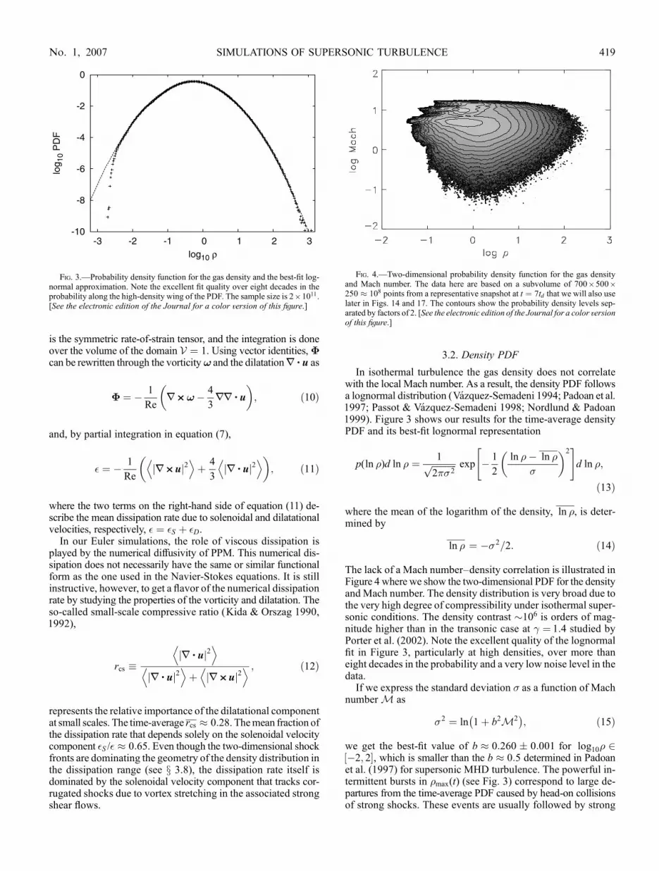
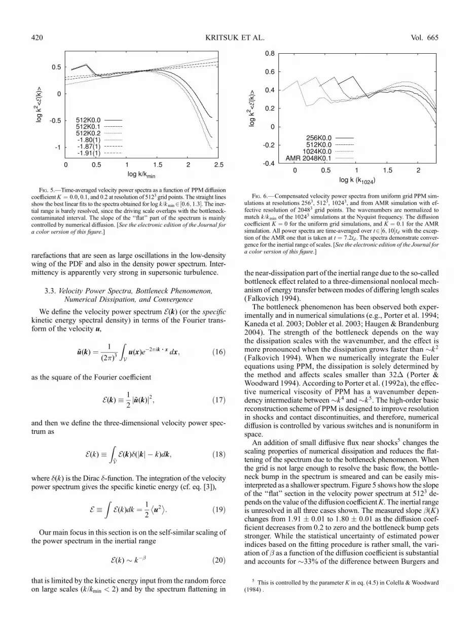
3.2. Density PDF

In isothermal turbulence the gas density does not correlatewith the local Mach number. As a result, the density PDF followsa lognormal distribution (Vazquez-Semadeni 1994; Padoan et al.1997; Passot & Vazquez-Semadeni 1998; Nordlund & Padoan1999). Figure 3 shows our results for the time-average densityPDF and its best-fit lognormal representation

p(ln �)d ln � ¼ 1ffiffiffiffiffiffiffiffiffiffiffi2��2

p exp � 1

2

ln �� ln �

�

� �2" #

d ln �;

ð13Þ

where the mean of the logarithm of the density, ln �, is deter-mined by

ln � ¼ ��2=2: ð14Þ

The lack of a Mach numberYdensity correlation is illustrated inFigure 4 where we show the two-dimensional PDF for the densityand Mach number. The density distribution is very broad due tothe very high degree of compressibility under isothermal super-sonic conditions. The density contrast �106 is orders of mag-nitude higher than in the transonic case at � ¼ 1:4 studied byPorter et al. (2002). Note the excellent quality of the lognormalfit in Figure 3, particularly at high densities, over more thaneight decades in the probability and a very low noise level in thedata.

If we express the standard deviation � as a function of Machnumber M as

�2 ¼ ln 1þ b2M2� �

; ð15Þ

we get the best-fit value of b � 0:260 � 0:001 for log10� 2½�2; 2�, which is smaller than the b � 0:5 determined in Padoanet al. (1997) for supersonic MHD turbulence. The powerful in-termittent bursts in �max(t) (see Fig. 3) correspond to large de-partures from the time-average PDF caused by head-on collisionsof strong shocks. These events are usually followed by strong

Fig. 3.—Probability density function for the gas density and the best-fit log-normal approximation. Note the excellent fit quality over eight decades in theprobability along the high-density wing of the PDF. The sample size is 2 ; 1011.[See the electronic edition of the Journal for a color version of this figure.]

Fig. 4.—Two-dimensional probability density function for the gas densityand Mach number. The data here are based on a subvolume of 700 ; 500 ;250 � 108 points from a representative snapshot at t ¼ 7td that we will also uselater in Figs. 14 and 17. The contours show the probability density levels sep-arated by factors of 2. [See the electronic edition of the Journal for a color versionof this figure.]

SIMULATIONS OF SUPERSONIC TURBULENCE 419No. 1, 2007

rarefactions that are seen as large oscillations in the low-densitywing of the PDF and also in the density power spectrum. Inter-mittency is apparently very strong in supersonic turbulence.

3.3. Velocity Power Spectra, Bottleneck Phenomenon,Numerical Dissipation, and Convergence

We define the velocity power spectrum E(k) (or the specifickinetic energy spectral density) in terms of the Fourier trans-form of the velocity u,

u(k) ¼ 1

(2�)3

ZVu(x)e�2�ik = x dx; ð16Þ

as the square of the Fourier coefficient

E(k) � 1

2u(k)j j2; ð17Þ

and then we define the three-dimensional velocity power spec-trum as

E(k) �ZVE(k)�(jkj � k)dk; ð18Þ

where �(k) is the Dirac �-function. The integration of the velocitypower spectrum gives the specific kinetic energy (cf. eq. [3]),

E �Z

E(k)dk ¼ 1

2u2� �

: ð19Þ

Our main focus in this section is on the self-similar scaling ofthe power spectrum in the inertial range

E(k) � k�� ð20Þ

that is limited by the kinetic energy input from the random forceon large scales (k /kmin < 2) and by the spectrum flattening in

the near-dissipation part of the inertial range due to the so-calledbottleneck effect related to a three-dimensional nonlocal mech-anism of energy transfer between modes of differing length scales(Falkovich 1994).The bottleneck phenomenon has been observed both exper-

imentally and in numerical simulations (e.g., Porter et al. 1994;Kaneda et al. 2003; Dobler et al. 2003; Haugen & Brandenburg2004). The strength of the bottleneck depends on the waythe dissipation scales with the wavenumber, and the effect ismore pronounced when the dissipation grows faster than �k 2

(Falkovich 1994). When we numerically integrate the Eulerequations using PPM, the dissipation is solely determined bythe method and affects scales smaller than 32� (Porter &Woodward 1994). According to Porter et al. (1992a), the effec-tive numerical viscosity of PPM has a wavenumber depen-dency intermediate between�k 4 and�k 5. The high-order basicreconstruction scheme of PPM is designed to improve resolutionin shocks and contact discontinuities, and therefore, numericaldiffusion is controlled by various switches and is nonuniform inspace.An addition of small diffusive flux near shocks5 changes the

scaling properties of numerical dissipation and reduces the flat-tening of the spectrum due to the bottleneck phenomenon. Whenthe grid is not large enough to resolve the basic flow, the bottle-neck bump in the spectrum is smeared and can be easily mis-interpreted as a shallower spectrum. Figure 5 shows how the slopeof the ‘‘flat’’ section in the velocity power spectrum at 5123 de-pends on the value of the diffusion coefficientK. The inertial rangeis unresolved in all three cases shown. The measured slope �(K)changes from 1:91 � 0:01 to 1:80 � 0:01 as the diffusion coef-ficient decreases from 0.2 to zero and the bottleneck bump getsstronger. While the statistical uncertainty of estimated powerindices based on the fitting procedure is rather small, the vari-ation of � as a function of the diffusion coefficient is substantialand accounts for �33% of the difference between Burgers and

5 This is controlled by the parameter K in eq. (4.5) in Colella & Woodward(1984) .

Fig. 5.—Time-averaged velocity power spectra as a function of PPM diffusioncoefficientK ¼ 0:0, 0.1, and 0.2 at resolution of 5123 grid points. The straight linesshow the best linear fits to the spectra obtained for log k /kmin2½0:6; 1:3�. The iner-tial range is barely resolved, since the driving scale overlaps with the bottleneck-contaminated interval. The slope of the ‘‘flat’’ part of the spectrum is mainlycontrolled by numerical diffusion. [See the electronic edition of the Journal fora color version of this figure.]

Fig. 6.—Compensated velocity power spectra from uniform grid PPM sim-ulations at resolutions 2563, 5123, 10243, and from AMR simulation with ef-fective resolution of 20483 grid points. The wavenumbers are normalized tomatch k /kmin of the 1024

3 simulations at the Nyquist frequency. The diffusioncoefficient K ¼ 0 for the uniform grid simulations, and K ¼ 0:1 for the AMRsimulation. All power spectra are time-averaged over t2½6; 10�td with the excep-tion of the AMR one that is taken at t ¼ 7:2td . The spectra demonstrate conver-gence for the inertial range of scales. [See the electronic edition of the Journal fora color version of this figure.]


Kolmogorov slopes. Clearly, it is difficult to get reliable estimatesfor the inertial range power indices from simulations with reso-lution up to 5123, since the slope of the spectrum is so dependenton numerical diffusivity. To study higher Mach number flowswith PPM, an even higher resolution would be required. Notethat with other numerical methods, one typically needs to useeven larger grids, since the amount of dissipation provided byPPM is quite small compared to what is usually given in finite-difference schemes. In low-resolution simulations with high nu-merical dissipation that depends on the wavenumber as �k2 orweaker, the power spectra appear steeper than they would havebeen when properly resolved.

In simulations with AMR, the grid resolution is nonuniform,and scale dependence (as well as nonuniformity) of numerical dif-fusion becomes evenmore complex. One should generally expecta more extended range of wavenumbers affected by numericaldissipation in AMR simulations than in uniform grid simulations,when the effective resolution is the same. The dependence of theeffective numerical diffusivity on the wavenumber in the AMRruns is, therefore, weaker than in simulations on uniform grids,and the bottleneck bump should be suppressed.

In Figure 6 we combined the velocity power spectra from theunigrid simulations at 2563, 5123, and 10243 grid points with thediffusion coefficient K ¼ 0 to illustrate the convergence ofthe inertial range scaling with the improved resolution. All threesimulations were performed with the same large-scale drivingforce, and the spectra were averaged over the same time interval,so the only difference between them is the resolution-controlledeffective Reynolds number. We plotted the compensated spectrak 2E(k) to specifically exaggerate the relatively small changes inthe slopes. The overplotted power spectrum from a single snap-shot from our largest to date AMR simulation with the effectiveresolution of 20483 grid points seems to confirm the (self-) con-vergence. Thus, one may hope that our estimates of the scalingexponents based on the time-averaged statistics from the 10243

simulation will not be too far off from those that correspond toRe ! 1. We further validate this statement in x 3.4, where wediscuss the scaling properties of the velocity structure functions.Note also the suppression of the bottleneck bump visible in theAMR spectrum that occurs due to the higher effective diffusivityas we discussed earlier.

Our reference velocity power spectrum from the 10243 sim-ulation is repeated in Figure 7 with the best-fit linear approx-imations. It follows a power law with an index � ¼ 1:95 � 0:02within the range of scales l2½40; 256�� and has a shallowerslope, �b ¼ 1:72, for the bottleneck bump. After Helmholtz de-composition, E(k) ¼ ES(k)þ ED(k), the spectra for the solenoidaland dilatational components show the inertial range power indicesof �S ¼ 1:92 � 0:02 and �D ¼ 2:02 � 0:02, respectively (seeFigs. 8 and 9). The difference in the slopes of ES(k) and ED(k) isabout 5 �, i.e., significant. Both spectra display flattening due tothe bottleneck with indices of �b;S ¼ 1:70 and �b;D ¼ 1:74 inthe near-dissipative range. The fraction of energy in dilatationalmodes quickly drops from about 50% at k ¼ kmin down to 30%at k /kmin � 50 and then returns back to a level of 45% at theNyquist frequency.

In summary, the inertial range scaling of the velocity powerspectrum in highly compressible turbulence tends to be closer tothe Burgers scaling with a power index of � ¼ 2 rather than tothe Kolmogorov � ¼ 5/3 scaling suggested for the mildly com-pressible transonic simulations by Porter et al. (2002). The inertialrange scaling exponents of the power spectra for the solenoidaland dilatational velocities are not the same, with the latter dem-onstrating a steeper Burgers scaling, containing about 30% of the

Fig. 7.—Velocity power spectrum compensated by k2. Note a large-scale ex-cess of power at l2½256; 1024�� due to external forcing, a short straight section inthe uncontaminated inertial subrange l2½40; 256��, and a small-scale excess atl < 40� due to the bottleneck phenomenon. The straight lines represent the least-squares fits to the data for log k /kmin2½0:6; 1:1� and log k /kmin2½1:2; 1:7�. [See theelectronic edition of the Journal for a color version of this figure.]

Fig. 8.—Same as Fig. 7, but for the solenoidal velocity component. [See theelectronic edition of the Journal for a color version of this figure.]

Fig. 9.—Same as Fig. 7, but for the dilatational velocity component. [See theelectronic edition of the Journal for a color version of this figure.]


total specific kinetic energy, and being responsible for up to 35%of the global dissipation rate (see x 3.1).

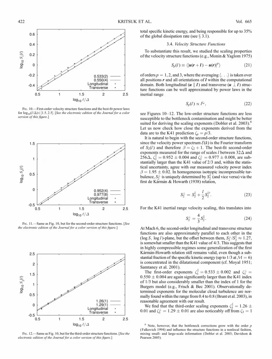
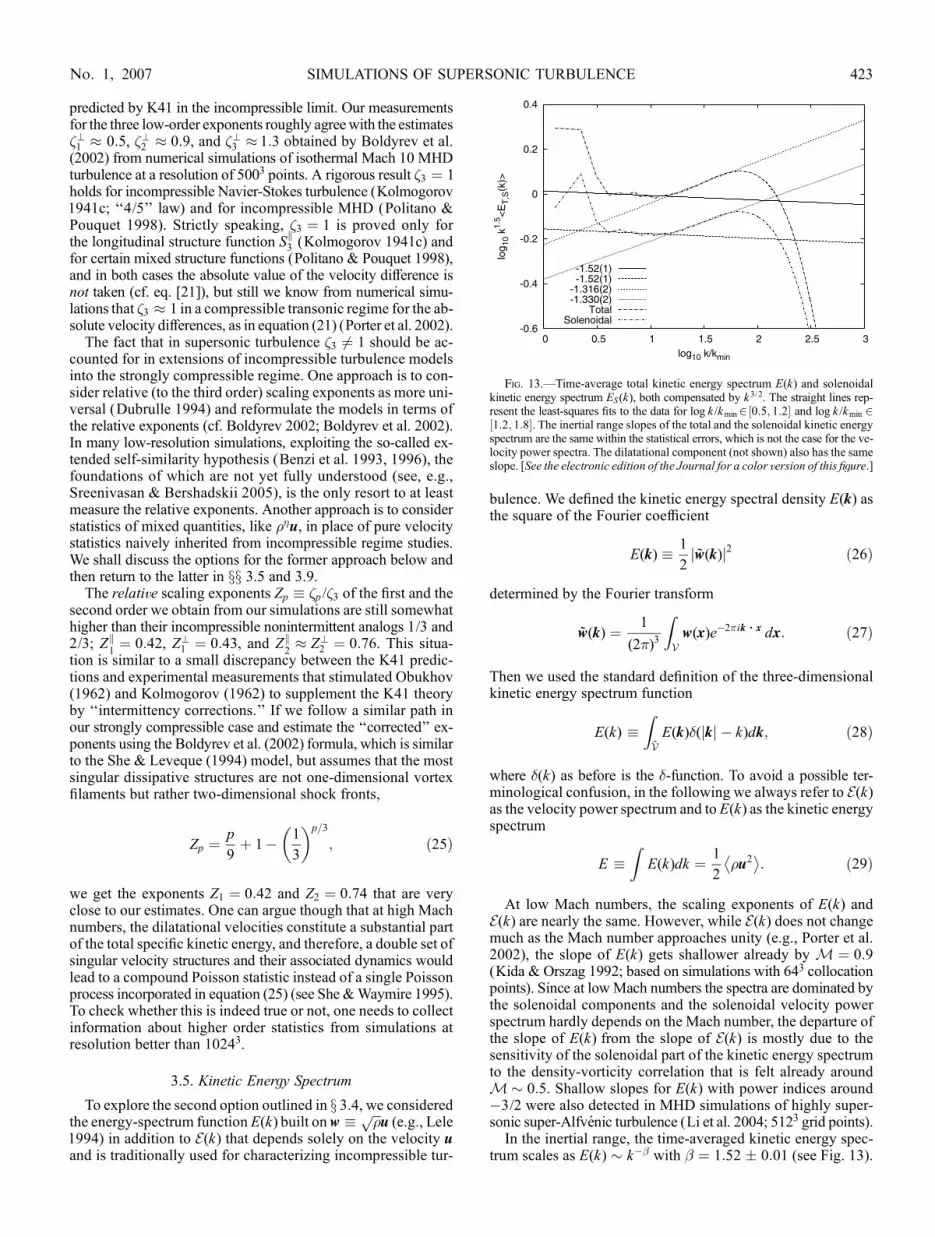
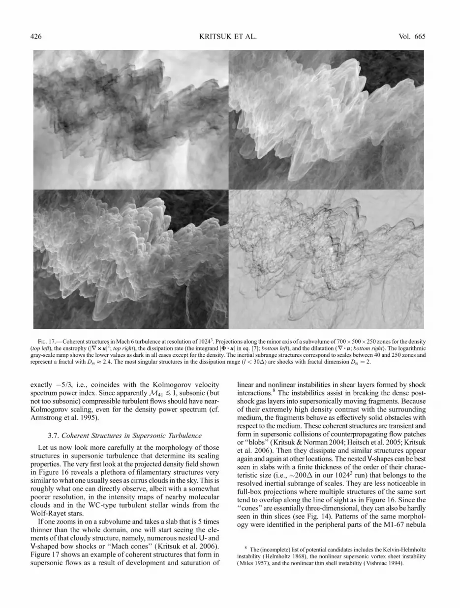
3.4. Velocity Structure Functions

To substantiate this result, we studied the scaling propertiesof the velocity structure functions (e.g., Monin &Yaglom 1975)

Sp(l ) � u(rþ l )� u(r)j jph i ð21Þ

of orders p ¼ 1, 2, and 3, where the averaging h: : :i is taken overall positions r and all orientations of l within the computationaldomain. Both longitudinal (u k l ) and transverse (u ? l ) struc-ture functions can be well approximated by power laws in theinertial range

Sp(l ) / lp ; ð22Þ

see Figures 10Y12. The low-order structure functions are lesssusceptible to the bottleneck contamination and might be bettersuited for deriving the scaling exponents (Dobler et al. 2003).6

Let us now check how close the exponents derived from thedata are to the K41 prediction p ¼ p/3.It is natural to begin with the second-order structure functions,

since the velocity power spectrum E(k) is the Fourier transformof S2(l ) and therefore � ¼ 2 þ 1. The best-fit second-orderexponents measured for the range of scales l between 32� and256�,

k2 ¼ 0:952 � 0:004 and ?2 ¼ 0:977 � 0:008, are sub-

stantially larger than the K41 value of 2/3 and, within the statis-tical uncertainty, agree with our measured velocity power index� ¼ 1:95 � 0:02. In homogeneous isotropic incompressible tur-bulence, S?2 is uniquely determined by S

k2 (and vice versa) via the

first de Karman & Howarth (1938) relation,

S?2 ¼ Sk2 þ

l

2Sk02 : ð23Þ

For the K41 inertial range velocity scaling, this translates into

S?2 ¼ 4

3Sk2 : ð24Þ

AtMach 6, the second-order longitudinal and transverse structurefunctions are also approximately parallel to each other in the(log S; log l )-plane, but the offset between them, S?2 /S

k2� 1:27,

is somewhat smaller than the K41 value of 4/3. This suggests thatin highly compressible regimes some generalization of the firstKarman-Howarth relation still remains valid, even though a sub-stantial fraction of the specific kinetic energy (up to 1/3 atM ¼ 6)is concentrated in the dilatational component (cf. Moyal 1951;Samtaney et al. 2001).The first-order exponents

k1 ¼ 0:533 � 0:002 and ?1 ¼

0:550 � 0:004 are again significantly larger than the K41 indexof 1/3 but also considerably smaller than the index of 1 for theBurgers model (e.g., Frisch & Bec 2001). Observationally de-termined exponents for the molecular cloud turbulence are nor-mally foundwithin the range from0.4 to 0.8 (Brunt et al. 2003), inreasonable agreement with our result.We find that the third-order scaling exponents

k3 ¼ 1:26 �

0:01 and ?3 ¼ 1:29 � 0:01 are also noticeably off from 3 ¼ 1

Fig. 10.—First-order velocity structure functions and the best-fit power lawsfor log10(l /�)2½1:5; 2:5�. [See the electronic edition of the Journal for a colorversion of this figure.]

Fig. 11.—Same as Fig. 10, but for the second-order structure functions. [Seethe electronic edition of the Journal for a color version of this figure.]

Fig. 12.—Same as Fig. 10, but for the third-order structure functions. [See theelectronic edition of the Journal for a color version of this figure.]

6 Note, however, that the bottleneck corrections grow with the order p(Falkovich 1994) and influence the structure functions in a nonlocal fashion,mixing small- and large-scale information (Dobler et al. 2003; Davidson &Pearson 2005).


predicted by K41 in the incompressible limit. Our measurementsfor the three low-order exponents roughly agreewith the estimates?1 � 0:5, ?2 � 0:9, and ?3 � 1:3 obtained by Boldyrev et al.(2002) from numerical simulations of isothermal Mach 10 MHDturbulence at a resolution of 5003 points. A rigorous result 3 ¼ 1holds for incompressible Navier-Stokes turbulence (Kolmogorov1941c; ‘‘4/5’’ law) and for incompressible MHD (Politano &Pouquet 1998). Strictly speaking, 3 ¼ 1 is proved only forthe longitudinal structure function S

k3 (Kolmogorov 1941c) and

for certain mixed structure functions (Politano & Pouquet 1998),and in both cases the absolute value of the velocity difference isnot taken (cf. eq. [21]), but still we know from numerical simu-lations that 3 � 1 in a compressible transonic regime for the ab-solute velocity differences, as in equation (21) (Porter et al. 2002).

The fact that in supersonic turbulence 3 6¼ 1 should be ac-counted for in extensions of incompressible turbulence modelsinto the strongly compressible regime. One approach is to con-sider relative (to the third order) scaling exponents as more uni-versal (Dubrulle 1994) and reformulate the models in terms ofthe relative exponents (cf. Boldyrev 2002; Boldyrev et al. 2002).In many low-resolution simulations, exploiting the so-called ex-tended self-similarity hypothesis (Benzi et al. 1993, 1996), thefoundations of which are not yet fully understood (see, e.g.,Sreenivasan & Bershadskii 2005), is the only resort to at leastmeasure the relative exponents. Another approach is to considerstatistics of mixed quantities, like �u, in place of pure velocitystatistics naively inherited from incompressible regime studies.We shall discuss the options for the former approach below andthen return to the latter in xx 3.5 and 3.9.

The relative scaling exponents Zp � p /3 of the first and thesecond order we obtain from our simulations are still somewhathigher than their incompressible nonintermittent analogs 1/3 and2/3; Zk

1¼ 0:42, Z?

1 ¼ 0:43, and Zk2� Z?

2 ¼ 0:76. This situa-tion is similar to a small discrepancy between the K41 predic-tions and experimental measurements that stimulated Obukhov(1962) and Kolmogorov (1962) to supplement the K41 theoryby ‘‘intermittency corrections.’’ If we follow a similar path inour strongly compressible case and estimate the ‘‘corrected’’ ex-ponents using the Boldyrev et al. (2002) formula, which is similarto the She & Leveque (1994) model, but assumes that the mostsingular dissipative structures are not one-dimensional vortexfilaments but rather two-dimensional shock fronts,

Zp ¼p

9þ 1� 1

3

� �p=3

; ð25Þ

we get the exponents Z1 ¼ 0:42 and Z2 ¼ 0:74 that are veryclose to our estimates. One can argue though that at high Machnumbers, the dilatational velocities constitute a substantial partof the total specific kinetic energy, and therefore, a double set ofsingular velocity structures and their associated dynamics wouldlead to a compound Poisson statistic instead of a single Poissonprocess incorporated in equation (25) (see She &Waymire 1995).To check whether this is indeed true or not, one needs to collectinformation about higher order statistics from simulations atresolution better than 10243.

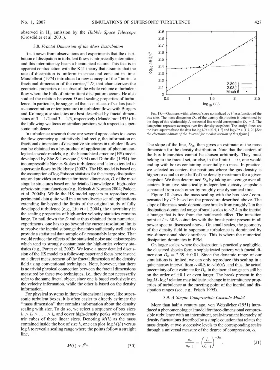
3.5. Kinetic Energy Spectrum

To explore the second option outlined in x 3.4, we consideredthe energy-spectrum function E(k) built onw � ffiffiffi

�p

u (e.g., Lele1994) in addition to E(k) that depends solely on the velocity uand is traditionally used for characterizing incompressible tur-

bulence. We defined the kinetic energy spectral density E(k) asthe square of the Fourier coefficient

E(k) � 1

2w(k)j j2 ð26Þ

determined by the Fourier transform

w(k) ¼ 1

(2�)3

ZVw(x)e�2�ik = x dx: ð27Þ

Then we used the standard definition of the three-dimensionalkinetic energy spectrum function

E(k) �ZVE(k)�(jkj � k)dk; ð28Þ

where �(k) as before is the �-function. To avoid a possible ter-minological confusion, in the following we always refer to E(k)as the velocity power spectrum and to E(k) as the kinetic energyspectrum

E �Z

E(k)dk ¼ 1

2�u2� �

: ð29Þ

At low Mach numbers, the scaling exponents of E(k) andE(k) are nearly the same. However, while E(k) does not changemuch as the Mach number approaches unity (e.g., Porter et al.2002), the slope of E(k) gets shallower already by M ¼ 0:9(Kida & Orszag 1992; based on simulations with 643 collocationpoints). Since at lowMach numbers the spectra are dominated bythe solenoidal components and the solenoidal velocity powerspectrum hardly depends on the Mach number, the departure ofthe slope of E(k) from the slope of E(k) is mostly due to thesensitivity of the solenoidal part of the kinetic energy spectrumto the density-vorticity correlation that is felt already aroundM� 0:5. Shallow slopes for E(k) with power indices around�3/2 were also detected in MHD simulations of highly super-sonic super-Alfvenic turbulence (Li et al. 2004; 5123 grid points).

In the inertial range, the time-averaged kinetic energy spec-trum scales as E(k) � k�� with � ¼ 1:52 � 0:01 (see Fig. 13).

Fig. 13.—Time-average total kinetic energy spectrum E(k) and solenoidalkinetic energy spectrum ES (k), both compensated by k 3

=2. The straight lines rep-resent the least-squares fits to the data for log k /kmin2½0:5; 1:2� and log k /kmin 2½1:2; 1:8�. The inertial range slopes of the total and the solenoidal kinetic energyspectrum are the same within the statistical errors, which is not the case for the ve-locity power spectra. The dilatational component (not shown) also has the sameslope. [See the electronic edition of the Journal for a color version of this figure.]


The spectrum displays flattening at high wavenumbers due to thebottleneck effect, which is similar to what we have already seenin the velocity power spectra E(k). The flat part scales roughlyas�k�1:3 and occupies the same range of wavenumbers as in thevelocity spectrum. Since the kinetic energy spectrum is sensi-tive to the rather sporadic activity of density fluctuations, time-averaging is essential to get a robust estimate for the power index.

We performed a decomposition of w � ffiffiffi�

pu into the solenoi-

dal and dilatational parts wS;D such that : = wS ¼ : < wD � 0and computed the energy spectra for both components, E(k) ¼ES(k)þ ED(k). The inertial range spectral exponents for thesolenoidal and dilatational components are the same, � ¼ 1:52 �0:01 for both, and also coincide with the slope of E(k). Thisremarkable property of E(k) suggests that in the supersonicregime7 we are dealing with a single compressible cascade ofkinetic energy where the density fluctuations provide a tightcoupling between the solenoidal and dilatational modes of w.This picture is similar in spirit to that discussed by Kornreich &Scalo (2000) in their x 3.7. However, in contrast to Kornreich &Scalo (2000) our simulations demonstrate that nonlinear HDinstabilities are heavily involved in the kinetic energy transferthrough the hierarchy of scales. The association of w with thekinetic energy distribution as a function of scale makes this quan-tity a better candidate than the pure velocity u for employing incompressible cascade models, since w uniquely represents thephysics of the cascade and there is no need to track the variationof ED(k)/E(k) as a function of wavenumber in the inertial sub-range in addition to variations with the rms Mach number.

The total kinetic energy power is dominated by the solenoidalcomponentwS over the whole spectrum.Within the inertial range,ES(k) contributes about 68% of the total power, then �66% inthe bottleneck-contaminated interval, and up to �74% furtherdown at the Nyquist frequency. Compare with the solenoidal partof the velocity power, ES(k), that constitutes about 65%Y70%within the inertial range and only 55% of the total power at theNyquist frequency (see x 3.3).

Figure 14 illustrates the difference in structures seen in theenstrophy field (top) and in the ‘‘denstrophy’’ field [j: <(

ffiffiffi�

pu)j2 /�, bottom] that helps to understand the small-scale

excess of power in ES(k) with respect to ES(k). While the corru-gated shock surfaces (U-shapes), which are also the regions ofvery strong shear, are seen as dark wormlike structures of excessenstrophy and denstrophy in both the top and the bottom panelsof Figure 14, nearly planar shock fronts that carry a negligibleamount of shear (this is also why they remain planar) are clearlymissing in the enstrophy plot. Since the denstrophy field containsa greater number of sharper small-scale structures, it should beexpected that ES(k) carries more small-scale power than ES(k).Overall, the structures captured as intense by the denstrophyfield closely follow the regions of high energy dissipation rate(see the integrand in eq. [7] and Fig. 17, bottom left).

3.6. Density Power Spectrum

The power spectrum of the gas density shows a short straightsection with a slope of�1:07 � 0:01 in the range of scales from 250� down to 40� followed by flattening due to a power

pileup at higher wavenumbers (see Fig. 15). Similar power-lawsections and excess of power in the same wavenumber rangeswere seen earlier in the velocity and the kinetic energy powerspectra (Figs. 7 and 13).At the resolution of 5123, the bottleneck bump at high wave-

numbers and the external forcing at low k leave essentially noroom for the uncontaminated inertial range in k-space, eventhough the density spectrum at 5123 (not shown) also has astraight power-law section. At 5123, the slope of the density

7 In our Mach 6 simulations at 10243, the sonic scale ls such that u(ls) �c ¼ 1 is located in the middle of the bottleneck bump, and thus, the velocitieswithin the inertial range are supersonic. One could possibly detect a break in thevelocity power spectrum from a steep Burgers-like supersonic scaling at low k toa shallow Kolmogorov-like transonic scaling at higher wavenumbers in Mach 6simulations with resolution of 40003 grid points or higher. Note, that as we showlater in x 3.9, the power spectrum of �1=3u would not show such a break andwould instead approximately follow the Kolmogorov 5/3 law all over the in-ertial interval.

Fig. 14.—Enstrophy (j: < uj2; top), density (middle), and ‘‘denstrophy’’(j: < (

ffiffiffi�

pu)j2 /�; bottom) distributions in a slice through the center of the

subvolume of the computational domain at t ¼ 7td . The logarithmic gray-scaleramp is used to show the highest values in black and the lowest values in white.


power spectrum, �0:90 � 0:02, is substantially shallower than�1.07 at 10243. Thus, spectral index estimates based on low-resolution simulations bear large uncertainties due to the bottle-neck contamination. We also note that the time-averaging overmany snapshots is essential to get the correct slope for the densitypower spectrum, since the density exhibits strong variations onvery short (compared to td) timescales. The spectrum tends to getshallower aftercollisions of strong shocks, when the PDF’s high-density wing rises above its average lognormal representation.

There are good reasons to believe that in weakly compressibleisothermal flows the three-dimensional density power spectrumscales in the inertial subrange as �k�7=3 (Bayly et al. 1992).Our 5123 transonic simulation atM ¼ 1 with purely solenoidaldriving (not shown) returned a time-average power index of�1:6 � 0:1, which is probably still too shallow due to the un-resolved inertial range (see also x 3.3). An index of �1.7 atM ¼ 1:2 was obtained by Kim & Ryu (2005) at the same reso-lution (butwith amore diffusive solver). Our simulations at higherresolution for M ¼ 6 give a slope of approximately �1.1. Ateven higher Mach numbers, the spectra tend to flatten further.From the continuity arguments, there should exist aMach numbervalueM41 such that the power index of the density spectrum is

Fig. 15.—Time-average density power spectrum compensated by k. Thestraight lines represent the least-squares fits to the data for log k /kmin2½0:6; 1:3�and log k /kmin2½1:4; 1:7�. [See the electronic edition of the Journal for a colorversion of this figure.]

Fig. 16.—Logarithm of the projected density from a snapshot of the AMR simulation with effective grid resolution of 20483 zones. The standard linear gray-scaleramp shows the highest density peaks in white and the most underdense voids in black.


exactly �5/3, i.e., coincides with the Kolmogorov velocityspectrum power index. Since apparentlyM41 P 1, subsonic (butnot too subsonic) compressible turbulent flows should have near-Kolmogorov scaling, even for the density power spectrum (cf.Armstrong et al. 1995).

3.7. Coherent Structures in Supersonic Turbulence

Let us now look more carefully at the morphology of thosestructures in supersonic turbulence that determine its scalingproperties. The very first look at the projected density field shownin Figure 16 reveals a plethora of filamentary structures verysimilar to what one usually sees as cirrus clouds in the sky. This isroughly what one can directly observe, albeit with a somewhatpoorer resolution, in the intensity maps of nearby molecularclouds and in the WC-type turbulent stellar winds from theWolf-Rayet stars.

If one zooms in on a subvolume and takes a slab that is 5 timesthinner than the whole domain, one will start seeing the ele-ments of that cloudy structure, namely, numerous nestedU- andV-shaped bow shocks or ‘‘Mach cones’’ (Kritsuk et al. 2006).Figure 17 shows an example of coherent structures that form insupersonic flows as a result of development and saturation of

linear and nonlinear instabilities in shear layers formed by shockinteractions.8 The instabilities assist in breaking the dense post-shock gas layers into supersonically moving fragments. Becauseof their extremely high density contrast with the surroundingmedium, the fragments behave as effectively solid obstacles withrespect to the medium. These coherent structures are transient andform in supersonic collisions of counterpropagating flow patchesor ‘‘blobs’’ (Kritsuk&Norman 2004; Heitsch et al. 2005; Kritsuket al. 2006). Then they dissipate and similar structures appearagain and again at other locations. The nestedV-shapes can be bestseen in slabs with a finite thickness of the order of their charac-teristic size (i.e., �200� in our 10243 run) that belongs to theresolved inertial subrange of scales. They are less noticeable infull-box projections where multiple structures of the same sorttend to overlap along the line of sight as in Figure 16. Since the‘‘cones’’ are essentially three-dimensional, they can also be hardlyseen in thin slices (see Fig. 14). Patterns of the same morphol-ogy were identified in the peripheral parts of the M1-67 nebula

Fig. 17.—Coherent structures in Mach 6 turbulence at resolution of 10243. Projections along the minor axis of a subvolume of 700 ; 500 ; 250 zones for the density(top left), the enstrophy (j: < uj2; top right), the dissipation rate (the integrand j% = uj in eq. [7]; bottom left), and the dilatation (: = u; bottom right). The logarithmicgray-scale ramp shows the lower values as dark in all cases except for the density. The inertial subrange structures correspond to scales between 40 and 250 zones andrepresent a fractal with Dm � 2:4. The most singular structures in the dissipation range (l < 30�) are shocks with fractal dimension Dm ¼ 2.

8 The (incomplete) list of potential candidates includes the Kelvin-Helmholtzinstability (Helmholtz 1868), the nonlinear supersonic vortex sheet instability(Miles 1957), and the nonlinear thin shell instability (Vishniac 1994).


observed in H� emission by the Hubble Space Telescope(Grosdidier et al. 2001).

3.8. Fractal Dimension of the Mass Distribution

It is known from observations and experiments that the distri-bution of dissipation in turbulent flows is intrinsically intermittentand this intermittency bears a hierarchical nature. This fact is inapparent contradiction with the K41 theory that assumes that therate of dissipation is uniform in space and constant in time.Mandelbrot (1974) introduced a new concept of the ‘‘intrinsicfractional dimension of the carrier,’’ D, that characterizes thegeometric properties of a subset of the whole volume of turbulentflow where the bulk of intermittent dissipation occurs. He alsostudied the relation between D and scaling properties of turbu-lence. In particular, he suggested that isosurfaces of scalars (suchas concentration or temperature) in turbulent flows with Burgersand Kolmogorov statistics are best described by fractal dimen-sions of 3� 1/2 and 3� 1/3, respectively (Mandelbrot 1975). Inthe following we focus on similar questions with respect to super-sonic turbulence.

In turbulence research there are several approaches to assessthe flow geometry quantitatively. Indirectly, the information onfractional dimension of dissipative structures in turbulent flowscan be obtained as a by-product of application of phenomeno-logical cascademodels, e.g., the hierarchical structure (HS)modeldeveloped by She & Leveque (1994) and Dubrulle (1994) forincompressible Navier-Stokes turbulence and later extended tosupersonic flows by Boldyrev (2002). The HS model is based onthe assumption of log-Poisson statistics for the energy dissipationrate and provides an estimate for fractal dimension,D, of the mostsingular structures based on the detailed knowledge of high-ordervelocity structure functions (e.g., Kritsuk&Norman 2004; Padoanet al. 2004b). While the HS model appears to reproduce ex-perimental data quite well in a rather diverse set of applicationsextending far beyond the limits of the original study of fullydeveloped turbulence (e.g., Liu et al. 2004), the uncertainty inthe scaling properties of high-order velocity statistics remainslarge. To nail down the D value thus obtained from numericalexperiments, one has to go beyond the current resolution limitsto resolve the inertial subrange dynamics sufficiently well and toprovide a statistical data sample of a reasonably large size. Thatwould reduce the effects of the statistical noise and anisotropieswhich tend to strongly contaminate the high-order velocity sta-tistics (e.g., Porter et al. 2002). We leave a more detailed discus-sion of the HS model to a follow-up paper and focus here insteadon a direct measurement of the fractal dimension of the densityfield using conventional techniques. Note, however, that thereis no trivial physical connection between the fractal dimensionsmeasured by these two techniques, i.e., they do not necessarilyrefer to the same fractal object, since one is based exclusively onthe velocity information, while the other is based on the densityinformation.

For physical systems in three-dimensional space, like super-sonic turbulent boxes, it is often easier to directly estimate the‘‘mass dimension’’ that contains information about the densityscaling with size. To do so, we select a sequence of box sizesl1 > l2 > : : : > ln and cover high-density peaks with concen-tric cubes of those linear sizes. Denoting M (li) as the masscontained inside the box of size li, one can plot logM (li) versuslog li to reveal a scaling range where the points follow a straightline,

M (l ) / lDm : ð30Þ

The slope of the line, Dm, then gives an estimate of the massdimension for the density distribution. Note that the centers ofthe box hierarchies cannot be chosen arbitrarily. They mustbelong to the fractal set, or else, in the limit l ! 0, one wouldend up with boxes containing essentially no mass. In practice,we selected as centers the positions where the gas density ishigher or equal to one-half of the density maximum for a givensnapshot. We then determined Dm by taking an average over allcenters from five statistically independent density snapshotsseparated from each other by roughly one dynamical time.

Figure 18 shows the mass scaling with the box size l com-pensated by l�2 based on the procedure described above. Theslope of the mass scale dependence breaks from roughly 2 in thedissipation-dominated range of small scales to�2.4 in the inertialsubrange that is free from the bottleneck effect. The transitionpoint at l � 30� coincides with the break point present in allpower spectra discussed above. On small scales, the geometryof the density field in supersonic turbulence is dominated bytwo-dimensional shock surfaces. This is where the numericaldissipation dominates in PPM.

On larger scales, where the dissipation is practically negligible,the clustered shocks form a sophisticated pattern with fractal di-mension Dm ¼ 2:39 � 0:01. Since the dynamic range of oursimulations is limited, we can only reproduce this scaling in aquite narrow interval from�40� to�160�, and thus, the actualuncertainty of our estimate forDm in the inertial range can still beon the order of �0.1 or even larger. The break present in thelogM - log l relationmay indicate a change in intermittency prop-erties of turbulence at the meeting point of the inertial and dis-sipation ranges (see, e.g., Frisch 1995).

3.9. A Simple Compressible Cascade Model

More than half a century ago, von Weizsacker (1951) intro-duced a phenomenological model for three-dimensional compres-sible turbulence with an intermittent, scale-invariant hierarchy ofdensity fluctuations described by a simple equation that relates themass density at two successive levels to the corresponding scalesthrough a universal measure of the degree of compression, �,

��1

¼ l�

l��1

� ��3�

: ð31Þ

Fig. 18.—Gasmasswithin a box of size l normalized by l 2 as a function of thebox size. The mass dimension Dm of the density distribution is determined bythe slope of this relationship. A horizontal line would correspond toDm ¼ 2. Thedata points represent averages over five density snapshots. The straight lines arethe least-squares fits to the data for log l /�2½0:5; 1:2� and log l/�2½1:7; 2�. [Seethe electronic edition of the Journal for a color version of this figure.]


The only free parameter of the model is the geometrical factor� which takes the value of 1 in a special case of isotropiccompression in three dimensions, 1/3 for a perfect one-dimensionalcompression, and zero in the incompressible limit.

The kinetic energy supplied to the system at large scales isbeing transferred through the hierarchy by nonlinear interactions.Lighthill (1955) pointed out that, in a compressible fluid, themeanvolume energy transfer rate �u2u/l is constant in a statisticalsteady state, so that

u � (l=�)1=3: ð32Þ

From these two equations, assuming mass conservation, Fleck(1996) derived a set of scaling relations for the velocity, specifickinetic energy, density, and mass:9

u � l1=3þ�; ð33Þ

E(k) � k�� k�5=3�2�; ð34Þ

� � l�3�; ð35Þ

M (l) � lDm � l3�3�; ð36Þ

where all the exponents depend on the compression measure �.The compressionmeasure, in turn, is a function of the rmsMachnumber of the turbulent flow. In the incompressible limit,M ! 0and � ! 0. There are also scaling relations for v � �1=3u that fol-low directly from equation (32) and extend the incompressibleK41velocity scaling into the compressible regime,10

v p ¼ �1=3u� p

� l p=3: ð37Þ

These hint at a unique generalization of the velocity structurefunctions for compressible flows,

Sp(l ) � v(rþ l )� v(r)j jph i � l p=3; ð38Þ

with S3 � l (see also the discussion in x 3.4). The scaling lawsexpressed by equation (38) should not necessarily be exact and,as the incompressible K41 scaling, may require ‘‘intermittencycorrections’’ that will be addressed in detail elsewhere. Ourdiscussion here is limited to low-order statistics ( p � 3) forwhich the ‘‘corrections’’ are supposedly small. The compressionmeasure� could also depend on the order p in addition to itsMachnumber dependency. However, as we show below, a linear ap-proximation � ¼ const built into this simple cascade model mayprove reasonable for the low-order density and velocity statistics.

Before turning to properties of the density-weighted velocitiesv, let us first assess the predictive power of Fleck’s model usingthe statistics we already derived. Since from the simulations weknow the scaling of the first-order velocity structure functions,we can get an estimate of the geometric factor � for the Mach 6flow using equation (33). Assuming the inertial range scaling,S1 � l 0:54, we get � � 0:21 andDm � 2:38 from equation (36).This is consistent with our direct measurement of the massdimension, Dm � 2:4, for the same range of scales.

We can also do a consistency check based on the second-orderstatistics. From the inertial range scaling of the second-order

structure functions, we get E(k) � k�1:97 and therefore � ¼ 0:15.This value corresponds to the fractal dimension Dm � 2:55 thatis higher, but still reasonably close to our direct estimate. Thediscrepancy can in part be attributed to a deficiency of Fleck’smodel that asymptotically approaches the space-filling K41cascade in the limit of weak compressibility (� ! 0) and thusdoes not take the full account of the intermittency of the velocityfield.It is interesting to compare the interface dimension Di intro-

duced by Meneveau & Sreenivasan (1990) for intermittent in-compressible turbulence based on the so-called Reynolds numbersimilarity

Di ¼ 2þ 1; ð39Þ

where 1 as before is the exponent of the first-order velocitystructure function, with the mass dimensionDm ¼ 3� 3�. Sinceboth quantities characterize the same intermittent structures, theymay well refer to the same fractal object in our compressible case.If one assumesDi ¼ Dm ¼ D, keeping inmind that 1 ¼ 1/3þ �as follows from equation (33), it is easy to compute the com-pression parameter � ¼ 1/6 � 0:16(6) as well as the fractal di-mension, D ¼ 2:5, that appear to be in accord with the originalproposal by Fleck (1996) and with the numbers listed above.Finally, we can use the scaling exponents of the velocity

power spectrum E(k) � k�1:97 and of the kinetic energy spec-trumE(k) � k�1:52 to find� from the density scaling from equa-tion (35). We get

� � E(k)

E(k) � k0:45 � l�3�; ð40Þ

and thus, � ¼ 0:15, consistent with the previous estimate basedon the second-order statistics. Overall, within the uncertainties,Fleck’s model appears to successfully reproduce the low-ordervelocity and density statistics from our numerical simulationsand supports our direct measurement of the mass dimensionDm

as well.Let us now check how well equation (37) is satisfied in our

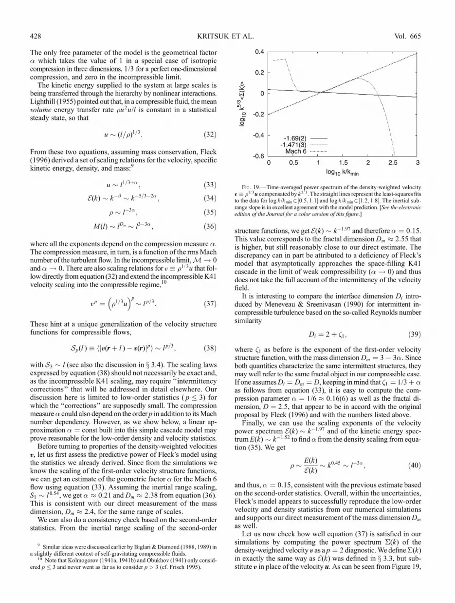
simulations by computing the power spectrum �(k) of thedensity-weighted velocity v as a p ¼ 2 diagnostic.We define�(k)in exactly the same way as E(k) was defined in x 3.3, but sub-stitute v in place of the velocity u. As can be seen from Figure 19,

Fig. 19.—Time-averaged power spectrum of the density-weighted velocityv � �1=3u compensated by k 5

=3. The straight lines represent the least-squares fitsto the data for log k /kmin2½0:5; 1:1� and log k /kmin2½1:2; 1:8�. The inertial sub-range slope is in excellent agreement with the model prediction. [See the electronicedition of the Journal for a color version of this figure.]

9 Similar ideas were discussed earlier by Biglari & Diamond (1988, 1989) ina slightly different context of self-gravitating compressible fluids.

10 Note that Kolmogorov (1941a, 1941b) and Obukhov (1941) only consid-ered p � 3 and never went as far as to consider p > 3 (cf. Frisch 1995).


the inertial range power index, � ¼ 1:69 � 0:02, is very close tothe Kolmogorov value of 5/3.

To further check our conjecture expressed by equation (38),we measured the first three scaling exponents for the modifiedstructure functions Sp using a subsample of 34 snapshots evenlydistributed in time through t2½5; 10�td using a sample of 2 ; 109

point pairs per PDF per snapshot. The resulting third-order ex-ponents are very close to unity as expected, ?3 ¼ 1:01 � 0:02and k

3¼ 0:95 � 0:02. This strongly suggests that a relationship

similar to Kolmogorov’s ‘‘4/5’’ law may hold for compressibleflows as well.

Both the first-order exponents ?1 ¼ 0:467 � 0:004 and k1 ¼

0:451 � 0:004 and the second-order exponents ?2 ¼ 0:80 �0:01 and k

2¼ 0:76 � 0:01 slightly deviate from the K41 p/3

scaling as would be the case in intermittent turbulence. The cor-responding relative (to the third order) exponents Z?

1 ¼ 0:46and Zk

1¼ 0:47 and Z?

2 ¼ 0:79 and Zk2¼ 0:80 are also somewhat

higher than their counterparts for the velocity structure functionsdiscussed in x 3.4, indicating certain structural differences be-tween the u and v fields.

Note, as the Mach number changes from M < 1 to M ¼ 6,the slope of the density power spectrum gets shallower from�7/3 to�1.1, but the slope of the velocity power spectrum getssteeper from�5/3 to�1.9. At the same time, the power spectrumof the mixed variable v remains approximately invariant, as pre-dicted by the model.

Our numerical experiments thus confirm one of the basic as-sumptions adopted in the compressible cascade model, namely,that equation (32) for the energy transfer rate holds true. The firstassumption concerning the properties of the self-similar hierarchi-cal density structure, equation (31) put forward by vonWeizsacker(1951), seems to be also satisfied in the simulations quite well, atleast to the first order.

4. DISCUSSION

Themajor deficiency of the numerical experiments discussedabove is still their limited spatial resolution that bounds theintegral scale Reynolds numbers to values much smaller thanthose estimated for the real molecular clouds. This hurdle ap-parently cannot be overcome in the near future, but still theprogress achieved in the past 15 years in this direction is veryimpressive.

The second important deficiency of our model is the lack ofmagnetic effects which are known to be essential for star forma-tion applications. This subject still remains a topic for the futurework awaiting the development of a high-quality MHD solversuitable to modeling of supersonic flows at moderately highReynolds numbers with computational resources available today.

Another set of potential issues relates to the external driv-ing force that is supposed to simulate the energy input by HDinstabilities in real molecular clouds. The large-scale drivingforce we used in these simulations is not perfectly isotropic dueto the uneven distribution of power between the solenoidal anddilatational modes (perhaps, a typical situation for the interstellarconditions). We also use a static driving force that could poten-tially cause some anomalies on timescales of many dynamicaltimes. However, while strong anisotropies can significantly affectthe scaling of high-order moments (Porter et al. 2002; Mininniet al. 2006), the departures from Kolmogorov-like scaling weobserve in the lower order statistics appear to be too strong to beexplained solely as a result of the specific properties of thedriving. The sensitivity of our result to turbulence forcing re-mains to be verified with future high-resolution simulationsinvolving a variety of driving options.

The options for observational validation of our numericalmodels are limited. Interstellar turbulence in general and super-sonic turbulence in molecular clouds in particular could hardlybe uniform and/or isotropic (Kaplan & Pikelner 1970). Thereare multiple driving mechanisms of different natures operatingon different scales in the ISM (Norman & Ferrara 1996; MacLow & Klessen 2004), so the source function of turbulence isexpected to be broadband. Various observational techniques em-ployed to extract information about the scaling properties of tur-bulence have their own limitations, including a finite instrumentalresolution, insufficiently large data sets, inability to fully accessthe three-dimensional information without additional a priori as-sumptions, etc. Moreover, complexity of the effective equation ofstate of the ISM and many other physical processes so far ignoredin the simplified numerical models should also make the com-parison of observations and simulations uncertain. Nevertheless,itmakes sense to compare our results with the scaling properties ofsupersonic turbulence obtained from observations.

Applying the velocity channel analysis (VCA) technique(Lazarian& Pogosyan 2000, 2006) to power spectra of integratedintensity maps and single-velocity channel maps of the Perseusregion, Padoan et al. (2006) found a velocity power spectrumindex � ¼ 1:8 that is reasonably close to our measurement � ¼1:95. The structure function exponents measured for the M1-67nebula by Grosdidier et al. (2001), 1 � 0:5 and 2 � 0:9, matchquite nicely with our results discussed in x 3.4, 1 ¼ 0:54 and2 ¼ 0:97.

Using maps of the 13CO J ¼ 1Y0 emission line of the molec-ular cloud complexes in Perseus, Taurus, and Rosetta, Padoanet al. (2004a) computed the power spectra of the column densityestimated using the LTE method (Dickman 1978). The slopesof the measured spectra corrected for temperature and saturationeffects on the 13CO J ¼ 1Y0 line,�0:74 � 0:07,�0:74 � 0:08,and�0:76 � 0:08, respectively, are notably shallower than ourestimate for the density spectrum power index �1:07 � 0:01(see x 3.6). The apparent 4 � discrepancy is most probably dueto an insufficiently high Mach number adopted in our simu-lations. Alternatively, it can be attributed to anisotropies in themolecular cloud turbulence, intermittent large-scale drivingforce acting on the clouds, or limitations of the LTE method.

As far as the fractal dimension is concerned, the observationalmeasurements for molecular clouds and star-forming regionstend to cluster around D ¼ 2:3 � 0:3 (Elmegreen & Falgarone1996, 2001). Stochastically variable turbulent (WC) winds from‘‘dustars’’ feeding the ISM also demonstrate similar fractal dimen-sion D ¼ 2:2Y2:3, and the same morphology of clumps formingand dissipating in real time is clearly seen in the outer parts ofthe wind where the picture is not smeared by projection effects(Grosdidier et al. 2001).

5. CONCLUSIONS

Using large-scale numerical simulations of nonmagnetic highlycompressible driven turbulence at an rms Mach number of 6, wewere able to resolve the inertial range scaling and have demon-strated that:

1. The probability density function of the gas density is per-fectly represented by a lognormal distribution over many decadesin probability as predicted from simple theoretical considerations.

2. Low-order velocity statistics deviate substantially fromKolmogorov laws for incompressible turbulence. Both velocitypower spectra and velocity structure functions show steeper thanKolmogorov slopes, with the scaling exponents of the third-ordervelocity structure functions far in excess of unity.


3. The density power spectrum is instead substantially shal-lower than in weakly compressible turbulent flows.

4. The kinetic energy power spectrum (built on w � ffiffiffi�

pu) is

shallower thanKolmogorov’s 5/3 law. The power spectra for boththe solenoidal and the dilatational parts of w obtained throughHelmholtz decomposition (w ¼ wS þ wD) have the same slopesas the total kinetic energy spectrum pointing to the unique energycascade captured by E(k); their shares in the total energy balanceare 68% and 32%, respectively.

5. As should have been expected, the mean volume energytransfer rate in compressible turbulent flows, �u2u/l, is very closeto constant in a statistical steady state. Our simulations show thatthe power spectrum of v � �1=3u scales approximately as k�5=3

and the third-order structure function of v scales linearly with l inthe inertial range.

6. The directly measured mass dimension of the ‘‘fractal’’density distribution is about 2.4 in the inertial range and 2.0 inthe dissipation range. The geometry of supersonic turbulence isdominated by clustered corrugated shock fronts.

These results strongly suggest that the Kolmogorov lawsoriginally derived for incompressible turbulence would alsohold for highly compressible flows as soon as they are ex-tended by replacing the pure velocity statistics with statistics

of mixed quantities, such as the density-weighted fluid ve-locity v � �1=3u.Both the scaling properties and the geometry of supersonic

turbulence we find in our numerical experiments support a phe-nomenological description of intermittent energy cascade in acompressible turbulent fluid and suggest a reformulation of in-ertial range intermittency models for compressible turbulencein terms of the proposed extension to the K41 theory.The scaling exponents of the velocity diagnostics, themorphol-

ogy of turbulent structures, and the fractal dimension of the massdistribution determined in our numerical experiments demon-strate good agreement with the corresponding observed quantitiesin supersonically turbulent molecular clouds and line radiationYdriven winds from carbon-sequence Wolf-Rayet stars.

We are grateful to 8ke Nordlund who kindly provided us withhis OpenMP parallel routines to compute the power spectra. Thisresearch was partially supported by NASA ATP grant NNG 05-6601G, NSF grants AST 05-07768 and AST 06-07675, andNRAC allocation MCA 098020S. We utilized computing re-sources provided by the SanDiego Supercomputer Center and theNational Center for Supercomputer Applications.

REFERENCES

Acker, A., Gesicki, K., Grosdidier, Y., & Durand, S. 2002, A&A, 384, 620Armi, L., & Flament, P. 1985, J. Geophys. Res., 90, 11779Armstrong, J. W., Rickett, B. J., & Spangler, S. R. 1995, ApJ, 443, 209Baty, H., Keppens, R., & Comte, P. 2003, Phys. Plasmas, 10, 4661Bayly, B. J., Levermore, C. D., & Passot, T. 1992, Phys. Fluids, 4, 945Benzi, R., Biferale, L., Ciliberto, S., Struglia, M. V., & Tripiccione, R. 1996,Physica D, 96, 162

Benzi, R., Ciliberto, S., Tripiccione, R., Baudet, C.,Massaioli, F., & Succi, S. 1993,Phys. Rev. E, 48, R29

Biglari, H., & Diamond, P. H. 1988, Phys. Rev. Lett., 61, 1716———. 1989, Physica D, 37, 206Boldyrev, S. 2002, ApJ, 569, 841Boldyrev, S., Nordlund, 8., & Padoan, P. 2002, ApJ, 573, 678Brunt, C. M. 2003, ApJ, 584, 293Brunt, C. M., Heyer, M. H., Vazquez-Semadeni, E., & Pichardo, B. 2003, ApJ,595, 824

Colella, P., & Woodward, P. R. 1984, J. Comput. Phys., 54, 174Davidson, P. A., & Pearson, B. R. 2005, Phys. Rev. Lett., 95, 214501de Karman, T., & Howarth, L. 1938, Proc. R. Soc. London A, 164, 192Dickman, R. L. 1978, ApJS, 37, 407Dobler,W., Haugen, N. E., Yousef, T. A., & Brandenburg, A. 2003, Phys. Rev. E,68, 026304

Dubrulle, B. 1994, Phys. Rev. Lett., 73, 959Elmegreen, B. G., & Elmegreen, D. M. 2001, AJ, 121, 1507Elmegreen, B. G., & Falgarone, E. 1996, ApJ, 471, 816Elmegreen, B. G., & Scalo, J. 2004, ARA&A, 42, 211Falkovich, G. 1994, Phys. Fluids, 6, 1411Fleck, R. C., Jr. 1996, ApJ, 458, 739Frisch, U. 1995, Turbulence: The Legacy of A. N. Kolmogorov (Cambridge:Cambridge Univ. Press)

Frisch, U., & Bec, J. 2001, in Les Houches 2000: New Trends in Turbulence,ed. M. Lesieur, A. Yaglom, & F. David (Berlin: Springer), 341

Gaffet, B. 1985, J. Fluid Mech., 156, 141Grosdidier, Y., Moffat, A. F. J., Blais-Ouellette, S., Joncas, G., & Acker, A.2001, ApJ, 562, 753

Haugen, N. E., & Brandenburg, A. 2004, Phys. Rev. E, 70, 026405Heitsch, F., Burkert, A., Hartmann, L. W., Slyz, A. D., & Devriendt, J. E. G.2005, ApJ, 633, L113

Helmholtz, H. 1868, Monasber. Berlin Akad., 215Kaneda, Y., Ishihara, T., Yokokawa, M., Itakura, K., & Uno, A. 2003, Phys.Fluids, 15, L21

Kaplan, S. A., & Pikelner, S. B. 1970, The Interstellar Medium (Cambridge:Harvard Univ. Press)

Kaplan, S. A., & Pronik, V. I. 1953, Akad. Nauk SSSR Dokl., 89, 643Keppens, R., Toth, G., Westermann, R. H. J., & Goedbloed, J. P. 1999, J. PlasmaPhys., 61, 1

Kida, S., & Orszag, S. A. 1990, J. Sci. Comput., 5, 85———. 1992, J. Sci. Comput., 7, 1Kim, J., & Ryu, D. 2005, ApJ, 630, L45Kolmogorov, A. N. 1941a, Akad. Nauk SSSR Dokl., 30, 299 (K41)———. 1941b, Akad. Nauk SSSR Dokl., 31, 538———. 1941c, Akad. Nauk SSSR Dokl., 32, 19———. 1962, J. Fluid Mech., 13, 82Kornreich, P., & Scalo, J. 2000, ApJ, 531, 366Kritsuk, A. G., & Norman, M. L. 2004, ApJ, 601, L55Kritsuk, A. G., Norman, M. L., & Padoan, P. 2006, ApJ, 638, L25Larson, R. B. 1981, MNRAS, 194, 809Lazarian, A., & Pogosyan, D. 2000, ApJ, 537, 720———. 2006, ApJ, 652, 1348Lele, S. K. 1994, Ann. Rev. Fluid Mech., 26, 211Li, P. S., Norman, M. L., Mac Low, M.-M., & Heitsch, F. 2004, ApJ, 605, 800Lighthill, M. J. 1955, in IAU Symp. 2, Gas Dynamics of Cosmic Clouds(Amsterdam: North Holland), 121

Liu, J., She, Z.-S., Guo, H., Li, L., & Ouyang, Q. 2004, Phys. Rev. E, 70, 036215Mac Low, M.-M., & Klessen, R. S. 2004, Rev. Mod. Phys., 76, 125Mandelbrot, B. B. 1974, J. Fluid Mech., 62, 331———. 1975, J. Fluid Mech., 72, 401Meneveau, C., & Sreenivasan, K. R. 1990, Phys. Rev. A, 41, 2246Miles, J. W. 1957, J. Fluid Mech., 3, 185Mininni, P. D., Alexakis, A., & Pouquet, A. 2006, Phys. Rev. E, 74, 016303Miura, A., & Pritchett, P. L. 1982, J. Geophys. Res., 87, 7431Monin, A. S., & Yaglom, A. M. 1975, Statistical Fluid Mechanics: Mechanicsof Turbulence, Vol. 2 (Cambridge: MIT Press)

Moyal, J. E. 1951, Proc. Cambridge Philos. Soc., 48, 329Nordlund, 8. K., & Padoan, P. 1999, in Interstellar Turbulence, ed. J. Franco &A. Carraminana (Cambridge: Cambridge Univ. Press), 218

Norman, C. A., & Ferrara, A. 1996, ApJ, 467, 280Obukhov, A. M. 1941, Akad. Nauk SSSR Dokl., 32, 22———. 1962, J. Fluid Mech., 13, 77Padoan, P., Jimenez, R., Juvela, M., & Nordlund, 8. 2004a, ApJ, 604, L49Padoan, P., Jimenez, R., Nordlund, 8., & Boldyrev, S. 2004b, Phys. Rev. Lett.,92, 191102

Padoan, P., Juvela, M., Kritsuk, A., & Norman, M. L. 2006, ApJ, 653, L125Padoan, P., & Nordlund, 8. 1997, preprint (astro-ph/9706176)———. 1999, ApJ, 526, 279———. 2002, ApJ, 576, 870Padoan, P., Nordlund, 8., & Jones, B. J. T. 1997, MNRAS, 288, 145Padoan, P., Nordlund, 8., Kritsuk, A. G., Norman, M. L., & Li, P. S. 2007, ApJ,661, 972

Passot, T., Pouquet, A., & Woodward, P. 1988, A&A, 197, 228Passot, T., & Vazquez-Semadeni, E. 1998, Phys. Rev. E, 58, 4501Politano, H., & Pouquet, A. 1998, Geophys. Res. Lett., 25, 273


Porter, D. H., Pouquet, A., Sytine, I., &Woodward, P. 1999, Physica A, 263, 263Porter, D. H., Pouquet, A., & Woodward, P. R. 1992a, Theor. Comput. FluidDynamics, 4, 13

———. 1992b, Phys. Rev. Lett., 68, 3156———. 1994, Phys. Fluids, 6, 2133———. 2002, Phys. Rev. E, 66, 026301Porter, D. H., & Woodward, P. R. 1994, ApJS, 93, 309Porter, D. H., Woodward, P. R., & Pouquet, A. 1998, Phys. Fluids, 10, 237Pouquet, A., Passot, T., & Leorat, J. 1991, in IAU Symp. 147, Fragmentation ofMolecular Clouds and Star Formation, ed. E. Falgarone, F. Boulanger, & G.Duvert (Dordrecht: Kluwer), 101

Ryu, D., Jones, T. W., & Frank, A. 2000, ApJ, 545, 475Samtaney, R., Pullin, D. I., & Kosovic, B. 2001, Phys. Fluids, 13, 1415She, Z.-S., & Leveque, E. 1994, Phys. Rev. Lett., 72, 336She, Z.-S., & Waymire, E. C. 1995, Phys. Rev. Lett., 74, 262Sreenivasan, K. R., & Bershadskii, A. 2005, Pramana J. Phys., 64, 315Sytine, I. V., Porter, D. H., Woodward, P. R., Hodson, S. W., & Winkler, K.-H.2000, J. Comput. Phys., 158, 225

Vazquez-Semadeni, E. 1994, ApJ, 423, 681Vishniac, E. T. 1994, ApJ, 428, 186von Weizsacker, C. F. 1951, ApJ, 114, 165


the statistics of supersonic isothermal turbulence

Documents