OFFPRINT

Simulating isothermal aging of snow

R. Vetter, S. Sigg, H. M. Singer, D. Kadau, H. J. Herrmann

and M. Schneebeli

EPL, 89 (2010) 26001

Please visit the new websitewww.epljournal.org

TARGET YOUR RESEARCH

WITH EPL

Sign up to receive the free EPL table ofcontents alert.

www.epljournal.org/alerts

January 2010

EPL, 89 (2010) 26001 www.epljournal.org

doi: 10.1209/0295-5075/89/26001

Simulating isothermal aging of snow

R. Vetter1, S. Sigg1, H. M. Singer1, D. Kadau1(a), H. J. Herrmann1 and M. Schneebeli2

1 IfB, Swiss Federal Institute of Technology ETH Zurich - 8093 Zurich, Switzerland2WSL Institute for Snow and Avalanche Research SLF - Davos, Switzerland

received 22 October 2009; accepted in final form 21 December 2009published online 1 February 2010

PACS 64.60.A – Specific approaches applied to studies of phase transitionsPACS 64.70.Hz – Solid-vapor transitionsPACS 92.40.ed – Snow

Abstract – A Monte Carlo algorithm to simulate the isothermal recrystallization process of snowis presented. The snow metamorphism is approximated by two mass redistribution processes:surface diffusion and sublimation-deposition. The algorithm is justified and its parametrization isdetermined. The simulation results are compared to experimental data, in particular, the temporalevolution of the specific surface area and the ice thickness. We find that the two effects ofsurface diffusion and sublimation-deposition can accurately model many aspects of the isothermalmetamorphism of snow. Furthermore, it is shown that sublimation-deposition is the dominantcontribution for temperatures close to the melting point, whereas surface diffusion dominates attemperatures far below the melting point. A simple approximation of gravitational compaction isimplemented to simulate density change.

Copyright c© EPLA, 2010

Introduction. – The structural transformation ofsnow as a result of recrystallization has become anincreasingly investigated field of research over the pastfew years. Isothermal metamorphism of snow was recentlystudied experimentally in ref. [1], providing measurementsof detailed microstructural properties. Most experimentswere performed with in vitro X-ray microtomography [2],while we used in situ X-ray microtomography. Thisapproach provides the possibility to directly analyze theevolution of the same snow crystals in space and time.Isothermal metamorphism of snow is a sintering process

between the ice grains forming the snow [3]. Various stud-ies, although not always agreeing in every point [4–7], leadto assume that amongst the possible mass redistributionprocesses such as sublimation-deposition, grain bound-ary diffusion, plastic flow, surface diffusion, viscous flowand volume diffusion, only a few processes significantlycontribute to the isothermal metamorphism of snow [1].Surface diffusion and sublimation-deposition are believedto be the most dominant ones [8,9]. Isothermal metamor-phism of snow has been stated to be similar to the evolu-tion of bicontinous interfaces during coarsening [10].Predictive simulations by means of numerical models

of isothermal recrystallization of snow are hoped to leadto a deeper understanding of the governing processes

(a)E-mail: dkadau@ethz.ch

of snow metamorphism and might become a helpfultool in applications such as avalanche forecasting. Thecurrent models [2,11] use a macroscopic approach. Herewe used a model which is based on a direct simulation bymeans of Monte Carlo processes, similar to the model ofref. [12], but using effective ice particles instead of realmolecules. The model presented in this paper implementsthe two dominant mass redistribution effects in isothermalmetamorphism, for the effective ice particles. In order todirectly compare and validate the simulation results withthe experimental ones, important structural quantities,the specific surface area and the shape of the ice matrix,are measured and compared.

Experiments. – Experimental data has been obtainedby Kaempfer and Schneebeli [1] from four samples offreshly fallen snow, which was sieved at −20 ◦C through a1mm sieve and filled in cylindrical sample holders with adiameter of 18.5mm, which were sealed to avoid subli-mation. The samples were kept for about 11 monthsin a temperature controlled environment at four differ-ent constant temperatures: −54 ◦C, −19.1 ◦C, −8.3 ◦Cand −1.6 ◦C. Roughly once per month, the samples werei) weighed, ii) the snow height in the sample holders wasdetermined, and iii) the samples were imaged with a microcomputer tomograph (µCT). During the µCT measure-ment, the samples were exposed to a temperature of

26001-p1

R. Vetter et al.

−15 ◦C for about two hours. The authors of ref. [1] reportthat this temperature change did not affect the experi-ment as this period is considered to be short comparedto the time scale of the processes involved in snow meta-morphism. The µCT images were taken at a resolution of10µm per voxel. This resolution is chosen as it is lowerthan the typical roughness of snow [9]. The imaged snowregion was about 5 × 5 × 5mm in size, which corre-sponds to a data block of 508 × 508 × 508 voxels (e.g.,see fig. 1). A marker was attached to this specific snowsample to be able to visualize the temporal evolution ofthe same cutout as its position moves due to gravitationalcollapse. For direct comparison, in our simulations we usedthe same sample as in the experiment (fig. 1). The simu-lation parameters have been adapted as described in thesection “Results”. The pictures visually match well, bothshow a similar coarsening behavior.

Modeling technique. – Snow metamorphism iscommonly modeled by macroscopic approaches usingsurface growth laws, e.g., the curvature-driven modelpresented by Flin et al. [2], or using phase field models,such as the recently presented temperature-driven modelof Kaempfer and Plapp [11]. A brief review on models forsnow metamorphism can be found in ref. [11]. Contrarilyto studying the details of crystal growth on a microscopicscale the sublimation-deposition and diffusion processesof individual atoms are modeled, e.g. in ref. [12].Here, we will use a similar way of determining the

sticking and sublimation probabilities for the sublimation-deposition process as well as the jump rate for diffusionas in crystal growth [12]. However, instead of consid-ering individual atoms as commonly in crystal growth,we use “effective ice particles”. For this reason we haveto determine the parameters in the model by adjustingto experimental data as no first principle “microscopic”parameters exist for these coarse grained particles. There-fore, we use the same size and shape as in the experi-ments (10µm cubes, see previous section). These effectiveparticles contain the complex interactions of microscopicproperties.The term sublimation-deposition, within this context,

refers to the three-step process of single particles vapor-izing from the snow-air interface into the air, vaportransport within the air, and eventually, single vaporparticles depositing again on the surface. The steps ofsublimation and deposition can easily be physicallymodeled. Important steps of the derivation will begiven later in this section. Monte Carlo processes arebased on probabilistic rules. Xiao et al. [12] derived theprobabilities of growth units to stick on crystal surfacesfor a two-dimensional triangular lattice, based on thesurface-free-energy minimization principle, using nearestand second-nearest-neighbor interactions. In this sectionwe derive in an analogous manner the probabilities of aneffective ice particle to transform from the solid state onthe surface into vapor and vice versa for the lattice given

Fig. 1: Snapshots of real samples used in experiments (left)compared to the simulated configuration (right) for a temper-ature of −8 ◦C (top to bottom: initial configuration, after 2weeks, 5 weeks, 7 weeks, and 10 weeks). As starting configura-tion for the simulation the experimental data has been used.Here, in the experiments the same cutout of the snow sample isshown. Due to unequal settling in the experiment, the sampleshows a slight “drift” to the right, whereas the simulation boxis fixed.

26001-p2

Simulating isothermal aging of snow

by the cubic voxel structure, and taking interactions toall 26 neighbors in the local 33 cube into account, i.e.the 3D Moore neighborhood [13,14]. In the following thisdefinition of neighbors is used.A general expression for the sublimation rate K−i can

be written as [12]

K−i = ν exp

(

−EikBT

)

= ν exp

(

−φnikBT

)

, (1)

where ν is a vibration factor [12] or frequency factor whichusually also depends on temperature [15], kBT the thermalenergy and Ei = φni the total binding energy of particle i,with φ the interaction energy of one particle with oneneighbor, assumed to be the same for all neighbors,and ni ∈ {0, . . . , 26} the number of occupied neighbors ofsite i.Similarly the attachment rate K+, at which particles

impinge onto the surface, can be written as [12]

K+ =Keqexp

(

Δµ

kBT

)

, (2)

where Keq is the equilibrium value of K+ and also

temperature dependent (Keq(T )), Δµ=∆GNA

the aver-age chemical-potential difference per vapor particle withΔG/NA =RT ln

ppeq/NA the average Gibbs free energy

at constant temperature in supersaturated vapor withrespect to the bulk average [16] per mole.Considering the equilibrium condition p= peq, n

eqi =

33−12 = 13, K

−

i =K+, we can eliminate Keq:

Keq = νexp(

− EikBT

)

exp(

∆µkBT

) = ν exp

(

−13φ

kBT

)

. (3)

For γ := exp(

∆µkBT

)

= ppeqand β := exp

(

− φkBT

)

we thus

find the probability, that particle i sticks to the surface tobe

P sticki =K+

K−i +K+=γβ13−ni

1+ γβ13−ni(4)

and accordingly, the probability to evaporate off thesurface

P leavei = 1−P sticki =1

1+ γβ13−ni. (5)

These probabilities directly depend on the number ofneighbors ni and the current vapor pressure ratio γ =

ppeq.

In the simulations, presented here, the initial value γ0will be set to unity, i.e. the initial average pressure isthe equilibrium pressure. For an isothermal process βis constant. In a similar way, the initial water vaporvolume fraction fV , which (together with γ0) determinesthe initial number of vaporous ice particles, is set to theequilibrium one (using the ideal gas law). The calculatedvalues are also listed in table 1.Vapor transport is, as a first approximation, modeled

by a random walk. As the connecting component between

sublimation and deposition, the vapor transport mustensure that in equilibrium sublimation and depositionrates are identical. This is achieved by performing therandom walk only for one single vapor particle at a timeuntil it impinges onto a surface.In practice, at each time step, for as many times as

specified by an evaporation rate KV a particle from thesurface is evaporated with probability P leavei , i.e. whilekeeping its position the particle is added to the vaporcontainer consisting of a list of vapor particles and theirpositions. Then, a randomly chosen particle of the vaporcontainer performs a random walk until it reaches the icesurface. It sticks at the surface with probability P sticki ,i.e. deleted from the vapor container and added to the icematrix. Otherwise it stays within the container.Surface diffusion describes the diffusive motion of parti-

cles on the surface of a solid material. It changes themicrostructure of the surface and results in smoothingrough surface regions. The surface diffusion rate dependson the strength of the particle-particle interaction. A prac-tical way to approximate it is to consider the interactionsto all neighbors, i.e. the number of neighbors multipliedwith a constant interaction energy. As for the sublimation-deposition process, we need to take into account 26 possi-ble directions for each move, each of which is chosen withthe same probability if the new site is unoccupied and theparticle remains on the surface. The jump rate Ki→j fromsite i to site j can be written in the following way [12]:

Ki→j = ν exp

(

−ΔEjikBT

)

. (6)

The activation energy ΔEji is the change of energycaused by this move, ΔEji ≈ φ(ni−nj), where φ denotesthe interaction energy between a pair of neighboringparticles, ni and nj the numbers of neighbors of sitei and j, respectively, and ν a vibration or frequencypre-factor (see above). In practice, at each time step,for as many times as specified by a diffusion rate KD,a random surface voxel i is selected for which the movingdirection is chosen randomly with two constraints: theremust not already exist a voxel j at the target site ofthe move and the voxel must remain on the surface. Thesecond constraint ensures that no voxel leaves the surfaceduring the surface diffusion process. If both constraintsare fulfilled, the move is executed with the Metropolisprobability Pi→j =min{1, exp(−φ(ni−nj)/kBT )} whichis essentially eq. (6) but with the vibration pre-factorincluded into the diffusion rate. Note that for fresh snowsamples the surface structure is such that for most cases adiffusion process leads to a lower energy and is thereforeaccepted. In these cases the speed of the coarseningprocess due to surface diffusion is determined only by thediffusion rate KD.Summarizing, the most important parameters are the

interaction energy φ, a temperature-independent propertyof the effective ice particles, and the evaporation anddiffusion rates KV and KD which are both temperature

26001-p3

R. Vetter et al.

Table 1: The four simulation settings used to reproduce theexperiment. The parameters φ, KV and KD used in thesimulations (single runs) are determined such that the imagesmatch the experiments well. fV (in brackets) is calculatedassuming the ideal-gas law for the effective ice particles.

Setting, T kBT/φ KD KV (fV )

1, −54 ◦C 0.80 5 1 (0.0001)2, −19 ◦C 0.93 19 17 (0.0022)3, −8 ◦C 0.97 26 40 (0.0043)4, −2 ◦C 0.99 32 88 (0.0061)

dependent as the vibration factor depends on T . To beused in the simulations these parameters have to bedetermined by comparison to the experimental resultswhich will be described in the next section. First, we willpresent results neglecting the compaction of the snow dueto gravity. Later in this paper, we introduce the effect ofgravity by using a simple compaction scheme.

Results. – A simple qualitative criterion for thecorrectness of the simulation results is given by visualinspection. Since Kaempfer and Schneebeli [1] published aseries of snapshots from the recorded µCT images, we cansimply check if the visual outcome of the program fits theexperimental observation, i.e. matching morphologicalmeasures such as the specific surface area or the icethickness (see below) judged “by eye”. Figure 1 shows oneexample of a short-term series (10 weeks) for a systemof 508× 508× 508 voxels corresponding to 5mm × 5mm× 5mm in the experiments to illustrate that visualmatching could be achieved reasonably well. Note thatconsidering that the volume fractions of the experimentalsample is around 30% the number of effective ice particlesof this simulation is about 40 million. For more detailedcomparison we used the original images by Kaempfer andSchneebeli for the long-term behavior (about 11 months),i.e. system sizes of 192× 192× 192 voxels correspondingto 2mm × 2mm × 2mm in the experiments. Consideringthat the volume fractions of the experimental samples arearound 30% the number of effective ice particles is over 2million. Table 1 shows the simulation parameters used tomatch the experiments at the temperatures indicated [1].Note, that the parameters for kBT/φ are all using thesame value for φ, which is the parameter we had todetermine.Note, that rescaling the evaporation and diffusion rates

(both multiplied by the same factor) mainly leads to aneffective rescaling of the simulation time, i.e. only theirratio is important and in principle they determine the timescale in the simulations. At low temperatures compactionis practically negligible as found in the experiments [1].The higher the temperature, the larger the density discrep-ancy between experiment and simulation output, wherethe compaction is not considered.Similarly to the experiments we analyze the specific

surface area as a function of time. According to ref. [17]

0 5000 10000

t [h]

0

0.01

0.02

0.03

0.04

0.05

0.06

0.07

As [

m-1

]

set 1 (-54°C) set 2 (-19°C) set 3 (-8°C) set 4 (-2°C) exp. (-54°C)

exp. (-19°C)

exp. (-8°C)

exp. (-2°C)

Fig. 2: (Colour on-line) Specific surface area As depending ontime for the simulations and experiments. The simulation stepsare scaled to real time such that they match the experimentsbest.

the specific surface area As obeys the law

As(t) =As,0

(

τ

τ + t

)1/n

(7)

with the initial specific surface area As,0, growth exponentn and a parameter τ , which determines the time scaling.Our simulation results strongly confirm this relationshipwhich is a non-trivial experimental measurement. Inall simulations the squared correlation coefficient R2

was larger than 0.999. Figure 2 shows the evolution ofthe specific surface area As for the four parameter sets(table 1). Here we deliberately chose to present results forsingle runs to directly compare to experiments. Due tothe large number of modeled ice particles still a relativegood average could be achieved. Superimposed are theexperimental results. Note, that the simulation steps arerescaled to real time, such that they match the experi-ments. For high temperatures (−2 ◦C, −8 ◦C) the long-term behavior differs, which is expected due to neglectingthe density increase due to gravity in the model for thesimulations presented above. For lower temperaturesthe long-term behavior matches well, as in that case thesample density does not increase much. For set 1 (−54 ◦C)the initial volume fractions were different, so that onlythe long-term behavior could be reproduced by thesimulations.The fit parameters according to eq. (7) are compared

in table 2. The simulations show a clear trend indicatingthat the exponent n decreases with increasing tempera-ture. However, for the experiments it is more difficult todetermine this exponent very accurately as the number ofmeasured points is limited, leading to differences betweenthe exponents of simulation and experiments. For verylow temperatures the simulation relaxes too fast in thebeginning, compared to the experiment. This can beexplained as the simulation uses Metropolis rates in

26001-p4

Simulating isothermal aging of snow

Table 2: Fit parameters obtained for the four simulationsettings (including error) and the corresponding experiments.The simulation steps are rescaled to real time as in fig. 2.

Setting, T nexp nsim τexp τsim

1, −54 ◦C 0.8 5.89± 0.05 25000h (470± 5)h2, −19 ◦C 2.20 2.93± 0.01 652.1h (175± 1.5)h3, −8 ◦C 3.55 2.60± 0.01 69.97h (93± 0.7)h4, −2 ◦C 3.00 2.44± 0.01 55.53h (73± 0.5)h

accordance with the hopping probability for atoms on acrystal surface. Thus, all diffusion processes lowering theenergy are accepted, which seems to be unrealistic for theeffective ice particles.Considering that the simulation parameters were only

determined using single runs for each parameter set andby visual matching of the figures compared to the exper-iments as well as adjusting the time scale in accordanceto the specific surface area, the simulations match theexperiments relatively well. In future investigations betterstatistics and a refined parameter determination bymatching morphological measures as the specific surfacearea and ice thickness quantitatively are necessary. Forthat purpose also more experimental data would beneeded (see also outlook). Additionally, investigating thetemperature dependence, e.g. of the parameters KV andKD (i.e. their ratio, see above), is crucial to predict thebehavior of snow samples for all possible temperatureswithout the need of new experimental measurements.The thickness of the ice matrix is another important

quantity which has been measured in the experiments.Here, we will use the thickness definition introduced byHildebrand and Ruegsegger [18] which can be used forarbitrary three-dimensional structures. The local thick-ness of a porous volume at point P inside the structure isdefined as the diameter of the sphere with maximal radiuswhich lies completely inside the structure and contains P .This definition gives a somewhat intuitive measure of thelocal thickness of a matrix trabecula. Each spatial pointof the structure (and in particular each snow voxel) isassigned a positive distance describing the structure thick-ness at that point. By measuring these thicknesses for eachvoxel of an ice matrix (at given time) one gets a thicknessdistribution, and can determine the average thickness.Legagneux and Domine [17] proposed the following

coarsening law for the average ice thickness 〈dtb〉 for snow:

〈dtb〉 (t) = (〈dtb,0〉n+Kt)

1

n (8)

with growth rate K, growth exponent n and initial icethickness 〈dtb,0〉. Our simulations agree with this functionwith very high precision (inset in fig. 3), thus confirmingthe validity of eq. (8). The ice thickness distribution hasbeen studied by Kaempfer and Schneebeli [1]. The mainfeature observed in the experiment is a broadening of thedistribution. As depicted in fig. 3 for setting 3 the samebehavior is found for the simulations.

0 0.1 0.2 0.3

dtb

[mm]

0

0.05

0.1

0.15

0.2

0.25

pro

bab

ilit

y

week 0week 5week 11week 17week 23week 30week 45

0 2000 4000 6000 8000t [h]

0.05

0.1

0.15

0.2

0.25

⟨dtb

⟩

set 3

K=6.97·10-6

, n=1.75

Fig. 3: (Colour on-line) Distribution of the ice thickness dtb forseveral snapshots at different times for the simulations. Theinset shows the corresponding time dependence of the averageice thickness 〈dtb〉, including a fit according to eq. (8).

Fig. 4: (Colour on-line) Illustration of the density measurementin the simulation. By using the simplified gravity rule onlythe lower part of the system could be used for measuring thedensity.

A difference between the experimental µCT imagemeasurements and our simulations discussed in the previ-ous section is the absence of density increase. There-fore, we introduced a simple gravity effect. As soon asa grain (piece of snow) is not connected with the bulkanymore it falls down to the point where at least onepoint on the surface is supported by another piece of snowfrom below. This simplified model of gravity simulates thecompaction of snow. However, mechanical behavior likerotation, translation and breaking are neglected. Duringthis process, when using a fixed size for the simulation box,the upper part of the system dilutes successively. There-fore, we only measure the density in the lower part ofthe system (here the lower half), as illustrated in fig. 4.Therefore, we used elongated systems of size of 192×192× 384 for the following measurements.

26001-p5

R. Vetter et al.

0 1000 2000 3000

t [h]

0.13

0.14

0.15

0.16

0.17

0.18

0.19

ρ [

1000 k

g/m

3]

set 1set 2set 3set 4

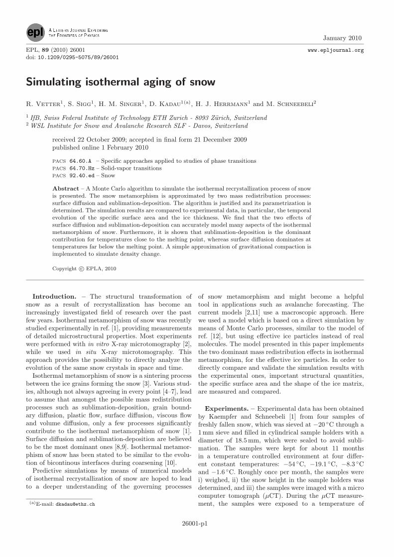
Fig. 5: (Colour on-line) Time evolution of the density in thesimulation using a simple model for gravity. The simulationsteps are rescaled to real time as in fig. 2.

The density measurements as depicted in fig. 5 featuresa step form as a consequence of the fact that not atevery time step unconnected clusters are found and moveddownwards. This behavior is also observed in the experi-ments [1], but it is much less pronounced due to the largersample size. The decrease in density between the jumpscan be explained by the fact that to measure the densityin the simulations only the lower half of the system isused (see above, fig. 4). Therefore, effective ice particlessublimated from the ice matrix in the lower half will moveto the upper half where more free space is available. Onaverage, the density increase measured in the simulation ismuch lower than in the experiments [1] for all four settings.This is expected as we use a strongly simplified model forgravity, only considering the most important process, the“falling” of the grains, but neglecting processes like slid-ing and rolling of grains, or breakage due to the load ofthe snow above, which certainly play a role in real snowsamples.

Conclusion and outlook. – A new simulation tech-nique using effective ice particles for the aging of snowis presented. We show that our Monte Carlo simulationincorporating the two basic processes of snow metamor-phism, sublimation-deposition and surface diffusion, canadequately model the experimentally observed behaviorof isothermal snow metamorphism. In accordance withLibbrecht [19], a transition to more surface-diffusion–dominated coarsening takes place at lower homologoustemperatures. In our simulations we could verify previ-ously suggested laws originating from classical sinteringtheory [20] for the time evolution of the specific surfacearea and average ice thickness. While classical sinter-ing theory assumes that an integer exponent n uniquelydescribes the process, our exponents n seems to varycontinuously. We ascribe this to the fact that the smallrange in homologous temperature where vapor and surface

diffusion interact leads to a transition from one processto the other. Until now, it has been unclear if the non-integer exponents deduced from experiments were an arti-fact or real. The simulation supports the view that thesenon-integer exponents are a real phenomenon of isother-mally sintering snow. To be able to use the simulationsas a predictive tool for snow metamorphism, a systematicparameter determination is needed. This will be an issuefor future studies as a better resolution in the experimentswould be needed to achieve more accurate parameters.The results of the simple gravity model are realistic forvery small strain rates as those in the experiment. Highstrain rates will create a much more complex behavior.

∗ ∗ ∗

We thank M. Heggli, B. Pinzer and H. Lowe forsupport in handling the data and suggestions to themanuscript.

REFERENCES

[1] Kaempfer T. U. and Schneebeli M., J. Geophys. Res.,112 (2007) D24101.

[2] Flin F., Brzoska J.-B., Lesaffre B., Coleou C. andPieritz R. A., J. Phys. D, 36 (2003) A49.

[3] Blackford J. R., J. Phys. D: Appl. Phys., 40 (2007)355.

[4] Maeno N. and Ebinuma T., J. Phys. Chem., 87 (1983)4103.

[5] Cabanes A., Legagneux L. and Domine F., Environ.Sci. Technol., 37 (2003) 661.

[6] Colbeck S. C., J. Appl. Phys., 84 (1998) 4585.[7] Colbeck S. C., J. Appl. Phys., 89 (2001) 4612.[8] Legagneux L., Taillandier A.-S. and Domine F.,J. Appl. Phys., 95 (2004) .

[9] Kerbrat M., Pinzer B., Huthwelker T., GaggelerH. W., Ammann M. and Schneebeli M., Atmos. Chem.Phys., 8 (2008) 1261.

[10] Kwon Y., Thornton K. and Voorhees P. W., EPL,86 (2009) 46005.

[11] Kaempfer T. U. and Plapp M., Phys. Rev. E, 79 (2009)031502.

[12] Xiao R.-F., Alexander J. I. D. and Rosenberger F.,Phys. Rev. A, 38 (1988) 2447.

[13] Zhang L., Strouthos C. G., Wang Z. and DeisboeckT. S., Math. Comput. Model., 49 (2009) 307.

[14] Ritter G. X. andWilson J. N., Handbook of ComputerAlgorithms in Image Algebra (CRC Press Inc.) 1996.

[15] Gilmer G. and Bennema P., J. Appl. Phys., 43 (1972)1347.

[16] Hill T. L., An Introduction to Statistical Thermo-dynamics (Dover, New York) 1986.

[17] Legagneux L. and Domine F., J. Geophys. Res., 110(2005) F04011.

[18] Hildebrand T. and Ruegsegger P., J. Microsc., 185(1997) 67.

[19] Libbrecht K. G., Rep. Prog. Phys., 68 (2005) 855.[20] Randall R. M., Sintering Theory and Practice (New

York, Wiley) 1996.

26001-p6