numerical simulation of condensation in a supersonic nozzle
TRANSCRIPT
UNIVERSITE CATHOLIQUE DE LOUVAIN
Abstract
Ecole Polytechnique de Louvain
Thermodynamique et Mecanique des Fluides (TFL)
Master in Mechanical Engineering
Numerical simulation of condensation in a supersonic nozzle for application
to ejectors in refrigeration
by Marina Gallach Palma
This thesis is a CFD study of a supersonic nozzle for ejector refrigeration applications.
Condensation of the working fluid is aimed inside the nozzle in order to study its conse-
quences. As a first approach to verify the built-in Wet Steam model in ANSYS Fluent,
a Laval nozzle is tested with water and compared with experimental data from Moses
and Stein [1].
Thanks to the User Defined Wet Steam Property Functions in the User Defined Wet
Steam model, the code is adapted for R134a both ideal and real gas properties and the
study is done with perfect and real gas properties. Anyway, the software presents certain
limitations and the real gas Peng-Robinson Equation Of State could not be implemented
due to convergence problems.

Acknowledgements
This thesis would not have been possible without the help and advice of Yann Bar-
tosiewicz. I would like to thank him for the patience and help guiding me along this
project. Thanks to him I have learned a lot about this field which I might have never
studied if it wasn’t for this thesis suggested by him.
To the friends that I have made in the department, who helped me going step by step.
To my friends who always supported me, and to Andreu for cheering on me to improve
every day.
To my parents for their patience and support to go on.
iii

Contents
Abstract i
Acknowledgements iii
Contents v
List of Figures vii
List of Tables ix
Abbreviations xi
1 Introduction 1
1.1 Context . . . . . . . . . . . . . . . . . . . . . . . . . . . . . . . . . . . . . 1
1.2 Ejector as a component . . . . . . . . . . . . . . . . . . . . . . . . . . . . 2
1.3 State of the art . . . . . . . . . . . . . . . . . . . . . . . . . . . . . . . . . 5
1.4 Objectives . . . . . . . . . . . . . . . . . . . . . . . . . . . . . . . . . . . . 7
1.4.1 Thesis structure . . . . . . . . . . . . . . . . . . . . . . . . . . . . 7
2 Physical and Numerical Model 9
2.1 Physical Model . . . . . . . . . . . . . . . . . . . . . . . . . . . . . . . . . 9
2.2 Wet Steam Model . . . . . . . . . . . . . . . . . . . . . . . . . . . . . . . 11
2.2.1 Flow equations . . . . . . . . . . . . . . . . . . . . . . . . . . . . . 11
2.2.2 Wet Steam Equation . . . . . . . . . . . . . . . . . . . . . . . . . . 12
2.2.3 Phase Change Model . . . . . . . . . . . . . . . . . . . . . . . . . . 13
2.3 RANS Turbulence Models . . . . . . . . . . . . . . . . . . . . . . . . . . . 15
2.3.1 Standard k-ε Model . . . . . . . . . . . . . . . . . . . . . . . . . . 16
2.3.2 Shear-Stress Transport k-ω Model . . . . . . . . . . . . . . . . . . 17
2.4 Wall approach . . . . . . . . . . . . . . . . . . . . . . . . . . . . . . . . . . 17
2.4.1 Wall Function . . . . . . . . . . . . . . . . . . . . . . . . . . . . . . 18
2.4.2 Wall Resolved . . . . . . . . . . . . . . . . . . . . . . . . . . . . . . 19
2.5 Solver/Numerical setup . . . . . . . . . . . . . . . . . . . . . . . . . . . . 19
3 Validation: Nozzle + Steam 21
3.1 Description of the cases . . . . . . . . . . . . . . . . . . . . . . . . . . . . 21
3.2 Numerical Setup . . . . . . . . . . . . . . . . . . . . . . . . . . . . . . . . 22
3.2.1 Mesh and Geometry . . . . . . . . . . . . . . . . . . . . . . . . . . 22
v
Contents vi
3.2.2 Boundary Conditions . . . . . . . . . . . . . . . . . . . . . . . . . 22
3.3 Results I . . . . . . . . . . . . . . . . . . . . . . . . . . . . . . . . . . . . . 23
3.3.1 Experiments No. 410-421 . . . . . . . . . . . . . . . . . . . . . . . 23
3.3.2 Turbulence . . . . . . . . . . . . . . . . . . . . . . . . . . . . . . . 28
3.4 Results II . . . . . . . . . . . . . . . . . . . . . . . . . . . . . . . . . . . . 29
3.4.1 ∆Tsaturation variations . . . . . . . . . . . . . . . . . . . . . . . . . 29
3.4.2 Shock Waves . . . . . . . . . . . . . . . . . . . . . . . . . . . . . . 31
4 Validation: Nozzle + Refrigerant 35
4.1 Description of the cases . . . . . . . . . . . . . . . . . . . . . . . . . . . . 35
4.1.1 Refrigerant . . . . . . . . . . . . . . . . . . . . . . . . . . . . . . . 35
4.2 Numerical Setup . . . . . . . . . . . . . . . . . . . . . . . . . . . . . . . . 36
4.2.1 Geometry and Mesh . . . . . . . . . . . . . . . . . . . . . . . . . . 36
4.2.2 Boundary Conditions . . . . . . . . . . . . . . . . . . . . . . . . . 36
4.2.3 R134a User Defined Functions . . . . . . . . . . . . . . . . . . . . 37
4.2.3.1 Ideal Gas Properties . . . . . . . . . . . . . . . . . . . . . 38
4.2.3.2 Real Gas Properties . . . . . . . . . . . . . . . . . . . . . 40
4.3 Results . . . . . . . . . . . . . . . . . . . . . . . . . . . . . . . . . . . . . . 42
4.3.1 Fully supersonic . . . . . . . . . . . . . . . . . . . . . . . . . . . . 43
4.3.2 Shock waves . . . . . . . . . . . . . . . . . . . . . . . . . . . . . . . 48
5 Conclusions 51
5.1 Conclusions . . . . . . . . . . . . . . . . . . . . . . . . . . . . . . . . . . . 51
5.2 Futur Work . . . . . . . . . . . . . . . . . . . . . . . . . . . . . . . . . . . 52
A Property functions for R134a 53
A.1 Saturation pressure function . . . . . . . . . . . . . . . . . . . . . . . . . . 53
A.2 Vapor property functions for real gas . . . . . . . . . . . . . . . . . . . . . 53
A.2.1 Cp−v . . . . . . . . . . . . . . . . . . . . . . . . . . . . . . . . . . . 53
A.2.2 Cv−v . . . . . . . . . . . . . . . . . . . . . . . . . . . . . . . . . . . 53
A.2.3 hv . . . . . . . . . . . . . . . . . . . . . . . . . . . . . . . . . . . . 53
A.2.4 sv . . . . . . . . . . . . . . . . . . . . . . . . . . . . . . . . . . . . 54
A.2.5 muv . . . . . . . . . . . . . . . . . . . . . . . . . . . . . . . . . . . 54
A.2.6 ktv . . . . . . . . . . . . . . . . . . . . . . . . . . . . . . . . . . . . 54
B User Defined Functions for R134a 55
B.1 UDF for ideal gas . . . . . . . . . . . . . . . . . . . . . . . . . . . . . . . . 55
B.1.1 Ideal Gas EOS - Ideal Gas Properties . . . . . . . . . . . . . . . . 55
B.1.2 Ideal Gas EOS - Real Gas Properties . . . . . . . . . . . . . . . . . 62
B.2 UDF for real gas . . . . . . . . . . . . . . . . . . . . . . . . . . . . . . . . 70
Bibliography 79
List of Figures
1.1 Example of an ejector in a solar air-conditioning cycle . . . . . . . . . . . 2
1.2 Qualitative P and v of an ejector . . . . . . . . . . . . . . . . . . . . . . . 3
1.3 Ejector Characteristic Curve . . . . . . . . . . . . . . . . . . . . . . . . . 4
1.4 Temperature entropy diagram [2] . . . . . . . . . . . . . . . . . . . . . . . 4
2.1 Nozzle operation regimes depending on inlet pressure from [3] . . . . . . . 10
2.2 Temperature - Entropy Plots . . . . . . . . . . . . . . . . . . . . . . . . . 11
2.3 Divisions of the near-wall region . . . . . . . . . . . . . . . . . . . . . . . 18
3.1 The 2D Laval nozzle . . . . . . . . . . . . . . . . . . . . . . . . . . . . . . 22
3.2 Pressure ratio - Exp. 410 and 421 . . . . . . . . . . . . . . . . . . . . . . . 24
3.3 Liquid Mass Fraction - Exp. 410 and 421 . . . . . . . . . . . . . . . . . . 24
3.4 ∆Tsat - Exp. 410 and 421 . . . . . . . . . . . . . . . . . . . . . . . . . . . 25
3.5 Logarithm Droplet Nucleation Rate - Exp. 410 and 421 . . . . . . . . . . 26
3.6 Pressure ratio of inviscid and experimental results for Exp No. 410 . . . . 26
3.7 T-s plots with Wet, Dry and Perfect gas cases . . . . . . . . . . . . . . . . 27
3.8 Contour Static Pressure [Pa ]- Exp. 410 . . . . . . . . . . . . . . . . . . . 27
3.9 Contour Logarithm Droplet Nucleation Rate [- ]- Exp. 410 . . . . . . . . 28
3.10 Pressure ratio plot comparing turbulence models - WS . . . . . . . . . . . 28
3.11 Liquid mass fraction plot comparing turbulence models - WS . . . . . . . 29
3.12 Pressure ratio of inviscid cases - ∆Tsat . . . . . . . . . . . . . . . . . . . . 30
3.13 Liquid Mass Fraction of inviscid cases - ∆Tsat . . . . . . . . . . . . . . . . 30
3.14 ∆Tsat of inviscid cases - ∆Tsat . . . . . . . . . . . . . . . . . . . . . . . . . 31
3.15 Pressure Ratio and ∆Tsat - SW . . . . . . . . . . . . . . . . . . . . . . . . 32
3.16 LMF and Log10(DNR) - SW . . . . . . . . . . . . . . . . . . . . . . . . . 32
3.17 Contour Static Pressure [Pa ]Wet k-ε - SW . . . . . . . . . . . . . . . . . 33
3.18 Log10(Droplet nucleation rate) contour plot, Wet k-ε - SW . . . . . . . . 33
3.19 Liquid Mass Fraction [- ]contour plot Wet k-ε - SW . . . . . . . . . . . . . 34
4.1 Pressure density plot at constant temperature . . . . . . . . . . . . . . . . 40
4.2 Qualitative P - v Plot for cubic EOS from [4] . . . . . . . . . . . . . . . . 41
4.3 Mach number plots for FS cases - PG . . . . . . . . . . . . . . . . . . . . 44
4.4 Pressure ratio plots for FS cases - PG . . . . . . . . . . . . . . . . . . . . 44
4.5 Liquid Mass Fraction plots for FS cases - PG . . . . . . . . . . . . . . . . 45
4.6 Log10(Droplet Nucleation Ratio) for Fully Supersonic cases -PG . . . . . 45
4.7 ∆Tsat for FS cases - PG . . . . . . . . . . . . . . . . . . . . . . . . . . . . 46
4.8 ∆Tsat for FS cases - PG & HG . . . . . . . . . . . . . . . . . . . . . . . . 47
vii
List of Figures viii
4.9 Contour plot for Liquid Mass Fraction [- ]for ∆Tsat=-3 K Fully Supersoniccases - HG . . . . . . . . . . . . . . . . . . . . . . . . . . . . . . . . . . . . 47
4.10 Pressure ratio for SW cases - R134a . . . . . . . . . . . . . . . . . . . . . 49
4.11 Mach number for SW cases - R134a . . . . . . . . . . . . . . . . . . . . . 49
4.12 Contour plot for Liquid Mass Fraction [- ]for ∆Tsat= -3 K SW cases - HG 50
4.13 ∆Tsat plot for SW cases . . . . . . . . . . . . . . . . . . . . . . . . . . . . 50
List of Tables
1.1 Vapor quality for wetness evaluation . . . . . . . . . . . . . . . . . . . . . 5
3.1 Geometry measurement of the mesh (half of the real nozzle) . . . . . . . . 22
3.2 Boundary conditions given by [1] and [5] . . . . . . . . . . . . . . . . . . . 23
3.3 Boundary conditions for shock waves in Wet Steam . . . . . . . . . . . . . 23
3.4 Mass flow rate values in Exp. No. 410-421 cases - WS . . . . . . . . . . . 27
3.5 Mass flow rate values in Turbulence cases - WS . . . . . . . . . . . . . . . 29
3.6 Mass flow rate values in ∆Tsat cases - WS . . . . . . . . . . . . . . . . . . 31
3.7 Mass flow rate values in Shock Wave cases - Wet Steam . . . . . . . . . . 33
4.1 Boundary conditions for fully supersonic cases - R134a . . . . . . . . . . . 37
4.2 Boundary conditions for shock wave cases - R134a . . . . . . . . . . . . . 37
4.3 Mass flow rate values in Fully supersonic Perfect and Hybrid cases - R134a 48
4.4 Mass flow rate values in SW PG and HG . . . . . . . . . . . . . . . . . . 49
ix

Abbreviations
CFD Computational Fluid Dynamics
DS Dry Steam
EOS Equation Of State
EWT Enhanced Wall Treatment
FS Fully Supersonic
GWP Global Warming Potential
HG Hybrid Gas
ODP Ozone Depletion Potential
P Pressure
PG Perfect Gas
RANS Reynolds Averaged Navier-Stokes
SST Shear Stress Transport
SW Shock Waves
T Temperature
UDF User Defined Functions
UDWSPF User Defined Wet Steam Property Functions
WS Wet Steam
xi

Chapter 1
Introduction
1.1 Context
Refrigeration technologies are significant for food processing and also for human thermal
comfort, among others. Due to global warming, the world’s warmest regions are expected
to increase electricity consumption for cooling systems. As a result, more fossil fuels will
be consumed leading to environmental pollution.
New cooling technologies, such as ejector refrigeration systems (ERS) [6], are being de-
veloped to avoid the use of primary energy. ERS provide mechanical simplicity together
with less electricity consumption in comparison with traditional vapor compression re-
frigeration systems. In addition, these newer systems consider the usage of low-quality
heat to activate the cycle and produce cooling. Many industries such as food or chemical
processing drop huge loads of heat to the environment when otherwise these loads could
be used for refrigeration that they might need after all.
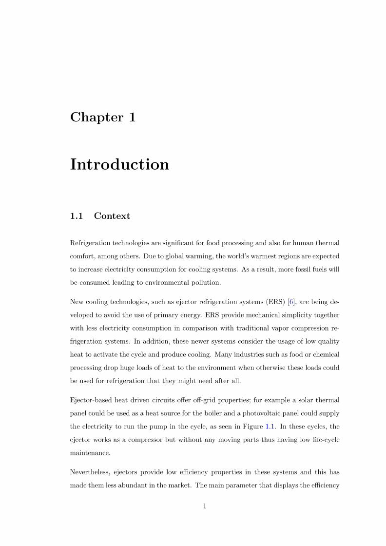
Ejector-based heat driven circuits offer off-grid properties; for example a solar thermal
panel could be used as a heat source for the boiler and a photovoltaic panel could supply
the electricity to run the pump in the cycle, as seen in Figure 1.1. In these cycles, the
ejector works as a compressor but without any moving parts thus having low life-cycle
maintenance.
Nevertheless, ejectors provide low efficiency properties in these systems and this has
made them less abundant in the market. The main parameter that displays the efficiency
1
2 Chapter 1. Introduction
Figure 1.1: Example of an ejector in a solar air-conditioning cycle
of a cycle is the Coefficient Of Performance (COP):
COP =cooling effect at the evaporator
energy input at the boiler and pump=
QeQb +Wp
(1.1)
where Qe and Qb are the cooling capacity at the evaporator and energy input to the
boiler, and Wp is the work consumed by the mechanical pump.
Another parameter which is relevant for the ejector performance is the entrainment
ratio, ω, and it is defined as:
ω =ms
mp(1.2)
where ms and mp are the mass flow rates for secondary and primary flows respectively.
1.2 Ejector as a component
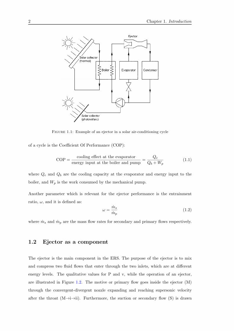
The ejector is the main component in the ERS. The purpose of the ejector is to mix
and compress two fluid flows that enter through the two inlets, which are at different
energy levels. The qualitative values for P and v, while the operation of an ejector,
are illustrated in Figure 1.2. The motive or primary flow goes inside the ejector (M)
through the convergent-divergent nozzle expanding and reaching supersonic velocity
after the throat (M→i→ii). Furthermore, the suction or secondary flow (S) is drawn
Chapter 1. Introduction 3
Figure 1.2: Qualitative P and v of an ejector.
into the supersonic motive jet. In the mixing section (ii→iii→iv) there is recompression
of the flows, producing one only flow at supersonic velocity. When reaching the diffuser
(iv→v→vi), the mixed flow must adjust to the outlet conditions and a series of shocks
and complex interactions take place (in Figure 1.2 there is one only shock as it is an
idealized case).
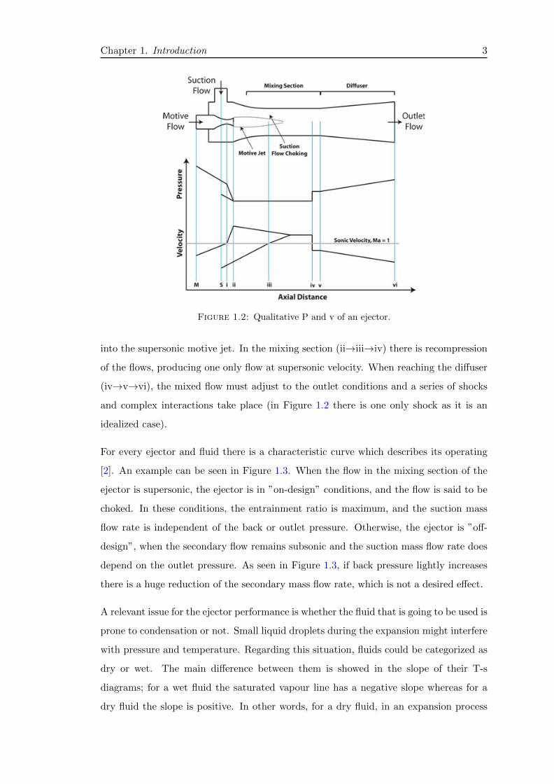
For every ejector and fluid there is a characteristic curve which describes its operating
[2]. An example can be seen in Figure 1.3. When the flow in the mixing section of the
ejector is supersonic, the ejector is in ”on-design” conditions, and the flow is said to be
choked. In these conditions, the entrainment ratio is maximum, and the suction mass
flow rate is independent of the back or outlet pressure. Otherwise, the ejector is ”off-
design”, when the secondary flow remains subsonic and the suction mass flow rate does
depend on the outlet pressure. As seen in Figure 1.3, if back pressure lightly increases
there is a huge reduction of the secondary mass flow rate, which is not a desired effect.
A relevant issue for the ejector performance is whether the fluid that is going to be used is
prone to condensation or not. Small liquid droplets during the expansion might interfere
with pressure and temperature. Regarding this situation, fluids could be categorized as
dry or wet. The main difference between them is showed in the slope of their T-s
diagrams; for a wet fluid the saturated vapour line has a negative slope whereas for a
dry fluid the slope is positive. In other words, for a dry fluid, in an expansion process
4 Chapter 1. Introduction
Figure 1.3: Ejector Characteristic Curve
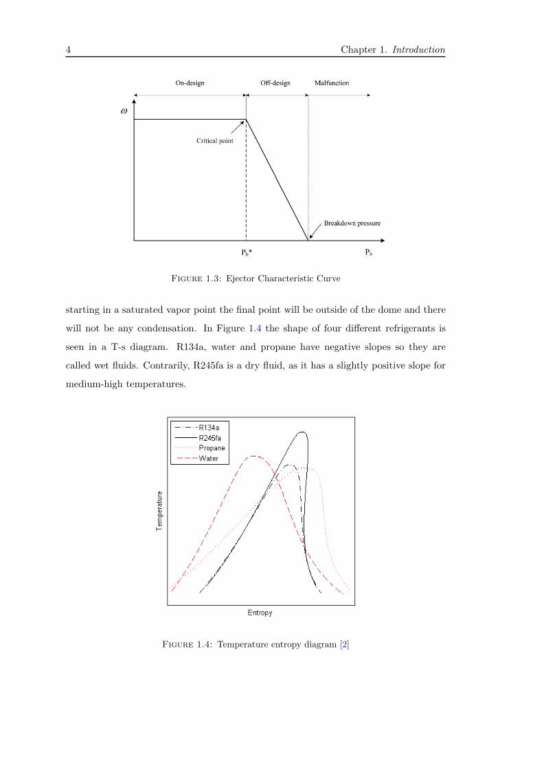
starting in a saturated vapor point the final point will be outside of the dome and there
will not be any condensation. In Figure 1.4 the shape of four different refrigerants is
seen in a T-s diagram. R134a, water and propane have negative slopes so they are
called wet fluids. Contrarily, R245fa is a dry fluid, as it has a slightly positive slope for
medium-high temperatures.
Figure 1.4: Temperature entropy diagram [2]
Chapter 1. Introduction 5
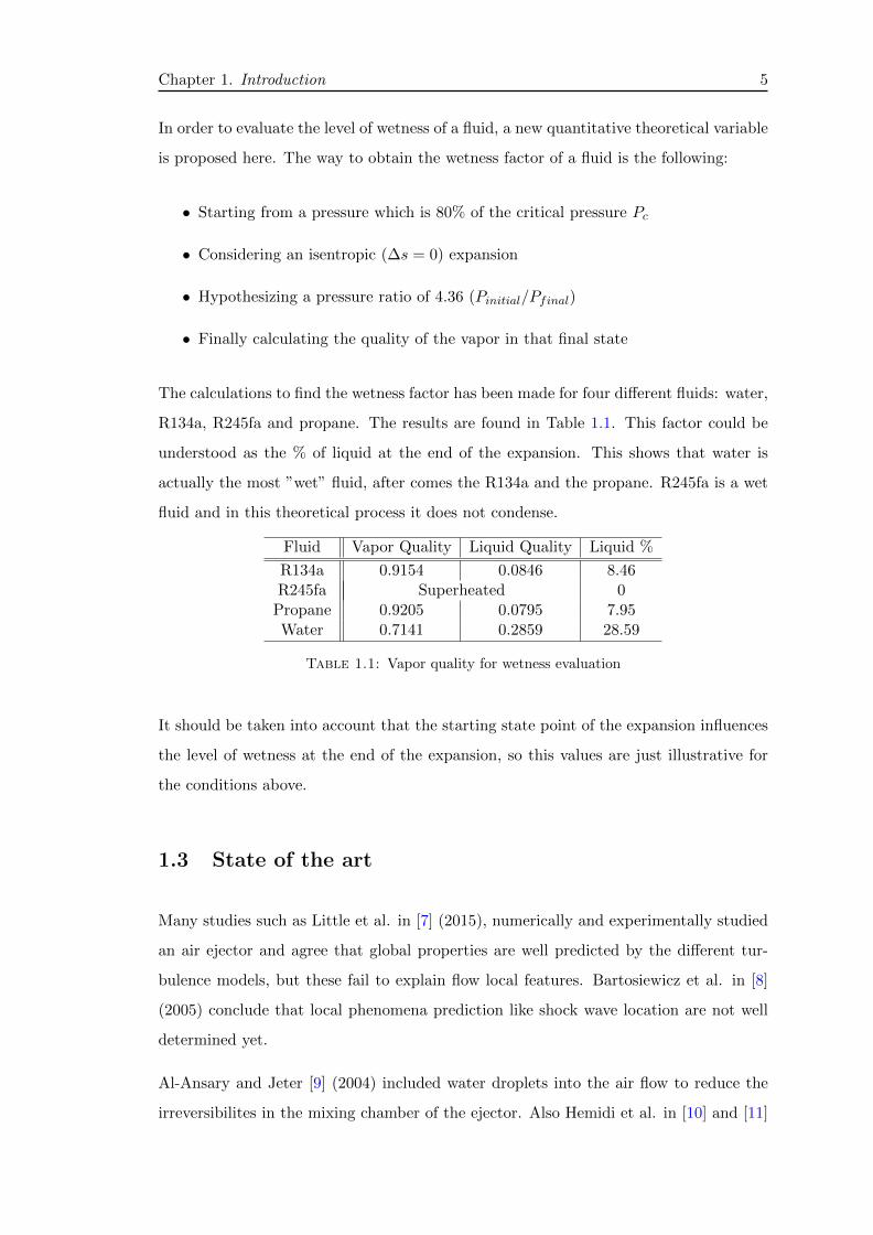
In order to evaluate the level of wetness of a fluid, a new quantitative theoretical variable
is proposed here. The way to obtain the wetness factor of a fluid is the following:
• Starting from a pressure which is 80% of the critical pressure Pc
• Considering an isentropic (∆s = 0) expansion
• Hypothesizing a pressure ratio of 4.36 (Pinitial/Pfinal)
• Finally calculating the quality of the vapor in that final state
The calculations to find the wetness factor has been made for four different fluids: water,
R134a, R245fa and propane. The results are found in Table 1.1. This factor could be
understood as the % of liquid at the end of the expansion. This shows that water is
actually the most ”wet” fluid, after comes the R134a and the propane. R245fa is a wet
fluid and in this theoretical process it does not condense.
Fluid Vapor Quality Liquid Quality Liquid %
R134a 0.9154 0.0846 8.46R245fa Superheated 0
Propane 0.9205 0.0795 7.95Water 0.7141 0.2859 28.59
Table 1.1: Vapor quality for wetness evaluation
It should be taken into account that the starting state point of the expansion influences
the level of wetness at the end of the expansion, so this values are just illustrative for
the conditions above.
1.3 State of the art
Many studies such as Little et al. in [7] (2015), numerically and experimentally studied
an air ejector and agree that global properties are well predicted by the different tur-
bulence models, but these fail to explain flow local features. Bartosiewicz et al. in [8]
(2005) conclude that local phenomena prediction like shock wave location are not well
determined yet.
Al-Ansary and Jeter [9] (2004) included water droplets into the air flow to reduce the
irreversibilites in the mixing chamber of the ejector. Also Hemidi et al. in [10] and [11]
6 Chapter 1. Introduction
(2009) had confirmed the difference between local and global properties. However and
in the same way as Al-Ansary and Jeter, these last two papers worked with air ejector
adding fine water droplets with an atomizer in order to simulate a two-phase flow. They
insisted that different physical properties such as speed of sound might change with the
water in air, which could modify some conditions.
Moses and Stein in [1] (1978) experimentally and numerically studied the growth of
water droplets in a Laval nozzle in order to predict condensation onset. They compared
the quantity of condensed liquid which comes from nucleation rate or droplet growth
laws. Later, Zori and Kelecy [5] (2005) study wet steam condensation in ANSYS Fluent
also in a Laval nozzle comparing the results with experimental data from Moses and
Stein.
Using refrigerant in simulations there is Elakhdar et al. [12] (2011) who performed a
simulation of an ejector with a refrigerant in vapor phase, but with a one-dimensional
mathematical model. Some studies such as the one made by Mazzelli and Milazzo
[13] (2014) avoided condensation issues and used dry fluids such as R245fa, eluding
the two-phase modelling. Bartosiewicz et al. [14] (2006) compared their CFD ejector
modelling with available 1-D data with R142b, but without condensation. They stated
that 1-D is not enough to predict operation at different conditions and suggested that an
experimental-CFD integration was needed in order to verify global and local properties.
Regarding the performance in the ejector, the studies made by Al-Ansary and Jeter
[9] and Hemidi et al. [10] hypothesized that the presence of liquid droplets at the end
of the nozzle can improve the entrainment effect of the ejector. In both cases, they
identified an improvement in ejector performance when the flow was not chocked (in
off-design conditions). In [10], this improvement is noted with the increase of about 10
to 40% of the entrainment ratio depending on the conditions. In any case, there was no
enhancement in the on-design operating.
Little and Garimella [15] (2015) performed an experimental study with R134a in an ejec-
tor and demonstrated that there is actually an improvement in COP up to a 12% when
the inlet conditions were more saturated. Experimental research with real refrigerant
ejector was also performed by Zegenhagen and Ziegler [16] (2015). They used R134a and
due the boundary conditions applied they avoid condensation effects inside the ejector.
Chapter 1. Introduction 7
1.4 Objectives
This thesis was suggested due to the scarcity of research on condensation simulation in
ejectors. The aim of this thesis is to study the condensation effects on a nozzle with
a real refrigerant such as R134a. This study is targeted to later be a tool to predict
behaviour of a full ejector with real gas as working fluid.
The main objective is to study the behaviour with condensation inside the nozzle. To do
so, the first step is to verify the built-in Wet Steam model in ANSYS Fluent simulating
software, which has water as fluid. After, with this model and the R134a refrigerant
properties inside the User Defined Wet Steam Property Functions (UDWSPF) the con-
densation consequences on the nozzle are going to be studied.
The final step of the thesis was thought to be simulating real gas properties in a full
ejector developed in Georgia Tech, but due to programming issues that will be presented
in the following sections, reaching that point was not possible.
1.4.1 Thesis structure
The thesis is divided in different chapters and each one is briefly described below.
In Chapter 2, the physical model inside the nozzle is described. The numerical model
and general set up for the Wet Steam build-in model are also detailed.
Chapter 3 reports the description of the first part of this thesis. It includes the cases’
features, its numerical set up and results for the nozzle study using water as refrigerant
liquid, considering ideal gas properties. This Chapter was thought to be the verification
of the built-in Wet Steam model in Fluent.
Chapter 4 reports the simulations of the nozzle using R134a as a refrigerant, including
the definition of the different cases, the numerical set up and the results. In this Chapter,
by using the user defined functions (UDF) the properties of the refrigerant are introduced
into the simulations.
In Chapter 5, the conclusions and future works to continue the research are outlined.

Chapter 2
Physical and Numerical Model
2.1 Physical Model
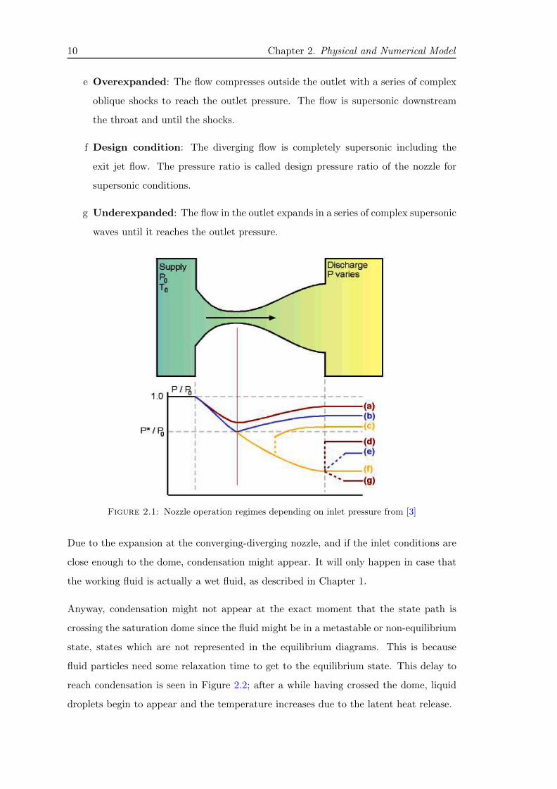
The usual operation of a nozzle is illustrated in Figure 2.1. The fluid flows from a high
pressure inlet to a lower pressure outlet. The plot shows the pressure ratio (pressure over
inlet pressure) depending on the position along the nozzle. The flow can have different
patterns depending on the boundary conditions and these are described below according
to Figure 2.1:
a Subsonic flow: The back pressure is too high to induce sonic flow in the throat.
The flow in the nozzle is subsonic. The outlet pressure is equal to the discharge
pressure and the exit jet is subsonic.
b Flow just chocked: The throat becomes sonic and the mass flux reaches its
maximum. Downstream, the flow is subsonic including exit jet.
c Shock in nozzle: The discharge pressure lies between pressures from conditions
(b) and (f), there is a normal-shock wave in the diverging section in order to cause
a subsonic flow back to the discharge condition. The throat is chocked and the
mass flow remains maximum.
d Shock at exit: The discharge pressure forces a normal-shock wave just at the
outlet. The flow is supersonic from the throat until the outlet, where after the
shock becomes subsonic.
9
10 Chapter 2. Physical and Numerical Model
e Overexpanded: The flow compresses outside the outlet with a series of complex
oblique shocks to reach the outlet pressure. The flow is supersonic downstream
the throat and until the shocks.
f Design condition: The diverging flow is completely supersonic including the
exit jet flow. The pressure ratio is called design pressure ratio of the nozzle for
supersonic conditions.
g Underexpanded: The flow in the outlet expands in a series of complex supersonic
waves until it reaches the outlet pressure.
Figure 2.1: Nozzle operation regimes depending on inlet pressure from [3]
Due to the expansion at the converging-diverging nozzle, and if the inlet conditions are
close enough to the dome, condensation might appear. It will only happen in case that
the working fluid is actually a wet fluid, as described in Chapter 1.
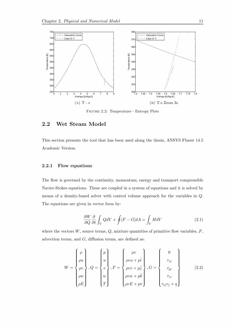
Anyway, condensation might not appear at the exact moment that the state path is
crossing the saturation dome since the fluid might be in a metastable or non-equilibrium
state, states which are not represented in the equilibrium diagrams. This is because
fluid particles need some relaxation time to get to the equilibrium state. This delay to
reach condensation is seen in Figure 2.2; after a while having crossed the dome, liquid
droplets begin to appear and the temperature increases due to the latent heat release.
Chapter 2. Physical and Numerical Model 11
0 1 2 3 4 5 6 7 8 9250
300
350
400
450
500
550
600
650
700
750
Entropy [kJ/kg·K]
Tem
pera
ture
[K]
Saturation CurveCase S−T
(a) T - s
7.4 7.45 7.5 7.55 7.6 7.65 7.7 7.75 7.8300
310
320
330
340
350
360
370
380
Entropy [kJ/kg·K]
Tem
pera
ture
[K]
Saturation CurveCase S−T
(b) T-s Zoom In
Figure 2.2: Temperature - Entropy Plots
2.2 Wet Steam Model
This section presents the tool that has been used along the thesis, ANSYS Fluent 14.5
Academic Version.
2.2.1 Flow equations
The flow is governed by the continuity, momentum, energy and transport compressible
Navier-Stokes equations. These are coupled in a system of equations and it is solved by
means of a density-based solver with control volume approach for the variables in Q.
The equations are given in vector form by:
∂W
∂Q
∂
∂t
∫VQdV +
∮[F −G]dA =
∫VHdV (2.1)
where the vectors W , source terms, Q, mixture quantities of primitive flow variables, F ,
advection terms, and G, diffusion terms, are defined as:
W =
ρ
ρu
ρv
ρw
ρE
, Q =
p
u
v
w
T
, F =
ρv
ρvu+ pi
ρvv + pj
ρvw + pk
ρvE + pv
, G =
0
τxi
τyi
τzi
τijvj + q
(2.2)
12 Chapter 2. Physical and Numerical Model
The total energy, E, is defined as:
E = h− p
ρ+v2
2(2.3)
where the Jacobian ∂W/∂Q is given by:
∂W
∂Q=
ρp 0 0 0 ρT
ρpu ρ 0 0 ρTu
ρpv 0 ρ 0 ρT v
ρpw 0 0 ρ ρTw
ρpH − δ ρu ρv ρw ρTH + ρCp
(2.4)
where
ρp =∂ρ
∂p
∣∣∣T, ρT =
∂ρ
∂T
∣∣∣p
(2.5)
Two additional transport equations are introduced to solve the droplet formation and
the mass transference between the two phases. Those are explained in the section 2.2.2.
This change in primary variables, described as preconditioning in [17], with respect to
the usual Navier-Stokes equation ( ∂∂t∫V WdV +
∮[F − G]dA =
∫V HdV ), is performed
in order to overcome the numerical stiffness at low Mach number areas due to the gap
between the fluid velocity v and the speed of sound c, that is when the fluid is weakly
compressible. In these zones, the stiffness of the equations leads to convergence problems
since the CFL criteria for compressible flow is connected with the sound of speed.
2.2.2 Wet Steam Equation
All the simulations performed, use the Wet Steam model available in ANSYS Fluent.
This software models the two-phase flow using Navier-Stokes equations, in addition to
two transport equations which the liquid-phase mass fraction (β) and the number of
liquid droplets per unit volume (η). For the Wet Steam model, only the density-based
solver is available. There are some assumptions that need to be considered for this
model:
• velocity slip between droplets and vapor-phase is negligible.
Chapter 2. Physical and Numerical Model 13
• interactions between the droplets are neglected.
• mass fraction of the condensed phase, or liquid mass fraction, β, is small: β < 0.2.
• as the size of droplets is tiny (0.1µm to 100µm), its volume is neglected.
Using the previous assumption the mixture density is connected with the vapor density:
ρ =ρv
1− β(2.6)
Also, the pressure and temperature of the mixture will be the same as the pressure and
temperature of the vapor-phase. However, the mixture properties which are related to
liquid and vapor properties through the liquid mass fraction β, use the following mixing
law:
φm = φlβ + (1− β)φv (2.7)
where φ represents one of the following thermodynamic properties: h, s, Cp, Cv, µ or kt.
The two transport equations that are added to solve condensation are the following:
• Governing the mass fraction of the condensed liquid phase (β):
∂ρβ
∂t+∇ · (ρ~vβ) = Γ (2.8)
where Γ is the mass generation rate caused by condensation and evaporation (kg
per unit volume per second).
• Modelling the evolution of the number density of the droplets per unit volume (η):
∂ρη
∂t+∇ · (ρ~vη) = ρI (2.9)
where I is the nucleation rate (number of new droplets per unit volume per second).
2.2.3 Phase Change Model
The phase change model assumes the next hypothesis:
• Condensation is homogeneous
14 Chapter 2. Physical and Numerical Model
• Droplet growth is based on average representative mean radii
• Droplet is assumed to be spherical
• Droplets are surrounded by infinite vapor space
• Heat capacity of the fine droplets is negligible compared with the latent heat
released in condensation.
The mass generation rate Γ in the classical nucleation theory during non-equilibrium
condensation process is given by the sum of mass increase due to nucleation (the for-
mation of critically sized droplets) and also due to the growth/demise of these droplets
[18].
Therefore, Γ is written as:
Γ =4
3πρlIr
3∗ + 4πρlηr
2∂r
∂t(2.10)
where r is the average radius of the droplet and r∗ is the Kelvin-Helmholtz critical droplet
radius, above this value the droplet will grow and below, the droplet will evaporate.
The critical radius, r∗, is given by [19]:
r∗ =2σ
ρlRT lnS(2.11)
where σ is the liquid surface tension evaluated at the temperature T , ρl is the condensed
liquid density and S is the super saturation ratio defined as the ratio of vapor pressure
to the equilibrium saturation pressure:
s =P
Psat(T )(2.12)
The expansion is usually fast, forcing not to move through equilibrium states and having
values of supersaturation ratio S higher than one.
Condensation process implies two mechanisms, the mass transfer from the vapor to
the droplets and the heat transfer between the droplets and the vapor as latent heat.
This energy transference is presented by Young [19] and used by Ishazaki [18] and is
Chapter 2. Physical and Numerical Model 15
represented as the average radius change of the droplet:
∂r
∂t=
P
hlvρl√
2πRT
γ + 1
2γCp(T0 − T ) (2.13)
where T0 is the droplet temperature.
The classical theory of homogeneous nucleation describes the formation of the liquid as
droplets of a supersaturated phase without impurities or irregular particles. The nucle-
ation rate given by the classical theory of homogeneous nucleation [18] and corrected for
non-isothermal effects is:
I =qc
1 + θ
ρ2vρl
√2σ
M3mπ
e− 4πr2∗σ
3kbT (2.14)
where qc is the evaporation coefficient, kb is the Boltzmann, Mm is the mass of one
molecule, σ is the liquid surface tension, and ρl is the liquid density at the temperature
T .
The non-isothermal correction factor, θ, is given by:
θ =2(γ − 1)
γ + 1
hlvRT
(hlvRT− 0.5) (2.15)
where hlv is the specific enthalpy of evaporation at pressure P and γ is the ratio of
specific heat capacities.
2.3 RANS Turbulence Models
In this thesis, turbulence modelling uses the RANS (Reynolds Averaged Navier-Stokes)
models.
Turbulent flows are depicted by fluctuation of all transported variables. These fluc-
tuations in velocity and the other variables might lead to fluctuations of energy and
momentum. In the cases that fluctuations are of small scales and have high frequency,
it is moderately expensive to compute. Alternately, the instantaneous governing equa-
tions can be ensemble averaged to eliminate these small scales, having a set of arranged
equations that are less costly to resolve. The velocity field in this method is averaged
over a time period which is much higher than time constant in velocity fluctuations.
16 Chapter 2. Physical and Numerical Model
These averaged equations are not closed (have more degrees of freedom) and they need
a closure known as Boussinesq hypothesis [20], which provides its closure. Boussinesq
hypothesis assumes that the turbulence is isotropic, which is a highly improbable if the
flow is not simple enough. The k-ε, RNG-k-ε and k-ω models are based on this approach.
There are different turbulence models in the RANS, and two of them are used in this
thesis.
2.3.1 Standard k-ε Model
The Standard k-ε is probably the most used turbulence model as it is robust and well-
validated. This model is only applicable for strongly turbulent flows since it is based on
the assumption that the flow is fully turbulent (renders the effects of molecular viscosity
negligible).
The Standard k-ε model is based on model transport equations for the turbulence kinetic
energy (k) and its dissipation rate (ε). The model transport equation for k is derived
from the exact equation, while the model transport equation for ε was obtained using
physical reasoning and bears little resemblance to its mathematically exact counterpart.
The turbulence kinetic energy, k, and its rate of dissipation, ε, are obtained from the
following transport equations:
∂
∂t+
∂
∂xi(ρkui) =
∂
∂xj
[(µ+
µtσk
)∂k
∂xj
]+Gk +Gb − ρε− YM + Sk (2.16)
Turbulent viscosity is obtained assuming its proportionality to the product between
turbulent velocity scale and turbulent distance, and is given by:
µt = ρ · Cµk2
ε(2.17)
The effective viscosity of the fluid under a turbulent regime is given by:
µeff = µ+ µt (2.18)
The model constants C1ε,C2ε, Cµ, σk, and σε have the following default values:
C1ε = 1.44, C2ε = 1.92, Cµ = 0.09, σk = 1.0, σε = 1.3 (2.19)
Chapter 2. Physical and Numerical Model 17
This model is used in all cases considering that it is the most common. It is also
suggested as slightly better by Hemidi et al. in [10] and Al-Ansary and Jeter [9].
2.3.2 Shear-Stress Transport k-ω Model
The SST (Shear-Stress Transport) k-ω model is a semi-empirical model based on trans-
port equations for the turbulent kinetic energy (k) and the specific dissipation rate (ω),
which can also be thought of as the ratio of k and ε (from previous model).
The turbulence kinetic energy, k, and the specific dissipation rate, ω, are obtained from
the following transport equations:
∂
∂t(ρ · k) +
∂
∂xi(ρ · k · ui) =
∂
∂xj
(Γk
∂k
∂xj
)+Gk − Yk + Sk (2.20)
∂
∂t(ρ · ω) +
∂
∂xi(ρ · ω · ui) =
∂
∂xj
(Γω
∂ω
∂xj
)+Gω − Yω + Sω (2.21)
The SST k-ω model has more accuracy for a wide range of flows such as transonic shock
waves and adverse and adverse pressure gradient flows. It is usually applied when the
flow is wall-resolved.
More information about turbulence models is found in the ANSYS Theory Guide [17].
2.4 Wall approach
Turbulent flows need some adaptations near the walls since the velocity is affected by the
no-slip condition at the wall. Accurate solving near the walls leads to better prediction
of the phenomena.
As seen in Figure 2.3, the near-wall region can be divided into three layers. The in-
ner layer, ”viscous sublayer” is almost laminar. In the outer layer, ”fully-turbulent”,
turbulence is more important. The intermediate region between the viscous and the
fully-turbulent is the buffer layer, where effects of molecular viscosity and turbulence
are equally important.
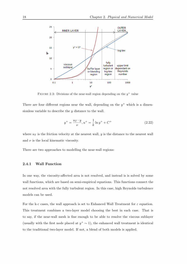
18 Chapter 2. Physical and Numerical Model
Figure 2.3: Divisions of the near-wall region depending on the y+ value
There are four different regions near the wall, depending on the y+ which is a dimen-
sionless variable to describe the y distance to the wall.
y+ =uT · yν
, u+ =1
kln y+ + C+ (2.22)
where uT is the friction velocity at the nearest wall, y is the distance to the nearest wall
and ν is the local kinematic viscosity.
There are two approaches to modelling the near-wall regions:
2.4.1 Wall Function
In one way, the viscosity-affected area is not resolved, and instead is is solved by some
wall functions, which are based on semi-empirical equations. This functions connect the
not resolved area with the fully turbulent region. In this case, high Reynolds turbulence
models can be used.
For the k-ε cases, the wall approach is set to Enhanced Wall Treatment for ε equation.
This treatment combines a two-layer model choosing the best in each case. That is
to say, if the near-wall mesh is fine enough to be able to resolve the viscous sublayer
(usually with the first node placed at y+ ∼ 1), the enhanced wall treatment is identical
to the traditional two-layer model. If not, a blend of both models is applied.
Chapter 2. Physical and Numerical Model 19
2.4.2 Wall Resolved
The other option is to have a fully resolved region until the wall, including the viscous
sublayer. In this case, the turbulence models applied need to be valid throughout the
near-wall area.
2.5 Solver/Numerical setup
To perform the mathematical simulation, the finite volume method is used, in which the
differential equations that control the physics are transformed to algebraic equations to
be solved numerically.
The settings of the coupled solver are described below:
• Finite volume method: the governing equations are discretized using a control
volume technique.
• Steady state.
• Discretization scheme: second order upwind.
• Central difference for viscous terms.
• Implicit (which allows having a Courant1 number bigger than 1).
• Roe flux splitting methodology.
• Gauss Siedel: The discretized system is solved in a coupled way with a Gauss-Siedel
algorithm.
All simulations have been run with second order discretization scheme, although in some
cases, the first part of the simulation was made with first order, and after converging, it
was changed to second order for a higher accuracy in the final results. The same pattern
was used after increasing the order for discretization for the Courant number, starting
from a low value around 0.5 or 1, and successively increasing it when the simulation was
approaching convergence.
1The Courant number is an adimensional parameter which direcly linked to the time step for theequation solving.
20 Chapter 2. Physical and Numerical Model
In most of the cases, the residuals easily decreased and became constant at values lower
than 10−4. However, in other situations, the residuals did not decrease below 10−2
but the solution did not vary and the results were taken into account. Also, to check
convergence the mass imbalance between inlet and outlet has been considered valid being
lower than 5%.
Grid dependency tests were not performed regarding that the aim of this thesis was not
to check if the grid was correct. As long as there is no experimental data to compare
with, the purpose was to test the model and create a code for the properties. A mesh
refinement near the wall was performed in one case to reach y+ ∼ 1 but the grid was so
fine that the time cost to compute was not acceptable to keep along the thesis.
Chapter 3
Validation: Nozzle + Steam
3.1 Description of the cases
In the first place, as an approach to study condensation properties, the simulations in
this chapter have been carried out with the built-in Wet Steam model. That is to say,
that the water and steam properties have been used instead of refrigerant, which will be
shown in Chapter 4.
The different cases are classified due to the inlet and outlet boundary conditions of the
nozzle.
• Exp. No. 410-421 : To check the difference between these two cases performed by
Moses and Stein [1].
• Turbulence : Compare a case with the two turbulence models.
• Shock Waves : Forcing to have shock waves inside the nozzle between the throat
and the outlet.
• ∆Tsat : Modifying T in the inlet to see the evolution of condensation while reducing
∆Tsat.
The aim of this variations is to check the differences between them, such as the conden-
sation starting point or the behaviour of the pressure and temperature.
21
22 Chapter 3. Validation: Nozzle + Steam
3.2 Numerical Setup
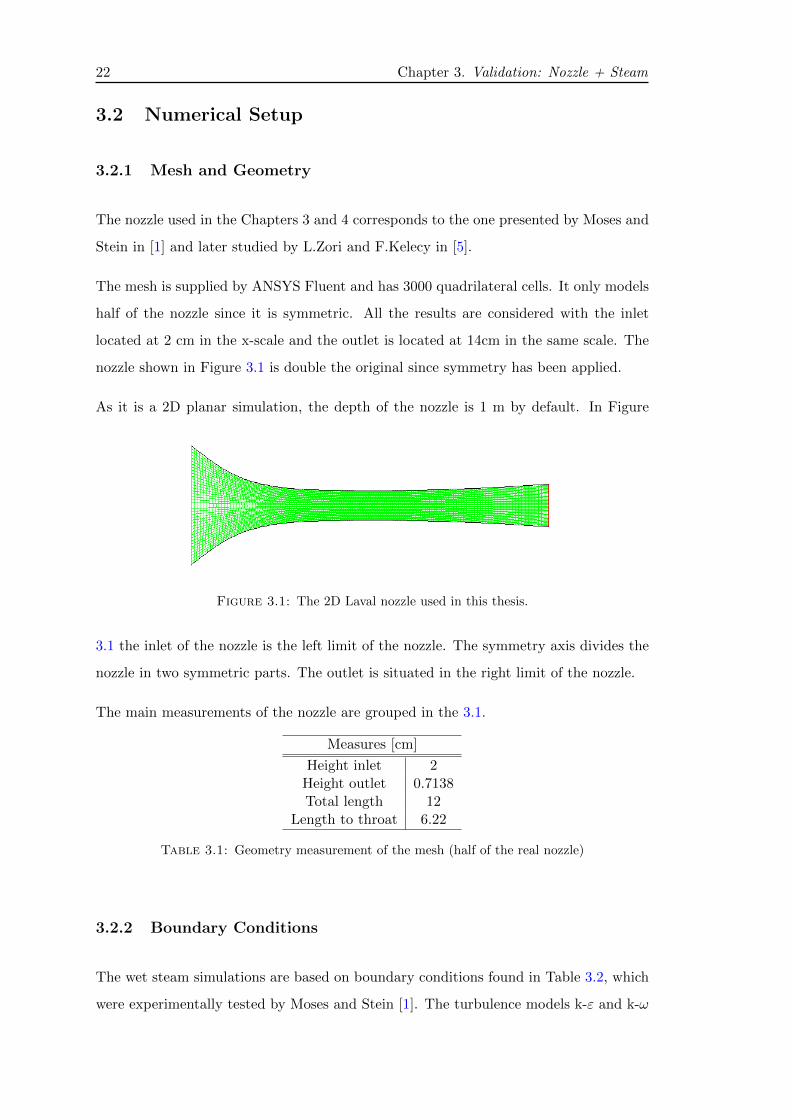
3.2.1 Mesh and Geometry
The nozzle used in the Chapters 3 and 4 corresponds to the one presented by Moses and
Stein in [1] and later studied by L.Zori and F.Kelecy in [5].
The mesh is supplied by ANSYS Fluent and has 3000 quadrilateral cells. It only models
half of the nozzle since it is symmetric. All the results are considered with the inlet
located at 2 cm in the x-scale and the outlet is located at 14cm in the same scale. The
nozzle shown in Figure 3.1 is double the original since symmetry has been applied.
As it is a 2D planar simulation, the depth of the nozzle is 1 m by default. In Figure
Figure 3.1: The 2D Laval nozzle used in this thesis.
3.1 the inlet of the nozzle is the left limit of the nozzle. The symmetry axis divides the
nozzle in two symmetric parts. The outlet is situated in the right limit of the nozzle.
The main measurements of the nozzle are grouped in the 3.1.
Measures [cm]
Height inlet 2Height outlet 0.7138Total length 12
Length to throat 6.22
Table 3.1: Geometry measurement of the mesh (half of the real nozzle)
3.2.2 Boundary Conditions
The wet steam simulations are based on boundary conditions found in Table 3.2, which
were experimentally tested by Moses and Stein [1]. The turbulence models k-ε and k-ω
Chapter 3. Validation: Nozzle + Steam 23
are also compared in the first part of the results with the boundary conditions of Exp.
No. 410 seen in Table 3.2.
Experiment No. Pinlet [Pa] Tinlet [K] Poutlet [Pa] Toutlet [K]
410 70727.5 377 5000 377421 66807.8 385 5000 385
Table 3.2: Boundary conditions given by [1] and [5]
In the second part of the results, the boundary conditions are modified varying the
superheating level of the inlet in the case of ∆Tsat evaluation, whereas in the shock wave
analysis, it is the back pressure which is modified. The boundary conditions in the shock
wave cases were checked in order to have one downstream the throat and upstream the
outlet and can be checked in Table 3.3. In the cases where there is turbulence, Turbulent
Pinlet [Pa] Tinlet [K] Poutlet [Pa] Toutlet [K]
70727.5 377 51995.7 377
Table 3.3: Boundary conditions for shock waves - WS
Intensity is imposed to be 5% and Hydraulic Diameter is Dh−inlet = 0.03922m and
Dh−outlet = 0.01417m.
3.3 Results I
This section is thought to be the description of the results related with the boundary
conditions. Experimental available results will be compared with the simulations.
3.3.1 Experiments No. 410-421
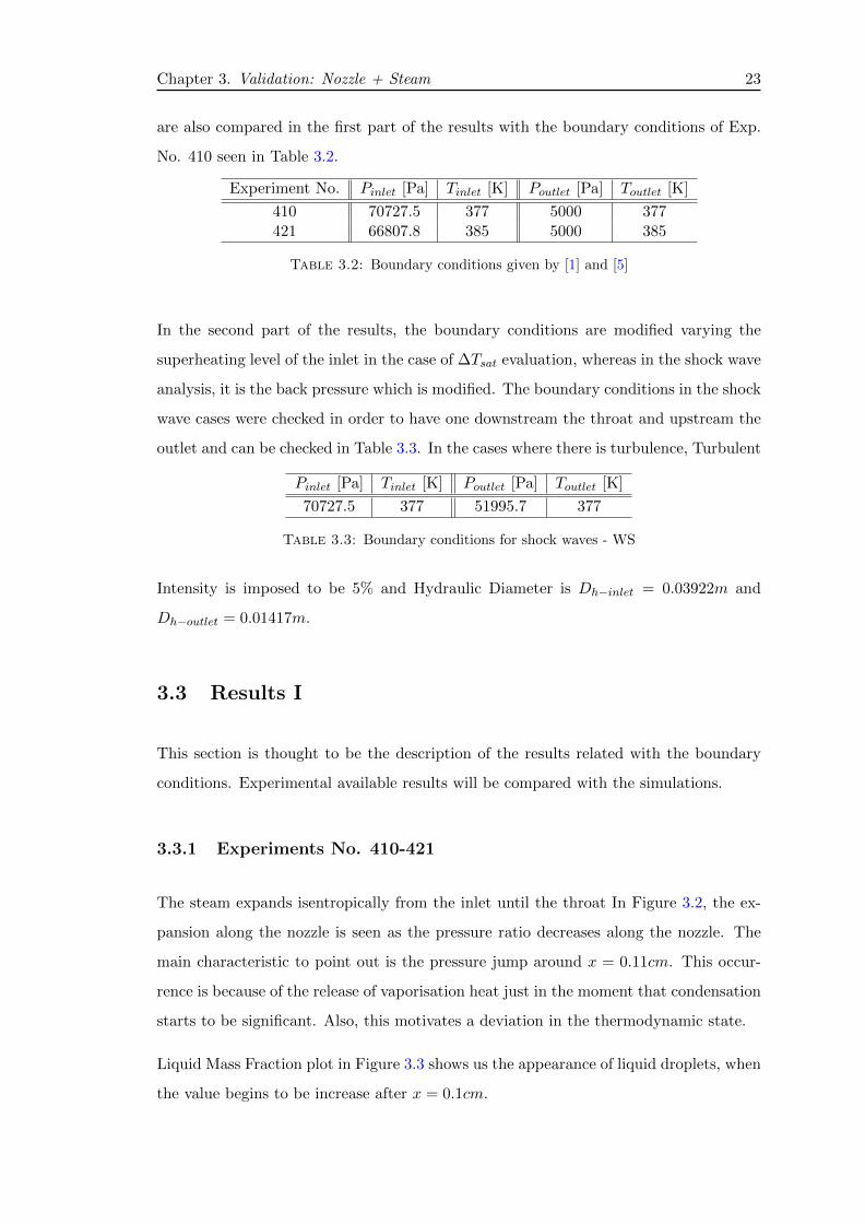
The steam expands isentropically from the inlet until the throat In Figure 3.2, the ex-
pansion along the nozzle is seen as the pressure ratio decreases along the nozzle. The
main characteristic to point out is the pressure jump around x = 0.11cm. This occur-
rence is because of the release of vaporisation heat just in the moment that condensation
starts to be significant. Also, this motivates a deviation in the thermodynamic state.
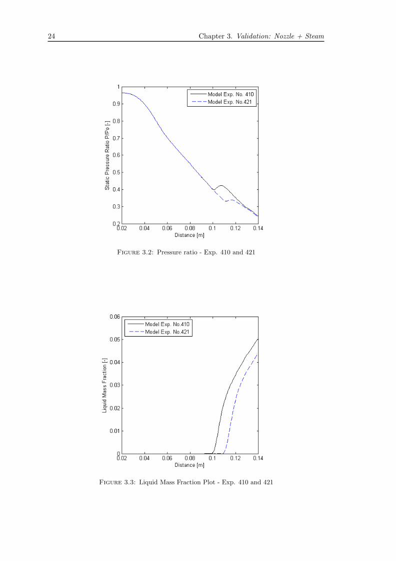
Liquid Mass Fraction plot in Figure 3.3 shows us the appearance of liquid droplets, when
the value begins to be increase after x = 0.1cm.
24 Chapter 3. Validation: Nozzle + Steam
Figure 3.2: Pressure ratio - Exp. 410 and 421
Figure 3.3: Liquid Mass Fraction Plot - Exp. 410 and 421
Chapter 3. Validation: Nozzle + Steam 25
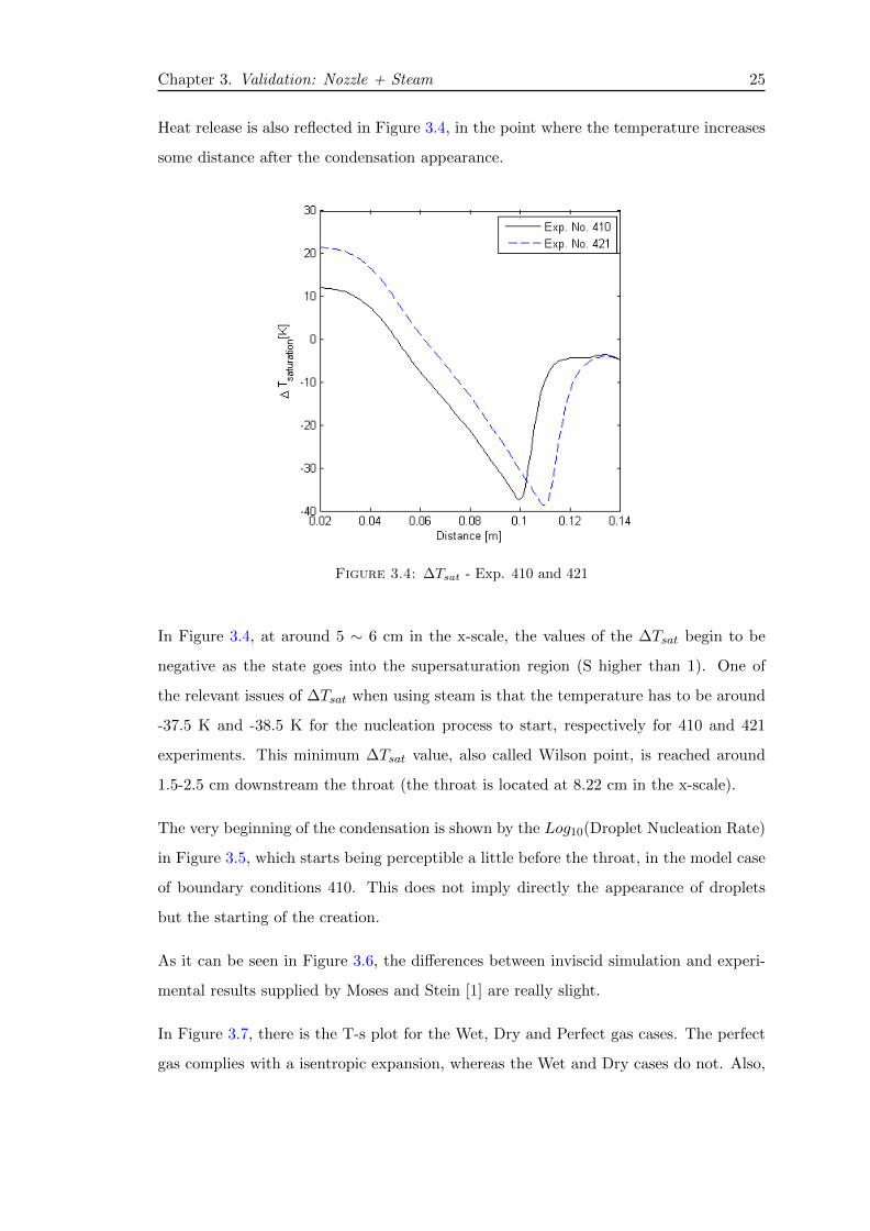
Heat release is also reflected in Figure 3.4, in the point where the temperature increases
some distance after the condensation appearance.
Figure 3.4: ∆Tsat - Exp. 410 and 421
In Figure 3.4, at around 5 ∼ 6 cm in the x-scale, the values of the ∆Tsat begin to be
negative as the state goes into the supersaturation region (S higher than 1). One of
the relevant issues of ∆Tsat when using steam is that the temperature has to be around
-37.5 K and -38.5 K for the nucleation process to start, respectively for 410 and 421
experiments. This minimum ∆Tsat value, also called Wilson point, is reached around
1.5-2.5 cm downstream the throat (the throat is located at 8.22 cm in the x-scale).
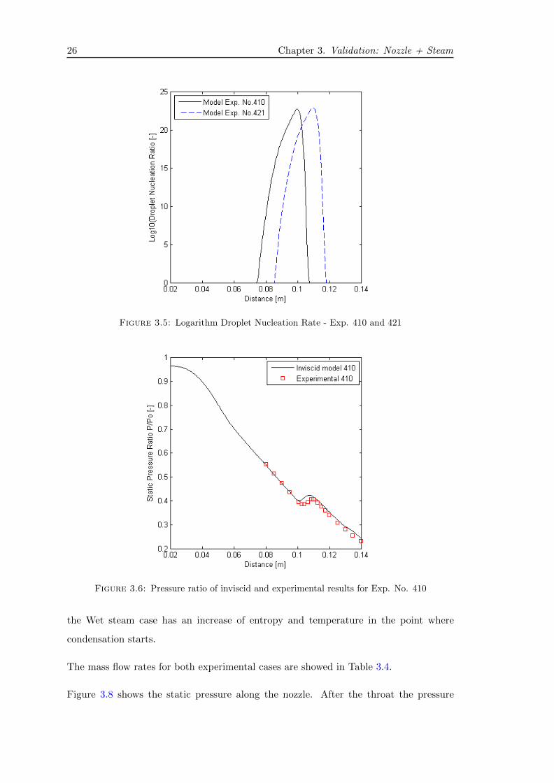
The very beginning of the condensation is shown by the Log10(Droplet Nucleation Rate)
in Figure 3.5, which starts being perceptible a little before the throat, in the model case
of boundary conditions 410. This does not imply directly the appearance of droplets
but the starting of the creation.
As it can be seen in Figure 3.6, the differences between inviscid simulation and experi-
mental results supplied by Moses and Stein [1] are really slight.
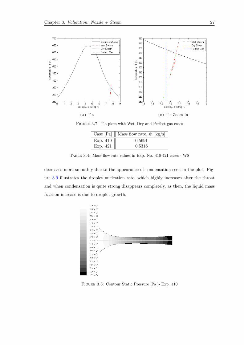
In Figure 3.7, there is the T-s plot for the Wet, Dry and Perfect gas cases. The perfect
gas complies with a isentropic expansion, whereas the Wet and Dry cases do not. Also,
26 Chapter 3. Validation: Nozzle + Steam
Figure 3.5: Logarithm Droplet Nucleation Rate - Exp. 410 and 421
Figure 3.6: Pressure ratio of inviscid and experimental results for Exp. No. 410
the Wet steam case has an increase of entropy and temperature in the point where
condensation starts.
The mass flow rates for both experimental cases are showed in Table 3.4.
Figure 3.8 shows the static pressure along the nozzle. After the throat the pressure
Chapter 3. Validation: Nozzle + Steam 27
(a) T-s (b) T-s Zoom In
Figure 3.7: T-s plots with Wet, Dry and Perfect gas cases
Case [Pa] Mass flow rate, m [kg/s]
Exp. 410 0.5691Exp. 421 0.5316
Table 3.4: Mass flow rate values in Exp. No. 410-421 cases - WS
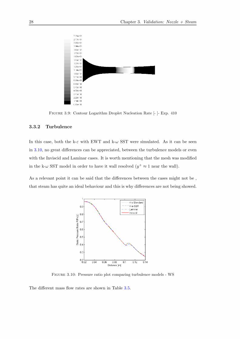
decreases more smoothly due to the appearance of condensation seen in the plot. Fig-
ure 3.9 illustrates the droplet nucleation rate, which highly increases after the throat
and when condensation is quite strong disappears completely, as then, the liquid mass
fraction increase is due to droplet growth.
Figure 3.8: Contour Static Pressure [Pa ]- Exp. 410
28 Chapter 3. Validation: Nozzle + Steam
Figure 3.9: Contour Logarithm Droplet Nucleation Rate [- ]- Exp. 410
3.3.2 Turbulence
In this case, both the k-ε with EWT and k-ω SST were simulated. As it can be seen
in 3.10, no great differences can be appreciated, between the turbulence models or even
with the Inviscid and Laminar cases. It is worth mentioning that the mesh was modified
in the k-ω SST model in order to have it wall resolved (y+ ≈ 1 near the wall).
As a relevant point it can be said that the differences between the cases might not be ,
that steam has quite an ideal behaviour and this is why differences are not being showed.
Figure 3.10: Pressure ratio plot comparing turbulence models - WS
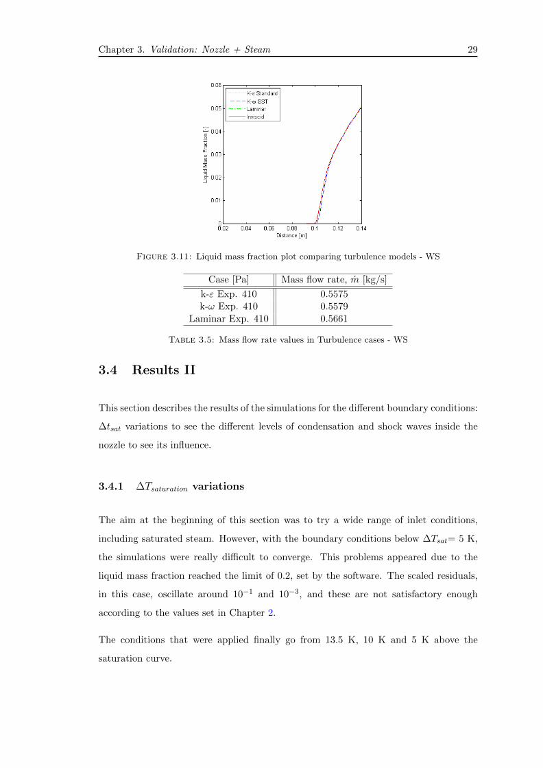
The different mass flow rates are shown in Table 3.5.
Chapter 3. Validation: Nozzle + Steam 29
Figure 3.11: Liquid mass fraction plot comparing turbulence models - WS
Case [Pa] Mass flow rate, m [kg/s]
k-ε Exp. 410 0.5575k-ω Exp. 410 0.5579
Laminar Exp. 410 0.5661
Table 3.5: Mass flow rate values in Turbulence cases - WS
3.4 Results II
This section describes the results of the simulations for the different boundary conditions:
∆tsat variations to see the different levels of condensation and shock waves inside the
nozzle to see its influence.
3.4.1 ∆Tsaturation variations
The aim at the beginning of this section was to try a wide range of inlet conditions,
including saturated steam. However, with the boundary conditions below ∆Tsat= 5 K,
the simulations were really difficult to converge. This problems appeared due to the
liquid mass fraction reached the limit of 0.2, set by the software. The scaled residuals,
in this case, oscillate around 10−1 and 10−3, and these are not satisfactory enough
according to the values set in Chapter 2.
The conditions that were applied finally go from 13.5 K, 10 K and 5 K above the
saturation curve.
30 Chapter 3. Validation: Nozzle + Steam
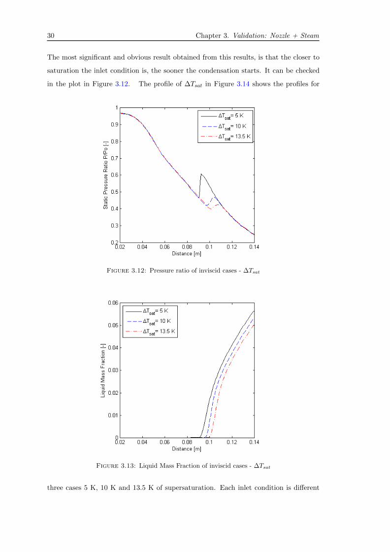
The most significant and obvious result obtained from this results, is that the closer to
saturation the inlet condition is, the sooner the condensation starts. It can be checked
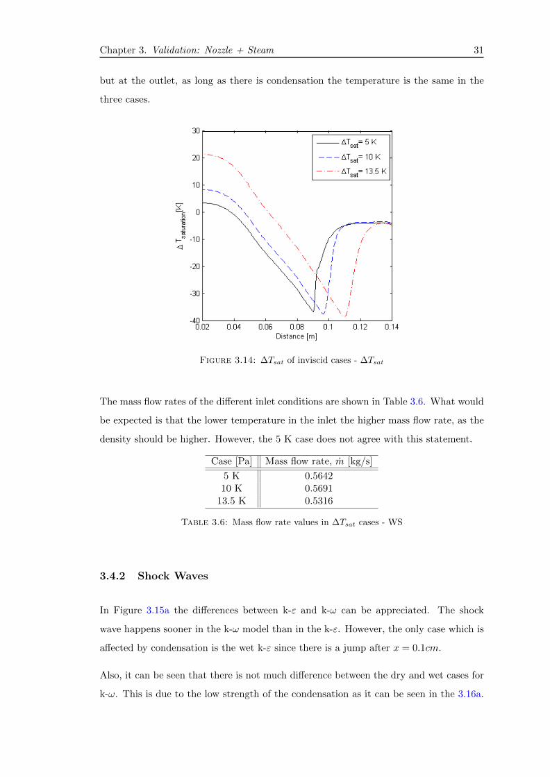
in the plot in Figure 3.12. The profile of ∆Tsat in Figure 3.14 shows the profiles for
Figure 3.12: Pressure ratio of inviscid cases - ∆Tsat
Figure 3.13: Liquid Mass Fraction of inviscid cases - ∆Tsat
three cases 5 K, 10 K and 13.5 K of supersaturation. Each inlet condition is different
Chapter 3. Validation: Nozzle + Steam 31
but at the outlet, as long as there is condensation the temperature is the same in the
three cases.
Figure 3.14: ∆Tsat of inviscid cases - ∆Tsat
The mass flow rates of the different inlet conditions are shown in Table 3.6. What would
be expected is that the lower temperature in the inlet the higher mass flow rate, as the
density should be higher. However, the 5 K case does not agree with this statement.
Case [Pa] Mass flow rate, m [kg/s]
5 K 0.564210 K 0.5691
13.5 K 0.5316
Table 3.6: Mass flow rate values in ∆Tsat cases - WS
3.4.2 Shock Waves
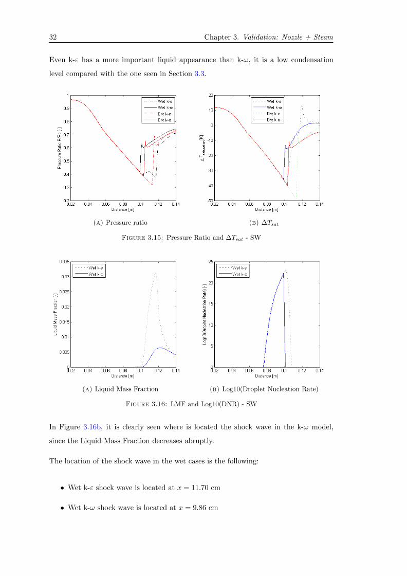
In Figure 3.15a the differences between k-ε and k-ω can be appreciated. The shock
wave happens sooner in the k-ω model than in the k-ε. However, the only case which is
affected by condensation is the wet k-ε since there is a jump after x = 0.1cm.
Also, it can be seen that there is not much difference between the dry and wet cases for
k-ω. This is due to the low strength of the condensation as it can be seen in the 3.16a.
32 Chapter 3. Validation: Nozzle + Steam
Even k-ε has a more important liquid appearance than k-ω, it is a low condensation
level compared with the one seen in Section 3.3.
(a) Pressure ratio (b) ∆Tsat
Figure 3.15: Pressure Ratio and ∆Tsat - SW
(a) Liquid Mass Fraction (b) Log10(Droplet Nucleation Rate)
Figure 3.16: LMF and Log10(DNR) - SW
In Figure 3.16b, it is clearly seen where is located the shock wave in the k-ω model,
since the Liquid Mass Fraction decreases abruptly.
The location of the shock wave in the wet cases is the following:
• Wet k-ε shock wave is located at x = 11.70 cm
• Wet k-ω shock wave is located at x = 9.86 cm
Chapter 3. Validation: Nozzle + Steam 33
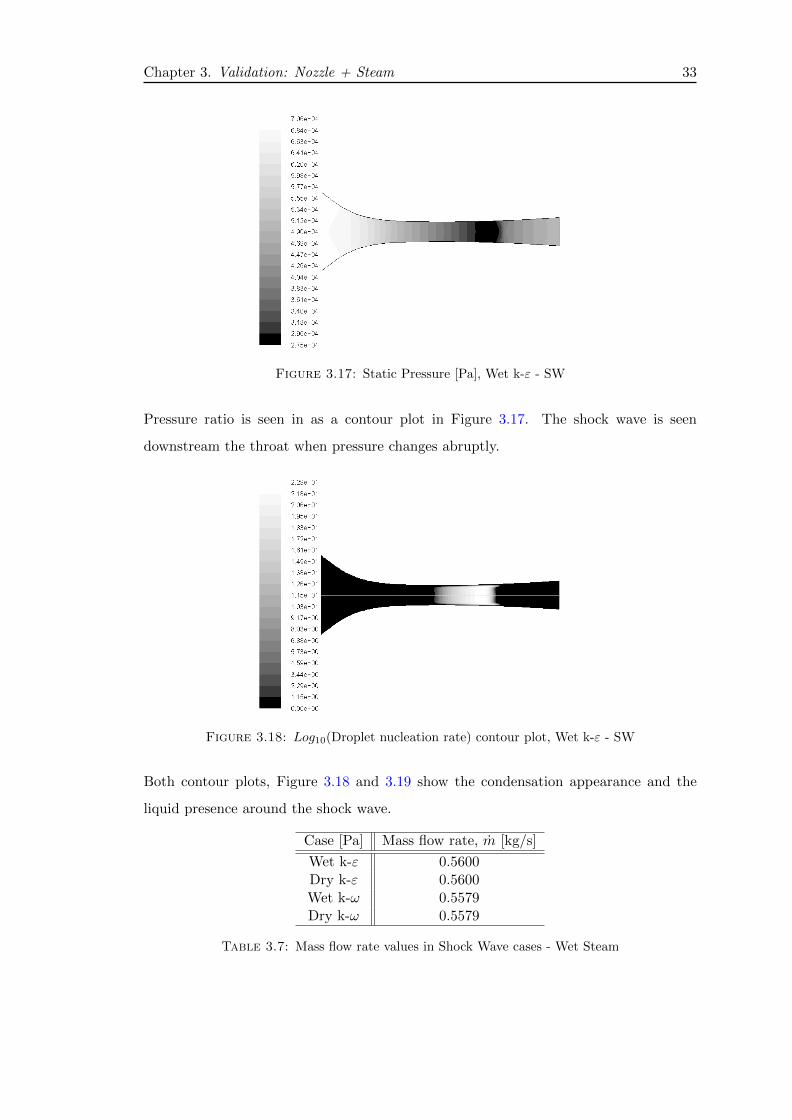
Figure 3.17: Static Pressure [Pa], Wet k-ε - SW
Pressure ratio is seen in as a contour plot in Figure 3.17. The shock wave is seen
downstream the throat when pressure changes abruptly.
Figure 3.18: Log10(Droplet nucleation rate) contour plot, Wet k-ε - SW
Both contour plots, Figure 3.18 and 3.19 show the condensation appearance and the
liquid presence around the shock wave.
Case [Pa] Mass flow rate, m [kg/s]
Wet k-ε 0.5600Dry k-ε 0.5600Wet k-ω 0.5579Dry k-ω 0.5579
Table 3.7: Mass flow rate values in Shock Wave cases - Wet Steam
34 Chapter 3. Validation: Nozzle + Steam
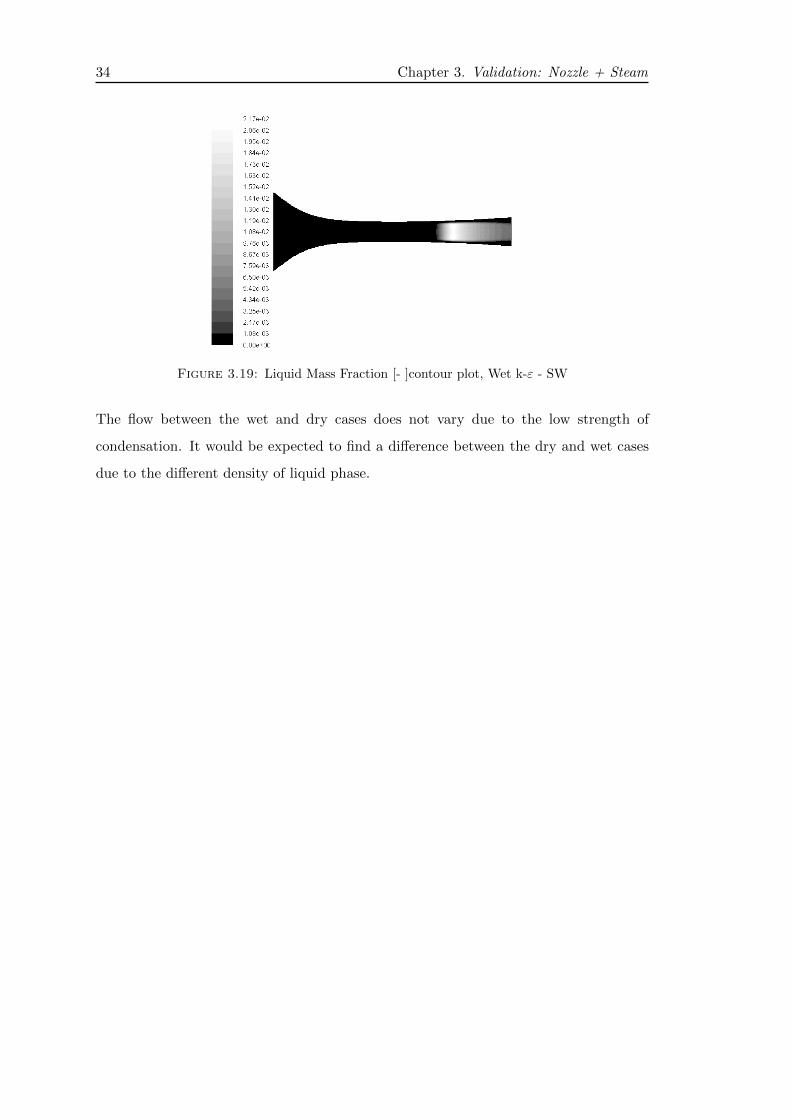
Figure 3.19: Liquid Mass Fraction [- ]contour plot, Wet k-ε - SW
The flow between the wet and dry cases does not vary due to the low strength of
condensation. It would be expected to find a difference between the dry and wet cases
due to the different density of liquid phase.
Chapter 4
Validation: Nozzle + Refrigerant
4.1 Description of the cases
The cases that will be studied in this Chapter have R134a as the working fluid. The
cases are divided in two parts. In the first part, the conditions are set to be fully
supersonic (FS), that is Ma=1 in the throat and Mach>1 downstream. In the second
part, a shock wave is forced to happen downstream of the throat and before the nozzle
outlet. The Boundary conditions are described carefully in section 4.2.2. For both
cases, the simulations are made for wet steam and dry steam, deactivating condensation
(considering steam as refrigerant vapor from now on).
Little and Garimella suggest in [15] that in conventional operation of a refrigeration cycle
the state in the entrance of the ejector, thus the nozzle, should be superheated at around
10 K. This works as a measure to protect the moving parts in case of using rotating
machinery. Anyway, the conditions will be varied downwards to study the consequences
of condensation in the motive flow of the ejector, which goes through the nozzle.
4.1.1 Refrigerant
Water, used in Chapter 3, offers high heat of vaporization and has no environmental
impact. It could be a perfect refrigerant if it was not for the limit in cooling temperature
(only above 0oC). Also, water has large specific volume and the cycle pipes diameter
should be too big. In contrast with the previous chapter, the working fluid here is R134a.
35
36 Chapter 4. Validation: Nozzle + Refrigerant
This refrigerant is a low temperature halocarbon which offers the advantage of low
GWP and no ODP compared with other halocarbons. As Chunnanond [2] suggests, the
halocarbon refrigerants provide larger performance and lower temperature requirements
for the heat recovery than water.
4.2 Numerical Setup
4.2.1 Geometry and Mesh
The geometry and mesh is the same that is described in Chapter 3.
4.2.2 Boundary Conditions
As previously seen, the cases that will be studied will be divided in four parts:
• Fully supersonic
– Dry Steam
– Wet Steam
• Shock wave
– Dry Steam
– Wet Steam
The boundary conditions used along this Chapter were set up regarding the recom-
mendations suggested by Little and Garimella [15]. It is known that there should be a
level of ∼ 10K of superheat. Anyway, the aim was to find condensation and the first
simulations showed that at this superheat level did not provide any liquid appearance.
The conditions for the Fully Supersonic cases are the ones seen in 4.1. The cases with
∆Tsat ≤ -4 K had a condensation level higher than the limit of the software (β = 0.2),
that is why the inlet boundary conditions do not go below that point.
The second part of the simulations were made in order to see the behaviour having shock
waves and condensation (if possible) in the nozzle, the back pressure is increased as seen
Chapter 4. Validation: Nozzle + Refrigerant 37
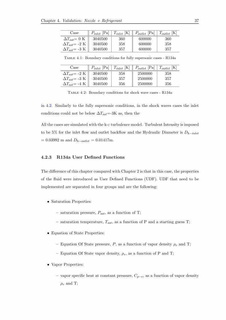
Case Pinlet [Pa] Tinlet [K] Poutlet [Pa] Toutlet [K]
∆Tsat= 0 K 3040500 360 600000 360∆Tsat= -2 K 3040500 358 600000 358∆Tsat= -3 K 3040500 357 600000 357
Table 4.1: Boundary conditions for fully supersonic cases - R134a
Case Pinlet [Pa] Tinlet [K] Poutlet [Pa] Toutlet [K]
∆Tsat= -2 K 3040500 358 2500000 358∆Tsat= -3 K 3040500 357 2500000 357∆Tsat= -4 K 3040500 356 2500000 356
Table 4.2: Boundary conditions for shock wave cases - R134a
in 4.2. Similarly to the fully supersonic conditions, in the shock waves cases the inlet
conditions could not be below ∆Tsat=-3K as, then the
All the cases are simulated with the k-ε turbulence model. Turbulent Intensity is imposed
to be 5% for the inlet flow and outlet backflow and the Hydraulic Diameter is Dh−inlet
= 0.03992 m and Dh−outlet = 0.01417m.
4.2.3 R134a User Defined Functions
The difference of this chapter compared with Chapter 2 is that in this case, the properties
of the fluid were introduced as User Defined Functions (UDF). UDF that need to be
implemented are separated in four groups and are the following:
• Saturation Properties:
– saturation pressure, Psat, as a function of T;
– saturation temperature, Tsat, as a function of P and a starting guess T;
• Equation of State Properties:
– Equation Of State pressure, P , as a function of vapor density ρv and T;
– Equation Of State vapor density, ρv, as a function of P and T;
• Vapor Properties:
– vapor specific heat at constant pressure, Cp−v, as a function of vapor density
ρv and T;
38 Chapter 4. Validation: Nozzle + Refrigerant
– vapor specific heat at constant volume, Cv−v, as a function of vapor density
ρv and T;
– vapor specific enthalpy, hv, as a function of vapor density ρv and T;
– vapor specific entropy, sv, as a function of vapor density ρv and T;
– vapor dynamic viscosity, µv, as a function of vapor density ρv and T;
– vapor thermal conductivity, ktv, as function of vapor density ρv and T;
• Liquid Properties:
– saturated liquid density, ρl, as function of T;
– saturated liquid specific heat at constant pressure ,Cp−l, as function of T;
– liquid dynamic viscosity, µl, as function of T;
– liquid thermal conductivity, ktl, as function of T;
– liquid surface tension, σ, as function of T;
The three different codes that were designed can be found in the Appendix B.
4.2.3.1 Ideal Gas Properties
The aim of the Ideal Gas UDF was to simplify the functions implemented at most, in
order to prevent errors. That is why most of the equations/functions were idealized and
reduced.
Saturation Properties: For Wet Steam, the saturation pressure and temperature were
extracted from [21] and it was checked in case R134a was also described. This refrigerant
was not available there, but was useful to understand the vapor properties pattern.
In the code for R134a, saturation pressure function is obtained from NIST REFPROP
[22]. The values of pressure and temperature are from the vapor-liquid saturation curve.
Pressure as a function of temperature is obtained using Microsoft Excel as a polynomial
regression of 6th grade.
In order to avoid loops due to not enough accuracy, the saturation temperature function
is based on an iterative method given by ANSYS Fluent User’s Guide [4].
Chapter 4. Validation: Nozzle + Refrigerant 39
Equation of State Properties: As ideal gas, the pressure, P , and vapor density, ρv,
are both given by the Ideal Gas equation:
P = ρv ·Rgas−v · T (4.1)
ρv =P
Rgas−v · T(4.2)
where T is the temperature and Rgas−v is the vapor gas constant equal to 81.490367
J/kg·K.
Vapor Properties:
Vapor specific heat at constant pressure, Cp−v, is built in a way which makes the entropy
as close as real enthalpy. Initially, Cp−v was a constant value, but the ideal gas enthalpy
was affecting negatively the simulations, having convergence problems.
Vapor specific heat at constant volume, Cv−v, complies the ideal gas equation:
R = Cp−v − Cv−v (4.3)
Enthalpy, h, complies with its ideal gas equation:
h = T · Cp−v (4.4)
Entropy, s, complies with the ideal gas equation:
s = Cp−v · ln(T
T0) +Rgas−v · ln(
P0
Rgas−v·) (4.5)
Vapor dynamic viscosity, µv, is a constant value based on the same structure as the
UDWSPF suggested in [4] p. 1424. It is a number close to the state in the inlet.
Vapor thermal conductivity, ktv, is also a constant value based on the same structure
as the UDWSPF suggested in [4] p. 1424. It is a number close to the state state in the
inlet.
Liquid Properties:
40 Chapter 4. Validation: Nozzle + Refrigerant
The liquid properties are all based on the polynomial regression of the values in a
saturated state from the NIST REFPROP library [22], as the liquid does not change
too much.
4.2.3.2 Real Gas Properties
Saturation Properties:
The saturation properties for the real gas are the same as in the ideal, since the state
values come from the NIST REFPROP library [22] which contain real gas state.
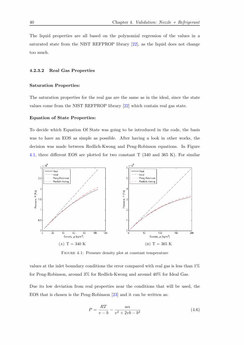
Equation of State Properties:
To decide which Equation Of State was going to be introduced in the code, the basis
was to have an EOS as simple as possible. After having a look in other works, the
decision was made between Redlich-Kwong and Peng-Robinson equations. In Figure
4.1, three different EOS are plotted for two constant T (340 and 365 K). For similar
(a) T = 340 K (b) T = 365 K
Figure 4.1: Pressure density plot at constant temperature
values at the inlet boundary conditions the error compared with real gas is less than 1%
for Peng-Robinson, around 3% for Redlich-Kwong and around 40% for Ideal Gas.
Due its low deviation from real properties near the conditions that will be used, the
EOS that is chosen is the Peng-Robinson [23] and it can be written as:
P =RT
v − b− aα
v2 + 2vb− b2(4.6)
Chapter 4. Validation: Nozzle + Refrigerant 41
where a = a(Tc), b = b(Tc), α, Tr, and k are:
a =0.457235R2T 2
c
Pc(4.7)
b =0.077796RTc
Pc(4.8)
α = (1 + k(1−√Tr))
2 (4.9)
Tr =T
Tc(4.10)
k = 0.37464 + 1.54226 · ω − 0.26992 · ω2 (4.11)
To implement the P function, all the constants above-mentioned need to be defined. But
for the v equation, there is:
v3 + v2(b− RT
P) + v(−3b2 − 2RTb
P+αa
P) + (b3 +
RTb2
P− αab
P) = 0 (4.12)
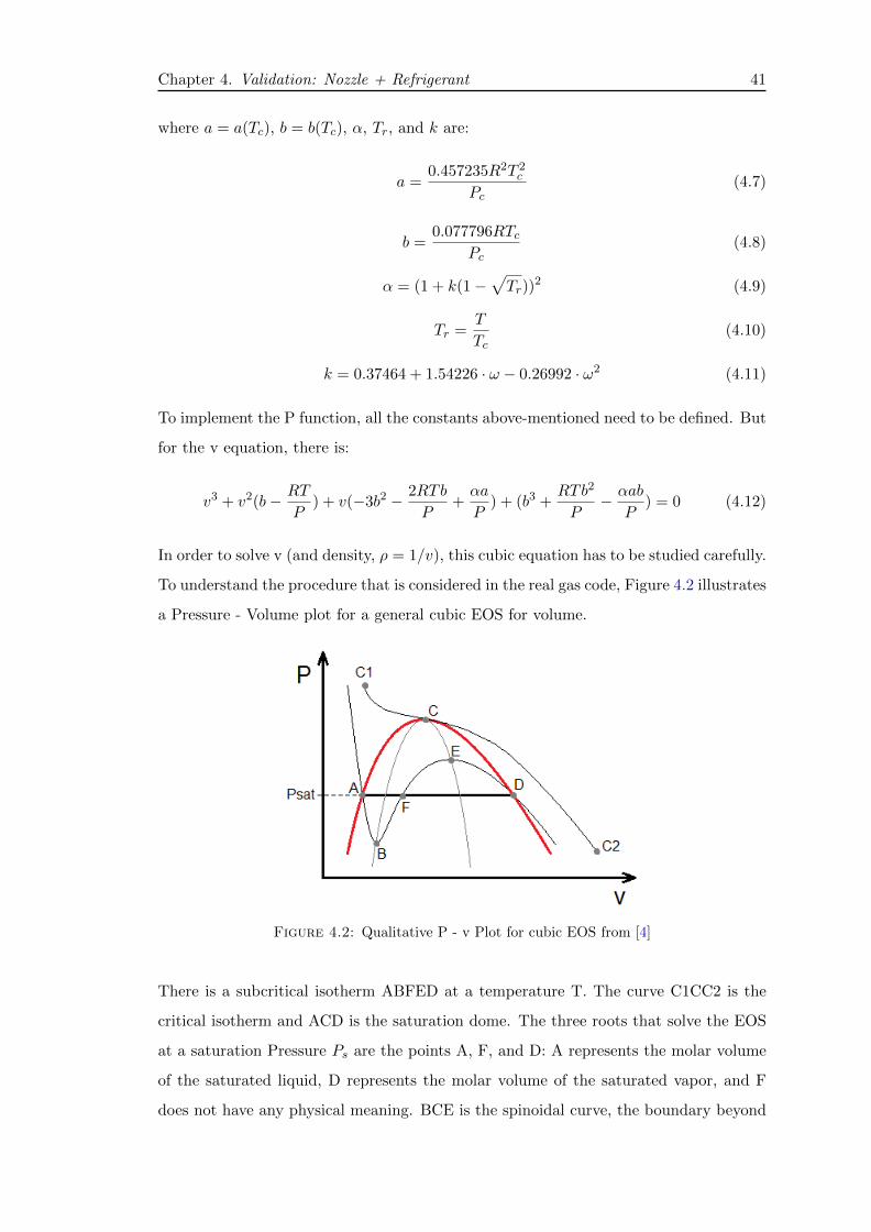
In order to solve v (and density, ρ = 1/v), this cubic equation has to be studied carefully.
To understand the procedure that is considered in the real gas code, Figure 4.2 illustrates
a Pressure - Volume plot for a general cubic EOS for volume.
Figure 4.2: Qualitative P - v Plot for cubic EOS from [4]
There is a subcritical isotherm ABFED at a temperature T. The curve C1CC2 is the
critical isotherm and ACD is the saturation dome. The three roots that solve the EOS
at a saturation Pressure Ps are the points A, F, and D: A represents the molar volume
of the saturated liquid, D represents the molar volume of the saturated vapor, and F
does not have any physical meaning. BCE is the spinoidal curve, the boundary beyond
42 Chapter 4. Validation: Nozzle + Refrigerant
the EOS is not valid as the local derivative of pressure with respect to volume becomes
positive.
Therefore, the root that it is ”correct” is the one on the right. In order to solve v, the
Newton-Raphson iterative pattern is implemented in this way:
Given the f(v) function, its derivative f ′(v) and a first guess v0, which is
the maximum v value acceptable (v = 1m3/kg), there is a first approxi-
mation for the root:
v1 = v0 −f(v0)
f ′(v0)(4.13)
It means that the point (v1, 0) is the intersection with the x axis of the tan-
gent of the function f at the point (x0, f(x0)). This process is performed
successively until the variation of the xn compared with the previous xn−1
is lower than a set limit. The code for this can be checked in Appendix
B in the Real Gas section.
Vapor Properties:
Vapor properties functions are build out of the properties supplied in REFPROP NIST
[22]. The saturation properties together with the vapor properties for a range of pressure
from 3,5 MPa to 50 kPa were used to create multiple linear regression functions with
ρ and T as input variables. The pattern for obtaining the functions was: including all
input variables T , ρ, T 2, ρ2 and T ·ρ. Perform a multiple linear regression, and check the
p-values of the variables. If a p-values is higher than 0.005 the corresponding variable
is removed from the model. After, perform another multiple linear regression and keep
the same criteria up to a point where all the p-values are lower than 0.05. Find the
equations of the vapor properties in Appendix A.
Liquid Properties:
The equations for liquid properties are the same as in ideal gas.
4.3 Results
Simulations with Ideal Gas came out properly until ∆Tsat = −3. After that point, the
maximum limit for the liquid mass fraction (β = 0.2) was reached, and the software
Chapter 4. Validation: Nozzle + Refrigerant 43
does not guarantee correct values. Also, due to this limit of the model, the simulations
are impossible to converge.
The main problem appeared with the Real Gas code, when at the very beginning of the
simulations, divergence problems turned out. Multiple solver adaptations were made to
avoid divergence:
• Courant number was reduced to 0.1
• Dicretization schemes were set to first order upwind
• Testing more favorable initialization values, and even with data from the perfect
gas simulation solution
Any of the adjustments worked, then the idea was to change the code starting with the
real gas properties. Trying to simplify and change the real gas properties did not turn
into any improvements, therefore, the next step was testing a new code with the perfect
gas EOS and real gas properties to see which and where was the problem. This code
worked almost as smoothly as the Perfect Gas code in terms of convergence. Below, this
mixed code is called Hybrid Gas (HG).
The results below are based only in the Perfect Gas and Hybrid Gas cases.
4.3.1 Fully supersonic
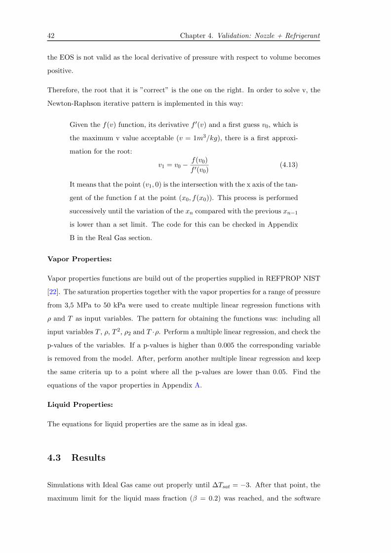
It can be checked if the flow is indeed fully supersonic by looking at the Mach number
in Figure 4.3, as Mach 1 is reached in the throat and then increases. In all cases, the
pattern for the Mach number is the same, only zooming in in the final the nozzle it is
seen a different behaviour for the wet case for ∆Tsat= -3 K.
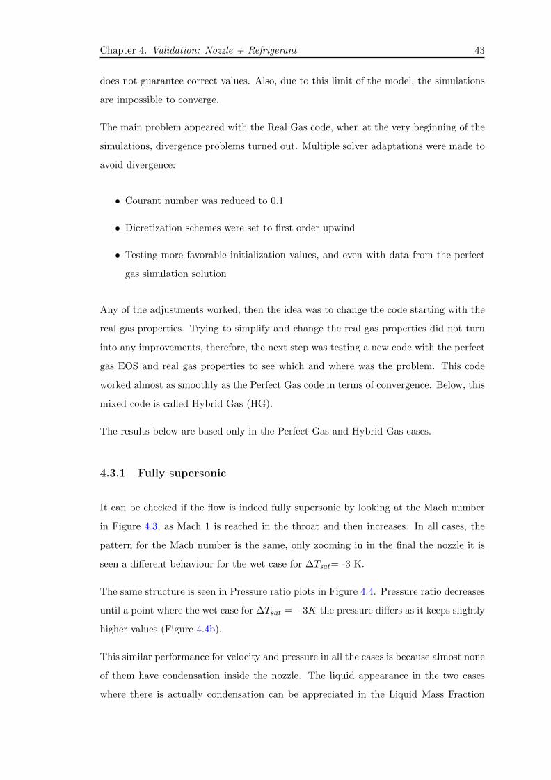
The same structure is seen in Pressure ratio plots in Figure 4.4. Pressure ratio decreases
until a point where the wet case for ∆Tsat = −3K the pressure differs as it keeps slightly
higher values (Figure 4.4b).
This similar performance for velocity and pressure in all the cases is because almost none
of them have condensation inside the nozzle. The liquid appearance in the two cases
where there is actually condensation can be appreciated in the Liquid Mass Fraction
44 Chapter 4. Validation: Nozzle + Refrigerant
(a) Mach Number (b) Mach Number - Zoom In
Figure 4.3: Mach number plots for FS cases - PG
(a) Pressure ratio (b) Pressure ratio - Zoom In
Figure 4.4: Pressure ratio plots for FS cases - PG
plots in Figure 4.5. As it can be seen, condensation is only noticeable in the ∆Tsat = -3
K, even though that in ∆Tsat = -2 K there is a start.
The strength of the condensation could be almost the same as the Droplet nucleation
ratio which gives an idea of the number of new droplets per unit volume and second. In
Figure 4.6, it is seen that the droplet appearance happens before in the -3K case, as it
is obviously inner in the saturation dome.
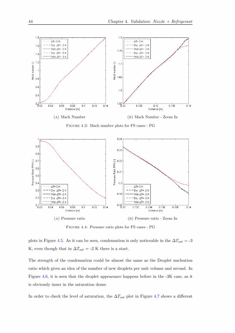
In order to check the level of saturation, the ∆Tsat plot in Figure 4.7 shows a different

Chapter 4. Validation: Nozzle + Refrigerant 45
(a) Liquid Mass Fraction (b) Liquid Mass Fraction - Zoom In
Figure 4.5: Liquid Mass Fraction plots for FS cases - PG
Figure 4.6: Log10(Droplet Nucleation Ratio) for Fully Supersonic cases - PG
46 Chapter 4. Validation: Nozzle + Refrigerant
pattern compared with the wet steam cases. First ∆tsat increases slightly and after
the throat it decreases more rapidly. In the case of ∆Tsat = -3K, the minimum value
of ∆Tsat is -11.6 K, below that point condensation has an enough important level and
there is a temperature jump due to the heat release. In the case of ∆Tsat = -2, where
there is a little condensation, the minimum value is reached on the outlet and is -11.5
K.
Figure 4.7: ∆Tsat for FS cases - PG
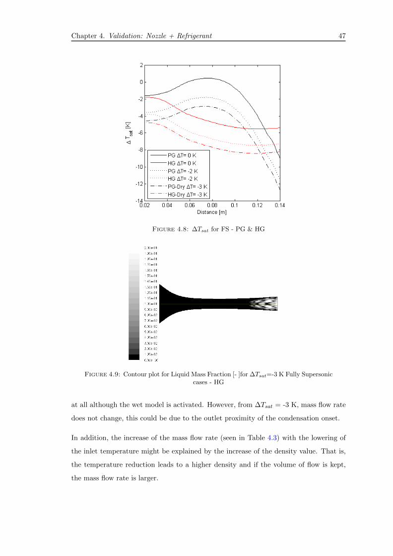
However, in the Hybrid gas cases there is a quite different pattern also for the ∆Tsat
as seen in Figure 4.8. The decrease during the expansion is less pronounced compared
with the Perfect Gas code results. This might be due to the different equations for the
Cp−v, Cv−v and kv.
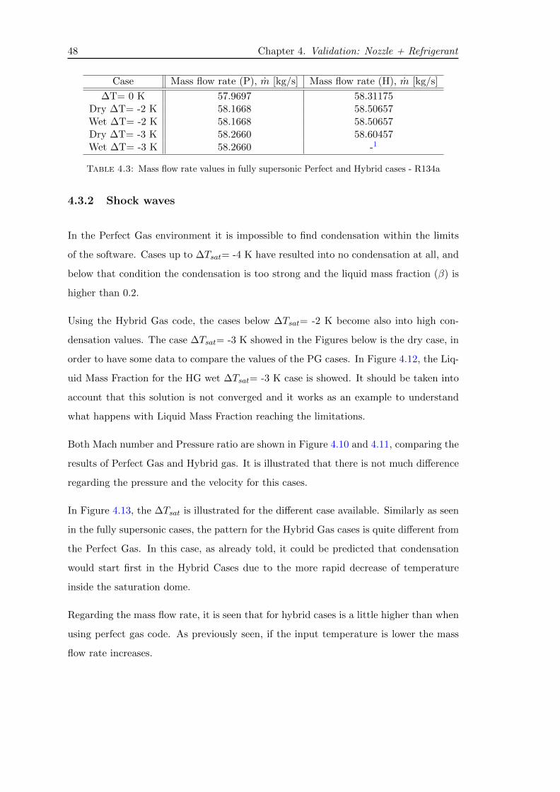
Anyway, in the Hybrid gas there are no available results with condensation because at
∆Tsat -3 K there was condensation but it was too strong for the software to support (β
was greater than 0.2 as it can be seen in the Figure 4.9). For Perfect gas cases, the limit
was reached in the values below ∆Tsat -4 K.
Regarding the mass flow rates in Table 4.3, in case ∆Tsat = 0 K, there is no condensation
at all so the mass flow rate is only specified once. In the case where ∆Tsat is -2 K, as
previously seen, the liquid fraction is so weak that the mass flow rate does not change
Chapter 4. Validation: Nozzle + Refrigerant 47
Figure 4.8: ∆Tsat for FS - PG & HG
Figure 4.9: Contour plot for Liquid Mass Fraction [- ]for ∆Tsat=-3 K Fully Supersoniccases - HG
at all although the wet model is activated. However, from ∆Tsat = -3 K, mass flow rate
does not change, this could be due to the outlet proximity of the condensation onset.
In addition, the increase of the mass flow rate (seen in Table 4.3) with the lowering of
the inlet temperature might be explained by the increase of the density value. That is,
the temperature reduction leads to a higher density and if the volume of flow is kept,
the mass flow rate is larger.
48 Chapter 4. Validation: Nozzle + Refrigerant
Case Mass flow rate (P), m [kg/s] Mass flow rate (H), m [kg/s]
∆T= 0 K 57.9697 58.31175Dry ∆T= -2 K 58.1668 58.50657Wet ∆T= -2 K 58.1668 58.50657Dry ∆T= -3 K 58.2660 58.60457Wet ∆T= -3 K 58.2660 -1
Table 4.3: Mass flow rate values in fully supersonic Perfect and Hybrid cases - R134a
4.3.2 Shock waves
In the Perfect Gas environment it is impossible to find condensation within the limits
of the software. Cases up to ∆Tsat= -4 K have resulted into no condensation at all, and
below that condition the condensation is too strong and the liquid mass fraction (β) is
higher than 0.2.
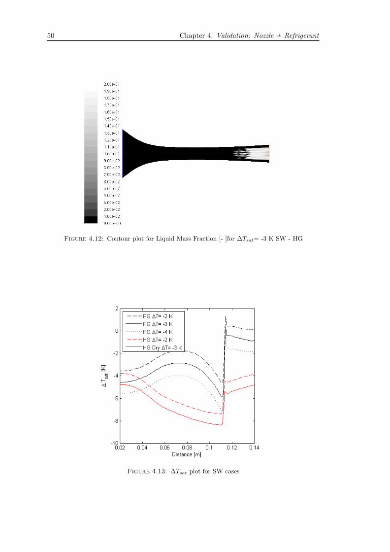
Using the Hybrid Gas code, the cases below ∆Tsat= -2 K become also into high con-
densation values. The case ∆Tsat= -3 K showed in the Figures below is the dry case, in
order to have some data to compare the values of the PG cases. In Figure 4.12, the Liq-
uid Mass Fraction for the HG wet ∆Tsat= -3 K case is showed. It should be taken into
account that this solution is not converged and it works as an example to understand
what happens with Liquid Mass Fraction reaching the limitations.
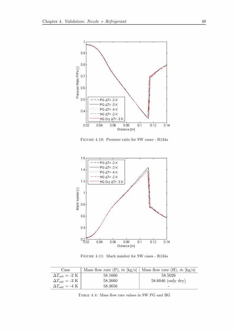
Both Mach number and Pressure ratio are shown in Figure 4.10 and 4.11, comparing the
results of Perfect Gas and Hybrid gas. It is illustrated that there is not much difference
regarding the pressure and the velocity for this cases.
In Figure 4.13, the ∆Tsat is illustrated for the different case available. Similarly as seen
in the fully supersonic cases, the pattern for the Hybrid Gas cases is quite different from
the Perfect Gas. In this case, as already told, it could be predicted that condensation
would start first in the Hybrid Cases due to the more rapid decrease of temperature
inside the saturation dome.
Regarding the mass flow rate, it is seen that for hybrid cases is a little higher than when
using perfect gas code. As previously seen, if the input temperature is lower the mass
flow rate increases.
Chapter 4. Validation: Nozzle + Refrigerant 49
Figure 4.10: Pressure ratio for SW cases - R134a
Figure 4.11: Mach number for SW cases - R134a
Case Mass flow rate (P), m [kg/s] Mass flow rate (H), m [kg/s]
∆Tsat = -2 K 58.1666 58.5026∆Tsat = -3 K 58.2660 58.6046 (only dry)∆Tsat = -4 K 58.3656 -
Table 4.4: Mass flow rate values in SW PG and HG
50 Chapter 4. Validation: Nozzle + Refrigerant
Figure 4.12: Contour plot for Liquid Mass Fraction [- ]for ∆Tsat= -3 K SW - HG
Figure 4.13: ∆Tsat plot for SW cases
Chapter 5
Conclusions
5.1 Conclusions
Wet Steam built-in model was studied and tested for different conditions. The results
have been useful to see how the model worked and how the properties were introduced
in the UDWSPF.
For the R134a, three codes have been developed: ideal gas, hybrid gas (ideal EOS and
real properties) and real gas. The simulations for The simulations were only possible
to run for ideal gas and hybrid gas, as the real gas cases were had divergence problems
related to the AMG solver. The results for ideal and hybrid gas have been studied
and compared between them. There are many differences that depend too much on the
code, so it should be further studied and developed in order to approximate the results
as much as possible to the reality.
In addition, many of the cases did not have condensation since the software has a limita-
tion for liquid mass fraction that has restricted a lot the range of boundary conditions.
This situation has been an important disadvantage that was not expected from the
beginning.
Experimental tests are needed in order to validate the CFD results in this case, otherwise
the results can only be compared with different models. This way, for example the most
appropriate turbulence model could be chosen in order to continue the simulations.
51
52 Chapter 5. Conclusions
5.2 Futur Work
Some pending work has been introduced during the thesis, however, the summary of the
ideas that should be developed and more studied are suggested below:
• Try to use the codes that work (perfect and hybrid) in a full ejector and study the
results.
• Go in depth in the mesh resolution. It was not in the objectives of the thesis but
it is really important.
• Study exhaustively the code for real gas and correct it:
– Modify the Ideal Gas EOS changing R value (which is the slope of the line
i.e. for P-ρ for a fixed T) to make it closer to the real gas states.
– Find a better and simpler equation of state to implement in the real gas code.
• Verify that the code works for different working fluids.
• Study in depth the different turbulence models, and compare the different calcu-
lation to experimental results.
Appendix A
Property functions for R134a
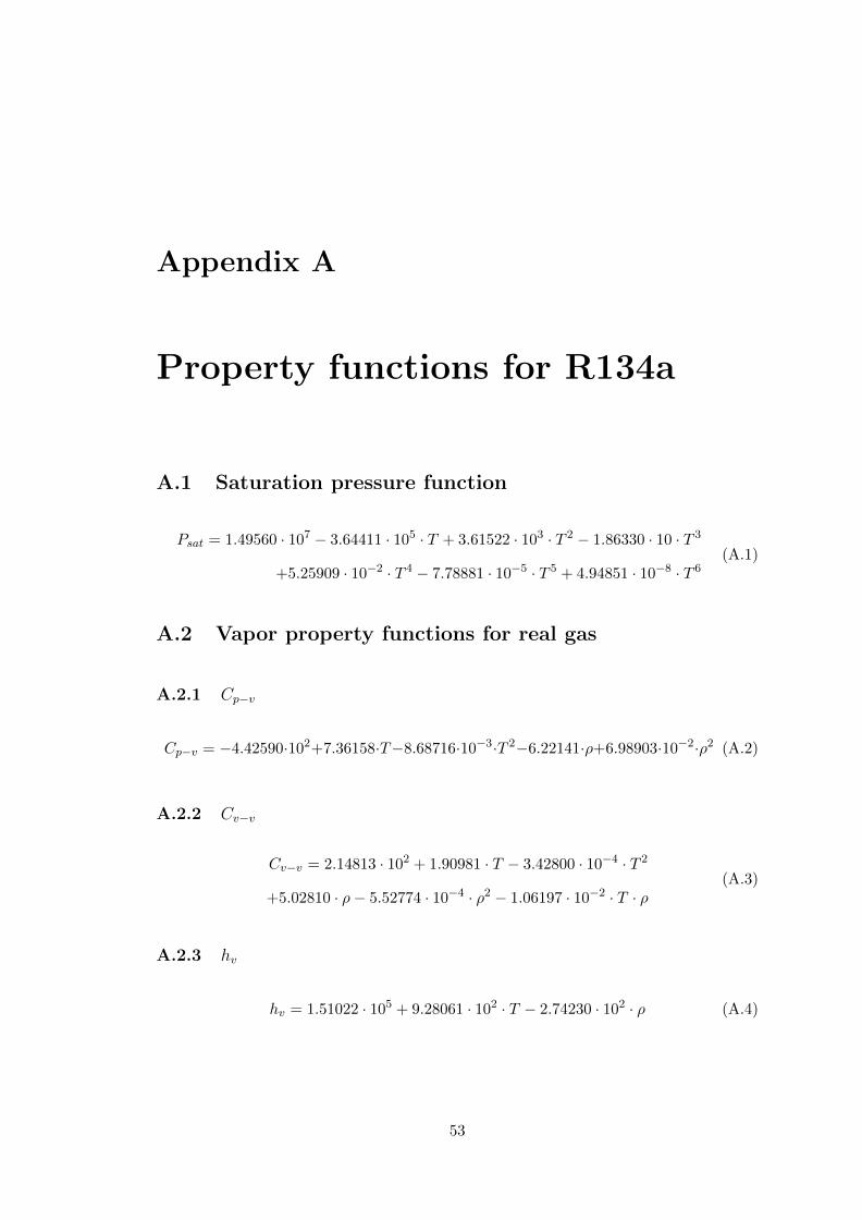
A.1 Saturation pressure function
Psat = 1.49560 · 107 − 3.64411 · 105 · T + 3.61522 · 103 · T 2 − 1.86330 · 10 · T 3
+5.25909 · 10−2 · T 4 − 7.78881 · 10−5 · T 5 + 4.94851 · 10−8 · T 6(A.1)
A.2 Vapor property functions for real gas
A.2.1 Cp−v
Cp−v = −4.42590·102+7.36158·T−8.68716·10−3·T 2−6.22141·ρ+6.98903·10−2·ρ2 (A.2)
A.2.2 Cv−v
Cv−v = 2.14813 · 102 + 1.90981 · T − 3.42800 · 10−4 · T 2
+5.02810 · ρ− 5.52774 · 10−4 · ρ2 − 1.06197 · 10−2 · T · ρ(A.3)
A.2.3 hv
hv = 1.51022 · 105 + 9.28061 · 102 · T − 2.74230 · 102 · ρ (A.4)
53
54 Appendix A. Property Functions for R134a
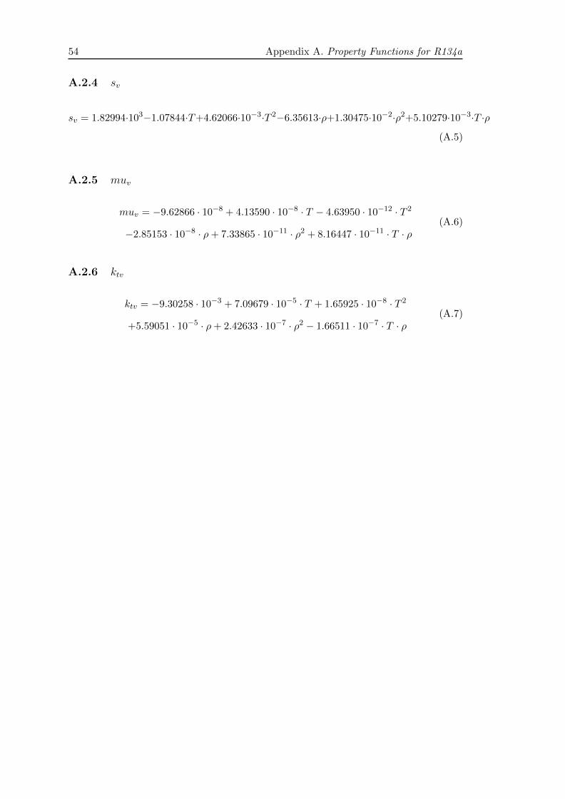
A.2.4 sv
sv = 1.82994·103−1.07844·T+4.62066·10−3·T 2−6.35613·ρ+1.30475·10−2·ρ2+5.10279·10−3·T ·ρ
(A.5)
A.2.5 muv
muv = −9.62866 · 10−8 + 4.13590 · 10−8 · T − 4.63950 · 10−12 · T 2
−2.85153 · 10−8 · ρ+ 7.33865 · 10−11 · ρ2 + 8.16447 · 10−11 · T · ρ(A.6)
A.2.6 ktv
ktv = −9.30258 · 10−3 + 7.09679 · 10−5 · T + 1.65925 · 10−8 · T 2
+5.59051 · 10−5 · ρ+ 2.42633 · 10−7 · ρ2 − 1.66511 · 10−7 · T · ρ(A.7)
Appendix B
User Defined Functions for R134a
B.1 UDF for ideal gas
B.1.1 Ideal Gas EOS - Ideal Gas Properties
/**********************************************************************/
/* User Defined R134a Properties:
EOS: Ideal Gas Eq.
Perfect Gas Properties
Real Liquid Properties
Author: Marina Gallach Palma
Date : 7 July 2015
*/
/**********************************************************************/
#include "udf.h"
#include "stdio.h"
#include "ctype.h"
#include "stdarg.h"
/*Global Constants for this model*/
real ws_TPP=169.85;
55
56 Appendix B. User Defined Functions for R134a
real ws_aaa=0.01;
real cpg=585.66;
/* Cp-vapor at low-pressure region*/
DEFINE_ON_DEMAND(I_do_nothing)
{/* This is a dummy function to allow us to use */
/* the Compiled UDFs utility*/
}
void wetst_init(Domain *domain)
{
/* You must initialize these material property constants..
they will be used in the wet steam model in fluent */
ws_Tc = 374.21; /*Critical Temp. */
ws_Pc = 4059300.0; /*Critical Pressure */
mw_f = 102.03; /*fluid droplet molecular weight (water) */
Rgas_v = 81.490367; /*vapor Gas Const*/
}
real wetst_satP(real T)
{
real psat;
real a0 = 1.49560E+07;
real a1 =-3.64411E+05;
real a2 = 3.61522E+03;
real a3 =-1.86330E+01;
real a4 = 5.25909E-02;
real a5 =-7.78881E-05;
real a6 = 4.94851E-08;
if (T > ws_Tc) T = ws_Tc ;
psat=a0+a1*T+a2*pow(T,2)+a3*pow(T,3)+a4*pow(T,4)+a5*pow(T,5)+a6*pow(T,6);
return psat; /*Pa */
}
Appendix B. User Defined Functions for R134a 57
real wetst_satT(real P, real T)
{
real tsat;
real dT,dTM,dTA,dP,p1,p2,dPdT;
real dt = 1.e-4;
int i ;
for (i=0; i<25; ++i)
{
if (T > ws_Tc) T = ws_Tc-0.5;
p1= wetst_satP(T) ;
p2= wetst_satP(T+dt) ;
dPdT = (p2-p1)/dt;
dP = P - p1 ;
dT = dP/dPdT;
dTA = fabs(dT);
dTM=0.1*T;
if(dTA>dTM) dT=dT*dTM/dTA;
T = T + dT;
if (fabs(dT)<TEMP_eps*T) break;
}
tsat = T;
return tsat; /*K */
}
real wetst_eosP(real rho, real T)
{
real P;
P = rho* Rgas_v * T ;
return P; /*Pa */
}
real wetst_eosRHO(real P, real T)
{
58 Appendix B. User Defined Functions for R134a
real rho;
rho = P/(Rgas_v * T);
return rho; /*kg/m3 */
}
real wetst_cpv(real T, real rho)
{
real cp;
real a0= 3.37519E+03;
real a1=-1.05456E+01;
real a2= 1.27550E-02;
cp = a0 + a1*T + a2*pow(T,2);
return cp; /* (J/Kg/K) */
}
real wetst_cvv(real T, real rho)
{
real cv;
cv = wetst_cpv(T,rho)-Rgas_v;
return cv; /* (J/Kg/K) */
}
real wetst_hv(real T,real rho)
{
real h;
h=T*wetst_cpv(T,rho);
return h; /* (J/Kg) */
}
real wetst_sv(real T, real rho)
{
real s;
real TDatum= 273.15;
real PDatum= 292800.0;
Appendix B. User Defined Functions for R134a 59
s=cpg*log(T/TDatum)+Rgas_v*log(PDatum/(Rgas_v*T*rho));
return s; /* (J/Kg/K) */
}
real wetst_muv(real T, real rho)
{
real muv;
muv=0.000011116;
return muv; /* (Kg/m/s) */
}
real wetst_ktv(real T, real rho)
{
real ktv;
ktv=0.012693;
return ktv; /* W/m/K */
}
real wetst_rhol(real T)
{
real rhol;
real a0=-2.19175E+04;
real a1= 5.90411E+02;
real a2=-6.04919E+00;
real a3= 3.25492E-02;
real a4=-9.74695E-05;
real a5= 1.54095E-07;
real a6=-1.00631E-10;
if (T > ws_Tc) T = ws_Tc;
rhol=a0+a1*T+a2*pow(T,2)+a3*pow(T,3)+a4*pow(T,4)+a5*pow(T,5)+a6*pow(T,6);
return rhol; /* (Kg/m3) */
}
real wetst_cpl(real T)
60 Appendix B. User Defined Functions for R134a
{
real cpl;
real a0= 1.09375E+06;
real a1=-2.68356E+04;
real a2= 2.71286E+02;
real a3=-1.44502E+00;
real a4= 4.27829E-03;
real a5=-6.67762E-06;
real a6= 4.29438E-09;
if (T > ws_Tc) T = ws_Tc ;
cpl=a0+a1*T+a2*pow(T,2)+a3*pow(T,3)+a4*pow(T,4)+a5*pow(T,5)+a6*pow(T,6);
return cpl; /* (J/Kg/K) */
}
real wetst_mul(real T)
{
real mul=0.0;
real a0= 3.35945E+02;
real a1=-7.13719E+00;
real a2= 6.32769E-02;
real a3=-2.98423E-04;
real a4= 7.88006E-07;
real a5=-1.10341E-09;
real a6= 6.39691E-13;
if (T > ws_Tc) T = ws_Tc ;
mul=a0+a1*T+a2*pow(T,2)+a3*pow(T,3)+a4*pow(T,4)+a5*pow(T,5)+a6*pow(T,6);
return mul; /* (Kg/m/s) */
}
real wetst_ktl(real T)
{
real ktl;
real a0= 3.29632E-01;
real a1=-1.75906E-03;
Appendix B. User Defined Functions for R134a 61
real a2= 5.44209E-06;
real a3=-9.77113E-09;
real a4= 6.46973E-12;
if (T > ws_Tc) T = ws_Tc ;
ktl = a0+a1*T+a2*pow(T,2)+a3*pow(T,3)+a4*pow(T,4);
return ktl; /* W/m/K */
}
real wetst_surft(real T)
{
real sigma;
real a0= 7.05060E-02;
real a1=-3.80307E-04;
real a2= 1.20556E-06;
real a3=-3.16555E-09;
real a4= 3.50343E-12;
if (T > ws_Tc) T = ws_Tc;
sigma=a0+a1*T+a2*pow(T,2)+a3*pow(T,3)+a4*pow(T,4);
return sigma ;/* N/m */
}
/* do not change the order of the function list */
UDF_EXPORT WS_Functions WetSteamFunctionList =
{
wetst_init, /*initialization function*/
wetst_satP, /*Saturation pressure*/
wetst_satT, /*Saturation temperature*/
wetst_eosP, /*equation of state*/
wetst_eosRHO, /*equation of state*/
wetst_hv, /*vapor enthalpy*/
wetst_sv, /*vapor entropy*/
wetst_cpv, /*vapor isobaric specific heat*/
wetst_cvv, /*vapor isochoric specific heat*/
62 Appendix B. User Defined Functions for R134a
wetst_muv, /*vapor dynamic viscosity*/
wetst_ktv, /*vapor thermal conductivity*/
wetst_rhol, /*sat. liquid density*/
wetst_cpl, /*sat. liquid specific heat*/
wetst_mul, /*sat. liquid viscosity*/
wetst_ktl, /*sat. liquid thermal conductivity*/
wetst_surft /*liquid surface tension*/
};
B.1.2 Ideal Gas EOS - Real Gas Properties
/**********************************************************************/
/*User Defined R134a Properties:
EOS: PERFECT GAS
PROPERTIES: REAL GAS (REFPROP)
Author: Marina Gallach Palma
Date : 10 July 2015*/
/**********************************************************************/
#include "udf.h"
#include "stdio.h"
#include "ctype.h"
#include "stdarg.h"
/*Global Constants for this model*/
real ws_TPP=169.85;
real ws_aaa=0.01;
real cpg=585.66;
/* Cp-vapor at low-pressure region*/
DEFINE_ON_DEMAND(I_do_nothing)
{/* This is a dummy function to allow us to use */
/* the Compiled UDFs utility*/
Appendix B. User Defined Functions for R134a 63
}
void wetst_init(Domain *domain)
{
/* You must initialize these material property constants..
they will be used in the wet steam model in fluent */
ws_Tc = 374.21; /*Critical Temp. */
ws_Pc = 4059300.0; /*Critical Pressure */
mw_f = 102.03; /*fluid droplet molecular weight (water) */
Rgas_v = 81.490367; /*vapor Gas Const*/
}
real wetst_satP(real T)
{
real psat;
real a0 = 1.49560E+07;
real a1 =-3.64411E+05;
real a2 = 3.61522E+03;
real a3 =-1.86330E+01;
real a4 = 5.25909E-02;
real a5 =-7.78881E-05;
real a6 = 4.94851E-08;
if (T > ws_Tc) T = ws_Tc ;
psat=a0+a1*T+a2*pow(T,2.0)+a3*pow(T,3.0)+a4*pow(T,4.0)+a5*pow(T,5.0)+a6*pow(T,6.0);
return psat; /*Pa */
}
real wetst_satT(real P, real T)
{
real tsat;
real dT,dTM,dTA,dP,p1,p2,dPdT;
real dt = 1.0e-4;
int i ;
for (i=0; i<25; ++i)
64 Appendix B. User Defined Functions for R134a
{
if (T > ws_Tc) T = ws_Tc-0.5;
p1= wetst_satP(T) ;
p2= wetst_satP(T+dt) ;
dPdT = (p2-p1)/dt;
dP = P - p1 ;
dT = dP/dPdT;
dTA = fabs(dT);
dTM=0.1*T;
if(dTA>dTM) dT=dT*dTM/dTA;
T = T + dT;
if (fabs(dT)<TEMP_eps*T) break;
}
tsat = T;
return tsat; /*K */
}
real wetst_eosP(real rho, real T)
{
real P;
P = rho* Rgas_v * T ;
return P; /*Pa */
}
real wetst_eosRHO(real P, real T)
{
real rho;
rho = P/(Rgas_v * T) ;
return rho; /*kg/m3 */
}
real wetst_cpv(real T, real rho)
{
Appendix B. User Defined Functions for R134a 65
real cp;
real act=-4.42590E+02;
real at= 7.36158E+00;
real at2=-8.68716E-03;
real ad= -6.22141E+00;
real ad2= 6.98903E-02;
if (T > 455.0) T = 455.0;
cp = act + at*T + at2*pow(T,2.0) + ad*rho + ad2*pow(rho,2.0);
return cp; /* (J/Kg/K) */
}
real wetst_cvv(real T, real rho)
{
real cv;
real act= 2.14813E+02;
real at= 1.90981E+00;
real at2=-3.42800E-04;
real ad= 5.02810E+00;
real ad2=-5.52774E-04;
real atd=-1.06197E-02;
if (T > 455.0) T = 455.0;
cv = act + at*T + at2*pow(T,2.0)+ ad*rho + ad2*pow(rho,2.0) + atd*T*rho;
return cv; /* (J/Kg/K) */
}
real wetst_hv(real T,real rho)
{
real h;
real act= 1.51022E+05;
real at= 9.28061E+02;
real ad= -2.74230E+02;
if (T > 455.0) T = 455.0;
h = act + at*T + ad*rho;
return h; /* (J/Kg) */
66 Appendix B. User Defined Functions for R134a
}
real wetst_sv(real T, real rho)
{
real s ;
real act= 1.82994E+03;
real at= -1.07844E+00;
real at2= 4.62066E-03;
real ad= -6.35613E+00;
real ad2= 1.30475E-02;
real atd= 5.10279E-03;
if (T > 455.0) T = 455.0;
s= act + at*T + at2*pow(T,2.0)+ ad*rho + ad2*pow(rho,2.0) + atd*T*rho;
return s; /* (J/Kg/K) */
}
real wetst_muv(real T, real rho)
{
real muv;
real act=-9.62866E-08;
real at= 4.13590E-08;
real at2=-4.63950E-12;
real ad= -2.85153E-08;
real ad2= 7.33865E-11;
real atd= 8.16447E-11;
if (T > 455.0) T = 455.0;
muv = act + at*T + at2*pow(T,2)+ ad*rho + ad2*pow(rho,2) + atd*T*rho;
return muv; /* (Kg/m/s) */
}
real wetst_ktv(real T, real rho)
{
real ktv;
real act=-9.30258E-03;
Appendix B. User Defined Functions for R134a 67
real at= 7.09679E-05;
real at2= 1.65925E-08;
real ad= 5.59051E-05;
real ad2= 2.42633E-07;
real atd=-1.66511E-07;
if (T > 455.0) T = 455.0;
ktv=act+at*T+at2*pow(T,2)+ad*rho+ad2*pow(rho,2)+atd*T*rho;
return ktv; /* W/m/K */
}
real wetst_rhol(real T)
{
real rhol;
real a0=-2.19175E+04;
real a1= 5.90411E+02;
real a2=-6.04919E+00;
real a3= 3.25492E-02;
real a4=-9.74695E-05;
real a5= 1.54095E-07;
real a6=-1.00631E-10;
if (T > ws_Tc) T = ws_Tc;
rhol=a0+a1*T+a2*pow(T,2)+a3*pow(T,3)+a4*pow(T,4)+a5*pow(T,5)+a6*pow(T,6);
return rhol; /* (Kg/m3) */
}
real wetst_cpl(real T)
{
real cpl;
real a0= 1.09375E+06;
real a1=-2.68356E+04;
real a2= 2.71286E+02;
real a3=-1.44502E+00;
real a4= 4.27829E-03;
real a5=-6.67762E-06;
68 Appendix B. User Defined Functions for R134a
real a6= 4.29438E-09;
if (T > ws_Tc) T = ws_Tc ;
cpl=a0+a1*T+a2*pow(T,2)+a3*pow(T,3)+a4*pow(T,4)+a5*pow(T,5)+a6*pow(T,6);
return cpl; /* (J/Kg/K) */
}
real wetst_mul(real T)
{
real mul=0.0;
real a0= 3.35945E+02;
real a1=-7.13719E+00;
real a2= 6.32769E-02;
real a3=-2.98423E-04;
real a4= 7.88006E-07;
real a5=-1.10341E-09;
real a6= 6.39691E-13;
if (T > ws_Tc) T = ws_Tc ;
mul=a0+a1*T+a2*pow(T,2)+a3*pow(T,3)+a4*pow(T,4)+a5*pow(T,5)+a6*pow(T,6);
return mul; /* (Kg/m/s) */
}
real wetst_ktl(real T)
{
real ktl;
real a0= 3.29632E-01;
real a1=-1.75906E-03;
real a2= 5.44209E-06;
real a3=-9.77113E-09;
real a4= 6.46973E-12;
if (T > ws_Tc) T = ws_Tc ;
ktl = a0+a1*T+a2*pow(T,2)+a3*pow(T,3)+a4*pow(T,4);
return ktl; /* W/m/K */
}
Appendix B. User Defined Functions for R134a 69
real wetst_surft(real T)
{
real sigma;
real a0= 7.05060E-02;
real a1=-3.80307E-04;
real a2= 1.20556E-06;
real a3=-3.16555E-09;
real a4= 3.50343E-12;
if (T > ws_Tc) T = ws_Tc;
sigma=a0+a1*T+a2*pow(T,2)+a3*pow(T,3)+a4*pow(T,4);
return sigma ;/* N/m */
}
/* do not change the order of the function list */
UDF_EXPORT WS_Functions WetSteamFunctionList =
{
wetst_init, /*initialization function*/
wetst_satP, /*Saturation pressure*/
wetst_satT, /*Saturation temperature*/
wetst_eosP, /*equation of state*/
wetst_eosRHO, /*equation of state*/
wetst_hv, /*vapor enthalpy*/
wetst_sv, /*vapor entropy*/
wetst_cpv, /*vapor isobaric specific heat*/
wetst_cvv, /*vapor isochoric specific heat*/
wetst_muv, /*vapor dynamic viscosity*/
wetst_ktv, /*vapor thermal conductivity*/
wetst_rhol, /*sat. liquid density*/
wetst_cpl, /*sat. liquid specific heat*/
wetst_mul, /*sat. liquid viscosity*/
wetst_ktl, /*sat. liquid thermal conductivity*/
wetst_surft /*liquid surface tension*/
};
70 Appendix B. User Defined Functions for R134a
B.2 UDF for real gas
/**********************************************************************/
/*
User Defined R134a Properties:
EOS: PENG ROBINSON
PROPERTIES: REAL GAS
Author: Marina Gallach Palma
Date : 11 July 2015*/
/**********************************************************************/
#include "udf.h"
#include "stdio.h"
#include "ctype.h"
#include "stdarg.h"
/*Global Constants for this model*/
real ws_TPP=169.85;
real ws_aaa=0.01;
real cpg=585.66;
real rho_min=1;
real abs_tol=1e-5;
/* Cp-vapor at low-pressure region*/
DEFINE_ON_DEMAND(I_do_nothing)
{/* This is a dummy function to allow us to use */
/* the Compiled UDFs utility*/
}
void wetst_init(Domain *domain)
{
/* You must initialize these material property constants..
they will be used in the wet steam model in fluent */
Appendix B. User Defined Functions for R134a 71
ws_Tc = 374.21; /*Critical Temp. */
ws_Pc = 4059300.0; /*Critical Pressure */
mw_f = 102.03; /*fluid droplet molecular weight (water) */
Rgas_v = 81.490367; /*vapor Gas Const*/
}
real wetst_satP(real T)
{
real psat;
real a0 = 1.49560E+07;
real a1 =-3.64411E+05;
real a2 = 3.61522E+03;
real a3 =-1.86330E+01;
real a4 = 5.25909E-02;
real a5 =-7.78881E-05;
real a6 = 4.94851E-08;
if (T > ws_Tc) T = ws_Tc ;
psat=a0+a1*T+a2*pow(T,2)+a3*pow(T,3)+a4*pow(T,4)+a5*pow(T,5)+a6*pow(T,6);
return psat; /*Pa */
}
real wetst_satT(real P, real T)
{
real tsat;
real dT,dTM,dTA,dP,p1,p2,dPdT;
real dt = 1.e-4;
int i ;
for (i=0; i<25; ++i)
{
if (T > ws_Tc) T = ws_Tc-0.5;
p1= wetst_satP(T) ;
p2= wetst_satP(T+dt) ;
dPdT = (p2-p1)/dt;
dP = P - p1 ;
72 Appendix B. User Defined Functions for R134a
dT = dP/dPdT;
dTA = fabs(dT);
dTM=0.1*T;
if(dTA>dTM) dT=dT*dTM/dTA;
T = T + dT;
if (fabs(dT)<TEMP_eps*T) break;
}
tsat = T;
return tsat; /*K */
}
real wetst_eosP(real rho, real T)
{
real P;
/*P = rho* Rgas_v * T ;*/
real a = (0.457235*Rgas_v*Rgas_v*ws_Tc*ws_Tc)/ws_Pc;
real b = (0.077796*Rgas_v*ws_Tc)/ws_Pc;
real acentric = 0.32684;
real k = 0.37464+1.54226*acentric-0.26992*acentric*acentric;
real alpha = (1.0+k*(1.0-sqrt(T/ws_Tc)))*(1.0+k*(1.0-sqrt(T/ws_Tc)));
if(rho<rho_min) rho=rho_min;
real v=1.0/rho;
P = ((Rgas_v*T)/(v-b))-(a*alpha/(v*v+2.0*v*b-b*b));
return P; /*Pa */
}
real wetst_eosRHO(real P, real T)
{
real v=1.0/rho_min;
real a = (0.457235*Rgas_v*Rgas_v*ws_Tc*ws_Tc)/ws_Pc;
real b = (0.077796*Rgas_v*ws_Tc)/ws_Pc;
real acentric = 0.32684;
real k = 0.37464+1.54226*acentric-0.26992*acentric*acentric;
Appendix B. User Defined Functions for R134a 73
real alpha = (1.0+k*(1.0-sqrt(T/ws_Tc)));
real a_2= b - Rgas_v*T/P;
real a_1=-3.0*b*b - 2.0*Rgas_v*b*T/P + alpha*a/P;
real a_0= b*b*b + Rgas_v*T*b*b/P - alpha*a*b/P;
real temp=0.0;
while(fabs(v-temp)>abs_tol)
{
real polynomial = v*v*v + a_2*v*v + a_1*v + a_0;
real derivative = 3.0*v*v + 2.0*a_2*v + a_1;
temp = v;
v = temp - polynomial/derivative;
}
real rho=1.0/v;
return rho; /*kg/m3 */
}
real wetst_cpv(real T, real rho)
{
real cp;
real act=-4.42590E+02;
real at= 7.36158E+00;
real at2=-8.68716E-03;
real ad= -6.22141E+00;
real ad2= 6.98903E-02;
cp = act + at*T + at2*pow(T,2) + ad*rho + ad2*pow(rho,2);
return cp; /* (J/Kg/K) */
}
real wetst_cvv(real T, real rho)
{
real cv;
real act= 2.14813E+02;
real at= 1.90981E+00;
real at2=-3.42800E-04;

74 Appendix B. User Defined Functions for R134a
real ad= 5.02810E+00;
real ad2=-5.52774E-04;
real atd=-1.06197E-02;
cv = act + at*T + at2*pow(T,2)+ ad*rho + ad2*pow(rho,2) + atd*T*rho;
return cv; /* (J/Kg/K) */
}
real wetst_hv(real T,real rho)
{
real h;
real act= 1.51022E+05;
real at= 9.28061E+02;
real ad= -2.74230E+02;
h = act + at*T + ad*rho;
return h; /* (J/Kg) */
}
real wetst_sv(real T, real rho)
{
real s ;
real act= 1.82994E+03;
real at= -1.07844E+00;
real at2= 4.62066E-03;
real ad= -6.35613E+00;
real ad2= 1.30475E-02;
real atd= 5.10279E-03;
s= act + at*T + at2*pow(T,2)+ ad*rho + ad2*pow(rho,2) + atd*T*rho;
return s; /* (J/Kg/K) */
}
real wetst_muv(real T, real rho)
{
real muv;
real act=-9.62866E-08;
Appendix B. User Defined Functions for R134a 75
real at= 4.13590E-08;
real at2=-4.63950E-12;
real ad= -2.85153E-08;
real ad2= 7.33865E-11;
real atd= 8.16447E-11;
muv = act + at*T + at2*pow(T,2.)+ ad*rho + ad2*pow(rho,2.) + atd*T*rho;
return muv; /* (Kg/m/s) */
}
real wetst_ktv(real T, real rho)
{
real ktv;
real act=-9.30258E-03;
real at= 7.09679E-05;
real at2= 1.65925E-08;
real ad= 5.59051E-05;
real ad2= 2.42633E-07;
real atd=-1.66511E-07;
ktv=act+at*T+at2*pow(T,2)+ad*rho+ad2*pow(rho,2)+atd*T*rho;
return ktv; /* W/m/K */
}
real wetst_rhol(real T)
{
real rhol;
real a0=-2.19175E+04;
real a1= 5.90411E+02;
real a2=-6.04919E+00;
real a3= 3.25492E-02;
real a4=-9.74695E-05;
real a5= 1.54095E-07;
real a6=-1.00631E-10;
if (T > ws_Tc) T = ws_Tc;
rhol=a0+a1*T+a2*pow(T,2)+a3*pow(T,3)+a4*pow(T,4)+a5*pow(T,5)+a6*pow(T,6);
76 Appendix B. User Defined Functions for R134a
return rhol; /* (Kg/m3) */
}
real wetst_cpl(real T)
{
real cpl;
real a0= 1.09375E+06;
real a1=-2.68356E+04;
real a2= 2.71286E+02;
real a3=-1.44502E+00;
real a4= 4.27829E-03;
real a5=-6.67762E-06;
real a6= 4.29438E-09;
if (T > ws_Tc) T = ws_Tc ;
cpl=a0+a1*T+a2*pow(T,2)+a3*pow(T,3)+a4*pow(T,4)+a5*pow(T,5)+a6*pow(T,6);
return cpl; /* (J/Kg/K) */
}
real wetst_mul(real T)
{
real mul=0.0;
real a0= 3.35945E+02;
real a1=-7.13719E+00;
real a2= 6.32769E-02;
real a3=-2.98423E-04;
real a4= 7.88006E-07;
real a5=-1.10341E-09;
real a6= 6.39691E-13;
if (T > ws_Tc) T = ws_Tc ;
mul=a0+a1*T+a2*pow(T,2)+a3*pow(T,3)+a4*pow(T,4)+a5*pow(T,5)+a6*pow(T,6);
return mul; /* (Kg/m/s) */
}
real wetst_ktl(real T)
Appendix B. User Defined Functions for R134a 77
{
real ktl;
real a0= 3.29632E-01;
real a1=-1.75906E-03;
real a2= 5.44209E-06;
real a3=-9.77113E-09;
real a4= 6.46973E-12;
if (T > ws_Tc) T = ws_Tc ;
ktl = a0+a1*T+a2*pow(T,2)+a3*pow(T,3)+a4*pow(T,4);
return ktl; /* W/m/K */
}
real wetst_surft(real T)
{
real sigma;
real a0= 7.05060E-02;
real a1=-3.80307E-04;
real a2= 1.20556E-06;
real a3=-3.16555E-09;
real a4= 3.50343E-12;
if (T > ws_Tc) T = ws_Tc;
sigma=a0+a1*T+a2*pow(T,2)+a3*pow(T,3)+a4*pow(T,4);
return sigma ;/* N/m */
}
/* do not change the order of the function list */
UDF_EXPORT WS_Functions WetSteamFunctionList =
{
wetst_init, /*initialization function*/
wetst_satP, /*Saturation pressure*/
wetst_satT, /*Saturation temperature*/
wetst_eosP, /*equation of state*/
wetst_eosRHO, /*equation of state*/
78 Appendix B. User Defined Functions for R134a
wetst_hv, /*vapor enthalpy*/
wetst_sv, /*vapor entropy*/
wetst_cpv, /*vapor isobaric specific heat*/
wetst_cvv, /*vapor isochoric specific heat*/
wetst_muv, /*vapor dynamic viscosity*/
wetst_ktv, /*vapor thermal conductivity*/
wetst_rhol, /*sat. liquid density*/
wetst_cpl, /*sat. liquid specific heat*/
wetst_mul, /*sat. liquid viscosity*/
wetst_ktl, /*sat. liquid thermal conductivity*/
wetst_surft /*liquid surface tension*/
};
Bibliography
[1] C. A. Moses and G. D. Stein. On the Growth of Steam Droplets Formed in a Laval
Nozzle Using Both Static Pressure and Light Scattering Measurements. Journal of
Fluids Engineering, 100(3):311–322, September 1978.
[2] K. Chunnanond and S. Aphornratana. Ejectors: Applications in refrigeration tech-
nology. Renewable and Sustainable Energy Reviews, 8(2):129–155, April 2004.
[3] X. Escale. Chapter 4. Compressible Pipe Flow. Departament de Mecanica de Fluids,
ETSEIB, Barcelona, 2013. Fluid Transport Course Slides.
[4] ANSYS Fluent User’s Guide. ANSYS Inc., release 16.0 edition, January 2015.
[5] L. Zori and F. Kelecy. Wet Steam Flow Modeling in a General CFD Flow Solver.
35th AIAA Fluid Dynamics Conference and Exhibit, Toronto, Ontario, Canada,
June 2005.
[6] X. Chen, S. Omer, M. Worall, and S. Riffat. Recent developments in ejector re-
frigeration technologies. Renewable and Sustainable Energy Reviews, 19:629–651,
March 2013.
[7] A. B. Little, Y. Bartosiewicz, and S. Garimella. Visualization and Validation of
Ejector Flow Field with Computational and First-Principles Analysis. Journal of
Fluids Engineering, 137(5), May 2015.
[8] Y. Bartosiewicz, Z. Aidoun, P. Desevaux, and Y. Mercadier. Numerical and ex-
perimental investigations on supersonic ejectors. International Journal of Heat and
Fluid Flow, 26:56–70, 2005.
[9] H. A. M. Al-Ansary and S. M. Jeter. Numerical and Experimental Analysis of
Single-Phase and Two-Phase Flow in Ejectors. HVAC&R Research, 10(4):521–538,
October 2004.
79
80 Bibliography
[10] A. Hemidi, F. Henry, S. Leclaire, J. Seynhaeve, and Y. Bartosiewicz. CFD analysis
of a supersonic air ejector. Part I: Experimental validation of a single-phase and
two-phase operation. Applied Thermal Engineering, 29:1523–1531, June 2009.
[11] A. Hemidi, F. Henry, S. Leclaire, J. Seynhaeve, and Y. Bartosiewicz. CFD analysis
of a supersonic air ejector. Part II: Relation between global operation and local flow
features. Applied Thermal Engineering, 29:2990–2998, June 2009.
[12] M. Elakhdar, E. Nehdi, L. Kairouani, and N. Tounsi. Simulation of an ejector used
in refrigeration systems. International Journal of Refrigeration, 34:1657–1667, 2011.
[13] F. Mazzelli and A. Milazzo. Performance analysis of a supersonic ejector cycle
working with R245fa. International Journal of Refrigeration, 49(5):79–92, Decem-
ber 2014.
[14] Y. Bartosiewicz, Z. Aidoun, and Y. Mercadier. Numerical assesment of ejector op-
eration for refrigeration applications based on CFD. Applied Thermal Engineering,
26:604–612, 2006.
[15] A. B. Little and S. Garimella. Ejector refrigeration systems for waste heat recovery
applications: Effects of condensation on performance. Unpublished, 2015.
[16] T. Zegenhagen and F. Ziegler. Experimental investigation of the characteristics of
a jet-ejector and jet-ejector cooling system operating with r134a as a refrigerant.
International Journal of Refrigeration, 2015. doi: 10.1016/j.ijrefrig.2015.01.001.
[17] ANSYS Fluent Theory Guide. ANSYS Inc., release 16.0 edition, January 2015.
[18] K. Ishazaki, T. Ikohagi, and H. Daiguji. A High-Resolution Numerical Method
for Transonic Non-equilibrium Condensation Flow Through a Steam Turbine Cas-
cade. In Proceedings of the 6th International Symposium on Computational Fluid
Dynamics, pages 479–484, 1995.
[19] J. B. Young. Two-Dimensional Nonequilibrium, Wet-Steam Calculations for Nozzles
and Turbines Cascades. Journal of Turbomachinery, 114:569–579, July 1992.
[20] F. G. Schmitt. About Boussinesq’s turbulent viscosity hypotesis: historical remarks
and a direct evaluation of its validity. Comptes Rendus Mecanique, Elsevier, 335:
617–627, 2007.
Bibliography 81
[21] W. C. Reynolds. THERMODYNAMIC PROPERTIES IN SI, graphs, tables and
computational equations for 40 substances. Department of Mechanical Engineering,
Stanford University, January 1979.
[22] E. W. Lemmon, M. L. Hubber, and M. O. McLinden. NIST Standard Refer-
ence Database 23: Reference Fluid Thermodynamic and Transport Properties-
REFPROP. National Institute of Standards and Technology, Standard Reference
Data Program, Gaithersburg, 2013. Version 9.1.
[23] D. Peng and D. B. Robinson. A New Two-Constant Equation of State. Ind. Eng.
Chem. Fundam., 15(1):569–579, February 1976.