evaporation, condensation and heat transfer
TRANSCRIPT

EVAPORATION, CONDENSATION AND
HEAT TRANSFER
Edited by Amimul Ahsan
Evaporation, Condensation and Heat Transfer Edited by Amimul Ahsan Published by InTech Janeza Trdine 9, 51000 Rijeka, Croatia Copyright © 2011 InTech All chapters are Open Access articles distributed under the Creative Commons Non Commercial Share Alike Attribution 3.0 license, which permits to copy, distribute, transmit, and adapt the work in any medium, so long as the original work is properly cited. After this work has been published by InTech, authors have the right to republish it, in whole or part, in any publication of which they are the author, and to make other personal use of the work. Any republication, referencing or personal use of the work must explicitly identify the original source. Statements and opinions expressed in the chapters are these of the individual contributors and not necessarily those of the editors or publisher. No responsibility is accepted for the accuracy of information contained in the published articles. The publisher assumes no responsibility for any damage or injury to persons or property arising out of the use of any materials, instructions, methods or ideas contained in the book. Publishing Process Manager Ivana Lorkovic Technical Editor Teodora Smiljanic Cover Designer Jan Hyrat Image Copyright Oshchepkov Dmitry, 2010. Used under license from Shutterstock.com First published August, 2011 Printed in Croatia A free online edition of this book is available at www.intechopen.com Additional hard copies can be obtained from [email protected] Evaporation, Condensation and Heat Transfer, Edited by Amimul Ahsan p. cm. ISBN 978-953-307-583-9

free online editions of InTech Books and Journals can be found atwww.intechopen.com

Contents
Preface IX
Part 1 Evaporation and Boiling 1
Chapter 1 Evaporation Phenomenon Inside a Solar Still: From Water Surface to Humid Air 3 Amimul Ahsan, Zahangir Alam, Monzur A. Imteaz, A.B.M. Sharif Hossain and Abdul Halim Ghazali
Chapter 2 Flow Boiling in an Asymmetrically Heated Single Rectangular Microchannel 23 Cheol Huh and Moo Hwan Kim
Chapter 3 Experimental and Computational Study of Heat Transfer During Quenching of Metallic Probes 49 B. Hernández-Morales, H.J. Vergara-Hernández, G. Solorio-Díaz and G.E. Totten
Chapter 4 Two Phase Flow Experimental Study Inside a Microchannel: Influence of Gravity Level on Local Boiling Heat Transfer 73 Sébastien Luciani
Chapter 5 The Evolution of Temperature Disturbances During Boiling of Cryogenic Liquids on Heat-Releasing Surfaces 95 Irina Starodubtseva and Aleksandr Pavlenko
Chapter 6 Pool Boiling of Liquid-Liquid Multiphase Systems 123 Gabriel Filipczak, Leon Troniewski and Stanisław Witczak
Part 2 Condensation and Cooling 151
Chapter 7 Steam Condensation in the Presence of a Noncondensable Gas in a Horizontal Tube 153 Kwon-Yeong Lee and Moo Hwan Kim
VI Contents
Chapter 8 Experimental Study for Condensation Heat Transfer Inside Helical Coil 169 Mohamed A. Abd Raboh, Hesham M. Mostafa, Mostafa A. M. Ali and Amr M. Hassaan
Chapter 9 Modelling the Thermo-Hydraulic Performance of Cooling Networks and Its Implications on Design, Operation and Retrofit 189 Martín Picón-Núñez, Lázaro Canizalez-Dávalos and Graham T. Polley
Chapter 10 Heat Exchange in Furnace Side Walls with Embedded Water Cooled Cooling Devices 207 Gabriel Plascencia
Part 3 Heat Transfer and Exchanger 225
Chapter 11 Heat Transfer in Buildings: Application to Solar Air Collector and Trombe Wall Design 227 H. Boyer, F. Miranville, D. Bigot, S. Guichard, I. Ingar, A. P. Jean, A. H. Fakra, D. Calogine and T. Soubdhan
Chapter 12 Heat Transfer in the Transitional Flow Regime 245 JP Meyer and JA Olivier
Chapter 13 Numerical Modeling of Cross-Flow Tube Heat Exchangers with Complex Flow Arrangements 261 Dawid Taler, Marcin Trojan and Jan Taler
Chapter 14 Metal Foam Effective Transport Properties 279 Jean-Michel Hugo, Emmanuel Brun and Frédéric Topin
Chapter 15 Heat Transfer Performances and Exergetic Optimization for Solar Heat Receiver 303 Jian-Feng Lu and Jing Ding
Chapter 16 Soret and Dufour Effects on Steady MHD Natural Convection Flow Past a Semi-Infinite Moving Vertical Plate in a Porous Medium with Viscous Dissipation in the Presence of a Chemical Reaction 325 Sandile Motsa and Stanford Shateyi
Part 4 Fluid and Flow 347
Chapter 17 Computational Fluid Dynamic Simulations of Natural Convection in Ventilated Facades 349 A. Gagliano, F. Patania, A. Ferlito, F. Nocera and A. Galesi
Contents VII
Chapter 18 Turbulent Heat Transfer in Drag-Reducing Channel Flow of Viscoelastic Fluid 375 Takahiro Tsukahara and Yasuo Kawaguchi
Chapter 19 Fluid Flow and Heat Transfer Analyses in Curvilinear Microchannels 401 Sajjad Bigham and Maryam Pourhasanzadeh
Chapter 20 Effects of Fluid Viscoelasticity in Non-Isothermal Flows 423 Tirivanhu Chinyoka
Chapter 21 Different Approaches for Modelling of Heat Transfer in Non-Equilibrium Reacting Gas Flows 439 E.V. Kustova and E.A. Nagnibeda
Chapter 22 High-Carbon Alcohol Aqueous Solutions and Their Application to Flow Boiling in Various Mini-Tube Systems 465 Naoki Ono, Atsushi Hamaoka, Yuki Eda and Koichi Obara
Chapter 23 Heat Transfer and Hydraulic Resistance in Rough Tubes Including with Twisted Tape Inserts 487 Stanislav Tarasevich and Anatoly Yakovlev
Chapter 24 Fluid Mechanics, Heat Transfer and Thermodynamic Issues of Micropipe Flows 511 A. Alper Ozalp
Chapter 25 Fundamentals of Paper Drying – Theory and Application from Industrial Perspective 535 Ajit K Ghosh

Preface
The theoretical analysis and modeling of heat and mass transfer rates produced in evaporation and condensation processes are significant issues in a design of wide range of industrial processes and devices. This book introduces advanced processes and modeling of evaporation, boiling, water vapor condensation, cooling, heat transfer, heat exchanger, fluid dynamic simulations, fluid flow, and gas flow to the international community. It includes 25 advanced and revised contributions, and it covers mainly (1) evaporation and boiling, (2) condensation and cooling, (3) heat transfer and exchanger, and (4) fluid and flow.
The first section introduces evaporation phenomenon, flow boiling, heat transfer during quenching, two-phase flow, temperature disturbances during boiling, and pool boiling.
The second section covers steam condensation, condensation inside helical coil, thermo-hydraulic performance of cooling networks, heat exchange with embedded cooling devices, and solar cooling systems.
The third section includes heat transfer in heat-released rod bundles, in buildings, in transitional flow regime, in stretching sheet, and in solar heat receiver, photovoltaic module thermal regulation, relative-air humidity sensing element, cross-flow tube heat exchanger, spiral plate heat exchanger, metal foam transport properties, and soret and dufour effects. The forth section presents computational fluid dynamic simulations, turbulent heat transfer, fluid flow, fluid viscoelasticity, non-equilibrium reacting gas flows, high-carbon alcohol aqueous solutions, hydraulic resistance in rough tubes, fluid mechanics, thermodynamic, and fundamental of paper drying.
The readers of this book will appreciate the current issues of modeling on evaporation, water vapor condensation, heat transfer and exchanger, and on fluid flow in different aspects. The approaches would be applicable in various industrial purposes as well. The advanced idea and information described here will be fruitful for the readers to find a sustainable solution in an industrialized society.
The editor of this book would like to express sincere thanks to all authors for their high quality contributions and in particular to the reviewers for reviewing the chapters.

X Preface
ACKNOWLEDGEMENTS
All praise be to Almighty Allah, the Creator and the Sustainer of the world, the Most Beneficent, Most Benevolent, Most Merciful, and Master of the Day of Judgment. He is Omnipresent and Omnipotent. He is the King of all kings of the world. In His hand is all good. Certainly, over all things Allah has power.
The editor would like to express appreciation to all who have helped to prepare this book. The editor expresses the gratefulness to Ms. Ivana Lorkovic, Publishing Process Manager, InTech Open Access Publisher, for her continued cooperation. In addition, the editor appreciatively remembers the assistance of all authors and reviewers of this book.
Gratitude is expressed to Mrs. Ahsan, Ibrahim Bin Ahsan, Mother, Father, Mother-in-Law, Father-in-Law, and Brothers and Sisters for their endless inspirations, mental supports and also necessary help whenever any difficulty.
Amimul Ahsan, Ph.D.
Department of Civil Engineering Faculty of Engineering
University Putra Malaysia Malaysia


Part 1
Evaporation and Boiling

1
Evaporation Phenomenon Inside a Solar Still: From Water Surface to Humid Air
Amimul Ahsan1,5, Zahangir Alam2, Monzur A. Imteaz3, A.B.M. Sharif Hossain4 and Abdul Halim Ghazali1
1University Putra Malaysia, Department of Civil Engineering, Faculty of Engineering, 2International Islamic University Malaysia, Department of Biotechnology Engineering,
Faculty of Engineering, 3Swinburne University of Technology, Faculty of Engineering and Industrial Science,
4University of Malaya, Institute of Biological Sciences, Faculty of Science, 5Green Engineering and Sustainable Technology Lab, Institute of Advanced Technology,
1,2,4Malaysia 3Australia
1. Introduction Solar stills of different designs have been proposed and investigated with a view to get greater distillate output (Murase et al., 2006). Solar stills are usually classified into two categories: a single-effect type and a multi-effect type that reuses wasted latent heat from condensation (Fath, 1998; Toyama et al., 1990). The integration between a solar collector and a still is classified into passive and active stills (Tiwari & Noor, 1996; Kumar & Tiwari; 1998). Single-effect passive stills are composed of convectional basin, diffusion, wick and membrane types (Murase et al., 2000; Korngold et al., 1996). The varieties of a still with cover cooling (Abu-Arabi et al., 2002; Abu-Hijleh et al., 1996) and a still with a multi-effect type basin (Tanaka et al., 2000) have been studied. A basin-type solar still is the most common among conventional solar stills (Chaibi, 2000; Nafey et al., 2000; Hongfei et al., 2002; Paul, 2002; Al-Karaghouli & Alnaser, 2004; Tiwari & Tiwari, 2008). A small experimental Tubular Solar Still (TSS) was constructed to determine the factors affecting the nocturnal production of solar stills (Tleimat & Howe, 1966). Furthermore, a detailed analysis of this TSS of any dimensions for predicting its nocturnal productivity was presented (Tiwari & Kumar, 1988). They (Tleimat & Howe, 1966; Tiwari & Kumar, 1988) mainly focused on the theoretical analysis of the nocturnal production of TSS. A simple transient analysis of a tubular multiwick solar still was presented by Kumar and Anand (1992). This TSS (Tleimat & Howe, 1966; Tiwari & Kumar, 1988; Kumar & Anand, 1992) is made of heavy glass and cannot be made easily in remote areas. The cost of glass is quite high as well (Ahsan et al., 2010). When water supply is cut off due to natural disasters (tsunamis, tornados, hurricanes, earthquakes, landslides, etc.) or unexpected accidents, a lightweight compact still, which is made of cheap and locally acquired materials, would be reasonable and practical. The second model of the TSS was, therefore, designed to meet these requirements and to improve some of the limitations of the basin-type still and of the TSS made of glass. Since
Evaporation, Condensation and Heat Transfer
4
the cover material (a vinyl chloride sheet) is a little heavy and cannot form into an ideal size easily (Islam, 2006; Fukuhara & Islam, 2006; Islam et al., 2005; Islam et al., 2007a), a polythene film was adopted as a cheap new material for the cover. Consequently, the cover weight and the cost of the second model were noticeably reduced and the durability was distinctly increased. These improvements also can help to assemble and to maintenance the second model of TSS easily for sustainable use (Ahsan et al., 2010). A complete numerical analysis on TSS has been presented by Ahsan & Fukuhara, 2008; Ahsan, 2009; Ahsan & Fukuhara, 2009; Ahsan & Fukuhara, 2010a, 2010b. Many researchers (Chaibi, 2000; Clark, 1990; Cooper, 1969; Dunkle, 1961; Hongfei et al., 2002; Malik et al., 1982; Shawaqfeh & Farid, 1995) have focused their research on conventional basin type stills rather than other types such as tubular still. Most of the heat and mass transfer models of the solar still have been described using temperature and vapor pressure on the water surface and still cover, without noting the presence of intermediate medium, i.e. humid air (Dunkle, 1961; Kumar & Anand, 1992; Tiwari & Kumar, 1988). Nagai et al. (2011) and Islam et al. (2007b), however, found that the relative humidity of the humid air is definitely not saturated in the daytime. Islam (2006) formulated the evaporation in the TSS based on the humid air temperature and on the relative humidity in addition to the water temperature and obtained an empirical equation of the evaporative mass transfer coefficient. Since the empirical equation does not have a theoretical background, it is still not known whether it can be used, when the trough size (width or length) is changed (Ahsan & Fukuhara, 2008). In this chapter, a comparison of the evaporation and distilled water production between the first model and second one is described. Additionally, this chapter aims to present the theoretical formulation of a model for the evaporation in a TSS by dimensional analysis.
2. Production principle The TSS consists of a transparent tubular cover and a black semicircular trough inside the tubular cover. The solar radiant heat after transmitting through a transparent tubular cover is mostly absorbed by water in the trough. Consequently, the water is heated up and evaporates. The water vapor density of the humid air increases associated with the evaporation from the water surface and then the water vapor is condensed on the inner surface of the tubular cover, releasing its latent heat of vaporization. Finally, the condensed water naturally trickles down toward the bottom of the tubular cover due to gravity and then is stored into a collector through a pipe equipped at the lower end of the tubular cover (Ahsan et al., 2010).
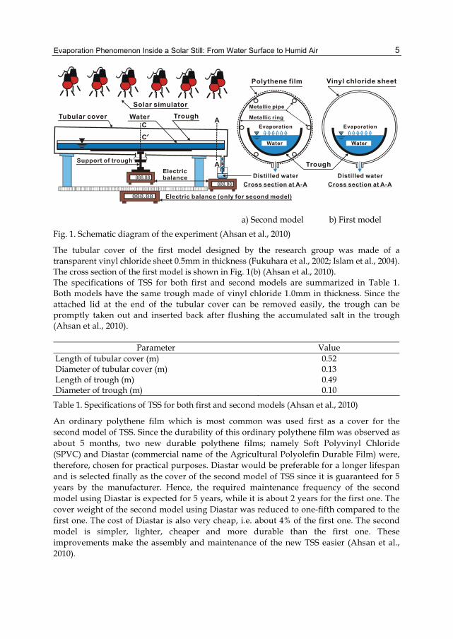
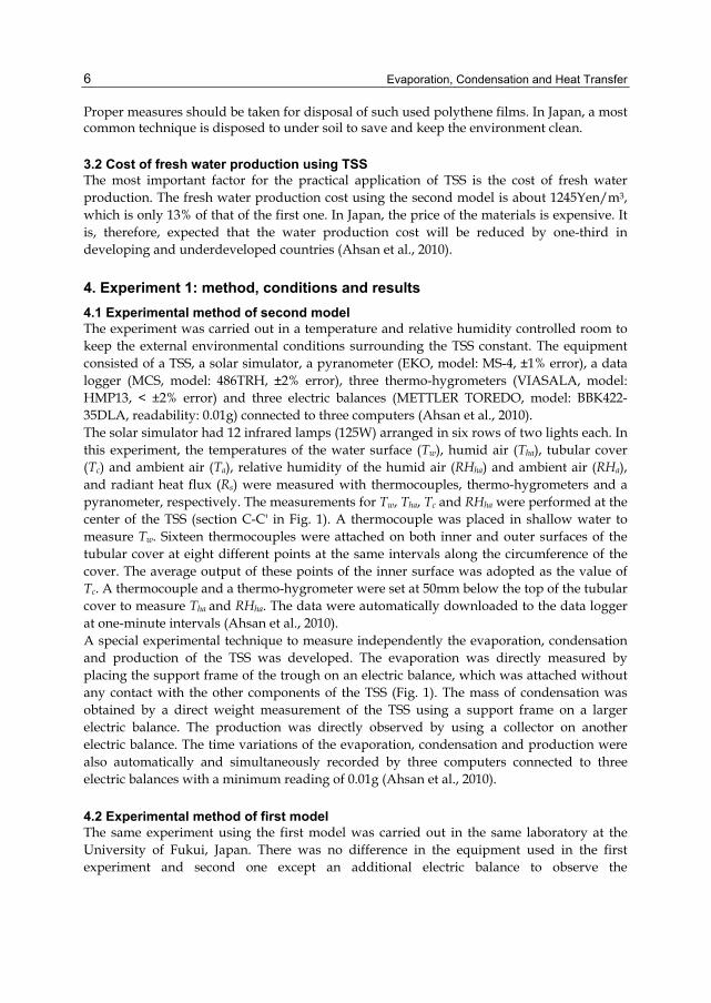
3. Overview of first model and second one 3.1 Structure of TSS Fig. 1(a) shows the cross section of the second model of the TSS. The frame was assembled with six GI pipes and six GI rings arranged in longitudinal and transverse directions, respectively. The GI pipe was 0.51m in length and 6mm in diameter. The GI ring was 0.38m in length and 2mm in diameter. The reasons for selection of GI material are light weight, cheap, available in market and commonly used in different purposes. The frame was wrapped with a tubular polythene film. The film is easily sealed by using a thermal-adhesion machine (Ahsan et al., 2010).
Evaporation Phenomenon Inside a Solar Still: From Water Surface to Humid Air
5
Tubular cover Trough Water
Electric balance
Solar simulator
Support of trough
Evaporation
Water
Distilled waterCross section at A-A
Evaporation
Distilled waterCross section at A-A
Trough
Polythene film Vinyl chloride sheet
A
A
C
C
Electric balance (only for second model) a) Second model b) First model
Fig. 1. Schematic diagram of the experiment (Ahsan et al., 2010)
The tubular cover of the first model designed by the research group was made of a transparent vinyl chloride sheet 0.5mm in thickness (Fukuhara et al., 2002; Islam et al., 2004). The cross section of the first model is shown in Fig. 1(b) (Ahsan et al., 2010). The specifications of TSS for both first and second models are summarized in Table 1. Both models have the same trough made of vinyl chloride 1.0mm in thickness. Since the attached lid at the end of the tubular cover can be removed easily, the trough can be promptly taken out and inserted back after flushing the accumulated salt in the trough (Ahsan et al., 2010).
Parameter Value Length of tubular cover (m) 0.52 Diameter of tubular cover (m) 0.13 Length of trough (m) 0.49 Diameter of trough (m) 0.10
Table 1. Specifications of TSS for both first and second models (Ahsan et al., 2010)
An ordinary polythene film which is most common was used first as a cover for the second model of TSS. Since the durability of this ordinary polythene film was observed as about 5 months, two new durable polythene films; namely Soft Polyvinyl Chloride (SPVC) and Diastar (commercial name of the Agricultural Polyolefin Durable Film) were, therefore, chosen for practical purposes. Diastar would be preferable for a longer lifespan and is selected finally as the cover of the second model of TSS since it is guaranteed for 5 years by the manufacturer. Hence, the required maintenance frequency of the second model using Diastar is expected for 5 years, while it is about 2 years for the first one. The cover weight of the second model using Diastar was reduced to one-fifth compared to the first one. The cost of Diastar is also very cheap, i.e. about 4% of the first one. The second model is simpler, lighter, cheaper and more durable than the first one. These improvements make the assembly and maintenance of the new TSS easier (Ahsan et al., 2010).
Evaporation, Condensation and Heat Transfer
6
Proper measures should be taken for disposal of such used polythene films. In Japan, a most common technique is disposed to under soil to save and keep the environment clean.
3.2 Cost of fresh water production using TSS The most important factor for the practical application of TSS is the cost of fresh water production. The fresh water production cost using the second model is about 1245Yen/m3, which is only 13% of that of the first one. In Japan, the price of the materials is expensive. It is, therefore, expected that the water production cost will be reduced by one-third in developing and underdeveloped countries (Ahsan et al., 2010).
4. Experiment 1: method, conditions and results 4.1 Experimental method of second model The experiment was carried out in a temperature and relative humidity controlled room to keep the external environmental conditions surrounding the TSS constant. The equipment consisted of a TSS, a solar simulator, a pyranometer (EKO, model: MS-4, ±1% error), a data logger (MCS, model: 486TRH, ±2% error), three thermo-hygrometers (VIASALA, model: HMP13, < ±2% error) and three electric balances (METTLER TOREDO, model: BBK422-35DLA, readability: 0.01g) connected to three computers (Ahsan et al., 2010). The solar simulator had 12 infrared lamps (125W) arranged in six rows of two lights each. In this experiment, the temperatures of the water surface (Tw), humid air (Tha), tubular cover (Tc) and ambient air (Ta), relative humidity of the humid air (RHha) and ambient air (RHa), and radiant heat flux (Rs) were measured with thermocouples, thermo-hygrometers and a pyranometer, respectively. The measurements for Tw, Tha, Tc and RHha were performed at the center of the TSS (section C-C' in Fig. 1). A thermocouple was placed in shallow water to measure Tw. Sixteen thermocouples were attached on both inner and outer surfaces of the tubular cover at eight different points at the same intervals along the circumference of the cover. The average output of these points of the inner surface was adopted as the value of Tc. A thermocouple and a thermo-hygrometer were set at 50mm below the top of the tubular cover to measure Tha and RHha. The data were automatically downloaded to the data logger at one-minute intervals (Ahsan et al., 2010). A special experimental technique to measure independently the evaporation, condensation and production of the TSS was developed. The evaporation was directly measured by placing the support frame of the trough on an electric balance, which was attached without any contact with the other components of the TSS (Fig. 1). The mass of condensation was obtained by a direct weight measurement of the TSS using a support frame on a larger electric balance. The production was directly observed by using a collector on another electric balance. The time variations of the evaporation, condensation and production were also automatically and simultaneously recorded by three computers connected to three electric balances with a minimum reading of 0.01g (Ahsan et al., 2010).
4.2 Experimental method of first model The same experiment using the first model was carried out in the same laboratory at the University of Fukui, Japan. There was no difference in the equipment used in the first experiment and second one except an additional electric balance to observe the
Evaporation Phenomenon Inside a Solar Still: From Water Surface to Humid Air
7
condensation flux for the second one. The results of the first model were then compared with the results of the second experiment using the second model (Ahsan et al., 2010).
4.3 Experimental conditions Table 2 summarizes the experimental conditions applied to both first and second models. The external experimental conditions were the same for both cases.
Parameter Value Temperature, Ta (°C) 15~35 Relative humidity, RHa (%) 40 Radiant heat flux, Rs (W/m2) 800 Water depth (mm) 20 Experimental duration (hr) 8
Table 2. Experimental conditions applied to both first and second models (Ahsan et al., 2010)
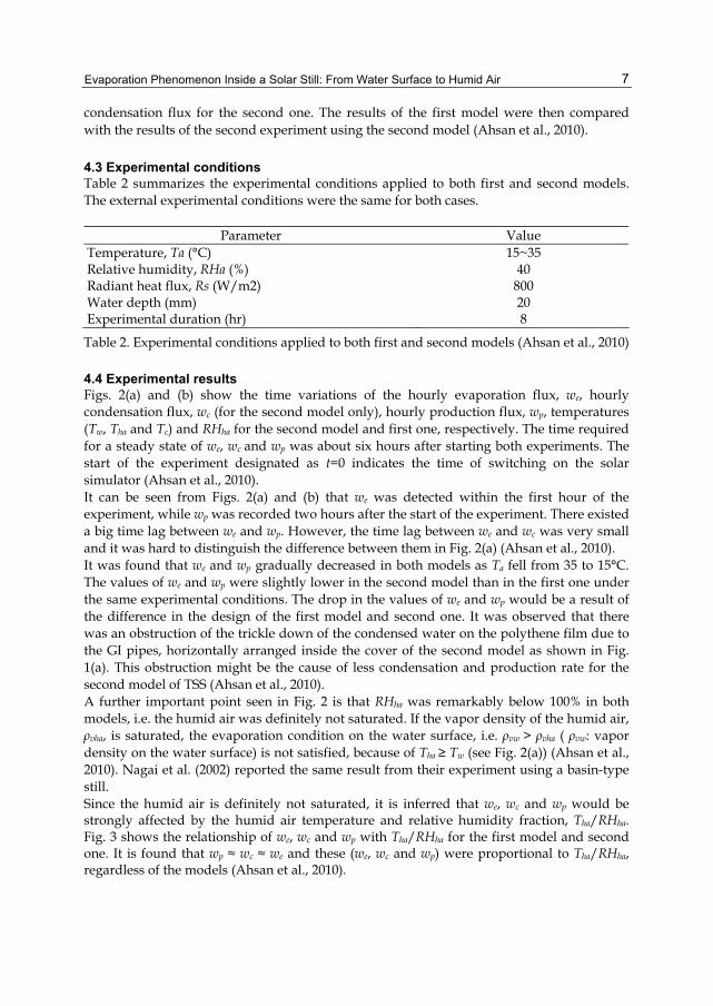
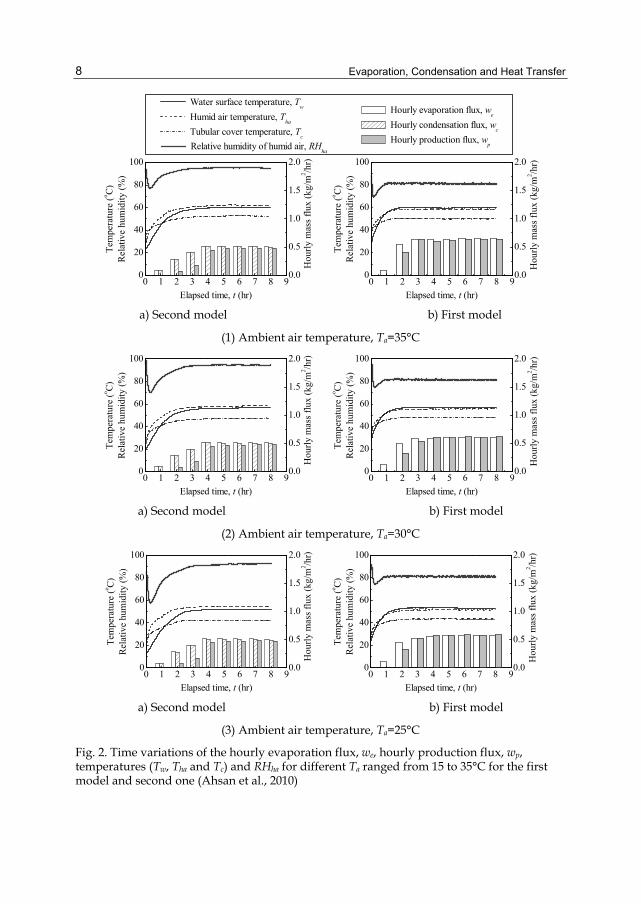
4.4 Experimental results Figs. 2(a) and (b) show the time variations of the hourly evaporation flux, we, hourly condensation flux, wc (for the second model only), hourly production flux, wp, temperatures (Tw, Tha and Tc) and RHha for the second model and first one, respectively. The time required for a steady state of we, wc and wp was about six hours after starting both experiments. The start of the experiment designated as t=0 indicates the time of switching on the solar simulator (Ahsan et al., 2010). It can be seen from Figs. 2(a) and (b) that we was detected within the first hour of the experiment, while wp was recorded two hours after the start of the experiment. There existed a big time lag between we and wp. However, the time lag between we and wc was very small and it was hard to distinguish the difference between them in Fig. 2(a) (Ahsan et al., 2010). It was found that we and wp gradually decreased in both models as Ta fell from 35 to 15°C. The values of we and wp were slightly lower in the second model than in the first one under the same experimental conditions. The drop in the values of we and wp would be a result of the difference in the design of the first model and second one. It was observed that there was an obstruction of the trickle down of the condensed water on the polythene film due to the GI pipes, horizontally arranged inside the cover of the second model as shown in Fig. 1(a). This obstruction might be the cause of less condensation and production rate for the second model of TSS (Ahsan et al., 2010). A further important point seen in Fig. 2 is that RHha was remarkably below 100% in both models, i.e. the humid air was definitely not saturated. If the vapor density of the humid air, ρvha, is saturated, the evaporation condition on the water surface, i.e. ρvw > ρvha ( ρvw: vapor density on the water surface) is not satisfied, because of Tha ≥ Tw (see Fig. 2(a)) (Ahsan et al., 2010). Nagai et al. (2002) reported the same result from their experiment using a basin-type still. Since the humid air is definitely not saturated, it is inferred that we, wc and wp would be strongly affected by the humid air temperature and relative humidity fraction, Tha/RHha. Fig. 3 shows the relationship of we, wc and wp with Tha/RHha for the first model and second one. It is found that wp ≈ wc ≈ we and these (we, wc and wp) were proportional to Tha/RHha, regardless of the models (Ahsan et al., 2010).
Evaporation, Condensation and Heat Transfer
8
0 1 2 3 4 5 6 7 8 90
20
40
60
80
100
0 1 2 3 4 5 6 7 8 90
20
40
60
80
100 Relative humidity of humid air, RH
ha
Hou
rly m
ass f
lux
(kg/
m2 /h
r)
Tem
pera
ture
(o C)
Rel
ativ
e hu
mid
ity (%
)
Elapsed time, t (hr)
Water surface temperature, Tw
Humid air temperature, Tha
Tubular cover temperature, Tc
Tem
pera
ture
(o C)
Rel
ativ
e hu
mid
ity (%
)
Elapsed time, t (hr)
0.0
0.5
1.0
1.5
2.0
Hou
rly m
ass f
lux
(kg/
m2 /h
r)
0.0
0.5
1.0
1.5
2.0
Hourly evaporation flux, we
Hourly condensation flux, wc
Hourly production flux, wp
a) Second model b) First model
(1) Ambient air temperature, Ta=35°C
0 1 2 3 4 5 6 7 8 90
20
40
60
80
100
0 1 2 3 4 5 6 7 8 90
20
40
60
80
100
Hou
rly m
ass f
lux
(kg/
m2 /h
r)
Tem
pera
ture
(o C)
Rel
ativ
e hu
mid
ity (%
)
Elapsed time, t (hr)
Tem
pera
ture
(o C)
Rel
ativ
e hu
mid
ity (%
)
Elapsed time, t (hr)
0.0
0.5
1.0
1.5
2.0
Hou
rly m
ass f
lux
(kg/
m2 /h
r)
0.0
0.5
1.0
1.5
2.0
a) Second model b) First model
(2) Ambient air temperature, Ta=30°C
0 1 2 3 4 5 6 7 8 90
20
40
60
80
100
0 1 2 3 4 5 6 7 8 90
20
40
60
80
100
Hou
rly m
ass f
lux
(kg/
m2 /h
r)
Tem
pera
ture
(o C)
Rel
ativ
e hu
mid
ity (%
)
Elapsed time, t (hr)
Tem
pera
ture
(o C)
Rel
ativ
e hu
mid
ity (%
)
Elapsed time, t (hr)
0.0
0.5
1.0
1.5
2.0
Hou
rly m
ass f
lux
(kg/
m2 /h
r)
0.0
0.5
1.0
1.5
2.0
a) Second model b) First model
(3) Ambient air temperature, Ta=25°C
Fig. 2. Time variations of the hourly evaporation flux, we, hourly production flux, wp, temperatures (Tw, Tha and Tc) and RHha for different Ta ranged from 15 to 35°C for the first model and second one (Ahsan et al., 2010)
Evaporation Phenomenon Inside a Solar Still: From Water Surface to Humid Air
9
0 1 2 3 4 5 6 7 8 90
20
40
60
80
100
0 1 2 3 4 5 6 7 8 90
20
40
60
80
100
Relative humidity of humid air, RHha
Hou
rly m
ass f
lux
(kg/
m2 /h
r)
Tem
pera
ture
(o C)
Rel
ativ
e hu
mid
ity (%
)
Elapsed time, t (hr)
Water surface temperature, Tw
Humid air temperature, Tha
Tubular cover temperature, Tc
Tem
pera
ture
(o C)
Rel
ativ
e hu
mid
ity (%
)
Elapsed time, t (hr)
0.0
0.5
1.0
1.5
2.0
Hou
rly m
ass f
lux
(kg/
m2 /h
r)
0.0
0.5
1.0
1.5
2.0
Hourly evaporation flux, we
Hourly condensation flux, wc
Hourly production flux, wp
a) Second model b) First model
(4) Ambient air temperature, Ta=20°C
0 1 2 3 4 5 6 7 8 90
20
40
60
80
100
0 1 2 3 4 5 6 7 8 90
20
40
60
80
100
Hou
rly m
ass f
lux
(kg/
m2 /h
r)
Tem
pera
ture
(o C)
Rel
ativ
e hu
mid
ity (%
)
Elapsed time, t (hr)
Tem
pera
ture
(o C)
Rel
ativ
e hu
mid
ity (%
)
Elapsed time, t (hr)
0.0
0.5
1.0
1.5
2.0
Hou
rly m
ass f
lux
(kg/
m2 /h
r)
0.0
0.5
1.0
1.5
2.0
a) Second model b) First model
(5) Ambient air temperature, Ta=15°C
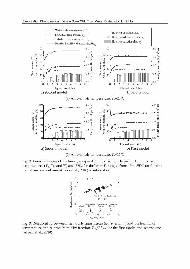
Fig. 2. Time variations of the hourly evaporation flux, we, hourly production flux, wp, temperatures (Tw, Tha and Tc) and RHha for different Ta ranged from 15 to 35°C for the first model and second one (Ahsan et al., 2010) (continuation)
0.4 0.5 0.6 0.7 0.80
0.2
0.4
0.6
0.8
Tha/RHha (°C/%)
Hou
rly m
ass f
lux
(kg/
m2 /h
r)
First Nil Second
Evaporation Condensation ProductionModel flux, we flux, wc flux, wp
wp= 0.045+0.618(Tha/RHha)R2= 0.808
Fig. 3. Relationship between the hourly mass fluxes (we, wc and wp) and the humid air temperature and relative humidity fraction, Tha/RHha, for the first model and second one (Ahsan et al., 2010)
Evaporation, Condensation and Heat Transfer
10
5. Theory of mass transfer 5.1 Previous evaporation model Islam (2006) formulated the evaporation in the TSS based on the humid air temperature and on the relative humidity in addition to the water temperature and obtained an empirical Eq. 1 of the evaporative mass transfer coefficient (m/s), hew,
3 41.37 10 5.15 10 ( )ew w ch T T− −= × + × − (1)
where, Tw = absolute temperature of the water surface; and Tc = absolute temperature of the tubular cover.
5.2 Purposes and research flow of present model The main purposes and procedures of this research are as follows: 1. Making an evaporation model with theoretical expression of hew 2. Verifying the validity of the evaporation model Three steps are taken in order to attain the two purposes described above. The purpose of the first step is to determine the value of m that is one of two unknown parameters in a new theoretical expression of hew derived by dimensional analysis. To achieve this, the evaporation experiment in this study (present laboratory-evaporation experiment) was designed and thus the correlation between the trough width, B, and hourly evaporation from the whole water surface in a trough, W, identifies the value of m (Ahsan & Fukuhara, 2008). The purpose of the second step is to determine the value of α that is another unknown parameter in the theoretical expression of hew using the previous laboratory-TSS experimental results. Consequently, the formulization of hew is given in the second step and the first purpose is completed. Finally, the purpose of the third step is to verify the validity of the evaporation model with the new hew formulized in the second step. Therefore, the calculated evaporation mass flux was compared with the observed data obtained from the previous field-TSS experiment. Furthermore, the calculation accuracy of the previous evaporation model and another model proposed by Ueda (2000) is examined using the same field-TSS experimental data. Thus, the second purpose is achieved (Ahsan & Fukuhara, 2008).
5.3 Humid air The density of the humid air (After Brutsaert, 1991) inside a TSS can be expressed as
0.3781o vha
d ha o
P eR T P
ρ⎛ ⎞
= −⎜ ⎟⎜ ⎟⎝ ⎠
(2)
where, Po = total pressure of the humid air; evha = partial pressure of water vapor in the humid air; Tha = absolute temperature of the humid air; and Rd = specific gas constant of dry air. Note that ρ=ρd+ρvha, where, ρd = density of dry air; and ρvha = density of water vapor in the humid air. The density of the humid air on the water surface, ρs, can be written as (Ahsan & Fukuhara, 2008)
0.3781o vws
d w o
P eR T P
ρ⎛ ⎞
= −⎜ ⎟⎜ ⎟⎝ ⎠
(3)
Evaporation Phenomenon Inside a Solar Still: From Water Surface to Humid Air
11
where, evw = saturated water vapor pressure. Similarly, ρs=ρd+ρvw, where, ρvw = density of saturated water vapor on the water surface. From Eqs. 2 and 3, the ratio of ρ to ρs is given by (Ahsan & Fukuhara, 2008)
0.3780.378
o vha w
s o vw ha
P e TP e T
ρρ
−= ⋅−
(4)
Since the following conditions, evw>evha and Tha≈Tw are usually observed in a TSS (see Table 5), ρ is greater than ρs. This implies that the buoyancy of air occurs on the water surface and might increase the evaporation from the water surface (Ahsan & Fukuhara, 2008).
5.4 Evaporation by natural convection We modified a diffusion equation proposed by Ueda (2000) that is applied for the evaporation from the water surface in the stagnant air with a uniform temperature. The modification of Ueda’s model (present model) is attributed to the difference in the applicable condition of the diffusion equation as shown in Table 3 (Ahsan & Fukuhara, 2008).
Present model Ueda’s model Evaporation equation
(diffusion type) vw vha
x me ew K
δ−= vw vha
x oe ew K
δ−=
Physical meaning of the coefficient
Km = Dispersion due to instability of humid air
Ko = Diffusion due to molecular motion
Air conditions on the water surface
Temperature (°C) Non-uniform
Upper part: low temperature, Lower part: high temperature
Uniform
Stability of air Unstable Neutral
Table 3. Differences between present and Ueda’s model (Ahsan & Fukuhara, 2008)
A modified diffusion equation to calculate the local evaporation mass flux, wx, from the water surface in a trough inside a TSS is expressed as (Ahsan & Fukuhara, 2008)
vw vhax m
e ew Kδ−= (5)
where, Km = dispersion coefficient of the water vapor; x = transverse distance from the edge of the trough; and δ = effective boundary layer thickness of vapor pressure, ev and depends on the convection due to the movement of the humid air in a TSS. Km is expressed as the product of a new parameter, αv, (Ahsan & Fukuhara, 2008) and the diffusion coefficient of water vapor in air, Ko (kg/m·s·Pa), i.e.
m v oK Kα= (6)
αv is referred to as “evaporativity” in this paper and is influenced by not only the strength of buoyancy mentioned above but also the instability of the humid air on the water surface, because the bottom boundary temperature of the humid air, Tw, is higher than the upper boundary temperature, Tc. This is the main reason why we used Km instead of Ko, which is expressed by the following equation (Ahsan & Fukuhara, 2008),
Evaporation, Condensation and Heat Transfer
12
vo
ha
DMKRT
= (7)
where, Mv = molecular weight of the water vapor; R = universal gas constant; and D = molecular diffusion coefficient of water vapor (m2/s) at a normal atmospheric pressure and is calculated by means of the following empirical equation (After Ueda, 2000),
1.75
40.241 10288
haTD − ⎛ ⎞= × ⎜ ⎟⎝ ⎠
(8)
Although Ko is a function of Tha, the change of Ko in the range of ordinary Tha is small. For example, Ko=1.93×10⁻¹⁰ kg/m·s·Pa for Tha=40°C and 2.07×10⁻¹⁰ kg/m·s·Pa for Tha=70°C (Ahsan & Fukuhara, 2008).
5.5 Dimensional analysis Evaporative mass transfer is generalized by empirical equations using a dimensional analysis and correlating experimental results. Assuming that the evaporation in a TSS is induced by natural convection, the relation between δ and x is characterized using a local Grashof number, Gr, and the Schmidt number, Sc (Ueda, 2000; Ahsan & Fukuhara, 2008).
( ) ( )( )
nx
v o vw vha
w xx f Gr Sc a Gr ScK e eδ α
= = ⋅ = ⋅−
(9)
The coefficient a and the power n are different for convection regimes of the humid air. The values of a and n are varied as follows (Ahsan & Fukuhara, 2008): a = 0.46 and n = 1/4 for the laminar natural convection (1<GrB·Sc<4×10⁴); and a = 0.21 and n = 1/3 for the turbulent natural convection (4×10⁴<GrB·Sc). The local Grashof number is formed as a function of x:
3
2s
s
gxGr ρ ρρν−= ⋅ (10)
where, g = gravitational acceleration; and ν = kinematic viscosity. The Schmidt number is denoted as
ScDν= (11)
The product of the Grashof number and the Schmidt number is expressed in the form
3gxGr Sc A
Dν⋅ = ⋅ (12)
where, 1s
A ρρ
= − . Substituting Eq. 12 into Eq. 9, wx is given by (Ahsan & Fukuhara, 2008)
3 1( )n
nx v o vw vha
Agw a K e e xD
αν
−⎡ ⎤= − ⎢ ⎥⎣ ⎦
(13)
Evaporation Phenomenon Inside a Solar Still: From Water Surface to Humid Air
13
The total evaporation mass per hour (kg/hr), i.e. hourly evaporation, W, can be obtained by integrating the local evaporation flux over the entire water surface, that is (Ahsan & Fukuhara, 2008),
2
03600 2
B /xW L w dx= × × ∫ (14)
where, B = width; and L = length of the trough. Integrating Eq. 14 yields the following form (Ahsan & Fukuhara, 2008):
( )n
mo vw vha
AgW C K L B e eD
αν⎡ ⎤= −⎢ ⎥⎣ ⎦
(15)
where, α (=aαv) = evaporation coefficient; m=3n; and13600 2 m
Cm
−×= .
When the water temperature, Tw, is different from the cover temperature, Tc, the coefficient A in Eq. 12 can be approximated by the following form (Ahsan & Fukuhara, 2008):
( )sw c
sA T T Tρ ρ β β
ρ−= ≈ − = Δ (16)
where, β = volumetric thermal expansion coefficient. Substituting Eq. 16 into Eq. 15, W is given by (Ahsan & Fukuhara, 2008)
( )n
mo vw vha
g TW C K L B e eD
βαν
Δ⎡ ⎤= −⎢ ⎥⎣ ⎦
(17)
Eq. 17 can be expressed in terms of the vapor density difference using the equation of state (Ahsan & Fukuhara, 2008),
( )n
mo v w vw ha vha
g TW C K L B R T TD
βα ρ ρν
Δ⎡ ⎤= −⎢ ⎥⎣ ⎦
(18)
where, Rv = specific gas constant of the water vapor. Taking into account of the fact, Tha≈Tw, Eq. 18 is approximated as follows (Ahsan & Fukuhara, 2008):
( )n
mo v vw vha
g TW C K L B R TD
βα ρ ρν
Δ⎡ ⎤= −⎢ ⎥⎣ ⎦
(19)
where, 2
w haT TT += . Eq. 19 is transformed as (Ahsan & Fukuhara, 2008)
*( )n
mo v vw vha
gW C K L B R TDβα ρ ρ
ν⎡ ⎤= −⎢ ⎥⎣ ⎦
(20)
where, * nT T T= Δ .
Evaporation, Condensation and Heat Transfer
14
Finally, the evaporation mass flux (kg/m2/s), w(=W/3600BL), is calculated by the following equation (Ahsan & Fukuhara, 2008),
( )ew vw vhaw h ρ ρ= − (21)
where, hew is given by (Ahsan & Fukuhara, 2008)
1
1 *2 nmmo
ew vgKh B R T
m Dβα
ν
−−⎡ ⎤= ⎢ ⎥
⎣ ⎦ (22)
5.6 Application of the present model to the present experiment When the vapor pressure difference, evw-evha, α and L are constant, Eq. 15 can be rewritten in terms of B (Ahsan & Fukuhara, 2008),
mW Bη= (23)
where, η (kg/m/hr) is expressed as (Ahsan & Fukuhara, 2008)
( )n
o vw vhaAgC K L e eD
η αν⎡ ⎤= −⎢ ⎥⎣ ⎦
(24)
Note that evha in Eq. 24 is the vapor pressure of the stagnant ambient air surrounding the trough for the present evaporation experiment (Ahsan & Fukuhara, 2008).
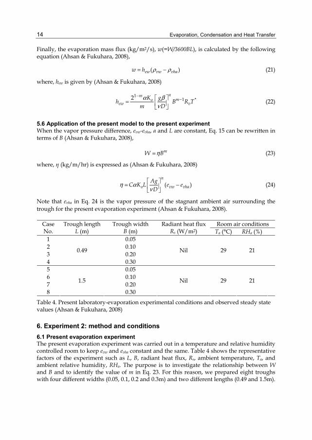
Room air conditions Case No.
Trough length L (m)
Trough width B (m)
Radiant heat flux Rs (W/m2) Ta (°C) RHa (%)
1 0.05 2 0.10 3 0.20 4
0.49
0.30
Nil 29 21
5 0.05 6 0.10 7 0.20 8
1.5
0.30
Nil 29 21
Table 4. Present laboratory-evaporation experimental conditions and observed steady state values (Ahsan & Fukuhara, 2008)
6. Experiment 2: method and conditions 6.1 Present evaporation experiment The present evaporation experiment was carried out in a temperature and relative humidity controlled room to keep evw and evha constant and the same. Table 4 shows the representative factors of the experiment such as L, B, radiant heat flux, Rs, ambient temperature, Ta, and ambient relative humidity, RHa. The purpose is to investigate the relationship between W and B and to identify the value of m in Eq. 23. For this reason, we prepared eight troughs with four different widths (0.05, 0.1, 0.2 and 0.3m) and two different lengths (0.49 and 1.5m).
Evaporation Phenomenon Inside a Solar Still: From Water Surface to Humid Air
15
The trough was made of a corrugated carton paper of 3.0mm in thickness and covered by a black polythene film of 0.05mm in thickness. To measure the value of W, we prepared four electric balances with a minimum reading of 0.01g and each trough was placed on each electric balance. All of the electric balances were connected to computers. In this way, W was automatically and simultaneously recorded in computers at five-minute intervals. Tw was measured with a thermocouple and was recorded in a data logger.Ta and RHa were monitored by a thermo-hygrometer (Ahsan & Fukuhara, 2008).
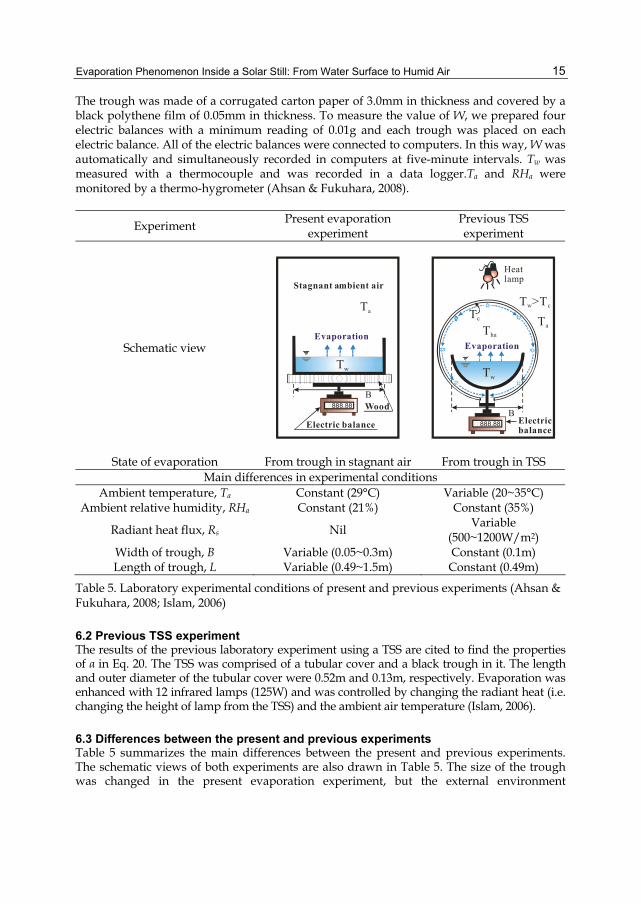
Experiment Present evaporation experiment
Previous TSS experiment
Schematic view
Evaporation
Tw
B
Ta
Stagnant a airmbient
Electric balance
888.88 Wood
Tc
Evaporation
Tw
Tha
B
Heatlamp
Ta
T >w Tc
888.88 Electricbalance
State of evaporation From trough in stagnant air From trough in TSS
Main differences in experimental conditions Ambient temperature, Ta Constant (29°C) Variable (20~35°C)
Ambient relative humidity, RHa Constant (21%) Constant (35%)
Radiant heat flux, Rs Nil Variable (500~1200W/m2)
Width of trough, B Variable (0.05~0.3m) Constant (0.1m) Length of trough, L Variable (0.49~1.5m) Constant (0.49m)
Table 5. Laboratory experimental conditions of present and previous experiments (Ahsan & Fukuhara, 2008; Islam, 2006)
6.2 Previous TSS experiment The results of the previous laboratory experiment using a TSS are cited to find the properties of α in Eq. 20. The TSS was comprised of a tubular cover and a black trough in it. The length and outer diameter of the tubular cover were 0.52m and 0.13m, respectively. Evaporation was enhanced with 12 infrared lamps (125W) and was controlled by changing the radiant heat (i.e. changing the height of lamp from the TSS) and the ambient air temperature (Islam, 2006).
6.3 Differences between the present and previous experiments Table 5 summarizes the main differences between the present and previous experiments. The schematic views of both experiments are also drawn in Table 5. The size of the trough was changed in the present evaporation experiment, but the external environment
Evaporation, Condensation and Heat Transfer
16
surrounding the trough maintained the same conditions. On the other hand, the external conditions (Rs and Ta) were changed in the previous experiment, but the same tough size (L=0.49m and B=0.1m) was used then (Ahsan & Fukuhara, 2008).
6.4 Previous field-TSS experiment In order to support the validity of the present model, the previous field experimental results are cited in this paper. The same specification of TSS was produced for both laboratory and filed experiments (Islam, 2006).
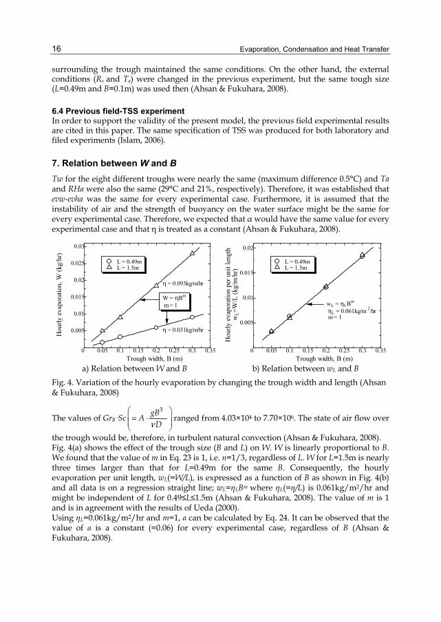
7. Relation between W and B Tw for the eight different troughs were nearly the same (maximum difference 0.5°C) and Ta and RHa were also the same (29°C and 21%, respectively). Therefore, it was established that evw-evha was the same for every experimental case. Furthermore, it is assumed that the instability of air and the strength of buoyancy on the water surface might be the same for every experimental case. Therefore, we expected that α would have the same value for every experimental case and that η is treated as a constant (Ahsan & Fukuhara, 2008).
0.05 0.1 0.15 0.2 0.25 0.3 0.35
0.005
0.01
0.015
0.02
0.025
0.03
0
W = ηBm
m = 1
Trough width, B (m)
Hou
rly e
vapo
ratio
n, W
(kg/
hr)
L = 0.49m L = 1.5m
η = 0.093kg/m/hr
η = 0.031kg/m/hr
0.05 0.1 0.15 0.2 0.25 0.3 0.35
0.005
0.01
0.015
0.02
0
wL = ηLBm
ηL = 0.061kg/m 2/hrm = 1
Trough width, B (m)
Hou
rly e
vapo
ratio
n pe
r uni
t len
gth
wL=
W/L
(kg/
m/h
r)
L = 0.49m L = 1.5m
a) Relation between W and B b) Relation between wL and B
Fig. 4. Variation of the hourly evaporation by changing the trough width and length (Ahsan & Fukuhara, 2008)
The values of GrB·Sc3gBA
Dν⎛ ⎞
= ⋅⎜ ⎟⎜ ⎟⎝ ⎠
ranged from 4.03×10⁴ to 7.70×10⁶. The state of air flow over
the trough would be, therefore, in turbulent natural convection (Ahsan & Fukuhara, 2008). Fig. 4(a) shows the effect of the trough size (B and L) on W. W is linearly proportional to B. We found that the value of m in Eq. 23 is 1, i.e. n=1/3, regardless of L. W for L=1.5m is nearly three times larger than that for L=0.49m for the same B. Consequently, the hourly evaporation per unit length, wL(=W/L), is expressed as a function of B as shown in Fig. 4(b) and all data is on a regression straight line; wL=ηLBm where ηL(=η/L) is 0.061kg/m2/hr and might be independent of L for 0.49≤L≤1.5m (Ahsan & Fukuhara, 2008). The value of m is 1 and is in agreement with the results of Ueda (2000). Using ηL=0.061kg/m2/hr and m=1, α can be calculated by Eq. 24. It can be observed that the value of α is a constant (=0.06) for every experimental case, regardless of B (Ahsan & Fukuhara, 2008).
Evaporation Phenomenon Inside a Solar Still: From Water Surface to Humid Air
17
8. Evaporation coefficient The results of the previous laboratory-TSS experiment under twelve sets of external conditions are quoted here (Islam, 2006). Since the vapor density difference, ρvw-ρvha, is different for every experimental case unlike the present evaporation experiment, α should be calculated by Eq. 25 after substituting m=1 into Eq. 20 (Ahsan & Fukuhara, 2008),
13 *3600 ( )o v vw vha
W
gK L BR TD
αβ ρ ρ
ν
=⎡ ⎤ −⎢ ⎥⎣ ⎦
(25)
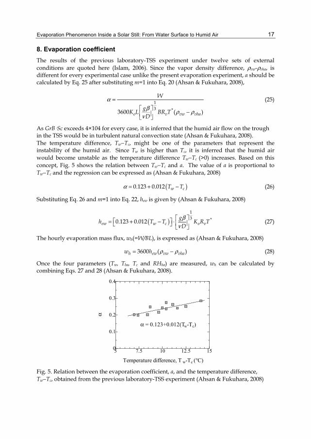
As GrB·Sc exceeds 4×10⁴ for every case, it is inferred that the humid air flow on the trough in the TSS would be in turbulent natural convection state (Ahsan & Fukuhara, 2008). The temperature difference, Tw−Tc, might be one of the parameters that represent the instability of the humid air. Since Tw is higher than Tc, it is inferred that the humid air would become unstable as the temperature difference Tw−Tc (>0) increases. Based on this concept, Fig. 5 shows the relation between Tw−Tc and α. The value of α is proportional to Tw−Tc and the regression can be expressed as (Ahsan & Fukuhara, 2008)
( )0.123 0.012 w cT Tα = + − (26)
Substituting Eq. 26 and m=1 into Eq. 22, hew is given by (Ahsan & Fukuhara, 2008)
( )13 *0.123 0.012ew w c o v
gh T T K R TDβ
ν⎡ ⎤⎡ ⎤= + − ⋅ ⎢ ⎥⎣ ⎦ ⎣ ⎦
(27)
The hourly evaporation mass flux, wh(=W/BL), is expressed as (Ahsan & Fukuhara, 2008)
3600 ( )h ew vw vhaw h ρ ρ= − (28)
Once the four parameters (Tw, Tha, Tc and RHha) are measured, wh can be calculated by combining Eqs. 27 and 28 (Ahsan & Fukuhara, 2008).
5 7.5 10 12.5 150
0.1
0.2
0.3
0.4
Temperature difference, T w-Tc (°C)
α
α = 0.123+0.012(Tw-Tc)
Fig. 5. Relation between the evaporation coefficient, α, and the temperature difference, Tw−Tc, obtained from the previous laboratory-TSS experiment (Ahsan & Fukuhara, 2008)
Evaporation, Condensation and Heat Transfer
18
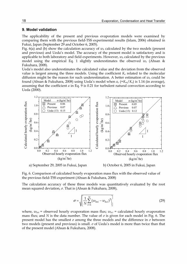
9. Model validation The applicability of the present and previous evaporation models were examined by comparing them with the previous field-TSS experimental results (Islam, 2006) obtained in Fukui, Japan (September 29 and October 6, 2005). Fig. 6(a) and (b) show the calculation accuracy of wh calculated by the two models (present and previous) and Ueda’s model. The accuracy of the present model is satisfactory and is applicable to both laboratory and field experiments. However, wh calculated by the previous model using the empirical Eq. 1 slightly underestimates the observed wh (Ahsan & Fukuhara, 2008). Ueda’s model also underestimates the calculated value and the deviation from the observed value is largest among the three models. Using the coefficient Ko related to the molecular diffusion might be the reason for such underestimation. A better estimation of wh could be found (Ahsan & Fukuhara, 2008) using Ueda’s model when αv (=Km/Ko) is 1.14 (in average), assuming that the coefficient a in Eq. 9 is 0.21 for turbulent natural convection according to Ueda (2000).
0.0 0.2 0.4 0.6 0.8 1.0 1.20.0
0.2
0.4
0.6
0.8
1.0
1.2 Model σ (kg/m2/hr)
Present 0.06Previous 0.07Ueda (13) 0.15
Cal
cula
ted
hour
ly e
vapo
ratio
n flu
x(k
g/m
2 /hr)
Observed hourly evaporation flux(kg/m2/hr)
11
0.0 0.2 0.4 0.6 0.8 1.0 1.20.0
0.2
0.4
0.6
0.8
1.0
1.2 Model σ (kg/m2/hr)
Present 0.05Previous 0.07Ueda (13) 0.12
Cal
cula
ted
hour
ly e
vapo
ratio
n flu
x(k
g/m
2 /hr)
Observed hourly evaporation flux(kg/m2/hr)
11
a) September 29, 2005 in Fukui, Japan b) October 6, 2005 in Fukui, Japan
Fig. 6. Comparison of calculated hourly evaporation mass flux with the observed value of the previous field-TSS experiment (Ahsan & Fukuhara, 2008)
The calculation accuracy of these three models was quantitatively evaluated by the root mean squared deviation, σ. That is (Ahsan & Fukuhara, 2008),
2
1
1 ( )N
hoi hcii
w wN
σ=
⎡ ⎤= −⎢ ⎥
⎢ ⎥⎣ ⎦∑ (29)
where, whoi = observed hourly evaporation mass flux; whci = calculated hourly evaporation mass flux; and N is the data number. The value of σ is given for each model in Fig. 6. The present model has the smallest σ among the three models and the difference in σ between two models (present and previous) is small. σ of Ueda’s model is more than twice than that of the present model (Ahsan & Fukuhara, 2008).
Evaporation Phenomenon Inside a Solar Still: From Water Surface to Humid Air
19
10. Conclusion The cover material of the first model of the Tubular Solar Still (TSS), a transparent vinyl chloride sheet was changed to a polythene film for the second model. Thus, the second model is simpler, lighter, cheaper and more durable than the first one. These improvements make the assembly and maintenance of the new TSS easier. A special experimental technique was developed to observe the evaporation, condensation and production performance independently and simultaneously. As a result, the evaporation was detected first and then the condensation and the production followed it in turn. As for second model, the hourly evaporation and production fluxes were slightly lower than the first one under the same experimental conditions. It was revealed that the relative humidity of the humid air was definitely not saturated and the hourly evaporation, condensation and production fluxes were proportional to the humid air temperature and relative humidity fraction (Ahsan et al., 2010). An evaporative mass transfer model was presented with a semi-theoretical expression of the evaporative mass transfer coefficient for a TSS using the dimensional analysis taking account of the humid air properties inside the still. Findings revealed from the present laboratory-evaporation experimental results that the hourly evaporation is linearly proportional to the trough width, B, regardless of the trough length, L, for 0.49≤L≤1.5m (Ahsan & Fukuhara, 2008). The movement of the humid air in the TSS belongs to turbulent natural convection state. The evaporation coefficient is proportional to the temperature difference between the water in a trough and the tubular still cover. The present model was able to reproduce the hourly evaporation mass flux obtained from the previous field-TSS experiment. It is concluded that once the four parameters (Ahsan & Fukuhara, 2008); that is, the water temperature, humid air temperature, tubular cover temperature and the relative humidity of humid air are measured, the present model is capable of evaluating the diurnal variation of evaporation mass flux from the water surface in a trough with an arbitrary size.
11. Acknowledgment Authors gratefully acknowledge Prof. Dr. Teruyuki Fukuhara, Prof. Dr. Shafiul Islam, Engr. Keiichi Waki, Engr. Hiroaki Terasaki, Dr. Akihiro Fujimoto, Dr. Yasuo Kita, Dr. Kazuo Okamura and Engr. Fumio Asano for their kind cooperation during staying in Fukui, Japan and for their continued friendly support. The partial financial support provided by the Ministry of Education, Science, and Culture of Japanese Government, Japan; Shimizu Corporation, Japan and Japan Cooperation Center, Petroleum (JCCP), Japan is also acknowledged.
12. Nomenclature B = width of the trough (m); D = molecular diffusion coefficient of water vapor (m2/s); ev = vapor pressure (Pa); evha = partial pressure of water vapor in the humid air (Pa); evw = saturated water vapor pressure (Pa); g = gravitational acceleration (9.807 m/s2); Gr = Grashof number (-);
Evaporation, Condensation and Heat Transfer
20
hew = evaporative mass transfer coefficient from water surface to humid air (m/s); Km = dispersion coefficient of the water vapor (kg/m·s·Pa); Ko = diffusion coefficient of the water vapor (kg/m·s·Pa); L = length of the trough (m); Mv = molecular weight of the water vapor (18.016 kg/kmol); Po = total pressure in the humid air (101325 Pa); R = universal gas constant (8315 J/kmol·K); Rd = specific gas constant of dry air (287.04 J/kg·K); Rs = radiant heat flux (W/m2); Rv = specific gas constant of the water vapor (461.5 J/kg·K); RHa = relative humidity of ambient air (%); RHha = relative humidity of humid air (%); Sc = Schmidt number (-); Ta = ambient air temperature (K); Tc = tubular cover temperature (K); Tha = humid air temperature (K); Tw = water surface temperature (K); T = mean temperature of water and humid air (K); w = evaporation mass flux (kg/m2·s); wh = hourly evaporation mass flux (kg/m2·hr); whci = calculated hourly evaporation mass flux (kg/m2·hr); whoi = observed hourly evaporation mass flux (kg/m2·hr); wL = hourly evaporation per unit length (kg/m·hr); wx = local evaporation mass flux (kg/m2·s); W = hourly evaporation (kg/hr); x = transverse distance from the edge of trough (m); α = evaporation coefficient (-); αv = evaporativity (-); β = volumetric thermal expansion coefficient (1/K); δ = effective boundary layer thickness of vapor pressure (m); ΔT = temperature difference between water surface and cover (K); ν = kinematic viscosity (m2/s); ρ = density of humid air (kg/m3); ρd = density of dry air (kg/m3); ρs = density of humid air on the water surface (kg/m3); ρvha = density of water vapor in the humid air at Tha (kg/m3); ρvw = density of saturated water vapor on the water surface at Tw (kg/m3); and σ = root mean squared deviation (kg/m2·hr).
13. References Ahsan, A. & Fukuhara, T. (2008). Evaporative Mass Transfer in Tubular Solar Still. J.
Hydroscience and Hydraulic Engineering, JSCE, vol. 26(2), 15-25. Ahsan, A. (2009). Production model of new tubular solar still and its productivity
characteristics. PhD thesis, University of Fukui, Japan, pp 45-73.
Evaporation Phenomenon Inside a Solar Still: From Water Surface to Humid Air
21
Ahsan, A. & Fukuhara, T. (2009). Condensation mass transfer in unsaturated humid air inside tubular solar still. Annual J. of Hydraulic Engineering, JSCE, vol. 53, 97-102.
Ahsan, A. & Fukuhara, T. (2010a). Mass and Heat Transfer Model of Tubular Solar Still. Solar Energy, vol. 84 (7), 1147-1156.
Ahsan, A. & Fukuhara, T. (2010b). Condensation Mass Transfer in Unsaturated Humid Air inside Tubular Solar Still. J. Hydroscience and Hydraulic Engineering, JSCE, vol. 28(1), 31-42.
Ahsan, A.; Islam K.M.S.; Fukuhara, T. & Ghazali, A.H. (2010). Experimental Study on Evaporation, Condensation and Production of a New Tubular Solar Still. Desalination, vol. 260 (1-3), 172-179.
Abu-Arabi, M.; Zurigat, Y.; Al-Hinai, H. & Al-Hiddabi, S. (2002). Modeling and performance analysis of a solar desalination unit with double-glass cover cooling. Desalination, 143, 173-182.
Abu-Hijleh, B.A.K. (1996). Enhanced solar still performance using water film cooling of the glass. Desalination, 107, 235-244.
Al-Karaghouli, A.A. & Alnaser, W.E. (2004). Performances of single and double basin solar-stills. Applied Energy, 78, 347-354.
Brutsaert, W. (1991). Evaporation into the atmosphere, Kluwer Academic Publishers, Netherlands, pp. 37-56.
Chaibi, M.T. (2000). Analysis by simulation of a solar still integrated in a greenhouse roof, Desalination, Vol.128, pp. 123-138.
Clark, J.A. (1990). The steady-state performance of a solar still, Solar Energy, Vol.44, No.1, pp. 43-49.
Cooper, P.I. (1969). Digital simulation of transient solar still processes, Solar Energy, Vol.12, pp. 313-331.
Dunkle, R.V. (1961). Solar Water Distillation: The roof type still and a multiple effect diffusion still, Proc. international heat transfer, ASME, University of Colorado, pp. 895-902.
Fath, H.E.S. (1998). Solar desalination: a promising alternative for water provision with free energy, simple technology and a clean environment. Desalination, 116, 45-56.
Fukuhara, T.; Asano, F.; Mutawa, H.A.A.; Nagai N. & Ito, Y. (2002). Production mechanism and performance of tubular solar still. Proc. IDA World Congress, Manama, Bahrain, March 8-13, BAH03-085.
Fukuhara, T. & Islam, K.M.S. (2006).Tubular solar desalination and improvement of soil moisture retention by date palm. In Arid Land Hydrogeology: In Search of a Solution to a Threatened Resource. Mohamed, A. M. O.; Ed.; Taylor and Francis, London, pp. 153-162.
Hongfei, Z.; Xiaoyan, Z.; Jing, Z. & Yuyuan, W. (2002). A group of improved heat and mass transfer correlations in solar stills, Energy Conversion and Management, Vol.43, pp. 2469-2478.
Islam, K.M.S.; Fukuhara, T. & Asano, F. (2004). Mass transfer in Tubular Solar Still. Proc. 59th Annual Conference, JSCE, Nagoya, Japan, September 8-10, pp. 236-237.
Islam, K.M.S.; Fukuhara, T.; Asano, F. & Mutawa, H.A.A. (2005). Productivity of the tubular solar still in the United Arab Emirates. Proc. of MTERM International Conference, Bangkok, Thailand, June 8-10, pp. 367-372.
Evaporation, Condensation and Heat Transfer
22
Islam, K.M.S. (2006). Heat and vapor transfer in tubular solar still and its production performance, PhD thesis, Department of Architecture and Civil Engineering, University of Fukui, Japan, pp. 33-52.
Islam, K.M.S.; Fukuhara, T. & Ahsan, A. (2007a). New Analysis of a tubular solar still, Proc. IDA World Congress, Spain, CD-ROM, IDAWC/MP07-041, pp. 1-12.
Islam, K.M.S.; Fukuhara, T. & Ahsan, A. (2007b). Tubular solar still-an alternative small scale fresh water management, Proc. international conference on water and flood management (ICWFM-2007), Bangladesh, pp. 291-298.
Kumar, A. & Anand, J.D. (1992). Modelling and performance of a tubular multiwick solar still, Solar Energy, Vol.17, No.11, pp. 1067-1071.
Kumar, S. & Tiwari, G.N. (1998). Optimization of collector and basin areas for a higher yield for active solar stills. Desalination, 116, 1-9.
Korngold, E.; Korin E. & Ladizhensky, I. (1996). Water desalination by pervaporation with hollow fiber membranes. Desalination, 107, 1221-1229.
Malik, M.A.S.; Tiwari, G.N.; Kumar, A. & Sodha, M.S. (1982). Solar Distillation: A practical study of a wide range of stills and their optimum design, construction and performance, Pergamon Press, Oxford, England, pp. 11-13.
Murase, K.; Tobataa, H.; Ishikawaa, M. & Toyama, S. (2006). Experimental and numerical analysis of a tube-type networked solar still for desert technology. Desalination, 190, 137–146.
Murase, K.; Komiyama, S.; Ikeya, A. & Furukawa, Y. (2000). Development of multi-effect membrane solar distillatory. Society of Sea Water Science, 54, 30-35.
Nafey, A.S.; Abdelkader, M.; Abdelmotalip, A. & Mabrouk, A.A. (2000). Parameters affecting solar still productivity. Energy Con. & Mang., 41, 1797-1809.
Nagai, N.; Takeuchi, M.; Masuda, S.; Yamagata, J.; Fukuhara, T. & Takano, Y. (2002). Heat transfer modeling and field test on basin-type solar distillation device, Proc. IDA World Congress, Bahrain, CD-ROM, Bah03-072.
Shawaqfeh, A.T. & Farid, M.M. (1995). New development in the theory of heat and mass transfer in solar stills, Solar Energy, Vol.55, No.6, pp. 527-535.
Tanaka, H.; Nosoko, T. & Nagata, T. (2000). A highly productive basin-type-multi-effect coupled solar still. Desalination, 130, 279-293.
Paul, I.D. (2002). New model of a basin-type solar still. J. Solar Energy Eng., ASME, 124, 311-314.
Tiwari, G.N. & Kumar, A. (1988). Nocturnal water production by tubular solar stills using waste heat to preheat brine, Desalination, Vol.69, pp. 309-318.
Tiwari, G.N. & Tiwari, A.K. (2008). Solar Distillation Practice For Water Desalination Systems. Anshan Limited, UK.
Tleimat, B.W. & Howe, E.D. (1966). Nocturnal production of solar distillers. Solar Energy, 10, 61-66.
Toyama, S.; Nakamura, M.; Murase, K. & Salah, H.M. (1990). Studies of desalting solar stills. Memories of the Faculty of Engineering, Nagoya University, Japan, 43, 1-53.
Tiwari, G.N. & Noor, M.A. (1996). Characterization of solar stills. Int. J. Solar Energy, 18, 147-171.
Ueda, M. (2000). Humidity and evaporation, Corona Publishing Co. Ltd., Japan, pp. 83-101.
2
Flow Boiling in an Asymmetrically Heated Single Rectangular Microchannel
Cheol Huh1 and Moo Hwan Kim2 1Korea Ocean Research and Development Institute (KORDI), 2Pohang University of Science and Technology (POSTECH),
Republic of Korea
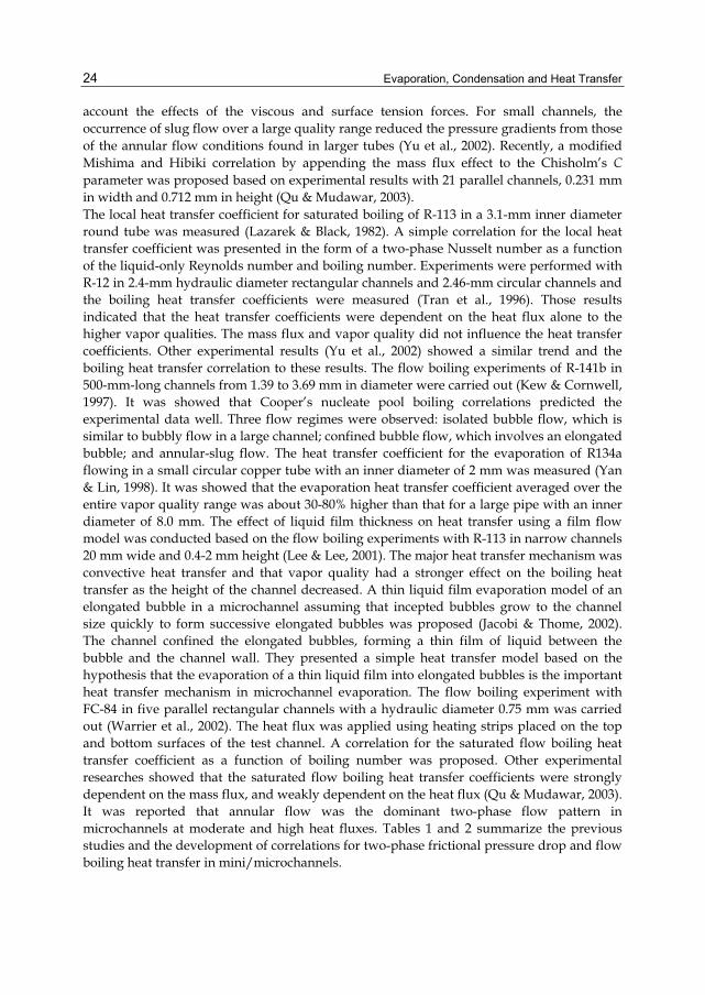
1. Introduction Heat transfer and fluid flow in microscale domains are found in many places such as microchannel heat sinks and microfluidic devices. In fact, microfluidic devices are the fastest growing area, and the development of these devices has greatly exceeded our ability to analyze them in detail. A two-phase microchannel heat sink is one of the best candidates for resolving this form of thermal management. Furthermore, limited pumping power capabilities in microscale devices have introduced concerns about large pressure drops in microchannel geometries. Many experimental investigations have been carried out to evaluate the pressure drop and heat transfer for in mini/microchannels. However, heat transfer and fluid flow in the microscale domain frequently display counterintuitive behavior due to the different forces dominating at micro-length scales. Therefore, experimental diagnostic techniques are essential for understanding two-phase pressure drop and flow boiling heat transfer in a microchannel. In addition, to elucidate the boiling heat transfer characteristics without interference from the flow distributor and the interactions between adjacent channels, it is necessary to study two-phase flow in a single microchannel. A modified Chisholm’s C parameter as a function of the hydraulic diameter based on measured the void fraction and frictional pressure drop for air-water flows in capillary tubes with inner diameters in the range of 1 to 4 mm was proposed (Mishima et al., 1993; Mishima & Hibiki, 1996). Two-phase flow pressure drop measurements for three refrigerants: R-134a, R-12, and R-113 were carried out (Tran et al., 2000). The experiments were performed in two round tubes (inner diameters of 2.46 and 2.92 mm) and one rectangular channel (4.06 x 1.7 mm). The measured two-phase frictional pressure drops were not accurately predicted by conventional macro-channel correlations. A new two-phase frictional multiplier based on Chisholm’s B-coefficient method (Chisholm, 1973) as a function of the dimensionless physical property coefficient and the confinement number was suggested. Another modified C parameter based on the Lockhart-Martinelli two-phase multiplier was proposed with an air-water two-phase pressure drop experiments in a narrow channel 20 mm in width and 0.4 to 4 mm in height (Lee & Lee, 2001). They proposed a modified C parameter based on the Lockhart-Martinelli two-phase multiplier to take into
Evaporation, Condensation and Heat Transfer
24
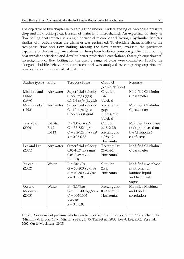
account the effects of the viscous and surface tension forces. For small channels, the occurrence of slug flow over a large quality range reduced the pressure gradients from those of the annular flow conditions found in larger tubes (Yu et al., 2002). Recently, a modified Mishima and Hibiki correlation by appending the mass flux effect to the Chisholm’s C parameter was proposed based on experimental results with 21 parallel channels, 0.231 mm in width and 0.712 mm in height (Qu & Mudawar, 2003). The local heat transfer coefficient for saturated boiling of R-113 in a 3.1-mm inner diameter round tube was measured (Lazarek & Black, 1982). A simple correlation for the local heat transfer coefficient was presented in the form of a two-phase Nusselt number as a function of the liquid-only Reynolds number and boiling number. Experiments were performed with R-12 in 2.4-mm hydraulic diameter rectangular channels and 2.46-mm circular channels and the boiling heat transfer coefficients were measured (Tran et al., 1996). Those results indicated that the heat transfer coefficients were dependent on the heat flux alone to the higher vapor qualities. The mass flux and vapor quality did not influence the heat transfer coefficients. Other experimental results (Yu et al., 2002) showed a similar trend and the boiling heat transfer correlation to these results. The flow boiling experiments of R-141b in 500-mm-long channels from 1.39 to 3.69 mm in diameter were carried out (Kew & Cornwell, 1997). It was showed that Cooper’s nucleate pool boiling correlations predicted the experimental data well. Three flow regimes were observed: isolated bubble flow, which is similar to bubbly flow in a large channel; confined bubble flow, which involves an elongated bubble; and annular-slug flow. The heat transfer coefficient for the evaporation of R134a flowing in a small circular copper tube with an inner diameter of 2 mm was measured (Yan & Lin, 1998). It was showed that the evaporation heat transfer coefficient averaged over the entire vapor quality range was about 30-80% higher than that for a large pipe with an inner diameter of 8.0 mm. The effect of liquid film thickness on heat transfer using a film flow model was conducted based on the flow boiling experiments with R-113 in narrow channels 20 mm wide and 0.4-2 mm height (Lee & Lee, 2001). The major heat transfer mechanism was convective heat transfer and that vapor quality had a stronger effect on the boiling heat transfer as the height of the channel decreased. A thin liquid film evaporation model of an elongated bubble in a microchannel assuming that incepted bubbles grow to the channel size quickly to form successive elongated bubbles was proposed (Jacobi & Thome, 2002). The channel confined the elongated bubbles, forming a thin film of liquid between the bubble and the channel wall. They presented a simple heat transfer model based on the hypothesis that the evaporation of a thin liquid film into elongated bubbles is the important heat transfer mechanism in microchannel evaporation. The flow boiling experiment with FC-84 in five parallel rectangular channels with a hydraulic diameter 0.75 mm was carried out (Warrier et al., 2002). The heat flux was applied using heating strips placed on the top and bottom surfaces of the test channel. A correlation for the saturated flow boiling heat transfer coefficient as a function of boiling number was proposed. Other experimental researches showed that the saturated flow boiling heat transfer coefficients were strongly dependent on the mass flux, and weakly dependent on the heat flux (Qu & Mudawar, 2003). It was reported that annular flow was the dominant two-phase flow pattern in microchannels at moderate and high heat fluxes. Tables 1 and 2 summarize the previous studies and the development of correlations for two-phase frictional pressure drop and flow boiling heat transfer in mini/microchannels.
Flow Boiling in an Asymmetrically Heated Single Rectangular Microchannel
25
The objective of this chapter is to gain a fundamental understanding of two-phase pressure drop and flow boiling heat transfer of water in a microchannel. An experimental study of flow boiling heat transfer in a single horizontal microchannel having a hydraulic diameter similar with bubble departure diameter was performed. To elucidate characteristics of the two-phase flow and flow boiling, identify the flow pattern, evaluate the prediction capability of the existing correlations for two-phase frictional pressure gradient and boiling heat transfer coefficient, and develop better predictable correlations, thorough experimental investigations of flow boiling for the quality range of 0-0.4 were conducted. Finally, the elongated bubble behavior in a microchannel was analyzed by comparing experimental observations and numerical calculations. Author (year) Fluid Test conditions Channel
geometry (mm) Remarks
Mishima and Hibiki (1996)
Air/water Superficial velocity 0.2-80 m/s (gas) 0.1-1.6 m/s (liquid)
Circular: 1-4; Vertical
Modified Chisholm C parameter
Mishima et al. (1993)
Air/water Superficial velocity 0.1-10 m/s (gas) 0.2-5 m/s (liquid)
Rectangular gap: 1.0, 2.4, 5.0; Vertical
Modified Chisholm C parameter
Tran et al. (2000)
R-134a, R-12, R-113
P = 138-856 kPa G = 33-832 kg/m2s q″ = 2.2-129 kW/m2 x = 0.02-0.95
Circular: 2.46, 2.92; Rectangular: 4.06x1.7; Horizontal
Modified two-phase multiplier based on the Chisholm B coefficient
Lee and Lee (2001)
Air/water Superficial velocity 0.05-18.7 m/s (gas) 0.03-2.39 m/s (liquid)
Rectangular: 20x0.4-2; Horizontal
Modified Chisholm C parameter
Yu et al. (2002)
Water P = 200 kPa G = 50-200 kg/m2s q″ = 10-300 kW/m2 x = 0.5-0.95
Circular: 2.98; Horizontal
Modified two-phase multiplier for laminar liquid and turbulent vapor
Qu and Mudawar (2003)
Water P = 1.17 bar G = 135-400 kg/m2sq″ = 400-1300 kW/m2 x = 0.5-0.95
Rectangular: 0.231x0.713; Horizontal
Modified Mishima and Hibiki correlation
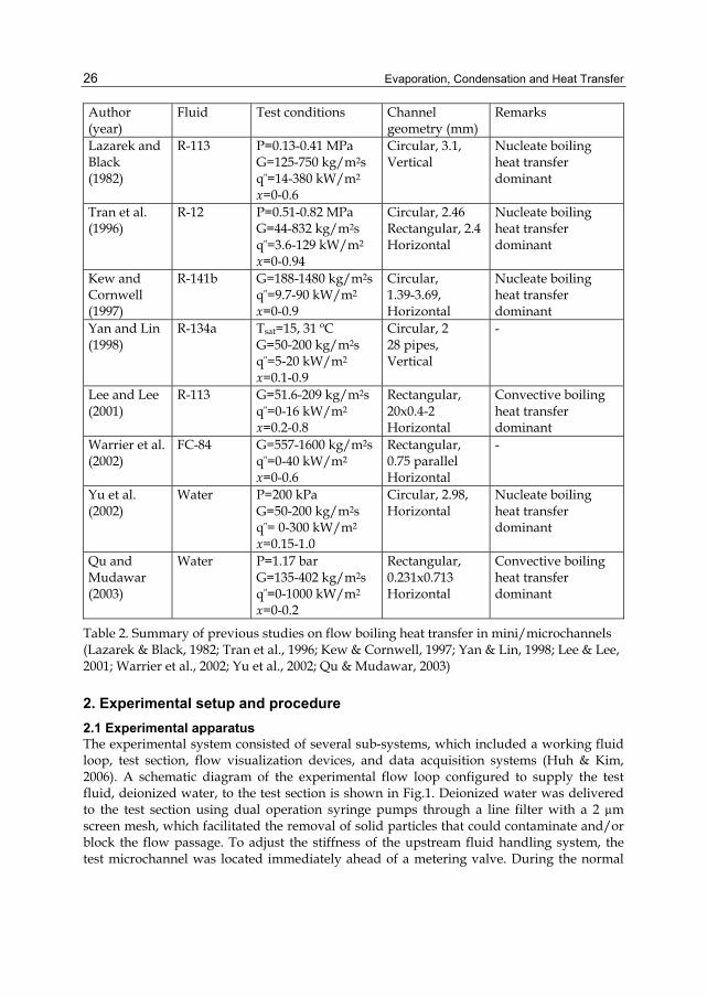
Table 1. Summary of previous studies on two-phase pressure drop in mini/microchannels (Mishima & Hibiki, 1996; Mishima et al., 1993; Tran et al., 2000; Lee & Lee, 2001; Yu et al., 2002; Qu & Mudawar, 2003)
Evaporation, Condensation and Heat Transfer
26
Author (year)
Fluid Test conditions Channel geometry (mm)
Remarks
Lazarek and Black (1982)
R-113 P=0.13-0.41 MPa G=125-750 kg/m2s q″=14-380 kW/m2 x=0-0.6
Circular, 3.1, Vertical
Nucleate boiling heat transfer dominant
Tran et al. (1996)
R-12 P=0.51-0.82 MPa G=44-832 kg/m2s q″=3.6-129 kW/m2 x=0-0.94
Circular, 2.46 Rectangular, 2.4 Horizontal
Nucleate boiling heat transfer dominant
Kew and Cornwell (1997)
R-141b G=188-1480 kg/m2s q″=9.7-90 kW/m2 x=0-0.9
Circular, 1.39-3.69, Horizontal
Nucleate boiling heat transfer dominant
Yan and Lin (1998)
R-134a Tsat=15, 31 ºC G=50-200 kg/m2s q″=5-20 kW/m2 x=0.1-0.9
Circular, 2 28 pipes, Vertical
-
Lee and Lee (2001)
R-113 G=51.6-209 kg/m2s q″=0-16 kW/m2 x=0.2-0.8
Rectangular, 20x0.4-2 Horizontal
Convective boiling heat transfer dominant
Warrier et al. (2002)
FC-84 G=557-1600 kg/m2s q″=0-40 kW/m2 x=0-0.6
Rectangular, 0.75 parallel Horizontal
-
Yu et al. (2002)
Water P=200 kPa G=50-200 kg/m2s q″= 0-300 kW/m2 x=0.15-1.0
Circular, 2.98, Horizontal
Nucleate boiling heat transfer dominant
Qu and Mudawar (2003)
Water P=1.17 bar G=135-402 kg/m2s q″=0-1000 kW/m2 x=0-0.2
Rectangular, 0.231x0.713 Horizontal
Convective boiling heat transfer dominant
Table 2. Summary of previous studies on flow boiling heat transfer in mini/microchannels (Lazarek & Black, 1982; Tran et al., 1996; Kew & Cornwell, 1997; Yan & Lin, 1998; Lee & Lee, 2001; Warrier et al., 2002; Yu et al., 2002; Qu & Mudawar, 2003)
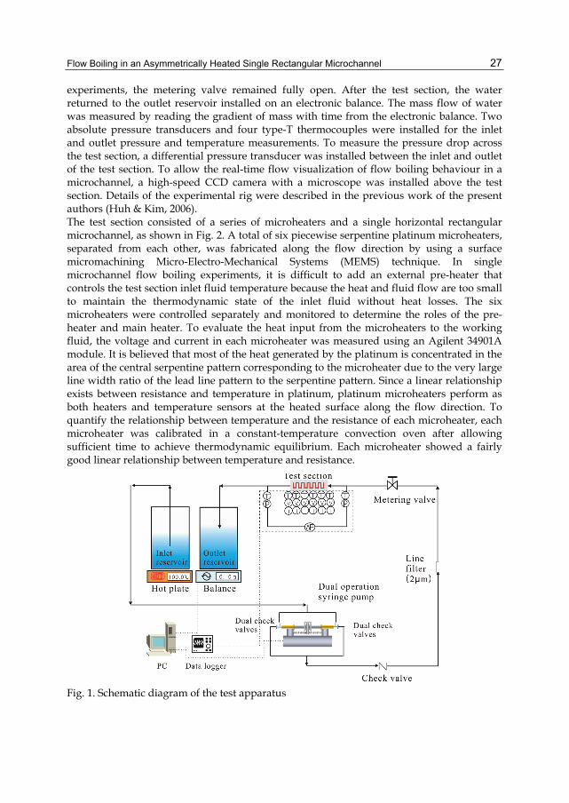
2. Experimental setup and procedure 2.1 Experimental apparatus The experimental system consisted of several sub-systems, which included a working fluid loop, test section, flow visualization devices, and data acquisition systems (Huh & Kim, 2006). A schematic diagram of the experimental flow loop configured to supply the test fluid, deionized water, to the test section is shown in Fig.1. Deionized water was delivered to the test section using dual operation syringe pumps through a line filter with a 2 µm screen mesh, which facilitated the removal of solid particles that could contaminate and/or block the flow passage. To adjust the stiffness of the upstream fluid handling system, the test microchannel was located immediately ahead of a metering valve. During the normal
Flow Boiling in an Asymmetrically Heated Single Rectangular Microchannel
27
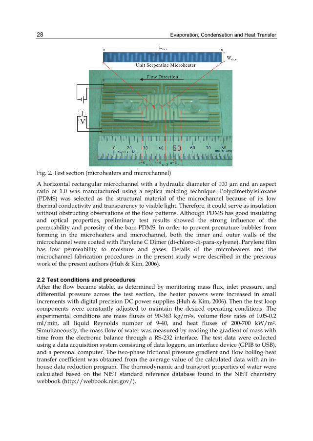
experiments, the metering valve remained fully open. After the test section, the water returned to the outlet reservoir installed on an electronic balance. The mass flow of water was measured by reading the gradient of mass with time from the electronic balance. Two absolute pressure transducers and four type-T thermocouples were installed for the inlet and outlet pressure and temperature measurements. To measure the pressure drop across the test section, a differential pressure transducer was installed between the inlet and outlet of the test section. To allow the real-time flow visualization of flow boiling behaviour in a microchannel, a high-speed CCD camera with a microscope was installed above the test section. Details of the experimental rig were described in the previous work of the present authors (Huh & Kim, 2006). The test section consisted of a series of microheaters and a single horizontal rectangular microchannel, as shown in Fig. 2. A total of six piecewise serpentine platinum microheaters, separated from each other, was fabricated along the flow direction by using a surface micromachining Micro-Electro-Mechanical Systems (MEMS) technique. In single microchannel flow boiling experiments, it is difficult to add an external pre-heater that controls the test section inlet fluid temperature because the heat and fluid flow are too small to maintain the thermodynamic state of the inlet fluid without heat losses. The six microheaters were controlled separately and monitored to determine the roles of the pre-heater and main heater. To evaluate the heat input from the microheaters to the working fluid, the voltage and current in each microheater was measured using an Agilent 34901A module. It is believed that most of the heat generated by the platinum is concentrated in the area of the central serpentine pattern corresponding to the microheater due to the very large line width ratio of the lead line pattern to the serpentine pattern. Since a linear relationship exists between resistance and temperature in platinum, platinum microheaters perform as both heaters and temperature sensors at the heated surface along the flow direction. To quantify the relationship between temperature and the resistance of each microheater, each microheater was calibrated in a constant-temperature convection oven after allowing sufficient time to achieve thermodynamic equilibrium. Each microheater showed a fairly good linear relationship between temperature and resistance.
Fig. 1. Schematic diagram of the test apparatus
Evaporation, Condensation and Heat Transfer
28
Fig. 2. Test section (microheaters and microchannel)
A horizontal rectangular microchannel with a hydraulic diameter of 100 µm and an aspect ratio of 1.0 was manufactured using a replica molding technique. Polydimethylsiloxane (PDMS) was selected as the structural material of the microchannel because of its low thermal conductivity and transparency to visible light. Therefore, it could serve as insulation without obstructing observations of the flow patterns. Although PDMS has good insulating and optical properties, preliminary test results showed the strong influence of the permeability and porosity of the bare PDMS. In order to prevent premature bubbles from forming in the microheaters and microchannel, both the inner and outer walls of the microchannel were coated with Parylene C Dimer (di-chloro-di-para-xylyene). Parylene film has low permeability to moisture and gases. Details of the microheaters and the microchannel fabrication procedures in the present study were described in the previous work of the present authors (Huh & Kim, 2006).
2.2 Test conditions and procedures After the flow became stable, as determined by monitoring mass flux, inlet pressure, and differential pressure across the test section, the heater powers were increased in small increments with digital precision DC power supplies (Huh & Kim, 2006). Then the test loop components were constantly adjusted to maintain the desired operating conditions. The experimental conditions are mass fluxes of 90-363 kg/m2s, volume flow rates of 0.05-0.2 ml/min, all liquid Reynolds number of 9-40, and heat fluxes of 200-700 kW/m2. Simultaneously, the mass flow of water was measured by reading the gradient of mass with time from the electronic balance through a RS-232 interface. The test data were collected using a data acquisition system consisting of data loggers, an interface device (GPIB to USB), and a personal computer. The two-phase frictional pressure gradient and flow boiling heat transfer coefficient was obtained from the average value of the calculated data with an in-house data reduction program. The thermodynamic and transport properties of water were calculated based on the NIST standard reference database found in the NIST chemistry webbook (http://webbook.nist.gov/).
Flow Boiling in an Asymmetrically Heated Single Rectangular Microchannel
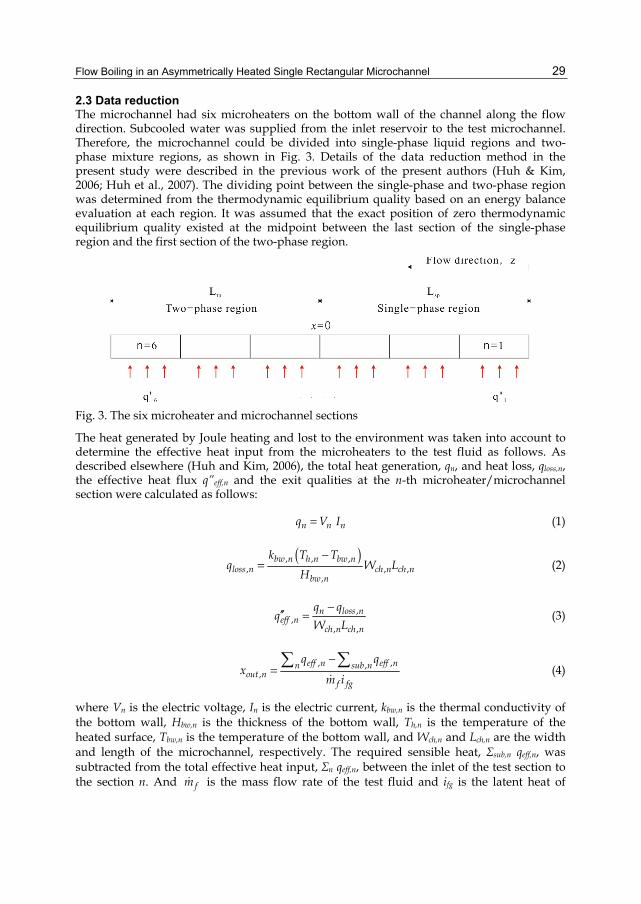
29
2.3 Data reduction The microchannel had six microheaters on the bottom wall of the channel along the flow direction. Subcooled water was supplied from the inlet reservoir to the test microchannel. Therefore, the microchannel could be divided into single-phase liquid regions and two-phase mixture regions, as shown in Fig. 3. Details of the data reduction method in the present study were described in the previous work of the present authors (Huh & Kim, 2006; Huh et al., 2007). The dividing point between the single-phase and two-phase region was determined from the thermodynamic equilibrium quality based on an energy balance evaluation at each region. It was assumed that the exact position of zero thermodynamic equilibrium quality existed at the midpoint between the last section of the single-phase region and the first section of the two-phase region.
Fig. 3. The six microheater and microchannel sections
The heat generated by Joule heating and lost to the environment was taken into account to determine the effective heat input from the microheaters to the test fluid as follows. As described elsewhere (Huh and Kim, 2006), the total heat generation, qn, and heat loss, qloss,n, the effective heat flux q”eff,n and the exit qualities at the n-th microheater/microchannel section were calculated as follows:
n n nq V I= (1)
( ), , ,
, , ,,
bw n h n bw nloss n ch n ch n
bw n
k T Tq W L
H−
= (2)
,,
, ,
n loss neff n
ch n ch n
q qq
W L−
′′ = (3)
, ,,
,eff n eff nn sub n
out nf fg
q qx
m i
−=∑ ∑
(4)
where Vn is the electric voltage, In is the electric current, kbw,n is the thermal conductivity of the bottom wall, Hbw,n is the thickness of the bottom wall, Th,n is the temperature of the heated surface, Tbw,n is the temperature of the bottom wall, and Wch,n and Lch,n are the width and length of the microchannel, respectively. The required sensible heat, Σsub,n qeff,n, was subtracted from the total effective heat input, Σn qeff,n, between the inlet of the test section to the section n. And fm is the mass flow rate of the test fluid and ifg is the latent heat of
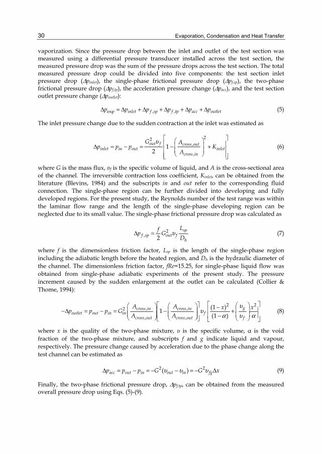
Evaporation, Condensation and Heat Transfer
30
vaporization. Since the pressure drop between the inlet and outlet of the test section was measured using a differential pressure transducer installed across the test section, the measured pressure drop was the sum of the pressure drops across the test section. The total measured pressure drop could be divided into five components: the test section inlet pressure drop (Δpinlet), the single-phase frictional pressure drop (Δpf,sp), the two-phase frictional pressure drop (Δpf,tp), the acceleration pressure change (Δpacc), and the test section outlet pressure change (Δpoutlet):
exp , ,inlet f sp f tp acc outletp p p p p pΔ = Δ + Δ + Δ + Δ + Δ (5)
The inlet pressure change due to the sudden contraction at the inlet was estimated as
22
,
,1
2out f cross out
inlet in out inletcross in
G Ap p p K
A
υ ⎡ ⎤⎛ ⎞⎢ ⎥⎜ ⎟Δ = − = − +⎢ ⎥⎜ ⎟⎝ ⎠⎢ ⎥⎣ ⎦
(6)
where G is the mass flux, υf is the specific volume of liquid, and A is the cross-sectional area of the channel. The irreversible contraction loss coefficient, Kinlet, can be obtained from the literature (Blevins, 1984) and the subscripts in and out refer to the corresponding fluid connection. The single-phase region can be further divided into developing and fully developed regions. For the present study, the Reynolds number of the test range was within the laminar flow range and the length of the single-phase developing region can be neglected due to its small value. The single-phase frictional pressure drop was calculated as
2, 2
spf sp out f
h
Lfp GD
υΔ = (7)
where f is the dimensionless friction factor, Lsp is the length of the single-phase region including the adiabatic length before the heated region, and Dh is the hydraulic diameter of the channel. The dimensionless friction factor, fRe=15.25, for single-phase liquid flow was obtained from single-phase adiabatic experiments of the present study. The pressure increment caused by the sudden enlargement at the outlet can be calculated (Collier & Thome, 1994):
2 2
, ,2
, ,
(1 )1(1 )
gcross in cross inoutlet out in in f
cross out cross out f
A A x xp p p GA A
υυ
α υ α
⎡ ⎤⎡ ⎤ ⎛ ⎞⎛ ⎞ ⎛ ⎞ −⎢ ⎥⎜ ⎟⎢ ⎥−Δ = − = − +⎜ ⎟ ⎜ ⎟⎜ ⎟ ⎜ ⎟ ⎜ ⎟−⎢ ⎥⎢ ⎥⎝ ⎠ ⎝ ⎠ ⎝ ⎠⎣ ⎦ ⎣ ⎦ (8)
where x is the quality of the two-phase mixture, υ is the specific volume, α is the void fraction of the two-phase mixture, and subscripts f and g indicate liquid and vapour, respectively. The pressure change caused by acceleration due to the phase change along the test channel can be estimated as
2 2( )acc out in out in fgp p p G G xυ υ υΔ = − = − − = − Δ (9)
Finally, the two-phase frictional pressure drop, Δpf,tp, can be obtained from the measured overall pressure drop using Eqs. (5)-(9).
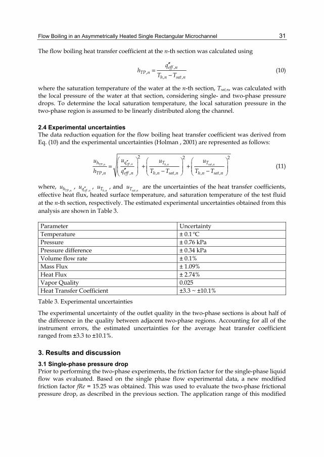
Flow Boiling in an Asymmetrically Heated Single Rectangular Microchannel
31
The flow boiling heat transfer coefficient at the n-th section was calculated using
,,
, ,
eff nTP n
h n sat n
qh
T T
′′=
− (10)
where the saturation temperature of the water at the n-th section, Tsat,n, was calculated with the local pressure of the water at that section, considering single- and two-phase pressure drops. To determine the local saturation temperature, the local saturation pressure in the two-phase region is assumed to be linearly distributed along the channel.
2.4 Experimental uncertainties The data reduction equation for the flow boiling heat transfer coefficient was derived from Eq. (10) and the experimental uncertainties (Holman , 2001) are represented as follows:
,, , ,
2 2 2
, , , , , ,
eff nTP n h n sat nqh T T
TP n eff n h n sat n h n sat n
uu u u
h q T T T T′′⎛ ⎞ ⎛ ⎞ ⎛ ⎞
⎜ ⎟= + +⎜ ⎟ ⎜ ⎟⎜ ⎟ ⎜ ⎟⎜ ⎟′′ − −⎝ ⎠ ⎝ ⎠⎝ ⎠ (11)
where, ,TP nhu ,
,eff nqu ′′ , ,h nTu , and
,sat nTu are the uncertainties of the heat transfer coefficients, effective heat flux, heated surface temperature, and saturation temperature of the test fluid at the n-th section, respectively. The estimated experimental uncertainties obtained from this analysis are shown in Table 3. Parameter Uncertainty Temperature ± 0.1 ºC Pressure ± 0.76 kPa Pressure difference ± 0.34 kPa Volume flow rate ± 0.1% Mass Flux ± 1.09% Heat Flux ± 2.74% Vapor Quality 0.025 Heat Transfer Coefficient ±3.3 ~ ±10.1%
Table 3. Experimental uncertainties
The experimental uncertainty of the outlet quality in the two-phase sections is about half of the difference in the quality between adjacent two-phase regions. Accounting for all of the instrument errors, the estimated uncertainties for the average heat transfer coefficient ranged from ±3.3 to ±10.1%.
3. Results and discussion 3.1 Single-phase pressure drop Prior to performing the two-phase experiments, the friction factor for the single-phase liquid flow was evaluated. Based on the single phase flow experimental data, a new modified friction factor fRe = 15.25 was obtained. This was used to evaluate the two-phase frictional pressure drop, as described in the previous section. The application range of this modified
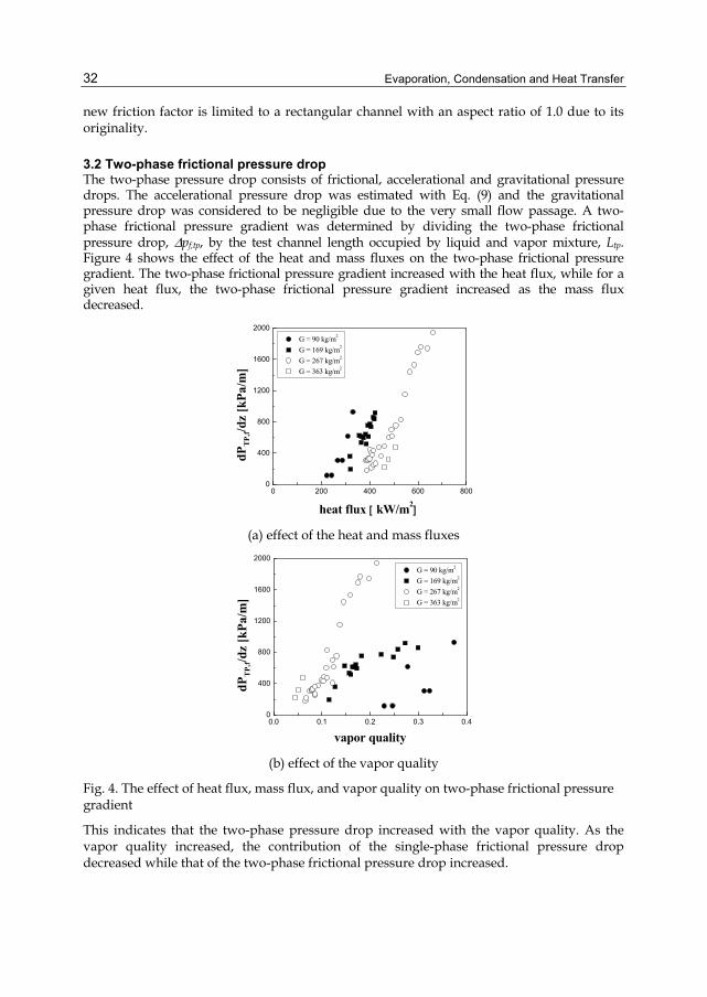
Evaporation, Condensation and Heat Transfer
32
new friction factor is limited to a rectangular channel with an aspect ratio of 1.0 due to its originality.
3.2 Two-phase frictional pressure drop The two-phase pressure drop consists of frictional, accelerational and gravitational pressure drops. The accelerational pressure drop was estimated with Eq. (9) and the gravitational pressure drop was considered to be negligible due to the very small flow passage. A two-phase frictional pressure gradient was determined by dividing the two-phase frictional pressure drop, Δpf,tp, by the test channel length occupied by liquid and vapor mixture, Ltp. Figure 4 shows the effect of the heat and mass fluxes on the two-phase frictional pressure gradient. The two-phase frictional pressure gradient increased with the heat flux, while for a given heat flux, the two-phase frictional pressure gradient increased as the mass flux decreased.
0 200 400 600 8000
400
800
1200
1600
2000 G = 90 kg/m2
G = 169 kg/m2
G = 267 kg/m2
G = 363 kg/m2
dPTP
,f/dz
[kPa
/m]
heat flux [ kW/m2] (a) effect of the heat and mass fluxes
0.0 0.1 0.2 0.3 0.40
400
800
1200
1600
2000 G = 90 kg/m2
G = 169 kg/m2
G = 267 kg/m2
G = 363 kg/m2
dPT
P,f/d
z [k
Pa/m
]
vapor quality (b) effect of the vapor quality
Fig. 4. The effect of heat flux, mass flux, and vapor quality on two-phase frictional pressure gradient
This indicates that the two-phase pressure drop increased with the vapor quality. As the vapor quality increased, the contribution of the single-phase frictional pressure drop decreased while that of the two-phase frictional pressure drop increased.
Flow Boiling in an Asymmetrically Heated Single Rectangular Microchannel
33
102 103 104102
103
104
-40 %
G = 90 kg/m2s G = 169 kg/m2s G = 267 kg/m2s G = 363 kg/m2s
dPT
P,f/d
z pr
ed [k
Pa/m
]
dPTP,f/dz exp [kPa/m]
+40 %
HomogeneousMAE=49.5%
102 103 104102
103
104
-40 %
Lockhart & MartinelliMAE=73.0%
+40 %
G = 90 kg/m2s G = 169 kg/m2s G = 267 kg/m2s G = 363 kg/m2s
dPT
P,f/d
z pr
ed [k
Pa/m
]
dPTP,f/dz exp [kPa/m]
(a) homogeneous flow model (b) Lockhart & Martinelli correlation
102 103 104102
103
104
FriedelMAE=83.4%
-40 %
G = 90 kg/m2s G = 169 kg/m2s G = 267 kg/m2s G = 363 kg/m2s
dPT
P,f/d
z pr
ed [k
Pa/m
]
dPTP,f/dz exp [kPa/m]
+40 %
102 103 104101
102
103
104
Mishima and HibikiMAE=87.2%
-40 %
G = 90 kg/m2s G = 169 kg/m2s G = 267 kg/m2s G = 363 kg/m2s
dPT
P,f/d
z pr
ed [k
Pa/m
]
dPTP,f/dz exp [kPa/m]
+40 %
(c) Friedel correlation (d) Mishima & Hibiki correlation
102 103 104101
102
103
104
G = 90 kg/m2s G = 169 kg/m2s G = 267 kg/m2s G = 363 kg/m2s
dPTP
,f/dz
pred
[kPa
/m]
dPTP,f/dz exp [kPa/m]
-40 %
Lee and LeeMAE=83.9%
+40 %
102 103 104101
102
103
104
G = 90 kg/m2s G = 169 kg/m2s G = 267 kg/m2s G = 363 kg/m2s
dPT
P,f/d
z pr
ed [k
Pa/m
]
dPTP,f/dz exp [kPa/m]
-40 %
Qu and MudawarMAE=86.9%
+40 %
(e) Lee & Lee correlation (f) Qu & Mudawar correlation
Fig. 5. Comparison of the two-phase frictional pressure gradient with predictions
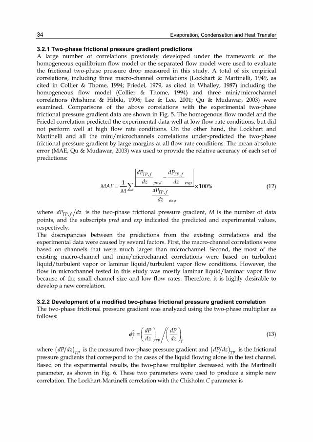
Evaporation, Condensation and Heat Transfer
34
3.2.1 Two-phase frictional pressure gradient predictions A large number of correlations previously developed under the framework of the homogeneous equilibrium flow model or the separated flow model were used to evaluate the frictional two-phase pressure drop measured in this study. A total of six empirical correlations, including three macro-channel correlations (Lockhart & Martinelli, 1949, as cited in Collier & Thome, 1994; Friedel, 1979, as cited in Whalley, 1987) including the homogeneous flow model (Collier & Thome, 1994) and three mini/microchannel correlations (Mishima & Hibiki, 1996; Lee & Lee, 2001; Qu & Mudawar, 2003) were examined. Comparisons of the above correlations with the experimental two-phase frictional pressure gradient data are shown in Fig. 5. The homogenous flow model and the Friedel correlation predicted the experimental data well at low flow rate conditions, but did not perform well at high flow rate conditions. On the other hand, the Lockhart and Martinelli and all the mini/microchannels correlations under-predicted the two-phase frictional pressure gradient by large margins at all flow rate conditions. The mean absolute error (MAE, Qu & Mudawar, 2003) was used to provide the relative accuracy of each set of predictions:
, ,
exp
,
exp
1 100%
TP f TP f
pred
TP f
dP dPdz dz
MAE dPMdz
−= ×∑ (12)
where ,TP fdP dz is the two-phase frictional pressure gradient, M is the number of data points, and the subscripts pred and exp indicated the predicted and experimental values, respectively. The discrepancies between the predictions from the existing correlations and the experimental data were caused by several factors. First, the macro-channel correlations were based on channels that were much larger than microchannel. Second, the most of the existing macro-channel and mini/microchannel correlations were based on turbulent liquid/turbulent vapor or laminar liquid/turbulent vapor flow conditions. However, the flow in microchannel tested in this study was mostly laminar liquid/laminar vapor flow because of the small channel size and low flow rates. Therefore, it is highly desirable to develop a new correlation.
3.2.2 Development of a modified two-phase frictional pressure gradient correlation The two-phase frictional pressure gradient was analyzed using the two-phase multiplier as follows:
2f
TP f
dP dPdz dz
φ ⎛ ⎞ ⎛ ⎞= ⎜ ⎟ ⎜ ⎟⎝ ⎠ ⎝ ⎠
(13)
where ( )TPdP dz is the measured two-phase pressure gradient and ( )TPdP dz is the frictional pressure gradients that correspond to the cases of the liquid flowing alone in the test channel. Based on the experimental results, the two-phase multiplier decreased with the Martinelli parameter, as shown in Fig. 6. These two parameters were used to produce a simple new correlation. The Lockhart-Martinelli correlation with the Chisholm C parameter is
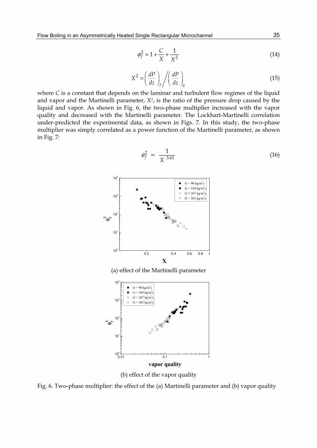
Flow Boiling in an Asymmetrically Heated Single Rectangular Microchannel
35
22
11fCX X
φ = + + (14)
2
f g
dP dPXdz dz
⎛ ⎞ ⎛ ⎞= ⎜ ⎟ ⎜ ⎟⎝ ⎠ ⎝ ⎠
(15)
where C is a constant that depends on the laminar and turbulent flow regimes of the liquid and vapor and the Martinelli parameter, X2, is the ratio of the pressure drop caused by the liquid and vapor. As shown in Fig. 6, the two-phase multiplier increased with the vapor quality and decreased with the Martinelli parameter. The Lockhart-Martinelli correlation under-predicted the experimental data, as shown in Figs. 7. In this study, the two-phase multiplier was simply correlated as a power function of the Martinelli parameter, as shown in Fig. 7:
23.611 f X
φ ∝ (16)
0.2 0.4 0.6 0.8 1100
101
102
103
104
G = 90 kg/m2s G = 169 kg/m2s G = 267 kg/m2s G = 363 kg/m2s
φ2 f
X (a) effect of the Martinelli parameter
0.01 0.1 1100
101
102
103
104
G = 90 kg/m2s G = 169 kg/m2s G = 267 kg/m2s G = 363 kg/m2s
φ2 f
vapor quality (b) effect of the vapor quality
Fig. 6. Two-phase multiplier: the effect of the (a) Martinelli parameter and (b) vapor quality
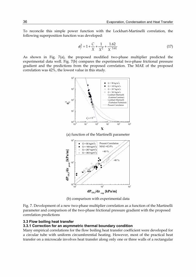
Evaporation, Condensation and Heat Transfer
36
To reconcile this simple power function with the Lockhart-Martinelli correlation, the following superposition function was developed:
22 3.61
1 1.621fCX X X
φ = + + + (17)
As shown in Fig. 7(a), the proposed modified two-phase multiplier predicted the experimental data well. Fig. 7(b) compares the experimental two-phase frictional pressure gradient and the predictions from the proposed correlation. The MAE of the proposed correlation was 42%, the lowest value in this study.
10-2 10-1 100 101 102 103100
101
102
103
104
φ2
φ α 1/X3.61
G = 90 kg/m2s G = 169 kg/m2s G = 267 kg/m2s G = 363 kg/m2s Lockhart-Martinelli
(Laminar/Laminar) Lockhart-Martinelli
(Turbulent/Turbulent) Present Correlation
φ2 f
X (a) function of the Martinelli parameter
102 103 104102
103
104
Present CorrelationMAE=42.0%
+40 %
G = 90 kg/m2s G = 169 kg/m2s G = 267 kg/m2s G = 363 kg/m2s
dPTP
,f/dz
pred
[kPa
/m]
dPTP,f/dz exp [kPa/m]
-40 %
(b) comparison with experimental data
Fig. 7. Development of a new two-phase multiplier correlation as a function of the Martinelli parameter and comparison of the two-phase frictional pressure gradient with the proposed correlation predictions
3.3 Flow boiling heat transfer 3.3.1 Correction for an asymmetric thermal boundary condition Many empirical correlations for the flow boiling heat transfer coefficient were developed for a circular tube with uniform circumferential heating. However, most of the practical heat transfer on a microscale involves heat transfer along only one or three walls of a rectangular
Flow Boiling in an Asymmetrically Heated Single Rectangular Microchannel
37
microchannel. To accommodate these different thermal boundary conditions due the asymmetric heating conditions in our apparatus, a correction method was introduced (Qu & Mudawar, 2003).
1,
4TP TP correlation
Nuh hNu
= (18)
where hTP,correlation is the heat transfer coefficient evaluated from a correlation, and Nu1 and Nu4 are the single-phase fully developed laminar flow Nusselt numbers for single- and four-wall heat transfer, respectively. The expressions for the single-phase Nusselt number of a rectangular channel with asymmetric heating boundary conditions was used (Shah & London, 1978):
2 3 4 51 8.229(1 2.197 4.090 4.844 3.437 1.049 )Nu β β β β β= − + − + − (19)
2 3 4 54 8.235(1 2.042 3.085 2.477 1.058 0.186 )Nu β β β β β= − + − + − (20)
where ch chW Hβ = is the aspect ratio of the rectangular channel. This correction method can be justified due to the fact that the laminar thin liquid film along the microchannel wall contribute the major heat transfer as shown in the flow patterns in the following section.
3.3.2 Flow boiling heat transfer It is commonly believed that two mechanisms govern heat transfer in saturated flow boiling: nucleate boiling and forced convective boiling (Whalley, 1987; Collier and Thome, 1994; Kandlikar et al., 1999). In the region dominated by nucleate boiling, bubbles are formed by nucleation at the superheated wall. The nucleate boiling heat transfer mechanism is a combination of bubble agitation, thermal boundary layer stripping, and evaporation. The heat transfer coefficient in this region is dependent on the heat flux, and is less sensitive to the mass flux and vapor quality. The nucleate boiling region is normally associated with the bubbly and slug flow patterns. In the region dominated by forced convective boiling, heat is carried away from the heated wall by forced convection in a thin liquid film to the liquid-vapor interface, where evaporation occurs. The heat transfer coefficient in this region is dependent on the mass flux and vapor quality, and is less sensitive to the heat flux. The forced convective boiling region is normally associated with the annular flow pattern. All heat transfer coefficients and observed flow patterns reported in this paper were measured and evaluated at the last section, n=6. The measured flow boiling heat transfer coefficients slightly increased with vapor quality until x = 0.15 and were independent of the mass flux and vapor quality for high quality, 0.4 > x > 0.15, as shown in Fig. 8. The weak dependency of the boiling heat transfer coefficient on the mass flux and vapor quality indicates that the major heat transfer mechanism is nucleate boiling. Although the heat transfer coefficient behaves as if nucleate boiling is the dominant heat transfer mechanism, the major flow pattern is similar to conventional annular flow. The main flow pattern observed at this section is rapid, long elongated slug bubble flow acting like annular flow, as shown in Fig. 9. For the most of the time, the flow pattern looks like thin liquid film flow at the heated wall and vapor flow in the core, as in annular flow. For lower vapor quality region, x < 0.15, intermittent vapor zone was appeared during the long elongated slug
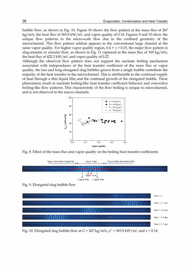
Evaporation, Condensation and Heat Transfer
38
bubble flow, as shown in Fig. 10. Figure 10 shows the flow pattern at the mass flux of 267 kg/m2s, the heat flux of 565.9 kW/m2, and vapor quality of 0.14. Figures 9 and 10 show the unique flow patterns in the micro-scale flow due to the confined geometry of the microchannel. This flow pattern seldom appears in the conventional large channel at the same vapor quality. For higher vapor quality region, 0.4 > x > 0.15, the major flow pattern is slug-annular or annular flow, as shown in Fig. 11 captured at the mass flux of 169 kg/m2s, the heat flux of 422.3 kW/m2, and vapor quality of 0.27. Although the observed flow pattern does not support the nucleate boiling mechanism associated with independence of the heat transfer coefficient of the mass flux or vapor quality, the fast and long elongated slug bubbles grown from a single bubble contribute the majority of the heat transfer in the microchannel. This is attributable to the continual supply of heat through a thin liquid film and the continual growth of the elongated bubble. These phenomena result in nucleate boiling-like heat transfer coefficient behavior and convective boiling-like flow patterns. This characteristic of the flow boiling is unique to microchannel, and is not observed in the macro-channels.
0.0 0.1 0.2 0.3 0.40
20
40
60
80
100
h TP [
kW/m
2 K]
vapor quality
G = 90 kg/m2s G = 169 kg/m2s G = 267 kg/m2s G = 363 kg/m2s
Fig. 8. Effect of the mass flux and vapor quality on the boiling heat transfer coefficients
Fig. 9. Elongated slug bubble flow
Fig. 10. Elongated slug bubble flow at G = 267 kg/m2s, q” = 565.9 kW/m2, and x = 0.14
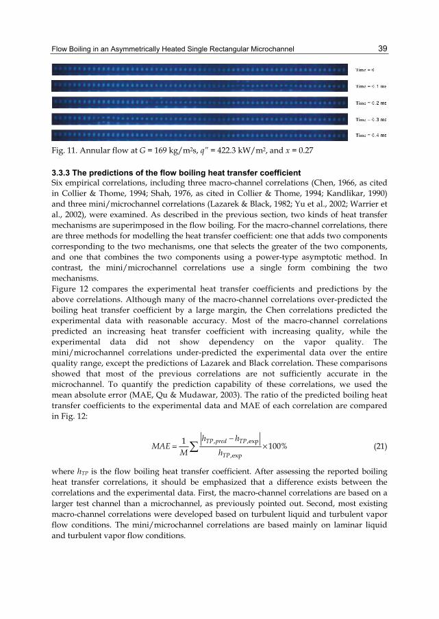
Flow Boiling in an Asymmetrically Heated Single Rectangular Microchannel
39
Fig. 11. Annular flow at G = 169 kg/m2s, q” = 422.3 kW/m2, and x = 0.27
3.3.3 The predictions of the flow boiling heat transfer coefficient Six empirical correlations, including three macro-channel correlations (Chen, 1966, as cited in Collier & Thome, 1994; Shah, 1976, as cited in Collier & Thome, 1994; Kandlikar, 1990) and three mini/microchannel correlations (Lazarek & Black, 1982; Yu et al., 2002; Warrier et al., 2002), were examined. As described in the previous section, two kinds of heat transfer mechanisms are superimposed in the flow boiling. For the macro-channel correlations, there are three methods for modelling the heat transfer coefficient: one that adds two components corresponding to the two mechanisms, one that selects the greater of the two components, and one that combines the two components using a power-type asymptotic method. In contrast, the mini/microchannel correlations use a single form combining the two mechanisms. Figure 12 compares the experimental heat transfer coefficients and predictions by the above correlations. Although many of the macro-channel correlations over-predicted the boiling heat transfer coefficient by a large margin, the Chen correlations predicted the experimental data with reasonable accuracy. Most of the macro-channel correlations predicted an increasing heat transfer coefficient with increasing quality, while the experimental data did not show dependency on the vapor quality. The mini/microchannel correlations under-predicted the experimental data over the entire quality range, except the predictions of Lazarek and Black correlation. These comparisons showed that most of the previous correlations are not sufficiently accurate in the microchannel. To quantify the prediction capability of these correlations, we used the mean absolute error (MAE, Qu & Mudawar, 2003). The ratio of the predicted boiling heat transfer coefficients to the experimental data and MAE of each correlation are compared in Fig. 12:
, ,exp
,exp
1 100%TP pred TP
TP
h hMAE
M h
−= ×∑ (21)
where hTP is the flow boiling heat transfer coefficient. After assessing the reported boiling heat transfer correlations, it should be emphasized that a difference exists between the correlations and the experimental data. First, the macro-channel correlations are based on a larger test channel than a microchannel, as previously pointed out. Second, most existing macro-channel correlations were developed based on turbulent liquid and turbulent vapor flow conditions. The mini/microchannel correlations are based mainly on laminar liquid and turbulent vapor flow conditions.
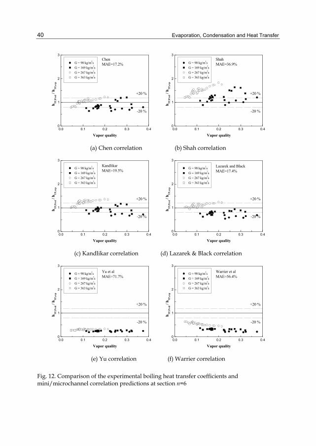
Evaporation, Condensation and Heat Transfer
40
0.0 0.1 0.2 0.3 0.40
1
2
3ChenMAE=17.2% G = 90 kg/m2s
G = 169 kg/m2s G = 267 kg/m2s G = 363 kg/m2s
+20 %
h TP,P
red /
h TP,e
xp
Vapor quality
-20 %
0.0 0.1 0.2 0.3 0.40
1
2
3ShahMAE=36.9% G = 90 kg/m2s
G = 169 kg/m2s G = 267 kg/m2s G = 363 kg/m2s
+20 %
h TP,P
red /
h TP,e
xp
Vapor quality
-20 %
(a) Chen correlation (b) Shah correlation
0.0 0.1 0.2 0.3 0.40
1
2
3KandlikarMAE=19.5% G = 90 kg/m2s
G = 169 kg/m2s G = 267 kg/m2s G = 363 kg/m2s
+20 %
h TP,P
red /
h TP,e
xp
Vapor quality
-20 %
0.0 0.1 0.2 0.3 0.40
1
2
3
Lazarek and BlackMAE=17.4%
G = 90 kg/m2s G = 169 kg/m2s G = 267 kg/m2s G = 363 kg/m2s
+20 %
h TP,P
red /
h TP,e
xp
Vapor quality
-20 %
(c) Kandlikar correlation (d) Lazarek & Black correlation
0.0 0.1 0.2 0.3 0.40
1
2
3
Yu et alMAE=71.7%
G = 90 kg/m2s G = 169 kg/m2s G = 267 kg/m2s G = 363 kg/m2s
+20 %
h TP,P
red /
h TP,e
xp
Vapor quality
-20 %
0.0 0.1 0.2 0.3 0.40
1
2
3
Warrier et alMAE=56.4%
G = 90 kg/m2s G = 169 kg/m2s G = 267 kg/m2s G = 363 kg/m2s
+20 %
h TP,P
red /
h TP,e
xp
Vapor quality
-20 %
(e) Yu correlation (f) Warrier correlation
Fig. 12. Comparison of the experimental boiling heat transfer coefficients and mini/microchannel correlation predictions at section n=6
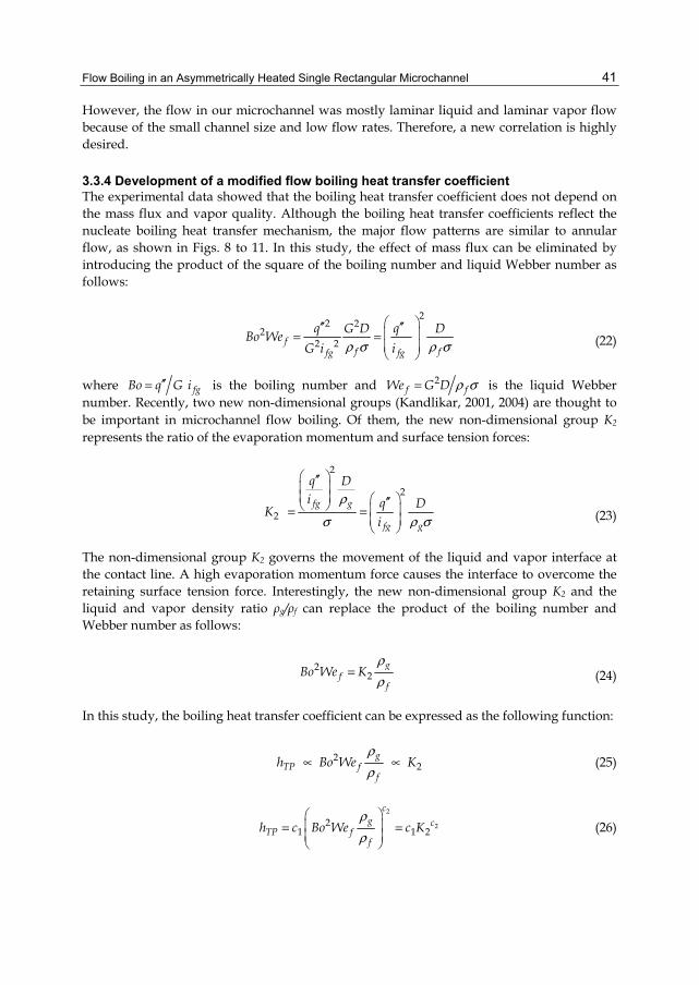
Flow Boiling in an Asymmetrically Heated Single Rectangular Microchannel
41
However, the flow in our microchannel was mostly laminar liquid and laminar vapor flow because of the small channel size and low flow rates. Therefore, a new correlation is highly desired.
3.3.4 Development of a modified flow boiling heat transfer coefficient The experimental data showed that the boiling heat transfer coefficient does not depend on the mass flux and vapor quality. Although the boiling heat transfer coefficients reflect the nucleate boiling heat transfer mechanism, the major flow patterns are similar to annular flow, as shown in Figs. 8 to 11. In this study, the effect of mass flux can be eliminated by introducing the product of the square of the boiling number and liquid Webber number as follows:
22 2
22 2f
f ffg fg
q qG D DBo WeG i iρ σ ρ σ
⎛ ⎞′′ ′′⎜ ⎟= =⎜ ⎟⎝ ⎠
(22)
where fgBo q G i′′= is the boiling number and 2f fWe G D ρ σ= is the liquid Webber
number. Recently, two new non-dimensional groups (Kandlikar, 2001, 2004) are thought to be important in microchannel flow boiling. Of them, the new non-dimensional group K2 represents the ratio of the evaporation momentum and surface tension forces:
2
2
2fg g
fg g
q Di q DK
i
ρ
σ ρ σ
⎛ ⎞′′⎜ ⎟⎜ ⎟ ⎛ ⎞′′⎝ ⎠ ⎜ ⎟= =
⎜ ⎟⎝ ⎠
(23)
The non-dimensional group K2 governs the movement of the liquid and vapor interface at the contact line. A high evaporation momentum force causes the interface to overcome the retaining surface tension force. Interestingly, the new non-dimensional group K2 and the liquid and vapor density ratio ρg/ρf can replace the product of the boiling number and Webber number as follows:
2
2g
ff
Bo We Kρρ
= (24)
In this study, the boiling heat transfer coefficient can be expressed as the following function:
22 g
TP ff
h Bo We Kρρ
∝ ∝ (25)
2
221 1 2
cg c
TP ff
h c Bo We c Kρρ
⎛ ⎞⎜ ⎟= =⎜ ⎟⎝ ⎠
(26)
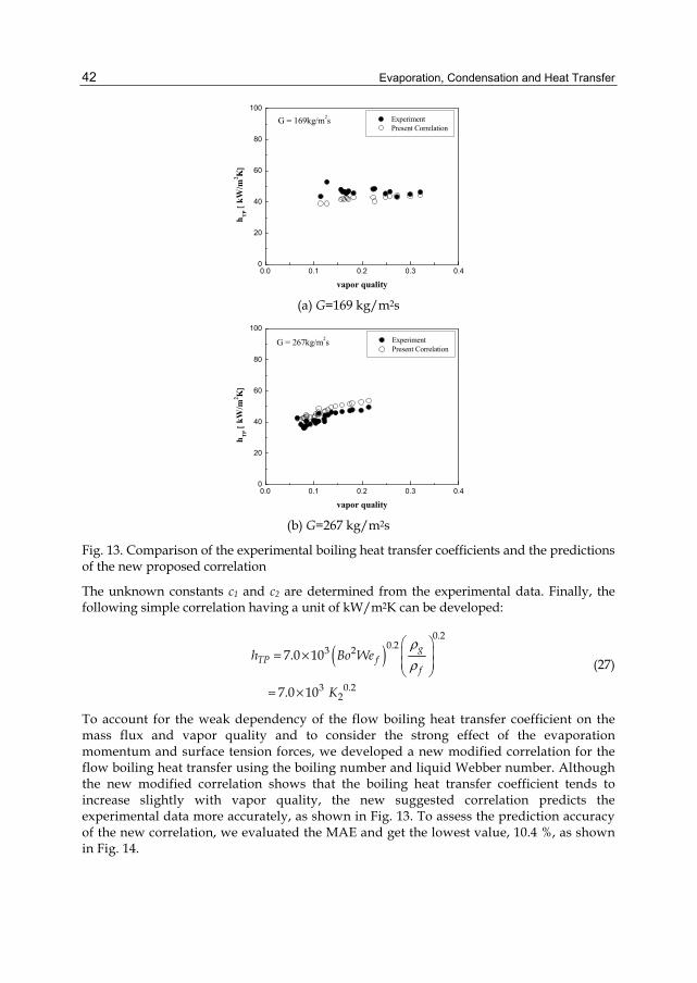
Evaporation, Condensation and Heat Transfer
42
0.0 0.1 0.2 0.3 0.40
20
40
60
80
100
G = 169kg/m2s
h TP [
kW/m
2 K]
vapor quality
Experiment Present Correlation
(a) G=169 kg/m2s
0.0 0.1 0.2 0.3 0.40
20
40
60
80
100
G = 267kg/m2s
h TP [
kW/m
2 K]
vapor quality
Experiment Present Correlation
(b) G=267 kg/m2s
Fig. 13. Comparison of the experimental boiling heat transfer coefficients and the predictions of the new proposed correlation
The unknown constants c1 and c2 are determined from the experimental data. Finally, the following simple correlation having a unit of kW/m2K can be developed:
( )0.2
0.23 2
3 0.22
7.0 10
7.0 10
gTP f
fh Bo We
K
ρρ
⎛ ⎞⎜ ⎟= ×⎜ ⎟⎝ ⎠
= ×
(27)
To account for the weak dependency of the flow boiling heat transfer coefficient on the mass flux and vapor quality and to consider the strong effect of the evaporation momentum and surface tension forces, we developed a new modified correlation for the flow boiling heat transfer using the boiling number and liquid Webber number. Although the new modified correlation shows that the boiling heat transfer coefficient tends to increase slightly with vapor quality, the new suggested correlation predicts the experimental data more accurately, as shown in Fig. 13. To assess the prediction accuracy of the new correlation, we evaluated the MAE and get the lowest value, 10.4 %, as shown in Fig. 14.
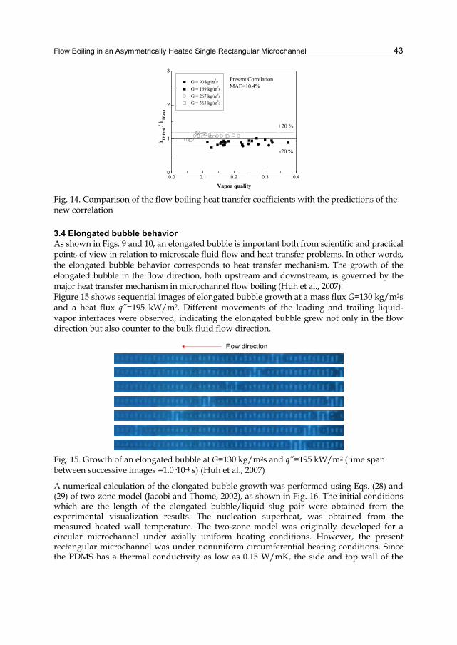
Flow Boiling in an Asymmetrically Heated Single Rectangular Microchannel
43
0.0 0.1 0.2 0.3 0.40
1
2
3
Present CorrelationMAE=10.4%
G = 90 kg/m2s G = 169 kg/m2s G = 267 kg/m2s G = 363 kg/m2s
+20 %
h TP,
Pred
/ h T
P,ex
p
Vapor quality
-20 %
Fig. 14. Comparison of the flow boiling heat transfer coefficients with the predictions of the new correlation
3.4 Elongated bubble behavior As shown in Figs. 9 and 10, an elongated bubble is important both from scientific and practical points of view in relation to microscale fluid flow and heat transfer problems. In other words, the elongated bubble behavior corresponds to heat transfer mechanism. The growth of the elongated bubble in the flow direction, both upstream and downstream, is governed by the major heat transfer mechanism in microchannel flow boiling (Huh et al., 2007). Figure 15 shows sequential images of elongated bubble growth at a mass flux G=130 kg/m2s and a heat flux q”=195 kW/m2. Different movements of the leading and trailing liquid-vapor interfaces were observed, indicating the elongated bubble grew not only in the flow direction but also counter to the bulk fluid flow direction.
Flow direction
Fig. 15. Growth of an elongated bubble at G=130 kg/m2s and q”=195 kW/m2 (time span between successive images =1.0·10-4 s) (Huh et al., 2007)
A numerical calculation of the elongated bubble growth was performed using Eqs. (28) and (29) of two-zone model (Jacobi and Thome, 2002), as shown in Fig. 16. The initial conditions which are the length of the elongated bubble/liquid slug pair were obtained from the experimental visualization results. The nucleation superheat, was obtained from the measured heated wall temperature. The two-zone model was originally developed for a circular microchannel under axially uniform heating conditions. However, the present rectangular microchannel was under nonuniform circumferential heating conditions. Since the PDMS has a thermal conductivity as low as 0.15 W/mK, the side and top wall of the
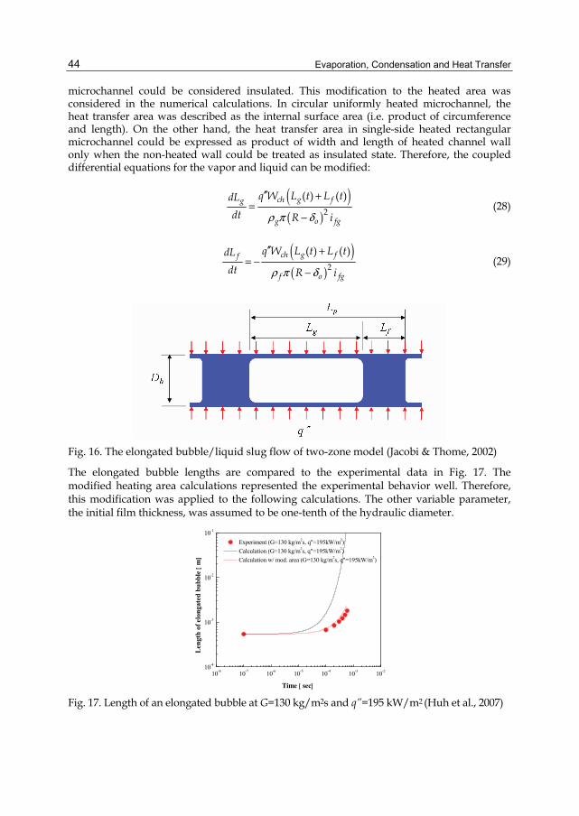
Evaporation, Condensation and Heat Transfer
44
microchannel could be considered insulated. This modification to the heated area was considered in the numerical calculations. In circular uniformly heated microchannel, the heat transfer area was described as the internal surface area (i.e. product of circumference and length). On the other hand, the heat transfer area in single-side heated rectangular microchannel could be expressed as product of width and length of heated channel wall only when the non-heated wall could be treated as insulated state. Therefore, the coupled differential equations for the vapor and liquid can be modified:
( )( )2
( ) ( )ch g fg
g o fg
q W L t L tdLdt R iρ π δ
′′ +=
− (28)
( )( )2
( ) ( )ch g ff
f o fg
q W L t L tdLdt R iρ π δ
′′ += −
− (29)
Fig. 16. The elongated bubble/liquid slug flow of two-zone model (Jacobi & Thome, 2002)
The elongated bubble lengths are compared to the experimental data in Fig. 17. The modified heating area calculations represented the experimental behavior well. Therefore, this modification was applied to the following calculations. The other variable parameter, the initial film thickness, was assumed to be one-tenth of the hydraulic diameter.
10-8 10-7 10-6 10-5 10-4 10-3 10-210-4
10-3
10-2
10-1
Experiment (G=130 kg/m2s, q"=195kW/m2) Calculation (G=130 kg/m2s, q"=195kW/m2) Calculation w/ mod. area (G=130 kg/m2s, q"=195kW/m2)
Leng
th o
f elo
ngat
ed b
ubbl
e [m
]
Time [ sec] Fig. 17. Length of an elongated bubble at G=130 kg/m2s and q”=195 kW/m2 (Huh et al., 2007)
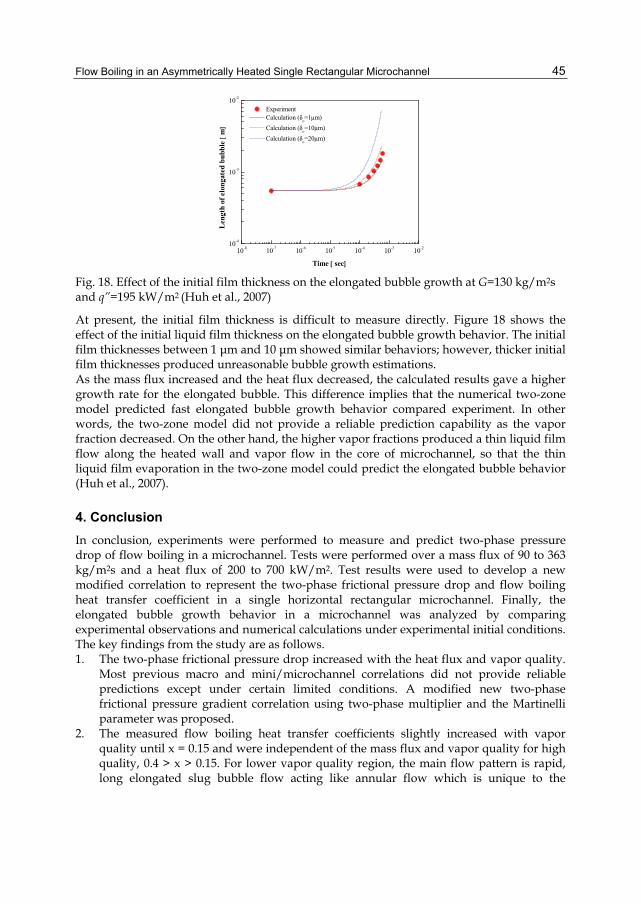
Flow Boiling in an Asymmetrically Heated Single Rectangular Microchannel
45
10-8 10-7 10-6 10-5 10-4 10-3 10-210-4
10-3
10-2
Experiment Calculation (δo=1μm) Calculation (δ
o=10μm)
Calculation (δo=20μm)
Leng
th o
f elo
ngat
ed b
ubbl
e [m
]
Time [ sec] Fig. 18. Effect of the initial film thickness on the elongated bubble growth at G=130 kg/m2s and q”=195 kW/m2 (Huh et al., 2007)
At present, the initial film thickness is difficult to measure directly. Figure 18 shows the effect of the initial liquid film thickness on the elongated bubble growth behavior. The initial film thicknesses between 1 μm and 10 μm showed similar behaviors; however, thicker initial film thicknesses produced unreasonable bubble growth estimations. As the mass flux increased and the heat flux decreased, the calculated results gave a higher growth rate for the elongated bubble. This difference implies that the numerical two-zone model predicted fast elongated bubble growth behavior compared experiment. In other words, the two-zone model did not provide a reliable prediction capability as the vapor fraction decreased. On the other hand, the higher vapor fractions produced a thin liquid film flow along the heated wall and vapor flow in the core of microchannel, so that the thin liquid film evaporation in the two-zone model could predict the elongated bubble behavior (Huh et al., 2007).
4. Conclusion In conclusion, experiments were performed to measure and predict two-phase pressure drop of flow boiling in a microchannel. Tests were performed over a mass flux of 90 to 363 kg/m2s and a heat flux of 200 to 700 kW/m2. Test results were used to develop a new modified correlation to represent the two-phase frictional pressure drop and flow boiling heat transfer coefficient in a single horizontal rectangular microchannel. Finally, the elongated bubble growth behavior in a microchannel was analyzed by comparing experimental observations and numerical calculations under experimental initial conditions. The key findings from the study are as follows. 1. The two-phase frictional pressure drop increased with the heat flux and vapor quality.
Most previous macro and mini/microchannel correlations did not provide reliable predictions except under certain limited conditions. A modified new two-phase frictional pressure gradient correlation using two-phase multiplier and the Martinelli parameter was proposed.
2. The measured flow boiling heat transfer coefficients slightly increased with vapor quality until x = 0.15 and were independent of the mass flux and vapor quality for high quality, 0.4 > x > 0.15. For lower vapor quality region, the main flow pattern is rapid, long elongated slug bubble flow acting like annular flow which is unique to the
Evaporation, Condensation and Heat Transfer
46
microchannel flow. For higher vapor quality region, the major flow pattern is slug-annular or annular flow.
3. The unique characteristics of flow boiling in a microchannel are the nucleate boiling-like heat transfer coefficient behavior and convective boiling-like flow patterns observed, which occur because the very fast, long elongated slug flow acts like annular flow.
4. Most reported macro- and mini/microchannel correlations do not provide sufficient prediction accuracy, except under limited conditions, due to the limitations of the small geometry and different flow regimes. A new modified flow boiling heat transfer coefficient correlation is proposed using the boiling number, liquid Webber number, and liquid-vapor density ratio.
5. The growth behavior of the long elongated bubbles was governed by thin film evaporation. In elongated bubble flow regime, the two-zone model represents the bubble behavior well as the vapor fraction increased. However, the two-zone should be corrected by considering different film profiles inside the microchannel and circumferentially non-uniform thermal boundary conditions.
5. Acknowledgment This work was conducted on behalf of the Ministry of Land, Transport and Maritime Affairs (MLTM) of Korean government under their “Development of Technology for CO2 Marine Geological Storage” program.
6. References Blevins, R.D. (1984). Applied Fluid Dynamics Handbook, Van Nostrand Reinhold Company,
ISBN 0-442-21296-8, New York Chisholm, D. (1967). A Theoretical Basis for the Lockhart-Martinelli Correlation for Two-
phase Flow. International Journal of Heat and Mass Transfer, Vol.10, No.12, (December 1967), pp. 1767–1778, ISSN 0017-9310
Chisholm, D. (1973). Pressure Gradients due to Friction during the Flow of Evaporation Two-phase Mixtures in Smooth Tubes and Channels. International Journal of Heat and Mass Transfer, Vol.16, No.2, (February 1973), pp. 347–358, ISSN 0017-9310
Collier, J.G. & Thome, J.R. (1994). Convective Boiling and Condensation (3rd Ed.), Oxford University Press, ISBN 0-19-856296-9, U.K
Holman, J.P. (2001). Experimental Methods for Engineers (7th Ed.), McGraw-Hill, ISBN 0-07-118165-2, New York
Huh, C., Choi, C.W. & Kim, M.H. (2007). Elongated Bubble Behavior during Flow Boiling in a Microchannel, Proceedings of The Eighteenth International Symposium on Transport Phenomena, Daejeon, Korea, August 27-30, 2007
Huh, C. & Kim, M.H. (2006). An Experimental Investigation of Flow Boiling in an Asymmetrically Heated Rectangular Microchannel, Experimental Thermal and Fluid Science, Vol.30, No.8, (August 2006), pp. 775–784, ISSN 0894-1777
Jacobi, A.M. & Thome, J.R. (2002). Heat Transfer Model for Evaporation of Elongated Bubble Flows in Microchannels. Journal of Heat Transfer, Vol.124, No.6, (December 2002), pp. 1131-1136, ISSN 0022-1481
Flow Boiling in an Asymmetrically Heated Single Rectangular Microchannel
47
Kandlikar, S.G. (1990). A General Correlation for Saturated Two-phase Flow Boiling Heat Transfer inside Horizontal and Vertical Tubes. Journal of Heat Transfer, Vol.112, No.1, (February 1990), pp. 219–228, ISSN 0022-1481
Kandlikar, S.G. (2001). A Theoretical Model to Predict Pool Boiling CHF Incorporating Effects of Contact Angle and Orientation. Journal of Heat Transfer, Vol.123, No.6, (December 2001), pp. 1071-1079, ISSN 0022-1481
Kandlikar, S.G. (2004). Heat Transfer Mechanisms during Flow Boiling in Microchannels. Journal of Heat Transfer, Vol.126, No.1, (February 2004), pp. 8-16, ISSN 0022-1481
Kandlikar, S.G., Shoji, M. & Dhir, V.K. (1999), Flow Boiling in Circular Tubes, In: Handbook of Boiling and Condensation, Taylor and Francis, ISBN 1-56032-634-4, NY
Kew, P.A. & Cornwell, K. (1997). Correlation for the Prediction of Boiling Heat Transfer in Small-diameter Channels. Applied Thermal Engineering, Vol.17, No.8-10, (August-October 1997), pp. 705-715, ISSN 1359-4311
Lazarek, G.M. & Black, S.H. (1982). Evaporative Heat Transfer, Pressure Drop and Critical Heat Flux in a Small Vertical Tube with R-113. International Journal of Heat and Mass Transfer, Vol.25, No.7, (July 1982), pp. 945–960, ISSN 0017-9310
Lee, H.J. & Lee, S.Y. (2001). Heat Transfer Correlation for Boiling Flows in Small Horizontal Channels with Low Aspect Ratios. International Journal of Multiphase Flow, Vol.27, No.12, (December 2001), pp. 2043-2062, ISSN 0301-9322
Lee, H.J. & Lee, S.Y. (2001). Pressure Drop Correlations for Two-phase Flow within Horizontal Channels with Small Heights. International Journal of Multiphase Flow, Vol.27, No.5, (May 2001), pp. 783-796, ISSN 0301-9322
Mishima, K. Hibiki, T. & Nishhara, H. (1993). Some Characteristics of Gas–liquid Flow in Narrow Rectangular Ducts. International Journal of Multiphase Flow, Vol.19, No.1, (February 1993), pp. 115–124, ISSN 0301-9322
Mishima, K. & Hibiki, T. (1996). Some Characteristics of Air–water Two-phase Flow in Small Diameter Vertical Tubes. International Journal of Multiphase Flow, Vol.22, No.4, (August 1996), pp. 703–712, ISSN 0301-9322
NIST Chemistry WebBook, Available from: <http://webbook.nist.gov/> Qu, W. & Mudawar, I. (2003). Flow Boiling Heat Transfer in Two-phase Micro-channel Heat
Sinks-I. Experimental Investigation and Assessment of Correlation Methods. International Journal of Heat and Mass Transfer, Vol.46, No.15, (July 2003), pp. 2755-2771, ISSN 0017-9310
Qu, W. & Mudawar, I. (2003). Measurement and Prediction of Pressure Drop in Two-phase Micro-channel Heat Sinks. International Journal of Heat and Mass Transfer, Vol.46, No.15, (July 2003), pp. 2737-2753, ISSN 0017-9310
Shah, R.K. & London, A.L. (1978). Laminar Flow Forced Convection in Ducts: A Source Book for Compact Heat Exchanger Analytical Data, Academic press, ISBN 978-0120200511, New York
Tran, T.N., Chyu, M.C., Wambsganss, M.W. & France, D.M. (2000). Two-phase Pressure Drop of Refrigerants during Flow Boiling in Small Channels: An Experimental Investigation and Correlation Development. International Journal of Multiphase Flow, Vol.26, No.11, (November 2000), pp. 1739–1754, ISSN 0301-9322
Tran, T.N., Wambsganss, M.W. & France, D.M. (1996). Small Circular- and Rectangular-Channel Boiling with Two Refrigerants. International Journal of Multiphase Flow, Vol.22, No.3, (June 1996), pp. 485-498, ISSN 0301-9322
Evaporation, Condensation and Heat Transfer
48
Warrier, G.R., Dhir, V.K. & Momoda, L.A. (2002). Heat Transfer and Pressure Drop in Narrow Rectangular Channel. Experimental Thermal and Fluid Science, Vol.26, No.1, (April 2002), pp. 53–64, ISSN 0894-1777
Whalley, P.B. (1987). Boiling, Condensation, and Gas-liquid Flow, Clarendon Press, ISBN 0-19-856181-4, Oxford, UK
Yan, Y.Y. & Lin, T.F. (1998). Evaporation Heat Transfer and Pressure Drop of Refrigerant R-134a in a Small Pipe. International Journal of Heat and Mass Transfer, Vol.41, No.24, (October 1998), pp. 4183–4194, ISSN 0017-9310
Yu W., France, D.M., Wambsganss, M.W. & Hull, J.R. (2002). Twophase Pressure Drop, Boiling Heat Transfer, and Critical Heat Flux to Water in a Small-diameter Horizontal Tube. International Journal of Multiphase Flow, Vol.28, No.6, (June 2002), pp. 927–941, ISSN 0301-9322
3
Experimental and Computational Study of Heat Transfer During Quenching of Metallic Probes
B. Hernández-Morales1, H.J. Vergara-Hernández2, G. Solorio-Díaz3 and G.E. Totten4
1Universidad Nacional Autónoma de México, 2Instituto Tecnológico de Morelia,
3Universidad Michoacana de San Nicolás de Hidalgo, 4Texas A&M University,
1,2,3México 4USA
1. Introduction Heat transfer from hot bodies such as steel, aluminum and other metals is vitally important for a wide range of industries such as chemical, nuclear and manufacturing (including steel hardening) industries. Hardening of steels (so-called martensitic- or bainitic-hardening) requires preheating (austenitizing) of the part to temperatures in the range of 750-1100 °C, from which the steel is quenched (i.e., rapidly cooled) in a defined way to obtain the desired mechanical properties such as hardness and yield strength. Most liquid quenchants used for this process exhibit boiling temperatures between 100 and 300 °C at atmospheric pressure. When parts are quenched in these fluids, wetting of the surface is usually time dependant, which influences the cooling process and the achievable hardness (Liscic et al., 2003). Heat transfer research related to cooling has been the source of fundamental studies since the early work by Fourier (Fourier, 1820). These early studies were typically performed by hot-wire anemometry (King, 1914; Russell, 1910). One of the first to report the results of fundamental heat transfer studies for the quenching of metals such as steel using cooling curve analysis (time vs. temperature curves) was Benedicks who utilized 4-12 mm diameter x 15-50 mm cylindrical carbon steel probes in his now-classic work (Benedicks, 1908). The advantage of using probes larger in diameter than thin platinum wire used for hot-wire anemometry tests is that it is possible to more easily measure thermal gradients through the cross-section upon cooling and to view surface cooling mechanisms. Benedicks work involved cooling hot steel (1000 ºC) in water at 4.5 – 16 ºC and in addition to cooling time from 700 ºC – 100 ºC, effects of the ratio of mass/surface area on cooling time were evaluated. In 1920, Pilling and Lynch measured the temperature at the center of 6.4 mm dia x 50 mm cylindrical carbon steel probes cooled (quenched) from 830 ºC into various vaporizable liquids (Pilling & Lynch, 1920). From this work, they identified three characteristic cooling mechanisms, so-called: A, B and C-stage cooling which are currently designated as film boiling, nucleate boiling and convective cooling, based on the cooling time-temperature and
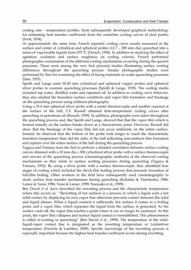
Evaporation, Condensation and Heat Transfer
50
cooling rate – temperature profiles. Scott subsequently developed graphical methodology for estimating heat transfer coefficients from the centerline cooling curves of steel probes (Scott, 1934). At approximately the same time, French reported cooling curve results measured at the surface and center of cylindrical and spherical probes (12.7 – 280 mm dia) quenched into a series of vaporizable liquids from 875 ºC (French, 1930). In addition to studying the effect of agitation, oxidation and surface roughness on cooling velocity, French performed photographic examination of the different cooling mechanisms occurring during the quench processes. These were among the very first pictorial studies illustrating surface wetting differences throughout the quenching process. Similar photographic studies were performed by Sato for examining the effect of facing materials on water quenching processes (Sato, 1933). Speith and Lange used 10-20 mm cylindrical and spherical copper probes and spherical silver probes to examine quenching processes (Speith & Lange, 1935). The cooling media included tap water, distilled water and rapeseed oil. In addition to cooling curve behavior, they also studied the boundary surface conditions and vapor film formation and breakage on the quenching process using schlieren photography. Using a 25.4 mm spherical silver probe with a center thermocouple and another exposed at the surface of the ball, T.F. Russell obtained time-temperature cooling curves after quenching in petroleum oil (Russell, 1939). In addition, photographs were taken throughout the quenching process and, like Speith and Lange, showed that that the vapor film which is formed initially on the surface breaks down at a characteristic point. However, Russell did show that the breakage of the vapor film did not occur uniformly on the entire surface. Instead, he observed that the bottom of the probe took longer to reach the characteristic transition temperature than did the sides of the ball indicating non-uniform film formation and rupture over the entire surface of the ball during the quenching process. Tagaya and Tamura were the first to perform a detailed correlation between surface cooling curves obtained with a 10 mm dia x 300 cylindrical silver probe with a surface thermocouple and movies of the quenching process (cinematographic methods) of the observed cooling mechanisms as they relate to surface wetting processes during quenching (Tagaya & Tamura, 1952). By using a silver probe with a surface thermocouple, they identified four stages of cooling which included the shock-film boiling process that preceeds formation of full-film boiling. Other workers in the field have subsequently used cinematography to study surface heat transfer mechanisms during quenching (Kobasko & Timchenko, 1986; Lainer & Tensi, 1996; Tensi & Lainer, 1999; Narazaki et al., 1999). Ben David et al. have described the rewetting process and the characteristic temperature where this occurs as: “Rewetting of hot surfaces is a process in which a liquid wets a hot solid surface by displacing its own vapor that otherwise prevents contact between the solid and liquid phases. When a liquid contacts a sufficiently hot surface it comes to a boiling point, and a vapor film, which separates the liquid from the surface, is generated. As the surface cools off, the vapor film reaches a point where it can no longer be sustained. At this point, the vapor film collapses and surface liquid contact is reestablished. This phenomenon is called re-wetting or quenching” (Ben David et al., 1999). The temperature at the solid-liquid-vapor contact line is designated as the rewetting temperature or Leidenfrost temperature (Frerichs & Luebben, 2009). Specific knowledge of the rewetting process is especially important because the highest heat transfer coefficient occurs during rewetting.
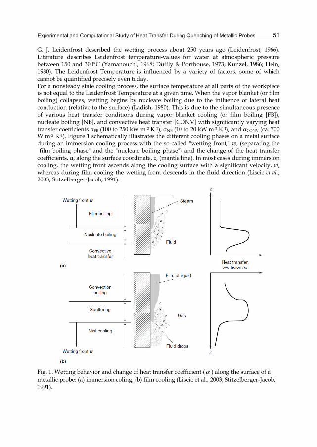
Experimental and Computational Study of Heat Transfer During Quenching of Metallic Probes
51
G. J. Leidenfrost described the wetting process about 250 years ago (Leidenfrost, 1966). Literature describes Leidenfrost temperature-values for water at atmospheric pressure between 150 and 300°C (Yamanouchi, 1968; Duffly & Porthouse, 1973; Kunzel, 1986; Hein, 1980). The Leidenfrost Temperature is influenced by a variety of factors, some of which cannot be quantified precisely even today. For a nonsteady state cooling process, the surface temperature at all parts of the workpiece is not equal to the Leidenfrost Temperature at a given time. When the vapor blanket (or film boiling) collapses, wetting begins by nucleate boiling due to the influence of lateral heat conduction (relative to the surface) (Ladish, 1980). This is due to the simultaneous presence of various heat transfer conditions during vapor blanket cooling (or film boiling [FB]), nucleate boiling [NB], and convective heat transfer [CONV] with significantly varying heat transfer coefficients αFB (100 to 250 kW m-2 K-1); αNB (10 to 20 kW m-2 K-1), and αCONV (ca. 700 W m-2 K-1). Figure 1 schematically illustrates the different cooling phases on a metal surface during an immersion cooling process with the so-called "wetting front," w, (separating the "film boiling phase" and the "nucleate boiling phase") and the change of the heat transfer coefficients, α, along the surface coordinate, z, (mantle line). In most cases during immersion cooling, the wetting front ascends along the cooling surface with a significant velocity, w, whereas during film cooling the wetting front descends in the fluid direction (Liscic et al., 2003; Stitzelberger-Jacob, 1991).
Fig. 1. Wetting behavior and change of heat transfer coefficient (α ) along the surface of a metallic probe: (a) immersion coling, (b) film cooling (Liscic et al., 2003; Stitzelberger-Jacob, 1991).
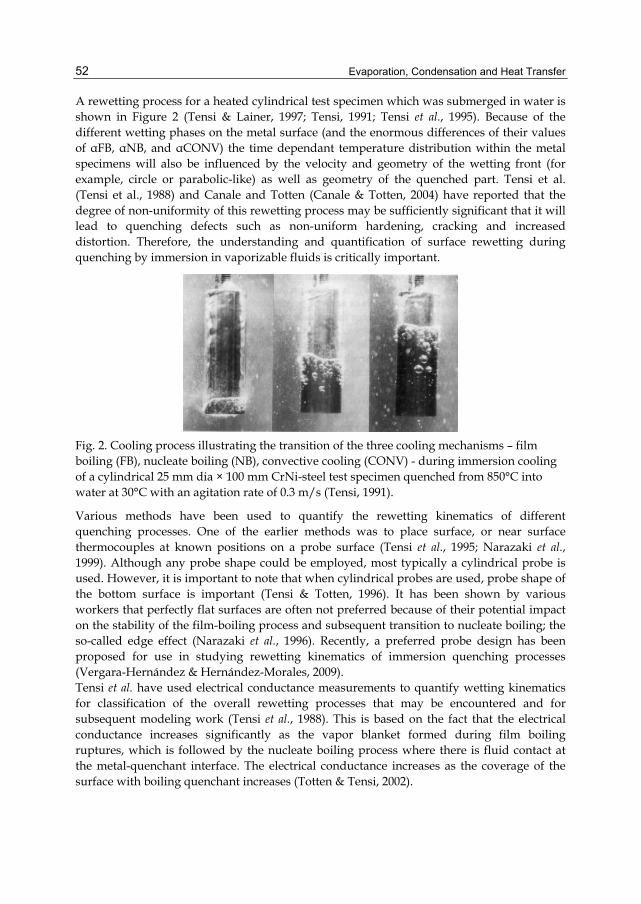
Evaporation, Condensation and Heat Transfer
52
A rewetting process for a heated cylindrical test specimen which was submerged in water is shown in Figure 2 (Tensi & Lainer, 1997; Tensi, 1991; Tensi et al., 1995). Because of the different wetting phases on the metal surface (and the enormous differences of their values of αFB, αNB, and αCONV) the time dependant temperature distribution within the metal specimens will also be influenced by the velocity and geometry of the wetting front (for example, circle or parabolic-like) as well as geometry of the quenched part. Tensi et al. (Tensi et al., 1988) and Canale and Totten (Canale & Totten, 2004) have reported that the degree of non-uniformity of this rewetting process may be sufficiently significant that it will lead to quenching defects such as non-uniform hardening, cracking and increased distortion. Therefore, the understanding and quantification of surface rewetting during quenching by immersion in vaporizable fluids is critically important.
Fig. 2. Cooling process illustrating the transition of the three cooling mechanisms – film boiling (FB), nucleate boiling (NB), convective cooling (CONV) - during immersion cooling of a cylindrical 25 mm dia × 100 mm CrNi-steel test specimen quenched from 850°C into water at 30°C with an agitation rate of 0.3 m/s (Tensi, 1991).
Various methods have been used to quantify the rewetting kinematics of different quenching processes. One of the earlier methods was to place surface, or near surface thermocouples at known positions on a probe surface (Tensi et al., 1995; Narazaki et al., 1999). Although any probe shape could be employed, most typically a cylindrical probe is used. However, it is important to note that when cylindrical probes are used, probe shape of the bottom surface is important (Tensi & Totten, 1996). It has been shown by various workers that perfectly flat surfaces are often not preferred because of their potential impact on the stability of the film-boiling process and subsequent transition to nucleate boiling; the so-called edge effect (Narazaki et al., 1996). Recently, a preferred probe design has been proposed for use in studying rewetting kinematics of immersion quenching processes (Vergara-Hernández & Hernández-Morales, 2009). Tensi et al. have used electrical conductance measurements to quantify wetting kinematics for classification of the overall rewetting processes that may be encountered and for subsequent modeling work (Tensi et al., 1988). This is based on the fact that the electrical conductance increases significantly as the vapor blanket formed during film boiling ruptures, which is followed by the nucleate boiling process where there is fluid contact at the metal-quenchant interface. The electrical conductance increases as the coverage of the surface with boiling quenchant increases (Totten & Tensi, 2002).
Experimental and Computational Study of Heat Transfer During Quenching of Metallic Probes
53
Tkachuk et al. have shown the importance of surface wetting properties of both the basestocks used to formulate oil quenchants and the effects of a wide range of different additives on surface wetting, especially as it relates to cooling rates (Tkachuk et al., 1989; Tkachuk et al., 1986). Not unexpectedly, as the wetting properties improve, the heat extraction capability increases resulting in higher cooling rates. However, these measurements were limited to room temperature and they did not describe the rewetting process during quenching using these fluid formulations. More recent work by Jagannath and Prabhu has however addressed many of these shortcomings by utilizing dynamic measurements on the quenching surface (Jagannath & Prabhu, 2009). While they do provide a dynamic measure of overall wetability, such measurements do not provide any quantification of the movement of the wetting front during the immersion quench. The method of choice to study surface rewetting process involves quantitative cinematography. Various workers have discussed experimental approaches to examining surface rewetting using different probe designs and experimental processes to study immersion quenching in vaporizable fluids (Lainer & Tensi, 1996; Tensi & Lainer, 1999; Hernández-Morales et al., 2009; Lübben et al., 2009; Frerichs & Lübben, 2009). These measurements have been invaluable in providing more realistic assessments in the modeling of heat flux, thermal gradients and residual stresses during quenching such as the work reported by Loshkaroev et al. (Loshkaroev et al., 1994). Given the importance of carefully monitoring the advance of the wetting front and deriving quantitative information about heat extraction during forced convective quenching, in this chapter, we describe detailed computational and experimental work to asses the usability of probes of different geometries. Also, results of wetting front kinematics and heat extraction obtained with a conical-end cylindrical probe are presented.
2. Experimental work The experimental apparatus is shown in Figure 3. The water in the main container is drawn with a ¼ HP pump and flows through a 90° elbow followed by a vertical plexiglass tube (44 mm I.D.). The water flowrate is set with a rotameter which is placed before the 90° elbow. After impacting the probe, the water is discharged in a secondary container. The desired water temperature is achieved with electrical heaters placed within the main container; the water temperature control was manual. From PIV (Particle Image Velocimetry) measurements conducted at several distances from the elbow it was found that the velocity profile was not fully developed until a position of 1.50 m along the vertical section of the plexiglass tube (Vergara-Hernández & Hernández-Morales, 2009). Thus, the probe tip was always located at 1.70 m from the elbow. The probe was heated in an electric furnace (in stagnant air) up to a temperature of 915 °C such that the temperature at the start of the quench was close to 900 °C in all experiments. To ensure a quick and controlled descent of the probe into the quench bath, the probe was attached to a steel lance which in turns was fitted to a moving spreader. Three probe geometries were considered: 1) flat-end cylinder, 2) hemispherical-end cylinder and 3) conical-end cylinder. The probes were machined from AISI 304 stainless steel stock bar and instrumented with 1/16”, Inconel-sheathed, type K (see Figure 4). The thermocouples were press-fitted into position. To keep water to enter into the space between the thermocouple and the bore wall, the top surface of the probe was covered with high temperature cement (Omega, model Omega 600).
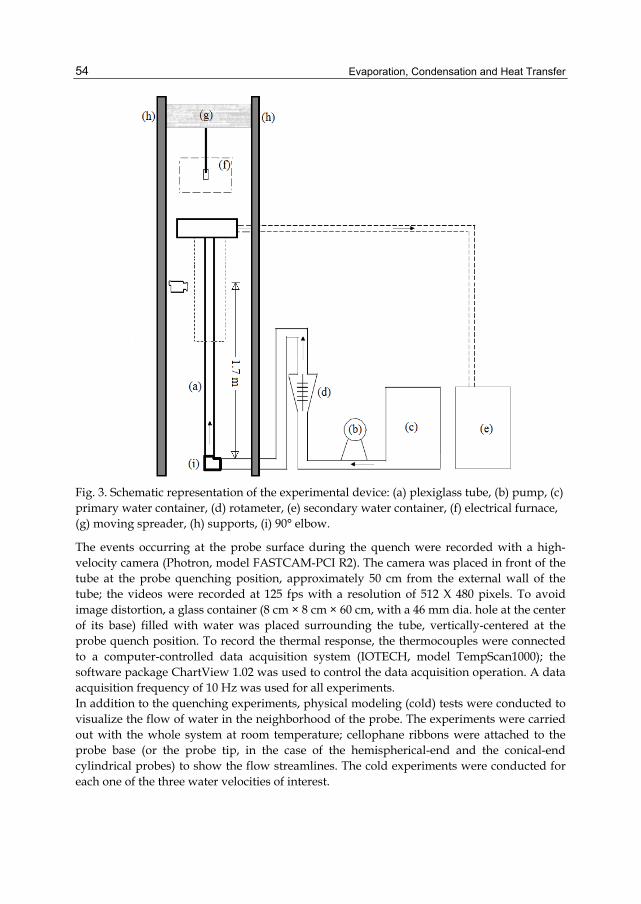
Evaporation, Condensation and Heat Transfer
54
Fig. 3. Schematic representation of the experimental device: (a) plexiglass tube, (b) pump, (c) primary water container, (d) rotameter, (e) secondary water container, (f) electrical furnace, (g) moving spreader, (h) supports, (i) 90° elbow.
The events occurring at the probe surface during the quench were recorded with a high-velocity camera (Photron, model FASTCAM-PCI R2). The camera was placed in front of the tube at the probe quenching position, approximately 50 cm from the external wall of the tube; the videos were recorded at 125 fps with a resolution of 512 X 480 pixels. To avoid image distortion, a glass container (8 cm × 8 cm × 60 cm, with a 46 mm dia. hole at the center of its base) filled with water was placed surrounding the tube, vertically-centered at the probe quench position. To record the thermal response, the thermocouples were connected to a computer-controlled data acquisition system (IOTECH, model TempScan1000); the software package ChartView 1.02 was used to control the data acquisition operation. A data acquisition frequency of 10 Hz was used for all experiments. In addition to the quenching experiments, physical modeling (cold) tests were conducted to visualize the flow of water in the neighborhood of the probe. The experiments were carried out with the whole system at room temperature; cellophane ribbons were attached to the probe base (or the probe tip, in the case of the hemispherical-end and the conical-end cylindrical probes) to show the flow streamlines. The cold experiments were conducted for each one of the three water velocities of interest.
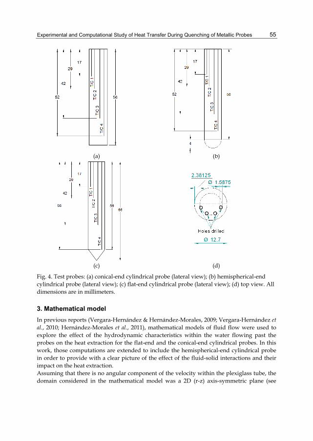
Experimental and Computational Study of Heat Transfer During Quenching of Metallic Probes
55
(a) (b)
(c) (d)
Fig. 4. Test probes: (a) conical-end cylindrical probe (lateral view); (b) hemispherical-end cylindrical probe (lateral view); (c) flat-end cylindrical probe (lateral view); (d) top view. All dimensions are in millimeters.
3. Mathematical model In previous reports (Vergara-Hernández & Hernández-Morales, 2009; Vergara-Hernández et al., 2010; Hernández-Morales et al., 2011), mathematical models of fluid flow were used to explore the effect of the hydrodynamic characteristics within the water flowing past the probes on the heat extraction for the flat-end and the conical-end cylindrical probes. In this work, those computations are extended to include the hemispherical-end cylindrical probe in order to provide with a clear picture of the effect of the fluid-solid interactions and their impact on the heat extraction. Assuming that there is no angular component of the velocity within the plexiglass tube, the domain considered in the mathematical model was a 2D (r-z) axis-symmetric plane (see

Evaporation, Condensation and Heat Transfer
56
Figure 5 (a)) where a Newtonian fluid is flowing under unsteady-state conditions; the whole system is treated as isothermal. To optimize computer resources, only half of the plane is simulated.The boundary conditions are indicated in Figure 5 (b). Similar computational domains and set of boundary conditions were used for the simulations corresponding to the hemispherical-end and the conical-end cylindrical probes.
(a) (b)
Fig. 5. (a) Computational domain (dimensions in mm) and (b) boundary conditions for the simulations corresponding to the flat-end cylindrical probe.
The objective of the mathematical model was to relate the hydrodynamic conditions to the characteristics of the vapor film and the re-wetting process by computing the evolution of: 1) the streamlines and 2) the velocity field within the fluid. The simulations were carried out for a system at room temperature and an incompressible fluid. Therefore, the governing equations (continuity and momentum conservation) may be written as:
0v∇ ⋅ = (1)
RDv p gDt
ρ τ τ ρ⎡ ⎤
⎡ ⎤ ⎡ ⎤= −∇ − ∇ ⋅ − ∇ ⋅ +⎢ ⎥ ⎣ ⎦ ⎣ ⎦⎢ ⎥⎣ ⎦ (2)
Where ρ is the fluid density, v is the fluid velocity vector, p is the dynamic pressure, τ is the stress tensor related to viscous flow Rτ is the Reynolds stress tensor and g is the acceleration vector due to the gravitational force. The overbars indicate time-averaged values. The k ε− turbulence model (Launder and Spalding, 1974) was used to describe the turbulent characteristics of the flow:
23 ( )
2 avgk u I= (3)
1/80.16(Re )HDI −= (4)
Inlet velocity
Probe surface
Simmetry
Outlet pressure
Wall tube
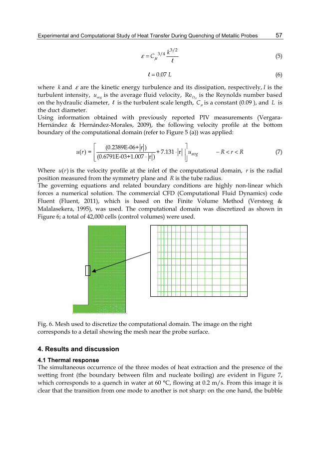
Experimental and Computational Study of Heat Transfer During Quenching of Metallic Probes
57
3/2
3/4 kCμε =l
(5)
0.07 L=l (6)
where k and ε are the kinetic energy turbulence and its dissipation, respectively, I is the turbulent intensity, avgu is the average fluid velocity, Re
HD is the Reynolds number based on the hydraulic diameter, l is the turbulent scale length, μC is a constant (0.09 ), and L is the duct diameter. Using information obtained with previously reported PIV measurements (Vergara-Hernández & Hernández-Morales, 2009), the following velocity profile at the bottom boundary of the computational domain (refer to Figure 5 (a)) was applied:
(0.2389E-06+ r )
( ) = + 7.131 r (0.6791E-03+1.007 r ) avgu r u R r R⎡ ⎤
⋅ − < <⎢ ⎥⋅⎢ ⎥⎣ ⎦
(7)
Where ( )u r is the velocity profile at the inlet of the computational domain, r is the radial position measured from the symmetry plane and R is the tube radius. The governing equations and related boundary conditions are highly non-linear which forces a numerical solution. The commercial CFD (Computational Fluid Dynamics) code Fluent (Fluent, 2011), which is based on the Finite Volume Method (Versteeg & Malalasekera, 1995), was used. The computational domain was discretized as shown in Figure 6; a total of 42,000 cells (control volumes) were used.
Fig. 6. Mesh used to discretize the computational domain. The image on the right corresponds to a detail showing the mesh near the probe surface.
4. Results and discussion 4.1 Thermal response The simultaneous occurrence of the three modes of heat extraction and the presence of the wetting front (the boundary between film and nucleate boiling) are evident in Figure 7, which corresponds to a quench in water at 60 °C, flowing at 0.2 m/s. From this image it is clear that the transition from one mode to another is not sharp: on the one hand, the bubble
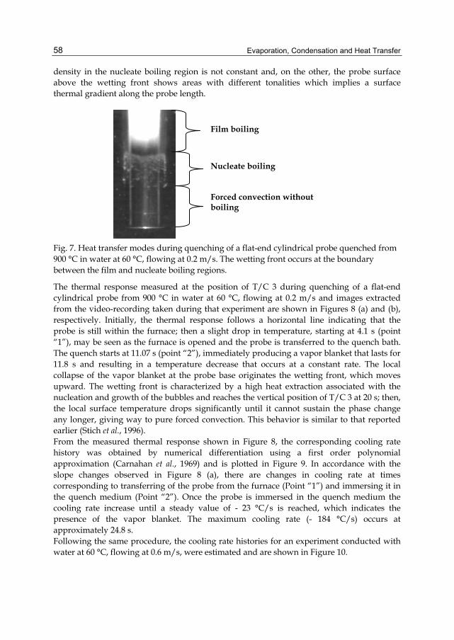
Evaporation, Condensation and Heat Transfer
58
density in the nucleate boiling region is not constant and, on the other, the probe surface above the wetting front shows areas with different tonalities which implies a surface thermal gradient along the probe length.
Fig. 7. Heat transfer modes during quenching of a flat-end cylindrical probe quenched from 900 °C in water at 60 °C, flowing at 0.2 m/s. The wetting front occurs at the boundary between the film and nucleate boiling regions.
The thermal response measured at the position of T/C 3 during quenching of a flat-end cylindrical probe from 900 °C in water at 60 °C, flowing at 0.2 m/s and images extracted from the video-recording taken during that experiment are shown in Figures 8 (a) and (b), respectively. Initially, the thermal response follows a horizontal line indicating that the probe is still within the furnace; then a slight drop in temperature, starting at 4.1 s (point “1”), may be seen as the furnace is opened and the probe is transferred to the quench bath. The quench starts at 11.07 s (point “2”), immediately producing a vapor blanket that lasts for 11.8 s and resulting in a temperature decrease that occurs at a constant rate. The local collapse of the vapor blanket at the probe base originates the wetting front, which moves upward. The wetting front is characterized by a high heat extraction associated with the nucleation and growth of the bubbles and reaches the vertical position of T/C 3 at 20 s; then, the local surface temperature drops significantly until it cannot sustain the phase change any longer, giving way to pure forced convection. This behavior is similar to that reported earlier (Stich et al., 1996). From the measured thermal response shown in Figure 8, the corresponding cooling rate history was obtained by numerical differentiation using a first order polynomial approximation (Carnahan et al., 1969) and is plotted in Figure 9. In accordance with the slope changes observed in Figure 8 (a), there are changes in cooling rate at times corresponding to transferring of the probe from the furnace (Point “1”) and immersing it in the quench medium (Point “2”). Once the probe is immersed in the quench medium the cooling rate increase until a steady value of - 23 °C/s is reached, which indicates the presence of the vapor blanket. The maximum cooling rate (- 184 °C/s) occurs at approximately 24.8 s. Following the same procedure, the cooling rate histories for an experiment conducted with water at 60 °C, flowing at 0.6 m/s, were estimated and are shown in Figure 10.
Film boiling
Nucleate boiling
Forced convection without boiling
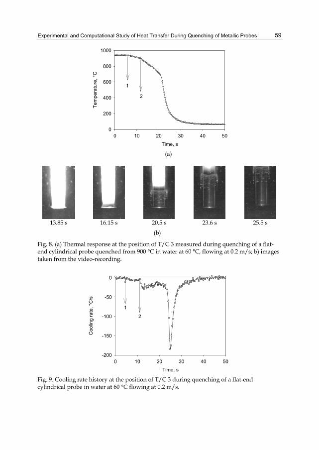
Experimental and Computational Study of Heat Transfer During Quenching of Metallic Probes
59
Time, s
0 10 20 30 40 50
Tem
pera
ture
, °C
0
200
400
600
800
1000
1
2
(a)
13.85 s 16.15 s 20.5 s 23.6 s 25.5 s
(b)
Fig. 8. (a) Thermal response at the position of T/C 3 measured during quenching of a flat-end cylindrical probe quenched from 900 °C in water at 60 °C, flowing at 0.2 m/s; b) images taken from the video-recording.
Time, s
0 10 20 30 40 50
Coo
ling
rate
, °C
/s
-200
-150
-100
-50
0
1
2
Fig. 9. Cooling rate history at the position of T/C 3 during quenching of a flat-end cylindrical probe in water at 60 °C flowing at 0.2 m/s.
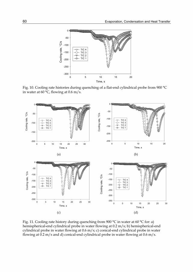
Evaporation, Condensation and Heat Transfer
60
Time, s0 5 10 15 20
Coo
ling
rate
, °C
/s
-300
-250
-200
-150
-100
-50
0
T/C 4T/C 3T/C 2T/C 1
Fig. 10. Cooling rate histories during quenching of a flat-end cylindrical probe from 900 °C in water at 60 °C, flowing at 0.6 m/s.
Time, s0 5 10 15 20
Coo
ling
rate
, °C
/s
-250
-200
-150
-100
-50
0
T/C 4T/C 3T/C 2T/C 1
Time, s0 5 10 15 20 25 30
-350
-300
-250
-200
-150
-100
-50
0
T/C 4T/C 3T/C 2T/C 1
Time, s0 5 10 15 20 25 30
Coo
ling
rate
, °C
/s
-200
-150
-100
-50
0
T/C 4T/C 3T/C 2T/C 1
(a) (b)
Time, s0 5 10 15 20 25 30
Coo
ling
rate
, °C
/s
-300
-250
-200
-150
-100
-50
0
T/C 4T/C 3T/C 2T/C 1
C
oolin
g ra
te, º
C/s
(c) (d)
Fig. 11. Cooling rate history during quenching from 900 °C in water at 60 °C for: a) hemispherical-end cylindrical probe in water flowing at 0.2 m/s; b) hemispherical-end cylindrical probe in water flowing at 0.6 m/s; c) conical-end cylindrical probe in water flowing at 0.2 m/s and d) conical-end cylindrical probe in water flowing at 0.6 m/s.
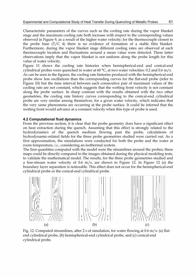
Experimental and Computational Study of Heat Transfer During Quenching of Metallic Probes
61
Characteristic parameters of the curves such as the cooling rate during the vapor blanket stage and the maximum cooling rate both increase with respect to the corresponding values observed in Figure 9, as a result of the higher water velocity; for the thermocouple closest to the probe base (T/C 4) there is no evidence of formation of a stable film blanket. Furthermore, during the vapor blanket stage different cooling rates are observed at each thermocouple location and fluctuations around a mean value were detected. These latter observations imply that the vapor blanket is not uniform along the probe length for this value of water velocity. Figure 11 shows the cooling rate histories when hemispherical-end and conical-end cylindrical probes were quenched in water at 60 °C, at two water velocities: 0.2 and 0.6 m/s. As can be seen in the figures, the cooling rate histories produced with the hemispherical-end probe show less oscillations than the corresponding curves for the flat-end probe (refer to Figure 10) but the time interval between each consecutive pair of maximum values of the cooling rate are not constant, which suggests that the wetting front velocity is not constant along the probe surface. In sharp contrast with the results obtained with the two other geometries, the cooling rate history curves corresponding to the conical-end cylindrical probe are very similar among themselves, for a given water velocity, which indicates that the very same phenomena are occurring at the probe surface. It could be inferred that the wetting front would advance at a constant velocity when this type of probe is used.
4.2 Computational fluid dynamics From the previous section, it is clear that the probe geometry does have a significant effect on heat extraction during the quench. Assuming that this effect is strongly related to the hydrodynamics of the quench medium flowing past the probe, calculations of hydrodynamic-related fields for the three probe geometries studied were carried out. As a first approximation, the simulations were conducted for both the probe and the water at room temperature, i.e., considering an isothermal system. The first quantities computed with the model were the streamlines around the probes; these maps could be directly compared to the images obtained during the physical modeling tests, to validate the mathematical model. The results, for the three probe geometries studied and a free-stream water velocity of 0.6 m/s, are shown in Figure 12. In Figure 12 (a) the boundary layer separation is noticeable. This effect does not occur for the hemispherical-end cylindrical probe or the conical-end cylindrical probe.
(a) (b) (c) Fig. 12. Computed streamlines, after 2 s of simulation, for water flowing at 0.6 m/s: (a) flat-end cylindrical probe, (b) hemispherical-end cylindrical probe, and (c) conical-end cylindrical probe.
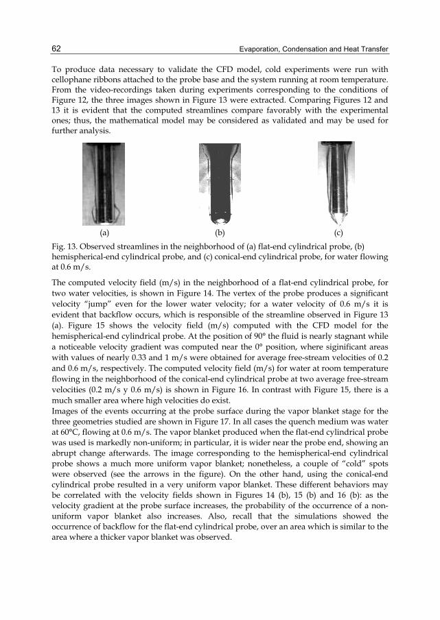
Evaporation, Condensation and Heat Transfer
62
To produce data necessary to validate the CFD model, cold experiments were run with cellophane ribbons attached to the probe base and the system running at room temperature. From the video-recordings taken during experiments corresponding to the conditions of Figure 12, the three images shown in Figure 13 were extracted. Comparing Figures 12 and 13 it is evident that the computed streamlines compare favorably with the experimental ones; thus, the mathematical model may be considered as validated and may be used for further analysis.
(a) (b) (c)
Fig. 13. Observed streamlines in the neighborhood of (a) flat-end cylindrical probe, (b) hemispherical-end cylindrical probe, and (c) conical-end cylindrical probe, for water flowing at 0.6 m/s.
The computed velocity field (m/s) in the neighborhood of a flat-end cylindrical probe, for two water velocities, is shown in Figure 14. The vertex of the probe produces a significant velocity “jump” even for the lower water velocity; for a water velocity of 0.6 m/s it is evident that backflow occurs, which is responsible of the streamline observed in Figure 13 (a). Figure 15 shows the velocity field (m/s) computed with the CFD model for the hemispherical-end cylindrical probe. At the position of 90° the fluid is nearly stagnant while a noticeable velocity gradient was computed near the 0° position, where siginificant areas with values of nearly 0.33 and 1 m/s were obtained for average free-stream velocities of 0.2 and 0.6 m/s, respectively. The computed velocity field (m/s) for water at room temperature flowing in the neighborhood of the conical-end cylindrical probe at two average free-stream velocities (0.2 m/s y 0.6 m/s) is shown in Figure 16. In contrast with Figure 15, there is a much smaller area where high velocities do exist. Images of the events occurring at the probe surface during the vapor blanket stage for the three geometries studied are shown in Figure 17. In all cases the quench medium was water at 60°C, flowing at 0.6 m/s. The vapor blanket produced when the flat-end cylindrical probe was used is markedly non-uniform; in particular, it is wider near the probe end, showing an abrupt change afterwards. The image corresponding to the hemispherical-end cylindrical probe shows a much more uniform vapor blanket; nonetheless, a couple of “cold” spots were observed (see the arrows in the figure). On the other hand, using the conical-end cylindrical probe resulted in a very uniform vapor blanket. These different behaviors may be correlated with the velocity fields shown in Figures 14 (b), 15 (b) and 16 (b): as the velocity gradient at the probe surface increases, the probability of the occurrence of a non-uniform vapor blanket also increases. Also, recall that the simulations showed the occurrence of backflow for the flat-end cylindrical probe, over an area which is similar to the area where a thicker vapor blanket was observed.
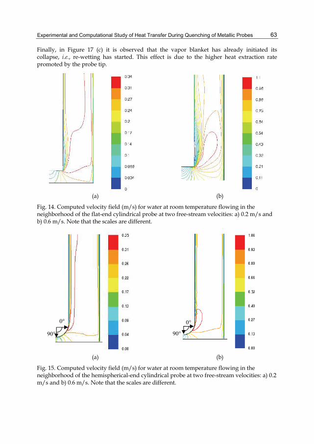
Experimental and Computational Study of Heat Transfer During Quenching of Metallic Probes
63
Finally, in Figure 17 (c) it is observed that the vapor blanket has already initiated its collapse, i.e., re-wetting has started. This effect is due to the higher heat extraction rate promoted by the probe tip.
(a) (b)
Fig. 14. Computed velocity field (m/s) for water at room temperature flowing in the neighborhood of the flat-end cylindrical probe at two free-stream velocities: a) 0.2 m/s and b) 0.6 m/s. Note that the scales are different.
(a) (b)
Fig. 15. Computed velocity field (m/s) for water at room temperature flowing in the neighborhood of the hemispherical-end cylindrical probe at two free-stream velocities: a) 0.2 m/s and b) 0.6 m/s. Note that the scales are different.
90°
0°
90° 0°
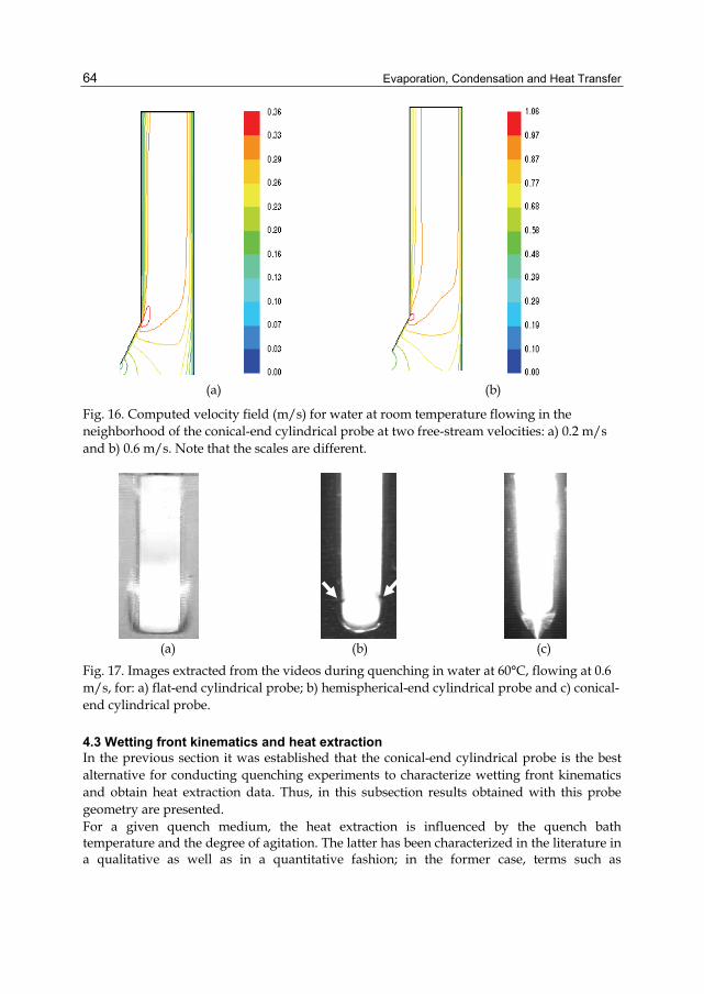
Evaporation, Condensation and Heat Transfer
64
(a) (b)
Fig. 16. Computed velocity field (m/s) for water at room temperature flowing in the neighborhood of the conical-end cylindrical probe at two free-stream velocities: a) 0.2 m/s and b) 0.6 m/s. Note that the scales are different.
(a) (b) (c) Fig. 17. Images extracted from the videos during quenching in water at 60°C, flowing at 0.6 m/s, for: a) flat-end cylindrical probe; b) hemispherical-end cylindrical probe and c) conical-end cylindrical probe.
4.3 Wetting front kinematics and heat extraction In the previous section it was established that the conical-end cylindrical probe is the best alternative for conducting quenching experiments to characterize wetting front kinematics and obtain heat extraction data. Thus, in this subsection results obtained with this probe geometry are presented. For a given quench medium, the heat extraction is influenced by the quench bath temperature and the degree of agitation. The latter has been characterized in the literature in a qualitative as well as in a quantitative fashion; in the former case, terms such as
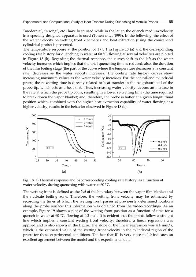
Experimental and Computational Study of Heat Transfer During Quenching of Metallic Probes
65
“moderate”, “strong”, etc., have been used while in the latter, the quench medium velocity in a specially designed apparatus is used (Totten et al., 1993). In the following, the effect of the water velocity on wetting front kinematics and heat extraction (using the conical-end cylindrical probe) is presented. The temperature response at the position of T/C 1 in Figure 18 (a) and the corresponding cooling rate history for quenching in water at 60 °C, flowing at several velocities are plotted in Figure 18 (b). Regarding the thermal response, the curves shift to the left as the water velocity increases which implies that the total quenching time is reduced; also, the duration of the film boiling stage (the part of the curve where the temperature decreases at a constant rate) decreases as the water velocity increases. The cooling rate history curves show increasing maximum values as the water velocity increases. For the conical-end cylindrical probe, the re-wetting time is directly related to heat transfer in the neighbourhood of the probe tip, which acts as a heat sink. Thus, increasing water velocity favours an increase in the rate at which the probe tip cools, resulting in a lower re-wetting time (the time required to break down the vapor blanket) and, therefore, the probe is hotter at a given longitudinal position which, combined with the higher heat extraction capability of water flowing at a higher velocity, results in the behavior observed in Figure 18 (b).
Time, s25 30 35 40 45 50 55
Tem
pera
ture
,°C
0
200
400
600
800
10000.2 m/s0.4 m/s0.6 m/s
T/C 1
Time, s30 40 50 60
Coo
ling
rate
, °C
/s
-160-140-120-100-80-60-40-20
020
0.2 m/s0.4 m/s0.6 m/sT/C 1
(a) (b)
Fig. 18. a) Thermal response and b) corresponding cooling rate history, as a function of water velocity, during quenching with water at 60 °C.
The wetting front is defined as the loci of the boundary between the vapor film blanket and the nucleate boiling zone. Therefore, the wetting front velocity may be estimated by recording the times at which the wetting front passes at previously determined locations along the probe surface; this information was obtained from the video-recordings. As an example, Figure 19 shows a plot of the wetting front position as a function of time for a quench in water at 60 °C, flowing at 0.2 m/s. It is evident that the points follow a straight line which implies a constant wetting front velocity; therefore, a linear regression was applied and is also shown in the figure. The slope of the linear regression was 4.4 mm/s, which is the estimated value of the wetting front velocity in the cylindrical region of the probe for these experimental conditions. The fact that R2 is very close to 1.0 indicates an excellent agreement between the model and the experimental data.
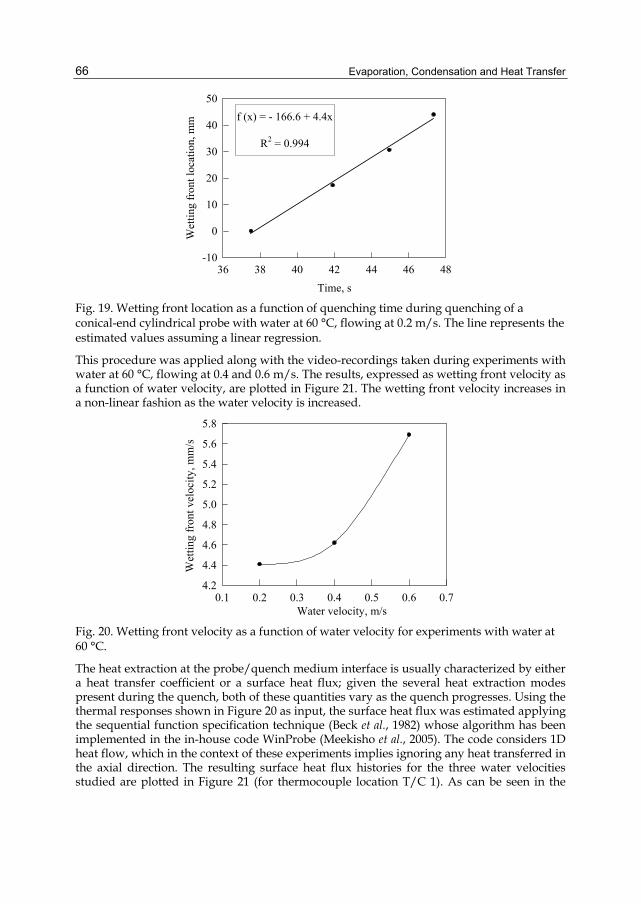
Evaporation, Condensation and Heat Transfer
66
Time, s36 38 40 42 44 46 48
Wet
ting
fron
t loc
atio
n, m
m
-10
0
10
20
30
40
50f (x) = - 166.6 + 4.4x
R2 = 0.994
Fig. 19. Wetting front location as a function of quenching time during quenching of a conical-end cylindrical probe with water at 60 °C, flowing at 0.2 m/s. The line represents the estimated values assuming a linear regression.
This procedure was applied along with the video-recordings taken during experiments with water at 60 °C, flowing at 0.4 and 0.6 m/s. The results, expressed as wetting front velocity as a function of water velocity, are plotted in Figure 21. The wetting front velocity increases in a non-linear fashion as the water velocity is increased.
0.1 0.2 0.3 0.4 0.5 0.6 0.74.2
4.4
4.6
4.8
5.0
5.2
5.4
5.6
5.8
Wet
ting
fron
t vel
ocity
, mm
/s
Water velocity, m/s Fig. 20. Wetting front velocity as a function of water velocity for experiments with water at 60 °C.
The heat extraction at the probe/quench medium interface is usually characterized by either a heat transfer coefficient or a surface heat flux; given the several heat extraction modes present during the quench, both of these quantities vary as the quench progresses. Using the thermal responses shown in Figure 20 as input, the surface heat flux was estimated applying the sequential function specification technique (Beck et al., 1982) whose algorithm has been implemented in the in-house code WinProbe (Meekisho et al., 2005). The code considers 1D heat flow, which in the context of these experiments implies ignoring any heat transferred in the axial direction. The resulting surface heat flux histories for the three water velocities studied are plotted in Figure 21 (for thermocouple location T/C 1). As can be seen in the
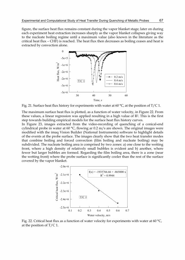
Experimental and Computational Study of Heat Transfer During Quenching of Metallic Probes
67
figure, the surface heat flux remains constant during the vapor blanket stage; later on during each experiment heat extraction increases sharply as the vapor blanket collapses giving way to the nucleate boiling regime until a maximum value (also known in the literature as the critical heat flux – CHF) is reached. The heat flux then decreases as boiling ceases and heat is extracted by convection alone.
Time, s30 40 50 60
Hea
t flu
x, W
/m2
-3e+6
-3e+6
-2e+6
-2e+6
-1e+6
-5e+5
0
0.2 m/s 0.4 m/s0.6 m/s
T/C 1
Fig. 21. Surface heat flux history for experiments with water at 60 °C, at the position of T/C 1.
The maximum surface heat flux is plotted, as a function of water velocity, in Figure 22. From these values, a linear regression was applied resulting in a high value of R2. This is the first step towards building empirical models for the surface heat flux history curves. In Figure 23, images extracted from the video-recording of quenching of a conical-end cylindrical probe in water at 60 °C, flowing ar 0.2 m/s are shown. The original images were modified with the imaq Vision Builder (National Instruments) software to highlight details of the events at the probe surface. The images clearly show that the two heat transfer modes that combine boiling and forced convection (film boiling and nucleate boiling) may be subdivided. The nucleate boiling area is comprised by two zones: a) one close to the wetting front, where a high density of relatively small bubbles is evident and b) another, where fewer but larger bubbles are formed. Regarding the film boiling area, there is a zone (near the wetting front) where the probe surface is significantly cooler than the rest of the surface covered by the vapor blanket.
f(x) = -1935766.66 + -865000 xR2 = 0.9944
Water velocity, m/s0.1 0.2 0.3 0.4 0.5 0.6 0.7
Crit
ical
hea
t flu
x, W
/m2
-2.5e+6
-2.4e+6
-2.3e+6
-2.2e+6
-2.1e+6
-2.0e+6
T/C 1
Fig. 22. Critical heat flux as a function of water velocity for experiments with water at 60 °C, at the position of T/C 1.
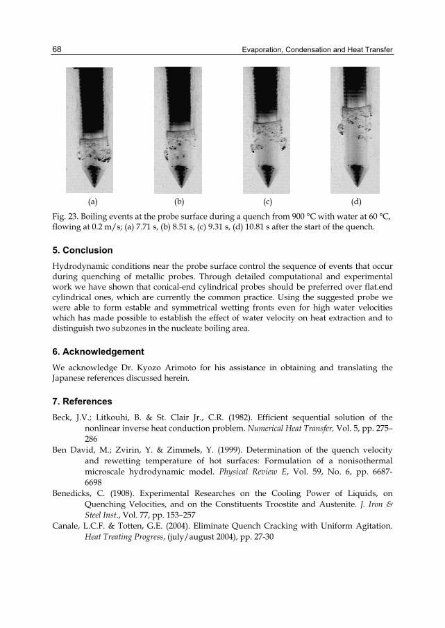
Evaporation, Condensation and Heat Transfer
68
(a) (b) (c) (d)
Fig. 23. Boiling events at the probe surface during a quench from 900 °C with water at 60 °C, flowing at 0.2 m/s; (a) 7.71 s, (b) 8.51 s, (c) 9.31 s, (d) 10.81 s after the start of the quench.
5. Conclusion Hydrodynamic conditions near the probe surface control the sequence of events that occur during quenching of metallic probes. Through detailed computational and experimental work we have shown that conical-end cylindrical probes should be preferred over flat.end cylindrical ones, which are currently the common practice. Using the suggested probe we were able to form estable and symmetrical wetting fronts even for high water velocities which has made possible to establish the effect of water velocity on heat extraction and to distinguish two subzones in the nucleate boiling area.
6. Acknowledgement We acknowledge Dr. Kyozo Arimoto for his assistance in obtaining and translating the Japanese references discussed herein.
7. References Beck, J.V.; Litkouhi, B. & St. Clair Jr., C.R. (1982). Efficient sequential solution of the
nonlinear inverse heat conduction problem. Numerical Heat Transfer, Vol. 5, pp. 275–286
Ben David, M.; Zvirin, Y. & Zimmels, Y. (1999). Determination of the quench velocity and rewetting temperature of hot surfaces: Formulation of a nonisothermal microscale hydrodynamic model. Physical Review E, Vol. 59, No. 6, pp. 6687- 6698
Benedicks, C. (1908). Experimental Researches on the Cooling Power of Liquids, on Quenching Velocities, and on the Constituents Troostite and Austenite. J. Iron & Steel Inst., Vol. 77, pp. 153–257
Canale, L.C.F. & Totten, G.E. (2004). Eliminate Quench Cracking with Uniform Agitation. Heat Treating Progress, (july/august 2004), pp. 27-30
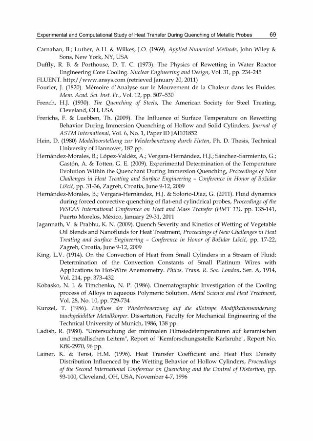
Experimental and Computational Study of Heat Transfer During Quenching of Metallic Probes
69
Carnahan, B.; Luther, A.H. & Wilkes, J.O. (1969). Applied Numerical Methods, John Wiley & Sons, New York, NY, USA
Duffly, R. B. & Porthouse, D. T. C. (1973). The Physics of Rewetting in Water Reactor Engineering Core Cooling. Nuclear Engineering and Design, Vol. 31, pp. 234-245
FLUENT. http://www.ansys.com (retrieved January 20, 2011) Fourier, J. (1820). Mémoire d’Analyse sur le Mouvement de la Chaleur dans les Fluides.
Mem. Acad. Sci. Inst. Fr., Vol. 12, pp. 507–530 French, H.J. (1930). The Quenching of Steels, The American Society for Steel Treating,
Cleveland, OH, USA Frerichs, F. & Luebben, Th. (2009). The Influence of Surface Temperature on Rewetting
Behavior During Immersion Quenching of Hollow and Solid Cylinders. Journal of ASTM International, Vol. 6, No. 1, Paper ID JAI101852
Hein, D. (1980) Modellvorstellung zur Wiederbenetzung durch Fluten, Ph. D. Thesis, Technical University of Hannover, 182 pp.
Hernández-Morales, B.; López-Valdéz, A.; Vergara-Hernández, H.J.; Sánchez–Sarmiento, G.; Gastón, A. & Totten, G. E. (2009). Experimental Determination of the Temperature Evolution Within the Quenchant During Immersion Quenching, Proceedings of New Challenges in Heat Treating and Surface Engineering – Conference in Honor of Božidar Lišcić, pp. 31-36, Zagreb, Croatia, June 9-12, 2009
Hernández-Morales, B.; Vergara-Hernández, H.J. & Solorio-Díaz, G. (2011). Fluid dynamics during forced convective quenching of flat-end cylindrical probes, Proceedings of the WSEAS International Conference on Heat and Mass Transfer (HMT 11), pp. 135-141, Puerto Morelos, México, January 29-31, 2011
Jagannath, V. & Prabhu, K. N. (2009). Quench Severity and Kinetics of Wetting of Vegetable Oil Blends and Nanofluids for Heat Treatment, Proceedings of New Challenges in Heat Treating and Surface Engineering – Conference in Honor of Božidar Lišcić, pp. 17-22, Zagreb, Croatia, June 9-12, 2009
King, L.V. (1914). On the Convection of Heat from Small Cylinders in a Stream of Fluid: Determination of the Convection Constants of Small Platinum Wires with Applications to Hot-Wire Anemometry. Philos. Trans. R. Soc. London, Ser. A, 1914, Vol. 214, pp. 373–432
Kobasko, N. I. & Timchenko, N. P. (1986). Cinematographic Investigation of the Cooling process of Alloys in aqueous Polymeric Solution. Metal Science and Heat Treatment, Vol. 28, No. 10, pp. 729-734
Kunzel, T. (1986). Einfluss der Wiederbenetzung auf die allotrope Modifikationsanderung tauchgekiihlter Metallkorper. Dissertation, Faculty for Mechanical Engineering of the Technical University of Munich, 1986, 138 pp.
Ladish, R. (1980). "Untersuchung der minimalen Filmsiedetemperaturen auf keramischen und metallischen Leitem", Report of "Kemforschungsstelle Karlsruhe", Report No. KfK-2970, 96 pp.
Lainer, K. & Tensi, H.M. (1996). Heat Transfer Coefficient and Heat Flux Density Distribution Influenced by the Wetting Behavior of Hollow Cylinders, Proceedings of the Second International Conference on Quenching and the Control of Distortion, pp. 93-100, Cleveland, OH, USA, November 4-7, 1996
Evaporation, Condensation and Heat Transfer
70
Launder, B. E. & Spalding, D. B. (1974). The numerical computation of turbulent flows. Comput. Methods Appl. Mech. Eng., Vol. 3, pp. 269-289
Leidenfrost, G. J. (1966). De Aqua Communis Nonnullis Tractus. Original from 1756. In: C. Waves, International Journal of MassTransfer, Vol. 9, pp. 1153-1166 (trans.)
Liscic, B.; Tensi, H.M.; Totten, G.E. & Webster, G.M. (2003). Non-Lubricating Process Fluids: Steel Quenching Technology. In: Fuels and Lubricants Handbook: Technology, Properties, Performance and Testing , G.E. Totten, S.R. Westbrook, R.J. Shah (Eds.) , pp. 587-634, ASTM International, West Conshocken, PA.
Loshkaroev, V.E.; Tensi, H.M.; Gese, H. & Stich, A. (1994). Calculation of Temperature and Heat Flux in Quenched Cylinders for Different Wetting Processes. Steel Research, Vol. 65, No. 9, pp. 390-395
Lübben, Th.; Frerichs, F.; Hoffmann, F. & Zoch, H.-W. (2009). Rewetting Behavior During Immersion Quenching, Proceedings of New Challenges in Heat Treating and Surface Engineering – Conference in Honor of Božidar Lišcić, pp. 23-30, Zagreb, Croatia, June 9-12, 2009
Meekisho, L.; Hernández-Morales, B.; Téllez-Martínez, J.S. & Chen, X. (2005). Computer-aided cooling curve analysis using WinProbe. Int. Journal of Materials and Product Technology, Vol 24, Nos. 1-4, pp. 155–169
Narazaki, M.; Asada, S. & Fukuhara, K. (1996). Recent Research on Cooling Power of Liquid Quenchants in Japan, Proceedings of the Second International Conference on Quenching and the Control of Distortion, pp. 37-46, Cleveland, OH, USA, November 4-7, 1996
Narazaki, M.; Kogawara, M.; Shirayori, A. & Fuchizawa, S. (1999). Influence of Wetting Behaviour on Cooling Characteristics during Quenching of Hot Metal, Proc. of The 3rd International Conference on Quenching and Control of Distortion, pp. 112-120, Prague, Czech Republic, March 24-26, 1999
Pilling, N.B. & Lynch, T.D. (1920). Cooling Properties of Technical Quenching Liquids. Trans. AIME, Vol. 62, pp. 665–688
Russell, A.S. (1910). The convection of heat from a body cooled by a stream of fluid. Philos. Mag., Vol. 20, No. 118, pp. 591–610
Russell, T.F. (1939). “Some Tests on Quenching Oils”, Spec. Report No.24, “Second Report of the Alloy Steels Research Committee,” Iron and Steel Inst., London, 1939, Section IX, Part 6, pp. 283–298
Sato, S. (1933) On the Effect of Facing on the Cooling Velocity of a specimen during Quenching. Metal Research,Vol.10,No.2,pp. 63–70 (in Japanese)
Scott , H. (1934). The Problem of Quenching Media for the Hardening of Steel. Trans. ASM, Vol. 22, pp. 577–604
Speith, K.G. & Lange, H. (1935). Ueber das Abschreckvermögen flüssiger Härtemittel. Mitt. Kais. – Wilh. –Inst. Eisenforschg., Vol. 17, pp. 175–184
Stich, A.; Spengler, A.; Spies, H.J. & Tensi H.M. (1996). Effect of probe geometry on cinematics and hardness for water quenching. Harterei-Technische Mitteilungen, Vol. 51, No. 4, pp. 215–222
Experimental and Computational Study of Heat Transfer During Quenching of Metallic Probes
71
Stitzelberger-Jakob, P. (1961). "Hartevorherbestimmung mit Hilfe des Benetzungsablaufes beim Tauchkiihlen von Stahlen", Dissertation, Faculty for Mechanical Engineering of the Technical University Munich, 160 pp.
Tagaya, M. & Tamura, I. (1952). Studies on the Quenching Media (1st Report) – An Analysis of Cooling Process During Quenching. Mem. Inst. Sci. Ind. Research, Vol. 9, pp. 85-102.
Tensi, H.; Stitzelberger-Jakob, P. & Kunzel, T. (1988). Cooling Bath Monitoring and Controlling the Kinematics of Wetting to Prevent Hardening Defects, (in German – “Kinematik der Benetzung uberwachen und steuern zum Vermeiden von Hartefehlern”), Maschinenmarkt, Vol. 4, No. 15, pp. 70-72, 74, 76
Tensi, H. M. (1991). Wetting Kinematics, In: Theory and Technology of Quenching: A Handbook, B. Liscic, H. M. Tensi, and W. Luty (Eds.), Springer- Verlag, Berlin, Germany
Tensi, H. M.; Stich, A. & Totten, G. E. (1995). Fundamentals of Quenching. Metal Heat Treating, (Mar/Apr 1995), pp. 20-28
Tensi, H.M. & Totten, G.E. (1996). Development of the Understanding of the Influence of Wetting Behavior on Quenching and the Merits in These Developments by Prof. Imao Tamura. Proceedings of the Second International Conference on Quenching and the Control of Distortion, pp. 17-27, Cleveland, OH, USA, November 4-7, 1996
Tensi, H. M. & Lainer, K. (1997). Wiederbenetzung und Warmeilbergang beim Tauchkiihlen in Hochleistungsolen. Harterei-Technische Mitteilungen, Vol. 52, pp. 298-303.
Tensi, H.M. & Lainer, K. (2000). Effect of Concave and Convex Surfaces on the Heat Transfer and Stress Development During Quenching in Synthetic High-Performance Hardening Oils. Proceedings of the 19th Heat Treating Society Conference Proceedings, pp. 446-452, Cincinatti, OH, USA, November 1-4, 1999
Tkachuk, T. I.; Rudakova, N. Ya.; Sheremeta, B. K. & Al’tschuler, M.A. (1986). Influence of the Component Composition of Quenching Oils on the Cooling Intensity in the Bubble Boiling Period. Metal Science and Heat Treatment, Vol. 28, No. 9-10, pp. 755-758
Tkachuk, T. I.; Sheremeta, B. K.; Rudakova, N. Ya. & Orazova, M. R. (1989). New Quenching Media Based on Petroleum Oils. Chemistry and Technology of Fuels and Oils, Vol. 25, No. 4, pp. 201-203
Totten, G.E.; Bates, C.E. & Clinton, N.A. (Eds.). (1993). Handbook of Quenchants and Quenching Technology, ASM International, Material Park, OH, USA
Totten, G.E. & Tensi, H.M. (2002). Quenching Fundamentals: Using Conductance Data to Characterize Quenchants. Heat Treating Progress, (July/August 2002), pp. O1-O4
Vergara-Hernández, H.J. & Hernández-Morales, B. (2009). A Novel Probe Design to Study Wetting Front Kinematics During Forced Convective Quenching. Experimental Thermal and Fluid Science, Vol. 33, pp. 797–807
Vergara-Hernández, H.J.; Hernández-Morales, B.; Solorio-Díaz, G. & Gutiérrez-Gnechi, G. (2010). Effect of vorticity and pressure gradients on wetting front kinematics during
Evaporation, Condensation and Heat Transfer
72
forced convective quenching, Proc. of the 18th Congress IFHTSE, pp. 5187-5195, Rio de Janeiro, Brazil, July 26-30, 2010
Versteeg, H.K. & Malalasekera, W. (1995). An Introduction to computational fluid dynamics. The finite volume method. Wiley, New York, NY, USA
Yamanouchi, A., (1968). Effect of Core Spray Cooling in Transient State after Loss of Cooling Accident. Journal of Nuclear Science and Technology, No. 5, pp. 547-558
4
Two Phase Flow Experimental Study Inside a Microchannel: Influence of Gravity Level on Local Boiling Heat Transfer
Sébastien Luciani Institut Universitaire des Systèmes Thermiques Industriels,
Université d’Aix Marseille I, Laboratoire IUSTI,
Technopôle de Château-Gombert, France
1. Introduction Flow boiling in microchannels is the most complex convective phase change process. Indeed, a lot of physical parameters influence the two-phase flow during boiling. Here, we will focus on the influence of one of this factor: the gravity level. Actually, there are not many mechanisms that have been proposed for the role of this bound on boiling phenomena. In fact, there is not complete agreement on the importance of gravity on heat and mass transfers with phase change because there is a lack of experimental data at this small scale and because reproducing different gravity levels during parabolic flights has a cost. In this line, the goal of this work is to obtain benchmark data on local heat transfer coefficient in a microchannel during normal and microgravity. We want to acquire a better knowledge of the elementary phenomena which control the heat and mass transfers during convective boiling. Indeed, boiling in microscale geometry is a very efficient mode of heat transfer since high heat and mass transfer coefficients are achieved. Actually, microchannels are widely used in industry and they are already attractive in many domains such as design of compact evaporators and heat exchangers. They provide an effective method of fluid movement and they have large heat dissipation capabilities. In these situations, their compact size and heat transfer abilities are unrivalled. In this chapter, the objective is to acquire better knowledge of the conditions that influence the two-phase flow under normal and microgravity. The expected results will contribute to the development of microgravity models. To perform these investigations, we used an experimental data coupling with an inverse method based on BEM (Boundary Element Method). This non intrusive approach allows us to solve a 3D multi domain IHCP (Inverse Heat Conduction Problem). With this analysis, we are able to quantify the local heat flux, the local temperature and the local heat transfer coefficient in a microchannel (254 µm) by inversing thermocouples data without disturbing the established flow.
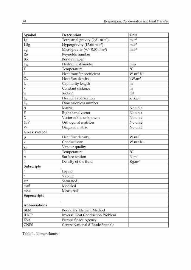
Evaporation, Condensation and Heat Transfer
74
Symbol Description Unit 1g Terrestrial gravity (9,81 m.s-2) m.s-2 1,8g Hypergravity (17,66 m.s-2) m.s-2 µg Microgravity (+/- 0,05 m.s-2) m.s-2 Re Reynolds number Bo Bond number Dh Hydraulic diameter mm T Temperature °C h Heat transfer coefficient W.m-2.K-1 Qw Heat flux density kW.m-2 Lc Capillarity length m x Constant distance m S Section m2 Lv Heat of vaporization kJ.kg-1 Fk Dimensionless number A Matrix No unit B Right hand vector No unit X Vector of the unknowns No unit U,V Orthogonal matrices No unit W Diagonal matrix No unit Greek symbol φ Heat flux density W.m-2 λ Conductivity W.m-1.K-1 χv Vapour quality θ Temperature °C σ Surface tension N.m-1 ρ Density of the fluid Kg.m-3 Subscripts l Liquid v Vapour sat Saturated mod Modeled meas Measured Superscripts Abbreviations BEM Boundary Element Method IHCP Inverse Heat Conduction Problem ESA Europe Space Agency CNES Centre National d’Etude Spatiale
Table 1. Nomenclature
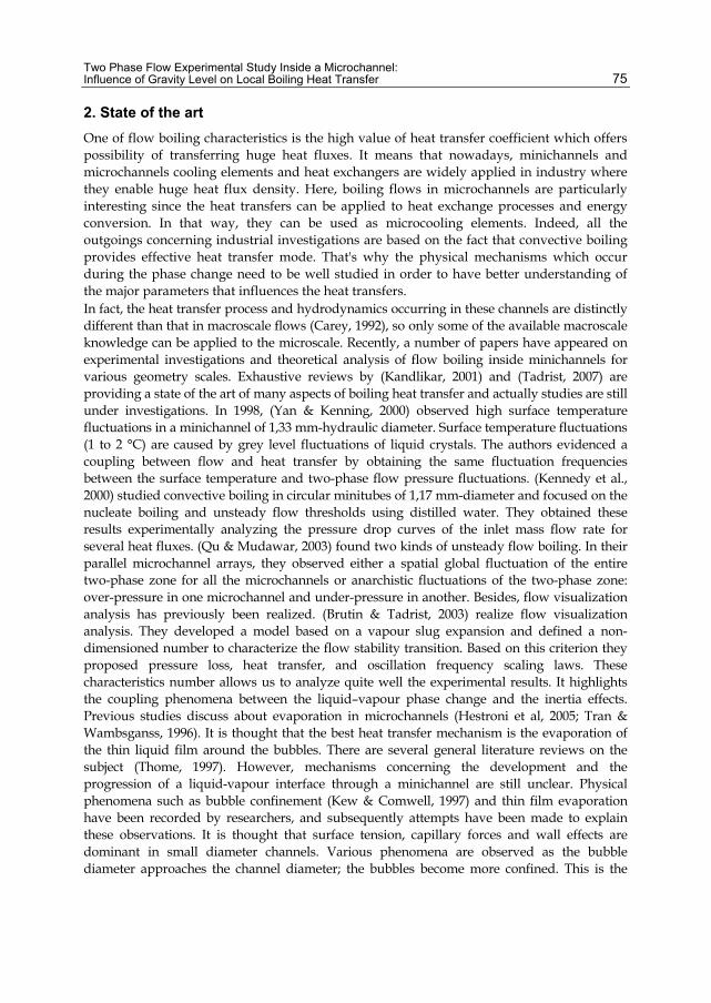
Two Phase Flow Experimental Study Inside a Microchannel: Influence of Gravity Level on Local Boiling Heat Transfer
75
2. State of the art One of flow boiling characteristics is the high value of heat transfer coefficient which offers possibility of transferring huge heat fluxes. It means that nowadays, minichannels and microchannels cooling elements and heat exchangers are widely applied in industry where they enable huge heat flux density. Here, boiling flows in microchannels are particularly interesting since the heat transfers can be applied to heat exchange processes and energy conversion. In that way, they can be used as microcooling elements. Indeed, all the outgoings concerning industrial investigations are based on the fact that convective boiling provides effective heat transfer mode. That's why the physical mechanisms which occur during the phase change need to be well studied in order to have better understanding of the major parameters that influences the heat transfers. In fact, the heat transfer process and hydrodynamics occurring in these channels are distinctly different than that in macroscale flows (Carey, 1992), so only some of the available macroscale knowledge can be applied to the microscale. Recently, a number of papers have appeared on experimental investigations and theoretical analysis of flow boiling inside minichannels for various geometry scales. Exhaustive reviews by (Kandlikar, 2001) and (Tadrist, 2007) are providing a state of the art of many aspects of boiling heat transfer and actually studies are still under investigations. In 1998, (Yan & Kenning, 2000) observed high surface temperature fluctuations in a minichannel of 1,33 mm-hydraulic diameter. Surface temperature fluctuations (1 to 2 °C) are caused by grey level fluctuations of liquid crystals. The authors evidenced a coupling between flow and heat transfer by obtaining the same fluctuation frequencies between the surface temperature and two-phase flow pressure fluctuations. (Kennedy et al., 2000) studied convective boiling in circular minitubes of 1,17 mm-diameter and focused on the nucleate boiling and unsteady flow thresholds using distilled water. They obtained these results experimentally analyzing the pressure drop curves of the inlet mass flow rate for several heat fluxes. (Qu & Mudawar, 2003) found two kinds of unsteady flow boiling. In their parallel microchannel arrays, they observed either a spatial global fluctuation of the entire two-phase zone for all the microchannels or anarchistic fluctuations of the two-phase zone: over-pressure in one microchannel and under-pressure in another. Besides, flow visualization analysis has previously been realized. (Brutin & Tadrist, 2003) realize flow visualization analysis. They developed a model based on a vapour slug expansion and defined a non-dimensioned number to characterize the flow stability transition. Based on this criterion they proposed pressure loss, heat transfer, and oscillation frequency scaling laws. These characteristics number allows us to analyze quite well the experimental results. It highlights the coupling phenomena between the liquid–vapour phase change and the inertia effects. Previous studies discuss about evaporation in microchannels (Hestroni et al, 2005; Tran & Wambsganss, 1996). It is thought that the best heat transfer mechanism is the evaporation of the thin liquid film around the bubbles. There are several general literature reviews on the subject (Thome, 1997). However, mechanisms concerning the development and the progression of a liquid-vapour interface through a minichannel are still unclear. Physical phenomena such as bubble confinement (Kew & Comwell, 1997) and thin film evaporation have been recorded by researchers, and subsequently attempts have been made to explain these observations. It is thought that surface tension, capillary forces and wall effects are dominant in small diameter channels. Various phenomena are observed as the bubble diameter approaches the channel diameter; the bubbles become more confined. This is the
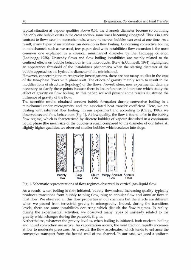
Evaporation, Condensation and Heat Transfer
76
typical situation at vapour qualities above 0.05, the channels diameter become so confining that only one bubble exists in the cross section, sometimes becoming elongated. This is in stark contrast to flows seen in macrochannels, where numerous bubbles can exist at one time. As a result, many types of instabilities can develop in flow boiling. Concerning convective boiling in minichannels such as we used, few papers deal with instabilities: flow excursion is the most common one explained in a classical minichannel diameter by the Ledinegg criterion (Ledinegg, 1938). Unsteady flows and flow boiling instabilities are mainly related to the confined effects on bubble behaviour in the microducts, (Kew &.Comwell, 1994) highlighted an appearance threshold of the instabilities phenomena when the starting diameter of the bubble approaches the hydraulic diameter of the minichannel. However, concerning the microgravity investigations, there are not many studies in the case of the two-phase flows with phase shift. The effects of gravity mainly seem to result in the modifications of structure (topology) of the flows. Nevertheless, new experimental data are necessary to clarify these points because there is less references in literature which study the effect of gravity on flow boiling. In this paper, we will present some results illustrated the influence of gravity of the flow. The scientific results obtained concern bubble formation during convective boiling in a minichannel under microgravity and the associated heat transfer coefficient. Here, we are dealing with saturated flow boiling. In our experiment and according to (Carey, 1992), we observed several flow behaviours (Fig. 1). At low quality, the flow is found to be in the bubbly flow regime, which is characterized by discrete bubbles of vapour disturbed in a continuous liquid phase (the mean size of the bubbles is small compared to the diameter of our tube). At slightly higher qualities, we observed smaller bubbles which coalesce into slugs.
Fig. 1. Schematic representations of flow regimes observed in vertical gas-liquid flow.
As a result, when boiling is first initiated, bubbly flow exists. Increasing quality typically produces transitions from bubbly to plug flow, plug to annular flow and annular flow to mist flow. We observed all this flow properties in our channels but the effects are different when we passed from terrestrial gravity to microgravity. Indeed, during the transitions levels, there are some instabilities occurring which disturb the flow regimes. In reality, during the experimental activities, we observed many types of unsteady related to the gravity which changes during the parabolic flights. Nethertheless, whatever the gravity level is, when boiling is initiated, both nucleate boiling and liquid convection are active. As vaporization occurs, the void fraction rapidly increases at low to moderate pressures. As a result, the flow accelerates, which tends to enhance the convective transport from the heated wall of the channel. In our case, we used a uniform
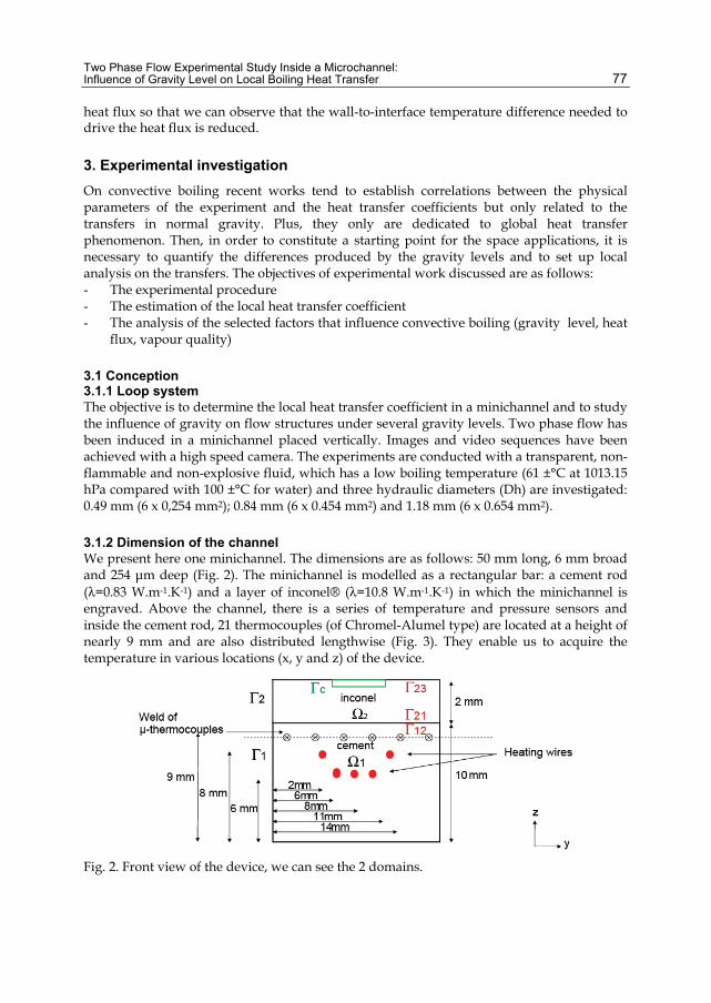
Two Phase Flow Experimental Study Inside a Microchannel: Influence of Gravity Level on Local Boiling Heat Transfer
77
heat flux so that we can observe that the wall-to-interface temperature difference needed to drive the heat flux is reduced.
3. Experimental investigation On convective boiling recent works tend to establish correlations between the physical parameters of the experiment and the heat transfer coefficients but only related to the transfers in normal gravity. Plus, they only are dedicated to global heat transfer phenomenon. Then, in order to constitute a starting point for the space applications, it is necessary to quantify the differences produced by the gravity levels and to set up local analysis on the transfers. The objectives of experimental work discussed are as follows: - The experimental procedure - The estimation of the local heat transfer coefficient - The analysis of the selected factors that influence convective boiling (gravity level, heat
flux, vapour quality)
3.1 Conception 3.1.1 Loop system The objective is to determine the local heat transfer coefficient in a minichannel and to study the influence of gravity on flow structures under several gravity levels. Two phase flow has been induced in a minichannel placed vertically. Images and video sequences have been achieved with a high speed camera. The experiments are conducted with a transparent, non-flammable and non-explosive fluid, which has a low boiling temperature (61 ±°C at 1013.15 hPa compared with 100 ±°C for water) and three hydraulic diameters (Dh) are investigated: 0.49 mm (6 x 0,254 mm2); 0.84 mm (6 x 0.454 mm2) and 1.18 mm (6 x 0.654 mm2).
3.1.2 Dimension of the channel We present here one minichannel. The dimensions are as follows: 50 mm long, 6 mm broad and 254 μm deep (Fig. 2). The minichannel is modelled as a rectangular bar: a cement rod (λ=0.83 W.m-1.K-1) and a layer of inconel® (λ=10.8 W.m-1.K-1) in which the minichannel is engraved. Above the channel, there is a series of temperature and pressure sensors and inside the cement rod, 21 thermocouples (of Chromel-Alumel type) are located at a height of nearly 9 mm and are also distributed lengthwise (Fig. 3). They enable us to acquire the temperature in various locations (x, y and z) of the device.
Fig. 2. Front view of the device, we can see the 2 domains.
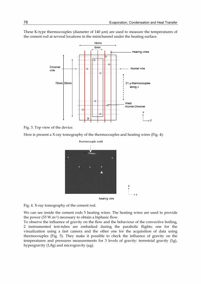
Evaporation, Condensation and Heat Transfer
78
These K-type thermocouples (diameter of 140 µm) are used to measure the temperatures of the cement rod at several locations in the minichannel under the heating surface.
Fig. 3. Top view of the device.
Here is present a X-ray tomography of the thermocouples and heating wires (Fig. 4):
Fig. 4. X-ray tomography of the cement rod.
We can see inside the cement rods 5 heating wires. The heating wires are used to provide the power (33 W.m-1) necessary to obtain a biphasic flow. To observe the influence of gravity on the flow and the behaviour of the convective boiling, 2 instrumented test-tubes are embarked during the parabolic flights; one for the visualization using a fast camera and the other one for the acquisition of data using thermocouples (Fig. 5). They make it possible to check the influence of gravity on the temperatures and pressures measurements for 3 levels of gravity: terrestrial gravity (1g), hypergravity (1,8g) and microgravity (µg).
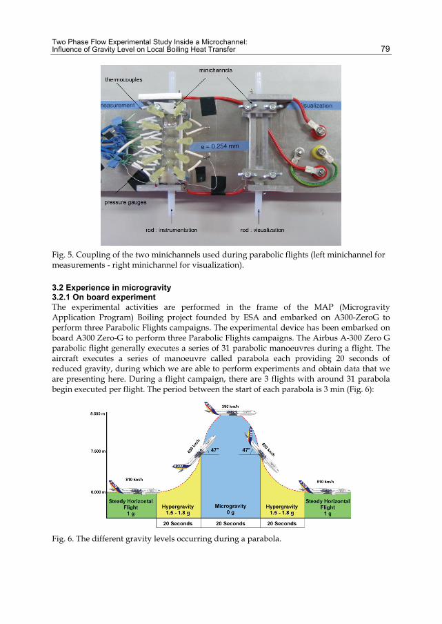
Two Phase Flow Experimental Study Inside a Microchannel: Influence of Gravity Level on Local Boiling Heat Transfer
79
Fig. 5. Coupling of the two minichannels used during parabolic flights (left minichannel for measurements - right minichannel for visualization).
3.2 Experience in microgravity 3.2.1 On board experiment The experimental activities are performed in the frame of the MAP (Microgravity Application Program) Boiling project founded by ESA and embarked on A300-ZeroG to perform three Parabolic Flights campaigns. The experimental device has been embarked on board A300 Zero-G to perform three Parabolic Flights campaigns. The Airbus A-300 Zero G parabolic flight generally executes a series of 31 parabolic manoeuvres during a flight. The aircraft executes a series of manoeuvre called parabola each providing 20 seconds of reduced gravity, during which we are able to perform experiments and obtain data that we are presenting here. During a flight campaign, there are 3 flights with around 31 parabola begin executed per flight. The period between the start of each parabola is 3 min (Fig. 6):
Fig. 6. The different gravity levels occurring during a parabola.
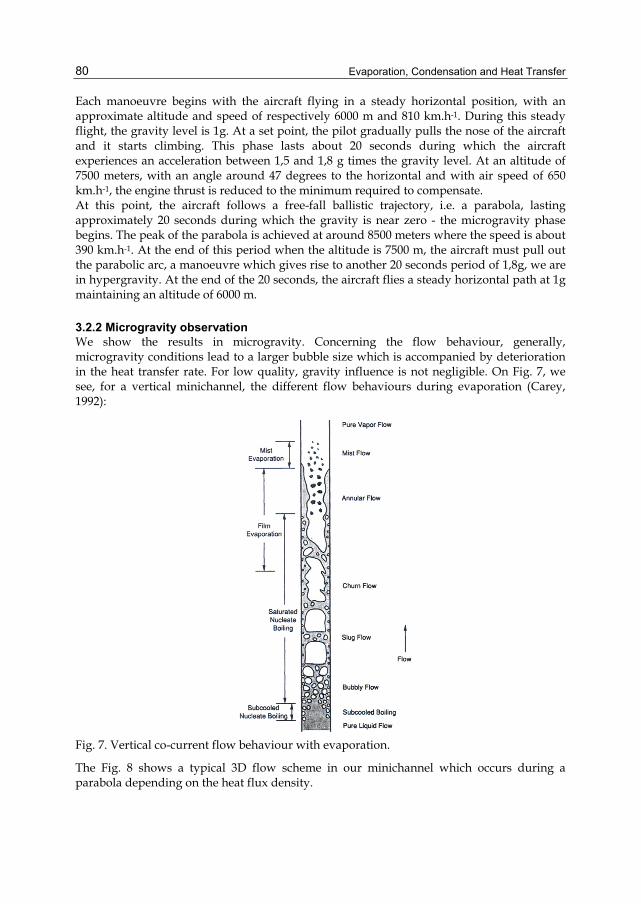
Evaporation, Condensation and Heat Transfer
80
Each manoeuvre begins with the aircraft flying in a steady horizontal position, with an approximate altitude and speed of respectively 6000 m and 810 km.h-1. During this steady flight, the gravity level is 1g. At a set point, the pilot gradually pulls the nose of the aircraft and it starts climbing. This phase lasts about 20 seconds during which the aircraft experiences an acceleration between 1,5 and 1,8 g times the gravity level. At an altitude of 7500 meters, with an angle around 47 degrees to the horizontal and with air speed of 650 km.h-1, the engine thrust is reduced to the minimum required to compensate. At this point, the aircraft follows a free-fall ballistic trajectory, i.e. a parabola, lasting approximately 20 seconds during which the gravity is near zero - the microgravity phase begins. The peak of the parabola is achieved at around 8500 meters where the speed is about 390 km.h-1. At the end of this period when the altitude is 7500 m, the aircraft must pull out the parabolic arc, a manoeuvre which gives rise to another 20 seconds period of 1,8g, we are in hypergravity. At the end of the 20 seconds, the aircraft flies a steady horizontal path at 1g maintaining an altitude of 6000 m.
3.2.2 Microgravity observation We show the results in microgravity. Concerning the flow behaviour, generally, microgravity conditions lead to a larger bubble size which is accompanied by deterioration in the heat transfer rate. For low quality, gravity influence is not negligible. On Fig. 7, we see, for a vertical minichannel, the different flow behaviours during evaporation (Carey, 1992):
Fig. 7. Vertical co-current flow behaviour with evaporation.
The Fig. 8 shows a typical 3D flow scheme in our minichannel which occurs during a parabola depending on the heat flux density.
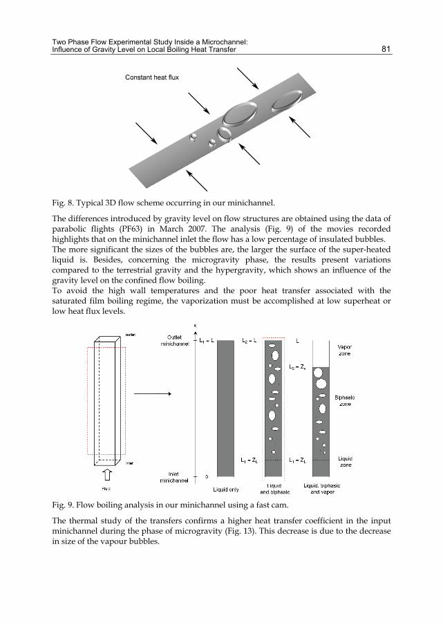
Two Phase Flow Experimental Study Inside a Microchannel: Influence of Gravity Level on Local Boiling Heat Transfer
81
Fig. 8. Typical 3D flow scheme occurring in our minichannel.
The differences introduced by gravity level on flow structures are obtained using the data of parabolic flights (PF63) in March 2007. The analysis (Fig. 9) of the movies recorded highlights that on the minichannel inlet the flow has a low percentage of insulated bubbles. The more significant the sizes of the bubbles are, the larger the surface of the super-heated liquid is. Besides, concerning the microgravity phase, the results present variations compared to the terrestrial gravity and the hypergravity, which shows an influence of the gravity level on the confined flow boiling. To avoid the high wall temperatures and the poor heat transfer associated with the saturated film boiling regime, the vaporization must be accomplished at low superheat or low heat flux levels.
Fig. 9. Flow boiling analysis in our minichannel using a fast cam.
The thermal study of the transfers confirms a higher heat transfer coefficient in the input minichannel during the phase of microgravity (Fig. 13). This decrease is due to the decrease in size of the vapour bubbles.
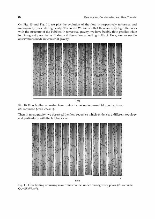
Evaporation, Condensation and Heat Transfer
82
On Fig. 10 and Fig. 11, we plot the evolution of the flow in respectively terrestrial and microgravity phase during nearly 20 seconds. We can see that there are very big differences with the structure of the bubbles. In terrestrial gravity, we have bubbly flow profiles while in microgravity we deal with slug and churn flow according to Fig. 7. Here, we can see the observations made in terrestrial gravity:
Fig. 10. Flow boiling occurring in our minichannel under terrestrial gravity phase (20 seconds, Qw=45 kW.m-2).
Then in microgravity, we observed the flow sequence which evidences a different topology and particularly with the bubble’s size.
Fig. 11. Flow boiling occurring in our minichannel under microgravity phase (20 seconds, Qw=45 kW.m-2).
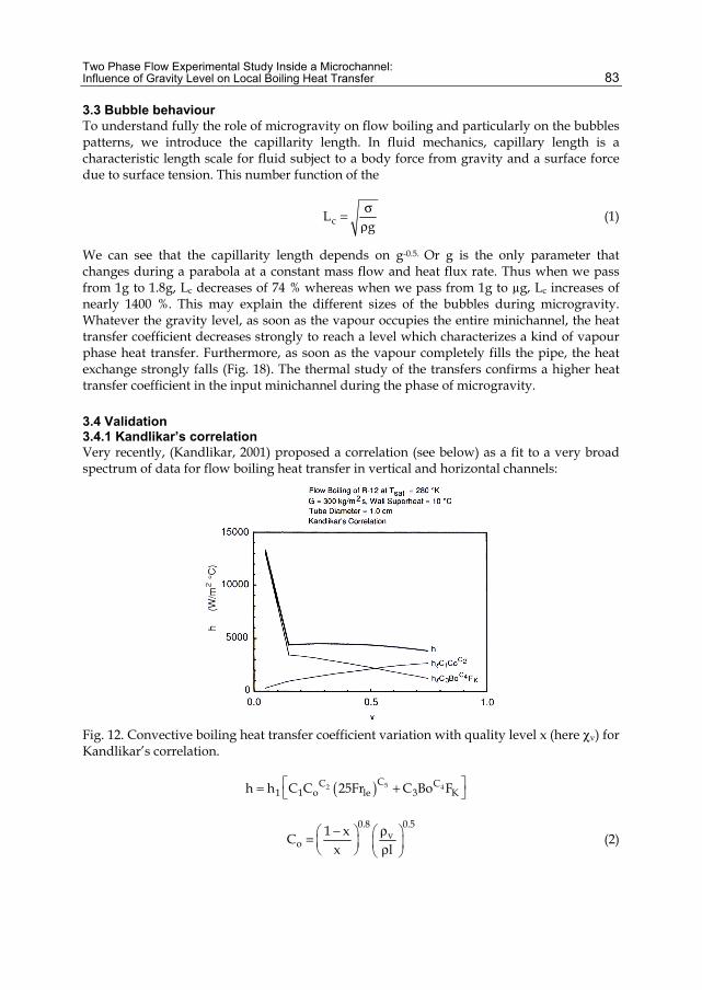
Two Phase Flow Experimental Study Inside a Microchannel: Influence of Gravity Level on Local Boiling Heat Transfer
83
3.3 Bubble behaviour To understand fully the role of microgravity on flow boiling and particularly on the bubbles patterns, we introduce the capillarity length. In fluid mechanics, capillary length is a characteristic length scale for fluid subject to a body force from gravity and a surface force due to surface tension. This number function of the
cLg
σ=ρ
(1)
We can see that the capillarity length depends on g-0.5. Or g is the only parameter that changes during a parabola at a constant mass flow and heat flux rate. Thus when we pass from 1g to 1.8g, Lc decreases of 74 % whereas when we pass from 1g to µg, Lc increases of nearly 1400 %. This may explain the different sizes of the bubbles during microgravity. Whatever the gravity level, as soon as the vapour occupies the entire minichannel, the heat transfer coefficient decreases strongly to reach a level which characterizes a kind of vapour phase heat transfer. Furthermore, as soon as the vapour completely fills the pipe, the heat exchange strongly falls (Fig. 18). The thermal study of the transfers confirms a higher heat transfer coefficient in the input minichannel during the phase of microgravity.
3.4 Validation 3.4.1 Kandlikar’s correlation Very recently, (Kandlikar, 2001) proposed a correlation (see below) as a fit to a very broad spectrum of data for flow boiling heat transfer in vertical and horizontal channels:
Fig. 12. Convective boiling heat transfer coefficient variation with quality level x (here χv) for Kandlikar’s correlation.
( ) 52 4CC C1 1 o le 3 Kh h C C 25Fr C Bo F⎡ ⎤= +⎣ ⎦
0.8 0.5
vo
1 xCx l− ρ⎛ ⎞ ⎛ ⎞= ⎜ ⎟ ⎜ ⎟ρ⎝ ⎠ ⎝ ⎠
(2)
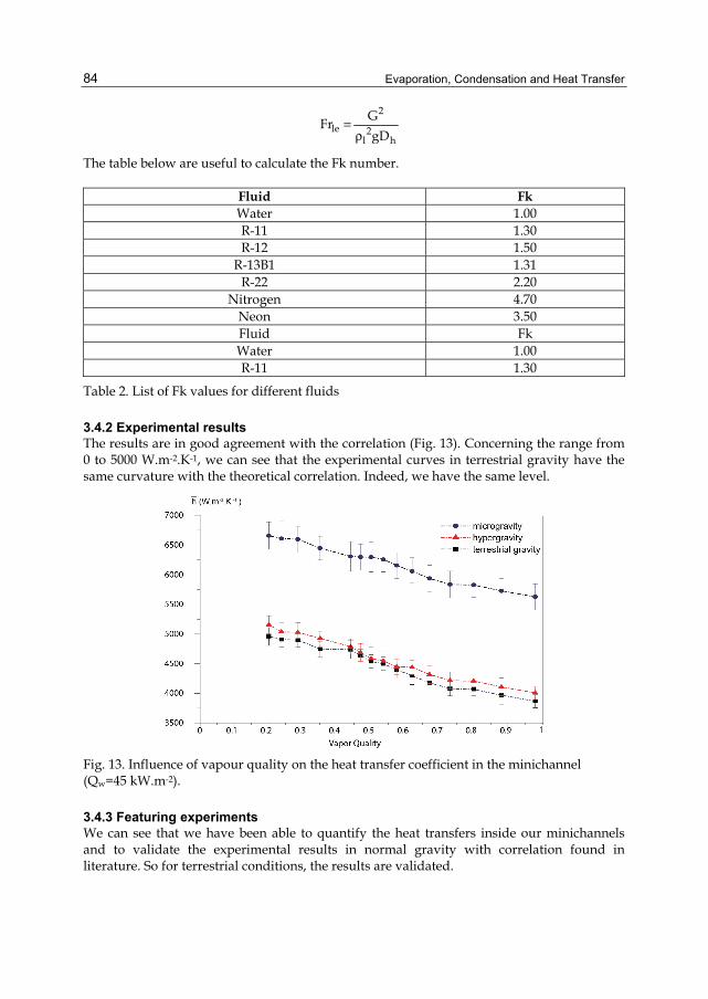
Evaporation, Condensation and Heat Transfer
84
2
le 2l h
GFrgD
=ρ
The table below are useful to calculate the Fk number.
Fluid Fk Water 1.00 R-11 1.30 R-12 1.50
R-13B1 1.31 R-22 2.20
Nitrogen 4.70 Neon 3.50 Fluid Fk Water 1.00 R-11 1.30
Table 2. List of Fk values for different fluids
3.4.2 Experimental results The results are in good agreement with the correlation (Fig. 13). Concerning the range from 0 to 5000 W.m-2.K-1, we can see that the experimental curves in terrestrial gravity have the same curvature with the theoretical correlation. Indeed, we have the same level.
Fig. 13. Influence of vapour quality on the heat transfer coefficient in the minichannel (Qw=45 kW.m-2).
3.4.3 Featuring experiments We can see that we have been able to quantify the heat transfers inside our minichannels and to validate the experimental results in normal gravity with correlation found in literature. So for terrestrial conditions, the results are validated.
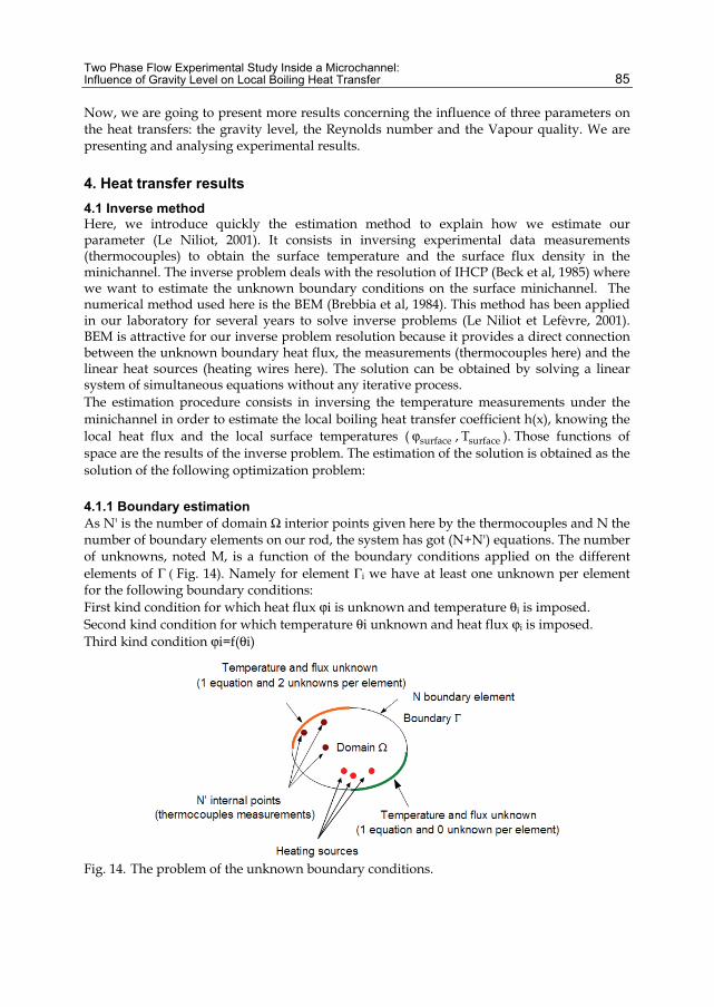
Two Phase Flow Experimental Study Inside a Microchannel: Influence of Gravity Level on Local Boiling Heat Transfer
85
Now, we are going to present more results concerning the influence of three parameters on the heat transfers: the gravity level, the Reynolds number and the Vapour quality. We are presenting and analysing experimental results.
4. Heat transfer results 4.1 Inverse method Here, we introduce quickly the estimation method to explain how we estimate our parameter (Le Niliot, 2001). It consists in inversing experimental data measurements (thermocouples) to obtain the surface temperature and the surface flux density in the minichannel. The inverse problem deals with the resolution of IHCP (Beck et al, 1985) where we want to estimate the unknown boundary conditions on the surface minichannel. The numerical method used here is the BEM (Brebbia et al, 1984). This method has been applied in our laboratory for several years to solve inverse problems (Le Niliot et Lefèvre, 2001). BEM is attractive for our inverse problem resolution because it provides a direct connection between the unknown boundary heat flux, the measurements (thermocouples here) and the linear heat sources (heating wires here). The solution can be obtained by solving a linear system of simultaneous equations without any iterative process. The estimation procedure consists in inversing the temperature measurements under the minichannel in order to estimate the local boiling heat transfer coefficient h(x), knowing the local heat flux and the local surface temperatures ( surfaceϕ , surfaceT ). Those functions of space are the results of the inverse problem. The estimation of the solution is obtained as the solution of the following optimization problem:
4.1.1 Boundary estimation As N' is the number of domain Ω interior points given here by the thermocouples and N the number of boundary elements on our rod, the system has got (N+N') equations. The number of unknowns, noted M, is a function of the boundary conditions applied on the different elements of Γ ( Fig. 14). Namely for element Γi we have at least one unknown per element for the following boundary conditions: First kind condition for which heat flux ϕi is unknown and temperature θi is imposed. Second kind condition for which temperature θi unknown and heat flux ϕi is imposed. Third kind condition ϕi=f(θi)
Fig. 14. The problem of the unknown boundary conditions.
Evaporation, Condensation and Heat Transfer
86
The elements, for which we have one equation, where the boundary condition is missing, let appear two unknowns. The only way to solve the fundamental heat transfer equation is to find some extra information, provided by measurements. In our case, we have interior measurements, given by thermocouples. They enable us with the knowledge of the boundary conditions to solve the problem and to calculate local heat flux and local surface temperatures along the minichannel. This estimation procedure consists in inversing the temperature measurements under the minichannel in order to estimate the local boiling heat transfer coefficient h(x). Those functions of space are the results of the inverse problem. The estimation of the solution is obtained using BEM as the solution of the following optimization problem:
( ){ }mod measT Tˆ ˆT ,surface surface −φ = arg min (3)
In this last expression, the vectors measT and modT respectively represent the vector of temperature measurements and the vector of the calculated temperatures. The unknown factors ( surfaceϕ , surfaceT ) are obtained by minimizing the difference between measurements and a mathematical modeling. Taking into account the specificity of formulation BEM., this minimization is not obtained explicitly but done through a function utilizing a linear combination of measurements. This formulation leads to a matrix system of simultaneous equation :
X = BA (4)
In this last equation, A is a matrix of dimension ((N+N)'×M), X the vector of the M unknowns including ( surfaceϕ , surfaceT ) and B of dimension (N+N') is containing a linear combination of the data measurements. If M=N+N' we obtain a square system of linear equation but most of the time we have M<N+N' and has more equations than unknown (see Sensitivity Study chapter) : our system presents 270 equations for 255 unknown factors (overdetermined system). A solution can be found by minimising the distance between vector AX and vector B. In order to find out an estimation X of the unknown exact solution X, we have to solve the optimization problem using a cost function (5). Assuming that the difference between AX and B can be considered as distributed according a Gaussian law we can find X solution of in the meaning of the least squares. Using this last property leads to the Ordinary Least Squares solution :
ˆ ⎧ ⎫⎛ ⎞⎜ ⎟⎨ ⎬⎝ ⎠⎩ ⎭
2X = arg min AX -B (5)
( ) ( )X = BT TA A A (6)
Actually, the inverse heat condition problem is ill-posed and very sensitive to the measurements errors. Considering the numerical aspects of the inversion, we obtain an ill-conditioned square matrix (ATA). Thus, we observe for the system numerical resolution an instability of the solution X with regards to the measurements the errors introduced into the vector B. As a consequence, we need to obtain a stable the solution of this system by using regularizations tools – Hansen. We propose in the following paragraph an example of
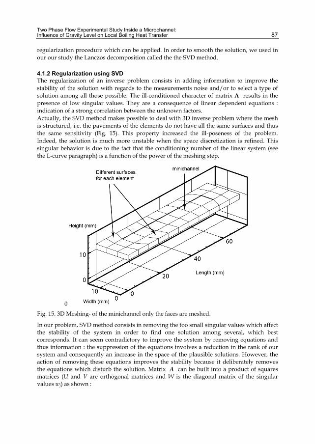
Two Phase Flow Experimental Study Inside a Microchannel: Influence of Gravity Level on Local Boiling Heat Transfer
87
regularization procedure which can be applied. In order to smooth the solution, we used in our our study the Lanczos decomposition called the the SVD method.
4.1.2 Regularization using SVD The regularization of an inverse problem consists in adding information to improve the stability of the solution with regards to the measurements noise and/or to select a type of solution among all those possible. The ill-conditioned character of matrix A results in the presence of low singular values. They are a consequence of linear dependent equations : indication of a strong correlation between the unknown factors. Actually, the SVD method makes possible to deal with 3D inverse problem where the mesh is structured, i.e. the pavements of the elements do not have all the same surfaces and thus the same sensitivity (Fig. 15). This property increased the ill-poseness of the problem. Indeed, the solution is much more unstable when the space discretization is refined. This singular behavior is due to the fact that the conditioning number of the linear system (see the L-curve paragraph) is a function of the power of the meshing step.
0
Fig. 15. 3D Meshing- of the minichannel only the faces are meshed.
In our problem, SVD method consists in removing the too small singular values which affect the stability of the system in order to find one solution among several, which best corresponds. It can seem contradictory to improve the system by removing equations and thus information : the suppression of the equations involves a reduction in the rank of our system and consequently an increase in the space of the plausible solutions. However, the action of removing these equations improves the stability because it deliberately removes the equations which disturb the solution. Matrix A can be built into a product of squares matrices (U and V are orthogonal matrices and W is the diagonal matrix of the singular values wj) as shown :
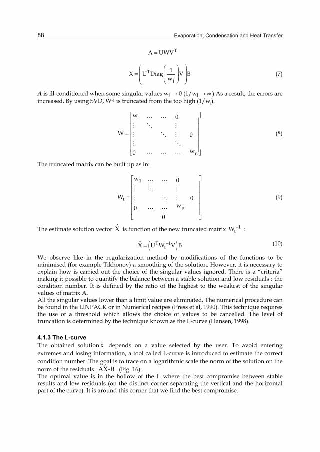
Evaporation, Condensation and Heat Transfer
88
TA UWV=
T
j
1X U Diag V Bw
⎛ ⎞⎛ ⎞⎜ ⎟⎜ ⎟=
⎜ ⎟⎜ ⎟⎝ ⎠⎝ ⎠ (7)
A is ill-conditioned when some singular values wj → 0 (1/wj →∞ ).As a result, the errors are increased. By using SVD, W-1 is truncated from the too high (1/wj).
1
n
w 0
W 0
w0
⎡ ⎤⎢ ⎥⎢ ⎥⎢ ⎥=⎢ ⎥⎢ ⎥⎢ ⎥⎣ ⎦
(8)
The truncated matrix can be built up as in:
1
t
p
w 0
W 0w0
0
⎡ ⎤⎢ ⎥⎢ ⎥⎢ ⎥=⎢ ⎥⎢ ⎥⎢ ⎥⎣ ⎦
(9)
The estimate solution vector X is function of the new truncated matrix 1tW − :
( )T 1tX U W V B−= (10)
We observe like in the regularization method by modifications of the functions to be minimised (for example Tikhonov) a smoothing of the solution. However, it is necessary to explain how is carried out the choice of the singular values ignored. There is a “criteria” making it possible to quantify the balance between a stable solution and low residuals : the condition number. It is defined by the ratio of the highest to the weakest of the singular values of matrix A. All the singular values lower than a limit value are eliminated. The numerical procedure can be found in the LINPACK or in Numerical recipes (Press et al, 1990). This technique requires the use of a threshold which allows the choice of values to be cancelled. The level of truncation is determined by the technique known as the L-curve (Hansen, 1998).
4.1.3 The L-curve The obtained solution X depends on a value selected by the user. To avoid entering extremes and losing information, a tool called L-curve is introduced to estimate the correct condition number. The goal is to trace on a logarithmic scale the norm of the solution on the norm of the residuals AX-Bˆ (Fig. 16). The optimal value is in the hollow of the L where the best compromise between stable results and low residuals (on the distinct corner separating the vertical and the horizontal part of the curve). It is around this corner that we find the best compromise.
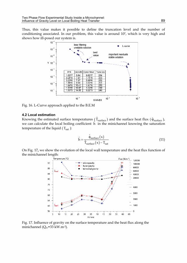
Two Phase Flow Experimental Study Inside a Microchannel: Influence of Gravity Level on Local Boiling Heat Transfer
89
Thus, this value makes it possible to define the truncation level and the number of conditioning associated. In our problem, this value is around 107, which is very high and shows how ill-posed our system is.
Fig. 16. L-Curve approach applied to the B.E.M
4.2 Local estimation Knowing the estimated surface temperatures ( surfaceT ) and the surface heat flux ( surfaceϕ ), we can calculate the local boiling coefficient h in the minichannel knowing the saturation temperature of the liquid ( satT ):
( )( )
surface
surface sat
ˆ xh
T x Tφ
=−
(11)
On Fig. 17, we show the evolution of the local wall temperature and the heat flux function of the minichannel length:
Fig. 17. Influence of gravity on the surface temperature and the heat flux along the minichannel (Qw=33 kW.m-2).
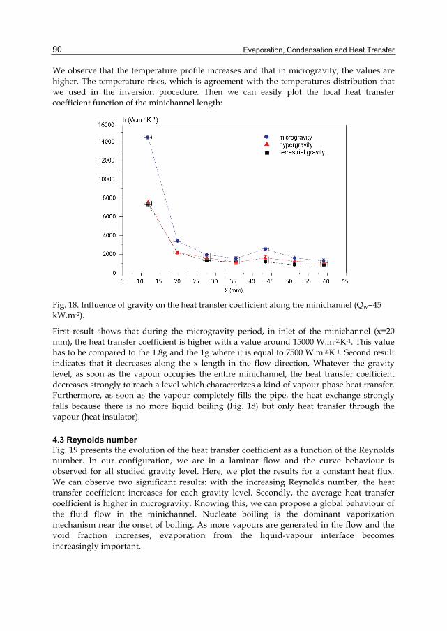
Evaporation, Condensation and Heat Transfer
90
We observe that the temperature profile increases and that in microgravity, the values are higher. The temperature rises, which is agreement with the temperatures distribution that we used in the inversion procedure. Then we can easily plot the local heat transfer coefficient function of the minichannel length:
Fig. 18. Influence of gravity on the heat transfer coefficient along the minichannel (Qw=45 kW.m-2).
First result shows that during the microgravity period, in inlet of the minichannel (x=20 mm), the heat transfer coefficient is higher with a value around 15000 W.m-2.K-1. This value has to be compared to the 1.8g and the 1g where it is equal to 7500 W.m-2.K-1. Second result indicates that it decreases along the x length in the flow direction. Whatever the gravity level, as soon as the vapour occupies the entire minichannel, the heat transfer coefficient decreases strongly to reach a level which characterizes a kind of vapour phase heat transfer. Furthermore, as soon as the vapour completely fills the pipe, the heat exchange strongly falls because there is no more liquid boiling (Fig. 18) but only heat transfer through the vapour (heat insulator).
4.3 Reynolds number Fig. 19 presents the evolution of the heat transfer coefficient as a function of the Reynolds number. In our configuration, we are in a laminar flow and the curve behaviour is observed for all studied gravity level. Here, we plot the results for a constant heat flux. We can observe two significant results: with the increasing Reynolds number, the heat transfer coefficient increases for each gravity level. Secondly, the average heat transfer coefficient is higher in microgravity. Knowing this, we can propose a global behaviour of the fluid flow in the minichannel. Nucleate boiling is the dominant vaporization mechanism near the onset of boiling. As more vapours are generated in the flow and the void fraction increases, evaporation from the liquid-vapour interface becomes increasingly important.

Two Phase Flow Experimental Study Inside a Microchannel: Influence of Gravity Level on Local Boiling Heat Transfer
91
Fig. 19. Influence of Reynolds number on the average heat transfer coefficient in the minichannel (Qw=45 kW.m-2).
4.4 Local quality We plot the local vapour quality as a function of the x-axis of the minichannel using the following equation:
wv
v l v
Q x(x)SL u
χ =ρ
(12)
First results (Fig. 20) show that the local quality increases along the main axis from the inlet to the outlet of the channel. This is in good agreement with the temperature profile we have on the boundary minichannel since at the outlet the temperature is higher (Fig. 17).
Fig. 20. Influence of local vapor quality as a function of the main flow axis (Qw=45 kW.m-2).
Evaporation, Condensation and Heat Transfer
92
A second result shows a non linear evolution because in our case the heat flux density is not constant. Indeed, the QW calculated on the wall minichannel varies around 2 %. This result is explicit at the inlet minichannel where we observe a short decrease since the error estimation is higher around these points. Besides, at the outlet minichannel, the local vapour quality (x=60 mm) tends to reach a value corresponding to the global outlet vapour quality.
v
out wv Total
w
⎛ ⎞χ = ⎜ ⎟⎜ ⎟
⎝ ⎠ (13)
When we are at the edges of our channel, the local value is close to the outlet vapour quality:
outv vx L
lim (x)→
χ = χ (14)
Where x is the abscissa of the minichannel and L is the final length. This comparison is used to validate our results. Here, we have plot four tends of the local vapour quality as a function of the minichannel axis. We observe on Fig. 13, that the heat transfer coefficient profile for the terrestrial gravity decreases when the vapour quality increases. This is in good agreement with our experimental data under terrestrial gravity conditions. Indeed, as quality increases, the Kandlikar correlation predicts a steadily decreasing heat transfer coefficient. The nucleate boiling contribution diminishes while the forced-convective effect decreases and there is a steady drop in heat transfer coefficient with quality. However, the experimental results can only be compared during terrestrial gravity because when we are in microgravity and hypergravity, the correlations is no longer valid. Actually, we can't find a model that predicts the behaviour of the boiling heat transfer coefficient when the gravity level changes. Plus, with the increasing Re, the outlet vapour fraction is decreasing meaning that the average vapour fraction is lower and dry out has less influence on heat transfer.
5. Conclusion and perspectives A study of two-phase flow regimes in a vertical rectangular minichannel is performed. Actually, flow boiling heat transfer in microgravity has received relatively little attention. Thus, the few experiments and the short duration of microgravity conditions do not allow a full understanding of the mechanisms controlling flow boiling heat transfers. But it is a starting point. In this study, we gathered all the results highlighted the influence of gravity on convective boiling in minichannels. Local values of wall surface temperature; heat flux and heat transfers were done and helped us to construct boiling curves. We perform analysis of the selected parameters which influence the mechanisms. Indeed, the analysis of temperature as a function of g confirms that gravity has an influence on flow and heat transfer. The microgravity generates vapour pocket structures which fill the width of the minichannel and the heat transfer coefficient is locally higher. Consequently, we can assume that microgravity influences the appearance of the vapour bubbles whose size varies depending parameter g. In the case of hypergravity and normal gravity, a classical bubbly flow structure is observed. Concerning the inverse method, we were able to solve a 3D IHCP. For the inverse methods, the sensors induce too many disturbances and accentuate the ill-posed character. These uncertainties lead to clear variations in the solution and particularly in the surface heat flux. One solution would be to add IR (infra-red)
Two Phase Flow Experimental Study Inside a Microchannel: Influence of Gravity Level on Local Boiling Heat Transfer
93
measurements while painting the lower face of the cement in black and placing a camera directly below and another would be to destroy the minichannels to estimate the locations of the thermocouples. In addition, all the experimental data are not totally transient. Indeed, we have some gravity phase changes which are steady so that using a normal steady approach to study convective boiling was successfully done. Thus, to use all our experimental data and to confirm our results, prediction of the convective boiling heat transfer coefficient requires a transient approach. That’s why we need to take into account these dynamic instabilities for further results. In outgoing experiments, to deal with more experimental data from the Parabolic Flight campaign, we will perform this transient formulation.
6. Acknowledgment We would especially like to thank the CNES (793/2002/CNES/8665) and ESA (MAP Boiling) for their financial support. We thank them for giving us access to the experimentation in microgravity on board the A300 Zero-G. We would also like to express our gratitude to Novespace® and more especially to Mr. Mora and Mr. Gai for their technical assistance during the campaigns PF52/CNES and PF53/ESA
7. References Carey V. P. (1992). Liquid-Vapour Phase Change Phenomena, Hemisphere Publishing
Corporation, New York Kandlikar S. G.(2001). Fundamental issues related to flow boiling in minichannels and
microchannels, Experiental Heat Transfer, Fluid Mechanics and Thermodynamics, Vol.1, Edizioni ETS, PISA, 2001.
Tadrist L. (October 2007). Flow Boiling in Microgravity Condition: Investigation Using Inverse Techniques. J. of Microgravity Science and Technology, October 26-28.
Yan Y. and Kenning D. B. R.(1998) Pressure fluctuations during boiling in a narrow channel. HTFS Research Symposium.
Kennedy J. E., Roach G. M., Dowling M. F., Abdel-Khalik S. I., Ghiaasiaan S. M., Jeter S. M., and Quershi Z. H.(February 2000). The onset of flow instability in uniformly heated horizontal microchannels. Journal of Heat Transfer, 122:118–125.
Qu W., Mudawar I. (2003). Flow boiling heat transfer in two-phase micro-channel heat sinks: Experimental investigation and assessment of correlations methods. International Journal of Heat and Mass Transfer, 46.
Brutin D. and Tadrist L. (October 2006). Destabilization mechanisms and scaling laws of convective boiling in a minichannel. AIAA Journal of Thermophysics and Heat Transfers, 20.
Hestroni G. et al.(2005). Fluid flow in microchannels. International Journal of Heat and Mass Transfer, pages 1982-1998.
Tran T.N., Wambsganss M.W. and D.M. (1996). Small circular and rectangular channel boiling with two refrigerants, International Journal of Multiphase Flow, pages 485-498.
Thome J.R. (2004). Boiling in microchannels: a review of experiment and theory. International Journal of Heat and Fluid Flow, pages 128-139.
Kew P.A. and Cornwell K. (1997). Correlations for the prediction of boiling heat transfer in small-diameter channels. Applied Thermal Engineering, pages 705-715.
Evaporation, Condensation and Heat Transfer
94
Ledinegg M. (1938). Instability flow during natural forced circulation, Warme, 61(8) :891-898. P. A. Kew and K. Cornwell. Confined bubble flow and boiling in narrow spaces. In 2nd, Int.
Heat Transfer Conference, Brighton 7, pages 473-478, 1994. J.V. Beck, B. Blackwell, C.R. St. Clair (1985). Inverse Heat Conduction, Ill-Posed Problems,
Wiley Interscience, New York. Brebbia C.A., Telles J.C.F. and Wrobel L.C.(1984). Boundary Element Techniques, Springer-
Verlag, Berlin and New York. Le Niliot C., Lefèvre F. (2001). A method for multiple steady line heat sources identification
in a diffusive system: application to an experimental 2D problem, International Journal of Heat and Mass Transfer, vol. 44, pp. 1425-1438.
Press W.H., Flannery B. P., Teulossky S. A., Vetterling W. T. (1990). Numerical Recipes, Cambridge.
Hansen P.C. (1998). Rank-Deficient and discrete Ill-posed Problems, SIAM, Philadelphie.
5
The Evolution of Temperature Disturbances During Boiling of Cryogenic Liquids on
Heat-Releasing Surfaces Irina Starodubtseva and Aleksandr Pavlenko
Kutateladze Institute of Thermophysics Siberian Branch of Russian Academy of Sciences, Russia
1. Introduction This publication is devoted to studying the regularities of the dynamics of temperature disturbances on the heat-releasing surfaces during boiling of cryogenic liquids under conditions of free convection and in the flowing-down wave liquid films. Crisis phenomena and dynamics of transient processes at boiling are the subject of intense experimental and theoretical investigations. Nucleate boiling liquid is one of the most effective ways to remove heat from the heat-releasing surface. Temperature disturbances with different spatial-temporal scales occur on heat-releasing surface during boiling. Perturbations of the fluctuation character are the inner features of boiling. Crises of boiling liquids occur due to the change of boiling regimes with significantly different intensities of heat transfer. The transition from one regime to another occurs over a finite time, which is determined by the velocity of site propagation and the linear scale, which characterizes the average distance between the sites arising under the influence of different kinds of fluctuations. Knowledge of such characteristics as stability and speed of propagation of film boiling regime on heat-releasing surface is important in cryogenic fluids, for example, due to the necessity of cooling of superconducting devices. The emergence of film boiling and their expansion along the heat-transfer surface drastically affects the heat removal, leading to crash - overheating of the heater surface and to its destruction. Dry spots formed in the pre-crisis mode in falling liquid films are the analogous sites of film boiling. Film flow of liquids (including cryogenic) are widely used in various technological processes for intensification of heat and mass transfer. Evaporation in the thin films of liquid provides high heat transfer rate at low cost and low temperature difference. The topicality of this subject matter is relates, in particular, to the development of efficient and compact systems for cooling of the elements of electronics and computers and high-productivity graphical processors whose response and lifetime are substantially dependent on the efficiency of dissipated-power removal. This raises the need for reliable prediction of the critical heat flux, whose excess leads to the complete draining of heat-releasing surface and uncontrolled heating. Study of heat transfer during boiling and evaporation of cryogenic fluids, a number of properties (purity, good wettability, near zero contact angles) differ essentially from properties of high-temperature liquids, is important to deepen understanding of the processes. This is a way to test the existing model descriptions of heat transfer and the development of transient processes and crisis phenomena.
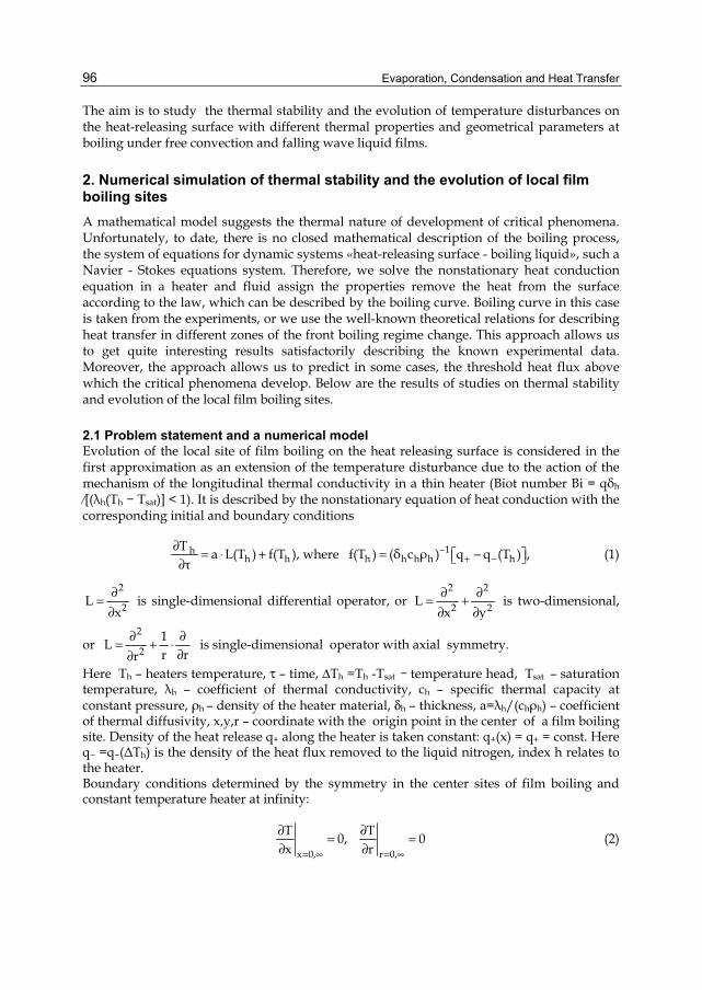
Evaporation, Condensation and Heat Transfer
96
The aim is to study the thermal stability and the evolution of temperature disturbances on the heat-releasing surface with different thermal properties and geometrical parameters at boiling under free convection and falling wave liquid films.
2. Numerical simulation of thermal stability and the evolution of local film boiling sites A mathematical model suggests the thermal nature of development of critical phenomena. Unfortunately, to date, there is no closed mathematical description of the boiling process, the system of equations for dynamic systems «heat-releasing surface - boiling liquid», such a Navier - Stokes equations system. Therefore, we solve the nonstationary heat conduction equation in a heater and fluid assign the properties remove the heat from the surface according to the law, which can be described by the boiling curve. Boiling curve in this case is taken from the experiments, or we use the well-known theoretical relations for describing heat transfer in different zones of the front boiling regime change. This approach allows us to get quite interesting results satisfactorily describing the known experimental data. Moreover, the approach allows us to predict in some cases, the threshold heat flux above which the critical phenomena develop. Below are the results of studies on thermal stability and evolution of the local film boiling sites.
2.1 Problem statement and a numerical model Evolution of the local site of film boiling on the heat releasing surface is considered in the first approximation as an extension of the temperature disturbance due to the action of the mechanism of the longitudinal thermal conductivity in a thin heater (Biot number Bi = qδh ⁄[(λh(Th − Tsat)] < 1). It is described by the nonstationary equation of heat conduction with the corresponding initial and boundary conditions
1hh h h h h h h
T a L(T ) f(T ), where f(T ) (δ c ρ ) q q (T ) ,τ
−+ −
∂ = ⋅ + = −⎡ ⎤⎣ ⎦∂ (1)
2
2Lx∂=∂
is single-dimensional differential operator, or 2 2
2 2Lx y∂ ∂= +∂ ∂
is two-dimensional,
or 2
21Lr rr
∂ ∂= + ⋅∂∂
is single-dimensional operator with axial symmetry.
Here Тh – heaters temperature, τ – time, ΔTh =Th -Tsat – temperature head, Tsat – saturation temperature, λh – coefficient of thermal conductivity, сh – specific thermal capacity at constant pressure, ρh – density of the heater material, δh – thickness, a=λh/(chρh) – coefficient of thermal diffusivity, х,y,r – coordinate with the origin point in the center of a film boiling site. Density of the heat release q+ along the heater is taken constant: q+(x) = q+ = const. Here q− =q−(ΔTh) is the density of the heat flux removed to the liquid nitrogen, index h relates to the heater. Boundary conditions determined by the symmetry in the center sites of film boiling and constant temperature heater at infinity:
x 0, r 0,
T T0, 0x r= ∞ = ∞
∂ ∂= =∂ ∂
(2)
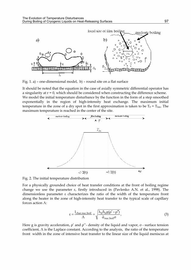
The Evolution of Temperature Disturbances During Boiling of Cryogenic Liquids on Heat-Releasing Surfaces
97
Fig. 1. а) – one-dimensional model, b) – round site on a flat surface
It should be noted that the equation in the case of axially symmetric differential operator has a singularity at r = 0, which should be considered when constructing the difference scheme. We model the initial temperature disturbance by the function in the form of a step smoothed exponentially in the region of high-intensity heat exchange. The maximum initial temperature in the zone of a dry spot in the first approximation is taken to be T0 = Tlim. The maximum temperature is reached in the center of the site.
Fig. 2. The initial temperature distribution
For a physically grounded choice of heat transfer conditions at the front of boiling regime change we use the parameter ε, firstly introduced in (Pavlenko A.N. et al., 1998). The dimensionless parameter ε characterizes the ratio of the width of the temperature front along the heater in the zone of high-intensity heat transfer to the typical scale of capillary forces action Λ:
h hchar.nuc.boil
nuc.boil
λ δ g(ρ ρ )lε ,Λ α σ
′ ′′−= = (3)
Here g is gravity acceleration, ρ’ and ρ’’- density of the liquid and vapor, σ - surface tension coefficient, Λ is the Laplace constant. According to the analysis, the ratio of the temperature front width in the zone of intensive heat transfer to the linear size of the liquid meniscus at
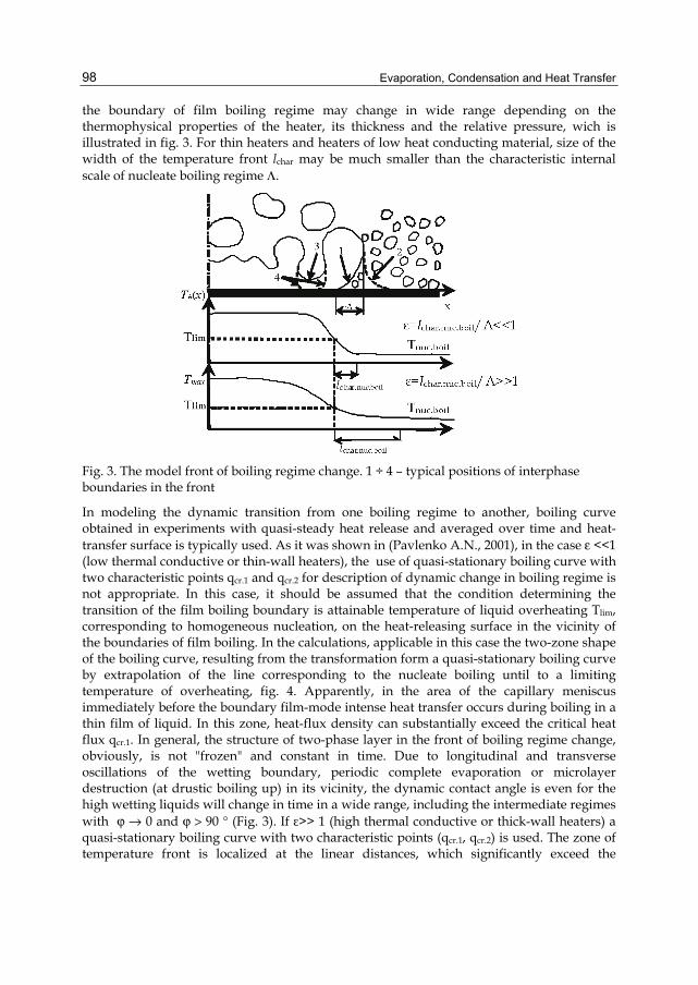
Evaporation, Condensation and Heat Transfer
98
the boundary of film boiling regime may change in wide range depending on the thermophysical properties of the heater, its thickness and the relative pressure, wich is illustrated in fig. 3. For thin heaters and heaters of low heat conducting material, size of the width of the temperature front lchar may be much smaller than the characteristic internal scale of nucleate boiling regime Λ.
Fig. 3. The model front of boiling regime change. 1 ÷ 4 – typical positions of interphase boundaries in the front
In modeling the dynamic transition from one boiling regime to another, boiling curve obtained in experiments with quasi-steady heat release and averaged over time and heat-transfer surface is typically used. As it was shown in (Pavlenko A.N., 2001), in the case ε <<1 (low thermal conductive or thin-wall heaters), the use of quasi-stationary boiling curve with two characteristic points qcr.1 and qcr.2 for description of dynamic change in boiling regime is not appropriate. In this case, it should be assumed that the condition determining the transition of the film boiling boundary is attainable temperature of liquid overheating Tlim, corresponding to homogeneous nucleation, on the heat-releasing surface in the vicinity of the boundaries of film boiling. In the calculations, applicable in this case the two-zone shape of the boiling curve, resulting from the transformation form a quasi-stationary boiling curve by extrapolation of the line corresponding to the nucleate boiling until to a limiting temperature of overheating, fig. 4. Apparently, in the area of the capillary meniscus immediately before the boundary film-mode intense heat transfer occurs during boiling in a thin film of liquid. In this zone, heat-flux density can substantially exceed the critical heat flux qcr.1. In general, the structure of two-phase layer in the front of boiling regime change, obviously, is not "frozen" and constant in time. Due to longitudinal and transverse oscillations of the wetting boundary, periodic complete evaporation or microlayer destruction (at drustic boiling up) in its vicinity, the dynamic contact angle is even for the high wetting liquids will change in time in a wide range, including the intermediate regimes with ϕ → 0 and ϕ > 90 ° (Fig. 3). If ε>> 1 (high thermal conductive or thick-wall heaters) a quasi-stationary boiling curve with two characteristic points (qcr.1, qcr.2) is used. The zone of temperature front is localized at the linear distances, which significantly exceed the
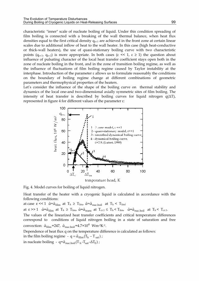
The Evolution of Temperature Disturbances During Boiling of Cryogenic Liquids on Heat-Releasing Surfaces
99
characteristic "inner" scale of nucleate boiling of liquid. Under this condition spreading of film boiling is connected with a breaking of the wall thermal balance, when heat flux densities equal to the first critical density qcr.1 are achieved in the front zone at certain linear scales due to additional inflow of heat to the wall heater. In this case (high heat-conductive or thick-wall heaters), the use of quasi-stationary boiling curve with two characteristic points (qcr.1, qcr.2) is more appropriate. In both cases (ε << 1, ε ≥ 1) the question about influence of pulsating character of the local heat transfer coefficient stays open both in the zone of nucleate boiling in the front, and in the zone of transition boiling regime, as well as the influence of fluctuations of film boiling regime caused by Taylor instability at the interphase. Introduction of the parameter ε allows us to formulate reasonably the conditions on the boundary of boiling regime change at different combinations of geometric parameters and thermophysical properties of the heaters. Let’s consider the influence of the shape of the boiling curve on thermal stability and dynamics of the local one-and two-dimensional axially symmetric sites of film boiling. The intensity of heat transfer is described by boiling curves for liquid nitrogen q(ΔT), represented in figure 4 for different values of the parameter ε:
Fig. 4. Model curves for boiling of liquid nitrogen.
Heat transfer of the heater with a cryogenic liquid is calculated in accordance with the following conditions: at case ε << 1 filmα=α at Тh ≥ Tlim, nuc.boilα=α at Тh < Tlim; at ε >> 1 filmα=α at Тh ≥ Tlim, transα=α at Тcr.1 ≤ Тh < Tlim, nuc.boilα=α at Тh < Tcr.1. The values of the linearized heat transfer coefficients and critical temperature differences correspond to conditions of liquid nitrogen boiling in a state of saturation and free convection: 4
film nuc.boilα =247, α =4.7×10 Wm-2K-1. Dependence of heat flux q on the temperature difference is calculated as follows: in the film boiling regime - film h satq α (T T )= − ; in nucleate boiling - nuc.boil h sat 0q=α (T -T -ΔT ) ;
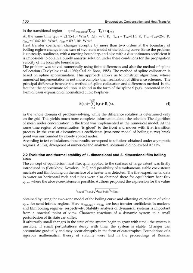
Evaporation, Condensation and Heat Transfer
100
in the transitional region - trans.boil cr.2 h cr.2q α (T T ) q= − + . At the same time qcr.1 = 21.15⋅104 Wm-2, ΔT0 =7.0 K, Tcr.1 – Tsat=11.5 K; Tlim -Тsat=26.0 К, qcr.2 = 0.642⋅104 Wm-2, qlim = 89.3⋅104 Wm-2. Heat transfer coefficient changes abruptly by more than two orders at the boundary of boiling regime change in the case of two-zone model of the boiling curve. Since the problem is unsteady, nonlinear, with a moving boundary, and also with a discontinuous coefficient it is impossible to obtain a purely analytic solution under these conditions for the propagation velocity of the local site boundaries. The problem was solved numerically using finite differences and also the method of spline collocation (Zav’yalov et al., 1980; Carl de Boor, 1985). The method of spline collocation is based on spline approximation. This approach allows us to construct algorithms, whose numerical implementation is not more complex then realization of difference schemes. The principal difference between the method of spline collocation and differences method is the fact that the approximate solution is found in the form of the spline S (x,τ), presented in the form of basis expansion of normalized cubic B-splines:
N+1
i ii=-1
S(x,τ)= b (τ)×B (x),∑ (4)
in the whole domain of problem-solving, while the difference solution is determined only on the grid. This yields much more complete information about the solution. The algorithm of mesh nodes concentration in the front was implemented in the numerical model. At the same time region of concentration "is glued" to the front and moves with it at transition process. In the case of discontinuous coefficients (two-zone model of boiling curve) break point was surrounded by closely spaced nodes. According to test calculations, these results correspond to solutions obtained under asymptotic regimes. At this, divergence of numerical and analytical solutions did not exceed 0.5÷1%.
2.2 Evolution and thermal stability of 1- dimensional and 2- dimensional film boiling sites The concept of equilibrium heat flux qequi, applied to the surfaces of large extent was firstly introduced in (Petukhov, Kovalev, 1962) and possibility of simultaneous stable coexistence nucleate and film boiling on the surface of a heater was detected. The first experimental data in water on horizontal rods and tubes were also obtained there for equilibrium heat flux qequi, where the above coexistence is possible. Authors proposed the expression for the value
equi cr.2 nuc.boil filmq =q α /α ,
obtained by using the two-zone model of the boiling curve and allowing calculation of value qequi for semi-infinite regions. Here nuc.boil filmα , α are heat transfer coefficients in nucleate and film boiling regimes, respectively. Stability analysis of dynamical systems is important from a practical point of view. Character reactions of a dynamic system to a small perturbation of its state can differ. If arbitrarily small changes in the state of the system begin to grow with time - the system is unstable. If small perturbations decay with time, the system is stable. Changes can accumulate gradually and may occur abruptly in the form of catastrophes. Foundations of a rigorous mathematical theory of stability were laid in the proceedings of Russian
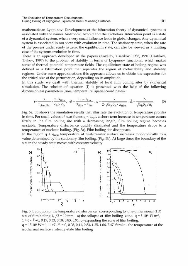
The Evolution of Temperature Disturbances During Boiling of Cryogenic Liquids on Heat-Releasing Surfaces
101
mathematician Lyapunov. Development of the bifurcation theory of dynamical systems is associated with the names Andronov, Arnold and their scholars. Bifurcation point is a state of a dynamical system, when a very small influence leads to global changes. Any dynamical system is associated in our view with evolution in time. The stationary state, when the rate of the process under study is zero, the equilibrium state, can also be viewed as a limiting case of the systems evolution in time. There is an approach developed in the papers (Kovalev, Usatikov, 1988, 1991; Usatikov, Tivkov, 1997) to the problem of stability in terms of Lyapunov functional, which makes sense of thermal potential temperature fields. The equilibrium state of boiling regime was defined as a bifurcation point that separates the region of metastability and stability regimes. Under some approximations this approach allows us to obtain the expression for the critical size of the perturbation, depending on its amplitude. In this study we dealt with thermal stability of local film boiling sites by numerical simulation. The solution of equation (1) is presented with the help of the following dimensionless parameters (time, temperature, spatial coordinates):
film
char.film h h h
τ τ ατ= = , τ c ρ δ
⋅ h lim
film lim
T TΘ ,T T
−=− h h film
xx ,2 λ δ /α
=⋅ h h i
ΔΔ .λ δ /α
= (5)
Fig. 5a, 5b shows the simulation results that illustrate the evolution of temperature profiles in time. For small values of heat fluxes q < qequi, a short-term increase in temperature occurs firstly in the film boiling site with a decreasing length, film boiling regime becomes unstable. Temperature disturbance quickly dissipated and the temperature drops to a temperature of nucleate boiling, (Fig. 5a). Film boiling site disappears. In the region q > qequi temperature of heat-transfer surface increases monotonically to a value determined by the stationary film boiling, (Fig. 5b). At large times the boundary of the site in the steady state moves with constant velocity.
Fig. 5. Evolution of the temperature disturbance, corresponding to one-dimensional (1D) site of film boiling. l0 /2 = 10 mm. a) the collapse of film boiling zone. q = 5⋅104 W m-2, 1 ÷ 6 - τ =0; 0.17; 0.33; 0.58; 0.83; 0.91. b) expanding the zone of film boiling, q = 15⋅104 Wm-2.⋅ 1 ÷7 - τ = 0, 0.08, 0.41, 0.83, 1.25, 1.66, 7.47. Stroke - the temperature of the isothermal surface at steady-state film boiling
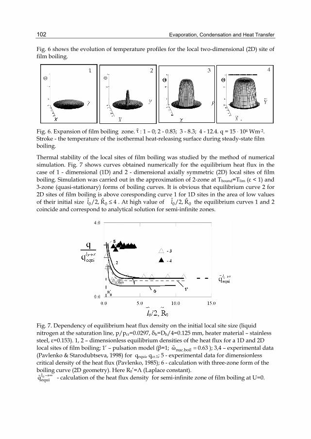
Evaporation, Condensation and Heat Transfer
102
Fig. 6 shows the evolution of temperature profiles for the local two-dimensional (2D) site of film boiling.
Fig. 6. Expansion of film boiling zone. τ : 1 – 0; 2 - 0.83; 3 - 8.3; 4 - 12.4. q = 15 ⋅ 104 Wm-2. Stroke - the temperature of the isothermal heat-releasing surface during steady-state film boiling.
Thermal stability of the local sites of film boiling was studied by the method of numerical simulation. Fig. 7 shows curves obtained numerically for the equilibrium heat flux in the case of 1 - dimensional (1D) and 2 - dimensional axially symmetric (2D) local sites of film boiling. Simulation was carried out in the approximation of 2-zone at Tbound=Tlim (ε < 1) and 3-zone (quasi-stationary) forms of boiling curves. It is obvious that equilibrium curve 2 for 2D sites of film boiling is above coresponding curve 1 for 1D sites in the area of low values of their initial size 0 0/2, R 4l ≤ . At high value of 0 0/2, Rl the equilibrium curves 1 and 2 coincide and correspond to analytical solution for semi-infinite zones.
Fig. 7. Dependency of equilibrium heat flux density on the initial local site size (liquid nitrogen at the saturation line, p/pcr=0.0297, δh=Dh/4=0.125 mm, heater material – stainless steel, ε=0.153). 1, 2 – dimensionless equilibrium densities of the heat flux for a 1D and 2D local sites of film boiling; 1’ – pulsation model (β=1; nuc.boilω 0.63= ); 3,4 – experimental data (Pavlenko & Starodubtseva, 1998) for qequi, qcr.1; 5 - experimental data for dimensionless critical density of the heat flux (Pavlenko, 1985); 6 - calculation with three-zone form of the boiling curve (2D geometry). Here R0’=Λ (Laplace constant).
0lequiq →∞ - calculation of the heat flux density for semi-infinite zone of film boiling at U=0.
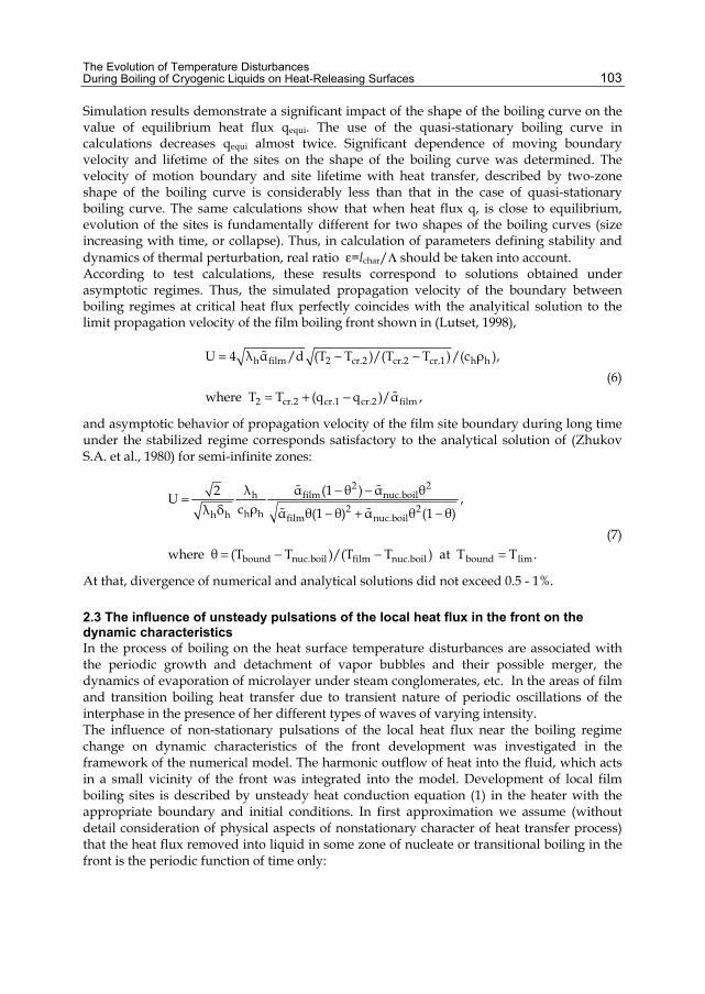
The Evolution of Temperature Disturbances During Boiling of Cryogenic Liquids on Heat-Releasing Surfaces
103
Simulation results demonstrate a significant impact of the shape of the boiling curve on the value of equilibrium heat flux qequi. The use of the quasi-stationary boiling curve in calculations decreases qequi almost twice. Significant dependence of moving boundary velocity and lifetime of the sites on the shape of the boiling curve was determined. The velocity of motion boundary and site lifetime with heat transfer, described by two-zone shape of the boiling curve is considerably less than that in the case of quasi-stationary boiling curve. The same calculations show that when heat flux q, is close to equilibrium, evolution of the sites is fundamentally different for two shapes of the boiling curves (size increasing with time, or collapse). Thus, in calculation of parameters defining stability and dynamics of thermal perturbation, real ratio ε=lchar/Λ should be taken into account. According to test calculations, these results correspond to solutions obtained under asymptotic regimes. Thus, the simulated propagation velocity of the boundary between boiling regimes at critical heat flux perfectly coincides with the analyitical solution to the limit propagation velocity of the film boiling front shown in (Lutset, 1998),
h film 2 cr.2 cr.2 cr.1 h h
2 cr.2 cr.1 cr.2 film
U 4 λ α /d (T T )/(T T )/(c ρ ),
where T T (q q )/α ,
= − −
= + − (6)
and asymptotic behavior of propagation velocity of the film site boundary during long time under the stabilized regime corresponds satisfactory to the analytical solution of (Zhukov S.A. et al., 1980) for semi-infinite zones:
2 2film nuc.boilh
2 2h hh h film nuc.boil
bound nuc.boil film nuc.boil bound lim
α (1 θ ) α θ2 λU ,с ρλ δ α θ(1 θ) α θ (1 θ)
where θ (T T )/(T T ) at Т Т .
− −=− + −
= − − = (7)
At that, divergence of numerical and analytical solutions did not exceed 0.5 - 1%.
2.3 The influence of unsteady pulsations of the local heat flux in the front on the dynamic characteristics In the process of boiling on the heat surface temperature disturbances are associated with the periodic growth and detachment of vapor bubbles and their possible merger, the dynamics of evaporation of microlayer under steam conglomerates, etc. In the areas of film and transition boiling heat transfer due to transient nature of periodic oscillations of the interphase in the presence of her different types of waves of varying intensity. The influence of non-stationary pulsations of the local heat flux near the boiling regime change on dynamic characteristics of the front development was investigated in the framework of the numerical model. The harmonic outflow of heat into the fluid, which acts in a small vicinity of the front was integrated into the model. Development of local film boiling sites is described by unsteady heat conduction equation (1) in the heater with the appropriate boundary and initial conditions. In first approximation we assume (without detail consideration of physical aspects of nonstationary character of heat transfer process) that the heat flux removed into liquid in some zone of nucleate or transitional boiling in the front is the periodic function of time only:
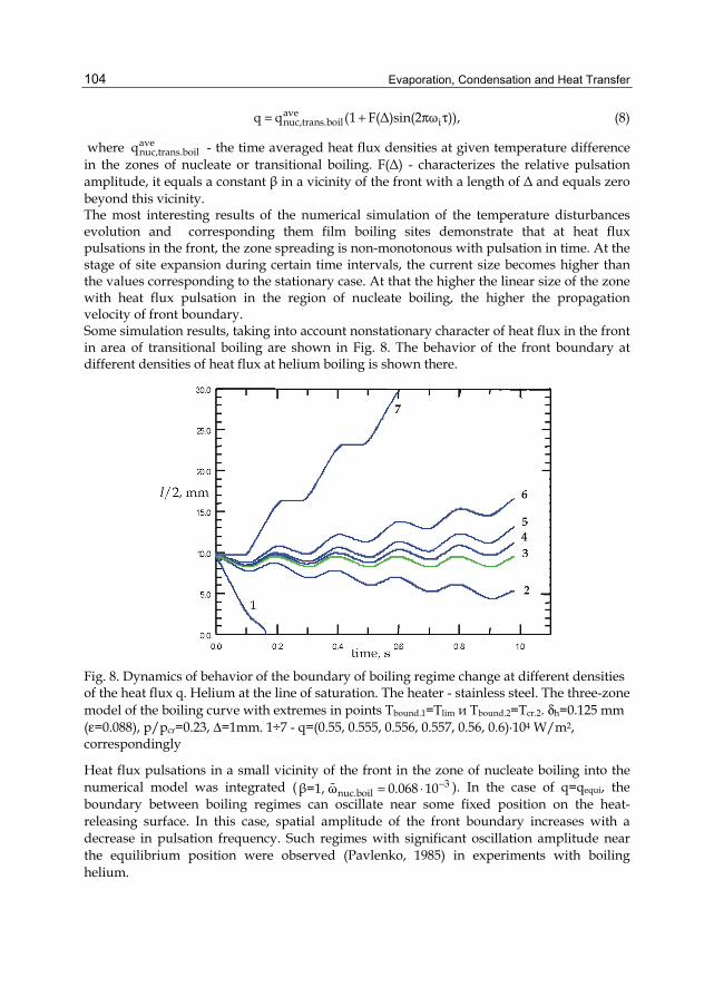
Evaporation, Condensation and Heat Transfer
104
avenuc,trans.boil iq q (1 F(Δ)sin(2 ω )),= + π τ (8)
where avenuc,trans.boilq - the time averaged heat flux densities at given temperature difference
in the zones of nucleate or transitional boiling. F(Δ) - characterizes the relative pulsation amplitude, it equals a constant β in a vicinity of the front with a length of Δ and equals zero beyond this vicinity. The most interesting results of the numerical simulation of the temperature disturbances evolution and corresponding them film boiling sites demonstrate that at heat flux pulsations in the front, the zone spreading is non-monotonous with pulsation in time. At the stage of site expansion during certain time intervals, the current size becomes higher than the values corresponding to the stationary case. At that the higher the linear size of the zone with heat flux pulsation in the region of nucleate boiling, the higher the propagation velocity of front boundary. Some simulation results, taking into account nonstationary character of heat flux in the front in area of transitional boiling are shown in Fig. 8. The behavior of the front boundary at different densities of heat flux at helium boiling is shown there.
Fig. 8. Dynamics of behavior of the boundary of boiling regime change at different densities of the heat flux q. Helium at the line of saturation. The heater - stainless steel. The three-zone model of the boiling curve with extremes in points Тbound.1=Тlim и Тbound.2=Тcr.2. δh=0.125 mm (ε=0.088), p/pcr=0.23, Δ=1mm. 1÷7 - q=(0.55, 0.555, 0.556, 0.557, 0.56, 0.6)·104 W/m2, correspondingly
Heat flux pulsations in a small vicinity of the front in the zone of nucleate boiling into the numerical model was integrated ( 3
nuc.boilβ=1, ω 0.068 10−= ⋅ ). In the case of q=qequi, the boundary between boiling regimes can oscillate near some fixed position on the heat-releasing surface. In this case, spatial amplitude of the front boundary increases with a decrease in pulsation frequency. Such regimes with significant oscillation amplitude near the equilibrium position were observed (Pavlenko, 1985) in experiments with boiling helium.
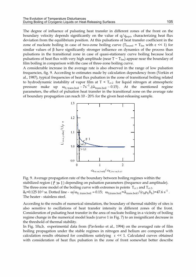
The Evolution of Temperature Disturbances During Boiling of Cryogenic Liquids on Heat-Releasing Surfaces
105
The degree of influence of pulsating heat transfer in different zones of the front on the boundary velocity depends significantly on the value of q/qequi, characterizing heat flux deviation from the equilibrium position. At this pulsations of heat transfer coefficient in the zone of nucleate boiling in case of two-zone boiling curve (Tbound = Tlim with ε << 1) for similar values of β have significantly stronger influence on dynamics of the process than pulsations in the transitional zone in case of quasi-stationary curve boiling because local pulsations of heat flux with very high amplitude (near T ~ Tlim) appear near the boundary of film boiling in comparison with the case of three-zone boiling curve. A considerable increase in the average rate is also observed in the range of low pulsation frequencies, fig. 9. According to estimates made by calculation dependency from (Verkin et al., 1987), typical frequencies of heat flux pulsation in the zone of transitional boiling related to hydrodynamic instability of vapor film at T < Tcr.2 for liquid nitrogen at atmospheric pressure make up 1
0, trans.boil trans.boilω 7s ,(ω 0.15)−∼ ∼ . At the mentioned regime parameters, the effect of pulsation heat transfer in the transitional zone on the average rate of boundary propagation can reach 10 - 20% for the given heat-releasing sample.
Fig. 9. Average propagation rate of the boundary between boiling regimes within the stabilized region ( 1τ ) depending on pulsation parameters (frequence and amplitude). The three-zone model of the boiling curve with extremes in points Тcr.1 and Тcr.2. δh=0.125⋅10-3 м. Dotted line - 0, trans.boilω ω 0.15;= -1
0,trans.boil trans.boil h h hω =α /(c ρ δ )=47.6 s . The heater - stainless steel.
According to the results of numerical simulation, the boundary of thermal stability of sites is also sensitive to oscillations of heat transfer intensity in different zones of the front. Consideration of pulsating heat transfer in the area of nucleate boiling in a vicinity of boiling regime change in the numerical model leads (curve 1 in Fig. 7) to an insignificant decrease in the threshold of thermal stability. In Fig. 10a,b, experimental data from (Pavlenko et al., 1994) on the averaged rate of film boiling propagation under the stable regimes in nitrogen and helium are compared with calculation results obtained for conditions satisfying ε << 1. Calculated curves obtained with consideration of heat flux pulsation in the zone of front somewhat better describe
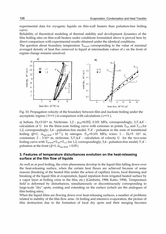
Evaporation, Condensation and Heat Transfer
106
experimental data for cryogenic liquids on thin-wall heaters than pulsation-free boiling curve. Reliability of theoretical modeling of thermal stability and development dynamics of the film boiling sites on thin-wall heaters under conditions formulated above is proved here by direct comparison with experimental results obtained under the identical conditions. The question about boundary temperature Tbound corresponding to the value of maximal averaged density of heat flux removed to liquid at intermediate values of ε on the front of regime change remains unsolved.
Fig. 10. Propagation velocity of the boundary between film and nucleate boiling under the asymptotic regime ( τ>>1 ) in comparison with calculations ( ε<<1 ).
a) helium. Dh=3·10-4 m. Nichrome. 1,2 - psat=0.052, 0.101 MPa, correspondingly; 3,3’,4,4’ - calculation of U for the three-zone boiling curve with extremes in points Tlim and Tcr.2 for 1,2, correspondingly; 3,4 - pulsation-free model; 3’,4’ - pulsation in the zone of transitional boiling (β=1; 3
nuc.boilω 10−= ); b) nitrogen. Psat=0.101 MPa; wires: 1 - Dh=5 ·10-5 m, constantan; 2 - 3·10-4 m, nichrome; 3,3’,4,4’ - calculation of velocity U for the two-zone boiling curve with Tbound=Tlim=Tcr.2 for 1,2, correspondingly; 3,4 - pulsation-free model; 3’,4’ - pulsation at the front ( nuc.boilβ=1; ω 0.05= )
3. Features of temperature disturbances evolution on the heat-releasing surface at the film flow of liquids As well as at pool boiling, the crisis phenomena develop in the liquid film falling down over the heat-releasing surface, when the certain heat fluxes are achieved because of some reasons (breaking of the heated film under the action of capillary forces, local thinning and breaking of the liquid film at evaporation, liquid repulsion from irrigated heated surface by a vapor layer at boiling crisis in the film, etc.) (Gimbutis, 1988; Katto, 1994). Temperature field is deformed by disturbances, simultaneously or discontinuously corresponding to large-scale "dry" spots, existing and extending on the surface (which are the analogues of film boiling sites). When the liquid films are flowing down over heat-releasing surfaces, a number of problems related to stability of the film flow arise. At boiling and intensive evaporation, the picture of film destruction due to the formation of local dry spots and their merging becomes
The Evolution of Temperature Disturbances During Boiling of Cryogenic Liquids on Heat-Releasing Surfaces
107
extremely complicated. Physics of crisis phenomena in boiling flowing-down films does not fully clear at present, and this makes it difficult to construct theoretical models and computational procedures enabling to predict the conditions of development of drying crisis and finally evaluate reliability of equipment operation intended for various purposes. Such detailed analysis is complicated by the limited amount of experimental data in a film flow of liquid on the heated surface in different hydrodynamic flows. The widespread use of cryogenic fluids in modern high performance systems and devices creates the need for reliable information on development of transition and crisis during boiling and evaporation of fuel in low-temperature liquids on different surfaces. In this connection, the line of these investigations is topical both from the scientific and practical viewpoints.
3.1 Edge effects. Features of temperature disturbances evolution on the surfaces with limited extension To describe the critical phenomena with intense heat transfer in falling wave films of cryogenic liquid on the limited-length heat-releasing surface, it is necessary to reveal the features of dynamics of temperature disturbances caused by the edge effects. Let’s investigate the features of the disturbances behavior, when the front approaches the edge of the heater. The boundary conditions: ∂Тh/∂x=0 for x=0 and x=Lh for a heater of finite length Lh correspond to the heater’s heat-insulated ends. For an infinite heater, we have ∂Th⁄∂x = 0 for x = 0 (symmetry condition) and h satT =T =q/α+T∞ for x=±∞. Numerical simulation results showed that the behavior of dry spots (temperature disturbances), localized at the edge of the heater, differ from the behavior of spots on the heater of infinite extent. The boundary of the dry spots can be moved on the surface of the heater until dry spot finally fills the entire surface of the heater. With front approach to the edge its dynamic characteristics and thermal stability have a features compared with the behavior of the front moving over the unlimited surface. As it was shown by analysis of the numerical results, the geometric parameter that determines whether one disturbance interacts with another and whether the heater boundary effects the velocity of the front, is characteristic thermal size
char h h nuc.boilλ δ /αl .
The physical meaning of this characteristic scale is the width of the temperature disturbance front in zone with high intensity of heat transfer. If one spot is located at a distance greater than lchar, it evolves as a single one. If dry spot is farther from the edge of the heater than lchar, in this case its behavior is identical to the behavior on the the surface of an infinite extent. The behavior of disturbance, located from the other at a distance less than lchar, differs from the behavior of a single disturbance, and behavior of the front closer to the borderline heaters at a distance less lchar, differs from the behavior of the front moving over the heater of infinite extent. The results of numerical simulation presented in Fig. 11a, 11b, demonstrate the influence of boundary conditions on the evolution of dry spots in time. The values of the velocity of the boundary of the local dry spot on the surface of the infinite heater and the heater of finite length Lh coincide until the region of high-intensity heat transfer decreases to a dimension of the order lchar. The boundary of the spot on the infinite heater continues moving with a constant velocity, whereas on the heater of finite length, we have a sharp nonlinear increase in the velocity, as the front approaches the heat-insulated edge, (Fig. 11a).
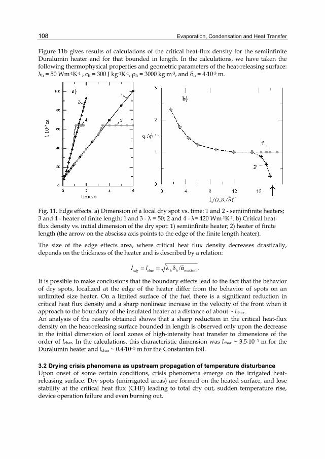
Evaporation, Condensation and Heat Transfer
108
Figure 11b gives results of calculations of the critical heat-flux density for the semiinfinite Duralumin heater and for that bounded in length. In the calculations, we have taken the following thermophysical properties and geometric parameters of the heat-releasing surface: λh = 50 Wm-1K-1 , ch = 300 J kg-1K-1, ρh = 3000 kg m-3, and δh = 4·10-3 m.
Fig. 11. Edge effects. a) Dimension of a local dry spot vs. time: 1 and 2 - semiinfinite heaters; 3 and 4 - heater of finite length; 1 and 3 - λ = 50; 2 and 4 - λ= 420 Wm-1K-1. b) Critical heat-flux density vs. initial dimension of the dry spot: 1) semiinfinite heater; 2) heater of finite length (the arrow on the abscissa axis points to the edge of the finite length heater).
The size of the edge effects area, where critical heat flux density decreases drastically, depends on the thickness of the heater and is described by a relation:
char h h nuc.boilλ δ /α .edgl l
It is possible to make conclusions that the boundary effects lead to the fact that the behavior of dry spots, localized at the edge of the heater differ from the behavior of spots on an unlimited size heater. On a limited surface of the fuel there is a significant reduction in critical heat flux density and a sharp nonlinear increase in the velocity of the front when it approach to the boundary of the insulated heater at a distance of about ~ lchar. An analysis of the results obtained shows that a sharp reduction in the critical heat-flux density on the heat-releasing surface bounded in length is observed only upon the decrease in the initial dimension of local zones of high-intensity heat transfer to dimensions of the order of lchar. In the calculations, this characteristic dimension was lchar ~ 3.5·10−3 m for the Duralumin heater and lchar ~ 0.4·10−3 m for the Constantan foil.
3.2 Drying crisis phenomena as upstream propagation of temperature disturbance Upon onset of some certain conditions, crisis phenomena emerge on the irrigated heat-releasing surface. Dry spots (unirrigated areas) are formed on the heated surface, and lose stability at the critical heat flux (CHF) leading to total dry out, sudden temperature rise, device operation failure and even burning out.
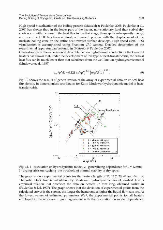
The Evolution of Temperature Disturbances During Boiling of Cryogenic Liquids on Heat-Releasing Surfaces
109
High-speed visualization of the boiling process (Matsekh & Pavlenko, 2005; Pavlenko et al., 2006) has shown that, in the lower part of the heater, non-stationary (and then stable) dry spots occur with increase in the heat flux in the first stage; these spots subsequently merge, and once the CHF has been attained, a transient process with the displacement of the nucleate-boiling zone on the entire heat-transfer surface develops. High-speed (4800 PPS) visualization is accomplished using Phantom v7.0 camera. Detailed description of the experimental apparatus can be found in (Matsekh & Pavlenko, 2005). Generalization of the experimental data obtained on high-thermal conductivity thick-walled heaters has shown that, under the development of this type of heat-transfer crisis, the critical heat flux can be much lower than that calculated from the well-known hydrodynamic model (Mudawar et al., 1987)
( ) ( ) 0.42 2/3 2crq ρ rU 0.121 ρ ρ σ ρU L .′′ ′ ′′ ′= (9)
Fig. 12 shows the results of generalization of the array of experimental data on critical heat flux density in dimensionless coordinates for Katto-Mudawar hydrodynamic model of heat-transfer crisis.
Fig. 12. 1 - calculation on hydrodynamic model, 2 - generalizing dependence for L = 12 mm; I - drying crisis on reaching the threshold of thermal stability of dry spots.
The graph shows experimental points for the heaters length of 12, 12.7, 20, 42 and 64 mm. The solid black line is calculation by Mudawar hydrodynamic model, dashed line is empirical relation that describes the data on heaters 12 mm long, obtained earlier in (Pavlenko & Lel, 1997). The graph shows that the deviation of experimental points from the calculated curves is the sooner, the longer the heater and a higher the liquid flow rate are. At the lowest values of estimated parameters We-1, the experimental points for all heaters employed in the work are in good agreement with the calculation on model dependence.
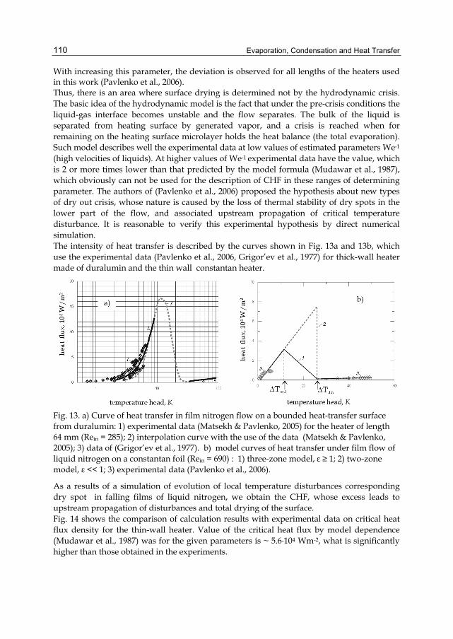
Evaporation, Condensation and Heat Transfer
110
With increasing this parameter, the deviation is observed for all lengths of the heaters used in this work (Pavlenko et al., 2006). Thus, there is an area where surface drying is determined not by the hydrodynamic crisis. The basic idea of the hydrodynamic model is the fact that under the pre-crisis conditions the liquid-gas interface becomes unstable and the flow separates. The bulk of the liquid is separated from heating surface by generated vapor, and a crisis is reached when for remaining on the heating surface microlayer holds the heat balance (the total evaporation). Such model describes well the experimental data at low values of estimated parameters We-1 (high velocities of liquids). At higher values of We-1 experimental data have the value, which is 2 or more times lower than that predicted by the model formula (Mudawar et al., 1987), which obviously can not be used for the description of CHF in these ranges of determining parameter. The authors of (Pavlenko et al., 2006) proposed the hypothesis about new types of dry out crisis, whose nature is caused by the loss of thermal stability of dry spots in the lower part of the flow, and associated upstream propagation of critical temperature disturbance. It is reasonable to verify this experimental hypothesis by direct numerical simulation. The intensity of heat transfer is described by the curves shown in Fig. 13a and 13b, which use the experimental data (Pavlenko et al., 2006, Grigor’ev et al., 1977) for thick-wall heater made of duralumin and the thin wall constantan heater.
Fig. 13. a) Curve of heat transfer in film nitrogen flow on a bounded heat-transfer surface from duralumin: 1) experimental data (Matsekh & Pavlenko, 2005) for the heater of length 64 mm (Rein = 285); 2) interpolation curve with the use of the data (Matsekh & Pavlenko, 2005); 3) data of (Grigor’ev et al., 1977). b) model curves of heat transfer under film flow of liquid nitrogen on a constantan foil (Rein = 690) : 1) three-zone model, ε ≥ 1; 2) two-zone model, ε << 1; 3) experimental data (Pavlenko et al., 2006).
As a results of a simulation of evolution of local temperature disturbances corresponding dry spot in falling films of liquid nitrogen, we obtain the CHF, whose excess leads to upstream propagation of disturbances and total drying of the surface. Fig. 14 shows the comparison of calculation results with experimental data on critical heat flux density for the thin-wall heater. Value of the critical heat flux by model dependence (Mudawar et al., 1987) was for the given parameters is ~ 5.6·104 Wm-2, what is significantly higher than those obtained in the experiments.
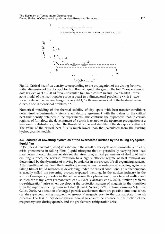
The Evolution of Temperature Disturbances During Boiling of Cryogenic Liquids on Heat-Releasing Surfaces
111
Fig. 14. Critical heat-flux density corresponding to the propagation of the drying front vs. initial dimension of the dry spot for film flow of liquid nitrogen on the foil: 2 - experimental data (Pavlenko et al., 2006) for a Constantan foil, (δh = 25·10−6 m and Rein = 690); 3 - three-zone model of the heat-transfer-curve, a quasi-two-dimensional problem, ε << 1; 4 - two-zone model of the heat-exchange curve, ε << 1; 5 - three-zone model of the heat-exchange curve, a one-dimensional problem, ε ≥ 1.
Numerical modeling of the thermal stability of dry spots with heat-transfer conditions determined experimentally yields a satisfactory agreement with the values of the critical heat-flux density obtained in the experiments. This confirms the hypothesis that, in certain regimes of film flow, the development of a crisis is related to the upstream propagation of a temperature disturbance, when the threshold of thermal stability of the dry spots is attained. The value of the critical heat flux is much lower than that calculated from the existing hydrodynamic models.
3.3 Features of rewetting dynamics of the overheated surface by the falling cryogenic liquid film In (Surtaev & Pavlenko, 2009) it is shown in the result of the cycle of experimental studies of crisis phenomena in falling films (liquid nitrogen) that at periodically varying heat load parameters of occurring metastable regular structures, critical parameters of drying of heat-emitting surface, the reverse transition to a highly efficient regime of heat removal are determined by the dynamics of moving boundaries in the process of self-organizing system. After resetting of heat load the transition process, when the surface starts cooling again by a falling film of liquid nitrogen, is developing under the critical conditions. This phenomenon is usually called the rewetting process (repeated wetting). In the nuclear industry in the study of emergency modes in the active zones this phenomenon was termed re-Bay and studied for many years (Yamanouchi et al., 1968; Gabaraev et al., 2001). Similar problems (re-refrigeration) arise when developing the protection system of magnets in the transition from the superconducting to normal state (Unal & Nelson, 1992; Brahim Bourouga & Jerome Gilles, 2010). At operation of charged particle accelerators there are possible situations when certain superconducting magnets, or group of magnets pass to the normal state (quench process). The task of cryogenic system here is to ensure the absence of destruction of the magnet cryostat during quench, and the problems re-refrigeration arise.
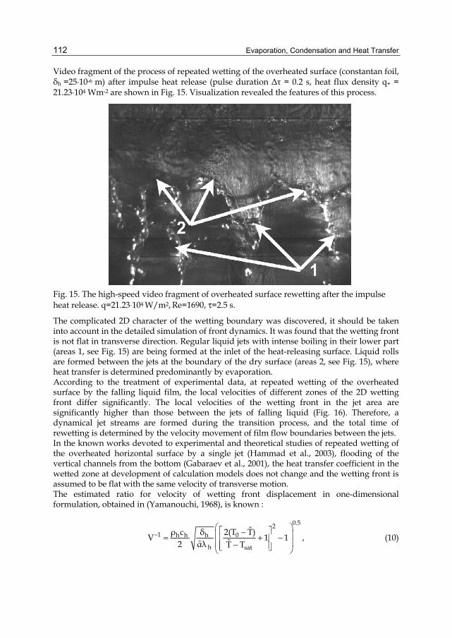
Evaporation, Condensation and Heat Transfer
112
Video fragment of the process of repeated wetting of the overheated surface (constantan foil, δh =25·10-6 m) after impulse heat release (pulse duration Δτ = 0.2 s, heat flux density q+ = 21.23·104 Wm-2 are shown in Fig. 15. Visualization revealed the features of this process.
Fig. 15. The high-speed video fragment of overheated surface rewetting after the impulse heat release. q=21.23⋅104 W/m2, Re=1690, τ=2.5 s.
The complicated 2D character of the wetting boundary was discovered, it should be taken into account in the detailed simulation of front dynamics. It was found that the wetting front is not flat in transverse direction. Regular liquid jets with intense boiling in their lower part (areas 1, see Fig. 15) are being formed at the inlet of the heat-releasing surface. Liquid rolls are formed between the jets at the boundary of the dry surface (areas 2, see Fig. 15), where heat transfer is determined predominantly by evaporation. According to the treatment of experimental data, at repeated wetting of the overheated surface by the falling liquid film, the local velocities of different zones of the 2D wetting front differ significantly. The local velocities of the wetting front in the jet area are significantly higher than those between the jets of falling liquid (Fig. 16). Therefore, a dynamical jet streams are formed during the transition process, and the total time of rewetting is determined by the velocity movement of film flow boundaries between the jets. In the known works devoted to experimental and theoretical studies of repeated wetting of the overheated horizontal surface by a single jet (Hammad et al., 2003), flooding of the vertical channels from the bottom (Gabaraev et al., 2001), the heat transfer coefficient in the wetted zone at development of calculation models does not change and the wetting front is assumed to be flat with the same velocity of transverse motion. The estimated ratio for velocity of wetting front displacement in one-dimensional formulation, obtained in (Yamanouchi, 1968), is known :
0.521 0h h h
h sat
2(T T)ρ c δV 1 1 ,2 αλ T T
−⎛ ⎞⎡ ⎤−⎜ ⎟= + −⎢ ⎥⎜ ⎟−⎢ ⎥⎣ ⎦⎝ ⎠
(10)
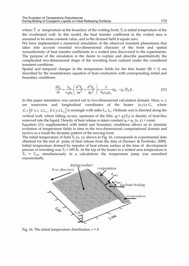
The Evolution of Temperature Disturbances During Boiling of Cryogenic Liquids on Heat-Releasing Surfaces
113
where: T is temperature at the boundary of the wetting front; T0 is initial temperature of the the overheated wall. In this model, the heat transfer coefficient in the wetted area is assumed to be some constant value, and in the drained field it equals zero. We have implemented a numerical simulation of the observed transient phenomena that takes into account essential two-dimensional character of the front and spatial nonuniformity of heat transfer coefficients in a wetted area discovered in the experiments. The purpose of the simulation is the desire to explain and describe quantitatively the complicated two-dimensional shape of the rewetting front realized under the considered transient conditions. Spatial and temporal changes in the temperature fields for the thin heater (Bi < 1) are described by the nonstationary equation of heat conduction with corresponding initial and boundary conditions:
2 2
h h h hh2 2
h h h h h
T λ T T 1 (q q (T )) .τ c ρ δ c ρx y + −
⎞⎛∂ ∂ ∂= + + −⎟⎜⎜ ⎟∂ ∂ ∂⎝ ⎠ (11)
In this paper simulation was carried out in two-dimensional calculation domain. Here, x, y are transverse and longitudinal coordinates of the heater (x,y) G,∈ where
{ }x yG 0 x L , 0 y L= ≤ ≤ ≤ ≤ is rectangle with sides Lx, Ly. Ordinate axis is directed along the vertical wall, where falling occurs, upstream of the film. q-= q-(Th) is density of heat-flux removed into the liquid. Density of heat release is taken constant q+= q+ (x, y) = const. Equation (11) supplemented with initial and boundary conditions allows us to simulate evolution of temperature fields in time in the two-dimensional computational domain and receive as a result the dynamic pattern of the moving front. The initial temperature of field T0 (x, y), shown in Fig. 16, corresponds to experimental data obtained for the end of pulse of heat release from the data of (Surtaev & Pavlenko, 2009). Initial temperature drained by impulse of heat release surface at the time of development process of rewetting was T0 = 693 K. At the top of the heater in a wetted area temperature is T0 = Tsat, simultaneously in a calculations the temperature jump was smoothed exponentially.
Fig. 16. The initial temperature distribution, τ = 0.
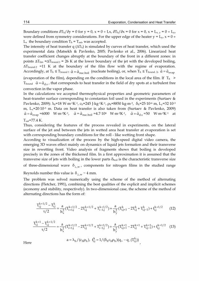
Evaporation, Condensation and Heat Transfer
114
Boundary conditions ∂Th/∂y = 0 for y = 0, x = 0 ÷ Lx, ∂Th/∂x = 0 for x = 0, x = Lx, y = 0 ÷ Ly, were defined from symmetry considerations. For the upper edge of the heater y = Ly, x = 0 ÷ Lx the boundary condition Th = Tsat, was accepted. The intensity of heat transfer q (ΔTh) is simulated by curves of heat transfer, which used the experimental data (Matsekh & Pavlenko, 2005; Pavlenko et al., 2006). Linearized heat transfer coefficient changes abruptly at the boundary of the front in a different zones: in points ΔTlim =ΔTbound.1 = 26 K at the lower boundary of the jet with the developed boiling, ΔTbound.2 =11 K at the boundary of the film flow with the regime of evaporation. Accordingly, at Th ≤ Tbound 1 nuc.boilα α= (nucleate boiling), or, when Th ≤ Tbound. 2, evapα α=
(evaporation of the film), depending on the conditions in the local area of the film. If Th > Tbound d.sα α= , that corresponds to heat transfer in the field of dry spots at a turbulent free convection in the vapor phase. In the calculations we accepted thermophysical properties and geometric parameters of heat-transfer surface corresponding to constantan foil used in the experiments (Surtaev & Pavlenko, 2009): λh=18 W·m-1K-1, сh=245 J·kg-1K-1, ρh=8850 kg·m-3, δh=25⋅10-6 m, Ly=32⋅10-3 m, Lx=20⋅10-3 m. Data on heat transfer is also taken from (Surtaev & Pavlenko, 2009)
evapα α= =6000 W·m-2K-1, nuc.boilα = α =4.7·104 W·m-2K-1, d.sα α= =50 W·m-2K-1 at
Тsat=77.4 К. Thus, considering the features of the process revealed in experiments, on the lateral surface of the jet and between the jets in wetted area heat transfer at evaporation is set with corresponding boundary conditions for the roll - like wetting front shape. According to visualization of the process by the high-speed digital video camera, the emerging 3D waves effect mainly on dynamics of liquid jets formation and their transverse size in rewetting front. Video analysis of fragments shows that boiling is developed precisely in the zones of the thickened film. In a first approximation it is assumed that the transverse size of jets with boiling in the lower parts δboil is the characteristic transverse size of three-dimensional wave ,wδ⊥ , components for nitrogen films in the studied range
Reynolds number this value is ,wδ⊥ ~ 4 mm. The problem was solved numerically using the scheme of the method of alternating directions (Fletcher, 1991), combining the best qualities of the explicit and implicit schemes (economy and stability, respectively). In two-dimensional case, the scheme of the method of alternating directions has the form of:
k 1/2 k
i,ji,j k 1/2 k 1/2 k 1/2 k k k k 1/2i,j 1 i,j i,j 1i 1,j i,j i 1,j i,j2 2
x y
T T a a(T 2T T ) (T 2T T ) fτ/2 h h
++ + + +
+ −+ −−
= − + + − + + (12)
k 1 k 1/2i,j i,j k 1/2 k 1/2 k 1/2 k 1 k 1 k 1 k 1/2
i,j 1 i,j i,j 1i 1,j i,j i 1,j i,j2 2x y
T T a a(T 2T T ) (T 2T T ) fτ/2 h h
+ ++ + + + + + +
+ −+ −−
= − + + − + + (13)
Here k k
h h h i,j h h h i,ja λ /(c ρ ), f 1/(δ с ρ )(q q (T ))+ −= = −,
The Evolution of Temperature Disturbances During Boiling of Cryogenic Liquids on Heat-Releasing Surfaces
115
hx, hy are mesh steps in the direction of x and y, correspondingly. In addition to basic values kijT and k+1
ijT an intermediate value, which can be formally considered as a value at
k+1/2 kτ=τ =τ +1/2 , is introduced. At each fractional time step one of the spatial differential operator is approximated by implicity (scalar factorizations are carried out in the respective coordinate direction) and the other are approximated explicitly. In the next fractional step following differential operator is approximated by implicitly, and the rest - explicity and so clearly. Solution in this case is reduced to the solution of two three-diagonal matrix systems that allows us to use one-dimensional factorization for finding the solution. Below in Fig. 17 shows the results of numerical simulations on the dynamics of movement of wetting fronts boundaries.
Fig. 17. Evolution of film flow boundary. δboil = 4 mm. ΔTbound.1=26 К in the bottom of the boiling jet. ΔTbound.2=11 К in the area with evaporating film. The time interval between curves Δτ = 0.5 s
Time-varying shape of the front is obtained as described above under the condition that at the initial time film in a local area of the upper part of the fuel surface, bounded by size δboil,x, δboil,y, is under the condition of boiling. In this case, the temperature on the boundary of evaporating film Tbound.2 = 88.4 K, on the boundary of boiling jet it is Tbound.1 = 103.4 K. The results of numerical experiments shown that the instantaneous velocity of boundary motion varies not linearly - there is a sharp increase in the velocity when moving down the front on the heater. It is caused by the fact that in the dried zone, the temperature of heat-releasing surface in absence of heat generation is markedly reduced in the transition process due to heat transfer at free convection in a vapor phase. Average velocity of moving boiling jets boundaries V1 is significantly higher than average velocity of the evaporated film boundary V2.
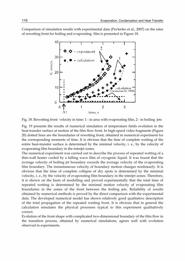
Evaporation, Condensation and Heat Transfer
116
Comparison of simulation results with experimental data (Pavlenko et al., 2007) on the rates of rewetting front for boiling and evaporating film is presented in Figure 18.
Fig. 18. Rewetting front velocity in time: 1 - in area with evaporating film, 2 - in boiling jets
Fig. 19 presents the results of numerical simulation of temperature fields evolution in the heat-transfer surface at motion of the film flow front. In high-speed video fragments (Figure 20) dotted lines are the boundaries of rewetting front, obtained in numerical experiment for the corresponding moments of time. It is obvious that the time of complete wetting of the entire heat-transfer surface is determined by the minimal velocity, i. e., by the velocity of evaporating film boundary in the interjet zones. The numerical experiment was carried out to describe the process of repeated wetting of a thin-wall heater cooled by a falling wave film of cryogenic liquid. It was found that the average velocity of boiling jet boundary exceeds the average velocity of the evaporating film boundary. The instantaneous velocity of boundary motion changes nonlinearly. It is obvious that the time of complete collapse of dry spots is determined by the minimal velocity, i. e., by the velocity of evaporating film boundary in the interjet zones. Therefore, it is shown on the basis of modelling and proved experimentally that the total time of repeated wetting is determined by the minimal motion velocity of evaporating film boundaries in the zones of the front between the boiling jets. Reliability of results obtained by numerical methods is proved by the direct comparison with the experimental data. The developed numerical model has shown relatively good qualitative description of the total propagation of the repeated wetting front. It is obvious that in general the calculation simulates the physical processes typical to this experiment qualitatively correct. Evolution of the front shape with complicated two-dimensional boundary of the film flow in the transition process, obtained by numerical simulations, agrees well with evolution observed in experiments.
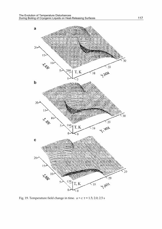
The Evolution of Temperature Disturbances During Boiling of Cryogenic Liquids on Heat-Releasing Surfaces
117
Fig. 19. Temperature field change in time. а ÷ c: τ = 1.5; 2.0; 2.5 s
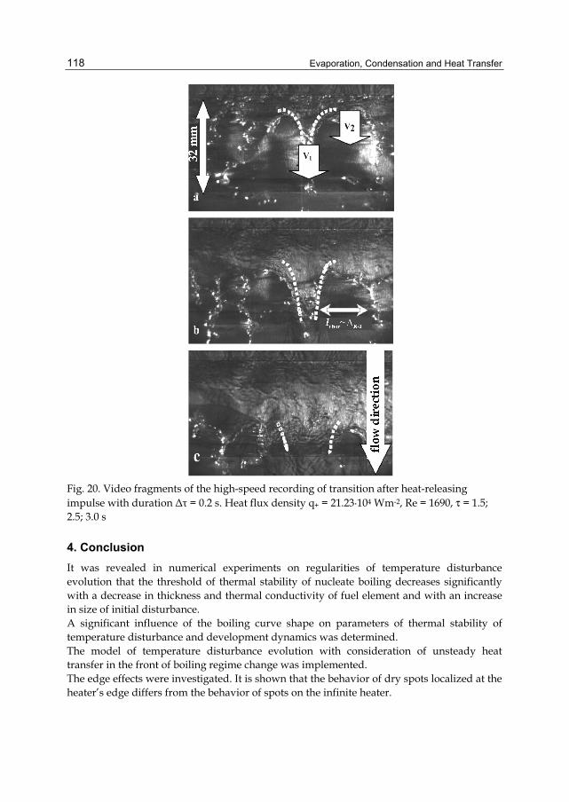
Evaporation, Condensation and Heat Transfer
118
Fig. 20. Video fragments of the high-speed recording of transition after heat-releasing impulse with duration Δτ = 0.2 s. Heat flux density q+ = 21.23·104 Wm-2, Re = 1690, τ = 1.5; 2.5; 3.0 s
4. Conclusion It was revealed in numerical experiments on regularities of temperature disturbance evolution that the threshold of thermal stability of nucleate boiling decreases significantly with a decrease in thickness and thermal conductivity of fuel element and with an increase in size of initial disturbance. A significant influence of the boiling curve shape on parameters of thermal stability of temperature disturbance and development dynamics was determined. The model of temperature disturbance evolution with consideration of unsteady heat transfer in the front of boiling regime change was implemented. The edge effects were investigated. It is shown that the behavior of dry spots localized at the heater’s edge differs from the behavior of spots on the infinite heater.
The Evolution of Temperature Disturbances During Boiling of Cryogenic Liquids on Heat-Releasing Surfaces
119
Numerical experiment confirms the hypothesis that under certain film flow conditions crisis development is determined by upstream propagation of temperature disturbance, when the threshold of thermal stability of dry spots is attained. This model allows us to predict the critical heat flux in the range of flow parameters, where the hydrodynamic model does not work. Dynamic process of superheated surface rewetting was simulated. Evolution of the front shape is studied; it is shown that the local velocities in different areas of two-dimensional wetting fronts differ considerably. The front shape obtained in numerical experiment is in satisfactory agreement with the shape observed in experiments with self-organized regular structures. Complete time of transition process is determined by the minimum velocity of evaporating liquid boundaries in the zones of the front between boiling jets. The model allows us to quantify the wetting front velocity and temperature fields in the heater, variable in space and time. The reliability of the results obtained has been confirmed by direct comparison with the existing analytical solutions in the limiting areas and to experimental data. The results obtained are important for revealing the fundamental regularities of the development of transient processes and crises in boiling and evaporation, including those in flowing-down liquid films, and for development of new approaches to the description of crisis phenomena for different laws of heat release.
5. Acknowledgements This work was financially supported by the Siberian Branch of the Russian Academy of Sciences (No. 68) and Russian Foundation for Basic Research (grant No. 09-08-00118-а).
6. Nomenclature c specific thermal capacity at constant pressure, J kg-1 K-1
g free-fall acceleration, m ⁄ s2 L heater length, m lchar characteristic linear scale of the temperature gradient, m l0, l initial and running dimensions of the dry spot, m p pressure, MPa q heat flux density, W⁄ m2 R0, R initial and running radii of the two-dimensional dry spot, m Re = 4Γ ⁄ ν film Reynolds number r latent heat of vaporization, J ⁄ kg T temperature, K U,V velocity, m ⁄ s
-1 2We =σ/(ρ'U L) reverse Weber number x coordinate along the heater with the point of reckoning at the center of the dry spot, m Greek Letters α=q/ TΔ heat transfer coefficient, Wm-2K-1 α linearized heat transfer coefficient, Wm-2K-1 Γ degree of irrigation, m2 ⁄ s
Evaporation, Condensation and Heat Transfer
120
ΔT = T − Tsat temperature head, K iΔ linear scale of pulsations of heat transfer coefficient
δ thickness, m λ coefficient of thermal conductivity, Wm-1K-1
' ''σ/g(ρ -ρ )Λ = Laplace constant, m ν kinematic viscosity, m2 ⁄ sec ρ density, kg ⁄ m3 σ surface-tension coefficient, N ⁄ m τ time, s ω frequency, s-1
0,i i h h hω α /(c ρ δ )= typical pulsation frequency for heat transfer coefficient
i 0,iω=ω /ω dimensionless pulsation frequency for heat transfer coefficient Subscripts and superscripts: ′ liquid ′′ vapor bound boundary char characteristic cr critical equi equilibrium of boiling regimes film film boiling h heater in inlet conditions lim limit overheating nuc.boil nucleate boiling sat saturation line trans.boil transitional boiling 0 initial ∞ infinite.
7. References Brahim Bourouga & Jerome Gilles. ( 2010). Roles of heat transfer modes on transient cooling
by quenching process, International Journal of Material Forming, Vol. 3, No. 2, pp. 77 – 88
Carl de Boor. (1985). A Practical Guide to Splines, Moscow, p. 304 Duffey, R.B. & Porthouse, D.T.C. (1973). The physics of rewetting in water reactor
emergency core cooling, Nuclear Engineering and Design, Vol. 25. Issue 3, pp. 379-394 Fletcher, K (1991). Numerical methods in fluid dynamics, Vol.1, p.504 Gabaraev, B.A.; Kovalev, S.A.; Molochnikov, Yu.S. et al. (2001). Rewetting and autowave
change of boiling modes, High Temperature, Vol. 39, No. 2, pp. 302 - 314 Gimbutis, G. (1988). Heat transfer at gravitation flow of a liquid film (in Russian), Vilnius,
Mokslas, p. 232 Grigor’ev, V.A.; Pavlov, Yu.M. and Ametistov, E.V. (1977). Boiling of Cryogenic Fluids (in
Russian), Energiya, Moscow
The Evolution of Temperature Disturbances During Boiling of Cryogenic Liquids on Heat-Releasing Surfaces
121
Hammad, J.; Mitsutake, Y.; Monde, M. (2003). Movement of maximum heat flux and wetting front during quenching of hot cylindrical block, Int. Symposium on Transient Convective Heat and Mass Transfer in Single and Two Phase Flows, Editors J. Padet, F. Arinc, Begell House, pp. 189 – 202
Katto, Y. (1994). Critical heat flux, Int. J. Multiphase Flow, Vol. 20, pp. 53 – 90 Kovalev, S.A.; Usatikov, C.V. (1988). Calculation-theoretical study on stability of bubble-
boiling and temperature pulsation of the wall heated by a hot liquid, J. Eng. Phys, Vol. 55, No. 5, pp. 803-810
Kovalev, S.A.; Usatikov, C.V. (1991). Estimate of boiling regime stability by means of Lyapunov functional, High Temperature, Vol. 29, No. 4, pp. 730-737
Lutset, M.O. (1998). Limit rate of boiling regime change, Techn. Phys. Lett., Vol. 24, No. 9, pp. 21 - 27
Matsekh, A.M. & Pavlenko, A.N. (2005). Heat-transfer and crisis phenomena features in falling films of cryogenic liquids, Thermophysics and Aeromechanics, Vol. 12, No. 1, pp. 105 - 119
Mudawar, I.A.; Incropera, T.A. and Incropera, U.P. (1987). Boiling heat transfer and critical heat flux in liquid film falling on vertically-mounted heat sources, Int. J. Heat Mass Transfer. Vol. 30, pp. 2083 − 2095
Pavlenko, A.N. (1985). Experimental study of propagation of film boiling boundary in cryogenic liquid, Actual Problems of Thermal Physics and Physical Hydrodynamics, Novosibirsk, pp. 307 – 317 (Proc. Collection, publ. by Inst. of Thermophysics SB RAS)
Pavlenko, A.N.; Chechovich, V.Yu. & Starodubtseva, I.P. (1994) Study of propagation dynamics for the site of film regime boiling, Russ. J. Eng. Thermophys., Vol. 4, No. 4, pp. 323 - 347
Pavlenko, A.N. & Lel, V.V. (1997) Heat transfer and crisis phenomena in falling films of cryogenic liquid, Russ. J. of Eng. Thermophysics. Vol. 7, No. 3 – 4, pp. 177 – 210
Pavlenko, A.N.; Starodubtseva, I.P. (1998). The study of the development dynamics of semi-infinite and local sites of film boiling, Thermophysics and Aeromechanics, Vol. 5, No. 2, pp. 195 - 207
Pavlenko, A.N. (2001) Transitional Processes at Boiling and Evaporation: Thesis for a Doctor’s degree, Novosibirsk
Pavlenko, A.N.; Matsekh, A.M.; Pecherkin, N.I.; Kneer, R.; Lel, V.V., and Surtaev, A.S. (2006) Heat transfer and crisis phenomena with intense boiling in the falling wave liquid films, Thermophysics and Aeromechanics, Vol. 13, No. 1, pp. 85 - 96
Pavlenko, A.N.; Starodubtseva I.P., and Surtaev, A.S. (2007). Features of dry spots evolution at the film flow of cryogenic liquids at nonstationary heat release, Thermophysics and Aeromechanics, 2007, Vol. 14, No. 4, pp. 505 - 513
Petukhov, B.S. & Kovalev, S.A. (1962). Measurement methods and some results fort the critical load at transition from the film to nucleate boiling, Thermal. Eng., Vol. 9, No. 5, pp. 65 - 72
Surtaev, A.S. & Pavlenko A.N. (2009). Crisis phenomena in falling liquid films at periodic heat loads, Thermophysics and Aeromechanics, Vol. 16, No. 3, pp. 459-468
Unal, C. & Nelson, R. (1992). A Phenomenological model of the thermal-hydraulics of convective boiling during the quenching of hot rod bundles. Thermal hydraulic model, Nuclear Engineering and Design , Vol. 136, p. 277

Evaporation, Condensation and Heat Transfer
122
Verkin, B.I.; Kirichenko, Yu.A. and Rusanov, K.B. (1987). Heat Transfer at Boiling of Cryogenic Liquids, Naukova Dumka, Kiev, p. 262
Yamanouchi, A. (1968). Effect of core spray cooling in transient state after loss-of-coolant accident, Journal Nucl. Sci. Technol., Vol. 5, pp. 547 – 558
Zav’yalov, Yu.S.; Kvasov, B.I.; Miroshnichenko, V.P. (1980). Spline-Function Methods (in Russian), Moscow, Nauka, p. 352
Zhukov, S.A.; Barelko, V.V.; Merzhanov, A.G. (1980). Wave processes on heat generating surfaces on pool boiling, Intern .J. Heat Mass Transfer, Vol. 24, No. 1, pp. 47 − 55
6
Pool Boiling of Liquid- Liquid Multiphase Systems
Gabriel Filipczak, Leon Troniewski and Stanisław Witczak Opole University of Technology,
Chemical and Process Engineering Department, Poland
1. Introduction Heat transfer to boiling liquid is an important problem in the unit operations of evaporation and distillation and also in other kinds of general processing, such as steam generation, petroleum processing and control of temperatures. In spite of frequently occurring cases of homogeneous liquid boiling, meet quite often in industrial practice the necessity to determine the heat transfer conditions during liquid nonhomogeneous mixture boiling, which the mixtures compose the multiphase systems of mutually insoluble (immiscible) liquids. As example the heating and evaporating processes connected with emulsions and other immiscible liquid systems, such as the water-oil mixtures or oiled refrigerating media, or the thermal processes of coal tar preparation can be enumerated. The last of the above-mentioned examples includes many necessary for tar processing unit operations and also technological processes, such as the tar thermal dewatering and distillation, as well as the watered oil-fraction processing. In each of the mentioned above as well as in many other cases meet the diversified heat transfer terms general for the reason of completely different nature of the liquids, including the physical properties of nonhomogeneous mixture components. In spite of many theoretical and experimental works the heat transfer conditions - and also the heat transfer coefficient values - for various media are still extremely difficult to determine. There is a lack of general models of boiling process, no agreed views concerning the heat transfer mechanism in such process exist. It will be emphasised, what is quite often noticed in literature (Cieśliński, 1996; Collier, 1981; Hobler, 1986) that the accessible models of pool boiling process permit to determine the heat transfer coefficients only after the suitable constants assuming, as determined on the basis of experimental investigations. It concerns also the pure liquids (or homogeneous mixtures), which the boiling process is relatively well known and described - although the heat transfer terms are being determined first of all on the basis of empirical models with the limited range of application. A great gap in literature exists with respect to liquid multicomponent mixtures or mixtures consisting of mutually insoluble liquids, while the boiling process of such mixtures is still not mastered enough. The rare works which are considered in literature (Alperi & Mitchell, 1986; Matthew et al., 2009, Mori et al., 1978, 1980) include the cases of durable water-oil emulsion boiling and that only in regard to the situation when the oil is the phase of lower
Evaporation, Condensation and Heat Transfer
124
density than water, also in the situation when a more volatile component of mixture is in direct contact with the heating surface (Gorenflo, 2001). The opposite situation can be met, among others, in cryogenic processes, e.g. during the liquefied gas mixture boiling on the water surface (Boe, 1997), but the peculiarity of such processes does not meet any analogy for the liquid boiling on the heated surface. In literature can also be found only a few works refer to the structures of boiling liquid-liquid mixtures and its effect on heat transfer conditions. One of these works is Greene’s et al., (1998) investigations, relative to the phenomenon of dissipation of the heavier fluid in a lighter as a result of the flow of vapour bubbles. Previously, Mori (1985) described the various configurations of "two-phase bubbles”, formed during vapour flow through a system of two liquids, in considering the phenomenon of evaporation and condensation, leading to the formation of an emulsion. A few problems of boiling of emulsions are described (Mori, 1978; Mori, 1980, as cited in Tachibana, 1972 and Satoh, 1973) and also with photographic recording systems phenomena of water-oil boiling (Mori, 1980). The other examples of experimental studies of mixtures boiling of liquid-liquid type are showed in table 1, as cited in literature (Gorenflo et al., 2001). Generally, the aside from the own investigations, for that so the wide range of proprieties of water-oil mixture components there is the large lack of knowledge in the literature both in the field of description of boiling phenomena and heat transfer conditions. Hence, recognition of kinetics of this process is still insufficient and unsatisfactory, especially for technical raw oil materials. From the very beginning, the source of such juncture leads not only in specific proprieties of the water-oil and oil-water mixtures but as well as in many peculiarities occurring during boiling of these types heterogeneous mixtures. It is necessary to emphasize meaningful stochastic character of this process as a results of development of different structures of the water-oil system as well as – what no concern of homogeneous liquids – significant influence the process time duration on heat transfer mechanism of boiling water-oil mixture at constant heat flux . The authors considered the problem of mutually insoluble liquid mixtures boiling in the course of testing a refrigeration unit, where boiling of oiled ammonia took place (Witczak, 1993, 1997), as well as during investigations of thermal dewatering of coal tars (Filipczak, 1991, 1993, 1997). In the above mentioned cases, the refrigerating oil and tar liquids were the components whose density was higher than that of the second phase. These components were in direct contact with the heating surface. As they have relatively high initial boiling temperature, the heat transfer conditions are considerably different from those presented in the subject literature. In other studies it was found (Troniewski, 2001) that the phenomena and peculiarities associated with boiling of such mixtures, resulting from changing of physical properties of mixtures and from heat transfer conditions. This is particularly connected with the structures evolving of liquid-liquid system during the boiling process. It was noted at the same a significant effect of time on development of structures during boiling with constant heat flux, and additionally - depending on the volume fraction of the oil phase in the mixture - the diferent structures with variable of this heat flux (Filipczak, 2000, 2008; Troniewski 2001, 2003, Witczak, 2008). In aim of solution to these problems the own investigations was carried out. The paper presents the results of laboratory experiments of pool boiling heat transfer from a horizontal copper plate to the water-oil and oil-water mixtures during nucleate boiling. The purpose of
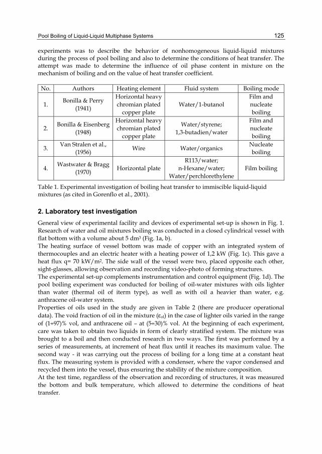
Pool Boiling of Liquid-Liquid Multiphase Systems
125
experiments was to describe the behavior of nonhomogeneous liquid-liquid mixtures during the process of pool boiling and also to determine the conditions of heat transfer. The attempt was made to determine the influence of oil phase content in mixture on the mechanism of boiling and on the value of heat transfer coefficient. No. Authors Heating element Fluid system Boiling mode
1. Bonilla & Perry (1941)
Horizontal heavy chromian plated
copper plate Water/1-butanol
Film and nucleate boiling
2. Bonilla & Eisenberg (1948)
Horizontal heavy chromian plated
copper plate
Water/styrene; 1,3-butadien/water
Film and nucleate boiling
3. Van Stralen et al., (1956) Wire Water/organics Nucleate
boiling
4. Wastwater & Bragg (1970) Horizontal plate
R113/water; n-Hexane/water;
Water/perchlorethylene Film boiling
Table 1. Experimental investigation of boiling heat transfer to immiscible liquid-liquid mixtures (as cited in Gorenflo et al., 2001).
2. Laboratory test investigation General view of experimental facility and devices of experimental set-up is shown in Fig. 1. Research of water and oil mixtures boiling was conducted in a closed cylindrical vessel with flat bottom with a volume about 5 dm3 (Fig. 1a, b). The heating surface of vessel bottom was made of copper with an integrated system of thermocouples and an electric heater with a heating power of 1,2 kW (Fig. 1c). This gave a heat flux q= 70 kW/m2. The side wall of the vessel were two, placed opposite each other, sight-glasses, allowing observation and recording video-photo of forming structures. The experimental set-up complements instrumentation and control equipment (Fig. 1d). The pool boiling experiment was conducted for boiling of oil-water mixtures with oils lighter than water (thermal oil of iterm type), as well as with oil a heavier than water, e.g. anthracene oil-water system. Properties of oils used in the study are given in Table 2 (there are producer operational data). The void fraction of oil in the mixture (εol) in the case of lighter oils varied in the range of (1÷97)% vol, and anthracene oil – at (5÷30)% vol. At the beginning of each experiment, care was taken to obtain two liquids in form of clearly stratified system. The mixture was brought to a boil and then conducted research in two ways. The first was performed by a series of measurements, at increment of heat flux until it reaches its maximum value. The second way - it was carrying out the process of boiling for a long time at a constant heat flux. The measuring system is provided with a condenser, where the vapor condensed and recycled them into the vessel, thus ensuring the stability of the mixture composition. At the test time, regardless of the observation and recording of structures, it was measured the bottom and bulk temperature, which allowed to determine the conditions of heat transfer.
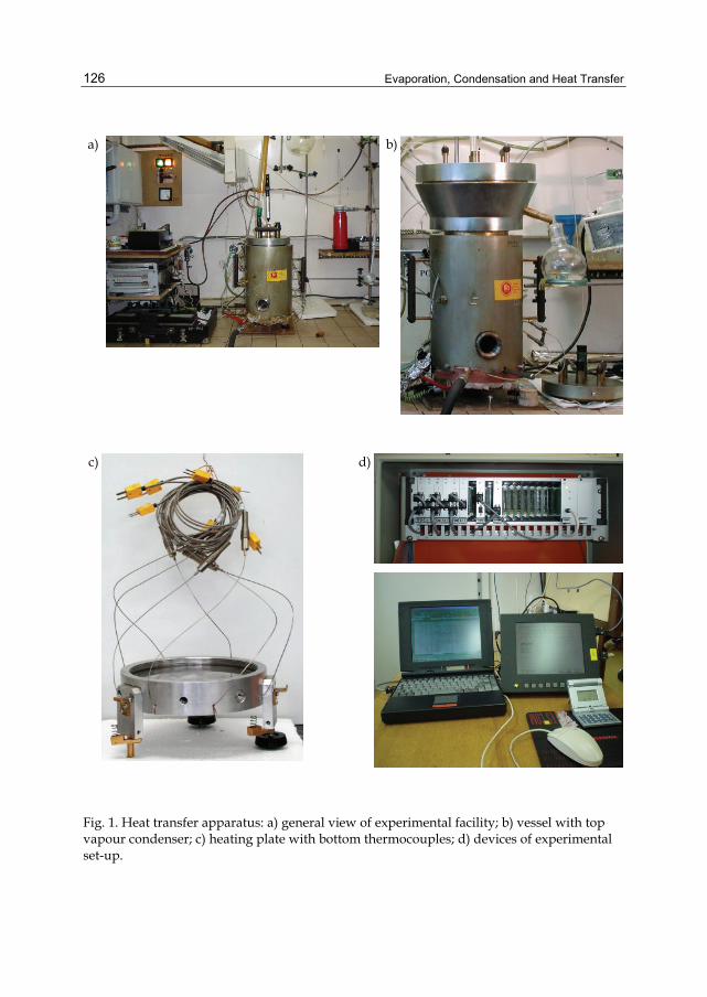
Evaporation, Condensation and Heat Transfer
126
a) b)
c)
d)
Fig. 1. Heat transfer apparatus: a) general view of experimental facility; b) vessel with top vapour condenser; c) heating plate with bottom thermocouples; d) devices of experimental set-up.
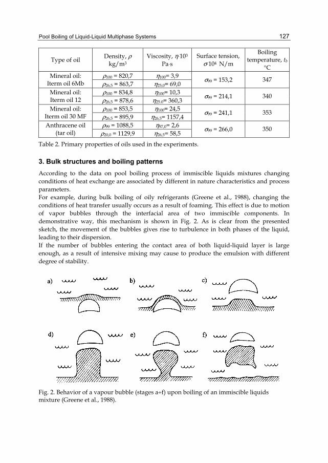
Pool Boiling of Liquid-Liquid Multiphase Systems
127
Type of oil Density, ρ kg/m3
Viscosity, η⋅103 Pa⋅s
Surface tension, σ⋅104 N/m
Boiling temperature, tb
°C ρ100 = 820,7 η100= 3,9 Mineral oil:
Iterm oil 6Mb ρ26,5 = 863,7 η25,0= 69,0 σ99 = 153,2 347
ρ100 = 834,8 η100= 10,3 Mineral oil: Iterm oil 12 ρ26,5 = 878,6 η25.0= 360,3
σ99 = 214,1 340
ρ100 = 853,5 η100= 24,5 Mineral oil: Iterm oil 30 MF ρ26,5 = 895,9 η26,5= 1157,4
σ99 = 241,1 353
ρ99 = 1088,5 η97,0= 2,6 Anthracene oil (tar oil) ρ20,0 = 1129,9 η26,5= 58,5
σ99 = 266,0 350
Table 2. Primary properties of oils used in the experiments.
3. Bulk structures and boiling patterns According to the data on pool boiling process of immiscible liquids mixtures changing conditions of heat exchange are associated by different in nature characteristics and process parameters. For example, during bulk boiling of oily refrigerants (Greene et al., 1988), changing the conditions of heat transfer usually occurs as a result of foaming. This effect is due to motion of vapor bubbles through the interfacial area of two immiscible components. In demonstrative way, this mechanism is shown in Fig. 2. As is clear from the presented sketch, the movement of the bubbles gives rise to turbulence in both phases of the liquid, leading to their dispersion. If the number of bubbles entering the contact area of both liquid-liquid layer is large enough, as a result of intensive mixing may cause to produce the emulsion with different degree of stability.
Fig. 2. Behavior of a vapour bubble (stages a÷f) upon boiling of an immiscible liquids mixture (Greene et al., 1988).
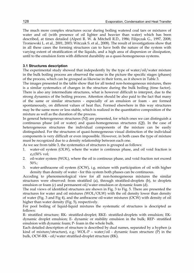
Evaporation, Condensation and Heat Transfer
128
The much more complex structures occur during boiling watered coal tars or mixtures of water and oil (with presence of oil lighter and heavier than water) which has been described, at times detailed (Alperi R. W. & Mitchell R.D., 1986; Filipczak G., 1997, 2008; Troniewski L. et al., 2001, 2003; Witczak S. et al., 2008). The result of investigations show that in all these cases the forming structures can to have both the nature of the system with varying extent of stratification of the liquids, and a high area of dispersion or dissipation, until to the emulsion form with different durability as a quasi-homogeneous systems.
3.1 Structures description The experimental study showed that indepedently by the type of water/oil/water mixture in the bulk boiling process are observed the same in the picture the specific stages (phases) of the process, which can be grouped as likewise in their form, as it shown in Table 3. The images presented in the table show that for all tested non-homogeneous mixtures, there is a similar systematics of changes in the structure during the bulk boiling (time factor). There is also any intermediate structures, what is however difficult to interpret, due to the strong dynamics of the boiling process. Attention should be also paid to the fact that many of the same or similar structures - especially of an emulsion or foam - are formed spontaneously, on different values of heat flux. Formed elsewhere in this way structures may be the same more or less stable, which is realized in the quantitative composition of the mixture as well as the duration of the process. In general heterogeneous structures (NJ) are presented, for which ones we can distinguish a continuous phase (oil or water) and quasi-homogeneous structures (QJ). In the case of heterogeneous structures the individual components of the mixture can be easily distinguished. For the structures of quasi-homogeneous visual distinction of the individual components is very difficult or even impossible. However, in both cases the type of mixture must be recognized due to a density relationship between each one. As we see from table 3, the systematics of structures is grouped as follows: 1. water-oil system (OLW), where the water is continous phase, and oil void fraction is
εol≤50% vol; 2. oil-water system (WOL), where the oil is continous phase, and void fraction not exceed
50%; 3. water-anthracene oil system (OCW), i.g. mixture with participation of oil with higher
density than density of water - for this system both phases can be continuous. Accoding to phenomenological view for all non-homogeneous mixtures the similar structures were observed: from stratified (a), through stratified-droplets (b), to droplets emulsion or foam (c) and permanent oil/water emulsion or dynamic foam (d). The real views of identified structures are shown in Fig. 3 to Fig. 5. There are presented the structures for water and oil mixtures (WOL/OLW) with the oil density lower than density of water (Fig. 3 and Fig 4), and the anthracene oil-water mixtures (OCW) with density of oil higher than water density (Fig. 5), respectively. For pool boiling of liquid-liquid mixtures the systematic of structures is descripted as follows: R- stratified structure; RK- stratified-droplet; RKE- stratified-droplets with emulsion; EK- dynamic droplet emulsion; E- dynamic or stability emulsion in the bulk; REP- stratified emulsion with dynamic foam; P- foam in the whole bulk. Each detailed description of structure is described by dual names, separated by a hyphen (a kind of mixture/structure), e.g.: WOL-P – water/oil - dynamic foam structure (P) in the bulk, OCW-RK - oil/water stratified-droplet structure (RK).
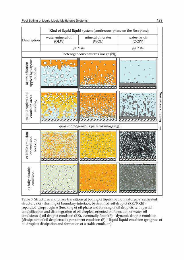
Pool Boiling of Liquid-Liquid Multiphase Systems
129
Kind of liquid-liquid system (continuous phase on the first place)
water-mineral oil (OLW)
mineral oil-water (WOL)
water-tar oil (OCW)
Description
ρol < ρw ρol > ρw
heterogeneous patterns image (NJ)
a) s
trat
ifica
tion
ripp
led
by v
apou
r bu
bble
s
b) o
il dr
ople
ts a
nd
emul
sion
are
as
rush
ing
quasi-homogeneous patterns image (QJ)
c) la
bile
em
ulsi
on
or e
mul
sion
br
eaki
ng
d) fu
lly d
urab
le
emul
sion
←
hea
t flu
x in
crea
sing
Table 3. Structures and phase transitions at boiling of liquid-liquid mixtures: a) separated structure (R) - sloshing of boundary interface; b) stratified–oil-droplet (RK/RKE) - separated-drops regime (breaking of oil phase and forming of oil droplets with partial emulsification and disintegration of oil droplets oriented on formation of water-oil emulsion); c) oil-droplet emulsion (EK), eventually foam (P) – dynamic droplet emulsion (dissipation of oil droplets); d) permanent emulsion (E) – liquid-liquid emulsion (progress of oil droplets dissipation and formation of a stable emulsion)
Evaporation, Condensation and Heat Transfer
130
Sometimes these changes occur very suddenly. It is a characteristic symptom for so called flash (explosive) boiling, observed practically for all investigated water/oil/water systems. In many cases this leads to the formation of very stable emulsions, what is characteristics for non-Newtonian fluids, with kinematic viscosity several times (one thousand and more) higher than the viscosity of the liquids forming a two-phase liquid-liquid system. Furthermore, in case of anthracene oil-water mixture boiling (OCW), the emulsion creation phenomenon takes place at the lower value of heat flux density, than in case of water-oil mixture. The state of mixture foaming appears more quickly, as well. For the obvious reasons (lack of liquid transparency) the precise observation of the phenomenon was impossible in this case. Moreover, the high rate of water steam bubbles created results in the high dispersion of oil phase, particularly in the vicinity of heating plate, where the sudden emulsion formation takes place. The emulsification intensifies at the further increase of heat flux density, what leads to mixture foaming till the “boiling over” effect is obtained. This is important that appearance of each structure can create with increasing or at constant value of heat flux. In the second case (q=const.) the time factor is very important - we distinguish the different transition time from stratified forms to more or less homogeneous. From phenomenological point of view the structures of the boiling liquid-liquid mixtures are as follows: 1. Water-oil mixtures (OLW) – Fig. 3 - heterogeneous structures (NJ): OLW-R - stratified structure. Oil layer located on the water is broken down by the vapour bubbles climbing to the top. The wavy motion is observed after initially stable interphases boundary; OLW-RK – stratified-droplet structure. The dissipation of mixture components take place as a result of turbulence in the liquid, formed by vapour bubbles move to the top. From the oil layer are pulled his portion in the form of drops of different size and shape and accumulate down to the water volume. On the other hand portions of water are entrained into the oil layer. As a consequence the foam is formed as a thin layer, floating on the free surface of the mixture in the form of large floccules, which tend to hold just below the surface layer oil. As a result of turbulence in the mixture, in great number portions of the oil phase are entrained in the heating plate area; OLW-RKE – stratified-droplets with emulsion. Non-transparent layer of emulsion is formed, which expands in the direction of the heating plate. A significant reduction in transparency of the mixture due to the presence of oil follows in the form of droplets, a portion of emulsions and foam. The oil in increasing amounts is deposited on the surface heating. 2. Water-oil mixtures (OLW) – Fig. 3 - quasi-homogeneous structures (QJ): OLW-EK – dynamic droplet emulsion. The oil is dispersed as small droplets, and different clouds of foam, circulating in the volume of the mixture. The structure is periodic, partial stratification, becoming more transparent. Structure is accompanied by occasional flash evaporation; OLW-E – dynamic or stability emulsion. As a result of further dissipation of oil phase the non-transparent emulsion is formed in whole volume of the mixture. Boiling is accompanied by explosiv (flash) evaporation of emulsion. 3. Oil-water mixtures (WOL) – Fig. 4 - heterogeneous structures (NJ): WOL-R - stratified structure. Oil layer forms remains on a layer of boiling water. Periodic structure is accompanied by flash evaporation and release of a portion of steam and water droplets to the volume of oil. As a result a sudden breaking initially stable phase boundary take place;
Pool Boiling of Liquid-Liquid Multiphase Systems
131
WOL-RK – stratified-droplet structure. Vapours bubbles are rising into the top layer of oil and leave behind traces of water (micro-droplets of water). At the interface exists a layer consisting of vapour bubbles, drops of water and oil. As a result of flash (explosive) evaporation components of mixture are mixed intensively. The portions of oil are deposited on the heating plate under the influence of turbulence. Further dispersion of phases leads to emulsion in the bulk volume (WOL-E); WOL-REP - stratified emulsion with dynamic foam. On the emulsion layer remains a dynamic layer of foam formed by the foaming of the emulsion (WOL-E). There has been a rapid increase of the mixture volume and sudden flash evaporation. The structure may take in the emulsion form in whole volume (WOL-E) or the dynamic foam in the bulk volume (WOL-P). 4. Oil-water mixtures (WOL) – Fig. 4 - quasi-homogeneous structures (QJ): WOL-E – dynamic or stability emulsion. The structure is almost totally non-transparent. It is accompanied by explosion evaporation at the beginning of formation of structures very rapidly, and then its intensity decreases. There are boiling with formation of quite a number of small bubbles. The structure may evolve in the stratified emulsion and foam (WOL-REP), and next to foam in the whole volume (WOL-P). WOL-P – dynamic foam structure. The mixture is totally non-transparent. It is characterized by sudden increase volume of foam and periodic stratification to emulsion-foam structure (WOL-REP). 5. Water-anthracene oil system (OCW) – Fig 5 – heterogeneous structures (NJ), OCW-R – stratified structure. Both phases are clearly separated. Steam bubbles are formed on the layer of oil, which is behind on the hot wall of the heating plate (the oil temperature is above the saturation temperature of water). The movement of vapour bubbles causes the oil layer surface wavy motion. OCW-RK – stratified-droplet structure. Forming and moving upward vapor bubbles cause turbulence in the mixture, which kidnap oil from the surface layer. Oil droplets are formed with of extended shapes. Boiling takes place on the much overheated portions of oil. Further disspersion of oil in water volume leads to decreases thickness of the oil and its breakdown take place. 6. Water-anthracene oil system (OCW) – Fig 5 – quasi-homogeneous structures (QJ): OCW-EK – dynamic droplet emulsion. The emulsion takes the form of small oil droplets dispersed in water volume. As a result of tearing of oil from bottom the water evaporates very rapidly by contact with preheated plate. There is flash (explosive) evaporation and intensive dissipation of oil. Depending on heat flux a periodic stratified-droplet (OCW-RK) or dynamic foam (OCW-P) are formed. OCW-P – dynamic foam structure. Consequently, by flash evaporation of water produce non-transparent dynamic foam in the bulk mixture. This causes a rapid increase of mixture volume. It should be noted that at boiling of the water-anthracene oil (Fig. 5) we has different, in relation to other tested mixtures, mechanism of formation of structures. This follows from the fact that anthracene oil is keeping on the heating plate, what delays the process of boiling water. The same time with the increase of heat flux leads to changes of structures of this system what is very intense, because they occur as a result of flash evaporation of water after contact with a highly superheated wall of heating plate. Additionally, in this case do not exist the conditions conducive to the formation of more stable emulsion, and only highly dynamic foam (totally non-transparent), which is usually re-stratification.
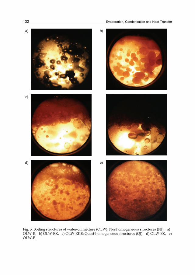
Evaporation, Condensation and Heat Transfer
132
a)
b)
c)
d)
e)
Fig. 3. Boiling structures of water-oil mixture (OLW). Nonhomogeneous structures (NJ): a) OLW-R, b) OLW-RK, c) OLW-RKE; Quasi-homogeneous structures (QJ): d) OLW-EK, e) OLW-E
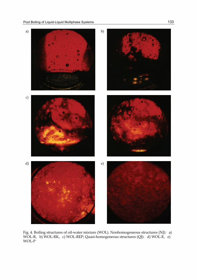
Pool Boiling of Liquid-Liquid Multiphase Systems
133
a)
b)
c)
d)
e)
Fig. 4. Boiling structures of oil-water mixture (WOL). Nonhomogeneous structures (NJ): a) WOL-R, b) WOL-RK, c) WOL-REP; Quasi-homogeneous structures (QJ): d) WOL-E, e) WOL-P
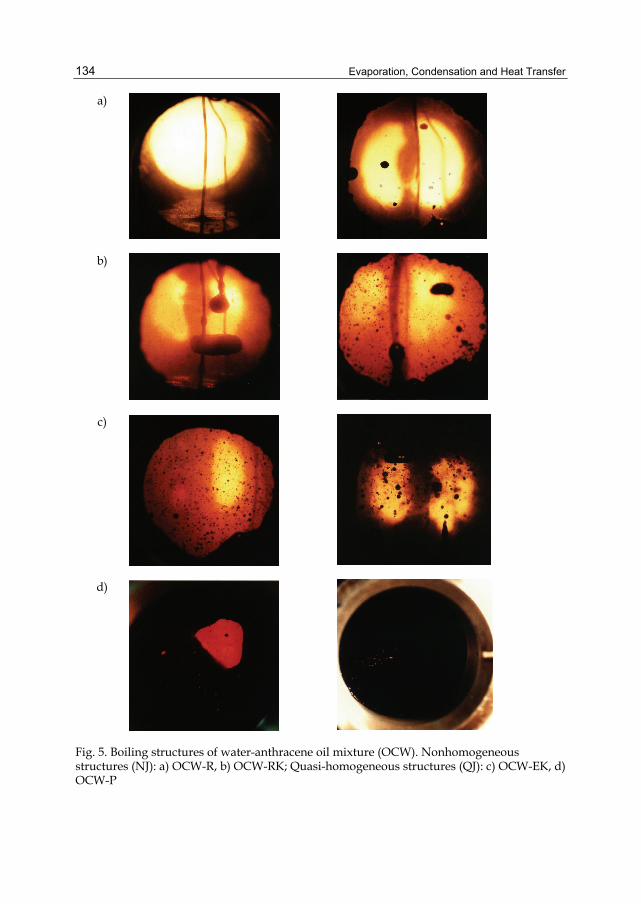
Evaporation, Condensation and Heat Transfer
134
a)
b)
c)
d)
Fig. 5. Boiling structures of water-anthracene oil mixture (OCW). Nonhomogeneous structures (NJ): a) OCW-R, b) OCW-RK; Quasi-homogeneous structures (QJ): c) OCW-EK, d) OCW-P
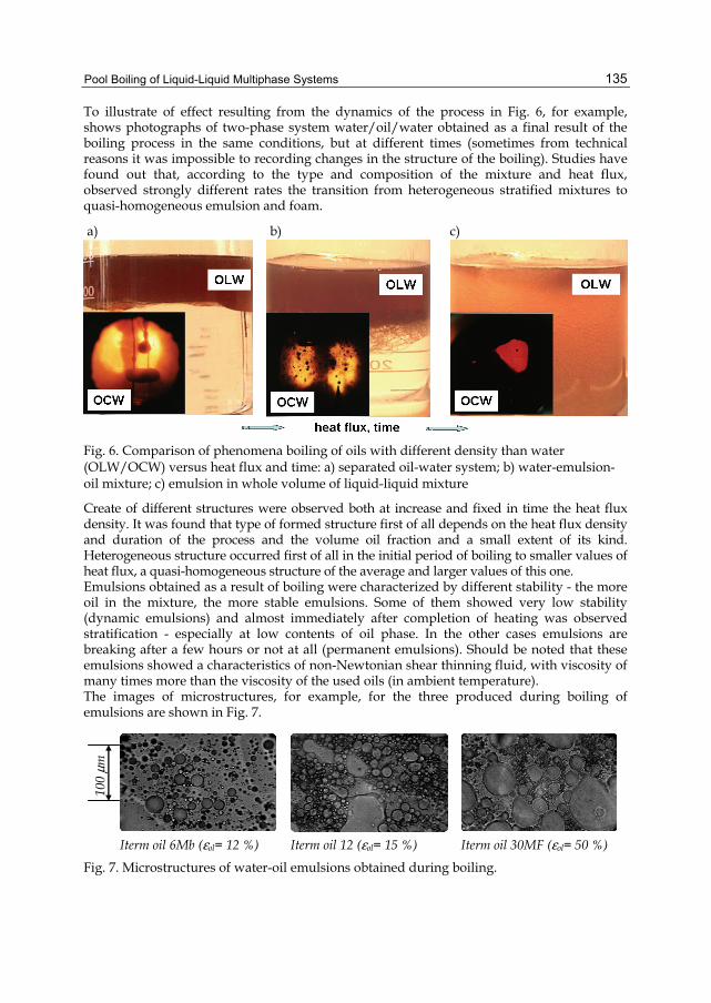
Pool Boiling of Liquid-Liquid Multiphase Systems
135
To illustrate of effect resulting from the dynamics of the process in Fig. 6, for example, shows photographs of two-phase system water/oil/water obtained as a final result of the boiling process in the same conditions, but at different times (sometimes from technical reasons it was impossible to recording changes in the structure of the boiling). Studies have found out that, according to the type and composition of the mixture and heat flux, observed strongly different rates the transition from heterogeneous stratified mixtures to quasi-homogeneous emulsion and foam.
a) b) c)
Fig. 6. Comparison of phenomena boiling of oils with different density than water (OLW/OCW) versus heat flux and time: a) separated oil-water system; b) water-emulsion-oil mixture; c) emulsion in whole volume of liquid-liquid mixture
Create of different structures were observed both at increase and fixed in time the heat flux density. It was found that type of formed structure first of all depends on the heat flux density and duration of the process and the volume oil fraction and a small extent of its kind. Heterogeneous structure occurred first of all in the initial period of boiling to smaller values of heat flux, a quasi-homogeneous structure of the average and larger values of this one. Emulsions obtained as a result of boiling were characterized by different stability - the more oil in the mixture, the more stable emulsions. Some of them showed very low stability (dynamic emulsions) and almost immediately after completion of heating was observed stratification - especially at low contents of oil phase. In the other cases emulsions are breaking after a few hours or not at all (permanent emulsions). Should be noted that these emulsions showed a characteristics of non-Newtonian shear thinning fluid, with viscosity of many times more than the viscosity of the used oils (in ambient temperature). The images of microstructures, for example, for the three produced during boiling of emulsions are shown in Fig. 7.
1
00 μ
m
Iterm oil 6Mb (εol= 12 %) Iterm oil 12 (εol= 15 %) Iterm oil 30MF (εol= 50 %)
Fig. 7. Microstructures of water-oil emulsions obtained during boiling.
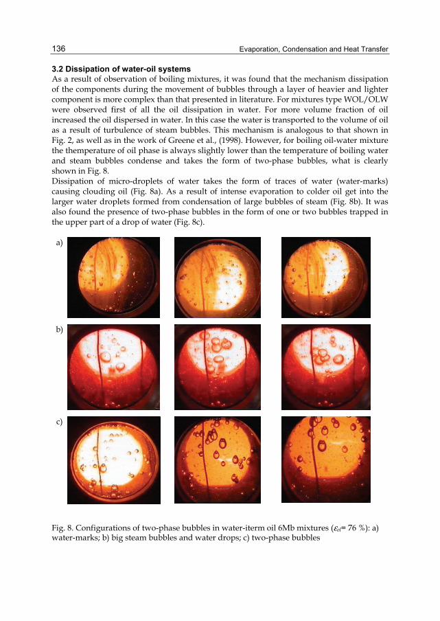
Evaporation, Condensation and Heat Transfer
136
3.2 Dissipation of water-oil systems As a result of observation of boiling mixtures, it was found that the mechanism dissipation of the components during the movement of bubbles through a layer of heavier and lighter component is more complex than that presented in literature. For mixtures type WOL/OLW were observed first of all the oil dissipation in water. For more volume fraction of oil increased the oil dispersed in water. In this case the water is transported to the volume of oil as a result of turbulence of steam bubbles. This mechanism is analogous to that shown in Fig. 2, as well as in the work of Greene et al., (1998). However, for boiling oil-water mixture the themperature of oil phase is always slightly lower than the temperature of boiling water and steam bubbles condense and takes the form of two-phase bubbles, what is clearly shown in Fig. 8. Dissipation of micro-droplets of water takes the form of traces of water (water-marks) causing clouding oil (Fig. 8a). As a result of intense evaporation to colder oil get into the larger water droplets formed from condensation of large bubbles of steam (Fig. 8b). It was also found the presence of two-phase bubbles in the form of one or two bubbles trapped in the upper part of a drop of water (Fig. 8c).
a)
b)
c)
Fig. 8. Configurations of two-phase bubbles in water-iterm oil 6Mb mixtures (εol= 76 %): a) water-marks; b) big steam bubbles and water drops; c) two-phase bubbles
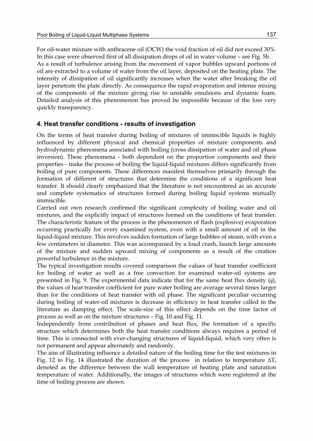
Pool Boiling of Liquid-Liquid Multiphase Systems
137
For oil-water mixture with anthracene oil (OCW) the void fraction of oil did not exceed 30%. In this case were observed first of all dissipation drops of oil in water volume – see Fig. 5b. As a result of turbulence arising from the movement of vapor bubbles upward portions of oil are extracted to a volume of water from the oil layer, deposited on the heating plate. The intensity of dissipation of oil significantly increases when the water after breaking the oil layer penetrate the plate directly. As consequence the rapid evaporation and intense mixing of the components of the mixture giving rise to unstable emulsions and dynamic foam. Detailed analysis of this phenomenon has proved be impossible because of the loss very quickly transparency.
4. Heat transfer conditions - results of investigation On the terms of heat transfer during boiling of mixtures of immiscible liquids is highly influenced by different physical and chemical properties of mixture components and hydrodynamic phenomena associated with boiling (cross dissipation of water and oil phase inversion). These phenomena - both dependent on the proportion components and their properties - make the process of boiling the liquid-liquid mixtures differs significantly from boiling of pure components. These differences manifest themselves primarily through the formation of different of structures that determine the conditions of a significant heat transfer. It should clearly emphasized that the literature is not encountered as an accurate and complete systematics of structures formed during boiling liquid systems mutually immiscible. Carried out own research confirmed the significant complexity of boiling water and oil mixtures, and the explicitly impact of structures formed on the conditions of heat transfer. The characteristic feature of the process is the phenomenon of flash (explosive) evaporation occurring practically for every examined system, even with a small amount of oil in the liquid-liquid mixture. This involves sudden formation of large bubbles of steam, with even a few centimeters in diameter. This was accompanied by a loud crash, launch large amounts of the mixture and sudden upward mixing of components as a result of the creation powerful turbulence in the mixture. The typical investigation results covered comparison the values of heat transfer coefficient for boiling of water as well as a free convection for examined water-oil systems are presented in Fig. 9. The experimental data indicate that for the same heat flux density (q), the values of heat transfer coefficient for pure water boiling are average several times larger than for the conditions of heat transfer with oil phase. The significant peculiar occurring during boiling of water-oil mixtures is decrease in efficiency in heat transfer called in the literature as damping effect. The scale-size of this effect depends on the time factor of process as well as on the mixture structures – Fig. 10 and Fig. 11. Independently from contribution of phases and heat flux, the formation of a specific structure which determines both the heat transfer conditions always requires a period of time. This is connected with ever-changing structures of liquid-liquid, which very often is not permanent and appear alternately and randomly. The aim of illustrating influence a detailed nature of the boiling time for the test mixtures in Fig. 12 to Fig. 14 illustrated the duration of the process in relation to temperature ∆T, denoted as the difference between the wall temperature of heating plate and saturation temperature of water. Additionally, the images of structures which were registered at the time of boiling process are shown.
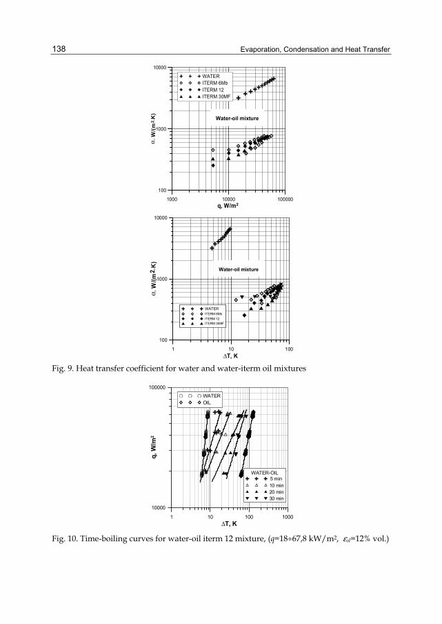
Evaporation, Condensation and Heat Transfer
138
1000 10000 100000q, W/m2
100
1000
10000
α, W
/(m2 .
K)
WATERITERM 6MbITERM 12ITERM 30MF
Water-oil mixture
1 10 100ΔT, K
100
1000
10000
α, W
/(m2 .
K)
WATERITERM 6MbITERM 12ITERM 30MF
Water-oil mixture
Fig. 9. Heat transfer coefficient for water and water-iterm oil mixtures
1 10 100 1000ΔT, K
10000
100000
q, W
/m2
WATEROIL
WATER-OIL 5 min10 min20 min30 min
Fig. 10. Time-boiling curves for water-oil iterm 12 mixture, (q=18÷67,8 kW/m2, εol=12% vol.)
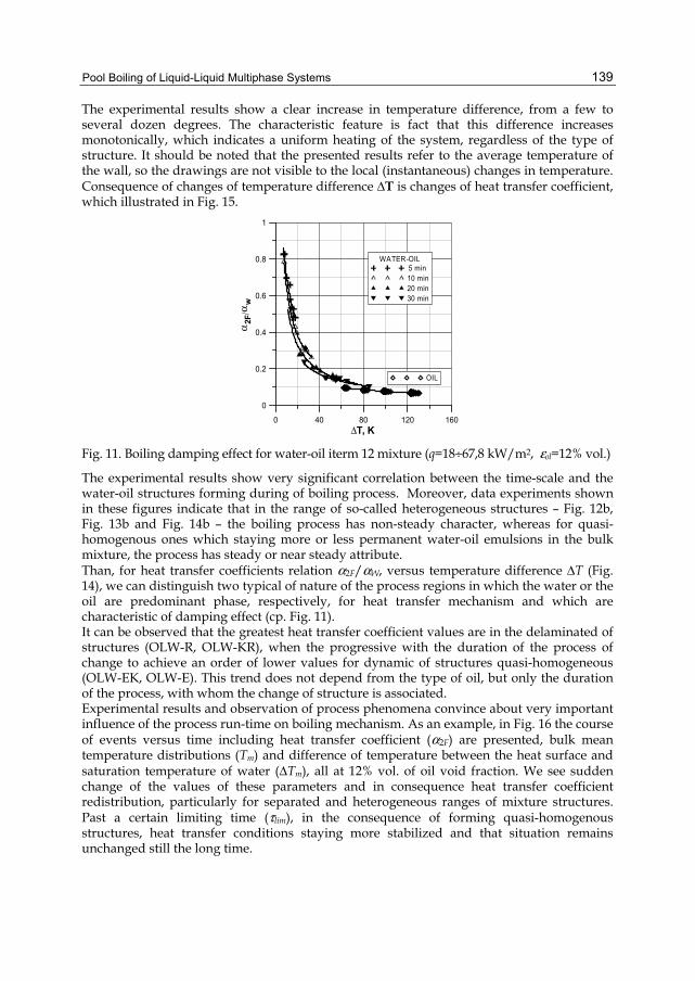
Pool Boiling of Liquid-Liquid Multiphase Systems
139
The experimental results show a clear increase in temperature difference, from a few to several dozen degrees. The characteristic feature is fact that this difference increases monotonically, which indicates a uniform heating of the system, regardless of the type of structure. It should be noted that the presented results refer to the average temperature of the wall, so the drawings are not visible to the local (instantaneous) changes in temperature. Consequence of changes of temperature difference ΔT is changes of heat transfer coefficient, which illustrated in Fig. 15.
0 40 80 120 160ΔT, K
0
0.2
0.4
0.6
0.8
1
α2F
/αw
OIL
WATER-OIL 5 min10 min20 min30 min
Fig. 11. Boiling damping effect for water-oil iterm 12 mixture (q=18÷67,8 kW/m2, εol=12% vol.)
The experimental results show very significant correlation between the time-scale and the water-oil structures forming during of boiling process. Moreover, data experiments shown in these figures indicate that in the range of so-called heterogeneous structures – Fig. 12b, Fig. 13b and Fig. 14b – the boiling process has non-steady character, whereas for quasi-homogenous ones which staying more or less permanent water-oil emulsions in the bulk mixture, the process has steady or near steady attribute. Than, for heat transfer coefficients relation α2F/αW, versus temperature difference ΔT (Fig. 14), we can distinguish two typical of nature of the process regions in which the water or the oil are predominant phase, respectively, for heat transfer mechanism and which are characteristic of damping effect (cp. Fig. 11). It can be observed that the greatest heat transfer coefficient values are in the delaminated of structures (OLW-R, OLW-KR), when the progressive with the duration of the process of change to achieve an order of lower values for dynamic of structures quasi-homogeneous (OLW-EK, OLW-E). This trend does not depend from the type of oil, but only the duration of the process, with whom the change of structure is associated. Experimental results and observation of process phenomena convince about very important influence of the process run-time on boiling mechanism. As an example, in Fig. 16 the course of events versus time including heat transfer coefficient (α2F) are presented, bulk mean temperature distributions (Tm) and difference of temperature between the heat surface and saturation temperature of water (ΔTm), all at 12% vol. of oil void fraction. We see sudden change of the values of these parameters and in consequence heat transfer coefficient redistribution, particularly for separated and heterogeneous ranges of mixture structures. Past a certain limiting time (τlim), in the consequence of forming quasi-homogenous structures, heat transfer conditions staying more stabilized and that situation remains unchanged still the long time.
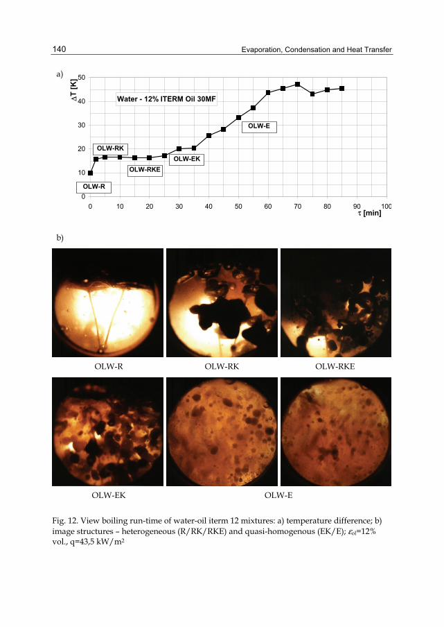
Evaporation, Condensation and Heat Transfer
140
a)
Water - 12% ITERM Oil 30MF
0
10
20
30
40
50
0 10 20 30 40 50 60 70 80 90 100τ [min]
ΔT [K
]
OLW-EKOLW-RKE
OLW-RK
OLW-R
OLW-E
b)
OLW-R OLW-RK OLW-RKE
OLW-EK OLW-E
Fig. 12. View boiling run-time of water-oil iterm 12 mixtures: a) temperature difference; b) image structures – heterogeneous (R/RK/RKE) and quasi-homogenous (EK/E); εol=12% vol., q=43,5 kW/m2
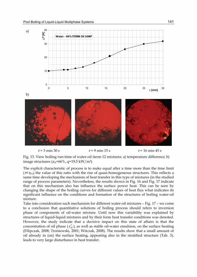
Pool Boiling of Liquid-Liquid Multiphase Systems
141
a) Water - 66% ITERM Oil 30MF
0
10
20
30
40
0 5 10 15 20 25 30τ [min]
ΔT
[K]
b)
τ = 3 min 30 s τ = 9 min 15 s τ = 16 min 45 s
Fig. 13. View boiling run-time of water-oil iterm 12 mixtures: a) temperature difference; b) image structures (εol=66%, q=19,5 kW/m2)
The explicit characteristic of process is to make equal after a time more than the time limit (τ<τlim) the value of this ratio with the rise of quasi-homogeneous structures. This reflects a same time developing the mechanism of heat transfer in this type of mixtures (in the studied range of process parameters). Nevertheless, the results shown in Fig. 16 and Fig. 17 indicate that on this mechanism also has influence the surface power heat. This can be seen by changing the shape of the boiling curves for different values of heat flux what indicates its significant influence on the conditions and formation of the structures of boiling water-oil mixture. Take into consideration such mechanism for different water-oil mixtures – Fig. 17 – we come to a conclusion that quantitative solutions of boiling process should refers to inversion phase of components of oil-water mixture. Until now this variability was explained by structures of liquid-liquid mixtures and by their form heat transfer conditions was denoted. However, the study indicate that a decisive impact on this state of affairs is that the concentration of oil phase ( olε ∗ ), as well as stable oil-water emulsion, on the surface heating (Filipczak, 2008; Troniewski, 2001; Witczak, 2008). The results show that a small amount of oil already in (on) the surface heating, appearing also in the stratified structure (Tab. 3), leads to very large disturbance in heat transfer.
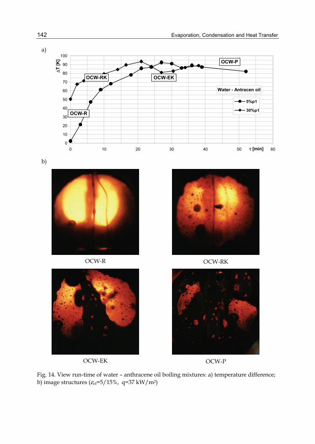
Evaporation, Condensation and Heat Transfer
142
a)
Water - Antracen oil
0
10
20
30
40
50
60
70
80
90
100
0 10 20 30 40 50 60τ [min]
ΔT [K
]
5%p1
30%p1OCW-R
OCW-RK OCW-EK
OCW-P
b)
OCW-R OCW-RK
OCW-EK OCW-P
Fig. 14. View run-time of water – anthracene oil boiling mixtures: a) temperature difference; b) image structures (εol=5/15%, q=37 kW/m2)
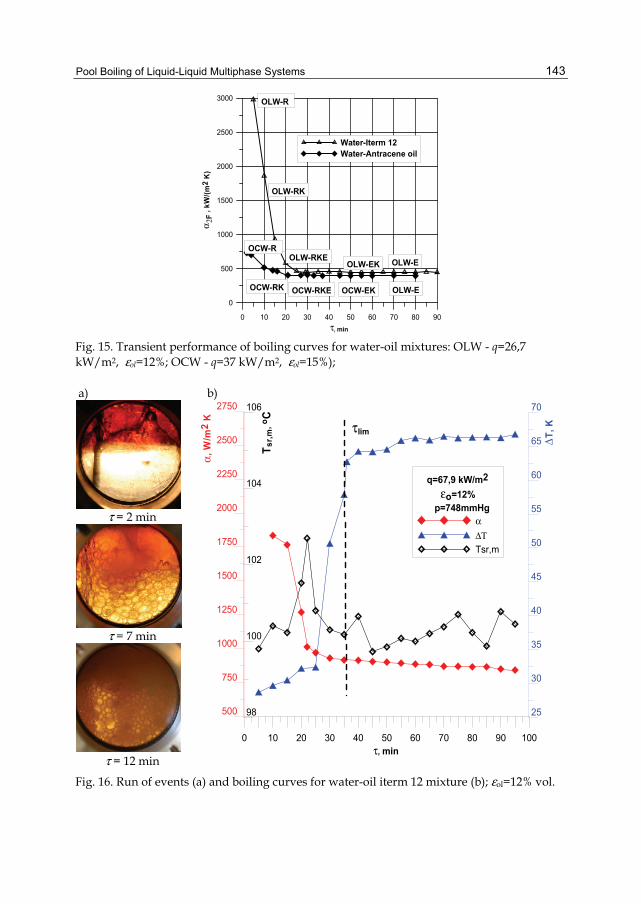
Pool Boiling of Liquid-Liquid Multiphase Systems
143
0 10 20 30 40 50 60 70 80 90τ, min
0
500
1000
1500
2000
2500
3000
α 2F
, kW
/(m2
K)
Water-Iterm 12Water-Antracene oil
OLW-RK
OLW-RKEOLW-EK OLW-E
OLW-R
OCW-R
OCW-RK OCW-RKE OCW-EK OLW-E
Fig. 15. Transient performance of boiling curves for water-oil mixtures: OLW - q=26,7 kW/m2, εol=12%; OCW - q=37 kW/m2, εol=15%);
a) b)
τ = 2 min
τ = 7 min
τ = 12 min
0 10 20 30 40 50 60 70 80 90 100τ, min
500
750
1000
1250
1500
1750
2000
2250
2500
2750
α, W
/m2
K
q=67,9 kW/m2
εo=12% p=748mmHg
αΔΤ Tsr,m
25
30
35
40
45
50
55
60
65
70
ΔT, K
98
100
102
104
106
T sr,m
, o C τlim
Fig. 16. Run of events (a) and boiling curves for water-oil iterm 12 mixture (b); εol=12% vol.
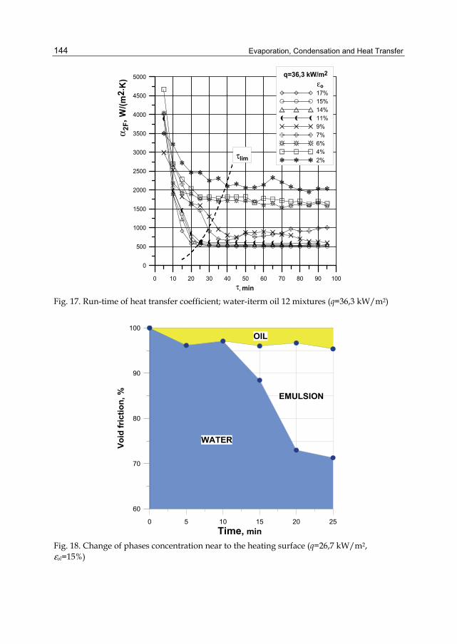
Evaporation, Condensation and Heat Transfer
144
0 10 20 30 40 50 60 70 80 90 100τ, min
0
500
1000
1500
2000
2500
3000
3500
4000
4500
5000
α 2F,
W/(m
2.K
) q=36,3 kW/m2
εo17%15%14%11%9%7%6%4%2%τlim
Fig. 17. Run-time of heat transfer coefficient; water-iterm oil 12 mixtures (q=36,3 kW/m2)
0 5 10 15 20 25Time, min
60
70
80
90
100
Void
fric
tion,
%
OIL
WATER
EMULSION
Fig. 18. Change of phases concentration near to the heating surface (q=26,7 kW/m2, εol=15%)
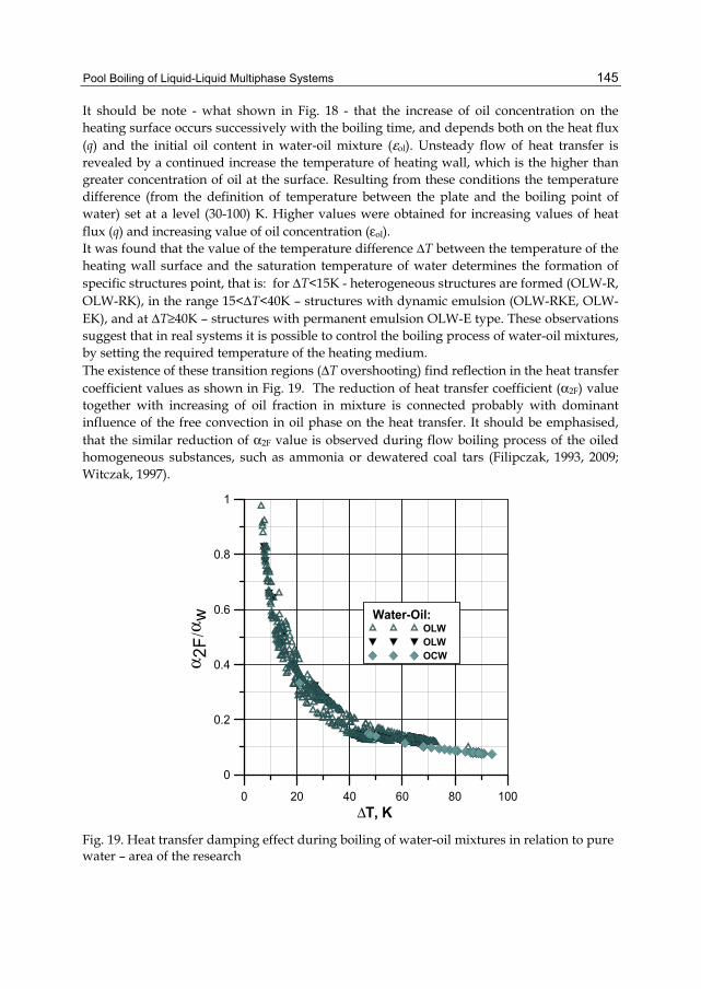
Pool Boiling of Liquid-Liquid Multiphase Systems
145
It should be note - what shown in Fig. 18 - that the increase of oil concentration on the heating surface occurs successively with the boiling time, and depends both on the heat flux (q) and the initial oil content in water-oil mixture (εol). Unsteady flow of heat transfer is revealed by a continued increase the temperature of heating wall, which is the higher than greater concentration of oil at the surface. Resulting from these conditions the temperature difference (from the definition of temperature between the plate and the boiling point of water) set at a level (30-100) K. Higher values were obtained for increasing values of heat flux (q) and increasing value of oil concentration (εol). It was found that the value of the temperature difference ∆T between the temperature of the heating wall surface and the saturation temperature of water determines the formation of specific structures point, that is: for ΔT<15K - heterogeneous structures are formed (OLW-R, OLW-RK), in the range 15<ΔT<40K – structures with dynamic emulsion (OLW-RKE, OLW-EK), and at ΔT≥40K – structures with permanent emulsion OLW-E type. These observations suggest that in real systems it is possible to control the boiling process of water-oil mixtures, by setting the required temperature of the heating medium. The existence of these transition regions (ΔT overshooting) find reflection in the heat transfer coefficient values as shown in Fig. 19. The reduction of heat transfer coefficient (α2F) value together with increasing of oil fraction in mixture is connected probably with dominant influence of the free convection in oil phase on the heat transfer. It should be emphasised, that the similar reduction of α2F value is observed during flow boiling process of the oiled homogeneous substances, such as ammonia or dewatered coal tars (Filipczak, 1993, 2009; Witczak, 1997).
0 20 40 60 80 100ΔT, K
0
0.2
0.4
0.6
0.8
1
α 2F/
α w
Water-Oil: OLWOLWOCW
Fig. 19. Heat transfer damping effect during boiling of water-oil mixtures in relation to pure water – area of the research
Evaporation, Condensation and Heat Transfer
146
The effect of damping, i.e. reduction - in relation to water boiling - of heat transfer rate during the water-oil mixture boiling has been shown in Fig. 19. As results from the line schedule (average relations), even a small fraction of oil on heating plate causes the strong lowering of the heat transfer coefficient. At the same time the higher is value of heat flux density (also, where the mixture can be in the form of emulsion or dynamic foam), the more significant is α2F value reduction. It will be emphasised that the higher is oil volume fraction in mixture, the higher is effect of heat transfer coefficient reduction. For the highest fraction of oil investigated the heat transfer coefficients are stabilising on an approximately constant level, near the values determined by the free convection in oils component (Fig. 9). Appointed on the investigation results the border condition describing limited time which indicates change of heat transfer conditions in the area of phase inversion was found experimentally as
8
lim 0,271,14 0,11
ol
2.18 10τDq εH
⋅=
⎛ ⎞⎜ ⎟⎝ ⎠
(1)
where relation D/H refers to diameter of heating surface (D) and high of bulk water-oil mixture (H) respectively. Basing on assumption that heating surface area is entirely covered by water-oil mixture, advantageously by emulsion, and it staying proportionally to oil and water concentration near thermal boundary layer ( olε ∗ , (1- olε ∗ ), respectively), the total temperature gradient is provided by components ratio, i.e.:
* *(1 )ol ol ol wT T Tε εΔ = Δ + − Δ (2)
Take into consideration that boiling process proceeds on uniform heat flux (q) by simple calculation we obtained the relation for total heat resistance as
* *
2
11 ol ol
F ol w
ε εα α α
−= + (3)
Hence,
2
*
1
1 1
F
w wol
ol
αα αε
α
=⎛ ⎞
+ −⎜ ⎟⎝ ⎠
(4)
Parameter olε ∗ indicates a set of oil concentration near heating surface and its value may be from domain 0 ≤ olε ∗ ≤ 1. When oil phase is absent from heating surface, what take place for stratified or more separable water-oil structures (see Fig. 2a, Fig. 3a), than 0olε ∗ = and heat transfer coefficient converges to 2F wα α= . On the other hand, for 1olε ∗ = oil liquid occupies all space of heating surface area (Fig. 3d, Fig. 4d, Fig. 5), and thus 2F olα α= .
Pool Boiling of Liquid-Liquid Multiphase Systems
147
It needs underlined that heat transfer coefficient aW put in equation (4) for water boiling should be calculate from
0,73,15w qα = (5)
as the best results of own experiments. Likewise, to aim calculation of heat transfer coefficient for natural convection and nucleate or transition boiling of oil phase on horizontal plates the new equation, similar to Michiejew view one, is proposed, as
0,250,25 PrNu 1,9Ra
Prol
ol olth
⎛ ⎞= ⎜ ⎟⎜ ⎟
⎝ ⎠ (6)
Equation (6) was verified for Rayleigh number of oil (Raol) from 1,06⋅108 to 6,8⋅1010. The empirical correlations useful for calculation of oil concentration at heating surface are as follows: - for non-steady conditions, i.e. for range restricted to separated or strongly
heterogeneous structures of water-oil mixtures
1,47 1,33 0,333
* 0,03681000 3600ol ol
q DH
τε ε ⎛ ⎞ ⎛ ⎞ ⎛ ⎞= ⎜ ⎟ ⎜ ⎟ ⎜ ⎟⎝ ⎠ ⎝ ⎠⎝ ⎠
(7)
- for steady run of process that is quasi-homogenous structures or fully development intermixed water-oil system and emulsions
10,21* 2 (1- ) q0,11
1000ol
ol olol
εε εε
−⎡ ⎤⎛ ⎞⎢ ⎥= + ⎜ ⎟⎢ ⎥⎝ ⎠⎣ ⎦
(8)
what is rightly over the limited time given by equation (1). At occurrence of intermediate or transitions structures the calculate programme according to heat transfer coefficient by equation (4) needs the less value of oil concentration olε ∗ obtained from equations (7) and (8). The computation results supported by statistic analysis show that in range of done experiments the proposed method describes heat transfer coefficient with mean error no more than 25% and may be used to prediction of heat transfer conditions upon pool boiling of water-oil mixtures different kinds. The results of this analysis indicate as well that irrespective of components concentration in water-oil systems with the help of equation (1) may evaluate the time for advantageous run of water-oil mixture boiling process.
5. Conclusions Based on results of experimental investigations the following most significant conclusions can be formulated:
Evaporation, Condensation and Heat Transfer
148
1. The process of boiling water-oil mixtures exhibits a number of peculiarities. They result from the diversified structure of liquid-liquid system and manifest themselves in a sudden variability of the process parameters.
2. The nature of the boiling process depends on the kind and composition of water-oil mixtures. Watering of mixtures favours the process of nucleation and contributes to quicker shattering of oil phase in the bulk. With a high of oil content, the heat transfer coefficient is dominated by free convection in the oil phase what leads to sudden decrease of heat transfer efficiency.
3. Depend on composition of water-oil mixture the heat transfer conditions are mirror of the steady as well as non-steady criteria and conditions. The first take place for separated form of water-oil mixture and second ones are beginning at quasi-homogeneous structures of this mixture (e.g. emulsions). The oil content has a very considerable effect on boiling curve then.
4. As the result of investigations, the phenomena connection occurring during pool boiling of two-phase water-oil mixture and the influence of time condition on process run of events and its parameters the relations for the value of heat transfer coefficient was worked out.
5. Description and structures systematics of boiling water/oil/water systems can greatly facilitate for further work on this process.
Symbols D – diameter of heating surface, m H – high of oil-water mixture (total level) Nu – Nusselt number Pr – Prandtl number q – heat flux, W/m2 T – temperature, K εol – void fraction of oil
olε ∗ – concentration of oil α – heat transfer coefficient, W/(m2·K) t – time, s
6. References Alperi R. W. & Mitchell R.D. (1986). Effect of oily fluid and surface contaminants on hest
transfer to boiling water, AIChE Journal, Vol. 30, No. 6, pp. 1028-1030 Boe R. (1997). Pool boiling of hydrocarbon mixtures on water. Int. Journal Heat Mass Transfer,
Vol. 41, No. 8-9, pp. 1003-1011 Collier J. G. (1981). Convective boiling and condensation. McGraw-Hill, New York Cieśliński J. T. (1996). Study of nucleate pool boiling on metallic rough and porous surfaces (in
Polish), Zeszyty Naukowe Politechniki Gdańskiej, Vol. 547, Mechanika No. 76. Gdańsk
Pool Boiling of Liquid-Liquid Multiphase Systems
149
Filipczak G. (1991). Tar dewatering in forced annular flow, In: Multiphase Flow and Heat Transfer, Ed. Xue-Jun Chen et al., Vol. 1, pp. 824-833, Hemisphere Publ. Corp., New York
Filipczak G. (1993). Heat transfer study on tar-steam flow, In: Heat and Mass Transfer, An Era of Change, Ed. Veziroglu T.N., Vol. 2, pp. 1255-1275, Nova Science Publ. Inc., New York
Filipczak G. (1997). Pool boilng heat transfer to tar-oil-water mixtures. Archives of Thermodynamics, Vo. 18, No. 1-2, pp. 73-85
Filipczak G. et al., (2000). Experimental assessment of pool boiling process for water-oil systems, Inż. i Ap. Chem., No. 3s, pp. 44-46
Filipczak G. et al., (2008). The anallysis of phenomena during boiling of a two-phase water-oil mixture, Przemysł Chemiczny, No. 87/2, pp. 116-120
Filipczak G. (2008). Heat transfer in two-phase tar-steam film flow, Inżynieria i Aparatura Chemiczna, No. 6, pp. 68-69
Gorenflo D. et al., (2001). Pool boiling heat transfer to binary mixtures with miscibility gap – Experimental results for a horizontal copper tube with 4,35 ID. Experimental Thermal and Fluid Science, Vol. 25, pp. 243-254
Greene et al., (1998). Onset of entrainment between immiscible liquid layer due to Rusing gas bubbles, Int. Journal Heat Mass Transfer, Vol. 31, No. 6, pp. 1309- 1317
Hobler T. (1986). Heat transfer and heat exchangers (in Polish), WNT, Warszawa Matthew L. et al., (2009). Boiling of dilute emelsion – Toward a new modeling framework,
Ind. Eng. Chem. Res. ol. 49, No. 12, pp. 5188-5196 Mori Y. H. et al., (1978). Pool boiling heat transfer to emulsions, Journal of Heat Transfer,
Trans. Am. Soc. Mech. Engrs Vol. 100, pp. 613-617 Mori Y. H. et al., (1980). Cinemicrophotographic study of boiling of water-in-oil emulsions,
Int. Journal Multiphas Flow, No. 6, pp. 255-266 Mori Y. H. (1985). Classification of two-phase vapour/liquid bubbles in an immiscible
liquids in relaion to direct contact evporation and condensation procsses. Int. Journal Multiphas Flow, No. 11, pp. 571-586
Witczak S. (1993). The influence of an oil presence on boiling ammonia during flow, 11th Int. Congress of Chemical Engineering, Chisa’93, Paper No. G8.51, Praha, Septeber 1993
Witczak S. (1997). Semi-empirical model of heat and flow processes during boiling of ammonia in pipes, Studies and Monographers vol. 91, Opole University of Technology Publ., Opole
Witczak S. et al., (2008). The influence of oil concentration on heat transfer conditions during pool boiling of water-oil mixtures, Inżynieria Chemiczna i Procesowa, Vol. 29, No. 4, pp. 859-867
Troniewski L. et al., (2001a). Boling of mixtures of immiscible liquids, Report of Scientific Work, KBN No. 3.T09C.079.14, Opole University of Technology, Opole
Troniewski L. et al., (2001b). Boling of immiscible liquid mixtures, Inżynieria Chemiczna i Procesowa, Vol. 22, No. 3E, pp. 1417-1422
Troniewski L. et al., (2003a). Pool boiling of water-oil systems. Part I. Bulk patterns of boiling mixtures, Inżynieria Chemiczna i Procesowa, Vol. 24, No. 2, pp. 191-206

Evaporation, Condensation and Heat Transfer
150
Troniewski L. et al., (2003b). Pool boiling of water-oil systems. Part II. Heat transfer, Inżynieria Chemiczna i Procesowa, Vol. 24, No. 2, pp. 207-216
Part 2
Condensation and Cooling

7
Steam Condensation in the Presence of a Noncondensable Gas in a Horizontal Tube
Kwon-Yeong Lee and Moo Hwan Kim Korea Atomic Energy Research Institute / Pohang University of Science and Technology,
Republic of Korea
1. Introduction Perhaps the most common flow configuration in which a convective condensation occurs is a flow in a horizontal circular tube. This configuration is encountered in air-conditioning and refrigeration condensers as well as condensers in Rankine power cycles. Although a convective condensation is also sometimes contrived to occur in a co-current vertical downward flow, a horizontal flow is often preferred because the flow can be repeatedly passed through the heat exchanger core in a serpentine fashion without trapping liquid or vapor in the return bends. (Carey, 1992) Horizontal heat exchangers are also widely used in the nuclear industry. Recently, a horizontal heat exchanger design has been proposed for a passive containment cooling system (PCCS) of future light water reactors. Current PCCS designs typically employ a vertical condenser. The horizontal design is proposed because horizontal heat exchangers have a potentially higher heat removal capability than vertical heat exchangers. (Wu & Vierow, 2006b) As well as, horizontal heat exchangers have less tube fouling, higher structural earthquake resistance which will improve the reliability of the safety system, and a large economic benefit because the shorter coolant pool allows for reduction in the containment height and volume. In spite of these advantages, there is a lack of mechanistic understanding of the heat transfer and fluid flow phenomena occurring in the heat exchanger tubes. This is mainly due to the fact that the phenomena are more complicated compared to the case of vertical heat exchangers. In vertical tubes the phenomena is mainly laminar or turbulent film condensation, whereas in horizontal tubes, the phenomena is complicated by strong asymmetry and flow regime transitions, which causes transitions in heat and mass transfer mechanisms. There is also the need for mechanistic analysis tools that can assess condenser performance. (Wu, 2005) There were many investigations for the condensation phenomena inside horizontal tubes to study the horizontal heat exchangers. However, almost all of them obtained tube section-averaged data without a noncondensable gas. Recently, Wu and Vierow (2006a, 2006b) studied experimentally the condensation of steam in a horizontal heat exchanger with air present, as shown in Fig. 1. In order to measure the condenser tube inner surface temperatures and to calculate the local heat fluxes, they developed an innovative thermocouple design that allowed for nonintrusive measurements. The experimental results show that the top of the condenser tube is a much better heat transfer surface. At any tube
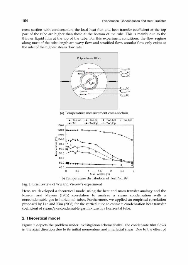
Evaporation, Condensation and Heat Transfer
154
cross section with condensation, the local heat flux and heat transfer coefficient at the top part of the tube are higher than those at the bottom of the tube. This is mainly due to the thinner liquid film at the top of the tube. For this experiment conditions, the flow regime along most of the tube length are wavy flow and stratified flow, annular flow only exists at the inlet of the highest steam flow rate.
(a) Temperature measurement cross-section
(b) Temperature distribution of Test No. 99
Fig. 1. Brief review of Wu and Vierow’s experiment
Here, we developed a theoretical model using the heat and mass transfer analogy and the Rosson and Meyers (1965) correlation to analyze a steam condensation with a noncondensable gas in horizontal tubes. Furthermore, we applied an empirical correlation proposed by Lee and Kim (2008) for the vertical tube to estimate condensation heat transfer coefficient of steam/noncondensable gas mixture in a horizontal tube.
2. Theoretical model Figure 2 depicts the problem under investigation schematically. The condensate film flows in the axial direction due to its initial momentum and interfacial shear. Due to the effect of
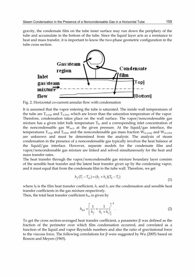
Steam Condensation in the Presence of a Noncondensable Gas in a Horizontal Tube
155
gravity, the condensate film on the tube inner surface may run down the periphery of the tube and accumulate in the bottom of the tube. Since the liquid layer acts as a resistance to heat and mass transfer, it is important to know the two-phase geometric configuration in the tube cross section.
Fig. 2. Horizontal co-current annular flow with condensation
It is assumed that the vapor entering the tube is saturated. The inside wall temperatures of the tube are Tw,top and Tw,bot, which are lower than the saturation temperature of the vapor. Therefore, condensation takes place on the wall surface. The vapor/noncondensable gas mixture has a given inlet bulk temperature Tb, and a corresponding inlet concentration of the noncondensable gas Wnc,b at the given pressure. At the liquid/gas interface, the temperatures Ti,top and Ti,bot, and the noncondensable gas mass fraction Wnc,i,top and Wnc,i,bot are unknown and must be determined from the analysis. The analysis of steam condensation in the presence of a noncondensable gas typically involves the heat balance at the liquid/gas interface. However, separate models for the condensate film and vapor/noncondensable gas mixture are linked and solved simultaneously for the heat and mass transfer rates. The heat transfer through the vapor/noncondensable gas mixture boundary layer consists of the sensible heat transfer and the latent heat transfer given up by the condensing vapor, and it must equal that from the condensate film to the tube wall. Therefore, we get
( ) ( )( )f i w c s b ih T T h h T T− = + −
(1)
where hf is the film heat transfer coefficient, hc and hs are the condensation and sensible heat transfer coefficients in the gas mixture respectively. Then, the total heat transfer coefficient htot is given by
1
1 1tot
f c sh
h h h
−⎡ ⎤⎢ ⎥= +
+⎢ ⎥⎣ ⎦. (2)
To get the cross section-averaged heat transfer coefficient, a parameter β was defined as the fraction of the perimeter over which film condensation occurred, and correlated as a function of the liquid and vapor Reynolds numbers and also the ratio of gravitational force to the viscous force. The following correlations for β were suggested by Wu (2005) based on Rosson and Meyers (1965).
Evaporation, Condensation and Heat Transfer
156
0.10.27 Remixβ = for
0.6 0.55Re Re 6.4 10mix l
Ga< × (3)
51.74 10Re Remix l
Gaβ−×= for
0.6 0.55Re Re 6.4 10mix l
Ga> × (4)
Then, the circumferentially averaged heat flux can be calculated as
" " "(1 )tot top botq q qβ β= + −
(5)
Here, the heat fluxes at the top and bottom of the horizontal tube are defined as
", ,( )top tot top b w topq h T T= − (6)
", ,( )bot tot bot b w botq h T T= − (7)
2.1 Condensate flow For stratified flow with higher vapor velocity, the vapor shear will affect the drain of the liquid and also change the mode of heat transfer at the bottom of the tube through the liquid pool from conduction to forced convection. Rosson and Meyers (1965) measured a single point value of the heat transfer coefficient for stratified, wavy and slug flows for methanol and acetone at atmospheric pressure. By rotating the condenser tube, they measured the variation of the heat transfer coefficient continuously decreased from the top of the tube to the bottom of the tube. They proposed different heat transfer correlations for top and bottom side of the tube. For top side of the tube, the heat transfer is similar to that of Nusselt but the effect of vapor shear is included:
1/43 1
0.12 ( )0.31Re( )
l l v l lvtop mix
l i w
g k hhT T d
ρ ρ ρμ
⎡ ⎤−= ⎢ ⎥
−⎢ ⎥⎣ ⎦. (8)
Here, the Remix represents the effect of vapor shear. For the bottom of the tube, no noticeable dependency of the Nu on the temperature was observed. The heat transfer coefficient depended on the vapor and liquid flow rate. The von Karman analogy between momentum transfer and heat transfer was used to predict the heat transfer coefficient.
, 8Re55 ln(5Pr 1)
Pr
l vt llbot
khd
Φ= ⋅
+ +. (9)
Here the parameter Φ is the two-phase multiplier for viscous laminar liquid flow and turbulent vapor flow, as presented by the Martinelli parameter with C=12.
1/2
211l
CX X
⎛ ⎞Φ = + +⎜ ⎟⎝ ⎠
(10)
Steam Condensation in the Presence of a Noncondensable Gas in a Horizontal Tube
157
where we used Martinelli correlation as
0.5 0.1 0.91v l
ttl v
xXx
ρ μρ μ
⎛ ⎞ ⎛ ⎞ −⎛ ⎞= ⎜ ⎟ ⎜ ⎟ ⎜ ⎟⎜ ⎟ ⎜ ⎟ ⎝ ⎠⎝ ⎠ ⎝ ⎠ (11)
2.2 Vapor/noncondensable gas mixture flow In this study, a stratification of the noncondensable gas concentration in the gas phase was assumed to be negligible, so the heat and mass transfer mechanism at everywhere inside the horizontal tube can be considered same. And the heat and mass transfer analogy was used to analysis steam condensation with noncondensable air in horizontal tubes. Therefore, the sensible and latent heat transfer rates can be calculated simultaneously. The sensible heat transfer coefficient can be expressed as
mixs mix
i
kh Nud
= (12)
and the condensation (or latent) heat transfer coefficient can be defined as
"
( )cond fg
cb i
m ih
T T=
−. (13)
To find "condm , the mass balance at the interface is calculated to yield the following equation:
" ", ( )v
cond v i tot ii
Wm D W my
ρ⎡ ⎤∂= − +⎢ ⎥∂⎣ ⎦
. (14)
As the condensate surface is impermeable to the noncondensable gases, we can think
", ( )nc
nc i tot ii
WD W my
ρ⎡ ⎤∂ =⎢ ⎥∂⎣ ⎦
. (15)
Also, as the sum of vapor and noncondensable gas mass fractions is unit, we can derive
nc vW Wy y
∂ ∂= −∂ ∂
. (16)
Solving for "totm from Eq. (15) and substituting it in Eq. (14) together with Eq. (16), Eq. (14)
can be simplified as
, ,"
, ,
( )( ( / ))1 (1 )
v b v iv icond m
v i v i
W WD W ym hW W
ρ −− ∂ ∂= =
− −, (17)
where hm is the mass transfer coefficient. Eq. (17) can be recast as
"
,
, ,( )nc icond
mixnc i nc b
Wm dShD W Wρ
=−
. (18)
Evaporation, Condensation and Heat Transfer
158
The modifications necessary to incorporate the condensate film roughness, developing flow, and suction effect on the heat and mass transfer involve modifying the Nusselt and Sherwood numbers, as discussed below.
2.2.1 Interface roughness Film roughness increases the heat transfer from the gas phase by influencing the turbulence pattern close to the interface and disrupting the gaseous laminar sublayer. A method to consider the effect of a wavy surface was considered with the concept of the simple model of Kim and Corradini (1990), which applies the mixing length theory presented by Kays and Crawford (1980) for a rough surface to the momentum, thermal, and mass concentration boundary layer. The local Nusselt and Sherwood numbers without suction for a smooth tube are calculated using Gnielinski correlation as
, 1/2 2/3( /8)(Re 1000)Pr
1 12.7( /8) (Pr 1)o sfNu
f
⎡ ⎤−= ⎢ ⎥
+ −⎢ ⎥⎣ ⎦ (19)
, 1/2 2/3( /8)(Re 1000)
1 12.7( /8) ( 1)o sf ScSh
f Sc
⎡ ⎤−= ⎢ ⎥
+ −⎢ ⎥⎣ ⎦ (20)
for 2300 ≤ Re ≤ 5 × 10⁶, Nuo,s = Sho,s = 3.66; for Re ≤ 2300, f is a Moody friction factor here only. Then, using the corrections suggested by Norris for the roughness of the heat transfer surface
, ,
nr
o r o ss
fNu Nuf
⎛ ⎞= ⎜ ⎟⎜ ⎟
⎝ ⎠ (21)
, ,
nr
o r o ss
fSh Shf
⎛ ⎞= ⎜ ⎟⎜ ⎟
⎝ ⎠, (22)
where 0.215 0.2150.68Pr 0.68n Sc= = and 0.250.0791Resf−= .
Here, the rough wall friction factor fr is calculated using Whalley and Hewitt correlation for pressures higher than 105 Pa as
1/3
1 24 lr s
mixf f
dρ δ
ρ
⎡ ⎤⎛ ⎞⎢ ⎥= + ⎜ ⎟⎜ ⎟⎢ ⎥⎝ ⎠⎣ ⎦. (23)
2.2.2 Suction effect In the vapor/noncondensable gas layer, the condensation process leads to thinning of the boundary layer, which is called the suction effect. This means that at the interface, the velocity component normal to the wall is not zero. Kays and Moffat obtained the following correlation for a boundary layer subject to suction experimentally:
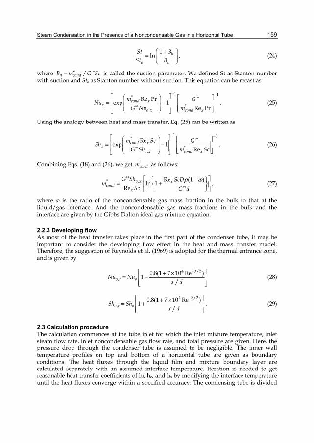
Steam Condensation in the Presence of a Noncondensable Gas in a Horizontal Tube
159
1ln h
o h
BStSt B
⎛ ⎞+= ⎜ ⎟⎜ ⎟⎝ ⎠
, (24)
where /h condB m G St∞′′= is called the suction parameter. We defined St as Stanton number with suction and Sto as Stanton number without suction. This equation can be recast as
1 1"
",
Re Prexp 1Re Pr
cond xx
o x cond x
m GNuG Nu m
− −∞
∞
⎡ ⎤⎛ ⎞ ⎡ ⎤⎢ ⎥⎜ ⎟= − ⎢ ⎥⎜ ⎟⎢ ⎥ ⎢ ⎥⎣ ⎦⎝ ⎠⎣ ⎦
. (25)
Using the analogy between heat and mass transfer, Eq. (25) can be written as
1 1"
",
Reexp 1Re
cond xx
o x cond x
m Sc GShG Sh m Sc
− −∞
∞
⎡ ⎤⎛ ⎞ ⎡ ⎤⎢ ⎥⎜ ⎟= − ⎢ ⎥⎜ ⎟⎢ ⎥ ⎢ ⎥⎣ ⎦⎝ ⎠⎣ ⎦
. (26)
Combining Eqs. (18) and (26), we get "condm as follows:
," Re (1 )ln 1Re
o x xcond
x
G Sh ScDmSc G d
ρ ω∞
∞⎡ ⎤−⎧ ⎫= +⎨ ⎬⎢ ⎥
⎩ ⎭⎣ ⎦, (27)
where ω is the ratio of the noncondensable gas mass fraction in the bulk to that at the liquid/gas interface. And the noncondensable gas mass fractions in the bulk and the interface are given by the Gibbs-Dalton ideal gas mixture equation.
2.2.3 Developing flow As most of the heat transfer takes place in the first part of the condenser tube, it may be important to consider the developing flow effect in the heat and mass transfer model. Therefore, the suggestion of Reynolds et al. (1969) is adopted for the thermal entrance zone, and is given by
4 3/2
,0.8(1 7 10 Re )1
/o t oNu Nux d
−⎡ ⎤+ ×= +⎢ ⎥⎢ ⎥⎣ ⎦
(28)
4 3/2
,0.8(1 7 10 Re )1
/o t oSh Shx d
−⎡ ⎤+ ×= +⎢ ⎥⎢ ⎥⎣ ⎦
. (29)
2.3 Calculation procedure The calculation commences at the tube inlet for which the inlet mixture temperature, inlet steam flow rate, inlet noncondensable gas flow rate, and total pressure are given. Here, the pressure drop through the condenser tube is assumed to be negligible. The inner wall temperature profiles on top and bottom of a horizontal tube are given as boundary conditions. The heat fluxes through the liquid film and mixture boundary layer are calculated separately with an assumed interface temperature. Iteration is needed to get reasonable heat transfer coefficients of hf, hc, and hs by modifying the interface temperature until the heat fluxes converge within a specified accuracy. The condensing tube is divided
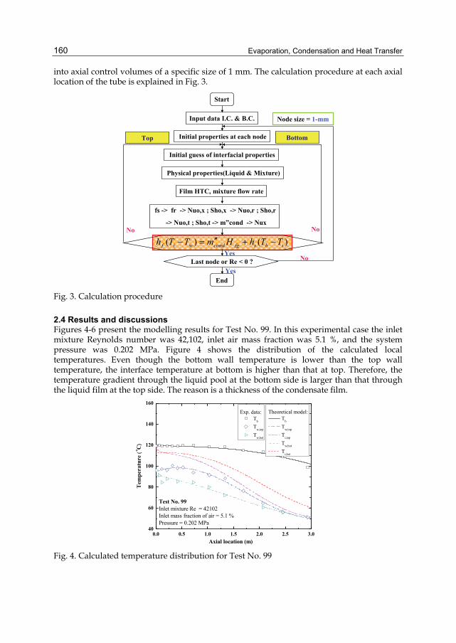
Evaporation, Condensation and Heat Transfer
160
into axial control volumes of a specific size of 1 mm. The calculation procedure at each axial location of the tube is explained in Fig. 3.
Start
Input data I.C. & B.C.
Initial properties at each node
Initial guess of interfacial properties
Physical properties(Liquid & Mixture)
Film HTC, mixture flow rate
fs -> fr -> Nuo,x ; Sho,x -> Nuo,r ; Sho,r
-> Nuo,t ; Sho,t -> m”cond -> Nux
( ) ( )f i w cond fg s b ih T T m H h T T′′− = + −
Last node or Re < 0 ?
End
No
NoYes
Yes
Node size = 1-mm
No
Top Bottom
Fig. 3. Calculation procedure
2.4 Results and discussions Figures 4-6 present the modelling results for Test No. 99. In this experimental case the inlet mixture Reynolds number was 42,102, inlet air mass fraction was 5.1 %, and the system pressure was 0.202 MPa. Figure 4 shows the distribution of the calculated local temperatures. Even though the bottom wall temperature is lower than the top wall temperature, the interface temperature at bottom is higher than that at top. Therefore, the temperature gradient through the liquid pool at the bottom side is larger than that through the liquid film at the top side. The reason is a thickness of the condensate film.
0.0 0.5 1.0 1.5 2.0 2.5 3.040
60
80
100
120
140
160
Test No. 99Inlet mixture Re = 42102Inlet mass fraction of air = 5.1 %Pressure = 0.202 MPa
Theoretical model: Tb
Tw,top
Ti,top
Tw,bot
Ti,bot
Axial location (m)
Tem
pera
ture
(o C
)
Exp. data: Tb
Tw,top
Tw,bot
Fig. 4. Calculated temperature distribution for Test No. 99
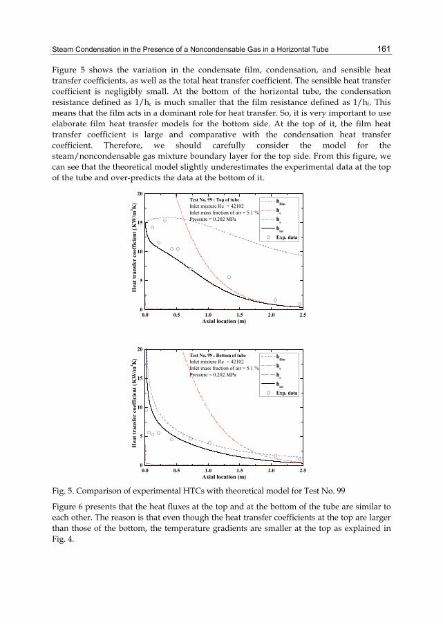
Steam Condensation in the Presence of a Noncondensable Gas in a Horizontal Tube
161
Figure 5 shows the variation in the condensate film, condensation, and sensible heat transfer coefficients, as well as the total heat transfer coefficient. The sensible heat transfer coefficient is negligibly small. At the bottom of the horizontal tube, the condensation resistance defined as 1/hc is much smaller that the film resistance defined as 1/hf. This means that the film acts in a dominant role for heat transfer. So, it is very important to use elaborate film heat transfer models for the bottom side. At the top of it, the film heat transfer coefficient is large and comparative with the condensation heat transfer coefficient. Therefore, we should carefully consider the model for the steam/noncondensable gas mixture boundary layer for the top side. From this figure, we can see that the theoretical model slightly underestimates the experimental data at the top of the tube and over-predicts the data at the bottom of it.
0.0 0.5 1.0 1.5 2.0 2.50
5
10
15
20Test No. 99 : Top of tubeInlet mixture Re = 42102Inlet mass fraction of air = 5.1 %Pressure = 0.202 MPa
Hea
t tra
nsfe
r co
effic
ient
(K
W/m
2 K)
Axial location (m)
hfilm
hc
hs
htot
Exp. data
0.0 0.5 1.0 1.5 2.0 2.50
5
10
15
20Test No. 99 : Bottom of tubeInlet mixture Re = 42102Inlet mass fraction of air = 5.1 %Pressure = 0.202 MPa
Hea
t tra
nsfe
r co
effic
ient
(K
W/m
2 K)
Axial location (m)
hfilm
hc
hs
htot
Exp. data
Fig. 5. Comparison of experimental HTCs with theoretical model for Test No. 99
Figure 6 presents that the heat fluxes at the top and at the bottom of the tube are similar to each other. The reason is that even though the heat transfer coefficients at the top are larger than those of the bottom, the temperature gradients are smaller at the top as explained in Fig. 4.
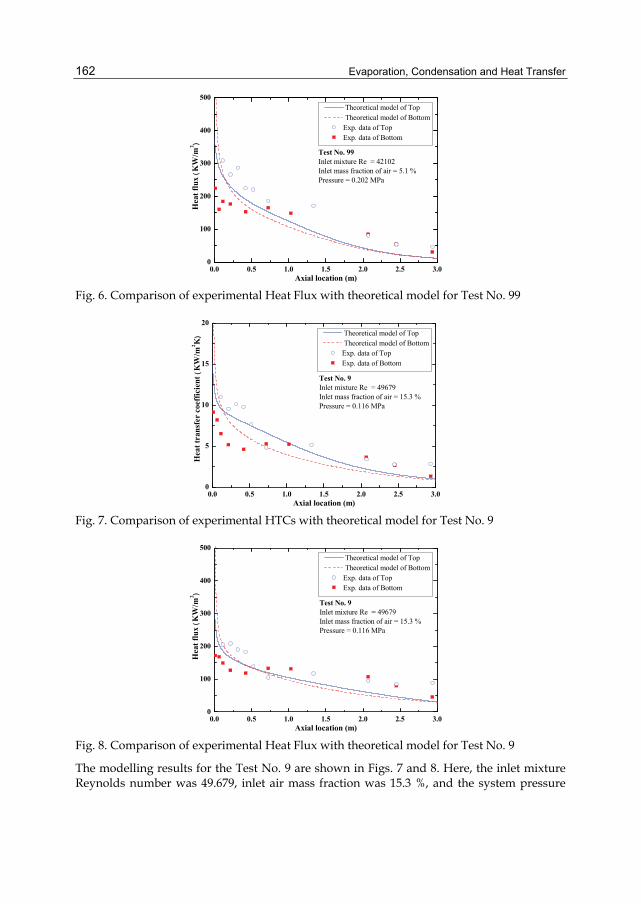
Evaporation, Condensation and Heat Transfer
162
0.0 0.5 1.0 1.5 2.0 2.5 3.00
100
200
300
400
500
Test No. 99Inlet mixture Re = 42102Inlet mass fraction of air = 5.1 %Pressure = 0.202 MPa
Hea
t flu
x (K
W/m
2 )
Axial location (m)
Theoretical model of Top Theoretical model of BottomExp. data of TopExp. data of Bottom
Fig. 6. Comparison of experimental Heat Flux with theoretical model for Test No. 99
0.0 0.5 1.0 1.5 2.0 2.5 3.00
5
10
15
20
Test No. 9Inlet mixture Re = 49679Inlet mass fraction of air = 15.3 %Pressure = 0.116 MPa
Hea
t tra
nsfe
r co
effic
ient
(KW
/m2 K
)
Axial location (m)
Theoretical model of Top Theoretical model of BottomExp. data of TopExp. data of Bottom
Fig. 7. Comparison of experimental HTCs with theoretical model for Test No. 9
0.0 0.5 1.0 1.5 2.0 2.5 3.00
100
200
300
400
500
Test No. 9Inlet mixture Re = 49679Inlet mass fraction of air = 15.3 %Pressure = 0.116 MPa
Hea
t flu
x (K
W/m
2 )
Axial location (m)
Theoretical model of Top Theoretical model of BottomExp. data of TopExp. data of Bottom
Fig. 8. Comparison of experimental Heat Flux with theoretical model for Test No. 9
The modelling results for the Test No. 9 are shown in Figs. 7 and 8. Here, the inlet mixture Reynolds number was 49.679, inlet air mass fraction was 15.3 %, and the system pressure
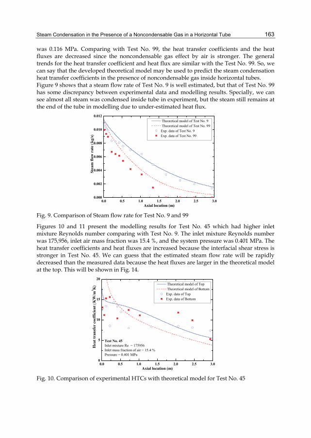
Steam Condensation in the Presence of a Noncondensable Gas in a Horizontal Tube
163
was 0.116 MPa. Comparing with Test No. 99, the heat transfer coefficients and the heat fluxes are decreased since the noncondensable gas effect by air is stronger. The general trends for the heat transfer coefficient and heat flux are similar with the Test No. 99. So, we can say that the developed theoretical model may be used to predict the steam condensation heat transfer coefficients in the presence of noncondensable gas inside horizontal tubes. Figure 9 shows that a steam flow rate of Test No. 9 is well estimated, but that of Test No. 99 has some discrepancy between experimental data and modelling results. Specially, we can see almost all steam was condensed inside tube in experiment, but the steam still remains at the end of the tube in modelling due to under-estimated heat flux.
0.0 0.5 1.0 1.5 2.0 2.5 3.00.000
0.002
0.004
0.006
0.008
0.010
0.012
Stea
m fl
ow r
ate (k
g/s)
Axial location (m)
Theoretical model of Test No. 9 Theoretical model of Test No. 99Exp. data of Test No. 9Exp. data of Test No. 99
Fig. 9. Comparison of Steam flow rate for Test No. 9 and 99
Figures 10 and 11 present the modelling results for Test No. 45 which had higher inlet mixture Reynolds number comparing with Test No. 9. The inlet mixture Reynolds number was 175,956, inlet air mass fraction was 15.4 %, and the system pressure was 0.401 MPa. The heat transfer coefficients and heat fluxes are increased because the interfacial shear stress is stronger in Test No. 45. We can guess that the estimated steam flow rate will be rapidly decreased than the measured data because the heat fluxes are larger in the theoretical model at the top. This will be shown in Fig. 14.
0.0 0.5 1.0 1.5 2.0 2.5 3.00
5
10
15
20
Test No. 45Inlet mixture Re = 175956Inlet mass fraction of air = 15.4 %Pressure = 0.401 MPa
Hea
t tra
nsfe
r co
effic
ient
(K
W/m
2 K)
Axial location (m)
Theoretical model of Top Theoretical model of BottomExp. data of TopExp. data of Bottom
Fig. 10. Comparison of experimental HTCs with theoretical model for Test No. 45
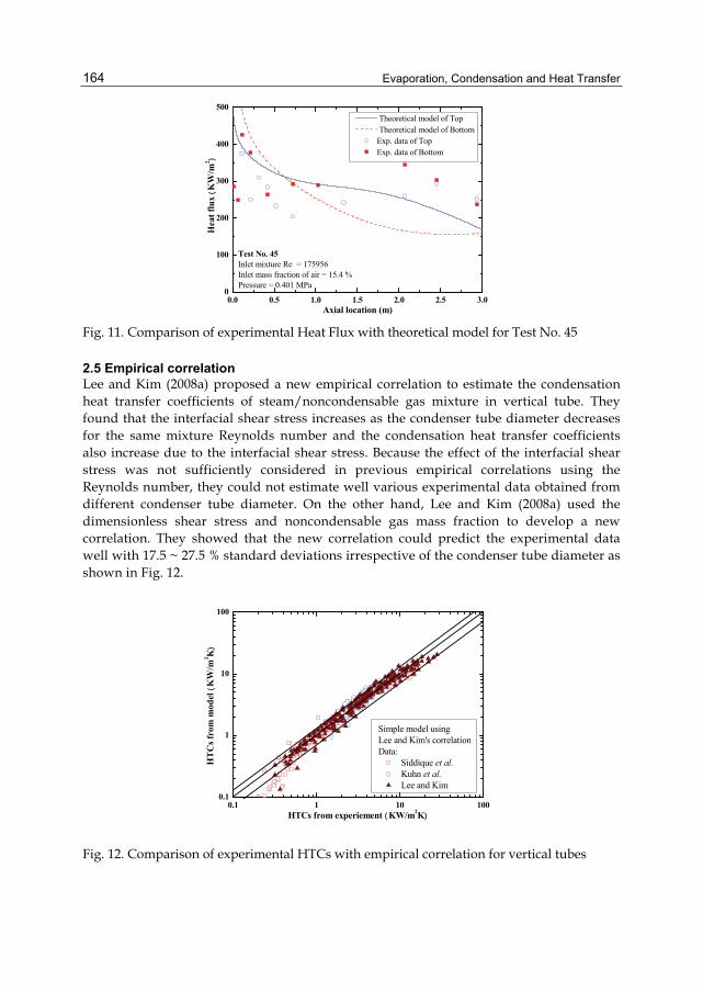
Evaporation, Condensation and Heat Transfer
164
0.0 0.5 1.0 1.5 2.0 2.5 3.00
100
200
300
400
500
Test No. 45Inlet mixture Re = 175956Inlet mass fraction of air = 15.4 %Pressure = 0.401 MPa
Hea
t flu
x (K
W/m
2 )
Axial location (m)
Theoretical model of Top Theoretical model of BottomExp. data of TopExp. data of Bottom
Fig. 11. Comparison of experimental Heat Flux with theoretical model for Test No. 45
2.5 Empirical correlation Lee and Kim (2008a) proposed a new empirical correlation to estimate the condensation heat transfer coefficients of steam/noncondensable gas mixture in vertical tube. They found that the interfacial shear stress increases as the condenser tube diameter decreases for the same mixture Reynolds number and the condensation heat transfer coefficients also increase due to the interfacial shear stress. Because the effect of the interfacial shear stress was not sufficiently considered in previous empirical correlations using the Reynolds number, they could not estimate well various experimental data obtained from different condenser tube diameter. On the other hand, Lee and Kim (2008a) used the dimensionless shear stress and noncondensable gas mass fraction to develop a new correlation. They showed that the new correlation could predict the experimental data well with 17.5 ~ 27.5 % standard deviations irrespective of the condenser tube diameter as shown in Fig. 12.
0.1 1 10 1000.1
1
10
100
Simple model using Lee and Kim's correlationData:
Siddique et al. Kuhn et al. Lee and Kim
HT
Cs f
rom
mod
el (
KW
/m2 K
)
HTCs from experiement (KW/m2K)
Fig. 12. Comparison of experimental HTCs with empirical correlation for vertical tubes
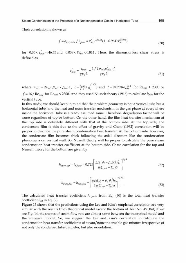
Steam Condensation in the Presence of a Noncondensable Gas in a Horizontal Tube
165
Their correlation is shown as
* 0.3124 0.402
exp, / (1 0.964 )mix pure mix ncf h h Wτ= = − (30)
for *0.06 46.65mixτ< < and 0.038 0.814ncW< < . Here, the dimensionless shear stress is defined as
2* 1 / 2 mix mixmixmix
f f
u fg L g L
ρττρ ρ
⋅= =
(31)
where Re /mix mix mix mixu dμ ρ= , ( )1/32 /fL gν= , and 1/40.079Remixf −= for Remix > 2300 or
16 /Remixf = for Remix < 2300. And they used Nusselt theory (1916) to calculate hpure for the vertical tube. In this study, we should keep in mind that the problem geometry is not a vertical tube but a horizontal tube, and the heat and mass transfer mechanism in the gas phase at everywhere inside the horizontal tube is already assumed same. Therefore, degradation factor will be same regardless of top or bottom. On the other hand, the film heat transfer mechanism at the top side is definitely different with that at the bottom side. At the top side, the condensate film is thin due to the effect of gravity and Chato (1962) correlation will be proper to describe the pure steam condensation heat transfer. At the bottom side, however, the condensate film becomes thick following the axial direction like the condensation phenomena on vertical wall. So, Nusselt theory will be proper to calculate the pure steam condensation heat transfer coefficient at the bottom side. Chato correlation for the top and Nusselt theory for the bottom are given by
1/43 '
,( )0.725( )
l l v l lvpure top Chato
l sat w
g k hh hT T D
ρ ρ ρμ
⎡ ⎤−= = ⎢ ⎥
−⎢ ⎥⎣ ⎦ (32)
1/43 '
,( )
4 ( )l l v l lv
pure bot Nusseltl sat w
g k hh hT T x
ρ ρ ρμ
⎡ ⎤−= = ⎢ ⎥
−⎢ ⎥⎣ ⎦ . (33)
The calculated heat transfer coefficient hexp,mix from Eq. (30) is the total heat transfer coefficient htot in Eq. (2). Figure 13 shows that the predictions using the Lee and Kim’s empirical correlation are very similar with the results from theoretical model except the bottom of Test No. 45. But, if we see Fig. 14, the shapes of steam flow rate are almost same between the theoretical model and the empirical model. So, we suggest the Lee and Kim’s correlation to calculate the condensation heat transfer coefficients of steam/noncondensable gas mixture irrespective of not only the condenser tube diameter, but also orientation.
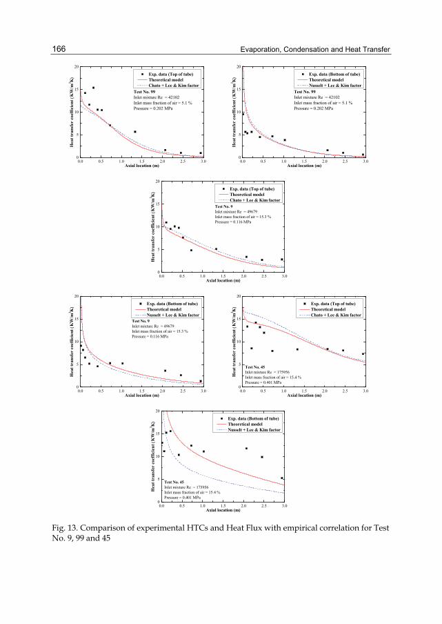
Evaporation, Condensation and Heat Transfer
166
0.0 0.5 1.0 1.5 2.0 2.5 3.00
5
10
15
20
Test No. 99Inlet mixture Re = 42102Inlet mass fraction of air = 5.1 %Pressure = 0.202 MPa
Hea
t tra
nsfe
r co
effic
ient
(K
W/m
2 K)
Axial location (m)
Exp. data (Top of tube) Theoretical model Chato + Lee & Kim factor
0.0 0.5 1.0 1.5 2.0 2.5 3.00
5
10
15
20
Test No. 99Inlet mixture Re = 42102Inlet mass fraction of air = 5.1 %Pressure = 0.202 MPa
Hea
t tra
nsfe
r co
effic
ient
(K
W/m
2 K)
Axial location (m)
Exp. data (Bottom of tube) Theoretical model Nusselt + Lee & Kim factor
0.0 0.5 1.0 1.5 2.0 2.5 3.00
5
10
15
20
Test No. 9Inlet mixture Re = 49679Inlet mass fraction of air = 15.3 %Pressure = 0.116 MPa
Hea
t tra
nsfe
r co
effic
ient
(K
W/m
2 K)
Axial location (m)
Exp. data (Top of tube) Theoretical model Chato + Lee & Kim factor
0.0 0.5 1.0 1.5 2.0 2.5 3.00
5
10
15
20
Test No. 9Inlet mixture Re = 49679Inlet mass fraction of air = 15.3 %Pressure = 0.116 MPa
Hea
t tra
nsfe
r co
effic
ient
(K
W/m
2 K)
Axial location (m)
Exp. data (Bottom of tube) Theoretical model Nusselt + Lee & Kim factor
0.0 0.5 1.0 1.5 2.0 2.5 3.00
5
10
15
20
Test No. 45Inlet mixture Re = 175956Inlet mass fraction of air = 15.4 %Pressure = 0.401 MPa
Hea
t tra
nsfe
r co
effic
ient
(K
W/m
2 K)
Axial location (m)
Exp. data (Top of tube) Theoretical model Chato + Lee & Kim factor
0.0 0.5 1.0 1.5 2.0 2.5 3.00
5
10
15
20
Test No. 45Inlet mixture Re = 175956Inlet mass fraction of air = 15.4 %Pressure = 0.401 MPa
Hea
t tra
nsfe
r co
effic
ient
(K
W/m
2 K)
Axial location (m)
Exp. data (Bottom of tube) Theoretical model Nusselt + Lee & Kim factor
Fig. 13. Comparison of experimental HTCs and Heat Flux with empirical correlation for Test No. 9, 99 and 45
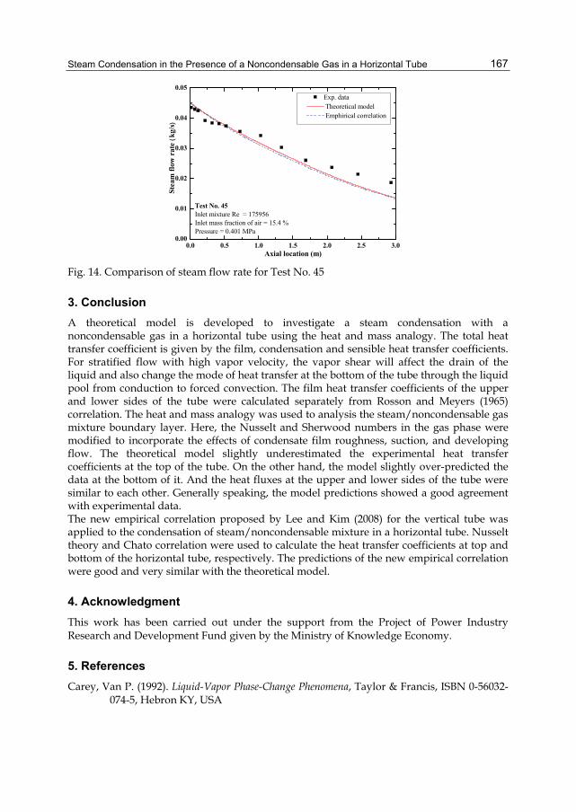
Steam Condensation in the Presence of a Noncondensable Gas in a Horizontal Tube
167
0.0 0.5 1.0 1.5 2.0 2.5 3.00.00
0.01
0.02
0.03
0.04
0.05
Test No. 45Inlet mixture Re = 175956Inlet mass fraction of air = 15.4 %Pressure = 0.401 MPa
Stea
m fl
ow r
ate (k
g/s)
Axial location (m)
Exp. data Theoretical model Emphirical correlation
Fig. 14. Comparison of steam flow rate for Test No. 45
3. Conclusion A theoretical model is developed to investigate a steam condensation with a noncondensable gas in a horizontal tube using the heat and mass analogy. The total heat transfer coefficient is given by the film, condensation and sensible heat transfer coefficients. For stratified flow with high vapor velocity, the vapor shear will affect the drain of the liquid and also change the mode of heat transfer at the bottom of the tube through the liquid pool from conduction to forced convection. The film heat transfer coefficients of the upper and lower sides of the tube were calculated separately from Rosson and Meyers (1965) correlation. The heat and mass analogy was used to analysis the steam/noncondensable gas mixture boundary layer. Here, the Nusselt and Sherwood numbers in the gas phase were modified to incorporate the effects of condensate film roughness, suction, and developing flow. The theoretical model slightly underestimated the experimental heat transfer coefficients at the top of the tube. On the other hand, the model slightly over-predicted the data at the bottom of it. And the heat fluxes at the upper and lower sides of the tube were similar to each other. Generally speaking, the model predictions showed a good agreement with experimental data. The new empirical correlation proposed by Lee and Kim (2008) for the vertical tube was applied to the condensation of steam/noncondensable mixture in a horizontal tube. Nusselt theory and Chato correlation were used to calculate the heat transfer coefficients at top and bottom of the horizontal tube, respectively. The predictions of the new empirical correlation were good and very similar with the theoretical model.
4. Acknowledgment This work has been carried out under the support from the Project of Power Industry Research and Development Fund given by the Ministry of Knowledge Economy.
5. References Carey, Van P. (1992). Liquid-Vapor Phase-Change Phenomena, Taylor & Francis, ISBN 0-56032-
074-5, Hebron KY, USA
Evaporation, Condensation and Heat Transfer
168
Kays, W. M. & Crawford, M. E. (1980). Convective Heat and Mass Transfer, MaGraw-Hill, ISBN 0-07-033457-9, New York, USA
Reynolds, H. C. ; Swearingen, T. B. & McEligot, D. M. (1969). Thermal Entry for Low Reynolds Number Turbulent Flow, Journal of Basic Engineering, Vol.91, pp.87-94, ISSN 0021-9223
Wu, T. & Vierow, K. (2006a). A Local Heat Flux Measurement Technique for Inclined Heat Exchanger Tubes, Experimental Heat Transfer, Vol.19, pp.1-14, ISSN 1521-0480
Wu, T. & Vierow, K. (2006b). Local Heat Transfer Measurements of Steam/Air Mixtures in Horizontal Condenser Tubes, International Journal of Heat Mass Transfer, Vol.49, pp.2491-2501, ISSN 0017-9310
Wu, T. (2005). Horizontal In-Tube Condensation in the Presence of a Noncondensable Gas, Ph. D. Dissertation, Purdue University, USA
Chato, J. C. (1962). Laminar Condensation inside Horizontal and Inclined Tubes, ASHRAE journal, Vol. 4, pp.52-60, ISSN 0001-2491
Kim, M. H. & Corradini, M. L. (1990). Modeling of condensation heat transfer in a reactor containment, Nuclear Engineering and Design, Vol. 118, pp. 193-212, ISSN 0029-5493
Lee, K.-Y. & Kim, M. H. (2008a). Experimental and empirical study of steam condensation heat transfer with a noncondensable gas in a small-diameter vertical tube, Nuclear Engineering and Design, Vol. 238, pp. 207-216, ISSN 0029-5493
Lee, K.-Y. & Kim, M. H. (2008b). Effect of an interfacial shear stress on steam condensation in the presence of a noncondensable gas in a vertical tube, International Journal of Heat Mass Transfer, Vol.51, pp.5333-5343, ISSN 0017-9310
Nusselt, W. A., (1916). “The surface condensation of water vapor”, Zeitschrift Ver. Deut. Ing., Vol. 60, pp. 541-546
Rosson, H. F. & Mayers, J. A. (1965). Point values of condensing film coefficients inside a horizontal tube, Chemical Engineering Progress Symposium Series, Vol. 61, pp. 190-199, ISSN 0069-2948
8
Experimental Study for Condensation Heat Transfer Inside Helical Coil
Mohamed A. Abd Raboh1, Hesham M. Mostafa2, Mostafa A. M. Ali2 and Amr M. Hassaan3
1Faculty of Engineering, Al Azhar University, 2Faculty of Engineering, King Abdulaziz University,
3Higher Technological Institute, Tenth of Ramadan City, 1,3Egypt 2K.S.A
1. Introduction Heat exchangers are one of the most common technological devices applied in refrigeration, air-conditioning, nuclear power generation, petrochemical, pharmaceutical, aerospace industries and food processing industries. Many options are available for obtaining compactness and efficiency in exchanging thermal power. In the field of tubular heat exchangers one possible way for reducing the space occupied by the exchanger is by bending tube axis in helicoidal shape. This option is particularly suitable when construction simplicity is needed and when the geometry of the place in which the exchanger has to be housed is the cylindrical one. Many advantages derive from this disposition, such as an excellent behavior in presence of severe thermal expansions; in fact the helical shape allows the exchanger to behave as a spring, thus accommodating the stresses due to the expansions. Helicoidal pipes have been extensively studied and used in a variety of engineering areas due to their high efficiency in heat transfer and compactness in volume. Han et al. [1] investigated the condensation heat transfer and pressure drop characteristics of R-134a in an annular helical pipe. The obtained results show that the refrigerant-side condensation heat transfer coefficients and pressure drops of R-134a increase with the mass flux of R-134a. The saturated temperatures have significant effects on the condensation heat transfer coefficients of R-134a in the annular helical pipe. Lin and Ebadian [2] investigated the condensation heat transfer and pressure drop of R-134a in annular helicoidal pipe at different orientations. The results shows that, the effect of individual parameter revealed that the refrigerant Nusselt number was larger at lower refrigerant saturation temperature, and would increase with the increase of mass flow rates of both refrigerant and cooling water. When the orientation increased from 0 degree to 90 degree, the percentage increase of refrigerant Nusselt number from 0 degree to 45 degree accounted for more than two times of that from 45 degree to 90 degree. Han et al. [3] investigate the condensation heat transfer of R-134a flow inside helical pipes at different orientations. The obtained results show that, the condensation heat transfer coefficient from the refrigerant side for the helical pipe at the inclined position is the highest, and the vertical position is the lowest. Laohalertdecha and Wongwises [4] studied the effect of corrugation pitch on the condensation heat transfer coefficient and pressure
Evaporation, Condensation and Heat Transfer
170
drop of R-134a inside horizontal corrugated tube. Murai et al. [5] studied structure of air–water two-phase flow in helically coiled tubes. The obtained results shows that, owing to the curvature of the tube, which provides centrifugal acceleration to the two-phase flow, the flow transition from bubbly to plug flow is considerably quickened compared to that in the flow in a straight tube. Also, in comparison with an upward inclined straight tube, small bubbles vanish away from the liquid slug in the case of a strong curvature owing to the centrifugal acceleration. Wongwises and Polsongkram [6] investigated the condensation heat transfer and pressure drop of R-134a in a helically coiled concentric tube-in-tube heat exchanger. Their obtained results show that, the average heat transfer coefficient increases with increasing average vapor quality and mass flux. The heat transfer coefficient increases very slightly with an increase in heat flux. On the contrary, it decreases with increasing saturation temperature. Li and Ji-tian [7] investigated the condensation heat transfer of R-134a in horizontal straight and helically tube in tube heat exchanger. Their results show that, the average heat transfer coefficient for the helical section is 4%-13.8% higher than that for the straight section. M. Moawed [8] investigated the forced convection from helical coiled tubes with different parameters. Their results showed that, for the same P/do, the higher values of Nusselt number (Num) can be obtained with a high value of D/do while the small value of Num can be obtained with a small value of D/do. Al-Hajeri et al. [9] investigated heat transfer performance during condensation of R-134a inside helicoidal tubes. Their experimental results show that, the average heat flux, refrigerant side heat transfer coefficient and overall heat transfer coefficients increase with increasing of the mass flux of flowing R-134a. The refrigerant side heat transfer coefficient and overall heat transfer coefficient decrease as the saturation temperature increases. Xin et al. [10] investigated an experimental study of single-phase and two-phase flow pressure drop in annular helicoidal pipes. Wongwises and Polsongkarm [11] investigated the evaporation heat transfer and pressure drop of HFC-134a in a helically coiled concentric tube-in-tube heat exchanger. Condensation of R134a flowing inside helicoidal pipe investigated by Laohalertdecha and Wongwises [12]. Their obtained results show that, the average heat flux of the refrigerant flow increases with the water flow rate. It is clear from the previous review and up to the knowledge of the authors that, there is a shortage in thesis which concerned with condensation of steam inside helical coil. Accordingly, in this work, an experimental study is done to investigate the effect of different operating parameters on the condensation heat transfer coefficient for steam flows inside helical coil.
2. Experimental test rig The experimental test rig is illustrated in Fig. 1. It is mainly consists of a circular inlet section, a rectangular cross section duct in which the tested helical coil is installed, and the heating steam loop. Air is drawn from the ambient by the blower 2.5 hp rated power (2). A flexible connection (3) separates the blower section and the rest of the wind tunnel to eliminate any vibrations promoted. The leaving air from the blower flows through a velocity meter (8) to measure the average air velocity inside the wind tunnel. Wind tunnel (4) walls are made of galvanized iron sheet of 1 mm thick. The basic dimensions for the wind tunnel are 2.5 m long, 670 mm wide and 330 mm high. Tested helical coil with different dimensions is fitted, vertical or inclined, at the middle of the test section, as shown in Fig. (1). To insure that a fully developed flow is achieved at the entrance of the test section (7), air is traveled through the entrance region (6) of 2 m long,
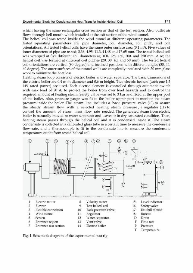
Experimental Study for Condensation Heat Transfer Inside Helical Coil
171
which having the same rectangular cross section as that of the test section. Also, outlet air flows through bell mouth which installed at the exit section of the wind tunnel. The helical coil was tested inside the wind tunnel at different operating parameters. The tested operating parameters are; pipe diameter, coil diameter, coil pitch, and coil orientations. All tested helical coils have the same outer surface area (0.1 m2). Five values of inner diameters of pipe are tested; 3.36, 4.95, 11.3, 14.48 and 17.65 mm. The tested helical coil was wrapped at five different coil diameters as; 100, 125, 150, 200, and 250 mm. Also; the helical coil was formed at different coil pitches (20, 30, 40, and 50 mm). The tested helical coil orientations are vertical (90 degree) and inclined positions with different angles (30, 45, 60 degree). The outer surfaces of the tunnel walls are completely insulated with 30 mm glass wool to minimize the heat loss. Heating steam loop consists of electric boiler and water separator. The basic dimensions of the electric boiler are 0.4 m in diameter and 0.6 m height. Two electric heaters (each one 1.5 kW rated power) are used. Each electric element is controlled through automatic switch with max load of 20 A; to protect the boiler from over load hazards and to control the required amount of heating steam. Safety valve was set to 3 bar and fixed at the upper port of the boiler. Also, pressure gauge was fit to the boiler upper port to monitor the steam pressure inside the boiler. The steam line includes a back pressure valve (10) to assure the steady stream flow with a selected heating steam pressure , a regulator (11) to control the amount of steam mass flow rate needed. The generated steam from electric boiler is naturally moved to water separator and leaves it in dry saturated condition. Then, heating steam passes through the helical coil and it is condensed inside it. The steam condensate is collected in a calibrated glass tube in a certain time to measure the condensate flow rate, and a thermocouple is fit to the condensate line to measure the condensate temperature outlet from tested helical coil.
Level indicator 15- Velocity meter 8- Electric motor 1- Safety valve 16- Test helical coil 9- Blower 2- Exit bill mouse 17- Back pressure valve 10- Flexible connection 3- Burette 18- Regulator 11- Wind tunnel 4- Drain D Water separator 12- Screen 5- Flow rate F Vent valve 13- Entrance region 6- Pressure P Electric boiler 14- Entrance test section 7- Temperature T
Fig. 1. Schematic diagram of the experimental test rig
Evaporation, Condensation and Heat Transfer
172
3. Measurements and methodology The experimental measurements are taken to determine the condensation heat transfer coefficient for the steam which flows inside helical coil. Prior to start of the experiments, the electric boiler filled with suitable volume of water. Glass level indicator was fixed in the side of the boiler to monitor the water level inside the boiler. The generated steam moves into the water separator to get it dry saturated steam. The steam was getting out from the water separator to the back pressure valve to get the suitable pressure which needed in the experiment. Then the regulator control the required amount of steam passed to the tested helical coil to condense inside it due to air flowing inside the wind tunnel on the outer surface of the coil. The experimental test rig is allowed to operate until the fluctuation in temperatures was about ±0.1 ºC. Then, steady state condition is reached. Once the test rig is reached to the desired steady state condition, the required measurements of temperature, pressure and volume flow rate are taken. Temperatures of inlet heating steam at inlet and condensate outlet from each tested helical coil are measured. Surface temperature, inlet and outlet air temperatures and other temperatures in different positions are measured by using 0.5 mm copper-constantan thermocouple (type k), which connected to a temperature recorder via multi point switch having an accuracy of ± 0.1 ºC. The uncertainty in temperature measurements is ±0.1 ºC. Due to the small amount of condensate from coil a calibrated constant volume tank and stop watch is used. Inlet steam pressure is measured by Bourdon pressure gauge with minimum readable value of ± 0.05 bar. Air velocity was measured by a hot wire anemometer sensor (type Testo 605-V1, of 8mm probe diameter), with a resolution of 0.01 m/s. The root-mean-square random error propagation analysis is carried out in the standard fashion using the measured experimental uncertainties of the basic independent parameters. The experimental uncertainties associated with these measurements technique are estimated to be approximately less than 12 % for condensation heat transfer coefficient.
4. Data reduction The basic measurements are analyzed using a computer reduction program to calculate the condensation heat transfer coefficient. At steady state, the total input heat from the heating steam which flows inside the helical coil (Qst) can be transferred to the flowing air inside wind tunnel. It is divided into useful heat to air (Qair ) and the remaining amount of heat transferred to the surroundings as heat loss (Qloss). The total input heat can be determined as follow;
st st g oQ = m (i - i )· (1)
Where; m.st : Steam flow rate inside helical coil, kg/s. ig : Specific enthalpy for dry saturated steam evaluated at the steam inlet pressure to the tested coil, J/kg. io : Specific enthalpy for condensate at the outlet from test coil, J/kg. The useful heat transfer to air flow inside the wind tunnel can be calculated from measuring mass flow rate which flow inside the helical coil and the temperature rise in the air as;
( ).air air air air,o air,iQ m Cp T T= −
(2)
Where:
Experimental Study for Condensation Heat Transfer Inside Helical Coil
173
m.air : Mass flow rate of air in the wind tunnel, kg/s. Cpair : Specific heat of air, J/kg oC. Tair,i : Inlet air temperature, oC. Tair,o : Outlet air temperature, oC. Then, the amount of heat loss from the test section to the surrounding (Qloss ) can be determined as the difference between input heat and useful heat as;
loss st airQ Q Q= − (3)
Heat flux (q") can be calculated from the following equation as;
st s,iq" Q / A= (4)
Where; As,i : Inner surface area of the pipe forming the tested helical coil, (As,i = пdiL). di : Inner pipe diameter, m. L : Pipe length, m. Accordingly, the condensation heat transfer coefficient (hc) can be calculated as;
( )''sat s,i h q / T T= − (5)
Where: Tsat : Saturation temperature for heating steam, oC. Ts,i : Average value for the inner surface temperature of the pipe, oC. Reynolds number can be defined as:
4Re st
i
mdπ μ
∗= · (6)
Where: µ: dynamic viscosity of steam at average bulk temperature. The average values for the Nusselt number (Nu), could be evaluated as,
ih dNuk∗
= (7)
Where, k: Thermal conductivity for working fluid.
5. Results and discussion Appropriate analysis for the experimental measurements; lead to obtain the heat flux and condensation heat transfer coefficient for different operating parameters. The studied operating conditions are pipe diameter, coil diameter, coil pitch, and coil orientations. All tested helical coils have the same outer surface area (0.1 m2).
5.1 Effect of inner pipe diameter The variation of heat flux versus temperature difference for different values of inner pipe diameters (di =3.36, 4.95, 11.3, 14.48 and 17.65 mm) at vertical position with coil pitch (P =30 mm) are shown in figures (2). It is observed that, for all the studied coil diameters (100, 125, 150, 200 and 250 mm), heat flux increases with decreasing inner pipe diameter until it reach
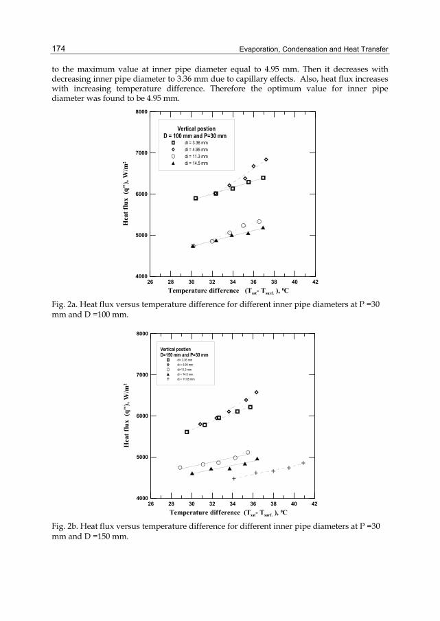
Evaporation, Condensation and Heat Transfer
174
to the maximum value at inner pipe diameter equal to 4.95 mm. Then it decreases with decreasing inner pipe diameter to 3.36 mm due to capillary effects. Also, heat flux increases with increasing temperature difference. Therefore the optimum value for inner pipe diameter was found to be 4.95 mm.
26 28 30 32 34 36 38 40 42Temperature difference (Tsat- Tsurf. ), 0C
4000
5000
6000
7000
8000
Hea
t flu
x (q
"), W
/m2
Vertical postionD = 100 mm and P=30 mm
di = 3.36 mmdi = 4.95 mmdi = 11.3 mmdi = 14.5 mm
Fig. 2a. Heat flux versus temperature difference for different inner pipe diameters at P =30 mm and D =100 mm.
26 28 30 32 34 36 38 40 42Temperature difference (Tsat- Tsurf. ), 0C
4000
5000
6000
7000
8000
Hea
t flu
x (q
"), W
/m2
Vertical postionD=150 mm and P=30 mm
di= 3.36 mmdi = 4.95 mmdi=11.3 mmdi = 14.5 mmdi = 17.65 mm
Fig. 2b. Heat flux versus temperature difference for different inner pipe diameters at P =30 mm and D =150 mm.
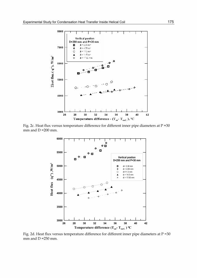
Experimental Study for Condensation Heat Transfer Inside Helical Coil
175
Fig. 2c. Heat flux versus temperature difference for different inner pipe diameters at P =30 mm and D =200 mm.
26 28 30 32 34 36 38 40 42Temperature difference (Tsat- Tsurf. ) 0C
3000
3500
4000
4500
5000
5500
6000
Hea
t flu
x (
q") ,
W/m
2
Vertical postionD=250 mm and P=30 mm
di= 3.36 mmdi = 4.95 mmdi=11.3 mmdi = 14.5 mmdi = 17.65 mm
Fig. 2d. Heat flux versus temperature difference for different inner pipe diameters at P =30 mm and D =250 mm.
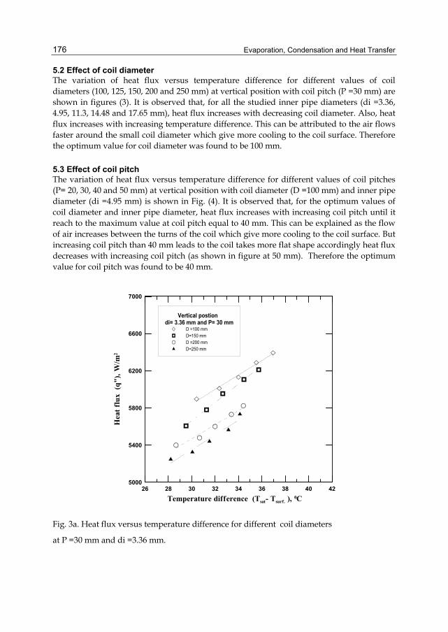
Evaporation, Condensation and Heat Transfer
176
5.2 Effect of coil diameter The variation of heat flux versus temperature difference for different values of coil diameters (100, 125, 150, 200 and 250 mm) at vertical position with coil pitch (P =30 mm) are shown in figures (3). It is observed that, for all the studied inner pipe diameters (di =3.36, 4.95, 11.3, 14.48 and 17.65 mm), heat flux increases with decreasing coil diameter. Also, heat flux increases with increasing temperature difference. This can be attributed to the air flows faster around the small coil diameter which give more cooling to the coil surface. Therefore the optimum value for coil diameter was found to be 100 mm.
5.3 Effect of coil pitch The variation of heat flux versus temperature difference for different values of coil pitches (P= 20, 30, 40 and 50 mm) at vertical position with coil diameter (D =100 mm) and inner pipe diameter (di =4.95 mm) is shown in Fig. (4). It is observed that, for the optimum values of coil diameter and inner pipe diameter, heat flux increases with increasing coil pitch until it reach to the maximum value at coil pitch equal to 40 mm. This can be explained as the flow of air increases between the turns of the coil which give more cooling to the coil surface. But increasing coil pitch than 40 mm leads to the coil takes more flat shape accordingly heat flux decreases with increasing coil pitch (as shown in figure at 50 mm). Therefore the optimum value for coil pitch was found to be 40 mm.
26 28 30 32 34 36 38 40 42 Temperature difference (Tsat- Tsurf. ), 0C
5000
5400
5800
6200
6600
7000
Hea
t flu
x (q
"), W
/m2
Vertical postion di= 3.36 mm and P= 30 mm
D =100 mmD=150 mmD =200 mmD=250 mm
Fig. 3a. Heat flux versus temperature difference for different coil diameters
at P =30 mm and di =3.36 mm.
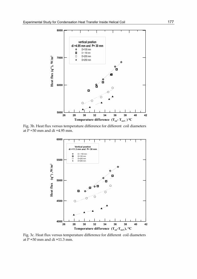
Experimental Study for Condensation Heat Transfer Inside Helical Coil
177
26 28 30 32 34 36 38 40 42 Temperature difference (Tsat- Tsurf. ) 0C
5000
6000
7000
8000
Hea
t flu
x (q
"), W
/m2
vertical postiondi =4.95 mm and P= 30 mm
D=100 mmD = 150 mmD=200 mmD=250 mm
Fig. 3b. Heat flux versus temperature difference for different coil diameters at P =30 mm and di =4.95 mm.
26 28 30 32 34 36 38 40 42Temperature difference (Tsat-Tsurf.), OC
4000
4500
5000
5500
6000
Hea
t flu
x (
q") ,
W/m
2
Vertical postiondi =11.3 mm and P= 30 mm
D = 100 mmD=150 mmD=200 mmD=250 mm
Fig. 3c. Heat flux versus temperature difference for different coil diameters at P =30 mm and di =11.3 mm.
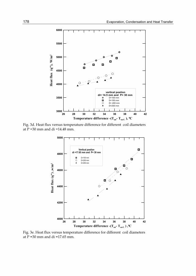
Evaporation, Condensation and Heat Transfer
178
26 28 30 32 34 36 38 40 42 Temperature difference -(Tsat- Tsurf. ), 0C
3000
3500
4000
4500
5000
5500
6000
Hea
t flu
x (q
"), W
/m2
vertical postiondi= 14.5 mm and P= 30 mm
D=100 mmD=150 mmD= 200 mmD=250 mm
Fig. 3d. Heat flux versus temperature difference for different coil diameters at P =30 mm and di =14.48 mm.
26 28 30 32 34 36 38 40 42 Temperature difference -(Tsat- Tsurf. ) ,0C
4000
4200
4400
4600
4800
5000
Hea
t flu
x (q
") ,w
/m2
Vertical postiondi =17.65 mm and P= 30 mm
D=150 mmD=200 mmD=250 mm
Fig. 3e. Heat flux versus temperature difference for different coil diameters at P =30 mm and di =17.65 mm.
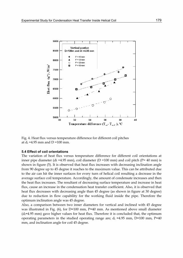
Experimental Study for Condensation Heat Transfer Inside Helical Coil
179
Fig. 4. Heat flux versus temperature difference for different coil pitches at di =4.95 mm and D =100 mm.
5.4 Effect of coil orientations The variation of heat flux versus temperature difference for different coil orientations at inner pipe diameter (di =4.95 mm), coil diameter (D =100 mm) and coil pitch (P= 40 mm) is shown in figure (5). It is observed that heat flux increases with decreasing inclination angle from 90 degree up to 45 degree it reaches to the maximum value. This can be attributed due to the air can hit the inner surfaces for every turn of helical coil resulting a decrease in the average surface coil temperature. Accordingly, the amount of condensate increases and then the heat flux increases. The resultant of decreasing surface temperature and increase in heat flux, cause an increase in the condensation heat transfer coefficient. Also, it is observed that heat flux decreases with decreasing angle than 45 degree (as shown in figure at 30 degree) due to reduction in flow capability for the working fluid inside the pipe. Therefore the optimum inclination angle was 45 degree. Also, a comparison between two inner diameters for vertical and inclined with 45 degree was illustrated in Fig. (6), for D=100 mm, P=40 mm. As mentioned above small diameter (di=4.95 mm) gave higher values for heat flux. Therefore it is concluded that, the optimum operating parameters in the studied operating range are; di =4.95 mm, D=100 mm, P=40 mm, and inclination angle for coil 45 degree.
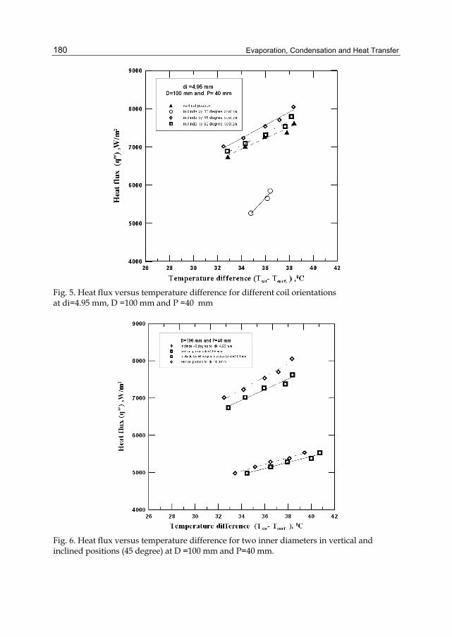
Evaporation, Condensation and Heat Transfer
180
Fig. 5. Heat flux versus temperature difference for different coil orientations at di=4.95 mm, D =100 mm and P =40 mm
Fig. 6. Heat flux versus temperature difference for two inner diameters in vertical and inclined positions (45 degree) at D =100 mm and P=40 mm.
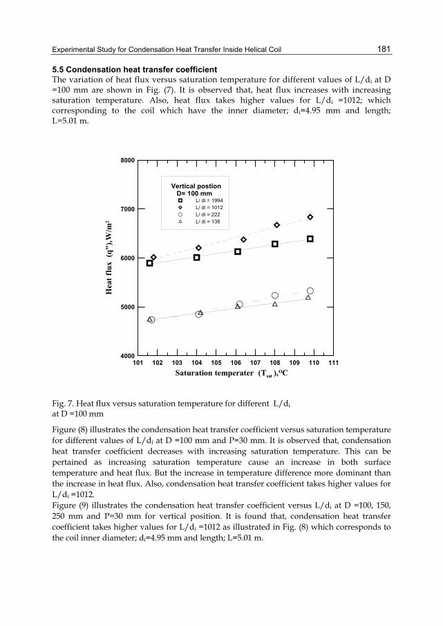
Experimental Study for Condensation Heat Transfer Inside Helical Coil
181
5.5 Condensation heat transfer coefficient The variation of heat flux versus saturation temperature for different values of L/di at D =100 mm are shown in Fig. (7). It is observed that, heat flux increases with increasing saturation temperature. Also, heat flux takes higher values for L/di =1012; which corresponding to the coil which have the inner diameter; di=4.95 mm and length; L=5.01 m.
101 102 103 104 105 106 107 108 109 110 111Saturation temperater (Tsat ),OC
4000
5000
6000
7000
8000
Hea
t flu
x (q
"),W
/m2
Vertical postionD= 100 mm
L/ di = 1994L/ di = 1012L/ di = 222L/ di = 138
Fig. 7. Heat flux versus saturation temperature for different L/di at D =100 mm
Figure (8) illustrates the condensation heat transfer coefficient versus saturation temperature for different values of L/di at D =100 mm and P=30 mm. It is observed that, condensation heat transfer coefficient decreases with increasing saturation temperature. This can be pertained as increasing saturation temperature cause an increase in both surface temperature and heat flux. But the increase in temperature difference more dominant than the increase in heat flux. Also, condensation heat transfer coefficient takes higher values for L/di =1012. Figure (9) illustrates the condensation heat transfer coefficient versus L/di at D =100, 150, 250 mm and P=30 mm for vertical position. It is found that, condensation heat transfer coefficient takes higher values for L/di =1012 as illustrated in Fig. (8) which corresponds to the coil inner diameter; di=4.95 mm and length; L=5.01 m.
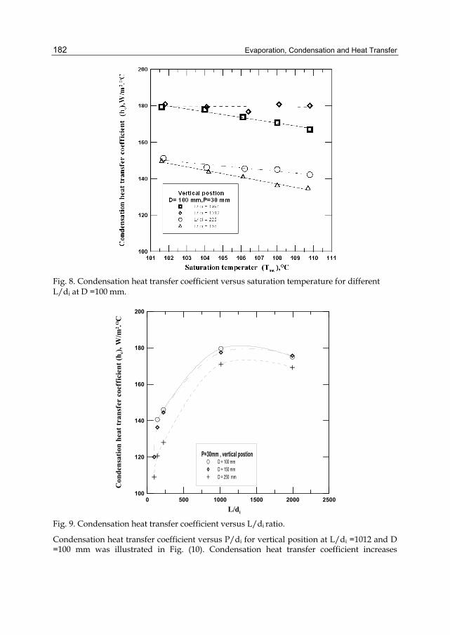
Evaporation, Condensation and Heat Transfer
182
Fig. 8. Condensation heat transfer coefficient versus saturation temperature for different L/di at D =100 mm.
0 500 1000 1500 2000 2500L/di
100
120
140
160
180
200
Con
dens
atio
n he
at tr
ansf
er c
oeff
icie
nt (h
c), W
/m2 .O
C
P=30mm , vertical postionD = 100 mmD = 150 mmD = 250 mm
Fig. 9. Condensation heat transfer coefficient versus L/di ratio.
Condensation heat transfer coefficient versus P/di for vertical position at L/di =1012 and D =100 mm was illustrated in Fig. (10). Condensation heat transfer coefficient increases
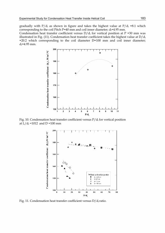
Experimental Study for Condensation Heat Transfer Inside Helical Coil
183
gradually with P/di as shown in figure and takes the highest value at P/di =8.1 which corresponding to the coil Pitch P=40 mm and coil inner diameter; di=4.95 mm. Condensation heat transfer coefficient versus D/di for vertical position at P =30 mm was illustrated in Fig. (11). Condensation heat transfer coefficient takes the highest value at D/di =20.2 which corresponding to the coil diameter D=100 mm and coil inner diameter; di=4.95 mm.
1 2 3 4 5 6 7 8 9 10 11P/di
150
160
170
180
190
200C
onde
nsat
ion
heat
tran
sfer
coe
ffic
ient
(h c)
,W/m
2 .OC
Fig. 10. Condensation heat transfer coefficient versus P/di for vertical position at L/di =1012 and D =100 mm
Fig. 11. Condensation heat transfer coefficient versus D/di ratio.
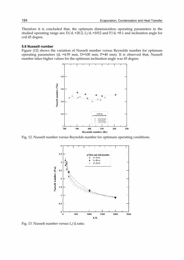
Evaporation, Condensation and Heat Transfer
184
Therefore it is concluded that, the optimum dimensionless operating parameters in the studied operating range are; D/di =20.2, L/di =1012 and P/di =8.1 and inclination angle for coil 45 degree.
5.6 Nusselt number Figure (12) shows the variation of Nusselt number versus Reynolds number for optimum operating parameters (di =4.95 mm, D=100 mm, P=40 mm). It is observed that, Nusselt number takes higher values for the optimum inclination angle was 45 degree.
180 190 200 210 220 230Reynolds number (Re)
1
1.2
1.4
1.6
1.8
2
Nus
selt
num
ber
(Nu)
P=40 mmdi =4.95 mm and D=100
inclinde 45 degreeinclinde 60 degree vertical 90 degree
Fig. 12. Nusselt number versus Reynolds number for optimum operating conditions.
Fig. 13. Nusselt number versus L/di ratio.
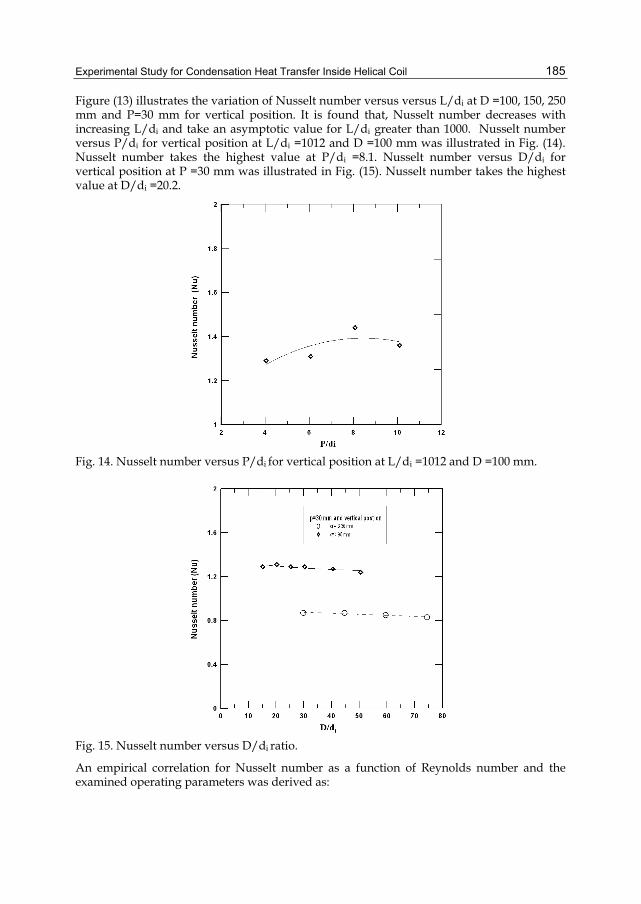
Experimental Study for Condensation Heat Transfer Inside Helical Coil
185
Figure (13) illustrates the variation of Nusselt number versus versus L/di at D =100, 150, 250 mm and P=30 mm for vertical position. It is found that, Nusselt number decreases with increasing L/di and take an asymptotic value for L/di greater than 1000. Nusselt number versus P/di for vertical position at L/di =1012 and D =100 mm was illustrated in Fig. (14). Nusselt number takes the highest value at P/di =8.1. Nusselt number versus D/di for vertical position at P =30 mm was illustrated in Fig. (15). Nusselt number takes the highest value at D/di =20.2.
Fig. 14. Nusselt number versus P/di for vertical position at L/di =1012 and D =100 mm.
Fig. 15. Nusselt number versus D/di ratio.
An empirical correlation for Nusselt number as a function of Reynolds number and the examined operating parameters was derived as:
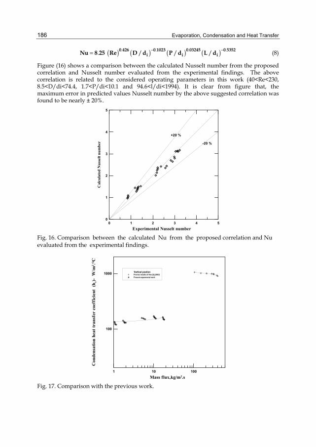
Evaporation, Condensation and Heat Transfer
186
( ) ( ) ( ) ( ). . . .. / / /− −= 0 426 0 1023 0 03245 0 5352i i iNu 8 25 Re D d P d L d (8)
Figure (16) shows a comparison between the calculated Nusselt number from the proposed correlation and Nusselt number evaluated from the experimental findings. The above correlation is related to the considered operating parameters in this work (40<Re<230, 8.5<D/di<74.4, 1.7<P/di<10.1 and 94.6<l/di<1994). It is clear from figure that, the maximum error in predicted values Nusselt number by the above suggested correlation was found to be nearly ± 20%.
0 1 2 3 4 5Experimental Nusselt number
0
1
2
3
4
5
Cal
cula
ted
Nus
selt
num
ber
+20 %
-20 %
Fig. 16. Comparison between the calculated Nu from the proposed correlation and Nu evaluated from the experimental findings.
1 10 100Mass flux,kg/m2.s
100
1000
Con
dens
atio
n he
at tr
ansf
er c
oeff
icie
nt (
h c)- W
/m2 .O
C
Vertical postionPrevios results of Han [3],(2003)Present expermental work
Fig. 17. Comparison with the previous work.
Experimental Study for Condensation Heat Transfer Inside Helical Coil
187
Figure (17) shows a comparison between condensation heat transfer coefficient for the present work and the previous work of Han et al. [3] which studied condensation heat transfer of R-134a flow inside helical pipes at different orientations. It clear from figure that comparison between the present works with the previous work gave fair agreement due to using steam in the present work as a working fluid.
6. Conclusions Experimental study was conducted to determine the condensation heat transfer of steam which flow inside helical coil. The operating parameters are; pipe diameter, coil diameter, coil pitch, and coil orientations. The obtained experiments results show that; condensation heat transfer coefficient increases with decreasing saturation temperature. Condensation heat transfer coefficient increases with the decrease pipe diameter and helical coil diameter then it is decreases. Also condensation heat transfer coefficient increases with the increase of coil pitch up to a certain value (p=40 mm) then it is decreases. Condensation heat transfer coefficient takes higher values for inclined position with angle 45o than the vertical and other inclination angles. Therefore the optimum operating parameters in the studied operating range are; di =4.95 mm, D= 100 mm, P=40 mm, and inclination angle for coil 45 degree. Accordingly the optimum dimensionless operating parameters in the studied operating range are; D/di =20.2, L/di =1012 and P/di =8.1. An empirical correlation for Nusselt number as a function of Reynolds number and the examined operating parameters. Comparison between the present works with the previous work gave fair agreement.
7. Nomenclature As : Surface area, m2. Cp : Specific heat, J/kg. oC d : Pipe diameter of the helical coil, m D : Helical coil diameter, m h : Condensation heat transfer coefficient, W/m2. oC i : Specific enthalpy, J/kg k : Thermal conductivity, W/m. oC L : helical coil length, m m. : Mass flow rate, kg/s P : Helical coil pitch, m Nu : Nusselt number, - Q : Heat transfer rate, W Re : Reynolds number, - q" : Heat flux, W/m2 T : Temperature, oC Greek symbols μ : Dynamic viscosity, kg/m.s
8. Subscripts air : air g : Dry saturated steam
Evaporation, Condensation and Heat Transfer
188
i : inner, inlet loss : loss o : outer, outlet s : surface st : steam
9. References [1] J.T. Han, C.X. Lin and M.A. Ebadian "Condensation heat transfer and pressure drop
characteristics of R-134a in an annular helical pipe" International Communications in Heat and Mass Transfer 32, (2005), pp. 1307-1316.
[2] C.X. Lin and M.A. Ebadian "Condensation heat transfer and pressure drop of R-134a in annular helicoidal pipe at different orientations" International Journal of Heat and Mass Transfer 50, (2007), pp. 4256–4264.
[3] J.T. Han, H.J. Kang, C.X. Lin, A. Awwad and M.A. Ebadian "Condensation heat transfer of R-134a flow inside helical pipes at different orientations", Int. Comm. Heat Mass Transfer, Vol. 30, no. 6, (2003), pp. 745-754.
[4] S. Laohalertdecha, S. Wongwises "The effects of corrugation pitch on the condensation heat transfer coefficient and pressure drop of R-134a inside horizontal corrugated tube" International Journal of Heat and Mass Transfer, Vol. 53, (2010), pp. 2924–2931.
[5] Y. Murai, S. Yoshikawa, S. Toda , M. Ishikawa and F. Yamamoto "Structure of air–water two-phase flow in helically coiled tubes" Nuclear Engineering and Design, Vol. 236, (2006), pp. 94–106.
[6] S. Wongwises and M. Polsongkram "Condensation heat transfer and pressure drop of HFC-134a in a helically coiled concentric tube-in-tube heat exchanger", International Journal of Heat and Mass Transfer, Vol. 49, (2006), pp. 4386–4398.
[7] S. Li and H. Ji-tian " condensation heat transfer of R-134a in horizontal straight and helically coiled tube-in-tube heat exchangers" Journal of hydrodynamics, Vol. 19, no. 6, (2007), pp. 677-682.
[8] M. Moawed "Experimental study of forced convection from helical coiled tubes with different parameters", Energy Conversion and Management, (2010), inpress
[9] M.H. Al-Hajeri, A.M. Koluib, M. Mosaad and S. Al-Kulaib" Heat transfer performance during condensation of R-134a inside helicoidal tubes" Energy Conversion and Management 48, (2007), pp. 2309–2315.
[10] R.C.Xin, A. Awwad, Z.F. Dong and M.A. Ebadian "Experimental study of single-phase and two-phase flow pressure drop in annular helicoidal pipes" International comn. heat and fluid flow 18, (1997), pp. 483-488.
[11] S. Wongwises, M. Polsongkram " Evaporation heat transfer and pressure drop of HFC-134a in a helically coiled concentric tube-in-tube heat exchanger" International Journal of Heat and Mass Transfer 49, (2006), pp. 658–670.
[12] S. Laohalertdecha, S. Wongwises "The effects of corrugation pitch on the condensation heat transfer coefficient and pressure drop of R-134a inside horizontal corrugated tube" International Journal of Heat and Mass Transfer 53, (2010), pp. 2924–2931.
9
Modelling the Thermo-Hydraulic Performance of Cooling Networks and Its Implications on
Design, Operation and Retrofit Martín Picón-Núñez, Lázaro Canizalez-Dávalos and Graham T. Polley
Department of Chemical Engineering, University of Guanajuato, México
1. Introduction The set of heat transfer equipment through which heating and cooling takes place within a process is known as the heat exchanger network. Heat exchanger networks are made up of three main subsystems: a) the heating network, where thermal energy from external sources is supplied to a process, b) the heat recovery network, where thermal energy available within a process is recovered in order to minimize the external energy consumption, and c) the cooling network, where the low grade thermal energy from a process is rejected to the environment. A cooling network is an essential part of a cooling system; its design, operation and retrofit is looked at in this chapter. The main components of a cooling system are the set of coolers or cooling network, the cooling system and the flow system which includes the pumping system and the pipeline. All the components of a cooling tower are linked and failure to appreciate this relation may lead to operating difficulties and excessive operating costs. In this chapter we look in detail at the interaction between these three components in the light of a thermo-hydraulic model. The thermal analysis is based on the application of the thermal effectiveness model originally developed for single heat exchangers. On the hydraulic side, the water distribution through the network depends on the pressure drop across the various branches that make up the network; this in turn has implications on the thermal performance of the coolers. During operation cooling systems are subject to changes in operating conditions that affect their heat removal capacity. These changes take place as a result of any of the following: plant throughput variations during the year; variations in ambient conditions that affect the performance of cooling towers; the performance of heat exchangers gets deteriorated over time due to fouling, etc. In practice, a cooling systems is commonly designed for point conditions; normally these point conditions correspond to the case where the whole system is well overdesigned. One problem with this practice is that the operating costs are much higher than they should be. This problem can be addressed by the proper application of a thermo-hydraulic model. In this context, this chapter shows the way a thermo-hydraulic model for cooling systems is developed and introduces its application in design. Cooling systems are normally designed for fixed conditions; for instance, they are specified by a given cooling load, water flow rate, pumping capacity and heat transfer surface area in
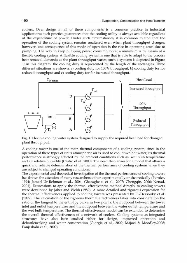
Evaporation, Condensation and Heat Transfer
190
coolers. Over design in all of these components is a common practice in industrial applications; such practice guarantees that the cooling utility is always available regardless of the expenditure of power. Under such circumstances, it is common to find that the operation of the cooling system remains unaltered even when plant throughput changes; however, one consequence of this mode of operation is the rise in operating costs due to pumping. The way to keep pumping power consumption at a minimum is by means of a flexible cooling system. A flexible cooling system is one that is able to adapt to the process heat removal demands as the plant throughput varies; such a systems is depicted in Figure 1; in this diagram, the cooling duty is represented by the length of the rectangles. Three different situations are shown: a) cooling duty for 100% throughput, b) cooling duty for for reduced throughput and c) cooling duty for for increased throughput.
A
B
C
DTin
Tout
Tw, return
Tw
Heat Load
ReducedThroughput
Increased throughput
100%Throughput
A
B
C
DTin
Tout
Tw, return
Tw
Heat Load
ReducedThroughput
Increased throughput
100%Throughput
Fig. 1. Flexible cooling water system designed to supply the required heat load for changed plant throughput.
A cooling tower is one of the main thermal components of a cooling system; since in the operation of these types of units atmospheric air is used to cool down hot water, its thermal performance is strongly affected by the ambient conditions such as: wet bulb temperature and air relative humidity (Castro et al., 2000). The need then arises for a model that allows a quick and reliable determination of the thermal performance of cooling systems when they are subject to changed operating conditions. The experimental and theoretical investigation of the thermal performance of cooling towers has drawn the attention of many researchers either experimentally or theoretically (Bernier, 1994; Jameel-Ur-Rehman et al., 2004; Gharagheizi et al., 2007; Chengqin, 2006; Nenad, 2001). Expressions to apply the thermal effectiveness method directly to cooling towers were developed by Jaber and Webb (1989). A more detailed and rigorous expression for the thermal effectiveness applied to cooling towers was presented by El–Dessouky et al. (1997). The calculation of the rigorous thermal effectiveness takes into consideration the ratio of the tangent to the enthalpy curve in two points: the midpoint between the tower inlet and outlet temperatures and the midpoint between the water outlet temperature and the wet bulb temperature. The thermal effectiveness model can be extended to determine the overall thermal effectiveness of a network of coolers. Cooling systems as integrated structures have also been studied either for design, improved operation and debottlenecking and water conservation (Giorgia et al., 2009; Majozi & Moodley,2008; Panjeshahi et al., 2009).
Modelling the Thermo-Hydraulic Performance of Cooling Networks and Its Implications on Design, Operation and Retrofit
191
The work by Picon-Nuñez et al. (2007) shows such application where they demonstrate that the thermal response of a network of coolers subject to changes in operating temperatures is independent of the structure. This finding, along with the concept of flexible design of single heat exchangers becomes the basis for undertaking the design of flexible cooling systems.
2. Hydraulic model It has been shown that the pressure loss due to valves and fittings is proportional to the fluid velocity raised to an exponent. In the turbulent region, this exponent varies between 1.8 and 2.1. However, in the majority of practical cases the pressure drop is calculated as a function of the square of the velocity. In the case of water distribution systems, it can readily be demonstrated that the pressure drop through heat exchangers, valves and fittings can be related to volumetric or mass flow rate by means of equation (1):
2ΔP = KV (1)
Where ∆P is the pressure drop, K is a loss constant and V is the volumetric flow rate. The term V can be expressed as a function of the fluid velocity and the flow area as:
V = uA (2)
Where u is defined as:
2Vu =πd
⎛ ⎞⎜ ⎟⎝ ⎠
(3)
The pressure drop through a straight pipe can be expressed as:
2lΔP = 2f ρud
⎛ ⎞⎜ ⎟⎝ ⎠
(4)
Where f is the friction factor, l is the pipe length, d is the pipe diameter and u is the fluid velocity. Substitution of equation (3) into equation (4) gives:
2
2l VΔP = 2fρd πd
⎛ ⎞⎛ ⎞⎜ ⎟⎜ ⎟
⎝ ⎠⎝ ⎠ (5)
From equation (5), the loss term (K) is defined as:
2
2l 1K = 2fρd πd
⎛ ⎞⎛ ⎞⎜ ⎟⎜ ⎟
⎝ ⎠⎝ ⎠ (6)
The advantage of using the volumetric flow rate instead of velocity in the determination of the pressure drop is that it remains constant as the fluid flows through the various components. In a typical cooling system branch the minimum components are: valves, pipeline and heat exchangers; so, application of Equation (1) to these components leads to:
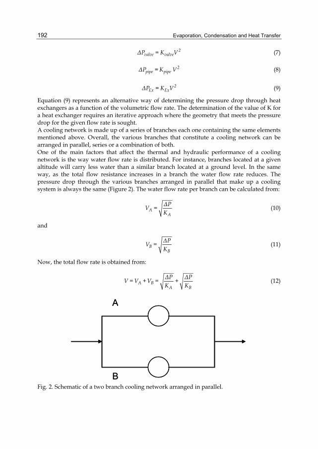
Evaporation, Condensation and Heat Transfer
192
2valve valveΔP = K V (7)
2pipe pipeΔP = K V (8)
2Ex ExΔP = K V (9)
Equation (9) represents an alternative way of determining the pressure drop through heat exchangers as a function of the volumetric flow rate. The determination of the value of K for a heat exchanger requires an iterative approach where the geometry that meets the pressure drop for the given flow rate is sought. A cooling network is made up of a series of branches each one containing the same elements mentioned above. Overall, the various branches that constitute a cooling network can be arranged in parallel, series or a combination of both. One of the main factors that affect the thermal and hydraulic performance of a cooling network is the way water flow rate is distributed. For instance, branches located at a given altitude will carry less water than a similar branch located at a ground level. In the same way, as the total flow resistance increases in a branch the water flow rate reduces. The pressure drop through the various branches arranged in parallel that make up a cooling system is always the same (Figure 2). The water flow rate per branch can be calculated from:
AA
ΔPV =K
(10)
and
BB
ΔPV =K
(11)
Now, the total flow rate is obtained from:
A BA B
ΔP ΔPV = V +V = +K K
(12)
A
B
A
B Fig. 2. Schematic of a two branch cooling network arranged in parallel.
Modelling the Thermo-Hydraulic Performance of Cooling Networks and Its Implications on Design, Operation and Retrofit
193
The value of K for the whole system in Figure 2 is given by equation (13) where the terms KA
and KB represent the resistances involved in each branch (pipeline, valves, fittings and heat exchanger):
A+B 2 2
A B
ΔP 1K = =V 1 1+
K K⎛ ⎞⎜ ⎟⎜ ⎟⎝ ⎠
(13)
For the case of piping, the K loss term is a function of the velocity whereas for valves and fittings its value is independent of it. The values of K for pipe fittings are given in Table 1.
3. Thermal model The exchanger thermal effectiveness (ε), represents the ratio of the actual heat load to the maximum load that can thermodynamically be transferred. From this definition it can be shown that the exchanger thermal effectiveness can be represented by the ratio of the temperature change that the stream that exhibits the CPmin undergoes to the maximum temperature difference that exists between streams. The CPmin stream is the one whose product heat capacity-mass flow rate is the lower of the two. For the temperature profiles shown in Figure 3, it can be shown that the expression for the thermal effectiveness according to the definition above is given by:
1 2
1 1
T - Tε =T - t
(14)
The exchanger thermal effectiveness can also be expressed as a function of Cr (Cr=CPmin/CPmax), the number of heat transfer units (NTU) and the exchanger flow arrangement. Expressions that relate these terms for a number of flow arrangements have been developed (Kays & London, 1984). For instance, for a one tube pass and two tube passes shell and tube heat exchanger, the expression that relates: ε, NTU and Cr is:
( )( )
( )
-11
22r1
22r r 1
22r
1+ exp -NTU 1+ Cε = 2 1+ C + 1+ C
1 - exp -NTU 1+ C
⎧ ⎫⎡ ⎤⎛ ⎞⎪ ⎪⎢ ⎥⎜ ⎟⎜ ⎟⎪ ⎪⎢ ⎥⎝ ⎠⎨ ⎬⎢ ⎥⎛ ⎞⎪ ⎪⎢ ⎥⎜ ⎟⎪ ⎪⎜ ⎟⎢ ⎥⎝ ⎠⎣ ⎦⎩ ⎭
(15)
The number of heat transfer units is defined as:
min
U ANTU =CP
(16)
Where U is the overall heat transfer coefficient and A is the heat transfer surface area. From the heat balance equation it can be shown that:
min 2 1r
max 1 2
CP t - tC = =CP T - T
(17)
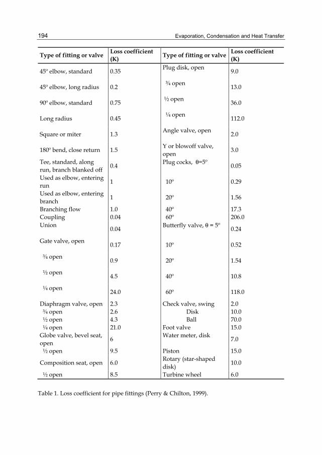
Evaporation, Condensation and Heat Transfer
194
Type of fitting or valve Loss coefficient (K) Type of fitting or valve Loss coefficient
(K)
45º elbow, standard 0.35 Plug disk, open 9.0
45º elbow, long radius 0.2 ¾ open 13.0
90º elbow, standard 0.75 ½ open 36.0
Long radius 0.45 ¼ open 112.0
Square or miter 1.3 Angle valve, open 2.0
180º bend, close return 1.5 Y or blowoff valve, open 3.0
Tee, standard, along run, branch blanked off 0.4 Plug cocks, θ=5º
0.05
Used as elbow, entering run 1 10º 0.29
Used as elbow, entering branch 1 20º 1.56
Branching flow 1.0 40º 17.3 Coupling 0.04 60º 206.0 Union 0.04 Butterfly valve, θ = 5º
0.24
Gate valve, open 0.17 10º 0.52
¾ open 0.9 20º 1.54
½ open 4.5 40º 10.8
¼ open 24.0 60º 118.0
Diaphragm valve, open 2.3 Check valve, swing 2.0 ¾ open 2.6 Disk 10.0 ½ open 4.3 Ball 70.0 ¼ open 21.0 Foot valve 15.0 Globe valve, bevel seat, open 6 Water meter, disk
7.0
½ open 9.5 Piston 15.0
Composition seat, open 6.0 Rotary (star-shaped disk) 10.0
½ open 8.5 Turbine wheel 6.0
Table 1. Loss coefficient for pipe fittings (Perry & Chilton, 1999).
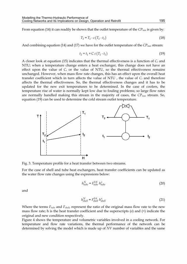
Modelling the Thermo-Hydraulic Performance of Cooling Networks and Its Implications on Design, Operation and Retrofit
195
From equation (14) it can readily be shown that the outlet temperature of the CPmin is given by:
( )2 1 1 1T = T - ε T - t (18)
And combining equation (14) and (17) we have for the outlet temperature of the CPmax stream:
( )2 1 1 1t = t +C ε T - t (19)
A closer look at equation (15) indicates that the thermal effectiveness is a function of Cr and NTU; when a temperature change enters a heat exchanger, this change does not have an effect upon the value of Cr or the value of NTU, so the thermal effectiveness remains unchanged. However, when mass flow rate changes, this has an effect upon the overall heat transfer coefficient which in turn affects the value of NTU , the value of Cr and therefore affects the thermal effectiveness. So, the thermal effectiveness changes and it has to be updated for the new exit temperatures to be determined. In the case of coolers, the temperature rise of water is normally kept low due to fouling problems; so large flow rates are normally handled making this stream in the majority of cases, the CPmax stream. So, equation (19) can be used to determine the cold stream outlet temperature.
T
H
T1
T2
t1
t2
T1
t2
T2
t1
T
H
T1
T2
t1
t2
T1
t2
T2
t1
Fig. 3. Temperature profile for a heat transfer between two streams.
For the case of shell and tube heat exchangers, heat transfer coefficients can be updated as the water flow rate changes using the expressions below:
N 0.8 otube tube tubeh = F h (20)
and
N 0.6 oshell shell shellh = F h (21)
Where the terms Ftube and Fshell, represent the ratio of the original mass flow rate to the new mass flow rate; h is the heat transfer coefficient and the superscripts (o) and (N) indicate the original and new condition respectively. Figure 4 shows the temperature and volumetric variables involved in a cooling network. For temperature and flow rate variations, the thermal performance of the network can be determined by solving the model which is made up of NV number of variables and the same
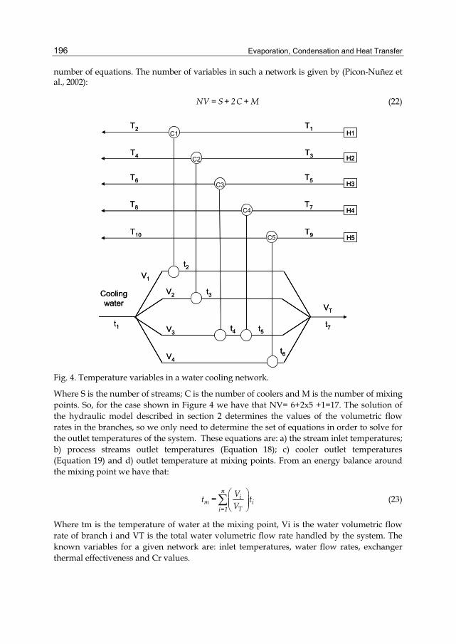
Evaporation, Condensation and Heat Transfer
196
number of equations. The number of variables in such a network is given by (Picon-Nuñez et al., 2002):
NV = S + 2 C + M (22)
C1
C3
C4
H1
H2
H3
H4
Coolingwater
C5 H5
C2
t1
t2
t3
t4 t5
t6
t7
T1T2
T3T4
T5T6
T7T8
T9T10
V1
V2
V3
V4
VT
C1
C3
C4
H1
H2
H3
H4
Coolingwater
C5 H5
C2
t1
t2
t3
t4 t5
t6
t7
T1T2
T3T4
T5T6
T7T8
T9T10
V1
V2
V3
V4
VT
Fig. 4. Temperature variables in a water cooling network.
Where S is the number of streams; C is the number of coolers and M is the number of mixing points. So, for the case shown in Figure 4 we have that NV= 6+2x5 +1=17. The solution of the hydraulic model described in section 2 determines the values of the volumetric flow rates in the branches, so we only need to determine the set of equations in order to solve for the outlet temperatures of the system. These equations are: a) the stream inlet temperatures; b) process streams outlet temperatures (Equation 18); c) cooler outlet temperatures (Equation 19) and d) outlet temperature at mixing points. From an energy balance around the mixing point we have that:
n
im i
Ti=1
Vt = tV⎛ ⎞⎜ ⎟⎜ ⎟⎝ ⎠
∑ (23)
Where tm is the temperature of water at the mixing point, Vi is the water volumetric flow rate of branch i and VT is the total water volumetric flow rate handled by the system. The known variables for a given network are: inlet temperatures, water flow rates, exchanger thermal effectiveness and Cr values.
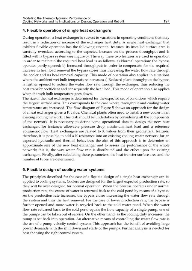
Modelling the Thermo-Hydraulic Performance of Cooling Networks and Its Implications on Design, Operation and Retrofit
197
4. Flexible operation of single heat exchangers
During operation, a heat exchanger is subject to variations in operating conditions that may result in a reduction or increase of the exchanger heat duty. A single heat exchanger that exhibits flexible operation has the following essential features: its installed surface area is carefully oversized according to the expected increase on the process throughput and is fitted with a bypass system (see Figure 3). The way these two features are used in operation in order to maintain the required heat load is as follows: a) Normal operation: the bypass operates partly opened; b) Increased throughput: in order to compensate for the required increase in heat load removal the bypass closes thus increasing the water flow rate through the cooler and its heat removal capacity. This mode of operation also applies in situations where the ambient wet bulb temperature increases; c) Reduced plant throughput: the bypass is further opened to reduce the water flow rate through the exchanger, thus reducing the heat transfer coefficient and consequently the heat load. This mode of operation also applies when the web bulb temperature goes down. The size of the heat exchanger is determined for the expected set of conditions which require the largest surface area. This corresponds to the case where throughput and cooling water temperature are increased. The flow diagram of Figure 5 shows an approach for the design of a heat exchanger given a K value. Chemical plants often need to install a new cooler in an existing cooling network. This task should be undertaken by considering all the components of the network. It is necessary to define some operational data to design the new heat exchanger, for instance: allowable pressure drop, maximum heat load and a reference volumetric flow. Heat exchangers are related to K values from their geometrical features; therefore, it is possible to add a K resistance into an existing cooling water network for an expected hydraulic and thermal behaviour; the aim of this approach is to determine an approximate size of the new heat exchanger and to assess the performance of the whole network; this is, the way water flow rate is distributed and the effect upon the existing exchangers. Finally, after calculating these parameters, the heat transfer surface area and the number of tubes are determined.
5. Flexible design of cooling water systems
The principles described for the case of a flexible design of a single heat exchanger can be applied to cooling systems. Coolers are designed for the largest expected production rate, so they will be over designed for normal operation. When the process operates under normal production rate, the excess of water is returned back to the cold pond by means of a bypass. As the production rate increases, the bypass closes increasing the water flow rate through the system and thus the heat removal. For the case of lower production rate, the bypass is further opened and more water is recycled back to the cold water pond. When the water flow rate returned back to the cold pond equals the flow capacity of a single pump, one of the pumps can be taken out of service. On the other hand, as the cooling duty increases, the pump is set back into operation. An alternative means of controlling the water flow rate is the use of a pump velocity control system. This approach has the benefit of avoiding large power demands with the shut down and starts of the pumps. Further analysis is needed for best choosing the right control system.
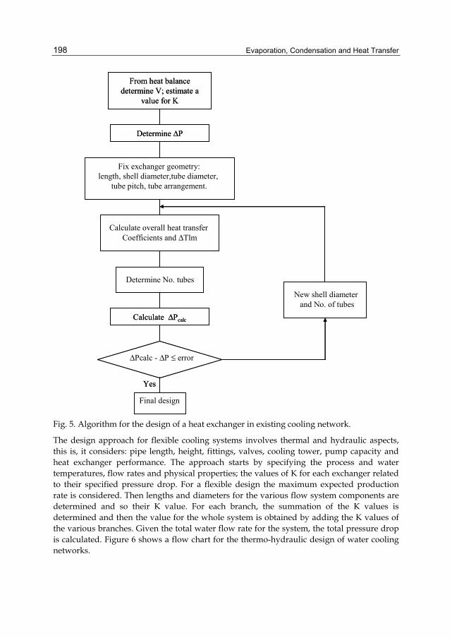
Evaporation, Condensation and Heat Transfer
198
From heat balance determine V; estimate a
value for K
Determine ΔP
Fix exchanger geometry:length, shell diameter,tube diameter,
tube pitch, tube arrangement.
Determine No. tubes
Calculate ΔPcalc
ΔPcalc - ΔP ≤ error
Yes
Final design
New shell diameterand No. of tubes
Calculate overall heat transferCoefficients and ΔTlm
Fig. 5. Algorithm for the design of a heat exchanger in existing cooling network.
The design approach for flexible cooling systems involves thermal and hydraulic aspects, this is, it considers: pipe length, height, fittings, valves, cooling tower, pump capacity and heat exchanger performance. The approach starts by specifying the process and water temperatures, flow rates and physical properties; the values of K for each exchanger related to their specified pressure drop. For a flexible design the maximum expected production rate is considered. Then lengths and diameters for the various flow system components are determined and so their K value. For each branch, the summation of the K values is determined and then the value for the whole system is obtained by adding the K values of the various branches. Given the total water flow rate for the system, the total pressure drop is calculated. Figure 6 shows a flow chart for the thermo-hydraulic design of water cooling networks.
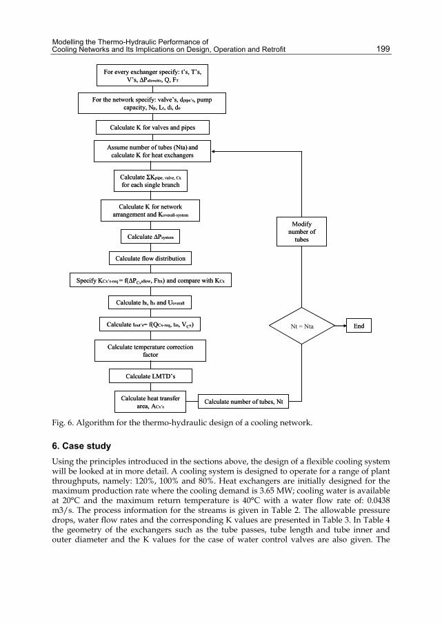
Modelling the Thermo-Hydraulic Performance of Cooling Networks and Its Implications on Design, Operation and Retrofit
199
For every exchanger specify: t’s, T’s, V’s, ΔPallowable, Q, FT
For the network specify: valve’s, dpipe’s, pump capacity, Np, Lt, di, do
Calculate K for valves and pipes
Assume number of tubes (Nta) and calculate K for heat exchangers
Calculate ΣKpipe, valve, Cx
for each single branch
Calculate K for network arrangement and Koverall-system
Calculate ΔPsystem
Calculate flow distribution
Specify KCx’s-req = f(ΔPCxallow, Fhx) and compare with KCx
Calculate tout’s= f(QCx-req, tin, VCx)
Calculate temperature correction factor
Calculate ht, hs and Uoverall
Calculate LMTD’s
Calculate heat transfer area, ACx’s
Calculate number of tubes, Nt
End
Modify number of
tubes
Nt = Nta
Fig. 6. Algorithm for the thermo-hydraulic design of a cooling network.
6. Case study Using the principles introduced in the sections above, the design of a flexible cooling system will be looked at in more detail. A cooling system is designed to operate for a range of plant throughputs, namely: 120%, 100% and 80%. Heat exchangers are initially designed for the maximum production rate where the cooling demand is 3.65 MW; cooling water is available at 20°C and the maximum return temperature is 40°C with a water flow rate of: 0.0438 m3/s. The process information for the streams is given in Table 2. The allowable pressure drops, water flow rates and the corresponding K values are presented in Table 3. In Table 4 the geometry of the exchangers such as the tube passes, tube length and tube inner and outer diameter and the K values for the case of water control valves are also given. The
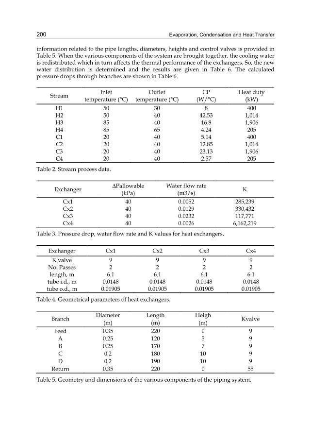
Evaporation, Condensation and Heat Transfer
200
information related to the pipe lengths, diameters, heights and control valves is provided in Table 5. When the various components of the system are brought together, the cooling water is redistributed which in turn affects the thermal performance of the exchangers. So, the new water distribution is determined and the results are given in Table 6. The calculated pressure drops through branches are shown in Table 6.
Stream Inlet temperature (°C)
Outlet temperature (°C)
CP (W/°C)
Heat duty (kW)
H1 50 30 8 400 H2 50 40 42.53 1,014 H3 85 40 16.8 1,906 H4 85 65 4.24 205 C1 20 40 5.14 400 C2 20 40 12.85 1,014 C3 20 40 23.13 1,906 C4 20 40 2.57 205
Table 2. Stream process data.
Exchanger ΔPallowable (kPa)
Water flow rate (m3/s) K
Cx1 40 0.0052 285,239 Cx2 40 0.0129 330,432 Cx3 40 0.0232 117,771 Cx4 40 0.0026 6,162,219
Table 3. Pressure drop, water flow rate and K values for heat exchangers.
Exchanger Cx1 Cx2 Cx3 Cx4 K valve 9 9 9 9
No. Passes 2 2 2 2 length, m 6.1 6.1 6.1 6.1
tube i.d., m 0.0148 0.0148 0.0148 0.0148 tube o.d., m 0.01905 0.01905 0.01905 0.01905
Table 4. Geometrical parameters of heat exchangers.
Branch Diameter (m)
Length (m)
Heigh (m) Kvalve
Feed 0.35 220 0 9 A 0.25 120 5 9 B 0.25 170 7 9 C 0.2 180 10 9 D 0.2 190 10 9
Return 0.35 220 0 55
Table 5. Geometry and dimensions of the various components of the piping system.
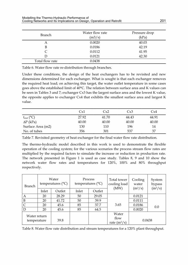
Modelling the Thermo-Hydraulic Performance of Cooling Networks and Its Implications on Design, Operation and Retrofit
201
Branch Water flow rate (m3/s)
Pressure drop (kPa)
A 0.0020 40.03 B 0.0186 42.19 C 0.0112 41.95 D 0.0121 42.30
Total flow rate 0.0438
Table 6. Water flow rate re-distribution through branches.
Under these conditions, the design of the heat exchangers has to be revisited and new dimensions determined for each exchanger. What is sought is that each exchanger removes the required heat load; on achieving this target, the water outlet temperature in some cases goes above the established limit of 40°C. The relation between surface area and K values can be seen in Tables 3 and 7; exchanger Cx3 has the largest surface area and the lowest K value, the opposite applies to exchanger Cx4 that exhibits the smallest surface area and largest K value.
Cx1 Cx2 Cx3 Cx4 tout (°C) 27.92 41.70 44.43 44.91 ΔP (kPa) 40.00 40.00 40.00 40.00 Surface Area (m2) 130 110 196 14 No. of tubes 356 301 537 37
Table 7. Revisited geometry of heat exchanger for the final water flow rate distribution.
The thermo-hydraulic model described in this work is used to demonstrate the flexible operation of the cooling system; for the various scenarios the process stream flow rates are multiplied by the required factors to simulate the increase or reduction in production rate. The network presented in Figure 1 is used as case study. Tables 8, 9 and 10 show the network water flow rates and temperatures for 120%, 100% and 80% throughput respectively.
Water temperatures (°C)
Process temperatures (°C)
Branch Inlet Outlet Inlet Outlet
Total tower cooling load
(MW)
Cooling water (m3/s)
System bypass (m3/s)
A 20 28.29 50 29.05 0.0121 B 20 41.72 50 39.9 0.0111 C 20 45.6 85 37.7 0.0186 D 20 45.6 85 64.5
3.65
0.0020
0.0
Water return temperature
39.8
Water flow
rate (m3/s)
0.0438
Table 8. Water flow rate distribution and stream temperatures for a 120% plant throughput.
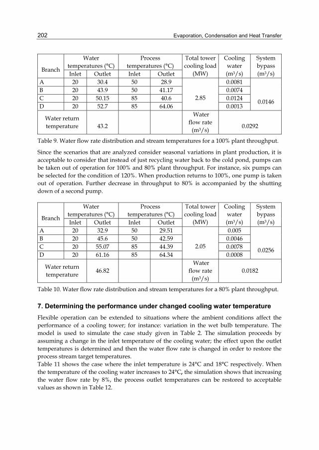
Evaporation, Condensation and Heat Transfer
202
Water
temperatures (°C) Process
temperatures (°C) Branch
Inlet Outlet Inlet Outlet
Total tower cooling load
(MW)
Cooling water (m3/s)
System bypass (m3/s)
A 20 30.4 50 28.9 0.0081 B 20 43.9 50 41.17 0.0074 C 20 50.15 85 40.6 0.0124 D 20 52.7 85 64.06
2.85
0.0013
0.0146
Water return temperature
43.2
Water flow rate
(m3/s)
0.0292
Table 9. Water flow rate distribution and stream temperatures for a 100% plant throughput.
Since the scenarios that are analyzed consider seasonal variations in plant production, it is acceptable to consider that instead of just recycling water back to the cold pond, pumps can be taken out of operation for 100% and 80% plant throughput. For instance, six pumps can be selected for the condition of 120%. When production returns to 100%, one pump is taken out of operation. Further decrease in throughput to 80% is accompanied by the shutting down of a second pump.
Water temperatures (°C)
Process temperatures (°C)
Branch Inlet Outlet Inlet Outlet
Total tower cooling load
(MW)
Cooling water (m3/s)
System bypass (m3/s)
A 20 32.9 50 29.51 0.005 B 20 45.6 50 42.59 0.0046 C 20 55.07 85 44.39 0.0078 D 20 61.16 85 64.34
2.05
0.0008
0.0256
Water return temperature 46.82
Water flow rate
(m3/s) 0.0182
Table 10. Water flow rate distribution and stream temperatures for a 80% plant throughput.
7. Determining the performance under changed cooling water temperature Flexible operation can be extended to situations where the ambient conditions affect the performance of a cooling tower; for instance: variation in the wet bulb temperature. The model is used to simulate the case study given in Table 2. The simulation proceeds by assuming a change in the inlet temperature of the cooling water; the effect upon the outlet temperatures is determined and then the water flow rate is changed in order to restore the process stream target temperatures. Table 11 shows the case where the inlet temperature is 24°C and 18°C respectively. When the temperature of the cooling water increases to 24°C, the simulation shows that increasing the water flow rate by 8%, the process outlet temperatures can be restored to acceptable values as shown in Table 12.

Modelling the Thermo-Hydraulic Performance of Cooling Networks and Its Implications on Design, Operation and Retrofit
203
The water return temperature for this case is 35.49°C and the cooling load 3.47 MW. Now, for the case where the cooling water enters at 18°C to the system, the heat removal rate will be higher than required. Therefore, the solution consists in reducing the flow rate. Table 13 shows the thermal performance of the exchangers; the cooling duty for this case is 3.53 MW and the water return temperature is 41.4°C. Since the performance is within acceptable values, the system needs not to adjust its water flow rate. Cooling water: 24°C Cooling water : 18°C Unit Tout (°C) tout (°C) Unit Tout (°C) tout (°C) Cx1 31.85 31.18 Cx1 27.66 26.84 Cx2 41.32 42.82 Cx2 39.32 41.16 Cx3 41 48.06 Cx3 36.32 44.42 Cx4 65.65 48.22 Cx4 63.75 44.6
Table 11. Temperature response at different cooling water inlet temperatures.
Cooling water: 24°C
Unit Process stream Tout (°C)
Process stream Target (°C)
Cooling water tout (°C)
Cx1 31.4 30 30.4 Cx2 40.6 40 41.87 Cx3 39.1 40 46 Cx4 65 65 46
Table 12. Process outlet temperatures after increasing water flow rate by 8%.
Cooling water: 18°C
Unit Process stream Tout (°C)
Process stream Target (°C)
Cooling water tout (°C)
Cx1 28.48 30 28.4 Cx2 40.6 40 42.85 Cx3 39.33 40 48 Cx4 64.93 65 48.6
Table 13. Thermal performance after reduction of cooling water temperature.
8. Conclusions Cooling systems are, in most applications, designed for a maximum fixed heat duty and its operation remains unchanged despite the variations in plant throughput. A disadvantage of this practice is that operating costs tend to be higher than they should be. Flexible operation is the capacity of the system to deliver the required heat load within some specific bounds. For instance, specific bounds may be the following: plant throughput may vary between a minimum and a maximum from normal production rate and the wet bulb temperature, which significantly affects the performance of a cooling tower, experiences changes between seasons. When a temperature or flow rate
Evaporation, Condensation and Heat Transfer
204
disturbance enters a cooling system, it propagates around until the steady state is reached. Since the steady state response of a cooling system is independent of the actual arrangement of the coolers then the heat load removal can be controlled through the use of a bypass scheme. With the operation of a flexible cooling system, the pumping power consumption is a variable that can also be controlled. Typically, the design of a cooling system is carried out by considering individual components at a time for a given set of operating conditions; when these components are placed together into a system, the water flow rate is no longer the same since it tends to re-distribute through the network depending on the resistance it encounters. The result of this phenomenon is that water flow rate distributes through the network so that the pressure drop in all branches of the system equates. So, a thermo-hydraulic model has to be implemented for the determination of the performance of a cooling system and it can be used to produce a design that meets the required flexibility. Such a model has been introduced in this work.
9. Nomenclature A heat exchanger surface area [m2] Cr heat capacity mass flow rate ratio C number of coolers in cooling network CPmin minimum heat capacity mass flow rate CPmax maximum heat capacity mass flow rate d diameter [m] h heat transfer coefficient [kJ/m2°C] FT logarithmic temperature correction factor K loss coefficient Lt tube lengths [m] M number of mixing point in a cooling network Nt number of tubes in heat exchanger Nta number of tubes assumed NP number passes NTU number of heat transfer units NV number of temperature variables in a cooling network Q heat load [kW] S number of streams T hot stream temperature [°C]. t cold stream temperature [°C] U overall heat transfer coefficient [W/m2°C] u fluid velocity [m/s] V volumetric flow rate [m3/s] Subscripts s shell side t tube side i inner condition o outer condition Superscripts N new condition
Modelling the Thermo-Hydraulic Performance of Cooling Networks and Its Implications on Design, Operation and Retrofit
205
o original condition m mixing point Greek letters ε thermal effectiveness ΔP pressure drop (kPa) ρ density [kg/m3]
10. References Bernier M A (1994). Cooling tower performance: theory and experiments. ASHRAE
Transactions Research : 114 – 121. Castro M M, Song T W, Pinto J M (2000). Minimization of operational costs in cooling water
Systems. Trans IchemE 78: Part A : 196 – 201. Chengqin R (2006). An analytical approach to the heat and mass transfer processes in
counterflow cooling towers. Journal of Heat Transfer Transactions of the ASME 128: 1142 – 1148.
EI – Dessouky H T A, AI – Haddad A A, I–Juwayhel F A (1997). Modified analysis of counter flow wet cooling towers. Journal of Heat Transfer Trans of ASME 119: 617 – 626.
Gharagheizi F, Reza H and Shohreh F (2007). Experimental study on the performance of mechanical cooling tower with two types of film packing. Energy Conversion and Management 48: 277 – 280.
Giorgia F, Cortinovis M, Ribeiro T, Paiva J L, Tah S W, Pinto J M (2009). Integrated analysis of cooling water systems: modeling and experimental validation. Applied Thermal Engineering 29: 3124–3131.
Jaber H T, Webb R T (1989). Design of cooling towers by the effectiveness – NTU method. ASME Journal of Heat Transfer 11: 873–843.
Jameel–Ur– Rehman K, Bilal A Q and Syed M Z A (2004). Comprehensive design and performance evaluation study of counter flow wet cooling towers. International Journal of Refrigeration 27 : 914–923.
M. Picón Núñez, J. Castro Páez and F. Vizcaíno García (2002). Steady state simulation for the de-bottlenecking of heat recovery networks. Applied Thermal Engineering 22 : 1673-1687.
Majozi T, Moodley A (2008). Simultaneous targeting and design for cooling water systems with multiple cooling water supplies. Computers and Chemical Engineering 32: 540–551.
Nenad M, Pertti H (2001). A comprehensive approach to cooling tower design. Applied Thermal Engineering 21: 899 – 915.
Panjeshahi M H, Ataeib A, Gharaiec M, Parandc R (2009). Optimum design of cooling water systems for energy and water conservation. Chem Eng Res Des 8: 7 , 200–209.
Perry and Cecil H. Chilton (1999). Fluid particle dynamics. Chemical Engineer’s Handbook, McGraw Hill.
Picón-Núñez M, Nila-Gasca C, Morales-Fuentes A (2007). Simplified model for the determination of the steady state response of cooling systems. Applied Thermal Engineering 27:1173–1181.

Evaporation, Condensation and Heat Transfer
206
W.M. Kays and A.L. London (1984). Compact heat exchangers, Third edition, McGraw Hill.
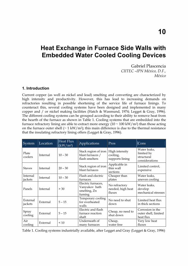
10
Heat Exchange in Furnace Side Walls with Embedded Water Cooled Cooling Devices
Gabriel Plascencia CIITEC –IPN México, D.F.,
México
1. Introduction Current copper (as well as nickel and lead) smelting and converting are characterized by high intensity and productivity. However, this has lead to increasing demands on refractories resulting in possible shortening of the service life of furnace linings. To counteract this, several cooling systems have been designed and implemented in many copper and / or nickel making facilities (Hatch & Wasmund, 1974; Legget & Gray, 1996). The different cooling systems can be grouped according to their ability to remove heat from the hearth of the furnace as shown in Table 1. Cooling systems that are embedded into the furnace refractory lining are able to extract more energy (10 ~ 100 kW/m2) than those acting on the furnace outer shell (~ 1 kW/m2); this main difference is due to the thermal resistance that the insulating refractory lining offers (Legget & Gray, 1996).
System Location Heat Flux (kW/m2) Applications Pros Cons
Plate coolers Internal 10 – 30
Stack region of iron blast furnaces / flash smelters
High intensity cooling, supports lining
Water leaks, limited by structural considerations
Staves Internal 20 – 30 Stack region of iron blast furnaces
Applicable in thin wall sections
Limited control, expensive
Internal jackets Internal 10 – 30 Flash and electric
furnaces Cheaper than plates
Water leaks, uneven cooling
Panels Internal > 30
Electric furnaces, Vanyukov bath smelting, Zn fuming
No refractory needed, high heat fluxes
Water leaks, develop mechanical stresses
External jackets External 5 – 15
Temporary cooling for overheated walls
No need to shut down
Limited heat flux in thick sections
Spray cooling External 5 – 15
Electric and flash furnace reaction shaft
Cheap, no need to shut down
Corrosion in the outer shell, limited heat flux
Air cooling External < 10 Underneath of
many furnaces Cheap, water free
Very low heat fluxes
Table 1. Cooling systems industrially available, after Legget and Gray (Legget & Gray, 1996)
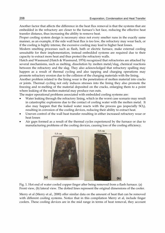
Evaporation, Condensation and Heat Transfer
208
Another factor that affects the difference in the heat flux removal is that the systems that are embedded in the refractory are closer to the furnace’s hot face, reducing the effective heat transfer distance, thus increasing the ability to remove heat. Proper cooling system design is necessary since not every smelter runs in the exactly same manner, as an example, if the side wall heat flux is too low, the refractory may wear back, or if the cooling is highly intense, the excessive cooling may lead to higher heat losses. Modern smelting processes such as flash, bath or electric furnace, make external cooling unsuitable for their implementation, instead embedded systems are required due to their capacity to extract more heat and thus protect the refractory walls. Hatch and Wasmund (Hatch & Wasmund, 1974) recognized that refractories are attacked by several mechanisms, such as melting, dissolution by molten metal/slag, chemical reactions between the refractory and the slag. They also acknowledged that refractory spalling may happen as a result of thermal cycling and also tapping and charging operations may promote refractory erosion due to the collision of the charging materials with the lining. Another problem related to the lining wear is the penetration of molten material into cracks or joints. Thermal cycling not only induces stresses into the lining they also promote the freezing and re-melting of the material deposited on the cracks, enlarging them to a point where leaking of the molten material may produce run outs. The major operational problems associated with embedded cooling systems are: • Water leaking through the refractory lining, which in the worst case scenario may result
in catastrophic explosions due to the contact of cooling water with the molten metal. It also may happen that the leaked water reacts with the process gas (especially SO2), resulting in corrosion of the cooling devices, reducing their ability to extract heat.
• Uneven control of the wall heat transfer resulting in either increased refractory wear or heat losses
• Air gaps formed as a result of the thermal cycles experienced by the furnace or due to manufacturing problems of the cooling devices, causing loss of the cooling efficiency.
(a) (b) Fig. 1. Hot end of water cooled copper finger after being removed from a flash furnace. (a) Front view, (b) lateral view. The dotted lines represent the original dimensions of the cooler.
Merry et al (Merry et al., 2000) offer similar data on the amount of heat that can be removed with different cooling systems. Notice that in this compilation Merry et al, include finger coolers. These cooling devices are in the mid range in terms of heat removal, they account
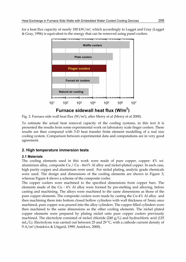
Heat Exchange in Furnace Side Walls with Embedded Water Cooled Cooling Devices
209
for a heat flux capacity of nearly 100 kW/m2, which accordingly to Legget and Gray (Legget & Gray, 1996) is equivalent to the energy that can be removed using panel coolers.
Furnace sidewall heat flux (W/m2)101 102 103 104 105 106 107
Natural air cooling
Forced air coolers
Finger coolers
Plate coolers
Waffle coolers
Fig. 2. Furnace side wall heat flux (W/m2), after Merry et al (Merry et al 2000).
To estimate the actual heat removal capacity of the cooling systems, in this text it is presented the results from some experimental work on laboratory scale finger coolers. These results are then compared with 3-D heat transfer finite element modelling of a real size cooling system. Comparison between experimental data and computations are in very good agreement.
2. High temperature immersion tests 2.1 Materials The cooling elements used in this work were made of pure copper, copper- 4% wt. aluminium alloy, composite Cu / Cu - 4wt% Al alloy and nickel-plated copper. In each case, high purity copper and aluminium were used. For nickel plating, analytic grade chemicals were used. The design and dimensions of the cooling elements are shown in Figure 3; whereas Figure 4 shows a scheme of the composite cooler. The copper coolers were machined to the specified dimensions from copper bars. The elements made of the Cu - 4% Al alloy were formed by pre-melting and alloying, before casting and machining. The alloys were machined to the same dimensions as those of the pure copper elements. The composite coolers were made by casting the Cu-4% Al alloy and then machining them into bottom closed hollow cylinders with wall thickness of 3mm; once machined, pure copper was poured into the alloy cylinders. The copper filled cylinders were then machined to the same dimensions as the other cooling elements. The nickel plated copper elements were prepared by plating nickel onto pure copper coolers previously machined. The electrolyte consisted of nickel chloride (240 g/L) and hydrochloric acid (125 mL/L). Electrolysis was carried out between 25 and 29 ºC, with a cathode current density of 9 A/m2 (Aniekwe & Utigard, 1999; Aniekwe, 2000).
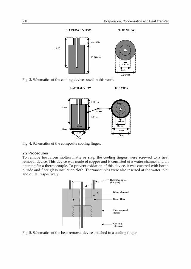
Evaporation, Condensation and Heat Transfer
210
Fig. 3. Schematics of the cooling devices used in this work.
Fig. 4. Schematics of the composite cooling finger.
2.2 Procedures To remove heat from molten matte or slag, the cooling fingers were screwed to a heat removal device. This device was made of copper and it consisted of a water channel and an opening for a thermocouple. To prevent oxidation of this device, it was covered with boron nitride and fibre glass insulation cloth. Thermocouples were also inserted at the water inlet and outlet respectively.
Thermocouples (k - type)
Cooling element
Water flow
Heat removal device
Water channel
Fig. 5. Schematics of the heat removal device attached to a cooling finger
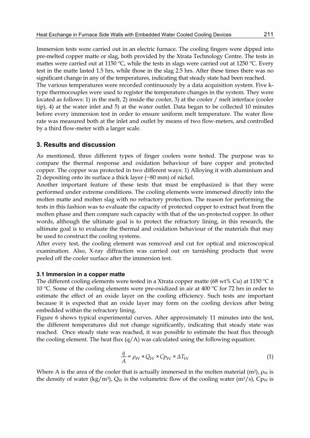
Heat Exchange in Furnace Side Walls with Embedded Water Cooled Cooling Devices
211
Immersion tests were carried out in an electric furnace. The cooling fingers were dipped into pre-melted copper matte or slag, both provided by the Xtrata Technology Centre. The tests in mattes were carried out at 1150 ºC, while the tests in slags were carried out at 1250 ºC. Every test in the matte lasted 1.5 hrs, while those in the slag 2.5 hrs. After these times there was no significant change in any of the temperatures, indicating that steady state had been reached. The various temperatures were recorded continuously by a data acquisition system. Five k-type thermocouples were used to register the temperature changes in the system. They were located as follows: 1) in the melt, 2) inside the cooler, 3) at the cooler / melt interface (cooler tip), 4) at the water inlet and 5) at the water outlet. Data began to be collected 10 minutes before every immersion test in order to ensure uniform melt temperature. The water flow rate was measured both at the inlet and outlet by means of two flow-meters, and controlled by a third flow-meter with a larger scale.
3. Results and discussion As mentioned, three different types of finger coolers were tested. The purpose was to compare the thermal response and oxidation behaviour of bare copper and protected copper. The copper was protected in two different ways: 1) Alloying it with aluminium and 2) depositing onto its surface a thick layer (~80 mm) of nickel. Another important feature of these tests that must be emphasized is that they were performed under extreme conditions. The cooling elements were immersed directly into the molten matte and molten slag with no refractory protection. The reason for performing the tests in this fashion was to evaluate the capacity of protected copper to extract heat from the molten phase and then compare such capacity with that of the un-protected copper. In other words, although the ultimate goal is to protect the refractory lining, in this research, the ultimate goal is to evaluate the thermal and oxidation behaviour of the materials that may be used to construct the cooling systems. After every test, the cooling element was removed and cut for optical and microscopical examination. Also, X-ray diffraction was carried out on tarnishing products that were peeled off the cooler surface after the immersion test.
3.1 Immersion in a copper matte The different cooling elements were tested in a Xtrata copper matte (68 wt% Cu) at 1150 ºC ± 10 ºC. Some of the cooling elements were pre-oxidized in air at 400 ºC for 72 hrs in order to estimate the effect of an oxide layer on the cooling efficiency. Such tests are important because it is expected that an oxide layer may form on the cooling devices after being embedded within the refractory lining. Figure 6 shows typical experimental curves. After approximately 11 minutes into the test, the different temperatures did not change significantly, indicating that steady state was reached. Once steady state was reached, it was possible to estimate the heat flux through the cooling element. The heat flux (q/A) was calculated using the following equation:
W W W Wq = ρ ×Q ×Cp ×ΔTA
(1)
Where A is the area of the cooler that is actually immersed in the molten material (m2), ρW is the density of water (kg/m3), QW is the volumetric flow of the cooling water (m3/s), CpW is
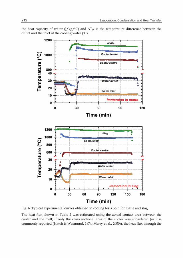
Evaporation, Condensation and Heat Transfer
212
the heat capacity of water (J/kg/ºC) and ΔTW is the temperature difference between the outlet and the inlet of the cooling water (ºC).
Fig. 6. Typical experimental curves obtained in cooling tests both for matte and slag.
The heat flux shown in Table 2 was estimated using the actual contact area between the cooler and the melt; if only the cross sectional area of the cooler was considered (as it is commonly reported (Hatch & Wasmund, 1974; Merry et al., 2000)), the heat flux through the
Time (min)0 30 60 90 120 150 180
Tem
pera
ture
(°C
)
0
10
20
30
600
800
1000
1200Slag
Cooler/slag
Cooler centre
Water outlet
Water inlet
Immersion in slag
Time (min)0 30 60 90 120
Tem
pera
ture
(°C
)
0
10
20
30
40800
1000
1200
Immersion in matte
Matte
Cooler/matte
Cooler centre
Water outlet
Water inlet
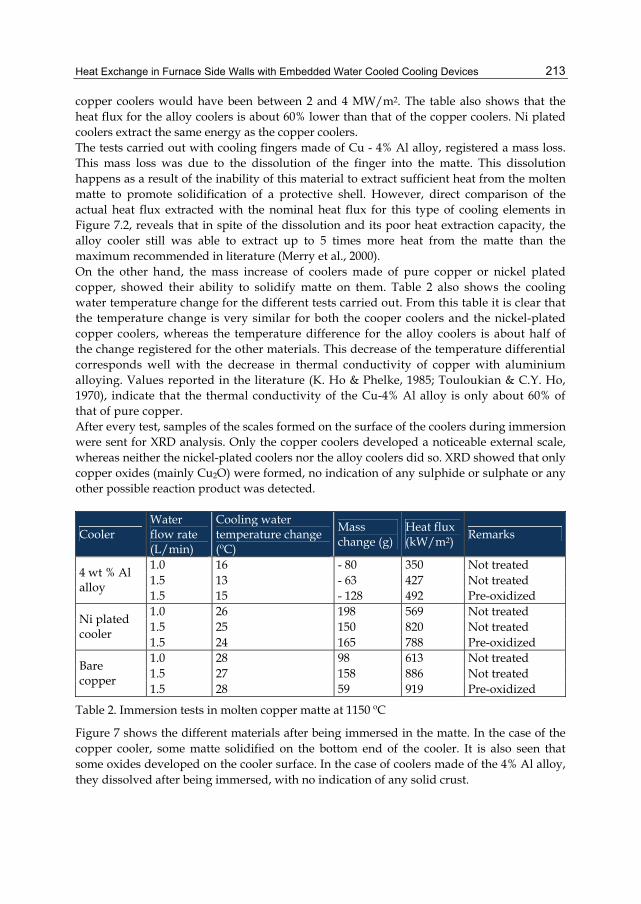
Heat Exchange in Furnace Side Walls with Embedded Water Cooled Cooling Devices
213
copper coolers would have been between 2 and 4 MW/m2. The table also shows that the heat flux for the alloy coolers is about 60% lower than that of the copper coolers. Ni plated coolers extract the same energy as the copper coolers. The tests carried out with cooling fingers made of Cu - 4% Al alloy, registered a mass loss. This mass loss was due to the dissolution of the finger into the matte. This dissolution happens as a result of the inability of this material to extract sufficient heat from the molten matte to promote solidification of a protective shell. However, direct comparison of the actual heat flux extracted with the nominal heat flux for this type of cooling elements in Figure 7.2, reveals that in spite of the dissolution and its poor heat extraction capacity, the alloy cooler still was able to extract up to 5 times more heat from the matte than the maximum recommended in literature (Merry et al., 2000). On the other hand, the mass increase of coolers made of pure copper or nickel plated copper, showed their ability to solidify matte on them. Table 2 also shows the cooling water temperature change for the different tests carried out. From this table it is clear that the temperature change is very similar for both the cooper coolers and the nickel-plated copper coolers, whereas the temperature difference for the alloy coolers is about half of the change registered for the other materials. This decrease of the temperature differential corresponds well with the decrease in thermal conductivity of copper with aluminium alloying. Values reported in the literature (K. Ho & Phelke, 1985; Touloukian & C.Y. Ho, 1970), indicate that the thermal conductivity of the Cu-4% Al alloy is only about 60% of that of pure copper. After every test, samples of the scales formed on the surface of the coolers during immersion were sent for XRD analysis. Only the copper coolers developed a noticeable external scale, whereas neither the nickel-plated coolers nor the alloy coolers did so. XRD showed that only copper oxides (mainly Cu2O) were formed, no indication of any sulphide or sulphate or any other possible reaction product was detected.
Cooler Water flow rate (L/min)
Cooling water temperature change (ºC)
Mass change (g)
Heat flux (kW/m2) Remarks
1.0 16 - 80 350 Not treated 1.5 13 - 63 427 Not treated 4 wt % Al
alloy 1.5 15 - 128 492 Pre-oxidized 1.0 26 198 569 Not treated 1.5 25 150 820 Not treated Ni plated
cooler 1.5 24 165 788 Pre-oxidized 1.0 28 98 613 Not treated 1.5 27 158 886 Not treated Bare
copper 1.5 28 59 919 Pre-oxidized
Table 2. Immersion tests in molten copper matte at 1150 ºC
Figure 7 shows the different materials after being immersed in the matte. In the case of the copper cooler, some matte solidified on the bottom end of the cooler. It is also seen that some oxides developed on the cooler surface. In the case of coolers made of the 4% Al alloy, they dissolved after being immersed, with no indication of any solid crust.
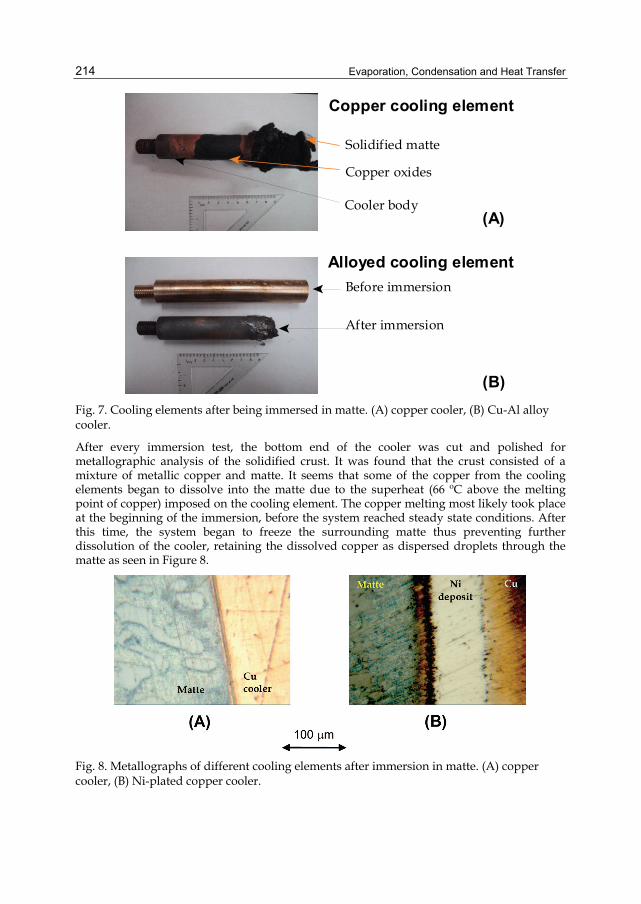
Evaporation, Condensation and Heat Transfer
214
Alloyed cooling element
Copper cooling element
Solidified matte
Cooler body
Copper oxides
(A)
(B)
After immersion
Before immersion
Fig. 7. Cooling elements after being immersed in matte. (A) copper cooler, (B) Cu-Al alloy cooler.
After every immersion test, the bottom end of the cooler was cut and polished for metallographic analysis of the solidified crust. It was found that the crust consisted of a mixture of metallic copper and matte. It seems that some of the copper from the cooling elements began to dissolve into the matte due to the superheat (66 ºC above the melting point of copper) imposed on the cooling element. The copper melting most likely took place at the beginning of the immersion, before the system reached steady state conditions. After this time, the system began to freeze the surrounding matte thus preventing further dissolution of the cooler, retaining the dissolved copper as dispersed droplets through the matte as seen in Figure 8.
Fig. 8. Metallographs of different cooling elements after immersion in matte. (A) copper cooler, (B) Ni-plated copper cooler.
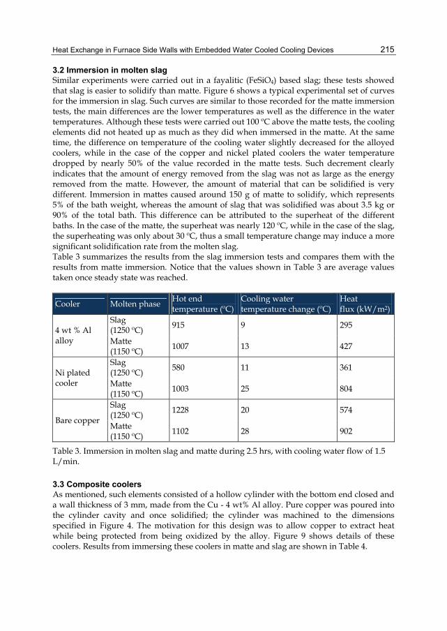
Heat Exchange in Furnace Side Walls with Embedded Water Cooled Cooling Devices
215
3.2 Immersion in molten slag Similar experiments were carried out in a fayalitic (FeSiO4) based slag; these tests showed that slag is easier to solidify than matte. Figure 6 shows a typical experimental set of curves for the immersion in slag. Such curves are similar to those recorded for the matte immersion tests, the main differences are the lower temperatures as well as the difference in the water temperatures. Although these tests were carried out 100 ºC above the matte tests, the cooling elements did not heated up as much as they did when immersed in the matte. At the same time, the difference on temperature of the cooling water slightly decreased for the alloyed coolers, while in the case of the copper and nickel plated coolers the water temperature dropped by nearly 50% of the value recorded in the matte tests. Such decrement clearly indicates that the amount of energy removed from the slag was not as large as the energy removed from the matte. However, the amount of material that can be solidified is very different. Immersion in mattes caused around 150 g of matte to solidify, which represents 5% of the bath weight, whereas the amount of slag that was solidified was about 3.5 kg or 90% of the total bath. This difference can be attributed to the superheat of the different baths. In the case of the matte, the superheat was nearly 120 ºC, while in the case of the slag, the superheating was only about 30 ºC, thus a small temperature change may induce a more significant solidification rate from the molten slag. Table 3 summarizes the results from the slag immersion tests and compares them with the results from matte immersion. Notice that the values shown in Table 3 are average values taken once steady state was reached.
Cooler Molten phase Hot end temperature (ºC)
Cooling water temperature change (ºC)
Heat flux (kW/m2)
Slag (1250 ºC) 915 9 295 4 wt % Al
alloy Matte (1150 ºC) 1007 13 427
Slag (1250 ºC) 580 11 361 Ni plated
cooler Matte (1150 ºC) 1003 25 804
Slag (1250 ºC) 1228 20 574
Bare copper Matte (1150 ºC) 1102 28 902
Table 3. Immersion in molten slag and matte during 2.5 hrs, with cooling water flow of 1.5 L/min.
3.3 Composite coolers As mentioned, such elements consisted of a hollow cylinder with the bottom end closed and a wall thickness of 3 mm, made from the Cu - 4 wt% Al alloy. Pure copper was poured into the cylinder cavity and once solidified; the cylinder was machined to the dimensions specified in Figure 4. The motivation for this design was to allow copper to extract heat while being protected from being oxidized by the alloy. Figure 9 shows details of these coolers. Results from immersing these coolers in matte and slag are shown in Table 4.
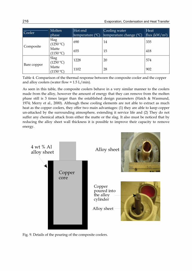
Evaporation, Condensation and Heat Transfer
216
Cooler Molten phase
Hot end temperature (ºC)
Cooling water temperature change (ºC)
Heat flux (kW/m2)
Slag (1250 ºC) 690 14 335
Composite Matte (1150 ºC) 655 15 418
Slag (1250 ºC) 1228 20 574
Bare copper Matte (1150 ºC) 1102 28 902
Table 4. Comparison of the thermal response between the composite cooler and the copper and alloy coolers (water flow = 1.5 L/min).
As seen in this table, the composite coolers behave in a very similar manner to the coolers made from the alloy, however the amount of energy that they can remove from the molten phase still is 3 times larger than the established design parameters (Hatch & Wasmund, 1974; Merry et al., 2000). Although these cooling elements are not able to extract as much heat as the copper coolers, they offer two main advantages: (1) they are able to keep copper un-attacked by the surrounding atmosphere, extending it service life and (2) They do not suffer any chemical attack from either the matte or the slag. It also must be noticed that by reducing the alloy sheet wall thickness it is possible to improve their capacity to remove energy.
Coppercore
4 wt % Alalloy sheet Alloy sheet
Copperpoured intothe alloycylinder
Alloy sheet
Fig. 9. Details of the pouring of the composite coolers.
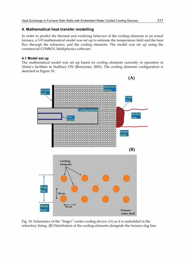
Heat Exchange in Furnace Side Walls with Embedded Water Cooled Cooling Devices
217
4. Mathematical heat transfer modelling In order to predict the thermal and oxidizing behavior of the cooling elements in an actual furnace, a 3-D mathematical model was set up to estimate the temperature field and the heat flux through the refractory and the cooling elements. The model was set up using the commercial COMSOL Multiphysics software.
4.1 Model set up The mathematical model was set up based on cooling elements currently in operation at Xtrata’s facilities in Sudbury ON (Berryman, 2001). The cooling elements configuration is sketched in Figure 10.
Slagline
Coolingelements
50 cm
50 cm
Furnaceouter shell
Mattelevel
Refractorylining
Waterchannel
Cooling element
Solidslag
Moltenslag
Moltenmatte
Furnaceshell
(A)
(B)
Fig. 10. Schematics of the “finger” cooler cooling device: (A) as it is embedded in the refractory lining. (B) Distribution of the cooling elements alongside the furnace slag line.
(A)
(B)
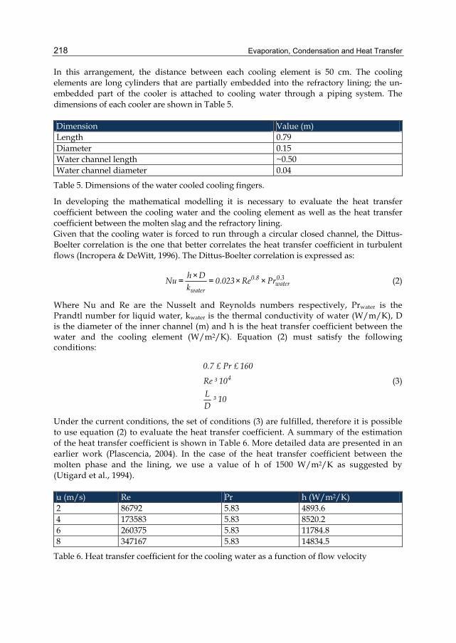
Evaporation, Condensation and Heat Transfer
218
In this arrangement, the distance between each cooling element is 50 cm. The cooling elements are long cylinders that are partially embedded into the refractory lining; the un-embedded part of the cooler is attached to cooling water through a piping system. The dimensions of each cooler are shown in Table 5. Dimension Value (m) Length 0.79 Diameter 0.15 Water channel length ~0.50 Water channel diameter 0.04
Table 5. Dimensions of the water cooled cooling fingers.
In developing the mathematical modelling it is necessary to evaluate the heat transfer coefficient between the cooling water and the cooling element as well as the heat transfer coefficient between the molten slag and the refractory lining. Given that the cooling water is forced to run through a circular closed channel, the Dittus- Boelter correlation is the one that better correlates the heat transfer coefficient in turbulent flows (Incropera & DeWitt, 1996). The Dittus-Boelter correlation is expressed as:
0.8 0.3water
water
h ×DNu = = 0.023× Re × Prk
(2)
Where Nu and Re are the Nusselt and Reynolds numbers respectively, Prwater is the Prandtl number for liquid water, kwater is the thermal conductivity of water (W/m/K), D is the diameter of the inner channel (m) and h is the heat transfer coefficient between the water and the cooling element (W/m2/K). Equation (2) must satisfy the following conditions:
4
0.7 £ Pr £ 160
Re ³ 10L ³ 10D
(3)
Under the current conditions, the set of conditions (3) are fulfilled, therefore it is possible to use equation (2) to evaluate the heat transfer coefficient. A summary of the estimation of the heat transfer coefficient is shown in Table 6. More detailed data are presented in an earlier work (Plascencia, 2004). In the case of the heat transfer coefficient between the molten phase and the lining, we use a value of h of 1500 W/m2/K as suggested by (Utigard et al., 1994). u (m/s) Re Pr h (W/m2/K) 2 86792 5.83 4893.6 4 173583 5.83 8520.2 6 260375 5.83 11784.8 8 347167 5.83 14834.5
Table 6. Heat transfer coefficient for the cooling water as a function of flow velocity
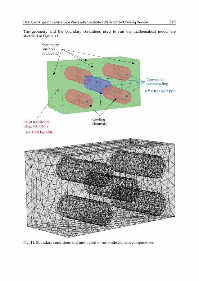
Heat Exchange in Furnace Side Walls with Embedded Water Cooled Cooling Devices
219
The geometry and the boundary conditions used to run the mathematical model are sketched in Figure 11.
Symmetrysurfaces(adiabatic)
Coolingelements
Convectivewater cooling
h 0.023 Re0.8 Pr0.3
Heat transfer @slag/refractory
h = 1500 W/m2/K
Fig. 11. Boundary conditions and mesh used to run finite element computations.
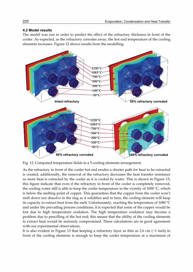
Evaporation, Condensation and Heat Transfer
220
4.2 Model results The model was run in order to predict the effect of the refractory thickness in front of the cooler. As expected, as the refractory corrodes away, the hot end temperature of the cooling elements increases. Figure 12 shows results from the modelling.
1230ºC
700ºC1083ºC
300ºC500ºC
100ºC50ºC
1220ºC
700ºC1083ºC
300ºC500ºC
100ºC50ºC
Intact refractory
90% refractory corroded 100% refractory corroded
50% refractory corroded
Fig. 12. Computed temperature fields in a 5 cooling elements arrangement.
As the refractory in front of the cooler hot end erodes a shorter path for heat to be extracted is created, additionally, the removal of the refractory decreases the heat transfer resistance so more heat is extracted by the cooler as it is cooled by water. This is shown in Figure 13; this figure indicate that even if the refractory in front of the cooler is completely removed, the cooling water still is able to keep the cooler temperature in the vicinity of 1000 ºC, which is below the melting point of copper. This guarantees that the copper from the cooler won’t melt down nor dissolve in the slag as it solidifies and in turn, the cooling element will keep its capacity to extract heat from the melt. Unfortunately, reaching the temperature of 1000 ºC and under the prevailing process conditions, it is expected that some of the copper would be lost due to high temperature oxidation. The high temperature oxidation may become a problem due to pencilling of the hot end; this means that the ability of the cooling elements to extract heat would be seriously compromised. These calculations are in good agreement with our experimental observations. It is also evident in Figure 13 that keeping a refractory layer as thin as 2.6 cm (~1 inch) in front of the cooling elements is enough to keep the cooler temperature at a maximum of
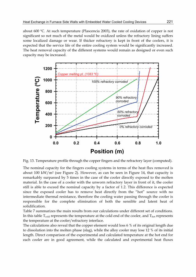
Heat Exchange in Furnace Side Walls with Embedded Water Cooled Cooling Devices
221
about 600 ºC. At such temperature (Plascencia 2003), the rate of oxidation of copper is not significant so not much of the metal would be oxidized unless the refractory lining suffers some localized damage or wear. If thicker refractory is kept in front of the coolers, it is expected that the service life of the entire cooling system would be significantly increased. The heat removal capacity of the different systems would remain as designed or even such capacity may be increased.
Position (m)0.0 0.2 0.4 0.6 0.8 1.0
Tem
pera
ture
(ºC
)
0
200
400
600
800
1000
1200
0% refractory corroded
50% refractory corroded
90% refractorycorroded
100% refractory corroded
Copper melting pt. (1083 ºC)
Fig. 13. Temperature profile through the copper fingers and the refractory layer (computed).
The nominal capacity for the fingers cooling systems in terms of the heat flux removed is about 100 kW/m2 (see Figure 2). However, as can be seen in Figure 14, that capacity is remarkably surpassed by 5 times in the case of the cooler directly exposed to the molten material. In the case of a cooler with the unworn refractory layer in front of it, the cooler still is able to exceed the nominal capacity by a factor of 1.2. This difference is expected since the exposed cooler has to remove heat directly from the “hot” source with no intermediate thermal resistance, therefore the cooling water passing through the cooler is responsible for the complete elimination of both the sensible and latent heat of solidification. Table 7 summarizes the main results from our calculations under different set of conditions. In this table Tcold represents the temperature at the cold end of the cooler, and Thot represents the temperature at the cooler/refractory interface. The calculations also reveal that the copper element would loss 6 % of its original length due to dissolution into the molten phase (slag), while the alloy cooler may lose 12 % of its initial length. Direct comparison of the experimental and calculated temperature at the hot end for each cooler are in good agreement, while the calculated and experimental heat fluxes
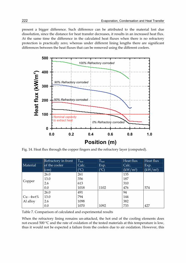
Evaporation, Condensation and Heat Transfer
222
present a bigger difference. Such difference can be attributed to the material lost due dissolution, since the distance for heat transfer decreases, it results in an increased heat flux. At the same time the difference in the calculated heat fluxes when there is no refractory protection is practically zero; whereas under different lining lengths there are significant differences between the heat fluxes that can be removed using the different coolers.
Position (m)0.0 0.2 0.4 0.6 0.8 1.0
Hea
t flu
x (k
W/m
2 )
0
100
200
300
400
500
0% Refractory corroded
90% Refractory corroded
100% Refractory corroded
50% Refractory corroded
Nominal capacityto extract heat
Fig. 14. Heat flux through the copper fingers and the refractory layer (computed).
Material Refractory in front of the cooler (cm)
Thot Calc. (ºC)
Thot Exp. (ºC)
Heat flux
Calc. (kW/m2)
Heat flux Exp. (kW/m2)
Copper
26.0 13.0 2.6 0.0
261 356 613 1018
1102
135 187 310 476
574
Cu - 4wt% Al alloy
26.0 13.0 2.6 0.0
491 794 1098 1070
1092
94 144 382 733
427
Table 7. Comparison of calculated and experimental results
When the refractory lining remains un-attacked, the hot end of the cooling elements does not exceed 500 ºC and the rate of oxidation of the tested materials at this temperature is low, thus it would not be expected a failure from the coolers due to air oxidation. However, this
Heat Exchange in Furnace Side Walls with Embedded Water Cooled Cooling Devices
223
situation is not likely. Since the slags used in copper making have a liquidus temperature around 1150 ºC and the actual slag operating temperature varies between 1250 and 1300 ºC, a superheat of 150 ºC is required to start the solidification of the slag. When we back calculate the superheat from the model results, we found that having the full refractory in front of the cooler would not allow to freeze the slag (superheat = 78 ºC) onto the lining surface, indeed the refractory is likely to be eroded. Even after losing 50 % of its original length (superheat = 119 ºC), no solid crust would be formed. In order to start the solidification of a protective slag shell, the lining would need to lose around 65 % of its initial length. In such case, the temperature at the hot end of the cooler would be in the vicinity of 700 ºC; therefore oxidation of copper may affect the performance of the cooling system. It also should be noticed that within the furnace, the actual temperature of the slag decreases towards the side walls. This will lead to decreased localized superheats, increased viscosity and decreased fluid flow. All these effects will tend to decrease the heat flux through the side walls, resulting in temperatures of the hot end of the cooler below those calculated above.
5. Summary It has been tested different copper based materials as a medium to extract heat from hot furnaces. The effect of high temperature oxidation on the overall performance of the cooling element was also studied. Immersion tests revealed that Cu - Al alloys do not oxidize. However, they are not able to extract heat as effectively as pure copper or nickel-plated copper, resulting in partial melting of the cooling element. These tests also showed that it is easier to solidify slag rather than matte. Numerical calculations may lead to the conclusion that unless the refractory lining is severely damaged, it is unlikely that oxidation of cooling elements would be responsible for the failure of the cooling system. However, the heat flux calculated in un-attacked linings imposes superheats on the slag below that required for freezing a protective shell of slag. Furthermore, in order to start the solidification of the slag onto the lining, for typical slag conditions it is required that the lining reduces its original length by at least 60 %, which may result in the oxidation of coolers made from copper.
6. References Aniekwe U V and Utigard T A. 1999, High-temperature oxidation of nickel-plated copper vs pure copper, Canadian Metallurgical Quarterly, 38, 4, pp. 277- 281. Aniekwe U V. 2000, Protection of Copper Coolers, M.A.Sc. Dissertation, University of Toronto, Toronto, ON, Canada. Berryman R. 2001, Private communication, May 2001 Hatch G G, Wasmund B O. 1974, U.S.
patent # 3,849,587, Nov. 19, 1974. Ho K and Phelke R D. 1985, Metal-Mold interfacial heat transfer, Metallurgical Transactions B, 16B, 3, pp. 585 - 594 Incropera F P and DeWitt D P, Fundamentals of Heat and Mass Transfer 4th Edition, John Wiley & sons., New York, U.S.A., 1996. Legget A.R., Gray N.B. (1996), Development and application of a novel refractory cooling
system. Proceedings of Advances in Refractories for the Metallurgical Industries II, Montréal, QC, Canada, August 1996.

Evaporation, Condensation and Heat Transfer
224
Merry J., Sarvinis J., Voermann N.(2000), Designing modern furnace cooling systems, JOM, 52, 2, pp. 62 - 64. Plascencia G, Utigard T A. 2003, Oxidation of copper at different temperatures. Proceedings of the Yazawa International Symposium, San Diego, Cal, USA, February 2003. Plascencia G. 2004, High Temperature Oxidation of copper and copper aluminium alloys – Impact on furnace sidewall cooling systems-, Ph. D. Dissertation, University of
Toronto, 2004 Touloukian Y S and Ho C Y Eds., Thermophysical Properties of Matter, Vol 1, Thermal
Conductivity of Metals and Alloys, Plenum press. New York, U.S.A., 1970. Utigard T A, Warczok A and Descalaux P. 1994, The measurement of the heat-transfer coefficient between high-temperature liquids and solid surfaces, Metallurgical
Transactions B, 25B, 1, pp. 43 - 51.

Part 3
Heat Transfer and Exchanger

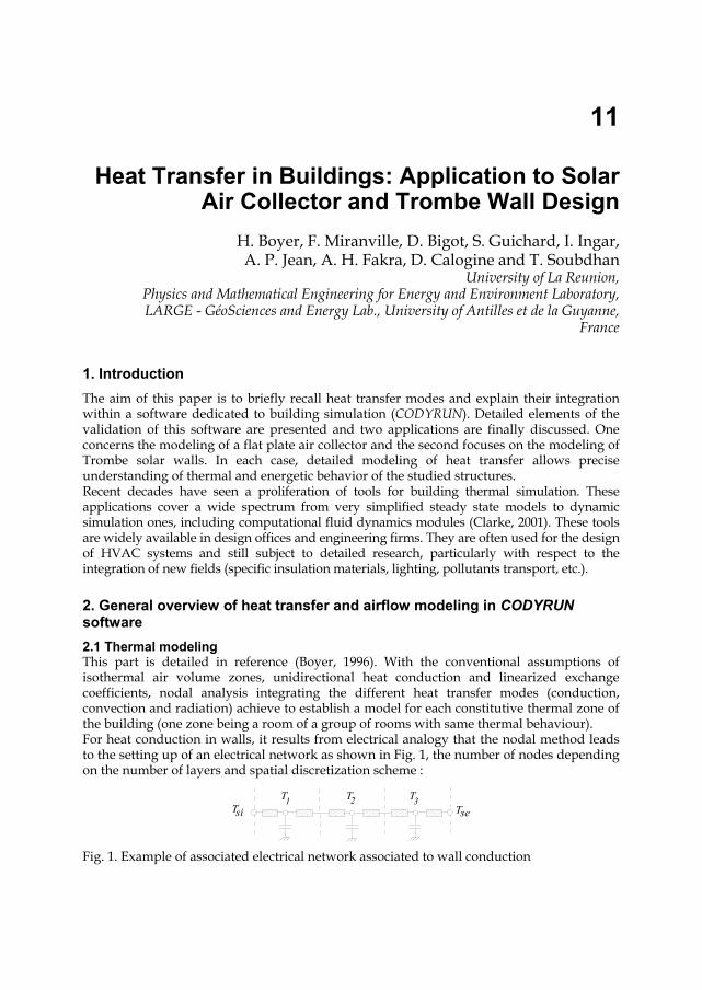
11
Heat Transfer in Buildings: Application to Solar Air Collector and Trombe Wall Design
H. Boyer, F. Miranville, D. Bigot, S. Guichard, I. Ingar, A. P. Jean, A. H. Fakra, D. Calogine and T. Soubdhan
University of La Reunion, Physics and Mathematical Engineering for Energy and Environment Laboratory, LARGE - GéoSciences and Energy Lab., University of Antilles et de la Guyanne,
France
1. Introduction The aim of this paper is to briefly recall heat transfer modes and explain their integration within a software dedicated to building simulation (CODYRUN). Detailed elements of the validation of this software are presented and two applications are finally discussed. One concerns the modeling of a flat plate air collector and the second focuses on the modeling of Trombe solar walls. In each case, detailed modeling of heat transfer allows precise understanding of thermal and energetic behavior of the studied structures. Recent decades have seen a proliferation of tools for building thermal simulation. These applications cover a wide spectrum from very simplified steady state models to dynamic simulation ones, including computational fluid dynamics modules (Clarke, 2001). These tools are widely available in design offices and engineering firms. They are often used for the design of HVAC systems and still subject to detailed research, particularly with respect to the integration of new fields (specific insulation materials, lighting, pollutants transport, etc.).
2. General overview of heat transfer and airflow modeling in CODYRUN software 2.1 Thermal modeling This part is detailed in reference (Boyer, 1996). With the conventional assumptions of isothermal air volume zones, unidirectional heat conduction and linearized exchange coefficients, nodal analysis integrating the different heat transfer modes (conduction, convection and radiation) achieve to establish a model for each constitutive thermal zone of the building (one zone being a room of a group of rooms with same thermal behaviour). For heat conduction in walls, it results from electrical analogy that the nodal method leads to the setting up of an electrical network as shown in Fig. 1, the number of nodes depending on the number of layers and spatial discretization scheme :
T TT T T
si se1 2 3
Fig. 1. Example of associated electrical network associated to wall conduction
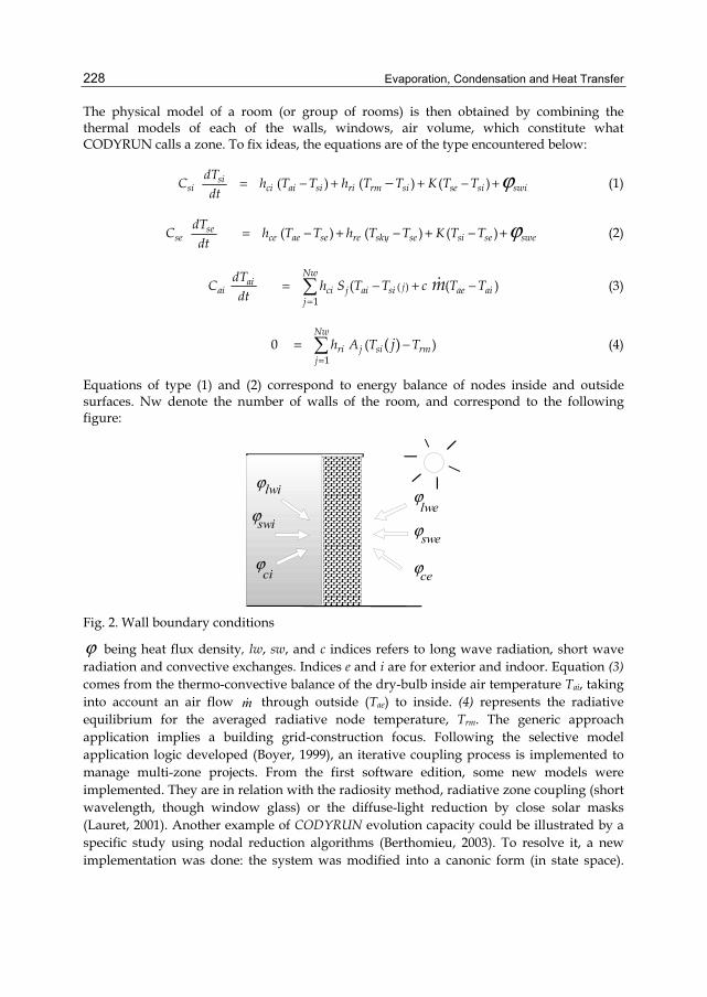
Evaporation, Condensation and Heat Transfer
228
The physical model of a room (or group of rooms) is then obtained by combining the thermal models of each of the walls, windows, air volume, which constitute what CODYRUN calls a zone. To fix ideas, the equations are of the type encountered below:
( ) ( ) ( )sisi ci ai si ri rm si se si swi
dTC h T T h T T K T Tdt
ϕ= − + + − +− (1)
( ) ( ) ( )sese ce ae se re sky se si se swe
dTC h T T h T T K T Tdt
ϕ= − + − + − + (2)
( )1
( ( )Nw
ai jai ci j ai si ae aij
dTC h S T T c T Tdt
m=
= − + −∑ (3)
1
0 ( )( )Nw
ri j si rmj
h A T Tj=
= −∑ (4)
Equations of type (1) and (2) correspond to energy balance of nodes inside and outside surfaces. Nw denote the number of walls of the room, and correspond to the following figure:
ϕ
ϕ
ϕ
ϕ
ϕ
ϕ
lwe
swe
ce
lwi
swi
ci
Fig. 2. Wall boundary conditions
ϕ being heat flux density, lw, sw, and c indices refers to long wave radiation, short wave radiation and convective exchanges. Indices e and i are for exterior and indoor. Equation (3) comes from the thermo-convective balance of the dry-bulb inside air temperature Tai, taking into account an air flow m through outside (Tae) to inside. (4) represents the radiative equilibrium for the averaged radiative node temperature, Trm. The generic approach application implies a building grid-construction focus. Following the selective model application logic developed (Boyer, 1999), an iterative coupling process is implemented to manage multi-zone projects. From the first software edition, some new models were implemented. They are in relation with the radiosity method, radiative zone coupling (short wavelength, though window glass) or the diffuse-light reduction by close solar masks (Lauret, 2001). Another example of CODYRUN evolution capacity could be illustrated by a specific study using nodal reduction algorithms (Berthomieu, 2003). To resolve it, a new implementation was done: the system was modified into a canonic form (in state space).
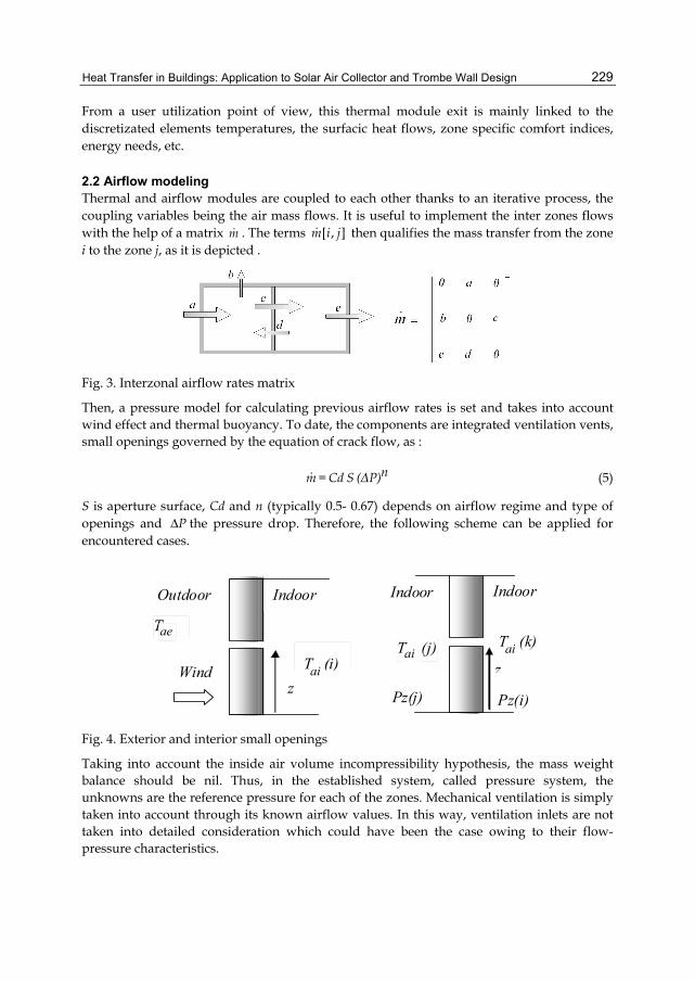
Heat Transfer in Buildings: Application to Solar Air Collector and Trombe Wall Design
229
From a user utilization point of view, this thermal module exit is mainly linked to the discretizated elements temperatures, the surfacic heat flows, zone specific comfort indices, energy needs, etc.
2.2 Airflow modeling Thermal and airflow modules are coupled to each other thanks to an iterative process, the coupling variables being the air mass flows. It is useful to implement the inter zones flows with the help of a matrix m . The terms [ , ]m i j then qualifies the mass transfer from the zone i to the zone j, as it is depicted .
Fig. 3. Interzonal airflow rates matrix
Then, a pressure model for calculating previous airflow rates is set and takes into account wind effect and thermal buoyancy. To date, the components are integrated ventilation vents, small openings governed by the equation of crack flow, as :
nm = Cd S (ΔP) (5)
S is aperture surface, Cd and n (typically 0.5- 0.67) depends on airflow regime and type of openings and PΔ the pressure drop. Therefore, the following scheme can be applied for encountered cases.
Outdoor Indoor Indoor
Wind z
z
Pz(j) Pz(i)
T ae
T (i)T (j)
aiai
T (k) ai
Indoor
Fig. 4. Exterior and interior small openings
Taking into account the inside air volume incompressibility hypothesis, the mass weight balance should be nil. Thus, in the established system, called pressure system, the unknowns are the reference pressure for each of the zones. Mechanical ventilation is simply taken into account through its known airflow values. In this way, ventilation inlets are not taken into detailed consideration which could have been the case owing to their flow-pressure characteristics.
Evaporation, Condensation and Heat Transfer
230
=
= ≠
=
= ≠
= −
=
⎧+ =⎪
⎪⎪⎪
+ =⎪⎪⎨⎪⎪⎪⎪⎪ + =⎪⎩
∑
∑
∑
i N
i 0,i 1
i N
i 0,i 2
i N 1
i 0
m( m ( 1 ) 0
m( m ( 2 ) 0
...
m( m ( N ) 0
vmc
vmc
vmc
i,1)
i,2)
i,N)
(6)
km ( )vmc is the flow extracted from zone k (by vents) and N the total number of zones. After the setting up of this non linear system, its resolution is performed using a variant of the Newton-Raphson (under relaxed method). This airflow model has recently been supplemented by a CO2 propagation model in buildings (Calogine, 2010).
2.3 Humidity transfers For decoupling reasons, zones dry temperatures, as well as inter zone airflows, have been previously calculated. At this calculation step, for a given building, each zone's specific humidity evolution depends on the matricial equation :
= +. .h h hC r A r B (7)
According to Duforestel’s model, an improvement of the hydric model (Lucas, 2003) was given by the use of a hygroscopic buffer. If we consider N as the number of zones, a linear system of dimension 2N is obtained and a finite difference scheme is used for numerical solution.
3. Some elements of CODYRUN validation 3.1 Inter model comparison A large number of comparisons on specific cases were conducted with various softwares, whether CODYBA, TRNSYS for thermal part, with AIRNET, BUS, for airflow calculation or even CONTAM, ECOTECT and ESP. To verify the correct numerical implementation of models, we compared the simulation results of our software with those from other computer codes (Soubdhan, 1999). The benchmark for inter-comparison software is the BESTEST procedure (Judkoff, 1983), (Judkoff, 1995). This procedure has been developed within the framework of Annex 21 Task 12 of the Solar Heating and Cooling Program (SHC) by the International Energy Agency (IEA). This tests the software simulation of the thermal behavior of building by simulating various buildings whose complexity grows gradually and comparing the results with other simulation codes (ESP DOE2, SERI-RES, CLIM2000, TRNSYS, ...). The group's collective experience has shown that when a program showed major differences with the so-called reference programs, the underlying reason was a bug or a faulty algorithm.
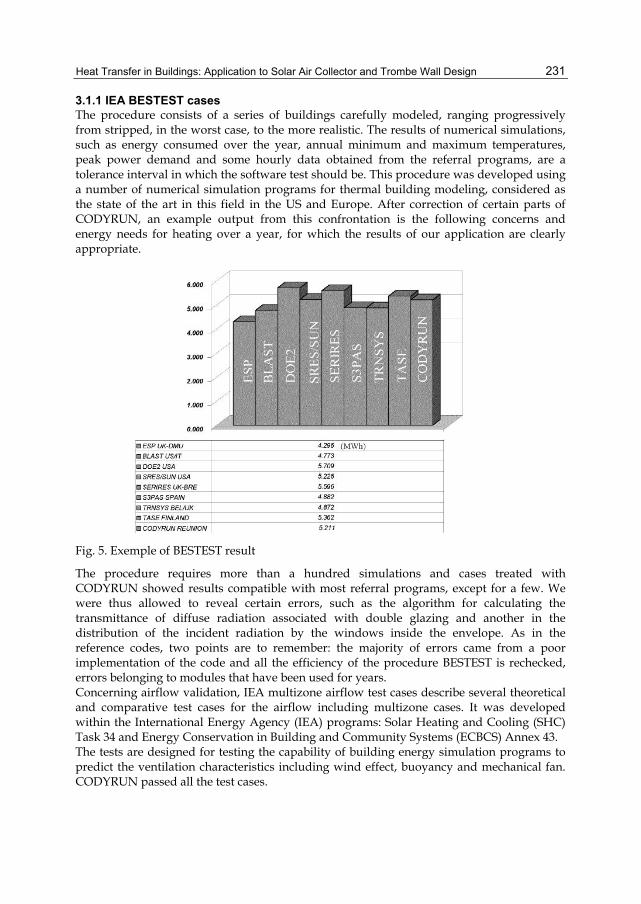
Heat Transfer in Buildings: Application to Solar Air Collector and Trombe Wall Design
231
3.1.1 IEA BESTEST cases The procedure consists of a series of buildings carefully modeled, ranging progressively from stripped, in the worst case, to the more realistic. The results of numerical simulations, such as energy consumed over the year, annual minimum and maximum temperatures, peak power demand and some hourly data obtained from the referral programs, are a tolerance interval in which the software test should be. This procedure was developed using a number of numerical simulation programs for thermal building modeling, considered as the state of the art in this field in the US and Europe. After correction of certain parts of CODYRUN, an example output from this confrontation is the following concerns and energy needs for heating over a year, for which the results of our application are clearly appropriate.
Fig. 5. Exemple of BESTEST result
The procedure requires more than a hundred simulations and cases treated with CODYRUN showed results compatible with most referral programs, except for a few. We were thus allowed to reveal certain errors, such as the algorithm for calculating the transmittance of diffuse radiation associated with double glazing and another in the distribution of the incident radiation by the windows inside the envelope. As in the reference codes, two points are to remember: the majority of errors came from a poor implementation of the code and all the efficiency of the procedure BESTEST is rechecked, errors belonging to modules that have been used for years. Concerning airflow validation, IEA multizone airflow test cases describe several theoretical and comparative test cases for the airflow including multizone cases. It was developed within the International Energy Agency (IEA) programs: Solar Heating and Cooling (SHC) Task 34 and Energy Conservation in Building and Community Systems (ECBCS) Annex 43. The tests are designed for testing the capability of building energy simulation programs to predict the ventilation characteristics including wind effect, buoyancy and mechanical fan. CODYRUN passed all the test cases.
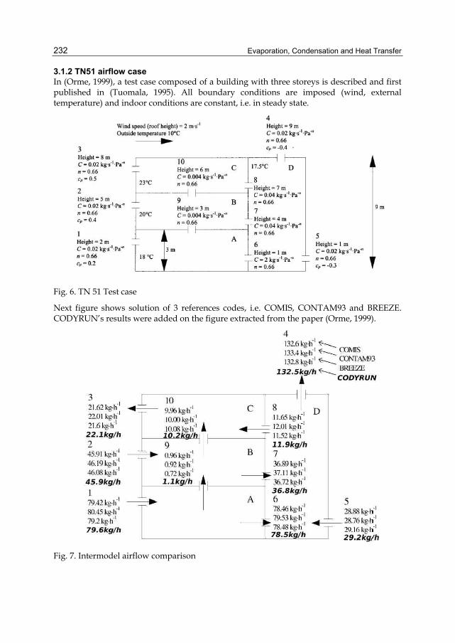
Evaporation, Condensation and Heat Transfer
232
3.1.2 TN51 airflow case In (Orme, 1999), a test case composed of a building with three storeys is described and first published in (Tuomala, 1995). All boundary conditions are imposed (wind, external temperature) and indoor conditions are constant, i.e. in steady state.
Fig. 6. TN 51 Test case
Next figure shows solution of 3 references codes, i.e. COMIS, CONTAM93 and BREEZE. CODYRUN’s results were added on the figure extracted from the paper (Orme, 1999).
Fig. 7. Intermodel airflow comparison
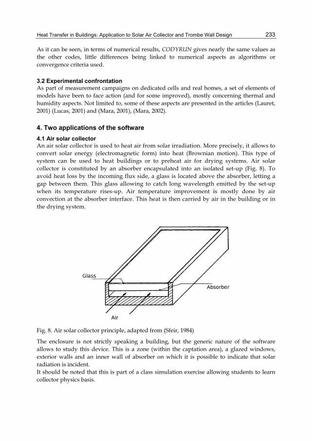
Heat Transfer in Buildings: Application to Solar Air Collector and Trombe Wall Design
233
As it can be seen, in terms of numerical results, CODYRUN gives nearly the same values as the other codes, little differences being linked to numerical aspects as algorithms or convergence criteria used.
3.2 Experimental confrontation As part of measurement campaigns on dedicated cells and real homes, a set of elements of models have been to face action (and for some improved), mostly concerning thermal and humidity aspects. Not limited to, some of these aspects are presented in the articles (Lauret, 2001) (Lucas, 2001) and (Mara, 2001), (Mara, 2002).
4. Two applications of the software 4.1 Air solar collector An air solar collector is used to heat air from solar irradiation. More precisely, it allows to convert solar energy (electromagnetic form) into heat (Brownian motion). This type of system can be used to heat buildings or to preheat air for drying systems. Air solar collector is constituted by an absorber encapsulated into an isolated set-up (Fig. 8). To avoid heat loss by the incoming flux side, a glass is located above the absorber, letting a gap between them. This glass allowing to catch long wavelength emitted by the set-up when its temperature rises-up. Air temperature improvement is mostly done by air convection at the absorber interface. This heat is then carried by air in the building or in the drying system.
Fig. 8. Air solar collector principle, adapted from (Sfeir, 1984)
The enclosure is not strictly speaking a building, but the generic nature of the software allows to study this device. This is a zone (within the captation area), a glazed windows, exterior walls and an inner wall of absorber on which it is possible to indicate that solar radiation is incident. It should be noted that this is part of a class simulation exercise allowing students to learn collector physics basis.
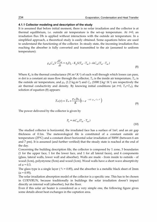
Evaporation, Condensation and Heat Transfer
234
4.1.1 Collector modeling and description of the study It is assumed that before initial moment, there is no solar irradiation and the collector is at thermal equilibrium, i.e. outside air temperature is the set-up temperature. At t=0, an irradiation flux Dh is applied without interactions with the outside air temperature. In a simplified approach, a theoretical study is easily obtained. Some equations below are used to understand the functioning of the collector. In steady state, the incoming irradiation flux reaching the absorber is fully converted and transmitted to the air (assumed to uniform temperature):
ai
as as 0 h p ai ae as ai aedTρ C V = D - K S(T - T ) - mC (T - T )dt
τ (8)
Where Kp is the thermal conductance (W.m-2.K-1) of each wall through which losses can pass, m dot is a constant air mass flow through the collector, Tai is the inside air temperature, Tae is the outside air temperature, and ρas (1.2 kg.m-3) and Cas (1000 J.kg-1.K-1) are respectively the air thermal conductivity and density. By knowing initial conditions (at t=0, Tai=Tae), the solution of equation (8) appears:
( )VCKth
aeaiasaseK
DTtT ρτ /0 1)( −−+= (9)
The power delivered by the collector is given by
u as ai aeP = mC (T - T )
(10)
The studied collector is horizontal, the irradiated face has a surface of 1m², and an air gap thickness of 0.1m. The meteorological file is constituted of a constant outside air temperature (25°C) and a constant direct horizontal solar irradiation of 500W (between 6 am and 7 pm). It is assumed (and further verified) that the steady state is reached at the end of the day. Concerning the building description file, the collector is composed by 1 zone, 3 boundaries (1 for the upper face, 1 for the lower face, and 1 for all lateral faces), and 4 components (glass, lateral walls, lower wall and absorber). Walls are made - from inside to outside - of wood (1cm), polystyrene (5cm) and wood (1cm). Wood walls have a short wave absorptivity of α = 0.3. The glass type is a single layer ( 0τ = 0.85), and the absorber is a metallic black sheet of 2mm (α = 0.95). The solar irradiation absorption model of the collector is a specific one. This has to be chosen in CODYRUN, because traditionally in buildings the solar irradiation doesn’t impact directly an internal wall (absorber), but the floor. Even if this solar air heater is considered as a very simple one, the following figure gives some details about heat exchanges in the captation area.
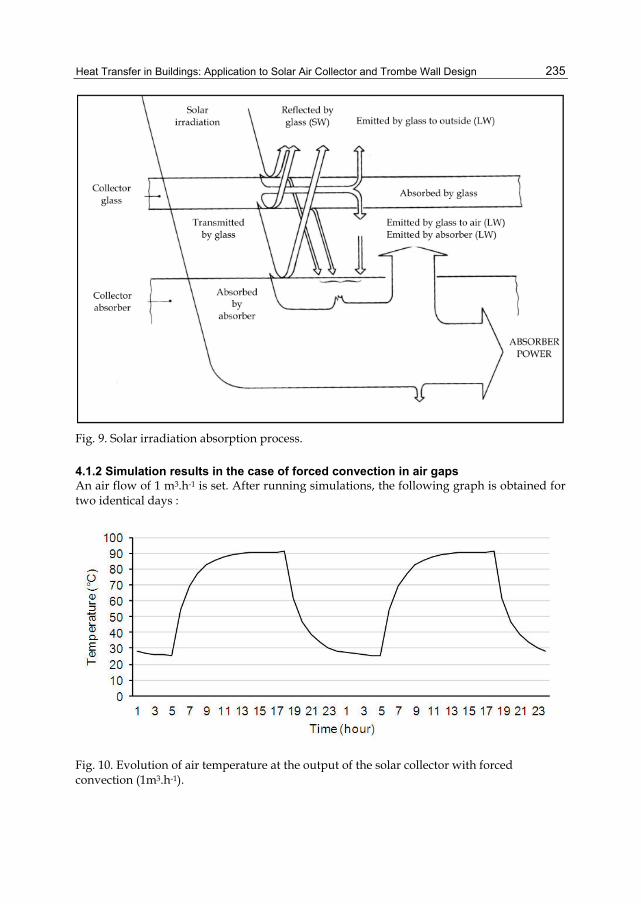
Heat Transfer in Buildings: Application to Solar Air Collector and Trombe Wall Design
235
Fig. 9. Solar irradiation absorption process.
4.1.2 Simulation results in the case of forced convection in air gaps An air flow of 1 m3.h-1 is set. After running simulations, the following graph is obtained for two identical days :
Fig. 10. Evolution of air temperature at the output of the solar collector with forced convection (1m3.h-1).
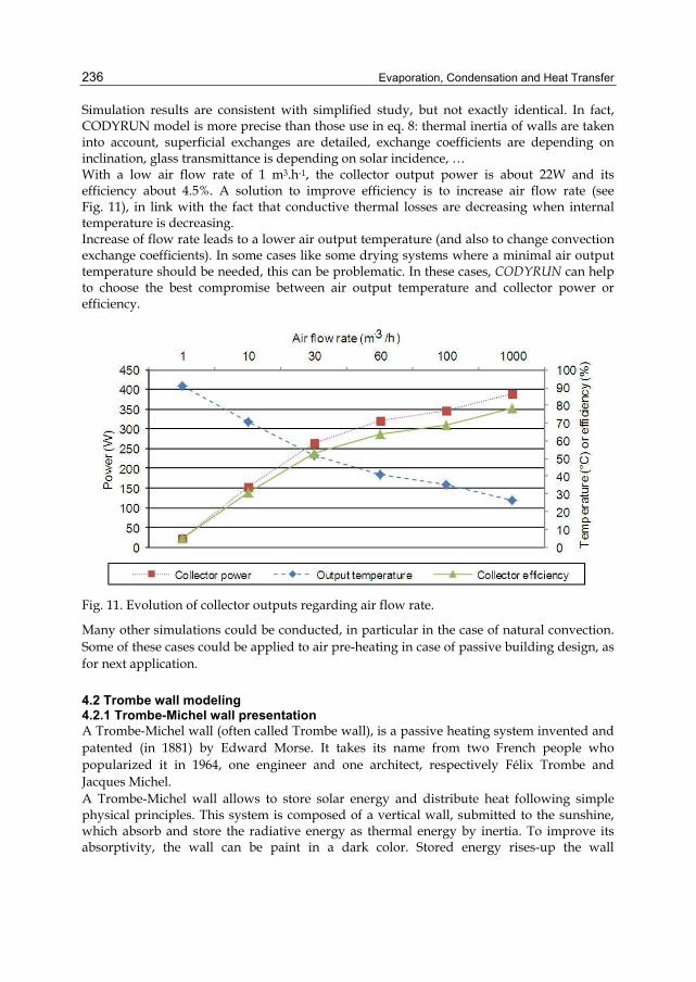
Evaporation, Condensation and Heat Transfer
236
Simulation results are consistent with simplified study, but not exactly identical. In fact, CODYRUN model is more precise than those use in eq. 8: thermal inertia of walls are taken into account, superficial exchanges are detailed, exchange coefficients are depending on inclination, glass transmittance is depending on solar incidence, … With a low air flow rate of 1 m3.h-1, the collector output power is about 22W and its efficiency about 4.5%. A solution to improve efficiency is to increase air flow rate (see Fig. 11), in link with the fact that conductive thermal losses are decreasing when internal temperature is decreasing. Increase of flow rate leads to a lower air output temperature (and also to change convection exchange coefficients). In some cases like some drying systems where a minimal air output temperature should be needed, this can be problematic. In these cases, CODYRUN can help to choose the best compromise between air output temperature and collector power or efficiency.
Fig. 11. Evolution of collector outputs regarding air flow rate.
Many other simulations could be conducted, in particular in the case of natural convection. Some of these cases could be applied to air pre-heating in case of passive building design, as for next application.
4.2 Trombe wall modeling 4.2.1 Trombe-Michel wall presentation A Trombe-Michel wall (often called Trombe wall), is a passive heating system invented and patented (in 1881) by Edward Morse. It takes its name from two French people who popularized it in 1964, one engineer and one architect, respectively Félix Trombe and Jacques Michel. A Trombe-Michel wall allows to store solar energy and distribute heat following simple physical principles. This system is composed of a vertical wall, submitted to the sunshine, which absorb and store the radiative energy as thermal energy by inertia. To improve its absorptivity, the wall can be paint in a dark color. Stored energy rises-up the wall
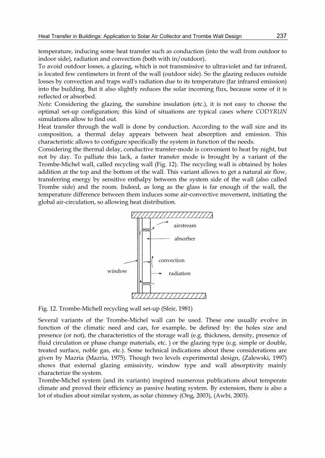
Heat Transfer in Buildings: Application to Solar Air Collector and Trombe Wall Design
237
temperature, inducing some heat transfer such as conduction (into the wall from outdoor to indoor side), radiation and convection (both with in/outdoor). To avoid outdoor losses, a glazing, which is not transmissive to ultraviolet and far infrared, is located few centimeters in front of the wall (outdoor side). So the glazing reduces outside losses by convection and traps wall's radiation due to its temperature (far infrared emission) into the building. But it also slightly reduces the solar incoming flux, because some of it is reflected or absorbed. Nota: Considering the glazing, the sunshine insulation (etc.), it is not easy to choose the optimal set-up configuration; this kind of situations are typical cases where CODYRUN simulations allow to find out. Heat transfer through the wall is done by conduction. According to the wall size and its composition, a thermal delay appears between heat absorption and emission. This characteristic allows to configure specifically the system in function of the needs. Considering the thermal delay, conductive transfer-mode is convenient to heat by night, but not by day. To palliate this lack, a faster transfer mode is brought by a variant of the Trombe-Michel wall, called recycling wall (Fig. 12). The recycling wall is obtained by holes addition at the top and the bottom of the wall. This variant allows to get a natural air flow, transferring energy by sensitive enthalpy between the system side of the wall (also called Trombe side) and the room. Indeed, as long as the glass is far enough of the wall, the temperature difference between them induces some air-convective movement, initiating the global air-circulation, so allowing heat distribution.
window
absorber
airstream
radiation
convection
Fig. 12. Trombe-Michell recycling wall set-up (Sfeir, 1981)
Several variants of the Trombe-Michel wall can be used. These one usually evolve in function of the climatic need and can, for example, be defined by: the holes size and presence (or not), the characteristics of the storage wall (e.g. thickness, density, presence of fluid circulation or phase change materials, etc. ) or the glazing type (e.g. simple or double, treated surface, noble gas, etc.). Some technical indications about these considerations are given by Mazria (Mazria, 1975). Though two levels experimental design, (Zalewski, 1997) shows that external glazing emissivity, window type and wall absorptivity mainly characterize the system. Trombe-Michel system (and its variants) inspired numerous publications about temperate climate and proved their efficiency as passive heating system. By extension, there is also a lot of studies about similar system, as solar chimney (Ong, 2003), (Awbi, 2003).
Evaporation, Condensation and Heat Transfer
238
There are several values usually used to describe Trombe-Michel wall functioning: • Transmitted energy through the wall by conduction, • Transmitted energy through the holes by sensitive enthalpy, • The system efficiency, defined as the rate between the energy received into the room
over the total energy received by the North wall (South hemisphere) in the meantime. • The FGS (solar benefits fraction), defined as the rate between the benefits from the
Trombe-Michel system and the energy needed by the room without it, for a room temperature of 22°C.
Nota: Even if the FGS refers to active heating systems, it allows to compare easily passive heating systems between them and to other installations.
4.2.2 Presentation of Trombe-Michel wall simulations under CODYRUN This numerical study is resolved by software simulations. The case study case presented here takes place in Antananarivo, Madagascar (Indian Ocean). The aim of the simulations conducted was to help this developing country to face low temperatures in classrooms during winter season. The word 'zone', used previously, is understood as CODYRUN vocable, correspond usually to one room. Into the actual description, isothermal air assumption is made into the capitation area. This consideration is taken as first approximation and can be possibly modified later to improve the model (e.g. replaced by linear gradient hypothesis, etc.). According to the bibliography, one of the main issues mentioned is about the convection coefficient into the Trombe side of the wall. Because of the system successively laminar and turbulent, convection correlation such as - Nu = f(Gr) – cannot be used. In this case, (Zalewski, 1997) says that the laminar coefficient evolve between 2 and 2.3 W.m-2.K-1 and the turbulent one evolve between 2.25 and 3.75 W.m-2.K-1. So, in a first approach, we approximate the temperature-evolving value of the convection coefficient as the average of the turbulent and laminar values (2.9 W.m-2.K-1 ). Considering thermo-circulation, the CODYRUN's airflow module allows to calculate air flows through wall's holes. This consideration and the case study description, the two areas (the Trombe system and the room) are studied coupled, which is a right physical representation of the reality. Results validity are certified by the fact that each module of CODYRUN, and their combinations, has been validated by comparison with experimental results, reference codes and BESTEST procedures. This multi-model code structure (Boyer, 1996) can be efficiently exploited by studies such as this one, where it is necessary to choose the convection coefficients by area or by wall, to mesh slightly the walls to calculate precisely the conductive fluxes, to choose a solar gains repartition model or equivalent sky temperature, etc. CODYRUN also creates numerous output simulation variables, in addition to the one related to the dry temperature area, such as sensible power outputs from mass exchange through wall holes, conductive fluxes through the wall, enthalpic zone balance and the PMV (Predictive Mean Vote, according to Gagge) of interior zone to quantify comfort conditions. It is also possible to explore the conductive flux through the Trombe-Michel wall glass. Simulation results are presented with meteorological data of Antananarivo coming from TRNSYS 16.0 software and its TMY2 documentation data file. According to this one, daily
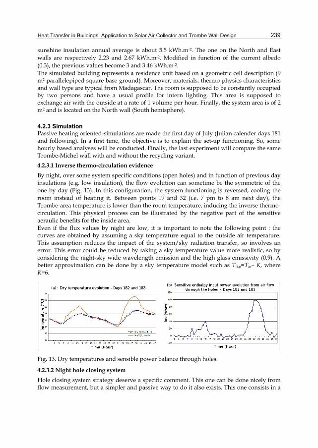
Heat Transfer in Buildings: Application to Solar Air Collector and Trombe Wall Design
239
sunshine insulation annual average is about 5.5 kWh.m-2. The one on the North and East walls are respectively 2.23 and 2.67 kWh.m-2. Modified in function of the current albedo (0.3), the previous values become 3 and 3.46 kWh.m-2. The simulated building represents a residence unit based on a geometric cell description (9 m² parallelepiped square base ground). Moreover, materials, thermo-physics characteristics and wall type are typical from Madagascar. The room is supposed to be constantly occupied by two persons and have a usual profile for intern lighting. This area is supposed to exchange air with the outside at a rate of 1 volume per hour. Finally, the system area is of 2 m2 and is located on the North wall (South hemisphere).
4.2.3 Simulation Passive heating oriented-simulations are made the first day of July (Julian calender days 181 and following). In a first time, the objective is to explain the set-up functioning. So, some hourly based analyses will be conducted. Finally, the last experiment will compare the same Trombe-Michel wall with and without the recycling variant. 4.2.3.1 Inverse thermo-circulation evidence By night, over some system specific conditions (open holes) and in function of previous day insulations (e.g. low insulation), the flow evolution can sometime be the symmetric of the one by day (Fig. 13). In this configuration, the system functioning is reversed, cooling the room instead of heating it. Between points 19 and 32 (i.e. 7 pm to 8 am next day), the Trombe-area temperature is lower than the room temperature, inducing the inverse thermo-circulation. This physical process can be illustrated by the negative part of the sensitive aeraulic benefits for the inside area. Even if the flux values by night are low, it is important to note the following point : the curves are obtained by assuming a sky temperature equal to the outside air temperature. This assumption reduces the impact of the system/sky radiation transfer, so involves an error. This error could be reduced by taking a sky temperature value more realistic, so by considering the night-sky wide wavelength emission and the high glass emissivity (0.9). A better approximation can be done by a sky temperature model such as Tsky=Tae– K, where K=6.
Fig. 13. Dry temperatures and sensible power balance through holes.
4.2.3.2 Night hole closing system Hole closing system strategy deserve a specific comment. This one can be done nicely from flow measurement, but a simpler and passive way to do it also exists. This one consists in a
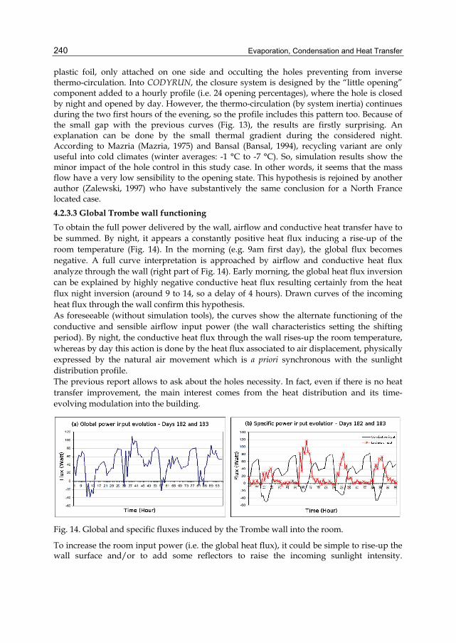
Evaporation, Condensation and Heat Transfer
240
plastic foil, only attached on one side and occulting the holes preventing from inverse thermo-circulation. Into CODYRUN, the closure system is designed by the “little opening” component added to a hourly profile (i.e. 24 opening percentages), where the hole is closed by night and opened by day. However, the thermo-circulation (by system inertia) continues during the two first hours of the evening, so the profile includes this pattern too. Because of the small gap with the previous curves (Fig. 13), the results are firstly surprising. An explanation can be done by the small thermal gradient during the considered night. According to Mazria (Mazria, 1975) and Bansal (Bansal, 1994), recycling variant are only useful into cold climates (winter averages: -1 °C to -7 °C). So, simulation results show the minor impact of the hole control in this study case. In other words, it seems that the mass flow have a very low sensibility to the opening state. This hypothesis is rejoined by another author (Zalewski, 1997) who have substantively the same conclusion for a North France located case. 4.2.3.3 Global Trombe wall functioning To obtain the full power delivered by the wall, airflow and conductive heat transfer have to be summed. By night, it appears a constantly positive heat flux inducing a rise-up of the room temperature (Fig. 14). In the morning (e.g. 9am first day), the global flux becomes negative. A full curve interpretation is approached by airflow and conductive heat flux analyze through the wall (right part of Fig. 14). Early morning, the global heat flux inversion can be explained by highly negative conductive heat flux resulting certainly from the heat flux night inversion (around 9 to 14, so a delay of 4 hours). Drawn curves of the incoming heat flux through the wall confirm this hypothesis. As foreseeable (without simulation tools), the curves show the alternate functioning of the conductive and sensible airflow input power (the wall characteristics setting the shifting period). By night, the conductive heat flux through the wall rises-up the room temperature, whereas by day this action is done by the heat flux associated to air displacement, physically expressed by the natural air movement which is a priori synchronous with the sunlight distribution profile. The previous report allows to ask about the holes necessity. In fact, even if there is no heat transfer improvement, the main interest comes from the heat distribution and its time-evolving modulation into the building.
Fig. 14. Global and specific fluxes induced by the Trombe wall into the room.
To increase the room input power (i.e. the global heat flux), it could be simple to rise-up the wall surface and/or to add some reflectors to raise the incoming sunlight intensity.
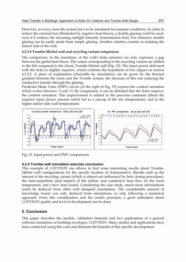
Heat Transfer in Buildings: Application to Solar Air Collector and Trombe Wall Design
241
However, in every cases the system have to be simulated for summer conditions. In order to reduce the external loss (illustrated by negative heat fluxes), a double glazing could be used, even if it reduces the incoming sunlight intensity (transmission loss). For reference, double glazing can be easily made from simple glazing. Another solution consists in isolating the indoor side of the wall. 4.2.3.4 Trombe-Michel wall and recycling variant comparison The comparison, in the meantime, of the wall's holes presence (or not), expresses a gap between the global heat fluxes. The values corresponding to the recycling variant are shifted to the left compared to the classic Trombe-Michel wall (Fig. 15). The input power delivered with the holes is slightly superior, which confirms the hypothesis of low impact on section 4.2.3.2. A piece of explanation (checkable by simulation) can be given by the thermal gradient between the room and the Trombe system, the decrease of this one reducing the conductive transfer through the glazing. Predicted Mean Votes (PMV) curves (of the right of Fig. 15) express the comfort sensation which evolve between -3 and +3. By comparison, it can be affirmed that the holes improve the comfort sensation. This improvement is related to the previous comment (about the superior input power amount which led to a rise-up of the dry temperature), and to the higher indoor side wall temperatures.
Fig. 15. Input power and PMV comparisons
4.2.4 Trombe wall simulation exercise conclusion This example of CODYRUN use allows to find some interesting results about Trombe-Michel wall configurations for the specific location of Antananarivo. Results such as the interest of the recycling variant (which is almost not influenced by hole closing procedure), the time-repartition (and impact) of the airflow and conductive heat flow on the room temperature, (etc.) have been found. Considering the case study, much more informations could be deduced from other well designed simulations. The considerable amount of knowledge found was only deduced from simulations, so only following a numerical approach. From this consideration and the results precision, a good estimation about CODYRUN quality and level of development can be done.
5. Conclusion This paper describes the models, validation elements and two applications of a general software simulation of building envelopes, CODYRUN. Many studies and applications have been conducted using this code and illustrate the benefits of this specific development.
Evaporation, Condensation and Heat Transfer
242
Conducted and sustained for over fifteen years, the specific developments made around CODYRUN led our team to be owner of a building simulation environment and develop connex themes such as validation or application to large scale in building architectural requirements. This evolving environment has enabled us to drive developments in methodological areas (Mara, 2001) (modal reduction, sensitivity analysis, coupling with genetic algorithms (Lauret, 2005), neural networks, meta models,...) or related to technological aspects (solar masks, integration of split-system, taking into account the radiant barriers products, ...). This approach allows a detailed understanding of the physical phenomena involved, the use of this application in teaching and capitalization within a work tool of a research team. Accompanied by the growth of computer capabilities, the subject of high environmental quality in buildings, our field becomes more complex by the integration of aspects other than those originally associated with the thermal aspects (environmental quality, including lighting, pollutants, acoustics, ...). Simultaneously, it is also essential to achieve a better efficiency in the transfer of knowledge and operational tools.
6. References Awbi H. (2003),Ventilation of buildings, Spon Press, ISBN 0415270-55-3. Balcomb J.D. & al. (1997), Passive solar heating of buildings, in Solar Architecture,
Proceedings of the aspen Energy Forum, Ann Arbor Science Publishers Inc., Aspen, Colorado, 1977.
Bansal N.K., Hauser G., Minke G. (1994). Passive Building design. A handbook of natural climatic control, Elsevier, ISBN 0-444-81745-X, Amsterdam (Netherlands)
Berthomieu T., Boyer H. (2003), « Intégration de la réduction équilibrée à un code de simulation hygro-thermo-aéraulique de bâtiments », Annales du Bâtiment et des Travaux Publics, n°6, Sept. 2003
Bigot D., Miranville, Fakra A.H., Ingar I., Guichard S., Boyer H. (2010). Thermal performance of photovoltaic systems integrated in buildings, In Solar Collectors and Panels, Theory and Applications, Sciyo, ISBN 978-953-7619-X-X.
Boyer H., Chabriat J.P., Grondin Perez B., Tourrand C., Brau J. (1996) Thermal building simulation and computer generation of nodal models, Building and Environment, 31(3), pp. 207-214.
Boyer H., Garde F., Gatina J.C., Brau J. (1998) A multi-model approach to building thermal simulation for design and research purpose, Energy and Buildings, 28, 1, pp. 71-79
Boyer H., Lauret A.P., Adelard L., Mara T.A. (1999) Building ventilation : a pressure airflow model computer generation and elements of validation, Energy and Buildings, 29, pp. 283-292.
Boyer H., Bastide A., Lauret P. (2005), CODYRUN, outil de simulation et d’aide à la conception thermo-aéraulique de bâtiments, Journée Thématique IBPSA/SFT Outils de simulation thermo-aéraulique du bâtiment, La Rochelle, 31 mars 2005
Boyer H., Lauret A.P., Adelard L., Mara T.A. (1999). Building ventilation : a pressure airflow model computer generation and elements of validation, Energy and Buildings, Vol. 29, 283-292, ISSN 0378-7788
Boyer H. & al. (1996), Thermal building simulation and computer generation of nodal models, Building and Environment, Vol. 31, 207-214, ISSN 0360-1323
Heat Transfer in Buildings: Application to Solar Air Collector and Trombe Wall Design
243
Buzzoni L. & al., Energy analysis of a passive solar system, Revue Génerale de Thermique, 411-416, 37, 1998
Calogine D., Boyer H., Ndoumbe S., Rivière C., Miranville F. (2010), Identification of parameters in building concentration dispersion model, Indoor Built Environment, Vol. 19, 2, 2010, 250-267, ISSN 1420-326X
Charbonnier S, Parant C, Pouget A. (1992), Guide le Thermique dans l’habitat neuf, bâtir une stratégie globale, Editions du moniteur, ISBN 2-281-11132-6
Clarke J. (2001). Energy simulation in building design, Butterworth-Heinemann, ISBN 0 7506 5082 6, Glasgow (Scotland)
Duffie J.A. and Beckman W.A. (1974), Solar Energy thermal processes, ISBN 0 471 22371-9, John Wiley & sons
Fakra A. H., Boyer H., Miranville F., Bigot D. (2010), A simple evaluation of global and diffuse luminous efficacy for all sky conditions in tropical and humid climate., Renewable Energy, Vol.36, January, 298-306, ISSN 0960-1481
Garde F., Boyer H., Gatina J.C. (1999). Demand side management in tropical island buildings. Elaboration of global quality standards for natural and low energy cooling in buildings, Building and Environment, Vol.34, 71-84, ISSN 0360-1323
Garde F., Boyer H., Célaire R. (2001), Bringing simulation to implementation : Presentation of a global approach in the design of passive solar buildings under humid tropical climates, Solar Energy, Vol.71, 109-120, ISSN 0038-092X
Lauret P., Mara T. A., Boyer H., Adelard L., Garde F (2001). A validation methodology aid for improving a thermal building model : how to account for diffuse radiation in a tropical climate, Energy and Buildings, Vol. 33, 711-718, ISSN 0378-7788
Lucas F., Mara T., Garde F., Boyer H. (1998), A comparison between CODYRUN and TRNSYS simulation codes for thermal building behaviour, Renewable Energy, Vol.15, 1624-1633, ISSN 0960-1481
Lauret P., Boyer H., Rivière C., Bastide, A. (2005), A genetic algorithm applied to the validation of building thermal models Energy and Buildings 37 (8), pp. 858-866
Mara T.A., Boyer H. and Garde F. (2002), Parametric Sensitivity Analysis of a Test Cell Thermal Model Using Spectral Analysis, Journal of Solar Energy Engineering, Vol. 124, August, 37-242, ISSN 0199-6231
Mara T.A., Garde F., Boyer H. and Mamode M. (2001). Empirical Validation of the Thermal Model of a Passive Solar Test Cell, Energy and Buildings, Vol.33, 2001, 589-599, ISSN 0378-7788
Mazria E, (1979) Le guide de l’énergie solaire passive, Parenthèses Editions, ISBN 2-86364-011-9 Miranville F., Boyer H., Lauret P., Lucas F. (2008), A Combined Approach for Determining
the Thermal Performance of Radiant Barriers under Field Conditions, Solar Energy, Vol. 82, 399-410, ISSN 0038-092X
Ong K.S., A mathematical model of a solar chimney, Renewable Energy, 28, 1047-1060, 2003. Orme M., Applicable ventilation model for air infiltration and ventilation calculations, AIVC
Technical Note 51, 1999 Raman P. & al., A passive solar system for thermal confort conditionning of building in
composite climates, Solar Energy, 70, 4, 319-329, 2001 Sfeir A.A. (1981), Guarracino G., Ingénierie des systèmes solaires, application à l’habitat,
Technique et Documentation, ISBN 2-85206-101-5

Evaporation, Condensation and Heat Transfer
244
Soubdhan T., Mara T., Boyer H., Younes A., (2000). Use of BESTEST procedure to improve a thermal simulation software, Renewable Energy, Vol., 1800-1803, ISSN 0960-1481
Tuomala P. , Rahola J., Combined air flow and thermal simulation of buildings, Building and Environment, .30, 2, pp.255-265 (1995)
Zalewski L. & al., Study of solar walls, validating a simulation model, Building and Environment, 109-121, 37, 2002 Zalewski L & al., Experimental thermal study of a solar wall composite type, Energy and Buildings, 7-8, 25, 1997.
12
Heat Transfer in the Transitional Flow Regime JP Meyer and JA Olivier
University of Pretoria, Department of Mechanical and Aeronautical Engineering,
South Africa
1. Introduction Transitional flow, whereby the motion of a fluid changes from laminar to turbulent flow, was successfully identified by Reynolds (1883) almost 130 years ago. According to ASHRAE (2009), for a round pipe, in general, laminar flow exists when the Reynolds number is less than 2 300. Fully turbulent flow exists when the Reynolds number is larger than 10 000 and transitional flow exists for Reynolds numbers between 2 300 and 10 000. Despite much work on transition and even though it is of considerable importance in determining pressure drop and heat transfer in convective flow, the underlying physics and the implications of this phenomenon have eluded complete understanding (Obot et al., 1990). ASHRAE further states that predictions are unreliable in the transitional flow regime. Cengel (2006) mentions that although transitional flow exists for Reynolds numbers between 2 300 and 10 000, it should be kept in mind that in many cases the flow becomes fully turbulent when the Reynolds number is larger than 4 000. It is normally advised when designing heat exchangers to remain outside the transitional flow regime due to the uncertainty and flow instability in this region. For this reason, little design information is available with specific reference to heat transfer and pressure drop data in the transitional flow regime. It has been known that there is a relationship between pressure drop and heat transfer generally referred to as the Reynolds analogy. Therefore, the relationship between friction factor and Nusselt number was studied by many and an overview of all the contributions on the subject is given by Colburn (1933). Obot et al. (1990) followed up on this previous work to investigate the role of transition in determining friction and heat transfer in smooth and rough passages. Later on they (Obot et al., 1997) took measurements of heat transfer and pressure drop in smooth tubes in laminar, transitional and turbulent flow over a wide range of Prandtl numbers. García et al. (2005) experimentally investigated helical wire coils fitted inside a round tube in order to characterise their thermohydraulic behaviour in laminar, transitional and turbulent flow. They did experiments over a wide range of Reynolds and Prandtl numbers and they found that at low Reynolds numbers, wire coils behave as a smooth tube but accelerate transition to critical Reynolds numbers down to 700. Furthermore, within the transition region, if wire coils are fitted inside a smooth tube heat exchanger, the heat transfer rate can be increased up to 200% while maintaining a constant pumping power. This is in comparison with the turbulent flow regime where wire coils increase pressure drop up to nine times and heat transfer up to four times compared with empty smooth
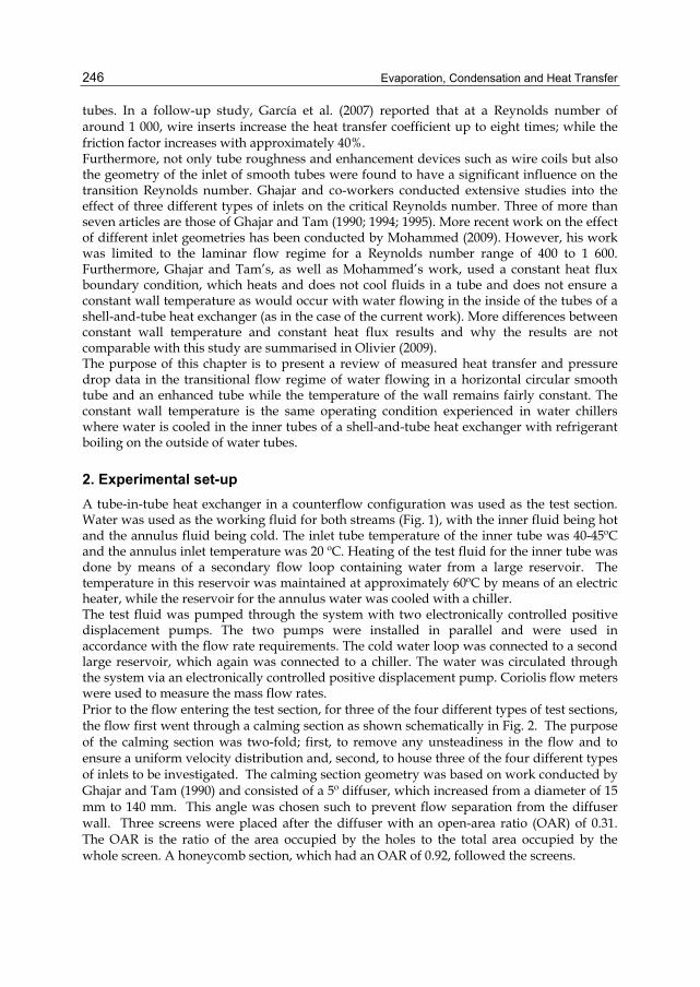
Evaporation, Condensation and Heat Transfer
246
tubes. In a follow-up study, García et al. (2007) reported that at a Reynolds number of around 1 000, wire inserts increase the heat transfer coefficient up to eight times; while the friction factor increases with approximately 40%. Furthermore, not only tube roughness and enhancement devices such as wire coils but also the geometry of the inlet of smooth tubes were found to have a significant influence on the transition Reynolds number. Ghajar and co-workers conducted extensive studies into the effect of three different types of inlets on the critical Reynolds number. Three of more than seven articles are those of Ghajar and Tam (1990; 1994; 1995). More recent work on the effect of different inlet geometries has been conducted by Mohammed (2009). However, his work was limited to the laminar flow regime for a Reynolds number range of 400 to 1 600. Furthermore, Ghajar and Tam’s, as well as Mohammed’s work, used a constant heat flux boundary condition, which heats and does not cool fluids in a tube and does not ensure a constant wall temperature as would occur with water flowing in the inside of the tubes of a shell-and-tube heat exchanger (as in the case of the current work). More differences between constant wall temperature and constant heat flux results and why the results are not comparable with this study are summarised in Olivier (2009). The purpose of this chapter is to present a review of measured heat transfer and pressure drop data in the transitional flow regime of water flowing in a horizontal circular smooth tube and an enhanced tube while the temperature of the wall remains fairly constant. The constant wall temperature is the same operating condition experienced in water chillers where water is cooled in the inner tubes of a shell-and-tube heat exchanger with refrigerant boiling on the outside of water tubes.
2. Experimental set-up A tube-in-tube heat exchanger in a counterflow configuration was used as the test section. Water was used as the working fluid for both streams (Fig. 1), with the inner fluid being hot and the annulus fluid being cold. The inlet tube temperature of the inner tube was 40-45ºC and the annulus inlet temperature was 20 ºC. Heating of the test fluid for the inner tube was done by means of a secondary flow loop containing water from a large reservoir. The temperature in this reservoir was maintained at approximately 60ºC by means of an electric heater, while the reservoir for the annulus water was cooled with a chiller. The test fluid was pumped through the system with two electronically controlled positive displacement pumps. The two pumps were installed in parallel and were used in accordance with the flow rate requirements. The cold water loop was connected to a second large reservoir, which again was connected to a chiller. The water was circulated through the system via an electronically controlled positive displacement pump. Coriolis flow meters were used to measure the mass flow rates. Prior to the flow entering the test section, for three of the four different types of test sections, the flow first went through a calming section as shown schematically in Fig. 2. The purpose of the calming section was two-fold; first, to remove any unsteadiness in the flow and to ensure a uniform velocity distribution and, second, to house three of the four different types of inlets to be investigated. The calming section geometry was based on work conducted by Ghajar and Tam (1990) and consisted of a 5º diffuser, which increased from a diameter of 15 mm to 140 mm. This angle was chosen such to prevent flow separation from the diffuser wall. Three screens were placed after the diffuser with an open-area ratio (OAR) of 0.31. The OAR is the ratio of the area occupied by the holes to the total area occupied by the whole screen. A honeycomb section, which had an OAR of 0.92, followed the screens.
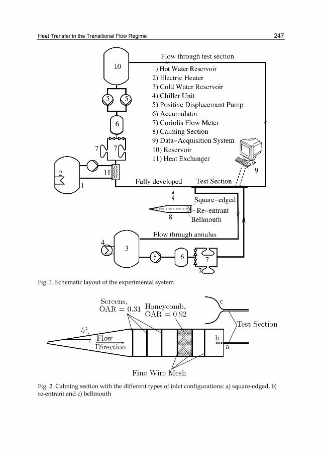
Heat Transfer in the Transitional Flow Regime
247
Fig. 1. Schematic layout of the experimental system
Fig. 2. Calming section with the different types of inlet configurations: a) square-edged, b) re-entrant and c) bellmouth
Evaporation, Condensation and Heat Transfer
248
Prior to and after the honeycomb, a wire mesh was placed with the wires having a diameter of 0.8 mm and the OAR being 0.54. Another fine wire mesh was inserted between the last honeycomb mesh and the test inlet. This mesh had a wire diameter of 0.3 mm and an OAR of 0.17. Three different inlets (Fig. 3) could be housed on the calming section, namely a square-edged, re-entrant and bellmouth inlet. These inlets are also shown in Fig. 2 as items a, b and c, respectively. The calming section was designed such that the inlets could easily be interchanged. The square-edged inlet is characterised by a sudden contraction of the flow. This is a typical situation encountered in the header of a shell-and-tube exchanger. The re-entrant inlet makes use of the square-edged inlet except that the tube slides into the inlet by one tube diameter. This would simulate a floating header in a shell-and-tube heat exchanger. The third type of inlet is the bellmouth. The bellmouth is characterised by a smooth contraction, having a contraction ratio of 8.8. The shape of the bellmouth was calculated with the method suggested by Morel (1975). The use of a bellmouth is thought to help in the reduction of fouling, although practical application thereof is uncommon in heat exchangers.
Fig. 3. Illustration of the different inlet geometries relative to the test section
The fourth type of inlet used was a fully developed inlet, which did not make use of the calming section. This inlet had an inner diameter being the same as that of the test section. The length of the fully developed inlet was determined in terms of the suggestion by Durst et al. (2005), which required a minimum length of 120-tube diameters. To ensure this minimum was met, the length of the inlet was chosen as 160-tube diameters. Cooling started, in the case of adiabatic tests, after this inlet section, while for the other inlets, cooling started after the calming section.
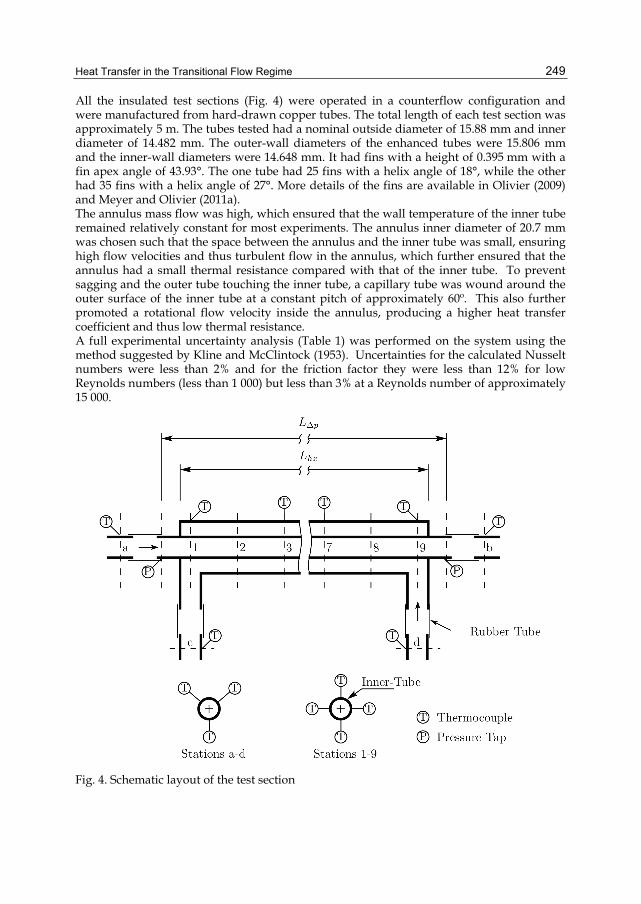
Heat Transfer in the Transitional Flow Regime
249
All the insulated test sections (Fig. 4) were operated in a counterflow configuration and were manufactured from hard-drawn copper tubes. The total length of each test section was approximately 5 m. The tubes tested had a nominal outside diameter of 15.88 mm and inner diameter of 14.482 mm. The outer-wall diameters of the enhanced tubes were 15.806 mm and the inner-wall diameters were 14.648 mm. It had fins with a height of 0.395 mm with a fin apex angle of 43.93°. The one tube had 25 fins with a helix angle of 18°, while the other had 35 fins with a helix angle of 27°. More details of the fins are available in Olivier (2009) and Meyer and Olivier (2011a). The annulus mass flow was high, which ensured that the wall temperature of the inner tube remained relatively constant for most experiments. The annulus inner diameter of 20.7 mm was chosen such that the space between the annulus and the inner tube was small, ensuring high flow velocities and thus turbulent flow in the annulus, which further ensured that the annulus had a small thermal resistance compared with that of the inner tube. To prevent sagging and the outer tube touching the inner tube, a capillary tube was wound around the outer surface of the inner tube at a constant pitch of approximately 60º. This also further promoted a rotational flow velocity inside the annulus, producing a higher heat transfer coefficient and thus low thermal resistance. A full experimental uncertainty analysis (Table 1) was performed on the system using the method suggested by Kline and McClintock (1953). Uncertainties for the calculated Nusselt numbers were less than 2% and for the friction factor they were less than 12% for low Reynolds numbers (less than 1 000) but less than 3% at a Reynolds number of approximately 15 000.
Fig. 4. Schematic layout of the test section
Evaporation, Condensation and Heat Transfer
250
3. Data reduction The inner tube's average heat transfer coefficient was obtained by making use of the overall heat transfer coefficient and the sum of the resistances, given by
1
i wi o o
1 1 1RA UA A
−⎡ ⎤
α = − −⎢ ⎥α⎣ ⎦ (1)
UA is the overall heat transfer coefficient, which can be obtained by means of the overall heat transferred and the log-mean temperature difference, calculated from the inlet and outlet temperatures of the inner tube and annulus
i
lmtd
QUAT
= (2)
iQ is the heat transferred in the inner tube, calculated as
i i pQ m C= ΔΤ (3)
while im and TΔ are, respectively, the inner-tube mass flow rate and the temperature difference between the in- and outlet of the inner tube. The specific heat values were obtained from IAPWS (2003), which are based on the fluid temperature. The annulus heat transfer coefficient was calculated by means of the annulus bulk temperature and the average inner-tube outer-wall temperature measurements. The bulk and average wall temperatures were obtained by making use of the trapezium rule to “integrate” over the whole length of the tube. Therefore, only a single bulk value for the annulus heat transfer coefficient was obtained. This is given by
( )i
oo o wo
QA T T
α =−
(4)
The inner-tube heat transfer rate was used for all the calculations since it had the lowest uncertainty. Throughout the tests, the annulus flow rate was kept as high as possible as this reduced the thermal resistance of the annulus, reducing its influence in Eq. (1) and hence decreasing the equation’s overall uncertainty. On average, the annulus thermal resistance was only 6% the value of the inner tube. All fluid properties were obtained from Wagner and Pruß (2002). Experimental data were only captured once an energy balance of less than 1% was achieved. At low inner-tube Reynolds numbers (<6 000), this requirement was not met due to the high annulus flow rate and its uncertainty. Tests were, however, conducted as checks by substantially lowering the annulus flow rate. These tests proved that the heat transfer error in the inner tube at low Reynolds numbers was indeed less than 1%. The Darcy-Weisbach friction factors were determined by
i2
p
2 pDfu LΔ
Δ=ρ
(5)
Heat Transfer in the Transitional Flow Regime
251
The bulk fluid properties used for the calculation of the Reynolds, Prandtl numbers, etc., were calculated at the average inner-tube fluid temperature, which, in turn, was determined by the resulting heat transfer coefficient, Eq. (1), as
ii wi
i
QT T= +α
(6)
Property Value Uncertainty
im 0.0087 - 0.0822 0.664 - 0.412%
om 0.429 - 0.445 0.164 - 0.260%
iin iout oin ooutT , T , T , T 20.35 - 65.67 0.011 - 0.46
oT 20.9 - 23.67 0.014 - 0.032
woT 21.33 - 25.53 0.011 - 0.055
wiT 21.34 - 25.61 0.011 - 0.055
iT 32.98 - 41.97 0.176 - 0.857
lmtdT 12.16 - 18.18 0.172 - 0.855
iQ 1 598 - 10 954 0.71 - 0.49% UA 131.5 - 605.8 1.02 - 1.08% Re 1 026 - 11 485 1.20 - 1.08% Nu 13.06 - 62.20 1.44 - 1.58% Pr 4.17 - 5.06 ±1.42% pΔ 45 - 1 583 4.71 - 1.59%
iα 558 - 2 710 1.04 - 1.22% f 0.0085 - 0.0212 2.84 - 11.28%
Table 1. Experimental range and uncertainties
4. Results In this section, the results are given. The experimental results are first validated for smooth tubes, by presenting friction factor data without heat transfer, whereafter the diabatic friction factors are given, followed by the heat transfer results in the form of Nusselt numbers. Lastly, the friction factors and heat transfer results of enhanced tubes are given.
4.1 Validation for smooth tube Figure 5 shows the adiabatic friction factor results with various inlet profiles. This figure shows how the transition region is manipulated by the use of different types of inlets (Olivier and Meyer, 2010). The square-edged inlet delays transition to Reynolds numbers of around 2 600, while the bellmouth inlet delays it to about 7 000. Transition for the re-entrant inlet did not differ much from the fully developed inlet. Thus, the smoother the inlet, the more delayed is transition. Laminar flow results for the various inlets, unlike the fully developed results, are slightly higher than the laminar friction factor obtained from the Poiseuille relation.
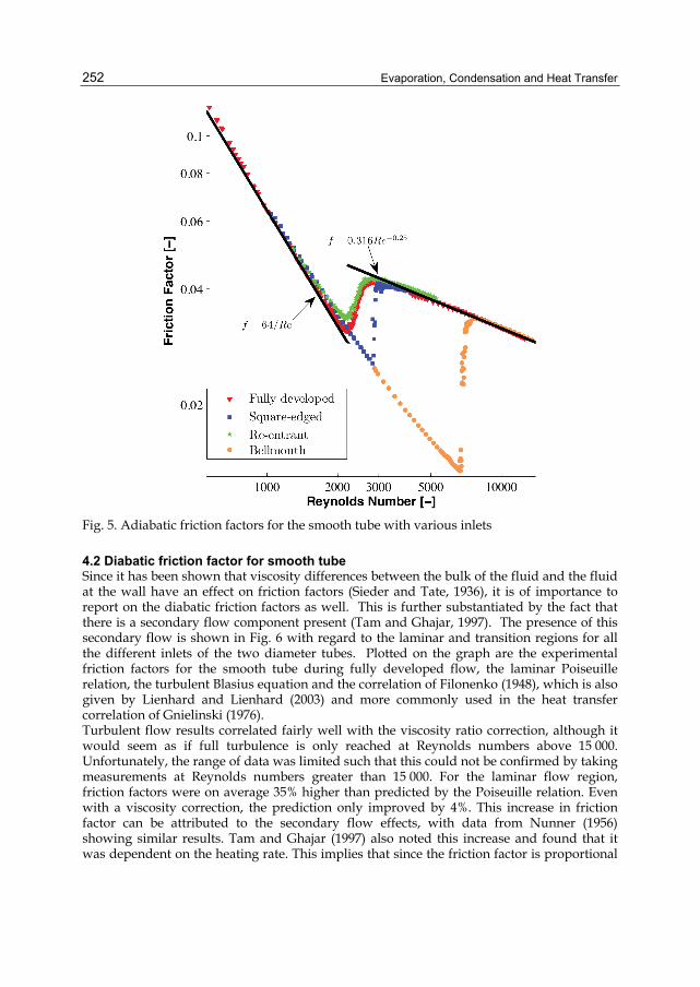
Evaporation, Condensation and Heat Transfer
252
Fig. 5. Adiabatic friction factors for the smooth tube with various inlets
4.2 Diabatic friction factor for smooth tube Since it has been shown that viscosity differences between the bulk of the fluid and the fluid at the wall have an effect on friction factors (Sieder and Tate, 1936), it is of importance to report on the diabatic friction factors as well. This is further substantiated by the fact that there is a secondary flow component present (Tam and Ghajar, 1997). The presence of this secondary flow is shown in Fig. 6 with regard to the laminar and transition regions for all the different inlets of the two diameter tubes. Plotted on the graph are the experimental friction factors for the smooth tube during fully developed flow, the laminar Poiseuille relation, the turbulent Blasius equation and the correlation of Filonenko (1948), which is also given by Lienhard and Lienhard (2003) and more commonly used in the heat transfer correlation of Gnielinski (1976). Turbulent flow results correlated fairly well with the viscosity ratio correction, although it would seem as if full turbulence is only reached at Reynolds numbers above 15 000. Unfortunately, the range of data was limited such that this could not be confirmed by taking measurements at Reynolds numbers greater than 15 000. For the laminar flow region, friction factors were on average 35% higher than predicted by the Poiseuille relation. Even with a viscosity correction, the prediction only improved by 4%. This increase in friction factor can be attributed to the secondary flow effects, with data from Nunner (1956) showing similar results. Tam and Ghajar (1997) also noted this increase and found that it was dependent on the heating rate. This implies that since the friction factor is proportional
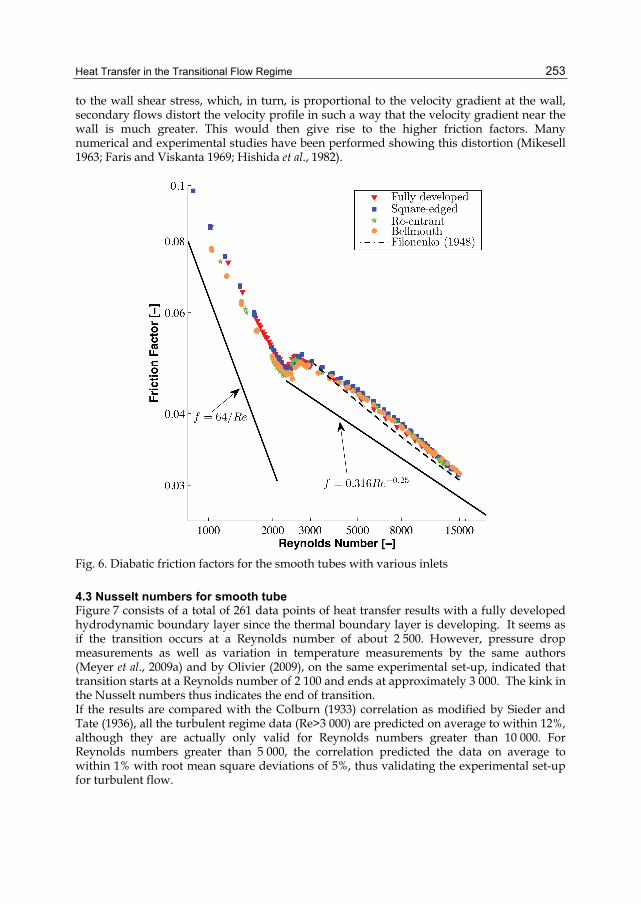
Heat Transfer in the Transitional Flow Regime
253
to the wall shear stress, which, in turn, is proportional to the velocity gradient at the wall, secondary flows distort the velocity profile in such a way that the velocity gradient near the wall is much greater. This would then give rise to the higher friction factors. Many numerical and experimental studies have been performed showing this distortion (Mikesell 1963; Faris and Viskanta 1969; Hishida et al., 1982).
Fig. 6. Diabatic friction factors for the smooth tubes with various inlets
4.3 Nusselt numbers for smooth tube Figure 7 consists of a total of 261 data points of heat transfer results with a fully developed hydrodynamic boundary layer since the thermal boundary layer is developing. It seems as if the transition occurs at a Reynolds number of about 2 500. However, pressure drop measurements as well as variation in temperature measurements by the same authors (Meyer et al., 2009a) and by Olivier (2009), on the same experimental set-up, indicated that transition starts at a Reynolds number of 2 100 and ends at approximately 3 000. The kink in the Nusselt numbers thus indicates the end of transition. If the results are compared with the Colburn (1933) correlation as modified by Sieder and Tate (1936), all the turbulent regime data (Re>3 000) are predicted on average to within 12%, although they are actually only valid for Reynolds numbers greater than 10 000. For Reynolds numbers greater than 5 000, the correlation predicted the data on average to within 1% with root mean square deviations of 5%, thus validating the experimental set-up for turbulent flow.
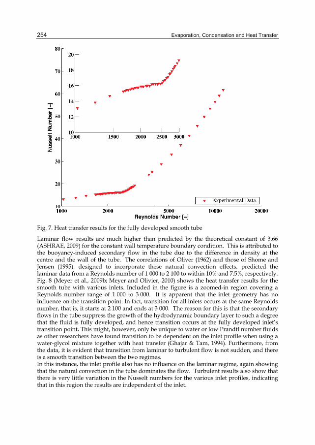
Evaporation, Condensation and Heat Transfer
254
Fig. 7. Heat transfer results for the fully developed smooth tube
Laminar flow results are much higher than predicted by the theoretical constant of 3.66 (ASHRAE, 2009) for the constant wall temperature boundary condition. This is attributed to the buoyancy-induced secondary flow in the tube due to the difference in density at the centre and the wall of the tube. The correlations of Oliver (1962) and those of Shome and Jensen (1995), designed to incorporate these natural convection effects, predicted the laminar data from a Reynolds number of 1 000 to 2 100 to within 10% and 7.5%, respectively. Fig. 8 (Meyer et al., 2009b; Meyer and Olivier, 2010) shows the heat transfer results for the smooth tube with various inlets. Included in the figure is a zoomed-in region covering a Reynolds number range of 1 000 to 3 000. It is apparent that the inlet geometry has no influence on the transition point. In fact, transition for all inlets occurs at the same Reynolds number, that is, it starts at 2 100 and ends at 3 000. The reason for this is that the secondary flows in the tube suppress the growth of the hydrodynamic boundary layer to such a degree that the fluid is fully developed, and hence transition occurs at the fully developed inlet’s transition point. This might, however, only be unique to water or low Prandtl number fluids as other researchers have found transition to be dependent on the inlet profile when using a water-glycol mixture together with heat transfer (Ghajar & Tam, 1994). Furthermore, from the data, it is evident that transition from laminar to turbulent flow is not sudden, and there is a smooth transition between the two regimes. In this instance, the inlet profile also has no influence on the laminar regime, again showing that the natural convection in the tube dominates the flow. Turbulent results also show that there is very little variation in the Nusselt numbers for the various inlet profiles, indicating that in this region the results are independent of the inlet.
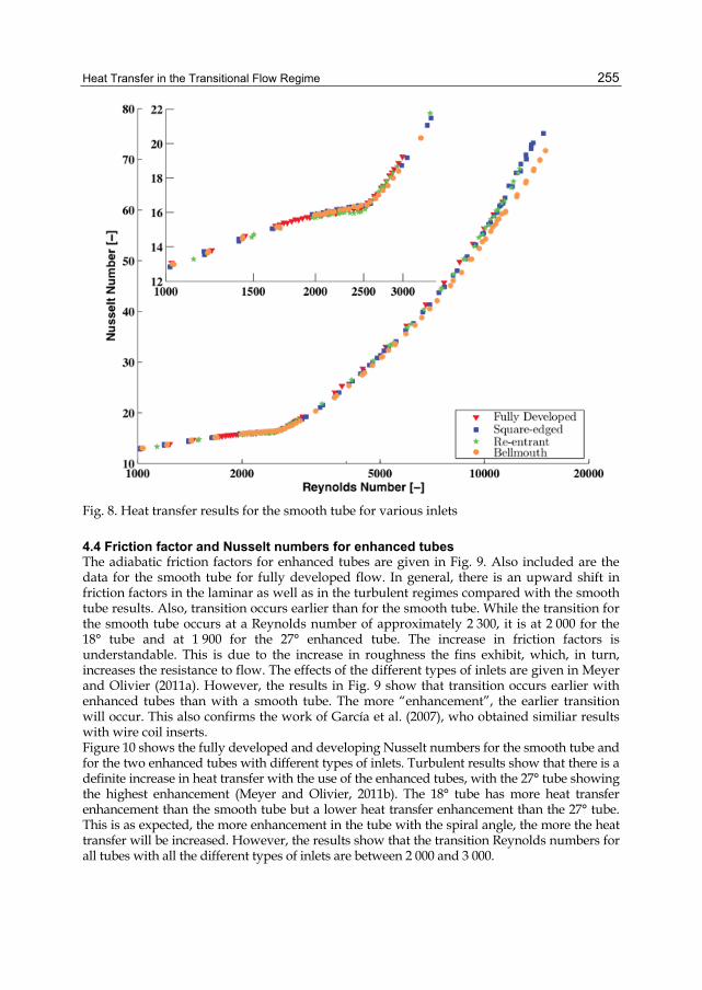
Heat Transfer in the Transitional Flow Regime
255
Fig. 8. Heat transfer results for the smooth tube for various inlets
4.4 Friction factor and Nusselt numbers for enhanced tubes The adiabatic friction factors for enhanced tubes are given in Fig. 9. Also included are the data for the smooth tube for fully developed flow. In general, there is an upward shift in friction factors in the laminar as well as in the turbulent regimes compared with the smooth tube results. Also, transition occurs earlier than for the smooth tube. While the transition for the smooth tube occurs at a Reynolds number of approximately 2 300, it is at 2 000 for the 18° tube and at 1 900 for the 27° enhanced tube. The increase in friction factors is understandable. This is due to the increase in roughness the fins exhibit, which, in turn, increases the resistance to flow. The effects of the different types of inlets are given in Meyer and Olivier (2011a). However, the results in Fig. 9 show that transition occurs earlier with enhanced tubes than with a smooth tube. The more “enhancement”, the earlier transition will occur. This also confirms the work of García et al. (2007), who obtained similiar results with wire coil inserts. Figure 10 shows the fully developed and developing Nusselt numbers for the smooth tube and for the two enhanced tubes with different types of inlets. Turbulent results show that there is a definite increase in heat transfer with the use of the enhanced tubes, with the 27° tube showing the highest enhancement (Meyer and Olivier, 2011b). The 18° tube has more heat transfer enhancement than the smooth tube but a lower heat transfer enhancement than the 27° tube. This is as expected, the more enhancement in the tube with the spiral angle, the more the heat transfer will be increased. However, the results show that the transition Reynolds numbers for all tubes with all the different types of inlets are between 2 000 and 3 000.
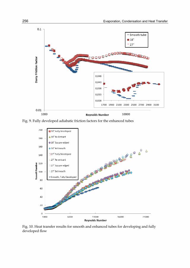
Evaporation, Condensation and Heat Transfer
256
Fig. 9. Fully developed adiabatic friction factors for the enhanced tubes
Fig. 10. Heat transfer results for smooth and enhanced tubes for developing and fully developed flow
0,028
0,033
0,038
0,043
0,048
1700 1900 2100 2300 2500 2700 2900 3100
Heat Transfer in the Transitional Flow Regime
257
5. Conclusion As modern chillers might operate in the transitional flow regime, heat transfer data are needed. Single-phase smooth tube pressure drop and heat transfer measurements for water were conducted in a horizontal circular smooth tube. An experimental set-up consisting of a tube-in-tube counterflow heat exchanger with the cooling of water as the working fluid, was used to obtain measurements within the transitional flow regime. Four different types of inlet geometries were used, i.e. hydrodynamically fully developed, square-edged, re-entrant and bellmouth. It was found from adiabatic friction factor results that transition from laminar to turbulent flow was strongly dependent on the type of inlet used. The smoother the inlet, the more transition was delayed. Results for the bellmouth inlet showed the largest delay, with transition only occurring at a Reynolds number of approximately 7 000. On the contrary, diabatic friction factor results showed that transition was independent of the type of inlet. Laminar friction factors were, however, much higher than the values predicted by the Poiseuille relation. This was also attributed to the natural convection flows influencing the boundary layer to such a degree that the shear stress at the tube wall was higher than normal. Laminar heat transfer results were much higher than their theoretically predicted values due to the secondary flows increasing the amount of mixing in the tube. Furthermore, heat transfer measurements showed that transition with water was totally independent of the type of inlet used and that transition for all the different types of inlets occurred at the same Reynolds number. This was due to the buoyancy-induced secondary flows suppressing the inlet disturbance. For enhanced tubes without heat transfer, it was found that transition occurs earlier than for smooth tubes and transition occurs earlier than for enhanced tubes. Also, the friction factors of enhanced tubes are higher than those of smooth tubes, as can be expected. With heat transfer it was found that, unlike results obtained from adiabatic flow, inlet disturbances had no effect on the transition. Transition occurs at a Reynolds number of approximately 2 000 to 3 000.
6. Nomenclature
A Area m2
iA Inner tube inside heat transfer area m2
oA Inner tube outside heat transfer area m2
Cp Specific heat J/kg.°C iD Inner diameter of tube m
f Darcy-Weisbach friction factor L Tube length m
im Inner-tube fluid mass flow rate kg/s
om Annulus fluid mass flow rate kg/s
Nu Nusselt number based on iD Pr Prandtl number
pΔ Differential pressure drop Pa
Evaporation, Condensation and Heat Transfer
258
iQ Heat transfer rate for inner-tube fluid W Re Reynolds number based on iD
wR Tube-wall resistance ˚C /W
iT Average fluid temperature for inner tube ˚C
oT Average fluid temperature for annulus ˚C
lmtdT Log-mean temperature difference ˚C
wiT Temperature of fluid at inner-tube inner wall ˚C
woT Temperture of fluid at inner-tube outer wall ˚C U Overall heat transfer coefficient W/m2˚C u Average fluid velocity in the inner tube m/s Greek symbols
iα Heat transfer coefficient of inner tube W/m2˚C
oα Heat transfer coefficient of annulus W/m2˚C ρ Fluid density kg/m3
Subscripts
in Inner tube, inlet out Inner tube, outlet hx Heat transfer
pΔ Pressure drop out Outer tube, out
7. References ASHRAE. (2009). Fluid flow, ASHRAE Handbook - Fundamentals, American Society of
Heating, Refrigerating and Air-Conditioning Engineers, Inc., Atlanta Cengel, Y.A. (2006). Heat and mass transfer, a practical approach, (Third edition), McGraw-Hill,
Singapore Colburn, A.P. (1933). A method of correlating forced convection heat transfer data and a
comparison with fluid friction, Transactions of the American Institute of Chemical Engineers, Vol. 19, pp. 174 - 210
Durst F.; Ray, S., Unsal, B. & Bayoumi, O.A. (2005). The development lengths of laminar pipe and channel flows, Journal of Fluids Engineering, Vol., 127, pp. 154-1160
Faris, G.N. & Viskanta, R. (1969). An analysis of laminar combined forced and free convection heat transfer in a horizontal tube, International Journal of Heat and Mass Transfer, Vol. 12, pp. 1295-1309
Filonenko, G.K. (1948). On friction factor for a smooth tube, All Union Thermotechnical Institute, Izvestija VTI, No. 10, Russia
García, A., Vicente, P.G. & Viedma, A. (2005). Experimental study of heat transfer enhancement with wire coil inserts in laminar-transition-turbulent regimes at different Prandtl numbers, International Journal of Heat and Mass Transfer, Vol. 48, pp. 4640 - 4651
Heat Transfer in the Transitional Flow Regime
259
García, A., Solano, J.P. Vicente, P.G. & Viedma, A. (2007). Enhancement of laminar and transitional flow heat transfer in tubes by means of wire coil inserts, International Journal of Heat and Mass Transfer, Vol. 50, pp. 3176 - 3189
Ghajar, A.J. & Tam, L.M. (1990). Laminar-transition-turbulent forced and mixed convective heat transfer correlations for pipe flows with different inlet configurations, HTD, Fundamentals of Forced Convective Heat Transfer, ASME, Vol. 181, pp. 15-23
Ghajar, A.J. & Tam, L.M. (1994). Heat transfer measurements and correlations in the transition region for a circular tube with three different inlet configurations, Experimental Thermal and Fluid Science, Vol. 8, pp. 79-90
Ghajar, A.J. & Tam, L.M. (1995). Flow regime maps for a horizontal pipe with uniform wall heat flux and three inlet configurations, Experimental Thermal and Fluid Science, Vol. 10, pp. 287- 297
Gnielinski, V. (1976). New Equation for Heat and Mass Transfer in Turbulent Pipe and Channel Flow, International Chemical Engineering, Vol. 16, pp. 359–368
Hishida, M., Nagano, Y. & Montesclaros, M.S. (1982). Combined forced and free convection in the entrance region of an isothermally heated horizontal pipe, Journal of Heat Transfer, Vol. 104, pp. 153-159
IAPWS. (2003). Uncertainties in Enthalpy for the IAPWS Formulation 1995 for the Thermodynamic Properties of Ordinary Water Substance for General and Scientific Use (IAPWS-95) and the IAPWS Industrial Formulation 1997 for the Thermodynamic Properties of Water and Steam (IAPWS-IF97), Advisory Note No 1
Kline, S.J. & McClintock, F.A. (1953). Describing uncertainties in single-sample experiments, Mechanical Engineering, Vol. 75, pp. 3 - 8
Lienhard, J.H. & Lienhard, J.H. (2003). A Heat Transfer Text Book, (Third edition), Cambridge: Phlogiston Press
Meyer, J.P., Liebenberg, L. & Olivier, J.A. (2009a). Pressure drop inside a smooth tube with different inlet geometries in the transitional flow regime for water cooled at a constant wall temperature, Proceedings of the 7th World Conference on Experimental Heat Transfer, Fluid Mechanics and Thermodynamics (ExHFT7), Krakow, Poland, pp. 1265 -1272, 28 June to 3 July
Meyer, J.P., Liebenberg, L. & Olivier, J.A. (2009b). Heat transfer characteristics of smooth circular tubes with different inlet geometries in the transitional flow regime, Proceedings of the 14th IAHR Cooling Tower and Air-Cooled Heat Exchanger Conference, Stellenbosch, paper number OP05, 1 – 3 December
Meyer, J.P. & Olivier, J.A. (2010). Heat transfer and pressure drop characteristics of circular smooth tubes in the transitional flow regime, Proceedings of the 19th International Congress of Chemical and Process Engineering CHISA 2010 and the 7th European Congress of Chemical Engineering ECCE7, Prague, Paper: I6.1, 28 August – 1 September
Meyer, J.P. & Olivier, J.A. (2011a). Transitional flow inside enhanced tubes for fully developed and developing flow with different types of inlet disturbances: Part I – adiabatic pressure drop, International Journal for Heat and Mass Transfer, Vol. 54, Issue 7-8, pp. 1587 – 1598
Meyer, J.P. & Olivier, J.A. (2011b). Transitional flow inside enhanced tubes for fully developed and developing flow with different types of inlet disturbances: Part II –
Evaporation, Condensation and Heat Transfer
260
heat transfer, International Journal for Heat and Mass Transfer, Vol. 54, Issue 7-8, pp. 1598 – 1607
Mikesell, R.D. (1963). The Effects of Heat Transfer on the Flow in a Horizontal Pipe, PhD thesis, Chemical Engineering Department, University of Illinois
Mohammed, H.A. (2009). The effect of different inlet geometries on laminar flow combined convection heat transfer inside a horizontal circular pipe, Applied Thermal Engineering, Vol. 29, pp. 581 - 590
Morel, T. (1975). Comprehensive design of axisymmetric wind tunnel contractions, Journal of Fluids Engineering, Vol. 97, pp. 225-233
Nunner, W. (1956). Heat transfer and pressure drop in rough tubes, VDI-Forschungsheft, 455-B5-39
Obot, N.T., Esen, E.B. & Rabas, T.J. (1990). The role of transition in determining friction and heat transfer in smooth and rough passages, International Journal of Heat and Mass Transfer, Vol. 33, No. 10, pp. 2133 - 2143
Obot, N.T., Das, L., Vakili, D.E. & Green, R.A. (1997). Effect of Prandtl number on smooth-tube heat transfer and pressure drop, International Communications in Heat and Mass Transfer, Vol. 24, No. 6, pp. 889 – 896
Oliver, D.R. (1962). The effect of natural convection on viscous-flow heat transfer in horizontal tubes, Chemical Engineering Science, Vol. 17, pp. 335-350
Olivier, J.A. (2009). Single-phase heat transfer and pressure drop of water inside horizontal circular smooth and enhanced tubes with different inlet configurations in the transitional flow regime, PhD thesis, University of Pretoria, Pretoria
Olivier, J.A. & Meyer, J.P. (2010). Single-phase heat transfer and pressure drop of the cooling of water inside smooth tubes for transitional flow with different inlet geometries (RP-1280), HVAC&R Research, Vol. 16, No. 4, pp. 471-496
Reynolds, O. (1883). An experimental investigation of the circumstances which determine whether the motion of water shall be direct or sinuous, and the law of resistance in parallel channels, Philosophical Transactions of the Royal Society of London, Vol. 174, pp. 935 – 982
Shome, B. & Jensen, M.K. (1995). Mixed convection laminar flow and heat transfer of liquids in isothermal horizontal circular ducts, International Journal of Heat and Mass Transfer, Vol. 38, No. 11, pp. 1945-1956
Sieder, E.N. & Tate, G.E. (1936). Heat transfer and pressure drop in liquids in tubes, Industrial and Engineering Chemistry, Vol. 28, No. 12, pp. 1429-1435
Tam, L.M. & Ghajar, A.J. (1997). Effect of inlet geometry and heating on the fully developed friction factor in the transition region of a horizontal tube, Experimental Thermal and Fluid Science, Vol. 15, pp. 52-64
Wagner, W. & Pruß, A. (2002). The IAPWS formulation 1995 for the thermodynamic properties of ordinary water substance for general and scientific use, Journal of Physical and Chemical Reference Data, Vol. 31, pp. 387-535
13
Numerical Modeling of Cross-Flow Tube Heat Exchangers with Complex Flow Arrangements
Dawid Taler1, Marcin Trojan2 and Jan Taler2
1Cracow University of Science and Technology (AGH), Department of Energy Systems and Environment Protection,
Faculty of Mechanical Engineering and Robotics, 2Cracow University of Technology,
Chair of Power Plant Machinery, Faculty of Mechanical Engineering,
Poland
1. Introduction
Cross-flow tube heat exchangers find many practical applications. An example of such an exchanger is a steam superheater, where steam flows inside the tubes while heating flue gas flows across the tube bundles. The mathematical derivation of an expression for the mean temperature difference becomes quite complex for multi-pass cross-flow heat exchangers with many tube rows and complex flow arrangement (Hewitt et al., 1994; Kröger, 2004; Rayaprolu, 2009; Stultz et al., 1992 ; Taler, 2009a). When calculating the heat transfer rate, the usual procedure is to modify the simple counter-flow LMTD (Logarithmic Mean Temperature Difference) method by a correction FT determined for a particular arrangement. The heat flow rate Q transferred from the hot to cool fluid is the product of the overall heat transfer coefficient UA, heat transfer area A, correction factor FT and logarithmic mean temperature difference ΔTlm. The heat transfer equation then takes the form:
A T lmQ U A F T= Δ
(1)
However, to calculate steam, flue gas and wall temperature distributions, a numerical model of the superheater is indispensable. Superheaters are tube bundles that attain the highest temperatures in a boiler and consequently require the greatest care in the design and operation. The complex superheater tube arrangements permit an economic trade-off between material unit costs and surface area required to obtain the prescribed steam outlet temperature. Very often, various alloy steels are used for each pass in modern boilers.
Evaporation, Condensation and Heat Transfer
262
High temperature heat exchangers like steam superheaters are difficult to model since the tubes receive energy from the flue gas by two heat transfer modes: convection and radiation. The division of superheaters into two types: convection and radiant superheaters is based on the mode of heat transfer that is predominant. In convection superheaters, the portion of heat transfer by radiation from the flue gas is small. A radiant superheater absorbs heat primarily by thermal radiation from the flue gas with little convective heat flow rate. The share of convection in the total heat exchange of platen superheaters located directly over the combustion chamber amounts only to 10 to 15%. In convective superheaters, the share of radiation heat exchange is lower, but cannot be neglected. Correct determination of the heat flux absorbed through the boiler heating surfaces is very difficult. This results, on the one hand, from the complexity of heat transfer by radiation of flue gas with a high content of solid ash particles, and on the other hand, from fouling of heating surfaces by slag and ash (Taler et al., 2009b). The degree of the slag and ash deposition is hard to assess, both at the design stage and during the boiler operation. In consequence, the proper size of superheaters can be adjusted only after boiler’s start-up. In cases when the temperature of superheated steam at the exit from the superheater stage under examination is higher than its design value, then the area of the surface of this stage has to be decreased. However, if the exit temperature of the steam is below the desired value, then the surface area is increased.
2. Mathematical model of the superheater To study the impact of superheater fouling on flue gas and steam temperatures, a numerical model of the entire superheater, has been developed. It was assumed that the outer tube surfaces are covered with bonded ash deposits with a uniform thickness. The temperature of the flue gas, tube walls, and steam was determined using the finite volume method (FVM) (Taler, 2009a). The subsequent stages of the superheater were modeled as either cross-parallel-flow or cross-counter-flow. As an example, a numerical model of the first stage convective will be presented in detail (Figs. 1 and 2). The first stage convective superheater is a pendant twelve-pass heat exchanger. The superheater is constructed of circular bare tubes and is situated at the back of the second and third stages of the superheater (Figs. 1 and 2). The tube is made of grade St 20 carbon steel, having a 42 mm outside diameter and 5mm thick wall. The superheated steam and the combustion products flow at right angles to each other. The convective superheater considered in the paper can be classified according to flow arrangement as a mixed-cross-flow heat exchanger (Figs. 2 and 3). Each individual pass consists of two tubes through which superheated steam flows parallel (Fig. 2). Based on the energy conservation principle, a mathematical model of steam superheater with 12 tube rows and complex flow arrangement was developed. The radiant and convective superheaters are located in boiler passes through which high temperature flue gas flows. The gas temperature drops from about 1100 ˚C at the exit of the furnace chamber to about 400 ˚C before entering the economizer. Radiant platen superheaters are located in areas of highest flue gas temperature and the water heater in the lowest temperature pass.
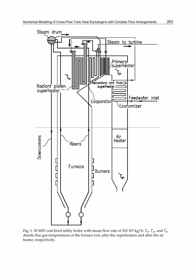
Numerical Modeling of Cross-Flow Tube Heat Exchangers with Complex Flow Arrangements
263
Fig. 1. 50 MW coal-fired utility boiler with steam flow rate of 210·103 kg/h: Tfe, Tgs, and Tge denote flue gas temperatures at the furnace exit, after the superheaters and after the air heater, respectively.

Evaporation, Condensation and Heat Transfer
264
Fig. 2. Arrangement of boiler heating surfaces.
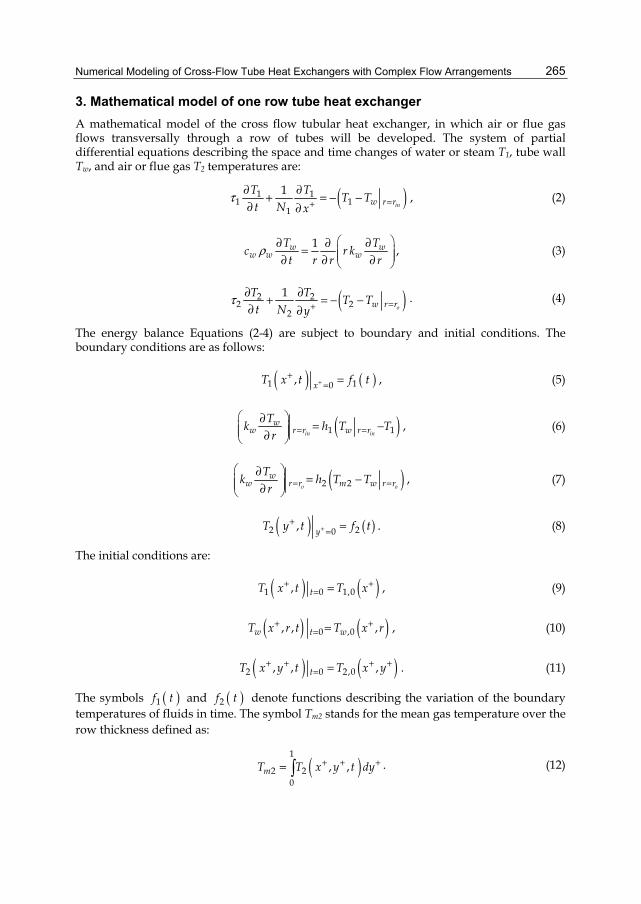
Numerical Modeling of Cross-Flow Tube Heat Exchangers with Complex Flow Arrangements
265
3. Mathematical model of one row tube heat exchanger A mathematical model of the cross flow tubular heat exchanger, in which air or flue gas flows transversally through a row of tubes will be developed. The system of partial differential equations describing the space and time changes of water or steam T1, tube wall Tw, and air or flue gas T2 temperatures are:
( )1 11 1
1
1inw r r
T T T Tt N x
τ =+∂ ∂
+ = − −∂ ∂
, (2)
1w ww w w
T Tc r kt r r r
ρ⎛ ⎞∂ ∂∂= ⎜ ⎟⎜ ⎟∂ ∂ ∂⎝ ⎠
, (3)
( )2 22 2
2
1ow r r
T T T Tt N y
τ =+∂ ∂+ = − −∂ ∂
. (4)
The energy balance Equations (2-4) are subject to boundary and initial conditions. The boundary conditions are as follows:
( ) ( )1 10, xT x t f t++
= = , (5)
( )1 1in in
ww r r w r r
Tk h T Tr = =
⎛ ⎞∂= −⎜ ⎟⎜ ⎟∂⎝ ⎠
, (6)
( )2 2o o
ww r r m w r r
Tk h T Tr = =
⎛ ⎞∂= −⎜ ⎟⎜ ⎟∂⎝ ⎠
, (7)
( ) ( )2 20, yT y t f t++
= = . (8)
The initial conditions are:
( ) ( )1 0 1,0, tT x t T x+ += = , (9)
( ) ( )0 ,0, , ,w t wT x r t T x r+ += = , (10)
( ) ( )2 0 2,0, , ,tT x y t T x y+ + + += = . (11)
The symbols ( )1f t and ( )2f t denote functions describing the variation of the boundary temperatures of fluids in time. The symbol Tm2 stands for the mean gas temperature over the row thickness defined as:
( )1
2 20
, ,mT T x y t dy+ + += ∫ . (12)
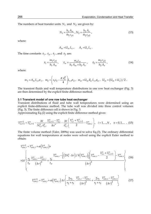
Evaporation, Condensation and Heat Transfer
266
The numbers of heat transfer units 1N and 2N are given by:
11
1 1
in
p
h ANm c
= , 22
2 2
o
p
h ANm c
= , (13)
where:
in in xA U L= , o o xA U L= .
The time constants 1τ , wτ , fτ , and 2τ are:
1 11
1
p
in
m ch A
τ = , 1 2
w ww
in o
m ch A h A
τ =+
, 2 22
2
p
o
m ch A
τ = , (14)
where:
1 1in xm A L ρ= , 2
2 1 2 24o
xdm s s Lπ ρ
⎛ ⎞= −⎜ ⎟⎜ ⎟⎝ ⎠
, w m w x wm U Lδ ρ= , ( ) / 2m in oU U U= + .
The transient fluids and wall temperature distributions in one row heat exchanger (Fig. 3) are then determined by the explicit finite difference method.
3.1 Transient model of one row tube heat exchanger Transient distributions of fluid and tube wall temperatures were determined using an explicit finite-difference method. The tube wall was divided into three control volumes (Fig. 3). The finite difference cell is shown in Fig. 3. Approximating Eq.(2) using the explicit finite difference method gives:
1, 1, 11, 1 1,11, 1 1, 1 ,
1, 1, 1, 2
n nn ni ii in n n
i i ww in n ni i i
T TT Tt tT T TN xτ τ
++++ + +
⎛ ⎞+−Δ Δ ⎜ ⎟= − − −⎜ ⎟Δ ⎝ ⎠
, 1,...,i N= , 0,1,...n = . (15)
The finite volume method (Taler, 2009a) was used to solve Eq.(3). The ordinary differential equations for wall temperatures at nodes were solved using the explicit Euler method to obtain:
( )
( )
( ) ( )( )
1, , ,
1, 1, 1, 1 , , ,
, , 022 2
2 /2
n n nww i ww i wm i
n ni in n n n n
wm i wm i ww i ww in nwm i ww i
w w
T T T
T TT h r k T T T
T T rrtr rr r
α+
+
= + ×
⎧ ⎫⎛ ⎞+⎡ ⎤⎪ ⎪⎜ ⎟− ⋅ Δ − −⎢ ⎥⎣ ⎦⎪ ⎪⎜ ⎟−⎪ ⎪⎝ ⎠×Δ +⎨ ⎬Δ Δ⎪ ⎪
⎪ ⎪⎪ ⎪⎩ ⎭
(16)
( )( ) ( ), , , ,1 3 2
, , , 2 22 3 2 3
2 2n n n nwz i wm i ww i wm in n n
wm i wm i wm iT T T Tr rT T T t
r r r rr rα+
⎡ ⎤− −⎢ ⎥= + Δ ⋅ +⎢ ⎥+ +Δ Δ⎣ ⎦
(17)
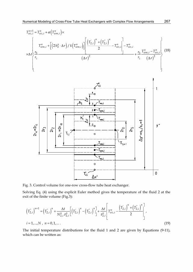
Numerical Modeling of Cross-Flow Tube Heat Exchangers with Complex Flow Arrangements
267
( )
( ) ( ) ( ) ( )
( ) ( )
1, , ,
' ''2 , 2,
, 2 , , ,
, ,5 32 2
2 /2
n n nwz i wz i wm i
n ni in n n n n
wm i wm i wz i wz in nwm i wz i
z z
T T T
T TT h r k T T T
T Tr rtr rr r
α+ = + ×
⎧ ⎫⎡ ⎤+⎪ ⎪⎢ ⎥⎡ ⎤+ ⋅ Δ − −⎪ ⎪⎢ ⎥⎢ ⎥⎣ ⎦⎪ ⎪⎢ ⎥ −⎪ ⎪⎣ ⎦×Δ +⎨ ⎬Δ Δ⎪ ⎪
⎪ ⎪⎪ ⎪⎪ ⎪⎩ ⎭
(18)
Fig. 3. Control volume for one-row cross-flow tube heat exchanger.
Solving Eq. (4) using the explicit Euler method gives the temperature of the fluid 2 at the exit of the finite volume (Fig.3):
( ) ( ) ( ) ( ) ( ) ( )' ''1 2, 2,'' '' ' ''
2, 2, 2, 2, ,2, 2, 2, 2
n nn n n n i in
i i i i wz in n ni i i
T Tt tT T T T TN τ τ
+⎡ ⎤+⎢ ⎥Δ Δ⎡ ⎤= + − + −⎢ ⎥⎢ ⎥
⎣ ⎦ ⎢ ⎥⎣ ⎦
,
1,...,i N= , 0,1,...n = . (19)
The initial temperature distributions for the fluid 1 and 2 are given by Equations (9-11), which can be written as:
Evaporation, Condensation and Heat Transfer
268
0, 0 ,ww i t ww iT T= = , 0
, 0 ,wm i t wm iT T= = , 0, 0 ,wz i t wz iT T= = , 1,...,i N= , (20)
where the symbols 0,ww iT , 0
,wm iT , and 0,wz iT denote the wall temperatures at the nodes.
The boundary conditions for fluids are given by Equations (5) and (8). The presented finite difference method is accurate and easy to program. In order to assure the stability of the calculations, the Courant conditions for both fluids and the stability condition for the Fourier equation defining transient heat conduction in the tube wall, should be satisfied.
4. Mathematical model of convective superheater The flow arrangement and division of the first stage convective superheater into finite volumes is depicted in Fig. 4. The superheated steam and the combustion products flow at right angles to each other. The first stage of a convective superheater can be classified according to flow arrangement as a mixed-cross-flow heat exchanger. The superheater tubes are arranged in-line (Fig. 5b). Each individual pass consists of two tubes through which superheated steam flows parallel. The tube’s outer surface is covered with a layer of ash deposits. In the following, finite volume heat balance equations will be formulated for the steam, the tube wall, and the flue gas. A steam side energy balance for the ith finite volume gives (Fig. 5a):
, , 1, , 1, 1, , 10 02
s i s iT Ts i s is ps s i in s w i s ps s i
T Tm c T d x h T m c Tπ ++
++⎛ ⎞
+ Δ − =⎜ ⎟⎝ ⎠
, (21)
Rearranging Eq. (21) gives
( ), 1
,
, , 1, 1 , 1, 2
s i
s i
T s i s is ps s i s i in s w iT
T Tm c T T A h T+ +
++⎛ ⎞
− =Δ −⎜ ⎟⎝ ⎠
, (22)
where the mesh tube inner surface is
in inA d xπΔ = Δ (23)
The steam average specific heat at constant pressure is given by:
( ) ( ), 1
,
, , 1,2
s i
s i
T ps s i ps s ips ps iT
c T c Tc c+ ++
≈ = (24)
After rewriting Eq. (22) in the form
, 1 , , 1,,
1 11 22
s i s ps i s in s i s in w is ps i s in
T m c h A T h A Tm c h A
+⎡ ⎤⎛ ⎞= − Δ + Δ⎢ ⎥⎜ ⎟⎝ ⎠⎣ ⎦+ Δ
, 1,...,i N= , (25)
the Gauss-Seidel method can be applied for an iterative solving nonlinear set of algebraic equations (25). Introducing the mesh number of transfer units for the steam:
( ) ( )1, ,2 , , 1
2s in s ins i s ps i s ps s i ps s i
h A h ANm c m c T c T+
+
Δ ΔΔ = =
⎡ ⎤+⎢ ⎥⎣ ⎦
(26)
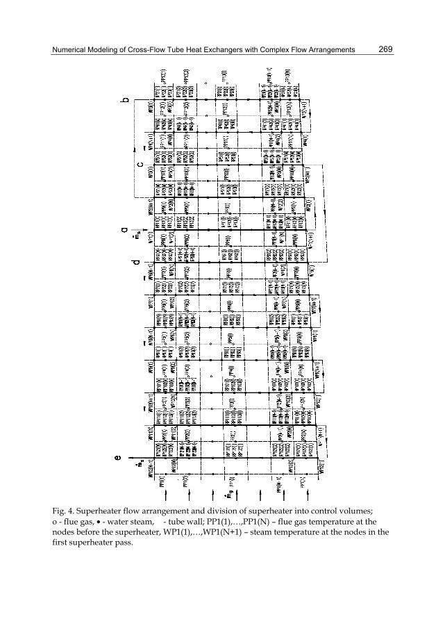
Numerical Modeling of Cross-Flow Tube Heat Exchangers with Complex Flow Arrangements
269
Fig. 4. Superheater flow arrangement and division of superheater into control volumes; o - flue gas, • - water steam, - tube wall; PP1(1),…,PP1(N) – flue gas temperature at the nodes before the superheater, WP1(1),…,WP1(N+1) – steam temperature at the nodes in the first superheater pass.
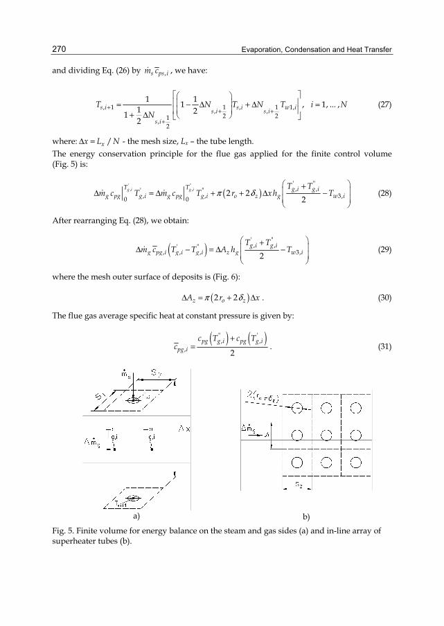
Evaporation, Condensation and Heat Transfer
270
and dividing Eq. (26) by ,s ps im c , we have:
, 1 1 , 1 1,, ,2 21,
2
1 11 , 1, ... ,1 212
s i s i w is i s is i
T N T N T i NN
+ + +
+
⎡ ⎤⎛ ⎞⎢ ⎥⎜ ⎟= − Δ + Δ =⎜ ⎟⎢ ⎥+ Δ ⎝ ⎠⎣ ⎦
(27)
where: /xx L NΔ = - the mesh size, Lx – the tube length. The energy conservation principle for the flue gas applied for the finite control volume (Fig. 5) is:
( )' ", ,
' ", ,' "
, , 3,0 02 2
2g i g iT T g i g i
g pg g i g pg g i o z g w iT T
m c T m c T r x h Tπ δ⎛ ⎞+⎜ ⎟Δ = Δ + + Δ −⎜ ⎟⎝ ⎠
(28)
After rearranging Eq. (28), we obtain:
( )' ", ,' "
, , , 3,2g i g i
g pg i g i g i z g w iT T
m c T T A h T⎛ ⎞+⎜ ⎟Δ − = Δ −⎜ ⎟⎝ ⎠
(29)
where the mesh outer surface of deposits is (Fig. 6):
( )2 2z o zA r xπ δΔ = + Δ . (30)
The flue gas average specific heat at constant pressure is given by:
( ) ( )" '
, ,, 2
pg g i pg g ipg i
c T c Tc
+= . (31)
a)
b)
Fig. 5. Finite volume for energy balance on the steam and gas sides (a) and in-line array of superheater tubes (b).
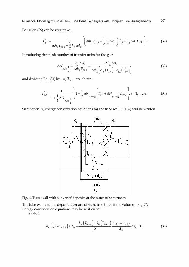
Numerical Modeling of Cross-Flow Tube Heat Exchangers with Complex Flow Arrangements
271
Equation (29) can be written as:
" ', , , 3,
,
1 11 22
g i g pg i g z g i g z w ig pg i g z
T m c h A T h A Tm c h A
⎡ ⎤⎛ ⎞= Δ − Δ + Δ⎢ ⎥⎜ ⎟⎝ ⎠⎣ ⎦Δ + Δ
. (32)
Introducing the mesh number of transfer units for the gas:
( ) ( )1 ' ", ,2 , ,
2g z g z
g i g pg i g pg g i pg g i
h A h AN
m c m c T c T+
Δ ΔΔ = =
Δ ⎡ ⎤Δ +⎢ ⎥⎣ ⎦
(33)
and dividing Eq. (33) by ,g pg im c we obtain:
" ', 1 , 1 3,, ,
2 21,2
1 11 , 1, ... , .1 212
g i g i w ig i g ig i
T N T N T i NN + +
+
⎡ ⎤⎛ ⎞⎢ ⎥⎜ ⎟= − Δ + Δ =⎜ ⎟⎢ ⎥+ Δ ⎝ ⎠⎣ ⎦
(34)
Subsequently, energy conservation equations for the tube wall (Fig. 6) will be written.
Fig. 6. Tube wall with a layer of deposits at the outer tube surfaces.
The tube wall and the deposit layer are divided into three finite volumes (Fig. 7). Energy conservation equations may be written as:
node 1
( ) ( ) ( )1, 2, 2, 1,, 1, 0
2w w i w w i w i w i
s s i w i in cw
k T k T T Th T T d dπ π
δ
+ −− + = , (35)
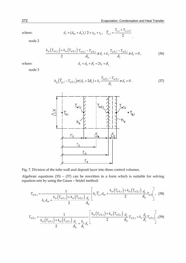
Evaporation, Condensation and Heat Transfer
272
where:
( ) , , 1,/ 2 ,
2s i s i
c in o in o s iT T
d d d r r T ++= + = + =
. node 2
( ) ( )1, 2, 1, 2, 3, 2, 0
2w w i w w i w i w i w i w i
c z sw z
k T k T T T T Td k dπ π
δ δ
+ − −+ = , (36)
where: 2s o z o zd d rδ δ= + = + . node 3
( ) ( ) 2, 3,, 3, 2 0w i w i
g g i w i o z z sz
T Th T T d k dπ δ π
δ−
− + + = . (37)
Fig. 7. Division of the tube wall and deposit layer into three control volumes.
Algebraic equations (35) – (37) can be rewritten in a form which is suitable for solving equation sets by using the Gauss – Seidel method:
( ) ( )( ) ( )1, 2,
1, , 21, 2,
12
2
w w i w w i cw i s s i in w
ww w i w w i cs in
w
k T k T dT h T d Tk T k T dh d
δ
δ
⎡ ⎤+⎢ ⎥= +⎢ ⎥+⎣ ⎦+
, (38)
( ) ( )( ) ( )1, 2,
2, 1, 3,1, 2,
12
2
w w i w w i c sw i w i z w i
w zw w i w w i c zs
w z
k T k T d dT T k Tk T k T d k d
δ δ
δ δ
⎡ ⎤+⎢ ⎥= +⎢ ⎥+⎣ ⎦+
, (39)
Numerical Modeling of Cross-Flow Tube Heat Exchangers with Complex Flow Arrangements
273
( )
( )3, , 2,1 2
2
sw i g o z g i z w i
zsg o z z
z
dT h d T k Tdh d k
δδ
δδ
⎡ ⎤= + +⎢ ⎥⎡ ⎤ ⎣ ⎦+ +⎢ ⎥⎣ ⎦
. (40)
Equations (38) – (40) can be used for building mathematical models of steam superheaters. To solve Eqs. (27), (34) and (38) – (40) two boundary conditions are prescribed: inlet steam temperature ,s inletT and flue gas temperature ,g inletT before the superheater:
,1(1) s inletWP T= and ,1( ) , 1,...,g inletPP I T I N= = (41)
5. Convection and radiation heat transfer coefficients
The convective heat transfer coefficient at the tube inner surface sh and the heat transfer on the flue gas side cgh were calculated using correlations given in (Kuznetsov et al., 1973). The effect of radiation on the heat transfer coefficient gh is accounted for by adding the radiation heat transfer coefficient rgh (Taler et al., 2009c; Kuznetsov et al., 1973) to the convective heat transfer, e.g. g cg rgh h h= + . For in-line arrays, in which tubes in successive rows are in-line in the direction of flue gas flow, the following correlation was used for calculating convective heat transfer coefficient
cgh (Kuznetsov et al., 1973):
0.65 0.330.2 Re Prcg s z g gNu C C= . (42)
Similar correlation was used for staggered tube arrays:
0.6 0.33Re Prcg s z g gNu C C= (43)
where: ( )2 /cg cg o z gNu h d kδ= + - Nusselt number, Re - Reynolds number, Pr - Prandtl number, ,s zC C - correction factors for tube arrangement and for the effect of number of tube rows in the array, respectively. The cross flow Reynolds number is given by: ( )maxRe /g g o z gw dρ δ μ= + , where gρ - density, gμ - dynamic viscosity, maxgw - maximum gas velocity, calculated for the minimum flow area between tubes normal to the local flow direction. For calculating the heat transfer coefficient on the steam side the well known Dittus – Boelter equation was used:
0.8 0.330.023Re Prs s s tNu C= (44)
where: tC - correction factor for surface-to-bulk physical property variations. The radiation heat transfer coefficients were also calculated using simple formulas, which are widely applied to the design of boilers and other heating equipment. The Standard Method (Kuznetsov et al., 1973; Kakaç, 1991) applies the following formula:
4 41
2g ww
rg gg w
T Th
T Tεσ ε
−+=−
(45)
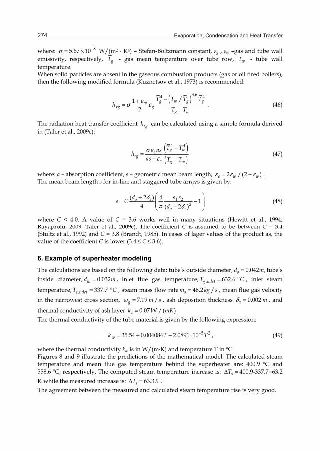
Evaporation, Condensation and Heat Transfer
274
where: 85.67 10σ −= × W/(m2 ⋅ K4) – Stefan-Boltzmann constant, εg , εw –gas and tube wall emissivity, respectively, gT - gas mean temperature over tube row, wT - tube wall temperature. When solid particles are absent in the gaseous combustion products (gas or oil fired boilers), then the following modified formula (Kuznetsov et al., 1973) is recommended:
( )3.64 4/1
2g w g gw
rg gg w
T T T Th
T Tεσ ε
−+=−
. (46)
The radiation heat transfer coefficient rgh can be calculated using a simple formula derived in (Taler et al., 2009c):
( )( )
4 4g we
rge g w
T Tashas T Tσ ε
ε
−=
+ − (47)
where: a – absorption coefficient, s – geometric mean beam length, 2 /(2 )e w wε ε ε= − . The mean beam length s for in-line and staggered tube arrays is given by:
1 22
( 2 ) 4 14 ( 2 )
o z
o z
s sds Cd
δπ δ
⎛ ⎞+= −⎜ ⎟⎜ ⎟+⎝ ⎠ (48)
where C < 4.0. A value of C = 3.6 works well in many situations (Hewitt et al., 1994; Rayaprolu, 2009; Taler et al., 2009c). The coefficient C is assumed to be between C = 3.4 (Stultz et al., 1992) and C = 3.8 (Brandt, 1985). In cases of lager values of the product as, the value of the coefficient C is lower (3.4 ≤ C ≤ 3.6).
6. Example of superheater modeling The calculations are based on the following data: tube’s outside diameter, 0.042 ,od m= tube’s inside diameter, 0.032ind m= , inlet flue gas temperature, , 632.6 ºg inletT C= , inlet steam
temperature, , 337.7 ºs inletT C= , steam mass flow rate 46.2 /sm kg s= , mean flue gas velocity in the narrowest cross section, 7.19 /gw m s= , ash deposition thickness 0.002z mδ = , and
thermal conductivity of ash layer 0.07 /( )zk W mK= . The thermal conductivity of the tube material is given by the following expression:
5 235.54 0.004084 2.0891 10wk T T−= + − ⋅ , (49)
where the thermal conductivity kw is in W/(m⋅K) and temperature T in ºC. Figures 8 and 9 illustrate the predictions of the mathematical model. The calculated steam temperature and mean flue gas temperature behind the superheater are: 400.9 ºC and 558.6 ºC, respectively. The computed steam temperature increase is: sTΔ = 400.9-337.7=63.2 K while the measured increase is: 63.3sT KΔ = . The agreement between the measured and calculated steam temperature rise is very good.
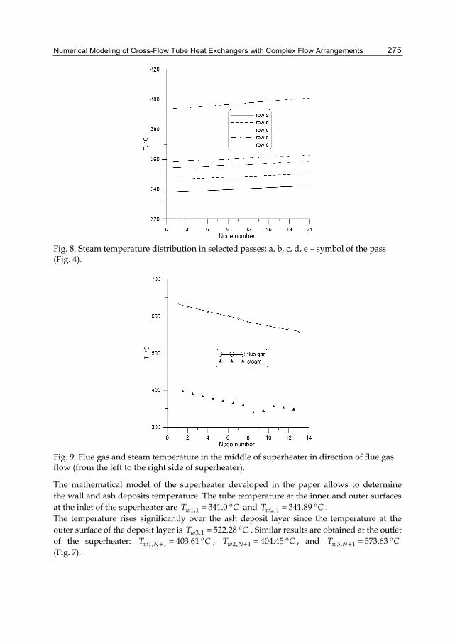
Numerical Modeling of Cross-Flow Tube Heat Exchangers with Complex Flow Arrangements
275
Fig. 8. Steam temperature distribution in selected passes; a, b, c, d, e – symbol of the pass (Fig. 4).
Fig. 9. Flue gas and steam temperature in the middle of superheater in direction of flue gas flow (from the left to the right side of superheater).
The mathematical model of the superheater developed in the paper allows to determine the wall and ash deposits temperature. The tube temperature at the inner and outer surfaces at the inlet of the superheater are 1,1 341.0 ºwT C= and 2,1 341.89 ºwT C= . The temperature rises significantly over the ash deposit layer since the temperature at the outer surface of the deposit layer is 3,1 522.28 ºwT C= . Similar results are obtained at the outlet of the superheater: 1, 1 403.61 ºw NT C+ = , 2, 1 404.45 ºw NT C+ = , and 3, 1 573.63 ºw NT C+ = (Fig. 7).
Evaporation, Condensation and Heat Transfer
276
It can be seen from the inspection of the results that the ash layer has a great influence on the temperature of ash deposit layer. With an increasing ash deposit layer the heat flow rate from the flue gas to the steam decreases since the temperature difference between the flue gas and ash deposit surface drops.
7. Conclusions Cross-flow tube heat exchangers find many applications in practice. An example of such an exchanger is a steam superheater, where the steam flows inside the tubes while heating flue gas flows across the tube bundles. The mathematical derivation of an expression for the mean temperature difference becomes quite complex for multi-pass cross-flow heat exchangers with many tube rows and complex flow arrangement. When calculating the heat transfer rate, the usual procedure is to modify the simple counter-flow LMTD (Logarithmic Mean Temperature Difference) method by a correction FT determined for a particular arrangement. The heat flow rate Q transferred from the hot to cool fluid is the product of the overall heat transfer coefficient UA, heat transfer area A, correction factor FT and logarithmic mean temperature difference ΔTlm. The heat transfer equation then takes the form: A T lmQ U A F T= Δ . However, to calculate the steam, flue gas and wall temperature distributions, a numerical model of the superheater is indispensable. Superheaters are the tube bundles that attain the highest temperatures in a boiler and consequently require the greatest care in the design and operation. The complex superheater tube arrangements permit the economic trade-off between material unit costs and surface area required to obtain the prescribed steam outlet temperature. Very often, various alloy steels are used for each pass in modern boilers. High temperature heat exchangers, like steam superheaters, are difficult to model since the tubes receive energy from the flue gas by two heat transfer modes: convection and radiation. The division of superheaters into two types: convection and radiant superheaters is based on the mode of heat transfer that is predominant. In convection superheaters, the portion of heat transfer by radiation from the flue gas is small. A radiant superheater absorbs heat primarily by thermal radiation from the flue gas with little convective heat flow rate. The share of convection in the total heat exchange of platen superheaters located directly over the combustion chamber amounts only to 10 to 15%. In convective superheaters, the share of radiation heat exchange is lower, but cannot be neglected. Correct determination of the heat flux absorbed through the boiler heating surfaces is very difficult. This results, on the one hand, from the complexity of heat transfer by radiation of flue gas with a high content of solid ash particles, and on the other hand, from the fouling of heating surfaces by slag and ash. The degree of the slag and ash deposition is hard to assess, both at the design stage and during the boiler operation. In consequence, the proper size of superheaters can be adjusted after taking the boiler into operation. In cases when the temperature of superheated steam at the exit from the superheater stage under examination is higher than design value, then the area of the surface of this stage has to be decreased. However, if the exit temperature of the steam is below the desired value, then the surface area is increased. To overcome the difficulties mentioned above, the general principles of mathematical modeling of steady-state and unsteady heat transfer in cross-flow tube heat exchangers with complex flow arrangements which allow of the simulation of multipass heat exchangers with many tube rows were presented. The finite volume method (FVM) was used to derive the algebraic equation system for determining flue gas, wall, and steam temperature at the
Numerical Modeling of Cross-Flow Tube Heat Exchangers with Complex Flow Arrangements
277
nodes of the finite volumes. A numerical model of multipass steam superheater with twelve passes was developed. The convection and radiation heat transfer was accounted for on the flue gas side. In addition, the deposit layer was assumed to cover the outer surface of the tubes. The calculation results were compared with the experimental data. The computed steam temperature increase over the entire superheater corresponds very well with the measured steam temperature rise. The developed modeling technique can especially be used for modeling tube heat exchangers when detail information on the tube wall temperature distribution is needed.
8. Symbols a - absorption coefficient, 1/m A - area, m2
inA , oA - inside and outside cross section area of the tube, m2 c - specific heat, J/(kg⋅K) c - mean specific heat, J/(kg⋅K)
pc - specific heat at constant pressure, J/(kg⋅K) FT - correction factor for a particular flow arrangement, h - heat transfer coefficient, W/(m2⋅K) k - thermal conductivity, W/(m⋅K)
xL - tube length in the heat exchanger, m Nu - Nusselt number m - mass, kg m - mass flow rate, kg/s Pr - Prandtl number Q - heat flow rate, W r - radius, m Re - Reynolds number s1 - pitch of tubes in plane perpendicular to flow (height of fin), m s2 - pitch of tubes in direction of flow, m t - time, s T - temperature, °C
'2T , ''
2T - gas temperature before and after tube row, °C U - perimeter, m UA - overall heat transfer coefficient, W/(m2⋅K)
inU , oU - inner and outer perimeter of the oval tube, respectively, m w - fluid velocity, m/s x, y, z - Cartesian coordinates
/ xx x L+ = - dimensionless coordinate
2/y y s+ = - dimensionless coordinate
8.1 Greek symbols /( )k cα ρ= - thermal diffusivity, m2/s
gmΔ - flue gas mass flow rate through the control volume , kg/s,
Evaporation, Condensation and Heat Transfer
278
TΔ - temperature difference, K xΔ , yΔ - control volume size in x and y direction, m
1 /x N+Δ = - dimensionless control volume size δ - thickness, m, ε - emissivity, ρ - density, kg/m3 τ - time constant, s
8.2 Subscripts g - flue gas lm - logarithmic mean m - mean r - tube s - steam w - wall in - inner o - outer 1 - fluid flowing inside the tube 2 - fluid flowing in perpendicular direction to tubes
9. References Brandt, F. (1985). Wärmeübertragung in Dampferzeugern und Wärmetauschern, FDBR-
Fachverband Dampfkessel-Behälter- und Rohrleitungsbau, ISBN 3-8027-2535-2 Vulkan-Verlag, Essen
Hewitt G. F., Shires G. L., Bott T.R. (1994). Process heat transfer, CRC Press, ISBN 0-8493-9918-1, Boca Raton
Kakaç, S., Boilers (1991). Evaporators, and Condensers, Wiley, ISBN 0471621706, New York, Kröger D. G. (2004). Air-cooled Heat Exchangers and Cooling Towers, ISBN 0820603007,
Chemical Publishing Company, New York, USA Kuznetsov N. V., Mitor V.V., Dubovskij I.E., Karasina E.S., Editors (1973). Standard Methods
of Thermal Design for Power Boilers, Central Boiler and Turbine Institute, Energija, UDK 621 181 001 24 : 536 7 (083 75), Moscow, (in Russian)
Rayaprolu K.(2009). Boilers for Power and Process, CRC Press, ISBN 978-14200-7536-6, Boca Raton
Stultz S.C., Kitto J.B., Editors (1992). Steam. Its Generation and Use., The Babcock & Wilcox Company, Fortieth edition, ISBN 09634570-0-4, Barberton, Ohio
Taler D. (2009a). Dynamics of Tube Heat Exchangers, University of Science Publishing Hous (UNWD AGH), ISSN 0867-6631, Cracow (in Polish)
Taler J., Trojan M., Taler D. (2009b). Archives of Thermodynamcs, Vol. 30, No. 2, 59 – 76, ISSN 1231 - 0956
Taler J., Taler D. (2009c). Heat Transfer Engineering, 30, 661-669, ISSN 0145-7632
14
Metal Foam Effective Transport Properties Jean-Michel Hugo1,2, Emmanuel Brun3 and Frédéric Topin1
1IUSTI Laboratory CNRS UMR 6595, Université de Provence, 2MOTA S.A. Cooling System, Z.I. les Paluds,
3European Synchrotron Radiation Facility, France
1. Introduction Solid foams are a relatively new class of multifunctional materials that present attractive thermal, mechanical, electrical and acoustic properties. Moreover, they also promote mixing and have excellent specific mechanical properties. They are widely quoted to present a random topology, high open porosity, low relative density and high thermal conductivity of the cell edges, large accessible surface area per unit volume (Ashby et al., 2000). Usually, geometric properties such as high tortuosity and high specific surface are proposed to explain their properties, although fluid tortuosity is close to 1 and specific surface is usually smaller than 10000m²/m3. They are nowadays proposed for their use in numerous applications such as compact heat exchangers, reformers, biphasic cooling systems and spreaders. They are also used in high-power batteries for lightweight cordless electronics, and catalytic field application such as fuel cells systems (Catillon et al., 2004; Dukhan et al., 2005; Mahjoob & Vafai, 2008; Tadrist et al., 2004). In this chapter, we expose experimental and numerical tools to determine effective transport properties of metal foam for mono-and-biphasic flow.
2. Representative volume element Definitions of a continuous medium equivalent to the real porous structure, as well as the definition of the applicability level of the macroscopic model, constitutes a tricky problem that has long been debated (Auriault, 1991; Baveye & Sposito, 1984; Marle, 1982; Quintard & Whitaker, 1991) among others. The forms of the used phenomenological laws have been obtained from correlations resulting from experiments and not from physical laws. The valuable expressions are much diversified and the choice for one or the other is only justified when compared with specific experiments. We thus consider, classically, that the foam could be assimilated to a homogeneous equivalent medium (Dullien, 1992). Thus, each measured quantities will not describe the foam sample itself, but rather a homogeneous media which has the same properties. There is yet no theoretical evidence to justify this assumption. Thus, we only consider that this condition is satisfied when the considered phenomenon occurs on a sufficient distance. Determination of a Rve is thus evaluation of the relevant distance for the considered observation.
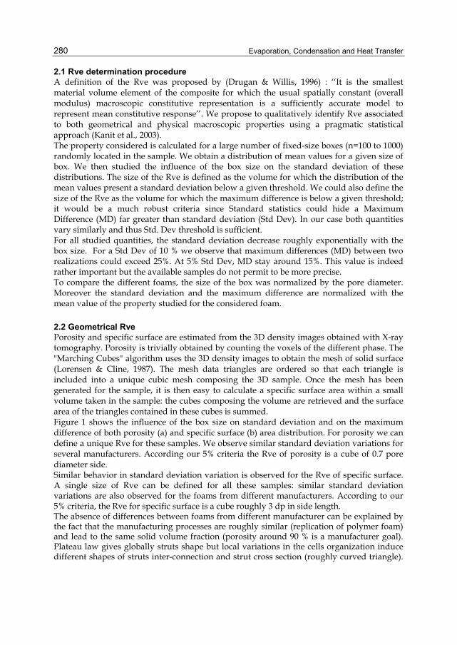
Evaporation, Condensation and Heat Transfer
280
2.1 Rve determination procedure A definition of the Rve was proposed by (Drugan & Willis, 1996) : ‘‘It is the smallest material volume element of the composite for which the usual spatially constant (overall modulus) macroscopic constitutive representation is a sufficiently accurate model to represent mean constitutive response’’. We propose to qualitatively identify Rve associated to both geometrical and physical macroscopic properties using a pragmatic statistical approach (Kanit et al., 2003). The property considered is calculated for a large number of fixed-size boxes (n=100 to 1000) randomly located in the sample. We obtain a distribution of mean values for a given size of box. We then studied the influence of the box size on the standard deviation of these distributions. The size of the Rve is defined as the volume for which the distribution of the mean values present a standard deviation below a given threshold. We could also define the size of the Rve as the volume for which the maximum difference is below a given threshold; it would be a much robust criteria since Standard statistics could hide a Maximum Difference (MD) far greater than standard deviation (Std Dev). In our case both quantities vary similarly and thus Std. Dev threshold is sufficient. For all studied quantities, the standard deviation decrease roughly exponentially with the box size. For a Std Dev of 10 % we observe that maximum differences (MD) between two realizations could exceed 25%. At 5% Std Dev, MD stay around 15%. This value is indeed rather important but the available samples do not permit to be more precise. To compare the different foams, the size of the box was normalized by the pore diameter. Moreover the standard deviation and the maximum difference are normalized with the mean value of the property studied for the considered foam.
2.2 Geometrical Rve Porosity and specific surface are estimated from the 3D density images obtained with X-ray tomography. Porosity is trivially obtained by counting the voxels of the different phase. The "Marching Cubes" algorithm uses the 3D density images to obtain the mesh of solid surface (Lorensen & Cline, 1987). The mesh data triangles are ordered so that each triangle is included into a unique cubic mesh composing the 3D sample. Once the mesh has been generated for the sample, it is then easy to calculate a specific surface area within a small volume taken in the sample: the cubes composing the volume are retrieved and the surface area of the triangles contained in these cubes is summed. Figure 1 shows the influence of the box size on standard deviation and on the maximum difference of both porosity (a) and specific surface (b) area distribution. For porosity we can define a unique Rve for these samples. We observe similar standard deviation variations for several manufacturers. According our 5% criteria the Rve of porosity is a cube of 0.7 pore diameter side. Similar behavior in standard deviation variation is observed for the Rve of specific surface. A single size of Rve can be defined for all these samples: similar standard deviation variations are also observed for the foams from different manufacturers. According to our 5% criteria, the Rve for specific surface is a cube roughly 3 dp in side length. The absence of differences between foams from different manufacturer can be explained by the fact that the manufacturing processes are roughly similar (replication of polymer foam) and lead to the same solid volume fraction (porosity around 90 % is a manufacturer goal). Plateau law gives globally struts shape but local variations in the cells organization induce different shapes of struts inter-connection and strut cross section (roughly curved triangle).
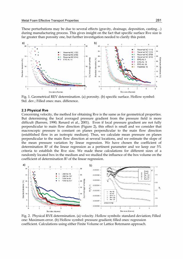
Metal Foam Effective Transport Properties
281
These perturbations may be due to several effects (gravity, drainage, deposition, casting…) during manufacturing process. This gives insight on the fact that specific surface Rve size is far greater than porosity one, but further investigation needed to clarify this point.
Fig. 1. Geometrical REV determination. (a) porosity. (b) specific surface. Hollow symbol: Std. dev.; Filled ones: max. difference.
2.3 Physical Rve Concerning velocity, the method for obtaining Rve is the same as for geometrical properties. But determining the local averaged pressure gradient from the pressure field is more difficult (Barrere, 1990; Renard et al., 2001). Even if local pressure gradient are not fully perpendicular to main flow direction (Figure 2), this effect is small and we consider that macroscopic pressure is constant on planes perpendicular to the main flow direction (established flow in an isotropic medium). Thus, we calculate mean pressure on planes perpendicular to the main flow direction at several locations, and we estimate the slope of the mean pressure variation by linear regression. We have chosen the coefficient of determination R2 of the linear regression as a pertinent parameter and we keep our 5% criteria to establish the Rve size. We made these calculations for different sizes of a randomly located box in the medium and we studied the influence of the box volume on the coefficient of determination R2 of the linear regression.
Fig. 2. Physical RVE determination. (a) velocity. Hollow symbols: standard deviation; Filled one: Maximum error. (b) Hollow symbol: pressure gradient; filled ones: regression coefficient. Calculations using either Finite Volume or Lattice Botzmann approach.
Evaporation, Condensation and Heat Transfer
282
Figure 2.a shows the influence of the box size on standard deviation and on the maximum difference of mean velocity. To establish Rve for the mean velocity value, we used the velocity field obtained from the computations (§3.3). No clear influence of the Reynolds number on RVE size can be identified for both methods on the studied range. We observe that for simulation, a box of 3 dp side seems to be sufficient to define the mean velocity for these Reynolds numbers. Figure 2.b presents the estimation of the pressure gradient by a linear regression and its coefficient of determination R2, for different volumes and different Reynolds numbers. The estimate of the pressure gradient is quite constant for a box 3 pore diameters in size and the associated coefficient of regression R2 is good (> 0.99). As a result, 3 pore diameters are sufficient to establish pressure drop Rve.
3. Single-phase flow 3.1 Flow law It is well known that flows at very low flow rates through a porous medium are governed by Darcy’s law (Darcy, 1856).
dP μ- = udz K
(1)
Where dP/dz is the pressure gradient along the main flow z-direction, µ the dynamic viscosity, u is Darcy’s or the seepage velocity and K (m²) is the permeability (or Darcy’s permeability) of the medium. For homogeneous porous media, a nonlinear relationship between the pressure drop and the flow rate characterize “high-velocity” flows. At high Reynolds number (strong inertia regime), the empirical Forchheimer equation is used to account for the deviation from Darcy’s law (incompressible fluid) (Eq.2) or extended to compressible fluid and expressed as a function of mass flow rate (Eq.3).
2dP(z) μ- = u +βρudz K
⎛ ⎞⎜ ⎟⎝ ⎠
(2)
2dρ(z)P(z) μ- = η+βηdz K
⎛ ⎞⎜ ⎟⎝ ⎠
(3)
Where ρ (kg.m-3) is the fluid density, η (kg.m-2.s-1) the mass flow rate and β (m−1) the inertia factor or the non-Darcy flow coefficient. In this formulation the Brinkman correction is neglected. That means that the pressure drop is considered as the sum of two terms: viscous (u, Darcy law) and inertia (u2) terms. Several authors have shown that the onset of the non-linear behavior (that is sometime called the weak inertia regime) may be described by a cubic law (Firdaous et al., 1997; Mei & Auriault, 1993; Wodie & Levy, 1991):
2
3dP μ ρ- = u + udz K μ
γ ⋅ (4)
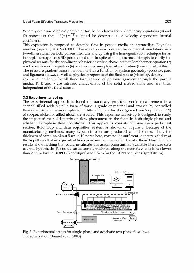
Metal Foam Effective Transport Properties
283
Where γ is a dimensionless parameter for the non-linear term. Comparing equations (4) and (2) shows up that ( ) γρβ u = u
μ could be described as a velocity dependant inertial
coefficient. This expression is proposed to describe flow in porous media at intermediate Reynolds number (typically 10<Re<10000). This equation was obtained by numerical simulations in a two-dimensional periodic porous medium, and by using the homogenization technique for an isotropic homogeneous 3D porous medium. In spite of the numerous attempts to clarify the physical reasons for the non-linear behavior described above, neither Forchheimer equation (2) nor the weak inertia equation (4) have received any physical justification (Fourar et al., 2004). The pressure gradient across the foam is thus a function of system geometry (porosity, pore and ligament size...), as well as physical properties of the fluid phase (viscosity, density). On the other hand, for all three formulations of pressure gradient through the porous media, K, β and γ are intrinsic characteristic of the solid matrix alone and are, thus, independent of the fluid nature.
3.2 Experimental set up The experimental approach is based on stationary pressure profile measurement in a channel filled with metallic foam of various grade or material and crossed by controlled flow rates. Several foam samples with different characteristics (grade from 5 up to 100 PPI) of copper, nickel, or allied nickel are studied. This experimental set-up is designed, to study the impact of the solid matrix on flow phenomena in the foam in both single-phase and adiabatic two-phase flow conditions. This apparatus consists of three main parts: test section, fluid loop and data acquisition system as shown on Figure 3. Because of the manufacturing methods, many types of foam are produced as flat sheets. Thus, the thickness of samples, about 5 up to 10 pores here, may not be sufficient to insure validity of the hypothesis that an equivalent homogeneous material could describe them. However, our results show nothing that could invalidate this assumption and all available literature data use this hypothesis. For tested cases, sample thickness along the main flow axis is not lower than 2.5mm for the 100PPI (Dp=500µm) and 2.5cm for the 10 PPI samples (Dp=5000µm).
Fig. 3. Experimental set-up for single-phase and adiabatic two-phase flow laws characterization (Bonnet et al., 2008).
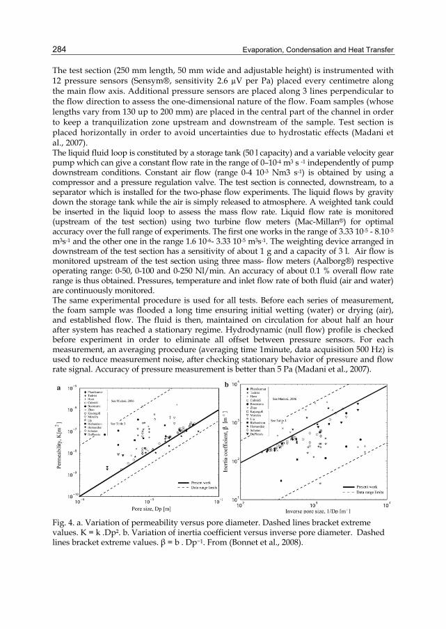
Evaporation, Condensation and Heat Transfer
284
The test section (250 mm length, 50 mm wide and adjustable height) is instrumented with 12 pressure sensors (Sensym®, sensitivity 2.6 µV per Pa) placed every centimetre along the main flow axis. Additional pressure sensors are placed along 3 lines perpendicular to the flow direction to assess the one-dimensional nature of the flow. Foam samples (whose lengths vary from 130 up to 200 mm) are placed in the central part of the channel in order to keep a tranquilization zone upstream and downstream of the sample. Test section is placed horizontally in order to avoid uncertainties due to hydrostatic effects (Madani et al., 2007). The liquid fluid loop is constituted by a storage tank (50 l capacity) and a variable velocity gear pump which can give a constant flow rate in the range of 0–10-4 m3 s -1 independently of pump downstream conditions. Constant air flow (range 0-4 10-3 Nm3 s-1) is obtained by using a compressor and a pressure regulation valve. The test section is connected, downstream, to a separator which is installed for the two-phase flow experiments. The liquid flows by gravity down the storage tank while the air is simply released to atmosphere. A weighted tank could be inserted in the liquid loop to assess the mass flow rate. Liquid flow rate is monitored (upstream of the test section) using two turbine flow meters (Mac-Millan®) for optimal accuracy over the full range of experiments. The first one works in the range of 3.33 10-5 - 8.10-5 m3s-1 and the other one in the range 1.6 10-6- 3.33 10-5 m3s-1. The weighting device arranged in downstream of the test section has a sensitivity of about 1 g and a capacity of 3 l. Air flow is monitored upstream of the test section using three mass- flow meters (Aalborg®) respective operating range: 0-50, 0-100 and 0-250 Nl/min. An accuracy of about 0.1 % overall flow rate range is thus obtained. Pressures, temperature and inlet flow rate of both fluid (air and water) are continuously monitored. The same experimental procedure is used for all tests. Before each series of measurement, the foam sample was flooded a long time ensuring initial wetting (water) or drying (air), and established flow. The fluid is then, maintained on circulation for about half an hour after system has reached a stationary regime. Hydrodynamic (null flow) profile is checked before experiment in order to eliminate all offset between pressure sensors. For each measurement, an averaging procedure (averaging time 1minute, data acquisition 500 Hz) is used to reduce measurement noise, after checking stationary behavior of pressure and flow rate signal. Accuracy of pressure measurement is better than 5 Pa (Madani et al., 2007).
Fig. 4. a. Variation of permeability versus pore diameter. Dashed lines bracket extreme values. K = k .Dp². b. Variation of inertia coefficient versus inverse pore diameter. Dashed lines bracket extreme values. β = b . Dp−1. From (Bonnet et al., 2008).
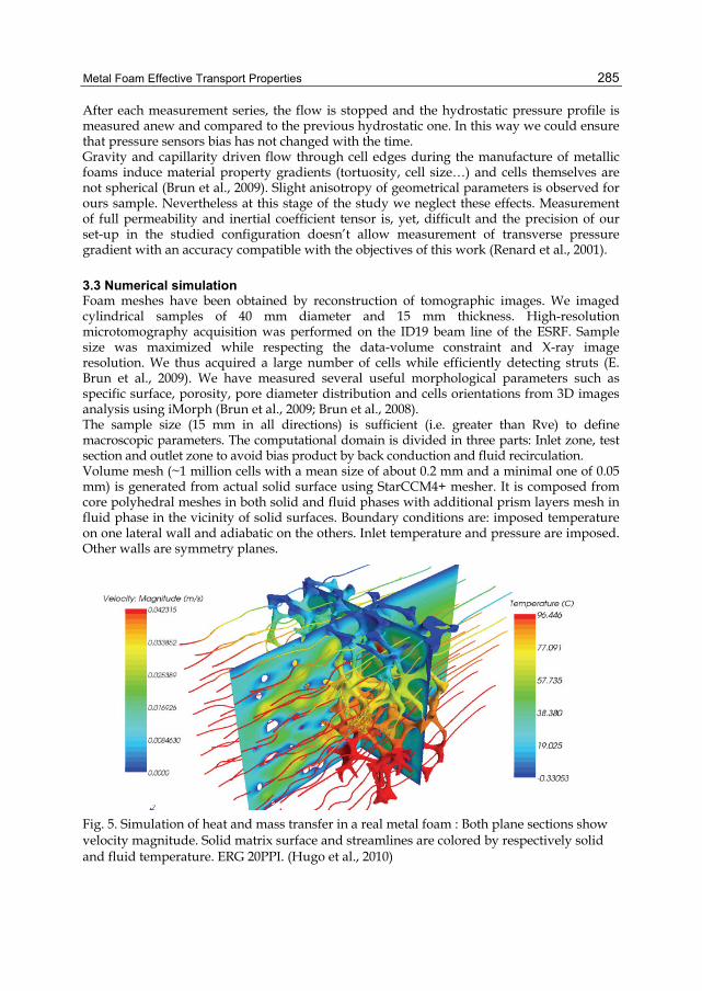
Metal Foam Effective Transport Properties
285
After each measurement series, the flow is stopped and the hydrostatic pressure profile is measured anew and compared to the previous hydrostatic one. In this way we could ensure that pressure sensors bias has not changed with the time. Gravity and capillarity driven flow through cell edges during the manufacture of metallic foams induce material property gradients (tortuosity, cell size…) and cells themselves are not spherical (Brun et al., 2009). Slight anisotropy of geometrical parameters is observed for ours sample. Nevertheless at this stage of the study we neglect these effects. Measurement of full permeability and inertial coefficient tensor is, yet, difficult and the precision of our set-up in the studied configuration doesn’t allow measurement of transverse pressure gradient with an accuracy compatible with the objectives of this work (Renard et al., 2001).
3.3 Numerical simulation Foam meshes have been obtained by reconstruction of tomographic images. We imaged cylindrical samples of 40 mm diameter and 15 mm thickness. High-resolution microtomography acquisition was performed on the ID19 beam line of the ESRF. Sample size was maximized while respecting the data-volume constraint and X-ray image resolution. We thus acquired a large number of cells while efficiently detecting struts (E. Brun et al., 2009). We have measured several useful morphological parameters such as specific surface, porosity, pore diameter distribution and cells orientations from 3D images analysis using iMorph (Brun et al., 2009; Brun et al., 2008). The sample size (15 mm in all directions) is sufficient (i.e. greater than Rve) to define macroscopic parameters. The computational domain is divided in three parts: Inlet zone, test section and outlet zone to avoid bias product by back conduction and fluid recirculation. Volume mesh (~1 million cells with a mean size of about 0.2 mm and a minimal one of 0.05 mm) is generated from actual solid surface using StarCCM4+ mesher. It is composed from core polyhedral meshes in both solid and fluid phases with additional prism layers mesh in fluid phase in the vicinity of solid surfaces. Boundary conditions are: imposed temperature on one lateral wall and adiabatic on the others. Inlet temperature and pressure are imposed. Other walls are symmetry planes.
Fig. 5. Simulation of heat and mass transfer in a real metal foam : Both plane sections show velocity magnitude. Solid matrix surface and streamlines are colored by respectively solid and fluid temperature. ERG 20PPI. (Hugo et al., 2010)
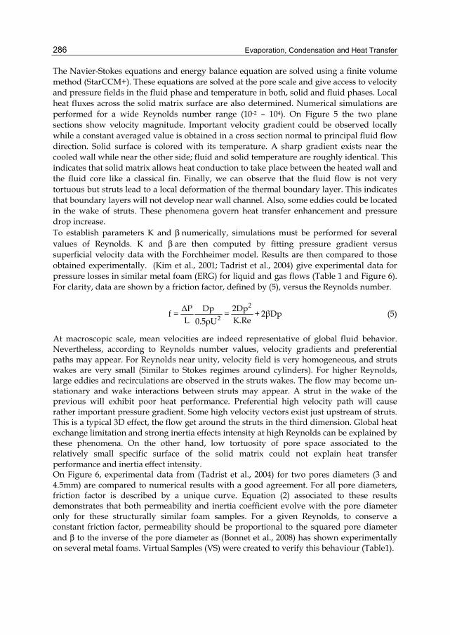
Evaporation, Condensation and Heat Transfer
286
The Navier-Stokes equations and energy balance equation are solved using a finite volume method (StarCCM+). These equations are solved at the pore scale and give access to velocity and pressure fields in the fluid phase and temperature in both, solid and fluid phases. Local heat fluxes across the solid matrix surface are also determined. Numerical simulations are performed for a wide Reynolds number range (10-2 – 104). On Figure 5 the two plane sections show velocity magnitude. Important velocity gradient could be observed locally while a constant averaged value is obtained in a cross section normal to principal fluid flow direction. Solid surface is colored with its temperature. A sharp gradient exists near the cooled wall while near the other side; fluid and solid temperature are roughly identical. This indicates that solid matrix allows heat conduction to take place between the heated wall and the fluid core like a classical fin. Finally, we can observe that the fluid flow is not very tortuous but struts lead to a local deformation of the thermal boundary layer. This indicates that boundary layers will not develop near wall channel. Also, some eddies could be located in the wake of struts. These phenomena govern heat transfer enhancement and pressure drop increase. To establish parameters K and β numerically, simulations must be performed for several values of Reynolds. K and β are then computed by fitting pressure gradient versus superficial velocity data with the Forchheimer model. Results are then compared to those obtained experimentally. (Kim et al., 2001; Tadrist et al., 2004) give experimental data for pressure losses in similar metal foam (ERG) for liquid and gas flows (Table 1 and Figure 6). For clarity, data are shown by a friction factor, defined by (5), versus the Reynolds number.
2
2ΔP Dp 2Dpf = = + 2βDpL K.Re0.5ρU
(5)
At macroscopic scale, mean velocities are indeed representative of global fluid behavior. Nevertheless, according to Reynolds number values, velocity gradients and preferential paths may appear. For Reynolds near unity, velocity field is very homogeneous, and struts wakes are very small (Similar to Stokes regimes around cylinders). For higher Reynolds, large eddies and recirculations are observed in the struts wakes. The flow may become un-stationary and wake interactions between struts may appear. A strut in the wake of the previous will exhibit poor heat performance. Preferential high velocity path will cause rather important pressure gradient. Some high velocity vectors exist just upstream of struts. This is a typical 3D effect, the flow get around the struts in the third dimension. Global heat exchange limitation and strong inertia effects intensity at high Reynolds can be explained by these phenomena. On the other hand, low tortuosity of pore space associated to the relatively small specific surface of the solid matrix could not explain heat transfer performance and inertia effect intensity. On Figure 6, experimental data from (Tadrist et al., 2004) for two pores diameters (3 and 4.5mm) are compared to numerical results with a good agreement. For all pore diameters, friction factor is described by a unique curve. Equation (2) associated to these results demonstrates that both permeability and inertia coefficient evolve with the pore diameter only for these structurally similar foam samples. For a given Reynolds, to conserve a constant friction factor, permeability should be proportional to the squared pore diameter and β to the inverse of the pore diameter as (Bonnet et al., 2008) has shown experimentally on several metal foams. Virtual Samples (VS) were created to verify this behaviour (Table1).
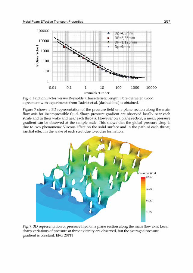
Metal Foam Effective Transport Properties
287
Fig. 6. Friction Factor versus Reynolds. Characteristic length: Pore diameter. Good agreement with experiments from Tadrist et al. (dashed line) is obtained.
Figure 7 shows a 3D representation of the pressure field on a plane section along the main flow axis for incompressible fluid. Sharp pressure gradient are observed locally near each struts and in their wake and near each throats. However on a plane section, a mean pressure gradient can be observed at the sample scale. This shows that the global pressure drop is due to two phenomena: Viscous effect on the solid surface and in the path of each throat; inertial effect in the wake of each strut due to eddies formation.
Fig. 7. 3D representation of pressure filed on a plane section along the main flow axis. Local sharp variations of pressure at throat vicinity are observed, but the averaged pressure gradient is constant. ERG 20PPI
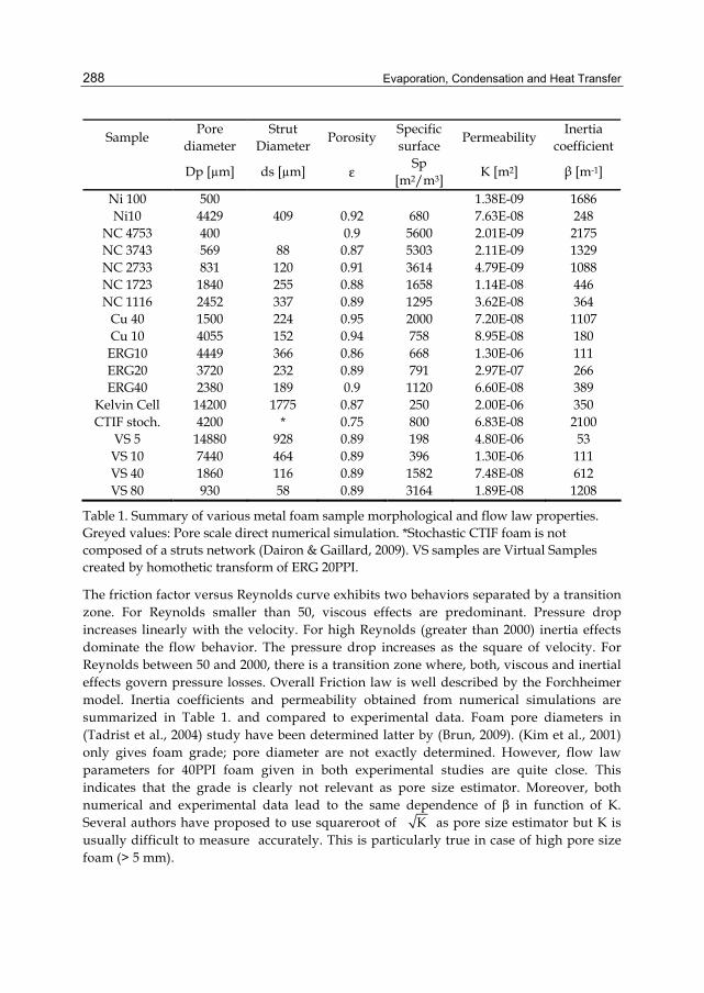
Evaporation, Condensation and Heat Transfer
288
Sample Pore diameter
Strut Diameter Porosity Specific
surface Permeability Inertia coefficient
Dp [µm] ds [µm] ε Sp
[m2/m3] K [m2] β [m-1]
Ni 100 500 1.38E-09 1686 Ni10 4429 409 0.92 680 7.63E-08 248
NC 4753 400 0.9 5600 2.01E-09 2175 NC 3743 569 88 0.87 5303 2.11E-09 1329 NC 2733 831 120 0.91 3614 4.79E-09 1088 NC 1723 1840 255 0.88 1658 1.14E-08 446 NC 1116 2452 337 0.89 1295 3.62E-08 364
Cu 40 1500 224 0.95 2000 7.20E-08 1107 Cu 10 4055 152 0.94 758 8.95E-08 180 ERG10 4449 366 0.86 668 1.30E-06 111 ERG20 3720 232 0.89 791 2.97E-07 266 ERG40 2380 189 0.9 1120 6.60E-08 389
Kelvin Cell 14200 1775 0.87 250 2.00E-06 350 CTIF stoch. 4200 * 0.75 800 6.83E-08 2100
VS 5 14880 928 0.89 198 4.80E-06 53 VS 10 7440 464 0.89 396 1.30E-06 111 VS 40 1860 116 0.89 1582 7.48E-08 612 VS 80 930 58 0.89 3164 1.89E-08 1208
Table 1. Summary of various metal foam sample morphological and flow law properties. Greyed values: Pore scale direct numerical simulation. *Stochastic CTIF foam is not composed of a struts network (Dairon & Gaillard, 2009). VS samples are Virtual Samples created by homothetic transform of ERG 20PPI.
The friction factor versus Reynolds curve exhibits two behaviors separated by a transition zone. For Reynolds smaller than 50, viscous effects are predominant. Pressure drop increases linearly with the velocity. For high Reynolds (greater than 2000) inertia effects dominate the flow behavior. The pressure drop increases as the square of velocity. For Reynolds between 50 and 2000, there is a transition zone where, both, viscous and inertial effects govern pressure losses. Overall Friction law is well described by the Forchheimer model. Inertia coefficients and permeability obtained from numerical simulations are summarized in Table 1. and compared to experimental data. Foam pore diameters in (Tadrist et al., 2004) study have been determined latter by (Brun, 2009). (Kim et al., 2001) only gives foam grade; pore diameter are not exactly determined. However, flow law parameters for 40PPI foam given in both experimental studies are quite close. This indicates that the grade is clearly not relevant as pore size estimator. Moreover, both numerical and experimental data lead to the same dependence of β in function of K. Several authors have proposed to use squareroot of K as pore size estimator but K is usually difficult to measure accurately. This is particularly true in case of high pore size foam (> 5 mm).
Metal Foam Effective Transport Properties
289
3.4 Heat transfer Direct experimental measurement of volume heat transfer coefficient is not easy for fluid flow crossing metal foam. Generally authors propose global heat transfer coefficient of a channel filled by a porous media (Kim et al., 2001). There are few works dealing with local heat transfer coefficient between fluid and solid phase (Serret, Stamboul, & Topin, 2007). However wall heat transfer coefficient is an averaging on different transport and diffusion properties on a known channel or heat exchanger geometry and can thus be used only in these cases. In the following section, we propose different analytical and numerical models to rely this coefficient and experimental or simulation data. Models can be used to determine heat transfer coefficient from data or to predict heat exchanger performance from the knowledge of thermal properties. Heat transfer law is also determined from direct numerical simulation performed on the real foam geometry (Hugo et al., 2010). Experimental set up described above is modified to perform heat transfer measurement. Thermocouples are added to measure local temperature along the main flow axis. Fluid flow can be heated before the channel or heat flux can be imposed on the channel wall. Two protocols are studied: • In the first case, the metal foam is heated by hot air flow and then cooled by air at
ambient temperature. Transient outlet temperature signal is used with .a 0D analytical model to evaluate heat transfer coefficient.
• In the second case, fluid flow at ambient temperature is imposed at the inlet. Heat flux is imposed on the channel wall. Temperature at the outlet is measured at steady state. A 2D two temperature model (non local thermal equilibrium (Moyne, 1997)) allows one determining numerically the heat transfer coefficient.
3.4.1 0D analytical model Metal foam is considered as thermally thin body and its temperature is considered as homogeneous and equals to Tm. Air flow temperature Ta is imposed at the channel inlet.
( ) ( ) ( )mp vol m fsolid
T1 C h T T 0t
∂− ε ⋅ ρ ⋅ ⋅ + ⋅ − =∂
(6)
in out exf in .
pfluid
T T PT T2
2 m C
+= = +⎛ ⎞
⋅ ⋅⎜ ⎟⎝ ⎠
(7)
Where ε (−) is the porosity, ρ(kg/m3) the metal density, Cp (J/kg/K) the metal heat capacity, η (kg/s) is air mass flow rate and hvol (W/m3/K) the volume heat transfer coefficient. Fluid temperature profile is considered as linear through the channel. A mean air temperature Tf is defined by (8).
( ) ( ) ( ) mex vol m f p solid
TP h V T T 1 V Ct
∂= ⋅ ⋅ − = − − ε ⋅ ⋅ ρ ⋅ ⋅∂
(8)
Previous equations lead to the following differential equation on foam temperature:
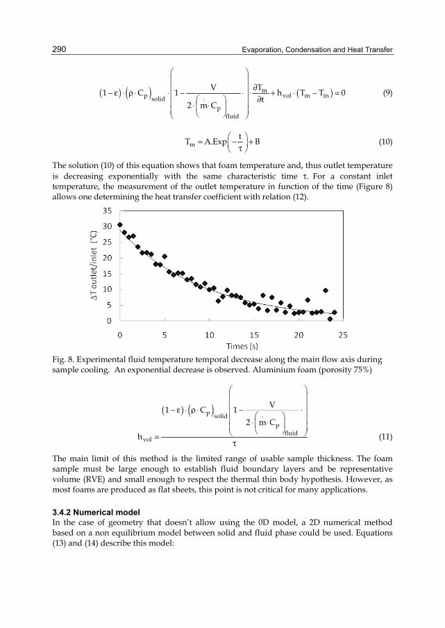
Evaporation, Condensation and Heat Transfer
290
( ) ( ) ( )mp vol m in.solid
pfluid
V T1 C 1 h T T 0t
2 m C
⎛ ⎞⎜ ⎟
∂⎜ ⎟− ε ⋅ ρ ⋅ ⋅ − ⋅ ⋅ + ⋅ − =⎜ ⎟ ∂⎛ ⎞⎜ ⎟⋅ ⋅⎜ ⎟⎜ ⎟⎝ ⎠⎝ ⎠
(9)
mtT A.Exp B⎛ ⎞= − +⎜ ⎟τ⎝ ⎠
(10)
The solution (10) of this equation shows that foam temperature and, thus outlet temperature is decreasing exponentially with the same characteristic time τ. For a constant inlet temperature, the measurement of the outlet temperature in function of the time (Figure 8) allows one determining the heat transfer coefficient with relation (12).
Fig. 8. Experimental fluid temperature temporal decrease along the main flow axis during sample cooling. An exponential decrease is observed. Aluminium foam (porosity 75%)
( ) ( )p .solidp
fluidvol
V1 C 12 m C
h
⎛ ⎞⎜ ⎟⎜ ⎟− ε ⋅ ρ ⋅ − ⋅⎜ ⎟⎛ ⎞⎜ ⎟⋅ ⋅⎜ ⎟⎜ ⎟⎝ ⎠⎝ ⎠=τ
(11)
The main limit of this method is the limited range of usable sample thickness. The foam sample must be large enough to establish fluid boundary layers and be representative volume (RVE) and small enough to respect the thermal thin body hypothesis. However, as most foams are produced as flat sheets, this point is not critical for many applications.
3.4.2 Numerical model In the case of geometry that doesn’t allow using the 0D model, a 2D numerical method based on a non equilibrium model between solid and fluid phase could be used. Equations (13) and (14) describe this model:
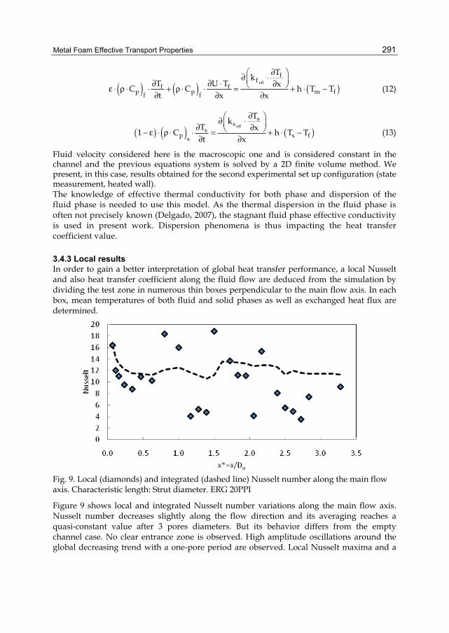
Metal Foam Effective Transport Properties
291
( ) ( ) ( )eff
ff
f fp p m ff f
TkT U T xC C h T Tt x x
∂⎛ ⎞∂ ⋅⎜ ⎟∂ ∂ ⋅ ∂⎝ ⎠ε ⋅ ρ ⋅ ⋅ + ρ ⋅ ⋅ = + ⋅ −∂ ∂ ∂
(12)
( ) ( ) ( )eff
ss
sp s fs
TkT x1 C h T Tt x
∂⎛ ⎞∂ ⋅⎜ ⎟∂ ∂⎝ ⎠− ε ⋅ ρ ⋅ ⋅ = + ⋅ −∂ ∂
(13)
Fluid velocity considered here is the macroscopic one and is considered constant in the channel and the previous equations system is solved by a 2D finite volume method. We present, in this case, results obtained for the second experimental set up configuration (state measurement, heated wall). The knowledge of effective thermal conductivity for both phase and dispersion of the fluid phase is needed to use this model. As the thermal dispersion in the fluid phase is often not precisely known (Delgado, 2007), the stagnant fluid phase effective conductivity is used in present work. Dispersion phenomena is thus impacting the heat transfer coefficient value.
3.4.3 Local results In order to gain a better interpretation of global heat transfer performance, a local Nusselt and also heat transfer coefficient along the fluid flow are deduced from the simulation by dividing the test zone in numerous thin boxes perpendicular to the main flow axis. In each box, mean temperatures of both fluid and solid phases as well as exchanged heat flux are determined.
Fig. 9. Local (diamonds) and integrated (dashed line) Nusselt number along the main flow axis. Characteristic length: Strut diameter. ERG 20PPI
Figure 9 shows local and integrated Nusselt number variations along the main flow axis. Nusselt number decreases slightly along the flow direction and its averaging reaches a quasi-constant value after 3 pores diameters. But its behavior differs from the empty channel case. No clear entrance zone is observed. High amplitude oscillations around the global decreasing trend with a one-pore period are observed. Local Nusselt maxima and a
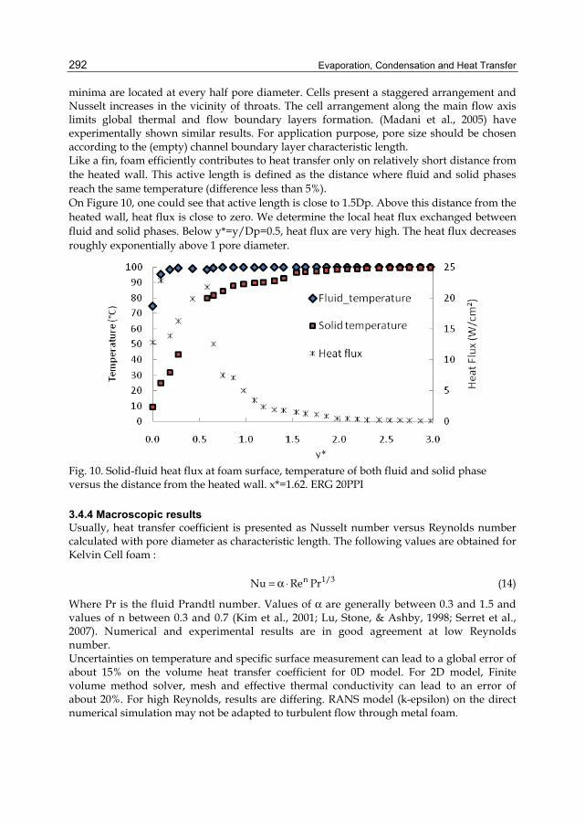
Evaporation, Condensation and Heat Transfer
292
minima are located at every half pore diameter. Cells present a staggered arrangement and Nusselt increases in the vicinity of throats. The cell arrangement along the main flow axis limits global thermal and flow boundary layers formation. (Madani et al., 2005) have experimentally shown similar results. For application purpose, pore size should be chosen according to the (empty) channel boundary layer characteristic length. Like a fin, foam efficiently contributes to heat transfer only on relatively short distance from the heated wall. This active length is defined as the distance where fluid and solid phases reach the same temperature (difference less than 5%). On Figure 10, one could see that active length is close to 1.5Dp. Above this distance from the heated wall, heat flux is close to zero. We determine the local heat flux exchanged between fluid and solid phases. Below y*=y/Dp=0.5, heat flux are very high. The heat flux decreases roughly exponentially above 1 pore diameter.
Fig. 10. Solid-fluid heat flux at foam surface, temperature of both fluid and solid phase versus the distance from the heated wall. x*=1.62. ERG 20PPI
3.4.4 Macroscopic results Usually, heat transfer coefficient is presented as Nusselt number versus Reynolds number calculated with pore diameter as characteristic length. The following values are obtained for Kelvin Cell foam :
n 1/3Nu Re Pr= α ⋅ (14)
Where Pr is the fluid Prandtl number. Values of α are generally between 0.3 and 1.5 and values of n between 0.3 and 0.7 (Kim et al., 2001; Lu, Stone, & Ashby, 1998; Serret et al., 2007). Numerical and experimental results are in good agreement at low Reynolds number. Uncertainties on temperature and specific surface measurement can lead to a global error of about 15% on the volume heat transfer coefficient for 0D model. For 2D model, Finite volume method solver, mesh and effective thermal conductivity can lead to an error of about 20%. For high Reynolds, results are differing. RANS model (k-epsilon) on the direct numerical simulation may not be adapted to turbulent flow through metal foam.
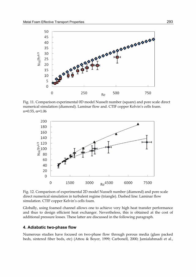
Metal Foam Effective Transport Properties
293
Fig. 11. Comparison experimental 0D model Nusselt number (square) and pore scale direct numerical simulation (diamond). Laminar flow and. CTIF copper Kelvin’s cells foam. n=0.55, α=1.06
Fig. 12. Comparison of experimental 2D model Nusselt number (diamond) and pore scale direct numerical simulation in turbulent regime (triangle). Dashed line: Laminar flow simulation. CTIF copper Kelvin’s cells foam.
Globally, using foamed channel allows one to achieve very high heat transfer performance and thus to design efficient heat exchanger. Nevertheless, this is obtained at the cost of additional pressure losses. These latter are discussed in the following paragraph.
4. Adiabatic two-phase flow Numerous studies have focused on two-phase flow through porous media (glass packed beds, sintered fiber beds, etc) (Attou & Boyer, 1999; Carbonell, 2000; Jamialahmadi et al.,
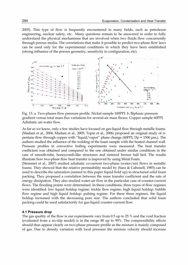
Evaporation, Condensation and Heat Transfer
294
2005). This type of flow is frequently encountered in many fields, such as petroleum engineering, nuclear safety, etc. Many questions remain to be answered in order to fully understand the physical mechanisms that are involved when two fluids flow concurrently through porous media. The correlations that make it possible to predict two-phase flow laws can be used only for the experimental conditions in which they have been established (strong influence of the porous geometry, sensitivity to configuration, etc).
Fig. 13. a. Two-phases flow pressure profile. Nickel sample 100PPI. b. Biphasic pressure gradient versus total mass flux variations for several air mass fluxes. Copper sample 60PPI. Adiabatic air-water flow.
As far as we know, only a few studies have focused on gas-liquid flow through metallic foams. (Madani et al., 2004; Madani et al., 2005; Topin et al., 2006) proposed an original study of n-pentane flow through copper with “liquid/vapor” phase change (40PPI, Dp = 1500 μm,). The authors studied the influence of the welding of the foam sample with the heated channel wall. Pressure profiles in convective boiling experiments were measured. The heat transfer coefficient was obtained and compared to the one obtained under similar conditions in the case of smooth-tube, honeycomb-like structures and sintered bronze ball bed. The results illustrate how two-phase flow heat transfer is improved by using Metal Foam. (Stemmet et al., 2007) studied adiabatic co-current two-phase (water/air) flows in metallic foams. They showed that the relative permeability model by (Saez & Cabonell, 1985) can be used to describe the saturation (named in this paper liquid hold up) in structured solid foam packing. They proposed a correlation between the mass transfer coefficient and the rate of energy dissipation. They also studied water-air flow in the particular case of counter-current flows. The flooding points were determined. In these conditions, three types of flow regimes were identified: low liquid holdup regime: trickle flow regime, high liquid holdup: bubble flow regime and high liquid holdup: pulsing regime. For these three regimes, the liquid holdup increased with the decreasing pore size. The authors concluded that solid foam packing could be used satisfactorily for gas-liquid counter-current flow.
4.1 Pressure drop The gas quality of the flow is our experiments vary from 0.5 up to 25 % and the void fraction (evaluated from a no-slip model) is in the range 80 up to 99%. The compressibility effects should thus appear clearly on two-phase pressure profile as the mixture is mainly composed of gas. Due to density variation with local pressure the mixture velocity should increase
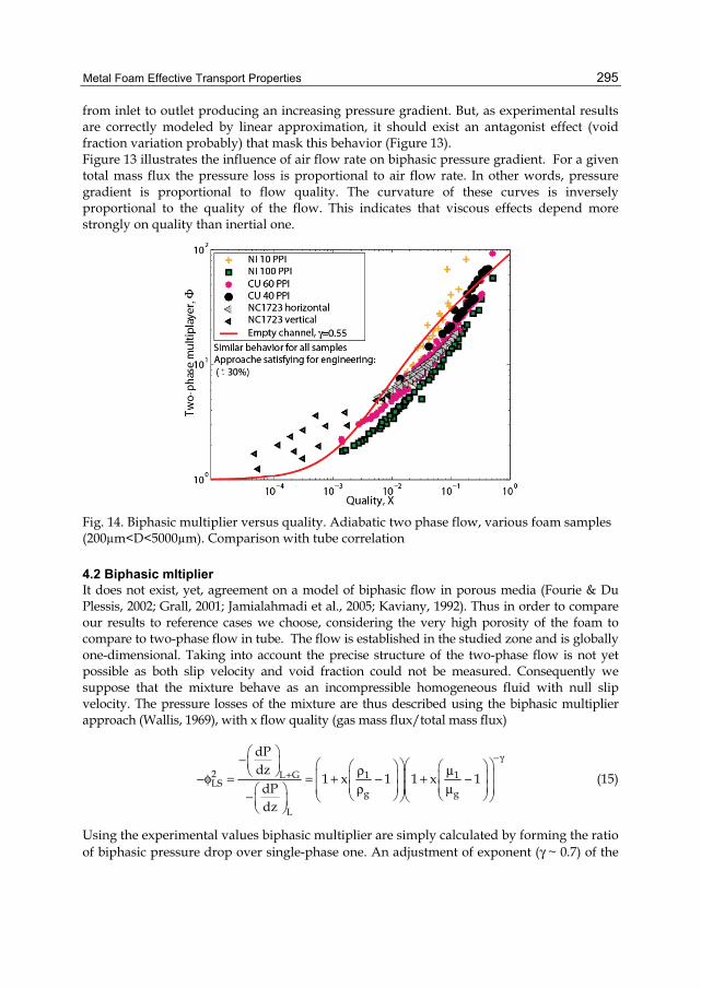
Metal Foam Effective Transport Properties
295
from inlet to outlet producing an increasing pressure gradient. But, as experimental results are correctly modeled by linear approximation, it should exist an antagonist effect (void fraction variation probably) that mask this behavior (Figure 13). Figure 13 illustrates the influence of air flow rate on biphasic pressure gradient. For a given total mass flux the pressure loss is proportional to air flow rate. In other words, pressure gradient is proportional to flow quality. The curvature of these curves is inversely proportional to the quality of the flow. This indicates that viscous effects depend more strongly on quality than inertial one.
Fig. 14. Biphasic multiplier versus quality. Adiabatic two phase flow, various foam samples (200µm<D<5000µm). Comparison with tube correlation
4.2 Biphasic mltiplier It does not exist, yet, agreement on a model of biphasic flow in porous media (Fourie & Du Plessis, 2002; Grall, 2001; Jamialahmadi et al., 2005; Kaviany, 1992). Thus in order to compare our results to reference cases we choose, considering the very high porosity of the foam to compare to two-phase flow in tube. The flow is established in the studied zone and is globally one-dimensional. Taking into account the precise structure of the two-phase flow is not yet possible as both slip velocity and void fraction could not be measured. Consequently we suppose that the mixture behave as an incompressible homogeneous fluid with null slip velocity. The pressure losses of the mixture are thus described using the biphasic multiplier approach (Wallis, 1969), with x flow quality (gas mass flux/total mass flux)
2 L G 1 1LS
g g
L
dPdz
1 x 1 1 x 1dPdz
−γ
+
⎛ ⎞−⎜ ⎟ ⎛ ⎞⎛ ⎞⎛ ⎞ ⎛ ⎞ρ μ⎝ ⎠ ⎜ ⎟⎜ ⎟⎜ ⎟ ⎜ ⎟−φ = = + − + −⎜ ⎟ ⎜ ⎟⎜ ⎟⎜ ⎟ρ μ⎛ ⎞ ⎝ ⎠ ⎝ ⎠− ⎝ ⎠⎝ ⎠⎜ ⎟
⎝ ⎠
(15)
Using the experimental values biphasic multiplier are simply calculated by forming the ratio of biphasic pressure drop over single-phase one. An adjustment of exponent (γ ~ 0.7) of the
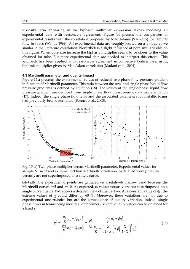
Evaporation, Condensation and Heat Transfer
296
viscosity term appearing in the biphasic multiplier expression allows modeling all experimental data with reasonable agreement. Figure 14 present the comparison of experimental results with the correlation proposed by Mac Adams (γ = -0.25) for laminar flow in tubes (Wallis, 1969). All experimental data are roughly located on a unique curve similar to the literature correlation. Nevertheless a slight influence of pore size is visible on this figure. When pore size increase the biphasic multiplier seems to be closer to the value obtained for tube. But more experimental data are needed to interpret this effect. This approach has been applied with reasonable agreement in convective boiling case, using biphasic multiplier given by Mac Adam correlation (Madani et al., 2004).
4.3 Martinelli parameter and quality impact Figure 15.a presents the experimental values of reduced two-phase flow pressure gradient in function of Martinelli parameter. This ratio between the two- and single-phase liquid flow pressure gradients is defined by equation (18). The values of the single-phase liquid flow pressure gradient are deduced from single phase flow measurement data using equation (17). Indeed, the single phase flow laws and the associated parameters for metallic foams had previously been determined (Bonnet et al., 2008).
Fig. 15. a) Two-phase multiplier versus Martinelli parameter. Experimental values for sample NC4753 and extreme Lockhart Martinelli correlation. b) detailed view χ values versus χ are not superimposed on a single curve.
Globally, the experimental points are gathered on a relatively narrow band between the Martinelli curves c=5 and c=10. As expected, φl values versus χ are not superimposed on a single curve. Figure 15-b shows a detailed view of Figure 15-a. At a constant value of φl , the extreme values of χ could differ by 60 %. Moreover, these variations are not due to experimental uncertainties but are the consequence of quality variation. Indeed, single phase flows in foams being inertial (Forchheimer), several quality values can be obtained for a fixed χ.
⎛ ⎞ ⎛ ⎞⎜ ⎟ ⎜ ⎟⎝ ⎠ ⎝ ⎠
2 2L LL L L L L2
22G 2GG G G L L
μ μμ + βρ u η + βηρlK Kχ = =μ ρg μ X Xμ + βρ u η + β ηK K 1 - X 1 - X
(16)
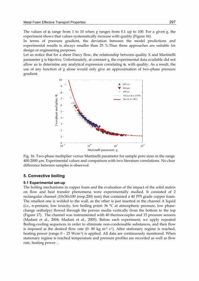
Metal Foam Effective Transport Properties
297
The values of φl range from 1 to 10 when χ ranges from 0.1 up to 100. For a given χ, the experiment shows that values systematically increase with quality (Figure 16). In terms of pressure gradient, the deviation between the model predictions and experimental results is always smaller than 25 %.Thus these approaches are suitable for design or engineering purposes. Let us notice that for a sheer Darcy flow, the relationship between quality X and Martinelli parameter χ is bijective. Unfortunately, at constant χ, the experimental data available did not allow us to determine any analytical expression correlating φL with quality. As a result, the use of any function of χ alone would only give an approximation of two-phase pressure gradient.
Fig. 16. Two-phase multiplier versus Martinelli parameter for sample pore sizes in the range 400-2000 µm. Experimental values and comparison with two literature correlations. No clear difference between samples is observed.
5. Convective boiling 5.1 Experimental set-up The boiling mechanisms in copper foam and the evaluation of the impact of the solid matrix on flow and heat transfer phenomena were experimentally studied. It consisted of 2 rectangular channel (10x50x100 (resp.200) mm) that contained a 40 PPI grade copper foam. The smallest one is welded to the wall, as the other is just inserted in the channel A liquid (i.e., n-pentane, low toxicity, low boiling point: 36 °C at atmospheric pressure, low phase-change enthalpy) flowed through the porous media vertically from the bottom to the top (Figure 17). The channel was instrumented with 40 thermocouples and 15 pressure sensors (Madani et al., 2004; Madani et al., 2005). Before each experiment, we apply repeated Boiling-cooling sequences in order to eliminate non-condensable substances, and then flow is imposed at the desired flow rate (0- 80 kg m-2 s-1). After stationary regime is reached, heating power (range 0 – 25 Wcm-2) is applied. All data are continuously monitored. When stationary regime is reached temperature and pressure profiles are recorded as well as flow rate, heating power…
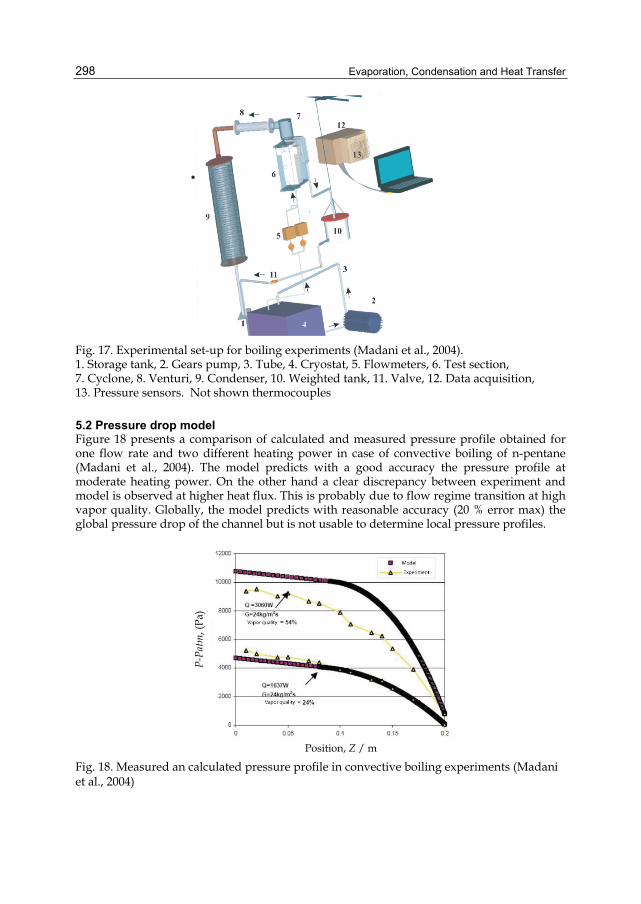
Evaporation, Condensation and Heat Transfer
298
Fig. 17. Experimental set-up for boiling experiments (Madani et al., 2004). 1. Storage tank, 2. Gears pump, 3. Tube, 4. Cryostat, 5. Flowmeters, 6. Test section, 7. Cyclone, 8. Venturi, 9. Condenser, 10. Weighted tank, 11. Valve, 12. Data acquisition, 13. Pressure sensors. Not shown thermocouples
5.2 Pressure drop model Figure 18 presents a comparison of calculated and measured pressure profile obtained for one flow rate and two different heating power in case of convective boiling of n-pentane (Madani et al., 2004). The model predicts with a good accuracy the pressure profile at moderate heating power. On the other hand a clear discrepancy between experiment and model is observed at higher heat flux. This is probably due to flow regime transition at high vapor quality. Globally, the model predicts with reasonable accuracy (20 % error max) the global pressure drop of the channel but is not usable to determine local pressure profiles.
Fig. 18. Measured an calculated pressure profile in convective boiling experiments (Madani et al., 2004)
P-Pa
tm, (
Pa)
Position, Z / m
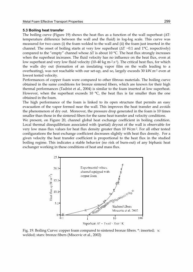
Metal Foam Effective Transport Properties
299
5.3 Boiling heat transfer The boiling curve (Figure 19) shows the heat flux as a function of the wall superheat (ΔT: temperature difference between the wall and the fluid) in log-log scale. This curve was measured for two cases (i) the foam welded to the wall and (ii) the foam just inserted in the channel. The onset of boiling starts at very low superheat (ΔT ~0.1 and 1°C, respectively) compared to the “empty” channel whose ΔT is about 10 °C. The heat flux strongly increases when the superheat increases. The fluid velocity has no influence on the heat flux, even at low superheat and very low fluid velocity (10–40 kg m-2.s-1). The critical heat flux, for which the walls dry out (formation of an insulating vapor film on the walls leading to a overheating), was not reachable with our set-up, and so, largely exceeds 30 kW.m-2 even at lowest tested velocity. Performances of copper foam were compared to other fibrous materials. The boiling curve obtained in the same conditions for bronze sintered fibers, which are known for their high thermal performances (Tadrist et al., 2004) is similar to the foam inserted at low superheat. However, when the superheat exceeds 10 °C, the heat flux is far smaller than the one obtained in the foam. The high performance of the foam is linked to its open structure that permits an easy evacuation of the vapor formed near the wall. This improves the heat transfer and avoids the phenomenon of dry out. Moreover, the pressure drop generated in the foam is 10 times smaller than those in the sintered fibers for the same heat transfer and velocity conditions. We present, on Figure 20, channel global heat exchange coefficient in boiling condition. Local thermal disequilibrium associated with (partial) dryout of the wall is observable for very low mass flux values for heat flux density greater than 10 Wcm-2. For all other tested configurations the heat exchange coefficient decreases slightly with heat flux density. For a given velocity the heat transfer coefficient is proportional to the heat flux in the studied boiling regime. This indicates a stable behavior (no risk of burn-out) of any biphasic heat exchanger working in these conditions of heat and mass flux.
Fig. 19. Boiling Curve: copper foam compared to sintered bronze fibers. *: inserted; x: welded; stars: bronze fibers (Miscevic et al., 2002)
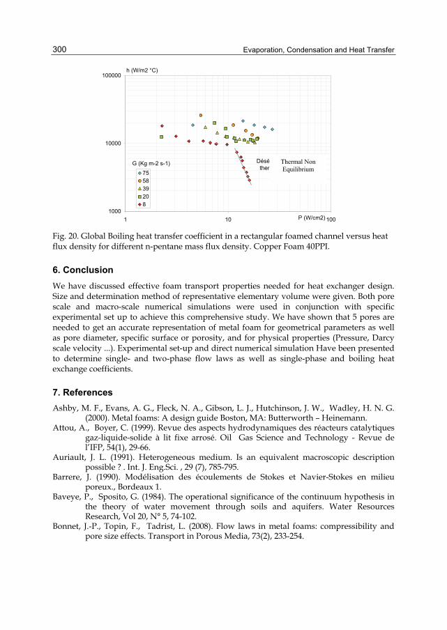
Evaporation, Condensation and Heat Transfer
300
1000
10000
100000
1 10 100
755839208
G (Kg m-2 s-1)
P (W/cm2)
h (W/m2 °C)
Déséquilibre thermique
Fig. 20. Global Boiling heat transfer coefficient in a rectangular foamed channel versus heat flux density for different n-pentane mass flux density. Copper Foam 40PPI.
6. Conclusion We have discussed effective foam transport properties needed for heat exchanger design. Size and determination method of representative elementary volume were given. Both pore scale and macro-scale numerical simulations were used in conjunction with specific experimental set up to achieve this comprehensive study. We have shown that 5 pores are needed to get an accurate representation of metal foam for geometrical parameters as well as pore diameter, specific surface or porosity, and for physical properties (Pressure, Darcy scale velocity ...). Experimental set-up and direct numerical simulation Have been presented to determine single- and two-phase flow laws as well as single-phase and boiling heat exchange coefficients.
7. References Ashby, M. F., Evans, A. G., Fleck, N. A., Gibson, L. J., Hutchinson, J. W., Wadley, H. N. G.
(2000). Metal foams: A design guide Boston, MA: Butterworth – Heinemann. Attou, A., Boyer, C. (1999). Revue des aspects hydrodynamiques des réacteurs catalytiques
gaz-liquide-solide à lit fixe arrosé. Oil Gas Science and Technology - Revue de l’IFP, 54(1), 29-66.
Auriault, J. L. (1991). Heterogeneous medium. Is an equivalent macroscopic description possible ? . Int. J. Eng.Sci. , 29 (7), 785-795.
Barrere, J. (1990). Modélisation des écoulements de Stokes et Navier-Stokes en milieu poreux., Bordeaux 1.
Baveye, P., Sposito, G. (1984). The operational significance of the continuum hypothesis in the theory of water movement through soils and aquifers. Water Resources Research, Vol 20, N° 5, 74-102.
Bonnet, J.-P., Topin, F., Tadrist, L. (2008). Flow laws in metal foams: compressibility and pore size effects. Transport in Porous Media, 73(2), 233-254.
Thermal Non Equilibrium
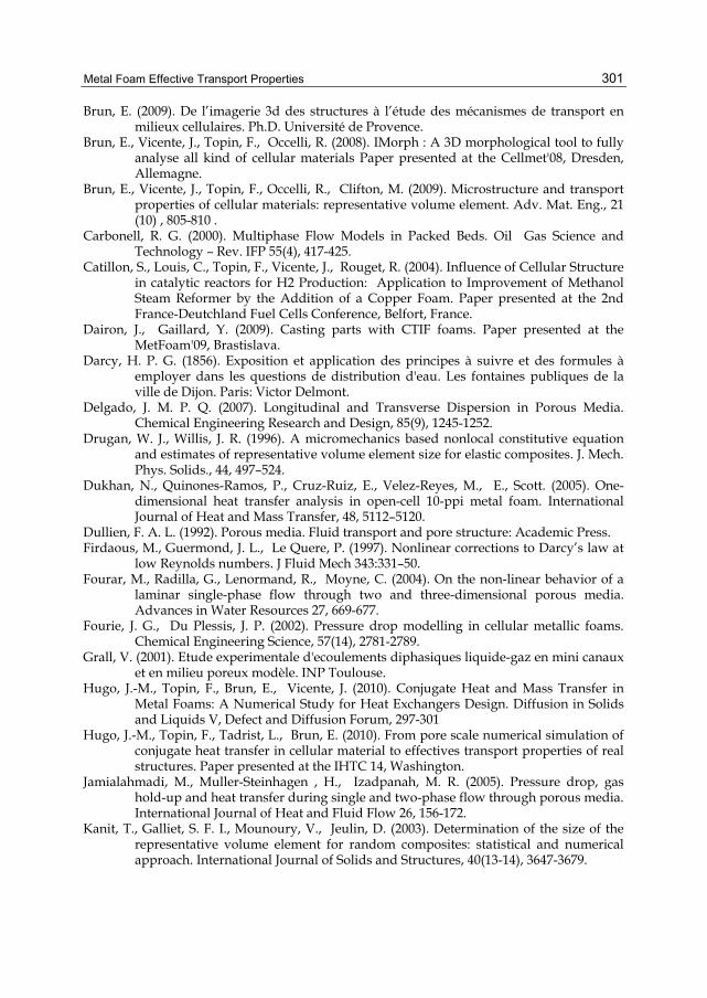
Metal Foam Effective Transport Properties
301
Brun, E. (2009). De l’imagerie 3d des structures à l’étude des mécanismes de transport en milieux cellulaires. Ph.D. Université de Provence.
Brun, E., Vicente, J., Topin, F., Occelli, R. (2008). IMorph : A 3D morphological tool to fully analyse all kind of cellular materials Paper presented at the Cellmet'08, Dresden, Allemagne.
Brun, E., Vicente, J., Topin, F., Occelli, R., Clifton, M. (2009). Microstructure and transport properties of cellular materials: representative volume element. Adv. Mat. Eng., 21 (10) , 805-810 .
Carbonell, R. G. (2000). Multiphase Flow Models in Packed Beds. Oil Gas Science and Technology – Rev. IFP 55(4), 417-425.
Catillon, S., Louis, C., Topin, F., Vicente, J., Rouget, R. (2004). Influence of Cellular Structure in catalytic reactors for H2 Production: Application to Improvement of Methanol Steam Reformer by the Addition of a Copper Foam. Paper presented at the 2nd France-Deutchland Fuel Cells Conference, Belfort, France.
Dairon, J., Gaillard, Y. (2009). Casting parts with CTIF foams. Paper presented at the MetFoam'09, Brastislava.
Darcy, H. P. G. (1856). Exposition et application des principes à suivre et des formules à employer dans les questions de distribution d'eau. Les fontaines publiques de la ville de Dijon. Paris: Victor Delmont.
Delgado, J. M. P. Q. (2007). Longitudinal and Transverse Dispersion in Porous Media. Chemical Engineering Research and Design, 85(9), 1245-1252.
Drugan, W. J., Willis, J. R. (1996). A micromechanics based nonlocal constitutive equation and estimates of representative volume element size for elastic composites. J. Mech. Phys. Solids., 44, 497–524.
Dukhan, N., Quinones-Ramos, P., Cruz-Ruiz, E., Velez-Reyes, M., E., Scott. (2005). One-dimensional heat transfer analysis in open-cell 10-ppi metal foam. International Journal of Heat and Mass Transfer, 48, 5112–5120.
Dullien, F. A. L. (1992). Porous media. Fluid transport and pore structure: Academic Press. Firdaous, M., Guermond, J. L., Le Quere, P. (1997). Nonlinear corrections to Darcy’s law at
low Reynolds numbers. J Fluid Mech 343:331–50. Fourar, M., Radilla, G., Lenormand, R., Moyne, C. (2004). On the non-linear behavior of a
laminar single-phase flow through two and three-dimensional porous media. Advances in Water Resources 27, 669-677.
Fourie, J. G., Du Plessis, J. P. (2002). Pressure drop modelling in cellular metallic foams. Chemical Engineering Science, 57(14), 2781-2789.
Grall, V. (2001). Etude experimentale d'ecoulements diphasiques liquide-gaz en mini canaux et en milieu poreux modèle. INP Toulouse.
Hugo, J.-M., Topin, F., Brun, E., Vicente, J. (2010). Conjugate Heat and Mass Transfer in Metal Foams: A Numerical Study for Heat Exchangers Design. Diffusion in Solids and Liquids V, Defect and Diffusion Forum, 297-301
Hugo, J.-M., Topin, F., Tadrist, L., Brun, E. (2010). From pore scale numerical simulation of conjugate heat transfer in cellular material to effectives transport properties of real structures. Paper presented at the IHTC 14, Washington.
Jamialahmadi, M., Muller-Steinhagen , H., Izadpanah, M. R. (2005). Pressure drop, gas hold-up and heat transfer during single and two-phase flow through porous media. International Journal of Heat and Fluid Flow 26, 156-172.
Kanit, T., Galliet, S. F. I., Mounoury, V., Jeulin, D. (2003). Determination of the size of the representative volume element for random composites: statistical and numerical approach. International Journal of Solids and Structures, 40(13-14), 3647-3679.
Evaporation, Condensation and Heat Transfer
302
Kaviany, M. (1992). Principles of heat transfer in porous media: Springer-Verlag. Kim, S. Y., Kang, B. H., Kim, J.-H. (2001). Forced convection from aluminum foam materials
in an asymmetrically heated channel. IJHMT, 44(7), 1451-1454. Lorensen, W. E., Cline, H. E. (1987). Marching Cubes: A High Resolution 3D Surface
Construction Algorithm. Computer Graphics, 21(3), 163-169. Lu, T. J., Stone, H. A., Ashby, M. F. (1998). Heat transfer in open- cell metal foams. Acta
Materialia, 46(10), 3619-3635. Madani, B., Topin, F., Tadrist, L. (2004). Ebullition convective dans les mousses métalliques :
Analyse expérimentale des effets de contact matrice solide -paroi. Paper presented at the Congrès de la SFT 04, Giens, France.
Madani, B., Topin, F., Tadrist, L., Bouhadef, K. (2005). Mesure du coefficient de transfert de chaleur local paroi-fluide dans un canal à mousse métallique en écoulement liquide et en ébullition. Paper presented at the 12ième JITH, Tanger, Maroc.
Madani, B., Topin, F., Tadrist, L., Rigollet, F. (2007). Flow laws in metallic foams: experimental determination of inertial and viscous contribution. Jounal of Porous Media, 10(1), 51-70.
Mahjoob, S., Vafai, K. (2008). A synthesis of fluid and thermal transport models for metal foam heat exchangers. International Journal of Heat and Mass Transfer, 51, 3701–3711.
Marle, C. (1982). On macroscopic equation governing multiphase flow with diffusion and chemical reactions in porous media. Int. J. Eng. Sci, 20(5), 643-662.
Mei, C., Auriault, J. L. (1993). The effect of weak inertia on flow through a porous medium. J. Fluid Mech., 222, 647-663.
Miscevic, M., Topin, F., Tadrist, L. (2002). Convective boiling phenomena in a sintered fibrous channel:Study of thermal non-equilibrium behavior Journal of Porous Media, 5(4), 229-239.
Moyne, C. (1997). Two-equation model for a diffusive process in porous media using the volume averaging method with an unsteady-state closure. Advances in Water Resources, 29(2-3), 63-76.
Quintard, M., Whitaker, S. (1991). Transport Process in ordered and disordered porous media. Paper presented at the 1991 ICHMT International Seminar on heat and mass transfer in porous media.
Renard, P., Genty, A., Stauffer, F. (2001). Laboratory détermination of the full permeability tensor. Journal of geophysical research, 106(B11), 26443-26452.
Saez, A. E., Cabonell, R. G. (1985). Hydrodynamic parameters for gas - liquid cocurrent flow in packed beds,. AIChE J, 31, 52 - 62.
Serret, D., Stamboul, T., Topin, F. (2007). Transferts dans les mousses métalliques :Mesure du coefficient d’échange de chaleur entre phases Paper presented at the Congrès de la SFT, SFT 07, Ille des Embiez.
Stemmet, C. P., van der Schaaf, J., Kuster, B. F. M., Schouten, J. C. (2007). Gas–liquid mass transfer and axial dispersion in solid foam packings. Chemical Engineering Science, 62, 5444 - 5450.
Tadrist, L., Miscevic, M., Rahli, O., Topin, F. (2004). About the Use of Fibrous Materials in Compact Heat Exchangers. Experimental Thermal and Fluid Science, 28, 193 – 199.
Topin, F., Bonnet, J.-P., Madani, B., Tadrist, L. (2006). Experimental Analysis of Multiphase Flow in Metallic foam: Flow Laws, Heat Transfer and Convective Boiling. Advanced material Engineering, 8(9), 890-899.
Wallis, G. (1969). One-Dimensional Two-Phase Flow New-York, NY: Mc graw Hill. Wodie, J. C., Levy, T. (1991). Correction non linéaire de la loi de Darcy. C. R. Acad. Sci.,
312(II), 157-161.
15
Heat Transfer Performances and Exergetic Optimization for Solar Heat Receiver
Jian-Feng Lu1 and Jing Ding School of Engineering,
Sun Yat-sen University, China
1. Introduction Solar energy is one kind of important resource for clean and renewable energy, and is widely investigated in many fields. In order to increase the operating temperature and thermodynamic efficiency, concentrated solar radiation is widely used to heat the working fluid in solar thermal power system (Trieb & Nitsch, 1998) and other industrial engineerings (Klein et al., 2007; Ali et al., 2008). Concentrated solar radiation (Kalogirou, 2004) can be collected by the parabolic trough collector, parabolic dish reflector, heliostat field, etc. The concentrated energy flux has been studied in kinds of solar energy system. Moustafa et al. (1995) measured the solar flux density distribution on a plane receiver due to a flat heliostat. Estrada et al. (2007) proposed a calorimeter to measure the concentrated solar power produced by a point focus solar concentrator. Solar thermal power system based on trough, dish or heliostat field is a very promising and challenging technology for its high operating temperature and thermodynamic efficiency. In solar thermal power plant (Odeh et al., 2003), the heat transfer medium in solar heat receiver is heated by concentrated solar radiation to some high temperature, and then it can be used to operate kinds of heat engine and generate electricity. As a result, the heat receiver (Ortega et al., 2008) is the key problem for the photo-thermal transformation, and the heat transfer performance of solar heat receiver is the hotspot for solar energy research. The basic types of heat receiver in concentrated solar thermal system mainly include heat pipe receiver (Fujiwara et al., 1990), parabolic trough solar receiver (Gong et al., 2010), cavity receiver (Wu et al., 2010), and multistage solar receiver (Taragan, 1999), etc. The dynamical and thermal characteristics of solar heat receiver have been investigated in much literature (Cui et al., 2008; Grena, 2010). In general, the heat losses from solar receiver mainly include three contributions: radiation heat loss, convective heat loss, and conduction heat loss. The radiation heat loss (Melchior et al., 2008; Li et al., 2010) is mainly dependent upon the receiver structure, wall temperature, and emissivity/absorptivity of the receiver walls, while the convective heat loss (Clausing, 1981) is mainly determined by the receiver structure, wall temperature, and wind velocity. The heat conduction loss (Zavoico, 2001) exists in cavity receiver through the insulation wall, and it can be ignored in many solar heat receivers.
1 Corresponding author
Evaporation, Condensation and Heat Transfer
304
In order to reduce the radiation heat loss, solar selective coatings are widely used in solar heat receiver. Tabor (1958) first reported the solar selective coating to increase the absorption efficiency of solar heat receiver. The ideal solar selective coating was considered to have good optical performance with high absorptivity and low emissivity. Kennedy (2002) introduced kinds of solar selective coatings under mid- to high-temperature conditions. Cindrella (2007) studied the real utility ranges of the solar selective coatings. Nilsson & Roos (2009) further evaluated the optical and thermal properties of coatings for energy efficient windows. In general, solar selective coatings mainly have six types: intrinsic coatings, semiconductor-metal tandems, multilayer coatings, multi-dielectric composite coatings, textured surfaces, and selectively solar-transmitting coatings. Intrinsic coatings are not effective enough but very stable, like metallic W (Agnihotri & Gupta, 1981), CaF2 (Pellegrini, 1980), SnO2 (Seraphin & Meinel, 1976) etc. Semiconductor-metal tandems as Si-based design can be used in a wide temperature range (Seraphin, 1976). Multilayer coatings (Andersson et al., 1980) can be very efficient for proper structure design. Metal-dielectric composite coatings (Arancibia et al., 2000; Gao et al., 2000) have a high absorptivity in the solar region, while that is transparent in the other region. Till now, solar selective coatings have been critical important topic for solar energy research. The convective heat loss (Siebers & Kraabel, 1984) is normally very difficult to determine but very important for the total energy loss of solar heat receiver. Clausing (1983) predicted the convective loss from solar central receivers from analytical model and experimental result. LeQuere et al. (1981a, 1981b) experimentally reported Nusselt number correlations for isothermal open cubical cavity for different inclination. Koenig & Marvin (1981) investigated convective heat loss in open cavity solar receivers, and proposed a calculating model in a large operating temperature range. Chan & Tien (1985, 1986) studied the laminar natural convection in shallow open cavities. Leibfried & Ortjohann (1995) investigated convective heat loss from upward and downward facing cavity receivers, and analyzed the effects of wall temperature, tilt angle, aperture-radius, geometry, ribs, and ventilation. Khubeiznet et al. (2002) measured natural convection heat transfer from an isothermal hemispherical cavity. Taumoefolau et al. (2004) described the convective loss from electrically heated cavity receiver under different inclinations and temperatures. Paitoonsurikarn et al. (2006) simulated the convective loss from solar cylindrical receiver and dish concentrating receiver. Sendhil & Reddy (2007, 2008) carried out numerical analyses of convective losses in rectangular, hemispherical solar cavity receiver and modified cavity receivers, respectively. In addition, the convective loss from heat receiver under wind condition is also investigated. Ma (1993) reported the experimental investigations on the convective loss under wind. Available literature also investigated combined heat loss from solar heat receiver including convection and radiation. Lage et al. (1992) simulated natural convection and radiation in a 2-D cavity with open end. McDonald (1995) reported the heat loss from an open cavity including convection and radiation. Dehghan & Behnia (1996) numerically studied combined natural convection conduction and radiation heat transfer in a discretely heated open cavity. Reddy & Kumar (2008) investigated the combined laminar natural convection and surface radiation heat transfer in a modified cavity receiver of solar parabolic dish. Prakash et al. (2009) investigated the heat losses from a solar cavity receiver, and found the natural convection and radiation played the premier role in the heat loss of the receiver. Muftuoglu & Bilgen (2008) simulated heat transfer in inclined rectangular receivers for concentrated solar radiation. The optimal structure design and operating conditions of solar heat receiver have also been investigated by various methods. Harris & Lenz (1985) found the thermal and optical losses from a cavity solar receiver were less than other types of receiver. Kaushika and Reddy (2000) designed the modified cavity receiver to perform minimum heat loss from the receiver with
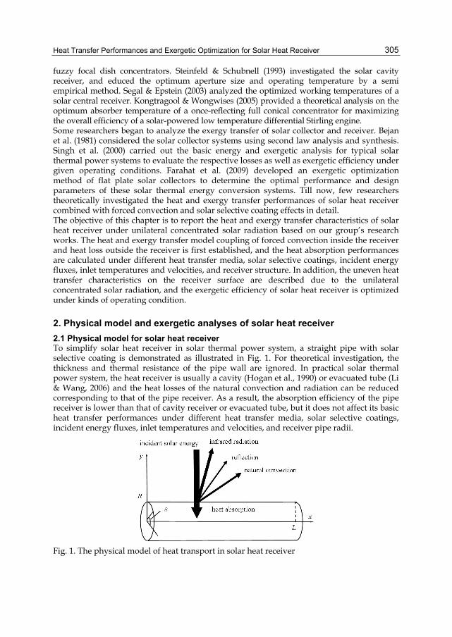
Heat Transfer Performances and Exergetic Optimization for Solar Heat Receiver
305
fuzzy focal dish concentrators. Steinfeld & Schubnell (1993) investigated the solar cavity receiver, and educed the optimum aperture size and operating temperature by a semi empirical method. Segal & Epstein (2003) analyzed the optimized working temperatures of a solar central receiver. Kongtragool & Wongwises (2005) provided a theoretical analysis on the optimum absorber temperature of a once-reflecting full conical concentrator for maximizing the overall efficiency of a solar-powered low temperature differential Stirling engine. Some researchers began to analyze the exergy transfer of solar collector and receiver. Bejan et al. (1981) considered the solar collector systems using second law analysis and synthesis. Singh et al. (2000) carried out the basic energy and exergetic analysis for typical solar thermal power systems to evaluate the respective losses as well as exergetic efficiency under given operating conditions. Farahat et al. (2009) developed an exergetic optimization method of flat plate solar collectors to determine the optimal performance and design parameters of these solar thermal energy conversion systems. Till now, few researchers theoretically investigated the heat and exergy transfer performances of solar heat receiver combined with forced convection and solar selective coating effects in detail. The objective of this chapter is to report the heat and exergy transfer characteristics of solar heat receiver under unilateral concentrated solar radiation based on our group’s research works. The heat and exergy transfer model coupling of forced convection inside the receiver and heat loss outside the receiver is first established, and the heat absorption performances are calculated under different heat transfer media, solar selective coatings, incident energy fluxes, inlet temperatures and velocities, and receiver structure. In addition, the uneven heat transfer characteristics on the receiver surface are described due to the unilateral concentrated solar radiation, and the exergetic efficiency of solar heat receiver is optimized under kinds of operating condition.
2. Physical model and exergetic analyses of solar heat receiver 2.1 Physical model for solar heat receiver To simplify solar heat receiver in solar thermal power system, a straight pipe with solar selective coating is demonstrated as illustrated in Fig. 1. For theoretical investigation, the thickness and thermal resistance of the pipe wall are ignored. In practical solar thermal power system, the heat receiver is usually a cavity (Hogan et al., 1990) or evacuated tube (Li & Wang, 2006) and the heat losses of the natural convection and radiation can be reduced corresponding to that of the pipe receiver. As a result, the absorption efficiency of the pipe receiver is lower than that of cavity receiver or evacuated tube, but it does not affect its basic heat transfer performances under different heat transfer media, solar selective coatings, incident energy fluxes, inlet temperatures and velocities, and receiver pipe radii.
Fig. 1. The physical model of heat transport in solar heat receiver
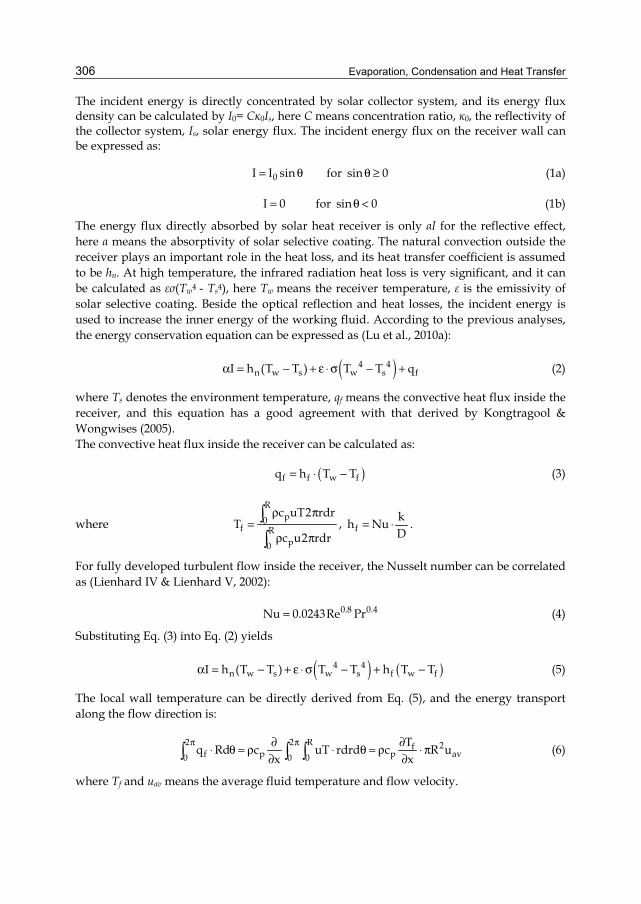
Evaporation, Condensation and Heat Transfer
306
The incident energy is directly concentrated by solar collector system, and its energy flux density can be calculated by I0= Cк0Is, here C means concentration ratio, к0, the reflectivity of the collector system, Is, solar energy flux. The incident energy flux on the receiver wall can be expressed as:
0I I sin= θ for sin 0θ ≥ (1a)
I 0= for sin 0θ < (1b)
The energy flux directly absorbed by solar heat receiver is only αI for the reflective effect, here α means the absorptivity of solar selective coating. The natural convection outside the receiver plays an important role in the heat loss, and its heat transfer coefficient is assumed to be hn. At high temperature, the infrared radiation heat loss is very significant, and it can be calculated as εσ(Tw4 - Ts4), here Tw means the receiver temperature, ε is the emissivity of solar selective coating. Beside the optical reflection and heat losses, the incident energy is used to increase the inner energy of the working fluid. According to the previous analyses, the energy conservation equation can be expressed as (Lu et al., 2010a):
( )4 4n w s w s fI h (T T ) T T qα = − + ε ⋅ σ − + (2)
where Ts denotes the environment temperature, qf means the convective heat flux inside the receiver, and this equation has a good agreement with that derived by Kongtragool & Wongwises (2005). The convective heat flux inside the receiver can be calculated as:
( )f f w fq h T T= ⋅ − (3)
where R
p0f R
p0
c uT2 rdrT
c u2 rdr
ρ π=
ρ π
∫∫
, fkh NuD
= ⋅ .
For fully developed turbulent flow inside the receiver, the Nusselt number can be correlated as (Lienhard IV & Lienhard V, 2002):
0.8 0.4Nu 0.0243Re Pr= (4)
Substituting Eq. (3) into Eq. (2) yields
( ) ( )4 4n w s w s f w fI h (T T ) T T h T Tα = − + ε ⋅ σ − + − (5)
The local wall temperature can be directly derived from Eq. (5), and the energy transport along the flow direction is:
2 2 R 2f
f p p av0 0 0Tq Rd c uT rdrd c R u
x xπ π∂ ∂⋅ θ = ρ ⋅ θ = ρ ⋅ π
∂ ∂∫ ∫ ∫ (6)
where Tf and uav means the average fluid temperature and flow velocity.
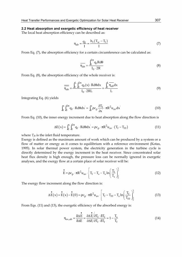
Heat Transfer Performances and Exergetic Optimization for Solar Heat Receiver
307
2.2 Heat absorption and exergetic efficiency of heat receiver The local heat absorption efficiency can be described as:
( )f w ffab
h T TqI I
−η = = (7)
From Eq. (7), the absorption efficiency for a certain circumference can be calculated as:
2f0
ab0
q Rd
I 2R
πθ
η =⋅
∫ (8)
From Eq. (8), the absorption efficiency of the whole receiver is:
L 2 L
f ab0 0 0ab
0
q (x) Rd dx dx
I 2RL L
π⋅ θ η
η = =⋅
∫ ∫ ∫ (9)
Integrating Eq. (6) yields
x 2 x' 2 'f
f p av'0 0 0Tq Rd dx c R u dxx
π ∂⋅ θ = ρ ⋅ π∂∫ ∫ ∫ (10)
From Eq. (10), the inner energy increment due to heat absorption along the flow direction is
( ) ( )x 2 ' 2f p av f f00 0
E x q Rd dx c R u T Tπ
Δ = ⋅ θ = ρ ⋅ π ⋅ −∫ ∫ (11)
where Tf0 is the inlet fluid temperature. Exergy is defined as the maximum amount of work which can be produced by a system or a flow of matter or energy as it comes to equilibrium with a reference environment (Kotas, 1995). In solar thermal power system, the electricity generation in the turbine cycle is directly determined by the exergy increment in the heat receiver. Since concentrated solar heat flux density is high enough, the pressure loss can be normally ignored in exergetic analyses, and the exergy flow at a certain place of solar receiver will be:
2 fp av f s s
s
TE c R u T T T lnT
• ⎡ ⎤⎛ ⎞= ρ ⋅ π ⋅ − −⎢ ⎥⎜ ⎟⎜ ⎟⎢ ⎥⎝ ⎠⎣ ⎦
(12)
The exergy flow increment along the flow direction is:
( ) ( ) ( ) 2 fp av f f0 s
f0
TE x E x E 0 c R u T T T lnT
• • • ⎡ ⎤⎛ ⎞Δ = − = ρ ⋅ π ⋅ − −⎢ ⎥⎜ ⎟⎜ ⎟⎢ ⎥⎝ ⎠⎣ ⎦
(13)
From Eqs. (11) and (13), the exergetic efficiency of the absorbed energy is:
f f sex,ab
f f f
E T T TE 1E E T T T
••∂Δ ∂ ⋅ δδΔη = = = −
δΔ ∂Δ ∂ ⋅ δ (14)
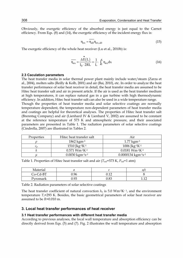
Evaporation, Condensation and Heat Transfer
308
Obviously, the exergetic efficiency of the absorbed energy is just equal to the Carnot efficiency. From Eqs. (8) and (14), the exergetic efficiency of the incident energy flux is:
ex ab ex,abη = η η (15)
The exergetic efficiency of the whole heat receiver (Lu et al., 2010b) is:
( ) Lex ex00
E L 1 dxI 2RL L
•Δ
η = = ⋅ η⋅ ∫ (16)
2.3 Caculation parameters The heat transfer media in solar thermal power plant mainly include water/steam (Zarza et al., 2004), molten salts (Reilly & Kolb, 2001) and air (Bai, 2010), etc. In order to analyze the heat transfer performance of solar heat receiver in detail, the heat transfer media are assumed to be Hitec heat transfer salt and air in present article. If the air is used as the heat transfer medium at high temperatures, it can replace natural gas in a gas turbine with high thermodynamic efficiency. In addition, Hitec heat transfer salt can also be used in a wide temperature range. Though the properties of heat transfer media and solar selective coatings are normally temperature dependent, the temperature non-dependent parameters of heat transfer media and coatings are helpful for theoretical analyses. The properties of Hitec heat transfer salt (Brenntag Company) and air (Lienhard IV & Lienhard V, 2002) are assumed to be constant at the reference temperature of 573 K and atmospheric pressure, and their associated parameters are presented in Table 1. The radiation parameters of solar selective coatings (Cindrella, 2007) are illustrated in Tables 2.
Properties Hitec heat transfer salt Air ρ 1862 kgm-3 1.77 kgm-3 cp 1510 Jkg-1K-1 1006 Jkg-1K-1 k 0.571 Wm-1K-1 0.0181 Wm-1K-1 μ 0.0030 kgm-1s-1 0.0000134 kgm-1s-1
Table 1. Properties of Hitec heat transfer salt and air (Tref=573 K, Pref=1 atm)
Material α ε α/ε Co-Cd-BT 0.96 0.12 8 Pyromark 0.93 0.83 1.12
Table 2. Radiation parameters of solar selective coatings
The heat transfer coefficient of natural convection hn is 5.0 Wm-2K- 1, and the environment temperature Ts=293 K. Besides, the basic geometrical parameters of solar heat receiver are assumed to be R=0.010 m.
3. Local heat transfer performances of heat receiver 3.1 Heat transfer performances with different heat transfer media According to previous analyses, the local wall temperature and absorption efficiency can be directly derived from Eqs. (5) and (7). Fig. 2 illustrates the wall temperature and absorption
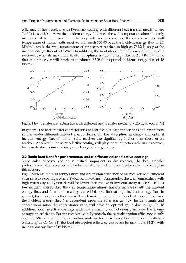
Heat Transfer Performances and Exergetic Optimization for Solar Heat Receiver
309
efficiency of heat receiver with Pyromark coating with different heat transfer media, where Tf=523 K, uav=5.0 ms-1. As the incident energy flux rises, the wall temperature almost linearly increases, while the absorption efficiency will first increase and then decrease. The wall temperature of molten salts receiver will reach 736.09 K at the incident energy flux of 2.5 MWm-2, while the wall temperature of air receiver reaches as high as 768.2 K only at the incident energy flux of 30 kWm-2. In addition, the local absorption efficiency of molten salts receiver reaches its maximum 92.46% at optimal incident energy flux of 2.0 MWm-2, while that of air receiver will reach its maximum 32.08% at optimal incident energy flux of 18 kWm-2.
0.0 0.5 1.0 1.5 2.0 2.5500
550
600
650
700
750
η
Tw
I (MWm-2)
K
0.84
0.86
0.88
0.90
0.92
0.94
10 15 20 25 30500
550
600
650
700
750
800η
Tw
I (kWm-2)
K
0.20
0.24
0.28
0.32
(a) Molten salts (b) Air
Fig. 2. Heat transfer characteristics with different heat transfer media (Tf=523 K, uav=5.0 m/s)
In general, the heat transfer characteristics of heat receiver with molten salts and air are very similar under different incident energy fluxes, but the absorption efficiency and optimal incident energy flux of molten salts receiver are significantly higher than those of air receiver. As a result, the solar selective coating will play more important role in air receiver, because its absorption efficiency can change in a large range.
3.2 Basic heat transfer performances under different solar selective coatings Since solar selective coating is critical important in air receiver, the heat transfer performances of air receiver will be further studied with different solar selective coatings in this section. Fig. 3 presents the wall temperature and absorption efficiency of air receiver with different solar selective coatings, where Tf=523 K, uav=5.0 ms-1. Apparently, the wall temperature with high emissivity as Pyromark will be lower than that with low emissivity as Co-Cd-BT. At low incident energy flux, the wall temperature almost linearly increases with the incident energy flux, and then its increasing rate will drop a little at high incident energy flux. In general, the absorption efficiency will reach maximum at optimal incident energy flux. Since the incident energy flux I is dependent upon the solar energy flux, incident angle and concentrator ratio, the concentrator ratio will have an optimal value due to Fig. 3b. In addition, solar selective coatings with low emissivity can obviously increase the energy absorption efficiency. For the receiver with Pyromark, the heat absorption efficiency is only about 30.5%, so it is not a good coating material for air receiver. For the receiver with low emissivity as Co-Cd-BT, the local absorption efficiency can reach its maximum 64.2% with incident energy flux of 15 kWm-2.
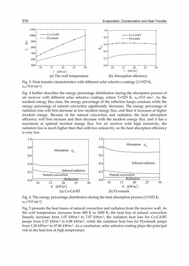
Evaporation, Condensation and Heat Transfer
310
10 15 20 25 30500
600
700
800
900
1000
1100T w
(K
)
I (kW/m2)
Co-Cd-BT Pyromark
10 15 20 25 300.0
0.2
0.4
0.6
0.8
1.0
Co-Cd-BT Pyromark
η ab
I (kW/m2) (a) The wall temperature (b) Absorption efficiency
Fig. 3. Heat transfer characteristics with different solar selective coatings (Tf=523 K, uav=5.0 ms-1)
Fig. 4 further describes the energy percentage distribution during the absorption process of air receiver with different solar selective coatings, where Tf=523 K, uav=5.0 ms-1. As the incident energy flux rises, the energy percentage of the reflection keeps constant, while the energy percentage of natural convection significantly decreases. The energy percentage of radiation loss will first decrease at low incident energy flux, and then it increases at higher incident energy. Because of the natural convection and radiation, the heat absorption efficiency will first increase and then decrease with the incident energy flux, and it has a maximum at optimal incident energy flux. For air receiver with high emissivity, the radiation loss is much higher than that with low emissivity, so the heat absorption efficiency is very low.
10 15 20 25 300.0
0.2
0.4
0.6
0.8
1.0
Absorption ηab
Infrared radiationNatural convection
Reflection
I (kW/m2)10 15 20 25 30
0.0
0.2
0.4
0.6
0.8
1.0
Absorption ηab
Infrared radiation
Natural convectionReflection
I (kW/m2) (a) Co-Cd-BT (b) Pyromark
Fig. 4. The energy percentage distribution during the heat absorption process (Tf=523 K, uav=5.0 ms-1)
Fig. 5 presents the heat losses of natural convection and radiation from the receiver wall. As the wall temperature increases from 400 K to 1000 K, the heat loss of natural convection linearly increases from 1.07 kWm-2 to 7.07 kWm-2, the radiation heat loss for Co-Cd-BT jumps from 0.17 kWm-2 to 6.08 kWm-2, while the radiation heat loss for Pyromark jumps from 1.20 kWm-2 to 47.06 kWm-2. As a conclusion, solar selective coating plays the principal role in the heat loss at high temperature.
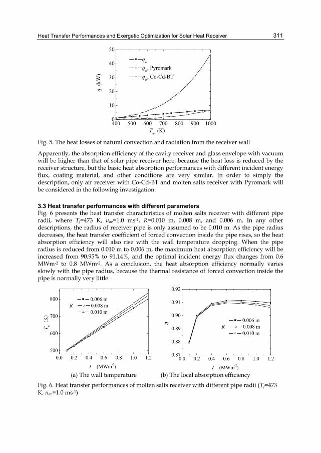
Heat Transfer Performances and Exergetic Optimization for Solar Heat Receiver
311
400 500 600 700 800 900 10000
10
20
30
40
50
Tw (K)
qn
qir, Pyromark qir, Co-Cd-BT
q (k
W)
Fig. 5. The heat losses of natural convection and radiation from the receiver wall
Apparently, the absorption efficiency of the cavity receiver and glass envelope with vacuum will be higher than that of solar pipe receiver here, because the heat loss is reduced by the receiver structure, but the basic heat absorption performances with different incident energy flux, coating material, and other conditions are very similar. In order to simply the description, only air receiver with Co-Cd-BT and molten salts receiver with Pyromark will be considered in the following investigation.
3.3 Heat transfer performances with different parameters Fig. 6 presents the heat transfer characteristics of molten salts receiver with different pipe radii, where Tf=473 K, uav=1.0 ms-1, R=0.010 m, 0.008 m, and 0.006 m. In any other descriptions, the radius of receiver pipe is only assumed to be 0.010 m. As the pipe radius decreases, the heat transfer coefficient of forced convection inside the pipe rises, so the heat absorption efficiency will also rise with the wall temperature dropping. When the pipe radius is reduced from 0.010 m to 0.006 m, the maximum heat absorption efficiency will be increased from 90.95% to 91.14%, and the optimal incident energy flux changes from 0.6 MWm-2 to 0.8 MWm-2. As a conclusion, the heat absorption efficiency normally varies slowly with the pipe radius, because the thermal resistance of forced convection inside the pipe is normally very little.
0.0 0.2 0.4 0.6 0.8 1.0 1.2500
600
700
800
Ι (MWm-2)
0.006 mR 0.008 m 0.010 m
T w (K
)
0.0 0.2 0.4 0.6 0.8 1.0 1.20.87
0.88
0.89
0.90
0.91
0.92
Ι (MWm-2)
0.006 mR 0.008 m 0.010 m
η
(a) The wall temperature (b) The local absorption efficiency
Fig. 6. Heat transfer performances of molten salts receiver with different pipe radii (Tf=473 K, uav=1.0 ms-1)
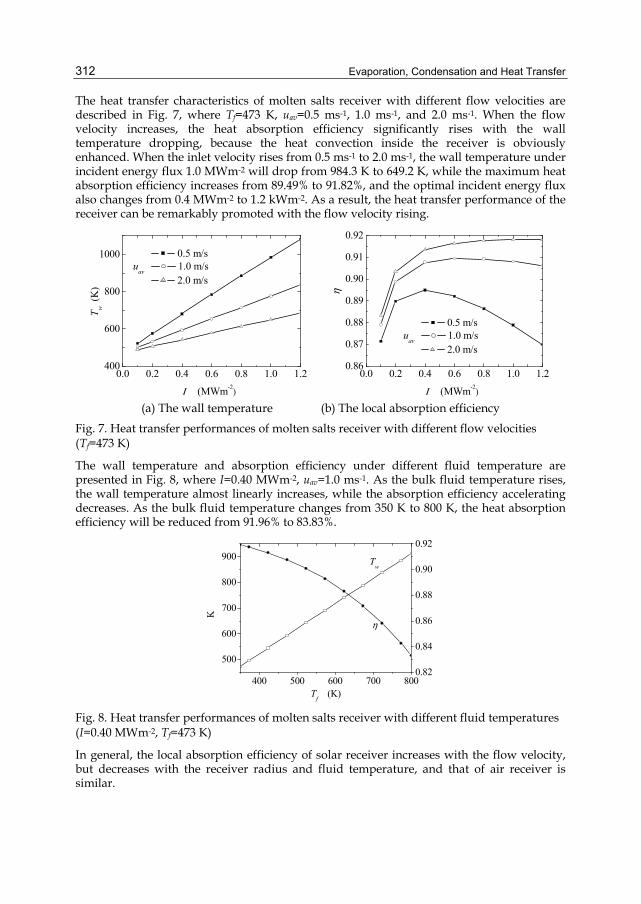
Evaporation, Condensation and Heat Transfer
312
The heat transfer characteristics of molten salts receiver with different flow velocities are described in Fig. 7, where Tf=473 K, uav=0.5 ms-1, 1.0 ms-1, and 2.0 ms-1. When the flow velocity increases, the heat absorption efficiency significantly rises with the wall temperature dropping, because the heat convection inside the receiver is obviously enhanced. When the inlet velocity rises from 0.5 ms-1 to 2.0 ms-1, the wall temperature under incident energy flux 1.0 MWm-2 will drop from 984.3 K to 649.2 K, while the maximum heat absorption efficiency increases from 89.49% to 91.82%, and the optimal incident energy flux also changes from 0.4 MWm-2 to 1.2 kWm-2. As a result, the heat transfer performance of the receiver can be remarkably promoted with the flow velocity rising.
0.0 0.2 0.4 0.6 0.8 1.0 1.2400
600
800
1000
Ι (MWm-2)
0.5 m/suav 1.0 m/s 2.0 m/s
T w (K
)
0.0 0.2 0.4 0.6 0.8 1.0 1.20.86
0.87
0.88
0.89
0.90
0.91
0.92
0.5 m/suav 1.0 m/s 2.0 m/s
Ι (MWm-2)
η
(a) The wall temperature (b) The local absorption efficiency
Fig. 7. Heat transfer performances of molten salts receiver with different flow velocities (Tf=473 K)
The wall temperature and absorption efficiency under different fluid temperature are presented in Fig. 8, where I=0.40 MWm-2, uav=1.0 ms-1. As the bulk fluid temperature rises, the wall temperature almost linearly increases, while the absorption efficiency accelerating decreases. As the bulk fluid temperature changes from 350 K to 800 K, the heat absorption efficiency will be reduced from 91.96% to 83.83%.
400 500 600 700 800
500
600
700
800
900
η
Tw
Tf (K)
K
0.82
0.84
0.86
0.88
0.90
0.92
Fig. 8. Heat transfer performances of molten salts receiver with different fluid temperatures (I=0.40 MWm-2, Tf=473 K)
In general, the local absorption efficiency of solar receiver increases with the flow velocity, but decreases with the receiver radius and fluid temperature, and that of air receiver is similar.
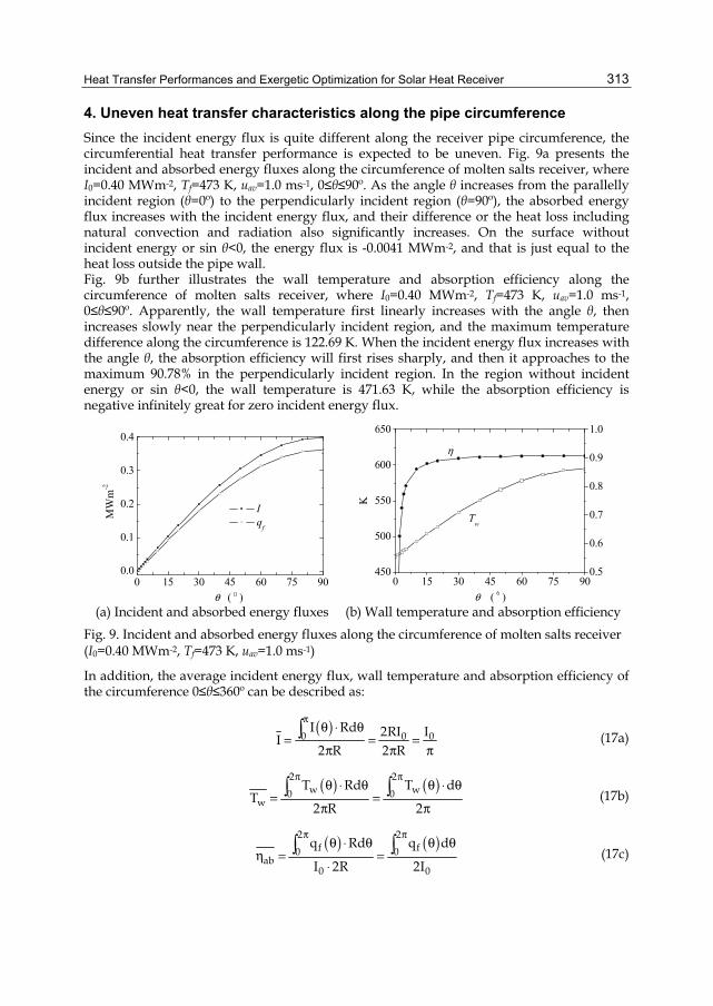
Heat Transfer Performances and Exergetic Optimization for Solar Heat Receiver
313
4. Uneven heat transfer characteristics along the pipe circumference Since the incident energy flux is quite different along the receiver pipe circumference, the circumferential heat transfer performance is expected to be uneven. Fig. 9a presents the incident and absorbed energy fluxes along the circumference of molten salts receiver, where I0=0.40 MWm-2, Tf=473 K, uav=1.0 ms-1, 0≤θ≤90º. As the angle θ increases from the parallelly incident region (θ=0º) to the perpendicularly incident region (θ=90º), the absorbed energy flux increases with the incident energy flux, and their difference or the heat loss including natural convection and radiation also significantly increases. On the surface without incident energy or sin θ<0, the energy flux is -0.0041 MWm-2, and that is just equal to the heat loss outside the pipe wall. Fig. 9b further illustrates the wall temperature and absorption efficiency along the circumference of molten salts receiver, where I0=0.40 MWm-2, Tf=473 K, uav=1.0 ms-1, 0≤θ≤90º. Apparently, the wall temperature first linearly increases with the angle θ, then increases slowly near the perpendicularly incident region, and the maximum temperature difference along the circumference is 122.69 K. When the incident energy flux increases with the angle θ, the absorption efficiency will first rises sharply, and then it approaches to the maximum 90.78% in the perpendicularly incident region. In the region without incident energy or sin θ<0, the wall temperature is 471.63 K, while the absorption efficiency is negative infinitely great for zero incident energy flux.
0 15 30 45 60 75 900.0
0.1
0.2
0.3
0.4
MW
m-2
θ ( )
I qf
0 15 30 45 60 75 90450
500
550
600
650
η
Tw
θ ( )
K
0.5
0.6
0.7
0.8
0.9
1.0
(a) Incident and absorbed energy fluxes (b) Wall temperature and absorption efficiency Fig. 9. Incident and absorbed energy fluxes along the circumference of molten salts receiver (I0=0.40 MWm-2, Tf=473 K, uav=1.0 ms-1)
In addition, the average incident energy flux, wall temperature and absorption efficiency of the circumference 0≤θ≤360º can be described as:
( )0 0 0
I Rd 2RI II2 R 2 R
πθ ⋅ θ
= = =π π π
∫ (17a)
( ) ( )2 2
w w0 0w
T Rd T dT
2 R 2
π πθ ⋅ θ θ ⋅ θ
= =π π
∫ ∫ (17b)
( ) ( )2 2
f f0 0ab
0 0
q Rd q d
I 2R 2I
π πθ ⋅ θ θ θ
η = =⋅
∫ ∫ (17c)
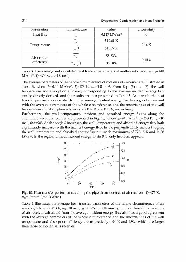
Evaporation, Condensation and Heat Transfer
314
Parameters nomenclature value uncertainty Heat flux I 0.127 MWm-2 0
wT 510.61 K Temperature ( )wT I 510.77 K
0.16 K
abη 88.63% Absorption efficiency ( )ab Iη 88.78%
0.15%
Table 3. The average and calculated heat transfer parameters of molten salts receiver (I0=0.40 MWm-2, Tf=473 K, uav=1.0 ms-1)
The average parameters of the whole circumference of molten salts receiver are illustrated in Table 3, where I0=0.40 MWm-2, Tf=473 K, uav=1.0 ms-1. From Eqs. (5) and (7), the wall temperature and absorption efficiency corresponding to the average incident energy flux can be directly derived, and the results are also presented in Table 3. As a result, the heat transfer parameters calculated from the average incident energy flux has a good agreement with the average parameters of the whole circumference, and the uncertainties of the wall temperature and absorption efficiency are 0.16 K and 0.15%, respectively. Furthermore, the wall temperature, incident and absorbed energy fluxes along the circumference of air receiver are presented in Fig. 10, where I0=20 kWm-2, Tf=473 K, uav=10 ms-1, 0≤θ≤90º. As the angle θ increases, the wall temperature and absorbed energy flux both significantly increases with the incident energy flux. In the perpendicularly incident region, the wall temperature and absorbed energy flux approach maximums of 772.15 K and 14.38 kWm-2. In the region without incident energy or sin θ<0, only heat loss appears.
0 20 40 60 80
0
5
10
15
20
25
30
Tw
I
qf
θ ( )
kWm
-2
400
480
560
640
720
800
K
Fig. 10. Heat transfer performances along the pipe circumference of air receiver (Tf=473 K, uav=10 ms-1, I0=20 kWm-2)
Table 4 illustrates the average heat transfer parameters of the whole circumference of air receiver, where Tf=473 K, uav=10 ms-1, I0=20 kWm-2. Obviously, the heat transfer parameters of air receiver calculated from the average incident energy flux also has a good agreement with the average parameters of the whole circumference, and the uncertainties of the wall temperature and absorption efficiency are respectively 4.04 K and 1.9%, which are larger than those of molten salts receiver.

Heat Transfer Performances and Exergetic Optimization for Solar Heat Receiver
315
Parameters nomenclature value uncertainty Heat flux I 6.37 kWm-2 0
wT 554.64 K Temperature ( )wT I 558.68 K
4.04 K
abη 62.8% Absorption efficiency ( )ab Iη 64.7%
1.9%
Table 4. The average and calculated heat transfer parameters of air receiver (Tf=473 K, uav=10 ms-1, I0=20 kWm-2)
In general, the average absorption efficiency along the whole circumference of molten salt receiver or air receiver is almost equal to the absorption efficiency corresponding to the average incident energy flux, and then
( ) ( )2f f0
q Rd 2 RI 2 RI I 2 R q Iπ
⋅ θ = π ⋅ η ≈ π ⋅ η = π ⋅∫ (18)
5. Heat transfer and absorption performances of the whole receiver In order to investigate the heat transfer performance of the whole receiver, the energy transport equation along x direction from Eqs. (6) and (18) is derived as:
( )2 R 2ff p p av0 0
Tq Rd c Tu r 2 rdr c R ux x
π ∂ ∂⋅ θ = ρ ⋅ π = ρ π∂ ∂∫ ∫ (19)
Substituting Eq. (18) into Eq. (19) yields
( ) 2ff p av
T2 R q I c R ux
∂π ⋅ = ρ π∂
(20)
Eq. (20) can be simplified as:
( )ff
p av
2q ITx c Ru
∂ =∂ ρ
(21)
Fig. 11 presents the heat transfer and absorption characteristics of molten salts receiver along the flow direction, where I0=0.40 MWm-2, Tf0=473 K. Apparently, the bulk fluid temperature and average wall temperature almost linearly increase along the flow direction. For higher flow velocity, the temperature difference of the fluid and wall is lower for higher heat transfer coefficient, and the temperature gradient along the flow direction is also smaller. As the flow velocity increases from 0.5 ms-1 to 2.0 ms-1, the average wall temperature in the outlet drops from 821.5 K to 574.0 K, and that can remarkably benefit the receiver material. The heat absorption efficiency of the receiver will be larger for high flow velocity, and the heat absorption efficiency in the outlet rises from 72.01% to 86.77% as the flow velocity increasing from 0.5 ms-1 to 2.0 ms-1. The heat transfer and absorption characteristics of air receiver along the flow direction is further described in Fig. 12, where I0=31.4 kWm-2, Tf0=523 K, uav=5.0 ms-1. Along the flow direction, the temperatures of fluid and wall increases, while the heat absorption
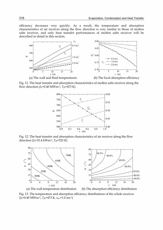
Evaporation, Condensation and Heat Transfer
316
efficiency decreases very quickly. As a result, the temperature and absorption characteristics of air receiver along the flow direction is very similar to those of molten salts receiver, and only heat transfer performances of molten salts receiver will be described in detail in this section.
0 5 10 15 20500
600
700
800
uav
2.0 ms-1
1.0 ms-1
0.5 ms-1
Tf
Tw
K
x (m) 0 5 10 15 20
0.70
0.75
0.80
0.85
0.90
0.5 m/suav 1.0 m/s 2.0 m/s
x (m)
η ab
(a) The wall and fluid temperatures (b) The local absorption efficiency
Fig. 11. The heat transfer and absorption characteristics of molten salts receiver along the flow direction (I0=0.40 MWm-2, Tf0=473 K)
0.0 0.2 0.4 0.6 0.8 1.0500
550
600
650
700
750
800
ηab
Tw
Tf
x (m)
K
0.40
0.45
0.50
0.55
0.60
Fig. 12. The heat transfer and absorption characteristics of air receiver along the flow direction (I0=31.4 kWm-2, Tf0=523 K)
0 4 8 12 16 200
15
30
45
60
75
90
500K
550K
600K
650K
700K
θ
(
)
x (m)0 4 8 12 16 20
0
15
30
45
60
75
90
60.0%80.0%85.0%
88.0%
89.0%
90.0%90.5%
θ
( )
x (m) (a) The wall temperature distribution (b) The absorption efficiency distribution
Fig. 13. The temperature and absorption efficiency distributions of the whole receiver (I0=0.40 MWm-2, Tf0=473 K, uav=1.0 ms-1)
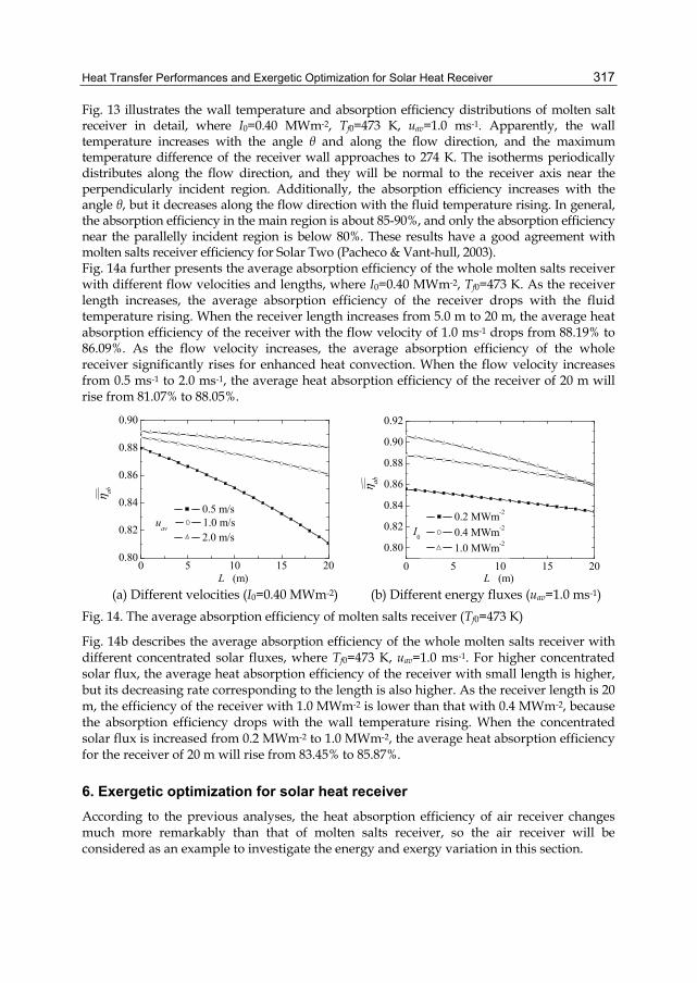
Heat Transfer Performances and Exergetic Optimization for Solar Heat Receiver
317
Fig. 13 illustrates the wall temperature and absorption efficiency distributions of molten salt receiver in detail, where I0=0.40 MWm-2, Tf0=473 K, uav=1.0 ms-1. Apparently, the wall temperature increases with the angle θ and along the flow direction, and the maximum temperature difference of the receiver wall approaches to 274 K. The isotherms periodically distributes along the flow direction, and they will be normal to the receiver axis near the perpendicularly incident region. Additionally, the absorption efficiency increases with the angle θ, but it decreases along the flow direction with the fluid temperature rising. In general, the absorption efficiency in the main region is about 85-90%, and only the absorption efficiency near the parallelly incident region is below 80%. These results have a good agreement with molten salts receiver efficiency for Solar Two (Pacheco & Vant-hull, 2003). Fig. 14a further presents the average absorption efficiency of the whole molten salts receiver with different flow velocities and lengths, where I0=0.40 MWm-2, Tf0=473 K. As the receiver length increases, the average absorption efficiency of the receiver drops with the fluid temperature rising. When the receiver length increases from 5.0 m to 20 m, the average heat absorption efficiency of the receiver with the flow velocity of 1.0 ms-1 drops from 88.19% to 86.09%. As the flow velocity increases, the average absorption efficiency of the whole receiver significantly rises for enhanced heat convection. When the flow velocity increases from 0.5 ms-1 to 2.0 ms-1, the average heat absorption efficiency of the receiver of 20 m will rise from 81.07% to 88.05%.
0 5 10 15 200.80
0.82
0.84
0.86
0.88
0.90
η ab
0.5 m/suav 1.0 m/s 2.0 m/s
L (m)0 5 10 15 20
0.80
0.82
0.84
0.86
0.88
0.90
0.92
I0
0.2 MWm-2
0.4 MWm-2
1.0 MWm-2
L (m)
η ab
(a) Different velocities (I0=0.40 MWm-2) (b) Different energy fluxes (uav=1.0 ms-1)
Fig. 14. The average absorption efficiency of molten salts receiver (Tf0=473 K)
Fig. 14b describes the average absorption efficiency of the whole molten salts receiver with different concentrated solar fluxes, where Tf0=473 K, uav=1.0 ms-1. For higher concentrated solar flux, the average heat absorption efficiency of the receiver with small length is higher, but its decreasing rate corresponding to the length is also higher. As the receiver length is 20 m, the efficiency of the receiver with 1.0 MWm-2 is lower than that with 0.4 MWm-2, because the absorption efficiency drops with the wall temperature rising. When the concentrated solar flux is increased from 0.2 MWm-2 to 1.0 MWm-2, the average heat absorption efficiency for the receiver of 20 m will rise from 83.45% to 85.87%.
6. Exergetic optimization for solar heat receiver According to the previous analyses, the heat absorption efficiency of air receiver changes much more remarkably than that of molten salts receiver, so the air receiver will be considered as an example to investigate the energy and exergy variation in this section.
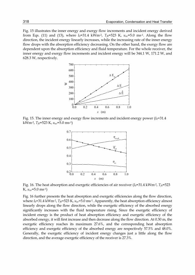
Evaporation, Condensation and Heat Transfer
318
Fig. 15 illustrates the inner energy and exergy flow increments and incident energy derived from Eqs. (11) and (13), where I0=31.4 kWm-2, Tf0=523 K, uav=5.0 ms-1. Along the flow direction, the incident energy linearly increases, while the increasing rate of the inner energy flow drops with the absorption efficiency decreasing. On the other hand, the exergy flow are dependent upon the absorption efficiency and fluid temperature. For the whole receiver, the inner energy and exergy flow increments and incident energy will be 344.1 W, 171.2 W, and 628.3 W, respectively.
0.0 0.2 0.4 0.6 0.8 1.00
100
200
300
400
500
600
700
Δ E
Δ E
Δ Ein
W
x (m) Fig. 15. The inner energy and exergy flow increments and incident energy power (I0=31.4 kWm-2, Tf0=523 K, uav=5.0 ms-1)
0.0 0.2 0.4 0.6 0.8 1.00.2
0.3
0.4
0.5
0.6
0.7ηex,ab
ηab
ηex
x (m)
Fig. 16. The heat absorption and exergetic efficiencies of air receiver (I0=31.4 kWm-2, Tf0=523 K, uav=5.0 ms-1)
Fig. 16 further presents the heat absorption and exergetic efficiencies along the flow direction, where I0=31.4 kWm-2, Tf0=523 K, uav=5.0 ms-1. Apparently, the heat absorption efficiency almost linearly drops along the flow direction, while the exergetic efficiency of the absorbed energy significantly increases with the fluid temperature rising. Since the exergetic efficiency of incident energy is the product of heat absorption efficiency and exergetic efficiency of the absorbed energy, it will first increase and then decrease along the flow direction. At 0.30 m, the exergetic efficiency reaches its maximum 27.6%, and the corresponding heat absorption efficiency and exergetic efficiency of the absorbed energy are respectively 57.5% and 48.0%. Generally, the exergetic efficiency of incident energy changes just a little along the flow direction, and the average exergetic efficiency of the receiver is 27.3%.
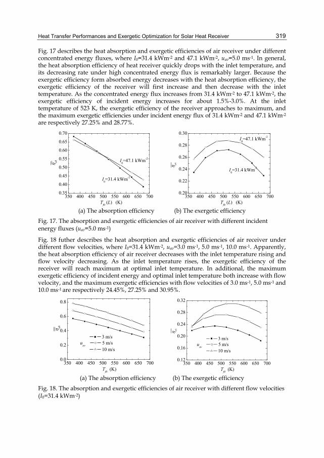
Heat Transfer Performances and Exergetic Optimization for Solar Heat Receiver
319
Fig. 17 describes the heat absorption and exergetic efficiencies of air receiver under different concentrated energy fluxes, where I0=31.4 kWm-2 and 47.1 kWm-2, uav=5.0 ms-1. In general, the heat absorption efficiency of heat receiver quickly drops with the inlet temperature, and its decreasing rate under high concentrated energy flux is remarkably larger. Because the exergetic efficiency form absorbed energy decreases with the heat absorption efficiency, the exergetic efficiency of the receiver will first increase and then decrease with the inlet temperature. As the concentrated energy flux increases from 31.4 kWm-2 to 47.1 kWm-2, the exergetic efficiency of incident energy increases for about 1.5%-3.0%. At the inlet temperature of 523 K, the exergetic efficiency of the receiver approaches to maximum, and the maximum exergetic efficiencies under incident energy flux of 31.4 kWm-2 and 47.1 kWm-2
are respectively 27.25% and 28.77%.
350 400 450 500 550 600 650 7000.35
0.40
0.45
0.50
0.55
0.60
0.65
0.70
I0=47.1 kWm-2
I0=31.4 kWm-2
η ab
Tf0 (L) (K)
350 400 450 500 550 600 650 7000.20
0.22
0.24
0.26
0.28
0.30I0=47.1 kWm-2
I0=31.4 kWm-2η ex
Tf0 (L) (K)
(a) The absorption efficiency (b) The exergetic efficiency
Fig. 17. The absorption and exergetic efficiencies of air receiver with different incident energy fluxes (uav=5.0 ms-1)
Fig. 18 futher describes the heat absorption and exergetic efficiencies of air receiver under different flow velocities, where I0=31.4 kWm-2, uav=3.0 ms-1, 5.0 ms-1, 10.0 ms-1. Apparently, the heat absorption efficiency of air receiver decreases with the inlet temperature rising and flow velocity decreasing. As the inlet temperature rises, the exergetic efficiency of the receiver will reach maximum at optimal inlet temperature. In additional, the maximum exergetic efficiency of incident energy and optimal inlet temperature both increase with flow velocity, and the maximum exergetic efficiencies with flow velocities of 3.0 ms-1, 5.0 ms-1 and 10.0 ms-1 are respectively 24.45%, 27.25% and 30.95%.
350 400 450 500 550 600 650 7000.0
0.2
0.4
0.6
0.8
Tf0 (K)
3 m/suav 5 m/s 10 m/s
η ab
350 400 450 500 550 600 650 700
0.12
0.16
0.20
0.24
0.28
0.32
Tf0 (K)
3 m/suav 5 m/s 10 m/s
η ex
(a) The absorption efficiency (b) The exergetic efficiency
Fig. 18. The absorption and exergetic efficiencies of air receiver with different flow velocities (I0=31.4 kWm-2)
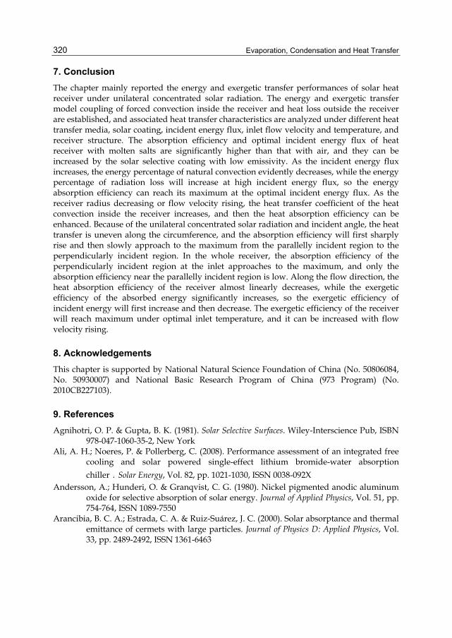
Evaporation, Condensation and Heat Transfer
320
7. Conclusion The chapter mainly reported the energy and exergetic transfer performances of solar heat receiver under unilateral concentrated solar radiation. The energy and exergetic transfer model coupling of forced convection inside the receiver and heat loss outside the receiver are established, and associated heat transfer characteristics are analyzed under different heat transfer media, solar coating, incident energy flux, inlet flow velocity and temperature, and receiver structure. The absorption efficiency and optimal incident energy flux of heat receiver with molten salts are significantly higher than that with air, and they can be increased by the solar selective coating with low emissivity. As the incident energy flux increases, the energy percentage of natural convection evidently decreases, while the energy percentage of radiation loss will increase at high incident energy flux, so the energy absorption efficiency can reach its maximum at the optimal incident energy flux. As the receiver radius decreasing or flow velocity rising, the heat transfer coefficient of the heat convection inside the receiver increases, and then the heat absorption efficiency can be enhanced. Because of the unilateral concentrated solar radiation and incident angle, the heat transfer is uneven along the circumference, and the absorption efficiency will first sharply rise and then slowly approach to the maximum from the parallelly incident region to the perpendicularly incident region. In the whole receiver, the absorption efficiency of the perpendicularly incident region at the inlet approaches to the maximum, and only the absorption efficiency near the parallelly incident region is low. Along the flow direction, the heat absorption efficiency of the receiver almost linearly decreases, while the exergetic efficiency of the absorbed energy significantly increases, so the exergetic efficiency of incident energy will first increase and then decrease. The exergetic efficiency of the receiver will reach maximum under optimal inlet temperature, and it can be increased with flow velocity rising.
8. Acknowledgements This chapter is supported by National Natural Science Foundation of China (No. 50806084, No. 50930007) and National Basic Research Program of China (973 Program) (No. 2010CB227103).
9. References Agnihotri, O. P. & Gupta, B. K. (1981). Solar Selective Surfaces. Wiley-Interscience Pub, ISBN
978-047-1060-35-2, New York Ali, A. H.; Noeres, P. & Pollerberg, C. (2008). Performance assessment of an integrated free
cooling and solar powered single-effect lithium bromide-water absorption chiller.Solar Energy, Vol. 82, pp. 1021-1030, ISSN 0038-092X
Andersson, A.; Hunderi, O. & Granqvist, C. G. (1980). Nickel pigmented anodic aluminum oxide for selective absorption of solar energy. Journal of Applied Physics, Vol. 51, pp. 754-764, ISSN 1089-7550
Arancibia, B. C. A.; Estrada, C. A. & Ruiz-Suárez, J. C. (2000). Solar absorptance and thermal emittance of cermets with large particles. Journal of Physics D: Applied Physics, Vol. 33, pp. 2489-2492, ISSN 1361-6463
Heat Transfer Performances and Exergetic Optimization for Solar Heat Receiver
321
Bai, F. W. (2010). One dimensional thermal analysis of silicon carbide ceramic foam used for solar air receiver. International Journal of Thermal Sciences, Vol. 49, pp. 2400-2404, ISSN 1290-0729
Bejan, A., Keary, D. W. & Kreith, F. (1981). Second law analysis and synthesis of solar collector systems. Journal of Solar Energy Engineering, Vol. 103, pp. 23-28, ISSN 0199-6231
Brenntag Company. Hitec heat transfer salt. pp. 3-10, Houston. Available from http://www.coal2nuclear.com/MSR%20-%20HITEC%20Heat%20Transfer%20Salt.pdf Chan, Y. L. & Tien, C. L. (1985). A numerical study of two-dimensional laminar natural
convection in shallow open cavities. International Journal of Heat and Mass Transfer, Vol. 28, pp. 603-612, ISSN 0017-9310
Chan, Y. L. & Tien, C. L. (1986). Laminar natural convection in shallow open cavities. ASME Journal of Heat Transfer, Vol. 108, pp. 305-309, ISSN 0022-1481
Cindrella, L. (2007). The real utility ranges of the solar selective coatings. Solar Energy Materials and Solar Cells, Vol. 91, pp. 1898-1901, ISSN 0927-0248
Clausing, A. M. (1981). An analysis of convective losses from cavity solar central receiver. Solar Energy, Vol. 27, pp. 295-300, ISSN 0038-092X
Clausing, A. M. (1983). Convective losses from cavity solar receivers - comparisons between analytical predictions and experimental results. Journal of Solar Energy Engineering, Vol. 105, pp. 29-33, ISSN 0199-6231
Cui, H. T.; Xing, Y. M.; Guo, Y. S.; Wang, Z. H.; Cui, H. C. & Yuan, A. G. (2008). Numerical simulation and experiment investigation on unit heat exchange tube for solar heat receiver. Solar Energy, Vol. 82, pp. 1229-1234, ISSN 0038-092X
Dehghan, A. A. & Behnia, M. (1996). Combined natural convection conduction and radiation heat transfer in a discretely heated open cavity. ASME Journal of Heat Transfer, Vol. 118, pp. 54-56, ISSN 0022-1481
Estrada, C. A.; Jaramillo, O. A.; Acosta, R. & Arancibia, B. C. A. (2007). Heat transfer analysis in a calorimeter for concentrated solar radiation measurements. Solar Energy, Vol. 81, pp. 1306-1313, ISSN 0038-092X
Farahat, S.; Sarhaddi, F., & Ajam, H. (2009). Exergetic optimization of flat plate solar collectors. Renewable Energy, Vol. 34, pp. 1169-1174, ISSN 0960-1481
Fujiwara, M.; Sano, T.; Suzuki, K. & Watanabe, S. Y. (1990). Thermal analysis and fundamental tests heat pipe receiver for solar dynamic space system. Journal of Solar Energy Engineering, Vol. 112, pp. 177-182, ISSN 0199-6231
Gao P.; Meng L. J.; Santos M. P.; Teixeira V. & Andritschky M. (2000). Characterization of ZrO2 films prepared by rf magnetron reactive sputtering at different O2 concentrations in the sputtering gases. Vacuum, Vol. 56, pp. 143-148, ISSN 0042-207X
Gong, G. J.; Huang, X. Y.; Wang, J. & Hao M. L. (2010). An optimized model and test of the China's first high temperature parabolic trough solar receiver. Solar Energy, Vol. 84, pp. 2230-2245, ISSN 0038-092X
Grena, R. (2010). Optical simulation of a parabolic solar trough collector. International Journal of Sustainable Energy, Vol. 29, pp. 19-36, ISSN 1478-646X
Hogan, R. E.; Diver, R. B. & Stine, W. B. (1990). Comparison of a cavity solar receiver numerical model and experimental data. Journal of Solar Energy Engineering, Vol. 112, pp. 183-190, ISSN 0199-6231
Evaporation, Condensation and Heat Transfer
322
Kalogirou, S. A. (2004). Solar thermal collectors and applications. Progress in Energy and Combustion Science, Vol. 30, pp. 231-295, ISSN 0360-1285
Kaushika, N. D. & Reddy, K. S. (2000). Performance of a low cost solar paraboloidal dish steam generating system. Energy Conversion and Management, Vol. 41, pp. 713-726, ISSN 0196-8904
Kennedy, C. E. (2002). Review of mid- to high-temperature solar selective absorber materials. NREL/TP-520-31267
Khubeiz, J. M.; Radziemska, E. & Lewandowski, W. M. (2002). Natural convective heat transfers from an isothermal horizontal hemisphericalcavity. Applied Energy, Vol. 73, pp. 261-275, ISSN 0306-2619
Klein, H. H.; Karni, J.; Ben-Zvi, R. & Bertocchi, R. (2007). Heat transfer in a directly irradiated solar receiver/reactor for solid-gas reactions.Solar Energy, Vol. 81, pp. 1227-1239, ISSN 0038-092X
Koenig, A. A. & Marvin, M. (1981). Convection heat loss sensitivity in open cavity solar receivers, final report. DOE Contract, No. EG77-C-04-3985
Kongtragool, B. & Wongwises, S. (2005). Optimum absorber temperature of a once reflecting full conical concentrator of a low temperature differential Stirling engine. Renewable Energy, Vol. 30, pp. 1671-1687, ISSN 0960-1481
Kotas, T. J. (1995). The exergy method of thermal plant analysis. Malabar, FL: Krieger Publish Company, ISBN 978-089-4649-41-7
Lage, J. L., Lim, J. S. & Bejan, A. (1992). Natural convection with radiation in a cavity with open top end. ASME Journal of Heat Transfer, Vol. 114, pp. 479-486, ISSN 0022-1481
Leibfried, U. & Ortjohann, J. (1995). Convective heat loss from upward and downward facing cavity receivers: measurements and calculations. Journal of Solar Energy Engineering, Vol. 117, pp. 75–84, ISSN 0199-6231
LeQuere, P.; Penot, F. & Mirenayat, M. (1981a). Experimental study of heat loss through natural convection from an isothermal cubic open cavity. Sandia Laboratory Report, SAND81-8014
LeQuere, P.; Humphrey, J. A. C. & Sherman, F. S. (1981b). Numerical calculation of thermally driven two-dimensional unsteady laminar flow in cavities of rectangular cross section. Numerical Heat Transfer, Vol. 4, pp. 249-283, ISSN 1521-0634
Li, M. & Wang, L. L. (2006). Investigation of evacuated tube heated by solar trough concentrating system. Energy Conversion and Management, Vol. 47, pp. 3591-3601, ISSN 0196-8904
Li, X.; Kong, W. Q.; Wang, Z. F.; Chang, C. & Bai, F. W. (2010). Thermal model and thermodynamic performance of molten salt cavity receiver. Renewable Energy, Vol. 35, pp. 981-988, ISSN 0960-1481
Lienhard, IV J. H., Lienhard, V J. H. (2002). A Heat Transfer Textbook. Phlogiston Press, Chambridge, ISBN 978-048-6479-31-6, Massachusetts, U.S.A
Lu, J. F.; Ding, J. & Yang, J. P. (2010a). Heat transfer performance of the receiver pipe under unilateral concentrated solar radiation. Solar Energy, Vol. 84, pp. 1879-1887, ISSN 0038-092X
Lu, J. F.; Ding, J. & Yang, J. P. (2010b). Heat transfer performance and exergetic optimization for solar receiver pipe. Renewable Energy, Vol. 35, pp. 1477-1483, ISSN 0960-1481
Ma, R. Y. (1993). Wind effects on convective heat loss from a cavity receiver for a parabolic concentrating solar collector. Sandia National Laboratories Report, SAND92-7293
Heat Transfer Performances and Exergetic Optimization for Solar Heat Receiver
323
McDonald, C. G. (1995). Heat loss from an open cavity. Sandia National Laboratories Report, SAND95-2939
Melchior, T.; Perkins, C.; Weimer, A. W. & Steinfeld, A. (2008). A cavity-receiver containing a tubular absorber for high-temperature thermochemical processing using concentrated solar energy. International Journal of Thermal Sciences, Vol. 35, pp. 981-988, ISSN 1290-0729
Moustafa, M.; Kadry, A. & Ornar M. (1995). Measurements of solar flux density distribution on a plane receiver due to a flat heliostat. Solar Energy, Vol. 54, pp. 403-411, ISSN 0038-092X
Muftuoglu, A. & Bilgen, E. (2008). Heat transfer in inclined rectangular receivers for concentrated solar radiation. International Communications in Heat and Mass Transfer, Vol. 35, pp. 551-556, ISSN 0735-1933
Nilsson, A. M. & Roos, A. (2009). Evaluation of optical and thermal properties of coatings for energy efficient windows. Thin Solid Films, Vol. 517, pp. 3173-3177, ISSN 0040-6090
Odeh, S. D.; Behnia, M. & Morrison, G. L. (2003). Performance evaluation of solar thermal electric generation systems. Energy Conversion and Management, Vol. 44, pp. 2425-2443, ISSN 0196-8904
Ortega, J. I.; Burgaleta, J. I. & Téllez F. M. (2008). Central receiver system solar power plant using molten salt as heat transfer fluid. Journal of Solar Energy Engineering, Vol. 130, pp. 024501-1-6, ISSN 0199-6231
Pacheco, J. E. & Vant-hull, L. L. (2003). Final results and operating experience of the Solar Two Project. Advances in solar energy Vol. 15, pp. 43-81, ISBN 978-184-4072-44-6
Paitoonsurikarn, S. & Lovegrove, K. (2006). A new correlation for predicting the free convection loss from solar dish concentrating receivers. Proceedings of 44th ANZSES conference, ISBN 978-097-5065-04-4, Australia
Pellegrini, G. (1980). Experimental methods for the preparation of selectively absorbing textured surfaces for photothermal solar conversion. Solar Energy Materials, Vol. 3, pp. 391-404, ISSN 0927-0248
Prakash, M.; Kedare, S. B. & Nayak, J. K. (2009). Investigations on heat losses from a solar cavity receiver. Solar Energy, Vol. 83, pp. 157-170, ISSN 0038-092X
Reddy, K. S. & Kumar N. S. (2008). Combined laminar natural convection and surface radiation heat transfer in a modified cavity receiver of solar parabolic dish. International Journal of Thermal Sciences, Vol. 47, pp. 1647-1657, ISSN 1290-0729
Reilly, H. E. & Kolb, G. J. (2001). An evaluation of molten-salt power towers including results of the solar two project. Sandia National Laboratories Report, SAND2001-3674
Segal, A & Epstein, M. (2003). Optimized working temperatures of a solar central receiver. Solar Energy, Vol. 75, pp. 503-510, ISSN 0038-092X
Sendhil, K. N. & Reddy, K. S. (2007). Numerical investigations of natural convection heat loss in modified cavity receiver for fuzzy focal solar dish. Solar Energy, Vol. 81, pp. 846-855, ISSN 0038-092X
Sendhil, K. N. & Reddy, K. S. (2008). Comparison of receivers for solar dish collector system. Energy Conversion and Management, Vol. 49, pp. 812-819, ISSN 0196-8904
Seraphin, B. O. & Meinel, A. B. (1976a). Optical Properties of Solids: New Developments. North Holland Publishing Co., ISBN 044-4110-05-4, Amsterdam
Evaporation, Condensation and Heat Transfer
324
Seraphin, B. O. (1976b). Chemical vapor deposition of thin semiconductor films for solar energy conversion. Thin Solid Films, Vol. 57, pp. 87- 94, ISSN 0040-6090
Siebers, D. L. & Kraabel, J. S. (1984). Estimating convective energy losses from solar central receivers. Sandia Laboratory Report, SAND84-8717
Singh, N.; Kaushik, S. C. & Misra R. D. (2000). Exergetic analysis of a solar thermal power system. Renewable Energy, Vol. 19, pp. 135-143, ISSN 0960-1481
Steinfeld, A. & Schubnell, M. (1993). Optimum aperture size and operating temperature of a solar cavity-receiver. Solar Energy, Vol. 50, pp. 19-25, ISSN 0038-092X
Tabor, H. (1958). Solar energy research: Program in the new desert research institute in Beersheba. Solar Energy, Vol. 2, pp. 3-6, ISSN 0038-092X
Taragan, E. (1999). A multistage solar receiver: the route to high temperature. Solar Energy, Vol. 67, pp. 3-11, ISSN 0038-092X
Taumoefolau, T.; Paitoonsurikarn, S.; Hughes, G. & Lovegrove, K. (2004). Experimental investigation of natural convection heat loss from a model solar concentrator cavity receiver. Journal of Solar Energy Engineering, Vol. 126, pp. 801-807, ISSN 0199-6231
Trieb, F. & Nitsch, J. (1998). Recommendations for the market introduction of solar thermal power stations. Renewable Energy, Vol. 14, pp. 17-22, ISSN 0960-1481
Wu, S. Y.; Xiao, L.; Cao, Y. D. & Li, Y. R. (2010). Convection heat loss from cavity receiver in parabolic dish solar thermal power system: A review. Solar Energy, Vol. 84, pp. 1342-1355, ISSN 0038-092X
Zarza, E.; Valenzuela, L.; Leon, J.; Hennecke, K.; Eck, M.; Weyers, H. D. & Eickhoff, M. (2004). Direct steam generation in parabolic troughs: Final results and conclusions of the DISS project. Energy, Vol. 29, pp. 635-644, ISSN 0360-5442
Zavoico, A. B. (2001). Solar power tower design basis document, Revision 0. Sandia National Laboratories Report, SAND2001-2100
0
Soret and Dufour Effects on Steady MHD NaturalConvection Flow Past a Semi-Infinite Moving
Vertical Plate in a Porous Medium with ViscousDissipation in the Presence of
a Chemical Reaction
Sandile Motsa1 and Stanford Shateyi21University of Swaziland
2University of Venda1Swaziland
2South Africa
1. Introduction
Transportation of heat through porous media has been a subject of many studies due to theincreasing need for a better understanding of the associated transport processes. There arenumerous practical applications which can be modeled or can be approximated as transportthrough porous media such as grain storage, packed sphere beds, high performance insulationfor buildings, migration of moisture through the air contained in fibrous insulations, heatexchange between soil and atmosphere sensible heat storage beds and beds of fossil fuels andgeothermal energy systems, among other areas. Double diffusive is driven by buoyancy dueto temperature and concentration gradients.Magnetohydrodynamic flows have many applications in solar physics, cosmic fluiddynamics, geophysics and in the motion of earth’s core as well as in chemical engineering andelectronics. Huges and Young (1996) gave an excellent summary of applications. Soret andDufour effects become significant when species are introduced at a surface in fluid domain,with different (lower) density than the surrounding fluid. When heat and mass transfer occursimultaneously in a moving fluid, the relations between the fluxes and the driving potentialsare more intricate in nature. It is now known that an energy flux can be generated not only bytemperature gradients but by composition gradients as well. This type of energy flux is calledthe Dufour or diffusion-thermo effect. We also have mass fluxes being created by temperaturegradients and this is called the Soret or thermal-diffusion. The effect of chemical reactiondepends on whether the reaction is heterogenous or homogenous.Motivated by previous works Abreu (et al. 2006) - Alam & Rahman (2006), Don & Solomonoff(1995) - Shateyi (2008) and many possible industrial and engineering applications, weaim in this chapter to analyze steady two-dimensional hydromagnetic flow of a viscousincompressible, electrically conducting and viscous dissipating fluid past a semi-infinite
16
2 Mass Transfer
moving permeable plate embedded in a porous medium in the presence of a reacting chemicalspecies, Dufour and Soret effects.The resultant non-dimensional ordinary differential equations are then solved numerically bythe Successive Linearization Method (SLM). The effects of various significant parameters suchas Hartmann, chemical reaction parameter, Soret number, Dufour number, Eckert number,permeability parameter and Grashof numbers on the velocity, temperature, concentration, aredepicted in figures and then discussed.The governing equations are transformed into a system of nonlinear ordinary differentialequations by using suitable local similarity transf. This chapter is arranged into five majorsections as follows. Section 1 gives an account of previous related works as well as definitionsto important terms. In section 2 we give the mathematical formulation of the problem and itsanalysis. A brief description of the method used in this chapter is presented in section 3. Insection 4 we provide the results and their discussion. Lastly the conclusion to the chapter ispresented in section 5.
2. Mathematical formulation
We consider a steady two-dimensional hydromagnetic flow of a viscous incompressible,electrically conducting and viscous dissipating fluid past a semi-infinite moving permeableplate embedded in a porous medium. We assume the flow to be in the x− direction, whichis taken along the semi-infinite plate and the y− axis to be normal to it. The plate ismaintained at a constant temperature Tw, which is higher than the free stream temperatureT∞ of the surrounding fluid and a constant concentration Cw which is greater than theconstant concentration C∞ of the surrounding fluid. A uniform magnetic field of strength B0is applied normal to the plate, which produces magnetic effect in the x− direction. The fluidis assumed to be slightly conducting, so that the magnetic Reynolds number is very smalland the induced magnetic field is negligible in comparison with the applied magnetic field.We also assumed that there is no applied voltage, so that electric field is absent. All the fluidproperties are assumed to be constant except that of the influence of the density variationwith temperature and concentration in the body force term. A first-order homogeneouschemical reaction is assumed to take place in the flow. With the usual boundary layer andBoussinesq approximations the conservation equations for the problem under considerationcan be written as
∂u∂x
+∂v∂y
= 0, (1)
u∂u∂x
+ v∂u∂y
= ν∂2u∂y2 + gβt(T − T∞) + gβc(C− C∞)− σB2
0ρ
u− μ
ρk∗ u, (2)
u∂T∂x
+ v∂T∂y
= α∂2T∂y2 +
Dkt
cscp
∂2C∂y2 + μ
(∂u∂y
)2, (3)
u∂C∂x
+ v∂C∂y
= D∂2C∂y2 +
Dkt
Tm
∂2T∂y2 − kc(C− C∞). (4)
The boundary conditions for the present problem are
u(x, 0) = U0, v(x, 0) = Vw(x), T(x, 0) = Tw, C(x, 0) = Cw,
u(x, ∞) = 0 , T(x, ∞) = T∞, C(x, ∞) = C∞, (5)
326 Evaporation, Condensation and Heat Transfer
Soret and Dufour Effects on Steady MHD Natural Convection Flow Past a Semi-Infinite Moving Vertical Plate in a Porous Medium with Viscous Dissipation in the Presence ofa Chemical Reaction 3
where U0 is the uniform velocity of the plate and Vw(x) is the suction velocity at theplate. u, v are the velocity components in the x, y directions, respectively, T and C arethe fluid temperature and concentration respectively. ν is the kinematic viscosity, μ is thedynamic viscosity, g is the gravitational force due to acceleration, ρ is the density, βt is thevolumetric coefficient of thermal expansion, βc is the volumetric coefficient of expansion withconcentration, α is the thermal diffusivity, B0 is the magnetic field of constant strength, D isthe coefficient of mass diffusivity, cp is the specific heat at constant pressure, Tm is the meanfluid temperature, kt is the thermal diffusion ratio, k∗ is the permeability, σ is the electricalconductivity of the fluid, kc is the chemical reaction parameter and cs is the concentrationsusceptibility.It is well known that boundary layer flows have a predominant flow direction and boundarylayer thickness is small compared to a typical length in the main flow direction. Boundarylayer thickness usually increases with increasing downstream distance, the basic equationsare transformed, as such, in order to make the transformed boundary layer thickness a slowlyvarying function of x, with this objective, the governing partial differential equations (2) - (4)are transformed by means of the following non-dimensional quantities
η = y
√U0
2νx, ψ =
√νxU0 f (η), T = T∞ + (Tw − T∞)θ(η), C = C∞ + (Cw − C∞)φ(η), (6)
where ψ(x, y) is the physical stream function, defined as u = ∂ψ/∂y and v = −∂ψ/∂x, sothat the continuity equation is automatically satisfied, θ is the non-dimensional temperaturefunction, φ is the non-dimensional concentration, f (η) is the dimensionless stream functionand η is the similarity variable.Upon substituting the above transformation (6) into the governing equations (2) - (4) we getthe following non-dimensional form
f ′′′+ f f ′′ − ( f ′)2 + Grθ + Gmφ− (M + Ω) f ′ = 0, (7)1
Prθ′′ + f θ′ + Duφ′′ + Ec f ′′2 = 0, (8)
1Sc
φ′′ + f φ′ + Srθ′′ − γφ = 0, (9)
where the primes denote differentiation with respect to η. M =2σB2
0xρU0
is the magnetic
parameter, Pr =νρcp
α is the Prandtl number, Sc = νD is the Schmidt number, Sr = Dkt(Tw−T∞)
νTm(Cw−C∞)
is the Soret number, Du = Dkt(Cw−C∞)νTm(Tw−T∞)
is the Dufour number, Gr =gβt(Tw−T∞)2x
U20
is the local
Grashof number, Gm =gβc(Cw−C∞)2x
U20
is the local modified Grashof number, γ = kcδ2
ν is the
chemical reaction parameter, Ec =U2
0cp(Tw−T∞)
is the Eckert number, Ω is the permeability
parameter, Re = xU0ν , is the Reynolds number. In view of the similarity transformations,
the boundary conditions transform into:
f (0) = fw, f ′(0) = 1, θ(0) = 1, φ(0) = 1,
f ′(∞) = 0, T(∞) = 0, C(∞) = 0, (10)
327Soret and Dufour Effects on Steady MHD Natural Convection Flow Past a Semi-Infinite Moving Vertical Plate in a Porous Medium with Viscous Dissipation ...
4 Mass Transfer
where fw = −Vw
√2x
νU0is the mass transfer coefficient such that fw > 0 indicates suction and
fw < 0 indicates blowing at the surface.
3. Successive Linearisation Method (SLM): Nonlinear systems of BVPs
In this section we describe the basic idea behind the proposed method of successivelinearisation method (SLM). We consider a general n-order non-linear system of ordinarydifferential equations which is represented by the non-linear boundary value problem of theform
L[Y(x), Y′(x), Y′′(x), . . . , Y(n)(x)] + N[Y(x), Y′(x), Y′′(x), . . . , Y(n)(x)] = 0, (11)
where Y(x) is a vector of unknown functions, x is an independent variable and the primesdenote ordinary differentiation with respect to x. The functions L and N are vector functionswhich represent the linear and non-linear components of the governing system of equations,respectively, defined by
L =
⎡⎢⎢⎢⎢⎢⎢⎣
L1
(y1, y2, . . . , yk; y′1, y′2, . . . , y′k; . . . ; y(n)
1 , y(n)2 , . . . , y(n)
k
)L2
(y1, y2, . . . , yk; y′1, y′2, . . . , y′k; . . . ; y(n)
1 , y(n)2 , . . . , y(n)
k
)...
Lk
(y1, y2, . . . , yk; y′1, y′2, . . . , y′k; . . . ; y(n)
1 , y(n)2 , . . . , y(n)
k
)
⎤⎥⎥⎥⎥⎥⎥⎦
, (12)
N =
⎡⎢⎢⎢⎢⎢⎢⎣
N1
(y1, y2, . . . , yk; y′1, y′2, . . . , y′k; . . . ; y(n)
1 , y(n)2 , . . . , y(n)
k
)N2
(y1, y2, . . . , yk; y′1, y′2, . . . , y′k; . . . ; y(n)
1 , y(n)2 , . . . , y(n)
k
)...
Nk
(y1, y2, . . . , yk; y′1, y′2, . . . , y′k; . . . ; y(n)
1 , y(n)2 , . . . , y(n)
k
)
⎤⎥⎥⎥⎥⎥⎥⎦
, (13)
Y(x) =
⎡⎢⎢⎢⎣
y1(x)y2(x)
...yk(x)
⎤⎥⎥⎥⎦ , (14)
where y1, y2, . . . , yk are the unknown functions. We define an initial guess Y0(x) of the solutionof (11) as
Y0(x) =
⎡⎢⎢⎢⎣
y1,0(x)y2,0(x)
...yk,0(x)
⎤⎥⎥⎥⎦ . (15)
For illustrative purposes, we assume that equation (11) is to be solved for x ∈ [a, b] subject tothe boundary conditions
Y(a) = Ya, Y(b) = Yb (16)
where Ya and Yb are given constants. As a guide to choosing the appropriate initial guess weconsider functions that satisfy the governing boundary conditions of equation (11).
328 Evaporation, Condensation and Heat Transfer
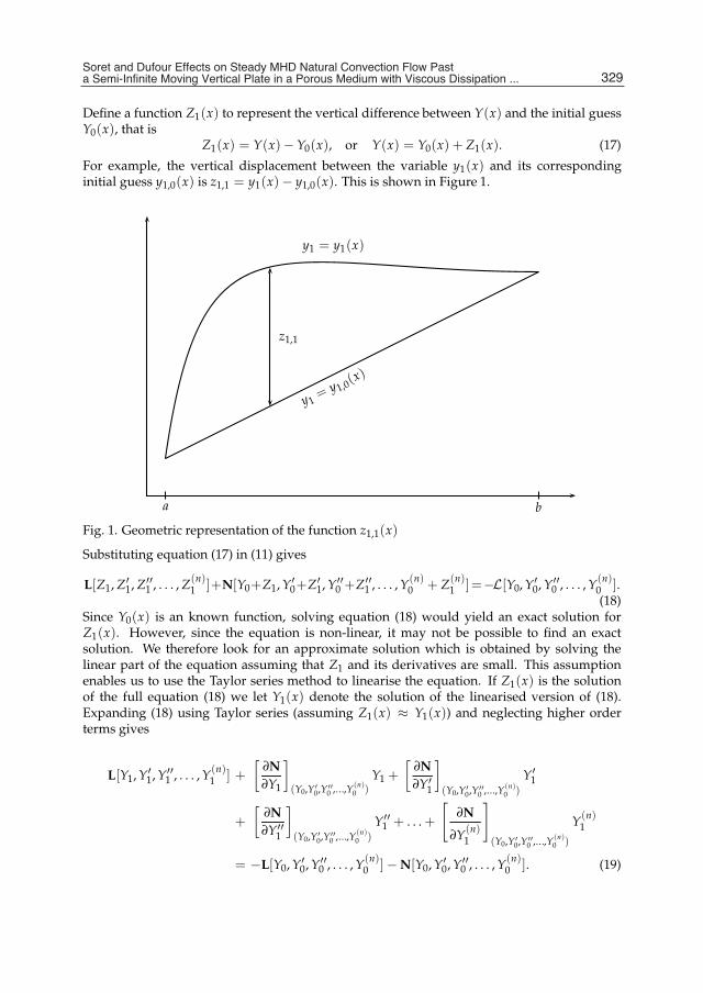
Soret and Dufour Effects on Steady MHD Natural Convection Flow Past a Semi-Infinite Moving Vertical Plate in a Porous Medium with Viscous Dissipation in the Presence ofa Chemical Reaction 5
Define a function Z1(x) to represent the vertical difference between Y(x) and the initial guessY0(x), that is
Z1(x) = Y(x)− Y0(x), or Y(x) = Y0(x) + Z1(x). (17)
For example, the vertical displacement between the variable y1(x) and its correspondinginitial guess y1,0(x) is z1,1 = y1(x)− y1,0(x). This is shown in Figure 1.
z1,1
y1= y1,0(
x)
y1 = y1(x)
a b
Fig. 1. Geometric representation of the function z1,1(x)
Substituting equation (17) in (11) gives
L[Z1, Z′1, Z′′1 , . . . , Z(n)1 ]+N[Y0+Z1, Y′0+Z′1, Y′′0 +Z′′1 , . . . , Y(n)
0 + Z(n)1 ]=−L[Y0, Y′0, Y′′0 , . . . , Y(n)
0 ].(18)
Since Y0(x) is an known function, solving equation (18) would yield an exact solution forZ1(x). However, since the equation is non-linear, it may not be possible to find an exactsolution. We therefore look for an approximate solution which is obtained by solving thelinear part of the equation assuming that Z1 and its derivatives are small. This assumptionenables us to use the Taylor series method to linearise the equation. If Z1(x) is the solutionof the full equation (18) we let Y1(x) denote the solution of the linearised version of (18).Expanding (18) using Taylor series (assuming Z1(x) ≈ Y1(x)) and neglecting higher orderterms gives
L[Y1, Y′1, Y′′1 , . . . , Y(n)1 ] +
[∂N∂Y1
](Y0,Y′0,Y′′0 ,...,Y(n)
0 )Y1 +
[∂N∂Y′1
](Y0,Y′0,Y′′0 ,...,Y(n)
0 )
Y′1
+
[∂N∂Y′′1
](Y0,Y′0,Y′′0 ,...,Y(n)
0 )
Y′′1 + . . . +
[∂N
∂Y(n)1
](Y0,Y′0,Y′′0 ,...,Y(n)
0 )
Y(n)1
= −L[Y0, Y′0, Y′′0 , . . . , Y(n)0 ]−N[Y0, Y′0, Y′′0 , . . . , Y(n)
0 ]. (19)
329Soret and Dufour Effects on Steady MHD Natural Convection Flow Past a Semi-Infinite Moving Vertical Plate in a Porous Medium with Viscous Dissipation ...
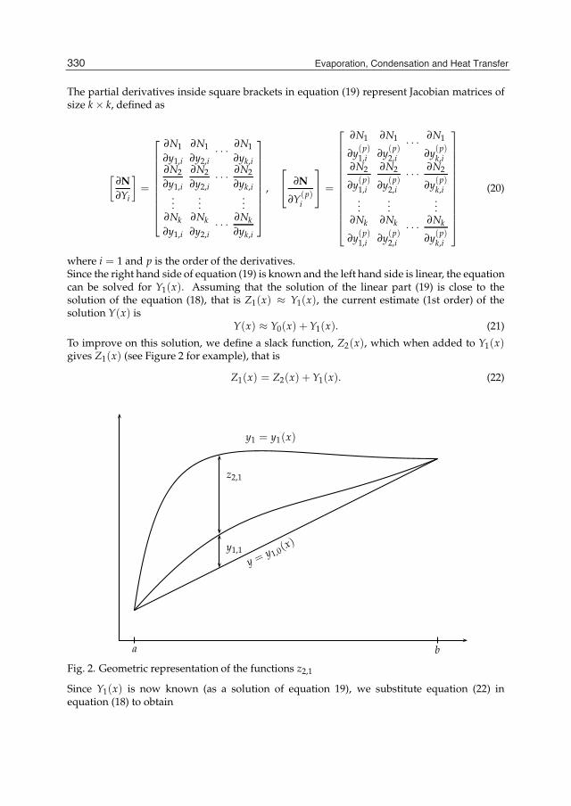
6 Mass Transfer
The partial derivatives inside square brackets in equation (19) represent Jacobian matrices ofsize k× k, defined as
[∂N∂Yi
]=
⎡⎢⎢⎢⎢⎢⎢⎢⎢⎢⎣
∂N1∂y1,i
∂N1∂y2,i
· · · ∂N1∂yk,i
∂N2
∂y1,i
∂N2
∂y2,i· · · ∂N2
∂yk,i...
......
∂Nk∂y1,i
∂Nk∂y2,i
· · · ∂Nk∂yk,i
⎤⎥⎥⎥⎥⎥⎥⎥⎥⎥⎦
,
⎡⎣ ∂N
∂Y(p)i
⎤⎦ =
⎡⎢⎢⎢⎢⎢⎢⎢⎢⎢⎢⎢⎢⎣
∂N1
∂y(p)1,i
∂N1
∂y(p)2,i
· · · ∂N1
∂y(p)k,i
∂N2
∂y(p)1,i
∂N2
∂y(p)2,i
· · · ∂N2
∂y(p)k,i
......
...∂Nk
∂y(p)1,i
∂Nk
∂y(p)2,i
· · · ∂Nk
∂y(p)k,i
⎤⎥⎥⎥⎥⎥⎥⎥⎥⎥⎥⎥⎥⎦
(20)
where i = 1 and p is the order of the derivatives.Since the right hand side of equation (19) is known and the left hand side is linear, the equationcan be solved for Y1(x). Assuming that the solution of the linear part (19) is close to thesolution of the equation (18), that is Z1(x) ≈ Y1(x), the current estimate (1st order) of thesolution Y(x) is
Y(x) ≈ Y0(x) + Y1(x). (21)
To improve on this solution, we define a slack function, Z2(x), which when added to Y1(x)gives Z1(x) (see Figure 2 for example), that is
Z1(x) = Z2(x) + Y1(x). (22)
z2,1
y1,1
y = y1,0(x)
y1 = y1(x)
a b
Fig. 2. Geometric representation of the functions z2,1
Since Y1(x) is now known (as a solution of equation 19), we substitute equation (22) inequation (18) to obtain
330 Evaporation, Condensation and Heat Transfer
Soret and Dufour Effects on Steady MHD Natural Convection Flow Past a Semi-Infinite Moving Vertical Plate in a Porous Medium with Viscous Dissipation in the Presence ofa Chemical Reaction 7
L[Z2, Z′2, Z′′2 , . . . , Z(n)2 ] + N[Y0 + Y1 + Z2+, Y′0 + Y′1 + Z′2, . . . , Y(n)
0 + Y(n)1 + Z(n)
2 ]
= −L[Y0 + Y1, Y′0 + Y′1, Y′′0 + Y′′1 , . . . , Y(n)0 + Y(n)
1 ]. (23)
Solving equation (23) would result in an exact solution for Z2(x). But since the equation isnon-linear, it may not be possible to find an exact solution. We therefore linearise the equationusing Taylor series expansion and solve the resulting linear equation. We denote the solutionof the linear version of equation (23) by Y2(x), such that Z2(x) ≈ Y2(x). Setting Z2(x) = Y2(x)and expanding equation (23), for small Y2(x) and its derivatives gives
L[Y2, Y′2, . . . , Y(n)2 ] +
[∂N∂Y2
](Y0+Y1,Y′0+Y′1,...,Y(n)
0 +Y(n)1 )
Y2 +
[∂N∂Y′2
](Y0+Y1,Y′0+Y′1,...,Y(n)
0 +Y(n)1 )
Y′2
+
[∂N∂Y′′2
](Y0+Y1,Y′0+Y′1,...,Y(n)
0 +Y(n)1 )
Y′′2 + . . . +
[∂N
∂Y(n)2
](Y0+Y1,Y′0+Y′1,...,Y(n)
0 +Y(n)1 )
Y(n)1
= −L[Y0 + Y1, Y′0 + Y′1, . . . , Y(n)0 + Y(n)
1 ]−N[Y0 + Y1, Y′0 + Y′1, . . . , Y(n)0 + Y(n)
1 ] (24)
where the partial derivatives inside square brackets in equation (24) represent Jacobianmatrices defined as in equation (20) with i = 2.After solving (24), the current (2nd order) estimate of the solution Y(x) is
Y(x) ≈ Y0(x) + Y1(x) + Y2(x). (25)
Next we define Z3(x) (see Figure 3) such that
Z2(x) = Z3(x) + Y2(x). (26)
Equation (26) is substituted in the non-linear equation (23) and the linearisation processdescribed above is repeated. This process is repeated for m = 3, 4, 5, . . . , i. In general, wehave
Zi(x) = Zi+1(x) + Yi(x). (27)
Thus, Y(x) is obtained as
Y(x) = Z1(x) + Y0(x), (28)
= Z2(x) + Y1(x) + Y0(x), (29)
= Z3(x) + Y2(x) + Y1(x) + Y0(x), (30)...
= Zi+1(x) + Yi(x) + . . . + Y3(x) + Y2(x) + Y1(x) + Y0(x), (31)
= Zi+1(x) +i
∑m=0
Ym(x). (32)
The procedure for obtaining each Zi(x) is illustrated in Figures 1, 2 and 3 respectively fori = 1, 2, 3.
331Soret and Dufour Effects on Steady MHD Natural Convection Flow Past a Semi-Infinite Moving Vertical Plate in a Porous Medium with Viscous Dissipation ...
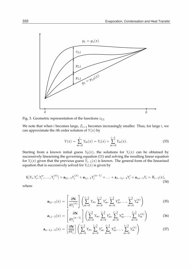
8 Mass Transfer
z3,1
y1,1
y2,1
y1= y1,0(
x)
y1 = y1(x)
a b
Fig. 3. Geometric representation of the functions z3,1
We note that when i becomes large, Zi+1 becomes increasingly smaller. Thus, for large i, wecan approximate the ith order solution of Y(x) by
Y(x) =i
∑m=0
Ym(x) = Yi(x) +i−1
∑m=0
Ym(x). (33)
Starting from a known initial guess Y0(x), the solutions for Yi(x) can be obtained bysuccessively linearising the governing equation (11) and solving the resulting linear equationfor Yi(x) given that the previous guess Yi−1(x) is known. The general form of the linearisedequation that is successively solved for Yi(x) is given by
L[Yi, Y′i , Y′′i , . . . , Y(n)i ] + a0,i−1Y(n)
i + a1,i−1Y(n−1)i + . . . + an−1,i−1Y′i + an,i−1Yi = Ri−1(x),
(34)where
a0,i−1(x) =
⎡⎣ ∂N
∂Y(n)i
⎤⎦(
i−1
∑m=0
Ym,i−1
∑m=0
Y′m,i−1
∑m=0
Y′′m, . . . ,i−1
∑m=0
Y(n)m
)(35)
a1,i−1(x) =
⎡⎣ ∂N
∂Y(n−1)i
⎤⎦(
i−1
∑m=0
Ym,i−1
∑m=0
Y′m,i−1
∑m=0
Y′′m, . . . ,i−1
∑m=0
Y(n)m
)(36)
an−1,i−1(x) =[
∂N∂Y′i
]( i−1
∑m=0
Ym,i−1
∑m=0
Y′m,i−1
∑m=0
Y′′m, . . . ,i−1
∑m=0
Y(n)m
)(37)
332 Evaporation, Condensation and Heat Transfer
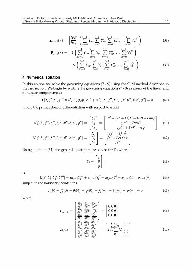
Soret and Dufour Effects on Steady MHD Natural Convection Flow Past a Semi-Infinite Moving Vertical Plate in a Porous Medium with Viscous Dissipation in the Presence ofa Chemical Reaction 9
an,i−1(x) =[
∂N∂Yi
]( i−1
∑m=0
Ym,i−1
∑m=0
Y′m,i−1
∑m=0
Y′′m, . . . ,i−1
∑m=0
Y(n)m
)(38)
Ri−1(x) = −L
(i−1
∑m=0
Ym,i−1
∑m=0
Y′m,i−1
∑m=0
Y′′m, . . . ,i−1
∑m=0
Y(n)m
)
−N
(i−1
∑m=0
Ym,i−1
∑m=0
Y′m,i−1
∑m=0
Y′′m, . . . ,i−1
∑m=0
Y(n)m
). (39)
4. Numerical solution
In this section we solve the governing equations (7 - 9) using the SLM method described inthe last section. We begin by writing the governing equations (7 - 9) as a sum of the linear andnonlinear components as
− L[ f , f ′, f ′′, f ′′′, θ, θ′, θ′′, φ, φ′, φ′′] + N[ f , f ′, f ′′, f ′′′, θ, θ′, θ′′, φ, φ′, φ′′] = 0, (40)
where the primes denote differentiation with respect to η and
L[ f , f ′, f ′′, f ′′′, θ, θ′, θ′′, φ, φ′, φ′′] =
⎡⎣ L1
L2L3
⎤⎦ =
⎡⎣ f ′′′ − (M + Ω) f ′ + Grθ + Gmφ
1Pr θ′′ + Duφ′′
1Sc φ′′ + Srθ′′ − γφ
⎤⎦ (41)
N[ f , f ′, f ′′, f ′′′, θ, θ′, θ′′, φ, φ′, φ′′] =
⎡⎣ N1
N2N3
⎤⎦ =
⎡⎣ f f ′′ − ( f ′)2
f θ′ + Ec( f ′′)2
f φ′
⎤⎦ . (42)
Using equation (34), the general equation to be solved for Yi, where
Yi =
⎡⎣ f
θφ
⎤⎦ , (43)
isL[Yi, Y′i , Y′′i , Y′′′i ] + a0,i−1Y′′′i + a1,i−1Y′′i + a2,i−1Y′i + a3,i−1Yi = Ri−1(η), (44)
subject to the boundary conditions
fi(0) = f ′i (0) = θi(0) = φi(0) = f ′i (∞) = θi(∞) = φi(∞) = 0. (45)
where
a0,i−1 =
⎡⎢⎢⎣
∂N1∂ f ′′′
∂N1∂θ ′′′
∂N1∂φ′′′
∂N2∂ f ′′′
∂N2∂θ ′′′
∂N2∂φ′′′
∂N3∂ f ′′′
∂N3∂θ ′′′
∂N3∂φ′′′
⎤⎥⎥⎦ =
⎡⎣ 0 0 0
0 0 00 0 0
⎤⎦ (46)
a1,i−1 =
⎡⎢⎢⎣
∂N1∂ f ′′
∂N1∂θ ′′
∂N1∂φ′′
∂N2∂ f ′′
∂N2∂θ ′′
∂N2∂φ′′
∂N3∂ f ′′
∂N3∂θ ′′
∂N3∂φ′′
⎤⎥⎥⎦ =
⎡⎣ ∑ fm 0 0
2Ec ∑ f ′′m 0 00 0 0
⎤⎦ (47)
333Soret and Dufour Effects on Steady MHD Natural Convection Flow Past a Semi-Infinite Moving Vertical Plate in a Porous Medium with Viscous Dissipation ...
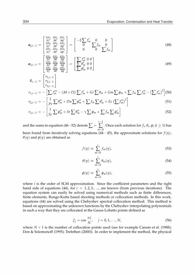
10 Mass Transfer
a2,i−1 =
⎡⎢⎢⎣
∂N1∂ f ′
∂N1∂θ ′
∂N1∂φ′
∂N2∂ f ′
∂N2∂θ ′
∂N2∂φ′
∂N3∂ f ′
∂N3∂θ ′
∂N3∂φ′
⎤⎥⎥⎦ =
⎡⎣−2 ∑ f ′m 0 0
0 ∑ fm 00 0 ∑ fm
⎤⎦ (48)
a3,i−1 =
⎡⎢⎢⎣
∂N1∂ f
∂N1∂θ
∂N1∂φ
∂N2∂ f
∂N2∂θ
∂N2∂φ
∂N3∂ f
∂N3∂θ
∂N3∂φ
⎤⎥⎥⎦ =
⎡⎣ ∑ f ′′m 0 0
∑ θ′m 0 0∑ φ′m 0 0
⎤⎦ (49)
Ri−1 =
⎡⎣ r1,i−1
r2,i−1r3,i−1
⎤⎦
r1,i−1 = −[∑ f ′′′m − (M + Ω)∑ f ′m + Gr ∑ θm + Gm ∑ φm + ∑ fm ∑ f ′′m −
(∑ f ′m
)2](50)
r2,i−1 = −[
1Pr ∑ θ′′m + Du ∑ φ′′m + ∑ fm ∑ θ′m + Ec
(∑ f ′′m
)2]
(51)
r3,i−1 = −[
1Sc ∑ φ′′m + Sr ∑ θ′′m − γ ∑ φm + ∑ fm ∑ φ′m
](52)
and the sums in equation (46 - 52) denote ∑ =i−1
∑m=0
. Once each solution for fi, θi, φi (i ≥ 1) has
been found from iteratively solving equations (44 - 45), the approximate solutions for f (η),θ(η) and φ(η) are obtained as
f (η) ≈i
∑m=0
fm(η), (53)
θ(η) ≈i
∑m=0
θm(η), (54)
φ(η) ≈i
∑m=0
φm(η), (55)
where i is the order of SLM approximation. Since the coefficient parameters and the righthand side of equations (44), for i = 1, 2, 3, . . ., are known (from previous iterations). Theequation system can easily be solved using numerical methods such as finite differences,finite elements, Runge-Kutta based shooting methods or collocation methods. In this work,equations (44) are solved using the Chebyshev spectral collocation method. This method isbased on approximating the unknown functions by the Chebyshev interpolating polynomialsin such a way that they are collocated at the Gauss-Lobatto points defined as
ξ j = cosπ jN
, j = 0, 1, . . . , N, (56)
where N + 1 is the number of collocation points used (see for example Canuto et al. (1988);Don & Solomonoff (1995); Trefethen (2000)). In order to implement the method, the physical
334 Evaporation, Condensation and Heat Transfer
Soret and Dufour Effects on Steady MHD Natural Convection Flow Past a Semi-Infinite Moving Vertical Plate in a Porous Medium with Viscous Dissipation in the Presence ofa Chemical Reaction 11
region [0, ∞) is transformed into the region [−1, 1] using the domain truncation technique inwhich the problem is solved on the interval [0, L] instead of [0, ∞). This leads to the mapping
η
L=
ξ + 12
, −1 ≤ ξ ≤ 1 (57)
where L is the scaling parameter used to invoke the boundary condition at infinity. Theunknown functions fi, θi and φi are approximated at the collocation points by
fi(ξ) ≈N
∑k=0
fi(ξk)Tk(ξ j), (58)
θi(ξ) ≈N
∑k=0
θi(ξk)Tk(ξ j), (59)
φi(ξ) ≈N
∑k=0
φi(ξk)Tk(ξ j), (60)
j = 0, 1, . . . , N, (61)
where Tk is the kth Chebyshev polynomial defined as
Tk(ξ) = cos[k cos−1(ξ)]. (62)
The derivatives of the variables at the collocation points are represented as
da fi
dηa =N
∑k=0
Dakj fi(ξk),
daθi
dηa =N
∑k=0
Dakjθi(ξk),
daφi
dηa =N
∑k=0
Dakjφi(ξk), j = 0, 1, . . . , N (63)
where a is the order of differentiation and D = 2LD with D being the Chebyshev spectral
differentiation matrix (see for example, Canuto et al. (1988); Trefethen (2000)). Substitutingequations (57 - 63) in (44) - (45) leads to the matrix equation given as
Mi−1Yi = Ri−1, (64)
subject to the boundary conditions
fi(ξN) =N
∑k=0
D0k fi(ξk) =N
∑k=0
DNk fi(ξk) = θi(ξN) = θi(ξ0) = φi(ξN) = φi(ξ0) = 0 (65)
whereMi−1 = A + a1,i−1D2 + a2,i−1D + a3,i−1 (66)
A =
⎡⎣D3 − (M + Ω)D GrI GmI
O 1Pr D2 DuD2
O SrD2 1Sc D2 − γI
⎤⎦ (67)
D =
⎡⎣D O O
O D OO O D
⎤⎦ (68)
335Soret and Dufour Effects on Steady MHD Natural Convection Flow Past a Semi-Infinite Moving Vertical Plate in a Porous Medium with Viscous Dissipation ...
12 Mass Transfer
and Yi and Ri−1 are (3N + 1)× 1 column vectors defined by
Yi =
⎡⎣ Fi
ΘiΦi
⎤⎦ , Ri−1 =
⎡⎣ r1,i−1
r2,i−1r3,i−1
⎤⎦ , (69)
where
Fi = [ fi(ξ0), fi(ξ1), . . . , fi(ξN−1), fi(ξN)]T, (70)
Θi = [θi(ξ0), θi(ξ1), . . . , θi(ξN−1), θi(ξN)]T, (71)
Φi = [φi(ξ0), φi(ξ1), . . . , φi(ξN−1), φi(ξN)]T, (72)
r1,i−1 = [r1,i−1(ξ0), r1,i−1(ξ1), . . . , r1,i−1(ξN−1), r1,i−1(ξN)]T, (73)
r2,i−1 = [r2,i−1(ξ0), r2,i−1(ξ1), . . . , r2,i−1(ξN−1), r2,i−1(ξN)]T, (74)
r3,i−1 = [r3,i−1(ξ0), r3,i−1(ξ1), . . . , r3,i−1(ξN−1), r3,i−1(ξN)]T, (75)
In the above definitions, ak,i−1, (k = 1, 2, 3) are now diagonal matrices of size 3(N + 1) ×3(N + 1) and the superscript T is the transpose.To impose the boundary conditions (65) on equation (64) we begin by splitting the matrix Min equation (64) into 9 blocks each of size (N + 1)× (N + 1) in such a way that M takes theform
Mi−1 =
⎡⎣ M11 M12 M13
M21 A22 M23M31 M32 M33
⎤⎦ (76)
We then modify the first and last rows of Mmn (m, n = 1, 2, 3) and rm,i−1 and the N − 1th rowof M1,1, M1,2, M1,3 in such a way that the modified matrices Mi−1 and Ri−1 take the form;
Mi−1 =
⎛⎜⎜⎜⎜⎜⎜⎜⎜⎜⎜⎜⎜⎜⎜⎜⎜⎜⎜⎜⎜⎜⎜⎜⎜⎜⎜⎜⎜⎜⎜⎝
D0,0 D0,1 · · · D0,N−1 D0,N 0 0 · · · 0 0 0 0 · · · 0 0
M11 M12 M13
DN,0 DN,1 · · · DN,N−1 DN,N 0 0 · · · 0 0 0 0 · · · 0 00 0 · · · 0 1 0 0 · · · 0 0 0 0 · · · 0 00 0 · · · 0 0 1 0 · · · 0 0 0 0 · · · 0 0
M21 M22 M23
0 0 · · · 0 0 0 0 · · · 0 1 0 0 · · · 0 00 0 · · · 0 0 0 0 · · · 0 0 1 0 · · · 0 0
M31 M32 M33
0 0 · · · 0 0 0 0 · · · 0 0 0 0 · · · 0 1
⎞⎟⎟⎟⎟⎟⎟⎟⎟⎟⎟⎟⎟⎟⎟⎟⎟⎟⎟⎟⎟⎟⎟⎟⎟⎟⎟⎟⎟⎟⎟⎠
, (77)
336 Evaporation, Condensation and Heat Transfer
Soret and Dufour Effects on Steady MHD Natural Convection Flow Past a Semi-Infinite Moving Vertical Plate in a Porous Medium with Viscous Dissipation in the Presence ofa Chemical Reaction 13
Ri−1 =
⎛⎜⎜⎜⎜⎜⎜⎜⎜⎜⎜⎜⎜⎜⎜⎜⎜⎜⎜⎜⎜⎜⎜⎜⎜⎜⎜⎜⎜⎜⎜⎜⎜⎜⎜⎝
0r1,i−1(ξ1)
...r1,i−1(ξN−2)
000
r2,i−1(ξ1)...
r2,i−1(ξN−2)r2,i−1(ξN−1)
00
r3,i−1(ξ1)...
r3,i−1(ξN−2)r3,i−1(ξN−1)
0
⎞⎟⎟⎟⎟⎟⎟⎟⎟⎟⎟⎟⎟⎟⎟⎟⎟⎟⎟⎟⎟⎟⎟⎟⎟⎟⎟⎟⎟⎟⎟⎟⎟⎟⎟⎠
(78)
After modifying the matrix system (64) to incorporate boundary conditions, the solution isobtained as
Yi = M−1i−1Ri−1. (79)
5. Results and discussion
In this section we present numerical calculations for different values of M, Gr, Gm, γ, Du,and fw for fixed values of Ω = 1, and Re = 1 to obtain a clear insight of the physicalproblem. In computing the numerical results presented in this paper, unless otherwise stated,the following values of physical parameters were used: M = 1, Ω = 1, Gr = 1, Gm = 1,Pr = 0.71, Sc = 0.6, Sr = 0.1, γ = 1, Ec = 1, fw = 0, Du = 0.1. The numerical results aredisplayed graphically. The effect of the Hartmann number M on the dimensionless velocityf ′(η), temperature θ(η) and concentration φ(η) profiles are respectively represented in Figs(a), (b) and (c). It is observed in these Figs, that the velocity decreases with the increase ofthe magnetic parameter, the value of the temperature profiles increase with the magneticparameter. The concentration of the fluid have a small increase with the increase of themagnetic parameter. The effects of a transverse magnetic field give rise to a resistive-typeforce called the Lorentz force. This force has the tendency to slow down the motion of thefluid flow and to increase its thermal boundary layer hence increasing the temperature of thefluid flow.Figure (d), (e) and (f) depict the effects of varying the local thermal free convection (Gr) withincreasing η on the dimensionless velocity, temperature and concentration. It is observed inFig (d) that the increase of the Grashof number leads to the increase of the velocity of the fluid.This is because the increase of Gr results in the increase of temperature gradients (T∞ − T∞),leads to the enhancement of the velocity due to the enhanced convection. From Fig (e) weobserve that the effect of increasing the values of thermal free convection is to reduce thetemperature profiles (θ). We also observe in Fig (f) that the concentration profiles decrease
337Soret and Dufour Effects on Steady MHD Natural Convection Flow Past a Semi-Infinite Moving Vertical Plate in a Porous Medium with Viscous Dissipation ...
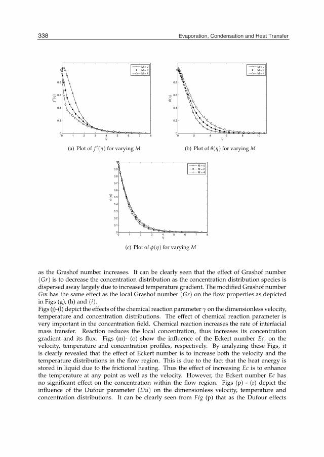
14 Mass Transfer
0 1 2 3 4 5 6 7 80
0.2
0.4
0.6
0.8
1
η
f′ (η)
M = 0M = 2M = 4
(a) Plot of f ′(η) for varying M
0 2 4 6 8 100
0.2
0.4
0.6
0.8
1
η
θ(η
)
M = 0M = 2M = 4
(b) Plot of θ(η) for varying M
0 1 2 3 4 5 6 7 80
0.1
0.2
0.3
0.4
0.5
0.6
0.7
0.8
0.9
1
η
φ(η
)
M = 0M = 2M = 4
(c) Plot of φ(η) for varying M
as the Grashof number increases. It can be clearly seen that the effect of Grashof number(Gr) is to decrease the concentration distribution as the concentration distribution species isdispersed away largely due to increased temperature gradient. The modified Grashof numberGm has the same effect as the local Grashof number (Gr) on the flow properties as depictedin Figs (g), (h) and (i).Figs (j)-(l) depict the effects of the chemical reaction parameter γ on the dimensionless velocity,temperature and concentration distributions. The effect of chemical reaction parameter isvery important in the concentration field. Chemical reaction increases the rate of interfacialmass transfer. Reaction reduces the local concentration, thus increases its concentrationgradient and its flux. Figs (m)- (o) show the influence of the Eckert number Ec, on thevelocity, temperature and concentration profiles, respectively. By analyzing these Figs, itis clearly revealed that the effect of Eckert number is to increase both the velocity and thetemperature distributions in the flow region. This is due to the fact that the heat energy isstored in liquid due to the frictional heating. Thus the effect of increasing Ec is to enhancethe temperature at any point as well as the velocity. However, the Eckert number Ec hasno significant effect on the concentration within the flow region. Figs (p) - (r) depict theinfluence of the Dufour parameter (Du) on the dimensionless velocity, temperature andconcentration distributions. It can be clearly seen from Fig (p) that as the Dufour effects
338 Evaporation, Condensation and Heat Transfer
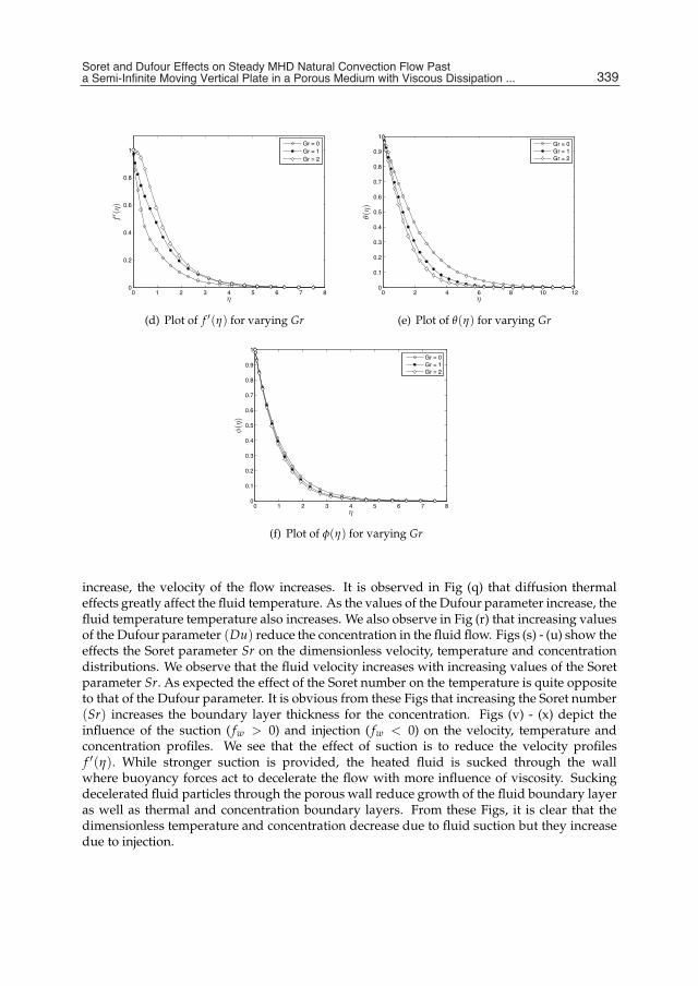
Soret and Dufour Effects on Steady MHD Natural Convection Flow Past a Semi-Infinite Moving Vertical Plate in a Porous Medium with Viscous Dissipation in the Presence ofa Chemical Reaction 15
0 1 2 3 4 5 6 7 80
0.2
0.4
0.6
0.8
1
η
f′ (η)
Gr = 0Gr = 1Gr = 2
(d) Plot of f ′(η) for varying Gr
0 2 4 6 8 10 120
0.1
0.2
0.3
0.4
0.5
0.6
0.7
0.8
0.9
1
η
θ(η
)
Gr = 0Gr = 1Gr = 2
(e) Plot of θ(η) for varying Gr
0 1 2 3 4 5 6 7 80
0.1
0.2
0.3
0.4
0.5
0.6
0.7
0.8
0.9
1
η
φ(η
)
Gr = 0Gr = 1Gr = 2
(f) Plot of φ(η) for varying Gr
increase, the velocity of the flow increases. It is observed in Fig (q) that diffusion thermaleffects greatly affect the fluid temperature. As the values of the Dufour parameter increase, thefluid temperature temperature also increases. We also observe in Fig (r) that increasing valuesof the Dufour parameter (Du) reduce the concentration in the fluid flow. Figs (s) - (u) show theeffects the Soret parameter Sr on the dimensionless velocity, temperature and concentrationdistributions. We observe that the fluid velocity increases with increasing values of the Soretparameter Sr. As expected the effect of the Soret number on the temperature is quite oppositeto that of the Dufour parameter. It is obvious from these Figs that increasing the Soret number(Sr) increases the boundary layer thickness for the concentration. Figs (v) - (x) depict theinfluence of the suction ( fw > 0) and injection ( fw < 0) on the velocity, temperature andconcentration profiles. We see that the effect of suction is to reduce the velocity profilesf ′(η). While stronger suction is provided, the heated fluid is sucked through the wallwhere buoyancy forces act to decelerate the flow with more influence of viscosity. Suckingdecelerated fluid particles through the porous wall reduce growth of the fluid boundary layeras well as thermal and concentration boundary layers. From these Figs, it is clear that thedimensionless temperature and concentration decrease due to fluid suction but they increasedue to injection.
339Soret and Dufour Effects on Steady MHD Natural Convection Flow Past a Semi-Infinite Moving Vertical Plate in a Porous Medium with Viscous Dissipation ...

16 Mass Transfer
0 1 2 3 4 5 6 7 80
0.2
0.4
0.6
0.8
1
η
f′ (η)
Gm = 0Gm = 1Gm = 2
(g) Plot of f ′(η) for varying Gm
0 2 4 6 8 10 120
0.1
0.2
0.3
0.4
0.5
0.6
0.7
0.8
0.9
1
η
θ(η
)
Gm = 0Gm = 1Gm = 2
(h) Plot of θ(η) for varying Gm
0 1 2 3 4 5 6 7 80
0.1
0.2
0.3
0.4
0.5
0.6
0.7
0.8
0.9
1
η
φ(η
)
Gm = 0Gm = 1Gm = 2
(i) Plot of φ(η) for varying Gm
340 Evaporation, Condensation and Heat Transfer
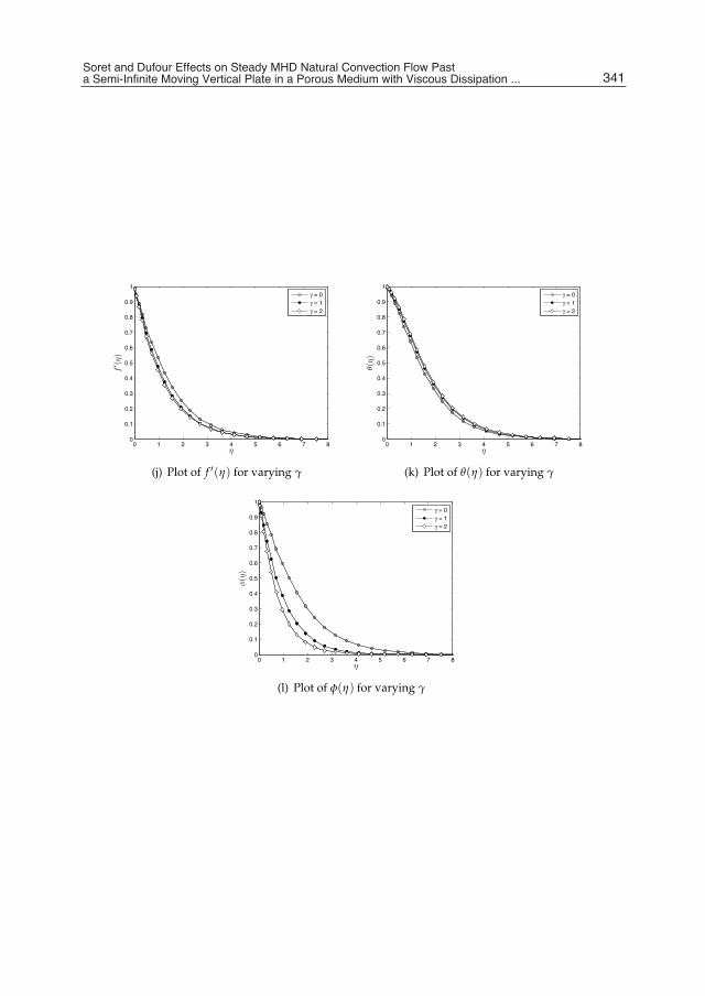
Soret and Dufour Effects on Steady MHD Natural Convection Flow Past a Semi-Infinite Moving Vertical Plate in a Porous Medium with Viscous Dissipation in the Presence ofa Chemical Reaction 17
0 1 2 3 4 5 6 7 80
0.1
0.2
0.3
0.4
0.5
0.6
0.7
0.8
0.9
1
η
f′ (η)
γ = 0γ = 1γ = 2
(j) Plot of f ′(η) for varying γ
0 1 2 3 4 5 6 7 80
0.1
0.2
0.3
0.4
0.5
0.6
0.7
0.8
0.9
1
η
θ(η
)
γ = 0γ = 1γ = 2
(k) Plot of θ(η) for varying γ
0 1 2 3 4 5 6 7 80
0.1
0.2
0.3
0.4
0.5
0.6
0.7
0.8
0.9
1
η
φ(η
)
γ = 0γ = 1γ = 2
(l) Plot of φ(η) for varying γ
341Soret and Dufour Effects on Steady MHD Natural Convection Flow Past a Semi-Infinite Moving Vertical Plate in a Porous Medium with Viscous Dissipation ...
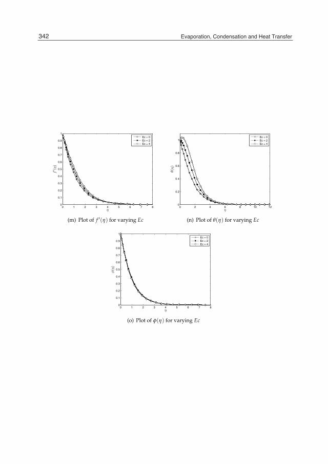
18 Mass Transfer
0 1 2 3 4 5 6 7 80
0.1
0.2
0.3
0.4
0.5
0.6
0.7
0.8
0.9
1
η
f′ (η)
Ec = 0Ec = 2Ec = 4
(m) Plot of f ′(η) for varying Ec
0 2 4 6 8 10 120
0.2
0.4
0.6
0.8
1
η
θ(η
)
Ec = 0Ec = 2Ec = 4
(n) Plot of θ(η) for varying Ec
0 1 2 3 4 5 6 7 80
0.1
0.2
0.3
0.4
0.5
0.6
0.7
0.8
0.9
1
η
φ(η
)
Ec = 0Ec = 2Ec = 4
(o) Plot of φ(η) for varying Ec
342 Evaporation, Condensation and Heat Transfer
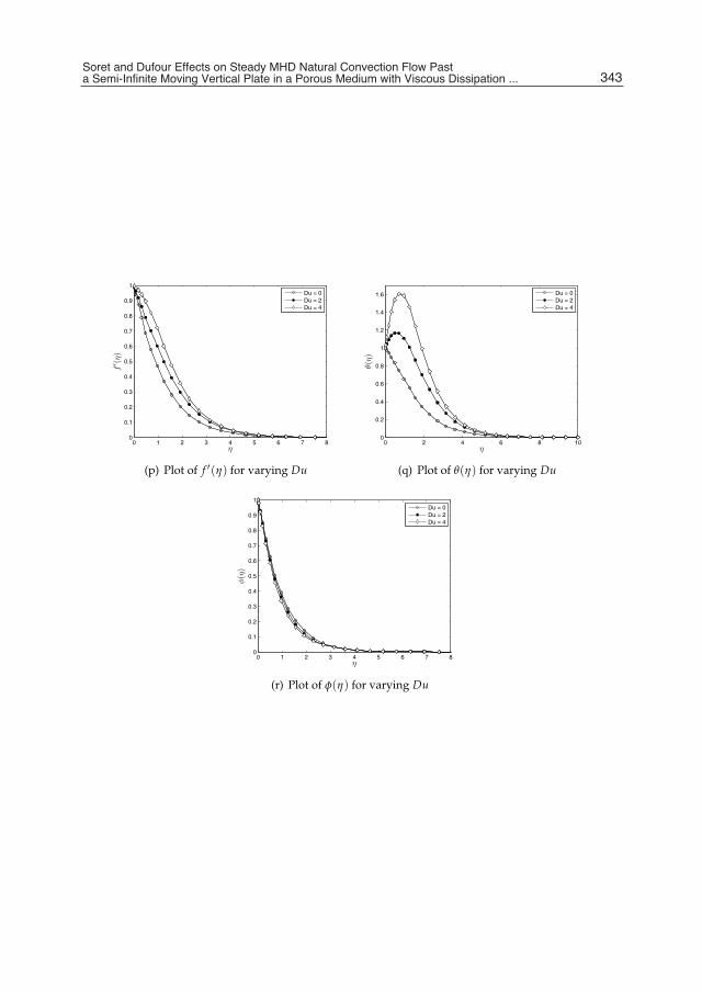
Soret and Dufour Effects on Steady MHD Natural Convection Flow Past a Semi-Infinite Moving Vertical Plate in a Porous Medium with Viscous Dissipation in the Presence ofa Chemical Reaction 19
0 1 2 3 4 5 6 7 80
0.1
0.2
0.3
0.4
0.5
0.6
0.7
0.8
0.9
1
η
f′ (η)
Du = 0Du = 2Du = 4
(p) Plot of f ′(η) for varying Du
0 2 4 6 8 100
0.2
0.4
0.6
0.8
1
1.2
1.4
1.6
η
θ(η
)
Du = 0Du = 2Du = 4
(q) Plot of θ(η) for varying Du
0 1 2 3 4 5 6 7 80
0.1
0.2
0.3
0.4
0.5
0.6
0.7
0.8
0.9
1
η
φ(η
)
Du = 0Du = 2Du = 4
(r) Plot of φ(η) for varying Du
343Soret and Dufour Effects on Steady MHD Natural Convection Flow Past a Semi-Infinite Moving Vertical Plate in a Porous Medium with Viscous Dissipation ...
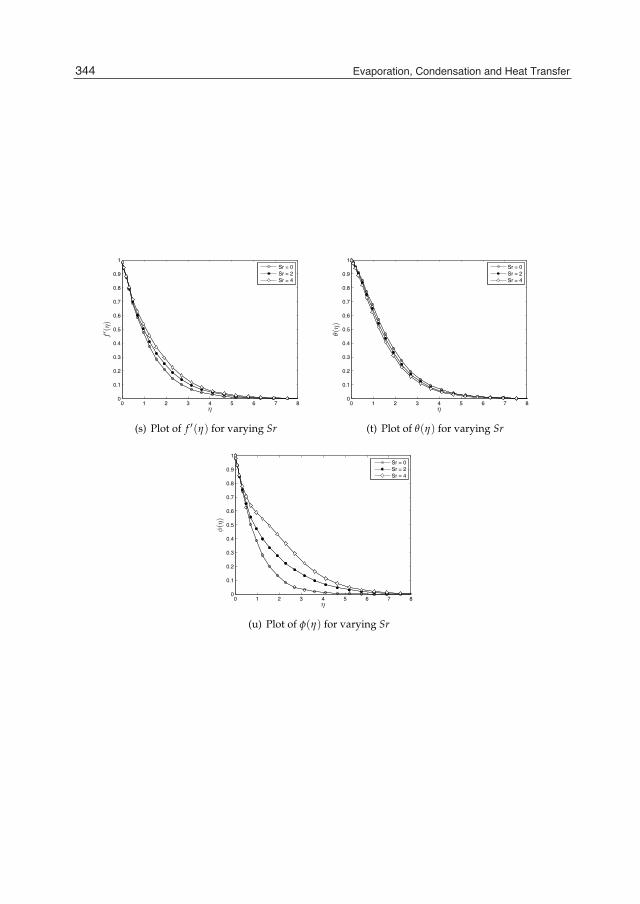
20 Mass Transfer
0 1 2 3 4 5 6 7 80
0.1
0.2
0.3
0.4
0.5
0.6
0.7
0.8
0.9
1
η
f′ (η)
Sr = 0Sr = 2Sr = 4
(s) Plot of f ′(η) for varying Sr
0 1 2 3 4 5 6 7 80
0.1
0.2
0.3
0.4
0.5
0.6
0.7
0.8
0.9
1
η
θ(η
)
Sr = 0Sr = 2Sr = 4
(t) Plot of θ(η) for varying Sr
0 1 2 3 4 5 6 7 80
0.1
0.2
0.3
0.4
0.5
0.6
0.7
0.8
0.9
1
η
φ(η
)
Sr = 0Sr = 2Sr = 4
(u) Plot of φ(η) for varying Sr
344 Evaporation, Condensation and Heat Transfer
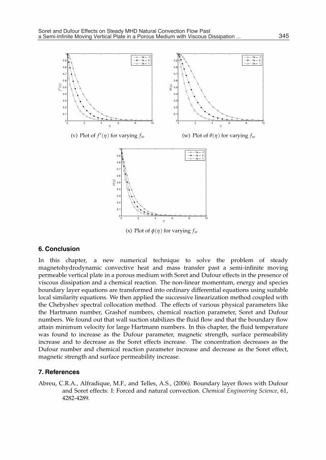
Soret and Dufour Effects on Steady MHD Natural Convection Flow Past a Semi-Infinite Moving Vertical Plate in a Porous Medium with Viscous Dissipation in the Presence ofa Chemical Reaction 21
0 2 4 6 8 100
0.1
0.2
0.3
0.4
0.5
0.6
0.7
0.8
0.9
1
η
f′ (η)
fw = −1fw = 0fw = 1
(v) Plot of f ′(η) for varying fw
0 2 4 6 8 100
0.1
0.2
0.3
0.4
0.5
0.6
0.7
0.8
0.9
1
η
θ(η
)
fw = −1fw = 0fw = 1
(w) Plot of θ(η) for varying fw
0 2 4 6 8 100
0.1
0.2
0.3
0.4
0.5
0.6
0.7
0.8
0.9
1
η
φ(η
)
fw = −1fw = 0fw = 1
(x) Plot of φ(η) for varying fw
6. Conclusion
In this chapter, a new numerical technique to solve the problem of steadymagnetohydrodynamic convective heat and mass transfer past a semi-infinite movingpermeable vertical plate in a porous medium with Soret and Dufour effects in the presence ofviscous dissipation and a chemical reaction. The non-linear momentum, energy and speciesboundary layer equations are transformed into ordinary differential equations using suitablelocal similarity equations. We then applied the successive linearization method coupled withthe Chebyshev spectral collocation method. The effects of various physical parameters likethe Hartmann number, Grashof numbers, chemical reaction parameter, Soret and Dufournumbers. We found out that wall suction stabilizes the fluid flow and that the boundary flowattain minimum velocity for large Hartmann numbers. In this chapter, the fluid temperaturewas found to increase as the Dufour parameter, magnetic strength, surface permeabilityincrease and to decrease as the Soret effects increase. The concentration decreases as theDufour number and chemical reaction parameter increase and decrease as the Soret effect,magnetic strength and surface permeability increase.
7. References
Abreu, C.R.A., Alfradique, M.F., and Telles, A.S., (2006). Boundary layer flows with Dufourand Soret effects: I: Forced and natural convection. Chemical Engineering Science, 61,4282-4289.
345Soret and Dufour Effects on Steady MHD Natural Convection Flow Past a Semi-Infinite Moving Vertical Plate in a Porous Medium with Viscous Dissipation ...
22 Mass Transfer
Afify, A.A., (2009). Similarity solution in MHD: Effects of thermal diffusion and diffusionthermo on free convective heat and mass transfer over a stretching surfaceconsidering suction and injection. Commun Nonlinear Sci Numer Simulat, 14,2202-2214.
El-Amin, M.F., (2004). Double dispersion effects on natural convection heat and mass transferin non-Darcy porous medium, Applied Mathematics and Computation 156, 1–17.
Alam, M.S., and Rahman, M.M., (2006). Dufour and Soret Effects on Mixed Convection FlowPast a Vertical Porous Flat Plate with Variable Suction. Nonlinear Analysis Modellingand Control, 11, 1, 3-12.
C. Canuto, M. Y. Hussaini, A. Quarteroni, and T. A. Zang, Spectral Methods in Fluid Dynamics,Springer-Verlag, Berlin, 1988.
Don, W. S. , A. Solomonoff.(2006). Accuracy and speed in computing the ChebyshevCollocation Derivative. SIAM J. Sci. Comput, 16(6) 1253–1268.
Gaikwad, S.N., Malashetty, M.S., and Prasad, K.R.,(2007). An analytical study of linear andnon-linear double diffusive convection with Soret and Dufour effects in couple stressfluid. International Journal of Non-Linear Mechanics, 42, 903-913.
Hayat, T., Mustafa M., and Pop, I., (2010). Heat and mass transfer for Soret and DufourŠseffect on mixed convection boundary layer flow over a stretching vertical surface in aporous medium filled with a viscoelastic fluid. Commun Nonlinear Sci Numer Simulat.15 1183-1196.
Huges, W.F and Young, F.J.,The Electro-Magneto Dynamics of fluids. John Wiley and Sons, NewYork, 1966.
Mansour, M.A., El-Anssary, N.F., and Aly, A.M., (2008). Effects of chemical reaction andthermal stratification on MHD free convective heat and mass transfer over a verticalstretching surface embedded in a porous media considering Soret and Dufournumbers. Journal of Chemical Engineering 145, 2, 340-345.
Ming-chun, LI., Yan-wen, T., and Yu-chun, Z. Soret and Dufour effects in strongly endothermicchemical reaction system of porous media. Trans. Nonferrous Met. Soc. China, 16,1200-1204.
Motsa, S.S., (2008). On the onset of convection in a porous layer in the presence of Dufour andSoret effects. SAMSA Journal of Pure and Applied Mathematics, 3, 58-65.
Motsa, S.S., P. Sibanda, S. Shateyi,(2010). A new spectral-homotopy analysis method forsolving a nonlinear second order BVP, Commun. Nonlinear Sci. Numer. Simul, 152293–2302.
Motsa, S. S., P. Sibanda, F. G. Awad, S. Shateyi, (2010). A new spectral-homotopy analysismethod for the MHD Jeffery-Hamel problem, Computer & Fluids, 39 1219–1225
Partha, M.K., (2008). Thermophoresis particle deposition in a non-Darcy porous mediumunder the influence of Soret, Dufour effects, Heat Mass Transfer, 44, 969–977.
Postelnicu, A., (2004).Influence of a magnetic field on heat and mass transfer by naturalconvection from vertical surfaces in porous media consdering Soret and Dufoureffects, International Journal of Heat and Mass Transfer, 47, 1467-1472.
Shateyi, S., (2008). Thermal radiation and buoyancy effects on heat and mass transferover a semi-infinite stretching surface with suction and blowing. Journal of AppliedMathematics, doi:10.1155/2008/414830.
L. N. Trefethen, Spectral Methods in MATLAB, SIAM, 2000.
346 Evaporation, Condensation and Heat Transfer

Part 4
Fluid and Flow

17
Computational Fluid Dynamic Simulations of Natural Convection in Ventilated Facades
A. Gagliano, F. Patania, A. Ferlito, F. Nocera and A. Galesi Department of Industrial and Mechanics Engineering, Faculty of Engineering,
University of Catania, Italy
1. Introduction The European Directive 2002/91/EC (Energy Performance of Buildings) aims to achieve minimum standards on the energy performance of new buildings and existing buildings that are subject to major renovation. To evaluate the energy performance of a building is necessary to calculate the energy required to satisfy the various services related to the standard usage of the building. In order to achieve the minimum standards for energy certification should be an approach to design alternative to the traditional one which allows to reduce significantly the building's energy requirements maintaining the level of indoor comfort. The energy needs of the building depend on the efficiency of envelope: when it was not designed and constructed correctly, the heat fluxes through the structures (vertical, horizontal, transparent, opaque) cause a large increase in final energy consumption. The heat exchanges depend on the temperature difference between the inner and the outer faces of the boundary element (horizontal or vertical) and the thermal resistance of the material (or combination of materials) that constitute the envelope and the contribute of solar radiation. In summer, especially during the days with high values of temperature and solar radiation, the building envelope should be designed and constructed so as to ensure adequate environmental conditions for thermal comfort in the indoor environment, even in absence of conditioning systems.
2. The ventilated facade system The ventilated facade is a multi-layer coating system that was born in Northern Europe in order to have an envelope that combine aesthetic aspect with a strong positive valence valuable in terms of insulation and energy saving. Subsequently the deep technological innovations have improved the system and it has found large use in many other countries with increasing recognition. Today the use of ventilated structures in new buildings is a widely used solution in architecture because it provides both high energy savings and elevated aesthetic - formal contents.
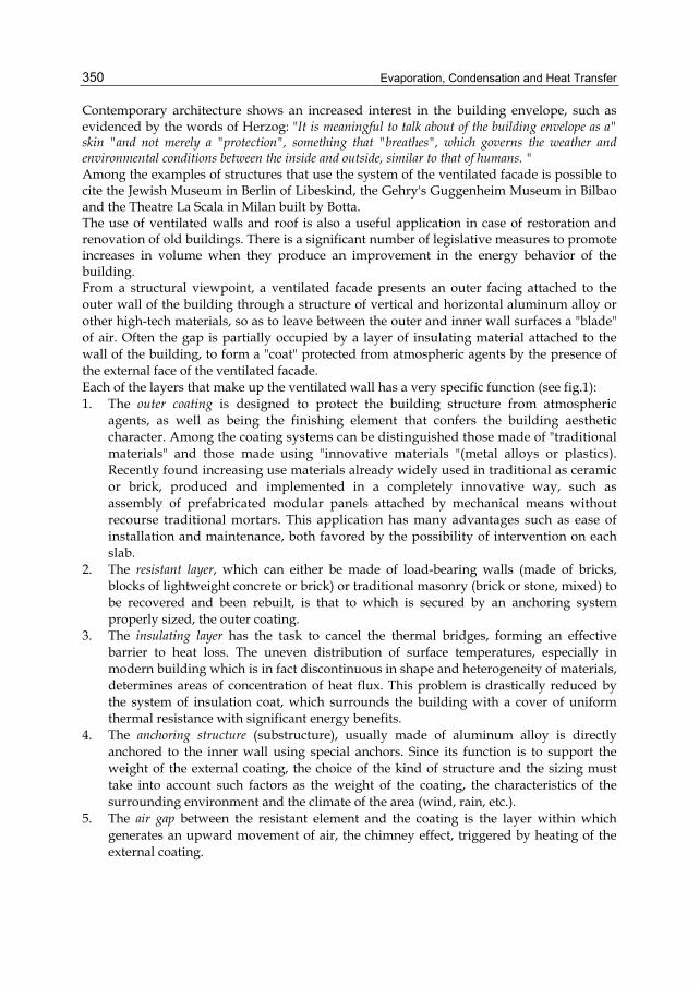
Evaporation, Condensation and Heat Transfer
350
Contemporary architecture shows an increased interest in the building envelope, such as evidenced by the words of Herzog: "It is meaningful to talk about of the building envelope as a" skin "and not merely a "protection", something that "breathes", which governs the weather and environmental conditions between the inside and outside, similar to that of humans. " Among the examples of structures that use the system of the ventilated facade is possible to cite the Jewish Museum in Berlin of Libeskind, the Gehry's Guggenheim Museum in Bilbao and the Theatre La Scala in Milan built by Botta. The use of ventilated walls and roof is also a useful application in case of restoration and renovation of old buildings. There is a significant number of legislative measures to promote increases in volume when they produce an improvement in the energy behavior of the building. From a structural viewpoint, a ventilated facade presents an outer facing attached to the outer wall of the building through a structure of vertical and horizontal aluminum alloy or other high-tech materials, so as to leave between the outer and inner wall surfaces a "blade" of air. Often the gap is partially occupied by a layer of insulating material attached to the wall of the building, to form a "coat" protected from atmospheric agents by the presence of the external face of the ventilated facade. Each of the layers that make up the ventilated wall has a very specific function (see fig.1): 1. The outer coating is designed to protect the building structure from atmospheric
agents, as well as being the finishing element that confers the building aesthetic character. Among the coating systems can be distinguished those made of "traditional materials" and those made using "innovative materials "(metal alloys or plastics). Recently found increasing use materials already widely used in traditional as ceramic or brick, produced and implemented in a completely innovative way, such as assembly of prefabricated modular panels attached by mechanical means without recourse traditional mortars. This application has many advantages such as ease of installation and maintenance, both favored by the possibility of intervention on each slab.
2. The resistant layer, which can either be made of load-bearing walls (made of bricks, blocks of lightweight concrete or brick) or traditional masonry (brick or stone, mixed) to be recovered and been rebuilt, is that to which is secured by an anchoring system properly sized, the outer coating.
3. The insulating layer has the task to cancel the thermal bridges, forming an effective barrier to heat loss. The uneven distribution of surface temperatures, especially in modern building which is in fact discontinuous in shape and heterogeneity of materials, determines areas of concentration of heat flux. This problem is drastically reduced by the system of insulation coat, which surrounds the building with a cover of uniform thermal resistance with significant energy benefits.
4. The anchoring structure (substructure), usually made of aluminum alloy is directly anchored to the inner wall using special anchors. Since its function is to support the weight of the external coating, the choice of the kind of structure and the sizing must take into account such factors as the weight of the coating, the characteristics of the surrounding environment and the climate of the area (wind, rain, etc.).
5. The air gap between the resistant element and the coating is the layer within which generates an upward movement of air, the chimney effect, triggered by heating of the external coating.
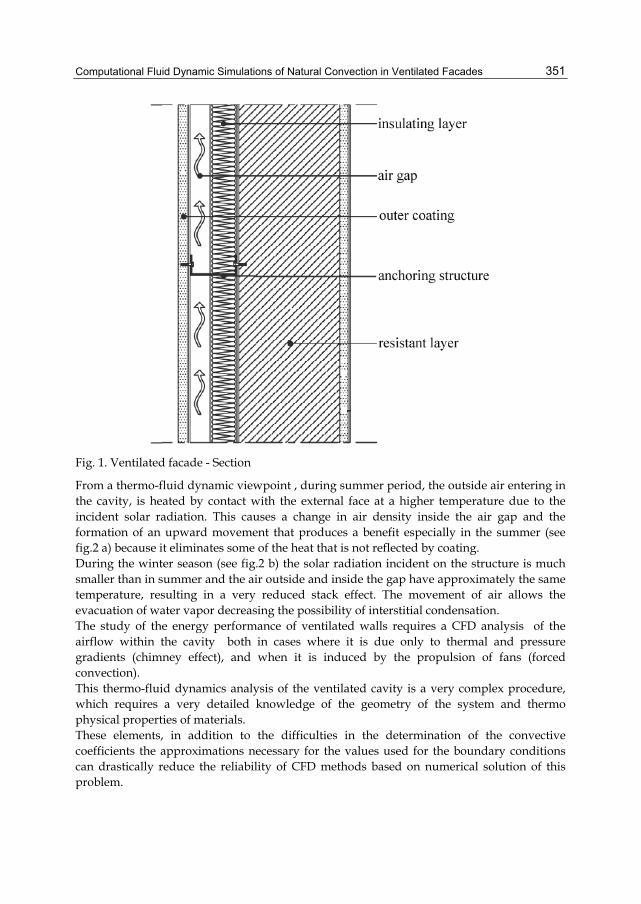
Computational Fluid Dynamic Simulations of Natural Convection in Ventilated Facades
351
Fig. 1. Ventilated facade - Section
From a thermo-fluid dynamic viewpoint , during summer period, the outside air entering in the cavity, is heated by contact with the external face at a higher temperature due to the incident solar radiation. This causes a change in air density inside the air gap and the formation of an upward movement that produces a benefit especially in the summer (see fig.2 a) because it eliminates some of the heat that is not reflected by coating. During the winter season (see fig.2 b) the solar radiation incident on the structure is much smaller than in summer and the air outside and inside the gap have approximately the same temperature, resulting in a very reduced stack effect. The movement of air allows the evacuation of water vapor decreasing the possibility of interstitial condensation. The study of the energy performance of ventilated walls requires a CFD analysis of the airflow within the cavity both in cases where it is due only to thermal and pressure gradients (chimney effect), and when it is induced by the propulsion of fans (forced convection). This thermo-fluid dynamics analysis of the ventilated cavity is a very complex procedure, which requires a very detailed knowledge of the geometry of the system and thermo physical properties of materials. These elements, in addition to the difficulties in the determination of the convective coefficients the approximations necessary for the values used for the boundary conditions can drastically reduce the reliability of CFD methods based on numerical solution of this problem.
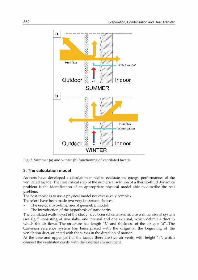
Evaporation, Condensation and Heat Transfer
352
Fig. 2. Summer (a) and winter (b) functioning of ventilated facade
3. The calculation model Authors have developed a calculation model to evaluate the energy performances of the ventilated façade. The first critical step of the numerical solution of a thermo-fluid dynamics problem is the identification of an appropriate physical model able to describe the real problem. The best choice is to use a physical model not excessively complex. Therefore have been made two very important choices: - The use of a two-dimensional geometric model; - The introduction of the hypothesis of stationarity. The ventilated walls object of the study have been schematized as a two-dimensional system (see fig.3) consisting of two slabs, one internal and one external, which delimit a duct in which the air flows. The structure has length “L” and thickness of the air gap “d”. The Cartesian reference system has been placed with the origin at the beginning of the ventilation duct, oriented with the y-axis in the direction of motion. At the base and upper part of the facade there are two air vents, with height “a”, which connect the ventilated cavity with the external environment.
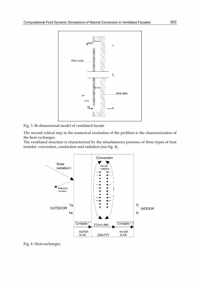
Computational Fluid Dynamic Simulations of Natural Convection in Ventilated Facades
353
Fig. 3. Bi-dimensional model of ventilated facade
The second critical step in the numerical resolution of the problem is the characterization of the heat exchanges. The ventilated structure is characterized by the simultaneous presence of three types of heat transfer: convection, conduction and radiation (see fig. 4).
Fig. 4. Heat exchanges
Evaporation, Condensation and Heat Transfer
354
The transmission of heat will be caused by: - convective and radiative exchanges between the external environment and the exterior
surface of the coating; - conductive heat exchange through the walls of the duct; - radiative exchange between the two slabs delimiting the air gap; - convective heat exchange between these slabs and the air circulating inside the channel; - convective and radiative exchanges between the indoor and the intrados of the inner
wall. The conductive heat transfer through the inner and outer walls has been characterized by the conductive thermal resistance defined by:
i
condii
sRλ
=∑ (1)
where si and λi and are respectively the thickness and thermal conductivity of the i-th layer of the wall. In steady-state analysis, the convective and the radiative heat transfers within the ventilated cavity can be represented with an acceptable level of accuracy considering two thermal resistances, r1 and r2, expressed by the following equations :
01
0A
A B
Rr rr r R
=+ +
and 02
0B
A B
Rr rr r R
=+ +
(2)
where rA and rB are the thermal resistances due to the convective exchange between the fluid and the two garments (A and B respectively), while the thermal resistance R0 characterizes the mutual radiative exchange between the two inner sides of the ventilated duct. The thermal resistance R0 has been expressed by the following equation:
1 2
01 1 1 12 2 2
1 1 1e eRA e A F A e
− −= + +⋅ ⋅ ⋅ (3)
where A1 and A2 are the areas of the two slabs, F12 is the view factor between the two parallel surfaces, while e1 and e2 are the emissivity coefficient on both sides of the duct. The convective thermal resistance (rA and rB) inside the ventilated channel have been assessed using the relationship of Gnielinski valid for Reynolds numbers (Re) higher than 2300. Using this model it is possible to calculate the Nusselt number of fluids in transient conditions from linear to turbulent flow which can be expressed as:
( )
( )0
2 3
Re 1000 Pr8
1 12.7 Pr 18
Nu
ξ
ξ
−=
+ − (4)
Where Pr is the Prandtl number and ξ represents the friction coefficient, calculated by means of the correlation discovered by Petukhov reported below:
Computational Fluid Dynamic Simulations of Natural Convection in Ventilated Facades
355
( )2
1
1.82log Re 1.64ξ =
− (5)
The influence of temperature has been considered with the introduction of the following relation:
0.36
0m
w
TNu NuT
⎛ ⎞= ⎜ ⎟⎜ ⎟
⎝ ⎠ (6)
where Tm is the mean temperature of the fluid in the cavity and Tw is the temperature of the wall of the ventilated duct. The convective thermal resistances (rA and rB) at inner and outer surfaces of the duct have been calculated by the equations:
0.36
0m
A uwA h
Tr NT D
λ⎛ ⎞= ⎜ ⎟⎜ ⎟
⎝ ⎠ and
0.36
0m
B uwB h
Tr NT D
λ⎛ ⎞= ⎜ ⎟⎜ ⎟
⎝ ⎠ (7)
where Dh is the hydraulic diameter defined as:
( )2hdLD
d L=
+ (8)
The third step of the numerical solution of the problem is the definition of energy and motions equations for the flow of the air inside a cavity. The steady state energy balance has been applied to a control volume, which represents the whole of modules with two opaque layers separated by the air channel. The time–averaged Navier-Stokes equations of motion for steady, compressible flow can be written as : - Conservation of mass (continuity) in ith direction
( ) 0vt
ρ∂ + ∇ ⋅ =∂
(9)
Where ρ is the air density and v the velocity vector - Conservation of momentum in ith direction
( ) ( ) ( )v vv p g Ft
ρ ρ τ ρ∂ + ∇ = −∇ + ∇ + +∂
(10)
where p is the static pressure, τ is the shear stress tensor, while gρ and F represent respectively the body and the external forces. - Conservation of energy
( ) ( )( ) eff i i eff hi
E v E p k T h j v St
ρ ρ τ⎡ ⎤∂ + ∇ ⋅ + = ∇ ⋅ ∇ − + ⋅ +⎡ ⎤ ⎢ ⎥⎣ ⎦∂ ⎢ ⎥⎣ ⎦
∑ (11)
where keff is the effective conductivity.
Evaporation, Condensation and Heat Transfer
356
The first three terms in the right side of the equation represent energy exchanges due to convection, conduction and viscous dissipation, while the term Sh includes the contributions of the heat produced by chemical reactions. The two transport equations for the standard k-epsilon model, also derived from the Navier-Stokes equations, can be written as follows: - Turbulent kinetic energy (k-equation)
( ) ( ) ti k b M k
i j k j
kk ku P P Y St x x x
μρ ρ μ ρεσ
⎡ ⎤⎛ ⎞∂ ∂ ∂ ∂⎢ ⎥+ = + + + − − +⎜ ⎟⎜ ⎟∂ ∂ ∂⎢ ⎥⎝ ⎠⎣ ⎦
(12)
- Kinetic energy of turbulence dissipation (ε-equation)
( ) ( ) ( )2
1 3 2t
i k bi j k j
u C P C P C St x x x k kε ε ε ε
μ ε ε ερε ρε μ ρσ
⎡ ⎤⎛ ⎞∂ ∂ ∂ ∂⎢ ⎥+ = + + + − +⎜ ⎟⎜ ⎟∂ ∂ ∂⎢ ⎥⎝ ⎠⎣ ⎦
(13)
Where the turbulent viscosity has been expressed as follow:
2
tkCμμ ρε
= (14)
The production of turbulent kinetic energy Pk can be expressed by the equation:
2k tP Sμ= (15)
where the term S is the average strain tensor expressed by the relation:
2 ij ijS S S≡ (16)
The effect of buoyancy forces is expressed by the following equation:
Pr
tb i
t i
TP gx
μβ ∂=∂
(17)
where Prt is the turbulent Prandtl number and gi is the component of gravity vector in the i-th direction. The constants have the following default values [1]:
C1ε =1,44, C2ε=1,92; C3ε =1; Cμ=0,09; σε=1,3.and σk=1,0. The governing equations have been solved using the finite volumes method that is particularly suitable for the integration of partial differential equations. These equations are integrated in a control volume with boundary conditions imposed at the borders. The interior of this domain is divided in many elementary volumes linked by mathematical relationships between adjacent volumes so is possible to solve the Navier-Stokes equations with the aid of a computer code.
4. Generation of the computational grid The solution of differential equations using numerical methods requires computational grids, commonly called meshes. The computational grid is a decomposition of the problem space into elementary domains.
Computational Fluid Dynamic Simulations of Natural Convection in Ventilated Facades
357
The simplicity of the domain of study has allowed the use of a structured grid characterized by the exclusive presence of 2D quadrilateral elements and a regular connectivity. The computational grids used to simulate the behavior of air in ventilated cavities in this study are simple quadrilateral mesh with a pitch of 0.5 cm in all directions. The resolution of the numerical problem in the regions close to the solid walls, have a significant impact on the reliability of the results obtained through numerical simulations, because in these areas arise the phenomena of vorticity and turbulence requiring the use of specific wall functions. The analysis was performed used the method called enhanced wall treatment, which involves the division of the computational domain in two regions: one where is predominant the effect of turbulence and another in which prevails the effect of viscosity, depending on of the value assumed by the turbulent Reynolds number, expressed using the following equation:
Reyy kρμ
= (18)
where y is the normal distance between the solid wall and the centers of the cell while k represents the turbulent kinetic energy in correspondence the wall.
5. Boundary conditions In mathematics, a boundary condition is a requirement that the solution of a differential equation must satisfy on the margins of its domain. Differential equation admits an infinite number of solutions and often to fix some additional conditions is needed to identify a particular solution, which will also be unique if the equation satisfies certain regularity assumptions. The inlet temperature T0 has been imposed coincident with the external temperature Te, while the pressure at the same section is equal to the atmospheric pressure p0=patm. The outlet pressure pL has been determined using the relationship:
0 Lp p gLρ= − (19)
The pressure drop located at the openings connecting the ventilated cavity to the external environment have been evaluated using the following equation:
2
2vp kρΔ = (20)
where v and ρ are the average velocity and density of the fluid while k is the localized loss coefficient, obtained experimentally, which assumes values k0= 0.5 and kL= 1 respectively at the inlet and the outlet sections. The determination of turbulent flow parameters, k and ε, has previously required the calculation of turbulent intensity Tu, which has been calculated using an empirical correlation specifically adopted for flows in pipes:
( )v'v
2 1 80.16 Re
hDTu−⎛ ⎞= =⎜ ⎟
⎝ ⎠ (21)
Evaporation, Condensation and Heat Transfer
358
The turbulent kinetic energy k has been calculated using: the equation:
( )232
k vTu= (22)
where v is the average velocity of flow. The rate of turbulent kinetic energy dissipation ε has been calculated using the formula:
33 24 kC
lμε = (23)
where Cμ is a constant characteristic of the empirical k-ε turbulence model that assumes the value of 0.01, while l is the turbulent length scale. An approximate relationship between the physical size of the pipe is the following:
0.07l L= (24)
where L is the characteristic size of the duct, which in the case of channels with non-circular section is coincident with the hydraulic diameter (L = Dh) The boundary conditions for natural convection case are summarized in Table 1.
y = 0 y = L x = 0 x = d p p= p0 p= p0-ρ0gL - - T T=T0 - T= T1 T= T2 v - - v=0 v=0 r - - r=r1 r=r2
k 2
0 0 032
k k Tu v= =
- k =0 k =0
ε
33 2
040
0
kCTuμε ε= =
- ε = 2 (μ/ρ) 3/2
0
w
C kx
μ
κ μ⎛ ⎞⎛ ⎞ ∂⎜ ⎟⎜ ⎟⎜ ⎟⎝ ⎠⎝ ⎠
ε = 2 (μ/ρ) 3/2
0
w
C kx
μ
κ μ⎛ ⎞⎛ ⎞ ∂⎜ ⎟⎜ ⎟⎜ ⎟⎝ ⎠⎝ ⎠
Table 1. Boundary conditions for natural convection case:
In the case of forced convection it has been defined the inlet velocity of the fluid while the boundary conditions imposed on other elements of the geometry of the channel are coincident with those used for the study carried out under natural convection.
6. The study sample The studied case involved the analysis of a module with a length L = 6 m, and a depth D = 1 m. The characteristic size of the ventilated duct have been chosen according with the values proposed by the reference in literature in order to obtain the best energy performance for this kind of structure. The Authors have studied four types of ventilated facade called respectively: P1, P2, P3 and P4.
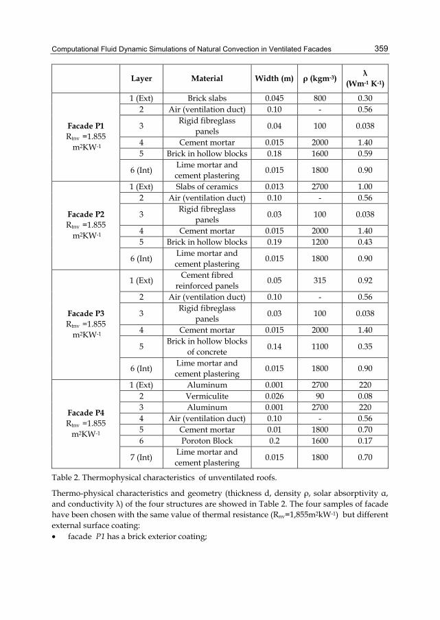
Computational Fluid Dynamic Simulations of Natural Convection in Ventilated Facades
359
Layer Material Width (m) ρ (kgm-3) λ
(Wm-1 K-1)
1 (Ext) Brick slabs 0.045 800 0.30 2 Air (ventilation duct) 0.10 - 0.56
3 Rigid fibreglass panels 0.04 100 0.038
4 Cement mortar 0.015 2000 1.40 5 Brick in hollow blocks 0.18 1600 0.59
Facade P1 Rtnv =1.855
m2KW-1
6 (Int) Lime mortar and cement plastering 0.015 1800 0.90
1 (Ext) Slabs of ceramics 0.013 2700 1.00 2 Air (ventilation duct) 0.10 - 0.56
3 Rigid fibreglass panels 0.03 100 0.038
4 Cement mortar 0.015 2000 1.40 5 Brick in hollow blocks 0.19 1200 0.43
Facade P2 Rtnv =1.855
m2KW-1
6 (Int) Lime mortar and cement plastering 0.015 1800 0.90
1 (Ext) Cement fibred reinforced panels 0.05 315 0.92
2 Air (ventilation duct) 0.10 - 0.56
3 Rigid fibreglass panels 0.03 100 0.038
4 Cement mortar 0.015 2000 1.40
5 Brick in hollow blocks of concrete 0.14 1100 0.35
Facade P3 Rtnv =1.855
m2KW-1
6 (Int) Lime mortar and cement plastering 0.015 1800 0.90
1 (Ext) Aluminum 0.001 2700 220 2 Vermiculite 0.026 90 0.08 3 Aluminum 0.001 2700 220 4 Air (ventilation duct) 0.10 - 0.56 5 Cement mortar 0.01 1800 0.70 6 Poroton Block 0.2 1600 0.17
Facade P4 Rtnv =1.855
m2KW-1
7 (Int) Lime mortar and cement plastering 0.015 1800 0.70
Table 2. Thermophysical characteristics of unventilated roofs.
Thermo-physical characteristics and geometry (thickness d, density ρ, solar absorptivity α, and conductivity λ) of the four structures are showed in Table 2. The four samples of facade have been chosen with the same value of thermal resistance (Rnv=1,855m2kW-1) but different external surface coating: • facade P1 has a brick exterior coating;
Evaporation, Condensation and Heat Transfer
360
• facade P2 has a coating of ceramic tiles; • facade P3 has a coating of cement fibred reinforced panels; • facade P4 has an external coating made of insulated panels in vermiculite covered with
aluminum on both sides. In all the studied cases, the outer layer is anchored to a supporting structure made of brick blocks. The facades P1, P2 and P3 present the insulating layer, consisting of a rigid fibreglass panel with a thickness of 4 cm, placed in the inner slab, while in the case of the facade P4 the coating panel also acts as insulation layer. The ventilation openings that connect the ventilated cavity with the external environment are placed at the base and at the upper part of facade and have a size of 20 cm x 100 cm The friction factors and heat transfer coefficients are assumed to be constant along the duct. Generally, the roughness value of the air duct is assumed to be quite high in order to take into account the presence of supports inside the air duct. Obviously this parameter is not uniform throughout the whole structure but it is realistic in the portion of the channel that is not affected by the presence of supporting elements. Therefore the sensitivity analysis for this parameter have been performed. The roughness b has been varied from 0,005 m up to 0,03 m. This sensitive analysis didn’t show significant variations both for the velocity profiles and for the energy performance of the ventilated facade. The value of roughness has been estimated as b = 0,02 m. The solar absorptivity coefficient α has been defined constant because its difference between the three studied cases is about from 0.02 up to 0.04, so it involves only a few hundredths of temperature degrees changes in the temperature sun-air Tas. According to the studies in references the solar absorption coefficient has been fixed in α = 0,8. Thermal resistances of inner and outer surfaces have been defined respectively ri =0.13 m2kW-1and re=0.04 m2kW-1.
7. Results and discussions The authors have studied the behavior of the four types of facades, both in case of natural ventilation and in the case of forced ventilation of the air in the duct. For the study of a typical summer situation have been considered the following reference conditions: - External temperature: Te = T0 = 301 K; - Indoor temperature: Ti = 297 K; - Incident solar radiation: I = 400 W/m2. The modeling of the real system has been performed using the computer code "Fluent"and the pre-processor "Gambit". The convergence criterion requires that the maximum relative difference between two consecutive iterations for each local variable is less than 10-3. Convergence has been generally obtained with a number of iterations, which varies from case to case, but always between 800 and 1200 iterations.
7.1 Natural ventilation Initially has been studied the behavior of the ventilated facade system in natural ventilation, with the motion of air in the cavity caused by thermal and pressure gradients. Figures 5 to 12 show the velocity and temperature profiles obtained for the four facades.
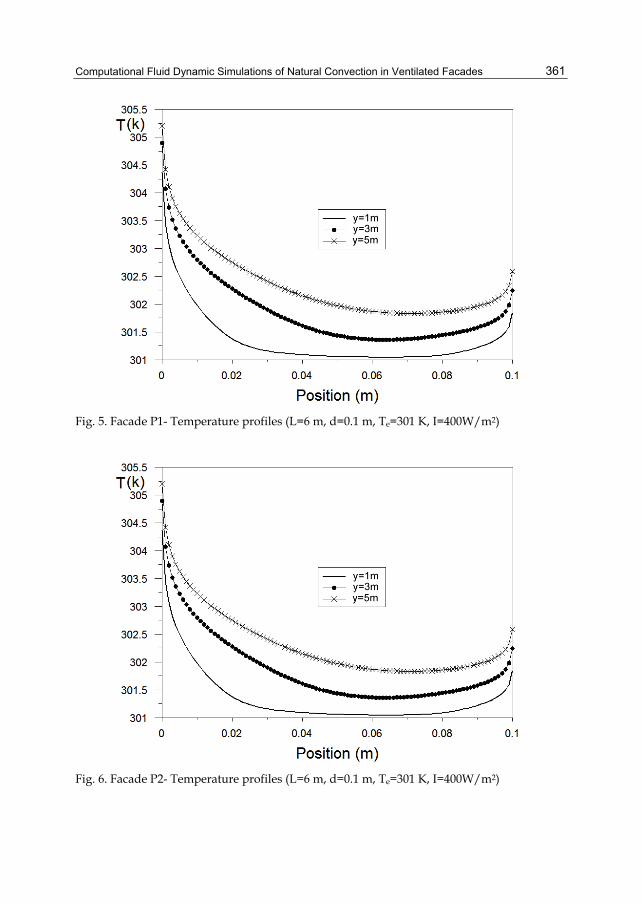
Computational Fluid Dynamic Simulations of Natural Convection in Ventilated Facades
361
Fig. 5. Facade P1- Temperature profiles (L=6 m, d=0.1 m, Te=301 K, I=400W/m2)
Fig. 6. Facade P2- Temperature profiles (L=6 m, d=0.1 m, Te=301 K, I=400W/m2)
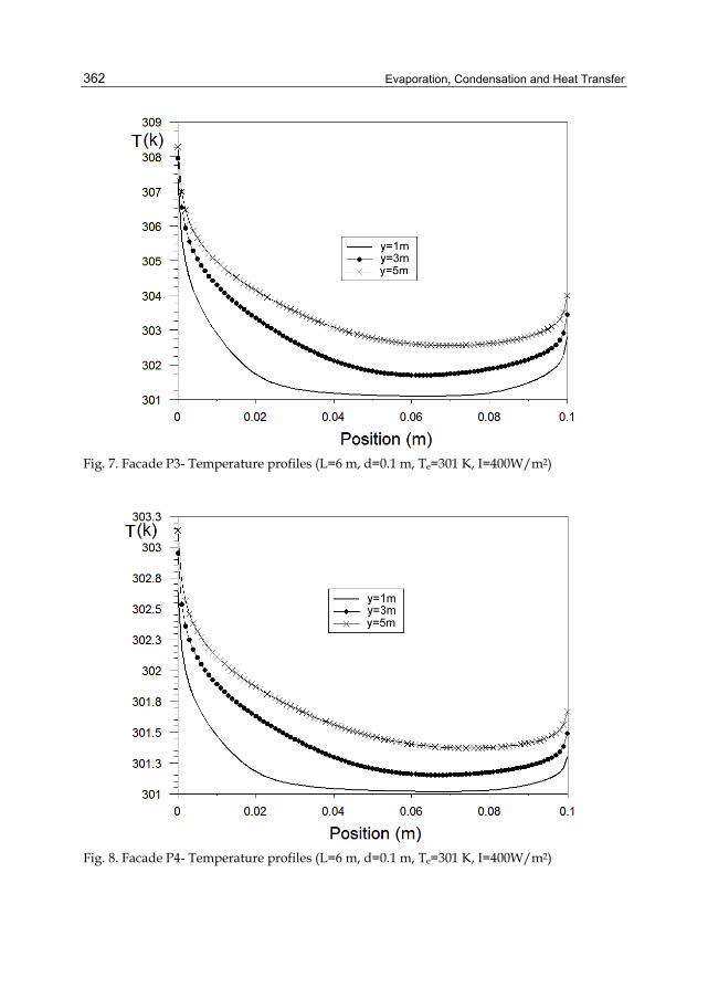
Evaporation, Condensation and Heat Transfer
362
Fig. 7. Facade P3- Temperature profiles (L=6 m, d=0.1 m, Te=301 K, I=400W/m2)
Fig. 8. Facade P4- Temperature profiles (L=6 m, d=0.1 m, Te=301 K, I=400W/m2)
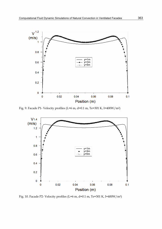
Computational Fluid Dynamic Simulations of Natural Convection in Ventilated Facades
363
Fig. 9. Facade P1- Velocity profiles (L=6 m, d=0.1 m, Te=301 K, I=400W/m2)
Fig. 10. Facade P2- Velocity profiles (L=6 m, d=0.1 m, Te=301 K, I=400W/m2)
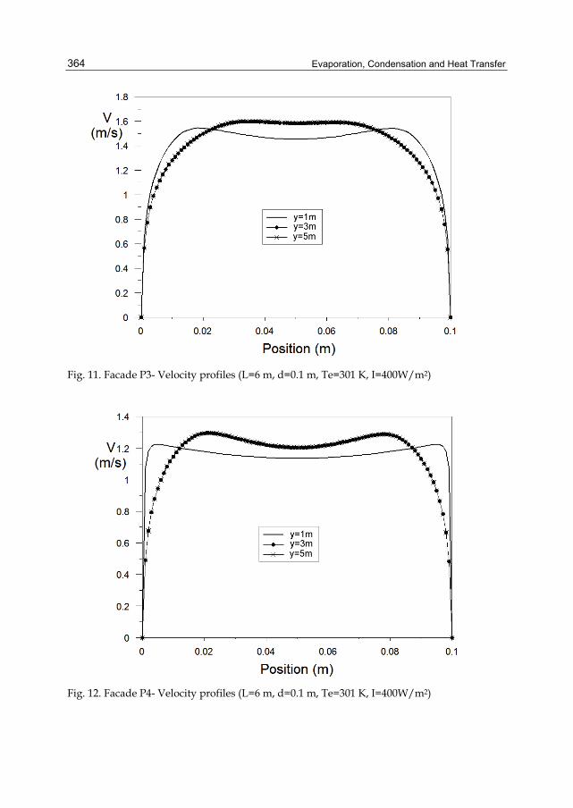
Evaporation, Condensation and Heat Transfer
364
Fig. 11. Facade P3- Velocity profiles (L=6 m, d=0.1 m, Te=301 K, I=400W/m2)
Fig. 12. Facade P4- Velocity profiles (L=6 m, d=0.1 m, Te=301 K, I=400W/m2)
Computational Fluid Dynamic Simulations of Natural Convection in Ventilated Facades
365
The temperature profiles show an increase of the air temperature inside the cavity along the direction of the motion. It also possible to observe two temperature boundary layers developed in correspondence of the two slabs. The fluid temperature decreases gradually moving away from the two surfaces delimiting the ventilated cavity and it reaches the value of undisturbed flow outside the thermal boundary layer. In the first section of the ventilation duct (1/6 of the total length of the facade), as is possible to see in the profile obtained for y=1 m, the temperature increases above in the part of the duct near the two walls, where viscous dissipation is maximum, while the air in the middle of the channel presents a temperature very close to the entrance value T0. At a distance from the entrance sufficiently high (3/6 of the total length of the facade), the air temperature in correspondence of the centerline increases too. From this section the temperature profile becomes “stable”. The temperature profiles obtained at the third section of the ventilation duct (5 / 6 of the total length of the facade) have the same trend as those obtained for the second section, but with higher overall temperatures. It is interesting to observe that in the case of the ventilated facade P4, the air flow inside the duct is heated less than the other two studied facades. In fact, for the facade P4 has been obtained the lowest value of air temperature inside the duct. The distributions of velocity observed in the cases of the walls P1,P2 and P4 show the characteristic trend of internal flows in natural convection. It is possible to observe the existence of two symmetric boundary layers developed near the two slabs that delimit the ventilated duct . The fluid velocity is zero in correspondence of the two walls (condition of adhesion to the wall) and increases with distance from the surface, until it reaches a maximum value (x = 0.02m) and then decreases again moving toward the center line (x = 0.05 m). In the first section of the ventilation duct, as shown by the velocity profiles obtained at the section located at y = 1 m, the air flow is not yet fully developed and it has a lower average speed of about 1 m / s for the wall P1, of 1.2 m / s for the walls and P2 and P4 of 1.5 m / s for the wall P3. In the case of the wall P3, velocity profiles show a parabolic trend with a maximum speed of 1.6 m/s on the centerline (x = 0.05 m).
7.2 Forced ventilation In the case of forced convection, the action of an mechanical propeller(one or more low power fan) that pushes the air inside the double-ventilated, increasing the effects due to local gradients of density characteristic of simple natural convection , has been simulated by imposing a speed input v0. The other boundary conditions have been imposed coincident with those used to study the motion of air in case of natural convection. The following figures (from 13 to 16) show the velocity and temperature profiles obtained for the ventilated wall P1, for two different values of inlet velocity, respectively, v0(1) = 1 m/s and v0(2) = 2 m/s. The temperature profiles (see fig. 13 and 14) show a very flattened trend in the middle of the channel with two points of maximum in correspondence to the two slabs. The increase of the velocity v0, imposed by the fan, causes both the decrease of the temperature difference between the two sides of the duct and the decrease of the temperature difference between the inlet and outlet cross-sections (TL -T0). Every way the ventilation heat flux, Qv= m cp(TL - T0), augment is caused by the increase of the mass air flow.
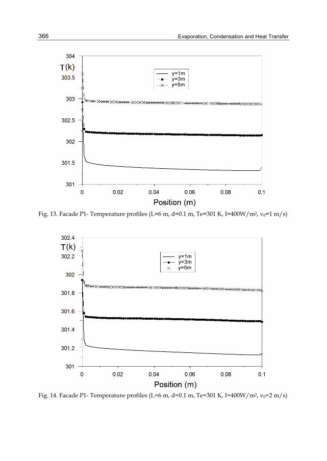
Evaporation, Condensation and Heat Transfer
366
Fig. 13. Facade P1- Temperature profiles (L=6 m, d=0.1 m, Te=301 K, I=400W/m2, v0=1 m/s)
Fig. 14. Facade P1- Temperature profiles (L=6 m, d=0.1 m, Te=301 K, I=400W/m2, v0=2 m/s)
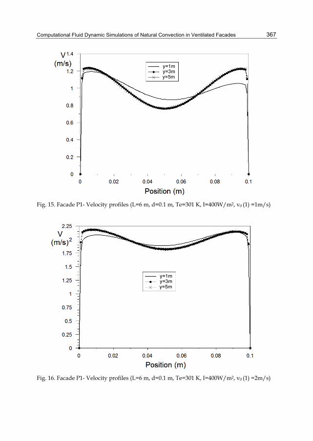
Computational Fluid Dynamic Simulations of Natural Convection in Ventilated Facades
367
Fig. 15. Facade P1- Velocity profiles (L=6 m, d=0.1 m, Te=301 K, I=400W/m2, v0 (1) =1m/s)
Fig. 16. Facade P1- Velocity profiles (L=6 m, d=0.1 m, Te=301 K, I=400W/m2, v0 (1) =2m/s)
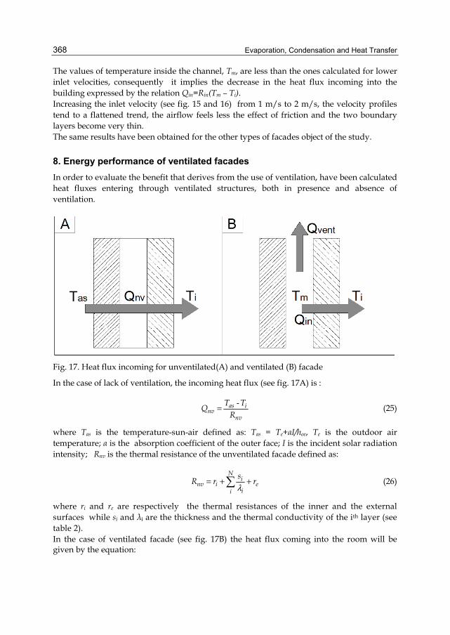
Evaporation, Condensation and Heat Transfer
368
The values of temperature inside the channel, Tm, are less than the ones calculated for lower inlet velocities, consequently it implies the decrease in the heat flux incoming into the building expressed by the relation Qin=Rin(Tm – Ti). Increasing the inlet velocity (see fig. 15 and 16) from 1 m/s to 2 m/s, the velocity profiles tend to a flattened trend, the airflow feels less the effect of friction and the two boundary layers become very thin. The same results have been obtained for the other types of facades object of the study.
8. Energy performance of ventilated facades In order to evaluate the benefit that derives from the use of ventilation, have been calculated heat fluxes entering through ventilated structures, both in presence and absence of ventilation.
Fig. 17. Heat flux incoming for unventilated(A) and ventilated (B) facade
In the case of lack of ventilation, the incoming heat flux (see fig. 17A) is :
-as inv
nv
T TQR
= (25)
where Tas is the temperature-sun-air defined as: Tas = Te+αI/hoe, Te is the outdoor air temperature; α is the absorption coefficient of the outer face; I is the incident solar radiation intensity; Rnv is the thermal resistance of the unventilated facade defined as:
N
inv i e
ii
sR r rλ
= + +∑ (26)
where ri and re are respectively the thermal resistances of the inner and the external surfaces while si and λi are the thickness and the thermal conductivity of the ith layer (see table 2). In the case of ventilated facade (see fig. 17B) the heat flux coming into the room will be given by the equation:
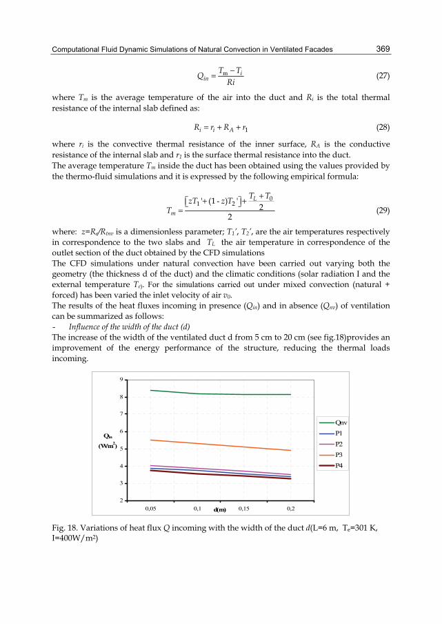
Computational Fluid Dynamic Simulations of Natural Convection in Ventilated Facades
369
m iin
T TQRi−= (27)
where Tm is the average temperature of the air into the duct and Ri is the total thermal resistance of the internal slab defined as:
1i i AR r R r= + + (28)
where ri is the convective thermal resistance of the inner surface, RA is the conductive resistance of the internal slab and r1 is the surface thermal resistance into the duct. The average temperature Tm inside the duct has been obtained using the values provided by the thermo-fluid simulations and it is expressed by the following empirical formula:
- 0
1 2' (1 ) '2
2
L
m
T TzT z TT
++ +⎡ ⎤⎣ ⎦= (29)
where: z=Re/Rtnv is a dimensionless parameter; T1’, T2’, are the air temperatures respectively in correspondence to the two slabs and TL the air temperature in correspondence of the outlet section of the duct obtained by the CFD simulations The CFD simulations under natural convection have been carried out varying both the geometry (the thickness d of the duct) and the climatic conditions (solar radiation I and the external temperature Te). For the simulations carried out under mixed convection (natural + forced) has been varied the inlet velocity of air v0. The results of the heat fluxes incoming in presence (Qin) and in absence (Qnv) of ventilation can be summarized as follows: - Influence of the width of the duct (d) The increase of the width of the ventilated duct d from 5 cm to 20 cm (see fig.18)provides an improvement of the energy performance of the structure, reducing the thermal loads incoming.
2
3
4
5
6
7
8
9
0,05 0,1 0,15 0,2d(m)
Qin
(W/m2)
QnvP1P2P3P4
Fig. 18. Variations of heat flux Q incoming with the width of the duct d(L=6 m, Te=301 K, I=400W/m2)
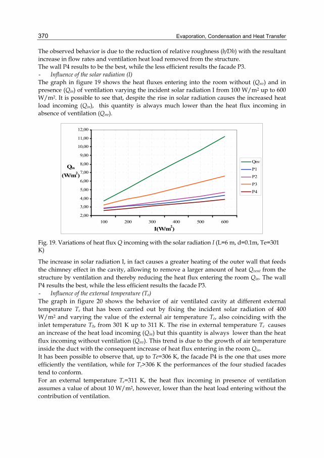
Evaporation, Condensation and Heat Transfer
370
The observed behavior is due to the reduction of relative roughness (b/Dh) with the resultant increase in flow rates and ventilation heat load removed from the structure. The wall P4 results to be the best, while the less efficient results the facade P3. - Influence of the solar radiation (I) The graph in figure 19 shows the heat fluxes entering into the room without (Qnv) and in presence (Qin) of ventilation varying the incident solar radiation I from 100 W/m2 up to 600 W/m2. It is possible to see that, despite the rise in solar radiation causes the increased heat load incoming (Qin), this quantity is always much lower than the heat flux incoming in absence of ventilation (Qnv).
2,00
3,00
4,00
5,00
6,00
7,00
8,00
9,00
10,00
11,00
12,00
100 200 300 400 500 600
I(W/m2)
Qin
(W/m2)
Qnv
P1
P2
P3
P4
Fig. 19. Variations of heat flux Q incoming with the solar radiation I (L=6 m, d=0.1m, Te=301 K)
The increase in solar radiation I, in fact causes a greater heating of the outer wall that feeds the chimney effect in the cavity, allowing to remove a larger amount of heat Qvent from the structure by ventilation and thereby reducing the heat flux entering the room Qin. The wall P4 results the best, while the less efficient results the facade P3. - Influence of the external temperature (Te) The graph in figure 20 shows the behavior of air ventilated cavity at different external temperature Te that has been carried out by fixing the incident solar radiation of 400 W/m2 and varying the value of the external air temperature Te, also coinciding with the inlet temperature T0, from 301 K up to 311 K. The rise in external temperature Te causes an increase of the heat load incoming (Qin) but this quantity is always lower than the heat flux incoming without ventilation (Qnv). This trend is due to the growth of air temperature inside the duct with the consequent increase of heat flux entering in the room Qin. It has been possible to observe that, up to Te=306 K, the facade P4 is the one that uses more efficiently the ventilation, while for Te>306 K the performances of the four studied facades tend to conform. For an external temperature Te=311 K, the heat flux incoming in presence of ventilation assumes a value of about 10 W/m2, however, lower than the heat load entering without the contribution of ventilation.
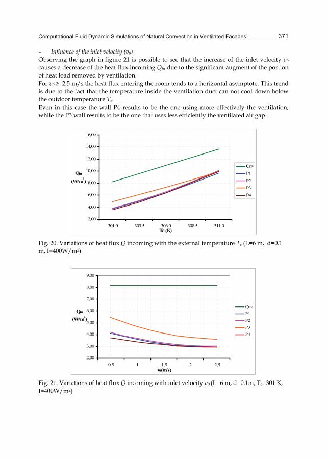
Computational Fluid Dynamic Simulations of Natural Convection in Ventilated Facades
371
- Influence of the inlet velocity (v0) Observing the graph in figure 21 is possible to see that the increase of the inlet velocity v0 causes a decrease of the heat flux incoming Qin due to the significant augment of the portion of heat load removed by ventilation. For v0 ≥ 2,5 m/s the heat flux entering the room tends to a horizontal asymptote. This trend is due to the fact that the temperature inside the ventilation duct can not cool down below the outdoor temperature Te. Even in this case the wall P4 results to be the one using more effectively the ventilation, while the P3 wall results to be the one that uses less efficiently the ventilated air gap.
2,00
4,00
6,00
8,00
10,00
12,00
14,00
16,00
301.0 303.5 306.0 308.5 311.0Te (K)
Qin
(W/m2)
Qnv
P1
P2
P3
P4
Fig. 20. Variations of heat flux Q incoming with the external temperature Te (L=6 m, d=0.1 m, I=400W/m2)
2,00
3,00
4,00
5,00
6,00
7,00
8,00
9,00
0,5 1 1,5 2 2,5v0(m/s)
Qin
(W/m2)
Qnv
P1
P2
P3
P4
Fig. 21. Variations of heat flux Q incoming with inlet velocity v0 (L=6 m, d=0.1m, Te=301 K, I=400W/m2)
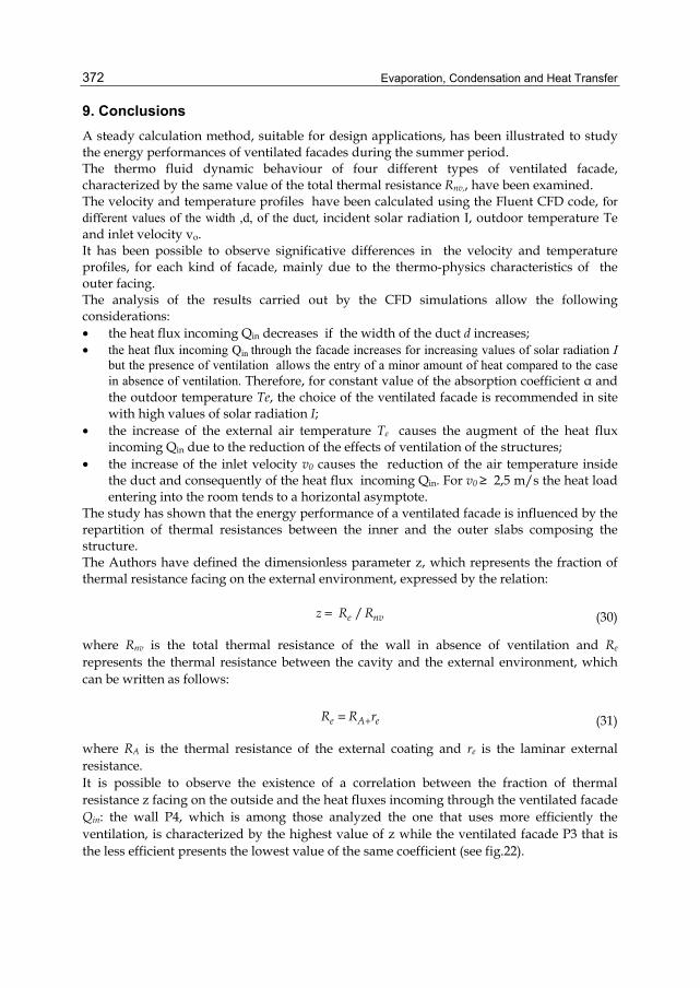
Evaporation, Condensation and Heat Transfer
372
9. Conclusions A steady calculation method, suitable for design applications, has been illustrated to study the energy performances of ventilated facades during the summer period. The thermo fluid dynamic behaviour of four different types of ventilated facade, characterized by the same value of the total thermal resistance Rnv,, have been examined. The velocity and temperature profiles have been calculated using the Fluent CFD code, for different values of the width ,d, of the duct, incident solar radiation I, outdoor temperature Te and inlet velocity vo. It has been possible to observe significative differences in the velocity and temperature profiles, for each kind of facade, mainly due to the thermo-physics characteristics of the outer facing. The analysis of the results carried out by the CFD simulations allow the following considerations: • the heat flux incoming Qin decreases if the width of the duct d increases; • the heat flux incoming Qin through the facade increases for increasing values of solar radiation I
but the presence of ventilation allows the entry of a minor amount of heat compared to the case in absence of ventilation. Therefore, for constant value of the absorption coefficient α and the outdoor temperature Te, the choice of the ventilated facade is recommended in site with high values of solar radiation I;
• the increase of the external air temperature Te causes the augment of the heat flux incoming Qin due to the reduction of the effects of ventilation of the structures;
• the increase of the inlet velocity v0 causes the reduction of the air temperature inside the duct and consequently of the heat flux incoming Qin. For v0 ≥ 2,5 m/s the heat load entering into the room tends to a horizontal asymptote.
The study has shown that the energy performance of a ventilated facade is influenced by the repartition of thermal resistances between the inner and the outer slabs composing the structure. The Authors have defined the dimensionless parameter z, which represents the fraction of thermal resistance facing on the external environment, expressed by the relation:
/e nvz R R= (30)
where Rnv is the total thermal resistance of the wall in absence of ventilation and Re represents the thermal resistance between the cavity and the external environment, which can be written as follows:
e A eR R r+= (31)
where RA is the thermal resistance of the external coating and re is the laminar external resistance. It is possible to observe the existence of a correlation between the fraction of thermal resistance z facing on the outside and the heat fluxes incoming through the ventilated facade Qin: the wall P4, which is among those analyzed the one that uses more efficiently the ventilation, is characterized by the highest value of z while the ventilated facade P3 that is the less efficient presents the lowest value of the same coefficient (see fig.22).
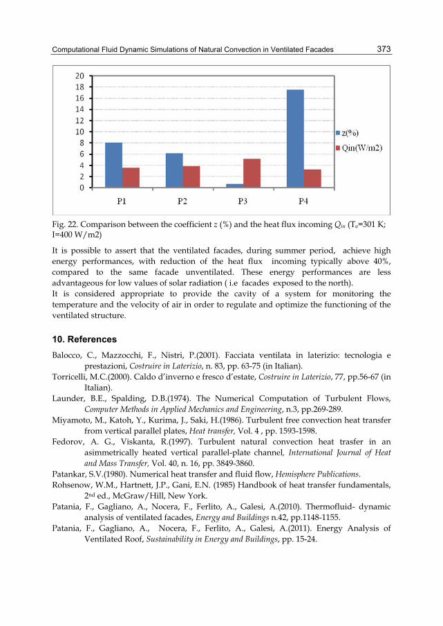
Computational Fluid Dynamic Simulations of Natural Convection in Ventilated Facades
373
Fig. 22. Comparison between the coefficient z (%) and the heat flux incoming Qin (Te=301 K; I=400 W/m2)
It is possible to assert that the ventilated facades, during summer period, achieve high energy performances, with reduction of the heat flux incoming typically above 40%, compared to the same facade unventilated. These energy performances are less advantageous for low values of solar radiation ( i.e facades exposed to the north). It is considered appropriate to provide the cavity of a system for monitoring the temperature and the velocity of air in order to regulate and optimize the functioning of the ventilated structure.
10. References Balocco, C., Mazzocchi, F., Nistri, P.(2001). Facciata ventilata in laterizio: tecnologia e
prestazioni, Costruire in Laterizio, n. 83, pp. 63-75 (in Italian). Torricelli, M.C.(2000). Caldo d’inverno e fresco d’estate, Costruire in Laterizio, 77, pp.56-67 (in
Italian). Launder, B.E., Spalding, D.B.(1974). The Numerical Computation of Turbulent Flows,
Computer Methods in Applied Mechanics and Engineering, n.3, pp.269-289. Miyamoto, M., Katoh, Y., Kurima, J., Saki, H.(1986). Turbulent free convection heat transfer
from vertical parallel plates, Heat transfer, Vol. 4 , pp. 1593-1598. Fedorov, A. G., Viskanta, R.(1997). Turbulent natural convection heat trasfer in an
asimmetrically heated vertical parallel-plate channel, International Journal of Heat and Mass Transfer, Vol. 40, n. 16, pp. 3849-3860.
Patankar, S.V.(1980). Numerical heat transfer and fluid flow, Hemisphere Publications. Rohsenow, W.M., Hartnett, J.P., Gani, E.N. (1985) Handbook of heat transfer fundamentals,
2nd ed., McGraw/Hill, New York. Patania, F., Gagliano, A., Nocera, F., Ferlito, A., Galesi, A.(2010). Thermofluid- dynamic
analysis of ventilated facades, Energy and Buildings n.42, pp.1148-1155. Patania, F., Gagliano, A., Nocera, F., Ferlito, A., Galesi, A.(2011). Energy Analysis of
Ventilated Roof, Sustainability in Energy and Buildings, pp. 15-24.

Evaporation, Condensation and Heat Transfer
374
Ciampi, M., Leccese, F., Tuoni, G. (2002) On the thermal behaviour of ventilated facades and roof, La Termotecnica, n.1, pp. 87-97 (in Italian).
Ciampi, M., Leccese, F., Tuoni, G.(2003). Ventilated facades energy performance in summer cooling of buildings, Solar Energy, n.75, 491–502
0
Turbulent Heat Transfer in Drag-ReducingChannel Flow of Viscoelastic Fluid
Takahiro Tsukahara and Yasuo KawaguchiTokyo University of Science
Japan
1. Introduction
The fascinating effects of minute quantities of high-molecular-weight polymer or surfactant,dissolved in water or another Newtonian fluid, on turbulent behaviors have stimulatedconsiderable research. The most striking phenomenon is the reduction of turbulent frictionaldrag in wall-bounded flows. As has been well known for 60 years since its first demonstrationby Toms (1949), drag reduction (DR) up to 80% can be achieved in appropriate conditions. Theapplication of this phenomenon, also called the “Toms effect”, to heat-transport systems suchas district heating and cooling systems has recently attracted attention as an energy-savingtechnology. The pumping power can be largely conserved by adding a few hundred ppm ofsurfactant solution to water so that the flow becomes laminar-like. One of the most successfulapplications of DR has been in the Trans-Alaska pipeline, where the desired discharge of anadditional million barrels of crude oil per day was accomplished by the use of polymericadditives rather than by constructing additional pumping systems.On the other hand, heat transfer reduction (HTR) for a drag-reducing flow is also significantand becomes large with increased DR. If conditions that give rise to large DR and smallHTR can be identified, then they should be ideal for the transport of heat in thermalsystems. Moreover, it is practically important to formulate phenomenological modelsand semiempirical correlations, similar to those employed in the description of turbulentNewtonian flows, for viscoelastic flows accompanied by DR and HTR.
1.1 Related studiesThe turbulence modulation of drag-reducing flows is more complicated than that of aNewtonian-fluid flow such as water. Fluid containing drag-reducing additives can begenerally treated as a non-Newtonian viscoelastic fluid, as assumed in the present study.A number of fundamental studies on DR have been carried out, in part because thesubject lies at the intersection of two complex and important fields of rheology andturbulence. Although it is practically difficult to analyze the interaction between additivesand turbulent motions at the molecular level, many key aspects of the drag-reducing flowhave gradually been elucidated. For instance, we already know that additives inhibit thetransfer of energy from the streamwise to the wall-normal velocity fluctuations, and thatthe strong vorticity fluctuation near the wall disappears in the drag-reducing flow. Thereare several reviews (Dimant & Poreh, 1976; Gyr & Bewersdorff, 1995; Hoyt, 1990; Lumley,
18
2 Heat Transfer
1969; Nadolink & Haigh, 1995; Procaccia et al. , 2008; Shenoy, 1984; White & Mungal, 2008)that highlight the progress made in understanding this subject.Recent direct numerical simulations (DNSs) based on various types of constitutive equationshave revealed some important characteristics common to turbulent pipe and channelflows subject to DR. Several features observed in experiments have been successfullyreproduced by these numerical analyses (Den Toonder et al., 1997; Dimitropoulos et al., 2001;2005; Jovanovic et al., 2006; Li et al., 2006; Sureshkumar & Beris, 1995; Sureshkumar et al.,1997; Tamano et al., 2007). The authors’ group (Yu & Kawaguchi, 2004; Yu et al., 2004;Yu & Kawaguchi, 2005; 2006) has simulated viscoelastic fluids by DNS with the Giesekusmodel. Although there are certain other commonly used models (e.g., FENE-P, Oldroyd-B),we selected the Giesekus model for our study because it can well describe the measuredapparent shear viscosity and extensional viscosity of the surfactant solution (cf. Wei et al.,2006). Through these studies, the occurrence of a high level of DR was found to require highelastic energy in a wide buffer layer with large relaxation time, that is, a high Weissenbergnumber (Weτ). More recent numerical studies by Roy et al. (2006) have suggested that, fora drag-reducing polymer solution, the self-sustaining process of wall turbulence becomesweaker owing to the effect of elasticity on the coherent structures. Their analysis also showedthat, at small Weτ , elasticity enhances the quasi-streamwise vortex structures. Similarly,Kim et al. (2008) reported that the autogeneration of new hairpin vortices typical of wallturbulence, which are closely related to the buffer layer, can be suppressed by the polymerstresses, thereby resulting in DR.Although research on drag-reducing flow with heat transfer is important for various kindsof heat-transport systems and interesting from a scientific perspective, there have been veryfew studies on this issue (Aguilar et al., 1999; 2001; Dimant & Poreh, 1976; Gasljevic et al.,2007; Li et al., 2004a;b; 2005), particularly in terms of numerical simulations (Gupta et al.,2005; Kagawa, 2008; Yu & Kawaguchi, 2005). Early experiments presented some empiricalmodels for heat transfer in drag-reducing flows (Dimant & Poreh, 1976) and showed thatthe heat-transfer coefficient was reduced at a rate faster than the accompanying DR(Cho & Hartnett, 1982), and that an analogous reduction of HTR was observed in the case ofdrag-reducing surfactant solution (Qi et al., 2001). Several attempts to enhance the efficiencyof the heat transfer in drag-reducing flows have been reported in the literature (Aly et al.,2006; Li et al., 2001; Qi et al., 2001). For instance, Qi et al. (2003) examined the methodologyof temporal heat-transfer enhancement of drag-reducing surfactants in heat exchangers andregaining DR downstream. Nevertheless, the trade-off between the DR and HTR in industrialapplications has not been completely understood. Furthermore, the mechanism of theHTR itself in drag-reducing flows has not been clearly established. As mentioned above,predictions of intermediate values of friction and heat transfer are not yet possible, even if therheological and thermal properties of a relevant fluid are known.
1.2 PurposeIn the research presented in this article, we addressed a wide range of issues related todrag-reducing flows by means of DNS on turbulent heat transfer; and we also reviewprevious DNS results (Kagawa, 2008; Tsukahara et al., 2011a; Tsukahara & Kawaguchi, 2011b)with additional computations. We have considered dilute surfactant solutions, in which theshear-thinning behavior is assumed to be negligible, but elongational viscoelastic effect istaken into account using a method for the extra elastic stresses. To achieve a clearer picture ofthe role of viscoelasticity, we have used DNS based on the Giesekus viscoelastic-fluid model.
376 Evaporation, Condensation and Heat Transfer
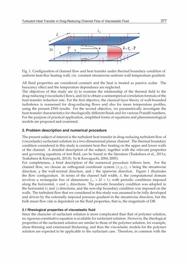
Turbulent Heat Transfer in Drag-ReducingChannel Flow of Viscoelastic Fluid 3
Fig. 1. Configuration of channel flow and heat transfer under thermal boundary condition ofuniform heat-flux heating wall, viz. constant streamwise uniform wall temperature gradient.
All fluid properties are considered constant and the heat is treated as passive scalar. Thebuoyancy effect and the temperature dependence are neglected.The objectives of this study are (i) to examine the relationship of the thermal field to thedrag-reducing (viscoelastic) flows, and (ii) to obtain a semiempirical correlation formula of theheat-transfer reduction rate. For the first objective, the classical layer theory of wall-boundedturbulence is reassessed for drag-reducing flows and also for mean temperature profiles,using the present DNS results. For the second objective, we parametrically investigate theheat-transfer characteristics for rheologically different fluids and for various Prandtl numbers.For the purpose of practical application, simplified forms of equations and phenomenologicalmodels are proposed and examined.
2. Problem description and numerical procedure
The present subject of interest is the turbulent heat transfer in drag-reducing turbulent flow of(viscoelastic) surfactant solution in a two-dimensional planar channel. The thermal boundarycondition considered in this study is constant heat-flux heating on the upper and lower wallsof the channel. A detailed description of the subject, together with the relevant propertiesand governing equations of test fluid, can be found in the literature (Tsukahara et al., 2011a;Tsukahara & Kawaguchi, 2011b; Yu & Kawaguchi, 2004; 2005).For completeness, a brief description of the numerical procedure follows here. For thechannel flow, we choose an orthogonal coordinate system (x, y, z), x being the streamwisedirection, y the wall-normal direction, and z the spanwise direction. Figure 1 illustratesthe flow configuration. In terms of the channel half width, δ, the computational domaininvolves a rectangular box of dimensions Lx × 2δ × Lz with periodic conditions imposedalong the horizontal, x and z, directions. The periodic boundary condition was adopted inthe horizontal (x and z) directions, and the non-slip boundary condition was imposed on thewalls. The turbulent flow that we considered in this study was assumed to be fully developedand driven by the externally imposed pressure gradient in the streamwise direction, but thebulk mean flow rate is dependent on the fluid properties, that is, the magnitude of DR.
2.1 Rheological properties of viscoelastic fluidSince the character of surfactant solution is more complicated than that of polymer solution,no rigorous constitutive equation is available for surfactant solution. However, the rheologicalproperties of the surfactant solution are similar to those of the polymer solution, for example,shear-thinning and extensional thickening, and thus the viscoelastic models for the polymersolution are expected to be applicable to the surfactant case. Therefore, in common with the
377Turbulent Heat Transfer in Drag-Reducing Channel Flow of Viscoelastic Fluid
4 Heat Transfer
dilute polymer solution, the fluid motion considered here is described by the conventionalcontinuity and momentum equations:
∇ · u = 0, (1)
ρDuDt
= −∇p +∇ · τtotal (2)
where ρ is the density (assumed constant), t the time, u = {u, v, w} the velocity, p the pressure,and τtotal the total extra stress tensor. For a homogeneous solution of a Newtonian solvent anda surfactant solute, the extra stress is decomposed as τtotal = τsolvent + τ , with a Newtoniansolvent component τsolvent = ρηsΔu, where the solvent kinematic viscosity ηs is constant,and there is an extra stress-tensor component due to additives, τ . To account for elasticityeffects,we employed a viscoelastic Giesekus constitutive equation to model the interactionbetween the elastic network structures and solvent, following a proposal by Giesekus (1982):
τ + λ
(Dτ
Dt− τ · ∇u−∇uT · τ
)+
αλ
ρηa(τ · τ ) = ρηa
(∇u +∇uT
), (3)
where λ, α, and ηa are, respectively, a constant relaxation time, the mobility factor, and theadditive contribution to the zero-shear-rate solution kinematic viscosity, η0. This model isknown to describe the power-law regions for viscosity and normal-stress coefficients and italso provides a reasonable description of the elongational viscosity (Bird, 1995). When λ = 0,we obtain the momentum equation for Newtonian fluid with the kinematic viscosity of ηs +ηa. Equation (3) with α = 0 corresponds to the Oldroyd-B model. Note that, in general, both λand ηa can be considered as functions of the stress or other state variables (e.g., temperature),but they will be assumed to be constants in the present study for simplicity.Kawaguchi et al. (2003) reported that the measured shear viscosities were well demonstratedby the Giesekus model for different temperatures and concentrations of surfactant solutionand that, using the model parameters obtained from the correlations, most of the measuredshear viscosities agreed with the prediction by the Giesekus model. Yu et al. (2004) adoptedthis model using parameters that were determined by well-fitting apparent shear viscositiesbased on measurement using rheometers. Their comparison between numerical andexperimental results revealed the rheological properties of a viscoelastic fluid of 75 ppm CTAC(cetyltrimethyl ammonium chloride) solution at 30◦C, namely, λ = 0.3 seconds, α = 0.005,and the viscosity ratio β = ηs/η0 = 0.2. It should be noted that the contribution of the additiveto the solution viscosity was relatively large compared with those obtained or assumed inprevious studies on DR. Since many experiments described in the literature were carried outat low concentrations of polymer and achieved significant DRs, most DNSs in the literatureemployed artificially low values without detailed measurement.
2.2 Governing equations for velocity fieldTo describe the system in a non-dimensional form, let us introduce the dimensionlessconformation tensor, cij, with which the instantaneous additive extra stress (τij) is given asan explicit function:
τ+ij =
c+ij − δij
λuτ/δ. (4)
378 Evaporation, Condensation and Heat Transfer
Turbulent Heat Transfer in Drag-ReducingChannel Flow of Viscoelastic Fluid 5
In the equation above, δij is the Kronecker delta. As for a characteristic velocity, the frictionvelocity (uτ) based on the mean pressure gradient in the streamwise direction is chosen:
uτ =
√τw
ρ=
√− δ
ρ
∂p∂x
. (5)
The dimensionless governing equations for an incompressible viscoelastic-fluid flow are thecontinuity, momentum conservation, and constitutive equations, which can be rewritten intensor form based on Equations (1)–(3) as follows:
∂ui
∂xi= 0, (6)
∂u+i
∂t�+ u+
j∂u+
i∂x�j
= − ∂p+
∂x�i+
β
Reτ
∂
∂x�j
(∂u+
i∂x�j
)+
(1− β)
Weτ
∂c+ij∂x�j
+∂p+
∂x�1δ1i. (7)
∂c+ij∂t�
+∂u+
k c+ij∂x�k
− c+ik∂u+
j
∂x�k− ∂u+
i∂x�k
c+kj +Reτ
Weτ
[c+ij − δij + α
(c+ik − δik
) (c+kj − δkj
)]= 0, (8)
where i = 1, 2, and 3 indicate the streamwise, wall-normal, and spanwise directions,respectively. The scales used to obtain the non-dimensional variables are uτ and η0. The lastterm on the right-hand side of Equation (7) corresponds to the mean pressure gradient drivingthe flow. The superscript "�" is used to denote non-dimensional distances (e.g., y� = y/δ) andthe superscript "+" denotes the wall unit.As suggested by Equation (7), the flow is defined by three control parameters:
Friction Reynolds number: Reτ =uτδ
η0, (9)
Weissenberg number: Weτ =λ
η0/u2τ
, (10)
Viscosity ratio: β =ηs
η0. (11)
Table 1 shows a summary of tested parameters for the Newtonian fluid (case 1) and the fourdifferent viscoelastic fluids.
2.3 Governing equation for thermal fieldWith the calculated flow field, the instantaneous temperature of T (x, y, z) was obtained byintegrating the equation of energy conservation:
∂T+
∂t�+ u+
j∂T+
∂x�j=
1ReτPr
∂2T+
∂x�j2 , (12)
with non-dimensionalization by the friction temperature. In the present simulation, thetemperature difference, θ (= Tw − T), is introduced with the following operation. Asillustrated in Fig. 1, both walls are uniformly heated with constant wall heat flux (but theinstantaneous heat flux is time-dependent), so that the statistically averaged temperature
379Turbulent Heat Transfer in Drag-Reducing Channel Flow of Viscoelastic Fluid
6 Heat Transfer
increases linearly with respect to the x direction. Therefore, T (x, y, z) can be divided intotwo parts:
T (x, y, z) =dTm
dxx− θ (x, y, z) , (13)
where Tm is the so-called bulk mean temperature defined as follows:
Tm =
∫ δ0 u 〈T〉 dy∫ δ
0 udy. (14)
Here, 〈T〉 is the temperature averaged in time and in the z direction, while an overbar denotesa quantity also averaged in the x direction. The denominator of Equation (14) correspondsto the bulk mean velocity, um =
∫ 10 udy�. From the heat flux balance and the present
configuration, the streamwise temperature gradient in Equation (13) becomes
dT+m
dx�=
1u+
m. (15)
Thus, with the above transformation, we can arrange the equation for θ (x, y, z) fromEquation (12) into the following form:
∂θ+
∂t�+ u+
j∂θ+
∂x�j=
1ReτPr
∂2θ+
∂x�j2 +
uum
. (16)
The boundary conditions for the momentum and thermal fields are:
ui = θ = 0, at y = 0 and 2δ. (17)
2.4 Simulation methodology and parametersThe current DNS is carried out by employing a finite-difference-method code solvingEquations (6)–(8) and (16), but the pressure Poisson equation was solved in Fourier spaceThe implicit dependence of velocity and pressure is decoupled by a fractional-step method.Time integration was performed via the second-order Adams-Bashforth method, but theimplicit second-order Crank-Nicolson method was for the viscous terms in the wall-normaldirection. A numerical scheme with fourth-order central difference was employed in the xand z directions, and that with second-order accuracy was applied in y. The above numericalscheme has been extensively used to study Newtonian channel flow and turbulent heattransfer problems (Kawamura et al., 1998; Kozuka et al., 2009).It is well known that the addition of a constitutive equation considerably modifies themathematical character of the resulting system of governing equations, where accumulationof numerical errors during time integration can cause a loss of positive definiteness and abreakdown of the numerical calculations, which can trigger the Hadamard instability (Joseph,1990). This instability issue in viscoelastic-flow calculations has been well documentedin the literature of steady-state viscoelastic flow simulations, and could be overcomeby improving the numerical methods (e.g., Basombrío et al., 1991; Fortin & Fortin, 1989;Sureshkumar & Beris, 1995). Nevertheless, in view of the high non-linearity of the governingequations, no complete mathematical theory has so far been available on the existenceand uniqueness of viscoelastic flows. In addition, the high Weissenberg-number problem
380 Evaporation, Condensation and Heat Transfer
Turbulent Heat Transfer in Drag-ReducingChannel Flow of Viscoelastic Fluid 7
Cases Fluid Reτ Weτ β Pr Rem ηeff/η0 DR%1 Newtonian 150 0 1.0 0.1, 1.0, 2.0 4650 1.000 —2 viscoelastic 150 10 0.5 0.1, 1.0, 2.0 5130 0.872 20.7%
3a viscoelastic 150 30 0.5 0.1, 1.0, 2.0 7900 0.690 62.8%3b viscoelastic 150 30 0.3 0.1, 1.0, 2.0 8860 0.518 69.5%4 viscoelastic 150 40 0.5 0.1, 1.0, 2.0 9210 0.654 71.5%
Table 1. Given and resultant flow parameters
remains an open question (see the review papers of Bird, 1995; Keunings, 1990). The upwinddifferencing scheme has been found necessary in order to ensure stable calculations. In oursimulation, the first/second-order MINMOD scheme was adapted to the convective term inEquation (8). This scheme is a composite flux-limiter scheme (almost identical to the SOUCUPscheme) consisting of the second-order central differencing and first-order upwind schemes(see Zhu & Rodi, 1991). More details on this can be found by referring to (Yu & Kawaguchi,2004).We considered the turbulent channel flow at a fixed friction Reynolds number of Reτ = 150and investigated the heat-transfer character in the drag-reducing turbulence. The fluidrheological parameters of the Weissenberg number and the viscosity ratio are varied betweenWeτ = 0 and 40 and β = 1.0 and 0.5. Recently, the present authors’s group (Kagawa, 2008;Tsukahara & Kawaguchi, 2011b) performed the DNSs with a Prandtl number of Pr = 2.0. Inthis work, their DNS is extended to include scalar transport with Prandtl numbers of 0.1 and1.0. A total of 15 cases have been simulated. They are described in Table 1. In both case 3a andcase 3b, the same Weissenberg number is given to examine the effect of variance in β, whilethe condition change among cases 2, 3a, and 4 is variation in Weτ at a constant β. The mobilityfactor of α = 0.001 is fixed under all DNSs for viscoelastic fluid.The horizontal computational domain sizes are Lx = 12.8δ and Lz = 6.4δ with discretizinginto 128× 128× 128 grid points in x, y, and z, respectively. The dimensionless grid resolutionsin the x and z directions are evenly distributed (Δx = 0.1, Δz = 0.05). In the wall-normaldirection, the non-uniform resolutions are stretched away from the walls, in which Δy rangesfrom 0.0015 at the walls to 0.030 at the channel center. These sizes in wall units, Δx+, Δy+,and Δz+, correspond to 15.0, 0.226–4.52, and 7.5, respectively. The time incremental interval,Δt+, is less than 1.5× 10⁻³.
2.5 Representative mean-flow variablesIn Table 1, important resultant characteristics regarding the mean flow are presented prior tothe discussion. To achieve reasonable scaling of various turbulent statistics, an effective wallkinematic viscosity ηeff was calculated from the proportionality between the total wall shearstress τw and the mean velocity gradient at the wall as follows:
τw
ρ= ηeff
(dudy
)y=0
. (18)
The ratio of ηeff/η0 in a viscoelastic flow is generally less than unity because extra stress dueto additives occurs in addition to the usual viscous stress. In a Newtonian flow, ηeff = η0. Asshown in Table 1, ηeff/η0 decreases to near 0.5 in case 3b, which is much smaller than in the
381Turbulent Heat Transfer in Drag-Reducing Channel Flow of Viscoelastic Fluid
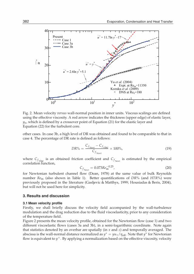
8 Heat Transfer
100 101 1020
10
20
30
40
u+ = y*
u+ = 2.6ln y*+5.1
u+ = 11.7ln y*–17
Yu et al. (2004) Expt. at Rem=11350Kozuka et al. (2009) DNS at Reτ=180
y*
u +
Present Case 1 Case 3a Case 3b
Fig. 2. Mean velocity versus wall-normal position in inner units. Viscous scalings are definedusing the effective viscosity. A red arrow indicates the thickness (upper edge) of elastic layer,ye, which is defined by a crossover point of Equation (21) for the elastic layer andEquation (22) for the turbulent core.
other cases. In case 3b, a high level of DR was obtained and found to be comparable to that incase 4. The percentage of DR rate is defined as follows:
DR% =Cf Newt
− Cf viscCf Newt
× 100%, (19)
where Cf visc is an obtained friction coefficient and Cf Newtis estimated by the empirical
correlation function,Cf Newt
= 0.073Re−0.25m , (20)
for Newtonian turbulent channel flow (Dean, 1978) at the same value of bulk Reynoldsnumber Rem (also shown in Table 1). Better quantifications of DR% (and HTR%) werepreviously proposed in the literature (Gasljevic & Matthys, 1999; Housiadas & Beris, 2004),but will not be used here for simplicity.
3. Results and discussion
3.1 Mean velocity profileFirstly, we shall briefly discuss the velocity field accompanied by the wall-turbulencemodulation and the drag reduction due to the fluid viscoelasticity, prior to any considerationof the temperature field.Figure 2 presents the mean velocity profile, obtained for the Newtonian flow (case 1) and twodifferent viscoelastic flows (cases 3a and 3b), in a semi-logarithmic coordinate. Note againthat statistics denoted by an overbar are spatially (in x and z) and temporally averaged. Theabscissa is the wall-normal distance normalized as y∗ = yuτ/ηeff. Note that y∗ for Newtonianflow is equivalent to y+. By applying a normalization based on the effective viscosity, velocity
382 Evaporation, Condensation and Heat Transfer
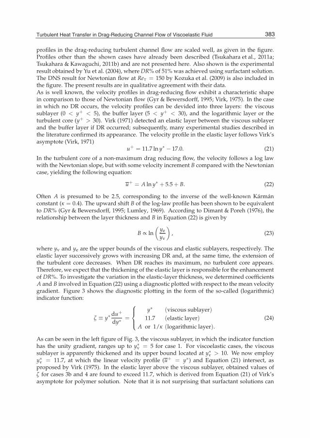
Turbulent Heat Transfer in Drag-ReducingChannel Flow of Viscoelastic Fluid 9
profiles in the drag-reducing turbulent channel flow are scaled well, as given in the figure.Profiles other than the shown cases have already been described (Tsukahara et al., 2011a;Tsukahara & Kawaguchi, 2011b) and are not presented here. Also shown is the experimentalresult obtained by Yu et al. (2004), where DR% of 51% was achieved using surfactant solution.The DNS result for Newtonian flow at Reτ = 150 by Kozuka et al. (2009) is also included inthe figure. The present results are in qualitative agreement with their data.As is well known, the velocity profiles in drag-reducing flow exhibit a characteristic shapein comparison to those of Newtonian flow (Gyr & Bewersdorff, 1995; Virk, 1975). In the casein which no DR occurs, the velocity profiles can be devided into three layers: the viscoussublayer (0 < y+ < 5), the buffer layer (5 < y+ < 30), and the logarithmic layer or theturbulent core (y+ > 30). Virk (1971) detected an elastic layer between the viscous sublayerand the buffer layer if DR occurred; subsequently, many experimental studies described inthe literature confirmed its appearance. The velocity profile in the elastic layer follows Virk’sasymptote (Virk, 1971)
u+ = 11.7 ln y∗ − 17.0. (21)
In the turbulent core of a non-maximum drag reducing flow, the velocity follows a log lawwith the Newtonian slope, but with some velocity increment B compared with the Newtoniancase, yielding the following equation:
u+ = A ln y∗ + 5.5 + B. (22)
Often A is presumed to be 2.5, corresponding to the inverse of the well-known Kármánconstant (κ = 0.4). The upward shift B of the log-law profile has been shown to be equivalentto DR% (Gyr & Bewersdorff, 1995; Lumley, 1969). According to Dimant & Poreh (1976), therelationship between the layer thickness and B in Equation (22) is given by
B ∝ ln(
ye
yv
), (23)
where yv and ye are the upper bounds of the viscous and elastic sublayers, respectively. Theelastic layer successively grows with increasing DR and, at the same time, the extension ofthe turbulent core decreases. When DR reaches its maximum, no turbulent core appears.Therefore, we expect that the thickening of the elastic layer is responsible for the enhancementof DR%. To investigate the variation in the elastic-layer thickness, we determined coefficientsA and B involved in Equation (22) using a diagnostic plotted with respect to the mean velocitygradient. Figure 3 shows the diagnostic plotting in the form of the so-called (logarithmic)indicator function:
ζ ≡ y∗ du+
dy∗ =
⎧⎪⎨⎪⎩
y∗ (viscous sublayer)11.7 (elastic layer)
A or 1/κ (logarithmic layer).(24)
As can be seen in the left figure of Fig. 3, the viscous sublayer, in which the indicator functionhas the unity gradient, ranges up to y∗v = 5 for case 1. For viscoelastic cases, the viscoussublayer is apparently thickened and its upper bound located at y∗v > 10. We now employy∗v = 11.7, at which the linear velocity profile (u+ = y∗) and Equation (21) intersect, asproposed by Virk (1975). In the elastic layer above the viscous sublayer, obtained values ofζ for cases 3b and 4 are found to exceed 11.7, which is derived from Equation (21) of Virk’sasymptote for polymer solution. Note that it is not surprising that surfactant solutions can
383Turbulent Heat Transfer in Drag-Reducing Channel Flow of Viscoelastic Fluid
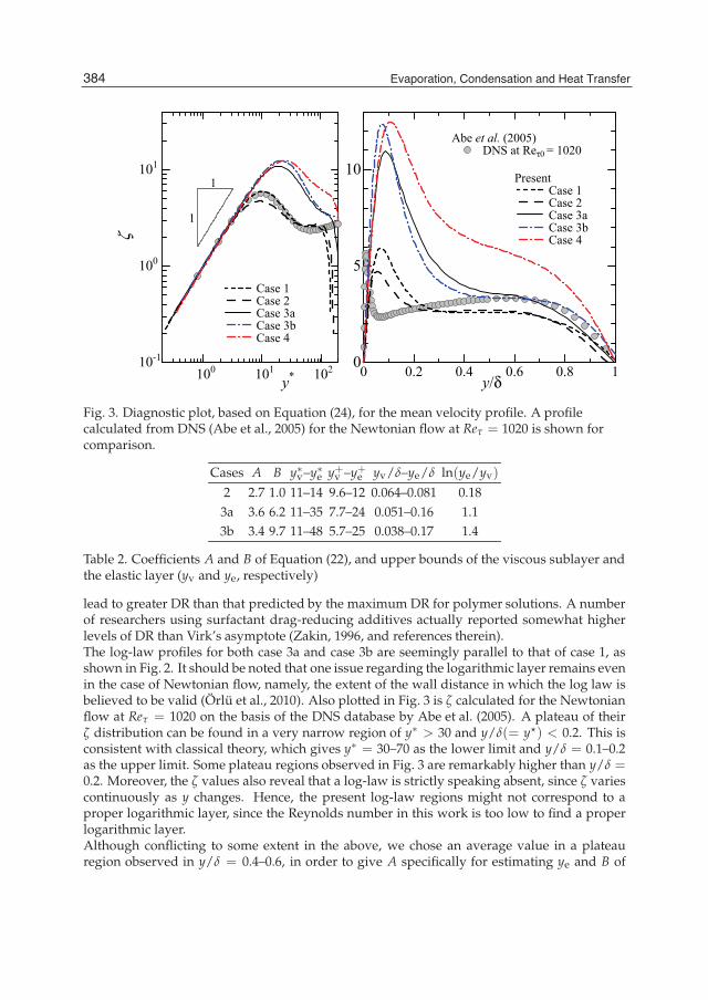
10 Heat Transfer
100 101 10210-1
100
101
Case 1 Case 2 Case 3a Case 3b Case 4
y*
ζ
1
1
0 0.2 0.4 0.6 0.8 10
5
10 Present Case 1 Case 2 Case 3a Case 3b Case 4
y/δ
Abe et al. (2005) DNS at Reτ0 = 1020
Fig. 3. Diagnostic plot, based on Equation (24), for the mean velocity profile. A profilecalculated from DNS (Abe et al., 2005) for the Newtonian flow at Reτ = 1020 is shown forcomparison.
Cases A B y∗v–y∗e y+v –y+e yv/δ–ye/δ ln(ye/yv)
2 2.7 1.0 11–14 9.6–12 0.064–0.081 0.183a 3.6 6.2 11–35 7.7–24 0.051–0.16 1.13b 3.4 9.7 11–48 5.7–25 0.038–0.17 1.4
Table 2. Coefficients A and B of Equation (22), and upper bounds of the viscous sublayer andthe elastic layer (yv and ye, respectively)
lead to greater DR than that predicted by the maximum DR for polymer solutions. A numberof researchers using surfactant drag-reducing additives actually reported somewhat higherlevels of DR than Virk’s asymptote (Zakin, 1996, and references therein).The log-law profiles for both case 3a and case 3b are seemingly parallel to that of case 1, asshown in Fig. 2. It should be noted that one issue regarding the logarithmic layer remains evenin the case of Newtonian flow, namely, the extent of the wall distance in which the log law isbelieved to be valid (Örlü et al., 2010). Also plotted in Fig. 3 is ζ calculated for the Newtonianflow at Reτ = 1020 on the basis of the DNS database by Abe et al. (2005). A plateau of theirζ distribution can be found in a very narrow region of y∗ > 30 and y/δ(= y�) < 0.2. This isconsistent with classical theory, which gives y∗ = 30–70 as the lower limit and y/δ = 0.1–0.2as the upper limit. Some plateau regions observed in Fig. 3 are remarkably higher than y/δ =0.2. Moreover, the ζ values also reveal that a log-law is strictly speaking absent, since ζ variescontinuously as y changes. Hence, the present log-law regions might not correspond to aproper logarithmic layer, since the Reynolds number in this work is too low to find a properlogarithmic layer.Although conflicting to some extent in the above, we chose an average value in a plateauregion observed in y/δ = 0.4–0.6, in order to give A specifically for estimating ye and B of
384 Evaporation, Condensation and Heat Transfer
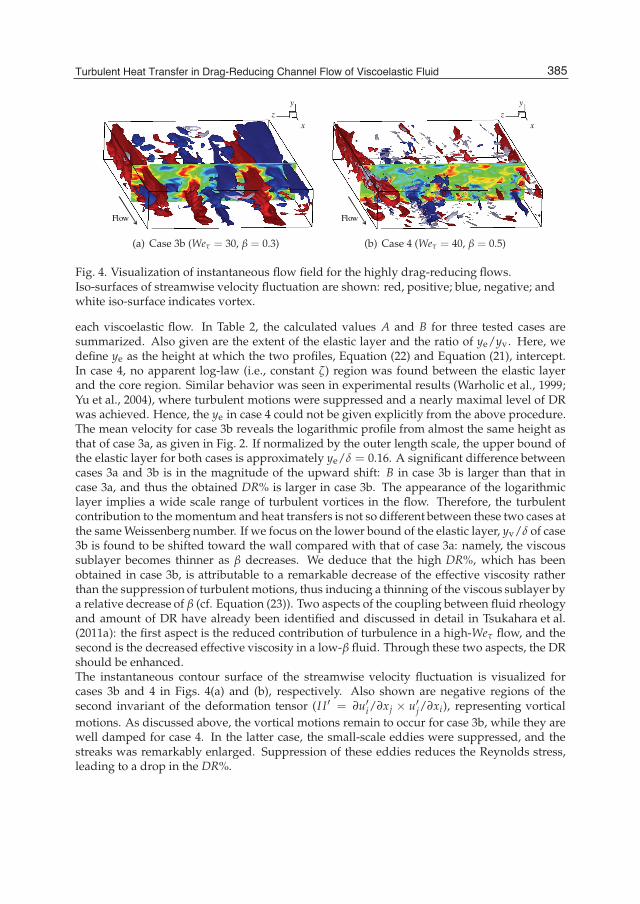
Turbulent Heat Transfer in Drag-ReducingChannel Flow of Viscoelastic Fluid 11
yz
x
Flow
(a) Case 3b (Weτ = 30, β = 0.3)
yz
x
Flow
(b) Case 4 (Weτ = 40, β = 0.5)
Fig. 4. Visualization of instantaneous flow field for the highly drag-reducing flows.Iso-surfaces of streamwise velocity fluctuation are shown: red, positive; blue, negative; andwhite iso-surface indicates vortex.
each viscoelastic flow. In Table 2, the calculated values A and B for three tested cases aresummarized. Also given are the extent of the elastic layer and the ratio of ye/yv. Here, wedefine ye as the height at which the two profiles, Equation (22) and Equation (21), intercept.In case 4, no apparent log-law (i.e., constant ζ) region was found between the elastic layerand the core region. Similar behavior was seen in experimental results (Warholic et al., 1999;Yu et al., 2004), where turbulent motions were suppressed and a nearly maximal level of DRwas achieved. Hence, the ye in case 4 could not be given explicitly from the above procedure.The mean velocity for case 3b reveals the logarithmic profile from almost the same height asthat of case 3a, as given in Fig. 2. If normalized by the outer length scale, the upper bound ofthe elastic layer for both cases is approximately ye/δ = 0.16. A significant difference betweencases 3a and 3b is in the magnitude of the upward shift: B in case 3b is larger than that incase 3a, and thus the obtained DR% is larger in case 3b. The appearance of the logarithmiclayer implies a wide scale range of turbulent vortices in the flow. Therefore, the turbulentcontribution to the momentum and heat transfers is not so different between these two cases atthe same Weissenberg number. If we focus on the lower bound of the elastic layer, yv/δ of case3b is found to be shifted toward the wall compared with that of case 3a: namely, the viscoussublayer becomes thinner as β decreases. We deduce that the high DR%, which has beenobtained in case 3b, is attributable to a remarkable decrease of the effective viscosity ratherthan the suppression of turbulent motions, thus inducing a thinning of the viscous sublayer bya relative decrease of β (cf. Equation (23)). Two aspects of the coupling between fluid rheologyand amount of DR have already been identified and discussed in detail in Tsukahara et al.(2011a): the first aspect is the reduced contribution of turbulence in a high-Weτ flow, and thesecond is the decreased effective viscosity in a low-β fluid. Through these two aspects, the DRshould be enhanced.The instantaneous contour surface of the streamwise velocity fluctuation is visualized forcases 3b and 4 in Figs. 4(a) and (b), respectively. Also shown are negative regions of thesecond invariant of the deformation tensor (I I ′ = ∂u′i/∂xj × u′j/∂xi), representing vorticalmotions. As discussed above, the vortical motions remain to occur for case 3b, while they arewell damped for case 4. In the latter case, the small-scale eddies were suppressed, and thestreaks was remarkably enlarged. Suppression of these eddies reduces the Reynolds stress,leading to a drop in the DR%.
385Turbulent Heat Transfer in Drag-Reducing Channel Flow of Viscoelastic Fluid
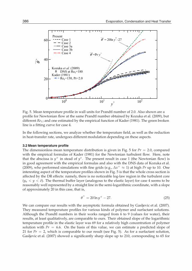
12 Heat Transfer
100 101 1020
20
40
60Present Case 1 Case 2 Case 3a Case 3b Case 4
Kozuka et al. (2009) DNS at Reτ=180Kader (1981) Reτ=150, Pr=2.0
y+
θ +
θ+=Pr·y+
θ+ = 20ln y*–27
Fig. 5. Mean temperature profile in wall units for Prandtl number of 2.0. Also shown are aprofile for Newtonian flow at the same Prandtl number obtained by Kozuka et al. (2009), butdifferent Reτ ; and one estimated by the empirical function of Kader (1981). The green brokenline is a fitting curve for case 4.
In the following sections, we analyze whether the temperature field, as well as the reductionin heat-transfer rate, undergoes different modulation depending on these aspects.
3.2 Mean temperature profileThe dimensionless mean temperature distribution is given in Fig. 5 for Pr = 2.0, comparedwith the empirical formulas of Kader (1981) for the Newtonian turbulent flow. Here, notethat the abscissa is y+ in stead of y∗. The present result in case 1 (the Newtonian flow) isin good agreement with the empirical formulas and also with the DNS data of Kozuka et al.(2009), who performed simulations with fine grids (e.g., Δx+ ≈ 1) at high Pr up to 10. Oneinteresting aspect of the temperature profiles shown in Fig. 5 is that the whole cross section isaffected by the DR effects: namely, there is no noticeable log-law region in the turbulent core(ye < y < δ). The thermal buffer layer (analogous to the elastic layer) for case 4 seems to bereasonably well represented by a straight line in the semi-logarithmic coordinate, with a slopeof approximately 20 in this case, that is,
θ+= 20 ln y+ − 27. (25)
We can compare our results with the asymptotic formula obtained by Gasljevic et al. (2007).They measured temperature profiles for various kinds of polymer and surfactant solutions.Although the Prandtl numbers in their works ranged from 6 to 9 (values for water), theirresults, at least qualitatively, are comparable to ours. Their obtained slope of the logarithmictemperature profile in the elastic layer was 69 for a relatively high concentration of polymersolution with Pr = 6.6. On the basis of this value, we can estimate a predicted slope of21 for Pr = 2, which is comparable to our result (see Fig. 5). As for a surfactant solution,Gasljevic et al. (2007) showed a significantly sharp slope up to 210, corresponding to 65 for
386 Evaporation, Condensation and Heat Transfer
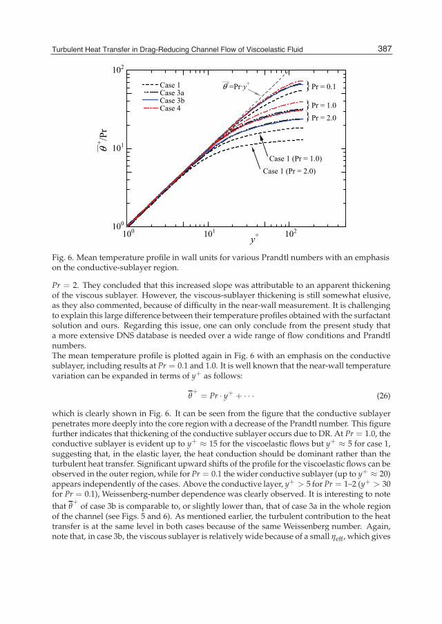
Turbulent Heat Transfer in Drag-ReducingChannel Flow of Viscoelastic Fluid 13
100 101 102100
101
102
Case 1 Case 3a Case 3b Case 4
y+
θ + /P
r
θ+=Pr·y+ Pr = 0.1}Pr = 1.0Pr = 2.0
}}
Case 1 (Pr = 2.0)Case 1 (Pr = 1.0)
Fig. 6. Mean temperature profile in wall units for various Prandtl numbers with an emphasison the conductive-sublayer region.
Pr = 2. They concluded that this increased slope was attributable to an apparent thickeningof the viscous sublayer. However, the viscous-sublayer thickening is still somewhat elusive,as they also commented, because of difficulty in the near-wall measurement. It is challengingto explain this large difference between their temperature profiles obtained with the surfactantsolution and ours. Regarding this issue, one can only conclude from the present study thata more extensive DNS database is needed over a wide range of flow conditions and Prandtlnumbers.The mean temperature profile is plotted again in Fig. 6 with an emphasis on the conductivesublayer, including results at Pr = 0.1 and 1.0. It is well known that the near-wall temperaturevariation can be expanded in terms of y+ as follows:
θ+= Pr · y+ + · · · (26)
which is clearly shown in Fig. 6. It can be seen from the figure that the conductive sublayerpenetrates more deeply into the core region with a decrease of the Prandtl number. This figurefurther indicates that thickening of the conductive sublayer occurs due to DR. At Pr = 1.0, theconductive sublayer is evident up to y+ ≈ 15 for the viscoelastic flows but y+ ≈ 5 for case 1,suggesting that, in the elastic layer, the heat conduction should be dominant rather than theturbulent heat transfer. Significant upward shifts of the profile for the viscoelastic flows can beobserved in the outer region, while for Pr = 0.1 the wider conductive sublayer (up to y+ ≈ 20)appears independently of the cases. Above the conductive layer, y+ > 5 for Pr = 1–2 (y+ > 30for Pr = 0.1), Weissenberg-number dependence was clearly observed. It is interesting to notethat θ
+ of case 3b is comparable to, or slightly lower than, that of case 3a in the whole regionof the channel (see Figs. 5 and 6). As mentioned earlier, the turbulent contribution to the heattransfer is at the same level in both cases because of the same Weissenberg number. Again,note that, in case 3b, the viscous sublayer is relatively wide because of a small ηeff, which gives
387Turbulent Heat Transfer in Drag-Reducing Channel Flow of Viscoelastic Fluid
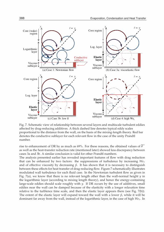
14 Heat Transfer
Viscous sublayer
Logarithmic layer
Core (wake) region
Viscous sublayer
Log. layer
Core region
Elasticlayer
(a) Case 1: Newtonian flow (b) Case 3a: viscoelastic flow
Viscous sublayer
Core region
Elasticlayer
Viscous sublayer
Log. layer
Core region
Elasticlayer
Conductive sublayer
yy∝l y y∝l
y y∝l
(d) Case 4: high Wet
y∝l
(c) Case 3b: low ß
y
Fig. 7. Schematic view of relationship between several layers and multiscale turbulent eddiesaffected by drag-reducing additives. A thick dashed line denotes typical eddy scalesproportional to the distance from the wall, on the basis of the mixing-length theory. Red bardenotes the conductive sublayer for each relevant flow in the case of the unity Prandtlnumber.
rise to enhancement of DR by as much as 69%. For these reasons, the obtained values of θ+
as well as the heat-transfer reduction rate (mentioned later) showed less discrepancy betweencases 3a and 3b. A similar conclusion is valid for other Prandtl numbers.The analysis presented earlier has revealed important features of flow with drag reductionthat can be enhanced by two factors: the suppressions of turbulence by increasing Weτ
and of effective viscosity by decreasing β. It has shown that it is necessary to distinguishbetween these effects for heat transfer of drag-reducing flow. Figure 7 schematically illustratesmodulated wall turbulence for each fluid case. In the Newtonian turbulent flow as given inFig. 7(a), we know that there is no relevant length other than the wall-normal height y inthe logarithmic layer (according to mixing length theory), and hence the energy-containinglarge-scale eddies should scale roughly with y. If DR occurs by the use of additives, smalleddies near the wall can be damped because of the elasticity with a longer relaxation timerelative to the turblence time scale, and then the elastic layer appears there (see Fig. 7(b)).The extent of the elastic layer will expand toward the wall with a lower β, while it will bedominant far away from the wall, instead of the logarithmic layer, in the case of high Weτ . In
388 Evaporation, Condensation and Heat Transfer
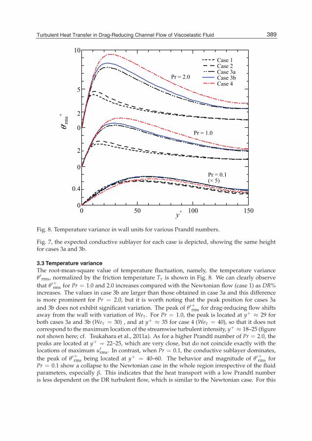
Turbulent Heat Transfer in Drag-ReducingChannel Flow of Viscoelastic Fluid 15
0 50 100 150
0
Case 1 Case 2 Case 3a Case 3b Case 4
y+
θ'rm
s+
Pr = 1.0
Pr = 0.1(× 5)
0
0
5
10
2
0.4
2
Pr = 2.0
Fig. 8. Temperature variance in wall units for various Prandtl numbers.
Fig. 7, the expected conductive sublayer for each case is depicted, showing the same heightfor cases 3a and 3b.
3.3 Temperature varianceThe root-mean-square value of temperature fluctuation, namely, the temperature varianceθ′rms, normalized by the friction temperature Tτ is shown in Fig. 8. We can clearly observethat θ′+rms for Pr = 1.0 and 2.0 increases compared with the Newtonian flow (case 1) as DR%increases. The values in case 3b are larger than those obtained in case 3a and this differenceis more prominent for Pr = 2.0, but it is worth noting that the peak position for cases 3aand 3b does not exhibit significant variation. The peak of θ′+rms for drag-reducing flow shiftsaway from the wall with variation of Weτ . For Pr = 1.0, the peak is located at y+ ≈ 29 forboth cases 3a and 3b (Weτ = 30) , and at y+ ≈ 35 for case 4 (Weτ = 40), so that it does notcorrespond to the maximum location of the streamwise turbulent intensity, y+ ≈ 18–25 (figurenot shown here; cf. Tsukahara et al., 2011a). As for a higher Prandtl number of Pr = 2.0, thepeaks are located at y+ = 22–25, which are very close, but do not coincide exactly with thelocations of maximum u′rms. In contrast, when Pr = 0.1, the conductive sublayer dominates,the peak of θ′+rms being located at y+ = 40–60. The behavior and magnitude of θ′+rms forPr = 0.1 show a collapse to the Newtonian case in the whole region irrespective of the fluidparameters, especially β. This indicates that the heat transport with a low Prandtl numberis less dependent on the DR turbulent flow, which is similar to the Newtonian case. For this
389Turbulent Heat Transfer in Drag-Reducing Channel Flow of Viscoelastic Fluid
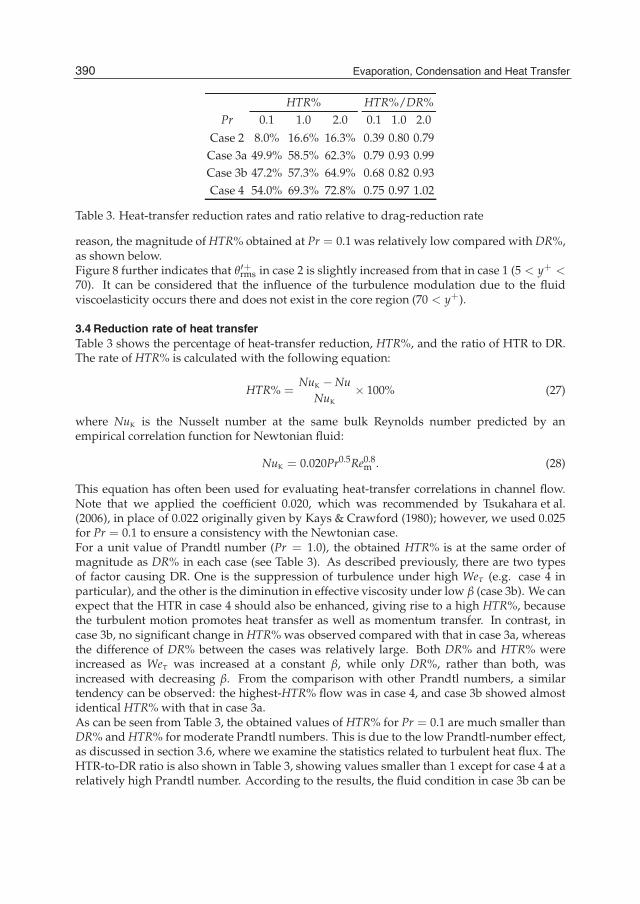
16 Heat Transfer
HTR% HTR%/DR%Pr 0.1 1.0 2.0 0.1 1.0 2.0
Case 2 8.0% 16.6% 16.3% 0.39 0.80 0.79Case 3a 49.9% 58.5% 62.3% 0.79 0.93 0.99Case 3b 47.2% 57.3% 64.9% 0.68 0.82 0.93Case 4 54.0% 69.3% 72.8% 0.75 0.97 1.02
Table 3. Heat-transfer reduction rates and ratio relative to drag-reduction rate
reason, the magnitude of HTR% obtained at Pr = 0.1 was relatively low compared with DR%,as shown below.Figure 8 further indicates that θ′+rms in case 2 is slightly increased from that in case 1 (5 < y+ <70). It can be considered that the influence of the turbulence modulation due to the fluidviscoelasticity occurs there and does not exist in the core region (70 < y+).
3.4 Reduction rate of heat transferTable 3 shows the percentage of heat-transfer reduction, HTR%, and the ratio of HTR to DR.The rate of HTR% is calculated with the following equation:
HTR% =NuK −Nu
NuK× 100% (27)
where NuK is the Nusselt number at the same bulk Reynolds number predicted by anempirical correlation function for Newtonian fluid:
NuK = 0.020Pr0.5Re0.8m . (28)
This equation has often been used for evaluating heat-transfer correlations in channel flow.Note that we applied the coefficient 0.020, which was recommended by Tsukahara et al.(2006), in place of 0.022 originally given by Kays & Crawford (1980); however, we used 0.025for Pr = 0.1 to ensure a consistency with the Newtonian case.For a unit value of Prandtl number (Pr = 1.0), the obtained HTR% is at the same order ofmagnitude as DR% in each case (see Table 3). As described previously, there are two typesof factor causing DR. One is the suppression of turbulence under high Weτ (e.g. case 4 inparticular), and the other is the diminution in effective viscosity under low β (case 3b). We canexpect that the HTR in case 4 should also be enhanced, giving rise to a high HTR%, becausethe turbulent motion promotes heat transfer as well as momentum transfer. In contrast, incase 3b, no significant change in HTR% was observed compared with that in case 3a, whereasthe difference of DR% between the cases was relatively large. Both DR% and HTR% wereincreased as Weτ was increased at a constant β, while only DR%, rather than both, wasincreased with decreasing β. From the comparison with other Prandtl numbers, a similartendency can be observed: the highest-HTR% flow was in case 4, and case 3b showed almostidentical HTR% with that in case 3a.As can be seen from Table 3, the obtained values of HTR% for Pr = 0.1 are much smaller thanDR% and HTR% for moderate Prandtl numbers. This is due to the low Prandtl-number effect,as discussed in section 3.6, where we examine the statistics related to turbulent heat flux. TheHTR-to-DR ratio is also shown in Table 3, showing values smaller than 1 except for case 4 at arelatively high Prandtl number. According to the results, the fluid condition in case 3b can be
390 Evaporation, Condensation and Heat Transfer
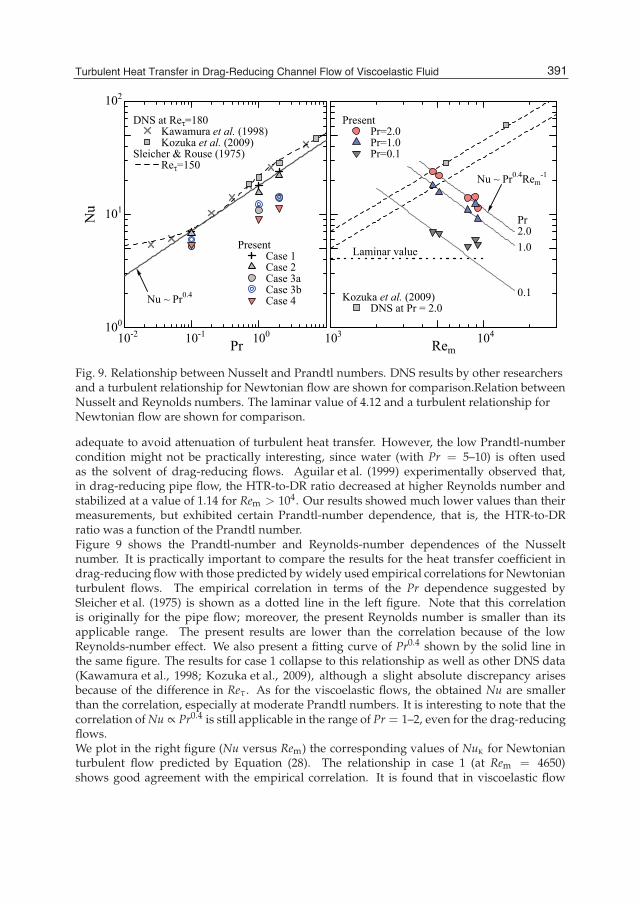
Turbulent Heat Transfer in Drag-ReducingChannel Flow of Viscoelastic Fluid 17
10-2 10-1 100100
101
102
Pr
Nu
Present Case 1 Case 2 Case 3a Case 3b Case 4Nu ~ Pr0.4
DNS at Reτ=180 Kawamura et al. (1998) Kozuka et al. (2009)Sleicher & Rouse (1975) Reτ=150
103 104Rem
Laminar value
Kozuka et al. (2009) DNS at Pr = 2.0
Present Pr=2.0 Pr=1.0 Pr=0.1
Pr2.01.0
0.1
Nu ~ Pr0.4Rem-1
Fig. 9. Relationship between Nusselt and Prandtl numbers. DNS results by other researchersand a turbulent relationship for Newtonian flow are shown for comparison.Relation betweenNusselt and Reynolds numbers. The laminar value of 4.12 and a turbulent relationship forNewtonian flow are shown for comparison.
adequate to avoid attenuation of turbulent heat transfer. However, the low Prandtl-numbercondition might not be practically interesting, since water (with Pr = 5–10) is often usedas the solvent of drag-reducing flows. Aguilar et al. (1999) experimentally observed that,in drag-reducing pipe flow, the HTR-to-DR ratio decreased at higher Reynolds number andstabilized at a value of 1.14 for Rem > 104. Our results showed much lower values than theirmeasurements, but exhibited certain Prandtl-number dependence, that is, the HTR-to-DRratio was a function of the Prandtl number.Figure 9 shows the Prandtl-number and Reynolds-number dependences of the Nusseltnumber. It is practically important to compare the results for the heat transfer coefficient indrag-reducing flow with those predicted by widely used empirical correlations for Newtonianturbulent flows. The empirical correlation in terms of the Pr dependence suggested bySleicher et al. (1975) is shown as a dotted line in the left figure. Note that this correlationis originally for the pipe flow; moreover, the present Reynolds number is smaller than itsapplicable range. The present results are lower than the correlation because of the lowReynolds-number effect. We also present a fitting curve of Pr0.4 shown by the solid line inthe same figure. The results for case 1 collapse to this relationship as well as other DNS data(Kawamura et al., 1998; Kozuka et al., 2009), although a slight absolute discrepancy arisesbecause of the difference in Reτ . As for the viscoelastic flows, the obtained Nu are smallerthan the correlation, especially at moderate Prandtl numbers. It is interesting to note that thecorrelation of Nu ∝ Pr0.4 is still applicable in the range of Pr = 1–2, even for the drag-reducingflows.We plot in the right figure (Nu versus Rem) the corresponding values of NuK for Newtonianturbulent flow predicted by Equation (28). The relationship in case 1 (at Rem = 4650)shows good agreement with the empirical correlation. It is found that in viscoelastic flow
391Turbulent Heat Transfer in Drag-Reducing Channel Flow of Viscoelastic Fluid
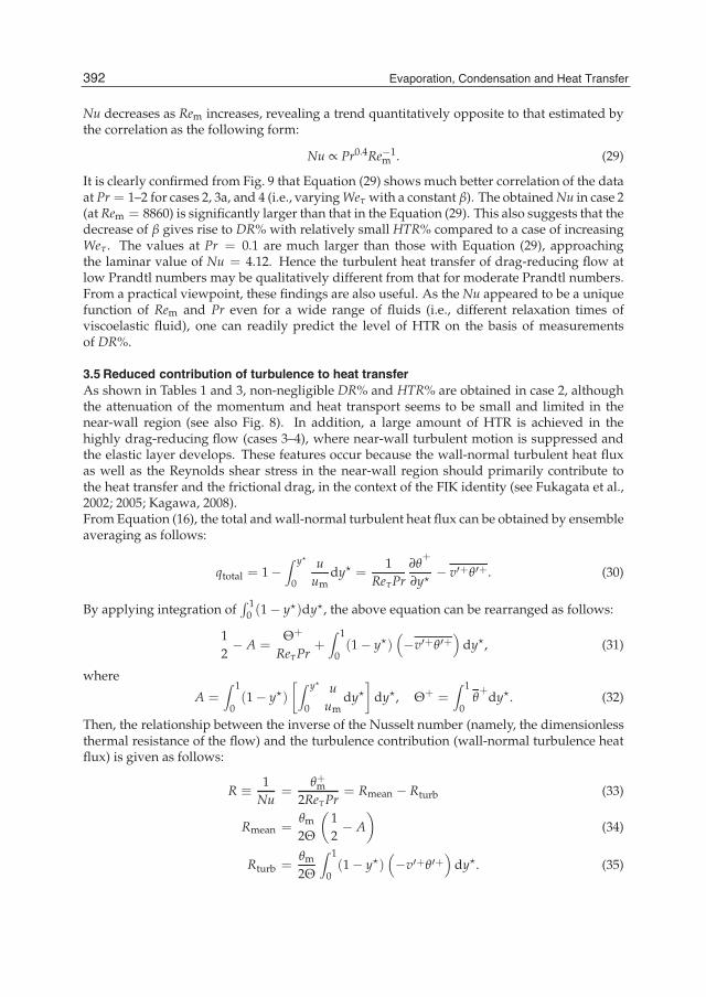
18 Heat Transfer
Nu decreases as Rem increases, revealing a trend quantitatively opposite to that estimated bythe correlation as the following form:
Nu ∝ Pr0.4Re−1m . (29)
It is clearly confirmed from Fig. 9 that Equation (29) shows much better correlation of the dataat Pr = 1–2 for cases 2, 3a, and 4 (i.e., varying Weτ with a constant β). The obtained Nu in case 2(at Rem = 8860) is significantly larger than that in the Equation (29). This also suggests that thedecrease of β gives rise to DR% with relatively small HTR% compared to a case of increasingWeτ. The values at Pr = 0.1 are much larger than those with Equation (29), approachingthe laminar value of Nu = 4.12. Hence the turbulent heat transfer of drag-reducing flow atlow Prandtl numbers may be qualitatively different from that for moderate Prandtl numbers.From a practical viewpoint, these findings are also useful. As the Nu appeared to be a uniquefunction of Rem and Pr even for a wide range of fluids (i.e., different relaxation times ofviscoelastic fluid), one can readily predict the level of HTR on the basis of measurementsof DR%.
3.5 Reduced contribution of turbulence to heat transferAs shown in Tables 1 and 3, non-negligible DR% and HTR% are obtained in case 2, althoughthe attenuation of the momentum and heat transport seems to be small and limited in thenear-wall region (see also Fig. 8). In addition, a large amount of HTR is achieved in thehighly drag-reducing flow (cases 3–4), where near-wall turbulent motion is suppressed andthe elastic layer develops. These features occur because the wall-normal turbulent heat fluxas well as the Reynolds shear stress in the near-wall region should primarily contribute tothe heat transfer and the frictional drag, in the context of the FIK identity (see Fukagata et al.,2002; 2005; Kagawa, 2008).From Equation (16), the total and wall-normal turbulent heat flux can be obtained by ensembleaveraging as follows:
qtotal = 1−∫ y�
0
uum
dy� =1
ReτPr∂θ
+
∂y�− v′+θ′+. (30)
By applying integration of∫ 1
0 (1− y�)dy�, the above equation can be rearranged as follows:
12− A =
Θ+
ReτPr+
∫ 1
0(1− y�)
(−v′+θ′+
)dy�, (31)
where
A =∫ 1
0(1− y�)
[∫ y�
0
uum
dy�]
dy�, Θ+ =∫ 1
0θ+
dy�. (32)
Then, the relationship between the inverse of the Nusselt number (namely, the dimensionlessthermal resistance of the flow) and the turbulence contribution (wall-normal turbulence heatflux) is given as follows:
R ≡ 1Nu
=θ+m
2ReτPr= Rmean − Rturb (33)
Rmean =θm
2Θ
(12− A
)(34)
Rturb =θm
2Θ
∫ 1
0(1− y�)
(−v′+θ′+
)dy�. (35)
392 Evaporation, Condensation and Heat Transfer
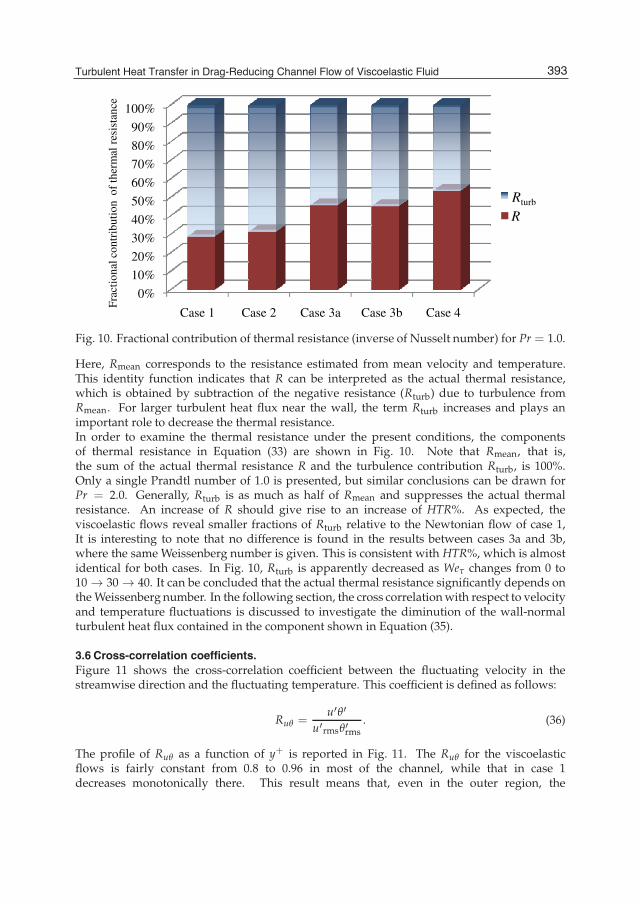
Turbulent Heat Transfer in Drag-ReducingChannel Flow of Viscoelastic Fluid 19
40%
50%
60%
70%
80%
90%
100%
RRturb
buti
on o
f th
erm
alre
sist
ance
0%
10%
20%
30%
40%
50%
60%
70%
80%
90%
100%
Case 1 Case 2 Case 3a Case 3b Case 4
RRturb
Frac
tion
al c
ontr
ibut
ion
of
ther
mal
resi
stan
ce
Fig. 10. Fractional contribution of thermal resistance (inverse of Nusselt number) for Pr = 1.0.
Here, Rmean corresponds to the resistance estimated from mean velocity and temperature.This identity function indicates that R can be interpreted as the actual thermal resistance,which is obtained by subtraction of the negative resistance (Rturb) due to turbulence fromRmean. For larger turbulent heat flux near the wall, the term Rturb increases and plays animportant role to decrease the thermal resistance.In order to examine the thermal resistance under the present conditions, the componentsof thermal resistance in Equation (33) are shown in Fig. 10. Note that Rmean, that is,the sum of the actual thermal resistance R and the turbulence contribution Rturb, is 100%.Only a single Prandtl number of 1.0 is presented, but similar conclusions can be drawn forPr = 2.0. Generally, Rturb is as much as half of Rmean and suppresses the actual thermalresistance. An increase of R should give rise to an increase of HTR%. As expected, theviscoelastic flows reveal smaller fractions of Rturb relative to the Newtonian flow of case 1,It is interesting to note that no difference is found in the results between cases 3a and 3b,where the same Weissenberg number is given. This is consistent with HTR%, which is almostidentical for both cases. In Fig. 10, Rturb is apparently decreased as Weτ changes from 0 to10 → 30 → 40. It can be concluded that the actual thermal resistance significantly depends onthe Weissenberg number. In the following section, the cross correlation with respect to velocityand temperature fluctuations is discussed to investigate the diminution of the wall-normalturbulent heat flux contained in the component shown in Equation (35).
3.6 Cross-correlation coefficients.Figure 11 shows the cross-correlation coefficient between the fluctuating velocity in thestreamwise direction and the fluctuating temperature. This coefficient is defined as follows:
Ruθ =u′θ′
u′rmsθ′rms. (36)
The profile of Ruθ as a function of y+ is reported in Fig. 11. The Ruθ for the viscoelasticflows is fairly constant from 0.8 to 0.96 in most of the channel, while that in case 1decreases monotonically there. This result means that, even in the outer region, the
393Turbulent Heat Transfer in Drag-Reducing Channel Flow of Viscoelastic Fluid
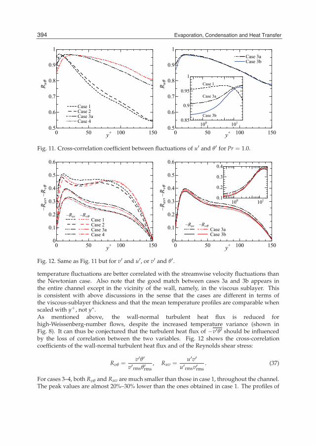
20 Heat Transfer
0 50 100 1500.5
0.6
0.7
0.8
0.9
1
Case 1 Case 2 Case 3a Case 4
y+
R uθ
100 1010.85
0.9
0.95
1Case 1
Case 3a
Case 3b
0 50 100 1500.5
0.6
0.7
0.8
0.9
1 Case 3a Case 3b
y+
R uθ
Fig. 11. Cross-correlation coefficient between fluctuations of u′ and θ′ for Pr = 1.0.
0 50 100 1500
0.1
0.2
0.3
0.4
0.5
0.6
–Ruv –Rvθ Case 1 Case 2 Case 3a Case 4
y+
–Ruv
, –R v
θ
0 50 100 1500
0.1
0.2
0.3
0.4
0.5
0.6
–Ruv –Rvθ Case 3a Case 3b
y+
–Ruv
, –R v
θ
100 1010.1
0.2
0.3
0.4
Fig. 12. Same as Fig. 11 but for v′ and u′, or v′ and θ′.
temperature fluctuations are better correlated with the streamwise velocity fluctuations thanthe Newtonian case. Also note that the good match between cases 3a and 3b appears inthe entire channel except in the vicinity of the wall, namely, in the viscous sublayer. Thisis consistent with above discussions in the sense that the cases are different in terms ofthe viscous-sublayer thickness and that the mean temperature profiles are comparable whenscaled with y+, not y∗.As mentioned above, the wall-normal turbulent heat flux is reduced forhigh-Weissenberg-number flows, despite the increased temperature variance (shown inFig. 8). It can thus be conjectured that the turbulent heat flux of −v′θ′ should be influencedby the loss of correlation between the two variables. Fig. 12 shows the cross-correlationcoefficients of the wall-normal turbulent heat flux and of the Reynolds shear stress:
Rvθ =v′θ′
v′rmsθ′rms, Ruv =
u′v′u′rmsv′rms
. (37)
For cases 3–4, both Rvθ and Ruv are much smaller than those in case 1, throughout the channel.The peak values are almost 20%–30% lower than the ones obtained in case 1. The profiles of
394 Evaporation, Condensation and Heat Transfer
Turbulent Heat Transfer in Drag-ReducingChannel Flow of Viscoelastic Fluid 21
Rvθ and Ruv for each case exhibit similar shapes throughout the channel, which also impliessimilarity between the variations of−v′θ′ and−u′v′ affected by DR. These features at Pr = 1.0can be seen also at the other Prandtl numbers (figure not shown) and also agree well withthose of experimental results and DNS for water (Gupta et al., 2005; Li et al., 2004a). This lesscorrelation between θ′ and v′ is responsible for the decrease of the wall-normal turbulent heatflux and the increase of HTR%, in the same way that the decrease of the Reynolds shear stressdue to the lower correlation between u′ and v′ should be responsible for DR%.
4. Conclusion
A series of direct numerical simulations (DNSs) of turbulent heat transfer in a channel flowunder the uniform heat-flux condition have been performed at low friction Reynolds number(Reτ = 150) and various Prandtl numbers in the range of Pr = 0.1 to 2.0. In order tosimulate viscoelastic fluids exhibiting drag reduction, the Giesekus constitutive equationwas employed, and we considered two rheological parameters of the Weissenberg number(Weτ), which characterizes the relaxation time of the fluid, and the viscosity ratio (β) of thesolvent viscosity to the total zero-shear rate solution viscosity. Several statistical turbulencequantities including the mean and fluctuating temperatures, the Nusselt number (Nu), andthe cross-correlation coefficients were obtained and analyzed with respect to their dependenceon the parameters as well as the obtained drag-reduction rate (DR%) and heat-transferreduction rate (HTR%).The following conclusion was drawn in this study. High DR% was achieved by two factors:(i) the suppressed contribution of turbulence due to high Weτ and (ii) the decrease of theeffective viscosity due to low β. A difference in the rate of increase of HTR% between thesefactors was found. This is attributed to the different dependencies of the elastic layer on βand Weτ . A case with low β gives rise to high DR% with low HTR% compared with thoseobtained with high Weτ. Differences were also found in various statistical data such as themean-temperature and the temperature-variance profiles. Moreover, it was found that in thedrag-reducing flow Nu should decrease as Rem increases, revealing the form of Equation (29)when Weτ was varied with a fixed β (=0.5). For a Prandtl number as low as 0.1, the obtainedHTR% was significantly small compared with the magnitude of DR% irrespective of differencein the rheological parameters.Although the present Reynolds and Prandtl numbers were considerably lower than thosecorresponding to conditions under which DR in practical flow systems is observed withdilute additive solutions, we have elucidated the dependencies of DR and HTR on rheologicalparameters through parametric DNS study. More extended DNS studies for higher Reynoldsand Prandtl numbers with a wide range of Weissenberg numbers might be necessary.The above conclusions have been drawn for very limited geometries such as straightduct and pipe. In terms of industrial applications, viscoelastic flows through complicatedgeometries should be investigated with detailed simulations. Moreover, modeling approachesfor viscoelastic turbulent flows have to be developed and these are essentially of RANS(Reynolds-averaged Navier-Stokes) techniques and of LES (large-eddy simulation). DNSstudies on these issues are ongoing (Kawamoto et al., 2010; Pinho et al., 2008; Tsukahara et al.,2011c) and the observations in these works will be valuable for those studying suchcomplicated flows using RANS and LES.
395Turbulent Heat Transfer in Drag-Reducing Channel Flow of Viscoelastic Fluid
22 Heat Transfer
5. Acknowledgments
The present computations were performed with the use of supercomputing resources atCyberscience Center of Tohoku University and Earth Simulator (ES2) at the Japan Agencyfor Marine-Earth Science and Technology. We also gratefully acknowledge the assistance ofMr. Takahiro Ishigami, who was a Master’s course student at Tokyo University of Science.This paper is a revised and expanded version of a paper entitled “Influence of rheologicalparameters on turbulent heat transfer in drag-reducing viscoelastic channel flow,” presentedat the Fourteenth International Heat Transfer Conference (Tsukahara et al., 2010).
6. References
Abe, H., Kawamura, H., & Matsuo, Y. (1998). Surface heat-flux fluctuations in a turbulentchannel flow up to Reτ = 1020 with Pr = 0.025 and 0.71, International Journal of Heatand Fluid Flow, Vol. 25, 404–419.
Aguilar, G., Gasljevic, K., & Matthys, E.F. (1999). Coupling between heat andmomentum transfer mechanisms for drag-reducing polymer and surfactantsolutions, Transactions of ASME C: Journal of Heat Transfer, Vol. 121, 796–802.
Aguilar, G., Gasljevic, K., & Matthys, E.F. (2001). Asymptotes of maximum friction and heattransfer reductions for drag-reducing surfactant solutions, International Journal of Heatand Mass Transfer, Vol. 44, 2835–2843.
Aly, W.I, Inaba, H., Haruki, N., & Horibe, A. (1999). Drag and heat transfer reductionphenomena of drag-reducing surfactant solutions in straight and helical pipes,Transactions of ASME C: Journal of Heat Transfer, Vol. 128, 800–810.
Basombrío, F.G., Buscaglia, G.C., & Dari, E.A. (1991). A new approach for the FEM simulationof viscoelastic flows, Journal of Non-Newtonian Fluid Mechanics, Vol. 39, 189–206.
Bird, R.B. (1995). Constitutive equations for polymeric liquids, Annual Review of FluidMechanics, Vol. 27, 169–193.
Cho, Y.I. & Hartnett, J.P. (1982). Non-Newtonian fluids in circular pipe flow. Advances in HeatTransfer, Vol. 15, 59–141.
Dean, R.D. (1978). Reynolds number dependence of skin friction and other bulk flow variablesin two-dimensional rectangular duct flow, Transactions of ASME I: Journal of FluidsEngineering, Vol. 100, 215–223..
Den Toonder, J.M.J., Hulsen, M.A., Kuiken, G.D.C., & Nieuwstadt, F.T.M. (1997). Dragreduction by polymer additives in a turbulent pipe flow: numerical and laboratoryexperiments, Journal of Fluid Mechanics, Vol. 337, 193–231 .
Dimant, Y. & Poreh, M. (1976). Heat transfer in flows with drag reduction. In: Advances in HeatTransfer, Vol. 12, Irvine, T.F. & Hartnett, J.P., (Ed.), pp. 77–113, Academic Press, Inc.,ISBN 0-12-020012-0, New York.
Dimitropoulos, C.D., Sureshkumar, R., Beris, A.N., & Handler, R.A. (2001). Budgets ofReynolds stress, kinetic energy and streamwise enstrophy in viscoelastic turbulentchannel flow, Physics of Fluids, Vol. 13, 1016–1027.
Dimitropoulos, C.D., Dubief, Y., Shaqfeh, E.S.G., Moin, P., & Lele, S.K. (2005). Direct numericalsimulation of polymer-induced drag reduction in turbulent boundary layer flow,Physics of Fluids, Vol. 17, 011705, 4 pp.
Fukagata, K., Iwamoto, K., & Kasagi, N. (2002). Contribution of Reynolds stress distributionto the skin friction in wall-bounded flows, Physics of Fluids, Vol. 14, L73–L76.
396 Evaporation, Condensation and Heat Transfer
Turbulent Heat Transfer in Drag-ReducingChannel Flow of Viscoelastic Fluid 23
Fukagata, K., Iwamoto, K., & Kasagi, N. (2005). Novel turbulence control strategy forsimultaneously achieving friction drag reduction and heat transfer augmentation, In:Proceedings of Fourth International Symposium on Turbulence and Shear Flow Phenomena,Humphrey, J.A.C. et al. (Ed.), pp. 307–312, Williamsburg, USA, 27–29 June 2005.
Fortin, M. & Fortin, M. (1989). A new approach for the FEM simulation of viscoelastic flows ,Journal of Non-Newtonian Fluid Mechanics, Vol. 32, 295–310.
Gasljevic, K. & Matthys, E.F. (1999). Improved quantification of the drag reductionphenomenon through turbulence reduction parameters, Journal of Non-NewtonianFluid Mechanics, Vol. 84, 123–130.
Gasljevic, K., Aguilar, G., & Matthys, E.F. (2007). Measurement of temperature profiles inturbulent pipe flow of polymer and surfactant drag-reducing solutions, Physics ofFluids, Vol. 19, 083105, 18 pp.
Giesekus, H. (1982). A simple constitutive equation for polymer fluids based on the concept ofdeformation-dependent tensorial mobility, Journal of Non-Newtonian Fluid Mechanics,Vol. 11, 69–109.
Gyr, A. & Bewersdorff, H.-W. (1995). Drag reduction of turbulent flows by additives, KluwerAcademic Publisher, ISBN 978-90-481-4555-3, Dordrecht.
Gupta, V.K., Sureshkumar, R., & Khomami, B. (2005). Passive scalar transport in polymerdrag-reduced turbulent channel flow, AIChE Journal, Vol. 51, 1938–1950.
Housiadas, K.D. & Beris, A.N. (2007). Characteristic scales and drag reduction evaluation inturbulent channel flow of nonconstant viscosity viscoelastic fluids, Physics of Fluids,Vol. 16, 1581–1586.
Hoyt, J.W. (1990). Drag reduction by polymers and surfactants, In: Viscous drag reduction inboundary layers, Bushnell, D.M. & Hefner, J.M., (Ed.), pp. 413–432, American Instituteof Aeronautics and Astronautics, Inc., ISBN 978-0-930403-66-5, Washington D.C.
Joseph, D.D. (1990). Fluid dynamics of viscoelastic liquids, Springer-Verlag, ISBN 978-0387971551,New York.
Jovanovic, J., Pashtrapanska, M., Frohnapfel, B., Durst, F., Koskinen, J., & Koskinen, K. (2006).On the mechanism responsible for turbulent drag reduction by dilute addition ofhigh polymers: theory, experiments, simulations, and predictions, Transactions ofASME I: Journal of Fluids Engineering, Vol. 128, 118–130.
Kader, B.A. (1981). Temperature and concentration profiles in fully turbulent boundary layers,International Journal of Heat and Mass Transfer, Vol. 24, 1541–1544.
Kagawa, Y., Yu, B., Kawaguchi, Y., Kawamura, H., & Shiraishi, Y. (2008). Turbulent heattransfer of viscoelastic fluid flow accompanied by drag reduction with DNS analysis,Progress in Computational Fluid Dynamics, Vol. 8, 477–485.
Kawaguchi, Y., Wei, J.J., Yu, B., & Feng, Z.P. (2003). Rheological characterization ofdrag-reducing cationic surfactant solution: shear and elongational viscosities ofdilute solutions, Proceedings of ASME/JSME 2003 4th Joint Fluids Summer EngineeringConference , pp. 721–728, Honolulu, Hawaii, USA, July 6–10, 2003.
Kawamoto, H., Tsukahara, T., Kawamura, H., & Kawaguchi, Y. (2010). Proposal of k-εmodel for visco-elastic fluid flow: toward prediction of drag-reducing turbulence,Proceedings of Eighth International ERCOFTAC Symposium on Engineering TurbulenceModelling and Measurements, pp. 350–355, Marseille, France, 9–11 June, 2010.
Kawamura, H., Ohsaka, K., Abe, H. & Yamamoto, K. (1998). DNS of turbulent heat transfer inchannel flow with low to mediumhigh Prandtl number fluid, International Journal ofHeat and Fluid Flow, Vol. 19, 482–491.
397Turbulent Heat Transfer in Drag-Reducing Channel Flow of Viscoelastic Fluid
24 Heat Transfer
Kays, W.M. & Crawford, M.E. (1980). Convective heat and mass transfer, Second edition,McGraw-Hill Book Company, Inc., ISBN 0-07-033457-9.
Keunings, R. (1990). Progress and challenges in computational rheology, Rheological Acta, Vol.29, 556–580.
Kim, K., Adrian, R.J., Balachandar, S., & Sureshkumar, R. (2008). Dynamics of hairpin vorticesand polymer-induced turbulent drag reduction, Physical Review Letter, Vol. 100,134504, 4pp.
Kozuka, M., Seki, Y., & Kawamura, H. (2009). DNS of turbulent heat transfer in a channelflow with a high spatial resolution, International Journal of Heat and Fluid Flow, Vol. 30,514–524.
Li, C.-F., Sureshkumar, R., & Khomami, B. (2006). Influence of rheological parameterson polymer induced turbulent drag reduction, Journal of Non-Newtonian FluidMechcanics, Vol. 140, 23–40.
Li, F.-C., Kawaguchi, Y., & Hishida, K. (2004a). Investigation on the characteristics ofturbulence transport for momentum and heat in a drag-reducing surfactant solutionflow, Physics of Fluids, Vol. 16, 3281–3295.
Li, F.-C., Wang, D.-Z., Kawaguchi, Y., & Hishida, K. (2004b). Simultaneous measurements ofvelocity and temperature fluctuations in thermal boundary layer in a drag-reducingsurfactant solution flow, Experiments in Fluids, Vol. 36, 131–140.
Li, F.-C.; Kawaguchi, Y., & Hishida, K. (2005). Structural analysis of turbulent transport in aheated drag-reducing channel flow with surfactant additives, International Journal ofHeat and Mass Transfer, Vol. 48, 965–973 .
Li, P.-W., Kawaguchi, Y., & Yabe, A. (2001). Transitional heat transfer and turbulentcharacteristics of drag-reducing flow through a contracted channel, Journal ofEnhanced Heat Transfer, Vol. 8, 23–40.
Lumley, J.L. (1969). Drag reduction by additives, Annual Review of Fluid Mechanics, Vol. 1,367–384.
Nadolink, R.H. & Haigh, W.W. (1995). Bibliography on skin friction reduction with polymersand other boundary-layer additives, Applied Mechanics Reviews, Vol. 48, 351–460.
Örlü, R., Fransson, J.H.M., & Alfredsson, P.H. (2010). On near wall measurements of wallbounded flows—The necessity of an accurate determination of the wall position,Progress in Aerospace Sciences, Vol. 46, 353–387.
Procaccia, I., L’vov, V.S., & Benzi, R. (2008). Colloquium: Theory of drag reduction by polymersin wall-bounded turbulence, Reviews of Modern Physics, Vol. 80, 225–247.
Pinho, F.T., Li, C.F., Younis, B.A., & Sureshkumar, R. (2008). A low Reynolds numberturbulence closure for viscoelastic fluids, Journal of Non-Newtonian Fluid Mechanics,Vol. 154, 89–108.
Qi, Y., Kawaguchi, Y., Lin, Z., Ewing, M., Christensen, R.N., & Zakin, J.L. (2001). Enhancedheat transfer of drag reducing surfactant solutions with fluted tube-in-tube heatexchanger, International Journal Heat and Mass Transfer, Vol. 44, 1495–1505.
Qi, Y., Kawaguchi, Y., Christensen, R.N., & Zakin, J.L. (2003). Enhancing heat transfer ability ofdrag reducing surfactant solutions with static mixers and honeycombs, InternationalJournal Heat and Mass Transfer, Vol. 46, 5161–5173.
Roy, A., Morozov, A., van Saarloos, W., & Larson, R.G. (2006). Mechanism of polymer dragreduction using a low-dimensional model, Physical Review Letter, Vol. 97, 234501, 4pp.
398 Evaporation, Condensation and Heat Transfer
Turbulent Heat Transfer in Drag-ReducingChannel Flow of Viscoelastic Fluid 25
Sleicher, C.A. & Rouse, M.W. (1975). A convenient correlation for heat transfer to constant andvariable property fluids in turbulent pipe flow, International Journal of Heat and FluidFlow, Vol. 18, 677–683.
Shenoy, A.V. (1984). A review on drag reduction with special reference to micellar systems,Colloid & Polymer Science, Vol. 262, 319–337.
Sureshkumar, R. & Beris, A.N. (1995). Effect of artificial stress diffusivity on the stability ofnumerical calculations and the flow dynamics of time-dependent viscoelastic flows,Journal of Non-Newtonian Fluid Mechanics, Vol. 60, 53–80.
Sureshkumar, R., Beris, A.N., & Handler, R.A. (1997). Direct numerical simulation of theturbulent channel flow of a polymer solution, Physics of Fluids, Vol. 9, 743–755.
Tamano, S., Itoh, M., Hoshizaki, K., & Yokota, K. (2007). Direct numerical simulation of thedrag-reducing turbulent boundary layer of viscoelastic fluid, Physics of Fluids, Vol.19, 075106, 17 pp.
Toms, B.A. (1949). Some observations on the flow of linear polymer solutions throughstraight tubes at large Reynolds numbers, Proceedings of the First International Congresson Rheology, Vol. 2, pp. 135–141, Netherlands, 1948, North-Holland PublishingCompany, Amsterdam.
Tsukahara, T., Iwamoto, K., Kawamura, H., & Takeda, T. (2006). DNS of heat transferin a transitional channel flow accompanied by a turbulent puff-like structure, In:Turbulence, Heat and Mass Transfer, Vol. 5, Hanjalic, K.; Nagano, Y.; & Jakirlic, S., (Ed.),pp. 193–196, ISBN 1-56700-229-3, Dubrovnik, Croatia, 25–29 September 2006, BegellHouse Inc., New York, Wallingford (UK).
Tsukahara, T., Ishigami, T., Kurano, J., & Kawaguchi, Y., (2010). Influence of rheologicalparameters on turbulent heat transfer in drag-reducing viscoelastic channel flow, In:Proceedings of 14th International Heat Transfer Conference, IHTC14-23138 (DVD), 10 pp.,Washington DC, USA, 8–13 August 2010.
Tsukahara, T., Ishigami, T., Yu, B., & Kawaguchi, Y. (2011a). DNS study on viscoelastic effectin drag-reduced turbulent channel flow, Journal of Turbulence, Vol. 12, No. 13, 13 pp.
Tsukahara, T. & Kawaguchi, Y. (2011b). Comparison of heat-transfer reduction indrag-reduced turbulent channel flows with different fluid and thermal boundaryconditions, Progress in Computational Fluid Dynamics, Vol. 11, Nos. 3/4, 216–226.
Tsukahara, T., Kawase, T., & Kawaguchi, Y. (2011c). DNS of viscoelastic turbulent channelflow with rectangular orifice at low Reynolds number, International Journal of Heatand Fluid Flow, Vol. 32, 529–538.
Virk, P.S. (1971). An elastic sublayer model for drag reduction by dilute solutions of linearmacromolecules, Journal of Fluid Mechanics, Vol. 45, 417–440.
Virk, P.S. (1975). Drag reduction fundamentals, AIChE Journal, Vol. 21, 625–656.Warholic, M., Schmidt, G., & Hanratty, T. (1999). The influence of a drag-reducing surfactant
on a turbulent velocity field. Journal of Fluid Mechanics, Vol. 388, 1–20.White, C.M. & Mungal, M.G. (2008). Mechanics and prediction of turbulent drag reduction
with polymer additives, Annual Review Fluid Mechacnics, Vol. 40, 235–256.Wei, J., Kawaguchi, Y., Yu, B., & Feng, Z. (2006). Rheological characteristics and turbulent
friction drag and heat transfer reductions of a very dilute cationic surfactant solution,Transactions of ASME C: J. Heat Transfer, Vol. 114, 977–983.
Yu, B. & Kawaguchi, Y. (2004). Direct numerical simulation of viscoelastic drag-reducing flow:a faithful finite difference method, Journal of Non-Newtonian Fluid Mechanics, Vol. 116,431–466.
399Turbulent Heat Transfer in Drag-Reducing Channel Flow of Viscoelastic Fluid

26 Heat Transfer
Yu, B., Li, F., & Kawaguchi, Y. (2004). Numerical and experimental investigation of turbulentcharacteristics in a drag-reducing flow with surfactant additives, International Journalof Heat and Fluid Flow, Vol. 25, 961–974.
Yu, B. & Kawaguchi, Y. (2005). DNS of fully developed turbulent heat transfer of a viscoelasticdrag-reducing flow, International Journal of Heat and Mass Transfer, Vol. 48, 4569–4578.
Yu, B. & Kawaguchi, Y. (2006). Parametric study of surfactant-induced drag reduction by DNS,International Journal of Heat and Fluid Flow, Vol. 27, 887–894.
Zhu, J. & Rodi, W. (1991). A low dispersion and bounded convection scheme, ComputerMethods in Applied Mechanics and Engineering, Vol. 92, 87–96.
Zakin, J.L., Myska, J., & Chara, Z. (1996). New limiting drag reduction and velocity profileasymptotes for nonpolymeric additives systems, AIChE Journal, Vol. 42, 3544–3546.
400 Evaporation, Condensation and Heat Transfer
19
Fluid Flow and Heat Transfer Analyses in Curvilinear Microchannels
Sajjad Bigham1 and Maryam Pourhasanzadeh2 1School of Mechanical Engineering, College of Engineering, University of Tehran,
2School of Mechanical Engineering, Power and Water University of Technology, 1,2Iran
1. Introduction Due to the wide application of curvy channels in industrial systems, various analytical, experimental and numerical works have been conducted for macro scale channels in curvilinear coordinate. Cheng [8] studied a family of locally constricted channels and in each case, the shear stress at the wall was found to be sharply increased at and near the region of constriction. O'Brien and Sparrow [9] studied the heat transfer characteristics in the fully developed region of a periodic channel in the Reynolds number range of Re=1500 to Re=25000. A level of heat transfer enhancement by about a factor of 2.5 over a conventional straight channel was observed, resulting from a highly complex flow pattern including a strong forward flow and an oppositely directed recalculating flow. Nishimura et al. [10] numerically and experimentally investigated flow characteristics in a channel with a symmetric wavy wall. They obtained the relationship between friction factor and Reynolds number. Also, they found that in the laminar flow range, the friction factor is inversely proportional to Reynolds number. Furthermore, there is small peak in the friction factor curve which was accredited to the flow transition. The numerical prediction of the pressure drop was in good agreement with the measured values until about Re= 350. Wang et al. [11] numerically studied forced convection in a symmetric wavy wall macro channel. Their results showed that the amplitudes of the Nusselt number and the skin-friction coefficient increase with an increase in the Reynolds number and the amplitude–wavelength ratio. The heat transfer enhancement is not significant at smaller amplitude wavelength ratio; however, at a sufficiently larger value of amplitude wavelength ratio the corrugated channel will be seen to be an effective heat transfer device, especially at higher Reynolds numbers. Also in microscale gas flows, various analytical, experimental and numerical works have been conducted. Arkilic et al. [12] investigated helium flow through microchannels. It is found that the pressure drop over the channel length was less than the continuum flow results. The friction coefficient was only about 40% of the theoretical values. Beskok et al. [13] studied the rarefaction and compressibility effects in gas microflows in the slip flow regime and for the Knudsen number below 0.3. Their formulation is based on the classical Maxwell/Smoluchowski boundary conditions that allow partial slip at the wall. It was
Evaporation, Condensation and Heat Transfer
402
shown that rarefaction negates compressibility. They also suggested specific pressure distribution and mass flow rate measurements in microchannels of various cross sections. Kuddusi et al. [14] studied the thermal and hydrodynamic characters of a hydrodynamically developed and thermally developing flow in trapezoidal silicon microchannels. It was found that the friction factor decreases if rarefaction and/or aspect ratio increase. Their work also showed that at low rarefactions the very high heat transfer rate at the entrance diminishes rapidly as the thermally developing flow approaches fully developed flow. Chen et al. [15] investigated the mixing characteristics of flow through microchannels with wavy surfaces. However, they modeled the wavy surface as a series of rectangular steps which seems to cause computational errors at boundary especially in micro-scale geometry. Also their working fluid was liquid and they imposed no-slip boundary conditions at the microchannel wall surface. Recently, Shokouhmand and Bigham [16] investigated the developing fluid flow and heat transfer through a wavy microchannel with numerical methods in curvilinear coordinate. They took the effects of creep flow and viscous dissipation into account. Their results showed that Knudsen number has declining effect on both the Cf.Re and Nusselt number on the undeveloped fluid flow. Furthermore, it was observed that the effect of viscous dissipation has a considerable effect in microchannels. This effect can be more significant by increasing Knudsen number. Also, it leads a singular point in Nusselt profiles. In addition, in two another articles, Shokouhmand et al. [17] and Bigham et al. [18] probed the developing fluid flow and heat transfer through a constricted microchannel with numerical methods in curvilinear coordinate. In these two works, several effects had been considered. The main purpose of this chapter is to explain the details of finding the fluid flow and heat transfer patterns with numerical methods in slip flow regime through curvilinear microchannels. Governing equations including continuity, momentum and energy with the velocity slip and temperature jump conditions at the solid walls are discretized using the finite-volume method and solved by SIMPLE algorithm in curvilinear coordinate. In addition, this chapter explains how the effects of creep flow and viscous dissipation can be assumed in numerical methods in curvilinear microchannels.
2. Physical model and governing equations To begin with, Fig. 1 shows the geometry of interest which is seen to be a two-dimensional symmetric constricted microchannel. The channel walls are assumed to extend to infinity in the z-direction (i.e., perpendicular to the plane). Steady laminar flow with constant properties is considered. The present work is concerned with both thermally and hydrodynamically developing flow cases. In this study the usual continuum approach is coupled with two main characteristics of the micro-scale phenomena, the velocity slip and the temperature jump. A general non-orthogonal curvilinear coordinate framework with (ξ,η) as independent variables is used to formulate the problem. The mathematical non-dimensional expression of constricted wall is given as
( ) 0.5 (1 cos(2 ( 0.125)))wxy x a πλ
= − + − − (1)
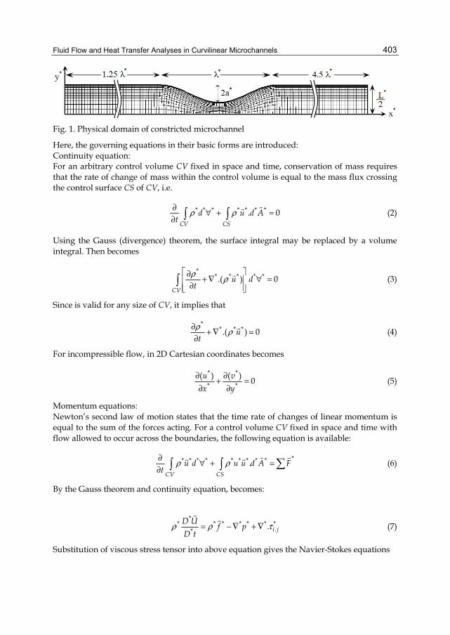
Fluid Flow and Heat Transfer Analyses in Curvilinear Microchannels
403
Fig. 1. Physical domain of constricted microchannel
Here, the governing equations in their basic forms are introduced: Continuity equation: For an arbitrary control volume CV fixed in space and time, conservation of mass requires that the rate of change of mass within the control volume is equal to the mass flux crossing the control surface CS of CV, i.e.
* * * * * * *. 0CV CS
d u d At
ρ ρ∂ ∀ + =∂ ∫ ∫ (2)
Using the Gauss (divergence) theorem, the surface integral may be replaced by a volume integral. Then becomes
*
* * * * *.( ) 0CV
u dt
ρ ρ⎡ ⎤∂ + ∇ ∀ =⎢ ⎥
∂⎢ ⎥⎣ ⎦∫ (3)
Since is valid for any size of CV, it implies that
*
* * *.( ) 0ut
ρ ρ∂ + ∇ =∂
(4)
For incompressible flow, in 2D Cartesian coordinates becomes
* *
* *( ) ( ) 0u vx y
∂ ∂+ =∂ ∂
(5)
Momentum equations: Newton’s second law of motion states that the time rate of changes of linear momentum is equal to the sum of the forces acting. For a control volume CV fixed in space and time with flow allowed to occur across the boundaries, the following equation is available:
** * * * * * * * *.
CV CSu d u u d A F
tρ ρ∂ ∀ + =
∂ ∑∫ ∫ (6)
By the Gauss theorem and continuity equation, becomes:
*
* * * * * * *.* . i j
D U f pD t
ρ ρ τ= − ∇ + ∇ (7)
Substitution of viscous stress tensor into above equation gives the Navier-Stokes equations
Evaporation, Condensation and Heat Transfer
404
* 2 * 2 *
* *2 * * * ** * * *2 *2( ) ( ) ( ) x
p u uu u v gx y x x y
ρ ρ μ ρ∂∂ ∂ ∂ ∂+ =− + + +∂ ∂ ∂ ∂ ∂
(8)
* 2 * 2 *
* * * * *2 ** * * *2 *2( ) ( ) ( ) y
p v vu v v gx y y x y
ρ ρ μ ρ∂∂ ∂ ∂ ∂+ = − + + +∂ ∂ ∂ ∂ ∂
(9)
Energy equation: The first law of thermodynamics states that the time rate of change of internal energy plus kinetic energy is equal to the rate of heat transfer less the rate of work done by the system. For a control volume CV this can be written as
* * * * * * *.CV CS
dEe d e u dA Q Wt dt
ρ ρ∂ ∀ + = = −∂ ∫ ∫ (10)
Applying the Gauss theorem and shrinking the volume to zero and then substituting the Fourier law of heat conduction gives
( ) ( )* * * *
** * * * * *P PC u T C v T T Tk k
x y x x y y
ρ ρ∂ ∂ ⎛ ⎞∂ ∂ ∂ ∂⎛ ⎞+ = + + Φ⎜ ⎟⎜ ⎟ ⎜ ⎟∂ ∂ ∂ ∂ ∂ ∂⎝ ⎠ ⎝ ⎠
(11)
2 22* * * *
** * * *[2 2 ]u v u v
x y y xμ
⎛ ⎞ ⎛ ⎞⎛ ⎞∂ ∂ ∂ ∂Φ = + + +⎜ ⎟ ⎜ ⎟⎜ ⎟⎜ ⎟ ⎜ ⎟ ⎜ ⎟∂ ∂ ∂ ∂⎝ ⎠ ⎝ ⎠ ⎝ ⎠
where Φ represents the dissipation function stems from viscous stresses. Non-dimensional variables are introduced as
*
*xxL
= ,*
*yyL
= ,*
*i
uuu
= , *
*i
vvu
= , *
* *2i i
ppuρ
= , i
w i
T TT T
θ −=−
* * *
Re i ii
u Lρμ
= ,* *
Re Pr ii i i
u LPeα
= = ,*2
( )i
ip w i
uEcC T T
=−
Here, Eci means the Eckert number. Then, non-dimensional governing equations are obtained as Non-dimensional continuity equation:
( ) ( ) 0u vx y
∂ ∂+ =∂ ∂
(12)
Non-dimensional momentum equations:
2 2
22 2
1( ) ( ) ( )Rei
p u uu uvx y x x y
∂∂ ∂ ∂ ∂+ =− + +∂ ∂ ∂ ∂ ∂
(13)
2 2
22 2
1( ) ( ) ( )Rei
p v vuv vx y y x y
∂∂ ∂ ∂ ∂+ =− + +∂ ∂ ∂ ∂ ∂
(14)
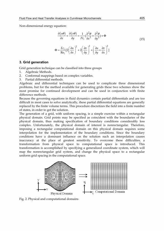
Fluid Flow and Heat Transfer Analyses in Curvilinear Microchannels
405
Non-dimensional energy equation:
( ) ( ) 2 2
2 21 ( )
i
u vx y Pe x yθ θ θ θ∂ ∂ ∂ ∂+ = + + Φ
∂ ∂ ∂ ∂
(15)
2 22
[2 2 ]Re
i
i
Ec u v u vx y y x
⎛ ⎞ ⎛ ⎞∂ ∂ ∂ ∂⎛ ⎞Φ = + + +⎜ ⎟ ⎜ ⎟⎜ ⎟ ⎜ ⎟ ⎜ ⎟∂ ∂ ∂ ∂⎝ ⎠ ⎝ ⎠ ⎝ ⎠
3. Grid generation Grid generation technique can be classified into three groups 1. Algebraic Methods. 2. Conformal mappings based on complex variables. 3. Partial differential methods. Algebraic and differential techniques can be used to complicate three dimensional problems, but for the method available for generating grids these two schemes show the most promise for continued development and can be used in conjunction with finite difference methods. Because the governing equations in fluid dynamics contain partial differentials and are too difficult in most cases to solve analytically, these partial differential equations are generally replaced by the finite volume terms. This procedure discretizes the field into a finite number of states, in order to get the solution. The generation of a grid, with uniform spacing, is a simple exercise within a rectangular physical domain. Grid points may be specified as coincident with the boundaries of the physical domain, thus making specification of boundary conditions considerably less complex. Unfortunately, the physical domain of interest is nonrectangular. Therefore, imposing a rectangular computational domain on this physical domain requires some interpolation for the implementation of the boundary conditions. Since the boundary conditions have a dominant influence on the solution such an interpolation causes inaccuracy at the place of greatest sensitivity. To overcome these difficulties, a transformation from physical space to computational space is introduced. This transformation is accomplished by specifying a generalized coordinate system, which will map the nonrectangular grid system, and change the physical space to a rectangular uniform grid spacing in the computational space.
Fig. 2. Physical and computational domains
Evaporation, Condensation and Heat Transfer
406
Transformation between physical (x,y) and computational (ξ,η) domains, important for body-fitted grids. Define the following relations between the physical and computational spaces:
( , )( , )x yx y
ξ ξη η
==
(16)
The chain rule for partial differentiation yields the following expression:
x x
y y
x
y
ξ ηξ η
ξ ηξ η
∂ ∂ ∂= +∂ ∂ ∂∂ ∂ ∂= +
∂ ∂ ∂
(17)
From above equations the following differential expressions are obtained
x y
x y
d dx dy
d dx dy
ξ ξ ξη η η
= +
= + (18)
which are written in a compact form as
x y
x y
d dxd dy
ξ ξξη η η
⎡ ⎤⎡ ⎤ ⎡ ⎤= ⎢ ⎥⎢ ⎥ ⎢ ⎥⎢ ⎥⎣ ⎦ ⎣ ⎦⎣ ⎦
(19)
Reversing the role of independent variables, i.e.,
( , )( , )
x xy y
ξ ηξ η
==
(20)
The following may be written
dx x d x ddy y d y d
ξ η
ξ η
ξ ηξ η
= += +
(21)
In a compact form they are written as
x xdx dy ydy d
ξ η
ξ η
ξη
⎡ ⎤⎡ ⎤ ⎡ ⎤= ⎢ ⎥⎢ ⎥ ⎢ ⎥⎢ ⎥⎣ ⎦ ⎣ ⎦⎣ ⎦
(22)
Comparing equations 19 and 22, it can be concluded that
1
x y
x y
x xy y
ξ η
ξ η
ξ ξη η
−⎡ ⎤ ⎡ ⎤=⎢ ⎥ ⎢ ⎥⎢ ⎥⎢ ⎥ ⎣ ⎦⎣ ⎦
(23)
From which
yx Jξ η= + , yx Jη ξ= − , xy Jξ η= − , xy Jη ξ= − (23)
Fluid Flow and Heat Transfer Analyses in Curvilinear Microchannels
407
Where
J x y x yξ η η ξ= − (23)
and is defined as the Jacobian of transformation [19].
4. Governing equations in computational space To formulate the problem, a continuum based approach is used. Here (ξ,η) are independent variables in general non-orthogonal curvilinear coordinate. The nondimensional governing equations can be written as: Non-dimensional continuity equation in curvilinear coordinate:
0C CU V
ξ η∂ ∂+ =∂ ∂ (24)
Non-dimensional momentum equations in curvilinear coordinate:
11 22 12 12
1( ) ( ) { ( ) ( ) ( ) ( )}Re
( ) ( )
C C
i
u u u uuU uV q q q q
y p y pη ξ
ξ η ξ ξ η η ξ η η ξ
ξ η
∂ ∂ ∂ ∂ ∂ ∂ ∂ ∂ ∂ ∂+ = + + +∂ ∂ ∂ ∂ ∂ ∂ ∂ ∂ ∂ ∂
∂ ∂− +∂ ∂
(25)
11 22 12 12
1( ) ( ) { ( ) ( ) ( ) ( )}Re
( ) ( )
C C
i
v v v vvU vV q q q q
x p x pη ξ
ξ η ξ ξ η η ξ η η ξ
ξ η
∂ ∂ ∂ ∂ ∂ ∂ ∂ ∂ ∂ ∂+ = + + +∂ ∂ ∂ ∂ ∂ ∂ ∂ ∂ ∂ ∂
∂ ∂+ −∂ ∂
(25)
Non-dimensional energy equation in curvilinear coordinate:
11 22 12 121( ) ( ) { ( ) ( ) ( ) ( )}C C
iU V q q q q
Peθ θ θ θθ θ
ξ η ξ ξ η η ξ η η ξ∂ ∂ ∂ ∂ ∂ ∂ ∂ ∂ ∂ ∂+ = + + + + Φ
∂ ∂ ∂ ∂ ∂ ∂ ∂ ∂ ∂ ∂ (26)
2 2 2i
i
Ec {2(u y u y ) 2( v x v x ) ( u x u x v y v y ) }Re J ξ η η ξ ξ η η ξ ξ η η ξ ξ η η ξΦ = − + − + + − + + −
Where
CU uy vxη η= − , CV uy vxξ ξ= − + , J x y x yξ η η ξ= −
2 211
1 ( )q y xJ η η= + , 12
1 ( )q x x y yJ ξ η ξ η
−= + , 2 222
1 ( )q x yJ ξ ξ= +
where Φ is viscous dissipation function that shows the effects of viscous stresses. u and v are the velocity components and CU and CV are the velocities in ξ,η.
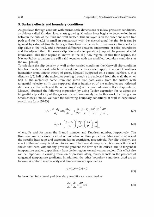
Evaporation, Condensation and Heat Transfer
408
5. Surface effects and boundary conditions As gas flows through conduits with micron scale dimensions or in low pressures conditions, a sublayer called Knudsen layer starts growing. Knudsen layer begins to become dominant between the bulk of the fluid and wall surface. This sublayer is on the order one mean free path and for Kn≤0.1 is small in comparison with the microchannel height. So it can be ignored by extrapolating the bulk gas flow towards the walls. This causes a finite velocity slip value at the wall, and a nonzero difference between temperature of solid boundaries and the adjacent fluid. It means a slip flow and a temperature jump will be present at solid boundaries. This flow regime is known as the slip flow regime. In this flow regime, the Navier–Stokes equations are still valid together with the modified boundary conditions at the wall [20-23]. To calculate the slip velocity at wall under rarified condition, the Maxwell slip condition has been widely used which is based on the first-order approximation of wall-gas interaction from kinetic theory of gases. Maxwell supposed on a control surface, s, at a distance δ/2, half of the molecules passing through s are reflected from the wall, the other half of the molecules come from one mean free path away from the surface with tangential velocity uλ. It was supposed that a fraction σv of the molecules are reflected diffusively at the walls and the remaining (1-σv) of the molecules are reflected specularly, Maxwell obtained the following expression by using Taylor expansion for uλ about the tangential slip velocity of the gas on this surface namely us. In this work, by using von-Smoluchowski model we have the following boundary conditions at wall in curvilinear coordinate form [20-23]:
22 3 (1 ) Re
2v s
s iv ww i
U KnU Knn Ec s
σ γ θσ π γ
⎛ ⎞− ∂ − ∂= + ⎜ ⎟⎜ ⎟∂ ∂⎝ ⎠ (27)
2 211 Pr
Ts
T wi
Knn
σ γ θθσ γ
⎛ ⎞⎛ ⎞− ∂⎛ ⎞= − ⎜ ⎟⎜ ⎟⎜ ⎟⎜ ⎟ + ∂⎝ ⎠⎝ ⎠⎝ ⎠ (28)
where, Pr and Kn mean the Prandtl number and Knudsen number, respectively. The Knudsen number shows the effect of rarefaction on flow properties. Also γ and σ represent the specific heat ratio and accommodation coefficient, respectively. For slip velocity, the effect of thermal creep is taken into account. The thermal creep which is a rarefaction effect shows that even without any pressure gradient the flow can be caused due to tangential temperature gradient, specifically from colder region toward warmer region. This effect also can be important in causing variation of pressure along microchannels in the presence of tangential temperature gradients. In addition, the other boundary conditions used are as follows. A uniform inlet velocity and temperature are specified as
u 1,v 0 , 0= = θ =
(29)
In the outlet, fully developed boundary conditions are assumed as
0u vx x x
θ∂ ∂ ∂= = =∂ ∂ ∂
(30)
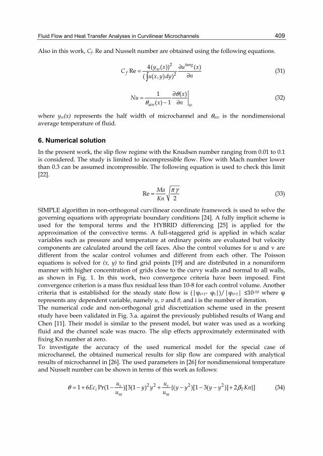
Fluid Flow and Heat Transfer Analyses in Curvilinear Microchannels
409
Also in this work, Cf. Re and Nusselt number are obtained using the following equations.
2
24( ( )) ( )Re
( ( , ) )
tangw
fy x u xC
nu x y dy∂=
∂∫ (31)
1 ( )( ) 1ave w
xNux n
θθ
∂=− ∂
(32)
where yw(x) represents the half width of microchannel and θave is the nondimensional average temperature of fluid.
6. Numerical solution In the present work, the slip flow regime with the Knudsen number ranging from 0.01 to 0.1 is considered. The study is limited to incompressible flow. Flow with Mach number lower than 0.3 can be assumed incompressible. The following equation is used to check this limit [22].
Re2
MaKn
π γ= (33)
SIMPLE algorithm in non-orthogonal curvilinear coordinate framework is used to solve the governing equations with appropriate boundary conditions [24]. A fully implicit scheme is used for the temporal terms and the HYBRID differencing [25] is applied for the approximation of the convective terms. A full-staggered grid is applied in which scalar variables such as pressure and temperature at ordinary points are evaluated but velocity components are calculated around the cell faces. Also the control volumes for u and v are different from the scalar control volumes and different from each other. The Poisson equations is solved for (x, y) to find grid points [19] and are distributed in a nonuniform manner with higher concentration of grids close to the curvy walls and normal to all walls, as shown in Fig. 1. In this work, two convergence criteria have been imposed. First convergence criterion is a mass flux residual less than 10-8 for each control volume. Another criteria that is established for the steady state flow is (|φi+1- φi|)/|φi+1| ≤10-10 where φ represents any dependent variable, namely u, v and θ, and i is the number of iteration. The numerical code and non-orthogonal grid discretization scheme used in the present study have been validated in Fig. 3.a. against the previously published results of Wang and Chen [11]. Their model is similar to the present model, but water was used as a working fluid and the channel scale was macro. The slip effects approximately exterminated with fixing Kn number at zero. To investigate the accuracy of the used numerical model for the special case of microchannel, the obtained numerical results for slip flow are compared with analytical results of microchannel in [26]. The used parameters in [26] for nondimensional temperature and Nusselt number can be shown in terms of this work as follows:
2 2 2 21 6 Pr(1 )[3(1 ) {( )[1 3( )] 2 }]s si T
m m
u uEc y y y y y y Knu u
θ β= + − − + − − − + (34)
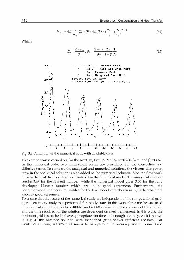
Evaporation, Condensation and Heat Transfer
410
2 1420 [27 (9 420 ) ( ) ]s s st
m m m
u u uNu Knu u u
β −∞ = + + − (35)
Which
2 vv
v
σβσ−= , 2 2 1
1 PrT
TT
σ γβσ γ−=
+ (23)
Fig. 3a. Validation of the numerical code with available data
This comparison is carried out for the Kn=0.04, Pr=0.7, Pe=0.5, Ec=0.286, βv =1 and βT=1.667. In the numerical code, two dimensional forms are considered for the convective and diffusive terms. To compare the analytical and numerical solutions, the viscous dissipation term in the analytical solution is also added to the numerical solution. Also the flow work term in the analytical solution is considered in the numerical model. The analytical solution results 3.47 for the Nusselt number, while the numerical model gives 3.53 for the fully developed Nusselt number which are in a good agreement. Furthermore, the nondimensional temperature profiles for the two models are shown in Fig. 3.b. which are also in a good agreement. To ensure that the results of the numerical study are independent of the computational grid; a grid sensitivity analysis is performed for steady state. In this work, three meshes are used in numerical simulation: 350×65, 400×75 and 450×85. Generally, the accuracy of the solution and the time required for the solution are dependent on mesh refinement. In this work, the optimum grid is searched to have appropriate run-time and enough accuracy. As it is shown in Fig. 4, the obtained solution with mentioned grids shows sufficient accuracy. For Kn=0.075 at Re=2, 400×75 grid seems to be optimum in accuracy and run-time. Grid
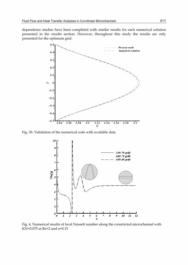
Fluid Flow and Heat Transfer Analyses in Curvilinear Microchannels
411
dependence studies have been completed with similar results for each numerical solution presented in the results section. However, throughout this study the results are only presented for the optimum grid.
Fig. 3b. Validation of the numerical code with available data
Fig. 4. Numerical results of local Nusselt number along the constricted microchannel with KN=0.075 at Re=2 and a=0.15
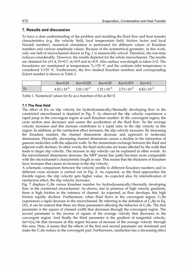
Evaporation, Condensation and Heat Transfer
412
7. Results and discussion To have a clear understanding of the problem and studding the fluid flow and heat transfer characteristics (e.g. the velocity field, local temperature field, friction factor and local Nusselt number), numerical simulation is performed for different values of Knudsen numbers and various amplitude values. Because of the symmetrical geometry, in this work, only one half of microchannel shown in Fig. 1 is numerically solved. Therefore, the run-time reduces considerably. However, the results depicted for the whole microchannel. The results are obtained for γ=1.4, Pr=0.7, σT=0.9 and σv=0.9. Also surface wavelength is taken λ=2. The boundaries are maintained at temperature Tw=70 oC and the uniform inlet temperature is considered Ti=25 oC. Furthermore, the five studied Knudsen numbers and corresponding Eckert number is shown in Table 1. Kn=0.01 Kn=0.025 Kn=0.05 Kn=0.075 Kn=0.1 Ec
-44.82 10× -33.01 10× -21.21 10× -22.71 10× -24.82 10×
Table 1. Numerical values for Ec as a function of Kn at Re=2
7.1 The flow field The effect of Kn on slip velocity for hydrodynamically/thermally developing flow in the constricted microchannel is depicted in Fig. 5. As observed the slip velocity experiences a rapid jump in the convergent region at each Knudsen number. In the convergent region, the cross section area decreases and causes the acceleration of the fluid flow. So the average velocity increases and this increase contributes to a rapid raise in the slip velocity in this region. In addition, as the rarefaction effect increases, the slip velocity increases. By increasing the Knudsen number, the channel dimensions decrease and approach to molecular dimensions. Physically, decreasing channel dimensions causes a decline in the interaction of gaseous molecules with the adjacent walls. So the momentum exchange between the fluid and adjacent walls declines. In other words, the fluid molecules are lesser affected by the walls that leads to larger slip velocity. The increase in slip velocity can be explained in other words. As the microchannel dimensions decrease, the MFP (mean free path) becomes more comparable with the microchannel’s characteristic length in size. This means that the thickness of Knudsen layer increases that causes an increase in the slip velocity. A schematic comparison between the velocity profile in different Knudsen numbers and in different cross sections is carried out in Fig. 6. As expected, as the fluid approaches the throttle region, the slip velocity gets higher value. As expected also, by intensification of rarefaction effect, the slip velocity increases. Fig. 7 displays Cf.Re versus Knudsen number for hydrodynamically/thermally developing flow in the constricted microchannel. As shown, due to presence of high velocity gradients, there is high friction in the entrance of channel. As expected, as flow develops, this high friction rapidly declines. Furthermore, when fluid flows in the convergent region, Cf.Re experiences a rapid decrease in the microchannel. By referring to the definition of Cf.Re in Eq. (31), it can be noticed that there are three parameters affecting the behavior of Cf.Re. The first parameter is the square of channel width that decreases through the convergent region. The second parameter is the inverse of square of the average velocity that decreases in the convergent region. And finally the third parameter is the gradient of tangential velocity, ∂utang(x)/∂n that increases in this region because of increase of the average velocity through this area. Here, it seems that the effects of the first and second parameter are dominant and make the Cf.Re reduce in the convergent part. Furthermore, rarefaction has a decreasing effect
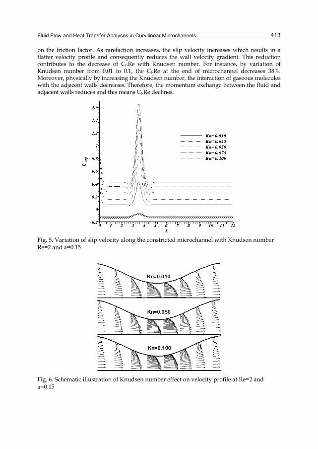
Fluid Flow and Heat Transfer Analyses in Curvilinear Microchannels
413
on the friction factor. As rarefaction increases, the slip velocity increases which results in a flatter velocity profile and consequently reduces the wall velocity gradient. This reduction contributes to the decrease of Cf.Re with Knudsen number. For instance, by variation of Knudsen number from 0.01 to 0.1, the Cf.Re at the end of microchannel decreases 38%. Moreover, physically by increasing the Knudsen number, the interaction of gaseous molecules with the adjacent walls decreases. Therefore, the momentum exchange between the fluid and adjacent walls reduces and this means Cf.Re declines.
Fig. 5. Variation of slip velocity along the constricted microchannel with Knudsen number Re=2 and a=0.15
Fig. 6. Schematic illustration of Knudsen number effect on velocity profile at Re=2 and a=0.15
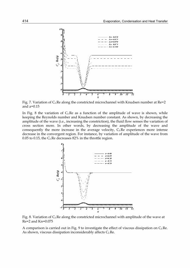
Evaporation, Condensation and Heat Transfer
414
Fig. 7. Variation of Cf.Re along the constricted microchannel with Knudsen number at Re=2 and a=0.15
In Fig. 8 the variation of Cf.Re as a function of the amplitude of wave is shown, while keeping the Reynolds number and Knudsen number constant. As shown, by decreasing the amplitude of the wave (i.e., increasing the constriction), the fluid flow senses the variation of cross section more. In other words, by decreasing the amplitude of the wave and consequently the more increase in the average velocity, Cf.Re experiences more intense decrease in the convergent region. For instance, by variation of amplitude of the wave from 0.05 to 0.15, the Cf.Re decreases 82% in the throttle region.
Fig. 8. Variation of Cf.Re along the constricted microchannel with amplitude of the wave at Re=2 and Kn=0.075
A comparison is carried out in Fig. 9 to investigate the effect of viscous dissipation on Cf.Re. As shown, viscous dissipation inconsiderably affects Cf.Re.
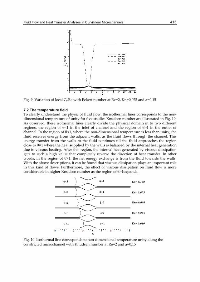
Fluid Flow and Heat Transfer Analyses in Curvilinear Microchannels
415
Fig. 9. Variation of local Cf.Re with Eckert number at Re=2, Kn=0.075 and a=0.15
7.2 The temperature field To clearly understand the physic of fluid flow, the isothermal lines corresponds to the non-dimensional temperature of unity for five studies Knudsen number are illustrated in Fig. 10. As observed, these isothermal lines clearly divide the physical domain in to two different regions, the region of θ<1 in the inlet of channel and the region of θ>1 in the outlet of channel. In the region of θ<1, where the non-dimensional temperature is less than unity, the fluid receives energy from the adjacent walls, as the fluid flows through the channel. This energy transfer from the walls to the fluid continues till the fluid approaches the region close to θ=1 where the heat supplied by the walls is balanced by the internal heat generation due to viscous heating. After this region, the internal heat generated by viscous dissipation gets to such a high value that completely reverse the direction of heat transfer. In other words, in the region of θ>1, the net energy exchange is from the fluid towards the walls. With the above descriptions, it can be found that viscous dissipation plays an important role in this kind of flows. Furthermore, the effect of viscous dissipation on fluid flow is more considerable in higher Knudsen number as the region of θ>1expands.
Fig. 10. Isothermal line corresponds to non-dimensional temperature unity along the constricted microchannel with Knudsen number at Re=2 and a=0.15
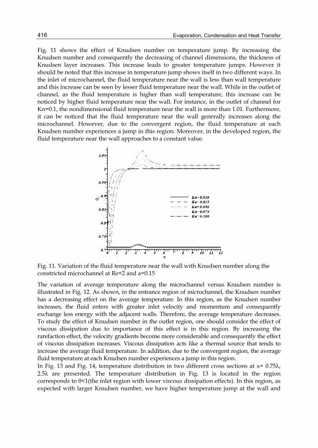
Evaporation, Condensation and Heat Transfer
416
Fig. 11 shows the effect of Knudsen number on temperature jump. By increasing the Knudsen number and consequently the decreasing of channel dimensions, the thickness of Knudsen layer increases. This increase leads to greater temperature jumps. However it should be noted that this increase in temperature jump shows itself in two different ways. In the inlet of microchannel, the fluid temperature near the wall is less than wall temperature and this increase can be seen by lesser fluid temperature near the wall. While in the outlet of channel, as the fluid temperature is higher than wall temperature, this increase can be noticed by higher fluid temperature near the wall. For instance, in the outlet of channel for Kn=0.1, the nondimensional fluid temperature near the wall is more than 1.01. Furthermore, it can be noticed that the fluid temperature near the wall generally increases along the microchannel. However, due to the convergent region, the fluid temperature at each Knudsen number experiences a jump in this region. Moreover, in the developed region, the fluid temperature near the wall approaches to a constant value.
Fig. 11. Variation of the fluid temperature near the wall with Knudsen number along the constricted microchannel at Re=2 and a=0.15
The variation of average temperature along the microchannel versus Knudsen number is illustrated in Fig. 12. As shown, in the entrance region of microchannel, the Knudsen number has a decreasing effect on the average temperature. In this region, as the Knudsen number increases, the fluid enters with greater inlet velocity and momentum and consequently exchange less energy with the adjacent walls. Therefore, the average temperature decreases. To study the effect of Knudsen number in the outlet region, one should consider the effect of viscous dissipation due to importance of this effect is in this region. By increasing the rarefaction effect, the velocity gradients become more considerable and consequently the effect of viscous dissipation increases. Viscous dissipation acts like a thermal source that tends to increase the average fluid temperature. In addition, due to the convergent region, the average fluid temperature at each Knudsen number experiences a jump in this region. In Fig. 13 and Fig. 14, temperature distribution in two different cross sections at x= 0.75λ, 2.5λ are presented. The temperature distribution in Fig. 13 is located in the region corresponds to θ<1(the inlet region with lower viscous dissipation effects). In this region, as expected with larger Knudsen number, we have higher temperature jump at the wall and
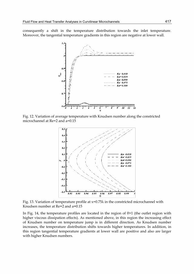
Fluid Flow and Heat Transfer Analyses in Curvilinear Microchannels
417
consequently a shift in the temperature distribution towards the inlet temperature. Moreover, the tangential temperature gradients in this region are negative at lower wall.
Fig. 12. Variation of average temperature with Knudsen number along the constricted microchannel at Re=2 and a=0.15
Fig. 13. Variation of temperature profile at x=0.75λ in the constricted microchannel with Knudsen number at Re=2 and a=0.15
In Fig. 14, the temperature profiles are located in the region of θ>1 (the outlet region with higher viscous dissipation effects). As mentioned above, in this region the increasing effect of Knudsen number on temperature jump is in different direction. As Knudsen number increases, the temperature distribution shifts towards higher temperatures. In addition, in this region tangential temperature gradients at lower wall are positive and also are larger with higher Knudsen numbers.
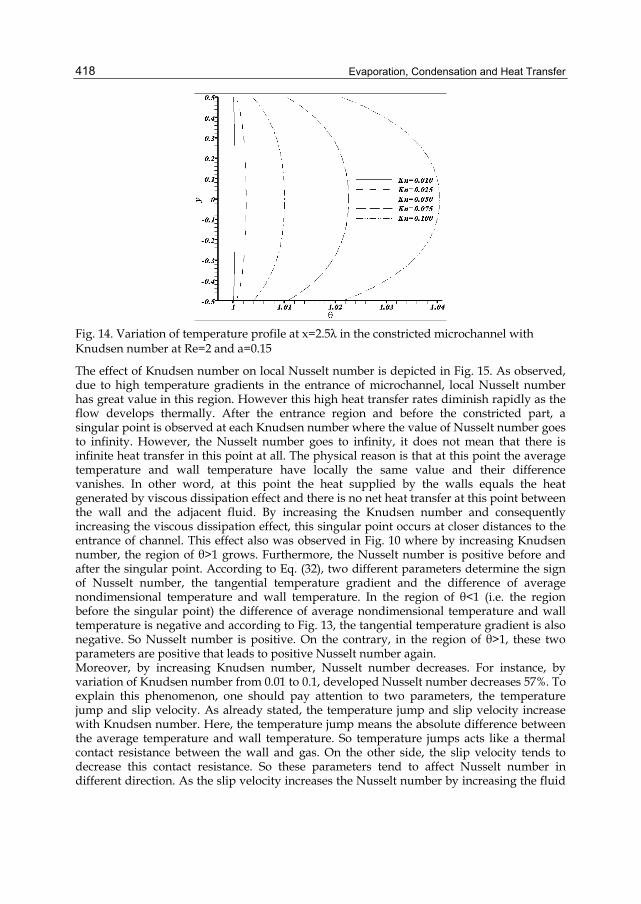
Evaporation, Condensation and Heat Transfer
418
Fig. 14. Variation of temperature profile at x=2.5λ in the constricted microchannel with Knudsen number at Re=2 and a=0.15
The effect of Knudsen number on local Nusselt number is depicted in Fig. 15. As observed, due to high temperature gradients in the entrance of microchannel, local Nusselt number has great value in this region. However this high heat transfer rates diminish rapidly as the flow develops thermally. After the entrance region and before the constricted part, a singular point is observed at each Knudsen number where the value of Nusselt number goes to infinity. However, the Nusselt number goes to infinity, it does not mean that there is infinite heat transfer in this point at all. The physical reason is that at this point the average temperature and wall temperature have locally the same value and their difference vanishes. In other word, at this point the heat supplied by the walls equals the heat generated by viscous dissipation effect and there is no net heat transfer at this point between the wall and the adjacent fluid. By increasing the Knudsen number and consequently increasing the viscous dissipation effect, this singular point occurs at closer distances to the entrance of channel. This effect also was observed in Fig. 10 where by increasing Knudsen number, the region of θ>1 grows. Furthermore, the Nusselt number is positive before and after the singular point. According to Eq. (32), two different parameters determine the sign of Nusselt number, the tangential temperature gradient and the difference of average nondimensional temperature and wall temperature. In the region of θ<1 (i.e. the region before the singular point) the difference of average nondimensional temperature and wall temperature is negative and according to Fig. 13, the tangential temperature gradient is also negative. So Nusselt number is positive. On the contrary, in the region of θ>1, these two parameters are positive that leads to positive Nusselt number again. Moreover, by increasing Knudsen number, Nusselt number decreases. For instance, by variation of Knudsen number from 0.01 to 0.1, developed Nusselt number decreases 57%. To explain this phenomenon, one should pay attention to two parameters, the temperature jump and slip velocity. As already stated, the temperature jump and slip velocity increase with Knudsen number. Here, the temperature jump means the absolute difference between the average temperature and wall temperature. So temperature jumps acts like a thermal contact resistance between the wall and gas. On the other side, the slip velocity tends to decrease this contact resistance. So these parameters tend to affect Nusselt number in different direction. As the slip velocity increases the Nusselt number by increasing the fluid
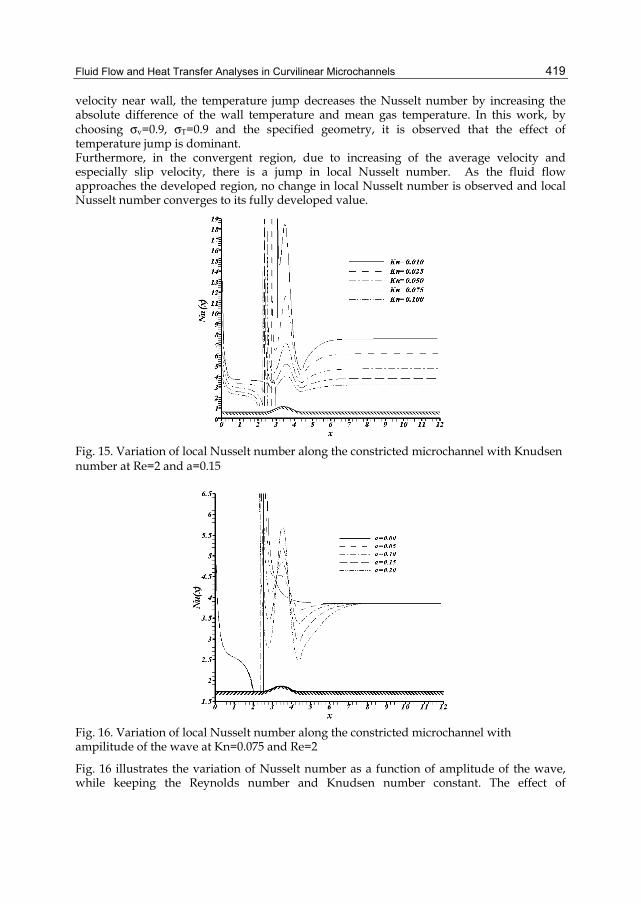
Fluid Flow and Heat Transfer Analyses in Curvilinear Microchannels
419
velocity near wall, the temperature jump decreases the Nusselt number by increasing the absolute difference of the wall temperature and mean gas temperature. In this work, by choosing σv=0.9, σT=0.9 and the specified geometry, it is observed that the effect of temperature jump is dominant. Furthermore, in the convergent region, due to increasing of the average velocity and especially slip velocity, there is a jump in local Nusselt number. As the fluid flow approaches the developed region, no change in local Nusselt number is observed and local Nusselt number converges to its fully developed value.
Fig. 15. Variation of local Nusselt number along the constricted microchannel with Knudsen number at Re=2 and a=0.15
Fig. 16. Variation of local Nusselt number along the constricted microchannel with ampilitude of the wave at Kn=0.075 and Re=2
Fig. 16 illustrates the variation of Nusselt number as a function of amplitude of the wave, while keeping the Reynolds number and Knudsen number constant. The effect of
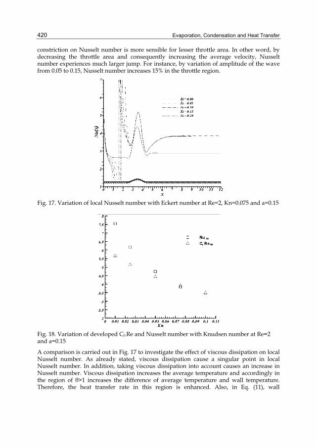
Evaporation, Condensation and Heat Transfer
420
constriction on Nusselt number is more sensible for lesser throttle area. In other word, by decreasing the throttle area and consequently increasing the average velocity, Nusselt number experiences much larger jump. For instance, by variation of amplitude of the wave from 0.05 to 0.15, Nusselt number increases 15% in the throttle region.
Fig. 17. Variation of local Nusselt number with Eckert number at Re=2, Kn=0.075 and a=0.15
Fig. 18. Variation of developed Cf.Re and Nusselt number with Knudsen number at Re=2 and a=0.15
A comparison is carried out in Fig. 17 to investigate the effect of viscous dissipation on local Nusselt number. As already stated, viscous dissipation cause a singular point in local Nusselt number. In addition, taking viscous dissipation into account causes an increase in Nusselt number. Viscous dissipation increases the average temperature and accordingly in the region of θ>1 increases the difference of average temperature and wall temperature. Therefore, the heat transfer rate in this region is enhanced. Also, in Eq. (11), wall
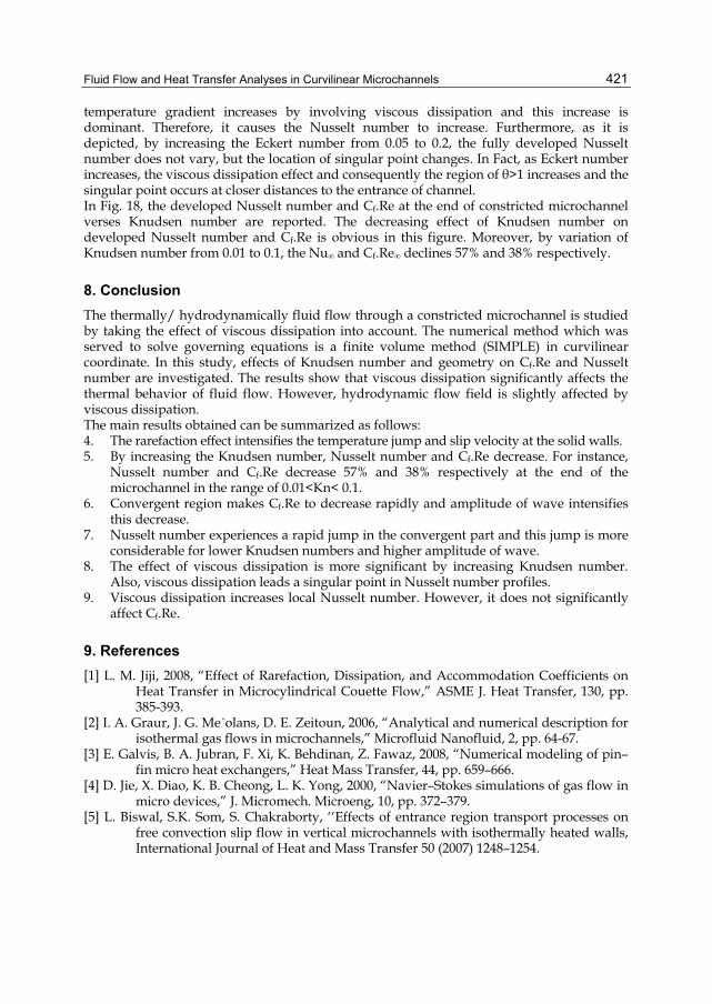
Fluid Flow and Heat Transfer Analyses in Curvilinear Microchannels
421
temperature gradient increases by involving viscous dissipation and this increase is dominant. Therefore, it causes the Nusselt number to increase. Furthermore, as it is depicted, by increasing the Eckert number from 0.05 to 0.2, the fully developed Nusselt number does not vary, but the location of singular point changes. In Fact, as Eckert number increases, the viscous dissipation effect and consequently the region of θ>1 increases and the singular point occurs at closer distances to the entrance of channel. In Fig. 18, the developed Nusselt number and Cf.Re at the end of constricted microchannel verses Knudsen number are reported. The decreasing effect of Knudsen number on developed Nusselt number and Cf.Re is obvious in this figure. Moreover, by variation of Knudsen number from 0.01 to 0.1, the Nu∞ and Cf.Re∞ declines 57% and 38% respectively.
8. Conclusion The thermally/ hydrodynamically fluid flow through a constricted microchannel is studied by taking the effect of viscous dissipation into account. The numerical method which was served to solve governing equations is a finite volume method (SIMPLE) in curvilinear coordinate. In this study, effects of Knudsen number and geometry on Cf.Re and Nusselt number are investigated. The results show that viscous dissipation significantly affects the thermal behavior of fluid flow. However, hydrodynamic flow field is slightly affected by viscous dissipation. The main results obtained can be summarized as follows: 4. The rarefaction effect intensifies the temperature jump and slip velocity at the solid walls. 5. By increasing the Knudsen number, Nusselt number and Cf.Re decrease. For instance,
Nusselt number and Cf.Re decrease 57% and 38% respectively at the end of the microchannel in the range of 0.01<Kn< 0.1.
6. Convergent region makes Cf.Re to decrease rapidly and amplitude of wave intensifies this decrease.
7. Nusselt number experiences a rapid jump in the convergent part and this jump is more considerable for lower Knudsen numbers and higher amplitude of wave.
8. The effect of viscous dissipation is more significant by increasing Knudsen number. Also, viscous dissipation leads a singular point in Nusselt number profiles.
9. Viscous dissipation increases local Nusselt number. However, it does not significantly affect Cf.Re.
9. References [1] L. M. Jiji, 2008, “Effect of Rarefaction, Dissipation, and Accommodation Coefficients on
Heat Transfer in Microcylindrical Couette Flow,” ASME J. Heat Transfer, 130, pp. 385-393.
[2] I. A. Graur, J. G. Me´olans, D. E. Zeitoun, 2006, “Analytical and numerical description for isothermal gas flows in microchannels,” Microfluid Nanofluid, 2, pp. 64-67.
[3] E. Galvis, B. A. Jubran, F. Xi, K. Behdinan, Z. Fawaz, 2008, “Numerical modeling of pin–fin micro heat exchangers,” Heat Mass Transfer, 44, pp. 659–666.
[4] D. Jie, X. Diao, K. B. Cheong, L. K. Yong, 2000, “Navier–Stokes simulations of gas flow in micro devices,” J. Micromech. Microeng, 10, pp. 372–379.
[5] L. Biswal, S.K. Som, S. Chakraborty, ‘‘Effects of entrance region transport processes on free convection slip flow in vertical microchannels with isothermally heated walls, International Journal of Heat and Mass Transfer 50 (2007) 1248–1254.
Evaporation, Condensation and Heat Transfer
422
[6] G. Hetsroni, A. Mosyak, E. Pogrebnyak, L.P. Yarin, Fluid flow in micro-channels, International Journal of Heat & Mass Transfer 48 (2005) 1982–1998.
[7] A. Beskok, G.E. Karniadakis, Simulation of heat and momentum transfer in complex microgeometries, J. Thermophys Heat Transfer 8 (1994) 647–655.
[8] R. T-S. Cheng, 1972, “Numerical Solution of the Navier-Stokes Equations by the Finite Element Method,” Phys. Fluids, 15, pp. 2098–2105.
[9] J. E. O'Brien and E. M. Sparrow, Corrugated-duct heat transfer, pressure drop, and flow visualization, J. Heat Transfer 104 (1982) 410-416.
[10] T. Nishimura, Y. Ohori, Y. Kawamura, 1984, “Flow characteristics in a channel with symmetric wavy wall for steady flow,” J. Chem. Eng. Jpn., 17, pp. 466-471.
[11] C. C. Wang, C. K. Chen, 2002, “Forced convection in a wavy-wall channel,” International Journal of Heat and Mass Transfer, 45, pp. 2587-2595.
[12] E. B. Arkilic, K. S. Breuer, M. A. Schmidt, 1994, “Gaseous Flow in Microchannels,” ASME Application of Microfabrication to Fluid Mechanics, 197, pp. 57–66.
[13] A. Beskok, G. E. Karniadakis, Trimmer, W., 1996, “Rarefaction and compressibility effects in gas microflows,” ASME Journal of Fluids Engineering, 118, pp. 448-456.
[14] L. Kuddusi, E. Çetegen, Thermal and hydrodyna-mic analysis of gaseous flow in trapezoidal silicon microchannels, International Journal of Thermal Sciences 48 (2009) 353–362.
[15] Cha’o-Kuang Chen, Ching-Chang Cho, Electro-kinetically-driven flow mixing in microchannels with wavy surface, Journal of Colloid and Interface Science 312 (2007) 470–480.
[16] H. Shokouhmand, S. Bigham, Slip-flow and heat transfer of gaseous flows in the entrance of a wavy microchannel, International Communications in Heat and Mass Transfer 37 (2010) 695–702.
[17] Hossein Shokouhmand, Sajjad Bigham , Rasool Nasr Isfahani, Effects of Knudsen number and geometry on gaseous flow and heat transfer in a constricted microchannel, Heat Mass Transfer (2011) 47:119–130.
[18] Sajjad Bigham, Hossein Shokouhmand, Rasool Nasr Isfahani, and Sajjad Yazdani, FLUID FLOW AND HEAT TRANSFER SIMULATION IN A CONSTRICTED MICROCHANNEL: EFFECTS OF RAREFACTION, GEOMETRY, AND VISCOUS DISSIPATION, Numerical Heat Transfer, Part A, 59: 209–230, 2011.
[19] K. A. Hoffman, 1989, Computational fluid dynamics for engineers, Engineering Education System, Austin.
[20] E. H. Kennard, 1938, Kinetic theory of gasses, McGraw-Hill, New York. [21] G. E. Karniadakis, A. Beskok, N. Aluru, 2004, Micro Flows and Nanoflows,
Fundamental and Simulation, Springer, USA. [22] S. Kandlikar, S. Garimella, D. Li, S. Colin, M. R. King, 2006, Heat Transfer And Fluid
Flow In Minichannels and Microchannels, Elsevier, Britain. [23] W. W. Liou, Y. Fang, Microfluid Mechanics, 2006, Principal and Modeling, McGraw-
Hill, New York. [24] S. V. Patankar, 1972, A calculation procedure for heat, mass and momentum transfer in
three-dimensional parabolic flows, Int J. Heat Mass Transf., 15, pp. 1787–1806. [25] D. B. Spalding, 1972, “A novel finite difference formulation for differential expressions
involving both first and second derivatives”, Int J Numer Methods Eng, 4, pp. 551-559.
[26] J. V. Rij, T. Ameel, T. Harman, 2009, “The effect of viscous dissipation and rarefaction on rectangular microchannel convective heat transfer,” International Journal of Thermal Sciences, 48, pp. 271–281.
0
Effects of Fluid Viscoelasticity inNon-Isothermal Flows
Tirivanhu ChinyokaUniversity of Cape Town
South Africa
1. Introduction
The study of non-Newtonian fluids is of fundamental importance in practically all branchesof science and engineering that deal with incompressible fluid flow. Blood rheology,food processing, petroleum engineering, polymer blending and pharmaceutical productdevelopment are only but a few areas in which non-Newtonian fluids play a major role.Inelastic fluids with shear rate dependent viscosities are an example of non-Newtonian fluids,such fluids are called Generalized Newtonian fluids. Fluids that exhibit elastic effects areanother example of non-Newtonian fluids, these fluids are called Viscoelastic fluids. Wefocus attention on viscoelastic fluids whose viscosities are either independent of appliedshear-rates (Boger fluids) or whose viscosities are shear-rate dependent (e.g. the GeneralizedOldryd-B fluids). In either case the fluid viscosity will be considered temperature dependentand our investigations will focus on the fluids’ heat transfer characteristics in simple flows.As in Chinyoka (2008; 2009a;b; 2010; 2011) the viscoelastic fluid behavior is compared tothat for corresponding inelastic (Newtonian and/or Generalized Newtonian) fluids and it isdemonstrated that depending on the physical application, viscoelasticity may or may not befavorable. For a comprehensive overview of non-Newtonian flows in general and viscoelasticfluid phenomena in particular, we refer to the excellent treatises of Bird et al. (1987); Ferry(1981).Investigations of heat transfer in fluid flow have mostly been conducted for inelastic fluids.Temperature dependent flows of viscoelastic fluids have been largely limited by the slowdevelopment of the relevant universally accepted non-isothermal constitutive models. Themathematical discussion of the constitutive modeling of non-isothermal effects in the flowof viscoelastic fluids is still underway and the references Dressler et al. (1999); Hütter et al.(2009); Peters & Baaijens (1997); Sugend et al. (1987); Wapperom & Hulsen (1998) provide aclear picture as to the current developments. What is now beyond doubt, among theserepresentative cited works, is that temperature changes in such flowing polymeric systemsshould at the very minimum capture the effects of the three processes; conductive heattransfer effects, entropic effects due to stress work and energetic effects due to the changesin the polymer orientations. Secondary effects, say due radiation and chemical reactionscan be included or neglected depending on the exact nature of the physical situation. Themajor difference between the most recent work Hütter et al. (2009) and previous works isthe realization in Hütter et al. (2009) that the usual modeling of energetic effects using theconformational tensor may fail to capture those energetic effects that may arise from fastdeformation/relaxation processes due to microscopic changes, say, resulting from continual
20
2 Will-be-set-by-IN-TECH
changes of orientation of adjacent atoms in a polymer chain. A local fast variable is thusused in Hütter et al. (2009) as opposed to the slow tensor used in Dressler et al. (1999);Peters & Baaijens (1997); Wapperom & Hulsen (1998) and all the similar related works.Microscopically-based models might thus currently not be our best choice since their energyequations are still an area of very active discussion. In the current work, we will thus focuson conformational tensor based models for the energetic effects. We however leave open thepossibility of revisiting this in the future, once the results of Hütter et al. (2009) have been fullytested experimentally and hence once the numerical values of the local variables needed arereadily available for actual polymeric systems.Simple flows of liquids undergoing exothermic reactions is a model problem in industrialprocesses involving chemically reactive lubricants and most petroleum products. Inlubrication applications it is of paramount importance to use fluids with delayed susceptibilityto thermal runaway phenomena else the lubricants are easily degraded and expensivematerial exposed to wear. Similarly it would be important to understand and be ableto anticipate and hopefully delay the onset of such thermal runaway phenomena in thepipeline transport of reactive petroleum products in order that the end-products remainusable. Investigations into reactive lubricants subjected to shear flow were carried out, say,in Chinyoka (2008) where it was demonstrated that viscoelastic (Oldroyd-B) liquids canwithstand higher values of the reaction parameter without undergoing thermal runaway asopposed to corresponding Newtonian lubricants. A similar investigation in Chinyoka (2010)also showed that the linear Phan-Thien-Tanner fluids also display better thermal loadingproperties compared to corresponding Newtonian fluids. A question thus naturally arises;is it always the case that viscoelastic fluids show better thermal loading properties (and hencedelayed thermal runaway) under exothermic reactions than corresponding Newtonian fluids?Our current investigations with Johnson-Segalman fluids show that the answer is negative.The viscoelastic models used in Chinyoka (2008; 2009a;b; 2010; 2011) exhibit a monotonic shearstress/shear rate relationship in simple shear flows. The Johnson-Segalman fluid, allows for anon-monotonic relationship between the shear stress and rate of shear. For certain values ofthe viscoelastic material parameters, the Johnson-Segalman model exhibits a non-monotonicstress-strain relationship. Under certain values of such parameters, only weak solutions areadmissible in pressure driven channel flow of Johnson-Segalman liquids. Physically, theweak solutions manifest as shear banding, where fluid near to the walls moves rapidly withhigh shear rates whereas the bulk fluid within the channel largely exhibits plug flow withvery low shear rates. This leads to jumps in the shear rates leading to zones of markedlydifferent shear-rates within the fluid and hence the name shear-banding. The shear bandingphenomenon has been observed experimentally in the flow of certain classes of viscoelasticfluids. The phrase “Johnson-Segalman fluid” refers to a class of fluids that exhibit shearbanding in experiment. The presence of high shear rate regions in the pressure driven flow ofJohnson-Segalman fluids can lead to larger increases in the fluid temperature and hence easysusceptibility to thermal runways phenomena (in case of reacting flows) compared to eventhe inelastic fluids.The main objective of this work is thus to demonstrate conditions under which fluidviscoelasticity may or may not enhance the thermal loading properties in real fluid flowsituations. The question of whether solutions of partial differential equations exist globallyin time or develop singularities in finite time remains a focus of attention in the scientificcommunity. The fact that problems of industrial and engineering significance are governedby these equations makes the discussion all the more important. For a comprehensiveoverview of the typical examples where finite-time blow-up, or at least very rapid growth,occurs in mechanical systems and in particular those of thermal-fluid mechanics refer to
424 Evaporation, Condensation and Heat Transfer
Effects of Fluid Viscoelasticity inNon-Isothermal Flows 3
Straughan (1998). In chemical kinetics, such finite time blow up of physical temperaturesis commonly referred to as thermal runaway and is closely connected with the so-calledKamenetskii parameter, named after the pioneering work of Frank-Kamenetskii (1969). Theneed to understand and control such phenomena as thermal runaway provides the impetusfor investigations like those chronicled in this work.The work in this chapter is organized as follows. Section (2) summarizes the constitutiveand mathematical models that are relevant in non-isothermal flow of polymeric (viscoelastic)fluids. In section (3), we look at the relative significance of the energy elastic effects in flow ofpolymeric fluids, basically summarizing the works in Chinyoka (2010); Hütter et al. (2009). Insections (4,5,6), we give some applications to reacting flows in lubrication, heat exchangersand convection driven flows respectively. The issues related to the pressure driven flowof Johnson-Segalman fluids are summarized in section (7) in which we also highlight somecurrent investigations involving non-isothermal flow of viscoelastic fluids with shear-ratedependent viscosity. Concluding remarks follow in section (8).
2. Mathematical modeling
The dimensionless governing equations for the velocity u, temperature T and extra stresscomponents τ are,
∇ · u = 0, (1)
ReDuDt
= −Re∇p +∇ · σ + F, (2)
Re PrDTDt
= ∇2T + Br QD + δ, (3)
τ + Weλ
(�τ −τ
DDt
ln(1 + αT))+ f (τ) = 2 β μp S. (4)
Here σ = τ + 2μs (1− β) S is the extra stress tensor, S = (∇u + (∇u)T)/2 is the deformationrate tensor and τ is the polymeric tensor, F represents body forces for the momentum equation,QD is the dissipation function that takes into account both entropic and energetic effects, δrepresents source terms for the energy equation, f (τ) is a nonlinear function of the polymerstress tensor, Re is the Reynolds number, Pr is the Prandtl number, Br is the Brinkman number,We is the Weissenberg number, β is the ratio of polymer to solvent viscosity. The timederivatives are defined by:
DADt
=∂A∂t
+ (u · ∇)A, (5)
and�τ= (1− ξ
2)∇τ +
ξ
2�τ , 0 ≤ ξ ≤ 2, (6)
where∇τ=
DDt
τ−∇u · τ− τ · (∇u)T,�τ=
DDt
τ + τ · ∇u + (∇u)T · τ. (7)
The Johnson Segalman model has 0 < ξ < 2, the lower convected Maxwell model has ξ = 2and all the other viscoelastic fluid models considered in this work have ξ = 0. Polymericfluids have 0 < β ≤ 1 so that β = 0 corresponds to inelastic fluids. The expressions forthe dimensionless dissipation function QD depends on the particular fluid model and will bespecified independently for each case.
425Effects of Fluid Viscoelasticity in Non-Isothermal Flows
4 Will-be-set-by-IN-TECH
The temperature dependence of the solvent viscosity, polymer viscosity and relaxation time isgiven by μs, μp and λ respectively. These will be specified in terms of William-Landel-Ferry(WLF), Arrhenius or Nahme shift factors.
3. Energy elastic effects
It is concluded in Hütter et al. (2009) that the usual modeling of energetic effects using theconformational tensor may fail to capture those energetic effects that may arise from fastdeformation/relaxation processes due to microscopic changes, say, resulting from continualchanges of orientation of adjacent atoms in a polymer chain. We illustrate these issues usingthe work in Chinyoka (2010). In this case, the dissipation function takes the form,
QD = γ(τ : S) + (1− γ)Tr(τ)
2Weλ, (8)
where the parameter γ signifies the ability of viscoelastic fluids to store energy due to theirelastic behavior. In particular, 0 ≤ γ ≤ 1, where γ = 0 corresponds to the case of pureenergy elasticity and γ = 1 corresponds to pure entropy. Allowance for exothermic reactionsis modeled via Arrhenius kinetics,
δ = δ1 exp(
T1 + αT
), (9)
where the reaction parameter, δ1 is also called the Frank-Kamenetskii parameter. Thenonlinear polymer stress function for the Phan-Thien-Tanner (PTT) model is given by,
f (τ) = εWeβ
Tr(τ)τ, (10)
where ε is a dimensionless quantity depending on the fluid. For the temperature dependenceof the viscosities and relaxation time respectively, we use the Nahme and WLF models. Inparticular, the solvent viscosity is modeled via a Nahme-type law:
μs(T) = exp(−εαT), (11)
and the polymer viscosity and relaxation time are modeled via the WLF equation,
μp(T) = exp(− αc1T
c2 + αT
), (12)
λ(T) = exp(− αc1T
c2 + αT
). (13)
The parameters c1 and c2 are respectively assigned the values 15 and 50 corresponding tothe case where the initial fluid temperature is close to the glass transition temperature andhence the polymer viscosity and relaxation times are strongly temperature dependent. Theparameter α is an activation energy parameter and isothermal flows have α = 0. We considerboth shear and pressure driven channel flow and consider no-slip conditions for velocity onthe walls. The channel wall temperatures are also kept constant (and uniform) and continuityof the stress tensors at the walls is enforced. We employ semi-implicit finite difference schemesfor the solution process of the highly nonlinear and transient problems. Such schemes were
426 Evaporation, Condensation and Heat Transfer
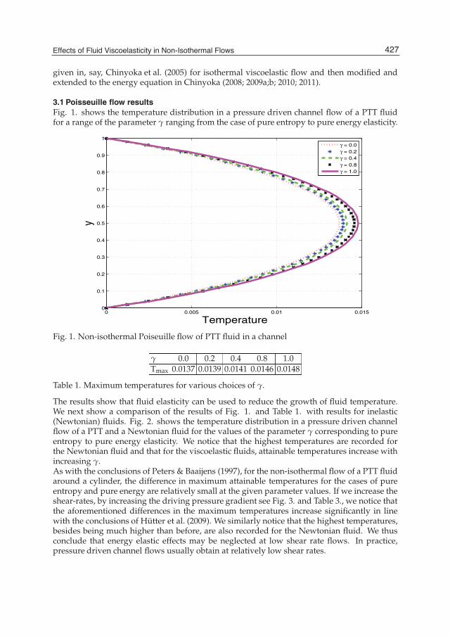
Effects of Fluid Viscoelasticity inNon-Isothermal Flows 5
given in, say, Chinyoka et al. (2005) for isothermal viscoelastic flow and then modified andextended to the energy equation in Chinyoka (2008; 2009a;b; 2010; 2011).
3.1 Poisseuille flow resultsFig. 1. shows the temperature distribution in a pressure driven channel flow of a PTT fluidfor a range of the parameter γ ranging from the case of pure entropy to pure energy elasticity.
0 0.005 0.01 0.0150
0.1
0.2
0.3
0.4
0.5
0.6
0.7
0.8
0.9
1
y
Temperature
γ = 0.0γ = 0.2γ = 0.4γ = 0.8γ = 1.0
Fig. 1. Non-isothermal Poiseuille flow of PTT fluid in a channel
γ 0.0 0.2 0.4 0.8 1.0Tmax 0.0137 0.0139 0.0141 0.0146 0.0148
Table 1. Maximum temperatures for various choices of γ.
The results show that fluid elasticity can be used to reduce the growth of fluid temperature.We next show a comparison of the results of Fig. 1. and Table 1. with results for inelastic(Newtonian) fluids. Fig. 2. shows the temperature distribution in a pressure driven channelflow of a PTT and a Newtonian fluid for the values of the parameter γ corresponding to pureentropy to pure energy elasticity. We notice that the highest temperatures are recorded forthe Newtonian fluid and that for the viscoelastic fluids, attainable temperatures increase withincreasing γ.As with the conclusions of Peters & Baaijens (1997), for the non-isothermal flow of a PTT fluidaround a cylinder, the difference in maximum attainable temperatures for the cases of pureentropy and pure energy are relatively small at the given parameter values. If we increase theshear-rates, by increasing the driving pressure gradient see Fig. 3. and Table 3., we notice thatthe aforementioned differences in the maximum temperatures increase significantly in linewith the conclusions of Hütter et al. (2009). We similarly notice that the highest temperatures,besides being much higher than before, are also recorded for the Newtonian fluid. We thusconclude that energy elastic effects may be neglected at low shear rate flows. In practice,pressure driven channel flows usually obtain at relatively low shear rates.
427Effects of Fluid Viscoelasticity in Non-Isothermal Flows
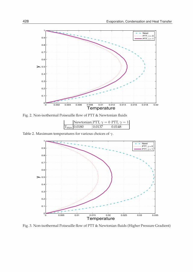
6 Will-be-set-by-IN-TECH
0 0.002 0.004 0.006 0.008 0.01 0.012 0.014 0.016 0.018 0.020
0.1
0.2
0.3
0.4
0.5
0.6
0.7
0.8
0.9
1
y
Temperature
NewtPTT, γ = 0PTT, γ = 1
Fig. 2. Non-isothermal Poiseuille flow of PTT & Newtonian fluids
Newtonian PTT, γ = 0 PTT, γ = 1Tmax 0.0180 0.0137 0.0148
Table 2. Maximum temperatures for various choices of γ.
0 0.005 0.01 0.015 0.02 0.025 0.03 0.0350
0.1
0.2
0.3
0.4
0.5
0.6
0.7
0.8
0.9
1
y
Temperature
NewtPTT, γ = 0PTT, γ = 1
Fig. 3. Non-isothermal Poiseuille flow of PTT & Newtonian fluids (Higher Pressure Gradient)
428 Evaporation, Condensation and Heat Transfer
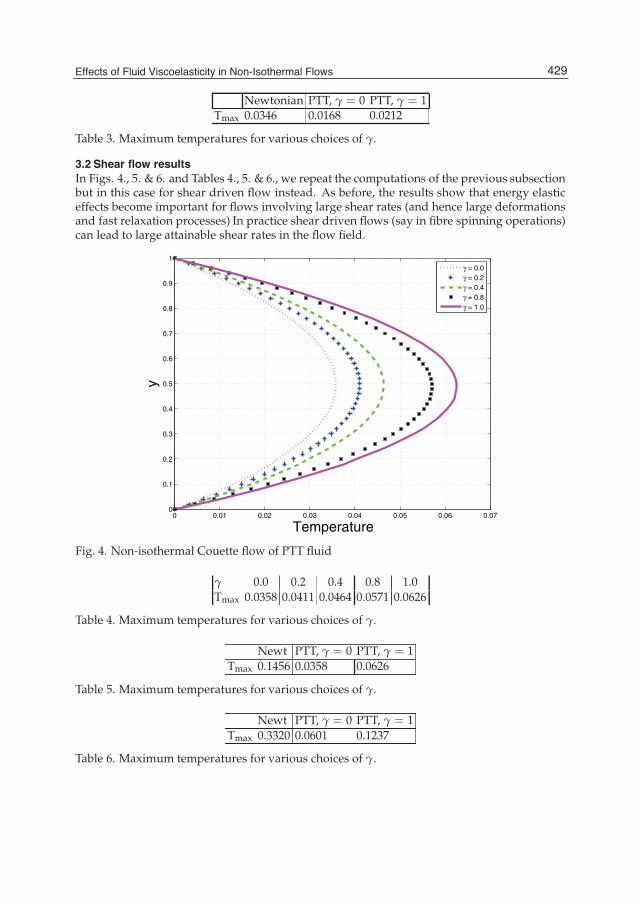
Effects of Fluid Viscoelasticity inNon-Isothermal Flows 7
Newtonian PTT, γ = 0 PTT, γ = 1Tmax 0.0346 0.0168 0.0212
Table 3. Maximum temperatures for various choices of γ.
3.2 Shear flow resultsIn Figs. 4., 5. & 6. and Tables 4., 5. & 6., we repeat the computations of the previous subsectionbut in this case for shear driven flow instead. As before, the results show that energy elasticeffects become important for flows involving large shear rates (and hence large deformationsand fast relaxation processes) In practice shear driven flows (say in fibre spinning operations)can lead to large attainable shear rates in the flow field.
0 0.01 0.02 0.03 0.04 0.05 0.06 0.070
0.1
0.2
0.3
0.4
0.5
0.6
0.7
0.8
0.9
1
y
Temperature
γ = 0.0γ = 0.2γ = 0.4γ = 0.8γ = 1.0
Fig. 4. Non-isothermal Couette flow of PTT fluid
γ 0.0 0.2 0.4 0.8 1.0Tmax 0.0358 0.0411 0.0464 0.0571 0.0626
Table 4. Maximum temperatures for various choices of γ.
Newt PTT, γ = 0 PTT, γ = 1Tmax 0.1456 0.0358 0.0626
Table 5. Maximum temperatures for various choices of γ.
Newt PTT, γ = 0 PTT, γ = 1Tmax 0.3320 0.0601 0.1237
Table 6. Maximum temperatures for various choices of γ.
429Effects of Fluid Viscoelasticity in Non-Isothermal Flows
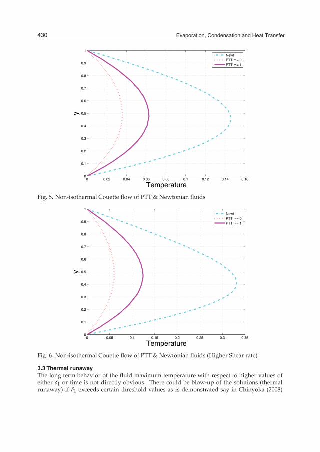
8 Will-be-set-by-IN-TECH
0 0.02 0.04 0.06 0.08 0.1 0.12 0.14 0.160
0.1
0.2
0.3
0.4
0.5
0.6
0.7
0.8
0.9
1
y
Temperature
NewtPTT, γ = 0PTT, γ = 1
Fig. 5. Non-isothermal Couette flow of PTT & Newtonian fluids
0 0.05 0.1 0.15 0.2 0.25 0.3 0.350
0.1
0.2
0.3
0.4
0.5
0.6
0.7
0.8
0.9
1
y
Temperature
NewtPTT, γ = 0PTT, γ = 1
Fig. 6. Non-isothermal Couette flow of PTT & Newtonian fluids (Higher Shear rate)
3.3 Thermal runawayThe long term behavior of the fluid maximum temperature with respect to higher values ofeither δ1 or time is not directly obvious. There could be blow-up of the solutions (thermalrunaway) if δ1 exceeds certain threshold values as is demonstrated say in Chinyoka (2008)
430 Evaporation, Condensation and Heat Transfer
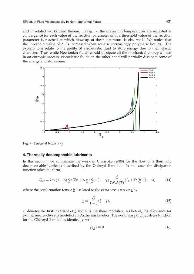
Effects of Fluid Viscoelasticity inNon-Isothermal Flows 9
and in related works cited therein. In Fig. 7, the maximum temperatures are recorded atconvergence for each value of the reaction parameter until a threshold value of the reactionparameter is reached at which blow-up of the temperature is observed. We notice thatthe threshold value of δ1 is increased when we use increasingly polymeric liquids. Theexplanations relate to the ability of viscoelastic fluid to store energy due to their elasticcharacter. Thus while Newtonian fluids would dissipate all the mechanical energy as heatin an entropic process, viscoelastic fluids on the other hand will partially dissipate some ofthe energy and store some.
0 0.5 1 1.5 2 2.5 3 3.5 4 4.50
0.5
1
1.5
2
2.5
3
3.5
δ1
Tmax
β=0β=0.2β=0.4β=0.8
Fig. 7. Thermal Runaway
4. Thermally decomposable lubricants
In this section, we summarize the work in Chinyoka (2008) for the flow of a thermallydecomposable lubricant described by the Oldroyd-B model. In this case, the dissipationfunction takes the form,
QD = 2μs (1− β) S : ∇u + γ τ : S + (1− γ)G
2Weλ(T)(I1 + Tr (b−1)− 6), (14)
where the conformation tensor b is related to the extra stress tensor τ by:
τ =G
1− ξ(b− I). (15)
I1 denotes the first invariant of b and G is the shear modulus. As before, the allowance forexothermic reactions is modeled via Arrhenius kinetics. The nonlinear polymer stress functionfor the Oldroyd-B model is identically zero,
f (τ) ≡ 0. (16)
431Effects of Fluid Viscoelasticity in Non-Isothermal Flows
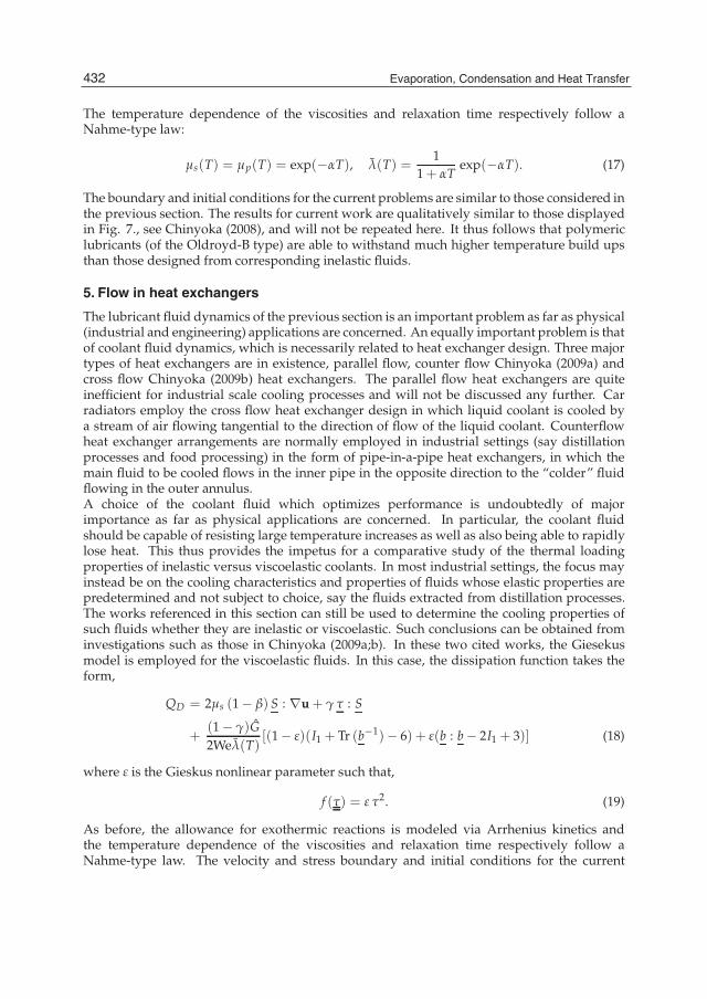
10 Will-be-set-by-IN-TECH
The temperature dependence of the viscosities and relaxation time respectively follow aNahme-type law:
μs(T) = μp(T) = exp(−αT), λ(T) =1
1 + αTexp(−αT). (17)
The boundary and initial conditions for the current problems are similar to those considered inthe previous section. The results for current work are qualitatively similar to those displayedin Fig. 7., see Chinyoka (2008), and will not be repeated here. It thus follows that polymericlubricants (of the Oldroyd-B type) are able to withstand much higher temperature build upsthan those designed from corresponding inelastic fluids.
5. Flow in heat exchangers
The lubricant fluid dynamics of the previous section is an important problem as far as physical(industrial and engineering) applications are concerned. An equally important problem is thatof coolant fluid dynamics, which is necessarily related to heat exchanger design. Three majortypes of heat exchangers are in existence, parallel flow, counter flow Chinyoka (2009a) andcross flow Chinyoka (2009b) heat exchangers. The parallel flow heat exchangers are quiteinefficient for industrial scale cooling processes and will not be discussed any further. Carradiators employ the cross flow heat exchanger design in which liquid coolant is cooled bya stream of air flowing tangential to the direction of flow of the liquid coolant. Counterflowheat exchanger arrangements are normally employed in industrial settings (say distillationprocesses and food processing) in the form of pipe-in-a-pipe heat exchangers, in which themain fluid to be cooled flows in the inner pipe in the opposite direction to the “colder” fluidflowing in the outer annulus.A choice of the coolant fluid which optimizes performance is undoubtedly of majorimportance as far as physical applications are concerned. In particular, the coolant fluidshould be capable of resisting large temperature increases as well as also being able to rapidlylose heat. This thus provides the impetus for a comparative study of the thermal loadingproperties of inelastic versus viscoelastic coolants. In most industrial settings, the focus mayinstead be on the cooling characteristics and properties of fluids whose elastic properties arepredetermined and not subject to choice, say the fluids extracted from distillation processes.The works referenced in this section can still be used to determine the cooling properties ofsuch fluids whether they are inelastic or viscoelastic. Such conclusions can be obtained frominvestigations such as those in Chinyoka (2009a;b). In these two cited works, the Giesekusmodel is employed for the viscoelastic fluids. In this case, the dissipation function takes theform,
QD = 2μs (1− β) S : ∇u + γ τ : S
+(1− γ)G2Weλ(T)
[(1− ε)(I1 + Tr (b−1)− 6) + ε(b : b− 2I1 + 3)] (18)
where ε is the Gieskus nonlinear parameter such that,
f (τ) = ε τ2. (19)
As before, the allowance for exothermic reactions is modeled via Arrhenius kinetics andthe temperature dependence of the viscosities and relaxation time respectively follow aNahme-type law. The velocity and stress boundary and initial conditions for the current
432 Evaporation, Condensation and Heat Transfer
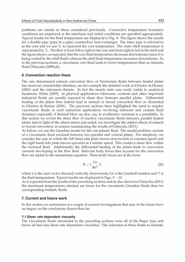
Effects of Fluid Viscoelasticity inNon-Isothermal Flows 11
problems are similar to those considered previously. Convective temperature boundaryconditions are employed at the interfaces and initial conditions are specified appropriately.Typical results for the fluid temperature are displayed in Fig. 8. The figure shows the resultsfor a double pipe (pipe in a pipe) counterflow heat exchanger. The inner pipe is referred toas the core and we use Tc to represent the core temperature. The outer shell temperature isrepresented by Ts. The flow is from left to right in the core and from right to left in the shell andthe figure shows, as expected, that the core fluid temperature decreases downstream (since it isbeing cooled by the shell fluid) whereas the shell fluid temperature increases downstream. Asin the previous sections, a viscoelastic core fluid leads to lower temperatures than an inelasticfluid Chinyoka (2009a;b).
6. Convection reaction flows
The one dimensional natural convection flow of Newtonian fluids between heated plateshas received considerable attention, see for example the detailed work in Christov & Homsy(2001) and the references therein. In fact the steady state case easily yields to analyticaltreatment, White (2005). In physical applications lubricants, coolants and other importantindustrial fluids are usually exposed to shear flow between parallel plates. Differentialheating of the plates thus indeed lead to natural or forced convection flow as illustratedin Christov & Homsy (2001). The previous sections have highlighted the need to employviscoelastic fluids in such industrial applications involving lubricant and coolant fluiddynamics especially if thermal blow up due, say, to exothermic reactions is a possibility. Inthis section we revisit the shear flow of reactive viscoelastic fluids between parallel heatedplates and in light of the observations just noted, we investigate the added effects of naturalor forced convection, in essence summarizing the results of Chinyoka (2011).As before, we use the Giesekus model for the viscoelastic fluid. The model problem consistsof a viscoelastic fluid enclosed between two parallel and vertical plates. For simplicity, weconsider the case in which the left hand side plate moves downwards at constant speed andthe right hand side plate moves upwards at a similar speed. This creates a shear flow withinthe enclosed fluid. Additionally, the differential heating of the plates leads to convectioncurrents developing in the flow field. Relevant body forces that account for the convectionflow are added to the momentum equation. These body forces are of the form:
F = iGrRe2 T, (20)
where i is the unit vector directed vertically downwards, Gr is the Grashoff number and T isthe fluid temperature. Typical results are displayed in Figs. 9. - 12.As is expected from the results of the preceding sections and as also shown in Chinyoka (2011)the maximum temperatures attained are lower for the viscoelastic Giesekus fluids than forcorresponding inelastic fluids.
7. Current and future work
In this section we summarize at a couple of current investigations that may in the future havean impact on the conclusions drawn thus far.
7.1 Shear rate dependent viscosityThe viscoelastic fluids chronicled in the preceding sections were all of the Boger type andhence all had non shear-rate dependent viscosities. The reduction of these fluids to inelastic
433Effects of Fluid Viscoelasticity in Non-Isothermal Flows
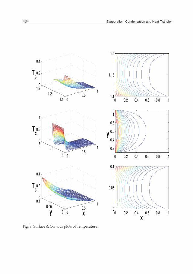
12 Will-be-set-by-IN-TECH
0 0.2 0.4 0.6 0.8 11.1
1.15
1.2
0 0.2 0.4 0.6 0.8 1
0.2
0.4
0.6
0.8
1
0 0.2 0.4 0.6 0.8 10
0.05
0.1
00.5
1
1.11.2
1.30
0.2
0.4
00.5
1
01
20
0.5
1
00.5
1
00.05
0.10
0.2
0.4
x x y
y
Ts
Tc
Ts
Fig. 8. Surface & Contour plots of Temperature
434 Evaporation, Condensation and Heat Transfer
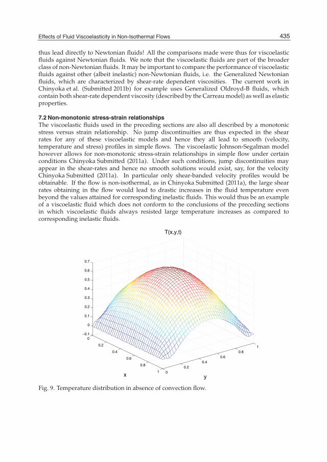
Effects of Fluid Viscoelasticity inNon-Isothermal Flows 13
thus lead directly to Newtonian fluids! All the comparisons made were thus for viscoelasticfluids against Newtonian fluids. We note that the viscoelastic fluids are part of the broaderclass of non-Newtonian fluids. It may be important to compare the performance of viscoelasticfluids against other (albeit inelastic) non-Newtonian fluids, i.e. the Generalized Newtonianfluids, which are characterized by shear-rate dependent viscosities. The current work inChinyoka et al. (Submitted 2011b) for example uses Generalized Oldroyd-B fluids, whichcontain both shear-rate dependent viscosity (described by the Carreau model) as well as elasticproperties.
7.2 Non-monotonic stress-strain relationshipsThe viscoelastic fluids used in the preceding sections are also all described by a monotonicstress versus strain relationship. No jump discontinuities are thus expected in the shearrates for any of these viscoelastic models and hence they all lead to smooth (velocity,temperature and stress) profiles in simple flows. The viscoelastic Johnson-Segalman modelhowever allows for non-monotonic stress-strain relationships in simple flow under certainconditions Chinyoka Submitted (2011a). Under such conditions, jump discontinuities mayappear in the shear-rates and hence no smooth solutions would exist, say, for the velocityChinyoka Submitted (2011a). In particular only shear-banded velocity profiles would beobtainable. If the flow is non-isothermal, as in Chinyoka Submitted (2011a), the large shearrates obtaining in the flow would lead to drastic increases in the fluid temperature evenbeyond the values attained for corresponding inelastic fluids. This would thus be an exampleof a viscoelastic fluid which does not conform to the conclusions of the preceding sectionsin which viscoelastic fluids always resisted large temperature increases as compared tocorresponding inelastic fluids.
00.2
0.40.6
0.81
0
0.2
0.4
0.6
0.8
1
−0.1
0
0.1
0.2
0.3
0.4
0.5
0.6
0.7
y
T(x,y,t)
x
Fig. 9. Temperature distribution in absence of convection flow.
435Effects of Fluid Viscoelasticity in Non-Isothermal Flows
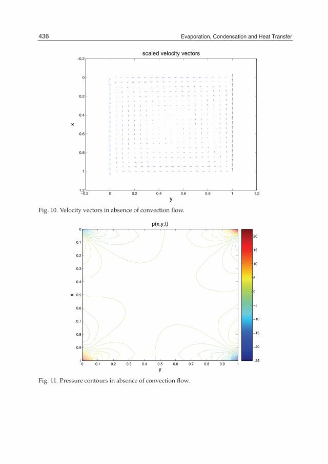
14 Will-be-set-by-IN-TECH
−0.2 0 0.2 0.4 0.6 0.8 1 1.2
−0.2
0
0.2
0.4
0.6
0.8
1
1.2
scaled velocity vectors
y
x
Fig. 10. Velocity vectors in absence of convection flow.
y
x
p(x,y,t)
0 0.1 0.2 0.3 0.4 0.5 0.6 0.7 0.8 0.9 1
0
0.1
0.2
0.3
0.4
0.5
0.6
0.7
0.8
0.9
1 −25
−20
−15
−10
−5
0
5
10
15
20
Fig. 11. Pressure contours in absence of convection flow.
436 Evaporation, Condensation and Heat Transfer
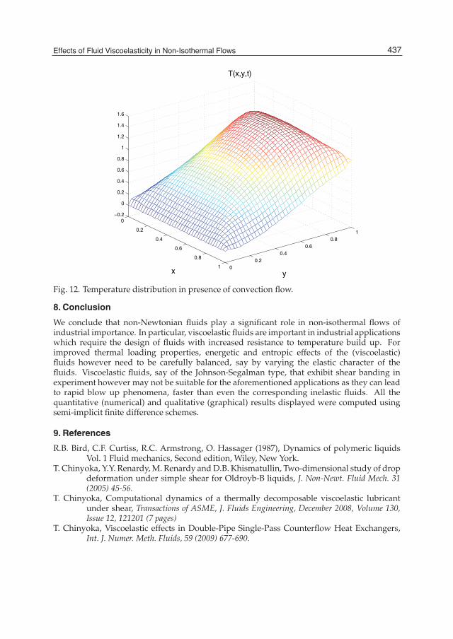
Effects of Fluid Viscoelasticity inNon-Isothermal Flows 15
00.2
0.40.6
0.81
0
0.2
0.4
0.6
0.8
1
−0.2
0
0.2
0.4
0.6
0.8
1
1.2
1.4
1.6
y
T(x,y,t)
x
Fig. 12. Temperature distribution in presence of convection flow.
8. Conclusion
We conclude that non-Newtonian fluids play a significant role in non-isothermal flows ofindustrial importance. In particular, viscoelastic fluids are important in industrial applicationswhich require the design of fluids with increased resistance to temperature build up. Forimproved thermal loading properties, energetic and entropic effects of the (viscoelastic)fluids however need to be carefully balanced, say by varying the elastic character of thefluids. Viscoelastic fluids, say of the Johnson-Segalman type, that exhibit shear banding inexperiment however may not be suitable for the aforementioned applications as they can leadto rapid blow up phenomena, faster than even the corresponding inelastic fluids. All thequantitative (numerical) and qualitative (graphical) results displayed were computed usingsemi-implicit finite difference schemes.
9. References
R.B. Bird, C.F. Curtiss, R.C. Armstrong, O. Hassager (1987), Dynamics of polymeric liquidsVol. 1 Fluid mechanics, Second edition, Wiley, New York.
T. Chinyoka, Y.Y. Renardy, M. Renardy and D.B. Khismatullin, Two-dimensional study of dropdeformation under simple shear for Oldroyb-B liquids, J. Non-Newt. Fluid Mech. 31(2005) 45-56.
T. Chinyoka, Computational dynamics of a thermally decomposable viscoelastic lubricantunder shear, Transactions of ASME, J. Fluids Engineering, December 2008, Volume 130,Issue 12, 121201 (7 pages)
T. Chinyoka, Viscoelastic effects in Double-Pipe Single-Pass Counterflow Heat Exchangers,Int. J. Numer. Meth. Fluids, 59 (2009) 677-690.
437Effects of Fluid Viscoelasticity in Non-Isothermal Flows
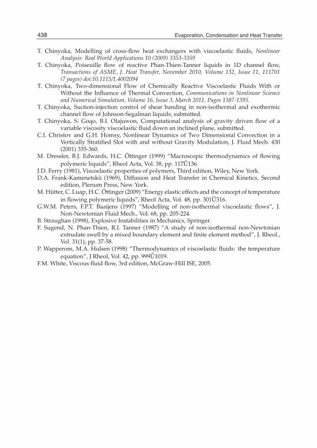
16 Will-be-set-by-IN-TECH
T. Chinyoka, Modelling of cross-flow heat exchangers with viscoelastic fluids, NonlinearAnalysis: Real World Applications 10 (2009) 3353-3359
T. Chinyoka, Poiseuille flow of reactive Phan-Thien-Tanner liquids in 1D channel flow,Transactions of ASME, J. Heat Transfer, November 2010, Volume 132, Issue 11, 111701(7 pages) doi:10.1115/1.4002094
T. Chinyoka, Two-dimensional Flow of Chemically Reactive Viscoelastic Fluids With orWithout the Influence of Thermal Convection, Communications in Nonlinear Scienceand Numerical Simulation, Volume 16, Issue 3, March 2011, Pages 1387-1395.
T. Chinyoka, Suction-injection control of shear banding in non-isothermal and exothermicchannel flow of Johnson-Segalman liquids, submitted.
T. Chinyoka, S. Goqo, B.I. Olajuwon, Computational analysis of gravity driven flow of avariable viscosity viscoelastic fluid down an inclined plane, submitted.
C.I. Christov and G.H. Homsy, Nonlinear Dynamics of Two Dimensional Convection in aVertically Stratified Slot with and without Gravity Modulation, J. Fluid Mech. 430(2001) 335-360.
M. Dressler, B.J. Edwards, H.C. Öttinger (1999) “Macroscopic thermodynamics of flowingpolymeric liquids”, Rheol Acta, Vol. 38, pp. 117U136.
J.D. Ferry (1981), Viscoelastic properties of polymers, Third edition, Wiley, New York.D.A. Frank-Kamenetskii (1969), Diffusion and Heat Transfer in Chemical Kinetics, Second
edition, Plenum Press, New York.M. Hütter, C. Luap, H.C. Öttinger (2009) “Energy elastic effects and the concept of temperature
in flowing polymeric liquids”, Rheol Acta, Vol. 48, pp. 301U316.G.W.M. Peters, F.P.T. Baaijens (1997) “Modelling of non-isothermal viscoelastic flows”, J.
Non-Newtonian Fluid Mech., Vol. 68, pp. 205-224.B. Straughan (1998), Explosive Instabilities in Mechanics, Springer.F. Sugend, N. Phan-Thien, R.I. Tanner (1987) “A study of non-isothermal non-Newtonian
extrudate swell by a mixed boundary element and finite element method”, J. Rheol.,Vol. 31(1), pp. 37-58.
P. Wapperom, M.A. Hulsen (1998) “Thermodynamics of viscoelastic fluids: the temperatureequation”, J Rheol, Vol. 42, pp. 999U1019.
F.M. White, Viscous fluid flow, 3rd edition, McGraw-Hill ISE, 2005.
438 Evaporation, Condensation and Heat Transfer
0
Different Approaches for Modellingof Heat Transfer in Non-Equilibrium
Reacting Gas Flows
E.V. Kustova and E.A. NagnibedaSaint Petersburg State University
Russia
1. Introduction
Modelling of heat transfer in non-equilibrium reacting gas flows is very important andpromising for many up-to-date practical applications. Thus, calculation of heat fluxes isneeded to solve the problem of heat protection for the surfaces of space vehicles enteringinto planet atmospheres.In high-temperature and hypersonic flows of gas mixtures, the energy exchange betweentranslational and internal degrees of freedom, chemical reactions, ionization and radiationresult in violation of thermodynamic equilibrium. Therefore the non-equilibrium effectsbecome of importance for a correct prediction of gas flow parameters and transport properties.The first attempt to take into account the excitation of internal degrees of freedom incalculations for the transport coefficients was made in 1913 by E. Eucken Eucken (1913),who introduced a phenomenological correction into the formula for the thermal conductivitycoefficient. Later on, stricter analysis for the influence of the excitation of internal degreesof freedom of molecules on heat and mass transfer was based on the kinetic theory of gases.Originally, in the papers concerning kinetic theory models for transport properties, mainlyminor deviations from the local thermal equilibrium were considered for non-reacting gasesFerziger & Kaper (1972); Wang Chang & Uhlenbeck (1951) and for mixtures with chemicalreactions Ern & Giovangigli (1994). In this approach non-equilibrium effects were takeninto account in transport equations by introducing supplementary kinetic coefficients: thecoefficient of volume viscosity in the expression for the pressure tensor and corrections to thethermal conductivity coefficient in the equation for the total energy flux. Such a descriptionof the real gas effects becomes insufficient under the conditions of finite (not weak) deviationsfrom the equilibrium, in which the energy exchange between some degrees of freedom andsome part of chemical reactions proceed simultaneously with the variation of gas-dynamicparameters. In this case characteristic times for gas-dynamic and relaxation processes becomecomparable, and therefore the equations for macroscopic parameters of the flow shouldbe coupled to the equations of physical-chemical kinetics. The transport coefficients, heatfluxes, diffusion velocities directly depend on non-equilibrium distributions, which may differsubstantially from the Boltzmann thermal equilibrium distribution. In this situation, theestimate for the impact of non-equilibrium kinetics on gas-dynamic parameters of a flow
21
2 Will-be-set-by-IN-TECH
and its dissipative properties becomes especially important. In recent years, these problemsreceive much attention, and new results have been obtained in this field on the basis of thegeneralized Chapman-Enskog method Nagnibeda & Kustova (2009), see also references inNagnibeda & Kustova (2009). The kinetic theory makes it possible to develop mathematicalmodels of a flow under different non-equilibrium conditions, i.e. to obtain closed systems ofthe non-equilibrium flow equations and to elaborate calculation procedures for transport andrelaxation properties.In the present chapter, on the basis of the kinetic theory developed in Nagnibeda & Kustova(2009), the mathematical models for calculation of heat transfer in strong non-equilibriumreacting mixtures are proposed for different conditions in a flow.
2. Theoretical models
The theoretical models adequately describing physical-chemical kinetics and transportproperties in a flow depend on relations between relaxation times of various kinetic processes.Experimental data show the significant difference in relaxation times of various processes.At the high temperature conditions which are typical just behind the shock front, theequilibrium over the translational and rotational degrees of freedom is established for asubstantially shorter time than that of vibrational relaxation and chemical reactions, andtherefore the following relation takes place Phys-Chem (2002); Stupochenko et al. (1967):
τtr < τrot � τvibr < τreact ∼ θ. (1)
In (1), τtr, τrot, τvibr and τreact are the the relaxation times for the translational, rotationaland vibrational degrees of freedom, and the characteristic time for chemical reactions; θ isthe mean time of the variation of gas-dynamics parameters. In this case for the descriptionof the non-equilibrium flow it is necessary to consider the equations of the state-to-statevibrational and chemical kinetics coupled to the gas dynamic equations. It is the most detaileddescription of the non-equilibrium flow. Transport properties in the flow depend not onlyon gas temperature and mixture composition but also on all vibrational level populations ofdifferent species Kustova & Nagnibeda (1998).More simple models of the flow are based on quasi-stationary multi-temperature orone-temperature vibrational distributions. In the vibrationally excited gas at moderatetemperatures, the near-resonant vibrational energy exchanges between molecules of the samechemical species occur much more frequently compared to the non-resonant transitionsbetween different molecules as well as transfers of vibrational energy to the translational androtational ones and chemical reactions:
τtr < τrot < τVV1 � τVV2 < τTRV < τreact ∼ θ. (2)
Here τVV1 , τVV2 , τTRV are, respectively, the mean times for the VV1 vibrational energyexchange between molecules of the same species, VV2 vibrational transitions betweenmolecules of different species and TRV transitions of the vibrational energy into other modes.Under this condition quasi-stationary (multi-temperature) distributions over the vibrationallevels establish due to rapid energy exchanges, and equations for vibrational level populationsare reduced to the equations for vibrational temperatures for different chemical species.
440 Evaporation, Condensation and Heat Transfer
Different Approaches for Modelling of Heat Transfer in Non-Equilibrium Reacting Gas Flows 3
Heat and mass transfer are specified by the gas temperature, molar fractions of species andvibrational temperatures of molecular components Chikhaoui et al. (1997).For tempered reaction regime, with the chemical reaction rate considerably lower than thatfor the internal energy relaxation, the following characteristic time relation takes place:
τtr < τint � τreact ∼ θ, (3)
τint is the mean time for the internal energy relaxation. Under this condition, thenon-equilibrium chemical kinetics can be described on the basis of the maintaining thermalequilibrium one-temperature Boltzmann distributions over internal energies of molecularspecies while transport properties are defined by the gas temperature and molar fractions ofmixture components Ern & Giovangigli (1994); Nagnibeda & Kustova (2009). The influenceof electronic excitation of atoms and molecules on the transport properties under the lastcondition is also considered in Kustova & Puzyreva (2009).Finally, if all relaxation processes and chemical reactions proceed faster than gas-dynamicparameters vary, the relaxation times satisfy the relation:
τtr < τint < τreact � θ. (4)
Under this condition, on the time scale θ a gas flow can be assumed thermally andchemically equilibrium or weakly non-equilibrium (Brokaw (1960); Butler & Brokaw (1957);Vallander et al. (1977)). In this case the closed system of governing equations of a flowcontains only conservation equations, and non-equilibrium effects in a viscous flow manifestthemselves mainly in transport coefficients.In the present contribution, for all these approaches, on the basis of the rigorous kinetictheory methods, we propose the closed sets of governing equations of a flow, expressions fortransport and relaxation terms in these equations and formulas for the calculation of transportcoefficients. The results of applications of proposed models for particular flows are brieflydiscussed. The comparison of the results obtained for heat transfer in different approachesbehind shock waves, in nozzle flows, in the non-equilibrium boundary layer and in a shocklayer near the re-entering body is discussed.
2.1 State-to-state model2.1.1 Distribution functions and governing equationsThe mathematical models of transport properties in non-equilibrium flows of reacting viscousgas mixtures are based on the first-order solutions of the kinetic equations for distributionfunctions fcij(r, u, t) over chemical species c, vibrational i and rotational j energy levels,particle velocities u, coordinates r and time t. In the case of strong deviations from thermaland chemical equilibrium in a flow, the kinetic processes may be divided for rapid and slowones and the kinetic equations for fcij(r, u, t) can be written in the form Nagnibeda & Kustova(2009)
∂ fcij
∂t+ uc · ∇ fcij =
1ε
Jrapcij + Jsl
cij, (5)
where Jrapcij , Jsl
cij are the collision operators for rapid and slow processes, respectively, the smallparameter ε represents the ratio of the characteristic times for rapid and slow processes ε =τrap/τsl ∼ τrap/θ � 1. Under the condition (5), the integral operator for rapid processes
441Different Approaches for Modelling of Heat Transfer in Non-Equilibrium Reacting Gas Flows
4 Will-be-set-by-IN-TECH
Jrapcij describes elastic collisions and rotational energy exchange whereas the operator for slow
processes Jslcij describes the vibrational energy exchange and chemical reactions:
Jrapcij = Jtr
cij + Jrotcij ,
Jslcij = Jvibr
cij + Jreactcij . (6)
The integral operators (6) are given in Ern & Giovangigli (1994); Nagnibeda & Kustova (2009).For the solution of the kinetic equations (5), (6) modification of the Chapman-Enskog methodfor rapid and slow processes Chikhaoui et al. (1997); Kustova & Nagnibeda (1998) is used.This method makes it possible to derive governing equations of the flow, expressions forthe dissipative and relaxation terms in these equations and algorithms for the calculation oftransport and reaction rate coefficients. The solution of the equations (5), (6) is sought as thegeneralized Chapman-Enskog series in the small parameter ε.The solution of the kinetic equations in the zero-order approximation
Jrap(0)cij = 0 (7)
is specified by the independent collision invariants of the most frequent collisions whichdefine rapid processes. These invariants include the momentum and particle total energywhich are conserved at any collision, and additional invariants for the most probable collisionswhich are given by any value independent of the velocity and rotational level j and dependingarbitrarily on the vibrational level i and chemical species c. The additional invariants appeardue to the fact that vibrational energy exchange and chemical reactions are supposed to befrozen in rapid processes. Based on the above set of the collision invariants, the zero-orderdistribution function takes the form
f (0)cij =( mc
2πkT
)3/2sci
jnci
Zrotci (T)
exp
(−mcc2
c2kT
−εci
j
kT
)(8)
Here, nci is the population of vibrational level i of species c, cc = uc − v, v is the macroscopicvelocity, εci
j is the rotational energy of the molecule at j-th rotational and i-th vibrational
levels, T is the gas temperature, mc is the molecular mass, k is the Boltzmann constant, scij
is the rotational statistical weight, Zrotci is the rotational partition function. For the rigid rotator
model, εcij = εc
j , Zrotci = Zrot
c = 8π2 IckTσh2 , Ic is the moment of inertia, h is the Planck constant, σ is
the symmetry factor.The distribution functions (8) are specified by the macroscopic gas parameters: nci(r, t)(c = 1, ..., L, i = 0, 1, ..., Lc, L is the number of chemical species, Lc is the number of excitedvibrational levels in species c), T(r, t), and v(r, t) which correspond to the set of the collisioninvariants of rapid processes.The closed set of equations for the macroscopic parameters nci(r, t), T(r, t), and v(r, t) followsfrom the kinetic equations and includes the conservation equations of momentum and totalenergy coupled to the relaxation equations of detailed state-to-state vibrational and chemical
442 Evaporation, Condensation and Heat Transfer
Different Approaches for Modelling of Heat Transfer in Non-Equilibrium Reacting Gas Flows 5
kinetics Nagnibeda & Kustova (2009):
dncidt
+ nci∇· v +∇· (nciVci) = Rci, c = 1, ..., L, i = 0, ..., Lc, (9)
ρdvdt
+∇· P = 0, (10)
ρdUdt
+∇· q + P : ∇v = 0. (11)
Here P is the pressure tensor, q is the total energy flux, Vci are diffusion velocities of moleculesat different vibrational states, U is the total energy per unit mass:
ρU =32
nkT + ρErot + ∑ci
εci nci +∑
cεcnc.
Erot is the rotational energy per unit mass, εci is the vibrational energy of a molecule of species
c at the i-th vibrational level, εc is the energy of formation of the particle of species c.The source terms in the equations (9) are expressed via the integral operators of slowprocesses:
Rci = ∑j
∫Jslcijd uc = Rvibr
ci + Rreactci . (12)
and characterize the variation of the vibrational level populations and atomic numberdensities caused by different vibrational energy exchanges and chemical reactions.For this approach, the vibrational level populations are included to the set of mainmacroscopic parameters, and the equations for their calculation are coupled to the equationsof gas dynamics. Particles of various chemical species in different vibrational states representthe mixture components, and the corresponding equations contain the diffusion velocities Vciof molecules at different vibrational states. Thus the diffusion of vibrational energies is thepeculiar feature of diffusion processes in the state-to-state approximation.
2.1.2 Transport propertiesIn the zero-order approximation of Chapman-Enskog method
P(0) = nkTI, q(0) = 0, V(0)ci = 0 ∀ c, i, (13)
I is the unity tensor.The set of governing equations in this case describes the detailed state-to-state vibrational andchemical kinetics in an inviscid non-conductive gas mixture flow in the Euler approximationNagnibeda & Kustova (2009). Taking into account the first-order approximation makes itpossible to consider dissipative properties in a non-equilibrium viscous gas.The first-order distribution functions can be written in the following structural formKustova & Nagnibeda (1998):
f (1)cij = f (0)cij
(− 1
nAcij · ∇ ln T − 1
n ∑dk
Ddkcij · ddk − 1
nBcij : ∇v− 1
nFcij∇ · v− 1
nGcij
). (14)
443Different Approaches for Modelling of Heat Transfer in Non-Equilibrium Reacting Gas Flows
6 Will-be-set-by-IN-TECH
The functions Acij, Ddkcij, Bcij, Fcij, and Gcij depend on the peculiar velocity cc and the flow
parameters: temperature T, velocity v, and vibrational level populations nci, and satisfy thelinear integral equations with linearized operator for rapid processes; dci are the diffusivedriving forces:
dci = ∇(nci
n
)+
(ncin− ρci
ρ
)∇ ln p. (15)
The transport kinetic theory in the state-to-state approximation was developed, for the firsttime, in Kustova & Nagnibeda (1998) and is given also in Nagnibeda & Kustova (2009). Theexpressions for the transport terms in the equations (9)-(11) in the first order approximationare derived on the basis of the distribution functions (14).The viscous stress tensor is described by the expression:
P = (p− prel)I− 2ηS− ζ∇ ·vI. (16)
Here, prel is the relaxation pressure, η and ζ are the coefficients of shear and bulk viscosity,S is the deformation rate tensor. The additional terms connected to the bulk viscosity andrelaxation pressure appear in the diagonal terms of the stress tensor in this case due to rapidinelastic TR exchange between the translational and rotational energies. The existence of therelaxation pressure is caused also by slow processes of vibrational and chemical relaxation. Ifall slow relaxation processes in a system disappear, then prel = 0.The diffusion velocity of molecular components c at the vibrational level i is specified in thestate-to-state approach by the expression Kustova & Nagnibeda (1998); Nagnibeda & Kustova(2009):
Vci = −∑dk
Dcidkddk − DTci∇ ln T, (17)
where Dcidk and DTci are the multi-component diffusion and thermal diffusion coefficients foreach chemical and vibrational species.The total energy flux in the first-order approximation has the form:
q = −λ′∇T − p ∑ci
DTcidci + ∑ci
(52
kT + 〈εci〉rot + εci + εc
)nciVci, (18)
where λtr + λrot is the thermal conductivity coefficient, 〈εci〉rot is the mean rotational energy.The coefficients λtr and λrot are responsible for the energy transfer associated with the mostprobable processes which, in the present case, are the elastic collisions and inelastic TR- andRR rotational energy exchanges. In the state-to-state approach, the transport of the vibrationalenergy is described by the diffusion of vibrationally excited molecules rather than the thermalconductivity. In particular, the diffusion of the vibrational energy is simulated by introducingthe independent diffusion coefficients for each vibrational state. It should be noted thatall transport coefficients are specified by the cross sections of rapid processes excepting therelaxation pressure depending also on the cross sections of slow processes of vibrationalrelaxation and chemical reactions.From the expressions (17), (18), it is seen that the energy flux and diffusion velocities includealong with the gradients of temperature and atomic number densities also the gradients ofall vibrational level populations with multi-component diffusion coefficients depending onthe vibrational levels of colliding molecules. In the state-to-state approach, the transport of
444 Evaporation, Condensation and Heat Transfer
Different Approaches for Modelling of Heat Transfer in Non-Equilibrium Reacting Gas Flows 7
vibrational energy is associated with diffusion of vibrationally excited molecules rather thanwith heat conductivity. This constitutes the main feature of the heat transfer and diffusionin the state-to-state approach and the fundamental difference between Vci and q and thediffusion velocities and heat flux obtained on the basis of one-temperature, multi-temperatureor weakly non-equilibrium approaches.The transport coefficients in the expressions (16)-(18) can be written in terms of functions Acij,Ddk
cij, Bcij, Fcij, and Gcij:
η =kT10
[B, B] , ζ = kT [F, F] , prel = kT [F, G] , (19)
Dcidk =1
3n
[Dci, Ddk
], DTci =
13n
[Dci, A
], λ′ = k
3[A, A] (20)
Here [A, B] are the bracket integrals associated with the linearized operator of rapid processes.They were introduced in Nagnibeda & Kustova (2009) for strongly non-equilibrium reactingmixtures similarly to those defined in Ferziger & Kaper (1972) for a non-reacting gas mixtureunder the conditions for weak deviations from the equilibrium.For the transport coefficients calculation in the state-to-state approximation, the functionsAcij, Ddk
cij, Bcij, Fcij, and Gcij are expanded into the Sonine polynomials in the reducedpeculiar velocity and those of Waldmann-Trübenbacher in the dimensionless rotationalenergy. For the coefficients of these expansions, the linear transport systems are derived inKustova & Nagnibeda (1998), Nagnibeda & Kustova (2009), and the transport coefficients areexpressed in terms of the solutions of these systems.Solving transport linear systems for multi-component mixtures in the state-to-stateapproximation is a very complicated technical problem because a great number of equationsshould be considered. A simplified technique for the calculation of the transport coefficientskeeping the main advantages of the state-to-state approach, is suggested in Kustova (2001).The assumptions proposed in this paper made it possible to noticeably reduce the number ofmulti-component diffusion and thermal diffusion coefficients and simplify the expressions forthe diffusion velocity and heat flux:
Vci = −Dcicidci − Dcc ∑k =i
dck − ∑d =c
Dcddd −DTc∇ ln T, (21)
q = −λ′∇T− p ∑c
DTcdc + ∑ci
(52
kT +⟨
εcij
⟩rot
+ εci + εc
)nciVci. (22)
Here, dc is the classical diffusive driving force associated to chemical species rather thanto the vibrational level Ferziger & Kaper (1972). It is important to emphasize that in theseformulae, after the simplifications, only the self-diffusion coefficients Dcici depend explicitlyon the vibrational quantum number.The systems for the calculation of the diffusion, viscosity and thermal conductivity coefficientscan be solved using the efficient numerical algorithms elaborated in Ern & Giovangigli (1994)for the solution of linear algebraic systems, or more traditional techniques used in classicalmonographs on the kinetic theory Chapman & Cowling (1970); Ferziger & Kaper (1972);Hirschfelder et al. (1954).
445Different Approaches for Modelling of Heat Transfer in Non-Equilibrium Reacting Gas Flows
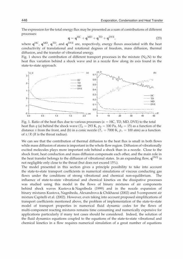
8 Will-be-set-by-IN-TECH
The expression for the total energy flux may be presented as a sum of contributions of differentprocesses:
q = qHC + qMD + qTD + qDVE, (23)
where qHC, qMD, qTD, and qDVE are, respectively, energy fluxes associated with the heatconductivity of translational and rotational degrees of freedom, mass diffusion, thermaldiffusion, and the transfer of vibrational energy.Fig. 1 shows the contribution of different transport processes in the mixture (N2,N) to theheat flux variation behind a shock wave and in a nozzle flow along its axis found in thestate-to-state approach.
0.0 0.5 1.0 1.5 2.0-2
-1
0
1
2
3(a)
x, cm
q /q
HC TD MD DVE
0 10 20 30 40 50
0.0
0.1
0.2
0.3
0.4
0.5
0.6
0.7
HC TD MD DVE
(b)q /q
x/R
Fig. 1. Ratio of the heat flux due to various processes (α = HC, TD, MD, DVE) to the totalheat flux q (a) behind the shock wave (T0 = 293 K, p0 = 100 Pa, M0 = 15) as a function of thedistance x from the front, and (b) in a conic nozzle (T∗ = 7000 K, p∗ = 100 atm) as a functionof x/R (R is the throat radius).
We can see that the contribution of thermal diffusion to the heat flux is small in both flowswhile mass diffusion of atoms is important in the whole flow region. Diffusion of vibrationallyexcited molecules plays more important role behind a shock than in a nozzle. Close to theshock front, heat conduction and mass diffusion compensate each other, and the main role inthe heat transfer belongs to the diffusion of vibrational states. In an expanding flow, qDVE isnot negligible only close to the throat (but does not exceed 15%).The model presented in this section gives a principle possibility to take into accountthe state-to-state transport coefficients in numerical simulations of viscous conducting gasflows under the conditions of strong vibrational and chemical non-equilibrium. Theinfluence of state-to-state vibrational and chemical kinetics on the dissipative processeswas studied using this model in the flows of binary mixtures of air componentsbehind shock waves Kustova & Nagnibeda (1999) and in the nozzle expansion ofbinary mixtures Kustova, Nagnibeda, Alexandrova & Chikhaoui (2002) and 5-component airmixture Capitelli et al. (2002). However, even taking into account proposed simplifications oftransport coefficients mentioned above, the problem of implementation of the state-to-statemodel of transport properties in numerical fluid dynamic codes for the flows ofmulti-component reacting mixtures remains time consuming and numerically expensive forapplications particularly if many test cases should be considered. Indeed, the solution ofthe fluid dynamics equations coupled to the equations of the state-to-state vibrational andchemical kinetics in a flow requires numerical simulation of a great number of equations
446 Evaporation, Condensation and Heat Transfer
Different Approaches for Modelling of Heat Transfer in Non-Equilibrium Reacting Gas Flows 9
for the vibrational level populations of all molecular species. Moreover, the closed systemof macroscopic equations in the state-to-state approach includes the state-dependent ratecoefficients of all vibrational energy transitions and chemical reactions. Experimentaland theoretical data on these rate coefficients and especially on the cross sections ofinelastic processes are rather scanty. Due to the above problems, simpler models based onquasi-stationary vibrational distributions are rather attractive for practical applications.Such approaches are considered in the next section.
2.2 Quasi-stationary modelsIn quasi-stationary approaches, the vibrational level populations are expressed in terms of afew macroscopic parameters, consequently, non-equilibrium kinetics can be described by aconsiderably reduced set of governing equations. Commonly used models are based on theBoltzmann distribution with the vibrational temperature different from the gas temperature.However, such a distribution appears not to be justified under the conditions of strongvibrational excitation, since it is valid solely for the harmonic oscillator model, whichdescribes adequately only the low vibrational states. In the present section, the transportkinetic theory is considered on the basis of the non-Boltzmann vibrational distributions takinginto account anharmonic vibrations.
2.2.1 Distribution functions and governing equationsQuasi-stationary models follow from the kinetic equations (5) under the conditions (2) forthe relaxation times. In this case, the integral operator of the most frequent collisions in thekinetic equations (5) for distribution functions includes the operator of VV1 vibrational energytransitions between molecules of the same species along with the operators of elastic collisionsand collisions with rotational energy exchanges:
Jrapcij = Jtr
cij + Jrotcij + JVV1
cij . (24)
The operator of slow processes Jslcij consists of the operator of VV2 vibrational transitions
between molecules of different species, the operator describing the transfer of vibrationalenergy into rotational and translational modes JTRV
cij , as well as the operator of chemicalreactions Jreact
cij :
Jslcij = JVV1
cij + JTRVcij + Jreact
cij . (25)
For the solution of Eqs. (5) with the collisional operators (24) and (25), the distributionfunction is expanded into the generalized Chapman-Enskog series in the small parameterε ∼ τVV1 /θ. In the zero-order approximation, the following equation for the distributionfunction is deduced:
Jtr(0)cij + Jrot(0)
cij + JVV1(0)cij = 0 (26)
The solution of these equations is specified by the invariants of the most frequent collisions. Inaddition to the momentum and total energy which are conserved in any collision, under thecondition (2) there are additional independent invariants of rapid processes: the number ofthe vibrational quanta in a molecular species c, and any value independent of the velocity,vibrational i and rotational j quantum numbers and depending arbitrarily on the particlechemical species c. Conservation of vibrational quanta presents an important feature of
447Different Approaches for Modelling of Heat Transfer in Non-Equilibrium Reacting Gas Flows
10 Will-be-set-by-IN-TECH
collisions resulting in the VV1 vibrational energy exchange between the molecules of the samespecies. The existence of a similar invariant for VV transitions in a single-component gaswas found for the first time in Treanor et al. (1968) where a non-equilibrium quasi-stationarysolution of balance equations for the vibrational level populations was found using thisinvariant. This solution is now called the Treanor distribution.In a gas mixture, during VV1 vibrational energy exchange between molecules of the samespecies, the number of vibrational quanta in a given species keeps constant. The existence ofthe other additional invariants is explained by the fact that under the condition (2), chemicalreactions are supposed to be slow and remain frozen in the most frequent collisions.Taking into account the system of collision invariants we obtain the zero-order distributionfunctions:
f (0)cij =( mc
2πkT
)3/2 ncsci
Zrotc (T)Zvibr
c (T, Tc1)
exp
(−mcc2
c2kT
−εc
j
kT− εc
i − iεc1
kT− iεc
1kTc
1
). (27)
Here, Zvibrc is the non-equilibrium vibrational partition function for molecules of species c:
Zvibrc = Zvibr
c (T, Tc1) = ∑
isc
i exp(− εc
i − iεc1
kT− iεc
1kTc
1
). (28)
Zrotc (T) is given in Section 2.1, Tc
1 is the temperature of the first vibrational level for eachmolecular species c. It should be noted that vibrational energy εc
i hereafter is countedfrom the energy of the zero-th level. The functions (27) represent the local equilibriumMaxwell-Boltzmann distribution of molecules over the velocity and rotational energy levelsand the nonequilibrium distribution over the vibrational states and chemical species. For thevibrational level populations, from Eq. (27) it follows:
nci =nc
Zvibrc (T, Tc
1)sc
i exp(− εc
i − iεc1
kT− iεc
1kTc
1
). (29)
It should be emphasized that nci depend on two temperatures (T and Tc1) because
translational-rotational and vibrational degrees of freedom are not isolated in the mostfrequent collisions as a consequence of the non-resonant character of VV1 exchange.The distribution function is specified by the macroscopic parameters nc, v, T, and Tc
1 . Thetemperature Tc
1 is associated to the additional collision invariant ic and is defined by the meanspecific number of vibrational quanta Wc in molecular species c:
ρcWc = ∑ij
ic
∫fcij duc. (30)
The expression (29) yields the non-equilibrium quasi-stationary Treanor distributionTreanor et al. (1968) in a multi-component gas mixture. Note that similarly to asingle-component gas, the distribution (29) describes adequately only the populations oflow vibrational levels ic ≤ ic∗, where ic∗ corresponds to the minimum of the function nci.It is explained by the fact that the number of vibrational quanta is conserved only at lowlevels ic ≤ ic∗. For the collisions of molecules at higher vibrational states ic > ic∗, theprobability of VV1 transitions becomes comparable to that of VV2 and VT vibrational energy
448 Evaporation, Condensation and Heat Transfer
Different Approaches for Modelling of Heat Transfer in Non-Equilibrium Reacting Gas Flows 11
exchanges. In the high gas temperature range, if T � Tc1, the level ic∗ appears to be close to
the last vibrational level ic = Lc and the Treanor distribution is valid for the entire range ofvibrational states. Such a situation is typical for the relaxation zone behind a shock wave. Fora strongly excited gas with a high vibrational energy supply (Tc
1 � T), the minimum of theTreanor distribution is located rather low, and the increasing branch of the distribution is notphysically consistent. In this case it is necessary to account for various relaxation channelsat different groups of vibrational levels. Non-equilibrium vibrational distributions takinginto account this effect was obtained for a one-component gas in Gordiets & Mamedov (1974);Kustova & Nagnibeda (1997) and are given also in Nagnibeda & Kustova (2009).Under the conditions when the anharmonic effects can be neglected, the distribution (29) isreduced to the non-equilibrium Boltzmann distribution with the vibrational temperature ofmolecular components Tc
v = Tc1 different from T:
nci =nc
Zvibrc
sci exp
(− εc
ikTc
1
), (31)
where the vibrational partition function takes the form
Zvibrc = Zvibr
c (Tc1) = ∑
isc
i exp(− εc
ikTc
1
). (32)
In the case of the local thermal equilibrium, the vibrational temperatures of all molecularspecies are equal to the gas temperature Tc
1 = T, and the Treanor distribution (29) is reducedto the one-temperature Boltzmann distribution:
nci =nc
Zvibrc
sci exp
(− εc
ikT
), (33)
Zvibrc = Zvibr
c (T) = ∑i
sci exp
(− εc
ikT
). (34)
The closed set of governing equations for the macroscopic parameters nc(r, t), v(r, t), T(r, t),and Tc
1(r, t) were derived in Chikhaoui et al. (2000; 1997), it includes conservation equationsfor the momentum and the total energy, equations for species number densities and additionalrelaxation equations for the specific numbers of vibrational quanta Wc in each molecularspecies c:
dnc
dt+ nc∇ · v +∇ · (ncVc) = Rreact
c , c = 1, ..., L, (35)
ρdvdt
+∇· P = 0, (36)
ρdUdt
+∇· q + P : ∇v = 0, (37)
ρcdWc
dt+∇ · qw,c = Rw
c −WcmcRreactc + Wc∇ · (ρcVc) , c = 1, ..., Lm. (38)
449Different Approaches for Modelling of Heat Transfer in Non-Equilibrium Reacting Gas Flows
12 Will-be-set-by-IN-TECH
(L is the total number of species, Lm is the number of molecular species).The conservation equations for the momentum and total energy (36) and (37) formallycoincide with the corresponding equations (10) and (11) obtained in the state-to-stateapproach. One should however bear in mind that in the multi-temperature approach, thetotal energy is a function of T, Tc
1, and nc:
ρU =32
nkT +Lm
∑c=1
ρcErot,c(T) +Lm
∑c=1
ρcEvibr,c(T, Tc1), (39)
Evibr,c(T, Tc1) is the specific vibrational energy of species c. The transport terms are expressed
as functions of the same set of macroscopic parameters.In Eqs. (35), (38), Vc is the diffusion velocity of species c. The value qw,c in Eq. (38) has thephysical meaning of the vibrational quanta flux of c molecular species and is introduced onthe basis of the additional collision invariant of the most frequent collisions ic:
qw,c = ∑ij
i∫
cc fcijduc. (40)
The source terms in Eqs. (35) are determined by the collision operator of chemical reactions
Rreactc = ∑
ij
∫Jreactcij duc. (41)
The production terms in the relaxation equations (38) for the specific numbers of vibrationalquanta are expressed as functions of collision operators of all slow processes: VV2 and TRVvibrational energy transfers and chemical reactions,
Rwc = ∑
iji∫
Jslcijd uc = Rw, VV2
c + Rw, TRVc + Rw, react
c . (42)
Thus the equations of non-equilibrium chemical kinetics (35) coupled to the conservationequations of the momentum and the total energy (36), (37), as well as to the relaxationequations (38) for the specific numbers of vibrational quanta in molecular components Wc (38)form a closed system of governing equations for the macroscopic parameters of a reacting gasmixture flow in the generalized multi-temperature approach. It is obvious that the system(35)–(38) is considerably simpler than the corresponding system (9)–(11) in the state-to-stateapproach, as it contains much fewer equations. Indeed, instead of ∑c Lc (c = 1, 2, ..., Lmstands for the molecular species) equations for the vibrational level populations, one shouldsolve Lm equations for the numbers of quanta and Lm equations for the number densities ofthe chemical components. Consequently, for a two-component mixture containing nitrogenmolecules and atoms, one relaxation equation for WN2 and one equation for the numberdensity of N2 molecules should be solved instead of 46 equations for the level populations.While studying the important for practical applications five-component air mixture N2, O2,NO, N, O in the state-to-state approach, one should solve LN2 + LO2 + LNO = 114 equationsfor the vibrational level populations. In the multi-temperature approach, they are reduced tosix equations: three for the molecular number densities and three for TN2
1 , TO21 , and TNO
1 .
450 Evaporation, Condensation and Heat Transfer
Different Approaches for Modelling of Heat Transfer in Non-Equilibrium Reacting Gas Flows 13
In a system of harmonic oscillators, the relaxation equations for the specific numbers ofvibrational quanta Wc (38) are transformed into those for the specific vibrational energy:
ρcdEvibr,c
dt+∇ · qvibr,c = Rvibr
c − Evibr,cmcRreactc + Evibr,c∇ · (ρcVc) , c = 1, 2, ..., Lm, (43)
withqvibr,c = εc
1qw,c, Rvibrc = εc
1Rwc . (44)
2.2.2 Transport propertiesIn the zero-order approximation of the Chapman-Enskog method, the transport terms arefound taking into account the distribution function (27):
P(0) = nkTI, q(0) = 0, q(0)w,c = 0, V(0)
c = 0 ∀ c, (45)
and the system (35)–38) takes the form typical for inviscid non-conductive flows ofmulti-component multi-temperature mixtures.The first-order distribution functions in the generalized multi-temperature approach take theform (see Chikhaoui et al. (1997); Nagnibeda & Kustova (2009):
f (1)cij = f (0)cij
(− 1
n Acij · ∇ ln T − 1n ∑d Ad(1)
cij · ∇ ln Td1 − 1
n ∑d Ddcij · dd−
− 1n Bcij : ∇v− 1
n Fcij∇ · v− 1n Gcij
). (46)
The coefficients Acij, Ad(1)cij , Bcij, Dd
cij, Fcij, and Gcij are functions of the peculiar velocity andmacroscopic parameters of the particles.The first-order transport terms in Eqs. (35)-(38) are obtained in Chikhaoui et al. (1997) (seealso Nagnibeda & Kustova (2009)) on the basis of the first-order distribution function (46).The expression for the viscous stress tensor formally coincides with Eq. (16), the shear andbulk viscosity coefficients, as well as the relaxation pressure, are specified in terms of bracketintegrals by the formulae (19). However, in the multi-temperature approach, the bracketintegrals [A, B] themselves are introduced differently compared to the state-to-state model.In the multi-temperature model the bracket integrals depend on the cross sections of elasticcollisions and collisions resulting in the RT and VV1 energy exchanges, i.e. on the crosssections of the most probable processes according to the relation (2) for the characteristicrelaxation times.In the multi-temperature approach, the relaxation pressure prel and bulk viscosity coefficientζ can be presented as the sums of two terms:
ζ = ζrot + ζvibr, prel = protrel + pvibr
rel , (47)
where the first term is due to inelastic RT rotational energy exchange, whereas the second isconnected to the VV1 transitions in each vibrational mode.The diffusion velocity in the first-order approximation takes the form
Vc = −∑d
Dcddd − DTc∇ ln T, (48)
451Different Approaches for Modelling of Heat Transfer in Non-Equilibrium Reacting Gas Flows
14 Will-be-set-by-IN-TECH
and the diffusion and thermal diffusion coefficients Dcd and DTc for the particles of eachchemical species are given by the formulae
Dcd =1
3n
[Dc, Dd
], DTc =
13n
[Dc, A
]. (49)
The total energy flux and the fluxes of vibrational quanta depend on the gradients of the gastemperature T, the temperatures of the first vibrational level Tc
1, and the molar fractions ofchemical species nc/n:
q = −(
λ′ + ∑c
λvt,c
)∇T−∑
c(λtv,c + λvv,c)∇Tc
1 − p ∑c
DTcdc + ∑c
ρchcVc, (50)
εc1qw,c = −λvt,c∇T− λvv,c∇Tc
1. (51)
The heat conductivity coefficients in the expressions (50), (51) are also introduced on the basisof the bracket integrals:
λ′ = k3
[A, A
], λvt,c =
kTc1
3T
[Ac(1), A
],
λtv,c =kT3Tc
1
[A, Ac(1)
], λvv,c =
k3
[Ac(1), Ac(1)
]. (52)
The coefficient λ′ describes the transport of the translational and rotational energy, as wellas of a small part of the vibrational energy, which is transferred to the translational modeas a result of the non-resonant VV1 transitions between molecules simulated by anharmonicoscillators. Hence the coefficient λ′ can be represented as a sum of three correspondingterms: λ′ = λtr + λrot + λanh. The coefficients λvv,c are associated with the transport ofvibrational quanta in each molecular species and thus describe the transport of the main partof vibrational energy εc
1Wc. The cross coefficients λvt,c, λtv,c are specified by both the transportof vibrational quanta and the vibrational energy loss (or gain) as a result of non-resonant VV1transitions. For low values of the ratio Tc
1/T, the coefficients λanh, λvt,c, and λtv,c are muchsmaller compared to λvv,c, and for the harmonic oscillator model λvt,c = λtv,c = λanh = 0since VV1 transitions appear to be strictly resonant. For the same reason, the coefficients ζvibrand pvibr
rel disappear in a system of harmonic oscillators.While writing Eq. (50) we take into account the definition for the specific enthalpy of c particles
hc =52
kTmc
+ Erot,c + Evibr,c +εc
mc, h = ∑
c
ρc
ρhc.
The expressions for the diffusion velocity and heat flux in the multi-temperature approachare significantly different from the corresponding expressions in the state-to-state approach.Within the framework of the state-to-state model, the diffusion velocities and heat fluxare determined by the gradients of temperature and all vibrational level populations, inthe quasi-stationary approach Vc and q depend on the gradients of chemical speciesconcentrations, the gas temperature and the temperatures of the first vibrational levels (or,for harmonic oscillators, vibrational temperatures) of molecular species. The number ofindependent diffusion coefficients in the multi-temperature model is considerably smaller
452 Evaporation, Condensation and Heat Transfer
Different Approaches for Modelling of Heat Transfer in Non-Equilibrium Reacting Gas Flows 15
than that in the approach accounting for the detailed vibrational kinetics. Therefore the use ofthe quasi-stationary vibrational distributions noticeably facilitates the heat fluxes calculationin a multi-component reacting gas mixture.The procedure for the derivation of transport linear systems for the calculation of transportcoefficients in the quasi-stationary approaches is similar to that described in Section 2.1.Following the standard technique, while searching the solutions of the linear integral
equations, we expand the unknown functions Acij, Ad(1)cij , Bcij, Dd
cij, Fcij, and Gcij specifyingthe transport coefficients into the series of the Sonine and Waldmann-Trübenbacherpolynomials. The trial functions are chosen in accordance with the right-hand sides of
the integral equations, which are specified by the zero-order distribution function f (0)cij (27)which describes the equilibrium distribution over the velocity and rotational energy andnon-equilibrium distribution over the vibrational energy. This determines some particularfeatures of the polynomials choice in the present case. Thus, in order to express thedependence of the unknown functions on the internal energy, the Waldmann-Trübenbacherpolynomials are introduced for the rotational energy as well as for the part of vibrationalenergy. The choice of the trial functions proposed in Chikhaoui et al. (1997) (see alsoNagnibeda & Kustova (2009)) makes it possible to derive the linear systems of algebraicequations for expansion coefficients. The transport coefficients are expressed via the solutionof these equations.The coefficients of the transport linear systems depend on the cross sections of elasticcollisions and inelastic ones specifying rapid relaxation processes whereas the source terms ingoverning equations involve the cross sections of slow processes of vibrational relaxation andchemical reactions. An important problem crucial for further development and applicationsof transport kinetic theory for non-equilibrium reacting gases, is determination of the crosssections of inelastic collisions. The most accurate calculations of the cross sections forinelastic collisions are based on quantum-mechanical and semi-classical trajectory methodsBilling & Fisher (1979); Esposito et al. (2000); Laganà & Garcia (1994). Among up-to-dateanalytical models for vibration transition probabilities we can recommend the forcedharmonic oscillator model Adamovich & Rich (1998) and generalizations of the SSH modelArmenise et al. (1996); Gordietz & Zhdanok (1986).The proposed multi-temperature model was applied in Chikhaoui et al. (2000) forthe simulation of gas-dynamic parameters, transport coefficients and heat fluxes innon-equilibrium reacting flows of 5-component air mixture behind shock waves. The flows ofbinary mixtures of air components behind shock waves are studied in Kustova & Nagnibeda(1999) and in nozzles in Kustova, Nagnibeda, Alexandrova & Chikhaoui (2002).
2.3 One-temperature modelsOne-temperature models of heat transfer in reacting flows follow from the kinetic equationsunder the conditions (3) and (4) when equilibration of translational and internal degrees offreedom proceeds much faster than the variation of gas dynamical parameters. It leads to thelocal thermal equilibrium in a flow or weak deviations from the local thermal equilibrium.In the case (3), chemical reactions proceed in a strongly non-equilibrium regime on thegas dynamic time scale whereas the condition (4) corresponds to equilibrium or weaklynon-equilibrium chemical kinetics.
453Different Approaches for Modelling of Heat Transfer in Non-Equilibrium Reacting Gas Flows
16 Will-be-set-by-IN-TECH
2.3.1 Non-equilibrium reactions regimeUnder the condition (3), the integral operator of rapid processes includes the operators ofall collisions resulting in the internal energy variation whereas the integral operator of slowprocesses is associated only with chemically reactive collisions:
Jrapcij = Jtr
cij + Jrotcij + Jvibr
cij = Jelcij + Jint
cij , (53)
Jslcij = Jreact
cij . (54)
The zero-order distribution function takes the form of the thermal equilibriumMaxwell-Boltzmann distribution:
f (0)cij =( mc
2πkT
)3/2 nc
Zintc (T)
scij exp
(−mcc2
c2kT
−εc
ij
kT
)(55)
with the gas temperature T,
Zintc (T) = ∑
ijsc
ij exp
(−
εcij
kT
)(56)
is the internal partition function, εcij is the total internal energy of a particle including rotational
and vibrational energies, nc are the non-equilibrium number densities of chemical species.In this approach the vibrational level populations have the form (33).The governing equations for the macroscopic parameters nc(r, t), v(r, t), and T(r, t), includethe equations of the one-temperature non-equilibrium chemical kinetics coupled to theconservation equations for the momentum and total energy:
dnc
dt+ nc∇ · v +∇ · (ncVc) = Rreact
c , c = 1, .., L, (57)
ρdvdt
+∇· P = 0, (58)
ρdUdt
+∇· q + P : ∇v = 0. (59)
Note that the total energy U in Eq. (59) is a function of temperature and species numberdensities since the vibrational energy is given by
ρEvibr =Lm
∑c=1
ρcEvibr,c =Lm
∑c=1
nc
Zvibrc (T)
∑i
sci εc
i exp(− εc
ikT
), (60)
where Zvibrc (T) is given by the formula (34).
The production terms in Eqs. (57) are defined by the operator of reactive collisions.In the zero-order approximation, the equations (57)–(59) describe an in-viscid non-conductivegas flow of a multi-component mixture with non-equilibrium chemical reactions.The first order transport terms are found using the procedure similar to one described in theprevious sections.
454 Evaporation, Condensation and Heat Transfer
Different Approaches for Modelling of Heat Transfer in Non-Equilibrium Reacting Gas Flows 17
The viscous stress tensor in the one-temperature approach is again expressed by the formula(16), the diffusion velocity is specified by Eq. (48). The coefficients of shear and bulk viscosity,the relaxation pressure and the diffusion and thermal diffusion coefficients are calculatedusing Eqs. (19), (49). However, one should bear in mind that in the one-temperature approach,contrary to the multi-temperature and state-to-state models, the bracket integrals in (19)related to the viscosity coefficients and relaxation pressure include the cross sections of elasticand all inelastic non-reactive collisions. The viscosity coefficients are determined by the crosssections of all kinds of energy transitions. The relaxation pressure depends on the same crosssections and, in addition, on the cross sections of chemically reactive collisions. The bracketintegrals specifying the diffusion and thermal diffusion coefficients also differ from those inthe multi-temperature approximation because they are specified by the cross sections of othercollisional processes and also due to the different form of the zero-order distribution functions.The total energy flux in the one-temperature approach is associated with thermal conductivity,diffusion and thermal diffusion:
q = −λ′∇T− p ∑c
DTcdc + ∑c
ρchcVc, (61)
the partial thermal conductivity coefficient is defined as follows
λ′ = k3[A, A] (62)
and describes the transport of all kinds of internal energy: λ′ = λtr + λint = λtr + λrot +λvibr (λvibr is the vibrational thermal conductivity coefficient). The thermal conductivitycoefficient depends on the cross sections of elastic and all inelastic collisions excepting thosechemically reactive. It is obvious that in the given case, the heat flux (61) takes the simplestform compared to that found in the framework of the state-to-state and multi-temperatureapproaches since it is determined only by the gradients of the gas temperature and molarfractions of the chemical species. The thermal conductivity coefficient λ′ cannot be measuredexperimentally since there is a thermal diffusion phenomenon also related to the temperaturegradient. For this reason, instead of the coefficient λ′, another heat conductivity coefficient isoften introduced Ferziger & Kaper (1972)
λ = λ′ − nk ∑c
kTcDTc , (63)
where kTc are the thermal diffusion ratios:
∑d
DcdkTd = DTc , c = 1, ..., L. (64)
In this case, the total energy flux can be rewritten as
q = −λ∇T + p ∑c
[kTc +
(52+
⟨εc
ij
kT
⟩+
εc
kT
)nc
n
]Vc, (65)
⟨εc
ij
⟩is the internal energy averaged with the Boltzmann distribution.
455Different Approaches for Modelling of Heat Transfer in Non-Equilibrium Reacting Gas Flows
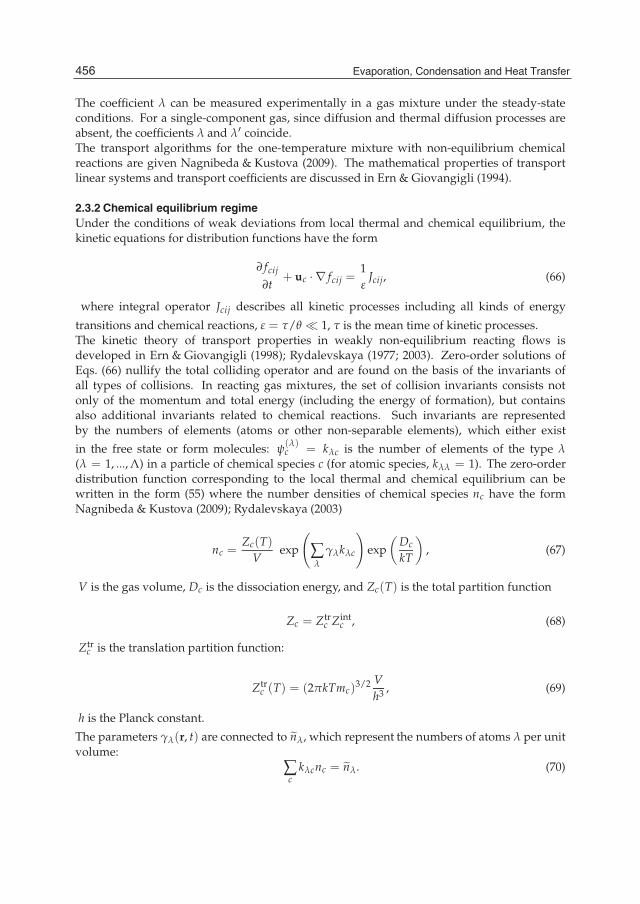
18 Will-be-set-by-IN-TECH
The coefficient λ can be measured experimentally in a gas mixture under the steady-stateconditions. For a single-component gas, since diffusion and thermal diffusion processes areabsent, the coefficients λ and λ′ coincide.The transport algorithms for the one-temperature mixture with non-equilibrium chemicalreactions are given Nagnibeda & Kustova (2009). The mathematical properties of transportlinear systems and transport coefficients are discussed in Ern & Giovangigli (1994).
2.3.2 Chemical equilibrium regimeUnder the conditions of weak deviations from local thermal and chemical equilibrium, thekinetic equations for distribution functions have the form
∂ fcij
∂t+ uc · ∇ fcij =
1ε
Jcij, (66)
where integral operator Jcij describes all kinetic processes including all kinds of energy
transitions and chemical reactions, ε = τ/θ � 1, τ is the mean time of kinetic processes.The kinetic theory of transport properties in weakly non-equilibrium reacting flows isdeveloped in Ern & Giovangigli (1998); Rydalevskaya (1977; 2003). Zero-order solutions ofEqs. (66) nullify the total colliding operator and are found on the basis of the invariants ofall types of collisions. In reacting gas mixtures, the set of collision invariants consists notonly of the momentum and total energy (including the energy of formation), but containsalso additional invariants related to chemical reactions. Such invariants are representedby the numbers of elements (atoms or other non-separable elements), which either exist
in the free state or form molecules: ψ(λ)c = kλc is the number of elements of the type λ
(λ = 1, ..., Λ) in a particle of chemical species c (for atomic species, kλλ = 1). The zero-orderdistribution function corresponding to the local thermal and chemical equilibrium can bewritten in the form (55) where the number densities of chemical species nc have the formNagnibeda & Kustova (2009); Rydalevskaya (2003)
nc =Zc(T)
Vexp
(∑λ
γλkλc
)exp
(Dc
kT
), (67)
V is the gas volume, Dc is the dissociation energy, and Zc(T) is the total partition function
Zc = Ztrc Zint
c , (68)
Ztrc is the translation partition function:
Ztrc (T) = (2πkTmc)
3/2 Vh3 , (69)
h is the Planck constant.
The parameters γλ(r, t) are connected to nλ, which represent the numbers of atoms λ per unitvolume:
∑c
kλcnc = nλ. (70)
456 Evaporation, Condensation and Heat Transfer
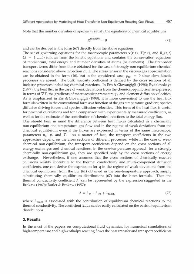
Different Approaches for Modelling of Heat Transfer in Non-Equilibrium Reacting Gas Flows 19
Note that the number densities of species nc satisfy the equations of chemical equilibrium
Rreact(0)c = 0 (71)
and can be derived in the form (67) directly from the above equations.The set of governing equations for the macroscopic parameters v(r, t), T(r, t), and nλ(r, t)(λ = 1, ..., L) follows from the kinetic equations and contains the conservation equationsof momentum, total energy and number densities of atoms (or elements). The first-ordertransport terms differ from those obtained for the case of strongly non-equilibrium chemicalreactions considered above in Section 2.3.1. The stress tensor in the viscous gas approximationcan be obtained in the form (16), but in the considered case, prel = 0 since slow kineticprocesses are absent. The bulk viscosity coefficient is defined by the cross sections of allinelastic processes including chemical reactions. In Ern & Giovangigli (1998); Rydalevskaya(1977), the heat flux in the case of weak deviations from the chemical equilibrium is expressedin terms of ∇T, the gradients of macroscopic parameters γλ and element diffusion velocities.As is emphasized in Ern & Giovangigli (1998), it is more convenient to use the heat fluxformula written in the conventional form as a function of the gas temperature gradient, speciesdiffusive driving forces and species diffusion velocities. This form of the heat flux is usefulfor practical calculations and for a comparison with experimentally measured coefficients, aswell as for the estimate of the contribution of chemical reactions to the total energy flux.One should bear in mind the difference between heat fluxes calculated in a chemicallynon-equilibrium one-temperature gas flow and in the regime of weak deviations from thechemical equilibrium even if the fluxes are expressed in terms of the same macroscopicparameters nc, p, and T. As a matter of fact, the transport coefficients in the twoapproaches depend on the cross sections of different processes: while in the case of weakchemical non-equilibrium, the transport coefficients depend on the cross sections of allenergy exchanges and chemical reactions, in the one-temperature approach for a stronglychemically non-equilibrium gas, they are specified only by the cross sections of energyexchange. Nevertheless, if one assumes that the cross sections of chemically reactivecollisions weakly contribute to the thermal conductivity and multi-component diffusioncoefficients, one can derive the expression for q in the regime of weak deviations from thechemical equilibrium from the Eq. (61) obtained in the one-temperature approach, simplysubstituting chemically equilibrium distributions (67) into the latter formula. Then thethermal conductivity coefficient λ′ can be represented by the expression suggested in theBrokaw (1960); Butler & Brokaw (1957):
λ = λtr + λint + λreact, (72)
where λreact is associated with the contribution of equilibrium chemical reactions to thethermal conductivity. The coefficient λreact can be easily calculated on the basis of equilibriumdistributions.
3. Results
In the most of the papers on computational fluid dynamics, for numerical simulations ofhigh-temperature and high-enthalpy reacting flows the heat transfer and transport coefficients
457Different Approaches for Modelling of Heat Transfer in Non-Equilibrium Reacting Gas Flows
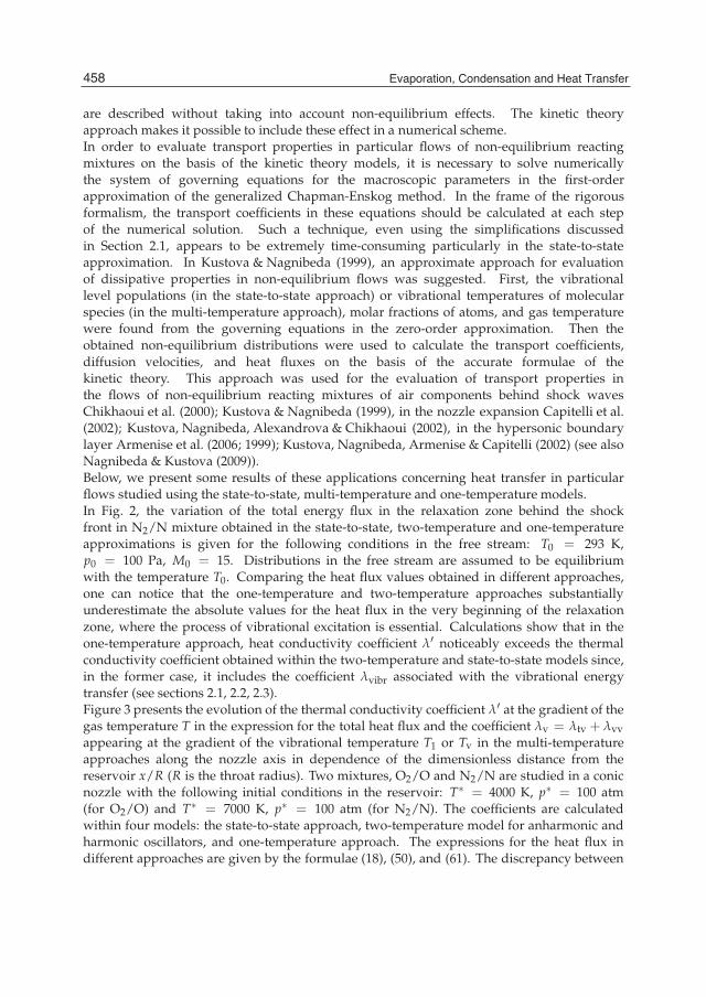
20 Will-be-set-by-IN-TECH
are described without taking into account non-equilibrium effects. The kinetic theoryapproach makes it possible to include these effect in a numerical scheme.In order to evaluate transport properties in particular flows of non-equilibrium reactingmixtures on the basis of the kinetic theory models, it is necessary to solve numericallythe system of governing equations for the macroscopic parameters in the first-orderapproximation of the generalized Chapman-Enskog method. In the frame of the rigorousformalism, the transport coefficients in these equations should be calculated at each stepof the numerical solution. Such a technique, even using the simplifications discussedin Section 2.1, appears to be extremely time-consuming particularly in the state-to-stateapproximation. In Kustova & Nagnibeda (1999), an approximate approach for evaluationof dissipative properties in non-equilibrium flows was suggested. First, the vibrationallevel populations (in the state-to-state approach) or vibrational temperatures of molecularspecies (in the multi-temperature approach), molar fractions of atoms, and gas temperaturewere found from the governing equations in the zero-order approximation. Then theobtained non-equilibrium distributions were used to calculate the transport coefficients,diffusion velocities, and heat fluxes on the basis of the accurate formulae of thekinetic theory. This approach was used for the evaluation of transport properties inthe flows of non-equilibrium reacting mixtures of air components behind shock wavesChikhaoui et al. (2000); Kustova & Nagnibeda (1999), in the nozzle expansion Capitelli et al.(2002); Kustova, Nagnibeda, Alexandrova & Chikhaoui (2002), in the hypersonic boundarylayer Armenise et al. (2006; 1999); Kustova, Nagnibeda, Armenise & Capitelli (2002) (see alsoNagnibeda & Kustova (2009)).Below, we present some results of these applications concerning heat transfer in particularflows studied using the state-to-state, multi-temperature and one-temperature models.In Fig. 2, the variation of the total energy flux in the relaxation zone behind the shockfront in N2/N mixture obtained in the state-to-state, two-temperature and one-temperatureapproximations is given for the following conditions in the free stream: T0 = 293 K,p0 = 100 Pa, M0 = 15. Distributions in the free stream are assumed to be equilibriumwith the temperature T0. Comparing the heat flux values obtained in different approaches,one can notice that the one-temperature and two-temperature approaches substantiallyunderestimate the absolute values for the heat flux in the very beginning of the relaxationzone, where the process of vibrational excitation is essential. Calculations show that in theone-temperature approach, heat conductivity coefficient λ′ noticeably exceeds the thermalconductivity coefficient obtained within the two-temperature and state-to-state models since,in the former case, it includes the coefficient λvibr associated with the vibrational energytransfer (see sections 2.1, 2.2, 2.3).Figure 3 presents the evolution of the thermal conductivity coefficient λ′ at the gradient of thegas temperature T in the expression for the total heat flux and the coefficient λv = λtv + λvvappearing at the gradient of the vibrational temperature T1 or Tv in the multi-temperatureapproaches along the nozzle axis in dependence of the dimensionless distance from thereservoir x/R (R is the throat radius). Two mixtures, O2/O and N2/N are studied in a conicnozzle with the following initial conditions in the reservoir: T∗ = 4000 K, p∗ = 100 atm(for O2/O) and T∗ = 7000 K, p∗ = 100 atm (for N2/N). The coefficients are calculatedwithin four models: the state-to-state approach, two-temperature model for anharmonic andharmonic oscillators, and one-temperature approach. The expressions for the heat flux indifferent approaches are given by the formulae (18), (50), and (61). The discrepancy between
458 Evaporation, Condensation and Heat Transfer
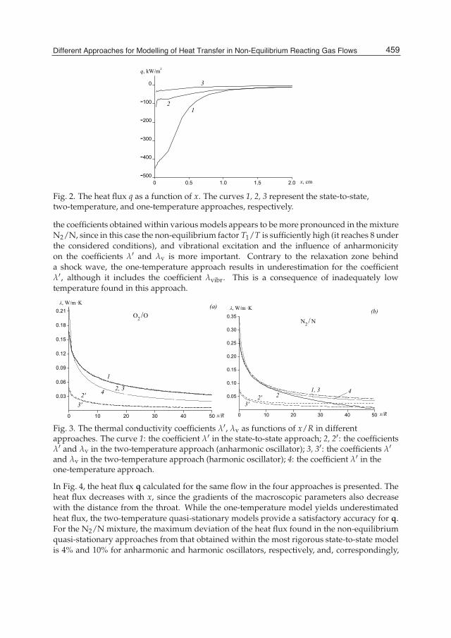
Different Approaches for Modelling of Heat Transfer in Non-Equilibrium Reacting Gas Flows 21
0 0.5 1.0 1.5 2.0-500
-400
-300
-200
-100
0
q, kW/m2
x, cm
3
21
Fig. 2. The heat flux q as a function of x. The curves 1, 2, 3 represent the state-to-state,two-temperature, and one-temperature approaches, respectively.
the coefficients obtained within various models appears to be more pronounced in the mixtureN2/N, since in this case the non-equilibrium factor T1/T is sufficiently high (it reaches 8 underthe considered conditions), and vibrational excitation and the influence of anharmonicityon the coefficients λ′ and λv is more important. Contrary to the relaxation zone behinda shock wave, the one-temperature approach results in underestimation for the coefficientλ′, although it includes the coefficient λvibr. This is a consequence of inadequately lowtemperature found in this approach.
0 10 20 30 40 50
0.03
0.06
0.09
0.12
0.15
0.18
0.21
x/R
, W/m ·K
O2 /O(a)
3'2' 4 2, 3
1
0 10 20 30 40 50
0.05
0.10
0.15
0.20
0.25
0.30
0.35
, W/m ·K
x/R
N2 / N(b)
2'3'
42
1, 3
Fig. 3. The thermal conductivity coefficients λ′, λv as functions of x/R in differentapproaches. The curve 1: the coefficient λ′ in the state-to-state approach; 2, 2′: the coefficientsλ′ and λv in the two-temperature approach (anharmonic oscillator); 3, 3′: the coefficients λ′and λv in the two-temperature approach (harmonic oscillator); 4: the coefficient λ′ in theone-temperature approach.
In Fig. 4, the heat flux q calculated for the same flow in the four approaches is presented. Theheat flux decreases with x, since the gradients of the macroscopic parameters also decreasewith the distance from the throat. While the one-temperature model yields underestimatedheat flux, the two-temperature quasi-stationary models provide a satisfactory accuracy for q.For the N2/N mixture, the maximum deviation of the heat flux found in the non-equilibriumquasi-stationary approaches from that obtained within the most rigorous state-to-state modelis 4% and 10% for anharmonic and harmonic oscillators, respectively, and, correspondingly,
459Different Approaches for Modelling of Heat Transfer in Non-Equilibrium Reacting Gas Flows
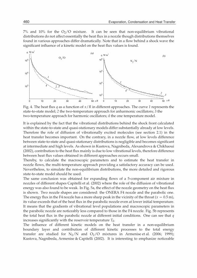
22 Will-be-set-by-IN-TECH
7% and 10% for the O2/O mixture. It can be seen that non-equilibrium vibrationaldistributions do not affect essentially the heat flux in a nozzle though distributions themselvesfound in various approaches differ dramatically. Note that in a flow behind a shock wave thesignificant influence of a kinetic model on the heat flux values is found.
0 10 20 30 40 50
103
104
105
x/R
q, W/m2
O2 /O(a)
4 2, 3
1
0 10 20 30 40 50
103
104
105
106
q, W/m2
x/R
N2 / N
(b)
432
1
Fig. 4. The heat flux q as a function of x/R in different approaches. The curve 1 represents thestate-to-state model; 2 the two-temperature approach for anharmonic oscillators; 3 thetwo-temperature approach for harmonic oscillators; 4 the one temperature model.
It is explained by the fact that the vibrational distributions behind the shock front calculatedwithin the state-to-state and quasi-stationary models differ substantially already at low levels.Therefore the role of diffusion of vibrationally excited molecules (see section 2.1) in theheat transfer becomes important. On the contrary, in a nozzle flow, at low levels differencebetween state-to-state and quasi-stationary distributions is negligible and becomes significantat intermediate and high levels. As shown in Kustova, Nagnibeda, Alexandrova & Chikhaoui(2002), contribution to the heat flux mainly is due to low vibrational levels, therefore differencebetween heat flux values obtained in different approaches occurs small.Thereby, to calculate the macroscopic parameters and to estimate the heat transfer innozzle flows, the multi-temperature approach providing a satisfactory accuracy can be used.Nevertheless, to simulate the non-equilibrium distributions, the more detailed and rigorousstate-to-state model should be used.The same conclusion was obtained for expanding flows of a 5-component air mixture innozzles of different shapes Capitelli et al. (2002) where the role of the diffusion of vibrationalenergy was also found to be weak. In Fig. 5a, the effect of the nozzle geometry on the heat fluxis shown. Two nozzle shapes are considered: the ONERA F4 nozzle and the parabolic one.The energy flux in the F4 nozzle has a more sharp peak in the vicinity of the throat (x = 0.5 m),its value exceeds that of the heat flux in the parabolic nozzle even at lower initial temperature.It means that the gradients of vibrational level populations and macroscopic parameters inthe parabolic nozzle are noticeably less compared to those in the F4 nozzle. Fig. 5b representsthe total heat flux in the parabolic nozzle at different initial conditions. One can see that qincreases significantly with the reservoir temperature T0.The influence of different kinetic models on the heat transfer in a non-equilibriumboundary layer and contribution of different kinetic processes to the total energytransfer are studied for N2/N and O2/O mixtures in Armenise et al. (2006; 1999);Kustova, Nagnibeda, Armenise & Capitelli (2002). It is interesting to emphasize noticeable
460 Evaporation, Condensation and Heat Transfer
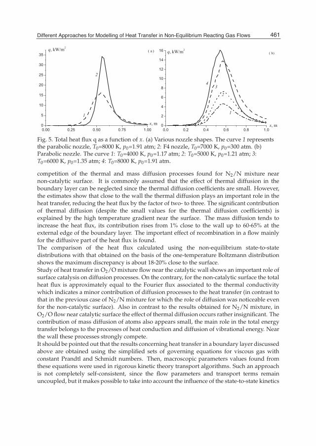
Different Approaches for Modelling of Heat Transfer in Non-Equilibrium Reacting Gas Flows 23
0.00 0.25 0.50 0.75 1.000
5
10
15
20
25
30
35
x, m
q, kW/m2
2
1
( a )
0.0 0.2 0.4 0.6 0.8 1.00
2
4
6
8
10
12
14
16 q, kW/m2
x, m
43
2
1
( b)
Fig. 5. Total heat flux q as a function of x. (a) Various nozzle shapes. The curve 1 representsthe parabolic nozzle, T0=8000 K, p0=1.91 atm; 2: F4 nozzle, T0=7000 K, p0=300 atm. (b)Parabolic nozzle. The curve 1: T0=4000 K, p0=1.17 atm; 2: T0=5000 K, p0=1.21 atm; 3:T0=6000 K, p0=1.35 atm; 4: T0=8000 K, p0=1.91 atm.
competition of the thermal and mass diffusion processes found for N2/N mixture nearnon-catalytic surface. It is commonly assumed that the effect of thermal diffusion in theboundary layer can be neglected since the thermal diffusion coefficients are small. However,the estimates show that close to the wall the thermal diffusion plays an important role in theheat transfer, reducing the heat flux by the factor of two- to three. The significant contributionof thermal diffusion (despite the small values for the thermal diffusion coefficients) isexplained by the high temperature gradient near the surface. The mass diffusion tends toincrease the heat flux, its contribution rises from 1% close to the wall up to 60-65% at theexternal edge of the boundary layer. The important effect of recombination in a flow mainlyfor the diffusive part of the heat flux is found.The comparison of the heat flux calculated using the non-equilibrium state-to-statedistributions with that obtained on the basis of the one-temperature Boltzmann distributionshows the maximum discrepancy is about 18-20% close to the surface.Study of heat transfer in O2/O mixture flow near the catalytic wall shows an important role ofsurface catalysis on diffusion processes. On the contrary, for the non-catalytic surface the totalheat flux is approximately equal to the Fourier flux associated to the thermal conductivitywhich indicates a minor contribution of diffusion processes to the heat transfer (in contrast tothat in the previous case of N2/N mixture for which the role of diffusion was noticeable evenfor the non-catalytic surface). Also in contrast to the results obtained for N2/N mixture, inO2/O flow near catalytic surface the effect of thermal diffusion occurs rather insignificant. Thecontribution of mass diffusion of atoms also appears small, the main role in the total energytransfer belongs to the processes of heat conduction and diffusion of vibrational energy. Nearthe wall these processes strongly compete.It should be pointed out that the results concerning heat transfer in a boundary layer discussedabove are obtained using the simplified sets of governing equations for viscous gas withconstant Prandtl and Schmidt numbers. Then, macroscopic parameters values found fromthese equations were used in rigorous kinetic theory transport algorithms. Such an approachis not completely self-consistent, since the flow parameters and transport terms remainuncoupled, but it makes possible to take into account the influence of the state-to-state kinetics
461Different Approaches for Modelling of Heat Transfer in Non-Equilibrium Reacting Gas Flows
24 Will-be-set-by-IN-TECH
on the flow parameters and heat transfer near the wall. Recently, a similar N2/N flow wasstudied in Orsini et al. (2008) within a more rigorous model incorporating the accurate kinetictheory transport algorithms directly into the boundary layer equations. In this paper, theaccurate set of the fluid dynamic equations was solved, and the results are compared to thoseobtained within the simplified formulation of the problem. Thereby, for the first time, thestate-to-state kinetics and transport properties were coupled self-consistently, and the role ofthe detailed vibrational kinetics in the heat transfer was estimated.In the paper Kustova et al. (2009), the accurate transport kinetic theory algorithms formulti-temperature mixtures containing CO2 molecules developed in Kustova & Nagnibeda(2006) in the first time, were implemented directly into the CFD numerical simulations of2D viscous hypersonic shock layer near a space craft entering to the Mars atmosphere andthe influence of non-equilibrium kinetics on fluid dynamic parameters and heat transfer in ashock layer was shown.
4. Conclusion
In the present Chapter, the problem of modelling of heat transfer in high temperaturehypersonic flows of reacting gas mixtures is considered. Theoretical models for transportproperties in reacting flows are proposed for the conditions of weak and strong deviationsfrom the local thermal and chemical equilibrium. Peculiarities of the kinetic theorytransport algorithms developed for various non-equilibrium conditions are discussed andrecommendations concerning the choice of an adequate kinetic model for the total energytransfer under particular conditions are given. The results of applications of proposed modelsfor different flows of reacting mixtures are demonstrated.
5. Acknowledgements
We are grateful to the Russian Foundation for Basic Research (Grant 11-01-00408) and Ministryof Education and Science of RF (Contract 13.G25.31.0076) for the support of this study.
6. References
Adamovich, I. & Rich, J. (1998). Three-dimensional nonperturbative analytic modelof vibrational energy transfer in atom-molecule collisions, J. Chem. Phys.109(18): 7711–7724.
Armenise, I., Barbato, M., Capitelli, M. & Kustova, E. (2006). State-to-state catalytic models,kinetics and transport in hypersonic boundary layers, J. Thermophys. Heat Transfer20(3): 465–476.
Armenise, I., Capitelli, M., Colonna, G. & Gorse, C. (1996). Nonequilibrium vibrationalkinetics in the boundary layer of re-entering bodies, J. Thermophys. Heat Transfer10(3): 397–405.
Armenise, I., Capitelli, M., Kustova, E. & Nagnibeda, E. (1999). The influence ofnonequilibrium kinetics on the heat transfer and diffusion near re-entering body, J.Thermophys. Heat Transfer 13(2): 210–218.
Billing, G. & Fisher, E. (1979). VV and VT rate coefficients in N2 by a quantum-classical model,Chem. Phys. 43: 395–401.
462 Evaporation, Condensation and Heat Transfer
Different Approaches for Modelling of Heat Transfer in Non-Equilibrium Reacting Gas Flows 25
Brokaw, R. (1960). Thermal conductivity of gas mixtures in chemical equilibrium II, J. Chem.Phys. 32: 1005.
Butler, J. & Brokaw, R. (1957). Thermal conductivity of gas mixtures in chemical equilibrium,J. Chem. Phys. 26: 1636.
Capitelli, M., Colonna, G., Kustova, E. & Nagnibeda, E. (2002). State-to-state kineticsand transport properties in supersonic air nozzle flows, Proceedings of the 4thEuropean Symposium on Aerothermodynamics for Space Vehicles, ESTEC, Noordwijk, TheNetherlands, ESA Publication Division, ESA SP–487. P. 137–143.
Chapman, S. & Cowling, T. (1970). The Mathematical Theory of Non-Uniform Gases, 3d edn,Cambridge University Press, Cambridge.
Chikhaoui, A., Dudon, J., Genieys, S., Kustova, E. & Nagnibeda, E. (2000). Multi-temperaturekinetic model for heat transfer in reacting gas mixture, Phys. Fluids 12(1): 220–232.
Chikhaoui, A., Dudon, J., Kustova, E. & Nagnibeda, E. (1997). Transport properties in reactingmixture of polyatomic gases, Physica A 247(1-4): 526–552.
Ern, A. & Giovangigli, V. (1994). Multicomponent Transport Algorithms, Lect. Notes Phys., Seriesmonographs, M24, Springer-Verlag.
Ern, A. & Giovangigli, V. (1998). The kinetic chemical equilibrium regime, Physica A260: 49–72.
Esposito, F., Capitelli, M. & Gorse, C. (2000). Quasi-classical dynamics and vibrational kineticsin N2(v)− N system, Chem. Phys. 257: 193–202.
Eucken, E. (1913). Ueber das Wärmeleitvermogen, die Spezifische Wärme und die innereReibung der Gase, Physik. Zeitschr 14: 324–332.
Ferziger, J. & Kaper, H. (1972). Mathematical Theory of Transport Processes in Gases,North-Holland, Amsterdam, London.
Gordiets, B. & Mamedov, S. (1974). Distribution function and vibrational energy relaxationrate in a system of anharmonic oscillators, Prikl. Mekh. Tekhn. Phys. 3: 13–22.
Gordietz, B. & Zhdanok, S. (1986). Analytical theory of vibrational kinetics of anharmonicoscillators, in M. Capitelli (ed.), Nonequilibrium Vibrational Kinetics, Springer-Verlag,Berlin, Heidelberg, New York, Tokyo, pp. 43–84.
Hirschfelder, J., Curtiss, C. & Bird, R. (1954). The Molecular Theory of Gases and Liquids, J.Wileyand Sons, New York.
Kustova, E. (2001). On the simplified state-to-state transport coefficients, Chem. Phys.270(1): 177–195.
Kustova, E. & Nagnibeda, E. (1997). Vibrational kinetics and transport processes in a stronglynon-equilibrium gas, Izvestiya RAN, Mekhanika Zhidkosti i Gasa 5: 150–160.
Kustova, E. & Nagnibeda, E. (1998). Transport properties of a reacting gas mixture with strongvibrational and chemical nonequilibrium, Chem. Phys. 233: 57–75.
Kustova, E. & Nagnibeda, E. (1999). State-to-state approach in the transport kinetic theory,Rarefied Gas Dynamics 21, Vol. 1, CEPADUES, Toulouse, France, pp. 231–238.
Kustova, E. & Nagnibeda, E. (2006). On a correct description of a multi-temperaturedissociating CO2 flow, Chem. Phys. 321: 293–310.
Kustova, E., Nagnibeda, E., Alexandrova, T. & Chikhaoui, A. (2002). On the non-equilibriumkinetics and heat transfer in nozzle flows, Chem. Phys. 276(2): 139–154.
Kustova, E., Nagnibeda, E., Armenise, I. & Capitelli, M. (2002). Non-equilibrium kinetics andheat transfer in O2/O mixtures near catalytic surfaces, J. Thermophys. Heat Transfer16(2): 238–244.
463Different Approaches for Modelling of Heat Transfer in Non-Equilibrium Reacting Gas Flows
26 Will-be-set-by-IN-TECH
Kustova, E., Nagnibeda, E., Shevelev, Y. & Syzranova, N. (2009). Non-equilibrium supersonicCO2 flows with real gas effects near a blunt body, in T. Abe (ed.), Rarefied GasDynamics: 26-th International Symposium, Vol. 1084 of AIP Conference Proceedings,pp. 831–836.
Kustova, E. & Puzyreva, L. (2009). Transport coefficients in nonequilibrium gas-mixture flowswith electronic excitation, Phys. Rev. E 80(4): 046407.
Laganà, A. & Garcia, E. (1994). Temperature dependence of N + N2 rate coefficients, J. Chem.Phys. 98: 502–507.
Nagnibeda, E. & Kustova, E. (2009). Nonequilibrium Reacting Gas Flows. Kinetic Theory ofTransport and Relaxation Processes, Springer Verlag, Berlin, Heidelberg.
Orsini, A., Rini, P., Taviani, V., Fletcher, D., Kustova, E. & Nagnibeda, E. (2008). State-to-statesimulation of non-equilibrium nitrogen stagnation line flows: Fluid dynamics andvibrational kinetics, J. Thermophys. Heat Transfer 22(3): 390–398.
Phys-Chem (2002). Physical and Chemical Processes in Gas Dynamics: Cross Sections andRate Constants for Physical and Chemical Processes. Volume I, Vol. I96 of Progress inAstronautics and Aeronautics.
Rydalevskaya, M. (1977). Formal kinetic description of gas mixtures with dissociation andrecombination, Aerodynamics of Rarefied Gases, Vol. IX, Leningrad University Press,Leningrad, pp. 5–20.
Rydalevskaya, M. (2003). Statistical and Kinetic Models in Physical-Chemical Gas Dynamics, SaintPetersburg Univ. Press, Saint Petersburg.
Stupochenko, Y., Losev, S. & Osipov, A. (1967). Relaxation in Shock Waves, Springer-Verlag,Berlin, Heidelberg, New York.
Treanor, C., Rich, I. & Rehm, R. (1968). Vibrational relaxation of anharmonic oscillators withexchange dominated collisions, J. Chem. Phys. 48: 1798.
Vallander, S., Nagnibeda, E. & Rydalevskaya, M. (1977). Some Questions of the KineticTheory of the Chemical Reacting Gas Mixture, Leningrad University Press, Leningrad.Translation: US AirForce FASTC–ID (RS) TO–0608–93.
Wang Chang, C. & Uhlenbeck, G. (1951). Transport phenomena in polyatomic gases, CM-681,University of Michigan Research Report.
464 Evaporation, Condensation and Heat Transfer
22
High-Carbon Alcohol Aqueous Solutions and Their Application to Flow Boiling in
Various Mini-Tube Systems Naoki Ono, Atsushi Hamaoka, Yuki Eda and Koichi Obara
Department of Engineering Science and Mechanics, Shibaura Institute of Technology,
Japan
1. Introduction The temperature dependence of the surface tension of certain high-carbon alcohol aqueous solutions such as those of butanol and pentanol is nonlinear. That is, the surface tension of the solution increases when it is heated beyond a certain temperature. Since this was discovered by Vochten et al. (Vochten & Petre, 1973) about 30 years ago, several experimental studies have examined the liquid motion of these alcohol aqueous solutions, focusing on how they differ from normal fluids. Simultaneously, several studies have attempted to apply the phenomenon to heat pipes (Abe, 2006a, 2006b) and other equipment to enhance heat transfer. The direction of the thermocapillary force in a liquid film of a nonlinear solution on a heated surface acts in the same direction as the solutocapillary force. This characteristic is expected to be remarkable in small-scale systems such as mini or micro channels. In this chapter, the authors report the following three findings: 1) new measurement results regarding the nonlinear temperature dependence of the surface tension of high-carbon alcohol aqueous solutions, 2) a simple application of the solution to flow boiling in a straight mini tube and 3) modified applications of the solution to flow boiling in a T-junction mini tube. Future applications of this study include miniature cooling systems such as those for CPUs and laser emitting devices although the use of a high-carbon alcohol aqueous solution would require further improvements and greater sophistication to be viable. Also, the precise mechanism of the combined force of the thermocapillary and solutocapillary effects need to be further investigated.
2. Temperature dependence of the surface tension of high-carbon alcohol aqueous solutions The surface tension of normal fluids decreases as their temperature increases. However, as aforementioned, in alcohol aqueous solutions such as those of butanol and pentanol, surface tension increases as the temperature rises above a certain point. The behaviour of fluids with this special characteristic (called ‘nonlinear thermocapillarity’ here) has been investigated by numerous researchers (Legros, 1986; Azouni & Petre, 1998)
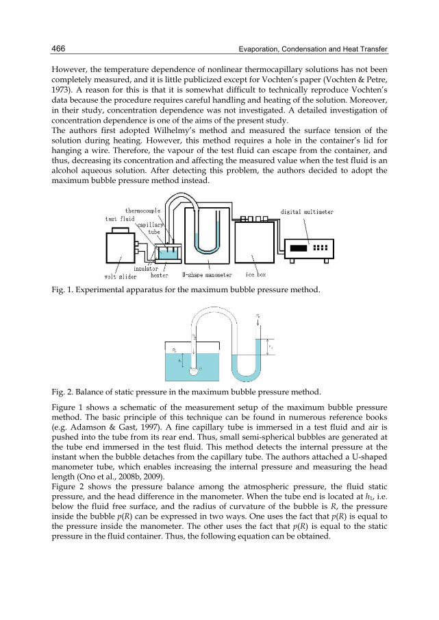
Evaporation, Condensation and Heat Transfer
466
However, the temperature dependence of nonlinear thermocapillary solutions has not been completely measured, and it is little publicized except for Vochten’s paper (Vochten & Petre, 1973). A reason for this is that it is somewhat difficult to technically reproduce Vochten’s data because the procedure requires careful handling and heating of the solution. Moreover, in their study, concentration dependence was not investigated. A detailed investigation of concentration dependence is one of the aims of the present study. The authors first adopted Wilhelmy’s method and measured the surface tension of the solution during heating. However, this method requires a hole in the container’s lid for hanging a wire. Therefore, the vapour of the test fluid can escape from the container, and thus, decreasing its concentration and affecting the measured value when the test fluid is an alcohol aqueous solution. After detecting this problem, the authors decided to adopt the maximum bubble pressure method instead.
Fig. 1. Experimental apparatus for the maximum bubble pressure method.
Fig. 2. Balance of static pressure in the maximum bubble pressure method.
Figure 1 shows a schematic of the measurement setup of the maximum bubble pressure method. The basic principle of this technique can be found in numerous reference books (e.g. Adamson & Gast, 1997). A fine capillary tube is immersed in a test fluid and air is pushed into the tube from its rear end. Thus, small semi-spherical bubbles are generated at the tube end immersed in the test fluid. This method detects the internal pressure at the instant when the bubble detaches from the capillary tube. The authors attached a U-shaped manometer tube, which enables increasing the internal pressure and measuring the head length (Ono et al., 2008b, 2009). Figure 2 shows the pressure balance among the atmospheric pressure, the fluid static pressure, and the head difference in the manometer. When the tube end is located at h1, i.e. below the fluid free surface, and the radius of curvature of the bubble is R, the pressure inside the bubble p(R) can be expressed in two ways. One uses the fact that p(R) is equal to the pressure inside the manometer. The other uses the fact that p(R) is equal to the static pressure in the fluid container. Thus, the following equation can be obtained.
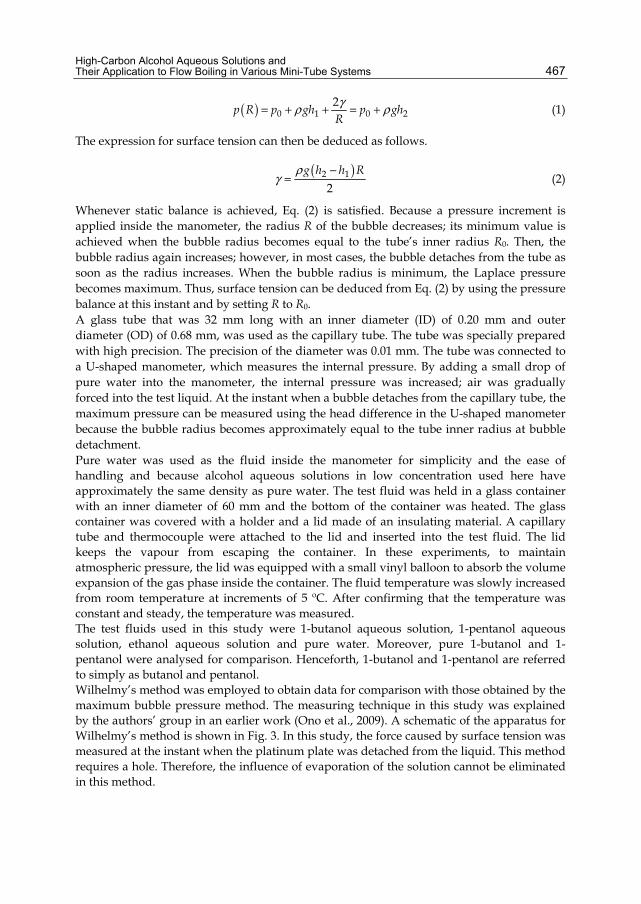
High-Carbon Alcohol Aqueous Solutions and Their Application to Flow Boiling in Various Mini-Tube Systems
467
( ) 0 1 0 22p R p gh p ghRγρ ρ= + + = + (1)
The expression for surface tension can then be deduced as follows.
( )2 1
2g h h Rρ
γ−
= (2)
Whenever static balance is achieved, Eq. (2) is satisfied. Because a pressure increment is applied inside the manometer, the radius R of the bubble decreases; its minimum value is achieved when the bubble radius becomes equal to the tube’s inner radius R0. Then, the bubble radius again increases; however, in most cases, the bubble detaches from the tube as soon as the radius increases. When the bubble radius is minimum, the Laplace pressure becomes maximum. Thus, surface tension can be deduced from Eq. (2) by using the pressure balance at this instant and by setting R to R0. A glass tube that was 32 mm long with an inner diameter (ID) of 0.20 mm and outer diameter (OD) of 0.68 mm, was used as the capillary tube. The tube was specially prepared with high precision. The precision of the diameter was 0.01 mm. The tube was connected to a U-shaped manometer, which measures the internal pressure. By adding a small drop of pure water into the manometer, the internal pressure was increased; air was gradually forced into the test liquid. At the instant when a bubble detaches from the capillary tube, the maximum pressure can be measured using the head difference in the U-shaped manometer because the bubble radius becomes approximately equal to the tube inner radius at bubble detachment. Pure water was used as the fluid inside the manometer for simplicity and the ease of handling and because alcohol aqueous solutions in low concentration used here have approximately the same density as pure water. The test fluid was held in a glass container with an inner diameter of 60 mm and the bottom of the container was heated. The glass container was covered with a holder and a lid made of an insulating material. A capillary tube and thermocouple were attached to the lid and inserted into the test fluid. The lid keeps the vapour from escaping the container. In these experiments, to maintain atmospheric pressure, the lid was equipped with a small vinyl balloon to absorb the volume expansion of the gas phase inside the container. The fluid temperature was slowly increased from room temperature at increments of 5 ºC. After confirming that the temperature was constant and steady, the temperature was measured. The test fluids used in this study were 1-butanol aqueous solution, 1-pentanol aqueous solution, ethanol aqueous solution and pure water. Moreover, pure 1-butanol and 1-pentanol were analysed for comparison. Henceforth, 1-butanol and 1-pentanol are referred to simply as butanol and pentanol. Wilhelmy’s method was employed to obtain data for comparison with those obtained by the maximum bubble pressure method. The measuring technique in this study was explained by the authors’ group in an earlier work (Ono et al., 2009). A schematic of the apparatus for Wilhelmy’s method is shown in Fig. 3. In this study, the force caused by surface tension was measured at the instant when the platinum plate was detached from the liquid. This method requires a hole. Therefore, the influence of evaporation of the solution cannot be eliminated in this method.
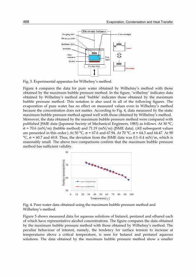
Evaporation, Condensation and Heat Transfer
468
Fig. 3. Experimental apparatus for Wilhelmy’s method.
Figure 4 compares the data for pure water obtained by Wilhelmy’s method with those obtained by the maximum bubble pressure method. In the figure, ‘wilhelmy’ indicates data obtained by Wilhelmy’s method and ‘bubble’ indicates those obtained by the maximum bubble pressure method. This notation is also used in all of the following figures. The evaporation of pure water has no effect on measured values even in Wilhelmy’s method because the concentration does not matter. According to Fig. 4, data measured by the static maximum bubble pressure method agreed well with those obtained by Wilhelmy’s method. Moreover, the data obtained by the maximum bubble pressure method were compared with published JSME data (Japanese Society of Mechanical Engineers, 1983) as follows. At 30 °C, σ = 70.6 (mN/m) (bubble method) and 71.19 (mN/m) (JSME data). (All subsequent values are presented in this order.) At 50 °C, σ = 67.6 and 67.94. At 70 °C, σ = 64.3 and 64.47. At 90 °C, σ = 60.7 and 60.8. Thus, the deviation from the JSME data was 0.1–0.4 mN/m, which is reasonably small. The above two comparisons confirm that the maximum bubble pressure method has sufficient validity.
50
60
70
80
0 10 20 30 40 50 60 70 80 90 100Temperature[℃]
Surf
ace
tens
ion[
mN
/m]
pure water[wilhelmy]
pure water[bubble]
Fig. 4. Pure water data obtained using the maximum bubble pressure method and Wilhelmy’s method.
Figure 5 shows measured data for aqueous solutions of butanol, pentanol and ethanol each of which have representative alcohol concentrations. The figure compares the data obtained by the maximum bubble pressure method with those obtained by Wilhelmy’s method. The peculiar behaviour of interest, namely, the tendency for surface tension to increase at temperatures above a critical temperature, is seen for butanol and pentanol aqueous solutions. The data obtained by the maximum bubble pressure method show a smaller
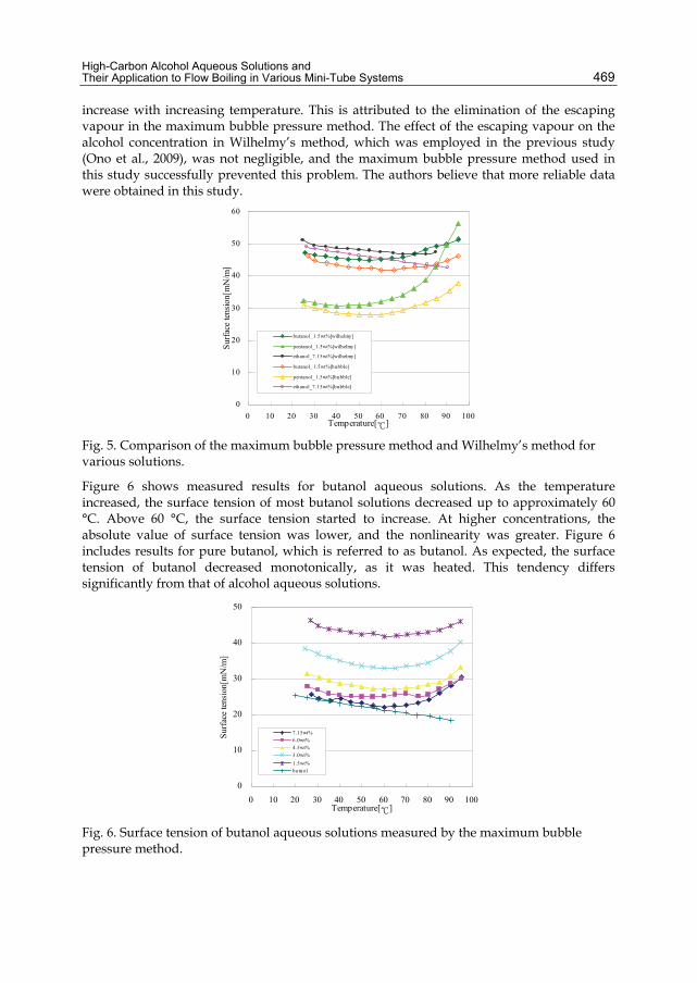
High-Carbon Alcohol Aqueous Solutions and Their Application to Flow Boiling in Various Mini-Tube Systems
469
increase with increasing temperature. This is attributed to the elimination of the escaping vapour in the maximum bubble pressure method. The effect of the escaping vapour on the alcohol concentration in Wilhelmy’s method, which was employed in the previous study (Ono et al., 2009), was not negligible, and the maximum bubble pressure method used in this study successfully prevented this problem. The authors believe that more reliable data were obtained in this study.
0
10
20
30
40
50
60
0 10 20 30 40 50 60 70 80 90 100Temperature[℃]
Surf
ace
tens
ion[
mN
/m]
butanol_1.5wt%[wilhelmy]
pentanol_1.5wt%[wilhelmy]
ethanol_7.15wt%[wilhelmy]
butanol_1.5wt%[bubble]
pentanol_1.5wt%[bubble]
ethanol_7.15wt%[bubble]
Fig. 5. Comparison of the maximum bubble pressure method and Wilhelmy’s method for various solutions.
Figure 6 shows measured results for butanol aqueous solutions. As the temperature increased, the surface tension of most butanol solutions decreased up to approximately 60 °C. Above 60 °C, the surface tension started to increase. At higher concentrations, the absolute value of surface tension was lower, and the nonlinearity was greater. Figure 6 includes results for pure butanol, which is referred to as butanol. As expected, the surface tension of butanol decreased monotonically, as it was heated. This tendency differs significantly from that of alcohol aqueous solutions.
0
10
20
30
40
50
0 10 20 30 40 50 60 70 80 90 100Temperature[℃]
Surf
ace
tens
ion[
mN
/m]
7.15wt%6.0wt%4.5wt%3.0wt%1.5wt%butnol
Fig. 6. Surface tension of butanol aqueous solutions measured by the maximum bubble pressure method.
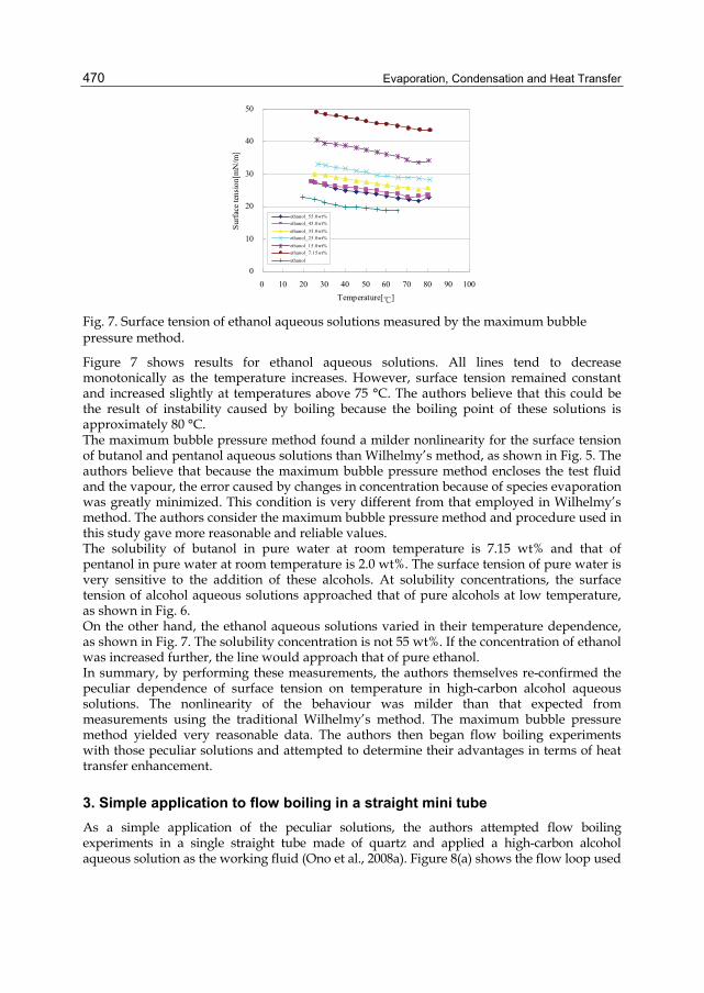
Evaporation, Condensation and Heat Transfer
470
0
10
20
30
40
50
0 10 20 30 40 50 60 70 80 90 100Temperature[℃]
Surf
ace
tens
ion[
mN
/m]
ethanol_55.0wt%ethanol_45.0wt%ethanol_35.0wt%ethanol_25.0wt%ethanol_15.0wt%ethanol_7.15wt%ethanol
Fig. 7. Surface tension of ethanol aqueous solutions measured by the maximum bubble pressure method.
Figure 7 shows results for ethanol aqueous solutions. All lines tend to decrease monotonically as the temperature increases. However, surface tension remained constant and increased slightly at temperatures above 75 °C. The authors believe that this could be the result of instability caused by boiling because the boiling point of these solutions is approximately 80 °C. The maximum bubble pressure method found a milder nonlinearity for the surface tension of butanol and pentanol aqueous solutions than Wilhelmy’s method, as shown in Fig. 5. The authors believe that because the maximum bubble pressure method encloses the test fluid and the vapour, the error caused by changes in concentration because of species evaporation was greatly minimized. This condition is very different from that employed in Wilhelmy’s method. The authors consider the maximum bubble pressure method and procedure used in this study gave more reasonable and reliable values. The solubility of butanol in pure water at room temperature is 7.15 wt% and that of pentanol in pure water at room temperature is 2.0 wt%. The surface tension of pure water is very sensitive to the addition of these alcohols. At solubility concentrations, the surface tension of alcohol aqueous solutions approached that of pure alcohols at low temperature, as shown in Fig. 6. On the other hand, the ethanol aqueous solutions varied in their temperature dependence, as shown in Fig. 7. The solubility concentration is not 55 wt%. If the concentration of ethanol was increased further, the line would approach that of pure ethanol. In summary, by performing these measurements, the authors themselves re-confirmed the peculiar dependence of surface tension on temperature in high-carbon alcohol aqueous solutions. The nonlinearity of the behaviour was milder than that expected from measurements using the traditional Wilhelmy’s method. The maximum bubble pressure method yielded very reasonable data. The authors then began flow boiling experiments with those peculiar solutions and attempted to determine their advantages in terms of heat transfer enhancement.
3. Simple application to flow boiling in a straight mini tube As a simple application of the peculiar solutions, the authors attempted flow boiling experiments in a single straight tube made of quartz and applied a high-carbon alcohol aqueous solution as the working fluid (Ono et al., 2008a). Figure 8(a) shows the flow loop used
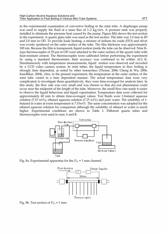
High-Carbon Alcohol Aqueous Solutions and Their Application to Flow Boiling in Various Mini-Tube Systems
471
in the experimental examination of convective boiling in the mini tube. A diaphragm pump was used to supply the fluid at a mass flux of 1–2 kg/m2s. A pressure tank was properly installed to eliminate the pressure beat caused by the pump. Figure 8(b) shows the test section in the experiment. A quartz glass tube was used as the test section. The tube was 1.0 mm in ID and 2.0 mm in OD. To provide Joule heating, a mixture of indium tin oxide (ITO) and silver was evenly sputtered on the outer surface of the tube. The film thickness was approximately 100 nm. Because the film is transparent, liquid motion inside the tube can be observed. Nine K-type thermocouples of 25 μm in OD were attached to the outer surface of the quartz tube with heat-resistant cement. The thermocouples were calibrated before performing the experiment by using a standard thermometer; their accuracy was confirmed to be within +0.2 K. Simultaneously with temperature measurements, liquid motion was observed and recorded by a CCD video camera system. In mini tubes, the liquid temperature in flow boiling is strongly time dependent, as noted by other researchers (Thome, 2006; Cheng & Wu, 2006; Kandlikar, 2004). Also, in the present experiment, the temperature at the outer surface of the mini tube varied in a time dependent manner. The actual temperature data were very complicated; to investigate them quantitatively, they were time-averaged for analysis later. In this study, the flow rate was very small and was chosen so that dry-out phenomena could occur near the midpoint of the length of the tube. Moreover, the small flow rate made it easier to observe the liquid behaviour and liquid vaporisation. Temperature data were collected for approximately 60 min to obtain time-averaged values. Test fluids were 1-butanol aqueous solution (7.15 wt%), ethanol aqueous solution (7.15 wt%) and pure water. The solubility of 1-butanol in water at room temperature is 7.15wt%. The same concentration was adopted for the ethanol aqueous solution for comparison although the solubility of ethanol in water is much higher. Experimental conditions are shown in Table 1. Different quartz tubes and thermocouples were used in runs A and B.
Fig. 8a. Experimental apparatus for the Din = 1 mm channel.
Fig. 8b. Test section of Din = 1 mm.
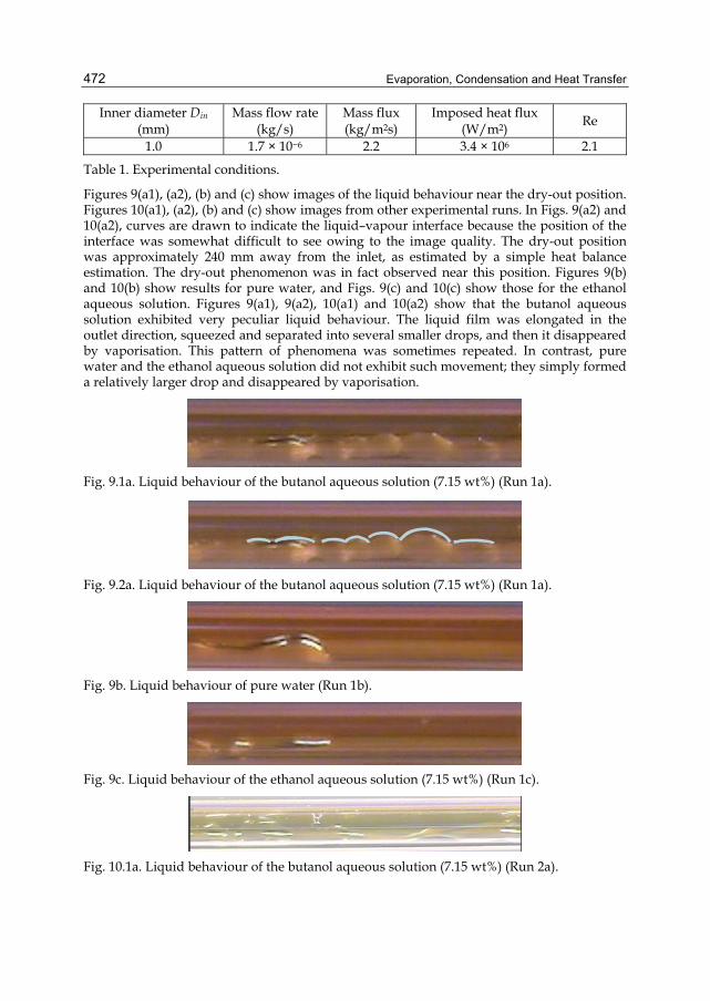
Evaporation, Condensation and Heat Transfer
472
Inner diameter Din (mm)
Mass flow rate (kg/s)
Mass flux (kg/m2s)
Imposed heat flux (W/m2) Re
1.0 1.7 × 10⁻⁶ 2.2 3.4 × 10⁶ 2.1
Table 1. Experimental conditions.
Figures 9(a1), (a2), (b) and (c) show images of the liquid behaviour near the dry-out position. Figures 10(a1), (a2), (b) and (c) show images from other experimental runs. In Figs. 9(a2) and 10(a2), curves are drawn to indicate the liquid–vapour interface because the position of the interface was somewhat difficult to see owing to the image quality. The dry-out position was approximately 240 mm away from the inlet, as estimated by a simple heat balance estimation. The dry-out phenomenon was in fact observed near this position. Figures 9(b) and 10(b) show results for pure water, and Figs. 9(c) and 10(c) show those for the ethanol aqueous solution. Figures 9(a1), 9(a2), 10(a1) and 10(a2) show that the butanol aqueous solution exhibited very peculiar liquid behaviour. The liquid film was elongated in the outlet direction, squeezed and separated into several smaller drops, and then it disappeared by vaporisation. This pattern of phenomena was sometimes repeated. In contrast, pure water and the ethanol aqueous solution did not exhibit such movement; they simply formed a relatively larger drop and disappeared by vaporisation.
Fig. 9.1a. Liquid behaviour of the butanol aqueous solution (7.15 wt%) (Run 1a).
Fig. 9.2a. Liquid behaviour of the butanol aqueous solution (7.15 wt%) (Run 1a).
Fig. 9b. Liquid behaviour of pure water (Run 1b).
Fig. 9c. Liquid behaviour of the ethanol aqueous solution (7.15 wt%) (Run 1c).
Fig. 10.1a. Liquid behaviour of the butanol aqueous solution (7.15 wt%) (Run 2a).
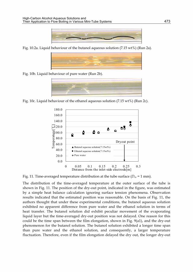
High-Carbon Alcohol Aqueous Solutions and Their Application to Flow Boiling in Various Mini-Tube Systems
473
Fig. 10.2a. Liquid behaviour of the butanol aqueous solution (7.15 wt%) (Run 2a).
Fig. 10b. Liquid behaviour of pure water (Run 2b).
Fig. 10c. Liquid behaviour of the ethanol aqueous solution (7.15 wt%) (Run 2c).
0.020.0
40.060.0
80.0100.0
120.0140.0
160.0180.0
0 0.05 0.1 0.15 0.2 0.25 0.3Distance from the inlet-side electrode[m]
Tem
pera
ture
[℃]
Butanol aqueous solution(7.15wt%)Ethanol aqueous solution(7.15wt%)Pure water
Dryout point
Fig. 11. Time-averaged temperature distribution at the tube surface (Din = 1 mm).
The distribution of the time-averaged temperature at the outer surface of the tube is shown in Fig. 11. The position of the dry-out point, indicated in the figure, was estimated by a simple heat balance calculation ignoring surface tension phenomena. Observation results indicated that the estimated position was reasonable. On the basis of Fig. 11, the authors thought that under these experimental conditions, the butanol aqueous solution exhibited no apparent difference from pure water and the ethanol solution in terms of heat transfer. The butanol solution did exhibit peculiar movement of the evaporating liquid layer but the time-averaged dry-out position was not delayed. One reason for this could be the time span between the film elongation, shown in Fig. 9(a1), and the dry-out phenomenon for the butanol solution. The butanol solution exhibited a longer time span than pure water and the ethanol solution, and consequently, a larger temperature fluctuation. Therefore, even if the film elongation delayed the dry out, the longer dry-out
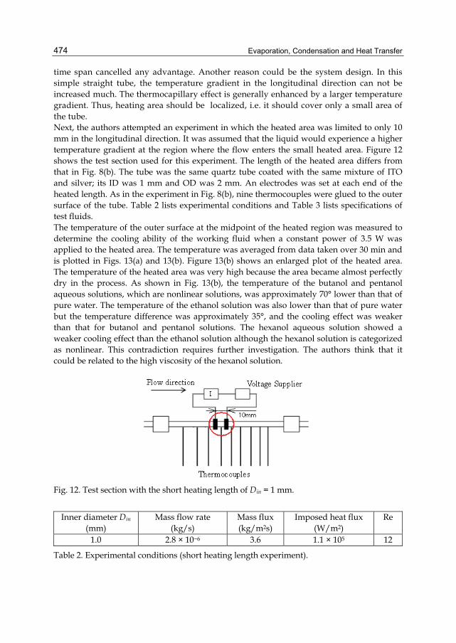
Evaporation, Condensation and Heat Transfer
474
time span cancelled any advantage. Another reason could be the system design. In this simple straight tube, the temperature gradient in the longitudinal direction can not be increased much. The thermocapillary effect is generally enhanced by a larger temperature gradient. Thus, heating area should be localized, i.e. it should cover only a small area of the tube. Next, the authors attempted an experiment in which the heated area was limited to only 10 mm in the longitudinal direction. It was assumed that the liquid would experience a higher temperature gradient at the region where the flow enters the small heated area. Figure 12 shows the test section used for this experiment. The length of the heated area differs from that in Fig. 8(b). The tube was the same quartz tube coated with the same mixture of ITO and silver; its ID was 1 mm and OD was 2 mm. An electrodes was set at each end of the heated length. As in the experiment in Fig. 8(b), nine thermocouples were glued to the outer surface of the tube. Table 2 lists experimental conditions and Table 3 lists specifications of test fluids. The temperature of the outer surface at the midpoint of the heated region was measured to determine the cooling ability of the working fluid when a constant power of 3.5 W was applied to the heated area. The temperature was averaged from data taken over 30 min and is plotted in Figs. 13(a) and 13(b). Figure 13(b) shows an enlarged plot of the heated area. The temperature of the heated area was very high because the area became almost perfectly dry in the process. As shown in Fig. 13(b), the temperature of the butanol and pentanol aqueous solutions, which are nonlinear solutions, was approximately 70° lower than that of pure water. The temperature of the ethanol solution was also lower than that of pure water but the temperature difference was approximately 35°, and the cooling effect was weaker than that for butanol and pentanol solutions. The hexanol aqueous solution showed a weaker cooling effect than the ethanol solution although the hexanol solution is categorized as nonlinear. This contradiction requires further investigation. The authors think that it could be related to the high viscosity of the hexanol solution.
Fig. 12. Test section with the short heating length of Din = 1 mm.
Inner diameter Din
(mm) Mass flow rate
(kg/s) Mass flux (kg/m2s)
Imposed heat flux (W/m2)
Re
1.0 2.8 × 10⁻⁶ 3.6 1.1 × 10⁵ 12
Table 2. Experimental conditions (short heating length experiment).
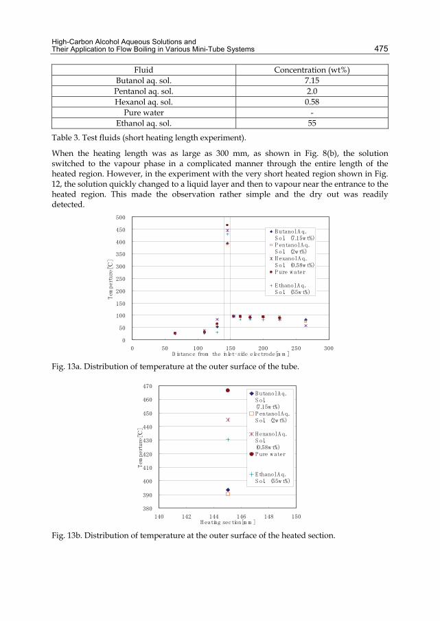
High-Carbon Alcohol Aqueous Solutions and Their Application to Flow Boiling in Various Mini-Tube Systems
475
Fluid Concentration (wt%) Butanol aq. sol. 7.15 Pentanol aq. sol. 2.0 Hexanol aq. sol. 0.58
Pure water - Ethanol aq. sol. 55
Table 3. Test fluids (short heating length experiment).
When the heating length was as large as 300 mm, as shown in Fig. 8(b), the solution switched to the vapour phase in a complicated manner through the entire length of the heated region. However, in the experiment with the very short heated region shown in Fig. 12, the solution quickly changed to a liquid layer and then to vapour near the entrance to the heated region. This made the observation rather simple and the dry out was readily detected.
0
50
100
150
200
250
300
350
400
450
500
0 50 100 150 200 250 300D istance from the inlet-side electrode[m m ]
Temperture[℃
]
B utanol A q.Sol. (7.15w t%)P entanol A q.Sol. (2w t%)H exanol A q.Sol. (0.58w t%)P ure w ater
Ethanol A q.Sol. (55w t%)
Fig. 13a. Distribution of temperature at the outer surface of the tube.
380
390
400
410
420
430
440
450
460
470
140 142 144 146 148 150H eating section[m m ]
Temperture[℃
]
B utanol A q.S ol.(7.15w t%)P entanol A q.S ol. (2w t%)
H exanol A q.S ol.(0.58w t%)P ure w ater
Ethanol A q.S ol. (55w t%)
Fig. 13b. Distribution of temperature at the outer surface of the heated section.
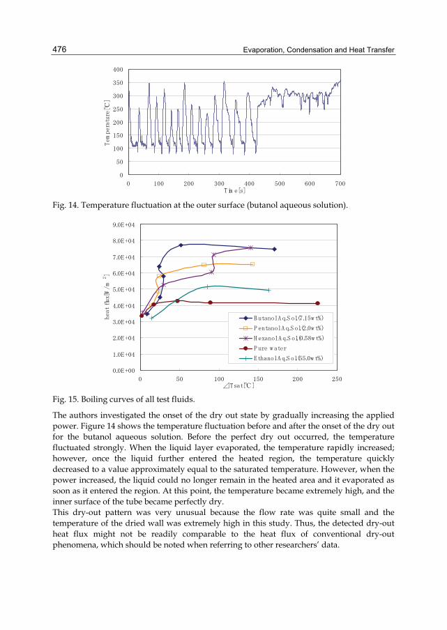
Evaporation, Condensation and Heat Transfer
476
0
50
100
150
200
250
300
350
400
0 100 200 300 400 500 600 700Tim e[s]
Temperature[℃
]
Fig. 14. Temperature fluctuation at the outer surface (butanol aqueous solution).
0.0E+00
1.0E+04
2.0E+04
3.0E+04
4.0E+04
5.0E+04
6.0E+04
7.0E+04
8.0E+04
9.0E+04
0 50 100 150 200 250⊿Tsat[℃]
heat flux[W/m
2]
B utanol A q.S ol.(7.15w t%)
P entanol A q.S ol.(2.0w t%)
H exanol A q.S ol.(0.58w t%)
P ure w ater
Ethanol A q.S ol.(55.0w t%)
Fig. 15. Boiling curves of all test fluids.
The authors investigated the onset of the dry out state by gradually increasing the applied power. Figure 14 shows the temperature fluctuation before and after the onset of the dry out for the butanol aqueous solution. Before the perfect dry out occurred, the temperature fluctuated strongly. When the liquid layer evaporated, the temperature rapidly increased; however, once the liquid further entered the heated region, the temperature quickly decreased to a value approximately equal to the saturated temperature. However, when the power increased, the liquid could no longer remain in the heated area and it evaporated as soon as it entered the region. At this point, the temperature became extremely high, and the inner surface of the tube became perfectly dry. This dry-out pattern was very unusual because the flow rate was quite small and the temperature of the dried wall was extremely high in this study. Thus, the detected dry-out heat flux might not be readily comparable to the heat flux of conventional dry-out phenomena, which should be noted when referring to other researchers’ data.
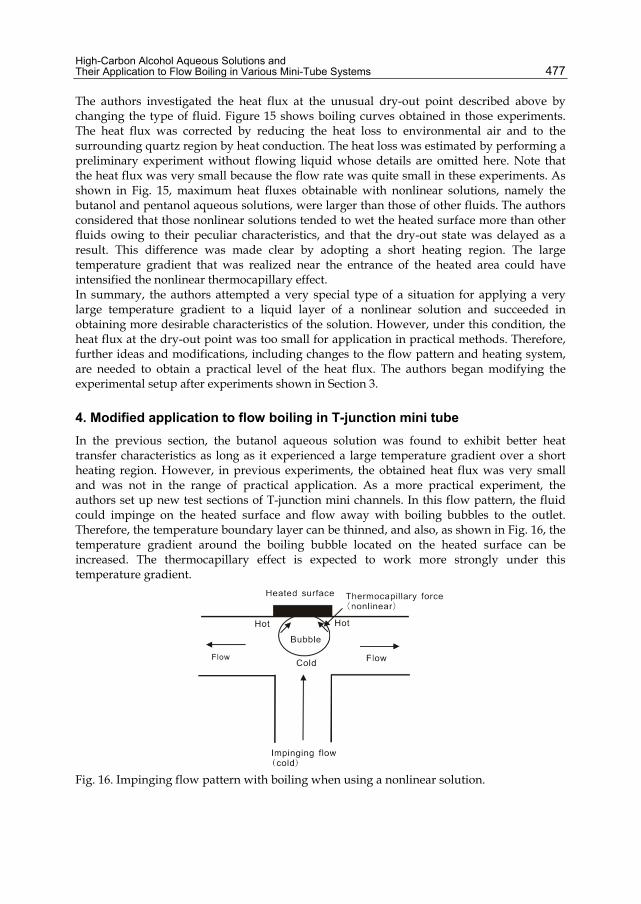
High-Carbon Alcohol Aqueous Solutions and Their Application to Flow Boiling in Various Mini-Tube Systems
477
The authors investigated the heat flux at the unusual dry-out point described above by changing the type of fluid. Figure 15 shows boiling curves obtained in those experiments. The heat flux was corrected by reducing the heat loss to environmental air and to the surrounding quartz region by heat conduction. The heat loss was estimated by performing a preliminary experiment without flowing liquid whose details are omitted here. Note that the heat flux was very small because the flow rate was quite small in these experiments. As shown in Fig. 15, maximum heat fluxes obtainable with nonlinear solutions, namely the butanol and pentanol aqueous solutions, were larger than those of other fluids. The authors considered that those nonlinear solutions tended to wet the heated surface more than other fluids owing to their peculiar characteristics, and that the dry-out state was delayed as a result. This difference was made clear by adopting a short heating region. The large temperature gradient that was realized near the entrance of the heated area could have intensified the nonlinear thermocapillary effect. In summary, the authors attempted a very special type of a situation for applying a very large temperature gradient to a liquid layer of a nonlinear solution and succeeded in obtaining more desirable characteristics of the solution. However, under this condition, the heat flux at the dry-out point was too small for application in practical methods. Therefore, further ideas and modifications, including changes to the flow pattern and heating system, are needed to obtain a practical level of the heat flux. The authors began modifying the experimental setup after experiments shown in Section 3.
4. Modified application to flow boiling in T-junction mini tube In the previous section, the butanol aqueous solution was found to exhibit better heat transfer characteristics as long as it experienced a large temperature gradient over a short heating region. However, in previous experiments, the obtained heat flux was very small and was not in the range of practical application. As a more practical experiment, the authors set up new test sections of T-junction mini channels. In this flow pattern, the fluid could impinge on the heated surface and flow away with boiling bubbles to the outlet. Therefore, the temperature boundary layer can be thinned, and also, as shown in Fig. 16, the temperature gradient around the boiling bubble located on the heated surface can be increased. The thermocapillary effect is expected to work more strongly under this temperature gradient.
Fig. 16. Impinging flow pattern with boiling when using a nonlinear solution.
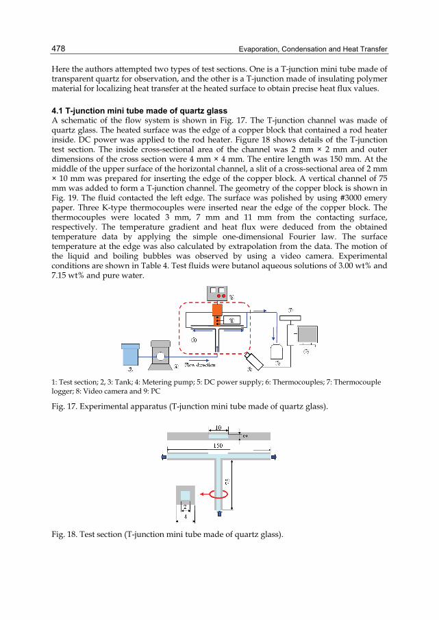
Evaporation, Condensation and Heat Transfer
478
Here the authors attempted two types of test sections. One is a T-junction mini tube made of transparent quartz for observation, and the other is a T-junction made of insulating polymer material for localizing heat transfer at the heated surface to obtain precise heat flux values.
4.1 T-junction mini tube made of quartz glass A schematic of the flow system is shown in Fig. 17. The T-junction channel was made of quartz glass. The heated surface was the edge of a copper block that contained a rod heater inside. DC power was applied to the rod heater. Figure 18 shows details of the T-junction test section. The inside cross-sectional area of the channel was 2 mm × 2 mm and outer dimensions of the cross section were 4 mm × 4 mm. The entire length was 150 mm. At the middle of the upper surface of the horizontal channel, a slit of a cross-sectional area of 2 mm × 10 mm was prepared for inserting the edge of the copper block. A vertical channel of 75 mm was added to form a T-junction channel. The geometry of the copper block is shown in Fig. 19. The fluid contacted the left edge. The surface was polished by using #3000 emery paper. Three K-type thermocouples were inserted near the edge of the copper block. The thermocouples were located 3 mm, 7 mm and 11 mm from the contacting surface, respectively. The temperature gradient and heat flux were deduced from the obtained temperature data by applying the simple one-dimensional Fourier law. The surface temperature at the edge was also calculated by extrapolation from the data. The motion of the liquid and boiling bubbles was observed by using a video camera. Experimental conditions are shown in Table 4. Test fluids were butanol aqueous solutions of 3.00 wt% and 7.15 wt% and pure water.
1: Test section; 2, 3: Tank; 4: Metering pump; 5: DC power supply; 6: Thermocouples; 7: Thermocouple logger; 8: Video camera and 9: PC
Fig. 17. Experimental apparatus (T-junction mini tube made of quartz glass).
Fig. 18. Test section (T-junction mini tube made of quartz glass).
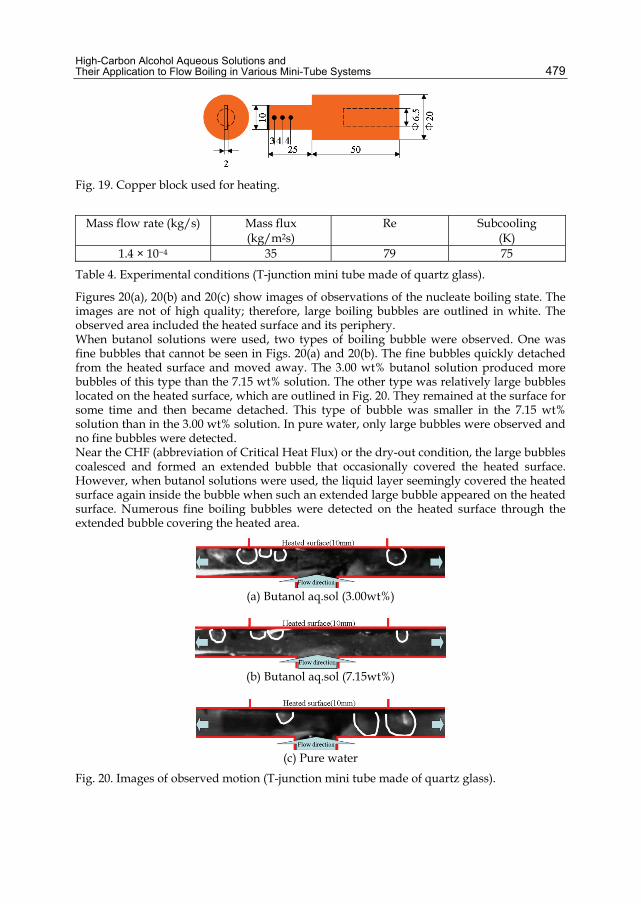
High-Carbon Alcohol Aqueous Solutions and Their Application to Flow Boiling in Various Mini-Tube Systems
479
Fig. 19. Copper block used for heating.
Mass flow rate (kg/s) Mass flux
(kg/m2s) Re Subcooling
(K) 1.4 × 10⁻⁴ 35 79 75
Table 4. Experimental conditions (T-junction mini tube made of quartz glass).
Figures 20(a), 20(b) and 20(c) show images of observations of the nucleate boiling state. The images are not of high quality; therefore, large boiling bubbles are outlined in white. The observed area included the heated surface and its periphery. When butanol solutions were used, two types of boiling bubble were observed. One was fine bubbles that cannot be seen in Figs. 20(a) and 20(b). The fine bubbles quickly detached from the heated surface and moved away. The 3.00 wt% butanol solution produced more bubbles of this type than the 7.15 wt% solution. The other type was relatively large bubbles located on the heated surface, which are outlined in Fig. 20. They remained at the surface for some time and then became detached. This type of bubble was smaller in the 7.15 wt% solution than in the 3.00 wt% solution. In pure water, only large bubbles were observed and no fine bubbles were detected. Near the CHF (abbreviation of Critical Heat Flux) or the dry-out condition, the large bubbles coalesced and formed an extended bubble that occasionally covered the heated surface. However, when butanol solutions were used, the liquid layer seemingly covered the heated surface again inside the bubble when such an extended large bubble appeared on the heated surface. Numerous fine boiling bubbles were detected on the heated surface through the extended bubble covering the heated area.
(a) Butanol aq.sol (3.00wt%)
(b) Butanol aq.sol (7.15wt%)
(c) Pure water
Fig. 20. Images of observed motion (T-junction mini tube made of quartz glass).
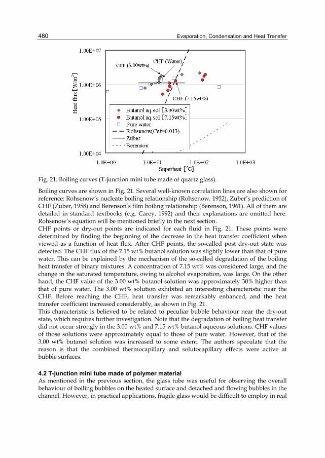
Evaporation, Condensation and Heat Transfer
480
Fig. 21. Boiling curves (T-junction mini tube made of quartz glass).
Boiling curves are shown in Fig. 21. Several well-known correlation lines are also shown for reference: Rohsenow’s nucleate boiling relationship (Rohsenow, 1952), Zuber’s prediction of CHF (Zuber, 1958) and Berenson’s film boiling relationship (Berenson, 1961). All of them are detailed in standard textbooks (e.g. Carey, 1992) and their explanations are omitted here. Rohsenow’s equation will be mentioned briefly in the next section. CHF points or dry-out points are indicated for each fluid in Fig. 21. These points were determined by finding the beginning of the decrease in the heat transfer coefficient when viewed as a function of heat flux. After CHF points, the so-called post dry-out state was detected. The CHF flux of the 7.15 wt% butanol solution was slightly lower than that of pure water. This can be explained by the mechanism of the so-called degradation of the boiling heat transfer of binary mixtures. A concentration of 7.15 wt% was considered large, and the change in the saturated temperature, owing to alcohol evaporation, was large. On the other hand, the CHF value of the 3.00 wt% butanol solution was approximately 30% higher than that of pure water. The 3.00 wt% solution exhibited an interesting characteristic near the CHF. Before reaching the CHF, heat transfer was remarkably enhanced, and the heat transfer coefficient increased considerably, as shown in Fig. 21. This characteristic is believed to be related to peculiar bubble behaviour near the dry-out state, which requires further investigation. Note that the degradation of boiling heat transfer did not occur strongly in the 3.00 wt% and 7.15 wt% butanol aqueous solutions. CHF values of those solutions were approximately equal to those of pure water. However, that of the 3.00 wt% butanol solution was increased to some extent. The authors speculate that the reason is that the combined thermocapillary and solutocapillary effects were active at bubble surfaces.
4.2 T-junction mini tube made of polymer material As mentioned in the previous section, the glass tube was useful for observing the overall behaviour of boiling bubbles on the heated surface and detached and flowing bubbles in the channel. However, in practical applications, fragile glass would be difficult to employ in real
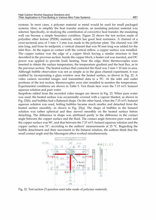
High-Carbon Alcohol Aqueous Solutions and Their Application to Flow Boiling in Various Mini-Tube Systems
481
systems. In most cases, a polymer material or metal would be used for small packaged systems. Here, to simplify the heat transfer analysis, an insulating polymer material was selected. Specifically, in studying the contribution of convective heat transfer, the insulating wall can become a simple boundary condition. Figure 22 shows the test section made of polyether ether ketone (PEEK) material, which has good heat resistance. A channel of a cross-sectional area of 3 mm × 3 mm was made in the polymer plate. The channel was 100 mm long, and from its midpoint, a vertical channel that was 50 mm long was added for the inlet flow. At the region in contact with the vertical inflow, a copper surface was installed. The copper surface was the edge of a copper block having a similar structure to that described in the previous section. Inside the copper block, a heater rod was inserted, and DC power was applied to provide Joule heating. Near the edge, three thermocouples were inserted to obtain the surface temperature, the temperature gradient and the heat flux, as in the previous section. The heated surface that contacted the fluid was 3 mm × 10 mm in area. Although bubble observation was not as simple as in the glass channel experiment, it was enabled by incorporating a glass window near the heated surface, as shown in Fig. 22. A video camera recorded images and transmitted data to a PC. At the inlet and outlet positions of the test section, thermocouples were also installed to monitor the temperature. Experimental conditions are shown in Table 5. Test fluids here were the 7.15 wt% butanol aqueous solution and pure water. Snapshots edited from the recorded video images are shown in Fig. 23. When pure water was used, the heated surface was occasionally covered with a vapour blanket, as shown in Fig. 23(b), and bubbles had a flattened shape. On the other hand, when the 7.15 wt% butanol aqueous solution was used, boiling bubbles became much smaller and detached from the heated surface smoothly, as shown in Fig. 23(a). The shape of bubbles in the butanol solution was rather spherical and they moved smoothly on the heated surface before detaching. The difference in shape was attributed partly to the difference in the contact angle between the copper surface and the fluid. The contact angle between pure water and the copper surface was 94°, and that between the 7.15 wt% butanol aqueous solution and the copper surface was 51°, according to the authors’ measurements at 25 °C. Regarding the bubble detachment and their movement in the butanol solution, the authors think that the small contact angle and the Marangoni effect worked simultaneously.
Inlet
O utletO utlet
G lass w indow
Inlet
O utletO utlet
G lass w indow
Fig. 22. Test section (T-junction mini tube made of polymer material).
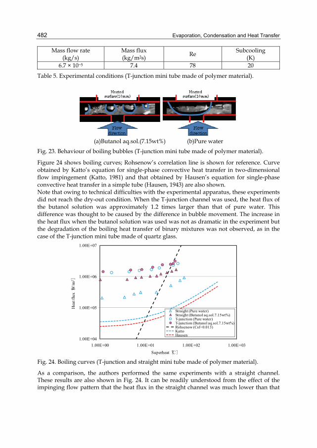
Evaporation, Condensation and Heat Transfer
482
Mass flow rate (kg/s)
Mass flux (kg/m2s) Re Subcooling
(K) 6.7 × 10⁻⁵ 7.4 78 20
Table 5. Experimental conditions (T-junction mini tube made of polymer material).
(a)Butanol aq.sol.(7.15wt%) (b)Pure water
Fig. 23. Behaviour of boiling bubbles (T-junction mini tube made of polymer material).
Figure 24 shows boiling curves; Rohsenow’s correlation line is shown for reference. Curve obtained by Katto’s equation for single-phase convective heat transfer in two-dimensional flow impingement (Katto, 1981) and that obtained by Hausen’s equation for single-phase convective heat transfer in a simple tube (Hausen, 1943) are also shown. Note that owing to technical difficulties with the experimental apparatus, these experiments did not reach the dry-out condition. When the T-junction channel was used, the heat flux of the butanol solution was approximately 1.2 times larger than that of pure water. This difference was thought to be caused by the difference in bubble movement. The increase in the heat flux when the butanol solution was used was not as dramatic in the experiment but the degradation of the boiling heat transfer of binary mixtures was not observed, as in the case of the T-junction mini tube made of quartz glass.
1.00E+04
1.00E+05
1.00E+06
1.00E+07
1.00E+00 1.00E+01 1.00E+02 1.00E+03
Straight (Pure water)Straight (Butanol aq.sol.7.15wt%)T-junction (Pure water)T-junction (Butanol aq.sol.7.15wt%)Rohsenow (Csf=0.013)KattoHausen
Superheat[℃]
Hea
t flu
x[W
/m2 ]
Fig. 24. Boiling curves (T-junction and straight mini tube made of polymer material).
As a comparison, the authors performed the same experiments with a straight channel. These results are also shown in Fig. 24. It can be readily understood from the effect of the impinging flow pattern that the heat flux in the straight channel was much lower than that
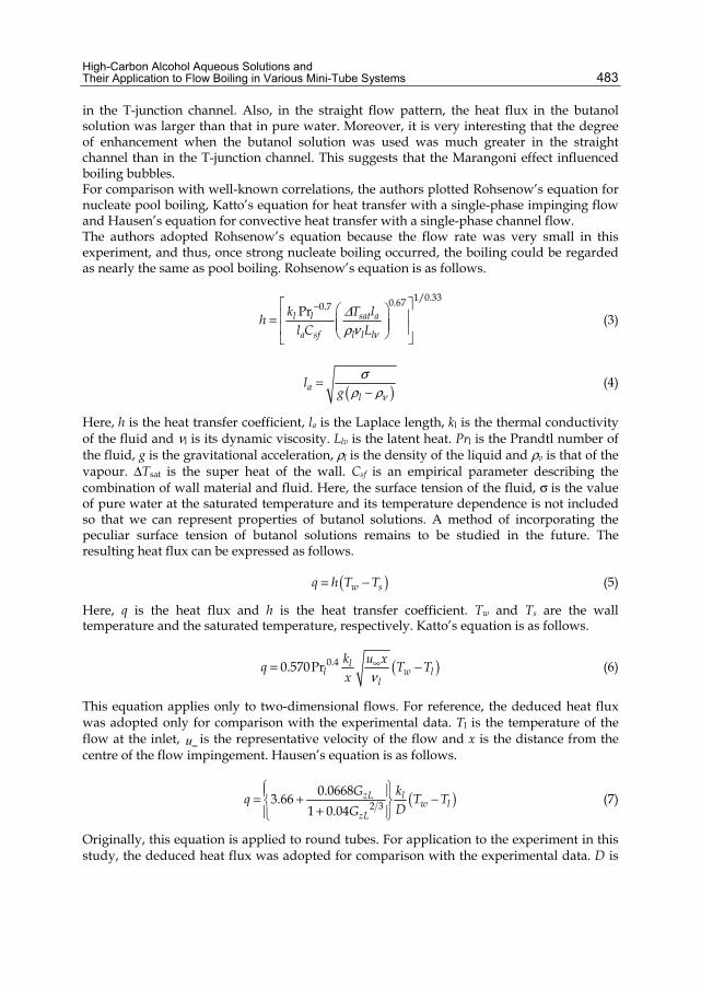
High-Carbon Alcohol Aqueous Solutions and Their Application to Flow Boiling in Various Mini-Tube Systems
483
in the T-junction channel. Also, in the straight flow pattern, the heat flux in the butanol solution was larger than that in pure water. Moreover, it is very interesting that the degree of enhancement when the butanol solution was used was much greater in the straight channel than in the T-junction channel. This suggests that the Marangoni effect influenced boiling bubbles. For comparison with well-known correlations, the authors plotted Rohsenow’s equation for nucleate pool boiling, Katto’s equation for heat transfer with a single-phase impinging flow and Hausen’s equation for convective heat transfer with a single-phase channel flow. The authors adopted Rohsenow’s equation because the flow rate was very small in this experiment, and thus, once strong nucleate boiling occurred, the boiling could be regarded as nearly the same as pool boiling. Rohsenow’s equation is as follows.
1/0.330.670.7Prl l sat a
a sf l l l
k T lhl C Lν
Δρν
−⎡ ⎤⎛ ⎞⎢ ⎥= ⎜ ⎟⎜ ⎟⎢ ⎥⎝ ⎠⎣ ⎦ (3)
( )al
lg ν
σρ ρ
=−
(4)
Here, h is the heat transfer coefficient, la is the Laplace length, kl is the thermal conductivity of the fluid and νl is its dynamic viscosity. Llv is the latent heat. Prl is the Prandtl number of the fluid, g is the gravitational acceleration, ρl is the density of the liquid and ρv is that of the vapour. ΔTsat is the super heat of the wall. Csf is an empirical parameter describing the combination of wall material and fluid. Here, the surface tension of the fluid, σ is the value of pure water at the saturated temperature and its temperature dependence is not included so that we can represent properties of butanol solutions. A method of incorporating the peculiar surface tension of butanol solutions remains to be studied in the future. The resulting heat flux can be expressed as follows.
( )w sq h T T= − (5)
Here, q is the heat flux and h is the heat transfer coefficient. Tw and Ts are the wall temperature and the saturated temperature, respectively. Katto’s equation is as follows.
( )0.40.570Pr ll w l
l
k u xq T Tx ν
∞= − (6)
This equation applies only to two-dimensional flows. For reference, the deduced heat flux was adopted only for comparison with the experimental data. Tl is the temperature of the flow at the inlet,
∞u is the representative velocity of the flow and x is the distance from the centre of the flow impingement. Hausen’s equation is as follows.
( )2 30.06683.66
1 0.04zL l
w lzL
G kq T TDG
⎧ ⎫⎪ ⎪= + −⎨ ⎬+⎪ ⎪⎩ ⎭
(7)
Originally, this equation is applied to round tubes. For application to the experiment in this study, the deduced heat flux was adopted for comparison with the experimental data. D is
Evaporation, Condensation and Heat Transfer
484
the effective diameter of the channel. GzL is the Graetz number, which can be defined as follows.
Re PrzL D lDGL
= (8)
L is the length of the heated region. ReD is the Reynolds number, which is defined as follows.
ReDl
uDν
= (9)
Here, u is the averaged velocity in the channel. As shown in Fig. 24, the measured heat flux data were larger than values obtained by Katto’s and Hausen’s equations. This is because experiments included boiling heat transfer as well as convective heat transfer. However, not all the data seemed to obey Rohsenow’s curve although the observation apparently revealed that weak nucleate boiling occurred. The authors think that the boiling in experiments was so weak that the heat transfer caused by boiling did not contribute much to the entire heat flux. New experiments in which the applied power can be increased to obtain both a strong nucleate boiling and a dry out will be needed for further investigation. The authors are now preparing such experiments to investigate the onset of the dry out and will report them in the near future. When the glass channel described in the previous section was used, the heat transfer improved abruptly near the dry-out point, as shown in Fig. 21. The authors expect that similar phenomena could occur in the polymer channel. Moreover, polymer material is generally hydrophobic; therefore, bubbles are less likely to stick to the surface. Thus, once boiling bubbles detach from the copper surface, they leave the copper surface smoothly and maintain heat transfer caused by their motion. These issues must be examined in future experiments. Although the above limitation existed in the current data, the authors believe that advantages of the butanol aqueous solution were clarified to some extent. In a prototype system made of insulating polymer material, the butanol aqueous solution can be thought to have the potential to enhance heat transfer in boiling with flow impingement inside mini channels.
5. Conclusion The authors have been performing various types of experiment to clarify and demonstrate advantages of high-carbon alcohol aqueous solutions for boiling heat transfer inside mini channels after confirming peculiar characteristics of the temperature dependence of surface tension by their own measurements. Findings and conclusions to date can be summarized as follows. 1. To investigate the peculiar temperature dependence of the surface tension of butanol
and other high-carbon alcohol aqueous solutions, a static maximum bubble pressure method was adopted, and measurements were performed. These measurements revealed the nonlinearity of the surface tension of those solutions and provided more reliable data than those obtained by Wilhelmy’s method.
2. When a butanol solution was applied to a simple long mini tube of 1 mm in diameter, the dry out was not delayed by using the solution. However, very unusual behaviour of
High-Carbon Alcohol Aqueous Solutions and Their Application to Flow Boiling in Various Mini-Tube Systems
485
the liquid layer, namely an extending motion of the liquid layer to a hotter region, was observed.
3. When the heating region was localized in the mini tube to obtain a large temperature gradient at the entrance of the region, the dry-out heat flux under a very small flow rate was larger when the high-carbon alcohol aqueous solution was used. However, owing to technical difficulties, this experiment had a heat flux of a very small order.
4. A T-junction mini channel was studied because this flow pattern could increase the temperature gradient around boiling bubbles remaining on the heated surface. Experiments revealed that the use of butanol aqueous solutions increased the dry-out heat flux somewhat in a T-junction channel made of glass. When a T-junction channel made of polymer material was used, the heat flux before the onset of the dry out was again somewhat increased by using these solutions.
As aforementioned, the authors are certain that high-carbon alcohol aqueous solutions can induce peculiar motion in the liquid layer and boiling bubbles. However, the advantage in heat transfer was not as dramatic and was limited to small values. On the other hand, some examples of their good characteristics were reported in pool boiling and large heat pipes (Abe, 2006a, 2006b). More modifications of flow conditions and flow patterns would be needed for adaption to the small-scale environment of mini channels. Another important issue requiring investigation is the mechanism of the Marangoni force acting on boiling bubbles. As long as an alcohol aqueous solution is used, the thermocapillary and solutocapillary forces will always coexist. In particular, when a butanol solution is used, directions of the two forces are the same; therefore, it is not yet clear which of the two forces is dominant in boiling bubbles. The authors began to observe the onset of the Marangoni convection around a small air bubble in a butanol aqueous solution (Eda et al., 2010). These results indicated a clear contribution of a peculiar thermocapillary force. They now plan to clarify the contribution ratio of each capillary force in butanol aqueous solutions.
6. Acknowledgements The authors would like to thank Prof M. Shoji, Mr S. Nishiguchi, Dr T.-H. Yen, Dr F. Takemura, Dr S. Matsumoto and Dr M. Tange for their helpful suggestions and aid in the research. They are also grateful to Mr T. Yoshida, Mr T. Kaneko, Mr M. Otsuka, Mr Y. Kumagai, Mr K. Kunimatsu, Mr K. Kawai, Mr T. Ueno and Mr Y. Nomura for their assistance in the experiments and measurements. This research was partially supported by the MEXT/JSPS, Grant-in-Aid for Scientific Research (C, No. 21560225).
7. References Abe, Y. (2006a). Thermal management with self-rewetting fluids, J. Jpn. Soc. Microgravity
Appl., Vol. 23, No. 2 (2006), pp. 80–87. Abe, Y. (2006b). Self-rewetting fluids, Ann. N.Y. Acad. Sci. 1077 (2006), pp. 650–667. Adamson, A.W. & Gast, A.P. (1997). Physical chemistry of surfaces, A Wiley-Interscience
publication (1997). Azouni, M.A. & Petre, G. (1998). J.Colloidal Int. Sci., 206 (1998), pp. 332–333. Berenson, P. J. (1961). Film boiling heat transfer from a horizontal surface, J. Heat Transfer,
Vol. 83, pp. 351, 1961.
Evaporation, Condensation and Heat Transfer
486
Carey, V. P. (1992). Liquid-Vapor Phase-Change Phenomena, (1992), Taylor and Francis. Cheng, P. & Wu, H.Y. (2006). Phase-change heat transfer in Microsystems, 13th Inter-
national Heat Transfer Conference, Key Note-02, 13–18 August, Sydney, Australia. Eda, Y., Kawai, K. & Ono, N. (2010). Observation of marangoni flow near the artificial air
bubble on heated surface in using alcohol aqueous solution, Seventh International Conference on Flow Dynamics (1–3 November 2010, Sendai, Japan), Proceedings pp. 448–449.
Hausen, H. (1943). VDI Z., No. 4, pp. 91, 1943, In: Heat transfer, Hallman, J.P., McGraw-Hill, 1976.
JSME Data Book: Thermophysical Properties of Fluids (1983), JSME (in Japanese). Kandlikar, S.G. (2004). Heat transfer mechanisms during flow boiling in microchannels, J.
Heat Transfer (Transactions ASME), 126 (2004), pp. 8–16. Katto, Y. (1981). In: JSME Data Book: Heat Transfer, 5th Edition (2009), JSME (in Japanese),
pp. 33. Legros, J.C. (1986). Acta Astronautica, 13–11 December 1986, pp. 697–703. Ono, N., Yoshida, T., Kaneko, T., Nishiguchi, S. & Shoji, M. (2009). Journal of Thermal Science
and Technology (JSME), Vol.4 (2009), No.2, pp.284-293. Ono, N., Yoshida, T., Kaneko, T., Nishiguchi, S. & Shoji, M. (2008a). Thermal Science and
Engineering, Vol. 16, No.3 (2008), pp. 79–85. Ono, N., Kaneko, T., Nishiguchi, S. & Shoji, M. (2008b). Proceedings of IFHT2008, (2008),
Paper No. 200, CD-ROM. Rohsenow, W.M. (1952). A method of correlating heat transfer data for surface boiling
liquids, Trans. ASME, Vol. 74, pp.969, 1952. Thome, J.R. (2006). Fundamentals of boiling and two-phase flows in microchannels, 13th
Inter-national Heat Transfer Conference, Key Note-14, 13–18 August, Sydney, Australia.
Vochten, R. & Petre, G. (1973). Study of the heat of reversible adsorption at the air-solution interface, J.Colloidal Science, 42-2(1973), pp. 320–327.
Zuber, N. (1958). On the stability of boiling heat transfer, Trans. ASME, Vol. 80, pp.711, 1958.
23
Heat Transfer and Hydraulic Resistance in Rough Tubes Including
with Twisted Tape Inserts Stanislav Tarasevich and Anatoly Yakovlev
Kazan State Technical University, Russia
1. Introduction
The spiral and cross-section wire insertions, knurls of a various configuration, microfinning, spherical, cylindrical, cone-shaped both other ledges and depressions, stamped surfaces etc. refer to the heat transfer intensifiers allowing considerably to augment a heat transfer at moderate or comparable growth of a pressure drop. The effect of a heat transfer intensification on rough surfaces is attained due to the additional vortex generation leading to raise of a turbulent diffusion in a conversion zone, to a turbulent kernel and due to lowering of stability and width of a viscous boundary layer with molecular thermal conduction at a surface. W. Nunner (1956) has determinated that in rough tubes at growth of ledge height of a roughness the heat transfer factors it is more to 3 times than value in smooth tubes. Intensifying agency of a roughness has been displayed in many subsequent papers (Dipprey & Sabersky, 1963; Isachenko et al., 1965; Kolar, 1965; Sheriff et al., 1964; Sheriff & Gumley, 1966; et al.). Among artificially roughened surfaces there are surfaces with a continuous roughness (for example, in the form of a thread) and with a discrete roughness (the roughness ledges pitch considerably exceeds their absolute sizes). The discrete roughness is more often preferable for heat transfer enhancement. However the continuous roughness of the outer and inner surfaces of tubes also can be effective for raise of heat transfer, especially at boiling and condensation (Berenson, 1962; Buznik et al., 1969; Danilova & Belsky, 1965; Ivanov et al., 1988; Nishikawa et al., 1982; et al.). The basic flow regularity in tubes with a continuous sand uniform granulous roughness has been determined in the first half of 20th century (Nikuradze, 1933; Schlichting, 1979; et al.). However the subsequent researches for tubes with a various uniform continuous "not sand" roughness (organized by the single-start and multiple-start cross threads with triangular, rectangular and rounded profiles, and also in the form of ring bores and spherical ledges with passage and chess arrangement) have displayed considerable divergences with an existing explanation of the action mechanism of a sand roughness and with theoretical models of a boundary layer on a rough surface (Ibragimov et al., 1978; Isachenko et al., 1965; et al.). Thus intensity of a heat transfer and pressure drop in tubes with various aspects of roughnesses is rather individually and also is defined by not only a relative height of
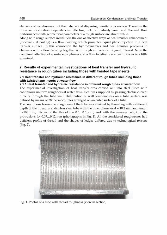
Evaporation, Condensation and Heat Transfer
488
elements of roughnesses, but their shape and disposing density on a surface. Therefore the universal calculation dependences reflecting link of hydrodynamic and thermal flow performances with geometrical parameters of a rough surface are absent while. Along with rough surface intensifiers the one of effective ways of heat transfer enhancement (especially at boiling) is a flow twisting which promotes liquid phase rejection to a heat transfer surface. In this connection the hydrodynamics and heat transfer problems in channels with a flow twisting together with rough surfaces call a great interest. Now the combined affecting of a surface roughness and a flow twisting on a heat transfer is a little examined.
2. Results of experimental investigations of heat transfer and hydraulic resistance in rough tubes including those with twisted tape inserts 2.1 Heat transfer and hydraulic resistance in different rough tubes including those with twisted tape inserts at water flow 2.1.1 Heat transfer and hydraulic resistance in different rough tubes at water flow The experimental investigation of heat transfer was carried out into steel tubes with continuous uniform roughness at water flow. Heat was supplied by passing electric current directly through the tube wall. Distribution of wall temperatures on a tube surface was defined by means of 28 thermocouples arranged on an outer surface of a tube. The continuous transverse roughness of the tube was attained by threading with a different depth of the thread in a stainless steel tube with the inner diameter d = 10.2 mm and length L=500 mm, pitches of the thread t = 0.3…0.5 mm, and with the average height of the protrusions Δ= 0.09…0.12 mm (photographs in Fig. 1). All the considered roughnesses had deficient profile of thread and the shapes of ledges differed due to technological reasons (Fig. 2).
Fig. 1. Photos of a tube with thread roughness (view in section)
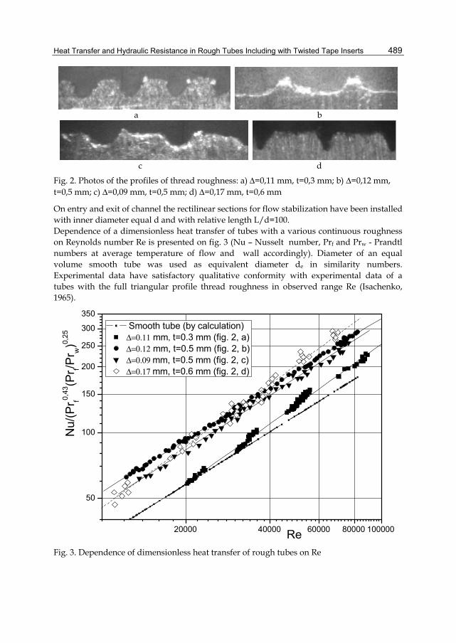
Heat Transfer and Hydraulic Resistance in Rough Tubes Including with Twisted Tape Inserts
489
a b
c d
Fig. 2. Photos of the profiles of thread roughness: a) Δ=0,11 mm, t=0,3 mm; b) Δ=0,12 mm, t=0,5 mm; c) Δ=0,09 mm, t=0,5 mm; d) Δ=0,17 mm, t=0,6 mm
On entry and exit of channel the rectilinear sections for flow stabilization have been installed with inner diameter equal d and with relative length L/d=100. Dependence of a dimensionless heat transfer of tubes with a various continuous roughness on Reynolds number Re is presented on fig. 3 (Nu – Nusselt number, Prf and Prw - Prandtl numbers at average temperature of flow and wall accordingly). Diameter of an equal volume smooth tube was used as equivalent diameter de in similarity numbers. Experimental data have satisfactory qualitative conformity with experimental data of a tubes with the full triangular profile thread roughness in observed range Re (Isachenko, 1965).
20000 40000 60000 80000 100000
50
100
150
200
250
300
350 Smooth tube (by calculation)Δ=0.11 mm, t=0.3 mm (fig. 2, a)Δ=0.12 mm, t=0.5 mm (fig. 2, b)Δ=0.09 mm, t=0.5 mm (fig. 2, c)Δ=0.17 mm, t=0.6 mm (fig. 2, d)
Nu/
(Pr f0,
43(P
r f/Pr w
)0,25
Re
Fig. 3. Dependence of dimensionless heat transfer of rough tubes on Re
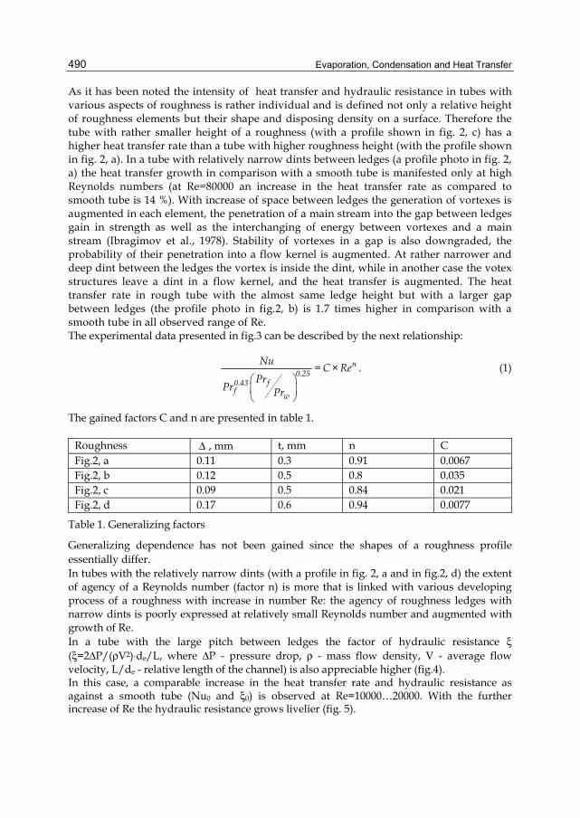
Evaporation, Condensation and Heat Transfer
490
As it has been noted the intensity of heat transfer and hydraulic resistance in tubes with various aspects of roughness is rather individual and is defined not only a relative height of roughness elements but their shape and disposing density on a surface. Therefore the tube with rather smaller height of a roughness (with a profile shown in fig. 2, c) has a higher heat transfer rate than a tube with higher roughness height (with the profile shown in fig. 2, a). In a tube with relatively narrow dints between ledges (a profile photo in fig. 2, a) the heat transfer growth in comparison with a smooth tube is manifested only at high Reynolds numbers (at Re=80000 an increase in the heat transfer rate as compared to smooth tube is 14 %). With increase of space between ledges the generation of vortexes is augmented in each element, the penetration of a main stream into the gap between ledges gain in strength as well as the interchanging of energy between vortexes and a main stream (Ibragimov et al., 1978). Stability of vortexes in a gap is also downgraded, the probability of their penetration into a flow kernel is augmented. At rather narrower and deep dint between the ledges the vortex is inside the dint, while in another case the votex structures leave a dint in a flow kernel, and the heat transfer is augmented. The heat transfer rate in rough tube with the almost same ledge height but with a larger gap between ledges (the profile photo in fig.2, b) is 1.7 times higher in comparison with a smooth tube in all observed range of Re. The experimental data presented in fig.3 can be described by the next relationship:
⎛ ⎞⎜ ⎟⎝ ⎠
n0.25
f0.43f
w
Nu =С× RePr
Pr Pr
. (1)
The gained factors C and n are presented in table 1.
Roughness Δ , mm t, mm n С Fig.2, a 0.11 0.3 0.91 0.0067 Fig.2, b 0.12 0.5 0.8 0.035 Fig.2, c 0.09 0.5 0.84 0.021 Fig.2, d 0.17 0.6 0.94 0.0077
Table 1. Generalizing factors
Generalizing dependence has not been gained since the shapes of a roughness profile essentially differ. In tubes with the relatively narrow dints (with a profile in fig. 2, a and in fig.2, d) the extent of agency of a Reynolds number (factor n) is more that is linked with various developing process of a roughness with increase in number Re: the agency of roughness ledges with narrow dints is poorly expressed at relatively small Reynolds number and augmented with growth of Re. In a tube with the large pitch between ledges the factor of hydraulic resistance ξ (ξ=2ΔP/(ρV2)⋅de/L, where ΔP - pressure drop, ρ - mass flow density, V - average flow velocity, L/de - relative length of the channel) is also appreciable higher (fig.4). In this case, a comparable increase in the heat transfer rate and hydraulic resistance as against a smooth tube (Nu0 and ξ0) is observed at Re=10000…20000. With the further increase of Re the hydraulic resistance grows livelier (fig. 5).
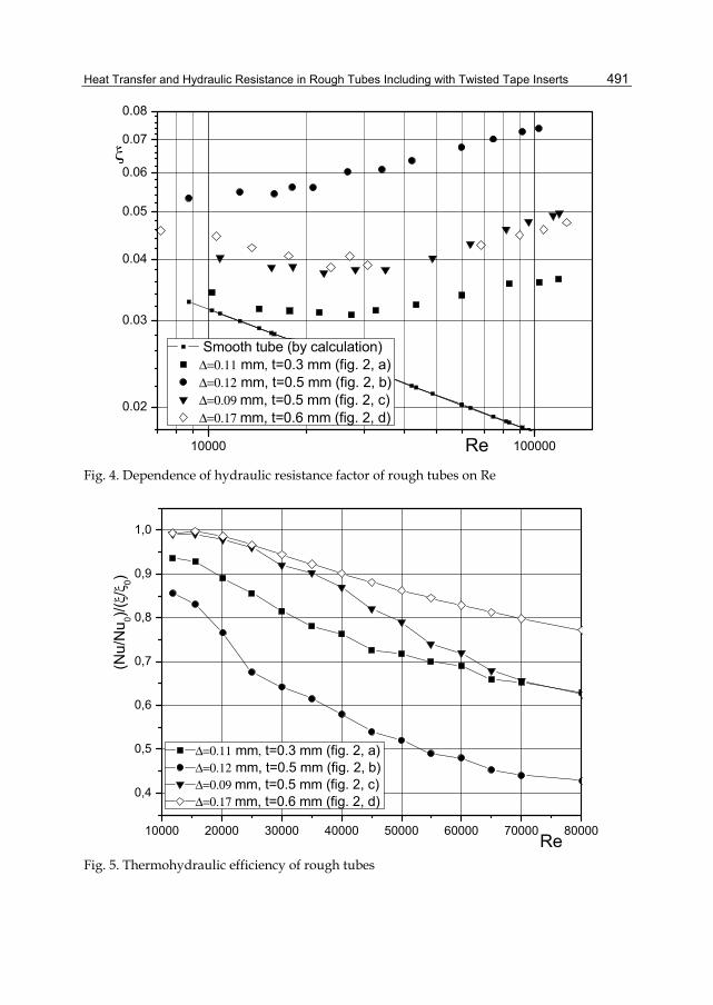
Heat Transfer and Hydraulic Resistance in Rough Tubes Including with Twisted Tape Inserts
491
10000 100000
0.02
0.03
0.04
0.05
0.06
0.07
0.08
Smooth tube (by calculation)Δ=0.11 mm, t=0.3 mm (fig. 2, a)Δ=0.12 mm, t=0.5 mm (fig. 2, b)Δ=0.09 mm, t=0.5 mm (fig. 2, c)Δ=0.17 mm, t=0.6 mm (fig. 2, d)
ξ
Re
Fig. 4. Dependence of hydraulic resistance factor of rough tubes on Re
10000 20000 30000 40000 50000 60000 70000 80000
0,4
0,5
0,6
0,7
0,8
0,9
1,0
Δ=0.11 mm, t=0.3 mm (fig. 2, a)Δ=0.12 mm, t=0.5 mm (fig. 2, b)Δ=0.09 mm, t=0.5 mm (fig. 2, c)Δ=0.17 mm, t=0.6 mm (fig. 2, d)
(Nu/
Nu 0)/(
ξ/ξ 0)
Re
Fig. 5. Thermohydraulic efficiency of rough tubes
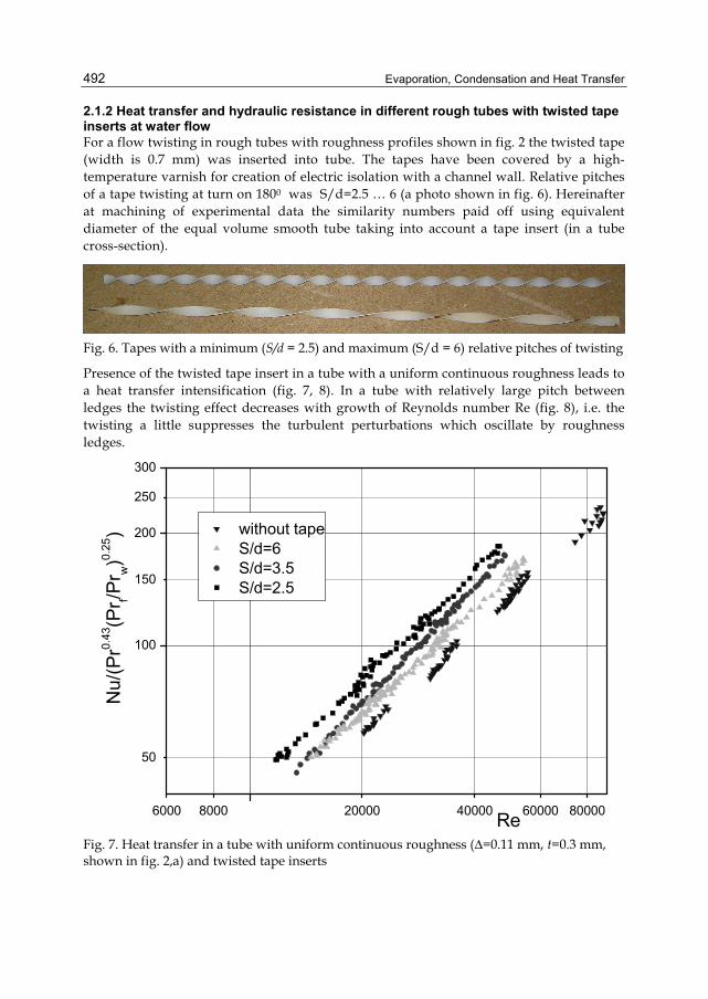
Evaporation, Condensation and Heat Transfer
492
2.1.2 Heat transfer and hydraulic resistance in different rough tubes with twisted tape inserts at water flow For a flow twisting in rough tubes with roughness profiles shown in fig. 2 the twisted tape (width is 0.7 mm) was inserted into tube. The tapes have been covered by a high-temperature varnish for creation of electric isolation with a channel wall. Relative pitches of a tape twisting at turn on 1800 was S/d=2.5 … 6 (a photo shown in fig. 6). Hereinafter at machining of experimental data the similarity numbers paid off using equivalent diameter of the equal volume smooth tube taking into account a tape insert (in a tube cross-section).
Fig. 6. Tapes with a minimum (S/d = 2.5) and maximum (S/d = 6) relative pitches of twisting
Presence of the twisted tape insert in a tube with a uniform continuous roughness leads to a heat transfer intensification (fig. 7, 8). In a tube with relatively large pitch between ledges the twisting effect decreases with growth of Reynolds number Re (fig. 8), i.e. the twisting a little suppresses the turbulent perturbations which oscillate by roughness ledges.
6000 8000 20000 40000 60000 80000
50
100
150
200
250
300
Re
Nu/
(Pr0.
43(P
r f/Pr w
)0.25
) without tape S/d=6 S/d=3.5 S/d=2.5
Fig. 7. Heat transfer in a tube with uniform continuous roughness (Δ=0.11 mm, t=0.3 mm, shown in fig. 2,а) and twisted tape inserts
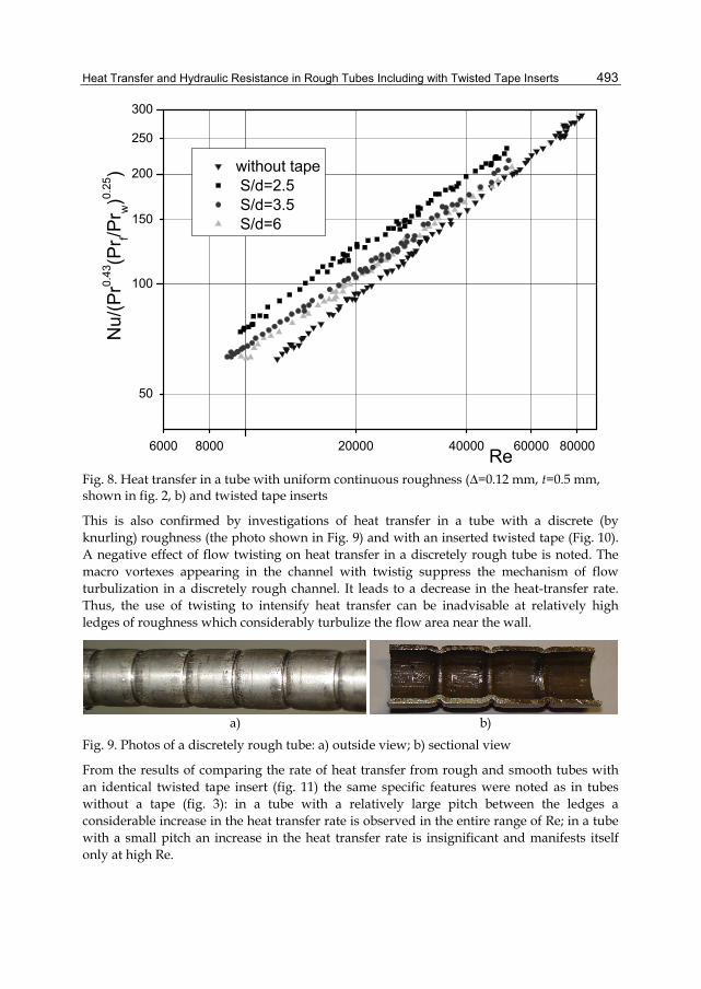
Heat Transfer and Hydraulic Resistance in Rough Tubes Including with Twisted Tape Inserts
493
6000 8000 20000 40000 60000 80000
50
100
150
200
250
300
Re
Nu/
(Pr0.
43(P
r f/Pr w
)0.25
) without tape S/d=2.5 S/d=3.5 S/d=6
Fig. 8. Heat transfer in a tube with uniform continuous roughness (Δ=0.12 mm, t=0.5 mm, shown in fig. 2, b) and twisted tape inserts
This is also confirmed by investigations of heat transfer in a tube with a discrete (by knurling) roughness (the photo shown in Fig. 9) and with an inserted twisted tape (Fig. 10). A negative effect of flow twisting on heat transfer in a discretely rough tube is noted. The macro vortexes appearing in the channel with twistig suppress the mechanism of flow turbulization in a discretely rough channel. It leads to a decrease in the heat-transfer rate. Thus, the use of twisting to intensify heat transfer can be inadvisable at relatively high ledges of roughness which considerably turbulize the flow area near the wall.
a) b)
Fig. 9. Photos of a discretely rough tube: a) outside view; b) sectional view
From the results of comparing the rate of heat transfer from rough and smooth tubes with an identical twisted tape insert (fig. 11) the same specific features were noted as in tubes without a tape (fig. 3): in a tube with a relatively large pitch between the ledges a considerable increase in the heat transfer rate is observed in the entire range of Re; in a tube with a small pitch an increase in the heat transfer rate is insignificant and manifests itself only at high Re.
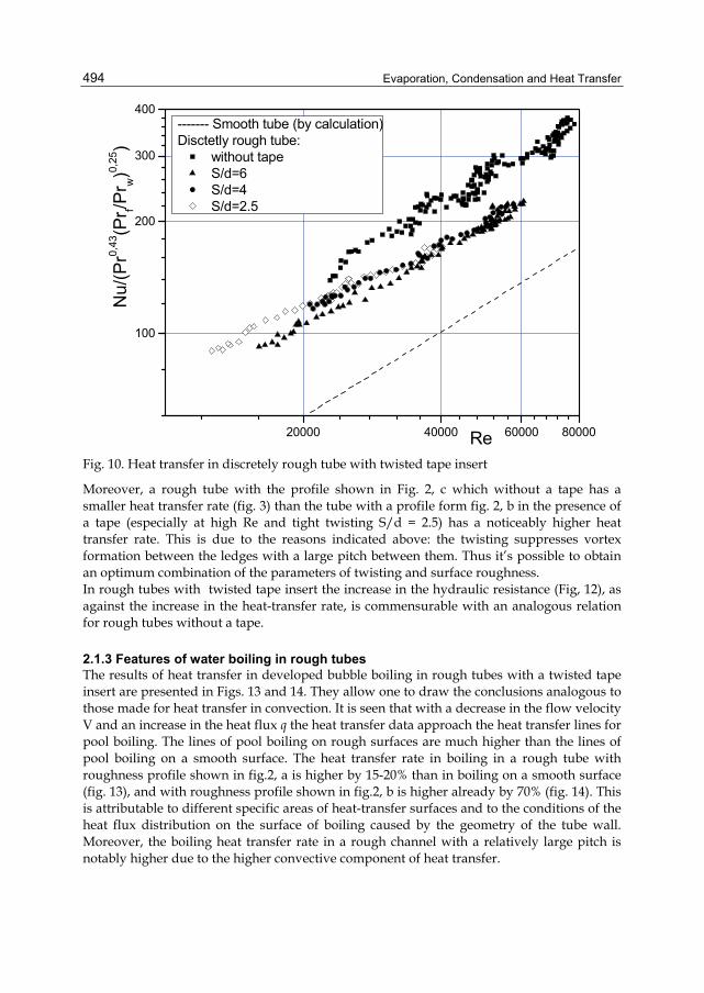
Evaporation, Condensation and Heat Transfer
494
20000 40000 60000 80000
100
200
300
400
Re
Nu/
(Pr0,
43(P
r f/Pr w
)0,25
)------- Smooth tube (by calculation)Disctetly rough tube:
without tape S/d=6 S/d=4 S/d=2.5
Fig. 10. Heat transfer in discretely rough tube with twisted tape insert
Moreover, a rough tube with the profile shown in Fig. 2, c which without a tape has a smaller heat transfer rate (fig. 3) than the tube with a profile form fig. 2, b in the presence of a tape (especially at high Re and tight twisting S/d = 2.5) has a noticeably higher heat transfer rate. This is due to the reasons indicated above: the twisting suppresses vortex formation between the ledges with a large pitch between them. Thus it’s possible to obtain an optimum combination of the parameters of twisting and surface roughness. In rough tubes with twisted tape insert the increase in the hydraulic resistance (Fig, 12), as against the increase in the heat-transfer rate, is commensurable with an analogous relation for rough tubes without a tape.
2.1.3 Features of water boiling in rough tubes The results of heat transfer in developed bubble boiling in rough tubes with a twisted tape insert are presented in Figs. 13 and 14. They allow one to draw the conclusions analogous to those made for heat transfer in convection. It is seen that with a decrease in the flow velocity V and an increase in the heat flux q the heat transfer data approach the heat transfer lines for pool boiling. The lines of pool boiling on rough surfaces are much higher than the lines of pool boiling on a smooth surface. The heat transfer rate in boiling in a rough tube with roughness profile shown in fig.2, a is higher by 15-20% than in boiling on a smooth surface (fig. 13), and with roughness profile shown in fig.2, b is higher already by 70% (fig. 14). This is attributable to different specific areas of heat-transfer surfaces and to the conditions of the heat flux distribution on the surface of boiling caused by the geometry of the tube wall. Moreover, the boiling heat transfer rate in a rough channel with a relatively large pitch is notably higher due to the higher convective component of heat transfer.
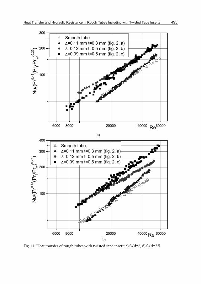
Heat Transfer and Hydraulic Resistance in Rough Tubes Including with Twisted Tape Inserts
495
6000 8000 20000 40000 60000
100
200
300N
u/(P
r0.43
(Pr f/P
r w)0.
25)
Re
Smooth tube Δ=0.11 mm t=0.3 mm (fig. 2, a) Δ=0.12 mm t=0.5 mm (fig. 2, b) Δ=0.09 mm t=0.5 mm (fig. 2, c)
a)
6000 8000 20000 40000 60000
100
200
300
400 Smooth tube Δ=0.11 mm t=0.3 mm (fig. 2, a) Δ=0.12 mm t=0.5 mm (fig. 2, b) Δ=0.09 mm t=0.5 mm (fig. 2, c)
Nu/
(Pr0,
43(P
r f/Pr w
)0,25
)
Re b)
Fig. 11. Heat transfer of rough tubes with twisted tape insert: а) S/d=6, б) S/d=2.5
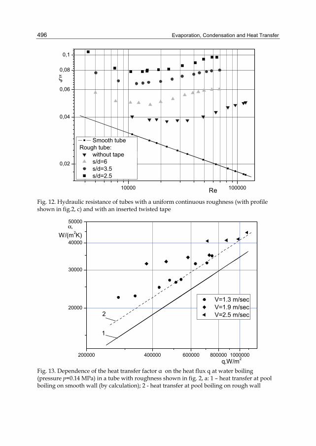
Evaporation, Condensation and Heat Transfer
496
10000 100000
0,02
0,04
0,06
0,08
0,1
Smooth tube Rough tube:
without tape s/d=6 s/d=3.5 s/d=2.5
ξ
Re Fig. 12. Hydraulic resistance of tubes with a uniform continuous roughness (with profile shown in fig.2, c) and with an inserted twisted tape
200000 400000 600000 800000 1000000
20000
30000
40000
50000
q,W/m2
α,W/(m2K)
V=1.3 m/sec V=1.9 m/sec V=2.5 m/sec2
1
Fig. 13. Dependence of the heat transfer factor α on the heat flux q at water boiling (pressure p=0.14 MPa) in a tube with roughness shown in fig. 2, a: 1 – heat transfer at pool boiling on smooth wall (by calculation); 2 - heat transfer at pool boiling on rough wall
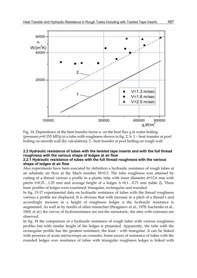
Heat Transfer and Hydraulic Resistance in Rough Tubes Including with Twisted Tape Inserts
497
100000 300000 600000 900000
20000
40000
60000
2
1
α,W/(m2K)
V=1.3 m/sec V=1.8 m/sec V=2.5 m/sec
q,W/m2
Fig. 14. Dependence of the heat transfer factor α on the heat flux q at water boiling (pressure p=0.155 MPa) in a tube with roughness shown in fig. 2, b: 1 – heat transfer at pool boiling on smooth wall (by calculation); 2 - heat transfer at pool boiling on rough wall
2.2 Hydraulic resistance of tubes with the twisted tape inserts and with the full thread roughness with the various shape of ledges at air flow 2.2.1 Hydraulic resistance of tubes with the full thread roughness with the various shape of ledges at air flow Also experiments have been executed by definition a hydraulic resistance of rough tubes at an adiabatic air flow at the Mach number M<0.3. The tube roughness was attained by cutting of a thread various a profile in a plastic tube with inner diameter d=12.6 mm with pitchs t=0.25…1.25 mm and average height of a ledges Δ =0.1…0.71 mm (table 2). Three basic profiles of ledges were examined: triangular, rectangular and rounded. In fig. 15-17 experimental data on hydraulic resistance of tubes with the thread roughness various a profile are displayed. It is obvious that with increase in a pitch of a thread t and accordingly increase in a height of roughness ledges Δ the hydraulic resistance is augmented. As well as by results of other researches (Ibragimov et al., 1978; Isachenko et al., 1965; et al.) the curves of hydroresistance are not the monotonic, the sites with extremes are observed. In fig. 18 the comparison of a hydraulic resistance of rough tubes with various roughness profiles but with similar height of the ledges is presented. Apparently, the tube with the rectangular profile has the greatest resistance, the least - with triangular. It can be linked with presence of acute microcrimps on crossetes. Some excess of resistance of tubes with the rounded ledges over resistance of tubes with triangular roughness ledges is linked with
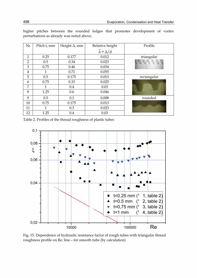
Evaporation, Condensation and Heat Transfer
498
higher pitches between the rounded ledges that promotes development of vortex perturbations as already was noted above. № Pitch t, mm Height Δ, mm Relative height
Δ = Δ/d Profile
1 0.25 0.177 0.012 2 0.5 0.34 0.023 3 0.75 0.46 0.034 4 1 0.71 0.055
triangular
5 0.5 0.175 0.013 6 0.75 0.33 0.025 7 1 0.4 0.03 8 1.25 0.6 0.046
rectangular
9 0.5 0.1 0.008 10 0.75 0.175 0.013 11 1 0.3 0.023 12 1.25 0.4 0.03
rounded
Table 2. Profiles of the thread roughness of plastic tubes
10000 1000000,02
0,04
0,06
0,08
0,1
t=0.25 mm (¹ 1, table 2)t=0.5 mm (¹ 2, table 2)t=0,75 mm (¹ 3, table 2)t=1 mm (¹ 4, table 2)
Re
ξ
Fig. 15. Dependence of hydraulic resistance factor of rough tubes with triangular thread roughness profile on Re: line – for smooth tube (by calculation)
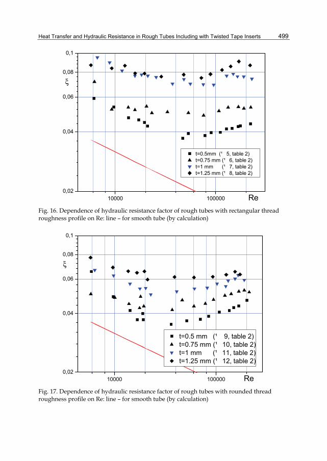
Heat Transfer and Hydraulic Resistance in Rough Tubes Including with Twisted Tape Inserts
499
10000 1000000,02
0,04
0,06
0,08
0,1
t=0.5mm (¹ 5, table 2)t=0.75 mm (¹ 6, table 2)t=1 mm (¹ 7, table 2)t=1.25 mm (¹ 8, table 2)
ξ
Re Fig. 16. Dependence of hydraulic resistance factor of rough tubes with rectangular thread roughness profile on Re: line – for smooth tube (by calculation)
10000 1000000,02
0,04
0,06
0,08
0,1
t=0.5 mm (¹ 9, table 2)t=0.75 mm (¹ 10, table 2)t=1 mm (¹ 11, table 2)t=1.25 mm (¹ 12, table 2)
ξ
Re Fig. 17. Dependence of hydraulic resistance factor of rough tubes with rounded thread roughness profile on Re: line – for smooth tube (by calculation)
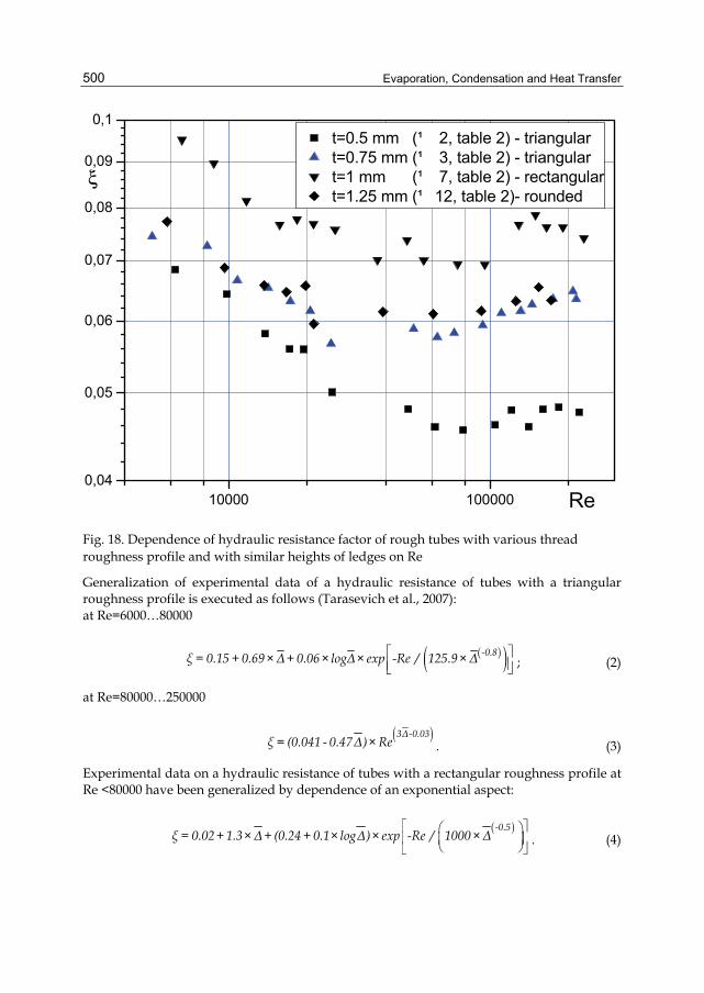
Evaporation, Condensation and Heat Transfer
500
10000 1000000,04
0,05
0,06
0,07
0,08
0,09
0,1t=0.5 mm (¹ 2, table 2) - triangulart=0.75 mm (¹ 3, table 2) - triangulart=1 mm (¹ 7, table 2) - rectangulart=1.25 mm (¹ 12, table 2)- rounded
Re
ξ
Fig. 18. Dependence of hydraulic resistance factor of rough tubes with various thread roughness profile and with similar heights of ledges on Re
Generalization of experimental data of a hydraulic resistance of tubes with a triangular roughness profile is executed as follows (Tarasevich et al., 2007): at Re=6000…80000
( )( )⎡ ⎤
⎢ ⎥⎣ ⎦-0.8ξ = 0.15 + 0.69 ×Δ+ 0.06 × logΔ× exp -Re / 125.9 ×Δ ; (2)
at Re=80000…250000
( )3Δ-0.03
ξ = (0.041 - 0.47Δ)× Re . (3)
Experimental data on a hydraulic resistance of tubes with a rectangular roughness profile at Re <80000 have been generalized by dependence of an exponential aspect:
( )⎡ ⎤⎛ ⎞
⎢ ⎥⎜ ⎟⎝ ⎠⎣ ⎦
-0.5ξ = 0.02 + 1.3×Δ+ (0.24 + 0.1× logΔ)× exp -Re / 1000 ×Δ . (4)
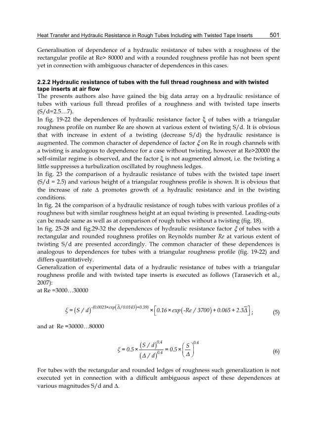
Heat Transfer and Hydraulic Resistance in Rough Tubes Including with Twisted Tape Inserts
501
Generalisation of dependence of a hydraulic resistance of tubes with a roughness of the rectangular profile at Re> 80000 and with a rounded roughness profile has not been spent yet in connection with ambiguous character of dependences in this cases.
2.2.2 Hydraulic resistance of tubes with the full thread roughness and with twisted tape inserts at air flow The presents authors also have gained the big data array on a hydraulic resistance of tubes with various full thread profiles of a roughness and with twisted tape inserts (S/d=2.5…7). In fig. 19-22 the dependences of hydraulic resistance factor ξ of tubes with a triangular roughness profile on number Re are shown at various extent of twisting S/d. It is obvious that with increase in extent of a twisting (decrease S/d) the hydraulic resistance is augmented. The common character of dependence of factor ξ on Re in rough channels with a twisting is analogous to dependence for a case without twisting, however at Re>20000 the self-similar regime is observed, and the factor ξ is not augmented almost, i.e. the twisting a little suppresses a turbulization oscillated by roughness ledges. In fig. 23 the comparison of a hydraulic resistance of tubes with the twisted tape insert (S/d = 2.5) and various height of a triangular roughness profile is shown. It is obvious that the increase of rate Δ promotes growth of a hydraulic resistance and in the twisting conditions. In fig. 24 the comparison of a hydraulic resistance of rough tubes with various profiles of a roughness but with similar roughness height at an equal twisting is presented. Leading-outs can be made same as well as at comparison of rough tubes without a twisting (fig. 18). In fig. 25-28 and fig.29-32 the dependences of hydraulic resistance factor ξ of tubes with a rectangular and rounded roughness profiles on Reynolds number Re at various extent of twisting S/d are presented accordingly. The common character of these dependences is analogous to dependences for tubes with a triangular roughness profile (fig. 19-22) and differs quantitatively. Generalization of experimental data of a hydraulic resistance of tubes with a triangular roughness profile and with twisted tape inserts is executed as follows (Tarasevich et al., 2007): at Re =3000…30000
( ) ( ) ( )⎡ ⎤⎣ ⎦
-(0.0023×exp Δ / 0.0143 +0.39)ξ = S / d × 0.16× exp -Re / 3700 + 0.065 + 2.3Δ ; (5)
and at Re =30000…80000
( )( )
⎛ ⎞⎜ ⎟⎝ ⎠
0.4 0.4
0.4S / d Sξ = 0.5 × = 0.5 ×
ΔΔ / d (6)
For tubes with the rectangular and rounded ledges of roughness such generalization is not executed yet in connection with a difficult ambiguous aspect of these dependences at various magnitudes S/d and Δ.
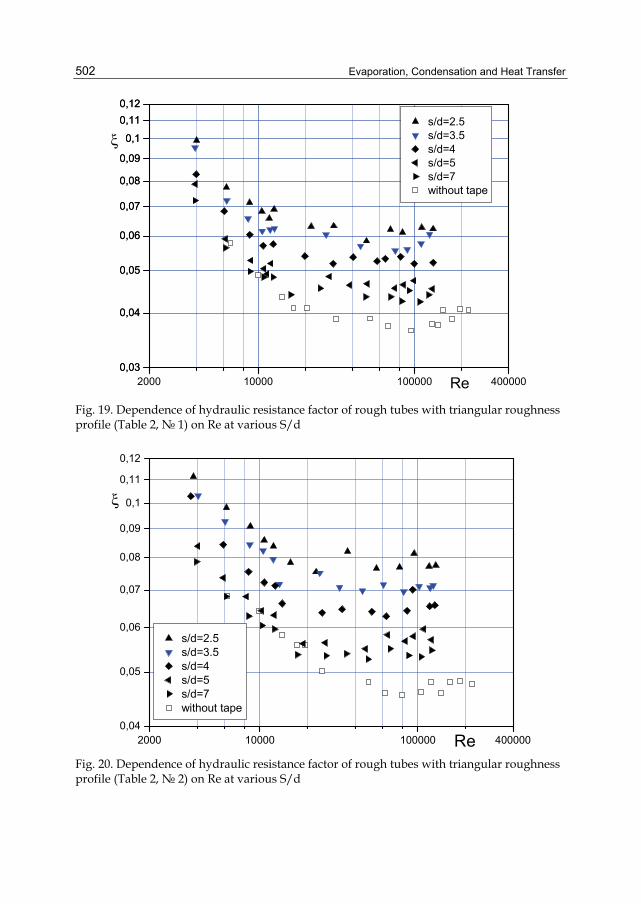
Evaporation, Condensation and Heat Transfer
502
2000 10000 100000 4000000,030,03
0,040,04
0,050,05
0,060,06
0,070,07
0,080,08
0,090,09
0,10,1
0,110,110,120,12
s/d=2.5s/d=3.5s/d=4s/d=5s/d=7without tape
ξ
Re
Fig. 19. Dependence of hydraulic resistance factor of rough tubes with triangular roughness profile (Table 2, № 1) on Re at various S/d
2000 10000 100000 4000000,04
0,05
0,06
0,07
0,08
0,09
0,1
0,11
0,12
s/d=2.5s/d=3.5s/d=4s/d=5s/d=7without tape
Re
ξ
Fig. 20. Dependence of hydraulic resistance factor of rough tubes with triangular roughness profile (Table 2, № 2) on Re at various S/d
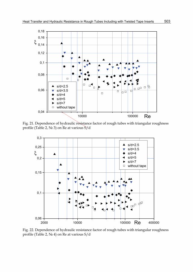
Heat Transfer and Hydraulic Resistance in Rough Tubes Including with Twisted Tape Inserts
503
10000 1000000,04
0,06
0,08
0,1
0,12
0,14
0,16
0,18
s/d=2.5s/d=3.5s/d=4s/d=5s/d=7without tape
ξ
Re Fig. 21. Dependence of hydraulic resistance factor of rough tubes with triangular roughness profile (Table 2, № 3) on Re at various S/d
2000 10000 100000 4000000,06
0,1
0,15
0,2
0,25
0,3
s/d=2.5s/d=3.5s/d=4s/d=5s/d=7without tape
ξ
Re Fig. 22. Dependence of hydraulic resistance factor of rough tubes with triangular roughness profile (Table 2, № 4) on Re at various S/d
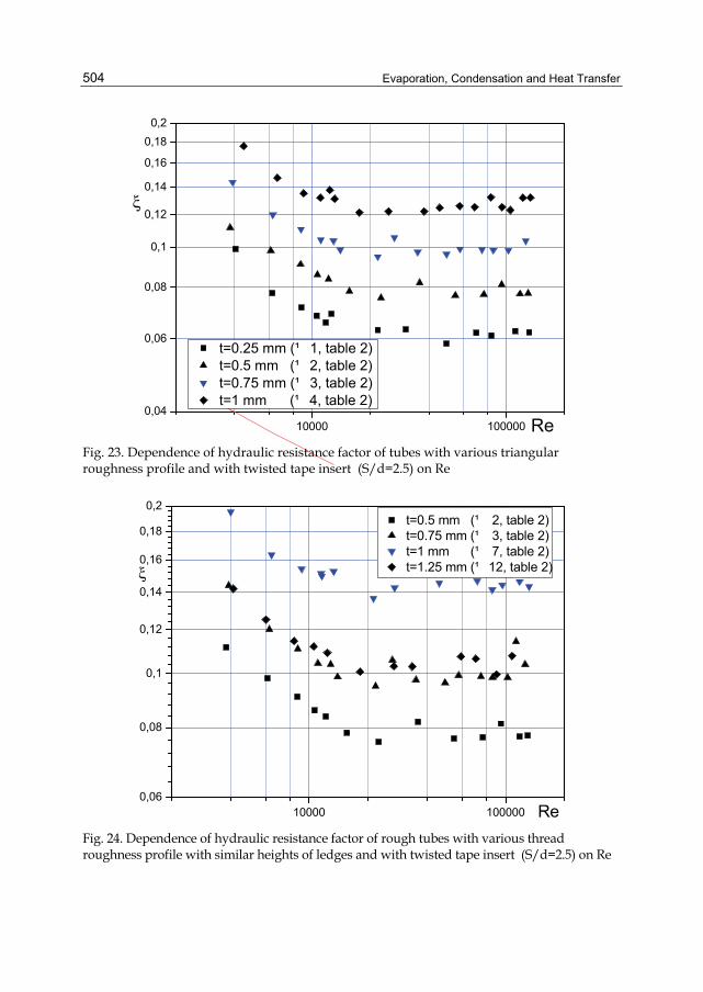
Evaporation, Condensation and Heat Transfer
504
10000 1000000,04
0,06
0,08
0,1
0,12
0,14
0,16
0,180,2
t=0.25 mm (¹ 1, table 2)t=0.5 mm (¹ 2, table 2)t=0.75 mm (¹ 3, table 2)t=1 mm (¹ 4, table 2)
ξ
Re Fig. 23. Dependence of hydraulic resistance factor of tubes with various triangular roughness profile and with twisted tape insert (S/d=2.5) on Re
10000 1000000,06
0,08
0,1
0,12
0,14
0,16
0,18
0,2t=0.5 mm (¹ 2, table 2)t=0.75 mm (¹ 3, table 2)t=1 mm (¹ 7, table 2)t=1.25 mm (¹ 12, table 2)
Re
ξ
Fig. 24. Dependence of hydraulic resistance factor of rough tubes with various thread roughness profile with similar heights of ledges and with twisted tape insert (S/d=2.5) on Re
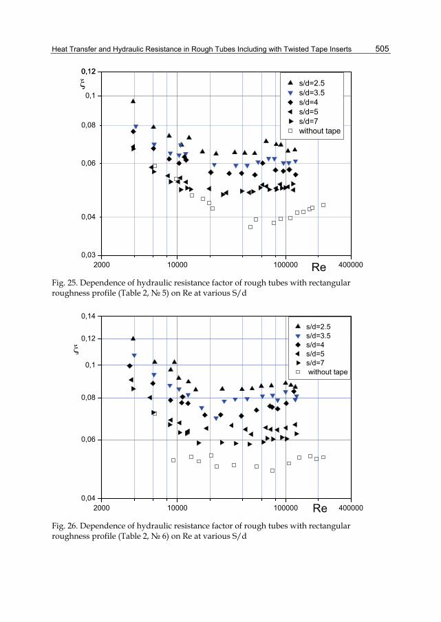
Heat Transfer and Hydraulic Resistance in Rough Tubes Including with Twisted Tape Inserts
505
2000 10000 100000 4000000,03
0,04
0,06
0,08
0,1
0,120,12s/d=2.5s/d=3.5s/d=4s/d=5s/d=7without tape
ξ
Re Fig. 25. Dependence of hydraulic resistance factor of rough tubes with rectangular roughness profile (Table 2, № 5) on Re at various S/d
2000 10000 100000 4000000,04
0,06
0,08
0,1
0,12
0,14s/d=2.5s/d=3.5s/d=4s/d=5s/d=7 without tape
ξ
Re Fig. 26. Dependence of hydraulic resistance factor of rough tubes with rectangular roughness profile (Table 2, № 6) on Re at various S/d
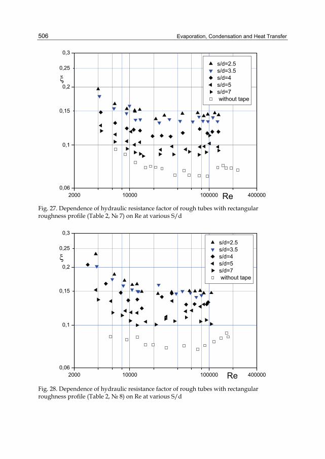
Evaporation, Condensation and Heat Transfer
506
2000 10000 100000 4000000,06
0,1
0,15
0,2
0,25
0,3
s/d=2.5s/d=3.5s/d=4s/d=5s/d=7 without tape
ξ
Re Fig. 27. Dependence of hydraulic resistance factor of rough tubes with rectangular roughness profile (Table 2, № 7) on Re at various S/d
2000 10000 100000 4000000,06
0,1
0,15
0,2
0,25
0,3
s/d=2.5s/d=3.5s/d=4s/d=5s/d=7 without tape
ξ
Re
Fig. 28. Dependence of hydraulic resistance factor of rough tubes with rectangular roughness profile (Table 2, № 8) on Re at various S/d
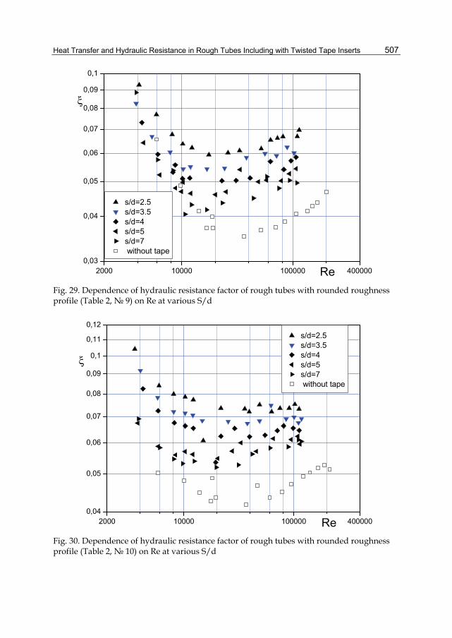
Heat Transfer and Hydraulic Resistance in Rough Tubes Including with Twisted Tape Inserts
507
2000 10000 100000 4000000,03
0,04
0,05
0,06
0,07
0,08
0,09
0,1
s/d=2.5s/d=3.5s/d=4s/d=5s/d=7 without tape
Re
ξ
Fig. 29. Dependence of hydraulic resistance factor of rough tubes with rounded roughness profile (Table 2, № 9) on Re at various S/d
2000 10000 100000 4000000,04
0,05
0,06
0,07
0,08
0,09
0,1
0,11
0,12s/d=2.5s/d=3.5s/d=4s/d=5s/d=7 without tape
ξ
Re
Fig. 30. Dependence of hydraulic resistance factor of rough tubes with rounded roughness profile (Table 2, № 10) on Re at various S/d
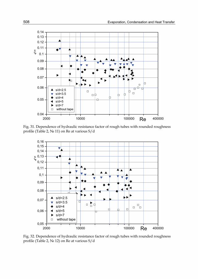
Evaporation, Condensation and Heat Transfer
508
2000 10000 100000 4000000.04
0.05
0.06
0.07
0.08
0.09
0.1
0.11
0.120.130.14
s/d=2.5s/d=3.5s/d=4s/d=5s/d=7 without tape
ξ
Re Fig. 31. Dependence of hydraulic resistance factor of rough tubes with rounded roughness profile (Table 2, № 11) on Re at various S/d
2000 10000 100000 4000000,05
0,06
0,07
0,08
0,09
0,1
0,11
0,12
0,130,140,150,16
s/d=2.5s/d=3.5s/d=4s/d=5s/d=7 without tape
ξ
Re Fig. 32. Dependence of hydraulic resistance factor of rough tubes with rounded roughness profile (Table 2, № 12) on Re at various S/d
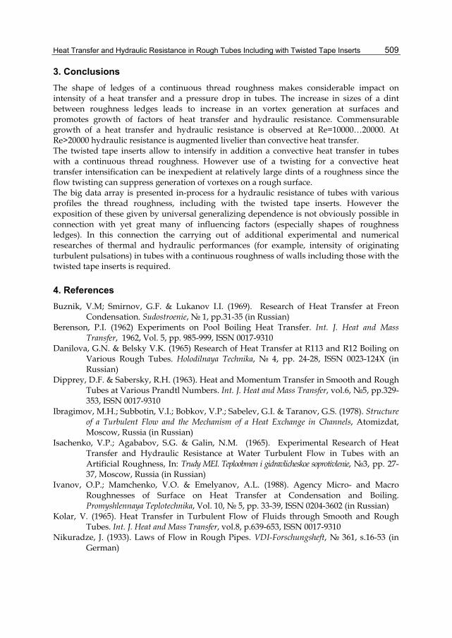
Heat Transfer and Hydraulic Resistance in Rough Tubes Including with Twisted Tape Inserts
509
3. Conclusions The shape of ledges of a continuous thread roughness makes considerable impact on intensity of a heat transfer and a pressure drop in tubes. The increase in sizes of a dint between roughness ledges leads to increase in an vortex generation at surfaces and promotes growth of factors of heat transfer and hydraulic resistance. Commensurable growth of a heat transfer and hydraulic resistance is observed at Re=10000…20000. At Re>20000 hydraulic resistance is augmented livelier than convective heat transfer. The twisted tape inserts allow to intensify in addition a convective heat transfer in tubes with a continuous thread roughness. However use of a twisting for a convective heat transfer intensification can be inexpedient at relatively large dints of a roughness since the flow twisting can suppress generation of vortexes on a rough surface. The big data array is presented in-process for a hydraulic resistance of tubes with various profiles the thread roughness, including with the twisted tape inserts. However the exposition of these given by universal generalizing dependence is not obviously possible in connection with yet great many of influencing factors (especially shapes of roughness ledges). In this connection the carrying out of additional experimental and numerical researches of thermal and hydraulic performances (for example, intensity of originating turbulent pulsations) in tubes with a continuous roughness of walls including those with the twisted tape inserts is required.
4. References Buznik, V.M; Smirnov, G.F. & Lukanov I.I. (1969). Research of Heat Transfer at Freon
Condensation. Sudostroenie, № 1, pp.31-35 (in Russian) Berenson, P.I. (1962) Experiments on Pool Boiling Heat Transfer. Int. J. Heat and Mass
Transfer, 1962, Vol. 5, pp. 985-999, ISSN 0017-9310 Danilova, G.N. & Belsky V.K. (1965) Research of Heat Transfer at R113 and R12 Boiling on
Various Rough Tubes. Holodilnaya Technika, № 4, pp. 24-28, ISSN 0023-124X (in Russian)
Dipprey, D.F. & Sabersky, R.H. (1963). Heat and Momentum Transfer in Smooth and Rough Tubes at Various Prandtl Numbers. Int. J. Heat and Mass Transfer, vol.6, №5, pp.329-353, ISSN 0017-9310
Ibragimov, M.H.; Subbotin, V.I.; Bobkov, V.P.; Sabelev, G.I. & Taranov, G.S. (1978). Structure of a Turbulent Flow and the Mechanism of a Heat Exchange in Channels, Atomizdat, Moscow, Russia (in Russian)
Isachenko, V.P.; Agababov, S.G. & Galin, N.M. (1965). Experimental Research of Heat Transfer and Hydraulic Resistance at Water Turbulent Flow in Tubes with an Artificial Roughness, In: Trudy MEI. Teploobmen i gidravlicheskoe soprotivlenie, №3, pp. 27-37, Moscow, Russia (in Russian)
Ivanov, O.P.; Mamchenko, V.O. & Emelyanov, A.L. (1988). Agency Micro- and Macro Roughnesses of Surface on Heat Transfer at Condensation and Boiling. Promyshlennaya Teplotechnika, Vol. 10, № 5, pp. 33-39, ISSN 0204-3602 (in Russian)
Kolar, V. (1965). Heat Transfer in Turbulent Flow of Fluids through Smooth and Rough Tubes. Int. J. Heat and Mass Transfer, vol.8, p.639-653, ISSN 0017-9310
Nikuradze, J. (1933). Laws of Flow in Rough Pipes. VDI-Forschungsheft, № 361, s.16-53 (in German)
Evaporation, Condensation and Heat Transfer
510
Nishikawa, K.; Fujiba, I.; Ohta, U. & Hidaka, S. (1982). Effect of Surface Roughness on the Nucleate Boiling Heat Transfer Over the Wide Range of Pressure, Proceedings of the Seventh International Heat Transfer Conference, vol.4, pp.61-66, ISBN 0891162992, 0891163425, München, Germany
Nunner, W. (1956). Heat Transfer and Pressure Drop in Rough Tubes. VDI-Forschungsheft, № 455, vol. 22, s.5-39 (in German)
Schlichting, H. (1979). Boundary Layer Theory, 7th ed., McGraw-Hill, , ISBN 0070553343, New York, USA
Sheriff, N.; Gumley, P. & France, J. (1964). Heat Transfer Characteristics of Roughened Surfaces. Chem. Process Engng, vol.45, pp.624-629, ISSN 0255-2701
Sheriff, N. & Gumley, P. (1966) Heat Transfer and Friction Properties of Surfaces with Discrete Roughnesses. Int. J. Heat and Mass Transfer, vol.9, pp.1297-1320, ISSN 0017-9310
Tarasevich, S.; Shchelchkov, A.; Yakovlev, A. (2007) Flow Friction of Pipes with Uniform Continuous Surface Roughness and Twisted Tape Insert, Proceedings of the 5-th Baltic Heat Transfer Conference, Saint-Petersburg, Russia, September 19-21, V.2., pp.244-249.
24
Fluid Mechanics, Heat Transfer and Thermodynamic Issues of Micropipe Flows
A. Alper Ozalp Department of Mechanical Engineering, Uludag University,
Turkey
1. Introduction Once the notion is aspired to examine the momentum and heat transfer characteristics of fluid flow in detail, the concept of energy mechanism is inevitably handled through both 1st and 2nd laws. Since the fundamental engineering phenomenon of internal flow is widely encountered in industrial installations, which may range from operations with non-Newtonian fluids (Yilbas & Pakdemirli, 2005) to heat exchangers (Stewart et al., 2005) and from geothermal district heating systems (Ozgener et al., 2007) even to micropipe systems (Kandlikar et al., 2003), the general scientific and technological frame of thermo-fluid operations has been in the consideration of several researchers. From methodological perspective, at macro level (d≥3 mm), the explicit analytical correlations are capable of characterizing the flow and heat transfer issues of internal laminar flows. However, when the pipe diameter coincides with the micro range (d≤1 mm) the order the pipe diameter and the level of surface roughness result in augmented entropy generation rates, besides give rise to substantial shifts in the velocity and temperature profiles from those of the characteristic recognitions, which as a consequence highlights the necessity in the identification of the so developed energy behaviors and the involved influential parameters related with the design, construction and operation of the object appliance. Through experimental and computational investigations, involved researchers considered both the fluid flow and heat transfer mechanisms of micropipe flows. Kandlikar et al. (2003), for single-phase flow with small hydraulic diameters, studied the effects of surface roughness on pressure drop and heat transfer and concluded that transition to turbulent flows occurs at Reynolds number values much below 2300. Laminar and transitional flows in dimpled tubes were experimentally investigated by Vicente et al. (2002); the onset of transition at a relatively low Reynolds number of 1400 with 10% higher roughness induced friction factors when compared to the smooth tube ones were their primary findings. Engin et al. (2004) reported significant departures in the flow characteristics, from the conventional laminar flow theory, due to wall roughness effects in micropipe flows. The grow of friction coefficient with higher Reynolds number and lower hydraulic diameter were the theoretical and experimental evaluations of Renaud et al. (2008) in trapezoidal micro-channels. Guo & Li (2003) studied the mechanism of surface roughness provoked surface friction and concluded that the early transition from laminar to turbulent flow arose due to the frictional activity. Smooth micro-tubes under adiabatic conditions were experimentally investigated by Parlak et al. (2011); they determined that, as long as the viscous heating effects are taken
Evaporation, Condensation and Heat Transfer
512
into account for micropipe diameters of d<100 μm, the measured data and the calculated data from Hagen–Poiseuille equation of laminar flow are fairly comparable. The works of Celata et al. (2006a,b) described the roles of surface roughness on viscous dissipation, the resulting earlier transitional activity, augmented friction factor values and elevated head loss data. As the role of the cross-sectional geometry on viscous dissipation and the minimum Reynolds number for which viscous dissipation effects can not be neglected was considered by Morini (2005), Wu & Cheng (2003) reported the rise of laminar apparent friction coefficient and Nusselt number with the increase of surface roughness especially at higher Reynolds numbers. The significance of viscous dissipation on the temperature field and on the friction factor was studied numerically and experimentally by Koo & Kleinstreuer (2004). Obot (2002) reported that (i) onset of transition to turbulent flow in smooth microchannels does not occur if the Reynolds number is less than 1000, (ii) Nusselt number varies as the square root of the Reynolds number in laminar flow. Slit type micro-channels were taken into experimental investigation by Almeida et al. (2010); their measurements for wide ranges of Reynolds number, hydraulic diameter and surface roughness proposed the systematic variation of frictional activity with micro structure and flow characteristics. Velocity slip and temperature jump phenomena in micro-flows were numerically investigated by Chen & Tian (2010). Wen et al. (2003) experimentally inspected the augmentation characteristics of heat transfer and pressure drop by the imposed wall heat flux, mass flux and different strip-type inserts in small tubes. Energy conversion of near-wall microfluidic transport for slip-flow conditions, including different channel aspect ratios, pressure coefficients and slip flow, were numerically considered by Ogedengbe et al. (2006). Petropoulos et al. (2010) carried out an experimental work on micropipe flows; in addition to reporting the variation of friction coefficient and pressure loss values with Reynolds number, they as well denoted the difficulties in sensitively measuring the velocity and pressure values. The influence of roughness level on the transition character in micropipe flows were recently reported by Celata et al. (2009); they as well added the appropriateness of Blasius and Colebrook equations for smooth and rough pipe cases respectively. In a more recent work Pitakarnnop et al. (2010) experimented micro-flows; they not only introduced a novel technique to enhance the measurement sensitivity but also compared their evaluations with different models for various gases and pressure ratios. The thermodynamic issues of thermal systems are mostly interpreted through 2nd law analysis, where the concepts of frictional, thermal and total entropy generation rates are considered to be the particular parameters of the phenomena of exergy. Ko (2006a) carried out a numerical work on the thermal design of a double-sine duct plate heat exchanger, from the point of entropy generation and exergy utilization. Second law characteristics in smooth micropipe were experimentally investigated by Parlak et al. (2011); they recorded augmentations in entropy generation with higher Reynolds number and with lower micropipe diameter. Sahin (1998), for a fully developed laminar viscous flow in a duct subjected to constant wall temperature, inspected the entropy generation analytically. He reported the promoted entropy generation due to viscous friction and further determined that the dependence of viscosity on temperature becomes essentially important in accurately evaluating the entropy generation. Richardson et al. (2000), in singly connected microchannels with finite temperature differences, investigated the existence of an optimum laminar frictional flow regime, based on 2nd law analysis. In computing the process irreversibility or loss of exergy, Kotas et al. (1995) validated the applicability of exergy balance, or the Gouy-Stodola theorem. Ratts & Raut (2004) employed the entropy generation
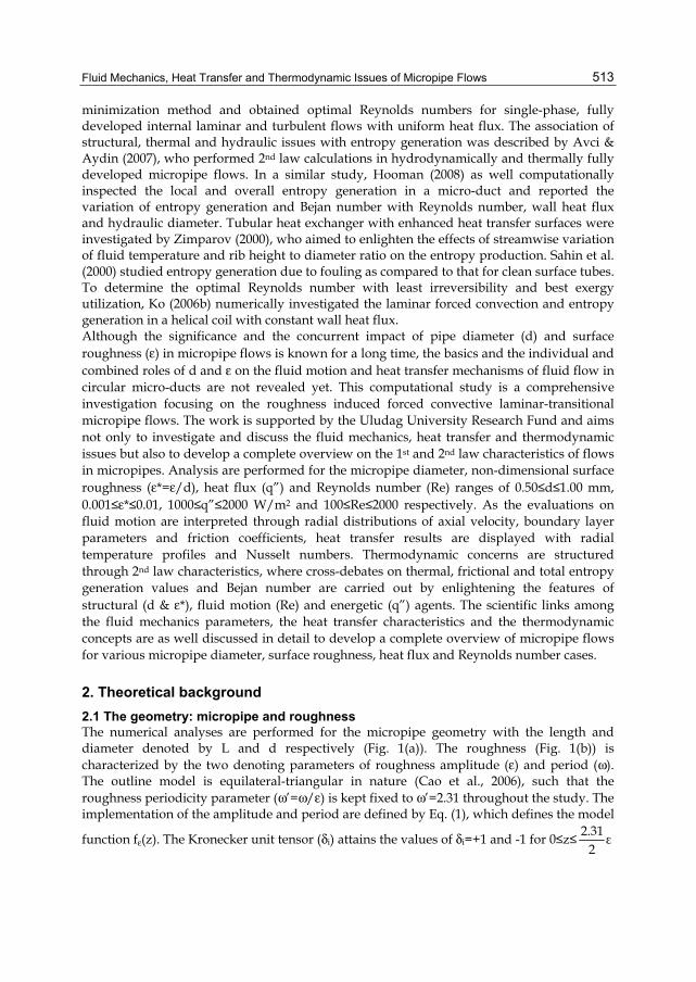
Fluid Mechanics, Heat Transfer and Thermodynamic Issues of Micropipe Flows
513
minimization method and obtained optimal Reynolds numbers for single-phase, fully developed internal laminar and turbulent flows with uniform heat flux. The association of structural, thermal and hydraulic issues with entropy generation was described by Avci & Aydin (2007), who performed 2nd law calculations in hydrodynamically and thermally fully developed micropipe flows. In a similar study, Hooman (2008) as well computationally inspected the local and overall entropy generation in a micro-duct and reported the variation of entropy generation and Bejan number with Reynolds number, wall heat flux and hydraulic diameter. Tubular heat exchanger with enhanced heat transfer surfaces were investigated by Zimparov (2000), who aimed to enlighten the effects of streamwise variation of fluid temperature and rib height to diameter ratio on the entropy production. Sahin et al. (2000) studied entropy generation due to fouling as compared to that for clean surface tubes. To determine the optimal Reynolds number with least irreversibility and best exergy utilization, Ko (2006b) numerically investigated the laminar forced convection and entropy generation in a helical coil with constant wall heat flux. Although the significance and the concurrent impact of pipe diameter (d) and surface roughness (ε) in micropipe flows is known for a long time, the basics and the individual and combined roles of d and ε on the fluid motion and heat transfer mechanisms of fluid flow in circular micro-ducts are not revealed yet. This computational study is a comprehensive investigation focusing on the roughness induced forced convective laminar-transitional micropipe flows. The work is supported by the Uludag University Research Fund and aims not only to investigate and discuss the fluid mechanics, heat transfer and thermodynamic issues but also to develop a complete overview on the 1st and 2nd law characteristics of flows in micropipes. Analysis are performed for the micropipe diameter, non-dimensional surface roughness (ε*=ε/d), heat flux (q”) and Reynolds number (Re) ranges of 0.50≤d≤1.00 mm, 0.001≤ε*≤0.01, 1000≤q”≤2000 W/m2 and 100≤Re≤2000 respectively. As the evaluations on fluid motion are interpreted through radial distributions of axial velocity, boundary layer parameters and friction coefficients, heat transfer results are displayed with radial temperature profiles and Nusselt numbers. Thermodynamic concerns are structured through 2nd law characteristics, where cross-debates on thermal, frictional and total entropy generation values and Bejan number are carried out by enlightening the features of structural (d & ε*), fluid motion (Re) and energetic (q”) agents. The scientific links among the fluid mechanics parameters, the heat transfer characteristics and the thermodynamic concepts are as well discussed in detail to develop a complete overview of micropipe flows for various micropipe diameter, surface roughness, heat flux and Reynolds number cases.
2. Theoretical background 2.1 The geometry: micropipe and roughness The numerical analyses are performed for the micropipe geometry with the length and diameter denoted by L and d respectively (Fig. 1(a)). The roughness (Fig. 1(b)) is characterized by the two denoting parameters of roughness amplitude (ε) and period (ω). The outline model is equilateral-triangular in nature (Cao et al., 2006), such that the roughness periodicity parameter (ω’=ω/ε) is kept fixed to ω’=2.31 throughout the study. The implementation of the amplitude and period are defined by Eq. (1), which defines the model
function fε(z). The Kronecker unit tensor (δi) attains the values of δi=+1 and -1 for 0≤z≤ 2.31 ε2
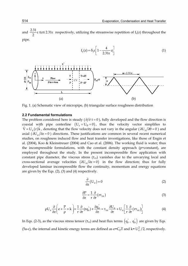
Evaporation, Condensation and Heat Transfer
514
and 2.31 ε2
≤z≤ 2.31ε respectively, utilizing the streamwise repetition of fε(z) throughout the
pipe.
ε i4f (z) δ ε 1 z
2.31ε⎡ ⎤= −⎢ ⎥⎣ ⎦
(1)
(a) (b)
Fig. 1. (a) Schematic view of micropipe, (b) triangular surface roughness distribution
2.2 Fundamental formulations The problem considered here is steady ( t 0∂ ∂ = ), fully developed and the flow direction is coaxial with pipe centerline ( )r θU U 0= = , thus the velocity vector simplifies to
( )zˆV U r k= , denoting that the flow velocity does not vary in the angular ( zU θ 0∂ ∂ = ) and
axial ( zU z 0∂ ∂ = ) directions. These justifications are common in several recent numerical studies, on roughness induced flow and heat transfer investigations, like those of Engin et al. (2004), Koo & Kleinstreuer (2004) and Cao et al. (2006). The working fluid is water; thus the incompressible formulations, with the constant density approach (ρ=constant), are employed throughout the study. In the present incompressible flow application with constant pipe diameter, the viscous stress (τzz) vanishes due to the unvarying local and cross-sectional average velocities ( )zU z 0∂ ∂ = in the flow direction; thus for fully developed laminar incompressible flow the continuity, momentum and energy equations are given by the Eqs. (2), (3) and (4) respectively.
( )zU 0z
∂ =∂
(2)
( )rzP 1 rτz r r
∂ ∂=∂ ∂
(3)
( )''
'' z zz r rz z rz
P 1 q U 1ρU e k (rq ) τ U rτz ρ r r z r r r⎛ ⎞∂ ∂ ∂ ∂ ∂⎡ ⎤+ + + + = +⎜ ⎟ ⎢ ⎥⎜ ⎟∂ ∂ ∂ ∂ ∂⎣ ⎦⎝ ⎠
(4)
In Eqs. (2-3), as the viscous stress tensor (τrz) and heat flux terms ( ''rq , )''
zq are given by Eqs.
(5a-c), the internal and kinetic energy terms are defined as e=CpT and k= 2zU /2, respectively.
Fluid Mechanics, Heat Transfer and Thermodynamic Issues of Micropipe Flows
515
T zrz
Uτ μr
∂=∂
'' Tr f
Tq κr
∂= −∂
'' Tz f
Tq κz
∂= −∂
(5a-c)
As given in Fig. 1(a), at the pipe inlet, pressure (Pin) and temperature (Tin) values are known and the exit pressure (Pex) is atmospheric. The flow boundary conditions are based on the facts that, on the pipe wall (r=R) no-slip condition and constant heat flux ( )''q exist, and flow and thermal values are maximum at the centerline (r=0). Denoting Uz=Uz(r) and T=T(r,z), the boundary conditions can be summarized as follows:
( ) ze z
Ur R f z U 0 & r 0 0r
∂= + → = = → =∂
(6a)
( )''r
e Tf
T q Tr R f z & r 0 0r rκ
∂ ∂= + → = − = → =∂ ∂
(6b)
( )in in exz 0 P P , T T & z L P 0 Man.= → = = = → = (6c)
The average fluid velocity (Uo) and temperature (To), at any cross-section in the pipe, are defined as
r R
zr 0
o 2
2π U (r)rdrU
πR
=
==∫
( )
r R
z pr 0
o 2o p o
2π U (r)C (r)T(r)rdrT
U C πR
=
==∫
(7a-b)
and the shear stress (τ) and mass flow rate (.
m ) are obtained from
2 T zf o
r R
1 dUτ C ρU μ2 dr =
= = r R.
o zr 0
m ρU A ρ2π U (r)rdr=
=
= = ∫ (8a-b)
where Cf, ρ and A stand for friction coefficient, density and cross-sectional area respectively. Denoting the surface and mean flow temperatures as Ts and To, identifying the thermal conductivity and convective heat transfer coefficient with κf and h, and labeling dynamic and kinematic viscosity of water by μ and ν (=μ/ρ), Reynolds number (Re) and Nusselt number (Nu) are characterized by Eqs. (9a-b).
oT
U dReν
= = oT
ρU dμ
Tf
hdNuκ
= = r R
s o
T drT T
=∂
∂−
(9a-b)
The temperature dependent character of water properties (ξ) is widely known (Incropera & DeWitt, 2001) and the scientific need in implementing their variation with temperature stands as a must in computational work. Thus the water properties of specific heat (Cp), kinematic viscosity and thermal conductivity are gathered (Incropera & DeWitt, 2001) and fitted into 6th order polynomials (Eq. (10)). As the superscript T denotes the temperature dependency, the peak uncertainty of 0.03% is realized in Eq. (10) for the complete set of properties.
Evaporation, Condensation and Heat Transfer
516
ζT=6 ja Tj
j 0∑=
(10)
Due to the existence of the velocity and temperature gradients in the flow volume, positive and finite volumetric entropy generation rate arises throughout the micropipe. In the guidance of the Gouy-Stodola theorem (Kotas et al., 1995), entropy generation can be considered to be directly proportional to the lost available work, which takes place as a result of the non-equilibrium phenomenon of exchange of energy and momentum within the fluid and at the solid boundaries. For a one-dimensional flow and two-dimensional temperature domain for incompressible Newtonian fluid flow in cylindrical coordinates, the local rate of entropy generation per unit volume ( )'''S can be calculated by Eq. (11a), where the temperature dependent character of both the thermal conductivity and the kinematic viscosity of water are as well taken into consideration. As the first term on the right side of Eq. (11a) stands for the local entropy generation due to finite temperature differences ( )'''
ΔTS in axial z and in radial r directions, the local frictional entropy generation ( )'''
ΔPS is defined by the second term. The input data, for either of the open (Eq. (11a)) or closed form (Eq. (11b)) illustrations of '''S , are attained by the computation of the temperature and the velocity fields through Eqs. (2-4).
2 2 2T T
''' f z2
κ T T μ USr z T rT
⎡ ⎤ ⎡ ⎤∂ ∂ ∂⎛ ⎞ ⎛ ⎞ ⎛ ⎞⎢ ⎥ ⎢ ⎥= + +⎜ ⎟ ⎜ ⎟ ⎜ ⎟∂ ∂ ∂⎢ ⎥ ⎢ ⎥⎝ ⎠ ⎝ ⎠ ⎝ ⎠⎣ ⎦ ⎣ ⎦ ''' ''' '''
ΔT ΔPS S S= + (11a-b)
Eqs. (12a-c) stand for the cross-sectional thermal ( )'ΔTS , frictional ( )'
ΔPS and total ( )'S entropy generation rates, where the common method is the integration of the local values over the cross-sectional area of the micropipe.
r R
' '''T T
r 0S 2π S rdr
=
Δ Δ=
= ∫ r R
' '''ΔP ΔP
r 0S 2π S rdr
=
=
= ∫ r R
' '''
r 0S 2π S rdr
=
=
= ∫ (12a-c)
Bejan number is defined as the ratio of the thermal entropy generation to the total value. The cross-sectional average value of Be is given by Eq. (13).
Be'ΔT'
SS
= (13)
Not only to identify the shift of the determined fluid motion and heat transfer characteristics from the conventional theory but also to spot the individual and combined roles of ε, d and Re on the transition mechanism, the basic theoretical equations are as well incorporated in the formulation set. The shift of the velocity profiles from the characteristic styles of laminar and turbulent regimes can be enlightened through comparisons with the classical laminar velocity profile and the modified turbulent logarithm law for roughness (Eqs. (14a-b)) (White, 1999).
2
o
U(r) r2 1U R
⎡ ⎤⎛ ⎞⎢ ⎥= − ⎜ ⎟⎢ ⎥⎝ ⎠⎣ ⎦
w
U(r) R r2.44ln 8.5ετ
ρ
−⎛ ⎞= +⎜ ⎟⎝ ⎠
(14a-b)
Fluid Mechanics, Heat Transfer and Thermodynamic Issues of Micropipe Flows
517
The laminar temperature profile formula for Constant Heat Flux (CHF) applications is given by Eq. (15) (Incropera & DeWitt, 2001).
4 2T 2
o f os T
p
2U κ R dT 3 1 r 1 rT(r) Tdz 16 16 R 4 RρC
⎡ ⎤⎛ ⎞ ⎛ ⎞ ⎛ ⎞⎢ ⎥= − + −⎜ ⎟ ⎜ ⎟ ⎜ ⎟⎢ ⎥⎝ ⎠ ⎝ ⎠⎝ ⎠ ⎣ ⎦ (15)
Boundary layer parameters like shape factor (H) (Eq. (16a)) and intermittency (γ) (Eq. (16b)) (White, 1999) are integrated into the discussions to strengthen the evaluations on the onset of transition, where Uc stands for the velocity at the pipe centerline. As the laminar (Hlam=3.36) and turbulent (Hturb=1.70) shape factor values are computed with Eq. (16a), by integrating the laminar (Eq. (14a)) and turbulent (Eq. (14b)) profiles, the shape factor data of the transitional flows were also calculated with Eq. (16a), however with the computationally evaluated corresponding velocity profiles.
r R
cr 0r R
c cr 0
U(r)1 rdrU
HU(r) U(r)1 rdrU U
=
==
=
⎛ ⎞−⎜ ⎟
⎝ ⎠=⎛ ⎞
−⎜ ⎟⎝ ⎠
∫
∫ lam
lam turb
H HγH H
−=−
(16a-b)
To clarify the role of surface roughness on the frictional activity, the classical and normalized friction coefficient values are evaluated by Eqs. (17a-c) (White, 1999).
T
r Rf 2
o o
dU2μdr
Cρ U
== ( )f lam16CRe
= ( )* ff
f lam
CCC
= (17a-c)
Viscous power loss (Ωloss) per unit volume is the last term on the right hand side of the energy equation (Eq. (4)). Due to incompressibility, velocity does not vary in the streamwise direction ( )zU z 0∂ ∂ = ; thus the viscous power loss data can be evaluated by Eq. (18).
( ) ( )z L r R
loss z rzz 0 r 0
12π U r rτ rdrdzr r
= =
= =
∂Ω =∂∫ ∫ (18)
2.3 Computational technique To ensure that the obtained solutions are independent of the grid employed and to examine the fineness of the computational grids, the flow domain of Fig. 1(a) is divided into m axial and n radial cells (m x n) and a series of successive runs, to fix the optimum axial and radial cell numbers, are performed. Preliminary test analyses pointed out the best possible cell orientation as m=500→850 and n=100→225 respectively, for d=1.00→0.50 mm. In the two-dimensional marching procedure, the axial and radial directions are scanned with forward difference discretization. To promote the computational capabilities and to enhance the concurrent interaction of the fluid flow, momentum structure and energy transfer (Eqs. (2-4)) characteristics of the considered scenario frame, the converted explicit forms of the principle equations are accumulated into the three-dimensional “Transfer Matrix”. To
Evaporation, Condensation and Heat Transfer
518
sensitively compute the velocity and temperature gradients on the pipe walls, the 20% of the radial region, neighboring the solid wall, is employed an adaptive meshing with radial-mesh width aspect ratio of 1.1→1.05 (d=1.00→0.50 mm). The influences of surface roughness and surface heat flux conditions, over the meshing intervals of the flow domain, are coupled by Direct Simulation Monte Carlo (DSMC) method. DSMC method, as applied by Wu & Tseng (2001) to a micro-scale flow domain, is a utilized technique especially for internal flow applications. DSMC method can couple the influences of surface roughness and surface heat flux conditions over the meshing intervals of the flow domain. The benefits become apparent when either the initial guesses on inlet pressure and inlet velocity do not result in convergence within the implemented mesh, or if the converged solution does not point out the desired Reynolds number in the pipe. The “Transfer Matrix” scheme and the DSMC algorithm are supported by cell-by-cell transport tracing technique to guarantee mass conservation, boundary pressure matching and thermal equilibrium within the complete mesh. For accurate simulation of the inlet/exit pressure boundaries and additionally to sensitively evaluate the energy transferred in the flow direction, in the form of heat swept from the micropipe walls, the concept of triple transport conservation is as well incorporated into the DSMC. Newton-Raphson method is employed in the solution procedure of the resulting nonlinear system of equations, where the convergence criterion is selected as 1x10⁻⁷ for each parameter in the solution domain. By modifying the inlet pressure and temperature, DSMC algorithm activates to regulate the Reynolds number of the former iteration step, if the Reynolds number does not attain the objective level.
3. Results and discussion The present research is carried out with the wide ranges of Reynolds number (Re=10–2000), micropipe diameter (d=0.50-1.00 mm), non-dimensional surface roughness (ε*=0.001-0.01) and wall heat flux ( ''q =1000–2000 W/m2) values, which in return creates the scientific platform not only to investigate their simultaneous and incorporated affects but also to identify the highlights and primary concerns of the fluid mechanics, heat transfer and thermodynamic issues of laminar-transitional micropipe flows. The considered micropipe diameter range is consistent with the micro-channel definition of Obot (2002) (d≤1.00 mm). The length of the micropipe (L=0.5 m), inlet temperature (Tin=278 K) and exit pressure (Pex=0 Pa) of water flow are kept fixed throughout the analyses. The non-dimensional surface roughness range is in harmony with those of Engin et al. (2004) (ε*≤0.08). On the other hand, to bring about applicable and rational heating, the imposed wall heat flux values are decided in conjunction with the Reynolds number and the accompanying mass flow rate ranges. Fluid mechanics issues are interpreted with radial velocity profiles, boundary layer parameters, friction coefficients, frictional power loss values. Issues on heat transfer are displayed by radial profiles of temperature and Nusselt numbers. Thermodynamic concepts are discussed in terms of the cross-sectional thermal, frictional and total entropy generation values and Bejan numbers. Scientific associations of the fluid mechanics, heat transfer and thermodynamic issues are also identified.
3.1 Fluid mechanics issues Issues on fluid mechanics are mainly related to the momentum characteristics of the micropipe flow and they are demonstrated by radial distributions of axial velocity profiles (VP) (Fig. 2), boundary layer parameters (Fig. 3), normalized friction coefficients (Cf*) (Fig. 4)
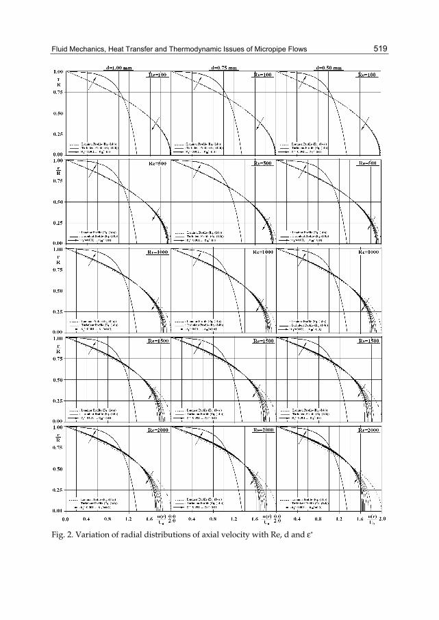
Fluid Mechanics, Heat Transfer and Thermodynamic Issues of Micropipe Flows
519
Fig. 2. Variation of radial distributions of axial velocity with Re, d and ε*
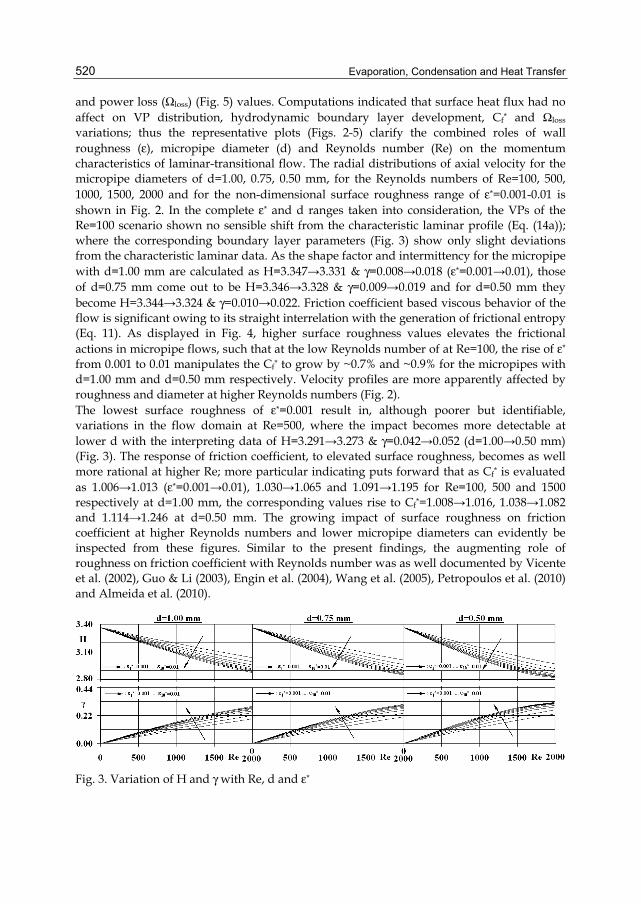
Evaporation, Condensation and Heat Transfer
520
and power loss (Ωloss) (Fig. 5) values. Computations indicated that surface heat flux had no affect on VP distribution, hydrodynamic boundary layer development, Cf* and Ωloss variations; thus the representative plots (Figs. 2-5) clarify the combined roles of wall roughness (ε), micropipe diameter (d) and Reynolds number (Re) on the momentum characteristics of laminar-transitional flow. The radial distributions of axial velocity for the micropipe diameters of d=1.00, 0.75, 0.50 mm, for the Reynolds numbers of Re=100, 500, 1000, 1500, 2000 and for the non-dimensional surface roughness range of ε*=0.001-0.01 is shown in Fig. 2. In the complete ε* and d ranges taken into consideration, the VPs of the Re=100 scenario shown no sensible shift from the characteristic laminar profile (Eq. (14a)); where the corresponding boundary layer parameters (Fig. 3) show only slight deviations from the characteristic laminar data. As the shape factor and intermittency for the micropipe with d=1.00 mm are calculated as H=3.347→3.331 & γ=0.008→0.018 (ε*=0.001→0.01), those of d=0.75 mm come out to be H=3.346→3.328 & γ=0.009→0.019 and for d=0.50 mm they become H=3.344→3.324 & γ=0.010→0.022. Friction coefficient based viscous behavior of the flow is significant owing to its straight interrelation with the generation of frictional entropy (Eq. 11). As displayed in Fig. 4, higher surface roughness values elevates the frictional actions in micropipe flows, such that at the low Reynolds number of at Re=100, the rise of ε* from 0.001 to 0.01 manipulates the Cf* to grow by ~0.7% and ~0.9% for the micropipes with d=1.00 mm and d=0.50 mm respectively. Velocity profiles are more apparently affected by roughness and diameter at higher Reynolds numbers (Fig. 2). The lowest surface roughness of ε*=0.001 result in, although poorer but identifiable, variations in the flow domain at Re=500, where the impact becomes more detectable at lower d with the interpreting data of H=3.291→3.273 & γ=0.042→0.052 (d=1.00→0.50 mm) (Fig. 3). The response of friction coefficient, to elevated surface roughness, becomes as well more rational at higher Re; more particular indicating puts forward that as Cf* is evaluated as 1.006→1.013 (ε*=0.001→0.01), 1.030→1.065 and 1.091→1.195 for Re=100, 500 and 1500 respectively at d=1.00 mm, the corresponding values rise to Cf*=1.008→1.016, 1.038→1.082 and 1.114→1.246 at d=0.50 mm. The growing impact of surface roughness on friction coefficient at higher Reynolds numbers and lower micropipe diameters can evidently be inspected from these figures. Similar to the present findings, the augmenting role of roughness on friction coefficient with Reynolds number was as well documented by Vicente et al. (2002), Guo & Li (2003), Engin et al. (2004), Wang et al. (2005), Petropoulos et al. (2010) and Almeida et al. (2010).
Fig. 3. Variation of H and γ with Re, d and ε*
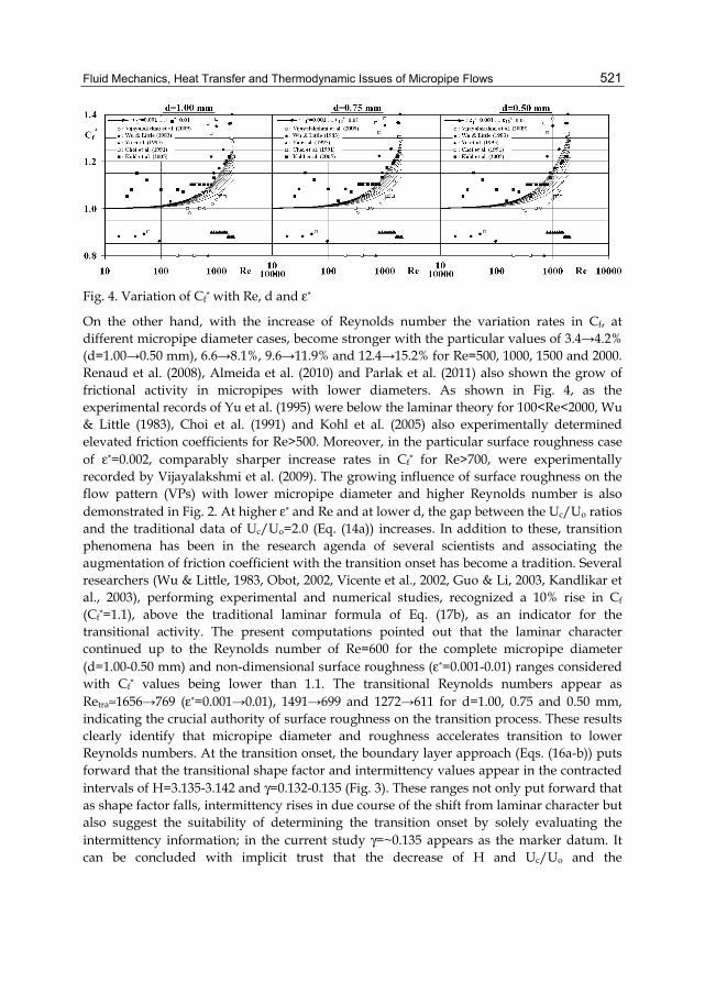
Fluid Mechanics, Heat Transfer and Thermodynamic Issues of Micropipe Flows
521
Fig. 4. Variation of Cf* with Re, d and ε*
On the other hand, with the increase of Reynolds number the variation rates in Cf, at different micropipe diameter cases, become stronger with the particular values of 3.4→4.2% (d=1.00→0.50 mm), 6.6→8.1%, 9.6→11.9% and 12.4→15.2% for Re=500, 1000, 1500 and 2000. Renaud et al. (2008), Almeida et al. (2010) and Parlak et al. (2011) also shown the grow of frictional activity in micropipes with lower diameters. As shown in Fig. 4, as the experimental records of Yu et al. (1995) were below the laminar theory for 100<Re<2000, Wu & Little (1983), Choi et al. (1991) and Kohl et al. (2005) also experimentally determined elevated friction coefficients for Re>500. Moreover, in the particular surface roughness case of ε*=0.002, comparably sharper increase rates in Cf* for Re>700, were experimentally recorded by Vijayalakshmi et al. (2009). The growing influence of surface roughness on the flow pattern (VPs) with lower micropipe diameter and higher Reynolds number is also demonstrated in Fig. 2. At higher ε* and Re and at lower d, the gap between the Uc/Uo ratios and the traditional data of Uc/Uo=2.0 (Eq. (14a)) increases. In addition to these, transition phenomena has been in the research agenda of several scientists and associating the augmentation of friction coefficient with the transition onset has become a tradition. Several researchers (Wu & Little, 1983, Obot, 2002, Vicente et al., 2002, Guo & Li, 2003, Kandlikar et al., 2003), performing experimental and numerical studies, recognized a 10% rise in Cf (Cf*=1.1), above the traditional laminar formula of Eq. (17b), as an indicator for the transitional activity. The present computations pointed out that the laminar character continued up to the Reynolds number of Re=600 for the complete micropipe diameter (d=1.00-0.50 mm) and non-dimensional surface roughness (ε*=0.001-0.01) ranges considered with Cf* values being lower than 1.1. The transitional Reynolds numbers appear as Retra≈1656→769 (ε*=0.001→0.01), 1491→699 and 1272→611 for d=1.00, 0.75 and 0.50 mm, indicating the crucial authority of surface roughness on the transition process. These results clearly identify that micropipe diameter and roughness accelerates transition to lower Reynolds numbers. At the transition onset, the boundary layer approach (Eqs. (16a-b)) puts forward that the transitional shape factor and intermittency values appear in the contracted intervals of H=3.135-3.142 and γ=0.132-0.135 (Fig. 3). These ranges not only put forward that as shape factor falls, intermittency rises in due course of the shift from laminar character but also suggest the suitability of determining the transition onset by solely evaluating the intermittency information; in the current study γ=~0.135 appears as the marker datum. It can be concluded with implicit trust that the decrease of H and Uc/Uo and the
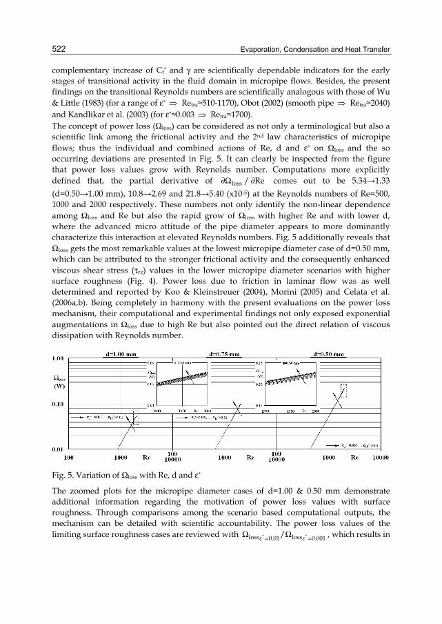
Evaporation, Condensation and Heat Transfer
522
complementary increase of Cf* and γ are scientifically dependable indicators for the early stages of transitional activity in the fluid domain in micropipe flows. Besides, the present findings on the transitional Reynolds numbers are scientifically analogous with those of Wu & Little (1983) (for a range of ε* ⇒ Retra≈510-1170), Obot (2002) (smooth pipe ⇒ Retra≈2040) and Kandlikar et al. (2003) (for ε*≈0.003 ⇒ Retra≈1700). The concept of power loss (Ωloss) can be considered as not only a terminological but also a scientific link among the frictional activity and the 2nd law characteristics of micropipe flows; thus the individual and combined actions of Re, d and ε* on Ωloss and the so occurring deviations are presented in Fig. 5. It can clearly be inspected from the figure that power loss values grow with Reynolds number. Computations more explicitly defined that, the partial derivative of loss∂Ω / Re∂ comes out to be 5.34→1.33 (d=0.50→1.00 mm), 10.8→2.69 and 21.8→5.40 (x10-5) at the Reynolds numbers of Re=500, 1000 and 2000 respectively. These numbers not only identify the non-linear dependence among Ωloss and Re but also the rapid grow of Ωloss with higher Re and with lower d, where the advanced micro attitude of the pipe diameter appears to more dominantly characterize this interaction at elevated Reynolds numbers. Fig. 5 additionally reveals that Ωloss gets the most remarkable values at the lowest micropipe diameter case of d=0.50 mm, which can be attributed to the stronger frictional activity and the consequently enhanced viscous shear stress (τrz) values in the lower micropipe diameter scenarios with higher surface roughness (Fig. 4). Power loss due to friction in laminar flow was as well determined and reported by Koo & Kleinstreuer (2004), Morini (2005) and Celata et al. (2006a,b). Being completely in harmony with the present evaluations on the power loss mechanism, their computational and experimental findings not only exposed exponential augmentations in Ωloss due to high Re but also pointed out the direct relation of viscous dissipation with Reynolds number.
Fig. 5. Variation of Ωloss with Re, d and ε*
The zoomed plots for the micropipe diameter cases of d=1.00 & 0.50 mm demonstrate additional information regarding the motivation of power loss values with surface roughness. Through comparisons among the scenario based computational outputs, the mechanism can be detailed with scientific accountability. The power loss values of the limiting surface roughness cases are reviewed with * *loss lossε 0.01 ε 0.001/= =Ω Ω , which results in
Fluid Mechanics, Heat Transfer and Thermodynamic Issues of Micropipe Flows
523
the ratios of 1.002→1.004 (d=1.00→0.50 mm), 1.009→1.014 and 1.035→1.055 at the Reynolds numbers of Re=500, 1000 and 2000 respectively. The growing action of surface roughness on power loss with lower micropipe diameter and higher Reynolds number can clearly be seen from these numbers.
3.2 Heat transfer issues The primary consequence of the transfer of energy to fluid flow comes into sight through the response of the thermal structure, namely the temperature profile (TP) development, of the concept domain. Since the momentum and energy mechanisms considerably interact, the applied wall heat flux and viscous dissipation based energy loss (Ωloss) on the solid walls simultaneously and strongly affect the TP in the fluid domain. Due to these facts and not only to identify the individual and combined roles of Reynolds number, micropipe diameter, surface roughness and heat flux on the thermal features of micropipe flows but also to display the deviation of the evaluated characteristics from the traditional laminar layout, Fig. 6 covers the TPs of various scenarios in conjunction with the laminar Constant Heat Flux (CHF) formula of Eq. (15) (Incropera & DeWitt, 2001). The figure shows that, in the complete Re and ε* cases taken into consideration, the TP of the micropipe with d=1.00 mm are almost identical. The independent nature of the TPs from ε* can as well be identified through the non-dimensional temperature gradients (ndTG) on the pipe-surface ( )( )r RT/ r =∂ ∂ . Such that, as the ndTG of the Reynolds number cases of
Re=500, 1000 and 2000 get the values of ndTG=6.01, 5.99, and 5.91 (x10-3) at the highest heat flux level of 2000 W/m2, they drop down to ndTG=3.00, 2.98 and 2.90 (x10-3) at the lowest level of 1000 W/m2. There exists almost a two times gap among the ndTG values of the limiting heat flux applications, where the grow of the ndTG with ''q can also be recognized as a result of enhanced heat addition on the walls of the thermal system. However, due to the promoted power loss values (Fig. 5) in the scenarios with higher Re and ε* and lower d, the comparison of the ndTGs among the limiting heat flux scenarios at d=0.50 mm bring about the ratios of ( ) ( )2 2r R q"=2000 W/m r Rq"=1000 W/mT/ r / T/ r= =∂ ∂ ∂ ∂ =~2.00 (Re=500), ~2.08
(Re=1000) and ~2.37 (Re=2000), evidently pointing out the synergy of Re on the affects of ''q on ndTG. On the other hand, ndTGs are evaluated to become moderate with the
increase of mass flow rate, more specifically with Reynolds number, depending on the promoted competence of energy embracing in those scenarios. Computations put forward that the impact of surface roughness on the TP development becomes stronger at lower micropipe diameters, more explicitly with micro-activity. For the lowest diameter of d=0.50 mm and at the highest heat flux condition of ''q =2000 W/m2, the plotted styles in Fig. 6 clarify that in the Reynolds number cases Re=500, 1000 and 2000 ndTG attains the values of 2.93→2.98 (x10-3) (ε*=0.001→0.01), 2.82→2.91 (x10-3) and 2.31→2.59 (x10-3) respectively. In the heat flux application of ''q =1000 W/m2, these gradients decrease down to ndTG=1.47→1.48 (x10-3), 1.36→1.40 (x10-3) and 0.98→1.09 (x10-3) at the identical Reynolds numbers. The increase of the ndTG with ε* is an evidence of the augmenting role surface roughness on heat transfer.
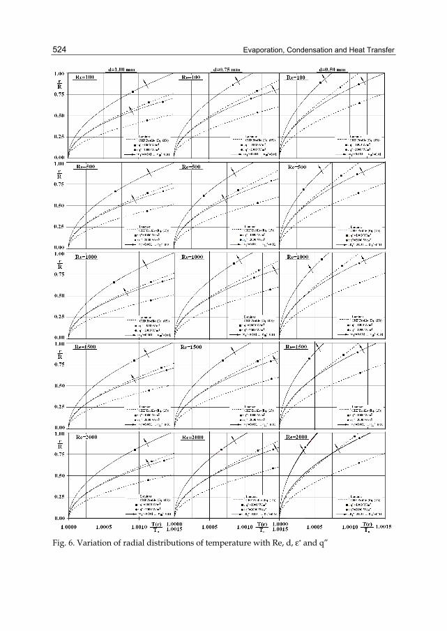
Evaporation, Condensation and Heat Transfer
524
Fig. 6. Variation of radial distributions of temperature with Re, d, ε* and q”
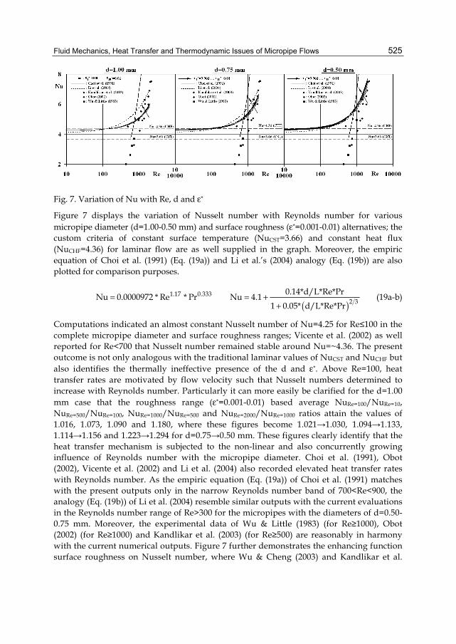
Fluid Mechanics, Heat Transfer and Thermodynamic Issues of Micropipe Flows
525
Fig. 7. Variation of Nu with Re, d and ε*
Figure 7 displays the variation of Nusselt number with Reynolds number for various micropipe diameter (d=1.00-0.50 mm) and surface roughness (ε*=0.001-0.01) alternatives; the custom criteria of constant surface temperature (NuCST=3.66) and constant heat flux (NuCHF=4.36) for laminar flow are as well supplied in the graph. Moreover, the empiric equation of Choi et al. (1991) (Eq. (19a)) and Li et al.’s (2004) analogy (Eq. (19b)) are also plotted for comparison purposes.
1.17 0.333Nu 0.0000972 * Re * Pr= ( )2 3
0.14*d/L*Re*PrNu 4.11 0.05* d/L*Re*Pr
= ++
(19a-b)
Computations indicated an almost constant Nusselt number of Nu=4.25 for Re≤100 in the complete micropipe diameter and surface roughness ranges; Vicente et al. (2002) as well reported for Re<700 that Nusselt number remained stable around Nu=~4.36. The present outcome is not only analogous with the traditional laminar values of NuCST and NuCHF but also identifies the thermally ineffective presence of the d and ε*. Above Re=100, heat transfer rates are motivated by flow velocity such that Nusselt numbers determined to increase with Reynolds number. Particularly it can more easily be clarified for the d=1.00 mm case that the roughness range (ε*=0.001-0.01) based average NuRe=100/NuRe=10, NuRe=500/NuRe=100, NuRe=1000/NuRe=500 and NuRe=2000/NuRe=1000 ratios attain the values of 1.016, 1.073, 1.090 and 1.180, where these figures become 1.021→1.030, 1.094→1.133, 1.114→1.156 and 1.223→1.294 for d=0.75→0.50 mm. These figures clearly identify that the heat transfer mechanism is subjected to the non-linear and also concurrently growing influence of Reynolds number with the micropipe diameter. Choi et al. (1991), Obot (2002), Vicente et al. (2002) and Li et al. (2004) also recorded elevated heat transfer rates with Reynolds number. As the empiric equation (Eq. (19a)) of Choi et al. (1991) matches with the present outputs only in the narrow Reynolds number band of 700<Re<900, the analogy (Eq. (19b)) of Li et al. (2004) resemble similar outputs with the current evaluations in the Reynolds number range of Re>300 for the micropipes with the diameters of d=0.50-0.75 mm. Moreover, the experimental data of Wu & Little (1983) (for Re≥1000), Obot (2002) (for Re≥1000) and Kandlikar et al. (2003) (for Re≥500) are reasonably in harmony with the current numerical outputs. Figure 7 further demonstrates the enhancing function surface roughness on Nusselt number, where Wu & Cheng (2003) and Kandlikar et al.
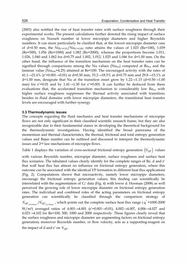
Evaporation, Condensation and Heat Transfer
526
(2003) also notified the rise of heat transfer rates with surface roughness through their experimental works. The present calculations further denoted the rising impact of surface roughness on Nusselt number at lower micropipe diameters and higher Reynolds numbers. It can more particularly be clarified that, at the lowest micropipe diameter case of d=0.50 mm, the Nuε*=0.01/Nuε*=0.001 ratio attains the values of 1.023 (Re=100), 1.039 (Re=500), 1.056 (Re=1000) and 1.082 (Re=2000), whereas the proportions become 1.011, 1.026, 1.040 and 1.062 for d=0.75 and 1.002, 1.012, 1.025 and 1.046 for d=1.00 mm. On the other hand, the influence of the transition mechanism on the heat transfer rates can be signified through comparisons among the Nu values (Nutra) computed at Retra and the laminar value (Nulam=4.25) attained at Re<100. The encouraged activity with the rates of 41.1→21.6% (ε*=0.001→0.01) at d=0.50 mm, 33.2→18.5% at d=0.75 mm and 29.8→15.1% at d=1.00 mm, designate that Nu at the transition onset grow by 1.22→1.15 (d=0.50→1.00 mm) for ε*=0.01 and by 1.41→1.30 for ε*=0.001. It can further be deduced from these evaluations that, the accelerated transition mechanism to considerably low Retra with higher surface roughness suppresses the thermal activity associated with transition; besides in fluid domains with lower micropipe diameters, the transitional heat transfer levels are encouraged with further synergy.
3.3 Thermodynamic issues The concepts regarding the fluid mechanics and heat transfer mechanisms of micropipe flows are not only significant in their classified scientific research frame, but they are also recognizable due to their fundamental stance in developing the theoretical background for the thermodynamic investigations. Having identified the broad panorama of the momentum and thermal characteristics, the thermal, frictional and total entropy generation values and Bejan number can be outlined and discussed to interpret the thermodynamic issues and 2nd law mechanisms of micropipe flows.
Table 1 displays the variation of cross-sectional frictional entropy generation ( )'ΔPS values
with various Reynolds number, micropipe diameter, surface roughness and surface heat flux scenarios. The tabulated values clearly identify for the complete ranges of Re, d and ε* that wall heat flux has almost no influence on frictional entropy generation, where this outcome can be associated with the identical VP formation in different heat flux applications (Fig. 2). Computations shown that microactivity, namely lower micropipe diameters, encourage the frictional entropy generation values; this finding can scientifically be interrelated with the augmentation of Cf* data (Fig. 4) with lower d. Hooman (2008) as well perceived the growing role of lower micropipe diameter on frictional entropy generation rates. The individual and combined roles of the acting parameters on frictional entropy generation can scientifically be classified through the comparison strategy of
d 0.50mm d 1.00mm
' 'ΔP ΔPS /S
= =, which points out the complete surface heat flux range ( ''q =1000-2000
W/m2) averaged ratios of 4.001→4.001 (ε*=0.001→0.01), 4.002→4.007, 4.006→4.027 and 4.023→4.102 for Re=100, 500, 1000 and 2000 respectively. These figures clearly reveal that the surface roughness and micropipe diameter are augmenting factors on frictional entropy generation; moreover Reynolds number, or flow velocity, acts as a supporting-reagent on the impact of d and ε* on '
ΔPS .
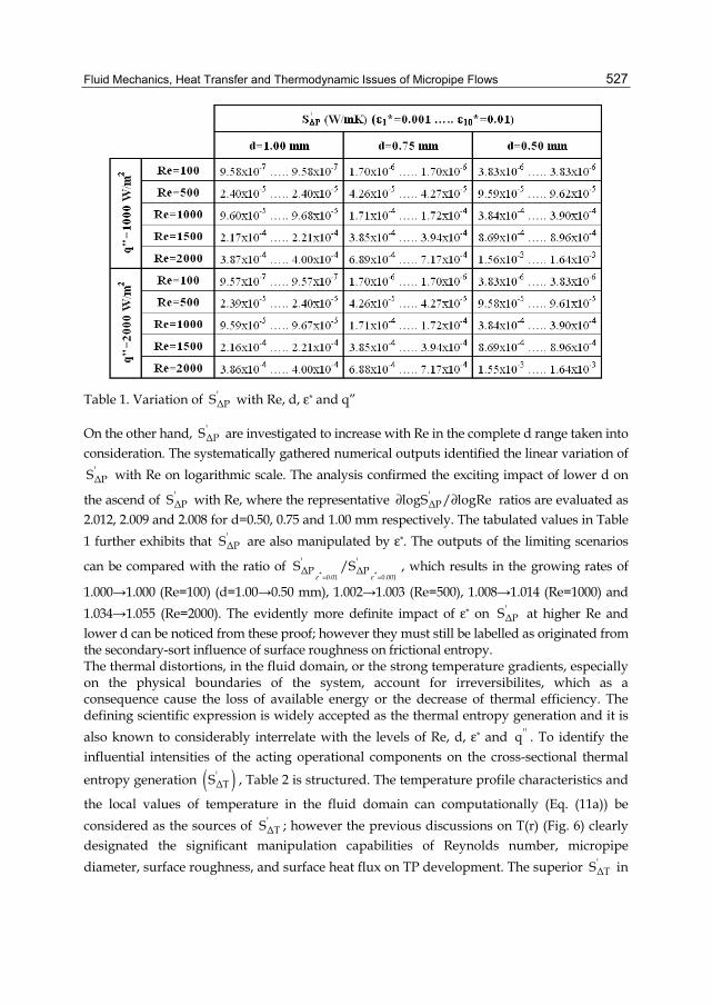
Fluid Mechanics, Heat Transfer and Thermodynamic Issues of Micropipe Flows
527
Table 1. Variation of 'ΔPS with Re, d, ε* and q”
On the other hand, 'ΔPS are investigated to increase with Re in the complete d range taken into
consideration. The systematically gathered numerical outputs identified the linear variation of 'ΔPS with Re on logarithmic scale. The analysis confirmed the exciting impact of lower d on
the ascend of 'ΔPS with Re, where the representative '
ΔPlogS / logRe∂ ∂ ratios are evaluated as 2.012, 2.009 and 2.008 for d=0.50, 0.75 and 1.00 mm respectively. The tabulated values in Table 1 further exhibits that '
ΔPS are also manipulated by ε*. The outputs of the limiting scenarios
can be compared with the ratio of * *0.01 0.001
' 'ΔP ΔPS /S
ε ε= =, which results in the growing rates of
1.000→1.000 (Re=100) (d=1.00→0.50 mm), 1.002→1.003 (Re=500), 1.008→1.014 (Re=1000) and 1.034→1.055 (Re=2000). The evidently more definite impact of ε* on '
ΔPS at higher Re and lower d can be noticed from these proof; however they must still be labelled as originated from the secondary-sort influence of surface roughness on frictional entropy. The thermal distortions, in the fluid domain, or the strong temperature gradients, especially on the physical boundaries of the system, account for irreversibilites, which as a consequence cause the loss of available energy or the decrease of thermal efficiency. The defining scientific expression is widely accepted as the thermal entropy generation and it is also known to considerably interrelate with the levels of Re, d, ε* and ''q . To identify the influential intensities of the acting operational components on the cross-sectional thermal
entropy generation ( )'ΔTS , Table 2 is structured. The temperature profile characteristics and
the local values of temperature in the fluid domain can computationally (Eq. (11a)) be considered as the sources of '
ΔTS ; however the previous discussions on T(r) (Fig. 6) clearly designated the significant manipulation capabilities of Reynolds number, micropipe diameter, surface roughness, and surface heat flux on TP development. The superior '
ΔTS in
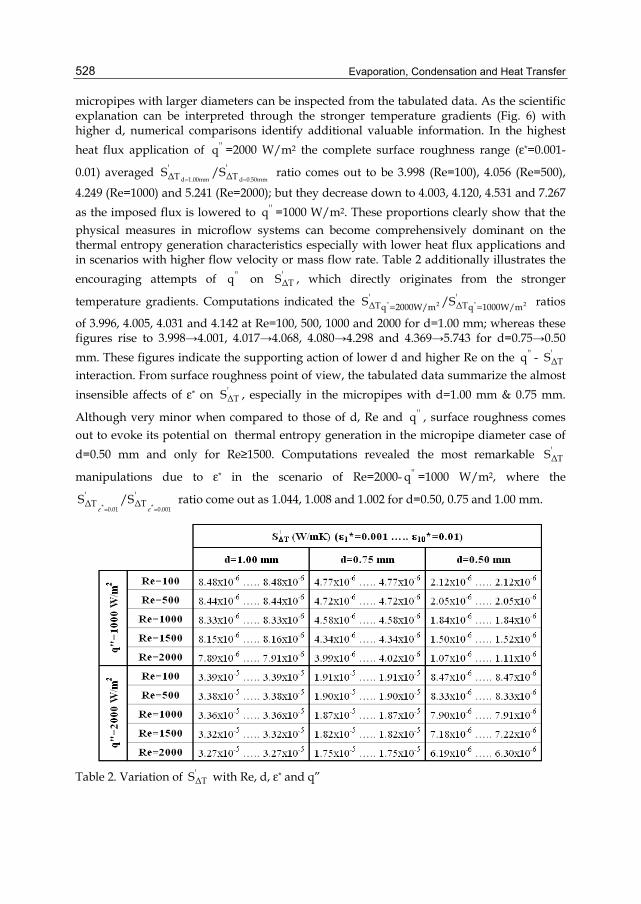
Evaporation, Condensation and Heat Transfer
528
micropipes with larger diameters can be inspected from the tabulated data. As the scientific explanation can be interpreted through the stronger temperature gradients (Fig. 6) with higher d, numerical comparisons identify additional valuable information. In the highest heat flux application of ''q =2000 W/m2 the complete surface roughness range (ε*=0.001-
0.01) averaged d 1.00mm d 0.50mm
' 'ΔT ΔTS /S
= = ratio comes out to be 3.998 (Re=100), 4.056 (Re=500),
4.249 (Re=1000) and 5.241 (Re=2000); but they decrease down to 4.003, 4.120, 4.531 and 7.267 as the imposed flux is lowered to ''q =1000 W/m2. These proportions clearly show that the physical measures in microflow systems can become comprehensively dominant on the thermal entropy generation characteristics especially with lower heat flux applications and in scenarios with higher flow velocity or mass flow rate. Table 2 additionally illustrates the encouraging attempts of ''q on '
ΔTS , which directly originates from the stronger
temperature gradients. Computations indicated the " 2 " 2' 'ΔT ΔTq 2000W/m q 1000W/mS /S= = ratios
of 3.996, 4.005, 4.031 and 4.142 at Re=100, 500, 1000 and 2000 for d=1.00 mm; whereas these figures rise to 3.998→4.001, 4.017→4.068, 4.080→4.298 and 4.369→5.743 for d=0.75→0.50 mm. These figures indicate the supporting action of lower d and higher Re on the ''q - '
ΔTS interaction. From surface roughness point of view, the tabulated data summarize the almost insensible affects of ε* on '
ΔTS , especially in the micropipes with d=1.00 mm & 0.75 mm.
Although very minor when compared to those of d, Re and ''q , surface roughness comes out to evoke its potential on thermal entropy generation in the micropipe diameter case of d=0.50 mm and only for Re≥1500. Computations revealed the most remarkable '
ΔTS
manipulations due to ε* in the scenario of Re=2000- ''q =1000 W/m2, where the
* *0.01 0.001
' 'ΔT ΔTS /S
ε ε= = ratio come out as 1.044, 1.008 and 1.002 for d=0.50, 0.75 and 1.00 mm.
Table 2. Variation of '
ΔTS with Re, d, ε* and q”
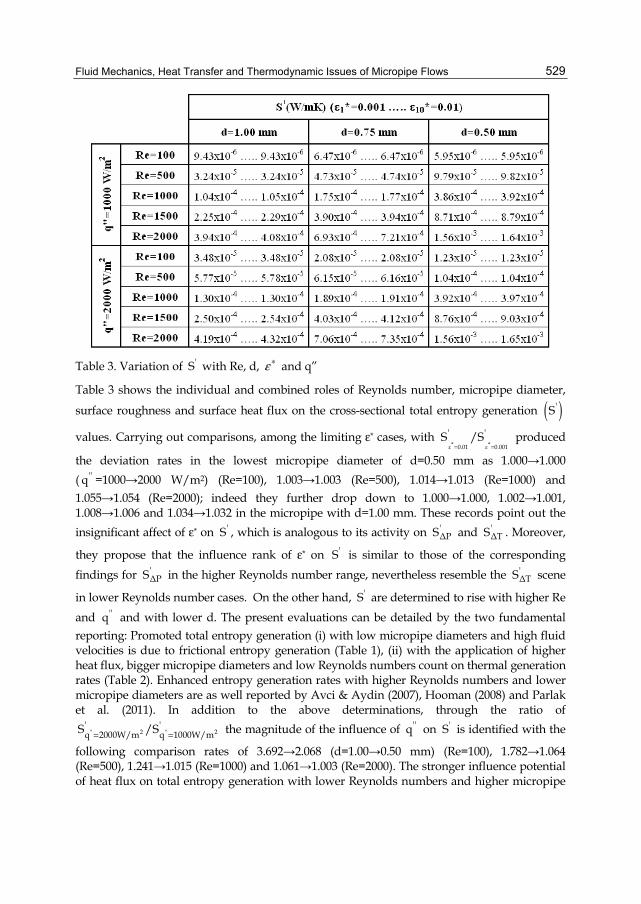
Fluid Mechanics, Heat Transfer and Thermodynamic Issues of Micropipe Flows
529
Table 3. Variation of 'S with Re, d, ε ∗ and q”
Table 3 shows the individual and combined roles of Reynolds number, micropipe diameter,
surface roughness and surface heat flux on the cross-sectional total entropy generation ( )'S
values. Carrying out comparisons, among the limiting ε* cases, with * *ε 0.01 ε 0.001
' 'S /S= =
produced
the deviation rates in the lowest micropipe diameter of d=0.50 mm as 1.000→1.000 ( ''q =1000→2000 W/m2) (Re=100), 1.003→1.003 (Re=500), 1.014→1.013 (Re=1000) and 1.055→1.054 (Re=2000); indeed they further drop down to 1.000→1.000, 1.002→1.001, 1.008→1.006 and 1.034→1.032 in the micropipe with d=1.00 mm. These records point out the insignificant affect of ε* on 'S , which is analogous to its activity on '
ΔPS and 'ΔTS . Moreover,
they propose that the influence rank of ε* on 'S is similar to those of the corresponding findings for '
ΔPS in the higher Reynolds number range, nevertheless resemble the 'ΔTS scene
in lower Reynolds number cases. On the other hand, 'S are determined to rise with higher Re and ''q and with lower d. The present evaluations can be detailed by the two fundamental reporting: Promoted total entropy generation (i) with low micropipe diameters and high fluid velocities is due to frictional entropy generation (Table 1), (ii) with the application of higher heat flux, bigger micropipe diameters and low Reynolds numbers count on thermal generation rates (Table 2). Enhanced entropy generation rates with higher Reynolds numbers and lower micropipe diameters are as well reported by Avci & Aydin (2007), Hooman (2008) and Parlak et al. (2011). In addition to the above determinations, through the ratio of
" 2 " 2' 'q 2000W/m q 1000W/mS /S= = the magnitude of the influence of ''q on 'S is identified with the
following comparison rates of 3.692→2.068 (d=1.00→0.50 mm) (Re=100), 1.782→1.064 (Re=500), 1.241→1.015 (Re=1000) and 1.061→1.003 (Re=2000). The stronger influence potential of heat flux on total entropy generation with lower Reynolds numbers and higher micropipe
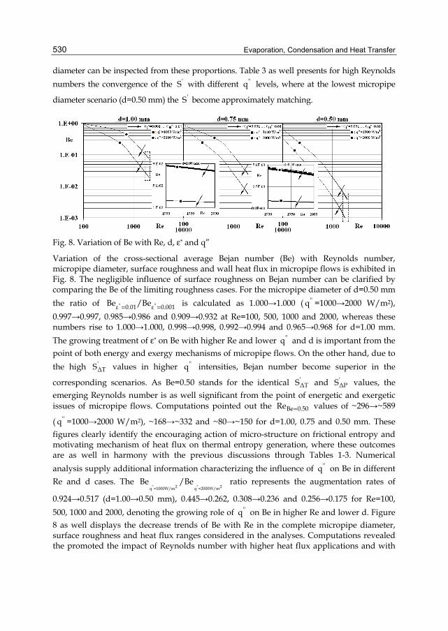
Evaporation, Condensation and Heat Transfer
530
diameter can be inspected from these proportions. Table 3 as well presents for high Reynolds numbers the convergence of the 'S with different ''q levels, where at the lowest micropipe
diameter scenario (d=0.50 mm) the 'S become approximately matching.
Fig. 8. Variation of Be with Re, d, ε* and q”
Variation of the cross-sectional average Bejan number (Be) with Reynolds number, micropipe diameter, surface roughness and wall heat flux in micropipe flows is exhibited in Fig. 8. The negligible influence of surface roughness on Bejan number can be clarified by comparing the Be of the limiting roughness cases. For the micropipe diameter of d=0.50 mm the ratio of * *ε 0.01 ε 0.001Be /Be= = is calculated as 1.000→1.000 ( ''q =1000→2000 W/m2), 0.997→0.997, 0.985→0.986 and 0.909→0.932 at Re=100, 500, 1000 and 2000, whereas these numbers rise to 1.000→1.000, 0.998→0.998, 0.992→0.994 and 0.965→0.968 for d=1.00 mm. The growing treatment of ε* on Be with higher Re and lower ''q and d is important from the point of both energy and exergy mechanisms of micropipe flows. On the other hand, due to the high '
ΔTS values in higher ''q intensities, Bejan number become superior in the
corresponding scenarios. As Be=0.50 stands for the identical 'ΔTS and '
ΔPS values, the emerging Reynolds number is as well significant from the point of energetic and exergetic issues of micropipe flows. Computations pointed out the Be 0.50Re = values of ~296→~589
( ''q =1000→2000 W/m2), ~168→~332 and ~80→~150 for d=1.00, 0.75 and 0.50 mm. These figures clearly identify the encouraging action of micro-structure on frictional entropy and motivating mechanism of heat flux on thermal entropy generation, where these outcomes are as well in harmony with the previous discussions through Tables 1-3. Numerical analysis supply additional information characterizing the influence of ''q on Be in different Re and d cases. The
" 2 " 2q 1000W/m q 2000W/mBe /Be
= = ratio represents the augmentation rates of
0.924→0.517 (d=1.00→0.50 mm), 0.445→0.262, 0.308→0.236 and 0.256→0.175 for Re=100, 500, 1000 and 2000, denoting the growing role of ''q on Be in higher Re and lower d. Figure 8 as well displays the decrease trends of Be with Re in the complete micropipe diameter, surface roughness and heat flux ranges considered in the analyses. Computations revealed the promoted the impact of Reynolds number with higher heat flux applications and with
Fluid Mechanics, Heat Transfer and Thermodynamic Issues of Micropipe Flows
531
lower diameter micropipes. On the other hand, Bejan numbers of the cases with higher heat flux and micropipe diameter came out to be advanced when compared with those of the other. This evaluation can be described by the encouraged thermal activity with the application of high heat flux on the pipe walls and through the enhanced thermal entropy generation rates in micropipes with higher diameter.
4. Conclusions The scientific findings of a comprehensive computational investigation, focusing on the roughness induced forced convective laminar-transitional micropipe flows, is reported. In the numerical analyses, Reynolds number, micropipe diameter, surface roughness and wall heat flux are considered in wide ranges. In the computations, as the converted explicit forms of the principle equations are accumulated into the three-dimensional Transfer Matrix, the influences of surface roughness and surface heat flux conditions are coupled by DSMC method. The Transfer Matrix scheme and the DSMC algorithm are as well supported by cell-by-cell transport tracing technique. To develop a complete overview on the 1st and 2nd law characteristics of flows in micropipes, fluid mechanics, heat transfer and thermodynamic issues are presented and discussed in detail. Radial distributions of axial velocity, boundary layer parameters, friction coefficients and power loss data are presented to recognize the fluid motion based concepts. The outputs on heat transfer results are demonstrated with radial temperature profiles and Nusselt numbers. Thermodynamic notions are interpreted with thermal, frictional and total entropy generation values and Bejan number. Scientific associations among the fluid mechanics, heat transfer and thermodynamic issues are also displayed, identified and revealed with academic liability.
5. Acknowledgement This research is supported by the Research Fund of the University of Uludag through project number: M(U)-2009/35.
6. References Almeida, A.; Geraldes, V. & Semiao, V. (2010). Microflow Hydrodynamics in Slits: Effects of
the Walls Relative Roughness and Spacer Inter-Filaments Distance. Chemical Engineering Science, Vol. 65, pp. 3660-3670, ISSN 0009-2509.
Avci, M. & Aydin, O. (2007). Second-Law Analysis of Heat and Fluid Flow in Microscale Geometries. International Journal of Exergy, Vol. 4, pp. 286-301, ISSN 1742-8297.
Cao, B.Y.; Chen, M. & Guo, Z.Y. (2006). Effect of Surface Roughness on Gas Flow in Microchannels by Molecular Dynamics Simulation. International Journal of Engineering Science, Vol. 44, pp. 927–937, ISSN 0020-7225.
Celata, G.P.; Cumo, M.; McPhail, S. & Zummo, G. (2006a). Characterization of Fluid Dynamic Behaviour and Channel Wall Effects in Microtube. International Journal of Heat and Fluid Flow, Vol. 27, pp. 135–143, ISSN 0142-727X.
Celata, G.P.; Morini, G.L.; Marconi, V.; McPhail, S.J. & Zummo, G. (2006b). Using Viscous Heating to Determine the Friction Factor in Microchannels – An Experimental Validation. Experimental Thermal and Fluid Science, Vol. 30, pp. 725–731, ISSN 0894-1777.
Evaporation, Condensation and Heat Transfer
532
Celata, G.P.; Lorenzini, M. & Morini, G.L. (2009). Friction Factor in Micropipe Gas Flow under Laminar, Transition and Turbulent Flow Regime. International Journal of Heat and Fluid Flow, Vol. 30, pp. 814-822, ISSN 0142-727X.
Chen, S. & Tian, Z.W. (2010). Simulation of Thermal Micro-Flow using Lattice Boltzmann Method with Langmuir Slip Model. International Journal of Heat and Fluid Flow, Vol. 31, pp. 227-235, ISSN 0142-727X.
Choi, S.B.; Barron, R.F. & Warrington, R.O. (1991). Fluid Flow and Heat Transfer in Microtubes. Micromechanical Sensors, Actuators and Systems, Vol. 32, pp. 123–134, ISSN 0924-4247.
Engin, T.; Dogruer, U.; Evrensel, C.; Heavin, S. & Gordaninejad, F. (2004). Effect of Wall Roughness on Laminar Flow of Bingham Plastic Fluids through Microtubes. Journal of Fluids Engineering - ASME Transactions, Vol. 126, pp. 880-883, ISSN 0098-2202.
Guo, Z.Y. & Li, Z.X. (2003). Size Effect on Microscale Single-Phase Flow and Heat Transfer. International Journal of Heat and Mass Transfer, Vol. 46, pp. 149–159, ISSN 0017-9310.
Hooman, K. (2008). Heat Transfer and Entropy Generation for Forced Convection through a Microduct of Rectangular Cross-Section: Effects of Velocity Slip, Temperature Jump, and Duct Geometry. International Communications in Heat and Mass Transfer, Vol. 9, pp. 1065-1068, ISSN 0735-1933.
Incropera, F.P. & DeWitt, D.P. (2001). Fundamentals of Heat and Mass Transfer, John Wiley & Sons, ISBN 9780471386506, New York.
Kandlikar, S.G.; Joshi, S. & Tian, S. (2003). Effect of Surface Roughness on Heat Transfer and Fluid Flow Characteristics at Low Reynolds Numbers in Small Diameter Tubes. Heat Transfer Engineering, Vol. 24, pp. 4–16, ISSN 0145-7632.
Ko, T.H. (2006a). Numerical Analysis of Entropy Generation and Optimal Reynolds Number for Developing Laminar Forced Convection in Double-Sine Ducts with Various Aspect Ratios. International Journal of Heat and Mass Transfer, Vol. 49, pp. 718–726, ISSN 0017-9310.
Ko, T.H. (2006b). Numerical Investigation of Laminar Forced Convection and Entropy Generation in a Helical Coil with Constant Wall Heat Flux. Numerical Heat Transfer Part-A, Vol. 49, pp. 257-278, ISSN 1040-7782.
Kohl, M.J.; Abdel-Khalik, S.I.; Jeter, S.M. & Sadowski, D.L. (2005). An Experimental Investigation of Microchannel Flow with Internal Pressure Measurements. International Journal of Heat and Mass Transfer, Vol. 48, pp. 1518–1533, ISSN 0017-9310.
Koo, J. & Kleinstreuer, C. (2004). Viscous Dissipation Effects in Microtubes and Microchannels. International Journal of Heat and Mass Transfer, Vol. 47, pp. 3159–3169, ISSN 0017-9310.
Kotas, T.J.; Mayhew, Y.R. & Raichura, R.C. (1995). Nomenclature for Exergy Analysis. Proceedings of the Institution of Mechanical Engineers-Part A, Vol. 209, pp. 275-280, ISSN 0263-7138.
Li, J.; Peterson, G.P. & Cheng, P. (2004). Three-Dimensional Analysis of Heat Transfer in a Micro-Heat Sink with Single Phase Flow. International Journal of Heat and Mass Transfer, Vol. 47, pp. 4215–4231, ISSN 0017-9310.
Morini, G.L. (2005). Viscous Heating in Liquid Flows in Micro-Channels. International Journal of Heat and Mass Transfer, Vol. 48, pp. 3637–3647, ISSN 0017-9310.
Fluid Mechanics, Heat Transfer and Thermodynamic Issues of Micropipe Flows
533
Obot, N.T. (2002). Toward a Better Understanding of Friction and Heat/Mass Transfer in Microchannels – A Literature Review. Microscale Thermophysical Engineering, Vol. 6, pp. 155–173, ISSN 1089-3954.
Ogedengbe, E.O.B.; Naterer, G.F. & Rosen, M.A. (2006). Slip Flow Irreversibility of Dissipative Kinetic and Internal Energy Exchange in Microchannels. Journal of Micromechanics and Microengineering, Vol. 16, pp. 2167–2176, ISSN 0960-1317.
Ozgener, L.; Hepbasli, A. & Dincer, I. (2007). Parametric Study of the Effect of Reference State on Energy and Exergy Efficiencies of Geothermal District Heating Systems (GDHSs): An Application of the Salihli GDHS in Turkey. Heat Transfer Engineering, Vol. 28, pp. 357–364, ISSN 0145-7632.
Parlak, N.; Gur, M.; Ari, V.; Kucuk, H. & Engin, T. (2011). Second Law Analysis of Water Flow through Smooth Microtubes under Adiabatic Conditions. Experimental Thermal and Fluid Science, Vol. 35, pp. 60-67, ISSN 0894-1777.
Petropoulos, A.; Kaltsas, G. & Randjelovic, D. (2010). Study of Flow and Pressure Field in Microchannels with Various Cross-Section Areas. Microelectronic Engineering, Vol. 87, pp. 827-829, ISSN 0167-9317.
Pitakarnnop, J.; Varoutis, S. & Valougeorgis, D. (2010). A Novel Experimental Setup for Gas Microflows. Microfluidics and Nanofluidics, Vol. 8, pp. 57-72, ISSN 1613-4982.
Ratts, E.B. & Raut, A.G. (2004). Entropy Generation Minimization of Fully Developed Internal Flow with Constant Heat Flux. Journal of Heat Transfer - ASME Transactions, Vol. 126, pp. 656-659, ISSN 0022-1481.
Renaud, L.; Malhaire, C. & Kleimann, P. (2008). Theoretical and Experimental Studies of Microflows in Silicon Microchannels. Materials Science & Engineering C-Biomimetric and Supramolecular Systems, Vol. 28, pp. 910-917, ISSN 0928-4931.
Richardson, D.H.; Sekulic, D.P. & Campo, A. (2000). Low Reynolds Number Flow Inside Straight Micro Channels with Irregular Cross Sections. Heat and Mass Transfer, Vol. 36, pp. 187-193, ISSN 0947-7411.
Sahin, A.Z. (1998). Second-Law Analysis of Laminar Viscous Flow through a Duct Subjected to Constant Wall Temperature. Journal of Heat Transfer - ASME Transactions, Vol. 120, pp. 77-83, ISSN 0022-1481.
Sahin, A.Z.; Zubair, S.M.; Al-Garni, A.Z. & Kahraman, R. (2000). Effect of Fouling on Operational Cost in Pipe Flow due to Entropy Generation. Energy Conversion and Management, Vol. 41, pp. 1485-1496, ISSN 0196-8904.
Stewart, S.W.; Shelton, S.V. & Aspelund, K.A. (2005) Finned-Tube Heat Exchanger Optimization Methodology. Heat Transfer Engineering, Vol. 26, pp. 22–28, ISSN 0145-7632
Vicente, P.G.; Garcia, A. & Viedma, A. (2002). Experimental Study of Mixed Convection and Pressure Drop in Helically Dimpled Tubes for Laminar and Transition Flow. International Journal of Heat and Mass Transfer, Vol. 45, pp. 5091–5105, ISSN 0017-9310.
Vijayalakshmi, K.; Anoop, K.B. & Patel, H.E. (2009). Effects of Compressibility and Transition to Turbulence on Flow through Microchannels. International Journal of Heat and Mass Transfer, Vol. 52, pp. 2196–2204, ISSN 0017-9310.
Wang, H.; Wang, Y. & Zhang, J. (2005). Influence of Ribbon Structure Rough Wall on the Microscale Poiseuille Flow. Journal of Fluids Engineering - ASME Transactions, Vol. 127, pp. 1140-1145, ISSN 0098-2202.
Evaporation, Condensation and Heat Transfer
534
Wen, M.Y.; Jang, K.J. & Yang, C.C. (2003). Augmented Heat Transfer and Pressure Drop of Strip-Type Inserts in the Small Tubes. Heat and Mass Transfer, Vol. 40, pp. 133–141, ISSN 0947-7411.
White, F.M. (1999). Fluid Mechanics, McGraw-Hill, ISBN 0-07-116848-6, Singapore. Wu, H.Y. & Cheng, P. (2003). An Experimental Study of Convective Heat Transfer in Silicon
Microchannels with Different Surface Conditions. International Journal of Heat and Mass Transfer, Vol. 46, pp. 2547–2556, ISSN 0017-9310.
Wu, J.S. & Tseng, K.C. (2001). Analysis of Micro-Scale Gas Flows with Pressure Boundaries using Direct Simulation Monte Carlo Method. Computers and Fluids, Vol. 30, pp. 711-735, ISSN 0045-7930.
Wu, P. & Little, W.A. (1983). Measurement of Friction Factors for the Flow of Gases in very Fine Channels used for Microminiature Joule–Thompson Refrigerators. Cryogenics, Vol. 23, pp. 273–277, ISSN 0011-2275.
Yilbas, B.S. & Pakdemirli, M. (2005) Entropy Generation Due to the Flow of a Non-Newtonian Fluid with Variable Viscosity in a Circular Pipe. Heat Transfer Engineering, Vol. 26, pp. 80–86, ISSN 0145-7632
Yu, D.; Warrington, R.; Baron, R. & Ameel, T. (1995). An Experimental and Theoretical Investigation of Fluid Flow and Heat Transfer in Microtubes, ASME/JSME Thermal Engineering Conference, pp. 523–530.
Zimparov, V. (2000). Extended Performance Evaluation Criteria for Enhanced Heat Transfer Surfaces: Heat Transfer through Ducts with Constant Wall Temperature. International Journal of Heat and Mass Transfer, Vol. 43, pp. 3137–3155, ISSN 0017-9310.
25
Fundamentals of Paper Drying – Theory and Application from Industrial Perspective
Ajit K Ghosh Principal, AKG Process Consulting, 33 McFarlane Court, Highett,
Australia
1. Introduction No manufactured product plays a more significant role in every area of human activity than paper and paper products. Its importance in everyday life is obvious from its use in recording, storage and dissemination of information. Virtually all writing and printing is done on paper. It is the most widely used wrapping and packaging material, and is important for structural applications. The uses and applications for pulp and paper products are virtually limitless. Apart from the products and services that it provides, the paper and pulp industry is one of the major manufacturing industries in the world providing employment for vast number of people and contribute to national economy. The paper making process is essentially a very large dewatering operation where a diluted solution of pulp suspension with less than 0.5% fibre solid is used. The major sections of a paper machine consist of: forming section, press section and dryer section. In the forming section, the fibres present in the diluted pulp and water slurry form paper web through drainage by gravity and applied suction below the forming fabric. In the press section additional water in removed by mechanical pressure applied through the nips of a series of presses or rotating rolls and the wet web is consolidated in this section. Most of the remaining water is evaporated and inter-fibre binding developed as the paper contacts a series of steam heated cylinder in the dryer section. Water removal from the wet web to the final moisture level between 6% and 7% is a critical step of papermaking. Majority of the functional properties of paper are developed in this section. In spite of its key role in papermaking, large equipment size, and large capital and operating costs, drying is arguably the least understood papermaking operation. Books on papermaking technology generally devote fewer pages to drying than other papermaking operations such as forming, pressing or calendaring. A similar situation is found in papermaking courses, in which drying occupies a shorter time than the proportion of space it takes in a paper machine. Furthermore, a large portion of that time is devoted to the description of the equipment by its suppliers rather than to its operation by the papermakers. The dryer section of a paper machine removes between 1.1 and 1.3 kg of water per kg of paper compared to 200 kg and 2.6 kg in the forming and press sections respectively. It is significantly more expensive to remove this water than for any other section of the machine (Reese, 1988). The relative costs of dewatering are: forming section 10%; press section 12% and dryer section 78%. The dryer section is by far the largest consumer of
Evaporation, Condensation and Heat Transfer
536
thermal energy of a paper machine. Other important facts about the dryer section and paper drying are the dryer section constitutes approximately 60% of the total length of a paper machine, except for a tissue machine; and almost 40% of total capital cost of the machine. The lack of knowledge about drying also persists in the mills. Detailed information and knowledge on the theory and operation of the other sections of the paper machine are quite often at the fingertip of the machine operators and technical staffs, while the dryer section is often at the bottom of the mills’ priority list. There are several reasons for this lack of knowledge and interest in this important papermaking operation. Perhaps the first among them is the wrong perception that drying has little effect on product quality. The other reason is the complexity of the paper drying process that involves heat transfer, evaporation and water removal processes where steam pressure, cylinder surface temperature, dryer pocket conditions, hood balance and condensate removal play key roles in determining drying capacity and final product quality. The operator and papermakers often treat the dryer section as a black box. Rising energy costs are forcing papermakers to pay more attention to energy efficiency, and specially steam usage. In many mills due attention is given to the steam and condensate system. However, the importance of hood balance and pocket air ventilation is quite often ignored. This could result in excessive energy consumption in the dryer section and/or reduction in drying efficiency with consequential loss in productivity. Deterioration of product quality could also be due to neglect in optimization of pocket ventilation system (Ghosh and Oxley, 2007).
1.1 Manufacture of paper The art of papermaking had its origin in China as early as 100 AD. The first mechanized papermaking process was carried out by Foudrinier brothers in UK in 1804. Since that time many improvements over the original paper machine have been made, but the basic construction remains basically the same. In virtually all papermaking of today, cellulose fibres are used as the raw material. The prime source of cellulose is trees, especially pine, spruce, birch and eucalyptus. Modern papermaking uses both virgin and recycled fibres, depending on the requirements of the final products. Pulp production from virgin fibres is generally divided into two main categories: chemical and mechanical pulping. In chemical pulping process wood chips are cooked in a digester with chemicals under pressure and at elevated temperatures. The relatively undamaged fibres are recovered via various unit operations. The yield is around 50%. Mechanical pulps have a much higher yield, more than 95%, but the fibres are treated more violently and are significantly shorter than chemically treated fibres. The most common method of mechanical pulping employs large rotating discs with sharp edges. The wood chips are pressed against the discs so that the chips are torn apart. Recycled fibres could be mixtures of both chemical and mechanical pulps at various proportions with varying level of contaminations as the papers used are post-consumer. The recycled papers are reslushed with water followed by separation of contaminants before being used in the papermaking process. Regardless of the nature of the pulp, whether it is chemical, mechanical or recycled, is either softwood or hardwood, the basics of papermaking are similar. Many chemical additives are used to promote certain properties of the final products, such as optical properties, dry and wet strength or resistance to water absorption. The pulp and additives are mixed in water
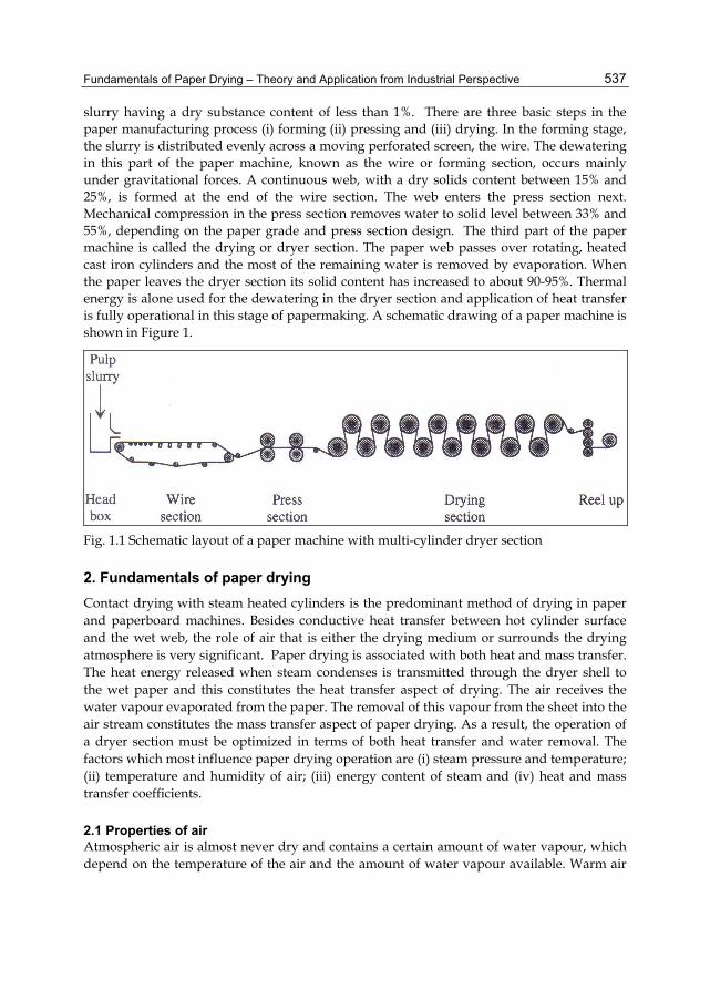
Fundamentals of Paper Drying – Theory and Application from Industrial Perspective
537
slurry having a dry substance content of less than 1%. There are three basic steps in the paper manufacturing process (i) forming (ii) pressing and (iii) drying. In the forming stage, the slurry is distributed evenly across a moving perforated screen, the wire. The dewatering in this part of the paper machine, known as the wire or forming section, occurs mainly under gravitational forces. A continuous web, with a dry solids content between 15% and 25%, is formed at the end of the wire section. The web enters the press section next. Mechanical compression in the press section removes water to solid level between 33% and 55%, depending on the paper grade and press section design. The third part of the paper machine is called the drying or dryer section. The paper web passes over rotating, heated cast iron cylinders and the most of the remaining water is removed by evaporation. When the paper leaves the dryer section its solid content has increased to about 90-95%. Thermal energy is alone used for the dewatering in the dryer section and application of heat transfer is fully operational in this stage of papermaking. A schematic drawing of a paper machine is shown in Figure 1.
Fig. 1.1 Schematic layout of a paper machine with multi-cylinder dryer section
2. Fundamentals of paper drying Contact drying with steam heated cylinders is the predominant method of drying in paper and paperboard machines. Besides conductive heat transfer between hot cylinder surface and the wet web, the role of air that is either the drying medium or surrounds the drying atmosphere is very significant. Paper drying is associated with both heat and mass transfer. The heat energy released when steam condenses is transmitted through the dryer shell to the wet paper and this constitutes the heat transfer aspect of drying. The air receives the water vapour evaporated from the paper. The removal of this vapour from the sheet into the air stream constitutes the mass transfer aspect of paper drying. As a result, the operation of a dryer section must be optimized in terms of both heat transfer and water removal. The factors which most influence paper drying operation are (i) steam pressure and temperature; (ii) temperature and humidity of air; (iii) energy content of steam and (iv) heat and mass transfer coefficients.
2.1 Properties of air Atmospheric air is almost never dry and contains a certain amount of water vapour, which depend on the temperature of the air and the amount of water vapour available. Warm air
Evaporation, Condensation and Heat Transfer
538
can absorb more water vapour than the same volume of cold air. Thus the condition of air in the dryer section is important. The relationship between the temperature of the air and the amount of water it contains is described by the psychorometric chart, which plots humidity versus temperature. Well established equations can also be used to calculate thermodynamic properties of air.
2.1.1 Partial vapour pressure Partial vapour pressure of free water can be calculated using Antoine’s equation (Perry, 1997):
ln( ) Bp AT C
= −+
(1)
where p partial pressure, kPa T temperature, Abs A, B, C constants; A= 8.007131; B = 1730.630; C= 233.426
At the beginning of drying, partial vapour pressure at the paper surface is the same as for a free water surface at corresponding temperature and this condition prevails as long as transport can bring new water to the surface replacing the water that evaporated. In the end phase of drying, partial vapour pressure on the web surface is lower than for free water surface at the corresponding temperature. This is because diffusion from the interior from the web controls vapour transport to the web surface and the hygroscopic nature of pulp fibres.
2.1.2 Relative humidity Relative humidity is the ratio between the amount of water contained in the air and the total amount it can contain at the same temperature and is expressed as percentage. When relative humidity reaches 100%, the air is said to be saturated and water vapour condenses in the air and falls out as small droplets. Relative humidity can be calculated from the following equation:
sRH = p * 100 / P (2)
where RH % relative humidity p partial vapour pressure, kPa Ps saturated vapour pressure of water at temperature T.
Evaporation can still take place at 100% RH if the vapour pressure of the water in the drying surface exceeds that of water at the same temperature, i.e. the drying surface is hotter than the surrounding saturated air. However, the water evaporated from the drying surface will form a mist since the ambient air is incapable of absorbing any more water vapour.
2.1.3 Absolute humidity Absolute humidity refers to the moisture content of the air and the typical units are kg H2O/kg dry air. Psychometric chart could be used to obtain humidity value provided wet
Fundamentals of Paper Drying – Theory and Application from Industrial Perspective
539
and dry bulb temperatures are known. Alternatively, it can be calculated from the partial vapour pressure of water in the air from the following equation:
( )w aH M p / M * P p⎡ ⎤= −⎣ ⎦ (3)
where H absolute humidity, H2O/kg dry air p partial vapour pressure, kPa P barometric pressure, kPa Mw Molecular weight of water: 18.02 Ma Molecular weight of air: 28.97
If relative humidity and temperature values are known, the absolute humidity can also be calculated using the following equation:
( )H 0.00620689 * RH * p / 1 .01 * RH * p= − (4)
where H Absolute humidity, H2O/kg dry air p partial vapour pressure, kPa and can be calculated using equation (1) RH relative humidity, %
2.1.4 Sorption isotherm Due to hygroscopic nature of paper, partial vapour pressure at the web surface or anywhere inside the web is a function of local temperature and moisture content. A correlation between relative humidity and the equilibrium moisture content at a constant temperature is a sorption isotherm. Equilibrium moisture content at a certain relative humidity gives slightly different values depending on whether the equilibrium is approached through wetting of initial dry materials (adsorption) or through drying (desorption). This phenomenon is called hysteresis. The sorption isotherm of paper depends on the type of fibres that have been used to manufacture the paper. Various correlations for sorption isotherms are available in the literature (Karlsson et al.,, 1993; Lampinen and Toivonen, 1984). The following one is best suitable for mechanical pulp (Heikkila, 1993):
2 4
1 3{( ) ( )}1C CC Z C TZeρ − += − (5)
where C1 = 47.58; C2 = 1.877; C3 = 0.10085/ oC; C4 = 1.0585 ρ Relative Humidity of air inside chamber/room/store ; ρ*100 Relative Humidity, % Z Equilibrium Moisture Ratio; Z*100 = Moisture Uptake, % T Temperature, oC
Graphical representation of equation (5) is shown in Figure 2.1.
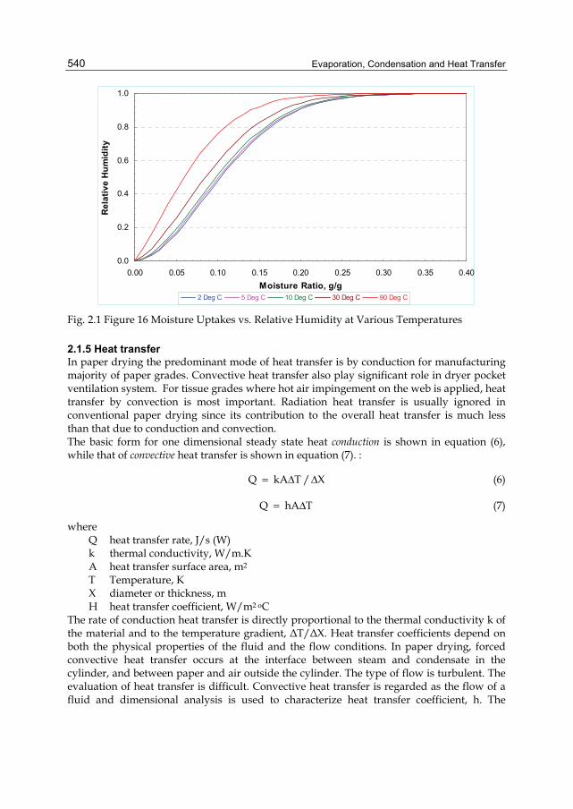
Evaporation, Condensation and Heat Transfer
540
0.0
0.2
0.4
0.6
0.8
1.0
0.00 0.05 0.10 0.15 0.20 0.25 0.30 0.35 0.40Moisture Ratio, g/g
Rel
ativ
e H
umid
ity
2 Deg C 5 Deg C 10 Deg C 30 Deg C 90 Deg C
Fig. 2.1 Figure 16 Moisture Uptakes vs. Relative Humidity at Various Temperatures
2.1.5 Heat transfer In paper drying the predominant mode of heat transfer is by conduction for manufacturing majority of paper grades. Convective heat transfer also play significant role in dryer pocket ventilation system. For tissue grades where hot air impingement on the web is applied, heat transfer by convection is most important. Radiation heat transfer is usually ignored in conventional paper drying since its contribution to the overall heat transfer is much less than that due to conduction and convection. The basic form for one dimensional steady state heat conduction is shown in equation (6), while that of convective heat transfer is shown in equation (7). :
Q kA T / X= Δ Δ (6)
Q hA T= Δ (7)
where Q heat transfer rate, J/s (W) k thermal conductivity, W/m.K A heat transfer surface area, m2 T Temperature, K X diameter or thickness, m H heat transfer coefficient, W/m2 oC
The rate of conduction heat transfer is directly proportional to the thermal conductivity k of the material and to the temperature gradient, ΔT/ΔX. Heat transfer coefficients depend on both the physical properties of the fluid and the flow conditions. In paper drying, forced convective heat transfer occurs at the interface between steam and condensate in the cylinder, and between paper and air outside the cylinder. The type of flow is turbulent. The evaluation of heat transfer is difficult. Convective heat transfer is regarded as the flow of a fluid and dimensional analysis is used to characterize heat transfer coefficient, h. The
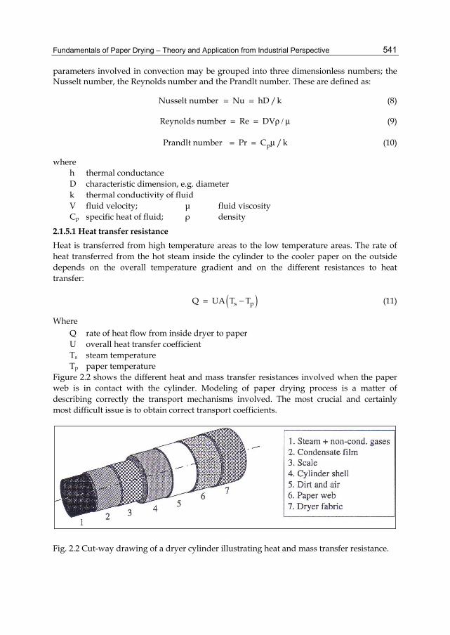
Fundamentals of Paper Drying – Theory and Application from Industrial Perspective
541
parameters involved in convection may be grouped into three dimensionless numbers; the Nusselt number, the Reynolds number and the Prandlt number. These are defined as:
Nusselt number Nu hD /k = = (8)
Reynolds number Re DV= = ρ / μ (9)
pPrandlt number Pr C /k= = μ (10)
where h thermal conductance D characteristic dimension, e.g. diameter k thermal conductivity of fluid V fluid velocity; μ fluid viscosity Cp specific heat of fluid; ρ density
2.1.5.1 Heat transfer resistance Heat is transferred from high temperature areas to the low temperature areas. The rate of heat transferred from the hot steam inside the cylinder to the cooler paper on the outside depends on the overall temperature gradient and on the different resistances to heat transfer:
( )s pQ UA T T= − (11)
Where
Q rate of heat flow from inside dryer to paper U overall heat transfer coefficient Ts steam temperature Tp paper temperature
Figure 2.2 shows the different heat and mass transfer resistances involved when the paper web is in contact with the cylinder. Modeling of paper drying process is a matter of describing correctly the transport mechanisms involved. The most crucial and certainly most difficult issue is to obtain correct transport coefficients.
Fig. 2.2 Cut-way drawing of a dryer cylinder illustrating heat and mass transfer resistance.
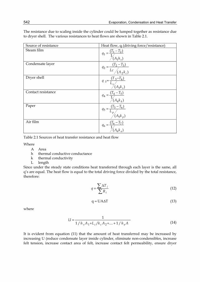
Evaporation, Condensation and Heat Transfer
542
The resistance due to scaling inside the cylinder could be lumped together as resistance due to dryer shell. The various resistances to heat flows are shown in Table 2.1.
Source of resistance Heat flow, qi (driving force/resistance) Steam film 1 2
1
1
( )1
( )s
T TqA h
−=
Condensate layer 2 32
2
( )
( )c
T TqLc A k
−=
Dryer shell 3 43
3
( )
( )s
s
T Tq LA k
−=
Contact resistance 4 54
4
( )1
( )k
T TqA k
−=
Paper 5 65
5
( )
( )p
p
T Tq LA k
−=
Air film 6 76
6
( )1
( )a
T TqA k
−=
Table 2.1 Sources of heat transfer resistance and heat flow
Where
A Area h thermal conductive conductance k thermal conductivity L length
Since under the steady state conditions heat transferred through each layer is the same, all q’s are equal. The heat flow is equal to the total driving force divided by the total resistance, therefore:
i
i
Tq
RΔ
= ∑∑
(12)
q UA T= Δ (13)
where
1 2
11 / / .... 1 /s c c a
Uh A L k A h A
=+ + +
(14)
It is evident from equation (11) that the amount of heat transferred may be increased by increasing U (reduce condensate layer inside cylinder, eliminate non-condensibles, increase felt tension, increase contact area of felt, increase contact felt permeability, ensure dryer
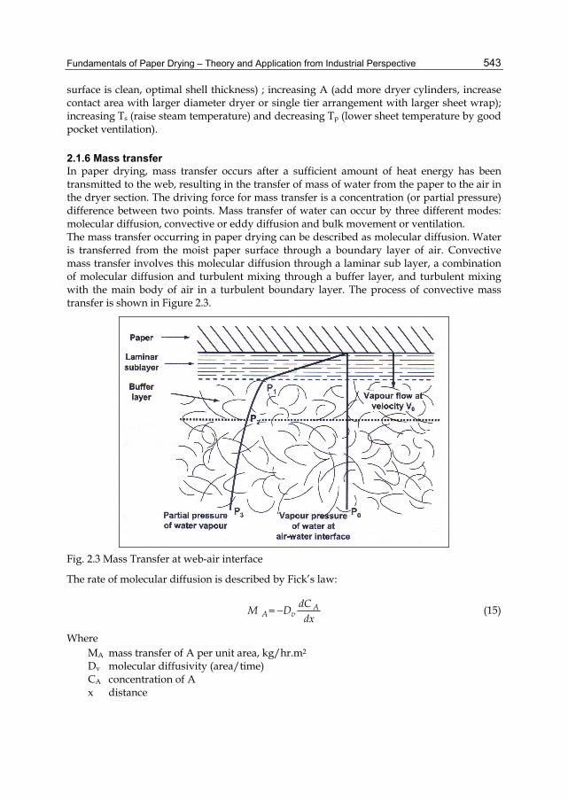
Fundamentals of Paper Drying – Theory and Application from Industrial Perspective
543
surface is clean, optimal shell thickness) ; increasing A (add more dryer cylinders, increase contact area with larger diameter dryer or single tier arrangement with larger sheet wrap); increasing Ts (raise steam temperature) and decreasing Tp (lower sheet temperature by good pocket ventilation).
2.1.6 Mass transfer In paper drying, mass transfer occurs after a sufficient amount of heat energy has been transmitted to the web, resulting in the transfer of mass of water from the paper to the air in the dryer section. The driving force for mass transfer is a concentration (or partial pressure) difference between two points. Mass transfer of water can occur by three different modes: molecular diffusion, convective or eddy diffusion and bulk movement or ventilation. The mass transfer occurring in paper drying can be described as molecular diffusion. Water is transferred from the moist paper surface through a boundary layer of air. Convective mass transfer involves this molecular diffusion through a laminar sub layer, a combination of molecular diffusion and turbulent mixing through a buffer layer, and turbulent mixing with the main body of air in a turbulent boundary layer. The process of convective mass transfer is shown in Figure 2.3.
Fig. 2.3 Mass Transfer at web-air interface
The rate of molecular diffusion is described by Fick’s law:
AA v
dCM Ddx
= − (15)
Where
MA mass transfer of A per unit area, kg/hr.m2 Dv molecular diffusivity (area/time) CA concentration of A x distance
Evaporation, Condensation and Heat Transfer
544
For water vapour diffusing from the paper into the surroundings, this concentration gradient is expressed as a partial pressure difference:
( )A g o lM k P – P= (16)
Where
kg mass transfer coefficient Po partial pressure of water at sheet surface Pl partial pressure of water in surrounding air
Similar to heat transfer, dimensional analysis and experimental evaluation can be used to determine the transfer coefficient. Although kg can be determined experimentally, for practical uses convective mass transfer can be expressed in the general form:
( )p aM KA P – P= (17)
Where
M rate of evaporation K overall mass transfer coefficient A evaporation area Pp vapour pressure of water in the paper Pa vapour pressure of water in surrounding air
The overall mass transfer coefficient K is a function of diffusivity within the web and convective air flow in the dryer pocket. Often, the air near the centre of the dryer pocket is more humid than the air at the pocket edges, which gives to non-uniform evaporation rates. Pocket ventilation with warm dry air is used to correct this situation. From the general mass transfer equation it can be seen that the evaporation rate can be maximized by increasing K (reduce the boundary layer of air using pocket ventilation), increasing A (increase the evaporation area), increasing Pp (the vapour pressure of water in the sheet can be increased by sheet temperature) and decreasing Pa (the vapour pressure in the air can be decreased by lowering the humidity through pocket ventilation and/or dryer design).
3. Paper drying principles and web structure As the paper web leaves the press section of a paper machine, considerably more than half of its weight is water. This water must be removed in the dryer section of the paper machine to the level between 6% and 8% of final water content, before the paper can be suitably used. The removal of water by use of steam heated cylinder, in spite of high capital investment and running cost, is an efficient process. Recent attempts to develop new drying methods other than cylinder drying have targeted to achieve higher drying efficiency, with improved functional properties of finished products. However, such methods are yet to be accepted in commercial paper manufacturing. It appears likely that new paper machines will incorporate multi-cylinder drying for many years to come.
3.1 Drying phases During the drying process, wet paper passes through three distinct phases before exiting as a dry sheet. Figure 3.1 shows the different phases: warm-up (period AB), constant rate
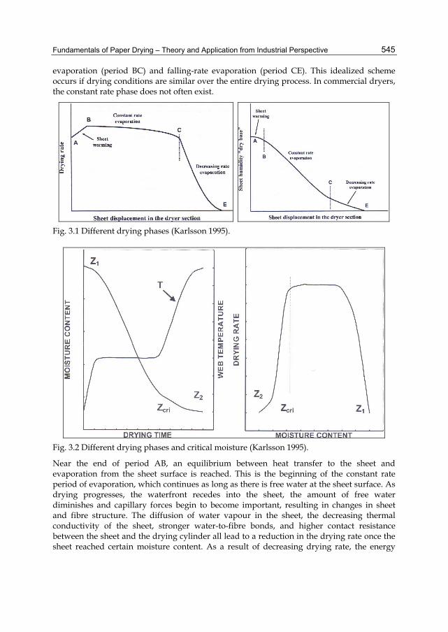
Fundamentals of Paper Drying – Theory and Application from Industrial Perspective
545
evaporation (period BC) and falling-rate evaporation (period CE). This idealized scheme occurs if drying conditions are similar over the entire drying process. In commercial dryers, the constant rate phase does not often exist.
Fig. 3.1 Different drying phases (Karlsson 1995).
Fig. 3.2 Different drying phases and critical moisture (Karlsson 1995).
Near the end of period AB, an equilibrium between heat transfer to the sheet and evaporation from the sheet surface is reached. This is the beginning of the constant rate period of evaporation, which continues as long as there is free water at the sheet surface. As drying progresses, the waterfront recedes into the sheet, the amount of free water diminishes and capillary forces begin to become important, resulting in changes in sheet and fibre structure. The diffusion of water vapour in the sheet, the decreasing thermal conductivity of the sheet, stronger water-to-fibre bonds, and higher contact resistance between the sheet and the drying cylinder all lead to a reduction in the drying rate once the sheet reached certain moisture content. As a result of decreasing drying rate, the energy
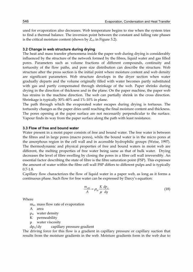
Evaporation, Condensation and Heat Transfer
546
used for evaporation also decreases. Web temperature begins to rise when the system tries to find a thermal balance. The inversion point between the constant and falling rate phases is the critical moisture content (shown by Zcri in Figure 3.2).
3.2 Change in web structure during drying The heat and mass transfer phenomena inside the paper web during drying is considerably influenced by the structure of the network formed by the fibres, liquid water and gas filled pores. Parameters such as volume fractions of different compounds, continuity and tortuosity of the flow paths, and pore size distribution can describe the structure. Web structure after the press section is the initial point where moisture content and web density are significant parameters. Web structure develops in the dryer section when water gradually departs and the volume originally filled with water becomes partly substituted with gas and partly compensated through shrinkage of the web. Paper shrinks during drying in the direction of thickness and in the plane. On the paper machine, the paper web has strains in the machine direction. The web can partially shrink in the cross direction. Shrinkage is typically 30%-40% and 1%-10% in plane. The path through which the evaporated water escapes during drying is tortuous. The tortuosity changes as the paper dries until reaching the final moisture content and thickness. The pores opening at the paper surface are not necessarily perpendicular to the surface. Vapour finds its way from the paper surface along the path with least resistance.
3.3 Flow of free and bound water Water present in a moist paper consists of free and bound water. The free water is between the fibres and in large pores (macro pores), while the bound water is in the micro pores at the amorphous region in the cell wall and in accessible hydrophilic groups (Weise, 1997). The thermodynamic and physical properties of free and bound waters in moist web are different, the melting properties of free water being same as that of bulk water. Drying decreases the level of fibre swelling by closing the pores in a fibre cell wall irreversibly. An essential factor describing the state of fibre is the fibre saturation point (FSP). This expresses the amount of water within the fibre cell wall FSP differs to different pulps and is typically 0.7-1.8. Capillary flow characterizes the flow of liquid water in a paper web, as long as it forms a continuous phase. Such flow for free water can be expressed by Darcy’s equation:
cevw
dpm KA dy
ρμ
= (18)
Where
mev mass flow rate of evaporation A area ρw water density K permeability μ water viscosity dpc/dy capillary pressure gradient
The driving force for this flow is a gradient in capillary pressure or capillary suction that results from the moisture gradients in the web. Moisture gradients form in the web due to
Fundamentals of Paper Drying – Theory and Application from Industrial Perspective
547
evaporation from the open surface of the web due to water vaporization at the interface where the wet web presses against a hot dryer surface and the formed water vapour diffuses towards inner parts of the web. When moisture content of the web decreases, the water phase gradually looses its continuity and splits into separate areas between which liquid flow is not possible anymore. Capillary flow of free water ends totally when moisture content falls below the fibre saturation point and all moisture is in the form of bound water. Bound water present in the micropores is adsorbed on the inner and outer surface of fibre wall as mono or multi-molecular layers. The first layer of water molecules closest to the surface is very strongly bound and has only limited mobility. The molecular movement along these layers is surface diffusion or diffusion of bound water. The driving force for this mass transfer mechanism is a gradient in concentration of bound water. Similar to capillary flow of free water, the movement of bound water can be expressed by similar equation:
bw bwbw d
m dzDA dy
ρ= (19)
Where
mbw mass flow rate of bound water A area; ρd = dry material density Dbw diffusivity of bound water
The diffusivity constant, Dbw, decreases sharply with decreasing moisture content and increases with increasing temperature.
4. Multicylinder drying and dryer configuration Use of steam as the main source of heat energy and the surface of rotating cylinder as the heat transfer area is the most common method of drying wet web to the finished products. Almost all paper machines around the globe manufacturing paper and paperboard use conventional steam heated cylinders or multi-cylinder drying configuration. Besides it providing good energy efficiency, cylinder drying enables supported web transfer, facilitates the web transport forward, and improves web smoothness. Cylinder drying also provides a means to prevent some web shrinkage in cross and machine directions. Most drying cylinders of paper machines are made of cast iron due to higher thermal conductivity compared to stainless steel (47 vs. 16 W/moC). The dryer ends or heads are also made of cast iron. The heads are bolted to the dryer shell at the ends of the dryer. Figure 4.1 shows a sectional view of dryer cylinder that includes all of its components such as steam supply and condensate exhaust devices. The most common dryers are 1.5 m and 1.8 m diameter. Shell thickness can vary, but 20-40 mm is common with a pressure rating as high as 1000 kPa.
4.1 Configuration of multicylinder dryers Generally all multi-cylinder dryers are configured either two-tier or single tier. Two-tier configuration is the most common. Such system is continuing since the beginning of paper drying using steam heated cylinder more than 100 years ago. Use of single tier configuration has been commercially introduced in late 1970. In all paper machines that have single tier
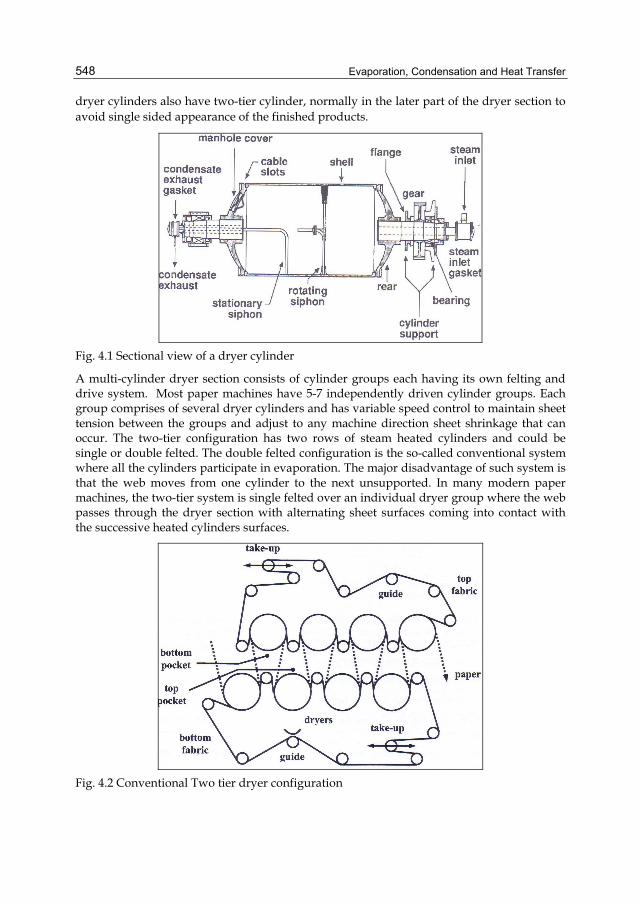
Evaporation, Condensation and Heat Transfer
548
dryer cylinders also have two-tier cylinder, normally in the later part of the dryer section to avoid single sided appearance of the finished products.
Fig. 4.1 Sectional view of a dryer cylinder
A multi-cylinder dryer section consists of cylinder groups each having its own felting and drive system. Most paper machines have 5-7 independently driven cylinder groups. Each group comprises of several dryer cylinders and has variable speed control to maintain sheet tension between the groups and adjust to any machine direction sheet shrinkage that can occur. The two-tier configuration has two rows of steam heated cylinders and could be single or double felted. The double felted configuration is the so-called conventional system where all the cylinders participate in evaporation. The major disadvantage of such system is that the web moves from one cylinder to the next unsupported. In many modern paper machines, the two-tier system is single felted over an individual dryer group where the web passes through the dryer section with alternating sheet surfaces coming into contact with the successive heated cylinders surfaces.
Fig. 4.2 Conventional Two tier dryer configuration
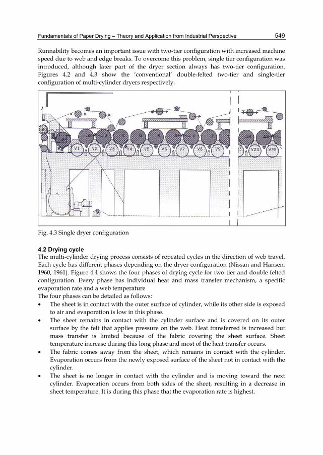
Fundamentals of Paper Drying – Theory and Application from Industrial Perspective
549
Runnability becomes an important issue with two-tier configuration with increased machine speed due to web and edge breaks. To overcome this problem, single tier configuration was introduced, although later part of the dryer section always has two-tier configuration. Figures 4.2 and 4.3 show the ‘conventional’ double-felted two-tier and single-tier configuration of multi-cylinder dryers respectively.
Fig. 4.3 Single dryer configuration
4.2 Drying cycle The multi-cylinder drying process consists of repeated cycles in the direction of web travel. Each cycle has different phases depending on the dryer configuration (Nissan and Hansen, 1960, 1961). Figure 4.4 shows the four phases of drying cycle for two-tier and double felted configuration. Every phase has individual heat and mass transfer mechanism, a specific evaporation rate and a web temperature The four phases can be detailed as follows: • The sheet is in contact with the outer surface of cylinder, while its other side is exposed
to air and evaporation is low in this phase. • The sheet remains in contact with the cylinder surface and is covered on its outer
surface by the felt that applies pressure on the web. Heat transferred is increased but mass transfer is limited because of the fabric covering the sheet surface. Sheet temperature increase during this long phase and most of the heat transfer occurs.
• The fabric comes away from the sheet, which remains in contact with the cylinder. Evaporation occurs from the newly exposed surface of the sheet not in contact with the cylinder.
• The sheet is no longer in contact with the cylinder and is moving toward the next cylinder. Evaporation occurs from both sides of the sheet, resulting in a decrease in sheet temperature. It is during this phase that the evaporation rate is highest.
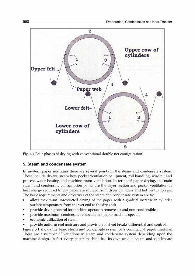
Evaporation, Condensation and Heat Transfer
550
Fig. 4.4 Four phases of drying with conventional double tier configuration.
5. Steam and condensate system In modern paper machines there are several points in the steam and condensate system. These include dryers, steam box, pocket ventilation equipment, roll handling, wire pit and process water heating and machine room ventilation. In terms of paper drying, the main steam and condensate consumption points are the dryer section and pocket ventilation as heat energy required to dry paper are sourced from dryer cylinders and hot ventilation air. The basic requirements and objectives of the steam and condensate system are to: • allow maximum unrestricted drying of the paper with a gradual increase in cylinder
surface temperature from the wet end to the dry end; • provide drying control for machine operator; remove air and non-condensibles; • provide maximum condensate removal at all paper machine speeds; • economic utilization of steam; • provide uniform reel moisture and provision of sheet breaks differential and control. Figure 5.1 shows the basic steam and condensate system of a commercial paper machine. There are a number of variations in steam and condensate system depending upon the machine design. In fact every paper machine has its own unique steam and condensate
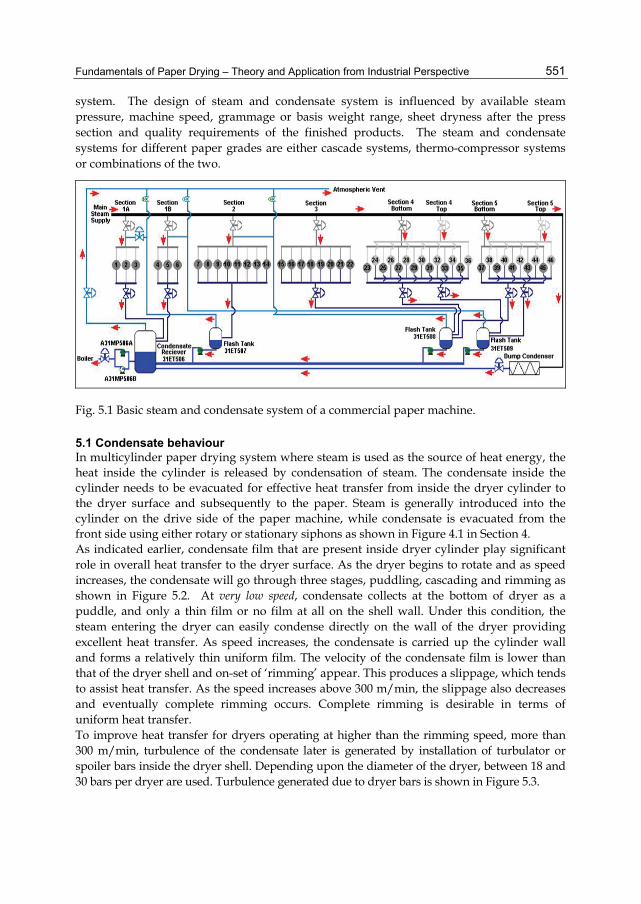
Fundamentals of Paper Drying – Theory and Application from Industrial Perspective
551
system. The design of steam and condensate system is influenced by available steam pressure, machine speed, grammage or basis weight range, sheet dryness after the press section and quality requirements of the finished products. The steam and condensate systems for different paper grades are either cascade systems, thermo-compressor systems or combinations of the two.
Fig. 5.1 Basic steam and condensate system of a commercial paper machine.
5.1 Condensate behaviour In multicylinder paper drying system where steam is used as the source of heat energy, the heat inside the cylinder is released by condensation of steam. The condensate inside the cylinder needs to be evacuated for effective heat transfer from inside the dryer cylinder to the dryer surface and subsequently to the paper. Steam is generally introduced into the cylinder on the drive side of the paper machine, while condensate is evacuated from the front side using either rotary or stationary siphons as shown in Figure 4.1 in Section 4. As indicated earlier, condensate film that are present inside dryer cylinder play significant role in overall heat transfer to the dryer surface. As the dryer begins to rotate and as speed increases, the condensate will go through three stages, puddling, cascading and rimming as shown in Figure 5.2. At very low speed, condensate collects at the bottom of dryer as a puddle, and only a thin film or no film at all on the shell wall. Under this condition, the steam entering the dryer can easily condense directly on the wall of the dryer providing excellent heat transfer. As speed increases, the condensate is carried up the cylinder wall and forms a relatively thin uniform film. The velocity of the condensate film is lower than that of the dryer shell and on-set of ‘rimming’ appear. This produces a slippage, which tends to assist heat transfer. As the speed increases above 300 m/min, the slippage also decreases and eventually complete rimming occurs. Complete rimming is desirable in terms of uniform heat transfer. To improve heat transfer for dryers operating at higher than the rimming speed, more than 300 m/min, turbulence of the condensate later is generated by installation of turbulator or spoiler bars inside the dryer shell. Depending upon the diameter of the dryer, between 18 and 30 bars per dryer are used. Turbulence generated due to dryer bars is shown in Figure 5.3.
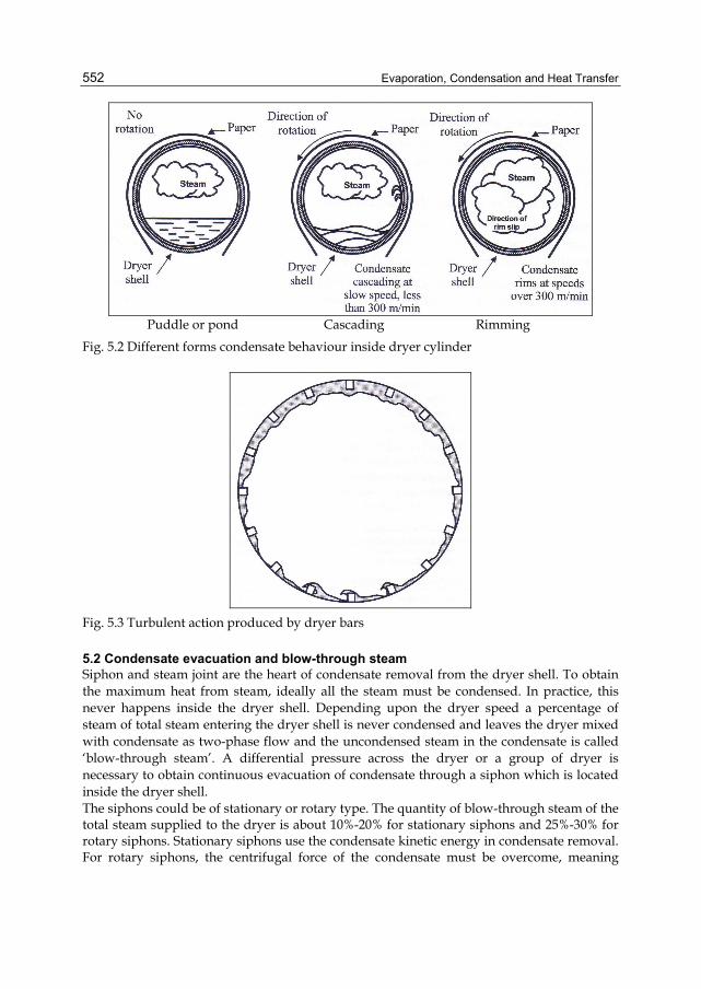
Evaporation, Condensation and Heat Transfer
552
Puddle or pond Cascading Rimming
Fig. 5.2 Different forms condensate behaviour inside dryer cylinder
Fig. 5.3 Turbulent action produced by dryer bars
5.2 Condensate evacuation and blow-through steam Siphon and steam joint are the heart of condensate removal from the dryer shell. To obtain the maximum heat from steam, ideally all the steam must be condensed. In practice, this never happens inside the dryer shell. Depending upon the dryer speed a percentage of steam of total steam entering the dryer shell is never condensed and leaves the dryer mixed with condensate as two-phase flow and the uncondensed steam in the condensate is called ‘blow-through steam’. A differential pressure across the dryer or a group of dryer is necessary to obtain continuous evacuation of condensate through a siphon which is located inside the dryer shell. The siphons could be of stationary or rotary type. The quantity of blow-through steam of the total steam supplied to the dryer is about 10%-20% for stationary siphons and 25%-30% for rotary siphons. Stationary siphons use the condensate kinetic energy in condensate removal. For rotary siphons, the centrifugal force of the condensate must be overcome, meaning
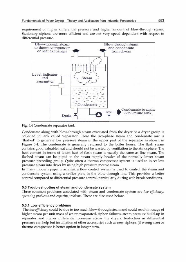
Fundamentals of Paper Drying – Theory and Application from Industrial Perspective
553
requirement of higher differential pressure and higher amount of blow-through steam. Stationary siphons are more efficient and are not very speed dependent with respect to differential pressure.
Fig. 5.4 Condensate separator tank
Condensate along with blow-through steam evacuated from the dryer or a dryer group is collected in tank called ‘separator’. Here the two-phase steam and condensate mix is ‘flashed’ to generate low pressure steam in the upper part of the separator as shown in Figure 5.4. The condensate is generally returned to the boiler house. The flash steam contains good valuable heat and should not be wasted by ventilation to the atmosphere. The heat content in terms of latent heat of flash steam is exactly the same as line steam. The flashed steam can be piped to the steam supply header of the normally lower steam pressure preceding group. Quite often a thermo compressor system is used to inject low pressure steam into dryer by using high pressure motive steam. In many modern paper machines, a flow control system is used to control the steam and condensate system using a orifice plate in the blow-through line. This provides a better control compared to differential pressure control, particularly during web break conditions.
5.3 Troubleshooting of steam and condensate system Three common problems associated with steam and condensate system are low efficiency; operating problems and capacity problems. These are discussed below.
5.3.1 Low efficiency problems The low efficiency could be due to too much blow-through steam and could result in usage of higher steam per unit mass of water evaporated, siphon failures, steam pressure build-up in separator and higher differential pressure across the dryers. Reduction in differential pressure can help but installation of other accessories such as new siphons (if wrong size) or thermo-compressor is better option in longer term.
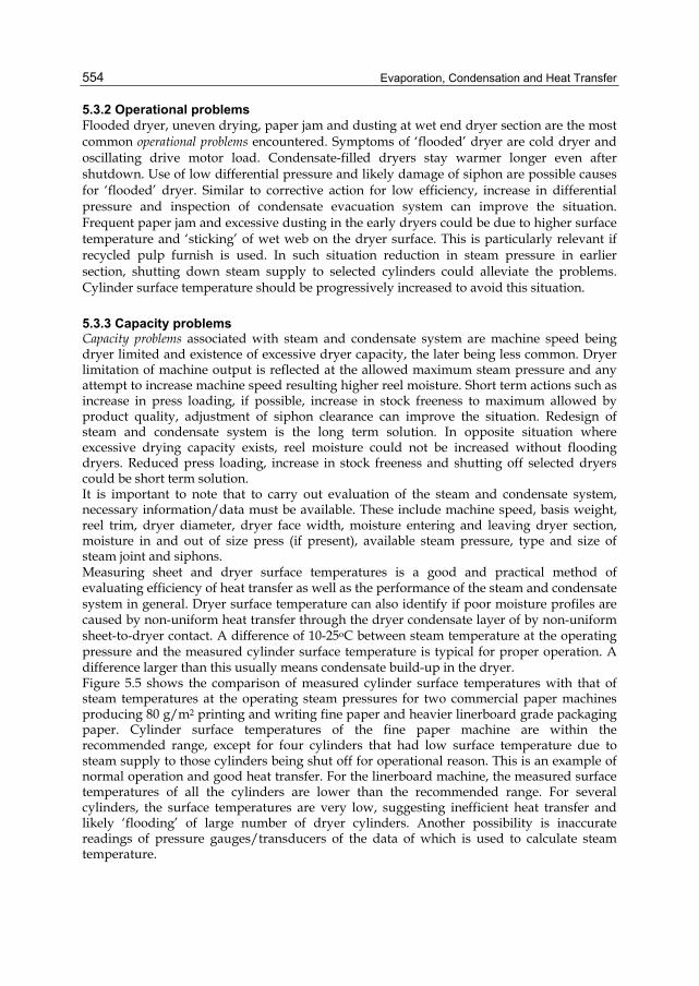
Evaporation, Condensation and Heat Transfer
554
5.3.2 Operational problems Flooded dryer, uneven drying, paper jam and dusting at wet end dryer section are the most common operational problems encountered. Symptoms of ‘flooded’ dryer are cold dryer and oscillating drive motor load. Condensate-filled dryers stay warmer longer even after shutdown. Use of low differential pressure and likely damage of siphon are possible causes for ‘flooded’ dryer. Similar to corrective action for low efficiency, increase in differential pressure and inspection of condensate evacuation system can improve the situation. Frequent paper jam and excessive dusting in the early dryers could be due to higher surface temperature and ‘sticking’ of wet web on the dryer surface. This is particularly relevant if recycled pulp furnish is used. In such situation reduction in steam pressure in earlier section, shutting down steam supply to selected cylinders could alleviate the problems. Cylinder surface temperature should be progressively increased to avoid this situation.
5.3.3 Capacity problems Capacity problems associated with steam and condensate system are machine speed being dryer limited and existence of excessive dryer capacity, the later being less common. Dryer limitation of machine output is reflected at the allowed maximum steam pressure and any attempt to increase machine speed resulting higher reel moisture. Short term actions such as increase in press loading, if possible, increase in stock freeness to maximum allowed by product quality, adjustment of siphon clearance can improve the situation. Redesign of steam and condensate system is the long term solution. In opposite situation where excessive drying capacity exists, reel moisture could not be increased without flooding dryers. Reduced press loading, increase in stock freeness and shutting off selected dryers could be short term solution. It is important to note that to carry out evaluation of the steam and condensate system, necessary information/data must be available. These include machine speed, basis weight, reel trim, dryer diameter, dryer face width, moisture entering and leaving dryer section, moisture in and out of size press (if present), available steam pressure, type and size of steam joint and siphons. Measuring sheet and dryer surface temperatures is a good and practical method of evaluating efficiency of heat transfer as well as the performance of the steam and condensate system in general. Dryer surface temperature can also identify if poor moisture profiles are caused by non-uniform heat transfer through the dryer condensate layer of by non-uniform sheet-to-dryer contact. A difference of 10-25oC between steam temperature at the operating pressure and the measured cylinder surface temperature is typical for proper operation. A difference larger than this usually means condensate build-up in the dryer. Figure 5.5 shows the comparison of measured cylinder surface temperatures with that of steam temperatures at the operating steam pressures for two commercial paper machines producing 80 g/m2 printing and writing fine paper and heavier linerboard grade packaging paper. Cylinder surface temperatures of the fine paper machine are within the recommended range, except for four cylinders that had low surface temperature due to steam supply to those cylinders being shut off for operational reason. This is an example of normal operation and good heat transfer. For the linerboard machine, the measured surface temperatures of all the cylinders are lower than the recommended range. For several cylinders, the surface temperatures are very low, suggesting inefficient heat transfer and likely ‘flooding’ of large number of dryer cylinders. Another possibility is inaccurate readings of pressure gauges/transducers of the data of which is used to calculate steam temperature.
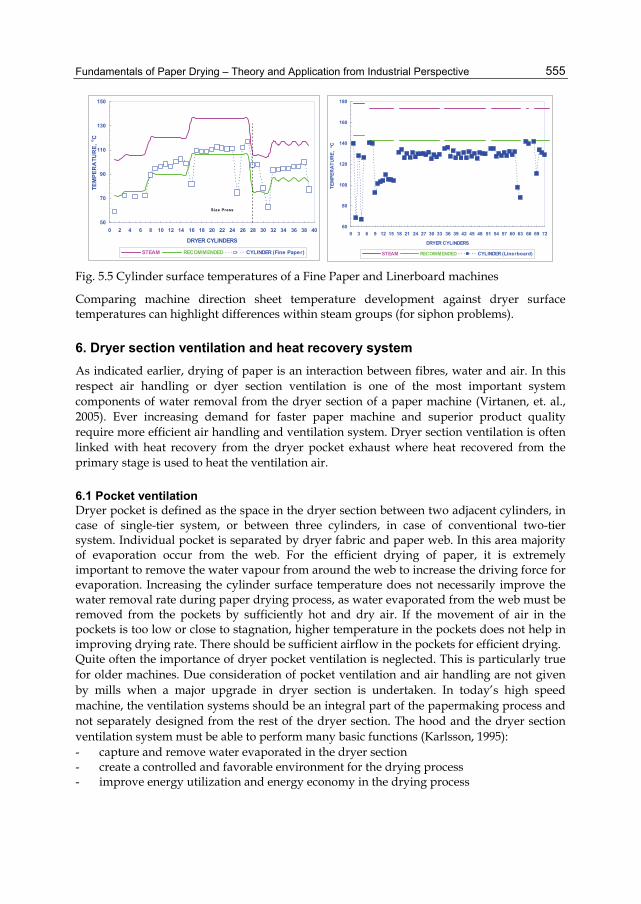
Fundamentals of Paper Drying – Theory and Application from Industrial Perspective
555
50
70
90
110
130
150
0 2 4 6 8 10 12 14 16 18 20 22 24 26 28 30 32 34 36 38 40
DRYER CYLINDERS
TEM
PER
ATU
RE,
o C
STEAM RECOMMENDED CYLINDER (Fine Paper)
Size Press
60
80
100
120
140
160
180
0 3 6 9 12 15 18 21 24 27 30 33 36 39 42 45 48 51 54 57 60 63 66 69 72
DRYER CYLINDERS
TEM
PER
ATU
RE,
o C
STEAM RECOMMENDED CYLINDER (Linerboard) Fig. 5.5 Cylinder surface temperatures of a Fine Paper and Linerboard machines
Comparing machine direction sheet temperature development against dryer surface temperatures can highlight differences within steam groups (for siphon problems).
6. Dryer section ventilation and heat recovery system As indicated earlier, drying of paper is an interaction between fibres, water and air. In this respect air handling or dyer section ventilation is one of the most important system components of water removal from the dryer section of a paper machine (Virtanen, et. al., 2005). Ever increasing demand for faster paper machine and superior product quality require more efficient air handling and ventilation system. Dryer section ventilation is often linked with heat recovery from the dryer pocket exhaust where heat recovered from the primary stage is used to heat the ventilation air.
6.1 Pocket ventilation Dryer pocket is defined as the space in the dryer section between two adjacent cylinders, in case of single-tier system, or between three cylinders, in case of conventional two-tier system. Individual pocket is separated by dryer fabric and paper web. In this area majority of evaporation occur from the web. For the efficient drying of paper, it is extremely important to remove the water vapour from around the web to increase the driving force for evaporation. Increasing the cylinder surface temperature does not necessarily improve the water removal rate during paper drying process, as water evaporated from the web must be removed from the pockets by sufficiently hot and dry air. If the movement of air in the pockets is too low or close to stagnation, higher temperature in the pockets does not help in improving drying rate. There should be sufficient airflow in the pockets for efficient drying. Quite often the importance of dryer pocket ventilation is neglected. This is particularly true for older machines. Due consideration of pocket ventilation and air handling are not given by mills when a major upgrade in dryer section is undertaken. In today’s high speed machine, the ventilation systems should be an integral part of the papermaking process and not separately designed from the rest of the dryer section. The hood and the dryer section ventilation system must be able to perform many basic functions (Karlsson, 1995): - capture and remove water evaporated in the dryer section - create a controlled and favorable environment for the drying process - improve energy utilization and energy economy in the drying process
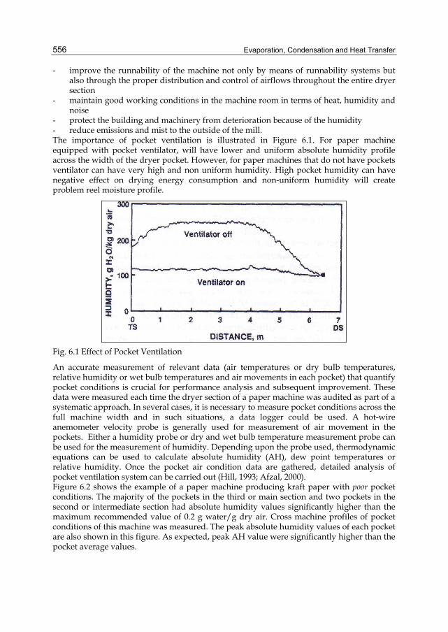
Evaporation, Condensation and Heat Transfer
556
- improve the runnability of the machine not only by means of runnability systems but also through the proper distribution and control of airflows throughout the entire dryer section
- maintain good working conditions in the machine room in terms of heat, humidity and noise
- protect the building and machinery from deterioration because of the humidity - reduce emissions and mist to the outside of the mill. The importance of pocket ventilation is illustrated in Figure 6.1. For paper machine equipped with pocket ventilator, will have lower and uniform absolute humidity profile across the width of the dryer pocket. However, for paper machines that do not have pockets ventilator can have very high and non uniform humidity. High pocket humidity can have negative effect on drying energy consumption and non-uniform humidity will create problem reel moisture profile.
Fig. 6.1 Effect of Pocket Ventilation
An accurate measurement of relevant data (air temperatures or dry bulb temperatures, relative humidity or wet bulb temperatures and air movements in each pocket) that quantify pocket conditions is crucial for performance analysis and subsequent improvement. These data were measured each time the dryer section of a paper machine was audited as part of a systematic approach. In several cases, it is necessary to measure pocket conditions across the full machine width and in such situations, a data logger could be used. A hot-wire anemometer velocity probe is generally used for measurement of air movement in the pockets. Either a humidity probe or dry and wet bulb temperature measurement probe can be used for the measurement of humidity. Depending upon the probe used, thermodynamic equations can be used to calculate absolute humidity (AH), dew point temperatures or relative humidity. Once the pocket air condition data are gathered, detailed analysis of pocket ventilation system can be carried out (Hill, 1993; Afzal, 2000). Figure 6.2 shows the example of a paper machine producing kraft paper with poor pocket conditions. The majority of the pockets in the third or main section and two pockets in the second or intermediate section had absolute humidity values significantly higher than the maximum recommended value of 0.2 g water/g dry air. Cross machine profiles of pocket conditions of this machine was measured. The peak absolute humidity values of each pocket are also shown in this figure. As expected, peak AH value were significantly higher than the pocket average values.
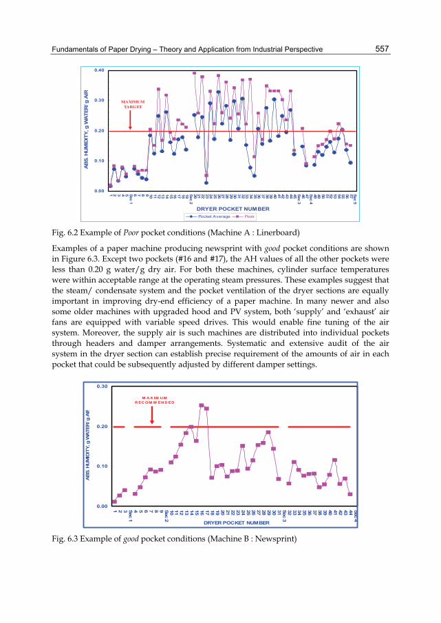
Fundamentals of Paper Drying – Theory and Application from Industrial Perspective
557
0.00
0.10
0.20
0.30
0.40
1 2 3 4 5 Sec 16 7 8 9 10 11 12 13 14 15 16 17 18 19 Sec 220 21 22 23 24 25 26 27 28 29 30 31 32 33 34 35 36 37 38 39 40 41 42 43 44 45 Sec 346 47 Sec 448 49 50 51 52 53 54 55 56 57 Sec 5
DRYER POCKET NUMBER
AB
S. H
UM
IDIT
Y, g
WA
TER
/ g A
IR
Pocket Average Peak
MAXIMUMTARGET
Fig. 6.2 Example of Poor pocket conditions (Machine A : Linerboard)
Examples of a paper machine producing newsprint with good pocket conditions are shown in Figure 6.3. Except two pockets (#16 and #17), the AH values of all the other pockets were less than 0.20 g water/g dry air. For both these machines, cylinder surface temperatures were within acceptable range at the operating steam pressures. These examples suggest that the steam/ condensate system and the pocket ventilation of the dryer sections are equally important in improving dry-end efficiency of a paper machine. In many newer and also some older machines with upgraded hood and PV system, both ‘supply’ and ‘exhaust’ air fans are equipped with variable speed drives. This would enable fine tuning of the air system. Moreover, the supply air is such machines are distributed into individual pockets through headers and damper arrangements. Systematic and extensive audit of the air system in the dryer section can establish precise requirement of the amounts of air in each pocket that could be subsequently adjusted by different damper settings.
0.00
0.10
0.20
0.30
1 2 3 Sec 14 5 6 7 8 9 Sec 210 11 12 13 14 15 16 17 18 19 20 21 22 23 24 25 26 27 28 29 30 31 Sec 332 33 34 35 36 37 38 39 40 41 42 43 44 Sec 4
DRYER POCKET NUMBER
AB
S. H
UM
IDIT
Y, g
WA
TER
/ g A
IR
M A X IM U MR EC OM M EN D ED
Fig. 6.3 Example of good pocket conditions (Machine B : Newsprint)
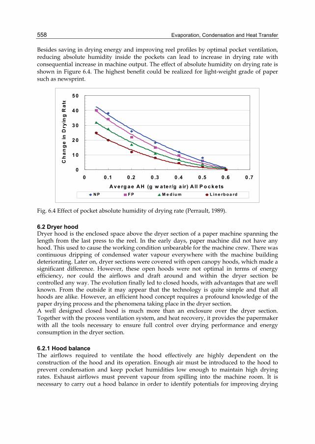
Evaporation, Condensation and Heat Transfer
558
Besides saving in drying energy and improving reel profiles by optimal pocket ventilation, reducing absolute humidity inside the pockets can lead to increase in drying rate with consequential increase in machine output. The effect of absolute humidity on drying rate is shown in Figure 6.4. The highest benefit could be realized for light-weight grade of paper such as newsprint.
0
1 0
2 0
3 0
4 0
5 0
0 0 .1 0 .2 0 .3 0 .4 0 .5 0 .6 0 .7
A v e rg a e A H (g w a te r/g a ir) A ll P o c k e ts
Ch
ang
e in
Dry
ing
Rat
e
N P F P M e d iu m L in e rb o a rd
Fig. 6.4 Effect of pocket absolute humidity of drying rate (Perrault, 1989).
6.2 Dryer hood Dryer hood is the enclosed space above the dryer section of a paper machine spanning the length from the last press to the reel. In the early days, paper machine did not have any hood. This used to cause the working condition unbearable for the machine crew. There was continuous dripping of condensed water vapour everywhere with the machine building deteriorating. Later on, dryer sections were covered with open canopy hoods, which made a significant difference. However, these open hoods were not optimal in terms of energy efficiency, nor could the airflows and draft around and within the dryer section be controlled any way. The evolution finally led to closed hoods, with advantages that are well known. From the outside it may appear that the technology is quite simple and that all hoods are alike. However, an efficient hood concept requires a profound knowledge of the paper drying process and the phenomena taking place in the dryer section. A well designed closed hood is much more than an enclosure over the dryer section. Together with the process ventilation system, and heat recovery, it provides the papermaker with all the tools necessary to ensure full control over drying performance and energy consumption in the dryer section.
6.2.1 Hood balance The airflows required to ventilate the hood effectively are highly dependent on the construction of the hood and its operation. Enough air must be introduced to the hood to prevent condensation and keep pocket humidities low enough to maintain high drying rates. Exhaust airflows must prevent vapour from spilling into the machine room. It is necessary to carry out a hood balance in order to identify potentials for improving drying
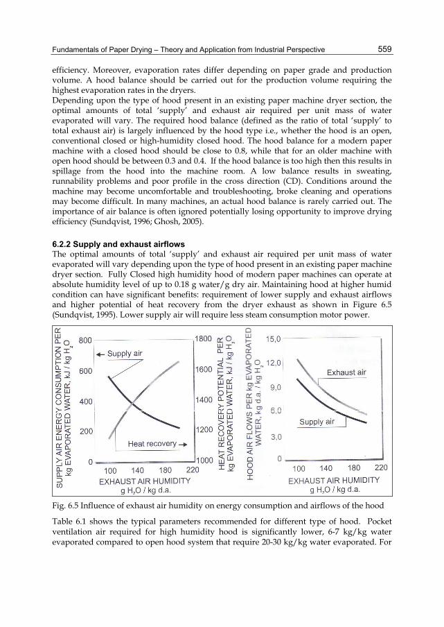
Fundamentals of Paper Drying – Theory and Application from Industrial Perspective
559
efficiency. Moreover, evaporation rates differ depending on paper grade and production volume. A hood balance should be carried out for the production volume requiring the highest evaporation rates in the dryers. Depending upon the type of hood present in an existing paper machine dryer section, the optimal amounts of total ‘supply’ and exhaust air required per unit mass of water evaporated will vary. The required hood balance (defined as the ratio of total ‘supply’ to total exhaust air) is largely influenced by the hood type i.e., whether the hood is an open, conventional closed or high-humidity closed hood. The hood balance for a modern paper machine with a closed hood should be close to 0.8, while that for an older machine with open hood should be between 0.3 and 0.4. If the hood balance is too high then this results in spillage from the hood into the machine room. A low balance results in sweating, runnability problems and poor profile in the cross direction (CD). Conditions around the machine may become uncomfortable and troubleshooting, broke cleaning and operations may become difficult. In many machines, an actual hood balance is rarely carried out. The importance of air balance is often ignored potentially losing opportunity to improve drying efficiency (Sundqvist, 1996; Ghosh, 2005).
6.2.2 Supply and exhaust airflows The optimal amounts of total ‘supply’ and exhaust air required per unit mass of water evaporated will vary depending upon the type of hood present in an existing paper machine dryer section. Fully Closed high humidity hood of modern paper machines can operate at absolute humidity level of up to 0.18 g water/g dry air. Maintaining hood at higher humid condition can have significant benefits: requirement of lower supply and exhaust airflows and higher potential of heat recovery from the dryer exhaust as shown in Figure 6.5 (Sundqvist, 1995). Lower supply air will require less steam consumption motor power.
Fig. 6.5 Influence of exhaust air humidity on energy consumption and airflows of the hood
Table 6.1 shows the typical parameters recommended for different type of hood. Pocket ventilation air required for high humidity hood is significantly lower, 6-7 kg/kg water evaporated compared to open hood system that require 20-30 kg/kg water evaporated. For
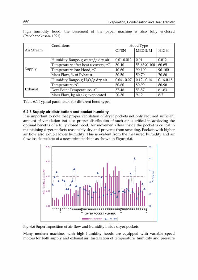
Evaporation, Condensation and Heat Transfer
560
high humidity hood, the basement of the paper machine is also fully enclosed (Panchapakesan, 1991).
Hood Type Air Stream
Conditions OPEN MEDIUM HIGH
Humidity Range, g water/g dry air 0.01-0.012 0.01 0.012 Temperature after heat recovery, oC 30-40 55-6590-100 60-65 Temperature into Hood, oC 40-60 90-100 90-100
Supply
Mass Flow, % of Exhaust 30-50 50-70 70-80 Humidity Range, g H2O/g dry air 0.04 - 0.07 0.12 - 0.14 0.16-0.18 Temperature, oC 50-60 80-90 80-90 Dew Point Temperature, oC 37-46 53-57 61-63
Exhaust
Mass Flow, kg air/kg evaporated 20-30 9-12 6-7
Table 6.1 Typical parameters for different hood types
6.2.3 Supply air distribution and pocket humidity It is important to note that proper ventilation of dryer pockets not only required sufficient amount of ventilation but also proper distribution of such air is critical in achieving the optimal benefits of a fully closed hood. Air movement/flow inside the pocket is critical in maintaining dryer pockets reasonably dry and prevents from sweating. Pockets with higher air flow also exhibit lower humidity. This is evident from the measured humidity and air flow inside pockets of a newsprint machine as shown in Figure 6.6.
0.00
0.10
0.20
0.30
0.401 2 3 4 Sec 15 6 7 8 9 10 11 12 13 14 Sec 215 16 17 18 19 20 21 22 23 24 25 26 27 28 29 30 31 32 33 Sec 334 35 36 37 38 39 40 41 42 43 44 45 Sec 4
DRYER POCKET NUMBER
Abs
. Hum
idity
, g a
ter/
g A
ir
0.0
0.5
1.0
1.5
2.0
2.5
Air
Flow
, m/s
Abs. Humidity Air Flow
Fig. 6.6 Superimposition of air flow and humidity inside dryer pockets
Many modern machines with high humidity hoods are equipped with variable speed motors for both supply and exhaust air. Installation of temperature, humidity and pressure
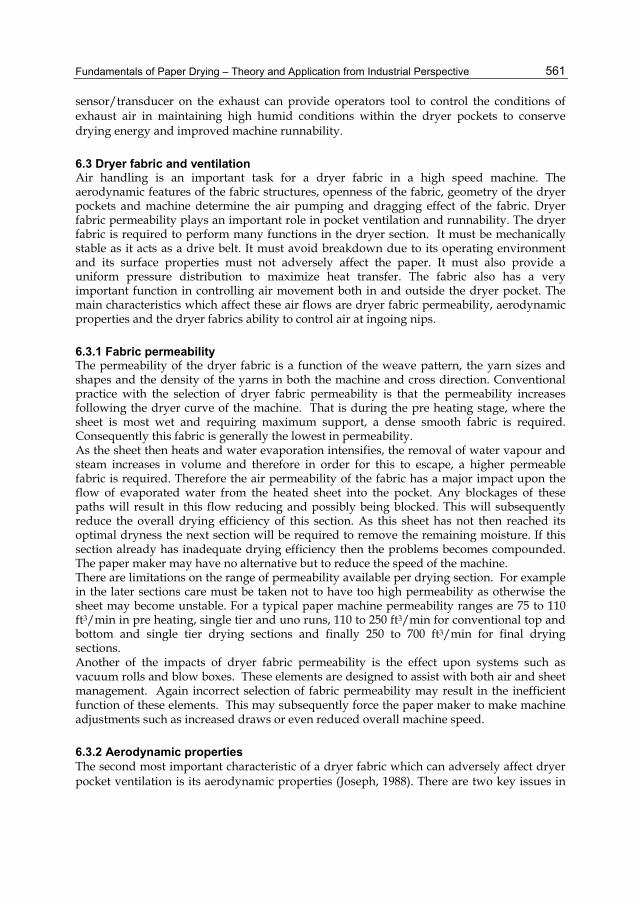
Fundamentals of Paper Drying – Theory and Application from Industrial Perspective
561
sensor/transducer on the exhaust can provide operators tool to control the conditions of exhaust air in maintaining high humid conditions within the dryer pockets to conserve drying energy and improved machine runnability.
6.3 Dryer fabric and ventilation Air handling is an important task for a dryer fabric in a high speed machine. The aerodynamic features of the fabric structures, openness of the fabric, geometry of the dryer pockets and machine determine the air pumping and dragging effect of the fabric. Dryer fabric permeability plays an important role in pocket ventilation and runnability. The dryer fabric is required to perform many functions in the dryer section. It must be mechanically stable as it acts as a drive belt. It must avoid breakdown due to its operating environment and its surface properties must not adversely affect the paper. It must also provide a uniform pressure distribution to maximize heat transfer. The fabric also has a very important function in controlling air movement both in and outside the dryer pocket. The main characteristics which affect these air flows are dryer fabric permeability, aerodynamic properties and the dryer fabrics ability to control air at ingoing nips.
6.3.1 Fabric permeability The permeability of the dryer fabric is a function of the weave pattern, the yarn sizes and shapes and the density of the yarns in both the machine and cross direction. Conventional practice with the selection of dryer fabric permeability is that the permeability increases following the dryer curve of the machine. That is during the pre heating stage, where the sheet is most wet and requiring maximum support, a dense smooth fabric is required. Consequently this fabric is generally the lowest in permeability. As the sheet then heats and water evaporation intensifies, the removal of water vapour and steam increases in volume and therefore in order for this to escape, a higher permeable fabric is required. Therefore the air permeability of the fabric has a major impact upon the flow of evaporated water from the heated sheet into the pocket. Any blockages of these paths will result in this flow reducing and possibly being blocked. This will subsequently reduce the overall drying efficiency of this section. As this sheet has not then reached its optimal dryness the next section will be required to remove the remaining moisture. If this section already has inadequate drying efficiency then the problems becomes compounded. The paper maker may have no alternative but to reduce the speed of the machine. There are limitations on the range of permeability available per drying section. For example in the later sections care must be taken not to have too high permeability as otherwise the sheet may become unstable. For a typical paper machine permeability ranges are 75 to 110 ft3/min in pre heating, single tier and uno runs, 110 to 250 ft3/min for conventional top and bottom and single tier drying sections and finally 250 to 700 ft3/min for final drying sections. Another of the impacts of dryer fabric permeability is the effect upon systems such as vacuum rolls and blow boxes. These elements are designed to assist with both air and sheet management. Again incorrect selection of fabric permeability may result in the inefficient function of these elements. This may subsequently force the paper maker to make machine adjustments such as increased draws or even reduced overall machine speed.
6.3.2 Aerodynamic properties The second most important characteristic of a dryer fabric which can adversely affect dryer pocket ventilation is its aerodynamic properties (Joseph, 1988). There are two key issues in
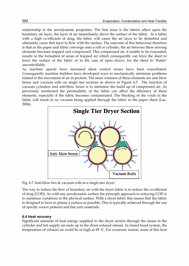
Evaporation, Condensation and Heat Transfer
562
relationship to the aerodynamic properties. The first issue is the fabrics affect upon the boundary air layer, the layer of air immediately above the surface of the fabric. In a fabric with a high co-efficient of drag, the fabric will cause the air layer to be disturbed and ultimately cause that layer to flow with the surface. The outcome of this behaviour therefore is that as the paper and fabric converge onto a roll or cylinder, the air between these moving elements becomes trapped and compressed. This compressed air, if unable to be evacuated, results in the formation of areas of trapped air which consequently can force the sheet to leave the surface of the fabric or in the case of open draws, for the sheet to ‘flutter’ uncontrollably. As machine speeds have increased sheet control issues have been exacerbated. Consequently machine builders have developed ways to mechanically minimize problems related to the movement of air in pockets. The most common of these elements are anti blow boxes and vacuum rolls on single tier sections as shown in Figure 6.7. The function of vacuum cylinders and anti-blow boxes is to minimize the build up of compressed air. As previously mentioned the permeability of the fabric can affect the efficiency of these elements, especially if the fabric becomes contaminated. The blocking of the voids in the fabric will result in no vacuum being applied through the fabric to the paper sheet (Luc, 2004).
Single Tier Dryer Section
Vacuum Rolls
Anti- blow boxes
Single Tier Dryer Section
Vacuum Rolls
Anti- blow boxes
Fig. 6.7 Anti-blow box & vacuum rolls in a single-tier dryer
The way to reduce the flow of boundary air with the dryer fabric is to reduce the co-efficient of drag (COD). As with any aerodynamic surface the principle approach to reducing COD is to minimize variations in the physical surface. With a dryer fabric this means that the fabric is designed to have as planar a surface as possible. This is typically achieved through the use of specific weave patterns and flat yarn materials.
6.4 Heat recovery Significant amounts of heat energy supplied to the dryer section through the steam in the cylinder and hot supply air ends up in the dryer exhaust stream. In closed hood system, the temperature of exhaust air could be as high as 85 oC. For economic reason, some of this heat
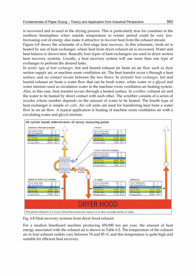
Fundamentals of Paper Drying – Theory and Application from Industrial Perspective
563
is recovered and re-used in the drying process. This is particularly true for countries in the northern hemisphere when outside temperature in winter period could be very low. Increasing cost of energy also make it attractive to recover heat from the exhaust stream. Figure 6.8 shows the schematic of a first stage heat recovery. In this schematic, fresh air is heated by use of heat exchanger, where heat from dryer exhaust air is recovered. Water and heat balance is shown here. Basically four types of heat exchangers are used in dryer section heat recovery systems. Usually, a heat recovery system will use more than one type of exchanger to perform the desired tasks. In air/air type of heat exchanger, hot and humid exhaust air heats an air flow such as dyer section supply air, or machine room ventilation air. The heat transfer occur s through a heat surface, and no contact occurs between the two flows. In air/water heat exchanger, hot and humid exhaust air heats a water flow that can be fresh water, white water or a glycol and water mixture used as circulation water in the machine room ventilation air heating system. Also, in this case, heat transfer occurs through a heated surface. In scrubber, exhaust air and the water to be heated by direct contact with each other. The scrubber consists of a series of nozzles whose number depends on the amount of water to be heated. The fourth type of heat exchanger is simple air coils. Air coil units are used for transferring heat from a water flow to an air flow. A typical application is heating of machine room ventilation air with a circulating water and glycol mixture.
Fig. 6.8 Heat recovery systems from dryer hood exhaust
For a modern linerboard machine producing 450,000 ton per year, the amount of heat energy associated with the exhaust air is shown in Table 6.2. The temperature of the exhaust air in four exhaust outlets vary between 74 and 85 oC and this temperature is quite high and suitable for efficient heat recovery.
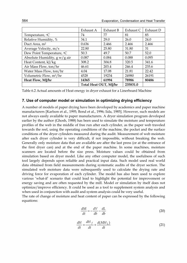
Evaporation, Condensation and Heat Transfer
564
Exhaust A Exhaust B Exhaust C Exhaust D Temperature, oC 74 77 81 85 Relative Humidity, % 34.1 29.0 26.0 24.0 Duct Area, m2 0.636 2.466 2.466 2.466 Average Velocity, m/s 22.80 25.80 31.80 31 Dew Point Temperature, oC 50.3 49.7 50.7 52.0 Absolute Humidity, g w/g air 0.087 0.084 0.088 0.095 Heat Content, kJ/kg 308.2 304.8 320.5 341.6 Air Mass Flow, ton/hr 46.61 203.4 246.4 235.6 Water Mass Flow, ton/hr 4.04 17.08 21.81 22.42 Volumetric Flow, m3/hr 4528 19234 24980 26191 Heat Flow, MJ/hr 14365 61994 78986 80486 Total Heat OUT, MJ/hr 235831.0
Table 6.2 Actual amounts of Heat energy in dryer exhaust for a Linerboard Machine
7. Use of computer model or simulation in optimizing drying efficiency A number of models of paper drying have been developed by academics and paper machine manufacturers [Karlson et al., 1995; Bond et al., 1996; Iida, 1985]. However, such models are not always easily available to paper manufacturers. A dryer simulation program developed earlier by the author (Ghosh, 1988) has been used to simulate the moisture and temperature profiles of the web in the middle of free run after each cylinder, as the paper web traveled towards the reel, using the operating conditions of the machine, the pocket and the surface conditions of the dryer cylinders measured during the audit. Measurement of web moisture after each dryer cylinder is very difficult, if not impossible, without breaking the web. Generally only moisture data that are available are after the last press (or at the entrance of the first dryer can) and at the end of the paper machine. In some machines, moisture scanners are located before the size press. Moisture values could be obtained from simulation based on dryer model. Like any other computer model, the usefulness of such tool largely depends upon reliable and practical input data. Such model used real world data obtained from field measurements during systematic audits of the dryer section. The simulated web moisture data were subsequently used to calculate the drying rate and driving force for evaporation of each cylinder. The model has also been used to explore various ‘what-if’ scenario that could lead to highlight the potential for improvement or energy saving and are often requested by the mill. Model or simulation by itself does not optimize/improve efficiency. It could be used as a tool to supplement system analysis and when used in conjunction with audit and system analysis could be very useful. The rate of change of moisture and heat content of paper can be expressed by the following equations:
dM dV dLdt db db
= − − (20)
( )f LdHdH d MHdt dt dt
= + (21)
Fundamentals of Paper Drying – Theory and Application from Industrial Perspective
565
( )QdTQ Fdb
= − (22)
( )VV
dCV Fdb
= − (23)
( )LdML Fdb
= − (24)
Where
dMdt
=Rate of change of moisture content in paper
dHdt
=Rate of change of heat content of paper
V = vapour flux L = liquid flux Q = heat transfer coefficient CV= water vapour concentration HV, HL, Hf = heat content of vapour, liquid and dry fibre FQ, FV, FL = heat, vapour and liquid transfer coefficient = f(M) M = gm water/gm fibre b = basis weight, g/m2 T = sheet temperature
The equation (20) and (21) can be solved by finite difference method. Web length in Machine Direction (MD) is divided into finite lengths (difference). Heat and mass transfer fluxes is calculated using web conditions at a certain location. This gives web condition at the neighboring location determined by the differential equations. This step is repeated from the beginning to the end of the dryer section In any model and simulation, the output of such model is always dependent on accurate and practical input of process data. When used in conjunction with audit and system analysis, dryer simulation model could be very useful. The model can be used to explore various ‘what-if’ scenarios such as changes in: • machine speed, basis weight • moisture, temperature of web to 1st dryer • steam pressure in any/whole section • dryer cylinder surface temperature • pocket conditions • size press operation • reel/size press (if size press is present and operational) moisture Model only gives temperature and moisture of the sheet at one location in the machine direction. Profile in cross direction is difficult to predict. Prediction of web moisture is useful, as it is difficult to measure on a running web, the speed of which can be as high as 2000 m/min, depending upon the machine design and paper grades made. Drying rate for each cylinder can also be calculated from the simulated moisture and the drying rates thus calculated can be very useful in identifying heat transfer problem with specific cylinder.
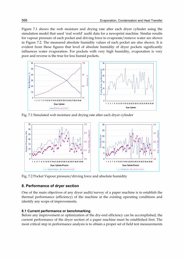
Evaporation, Condensation and Heat Transfer
566
Figure 7.1 shows the web moisture and drying rate after each dryer cylinder using the simulation model that used ‘real world’ audit data for a newsprint machine. Similar results for vapour pressure of each pocket and driving force to evaporate/remove water are shown in Figure 7.2. The measured absolute humidity values of each pocket are also shown. It is evident from these figures that level of absolute humidity of dryer pockets significantly influences water evaporation. For pockets with very high humidity, evaporation is very poor and reverse is the true for less humid pockets.
0
10
20
30
40
50
60
1 3 5 7 9 11 13 15 17 19 21 23 25 27 29 31 33 35 37 39 41 43 45
Dryer Cylinder
Web
Moi
stur
e, %
40
60
80
100
Dry
ness
, %
M oisture Dryness
0
5
10
15
20
25
30
1 3 5 7 9 11 13 15 17 19 21 23 25 27 29 31 33 35 37 39 41 43 45
Dryer Cylinder
Dry
ing
Rat
e, k
g W
ater
/hr/m
2
Fig. 7.1 Simulated web moisture and drying rate after each dryer cylinder
0
5
10
15
20
25
30
35
1 3 5 7 9 11 13 15 17 19 21 23 25 27 29 31 33 35 37 39 41 43 45
Dryer Cylinder/Pocket
Vapo
ur P
ress
ure,
kPa
0.0
0.1
0.2
0.3
0.4
Abs
. Hum
idity
, g W
/g A
ir
Vapour Pressure Absolute Humidity
0
5
10
15
20
25
30
1 3 5 7 9 11 13 15 17 19 21 23 25 27 29 31 33 35 37 39 41 43 45
Dryer Cylinder/Pocket
Driv
ing
Forc
e
0.0
0.1
0.2
0.3
0.4
Abs
. Hum
idity
, g W
/g A
ir
Driving Force Abso lute Humidity
Fig. 7.2 Pocket Vapour pressure/driving force and absolute humidity
8. Performance of dryer section One of the main objectives of any dryer audit/survey of a paper machine is to establish the thermal performance (efficiency) of the machine at the existing operating conditions and identify any scope of improvements.
8.1 Current performance or benchmarking Before any improvement or optimization of the dry-end efficiency can be accomplished, the current performance of the dryer section of a paper machine must be established first. The most critical step in performance analysis is to obtain a proper set of field test measurements
Fundamentals of Paper Drying – Theory and Application from Industrial Perspective
567
and observations. All equipment information and sizes must be checked in the field and compared with the flow schematics of the system. Field testing is generally carried out to: • establish machine operating conditions, speeds and sheet moisture. • establish drying curves. • measure energy consumption. • determine the operating problems and procedures through detailed discussions with
the operators. • obtain physical data for the system analysis. • assess the physical condition of the equipment. • establish key performance indicators. • compare the performance indicators of the machine with similar top performing
machines making the same grades. Systematic measurement of the steam and condensate system, the pocket ventilation system and the hood balance around the dryer section is a pre-requisite in optimizing dryer performance (Hill, 1997; Perrault, 1989). Once such measurements are carried out, proper analysis of such data will quantify the present conditions/performance of the dryer section of a paper machine, compare dry end efficiency of the machine with others in the industry making similar grade, identify the scopes for improvement in drying efficiency and subsequent energy saving. Field data can also be used for simulation model in quantifying potential tangible benefits.
8.2 Field measurements for performance evaluation Once this has been established further follow on work are required. The systematic approach that can be used comprised the following steps: • Measurement of cylinder surface temperatures, pocket temperatures, pocket humidity
values, air movements in each pocket, web temperature after each dryer cylinder across the full width of the machine/pocket;
• Measurement of condensate flow from each separator and check the steam pressures of each section including the blow-through steam;
• Measurement of air conditions (flow, temperature, humidity) of supply and exhaust air; • Analysis of data, including overall water and energy balance over the entire dryer
section and over individual heat recovery system; • Exploration of various ‘what-if’ scenario through simulation model using measured
data to quantify potential tangible benefits that could be achieved if the problems identified are fixed;
• Repeat audit/surveys following corrective actions based on preceding audits.
8.3 Performance indices Performance of the dryer section of a paper machine can be described by various means. However, the commonly used dryer performance indicators are : • TAPPI (Technical Association Pulp and Paper Industry) drying rate (kg water
removed/hr/m2 of surface area); • steam efficiency (kg steam used/kg of water evaporated); • production efficiency (kg steam used/kg of paper produced) and • energy efficiency (mega joule of energy required per ton of water removed).
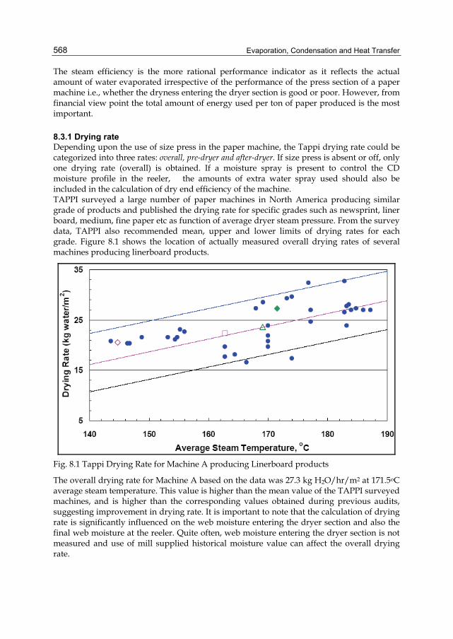
Evaporation, Condensation and Heat Transfer
568
The steam efficiency is the more rational performance indicator as it reflects the actual amount of water evaporated irrespective of the performance of the press section of a paper machine i.e., whether the dryness entering the dryer section is good or poor. However, from financial view point the total amount of energy used per ton of paper produced is the most important.
8.3.1 Drying rate Depending upon the use of size press in the paper machine, the Tappi drying rate could be categorized into three rates: overall, pre-dryer and after-dryer. If size press is absent or off, only one drying rate (overall) is obtained. If a moisture spray is present to control the CD moisture profile in the reeler, the amounts of extra water spray used should also be included in the calculation of dry end efficiency of the machine. TAPPI surveyed a large number of paper machines in North America producing similar grade of products and published the drying rate for specific grades such as newsprint, liner board, medium, fine paper etc as function of average dryer steam pressure. From the survey data, TAPPI also recommended mean, upper and lower limits of drying rates for each grade. Figure 8.1 shows the location of actually measured overall drying rates of several machines producing linerboard products.
Fig. 8.1 Tappi Drying Rate for Machine A producing Linerboard products
The overall drying rate for Machine A based on the data was 27.3 kg H2O/hr/m2 at 171.5oC average steam temperature. This value is higher than the mean value of the TAPPI surveyed machines, and is higher than the corresponding values obtained during previous audits, suggesting improvement in drying rate. It is important to note that the calculation of drying rate is significantly influenced on the web moisture entering the dryer section and also the final web moisture at the reeler. Quite often, web moisture entering the dryer section is not measured and use of mill supplied historical moisture value can affect the overall drying rate.
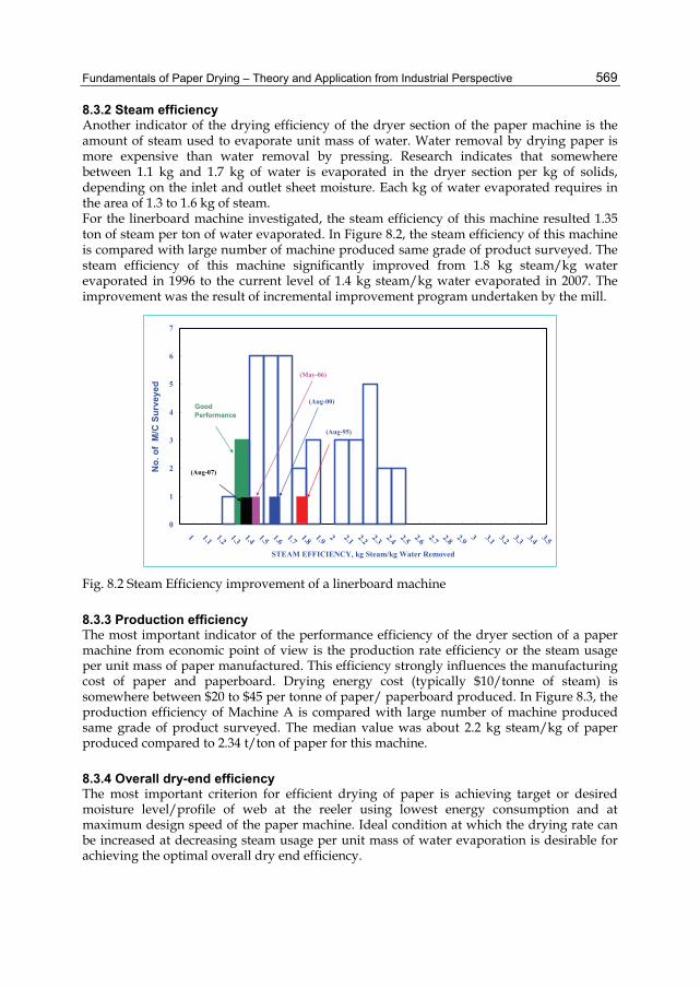
Fundamentals of Paper Drying – Theory and Application from Industrial Perspective
569
8.3.2 Steam efficiency Another indicator of the drying efficiency of the dryer section of the paper machine is the amount of steam used to evaporate unit mass of water. Water removal by drying paper is more expensive than water removal by pressing. Research indicates that somewhere between 1.1 kg and 1.7 kg of water is evaporated in the dryer section per kg of solids, depending on the inlet and outlet sheet moisture. Each kg of water evaporated requires in the area of 1.3 to 1.6 kg of steam. For the linerboard machine investigated, the steam efficiency of this machine resulted 1.35 ton of steam per ton of water evaporated. In Figure 8.2, the steam efficiency of this machine is compared with large number of machine produced same grade of product surveyed. The steam efficiency of this machine significantly improved from 1.8 kg steam/kg water evaporated in 1996 to the current level of 1.4 kg steam/kg water evaporated in 2007. The improvement was the result of incremental improvement program undertaken by the mill.
0
1
2
3
4
5
6
7
1 1.1 1.2 1.3 1.4 1.5 1.6 1.7 1.8 1.9 2 2.1 2.2 2.3 2.4 2.5 2.6 2.7 2.8 2.9 3 3.1 3.2 3.3 3.4 3.5
STEAM EFFICIENCY, kg Steam/kg Water Removed
No.
of
M/C
Sur
veye
d
(May-06)
GoodPerformance
(Aug-00)
(Aug-95)
(Aug-07)
Fig. 8.2 Steam Efficiency improvement of a linerboard machine
8.3.3 Production efficiency The most important indicator of the performance efficiency of the dryer section of a paper machine from economic point of view is the production rate efficiency or the steam usage per unit mass of paper manufactured. This efficiency strongly influences the manufacturing cost of paper and paperboard. Drying energy cost (typically $10/tonne of steam) is somewhere between $20 to $45 per tonne of paper/ paperboard produced. In Figure 8.3, the production efficiency of Machine A is compared with large number of machine produced same grade of product surveyed. The median value was about 2.2 kg steam/kg of paper produced compared to 2.34 t/ton of paper for this machine.
8.3.4 Overall dry-end efficiency The most important criterion for efficient drying of paper is achieving target or desired moisture level/profile of web at the reeler using lowest energy consumption and at maximum design speed of the paper machine. Ideal condition at which the drying rate can be increased at decreasing steam usage per unit mass of water evaporation is desirable for achieving the optimal overall dry end efficiency.
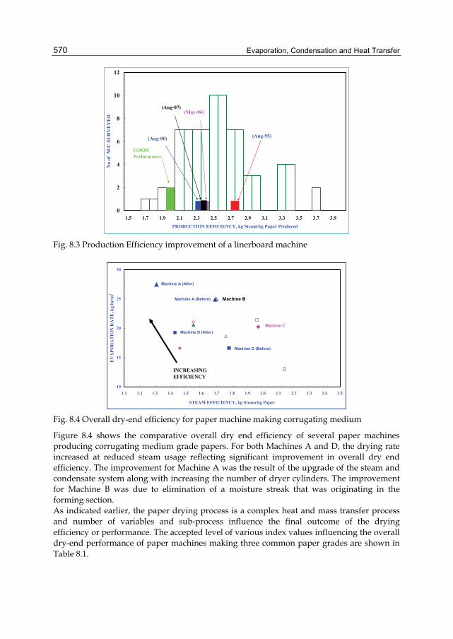
Evaporation, Condensation and Heat Transfer
570
0
2
4
6
8
10
12
1.5 1.7 1.9 2.1 2.3 2.5 2.7 2.9 3.1 3.3 3.5 3.7 3.9PRODUCTION EFFICIENCY, kg Steam/kg Paper Produced
No
of M
/C S
UR
VEY
ED(May-06)
GOODPerformance
(Aug-00) (Aug-95)
(Aug-07)
Fig. 8.3 Production Efficiency improvement of a linerboard machine
10
15
20
25
30
1.1 1.2 1.3 1.4 1.5 1.6 1.7 1.8 1.9 2.0 2.1 2.2 2.3 2.4 2.5
STEAM EFFICIENCY, kg Steam/kg Paper
EV
APO
RA
TIO
N R
AT
E, k
g/hr
/m2
INCREASINGEFFICIENCY
Machine D (Before)
Machine C
Machine B
Machine A (After)
Machine A (Before)
Machine D (After)
Fig. 8.4 Overall dry-end efficiency for paper machine making corrugating medium
Figure 8.4 shows the comparative overall dry end efficiency of several paper machines producing corrugating medium grade papers. For both Machines A and D, the drying rate increased at reduced steam usage reflecting significant improvement in overall dry end efficiency. The improvement for Machine A was the result of the upgrade of the steam and condensate system along with increasing the number of dryer cylinders. The improvement for Machine B was due to elimination of a moisture streak that was originating in the forming section. As indicated earlier, the paper drying process is a complex heat and mass transfer process and number of variables and sub-process influence the final outcome of the drying efficiency or performance. The accepted level of various index values influencing the overall dry-end performance of paper machines making three common paper grades are shown in Table 8.1.
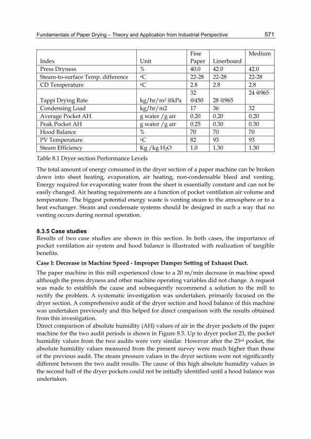
Fundamentals of Paper Drying – Theory and Application from Industrial Perspective
571
Index Unit Fine Paper Linerboard
Medium
Press Dryness % 40.0 42.0 42.0 Steam-to-surface Temp. difference oC 22-28 22-28 22-28 CD Temperature oC 2.8 2.8 2.8
Tappi Drying Rate kg/hr/m2 @kPa 32 @450 28 @965
24 @965
Condensing Load kg/hr/m2 17 36 32 Average Pocket AH g water /g air 0.20 0.20 0.20 Peak Pocket AH g water /g air 0.25 0.30 0.30 Hood Balance % 70 70 70 PV Temperature oC 82 93 93 Steam Efficiency Kg /kg H2O 1.0 1.30 1.30
Table 8.1 Dryer section Performance Levels
The total amount of energy consumed in the dryer section of a paper machine can be broken down into sheet heating, evaporation, air heating, non-condensable bleed and venting. Energy required for evaporating water from the sheet is essentially constant and can not be easily changed. Air heating requirements are a function of pocket ventilation air volume and temperature. The biggest potential energy waste is venting steam to the atmosphere or to a heat exchanger. Steam and condensate systems should be designed in such a way that no venting occurs during normal operation.
8.3.5 Case studies Results of two case studies are shown in this section. In both cases, the importance of pocket ventilation air system and hood balance is illustrated with realization of tangible benefits.
Case I: Decrease in Machine Speed - Improper Damper Setting of Exhaust Duct. The paper machine in this mill experienced close to a 20 m/min decrease in machine speed although the press dryness and other machine operating variables did not change. A request was made to establish the cause and subsequently recommend a solution to the mill to rectify the problem. A systematic investigation was undertaken, primarily focused on the dryer section. A comprehensive audit of the dryer section and hood balance of this machine was undertaken previously and this helped for direct comparison with the results obtained from this investigation. Direct comparison of absolute humidity (AH) values of air in the dryer pockets of the paper machine for the two audit periods is shown in Figure 8.5. Up to dryer pocket 23, the pocket humidity values from the two audits were very similar. However after the 23rd pocket, the absolute humidity values measured from the present survey were much higher than those of the previous audit. The steam pressure values in the dryer sections were not significantly different between the two audit results. The cause of this high absolute humidity values in the second half of the dryer pockets could not be initially identified until a hood balance was undertaken.
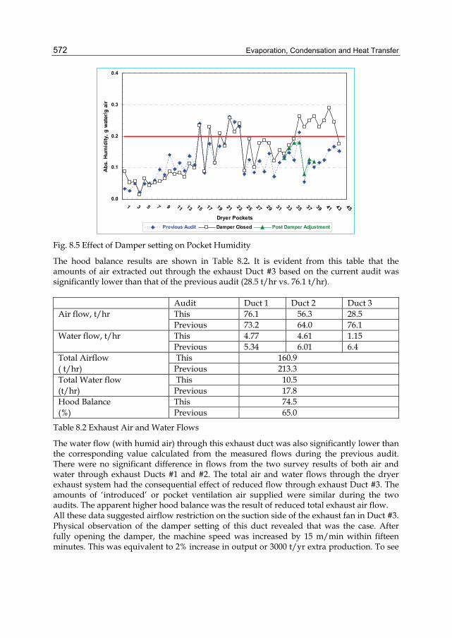
Evaporation, Condensation and Heat Transfer
572
0.0
0.1
0.2
0.3
0.4
1 3 5 7 9 11 13 15 17 19 21 23 25 27 29 31 33 35 37 39 41 43 45
Dryer Pockets
Abs
. Hum
idity
, g w
ater
/g a
ir
Previous Audit Damper Closed Post Damper Adjustment
Fig. 8.5 Effect of Damper setting on Pocket Humidity
The hood balance results are shown in Table 8.2. It is evident from this table that the amounts of air extracted out through the exhaust Duct #3 based on the current audit was significantly lower than that of the previous audit (28.5 t/hr vs. 76.1 t/hr).
Audit Duct 1 Duct 2 Duct 3 Air flow, t/hr This 76.1 56.3 28.5 Previous 73.2 64.0 76.1 Water flow, t/hr This 4.77 4.61 1.15 Previous 5.34 6.01 6.4 Total Airflow This 160.9 ( t/hr) Previous 213.3 Total Water flow This 10.5 (t/hr) Previous 17.8 Hood Balance This 74.5 (%) Previous 65.0
Table 8.2 Exhaust Air and Water Flows
The water flow (with humid air) through this exhaust duct was also significantly lower than the corresponding value calculated from the measured flows during the previous audit. There were no significant difference in flows from the two survey results of both air and water through exhaust Ducts #1 and #2. The total air and water flows through the dryer exhaust system had the consequential effect of reduced flow through exhaust Duct #3. The amounts of ‘introduced’ or pocket ventilation air supplied were similar during the two audits. The apparent higher hood balance was the result of reduced total exhaust air flow. All these data suggested airflow restriction on the suction side of the exhaust fan in Duct #3. Physical observation of the damper setting of this duct revealed that was the case. After fully opening the damper, the machine speed was increased by 15 m/min within fifteen minutes. This was equivalent to 2% increase in output or 3000 t/yr extra production. To see
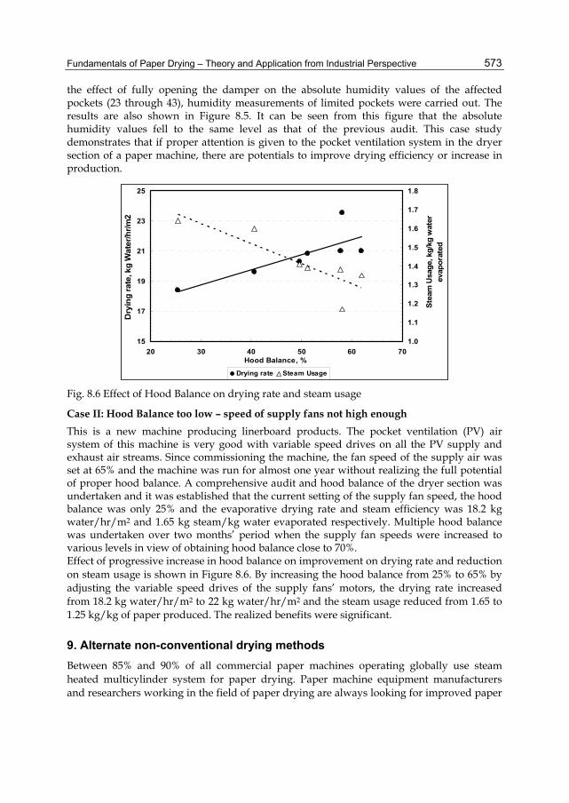
Fundamentals of Paper Drying – Theory and Application from Industrial Perspective
573
the effect of fully opening the damper on the absolute humidity values of the affected pockets (23 through 43), humidity measurements of limited pockets were carried out. The results are also shown in Figure 8.5. It can be seen from this figure that the absolute humidity values fell to the same level as that of the previous audit. This case study demonstrates that if proper attention is given to the pocket ventilation system in the dryer section of a paper machine, there are potentials to improve drying efficiency or increase in production.
15
17
19
21
23
25
20 30 40 50 60 70Hood Balance, %
Dry
ing
rate
, kg
Wat
er/h
r/m2
1.0
1.1
1.2
1.3
1.4
1.5
1.6
1.7
1.8
Stea
m U
sage
, kg/
kg w
ater
ev
apor
ated
Drying rate Steam Usage Fig. 8.6 Effect of Hood Balance on drying rate and steam usage
Case II: Hood Balance too low – speed of supply fans not high enough This is a new machine producing linerboard products. The pocket ventilation (PV) air system of this machine is very good with variable speed drives on all the PV supply and exhaust air streams. Since commissioning the machine, the fan speed of the supply air was set at 65% and the machine was run for almost one year without realizing the full potential of proper hood balance. A comprehensive audit and hood balance of the dryer section was undertaken and it was established that the current setting of the supply fan speed, the hood balance was only 25% and the evaporative drying rate and steam efficiency was 18.2 kg water/hr/m2 and 1.65 kg steam/kg water evaporated respectively. Multiple hood balance was undertaken over two months’ period when the supply fan speeds were increased to various levels in view of obtaining hood balance close to 70%. Effect of progressive increase in hood balance on improvement on drying rate and reduction on steam usage is shown in Figure 8.6. By increasing the hood balance from 25% to 65% by adjusting the variable speed drives of the supply fans’ motors, the drying rate increased from 18.2 kg water/hr/m2 to 22 kg water/hr/m2 and the steam usage reduced from 1.65 to 1.25 kg/kg of paper produced. The realized benefits were significant.
9. Alternate non-conventional drying methods Between 85% and 90% of all commercial paper machines operating globally use steam heated multicylinder system for paper drying. Paper machine equipment manufacturers and researchers working in the field of paper drying are always looking for improved paper
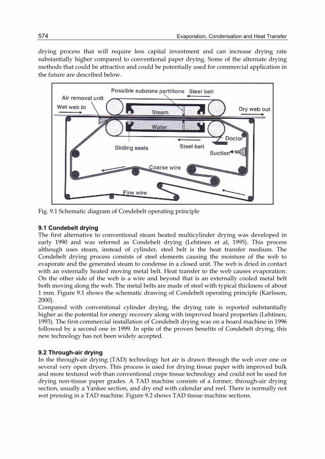
Evaporation, Condensation and Heat Transfer
574
drying process that will require less capital investment and can increase drying rate substantially higher compared to conventional paper drying. Some of the alternate drying methods that could be attractive and could be potentially used for commercial application in the future are described below.
Fig. 9.1 Schematic diagram of Condebelt operating principle
9.1 Condebelt drying The first alternative to conventional steam heated multicylinder drying was developed in early 1990 and was referred as Condebelt drying (Lehtinen et al, 1995). This process although uses steam, instead of cylinder, steel belt is the heat transfer medium. The Condebelt drying process consists of steel elements causing the moisture of the web to evaporate and the generated steam to condense in a closed unit. The web is dried in contact with an externally heated moving metal belt. Heat transfer to the web causes evaporation. On the other side of the web is a wire and beyond that is an externally cooled metal belt both moving along the web. The metal belts are made of steel with typical thickness of about 1 mm. Figure 9.1 shows the schematic drawing of Condebelt operating principle (Karlsson, 2000). Compared with conventional cylinder drying, the drying rate is reported substantially higher as the potential for energy recovery along with improved board properties (Lehtinen, 1993). The first commercial installation of Condebelt drying was on a board machine in 1996 followed by a second one in 1999. In spite of the proven benefits of Condebelt drying, this new technology has not been widely accepted.
9.2 Through-air drying In the through-air drying (TAD) technology hot air is drawn through the web over one or several very open dryers. This process is used for drying tissue paper with improved bulk and more textured web than conventional crepe tissue technology and could not be used for drying non-tissue paper grades. A TAD machine consists of a former, through-air drying section, usually a Yankee section, and dry end with calendar and reel. There is normally not wet pressing in a TAD machine. Figure 9.2 shows TAD tissue machine sections.
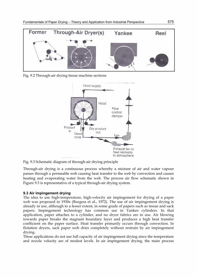
Fundamentals of Paper Drying – Theory and Application from Industrial Perspective
575
Fig. 9.2 Through-air drying tissue machine sections
Fig. 9.3 Schematic diagram of through-air drying principle
Through-air drying is a continuous process whereby a mixture of air and water vapour passes through a permeable web causing heat transfer to the web by convection and causes heating and evaporating water from the web. The process air flow schematic shown in Figure 9.3 is representative of a typical through-air drying system.
9.3 Air impingement drying The idea to use high-temperature, high-velocity air impingement for drying of a paper web was proposed in 1930s (Burgess et al., 1972). The use of air impingement drying is already in use, although to a lesser extent, in some grade of papers such as tissue and sack papers. Impingement technology has common use in Yankee cylinders. In that application, paper attaches to a cylinder, and no dryer fabrics are in use. Air blowing towards paper breaks the stagnant boundary layer and produces a high heat transfer coefficient on the paper surface. Heat transfer primarily occurs through convection. In flotation dryers, sack paper web dries completely without restrain by air impingement drying. These applications do not use full capacity of air impingement drying since the temperature and nozzle velocity are of modest levels. In air impingement drying, the main process
Evaporation, Condensation and Heat Transfer
576
parameters are air temperature, jet velocity, air moisture content and muzzle geometry. Two important parameters concerning evaporation capacity are jet temperature and jet speed. Although the full potential of air impingement drying of paper web is not realized yet, this technology is a very viable alternative to paper drying. It offers many advantages compared with conventional steam drying cylinder, namely, high drying rates, short dryer section, fast drying response, better profiling and curl control.
9.4 Impulse drying Impulse drying is a water removal process where a moist web passes through a high temperature press nip. The method combines elements of wet pressing and hot surface drying. Typical characteristics of the nip are a roll surface temperature of 150oC-500oC, nip pressure of 0.3-7 MPa, and nip residence time of up to 100 ms. The first detailed published work on impulse drying was made in 1985 (Wahren, 1985). A single unit could replace an extensive part of the current dryer section and last nip of the press section. Besides the high drying capacity, impulse drying provides possibilities to modify paper properties. In spite of promise of huge benefits, the impulse drying technology did not lead to a commercial application. This is largely due to large number of technical problems related to practical operation yet to be resolved.
9.5 Steam drying The idea to use steam as a drying medium is not new. Some industrial applications for wood and coal drying date from 1930s. Renewed interest for using steam in convective dryers rather than hot air appeared in the late 1970s probably due to energy crisis at that time. In principle, any direct air dryer can operate with steam. To-day, industrial scale steam dryers have use for textile webs, market pulp and lumber. The first patent to apply the concept of steam drying for paper appeared in the early 1950s. A good review of research work on steam drying of paper is available in the literature (Douglas, 1994). Compare to air drying, steam as a drying medium can offer many advantages. The most interesting is the potential to save energy. If the exhaust steam has use elsewhere in the process, the net energy consumption may be very low. Another advantage is safer operation, i.e., no fire or explosion hazard. The drying rate is higher in steam drying than air drying if the operating temperature is high. Despite intensive theoretical and experimental work on steam drying, no industrial steam drying applications for paper webs exist to-day.
9.6 Micro-Waves drying The possibilities of using micro-waves for paper drying have been examined extensively. Laboratory equipment for micro-wave drying has been built and many potential advantages have been shown to exist (Warner, 1966). The main advantage of using micro-wave energy for paper drying would seem to be the possibility of obtaining an even and uniform moisture profile at the desired level. The absorption of micro-wave energy is roughly proportional to the moisture content of the web. This means that areas of higher moisture content will be more strongly heated than areas with lower moisture content which will result in an automatic leveling-out the moisture across the sheet. Use of micro-wave for complete drying of wet paper web is not commercially feasible for number of reasons. However, it could be used at the final stage of paper drying along with conventional cylinder drying process for evening out moisture profile in the reeler. Similar approach using infra-red or impact drying is used in commercial paper machines.
Fundamentals of Paper Drying – Theory and Application from Industrial Perspective
577
10. Drying and paper quality The properties of final paper product are strongly influenced by the web conditions in the dryer section including temperature, moisture content and state of stresses. During drying process, due to evaporative dewatering, the fibre shrinks and causes stress on the web. Controlling the stress in the dryer section can improve strength properties in the web. Other major problem is the non-uniformity of shrinkage in the cross direction that can be caused in the dryer section with consequential effect of quality and machine runnability. By the time the wet web enters the dryer section, the fibre wall has already collapsed due to contraction of fibre network during forming in the forming section. The collapse occurs in the press section and almost all water from the lumen has been removed prior to entering in the dryer section. During drying process, both the bound and free water is progressively diffused out and eventually removed, causing irreversible closure of the macro and micro pores in a fibre cell wall. Paper shrinks during drying in the direction of thickness and in its plane. On the paper machine, the paper web is strained in the machine direction and allowed to shrink in the cross direction. The edges of the web shrink more than the middle of the web. A shrinkage profile therefore exist in the cross direction. This leads to variation in the properties of the paper in the cross direction. The level of stress during the drying process significantly influences the elastic properties of paper. If the web dries under restraint, it will have a higher modulus of elasticity, higher tensile strength and better dimensional stability than a web allowed to shrink during drying. The differences in paper properties are due to different drying stress and stress concentration levels and changes in crystallinity and fibre orientation (Htun, 1980). Wire marking on the paper is an important quality issue, particularly for certain papers, such as cigarette paper or special fine paper grades. Three different types of markings are possible: mechanical or imprint marking; evaporation marking and marking due to uneven support. This type of marking is not a marking seen as a plane difference in the paper surface, but as a visual defect especially visible with transillumination. The evaporation marking is usually the result of uneven drying due to permeability differences in the fabric or seam area and web contact. The drying process in the paper machine dryer section can influence two important quality parameters, paper curl and cockle. Presence of both curl and cockle are undesirable form paper’s functionality aspect. The original reason for curl is the difference in fibre orientation through the thickness of a paper. Other factors such as stressing and drying also have significant effects on curl. A sheet with a total uniform structure through its thickness will curl if dried non-uniformly. Non-uniform drying can be the result of a temperature difference between the top and bottom dryer cylinders. Cockle is a localized defect on paper that is the results of shrinkage and deformation of fibres while drying. Drying parameters that can aggravate cockle are sticking of sheet on hot dryer surface, high wet end dryer surface temperature and too rapid drying.
10.1 Drying induced cross direction (CD) profile Two most critical profiles in the cross direction of paper web that influence its functionality at end-user application are moisture and shrinkage. The dryer section may lead to non-
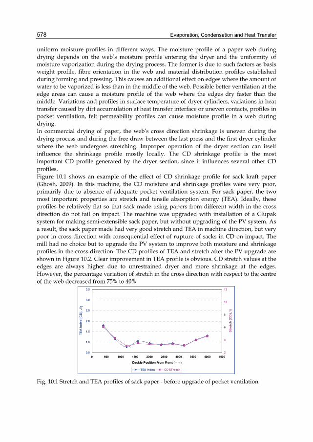
Evaporation, Condensation and Heat Transfer
578
uniform moisture profiles in different ways. The moisture profile of a paper web during drying depends on the web’s moisture profile entering the dryer and the uniformity of moisture vaporization during the drying process. The former is due to such factors as basis weight profile, fibre orientation in the web and material distribution profiles established during forming and pressing. This causes an additional effect on edges where the amount of water to be vaporized is less than in the middle of the web. Possible better ventilation at the edge areas can cause a moisture profile of the web where the edges dry faster than the middle. Variations and profiles in surface temperature of dryer cylinders, variations in heat transfer caused by dirt accumulation at heat transfer interface or uneven contacts, profiles in pocket ventilation, felt permeability profiles can cause moisture profile in a web during drying. In commercial drying of paper, the web’s cross direction shrinkage is uneven during the drying process and during the free draw between the last press and the first dryer cylinder where the web undergoes stretching. Improper operation of the dryer section can itself influence the shrinkage profile mostly locally. The CD shrinkage profile is the most important CD profile generated by the dryer section, since it influences several other CD profiles. Figure 10.1 shows an example of the effect of CD shrinkage profile for sack kraft paper (Ghosh, 2009). In this machine, the CD moisture and shrinkage profiles were very poor, primarily due to absence of adequate pocket ventilation system. For sack paper, the two most important properties are stretch and tensile absorption energy (TEA). Ideally, these profiles be relatively flat so that sack made using papers from different width in the cross direction do not fail on impact. The machine was upgraded with installation of a Clupak system for making semi-extensible sack paper, but without upgrading of the PV system. As a result, the sack paper made had very good stretch and TEA in machine direction, but very poor in cross direction with consequential effect of rupture of sacks in CD on impact. The mill had no choice but to upgrade the PV system to improve both moisture and shrinkage profiles in the cross direction. The CD profiles of TEA and stretch after the PV upgrade are shown in Figure 10.2. Clear improvement in TEA profile is obvious. CD stretch values at the edges are always higher due to unrestrained dryer and more shrinkage at the edges. However, the percentage variation of stretch in the cross direction with respect to the centre of the web decreased from 75% to 40%
0.5
1.0
1.5
2.0
2.5
3.0
3.5
0 500 1000 1500 2000 2500 3000 3500 4000 4500
Deckle Position From Front (mm)
TEA
Inde
x (C
D),
J/g
2
4
6
8
10
12
Stre
tch
(CD
), %
TEA Index CD STretch
Fig. 10.1 Stretch and TEA profiles of sack paper - before upgrade of pocket ventilation
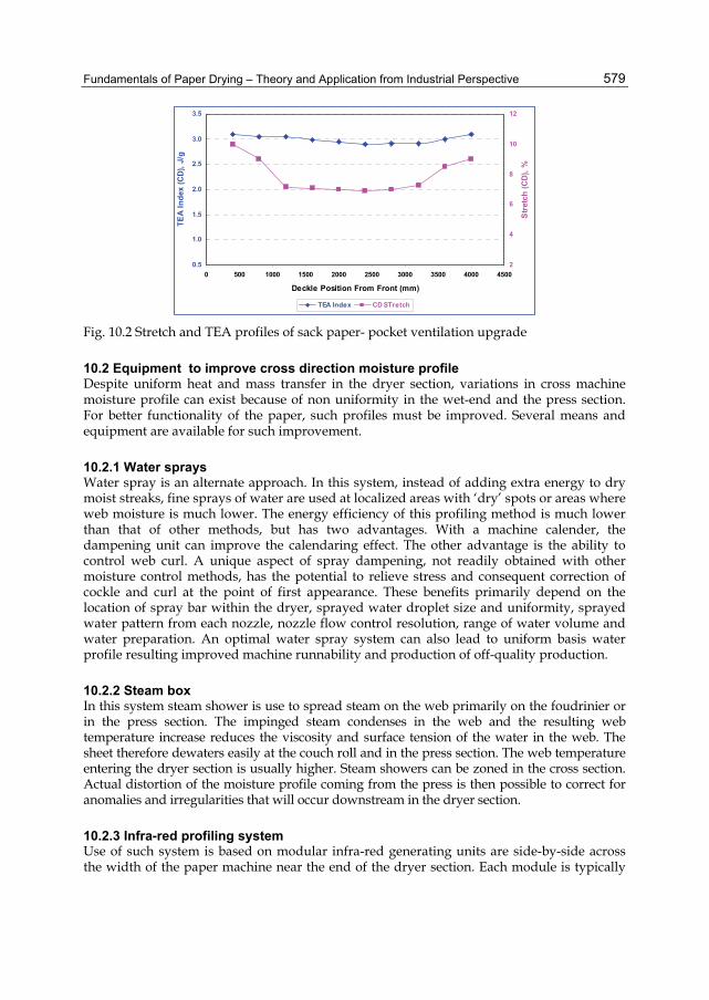
Fundamentals of Paper Drying – Theory and Application from Industrial Perspective
579
0.5
1.0
1.5
2.0
2.5
3.0
3.5
0 500 1000 1500 2000 2500 3000 3500 4000 4500
Deckle Position From Front (mm)
TEA
Inde
x (C
D), J
/g
2
4
6
8
10
12
Stre
tch
(CD)
, %
TEA Index CD STretch
Fig. 10.2 Stretch and TEA profiles of sack paper- pocket ventilation upgrade
10.2 Equipment to improve cross direction moisture profile Despite uniform heat and mass transfer in the dryer section, variations in cross machine moisture profile can exist because of non uniformity in the wet-end and the press section. For better functionality of the paper, such profiles must be improved. Several means and equipment are available for such improvement.
10.2.1 Water sprays Water spray is an alternate approach. In this system, instead of adding extra energy to dry moist streaks, fine sprays of water are used at localized areas with ‘dry’ spots or areas where web moisture is much lower. The energy efficiency of this profiling method is much lower than that of other methods, but has two advantages. With a machine calender, the dampening unit can improve the calendaring effect. The other advantage is the ability to control web curl. A unique aspect of spray dampening, not readily obtained with other moisture control methods, has the potential to relieve stress and consequent correction of cockle and curl at the point of first appearance. These benefits primarily depend on the location of spray bar within the dryer, sprayed water droplet size and uniformity, sprayed water pattern from each nozzle, nozzle flow control resolution, range of water volume and water preparation. An optimal water spray system can also lead to uniform basis water profile resulting improved machine runnability and production of off-quality production.
10.2.2 Steam box In this system steam shower is use to spread steam on the web primarily on the foudrinier or in the press section. The impinged steam condenses in the web and the resulting web temperature increase reduces the viscosity and surface tension of the water in the web. The sheet therefore dewaters easily at the couch roll and in the press section. The web temperature entering the dryer section is usually higher. Steam showers can be zoned in the cross section. Actual distortion of the moisture profile coming from the press is then possible to correct for anomalies and irregularities that will occur downstream in the dryer section.
10.2.3 Infra-red profiling system Use of such system is based on modular infra-red generating units are side-by-side across the width of the paper machine near the end of the dryer section. Each module is typically
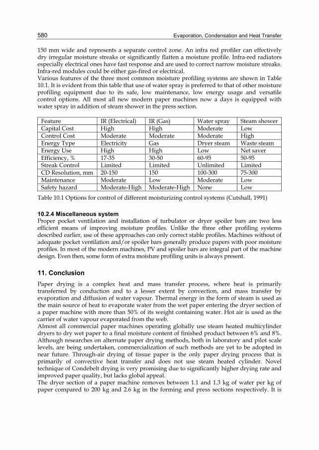
Evaporation, Condensation and Heat Transfer
580
150 mm wide and represents a separate control zone. An infra red profiler can effectively dry irregular moisture streaks or significantly flatten a moisture profile. Infra-red radiators especially electrical ones have fast response and are used to correct narrow moisture streaks. Infra-red modules could be either gas-fired or electrical. Various features of the three most common moisture profiling systems are shown in Table 10.1. It is evident from this table that use of water spray is preferred to that of other moisture profiling equipment due to its safe, low maintenance, low energy usage and versatile control options. All most all new modern paper machines now a days is equipped with water spray in addition of steam shower in the press section.
Feature IR (Electrical) IR (Gas) Water spray Steam shower Capital Cost High High Moderate Low Control Cost Moderate Moderate Moderate High Energy Type Electricity Gas Dryer steam Waste steam Energy Use High High Low Net saver Efficiency, % 17-35 30-50 60-95 50-95 Streak Control Limited Limited Unlimited Limited CD Resolution, mm 20-150 150 100-300 75-300 Maintenance Moderate Low Moderate Low Safety hazard Moderate-High Moderate-High None Low
Table 10.1 Options for control of different moisturizing control systems (Cutshall, 1991)
10.2.4 Miscellaneous system Proper pocket ventilation and installation of turbulator or dryer spoiler bars are two less efficient means of improving moisture profiles. Unlike the three other profiling systems described earlier, use of these approaches can only correct stable profiles. Machines without of adequate pocket ventilation and/or spoiler bars generally produce papers with poor moisture profiles. In most of the modern machines, PV and spoiler bars are integral part of the machine design. Even then, some form of extra moisture profiling units is always present.
11. Conclusion Paper drying is a complex heat and mass transfer process, where heat is primarily transferred by conduction and to a lesser extent by convection, and mass transfer by evaporation and diffusion of water vapour. Thermal energy in the form of steam is used as the main source of heat to evaporate water from the wet paper entering the dryer section of a paper machine with more than 50% of its weight containing water. Hot air is used as the carrier of water vapour evaporated from the web. Almost all commercial paper machines operating globally use steam heated multicylinder dryers to dry wet paper to a final moisture content of finished product between 6% and 8%. Although researches on alternate paper drying methods, both in laboratory and pilot scale levels, are being undertaken, commercialization of such methods are yet to be adopted in near future. Through-air drying of tissue paper is the only paper drying process that is primarily of convective heat transfer and does not use steam heated cylinder. Novel technique of Condebelt drying is very promising due to significantly higher drying rate and improved paper quality, but lacks global appeal. The dryer section of a paper machine removes between 1.1 and 1.3 kg of water per kg of paper compared to 200 kg and 2.6 kg in the forming and press sections respectively. It is
Fundamentals of Paper Drying – Theory and Application from Industrial Perspective
581
significantly more expensive to remove this water by drying compared to any other mechanical means. In spite of its key role in papermaking, large equipment size, and large capital and operating costs, drying is arguably the least understood papermaking operation. Detailed analysis of the main components involving dryer section by using data from field measurements is vital in identifying root cause(s) of poor dry end efficiency of a paper machine and for potential improvement. Tuning of the steam and condensate, pocket air ventilation systems and hood balance are critical for optimizing dryer section of a paper machine. The importance of pocket air ventilation and hood balance in paper drying is quite often ignored during operation of the dryer section of a paper machine. The case studies presented suggest that significant improvement in paper machine efficiency or product quality can be achieved if due attention is given to the dryer section. Unlike drying of other materials, paper drying process is different due to unique characteristics of paper sheet that is made of fibre network in which the cellulose fibres are held together through hydrogen bonding. Fibre properties and structure of the paper sheet is strongly influenced by pulping processes and types of fibres used in papermaking, presence of macro and micro pores. Various physical laws control removal and evaporation of free and bound water from wet web. Many of the key functional properties of the finished product are developed during the drying stage of the papermaking process. Controlling of moisture and shrinkage profiles in the cross direction of the width of paper web during paper drying is critical in end-user performance of finished paper products.
12. References Afzal, A., “Improving Dryer Performance”, Tappi Journal, p61, Vol. 83(5), 2000. Arenander, S. and Wahren, D., Tappi J. 66(9):123(1983). Bond, J., Gomes, V., and Douglas, W., “Computer simulation of drying paper by multiple
techniques”., Pulp Paper Canada, 97 (12):110 (1996). Burgess, B., Chapman, S. and Seto, W., Pulp Paper Mag. Can. 73 (11):323 (1972). Cutshall, K., in Pulp and Paper Manufacturer (B.A.: Thorp, Ed.), vol. 7, Tappi Press, Atlanta,
1991, Chap. XVII, p. 403. Douglas, J. W. M, Drying Technology 12(6):1341 (1994). Ghosh, A.K.; Allan, R.J. and Harris, D.J., "Simulation of Web Drying in a Paper Machine
Dryer - an Optimization Tool", Paper presented at 42nd Annual General conference of The Technical Association of the Australian and New Zealand Pulp and paper Industry (Appita), held at Hobart, Australia, 1988.
Ghosh, A.K. – Drysim: a combined audit and simulation tool to improve overall dry end efficiency, Appita J., 51(4):274 (1998).
Ghosh, A.K. – Optimization of paper machine dryer section. Proceedings of 7th International Conference on Pulp, Paper and Conversion Industry, New Delhi (2005).
Ghosh, A.K. and Oxley, F., “Pocket ventilation – an often forgotten area of paper drying”, Appita J., 60(4):301-308 (2007).
Ghosh, A.K., “A Systematic Approach to Optimise Dryer Performance and Energy Savings – Case Studies”, Tappi PaperCon09 Conference, May 31 – June 03, 2009, St. Louis, MO, USA.
Heikkila, P.,”A study on the drying process of pigment coated paper webs”, Ph.D. Thesis, Abo Akademi, Turku, Finland, 1993.
Hill, K. C. - Analyzing the dryer section’s steam and condensate system, Tappi J. 76(6):105(1993).
Evaporation, Condensation and Heat Transfer
582
Hill, K., “Dryer Section Troubleshooting”, Tappi Practical Aspects of Pressing and Drying Short Court, p793-812, Orange Beach, Al, USA, March 16-21 (1997).
Htun, M., “The influence of drying strategies on mechanical properties of paper”, dissertation, The Royal Institute of Technology, Stockholm, Sweden, 1980.
Iida, K., “Computer simulation of web drying in a paper machine dryer section”, Japan Tappi 39(5):469 (1985).
Joseph, M. - Paper Age, April 1988. Karlsson, M. - Papermaking Science and Technology: Papermaking Part 2, Drying, (ed), Published
by Finnish Engineers’ Association and Tappi, Chapter 9 (2000). Karlsson, M., Timofeev,)., Paavola, P.,Malashenko,A., and Taskinen,P., ”Analysis of
Performance of a multicylinder dryer, using computer model and experimental data”, Appita J., 48(2):143 (1995).
Karlsson, M. and Paltakari, J., Soininen, M. and Paulapuro, H., “A simulation model for board and paper machine dryer section”, pp 9-16 in ASME HTD, vol. 238, 1993.
Kormano, P., “Steam and Condensate Systems: Consideration for Dryer Section Runnability”, Tappi/PIMA PaperCon’08 Conference, May 4-7 2008, Dallas, TX, USA.
Lampinen, M. J., and Toivonen, K., “Application of a thermodynamic theory to determine capillary pressure and other fundamental material properties affecting the drying process”, pp 238-244 in AS Mujumdar (ed) Drying ’84 Hemisphere punl. Corp., Washington, 1984.
Luc, M. - Aero Journal, Jan 2004. Lehtinen, J., “Test results with Condebelt drying process”, OFE Symposium, Berlin, 1993. Lehtinen, J., “An overview of Condebelt drying: Quality results and process development”,
Ecopaper Tech Conference, The Finnish Pulp and Paper Research Institute and the Finnish Paper Engineers’ Association, Helsinki, p425 (1995).
Nissan, A.H. and Hansen, D., “Heat and mass transfer in cylinder drying: Part I. unfelted cylinders”, AIChE Journal 6(4) pp 606-611, 1960.
Nissan, A.H. and Hansen, D., “Heat and mass transfer in cylinder drying: Part II. felted cylinders”, AIChE Journal 7(4) pp 635-611, 1961.
Panchapakesan, B., “Enclosed PM Hood operating at high humidity conserve energy”, Pup Paper 133, April (1991).
Perry, R.H, and Green, D.W., Perry’s Chemical Engineers’ Handbook, 7th Edition, p4-15, 1997. Perrault, R., “Troubleshooting design and operation of the dryer section”, Tappi Papermaker
Conference, p199 (1989). Reese, J.R. – High humidity hoods conserve energy and improve runnability, Tappi
Engineering Conference, p653 (1988). Reese, J.R., “Observations from Testing Dryer Section Performance”, Tappi Journal, p 198-
202, October (1992). Virtanen, E., Gerlander, R. and Pitkaniemi, I., “Energy consumption in dryer section”,
Paperi ja Puu – Paper and Timber, p 322Vol 87(5), 2005. Sundqvist, H., “Efficient Dryer Hood Design Improves Dryer Section Performance”, Pulp &
Paper, P83, April (1996). Wahren, D., “Impulse drying”, Proceedings of the 1985 Executives’ conference, The Institute
of Paper Chemistry, Appleton, WI, p54. Warner, H.C., “Microwave processing of sheet materials”, Journal of Microwave Power, Vol.
1, pp81-88 (1966). Weise, U., “Characterization and mechanism of changes in wood pulp fibres caused by
water removal”, Doctoral Thesis, Helsinki University of Technology, published in Acta Polytechnica Scandinavica, Chemical Technology Series, No. 249, Espoo 1997.