Seediscussions,stats,andauthorprofilesforthispublicationat:https://www.researchgate.net/publication/283909529

TheregionaleconomicimpactofoilandgasextractioninTexas

ArticleinEnergyPolicy·December2015

ImpactFactor:2.58·DOI:10.1016/j.enpol.2015.08.032

CITATION

1

READS

21

1author:

JimLee

TexasA&MUniversity-CorpusChristi

36PUBLICATIONS745CITATIONS

SEEPROFILE

Allin-textreferencesunderlinedinbluearelinkedtopublicationsonResearchGate,

lettingyouaccessandreadthemimmediately.

Availablefrom:JimLee

Retrievedon:08June2016

The regional economic impact of oil and gas extraction in Texas

Jim LeeTexas A&M University‐Corpus Christi, 6300 Ocean Drive, Corpus Christi, TX 78412, USA

H I G H L I G H T S

� Economic impacts and multiplier effects differ between oil and gas wells in Texas.� Interactions among local economies raise employment and income effects.� Impacts persist over time, raising the long-run multipliers.� Greater economic impacts from newly drilled wells than legacy wells.

a r t i c l e i n f o

Article history:Received 2 May 2015Received in revised form17 August 2015Accepted 28 August 2015

Jel classification:Q3R12O13

Keywords:Oil and gas extractionDynamic spatial panel modelMultiplier effectsRegional economic impact

a b s t r a c t

This paper empirically investigates the regional economic impact of oil and gas extraction in Texas duringthe recent shale oil boom. Regressions with county-level data over the period 2009–2014 supportsmaller multiplier effects on local employment and income than corresponding estimates drawn frompopular input–output-based studies. Economic impacts were larger for extraction from gas wells than oilwells, while the drilling phase generated comparable impacts. Estimates of economic impacts are greaterin a dynamic spatial panel model that allows for spillover effects across local economies as well as overtime.

& 2015 Elsevier Ltd. All rights reserved.

1. Introduction

1.1. Background

More than a century after the discovery of the Spindletop oil-field in 1901, Texas experienced another oil boom along with otheroil-rich regions across the United States. The Lone Star state isarguably the most interesting case not only because of its histor-ical reliance on natural resources, but also because of its leadingrole in the overall size of proven reserves as well as the volumes ofcrude oil and natural gas production from its various formations.

The recent oil boom, which began to unfold in 2008, was anextension of the so-called shale revolution. In contrast to con-ventional techniques, drilling of shale, or tight, oil and natural gashas been driven primarily by advances in technologies called hy-draulic fracturing and horizontal drilling. After nearly a decade of

development in shale gas extraction, shale oil production alsoaccelerated in the wake of soaring oil prices, which reached recordlevels more than US$100 in mid-2008 before falling by half withinthe following year. Crude oil production in Texas more than tripledbetween 2008 and 2014, according to U.S. Energy InformationAdministration (EIA).

In the wake of the 2007–2009 Great Recession, much of theUnited States struggled with relatively slow economic recovery.Meanwhile, the shale oil boom was widely perceived as a “gamechanger” for Texas’s statewide economy as well as its local com-munities. A number of private consultants and university re-searchers (e.g., Scott, 2009; PerrymanGroup, 2009, 2011; Tunstall,2011, 2012, 2013, 2014; Ewing et al., 2014) have documented theregional economic impacts of the surging oil and gas drilling ac-tivity in the state’s major shale formations, notably the Barnett,Permian Basin and Eagle Ford. Those studies, which receivedsubstantial media attention, were typically commissioned bygovernment officials and business associations, which rely on thefindings to make public policy and business decisions.

Contents lists available at ScienceDirect

journal homepage: www.elsevier.com/locate/enpol

Energy Policy

http://dx.doi.org/10.1016/j.enpol.2015.08.0320301-4215/& 2015 Elsevier Ltd. All rights reserved.

E-mail address: jim.lee@tamucc.edu

Energy Policy 87 (2015) 60–71

The conventional approach of those so-called “impact” studiesdraws on an input–output model customized for the region underinvestigation. Those findings have been subjected to criticism inthe academic literature. For instance, input–output analysis relieson the assumption that the economy operates with excess capa-city, including elastic labor supply (Dwyer et al., 2000), and nocrowding out or leakage effects can occur (Carlson and Spencer,1975; Kinnaman, 2011; Lee, 2015). For this reason, ex-ante esti-mates based on popular input–output models may misrepresentthe actual economic impacts of a sizable change in economic ac-tivity. Nevertheless, since the shale oil boom evolved in theaftermath of the Great Recession, those modeling assumptionsmay not be especially restrictive as a representation of regional

communities with substantial economic slack.An alternative empirical methodology is econometric analysis

with cross-sectional data of local economies. The literature con-cerning ex-post economic effects of the recent shale revolution is,however, confined mostly to natural gas extraction (e.g., Brown,2014; Paredes et al., 2015; Weber, 2012, 2014; Hartley et al., 2015).Given the short history of the recent shale oil boom, econometric-based analysis concerning its regional economic impacts is absent.

The recent shale oil boom in the United States might haveended in late 2014 as crude oil prices fell precipitously from aboveUS$100 in July 2014 to below US$50 by January 2015. It wouldtherefore be interesting to account for what this oil cycle broughtto the regional economies of the top producing regions. To this

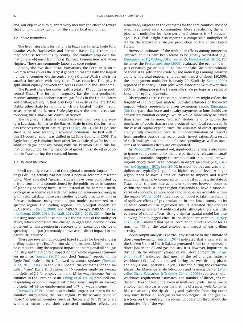
Fig. 1. Texas shale formations.

J. Lee / Energy Policy 87 (2015) 60–71 61

end, our objective is to quantitatively measure the effect of Texas’sshale oil and gas extraction on the state's local economies.

1.2. Shale formations

The five major shale formations in Texas are Barnett, Eagle Ford,Granite Wash, Haynesville and Permian Basin. Fig. 1 contains amap of those formations by county. The counties atop each for-mation are obtained from Texas Railroad Commission and BakerHughes. Those are commonly known as core regions.

Among the five shale Texas formations, the Permian Basin inwestern Texas covers the largest geographical area with the largestnumber of counties. On the contrary, the Granite Wash shale is thesmallest formation with only three Texas counties. This play issplit about equally between the Texas Panhandle and Oklahoma.

The Barnett shale lies underneath a total of 17 counties in northcentral Texas. That formation arguably has the most produciblereserves among all onshore natural gas fields in the United States,and drilling activity in that play began as early as the late 1990s.Unlike other shale formations which are located mostly in ruralareas, parts of the Barnett Shale play cover the urban areas sur-rounding the Dallas–Fort Worth Metroplex.

The Haynesville shale is located between East Texas and wes-tern Louisiana. Similar to the Barnett shale in size, this formationhas reserves mostly in natural gas (Kaiser, 2012). The Eagle Fordshale is the most recently discovered formation. The first well inthis 23-county region was drilled in La Salle County in 2008. TheEagle Ford play is distinct from other Texas shale plays for its oil inaddition to gas deposits. Along with the Permian Basin, this for-mation accounted for the majority of growth in shale oil produc-tion in Texas during the recent oil boom.

1.3. Related literature

Until recently, measures of the regional economic impact of oilor gas drilling activity had not been a popular academic researchtopic. Most so-called “impact” studies have been conducted byprivate consultants commissioned by the public sector in supportof planning or policy formulation. Instead of the common meth-odology in academic research that relies on econometric analysiswith historical data, those case studies typically provide ex ante orforecast estimates using input–output models customized to aspecific region. The leading regional input–output models areBEA’s RIMS II (Scott, 2009) and IMPLAN Group's IMPLAN (Perry-manGroup, 2009, 2011; Tunstall, 2011, 2012, 2013, 2014). One in-teresting outcome of those models is the estimate of the multipliereffect, which represents the change in aggregate income or em-ployment within a region in response to an exogenous change ofspending or output (commonly known as the direct impact) in oneparticular industry.

There are several input–output based studies for the oil and gasdrilling industry in Texas’s major shale formations. Multipliers canbe computed using the reported impact on the regional oil and gasindustry and the reported impact on the whole regional economy.For instance, Tunstall (2011) published “impact” reports for theEagle Ford shale in 2011, followed by annual updates (Tunstall,2012, 2013, 2014). In the 2012 update, the estimates for the so-called “core” Eagle Ford region of 15 counties imply an averagemultiplier of 2.2 for employment and 1.3 for wage income. For thecounties in the Permian Basin, Ewing et al. (2014) produced cor-responding economic impact estimates, which imply an averagemultiplier of 1.9 for employment and 1.47 for wage income.

Tunstall's 2014 update also includes impact estimates for sixcounties surrounding the core region. Partly because some ofthose “peripheral” counties, such as Nueces and San Patricio, arewithin a metro area, their estimated multiplier effects are

remarkably larger than the estimates for the core counties, most ofwhich represent rural communities. More specifically, the em-ployment multiplier for those peripheral counties is 4.5 on aver-age. IHS Global Insight also reported a comparable multiplier of4.1 for the impact of shale gas production on the entire UnitedStates.

However, estimates of the multiplier effects among numerous“impact” studies have been found to be grossly overstated (e.g.,Kinnaman, 2011; Weber, 2012; Lee, 2015; Paredes et al., 2015). Forinstance, the PerrymanGroup (2009) evaluated the economic im-pact of natural gas drilling in the Barnett shale. Given the estimateof about 7000 jobs in the crude oil and natural gas mining industryalong with a total regional employment impact of about 130,000,the employment multiplier is nearly 20. Similarly, Scott (2009)reported that nearly 33,000 jobs were associated with fewer than500 gas drilling jobs in the Haynesville shale perhaps as a result oflease and royalty payments.

Discrepancies across those implied multipliers might reflect thefragility of input–output analysis, but also estimates of the directimpact, which represents a given exogenous shock. Kinnaman(2011) argued that lease and royalty payments to households areconsidered windfall earnings, which would more likely be savedthan spent. Furthermore, “impact” studies tend to ignore thepurchases of goods that are not produced with local resources. Inthe case of capital expenditures, the amounts of direct spendingare typically overstated because of underestimation of importsfrom suppliers outside the region under investigation. As a resultof such leakages, the amounts of direct spending as well as mea-sures of secondary effects are exaggerated.

As Weber (2012) pointed out, input–output analysis also tendsto ignore supply constraints that are particularly relevant to smallregional economies. Supply constraints result in potential crowd-ing-out effects from large increases in direct spending (e.g., Carl-son and Spencer, 1975; Lee, 2015). In input–output analysis, mul-tipliers are typically larger for a higher regional level. A largerregion tends to have a smaller leakage to imports and fewersupply constraints. As compared to individual counties, the state ofTexas better captures interactions or spillovers between countieswithin that state. A larger region also tends to have a more di-versified economy, as more goods and services are available withinthe region. Weber (2014) used a spatial model to take into accountof spillover effects of gas production in one Texas county on itsadjacent counties. The regression results indicated that one gasmining job generates 1.4 additional jobs, although there was littleevidence of spatial effects. Using a similar spatial model but alsoallowing for the lagged effect in the dependent variable, Hartleyet al. (2015) showed that spatial correlation effects account for asmuch as 17% of the total employment impact of gas drillingactivity.

Input–output analysis is particularly sensitive to the estimate ofdirect employment. Tunstall (2014) indicated that a new well inthe Bakken Shale of North Dakota generated 3 full-time-equivalentdirect jobs in the oil and gas industry. It is, however, important todistinguish the different phases of well development. Brundageet al. (2011) indicated that most of the oil and gas industryworkforce (13 jobs) is employed during the well drilling phase,and only a small portion (0.2 job) is needed during the extractionphase. The Marcellus Shale Education and Training Center (Mar-cellus Shale Education & Training Center, 2009) reported similarworkforce requirement estimates. The number of direct jobs re-duces further for additional wells in multi-well pads. The nature ofemployment also varies over the lifetime of a given well. Activitieslike constructing the rig, drilling and hydraulic fracturing occuronly once before oil and gas extraction begins. Oil and gas ex-traction, on the contrary, is a recurring operation throughout theproductive life of the well.

J. Lee / Energy Policy 87 (2015) 60–7162

Against the above background, econometric studies with his-torical data have unequivocally generated smaller multiplier esti-mates than comparable multipliers derived from input–outputstudies. The bulk of the academic literature, however, focuses onnatural gas production. In light of the recent oil boom, thispaper seeks to shed light on the economic impacts of oil produc-tion in comparison with gas production.

2. Methods

2.1. Data

To explore the effect of oil and gas extraction on local em-ployment and income, we look at annual Texas county-level data.Despite its popularity in the related literature, county-level dataare by no means perfect for measuring the local impacts of an oilboom. This level of data disaggregation is more suitable for dis-cerning “local” effects than more aggregated measures at themetro area or state level. Counties are the smallest geographicalareas for which the U.S. government regularly reports economicdata. However, differences in county size and commuting patterncan potentially affect the observed local economic effects due todisparities in labor and capital mobility. In this paper, we attemptto capture the possible geographical effects of economic interac-tions and labor mobility using a spatial regression model as de-scribed below.1

Most data are obtained from the U.S. Bureau of EconomicAnalysis (BEA). The income and employment data are obtainedfrom the BEA’s Local Area Personal Income and Employment da-tabase. Income is measured by personal income by place of re-sidence. The employment measures include full-time, part-time,and self-employed workers. As opposed to income, wage andsalary employment is on a place-of-work basis. In this study, theoil and gas industry refers specifically to activities related to oiland gas extraction (NAICS 211), and support activities for oil andgas extraction (NAICS 213). Employment and personal income inthe oil and gas industry are measured correspondingly.

2.2. Oil and gas wells

We measure the intensity of oil and gas extraction by thenumbers of oil and gas wells. Data on the numbers of oil and gaswells are obtained from the Texas Railroad Commission. Althoughthe majority of Texas wells contain both crude oil and natural gas,the oil or gas well designation depends on what a well is drilledprimarily for. As explained by Hartley et al. (2015), the number ofwells completed captures the peak impact of shale drilling onemployment as the date of well completion indicates the end ofthe construction period and the beginning of its production. Whileactivity during the more lengthy production phase is important forpublic policy formulation, most “impact” studies focus on thedrilling of new wells. From this perspective, we report results forthe number of new wells drilled in addition to the total number ofactive wells.

For a particular well, the full-time-equivalent workforce needsare found to be substantially greater in the drilling phase than theproduction phase (Brundage et al., 2011; Marcellus Shale Educa-tion & Training Center, 2009). However, according to MarcellusShale Education & Training Center (2009), the workforce needs aremuch more difficult to pinpoint for a specific area, like a county,

during the drilling phase than the production phase. The directworkforce needed to drill one well involves more than 400 in-dividuals in 150 occupations typically working for a few months asopposed to a full year. Their workplace locations or residency alsodepend on a number of factors. By contrast, most direct workersduring the production phase are based at offices near the wellsand their jobs are considered permanent positions. For thesereasons, we expect different local economic impacts betweennewly drilled wells and legacy wells.

In addition to the total number of wells, the economic effects ofoil wells are considered separately from those of gas wells. Unlikecrude oil prices, which tended to rise over the observation periodbetween 2009 and 2014, natural gas prices hovered around rela-tively low levels below $5 per million BTU. As a result of the increasein the price of oil relative the price of natural gas, the U.S. productionof shale oil increased during that period while gas production re-mained flat. Beginning in 2011, the number of gas wells in the Per-mian Basin declined over time in response to low natural gas prices.Likewise, fewer gas wells were drilled in the Haynesville shale after2012. The different trends between natural gas prices and crude oilprices might have generated different economic impacts between oiland gas wells among Texas shale formations.

According to the U.S. Energy Information Administration(2013), nearly half of new wells in recent years contained bothcrude oil and natural gas, oil and gas producers increasingly tar-geted those wells for oil as opposed to gas production. Hydro-carbon products in the liquid state at the wellhead are treated asoil, and unprocessed gas products are treated as natural gas.

2.3. Summary statistics

Table 2 presents summary statistics of the key variables in ourempirical work. Out of the total 254 Texas counties, 107 countieslie within one of the five shale formations. All statistics other thanthe last two columns are averages of the counties within thespecific regions. The numbers of counties comprising each regionare listed at the top the table. The first panel shows the averagecounty employment levels in 2009 and 2014, as well as the annualpercentage changes over the periods of 2009–2014 and 2000–2009. The 2009–2014 period, which represents the time horizon ofthe U.S. shale oil boom, is the focus of our regression analysis. Datain the 2000–2009 period represent historical trends prior to theoil boom. Except for the Barnett shale, the employment size ofshale counties is on average smaller than the statewide average.This can be explained in part by the fact that the majority of shaleoil and gas wells are located in rural communities with a smallerpopulation and workforce.

Texas county employment tended to grow more rapidly duringthe shale oil boom than the preceding 10-year period. Counties inthe Eagle Ford shale experienced the strongest overall employ-ment growth between 2009 and 2014, when local employment inthe oil and gas industry expanded by more than 50% per year onaverage. Meanwhile, counties in the Permian Basin also witnesseddramatic growth in oil and gas employment exceeding 60% an-nually, but their overall annual employment growth was only closeto the statewide average of 2%.

The Barnett shale is the only region with overall employmentgrowing at a relatively slower pace during the oil boom period of2009–2014. Oil and gas employment growth also slowed down to11.6% annually from 18.4% in the decade prior to 2009. As pointedout in the preceding section, this formation has predominantlynatural gas proved reserves as opposed to oil. In other shale re-gions with more oil reserves, oil and gas employment grew at leasttwice as fast during the shale oil boom period than earlier.

Table 1 also shows the averages of counties' total personal in-come as well as income in the oil and gas industry. Total personal

1 In the cases that industry level data are suppressed to avoid disclosure ofconfidential information, we entered a zero because the data are typically verysmall (less than 5).

J. Lee / Energy Policy 87 (2015) 60–71 63

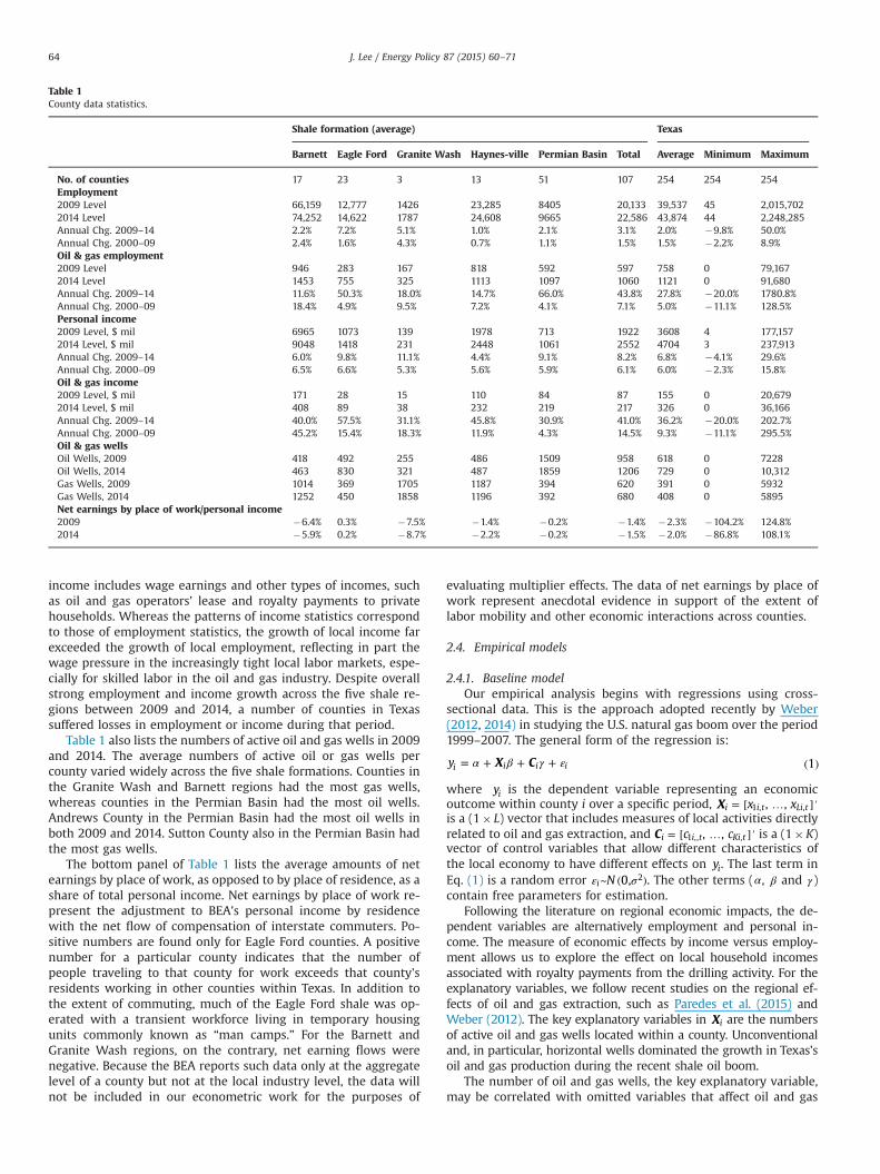
income includes wage earnings and other types of incomes, suchas oil and gas operators’ lease and royalty payments to privatehouseholds. Whereas the patterns of income statistics correspondto those of employment statistics, the growth of local income farexceeded the growth of local employment, reflecting in part thewage pressure in the increasingly tight local labor markets, espe-cially for skilled labor in the oil and gas industry. Despite overallstrong employment and income growth across the five shale re-gions between 2009 and 2014, a number of counties in Texassuffered losses in employment or income during that period.

Table 1 also lists the numbers of active oil and gas wells in 2009and 2014. The average numbers of active oil or gas wells percounty varied widely across the five shale formations. Counties inthe Granite Wash and Barnett regions had the most gas wells,whereas counties in the Permian Basin had the most oil wells.Andrews County in the Permian Basin had the most oil wells inboth 2009 and 2014. Sutton County also in the Permian Basin hadthe most gas wells.

The bottom panel of Table 1 lists the average amounts of netearnings by place of work, as opposed to by place of residence, as ashare of total personal income. Net earnings by place of work re-present the adjustment to BEA’s personal income by residencewith the net flow of compensation of interstate commuters. Po-sitive numbers are found only for Eagle Ford counties. A positivenumber for a particular county indicates that the number ofpeople traveling to that county for work exceeds that county'sresidents working in other counties within Texas. In addition tothe extent of commuting, much of the Eagle Ford shale was op-erated with a transient workforce living in temporary housingunits commonly known as “man camps.” For the Barnett andGranite Wash regions, on the contrary, net earning flows werenegative. Because the BEA reports such data only at the aggregatelevel of a county but not at the local industry level, the data willnot be included in our econometric work for the purposes of

evaluating multiplier effects. The data of net earnings by place ofwork represent anecdotal evidence in support of the extent oflabor mobility and other economic interactions across counties.

2.4. Empirical models

2.4.1. Baseline modelOur empirical analysis begins with regressions using cross-

sectional data. This is the approach adopted recently by Weber(2012, 2014) in studying the U.S. natural gas boom over the period1999–2007. The general form of the regression is:

X Cy 1i i i iα β γ ε= + + + ( )

where yi is the dependent variable representing an economicoutcome within county i over a specific period, X x x, ,i i t Li t1 , ,= [ … ]′is a (1� L) vector that includes measures of local activities directlyrelated to oil and gas extraction, and C c c, ,i i t Ki t1 ,, ,= [ … ]′ is a (1�K)vector of control variables that allow different characteristics ofthe local economy to have different effects on yi. The last term inEq. (1) is a random error N 0,i

2ε σ~ ( ). The other terms (α, β and γ)contain free parameters for estimation.

Following the literature on regional economic impacts, the de-pendent variables are alternatively employment and personal in-come. The measure of economic effects by income versus employ-ment allows us to explore the effect on local household incomesassociated with royalty payments from the drilling activity. For theexplanatory variables, we follow recent studies on the regional ef-fects of oil and gas extraction, such as Paredes et al. (2015) andWeber (2012). The key explanatory variables in Xi are the numbersof active oil and gas wells located within a county. Unconventionaland, in particular, horizontal wells dominated the growth in Texas’soil and gas production during the recent shale oil boom.

The number of oil and gas wells, the key explanatory variable,may be correlated with omitted variables that affect oil and gas

Table 1County data statistics.

Shale formation (average) Texas

Barnett Eagle Ford Granite Wash Haynes-ville Permian Basin Total Average Minimum Maximum

No. of counties 17 23 3 13 51 107 254 254 254Employment2009 Level 66,159 12,777 1426 23,285 8405 20,133 39,537 45 2,015,7022014 Level 74,252 14,622 1787 24,608 9665 22,586 43,874 44 2,248,285Annual Chg. 2009–14 2.2% 7.2% 5.1% 1.0% 2.1% 3.1% 2.0% �9.8% 50.0%Annual Chg. 2000–09 2.4% 1.6% 4.3% 0.7% 1.1% 1.5% 1.5% �2.2% 8.9%Oil & gas employment2009 Level 946 283 167 818 592 597 758 0 79,1672014 Level 1453 755 325 1113 1097 1060 1121 0 91,680Annual Chg. 2009–14 11.6% 50.3% 18.0% 14.7% 66.0% 43.8% 27.8% �20.0% 1780.8%Annual Chg. 2000–09 18.4% 4.9% 9.5% 7.2% 4.1% 7.1% 5.0% �11.1% 128.5%Personal income2009 Level, $ mil 6965 1073 139 1978 713 1922 3608 4 177,1572014 Level, $ mil 9048 1418 231 2448 1061 2552 4704 3 237,913Annual Chg. 2009–14 6.0% 9.8% 11.1% 4.4% 9.1% 8.2% 6.8% �4.1% 29.6%Annual Chg. 2000–09 6.5% 6.6% 5.3% 5.6% 5.9% 6.1% 6.0% �2.3% 15.8%Oil & gas income2009 Level, $ mil 171 28 15 110 84 87 155 0 20,6792014 Level, $ mil 408 89 38 232 219 217 326 0 36,166Annual Chg. 2009–14 40.0% 57.5% 31.1% 45.8% 30.9% 41.0% 36.2% �20.0% 202.7%Annual Chg. 2000–09 45.2% 15.4% 18.3% 11.9% 4.3% 14.5% 9.3% �11.1% 295.5%Oil & gas wellsOil Wells, 2009 418 492 255 486 1509 958 618 0 7228Oil Wells, 2014 463 830 321 487 1859 1206 729 0 10,312Gas Wells, 2009 1014 369 1705 1187 394 620 391 0 5932Gas Wells, 2014 1252 450 1858 1196 392 680 408 0 5895Net earnings by place of work/personal income2009 �6.4% 0.3% �7.5% �1.4% �0.2% �1.4% �2.3% �104.2% 124.8%2014 �5.9% 0.2% �8.7% �2.2% �0.2% �1.5% �2.0% �86.8% 108.1%

J. Lee / Energy Policy 87 (2015) 60–7164

drilling activities as well as the local economy. Regression ex-cluding those confounding factors would result in biased estimatesdue to endogeneity in the explanatory variables. Following recentstudies (e.g., Weber, 2012, 2014; Brown, 2014), the control vari-ables in Ci capture a multitude of local labor market, economic andgeographic characteristics that might have affected the intensity ofoil and gas extraction as well as the local economy. The first set ofcontrol variables reflect the structure of the local economy, in-cluding the shares of total income earnings accounted for by theagricultural, construction, manufacturing, and retail sectors.

Each county's pre-existing economic condition is captured byper capital income in the base year. Heterogeneity across countiesis also captured by the population density, which tends to behigher in urban or metro areas. Energy companies may lease landfor less in economically depressed areas. Similarly, becauseproximity to oil or gas wells tends to lower property values andthe quality of life, wealthier communities might have more in-centive and capability to fight fracking wells (Weber, 2012).

Geological characteristics, such as reserves, would also affectenergy companies’ decision to drill in a particular area. Thosefactors are captured by a set of binary dummy variables for the fiveshale formations. Different shale plays have different recoveryrates for oil or gas extraction, and their output differs by densityand other quality factors. Following Weber (2012, 2014) and Fetzer(2014), we will also consider a similar variable, which is measuredby the percent of a county covering a shale formation.

As Weber (2012) pointed out, there is a considerable lag be-tween the time a well is first drilled and the time oil or gas flowsout of the ground. Moreover, it takes time to build the capital in-frastructure for the drilling activity as well as a logistical networkfor transporting the oil or gas supplies to refineries or storage sites.From those perspectives, we attempt to capture the cumulativeeffects of oil and gas extraction by looking at changes in economicvariables over the 6-year period between 2009 and 2014. Thissample period captures the interval of the shale oil boom. As such,the dependent variable yi in the cross-section model is the dif-ference between the county employment or income levels be-tween 2009 and 2014.

2.4.2. Difference-in-difference regressionsDespite our efforts to control for factors that might have af-

fected local economic conditions across counties beyond oil andgas extraction, the regression model as captured by Eq. (1) doesnot allow for the possibility that shale counties might have overallbeen performing better or worse than other counties prior to theoil boom. To account for the effects of past trends, we adopt thedifference-in-difference approach (see, e.g., Weber, 2012; Lee,2015), which replaces the dependent variable with a relativemeasure. More specifically, the transformed dependent variable isdefined as ⎡⎣ ⎤⎦y y y y y/ 5/9 /i i i i i,2009 ,2014 ,2009 ,2009 ,2000( )× ( ) − × , which

assumes a linear growth trend. In words, the transformed variableequals the growth rate of economic activity between 2009 and2014 less the growth rate of economic activity between 2000 and2009, the latter of which is scaled to conform to the shorter timeinterval under investigation. This difference-in-difference specifi-cation is equivalent to controlling for the counterfactual conditionthat a county's economy was growing at its historical pace. Data ofoil and gas well counts are transformed accordingly. Accordingly,the base year for the control variables is set at 2000.

Our cross-sectional data model has a major drawback, never-theless. Despite our efforts to control for heterogeneity acrosscounties and endogeneity in drilling activity, it is difficult to as-certain that regression results are free of the potential bias due tounobserved omitted variables. One common strategy to mitigatethose potential effects is the panel data approach, which pools

time series and cross-sectional data together.2

2.4.3. Panel data modelsThis subsection outlines the panel data models for our em-

pirical work. For county i (i¼1, 2, …, N) in year t (t¼1, 2, …, T), thebasic panel data framework can be expressed as:

Zy 2it it i t itΘ μ λ ε= + + + ( )

where Z x x ; c c1, , , , ,it i t Li t i t Ki t1 , , 1 , ,[ ]= … … ′ is a (LþKþ1) vector ofexplanatory variables, and , , , L K0 1Θ θ θ θ= [ … ]+ is a corresponding(LþKþ1) vector of unknown parameters. The term iμ captures theso-called individual effects, which represent time-invariant, orcross-sectional, heterogeneity across counties. The term tλ cap-tures time effects, which represent time-varying factors that arecommon to all counties in the sample. The last term itε representsa purely random shock.

In panel regressions, the time-invariant effects can be treatedas fixed effects or random effects. In line with the econometricliterature that analyzes geographical or spatial effects in the panelsetting (see below), we have followed the popular approach of thetwo-way fixed-effects estimator, which treats both individual ef-fects and time effects with dummy variables. The individual effectsin iμ are eliminated from Eq. (2) by demeaning the variables onboth sides of the equation. The intercept term 0θ is also eliminatedas a result. The dependent variable after the transformation be-comes y y yit it i*= − ̅ where yi̅ is the sample mean. The fixed time ef-fects tλ are eliminated analogously but over the time dimension.The coefficients in Θ without the intercept can be estimated byordinary least squares (OLS). An alternative strategy to eliminatethe unobserved time-invariant effects is taking the first differen-cing transformation of Eq. (2), so that the dependent variable aftertransformation is y y y .it it it 1*= − − This treatment is analogous to theabove difference-in-difference approach to cross-sectional data.

To explore lasting effects in economic activity over time, weextend the static panel data model to a first-order autoregressiveAR(1) representation:

Zy y 3it it it i t it1 Θρ μ λ ε= + + + + ( )−

where the new coefficient ρ captures the temporal effects giventhe introduction of the lagged dependent variable.3 The first-dif-ference model specification is equivalent to 1ρ = . However, unlikethe specification in Eq. (2), the OLS estimator of Θ in Eq. (3) withfixed-effects is inconsistent. Hsiao (2003) indicated that the de-meaning procedure creates a correlation between the demeanedlagged dependent variable and the demeaned error term. Hsiaoet al. (2002) further showed that this bias can be resolved with amaximum-likelihood (ML) procedure based on the model’s un-conditional likelihood function. In addition to capturing the laggedeffects in the dependent variable, Eq. (3) allows us to measure thelong-run effect of a change in the explanatory variable. For in-stance, the long-run response of yit to xit is measured as / 1 .iθ ρ( − )

Eq. (3) captures two distinct characteristics in panel data,namely the temporal effects through the inclusion of the laggeddependent variable, and the time-invariant cross-sectional effectsthrough the fixed-effects estimator. However, the regressionmodel ignores spatial interactions among counties at each timeperiod. Spatial interactions can occur in the form of spillover and

2 Nevertheless, the difference-in-difference approach deserves attention. As areferee pointed out, our cross-sectional model corresponds to differencing paneldata and thus it is not the conventional cross-sectional models that capture onlyvariations across space without the time dimension.

3 Conceptually, additional autoregressive lags as well as lags in the in-dependent variables can be added to the model. Preliminary analysis, however,shows that those terms are not statistically significant, meaning that the AR(1) model adequately describes the dynamics of the data.

J. Lee / Energy Policy 87 (2015) 60–71 65

feedback effects, externality, or competition in labor or capitalresources. To capture spatial interactions in addition to time dy-namics, we consider a dynamic spatial panel data model (Le Sageand Pace, 2009):

Z Zy y w 4it i t it j

Nij jt i t it0 , 1 1

∑Ψ Φρ μ λ ε= + + + + + ( )− =

where wij is an element of an N N× matrix W wij={ } with pre-specified spatial weights that reflect the spatial arrangements ofthe counties in the sample. More specifically, wij is equal to one ifcounty i and county j are physically adjacent counties, and zerootherwise. To exclude the self-neighbor effect, the diagonal ele-ments of W are set to zero.

The spatially lagged term ZwjN

ij jt1∑ = introduces con-temporaneous spatial correlation to the independent variables.The vector of coefficients Φ captures the spatial effects in the in-dependent variables, while the vector of coefficients Ψ measuresthe response to a change in the independent variables withoutspatial effects. By comparison, the term Zit contains own-areacharacteristics, whereas the linear combination of the spatiallylagged term captures characteristics of neighboring areas. In ourcase, the spatially lagged term will capture the response of onecounty to the average change in wells of its contiguous neighbors.

One common approach in the spatial econometric literature isto apply a model that includes a corresponding spatially laggeddependent variable ( w yj

Nij j t1 , 1∑ = − ) along with the spatially lagged

covariates. However, Gibbsons and Overman (2012) underscoredthe potential problem of identifying the causal effects of the in-dependent variables of interest in the presence of the spatiallylagged dependent variable. As in Weber (2014), we adopt theirrecommendation and include only Zwj

Nij jt1∑ = in the empirical

model. For estimation, we apply the ML procedure suggested byAnselin et al. (2006) and Elhorst (2010, 2014).

Eq. (4) allows us to measure, for instance, employment in oneparticular county in relation to the drilling activity in that countyas well as the drilling activity in its neighboring counties. To ex-plore the extent of spatial or “indirect” effects, we use the parti-tioning technique suggested by Le Sage and Pace (2009). Let

⎡⎣ ⎤⎦y y y y, ,t t t Nt1 2= … ′, ⎡⎣ ⎤⎦y y y y, , , T1 2= ′ ′ … ′ ′, Z Z Z Z, , ,t t t Nt1 2= [ ′ ′ … ′ ]′,and Z Z Z Z, , , T1 2= [ ′ ′ … ′ ]′. The “direct” and “indirect” effects for therth explanatory variable are drawn from an N N× matrix of partialderivatives associated with a change in each of the explanatoryvariables:

y Z WI/ 5r N r rΨ Φ∂ ∂ ′ = + ( )

where the subscript r denotes the rth row of a matrix. For the rthexplanatory variable, the average of the diagonal elements of thismatrix represents the “direct” effect, which measures how theexplanatory variable in one county affects the dependent variable

of that county (own-partial derivatives). The “indirect” effect ismeasured by the average of the cumulative sum of the matrix’soff-diagonal elements (cross-partial derivatives). The “total” effectis the sum of the “direct” and “indirect” effects.

3. Results and discussions

This section summarizes the estimation results of the modelsoutlined in the preceding section. The cross-sectional sampleconsists of the 254 counties in the state of Texas. The dependentvariable is measured alternatively by employment and personalincome. For each of the two alternative economic outcomes, re-gressions were run for the county total and again for the oil andgas industry. Standard errors in all regressions are robust to arbi-trary heteroskedasticity.

The key explanatory variables of our interest are oil and gaswell counts as measures of drilling and extraction activities. Ourmeasures of the multiplier effects equal the ratios of the estimatedcoefficients (total effects) on well counts in the regressions fortotal economic outcomes over the corresponding coefficients (di-rect effects) in the regressions for outcomes in the oil and gasindustry. This is the common approach among recent econo-metric-based studies on the economic impacts of the oil and gasindustry (e.g., Brown, 2014; Weber, 2014; Hartley, et al., 2015).

3.1. Direct estimation of multipliers

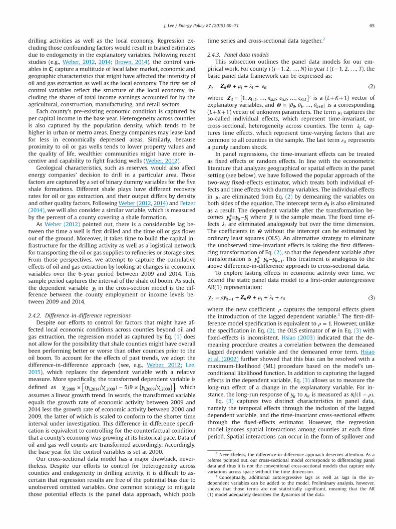
Instead of separate regressions for total employment and em-ployment in the oil and gas industry, employment multipliers canbe obtained “directly” by regressing total employment on oil andgas employment. The coefficient on that key explanatory variablerepresents the response of total employment to a change in oil andgas employment, other things being equal. For comparison pur-poses, we began our empirical work with those regressions.

Table 2 shows the key results of the “direct” regressions withcross-sectional and panel data. The cross-section model was esti-mated alternatively with the OLS and instrumental variable (IV)methods. Total county employment and income are the alternativedependent variables. The table displays the coefficient estimates forcounty employment and income in the oil and gas industry as al-ternative explanatory variables. Regressions were run along with allcontrol variables (Ci) discussed in the previous section. More spe-cifically, the OLS regressions include local per capita income, popu-lation density, the income shares of four major economic sectors,and dummy variables representing different shale formations. In theIV regressions, the above control variables serve as instruments.Following Weber (2012, 2014) and Fetzer (2014), we replaced thedummy variables with the percent of a given county covering a shaleformation as an instrument. The set of instruments were found to berelevant based on the F-tests for the instruments in explaining thekey explanatory variables. The F-statistic is 19.10 for industry em-ployment, and 90.04 for industry income. Both statistics are statis-tically significant at the 1% level. According to the table, the em-ployment multipliers are about 6 and the income multipliers areabout 4. By comparison, the IV multiplier estimates are slightly lar-ger than their OLS counterparts.

Instead of cross-sectional data, we also ran corresponding re-gressions with panel data. We also applied the two-way fixed-ef-fects and first-difference estimators as discussed in Section 2above. The point estimates of the fixed-effects regressions areclose to the OLS estimates, albeit slightly smaller in size. Bycomparison, the first-difference regressions generate even smallerpoint estimates for the multipliers.

Those “direct” regressions, however, do not distinguish possibledifferential effects between oil wells and gas wells. As shown

Table 2Direct estimations of multipliers.

Employment Income

(A) Cross-sectional dataOLS 5.89** 3.51*

(2.26) (11.79)IV 6.90* 4.10*

(6.28) (14.78)(B) Panel dataFixed effects 4.63* 2.63*

(2.88) (16.08)First difference 3.01* 2.39*

(2.24) (27.33)

Notes: * and ** represent statistical significance at the 1% and 5% levels, respec-tively. Absolute t-statistics are in parentheses.

J. Lee / Energy Policy 87 (2015) 60–7166

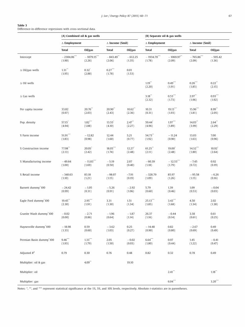
Table 3Difference-in-difference regressions with cross-sectional data.

(A) Combined oil & gas wells (B) Separate oil & gas wells

Δ Employment Δ Income ($mil) Δ Employment Δ Income ($mil)

Total Oil/gas Total Oil/gas Total Oil/gas Total Oil/gas

Intercept �2304.06*** �1079.15*** �843.49** �612.25 �1934.70*** �1069.97** �765.86*** �595.42(1.90) (2.26) (2.06) (1.35) (1.78) (2.09) (2.09) (1.36)

Δ Oil/gas wells 1.31** 0.32* 0.27*** 0.01(1.95) (2.88) (1.78) (1.53)

Δ Oil wells 1.19** 0.49*** 0.26*** 0.22**

(2.20) (1.91) (1.85) (2.15)

Δ Gas wells 3.18** 0.53*** 2.97** 0.93***

(2.32) (1.73) (1.96) (1.92)

Per capita income 33.82 20.76** 20.90** 10.62** 10.31 19.13*** 15.96*** 8.99**

(0.97) (2.03) (2.43) (2.36) (0.31) (1.93) (1.81) (2.05)

Pop. density 57.15* 1.82*** 13.55* 2.47** 59.44* 1.97*** 14.03** 2.64**

(4.94) (1.88) (4.10) (2.27) (4.96) (1.89) (3.99) (2.29)

% Farm income 51.91*** �12.82 12.44 5.21 54.73** �11.24 13.03 7.00(1.83) (0.98) (1.60) (0.77) (1.92) (0.90) (1.63) (0.96)

% Construction income 77.98** 20.05* 18.03*** 12.27* 61.25** 19.00* 14.52*** 10.92*

(2.13) (2.42) (1.74) (2.48) (2.11) (2.48) (1.80) (2.64)

% Manufacturing income �49.64 �11.83*** �5.19 2.07 �60.39 �12.53*** �7.45 0.92(1.00) (1.69) (0.50) (0.40) (1.18) (1.79) (0.72) (0.19)

% Retail income �340.63 83.18 �98.07 –7.91 �328.79 85.97 �95.58 �6.26(1.10) (1.21) (1.15) (0.19) (1.09) (1.26) (1.15) (0.16)

Barnett dummy*100 �24.42 �1.05 �5.26 �2.92 5.79 1.39 1.09 �0.04(0.99) (0.31) (0.91) (1.06) (0.60) (0.46) (0.53) (0.03)

Eagle Ford dummy*100 19.45** 2.95*** 3.31 1.51 25.13*** 3.43*** 4.50 2.02(2.30) (1.91) (1.30) (1.34) (1.85) (1.68) (1.34) (1.38)

Granite Wash dummy*100 �0.02 �2.71 �1.96 �1.87 26.37 �0.44 3.58 0.61(0.00) (0.86) (0.64) (1.14) (1.16) (0.14) (0.61) (0.25)

Haynesville dummy*100 �18.98 0.59 �3.62 0.25 �14.48 0.82 �2.67 0.49(1.33) (0.60) (1.03) (0.27) (0.90) (0.80) (0.69) (0.49)

Permian Basin dummy*100 9.46*** 1.33*** 2.05 �0.02 6.64*** 0.97 1.45 �0.41(1.93) (1.79) (1.50) (0.03) (1.80) (0.44) (1.22) (0.47)

Adjusted R2 0.79 0.30 0.76 0.48 0.82 0.32 0.78 0.49

Multiplier: oil & gas 4.09** 19.10

Multiplier: oil 2.41** 1.18**

Multiplier: gas 6.04*** 3.20***

Notes: *, **, and *** represent statistical significance at the 1%, 5%, and 10% levels, respectively. Absolute t-statistics are in parentheses.

J. Lee / Energy Policy 87 (2015) 60–71 67

below, this distinction is important for understanding develop-ments during the recent shale oil boom. For this reason, thoseresults in Table 2 simply serve as a robustness check for the em-pirical work to be presented below.

3.2. Cross-sectional data

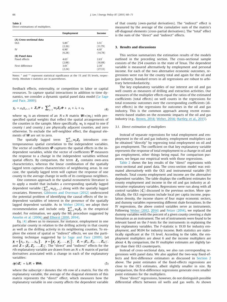
Table 3 shows the estimation results for the difference-in-dif-ference model specification as detailed in Section 2 above. To re-iterate, the dependent variables and the key explanatory variables(oil wells and gas wells) are measured relative to its historicaltrend over the 2000–2009 period. The key variables of interest arechanges (Δ) in the numbers of active oil wells and gas wells be-tween 2009 and 2014 relative to the 2000–2009 period. As dis-cussed above, the control variables are per capita personal income,population density, and the percentages of personal income in theagriculture, construction, manufacturing, and retail sectors.4

Regressions were applied to a cross-section of 254 Texas counties.Panel A of Table 3 contains estimates with the combined oil and

gas well counts as a single explanatory variable. The second andthird columns display, respectively, estimates for the regressionswith a county's total employment and employment in the oil andgas industry as alternative dependent variables. Except for the oiland gas income equation, the estimates of the intercept term arestatistically significant and negative, meaning that those localeconomies on average would have fared worse in 2014 than in 2009without oil and gas activities. According to the regression results,0.3 direct job was added when a county drilled one additional well,and the well brought one additional job across non-mining in-dustries. The corresponding estimates for the personal incomeequation in the fourth and fifth columns are weaker in statisticalsense. About $0.3 million in county total income was associated withone additional well. The estimate for income in the oil and gas in-dustry, however, is not statistically different from zero.

As explained in Section 2 above, the coefficient estimates forwell counts in the “total impact’ and “direct impact” regressionscan be used to calculate the employment and income multipliers.The bottom of panel A shows those multiplier estimates. For em-ployment, the multiplier of 4.09 (¼1.31/0.32) is comparable to the“implied” multipliers derived from some popular “impact” studies(e.g., IHS Global Insight, 2011) but smaller than other studies(e.g., PerrymanGroup, 2009; Scott, 2009). For income, however,the multiplier is not statistically meaningful.

Table 3 also lists coefficient estimates for the control variables.According to the estimates in panel A, local per capita income, po-pulation density and different aspects of industrial composition canmeaningfully explain employment growth. While drilling activityoccurred largely in rural areas, the results suggest that economicimpacts were larger in more developed communities with higherper capita income levels or higher population density. This impliesthat more developed areas, which tend to have more capital andlabor resources as well as more developed infrastructure, are moreready to reap the potential impact of a positive economic shock.

The estimates for the dummy variables suggest that oil and gaswells in the Eagle Ford and Permian Basin formations tended togenerate more jobs than other shale formations. The estimates forthe other regions are not significantly different from zero. Oil andgas production grew more rapidly in those two plays as a result ofnewly drilled wells, which were more productive than “legacy”wells more commonly found in other plays. By comparison, thelarger estimates for the Eagle Ford play reflect its more rapid

expansion in new wells. Moreover, in contrast to the Permian Basin,which had both conventional and unconventional wells, the EagleFord play had mostly unconventional or horizontal wells thatrequired more labor and capital to drill than conventional wells.

Instead of estimations with active oil and gas wells together,panel B of the table shows estimates for oil wells and gas wells asseparate explanatory variables. Gauged by the adjusted R2's, thespecification with those separate variables (panel B) providesmarginally more explanatory power than aggregating the twotypes of wells (panel A). The different economic impacts can berealized in the coefficient estimates. For oil wells, the four coeffi-cient estimates are close to those in panel A. For gas wells, how-ever, the corresponding point estimates are noticeably larger.

A comparison of the respective estimates for the two types ofwells indicates overall higher employment and income impactsfrom gas wells relative to oil wells. The bottom of panel B showsthe implied multipliers calculated from the coefficient estimatesfor wells. The employment multiplier is 6.04 for gas wells, com-pared with 2.41 for oil wells. The estimate for oil wells are com-parable to Weber's (2014) multiplier estimate for gas wells. In-terestingly, the corresponding multiplier in panel A is betweenthose two estimates. Similarly, the income multiplier for gas wellsis more than double that for oil wells. While those estimates areoverall comparable to the estimates from “direct” estimations inTable 2, the disparities between oil and gas wells are interesting.

The findings concerning higher economic impacts from gaswells than oil wells are, however, counterintuitive. Capitalspending is largely the same for developing a gas well as for an oilwell. However, developments in the output markets might haveaffected the average productivity of the two types of wells in Texasand thus their economic impact on local economies. Between 2009and mid-2014, crude oil prices followed a steady upward trendwhile natural gas prices remained relatively low. Meanwhile, thetotal number of new oil wells in Texas grew exponentially, and thenumber of new gas wells remained relatively steady or declined indifferent counties. Higher crude oil prices provided energy com-panies more incentives to drill new oil wells and refrack old wellsthat would otherwise be uneconomical to operate. On the con-trary, companies might have responded to low natural gas pricesby shutting down less productive gas wells and drilling only mostproductive wells. In this case, the average production rate of theexisting gas wells would increase.

The existing infrastructure across Texas might have also playeda role in the differential economic impacts between oil and gasproduction. Natural gas production across the shale formations hasleveraged some well-established networks of pipelines in thatregion. Similar logistical infrastructure was, however, lacking foroil production in the earlier years of the boom. Particularly for theEagle Ford play, much of the crude oil production was transportedin relatively long distance to refineries by trucks before the pipe-line capacity was developed to accommodate the productionsurge. Roadways and other logistical facilities were also less de-veloped in rural areas where much of the shale drilling activityoccurred. The potential impact of oil production might have beenlimited by such logistical disadvantages, which were more pre-valent during the beginning of the oil boom.

3.3. Dynamic panel models

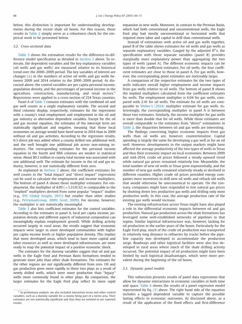
This subsection presents results of panel data regressions thatallow for dynamic interactions in economic variables in both timeand space. Table 4 shows the results of a panel regression modelrepresented by Eq. (3) above. The right hand side of the equationincludes a lagged dependent variable to capture the possiblelasting effects in economic outcomes. As discussed above, as aresult of the application of the fixed effects and first-difference

4 In preliminary analysis, we also included interaction terms and other controlvariables, such as a dummy variable for a county being part of a metro area. Theirestimates are not statistically significant and thus they are omitted in our reportedresults.

J. Lee / Energy Policy 87 (2015) 60–7168

estimators, the intercept and all time-invariant variables droppedout of the regressions. With six panels between 2009 and 2014,and a cross-section of 254 counties, the total number of observa-tions (N� T) is equal to 1524.

Panel A of Table 4 shows the estimates for lagged dependentvariable and the combined active oil and gas wells. The resultingmultipliers are similar between the two alternative regressiontechniques. In particular, the two implied employment multipliersslightly below 3.5 are comparable to the previous regressions es-timated with panel data (Tables 2 and 3). The income multiplierabout 4.0, by comparison, is relatively larger than the corre-sponding estimate in “direct” estimations (Table 2).

Panel B of Table 4 shows the corresponding estimation resultsfor treating active oil wells and gas wells as separate explanatoryvariables. As for the cross-sectional data in Table 3, the point es-timates for gas wells are appreciably larger than the correspondingestimates for oil wells, and the corresponding estimates for oil andgas wells together (panel A) fall between those separate estimates.

In addition to disparities between oil and gas wells, Table 4highlights the time and spatially lagged effects. The dynamic ef-fects in the time dimension are captured by the coefficients on thelagged dependent variables. Most estimates for those auto-regressive coefficients are close to one in the fixed-effects re-gressions with data in levels. The estimates are much smallerwhen the data take a first-differencing transformation. Based onthe Im et al. (2003) tests for a unit-root in panel data, the nullhypothesis of a unit root across all counties in the sample cannotbe rejected for the employment and income data. In light of thosetest results, the dependent variables are not stationary and thusregressions with data in levels may generate spurious estimates.

However, in Table 4, even the first-difference model ignores thepresence of spatial effects. To examine the statistical significanceof spatial effects, we applied Pesaran's (2004) test for cross-

sectional dependence (CD) in the residuals of regressions in Ta-ble 4. The CD statistics under the null of cross-sectional in-dependence are reported at the bottom of the two panels. The nullhypothesis is uniformly rejected in all cases, giving strong moti-vation for modeling spatial effects in the panel data models.

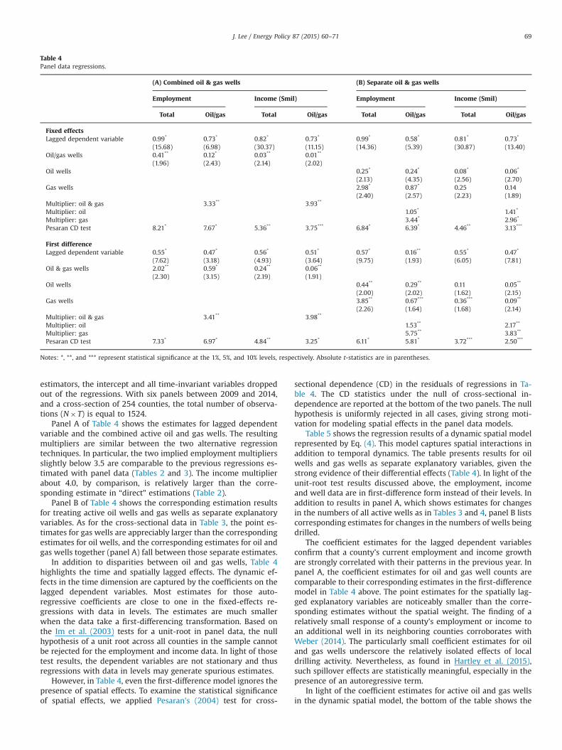
Table 5 shows the regression results of a dynamic spatial modelrepresented by Eq. (4). This model captures spatial interactions inaddition to temporal dynamics. The table presents results for oilwells and gas wells as separate explanatory variables, given thestrong evidence of their differential effects (Table 4). In light of theunit-root test results discussed above, the employment, incomeand well data are in first-difference form instead of their levels. Inaddition to results in panel A, which shows estimates for changesin the numbers of all active wells as in Tables 3 and 4, panel B listscorresponding estimates for changes in the numbers of wells beingdrilled.

The coefficient estimates for the lagged dependent variablesconfirm that a county’s current employment and income growthare strongly correlated with their patterns in the previous year. Inpanel A, the coefficient estimates for oil and gas well counts arecomparable to their corresponding estimates in the first-differencemodel in Table 4 above. The point estimates for the spatially lag-ged explanatory variables are noticeably smaller than the corre-sponding estimates without the spatial weight. The finding of arelatively small response of a county’s employment or income toan additional well in its neighboring counties corroborates withWeber (2014). The particularly small coefficient estimates for oiland gas wells underscore the relatively isolated effects of localdrilling activity. Nevertheless, as found in Hartley et al. (2015),such spillover effects are statistically meaningful, especially in thepresence of an autoregressive term.

In light of the coefficient estimates for active oil and gas wellsin the dynamic spatial model, the bottom of the table shows the

Table 4Panel data regressions.

(A) Combined oil & gas wells (B) Separate oil & gas wells

Employment Income ($mil) Employment Income ($mil)

Total Oil/gas Total Oil/gas Total Oil/gas Total Oil/gas

Fixed effectsLagged dependent variable 0.99* 0.73* 0.82* 0.73* 0.99* 0.58* 0.81* 0.73*

(15.68) (6.98) (30.37) (11.15) (14.36) (5.39) (30.87) (13.40)Oil/gas wells 0.41** 0.12* 0.03** 0.01**

(1.96) (2.43) (2.14) (2.02)Oil wells 0.25* 0.24* 0.08* 0.06*

(2.13) (4.35) (2.56) (2.70)Gas wells 2.98* 0.87* 0.25 0.14

(2.40) (2.57) (2.23) (1.89)Multiplier: oil & gas 3.33** 3.93**

Multiplier: oil 1.05* 1.41*

Multiplier: gas 3.44* 2.96*

Pesaran CD test 8.21* 7.67* 5.36** 3.75*** 6.84* 6.39* 4.46** 3.13***

First differenceLagged dependent variable 0.55* 0.47* 0.56* 0.51* 0.57* 0.16** 0.55* 0.47*

(7.62) (3.18) (4.93) (3.64) (9.75) (1.93) (6.05) (7.81)Oil & gas wells 2.02** 0.59* 0.24** 0.06**

(2.30) (3.15) (2.19) (1.91)Oil wells 0.44** 0.29** 0.11 0.05**

(2.00) (2.02) (1.62) (2.15)Gas wells 3.85** 0.67*** 0.36*** 0.09**

(2.26) (1.64) (1.68) (2.14)Multiplier: oil & gas 3.41** 3.98**

Multiplier: oil 1.53** 2.17**

Multiplier: gas 5.75** 3.83**

Pesaran CD test 7.33* 6.97* 4.84** 3.25* 6.11* 5.81* 3.72*** 2.50***

Notes: *, **, and *** represent statistical significance at the 1%, 5%, and 10% levels, respectively. Absolute t-statistics are in parentheses.

J. Lee / Energy Policy 87 (2015) 60–71 69

implications of the dynamic effects in both spatial and time di-mensions. In the context of spatial dynamics, a “total effect”coefficient captures a county’s response of one additional well inits area as well as its adjacent counties. According to those mea-sures computed using the procedure explained in Section 2.4above, the employment impact of one county’s oil and gas wellsincreases by about 10% when the “indirect spatial effect” of othercounties are also taken into consideration. This finding is in linewith the results reported by Hartley et al. (2015) for gas produc-tion. The extent of such neighborhood effects is even larger (over25%) for income.

The bottom part of Table 5 lists measures of the short-run, orimpact, multipliers using the ratios of the respective “total effect”coefficients. The identified spatial effects raise in varying degreesthe “total” impacts of oil and gas wells on both the region as awhole as well as the oil and gas industry. The resulting short-runmultipliers are comparable to the corresponding estimates in Ta-ble 4 (first-difference model). Measures of the regional economicimpacts of oil and gas extraction are even larger if the temporaleffect is also taken into consideration. As explained in Section 2.4above, the long-run multipliers can be computed using the “totaleffect” coefficients and the autoregressive coefficients.

The multiplier measures in Table 5 suggest that one job in oilextraction generates another 1.65 jobs in other industries in thelong run. By comparison, the long-run economic impacts are largerfor gas wells than for oil wells. One additional active gas wellsupports a total of 3.65 jobs within a county in the short run, with0.68 job directly associated with drilling and extraction. Suchfindings corroborate with the results in Hartley et al. (2015). Thelong-run multiplier is 8.42 for employment and 5.24 for income.

As an alternative to changes in the numbers of active wells,panel B of Table 5 lists estimation results using changes in thenumbers of new wells drilled as the key explanatory variables.5

Compared with corresponding estimates in panel A, the estimatesfor employment and income impacts are much higher when thedata of newly drilled wells are used. In line with the engineering-based workforce assessments reported by Brundage et al. (2011)and Marcellus Shale Education & Training Center (2009), the es-timate for the “direct” employment impact is nearly 10 local jobsfor drilling one additional gas well within a particular county.About 5 more jobs are created among other industries in thatcounty. The inclusion of neighborhood effects captured by thespatially lagged term generates another 0.42 job.

Similar to the results for employment, the estimated impacts ofdrilling one additional well on income are larger than their cor-responding estimates using the numbers of all active wells.However, in contrast to those estimates in panel A, the coefficientestimates are similar between oil and gas wells because there islittle difference between the construction as well as drilling thesetwo types of wells. This implies that their differences are attribu-table mainly to differences during the production phase of thosewells (recall Section 3.2). With similar coefficient estimates for theeconomic outcomes between oil and gas wells, the resultingmultipliers for gas wells are now comparable to those for oil wells.

4. Conclusions and policy implications

In this paper, we have estimated the impact of oil and gas ex-traction on local economies during the most recent Texas shale oilboom period between 2009 and 2014. We first applied conven-tional cross-section and panel data models to county-level em-ployment and income data. We first found that local communitiesin Texas would have lost jobs and income during that period if notfor shale energy boom.

We also found evidence in support of larger economic impactsfrom gas wells than oil wells. One interpretation for this findingstems from the different price dynamics between oil and naturalgas markets during the oil boom period. This echoed the morerecent episode of falling oil prices beginning in late 2014. In re-sponse to developments in oil markets, the number of operating

Table 5Dynamic spatial model regression results.

(A) Active wells (B) Newly drilled wells

Δ Employment Income Δ Employment Δ Income

Total Oil/gas Total Oil/gas Total Oil/gas Total Oil/gas

Regression estimatesLagged dependent variable 0.54* 0.27* 0.53** 0.42* 0.67* 0.27* 0.53* 0.41*

(7.03) (2.60) (2.41) (10.99) (7.30) (2.59) (2.47) (10.83)Δ Oil wells 0.39** 0.24** 0.08** 0.03** 14.61* 8.07* 2.10*** 2.12**

(2.18) (2.11) (1.92) (2.03) (2.75) (3.64) (1.74) (1.98)Δ Gas wells 3.26** 0.62*** 0.34** 0.09** 15.18*** 9.84* 2.24* 1.20**

(2.13) (1.86) (2.06) (1.99) (1.92) (5.18) (6.11) (2.26)W� (Δ Oil wells) 0.05** 0.03*** 0.03** 0.01** 0.28* 0.15* 0.23*** 0.05***

(2.06) (1.87) (2.07) (2.02) (2.59) (3.21) (1.77) (1.86)W� (Δ Gas wells) 0.39** 0.06** 0.11** 0.02*** 0.42*** 0.22* 0.37* 0.03**

(2.24) (1.96) (1.98) (1.86) (1.87) (5.46) (5.89) (2.20)Log likelihood �8405.06 �7509.13 �7130.58 �6431.72 �8459.83 �7556.26 �7175.66 �6479.70Multiplier effectsOil wells

Total effect (coefficient) 0.44** 0.26** 0.11** 0.05** 14.89* 8.22* 2.33** 2.17**

Short run multiplier 1.68** 2.39** 1.81* 2.00**

Long run multiplier 2.65** 2.99** 3.99* 2.51**

Gas wellsTotal effect (coefficient) 3.65** 0.68** 0.45*** 0.11** 15.60** 10.05* 2.61* 1.22**

Short run multiplier 5.35** 4.19** 1.55* 2.13**

Long run multiplier 8.42** 5.24** 3.41* 2.68**

Notes: *, **, and *** represent statistical significance at the 1%, 5%, and 10% levels, respectively. Absolute t-statistics are in parentheses.

5 Only the current values of well counts are included in estimations as pastvalues have been found to be not statistically significant. Similar estimation resultsfor newly drilled wells have been obtained for the models presented in Tables 3 and4, but they are not reported here in order to save space.

J. Lee / Energy Policy 87 (2015) 60–7170

oil rigs fell precipitously without corresponding reductions incrude oil production. As least productive oil wells were shut down,the average production rate of the remaining oil wells and theiraverage income impact rose as a result.

Despite relatively robust estimates from the basic panel datamodels, we investigated the roles of temporal and spatial effects inlocal economies within a dynamic spatial framework. The allow-ance for spatial interactions across counties raises the estimates ofoil and gas wells’ total economic impacts in Texas. Measures of theemployment and income effects rise further when the time dy-namic effect is also taken into consideration.

Policymakers typically rely on input–output-based analysis toassess how changes of an industry affect local economies. Suchmethodology has been subject to criticisms in the academic litera-ture (e.g., Carlson and Spencer, 1975; Lee, 2015). Similarly, consultingreports that have been adopted for designing public policy targetingrecent development in the shale industry are found to grosslyoverstate the regional economic effects of that industry in variousshale gas formations (e.g., Kinnaman, 2011; Weber, 2012; Paredeset al., 2015). We have shown that the total regional employmentimpact of oil and gas activity could be as much as 10% larger if weallow for economic interactions among counties. This neighborhoodeffect is even greater when economic impact is measured by incomeinstead of employment. Moreover, in line with previous findings(e.g., Brundage et al., 2011; Marcellus Shale Education & TrainingCenter, 2009), we have found remarkably larger economic impactsfrom newly drilled wells than legacy wells, highlighting the chan-ging role of a particular well in different stages.

Our finding of spatial effects in oil and gas activity has a directbearing on public policy toward sustainable regional economicdevelopment. For instance, local governments should monitorclosely the economies of their neighboring communities in addi-tion to their own economies. While more developed local areastend to be more ready to reap the full impact of a positive eco-nomic shock, state or federal governments can boost the extent ofeconomic impacts at a regional level by promoting more economicinteractions among local communities. Among other things, lo-gistical networks might have played a role in explaining the dif-ferential impacts of oil and gas wells during the recent shale boom.Geographical spillover or feedback effects may expand with amore developed infrastructure network that facilities resourcemobility and other logistics.

Despite the consideration of regional spillover effects and long-run dynamics, the estimates of employment and income multi-pliers remain below corresponding multipliers implied by popularinput–output based studies (e.g., PerrymanGroup, 2009; Scott,2009). Those input–output based studies analyze the regionaleconomic effects of all developments related to oil and gas drillingand production instead of focusing on changes in the oil and gasindustry alone. Discrepancies with our findings would thereforereflect in part the significance of factors other than the industrymultipliers embedded in input–output models, including royaltyand lease payments, and public infrastructure spending associatedwith development of that industry.

Acknowledgment

The author acknowledges financial support from the 2013-14Texas Research Development Funds (No. 1410173). This paper and itsempirical work also benefitted from helpful comments and sug-gestions of three journal reviewers.

References

Anselin, L., Le Gallo, J., Jayet, H., 2006. Spatial panel econometrics. In: Matyas, L.,Sevestre, P. (Eds.), The Econometrics of Panel Data, Fundamentals and RecentDevelopments in Theory and Practice, 3rd ed. Kluwer, Dordrecht, pp. 901–969.

Brown, J.P., 2014. Production of national gas from shale in local economies: a re-source blessing or curse? Federal Reserve Bank of Kansas City. Econ. Rev. 99,5–33.

Brundage, T.L., Jacquet, J., Kelsey, T.W., Lobdell, J., Lorson, J.F., Michael, L.L., Murphy,T.B., 2011. Pennsylvania Statewide Marcellus Shale Workforce Needs. MarcellusShale Education and Training Center, Williamsport.

Dwyer, L., Forsyth, P., Madden, J., Spurr, R., 2000. Economic impacts of inboundtourism under different assumptions regarding the macroeconomy. Curr. IssuesTour. 3, 325–339.

Carlson, K.M., Spencer, R.W., 1975. Crowding out and its critics. Fed. Reserve BankSt. Louis Rev. 57, 2–17.

Elhorst, J.P., 2010. Spatial panel data models. In: Fischer, M.M., Getis, A. (Eds.),Handbook of Applied Spatial Analysis: Software Tools, Methods and Applica-tions, pp. 377–408.

Elhorst, J.P., 2014. Spatial Econometrics, From Cross-Sectional Data to Spatial Panels.Springer, New York.

Ewing, B.T., Marshall, C.W., McInturff, T., McInturff, R.N., 2014. Economic Impact ofthe Permian Basin’s Oil & Gas Industry. Report Prepared for Permian BasinPetroleum Association, Texas Tech University.

Fetzer, T., 2014. Fracking Growth, Center for Economic Performance, DiscussionPaper, No. 1278.

Gibbsons, S., Overman, H.G., 2012. Mostly pointless spatial econometrics? J. Reg. Sci.52, 172–191.

Hartley, P.R., Medlock, K.B., Temzelides, T., Zhang, X., 2015. Local employment im-pact from competing energy sources: Shale gas versus wind generation inTexas. Energy Econ. 49, 610–619.

Hsiao, C., 2003. Analysis of Panel Data, 2nd ed. Cambridge University Press,Cambridge.

Hsiao, C., Pesaran, M., Tahmiscioglu, A., 2002. Maximum likelihood estimation offixed effects dynamic panel data models covering short time periods. J. Econ-om. 109, 107–150.

IHS Global Insight, 2011. The Economic and Employment Contributions of Shale Gasin the United States. Report Prepared for American's Natural Gas Alliance.

Im, K.S., Pesaran, M.H., Shin, Y., 2003. Testing for unit roots in heterogeneous pa-nels. J. Econom. 115, 53–74.

Kaiser, M.J., 2012. Haynesville shale play economic analysis. J. Pet. Sci. Eng. 82–83,75–89.

Kinnaman, T.C., 2011. The economic impact of shale gas extraction: a review ofexisting studies. Ecol. Econ. 70, 1243–1249.

Le Sage, J.P., Pace, R.K., 2009. Introduction to Spatial Econometrics. Taylor andFrancis/CRC Press, New York.

Lee, J., 2015. The Regional Economic Effects of Military Base Realignments andClosures, Defence and Peace Economics, Forthcoming.

Paredes, D., Komarek, T., Loveridge, S., 2015. Income and employment effects ofshale gas extraction windfalls: evidence from the Marcellus region. EnergyEcon. 47, 112–120.

Marcellus Shale Education & Training Center, 2009. Marcellus Shale WorkforceNeeds Assessment.

PerrymanGroup, 2009. An Enduring Resource: A Perspective on the Past, Present,and Future Contribution of the Barnett Shale to the Economy of Fort Worth andthe Surrounding Area.

PerrymanGroup, 2011. The Impact of the Barnett Shale on Business Activity in theSurrounding Region and Texas: an Assessment of the First Decade of ExtensiveDevelopment. Report Prepared for the Fort Worth Chamber of Commerce.

Pesaran, M., 2004. General Diagnostic Tests for Cross Section Dependence in Panels.Cambridge Working Papers in Economics, No. 435. University of Cambridge.

Scott, L.C., 2009. The Economic Impact of the Haynesville Shale on the LouisianaEconomy in 2008.

Tunstall, T., 2011. Economic Impact of the Eagle Ford Shale. Center for Communityand Business Research at the University of Texas at San Antonio's Institute forEconomic Development.

Tunstall, T., 2012. Economic Impact of the Eagle Ford Shale. Center for Communityand Business Research at the University of Texas at San Antonio's Institute forEconomic Development.

Tunstall, T., 2013. Economic Impact of the Eagle Ford Shale. Center for Communityand Business Research at the University of Texas at San Antonio's Institute forEconomic Development.

Tunstall, T., 2014. Economic Impact of the Eagle Ford Sshale. Center for Communityand Business Research at the University of Texas at San Antonio’s Institute forEconomic Development.

U.S. Energy Information Administration, 2013. Drilling Often Results in Both Oil andNatural Gas Production, Today in Energy, October 29, 2013. Available online at:⟨http://www.eia.gov/todayinenergy/detail.cfm?id¼13571⟩. (accessed 14.02.15.).

Weber, J.G., 2012. The effect of a natural gas boom on employment and income inColorado, Texas, and Wyoming. Energy Econ. 34, 1580–1588.

Weber, J.G., 2014. A Decade of natural gas development: the makings of a resourcecurse? Resour. Energy Econ. 37, 168–183.

J. Lee / Energy Policy 87 (2015) 60–71 71