the looks of an odour - visualising neural odour response patterns in real time

RESEARCH Open Access

The looks of an odour - Visualising neural odourresponse patterns in real timeMartin Strauch1,2*, Clemens Müthing1, Marc P Broeg1, Paul Szyszka2, Daniel Münch2, Thomas Laudes2,Oliver Deussen1, Cosmas Giovanni Galizia2, Dorit Merhof1

From 2nd IEEE Symposium on Biological Data VisualizationSeattle, WA, USA. 14-15 October 2012

Abstract

Background: Calcium imaging in insects reveals the neural response to odours, both at the receptor level on theantenna and in the antennal lobe, the first stage of olfactory information processing in the brain. Changes ofintracellular calcium concentration in response to odour presentations can be observed by employing calcium-sensitive, fluorescent dyes. The response pattern across all recorded units is characteristic for the odour.

Method: Previously, extraction of odour response patterns from calcium imaging movies was performed offline,after the experiment. We developed software to extract and to visualise odour response patterns in real time. Anadaptive algorithm in combination with an implementation for the graphics processing unit enables fastprocessing of movie streams. Relying on correlations between pixels in the temporal domain, the calcium imagingmovie can be segmented into regions that correspond to the neural units.

Results: We applied our software to calcium imaging data recorded from the antennal lobe of the honeybee Apismellifera and from the antenna of the fruit fly Drosophila melanogaster. Evaluation on reference data showed resultscomparable to those obtained by previous offline methods while computation time was significantly lower.Demonstrating practical applicability, we employed the software in a real-time experiment, performingsegmentation of glomeruli - the functional units of the honeybee antennal lobe - and visualisation of glomerularactivity patterns.

Conclusions: Real-time visualisation of odour response patterns expands the experimental repertoire targeted atunderstanding information processing in the honeybee antennal lobe. In interactive experiments, glomeruli can beselected for manipulation based on their present or past activity, or based on their anatomical position. Apart fromsupporting neurobiology, the software allows for utilising the insect antenna as a chemosensor, e.g. to detect or toclassify odours.

IntroductionMotivationOdours take many shapes, and equipped with an insectbrain and a neuroimaging device one can reveal theseshapes, turning chemicals into patterns and images.In the conference version of this paper [1], we have

introduced an imaging system that can read out andprocess brain activity in real time, making the neural

representations of odours accessible. The biological moti-vation is that access to ongoing brain activity is the basisfor analysing storage and processing of information inthe brain, observing, for example, the activity patterns inresponse to odour stimulation. In particular, transform-ing odours into patterns and images does not only benefitbasic neuroscientific research: It also allows us to utilise aliving organism with highly sensitive olfactory organs as achemosensor, where the patterns and the distancesbetween them contain information about odour identityand dissimilarity.

* Correspondence: [email protected] Center for Interactive Data Analysis, Modelling and VisualExploration (INCIDE), University of Konstanz, 78457 Konstanz, GermanyFull list of author information is available at the end of the article

Strauch et al. BMC Bioinformatics 2013, 14(Suppl 19):S6http://www.biomedcentral.com/1471-2105/14/S19/S6

© 2013 Strauch et al; licensee BioMed Central Ltd. This is an open access article distributed under the terms of the Creative CommonsAttribution License (http://creativecommons.org/licenses/by/2.0), which permits unrestricted use, distribution, and reproductionin any medium, provided the original work is properly cited. The Creative Commons Public Domain Dedication waiver(http://creativecommons.org/publicdomain/zero/1.0/) applies to the data made available in this article, unless otherwise stated.

mailto:[email protected]

http://creativecommons.org/licenses/by/2.0

http://creativecommons.org/publicdomain/zero/1.0/

We consider two application scenarios for real-timevisualisation of odours using insect brains. In insects, thefirst stage of odour perception is formed by the odourreceptor neurons on the antenna. Here, we utilise cal-cium imaging to record from the antenna of the fruit flyDrosophila melanogaster. While such data provides onlylittle information about signal processing in the brain,receptor neurons on the antenna are easy to accessexperimentally and they are excellent chemosensingdevices. As such they are a promising alternative to artifi-cial chemosensors, also referred to as electronic noses(see e.g. [2-5]), that find application in environmentalmonitoring, chemical industry or security.The second stage of odour processing in the insect

brain is the antennal lobe (AL), a dedicated olfactory cen-ter where odours are represented by activity patterns ofneural units, the so-called glomeruli [6]. A network ofinterneurons connects the glomeruli, and unravelling thefunction of this network in processing odour informationis the topic of ongoing research. The honeybee AL is anestablished model for studying odour learning and mem-ory [7], and neuropharmacological tools [8,9] have beendeveloped to manipulate the network of interneurons.Here, the real-time aspect of odour visualisation is espe-cially relevant as decisions can be based on prior activity,targeting e.g. glomeruli that have previously been part ofa response pattern.From an image processing perspective, both application

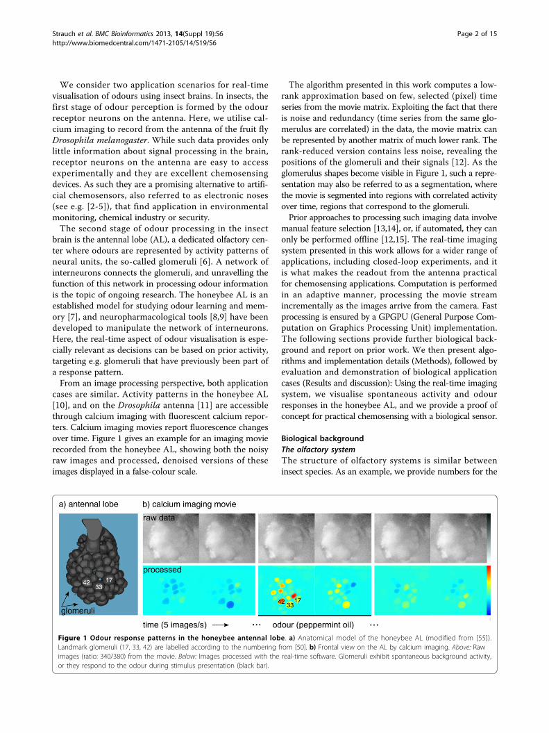
cases are similar. Activity patterns in the honeybee AL[10], and on the Drosophila antenna [11] are accessiblethrough calcium imaging with fluorescent calcium repor-ters. Calcium imaging movies report fluorescence changesover time. Figure 1 gives an example for an imaging movierecorded from the honeybee AL, showing both the noisyraw images and processed, denoised versions of theseimages displayed in a false-colour scale.

The algorithm presented in this work computes a low-rank approximation based on few, selected (pixel) timeseries from the movie matrix. Exploiting the fact that thereis noise and redundancy (time series from the same glo-merulus are correlated) in the data, the movie matrix canbe represented by another matrix of much lower rank. Therank-reduced version contains less noise, revealing thepositions of the glomeruli and their signals [12]. As theglomerulus shapes become visible in Figure 1, such a repre-sentation may also be referred to as a segmentation, wherethe movie is segmented into regions with correlated activityover time, regions that correspond to the glomeruli.Prior approaches to processing such imaging data involve

manual feature selection [13,14], or, if automated, they canonly be performed offline [12,15]. The real-time imagingsystem presented in this work allows for a wider range ofapplications, including closed-loop experiments, and itis what makes the readout from the antenna practicalfor chemosensing applications. Computation is performedin an adaptive manner, processing the movie streamincrementally as the images arrive from the camera. Fastprocessing is ensured by a GPGPU (General Purpose Com-putation on Graphics Processing Unit) implementation.The following sections provide further biological back-ground and report on prior work. We then present algo-rithms and implementation details (Methods), followed byevaluation and demonstration of biological applicationcases (Results and discussion): Using the real-time imagingsystem, we visualise spontaneous activity and odourresponses in the honeybee AL, and we provide a proof ofconcept for practical chemosensing with a biological sensor.

Biological backgroundThe olfactory systemThe structure of olfactory systems is similar betweeninsect species. As an example, we provide numbers for the

Figure 1 Odour response patterns in the honeybee antennal lobe. a) Anatomical model of the honeybee AL (modified from [55]).Landmark glomeruli (17, 33, 42) are labelled according to the numbering from [50]. b) Frontal view on the AL by calcium imaging. Above: Rawimages (ratio: 340/380) from the movie. Below: Images processed with the real-time software. Glomeruli exhibit spontaneous background activity,or they respond to the odour during stimulus presentation (black bar).


of 15

honeybee Apis mellifera. On the antenna, approximately60,000 odour receptor neurons interact physically with theodour molecules. These 60,000 neurons converge onto 160glomeruli in the AL, where each glomerulus collects inputfrom receptor neurons of one type. The glomeruli are bun-dles of synapses and appear as spherical structures with adiameter between 30 and 50 µm. At the AL stage, eachodour is represented by an activity pattern across the 160glomeruli. Further upstream, this compact representationis widened again, as the projection neurons project fromthe glomeruli to approximately 160,000 Kenyon cells, astage where odours are represented by sparser, high-dimensional patterns. [16,17] While implementation detailsdiffer between species, the combinatorial coding of odoursby activity patterns across glomeruli, in the insect AL or inthe vertebrate olfactory bulb, is a common feature of olfac-tory systems and can also be found in humans [18].Odour responses in the ALCalcium imaging using calcium-sensitive fluorescent dyesgrants us access to the odour response patterns in the ALof the honeybee Apis mellifera [10]. These odour responsepatterns reflect the response properties of the odourreceptor neurons, as well as additional processing thattakes place in the AL. Interneurons connecting the glo-meruli perform further computations such as contrastenhancement [10].For an example of odour response patterns in the hon-

eybee AL, see Figure 1. The activity pattern of glomeruli(between ca. 20 and 40 of the glomeruli are visible in animaging movie) fluctuates at a low amplitude when noodour is present. After stimulation with an odour (indi-cated by the black bar), glomeruli exhibit individualresponses to the odour. As a result, the activity patternacross glomeruli changes in way that is characteristic forthe odour. The same odour elicits a similar pattern in dif-ferent bees [6].There is evidence that not only the identity of a parti-

cular odour is encoded by the corresponding glomerularresponse pattern, but that also chemical [19] and per-ceptual [20] (dis)similarity are reflected by the (dis)simi-larity of response patterns, suggesting that responsepattern space is a rather faithful representation of che-mical space.Odour responses on the antennaGlomerular response patterns, as measured in the honeybeerecordings from this work, are the output signal of the AL,i.e. they are the result of integrating all receptor neurons ofone type and of further processing that occurs in the ALnetwork of interneurons. While odour coding is improvedafter this processing [21], the results of this paper suggestthat chemical identity and (dis)similarity can alreadybe inferred from receptor neuron signals recorded on theantenna, the earliest stage in the olfactory processing

pipeline where response patterns are easily accessible with-out dissecting the brain.In this work, antenna data was recorded in the fruit fly

Drosophila melanogaster. The genetic tools that are avail-able for Drosophila make it possible to express a calciumreporter directly in the receptor neurons on the antenna.Instead of expressing the reporter in cells of one type, ashas been done before [11], the approach pursued here isto measure signals from a large set of different receptorcells that all express the general olfactory co-receptorOrco that these cells bear in addition to a specific odourreceptor. This allows us to measure broad odourresponse patterns across many receptors. The segmenta-tion approach presented in this paper is then used to toextract individual response units from the imaging moviebased on their differential responses to a series of 32 dif-ferent odours.

Related workComputational approaches to analysing imaging data canbe classified as being either synthetic or analytic. In asynthetic approach, similar to common procedures foranalysing fMRI data, Stetter et al. [22] have set up non-linear functions that they fitted to the individual (pixel)time series of the imaging movie. These functions canaccount e.g. for dye bleaching over time and for differentneural signal components. Rather than performing bot-tom-up synthetic reconstruction of the imaging movie,analytic approaches decompose (bottom-down) themovie into factors. These are matrix factorisation ordecomposition methods that exist in many different fla-vours, e.g. the well-known Principal Component Analysis(PCA). In particular Independent Component Analysis(ICA) has found widespread application on imaging data[15,23-26]. While ICA can be seen as a matrix decompo-sition method, the motivating paradigm for ICA is sourceseparation. Under the assumption that there are underly-ing source signals that are statistically independent (andnon-Gaussian), ICA algorithms (e.g. [27]) aim at recover-ing or separating these source signals on sample datawhere the sources appear in mixed form, e.g. neural sig-nals mixed with measurement artifacts.A recent convex analysis approach [12] (s.a. Methods),

performs a factorisation of the movie matrix based onextremal column vectors from the boundary of the convex/conical hull of the data. Under the assumption that puresignal sources are present in the data, finding the extremalcolumn vectors identifies these pure signal sources.Traditionally, calcium imaging data from the insect AL

has been processed by semi-automatic methods that per-form e.g. image smoothing, but that still require humaninteraction to select regions of interest [13,14]. From themethods listed above, those that require human interaction


of 15

appear less suited for real-time processing on a moviestream. So far, no real-time implementations of the com-putational approaches exist, the software implementationsfrom [12,15] being only suited for offline data analysis.

MethodsBiological methodsImaging the honeybee ALFor honeybees, it has been shown that projection neu-ron firing rate correlates with changes in intracellularcalcium [28]. Staining with calcium-sensitive fluorescentdyes and excitation of the dyes with UV-light thus leadsto a good proxy signal for brain activity [29].Calcium imaging with forager honeyebees (Apis melli-

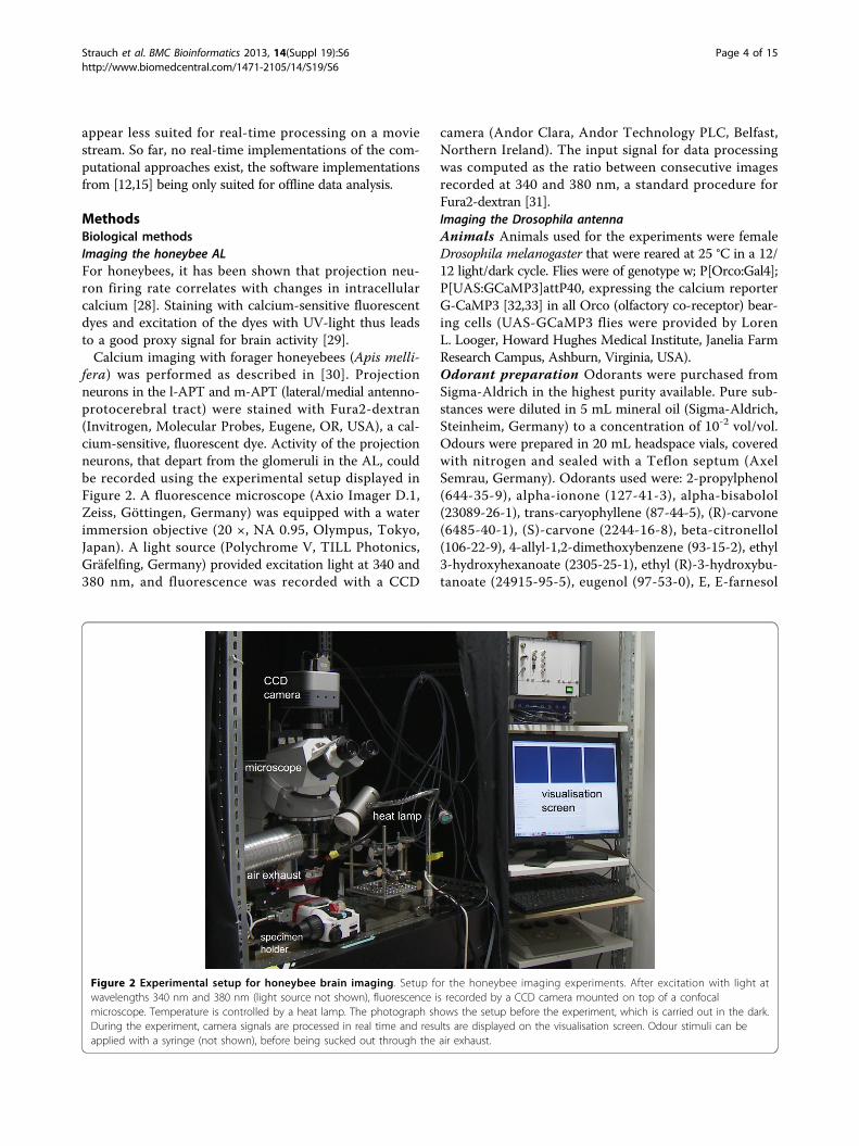
fera) was performed as described in [30]. Projectionneurons in the l-APT and m-APT (lateral/medial antenno-protocerebral tract) were stained with Fura2-dextran(Invitrogen, Molecular Probes, Eugene, OR, USA), a cal-cium-sensitive, fluorescent dye. Activity of the projectionneurons, that depart from the glomeruli in the AL, couldbe recorded using the experimental setup displayed inFigure 2. A fluorescence microscope (Axio Imager D.1,Zeiss, Göttingen, Germany) was equipped with a waterimmersion objective (20 ×, NA 0.95, Olympus, Tokyo,Japan). A light source (Polychrome V, TILL Photonics,Gräfelfing, Germany) provided excitation light at 340 and380 nm, and fluorescence was recorded with a CCD

camera (Andor Clara, Andor Technology PLC, Belfast,Northern Ireland). The input signal for data processingwas computed as the ratio between consecutive imagesrecorded at 340 and 380 nm, a standard procedure forFura2-dextran [31].Imaging the Drosophila antennaAnimals Animals used for the experiments were femaleDrosophila melanogaster that were reared at 25 °C in a 12/12 light/dark cycle. Flies were of genotype w; P[Orco:Gal4];P[UAS:GCaMP3]attP40, expressing the calcium reporterG-CaMP3 [32,33] in all Orco (olfactory co-receptor) bear-ing cells (UAS-GCaMP3 flies were provided by LorenL. Looger, Howard Hughes Medical Institute, Janelia FarmResearch Campus, Ashburn, Virginia, USA).Odorant preparation Odorants were purchased fromSigma-Aldrich in the highest purity available. Pure sub-stances were diluted in 5 mL mineral oil (Sigma-Aldrich,Steinheim, Germany) to a concentration of 10-2 vol/vol.Odours were prepared in 20 mL headspace vials, coveredwith nitrogen and sealed with a Teflon septum (AxelSemrau, Germany). Odorants used were: 2-propylphenol(644-35-9), alpha-ionone (127-41-3), alpha-bisabolol(23089-26-1), trans-caryophyllene (87-44-5), (R)-carvone(6485-40-1), (S)-carvone (2244-16-8), beta-citronellol(106-22-9), 4-allyl-1,2-dimethoxybenzene (93-15-2), ethyl3-hydroxyhexanoate (2305-25-1), ethyl (R)-3-hydroxybu-tanoate (24915-95-5), eugenol (97-53-0), E, E-farnesol

Figure 2 Experimental setup for honeybee brain imaging. Setup for the honeybee imaging experiments. After excitation with light atwavelengths 340 nm and 380 nm (light source not shown), fluorescence is recorded by a CCD camera mounted on top of a confocalmicroscope. Temperature is controlled by a heat lamp. The photograph shows the setup before the experiment, which is carried out in the dark.During the experiment, camera signals are processed in real time and results are displayed on the visualisation screen. Odour stimuli can beapplied with a syringe (not shown), before being sucked out through the air exhaust.


of 15

(106-28-5), geraniol (106-24-1), heptyl acetate (112-06-1),hexyl acetate (142-92-7), hexyl butyrate (2639-63-6),isoamyl tiglate (41519-18-0), iso-eugenol (97-54-1),4-isopropylbenzaldehyde (122-03-2), linalool (78-70-6),methyl 3-hydroxy hexanoate (21188-58-9), 4-methoxy-benzaldehyde (123-11-5), methyl jasmonate (39924-52-2),(1R)-myrtenal (564-94-3), nonanal (124-19-6), nonanone(821-55-6), octyl acetate (112-14-1), phenylacetaldehyde(122-78-1), 4-hydroxy-3-methoxybenzaldehyde (121-33-5),gamma-propyl-gamma-butyrolactone (105-21-5), alpha-terpineol (10482-56-1) and alpha-thujone (546-80-5).Stimulus application A computer-controlled autosam-pler (PAL, CTC Switzerland) was used for automaticodour application. 2 mL of headspace was injected in two1 mL portions at timepoints 6 s and 9 s with an injectionspeed of 1 mL/s into a continuous flow of purified airflowing at 60 mL/min. The stimulus was directed to theantenna of the animal via a Teflon tube (inner diameter1 mm, length 38 cm).The interstimulus interval was approximately 2 min.

Solvent control and reference odorants (heptyl acetateand nonanone) were measured after every five stimuli(one block). The autosampler syringe was flushed withpurified air for 30 s after each injection and washed withpentane (Merck, Darmstadt, Germany) automaticallyafter each block of stimuli.Calcium imaging Calcium imaging was performed with afluorescence microscope (BX51WI, Olympus, Tokyo,Japan) equipped with a 50x air lens (Olympus LM Plan FI50x/0.5). A CCD camera (TILL Imago, TILL Photonics,Gräfelfing, Germany) was mounted on the microscope,recording with 4x4 pixel on-chip binning, resulting in160x120 pixel sized images. For each stimulus, recordingsof 20 s at a rate of 4 Hz were performed using TILL Vision(TILL Photonics, Gräfelfing, Germany).A monochromator (Polychrome II, TILL Photonics,

Gräfelfing, Germany) produced excitation light of 470 nmwavelength which was directed onto the antenna via a500 nm low-pass filter and a 495 nm dichroic mirror.Emission light was filtered through a 505 nm high-passemission filter.Flies were mounted in custom-made holders, placed

with their neck into a slit. The head was fixed to theholder with a drop of low-melting wax. A half electronmicroscopy grid was placed on top of the head, stabilisingthe antenna by touching the 2nd, but not the 3rd antennalsegment.

Matrix factorisation frameworkWe first describe the general matrix factorisation frame-work for imaging movies. The framework is illustrated inFigure 3. An imaging movie can be cast into matrix formby flatting the two-dimensional images with n pixels intorow vectors of length n. The movie matrix Am × n has

m time points and n pixels. The rows of the movie matrix,A(i), contain images or time points. The columns, A(j),contain pixels or time series.We consider a factorisation of A into a matrix Tm × k of

k time series and a matrix Sk × n of k images, wherek n, m. This provides a low-rank approximation Ak tothe original matrix A:

Am×n : Ak = Tm×kSk×n =k∑

r=1

TIrSrJ (1)

In imaging movies, all pixels that report the signal of thesame glomerulus are correlated with each other (apartfrom the noise), which causes redundancy in A. It is thuspossible to construct a good approximation with small k,such that‖ A − TS ‖ is small.The optimal rank-k approximation with respect to the

aforementioned norm difference can be computed withPrincipal Component Analysis (PCA) [34]. However, theimages in S computed by PCA are not sparse, withalmost all pixels being different from zero [12]. Theimages in S, and the corresponding time series in T, canthus hardly be interpreted as the boundaries or the signal,respectively, of a particular neural unit. By definition,principal components need to be orthogonal to eachother, which often prevents them from closely fitting theunderlying source signals.Ideally, as in the example from Figure 3, the images in

S should be sparse, with only few pixels being differentfrom zero. The k time series in T should be selected fromk different glomeruli with the corresponding rows in thesparse S marking positions and boundaries of the glomer-uli. We have shown in [12] that there is a method, theconvex cone algorithm, that can achieve a factorisationwith such favourable properties on imaging data.

Convex cone algorithmIn this section, we review the convex cone algorithm from[12]. It is based on a non-negative mixture model for ima-ging data:

A = TS0+ + N (2)

The movie matrix A can be described by basis time ser-ies in T that are combined by coefficients in the non-negative matrix S0+. Residual noise is accounted for by N.We assume that the columns A(j) of the movie matrix

contain either pure glomerulus signals or mixed signals, i.e. linear combinations (with non-negative coefficients) ofthe pure signals. At the fringes of a glomerulus, close tothe neighbour glomeruli, such mixed signals can occurwhen a glomerulus signal is contaminated with additivelight scatter from one or more neighbour glomeruli. Evenif a glomerulus does not respond to an odour, light scattercan give the impression of a signal. In the middle of the


of 15

glomeruli, that are rather large, circular objects, light scat-ter from the (distant) pixels of the neighbour glomeruli isless likely, and we assume that here the pixels containpure signals.For the matrix factorisation framework from Figure 3,

we would like to select one pure signal from each glomer-ulus into T. Mixtures can then be modelled by S0+. WhileS0+ can be computed easily given A and T, the challengingpart is the selection of time series from the glomeruliinto T.Geometrically, the columns in T span a convex cone

[35,36] that contains a part of the data points in A. Datapoints that lie within the cone can be reconstructedexactly by linear combination (with non-negative coeffi-cients) of the columns in T . Data points that lie outside ofthe cone can be approximated by projecting them to theboundary of the cone, where the approximation errordepends on the distance to the boundary.From convex analysis we know that the set of extreme

vectors of A is the minimal generator of the convex conethat contains the entire A [35,36]. With the extreme vec-tors we can span a volume that contains all data points ofA and that thereby reduces the approximation error tozero. For imaging movies, the extreme columns vectorsare also the columns with the pure signals from the mid-dle of the glomeruli, whereas the mixed signal columns,that can be combined from the extreme, pure signal col-umns, lie within the cone.Following this motivation, the convex cone algorithm

[12] makes locally optimal choices for the next extremecolumn vector. With each new vector selected by thealgorithm, the columns in T span a larger (≥) volume.The convex cone algorithm starts with matrix A1 := A,

selecting the column with index p that has the largest

Euclidean norm: arg maxp||A(p)1|| This column becomes

the first column of T, T(1) := A(p)1. Then, a matching

S(1) := AT1T

(1) is computed (for simplicity we omit the

non-negativity constraint on S). The movie matrix isdowndated as A2 := A1 − T(1)S(1). In the new matrix A

2 at iteration 2, the influence of the first column T(1) isremoved. We then select the column that is farthest awayfrom the boundary of the cone, i.e. the column with thelargest norm in A2. This is an estimate for the nextextreme column vector, and we fill this column into T(2).We repeat the process until c columns are selected. In

the following, we reserve c for the (user-specified) num-ber of columns selected by the convex cone algorithm,and k for the number of principal components in thePCA step that is performed before the convex conealgorithm.

Working on a movie streamThere are two motivations for performing PCA as a pre-processing prior to the convex cone algorithm. First, keep-ing only the top-k principal components reduces noise,which can make selection of extreme columns morerobust. Second, we can utilise PCA to reduce computationtime. For the real-time application, the movie matrix Agrows by one row at each time point. The complexity ofthe convex cone algorithm is in the order O(mnc) if runonce on the complete matrix A. For a growing moviematrix this would quickly accumulate a large overhead,the cost of performing the convex cone algorithm at eachtime point beingO(1nc + 2nc + . . . + mnc).If we utilise PCA to keep, at all times, a compact sum-

mary matrix of constant size, we can remove the depen-dency on the growing time dimension. We propose touse an incremental PCA (IPCA) approach that computesthe matrix Vk of the top-k principal components at eachtime point, where Vk is updated at low cost given the oldversion of Vk and the current image received from themovie stream. The convex cone algorithm is then nolonger performed directly on A, but on Vk. As Vk is theminimiser of ||A − Vk||, moderate values for k are suffi-cient in practice.

Figure 3 Illustration of the matrix factorisation framework. Matrix factorisation framework for imaging movies: The movie in matrix A isapproximated by the product of the k time series in T and the k images in S, forming the rank-k matrix Ak.


of 15

Several publications have treated IPCA algorithms[37-42]. Here, we rely on the CCIPCA algorithm by Wenget al. [39]. Several successful applications of CCIPCA canbe demonstrated [43-45]. In these cases, CCIPCA was alsoused to incrementalise another algorithm by providing anupdated version of matrix Vk at each time point. CCIPCAcosts a constant O(nk) operations per update, whichamounts toO(mnk) for processing the entire movie once.Here, we outline the basic principle behind CCIPCA.

The first principal component is approximated as themean of the images received so far. The second principalcomponent is approximated as the mean of the imagesfrom which the projection onto the first PC has beensubtracted, etc. This approach allows for incrementalupdates, and it completely avoids the time-consumingconstruction of a large n × n covariance matrix, whichwould be required by standard PCA approaches thatcompute the eigenvectors of the covariance matrix. Inthe following, we briefly outline the CCIPCA iteration.For further details on CCIPCA, see [39]. A convergenceproof is given in [46].We assume that the movie matrix grows by one image,

A(i), at time point i. The r =1, ..., k rows of the principalcomponent matrix V = Vk are initialised with k arbitrary,orthogonal vectors. Then, V is upated at each time pointusing the current image A(i), where principal component

V(r) at time point i is denoted Vi(r):

Vi(r) :=

i − 1i

Vi−1(r) +

1iA(i)A

T(i)

Vi−1(r)

‖ Vi−1(r) ‖

(3)

Then, image A(i) is downdated by subtracting the projec-

tion onto Vi(r):

A(i) := A(i) − AT(i)

Vi(r)

‖ Vi(r) ‖

Vi(r)

‖ Vi(r) ‖

(4)

After updating the rth principal component in thisway, we can return to Equation (3) to update V(r+1)

(Algorithm 1).Algorithm 1: Vi = Update_IPCA (V i−1,A(i), k , i)for all r Î [0, k − 1] do

Vi(r) :=

i − 1i

Vi−1(r) +

1iA(i)A

T(i)

Vi−1(r)

‖ Vi−1(r) ‖

A(i) := A(i) − AT(i)

Vi(r)∥∥∥Vi(r)

∥∥∥

Vi(r)∥∥∥Vi(r)

∥∥∥

end for

Cone_updating: Visualisation in real timeCombining CCIPCA (Algorithm 1) and the convex conealgorithm leads to the algorithm at the core of the real-time imaging system: Cone_updating (Algorithm 2). Eachimage A(i) at time point i is first preprocessed by pixel-wise z-score normalisation: Subtract µ, the mean, anddivide by s, the standard deviation. Both, µ and s of apixel, can be updated as the movie stream proceeds.After normalisation, the matrix V of the top-k principal

components is updated with the current image: Vi :=Update_IPCA(Vi−1, A(i), k, i). Finally, the Convex_cone_algorithm (Vi, c) is applied to select c pixels (columns)from the current version of V.As the movie matrix A grows, the incremental estimates

for µ, s and V improve. As a consequence, the c columnsselected by the convex cone algorithm are better estimatesof the extreme column vectors of A, the vectors that con-tain the pure glomerulus signals. In the matrix factorisa-tion framework, these are are the columns for matrix T,and the corresponding S indicates glomerulus position(Figure 3).Visualisations of brain activity, such as in Figure 1, can

be achieved by low-rank approximation, using matricesT and S: Ak = TS. At time point i we do not yet knowthe final T and S, and therefore we obtain the approxi-mation A(i) asA(i) := A(i)S

iSi, where Si is the currentversion of S.For offline data visualisation, the colour scale can be

adjusted to the maximum and minimum value of A. Forreal-time display, using one colour scale for the entiremovie, maximum and minimum have to be updatedincrementally. To avoid level changes, e.g. by long-termphotobleaching of the calcium dye, data was high-passfiltered (0:025 Hz) before display in a false-colour scale(as in Figure 1).Algorithm 2 : S = Cone_updating (A(m × n), c, k)Initialise V1for all i Î [0, m - 1] doA(i) := z_score_normalise (A(i))if i > 1 thenVi:= Update_IPCA(V i-1,A(i), k, i)Si := Convex_cone_algorithm (Vi, c)

A(i) := A(i)SiSi// low-rank approximation to

image A(i)

end ifend for

ImplementationsWe consider three implementations of the convex conealgorithm. Two implementations were written in Java,Java_offline, the reference implementation from [12], andJava_online. Java_offline performs exact offline PCA, fol-lowed by the convex cone algorithm, whereas Java_online


of 15

(implementation of Algorithm 1) uses incremental PCAinstead. Both Java implementations were performed inKNIME [47] (http://www.knime.org), a data pipeliningenvironment.Finally, we implemented the incremental online variant

(Algorithm 1) using GPGPU: GPGPU_online. Z-scorenormalisation and the time-consuming PCA were imple-mented for the GPU with the NVIDIA CUDA [48] BasicLinear Algebra Subroutines (cuBLAS) (http://developer.nvidia.com/cublas) and the CUDA Linear Algebra library(CULA) (http://www.culatools.com/). The actual convexcone algorithm was run on the CPU.TILL Photonics Live Acquisition (LA) Software 2.0 [49]

was employed to control experimental hardware and exci-tation light intensity. GPGPU_online accessed the moviestream directly from the camera using a custom-built soft-ware interface kindly provided by TILL Photonics.

Results and discussionThis sections starts with a technical evaluation of the pro-posed algorithm and a comparison of different implemen-tations. We then demonstrate practical applicability in anexperiment with honeybees and show how the techniquesdeveloped in this work can be utilised to turn the insectantenna into a living chemosensor. We conclude with adiscussion regarding the impact that real-time processingof neural activity can have.

Performance measuresComputing timeThe motivations for adapting the matrix factorisation fra-mework to the datastream domain were the ability to per-form incremental updates upon arrival of new data, and ofcourse the ability to process data with minimal time delay.For evaluation, we performed computation time measure-ments on a reference dataset. Measurements were carriedout using an Intel Core i7 950 (3.07 GHz) CPU and aNVIDIA.GeForce GTX 285 (648 MHz, 1024 MB) GPU. The

Java_offline and Java_online implementations were run inKNIME (http://www.knime.org) workflows, and, for com-parability with the C-implementation GPGPU_online,time measurements do only include the actual computa-tion time and not the time for data transfer betweennodes in the KNIME workflow.The dataset consisted of 11 imaging movies of the hon-

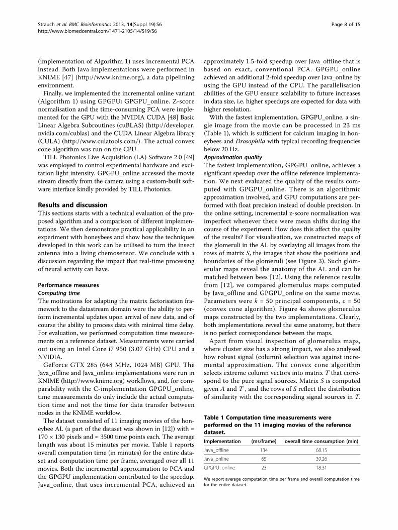
eybee AL (a part of the dataset was shown in [12]) with ≈170 × 130 pixels and ≈ 3500 time points each. The averagelength was about 15 minutes per movie. Table 1 reportsoverall computation time (in minutes) for the entire data-set and computation time per frame, averaged over all 11movies. Both the incremental approximation to PCA andthe GPGPU implementation contributed to the speedup.Java_online, that uses incremental PCA, achieved an

approximately 1.5-fold speedup over Java_offline that isbased on exact, conventional PCA. GPGPU_onlineachieved an additional 2-fold speedup over Java_online byusing the GPU instead of the CPU. The parallelisationabilities of the GPU ensure scalability to future increasesin data size, i.e. higher speedups are expected for data withhigher resolution.With the fastest implementation, GPGPU_online, a sin-

gle image from the movie can be processed in 23 ms(Table 1), which is sufficient for calcium imaging in hon-eybees and Drosophila with typical recording frequenciesbelow 20 Hz.Approximation qualityThe fastest implementation, GPGPU_online, achieves asignificant speedup over the offline reference implementa-tion. We next evaluated the quality of the results com-puted with GPGPU_online. There is an algorithmicapproximation involved, and GPU computations are per-formed with float precision instead of double precision. Inthe online setting, incremental z-score normalisation wasimperfect whenever there were mean shifts during thecourse of the experiment. How does this affect the qualityof the results? For visualisation, we constructed maps ofthe glomeruli in the AL by overlaying all images from therows of matrix S, the images that show the positions andboundaries of the glomeruli (see Figure 3). Such glom-erular maps reveal the anatomy of the AL and can bematched between bees [12]. Using the reference resultsfrom [12], we compared glomerulus maps computedby Java_offline and GPGPU_online on the same movie.Parameters were k = 50 principal components, c = 50(convex cone algorithm). Figure 4a shows glomerulusmaps constructed by the two implementations. Clearly,both implementations reveal the same anatomy, but thereis no perfect correspondence between the maps.Apart from visual inspection of glomerulus maps,

where cluster size has a strong impact, we also analysedhow robust signal (column) selection was against incre-mental approximation. The convex cone algorithmselects extreme column vectors into matrix T that corre-spond to the pure signal sources. Matrix S is computedgiven A and T , and the rows of S reflect the distributionof similarity with the corresponding signal sources in T.

Table 1 Computation time measurements wereperformed on the 11 imaging movies of the referencedataset.

Implementation (ms/frame) overall time consumption (min)

Java_offline 134 68.15

Java_online 65 39.26

GPGPU_online 23 18.31

We report average computation time per frame and overall computation timefor the entire dataset.


of 15

http://www.knime.org

http://developer.nvidia.com/cublas

http://developer.nvidia.com/cublas

http://www.culatools.com/

http://www.knime.org

This gives rise to the clusters of similar pixels in S and onthe glomerulus map. Preprocessing, such as incrementalz-score normalisation and incremental PCA, and a post-processing step employed in [12] to remove the residualnoise N (Equation 2) all have an impact on signal similar-ity and thus influence cluster size. This affects especiallyclusters that correspond to e.g. areas of similarly strongbackground staining, illumination artifacts etc. that donot have such clearly distinct signals as the glomeruli.To evaluate signal selection independent of cluster size,

we visualised the positions of the columns selected by theoffline reference implementation Java_offline, along withthe positions of the columns selected by GPGPU_online.For the reference implementation, we included only glo-merular signals, i.e. those that could be identified bymatching glomerulus maps to the anatomical honeybeeAL atlas [50]. Figure 4b shows that the positions of sig-nals selected by GPGPU_online (black circles) are ingood correspondence with the glomerulus “targets” pro-vided by Java_offline (red triangles). We conclude thatselection of relevant signals, i.e. glomerular signals, isrobust against incremental approximation in the onlinesetting.

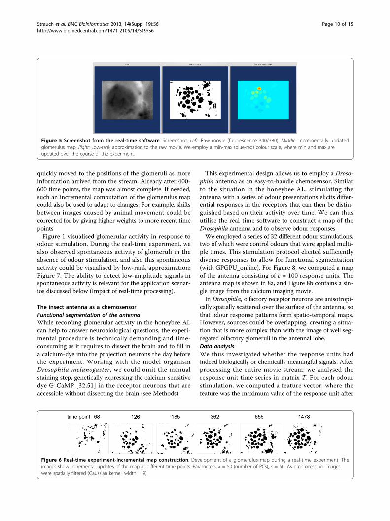
Documentation of a real-time experiment in thehoneybee ALTo demonstrate practical applicability, we performed areal-time experiment with honeybees. We used theexperimental setup from Figure 2 and GPGPU_online,the software implementation that proved fastest in theevaluation. For a screenshot, see Figure 5. During theexperiment, three windows were constantly updated: Theraw fluorescence signal, shown as the ratio between con-secutive measurements with 340 nm and 380 nm excita-tion light (see Methods), a map of the glomeruli in theAL, and the low-rank approximation to the currentimage. Movie documentations of the real-time experi-ment (Additional files 1 and 2) are available online.The glomerulus map is a segmentation of the image

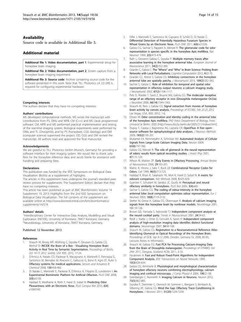
plane into regions with correlated activity over time. Withthe growing movie stream, more and more informationabout correlations between pixels becomes available.Figure 6 shows the gradual development of a glomerulusmap during the course of the experiment. While at earlytime points many of the c basis signals were still influ-enced by the initialisation of the (not yet converged) incre-mental PCA (row of points in the left upper corner), they

Figure 4 Quality evaluation: Online implementation vs. offline reference implementation. a) Comparing results of Java_offline andGPGPU_online using glomerulus maps for three bees (data from [12]). Top: Java_offline. Bottom: GPGPU_online. b) Positions of signals (columns)selected by the different implementations. Black circles: Positions of all c = 50 columns selected by GPGPU_online. Red triangles: Subset ofsignals (columns) selected by the reference implementation Java_offline. The subset contains only those signals that correspond to glomeruli.Glomeruli were identified based on their position in the maps, using the anatomical honeybee AL atlas [50].


of 15

quickly moved to the positions of the glomeruli as moreinformation arrived from the stream. Already after 400-600 time points, the map was almost complete. If needed,such an incremental computation of the glomerulus mapcould also be used to adapt to changes: For example, shiftsbetween images caused by animal movement could becorrected for by giving higher weights to more recent timepoints.Figure 1 visualised glomerular activity in response to

odour stimulation. During the real-time experiment, wealso observed spontaneous activity of glomeruli in theabsence of odour stimulation, and also this spontaneousactivity could be visualised by low-rank approximation:Figure 7. The ability to detect low-amplitude signals inspontaneous activity is relevant for the application scenar-ios discussed below (Impact of real-time processing).

The insect antenna as a chemosensorFunctional segmentation of the antennaWhile recording glomerular activity in the honeybee ALcan help to answer neurobiological questions, the experi-mental procedure is technically demanding and time-consuming as it requires to dissect the brain and to fill ina calcium-dye into the projection neurons the day beforethe experiment. Working with the model organismDrosophila melanogaster, we could omit the manualstaining step, genetically expressing the calcium-sensitivedye G-CaMP [32,51] in the receptor neurons that areaccessible without dissecting the brain (see Methods).

This experimental design allows us to employ a Droso-phila antenna as an easy-to-handle chemosensor. Similarto the situation in the honeybee AL, stimulating theantenna with a series of odour presentations elicits differ-ential responses in the receptors that can then be distin-guished based on their activity over time. We can thusutilise the real-time software to construct a map of theDrosophila antenna and to observe odour responses.We employed a series of 32 different odour stimulations,

two of which were control odours that were applied multi-ple times. This stimulation protocol elicited sufficientlydiverse responses to allow for functional segmentation(with GPGPU_online). For Figure 8, we computed a mapof the antenna consisting of c = 100 response units. Theantenna map is shown in 8a, and Figure 8b contains a sin-gle image from the calcium imaging movie.In Drosophila, olfactory receptor neurons are anisotropi-

cally spatially scattered over the surface of the antenna, sothat odour response patterns form spatio-temporal maps.However, sources could be overlapping, creating a situa-tion that is more complex than with the image of well seg-regated olfactory glomeruli in the antennal lobe.Data analysisWe thus investigated whether the response units hadindeed biologically or chemically meaningful signals. Afterprocessing the entire movie stream, we analysed theresponse unit time series in matrix T. For each odourstimulation, we computed a feature vector, where thefeature was the maximum value of the response unit after

Figure 5 Screenshot from the real-time software. Screenshot. Left: Raw movie (fluorescence 340/380), Middle: Incrementally updatedglomerulus map. Right: Low-rank approximation to the raw movie. We employ a min-max (blue-red) colour scale, where min and max areupdated over the course of the experiment.

Figure 6 Real-time experiment-Incremental map construction. Development of a glomerulus map during a real-time experiment. Theimages show incremental updates of the map at different time points. Parameters: k = 50 (number of PCs), c = 50. As preprocessing, imageswere spatially filtered (Gaussian kernel, width = 9).


of 15

presentation of the respective odour (and before the startof the next odour measurement): Figure 9a.Clustering these feature vectors (Figure 9b) shows that

feature vectors for repeated applications of the sameodour, e.g. nonanone, cluster together. The odourlesscontrol measurements (mineral oil, air, N2) appearclearly separated from the odourous substances, andchemically similar odours end up in the same cluster(ethyl- and methyl-3-hydroxy-methanoate). This servesas a proof of concept, demonstrating that the real-timeimaging system can, in principle, both recognise knownodours and estimate the identity of unknown odours bytheir similarity to reference odours.While distances between odour molecules are in part

well reflected by response pattern distances, this is notalways the case. For example, iso-eugenol does not fitinto the heptyl acetate cluster, and 2-propylphenol lacksclear responses and therefore ends up in the (odourless)oil/air cluster. Further experiments are needed to evalu-ate whether representation of chemical identity can beoptimised by recording more or different response units,e.g. in a different focal plane.It also needs to be tested whether the observed odour

responses are stereotypical across many individuals.As a first approach, we replicated the experiment fromFigure 9, finding a high correlation (Pearson correlation0.86, p =0.001, Mantel test for correlation of distance

matrices) between the odour × odour Euclidean distancematrices (based on the feature vectors) from bothexperiments, indicating that the relative dissimilarity ofodours could be conserved between individuals.How can the system be applied?Artificial chemosenors, so-called electronic noses [2-5] areimportant tools for environmental monitoring, healthcareor security applications. They do, however, not yet reachthe efficiency and sensitivity of biological olfactory sys-tems. The real-time software can extract features from cal-cium imaging recordings, directly accessing the Drosophilaantenna as a biological chemosensor. Such feature vectors(Figure 9a) can be used to visualise molecular identity, orthey can be subject to further processing, e.g. by classifiers,aiming to determine the identity of an unknown chemicalsubstance. There are two points to making the biologicalchemosensor practical: 1) Working with non-invasive bio-logical techniques that allow for easy handling of the flies,2) Software that can process the continuous stream ofodour plumes encountered in a real-world application.

Impact of real-time processingGoing beyond the specific example of the chemosensorapplication, real-time processing has a wider range ofapplicability that involves any kind of interactive experi-mentation. This belongs to future work that is made possi-ble with the real-time technology.

Figure 7 Real-time experiment-Visualisation of spontaneous background activity. Spontaneous background activity of glomeruli in thehoneybee AL, visualised by low-rank approximation. Top: Fluorescence images recorded at 5 Hz. Each image is the ratio of consecutive imagesrecorded with 340 nm and with 380 nm excitation light (see Methods). Bottom: The same images after processing with the real-time software.

Figure 8 Map of a Drosophila antenna. Map of response units on the Drosophila antenna computed with GPGPU_online (k = 50, c = 100). b)Image from the antenna calcium imaging movie.


of 15

Motivating examplesIt is increasingly clear that perception is influenced byboth the stimulus and the prior state of the brain. Forexample, brain oscillations during the pre-stimulusinterval influence how a human subject perceives anauditory stimulus in an experimental setup targeted atmultimodal sensory integration [52]. Sensory experience

without external stimulation, stemming only from thecurrent state of the brain, is known from medical phe-nomena such as tinnitus [53].For honeybees, there is first evidence in the direction

that spontaneous background activity of the glomeruli inthe AL carries information about odours that have beenencountered recently: Glomerular activity patterns similar

Figure 9 Analysis of the Drosophila antenna recording. a) Maximum response (after odour stimulation) for response units (y-axis) and aseries of odour stimulations (x-axis). All odours were dissolved in (odourless) mineral oil, which was also given multiple times as a control. As areference, the odours nonanone and heptyl acetate were applied multiple times. Response units are sorted by response to the first nonanonestimulation. Odours are sorted by name. The log colour scale ranges from blue (global min) to red (global max). b) Hierarchical clustering of theodour feature vectors from a) using Ward’s method (stats package for R) based on Euclidean distances between the feature vectors. Markedclusters: Odourless substances (grey), hexanoates (purple), heptyl acetate (green), nonanone (blue).


of 15

to a particular odour response pattern reverberate minutesafter the actual response has been elicited by odour stimu-lation [54].Considering the growing interest in ongoing brain activ-

ity, it is increasingly important to develop experimentalstrategies that allow stimulus presentations to be condi-tional on ongoing brain activity states. With the real-timemethods presented in this work, glomeruli can be targetedbecause of their responses to odours or because they arepart of reverberating patterns in spontaneous backgroundactivity.Real-time processing is necessary to answer funda-

mental questions regarding the role of ongoing brainactivity: Is it a side-effect that simply occurs as a conse-quence of neuron and network properties? Are patternsin spontaneous activity actually read out for further pro-cessing in the brain? In conditioning experiments [7],bees learn to associate an odour with a sugar reward.Can rewarding a pattern in spontaneous activity havethe same effect as rewarding the actual odour?Added value by real-time processingFrom a biological perspective, the added value providedby the real-time software is that brain activity can beinterpreted based on processed information. Only milli-seconds after the activity occurs, we can regard not onlyraw pixel values, but anatomically distinct and identifi-able units, the olfactory glomeruli in our case.While analysis of neural data is often is performed

pixel-wise (or voxel-wise), the brain encodes odours inpatterns across glomeruli. Being able to work on a glo-merulus level allows us to match the odour responsepatterns we observe with known response patterns froma database, which can reveal the chemical identity of thestimulus molecule. For spontaneous background activity,we can analyse the distribution of glomerular patternsthat informs us about the state the antennal lobe net-work is in, i.e. the prior state that is relevant for howthe stimulus will be perceived.How fast is fast enough?Closed loop experiments, where measured brain activitycontrols experimental settings, require that data proces-sing is faster than recording speed. In calcium imagingexperiments, images are often recorded at frequencies of20 Hz or slower. Thus, any processing of 50 ms/frame orfaster is appropriate. Recordings with voltage-sensitivedyes, for example, are generally useful at 50 Hz or faster:The fastest neuronal processes, the action potentials,have a duration of 1-3 ms, so recordings at 1000 Hzwould be ideal. The current speed of 23 ms/frame (Table1) is already getting close to the 50 Hz value, but it is stillfar from the ideal 1000 Hz.For many experiments, fast processing is a requirement,

e.g. if we wish to follow and react to fluctuations in

spontaneous activity. For the chemosensor task, the advan-tage lies in the fact that we can directly query a biologicalchemosensor instead of waiting for results from post-hocdata analysis. Fast processing reduces the delay of the che-mical analysis and allows for high-throughput assays.

ConclusionsIn the brain, odours are represented as activity patternsacross many neurons. Calcium imaging is a technique thatlends itself to extracting such activity patterns, as it allowsto record many units simultaneously. So far, software forcalcium imaging data has focussed on offline data proces-sing [12-15]. The algorithms and software presented inthis work process calcium imaging movies online, makingthe neural representations of odours accessible directlywhen they occur.Algorithmically, we rely on a matrix factorisation that

is updated with every new image that arrives from themovie stream. A low-rank approximation to the moviematrix serves as a compact representation of the calciumimaging movie, discarding noise and highlighting neuralsignals. This serves as the basis for further visualisations,such as functional maps of the glomeruli in the AL: Glo-merulus borders are not defined by anatomy, but byfunction, i.e. activity (in response to odours) of pixelsover time. This eliminates the need for registration ofimaging data to anatomical stainings.Such maps and the visualisation obtained by low-rank

approximation reveal the “looks of an odour”, the initialodour response pattern on the antenna, or, after data inte-gration and processing has taken place, the glomerularresponse pattern in the AL.Both odour representations have applications that

profit from real-time processing. The role of the AL net-work in shaping the odour response patterns can now beinvestigated using closed-loop experiments, where priorsystem states influence current experimental parameters.Staining an array of receptor neurons with a singlegenetic construct, accompanied by online processing,provides easy access to odour response patterns, makingreal-time chemosensing with a biological sensor practical.Visualising the neural representation of odours serves

also to map perceptional spaces. Distances betweenodour response patterns are an estimate for perceptional(dis)similarity between odours [20] throughout differentstages of odour information processing in the same indi-vidual, and also between individuals and even species,leading to species-specific odour perception spaces.For such and further applications, the algorithmic and

visualisation framework developed here enables fullyautomatic processing of odour response data without theneed for human interaction to define e.g. regions ofinterest.


of 15

AvailabilitySource code is available in Additional file 3.

Additional material

Additional file 1: Video documentation, part 1. Experimental setup forhoneybee brain imaging.

Additional file 2: Video documentation, part 2. Screen capture from ahoneybee brain imaging experiment.

Additional file 3: Source code. Archive containing source code for thesoftware presented in this work. Note that TILL Photonics LA 2.0 [49] isrequired for configuring experimental hardware.

Competing interestsThe authors declare that they have no competing interests.

Authors’ contributionsMS developed computational methods. MS wrote the manuscript withcontributions from PS, DMü and MPB. CM (C++) and MS (Java) programmedsoftware. CM, MPB and MS performed practical implementation and testingof the real-time imaging system. Biological experiments were performed byDMü and TL (Drosophila), and by PS (honeybee). CGG (biology) and DM(computer science) supervised the project. OD, CGG and DM revised themanuscript. All authors read and approved the final manuscript.

AcknowledgementsWe are grateful to TILL Photonics GmbH (Munich, Germany) for providing asoftware interface for their imaging system. We would like to thank JuliaRein for the honeybee reference data, and Jacob Stierle for assistance withhandling and preparing bees.

DeclarationsThis publication was funded by the IEEE Symposium on Biological DataVisualization (BioVis) as a supplement of highlights.The articles in this supplement have undergone the journal’s standard peerreview process for supplements. The Supplement Editors declare that theyhave no competing interests.This article has been published as part of BMC Bioinformatics Volume 14Supplement 19, 2013: Highlights from the 2nd IEEE Symposium onBiological Data Visualization. The full contents of the supplement areavailable online at http://www.biomedcentral.com/bmcbioinformatics/supplements/14/S19.

Authors’ details1Interdisciplinary Center for Interactive Data Analysis, Modelling and VisualExploration (INCIDE), University of Konstanz, 78457 Konstanz, Germany.2Neurobiology, University of Konstanz, 78457 Konstanz, Germany.

Published: 12 November 2013

References1. Strauch M, Broeg MP, Müthing C, Szyszka P, Deussen O, Galizia CG,

Merhof D: INCIDE the Brain of a Bee - Visualising Honeybee BrainActivity in Real Time by Semantic Segmentation. Proceedings of BioVis,Oct 14-15 2012, Seattle, USA IEEE; 2012, 17-24.

2. D’Amico A, Natale CD, Paolesse R, Macagnano A, Martinelli E, Pennazza G,Santonico M, Bernabei M, Roscioni C, Galluccio G, Bono R, Agro EF, Rullo S:Olfactory systems for medical applications. Sensors and Actuators B:Chemical 2008, 130:458-465.

3. Di Natale C, Martinelli E, Paolesse R, D’Amico A, Filippini D, Lundström I: AnExperimental Biomimetic Platform for Artificial Olfaction. PLoS ONE 2008,3(9):e3139.

4. Haddad R, Medhanie A, Roth Y, Harel D, Sobel N: Predicting OdorPleasantness with an Electronic Nose. PLoS Comput Biol 2010, 6(4):e1000740.

5. Eifler J, Martinelli E, Santonico M, Capuano R, Schild D, Di Natale C:Differential Detection of Potentially Hazardous Fusarium Species inWheat Grains by an Electronic Nose. PLoS ONE 2011, 6(6):e21026.

6. Galizia CG, Sachse S, Rappert A, Menzel R: The glomerular code for odorrepresentation is species specific in the honeybee Apis mellifera. NatNeurosci 1999, 2(5):473-478.

7. Rath L, Giovanni Galizia C, Szyszka P: Multiple memory traces afterassociative learning in the honeybee antennal lobe. European Journal ofNeuroscience 2011, 34(2):352-360.

8. Girardin C, Galizia C: The “Where” and “Who” in Brain Science: Probing BrainNetworks with Local Perturbations. Cognitive Computation 2012, 4:63-70.

9. Girardin CC, Kreissl S, Galizia CG: Inhibitory connections in the honeybeeantennal lobe are spatially patchy. J Neurophysiol 2013, 109(2):332-343.

10. Sachse S, Galizia C: Role of inhibition for temporal and spatial odorrepresentation in olfactory output neurons: a calcium imaging study.J Neurophysiol 2002, 87(2):1106-1117.

11. Pelz D, Roeske T, Syed Z, Bruyne Md, Galizia CG: The molecular receptiverange of an olfactory receptor in vivo (Drosophila melanogaster Or22a).J Neurobiol 2006, 66(14):1544-1563.

12. Strauch M, Rein J, Galizia CG: Signal extraction from movies of honeybeebrain activity by convex analysis. Proceedings of ICCABS, Feb 23-25 2012Las Vegas, USA, IEEE; 2012, 1-6.

13. Ditzen M: Odor concentration and identity coding in the antennal lobeof the honeybee Apis mellifera. PhD thesis Department of Biology, FreieUniversit¨at Berlin; 2005 [http://www.diss.fu-berlin.de/2005/211/indexe.html].

14. Dupuy F, Casasa J, Bagneresa AG, Lazzaria CR: OpenFluo: A free open-source software for optophysiological data analyses. J Neurosci Methods2009, 183(2):195-201.

15. Mukamel EA, Nimmerjahn A, Schnitzer MJ: Automated Analysis of CellularSignals from Large-Scale Calcium Imaging Data. Neuron 2009,63(6):747-760.

16. Galizia CG, Menzel R: The role of glomeruli in the neural representationof odors: results from optical recording studies. J Insect Phys 2001,47:115-129.

17. Wilson RI, Mainen ZF: Early Events in Olfactory Processing. Annual Reviewof Neuroscience 2006, 29:163-201.

18. Malnic B, Hirono J, Sato T, Buck LB: Combinatorial Receptor Codes forOdors. Cell 1999, 96(5):713-723.

19. Haddad R, Khan R, Takahashi YK, Mori K, Harel D, Sobel N: A metric forodorant comparison. Nat Methods 2008, 5:425-429.

20. Guerrieri F, Schubert M, Sandoz JC, Giurfa M: Perceptual and neuralolfactory similarity in honeybees. PLoS Biol 2005, 3(4):e60.

21. Sachse S, Galizia CG: The coding of odour-intensity in the honeybeeantennal lobe: local computation optimizes odour representation. Eur JNeurosci 2003, 18(8):2119-2132.

22. Stetter M, Greve H, Galizia CG, Obermayer K: Analysis of calcium imagingsignals from the honeybee brain by nonlinear models. NeuroImage 2001,13:119-128.

23. Brown GD, Yamada S, Sejnowski TJ: Independent component analysis atthe neural cocktail party. Trends in Neurosciences 2001, 24:54-63.

24. Reidl J, Starke J, Omer D, Grinvald A, Spors H: Independent componentanalysis of high-resolution imaging data identifies distinct functionaldomains. NeuroImage 2007, 34:94-108.

25. Strauch M, Galizia CG: Registration to a Neuroanatomical Reference Atlas-Identifying Glomeruli in Optical Recordings of the Honeybee Brain.Proceedings of GCB, Sep 9-12 2008, Dresden, Germany GI; 2008, 85-95,Lectures Notes in Informatics.

26. Strauch M, Galizia CG: Fast PCA for Processing Calcium-Imaging Datafrom the Brain of Drosophila melanogaster. Proceedings of DTMBIO, Oct24th 2011, Glasgow, Scotland ACM; 2011, 3-10.

27. Hyvärinen A: Fast and Robust Fixed-Point Algorithms for IndependentComponent Analysis. IEEE Transactions on Neural Networks 1999,10(3):626-634.

28. Galizia CG, Kimmerle B: Physiological and morphological characterizationof honeybee olfactory neurons combining electrophysiology, calciumimaging and confocal microscopy. J Comp Physiol A 2004, 190:21-38.

29. Grienberger C, Konnerth A: Imaging Calcium in Neurons. Neuron 2012,73(5):862-885.

30. Szyszka P, Demmler C, Oemisch M, Sommer L, Biergans S, Birnbach B,Silbering AF, Galizia CG: Mind the Gap: Olfactory Trace Conditioning inHoneybees. J Neurosci 2011, 31(20):7229-7239.


of 15

http://www.biomedcentral.com/content/supplementary/1471-2105-14-S19-S6-S1.mp4

http://www.biomedcentral.com/content/supplementary/1471-2105-14-S19-S6-S2.mp4

http://www.biomedcentral.com/content/supplementary/1471-2105-14-S19-S6-S3.7z

http://www.biomedcentral.com/bmcbioinformatics/supplements/14/S19

http://www.biomedcentral.com/bmcbioinformatics/supplements/14/S19

http://www.ncbi.nlm.nih.gov/pubmed/18769554?dopt=Abstract
















http://www.diss.fu-berlin.de/2005/211/indexe.html


























31. O’Connor N, Silver RB: Ratio Imaging: Practical Considerations forMeasuring Intracellular Ca2+ and pH in Living Cells. In Digital Microscopy,3rd Edition, Volume 81 of Methods in Cell Biology. Academic Press;Sluder G,Wolf DE 2007:415-433.

32. Nakai J, Ohkura M, Imoto K: A high signal-to-noise Ca2+ probe composedof a single green fluorescent protein. Nat Biotech 2001, 19(2):137-141.

33. Tian L, Hires SA, Mao T, Huber D, Chiappe ME, Chalasani SH, Petreanu L,Akerboom J, McKinney SA, Schreiter ER, Bargmann CI, Jayaraman V,Svoboda K, Looger LL: Imaging neural activity in worms, flies and micewith improved GCaMP calcium indicators. Nat Meth 2009, 6(12):875-881.

34. Jolliffe IT: Principal Component Analysis. 2 edition. New York/Berlin/Heidelberg: Springer; 2002, [ISBN: 0387954422].

35. Rockafellar RT: Convex Analysis Princeton, NJ: Princeton University Press;1970, [ISBN: 0691080690].

36. Dattoro J: Convex Optimisation & Euclidean Distance Geometry MebooPublishing, Palo Alto, CA; 2011, [ISBN: 0976401304].

37. Skocaj D, Leonardis A: Weighted and Robust Incremental Method forSubspace Learning. Proceedings of ICCV, Oct 14-17 2003, Nice, France IEEE;2003, 1494-1501.

38. Skocaj D, Leonardis A, Bischof H: Weighted and robust learning ofsubspace representations. Pattern Recognition 2007, 40(5):1556-1569.

39. Weng J, Zhang Y, Hwang W: Candid Covariance-free IncrementalPrincipal Component Analysis. IEEE Trans Pattern Analysis and MachineIntelligence 2003, 25:1034-1040.

40. Yan S, Tang X: Largest-eigenvalue-theory for incremental principalcomponent analysis. International Conference on Image Processing (ICIP), Sep11-14 2005, Genoa, Italy IEEE; 2005, 1181-1184.

41. Zhao H, Yuen PC, Kwok JT: A novel incremental principal componentanalysis and its application for face recognition. IEEE Transactions onSystems, Man, and Cybernetics B 2006, 36:873-886.

42. Huang D, Yi Z, Pu X: A New Incremental PCA Algorithm With Applicationto Visual Learning and Recognition. Neural Processing Letters 2009,30(3):171-185.

43. Yan J, Zhang B, Yan S, Yang Q, Li H, Chen Z, Xi W, Fan W, Ma WY,Cheng Q: IMMC: incremental maximum margin criterion. Proceedings ofSIGKDD, Aug 22-25 2004, Seattle, USA ACM; 2004, 725-730.

44. Dagher I, Nachar R: Face Recognition Using IPCA-ICA Algorithm. IEEETrans Pattern Anal Mach Intell 2006, 28(6):996-1000.

45. Kompella VR, Luciw MD, Schmidhuber J: Incremental Slow FeatureAnalysis. Proceedings of IJCAI, Jul 16-22 2011, Barcelona, Spain AAAI Press;2011, 1354-1359.

46. Zhang Y, Weng J: Convergence analysis of complementary candidincremental principal component analysis. Tech rep, Comput Sci Eng,Michigan State Univ 2001.

47. Berthold M, Cebron N, Dill F, Gabriel T, Kötter T, Meinl T, Ohl P, Sieb C,Thiel K, Wiswedel B: KNIME: The Konstanz Information Miner. In DataAnalysis, Machine Learning and Applications. Springer Berlin Heidelberg;Preisach C, Burkhardt H, Schmidt-Thieme L, Decker R 2008:319-326, Studiesin Classification, Data Analysis, and Knowledge Organization.

48. Corporation N: NVIDIA CUDA Compute Unified Device ArchitectureProgramming Guide NVIDIA Corporation; 2007.

49. TILL Photonics: Live Acquisition Software. Website 2011 [http://www.till-photonics.com/Products/la.php].

50. Galizia CG, McIlwrath SL, Menzel R: A digital three-dimensional atlas ofthe honeybee antennal lobe based on optical sections acquired byconfocal microscopy. Cell Tissue Res 1999, 295(3):383-394.

51. Wang JW, Wong AM, Flores J, Vosshall LB, Axel R: Two-Photon CalciumImaging Reveals an Odor-Evoked Map of Activity in the Fly Brain. Cell2003, 112(2):271-282.

52. Keil J, Müller N, Ihssen N, Weisz N: On the Variability of the McGurk Effect:Audiovisual Integration Depends on Prestimulus Brain States. CerebralCortex 2012, 22:221-231.

53. Weisz N, Dohrmann K, Elbert T: The relevance of spontaneous activity forthe coding of the tinnitus sensation. In Tinnitus: Pathophysiology andTreatment, Volume 166 of Progress in Brain Research. Elsevier;Langguth B,Hajak G, Kleinjung T, Cacace A, Møller A 2007:61-70.

54. Galàn RF, Weidert M, Menzel R, Herz AVM, Galizia CG: Sensory memory forodors is encoded in spontaneous correlated activity between olfactoryglomeruli. Neural Comput 2006, 18:10-25.

55. Brandt R, Rohlfing T, Rybak J, Krofczik S, Maye A, Westerhoff M, Hege HC,Menzel R: Three-dimensional average-shape atlas of the honeybee brainand its applications. J Comp Neurol 2005, 492:1-19.

doi:10.1186/1471-2105-14-S19-S6Cite this article as: Strauch et al.: The looks of an odour - Visualisingneural odour response patterns in real time. BMC Bioinformatics 201314(Suppl 19):S6.

Submit your next manuscript to BioMed Centraland take full advantage of:

• Convenient online submission

• Thorough peer review

• No space constraints or color figure charges

• Immediate publication on acceptance

• Inclusion in PubMed, CAS, Scopus and Google Scholar

• Research which is freely available for redistribution

Submit your manuscript at www.biomedcentral.com/submit


of 15


http://www.till-photonics.com/Products/la.php

http://www.till-photonics.com/Products/la.php













the looks of an odour - visualising neural odour response patterns in real time

Documents