The application of artificial intelligent tools to the transmissionexpansion problem

Tawfiq Al-Saba a,*, Ibrahim El-Amin b

a Saudi Aramco, Dhahran 31261, Saudi Arabiab Electrical Engineering Department, King Fahd University of Petroleum and Minerals, Dhahran 31261, Saudi Arabia

Received 24 July 2001; accepted 22 January 2002

Abstract

The purpose of transmission expansion problem (TEP) is to determine the timing and type of new transmission facilities. The TEP

has been formulated as an optimization problem. The objective was to minimize the transmission investment costs that handle the

increased load and the additional generation requirements in terms of line additions and power losses. Several constraints were

considered including the power flow on the network lines, the right-of-way’s validity and its maximum line addition. The TEP was

then solved using artificial intelligence (AI) tools such as the genetic algorithm, Tabu search and artificial neural networks (ANNs)

with linear and quadratic programming models. The effectiveness of the AI methods in dealing with small and large-scale systems

was tested through the applications of a six-bus system, the IEEE-24 bus network and a Saudi Arabian network. The hybridization

of GA, TS and ANN has several features. Its results confirm that it is superior in dealing with a large-scale problem in which the size

of the search spaces increases exponentially with the dimension of the network. # 2002 Elsevier Science B.V. All rights reserved.

Keywords: Artificial intelligent tools; Transmission expansion problem; Artificial neural networks

1. Introduction

The purpose of transmission system planning is to

determine the timing and type of new transmission

facilities. The facilities are required in order to provide

adequate transmission capacity to cope with future

generating additions and power flow requirements.

The transmission plans may require the introduction

of higher voltage levels, the installation of new transmis-

sion elements and new substations. Transmission system

planners tend to use many methods to address the

expansion problem. Planners utilize automatic expan-

sion models to determine an optimum expansion system

by minimizing the mathematical objective function

subject to a number of constraints [1�/6].

Many researchers have investigated methods and

algorithms in order to solve the transmission expansion

problem (TEP). One of these is a static optimization

model that determines the optimum network expansion

without considering the timing of the expansion. It can

be modeled using linear, integer or quadratic program-

ming techniques, a decomposition approach or the

gradient search method. In 1988, linear programming

was used based on a maximum principle by Kim and

others [7]. Also, Villarana et al. modeled the network in

such a way as to use a DC power flow [8]. Integer

programming has been applied though a static network

synthesis method that uses an implicit enumeration

search procedure [9]. Quadratic programming was

applied by Al-Hamouz to a Jordanian power system

[10]. The objective was to obtain the exact cost of power

losses and capital investment in the new facilities. Levi

and Calovic applied the decomposition approach based

method in 1991 for a Yugoslavian power system [11].

Also, Romero and Monticelli developed a hierarchical

decomposition approach in 1994 [12]. Hsu et al. applied

the gradient search method using an oscillatory stability

consideration index [13]. Unlike static transmission

network expansion models, time-phased or dynamic

optimization models take into account the timing of

new installations through a given time horizon [14]. El-

Metwally and Harb applied this model using an

* Corresponding author.

E-mail addresses: sabatt@aramco.com.sa (T. Al-Saba),

imelamin@kfupm.edu.sa (I. El-Amin).

Electric Power Systems Research 62 (2002) 117�/126

www.elsevier.com/locate/epsr

0378-7796/02/$ - see front matter # 2002 Elsevier Science B.V. All rights reserved.

PII: S 0 3 7 8 - 7 7 9 6 ( 0 2 ) 0 0 0 3 7 - 8

admittance approach and the quadratic programming

technique.

The TEP can be solved using artificial intelligence

tools (AI). These tools include simulated annealing(SA), genetic algorithm (GA), artificial neural networks

(ANN) and Tabu search (TS). Romero et al. applied SA

in 1996 [15]. In 1997, Romero and others also applied

SA using computer multi-processors [16]. GA was used

in 1996 to determine an economically adopted elective

transmission system in a deregulated open access

environment though the application of a Chilean electric

system [17]. Also, in 1998, Gallego et al. applied GA tothe north-northeastern and southern electrical systems

in Brazil [18]. ANN was used, in 1995, using neuron

computing hybridized with GA [19]. In this method, the

authors improved solutions compared to the individual

use of these methods. Finally, TS uses memory structure

to direct the search process using a neighborhood

strategy. In 1998, Romero et al. proposed a hybrid

method that incorporates the basic concepts of TS, SA,and GA [20].

2. Mathematical modeling of the transmission expansion

problem

2.1. The objective function

The TEP can be formulated in the following terms:

minn�XNB

i�1

XNB

j�1

cijnij�KXNL

i�1

I2i Ri (1)

where cij is the cost of the additional circuits in branch

i �/j ; nij is the number of circuits added to the branch i �/j ;

NB is the total number of buses in the system; K is the

loss coefficient, K�/8760�/NYE�/Ckwh; NYE is theestimated lifetime of the expansion network (years);

CkWh: is the cost of one kWh ($US/kWh); Ri is the

resistance of the ith line; Ii is the flow on the ith line;

and NL is the number of the existing lines.

The first term of the objective function represents the

capital costs of the new lines. The second term

represents the costs of the system power loss. The

system power flow and losses will change as a result ofline additions.

Eq. (1) is a typical hard combinatorial problem. It is

prone to combinatorial explosion as the number of

decision variables increases. An extra complication

relates to the fact that there are cases in which the

planning does not simply mean the reinforcement of an

existing network. The loss coefficient (K ) depends on the

number of years of operation and the kWh cost. The DCload flow is used in the problem formulation where the

current (I ) is approximately equal to the power flow,

and voltage is assumed to be unity at all buses.

2.2. Transmission expansion constraints

Several restrictions have to be modeled in a mathe-

matical representation to ensure that the mathematicalsolutions are in line with the planning requirements.

These constraints are as follows.

2.3. Limits in branch power flow

½Pmaxil ½�Pil (2)

where Pilmax is the maximum branch power flow between

the buses i and l .

In a D.C. load flow model, each element of the branch

power flow in constraint (2) can be described as follows:

Pil �(Zil=xil)(ui�ul) (3)

where Zil is the total number of parallel links between

the buses of i and l ; xil is the reactance of link of branch

i to l ; and uI is the voltage angles of the terminal buses

of branch I.In a matrix form, Eq. (3) becomes:

Bu�P (4)

where B is the susceptance matrix whose elements are

Bil �/�/(1/xil ) for the off-diagonal terms, and Bii �/SBil

for the diagonal terms; Xil is the total reactance ofbranch (i , l ); l � /Oi are the branches connected to bus i ;

and u is the vector of nodal voltage angles.

2.3.1. Bus voltage angle

This constraint can be stated as the calculated phase

angle at bus i . The calculated angle, uical, should be less

than the maximum phase angle uimax.

½umaxi ½] ½ucal

i ½ (5)

2.3.2. Right-of-way

It is important to know the line location and the

capacity of the required lines. This is because the

planners have to meet the community standards ofvisual impact on the environment along with the

economic considerations. So, the acquisition of right

of way has to be considered by the planner and should

be included as a constraint of the problem. Mathema-

tically, this constraint defines the line location and the

maximum number of lines that can be installed in a

specified location. It is represented by:

05nij 5nmaxij (6)

where nij is the total number of circuits added in branch

i �/j , nij �/xij /gij ; xij is the total reactance added in branch

i �/j ; and gij is the initial line reactance in the line i �/j .

T. Al-Saba, I. El-Amin / Electric Power Systems Research 62 (2002) 117�/126118

2.3.3. Power balance at the network buses

This constraint checks for the additional[u1] genera-

tion. Mathematically, this is represented by:

g�d�Bu�r (7)

where g is the generation vector in the existing power

plants; d is the load demand vector in all network nodes;

B is the susceptance matrix whose elements are the

imaginary parts of the nodal admittance of existing ones

(Bijexisting) and the added lines to the existing network

(Bijadded); u is the bus voltage angle phase vector; and r is

the extra generation needed in case of high transmission

losses or an unbalanced power system.

3. Proposed solution algorithms

This paper aims to obtain the optimal design using afast automatic decision-maker. An intelligent tool starts

from a random state and it proceeds to allocate the

calculated cost recursively until the stage of the negotia-

tion point is reached. These intelligent tools, GA, TS

and ANN, are flexible to handle and easy to implement.

This section will explain simulation procedures in order

to handle the TEP. The hybridization methods of these

techniques will also be explained.

3.1. Genetic algorithm approach

The GA used in this research is the simple GA [21�/

23], and a plural number of identical individuals are

allowed to exist in the population. The genetic operation

is carried out until the population converges to an

individual. Through its application to the TEP problem,offspring (chromosome) length represents the number of

the available rights-of-way in the network while the

offspring itself represents the number of the newly

added lines. Also, the cost of the new addition is

represented in the fitness function.

3.2. Tabu search

TS has its antecedents in methods designed to cross

boundaries of feasibility or local optimality normally

treated as barriers, and systematically to impose and

release constraints to permit exploration of otherwise

forbidden regions [24,25]. The TS search used in this

work is a simple algorithm with a neighborhood search

method. Through its application to the TEP problem,the solution vector represents the number of new

additions in each right-of-way. The cost of the new

addition is represented in the objective function.

3.3. Hybridization algorithm

It is observed that the GA has the feature of

combining the solution while the TS is a systematicexploration of memory function in search processes [26].

By taking advantage of these features to improve the

performance in terms of obtaining the optimal solution,

new mechanisms of solution search are used. Two forms

of hybridization between GA and TS are considered.

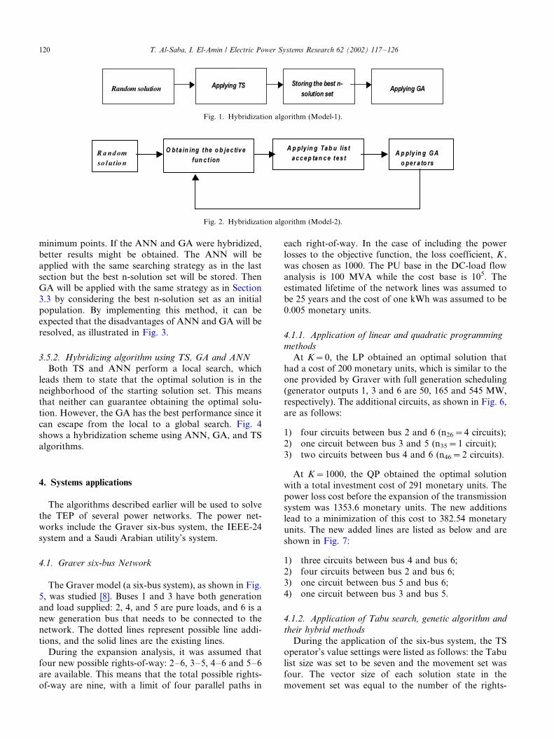
3.3.1. Hybridization of TS and GA (Model-1)

In this method, TS will be applied with the samesearching strategy as in Section 3.2, but the best n-

solution set will be stored. Then GA will be applied to

start from the best n-solution set as an initial population.

This is illustrated in Fig. 1.

3.3.2. Hybridization (Model-2)

Since the neighborhood method was applied in the TS

algorithm, the proposed method here will be to apply

GA operators in place of the neighborhood method.The proposed algorithm will be as follows. The first step

starts from the random solution set then obtains the

objective function and applies the stopping criteria. The

second step is to apply the Tabu list acceptance test. The

last is to apply the GA operators to generate a new

solution set. Fig. 2 illustrates this hybridization proce-

dure.

3.4. Artificial neural network model (ANN)

An ANN with a multi-layer perceptron model using a

back-propagation algorithm is the proposed algorithm

for TEP applications [27,28]. The output neurons

represent the solution state at each iteration while the

state represents the number of lines that should be

added in each right-of-way in the network. Also, thecosts of these additions are represented in the objective

function.

3.5. Hybridization methods With ANN

Two hybridization methods are used. The first one is

the hybridization algorithm between the ANN and GA

while the other one is the ANN hybridized with TS andGA.

3.5.1. ANN hybridized With GA

Since the ANN performs the local search, it will

converge to the feasible solutions in the neighborhood

of the initial state. If the initial state is set in the

neighborhood of the optimal solution, the solution may

be obtained. This is generally difficult if there is noinformation relating to the optimal solution. On the

other hand, the GA forms a population based on a

multi-point parallel search while escaping from local

T. Al-Saba, I. El-Amin / Electric Power Systems Research 62 (2002) 117�/126 119

minimum points. If the ANN and GA were hybridized,better results might be obtained. The ANN will be

applied with the same searching strategy as in the last

section but the best n-solution set will be stored. Then

GA will be applied with the same strategy as in Section

3.3 by considering the best n-solution set as an initial

population. By implementing this method, it can be

expected that the disadvantages of ANN and GA will be

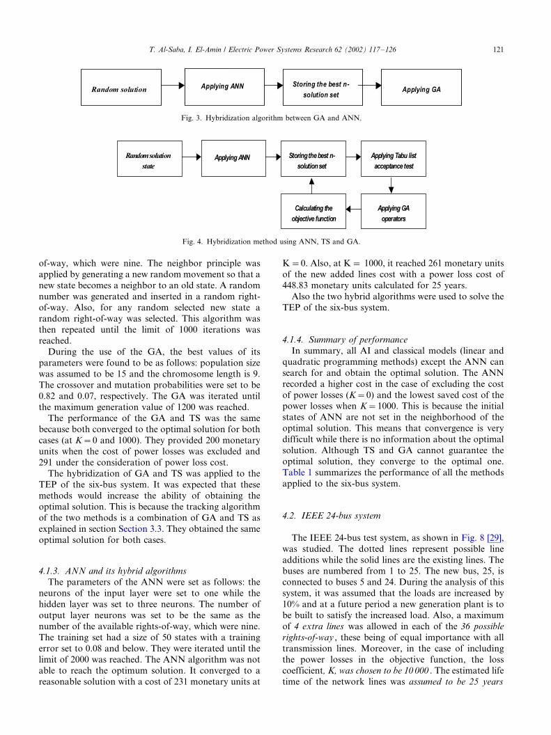
resolved, as illustrated in Fig. 3.

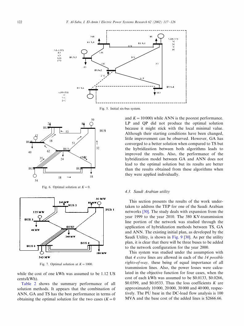
3.5.2. Hybridizing algorithm using TS, GA and ANN

Both TS and ANN perform a local search, which

leads them to state that the optimal solution is in theneighborhood of the starting solution set. This means

that neither can guarantee obtaining the optimal solu-

tion. However, the GA has the best performance since it

can escape from the local to a global search. Fig. 4

shows a hybridization scheme using ANN, GA, and TS

algorithms.

4. Systems applications

The algorithms described earlier will be used to solve

the TEP of several power networks. The power net-works include the Graver six-bus system, the IEEE-24

system and a Saudi Arabian utility’s system.

4.1. Graver six-bus Network

The Graver model (a six-bus system), as shown in Fig.

5, was studied [8]. Buses 1 and 3 have both generation

and load supplied: 2, 4, and 5 are pure loads, and 6 is a

new generation bus that needs to be connected to the

network. The dotted lines represent possible line addi-

tions, and the solid lines are the existing lines.

During the expansion analysis, it was assumed thatfour new possible rights-of-way: 2�/6, 3�/5, 4�/6 and 5�/6

are available. This means that the total possible rights-

of-way are nine, with a limit of four parallel paths in

each right-of-way. In the case of including the powerlosses to the objective function, the loss coefficient, K ,

was chosen as 1000. The PU base in the DC-load flow

analysis is 100 MVA while the cost base is 105. The

estimated lifetime of the network lines was assumed to

be 25 years and the cost of one kWh was assumed to be

0.005 monetary units.

4.1.1. Application of linear and quadratic programming

methods

At K�/0, the LP obtained an optimal solution that

had a cost of 200 monetary units, which is similar to theone provided by Graver with full generation scheduling

(generator outputs 1, 3 and 6 are 50, 165 and 545 MW,

respectively). The additional circuits, as shown in Fig. 6,

are as follows:

1) four circuits between bus 2 and 6 (n26�/4 circuits);

2) one circuit between bus 3 and 5 (n35�/1 circuit);

3) two circuits between bus 4 and 6 (n46�/2 circuits).

At K�/1000, the QP obtained the optimal solution

with a total investment cost of 291 monetary units. The

power loss cost before the expansion of the transmissionsystem was 1353.6 monetary units. The new additions

lead to a minimization of this cost to 382.54 monetary

units. The new added lines are listed as below and are

shown in Fig. 7:

1) three circuits between bus 4 and bus 6;

2) four circuits between bus 2 and bus 6;

3) one circuit between bus 5 and bus 6;

4) one circuit between bus 3 and bus 5.

4.1.2. Application of Tabu search, genetic algorithm and

their hybrid methods

During the application of the six-bus system, the TS

operator’s value settings were listed as follows: the Tabulist size was set to be seven and the movement set was

four. The vector size of each solution state in the

movement set was equal to the number of the rights-

Fig. 1. Hybridization algorithm (Model-1).

Fig. 2. Hybridization algorithm (Model-2).

T. Al-Saba, I. El-Amin / Electric Power Systems Research 62 (2002) 117�/126120

of-way, which were nine. The neighbor principle was

applied by generating a new random movement so that a

new state becomes a neighbor to an old state. A random

number was generated and inserted in a random right-

of-way. Also, for any random selected new state a

random right-of-way was selected. This algorithm wasthen repeated until the limit of 1000 iterations was

reached.

During the use of the GA, the best values of its

parameters were found to be as follows: population size

was assumed to be 15 and the chromosome length is 9.

The crossover and mutation probabilities were set to be

0.82 and 0.07, respectively. The GA was iterated until

the maximum generation value of 1200 was reached.The performance of the GA and TS was the same

because both converged to the optimal solution for both

cases (at K�/0 and 1000). They provided 200 monetary

units when the cost of power losses was excluded and

291 under the consideration of power loss cost.

The hybridization of GA and TS was applied to the

TEP of the six-bus system. It was expected that these

methods would increase the ability of obtaining theoptimal solution. This is because the tracking algorithm

of the two methods is a combination of GA and TS as

explained in section Section 3.3. They obtained the same

optimal solution for both cases.

4.1.3. ANN and its hybrid algorithms

The parameters of the ANN were set as follows: the

neurons of the input layer were set to one while the

hidden layer was set to three neurons. The number of

output layer neurons was set to be the same as the

number of the available rights-of-way, which were nine.

The training set had a size of 50 states with a training

error set to 0.08 and below. They were iterated until thelimit of 2000 was reached. The ANN algorithm was not

able to reach the optimum solution. It converged to a

reasonable solution with a cost of 231 monetary units at

K�/0. Also, at K�/ 1000, it reached 261 monetary units

of the new added lines cost with a power loss cost of

448.83 monetary units calculated for 25 years.

Also the two hybrid algorithms were used to solve the

TEP of the six-bus system.

4.1.4. Summary of performance

In summary, all AI and classical models (linear and

quadratic programming methods) except the ANN can

search for and obtain the optimal solution. The ANN

recorded a higher cost in the case of excluding the cost

of power losses (K�/0) and the lowest saved cost of thepower losses when K�/1000. This is because the initial

states of ANN are not set in the neighborhood of the

optimal solution. This means that convergence is very

difficult while there is no information about the optimal

solution. Although TS and GA cannot guarantee the

optimal solution, they converge to the optimal one.

Table 1 summarizes the performance of all the methods

applied to the six-bus system.

4.2. IEEE 24-bus system

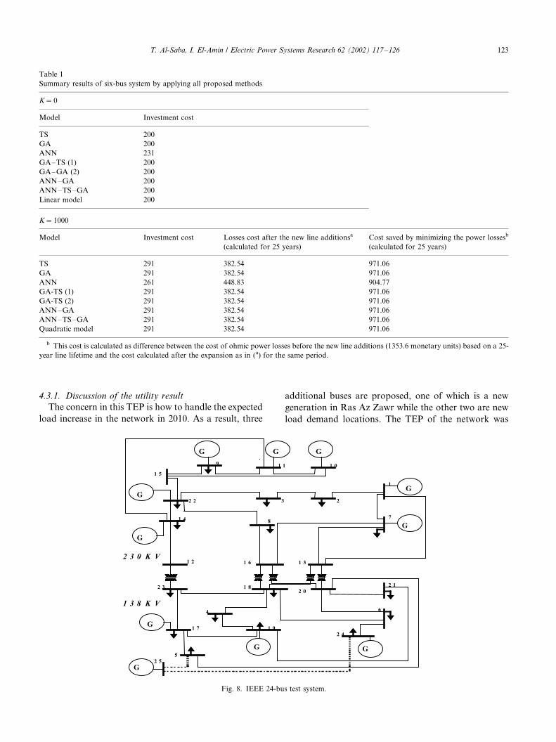
The IEEE 24-bus test system, as shown in Fig. 8 [29],

was studied. The dotted lines represent possible line

additions while the solid lines are the existing lines. Thebuses are numbered from 1 to 25. The new bus, 25, is

connected to buses 5 and 24. During the analysis of this

system, it was assumed that the loads are increased by

10% and at a future period a new generation plant is to

be built to satisfy the increased load. Also, a maximum

of 4 extra lines was allowed in each of the 36 possible

rights-of-way , these being of equal importance with all

transmission lines. Moreover, in the case of includingthe power losses in the objective function, the loss

coefficient, K, was chosen to be 10 000 . The estimated life

time of the network lines was assumed to be 25 years

Fig. 3. Hybridization algorithm between GA and ANN.

Fig. 4. Hybridization method using ANN, TS and GA.

T. Al-Saba, I. El-Amin / Electric Power Systems Research 62 (2002) 117�/126 121

while the cost of one kWh was assumed to be 1.12 US

cents/kWh).Table 2 shows the summary performance of all

solution methods. It appears that the combination of

ANN, GA and TS has the best performance in terms of

obtaining the optimal solution for the two cases (K�/0

and K�/10 000) while ANN is the poorest performance.

LP and QP did not produce the optimal solution

because it might stick with the local minimal value.

Although their starting conditions have been changed,

little improvement can be observed. However, GA has

converged to a better solution when compared to TS but

the hybridization between both algorithms leads to

improved the results. Also, the performance of the

hybridization model between GA and ANN does not

lead to the optimal solution but its results are better

than the results obtained from these algorithms when

they were applied individually.

4.3. Saudi Arabian utility

This section presents the results of the work under-

taken to address the TEP for one of the Saudi Arabian

networks [30]. The study deals with expansion from the

year 1999 to the year 2010. The 380 KV-transmission

line portion of the network was studied through the

application of hybridization methods between TS, GA

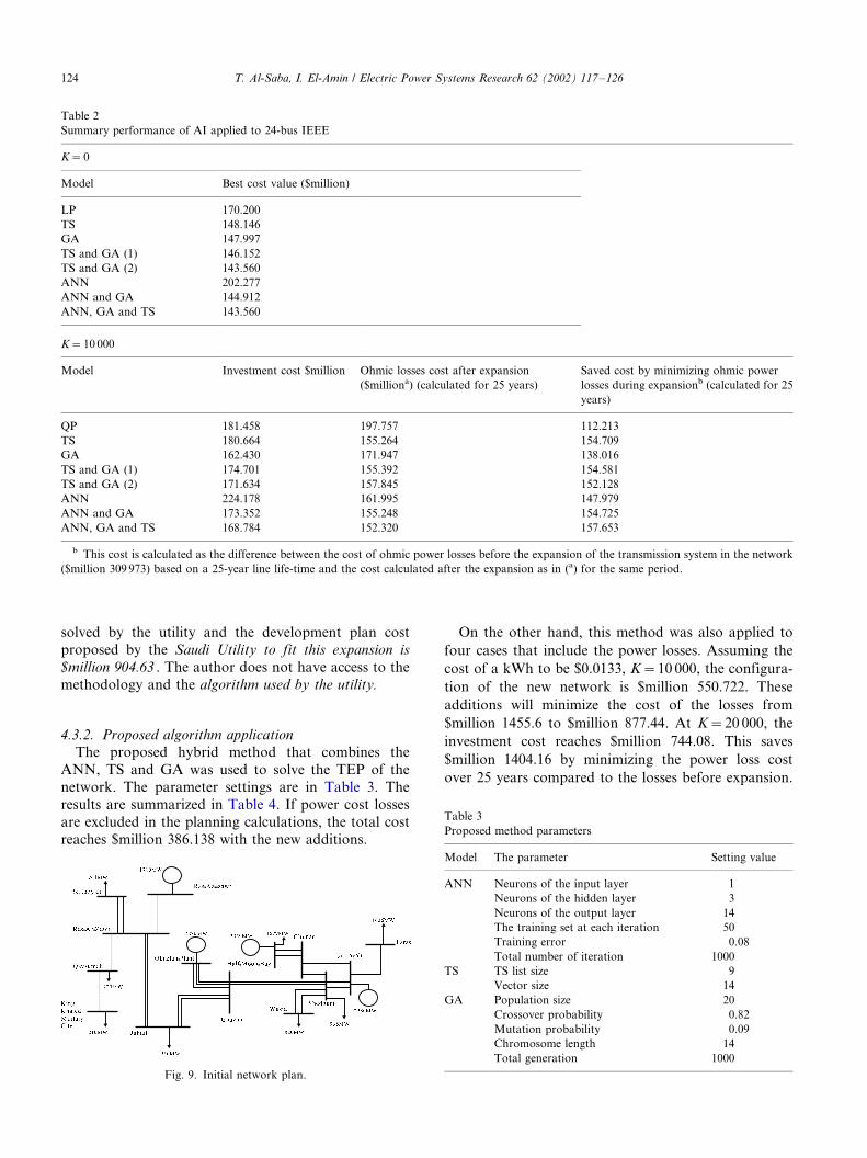
and ANN. The existing initial plan, as developed by the

Saudi Utility, is shown in Fig. 9 [30]. As per the utility

plan, it is clear that there will be three buses to be added

to the network configuration for the year 2000.

This system was studied under the assumption with

that 4 extra lines are allowed in each of the 14 possible

rights-of-way, these being of equal importance of all

transmission lines. Also, the power losses were calcu-

lated in the objective function for four cases, when the

cost of each kWh was assumed to be $0.0133, $0.0266,

$0.0399, and $0.0533. Thus the loss coefficients K are

approximately 10 000, 20 000, 30 000 and 40 000, respec-

tively. The PU base in the DC-load flow analysis is 100

MVA and the base cost of the added lines is $2666.66.

Fig. 5. Initial six-bus system.

Fig. 6. Optimal solution at K�/0.

Fig. 7. Optimal solution at K�/1000.

T. Al-Saba, I. El-Amin / Electric Power Systems Research 62 (2002) 117�/126122

4.3.1. Discussion of the utility result

The concern in this TEP is how to handle the expected

load increase in the network in 2010. As a result, three

additional buses are proposed, one of which is a new

generation in Ras Az Zawr while the other two are new

load demand locations. The TEP of the network was

Table 1

Summary results of six-bus system by applying all proposed methods

K�0

Model Investment cost

TS 200

GA 200

ANN 231

GA�/TS (1) 200

GA�/GA (2) 200

ANN�/GA 200

ANN�/TS�/GA 200

Linear model 200

K�1000

Model Investment cost Losses cost after the new line additionsa

(calculated for 25 years)

Cost saved by minimizing the power lossesb

(calculated for 25 years)

TS 291 382.54 971.06

GA 291 382.54 971.06

ANN 261 448.83 904.77

GA-TS (1) 291 382.54 971.06

GA-TS (2) 291 382.54 971.06

ANN�/GA 291 382.54 971.06

ANN�/TS�/GA 291 382.54 971.06

Quadratic model 291 382.54 971.06

b This cost is calculated as difference between the cost of ohmic power losses before the new line additions (1353.6 monetary units) based on a 25-

year line lifetime and the cost calculated after the expansion as in (a) for the same period.

Fig. 8. IEEE 24-bus test system.

T. Al-Saba, I. El-Amin / Electric Power Systems Research 62 (2002) 117�/126 123

solved by the utility and the development plan cost

proposed by the Saudi Utility to fit this expansion is

$million 904.63 . The author does not have access to the

methodology and the algorithm used by the utility.

4.3.2. Proposed algorithm application

The proposed hybrid method that combines the

ANN, TS and GA was used to solve the TEP of the

network. The parameter settings are in Table 3. The

results are summarized in Table 4. If power cost losses

are excluded in the planning calculations, the total cost

reaches $million 386.138 with the new additions.

On the other hand, this method was also applied to

four cases that include the power losses. Assuming the

cost of a kWh to be $0.0133, K�/10 000, the configura-

tion of the new network is $million 550.722. These

additions will minimize the cost of the losses from

$million 1455.6 to $million 877.44. At K�/20 000, the

investment cost reaches $million 744.08. This saves

$million 1404.16 by minimizing the power loss cost

over 25 years compared to the losses before expansion.

Table 2

Summary performance of AI applied to 24-bus IEEE

K�0

Model Best cost value ($million)

LP 170.200

TS 148.146

GA 147.997

TS and GA (1) 146.152

TS and GA (2) 143.560

ANN 202.277

ANN and GA 144.912

ANN, GA and TS 143.560

K�10 000

Model Investment cost $million Ohmic losses cost after expansion

($milliona) (calculated for 25 years)

Saved cost by minimizing ohmic power

losses during expansionb (calculated for 25

years)

QP 181.458 197.757 112.213

TS 180.664 155.264 154.709

GA 162.430 171.947 138.016

TS and GA (1) 174.701 155.392 154.581

TS and GA (2) 171.634 157.845 152.128

ANN 224.178 161.995 147.979

ANN and GA 173.352 155.248 154.725

ANN, GA and TS 168.784 152.320 157.653

b This cost is calculated as the difference between the cost of ohmic power losses before the expansion of the transmission system in the network

($million 309 973) based on a 25-year line life-time and the cost calculated after the expansion as in (a) for the same period.

Fig. 9. Initial network plan.

Table 3

Proposed method parameters

Model The parameter Setting value

ANN Neurons of the input layer 1

Neurons of the hidden layer 3

Neurons of the output layer 14

The training set at each iteration 50

Training error 0.08

Total number of iteration 1000

TS TS list size 9

Vector size 14

GA Population size 20

Crossover probability 0.82

Mutation probability 0.09

Chromosome length 14

Total generation 1000

T. Al-Saba, I. El-Amin / Electric Power Systems Research 62 (2002) 117�/126124

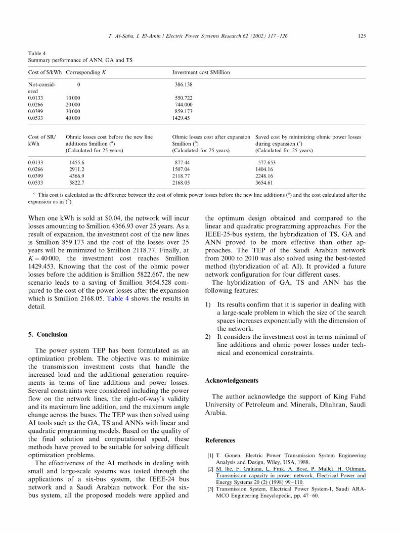
When one kWh is sold at $0.04, the network will incurlosses amounting to $million 4366.93 over 25 years. As a

result of expansion, the investment cost of the new lines

is $million 859.173 and the cost of the losses over 25

years will be minimized to $million 2118.77. Finally, at

K�/40 000, the investment cost reaches $million

1429.453. Knowing that the cost of the ohmic power

losses before the addition is $million 5822.667, the new

scenario leads to a saving of $million 3654.528 com-pared to the cost of the power losses after the expansion

which is $million 2168.05. Table 4 shows the results in

detail.

5. Conclusion

The power system TEP has been formulated as an

optimization problem. The objective was to minimize

the transmission investment costs that handle the

increased load and the additional generation require-

ments in terms of line additions and power losses.

Several constraints were considered including the power

flow on the network lines, the right-of-way’s validity

and its maximum line addition, and the maximum anglechange across the buses. The TEP was then solved using

AI tools such as the GA, TS and ANNs with linear and

quadratic programming models. Based on the quality of

the final solution and computational speed, these

methods have proved to be suitable for solving difficult

optimization problems.

The effectiveness of the AI methods in dealing with

small and large-scale systems was tested through theapplications of a six-bus system, the IEEE-24 bus

network and a Saudi Arabian network. For the six-

bus system, all the proposed models were applied and

the optimum design obtained and compared to thelinear and quadratic programming approaches. For the

IEEE-25-bus system, the hybridization of TS, GA and

ANN proved to be more effective than other ap-

proaches. The TEP of the Saudi Arabian network

from 2000 to 2010 was also solved using the best-tested

method (hybridization of all AI). It provided a future

network configuration for four different cases.

The hybridization of GA, TS and ANN has thefollowing features:

1) Its results confirm that it is superior in dealing witha large-scale problem in which the size of the search

spaces increases exponentially with the dimension of

the network.

2) It considers the investment cost in terms minimal of

line additions and ohmic power losses under tech-

nical and economical constraints.

Acknowledgements

The author acknowledge the support of King Fahd

University of Petroleum and Minerals, Dhahran, Saudi

Arabia.

References

[1] T. Gonen, Electric Power Transmission System Engineering

Analysis and Design, Wiley, USA, 1988.

[2] M. llic, F. Galiana, L. Fink, A. Bose, P. Mallet, H. Othman,

Transmission capacity in power network, Electrical Power and

Energy Systems 20 (2) (1998) 99�/110.

[3] Transmission System, Electrical Power System-I, Saudi ARA-

MCO Engineering Encyclopedia, pp. 47�/60.

Table 4

Summary performance of ANN, GA and TS

Cost of $/kWh Corresponding K Investment cost $Million

Not-consid-

ered

0 386.138

0.0133 10 000 550.722

0.0266 20 000 744.000

0.0399 30 000 859.173

0.0533 40 000 1429.45

Cost of SR/

kWh

Ohmic losses cost before the new line

additions $million (a)

(Calculated for 25 years)

Ohmic losses cost after expansion

$million (b)

(Calculated for 25 years)

Saved cost by minimizing ohmic power losses

during expansion (c)

(Calculated for 25 years)

0.0133 1455.6 877.44 577.653

0.0266 2911.2 1507.04 1404.16

0.0399 4366.9 2118.77 2248.16

0.0533 5822.7 2168.05 3654.61

c This cost is calculated as the difference between the cost of ohmic power losses before the new line additions (a) and the cost calculated after the

expansion as in (b).

T. Al-Saba, I. El-Amin / Electric Power Systems Research 62 (2002) 117�/126 125

[4] R. Billinton, J. Oteng-Adjei, Utilization of interrupted energy

assessment rates in generation and transmission system planning,

IEEE Transaction on Power Systems 6 (3) (1991) 1245�/1253.

[5] M.E. El-Hawary, G.S. Christensen, Optimal Operation of Electric

Power System, Academic Press, New York, USA, 1979.

[6] W.L. Weeks, Transmission and Distribution of Electrical Energy,

Harper and Row Publishers, New York, USA, 1981.

[7] K.J. Kim, Y.M. Park, K.Y. Lee, Optimal long term transmission

expansion planning based on maximum principle, IEEE Transac-

tion on Power Systems 3 (1988) 4.

[8] R. Villosana, L.L. Garver, S.J. Solon, Transmission network

planning using linear programming, IEEE Transaction on Power

Apparatus and System PAS-104 (2) (1985) 349�/356.

[9] R. Romero, A. Monticelli, A zero�/one implicit enumeration

method for optimizing investments in transmission expansion

planning, IEEE Transactions on Power Systems 9 (3) (1994)

1385�/1391.

[10] Z.M. Al-Hamouz, Transmission Network Planning Using Quad-

ratic Programming, Master’s Thesis, Jordan University of

Sciences and Technology, 1989.

[11] V.A. Levi, M.S. Calovic, A new decomposition based method for

optimal expansion planning of large transmission networks, IEEE

Transaction on Power System 6 (1991) 3.

[12] R. Romero, A. Monticelli, A hierarchical decomposition ap-

proach for transmission network expansion planning, IEEE

Transaction on Power Systems 9 (1) (1994) 373�/380.

[13] Y.-Y. Hsu, P.-H. Huang, C.-J. Lin, C.-T. Huang, Oscillatory

stability considerations in transmission expansion planning, IEEE

Transaction on Power System 4 (3) (1989) 1110�/1114.

[14] M.M. El-Metwally, A.M. Harb, Transmission planning using

admittance approach and quadratic programming, Electrical

Machines and Power Systems 21 (1993) 61�/83.

[15] R. Romero, R.A. Gallego, A. Monticelli, Transmission system

expansion planning by simulated annealing, IEEE Transaction on

Power System 11 (1) (1996) 364�/369.

[16] R. Romero, R.A. Gallego, A. Monticelli, Parallel simulated

annealing applied to long term transmission network expansion

planning, IEEE Transaction on Power Systems 12 (1997) 1.

[17] H. Radnick, R. Palam, E. Cura, C. Silva, Economically adapted

transmission systems in open access schemes*/application of

genetic algorithms, IEEE Transaction on Power Systems 11 (3)

(1996) 1427�/1440.

[18] R. Romero, R.A. Gallego, A. Monticelli, Transmission system

expansion planning by an extended genetic algorithm, IEEE

Transaction on Power Systems 145 (3) (1998) 329�/335.

[19] K. Yoshimoto, K. Yasuda, R. Yokoyama, Transmission expan-

sion planning using neuro-computing hybridized with genetic

algorithm, IEEE Transaction on Neural Network 1 (1995) 126�/

131.

[20] R. Romero, R.A. Gallego, A. Monticelli, Comparative studies on

non-convex optimization methods for transmission network

expansion planning, IEEE Transaction on Power Systems 13 (3)

(1998) 822�/828.

[21] D.E. Goldberg, Genetic Algorithm in Search, Optimization and

Machine Learning, Addison Wesley, Reading, MA, 1989.

[22] Z. Michalewicz, Genetic Algorithm�/Data Structures�/Evolu-

tion Programs, Springer-Verlag, Berlin, Heidelberg, New York,

USA, 1992.

[23] L. Davis, Handbook of Genetic Algorithms, Van Nostrand, New

York, 1991.

[24] R.L. Daniels, J.B. Mazzola, A Tabu search heuristic for the

flexible-resource flow shop scheduling program, Annals of

Operation and Research 41 (1993) 207�/230.

[25] M. Dell Amico, M. Trubian, Applying tabu search to the jop-

shop scheduling problem, Annals of Operation and Research 41

(1993) 253�/278.

[26] M. Laguna, T. Feo, H. Elrod, Genetic algorithm and tabu search:

hybrids for optimization, Operations Research 42 (4) (1994) 677�/

687.

[27] T.T. Al-Saba, I.M. El-Amin, Artificial neural network as applied

to long-term demand forecasting, Artificial Intelligence in En-

gineering 13 (2) (1999) 189�/197.

[28] D. Highlay, T. Hilmns, Load forecasting by ANN, Computer

Application in Power IEEE 6 (3) (1994) 10�/15.

[29] A.O. Ekwu, B.J. Cory, Transmission system expansion planning

by interactive method, IEEE Transaction on Power Apparatus

and System. PAS-103 (7) (1984) 1583�/1591.

[30] SCECO-East and Central Reference Scenario at 2000 and 2010 at

Peak Load Developed at June 1995. File # LF6-3-LDVG and

LF6-5-LDVG.

T. Al-Saba, I. El-Amin / Electric Power Systems Research 62 (2002) 117�/126126