the application and extension of retrograde software analysis
TRANSCRIPT
Perisic A. The Application and Extension of Retrograde Software Analysis
[email protected] 94dab034-eb78-4adc-b0f0-967e9f904ac3
1
ORIGINAL ARTICLE
The Application and Extension of Retrograde
Software Analysis Aleksandar Perisic, M.Sc.
The retrograde software analysis is a method that emanates from executing a program backwards - instead of taking input data
and following the execution path, we start from output data and by executing the program backwards, command by command,
analyze data that could lead to the current output. The changed perspective forces a developer to think in a new way about the
program. It can be applied as a thorough procedure or casual method. With this method, we have many advantages in testing,
algorithm and system analysis. For example, in testing the advantage is obvious if the set of output data is smaller than possible
inputs. For some programs or algorithms, we know more precisely the output data, so this retrograde analysis can help in
reducing the number of test cases or even in strict verification of an algorithm. The difficulty lies in the fact that we need types
of data that no programming language currently supports, so we need additional effort to understand how this method works,
or what effort we need to create the tools of automation testing. Although it is rooted in testing, if we would develop a
retrograde testing environment, we would have created a new language different from anything currently on the market. The
obvious advantage of this language would be a built-in parallel processing power. The key lies in understanding the ties
between these two worlds, which is what we are trying to decipher here. In the work, we explain how to reduce the number of
test cases to linear for sorting networks, and, as an introduction, give the in-depth retrograde analysis of several basic
algorithms like binary search, maximum sum sub-array, random shuffling and inverse in-place permutation. We explain how
parallelism can be used to speed up search of unsorted database even in classical case without going to quantum level, and
propose some formalism that can help creating the Retrograde language.
Introduction
Le bon Dieu est dans le detail. Gustave Flaubert (1821-1880)
We introduce retrograde software analysis through testing. We will call it retrograde testing. A program is understood and engineered as a chained combination of methodologies, like algorithms, that resolve partial problems, all of which are part of the final solution for the problem or activity the program was designed for. Its execution goes forward in time. It is of essential interest to observe the final software solution from all possible angles in order to be able to verify it. Testing is the science of measuring and ensuring the software quality. It is a discipline that includes various methods where empirical and theoretical standpoints are mixed with different proportions and success. White box testing is a type of testing where the code and internals of the program are known and available to the testing team. Black box testing is a type of testing where the code and internals of the program are considered only through external specification. A real test is commonly a combination of these two, known as gray testing. The testing team can decide to use or combine: path testing, where several carefully chosen paths through the program are used and scrutinized, up to creating automation tests, which are going to ensure that the chosen paths execute correctly; loop testing, where each loop is additionally analyzed for its correctness; boundary testing, where the test input is carefully chosen to correspond to the rare and special values or range of values, like value 0, empty array, null value,…; domain testing, where input is selected and test executed as to prove that no incorrect states are ever met, like missed variable initialization, incorrect array access index…; function testing, where the input is prepared based on functional specification and the function fed with both expected and unexpected input data; system testing, where the entire system is tested in order to check if it meets the specification; and much more. Whenever we test a program or system, we actually decide about the testing outcome first. We know what to expect generally from every test or group of tests. We know that a domain test is going to provide the answer whether a program has incorrect states; function test, if output data are those input data should effect; loop test, whether we have an infinite loop situation; and so on. We start from what we expect, first on the abstract and technical level of testing procedure
Peter A. The Application and Extension of Retrograde Software Analysis
2
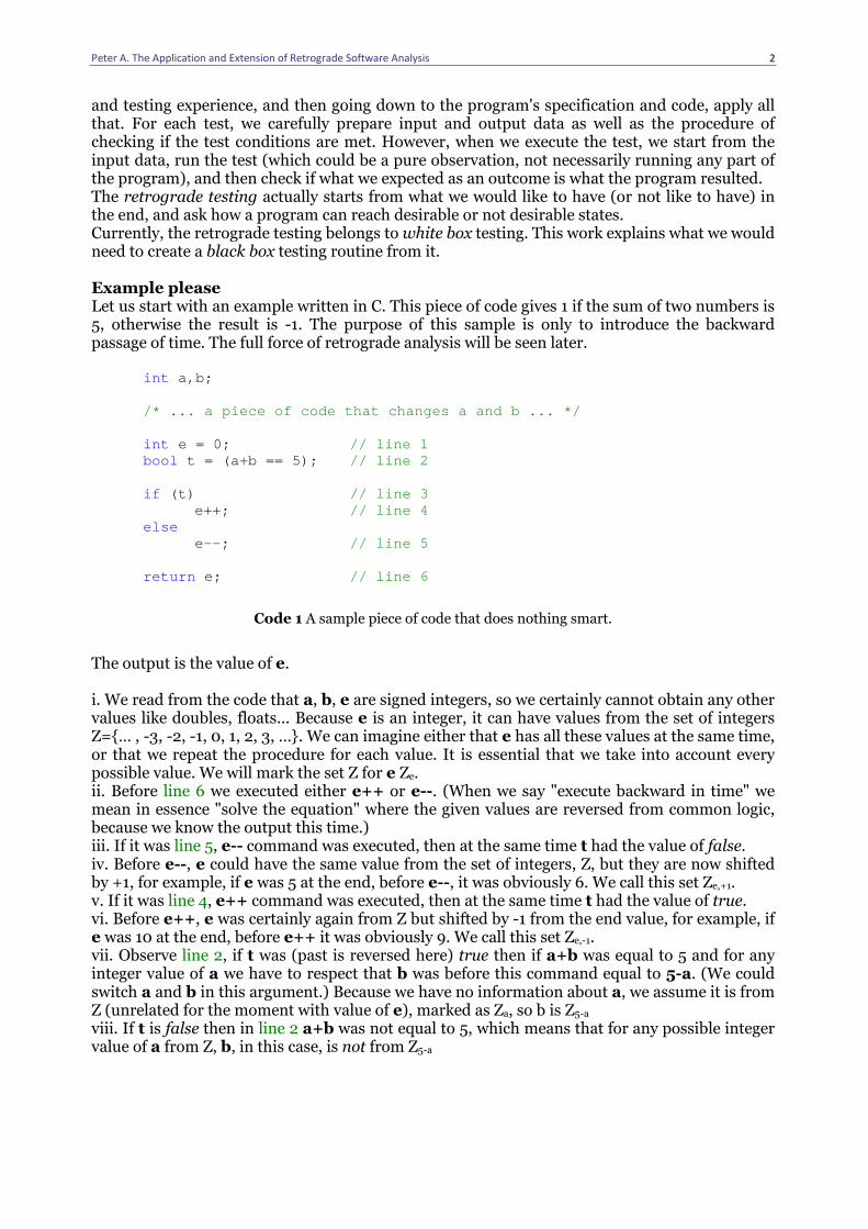
and testing experience, and then going down to the program's specification and code, apply all that. For each test, we carefully prepare input and output data as well as the procedure of checking if the test conditions are met. However, when we execute the test, we start from the input data, run the test (which could be a pure observation, not necessarily running any part of the program), and then check if what we expected as an outcome is what the program resulted. The retrograde testing actually starts from what we would like to have (or not like to have) in the end, and ask how a program can reach desirable or not desirable states. Currently, the retrograde testing belongs to white box testing. This work explains what we would need to create a black box testing routine from it. Example please Let us start with an example written in C. This piece of code gives 1 if the sum of two numbers is 5, otherwise the result is -1. The purpose of this sample is only to introduce the backward passage of time. The full force of retrograde analysis will be seen later.
int a,b;
/* ... a piece of code that changes a and b ... */
int e = 0; // line 1 bool t = (a+b == 5); // line 2
if (t) // line 3 e++; // line 4 else e--; // line 5 return e; // line 6
Code 1 A sample piece of code that does nothing smart.
The output is the value of e. i. We read from the code that a, b, e are signed integers, so we certainly cannot obtain any other values like doubles, floats... Because e is an integer, it can have values from the set of integers Z={… , -3, -2, -1, 0, 1, 2, 3, …}. We can imagine either that e has all these values at the same time, or that we repeat the procedure for each value. It is essential that we take into account every possible value. We will mark the set Z for e Ze. ii. Before line 6 we executed either e++ or e--. (When we say "execute backward in time" we mean in essence "solve the equation" where the given values are reversed from common logic, because we know the output this time.) iii. If it was line 5, e-- command was executed, then at the same time t had the value of false. iv. Before e--, e could have the same value from the set of integers, Z, but they are now shifted by +1, for example, if e was 5 at the end, before e--, it was obviously 6. We call this set Ze,+1. v. If it was line 4, e++ command was executed, then at the same time t had the value of true. vi. Before e++, e was certainly again from Z but shifted by -1 from the end value, for example, if e was 10 at the end, before e++ it was obviously 9. We call this set Ze,-1. vii. Observe line 2, if t was (past is reversed here) true then if a+b was equal to 5 and for any integer value of a we have to respect that b was before this command equal to 5-a. (We could switch a and b in this argument.) Because we have no information about a, we assume it is from Z (unrelated for the moment with value of e), marked as Za, so b is Z5-a viii. If t is false then in line 2 a+b was not equal to 5, which means that for any possible integer value of a from Z, b, in this case, is not from Z5-a
Peter A. The Application and Extension of Retrograde Software Analysis
3
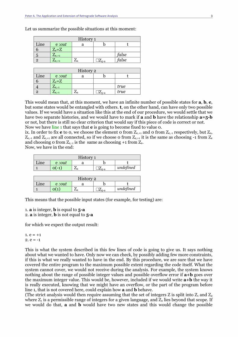
Let us summarize the possible situations at this moment:
History 1 Line e :out a b t 6 Ze=Z 5 Ze,+1 false 2 Ze,+1 Za ∉Z5-a false
History 2
Line e :out a b t 6 Ze=Z 4 Ze,-1 true 2 Ze,-1 Za ∈Z5-a true
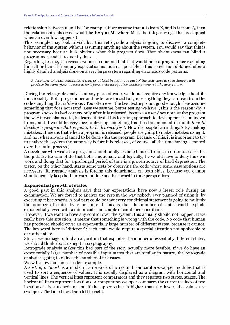
This would mean that, at this moment, we have an infinite number of possible states for a, b, e, but some states would be entangled with others. t, on the other hand, can have only two possible values. If we would have a situation like this at the end of our procedure, we would settle that we have two separate histories, and we would have to mark if a and b have the relationship a=5-b or not, but there is still no clear criterion that would say if this piece of code is correct or not. Now we have line 1 that says that e is going to become fixed to value 0. ix. In order to fix e to 0, we choose the element 0 from Ze,+1 and 0 from Ze,-1 respectively, but Ze, Ze,-1 and Ze,+1 are all connected, so if we choose 0 from Ze,+1 it is the same as choosing -1 from Ze and choosing 0 from Ze,-1 is the same as choosing +1 from Ze. Now, we have in the end:
History 1 Line e :out a b t 1 0(-1) Za ∉Z5-a undefined
History 2
Line e :out a b t 1 0(1) Za ∈Z5-a undefined
This means that the possible input states (for example, for testing) are: 1. a is integer, b is equal to 5-a 2. a is integer, b is not equal to 5-a for which we expect the output result: 1. e = +1 2. e = -1 This is what the system described in this few lines of code is going to give us. It says nothing about what we wanted to have. Only now we can check, by possibly adding few more constraints, if this is what we really wanted to have in the end. By this procedure, we are sure that we have covered the entire program to the maximum possible extent regarding the code itself. What the system cannot cover, we would not receive during the analysis. For example, the system knows nothing about the range of possible integer values and possible overflow error if a+b goes over the maximum integer value. This would be, however, included if we would write a+b the way it is really executed, knowing that we might have an overflow, or the part of the program before line 1, that is not covered here, could explain how a and b behave. (The strict analysis would then require assuming that the set of integers Z is split into Z1 and Z2 where Z1 is a permissible range of integers for a given language, and Z2 lies beyond that scope. If we would do that, a and b would have two new states and this would change the possible
Peter A. The Application and Extension of Retrograde Software Analysis
4
relationship between a and b. For example, if we assume that a is from Z1 and b is from Z2 then the relationship observed would be b=5-a+M, where M is the integer range that is skipped when an overflow happens.) This example may look trivial, but this retrograde analysis is going to discover a complete behavior of the system without assuming anything about the system. You would say that this is not necessary because it is obvious what this program does. That obviousness can blind a programmer, and it frequently does. Regarding testing, the reason we need some method that would help a programmer excluding himself or herself from any expectation as much as possible is this conclusion obtained after a highly detailed analysis done on a very large system regarding erroneous code patterns:
A developer who has committed a bug, or at least brought one part of the code close to such danger, will produce the same effect as soon as he is faced with an equal or similar problem in the near future.
During the retrograde analysis of any piece of code, we do not require any knowledge about its functionality. Both programmer and tester are forced to ignore anything they can read from the code - anything that is 'obvious'. Too often even the best testing is not good enough if we assume something that does not stand. Less we assume, better testing we have. (This is the reason why a program shows its bad corners only after it is released, because a user does not use the program the way it was planned to, he learns it first. This learning approach to development is unknown to me, and it would be very nice to develop something that has this moment in mind: how to develop a program that is going to be learned first. How do people learn things? By making mistakes. It means that when a program is released, people are going to make mistakes using it, and not what anyone planned to be done with the program. Because of this, it is important to try to analyze the system the same way before it is released, of course, all the time having a control over the entire process.) A developer who wrote the program cannot totally exclude himself from it in order to search for the pitfalls. He cannot do that both emotionally and logically; he would have to deny his own work and doing that for a prolonged period of time is a proven source of hard depression. The tester, on the other hand, starts some tests by observing the code where some assumptions are necessary. Retrograde analysis is forcing this detachment on both sides, because you cannot simultaneously keep both forward in time and backward in time perspectives. Exponential growth of states A good part in this analysis says that our expectations have now a lesser role during an examination. We are forced to analyze the system the way nobody ever planned of using it, by executing it backwards. A bad part could be that every conditional statement is going to multiply the number of states by 2 or more. It means that the number of states could explode exponentially, even with a minor code and couple of combined conditions. However, if we want to have any control over the system, this actually should not happen. If we really have this situation, it means that something is wrong with the code. No code that human has produced should cover an exponentially large number of different states, because it cannot. The key word here is "different": each state would require a special attention not applicable to any other state. Still, if we manage to find an algorithm that explodes the number of essentially different states, we should think about using it in cryptography. Retrograde analysis makes this bad part of the story actually more feasible. If we do have an exponentially large number of possible input states that are similar in nature, the retrograde analysis is going to reduce the number of test cases. We will show here one excellent example. A sorting network is a model of a network of wires and comparator-swapper modules that is used to sort a sequence of values. It is usually displayed as a diagram with horizontal and vertical lines. The vertical lines represent comparators and they separate two states, stages. The horizontal lines represent locations. A comparator-swapper compares the current values of two locations it is attached to, and if the upper value is higher than the lower, the values are swapped. The time flows from left to right.
Peter A. The Application and Extension of Retrograde Software Analysis
5
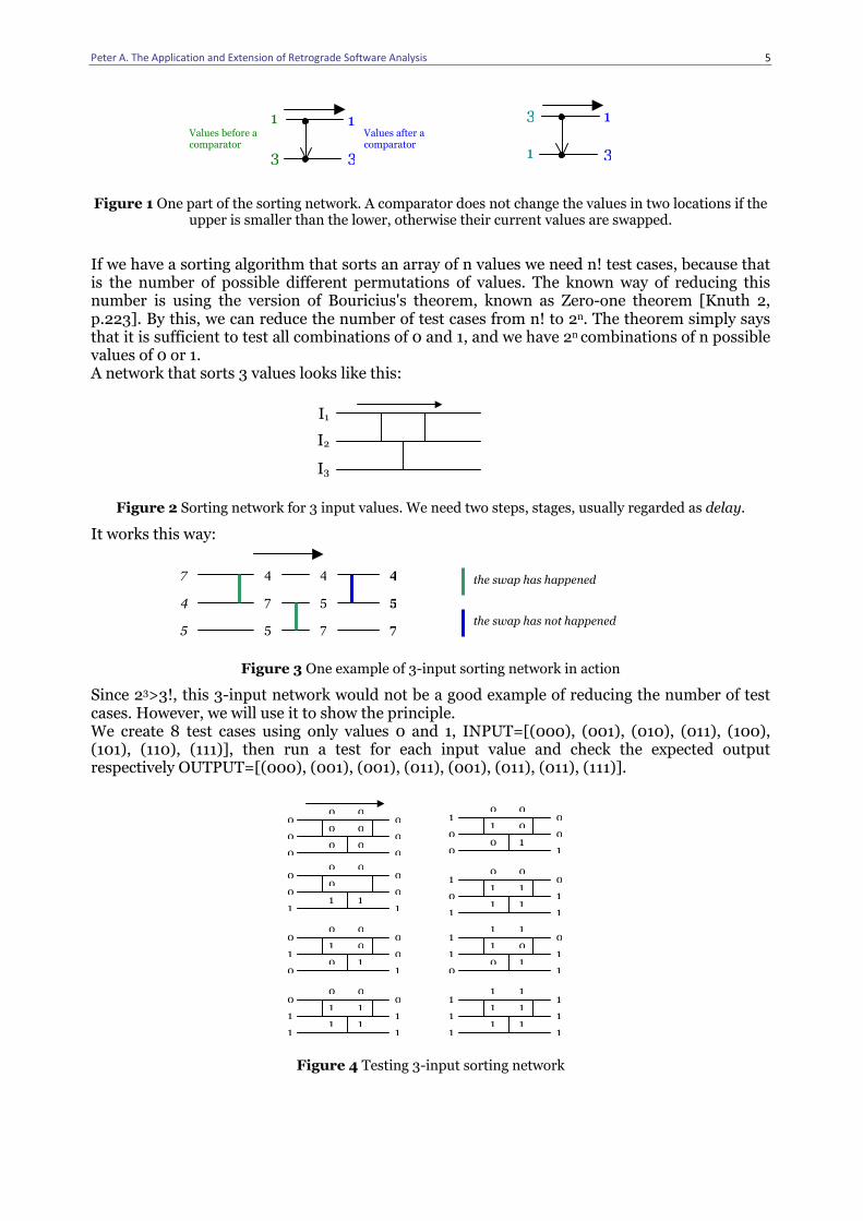
Figure 1 One part of the sorting network. A comparator does not change the values in two locations if the upper is smaller than the lower, otherwise their current values are swapped.
If we have a sorting algorithm that sorts an array of n values we need n! test cases, because that is the number of possible different permutations of values. The known way of reducing this number is using the version of Bouricius's theorem, known as Zero-one theorem [Knuth 2, p.223]. By this, we can reduce the number of test cases from n! to 2n. The theorem simply says that it is sufficient to test all combinations of 0 and 1, and we have 2n
combinations of n possible values of 0 or 1. A network that sorts 3 values looks like this:
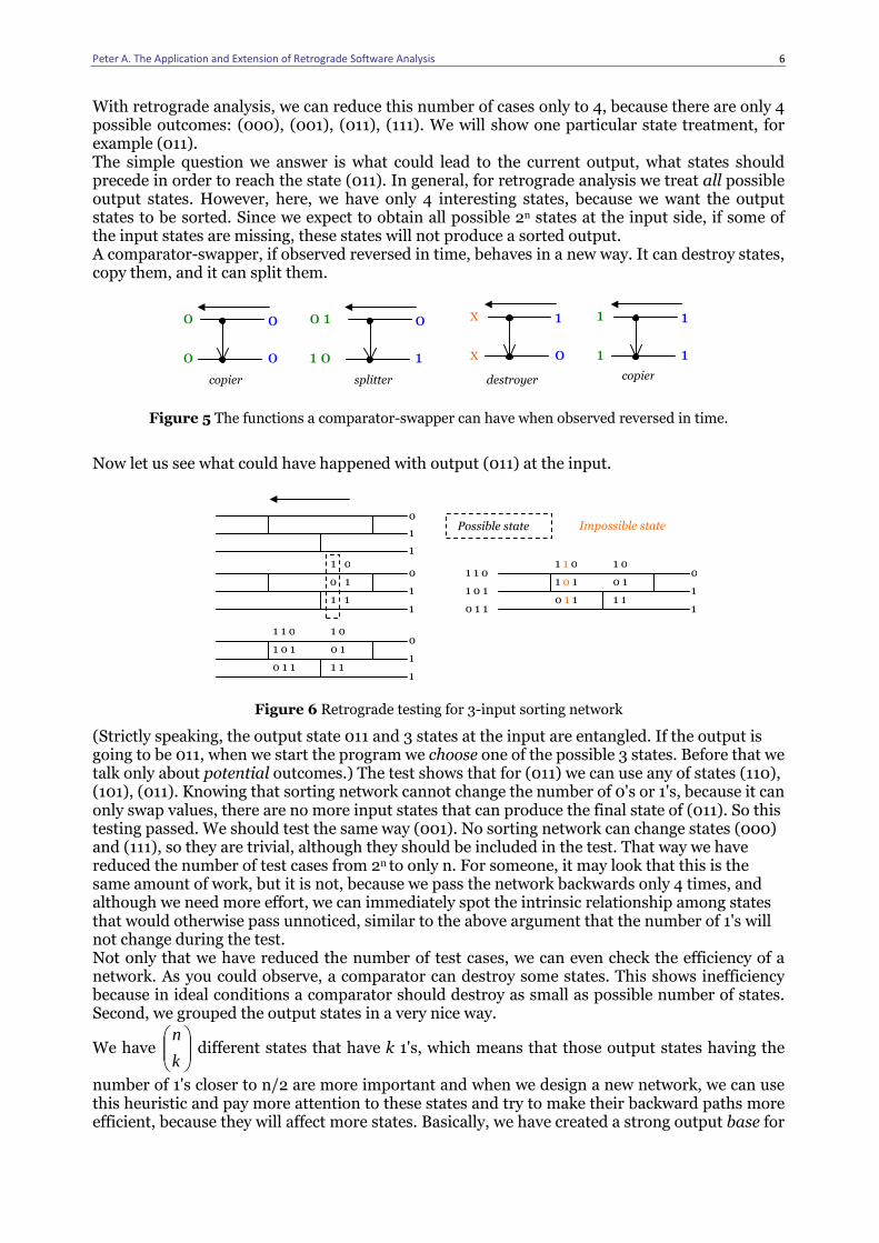
Figure 2 Sorting network for 3 input values. We need two steps, stages, usually regarded as delay.
It works this way:
Figure 3 One example of 3-input sorting network in action
Since 23>3!, this 3-input network would not be a good example of reducing the number of test cases. However, we will use it to show the principle. We create 8 test cases using only values 0 and 1, INPUT=[(000), (001), (010), (011), (100), (101), (110), (111)], then run a test for each input value and check the expected output respectively OUTPUT=[(000), (001), (001), (011), (001), (011), (011), (111)].
Figure 4 Testing 3-input sorting network
7
4
5
4
7
5
4
5
7
4
5
7the swap has not happened
the swap has happened
o o o
o o o
o o o
o o o
o o 1
o o 1
o
1
o o 1
o 1 o
o 1 o
o o 1
o o 1
o 1 1
o 1 1
o 1 1
o 1 1
1 o o
o 1 o
o o 1
o o 1
1 o 1
o 1 1
o 1 1
o 1 1
1 1 o
1 1 o
1 o 1
o 1 1
1 1 1
1 1 1
1 1 1
1 1 1
3
1
1
3
1
3
1
3
Values before a comparator
Values after a comparator
I1
I2
I3
Peter A. The Application and Extension of Retrograde Software Analysis
6
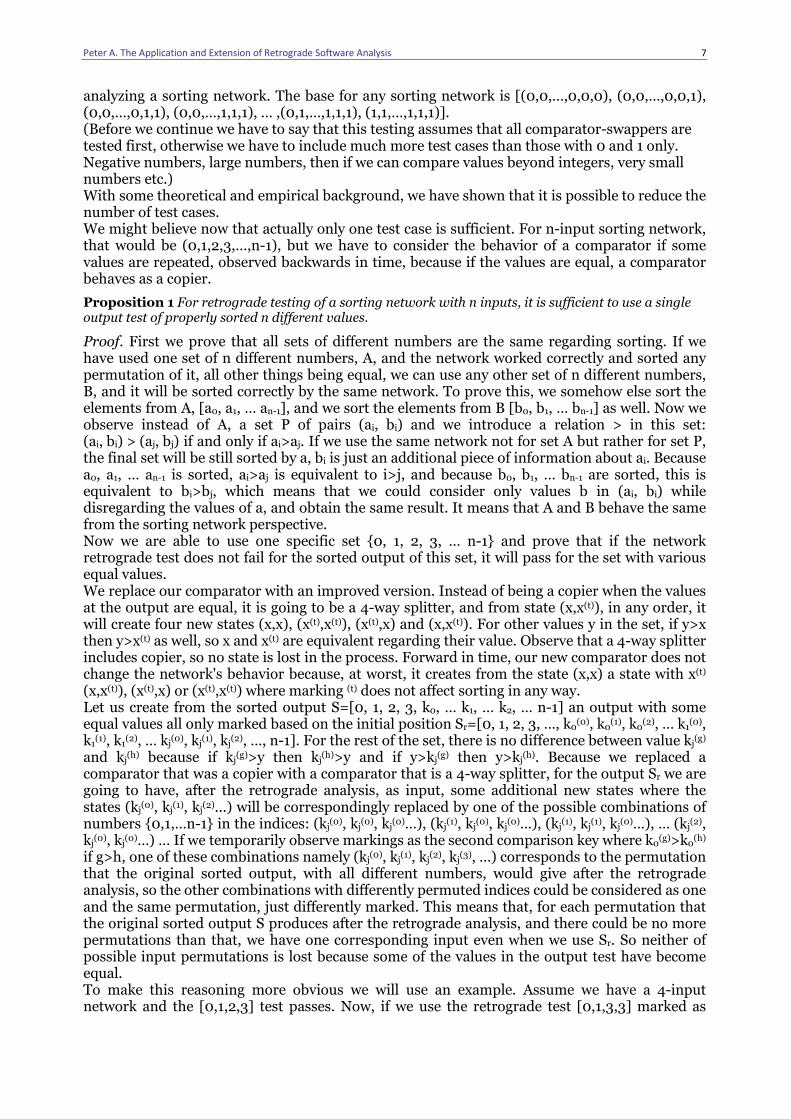
With retrograde analysis, we can reduce this number of cases only to 4, because there are only 4 possible outcomes: (000), (001), (011), (111). We will show one particular state treatment, for example (011). The simple question we answer is what could lead to the current output, what states should precede in order to reach the state (011). In general, for retrograde analysis we treat all possible output states. However, here, we have only 4 interesting states, because we want the output states to be sorted. Since we expect to obtain all possible 2n states at the input side, if some of the input states are missing, these states will not produce a sorted output. A comparator-swapper, if observed reversed in time, behaves in a new way. It can destroy states, copy them, and it can split them.
Figure 5 The functions a comparator-swapper can have when observed reversed in time.
Now let us see what could have happened with output (011) at the input.
Figure 6 Retrograde testing for 3-input sorting network
(Strictly speaking, the output state 011 and 3 states at the input are entangled. If the output is going to be 011, when we start the program we choose one of the possible 3 states. Before that we talk only about potential outcomes.) The test shows that for (011) we can use any of states (110), (101), (011). Knowing that sorting network cannot change the number of 0's or 1's, because it can only swap values, there are no more input states that can produce the final state of (011). So this testing passed. We should test the same way (001). No sorting network can change states (000) and (111), so they are trivial, although they should be included in the test. That way we have reduced the number of test cases from 2n to only n. For someone, it may look that this is the same amount of work, but it is not, because we pass the network backwards only 4 times, and although we need more effort, we can immediately spot the intrinsic relationship among states that would otherwise pass unnoticed, similar to the above argument that the number of 1's will not change during the test. Not only that we have reduced the number of test cases, we can even check the efficiency of a network. As you could observe, a comparator can destroy some states. This shows inefficiency because in ideal conditions a comparator should destroy as small as possible number of states. Second, we grouped the output states in a very nice way.
We have
k
n different states that have k 1's, which means that those output states having the
number of 1's closer to n/2 are more important and when we design a new network, we can use this heuristic and pay more attention to these states and try to make their backward paths more efficient, because they will affect more states. Basically, we have created a strong output base for
o 1 1
1 o o 1 1 1
o 1 1
1 1 o
1 o 1 o 1 1
1 o o 1 1 1
o 1 1
1 1 o
1 o 1 o 1 1
1 1 o
1 o 1 o 1 1
1 o o 1 1 1
o 1 1
Possible state Impossible state
0
0
0
0
0 1
1 0
0
1
x
x
1
0
1
1
1
1
copier splitter destroyer copier
Peter A. The Application and Extension of Retrograde Software Analysis
7
analyzing a sorting network. The base for any sorting network is [(0,0,…,0,0,0), (0,0,…,0,0,1), (0,0,…,0,1,1), (0,0,…,1,1,1), … ,(0,1,…,1,1,1), (1,1,…,1,1,1)]. (Before we continue we have to say that this testing assumes that all comparator-swappers are tested first, otherwise we have to include much more test cases than those with 0 and 1 only. Negative numbers, large numbers, then if we can compare values beyond integers, very small numbers etc.) With some theoretical and empirical background, we have shown that it is possible to reduce the number of test cases. We might believe now that actually only one test case is sufficient. For n-input sorting network, that would be (0,1,2,3,…,n-1), but we have to consider the behavior of a comparator if some values are repeated, observed backwards in time, because if the values are equal, a comparator behaves as a copier.
Proposition 1 For retrograde testing of a sorting network with n inputs, it is sufficient to use a single output test of properly sorted n different values.
Proof. First we prove that all sets of different numbers are the same regarding sorting. If we have used one set of n different numbers, A, and the network worked correctly and sorted any permutation of it, all other things being equal, we can use any other set of n different numbers, B, and it will be sorted correctly by the same network. To prove this, we somehow else sort the elements from A, [a0, a1, … an-1], and we sort the elements from B [b0, b1, … bn-1] as well. Now we observe instead of A, a set P of pairs (ai, bi) and we introduce a relation > in this set: (ai, bi) > (aj, bj) if and only if ai>aj. If we use the same network not for set A but rather for set P, the final set will be still sorted by a, bi is just an additional piece of information about ai. Because a0, a1, … an-1 is sorted, ai>aj is equivalent to i>j, and because b0, b1, … bn-1 are sorted, this is equivalent to bi>bj, which means that we could consider only values b in (ai, bi) while disregarding the values of a, and obtain the same result. It means that A and B behave the same from the sorting network perspective. Now we are able to use one specific set {0, 1, 2, 3, … n-1} and prove that if the network retrograde test does not fail for the sorted output of this set, it will pass for the set with various equal values. We replace our comparator with an improved version. Instead of being a copier when the values at the output are equal, it is going to be a 4-way splitter, and from state (x,x(t)), in any order, it will create four new states (x,x), (x(t),x(t)), (x(t),x) and (x,x(t)). For other values y in the set, if y>x then y>x(t) as well, so x and x(t) are equivalent regarding their value. Observe that a 4-way splitter includes copier, so no state is lost in the process. Forward in time, our new comparator does not change the network's behavior because, at worst, it creates from the state (x,x) a state with x(t) (x,x(t)), (x(t),x) or (x(t),x(t)) where marking (t) does not affect sorting in any way. Let us create from the sorted output S=[0, 1, 2, 3, k0, … k1, … k2, … n-1] an output with some equal values all only marked based on the initial position Sr=[0, 1, 2, 3, …, k0
(0), k0(1), k0
(2), … k1(0),
k1(1), k1
(2), … kj(0), kj
(1), kj(2), …, n-1]. For the rest of the set, there is no difference between value kj
(g) and kj
(h) because if kj(g)>y then kj
(h)>y and if y>kj(g) then y>kj
(h). Because we replaced a comparator that was a copier with a comparator that is a 4-way splitter, for the output Sr we are going to have, after the retrograde analysis, as input, some additional new states where the states (kj
(0), kj(1), kj
(2)...) will be correspondingly replaced by one of the possible combinations of numbers {0,1,…n-1} in the indices: (kj
(0), kj(0), kj
(0)…), (kj(1), kj
(0), kj(0)…), (kj
(1), kj(1), kj
(0)…), … (kj(2),
kj(0), kj
(0)…) … If we temporarily observe markings as the second comparison key where k0(g)>k0
(h) if g>h, one of these combinations namely (kj
(0), kj(1), kj
(2), kj(3), …) corresponds to the permutation
that the original sorted output, with all different numbers, would give after the retrograde analysis, so the other combinations with differently permuted indices could be considered as one and the same permutation, just differently marked. This means that, for each permutation that the original sorted output S produces after the retrograde analysis, and there could be no more permutations than that, we have one corresponding input even when we use Sr. So neither of possible input permutations is lost because some of the values in the output test have become equal. To make this reasoning more obvious we will use an example. Assume we have a 4-input network and the [0,1,2,3] test passes. Now, if we use the retrograde test [0,1,3,3] marked as
Peter A. The Application and Extension of Retrograde Software Analysis
8
[0,1,3(0),3(1)] with the above new type of network, we would obtain, among else, these similar input states [3(0),0,1,3(0)], [3(1),0,1,3(1)], [3(0),0,1,3(1)], [3(1),0,1,3(0)]... We can take [3(0),0,1,3(1)] and claim that it behaves the same as permutation [2,0,1,3] that we would get from the original test. Other 3 versions of this permutation are just differently marked. Because the original test reaches all input states, i.e. all permutations of {0,1,2,3}, we can obtain all possible permutations of {0,1,3,3} again simply by replacing 2 by 3 in each permutation with some states doubled. So if the network shows a proper behavior during the retrograde test with sorted different numbers, we do not have to use a test with any equal numbers. This means that we can use only one test case [0, 1, 2, 3, … n-1] for retrograde analysis.
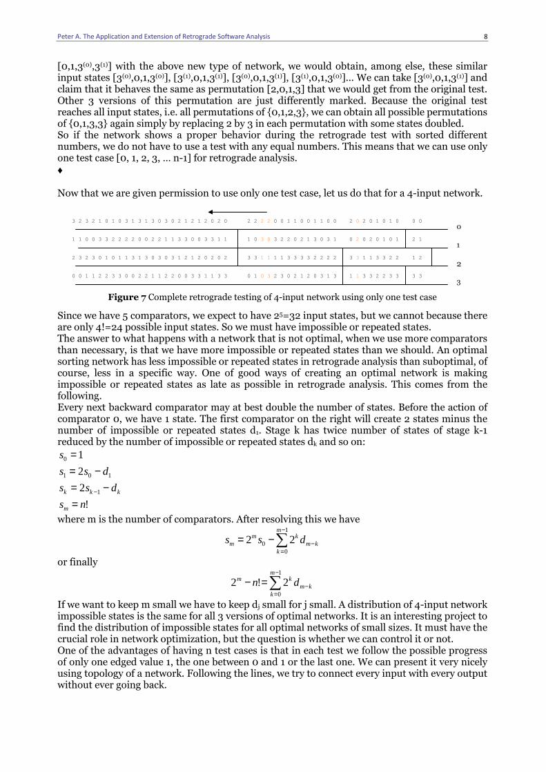
♦ Now that we are given permission to use only one test case, let us do that for a 4-input network.
Figure 7 Complete retrograde testing of 4-input network using only one test case
Since we have 5 comparators, we expect to have 25=32 input states, but we cannot because there are only 4!=24 possible input states. So we must have impossible or repeated states. The answer to what happens with a network that is not optimal, when we use more comparators than necessary, is that we have more impossible or repeated states than we should. An optimal sorting network has less impossible or repeated states in retrograde analysis than suboptimal, of course, less in a specific way. One of good ways of creating an optimal network is making impossible or repeated states as late as possible in retrograde analysis. This comes from the following. Every next backward comparator may at best double the number of states. Before the action of comparator 0, we have 1 state. The first comparator on the right will create 2 states minus the number of impossible or repeated states d1. Stage k has twice number of states of stage k-1 reduced by the number of impossible or repeated states dk and so on:
10 =s
101 2 dss −=
kkk dss −= −12
!nsm =
where m is the number of comparators. After resolving this we have
∑−
=−−=
1
00 22
m
kkm
kmm dss
or finally
∑−
=−=−
1
0
2!2m
kkm
km dn
If we want to keep m small we have to keep dj small for j small. A distribution of 4-input network impossible states is the same for all 3 versions of optimal networks. It is an interesting project to find the distribution of impossible states for all optimal networks of small sizes. It must have the crucial role in network optimization, but the question is whether we can control it or not. One of the advantages of having n test cases is that in each test we follow the possible progress of only one edged value 1, the one between 0 and 1 or the last one. We can present it very nicely using topology of a network. Following the lines, we try to connect every input with every output without ever going back.
0
1
2
3
0 0
2 1
1 2
3 3
2 0 2 0 1 0 1 0
0 2 0 2 0 1 0 1
3 3 1 1 3 3 2 2
1 1 3 3 2 2 3 3
2 2 2 2 0 0 1 1 0 0 1 1 0 0
1 0 3 0 3 2 2 0 2 1 3 0 3 1
3 3 1 1 1 1 3 3 3 3 2 2 2 2
0 1 0 3 2 3 0 2 1 2 0 3 1 3
3 2 3 2 1 0 1 0 3 1 3 1 3 0 3 0 2 1 2 1 2 0 2 0
1 1 0 0 3 3 2 2 2 2 0 0 2 2 1 1 3 3 0 0 3 3 1 1
2 3 2 3 0 1 0 1 1 3 1 3 0 3 0 3 1 2 1 2 0 2 0 2
0 0 1 1 2 2 3 3 0 0 2 2 1 1 2 2 0 0 3 3 1 1 3 3

Peter A. The Application and Extension of Retrograde Software Analysis
9
Figure 8 Retrograde testing fails for assumed 4-input sorting network.
The second condition is that we have an option of connecting input and output without a clash. A clash condition is a case when 1. two paths combination creates at least one impossible state, or 2. when paths overlap so that a swapper cannot be activated. Impossible states or inactive swappers could exclude some inputs. The only way to avoid it is to try to find another combination of paths that does not have a clash.
Figure 9 An assumed 4-input sorting network that can connect each input with output, but has the clash conditions that cannot be avoided: input 0 and output 2 cannot be connected in any other way, as well as
input 2 and output 3, but the combination of paths excludes the state 1010. The state 1100 cannot be achieved this way at all. If we try another way to obtain the input state 1010, we succeed, but we fail again for 1100 because the paths would overlap and swapper s1 would not be activated. Check that input 1100
does not lead to sorted output.
Although not always within a strict realm of software world and coding, this chapter illustrates the power of retrograde analysis. Loop treatment If we are in danger of having explosion of states with each conditional statements, then what to say about loops. How can they be effectively treated with retrograde testing? First, let us condense what we have shown so far:
i. Retrograde testing forces a developer or tester to analyze the code in an unexpected way ii. Retrograde testing reveals what the system does without any assumption that was not built
into the code already iii. Retrograde testing is strict iv. Retrograde testing may reduce the number of test cases
When we normally test a loop, we have several standard problems that must be treated accordingly: 1. A loop must have a definable invariant that is constant throughout the loop execution 2. A loop must have a correct boundary behavior, especially when it starts and when it exits 3. A loop, normally, must provably exit With retrograde analysis, these tasks become obvious, and you have to complete them if you want to analyze any loop properly. The difference is that you start where the standard analysis ends. Example is as trivial as possible, but nonetheless, useful. It does not show the power of retrograde testing only the principles applied.
0
0
0
1
0
0
0
1
0
0
0
1
0
0
0
1
0
0
1
1
0
0
1
1
0
0
1
1
impossible to connect without going back
0 0 1 1
1
0
0 0 1 1 s1
1
1
Peter A. The Application and Extension of Retrograde Software Analysis
10
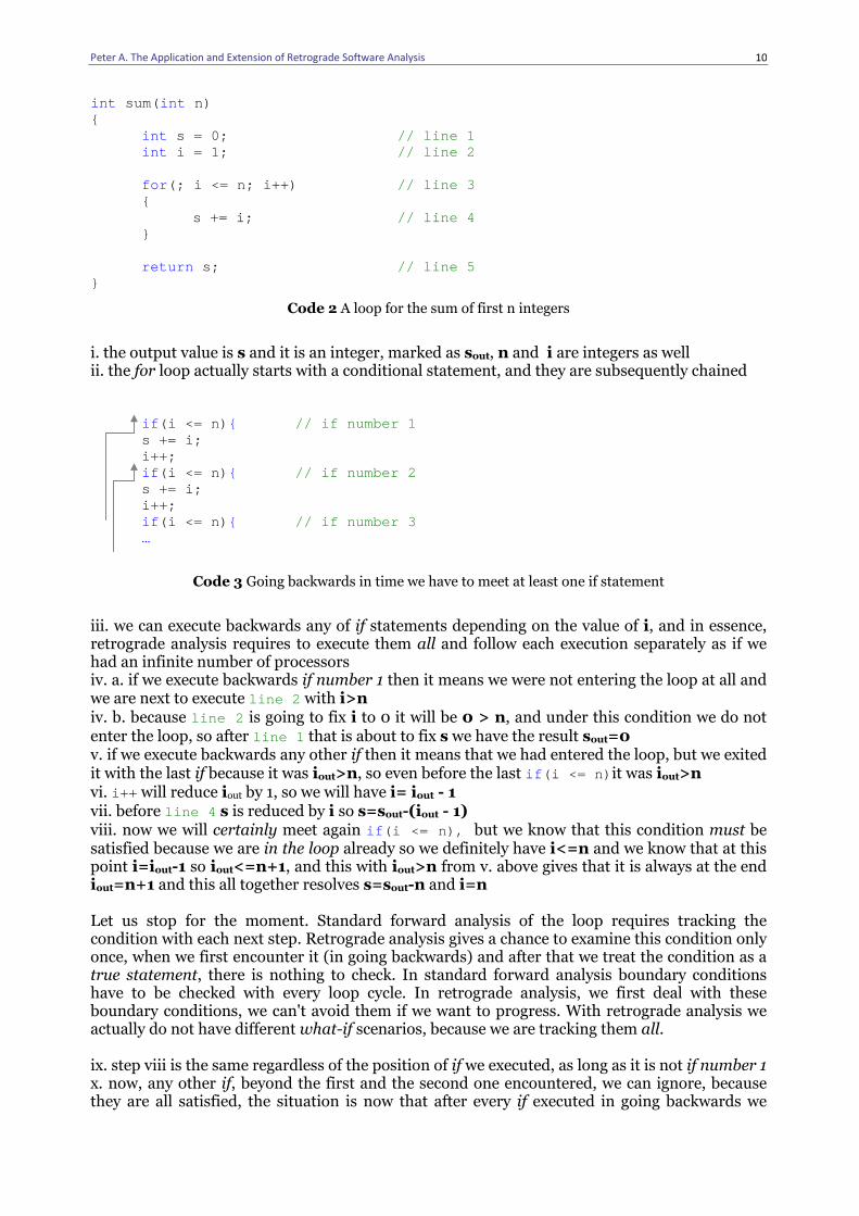
int sum( int n) { int s = 0; // line 1 int i = 1; // line 2 for (; i <= n; i++) // line 3 { s += i; // line 4 } return s; // line 5 }
Code 2 A loop for the sum of first n integers
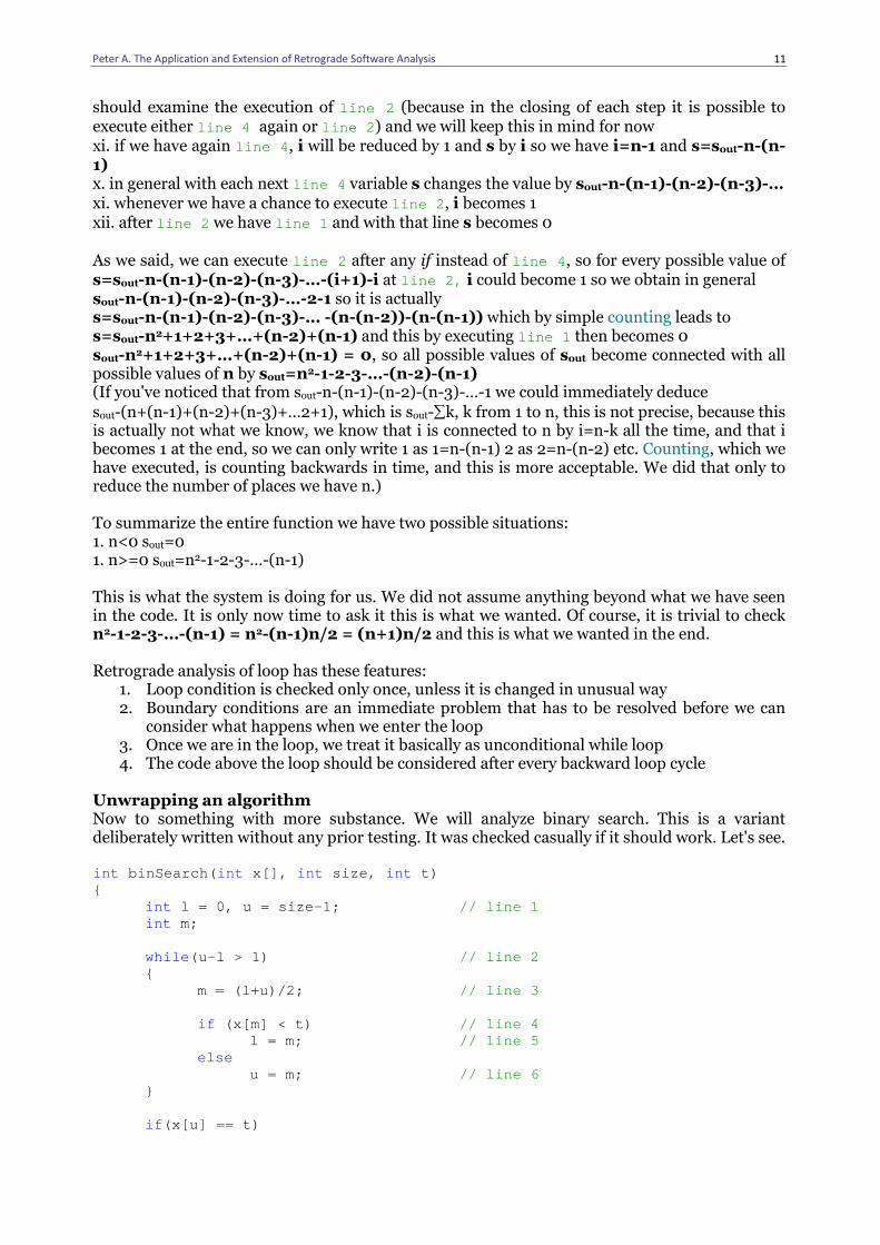
i. the output value is s and it is an integer, marked as sout, n and i are integers as well ii. the for loop actually starts with a conditional statement, and they are subsequently chained if (i <= n) { // if number 1 s += i;
i++; if (i <= n) { // if number 2 s += i;
i++; if (i <= n) { // if number 3 …
Code 3 Going backwards in time we have to meet at least one if statement
iii. we can execute backwards any of if statements depending on the value of i, and in essence, retrograde analysis requires to execute them all and follow each execution separately as if we had an infinite number of processors iv. a. if we execute backwards if number 1 then it means we were not entering the loop at all and we are next to execute line 2 with i>n iv. b. because line 2 is going to fix i to 0 it will be 0 > n, and under this condition we do not enter the loop, so after line 1 that is about to fix s we have the result sout=0 v. if we execute backwards any other if then it means that we had entered the loop, but we exited it with the last if because it was iout>n, so even before the last if (i <= n) it was iout>n vi. i++ will reduce iout by 1, so we will have i= iout - 1 vii. before line 4 s is reduced by i so s=sout-(iout - 1) viii. now we will certainly meet again if (i <= n), but we know that this condition must be satisfied because we are in the loop already so we definitely have i<=n and we know that at this point i=iout-1 so iout<=n+1, and this with iout>n from v. above gives that it is always at the end iout=n+1 and this all together resolves s=sout-n and i=n Let us stop for the moment. Standard forward analysis of the loop requires tracking the condition with each next step. Retrograde analysis gives a chance to examine this condition only once, when we first encounter it (in going backwards) and after that we treat the condition as a true statement, there is nothing to check. In standard forward analysis boundary conditions have to be checked with every loop cycle. In retrograde analysis, we first deal with these boundary conditions, we can't avoid them if we want to progress. With retrograde analysis we actually do not have different what-if scenarios, because we are tracking them all. ix. step viii is the same regardless of the position of if we executed, as long as it is not if number 1 x. now, any other if, beyond the first and the second one encountered, we can ignore, because they are all satisfied, the situation is now that after every if executed in going backwards we
Peter A. The Application and Extension of Retrograde Software Analysis
11
should examine the execution of line 2 (because in the closing of each step it is possible to execute either line 4 again or line 2 ) and we will keep this in mind for now xi. if we have again line 4 , i will be reduced by 1 and s by i so we have i=n-1 and s=sout-n-(n-1) x. in general with each next line 4 variable s changes the value by sout-n-(n-1)-(n-2)-(n-3)-… xi. whenever we have a chance to execute line 2 , i becomes 1 xii. after line 2 we have line 1 and with that line s becomes 0 As we said, we can execute line 2 after any if instead of line 4 , so for every possible value of s=sout-n-(n-1)-(n-2)-(n-3)-…-(i+1)-i at line 2, i could become 1 so we obtain in general sout-n-(n-1)-(n-2)-(n-3)-…-2-1 so it is actually s=sout-n-(n-1)-(n-2)-(n-3)-… -(n-(n-2))-(n-(n-1)) which by simple counting leads to s=sout-n2+1+2+3+…+(n-2)+(n-1) and this by executing line 1 then becomes 0 sout-n2+1+2+3+…+(n-2)+(n-1) = 0, so all possible values of sout become connected with all possible values of n by sout=n2-1-2-3-…-(n-2)-(n-1) (If you've noticed that from sout-n-(n-1)-(n-2)-(n-3)-…-1 we could immediately deduce
sout-(n+(n-1)+(n-2)+(n-3)+…2+1), which is sout-∑k, k from 1 to n, this is not precise, because this is actually not what we know, we know that i is connected to n by i=n-k all the time, and that i becomes 1 at the end, so we can only write 1 as 1=n-(n-1) 2 as 2=n-(n-2) etc. Counting, which we have executed, is counting backwards in time, and this is more acceptable. We did that only to reduce the number of places we have n.) To summarize the entire function we have two possible situations: 1. n<0 sout=0 1. n>=0 sout=n2-1-2-3-…-(n-1) This is what the system is doing for us. We did not assume anything beyond what we have seen in the code. It is only now time to ask it this is what we wanted. Of course, it is trivial to check n2-1-2-3-…-(n-1) = n2-(n-1)n/2 = (n+1)n/2 and this is what we wanted in the end. Retrograde analysis of loop has these features:
1. Loop condition is checked only once, unless it is changed in unusual way 2. Boundary conditions are an immediate problem that has to be resolved before we can
consider what happens when we enter the loop 3. Once we are in the loop, we treat it basically as unconditional while loop 4. The code above the loop should be considered after every backward loop cycle
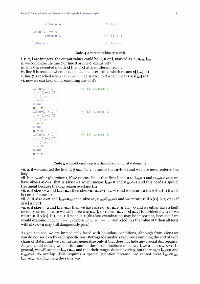
Unwrapping an algorithm Now to something with more substance. We will analyze binary search. This is a variant deliberately written without any prior testing. It was checked casually if it should work. Let's see. int binSearch( int x[], int size, int t) { int l = 0, u = size-1; // line 1 int m; while (u-l > 1) // line 2 { m = (l+u)/2; // line 3 if (x[m] < t) // line 4 l = m; // line 5 else u = m; // line 6 } if (x[u] == t)
Peter A. The Application and Extension of Retrograde Software Analysis
12
return u; // line 7 if (x[l] == t) return l; // line 8 return -1; // line 9 }
Code 4 A variant of binary search
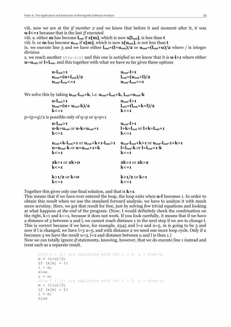
i. u, t, l are integers, the output values could be -1, u or l, marked as -1, uout, lout ii. we could execute line 7 or line 8 or line 9, exclusively iii. line 9 is executed if both x[l] and x[u] are different from t iv. line 8 is reached when if (x[l] == t) is executed which means x[lout] is t v. line 7 is reached when if (x[u] == t) is executed which means x[uout] is t vi. now we can keep on by executing any of if's
if (u-l > 1){ // if number 1 m = (l+u)/2; if (x[m] < t) l = m; else u = m; if (u-l > 1){ // if number 2 m = (l+u)/2; if (x[m] < t) l = m; else u = m; if (u-l > 1){ // if number 3 m = (l+u)/2; if (x[m] < t) l = m; else u = m; …
Code 5 A conditional loop is a chain of conditional statements
vii. a. if we executed the first if, if number 1, it means that u-l<=1 and we have never entered the loop vii. b. now after if number 1, if we execute line 1 that fixes l and u to lout=0 and uout=size-1 we have size-1-0<=1, that is size<=2 which means lout=0 and uout<=1 and this needs a special treatment because the uout region overlaps lout vii. c. if size<=2 and lout<uout then size=2, uout=1, lout=0 and we return 0 if x[0] is t, 1 if x[1] is t or -1 if none is t vii. d. if size<=2 and lout=uout then size=1, uout=lout=0 and we return 0 if x[0] is t, or -1 if x[o] is not t vii. e. if size<=2 and lout>uout then we have size<=0, uout<0, lout=0 and we either have a fault memory access in case we can't access x[uout], or return uout if x[uout] is accidentally t; or we return 0 if x[0] is t, or -1 if none is t (this last examination may be important, because if we would examine if (x[l] == t) before if (x[u] == t) and x[0] has the value of t then all tests with size<=o may still dangerously pass) As you can see, we are immediately faced with boundary conditions, although from size<=2 you do not see exactly each specific one. Retrograde analysis requires examining the end of each chain of states, and we can further generalize only if that does not hide any crucial discrepancy. As you could notice, we had to examine these combinations of states: lout=0 and uout<=1. In general, we will see that lout<uout and that their ranges do not overlap, but the ranges lout=0 and uout<=1 do overlap. This requires a special attention because, we cannot treat lout<uout, lout>uout and lout=uout the same way.
Peter A. The Application and Extension of Retrograde Software Analysis
13
viii. now we are at the if number 2 and we know that before it and moment after it, it was u-l<=1 because that is the last if executed viii. a. either m has become lout if x[m], which is now x[lout], is less than t viii. b. or m has become uout if x[m], which is now x[uout], is not less than t ix. we execute line 3 and we have either lout=(l+uout)/2 or uout=(lout+u)/2 where / is integer division x. we reach another if (u-l>1) and this one is satisfied so we know that it is u-l>1 where either u=uout or l=lout, and this together with what we have so far gives these options
u-lout>1 uout-l>1 uout=(u+lout)/2 lout=(uout+l)/2 uout-lout<=1 uout-lout<=1
We solve this by taking uout-lout=k, i.e. uout=lout+k, lout=uout-k
u-lout>1 uout-l>1 uout=(u+ uout-k)/2 lout=(lout+k+l)/2 k<=1 k<=1
p=(p+q)/2 is possible only of q=p or q=p+1
u-lout>1 uout-l>1 u-k=uout or u-k=uout+1 l+k=lout or l+k=lout+1 k<=1 k<=1
uout+k-lout>1 or uout+k+1-lout>1 uout-lout+k>1 or uout-lout-1+k>1 u=uout-k or u=uout+1+k l=lout-k or l=lout+1-k k<=1 k<=1
2k>1 or 2k>0 2k>1 or 2k>2 k<=1 k<=1
k>1/2 or k>0 k>1/2 or k>1 k<=1 k<=1
Together this gives only one final solution, and that is k=1. This means that if we have ever entered the loop, the loop exits when u-l becomes 1. In order to obtain this result when we use the standard forward analysis, we have to analyze it with much more scrutiny. Here, we got that result for free, just by solving few trivial equations and looking at what happens at the end of the program. (Now, I would definitely check the combination on the right, k>1 and k<=1, because it does not work. If you look carefully, it means that if we have a distance of 3 between u and l, we cannot reach distance 1 in the next step if we are to change l. This is correct because if we have, for example, 2345 and l=2 and u=5, m is going to be 3 and now if l is changed, we have l=3 u=5, and with distance 2 we need one more loop cycle. Only if u becomes 3 we have the result u=3, l=2 and distance between u and l is then 1.) Now we can totally ignore if statements, knowing, however, that we do execute line 1 instead and treat each as a separate result.
if(u-l > 1){ try replacing with int l = 0, u = size -1; m = (l+u)/2; if (x[m] < t) l = m; else u = m; if(u-l > 1){ try replacing with int l = 0, u = size -1; m = (l+u)/2; if (x[m] < t) l = m; else
Peter A. The Application and Extension of Retrograde Software Analysis
14
u = m; if(u-l > 1){ try replacing with int l = 0, u = size -1; m = (l+u)/2; if (x[m] < t) l = m; else u = m; …
Code 6 Each if could be followed (backward) by the execution of line 1
xi. The piece of code
if (x[m] < t) l = m;
else u = m;
is going to change the value of l or u and make either l=m or u=m so before it (backward in time) either l or u will change to something else xii. The piece of code
m = (l+u)/2;
could be combined into one of these two m = (l+u)/2; m = (l+u)/2; l = m; u = m;
so we could have one of these
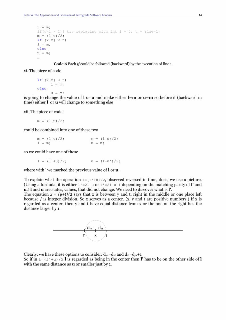
l = (l'+u)/2; u = (l+u')/2; where with ' we marked the previous value of l or u. To explain what the operation l=(l'+u)/2 , observed reversed in time, does, we use a picture. (Using a formula, it is either l'=2l-u or l'=2l-u-1 depending on the matching parity of l' and u.) l and u are states, values, that did not change. We need to discover what is l'. The equation x = (y+t)/2 says that x is between y and t, right in the middle or one place left because / is integer division. So x serves as a center. (x, y and t are positive numbers.) If x is regarded as a center, then y and t have equal distance from x or the one on the right has the distance larger by 1.
Clearly, we have these options to consider: dyx=dxt and dxt=dyx+1 So if in l=(l'+u)/2 l is regarded as being in the center then l' has to be on the other side of l with the same distance as u or smaller just by 1.
y x t
dyx dxt
Peter A. The Application and Extension of Retrograde Software Analysis
15
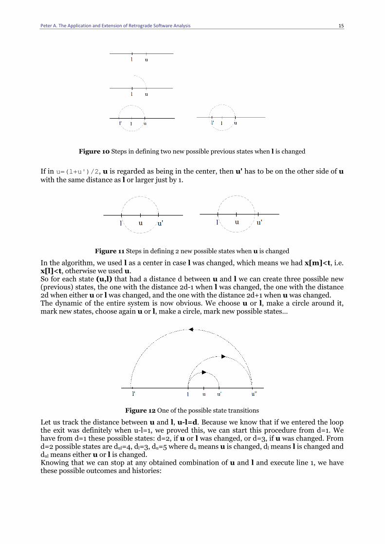
Figure 10 Steps in defining two new possible previous states when l is changed
If in u=(l+u')/2 , u is regarded as being in the center, then u' has to be on the other side of u with the same distance as l or larger just by 1.
Figure 11 Steps in defining 2 new possible states when u is changed
In the algorithm, we used l as a center in case l was changed, which means we had x[m]<t, i.e. x[l]<t, otherwise we used u. So for each state (u,l) that had a distance d between u and l we can create three possible new (previous) states, the one with the distance 2d-1 when l was changed, the one with the distance 2d when either u or l was changed, and the one with the distance 2d+1 when u was changed. The dynamic of the entire system is now obvious. We choose u or l, make a circle around it, mark new states, choose again u or l, make a circle, mark new possible states…
Figure 12 One of the possible state transitions
Let us track the distance between u and l, u-l=d. Because we know that if we entered the loop the exit was definitely when u-l=1, we proved this, we can start this procedure from d=1. We have from d=1 these possible states: d=2, if u or l was changed, or d=3, if u was changed. From d=2 possible states are dul=4, dl=3, du=5 where du means u is changed, dl means l is changed and dul means either u or l is changed. Knowing that we can stop at any obtained combination of u and l and execute line 1, we have these possible outcomes and histories:
Peter A. The Application and Extension of Retrograde Software Analysis
16
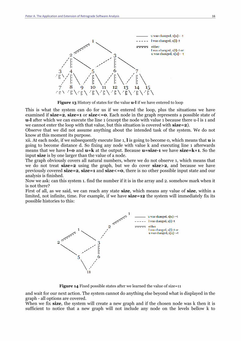
Figure 13 History of states for the value u-l if we have entered to loop
This is what the system can do for us if we entered the loop, plus the situations we have examined if size=2, size=1 or size<=0. Each node in the graph represents a possible state of u-l after which we can execute the line 1 (except the node with value 1 because there u-l is 1 and we cannot enter the loop with that value, but this situation is covered with size=2). Observe that we did not assume anything about the intended task of the system. We do not know at this moment its purpose. xii. At each node, if we subsequently execute line 1, l is going to become 0, which means that u is going to become distance d. So fixing any node with value k and executing line 1 afterwards means that we have l=0 and u=k at the output. Because u=size-1 we have size=k+1. So the input size is by one larger than the value of a node. The graph obviously covers all natural numbers, where we do not observe 1, which means that we do not treat size=2 using the graph, but we do cover size>2, and because we have previously covered size=2, size=1 and size<=0, there is no other possible input state and our analysis is finished. Now we ask: can this system 1. find the number if it is in the array and 2. somehow mark when it is not there? First of all, as we said, we can reach any state size, which means any value of size, within a limited, not infinite, time. For example, if we have size=12 the system will immediately fix its possible histories to this:
Figure 14 Fixed possible states after we learned the value of size=11
and wait for our next action. The system cannot do anything else beyond what is displayed in the graph - all options are covered. When we fix size, the system will create a new graph and if the chosen node was k then it is sufficient to notice that a new graph will not include any node on the levels bellow k to
Peter A. The Application and Extension of Retrograde Software Analysis
17
understand that the graph with fixed size is going to have a fixed number of nodes and edges. (One additional path on the right of nodes 3, 7, 15, … 2j-1, j>1, does not change this conclusion, because the node 2j-1 is adding only one path towards 1, and it is the path: {2j-1
, 2j-2, 2j-3 … 4, 2, 1}
with exactly j edges.) In a new limited graph, we have a path to follow for any chain of changes of u and l. This means that we can create a history whatever value of x[m] we find, and we will keep backward
execution active either if x[m]<t or x[m]≥≥≥≥ t. First, in the original unlimited graph any distance d has an answer to the situation when l is changed and to the situation when u is changed. A new limited graph preserves all paths from any included node to its predecessor, so any node in
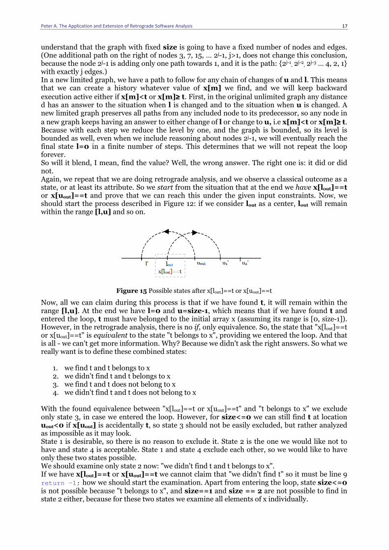
a new graph keeps having an answer to either change of l or change to u, i.e x[m]<t or x[m]≥≥≥≥ t. Because with each step we reduce the level by one, and the graph is bounded, so its level is bounded as well, even when we include reasoning about nodes 2j-1, we will eventually reach the final state l=0 in a finite number of steps. This determines that we will not repeat the loop forever. So will it blend, I mean, find the value? Well, the wrong answer. The right one is: it did or did not. Again, we repeat that we are doing retrograde analysis, and we observe a classical outcome as a state, or at least its attribute. So we start from the situation that at the end we have x[lout]==t or x[uout]==t and prove that we can reach this under the given input constraints. Now, we should start the process described in Figure 12: if we consider lout as a center, lout will remain within the range [l,u] and so on.
Figure 15 Possible states after x[lout]==t or x[uout]==t
Now, all we can claim during this process is that if we have found t, it will remain within the range [l,u]. At the end we have l=0 and u=size-1, which means that if we have found t and entered the loop, t must have belonged to the initial array x (assuming its range is [0, size-1]). However, in the retrograde analysis, there is no if, only equivalence. So, the state that "x[lout]==t or x[uout]==t" is equivalent to the state "t belongs to x", providing we entered the loop. And that is all - we can't get more information. Why? Because we didn't ask the right answers. So what we really want is to define these combined states:
1. we find t and t belongs to x 2. we didn't find t and t belongs to x 3. we find t and t does not belong to x 4. we didn't find t and t does not belong to x
With the found equivalence between "x[lout]==t or x[uout]==t" and "t belongs to x" we exclude only state 3, in case we entered the loop. However, for size<=0 we can still find t at location uout<0 if x[uout] is accidentally t, so state 3 should not be easily excluded, but rather analyzed as impossible as it may look. State 1 is desirable, so there is no reason to exclude it. State 2 is the one we would like not to have and state 4 is acceptable. State 1 and state 4 exclude each other, so we would like to have only these two states possible. We should examine only state 2 now: "we didn't find t and t belongs to x". If we have x[lout]==t or x[uout]==t we cannot claim that "we didn't find t" so it must be line 9 return -1; how we should start the examination. Apart from entering the loop, state size<=0 is not possible because "t belongs to x", and size==1 and size == 2 are not possible to find in state 2 either, because for these two states we examine all elements of x individually.
Peter A. The Application and Extension of Retrograde Software Analysis
18
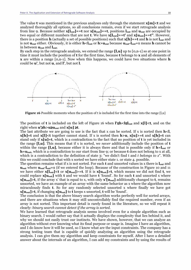
The value t was mentioned in the previous analyses only through the statement x[m]<t and we analyzed thoroughly all options, so all conclusions remain, even if we start retrograde analysis from line 9. Because neither x[lout]==t nor x[uout]==t, positions lout and uout are occupied by two equal or different numbers that are not t. We have x[lout]==t' and x[uout]==t''. However, there is a position h (actually a set of possible positions) such that x[h]==t and h is not lout and is not uout either. Obviously, it is either h<lout or h>uout because uout-lout=1 means h cannot be in between uout and lout. By each step in the retrograde analysis, we extend the range [l,u] up to [0,n-1] so at one point in time it must include the position of t for the first time, because t belongs to x and all elements of x are within a range [0,n-1]. Now when this happens, we could have two situations where h could be u', but not u, and l', but not l.
Figure 16 Possible moments when the position of t is included for the first time into the range [l,u]
The position of t is included on the left of Figure 16 when l'≤≤≤≤h<l≤≤≤≤lout and x[l]<t, and on the
right when u'≥≥≥≥h>u≥≥≥≥uout and x[u] ≥≥≥≥t. The last attribute we are going to use is the fact that x can be sorted. If x is sorted then h<l, x[h]=t and x[l]<t together cannot stand. If x is sorted then h>u, x[u]>=t and x[h]=t can stand only if x[u]=t, which is a contradiction to the fact that no position of t is yet included in the range [l,u]. This means that if x is sorted, we never additionally include the position of t within the range [l,u], because either it is always there and that is possible only if h=lout or h=uout, which is a contradiction to our start from line 9; or because t does not belong to x at all, which is a contradiction to the definition of state 3: "we didn't find t and t belongs to x". With this we could conclude that with x sorted we have either state 1. or state 4. possible. The question remains what if x is not sorted. For each t and unsorted values in x there is lout and uout where uout-lout=1 (if we entered the loop). Because of the construction in Figure 10 and 11 we have either x[lout]<t or x[uout]>=t. If it is x[uout]>t, which means we did not find t, we could replace x[uout] with t and we would have t 'found'. So for each t and unsorted x where x[uout]>t, if the array x' that is equal to x, with only x'[uout] additionally changed to t, remains unsorted, we have an example of an array with the same behavior as x where the algorithm now miraculously finds t. So for any randomly selected unsorted x where finally we have got x[uout]>t, if changing x[uout] to t keeps x unsorted, t will be 'found'. The conclusion is that the above binary search algorithm works perfectly well for sorted arrays, and there are situations when it may still uncontrollably find the required number, even if an array is not sorted. This important detail is rarely found in the literature, so we will repeat it clearly: binary search cannot detect if the array is sorted. We have learned that retrograde analysis seems involved even for a simple algorithm such as binary search. I would rather say that it actually displays the complexity that lies behind it, and why we should not easily trust our instincts. We have shown, however, that we can analyze an algorithm without ever knowing what its final purpose or usage is. Imagine I have an algorithm, and I do know how it will be used, so I know what are the input constraints. The company has a strong testing team that is capable of quickly analyzing an algorithm using the retrograde analysis. I can give them my algorithm and keep constraints for myself. After I have a detailed answer about the internals of an algorithm, I can add my constraints and by using the results of
Peter A. The Application and Extension of Retrograde Software Analysis
19
the retrograde analysis check if it works for the planned task. That way, I can offer my program to any testing company more safely. Algorithms that are backward This principle of following states during a retrograde analysis is already used with some known forward classical algorithms, although it is not obvious. For example, the algorithm for random shuffle uses it. If we have a good random generator, shuffling an array with n elements can be done in O(n). This is how it looks: void rand_shuffle( int x[], int n) { int t; int pos; for ( int i = n-1; i > 0; i--) {
// pos is selected randomly from 0 to i (including 0 and i) pos = rand()%(i+1); // swap x[pos]<->x[i] t = x[i]; x[i] = x[pos]; x[pos]=t; } }
Code 7 Random shuffling that starts from the full range
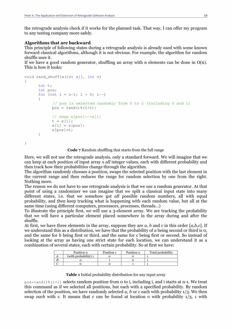
Here, we will not use the retrograde analysis, only a standard forward. We will imagine that we can keep at each position of input array x all integer values, each with different probability and then track how their probabilities change through the algorithm. The algorithm randomly chooses a position, swaps the selected position with the last element in the current range and then reduces the range for random selection by one from the right. Nothing more. The reason we do not have to use retrograde analysis is that we use a random generator. At that point of using a randomizer we can imagine that we split a classical input state into many different states, i.e. that we somehow got all possible random numbers, all with equal probability, and then keep tracking what is happening with each random value, but all at the same time (using different computers, processors, processes, threads…) To illustrate the principle first, we will use a 3-element array. We are tracking the probability that we will have a particular element placed somewhere in the array during and after the shuffle. At first, we have three elements in the array, suppose they are a, b and c in this order [a,b,c]. If we understand this as a distribution, we have that the probability of a being second or third is 0, and the same for b being first or third, and the same for c being first or second. So instead of looking at the array as having one strict state for each location, we can understand it as a combination of several states, each with certain probability. So at first we have:
Table 1 Initial probability distribution for any input array
pos=rand()%(i+1) selects random position from 0 to i, including i, and i starts at n-1. We treat this command as if we selected all positions, but each with a specified probability. By random selection of the position, we have randomly selected a, b or c each with probability 1/3. We then swap each with c. It means that c can be found at location o with probability 1/3, 1 with
Position 0 Position 1 Position 2 Total probability A (with probability) 1 0 0 1 B 0 1 0 1 C 0 0 1 1
Peter A. The Application and Extension of Retrograde Software Analysis
20
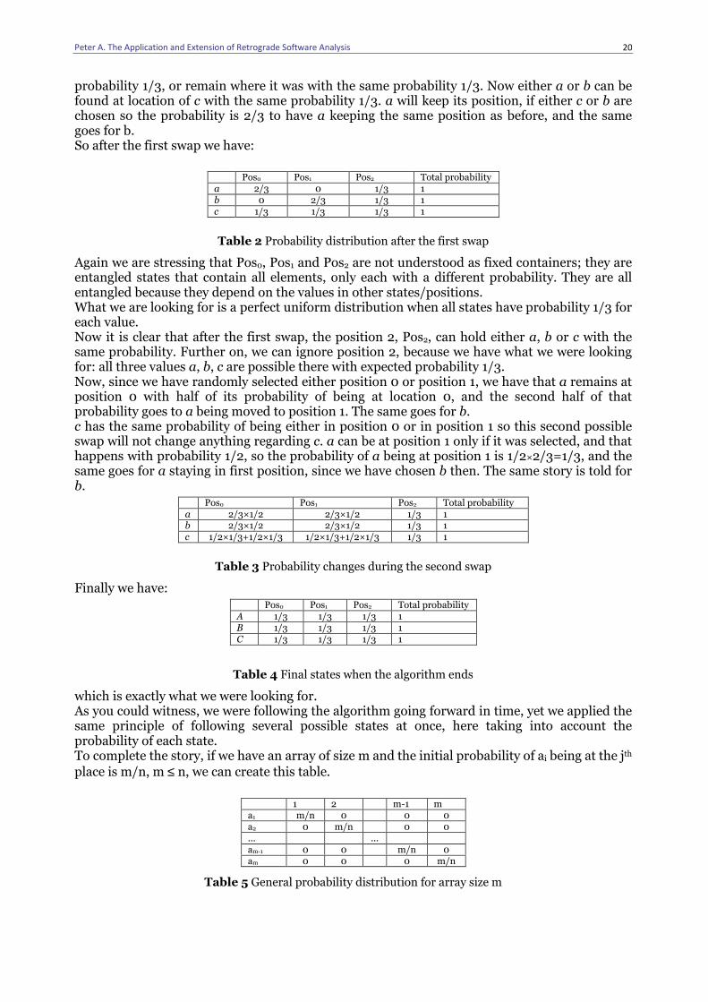
probability 1/3, or remain where it was with the same probability 1/3. Now either a or b can be found at location of c with the same probability 1/3. a will keep its position, if either c or b are chosen so the probability is 2/3 to have a keeping the same position as before, and the same goes for b. So after the first swap we have:
Table 2 Probability distribution after the first swap
Again we are stressing that Pos0, Pos1 and Pos2 are not understood as fixed containers; they are entangled states that contain all elements, only each with a different probability. They are all entangled because they depend on the values in other states/positions. What we are looking for is a perfect uniform distribution when all states have probability 1/3 for each value. Now it is clear that after the first swap, the position 2, Pos2, can hold either a, b or c with the same probability. Further on, we can ignore position 2, because we have what we were looking for: all three values a, b, c are possible there with expected probability 1/3. Now, since we have randomly selected either position 0 or position 1, we have that a remains at position 0 with half of its probability of being at location 0, and the second half of that probability goes to a being moved to position 1. The same goes for b. c has the same probability of being either in position 0 or in position 1 so this second possible swap will not change anything regarding c. a can be at position 1 only if it was selected, and that happens with probability 1/2, so the probability of a being at position 1 is 1/2×2/3=1/3, and the same goes for a staying in first position, since we have chosen b then. The same story is told for b.
Table 3 Probability changes during the second swap
Finally we have:
Table 4 Final states when the algorithm ends
which is exactly what we were looking for. As you could witness, we were following the algorithm going forward in time, yet we applied the same principle of following several possible states at once, here taking into account the probability of each state. To complete the story, if we have an array of size m and the initial probability of ai being at the jth
place is m/n, m ≤ n, we can create this table.
Table 5 General probability distribution for array size m
Pos0 Pos1 Pos2 Total probability a 2/3 0 1/3 1 b 0 2/3 1/3 1 c 1/3 1/3 1/3 1
Pos0 Pos1 Pos2 Total probability a 2/3×1/2 2/3×1/2 1/3 1 b 2/3×1/2 2/3×1/2 1/3 1 c 1/2×1/3+1/2×1/3 1/2×1/3+1/2×1/3 1/3 1
Pos0 Pos1 Pos2 Total probability A 1/3 1/3 1/3 1 B 1/3 1/3 1/3 1 C 1/3 1/3 1/3 1
1 2 m-1 m a1 m/n 0 0 0 a2 0 m/n 0 0 ... ... am-1 0 0 m/n 0 am 0 0 0 m/n
Peter A. The Application and Extension of Retrograde Software Analysis
21
If we randomly select any of ai and swap with am, we have that am will get to any of m places with the same probability as staying where it was, and that is 1/m. The others will either stay where they were or move to position m. They move with the probability 1/m×m/n = 1/n or stay with the probability (m-1)/m×m/n =(m-1)/n. What we have after a swap is this:
Table 6 The probability distribution after the swap
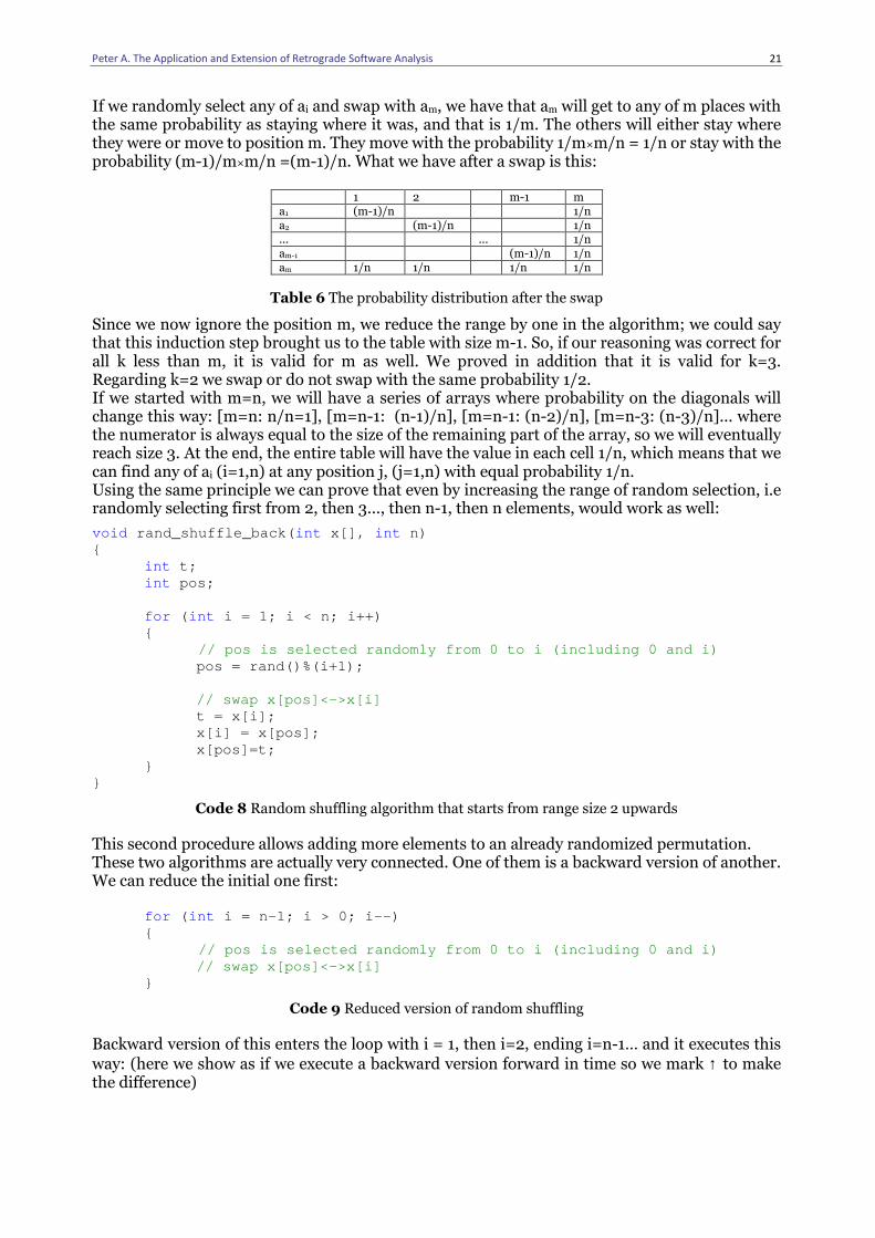
Since we now ignore the position m, we reduce the range by one in the algorithm; we could say that this induction step brought us to the table with size m-1. So, if our reasoning was correct for all k less than m, it is valid for m as well. We proved in addition that it is valid for k=3. Regarding k=2 we swap or do not swap with the same probability 1/2. If we started with m=n, we will have a series of arrays where probability on the diagonals will change this way: [m=n: n/n=1], [m=n-1: (n-1)/n], [m=n-1: (n-2)/n], [m=n-3: (n-3)/n]... where the numerator is always equal to the size of the remaining part of the array, so we will eventually reach size 3. At the end, the entire table will have the value in each cell 1/n, which means that we can find any of ai (i=1,n) at any position j, (j=1,n) with equal probability 1/n. Using the same principle we can prove that even by increasing the range of random selection, i.e randomly selecting first from 2, then 3..., then n-1, then n elements, would work as well:
void rand_shuffle_back( int x[], int n) { int t; int pos; for ( int i = 1; i < n; i++) {
// pos is selected randomly from 0 to i (including 0 and i) pos = rand()%(i+1); // swap x[pos]<->x[i] t = x[i]; x[i] = x[pos]; x[pos]=t; } }
Code 8 Random shuffling algorithm that starts from range size 2 upwards
This second procedure allows adding more elements to an already randomized permutation. These two algorithms are actually very connected. One of them is a backward version of another. We can reduce the initial one first: for ( int i = n-1; i > 0; i--) {
// pos is selected randomly from 0 to i (including 0 and i) // swap x[pos]<->x[i] }
Code 9 Reduced version of random shuffling
Backward version of this enters the loop with i = 1, then i=2, ending i=n-1… and it executes this
way: (here we show as if we execute a backward version forward in time so we mark ↑ to make the difference)
1 2 m-1 m a1 (m-1)/n 1/n a2 (m-1)/n 1/n ... ... 1/n am-1 (m-1)/n 1/n am 1/n 1/n 1/n 1/n
Peter A. The Application and Extension of Retrograde Software Analysis
22
for ↑ ( int i = 1; i <= n-1; i++) { // swap x[pos]<->x[i]
// pos is selected randomly from 0 to i (including 0 and i) }
Code 10 Reduced backward version of random shuffling
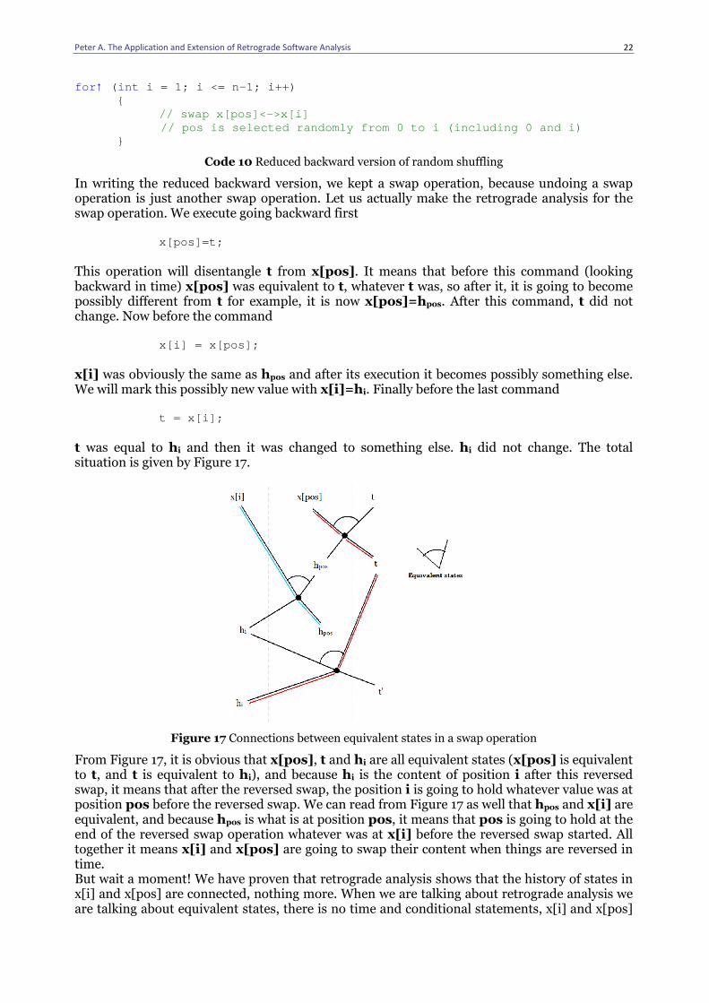
In writing the reduced backward version, we kept a swap operation, because undoing a swap operation is just another swap operation. Let us actually make the retrograde analysis for the swap operation. We execute going backward first x[pos]=t; This operation will disentangle t from x[pos]. It means that before this command (looking backward in time) x[pos] was equivalent to t, whatever t was, so after it, it is going to become possibly different from t for example, it is now x[pos]=hpos. After this command, t did not change. Now before the command x[i] = x[pos]; x[i] was obviously the same as hpos and after its execution it becomes possibly something else. We will mark this possibly new value with x[i]=hi. Finally before the last command
t = x[i]; t was equal to hi and then it was changed to something else. hi did not change. The total situation is given by Figure 17.
Figure 17 Connections between equivalent states in a swap operation
From Figure 17, it is obvious that x[pos], t and hi are all equivalent states (x[pos] is equivalent to t, and t is equivalent to hi), and because hi is the content of position i after this reversed swap, it means that after the reversed swap, the position i is going to hold whatever value was at position pos before the reversed swap. We can read from Figure 17 as well that hpos and x[i] are equivalent, and because hpos is what is at position pos, it means that pos is going to hold at the end of the reversed swap operation whatever was at x[i] before the reversed swap started. All together it means x[i] and x[pos] are going to swap their content when things are reversed in time. But wait a moment! We have proven that retrograde analysis shows that the history of states in x[i] and x[pos] are connected, nothing more. When we are talking about retrograde analysis we are talking about equivalent states, there is no time and conditional statements, x[i] and x[pos]
Peter A. The Application and Extension of Retrograde Software Analysis
23
could be any combination of states. Thus we should say that a swap operation applied to any two combinations of states A-B is going to swap their content so A is going to become B and B is going to become A simultaneously. Observe path that leads x[pos] to hi and the path that leads x[i] to hpos there was no destruction of any kind, we obviously just respelled i to pos and pos to i. Was this swap examination really necessary? Couldn't we just take for granted that it works, even if observed reversed in time? Well, if it was a mathematical operation, then yes, but we actually have a surrogate of a swap operation written in C. And second, we are not just trying to prove that any operation written in classical way works. We are trying to discover what principle lies beneath it in order to understand it better and to show some retrograde analysis formalism. There are other ways of doing a swap operation that do not require the third variable, but all of them implicitly destroy states involved, and recreate only some of the previous attributes: a = a^b; b = a^b; a = a^b;
a=a+b; b=a-b; a=a-b;
a=a*b; b=a/b; a=a/b;
Code 11 Some possible swap operation variants. Knowing at one moment only a+b, a^b or a*b we can't immediately read both states, so something is lost in the process, but later recreated.
(It is interesting that we can use operation XOR, ^, to keep two states at the same time in the same location. It speaks that, to some extent, we can still combine information within a classical machine even though a swap operation looks unavoidable because we can't keep two pieces of information in the same location, it goes that way from the basics - we have one bit being either 0 or 1.) Now let us examine the entire algorithm more. As we said a backward version is the version that includes all possible states so // swap x[pos]<->x[i] should be observed as executed for all possible values of pos. We do not have any restrictions apart from pos being an integer, thus pos can have, at this point, any integer value, and we imagine having them all. In the next command, the number of possible states we are going to track is reduced and clearly defined with a random selection of pos from o to i, which means that we are interested only in swapping i with any of positions from o to i, but this is the same step in both versions: it is the same to first take a position from o to i and swap it with ith position, or swap every conceivable position with ith and then extract only those from o to i. So the body of the loop is the same observed from forward and backward direction, and we could easily write:
{
// pos is selected randomly from 0 to i (including 0 and i) // swap x[pos]<->x[i] }
Code 12 A reduced backward version of random shuffling with random selection executed as the first command
and there would be no changes in the algorithm's behavior. But this last version is actually the same as the forward version of rand_shuffle_back . So rand_shuffle_back and rand_shuffle are backward inversions to each other. This is expected: randomizing a permutation is an inverse operation to itself. Inverse is inverse is inverse It is time to offer some formalism to the retrograde analysis. We treat each variable as a state, and mark its progression from bottom to top. We mark the current state for variable a by a{k} and we can create new states either by changing k a{k} to a{k+1} or by splitting a{{k,0}}
Peter A. The Application and Extension of Retrograde Software Analysis
24
a{{k,1}}. It is understood that {k} is equivalent to {k,0} and actually to {k,0,0,…}. We record all possible states as a{k1, k2, k3…} We may mark with ↑ that the program was executed backwards so we will write …
3↑ 2↑
1 ↑ when the program actually executes line 3, line 2, line 1. We treat here: value change, if statement, loop and function call. Value change, if the value/state was changed, we take that some other yet unknown value was there before y = a; a = b;
2↑ y = a{1}; 1↑ a{0} = b;
This statement says that before a was changed to b, and became a{0}, a was something else, a{1}. If statement splits the backward execution path in two, when the condition is satisfied and when it is not y = x; if ( condition) {
y = x; x = a;
} x = b;
5↑ y{r 3,r 4} = x{{1,1},2}; 4↑ { 3↑ y{r 1} = x{2}; 2↑ x{1} = a; }( condition) 1↑ x{0} = b;
The backward execution says that before x becomes b, it was something else, and if we were inside if then x was x{1}, which is the same as x{{1,0}}, but if we were not inside if statement we had another value for x, which is x{{1,1}}, so before if we could have either what was before x{o} without if, and that is x{{1,1}}, or x{2}. It is important to have encoded information that the condition is satisfied or not. We could use x{3} and x{4} if, for some time, we are not interested in connections between states x{o}, x{{1,1}} and x{2}, the same way we did for y. While loop in general creates three paths: we didn't enter, we entered once, and we entered multiple times. At the exit, the loop condition was not fulfilled; however, during the course of the loop, the condition was satisfied. y = x; while ( condition) {
y = x; x = a;
} x = b;
7↑ y{r K+1} = x{{1,1},2,K+1}; 6↑ ( condition){… 5↑ y{r k} = x{k+1};
x{k} = a; 4↑ ( condition){ 3↑ y{r 1} = x{2};
x{1} = a; } 2↑ (! condition) 1↑ x{0} = b;
Peter A. The Application and Extension of Retrograde Software Analysis
25
This backward statement says that if we did not enter while loop, we had before x{0} value x{{1,1}}, if we entered once we had x{1} inside the loop and before the loop x{2}, if we entered more than once we had x{k} inside the loop and x{K+1} before the loop started (capital K marks we are not in the loop). The advantage of retrograde analysis is that we observe a loop condition only once at the loop's exit, and not during the loop, when we treat the condition as true. Do loop is the same as while loop, in the example it just does not have x{{1,1}} because we had to enter the loop at least once y = x; do{
y = x; x = a;
} while ( condition); x = b;
9↑ y{r K+1} = x{2,K+1}; 8↑ ( condition){… 7↑ y{r k} = x{k+1}; 6↑ x{k} = a; 5↑ ( condition){ 4↑ y{r 1} = x{2}; 3↑ x{1} = a; } 2↑ (! condition) 1↑ x{0} = b;
Other behaviors could be easily derived, function call - we start execution from bottom to top, and treat input parameters as the final values etc. int func_name( int a, int &b); a = p; b = q; func_name(a,b); a = r; b = s;
5↑ a{k} = p; 4↑ b{k} = q; 3↑ func_name(a{k},b{k}); 2↑ a{0} = r; 1↑ b{0} = s;
For simple code, we can use other markers like ', '', ''', or {0},{1},{2} instead of {0}, {1}, {2}. In C++, for example, creating an object with new would be equal to calling a constructor in reverse, delete would be equal to resurrecting an object by calling its destructor in reverse and so on. Although some of these processes might not be deterministic in nature, it does not change the force of retrograde analysis; we observe all moments when they could have happened. Currently, we have analyzers that create structures that aid a compiler analyzing the code. Binary decision diagram is one of them. In essence, this analysis does not require much different structures. What is different is that, first, even though it can be used in formal verification, it can be used equally well only to capture the complexity and major test cases we should not avoid. Second, it relies on what a developer already knows how to do, and although we are writing our examples in C, any other language has the same property that it can be executed backwards. Third, the power that a developer gets by having a strict method for digging as deep as he likes within existing code is very important. If you believe that we already have many forward methods of testing, we have to say that none of them is shifting the perspective as powerful. They do help about testing, but they do not have that specific universality the backward method has. Retrograde analysis is a strict method. There are other areas of human enterprise where shifting perspective is a welcomed technique as well. Before we start examining why it would be very nice to create a programming language that would help executing retrograde analysis or creating programs on its own, one more example that would help showing a complete course of analysis.
Peter A. The Application and Extension of Retrograde Software Analysis
26
void inverse_perm( int x[], int size) { int p = 1; int v; int hv; while (p <= size) { hv = p; p = x[p]; if (!(p < 0))
{ do { v = x[p]; x[p] = -hv; hv = p; p = v;
} while (!(x[p] < 0));
} x[hv] = -x[hv]; p = hv + 1;
} }
Code 13 Inverting a permutation, the array x starts from 1 to size (not from 0 to size-1) and it holds all different numbers from 1 to size
Inversion of permutation is an interesting algorithm because for one input we expect exactly one output and vice versa, so the test cases are difficult to group. We have one while loop that creates three essential paths. If we entered while loop we have if and do that combined can create three paths. Overall we have 13 basic test paths to follow (3×3 in case we entered while more than once +3 in case we entered while twice +1 if we did not enter while). This is not too much to analyze and some paths are simple enough. Using the above notation, we can analyze all 13 paths at the same time, but this would be cumbersome to explain here, so we continue one by one. Let us analyze one moment needed for this program using forward and retrograde analysis. We will prove that if we have a permutation of numbers from 1 to n, then the following procedure ends where it started: if we choose one number k from the permutation then skip to position k and choose its value k'=x[k], then choose the next number taking k' as a position k''=x[k'] and so on, we will definitely end this cycle meeting k again. In essence, we prove that each permutation can be split into these cycles. First, because we have a finite set of numbers, using this procedure we will eventually exhaust all of them so we will definitely meet one number again, soon or later. Forward Suppose we met number p(t) that is not p again. p(1) = x[p] p(2) = x[p(1)] p(3) = x[p(2)]
… p(t-1) = x[p(t-2)] p(t) = x[p(t-1)] … p(s) = x[p(s-1)]
p(t) = x[p(s)]
part a
part b
Peter A. The Application and Extension of Retrograde Software Analysis
27
All numbers from part a and part b are different except p(t), but this means we have two different positions with equal values p(t-1) and p(s). However, we do not have, all numbers are different. So p(t-1) and p(s) are the same and because they have unique positions, p(t-2) and p(s-1) are the same and so on. With that, part a and part b become the same and we do return exactly to p again.
♦ Backward We observe the chain backwards. So if we start from p then we ask what was the position p(1), and that position must exist, for which x[p(1)]=p and so on. If we eventually meet twice some p(t) different from p the situation is like this x[p(1)]=p x[p(2)]=p(1) x[p(3)]=p(2)
… x[p(t-1)]=p(t-2) x[p(t)]=p(t-1) …
x[p(s)]=p(s-1)
x[p(t)]=p(s)
All numbers from part a and part b are different except p(t) which means that x[p(t)] holds two different values, which is impossible. So p(s) and p(t-1) are the same, and because they represent positions in the previous steps, x[p(s)] and x[p(t-1)] are the same and so on. So part a and part b have to be the same and we do return exactly to p.
♦ Elementary, Watson? Sure. Yet, even this example shows the difference. When we are doing forward analysis, we are using the fact that we don't have two positions with equal values, which actually requires an explanation: it comes from the fact that all numbers are different. In retrograde analysis, we are using a far more obvious and fundamental fact and that is that we cannot keep two different values at the same location. (If you wonder why we do not have to use the condition that all numbers are different, it is because we use the positions, which are unique on their own.) We have to reiterate why we are doing this perspective shifting. It is essential to understand that even a very simple program covers possibly a very high number of states, and only one wrong is sufficient to break everything (the story about Intel Pentium bug can quickly convince anyone). Each programmer improves his skills by programming new problems and trying new styles. Most of the techniques we are using today came into being from experience. If we look at algorithms classification only, we find: brute-force, divide and conquer, dynamic programming, the greedy method, linear programming, reduction, search and enumeration etc. but this is the classification of existing algorithms. It is a Kepler's collection of rules. Knuth tried to make a new Newton's job of shaping that into some related mathematical laws. A programmer is learning both. Being a mathematician, he is required to define as precise as possible a model for the problem. Being an engineer, he has to create a robust solution. After he has completed his solution, he is immediately faced with the testing phase where he fixes the problems in the code or design. Every programmer should think not only about the problem he is faced with, but if he wants to progress: why and how I, or the team, or the company, or the theory made this error. Only by finding the key problem, he can improve his skills, otherwise he, or the team, or the company, or the theory will produce the same error again. People choose programming because they like it, and something about that is intuitively clear to them, and they keep on. Just by looking at the simple example of binary search, we can see that programming cannot be easy, because the intuitively clear method of binary search is all but simple. How many programmers today are aware that it is not easy? How many companies are not going to hire a developer who makes even the slightest pause before writing the binary search algorithm recorded in his head as an eternal religious truth? One can easily assure
part a
part b
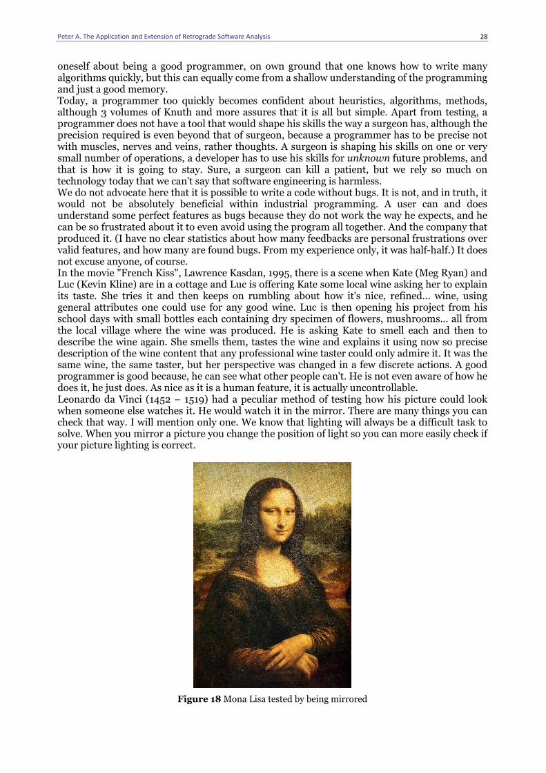
Peter A. The Application and Extension of Retrograde Software Analysis
28
oneself about being a good programmer, on own ground that one knows how to write many algorithms quickly, but this can equally come from a shallow understanding of the programming and just a good memory. Today, a programmer too quickly becomes confident about heuristics, algorithms, methods, although 3 volumes of Knuth and more assures that it is all but simple. Apart from testing, a programmer does not have a tool that would shape his skills the way a surgeon has, although the precision required is even beyond that of surgeon, because a programmer has to be precise not with muscles, nerves and veins, rather thoughts. A surgeon is shaping his skills on one or very small number of operations, a developer has to use his skills for unknown future problems, and that is how it is going to stay. Sure, a surgeon can kill a patient, but we rely so much on technology today that we can't say that software engineering is harmless. We do not advocate here that it is possible to write a code without bugs. It is not, and in truth, it would not be absolutely beneficial within industrial programming. A user can and does understand some perfect features as bugs because they do not work the way he expects, and he can be so frustrated about it to even avoid using the program all together. And the company that produced it. (I have no clear statistics about how many feedbacks are personal frustrations over valid features, and how many are found bugs. From my experience only, it was half-half.) It does not excuse anyone, of course. In the movie "French Kiss", Lawrence Kasdan, 1995, there is a scene when Kate (Meg Ryan) and Luc (Kevin Kline) are in a cottage and Luc is offering Kate some local wine asking her to explain its taste. She tries it and then keeps on rumbling about how it's nice, refined… wine, using general attributes one could use for any good wine. Luc is then opening his project from his school days with small bottles each containing dry specimen of flowers, mushrooms… all from the local village where the wine was produced. He is asking Kate to smell each and then to describe the wine again. She smells them, tastes the wine and explains it using now so precise description of the wine content that any professional wine taster could only admire it. It was the same wine, the same taster, but her perspective was changed in a few discrete actions. A good programmer is good because, he can see what other people can't. He is not even aware of how he does it, he just does. As nice as it is a human feature, it is actually uncontrollable. Leonardo da Vinci (1452 – 1519) had a peculiar method of testing how his picture could look when someone else watches it. He would watch it in the mirror. There are many things you can check that way. I will mention only one. We know that lighting will always be a difficult task to solve. When you mirror a picture you change the position of light so you can more easily check if your picture lighting is correct.
Figure 18 Mona Lisa tested by being mirrored
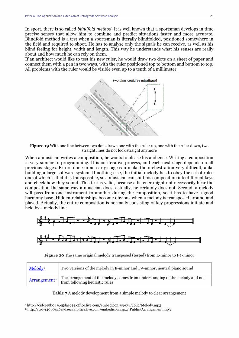
Peter A. The Application and Extension of Retrograde Software Analysis
29
In sport, there is so called blindfold method. It is well known that a sportsman develops in time precise senses that allow him to combine and predict situations faster and more accurate. Blindfold method is a test when a sportsman is literally blindfolded, positioned somewhere in the field and required to shoot. He has to analyze only the signals he can receive, as well as his blind feeling for height, width and length. This way he understands what his senses are really about and how much he can rely on them. If an architect would like to test his new ruler, he would draw two dots on a sheet of paper and connect them with a pen in two ways, with the ruler positioned top to bottom and bottom to top. All problems with the ruler would be visible even up to a tenth of a millimeter.
Figure 19 With one line between two dots drawn one with the ruler up, one with the ruler down, two straight lines do not look straight anymore
When a musician writes a composition, he wants to please his audience. Writing a composition is very similar to programming. It is an iterative process, and each next stage depends on all previous stages. Errors done in an early stage can make the orchestration very difficult, alike building a large software system. If nothing else, the initial melody has to obey the set of rules one of which is that it is transposable, so a musician can shift his composition into different keys and check how they sound. This test is valid, because a listener might not necessarily hear the composition the same way a musician does; actually, he certainly does not. Second, a melody will pass from one instrument to another during the composition, so it has to have a good harmony base. Hidden relationships become obvious when a melody is transposed around and played. Actually, the entire composition is normally consisting of key progressions initiate and held by a melody line.
Figure 20 The same original melody transposed (tested) from E-minor to F#-minor
Melody1 Two versions of the melody in E-minor and F#-minor, neutral piano sound
Arrangement2 The arrangement of the melody comes from understanding of the melody and not from following heuristic rules
Table 7 A melody development from a simple melody to clear arrangement
1 http://cid-140b04a6e5daec44.office.live.com/embedicon.aspx/.Public/Melody.mp3 2 http://cid-140b04a6e5daec44.office.live.com/embedicon.aspx/.Public/Arrangement.mp3
Peter A. The Application and Extension of Retrograde Software Analysis
30
We should definitely have such methods in software industry, and that should be something a developer with current knowledge could understand. Currently, in order to shift this perspective, we shift the entire project to the testing department team where the testing team and the development team are separated and have a different role; they are frequently opposed to each other. This behavior has come from the practice, but it absolutely does not mean that if we have a kind of competition between testing and development team we are going to have a better product. (It is like saying that if we let man and wife in a boxing ring every day, we will have a better marriage.) Retrograde analysis offers a complete depiction about the program we are testing, and it can be used in many different ways. Retrograde analysis forces a developer to get out of his skin, experience, habit, during the analysis. When you face an average technical person with programming, he is somewhat confused with restrictions imposed by any programming language, and in time he gets accustomed and it comes natural to him. Although it seems difficult and involving, retrograde analysis is such because we are not used to that way of thinking, it looks like eating soup with a fork. However, by doing retrograde analysis, we get a complete picture about any system, and because we currently do not have that norm, it means that, at the moment, an average developer has predominantly intuitive knowledge about the system he is developing, throughout the entire industry. At universities, we teach people the software programming as heuristic - heuristic is what they use - heuristic is what they write - heuristic is what they keep on writing. It is not a huge problem on its own, because programming is shaped through experience and industry like anything else is, but it is the problem that a programmer does not really understand how much of his way of thinking goes actually as a heuristic. A splendid example of this process of thinking is given in Programming Pearls [Bentley p.83], where it is explained the process of how a scanning algorithm for maxsum problem was found. That is how it goes when you are programming. You have an idea, you test the idea starting from that idea again, using the same thinking process that gave you that idea, because you can’t force yourself into any other way of thinking. Retrograde analysis is forcing you into it. It makes a programmer looking in the 'simple' binary search explained above with much different thoughts than before. The problems in programming are coming from partial understanding of the solution and invisibility of the part that is not well understood. Not only that. Retrograde analysis is always showing the underlying principle or method that is used, which we do not have to be totally aware of when we use an algorithm, because we might just be aware that it works and have a specific way of proving it, if we believe we need one. Every algorithm on its own is actually so rich that there should be no reason for not getting into it as deep as we can and unravel why and how it works, and what is best, all that directly from the code. With ever improving technology we should know not only that something works, but rather why it works, so we could quickly adjust the underlying principle to a new device: electronic, quantum, sound, optical… name it. The underlying general principles are described in almost every book about algorithms as a choice between: brute-force, divide and conquer, dynamic programming, the greedy method, linear programming, reduction, search and enumeration and couple more. Beyond that it usually all runs into a specialized area of mathematics, in case you want to deal with a particular type of problems, a type that might or might not be applicable to the problem a developer is facing with. Retrograde analysis shows actually an entire new world beneath each algorithm, and it is very worth exploring it. We are going to explain as well what we would need if we want to create an environment that would be able to execute a program backwards. Retrograde analysis does not require any immediate effort like forward analysis. It starts in a strict way, not different from solving equations, and only later it needs some thinking in order to decide whether it resolves the final problem. A developer is free not to think about whether his program or methods works at first3. When you start retrograde analysis it is actually required.
3 Whenever I tackle a particular algorithm with the retrograde analysis, it is always that initial fear that if I really allow everything, the way retrograde analysis starts, then something is going to be wrong in the end for sure. The programming habits obviously made me extremely cautious, so it is an alarm triggering in my head with this suddenly
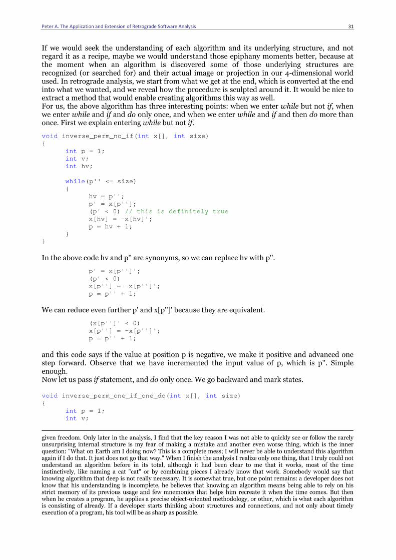
Peter A. The Application and Extension of Retrograde Software Analysis
31
If we would seek the understanding of each algorithm and its underlying structure, and not regard it as a recipe, maybe we would understand those epiphany moments better, because at the moment when an algorithm is discovered some of those underlying structures are recognized (or searched for) and their actual image or projection in our 4-dimensional world used. In retrograde analysis, we start from what we get at the end, which is converted at the end into what we wanted, and we reveal how the procedure is sculpted around it. It would be nice to extract a method that would enable creating algorithms this way as well. For us, the above algorithm has three interesting points: when we enter while but not if, when we enter while and if and do only once, and when we enter while and if and then do more than once. First we explain entering while but not if.
void inverse_perm_no_if( int x[], int size) { int p = 1; int v; int hv; while (p'' <= size) { hv = p''; p' = x[p'']; (p' < 0) // this is definitely true x[hv] = -x[hv]'; p = hv + 1;
} } In the above code hv and p'' are synonyms, so we can replace hv with p''.
p' = x[p'']'; (p' < 0) x[p''] = -x[p'']'; p = p'' + 1; We can reduce even further p' and x[p'']' because they are equivalent.
(x[p'']' < 0) x[p''] = -x[p'']'; p = p'' + 1; and this code says if the value at position p is negative, we make it positive and advanced one step forward. Observe that we have incremented the input value of p, which is p''. Simple enough. Now let us pass if statement, and do only once. We go backward and mark states. void inverse_perm_one_if_one_do( int x[], int size) { int p = 1; int v;
given freedom. Only later in the analysis, I find that the key reason I was not able to quickly see or follow the rarely unsurprising internal structure is my fear of making a mistake and another even worse thing, which is the inner question: "What on Earth am I doing now? This is a complete mess; I will never be able to understand this algorithm again if I do that. It just does not go that way." When I finish the analysis I realize only one thing, that I truly could not understand an algorithm before in its total, although it had been clear to me that it works, most of the time instinctively, like naming a cat "cat" or by combining pieces I already know that work. Somebody would say that knowing algorithm that deep is not really necessary. It is somewhat true, but one point remains: a developer does not know that his understanding is incomplete, he believes that knowing an algorithm means being able to rely on his strict memory of its previous usage and few mnemonics that helps him recreate it when the time comes. But then when he creates a program, he applies a precise object-oriented methodology, or other, which is what each algorithm is consisting of already. If a developer starts thinking about structures and connections, and not only about timely execution of a program, his tool will be as sharp as possible.
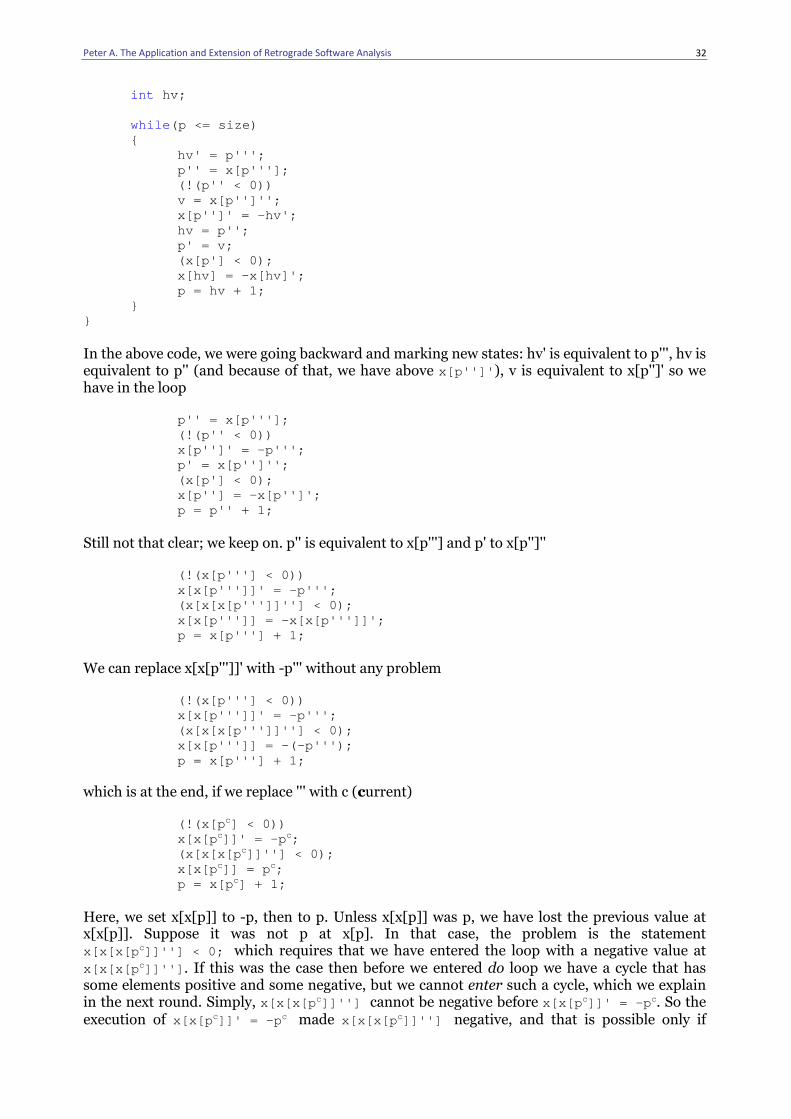
Peter A. The Application and Extension of Retrograde Software Analysis
32
int hv; while (p <= size) { hv' = p'''; p'' = x[p''']; (!(p'' < 0)) v = x[p'']''; x[p'']' = -hv';
hv = p''; p' = v; (x[p'] < 0); x[hv] = -x[hv]'; p = hv + 1;
} } In the above code, we were going backward and marking new states: hv' is equivalent to p''', hv is equivalent to p'' (and because of that, we have above x[p'']' ), v is equivalent to x[p'']' so we have in the loop p'' = x[p''']; (!(p'' < 0)) x[p'']' = -p'''; p' = x[p'']''; (x[p'] < 0); x[p''] = -x[p'']'; p = p'' + 1; Still not that clear; we keep on. p'' is equivalent to x[p'''] and p' to x[p'']'' (!(x[p'''] < 0)) x[x[p''']]' = -p'''; (x[x[x[p''']]''] < 0); x[x[p''']] = -x[x[p''']]'; p = x[p'''] + 1; We can replace x[x[p''']]' with -p''' without any problem (!(x[p'''] < 0)) x[x[p''']]' = -p'''; (x[x[x[p''']]''] < 0); x[x[p''']] = -(-p'''); p = x[p'''] + 1; which is at the end, if we replace ''' with c (current) (!(x[p c] < 0)) x[x[p c]]' = -p c; (x[x[x[p c]]''] < 0); x[x[p c]] = p c; p = x[p c] + 1; Here, we set x[x[p]] to -p, then to p. Unless x[x[p]] was p, we have lost the previous value at x[x[p]]. Suppose it was not p at x[p]. In that case, the problem is the statement x[x[x[p c]]''] < 0; which requires that we have entered the loop with a negative value at x[x[x[p c]]''] . If this was the case then before we entered do loop we have a cycle that has some elements positive and some negative, but we cannot enter such a cycle, which we explain in the next round. Simply, x[x[x[p c]]''] cannot be negative before x[x[p c]]' = -p c. So the execution of x[x[p c]]' = -p c made x[x[x[p c]]''] negative, and that is possible only if
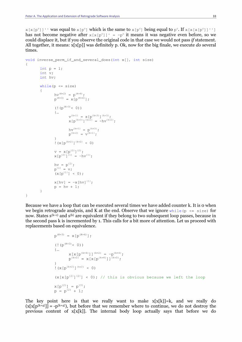
Peter A. The Application and Extension of Retrograde Software Analysis
33
x[x[p c]]'' was equal to x[p c] which is the same to x[p c] being equal to pc. If x[x[x[p c]]''] has not become negative after x[x[p c]]' = -p c it means it was negative even before, so we could displace it, but if you observe the original code in that case we would not pass if statement. All together, it means: x[x[p]] was definitely p. Ok, now for the big finale, we execute do several times. void inverse_perm_if_and_several_does( int x[], int size) { int p = 1; int v; int hv; while (p <= size) { hv (K+2) = p (K+4) ; p (K+3) = x[p (K+4) ]; (!(p (K+3) < 0))
{… v {k+1} = x[p {k+3} ] {k+3} ; x[p {k+3} ] {k+2} = -hv {k+2} ; hv {k+1} = p {k+3} ; p {k+2} = v {k+1} ; } !(x[p {k+2} ] {k+2} < 0) v = x[p {2} ] {2} ; x[p {2} ] {1} = -hv {1} ; hv = p {2} ; p {1} = v;
(x[p {1} ] < 0); x[hv] = -x[hv] {1} ; p = hv + 1;
} }
Because we have a loop that can be executed several times we have added counter k. It is 0 when we begin retrograde analysis, and K at the end. Observe that we ignore while (p <= size) for now. States s{k+1} and s{k} are equivalent if they belong to two subsequent loop passes, because in the second pass k is incremented by 1. This calls for a bit more of attention. Let us proceed with replacements based on equivalence. p (K+3) = x[p (K+4) ]; (!(p (K+3) < 0))
{… x[x[p {k+4} ]] {k+2} = -p {k+4} ; p {k+2} = x[x[p {k+4} ]] {k+3} ; } !(x[p {k+2} ] {k+2} < 0)
(x[x[p {2} ] {2} ] < 0); // this is obvious because we left the loop
x[p {2} ] = p {3} ;
p = p {2} + 1; The key point here is that we really want to make x[x[k]]=k, and we really do (x[x[p{k+4}]] = -p{k+4}), but before that we remember where to continue, we do not destroy the previous content of x[x[k]]. The internal body loop actually says that before we do
Peter A. The Application and Extension of Retrograde Software Analysis
34
x[x[p]] = -p we save the value by p = x[x[p]] , and we do that two loop cycles away, which is actually fine because we start from 1. getting p, then 2. we pass on to x[p], and then only in 3. we deal with x[x[p]] that should have value p, but this last is obviously two steps away from 1. getting p. The second important moment is that we are the one who sets the negative values and when we met the condition (x[x[p {2} ]] < 0) for the first time, that is the first position we had made negative by the first execution of x[x[p {k+4} ]] {k+2} = -p {k+4} . It has to be so because any permutation cycle has all positive elements before we entered it. However, this means that we must have p{K+4}=p{2} or that, before we probe while (p <= size) again, we are going to move forward exactly one step from where we started. Now all together. The purpose of do loop is to mark a cycle that starts from position p by negating the members so we would not enter it again. If we do not enter do more than once that means we have x[p]=p already. In going forward from p to p=p+1 we make positive any value that became negative in some of the previous passes. All we need now is to prove that p is incremented, i.e. that we can't go back, and we do not because we enter each permutation cycle from its member in the lowest position. Curiously enough, if we ignore p = p {2} + 1 , the rest of algorithm is symmetrical regarding positing x[m] and values m. You can guess the reason. Now the obvious good test cases are 1. different array sizes including 0; 2. different cycles with some elements fixed into their original position; 3. creating differently positioned permutation cycles; 4. making a large random permutation in order to measure a possible large memory skip etc. This algorithm is very nice and apart from possible large memory skips, it does not have too much minuses, it runs in O(n), actually we could be more, it is at worst 2n because we can meet the same location only twice, once in a permutation cycle and second time when we sweep across the array by incrementing the position. Nevertheless, there is one moment that is used with many other algorithms and it looks a bit of imperfect. We use negation to mark when we cross the position. Now who said that we could do that? There is one flapping question about programming that remains really within the realm of magic. When and how can we mix the information? First of all, it is definitely permissible, but never truly defined what kind of information and how we can mix it on a classical computer. 32-bit integer can hold information about: value, sign, zero indicator, modulo, bit-position, maximum integer value…; float can hold: value, sign, floor, zero indicator, minimum float…; string can hold: text, number, float, expression, GUID, cipher…; boolean can hold: true and false; character can hold information about: letter, coding, language, subrange… It is not always clear whether a programmer can mix the information and what the limitations are. For example, a programmer offers an algorithm whose speed up is based on reducing memory consumption - the above example is doing that. However, some situations require further notation about the constraints imposed. We may use a 32-bit integer to mark when the position is negative, and with that we immediately reduce the possible permutation length to only a 16-bit number. Now, if you think carefully about achieving x[x[k]]=k within a 32-bit integer where you can use only 16 bits, there is another solution where you keep the value of an element in the lower two bytes and then, in one pass, record in the upper two bytes the position (if element n is at position k, you record in the two upper bytes at k, the number n). Now, you need only to swap the upper two bytes with the lower two bytes in the second pass. Negating a position is better understood as sacrificing only one bit out of max, 32 for example, to mark if we have passed the element or not. So we could use XOR equally well and keep the permutation values 31-bit long. The changes in the code are simple:
void inverse_perm( uint x[], u int size) if (x[p]&0x80000000 != 0);
x[x[p]] = hv^0x80000000; and so on.
Whenever we mix and use combined information within one basic type, we try to overcome the limitations of a classical machine. This comes with the price that 1. such combinations are possibly restricted to hardware, 2. that secondary pieces of information hidden within the type are not obvious and may pass undetectable and untested.
Peter A. The Application and Extension of Retrograde Software Analysis
35
A developer should understand that the same type can hold many pieces of information at the same time, and that the best algorithms exploit this more than any other language feature. However, this possibility must not be abused, and it will not be if a developer keeps in mind that we are not dealing with letters and numbers, but rather with encoded information that flows when we start a program. Retrograde analysis makes these informational combinations more obvious and a developer cannot exclude any of them from the analysis. Maximum sum scanning algorithm This part of the story adds the explanation how retrograde analysis can help when we have a hidden mathematical subtlety in the solution. In Programming Pearls, there is an entire chapter dedicated to this problem. Find the maximum positive sum of a contiguous sub-array in an array. The final solution leads to this code in C: int maxsum( int a[], int size) { int max_res = 0; int y = 0; for ( int i = 0; i < size; i++) { y = y+a[i]; if (y > 0)
{ if (max_res < y) max_res = y; } else y = 0; } return max_res; }
Code 14 Finding a contiguous sub-array with maximum sum
We start our retrograde analysis noting that output result max_res is actually an attribute of the structure obtained by this part of the code:
for ( int i = 0; i < size; i++) {
y = y+a[i]; if (y > 0){ // } else y = 0; }
because it does not affect states y in any way, and because of that we can postpone its analysis. The above code is actually
for ( int i = 0; i < size; i++) {
y = y+a[i];
if (y <= 0) y = 0; }
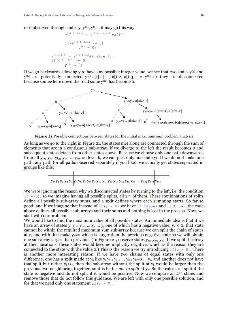
Peter A. The Application and Extension of Retrograde Software Analysis
36
or if observed through states y, y{0}, y{1}… it may go this way
y {{k,1},k+1} = y {{k+1,1},k+2} +a[i];
if (y {{k,1},k+1} <= 0) y {k} = 0;
y {{1,1},2} = y {{2,1},3} +a[size-1];
if (y {{1,1},2} <= 0) y {1} = 0;
If we go backwards allowing y to have any possible integer value, we see that two states y{g} and y{h} are potentially connected y{g}-a[i]-a[i-1]-a[i-2]-a[i-3]-…= y{h} or they are disconnected because somewhere down the road some y{m} has become 0.
Figure 21 Possible connections between states for the initial maximum sum problem analysis
As long as we go to the right in Figure 21, the states met along are connected through the sum of elements that are in a contiguous sub-array. If we diverge to the left the result becomes 0 and subsequent states detach from other states above. Because we choose only one path downwards from all yk1, yk2, yk3, yk4, … ykm on level k, we can pick only one state yk. If we do and make one path, any path (or all paths observed separately if you like), we actually get states separated in groups like this: We were ignoring the reason why we disconnected states by turning to the left, i.e. the condition if (y>0) , so we imagine having all possible splits, all 2n-1 of them. These combinations of splits define all possible sub-array sums, and a split defines where each summing starts. So far so good; and if we imagine that instead of if (y > 0) we have if ( false ) and if ( true ) , the code above defines all possible sub-arrays and their sums and nothing is lost in the process. Now, we start with our problem. We would like to find the maximum value of all possible states. An immediate idea is that if we have an array of states yi yi+1 yi+2 … yk … yj one of which has a negative value, yk < 0, that state cannot be within the required maximum sum sub-array because we can split the chain of states at yk and with that make yk=0 which is larger than the previous negative state so we will obtain one sub-array larger than previous. (In Figure 21, observe states y11, y21, y23. If we split the array at their locations, these states would become implicitly negative, which is the reason they are connected to the state with the value 0.) This is the reason we try introducing if (y > 0) . There is another more interesting reason. If we have two chains of equal states with only one difference, one has a split made at yk like yi yi+1 yi+2 … yk-1 yk=0 … yj, and another does not have that split but rather yk>0, then the sub-array without the split at yk would be larger than the previous two neighboring together, so it is better not to split at yk. So the rules are: split if the state is negative and do not split if it would be positive. Now we compare all 2n-1 states and remove those that do not follow this guidance. We are left with only one possible solution, and for that we need only one statement if (y > 0) .
y01
0 y12=y01-a[size-1]
y22=y11-a[size-2] 0 y24=y01-a[size-1]-a[size-2] 0
y34=y11-a[size-2]-a[size-3] 0 0 y32=y21-a[size-3]
0 y36=y23-a[size-3] y38=y01-a[size-1]-a[size-2]-a[size-3]
0
y0 y1 y2 y3 y4 y5 y6 y7 y8 y9 y10 y11 y12 y13 y14 y15 y16 … yn-3 yn-2 yn-1
Peter A. The Application and Extension of Retrograde Software Analysis
37
As simple as it looks, it is a rare occasion, don't be seduced by the simplicity. The algorithm given above is the one that describes this structure: If yi+1 … yj is a series of positive states, we can't split any of them, and for any existing split we can't remove it, otherwise it would affect our guidelines, and we would have two different solutions that differ in one split at least. The explanation of this structure is: sum numbers from the left until you reach a negative result when you should reset the sum to zero and keep on. However, we followed two guidelines, nothing more. Why are we sure we are not going to miss the maximum sum sub-array, because nobody mentioned anything about maximum sum, it is just implicit in the guidelines and from that perspective it is a heuristic? First, let us see why even the maxsum sub-array must start with states yk=0. Assume we have three states y1 … y2 … y3, and y12 is positive and y23 is the maxsum sub-array. Then, y23 would definitely try to extend itself towards y1, so we would have a larger sub-array with a larger sum y13=y12+y23. It means that if y23 is the maxsum sub-array then y12 cannot be positive, so there has to be a split between y2 and y3. We need one more ingredient. We have to prove that maxsum sub-array cannot contain a split. Assume we have 4 not necessarily neighboring states y1 … y2 … y3 … y4 where y14=y13+y34 and y14=y12+y24 where y24 is the maxsum sub-array. Assume y13 is negative, so there is a split after y3. If y12 is positive, as we've just seen, the array y24 would not remain as such with its maximum sum, it would definitely extend itself and connect state y2 to y1 because y12 is positive. Thus, it would enlarge y24 for sure. However, if y24 would do that it would suddenly contain y13, which is negative, so it would be better if we would remain with y34 only. Because of this, the maxsum y24 cannot have that position while containing a split, so the maxsum sub-array cannot contain any split. This is actually something that is not directly obvious. It needs to be proved. I am saying all this just to point one thing: the fact that this algorithm works is not in any way obvious. This algorithm is an excellent idea that can be proven to work. So the maxsum sub-array is not a problem that explains how a programmer should develop a program, it is a rare situation that we meet a mathematically useful subtlety, but it does explain how he does it, because it follows the rules of best practice. If this algorithm were not supported by a very subtle connection between all sub-arrays of the array, the algorithm would never work. This connection is so subtle that it cannot be extended to higher dimensions, and we will show why. Only now, with all ingredients above, it is safe to introduce the operation with max_res that scans each sub-array between splits in order to find the maximum sum. This part is actually a practical moment. We could say that this algorithm combines a beautifully hinted heuristic with one known practical solution (heuristic: split the entire array into negative sub-arrays from the left; practicality: search for the maximum value among them). To go to the bottom of this algorithm, I will go a step further. You would imagine that if you do this same algorithm going backwards you must have got the same maxsum sub-array (this change in the code would occur for ( int i = size-1; i >= 0; i--) ). Well you would, but you do not get the same locations where the array is split. Look at the example:
1 -2 | 3 4 5 -7 -12 | 3 8
1 -2 3 4 5 | -7 | -12 3 8
Figure 22 Different splitting segments when doing forward and backward sum
This moment is the reason we need a clear explanation of the algorithm, otherwise it can be confusing. (When I saw this for the first time, I was scratching my head.) We said that introducing max_res is a practical moment. Why? Because we know that the maxsum
y0 y1 y2 … yi1>=0 yi1+1<0 … yi2>=0 yi2+1<0 … yn-3 yn-2 yn-1
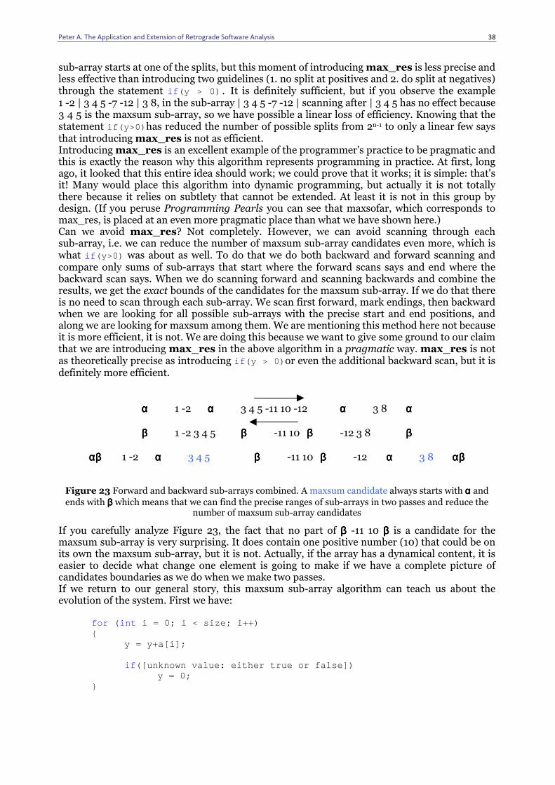
Peter A. The Application and Extension of Retrograde Software Analysis
38
sub-array starts at one of the splits, but this moment of introducing max_res is less precise and less effective than introducing two guidelines (1. no split at positives and 2. do split at negatives) through the statement if (y > 0). It is definitely sufficient, but if you observe the example 1 -2 | 3 4 5 -7 -12 | 3 8, in the sub-array | 3 4 5 -7 -12 | scanning after | 3 4 5 has no effect because 3 4 5 is the maxsum sub-array, so we have possible a linear loss of efficiency. Knowing that the statement if (y>0) has reduced the number of possible splits from 2n-1 to only a linear few says that introducing max_res is not as efficient. Introducing max_res is an excellent example of the programmer's practice to be pragmatic and this is exactly the reason why this algorithm represents programming in practice. At first, long ago, it looked that this entire idea should work; we could prove that it works; it is simple: that's it! Many would place this algorithm into dynamic programming, but actually it is not totally there because it relies on subtlety that cannot be extended. At least it is not in this group by design. (If you peruse Programming Pearls you can see that maxsofar, which corresponds to max_res, is placed at an even more pragmatic place than what we have shown here.) Can we avoid max_res? Not completely. However, we can avoid scanning through each sub-array, i.e. we can reduce the number of maxsum sub-array candidates even more, which is what if (y>0) was about as well. To do that we do both backward and forward scanning and compare only sums of sub-arrays that start where the forward scans says and end where the backward scan says. When we do scanning forward and scanning backwards and combine the results, we get the exact bounds of the candidates for the maxsum sub-array. If we do that there is no need to scan through each sub-array. We scan first forward, mark endings, then backward when we are looking for all possible sub-arrays with the precise start and end positions, and along we are looking for maxsum among them. We are mentioning this method here not because it is more efficient, it is not. We are doing this because we want to give some ground to our claim that we are introducing max_res in the above algorithm in a pragmatic way. max_res is not as theoretically precise as introducing if (y > 0) or even the additional backward scan, but it is definitely more efficient.
αααα 1 -2 αααα 3 4 5 -11 10 -12 αααα 3 8 αααα
ββββ 1 -2 3 4 5 ββββ -11 10 ββββ -12 3 8 ββββ
ααααββββ 1 -2 αααα 3 4 5 ββββ -11 10 ββββ -12 αααα 3 8 ααααββββ
Figure 23 Forward and backward sub-arrays combined. A maxsum candidate always starts with αααα and
ends with ββββ which means that we can find the precise ranges of sub-arrays in two passes and reduce the number of maxsum sub-array candidates
If you carefully analyze Figure 23, the fact that no part of ββββ -11 10 ββββ is a candidate for the maxsum sub-array is very surprising. It does contain one positive number (10) that could be on its own the maxsum sub-array, but it is not. Actually, if the array has a dynamical content, it is easier to decide what change one element is going to make if we have a complete picture of candidates boundaries as we do when we make two passes. If we return to our general story, this maxsum sub-array algorithm can teach us about the evolution of the system. First we have: for ( int i = 0; i < size; i++) {
y = y+a[i];
if ([ unknown value: either true or false]) y = 0; }
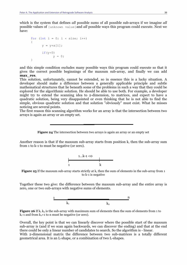
Peter A. The Application and Extension of Retrograde Software Analysis
39
which is the system that defines all possible sums of all possible sub-arrays if we imagine all possible values of [ unknown value] and all possible ways this program could execute. Next we have:
for ( int i = 0; i < size; i++) {
y = y+a[i];
if (y<0) y = 0; } and this simple condition excludes many possible ways this program could execute so that it gives the correct possible beginnings of the maxsum sub-array, and finally we can add max_res. This solution, unfortunately, cannot be extended, so in essence this is a lucky situation. A developer should make a difference between a generally applicable principle and subtle mathematical structures that lie beneath some of the problems in such a way that they could be explored for the algorithmic solution. He should be able to use both. For example, a developer might try to extend the scanning idea to 2-dimension, to matrices, and expect to have a quadratic solution, being very disappointed or even thinking that he is not able to find the simple, obvious quadratic solution and that solution "obviously" must exist. What he misses noticing are several points. The first reason this scanning algorithm works for an array is that the intersection between two arrays is again an array or an empty set.
Figure 24 The intersection between two arrays is again an array or an empty set
Another reason is that if the maxsum sub-array starts from position k, then the sub-array sum from 1 to k-1 to must be negative (or zero).
Figure 25 If the maxsum sub-array starts strictly at k, then the sum of elements in the sub-array from 1 to k-1 is negative
Together these two give: the difference between the maxsum sub-array and the entire array is zero, one or two sub-arrays with negative sums of elements.
Figure 26 If k1 k2 is the sub-array with maximum sum of elements then the sum of elements from 1 to k1-1 and from k2+1 to n must be negative (or zero).
Overall, the key point is that we can linearly discover where the possible start of the maxsum sub-array is (and if we scan again backwards, we can discover the ending) and that at the end there could be only a linear number of candidates to search. So the algorithm is - linear. With 2-dimensional matrix the difference between two sub-matrices is a totally different geometrical area. It is an L-shape, or a combination of two L-shapes.
1 n
k1 k2
k 1
1…k-1 <0
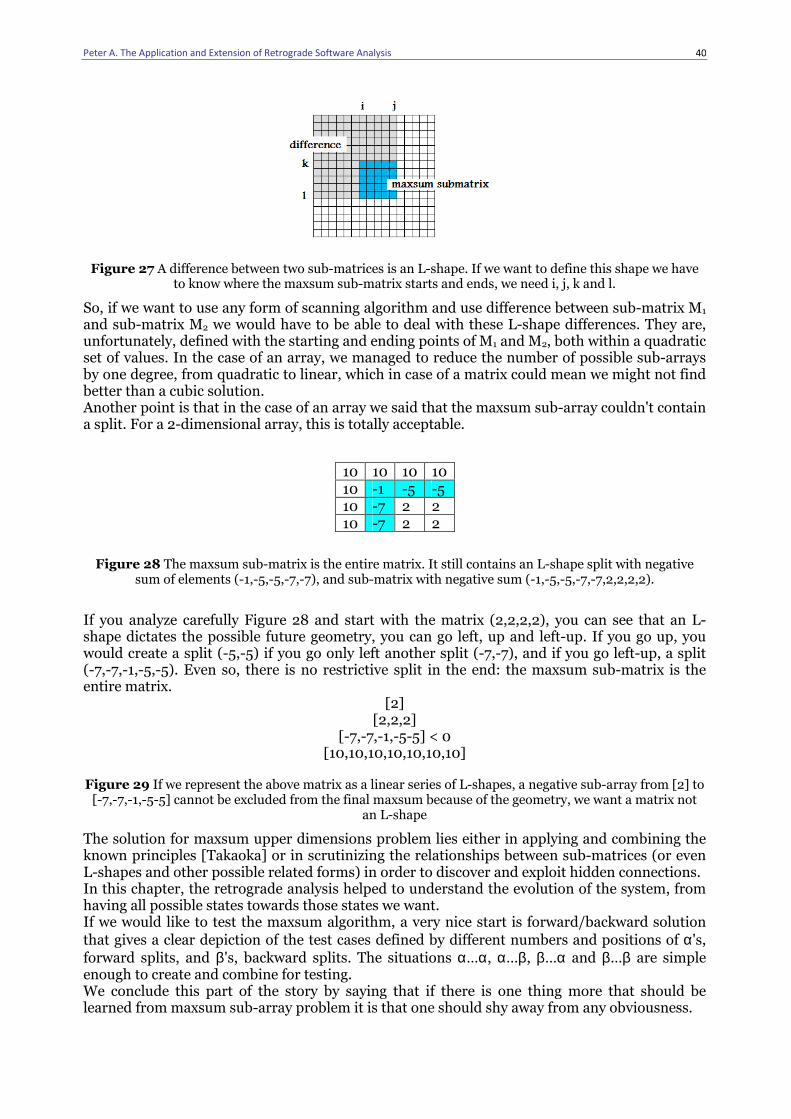
Peter A. The Application and Extension of Retrograde Software Analysis
40
Figure 27 A difference between two sub-matrices is an L-shape. If we want to define this shape we have to know where the maxsum sub-matrix starts and ends, we need i, j, k and l.
So, if we want to use any form of scanning algorithm and use difference between sub-matrix M1 and sub-matrix M2 we would have to be able to deal with these L-shape differences. They are, unfortunately, defined with the starting and ending points of M1 and M2, both within a quadratic set of values. In the case of an array, we managed to reduce the number of possible sub-arrays by one degree, from quadratic to linear, which in case of a matrix could mean we might not find better than a cubic solution. Another point is that in the case of an array we said that the maxsum sub-array couldn't contain a split. For a 2-dimensional array, this is totally acceptable.
Figure 28 The maxsum sub-matrix is the entire matrix. It still contains an L-shape split with negative sum of elements (-1,-5,-5,-7,-7), and sub-matrix with negative sum (-1,-5,-5,-7,-7,2,2,2,2).
If you analyze carefully Figure 28 and start with the matrix (2,2,2,2), you can see that an L-shape dictates the possible future geometry, you can go left, up and left-up. If you go up, you would create a split (-5,-5) if you go only left another split (-7,-7), and if you go left-up, a split (-7,-7,-1,-5,-5). Even so, there is no restrictive split in the end: the maxsum sub-matrix is the entire matrix.
[2] [2,2,2]
[-7,-7,-1,-5-5] < 0 [10,10,10,10,10,10,10]
Figure 29 If we represent the above matrix as a linear series of L-shapes, a negative sub-array from [2] to [-7,-7,-1,-5-5] cannot be excluded from the final maxsum because of the geometry, we want a matrix not
an L-shape
The solution for maxsum upper dimensions problem lies either in applying and combining the known principles [Takaoka] or in scrutinizing the relationships between sub-matrices (or even L-shapes and other possible related forms) in order to discover and exploit hidden connections. In this chapter, the retrograde analysis helped to understand the evolution of the system, from having all possible states towards those states we want. If we would like to test the maxsum algorithm, a very nice start is forward/backward solution
that gives a clear depiction of the test cases defined by different numbers and positions of α's,
forward splits, and β's, backward splits. The situations α…α, α…β, β…α and β…β are simple enough to create and combine for testing. We conclude this part of the story by saying that if there is one thing more that should be learned from maxsum sub-array problem it is that one should shy away from any obviousness.
10 10 10 10 10 -1 -5 -5 10 -7 2 2 10 -7 2 2
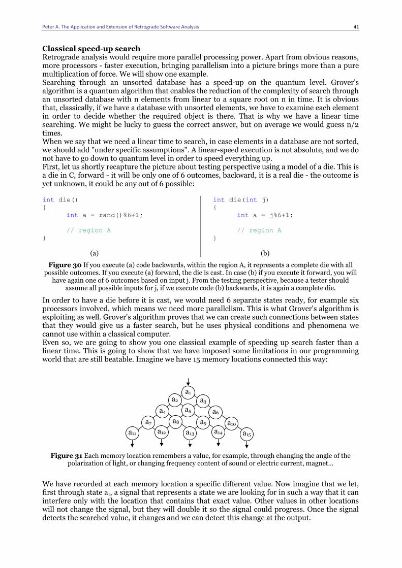
Peter A. The Application and Extension of Retrograde Software Analysis
41
Classical speed-up search Retrograde analysis would require more parallel processing power. Apart from obvious reasons, more processors - faster execution, bringing parallelism into a picture brings more than a pure multiplication of force. We will show one example. Searching through an unsorted database has a speed-up on the quantum level. Grover's algorithm is a quantum algorithm that enables the reduction of the complexity of search through an unsorted database with n elements from linear to a square root on n in time. It is obvious that, classically, if we have a database with unsorted elements, we have to examine each element in order to decide whether the required object is there. That is why we have a linear time searching. We might be lucky to guess the correct answer, but on average we would guess n/2 times. When we say that we need a linear time to search, in case elements in a database are not sorted, we should add "under specific assumptions". A linear-speed execution is not absolute, and we do not have to go down to quantum level in order to speed everything up. First, let us shortly recapture the picture about testing perspective using a model of a die. This is a die in C, forward - it will be only one of 6 outcomes, backward, it is a real die - the outcome is yet unknown, it could be any out of 6 possible:
int die() { int a = rand()%6+1; // region A }
(a)
int die( int j) {
int a = j%6+1;
// region A }
(b)
Figure 30 If you execute (a) code backwards, within the region A, it represents a complete die with all possible outcomes. If you execute (a) forward, the die is cast. In case (b) if you execute it forward, you will
have again one of 6 outcomes based on input j. From the testing perspective, because a tester should assume all possible inputs for j, if we execute code (b) backwards, it is again a complete die.
In order to have a die before it is cast, we would need 6 separate states ready, for example six processors involved, which means we need more parallelism. This is what Grover's algorithm is exploiting as well. Grover's algorithm proves that we can create such connections between states that they would give us a faster search, but he uses physical conditions and phenomena we cannot use within a classical computer. Even so, we are going to show you one classical example of speeding up search faster than a linear time. This is going to show that we have imposed some limitations in our programming world that are still beatable. Imagine we have 15 memory locations connected this way:
Figure 31 Each memory location remembers a value, for example, through changing the angle of the polarization of light, or changing frequency content of sound or electric current, magnet…
We have recorded at each memory location a specific different value. Now imagine that we let, first through state a1, a signal that represents a state we are looking for in such a way that it can interfere only with the location that contains that exact value. Other values in other locations will not change the signal, but they will double it so the signal could progress. Once the signal detects the searched value, it changes and we can detect this change at the output.
a2 a3
a4 a5 a6
a7 a8 a9 a10
a11 a12 a13 a14 a15
a1
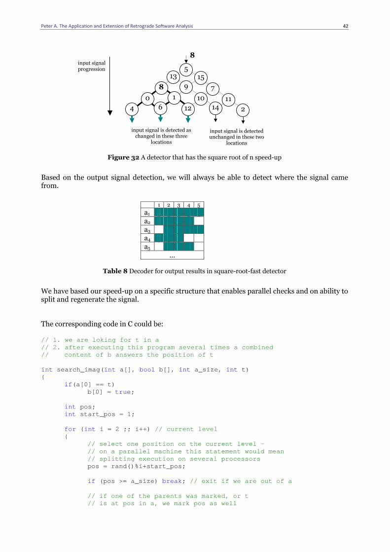
Peter A. The Application and Extension of Retrograde Software Analysis
42
Figure 32 A detector that has the square root of n speed-up
Based on the output signal detection, we will always be able to detect where the signal came from.
Table 8 Decoder for output results in square-root-fast detector
We have based our speed-up on a specific structure that enables parallel checks and on ability to split and regenerate the signal. The corresponding code in C could be: // 1. we are loking for t in a // 2. after executing this program several times a combined // content of b answers the position of t int search_imag( int a[], bool b[], int a_size, int t) { if (a[0] == t) b[0] = true ; int pos; int start_pos = 1; for ( int i = 2 ;; i++) // current level {
// select one position on the current level - // on a parallel machine this statement would mean // splitting execution on several processors pos = rand()%i+start_pos;
if (pos >= a_size) break ; // exit if we are out of a
// if one of the parents was marked, or t
// is at pos in a, we mark pos as well
1 2 3 4 5
a1 a2 a3 a4 a5
…
13 15
8 9 7
0 1 10 11
4 6 12 14 2
5
8
input signal is detected as changed in these three
locations
input signal is detected unchanged in these two
locations
input signal progression
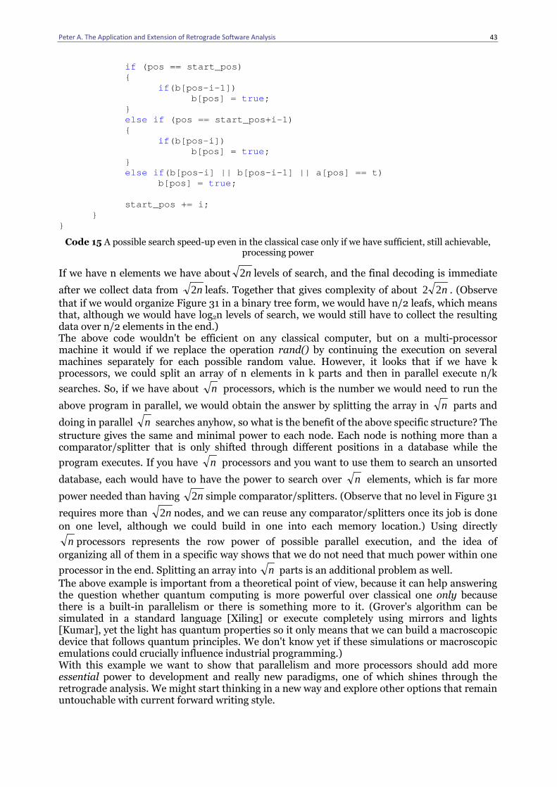
Peter A. The Application and Extension of Retrograde Software Analysis
43
if (pos == start_pos) { if (b[pos-i-1]) b[pos] = true ; } else if (pos == start_pos+i-1) { if (b[pos-i]) b[pos] = true ; } else if (b[pos-i] || b[pos-i-1] || a[pos] == t) b[pos] = true ; start_pos += i; } }
Code 15 A possible search speed-up even in the classical case only if we have sufficient, still achievable, processing power
If we have n elements we have about n2 levels of search, and the final decoding is immediate
after we collect data from n2 leafs. Together that gives complexity of about n22 . (Observe
that if we would organize Figure 31 in a binary tree form, we would have n/2 leafs, which means that, although we would have log2n levels of search, we would still have to collect the resulting data over n/2 elements in the end.) The above code wouldn't be efficient on any classical computer, but on a multi-processor machine it would if we replace the operation rand() by continuing the execution on several machines separately for each possible random value. However, it looks that if we have k processors, we could split an array of n elements in k parts and then in parallel execute n/k
searches. So, if we have about n processors, which is the number we would need to run the
above program in parallel, we would obtain the answer by splitting the array in n parts and
doing in parallel n searches anyhow, so what is the benefit of the above specific structure? The
structure gives the same and minimal power to each node. Each node is nothing more than a comparator/splitter that is only shifted through different positions in a database while the
program executes. If you have n processors and you want to use them to search an unsorted
database, each would have to have the power to search over n elements, which is far more
power needed than having n2 simple comparator/splitters. (Observe that no level in Figure 31
requires more than n2 nodes, and we can reuse any comparator/splitters once its job is done
on one level, although we could build in one into each memory location.) Using directly
n processors represents the row power of possible parallel execution, and the idea of
organizing all of them in a specific way shows that we do not need that much power within one
processor in the end. Splitting an array into n parts is an additional problem as well.
The above example is important from a theoretical point of view, because it can help answering the question whether quantum computing is more powerful over classical one only because there is a built-in parallelism or there is something more to it. (Grover's algorithm can be simulated in a standard language [Xiling] or execute completely using mirrors and lights [Kumar], yet the light has quantum properties so it only means that we can build a macroscopic device that follows quantum principles. We don't know yet if these simulations or macroscopic emulations could crucially influence industrial programming.) With this example we want to show that parallelism and more processors should add more essential power to development and really new paradigms, one of which shines through the retrograde analysis. We might start thinking in a new way and explore other options that remain untouchable with current forward writing style.
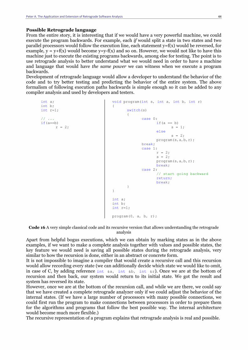
Peter A. The Application and Extension of Retrograde Software Analysis
44
Possible Retrograde language From the entire story, it is interesting that if we would have a very powerful machine, we could execute the program backwards. For example, each if would split a state in two states and two parallel processors would follow the execution line, each statement y=f(x) would be reversed, for example, y = y+f(x) would become y=y-f(x) and so on. However, we would not like to have this machine just to execute the existing programs backwards, among else for testing. The point is to use retrograde analysis to better understand what we would need in order to have a machine and language that would have the same power we can witness when we execute a program backwards. Development of retrograde language would allow a developer to understand the behavior of the code and to try better testing and predicting the behavior of the entire system. The above formalism of following execution paths backwards is simple enough so it can be added to any compiler analysis and used by developers and testers.
int a; int b; int r=1; // ... if (a==b) r = 2;
void program( int s, int a, int b, int r) { switch (s) { case 0: if (a == b) s = 1; else s = 2; program(s,a,b,r); break ; case 1: r = 2;
s = 2; program(s,a,b,r); break ; case 2:
// start going backward return;
break ; } } int a; int b; int r=1; program(0, a, b, r);
Code 16 A very simple classical code and its recursive version that allows understanding the retrograde analysis
Apart from helpful bogus executions, which we can obtain by marking states as in the above examples, if we want to make a complete analysis together with values and possible states, the key feature we would need is saving all possible states during the retrograde analysis, very similar to how the recursion is done, either in an abstract or concrete form. It is not impossible to imagine a compiler that would create a recursive call and this recursion would allow recording every state (we can additionally decide which state we would like to omit, in case of C, by adding reference int &a, int &b, int &r ). Once we are at the bottom of recursion and then back, our system would return to its initial state. We got the result and system has reversed its state. However, once we are at the bottom of the recursion call, and while we are there, we could say that we have created a complete retrograde analyzer only if we could adjust the behavior of the internal states. (If we have a large number of processors with many possible connections, we could first run the program to make connections between processors in order to prepare them for the algorithms and programs that follow the best possible way. The internal architecture would become much more flexible.) The recursive representation of a program explains that retrograde analysis is real and possible.
Peter A. The Application and Extension of Retrograde Software Analysis
45
With ever-growing machine power, we are more and more capable of executing the same program with many different inputs, only if we are sure that this would help anything in the end. (For example, if we would connect one thousand simple processors, as in Figure 31, we could process a search over one million records one thousand times faster, and that is no kind of simulation. On the quantum level soon, we might not have any limitations of this kind.) Retrograde analysis shows that it would help a lot; imagine the situation when a compiler is doing retrograde analysis of a program while it is in a design process. A developer could immediately notice many problems within his code. Retrograde language would help writing a code in a more direct manner, not starting from imposed limitations, but rather from what we want. Actually, many existing libraries, like STL, try to reduce the limitation of forward writing style, but the underlying system and a new writing style still remains complex. Retrograde analysis is an excellent starting point, because any programmer can intuitively understand its implication and execution and have a direct and very fast improvement in testing, algorithm and system design. In order to form the Retrograde language, we would have to rewrite a serious amount of code and algorithms in order to make the best practice out of it. However, even without this language specified, the retrograde analysis should have its place in modern programming practice.
Peter A. The Application and Extension of Retrograde Software Analysis
46
Personal note The idea for this entire method came from personal experience. For many years, I was using this method, or versions of the same, unaware that it could be defined as a method, or that it is special in any sense, like reading the book backwards. So, one day in one company… we had a project that required the usage of a compiler analyzer. We used its output for our project. Suddenly, during our specific usage, a compiler displayed a bug: it would crash if the same variable, a pointer, was used first in a loop and then far, far away (in another galaxy) in the code, unexpectedly and unreasonably, its value was changed. After carefully examining the piece of code that crashed the compiler, I realized that a programmer would not normally write a piece of code like that, there was no reason to use the pointer, again for totally different object so far from its initial usage. Suddenly, I realized that this specific part of a compiler analyzer was tested for more or less usual code, as huge as the test base was indeed, and these really abnormal situations were not properly covered, because, how would you do that: by writing a piece of code after a piece of code with apparently nonsensical combinations of loops, operators, functions?; but that would take millennia first to conjure and then to combine in any programming language. Well… As mentioned earlier, our project was related partially to compiling, so it was essential to have had the compiler operational first, and to check if it was really fitted for our new purpose, so I had to think about how we used the compiler analyzer and what was different from using this compiler in a regular way. Apart from running our analyzer through huge existing pieces of code, I would write literally thousand test cases with all more apparently nonsensical code patterns and all that in a half dozen of different languages and with several methodologies. For two months. Only that. (And few splashes of water in the ring corner occasionally by my colleagues to stay awake.) My test codes were more powerful than running the analyzer through existing code, by measure, although it was million times less code employed and the result would be obtained within minutes, not hours. Close to the project ending, I was literally able to write only one test case that would cover tens of normal test cases in a few lines and astonish the programmer with bugs logged within minutes of his code submission, or to confirm that there were no bugs, just as quick as if I knew what he was going to write. This story covers how it was really done, although behind all this lie much deeper principles that have been built for almost three decades. Aleksandar Perisic, [email protected]
Peter A. The Application and Extension of Retrograde Software Analysis
47
References Bentley J., Programming Pearls, 2nd edition, Addison-Wesley, 2000. Knuth D., The Art of Computer Programming, Volume 1 Fundamental Algorithm, 3rd Edition, Addison-Wesley, 1997. Knuth D., The Art of Computer Programming, Volume 2 Sorting and Searching, 2nd Edition, Addison-Wesley, 1997. Kumar P., D’Ariano G., Hirota O. Quantum Communication, Computing, and Measurement 2, Springer US, 2000. Takaoka T. Efficient algorithms for the maximum sub-array problem by distance matrix multiplication, Electronic Notes in Theoretical Computer Science 61., 2002. Xiling X., Hanwu C., Kaizhong C., Zhiqiang L. On the Research of BDD Based Simulation of Grover's Algorithm, Genetic and Evolutionary Computing, 2008. WGEC '08. Second International Conference 2008.