the alice instrument and the measured cosmic ray elemental abundances

Astroparticfe Physics 1(1992133-45 Noah-Holland

Astroparticle Physics

The ALICE instrument and the measured cosmic ray elemental abundances

University of Siegen, Siegen, Germany

Received S June 1992

A Large Isotopic ~rn~sit~~n E~~rimen~ <ALICE> is a bal~~~-bo~e s~c~omet~r which can dete~~~e the eleme*ttat and imtopic composition of galactic cosmic rays with energies near 1 GeV/nucIeon. ALICE was flown from Prince Albert, Canada in August 1987, and remained at float altitude ~~~~ feet) for 14.7 hours. In this paper, we describe the experimental methods and analysis which wifl be used for subsequent isotopic analysis. We obtained very precise charge resolution over the entire designed range: 0.10 and 0.16 charge units at neon and iron, respectively. Results on the galactic cosmic ray abundances and absolute fluxes af the elements from neon through nickel are reported.

1. Intmduction

Studies of the elemental and isotopic abundances of any kind of matter in the universe are of fundamental astrophysical importan&e to understand the nucieosynthesis processes and the evolution of elements in our gaIaxy ~a~i~ular~y~ Cosmic rays are in addition a unique probe of matter since they have gone through acceleration processes and encomzzered a variety of different interactions during propagation through the interstellar medium. AdditionaIIy the studies of cosmic ray species provide reliable information about the structure and strength of the galactic magnetic fields, the density of the intersteIlar gas and acceleration conditions.

~u~~s~~~~ fa: E.R. Christian, Goddard Space Flight Center, Code 661, Greenbelt, MD 20771, USA. r Also at: Bartaf Research Institnte, University of D&ware,

Newark, DE lY716, USA. I Alsa at: TATA Institute, Bombay, India.

Elsevier Science Publishers B.V.

In this paper we will introduce the experimental concept of the ALICE instrument which uti- lizes the ~h~renk~~-range technique for isotope identification. The experiment provided information about the efementaf and isotopic composition for in~m~ng nuclei between silicon and iron with kinetic energies from 350 M&V/n to 800 h&V/n at the instr~~nt. We will describe the characteristics of the. individual detectors and present the efemental composition of cosmic rays measured with the instrument. In a separate paper we will focus on the analysis of the isotopic composition results.

The Dimensions and the ~nfigu~ation of the ALrCE telescope and the assembly of the various detectors are shown in fig, 1. ALICE measures the charge, the velocity, the range, and the trajectories of the incoming particles using, respec-

34 J.A. Esposito et al. / The ALICE instrument and measured cosmic ray elemental abundance

tively: two scintillators, one Cherenkov counter, a cellulose nitrate (CN) range stack, and a total of 12 drift chambers, 6 for each coordinate, X and Y. Mass determination for isotope analysis will combine the charge and Cherenkov signals with the residual range of the particle as measured in the passive range stack. A crucial experimental task was to locate reliably the stopping end of a particle track in the passive range stack. As will be shown later the high resolution drift chamber trajectories enables us succesfully to match these tracks in the CN stack with corresponding electronic event data. A penetration counter, which is located directly underneath the CN stack, detects particles which penetrate the full range stack as well as the fragments resulting from charge- changing interactions in the instruments. The penetration counter was set to be sensitive to Z 2 1 particles. Thus particles which undergo charge-changing interactions in the instrument can be removed from the subsequent analysis.

The instrument has a geometric factor of N 0.88 m2 sr and the total weight of the experiment in its gondola was 1825 kg (4023 Ibs).

This paper reports the results of the second 1987 flight of the ALICE instrument from Prince Albert, Saskatchewan, Canada (53” N lat., 2.54” E long.). The first 1987 flight was launched on the evening of 4 August, but a slow ascent (7 hours) and a balloon burst at daybreak resulted in a very

Cherenkov counter

L- Penetration counter

Fig. 1. The ALICE instrument.

short flight (1; hours at float). Luckily the land- ing and recovery went smoothly, and after a few minor repairs, ALICE was again launched on 15 August. This flight obtained 14.7 hours of data at float altitude with 675000 triggered events. The average residual atmospheric depth was 4.85 g/cm2.

3. The design and resolution of individual detectors

The separation of isotopes in the ALICE charge range is an e~erimently challenging task, since the measurements from the individual detectors must typically have a resolution of less than 1% including all sources of error. In the following sections, we will describe in detail the ALICE detectors and will discuss the intrinsic resolution derived from the flight data.

3.1. The scintillation detectors and the Cherenkov counter

The scintillation chambers, S, and S,, and the Cherenkov chamber have similar design and geo- metrical properties, and are depicted in fig. 2. The inner surfaces of the chambers were coated with white barium sulfate (BaSO,) paint which has a reflectivity of _ 96% in the visible portion of the light spectrum. Each scintillation counter had sixteen equally spaced RCA 83006M T-cup photo-multiplier tubes (PMTs), four to a side, with a 1.16 cm thick PS-10 plastic scintillator placed on the bottom of the diffusive box. Addi- tionally each of the scintillation counters had four RCA 8575 PMTs (one on each side) to provide a fast trigger for the experiment.

Because of a thicker radiator and to obtain more light yield, the Cherenkov counter was taller in size and had a total of 24 PMTs, set six to a side. The PMTs were set in the top half of the counter and the 5 cm thick Pilot-425 radiator was placed at the bottom of the diffusive box.

The intrinsic limit in resolution of these detectors is determined by the number of photoelectrons one obtains in the collected light. But this intrinsic limit can only be reached if one is able

J.A. Esposito et al. / The ALICE instrument and measured cosmic ray elemental abundance 35

to correct for a number of systematic effects which add to the fluctuations, such as: - path-length variations due to different angles

of incidence, - corrections for the time dependent gain

changes in the PMTs and their ADCs during the balloon flight,

- corrections to the non-uniformities of light collection over the large detector areas.

The precise measurement of the trajectories allowed a correction to the variation in path length to a level better than 1%.

Changes in the gain of the PMTs and the ADC-pedestals are normally due to changes in the temperature during the course of the balloon flight, which in our flight varied between - 10°C and + 15°C (internal ambient air temperature). This resulted in an observed change in the gain of the individual PMTs of - 22% and a shift of the ADC-pedestals of roughly 3%. We used two steps to correct the time drifts of the PMT responses. First, the high voltage applied to the PMTs was monitored throughout the flight and this data, combined with the calibrated gain voltage curves

r-114 3 cm 1

L5 cm THICK CHERENKOV

Fig. 2. Plane view of a scintillation chamber (left part, 16 PMT’s) and the Cherenkov counter (right part, total of 24 PMT’s).


for each of the individual PMTs, was used to correct most of the 22% change in gain.

Second order corrections were made to the Cherenkov measurements using the flight data. With a strict cut on silicon events, the high energy (saturated) edge of the Cherenkov reponse (C,,,) could be monitored for individual tubes over the entire flight and used to make the time adjustments. Shifts in the pedestals of the ADCs were monitored by frequent pedestal calibration runs during the balloon flight and, for the PMTs viewing the Cherenkov counter, we had a contin- uous cross-check from those events which triggered the instrument but missed the Cherenkov radiator.

Another important aspect is the non-uniform- ity of light collection over the large area of the radiators. In the scintillation counters, we found that the light collection for a single PMT varied by a factor of 2.5 over the counter, and in the Cherenkov counter the variation was a factor of 1.7. Maps of the individual tube responses were used to correct these non-uniformities in the light collection. Neon, magnesium, and silicon flight events were used to construct the maps for the scintillators. The data used were corrected for gain and pedestal drifts and for path length variations as mentioned above.

The Cherenkov counter is one of the critical detectors in determining the mass of the incoming cosmic ray nuclei. Cherenkov radiation is emitted when a charged particle passes through matter with a velocity greater than the group velocity of light in the material; p = u/c > l/n, where n is the index of refraction. The light emmission per unit pathlength is given by the formula

dC 1 -Al___ dx (ni#.

(1)

A signal resolution of better than 1% is required in the Cherenkov counter to obtain sufficient isotope resolution. For this reason, we calibrated the Cherenkov counter at the Brookhaven accelerator, exposing it to relativistic (N 14 GeV/nucleon) silicon particles. The non-uniform light collection was mapped for each tube on a 5

peak: OS %

0 re, (mean) 1x1

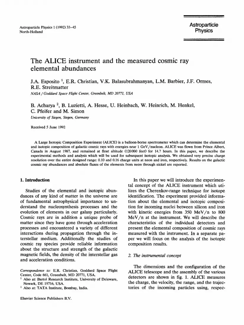
Fig. 3. Distribution of the relative deviations from the mean signal in scintillator 1 for iron events, as given in eq. (2).

cm by 5 cm grid, and a two dimensional spline function was fit to these data points. The spline functions were used to normalize all flight events to an equivalent response at the center of the detector.

A determination of how well these corrections have succeeded in removing systematics from the scintillators and the Cherenkov counter may be made by examining the distribution of residual fluctuations which exist after all corrections are applied. The resolution observed in the scintillators for iron particles is shown in fig. 3. We have plotted the relative sigma of the mean for iron events:

o;,i(%)

(Pmti - (pmt>)2 (pmtj2

x 100,

(2)

where pmt, is the individual phototube response (1 15 i s 161, (pmt) is the average phototube response, and N = 16 (the total number of PMT’s). The amount of light produced by iron nuclei is large, so the resolution due to photoelectron statistics is small and the - 0.5% ~u~tuations shown in fig. 3 give the upper limit on remaining systematic errors.

In fig. 4 we have plotted the relative sigma of the mean for silicon and iron events in the Cherenkov counter versus the Cherenkov re-

3.A. Esposito et al. / The ALICE instrument and measured cosmic ray elemental ahndance 37

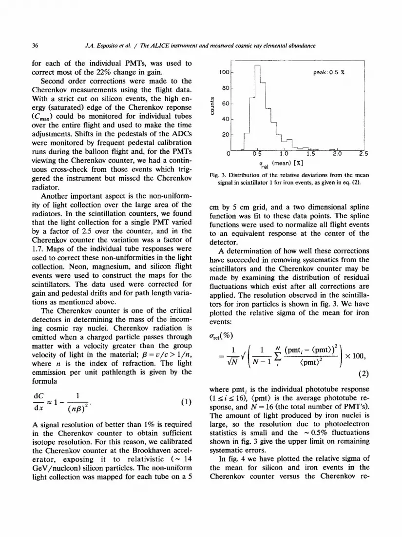
sponse. The dashed curve in fig, 4 shows the intrinsic fluctuations expected due to photelec- tron statistics assuming that a single phototube observes 6 photoelectrons for a relativistic singly charge particle. The solid curve includes a 0.5% residual systematic error and the data is clearly consistent with these assumptions. It is also consistent with a value of 5.7 Z2 photoelectrons per tube which was derived from flight silicon events and the response of 2 sets of 12 Cherenkov tubes using the “ratio function” technique. This method relies on the fact that the ratio of two indepen- dent random variables has statistical properties which can be directly related to the mean and variance of the two random variables [il. In the case of the ALICE Cherenkov data, the variables were taken as the summed signal from “even” and “odd” photomultipliers.

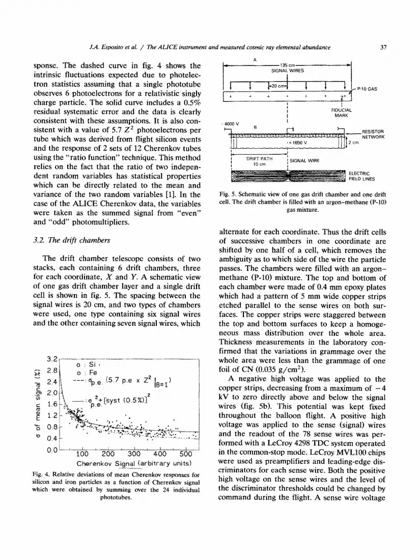
The drift chamber telescope consists of two stacks, each containing 6 drift chambers, three for each coordinate, X and Y. A schematic view of one gas drift chamber layer and a single drift cell is shown in fig. 5. The spacing between the signal wires is 20 cm, and two types of chambers were used, one type containing six signal wires and the other containing seven signal wires, which

0 : si 1

0 : Fe ---: %,& (5.7 p.e x z2 InEll

Cherenkov Signal (arbitrary units) ---~- Fig. 4. Relative deviations of mean Cherenkov responses for silicon and iron particles as a function of Cherenkov signal which were obtained by summing over the 24 individual

phototubes.

f i 20 cm I t f 1 P-10GAS

+ + + + + + 7+

/ i i

FIDUCIAL MARK

- 4000 v I

NETWORK

I DRIFT PATH j SIGNAL WIRE I 1Ocm I

ELECTRIC FIELD LINES

Fig. 5. Schematic view of one gas drift chamber and one drift cell. The drift chamber is filled with an argon-methane (P-10)

gas mixture.

alternate for each coordinate. Thus the drift cells of successive chambers in one coordinate are shifted by one half of a cell, which removes the ambiguity as to which side of the wire the particle passes. The chambers were filled with an argon- methane (P-10) mixture. The top and bottom of each chamber were made of 0.4 mm epoxy plates which had a pattern of 5 mm wide copper strips etched parallel to the sense wires on both surfaces. The copper strips were staggered between the top and bottom surfaces to keep a homoge- neous mass distribution over the whole area. Thickness measurements in the laboratory con- firmed that the variations in grammage over the whole area were less than the grammage of one foii of CN (0.035 g/cm2).

A negative high voltage was applied to the copper strips, decreasing from a ma~mum of - 4 kV to zero directly above and below the signal wires (fig. 5b). This potential was kept fixed throughout the balloon flight. A positive high voltage was applied to the sense (signal) wires and the readout of the 78 sense wires was per- formed with a LeCroy 4298 TDC system operated in the common-stop mode. LeCroy MVLlOO chips were used as preamplifiers and leading-edge dis- criminators for each sense wire. Both the positive high voltage on the sense wires and the level of the discriminator thresh~ids could be changed by command during the flight. A sense wire voltage


of + 1650 V could be used to measure charge one particles and was used to obtain muon tracks on the ground. During the flight, the sense wire voltage was reduced to about + 1280 V to measure the heavy ions. A further discussion of the different chamber voltages needed for different charge ranges can be found in ref. [2].

In order to convert the measured drift time to the position where the incoming particle pene- trated the drift chamber, one must know the correct drift-time versus position relationship. It depends upon the electric field, the gas pressure, the type of gas, and the temperature of the gas, and so is a complex problem. But in practice, one can use the fact that the particle trajectories are straight lines to empirically obtain the drift-time as a function of position from the data. This is an iterative process in which one starts with a rea- sonable assumption for the drift-time position function derived from integrating the drift-time distribution. Then the measured drift-times and the correlated positions define a straight track through the drift chamber assembly using the method of Ieast squares. This track defines a new position corresponding to the measured drift-time and in a repeated process, one obtains a stable drift-time versus position relationship which pro- vides the best fit to straight tracks. This relationship can change over the flight and therefore must be monitored as a function of time.

In fig. 6 we show the spatial resolution obtained in the flight for particles of different charge and for almost vertical incident particles. The dynamic range in charge detection efficiency was 100% for iron particles and 97% for oxygen. The spatial resolution was not found to be a function of the drift distance, but an angular dependence was observed, as shown in fig. 7.

These drift chambers were able to measure the tracks of particles over the charge range 2 = 8 to Z = 26 with a spatial resolution of N 200 pm for the Iowest charges and slowly degrading in resolution to N 600 Frn for iron. We attribute the decrease in resolution to the increase in delta-ray (knock-on) electrons produced by the heavier charges and have investigated these processes previously at accelerators. The resolution obtained with these chambers provided accurate

800

0°<Q<300 700 -

! z 600- s

.- Ti

Charge Z

3

Fig. 6. Drift chamber spatial resolution for different projectile charges with incident angle between 0 and 30 degrees.

positions for corrections in the scintillators and Cherenkov counters, allowed us to perform precise angle corrections, and enabled us to success- fully locate the particle tracks in the CN range stack.

3.3. Cellulose nitrate range stack

The CN range stack is composed of two side- by-side stacks of large area CN sheets (60 cm X

120 cm x 250 pm>. Each stack contains 425 sheets providing a total column density of 14.275 g/cm2 and a tota foil area of 612 m2. Particles which stop in the CN damage the material due to the high ionization losses, especially at the end of their range. An etching process generates holes in a number of successive foils at the end of the

/ / 30 40

Incident angle (degrees)

Fig. 7. Drift chamber spatial resolution for projectiles from oxygen to magnesium as a function of incident angle.

J.A. Esposito et al. / 71ie ALICE ~~striirnent and measured cosmic ray elcmentaal abundance 39

track which allows the particfe range to be measured [3-51. This measurement is required to identify the mass of the cosmic ray, but is not used in the charge anaiysis described here.

4. Charge composition at the instrument

The charge is primarily determined from the two scintillators, but the reponse in the Cherenkov counter was used to correct for energy dependent scintillator responses. After these corrections, we selected events which satisfied the following: - no signal in the penetration counter below the

CN stack, - a well defined track observed in the drift

chambers (response in 5 or more drift chamber layers per coordinate),

- a consistent charge identification in S, and S,. This requires that I Z, - Z, I < 2(a, + ~~1, where Z, and Z, are the charge measured in S, and S,, and W, and u2 are the charge resolution in the two scintillators.

These selection criteria remove most of the interactions in the experiment. The selected events are shown in fig. 8 where we have plotted the mean charge from the two scintillators versus the square root of the Cherenkov signal. Due to differing energy loss rates within the detectors as a function of particle charge, the first two selec-

r- -7

: ,,.. Fe

Ca

20 40 60 80 100

J Cherenkov SWY

Fig. 8. Mean charge versus Cherenkov signal for particles which were registered in the bottom drift chamer stack and did not enter the Penetration counter {and thus stopped in

the range stack).

7 ^_ ---._

Mg (3 = 0.11

.16

3 Ca

1 ‘4

IlbY IL-A, 8 12 16 20 24 28

Charge Z

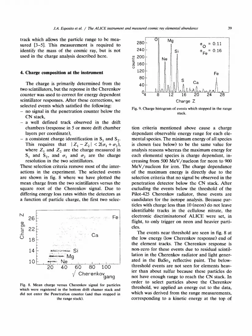
Fig. 9. Charge histogram of events which stopped in the range stack.

tion criteria mentioned above cause a charge dependant observable energy range for each elemental species. The minimum energy of all species is chosen (see below) to be the same value for analysis reasons whereas the maximum energy for each elemental species is charge dependant, in- creasing from 500 MeV/nucleon for neon to 900 MeV/nucleon for iron. The charge dependance of the ma~mum energy is directly due to the selection criteria that no signal be observed in the penetration detector below the CN stack. After excluding the events below the threshold of the Pilot-425 Cherenkov radiator, these events are candidates for the isotope analysis. Because particles with charge less than 10 (neon) do not leave identifiable tracks in the cellulose nitrate, the electronic discriminatorsof ALICE were set, in flight, to only trigger on neon and heavier particles.

The events near threshold are seen in fig, fi at the low energy (low Cherenkov response) end of the element tracks. The Cherenkov response is non-zero for these events due to residual scintillation in the Cherenkov radiator and Iight gener- ated in the BaSo, reflective paint. The below- threshold events are not seen for elements heavier than about sulfur because these particles do not have enough range to reach the CN stack. in order to select particles above the Cherenkov threshold, we applied an energy cut to the data, which was derived from the range measurements, corresponding to a kinetic energy at the top of


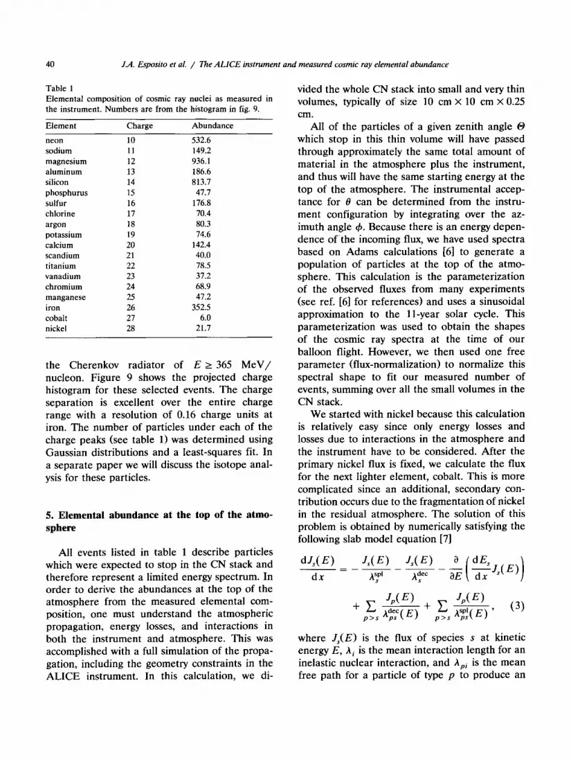
Table 1 Elemental composition of cosmic ray nuclei as measured in the instrument. Numbers are from the histogram in fig. 9.

Element Charge Abundance

neon 10 532.6 sodium 11 149.2 magnesium 12 936.1 aluminum 13 186.6 silicon 14 813.7 phosphurus 15 47.7 sulfur 16 176.8 chlorine 17 70.4 argon 18 80.3 potassium 19 74.6 calcium 20 142.4 scandium 21 40.0 titanium 22 78.5 vanadium 23 37.2 chromium 24 68.9 manganese 25 47.2 iron 26 352.5 cobalt 27 6.0 nickel 28 21.7

the Cherenkov radiator of E 2 365 MeV/ nucleon. Figure 9 shows the projected charge histogram for these selected events. The charge separation is excellent over the entire charge range with a resolution of 0.16 charge units at iron. The number of particles under each of the charge peaks (see table 1) was determined using Gaussian distributions and a least-squares fit. In a separate paper we will discuss the isotope analysis for these particles.

5. Elemental abundance at the top of the atmosphere

All events listed in table 1 describe particles which were expected to stop in the CN stack and therefore represent a limited energy spectrum. In order to derive the abundances at the top of the atmosphere from the measured elemental composition, one must understand the atmospheric propagation, energy losses, and interactions in both the instrument and atmosphere. This was accomplished with a full simulation of the propagation, including the geometry constraints in the ALICE instrument. In this calculation, we di-

vided the whole CN stack into small and very thin volumes, typically of size 10 cm X 10 cm X 0.25 cm.

All of the particles of a given zenith angle 0 which stop in this thin volume will have passed through approximately the same total amount of material in the atmosphere plus the instrument, and thus will have the same starting energy at the top of the atmosphere. The instrumental accep- tance for 0 can be determined from the instrument configuration by integrating over the az- imuth angle 4. Because there is an energy dependence of’the incoming flux, we have used spectra based on Adams calculations 161 to generate a population of particles at the top of the atmosphere. This calculation is the parameterization of the observed fluxes from many experiments (see ref. [6] for references) and uses a sinusoidal approximation to the 11-year solar cycle. This parameterization was used to obtain the shapes of the cosmic ray spectra at the time of our balloon flight. However, we then used one free parameter (flux-normalization) to normalize this spectral shape to fit our measured number of events, summing over all the small volumes in the CN stack.

We started with nickel because this calculation is relatively easy since only energy losses and losses due to interactions in the atmosphere and the instrument have to be considered. After the primary nickel flux is fixed, we calculate the flux for the next lighter element, cobalt. This is more complicated since an additional, secondary con- tribution occurs due to the fragmentation of nickel in the residual atmosphere. The solution of this problem is obtained by numerically satisfying the following slab model equation 171

dJs(E) -= dx

J,(E) +c-

J,( El p>s $3E) +c-

p>s AS,S1(E) ’ (3)

where J,(E) is the flux of species s at kinetic energy E, Ai is the mean interaction length for an inelastic nuclear interaction, and APj is the mean free path for a particle of type p to produce an

J.A. Esposito et al. / The ALICE instrument and measured cosmic ray elemental abundance 41

Table 2a Table 2b

Partial cross-sections (in mb) at 800 MeV/nucleon. Total cross-sections in different targets (mb).

Projectile Projectile fragment

Z Z-l Z-2 z-3 z-4

13 38.0 31.0 22.0 24.0

18 13.0 6.0 14.0 8.0

22 29.0 3.0 13.0 9.0

26 55.0 51.0 5.0 26.0

Charge Z Air Plexiglass Cellulose nitrate

14 1646.0 1263.0 1452.0

18 1886.0 1474.0 1677.0

22 2023.0 1596.0 1807.0

26 2148.0 1707.0 lY25.0

i-type particle, both by nuclear interaction (spl) or radioactive decay (dec). In this equation the flux-

and energy loss terms are negative and creation terms are positive. The spallation cross-sections used were calculated with equations developed by Juergen Beer [8]. Based on accelerator measurements he modified the Silberberg and Tsao semiempirical formulae [9] for hydrogen targets by introducing target factors to fit to heavier target materials like those used in the experiment setup.

For the total inelastic cross-sections, we used the energy dependent semiclassical model developed by Karol [lo] based on the energy dependent nucleon-nucleon cross-sections. For the en-

ergy loss we used a procedure developed in CERN and a computer code developed by Salamon [ 111. This equation was solved numerically for the different path lengths through the atmosphere and the nickel flux was used as a source term for secondary production. The primary cobalt flux was then adjusted to match the measured number of events. This procedure can be repeated for the next lighter element and so on. For comparison with other calculations table 2a illustrates some of the partial cross-sections for charge changing nuclear interactions at 800 MeV/nucleon as used in our calculation, and table 2b presents some of the total cross-sections for fragmentation in typi- cal target materials of this experiment. The numbers in these tables represent cross-sections used

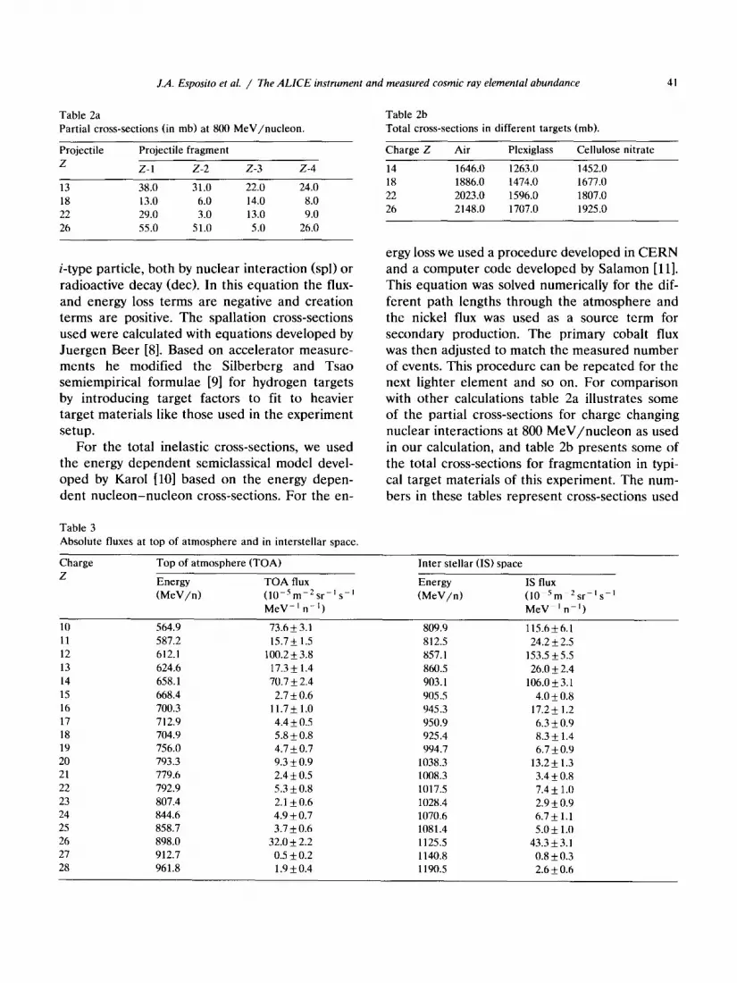
Table 3

Absolute fluxes at top of atmosphere and in interstellar space

Charge Z

10

11

12 13

14 15

16 17

18 19

20 21

22

23

24 25

26

27 28

Top of atmosphere (TOA) Inter stellar (IS) space

Energy TOA flux Energy IS flux

(McV/n) (10-Sm-2sr-ls~l (MeV/n) (,0~“m~2sr-ls-l

MeV-’ n-‘) MeV-In-‘)

564.9 73.6k3.1 809.9 115.6k6.1

587.2 15.7* 1.5 812.5 24.2 2.5 f

612.1 100.2+3.8 857.1 153.5 5.5 *

624.6 17.3 1.4 + 860.5 26.0 + 2.4

658.1 70.7 2.4 f 903.1 106.0 3.1 +

668.4 2.7 0.6 f 905.5 4.0 k 0.8

700.3 11.7+1.0 945.3 17.2+ 1.2 712.9 4.4 0.5 + 950.9 6.3 + 0.9

704.9 5.8f0.8 925.4 8.3+ 1.4 756.0 4.7 0.7 f 994.7 6.7kO.9

793.3 9.3 0.9 + 1038.3 13.2+ 1.3 779.6 2.4kO.5 1008.3 3.4+0.8 792.9 5.3kO.8 1017.5 7.4* 1.0 807.4 2.1 +0.6 1028.4 2.9 + 0.9 844.6 4.9+0.7 1070.6 6.7+ 1.1 858.7 3.7+0.6 1081.4 5.0+ 1.0 898.0 32.0 2.2 f 1125.5 43.3k3.1

912.7 0.5 0.2 + 1140.8 0.8 f 0.3 961.8 1.9+0.4 1190.5 2.6kO.6


by the algorithm, their actual values are certainly not better defined than _+ 10%.

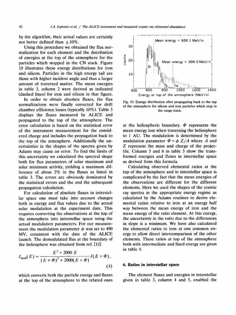
Using this procedure we obtained the flux normalization for each element and the distribution of energies at the top of the atmosphere for the particles which stopped in the CN stack. Figure 10 illustrates these energy distributions for iron and silicon. Particles in the high energy tail are those with higher incident angle and thus a larger amount of traversed matter. The mean energies in table 3, column 2 were derived as indicated (dashed lines) for iron and silicon in that figure.

In order to obtain absolute fluxes, the flux normalizations were finally corrected for drift chamber efficiency losses (typically 10%). Table 3 displays the fluxes measured by ALICE and propagated to the top of the atmosphere. The error calculation is based on the statistical error of the instrument measurement for the considered charge and includes the propagation back to the top of the atmosphere. Additionally the un- certainties in the shapes of the spectra given by Adams may cause an error. To find the limits of this uncertainty we calculated the spectral shape both for flux parameters of solar maximum and solar minimum activity, yielding a maximum dif- ference of about 2% in the fluxes as listed in table 3. The errors are obviously dominated by the statistical errors and the and the subsequent propagation calculation.

For calculation of absolute fluxes in interstellar space one must take into account changes both in energy and flux values due to the actual solar modulation at the experiment date. This requires converting the observations at the top of the atmosphere into interstellar space using the actual modulation parameters. For our measurement the m~ulation parameter 4 was set to 490 MV, consistent with the date of the ALICE launch. The demodulated flux at the boundary of the heliosphere was obtained from ref. [12l

E2f2000 E Jmod(E) =

(E+@)2+2000(E+@) J(E+@),

(4) 6. Ratios in interstellar space

which converts both the particle energy and fluxes The element fluxes and energies in interstellar at the top of the atmosphere to the related ones given in table 3, column 4 and 5, enabled the

I ’ m--.-----

: Mean energy = 658.1 MeV/n

Energy at top of the atmosphere (MeV/n)

Fig. 10. Energy distribution after propagating back to the top of the atmosphere for silicon and iron particles which stop in

the range stack.

at the heliospheric boundary. Q, represents the mean energy loss when traversing the heliosphere to 1 AU. The modulation is determined by the modulation parameter @ = 4 Z/A where A and 2 represent the mass and charge of the projectile. Column 5 and 6 in table 3 show the trans- formed energies and fluxes in interstellar space as derived from this formula.

Calculating observed elemental ratios at the top of the atmosphere and in interstellar space is complicated by the fact that the mean energies of the observations are different for the different elements. Here we used the shapes of the cosmic ray spectra in the appropriate energy regime as calculated by the Adams routines to derive elemental ratios relative to iron at an energy half way between the mean energy of iron and the mean energy of the ratio element. At this energy, the uncertainty in the ratio due to the differences in slope is a minimum. We have also calculated the elemental ratios to iron at one common energy to allow direct intercomparison of the other elements. These ratios at top of the atmosphere both with intermediate and fixed energy are given in tabie 4.

J.A. Esposito et al. / The ALICE instrumenl and measured cosmic ray elemental abundance 43

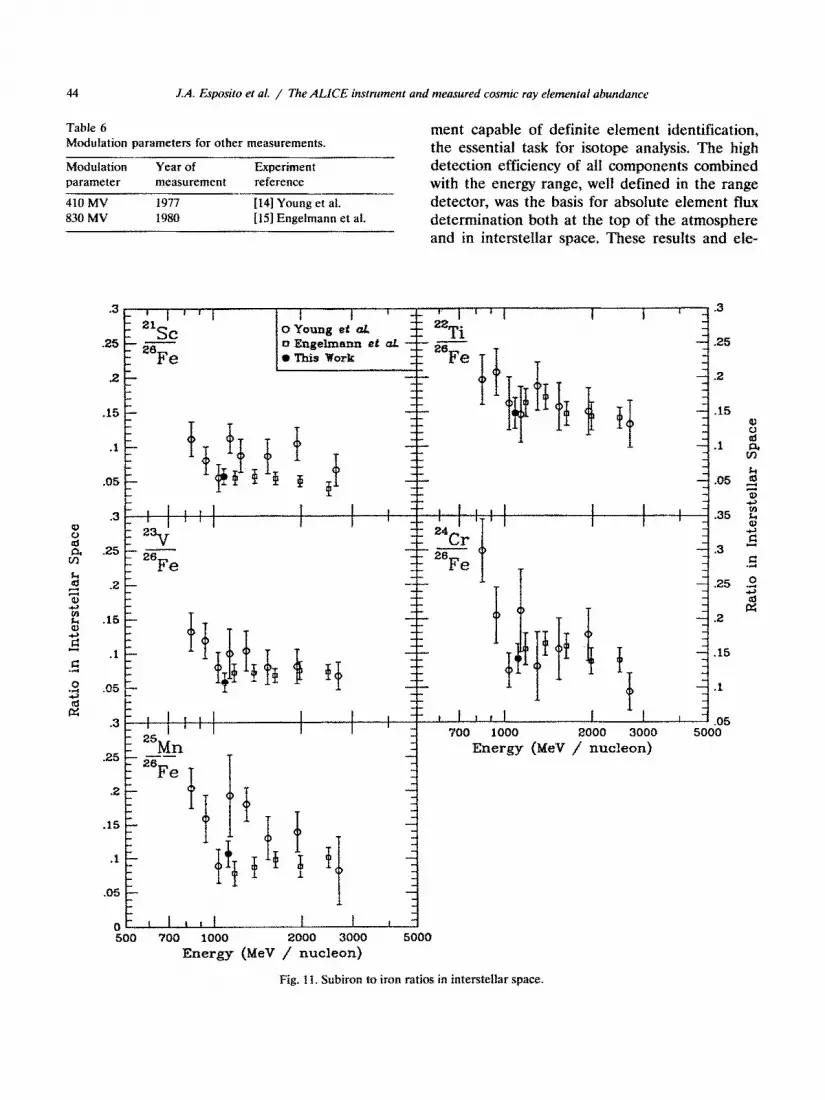
calculation of ratios outside the heliosphere, using the demodulated Adams spectra slopes both for intermediate energy extrapolation and extrapolation to one fiied energy (10.50 MeV/n) as explained before. Table 5 shows element ratios relative to iron in interstellar space at intermediate energy values listed in column 2. Again, to give the opportunity of direct intercomparison at one fixed energy column 4 displays the element ratio versus iron at 1050 MeV/n. The only way to compare measurements by different experimenta- tors at different dates is to derive the specific interstellar experiment values individually. As an example, fig. 11 shows the measured abundance ratio to iron of several different elements as derived from the ALICE measurement and finally transferred to interstellar space in comparison with the results of other authors [14,15]. These published fluxes and energy values at the top of the atmosphere were converted to interstellar space fluxes and energies as described above. The applied modulation parameters, listed below in table 6, are consistent with the experiment dates and were taken from a publication by

Table 4 Element ratios vs. iron at intermediate and one fixed energy

at the top of the atmosphere.

Charge Energy

2 (MeV/n)

10 731.5

11 738.1

12 755.1

13 761.3

14 778.1

15 783.2

16 799.2

17 805.5

18 801.5 19 827.0

20 845.7 21 838.8

22 845.5

23 852.7 24 871.3

25 878.4

26 898.0 27 905.4

28 929.9

Abundances relative to Fe

at intermediate E at 830 MeV/n

1.424 + 0.097 1.324+0.091

0.316+0.031 0.295 f 0.029

2.083kO.129 1.973+0.123

0.366 f 0.033 0.349 f 0.032

1.575*0.100 1.518*0.096

0.060 f 0.009 0.059 f 0.009

0.276 k 0.025 0.270 f 0.025

0.110*0.014 0.109+0.014

0.146+0.018 0.145kO.018

0.124*0.016 0.124+0.016 0.259 f 0.026 0.259 f 0.026 0.066 * 0.011 0.066 f 0.011

0.148+0.018 0.148+0.018 0.059 f 0.010 0.059 f 0.010 0.143 + 0.019 0.144+ 0.019

0.109+0.017 0.110~0.017 = 1.000 = 1.000

0.020 f 0.009 0.020 * 0.009

0.065 + 0.014 0.065 + 0.014

Table 5

Element ratios vs. iron at intermediate and one fixed energy

at the heliospheric boundary.

Charge Energy Abundance relative to Fe

2 (MeV/n) at intermediate E at 1050 MeV/n

10 967.7 1.497&0.103 1.402 & 0.009

11 969.1 0.316*0.031 0.297 f 0.029

12 991.3 2.189k0.136 2.092 + 0.130

13 993.0 0.375 f 0.034 0.359 f 0.027

14 1014.3 1.655+0.105 1.611 +0.102

15 1015.5 0.062 f 0.009 0.060 k 0.009

16 1035.4 0.290 f 0.027 0.287 + 0.026

17 1038.2 0.113+0.015 0.113~0.015

18 1025.5 0.143+0.018 0.143kO.018

19 1060.1 0.128+0.016 0.128+0.016

20 1081.9 0.271 f 0.027 0.271 f 0.027

21 1066.8 0.066 * 0.011 0.066 f 0.011

22 1071.5 0.146+0.018 0.147kO.018

23 1076.9 0.058 f 0.010 0.059 + 0.010

24 1098.1 0.142kO.019 0.144+0.019

25 1103.5 0.107~0.017 0.108*0.017

26 1125.5 = 1.000 = 1.000

27 1133.2 0.015 +0.009 0.015 + 0.009

28 1157.9 0.065 f 0.014 0.065 f 0.014

Garcia-Munoz et al. [13]. The ALICE results are seen to be in substantial agreement with this earlier work. All of the observed elements have similar charge to mass ratios, and therefore the effects of modulation on the ratios are small, as can be seen by comparing tables 4 and 5.

7. Conclusion

In this paper we focussed on the experimental concept and the performance of the individual detectors of the ALICE instrument. The main experimental challenges were to attain the precise resolutions required of the several detectors, and to combine the measurement from electronic detectors with a well defined range derived from a passive cellulose nitrate range stack. To demon- strate that the use of the drift chambers with their high spatial resolution enables the correct matching between active and passive detector responses will be part of another paper devoted to the subsequent isotope analysis. The ALICE instrument was shown to provide a charge measure-


Table 6 M~ulation parameters for other measurements.

Modulation Year of Experiment parameter measurement reference

410 MV 1977 [14] Young et al. 830 MV 1980 [15] Engelmann et al.

ment. capable of definite element identification, the essential task for isotope analysis. The high detection efficiency of al1 components combined with the energy range, well. defined in the range detector, was the basis for absoIute element flux determination both at the top of the atmosphere and in interstellar space. These results and ele-

*3L, I ,,, I

~

“‘ic

I I 1’ i i , I I L .3

0 Young et a& .25 -

22Ti 26Fe

0 Engelmann at CXL 0 This Work

P 1

.25

.2

.15

.l

.15 iZ- T,

I PII I 1

I .05 ,700 1000 2000 3000 5000

Energy (MeY / nucleon)

OF * “II I I t 1

500 700 1000 2000 3000 5000

Energy (MeV / nucleon)

Fig. I 1. Subiron to iron ratios in interstellar space.

J.A. Esposito et al. / The ALlCE i~~~rne~t and measured cosmic ray e~emeni~l ~b~~~e 45

ment ratios are documented and compared with results of other authors.

Acknowledgements

We gratefully acknowledge the support of this project by the NASA Supporting Research and Technology program (SR &T) and the Deutsche Forsch~ngsgemein~haft (DFG).

Also thanks to a NATO grant N 0325/84 which covered part of our travel expences. We are grateful to R. Greer, T. Laws, G. Latsch, K. Schmeck and D. Righter, without whose dedi- cated technical and engineering support the AL- ICE experiment could not have been done. We thank the personnel of the National Scientific Ballon Facility (NSBF) for their professionalism in carrying out our flight and K, Hazelwood in particular for having a highly sucessful campaign in difficult circumstances.

References

[l] W.T. Eadie, D. Drijard, FE. James, M. Roes, B. Sad&et, Statistical Methods in Experimental Physics (North-Holland, Amsterdam, 1971).

[Z] M. Simon, M. Henkel, R. Hundt, K.D. Mathis, G. Schieweck and T. Suck, Nucl. Instrum. Methods 221 (1984) 446.

[31

k4l

ISJ

[61

I71

181 [91

001 [Ill

I121

[I31

041

051

A. Hesse, B.S. Acharya, U. Heinbach, W. Heinrich, M. Nenkel, 3. Luzietti, C. Koch, M. Simon, V.K. Balasub- rahmanyan, L.M. Barbier, E.R. Christian, J.A. Esposito, J.F. Ormes and R.E. Streitmatter, Int. J. Radiat. Appl: Instrum. 19 (1991) 689. W. Heinrich, M. Simon, H.O. Tittel, J.F. Ormes, V.K. Balasubrahmanyan and R.E. Streitmatter, in: Solid State Nuclear Track Detectors, Proc. 11 th Int. Conf., Bristol (Pergamon, Oxford, 1982) p. 863. W. Trakowski, B. Schaefer, J. Treute. A. Sonntag, C. Brechtmann, J. Beer and W. Heinrich, Nucl. Instrum. Methods 223 (1984) 92. J.H. Adams, R. Silherberg and C.H. Tsao, Cosmic Ray Effects on Microelectronics Part I: The near-Earth Parti- cle Environment, NRL Memorandum Report, Naval Re- search Laboratory, Washington, DC (1981). R.3. Protheroe, J.F. Ormes and GM. Comstock, Astro- phys. J. 247 (1981) 362. J. Beer, Ph. D. Thesis, University of Siegen (1985). C.H. Tsao, R. Silberberg and J.R. Letaw, in: Proc. 18th Int. Cosmic Ray Conf., Bangalore (19831, Vol. 2, p. 44. P. Karol, J. Phys. Rev. C I1 (197% 1203. M.H. Salamon and S.P. Ahlen, Phys. Rev. B 24 (1981) 5026. L.J. Gleeson and W.I. Axford, Astrophys. J. 154 (1968) 1011. M. Garcia-Muno~, J.A. Simpson, T.G. Guzik, J.P. Wefel and S.H. Margolis, Astrophys. J. Suppl. Ser. 464 (1987) 269. J.S. Young, P.S. Freier, C.J. Waddington, N.R. Brewster and R.K. Fickle, Astrophys. J. 246 (1981) 1014. J.J. Engelmann, P. Ferrando, A. Soutoul, P. Goret, E. Juliusson, I_.. K~h-Miramond, N. Lund, P. Masse, B. Peters, N. Petrou and IL. Rasmussen, Astron. Astro- phys. 233 (1990) 96.

the alice instrument and the measured cosmic ray elemental abundances

Documents