arX

iv:a

stro

-ph/

0410

602v

1 2

5 O

ct 2

004

Abundances and Depletions of Interstellar Oxygen

Adam G. Jensen, Brian L. Rachford, and Theodore P. Snow

Center for Astrophysics and Space Astronomy

Department of Astrophysical and Planetary Sciences, University of Colorado at Boulder

Campus Box 389

Boulder, CO 80309-0389

Adam.Jensen@colorado.edu, rachford@casa.colorado.edu,

tsnow@casa.colorado.edu

ABSTRACT

We report on the abundance of interstellar neutral oxygen (OI) for 26 sight-

lines, using data from the Far Ultraviolet Spectroscopic Explorer (FUSE), the In-

ternational Spectroscopic Explorer (IUE), and the Hubble Space Telescope (HST).

OI column densities are derived by measuring the equivalent widths of several

ultraviolet absorption lines, and subsequently fitting those to a curve of growth.

We consider both our general sample of 26 sightlines and a more restrictive sam-

ple of 10 sightlines that utilize HST data for a measurement of the weak 1355 A

line of oxygen, and are thus better constrained due to our sampling of all three

sections of the curve of growth. The column densities of our HST sample show

ratios of O/H that agree with the current best solar value if dust is considered,

with the possible exception of one sightline (HD 37903). We note some very

limited evidence in the HST sample for trends of increasing depletion with re-

spect to RV and f(H2), but the trends are not conclusive. Unlike a recent result

from Cartledge et al. (2004), we do not see evidence for increasing depletion with

respect to 〈nH〉, but our HST sample contains only two points more dense than

the critical density determined in that paper. The column densities of our more

general sample show some scatter in O/H, but most agree with the solar value

to within errors. We discuss these results in the context of establishing the best

method for determining interstellar abundances, the unresolved question of the

best value for O/H in the interstellar medium (ISM), the O/H ratios observed in

Galactic stars, and the depletion of gas-phase oxygen onto dust grains.

Subject headings: ISM: abundances — ISM: depletions — ultraviolet: ISM

– 2 –

1. INTRODUCTION AND BACKGROUND

As the third most abundant element in the Galaxy after hydrogen and helium, oxygen

is an important component in interstellar chemistry and dust grain models. The exact

abundance of gas-phase oxygen relative to hydrogen has been in question for quite some

time. The question of whether oxygen accumulates onto dust grains to varying degrees in

different environments has also been investigated. While recent research seems to be moving

towards a picture of constant oxygen depletion from the gas, questions remain, especially

with regard to the possible dependence of oxygen depletion on cloud density. There is much

work to be done in examining sightlines with more extreme physical properties—sightlines

that have been previously ignored due to observational considerations.

Interstellar absorption lines in the ultraviolet were first detected with sounding rockets,

e.g. Morton & Spitzer (1966). Detailed studies of neutral oxygen in the interstellar medium

became possible with the introduction of ultraviolet satellites such as Copernicus and IUE in

the 1970s. Studies such as those by Morton (1974), Morton (1975), Zeippen et al. (1977), de

Boer (1979), and de Boer (1981) each focused on the study of an individual sightline, finding

that gas-phase oxygen was depleted relative to the solar value. Morton et al. (1973) also

studied the column densities of several different atomic species, including neutral oxygen,

for five sightlines.

The first extensive survey to determine the general interstellar value of O/H was reported

by York et al. (1983). Their study included 53 sightlines. Of these, oxygen column densities

were determined in 14 cases, while column density upper limits were determined in 16 cases

and column density lower limits were determined in 20 cases (they did not report on OI

for the final three sightlines). Their analysis used the weak 1355 A line of OI, relying on

the assumption that NI and OI have a similar b-value. They determined column densities

by using this b-value to apply an appropriate saturation correction to the 1355 A line when

necessary. In a few cases, the 988 A triplet of OI was used, but further details were not

given. The conclusion of this study was that interstellar O/H is between 40% and 70% of the

assumed solar value, from Withbroe (1971), of approximately 690 oxygen atoms per million

hydrogen atoms (later studies have assumed different solar values of the solar O/H ratio, and

the correct value is still very much in dispute; see §5.3 for a brief discussion). Additionally,

York et al. (1983) concluded that there is no evidence of systematically enhanced depletion

as reddening (i.e. total hydrogen column density) increases. Rather, they found some limited

evidence that sightlines with log N(Htot) < 20.5 are more depleted (with the mean O/H ratio

approximately 40% solar) than sightlines with log N(Htot) > 20.5 (with the mean O/H ratio

approximately 70% solar).

Keenan et al. (1985) explored 26 sightlines—including one sightline from York et al.

– 3 –

(1983)—and found an average O/H ratio that is 50% of the solar value by Withbroe (1971).

In contrast to the results of York et al. (1983), Keenan et al. (1985) did not find a significant

difference between sightlines with log N(Htot) < 20.5 and those with log N(Htot) > 20.5.

An important recent survey of interstellar oxygen was performed by Meyer et al. (1998).

Their study covered 13 sightlines and involved detailed analysis of the 1355 A line of OI using

the Goddard High Resolution Spectrograph (GHRS) on the Hubble Space Telescope. These

13 sightlines included four for which the column density had been previously determined,

and three for which a saturation correction (estimated from MgII and NI) was applied.

The study found the mean O/H to be 319 ± 14 ppm, with the largest deviation from the

mean less than 18%. Assuming as many as 180 oxygen atoms in the dust phase per million

hydrogen atoms, a value consistent with many theoretical models (see §5.3), this corresponds

to a total O/H ratio approximately two-thirds of the Grevesse & Noels (1993) solar value,

(O/H)⊙ = 741 ± 130 ppm. Additionally, Meyer et al. (1998) did not find any systematic,

statistically significant variation of O/H with respect to the total column density of hydrogen

(N(Htot)), the average volume density of hydrogen along the sightline (〈nH〉), or the molecular

fraction of hydrogen (f(H2) = 2N(H2)/[2N(H2) + N(OI)]). We note that the Meyer et al.

(1998) study was confined to stars with AV . 1.0 mag.

Studies since Meyer et al. (1998) may exhibit systematic differences from previous stud-

ies, in both total oxygen column density and O/H ratio relative to solar, for the following

reasons:

• Revision of the f -value for the weak 1355 A transistion (see §3.4) from 1.25× 10−6 to

1.16 × 10−6, as suggested by Welty et al. (1999)

• Revision of the solar O/H ratio from approximately 700 ppm or more (Withbroe 1971;

Grevesse & Noels 1993) to approximately 550 ppm or less (Allende Prieto et al. 2001;

Holweger 2001; Asplund et al. 2004)

In comparing results with Meyer et al. (1998), more recent authors (Cartledge et al. 2001;

Andre et al. 2003; Cartledge et al. 2004) have made a linear correction to the reported O/H

ratios of Meyer et al. (1998) to reflect the change in f -value. With the change, the mean

Meyer et al. (1998) value becomes O/H = 343± 15 ppm. Additionally, assuming Odust/H is

as large as 180 ppm, the total O/H ratio can be reconciled with the revised solar value.

Cartledge et al. (2001) examined 11 sightlines using the Space Telescope Imaging Spec-

trograph (STIS) onboard HST to observe the 1355 A line. This study used two methods:

profile fitting, where velocity information from other atomic species is incorporated into

the fit of the oxygen line; and the apparent optical depth (AOD) method, where it is as-

– 4 –

sumed that the line does not contain unresolved saturated structure and the measurement

represents a lower limit on column density if the assumption fails (profile fitting can suffer

from the same problem if unresolved, saturated structure is present and none of the velocity

information from other species reveals such structure). Cartledge et al. (2001) analyzed a

subset of seven sightlines, and compared them with the 13 sightlines measured with GHRS

from Meyer et al. (1998). They found that five of the seven sightlines measured with STIS

lie below the O/H mean (adjusted for the new f -value of the 1355 A line) determined by

Meyer et al. (1998). These five sightlines have five of the six highest hydrogen column den-

sities in the combined sample of 20 sightlines. This result is similar to O/Kr ratios reported

in the same work, where some sightlines with higher total oxygen content exhibit oxygen

depletion relative to krypton (a noble gas that is likely to be found almost exclusively in

the gas phase). Despite this, the oxygen column densities for only two sightlines have 1-σ

uncertainties that exclude the possibility of consistency with the Meyer et al. (1998) mean

for O/H. The evidence that there is oxygen depletion with respect to krypton, however, is

somewhat more convincing.

Moos et al. (2002) were among the first to use FUSE to measure the equivalent widths

of several different transistions for neutral oxygen, and to subsequently measure oxygen

column densities by using curves of growth. They did so for seven sightlines less than 180 pc

in length. Despite large uncertainties and potential systematic errors from inhomogeneous

determinations of atomic hydrogen, the seven sightlines were found to have O/H ratios from

234 to 479 ppm—consistent within a factor of 2.1. Excluding the sightline BD+28◦2411, the

range is 363 to 479 ppm—consistent within a factor of 1.3. Within the uncertainties, these

results are consistent with Meyer et al. (1998).

The next major survey of interstellar oxygen was by Andre et al. (2003). This survey

measured the oxygen content of 19 sightlines using STIS. Similar to Cartledge et al. (2001),

Andre et al. (2003) used both profile fitting and the AOD method to determine column

densities. Their analysis produced a mean O/H = 408± 13 ppm. The standard deviation in

their sample was 59 ppm. Andre et al. (2003) included the previous results of Cartledge et

al. (2001) and Meyer et al. (1998) to find a mean O/H = 362 ppm, with a standard deviation

of approximately 20%. Andre et al. (2003) took the average of values by Allende Prieto et al.

(2001) and Holweger (2001), 517± 58 ppm, as the solar value of O/H. Both the O/H mean

of the 19 sightlines of the Andre et al. (2003) sample and the O/H mean of the combined

sample can be reconciled with this solar value if dust is considered.

The most recent interstellar oxygen survey was by Cartledge et al. (2004), probing 36

sightlines using the same methods as Cartledge et al. (2001), and adding previous results

for 20 sightlines, discussed results for a cumulative sample of 56 sightlines. The results of

– 5 –

Cartledge et al. (2004) reinforce the conclusions of Cartledge et al. (2001) with many more

data points. Specifically, a 4-parameter Boltzmann function is fit to the ensemble of O/H

ratios when plotted against 〈nH〉, with an apparent transition centered at 〈nH〉 ≈ 1.5 cm−3.

This phenomenon is somewhat surprising in that it is not clear why 〈nH〉 should accurately

trace the environment of a sightline; rather it is more commonly expected that reddening

parameters, e.g. AV or EB−V , should be a better trace of the individual clouds that dominate

a given sightline. However, the trend seen by Cartledge et al. (2004) is not new; results by

Snow et al. (2002), Jenkins et al. (1986), Spitzer (1985), and many other references cited

therein have shown that the sightline characteristic with the most consistent correlation

for enhanced depletion of many different elements is 〈nH〉. Spitzer (1985) discussed the

possibility that 〈nH〉 traces the superposition of three phases of the ISM: a warm, low-

density phase, a cold, moderate-density phase, and a cold, high-density phase. Regardless

of the theoretical difficulties of determining a comprehensive picture for why 〈nH〉 traces

the interstellar environment so well, this most recent result of Cartledge et al. (2004) is

the first time that this has been detected for oxygen. The fit found by Cartledge et al.

(2004) suggests that Odust/H = 192 ± 51 ppm in the higher density sightlines, compared to

Odust/H = 86 ± 51 ppm in lower density sightlines. As discussed in that paper, the increase

of over 100 ppm is difficult to account for with most dust models. Of note, Cartledge et

al. (2004) adopt a slightly different value for the solar oxygen abundance than Andre et al.

(2003). Cartledge et al. (2004) adopt (O/H)⊙ = 476 ± 50 ppm, the weighted average of

Holweger (2001) and Asplund et al. (2004), as opposed to the straight average of Allende

Prieto et al. (2001) and Holweger (2001) adopted by Andre et al. (2003).

Taking all these results into account, the emerging picture is that interstellar O/H is

relatively constant over a wide range of environments. If Odust/H . 180 ppm, then the

interstellar O/H ratio can be reconciled with the solar value. There are two exceptions to

the observed constancy. The first exception is the Cartledge et al. (2001) study that hints

at the evidence of, but does not conclusively prove, enhanced depletions in sightlines with

higher total oxygen and hydrogen column densities. The second exception is the Cartledge

et al. (2004) study that shows a small but clear depletion effect as 〈nH〉 becomes larger than

1.5 cm−3. This is in strong contrast to the results for many other atomic species such as

iron, silicon, and aluminum, species that show highly enhanced depletion in sightlines with

higher reddening.

One assumption concerning these studies that should be noted is that the ionization

energies of OI and HI are very similar, at 13.618 eV and 13.598 eV, respectively. This means

that the fractional contribution to the total oxygen abundance from ionized oxygen (OII,

OIII, etc.) will be mirrored by the fractional contribution to the total hydrogen abundance

from HII. A charge exchange reaction between oxygen and hydrogen also constrains this

– 6 –

relationship (Field & Stiegman 1971). Since the dissociation energy of molecular hydrogen

is only 4.476 eV, the assumption that O/H is independent of ionization fraction holds across

all molecular fractions as well. In particular, the fact that a cloud has a high molecular

fraction would tend to reveal that the ionization fraction is very small, since the majority

of molecular hydrogen would be destroyed before significant ionization of atomic hydrogen

would occur.

The goal of this study is to add to the current body of knowledge concerning interstellar

oxygen by determining the O/H ratio for several sightlines observed by FUSE. We supplement

the FUSE data with HST and IUE data where possible. Here we report on our measurements

of the equivalent widths of several neutral oxygen absorption lines for each sightline, and our

fits of these to curves of growth, from which we determined the b-values and column densities

of oxygen. The curve of growth method was used in the hope of avoiding assumptions about

b-values and subsequent saturation corrections. We then looked for systematic differences in

O/H with respect to total hydrogen and various reddening parameters.

As a side goal, we aimed to determine the utility of FUSE for observing oxygen ab-

sorption lines shortward of ∼ 1100 A, a wavelength region that is not covered by HST or

IUE and has been observed only to a limited extent with Copernicus, but where a number

of weak-to-medium strength OI lines are found. With some exceptions, e.g. Zeippen et al.

(1977), studies of interstellar oxygen have been limited to analysis of the 1355 A line of oxy-

gen which, though weaker than the FUSE lines, is sometimes strong enough to be saturated.

While the more recent of these studies have taken into account the profiles of other species

to formulate a comprehensive picture of the cloud structure along a given sightline, there

remains the possibility of saturation effects for individual velocity components. It is not

yet known whether studies such as this paper and Moos et al. (2002) can equal or perhaps

improve upon the results of previous studies by taking into account all the information that

is now available to us through FUSE in the form of many far-UV OI lines.

2. OBSERVATIONS AND DATA REDUCTION

Data were taken from FUSE, HST, and IUE. The sightlines were chosen from a sample

observed by FUSE as part of a molecular hydrogen survey conducted by Rachford et al.

(2002) and continued in Rachford et al. (2004 in prep.). The original FUSE sample included

34 sightlines, and HST or IUE data were available for 27 of these sightlines. For four sightlines

(the sightlines towards HD 43384, HD 166734, HD 281159, and NGC 2264 67, a.k.a. Walker

67) we were unable to measure the equivalent widths of any absorption lines. We do not

report further on these sightlines. Basic stellar data for the stars of the other 30 sightlines

– 7 –

is given in Table 1. Values for hydrogen column densities and reddening parameters along

the lines of sight are given in Tables 2 and 3, respectively.

2.1. FUSE Data

Data are collected with the FUSE satellite by four channels, two with a lithium fluoride

detector (LiF1 and LiF2) and two with a silicon carbide detector (SiC1 and SiC2). Each

channel contains two data segments, designated as A and B, covering adjacent wavelength

regions. The lithium fluoride channels cover the wavelength region from 989-1188 A, while

the silicon carbide channels cover the region from 905-1104 A. Samples of FUSE spectra are

shown in Figure 1.

The pixel scale of FUSE is ∼ 0.007 A. Knowledge of the FWHM of weak lines is

necessary because the theoretical line must be convolved with instrumental resolution when

we make theoretical profile fits. We measured weak lines in the FUSE spectra and found

the full-width at half-max (FWHM) of these lines to be 0.074 A. This is the value for the

instrumental resolution element used in our model that iteratively fits a Voigt profile to an

absorption line. This model was used in certain sightlines to fit moderately saturated lines

of oxygen (see §3.1 and §3.2).

The data were reduced with the CALFUSE pipeline, versions 2.0.5 or 2.1.6. Data from

different data segments are not coadded; rather, the data segment with the best signal-to-

noise (S/N) is selected, with other data segments providing a check for consistency.

2.2. HST Data

Archived HST data taken by STIS were available for nine sightlines: HD 24534, HD

27778, HD 37903, HD 185418, HD 192639, HD 206267, HD 207198, HD 207538, and HD

210839. The oxygen content of many of these sightlines has been analyzed previously with

either STIS or GHRS (see Table 9). We also use the equivalent width for the 1355 A line

of the HD 154368 sightline that was measured by Snow et al. (1996) using GHRS data.

Samples of HST spectra are shown in Figure 2.

The pixel scale of the STIS observations is ∼ 0.006 A. Measuring weak lines, we find

FWHM values as small as 0.017 A. In fitting the 1302 A line of OI (see §3.3), we used this

value for the instrumental resolution in our model that fits a Voigt profile.

We used on-the-fly calibrated STIS data. In many cases we had multiple observations.

– 8 –

We coadded observations of similar echelle order, adding errors in quadrature. When the

targeted line was observed in multiple echelle orders, we analyzed separate echelle orders

independently, then took an average of the results in determining our final equivalent widths.

2.3. IUE Data

High-dispersion data taken with the Short Wavelength Prime (SWP) camera onboard

the IUE satellite were available on the MAST archive for 26 of the original 34 sightlines,

and 25 of the 30 sightlines for which we were able to measure at least one equivalent width.

All of the sightlines for which HST data were available also had available IUE data, with

the exception of HD 185418. Low-dispersion data were available, but do not clearly resolve

either the 1302 A or 1355 A line of OI and were not used. Samples of IUE spectra are shown

in Figure 3.

The pixel scale of IUE is 0.05 A. We measured weak lines in the IUE spectra and found

the FWHM of these lines to be 0.156 A or more. This is the resolution element value used

in calculating an upper limit on equivalent widths of undetected lines (see §3.7).

Where multiple observations were available, we coadded observations of similar aperture.

Bad pixels are corrected by using an interpolation between neighboring points. Where

multiple bad pixels are adjacent, we examine the spectra. We find multiple adjacent bad

pixels to be correlated with saturated absorption lines, and correct for this by setting the

flux to zero at these points, if all spectra used in coadding show the same pattern of bad

pixels.

When available, we analyzed data from both large and small apertures independently,

and adopted a straight average of the resulting equivalent widths. Results for the two

equivalent widths are usually consistent within the errors. We conclude that there is not a

clear systematic difference between the two apertures that affects the two absorption lines

that are under examination in this data. All measured equivalent widths are either from

large-aperture observations or an average—small aperture data are never used exclusively.

For eight of the sightlines where both HST and IUE data were available, we preferentially

used our results from HST due to the higher resolution and S/N. We examined the equivalent

widths of the 1302 A line of OI in both HST and IUE in the cases where both data sets are

available. In two cases (HD 207198 and HD 207538) the equivalent widths were consistent. In

the other six cases, the IUE results seem to underestimate the equivalent width as compared

to the HST data at the 1- or 2-σ level. There is a ninth case, HD 154368, where there are

GHRS results found in the literature (Snow et al. 1996). As mentioned in §4.4, the IUE

– 9 –

equivalent width we measure in this case is larger than the equivalent width determined by

Snow et al. (1996), though that equivalent width is based on a theoretical profile derived from

another line and appears to be too narrow when plotted against the data. It is thus unclear

whether or not there is a systematic difference between the HST and IUE data, though the

possibility exists that IUE data underestimates the equivalent width of the strong line.

Massa et al. (1998) examined the scientific quality of the IUE archived data, and noted

several aspects of the spectra that create uncertainty, including time-dependent effects on

strong absorption lines and certain special cases where the cores of saturated lines that

should be zero are instead a significant fraction (positive or negative) of the continuum.

Potential effects on the 1302 A and 1355 A lines and the surrounding spectral region are not

specifically discussed. The 1355 A is too weak to be observed in most IUE spectra, so the

greatest concern would be with regard to the 1302 A line and whether or not it exhibits time-

dependent effects similar to those Massa et al. (1998) found in Lyman-α, a CIII multiplet

at 1175 A, and NV lines near 1240 A. In spite of these problems, additional calibration

techniques for the IUE data are not apparent and we do not correct these spectra further.

Instead, we note here the general effect of uncertainty in a strong line like the 1302 A line.

If we have underestimated the true equivalent width of the 1302 A line, then our curve of

growth analysis will underestimate the column density and/or overestimate the b-value. On

the other hand, if we overestimate the equivalent width of the 1302 A line, then our curve

of growth analysis will overestimate the column density and/or underestimate the b-value.

These effects will be the most significant when there are fewer other lines included in the

analysis.

3. OBSERVED OI ABSORPTION LINES

The first step in determining column densities by a curve of growth is to measure the

equivalent widths of multiple absorption lines. Since there are two degrees of freedom in

fitting the equivalent widths to a curve of growth (column density N and velocity parameter

b), whether or not we have a unique solution and/or a well-determined constraint depends

on the number of equivalent widths fit to the curve. One equivalent width provides a family

of solutions, i.e., a unique column density can only be determined if a b-value is assumed, or

vice-versa. Two equivalent widths provide a unique solution, but with two free parameters

the best χ2 cannot be converted into meaningful confidence intervals unless either N or b

is assumed. Three or more equivalent widths provide a unique solution and the ability to

determine confidence intervals. Consequently, the goal for each sightline was to measure the

equivalent widths of at least three different absorption lines of OI.

– 10 –

The following is a description of the OI absorption lines that were used in our analysis.

Wavelengths, f -values, damping constants, and the instrument that was used for the obser-

vations of each of these lines are summarized in Table §4. All atomic data in this section is

taken from Morton (2003).

3.1. Lines Below 1000 A

We identify six different OI absorption lines below 1000 A that are useful in our study.

These lines range in oscillator strength from 1.77× 10−4 to 3.65× 10−3. None of these lines

have damping constants that are reported in Morton (2003). These lines can be observed

in the SiC1B and SiC2A data segments of FUSE in the spectra with the best S/N. In the

spectra of most sightlines, these lines are not identified.

Four of the lines (at 921.857 A, 922.200 A, 936.6295 A, and 976.4481 A) suffer from

mild blending with H2 lines in some spectra. In these cases, we attempt simultaneous fitting

of the OI line and the blending line if there is a separation between the cores that is resolved.

If there is not separation in the cores, then we do not attempt fitting.

We use Gaussians fits for these lines where possible, but a few cases require a Voigt

profile. We use a fitting routine that generates a Voigt profile from the parameters of column

density and b-value. Since we do not know the value of the damping constant γ for these

lines, we must supply the routine with a placeholding value for γ, and cannot use data from

our fits to contrain column density or b-value from a single line. However, the equivalent

widths are still useful in the curve of growth analysis.

We should note that the utility of these lines is ultimately limited because of the large

uncertainties associated with them. The two major sources of uncertainty are blends with

other lines and an uncertain continuum. The latter source of uncertainty is very important

for the four lines below 930 A. However, the inclusion of these lines where possible still

represents an important aspect of our study.

3.2. 1039 A Line

The 1039.2304 A line is the second strongest oxygen line seen in the FUSE spectra, after

the strongest component of the 988 A triplet (which was not used; see §3.5). Its strength

and isolation from other lines make it a staple of this study. The line is visible in four data

segments of FUSE: LiF1A, LiF2B, SiC1A, and SiC2B. The LiF1A data segment provided

the best data and those data were used in most cases.

– 11 –

The line is found in the redward damping wing of an H2 bandhead centered at ∼ 1037

A. The line has an oscillator strength of f = 9.07 × 10−3. The line was usually fit with a

Gaussian, but in some cases was broad enough that a Voigt profile was required. Unlike the

lines below 1000 A we know the damping constant of the line, γ = 1.87× 108, and therefore

Voigt profile fits to this line can potentially be used to extract column density and b-value.

However, the values obtained may be poorly constrained, limited by the coupling of column

density and b-value, the resolution of FUSE, and the data quality of each individual sightline.

However, measuring the equivalent width remains useful for the curve of growth analysis.

3.3. 1302 A Line

The 1302.1685 A line is the strongest line used in this analysis, with an oscillator strength

of f = 4.80 × 10−2. The large damping constant, γ = 5.65 × 108, indicates that this line is

on or near the “square-root region” of the curve of growth. In our analysis of IUE spectra,

the 1302 A line was fit with a Gaussian, as the damping wings are not clearly resolved, and

the spectrum is crowded with many other nearby lines (also fit with Gaussians) that makes

identification of the continuum more difficult. A Gaussian fit still provides a reasonable

approximation for the equivalent width in cases where saturation is marginally detected in

the profile of the line.

For cases in which HST data were available, the damping wings of the line were evident,

and the line was fit with a Voigt profile. As with the 1039 A line, Voigt profile fits may

provide direct information about the column density and b-value, but the strength of the

constraints vary. Additionally, while the 1039 A line is almost always on the “flat region”

of the curve of growth, where column density and b-value are highly coupled, the 1302 A

line always shows damping wings in the HST data, and is found in a transition region in

the curve of growth where the profile depends strongly on both column density and b-value.

As the damping wings become stronger, however, the profile begins to become insensitive to

b-value. When available, equivalent widths measured from HST superceded those from IUE

(except for the case of HD 154368; see §2.3 and §4.4).

In the HST data, either one or two absorption features are seen in the blue wing of the

1302 A line. One of these features appeared consistently and is a singly-ionized phosphorous

line; the other line was not seen in all spectra and remains unidentified. These lines were fit

independently with Gaussians and divided out of the spectra before the 1302 A line was fit.

As with many of the lines in this study, the 1302 A line is one component of a multiplet,

in this case a triplet, but the 1304.8576 A and 1306.0286 A components of the triplet are

– 12 –

absorption lines from two different excited states. Thus, the column densities corresponding

to the equivalent widths of those lines are the column denisities of the excited states, and

would not have been useful in our analysis without an assumption about the excitation

mechanism. These excited lines were observed in the HST spectra, and may be worth

further study that is beyond the scope of this paper.

3.4. 1355 A Line

The 1355.5977 A line is the weakest line used in this analysis, with an oscillator strength

of f = 1.16×10−6. This line has been used extensively to determine oxygen column densities

by itself, either by assuming it contains no unresolved saturated structure; by ignoring the

possibility of such structure and merely obtaining a lower limit on column density; or by using

information from other elements to aid in determining the component structure of the line.

In our analysis, 1355 A lines were fit with Gaussians, either in HST or IUE data. In cases

where a single Gaussian was a poor fit, multiple Gaussians were fit under the assumption that

we were dealing with resolved component structure. This resolved component structure was

only observed in the HST data. Resolved component structure in the 1355 A line may suggest

the need for a curve of growth analysis that accounts for more complex velocity structure.

Such analysis is for the most part beyond the scope of this paper, but is discussed briefly

in §5.2. HST data superceded IUE data when available. For one sightline (HD 154368), we

used an equivalent width from Snow et al. (1996), measured from GHRS spectra.

3.5. Omitted Lines

There are many other neutral oxygen lines that fall in the wavelength range covered

by FUSE. For example, the triplet at 988 A has been used in at least least one other study

(York et al. 1983), but in our data, there are a few problems. The first is that the spectral

region surrounding the line contains some of the strongest telluric lines in the wavelength

region covered by FUSE (Feldman et al. 2000), including OI emission from the 988 A triplet.

In the spectra with the lowest S/N, this airglow dominates. In other spectra, the strength

of the effect is unclear.

Secondly, the resolution FUSE (∼ 15-20 km s−1) dictates that the components of the

triplet, with the greatest separation between two components ∼ 36 km s−1, should be re-

solved if they are weak. However, the strongest component of the triplet is comparable in

strength to the 1302 A line, with oscillator strengths similar to within 3.5%. Therefore,

– 13 –

at typical OI column densities, the line is broadened well beyond a single FUSE resolution

element, and the components of the triplet are blended. This is in addition to some mild

blends with weak H2 lines, and a very uncertain continuum due to strong H2 bands in the

surrounding region.

A third problem is that the damping constant of the components of the triplet are

unknown. Using the Eistein A coefficients found in Morton (2003), some lower limits on

γ for each component might be determined, but the true value would still be somewhat

uncertain. Given its strength, the equivalent width of the strongest component of the 988

A triplet should be strongly dependent in many cases on its damping constant (though the

spectrum will not necessarily reveal a clearly damped profile). Thus, a direct profile fit of

the blended components of the triplet would be very uncertain. Equally uncertain would be

the point of reference for this line on our curve of growth analysis. We have therefore elected

not to include it in our results.

Lines at 924.950 A and 937.8405 A were also detected, but strong H2 lines make the

surrounding continuum impossible to measure. The latter line may also be suject to con-

tamination from an FeII line, but the FeII line should be much weaker given typical relative

column densities of FeII and OI.

In addition to the lines just discussed, Table 5 lists the remaining OI lines with wave-

lengths in the FUSE region and the reasons they are not used in our study. The reasons

for omitting the remaining lines is that they are all either too weak to be detected, are too

heavily blended with other atomic or molecular lines, or are completely wiped out by very

strong atomic or molecular lines. There are no other UV absorption lines of oxygen in the

range covered by either HST or IUE. Since we do not expect to see strong absorption lines

from excited states (such as the “forbidden” 6300 A transition) and were they detectable we

would need an assumption on relative populations to use excited states in constraining total

column density, we do not consider lines outside of the ultraviolet region.

3.6. Errors

Errors on equivalent width measurements take two forms. When absorption lines are

fit with a Gaussian, errors are taken from standard error propagation of the curve-fitting

routine and the functional form of a Gaussian. When absorption lines are fit to a Voigt profile,

errors are not clear due to the lack of a functional form (the Voigt profile is fit iteratively

and involves convolution with the instrumental resolution element). Therefore, we estimate

1-σ errors by first taking the difference between the fit and the data (both normalized) at

– 14 –

each point. The uncertainty is then estimated to be twice the standard deviation of this

difference, multiplied by the wavelength range of the fit. This is a very conservative estimate

of the error, but is adopted for lack of a more rigorous method.

3.7. Upper Limits

We attempted to obtain an upper limit on the equivalent width of these lines for cases

where the line was not detected. This is done by the relationship Wλ,max = ∆λNσ/(S/N),

where ∆λ is the FWHM of a weak, unresolved line (i.e., the resolution element of the

instrument), Nσ is the N -σ confidence level desired, and S/N is the signal-to-noise (the

average of the continuum divided by its standard deviation). Upper limits calculated in this

manner assume that the line is unsaturated (i.e. on the linear part of the curve of growth),

which may not necessarily be the case.

We calculated upper limits for many of the absorption lines seen in the FUSE data, and

for the 1355 A line when it was undetected in the IUE data. The calculated upper limits

for the FUSE lines are very large. Because these upper limits are so large, they did not

provide a useful constraint on the oxygen column density for any of our sightlines, and are

not included. However, the 1355 A line provided relevant constraints for a few sightlines,

and 1- and 2-σ upper limits are included in our curve of growth plots (Figures 4-8). Most

of the 1355 A line upper limits are consistent with our adopted results at the 2-σ level.

Two exceptions are HD 53367 and HD 168076 (both sightlines for which we measure the

equivalent widths of only two absorption lines; discussed in §4.2). However, our results for

both of these poorly-constrained sightlines agree with the upper limits at the 3-σ level. This

discussion neglects saturation effects, which would tend to reconcile equivalent width upper

limits with the column density and b-value of a given solution.

4. COLUMN DENSITIES

For each sightline, the equivalent widths were fit to a curve of growth. Each curve of

growth was constructed using the damping constant of either the 1039 A line (γ = 1.87×108)

or the 1302 A line (γ = 5.65 × 108). For each damping constant, a family of curves was

constructed with b-values ranging from 0.1-25.0 km s−1, in increments of 0.1 km s−1. For each

sightline, the set of equivalent widths was fit to the constructed family of curves by calculating

χ2 for each b-value and column densities from log N(OI) = 15.00 to log N(OI) = 25.00, in

increments of 0.01 dex. All lines except for the 1302 A line were compared to the curves of

– 15 –

growth with the 1039 A line damping constant, while the 1302 A was compared to a curve

of growth with the same b-value but its own damping constant. The damping constants of

lines weaker than the 1039 A line do not need to be considered, as those lines are unlikely

to be found on the portions of the curve of growth where the curve is strongly dependent on

the damping constant.

These calculations result in a 250×1001 array of χ2 values, one for every pair of column

density and b-value. The smallest χ2 is selected as the best solution. With consideration

for the number of degrees of freedom of the fit (number of equivalent widths fit minus the

two degrees of freedom in the construction of the curve of growth), we determine the 1-, 2-,

and 3-σ confidence intervals. The best fits for curves of growth with at least three measured

equivalent widths are reported in Table 7, with 1-σ errors. Curves of growth with fewer than

three measured equivalent widths are discussed in §4.2 and §4.3.

Table 2 summarizes the data on our program stars. Molecular hydrogen column den-

sities are taken from recent FUSE studies (Rachford et al. 2002, 2004 in prep.). In these

papers N(H2) is determined for each sightline by fitting several low-J lines. Atomic hydro-

gen densities are taken from several sources, listed in Table 2. We adopt literature values

where they exist. For four sightlines (HD 27778, HD 40893, HD 53367, and HD 62542), we

estimated the total hydrogen column densities using the relationship given by Bohlin et al.

(1978), and then inferred total atomic hydrogen column densities based on our molecular

hydrogen results. Of these four sightlines, we measured only one equivalent width for the

sightline towards HD 40893 (see §4.3) and two equivalent widths for HD 53367 and HD

62542 (see §4.2). We consider only the result for the sightline towards HD 27778 to be a

well-constrained result for the oxygen column density. We believe that potential system-

atic effects from using this relationship will be largely alleviated by the conservative error

assumed in HI column density (±0.30 dex).

In discussion of subsolar or supersolar O/H ratios, we adopt (O/H)⊙ = 500 ± 75 ppm

for simplicity. We believe this value is representative of the most recent results for the solar

oxygen abundance (Allende Prieto et al. 2001; Holweger 2001; Asplund et al. 2004), without

selecting any particular value regarding a question with an ever-changing answer (see §5.3).

We report on the whole of our results in §5. In the rest of this section we describe

sightlines that require special analysis. Adopted curves of growth are shown for all sightlines

in Figures 4-8.

– 16 –

4.1. Outliers

Several sightlines produced what seem to be anomalous values for O/H. Specifically,

four sightlines with at least three data points on the curve of growth have O/H ratios with

1-σ errors that do not overlap with the range of 50-100% of our adopted solar O/H ratio

of 500 ± 75 ppm. Since O/H ratios that are supersolar or less than 50% solar are very

atypical of what is found in the current literature, we examine these outliers first before we

draw conclusions on the sample as a whole. We discuss alternate solutions if the least well-

constrained lines are omitted. We also make direct profile fits by constructing theoretical

absorption profiles to the 1039 A line to see if we can place constraints on either b-value

or column density. This is particularly useful when there are multiple solutions that are

not excluded to a given confidence level in the χ2 array that we calculate, and the differing

solutions have different b-values. We comment on these four sightlines below.

4.1.1. HD 37903

HD 37903 is the only sightline for which we have HST data that meets our criterion

as an outlier. We derive a column density of log N(OI) = 17.74, while in previous work

Cartledge et al. (2001) derive a column density of log N(OI) = 17.88. It is worthing noting

the unusual spectrum of this sightline, filled with absorption from vibrationally excited H2

as well as near-IR H2 Meyer et al. (2001), indicating that this sightline is subject to unusual

physical coniditions that may affect elemental abundances and depletions. A more complete

discussion of the difficulties in analyzing this sightline, our results as compared to those of

Cartledge et al. (2001), and the best estimate of the column density is found in §4.4 and

§5.2. Here we note that if we adopt the Cartledge et al. (2001) column density, this line no

longer meets our outlier criterion, and as discussed in §4.4, our results may be in agreement

with Cartledge et al. (2001) if complex velocity structure is considered.

4.1.2. HD 42087

The initial analysis of the sightline toward HD 42087 included the 925 A, 936 A, 1039 A,

1302 A, and 1355 A lines of OI. The 1302 A and 1355 A lines were taken from IUE data. The

best fit for the measured equivalent widths is log N(OI) = 18.53+0.18−0.22, on a curve of growth

with b = 9.4 km s−1. This implies log (O/H) = −2.97, or O/H = 1068 ppm. However, there

are many questions concerning the equivalent widths. The 1355 A line is a very poorly

determined point, as it is barely a 3-σ detection. The equivalent width is much larger than

– 17 –

would be expected as compared to other lines (e.g., it is more than one-third the equivalent

width of the much stronger 1039 A line), and may be subject to significant uncertainty in

the continuum of the IUE spectra. The 925 A and 936 A lines are even more uncertain,

approximately 2-σ detections. If these questionable lines are removed, however, we are left

with only a two point curve of growth. This would leave us with a very poor constraint, but

a slightly higher b-value of 10.2 km s−1, and the best fit for the oxygen column density would

be reduced somewhat to log N(OI) = 18.40. Direct profile fitting of the 1039 A line does not

provide a useful constraint on either column density or b-value in this case. Due to the lack

of a significant constraint on the two-point curve of growth, we do not adopt an alternate

solution for the column density. Instead, we accept the initially determined column density

with some reservation, and note that the 2-σ error of the solution with all lines included

overlaps with the range we specified as our criterion for when a sightline is not an outlier.

4.1.3. HD 152236

Toward HD 152236, the 1039 A, 1302 A, and 1355 A lines were observed. Despite a

seemingly well-fit curve of growth, the resulting column density (log N(OI) = 19.20) is the

highest of any of the sightlines in our sample, which also results in one of the highest O/H

ratios in the sample (2276 ppm). The b-value of 15.3 km s−1 is also larger than we typically

see in other sightlines.

The IUE spectrum of HD 152236 has an extremely uncertain continuum due to a variety

of stellar features. This uncertain continuum affects our measurement of both the 1302 A

and 1355 A lines, and leads us to believe that the equivalent widths of these two lines

may have much larger errors than the standard error assumed from the errors in the fit

parameters and photon noise. The large uncertainties and low resolution in the IUE spectra

make profile fitting of the 1302 A and 1355 A lines useless, but the 1039 A line may provide

a constraint. Direct profile fitting of the 1039 A line shows the line is best fit by a b-value of

14.6 km s−1 and a column density of log N(OI) = 18.57. This would correspond to an O/H

ratio of 537 ppm. However, this fit is not well-constrained, and the profile is still relatively

consistent with the larger column density from our curve of growth. The b-values of the curve

of growth and the profile fit are consistent because in both cases the greatest constraint is

the 1039 A line. Therefore, we can be confident that we have determined the b-value to some

level of accuracy, but column density cannot be well-constrained.

– 18 –

4.1.4. HD 199579

Our initial analysis of HD 199579 results in a column density of log N(OI) = 16.92 and

a b-value of 15.5 km s−1. This column density corresponds to an O/H ratio of 47 ppm. The

equivalent widths used in this analysis, however, are better determined than in most of the

other sightlines with O/H ratios flagged as potentially anomalous. Ultimately this may be a

case of real, significant depletion, but only if the b-value of 15.5 km s−1—which is among the

largest measured in this survey, and larger than any b-value measured among the sightlines

with HST data that we consider our best-constrained sightlines—is reasonable. Direct profile

fitting of the 1039 A line favors a solution of log N(OI) ∼ 18.0 and b ∼ 10 km s−1 over the

larger b-value and smaller column density, but the results are not conclusive. A solution

with log N(OI) ∼ 18.0 and b ∼ 10 km s−1 would not be a case of enhanced depletion.

4.1.5. Conclusions Regarding Outliers

In conclusion, we find that two of the four cases of apparent outliers (HD 42087 and

HD152236) have a great deal of uncertainty in the some of the equivalent widths used in

their curves of growth, particularly in the lines measured with IUE. Both of these sightlines

are supersolar in O/H ratio if our values are adopted. The other two sightlines (HD 37903

and HD 199579) are below 50% solar in O/H ratio if our values are adopted. However,

comparison of our results with Cartledge et al. (2001) may shed light on the case with HD

37903 (see §4.4 and §5.2). The adoption of our value would imply moderately enhanced

depletion of oxygen in this sightline. In the case of HD 199579, profile fitting of the 1039

A line suggests a slightly different solution (that is not subsolar) may be more appropriate,

though the results are not conclusive.

4.2. Two-Point Curves of Growth

On many sightlines, we were not able to measure the equivalent widths of more than

two absorption lines. With only two equivalent widths, we can obtain a unique solution

by finding the column density and b-value that minimize χ2. However, since the number of

degrees of freedom in the fit (number of fitted points minus the number of degrees of freedom

in constructing the curve of growth) on a two-point curve of growth is zero, the confidence

intervals are undefined and we cannot provide 1-σ uncertainties on these fits.

Furthermore, given the nature of the free parameters in finding a best fit on the curve

of growth, it is often the case with only two equivalent widths that there are two local

– 19 –

minima of χ2, consisting of a solution with a higher b-value and a lower column density, and

a solution with a lower b-value and a higher column density. Usually these solutions place

the two measured equivalent widths near either transition region of the curve of growth, i.e.

where the linear portion transitions into the flat protion or where the flat portion transitions

into the square-root portion.

We measure the equivalent widths of only two OI absorption lines for HD 38087, HD

46056, HD 53367, HD 62542, HD 73882, HD 168076, HD 170740, HD 179406, HD 197512,

and HD 210121. In all cases except HD 62542, HD 73882, HD 168076, and HD 197512 we

find two local minima in the χ2 analysis. These results, with solutions corresponding to both

local χ2 minima, are given in Table 8. Errors quoted in this table are ranges for which the

absolute (i.e. unreduced) χ2 ≤ 0.1, since we cannot convert χ2 into a confidence interval

with only two data points and two free parameters. Where two solutions are present, we

also comment on the adopted solution for each sightline.

The adopted solutions are selected on the basis of one or more criteria. The first criterion

is consistency with the profile of the 1039 A line, which can at times give a good constraint

on the b-value of the sightline. This is the case for HD 46056, HD 53367, HD 170740. If the

profile of the 1039 A line is inconclusive, we choose the solution with a column density that

is more consistent with our results for other sightlines in terms of O/H ratio and b-value. We

do this for HD 38087, HD 179406, and HD 210121. In all six cases with multiple solutions,

we adopt the solution with the smaller b-value (justified by direct profile fitting in three

cases). Adopted solution b-values are 12.2 km s−1 or less, while five of the six b-values of

the alternate solutions are greater than or equal to 18.0 km s−1, with the sixth alternate

solution b-value (for HD 179406) equal to 13.6 km s−1. A b-value as large as 18.0 km s−1

is larger than would be expected in typical interstellar medium conditions and inconsistent

with the b-values of our better-constrained sightlines, so our selection of the solutions with

a smaller b-value seems well justified. For the case of HD 179406, where the b-value of both

solutions is less than 18.0 km s−1, we note that Hanson et al. (1992) find a column density

of log N(OI) = 17.79, in close agreement with our adopted solution of log N(OI) = 17.77.

They also find a b-value of ∼ 6 km s−1, a value that is within the errors of our b-value of

5.9 km s−1 (see Table 9 and discussion in §4.4).

The remaining four cases of HD 62542, HD 73882, HD 168076, and HD 197512 do not

have two local minima in the χ2 analysis. However, all of these sightlines have very large

errors in column density and b-value that are inclusive of what we consider to be reasonable

values.

We add these solutions to our plots of O/H abundance against various physical param-

eters of the various sightlines in Figures 9-10. These plots show that the adopted solutions

– 20 –

for the two-point curves of growth, though not tightly constrained and showing some scatter,

agree to within the errors with an O/H ratio that is no more than solar and no more than

50% depleted from the solar value. Thus, while we cannot give them significant weight for

lack of constraint, we note that our adopted solutions for these sightlines are consistent with

the rest of our sample in terms of column density and O/H ratio, and the selection of these

solutions is justified by reasonable constraints on their b-values.

4.3. One-Point Curves of Growth

The sightlines towards HD 40893, HD 164740, HD 167971, and HD 203938 each had only

one observed aborption line of oxygen each. For HD 167971 the 1302 A line was observed

with IUE, and for HD 40893, HD 164740, and HD 203938 the 1039 A line was observed with

FUSE. The equivalent widths for these lines are reported with the equivalent widths from

the other sightlines in Table 6. Also reported is an upper limit from IUE data on the 1355 A

line for HD 167971. However, since one equivalent width does not provide a unique solution

for the column density without an assumed b-value, we cannot determine column densities

for these sightlines. It has been suggested, e.g. York et al. (1983), that the b-value of NI can

be used as a proxy for the b-value of OI, though our results may suggest otherwise (see §5.2).

Depending on the answer to this question, further work on NI could be combined with our

results to determine the OI column density for a given sightline. However, such a column

density would still be poorly constrained if the equivalent widths were on the flat region of

the curve of growth. Since we do not report on column densities, the minimal results from

these sightlines are not included in our final analysis of abundances and depletions.

4.4. Comparison With Previous Work

Nine of our sightlines have been examined in earlier work, including two sightlines that

were examined twice previously (HD 24534 and HD 185418) and another sightline examined

three times previously (HD 192639). We compare our results to this previous work in Table

§9. Of these nine sightlines, five (HD 154368, HD 179406, HD 185418, HD 192639, and HD

210839) show very close agreement with the previous work. These five sightlines include the

two special cases of HD 154368 and HD 179406. In our analysis of the sightline toward HD

154368, we used the Snow et al. (1996) value for the equivalent width of the 1355 A line,

so the results we are comparing are not completely independent. However, our measured

equivalent widths for the 1039 A and 1302 A lines, in conjunction with the Snow et al. (1996)

equivalent width for the 1355 A line, produce a consistent curve of growth. Snow et al. (1996)

– 21 –

also measured an equivalent width for the 1302 A line using a theoretical simulation based

on their 1355 A line results, but the theoretical fit for this line, when plotted against the

spectral data, appears to be too narrow. The errors on this equivalent width are also very

small. We elect to use our IUE equivalent width, which was larger but with more conservative

error bars. HD 179406 was a sightline for which we measured equivalent widths for only two

absorption lines, and thus we have multiple solutions. However, our adopted solution for

this sightline is consistent with the solution of Hanson et al. (1992) in both column density

and b-value (see §4.2 and Table 8).

Our results do not agree to within errors with previous results for HD 27778, HD 37903,

and HD 207198, all previously studied by Cartledge et al. (2001). Our result for HD 24534

agrees with a recent result by Knauth et al. (2003), but is significantly smaller than an older

result by Snow et al. (1998).

Our result for HD 27778 is log N(OI) = 18.05, while Cartledge et al. (2001) finds

log N(OI) = 17.83. Cartledge et al. (2001) use a profile fit for the 1355 A line that contains

two components separated by 4 km s−1, with b-values of 1.9 km s−1 and 2.2 km s−1. This

corresponds to an “effective b-value” (see §5.2) of ∼ 3 km s−1, which is what our curve of

growth analysis and a single-component Gaussian approximation to the line found. We

generated simulated profiles of all three of our measured lines (1039 A, 1302 A, and 1302

A) in an attempt to discern where this inconsistency arises. Simulated profiles to the 1039

A line do not show a detectable difference between our results and those of Cartledge et al.

(2001). However, the 1302 A line provides some evidence in favor of our value. The column

density and b-value we derive from our curve of growth method provide a very accurate fit

to the profile of the 1302 A line, while the corresponding values from Cartledge et al. (2001)

produce a profile that is too narrow in the core and that underestimates the damping wings.

If favor of the results of Cartledge et al. (2001) is the fact that our column density generates

a simulated profile of the 1355 A line that is too strong. However, if we take a lower column

density (log N(OI) = 17.96) and higher b-value (3.4 km s−1) that are within our 1-σ errors,

we can generate a 1355 A line profile that is consistent with the data.

Using the column density of Cartledge et al. (2001) but a larger b-value (which would

be appropriate if additional weak componets of OI are hidden in the noise surrounding the

1355 A line; see §5.2) can fit the core of the 1302 A line profile, but still underestimates the

damping wings. It is therefore likely that the profile fitting methods used by Cartledge et

al. (2001) did not detect some amount of saturation, and a compromise between our values

for the column density (log N(OI) ∼ 17.95) represents the best solution.

The most complicated case of disagreement is the sightline towards HD 37903. The

spectrum of HD 37903 is rife with absorption lines from vibrationally excited H2, and there-

– 22 –

fore oxygen lines that are distinct in the spectra of other sightlines may be contaminated

in the spectrum of the sightline towards HD 37903. The 1355 A line is narrow enough to

avoid contamination; however, it is difficult to estimate the contamination from the excited

lines on the 1039 A and 1302 A lines because the population of each vibrationally excited

state of H2 is not clear. Nevertheless, reasonable upper limits on the important excited lines

are not enough to account for the fact that the 1039 A and 1302 A lines are much broader

than would be expected if their profiles were generated by the single-component b-value

(1.6 km s−1) of the 1355 A line (even if a much larger column density is chosen, the wings

grow faster than the broad core). The only explanation for the discrepancy in apparent

b-value between the stronger lines and the and weak 1355 A line is that there are very weak

components hidden in the noise surrounding the weak line. These weak components would

not contribute significantly to the column density, but would increase the effective b-value

of the stronger lines (see §5.2).

With consideration for the excited H2 lines and inconsistent OI line profiles that com-

plicate our analysis of HD 37903, our results for the column density still differ from those of

Cartledge et al. (2001), who measures a column density of log N(OI) = 17.88 compared to

our result of log N(OI) = 17.74. The two results are mutually exlusive at the 2-σ confidence

level. The results of Cartledge et al. (2001), which are based on a single cloud component,

do a better job of reproducing the data for the 1355 A line profile than the results of our

curve of growth method; our column density is too small to produce the line without a

large b-value, but a larger b-value is inconsistent with the line profile. The profiles of the

1039 A and 1302 A lines suggest a b-value of ∼ 9 km s−1, and do not distinguish between

log N(OI) = 17.74 and log N(OI) = 17.88. If we artificially reduce the weight of the 1355 A

line (by artificially increasing the equivalent width uncertainty), our column density result

with the curve of growth method increases, as the stronger lines dominate and the 1355 A

line is “pulled off” the linear portion of the curve of growth to a higher column density. To

produce a consistent picture without this artificial weighting would require a curve of growth

that accounted for multiple cloud components. The likely result of this method is that the

most consistent picture would come from a higher column density similar to that derived by

Cartledge et al. (2001).

Our column density for HD 207198 (log N(OI) = 18.30) is significantly larger than the

column density of log N(OI) = 18.13 found by Cartledge et al. (2001). The two results

are mutually exclusive at the 1-σ confidence level but are consistent within 2-σ. As with

HD 37903, the column density of Cartledge et al. (2001) provides a better fit to the 1355

A line than our column density and b-value (3.5 km s−1) derived from the curve of growth.

The cloud components found by Cartledge et al. (2001) are at velocities of −20, −16, −12,

and −9 km s−1 with b-values of 1.2, 1.4, 1.2, and 0.7 km s−1, respectively. Both that set of

– 23 –

components and our curve of growth b-value do not accurately reproduce the broad profiles

of the 1039 A and 1302 A. The 1039 A line profile is more sensitive to b-value and relatively

independent of the choice of column density, while the 1302 A profile marginally favors the

smaller column density.

The final sightline where our measured oxygen column density does not agree to within

errors with previous work is HD 24534, which was examined by Snow et al. (1998) and

Knauth et al. (2003). Our result for the column density of this sightline is smaller than that

of Snow et al. (1998) by 0.29 dex. Based on Lien (1984), Snow et al. (1998) assumed the

b-value of dominant ions in the sightline towards HD 24534 is 1.0 km s−1, and applied an

appropriate saturation correction to the 1355 A line to determine column density. However,

while our equivalent width for the 1355 A line agrees with Snow et al. (1998), our curve

of growth analysis results in a best fit with b = 6.6 ± 0.3 km s−1, placing the 1355 A line

on the linear portion of the curve, away from any significant saturation. This b-value is

greatly constrained by observations of the 1039 A line, which were not available to Snow et

al. (1998). The b-value of oxygen along this sightline cannot be as low as 1.0 km s−1 unless

our equivalent width for either the 1039 A line or the 1355 A line is significantly in error.

Since we have high-resolution HST data for this line of sight, we can directly constrain the

b-value of the 1355 A line from its observed width. The b-value measured for the weak line

is 2.0 km s−1 (the apparent inconsistency between this number and the value from the curve

of growth is discussed in §5.2). While this b-value may still be small enough to require a

small saturation correction, it is clear that the b-value assumed by Snow et al. (1998) is too

small and the resulting column density is too large. Furthermore, as discussed in §5.2, direct

profile fitting of other absorption lines is consistent with our measured column density, but

not that of Snow et al. (1998). The more recent result from Knauth et al. (2003) agrees with

our value for the column density, but details of the profile and b-value are not given in that

paper.

5. RESULTS AND DISCUSSION

The value we adopt to summarize our O/H results depends on the sample we include.

If we take the results for the 10 sightlines for which HST data were available, we find a mean

O/H of 421+47−33 ppm, with a standard deviation of 29%. As discussed further in §5.1, it is

fair to consider these sightlines separately since the HST data provide the best-constrained

equivalent widths for the 1302 and 1355 A lines, and the presence of these two lines gives the

widest range in log fλ, constraining all three parts of the curve of growth. This mean value

for the O/H ratio agrees very closely with Andre et al. (2003) and the low-density sightline

– 24 –

mean of Cartledge et al. (2004). If we include all 26 sightlines for which we determined O/H

(including our adopted solutions for the 10 two-point curves of growth), our mean O/H is

468+103−46 ppm, with a standard deviation of 98%. Given the conservative error bars, this value

is still consistent with a solar abundance and also relatively consistent with, though larger

than, the values measured by Andre et al. (2003) and Cartledge et al. (2004).

We plot the logarithmic ratio of gas-phase oxygen to hydrogen against total hydrogen

column density and distance in Figures 9 and 10, plotting both the general sample and the

HST sample separately to show the difference in the samples. The plots show the scatter in

the O/H ratio for our less well-constrained lines of sight and no trend is apparent, except for

perhaps with respect to distance to the illuminating star, i.e., the length of the sightline. The

most significant scatter in our O/H determinations occurs almost exclusively for sightlines

greater than 1100 pc in length. If, contrary to the reservation expressed in §4.1, we accept

our column densities for these sightlines, the reason for these deviations may be that over

such distances we are sampling local inhomogeneities. However, this would be in contrast to

the results of Andre et al. (2003), who find consistent O/H ratios for many sightlines greater

than 1000 pc in length. Additionally, if we are observing local inhomogeneities, it is difficult

to know where they occur with respect to distance since our measurements of equivalent

width are integrated over the entire sightline. However, with the previous discussion of

§4.1 in mind, noting the large qualitative uncertainties and potential alternate solutions for

many of these sightlines, the fact that the greater scatter in our results occurs for sightlines

greater than 1000 pc in length is likely coincidental. When we consider the sample of 10

HST sightlines separately, any possible trend disappears. The HST sightlines are at most

1100 pc in length and do not show any increased scatter with respect to distance.

The HST sample is plotted against AV , EB−V , 〈nH〉, RV , and f(H2) in Figures 9-15.

In the HST sample we find the O/H ratios for two sightlines (HD 24534 and HD 37903) do

not agree within the errors with the mean value found by Andre et al. (2003) or the mean

value found by Cartledge et al. (2004) for sightlines with a lower density than their derived

critical density they of 〈nH〉 = 1.5 cm−3. As discussed in §4.4, there is some discrepancy

between our result and that of Cartledge et al. (2001) for HD 37903. However, whether our

O/H ratio or that of Cartledge et al. (2001) is adopted, it is the smallest O/H ratio of all 10

sightlines in the HST sample. Our derived O/H ratio for HD 154368 is similar to that of HD

24534, but with much larger error bars that include the Andre et al. (2003) and low-density

Cartledge et al. (2004) means.

There is the possible hint of two trends in the HST sample. HD 24534, HD37903, and

HD 154368, with the lowest O/H ratios in the sample, also have the three largest values

of RV , the ratio of total to selective extinction, in the HST sample. These three sightlines,

– 25 –

along with HD 27778, are the only four sightlines in the HST sample with molecular hydrogen

fractions greater than 0.5. However, both of these trends are far from definite and we do not

want to overstate the case based on only these three points in a sample of just 10 points.

Some implications of the possibility of a trend with RV are discussed in §5.3.

In addition to the lack of a trend with AV and EB−V , we do not see a trend with respect

to 〈nH〉, the trend that has been seen by Cartledge et al. (2004). However, comparing our

sample size of 10 sightlines to the 56 sightlines of Cartledge et al. (2004) indicates the absence

of evidence is not necessarily the evidence of absence. In our HST sample, only HD 27778

and HD 210839 are more dense than the critical density determined by Cartledge et al.

(2004). Both of these sightlines have O/H ratios larger than the Andre et al. (2003) and

low-density Cartledge et al. (2004) means, though consistent within the errors. HD 24534,

HD 37903, and HD 154368 all have 〈nH〉 between 1.1 and 1.4 cm−3.

5.1. Evaluation of Methods

The difference between our HST and general samples sheds some light on the methods

that we should use. The HST sample uses data on the 1355 A line. Even if the line is

somewhat saturated, it is weak enough that it produces a moderately strong constraint on

the column density. When combined with results from other lines, such as the 1039 A line,

we can determine a b-value rather than merely assuming one. Hindering this, however, is

the fact that the velocity structure may be very complex, requiring multi-component curves

of growth for the most accurate picture (see §5.2).

Our conclusion regarding the utility of the FUSE data for determining neutral oxygen

column densities is mixed. We note the case of HD 24534 discussed in §4.4 where mea-

surements of absorption lines in the FUSE wavelength region led to a significant revision

in b-value and resulting column density compared to a previous study (Snow et al. 1998),

when used in conjunction with HST measurements of the 1355 A line, a result confirmed by

another study (Knauth et al. 2003). This result indicates the possible importance of using

FUSE data in oxygen column density determinations. However, FUSE lines without support

from HST data can often lead to poorly constrained column densities. Even though IUE can

measure the two lines at 1302 A and 1355 A, uncertainties in the IUE spectra complicate

matters, and the 1355 A line is typically not observed. Our evaluation of the FUSE data in

this context is that the far-UV lines should be viewed as a very useful tool in conjunction

with good data on the 1355 A line, but the far-UV data alone have some limitations if such

additional data are not available. Compared to recent studies that use profile fitting, the

curve of growth method is inferior when using the lines found in FUSE without HST mea-

– 26 –

surements of the 1302 A and 1355 A lines. However, when HST measurements of these lines

are available, a curve of growth with the addition of the medium-strength FUSE lines seems

to provide results similar to profile fitting in most cases. In §4.4 we discussed the fact that

there are two cases of discrepancy where the evidence seems to favor previous profile fitting

results (HD 37903 and HD 207198) based on consistency with the line profiles. In both of

these cases the reason for the discrepancy seems to arise from the fact that the sightline has

a complex velocity structure that cannot be easily approximated by a single cloud. However,

in one case where a single cloud is a good approximation (HD 27778), the curve of growth

indicates that the profile fitting methods were unable to detect some saturation, a suggestion

that is reinforced by the line profiles of the stronger lines.

Our biggest points of concern with respect to systematic errors are the inhomogeneous

determinations of hydrogen (particularly for sightlines where only the reddening relationship

was used to determine total hydrogen) and the fact that both sightlines with an IUE mea-

surement of the 1355 A line (HD 42087 and HD 152236) had anomalously high O/H ratios.

Future work will undoubtedly allow us to resolve the first issue and refine our results. With

respect to the second point, as discussed in §4.1.2 and §4.1.3, there is a great deal of un-

certainty with both of the 1355 A line measurements for these sightlines, including possible

contamination from stellar lines. It would be presumptuous to assume a systematic error

in the IUE data based on only two data points that are admittedly not well-determined.

Furthermore, if our derived column densities are accurate, this would likely be the result of

a selection effect: the IUE data has the poorest S/N and resolution of all the data used, and

we would only be likely to conclusively observe the 1355 A line in a sightline with a very

large oxygen column density.

5.2. b-values

The mean b-value of the HST sample is 7.7+0.4−0.3 km s−1 with a standard deviation of 49%.

If we include all 26 sightlines, we find a mean b-value of 9.4+0.5−0.3 km s−1 with a standard devi-

ation of 47%. These b-values are somewhat larger than the typical b-values (∼ few km s−1)

assumed for oxygen in many previous studies, e.g. York et al. (1983). It may also be an in-

dication that the b-value for neutral oxygen is inconsistent with the b-values of other atomic

species, which may provide insight into variability of composition in clouds along a given

line of sight. For example, these average b-values are on the upper end of the NI b-values

found by York et al. (1983). Since NI has an ionization potential that is slightly smaller

than oxygen, it is possible that cloud components along the line of sight subject to ionizing

influences (e.g., shocks and radiation) contain a smaller than average ratio of neutral nitro-

– 27 –

gen to neutral oxygen, while at the same time being the cloud components with the largest

velocity dispersions due to the energy imparted by these ionizing influences. This would

allow for the possibility that the b-value of oxygen is larger than the b-value of nitrogen. If

this scenario of differing b-values for different atomic species is found to be common, it may

provide some insight into the dynamics and composition of various cloud components along

a given sightline.

For the sightlines that have data from HST, we can attempt to directly measure the

“effective” b-value of the 1302 A and 1355 A lines, albeit through different methods. The

b-value of the 1355 A line can be inferred through the Gaussian width of the fit. The b-

value of the 1302 A line is derived through the fit of a Voigt profile. In the context of this

paper, a Voigt profile is any saturated profile, one that may include damping wings. In all

cases of the 1302 A line with HST data, the damping wings were apparent. When strong

damping wings are present, the b-value and column can be determined simultaneously with

reasonable accuracy (in our measurements, the 1302 A line was never strong enough for

the profile to be completely independent of b-value). The 1039 A line, which was usually

well-fit by a Gaussian but occasionally required the fitting of a Voigt profile, can also be fit

with the same Voigt profile program in all cases to determine b-value and column density

(in cases of minimal saturation, the profile reduces to a Gaussian). However, because the

1039 A line is usually on the flat portion of the curve of growth, there can be a fairly wide

range of solutions for the b-value and column density that produce reasonable fits. Yet if one

parameter (b-value or column density) is fixed (for consistency with the other profiles), the

other parameter can be determined. Fitting Voigt profiles to lines below 1000 A (discussed

in §3.1), where the spectrum had many other interfering lines and a much more uncertain

continuum, was used in a few cases to determine equivalent widths, but is less useful for

direct determinations of column density and b-value.

Through an iterative process of fitting one of the three major lines (1039 A, 1302 A,

and 1355 A) for both column density and b-value, and then generating simulated absorption

profiles for the other lines for consistency, we examined the nature of the nine sightlines

where we had high-resolution STIS data. In this process, it was initially assumed that the

absorption lines were well-represented by a single-component cloud along the line of sight

with a specific b-value. Using a combination of results from this process and results from

the literature where applicable, we also engaged in multiple-component fitting and profile

generation.

Using this method, the sightlines towards HD 206267 and HD 207538 are the simplest

cases to check for consistency. The column density and b-value derived through the curve

of growth method generated reasonable fits within the errors to the observed profiles of the

– 28 –

three major lines. The evidence that these sightlines are not well-represented by a single-

cloud approximation is very limited from the oxygen lines. These two sightlines are the

only sightlines in our HST sample that have not previously been included in oxygen studies

(see §4.4), but optical spectra of these sightlines have been published in Pan et al. (2004).

While the optical spectra of elements such as potassium do reveal multiple cloud components

within ∼ 10 km s−1 of each other for these sightlines, this is consistent with the b-values of

6.3 km s−1 (HD 206267) and 5.4 km s−1 (HD 207538) that were determined with the curve

of growth method and verified through profile generation.

Another relatively simple case is the sightline towards HD 27778. Using profile fitting

methods, Cartledge et al. (2001) find two major cloud components in this sightline. However,

the weak 1355 A line does not show independent evidence of this, and can be fit well by a

single Gaussian. A consistent picture of column density and b-value can be achieved with

the single-component approximation.

The sightline towards HD 210839 was reported on by Andre et al. (2003). Observations

of the 1355 A line make it apparent that there is a complex velocity structure along this line

of sight. We used the velocity measurements of Andre et al. (2003) to generate profiles for

the three major lines that fit the data well. The column density used to generate these pro-

files was the same as the column density independently measured by Andre et al. (2003) and

through our single-component curve of growth analysis. The curve of growth analysis mea-

sured a b-value of approximately 9 km s−1, which also generates relatively accurate profiles

in the single-component approximation. This is anecdotal evidence, along with our earlier

analysis of HD 206267 and HD 207538, that sometimes even complex velocity structure can

be well-approximated by a single b-value.

Other sightlines showed an interesting property: consistent single-component profiles

could be generated for the various absorption lines with a consistent column density, but

with the b-value increasing with the strength of the line. This is physically possible if the

lines are not best represented by a single-component cloud, but rather there are one or more

small, undetected components hidden in the noise near the weak 1355 A line. These small

components would not significantly contribute to the overall column density, but would

contribute to the profile of the stronger lines. While this may be physically reasonable,

simple attempts to model this phenomenon through profile generation were unsuccessful.

For the sightline towards HD 24534, appropriate profiles for all three major lines can

be generated with a consistent column density of log N(OI) = 17.83, but with increasing

b-values under the single-component assumption: 2.0 km s−1 for the 1355 A line, 6.5 km s−1

for the 1039 A line, and 8.2 km s−1 for the 1302 A line. This suggests that that the line

of sight is not best represented by a single cloud component, but that our column density

– 29 –

is accurate. The curve of growth method suggests this same column density, and a b-value

closest to the value measured for the 1039 A line. The curve of growth analysis caused us

to reject an old literature value for the oxygen column density towards HD 24534 (see §4.4),

and the profile fitting of the stronger lines confirms this.

The sightlines towards HD 185418, HD 192639, and HD 207198 present similar problems.

In all three cases, multiple components are obvious in the weak line 1355 A or have been

assumed elsewhere in the literature. Yet generating profiles for the 1039 A and 1302 A lines

in a given sightline using a column density consistent with the weak line and the measured

or assumed multiple components of the weak line does not produce good results, in that

the generated profiles of the stronger lines are either weaker or narrower than observed

in the data. Relatively consistent results can be obtained through the single-component

approximation for a consistent column density but increasing b-values with the strength of

the absorption line. Once again, this suggests that there are one or more hidden weak cloud

components.

As discussed in §4.4, the sightline towards HD 37903 is complicated because of absorp-

tion lines from vibrationally excited H2 in the spectrum. However, the strongest H2 lines

that might influence the measurement of the oxygen lines have rotational excitation levels

of J = 7 or greater, and it is unlikely that the potential contamination from H2 is solely re-

sponsible for the observed increase of b-value in the stronger lines with the single-component

approximation. In keeping with Cartledge et al. (2001), we measure the the apparent b-value

of the 1355 A line to be 1.6 km s−1; however, the b-value of the 1302 A line is greater than

9 km s−1 when approximated as a single component. We may once again infer there are

hidden weak components near the narrow 1355 A line. As discussed in §4.4, a moderate

range of column densities, when paired with the correct b-value, can produce a reasonable

approximation to the 1302 A line.

If we assume that this model of very weak undetected components is correct, determining

the best b-value and column density for this type of distribution along the line of sight would

best be served by the use of a multi-component curve of growth. While the curves of growth

we have used contain two separate damping wing regions to accommodate the differing

damping constants of the 1039 A and 1302 A lines, a multi-component curve of growth in

this context refers to a curve of growth with the assumption of multiple cloud components,

possibly each with its own b-value. This type of curve of growth possesses a “multi-tiered”

flat region. For lack of constraining data points, we have not used multi-component curves

of growth, though some of our sightlines are suggestive of the need for them.

If indeed many or most sightlines are better represented by a multi-component curve

of growth, it partially mitigates the discrepancy between our study and previous studies

– 30 –

discussed at the beginning of this section, as previous studies have measured smaller b-values

for the weak 1355 A line than our measurements through the curve of growth method. Multi-

component curves of growth might be a good compromise between the two methods. Whereas

previous studies such as York et al. (1983) applied a saturation correction based on b-value

and single-component curves of growth might have a higher b-value (corresponding to an

approximate “effective” b-value for multiple components) and not apply the same correction,

multi-component curves of growth would most effectively consider the constraints from all

the observed absorption lines. The difficulty would be in obtaining a quality constraint on

each line. Future work with higher S/N spectra and the well-constrained detection of lines

below 1000 A will hopefully allow us to explore this important issue in greater depth.

5.3. Dust Grains

We have quoted a theoretical upper limit from Cardelli et al. (1996) on the amount

of oxygen that is tied up in interstellar dust grains, Odust/H . 180 ppm. This limit comes

from an assumption on the composition of grains, and the limited amount of other elements

(Fe, Si, Mg, etc.) that are available to combine with oxygen in the form of silicates in these

grains. Using the mean of our HST sample, we find Odust/H ≈ 79 ppm, with the assumption

that the total (gas + dust) oxygen content of the ISM is equal to the solar value and with the

upper limit determined by the lower gas-phase O/H ratio of our best determined sample. We

do not estimate errors on this value since it is highly dependent on the solar value assumed.

Given the conservative errors on each sightline and the cumulative range in the solar O/H

ratio spanned by the results of Allende Prieto et al. (2001), Holweger (2001), and Asplund

et al. (2004), this upper limit on dust-phase oxygen abundance may be uncertain by a factor

of two or more.

Andre et al. (2003) use similar reasoning (but a slightly lower ISM O/H ratio and a

slightly higher solar O/H ratio) to determine Odust/H ≈ 109 ppm. If it is first assumed that

maximum amount of oxygen available for dust (Odust/H . 180 ppm) is in fact in dust and

the current measurement of dust is the percentage resilient to shocks, then the Andre et al.

(2003) result implies that 60% of dust grains containing silicates is resilient to shocks. The

results of our HST sample are in approximate agreement with this (we find 44% resiliency).

An alternate interpretation to this presumed resiliency is the possibility that there are more

oxides than silicates in grains, allowing for the enhanced depletion of elements such as iron,

magnesium, and silicon, without requiring as much depletion of oxygen.

We noted that our results hint at a trend of increasing depletion with increasing RV .

Papers by Cardelli et al. (1988, 1989) have shown that most features of the UV extinction

– 31 –

curve can be determined to good approximation if the single parameter of RV is known.

Other studies such as Mathis & Wallenhorst (1982) and Mathis & Whiffen (1989) have shown

that larger values of RV require grain size distributions weighted towards larger particles.

Thus, a trend of enhanced depletion with RV would imply that the depletion of oxygen is

tied to grain size. In the coldest, most dense environments large grains can accrete materials

directly from the gas phase to mantles surrounding their cores, and the previously mentioned

theoretical limits on oxygen in dust (based on the assumption that all oxygen in dust is found

in silicates and oxides and limited by abundances of other elements) do not necessarily apply.

This would be a means for the enhanced depletion of oxygen. In fact, if these skewed size

distributions are the result of accretion, abundant elements such as carbon, nitrogen, or

oxygen would be the required source of accretion material as refractory elements such as

iron and calcium can only account for a limited increase in total grain volume (Cardelli

et al. 1989). However, grain coagulation from collisions can also account for skewed size

distributions and in some cases is a better fit to the total extinction per hydrogen nucleus

(Cardelli et al. 1989).

The problem with any interpretation of our result for the amount of oxygen in dust

is our underlying assumption that the solar abundance of oxygen is the correct value with

which to compare the total oxygen abundance in the ISM, and therefore the value from which

we derive the amount of oxygen in dust. As discussed in §1, the accepted solar ratio of O/H

has undergone significant revision in recent years, raising questions of how well this value

is known. To this point, the most recent values (Allende Prieto et al. 2001; Holweger 2001;

Asplund et al. 2004) together suggest that, within the 1-σ errors, the true solar O/H ratio

is only known to a precision of ∼ 30% the average value adopted in this paper. Published

values of solar O/H before Withbroe (1971) show an even larger spread (Sofia 2004).

5.4. O/H of Galactic Stars

Even if the solar ratio of O/H was well known, would it be appropriate to use it as

the standard value for the total ISM oxygen abundance? This question has been raised

concerning krypton (which should not be depleted onto grains) by Cardelli & Meyer (1997),

who find the average Kr/H ratio in the ISM to be ∼ 60% of the solar ratio. Subsequent

studies (Meyer et al. 1998; Andre et al. 2003) have reviewed potential reasons for a deficit in

the local ISM of elements such as krypton and oxygen: enrichment of the presolar nebula,

migration of the Sun from a smaller Galacto-centric distance, and infall of metal-poor gas

onto the ISM. Another possibility is metallicity enhancement resulting from the late infall

of exoplanets or other metal-rich material onto the parent star (in this case the Sun). If

– 32 –

convection has begun in the parent star, the metals would remain in the photosphere and

the observed metallicity would be enhanced relative to the actual metallicity. Our study does

not place strict enough constraints to comment on the relative probability of these scenarios.

However, the fact remains that the solar value of O/H is still in some question, and even

if this were not the case, our estimation of oxygen in dust is very uncertain given that we

cannot assume the solar value of O/H is equivalent to the average value in the ISM.

Snow & Witt (1996) and Sofia & Meyer (2001) both performed surveys of B, F, and G

stars, finding that B stars have O/H ratios of ∼ 350 ppm, while F and G stars have O/H

ratios of ∼ 450 ppm. Both of these values are smaller than the current best values for the

solar O/H ratio. Additionally the O/H ratios for B stars, expected to best represent the ISM

due to their recent formation, tend to be significantly lower than the average measured gas-

phase O/H ratio of the ISM. Similarly, the O/H ratios for F and G stars are not much larger

than the average measured gas-phase O/H ratio of the ISM. Both samples show spreads that

are larger than the uncertainties, a result that is in contrast with studies such as Meyer et

al. (1998) and Andre et al. (2003), which show a very consistent O/H ratio across many

sightlines.

The question must be asked as to how there can be such a large variation in the O/H

ratios in stars that formed from a well-mixed ISM, where O/H is constant. The answer

likely lies in aspects of stellar formation that are not yet fully understood. For example,

Snow (2000) suggests that ambipolar diffusion in star-forming clouds might be able to carry

away some ions and thus deplete metals in the material that stars form from. Furthermore,

photoablation of the disks of the most massive stars may prevent the type of late metallicity

“pollution” discussed above, thus explaining why B stars have significantly lower O/H ratios

than F and G stars. A better understanding of these issues will give further insight into

whether or not the elemental abundances of the Sun or any subset of observed stars can be

used as a good proxy for the abundances of the ISM.

5.5. Future Work

There is much work to be done concerning oxygen in the interstellar medium. While this

study is consistent with the picture that there is a constant depletion (relative to the solar

value) of gas-phase oxygen abundance relative to hydrogen and that enhanced depletions

in dense regions have not been conclusively observed, we have not increased the overall

constraints already established by studies such as Meyer et al. (1998), Cartledge et al. (2001,

2004), and Andre et al. (2003). Perhaps with continued investigation into sightlines of very

high reddening, we will conclusively observe our suggested trend with RV . However, this

– 33 –

will be very difficult to do with current instrumentation, as the highly-reddened sightlines

desired produce spectra with the poorest S/N. Further work with FUSE and the possibility

of a second FUSE satellite, with wavelength coverage to observe the important 1039 A line

and other lines blueward of 1000 A, would help to constrain the curve of growth in many

cases. Finally, future work by infrared space telescopes SIRTF and the James Webb Space

Telescope (JWST) should help to constrain the composition and amount of interstellar dust

through solid-state IR features, perhaps allowing an appropriate standard of the total (gas +

dust) O/H ratio to be determined from a direct measurement of dust-phase oxygen, rather

than inferring dust-phase oxygen from an assumed total O/H ratio. Unfortunately, the

futures of UV instruments that are or were to be installed on HST, specifically STIS and

the Cosmic Origins Spectrograph (COS), are currently unknown.

There is also work to be done concerning other atomic species. If oxygen does not

become significantly depleted onto grains in dense environments, what elements do make

up the grains? Additionally, is the total amount of material in dust grains consistent with

current models? Is there conclusive evidence of a local elemental deficit? Why are the

krypton and sulfur abundances in the local ISM significantly subsolar? Studies such as those

by Cartledge et al. (2001, 2004) and Andre et al. (2003) have reconciled the ISM value of

O/H with the solar value if dust is included, but the opposite question remains: is there

enough oxygen to form the large number of grains that are required by the depletion of other

elements?

6. SUMMARY

In summary, we measure equivalent widths for neutral oxygen absorption lines along 30

sightlines, and determine column densities for 26 of these sightlines. Our best-constrained

column densities agree very closely with the interstellar O/H ratios derived by Andre et

al. (2003) and Cartledge et al. (2004). Our less well-constrained column densities show

some scatter in O/H, but many agree (to within errors) with the solar value we adopt of

O/H=500 ± 75 ppm. We find an O/H mean of 421+47−33 ppm, with a standard deviation of

29%, for our 10 best-determined points, and an O/H mean of 468+103−46 ppm, with a standard

deviation of 98%, for all 26 sightlines included in our final analysis. The two cases of an

apparent supersolar abundance have questions, as discussed in §4.1. There are two potential

cases of significantly enhanced depletion in our sample, the sightlines toward HD 37903 and

HD 199579. Our results for neither sightline are conclusive, as the O/H ratio of HD 37903

may still be consistent with the more moderately enhanced depletion found by Cartledge et

al. (2004), and profile fitting of the 1039 A line in the HD 199579 spectrum suggests that a

– 34 –

smaller b-value and larger column density is a better solution.

We argue for a revision of the neutral oxygen column density in the sightline towards

HD 24534, studied previously by Snow et al. (1996). Our revision is consistent with a recent

result by Knauth et al. (2003). We also suggest that the literature value for the neutral

oxygen column density in the sightline towards HD 27778 (Cartledge et al. 2001) may need

revision, a suggestion supported by profile fitting of the stronger oxygen lines.

A curve of growth analysis will be accomplished best in the near future by the simulta-

neous use of FUSE and HST data, as FUSE data alone cannot consistently provide a strong

constraint on the column density of oxygen. When HST data are available, we argue that

our curve of growth method produces results similar to profile fitting methods in most cases

and can be considered an appropriate parallel technique for determining elemental column

densities.

Our general sample does not show convincing evidence of enhanced depletion of oxygen

that is systematic with respect to any reddening parameters along the line of sight (e.g., AV ,

nH , etc.). However, the enhanced depletion effect with respect to 〈nH〉 found by Cartledge

et al. (2004) is small and would not be seen in our general sample. Our better-constrained

HST sample does not show the effect found by Cartledge et al. (2004), though this is based

on a minimal number of points. In the HST sample, we find some very limited evidence that

depletion increases with respect to RV and f(H2), but the results are far from conclusive.

Further confirmation of these possible trends and the trend with respect to 〈nH〉 will be

important as we move closer to a definitive answer for the overall abundance of interstellar

oxygen.

This research has been supported by NASA contract 2430-60020 to the University of

Colorado. We would also like to acknowledge D. C. Morton for a helpful discussion of atomic

data, S. I. B. Cartledge for a discussion of our results and methods, and B. A. Keeney, J.

Bally, and the anonymous referee for helpful comments on the manuscript.

REFERENCES

Allende Prieto, C., Lambert, D. L., & Asplund, M. 2001, ApJ, 556, L63.

Andre, M. K., et al. 2003, ApJ, 591, 1000.

Asplund, M., Grevesse, N., Sauval, A. J., Allende Prieto, C., & Kiselman, D. 2004, A&A,

417, 751.

– 35 –

Bohlin, R. C., Savage, B. D., & Drake, J. F. 1978, ApJ, 224, 132.

Cardelli, J. A., Meyer, D. M., Jura, M., & Savage, B. D. 1996, ApJ, 467, 334.

Cardelli, J. A., Clayton, G. C., & Mathis, J. S. 1989, ApJ, 329, L33.

Cardelli, J. A., Clayton, G. C., & Mathis, J. S. 1989, ApJ, 345, 245.

Cardelli, J. A. & Meyer, D. M. 1997, ApJ, 477, L57.

Cartledge, S. I. B., Meyer, D. M., Lauroesch, J. T., & Sofia, U. J. 2001, ApJ, 562, 394.

Cartledge, S. I. B., Lauroesch, J. T., Meyer, D. M., & Sofia, U. J. ApJ, in press.

de Boer, K. S. 1979, ApJ, 229, 132.

de Boer, K. S. 1981, ApJ, 244, 848.

Diplas, A. & Savage, B. D. 1994, ApJ, 93, 211.

Feldman, P. D., Shanow, D. J., Kruk, J. W., Murphy, E. M., & Moos, H. W. 2000, JGR,

106, 8119.

Field G. B., Steigman G. 1971, ApJ, 166, 59.

Fitzpatrick, E. L. & Massa, D. 1990, ApJS, 72, 163.

Grevesse, N., & Noels, A. 1993, Origin and Evolution of the Elements, ed. N. Prantzos, E.

Vangioni-Flam, & M. Casse (Cambridge: Cambridge Univ. Press), 15.

Hanson, M. M., Snow, T. P., & Black, J. H. 1992, ApJ, 392, 571.

Holweger, H. 2001, AIP Conf. Proc. 598: Joint SOHO/ACE workshop “Solar and Galactic

Composition”, 23.

Jenkins, E. B., Savage, B. D., & Spitzer, L. 1986, ApJ, 301, 355.

Keenan, F. P., Hibbert, A., & Dufton, P. L. 1985, ApJ, 147, 89.

Knauth, D. C., Andersson, B.-G., McCandliss, S. R., & Moos, H. W. 2003, ApJ, 596, L51.

Lien, D. J. 1984, Ph.D. dissertation, Univ. Illinois.

Mathis, J. S. & Wallenhorst, S. G. 1982, ApJ, 244, 483.

Mathis, J. S. & Whiffen, S. G. 1982, ApJ, 341, 805.

– 36 –

Massa, D., Van Steenberg, M. E., Oliversen, N., & Lawton, P. 1998, Proc. of the Conf.

Ultraviolet Astrophysics, Beyond the IUE Final Archive (Noordwijk: ESA SP-413),

723.

Meyer, D. M., Jura, M., & Cardelli, J. A. 1998, ApJ, 493, 222.

Meyer, D. M., Lauroesch, J. T., Sofia, U. J., Draine, B. T., & Bertoldi, F. 2001, ApJ, 553,

L59.

Moos, H. W. et al. 2002, ApJS, 140, 3.

Morton, D. C. 1974, ApJ, 193, L35.

Morton, D. C. 1975, ApJ, 197, 85.

Morton, D. C. 2003, ApJS, 149, 205.

Morton, D. C., Drake, J. F., Jenkins, E. B., Rogerson, J. B., Spitzer, L., & York, D. G. 1973,

ApJ, 181, L103.

Morton, D. C. & Spitzer, L. 1966, ApJ, 144, 1.

Pan, K., Federman, S. R., Cunha, K., Smith, V. V., & Welty, D. E. 2004, ApJS, 151, 313.

Rachford, B. L. et al. 2001, ApJ, 555, 839.

Rachford, B. L. et al. 2002, ApJ, 577, 221.

Rachford, B. L. In preparation.

Savage, B. D., Bohlin, R. C., Drake, J. F., & Budich, W. 1977, ApJ, 216, 291.

Sofia, U. J. 2004, ASP Conf. Ser. 309, Astrophysics of Dust, ed. A. N. Witt, G. C. Clayton,

& B. T. Draine (San Francisco: ASP), 393.

Sofia, U. J. & Meyer, D. M. 2001, ApJ, 554, L221.

Sonnentrucker, P., Friedman, S. D., Welty, D. E., York, D. G., & Snow, T. P. 2002, ApJ,

576, 241.

Snow, T. P. 2000, JGR, 105, 10239.

Snow, T. P., Black, J. H., van Dishoeck, E. F., Burks, G., Crutcher, R. M., Lutz, B. L.,

Hanson, M. M., & Shuping, R. Y. 1996, ApJ, 465, 245.

– 37 –

Snow, T. P., Hanson, M. M., Black, J. H., van Dishoeck, E. F., Crutcher, R. M., & Lutz, B.

L. 1998, ApJ, 496, L113.

Snow, T. P., Rachord, B. L., & Figoski, L. 2002, ApJ, 573, 662.

Snow, T. P. & Witt, A. N. 1996, ApJ, 468, L65.

Spitzer, L. 1985, ApJ, 290, L21.

Welty, D. E. & Fowler, J. R. 1992, ApJ, 393, 193.

Welty, D. E., Hobbs, L. M., Lauroesch, J. T., Morton, D. C., Spitzer, L., & York, D. G.

1999, ApJS, 124, 465.

Withbroe, G. K. 1971, The Menzel Symposium, ed. K. B. Gebbie (NBS Spec. Pub. 353;

Washington, D.C.: GPO).

York, D. G., Spitzer, L., Bohlin, R. C., Hill, J., Jenkins, E. B., Savage, B. D., & Snow, T.

P. 1983, ApJ, 266, L55.

Zeippen, C. J., Seaton, M. J., & Morton, D. C. 1977, MRNAS, 181, 527.

This preprint was prepared with the AAS LATEX macros v5.2.

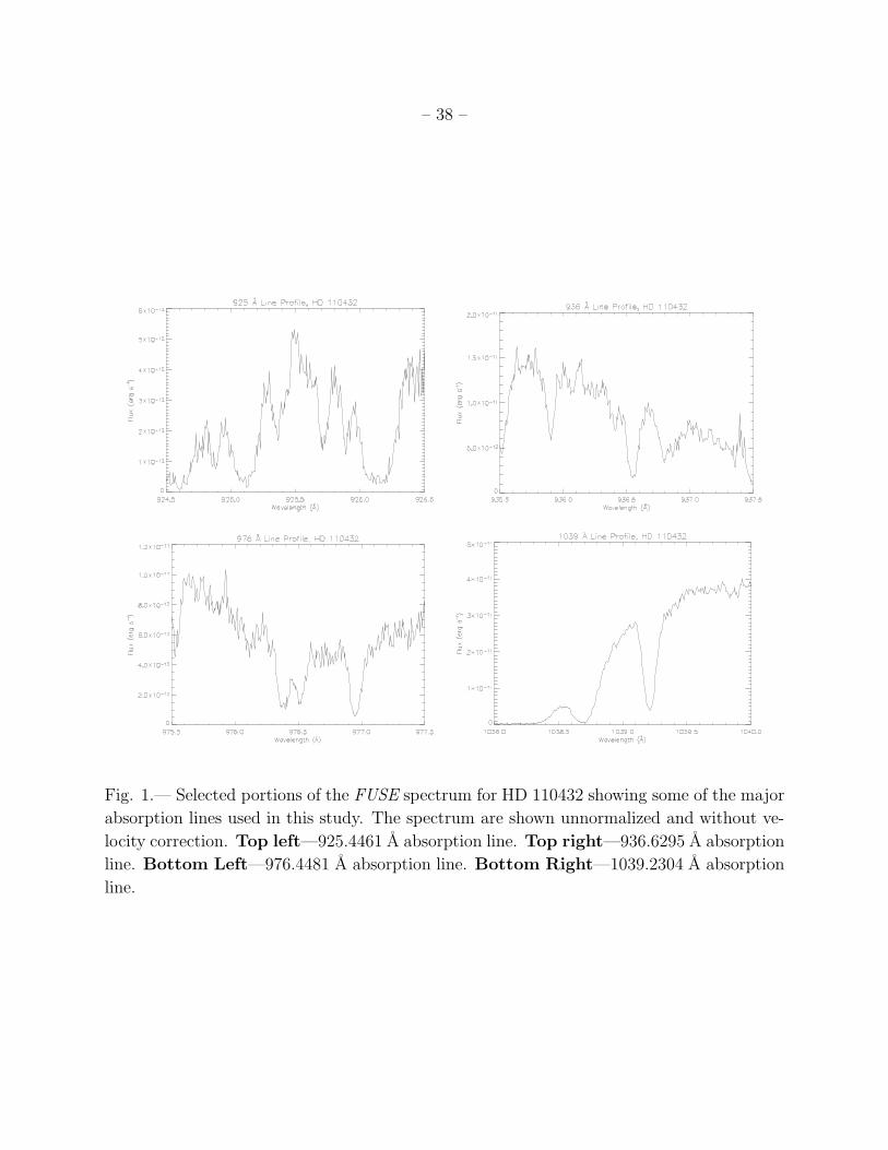
– 38 –

Fig. 1.— Selected portions of the FUSE spectrum for HD 110432 showing some of the major

absorption lines used in this study. The spectrum are shown unnormalized and without ve-

locity correction. Top left—925.4461 A absorption line. Top right—936.6295 A absorption

line. Bottom Left—976.4481 A absorption line. Bottom Right—1039.2304 A absorption

line.

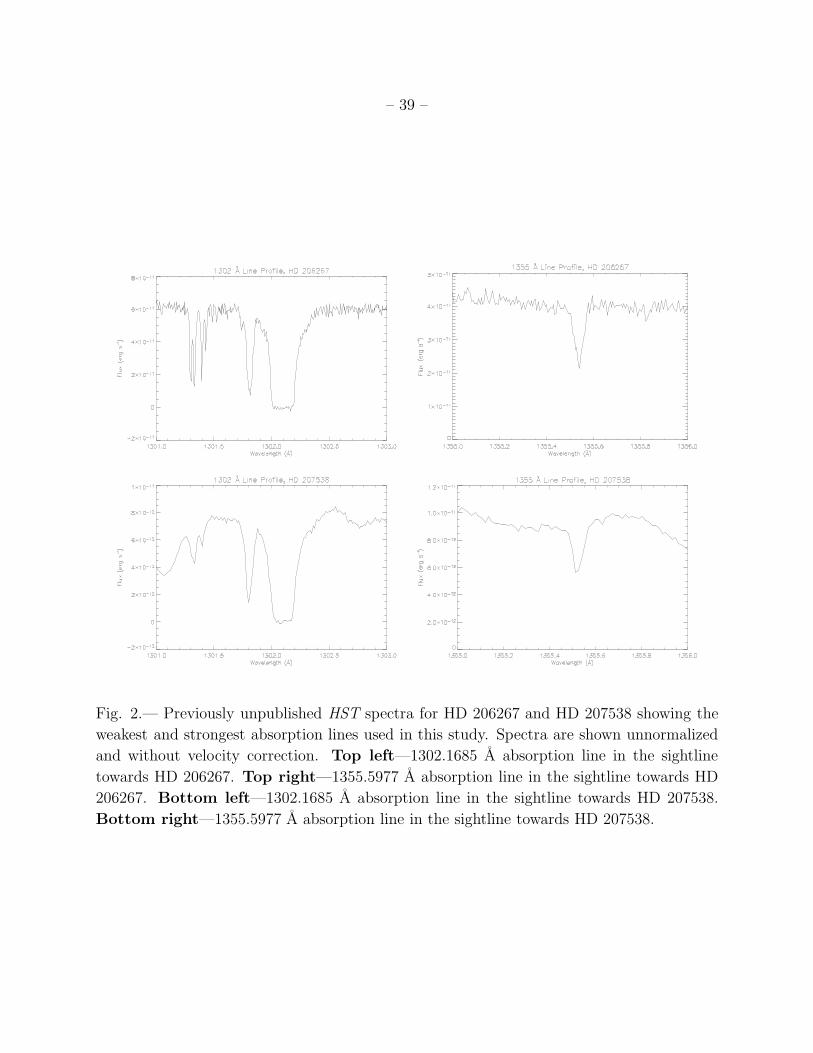
– 39 –

Fig. 2.— Previously unpublished HST spectra for HD 206267 and HD 207538 showing the

weakest and strongest absorption lines used in this study. Spectra are shown unnormalized

and without velocity correction. Top left—1302.1685 A absorption line in the sightline

towards HD 206267. Top right—1355.5977 A absorption line in the sightline towards HD

206267. Bottom left—1302.1685 A absorption line in the sightline towards HD 207538.

Bottom right—1355.5977 A absorption line in the sightline towards HD 207538.

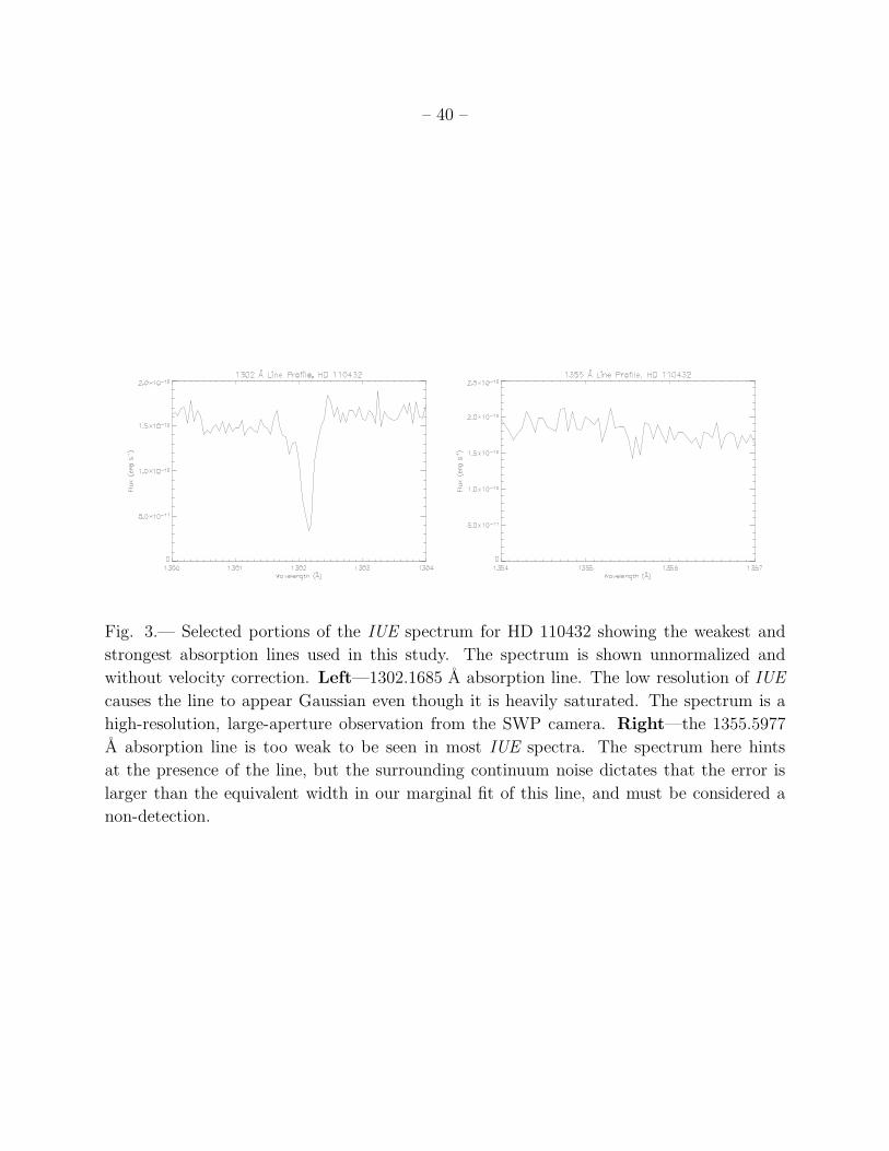
– 40 –

Fig. 3.— Selected portions of the IUE spectrum for HD 110432 showing the weakest and

strongest absorption lines used in this study. The spectrum is shown unnormalized and

without velocity correction. Left—1302.1685 A absorption line. The low resolution of IUE

causes the line to appear Gaussian even though it is heavily saturated. The spectrum is a

high-resolution, large-aperture observation from the SWP camera. Right—the 1355.5977

A absorption line is too weak to be seen in most IUE spectra. The spectrum here hints

at the presence of the line, but the surrounding continuum noise dictates that the error is

larger than the equivalent width in our marginal fit of this line, and must be considered a

non-detection.

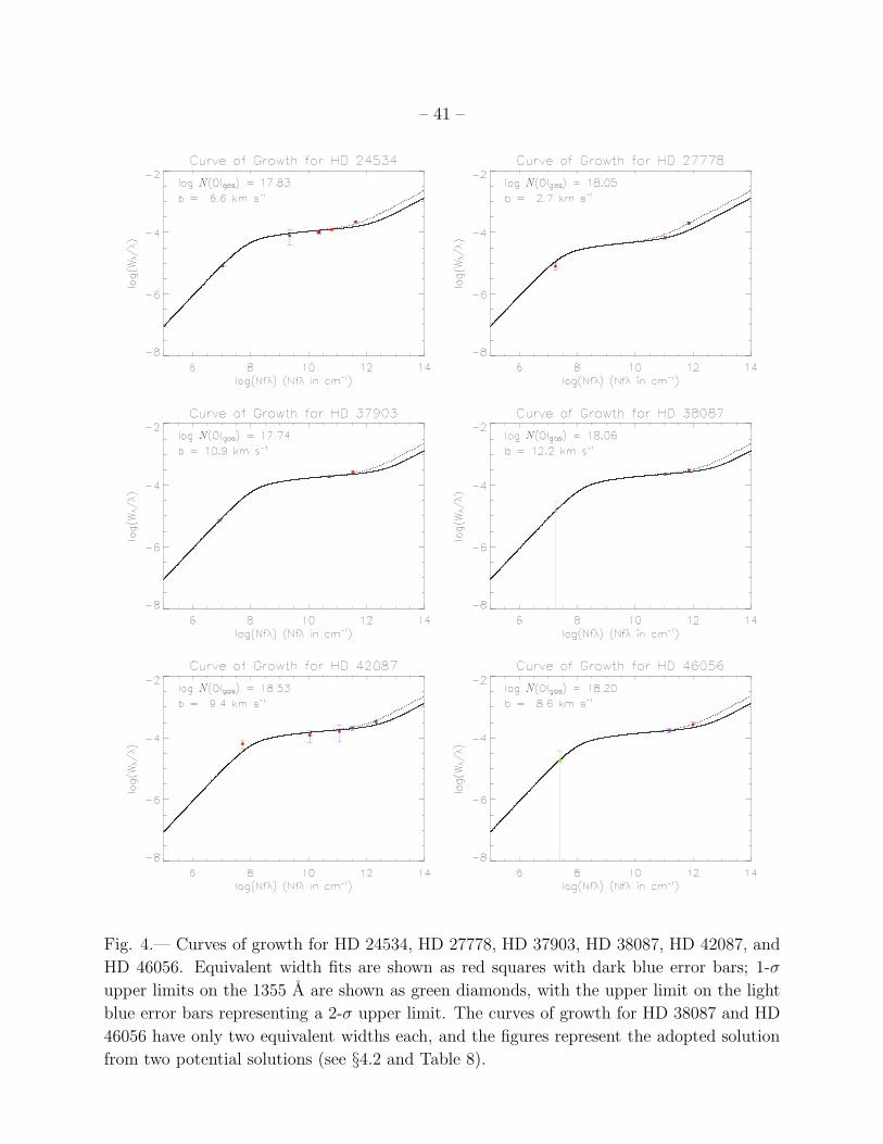
– 41 –

Fig. 4.— Curves of growth for HD 24534, HD 27778, HD 37903, HD 38087, HD 42087, and

HD 46056. Equivalent width fits are shown as red squares with dark blue error bars; 1-σ

upper limits on the 1355 A are shown as green diamonds, with the upper limit on the light

blue error bars representing a 2-σ upper limit. The curves of growth for HD 38087 and HD

46056 have only two equivalent widths each, and the figures represent the adopted solution

from two potential solutions (see §4.2 and Table 8).

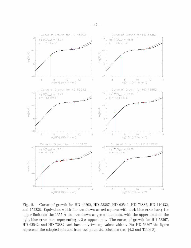
– 42 –

Fig. 5.— Curves of growth for HD 46202, HD 53367, HD 62542, HD 73882, HD 110432,

and 152236. Equivalent width fits are shown as red squares with dark blue error bars; 1-σ

upper limits on the 1355 A line are shown as green diamonds, with the upper limit on the

light blue error bars representing a 2-σ upper limit. The curves of growth for HD 53367,

HD 62542, and HD 73882 each have only two equivalent widths. For HD 53367 the figure

represents the adopted solution from two potential solutions (see §4.2 and Table 8).

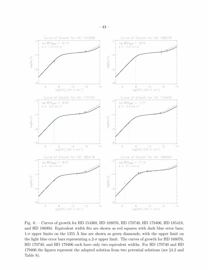
– 43 –

Fig. 6.— Curves of growth for HD 154368, HD 168076, HD 170740, HD 179406, HD 185418,

and HD 186994. Equivalent width fits are shown as red squares with dark blue error bars;

1-σ upper limits on the 1355 A line are shown as green diamonds, with the upper limit on

the light blue error bars representing a 2-σ upper limit. The curves of growth for HD 168076,

HD 170740, and HD 179406 each have only two equivalent widths. For HD 170740 and HD

179406 the figures represent the adopted solution from two potential solutions (see §4.2 and

Table 8).

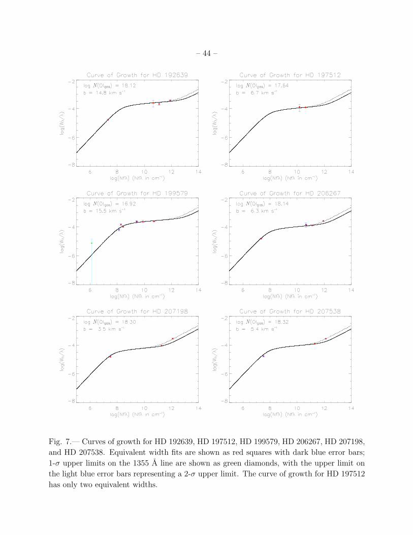
– 44 –

Fig. 7.— Curves of growth for HD 192639, HD 197512, HD 199579, HD 206267, HD 207198,

and HD 207538. Equivalent width fits are shown as red squares with dark blue error bars;

1-σ upper limits on the 1355 A line are shown as green diamonds, with the upper limit on

the light blue error bars representing a 2-σ upper limit. The curve of growth for HD 197512

has only two equivalent widths.

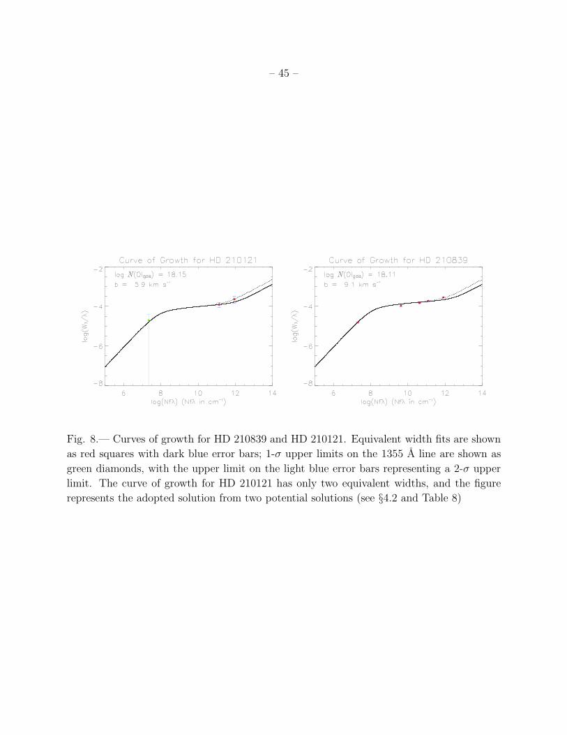
– 45 –

Fig. 8.— Curves of growth for HD 210839 and HD 210121. Equivalent width fits are shown

as red squares with dark blue error bars; 1-σ upper limits on the 1355 A line are shown as

green diamonds, with the upper limit on the light blue error bars representing a 2-σ upper

limit. The curve of growth for HD 210121 has only two equivalent widths, and the figure

represents the adopted solution from two potential solutions (see §4.2 and Table 8)

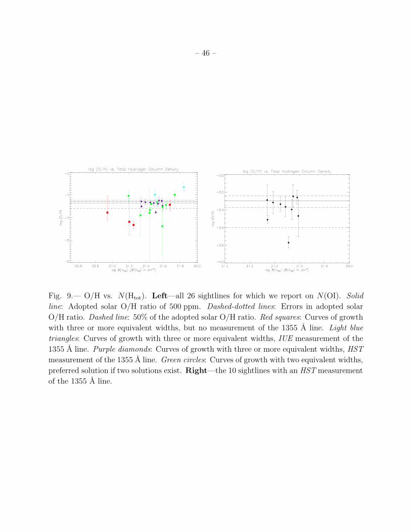
– 46 –

Fig. 9.— O/H vs. N(Htot). Left—all 26 sightlines for which we report on N(OI). Solid

line: Adopted solar O/H ratio of 500 ppm. Dashed-dotted lines: Errors in adopted solar

O/H ratio. Dashed line: 50% of the adopted solar O/H ratio. Red squares: Curves of growth

with three or more equivalent widths, but no measurement of the 1355 A line. Light blue

triangles: Curves of growth with three or more equivalent widths, IUE measurement of the

1355 A line. Purple diamonds: Curves of growth with three or more equivalent widths, HST

measurement of the 1355 A line. Green circles: Curves of growth with two equivalent widths,

preferred solution if two solutions exist. Right—the 10 sightlines with an HST measurement

of the 1355 A line.

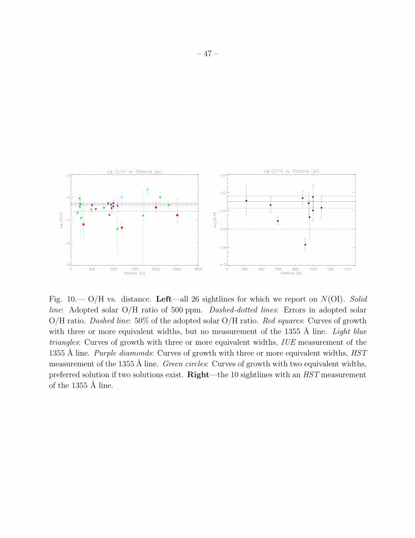
– 47 –

Fig. 10.— O/H vs. distance. Left—all 26 sightlines for which we report on N(OI). Solid

line: Adopted solar O/H ratio of 500 ppm. Dashed-dotted lines: Errors in adopted solar

O/H ratio. Dashed line: 50% of the adopted solar O/H ratio. Red squares: Curves of growth

with three or more equivalent widths, but no measurement of the 1355 A line. Light blue

triangles: Curves of growth with three or more equivalent widths, IUE measurement of the

1355 A line. Purple diamonds: Curves of growth with three or more equivalent widths, HST

measurement of the 1355 A line. Green circles: Curves of growth with two equivalent widths,

preferred solution if two solutions exist. Right—the 10 sightlines with an HST measurement

of the 1355 A line.

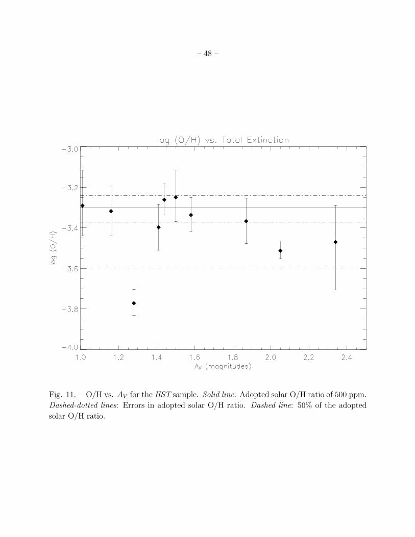
– 48 –

Fig. 11.— O/H vs. AV for the HST sample. Solid line: Adopted solar O/H ratio of 500 ppm.

Dashed-dotted lines: Errors in adopted solar O/H ratio. Dashed line: 50% of the adopted

solar O/H ratio.

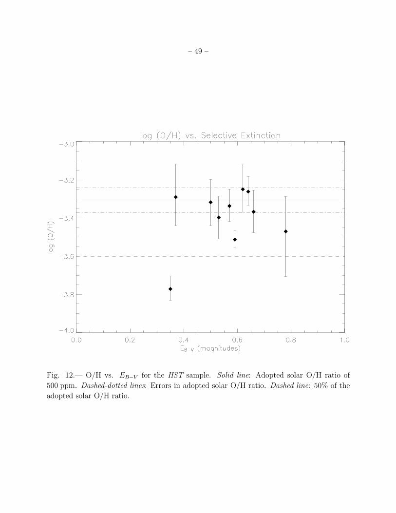
– 49 –

Fig. 12.— O/H vs. EB−V for the HST sample. Solid line: Adopted solar O/H ratio of

500 ppm. Dashed-dotted lines: Errors in adopted solar O/H ratio. Dashed line: 50% of the

adopted solar O/H ratio.

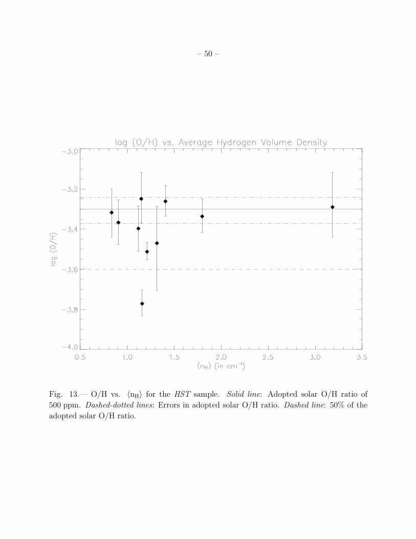
– 50 –

Fig. 13.— O/H vs. 〈nH〉 for the HST sample. Solid line: Adopted solar O/H ratio of

500 ppm. Dashed-dotted lines: Errors in adopted solar O/H ratio. Dashed line: 50% of the

adopted solar O/H ratio.

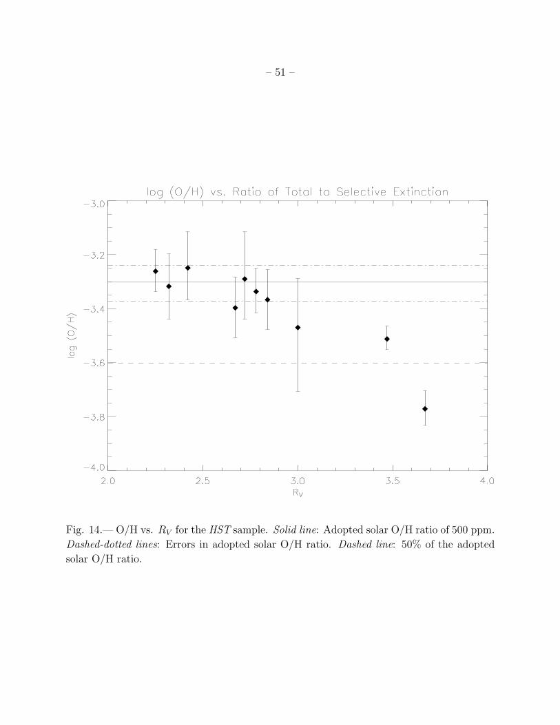
– 51 –

Fig. 14.— O/H vs. RV for the HST sample. Solid line: Adopted solar O/H ratio of 500 ppm.

Dashed-dotted lines: Errors in adopted solar O/H ratio. Dashed line: 50% of the adopted

solar O/H ratio.

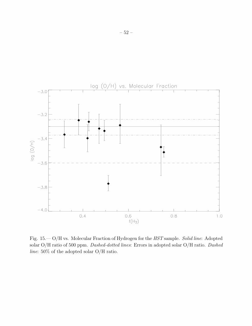
– 52 –

Fig. 15.— O/H vs. Molecular Fraction of Hydrogen for the HST sample. Solid line: Adopted

solar O/H ratio of 500 ppm. Dashed-dotted lines: Errors in adopted solar O/H ratio. Dashed

line: 50% of the adopted solar O/H ratio.

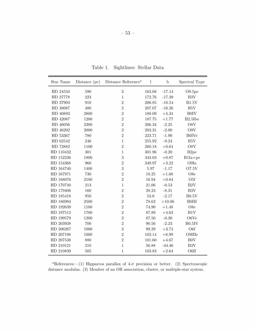
– 53 –

Table 1. Sightlines: Stellar Data

Star Name Distance (pc) Distance Referencea l b Spectral Type

HD 24534 590 2 163.08 -17.14 O9.5pe

HD 27778 223 1 172.76 -17.39 B3V

HD 37903 910 2 206.85 -16.54 B1.5V

HD 38087 480 2 207.07 -16.26 B5V

HD 40893 2800 2 180.09 +4.34 B0IV

HD 42087 1200 2 187.75 +1.77 B2.5Ibe

HD 46056 2300 2 206.34 -2.25 O8V

HD 46202 2000 2 203.31 -2.00 O9V

HD 53367 780 2 223.71 -1.90 B0IVe

HD 62542 246 1 255.92 -9.24 B5V

HD 73882 1100 2 260.18 +0.64 O8V

HD 110432 301 1 301.96 -0.20 B2pe

HD 152236 1800 3 343.03 +0.87 B1Ia+pe

HD 154368 960 2 349.97 +3.22 O9Ia

HD 164740 1400 3 5.97 -1.17 O7.5V

HD 167971 730 2 18.25 +1.68 O8e

HD 168076 2100 2 16.94 +0.84 O5f

HD 170740 213 1 21.06 -0.53 B2V

HD 179406 160 2 28.23 -8.31 B3V

HD 185418 950 2 53.6 -2.17 B0.5V

HD 186994 2500 2 78.62 +10.06 B0III

HD 192639 1100 2 74.90 +1.48 O8e

HD 197512 1700 2 87.89 +4.63 B1V

HD 199579 1200 2 87.50 -0.30 O6Ve

HD 203938 700 2 90.56 -2.23 B0.5IV

HD 206267 1000 3 99.29 +3.74 O6f

HD 207198 1000 2 103.14 +6.99 O9IIIe

HD 207538 880 2 101.60 +4.67 B0V

HD 210121 210 1 56.88 -44.46 B3V

HD 210839 505 1 103.83 +2.64 O6If

aReferences:—(1) Hipparcos parallax of 4-σ precision or better. (2) Spectroscopic

distance modulus. (3) Member of an OB association, cluster, or multiple-star system.

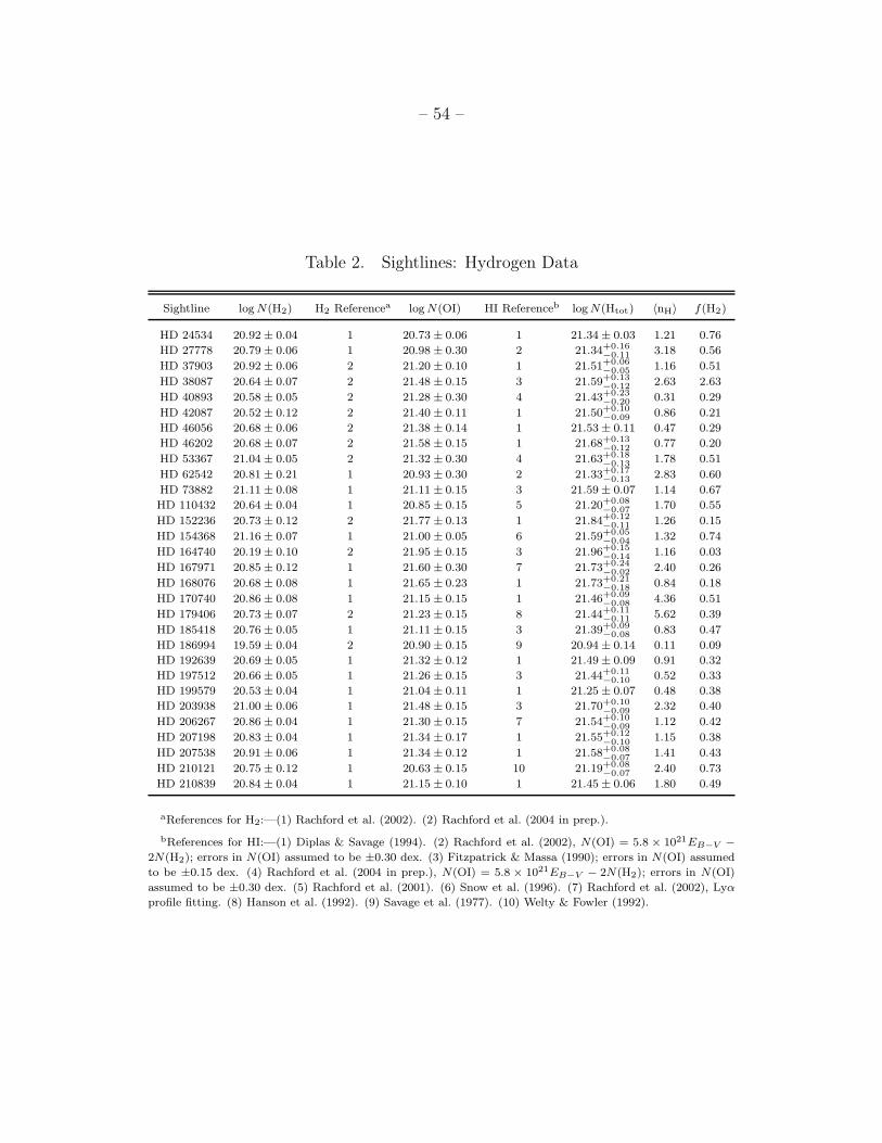
– 54 –

Table 2. Sightlines: Hydrogen Data

Sightline log N(H2) H2 Referencea log N(OI) HI Referenceb log N(Htot) 〈nH〉 f(H2)

HD 24534 20.92 ± 0.04 1 20.73 ± 0.06 1 21.34 ± 0.03 1.21 0.76

HD 27778 20.79 ± 0.06 1 20.98 ± 0.30 2 21.34+0.16−0.11

3.18 0.56

HD 37903 20.92 ± 0.06 2 21.20 ± 0.10 1 21.51+0.06−0.05

1.16 0.51

HD 38087 20.64 ± 0.07 2 21.48 ± 0.15 3 21.59+0.13−0.12

2.63 2.63

HD 40893 20.58 ± 0.05 2 21.28 ± 0.30 4 21.43+0.23−0.20

0.31 0.29

HD 42087 20.52 ± 0.12 2 21.40 ± 0.11 1 21.50+0.10−0.09

0.86 0.21

HD 46056 20.68 ± 0.06 2 21.38 ± 0.14 1 21.53 ± 0.11 0.47 0.29

HD 46202 20.68 ± 0.07 2 21.58 ± 0.15 1 21.68+0.13−0.12

0.77 0.20

HD 53367 21.04 ± 0.05 2 21.32 ± 0.30 4 21.63+0.18−0.13

1.78 0.51

HD 62542 20.81 ± 0.21 1 20.93 ± 0.30 2 21.33+0.17−0.13

2.83 0.60

HD 73882 21.11 ± 0.08 1 21.11 ± 0.15 3 21.59 ± 0.07 1.14 0.67

HD 110432 20.64 ± 0.04 1 20.85 ± 0.15 5 21.20+0.08−0.07

1.70 0.55

HD 152236 20.73 ± 0.12 2 21.77 ± 0.13 1 21.84+0.12−0.11

1.26 0.15

HD 154368 21.16 ± 0.07 1 21.00 ± 0.05 6 21.59+0.05−0.04

1.32 0.74

HD 164740 20.19 ± 0.10 2 21.95 ± 0.15 3 21.96+0.15−0.14

1.16 0.03

HD 167971 20.85 ± 0.12 1 21.60 ± 0.30 7 21.73+0.24−0.02

2.40 0.26

HD 168076 20.68 ± 0.08 1 21.65 ± 0.23 1 21.73+0.21−0.18

0.84 0.18

HD 170740 20.86 ± 0.08 1 21.15 ± 0.15 1 21.46+0.09−0.08

4.36 0.51

HD 179406 20.73 ± 0.07 2 21.23 ± 0.15 8 21.44+0.11−0.11

5.62 0.39

HD 185418 20.76 ± 0.05 1 21.11 ± 0.15 3 21.39+0.09−0.08

0.83 0.47

HD 186994 19.59 ± 0.04 2 20.90 ± 0.15 9 20.94 ± 0.14 0.11 0.09

HD 192639 20.69 ± 0.05 1 21.32 ± 0.12 1 21.49 ± 0.09 0.91 0.32

HD 197512 20.66 ± 0.05 1 21.26 ± 0.15 3 21.44+0.11−0.10

0.52 0.33

HD 199579 20.53 ± 0.04 1 21.04 ± 0.11 1 21.25 ± 0.07 0.48 0.38

HD 203938 21.00 ± 0.06 1 21.48 ± 0.15 3 21.70+0.10−0.09

2.32 0.40

HD 206267 20.86 ± 0.04 1 21.30 ± 0.15 7 21.54+0.10−0.09

1.12 0.42

HD 207198 20.83 ± 0.04 1 21.34 ± 0.17 1 21.55+0.12−0.10

1.15 0.38

HD 207538 20.91 ± 0.06 1 21.34 ± 0.12 1 21.58+0.08−0.07

1.41 0.43

HD 210121 20.75 ± 0.12 1 20.63 ± 0.15 10 21.19+0.08−0.07

2.40 0.73

HD 210839 20.84 ± 0.04 1 21.15 ± 0.10 1 21.45 ± 0.06 1.80 0.49

aReferences for H2:—(1) Rachford et al. (2002). (2) Rachford et al. (2004 in prep.).

bReferences for HI:—(1) Diplas & Savage (1994). (2) Rachford et al. (2002), N(OI) = 5.8 × 1021EB−V −

2N(H2); errors in N(OI) assumed to be ±0.30 dex. (3) Fitzpatrick & Massa (1990); errors in N(OI) assumed

to be ±0.15 dex. (4) Rachford et al. (2004 in prep.), N(OI) = 5.8 × 1021EB−V − 2N(H2); errors in N(OI)

assumed to be ±0.30 dex. (5) Rachford et al. (2001). (6) Snow et al. (1996). (7) Rachford et al. (2002), Lyα

profile fitting. (8) Hanson et al. (1992). (9) Savage et al. (1977). (10) Welty & Fowler (1992).

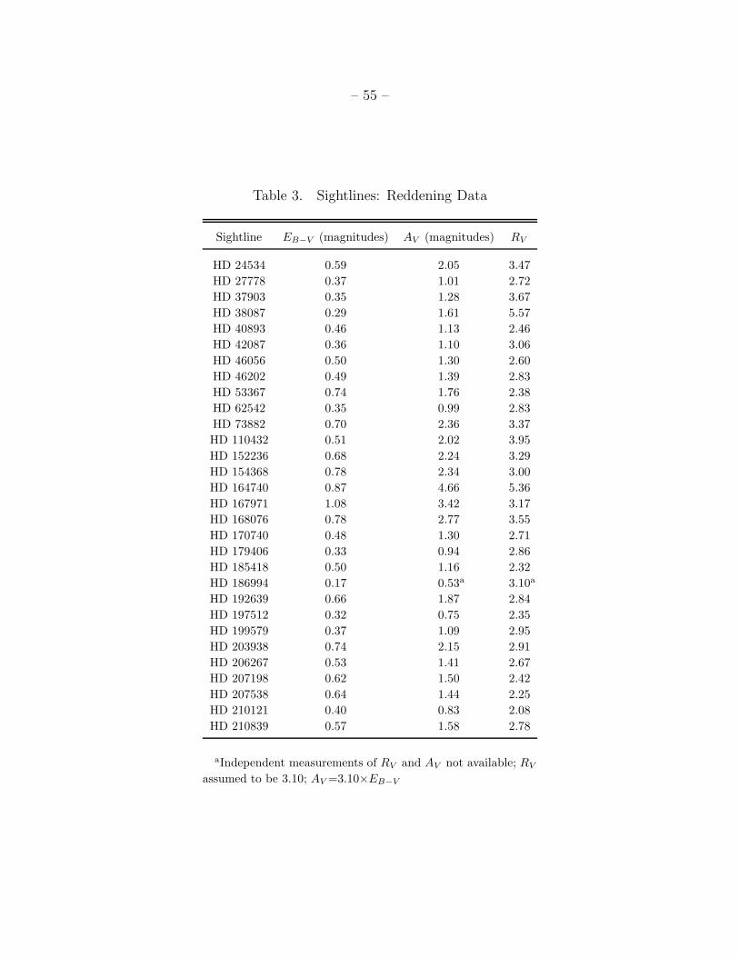
– 55 –

Table 3. Sightlines: Reddening Data

Sightline EB−V (magnitudes) AV (magnitudes) RV

HD 24534 0.59 2.05 3.47

HD 27778 0.37 1.01 2.72

HD 37903 0.35 1.28 3.67

HD 38087 0.29 1.61 5.57

HD 40893 0.46 1.13 2.46

HD 42087 0.36 1.10 3.06

HD 46056 0.50 1.30 2.60

HD 46202 0.49 1.39 2.83

HD 53367 0.74 1.76 2.38

HD 62542 0.35 0.99 2.83

HD 73882 0.70 2.36 3.37

HD 110432 0.51 2.02 3.95

HD 152236 0.68 2.24 3.29

HD 154368 0.78 2.34 3.00

HD 164740 0.87 4.66 5.36

HD 167971 1.08 3.42 3.17

HD 168076 0.78 2.77 3.55

HD 170740 0.48 1.30 2.71

HD 179406 0.33 0.94 2.86

HD 185418 0.50 1.16 2.32

HD 186994 0.17 0.53a 3.10a

HD 192639 0.66 1.87 2.84

HD 197512 0.32 0.75 2.35

HD 199579 0.37 1.09 2.95

HD 203938 0.74 2.15 2.91

HD 206267 0.53 1.41 2.67

HD 207198 0.62 1.50 2.42

HD 207538 0.64 1.44 2.25

HD 210121 0.40 0.83 2.08

HD 210839 0.57 1.58 2.78

aIndependent measurements of RV and AV not available; RV

assumed to be 3.10; AV =3.10×EB−V

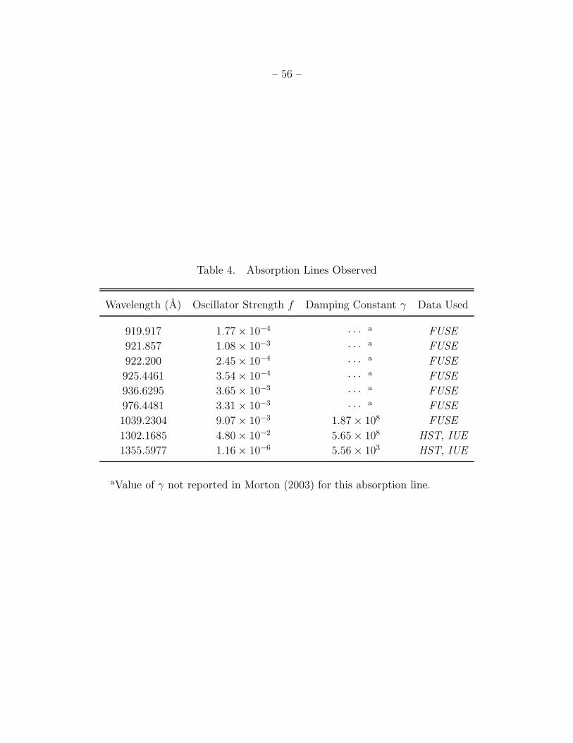
– 56 –

Table 4. Absorption Lines Observed

Wavelength (A) Oscillator Strength f Damping Constant γ Data Used

919.917 1.77 × 10−4 · · · a FUSE

921.857 1.08 × 10−3 · · · a FUSE

922.200 2.45 × 10−4 · · · a FUSE

925.4461 3.54 × 10−4 · · · a FUSE

936.6295 3.65 × 10−3 · · · a FUSE

976.4481 3.31 × 10−3 · · · a FUSE

1039.2304 9.07 × 10−3 1.87 × 108 FUSE

1302.1685 4.80 × 10−2 5.65 × 108 HST, IUE

1355.5977 1.16 × 10−6 5.56 × 103 HST, IUE

aValue of γ not reported in Morton (2003) for this absorption line.

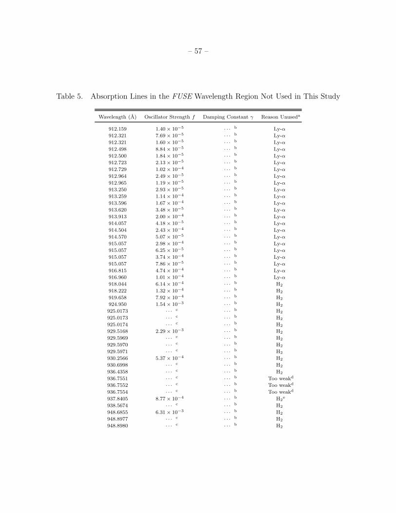
– 57 –

Table 5. Absorption Lines in the FUSE Wavelength Region Not Used in This Study

Wavelength (A) Oscillator Strength f Damping Constant γ Reason Unuseda

912.159 1.40 × 10−5 · · · b Ly-α

912.321 7.69 × 10−5 · · · b Ly-α

912.321 1.60 × 10−5 · · · b Ly-α

912.498 8.84 × 10−5 · · · b Ly-α

912.500 1.84 × 10−5 · · · b Ly-α

912.723 2.13 × 10−5 · · · b Ly-α

912.729 1.02 × 10−4 · · · b Ly-α

912.964 2.49 × 10−5 · · · b Ly-α

912.965 1.19 × 10−5 · · · b Ly-α

913.250 2.93 × 10−5 · · · b Ly-α

913.259 1.14 × 10−4 · · · b Ly-α

913.596 1.67 × 10−4 · · · b Ly-α

913.620 3.48 × 10−5 · · · b Ly-α

913.913 2.00 × 10−4 · · · b Ly-α

914.057 4.18 × 10−5 · · · b Ly-α

914.504 2.43 × 10−4 · · · b Ly-α

914.570 5.07 × 10−5 · · · b Ly-α

915.057 2.98 × 10−4 · · · b Ly-α

915.057 6.25 × 10−5 · · · b Ly-α

915.057 3.74 × 10−4 · · · b Ly-α

915.057 7.86 × 10−5 · · · b Ly-α

916.815 4.74 × 10−4 · · · b Ly-α

916.960 1.01 × 10−4 · · · b Ly-α

918.044 6.14 × 10−4 · · · b H2

918.222 1.32 × 10−4 · · · b H2

919.658 7.92 × 10−4 · · · b H2

924.950 1.54 × 10−3 · · · b H2

925.0173 · · · c · · · b H2

925.0173 · · · c · · · b H2

925.0174 · · · c · · · b H2

929.5168 2.29 × 10−3 · · · b H2

929.5969 · · · c · · · b H2

929.5970 · · · c · · · b H2

929.5971 · · · c · · · b H2

930.2566 5.37 × 10−4 · · · b H2

930.6998 · · · c · · · b H2

936.4358 · · · c · · · b H2

936.7551 · · · c · · · b Too weakd

936.7552 · · · c · · · b Too weakd

936.7554 · · · c · · · b Too weakd

937.8405 8.77 × 10−4 · · · b H2e

938.5674 · · · c · · · b H2

948.6855 6.31 × 10−3 · · · b H2

948.8977 · · · c · · · b H2

948.8980 · · · c · · · b H2

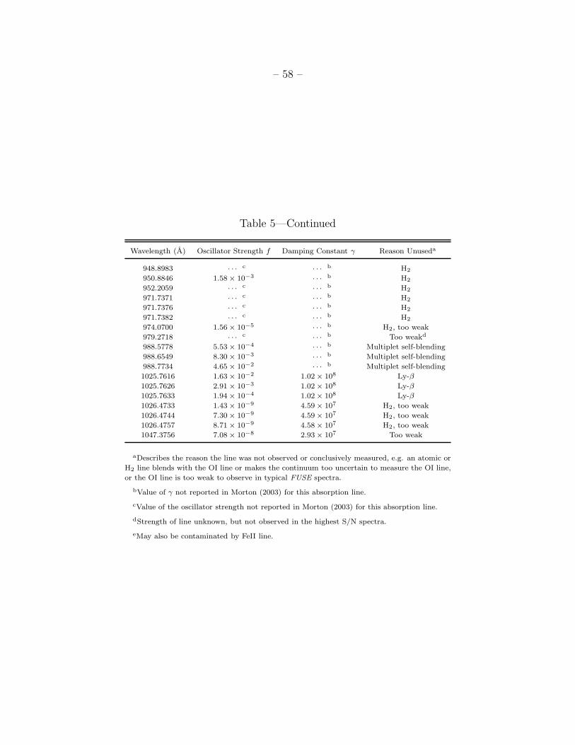
– 58 –

Table 5—Continued

Wavelength (A) Oscillator Strength f Damping Constant γ Reason Unuseda

948.8983 · · · c · · · b H2

950.8846 1.58 × 10−3 · · · b H2

952.2059 · · · c · · · b H2

971.7371 · · · c · · · b H2

971.7376 · · · c · · · b H2

971.7382 · · · c · · · b H2

974.0700 1.56 × 10−5 · · · b H2, too weak

979.2718 · · · c · · · b Too weakd

988.5778 5.53 × 10−4 · · · b Multiplet self-blending

988.6549 8.30 × 10−3 · · · b Multiplet self-blending

988.7734 4.65 × 10−2 · · · b Multiplet self-blending

1025.7616 1.63 × 10−2 1.02 × 108 Ly-β

1025.7626 2.91 × 10−3 1.02 × 108 Ly-β

1025.7633 1.94 × 10−4 1.02 × 108 Ly-β

1026.4733 1.43 × 10−9 4.59 × 107 H2, too weak

1026.4744 7.30 × 10−9 4.59 × 107 H2, too weak

1026.4757 8.71 × 10−9 4.58 × 107 H2, too weak

1047.3756 7.08 × 10−8 2.93 × 107 Too weak

aDescribes the reason the line was not observed or conclusively measured, e.g. an atomic or

H2 line blends with the OI line or makes the continuum too uncertain to measure the OI line,

or the OI line is too weak to observe in typical FUSE spectra.

bValue of γ not reported in Morton (2003) for this absorption line.

cValue of the oscillator strength not reported in Morton (2003) for this absorption line.

dStrength of line unknown, but not observed in the highest S/N spectra.

eMay also be contaminated by FeII line.

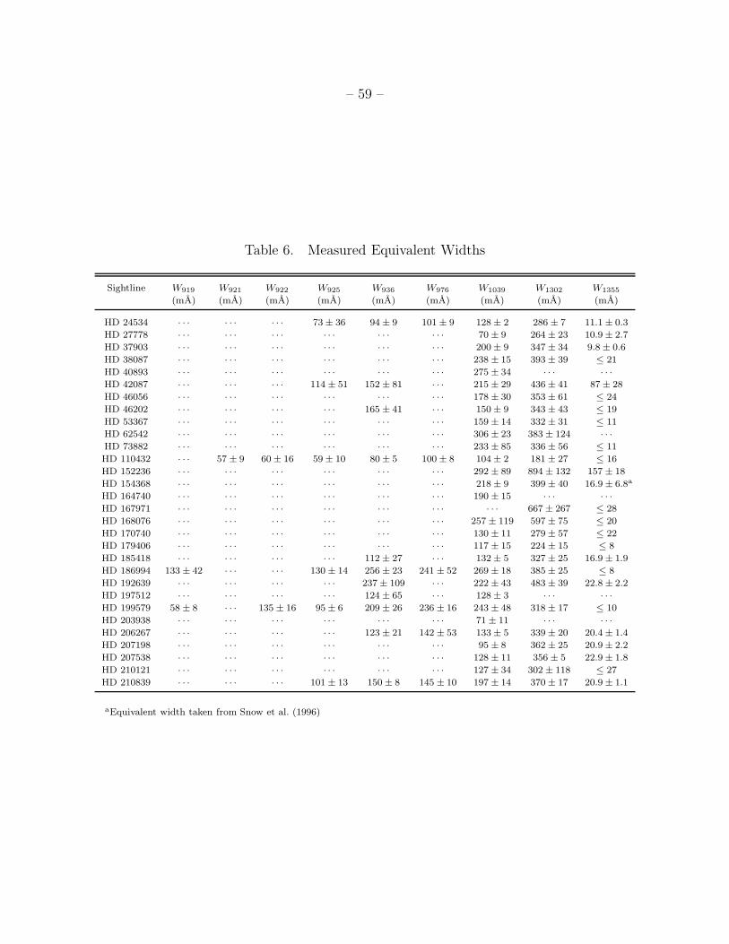
– 59 –

Table 6. Measured Equivalent Widths

Sightline W919 W921 W922 W925 W936 W976 W1039 W1302 W1355

(mA) (mA) (mA) (mA) (mA) (mA) (mA) (mA) (mA)

HD 24534 · · · · · · · · · 73 ± 36 94 ± 9 101 ± 9 128 ± 2 286 ± 7 11.1 ± 0.3

HD 27778 · · · · · · · · · · · · · · · · · · 70 ± 9 264 ± 23 10.9 ± 2.7

HD 37903 · · · · · · · · · · · · · · · · · · 200 ± 9 347 ± 34 9.8 ± 0.6

HD 38087 · · · · · · · · · · · · · · · · · · 238 ± 15 393 ± 39 ≤ 21

HD 40893 · · · · · · · · · · · · · · · · · · 275 ± 34 · · · · · ·

HD 42087 · · · · · · · · · 114 ± 51 152 ± 81 · · · 215 ± 29 436 ± 41 87 ± 28

HD 46056 · · · · · · · · · · · · · · · · · · 178 ± 30 353 ± 61 ≤ 24

HD 46202 · · · · · · · · · · · · 165 ± 41 · · · 150 ± 9 343 ± 43 ≤ 19

HD 53367 · · · · · · · · · · · · · · · · · · 159 ± 14 332 ± 31 ≤ 11

HD 62542 · · · · · · · · · · · · · · · · · · 306 ± 23 383 ± 124 · · ·

HD 73882 · · · · · · · · · · · · · · · · · · 233 ± 85 336 ± 56 ≤ 11

HD 110432 · · · 57 ± 9 60 ± 16 59 ± 10 80 ± 5 100 ± 8 104 ± 2 181 ± 27 ≤ 16

HD 152236 · · · · · · · · · · · · · · · · · · 292 ± 89 894 ± 132 157 ± 18

HD 154368 · · · · · · · · · · · · · · · · · · 218 ± 9 399 ± 40 16.9 ± 6.8a

HD 164740 · · · · · · · · · · · · · · · · · · 190 ± 15 · · · · · ·

HD 167971 · · · · · · · · · · · · · · · · · · · · · 667 ± 267 ≤ 28

HD 168076 · · · · · · · · · · · · · · · · · · 257 ± 119 597 ± 75 ≤ 20

HD 170740 · · · · · · · · · · · · · · · · · · 130 ± 11 279 ± 57 ≤ 22

HD 179406 · · · · · · · · · · · · · · · · · · 117 ± 15 224 ± 15 ≤ 8

HD 185418 · · · · · · · · · · · · 112 ± 27 · · · 132 ± 5 327 ± 25 16.9 ± 1.9

HD 186994 133 ± 42 · · · · · · 130 ± 14 256 ± 23 241 ± 52 269 ± 18 385 ± 25 ≤ 8

HD 192639 · · · · · · · · · · · · 237 ± 109 · · · 222 ± 43 483 ± 39 22.8 ± 2.2

HD 197512 · · · · · · · · · · · · 124 ± 65 · · · 128 ± 3 · · · · · ·

HD 199579 58 ± 8 · · · 135 ± 16 95 ± 6 209 ± 26 236 ± 16 243 ± 48 318 ± 17 ≤ 10

HD 203938 · · · · · · · · · · · · · · · · · · 71 ± 11 · · · · · ·

HD 206267 · · · · · · · · · · · · 123 ± 21 142 ± 53 133 ± 5 339 ± 20 20.4 ± 1.4

HD 207198 · · · · · · · · · · · · · · · · · · 95 ± 8 362 ± 25 20.9 ± 2.2

HD 207538 · · · · · · · · · · · · · · · · · · 128 ± 11 356 ± 5 22.9 ± 1.8

HD 210121 · · · · · · · · · · · · · · · · · · 127 ± 34 302 ± 118 ≤ 27

HD 210839 · · · · · · · · · 101 ± 13 150 ± 8 145 ± 10 197 ± 14 370 ± 17 20.9 ± 1.1

aEquivalent width taken from Snow et al. (1996)

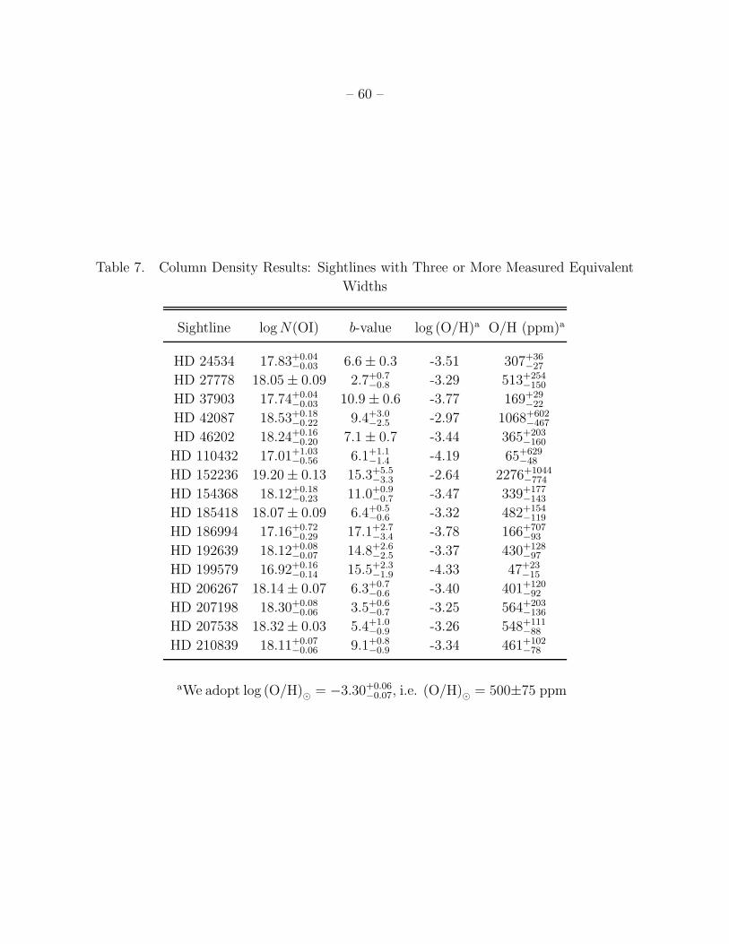
– 60 –

Table 7. Column Density Results: Sightlines with Three or More Measured Equivalent

Widths

Sightline log N(OI) b-value log (O/H)a O/H (ppm)a

HD 24534 17.83+0.04−0.03 6.6 ± 0.3 -3.51 307+36

−27

HD 27778 18.05 ± 0.09 2.7+0.7−0.8 -3.29 513+254

−150

HD 37903 17.74+0.04−0.03 10.9 ± 0.6 -3.77 169+29

−22

HD 42087 18.53+0.18−0.22 9.4+3.0

−2.5 -2.97 1068+602−467

HD 46202 18.24+0.16−0.20 7.1 ± 0.7 -3.44 365+203

−160

HD 110432 17.01+1.03−0.56 6.1+1.1

−1.4 -4.19 65+629−48

HD 152236 19.20 ± 0.13 15.3+5.5−3.3 -2.64 2276+1044

−774

HD 154368 18.12+0.18−0.23 11.0+0.9

−0.7 -3.47 339+177−143

HD 185418 18.07 ± 0.09 6.4+0.5−0.6 -3.32 482+154

−119

HD 186994 17.16+0.72−0.29 17.1+2.7

−3.4 -3.78 166+707−93

HD 192639 18.12+0.08−0.07 14.8+2.6

−2.5 -3.37 430+128−97

HD 199579 16.92+0.16−0.14 15.5+2.3

−1.9 -4.33 47+23−15

HD 206267 18.14 ± 0.07 6.3+0.7−0.6 -3.40 401+120

−92

HD 207198 18.30+0.08−0.06 3.5+0.6

−0.7 -3.25 564+203−136

HD 207538 18.32 ± 0.03 5.4+1.0−0.9 -3.26 548+111

−88

HD 210839 18.11+0.07−0.06 9.1+0.8

−0.9 -3.34 461+102−78

aWe adopt log (O/H)⊙ = −3.30+0.06−0.07, i.e. (O/H)⊙ = 500±75 ppm

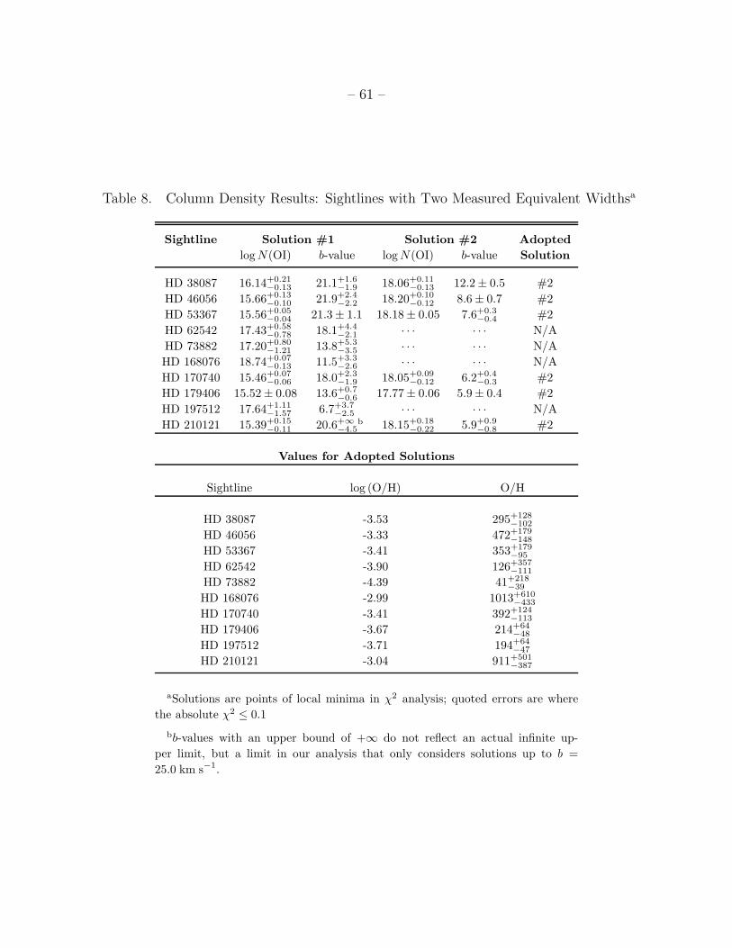
– 61 –

Table 8. Column Density Results: Sightlines with Two Measured Equivalent Widthsa

Sightline Solution #1 Solution #2 Adopted

log N(OI) b-value log N(OI) b-value Solution

HD 38087 16.14+0.21−0.13 21.1+1.6

−1.9 18.06+0.11−0.13 12.2 ± 0.5 #2

HD 46056 15.66+0.13−0.10 21.9+2.4

−2.2 18.20+0.10−0.12 8.6 ± 0.7 #2

HD 53367 15.56+0.05−0.04 21.3 ± 1.1 18.18 ± 0.05 7.6+0.3

−0.4 #2

HD 62542 17.43+0.58−0.78 18.1+4.4

−2.1 · · · · · · N/A

HD 73882 17.20+0.80−1.21 13.8+5.3

−3.5 · · · · · · N/A

HD 168076 18.74+0.07−0.13 11.5+3.3

−2.6 · · · · · · N/A

HD 170740 15.46+0.07−0.06 18.0+2.3

−1.9 18.05+0.09−0.12 6.2+0.4

−0.3 #2

HD 179406 15.52 ± 0.08 13.6+0.7−0.6 17.77 ± 0.06 5.9 ± 0.4 #2

HD 197512 17.64+1.11−1.57 6.7+3.7

−2.5 · · · · · · N/A

HD 210121 15.39+0.15−0.11 20.6+∞

−4.5b 18.15+0.18

−0.22 5.9+0.9−0.8 #2

Values for Adopted Solutions

Sightline log (O/H) O/H

HD 38087 -3.53 295+128−102

HD 46056 -3.33 472+179−148

HD 53367 -3.41 353+179−95

HD 62542 -3.90 126+357−111

HD 73882 -4.39 41+218−39

HD 168076 -2.99 1013+610−433

HD 170740 -3.41 392+124−113

HD 179406 -3.67 214+64−48

HD 197512 -3.71 194+64−47

HD 210121 -3.04 911+501−387

aSolutions are points of local minima in χ2 analysis; quoted errors are where

the absolute χ2 ≤ 0.1

bb-values with an upper bound of +∞ do not reflect an actual infinite up-

per limit, but a limit in our analysis that only considers solutions up to b =

25.0 km s−1.

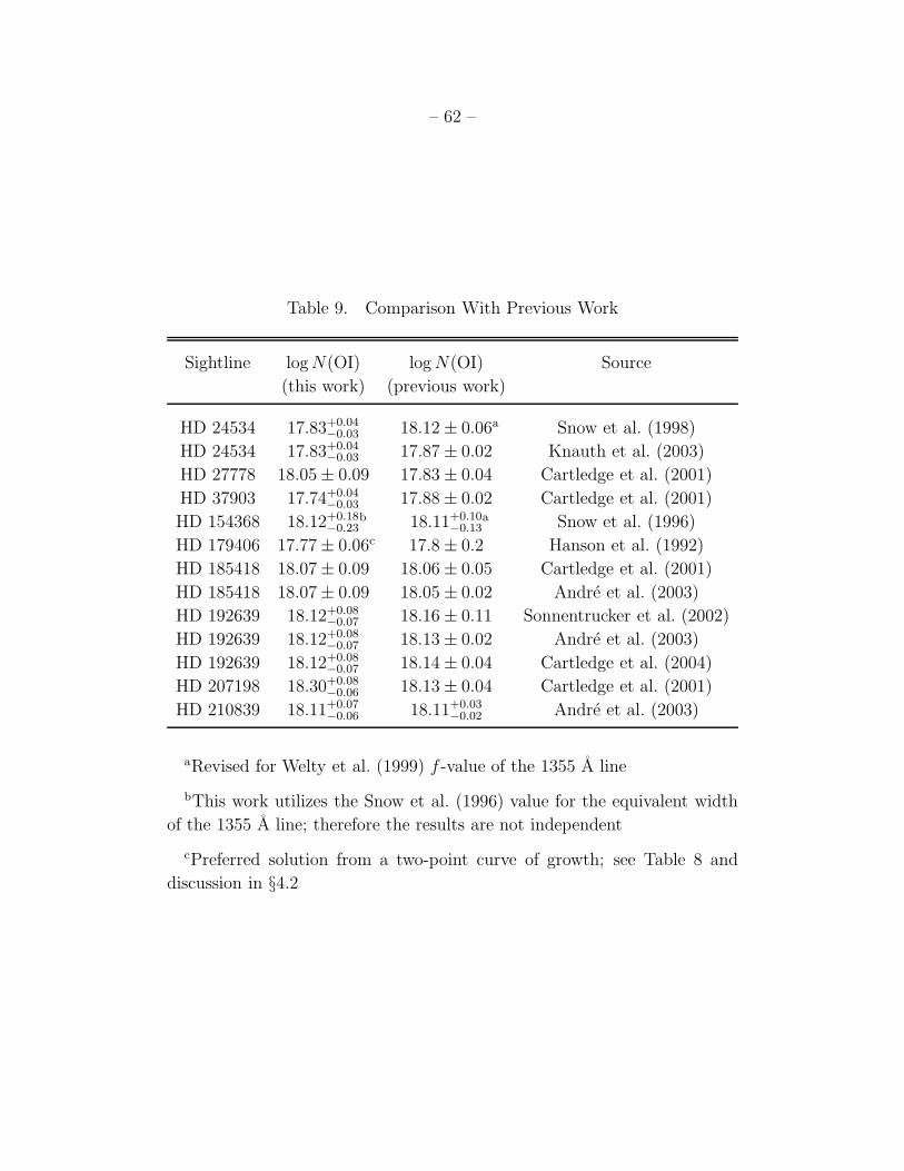
– 62 –

Table 9. Comparison With Previous Work

Sightline log N(OI) log N(OI) Source

(this work) (previous work)

HD 24534 17.83+0.04−0.03 18.12 ± 0.06a Snow et al. (1998)

HD 24534 17.83+0.04−0.03 17.87 ± 0.02 Knauth et al. (2003)

HD 27778 18.05 ± 0.09 17.83 ± 0.04 Cartledge et al. (2001)

HD 37903 17.74+0.04−0.03 17.88 ± 0.02 Cartledge et al. (2001)

HD 154368 18.12+0.18−0.23

b 18.11+0.10−0.13

a Snow et al. (1996)

HD 179406 17.77 ± 0.06c 17.8 ± 0.2 Hanson et al. (1992)

HD 185418 18.07 ± 0.09 18.06 ± 0.05 Cartledge et al. (2001)

HD 185418 18.07 ± 0.09 18.05 ± 0.02 Andre et al. (2003)

HD 192639 18.12+0.08−0.07 18.16 ± 0.11 Sonnentrucker et al. (2002)

HD 192639 18.12+0.08−0.07 18.13 ± 0.02 Andre et al. (2003)

HD 192639 18.12+0.08−0.07 18.14 ± 0.04 Cartledge et al. (2004)

HD 207198 18.30+0.08−0.06 18.13 ± 0.04 Cartledge et al. (2001)

HD 210839 18.11+0.07−0.06 18.11+0.03

−0.02 Andre et al. (2003)

aRevised for Welty et al. (1999) f -value of the 1355 A line

bThis work utilizes the Snow et al. (1996) value for the equivalent width

of the 1355 A line; therefore the results are not independent

cPreferred solution from a two-point curve of growth; see Table 8 and

discussion in §4.2