galactic outflows and evolution of the interstellar medium

arX

iv:1

112.

2182

v1 [

astr

o-ph

.CO

] 9

Dec

201

1

Mon. Not. R. Astron. Soc. 000, 1–17 (XXX) Printed 12 December 2011 (MN LATEX style file v2.2)

Galactic Outflows and Evolution of the Interstellar

Medium

Benoit Cote,1,2⋆, Hugo Martel,1,2 Laurent Drissen,1,2 and Carmelle Robert1,21Departement de physique, de genie physique et d’optique, Universite Laval, Quebec, QC, G1V 0A6, Canada2Centre de Recherche en Astrophysique du Quebec

Accepted XXX. Received XXX; in original form XXX

ABSTRACT

We present a model to self-consistently describe the joint evolution of starburst galax-ies and the galactic wind resulting from this evolution. This model will eventually beused to provide a subgrid treatment of galactic outflows in cosmological simulations ofgalaxy formation and the evolution of the intergalactic medium (IGM). We combinethe population synthesis code Starburst99 with a semi-analytical model of galacticoutflows and a model for the distribution and abundances of chemical elements insidethe outflows. Starting with a galaxy mass, formation redshift, and adopting a particu-lar form for the star formation rate, we describe the evolution of the stellar populationsin the galaxy, the evolution of the metallicity and chemical composition of the inter-stellar medium (ISM), the propagation of the galactic wind, and the metal-enrichmentof the intergalactic medium. The model takes into account the full energetics of thesupernovae and stellar winds and their impact on the propagation of the galactic wind,the depletion of the ISM by the galactic wind and its impact on the subsequent evo-lution of the galaxy, as well as the evolving distributions and abundances of metalsin the galactic wind. In this paper, we study the properties of the model, by varyingthe mass of the galaxy, the star formation rate, and the efficiency of star formation.Our main results are the following: (1) For a given star formation efficiency f∗, a moreextended period of active star formation tends to produce a galactic wind that reachesa larger extent. If f∗ is sufficiently large, the energy deposited by the stars completelyexpels the ISM. Eventually, the ISM is being replenished by mass loss from supernovaeand stellar winds. (2) For galaxies with masses above 1011M⊙, the material ejectedin the IGM always falls back onto the galaxy. Hence lower-mass galaxies are the onesresponsible for enriching the IGM. (3) Stellar winds play a minor role in the dynam-ical evolution of the galactic wind, because their energy input is small compared tosupernovae. However, they contribute significantly to the chemical composition of thegalactic wind. We conclude that the history of the ISM enrichment plays a determi-nant role in the chemical composition and extent of the galactic wind, and thereforeits ability to enrich the IGM.

Key words: cosmology: theory — galaxies: evolution — intergalactic medium —ISM: abundances — stars: winds, outflows — supernovae: general.

1 INTRODUCTION

Galactic winds and outflows are the primary mechanismby which galaxies deposit energy and metal-enriched gasinto the intergalactic medium (IGM).1 This can greatly af-

⋆ E-mail: [email protected] Some authors make a distinction between galactic winds, whichare generated over most of the lifetime of the galaxy and injectenergy and metals at a steady rate, and galactic outflows, whichresult from violent processes like starbursts, are short-lived, and

fect the evolution of the IGM, and the subsequent forma-tion of other generations of galaxies. Feedback by galacticoutflows can provide an explanation for the observed highmass-to-light ratio of dwarf galaxies and the abundance ofdwarf galaxies in the Local Group, and can solve variousproblems with galaxy formation models, such as the over-

eject material at large enough distances into the IGM to eventu-ally reach other galaxies. In this paper, we use one or the otherto designate any material that is ejected from the galaxy anddeposited into the IGM.

c© XXX RAS

http://arxiv.org/abs/1112.2182v1

2 Benoit Cote et al.

cooling and angular momentum problems (see Benson 2010and references therein). Galactic outflows can explain themetals observed in the IGM via the Lyman-α forest (e.g.Meyer & York 1987; Schaye et al. 2003; Pieri & Haehnelt2004; Aguirre et al. 2008; Pieri et al. 2010a,b), the en-tropy content and scaling relations in X-ray clusters(Kaiser 1991; Evrard & Henry 1991; Cavaliere et al. 1997;Tozzi & Norman 2001; Babul et al. 2002; Voit et al. 2002),and provide observational tests that can constrain theoreti-cal models of galaxy evolution. Local examples of spectacu-lar outflows in dwarf starburst galaxies include those of theextremely metal-poor I Zw 18 (Pequignot 2008; Jamet et al.2010) and NGC1569 (Westmoquette et al. 2009). More mas-sive spirals, such as NGC7213 (Hameed et al. 2001), alsoshow evidence of global outflows. For a review of the sub-ject, see Veilleux et al. (2005).

1.1 Galactic Outflow Models

Large-scale cosmological simulations have become a majortool in the study of galaxy formation and the evolution of theIGM at cosmological scales. These simulations start at highredshift with a primordial mixture of dark and baryonic mat-ter, and a spectrum of primordial density perturbations. Thealgorithm simulates the evolution of the system by solvingthe equations of gravity, hydrodynamics, and (sometimes)radiative transfer. Adding the effect of galactic outflows inthese simulations poses a major practical problem. In onehand, the computational volume must be sufficiently largeto contain a “fair” sample of the universe, typically sev-eral tens of Megaparsecs. On the other hand, the physicalprocesses responsible for generating the outflows take placeinside galaxies, at scales of kiloparsecs or less. This repre-sents at the very minimum 4 orders of magnitude in lengthand 12 orders of magnitude in mass, which is beyond thecapability of current computers. Since we cannot simulateboth large and small scales simultaneously, the usual solu-tion consists of simulating the larger scales and using a sub-

grid physics treatment for the smaller scale. Cosmologicalsimulations can predict the location of the galaxies that willproduce the outflow, but cannot resolve the inner structureof these galaxies with sufficient resolution to simulate theactual generation of the outflow. Instead, the algorithm willuse a prescription to describe the propagation of the outflowand its effect on the surrounding material.

One possible approach consists of depositing momen-tum or thermal energy “by hand” into the system, tosimulate the effect of galactic outflows on the surround-ing material (Scannapieco et al. 2001; Theuns et al.2002; Springel & Hernquist 2003; Cen et al. 2005;Oppenheimer & Dave 2006; Kollmeier et al. 2006). Thealgorithm determines the location of the galaxies producingthe outflows and calculates the amount of momentumor thermal energy deposited into the IGM based on thegalaxy properties (mass, formation redshift . . .). Then, inparticle-based algorithms like smoothed particle hydrody-namics (SPH), this momentum or energy is deposited onthe nearby particles, while in grid-based algorithms it isdeposited on the neighboring grid points. This will resultin the formation and expansion of a cavity around eachgalaxy, which is properly simulated by the algorithm.

A second approach consists of combining the numer-

ical simulation with an analytical model for the outflows.Tegmark et al. (1993) have developed an analytical modelto describe the propagation of galactic outflows in an ex-panding universe. In this model, a certain amount of en-ergy is released into the interstellar medium (ISM) bysupernovae (SNe) during an initial starburst. This en-ergy drives the expansion of a spherical shell that prop-agates into the surrounding IGM, until it reaches pres-sure equilibrium. This model, or variations of it, has beenused extensively to study the effect of galactic outflowson the IGM (Furlanetto & Loeb 2001; Madau et al. 2001;Scannapieco & Broadhurst 2001; Scannapieco et al. 2002;Scannapieco & Oh 2004; Levine & Gnedin 2005; Pieri et al.2007, hereafter PMG07; Samui et al. 2008; Germain et al.2009; Pinsonneault et al. 2010). In this approach, the evo-lution of the IGM and the propagation of the outflow arecalculated separately, but not independently as they can in-fluence one another. The presence of density inhomogeneitiesin the IGM can affect the propagation of the outflow, whileenergy and metals carried by the outflow can modify theevolution of the IGM.

There are several limitations with this second approach.In particular, it assumes that the initial starburst, whichoccurred during the formation of the galaxy, is the onlysource of energy driving the expansion of the outflow. First,the starburst lasts for a short period of time, typically50 million years. Hence, we would expect to observe veryfew galaxies having an outflow. Furthermore these galaxieswould be just forming and therefore would have complex andchaotic structures. Observations show instead that outflowsare ubiquitous and often originate from well-relaxed galax-ies (see Veilleux et al. 2005 and references therein). Second,even though the injection rate of energy is maximum dur-ing the initial starburst, the total amount of energy whichis injected afterward by all generations of SNe and stellarwinds could be comparable or even more important. Evenif this energy is injected slowly over a large period of time,the cumulative effect could be significant. Indeed, an initialoutflow caused by a starburst could be followed by a steadygalactic wind that would last up to the present. The role ofstellar winds has been mostly ignored in analytical modelsand numerical simulations of galactic outflows. Third, thereis the possibility that accretion of intergalactic gas onto thegalaxy might trigger a second starburst. Finally, a recentstudy (Sharp & Bland-Hawthorn 2010) suggests that thereis a significant time delay between the initial starburst andthe onset of the outflow, something not considered by cur-rent models.

Another important issue is the amount of metals con-tained in the outflow, the spatial distribution of metals inthe outflow, and the relative abundances of the various ele-ments. The metallicity of the outflow depends on the metal-licity of the ISM at the time of the starburst. The met-als contained in the ISM at that time can have several ori-gins: (1) metals already present in the gas when the galaxyformed, (2) the SNe produced during the starburst, and (3)the stellar winds generated by massive stars and AGB ob-jects. Hence, the composition of the outflows will depend onthe epoch of formation of the galaxy (which determines theinitial metal abundances), as well as the relative amount ofmetals injected into the ISM by Type Ia SNe, core-collapseSNe (Types Ib, Ic and II), and winds, and the timing of these

c© XXX RAS, MNRAS 000, 1–17

Galactic Outflows and Evolution of the ISM 3

various processes. As for the amount of metals injected in theIGM, models often assume that it is proportional to the massof the galaxy, and do not provide a description of the distri-bution of metals in the outflow and the relative abundancesof the elements (Scannapieco & Broadhurst 2001; PMG07).

1.2 Objectives

Our goal is to develop a new galaxy evolution model to im-

prove the treatment of galactic winds in cosmological sim-

ulations. This model will describe not only an initial star-burst and its resulting outflow, but the entire subsequentevolution of a galaxy up to the present. It will take intoaccount the progressive injection of energy by SNe and stel-lar winds (which could cause a steady galactic wind thatwould follow the outflow and last up to the present), and thetime-evolution of the metallicity and composition of the ISMthat would directly affect the composition of the galacticwind. It will also provide a description of the metal content,metal distribution, and chemical composition of the galacticwind. This emphasis on the structure and composition ofthe galactic wind is what distinguish our model from recentsemi-analytical models of galaxy formation, which tend tofocus on reproducing the properties of the galaxies them-selves (luminosity and mass functions, halo properties, disksizes, . . .). For a review of the various semi-analytical mod-els, see Baugh (2006). Our approach combines a populationsynthesis algorithm to describe the stellar content of thegalaxy, an analytical model for the expansion of the galac-tic wind, and a new model for the distribution of elementsinside the galactic wind.

The paper is organized as follows: in §2, we describethe method we use to calculate the mass and chemical com-position of stellar winds and SN ejecta, a key ingredient ofour algorithm. In §3, we describe the basic equations for theevolution of the ISM. In §4, we describe our galaxy windmodel. Results are presented in §5, and conclusions in §6.

2 POPULATION SYNTHESIS MODEL

2.1 Starburst99

Starburst99 (Leitherer et al. 1992; Leitherer & Heckman1995; Leitherer et al. 1999; Vazquez & Leitherer 2005) isthe population synthesis code we selected to simulate theproperties of the stellar winds and SNe produced by stellarpopulations with various characteristics. In this project, allsimulations use an instantaneous SFR to produce a stellarpopulation of mass Mpop = 106 M⊙, with a standard IMF asdefined by Kroupa (2001). This population is evolved up toa final time tfinal = 1Gyr, with a timestep ∆t = 104yr (smallenough to reproduce each evolutionary phase). The evolu-tionary tracks are a combination of the Geneva tracks atyoung ages (6 108Myr) with the Padova tracks at old ages,to better reproduce the mass loss phases of the massive starsas well as those of smaller-mass objects. We consider fourvalues of the initial metallicity (Zi = 0.001, 0.004, 0.008, andsolar metallicity 0.02). We also specify that all stars with aninitial mass Mi of 8 to 120M⊙ will end as SNe. Binary sys-tems which may also produce SNe are not included in thiscode and not considered here.

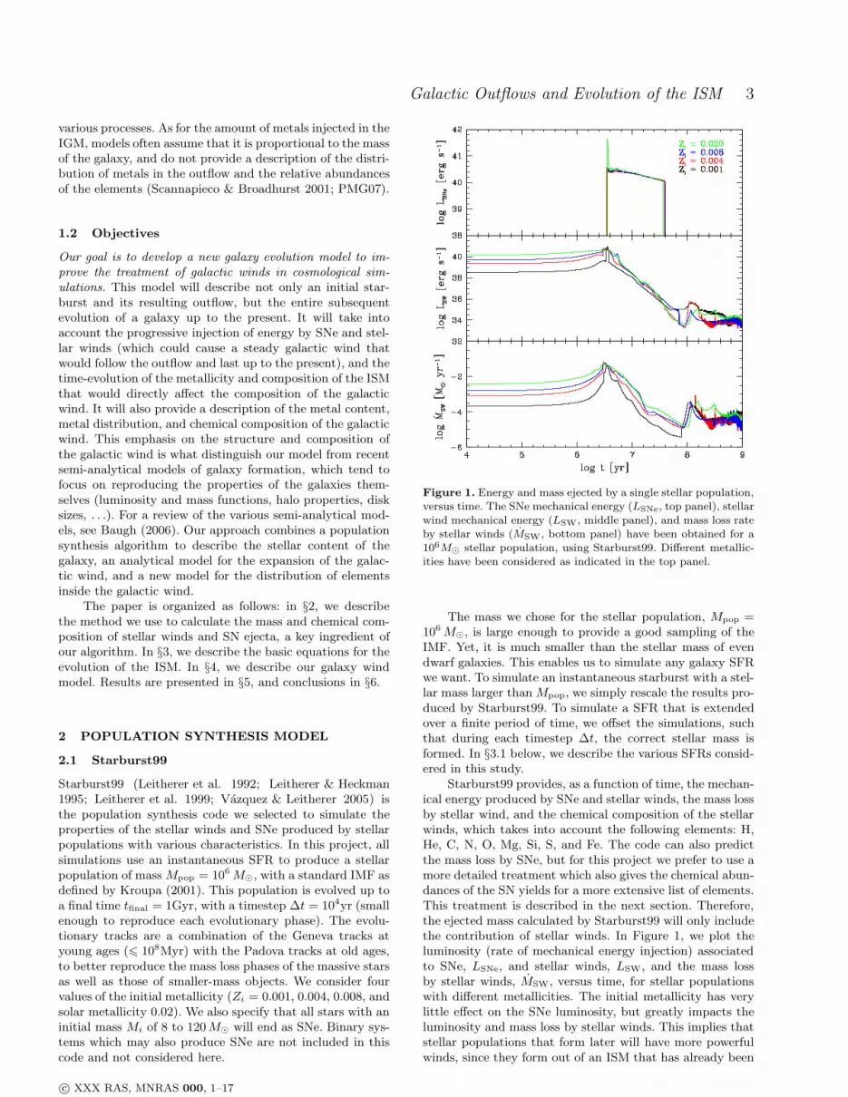
Figure 1. Energy and mass ejected by a single stellar population,versus time. The SNe mechanical energy (LSNe, top panel), stellarwind mechanical energy (LSW, middle panel), and mass loss rateby stellar winds (MSW, bottom panel) have been obtained for a106M⊙ stellar population, using Starburst99. Different metallic-ities have been considered as indicated in the top panel.

The mass we chose for the stellar population, Mpop =106 M⊙, is large enough to provide a good sampling of theIMF. Yet, it is much smaller than the stellar mass of evendwarf galaxies. This enables us to simulate any galaxy SFRwe want. To simulate an instantaneous starburst with a stel-lar mass larger than Mpop, we simply rescale the results pro-duced by Starburst99. To simulate a SFR that is extendedover a finite period of time, we offset the simulations, suchthat during each timestep ∆t, the correct stellar mass isformed. In §3.1 below, we describe the various SFRs consid-ered in this study.

Starburst99 provides, as a function of time, the mechan-ical energy produced by SNe and stellar winds, the mass lossby stellar wind, and the chemical composition of the stellarwinds, which takes into account the following elements: H,He, C, N, O, Mg, Si, S, and Fe. The code can also predictthe mass loss by SNe, but for this project we prefer to use amore detailed treatment which also gives the chemical abun-dances of the SN yields for a more extensive list of elements.This treatment is described in the next section. Therefore,the ejected mass calculated by Starburst99 will only includethe contribution of stellar winds. In Figure 1, we plot theluminosity (rate of mechanical energy injection) associatedto SNe, LSNe, and stellar winds, LSW, and the mass lossby stellar winds, MSW, versus time, for stellar populationswith different metallicities. The initial metallicity has verylittle effect on the SNe luminosity, but greatly impacts theluminosity and mass loss by stellar winds. This implies thatstellar populations that form later will have more powerfulwinds, since they form out of an ISM that has already been



enriched in metals by earlier populations. Figure 1 shows asudden increase in wind power around 1 - 2 × 106yr, justprior to the arrival of the first SNe, which is caused by theevolved stages of OB stars, i.e. the Wolf-Rayet stars. Theincrease in mass loss after 108yr is caused by the low-massstars on the AGB.

2.2 SN Abundances

Except in situations where the metallicity of the stars islarger or equal to solar, the enrichment of the ISM is domi-nated by SNe (see Fig. 8 of Leitherer et al. 1992). Thus, it isimportant to know the composition of the material ejectedby SNe as a function of the initial mass and metallicity ofthe stellar progenitors. Several groups have used models ofstellar evolution and nucleosynthesis to produce tables ofchemical abundances for SN ejecta. These studies are sum-marized in Table 1. The first column gives the authors ofthe papers; the second and third columns list the metallic-ities and initial masses considered, respectively; the fourthcolumn indicates whether or not mass loss prior to the SNexplosion was included in the model.

Although very useful, these studies are not fullysatisfactory for our work. The first three studies(Woosley & Weaver 1995; Chieffi & Limongi 2004;Nomoto et al. 2006, hereafter N06) consider a wide range ofmetallicities, from no metallicity (Z = 0) to solar metallicity(Z⊙ = 0.02), but are limited to initial masses Mi 6 40M⊙.The next three studies (Woosley & Heger 2007, hereafterWH07; Limongi & Chieffi 2007; Heger & Woosley 2010,hereafter HW10) consider initial masses up to 100 - 120M⊙,but only one value of the metallicity. Also, three of thesestudies do not include mass loss prior to the explosion,which is critical in our models since we include stellar windeffects. The study that comes the closest to our needs is theone of N06. This is the only study that covers metallicitiesin the range Z = 0 - Z⊙ and includes mass loss. However, itsmass range only goes from 13 to 40M⊙. These tables needto be extrapolated both at the low-mass and high-massend to cover the full range of SNe progenitor masses. Inthis paper, we assume an IMF with lower and upper masslimits of 1 and 120M⊙, respectively, and SNe progenitormasses in the range Mi = 8 - 120M⊙. The lower limit of8M⊙ is the most commonly used, but that value is actuallyquite uncertain, and could have an important effect on theresults (see Fig. 5 below).

The top panel of Figure 2 shows the mass ejected bySNe versus initial mass and metallicity, calculated with thetables of N06 (solid curves). An interesting feature is thelinear relation between Mej and Mi at Z = 0. Also, all thecurves converge together at Mi = 13M⊙, suggesting thatfor initial masses Mi < 13M⊙, the ejected mass is indepen-dent of metallicity. To extrapolate down to Mi = 8M⊙, weused the composition for Mi = 13M⊙, modulated using thelinear regression at Z = 0 calculated with the software Slope(Isobe et al. 1990). The result is also shown in Figure 2.

Extrapolation up to 120M⊙ can be tricky, especially ifmass loss is considered. Several approaches have been sug-gested in the literature, especially at the high-mass end.Martinez-Serrano et al. (2008) extrapolate the mass ejectedMej and chemical composition of the ejecta linearly up toMi = 100M⊙. Oppenheimer & Dave (2008) assume similar

Figure 2. Top panel: Total mass ejected by one SN versus theinitial mass of the progenitor, according to the tables of N06(solid lines), WH07 (lower dotted line), and HW10 (upper dottedline). Colors represent various metallicities, as indicated. Bottompanel: Total mass ejected by one SN versus the initial mass ofthe progenitor after extrapolating down to Mi = 8M⊙ and upto Mi = 120M⊙, for metallicities Z = 0 (solid black line) andZ = Z⊙ (solid green line), after extrapolating over all metallici-ties available in N06 (blue and red lines), and after interpolatingto the metallicity Z = 0.008 used by Starburst99 (purple line).

ejecta for stars in the range Mi = 35 - 100M⊙ and also forstars in the range Mi = 10 - 13M⊙. Tornatore et al. (2007)and Scannapieco et al. (2005) assume that stars with ini-tial masses larger than 40M⊙ end up directly in a blackhole, with no ejecta. Using linear interpolation up to Mi =120M⊙ would be risky. The relation between Mej and Mi

becomes metallicity-dependent for Mi > 25 - 30M⊙, im-plying that only two or three points would be available toextrapolate over a mass interval three times wider than theone of N06. Furthermore at Z = Z⊙, Mej eventually de-creases with increasing initial mass and a linear extrapo-lation would eventually lead negative values before reach-ing Mi = 120M⊙. Setting the ejected mass to zero forMi > 40M⊙ is not a good solution either. Even if the SN re-sults in the formation of a black hole, that black hole is neveras massive as the progenitor (Woosley et al. 2002; WH07;Limongi & Chieffi 2008; Zhan et al. 2008; Belczynski et al.2010). Using a copy of the M = 40M⊙ at larger massesis not realistic either since the tendency clearly shows thatthere is more material ejected for larger initial masses, ex-cept at Z⊙.

Since none of the three extrapolation methods consid-ered so far is satisfactory for extrapolating up to 120M⊙,we developed an alternative method. We started by extrap-olating the table of N06 at Z = 0 and also Z⊙, by com-bining them with the tables of HW10 and WH07, respec-tively. The top panel of Figure 2 shows the Z⊙ relation ofWH07 and the Z = 0 relation of HW10 (dotted curves). TheZ = Z⊙ relations of N06 and WH07 differ significantly inthe range Mi = 20 - 40M⊙. This is likely the consequenceof using a different prescription for the mass loss duringthe pre-SN phase. In the model of WH07, the ejected massreaches a maximum around Mi = 21M⊙, then decreases



Table 1. SN yields available in the literature.

Paper Z Mi [M⊙] M

Woosley & Weaver (1995) 0, 2× 10−6, 2× 10−4, 0.002, 0.02 11, 12, 13, 15, 18, 19, 20, 25, 30, 35, 40 noChieffi & Limongi (2004) 0, 10−6, 10−4, 0.001, 0.006, 0.02 13, 15, 20, 25, 30, 35 noNomoto et al. (2006) 0, 0.001, 0.004, 0.02 13, 15, 18, 20, 25, 30, 35, 40 yesWoosley & Heger (2007) 0.02 32 Mi’s between 12 and 120 yesLimongi & Chieffi (2007) 0.02 15 Mi’s between 10 and 120 yesHeger & Woosley (2010) 0 120 Mi’s between 10 and 100 no

with increasing initial mass, and finally reaches a plateau atMej = 4M⊙, which represents the minimum mass a SN caneject. Assuming that this limit is correct, we extrapolatedthe Z⊙ model of N06 until it reaches the model of WH07(around Mi = 70M⊙). We then switched to the model ofWH07 to complete the extrapolation up to Mi = 120M⊙.For Z = 0, the results of N06 and HW10 are essentiallyidentical in the range Mi = 13 - 30M⊙, and very similarin the range Mi = 30 - 40M⊙. To combine them, we usedthe tables of N06 in the range Mi = 8 - 40M⊙ and the ta-bles of HW10 in the range Mi = 55 - 120M⊙, Between 40and 55M⊙, we interpolated between these two masses. Theresults are shown in the bottom panel of Figure 2.

At the two intermediate metallicities Z = 0.001 and0.004, the values of the ejected masses should lie between thevalues for Z = 0 and Z⊙ (Fig. 2). If the mass loss due to stel-lar winds were neglected, the masses ejected by SNe shouldbe the same as for models with Z = 0. The mass loss associ-ated with massive stars is proportional to Zα, where α ≃ 0.6- 0.8 (Vink et al. 2001; Vink & de Koter 2005; Krticka 2006;Mokiem et al. 2007). We then interpolated to get the massejected by SNe at any metallicity:

Mej(Mi, Z) = Mej(Mi, 0) − τ (Mi, Z)M , M = AZα , (1)

where A is a constant, and τ (Mi, Z) is the lifetime of a starof initial mass Mi and metallicity Z. We made the approxi-mation that the lifetime does not vary much with metallicity,τ (Mi, Z) ≈ τ (Mi). Equation (1) becomes:

Mej(Mi, Z) = Mej(Mi, 0) −B(Mi)Zα . (2)

where the function B(Mi) was calculated from the massesejected at Z = Z⊙:

B(Mi) =Mej(Mi, Z⊙)−Mej(Mi, 0)

Zα⊙

. (3)

We choose the value α = 0.625, which minimizes the dis-continuity at M = 40M⊙. Figure 2 shows all the modelsof N06 after extrapolation. For Z = 0.004 and 0.001, themass loss is not as extreme as in the case Z = Z⊙. For thatreason, we used the composition of the 40M⊙ models mod-ulated according to the value of Mej for all the initial massesMi > 40M⊙.

Next we determined the composition of the ejectedmasses, for Z = 0 and Z⊙. Table 2 shows the hydrogenmass, helium mass, and total mass ejected for the WH07models. The cases presented are extreme. The mass loss bystellar winds is sufficiently large to expel the entire hydrogenenvelop and most of the helium as well. This indicates thatthese stars have evolved through a Wolf-Rayet stage, result-ing in SNe of Type Ib or Ic. Hence, most of the materialejected is composed of metals. For this reason, we treated

Table 2. Hydrogen mass, helium mass, and total mass ejectedby SNe versus initial mass at solar metallicity, according to thetable of WH07.

Mi[M⊙] MH[M⊙] MHe[M⊙] Mej[M⊙]

40 0.223 1.640 9.7450 5.51× 10−8 0.068 7.9460 1.77× 10−7 0.120 5.6570 1.16× 10−7 0.152 4.3580 1.04× 10−7 0.156 4.34100 1.77× 10−7 0.181 3.96120 1.39× 10−7 0.172 3.92

hydrogen and helium as we treated the total mass ejected: wefollowed the tables of N06 until it reaches the model of WH07and then switched to the model of WH07 (Fig. 3). The re-minder of the ejected mass was assumed to have the chemicalcomposition corresponding to the Mi = 40M⊙ model. ForZ = 0, the complete composition of the Mi = 40M⊙ modelwas used.

Starburst99 requires tables of SNe at metallicities Z =0.001, 0.004, 0.008, and 0.02. At this point we have tablesat Z = 0.004 and 0.02. For Z = 0.008, we interpolatedbetween the tables at Z = 0.004 and 0.02 using logZ as aninterpolation variable. We now have a full set of SN tablesthat provides the ejected mass and composition of the ejecta,for all progenitors in the range Mi = 8 - 120M⊙ and Z = 0 -Z⊙. Figure 2 shows the ejected mass versus progenitor mass.

At each timestep during the simulation, Starburst99provides the number of SNe and their luminosity (adopt-ing that each SN produces 1051ergs; McKee 1990). The SNtables are then used to calculate at every timestep the massand composition of the material deposited into the ISM. Forsimulations with initial metallicity Z = 0, we use the lumi-nosity at Z = 0.001 which is the smallest value consideredby Starburst99. Figure 4 shows the mass loss rate due toSNe for a 106 M⊙ instantaneous burst. This completes theresults shown in Figure 1. In the top panel of Figure 5, weplot the total mass ejected by SNe versus metallicity, forthe same population. The dotted curve shows our extrapo-lation method, while the solid curves show the three othermethods. The “constant” method of Oppenheimer & Dave(2008) (using the ejecta for Mi = 40M⊙ at higher masses) isthe one which resembles our method the most, but there aresignificant differences. This justifies a posteriori the methodwe have developed in this section.

We assume a minimum progenitor mass of Mi = 8M⊙,but we also generated other tables using different values.The bottom panel of Figure 5 shows the ejected mass forminimum progenitor masses of Mi = 6M⊙, Mi = 8M⊙ (the



Figure 3. Hydrogen (top) and helium mass (bottom) ejected byone SN versus the initial mass of the progenitor, according to thetables of N06 (solid lines), after extrapolating down to Mi = 8M⊙

and up to Mi = 120M⊙, for Z = Z⊙. The dotted line illustratesthe Z = Z⊙ model of WH07. Colors have the same meaning asin Figure 2.

Figure 4.Mass loss rate by SNe versus time. Number of stars andSN explosions are from a Starburst99 model for an instantaneousburst with a standard IMF and a total mass of 106M⊙. Massejected by each SN comes from our extended tables. Differentmetallicities have been considered as indicated.

value assumed in this paper), and Mi = 10M⊙. The differ-ences are of order 50%, with the ejected mass being largerfor a smaller minimum progenitor mass. This shows thatthe particular choice of minimum progenitor mass can havea impact on the results, and we intend to investigate thisissue in more details in future work. Here we focus on thecase of a minimum progenitor mass of Mi = 8M⊙.

In a recent paper, Horiuchi et al. (2011) point to aserious “supernova rate problem”: the measured cosmicmassive-star formation rate predicts a rate of core-collapsesupernovae about twice as large as the observed rate, at leastfor redshifts between 0 and 1, where surveys are thought tobe quite complete. Several explanations are proposed to ex-plain this major discrepancy, including a large fraction ofunusually faint (intrinsically or dust-attenuated), and thusunaccounted for, core-collapse SNe and a possible overesti-mate of the star formation rate based on the current estima-tors. If indeed this supernova rate problem is real, the SFR

Figure 5. Mass ejected by SNe versus metallicity, Top panel:results obtained with our extrapolation method for the SNmass ejected as a function of the progenitor initial mass, us-ing the same stellar population model as in Figure 4 (dottedcurve), compared with results obtained with different extrapo-lation methods (solid curves): from top to bottom: linear ex-trapolation of Martinez-Serrano et al. (2008), constant approx-imation of Oppenheimer & Dave (2008), and no-ejecta approxi-mation of Tornatore et al. (2007) and Scannapieco et al. (2005).Bottom panel results obtained with our extrapolation method, forvarious values of the minimum initial mass. From top to bottom,Mi = 6M⊙, 8M⊙, and 10M⊙.

(see §5.1) might have to be scaled accordingly. However, allsimulations presented in this paper start at redshift z = 15,and terminate at redshifts between 6 and 9. It is not clearthat there is a supernova rate problem at these redshifts.

3 EVOLUTION OF THE INTERSTELLAR

MEDIUM

During the evolution of a galaxy, the ISM is constantly en-riched by ejecta from stellar winds and SNe. Hence, everygeneration of stars provides an environment richer in met-als for the future generations. The level of this enrichmentdepends on the SFR, since the metal production increaseswith the number of stars formed. To simulate this process,we designed an algorithm that combines the outputs of Star-burst99 with the SNe tables of N06.

3.1 Initial Conditions

We consider a galaxy with a total mass Mgal. We assumethat the ratio of baryons to dark matter in the galaxy isequal to the universal ratio, which is a valid assumption forthe initial stages of the galaxy. The baryonic mass of thegalaxy is then given by

Mb =Ωb0

Ω0

Mgal , (4)

where Ω0 and Ωb0 are the total and baryon density pa-rameters, respectively. We assume that each galaxy startsup with a primordial composition of hydrogen and helium(X = 0.755 and Y = 0.245). The formation of the galaxy



results in a starburst, during which a fraction f∗ of the bary-onic mass is converted into stars. The total mass in stars atthe end of the starburst is therefore

M∗ = f∗Mb . (5)

We refer to the parameter f∗ as the star formation efficiency.We consider three different types of star formation rate:

instantaneous, constant, and exponential. With an instan-taneous SFR, all stars form at t = 0. In the other cases, thestellar mass formed M∗ and the star formation rate M∗ arerelated by∫ tf

0

M∗(t)dt = M∗ , (6)

where tf is the final time of the simulation. For a constantSFR, we have

M∗ =M∗

tburst, (7)

where tburst is the duration of the starburst. We usuallychoose a value for M∗ and solve equation (7) for tburst. Foran exponential SFR, we have

M∗ =M∗

tce−t/tc , (8)

where tc = 5 × 107yrs is the characteristic time. Since starformation never ends in this case, the stellar mass formeddepends on the final time tf . Equation (8) is valid in thelimit tf ≫ tc.

There are some caveats about equations (4) and (5).The infalling gas must cool and form molecular clouds whichthen fragment into stars. If star formation is delayed until allthe gas has cooled, then equation (4) would be valid, but itis more likely that star formation will start while a fractionof the gas has not cooled yet. SNe and stellar winds fromthat first generation of stars will inhibit the formation ofsubsequent generations of stars, by reheating the ISM andpossibly expelling some of it in the form of a galactic out-flow. Observations of galaxies in the redshift range 0 < z < 4show that star formation is a very inefficient process, withM∗/Mgal < 0.03 (Behroozi et al. 2010). Hence, the value ofMb in equation (4) is an upper limit, which does not take intoaccount the gas lost by galactic outflows. As for the reheat-ing of the gas and suppression of inflow, it is implicitly takeninto account in equation (5) by introducing a star formationefficiency f∗. The mass of gas that was reheated and pre-vented from forming stars isMreheat = (1−f∗)Mb. In this pa-per, we consider star formation efficiencies f∗ = 0.1, 0.2, 0.5,and 1.0. Equations (4) and (5) then give M∗/Mgal = 0.016,0.032, 0.081 and 0.162, respectively. The first two values areconsistent with observations. The last two values are quiteextreme, and we considered them mostly to investigate thebehavior of the model under extreme conditions.

In this paper, we impose various forms for the SFR toinvestigate the effect of the SFR on the properties of thegalactic outflows. The effect of feedback and reheating ofthe ISM is all contained implicitly in the value of f∗. Toprovide a proper treatment of the aforementioned feedbackprocesses, we intend to modify the model such that the SFRwill be recalculated at every time step, from the physicalconditions of the ISM gas at that time, taking into accountthe effect of all previous generation of stars. This will pro-vide a consistent treatment of feedback and self-regulating

star formation, and eliminate the need to specify a prioria star formation efficiency f∗. This will be the subject of aforthcoming paper.

3.2 Evolution of the Mass and Composition of the

ISM

Our algorithm tracks the evolution of MISMX, the mass of

element X contained in the ISM. At the beginning of eachtimestep, the total mass of the ISM is given by

MISM(t) =∑

X

MISMX(t) , (9)

where the sum is over all elements included in the algo-rithm, that is all elements from hydrogen (X = 1) to gallium(X = 31). These quantities are initialized at the beginningof the simulation, and updated during each timestep ∆t, asfollows. First, we calculate the mass ejected by stellar windsand SNe. We include the contribution from all stars presentat that time, taking into account their current ages, initialmetallicities, and initial masses:

MSWX(t) =

∑

k

MSB99SWX

(τk, Zk,Mk)∆t , (10)

MSNeX(t) =∑

k

MSB99SNeX

(τk, Zk,Mk)∆t . (11)

where τk, Zk, and Mk are the current age, initial metallicity,and mass of population k, respectively. The sums are overall the stellar populations that have already formed by timet. The superscript SB99 indicates quantities calculated byStarburst99. We also calculate the total luminosity producedby SNe and stellar winds:

LSW(t) =∑

k

LSB99SW (τk, Zk,Mk) , (12)

LSNe(t) =∑

k

LSB99SNe (τk, Zk,Mk) . (13)

We then remove from the ISM the total mass of thestars born during that timestep, and the mass removed bythe galactic wind, and add the material ejected by SNe andstellar winds:

MISMX(t+∆t) = MISMX

(t)−MISMX

(t)

MISM(t)

[

M∗(t)

+MGW(t)]

∆t+MSWX(t) +MSNeX(t) , (14)

where MGW(t) is the rate of mass loss by galactic wind (thecalculation of MGW is presented in the next section). Themass remove from the ISM by the star formation processis used to generate several new stellar populations. Eachpopulation is given an initial mass Mk, an initial metallicityZk equal to the metallicity Z(t) of the ISM at that time,and we set the age τk of these new populations to zero. Wethen recompute the ISM metallicity:

Z(t+∆t) =[

MISM(t+∆t)−MISMH(t+∆t)

−MISMHe(t+∆t)

]/

MISM(t+∆t) . (15)

This expression accounts for the material removed from theISM by the star formation process and the galactic wind,and it also considers the enriched material added by stars



already formed. Finally, we update the age of every stellarpopulation:

τk(t+∆t) = τk(t) + ∆t , for all k . (16)

These operations are repeated at every timestep in the sim-ulation.

In our model, MISMXis a function of time only. This

assumes that metals ejected into the ISM by SNe and stel-lar winds are instantaneously mixed. This commonly-usedapproximation has the advantage of being simple to imple-ment. However, in reality, it will take some finite time beforethe metals are fully mixed. For this reason, the efficiency ofmetal-enrichment of the IGM in our model should be con-sidered as an upper limit.

Starburst99 cannot calculate directly the mass loss andluminosities appearing in equations (10) to (13) for any ini-tial metallicity Zi. It is limited to the values Zi = 0.001,0.004, 0.008, and 0.02. We therefore need to interpolate theresults of Starburst99 in order to get the quantities MSB99

and LSB99. For values of Zi in the range [0.001, 0.02], wecalculate MSB99 and LSB99 at the metallicities immediatelybefore and after Zi, and interpolate between them, usingequations of the form

log MSB99 = A logZi +B , (17)

logLSB99 = C logZi +D . (18)

In the range [0, 0.001], we treat stellar winds and SNe dif-ferently. We assume that, in that range, the mass loss bystellar wind is proportional to Zα

i , with α ≈ 0.625, as inequations (1) to (3). Hence,

MSB99SW (Zi) = MSB99

SW (0.001)(

Zi

0.001

)0.625

, (19)

LSB99SW (Zi) = LSB99

SW (0.001)(

Zi

0.001

)0.625

. (20)

For SNe, we use the values LSB99SNe (Zi = 0.001) at lower

metallicities. This is a valid approximation because the de-pendence of the stellar lifetimes on metallicity is weak, asFigure 1 shows.

3.3 Mass Loss by Galactic Wind

The presence of a galactic wind enables a fraction of theISM to escape the galaxy and enrich the surrounding IGM.Since the wind is generated by the thermal energy depositedin the ISM by stars, we expect the mechanical energy ofthe galactic wind to be proportional to the rate of energyinjection by SNe and stellar winds:

1

2MGW(t)V 2

GW ∝ L(t) , (21)

where MGW and VGW are the mass loss rate by galactic windand the velocity of the wind, respectively. The galactic windwill create a cavity expanding into the IGM (see § 4 below).The expansion of the cavity is driven by the mechanicalenergy MGW(t)V 2

GW/2 deposited into the IGM by the wind,but does not depend separately on MGW and VGW. Hence, todetermine MGW, we must make an additional assumption.There are two limiting cases: One limit consists of havingMGW constant, in which case increasing the number of SNewill increase the wind velocity. The opposite limit consists

of having a constant wind velocity VGW, in which case anincrease in the number of SNe results in a larger amount ofmatter being ejected.

It would take detailed high-resolution simulations to de-termine which of these limits is correct. Ultimately, the criti-cal factor should be the spatial distribution of SNe. A singleSN will only affect the ISM located in its vicinity. In thecase of several SNe, there collective effect should criticallydepend on their level of clustering. If all SNe are concen-trated in a same location, the same region will be affected,and the net effect will be to eject the same matter, but at alarger velocity. If instead the SNe are distributed through-out the galaxy, each SN will affect a different part of theISM, and the net result will be to eject more material, butat the same velocity. This last case is the limit we adoptin this paper. Consequently, the reader should keep in mindthat our estimates of the amount of material ejected is anupper limit. Under this assumption the rate of mass loss bythe galactic wind is proportional to the luminosity,

MGW(t) ∝ L(t) , (22)

To determine the constant of proportionality, we firstintegrate the functions MGW(t) and L(t) over the lifetimeof the galaxy:

M totGW =

∫ tf

0

MGW dt , (23)

Etot =

∫ tf

0

Ldt , (24)

where M totGW is the total mass ejected into the galactic wind,

and Etot is the total energy deposited in the ISM. We canrewrite equation (22) as

MGW(t) =M tot

GW

EtotL(t) . (25)

The problem is that M totGW and Etot are not known until

the simulation is completed, and to perform the simulation,we need to know these quantities in advance in order tocalculate MGW at every timestep. To solve this problem, wereplace M tot

GW and Etot in equation (25) by approximationsthat can be calculated ab initio, before actually performingthe simulation.

3.3.1 Estimate of Etot.

The luminosity L(t) is calculated as the simulation proceeds,but we can estimate it as follows: first, as we shall see below,the contribution of stellar winds to the luminosity becomesnegligible once the SNe phase starts. If we neglect stellarwinds, and also neglect the weak dependence of the SN lu-minosity on the metallicity (see Fig. 1), we can directly es-timate the luminosity from the star formation rate M∗. Wedefine an integrated mass loss rate F (t) using:

F (t+ tonset) ≡

∫ t

t−tactive

M∗(t′)dt′ , (26)

where tonset is the time elapsed between the formation ofthe stellar population and the onset of the first SN, and



Figure 6. Solid curve: SNe luminosity versus time, for a 109M⊙

galaxy with an exponential SFR and a star formation efficiencyf∗ = 0.1. Dotted curve: Integrated mass loss rate F (t), for thesame galaxy.

tactive is the time duration of the SNe phase.2 Figure 6shows the luminosity L(t) obtain from the simulation, andthe quantity F (t) calculated using tonset = 3.11Myr andtactive = 39.2Myr (Fig. 1). To a very good approximation,F (t) is proportional to L(t). We can therefore approximateequation (25) as

MGW =M tot

GW

F totF (t) , (27)

where

F tot =

∫ tf

0

F dt . (28)

Both F (t) and F tot are calculated at the beginning of thesimulation.

3.3.2 Estimate of M totGW.

We still need to determine the total mass ejected by thegalactic wind, M tot

GW, to be able to use equation (27). Likethe total energy deposited in the ISM, Etot, M tot

GW is notknown until the simulation is completed. To estimate it, wereplace MGW in equation (23) by an approximation that canbe calculated at the beginning of the simulation. We thenintegrate to get M tot

GW, we substitute that value in equa-tion (27), which then provides the mass loss by galactic windduring the simulation. To find an initial approximation forMGW, we first notice that observations at different redshiftssuggest a relation between the mass loss by galactic windsand the star formation rate (Martin 1999), often expressedin terms of the ratio

η ≡MGW

M∗

. (29)

This value appears to vary significantly among galax-ies, with values ranging from 0.01 to 10 (Veilleux et al.2005). Murray et al. (2005) derived analytical relations be-tween the factor η and the velocity dispersion σ, for bothmomentum-driven and energy-driven winds. We focus in this

2 The lifetimes of the shortest-lived and longest-lived progenitorsare therefore tonset and tonset + tactive, respectively.

Figure 7. Escape fraction versus redshift, for a 109M⊙ galaxywith a star formation efficiency f∗ = 0.1.

paper on energy-driven winds, but will consider momentum-driven winds in future work. For energy-driven winds,Murray et al. (2005) derived the following relation:

MGW = M∗ ξ0.1 ε3

(

300 km s−1

σ

)2

, (30)

where σ is the velocity dispersion, ε3 ≡ 1000Etot/M∗c2, and

ξ0.1 ≡ fw/0.1, with fw(Mgal) the fraction of energy providedby stars that is used to power the wind, for a galaxy ofmass Mgal (Scannapieco et al. 2002). To calculate ε3, we useStarburst99 with a 106M⊙ stellar population and a standardIMF. The total energy Etot produced by SNe and stellarwinds is always of the order of 1055.3ergs, for all metallicities.This gives ε3 = 0.011. Equation (30) reduces to

MGW = 0.11M∗fw

(

300 kms−1

σ

)2

. (31)

For a galaxy of mass Mgal, the velocity dispersion σ is cal-culated using the equation of Oppenheimer & Dave (2008):

σ = 200

[

Mgal

5× 1012M⊙

hH(zgf)

H0

]1/3

kms−1 , (32)

where zgf is the formation redshift of the galaxy, H is theHubble parameter, with H0 being its present value, and h =H0/100 km s−1 Mpc−1. Equations (31) and (32) give us anestimate of MGW. We then apply equation (23) to calculateM tot

GW, which we substitute in equation (27). This equation isthen used to calculate the mass loss by galactic wind duringthe simulation [eq. (14)].

The parameter fesc is defined as the fraction of the ISMmass that escapes the galaxy:

fesc =M tot

GW

Mb=

Ω0

Ωb0

M totGW

Mgal

. (33)

Figure 7 shows fesc versus formation redshift zgf , for variousgalactic masses Mgal, with a star formation efficiency of f∗ =0.1. The dependence on zgf comes entirely from the factorH(zgf) in equation (32). Galaxies that form earlier have alarger velocity dispersion σ for a given mass Mgal. Lower-mass galaxies eject a larger fraction of their ISM than highermass galaxies, and for a 108M⊙ galaxy, we get fesc > 1,which simply means that the entire ISM will be ejected fromthe galaxy (so the actual fesc is unity).



4 GALACTIC WIND MODEL

4.1 The Dynamics of the Expansion

Tegmark et al. (1993, hereafter TSE) presented a formula-tion of the expansion of isotropic galactic winds in an ex-panding universe. In this formulation, the injection of ther-mal energy produces an outflow of radius R, which consistsof a dense shell of thickness Rδ containing a cavity. A frac-tion 1 − fm of the mass of the gas is piled up in the shell,while a fraction fm of the gas is distributed inside the cavity.We normally assume δ ≪ 1, fm ≪ 1, that is, most of thegas is located inside a thin shell. This is called the thin-shellapproximation.

The evolution of the shell radius R expanding out of ahalo of mass Mgal, is described by the following system ofequations:

R =8πG(p− pext)

ΩbH2R−

3

R(R−HR)2 −

ΩH2R

2

−GMgal

R2, (34)

p =L

2πR3−

5Rp

R, (35)

where a dot represents a time derivative, Ω, Ωb, and H arethe total density parameter, baryon density parameter, andHubble parameter at time t, respectively, L is the luminosity,p is the pressure inside the cavity resulting from this lumi-nosity, and pext is the external pressure of the IGM. The fourterms in equation (34) represent, from left to right, the driv-ing pressure of the outflow, the drag due to sweeping up theIGM and accelerating it from velocity HR to velocity R, andthe gravitational deceleration caused by the expanding shelland by the halo itself. The two terms in equation (35) repre-sent the increase in pressure caused by injection of thermalenergy, and the drop in pressure caused by the expansion ofthe wind, respectively.

The external pressure, pext, depends upon the densityand temperature of the IGM. As in PMG07, we will assumea photoheated IGM made of ionized hydrogen and singly-ionized helium (mean molecular mass µ = 0.611), with afixed temperature TIGM = 104K (Madau et al. 2001) andan IGM density equal to the mean baryon density ρb. Theexternal pressure at redshift z is then given by:

pext(z) =ρbkTIGM

µ=

3Ωb,0H20kTIGM(1 + z)3

8πGµ. (36)

The luminosity L is the rate of energy deposition ordissipation within the wind and is given by:

L(t) = fw(LSNe + LSW)− Lcomp , (37)

where LSNe and LSW are the total luminosity responsible forgenerating the wind, as given by equations (13) and (12),respectively. Lcomp represents the cooling due to Comptondrag against CMB photons and is given by:

Lcomp =2π3

45

σth

me

(

kTγ0

hc

)4

(1 + z)4pR3 , (38)

where σt is the Thomson cross section, and Tγ0 is the presentCMB temperature.

The expansion of the wind is initially driven by theluminosity. After the SNe turn off, the outflow enters the

“post-SN phase.”3 The pressure inside the wind keeps driv-ing the expansion, but this pressure drops since there is noenergy input from SNe. Eventually, the pressure will dropdown to the level of the external IGM pressure. At thatpoint, the expansion of the wind will simply follow the Hub-ble flow.

4.2 Metal Distribution inside the Galactic Wind

In the TSE model, the baryon density inside the cavity isρi = ρb(t)fm/(1 − δ)3, while the baryon density inside theshell is ρs = ρb(t)(1− fm)/[1− (1− δ)3]. This gives a massM = 4πR3ρb(t)/3 inside the volume of radius R, which isprecisely the mass of the IGM within that radius in the ab-sence of a wind. Therefore, in the TSE model, the materialinside the shell is swept IGM material, while the material in-side the cavity is IGM material left behind. The mass MGW

added by the galactic wind is neglected in the TSE model.

Hence, the TSE model does not predict the distribution ofthat mass inside the cavity. This means that any distribu-tion we chose would not violate the assumptions on whichthe TSE model is based.

The simplest approximation for the distribution of met-als in the wind consists of assuming that the metals car-ried by the galactic wind are spread evenly inside the cav-ity (see Scannapieco et al. 2002; PMG07; Barai et al. 2011).This poses a problem for the metals ejected near the endof the post-SN phase, just before the wind joins the Hubbleflow. These metals would have to be carried across the en-tire radius of the cavity, at velocities that exceed the windvelocity. Processes such as turbulence and diffusion couldhomogenize the distribution of metals inside the cavity, butonly over a finite time period. In this paper, we take theopposite approach, by assuming no mixing. Hence, the gasthat escapes the galaxy early on will travel larger distancesthan the gas that escapes later. Since the metallicity andcomposition of the ISM evolves with time, the galactic windwill acquire both a metallicity gradient and a compositiongradient, with the inner parts containing a larger propor-tion of metals. To simulate such wind, we use a system ofconcentric spherical shells. At the end of every timestep, thecode calculates the amount of gas that will be added to thegalactic wind:

∆MGW(ti) = MGW(ti)∆t , (39)

where ti is the time corresponding to the timestep. After thefirst time step, the wind reaches a radius R1 ≡ RGW(∆t).We deposit the wind material produced during that timestep into the sphere of radius RGW(∆t), which constitutesour central shell. After the second timestep, the wind nowreaches radius R2 ≡ RGW(2∆t). We first transfer the windmaterial located between 0 and R1 into a shell of inner ra-dius R1 and outer radius R2, and we then deposit the windmaterial produced during the second timestep into the cen-tral shell. This process is then repeated. At every timestepn, a new shell is created between radii Rn and Rn−1, all thewind material is shifted outward by one shell, and the newmaterial is deposited into the central shell. Finally, when the

3 The stellar winds are still on, but their contribution is negligibleat this point.



Figure 8. Mass of some elements present in the ISM versus red-shift, for a 109M⊙ galaxy with a star formation efficiency f∗ = 0.1and an exponential SFR. The colors corresponds to various ele-ments, as indicated. Solid lines: simulation without galactic wind;dashed lines: simulation with galactic wind.

wind enters the post-SN phase, we no longer deposit materielinto the wind, and the shells expand homologously with thecavity. One nice feature of this model is that it has no freeparameter. In particular, if does not depend on the value ofthe timestep. Using a different timestep would change theresolution at which the wind profile is determined, but notthe profile itself.

5 RESULTS

Here we use the algorithm described in §4 to study the evolu-tion of starburst galaxies, in a concordance ΛCDM universewith density parameter Ω0 = 0.27, baryon density parame-ter Ωb0 = 0.044, cosmological constant λ0 = 0.73, and Hub-ble constant H0 = 71 kms−1Mpc−1 (h = 0.71). Because theparameter space is large, we focus on a fiducial case: a dwarfgalaxy of mass Mgal = 109M⊙ forming at zgf = 15. This caseis particularly important because the vast majority of galax-ies in the universe are dwarfs, and in CDM cosmology, thesegalaxies tend to form at high redshift (e.g. Blumenthal et al.1984). Also our model assumes that galaxies form by mono-lithic collapse and not by the merger of well-formed galax-ies, an assumption that is more appropriate for dwarfs (e.g.Blumenthal et al. 1984). Note that the value of zgf mattersin the model. It affects the expansion of the galactic wind,which in turns affects the evolution of the ISM.

We performed two simulations, one with our basicmodel, and another one in which we turned off the galacticwind. Figure 8 shows the abundances of a few elements inthe ISM. Most of the ISM enrichment occurs between red-shifts z = 15 and z = 13, during the epoch of intense SNeactivity. At lower redshifts, the enrichment by stellar windsdominates. The effect of the galactic wind is very small.Adding the wind results in a 10% increase in ISM metal-licity, caused by the removal of low-metallicity ISM duringthe early stages of the wind. The effect the galactic windcan be much more significant but this requires a smallergalactic mass Mgal or a larger star formation efficiency f∗,or SFR much more extended in time than the ones we haveconsidered.

In the next three subsections, we explore the parameterspace by varying, respectively, the SFR, the star formationefficiency f∗, and the mass Mgal of the galaxy.

Figure 9. Mass loss rate of stars versus redshift, for a 109M⊙

galaxy with a star formation efficiency f∗ = 0.1. The various col-ors represent different SFRs, as indicated. Solid lines: simulationswith SNe only; dotted lines: simulations with SNe and stellarwinds.

5.1 Star Formation Rate

Figure 9 shows the mass returned to the ISM by stellar windsand SNe, versus redshift, for the different SFRs. With an in-stantaneous SFR, there is only one stellar population andthe mass loss profile is identical to the one provided by SB99.Stellar winds are absent in this case because all the starswere formed in a metal-free ISM. For the constant SFR, theincrease in mass returned to the ISM is caused by the for-mation of more and more stars. Since SNe dominate overstellar winds, a plateau is eventually reached when the timeof the simulation is equal to the lifetime of the SNe for thefirst generation of stars. After that moment, the contribu-tion of a new population is compensated by the death ofan old population. The processus is the same for the expo-nential SFR, except that the mass of the stellar populationsdecreases with time. Hence, the death of an old population isreplaced by the birth of a less-massive population, which ex-plains the absence of a plateau. For the constant SFR, thereis a sudden drop at z = 10.7 which corresponds to the lastSNe explosions. The material ejected after that correspondsto the giant phase of low-mass stars.

Figure 10 shows the luminosity, internal pressure, andcomoving radius of the galactic wind, for the various SFRs.Again, stellar winds do not have much effect on the results.One interesting aspect is that an extended period of star for-mation tends to produce a larger final radius for the outflow,compared with an instantaneous SFR, even though the totalstellar mass M∗ formed is the same. The top panel of Fig-ure 11 shows the density profiles of the galactic wind. Thedensity gradients are very strong, with the density droppingby 3 − 5 orders of magnitude from the center to the edge.This is caused mostly by the dilution resulting from the ex-pansion. The outer density profile is lower for the constantSFR than for the instantaneous and exponential ones. Inour galactic wind model, the outer parts of the wind con-tain gas that was expelled by the galaxy at early time. Theamount of material ejected during the early phases will de-pend of the mass loss rate MGW at that time, which is pro-portional to L(t) [eq. (25)]. As Figure 10 shows, in the earlyphases, L(t) is larger for the instantaneous and exponentialSFR’s than for the constant SFR, which leads to a largeramount of material being ejected, material which ends upin the outer parts of the wind. The dashed line shows the



Figure 10. Luminosity (top panel), internal pressure (middlepanel), and comoving radius of the galactic wind (bottom panel)versus redshift, for a 109M⊙ galaxy with a star formation effi-ciency f∗ = 0.1. Colors and linetypes have the same meaning asin Figure 9. The solid black lines show, for comparison, the modelof PMG07. The dotted black line in the middle panel shows theexternal pressure of the IGM.

density of the IGM inside the cavity, assuming fm = 0.1.Not surprisingly, the wind density exceeds the IGM densityinside the galaxy, or immediately outside it. But at largerradii, the wind density drops several orders of magnitudebelow the IGM density. We calculated the mass of the IGMinside the cavity, assuming a shell thickness δ = 0.05. Forthe 5 cases plotted in Figure 11, the values are in the range3.86− 7.27× 108M⊙. The mass added by the galactic windis 2.73 × 107M⊙, or between 3.8% and 7.1% of the mass inthe cavity. This justifies a posteriori the assumption madeby TSE that the mass added by the wind can be neglected.

The middle panel of Figure 11 shows the cumulativemass profile of the galactic wind, that is, the mass MGW(r)between 0 and r. Even though the density is maximum in thecenter, the actual amount of ejecta located near the galaxyis negligible. For a galaxy of mass 109M⊙, collapsing at red-shift z = 15, the virial radius is r200 = 2kpc, and the radiusof the stellar component is even smaller. Essentially all thegas contained in the galactic wind has been ejected from thegalaxy, and most of it is located at radius r > 100 kpc.

The bottom panel of Figure 11 shows the metallic-ity profiles. The metallicity gradients have a different ori-gin, since the dilution caused by the expansion of the windequally affects metals, hydrogen, and helium. Since the ma-terial located in the outer parts of the wind was ejected ear-lier than material located in the inner parts, the metallicitygradient simply reflects the time-evolving chemical compo-sition of the ISM. With an instantaneous SFR, the ISM isenriched in metals very rapidly. Hence, the gas ejected intothe galactic wind at early times is already metal-rich. As a

Figure 11. Density profile (top), cumulative mass profile (mid-dle), and metallicity profile (bottom) of material ejected into theIGM by the galactic wind, at z = 0, for a 109M⊙ galaxy with astar formation efficiency f∗ = 0.1. Colors and linetypes have thesame meaning as in Figures 9 and 10. The dashed curves showthe results for an exponential SFR with minimum SNe progeni-tor masses Mi = 6M⊙ and Mi = 10M⊙. In the top panel, thehorizontal dashed line shows the density of the IGM inside thecavity, assuming fm = 0.1.

result, the metallicity in the outer parts of the wind is largerfor the instantaneous SFR than for the other SFRs.

The dashed curves in Figure 11 show the effect of chang-ing the minimum SNe progenitor mass (for an exponentialSFR). Lowering the minimum mass from 8M⊙ to 6M⊙ in-crease the final radius of the outflow by 12% and the totalmass ejected by 59%. Increasing the minimummass to 10M⊙

reduces the final radius of the outflow by 8% and the totalmass ejected by 21%.

5.2 Efficiency of the Star Formation

Figure 12 shows the effect of varying the efficiency of starformation for a 109M⊙ galaxy with an exponential SFR.Apart from the fact that the mass loss rate increases withthe number of stars formed, the most striking feature of thisfigure is that, for f∗ > 0.5, the galactic wind can be suffi-ciently powerful to eject the totality of the ISM. Eventually,the ISM is replenished by SN ejecta and stellar winds pro-duced by stars already formed. Figure 13 shows that stellarwinds are more significant with f∗ = 0.5 than with f∗ = 1.Lowering f∗ spreads star formation over a longer period oftime, enabling stars to form in an environment richer inmetals, and resulting in stronger stellar winds.

Figure 14 shows the evolution of the ISM metallicity.The metallicity increases faster with a higher star formationefficiency, since there are more stars available to enrich theISM.When all the gas in the galaxy is eventually ejected intothe IGM, the metallicity experiences a sudden increase be-



Figure 12. Rate of mass loss by SNe (blue), stellar winds (red), and galactic wind (black) versus redshift, for a 109M⊙ galaxy withan exponential SFR. Solid lines: simulations with SNe only; dotted lines: simulations with SNe and stellar winds. The various panelscorrespond to different star formation efficiencies f∗, as indicated. In the top panels, the solid and dotted lines are indistinct for thegalactic winds and SNe.

Figure 13. Rate of mass converted to stars versus redshift, for a109M⊙ galaxy with an exponential SFR. Solid lines: simulationswith SNe only; dotted lines: simulations with SNe and stellarwinds. The various colors correspond to different star formationefficiencies f∗, as indicated. For f∗ = 0.2 and 0.1, the solid anddotted lines are indistinct.

fore reaching a maximum value. This sudden increase occurswhen the mass remaining into the ISM becomes similar tothe mass returned by stars. Then, the mass of the ISM keepsdropping, and the metallicity approaches the value corre-sponding to the last stellar ejecta. Afterward, the metallic-ity decreases because the last SNe ejected fewer and fewermetals. Then, when stellar winds are taken into account,the metallicity of the ISM continue to decrease with timebecause low-mass stars in their giant phases eject materialcomposed mostly of hydrogen and helium.

Figure 15 shows the evolution of the composition ofthe ISM. The importance of stellar winds becomes naturallylarger when the star formation efficiency increases. The stel-lar winds do not have much effect on the total mass of the

Figure 14. Metallicity of the ISM versus redshift, for a 109M⊙

galaxy with an exponential SFR. Colors and linetypes have thesame meaning as in Figure 13.

ISM. However, there is a significant difference in the abun-dances of carbon and nitrogen for f∗ > 0.1. Figure 16 showsthe density of various elements inside the galactic wind. Theexternal part of the galactic wind has the composition of theISM during the early phases. To have a significant effect onthe composition of the external regions of the galactic wind,which are the prime contributor to the IGM enrichment,the enrichment of the ISM must happen rapidly, which isthe case when f∗ is large. Figure 17 shows th metallicityprofile of the galactic wind, for the various values of f∗. Theamount of metal ejected into the IGM seems large enoughto fit observations. Various studies indicate that the IGMmetallicity at redshifts between 2.5 and 3.5 is of the orderof 10−2.5Z⊙ (Songaila & Cowie 1996; Hellsten et al. 1998;Rauch et al. 1997; Dave et al. 1998).



Figure 15. Mass of various elements present in the ISM versus redshift, for a 109M⊙ galaxy with an exponential SFR. The variouspanels correspond to different star formation efficiencies f∗, as indicated. The colors corresponds to various elements, as indicated. Solidlines: simulations with SNe only; dotted lines: simulations with SNe and stellar winds.

Figure 16. Density profile of material ejected in the IGM, for a 109M⊙ galaxy with an exponential SFR. Black lines: total density;colored lines: density of various elements, as indicated. Linetypes have the same meaning as in Figure 15.



5.3 The Mass of the Galaxy

Usually, the evolution of the ISM is unaffected by the mass ofthe host galaxy. Increasing the mass of the galaxy increasesthe mass of the ISM, the mass in stars, the amount of gasejected by SNe and stellar winds, and the amount of met-als ejected by exactly the same factor. The only thing thatmight affect this tendency is the mass loss caused by thegalactic wind. If the power of the wind is moderate, the evo-lution of the ISM will be unaffected. This is the case for themost massive galaxies, because the energy deposited is lessand less coherent, which reduces the fraction of energy fwused to produce the galactic wind. For less massive galaxies,the ISM is more enriched, because the galactic wind expelsmore gas, which increases the relative importance of metalsreturned by stars.

Figure 18 shows the comoving radius of the galacticwind, for galaxies of various masses, all having f∗ = 0.1and an exponential SFR. The final radius increases withthe mass, but this effect is weak and gets weaker at largermasses. The radius of the galactic wind R increases by a fac-tor of 1.6 from 108M⊙ to 109M⊙, and 1.13 from 109M⊙ to1010M⊙. This results from the competition between severaleffects. The energy deposited into the ISM by SNe and stel-lar winds increases linearly with Mgal, but the fraction fw ofthat energy which is used to power the wind decreases withMgal. At large masses, fw ∝ 1/Mgal and the two effects can-cel out. At smaller masses, fw decreases slower than 1/Mgal

and the energy available to power the wind increases withmass. That energy must compete with the gravitational pullof the galaxy [last term in eq. (34)], which increases withgalactic mass. This effect reduces further the final radiusof the wind, and at large masses R actually decreases withincreasing mass. We do not include masses Mgal = 1011M⊙

and 1012M⊙ in Figure 18, because the galactic wind does noteven start for those objects. With an instantaneous SFR,we can maximize the effect of the energy deposition andproduce a wind from Mgal = 1011M⊙, but this wind re-mains gravitationally bound to the galaxy and eventuallyfalls back.

6 SUMMARY AND CONCLUSION

We have combined a population synthesis code, interpola-tion tables for the mass and composition of SN ejecta, andan analytical model for galactic winds into a single algo-rithm that self-consistently describes the evolution of star-burst galaxies. This model describes the evolution of thestellar populations in the galaxy, the evolution of the massand chemical composition of the ISM, the propagation ofthe galactic wind, and the distribution and abundances ofmetals inside the galactic wind. In particular, the algorithm(1) provides a detailed calculation of the energy depositedinto the ISM by SNe and stellar winds, which is respon-sible for driving the galactic wind, (2) takes into accountthe time-evolution of the chemical composition of the ISM,which directly affect the composition of the galactic wind,and (3) takes into account the removal of the ISM by galac-tic winds, which affects the metallicity of the ISM, and themetallicity of the stellar populations to follow.

Our first results concern the SFR for the galaxy. For

Figure 17. Metallicity profile of material ejected in the IGM atz = 0, for a 109M⊙ galaxy with an exponential SFR. The variouscolors represent different star formation efficiencies f∗. Colors andlinetypes have the same meaning as in Figures 13 and 14.

Figure 18. Comoving radius of galactic wind versus redshift, forgalaxies with an exponential SFR and a star formation efficiencyf∗ = 0.1, for various galaxy masses Mgal in solar masses. Solidlines: simulations with SNe only; dotted lines: simulations withSNe and stellar winds.

a given star formation efficiency f∗, a longer SFR tends toproduce a galactic wind that reaches a larger extent, butthis wind will be less dense. By increasing the star forma-tion efficiency, we can produce a wind that reaches a largerextent and has a higher metallicity near its front. In somecases, the energy deposited by the stars is sufficient to com-pletely expel the ISM. When it happens, star formation isshut down, and the galactic wind enters the post-SN phaseprematurely. Hence, paradoxically, an increase in the starformation rate can sometimes result in a galactic wind thatreaches a smaller extend. This happens with galaxies ofmasses Mgal = 108M⊙ or less, because their shallow po-tential well enables the complete removal of the ISM by thegalactic wind.

For galaxies with mass above 1011M⊙, the materialejected in the IGM always falls back onto the galaxy, nomatter the value of f∗. Therefore, in the case of energy-driven galactic winds, lower-mass galaxies are more likelyto be the ones responsible for enriching the IGM and po-tentially perturbing the formation of nearby galaxies. Below1011M⊙, the extent of the galactic wind and its mass andmetal content both increase with the mass of the galaxyat constant f∗. With different values of f∗, a less massivegalaxy can sometimes produce a larger wind.

Our current model does not take into account the ef-fect of Type Ia SNe. These are difficult to include, becauseof the uncertainties on the lifetime of the progenitors. The



simulations presented in this paper start at redshift z = 15,and end between redshifts z = 9 and 6. The correspondingtime periods are shorter than 1Gyr, which is shorter thanthe lifetime of several Type Ia progenitors. The energy pro-duced by Type Ia SNe is about 20% of the energy producedby Type II SNe (see Fig. 10 of Benson 2010). Hence, in-cluding the Type Ia SNe would result in a slightly largerfinal radius for the outflow. A Type Ia SNe can produceup to 7 times more iron than a Type II SNe (see modelW7 in Nomoto et al. 1997), and their contribution to theiron enrichment of the ISM become important after 1Gyr(Wiersma 2010). Hence, the abundances of iron we presentin this paper are underestimated. But because of the delay,the additional iron produced would remain in the inner partsof the galactic wind.

We have assumed a minimum value of Mi = 8M⊙ forthe minimum mass of SNe progenitors. However, the correctvalue is actually quite uncertain. We did a few simulationswith minimum masses of 6M⊙ and 10M⊙. Our preliminaryresults show differences of order 10% in the final radius ofthe outflow, and of order 20-60% in the total mass ejected,with the largest effect occurring when Mi is reduced. Weintend to study this in more detail in the future.

To conclude, properties of galactic winds depend on thehost galaxy properties, such as the mass or star formationefficiency. The history of the ISM enrichment plays a de-terminant role in the chemical composition and extent ofthe galactic wind, and therefore its ability to enrich theIGM. The next step will consist of implementing this galac-tic outflow model into large-scale cosmological simulationsof galaxy formation and the evolution of the IGM. Thesewill be the first simulation of this kind to include a detailedtreatment of the stellar winds and their impact on the chem-ical enrichment of the IGM

ACKNOWLEDGMENTS

This research is supported by the Canada Research Chairprogram and NSERC. BC is supported by the FQRNT grad-uate fellowship program.

REFERENCES

Aguirre, A., Dow-Hygelund, C., Schaye, J., & Theuns, T.2008, ApJ, 689, 851

Babul, A., Balogh, M. L., Lewis, G. F., & Poole, G. B.2002, MNRAS, 330, 329

Barai, P., Martel, H., & Germain, J. 2011, ApJ, 727, 54Baugh, C. M. 2006, Rep.Prog.Phys., 69, 3101Behroozi, P. S., Conroy, C., & Wechsler, R. H. 2010, ApJ,717, 379

Belczynski, K., Bulik, T., Fryer, C. L., Ruiter, A., Valsec-chi, F., Vink, J. S., & Hurley, J. R. 2010, ApJ, 714, 1217

Benson, A. 2010, Phys. Rep., 495, 33Blumenthal, G. R., Faber, S. M., Primack, J. R., & Rees,M. J. 1984, Nature, 311, 517

Cavaliere, A., Menci, N., & Tozzi, P. 1997, ApJ, 484, L21Cen, R., Nagamine, K., & Ostriker, J. P. 2005, ApJ, 635,86

Chieffi, A., & Limongi, M. 2004, ApJ, 608, 405

Dave, R., Hellsten, U., Hernquist, L., Katz, N., & Wein-berg, D. H. 1998, ApJ, 509, 661

Evrard, A. E., & Henry, J. P. 1991, ApJ, 383, 95Furlanetto, S. R., & Loeb, A. 2001, ApJ, 556, 619Germain, J., Barai, P., & Martel, H. 2009, ApJ, 704, 1002Hameed, S., Blank, D. L., Young, L. M., & Devereux, N.2001, ApJL, 546, 97

Heger, A., & Woosley, S. E. 2010, ApJ, 724, 341 (HW10)Hellsten, U., Dave, R., Hernquist, L., Weinberg, D. H., &Katz, N., 1997, ApJ, 487, 482

Horiuchi, S., Beacom, J. F., Kochanek, C. S., Prieto, J.L., Stanek, K. Z., & Thompson, T. A. 2011, preprint(arXiv:1102.1977v1)

Isobe, T., Feigelson, E. D., Akritas, M., & Babu, G. J. 1990,ApJ, 364, 104

Jamet, L., Cervino, M., Luridiana, V., Perez, E., &Yakobchuk, T. 2010, A&A, 509, 10

Kaiser, N. 1991, ApJ, 383, 104Kollmeier, J. A., Miralda-Escude, J., Cen, R., & Ostriker,J. P. 2006, ApJ, 638, 52

Kroupa, P. 2001, MNRAS, 322, 231Krticka, J. 2006, MNRAS, 367, 1282Leitherer, C., & Heckman, T. M. 1995, ApJS, 96, 9Leitherer, C., Robert, C., & Drissen, L. 1992, ApJ, 401,596

Leitherer, C., Schaerer, D., Goldader, J. F., Gonzalez Del-gado, R. M., Robert, C., Kune, D. F., de Mello, D. F., &Heckman, T. M. 1999, ApJS, 123, 3

Levine, R., & Gnedin, R. Y. 2005, ApJ, 632, 727Limongi, M., & Chieffi, A. 2007, in The Multicolored Land-scape of Compact Objects and Their Explosive Origins.AIP Conference Proceedings, Volume 924, p. 226

Limongi, M., & Chieffi, A. 2008, EAS Publication Series,Volume 32, p. 233

Madau, P., Ferrara, A., & Rees, M. J. 2001, ApJ, 555, 92Martin, C. L. 1999, ApJ, 513, 156Martinez-Serrano, F. J., Serna, A., Dominguez-Tenreiro,R., & Molla, M. 2008, MNRAS, 388, 39

McKee, C. F. 1990, The Evolution of the ISM, ed. L. Blitz(Provo: Brigham Young University), p. 3

Meyer, D. M., & York, D. G. 1987, ApJ, 315, L5Mokiem, M. R., et al. 2007, A&A, 473, 603Murray, N., Quataert, E., & Thompson, T. A. 2005, ApJ,618, 569

Nomoto, K., et al. 1997, Nucl.Phys.A, 621, 467Nomoto, K., Tominaga, N., Umeda, H., Kobayashi, C., &Maeda, K. 2006, Nucl.Phys.A, 777, 424 (N06)

Oppenheimer, B. D., & Dave. R. 2006, MNRAS, 373, 1265Oppenheimer, B. D., & Dave. R. 2008, MNRAS, 387, 577Pequignot, D. 2008, A&A, 478, 371Pieri, M. M., Frank, S., Mathur, S., Weinberg, D. H., York,D. G., & Oppenheimer, B. D. 2010a, ApJ, 716, 1084

Pieri, M. M., Frank, S., Mathur, S., Weinberg, D. H., &York, D. G. 2010b, 724, 69L

Pieri, M. M., & Haehnelt, M. G. 2004, MNRAS, 347, 985Pieri, M. M., Martel, H., & Grenon, C. 2007, ApJ, 658, 36(PMG07)

Pinsonneault, S., Martel, H. & Pieri, M. M. 2010, ApJ, 725,208

Rauch, M., Haehnelt, M. G., & Steinmetz, M. 1997, ApJ,481, 601

Samui, S., Subramanian, K., & Srianand, R. 2008, MN-


http://arxiv.org/abs/1102.1977


RAS, 385, 783Scannapieco, E., & Broadhurst, T. 2001, ApJ, 549, 28Scannapieco, E., Ferrara, A., & Madau, P. 2002, ApJ, 574,590

Scannapieco, E., & Oh, S. P. 2004, ApJ, 608, 62Scannapieco, E., Thacker, R. J., & Davis, M. 2001, ApJ,557, 605

Scannapieco, E., Tissera, P. B., White, S. D. M., &Springel, V. 2005, MNRAS, 364, 552

Schaye, J., Aguirre, A., Kim, T., Theuns, T., Rauch, M.,& Sargent, W. L. W. 2003, ApJ, 596, 768

Sharp, R. G., & Bland-Hawthorn, J. 2010, ApJ, 711, 818Songaila, A., & Cowie, L. L. 1996, ApJ, 112, 335Springel, V., & Hernquist, L. 2003, MNRAS, 312, 334Tegmark, M., Silk, J., & Evrard, A. 1993, ApJ, 417, 54Theuns, T., Viel, M., Kay, S., Schaye, J., Carswell, R. F.,& Tzanavaris, P. 2002, ApJ, 578, L5

Tornatore, L., Borgani, S., Dolag, K., & Matteucci, F. 2007,MNRAS, 381, 1050

Tozzi, P., & Norman, C. 2001, ApJ, 546, 63Vazquez, G. A., & Leitherer, C. 2005, ApJ, 621, 695Veilleux, S., Cecil, G., & Bland-Hawthorn, J. 2005,ARA&A, 43, 769

Vink, J, S., & de Koter, A. 2005, A&A, 442, 587Vink, J, S., de Koter, A., & Lamers, H. J. G. L. M. 2001,A&A, 369, 574

Voit, M. G., Bryan, G. L., Balogh, M. L., & Bower, R. G.2002, ApJ, 576, 601

Westmoquette, M. S., Smith, L. J., Gallagher, J. S., & Ex-ter, K. M. 2009, Ap&SS, 324, 187

Wiersma, R. 2010, PhD Thesis, University of LeidenWoosley, S. E., & Heger, A., 2007, Phys.Rep., 442, 269(WH07)

Woosley, S. E., Heger, A., & Weaver, T. A. 2002,Rev.Mod.Phys., 74, 1015

Woosley, S. E., & Weaver, T. A. 1995, ApJS, 101, 181Zhan, W., Woosley, S. E., & Heger, A. 2008, ApJ, 679, 639


galactic outflows and evolution of the interstellar medium

Documents