the 3-string vertex and the ads/cft duality in the pp-wave limit
TRANSCRIPT

arX
iv:h
ep-t
h/03
0402
5v3
22
Apr
200
4
CPHT-RR-013.03.03LPTENS-03/09LPTHE-P03-06
NORDITA-2003-15HE
The 3–string vertex and the AdS/CFTduality in the PP–wave limit
Paolo Di Vecchiaa, Jens Lyng Petersenb, Michela Petrinic,Rodolfo Russod, Alessandro Tanzinie
a NORDITA, Blegdamsvej 17, DK-2100 Copenhagen Ø, Denmark
b The Niels Bohr Institute, Blegdamsvej 17, DK-2100 Copenhagen Ø, Denmark
c Centre de Physique Theorique, Ecole Polytechnique1, 91128 Palaiseau Cedex, France
d Laboratoire de Physique Theorique de l’Ecole Normale Superieure,
24 rue Lhomond, F-75231 Paris Cedex 05, France
e LPTHE, Universite de Paris VI-VII, 4 Place Jussieu 75252 Paris Cedex 05, France.
[email protected], [email protected], [email protected], [email protected],
Abstract
We pursue the study of string interactions in the PP-wave background andshow that the proposal of hep-th/0211188 can be extended to a full supersymmetricvertex. Then we compute some string amplitudes in both the bosonic and fermionicsector, finding agreement with the field theory results at leading order in λ′.
1Unite mixte du CNRS et de l’EP, UMR 7644
1 Introduction
The dynamics of type IIB strings on the maximally supersymmetric PP–wave back-ground [1, 2] has been extensively investigated in the last year. Technically, this hasbeen possible because in the Green–Schwarz formalism the light–cone string actioncontains only free fields [3, 4]. By using this basic result, various different aspectsof string dynamics on PP–wave backgrounds have been analyzed.
At the conceptual level the motivation for studying strings on PP–waves istwofold. On one side, it is interesting by itself to have the possibility to test stringtheory on a curved background (which is even not asymptotically flat). On theother side, Berenstein, Maldacena and Nastase [5] showed that the dynamics ofstring theory in these backgrounds is directly connected to that of (Super) Yang–Mills theories. This relation appears to be a “corollary” of the AdS/CFT duality [6]and can be used both to derive new predictions on the gauge theory side and tounderstand better the original duality itself. We will focus only on the simplestcase of the maximally supersymmetric PP–wave background. This backgroundcan be obtained [1, 5] by performing a Penrose limit [7, 8] of AdS5 × S5, whereone keeps only the perturbations with large energy and large spin along a chosenSO(2) inside the five–sphere. This limit can be translated [5] to the N = 4 SYMside by using the standard AdS/CFT dictionary. The result is a non–’t-Hooftianlimit where λ = g2
Y MNc → ∞. Most of the gauge invariant operators shoulddecouple in this limit since their conformal dimensions diverge. On the other hand,a particular set of operators [5] (which we call collectively BMN operators) havea well defined conformal dimension even in the limit and there is a one–to–onecorrespondence between this set and the type IIB string spectrum on the PP–wavebackground [5]. The BMN operators are characterized by having J >> 1, where Jis the R–symmetry charge under the generator singled out in the Penrose limit onthe supergravity side. In formulae the limit is defined as λ→ ∞ with gY M ∼ const,and the surviving operators are characterized by1
∆, J → ∞ , with λ′ =λ
J2∼ const. , g2 =
J2
Nc∼ const. , ∆−J ∼ const. . (1.1)
In this paper we focus on the study of the 3–string interaction on the PP–wave background and discuss the implications of our results for the PP–wave/CFTduality. A first proposal for the 3–string vertex was put forward in [11]. This vertexwas subsequently corrected and completed in various papers [12], [13] and [14]. Thebasic idea of these papers is to apply the techniques used in the flat space case[15, 16, 17, 18] also to the PP–wave background. The explicit form of the stringinteraction is obtained in two steps. First one rewrites in terms of string oscillatorsthe delta functional ensuring the smoothness of the string world–sheet. This yields a3–vertex that is invariant under all the continuous kinematical symmetries2. Then
1The relevance of the double scaling limit has been first stressed in [9, 10].2In the light–cone quantization the symmetries are divided in two types: the symmetries that
1

following closely [18], this 3–string vertex has been supplemented by a prefactorso that it transforms correctly also under the dynamical symmetries. The finalformulation of the prefactor has been given in [14]. However, it has been noticedin [19] that this approach does not constrain completely the form of the 3–stringvertex and that a different starting point is possible. The basic idea is to use thesame techniques as in [15, 16, 17, 18] but to build the PP–wave string vertex onthe unique vacuum of the theory. In [20] this approach has been used to derive a3–string vertex satisfying all the kinematical constraints.
In Section 2 we show that there is a simple supersymmetric completion forthe vertex of [20] which seems very promising for two reasons. On one side, asdiscussed in the paragraph 2.3, this supersymmetric vertex shares some strikingsimilarity with the behaviour of supergravity on AdS5 × S5. This suggest thatthe 3–state interaction on the PP–wave should be compared with the results inAdS5 × S5 rather than with those of flat–space. On the other side the vertexpresented here represents a simple way to realize the proposal of [10] for comparingstring and field theory quantities. In Section 3 we discuss some concrete examples.As in [10], we stay at leading order in λ′, but we consider also BMN operatorswith vector and fermion impurities (and not only those with bosonic impurities).The proposal of [10] has been subsequently criticized [21, 22] and some alternativeprescriptions have been proposed [23, 24, 25, 26, 27, 28, 29, 30]. In the Conclusionswe review the arguments usually presented against [10] and the various alternativeproposals. In our opinion none of the proposals made so far can be surely discardedin the present state, not even the one of [10] that provides the simplest possiblesetup. The main point we want to stress is that the PP–wave/CFT duality hasto be treated as close as possible to the usual AdS/CFT. In fact, the physicalstates of the PP–wave background are also present in the full AdS5 ×S5 geometry;working in the plane wave approximation means just keeping the leading order inthe limits (1.1)3. Thus it would be highly desirable that the results obtained inthe PP–wave geometry could be interpreted on the gauge theory side by meansof the usual AdS/CFT dictionary. We are still far from this goal, mainly becauseone crucial ingredient [32, 33] of AdS/CFT duality is clearly spelled only in thesupergravity limit (i.e. the boundary conditions to impose on the string partitionfunction). However we think that the vertex presented in this paper is a step forwardin this direction.
preserve the light–cone conditions are called kinematical, and all the other are dynamical. Thereis a clear physical reason for this nomenclature. The kinematical generators commute with thecondition x+ ∼ τ , so they act at fixed light–cone time and are not modified by switching onthe interaction. All the other generators can receive corrections and depend non–trivially on thecoupling constant.
3Also the subleading correction beyond the PP–wave limit has been considered in [31].
2

2 The supersymmetric 3–string vertex
2.1 Our conventions for the free string
The free motion of a IIB superstring in the maximally supersymmetric PP–wavebackground can be described by the sum of the following 2D actions4
Sb =1
4πα′
∫dτ∫ 2π|α|
0dσ[(∂τx)
2 − (∂σx)2 − µ2x2
], (2.1)
Sf =1
4πα′
∫dτ∫ 2π|α|
0dσ{ie(α)
[θ∂τθ + θ∂τ θ + θ∂σθ + θ∂σ θ
]− 2µθΠθ
}. (2.2)
Lorentz indices have been suppressed for sake of simplicity; the 8 bosons xI and the8 fermions θa are always contracted with a Kronecker δ except for the mass termin Sf , where Π = σ3 ⊗ 14×4 appears. As usual, we indicate with α′ the Regge slope,while α = α′p+ is the rescaled light–cone momentum5 and e(α) = 1 if α > 0 ande(α) = −1 if α < 0. This form for Sb + Sf follows directly from specializing tolight–cone gauge the covariant action written in [3, 4]6. It is also useful to rewritethe fermionic action in terms of two real spinors
Sf =1
4πα′
∫dτ∫ 2π|α|
0dσ i
{e(α)
[θ1∂+θ
1 + θ2∂−θ2]− 2µθ1Πθ2
}, ∂± = ∂τ ± ∂σ ,
(2.3)where θ1 and θ2 are related to the complex θ by
θ =θ1 + iθ2
√2
, θ =θ1 − iθ2
√2
. (2.4)
From Eqs. (2.1) and (2.2) it is straightforward to derive the mode expansions,the commutation relations and the expressions for the free symmetry generators.Let us recall here some of these ingredients which we will use in what follows:
ωn =√n2 + (µα)2 is the frequency of the nth string mode and
cn =1
√1 + ρ2
n
, ρn =ωn − n
µα. (2.5)
At τ = 0 the mode expansion for the fermionic fields7 is
θ = θ0 +√
2∞∑
n=1
[θn cos
nσ
|α| + θ−n sinnσ
|α|
], (2.6)
4We take µ > 0.5As usual in the study of string interaction in the light–cone, we work with dimensionful (τ, σ),
so α can be also seen as parameterizing the length of the string.6Often in the literature a redefinition of the spinor coordinates is adopted (θ → eiπ/4θ).7Our conventions for the bosonic modes are equal to those of [11, 13].
3

where the modes θn can be rewritten in terms of bn’s that satisfy canonical com-mutation relations {bn, b†m} = δnm, {bn, bm} = {b†n, b†m} = 0
θ0 =
√α′
2√|α|
[(1 + e(α)Π)b0 + e(α)(1 − e(α)Π)b†0
], (2.7)
θn =
√α′
√2|α|
√n
ω(n)
[P−1
n bn + e(α)Pnb†−n
], (2.8)
θ−n = i
√α′
√2|α|
√n
ω(n)
[P−1
n b−n − e(α)Pnb†n
]. (2.9)
where P is a diagonal matrix in the spinor space
P±1n = cn
√ωn
n(1 ∓ ρnΠ) =
1√
1 − ρ2n
(1 ∓ ρnΠ) . (2.10)
The conjugate fermionic momentum is λconj = −iλ = −i e(α)2πα′
θ and its mode expan-sion at τ = 0 is
λ =1
2π|α|
{λ0 +
√2
∞∑
n=1
[λn cos
nσ
|α| + λ−n sinnσ
|α|
]}. (2.11)
In terms of the bn’s one has
λ0 =
√|α|
2√α′
[e(α)(1 − e(α)Π)b0 + (1 + e(α)Π)b†0
], (2.12)
λn =
√|α|√2α′
√n
ω(n)
[e(α)Pnb−n + P−1
n b†n], (2.13)
λ−n = −i√|α|
√2α′
√n
ω(n)
[P−1
n b†−n − e(α)Pnbn]. (2.14)
The generator of the x+ → x+ + const. transformation is just the canonical Hamil-tonian multiplied by e(α), since in the light–cone gauge x+ is identified with τ(x+ = e(α)τ). In the fermionic sector H reads
Hf = e(α)∫ 2πα
0dσ
(2∑
i=1
∂τθiλi − Lf
)=
1
α
∞∑
n=−∞
ωn
2(b†nbn − bnb
†n) . (2.15)
A similar expression holds also for the bosonic sector, so that the vacuum energyof the oscillators cancels and one can write
H =1
α
∞∑
n=−∞ωn(a†nan + b†nbn) . (2.16)
4

In the following we will need the explicit expression for the 16 dynamical super-charges
Q− = e(α)
√α′µ
2|α|γ ·[a0 (1 + e(α)Π) + a†0 (1 − e(α)Π)
]λ0 + (2.17)
+1
√|α|
∞∑
n=1
√nγ ·
[a†nPnb−n + e(α)anP
−1n b†n + ia†−nPnbn − ie(α)a−nP
−1n b†−n
],
Q− =
√µ|α|2α′ γ ·
[a0 (1 − e(α)Π) + a†0 (1 + e(α)Π)
]θ0 +
+1
√|α|
∞∑
n=1
√nγ ·
[a†nP
−1n bn + e(α)anPnb
†−n + ia†−nP
−1n b−n − ie(α)a−nPnb
†n
].
Instead of working directly with these expressions it is better to introduce thefollowing linear combinations
Q =1√2
(Q− + Q−
), Q =
i√2
(Q− − Q−
). (2.18)
The reason is that in the µ→ 0 limit Q contains just left moving oscillators, while Qdepends only on the right moving ones so that Q and Q are the direct generalizationof the supercharges usually considered in flat–space computations. These chargessatisfy the algebra8
{Qa, Qb} = 2δab(H + T ) , {Qa, Qb} = 2δab(H − T ) (2.19)
{Qa, Qb} = µ[−(γijΠ)abJ
ij + (γi′j′Π)abJi′j′]. (2.20)
Notice the appearance of T in (2.19):
T = ie(α)∫ 2π|α|
0[∂σx(σ) p(σ) + ∂σθ(σ)λ(σ)] dσ
=∞∑
n=1
n
α
[(b†nb−n + b†−nbn) − i(a†na−n − a†−nan)
]. (2.21)
At first sight the presence of T looks strange since it seems that the operatorexpressions of the supercharges (2.17) do not realize the PP–wave superalgebra [2,3]. However, if one rewrites T in terms of the BMN–oscillators ai and ba (see (3.19)and (3.27) respectively), it is easy to see that T = 0 when the level matchingcondition is imposed. Thus the supercharges in (2.17) provide a representation ofthe superalgebra in the physical part of the whole Hilbert space; however for thesubsequent manipulation it is important to remember that the anticommutationrules among the supercharges contain the operator T .
8The relative sign between J ij and J i′j′ has been noticed in [34]
5
2.2 The kinematical symmetries
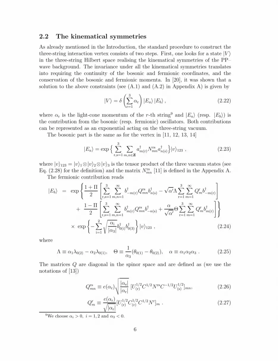
As already mentioned in the Introduction, the standard procedure to construct thethree-string interaction vertex consists of two steps. First, one looks for a state |V 〉in the three-string Hilbert space realising the kinematical symmetries of the PP–wave background. The invariance under all the kinematical symmetries translatesinto requiring the continuity of the bosonic and fermionic coordinates, and theconservation of the bosonic and fermionic momenta. In [20], it was shown that asolution to the above constraints (see (A.1) and (A.2) in Appendix A) is given by
|V 〉 = δ
(3∑
r=1
αr
)|Ea〉 |Eb〉 , (2.22)
where αr is the light-cone momentum of the r-th string9 and |Ea〉 (resp. |Eb〉) isthe contribution from the bosonic (resp. fermionic) oscillators. Both contributionscan be represented as an exponential acting on the three-string vacuum.
The bosonic part is the same as for the vertex in [11, 12, 13, 14]
|Ea〉 = exp{ 3∑
r,s=1
∑
m,n∈Z
a†m(r)Nrsmna
†n(s)
}|v〉123 , (2.23)
where |v〉123 = |v〉1⊗|v〉2⊗|v〉3 is the tensor product of the three vacuum states (seeEq. (2.28) for the definition) and the matrix N rs
mn [11] is defined in the Appendix A.The fermionic contribution reads
|Eb〉 = exp
1 + Π
2
3∑
r,s=1
∞∑
m,n=1
b†−m(r)Qrsmnb
†n(s) −
√α′Λ
3∑
r=1
∞∑
m=1
Qrmb
†−m(r)
+1 − Π
2
3∑
r,s=1
∞∑
m,n=1
b†m(r)Qrsmnb
†−n(s) +
α√α′Θ
3∑
r=1
∞∑
m=1
Qrmb
†m(r)
× exp
{−
2∑
i=1
√αi
|α3|b†0(i)b
†0(3)
}|v〉123 , (2.24)
where
Λ ≡ α1λ0(2) − α2λ0(1), Θ ≡ 1
α3(θ0(1) − θ0(2)), α ≡ α1α2α3 . (2.25)
The matrices Q are diagonal in the spinor space and are defined as (we use thenotations of [13])
Qrsmn ≡ e(αr)
√√√√ |αs||αr|
[U1/2(r) C
1/2N rsC−1/2U1/2(s) ]mn, (2.26)
Qrm ≡ e(αr)√
|αr|[U
1/2(r) C
1/2(r) C
1/2N r]m . (2.27)
9We choose αi > 0, i = 1, 2 and α3 < 0.
6

As vacuum state |v〉, we choose the state of minimal (zero) energy, which is anni-hilated by all annihilation modes
an(r)|v〉r = 0 , bn(r)|v〉r = 0 ∀n. (2.28)
This choice of vacuum represents the main difference between the proposals in[19, 20] and [11, 12, 13, 14]10. Notice that the last line of (2.24) is just a rewritingof the zero–mode structure proposed in [19]. In [19] the idea to construct the vertexon the vacuum (2.28) was suggested by the study of a Z2 symmetry present inthe supergravity background. The structure of (2.24) in the b0 Hilbert space isthe origin of the differences between the two vertices. This structure can also beunderstood in a different way by considering the path integral treatment of thefermionic “zero–modes” b0. In Eq. (2.24) these are treated on the same footing asall the other modes. This is a very natural approach in the PP–wave backgroundbecause b0 is not really a zero–mode, but it is an harmonic oscillator exactly as thestringy modes (the only difference is that its energy is just µ and is independentof α′). On the contrary in [11, 12, 13, 14] the (θ0, λ0) sector has been treated inthe same way as in flat space. Thus in their case |Eb〉 has the same structurefound in the flat space vertex [18]. In particular it contains an explicit δ–function(∑
r λ0(r)) imposing a selection rule: string amplitudes are zero, unless the externalstates soak up the fermions present in the δ–function. From the path integral pointof view this result is natural only in flat space. In this case, in fact, the λ0’s aregenuine zero–modes appearing only in the measure and can not be saturated bythe weight factor exp (iS). This yields a δ–function enforcing a selection rule inthe amplitudes. In the PP–wave case, on the contrary, all modes have a non–vanishing energy, thus one does not expect any selection rule. The vertex (2.24)exactly realizes this expectation, since it enforces the fermionic constraints with anexponential structure also in the b0 sector, instead of imposing the constraint as inflat space: δ(
∑r λ0(r)) →
∑r λ0(r)|0〉123.
As a final remark, we would like to mention that an alternative approach canbe used to derive (2.23) and (2.24). We have verified that this form of the ver-tex follows uniquely from a path integral treatment [35]. We made use of the factthat the system may be considered as a sum of harmonic oscillators, in particularwe treated the fermionic zero mode oscillators on the same footing as all others.Boundary conditions are conveniently specified in a coherent state basis, equivalentto the Bargmann-Fock formalism [36, 37]. We have also explicitly verified that thiskinematical vertex in fact satisfies the complete set of kinematical constraints. Inthe path integral formalism the prefactor originates from the fact that the light conegauge and κ gauge conditions cannot be imposed at the point on the world sheet
10In [11, 12, 13, 14] the fermionic part of the vertex is built by acting on the ground state |0〉
an(r)|0〉r = 0 ∀n , bn|0〉 = 0 ∀n 6= 0, θ0|0〉 = 0 . (2.29)
7

where the 3 strings join. Ignoring this complication yields exactly the kinematicalpart of the vertex. Rather than attempting to derive the prefactor from first prin-ciples we follow the standard approach of seeking a supersymmetric completion asdescribed below.
2.3 Supersymmetric completion
In order for the full supersymmetry algebra to be satisfied at the interacting level,the kinematical vertex has to be completed with a polynomial prefactor. An analo-gous construction also applies for the dynamical supersymmetry generators Q andQ. Of course, the addition of the prefactor should not change the properties of thevertex under the kinematical symmetries. As for the dynamical symmetries, if wedefine the full hamiltonian and dynamical charges as |H3〉, |Q3a〉 and |Q3a〉 11, theyhave to satisfy
3∑
r=1
Q(r)a|Q3b〉 +3∑
r=1
Q(r)b|Q3a〉 = 2δab|H3〉 , (2.30)
3∑
r=1
Q(r)a|Q3b〉 +3∑
r=1
Q(r)b|Q3a〉 = 2δab|H3〉 , (2.31)
3∑
r=1
Q(r)a|Q3b〉 +3∑
r=1
Q(r)b|Q3a〉 = 0 . (2.32)
To our knowledge there is no way to derive the prefactor from first principles, thestandard approach being to write a suitable ansatz and then check that it is invariantunder all symmetries [17, 18]. To proceed further, some physical inputs are thenrequired. In [38] a supersymmetric completion of the kinematical vertex (2.22) hasbeen obtained by requiring the continuity in the flat space µ → 0 limit. This forcesto assign an even Z2 parity to the state |0〉 (2.29). In this case the string vacuumhas to be Z2–odd because |v〉 and |0〉 have opposite parity [19]. Correspondingly,the prefactor proposed in [38] is also Z2–odd, ensuring the Z2–invariance of theinteraction vertex. This vertex has been shown in [39] to be equivalent to thatof [11, 12, 14].
Here we present a different approach: following the gauge theory intuition, thevacuum state of the string Fock space is defined to be even under the discrete Z2
symmetry. Thus we are led to give up the continuity of the flat space limit µ → 0for the string interaction. Also in this case it is possible to build a string vertex thatis invariant under the Z2 transformation. In this case, this symmetry is realizedexplicitly, i.e. both the interaction and the vacuum state are Z2 invariant at thesame time. A very simple way to realize the supersymmetry algebra is to act on the
11For the relation between these states and the corresponding interaction operators, see forexample Eq.(3.12) of [11]
8

kinematical vertex with the free part of the hamiltonian and the dynamical charges
|H3〉 =3∑
r=1
Hr|V 〉 , |Q3a〉 =3∑
r=1
Qra |V 〉 , |Q3a〉 =3∑
r=1
Qra |V 〉 . (2.33)
With this ansatz the relations (2.30) and (2.32) are a direct consequence of thefree–theory algebra (2.19)–(2.20)12. It only remains to check that the full ansatzstill satisfies the kinematical constraints. To this purpose we need the explicitexpressions for the prefactors in (2.33) and to prove that the various constituentscommute with the constraints in (A.1), (A.2). Commuting the annihilation modesin H and Q through the kinematical vertex, we obtain
|H3〉 = −α′
α(1 − 4µαK)
[1
4(K2 + K2) +
1 + Π
2WΛYΛ +
1 − Π
2WΘYΘ
]|V 〉 ,
|Q3a〉 = − α′√
2α(1 − 4µαK) KIγI
ab (YΛ − YΘ)b |V 〉 , (2.34)
|Q3a〉 = −i α′√
2α(1 − 4µαK) KIγI
ab (YΛ + YΘ)b |V 〉 ,
where K = −(1/4)BΓ−1B (see Appendix A for the definition of the matrix Γ).This remarkably simple form has a very similar structure to what was proposed inthe string bit formalism [40, 41, 42, 27]. As in [11], the contribution of the bosonicoscillators is contained in
K = K0 + K+ + K− , K = K0 + K+ −K− . (2.35)
where
K0 = P − iµα
α′R =
√2
α′√µα1α2(
√α1a
†(2)0 −√
α2a(1)†0 ) , (2.36)
K+ = − 1√α′
α
1 − 4µαK
3∑
r=1
∞∑
n=1
[1
αr
(CC1/2(r) U
−1(r) N
r)n
]a†n(r) , (2.37)
K− = − i√α′
α
1 − 4µαK
3∑
r=1
∞∑
n=1
[1
αr(CC
1/2(r) N
r)n
]a†−n(r) . (2.38)
Similarly, for the fermionic oscillators we introduced the operators YΛ and YΘ
YΛ =1 + Π
2
Λ − α√
α′
3∑
r=1
e(αr)√|αr|
(C1/2(r) C
1/2U−1/2(r) N r)n
1 − 4µαKb†n(r)
, (2.39)
YΘ =1 − Π
2
αα′Θ +
α√α′
3∑
r=1
e(αr)√|αr|
(C1/2(r) C
1/2U−1/2(r) N r)n
1 − 4µαKb†−n(r)
,
12One has to set T = 0 to get the usual commutation relations and use the fact that thekinematical vertex is annihilated by generators J ij and J i′j′ , since it is SO(4)× SO(4) invariant.
9
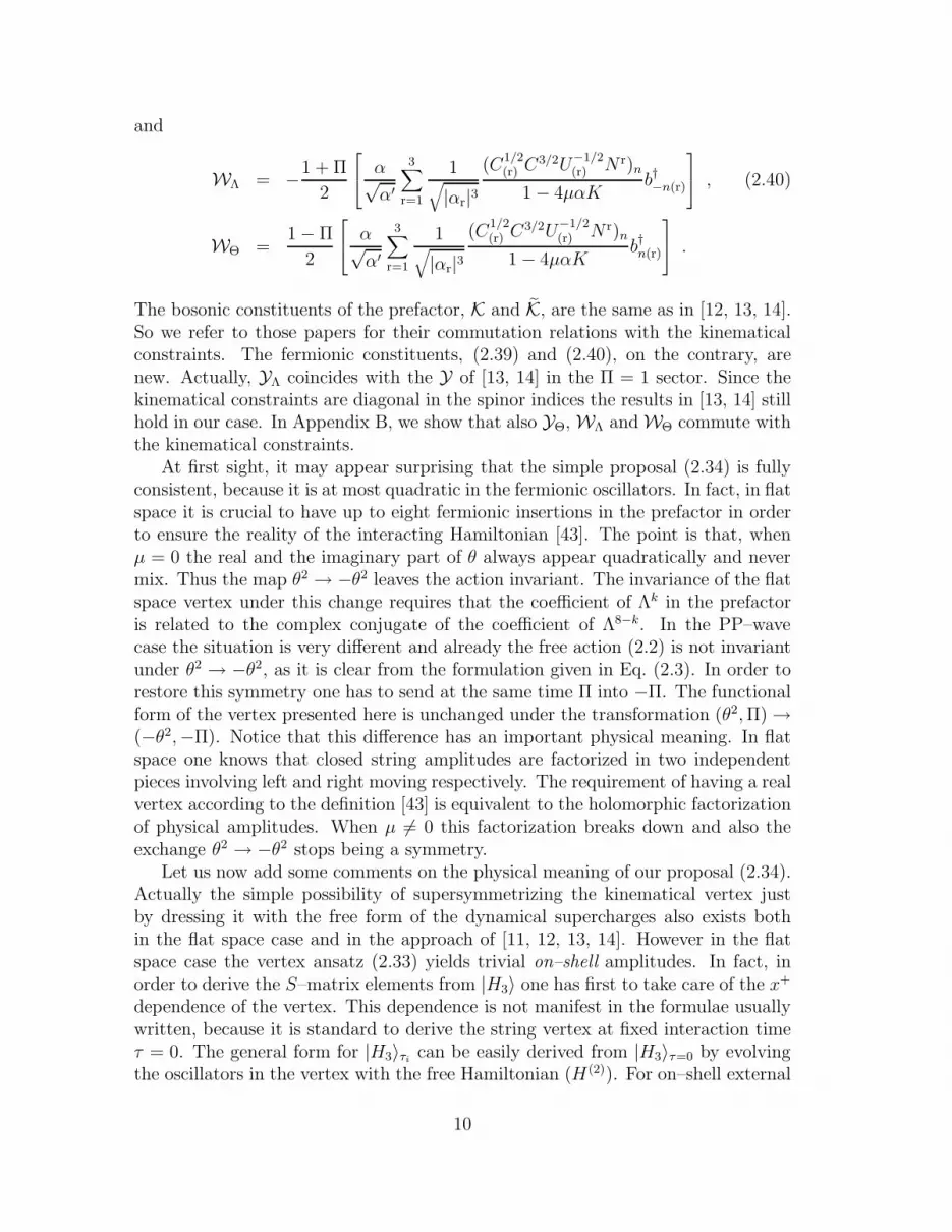
and
WΛ = −1 + Π
2
α√α′
3∑
r=1
1√|αr|3
(C1/2(r) C
3/2U−1/2(r) N r)n
1 − 4µαKb†−n(r)
, (2.40)
WΘ =1 − Π
2
α√
α′
3∑
r=1
1√|αr|3
(C1/2(r) C
3/2U−1/2(r) N r)n
1 − 4µαKb†n(r)
.
The bosonic constituents of the prefactor, K and K, are the same as in [12, 13, 14].So we refer to those papers for their commutation relations with the kinematicalconstraints. The fermionic constituents, (2.39) and (2.40), on the contrary, arenew. Actually, YΛ coincides with the Y of [13, 14] in the Π = 1 sector. Since thekinematical constraints are diagonal in the spinor indices the results in [13, 14] stillhold in our case. In Appendix B, we show that also YΘ, WΛ and WΘ commute withthe kinematical constraints.
At first sight, it may appear surprising that the simple proposal (2.34) is fullyconsistent, because it is at most quadratic in the fermionic oscillators. In fact, in flatspace it is crucial to have up to eight fermionic insertions in the prefactor in orderto ensure the reality of the interacting Hamiltonian [43]. The point is that, whenµ = 0 the real and the imaginary part of θ always appear quadratically and nevermix. Thus the map θ2 → −θ2 leaves the action invariant. The invariance of the flatspace vertex under this change requires that the coefficient of Λk in the prefactoris related to the complex conjugate of the coefficient of Λ8−k. In the PP–wavecase the situation is very different and already the free action (2.2) is not invariantunder θ2 → −θ2, as it is clear from the formulation given in Eq. (2.3). In order torestore this symmetry one has to send at the same time Π into −Π. The functionalform of the vertex presented here is unchanged under the transformation (θ2,Π) →(−θ2,−Π). Notice that this difference has an important physical meaning. In flatspace one knows that closed string amplitudes are factorized in two independentpieces involving left and right moving respectively. The requirement of having a realvertex according to the definition [43] is equivalent to the holomorphic factorizationof physical amplitudes. When µ 6= 0 this factorization breaks down and also theexchange θ2 → −θ2 stops being a symmetry.
Let us now add some comments on the physical meaning of our proposal (2.34).Actually the simple possibility of supersymmetrizing the kinematical vertex justby dressing it with the free form of the dynamical supercharges also exists bothin the flat space case and in the approach of [11, 12, 13, 14]. However in the flatspace case the vertex ansatz (2.33) yields trivial on–shell amplitudes. In fact, inorder to derive the S–matrix elements from |H3〉 one has first to take care of the x+
dependence of the vertex. This dependence is not manifest in the formulae usuallywritten, because it is standard to derive the string vertex at fixed interaction timeτ = 0. The general form for |H3〉τi
can be easily derived from |H3〉τ=0 by evolvingthe oscillators in the vertex with the free Hamiltonian (H(2)). For on–shell external
10

states the usual recipe [15, 16] is that the S–matrix is derived by integrating overthe interaction time
Aphys. =∫ ∞
−∞123〈state|H3〉τ dτ = δ
(3∑
r=1
Hr2
)
123〈state|H3〉τ=0 . (2.41)
This shows that one has the possibility to redefine the off–shell vertices by addingterms with the structure of (2.33), but these terms will not contribute to the S–matrix. In the present case one is not interested in S-matrix elements but in matrixelements of the interaction hamiltonian, and these are picked out by the short timetreatment. In any case the S-matrix energy conservation would correspond to asimilar delta function on conformal dimensions on the field theory side, which isclearly unreasonable.
Further evidence supporting (2.33) and the interpretation just proposed comesfrom what is known of supergravity on AdS5 × S5. The vertex derived here shouldplay the same role as the cubic bulk couplings derived from the compactification ofIIB theory on AdS5×S5 [44]. We should then be able to compare the results of our|H3〉 for supergravity states with the (leading order in J) results obtained in AdS5×S5. It is interesting to notice that the bulk vertices obtained in [44] for 3 scalarsare indeed proportional to ∆1 + ∆2 − ∆3, exactly as the string 3–point functionsderived from |H3〉 (2.33). It is also important to notice that in AdS/CFT this factoris necessary to have meaningful 3–point functions dual to extremal correlators (∆1+∆2 = ∆3) [45]. Indeed, in the extremal case the integration over the AdS5 positionof the bulk vertex is divergent [46] and cancels exactly the factor ∆1 + ∆2 − ∆3 inthe bulk vertex, leaving the expected field theory result. This pattern seems to bea general feature of extremal correlators and not just a peculiarity of correlatorsamong chiral primaries13. Thus it is natural to expect that the 3–point verticesamong supergravity BMN states both in AdS and in the PP–wave backgroundare proportional to the
∑rH
r2. Notice that the vanishing of the energy conserving
amplitudes is also one of the requirements of the holographic string field theoryproposed in [48, 49]14.
As a final comment let us come back to the prescription for deriving the physi-cally meaningful data from |H3〉. In the next section, we will check that the idea [10]of comparing field theory results with the interacting hamiltonian matrix elementdivided by
∑rH
r2 (see (3.1)) works very well at leading order in λ′. This proposal
is very natural since it is strongly reminiscent of the formula obtained in quantummechanics describing the first order transition probability induced by a perturba-tion acting for a very short time. It is then likely that this prescription has to becorrected in order to check the duality at higher orders in λ′. It would be inter-esting to see whether the analogy with quantum mechanics can be helpful in thisgeneralization, following for instance the ideas in [50]. One can say that in the
13See for instance [47], where the correlator between one scalar and two spinors was considered.14In [48, 49] it was also noticed that the fermionic action can be made SO(8) symmetric by the
redefinition (θ1, θ2) → (θ1, Πθ2). This symmetry is satisfied by our vertex (2.34).
11

PP–wave/CFT duality we are in the opposite situation with respect to the usualAdS/CFT computations: we have an explicit and complete expressions for the 3–states coupling (while in AdS it is a challenging computation even to derive some ofthese couplings), but we do not have a completely clear prescription to relate themto the field theory side. One needs the analogue of the prescription in [32, 33].Usually in AdS computations one uses the bulk–to–boundary propagator, but nosimple analogue of this ingredient has been found in the PP–wave case so far.
3 Comparison between string and field theory re-
sults
The PP-wave vertex discussed in the previous section is in agreement with theproposal of [10] for comparing the string theory interaction with the three–pointcorrelators of N = 4 SYM theory. This proposal is motivated by the standardAdS/CFT dictionary between bulk and boundary correlation functions [32]: sincethe light-cone interaction vertex on the PP-wave in (2.33) can be understood asthe generating functional of the correlation functions among string states, it isnatural to put it in correspondence with the correlation functions of the dual fieldtheory operators. A more general motivation for this proposal was indeed providedin [48, 49] by considering the Penrose limit of the AdS/CFT bulk–to–boundaryformula of [32]. A specific prescription was proposed in [10] for the leading orderin 1/µ
(〈1| ⊗ 〈2| ⊗ 〈3|) |H3〉∑r (Hr
2)= Cijk , (3.1)
where Cijk is the coefficient appearing in the correlator among three BMN operatorsof R-charge Ji
〈Oi(xi)Oj(xj)Ok(xk)〉 =Cijk
(xij)∆
(0)i
+∆(0)j
−∆(0)k (xik)
∆(0)i
+∆(0)k
−∆(0)j (xjk)
∆(0)j
+∆(0)k
−∆(0)i
,
(3.2)and depends on the quantum numbers Ji and on the value of the BMN phase factors.Notice that in (3.2) we write the canonical dimensions ∆(0) of the BMN operators.In fact we will be concerned only with the comparison at the leading order in 1/µ,i.e. at the tree level in the field theory.
The proposal (3.1) has been questioned in the subsequent literature [21, 22],and other conjectures were put forward [23, 24, 25, 28]. The main argument whichshould invalidate (3.1) is the appearance of a mixing between single and multi-traceBMN operators at the genus-one order g2 = J2/Nc of the graph expansion [51, 52].This mixing affects the tree–level evaluation of the field theory correlators (3.2).Thus, if taken into account in the dictionary (3.1), it would spoil the agreementwith the string theory results. We notice however that similar issues appear alreadyin the usual AdS/CFT correspondence for extremal correlators [45] (see also [53]).
12
For these correlators the mixing is enhanced and should in principle be taken intoaccount in the comparison with the supergravity calculations. Actually, as wasshown in [45], this is not the case, and one gets agreement between single–traceextremal correlators and three-point functions of supergravity on AdS5×S5, withoutinvoking any mixing. Moreover, following the arguments of [54], the identificationbetween the number of traces and the number of string states should be valid as longas the SYM operators are not too “big”. A simple quantitative characterization ofbig operators can be derived by realizing that overlap between single and double
traces is of order√JJ ′(J − J ′)/N . If this is not negligible in the planar limit, then
we are dealing with big operators. This shows that, even if the BMN operators are
made of an infinite number of fields, they are never big since√JJ ′(J − J ′)/N ∼
g2/√J → 0. Thus the usual rules of AdS/CFT should apply: the single trace
operators should correspond to the elementary string states while the multi-traceoperators should be bound states and so they are not present in the spectrum ofthe free string.
Further support to this picture comes from the fact that computations withmulti–trace operators in the AdS/CFT correspondence seem to be related to stringinteractions which are non–local on the world sheet [55, 56]. Since the leading corre-lators in the BMN limit (1.1) are extremal correlators (for the supergravity modes)or non-BPS deformations of these (for the string modes), it is natural to expectthat the same features are shared by the limiting PP-wave/CFT correspondenceand that the local vertex (2.34) has to be compared with single–trace correlators.
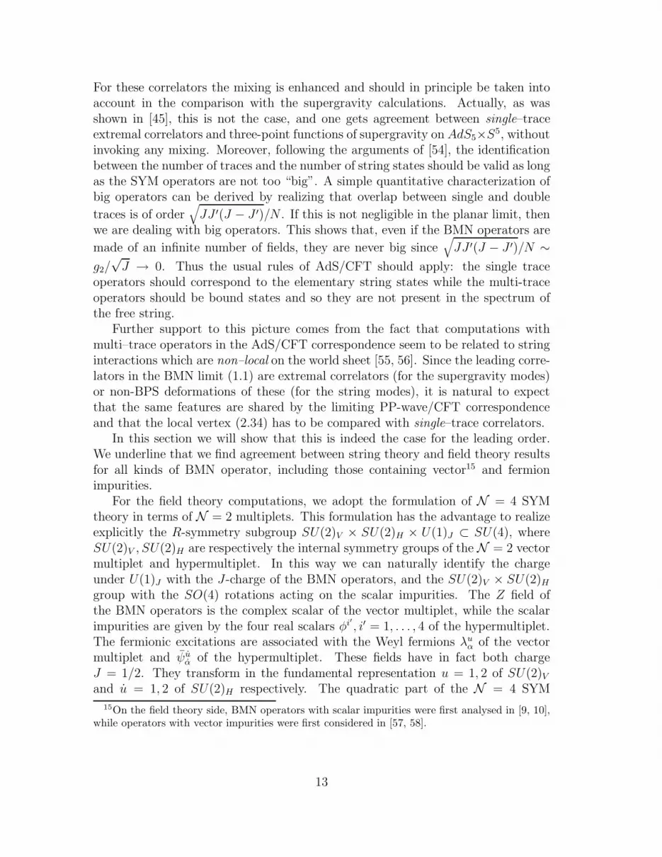
In this section we will show that this is indeed the case for the leading order.We underline that we find agreement between string theory and field theory resultsfor all kinds of BMN operator, including those containing vector15 and fermionimpurities.
For the field theory computations, we adopt the formulation of N = 4 SYMtheory in terms of N = 2 multiplets. This formulation has the advantage to realizeexplicitly the R-symmetry subgroup SU(2)V × SU(2)H × U(1)J ⊂ SU(4), whereSU(2)V , SU(2)H are respectively the internal symmetry groups of the N = 2 vectormultiplet and hypermultiplet. In this way we can naturally identify the chargeunder U(1)J with the J-charge of the BMN operators, and the SU(2)V × SU(2)H
group with the SO(4) rotations acting on the scalar impurities. The Z field ofthe BMN operators is the complex scalar of the vector multiplet, while the scalarimpurities are given by the four real scalars φi′, i′ = 1, . . . , 4 of the hypermultiplet.The fermionic excitations are associated with the Weyl fermions λu
α of the vectormultiplet and ψu
α of the hypermultiplet. These fields have in fact both chargeJ = 1/2. They transform in the fundamental representation u = 1, 2 of SU(2)V
and u = 1, 2 of SU(2)H respectively. The quadratic part of the N = 4 SYM
15On the field theory side, BMN operators with scalar impurities were first analysed in [9, 10],while operators with vector impurities were first considered in [57, 58].
13

lagrangian is16
L =1
g2Y M
Tr[14FmnFmn +DmZD
mZ +1
2Dmφ
i′Dmφi′ (3.3)
+ λuDmσmλu + ψuDmσ
mψu],
where the covariant derivative is Dm ≡ ∂m + [Am, ·]. The Green function for thecomplex field Z is then G(x− x′) = g2
Y M/4π2(x− x′)2. The BMN operator associ-
ated to the string theory vacuum is
OJvac(x) =
1√JNJ
Tr[ZJ](x) , (3.4)
with N = g2Y MNc/4π
2. For single impurities we define
OJi (x) = N1Tr
[DiZZ
J](x), OJ
i′(x) = N1Tr[φi′ZJ
](x), (3.5)
OJα = N1Tr
[λαZ
J](x), OJ
α = N1Tr[ψαZJ
](x), (3.6)
with N1 = 1/√
2NJ+1. The first operator in (3.6) corresponds to the insertion ofa string fermionic oscillator of chirality Π = 1, while the second to the chiralityΠ = −1. For double impurities we define (in the dilute gas approximation)
OJji,m(x) = N2
J∑l=0
ql Tr[DjZZ
lDiZZJ−l](x), (3.7)
OJαβ,m(x) = N2
J∑l=0
ql Tr[λαZ
lλβZJ−l](x), (3.8)
with N2 = (1/2)√
(J + 1)NJ+2. To simplify notations, in the above formulae the
BMN phase factor is ql = exp(2πim l+1
J+2
), and the R–symmetry indices of the
fermions are suppressed. The barred operators are defined according to the rulessuggested by the radial quantization [59]. For example, for double–vector impuritieswe define17
OJij,m(x) ≡ N2 (r2)J+2
J∑
l=0
qlTr[(CikDk r
2Z)Z l(CjhDh r2Z)ZJ−l
](x) , (3.9)
where Cik(x) = δik − 2xixk/r2 is the tensor associated to the conformal inversion
transformation x′i = xi/r2, with ∂x′i/∂xk = Cik(x)/r
2. For fermionic impurities wedefine
OJα(x) ≡ N1(r
2)J+3/2Tr[(λ 6 x)αZJ)
](x) , (3.10)
OJα(x) ≡ N1(r
2)J+3/2Tr[(ψ 6x)αZ
J)](x) , (3.11)
16We adopt the following convention for the sigma matrices: σm = (iσc,1) and σm = (−iσc,1),where σc are the Pauli matrices.
17M. Petrini, R. Russo and A. Tanzini are happy to acknowledge collaboration with C.S. Chuand V.V. Khoze about the definition of the barred operators in field theory. See also [30].
14
with 6 x ≡ σααk xk/r, 6x ≡ σk
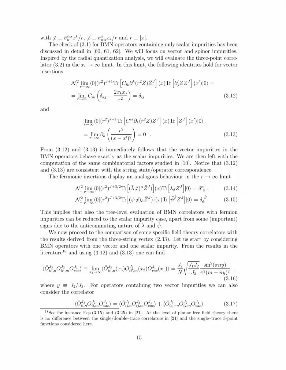
ααxk/r and r ≡ |x|.The check of (3.1) for BMN operators containing only scalar impurities has been
discussed in detail in [60, 61, 62]. We will focus on vector and spinor impurities.Inspired by the radial quantization analysis, we will evaluate the three-point corre-lator (3.2) in the xi → ∞ limit. In this limit, the following identities hold for vectorinsertions
N 21 lim
r→∞〈0|(r2)J+1Tr
[Cik∂
k(r2Z)ZJ](x)Tr
[∂′jZZ
J](x′)|0〉 =
= limr→∞
Cik
(δkj −
2xkxj
r2
)= δij (3.12)
and
limr→∞
〈0|(r2)J+1Tr[Cik∂k(r
2Z)ZJ](x)Tr
[ZJ](x′)|0〉
= limr→∞
∂k
(r2
(x− x′)2
)= 0 . (3.13)
From (3.12) and (3.13) it immediately follows that the vector impurities in theBMN operators behave exactly as the scalar impurities. We are then left with thecomputation of the same combinatorial factors studied in [10]. Notice that (3.12)and (3.13) are consistent with the string state/operator correspondence.
The fermionic insertions display an analogous behaviour in the r → ∞ limit
N 21 lim
r→∞〈0|(r2)J+3/2Tr
[(λ 6 x)αZJ)
](x)Tr
[λβZ
J]|0〉 = δα
β , (3.14)
N 21 lim
r→∞〈0|(r2)J+3/2Tr
[(ψ 6x)αZ
J)](x)Tr
[ψβZJ
]|0〉 = δ β
α . (3.15)
This implies that also the tree-level evaluation of BMN correlators with fermionimpurities can be reduced to the scalar impurity case, apart from some (important)signs due to the anticommuting nature of λ and ψ.
We now proceed to the comparison of some specific field theory correlators withthe results derived from the three-string vertex (2.33). Let us start by consideringBMN operators with one vector and one scalar impurity. From the results in theliterature18 and using (3.12) and (3.13) one can find
〈OJ3ii′,nO
J2ii′,mO
J1vac〉 ≡ lim
x3→∞〈OJ3
ii′,n(x3)OJ2ii′,m(x2)O
J1vac(x1)〉 =
J2
N
√J1J2
J3
sin2(πny)
π2(m− ny)2,
(3.16)where y ≡ J2/J3. For operators containing two vector impurities we can alsoconsider the correlator
〈OJ3ii,nO
J2ii,mO
J1vac〉 = 〈OJ3
ij,nOJ2ij,mO
J1vac〉 + 〈OJ3
ij,−nOJ2ij,mO
J1vac〉 (3.17)
18See for instance Eqs.(3.15) and (3.25) in [21]. At the level of planar free field theory thereis no difference between the single/double–trace correlators in [21] and the single–trace 3-pointfunctions considered here.
15

The last term in (3.17) comes from the fact that impurities with the same vectorindex can be contracted in two different ways, and the exchange of two impuritiesinduces a change of sign in the BMN phase according to the definition (3.7).
Let us now see how these results are reproduced from the µ → ∞ limit ofstring theory. Due to the form (2.33) of the prefactor, the non–trivial part of theproposal (3.1) is simply given by the coefficient Cijk. This justifies the approach of[60, 61, 62], and we can focus only on the kinematical part (2.22) of the 3–stringvertex and rewrite (3.1) as
〈i|〈j|〈k|V 〉 =Cijk
C(0)ijk
, (3.18)
where C(0)ijk =
√J1J2J3/N is the combinatorial factor of the Green function among
three vacuum operators (3.4). This factor ensures the same normalization for thetwo sides of (3.18), since the string overlap 123〈v|V 〉 is set equal to one. For thecomparison with field theory it is useful to recall the dictionary between the BMNoscillators a and those used in the previous section
an =1√2(an − ia−n) , a−n =
1√2(an + ia−n) . (3.19)
According to the string state/operator mapping, the relevant amplitude is
AIJb = 〈α1, α2, α3|aI
n(3)aJ−n(3)a
Im(2)a
J−m(2)|V 〉 (3.20)
=1
4〈α1, α2, α3|
(aI
n(3)aJn(3) + aI
−n(3)aJ−n(3) + iaI
n(3)aJ−n(3) − iaI
−n(3)aJn(3)
)
×(aI
m(2)aJm(2) + aI
−m(2)aJ−m(2) + iaI
m(2)aJ−m(2) − iaI
−m(2)aJm(2)
)|V 〉 .
We will compute the string theory amplitudes in the µ → ∞ limit by using therelation N rs
−m−n = −(U(r)NrsU(s))mn and the expansions
N32nm ∼ 2
π
ny3/2 sin(πny)
m2 − n2y2, with n,m > 0 (3.21)
U(i) ∼ n
2µαi
, U(3) ∼ −2µα3
n. (3.22)
Let us first analyze the case I = i, J = i′. The amplitude (3.20) then becomes
Aii′
b =1
4
[N32
nm −N32−n−m
]2 ∼ ysin2(πny)
π2(m− ny)2, (3.23)
where in the last step we kept only the leading term in the µ → ∞ limit. By using(3.16) this provides a first check of (3.18). If we instead take I = J = i, (3.20)becomes
Aiib =
1
2
[(N32
nm)2 + (N32−n−m)2 +
1
2(N33
nn +N33−n−n)(N22
mm +N22−m−m)
]
∼ y
π2sin2(πny)
[1
(m− ny)2+
1
(m+ ny)2
], (3.24)
16

where the two terms in the last parenthesis reproduce the r.h.s. of (3.17). Noticethat the terms proportional to N33 and N22 do not contribute at the leading order.
We now pass to the analogous correlation functions for BMN operators withfermionic impurities. By using (3.14) and (3.15) their evaluation is reduced to thesame combinatorics as for the scalar impurities case. Thus we have
〈OJ3
αβ,nOJ2
αβ,mOJ1〉 = −J2
N
√J1J2
J3
sin2(πny)
π2(m− ny)2, (3.25)
which coincides with (3.16). For operators containing spinors of the same flavourwe can also consider
〈OJ3αα,nO
J2αα,mO
J1vac〉 = 〈OJ3
αβ,nOJ2αβ,mO
J1vac〉 − 〈OJ3
αβ,−nOJ2αβ,mO
J1vac〉 . (3.26)
Notice that due to the fermionic nature of the impurities one gets a relative minussign in (3.26) with respect to (3.17).
The string amplitudes related to these correlators can be easily computed from(2.24) by using the dictionary
bn =1√2(bn + b−n) , b−n = − i√
2(bn − b−n) . (3.27)
In this case the relevant amplitude is
Aabf = 〈α1, α2, α3|ban(3)b
b−n(3)b
am(2)b
b−m(2)|V 〉 = −1
4
[(Q23
mn)2 + (Q32nm)2 − 2Q23
mnQ32nm
].
(3.28)By using now (2.26) we get at the leading order in 1/µ
Q32nm ∼ −N32
nm , Q23mn ∼ −N23
−m−n . (3.29)
This shows that in the large µ limit (3.28) takes the same form as (3.23), in agree-ment with the field theory result. Also the correlator (3.26) is reproduced by thecorresponding string amplitude
Aaaf = 〈α1, α2, α3|ban(3)b
a−n(3)b
am(2)b
a−m(2)|V 〉 =
[−Q33
nnQ22mm +Q23
mnQ32nm
]∼ N23
−m−nN32nm.
(3.30)This is again in agreement with the field theory result since
N23mnN
32nm ∼ − y
π2sin2(πny)
[1
(m− ny)2− 1
(m+ ny)2
]. (3.31)
Notice that the agreement in the fermion sector crucially depends on the form ofour vertex (2.24). In fact, some fermionic amplitudes were derived also by using theproposal of [14] (see the last section of that paper). These results are quite differentfrom ours because of the different zero mode structure of their vertex and have notbeen related to any field theory result.
17
4 Conclusions
In this paper we presented a supersymmetric string vertex that completes the con-struction of [19, 20]. We argued that this vertex has all the necessary propertiesto describe the local interaction of three strings in the maximally supersymmetricPP–wave background. We also observe that our vertex might be seen as an explicitrealization of ”holographic string field theory” of [48, 49]. A different supersym-metric completion of the construction of [19, 20] was provided in [38] by requiringthe continuity of the flat space limit µ → 0. This vertex has been shown in [39] tobe equivalent to that in [11, 12, 13, 14].
Let us summarize here the main features of our proposal, since it is ratherdifferent from the one of [11, 12, 13, 14]. First, from the very beginning of ourconstruction we gave up the idea of smoothly connecting our vertex to the oneof flat space [18] when the parameter controlling the curvature of the backgroundis sent to zero (µ → 0). One can argue that this limit is singular due to theenhancement of the isometry group that takes place exactly at the point µ = 0.One consequence of this fact is that for all values of µ the modes a0 and b0 of thestring expansion are harmonic oscillators and only for µ = 0 one has to deal withgenuine zero–modes p0 and λ0. For this reason we treated the modes a0 and b0 onthe same footing as all the other modes in the string expansion. Moreover, sincewe do not expect any δ–function on the energies in the matrix elements, there isno reason why the string 2–point functions should be diagonal at all (perturbative)orders. It is an open possibility that the identification between string states andsingle–trace field theory operators originally proposed in [5] is actually valid alsoat higher orders. We took this point of view, since it allows to keep the physicalintution of identifying the closed string with the “long” BMN trace made out of Z’sand the string excitations with the BMN impurities.
In the second part of the paper we used the proposal of [10] and compared thematrix elements of our 3–string vertex with the corresponding field theory corre-lators at leading order in λ′. The two results match in all cases. Our analysisconcerns 3–point correlators of BMN operators with double insertions of scalar,vector and fermion impurities and provide a test for the various building blocks ofour string vertex in the µ → ∞ limit. The proposal of [10] has been criticized inthe subsequent literature also from the field theory point of view. It was arguedthat the presence of mixing between single–trace and multi–trace BMN operatorshad to be taken into account also at the level of planar computations. This affectsthe tree–level expression of the 3–point correlators and thus spoils the agreementwith string theory results. However, the inclusion of this mixing in the comparisonwith bulk amplitudes seems a rather unnatural procedure from the point of viewof the AdS/CFT correspondence. In fact, as we discussed in Section 3, a similarsituation appears also in the standard AdS/CFT duality in the case of extremalcorrelators. There the results found in AdS5 × S5 supergravity agree with fieldtheory computations without invoking the mixing.
18

Let us finally comment on the other methods for comparing field and stringtheory that have been proposed [23, 24, 25, 28]. There are basically two distinctapproaches. In the first one, the idea is to interpret the relation ∆ − J = H asan operator equation and to identify the matrix elements of the string Hamiltonianwith those of ∆ − J between multi–trace operators. Technically this requires amodification of the dictionary between string states and field theory operators.However this new map contains several free parameters that are fixed by imposing
the matching with the string theory results. In the more recent literature, thishas been done by using the string vertex proposed by [11, 12, 13, 14]. However,it is possible to choose a different basis in field theory in order to get agreementwith the results of the string vertex (2.33) presented here19. In order to get a non–trivial check in this approach one is obliged to go to higher orders in the parametercontrolling the genus expansion. At this level the computations are rather involved.Moreover, at subleading order only the field theory answer is known and is comparedwith results extrapolated from the tree–level string vertex by using the quantummechanical perturbation theory. Genuine computations on the torus for the massof string states remain a challenging open problem. Another approach advocatedin [28] is to fix a new dictionary by taking, on the field theory side, the operators withdefinite conformal properties. The comparison with string theory has been done byusing the kinematical vertex of [20] supplemented by a prefactor phenomenologicallyderived by the inputs coming from field theory. This prefactor is different fromthe one presented here, because it treats the an modes with positive and negativefrequency in a different way. Actually in string computations, like for instance thatof the action of Q on the kinematical vertex (2.34), both kinds of modes are treatedon the same footing and appear always together in the combinations K and K.
The advantage of the setup presented here, beyond its semplicity, is that thereare no “free parameters” that can be modified and each computation represents atest for the proposal. It would be very interesting to see whether the agreementis preserved when operators with more than two impurities are considered. Themain limitation of our approach is that it only considers the leading order in λ′.Generalizing it beyond this approximation is an important open problem. On theother hand, since there are two different proposals for the 3–string vertex both sat-isfying the same super–algebra, it is also important to analyze again the derivationof |H3〉. Clearly to understand the origin of the differences it is necessary to use inthe derivation a dynamical principle (like the path integral) instead of symmetryarguments. Work is in progress along these directions.
Acknowledgments
We would like to thank C. Bachas, C.S. Chu and C. Kristjansen for interestingdiscussions and suggestions. This work is supported in part by EU RTN contracts
19See for example the first version of [23].
19

HPRN-CT-2000-00122 and HPRN-CT-2000-00131. M.P., R.R. and A.T. are sup-ported by European Commission Marie Curie Postdoctoral Fellowships.
Appendix A: Definitions
In this Appendix we recall some of the definitions we use in the paper (we referto [13] for a more detailed list of formulae and identities). Let us start with themode expansion of the kinematical contraints
xm(3) = −∞∑
n=−∞
2∑
i=1
αi
α3X(i)
mnxn(i) , pm(3) = −∞∑
n=−∞
2∑
i=1
X(i)mnpn(i) , (A.1)
θm(3) = −∞∑
n=−∞
2∑
i=1
αi
α3X(i)
mnθn(i) , λm(3) = −∞∑
n=−∞
2∑
i=1
X(i)mnλn(i) , (A.2)
where the matrices X are
X(r)mn ≡
(C1/2ArC−1/2)mn , m > 0 , n > 0 ,α3
αr(C−1/2ArC1/2)−m,−n , m < 0 , n < 0 ,
− 1√2ǫrsαs(C
1/2B)m , m > 0 , n = 0 ,1 , m = 0 = n ,0 , otherwise .
(A.3)
All the quantities in the equations below are defined for m,n > 0
Cmn = mδmn ,
A(1)mn = (−1)n 2
√mnβ
π
sinmπβ
m2β2 − n2,
A(2)mn =
2√mn(β + 1)
π
sinmπβ
m2(β + 1)2 − n2,
A(3)mn = δmn,
Bm = −2
π
α3
α1α2m−3/2 sinmπβ. (A.4)
The matrices N rsmn and N r
m in the definition of the Q’s are given by
N rsmn = δrsδmn − 2
(C
1/2(r) C
−1/2A(r) T Γ−1A(s)C−1/2C1/2(s)
)
mn, (A.5)
N rs−m−n = −(U(r)N
rsU(s))mn , N rm = −(C−1/2A(r) T Γ−1B)m ,
where C(s) = δmn ω(r)m = δmn
√m2 + (µα(r)), Γ =
∑3r=1A
(r)U(r)A(r) T and finally
U(r) = C−1(C(r) − µαr1
).
20
Appendix B: Prefactor
In this Appendix we show that the fermionic constituents of the prefactor, YΘ,WΛ and WΘ, commute with the kinematical constraints (A.2). The fermionic con-stituents of the prefactor have to satisfy (the bosonic commutators are triviallyzero)
{ 3∑
r=1
∑
n∈Z
αrX(r)mnθn(r) ,YΘ
}= 0,
{ 3∑
r=1
∑
n∈Z
X(r)mnλn(r) ,YΘ
}= 0 , (B.1)
{ 3∑
r=1
∑
n∈Z
αrX(r)mnθn(r) ,WΛ(Θ)
}= 0,
{ 3∑
r=1
∑
n∈Z
X(r)mnλn(r) ,WΛ(Θ)
}= 0, (B.2)
where we expanded the fermionic constraints in oscillation modes. As usual [13, 14,20] it is convenient to split the above equations for m > 0, m < 0 and m = 0.
Consider first the anticommutators of WΛ. Since WΛ only contains b†−n oscilla-tors the non-trivial anticommutators are those with the constraints containing b−n.By using the mode expansions of θ and λ, one obtains for m > 0
{ 3∑
r=1
∞∑
n=1
X(r)mnλn(r) ,WΛ
}= − 1
2√α′
α
1 − 4µαK
3∑
r=1
1
αr
(C1/2ArC3/2N r)m = 0 (B.3)
because of Eq. (5.12) of [13]. For m < 0
{ 3∑
r=1
∞∑
n=1
αrX(r)−m−nθ−n(r) ,WΛ
}= − i√
α′α
1 − 4µαK
3∑
r=1
C1/2m
[ 1
α2r
(ArC3/2C(r)Nr)m
+µ
αr
(ArC3/2N r)m
]= 0 (B.4)
The two terms in this equation vanish because of Eq. (5.14) and (5.12) of [13].For WΘ, the situation is very similar. WΘ only contains b†n oscillators, so the
non-trivial anticommutators are
{ 3∑
r=1
∞∑
n=1
αrX(r)mnθn(r) ,WΘ
}for m > 0 ,
{ 3∑
r=1
∞∑
n=1
X(r)−m−nλ−n(r) ,WΛ
}for m < 0 ,
(B.5)which give respectively Eq. (B.3) and (B.4).
Finally we have to compute the anticommutator of YΘ. In this case also thecontribution of the zero modes has to be taken into account. For m > 0 there isonly one non-trivial anticommutator
{ 3∑
r=1
∞∑
n=0
X(r)mnλn(r) ,YΘ
}=
α
2√α′C
1/2m
[1
1 − 4µαK
3∑
r=1
(ArC1/2U−1(r) N
r)m +Bm
]= 0 .
(B.6)
21

To prove Eq. (B.6), it is convenient to rewrite U−1m(r) = Um(r) + 2µαrC
−1m . Then by
using Eq. (B.5) of [13] in the first term and Eq. (B.9) in the second, it is easy tosee that (B.6) vanishes. For m < 0 the non-trivial anticommutator reads
{ 3∑
r=1
∞∑
n=1
αrX(r)−m−nθ−n(r) ,YΘ
}=
i√α′
αα3
1 − 4µαK
3∑
r=1
1
αr
(C−1/2ArC3/2N r)m = 0,
(B.7)which is zero by Eq. (B.12) of [13]. For m = 0 the anticommutators for the zeromodes are easily checked to be zero.
References
[1] M. Blau, J. Figueroa-O’Farrill, C. Hull, and G. Papadopoulos, Class. Quant.Grav. 19, L87 (2002), hep-th/0201081.
[2] M. Blau, J. Figueroa-O’Farrill, C. Hull, and G. Papadopoulos, JHEP 01, 047(2002), hep-th/0110242.
[3] R. R. Metsaev, Nucl. Phys. B625, 70 (2002), hep-th/0112044.
[4] R. R. Metsaev and A. A. Tseytlin, Phys. Rev. D65, 126004 (2002), hep-th/0202109.
[5] D. Berenstein, J. M. Maldacena, and H. Nastase, JHEP 04, 013 (2002), hep-th/0202021.
[6] J. M. Maldacena, Adv. Theor. Math. Phys. 2, 231 (1998), hep-th/9711200.
[7] R. Penrose, in Differential Geometry and Relativity, edited by M. Chaen andM. Flato, Riedel, Dordrecht, Netherlands, 1976.
[8] R. Gueven, Phys. Lett. B482, 255 (2000), hep-th/0005061.
[9] C. Kristjansen, J. Plefka, G. W. Semenoff, and M. Staudacher, Nucl. Phys.B643, 3 (2002), hep-th/0205033.
[10] N. R. Constable et al., JHEP 07, 017 (2002), hep-th/0205089.
[11] M. Spradlin and A. Volovich, Phys. Rev. D66, 086004 (2002), hep-th/0204146.
[12] M. Spradlin and A. Volovich, JHEP 01, 036 (2003), hep-th/0206073.
[13] A. Pankiewicz, JHEP 09, 056 (2002), hep-th/0208209.
[14] A. Pankiewicz and J. Stefanski, B., (2002), hep-th/0210246.
[15] E. Cremmer and J.-L. Gervais, Nucl. Phys. B76, 209 (1974).
22

[16] E. Cremmer and J.-L. Gervais, Nucl. Phys. B90, 410 (1975).
[17] M. B. Green and J. H. Schwarz, Nucl. Phys. B218, 43 (1983).
[18] M. B. Green, J. H. Schwarz, and L. Brink, Nucl. Phys. B219, 437 (1983).
[19] C.-S. Chu, V. V. Khoze, M. Petrini, R. Russo, and A. Tanzini, (2002), hep-th/0208148.
[20] C.-S. Chu, M. Petrini, R. Russo, and A. Tanzini, (2002), hep-th/0211188.
[21] N. Beisert, C. Kristjansen, J. Plefka, G. W. Semenoff, and M. Staudacher,Nucl. Phys. B650, 125 (2003), hep-th/0208178.
[22] N. R. Constable, D. Z. Freedman, M. Headrick, and S. Minwalla, JHEP 10,068 (2002), hep-th/0209002.
[23] D. J. Gross, A. Mikhailov, and R. Roiban, (2002), hep-th/0208231.
[24] R. A. Janik, Phys. Lett. B549, 237 (2002), hep-th/0209263.
[25] J. Gomis, S. Moriyama, and J.-w. Park, (2002), hep-th/0210153.
[26] J. Gomis, S. Moriyama, and J.-w. Park, (2003), hep-th/0301250.
[27] J. Pearson, M. Spradlin, D. Vaman, H. Verlinde, and A. Volovich, (2002),hep-th/0210102.
[28] C.-S. Chu and V. V. Khoze, (2003), hep-th/0301036.
[29] G. Georgiou and V. V. Khoze, (2003), hep-th/0302064.
[30] C.-S. Chu, V. V. Khoze, and G. Travaglini, (2003), hep-th/0303107.
[31] A. Parnachev and A. V. Ryzhov, JHEP 10, 066 (2002), hep-th/0208010.
[32] S. S. Gubser, I. R. Klebanov, and A. M. Polyakov, Phys. Lett. B428, 105(1998), hep-th/9802109.
[33] E. Witten, Adv. Theor. Math. Phys. 2, 253 (1998), hep-th/9802150.
[34] J.-w. Kim, B.-H. Lee, and H. S. Yang, (2003), hep-th/0302060.
[35] R. Russo and A. Tanzini, (2004), hep-th/0401155.
[36] L. D. Faddeev, In *Les Houches 1975, Proceedings, Methods In Field Theory*,Amsterdam 1976, 1-40.
[37] C. Itzykson and J.-B. Zuber, Quantum Field Theory (McGraw–Hill, 1985).
23

[38] A. Pankiewicz, JHEP 06, 047 (2003), hep-th/0304232.
[39] A. Pankiewicz and J. Stefanski, B., (2003), hep-th/0308062.
[40] H. Verlinde, (2002), hep-th/0206059.
[41] J. Zhou, Phys. Rev. D67, 026010 (2003), hep-th/0208232.
[42] D. Vaman and H. Verlinde, (2002), hep-th/0209215.
[43] M. B. Green and J. H. Schwarz, Phys. Lett. B 122 (1983) 143.
[44] S.-M. Lee, S. Minwalla, M. Rangamani, and N. Seiberg, Adv. Theor. Math.Phys. 2, 697 (1998), hep-th/9806074.
[45] E. D’Hoker, D. Z. Freedman, S. D. Mathur, A. Matusis, and L. Rastelli, (1999),hep-th/9908160.
[46] D. Z. Freedman, S. D. Mathur, A. Matusis, and L. Rastelli, Nucl. Phys. B546,96 (1999), hep-th/9804058.
[47] A. M. Ghezelbash, K. Kaviani, S. Parvizi, and A. H. Fatollahi, Phys. Lett.B435, 291 (1998), hep-th/9805162.
[48] S. Dobashi, H. Shimada and T. Yoneya, (2002), hep-th/0209251.
[49] T. Yoneya, (2003), hep-th/0304183.
[50] N. Beisert, C. Kristjansen, J. Plefka, and M. Staudacher, (2002), hep-th/0212269.
[51] M. Bianchi, B. Eden, G. Rossi, and Y. S. Stanev, Nucl. Phys. B646, 69 (2002),hep-th/0205321.
[52] G. Arutyunov, S. Penati, A. Petkou, A. Santambrogio and E. Sokatchev, Nucl.Phys. B643, 49 (2002), hep-th/0206020.
[53] H. Liu and A. A. Tseytlin, JHEP 10, 003 (1999), hep-th/9906151.
[54] V. Balasubramanian, M. Berkooz, A. Naqvi and M. J. Strassler, JHEP 0204,034 (2002), hep-th/0107119.
[55] O. Aharony, M. Berkooz, and E. Silverstein, JHEP 08, 006 (2001), hep-th/0105309.
[56] O. Aharony, M. Berkooz, and E. Silverstein, Phys. Rev. D65, 106007 (2002),hep-th/0112178.
[57] U. Gursoy, (2002), hep-th/0208041.
24

[58] T. Klose, (2003), hep-th/0301150.
[59] S. Fubini, A. J. Hanson, and R. Jackiw, Phys. Rev. D7, 1732 (1973).
[60] Y.-j. Kiem, Y.-b. Kim, S.-m. Lee, and J.-m. Park, Nucl. Phys. B642, 389(2002), hep-th/0205279.
[61] M.-x. Huang, Phys. Lett. B542, 255 (2002), hep-th/0205311.
[62] C.-S. Chu, V. V. Khoze, and G. Travaglini, JHEP 06, 011 (2002), hep-th/0206005.
25