quantum cosmology and ads/cft
TRANSCRIPT

arX
iv:h
ep-t
h/00
0706
4v3
26
Jul 2
000
hep-th/0007064
HUTP-00/A028
Quantum Cosmology and AdS/CFT
Luis Anchordoquia,1, Carlos Nunezb,2 and Kasper Olsenb,3
aDepartment of Physics, Northeastern University
Boston, MA 02115, USA
b Department of Physics, Harvard University
Cambridge, MA 02138, USA
In this paper we study the creation of brane–worlds in AdS bulk. We first consider
the simplest case of onebranes in AdS3. In this case we are able to properly describe
the creation of a spherically symmetric brane-world deriving a general expression for
its wavefunction. Then, we sketch the AdSd+1 set–up within the context of the WKB
approximation. Finally, we comment on these scenarios in light of the AdS/CFT
correspondence.

Contents
1 Introduction 1
2 Brane–world in AdS3 3
2.1 Wheeler–DeWitt Equation . . . . . . . . . . . . . . . . . . . . . . . . . 3
2.2 Qualitative Behaviour of Wavefunctions . . . . . . . . . . . . . . . . . . 6
2.3 WKB Approximation . . . . . . . . . . . . . . . . . . . . . . . . . . . . 9
3 Brane–world in AdSd+1 11
3.1 Cosmology on the Brane . . . . . . . . . . . . . . . . . . . . . . . . . . 11
3.2 Semiclassical Corrections . . . . . . . . . . . . . . . . . . . . . . . . . . 12
4 Relation to AdS/CFT Correspondence 13
4.1 Generalities . . . . . . . . . . . . . . . . . . . . . . . . . . . . . . . . . 13
4.2 Dual Boundary Theory . . . . . . . . . . . . . . . . . . . . . . . . . . . 14
4.3 Physical Implications . . . . . . . . . . . . . . . . . . . . . . . . . . . . 16
A Appendix 19
1 Introduction
The idea that spacetime has more than four dimensions is actually quite old. Already
in the 1920’s, Kaluza suggested that gravity and electromagnetism can be interpreted
as the degrees of freedom of the metric of a five-dimensional spacetime [1]. Later,
Klein [2] gave an explanation for the fact that the extra dimension is not observed by
suggesting that the extra dimension is compact and very small. Since then the idea
has been studied from many different perspectives e.g. in Kaluza-Klein supergravity
theories and also in string theories – where more than three spatial dimensions naturally
arise but the extra dimensions are usually assumed to be of Planck size for not been
directly observable. In another direction it has been suggested [3] that spacetime can
have more than three noncompact spatial dimensions if we live on a four-dimensional
domain wall which is embedded in the higher dimensions. More recently, there has been
a renewed interest in the topic since progresses in string theories [4] have modified the
old scenario (where the extra dimensions cannot exceed the tiny scale ∼ 1 TeV−1 ∼10−19 m) suggesting that Standard Model gauge interactions could be confined to a
four-dimensional subspace – or brane–world – whereas gravity can still propagate in
the whole bulk spacetime. Actually, the possibility that part of the standard model
1
particles live in large (TeV) extra dimensions was first put forward in connection to the
problem of supersymmetry breaking in string theory [5]. These scenarios presents us
with the enticing possibility to explain some long-standing particle physics problems
by geometrical means [6, 7, 8].
In the canonical example of [6], spacetime is a direct product of ordinary four-
dimensional spacetime and a (flat) spatial d-torus of common linear size rc. Within
this simple model, the large hierarchy between the weak scale and the fundamental scale
of gravity can be eliminated. However, the hierarchy only arises in the presence of a
large volume for the compactified dimension which is very difficult to justify. A more
compelling scenario was introduced by Randall and Sundrum (herein RS). Reviving an
old idea [3], RS proposed a set–up with the shape of a gravitational condenser in which
two branes of opposite tension (which gravitationally repel each other) are stabilized
by a slab of anti-de Sitter (AdS) space [7]. In this model the extra dimension is strongly
curved, and the distance scales on the brane with negative tension are exponentially
smaller than those on the positive tension brane. Such exponential suppression can
then naturally explain why the observed physical scales are so much smaller than the
Plank scale. In further work RS found that gravitons can be localized on a brane
which separates two patches of AdS5 spacetime [8], suggesting that it is possible to
have an infinite extra dimension [9]. The question whether this scenario reproduces
the usual four-dimensional gravity beyond the Newton’s law has been analyzed [10]
and cosmological considerations of models with large extra dimensions confirms that
they are at least consistent candidates for describing our world [11]. These ideas have
raised a lot of interest in the subject and several groups have begun to work on possible
experimental signatures of the extra dimension(s) [12].
In this paper we shall discuss the creation of brane–worlds in AdS bulk. The approx-
imation scheme to be used is the minisuperspace restriction of the canonical Wheeler–
DeWitt formalism. The basic idea of this approach, commonly adopted in quantum
cosmology calculations [13], is to separate the space-like metric into “modes”, and then
insist that all the “translational” modes are “frozen out” by using the classical field
equations, leaving only the scale factor to be quantized. The outline of the paper is
as follows. We begin in section 2 by deriving a brane-big-bang in AdS3. This lower–
dimensional model provides a simple setting in which certain basic physical phenomena
can be easily demonstrated while avoiding the mathematical complexities associated
with the higher–dimensional counterparts. In section 3 we consider multi-dimensional
brane-worlds, discussing the possible cosmologies within the WKB approximation. In
section 4 we analyze the implications of the AdS/CFT correspondence to quantum
cosmology.
2
2 Brane–world in AdS3
2.1 Wheeler–DeWitt Equation
In this section we consider the creation of a onebrane in AdS3 within the frame-
work of quantum cosmology [13]. Thus the universe will initially be described by
three–dimensional Anti-de Sitter space in which onebrane bubbles can nucleate spon-
taneously. As we shall see below, these bubbles appear (classically) at a critical size
and then expand.
We thus begin by considering the action for a onebrane coupled to gravity,
Stot =Lp
16π
∫
Ωd3x
√g(
R +2
ℓ2
)
+Lp
8π
∫
∂Ωd2x
√γ K + T
∫
∂Ωd2x
√γ, (1)
where K stands for the trace of the extrinsic curvature of the boundary, γ is the
induced metric on the brane, and T is the brane tension.4 The first term is the usual
Einstein-Hilbert (EH) action with a negative cosmological constant (Λ = −1/ℓ2). The
second term is the Gibbons-Hawking (GH) boundary term, necessary for a well defined
variational problem [15]. The third term corresponds to a constant “vacuum energy”,
i.e. a cosmological term on the boundary.
We wish to consider a brane which bounds two regions of AdS3. If we further
specialize to the case of spherical symmetry [14] where
ds23 = −
(
1 +y2
ℓ2
)
dt2 +
(
1 +y2
ℓ2
)−1
dy2 + y2dφ2, (2)
the geometry is uniquely specified by a single degree of freedom, the “radius” of the
brane A(τ). The τ coordinate denotes proper time as measured along the brane-world.
The computation of the GH boundary term has now reduced to that of computing the
two non-trivial components of the second fundamental form. From Eq. (2) we find
(see Appendix for details):
Kφφ =
1
A
[
1 +A2
ℓ2+ A2
]1/2
, (3)
and
Kττ =
[
A +A
ℓ2
]
[
1 +A2
ℓ2+ A2
]−1/2
, (4)
4In our convention, the extrinsic curvature is defined as Kµν = 1/2(∇µnν +∇ν nµ), where nν is theoutward pointing normal vector to the boundary ∂Ω. Lower Greek subscripts run from 0 to 2, capitalGreek subscripts from 0 to d, and capital Latin subscripts from 0 to (d − 1). Throughout the paperwe adopt geometrodynamic units so that G ≡ 1, c ≡ 1 and h ≡ L2
p ≡ M2p , where Lp and Mp are the
Planck length and Planck mass, respectively.
3
(where the dot denote a derivative with respect to proper time). After integration by
parts the gravitational Lagrangian restricted to this minisuperspace may be identified
as,
L =Lp
2
−A arcsinh
A√
1 + A2/ℓ2
+
√
1 +A2
ℓ2+ A2
. (5)
The classical Wheeler–DeWitt Hamiltonian is now easily extracted. In order to do this
we compute the conjugate momentum to A,
p =∂L
∂A= −Lp
2arcsinh
A√
1 + A2/ℓ2
. (6)
This relation may be inverted to yield, A = −(1 + A2/ℓ2)1/2 sinh(2p/Lp), so that the
Wheeler–DeWitt Hamiltonian is
Htot ≡ pA− Ltot = −2πAT − Lp
2
√
1 +A2
ℓ2cosh(2p/Lp). (7)
Eq. (7) can be rewritten as,
Htot = −2πAT − Lp
2
√
1 +A2
ℓ2+ A2. (8)
The Hamiltonian constraint – which follows from the requirement of diffeomorphism
invariance – is Htot = 0, or equivalently,
A2 = −1 − A2
(
1
ℓ2− 16π2T
2
L2p
)
. (9)
Observe that the constraint equation is consistent with the covariant conservation of
the stress-energy tensor and reproduces the classical Einstein field equations of motion.
It is easy to see from Eq. (9) that in order to obtain a real solution we need T 6= 0.
Furthermore, the brane–world is (classically) bounded by a minimum radius
A20 =
(
−1
ℓ2+
16π2T 2
L2p
)−1
, (10)
with 16π2ℓ2T 2/L2p > 1. In other words, the brane bubbles appear classically at a critical
size and then their expansion is governed by (9). Note that as the world approaches
the minimum size the expansion tends to zero. Once the world is dynamically stable it
experiences an everlasting expansion. However, we shall soon see that quantum effects
permit well–behaved wave functions for vanishing T . With the classical dynamics of
the model understood and the Wheeler–DeWitt Hamiltonian at hand, quantization
4
is straightforward. Canonical quantization proceeds via the usual replacement p →−ih∂/∂A. Naturally, the resulting quantum Hamiltonian has a factor order ambiguity.
This factor-ordering ambiguity may be removed in a natural (though not unique) way
by demanding that the quantum Hamiltonian be Hermitian,
Htot =Lp
2
(
1 +A2
ℓ2
)1/4
cos
[
2Lp∂
∂A
](
1 +A2
ℓ2
)1/4
+ 2πAT. (11)
That this Hamiltonian is Hermitian may formally be seen by Taylor-series expansion
of the cosine. A more precise statement is that this Hamiltonian acts on the Hilbert
space of square-integrable functions defined on the half–interval [0,∞) subject to the
constraint ψ(0) = 0. This is most easily seen by noting that the Hamiltonian is
Hermitian on L2([0,∞)) only if ψ(0) = 0.5
The wave function of the brane-world is determined in the usual fashion by the
Wheeler–DeWitt equation Htotψ(A) = 0. For the special case of T = 0 we find the
following solution:
ψmn(A) = Cmn(ϕm − ϕn), (12)
with
ϕj =
(
1 +A2
ℓ2
)−1/4
exp
[
−(
j +1
2
)
π
2
A
Lp
]
. (13)
(See Fig.1. for a plot of some of these wavefunctions). Here m and n are integer valued
quantum numbers describing the internal state of the brane. Negatives values of m, n
are not normalizable and so need to be discarded, as is the case when m = n. Note
that the appropriate normalization is∫ |ψ|2dA = 1, and that ψ(0) = 0, as required. In
fact the two terms in ψmn individually satisfy the differential equation Hgravityψ = 0,
but do not individually satisfy the boundary condition. By appropriate choice of Cmn
these states may be normalized, though they are not orthogonal to one another. The
normalization constant takes the rather complicated form:
Cmn =
ℓπ
2[H0(ℓ(m+ 1/2)π/Lp) +H0(ℓ(n+ 1/2)π/Lp) − 2H0(ℓ(m+ n+ 1)π/2Lp)
−N0(ℓ(m+ 1/2)π/Lp) −N0(ℓ(n+ 1/2)π/Lp) + 2N0(ℓ(m+ n+ 1)π/2Lp)]−1/2 ,(14)
where H0(z) is the Struve function and N0(z) is Neumann’s function6. With the
wavefunctions at hand, one can calculate the mean value of the “radius” of the brane,5Here, the Hilbert space scalar-product is given by the sum over all possible configurations (i.e.
sizes) of the brane-world. Henceforth, for any operator O acting over any brane-wave-function ψj ,
< ψk|O|ψj >=∫∞
0ψ∗
k Oψj dA. In other words, A is a parameter which governs the evolution of thebrane along the null geodesic congruence of the extra dimension.
6These functions have the following respective integral representations: H0(z) = 2π
∫ 1
0sin(zt) dt√
1−t2and
N0(z) = − 2π
∫∞
1cos(zt) dt√
t2−1.
5

Figure 1: Some sample wavefunctions for T = 0 (upper is ψ2,3, middle is ψ1,2 andlower is ψ0,1).
i.e.
〈A〉 =
∫
A|ψmn|2dA∫ |ψmn|2dA
. (15)
The integral in the numerator can be evaluated exactly but involves Meijer’s G-function
G3113 and so the expression for 〈A〉 is not of much practical use (anyhow, by dimensional
analysis one would expect that this number would be of order Lp). Using numerical
integration we have found 〈A〉0,1 = 0.54, 〈A〉1,2 = 0.01 and 〈A〉2,3 = 10−3 in units of Lp
and for ℓ = 1.
2.2 Qualitative Behaviour of Wavefunctions
In this subsection we take a first look at the problem of finding solutions to the Wheeler–
DeWitt equation with T 6= 0 (in the next subsection we discuss the solutions in the
WKB approximation). The relevant equation is:
Htotψ(A) = 0 (16)
or, more explicitly
Lp
2
(
1 +A2
ℓ2
)1
4
cos
[
2Lp∂
∂A
](
1 +A2
ℓ2
)1/4
ψ + 2πTAψ = 0. (17)
After defining ϕ ≡ (1 + A2/ℓ2)1/4 ψ, and the operator
∆ ≡∞∑
n=0
(−1)n (2Lp)2n
2n!
∂2n
∂A2n, (18)
6

we see that we have to solve
∆ϕ+4πTA
Lp
√
1 + A2/ℓ2ϕ = 0. (19)
In order to gain some intuition for the behaviour of the solutions of this equation we
will look for solutions in the two limits A/ℓ ≫ 1 and A/ℓ ≪ 1. In the case A/ℓ ≫ 1,
using a trial solution of the form ϕ = eλA, we find that Eq. (19) reduces to the following
condition:
cos(2Lpλ) = −4πTℓ
Lp. (20)
This is essentially the same condition as found before. Indeed, if 16π2ℓ2T 2/L2p > 1
then λ will have pure imaginary values, leading to an oscillatory solution at infinity,
that is not acceptable since it is not normalizable (it would in any case imply a delta
function normalization, that we are not considering here) and should be something like
a “classical” solution. On the other hand, if 16π2ℓ2T 2/L2p ≤ 1, λ will have two real
solutions λ± of which one has to choose the negative one, with the same criteria of
normalizability as before.
0.2 0.4 0.6 0.8
0.02
0.04
0.06
0.08
0.1
0.12
0.14
Figure 2: Square of the wave function ψ for small values of the variable a
In order to analyze more carefully the behaviour of the wave function for A/ℓ ≪ 1,
let us consider performing the following change of variables
A→ 2Lpa. (21)
With this change of variables and after scaling ψ → ϕ as above, the Wheeler–DeWitt
equation reads:
∆ϕ+8πTa
√
1 + 4L2pa
2/ℓ2ϕ = 0, (22)
7
where
∆ =∞∑
n=0
(−1)n
(2n)!
∂2n
∂a2n. (23)
It makes sense, since the factor Lp/ℓ is small, to analyze the behaviour of this equation
for small values of the variable a and expand the square root in series.
The plot in Fig. 2 shows the behaviour, in the interval [0, 1], of the square of the wave
function |ψ|2 that solves numerically Eq.(22), where we have considered eighteen orders
of derivatives in ∆. It is observed that |ψ|2 has a maximum at A ∼ Lp as expected.
It is worth to point out that the solutions with less derivatives have similar behaviour
in the interval considered. It should be interesting to find a method to analyze the
complete series.
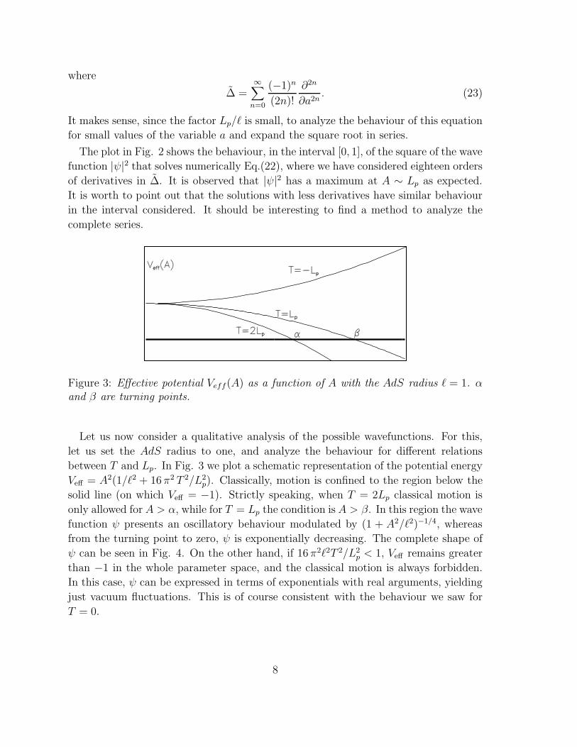
Figure 3: Effective potential Veff(A) as a function of A with the AdS radius ℓ = 1. αand β are turning points.
Let us now consider a qualitative analysis of the possible wavefunctions. For this,
let us set the AdS radius to one, and analyze the behaviour for different relations
between T and Lp. In Fig. 3 we plot a schematic representation of the potential energy
Veff = A2(1/ℓ2 + 16 π2 T 2/L2p). Classically, motion is confined to the region below the
solid line (on which Veff = −1). Strictly speaking, when T = 2Lp classical motion is
only allowed for A > α, while for T = Lp the condition is A > β. In this region the wave
function ψ presents an oscillatory behaviour modulated by (1 + A2/ℓ2)−1/4, whereas
from the turning point to zero, ψ is exponentially decreasing. The complete shape of
ψ can be seen in Fig. 4. On the other hand, if 16 π2ℓ2T 2/L2p < 1, Veff remains greater
than −1 in the whole parameter space, and the classical motion is always forbidden.
In this case, ψ can be expressed in terms of exponentials with real arguments, yielding
just vacuum fluctuations. This is of course consistent with the behaviour we saw for
T = 0.
8
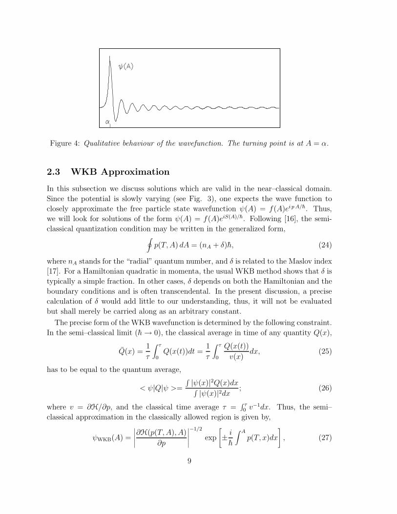
Figure 4: Qualitative behaviour of the wavefunction. The turning point is at A = α.
2.3 WKB Approximation
In this subsection we discuss solutions which are valid in the near–classical domain.
Since the potential is slowly varying (see Fig. 3), one expects the wave function to
closely approximate the free particle state wavefunction ψ(A) = f(A)ei p A/h. Thus,
we will look for solutions of the form ψ(A) = f(A)eiS(A)/h. Following [16], the semi-
classical quantization condition may be written in the generalized form,∮
p(T,A) dA = (nA + δ)h, (24)
where nA stands for the “radial” quantum number, and δ is related to the Maslov index
[17]. For a Hamiltonian quadratic in momenta, the usual WKB method shows that δ is
typically a simple fraction. In other cases, δ depends on both the Hamiltonian and the
boundary conditions and is often transcendental. In the present discussion, a precise
calculation of δ would add little to our understanding, thus, it will not be evaluated
but shall merely be carried along as an arbitrary constant.
The precise form of the WKB wavefunction is determined by the following constraint.
In the semi–classical limit (h→ 0), the classical average in time of any quantity Q(x),
Q(x) =1
τ
∫ τ
0Q(x(t))dt =
1
τ
∫ τ
0
Q(x(t))
v(x)dx, (25)
has to be equal to the quantum average,
< ψ|Q|ψ >=
∫ |ψ(x)|2Q(x)dx∫ |ψ(x)|2dx ; (26)
where v = ∂H/∂p, and the classical time average τ =∫ τ0 v
−1dx. Thus, the semi–
classical approximation in the classically allowed region is given by,
ψWKB(A) =
∣
∣
∣
∣
∣
∂H(p(T,A), A)
∂p
∣
∣
∣
∣
∣
−1/2
exp
[
± i
h
∫ A
p(T, x)dx
]
, (27)
9
while in the classical forbidden region it reads,
ψWKB(A) =
∣
∣
∣
∣
∣
∂H(p(T,A), A)
∂p
∣
∣
∣
∣
∣
−1/2
exp
[
±1
h
∫ A
p(T, x)dx
]
. (28)
It is easily seen that for the typical Hamiltonian quadratic in momentum this general-
ized prescription reduces to the usual WKB approximation.
The conjugate momenta results in a multi-valued function:
p(T,A) = ±Lp
2
arccosh
−4πTA
Lp
√
1 + A2/ℓ2
+ 2πin
. (29)
Here arcosh(x) is taken to map [1,∞) → [0,∞), and ± refers to outgoing/ingoing
directions. In this scheme the imaginary contribution to p(T,A) does not contribute to
the quantization condition. The quantum number n, however, does contribute when
estimating the WKB wave function. In the classical allowed region we get,
ψWKB(A) =exp[−nπA/Lp]
| − 1 −A2(16π2T 2/L2p − 1/ℓ2)|1/4
e±iΘ(A), (30)
where
Θ =1
h
∫ A Lp
2arccosh
−4πTx
Lp
√
1 + x2/ℓ2
dx. (31)
Note that in the limit A/ℓ << 1,
Θ =A
2Lp
arccosh
[
−4πTA
L2p
]
. (32)
Thus, we recover the behaviour found in the previous subsection, ψ exponentially
increases from zero to the turning point.
If we now flip T → −T , and use arcosh(−x) = arccosh(x) + iπ, we find that
ψWKB(A) =exp[−(n + 1)πA/Lp]
| − 1 − A2(16π2T 2/L2p − 1/ℓ2)|1/4
e±iΘ(A) (33)
are WKB eigenmodes corresponding to an eigenvacuumenergy −T .
This semiclassical solution blows up at the turning points, where A goes to zero.
This in itself may be tolerated if the wavefunction is normalizable. The matching
of the wavefunction at the turning points may still be done by examining the wave
equation more closely in the vicinity of the turning point.
10
3 Brane–world in AdSd+1
3.1 Cosmology on the Brane
We turn now to a more general analysis independent of the dimension, i.e., for AdSd+1
with d > 1. The expression for the total action is given by,
Stot =L(3−d)
p
16π
∫
Ωdd+1x
√g
(
R +d (d− 1)
ℓ2
)
+L(3−d)
p
8π
∫
∂Ωddx
√γ K+T
∫
∂Ωddx
√γ. (34)
Let us also generalize the possible symmetries on the bulk which yield different Robertson–
Walker like cosmologies. The most general AdSd+1 metric can be written as,
ds2 = −(
k +y2
ℓ2
)
dt2 +
(
k +y2
ℓ2
)−1
dy2 + y2dΣ2k, (35)
where k takes the values 0,−1, 1 for flat, hyperbolic, or spherical geometries respectively
and where dΣ2k is the corresponding metric on the unit (d − 1)-dimensional plane,
hyperboloid, or sphere. It should be stressed that if k = −1, an event horizon appears
at y = ℓ. With this in mind, one can trivially generalize the discussion in the appendix
to get,
Kφi
φi=
1
A
[
k +A2
ℓ2+ A2
]1/2
, (36)
and
Kττ =
[
A+A
ℓ2
]
[
k +A2
ℓ2+ A2
]−1/2
, (37)
where i runs from 1 to (d − 1). In terms of these quantities, the Einstein equation
reads [18],
TgΞΥδ
Ξ
A δΥ
B =L3−d
p
4 π[KAB − tr(K)g
ΞΥδ
Ξ
A δΥ
B]. (38)
Its non–trivial components are,
T = −L(3−d)p
4π
(d− 1)
A
(
k +A2
ℓ2+ A2
)1/2
, (39)
and
T = −L(3−d)p
4π
(d− 2)
A
(
k +A2
ℓ2+ A2
)1/2
+A+ A/ℓ2
√
k + A2 + A2/ℓ2
. (40)
It is easily seen that Eqs. (39) and (40) imply the conservation of the stress energy.
The evolution of the system is thus governed by,
A2 = −k − A2
(
1
ℓ2− 16π2 T 2
(d− 1)2 L2(3−d)p
)
. (41)
11
A somewhat unusual feature of brane physics can be analyzed from Eq. (41) (the
five–dimensional case was already discussed by Kraus, Ref. [11]). Recall that in the
spherical case, the classical behaviour of the brane is bounded by a minimum radius
A20 =
(
− 1
ℓ2+
16 π2 T 2
(d− 1)2 L2(3−d)p
)−1
, (42)
but once the brane reaches that “size” it expands forever. Thus, contrary to the stan-
dard Robertson Walker cosmology, the spherically symmetric brane – corresponding to
k = 1 – represents an open world. Furthermore, depending on the value of T we can
also obtain a closed world with hyperbolic symmetry, i.e. with k = −1. On the one
hand, if16π2T 2ℓ2
(d− 1)2L2(3−d)p
≥ 1, (43)
the classical solution does not have turning points yielding an open world. It should
be remarked, however, that for k = 1 the spacetime has no event horizons, whereas if
k = −1, the brane crosses an event horizon (at A = ℓ) in a finite proper time.
On the other hand, if16π2T 2ℓ2
(d− 1)2L2(3−d)p
< 1, (44)
the classical solution has two turning points representing a big–bang and a big–crunch.
Again, the spacetime has an event horizon at finite proper distance from the brane. If
k = 0, one obtains a solution only if the inequality (43) is satisfied. In the critical, case
the solution represents the RSd+1 brane–world. At this stage, it is noteworthy that a
comprehensive analysis of a domain wall that inflates, either moving through the bulk
or with the bulk inflating too, was first discussed by Chamblin–Reall [11].
3.2 Semiclassical Corrections
With the field equations for an expanding (d− 1)-brane in hand, the generalization of
the WKB approximation to AdSd+1 is straightforward. Of particular interest is AdS5.7
Let us specialize again to the case of a spherically symmetric brane. In such a case,
Eq. (34) can be re–written as
Stot =1
Lp
∫
dτ
−A3
3ℓ2
√
A2 + A2/ℓ2 + 1
1 + A2/ℓ2+ 3A
√
1 + A2/ℓ2 + A2
− 2AA arcsinh
A√
1 + A2/ℓ2
+ T∫
∂Ωd4x
√γ. (45)
7Note that if k = 0 and T = 3/(4πLpℓ), one recovers the RS–world.
12
For positive eigenvalues of T , the solution in the classical allowed region is then given
by,
ψWKB(A) =exp[−2 π n (A/Lp)
2]
| − 1 − A2/ℓ2 +G2)|1/4e±i
∫
Ap dx, (46)
with p ≡ ∂L5/∂A, and G(A) = 4πA2TLp/3. The oscillating part will be a real
exponential term in the classically forbidden region.
4 Relation to AdS/CFT Correspondence
4.1 Generalities
Another, seemingly different, but in fact closely related subject we will discuss in this
section is the AdS/CFT correspondence [19]. This map provides a “holographic”
projection of the AdS gravitational system into the physics of the gauge theory. In the
standard noncompact AdS/CFT set up, gravity is decoupled from the dual boundary
theory. The prime example here being the duality between Type IIB on AdS5 × S5
and N = 4 supersymmetric U(N) Yang-Mills in d = 4 with coupling gY M (the t’Hooft
coupling is defined as λ = g2Y MN). In this case it is known that the parameters of the
CFT are related to those of the supergravity theory by [19, 20]
ℓ = λ1/4ls (47)
ℓ3
L3p
=2N2
π, (48)
where ls is the string length. The supergravity description is valid when λ and N
are large (so that stringy effects are small). However, it is natural to suppose (in the
spirit of AdS/CFT ) that any RS-like model should properly be viewed as a coupling
of gravity to whatever strongly coupled conformal theory the AdS geometry is dual to.
In the following discussion, inspired in [23], we unfold on this hypothesis: The most
general action for a RS–like model in AdSd+1 is given by
SRS = SEH + SGH + 2S1 + Sm, (49)
where S1 is the counterterm (T/2)∫
ddx√γ. The last term Sm is the action for matter
on the brane which was not included in Eq. (34), but it is included here for com-
pleteness. Now, to apply the AdS/CFT -correspondence, there is the question of the
definition of the gravitational action in AdSd+1. The standard action – corresponding
to the two first terms of Eq. (34) – is divergent for generic geometries and one must add
certain “counterterms” to obtain a finite action [21, 22]. Then we have schematically,
Sgrav = SEH + SGH + S1 + S2 + S3 + · · · , (50)
13
where Sk is of order 2(k−1) in derivatives of the boundary metric. Specifically, S2 and
S3 are the counterterms discussed in [23]. They are expressed in terms of the boundary
metric:
S2 ∝∫
ddx√γR (51)
and
S3 ∝∫
ddx√γ
(
RijRij − d
4(d− 1)R2
)
. (52)
Some of the higher–order counterterms were computed in [22]. For a given dimension
d, however, one only needs to add a finite number of counterterms, specifically terms
of order 2n < d in derivatives of the boundary metric.
In [21] the counterterms were found for AdS3, AdS4 and AdS5 by requiring a finite
mass density of the spacetime. In the first case it was found, that only S1 is needed,
while in the latter cases both S1 and S2 are needed. Kraus et al. [22] later derived a
method for generating the required counterterms for any dimension d. Furthermore,
in [21] it was also noted that for the case of AdS5 one could add terms of higher order
in derivatives of the metric, as for example the counterterm S3 but without changing
the mass of the spacetime. Confronted with this ambiguity we face the question of
which counterterms should be added in for example AdS5. For that, we note that in
order to apply the AdS/CFT–correspondence we should require that the symmetries
on both sides of the correspondence match. The Weyl anomaly was computed in [24]
for gravity theories in AdSd+1 and we can then apply this result to fix the possible
counterterms. For d odd there is no such anomaly and the divergent part of the
(super)gravity action is canceled by the addition of the above mentioned counterterms.
This implies, for example, that for AdS4 we should only add S1 and S2. For d even
there is a nonvanishing anomaly [24]. For AdS3 this means that both S1 and S2 should
be added and for AdS5 we should add the terms S1, S2 and S3. So, the requirement of
finiteness of the action together with the matching of Weyl anomalies fixes the precise
form of the supergravity action in AdSd+1.
4.2 Dual Boundary Theory
Now, using the AdS/CFT -correspondence, one can easily show that the RS–model in
dimension d+ 1 is dual to a d–dimensional CFT (which we call the RS CFT ) with a
coupling to matter fields and the domain wall given by the action 2S2 + 2S3 + · · · +Sm, where we should remember that for AdS3 and AdS4, the S3–term is absent but
appears in all higher–dimensional cases. To illustrate this point, let us now analyze
the AdS/CFT for the simplest three–dimensional example. We will work in Euclidean
space in order to avoid definition problems in the path integral. In this case the RS
14
action (without matter) is given by
SRS = − Lp
16π
∫
Ωd3x
√g(
R +2
ℓ2
)
− Lp
8π
∫
∂Ωd2x
√γ K − Lp
4π
∫
∂Ωd2x
√γ, (53)
which is essentially the same as in Eq. (1) but now with the tension T fixed to be
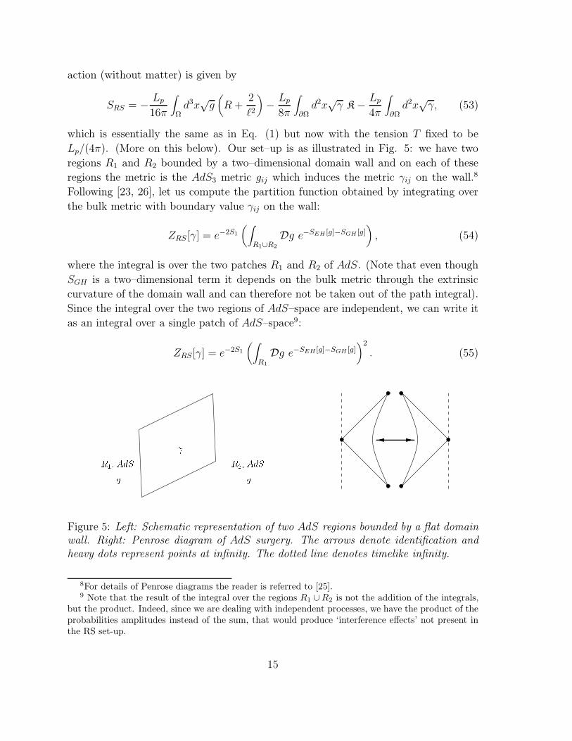
Lp/(4π). (More on this below). Our set–up is as illustrated in Fig. 5: we have two
regions R1 and R2 bounded by a two–dimensional domain wall and on each of these
regions the metric is the AdS3 metric gij which induces the metric γij on the wall.8
Following [23, 26], let us compute the partition function obtained by integrating over
the bulk metric with boundary value γij on the wall:
ZRS[γ] = e−2S1
(∫
R1∪R2
Dg e−SEH [g]−SGH [g])
, (54)
where the integral is over the two patches R1 and R2 of AdS. (Note that even though
SGH is a two–dimensional term it depends on the bulk metric through the extrinsic
curvature of the domain wall and can therefore not be taken out of the path integral).
Since the integral over the two regions of AdS–space are independent, we can write it
as an integral over a single patch of AdS–space9:
ZRS[γ] = e−2S1
(∫
R1
Dg e−SEH [g]−SGH [g])2
. (55)
R1, AdSg gR2, AdSFigure 5: Left: Schematic representation of two AdS regions bounded by a flat domainwall. Right: Penrose diagram of AdS surgery. The arrows denote identification andheavy dots represent points at infinity. The dotted line denotes timelike infinity.
8For details of Penrose diagrams the reader is referred to [25].9 Note that the result of the integral over the regions R1 ∪R2 is not the addition of the integrals,
but the product. Indeed, since we are dealing with independent processes, we have the product of theprobabilities amplitudes instead of the sum, that would produce ‘interference effects’ not present inthe RS set-up.
15
Now according to the discussion above, the partition function for a consistent gravity
theory in AdS3, with finite mass of spacetime and appropriate central charge, is
Zgrav[γ] =∫
[γ]Dg e−SEH [g]−SGH [g]−S1[γ]−S2[γ]
= e−S1[γ]−S2[γ]∫
[γ]Dg e−SEH [g]−SGH [g]
= e−WCF T [γ], (56)
and according to the AdS/CFT it should be identified with the generating functional
for connected Green’s functions of the RS CFT as above. By combining Eq. (55) and
(56) we finally obtain:
ZRS [γ] = e−2WCF T [γ]+2S2[γ]. (57)
This shows that the RS–like model in AdS3 is equivalent to a CFT coupled to gravity
with action 2S2. This dual gravity theory is actually two–dimensional since 2S2 is the
Einstein–Hilbert action for two–dimensional gravity. Similar correspondences can be
derived in higher–dimensional cases. For example we have:
S(4)RS ↔ W
(4)RS − 2S2 + Sm, (58)
while
S(5)RS ↔ W
(5)RS − 2S2 − 2S3 + Sm. (59)
Here WRS stands for the generating functional of connected Green’s functions of the
boundary (RS) CFT , that is twice the CFT induced on the brane. Note that, as in the
case of AdS3, −2S2 is the Einstein-Hilbert action for d–dimensional gravity and so the
RS model is equivalent to d-dimensional gravity coupled to a CFT with corrections to
gravity coming from the third counterterm S3 (at least for d > 3). This alone, however,
does not tell us what the RS CFT actually is10, but rather that the RS model in d+1
dimensions can be viewed as a d-dimensional gravity (including corrections) coupled
to a CFT with matter.11 And so, for example, in the case of AdS5 this is another way
to see why gravity is trapped on the four–dimensional domain wall and why there are
corrections to Einstein gravity. (However, there are no such corrections in the case of
AdS3 and AdS4 as we argued above).
4.3 Physical Implications
Up to this point we have kept the tension of the domain wall, T , arbitrary. Because
of the various bounds described in sections 2 and 3 for different behaviours of the
10The boundary CFT can be found for the case of AdS3[27].11Related ideas were discussed in [28].
16
braneworld, it is important to see what one might expect. Let us again first restrict
to AdS3 for simplicity. It is well known that gravity in asymptotically AdS3 spacetime
has a holographic description as a 1+1 dimensional conformal field theory with central
charge c = 3 ℓMp/2 [29]. In order to recover the geometry discussed in section 2,
one must glue two copies of such bounded AdS3 spacetimes, and then integrate over
boundary metrics. Consequently, one has two copies of the matter action on the
boundary, with total central charge c = 3 ℓMp. In addition, if R > 0 the conformal
anomaly of the CFT increases the effective tension on the domain wall, T > Lp/4πℓ,
yielding a de Sitter universe with an effective cosmological constant driving inflation.12
An (early) inflationary epoch looks very promising. The tremendous expansion during
inflation may blow up a small sized region of the world (which was causally connected
before inflation) to a size much greater than our current horizon. Therefore, it can be
expected that the observable part of the brane looks smooth and flat, regardless of the
initial curvature of the brane that inflated.13 Furthermore, if we consider conformal
matter on the brane the inflationary phase is unstable and could decay into a matter
dominated universe with thermalized regions, in agreement with current observations
[31].
Another interesting process which could lead to brane–world reheating is as fol-
lows: During inflation trapped regions of false vacuum (within their Schwarzchild radii)
caught between bubbles of true vacuum may give rise to the creation of primordial black
strings. Now, it is well–known that the black string solution suffers from a Gregory–
Laflamme instability [32] leading to the formation of stable black cigars on the brane.
In addition, it was shown in [33] that the nucleation of supermassive bulk black holes
is highly supressed compared to the above mentioned process. Thus, prompted by
the conventional arena [34], one could speculate that the Hawking–evaporation of pri-
mordial black cigars slows down inflation. On the other hand, one could assume the
existence of such a bulk black hole. Even in this case, the (brane-world/bulk-black-
hole) system evolves towards a configuration of thermal equilibrium as was recently
shown in [35].
Let us now briefly discuss a general n-dimensional brane-world that falls under the
action of a higher dimensional gravitational field. The system can be decomposed
into falling shells (which do not interact with each other or with the environment that
generates the metric), with trajectories described by the scale factor A(τ). From the
12A few words of caution; it is quite possible that the truncation from an infinite number of de-grees of freedom down to only one degree of freedom, A(τ), has also drastically truncated the realphysics. Unfortunately, a treatment using Wheeler’s full superspace is beyond the scope of our presentcalculation abilities.
13Note that a flat Robertson-Walker Universe requires a total energy density equal to the criticaldensity ρcr, whereas ordinary matter contributes only about a 5% of ρcr. A novel solution to thisproblem consistent with a large body of observations is the so-called “Manifold Universe” [30].
17
above discussion it is clear that the value of T will depend on the symmetries of the
domain wall. It is easily seen, for instance, that if k = −1 then
T <(d− 1)L3−d
p
4πℓ, (60)
yielding a closed universe. Roughly speaking, the cosmological constant induced by
the conformal anomaly accelerates/slows down the brane to balance the null geodesic
congruence in the bulk, shirking the world’s pinch off. We recall that if k = −1, the
spacetime has an undesirable event horizon that must be reached by the brane in a
finite proper time.
Despite the fact that it is contrary to the spirit of RS-worlds, it would be nice to
add “matter fields” in the bulk to study the quantum cosmology and the dual CFT
coupled to gravity that in this case should be deformed by the insertion of operators.
Even though many kind of interesting phenomena are recognized, brane-world cos-
mology remains thoroughly non-understood. The lower dimensional model here dis-
cussed can hopefully illuminate the “physical AdS5 cosmology”.
Acknowledgements
We would like to thank Vijay Balasubramanian, Thomas Hertog, Finn Larsen, Juan
Maldacena, Francisco Villaverde, Matt Visser, and Allan Widom for useful discus-
sions/correspondence. Special thanks go to Harvey Reall for a critical reading of the
manuscript and valuable comments. The work of LA and CN was supported by CON-
ICET Argentina, and that of KO by the Danish Natural Science Research Council.
18
A Appendix
Here we present a calculation of the second fundamental form of the metric in Eq. (2)
(it should be remarked that this calculation is a direct analog to that of Ref. [36], and
it is included just for the sake of completeness).
Let us start by introducing a Gaussian normal coordinate system in the neighborhood
of the brane. We shall denote the one–dimensional surface swept out by the brane by
Σ. Let us introduce a coordinate system φ⊥ on Σ. Next we consider all the geodesics
which are orthogonal to Σ, and choose a neighborhood N around Σ so that any point
p ∈ N lies on one, and only one, geodesic. The first coordinate of p is determined by
the intersection of this geodesic with Σ. The full set of spatial coordinates is then given
by (φ⊥; η), while the surface Σ under consideration is taken to be located at η = 0 so
that Eq. (2) can be rewritten as
ds2 = −(
1 +y2
ℓ2
)
dt2 + dη2 + y2dφ2, (1)
fixed by the relation, dy/dη = (1 + y2/ℓ2)1/2. The second fundamental form in such a
coordinate–system reads
Kµν ≡ 1
2
∂gµν
∂η
∣
∣
∣
∣
∣
η=0,y=A
, (2)
and its non-trivial components are
Ktt =
A
ℓ2
(
1 +A2
ℓ2
)−1/2
, (3)
Kφφ =
1
A
(
1 +A2
ℓ2
)1/2
. (4)
To analyze the dynamics of the system, we permit the radius of the brane to become
a function of time A→ A(τ). Recall that the symbol τ is used to denote proper time as
measured by co–moving observers on the brane–world. Let the position of the brane be
described by xµ(τ, φ) ≡ (t(τ), A(τ), φ), so that the velocity of a piece of stress-energy
at the brane (uµuµ = −1) is
uµ ≡ dxµ
dτ=
(
dt
dτ,dA
dτ, 0
)
. (5)
We remind the reader that
ds2 = −(
1 +A2
ℓ2
)
dt2 +
(
dA
dt
)2 (
1 +A2
ℓ2
)−1
dt2 + A2dφ2 (6)
19
so,
dτ 2 = −dt2
−(
1 +A2
ℓ2
)
+
(
dA
dt
)2 (
1 +A2
ℓ2
)−1
(7)
or equivalently,
dτ 2 = −dt2
−(
1 +A2
ℓ2
)2
+
(
dA
dt
)2
(
1 +A2
ℓ2
)−1
. (8)
SincedA
dt=dA
dτ
dτ
dt, (9)
we first get,
−(
1 +A2
ℓ2
)(
dτ
dt
)2
= −(
1 +A2
ℓ2
)2
+ A2
(
dτ
dt
)2
(10)
and then,
dt
dτ=
√
A2 + A2/ℓ2 + 1
1 + A2/ℓ2. (11)
Let us denote by nµ the unit normal vector to the brane, which satisfies uµnµ = 0 and
nµnµ = 1; its components are nµ = (A/(1 + A2/ℓ2), (1 + A2/ℓ2 + A2)1/2, 0), such that
the coordinate y is increasing in the direction nµ. Thus we obtain
Kφφ =
1
y
∂y
∂η
∣
∣
∣
∣
∣
y=A
=1
A
(
1 +A2
ℓ2+ A2
)1/2
. (12)
To evaluate Kττ one can proceed in two alternative ways. First one can simply use the
definition Kµν = 12∇(µnν), giving:
Ktt =1
2∇(tnt) =
dnt
dτ
dτ
dt− Γη
tt nη = − 1 + A2/ℓ2√
1 + A2 + A2/ℓ2(A+ A/ℓ2), (13)
that using
Kττ =∂xµ
∂xτ
∂xν
∂xτKµν , (14)
immediately yields
Kττ = K
tt =
A+ A/ℓ2√
1 + A2 + A2/ℓ2. (15)
Alternatively, one can easily check this last result by observing that
Kττ ≡ −Kττ = −uµuν
Kµν = −uµuν∇µnν = uµnν∇µuν = nµ(uν∇νu
µ) = nµqµ, (16)
20
where qµ is the four acceleration of the brane. Now, by the spherical symmetry of the
problem the four acceleration is proportional to the unit normal, qµ ≡ q nµ, so Kττ = q.
To explicitly evaluate the four acceleration, utilize the fact that ξµ ≡ ∂µt ≡ (1, 0, 0) is a
Killing vector for the underlying geometry. At the brane, the components of this vector
are ξµ = (−[1 + A2/ℓ2], 0, 0), so that ξµnµ = −A and ξµu
µ = −(1 + A2/ℓ2 + A2)1/2.
With this in mind, comparing
d
dτ(ξµu
µ) = ξµ q nµ = −q A, (17)
andd
dτ(ξµu
µ) = −A A/ℓ2 + A√
1 + A2/ℓ2 + A, (18)
we get
Kττ =
A/ℓ2 + A√
1 + A2/ℓ2 + A=
d
dτ
arcsinh
A√
1 + A2/ℓ2
+A
ℓ2dt
dτ; (19)
this result agrees with that of Eq. (15). Having calculated the nontrivial components of
the second fundamental form we can now derive a simpler expression for the relevant
gravity–action (1) in AdS3. Since√g d3x → 2π A dAdt and
√γ d2x → 2π Adτ an
integration by parts finally leads to
Sgravity =Lp
2
∫
dτ
−A arcsinh
A√
1 + A2/ℓ2
+
√
1 +A2
ℓ2+ A2
. (20)
21
References
[1] T. Kaluza, Akad. Wiss. Phys. Math. K1, 966 (1921).
[2] O. Klein, Z.Phys. 37, 895 (1926).
[3] V. Rubakov and M. Shaposhnikov, Phys. Lett. 125B, 136 (1983); M. Visser, Phys.
Lett. B159, 22 (1985).
[4] J. Polchinski, Phys. Rev. Lett 75, 4724 (1995) [hep-th/9510017]; P. Horava and
E. Witten, Nucl. Phys. B460, 506 (1996) [hep-th 9510209], Nucl. Phys. B 475,
94 (1996) [hep-th/9603142].
[5] I. Antoniadis, Phys. Lett. B 246 (1990) 377.
[6] N. Arkani-Hamed, S. Dimopoulos and G. Dvali, Phys. Lett. B 429, 263 (1998); I.
Antoniadis, N. Arkani-Hamed, S. Dimopoulos and G. Dvali, Phys. Lett. B 436,
257 (1998).
[7] L. Randall and R. Sundrum, Phys. Rev. Lett. 83, 3370 (1999) [hep-ph/9905221].
[8] L. Randall and R. Sundrum, Phys. Rev. Lett. 83, 4690 (1999) [hep-th/9906064].
[9] J. Lykken and L. Randall, JHEP 0006, 014 (2000) [hep-th/9908076].
[10] A. Chamblin and G. W. Gibbons, Phys. Rev. Lett. 84, 1090 (2000) [hep-
th/9909130]; A. Chamblin, S. W. Hawking and H. S. Reall, Phys. Rev D 61,
065007 (2000) [hep-th/9909205]; R. Emparan, G. T. Horowitz and R. C. Myers,
JHEP 0001, 007 (2000) [hep-th/9911043]; R. Emparan, G. T. Horowitz and R.
C. Myers, JHEP 0001, 021 (2000) [hep-th/9912135]; J. Garriga and T. Tanaka,
Phys. Rev. Lett. 84 2778 (2000) [hep-th/9911055]; M. Sasaki, T. Shiromizu and K.
Maeda, [hep-th/9912233]; A Chamblin, C. Csaki, J. Erlich and T. J. Hollowood,
Phys. Rev. D (to be published) [hep-th/0002076]; S. B. Giddings, E. Katz and L.
Randall, JHEP 0003, 023 (2000) [hep-th/0002091]; C. Grojean, [hep-th/0002130].
[11] H. A. Chamblin and H. S. Reall, Nucl. Phys. B 562, 133 (1999) [hep-th/9903225];
N. Arkani-Hamed, S. Dimopoulos, N. Kaloper, and J. March Russell, Nucl. Phys.
B 567, 189 (2000) [hep-ph/9903224]; N. Kaloper, Phys. Rev. D 60, 123506 (1999)
[hep-th/9905210]; C. Csaki, M. Graesser, C. Kolda, J. Terning, Phys. Lett. B 462,
34 (1999) [hep-ph/9906513]; J. M. Cline, C. Grojean and G. Servant, Phys. Rev.
Lett. 83, 4245 (1999) [hep-ph/9906523]; H. B. Kim and H. D. Kim, Phys. Rev.
D 61, 064003 (2000) [hep-th/9909053]; P. Kanti, I. I. Kogan, K. A. Olive and
M. Pospelov, Phys. Lett. B 468, 31 (1999) [hep-ph/9909481]; J. Cline, C. Gro-
jean and G. Servant, Phys. Lett. B 472, 302 (2000) [hep-ph/9909496]; P. Kraus,
22
JHEP 9912 011 (1999) [hep-th/9910149]; S. Nam, [hep-th/9911237]; C. Csaki, M.
Graesser, L. Randall and J. Terning, [hep-ph/9911406]; D. Ida, [gr-qc/9912002];
N. Kaloper, Phys. Lett. B 474, 269 (2000) [hep-th/9912125]; M. Cvetic and J.
Wang, [hep-th/9912187]; S. Mukohyama, T. Shiromizu, and K. Maeda, [hep-
th/9912287]; L. A. Anchordoqui and S. E. Perez Bergliaffa, Phys. Rev. D (to
be published) [gr-qc/0001019]; K. Koyama and J. Soda, Phys. Lett. B (to be
published) [gr-qc/0001033]; C. Csaki, J. Erlich, T. J. Hollowood and J. Terning
[hep-th/0003076]; N. Deruelle and T. Dolezel, [gr-qc/0004021]; C. Barcelo and M.
Visser, [hep-th/0004022]; C. Barcelo and M. Visser, Phys. Lett. B 482, 183 (2000)
[hep-th/0004056]; H. Stoica, S. H. Henry Tye and I. Wasserman, [hep-th/0004126];
R. Maartens, [hep-th/0004166]; P. F. Gonzalez-Diaz, [gr-qc/0004078]; D. Langlois,
[hep-th/0005025]; V. Barger, T. Han, T. Li, J. D. Lykken and D. Marfatia, [hep-
ph/0006275].
[12] G. F. Giudice, R. Rattazzi and J. D. Wells, Nucl. Phys. B 544, 3 (1999) [hep-
ph/9811291]; M. Acciarri et al. (L3 Collaboration), Phys. Lett. B 470, 281 (1999)
[hep-ex/9910056]; S. Cullen, M. Perelstein and M. E. Peskin, [hep-ph/0001166];
Z. K. Silagadze, [hep-ph/0002255]; C. Adloff et al. (H1 Collaboration), [hep-
exp/0003002]; K. Cheung, [hep-ph/0003306].
[13] J. B. Hartle and S. W. Hawking, Phys. Rev. D 28, 2960 (1983).
[14] S. Deser and R. Jackiw, Ann. Phys. 153, 405 (1984).
[15] G. W. Gibbons and S. W. Hawking, Phys. Rev. D 15, 2752 (1977).
[16] M. Visser, Phys. Rev. D 43, 402 (1991).
[17] M. Brack and R. K. Bhaduri, Semiclassical Physics, (Addison-Wesley, 1997).
[18] M. Visser, Lorentzian Wormholes, (AIP Press, Woodbury, N.Y. 1995); see in
particular, chapter 14.
[19] J. Maldacena, Adv. Theor. Math. Phys. 2, 231 (1998) [hep-th/9711200].
[20] O. Aharony, S. S. Gubser, J. Maldacena, H. Ooguri, and Y. Oz, [hep-th/9905111].
[21] V. Balasubramanian and P. Kraus, Commun. Math. Phys. 208, 413 (1999) [hep-
th/9902121].
[22] P. Kraus, F. Larsen and R. Siebelink, [hep-th/9906127].
[23] S. W. Hawking, T. Hertog, H. S. Reall, Phys. Rev. D 62, 043501, (2000) [hep-
th/0003052].
23
[24] M. Henningson and K. Skenderis, JHEP 9807, 023 (1998) [hep-th/9806087].
[25] S. W. Hawking and G. F. R. Ellis, The Large Scale Structure of Spacetime, (Cam-
bridge University Press, England, 1973). See also [20] for a comprehensive discus-
sion of the AdS spacetime. The Penrose diagram of the AdS space with a flat
domain wall was taken from [23].
[26] S. S. Gubser, [hep-th/9912001].
[27] S. Hawking, J. Maldacena and A. Strominger, [hep-th/0002145].
[28] S. Nojiri, S. D. Odintsov and S. Zerbini, Phys. Rev. D (to be published) [hep-
th/0001192]; S. Nojiri and S. D. Odintsov, Phys. Lett. B (to be published) [hep-
th/0004097].
[29] J. D. Brown and M. Henneaux, Comm. Math. Phys. 104, 207 (1986).
[30] N. Arkani-Hamed, S. Dimopoulos, G. Dvali and N. Kaloper, [hep-ph/9911386].
[31] A. A. Starobinsky, Phys. Lett. B 91, 99 (1980).
[32] R. Gregory and R. Laflamme, Phys. Rev. Lett. 70, 2837 (1993).
[33] J. Garriga and M. Sasaki, [hep-th/9912118].
[34] J. D. Barrow, E. J. Copeland, E. W. Kolb and A. R. Liddle, Phys. Rev. D 43,
984 (1991).
[35] A. Chamblin, A. Karch and A. Nayeri, [hep-th/0007060].
[36] S. K. Blau, E. I. Guendelman and A. H. Guth, Phys. Rev. D 35, 1747 (1987); M.
Visser, Nucl. Phys. B 328, 203 (1989).
24