Testing for Localisation Using Micro-Geographic Data∗

Gilles Duranton§

London School of Economics

Henry G. Overman‡

London School of Economics

Revised version: 6 December 2004

ABSTRACT: To study the detailed location patterns of industries, and particularly the tend-ency for industries to cluster relative to overall manufacturing, we develop distance-basedtests of localisation. In contrast to previous studies, our approach allows us to assessthe statistical significance of departures from randomness. In addition, we treat spaceas continuous instead of using an arbitrary collection of geographical units. This avoidsproblems relating to scale and borders. We apply these tests to an exhaustive UK data set.For four-digit industries, we find that (i) 52% of them are localised at a 5% confidence level,(ii) localisation mostly takes place at small scales below 50 kilometres, (iii) the degree oflocalisation is very skewed, and (iv) industries follow broad sectoral patterns with respectto localisation. Depending on the industry, smaller establishments can be the main driversof both localisation and dispersion. Three-digit sectors show similar patterns of localisationat small scales as well as a tendency to localise at medium scales.

Key words: Localisation, Clusters, K-density, Spatial Statistics.JEL classification: C19, R12, L70.

∗Thanks to Oriana Bandiera, Roger Bivand, Ian Gordon, Hidehiko Ichimura, Barry McCormick, TomoyaMori, Diego Puga, Danny Quah, Steve Redding, Stuart Rosenthal, Bernard Salanié, Tony Venables, Qiwei Yao,two anonymous referees, and to seminar participants at a CEPR network meeting in Villars, a CEPR workshopin Barcelona, the RSAI 2001 annual meetings in Charleston, the RGS 2003 annual meetings in London, TheNorwegian School of Economics (Bergen), University of Glasgow, Université de Lyon, Université de Namur,University of Nottingham, University of Sussex, University of Toronto, and the London School of Economicsfor comments and discussions which greatly helped us clarify our minds on crucial steps of the paper. Weare also grateful to Rachel Griffith, Felix Ritchie, and Helen Simpson for helping us with the data and to NickGill for his first-class research assistance. Finally, this project could not have started without pump-primingfinancial support from STICERD. Financial support from the Economic and Social Research Council (ESRC GrantR000239878) and the Leverhulme Trust is also gratefully acknowledged. This paper uses data that are CrownCopyright and reproduced with the permission of the HMSO Controller and the Queen’s Printer for Scotland.However, the use of these data does not imply ONS endorsement of either the interpretation or the analysis inthis paper.

§Department of Geography and Environment, London School of Economics, Houghton Street, Lon-don WC2A 2AE, United Kingdom. Also affiliated with the Centre for Economic Policy Research,and the Centre for Economic Performance at the London School of Economics, g.duranton@lse.ac.uk,http://cep.lse.ac.uk/~duranton.

‡Department of Geography and Environment, London School of Economics, Houghton Street, Lon-don WC2A 2AE, United Kingdom. Also affiliated with the Centre for Economic Policy Research, andthe Centre for Economic Performance at the London School of Economics, h.g.overman@lse.ac.uk,http://cep.lse.ac.uk/~overman.

1. Introduction

At least since Alfred Marshall’s (1890) Principles, the tendency for industries to cluster in someareas has fascinated economists and geographers alike. More recently, some of these clusters havecaught the imagination of policy makers. Following Silicon Valley’s success, clusters are seen bymany as the magical formula for regional development. In light of this, the tendency for firmsto localise (i.e., to concentrate over and above overall economic activity) raises a large number ofquestions about the forces at work and their welfare implications.1 Furthermore, what we maylearn about spatial clustering is relevant well beyond the realm of economic geography. Manyexplanations of spatial clustering rely on some form of external increasing returns which also figureprominently in theories of international trade, industrial organisation and economic growth.

In this paper however, we step back from policy and theoretical concerns and think again aboutthe stylised facts to be explained. First and foremost, how general and how strong is the tendencyfor industries to cluster? We do not question Marshall’s historical examples of the clustering ofcutlery producers in Sheffield or jewellers in Birmingham. Neither do we deny Silicon Valley’simportance in micro-electronics and software. However, it is worth asking if these examples arethe exception rather than the rule. To inform both theory and policy, it is also crucial to knowat which spatial scale this clustering occurs. In the United Kingdom (UK), the localisation of thecutlery industry in one area of Sheffield is different from that of the motor sport industry spreadingover more than 100 kilometres along the Thames Valley. Finally, it is important to know whethersmall or large establishments are the main driver of localisation and investigate its sectoral scope.

Building on previous research in spatial statistics, we develop a novel way to test for localisationand answer key questions about the extent of localisation, the spatial scales at which it takes place,and its sectoral scope. Our test is based on a measure of localisation, which is comparable acrossindustries, and controls for both the overall tendency of manufacturing to agglomerate and forthe degree of industrial concentration. These three requirements have already been recognisedby the literature. However in this paper we argue that any measure of localisation should alsobe unbiased with respect to scale and spatial aggregation and that any test of localisation shouldreport the significance of the result. Our approach satisfies these two additional properties. Let usconsider each of these five requirements in turn.

Obviously, any test of localisation must be based on a measure that is comparable across indus-tries. This measure must also control for the general tendency of manufacturing to agglomerate.For instance in the United States (US), even in the absence of any tendency towards localisation, wewould expect any typical industry to have more employment in California than in Montana. Thisis simply because the former has a population more than 30 times as large as the latter. These firsttwo requirements have been recognised in the literature for a long time. Most traditional measures,like Gini indices, are able to satisfy them when properly employed.

Since Ellison and Glaeser (1997), it is also widely recognised that any informative measureof localisation must control for industrial concentration. To understand the distinction between

1Following Hoover (1937), the agglomeration of a particular industry after "controlling" for that of general manufac-turing is referred to as localisation.

1

localisation and industrial concentration, note that in an industry with no tendency for clustering,the location patterns of the plants are determined by purely idiosyncratic factors. Hence, they arerandom to the outside observer. A relevant metaphor for the location patterns of such an industrymight then be that of darts thrown randomly at a map. Because the number of plants in anyindustry is never arbitrarily large, such random location processes cannot be expected to generateperfectly regular location patterns. For instance, according to Ellison and Glaeser (1997), 75% of theemployees in the US vacuum cleaner industry work in one of four main plants. Even if these plantslocate separately, four locations must account for at least 75% of the employment in this industrywithout it being localised in any meaningful way. In short, unevenness does not necessarilymean an industry is localised. Unfortunately traditional measures of localisation only measureunevenness. In the spirit of this dartboard metaphor, Ellison and Glaeser (1997) convincingly makethe case that when looking at the location patterns of particular industries, the null hypothesisshould be one of spatial randomness conditional on both industrial concentration and the overallagglomeration of manufacturing. The index they develop satisfies these two requirements and iscomparable across industries. Taking a similar dartboard approach, Maurel and Sédillot (1999) andDevereux, Griffith, and Simpson (2004) develop alternative indices of localisation with the sameproperties.

However, just like the more traditional indices, these "second generation" measures still ex-anteallocate establishments (i.e., points located on a map), to counties, regions or states (i.e., spatialunits at a given level of aggregation). In other words, they transform dots on a map into units in boxes.Aggregating data this way has the obvious advantage of making computations simple but it meansthrowing away a large amount of information and leads to a range of aggregation problems.

Most obviously, aggregation restricts the analysis to only one spatial scale, be it the county,region, or state. Exploring a different spatial scale requires another aggregation and running theanalysis again. This is limiting because in most countries the number of levels of aggregation iscommonly limited to two or three. More importantly, it is difficult to compare the results acrossdifferent scales. For instance, questions regarding how much industries are localised at the countylevel after controlling for localisation at the regional level cannot be precisely answered sinceexisting indices are usually not easily additive across different levels of aggregation. Furthermore,most existing spatial units are defined according to administrative needs not economic relevance.To make matters worse, these units are often very different in population and size so that mostexisting aggregations tend to mix different spatial scales. For instance, analysing the localisationof industries at the level of US states involves comparisons between Rhode Island and California,which is geographically more than 150 times as large.

Another major issue is that aggregating establishments at any spatial level leads to spuriouscorrelations across aggregated variables. The problem typically worsens as higher levels of ag-gregations are considered. This problem is well recognised by quantitative geographers (Yule andKendall, 1950; Cressie, 1993) and is known as the Modifiable Areal Unit Problem (MAUP).

Finally, and importantly, after aggregation has taken place, spatial units are treated symmetric-ally so that plants in neighbouring spatial units are treated in exactly the same way as plants atopposite ends of a country. This creates a downwards bias when dealing with localised industries

2

that cross an administrative boundary. This problem worsens as smaller spatial units are analysed.For instance in the UK, manufacture of machinery for textile is highly localised but the borderbetween the East and West Midlands regions cuts the main cluster in half. Using UK countieswould make matters even worse. Any good measure of localisation must avoid these aggregationproblems. Ours does, by directly using the distances between observations and thus working incontinuous space rather than aggregating observations within administrative units.

The last requirement for any test of localisation relates to its statistical significance. Given ourdefinitions, in the absence of localisation, the location of an industry is random conditional onindustrial concentration and the location of overall manufacturing. Thus any statement aboutnon-randomness can only be probabilistic. The literature mentioned above only offers localisationindices with no indication of statistical significance. In contrast, we analyse the statistical signific-ance of departures from randomness using a Monte-Carlo approach.

In summary, any test of localisation should rely on a measure which (i) is comparable acrossindustries; (ii) controls for the overall agglomeration of manufacturing; (iii) controls for industrialconcentration; (iv) is unbiased with respect to scale and aggregation. The test should also (v) givean indication of the significance of the results. The approach we propose here satisfies these fiverequirements. We build on work by quantitative geographers on spatial point patterns (see Cressie,1993, for a comprehensive review) that we extend to address issues of spatial scale and significance.The basic idea in our geo-computations is to consider the distribution of distances between pairsof establishments in an industry and to compare it with that of hypothetical industries with thesame number of establishments which are randomly distributed conditional on the distribution ofaggregate manufacturing.2

We apply our approach to an exhaustive UK manufacturing data set. Four main conclusionsemerge with respect to four-digit industries: (i) 52% of them are localised at a 5% confidence level,(ii) localisation takes place mostly between 0 and 50 kilometres, (iii) the degree of localisation isvery skewed across industries, and (iv) industries that belong to the same industrial branch tend tohave similar localisation patterns. In part, our results are entirely new as we know of no previoussystematic attempt to measure the scale of localisation. Where our results can be compared withprevious work, there are marked differences. For instance, 94% of UK four-digit industries arelocalised according to the Ellison-Glaeser (EG) index compared to 52% using our approach.

When looking at the location patterns of establishments with few employees we find a widevariety of behaviours. In some industries (often related to publishing, chemicals or electric ma-chinery), smaller establishments tend to be more localised than larger establishments. In otherindustries, like food and beverages or non-metallic mineral products, the opposite holds: Smallerestablishments are located away from the main clusters. Regarding the sectoral scope of local-

2Our philosophy when developing this methodology has been to impose a set of statistical requirements on our test.An alternative would be to develop tests based on an underlying economic model. As will become clear below, ourtest is also consistent with such a model-based approach. In this sense, our approach develops a test of the simplestpossible location model (i.e., pure randomness conditional on the distribution of overall manufacturing). In futurework, we expect to develop our methodology to test more sophisticated theories of industrial location. The key barrierto achieving this is the difficulty of generating counterfactual location patterns from such theories. An alternative wouldbe to use the indices of localisation we derive below as endogenous variables and regress them on a set of industrycharacteristics as in Rosenthal and Strange (2001).

3

isation, a range of interesting facts emerge. There are no marked differences between four- andfive-digit industries, whereas three-digit sectors tend to exhibit different patterns. In particular,with three-digit sectors, localisation is equally important at small scales (0 − 50 kilometres) and ata more regional level (80 − 140 kilometres). We find that these regional effects are caused by thetendency of four-digit industries that are part of the same sectors to co-localise at this spatial scale.

The rest of the paper is organised as follows. The next section describes our data. Section 3outlines our methodology. Baseline results for the localisation of four-digit UK industries are givenin Section 4. These results are complemented in Section 5 where we take into account the size ofestablishments. Section 6 presents further results about the scope of localisation. The last sectioncontains some concluding thoughts.

2. Data

Our empirical analysis uses exhaustive establishment level data from the 1996 Annual RespondentDatabase (ARD) which is the data underlying the Annual Census of Production in the UK. Collectedby the Office for National Statistics (ONS), the ARD is an extremely rich data set which containsinformation about all UK establishments (see Griffith, 1999, for a detailed description of this data).We restrict ourselves to production establishments in manufacturing industries using the Stand-ard Industrial Classification (SIC) 92 (SIC15000 to 36639) for the whole country except NorthernIreland.3 For every establishment, we know its postcode, five-digit industrial classification, andnumber of employees. Note that, when referring to SIC two-, three-, four-, and five-digit categories,we will speak of industrial branches, sectors, industries and sub-industries respectively.

The postcode is particularly useful for locating plants. In the UK, postcodes typically refer to oneproperty or a very small group of dwellings. Large buildings may even comprise more than onepostcode. See Raper, Rhind, and Shepherd (1992) for a complete description of the UK postcodesystem. The CODE-POINT data set from the Ordnance Survey (OS) gives spatial coordinates forall UK postcodes. This data is the most precise postcode geo-referencing data available for the UK.Each Code-Point record contains information about its location, and about the number and type ofpostal delivery points. By merging this data together with the ARD we can generate very detailedinformation about the geographical location of all UK manufacturing establishments. In so doing,we could directly establish the Eastings and Northings for around 90% of establishments. Thesegive the grid reference for any location taking as the origin a point located South West of the UK.

The main problem for the remaining 10%, for which the postcode could not be matched withspatial co-ordinates, relates to postcode updates. These take place when new postcodes are createdin a particular postcode area. Unfortunately, this could be a source of systematic rather thanrandom errors as wrong postcodes will be reported more frequently in areas where an updaterecently took place. To reduce this source of systematic error to a minimum, we checked our dataagainst all postcode updates since 1992. This left us with 5% of establishments that could notbe given a grid reference. We believe that the missing 5% of the ARD we could not match withCODE-POINT truly reflect random errors due to reporting mistakes. This left us with a population

3We use the terms establishment and plant interchangeably.

4

of 176,106 establishments. For 99.99% of them, the OS acknowledges a potential location errorbelow 100 metres. For the remaining 26 observations, the maximum error is a few kilometres.

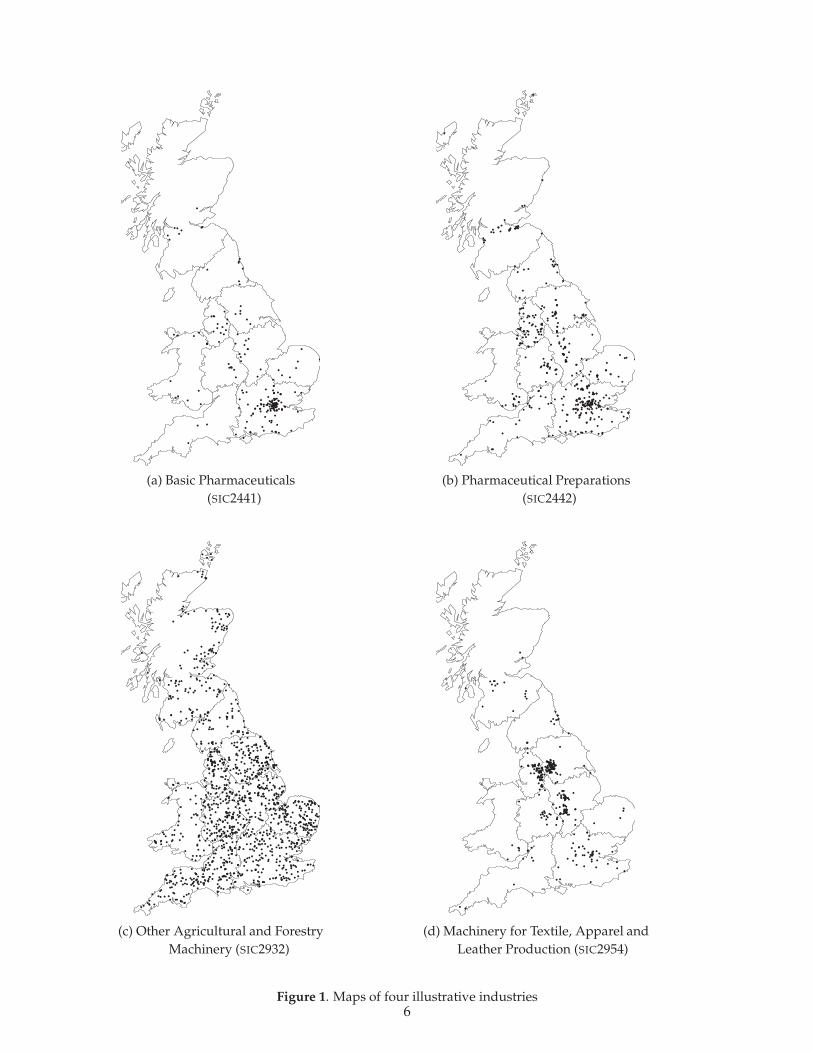
Figures 1(a-d) map this location information for four industries: Basic Pharmaceuticals(SIC2441), Pharmaceutical Preparations (SIC2442), Other Agricultural and Forestry Machinery(SIC2932), and Machinery for Textile, Apparel and Leather Production (SIC2954). Each dot rep-resents a production establishment. As can be seen from the maps, Machinery for Textile, Appareland Leather Production (SIC2954) looks very localised whereas Other Agricultural and ForestryMachinery (SIC2932) is very dispersed. These are extreme cases. Basic Pharmaceuticals (SIC2441)and Pharmaceutical Preparations (SIC2442) are more representative of the typical pattern. Whetheror not these last two industries are localised is far from obvious. In the exposition of the method-ology below, we keep using these four industries for illustrative purposes. However, the mainresults will consider all industries.

3. Methodology

Our analysis is conceptually simple. We first select the relevant establishments. The secondstep is to compute the density of bilateral distances between all pairs of establishments in anindustry. This measure is unbiased with respect to spatial scale and aggregation and thus satisfiesour fourth requirement. The third step is to construct counterfactuals. To satisfy our first andthird requirements about comparability across industry and the need to control for industrialconcentration, we consider hypothetical industries with the same number of establishments. Anyexisting establishment, regardless of its industry, is assumed to occupy one site. Establishmentsin our hypothetical industries are randomly allocated across these existing sites. This controlsfor the overall distribution of manufacturing and thus satisfies our second requirement. Finallywe construct local confidence intervals and global confidence bands to take care of our fifthrequirement. This allows us to compare the actual distribution of distances to randomly generatedcounterfactuals and to assess the significance of departures from randomness. We now describethese steps in greater detail.

Selection of observations

For any particular industry (and more generally for any partition of our population of establish-ments), we first select the relevant observations. The main issue to consider here is the largenumber of small establishments, which may have different location patterns. For instance innaval constructions, there are many very small establishments of one to ten employees locatedinland whereas all the large establishments are located on a coast. It seems likely that theseestablishments, although classified in the same industry, do not do the same thing. One alternativeis to ignore this problem and consider the whole population of UK production establishments.A second possibility would be to consider a size threshold and retain only establishments withemployment above this threshold. We then need to choose between an absolute and a relativethreshold. Dropping all establishments with less than 10 workers may be reasonable for navalconstruction but less so for publishing. Such reasoning suggests the use of a relative threshold

5

(a) Basic Pharmaceuticals (b) Pharmaceutical Preparations(SIC2441) (SIC2442)

(c) Other Agricultural and Forestry (d) Machinery for Textile, Apparel andMachinery (SIC2932) Leather Production (SIC2954)

Figure 1. Maps of four illustrative industries6

where we select establishments by decreasing size so that say 90% of employment is considered.A last possibility is to weight establishments by their employment.

We implement all three approaches. In our baseline analysis (Section 4), we consider all es-tablishments independent of size. In Section 5, we then consider only the largest establishmentsof any industry comprising at least 90% of employment. In the same section, we also weightestablishments by employment. Note that this captures a slightly different concept: weighting byemployment gives a measure of the localisation of employment and no longer that of establish-ments.

Kernel estimates of K-densities

Next, for industry A with n establishments, we calculate the Euclidian distance between every pairof establishments. This generates n(n−1)

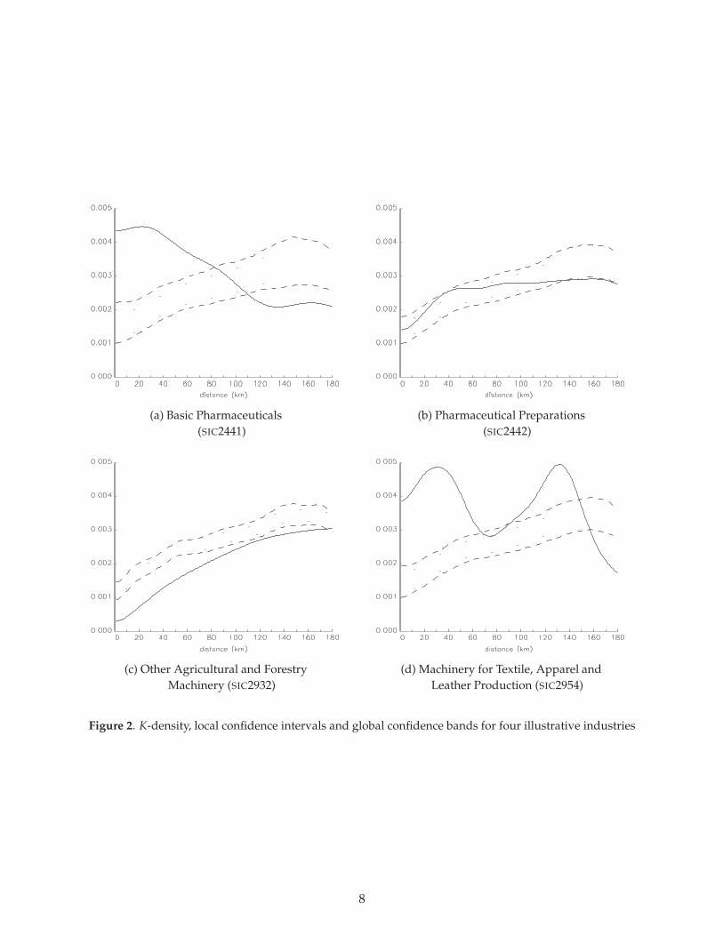
2 unique bilateral distances. Although the location of nearlyall establishments in our data is known with a high degree of precision, any Euclidian distance isonly a proxy for the true physical distance between establishments. The curvature of the earth is afirst source of systematic error. However it is easy to verify that in the UK the maximum possibleerror caused by the curvature of the earth is below one kilometre. The second source of systematicerror is that journey times for any given distance might differ between low and high-density areas.However, there are opposing effects at work. In low-density areas, roads are fewer (so actualjourney distances are much longer than Euclidean distances) whereas in high-density areas theyare more numerous (so Euclidean distances are a good approximation to actual) but also morecongested. It is unclear which effect dominates so we impose no specific correction.4 We are stillleft with random errors. For example, the real distance between two points along a straight roadis equal to its Euclidian distance whereas that between two points on opposite sides of a river isusually well above its Euclidian counterpart. Given this noise in the measurement of distances, wedecided to kernel-smooth when estimating the distribution of bilateral distances.

Denote by di,j, the Euclidian distance between establishments i and j. Given n establishments,the estimator of the density of bilateral distances (henceforth K-density) at any point d is:

K(d) =1

n(n − 1)h

n−1

∑i=1

n

∑j=i+1

f(

d − di,j

h

)(1)

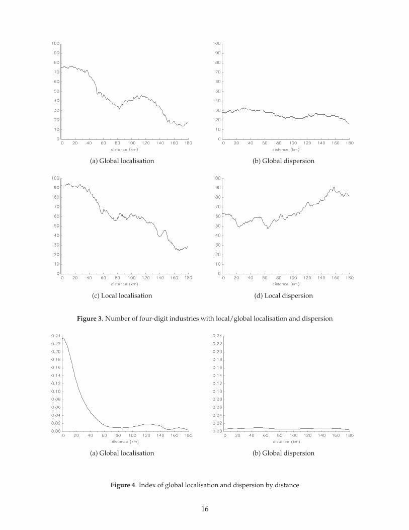
where h is the bandwidth and f is the kernel function. All densities are calculated using a Gaussiankernel with the bandwidth set as per Section 3.4.2 of Silverman (1986). The solid lines in Figures2(a-d) plot these densities for the same four industries as previously. The dashed and dotted linesin the figures, which refer to local and global confidence bands, will be explained later.

Estimation issues

Before going further, we briefly discuss several estimation issues.Because distances cannot be negative, we need to constrain our density estimates to be zero for

negative distances. One possible solution is to estimate the kernel density ignoring this boundary

4According to Combes and Lafourcade (2005), the correlation between Euclidian distances and generalised transportcosts (computed from real transport data) for France is extremely high at 0.97.

7

(a) Basic Pharmaceuticals (b) Pharmaceutical Preparations(SIC2441) (SIC2442)

(c) Other Agricultural and Forestry (d) Machinery for Textile, Apparel andMachinery (SIC2932) Leather Production (SIC2954)

Figure 2. K-density, local confidence intervals and global confidence bands for four illustrative industries

8

restriction, then to set the estimate to zero for negative distances and re-scale at all other distancesto ensure that the density still sums to one. Unfortunately, this uniform re-scaling means thatdistances near to the boundary will contribute less to our density estimate and thus that the weightof the distribution near zero will be underestimated. Instead we deal with this boundary problemby adopting the reflection method proposed in Section 2.10 of Silverman (1986).5

The nature of our data implies two important differences with respect to standard kernel densityestimation. Note first that each actual K-density is calculated on the basis of a census of the entireindustry population. If, instead of a census, we had a random sample of firms from each industrywe would need to worry about the statistical variation due to the estimation of the actual K-density.Applications of the techniques developed below to samples of firms from particular industriescould allow for this statistical variation to be taken into account but the exhaustive nature of ourdata means that we are able to ignore it in what follows (see Efron and Tibshirani, 1993 and Quah,1997, for further discussion of these issues as well as Davison and Hinkley, 1997 for a discussionmore focused on point patterns).

The second difference stems from the fact that the spatial nature of our data implies strongdependence between the bilateral distances that are used to calculate the density. This strongdependence arises because the observations of interest are actually the points that generate thesebilateral distances. Even if the underlying points are independently located, the bilateral distancesbetween these points will not be independent.6 This has implications for the sampling theoryof our estimator, KA(d). In situations where the observations are independent (or only weaklydependent) then the limiting distribution of this estimator can be derived using a central limittheorem for U-statistics. Section 3.7 of Silverman (1986) provides more details of these asymptoticproperties. Unfortunately, such results are not available for the spatial point pattern data that weconsider here. See Cressie (1993) and Diggle (2003) for further discussion. This means that we willhave to rely on Monte-Carlo results in order to test for departures from randomness. This is theissue to which we now turn.

Constructing counterfactuals

At this stage, we need to decide on the relevant counterfactuals to which our K-densities should becompared. In this respect, note that the analysis of localisation is informative only to the extent thatit captures interactions across establishments or between establishments and their environment.Consequently the number of firms in each industry and the size-distribution therein are taken asgiven.7

5If the original data set for industry A is X1, X2, ... the reflected data set is X1,−X1, X2,−X2.... We then estimateK∗

A(d) using this augmented data set and define KA(d) = 2K∗A(d) if d > 0 and KA(d) = 0 if d ≤ 0.

6See below for more on this issue.7That is we take increasing returns within the firm as given. Ultimately however, any fully satisfactory approach to

these issues must treat the size of firms as endogenous. Thus, a joint-analysis of the spatial distribution of firms togetherwith that of employment within firms is in order. Our analysis is able to deal with the spatial distribution of any subsetof establishments as well as with the spatial distribution of employment but cannot directly say anything about theboundaries of the firm.

9

To satisfy our second condition, we need to control for the overall tendency of manufacturingto agglomerate. Furthermore, we need to allow for the fact that in the UK zoning and planning re-strictions are ubiquitous. Manufacturing cannot locate in many areas of the country (e.g., the Lakedistrict, London’s green belt, etc). Hence, to control for overall agglomeration and the regulatoryframework, we consider that the set of all existing "sites", S, currently used by a manufacturingestablishment constitutes the set of all possible locations for any plant.8

How should we test whether the sites occupied by a particular industry can be considereda random draw from all existing sites? One possibility would be to calculate the distributionof bilateral distances for all establishments and then to compare the estimated distribution fora particular industry to this distribution. Sampling distances directly from the density of distancesfor the whole of manufacturing would make it possible to calculate exact confidence intervalsbecause the density at each level of distance could then be treated as the result of repeated binomialdraws. However, this short-cut amounts to treating the bilateral distances between points asindependent, which they are not as already argued above.9 To see this, consider directly drawingbilateral distances for the simplest case of three plants. It is possible with a small but non-negligibleprobability to obtain three bilateral distances above 700 kilometres. However, it is impossible tohave three plants a distance of 700 kilometres from each other in the UK as such an equilateraltriangle simply cannot fit on its territory.

To avoid this problem, we need to construct counterfactuals by first drawing locations from theoverall population of sites and then calculating the set of bilateral distances. For each industry werun 1000 simulations.10 For each simulation we sample as many sites as there are establishmentsin the industry under scrutiny. Since establishments are created over time and since any existingsite hosts only one establishment, sampling is done without replacement. Thus for any industryA with n establishments, we generate our counterfactuals Am for m = 1,2,...,1000, by sampling nelements without replacement from S so that each simulation is equivalent to a random reshufflingof establishments across sites. This controls for both industrial concentration and the overallagglomeration of manufacturing. Other alternatives are possible. For instance one could draw thecounterfactuals from the set of all UK postcodes. Given that the number of residential addressesfar out-weigh that of manufacturing addresses, this would control for the overall distribution ofpopulation instead. However we think it is more informative to control for the overall distributionof manufacturing given the constraints on manufacturing location in the UK.11 Once we have thecounterfactual, we calculate the smoothed density for each simulation exactly as we did for thereal industry.

Before moving on, we note that detailed investigation suggests that the lack of independencebetween distances is important beyond very small samples. By running a very large number of

8A site is where one establishment is located – when two establishments share the same postcode, two different sitesare distinguished.

9It is this dependence that rules out the use of the asymptotic results reported in Section 3.7 of Silverman (1986).10We also repeated our simulations 2,000 and 10,000 times for a few industries with very similar results.11An important avenue for future research is to develop counterfactuals from more sophisticated theories of industrial

location and test them in the same fashion as below. We view randomness conditional on overall agglomeration as thefirst and most obvious null hypothesis to be tested but this is by no means the only one.

10

simulations (10,000) for a few medium-sized industries, we found that the differences betweenpoint-generated and distance-generated K-densities are too large for us to be able to sample dis-tances directly. For instance, for an industry with 200 establishments (which corresponds roughlyto the median number of establishments for four-digit industries), we found that the confidenceintervals were about twice as large when drawing distances directly.

Local confidence intervals

The next step is to calculate local confidence intervals. We consider all distances between 0 and180 kilometres. This threshold is the median distance between all pairs of manufacturing establish-ments. Any ’abnormally’ high values for the distance density, KA(d), for d > 180 could in principlebe interpreted as dispersion but this information is redundant if we consider both lower and upperconfidence intervals for d < 180. This reflects the fact that the densities must sum to one overthe entire range of distances (0 − 1000 kilometres). Hence we restrict our analysis to the interval[0,180]. For each industry, for each kilometre in this interval we rank our simulations in ascendingorder and select the 5th and 95th percentile to obtain a lower 5% and an upper 5% confidenceinterval that we denote KA(d) and KA(d) respectively. When for industry A, KA(d) > KA(d), thisindustry is said to exhibit localisation at distance d (at a 5% confidence level). Symmetrically, whenKA(d) < KA(d), this industry is said to exhibit dispersion at distance d (at a 5% confidence level).12 Wecan also define an index of localisation

γA(d) ≡ max(

KA(d) − KA(d),0)

, (2)

as well as an index of dispersion

ψA(d) ≡ max(

KA(d) − KA(d),0)

. (3)

To reject the hypothesis of randomness at distance d because of localisation (dispersion), we onlyneed γA(d) > 0 (ψA(d) > 0). The exact value of these two indices does not matter. However, theindices do indicate how much localisation and dispersion there is at any level of distance.

Graphically, localisation (dispersion) is detected when the K-density of one particular industrylies above (below) its local upper (lower) confidence interval. The two dotted lines in Figures 2(a-d)plot these local confidence intervals for our four illustrative industries. For instance, Machinery forTextile, Apparel and Leather Production (SIC2954) exhibits localisation for every kilometre from 0to 60 whereas Other Agricultural and Forestry Machinery (SIC2932) exhibits dispersion over thesame range of distances. Note that the shape of these confidence intervals reflect the distributionof overall manufacturing.

12Dispersion here is precisely defined as having fewer establishments at distance d than randomness would predict.In other words the distribution of a dispersed industry is "too regular". A direct analogy can be made with randomdraws of zeros and ones under equal probability. A string of 10 zeros out of ten draws is rather unlikely and akin to ourconcept of localisation. Alternatively, five zeros alternating with five ones is as unlikely and this extreme regularity isinterpreted in a geographical context as dispersion.

11

Global confidence bands

The calculation of γA(d) and ψA(d) only allows us to make local statements (i.e. at a given dis-tance) about departures from randomness. These local statements however do not correspond tostatements about the global location patterns of an industry. Even a randomly distributed industrywill exhibit dispersion or localisation for some level of distance with quite a high probability. Tosee this, recall that there is a 5% probability an industry shows localisation for each kilometre, sothat the probability of this happening for at least one kilometre among 180 is quite high even whenwe account for the fact that smoothing induces some autocorrelation in the K-density estimatesacross distances.

Our last step is thus to construct global confidence bands so that statements can also be madeabout the overall location patterns of an industry. There are infinitely many ways to draw a bandsuch that no less than 95% of a series of randomly generated K-densities lie above or below thatband. The restriction we impose here is standard: we choose identical local confidence intervals atall levels of distance such that the global confidence level is 5%. That is, deviations by randomlygenerated K-densities are equally likely across all levels of distances to make the confidence bandsneutral with respect to distances.

Here, we cannot use the standard Bonferroni method which considers the local confidenceinterval y such that in our case (1 − y)181 = 5% since it ignores the positive autocorrelation acrossdistances and would thus give us confidence bands that are too wide. Instead, the solution is togo back to our simulated industries and look for the upper and lower local confidence intervalssuch that, when we consider them across all distances between 0 and 180, only 5% of our randomlygenerated K-densities hit them. The local confidence levels associated with these confidence bandswill of course be below 5%.

Even with 1000 simulations however, there may not be any local confidence level such that wecan capture exactly 95% of our randomly generated K-densities. This problem is solved easilyby interpolating. The second worry is that we may need to consider the local 99.9th or even the100.0th percentile to get a 5% confidence band. The variance of these randomly generated extremebounds (i.e., the extreme or the second extreme value in the simulations) is potentially quite highwhich means a low degree of precision for the corresponding bands. However, because localisationand dispersion are correlated across distances (be it only because of optimal smoothing), the localconfidence level such that 5% of our randomly generated industries deviate is typically around99%, i.e., the 10th extreme value, for which the variance is much lower.

Denote KA(d) the upper confidence band of industry A. This band is hit by 5% of our simula-tions between 0 and 180 kilometres. When KA(d) > KA(d) for at least one d ∈ [0,180] this industryis said to exhibit global localisation (at a 5% confidence level). Turning to global dispersion, recall thatby construction, our distance densities must sum to one. Thus an industry which is very localisedat short distances can show dispersion at larger distances. In other words, for strongly localisedindustries, dispersion is just an implication of localisation. This discussion suggests the followingdefinition: The lower confidence band of industry A, KA(d), is such that it is hit by 5% of therandomly generated K-densities that are not localised. An industry is then said to exhibit globaldispersion (at a 5% confidence level) when KA(d) < KA(d) for at least one d ∈ [0,180] and the industry

12

does not exhibit localisation. As before, we can define:

ΓA(d) ≡ max(

KA(d) − KA(d),0)

, (4)

an index of global localisation and

ΨA(d) ≡{

max(

KA(d) − KA(d),0)

if ∑d=180d=0 ΓA(d) = 0,

0 otherwise,(5)

an index of global dispersion.Graphically, global localisation is detected when the K-density of one particular industry lies

above its upper confidence band. Global dispersion is detected when the K-density lies below thelower confidence band and never lies above the upper confidence band. For our four illustrativeindustries, the global confidence bands are represented by the two dashed lines in Figures 2(a-d).For instance, Machinery for Textile, Apparel and Leather Production (SIC2954) exhibits globallocalisation whereas Other Agricultural and Forestry Machinery (SIC2932) exhibits dispersion.Pharmaceutical Preparations (SIC2442) shows neither global localisation nor dispersion while BasicPharmaceuticals (SIC2441) shows global localisation and thus by definition no dispersion eventhough its K-density does go beneath the lower confidence band.

Interpretation and examples

To understand better what these tests capture, let us consider a few examples. Take first anindustry like Basic Pharmaceuticals (SIC2441) with a cluster of plants around London. This clusterimplies a high density for distances between 0 and 60 kilometres and this industry thus showslocalisation between these distances. Consider now an industry like Machinery for Textile, Appareland Leather Production (SIC2954) with a cluster of plants around Manchester and another aroundBirmingham. The large number of establishments located close to each other in both Manchesterand Birmingham still implies localisation between 0 and 50 kilometres. Furthermore, Manchesterand Birmingham are quite close to each other so that there is also localisation for distances between100 and 140 kilometres. Had the second cluster been in London instead of Birmingham, this secondpeak of distance would not show-up in our analysis as Manchester and London are more than180 kilometres from each other. A multiplicity of peaks in our distance density thus indicates amultiplicity of clusters close to each other. Consider now the more contrived case of an industrylocated mostly in one region but with regularly dispersed plants (in order to serve local marketsfor instance). Such an industry would be locally dispersed at short distances, but also localised athigher levels of distances (capturing the fact that it is present in only one region).

A limit common to all approaches, including ours, is that we cannot detect non-random patternsif they do not involve localisation or dispersion. Thus we may accept as random some industrieswhose location is clearly non-random, for example industries located along a coast or a railwayline. However the likelihood of such a type-II error decreases with the number of establishments.For instance, an industry with plants along a straight line is localised at short distances (thenumber of neighbours increases linearly with distance whereas if location is random, the increaseis quadratic) and this should be detected provided there are enough establishments.

13

Finally, note that a cluster of establishments is more likely to be found in the Midlands, whichhas a lot of manufacturing than, say, in Northern Scotland which has very little. Our analysisdoes not directly deal with this, since as a first step we want to be able to make statements aboutpatterns in particular industries in relation to general manufacturing and not about the patterns ofspecialisation of particular local economies. The analysis of specialisation is conceptually distinctfrom that of localisation and as it requires different tools it is beyond the scope of this paper.

Before presenting our results, it is worth considering what we can and cannot learn from thistype of analysis. Localisation is compatible with any explanation of clustering that relies on someform of external effect but also with any explanation based on fixed natural endowments. LikeEllison and Glaeser (1997), we think that it is helpful to be able to make statements about thelocation pattern of an industry without knowing the right mix of external economies and naturalendowments that led to this pattern. In the Appendix, we develop a simple economic model whichshows that our test is indeed one of randomness versus localisation resulting from either externaleconomies or natural endowments.

4. Baseline results for four-digit industries

In this section we describe our results for UK four-digit industries using the complete populationof plants.

How many industries deviate and where

We consider 234 industries (out of 239) that have more than 10 establishments. 205 deviate locallyat some distance over the range. Correcting for global confidence bands as outlined in Section3 leads us to conclude that 177 industries differ significantly from randomness at the 5% level ofsignificance. The detailed breakdown is as follows. We find that 122 industries, that is 52% of them,are localised whereas 55 industries (24%) are dispersed, and 57 (24%) do not deviate significantlyfrom randomness. From our results, localisation is not as widespread as earlier studies led us tobelieve whereas dispersion seems much more prevalent. Devereux et al. (2004) on comparable UK

data, Ellison and Glaeser (1997) on US data, or Maurel and Sédillot (1999) on French data find thatbetween 75 and 95% of industries are localised according to the EG index and less than 15% aredispersed. Note however that these papers deal with the localisation of employment and not thatof plants. See below for a comparison between our approach when weighting by employment andthe EG index using the same data.

To go further and to look at scale issues, Table 1 considers the fraction of industries which showlocalisation at three thresholds (5, 30 and 150 kilometres). A majority of industries that deviate forany of these three threshold tend to do it for both 5 and 30 kilometres. These results are confirmedwhen looking more broadly at cross-industry patterns. Figure 3 shows the number of localisedand dispersed industries for each level of distance. Both local and global localisation results showroughly similar patterns for localisation. At low distances, a significant proportion of industriesare localised. The number of localised industries is on a high plateau between 0 and 40 kilometres,then falls sharply with distance up to around 80 kilometres and then begins to rise again with

14

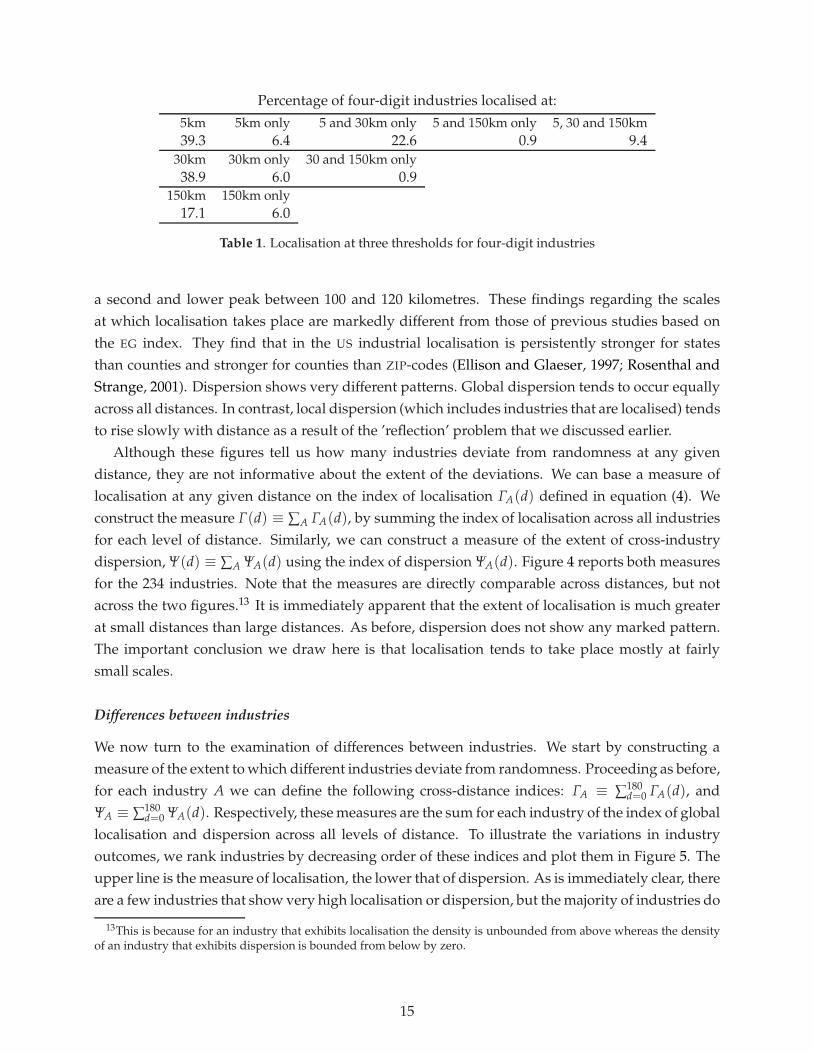
Percentage of four-digit industries localised at:5km 5km only 5 and 30km only 5 and 150km only 5, 30 and 150km39.3 6.4 22.6 0.9 9.4

30km 30km only 30 and 150km only38.9 6.0 0.9

150km 150km only17.1 6.0

Table 1. Localisation at three thresholds for four-digit industries

a second and lower peak between 100 and 120 kilometres. These findings regarding the scalesat which localisation takes place are markedly different from those of previous studies based onthe EG index. They find that in the US industrial localisation is persistently stronger for statesthan counties and stronger for counties than ZIP-codes (Ellison and Glaeser, 1997; Rosenthal andStrange, 2001). Dispersion shows very different patterns. Global dispersion tends to occur equallyacross all distances. In contrast, local dispersion (which includes industries that are localised) tendsto rise slowly with distance as a result of the ’reflection’ problem that we discussed earlier.

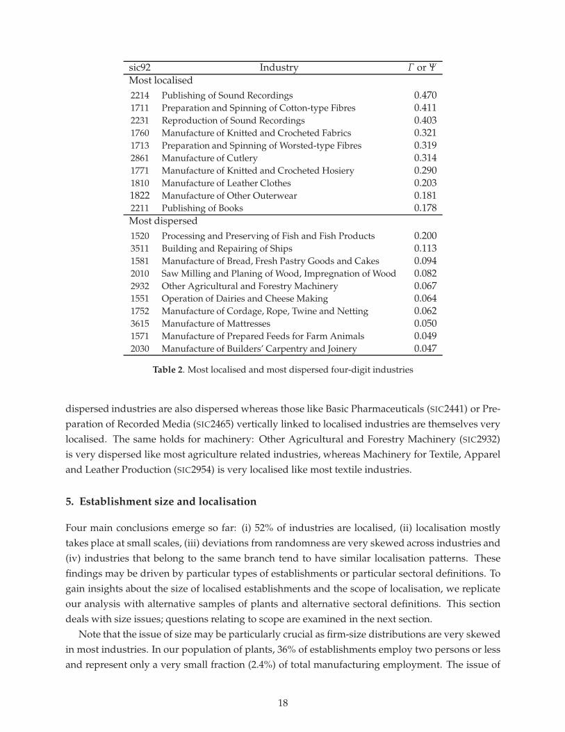
Although these figures tell us how many industries deviate from randomness at any givendistance, they are not informative about the extent of the deviations. We can base a measure oflocalisation at any given distance on the index of localisation ΓA(d) defined in equation (4). Weconstruct the measure Γ(d) ≡ ∑A ΓA(d), by summing the index of localisation across all industriesfor each level of distance. Similarly, we can construct a measure of the extent of cross-industrydispersion, Ψ(d) ≡ ∑A ΨA(d) using the index of dispersion ΨA(d). Figure 4 reports both measuresfor the 234 industries. Note that the measures are directly comparable across distances, but notacross the two figures.13 It is immediately apparent that the extent of localisation is much greaterat small distances than large distances. As before, dispersion does not show any marked pattern.The important conclusion we draw here is that localisation tends to take place mostly at fairlysmall scales.

Differences between industries

We now turn to the examination of differences between industries. We start by constructing ameasure of the extent to which different industries deviate from randomness. Proceeding as before,for each industry A we can define the following cross-distance indices: ΓA ≡ ∑180

d=0 ΓA(d), andΨA ≡ ∑180

d=0 ΨA(d). Respectively, these measures are the sum for each industry of the index of globallocalisation and dispersion across all levels of distance. To illustrate the variations in industryoutcomes, we rank industries by decreasing order of these indices and plot them in Figure 5. Theupper line is the measure of localisation, the lower that of dispersion. As is immediately clear, thereare a few industries that show very high localisation or dispersion, but the majority of industries do

13This is because for an industry that exhibits localisation the density is unbounded from above whereas the densityof an industry that exhibits dispersion is bounded from below by zero.

15

(a) Global localisation (b) Global dispersion

(c) Local localisation (d) Local dispersion

Figure 3. Number of four-digit industries with local/global localisation and dispersion

(a) Global localisation (b) Global dispersion

Figure 4. Index of global localisation and dispersion by distance

16

Figure 5. Distribution of global localisation and dispersion by four-digit industries

not see such extreme outcomes. This highly skewed distribution of localisation confirms previousfindings (Ellison and Glaeser, 1997; Devereux et al., 2004; Maurel and Sédillot, 1999).

To give some idea of the reality underlying Figure 5, Table 2 lists the 10 most localised industriesand the 10 most dispersed. Interestingly, more than a century after Marshall (1890), Cutlery(SIC2861) is still amongst the most localised industries. Six textile or textile-related industries arealso in the same list together with three media-based industries. These highly localised industriesare fairly exceptional. In contrast, the mean industry (after ranking industries by their degree oflocalisation) is barely more localised than if randomly distributed. It is mostly food-related indus-tries together with industries with high transport costs or high dependence on natural resourcesthat show dispersion.

Our main focus in this paper is on the proportion of manufacturing sectors that are localised.However, it is interesting to notice that a number of industries that appear in Table 2 are fairlysmall in terms of overall employment. This raises the question as to whether the percentageof manufacturing workers employed in localised industries is above or below the percentage ofsectors that are localised. Weighting sectors by their share in manufacturing employment, wefind that 67% of UK manufacturing employers work in sectors that are localised. This showsthat localised sectors tend to have a larger share of manufacturing employment. Offsetting this,however, is the fact that the employment share weighted mean of the index of globalisation, ΓA, is30% lower than the un-weighted mean of the index. That is, larger sectors tend to be less stronglylocalised.

Finally, it is also interesting to notice that for many (two-digit) branches, related industrieswithin the same branch tend to follow similar patterns. Table 3 breaks down localisation of indus-tries by branches. For instance nearly all Food and Drink industries (SIC15) or Wood, Petroleum,and Mineral industries (SIC20, 23, and 26) are not localised. By contrast, most Textile, Publishing,Instrument and Appliances industries (SIC17 − 19, 22, and 30 − 33) are localised. The two mainexceptions are Chemicals (SIC24) and Machinery (SIC29). In these two branches, however, the moredetailed patterns are telling. Chemical industries such as Fertilisers (SIC2415) vertically linked to

17

sic92 Industry Γ or Ψ

Most localised2214 Publishing of Sound Recordings 0.4701711 Preparation and Spinning of Cotton-type Fibres 0.4112231 Reproduction of Sound Recordings 0.4031760 Manufacture of Knitted and Crocheted Fabrics 0.3211713 Preparation and Spinning of Worsted-type Fibres 0.3192861 Manufacture of Cutlery 0.3141771 Manufacture of Knitted and Crocheted Hosiery 0.2901810 Manufacture of Leather Clothes 0.2031822 Manufacture of Other Outerwear 0.1812211 Publishing of Books 0.178Most dispersed1520 Processing and Preserving of Fish and Fish Products 0.2003511 Building and Repairing of Ships 0.1131581 Manufacture of Bread, Fresh Pastry Goods and Cakes 0.0942010 Saw Milling and Planing of Wood, Impregnation of Wood 0.0822932 Other Agricultural and Forestry Machinery 0.0671551 Operation of Dairies and Cheese Making 0.0641752 Manufacture of Cordage, Rope, Twine and Netting 0.0623615 Manufacture of Mattresses 0.0501571 Manufacture of Prepared Feeds for Farm Animals 0.0492030 Manufacture of Builders’ Carpentry and Joinery 0.047

Table 2. Most localised and most dispersed four-digit industries

dispersed industries are also dispersed whereas those like Basic Pharmaceuticals (SIC2441) or Pre-paration of Recorded Media (SIC2465) vertically linked to localised industries are themselves verylocalised. The same holds for machinery: Other Agricultural and Forestry Machinery (SIC2932)is very dispersed like most agriculture related industries, whereas Machinery for Textile, Appareland Leather Production (SIC2954) is very localised like most textile industries.

5. Establishment size and localisation

Four main conclusions emerge so far: (i) 52% of industries are localised, (ii) localisation mostlytakes place at small scales, (iii) deviations from randomness are very skewed across industries and(iv) industries that belong to the same branch tend to have similar localisation patterns. Thesefindings may be driven by particular types of establishments or particular sectoral definitions. Togain insights about the size of localised establishments and the scope of localisation, we replicateour analysis with alternative samples of plants and alternative sectoral definitions. This sectiondeals with size issues; questions relating to scope are examined in the next section.

Note that the issue of size may be particularly crucial as firm-size distributions are very skewedin most industries. In our population of plants, 36% of establishments employ two persons or lessand represent only a very small fraction (2.4%) of total manufacturing employment. The issue of

18

Two-digit branch Number offour-digitindustries

no. globallocalisation≤ 60 km

no. globallocalisation> 60 km

15000 Food products and beverages 30 1 016000 Tobacco products 1 1 017000 Textiles 20 16 918000 Wearing apparels, dressing, etc 6 6 319000 Tanning and dressing of leather, footwear 3 3 320000 Wood and products of wood, etc 6 0 021000 Pulp, paper and paper products 7 2 122000 Publishing, printing and recorded media 13 13 823000 Coke, refined petroleum products 3 0 024000 Chemical and chemical products 20 8 825000 Rubber and plastic products 7 1 326000 Other non-metallic mineral products 24 4 227000 Basic metals 17 11 1028000 Fabricated metal products 16 9 1229000 Other machinery and equipment 20 6 930000 Office machinery and computers 2 2 231000 Electrical machinery 7 2 532000 Radio, Televisions and other appliances 3 3 333000 Instruments 5 3 434000 Motor vehicles, trailers, etc 3 1 335000 Other transport equipment 8 2 236000 Furniture and other products 13 4 500000 Aggregate 234 98 92

Table 3. Localisation by two-digit branch

firm-size is also important from a policy perspective. Policies encouraging dispersion are not likelyto be very successful if it is only small establishments that can be dispersed, whereas clusteringpolicies might be more difficult to implement if it is only large establishments that cluster. Finally,the type of establishments, big or small, that cluster or disperse is potentially very informativeabout the relevance of particular theories.

Four-digit industries when censoring the smallest plants

In this section we repeat our baseline analysis after censoring for the smallest plants in eachindustry. There are two reasons for doing this. First it checks the robustness of our results toaggregation errors introduced by the classification system. In certain industries (say shipbuildingto take our earlier example) small plants might not do the same thing as large plants. Second, inindustries where aggregation errors do not occur, it is still possible that the location behaviour ofsmall and large plants differ. Note that the ability to focus on and separately analyse any subset of

19

(a) Number of localised industries (b) Index of global localisation

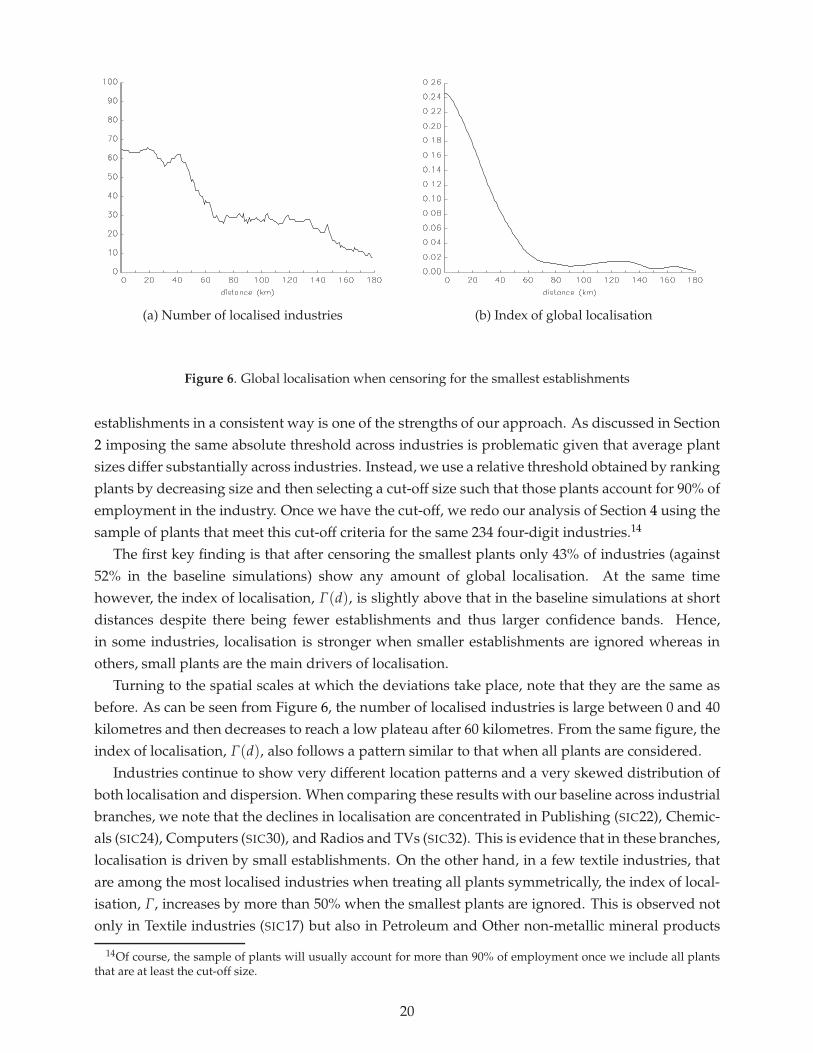
Figure 6. Global localisation when censoring for the smallest establishments

establishments in a consistent way is one of the strengths of our approach. As discussed in Section2 imposing the same absolute threshold across industries is problematic given that average plantsizes differ substantially across industries. Instead, we use a relative threshold obtained by rankingplants by decreasing size and then selecting a cut-off size such that those plants account for 90% ofemployment in the industry. Once we have the cut-off, we redo our analysis of Section 4 using thesample of plants that meet this cut-off criteria for the same 234 four-digit industries.14

The first key finding is that after censoring the smallest plants only 43% of industries (against52% in the baseline simulations) show any amount of global localisation. At the same timehowever, the index of localisation, Γ(d), is slightly above that in the baseline simulations at shortdistances despite there being fewer establishments and thus larger confidence bands. Hence,in some industries, localisation is stronger when smaller establishments are ignored whereas inothers, small plants are the main drivers of localisation.

Turning to the spatial scales at which the deviations take place, note that they are the same asbefore. As can be seen from Figure 6, the number of localised industries is large between 0 and 40kilometres and then decreases to reach a low plateau after 60 kilometres. From the same figure, theindex of localisation, Γ(d), also follows a pattern similar to that when all plants are considered.

Industries continue to show very different location patterns and a very skewed distribution ofboth localisation and dispersion. When comparing these results with our baseline across industrialbranches, we note that the declines in localisation are concentrated in Publishing (SIC22), Chemic-als (SIC24), Computers (SIC30), and Radios and TVs (SIC32). This is evidence that in these branches,localisation is driven by small establishments. On the other hand, in a few textile industries, thatare among the most localised industries when treating all plants symmetrically, the index of local-isation, Γ, increases by more than 50% when the smallest plants are ignored. This is observed notonly in Textile industries (SIC17) but also in Petroleum and Other non-metallic mineral products

14Of course, the sample of plants will usually account for more than 90% of employment once we include all plantsthat are at least the cut-off size.

20

(SIC23 and 26). In these industries, smaller establishments are more dispersed. This finding isconfirmed when looking at the patterns of dispersion. Only 19% of industries (against 24% inthe baseline) exhibit global dispersion when censoring for the smallest establishments. Overall,the location patterns of small establishments vary a lot across industries but in general are moreextreme with stronger tendencies towards either localisation or dispersion.

Four-digit industries when weighting for employment

As we made clear above, censoring for the smallest establishments sheds light on their location pat-terns when comparing the results with those obtained for the whole population of plants. Howeverthis approach does not allow a detailed analysis of location patterns for larger establishments. Italso maintains the establishment as the basic unit of observation. In some instances it is interestingto take instead the worker as the unit of observation. In this case we need to consider the bilateraldistances between all pairs of workers who belong to different establishments.

Denoting the employment of firm i by e(i), the estimator of the K-density becomes:

KempA (d) =

1h ∑n−1

i=1 ∑nj=i+1 e(i)e(j)

n−1

∑i=1

n

∑j=i+1

e(i)e(j) f(

d − di,j

h

)(6)

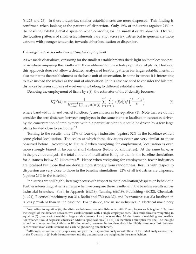
where bandwidth, h, and kernel function, f , are chosen as for equation (1). Note that we do notconsider the zero distances between employees in the same plant so localisation cannot be drivenby the concentration of employment within a particular plant but could be driven by a few largeplants located close to each other.15

Turning to the results, only 43% of four-digit industries (against 52% in the baseline) exhibitsome global localisation. The scales at which these deviations occur are very similar to thoseobserved before. According to Figure 7 when weighting for employment, localisation is evenmore strongly biased in favour of short distances (below 50 kilometres). At the same time, asin the previous analysis, the total amount of localisation is higher than in the baseline simulationsfor distances below 50 kilometres.16 Hence when weighting for employment, fewer industriesare localised but those that are deviate more strongly from randomness. Results with respect todispersion are very close to those in the baseline simulations: 22% of all industries are dispersed(against 24% in the baseline).

Industries are still highly heterogeneous with respect to their localisation/dispersion behaviour.Further interesting patterns emerge when we compare these results with the baseline results acrossindustrial branches. First, in Apparels (SIC18), Tanning (SIC19), Publishing (SIC22), Chemicals(SIC24), Electrical machinery (SIC31), Radio and TVs (SIC32), and Instruments (SIC33) localisationis less prevalent than in the baseline. For instance, five in six industries in Electrical machinery

15According to equation (6), the distance between two establishments with 10 employees each is given 100 timesthe weight of the distance between two establishments with a single employee each. This multiplicative weighting inequation (6) gives a lot of weight to large establishments close to one another. Milder forms of weighting are possible.For instance it could be possible to use an additive specification, e(i)+ e(j), rather than a multiplicative one. The thoughtexperiment corresponding to this specification would, however, be less clear since it implicitly assumes a ’link’ betweeneach worker in an establishment and each neighbouring establishment.

16Although, we cannot strictly speaking compare the Γ(d)s in this analysis with those of the initial analysis, note thatin the K-density in (6) both the numerator and the denominator are weighted in the same fashion.

21

(a) Number of localised industries (b) Index of global localisation

Figure 7. Global localisation when weighting establishments by their employment

show localisation in the initial results whereas only one still shows localisation when weightingestablishments by employment. In two other branches, Food and beverages (SIC15) and Othernon-metallic mineral products (SIC26), the exact opposite happens. For instance, only one foodindustry in the baseline shows localisation while five do when weighting by employment.

These findings are fully consistent with those obtained when censoring for smaller firms. Fur-thermore findings reported in Holmes and Stevens (2002) allow a comparison with US manufac-turing although we note that his comparison should be interpreted with caution given differencesin the methodologies employed. Holmes and Stevens (2002) examine the location patterns oflarge plants in US manufacturing using the EG index. They find that large plants tend to be morelocalised than their whole industry. In broad agreement with this tendency, we observe an increasein our index of localisation, Γ(d), for the UK when censoring for small plants. However, in contrastwith US findings, localisation in the UK is driven by large firms in only some industrial branches.

More generally, it must be emphasised that taking plant size into account reinforces the fourmain conclusions obtained so far.17 Localisation is detected in at most half of the industries. Devi-ations still occur at a scale of 0 to 50 kilometres. There is still a lot of cross-industry heterogeneitywith respect to localisation and dispersion. This is compounded by cross-industry differences inlocation patterns between small and large establishments. Finally we observe broad patterns ofclustering of small vs large establishments by industrial branch.

Before turning to a detailed comparison between our approach and the EG index, it must benoted that the two approaches developed here to examine patterns of localisation by establishmentsize could be further refined. Instead of considering only one threshold, we could consider finerclasses of establishment sizes in each industries. The counterfactuals could also be modified.For instance, imagine that establishment size constrains location choices to a set of ‘appropriate’sites. Then, we could construct counterfactuals that only allow large firms to locate on large sites

17Interestingly when industries are ranked by decreasing localisation the Spearman rank correlation when weightingby employment with the baseline is 0.77 whereas that with the ranking when censoring for establishment size is 0.74.

22

and small firms to locate only on sites currently occupied by a small firm. These questions aswell as broader issues about which type of establishment localise (e.g., independent vs affiliated,indigenous vs foreign owned, etc) are explored in Duranton and Overman (2005). The importantthing to note here is that our technique is flexible enough to accommodate for these variants andthis makes it possible to explore many other questions.

Comparison with the EG index

The index developed by Ellison and Glaeser (1997) is equal to

EGA ≡ gA − HA

1 − HA, (7)

where HA ≡ ∑j xA(j)2 is the Herfindahl index of industrial concentration for industry A, xA(j) isthe share of employment of establishment j in industry A, gA is a raw localisation index equal to

gA ≡ ∑i(sA(i) − s(i))2

1 − ∑i s(i)2 , (8)

sA(i) is the share of area i in industry A, and s(i) the areas share in total manufacturing. Anypositive value for this index is interpreted as localisation. Ellison and Glaeser (1997) also arguethat a value between 0 and 0.02 signals weak localisation and anything above 0.05 is interpretedas a strong tendency to localise. To compare with our methodology, we apply this index to the 120postcode areas of the UK (without Northern Ireland) using the total population of plants. Note thatpostcode areas are on average less populated than US states but larger than US counties.

The mean value of the EG index across 234 UK industries is 0.034 and the median is at 0.011.These figures are above their corresponding values for US counties but below those of US statesaccording to Ellison and Glaeser (1997)’s calculations. We also find that 94% of UK industrieshave a positive EG index and thus exhibit some localisation. This proportion is very close to thatobtained by Ellison and Glaeser (1997) for the US (97%).

As the EG index not only controls for the lumpiness of plants but also for their size distribution,it is a-priori best compared to our results when plants are weighted by employment. The contrastis strong since we find 43% of industries to be localised (against 94%) and 22% to be dispersed(against 6%). When ranking industries by decreasing EG index, we need to choose a cut-off valueof 0.015 to ensure that 43% of industries are defined as localised, suggesting that Ellison andGlaeser (1997)’s definition of weak localisation (EG index above 0 but less than 0.02) is probablynot appropriate. For UK manufacturing plants this definition of weak localisation mostly definesindustries whose location patterns are not significantly different from randomness.

Furthermore, in addition to the substantial differences in terms of number of localised in-dustries, individual industries show different outcomes between the two measures. Across allindustries, the Spearman rank-correlation between the EG index and our ranking is statisticallysignificant at 0.41. Focusing on the most localised industries we find that the two methods agreeon only 5 out of 10 industries. Interestingly two publishing industries and Jewelry, which wefind to be very localised, are ranked above 30 according to the EG index. Looking at the detailedlocation patterns of Jewelry and these two publishing industries is informative. Studying the maps

23

for these sectors, we see that they are indeed very localised around London (with a second clusterin Birmingham for Jewelry). The EG index does not capture this localisation as the Greater Londonregion is divided into different postcode areas, which are then treated as completely unrelatedentities in the calculation of the index.

We believe this comparison highlights a number of advantages of our approach. First, allocatingdots on a map to units in a box introduces border effects that bias downwards existing measuresof localisation. We believe this downward border bias is why the EG index is consistently foundto increase with the size of spatial units. On its own, this downward bias would tend to increasethe number of localised industries identified by our methodology which avoids this border effect.However, offsetting this is the fact that ignoring the significance of departures from randomnessbiases existing measures of localisation upwards. Our methodology removes border effects andallows for significance, and our results show that the latter effect dominates. Second, the relevantgeographical scales for localisation emerge naturally from our analysis because we do not need toarbitrarily define the size of units ex-ante. Existing indices are calculated over only one partitionof space, whereas we have shown that different industries localise at different spatial scales. Thisproblem is compounded by the fact that small scales (urban and metropolitan) turn out to beparticularly important and this level of aggregation is not very well captured when using spatialunits such as US states, European regions, UK or US counties or UK postcode areas (for which thecorrespondence with the urban scale is good only for medium-sized cities). Finally we are ableto deal flexibly with the crucial issue of the size distribution of establishments. To understandwhy flexibility is important, note that our three approaches outlined above yield similar aggregateresults with respect to the extent and scales of localisation, but that there are sizable differences forparticular industries. This reflects the fact that there are marked differences in location patternsbetween small and large establishments and that the nature of those differences also varies acrossindustries. Existing indices are narrowly constrained in the way they deal with the distributionof establishment size (e.g. through a Herfindahl index in the EG case) whereas our approach isflexible and could easily be extended to other weighting methods.

6. The scope of localisation

We now consider three extensions of our methodology related to the scope of the localisation thatwe observe. First, we evaluate the sectoral scope of localisation by replicating our baseline analysisfor alternative three and five-digit sectoral classifications. Second, we consider whether we canidentify localisation effects for four-digit industries within three-digit sectors. Third, we examinethe tendency for different establishments in four-digit industries within the same sectors to co-locate.

Localisation of five-digit sub-industries

In the UK, 33 four-digit industries (out of 239) are sub-divided into more finely defined five-digitsub-industries. We consider only the 58 (out of 76) five-digit sub-industries that have more than10 establishments. Correcting for global confidence bands, we find that 44 of these sub-industries

24

(76%) deviate significantly from randomness. More precisely, 45% are localised, 31% are dispersed,while we cannot reject randomness for the remaining 24%.

These figures are not very different from those for four-digit industries. However, it is moremeaningful to compare them with the patterns observed in the corresponding industrial branchesinstead of the whole sample since sub-industries are more prevalent in some branches than in oth-ers. The branch with most sub-industries, 15 out of 58, is Food and beverage (SIC15). There, four-digit industries generally show dispersion and so do sub-industries. 13 out of 58 sub-industriesare in Textiles (SIC17) and Apparel (SIC18). These are mostly localised, sometimes highly so, justlike their four-digit counterparts. The third large group, accounting for 12 sub-industries, is inChemicals (SIC24) and Machinery (SIC29). They show mixed patterns just like their correspondingindustries.

When looking more closely at the differences between industries and their related sub-industries, three findings emerge. First, when the patterns of localisation are strong for industries,they are often even stronger for their sub-industries.18 Second, we find (in both Food and Ma-chinery) that industries showing either a dispersed or a seemingly random pattern are sometimescomposed of one sub-industry that is localised and one that is only slightly dispersed. This impliesthat some of the lack of localisation that we detect for industries reflects a classification problem– five-digit sub-industries can show different non-random behaviours which look random whenthese are lumped together. Hence, using more finely defined industrial categories allows us touncover some patterns that were so far hidden.19 Third, in some instances when an industryshows minor dispersion or localisation (in terms of ΨA or ΓA) we often cannot reject randomnessfor related five-digit components because these are smaller and thus have larger confidence bands.Thus, moving to a five-digit classification sometimes allows us to pick up more detail in thelocation patterns, but at the cost of greater imprecision reflected in the width of the confidencebands. In total, the increase in sectoral detail appears to offset the imprecision, so that we rejectrandomness for approximately the same proportion of industries.

Localisation of three-digit sectors

We now turn to the comparison between three-digit sectors and four-digit industries. Of 103sectors, 87% of them deviate globally at some level of distance. The proportion that are localisedor dispersed is higher than in the baseline: 58% and 29% respectively against 52% and 24% forfour-digit industries.

18However, some interesting details emerge. For example, for clothing industries, plants that produce women’sclothing are always more localised than plants producing men’s clothing.

19However, note that production establishments must report only one SIC even though they may be engaged indifferent industries. Since multi-activity is more likely in closely related industries, classification errors become moreimportant as industries are more finely defined. Note also that five-digit sub-industries are only marginally more finelydefined than four-digit industries. For instance SIC1751, Carpet and rugs, distinguishes between SIC17511, Woven carpetand rugs, and SIC17512, Tufted carpet and rugs. Such a fine distinction may not capture very many differences acrossestablishments possibly using the same type of workers, and sharing the same customers and suppliers. In contrast, thedifference between three-digit sectors and four-digit industries is markedly stronger. For instance SIC175, Manufactureof other textiles, is sub-divided into four very different industries: Carpets and rugs (1751), Cordage, rope and netting(1752), Non-wovens (1753) and Other textiles (1754).

25

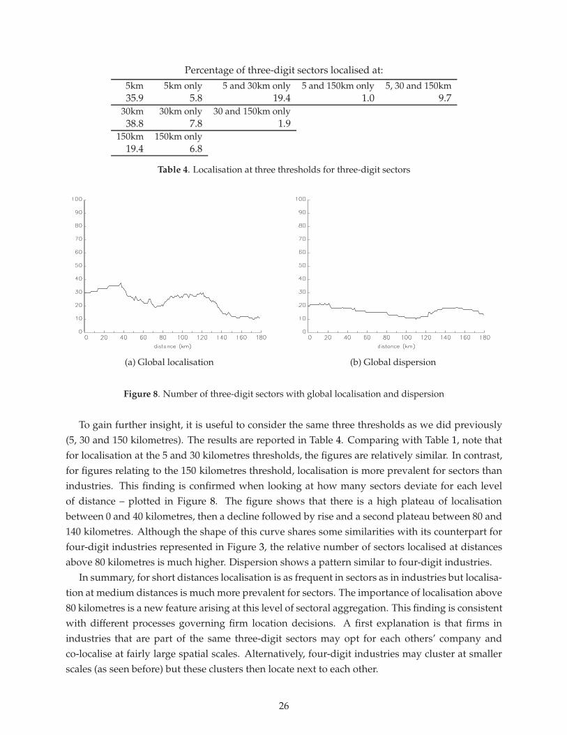
Percentage of three-digit sectors localised at:5km 5km only 5 and 30km only 5 and 150km only 5, 30 and 150km35.9 5.8 19.4 1.0 9.7

30km 30km only 30 and 150km only38.8 7.8 1.9

150km 150km only19.4 6.8

Table 4. Localisation at three thresholds for three-digit sectors

(a) Global localisation (b) Global dispersion

Figure 8. Number of three-digit sectors with global localisation and dispersion

To gain further insight, it is useful to consider the same three thresholds as we did previously(5, 30 and 150 kilometres). The results are reported in Table 4. Comparing with Table 1, note thatfor localisation at the 5 and 30 kilometres thresholds, the figures are relatively similar. In contrast,for figures relating to the 150 kilometres threshold, localisation is more prevalent for sectors thanindustries. This finding is confirmed when looking at how many sectors deviate for each levelof distance – plotted in Figure 8. The figure shows that there is a high plateau of localisationbetween 0 and 40 kilometres, then a decline followed by rise and a second plateau between 80 and140 kilometres. Although the shape of this curve shares some similarities with its counterpart forfour-digit industries represented in Figure 3, the relative number of sectors localised at distancesabove 80 kilometres is much higher. Dispersion shows a pattern similar to four-digit industries.

In summary, for short distances localisation is as frequent in sectors as in industries but localisa-tion at medium distances is much more prevalent for sectors. The importance of localisation above80 kilometres is a new feature arising at this level of sectoral aggregation. This finding is consistentwith different processes governing firm location decisions. A first explanation is that firms inindustries that are part of the same three-digit sectors may opt for each others’ company andco-localise at fairly large spatial scales. Alternatively, four-digit industries may cluster at smallerscales (as seen before) but these clusters then locate next to each other.

26

Problems also arise when trying to interpret the amount of localisation observed for distancesbelow 40 kilometres. It could be the case that what we detect here as localisation for three-digitsectors is in fact localisation in the four-digit industries within these sectors. For instance, loc-alisation in Pharmaceuticals (SIC244) might be driven mostly by the strong tendency of Basicpharmaceuticals (SIC2441) to cluster. Alternatively, this finding could be driven by a tendencyfor firms across different industries that are part of the same sector to co-localise at this spatialscale. For instance in Pharmaceuticals (SIC244), firms in Pharmaceutical preparations (SIC2442)may try to locate close to firms in Basic pharmaceuticals (SIC2441) just like producers of car partsmay seek to locate close to car assemblers.

Hence with regard to the localisation of three-digit sectors, we must contemplate three possibleexplanations. First, there could be a classification problem where the relevant level of analysisis three-digit sectors instead of four-digit industries. Previous findings for four-digit industrieswould then reflect what happens in sectors. Second, the classification problem may be in theopposite direction and sectoral localisation may just reflect localisation of four-digit industries. Inthis case, the relevant level of analysis is the four-digit industry since sectoral localisation is drivenby localisation in one or more industries within the sector. Third, and more subtly, there maybe some location differences between industries in the same sector so that the relevant level ofanalysis is still the four-digit industry, but at the same time, there may also be some interactionshappening between these industries leading plants in different industries to opt for locations closeto one another.

To assess these three explanations, we look at the location patterns of industries within sectors.In the next sub-section we show that localisation is still strong in four-digit industries even aftercontrolling for the location of the three-digit sectors. That is, the second and third explanations arepreferred to the first. Later on, we test the second explanation against the third. Our results thereoffer some support for both of these explanations.

Localisation within three-digit sectors

If the relevant level of aggregation is the three-digit sector, we expect plants in localised industriesto locate close to other plants in the same sector irrespective of the industry they belong to. Thusafter controlling for the location of the three-digit sector, four-digit industries should exhibit notendency to localise. Alternatively, if the relevant level of aggregation is the four-digit industry, westill expect to observe industry effects after controlling for the location of the sector.

Whether four-digit industries still show localisation after controlling for the overall localisationof their three-digit sectors can be answered with a simple modification of the main approachdescribed in Section 3. Instead of sampling the counterfactuals from the overall set of manufac-turing sites, S, it is possible to sample only from the sites occupied by firms in the same sector.Thus the approach is the same throughout, but for any four-digit industry A which comprises nestablishments and is part of sector B, just sample without replacement n sites from SB the set ofsites occupied by an establishment part of sector B instead of sampling from S.20

20The concept of "co-agglomeration" used by Ellison and Glaeser (1997) is also in this spirit since it is based on thedifference between the EG index of the sector and the weighted average of the EG indices of each individual industry.

27

There are 184 industries that are part of a three-digit sector containing at least two industries.Of these, we find that 48% show localisation. This is very marginally less than with our baseline.However, for all distances under 150km fewer industries deviate and the amount of localisationcaptured by Γ is somewhat lower than in the baseline (substantially lower for distances under60km). With respect to dispersion, the figure is at 18%, much lower than for the baseline (24%).

From this we conclude that when controlling for the location of the parent sector, industriestend to exhibit slightly less localisation and dispersion. Interestingly, we note that for Textile(SIC17), Publishing (SIC22) and Basic metals (SIC27) industries, far fewer industries are localisedwith respect to their parent sector than general manufacturing. For instance, in Publishing only fiveindustries in 13 are localised in their parent sector against all of them in the baseline analysis.21 Still,five of the 10 most localised industries in Table 2 remain among the 10 most localised industrieswhen controlling for the location of their parent sectors. However, their Γ has on average a valueless than half of that in the baseline.

In conclusion, the three-digit sector to which an industry belongs explains some of its locationbehaviour but not all. Differences between four-digit industries remain substantial suggestingthat we must take them as our basic level of analysis. However, further analysis is necessaryto understand the strong sector effects we observe. It could be that plants in related industrieshave a tendency to localise in the same areas but that location decisions are independent acrossthe industries. Thus this localisation may be a purely random outcome of clusters happeningto be close to each other. Alternatively the factors driving localisation in these industries couldshare some similarities and thus lead their establishments to cluster together. These two types ofexplanation are similar in that they both suggest that plants in related industries have independentlocation patterns (i.e. the location of one industry does not directly influence that of another). Inthis case, we can talk of joint-localisation. The opposite case is where establishments in an industrymay decide to locate close to establishments in related industries. In this case location patternsacross industries are no longer independent and we can speak of co-localisation.

Localisation across industries within three-digit sectors

Despite some attention in the recent literature (Ellison and Glaeser, 1997; Devereux et al., 2004)and its crucial importance with respect to many theoretical and policy concerns, very little isknown about co-localisation.22 Although it is easy to define co-localisation as the tendency ofdifferent industries to opt for each other’s company and as a result to cluster together, measuringco-localisation and distinguishing from joint-localisation is much more complex than analysinglocalisation. To see why, consider the following generalised version of equation (1):

K(A,B)(d) =1

P(nA,nB)h

nA

∑i=1

nB

∑j=1j �=i

f(

d − di,j

h

)(9)

21The reason is that most industries in Publishing are based around London. The same hold for Birmingham andBasic Metals, Manchester and Textile, etc.

22The term co-agglomeration is also used in the literature. For consistency with respect to the terminology used sofar, we speak of co-localisation. Note however that the existing literature does not distinguish between joint-localisationand co-localisation.

28

where bandwidth (h) and kernel function ( f ) are chosen as for equation (1), A and B are two(possibly overlapping) subsets from the population of establishments, S, and P(nA,nB) is thetotal number of unique bilateral distances between pairs of different establishments with oneestablishment from each subset.23 The density K(A,B)(.) is a straightforward generalisation of KA(.)which allows us to calculate the density of bilateral distances between establishments in any twosubsets from a population.

Then, it remains to define the counterfactuals which this distribution should be compared to.In this respect, note that tests over K(A,B)(.) may involve counterfactuals A and B drawn from anysubset of S. A priori this implies a considerable number of possible tests. Many of these tests arenot very informative with respect to co-localisation. For instance calculating the bilateral distancedensity using equation (9) for two four-digit industries A and B that belong to the same sector andcomparing it to counterfactuals generated by sampling from the overall population of firms leadsto results that are highly problematic to interpret. The reason is that localisation in two industriescan also generate some form of joint-localisation across the same two industries. A measure basedon sampling from the overall population cannot distinguish between co-localisation and joint-localisation and thus confuses the two explanations.

Among all the possible tests one could construct using (9), we believe one exercise is of particu-lar interest here – to see whether there is some tendency for localisation across different four-digitindustries after controlling for the overall tendency of the establishments of both industries tocluster. To investigate this, we can apply equation (9) to any two four-digit industries, A and Bthat are part of the same three-digit industries, and sample our counterfactuals from the set of allsites occupied by an establishment in either of these industries, A ∪ B. The intuition behind thistest is very simple. It allows us to determine whether plants in an industry (A) have a tendencyto be closer to plants in related industries (B) that are part of the same sector than to plants inthe same industry (A). For instance after controlling for the localisation tendency of the partitioncomposed of Basic Pharmaceuticals and Pharmaceutical Preparations (SIC2441 and 2442), it allowsus to test whether plants in SIC2442 tend to locate closer to plants in SIC2441 than randomnesswould suggest. Note that this is a strong test since upper deviations from randomness mean thatestablishments in these industries are attracted to each other even after controlling for whatevertendency they have to cluster. At the same time, being unable to reject randomness is no rejectionof industries being co-localised in some sense.

There are 317 possible pairs of four-digit industries that are part of the same three-digit sectors.Local co-localisation is detected in 56% of the pairs but the proportion falls to 34% when controllingfor global confidence bands. Furthermore, the extent of co-localisation, as measured by Γ isnever very large. Hence there seems to be a fairly widespread tendency for related industriesto co-localise but the tendency is not of overwhelming intensity. Turning to lower deviations, orco-dispersions, they occur locally in 31% of industry pairs and 29% when controlling for globalconfidence bands. The tendency for pairs of industries to separate is thus slightly less widespreadthan their tendency to co-localise but it takes place with greater intensity when it does (reflecting

23If A and B are the same set (A ∼ B) then P(nA,nB) = nA(nA−1)2 . If A and B are disjoint sets (A ∩ B = ∅) then

P(nA,nB) = nAnB.

29

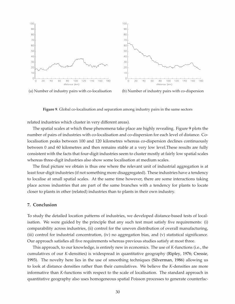
(a) Number of industry pairs with co-localisation (b) Number of industry pairs with co-dispersion

Figure 9. Global co-localisation and separation among industry pairs in the same sectors

related industries which cluster in very different areas).The spatial scales at which these phenomena take place are highly revealing. Figure 9 plots the

number of pairs of industries with co-localisation and co-dispersion for each level of distance. Co-localisation peaks between 100 and 120 kilometres whereas co-dispersion declines continuouslybetween 0 and 60 kilometres and then remains stable at a very low level.These results are fullyconsistent with the facts that four-digit industries seem to cluster mostly at fairly low spatial scaleswhereas three-digit industries also show some localisation at medium scales.

The final picture we obtain is thus one where the relevant unit of industrial aggregation is atleast four-digit industries (if not something more disaggregated). These industries have a tendencyto localise at small spatial scales. At the same time however, there are some interactions takingplace across industries that are part of the same branches with a tendency for plants to locatecloser to plants in other (related) industries than to plants in their own industry.

7. Conclusion

To study the detailed location patterns of industries, we developed distance-based tests of local-isation. We were guided by the principle that any such test must satisfy five requirements: (i)comparability across industries, (ii) control for the uneven distribution of overall manufacturing,(iii) control for industrial concentration, (iv) no aggregation bias, and (v) statistical significance.Our approach satisfies all five requirements whereas previous studies satisfy at most three.

This approach, to our knowledge, is entirely new in economics. The use of K-functions (i.e., thecumulatives of our K-densities) is widespread in quantitative geography (Ripley, 1976; Cressie,1993). The novelty here lies in the use of smoothing techniques (Silverman, 1986) allowing usto look at distance densities rather than their cumulatives. We believe the K-densities are moreinformative than K-functions with respect to the scale of localisation. The standard approach inquantitative geography also uses homogeneous spatial Poisson processes to generate counterfac-

30

tuals.24 We differ from this by sampling randomly from a set of sites which allows us to control forthe overall distribution of manufacturing.25 Finally, we construct proper confidence intervals andconfidence bands instead of taking the envelope of a small number of simulations.

We applied our tests to an exhaustive UKmanufacturing data set. Our main findings are:

• 52% of four-digit industries exhibit localisation at a 5% confidence level and 24% of themshow dispersion at the same confidence level.

• Localisation in four-digit industries takes place mostly between 0 and 50 kilometres.

• The extent of localisation and dispersion are very skewed across industries.

• Four- and five-digit industries follow broad sector and branch patterns with respect to local-isation.

• In some industrial branches, localisation at the industry level is driven by larger establish-ments, whereas in others it is smaller establishments which have a tendency to cluster.

• Localisation and dispersion are as frequent in three-digit sectors as in four-digit industriesfor distances below 80 kilometres. Three-digit sectors also show a lot of localisation atthe regional scale (80 − 140 kilometres) due, at least in part, to the tendency of four-digitindustries to co-localise at this spatial scale.

Some of these results confirm previous findings in the literature. For instance, the high levels ofheterogeneity in location patterns across industries have been observed by most previous studies.Other results are in stark contrast. For instance, we do not find as many industries to be localised aspreviously claimed. Along the same lines, we find the propensity for dispersion to be stronger thanone may have believed. Our results about broad sectoral effects are also stronger than previouslyobtained. Our results on plant size suggest that differences in location behaviour between largeand small plants are more nuanced than earlier studies have led us to believe. Finally our resultsabout the scale and the scope of localisation are to a large extent completely new as the toolspreviously available were not suited to an exploration of these issues.

Many detailed issues remain to be investigated as regards the issues of localisation, dispersion,and co-localisation. For instance, one may wish to compare the behaviour of independent plantswith that of affiliated plants or that of foreign plants versus domestic ones. Also, much remains tobe learnt about co-localisation in vertically linked industries, etc. We hope to be able to shed light

24That is they assume that under the null hypothesis of randomness the probability of a point occurring in any regionR is proportional to the area of R. Marcon and Puech (2003) use these standard approaches based on homogenousspatial Poisson processes to study industrial location in France. Their paper clearly demonstrates the problems withapplying standard techniques directly to the study of localisation. For example, their results suggest that all industriesare concentrated — hardly surprising given the fact that aggregate activity in France is very concentrated around Paris!

25With our emphasis on Monte-Carlo simulations to allow for the uneven distribution of aggregate activity, ourapproach shares some similarities with very recent work on the use of case-control counterfactuals for the application ofspatial point patterns in epidemiology. In that literature, however, counterfactuals are constructed by taking the locationof individuals as given and then randomly deciding whether individuals are healthy. We believe that our approach oftaking a firm’s sector as given and treating location as random is a more suitable thought experiment when studyinglocalisation. See Diggle (2003).

31

on these questions in future research. Furthermore, we would like to see our approach replicatedfor other countries. Data availability is certainly an issue here. Note however that several countriesincluding Canada and France are currently developing geo-coded data similar to those availablein the UK. For many countries including the US, such developments are less likely in the very nearfuture.26 However, in these countries establishment level data are often available at a very finelevel of geographic aggregation like census tracts or zipcode areas in the US. Our methodology caneasily be adapted to this type of data by randomly allocating establishments within the smallestavailable spatial units. In this case, the error made on the location is of the same magnitude asthe square-root of the area of the smallest spatial unit. Provided the areas are relatively small, wesuspect that this error will be far outweighed by the improvement with respect to meeting the fiverequirements that we outline above.

In future work, we also wish to develop our distance-based approach to test more sophisticatedmodels of industrial location. So far we have only tested the simplest non-trivial model of indus-trial location: randomness conditional on overall manufacturing agglomeration. It is obvious thatdifferent counterfactuals could be generated by using more sophisticated theoretical frameworks.These theories could be tested as here, by looking at deviations from confidence bands computedfrom counterfactuals (again to be generated from the theories to be tested). Alternatively, onecould use our indices of localisation as endogenous variables and regress them on a set of industrycharacteristics.

As a final point, note that distance-based analyses can be applied beyond industrial geography.Any data with detailed geographical information readily lends itself to this type of analysis.In the past, studies involving distance based measures could be performed only on very smallpopulations (Cressie, 1993) for lack of computing power and precise enough data. These twoobstacles are gradually being removed and we hope to see more of this type of study in the future.Furthermore, and as shown in part by our study, distance-based analysis not only allows us toanswer long standing empirical questions in a more precise and accurate way but it also allows usto address new questions that could not previously be tackled.

26See Holmes and Stevens (2004) for a detailed discussion of North American data sources.

32

References

Combes, Pierre-Philippe and Miren Lafourcade. 2005. Transport costs: Measures, determinants,and regional policy implications for France. Journal of Economic Geography (forthcoming).

Cressie, Noel A. C. 1993. Statistics for Spatial Data. New York: John Wiley.

Davison, Anthony C. and David V. Hinkley. 1997. Bootstrap Methods and their Application. Cam-bridge: Cambridge University Press.

Devereux, Michael P., Rachel Griffith, and Helen Simpson. 2004. The geographic distribution ofproduction activity in the UK. Regional Science and Urban Economics 35(5):533–564.

Diggle, Peter J. 2003. Statistical Analysis of Spatial Point Patterns. New York: Oxford UniversityPress.

Duranton, Gilles and Henry G. Overman. 2005. Detailed location patterns of UK manufacturingindustries. Processed, London School of Economics.

Efron, Bradley and Robert J. Tibshirani. 1993. An Introduction to the Bootstrap. New York: Chapmanand Hall.

Ellison, Glenn and Edward L. Glaeser. 1997. Geographic concentration in US manufacturingindustries: A dartboard approach. Journal of Political Economy 105(5):889–927.

Griffith, Rachel. 1999. Using the ard establishment level data: an application to estimating produc-tion functions. Economic Journal 109(456):F416–F442.

Holmes, Thomas J. and John J. Stevens. 2002. Geographic concentration and establishment scale.Review of Economics and Statistics 84(4):682–690.

Holmes, Thomas J. and John J. Stevens. 2004. Spatial distribution of economic activities in NorthAmerica. In Vernon Henderson and Jacques-François Thisse (eds.) Handbook of Regional andUrban Economics, volume 4. Amsterdam: North-Holland.

Hoover, Edgar M. 1937. Location Theory and the Shoe and Leather Industries. Cambridge, Mass.:Harvard University Press.

Marcon, Eric and Florence Puech. 2003. Evaluating the geographic concentration of industriesusing distance-based methods. Journal of Economic Geography 3(4):409–428.

Marshall, Alfred. 1890. Principles of Economics. London: Macmillan.

Maurel, Françoise and Béatrice Sédillot. 1999. A measure of the geographic concentration of frenchmanufacturing industries. Regional Science and Urban Economics 29(5):575–604.

Quah, Danny T. 1997. Empirics for growth and distribution: Stratification, polarization, andconvergence clubs. Journal of Economic Growth 2(1):27–59.

Raper, Jonathan F., David W. Rhind, and John W. Shepherd. 1992. Postcodes : The New Geography.Harlow, Essex: Longman Scientific and Technical.

Ripley, Brian D. 1976. The second-order analysis of stationary point processes. Journal of AppliedProbability 13(2):255–266.

Rosenthal, Stuart A. and William C. Strange. 2001. The determinants of agglomeration. Journal ofUrban Economics 50(2):191–229.

33

Silverman, Bernard W. 1986. Density Estimation for Statistics and Data Analysis. New York: Chapmanand Hall.

Yule, George U. and Maurice G. Kendall. 1950. An Introduction to the Theory of Statistics. London:Griffin.

Appendix A. A model

Consider N establishments and Z, a set of points on the Euclidian plane whose cardinal is muchlarger than N. The elements of Z are called potential sites. Denote by dj,k the Euclidian distancebetween the potential sites j and k. Z is such that:

∀j ∈ Z, dO,j ≤ d , (A 1)

where d is the maximum distance between a potential site and the origin O. Each potential site jfor establishment i has a value equal to:

Vj(i) = vj + εi,j + gj,A(i) , (A 2)

where vj is the intrinsic value of the potential site, εi,j is a positive i.i.d. random component,and gj,A(i) is an industry specific component which applies to all establishments which belongto industry A. The component vj reflects the fact that some potential sites are more desirable irre-spective of one’s industry. The random component εi,j captures all the factors that are idiosyncraticto establishment i with respect to the potential site j. Finally, the industry specific component issuch that

gj,A(i) = ∑k

G(dj,k) , (A 3)

where the k are attraction points in the Euclidian space for all establishments in industry A. Thedecay function G(.) is such that G′ < 0 and G′′ > 0. Attraction points capture the effect oflocalised natural endowments. Establishments gain from being closer to these attraction points.The location decisions among the potential sites depend thus on three factors, their intrinsic valueswhich apply symmetrically to all establishments, their idiosyncratic values which apply differentlyto all establishments and the location value g which applies symmetrically to all establishments inthe same industry.

Potential sites are allocated sequentially. The equilibrium is such that the first establishmentoccupies the site it values most. The second establishment occupies the site it values most amongthe remaining ones, etc. Denote by S the set of all occupied sites and SA the set of occupied sitesby the establishments of industry A in equilibrium. Note that the industry-specific location valueis defined by fixed natural endowments. The model can however be easily generalised to spatialdistortions generated by local externalities (see Ellison and Glaeser, 1997, for a justification anddetails on the observational equivalence between fixed natural endowments and local externalit-ies). The only complication is that local externalities, which make relative (and no longer absolute)location matter, would leave some room for multiple equilibria.

34

The null hypothesis for industry A is

H0 : g.,A = 0 , (A 4)

This null is equivalent to SA being a random sample of Z in equilibrium. To reject this, it issufficient to have the K-density for industry A to be different from that of an industry with thesame number of establishments occupying sites randomly sampled from Z. Unfortunately, we donot observe Z, the set of potential sites.

Our empirical strategy relies on the fact that Z can be proxied by S. For this approximationto be valid we need (i) all industries to be small with respect to overall manufacturing so that wehave a large number of them, (ii) that the location of attraction points must be independent acrossindustries and (iii) Var(g) � Var(v + ε) in almost all industries. The last condition requires thatthe effects of natural endowments must not be so strong as to make some industries cluster verytightly. Otherwise, the proportion of very short bilateral distances between elements of S would belarger than that of Z. Conditions (i)-(iii) indicate that mild clustering in industries is not a worryprovided industries are small and clustering across industries is independent. In this case, the lawof large number applies and S is approximately a random sample of Z. It is then possible to samplecounterfactuals from S rather than Z.

35