HAL Id: hal-01007323https://hal.archives-ouvertes.fr/hal-01007323

Submitted on 12 Jun 2017

HAL is a multi-disciplinary open accessarchive for the deposit and dissemination of sci-entific research documents, whether they are pub-lished or not. The documents may come fromteaching and research institutions in France orabroad, or from public or private research centers.

L’archive ouverte pluridisciplinaire HAL, estdestinée au dépôt et à la diffusion de documentsscientifiques de niveau recherche, publiés ou non,émanant des établissements d’enseignement et derecherche français ou étrangers, des laboratoirespublics ou privés.

Distributed under a Creative Commons Attribution| 4.0 International License

Strain Localisation and Damage Measurement by Full3D Digital Image Correlation: Application to 15-5PH

Stainless SteelTong Wu, Michel Coret, Alain Combescure

To cite this version:Tong Wu, Michel Coret, Alain Combescure. Strain Localisation and Damage Measurement by Full3D Digital Image Correlation: Application to 15-5PH Stainless Steel. Strain, Wiley-Blackwell, 2011,47 (1), pp.49-61. �10.1111/j.1475-1305.2008.00600.x�. �hal-01007323�

Strain Localisation and Damage Measurementby Full 3D Digital Image Correlation: Applicationto 15-5PH Stainless Steel

T. Wu, M. Coret and A. Combescure

Universite de Lyon, INSA-Lyon, LaMCoS, CNRS UMR5259, F69621 Villeurbanne, France

ABSTRACT: The objective of this paper is to propose a method for measuring damage in ductile

materials, from its inception to rupture. In the first stage of damage, which occurs before locali-

sation, the usual method for determining damage through the measurement of stiffness variation is

used. A damageable elastic–plastic model of the modified Lemaitre/Chaboche type is identified from

these tests. An original method is proposed for measuring damage following the initiation of strain

localisation. This method is based on a full 3D image correlation analysis using four cameras. The

principle of the method consists in identifying the damage through tensile experiments on thin, flat-

notched specimens subjected to tensile loading. Speckles are applied on both faces of each specimen

in order to follow the strain fields on the two faces at the same time. These two strain fields are

digitised simultaneously by two synchronised sets of two digital cameras. This paper shows how this

method enables one to identify strain localisation and deduce the evolution of damage directly.

Here, the method is developed for 15-5 PH stainless steel.

KEY WORDS: 3D digital image correlation, continuum damage mechanics, ductile fracture, strain

localisation

Introduction

The fracture of materials is a complex process in

which the mechanical properties deteriorate through

damage and cracking because of volume or surface

discontinuities. In the case of ductile materials, the

initiation phase of the damage is called diffuse

necking and results essentially in a loss of stiffness.

This is followed by an accumulation of damage

leading invariably to strain localisation, also called

localised necking, and ends with rupture of the

material. The type of fracture observed is analysed in

the second part of the paper, in which fracture is

observed on the microscale.

Here, the damage models used for analysing the

diffuse damage phase are defined within the frame-

work of the thermodynamics of irreversible processes

[1]. Some models use cavities or porous solid plas-

ticity to represent damage [2, 3]. These theories,

which assume damage to be isotropic, use a single

scalar variable defined as the volume fraction of

cavities in a representative volume element. Other

models are based on continuum damage mechanics

(CDM) [4, 5]. In CDM, damage is associated with the

critical strain energy density in the constitutive

equations governing the irreversible processes in the

material. In the case of ductile materials, these two

families of models represent, through different

approaches, a single phenomenon: the growth of

microvoids [6].

In this paper, we attempt to show how damage can

be measured from its inception to fracture, which is

still a difficult problem. The section succeeding the

subsequent one focuses on the measurement of

damage during diffuse necking. A usual method in

which damage is measured directly through the

stiffness variation of metallic specimens is reviewed.

These measurements enable one to identify a damage

model of the Lemaitre type [6] which has been

modified by the authors [7, 8].

The succeeding section proposes a new methodol-

ogy for measuring damage during localised necking.

This direct method circumvents the delicate problem

of inverse identification one usually has to deal with

[3]. In order to do that, one uses flat-notched speci-

mens (FNS), the strains of which on both faces are

measured by 3D stereocorrelation. Thus, one obtains

the local surface strain field and the thickness field

throughout the test, which enables one to deduce

damage as a local volume increase.

1

This research study was applied to a 15-5PH stain-

less steel alloy (AMS5659), a high-strength member

of the martensitic precipitation-hardened stainless

steel family which is commonly used for aerospace

components such as valves, shafts, fasteners, fittings

or gears. The specific 15-5PH we used in our

experiment is H1025 (Condition H1025), i.e. a

precipitation-hardened steel which has been heat

solution-treated at 1025 ± 15 F for 4 h, then air-

cooled. The chemical composition of 15-5PH H1025

is shown in Table 1. On the microscopic scale, this

steel is martensitic at low temperatures and austenitic

at high temperatures.

Evaluation of the Microscopic Damage

Microscopic observations were performed in order to

study the damage mechanism on the microscale and

to help choose an appropriate damage model.

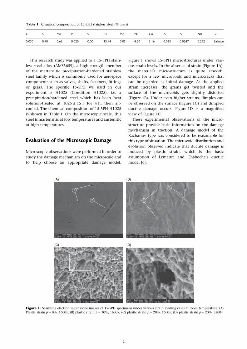
Figure 1 shows 15-5PH microstructures under vari-

ous strain levels. In the absence of strain (Figure 1A),

the material’s microstructure is quite smooth,

except for a few microvoids and microcracks that

can be regarded as initial damage. As the applied

strain increases, the grains get twisted and the

surface of the microvoids gets slightly distorted

(Figure 1B). Under even higher strains, dimples can

be observed on the surface (Figure 1C) and dimpled

ductile damage occurs. Figure 1D is a magnified

view of Figure 1C.

These experimental observations of the micro-

structure provide basic information on the damage

mechanism in traction. A damage model of the

Kachanov type was considered to be reasonable for

this type of situation. The microvoid distribution and

evolution observed indicate that ductile damage is

induced by plastic strain, which is the basic

assumption of Lemaitre and Chaboche’s ductile

model [6].

Table 1: Chemical composition of 15-5PH stainless steel (% mass)

C Si Mn P S Cr Mo Ni Cu Al N NB Fe

0.030 0.40 0.66 0.020 0.001 15.44 0.05 4.50 3.16 0.013 0.0247 0.292 Balance

(A) (B)

(C) (D)

Figure 1: Scanning electron microscope images of 15-5PH specimens under various strain loading cases at room temperature. (A)

Plastic strain p = 0%, 1600·; (B) plastic strain p = 10%, 1600·; (C) plastic strain p = 20%, 1600·; (D) plastic strain p = 20%, 3200·

2

Identification of MacroscopicDamage on Standard Round BarSpecimens

Theoretical model

The damage variable, as introduced by Kachanov [4],

is defined based on the irreversible processes leading

to nucleation and to the growth of microvoids and

microcracks in the entire volume of the specimen. All

types of voids and cracks (both intergranular and

transgranular) which lead to deterioration of the

integrity of the material are accounted for. For

homogeneous and isotropic damage, the damage

variable can be defined in the representative volume

element (RVE):

D ¼ SD

S(1)

where S is the area of the intersection of the plane

being considered with the RVE and SD is the effective

area of the intersections of all microcracks and

microvoids in S.

Following the thermodynamic approach of

Lemaitre and Chaboche [5], the damage rate variable

is related to the equivalent plastic strain rate. In the

case of uniaxial ductile plastic damage strain, the

model is the following:

_D ¼Dc

pR�pD_p if p>pD and r > 0

0 otherwise

�: (2)

where Dc represents the critical damage, p the accu-

mulated equivalent plastic strain and pR its value at

rupture. pD is the threshold-equivalent accumulated

plastic strain and r is the applied stress. The dot

symbol denotes the time derivative.

The experimental damage results of 15-5PH show

that in a uniaxial tensile test the damage is a non-

linear function of the plastic strain. In order to match

the experimental data, we propose to introduce an

initial damage D0 and a power law characterised by

an exponent a. For uniaxial loading, we get:

_D ¼ Dc �D0ð Þa _p ppR�pD

� �a�1if p > pD and r > 0

0 otherwise

((3)

Dð0Þ ¼ D0

The damage exponent a is an additional material

parameter. Finally, our model has five material

parameters (pD, pR, D0, Dc, a), whereas Lemaitre

and Chaboche’s basic ductile model has only

three material damage parameters (pD, pR, Dc). It

is obvious that our model reduces to Lemaitre

and Chaboche’s model if D0 = 0 and a = 1. The iden-

tification of this model consists in setting the values

of the five coefficients by means of tensile tests.

Let us observe that in most structures the applied

stress is not uniaxial. Following Lemaitre and Chab-

oche’s method of obtaining 3D models [5, 6], the 3D

damage model is described in rate form by the fol-

lowing equation:

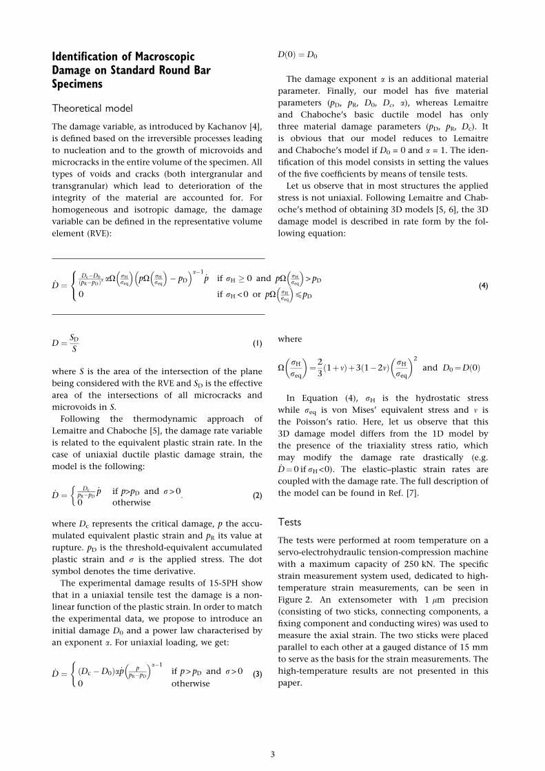
where

XrH

req

� �¼ 2

3ð1þ mÞþ3ð1�2mÞ rH

req

� �2

and D0¼Dð0Þ

In Equation (4), rH is the hydrostatic stress

while req is von Mises’ equivalent stress and m is

the Poisson’s ratio. Here, let us observe that this

3D damage model differs from the 1D model by

the presence of the triaxiality stress ratio, which

may modify the damage rate drastically (e.g._D¼0 if rH <0). The elastic–plastic strain rates are

coupled with the damage rate. The full description of

the model can be found in Ref. [7].

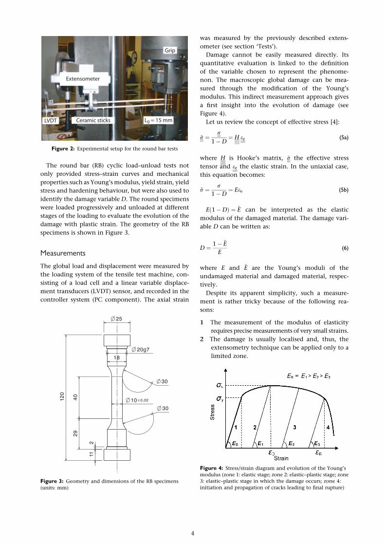
Tests

The tests were performed at room temperature on a

servo-electrohydraulic tension-compression machine

with a maximum capacity of 250 kN. The specific

strain measurement system used, dedicated to high-

temperature strain measurements, can be seen in

Figure 2. An extensometer with 1 lm precision

(consisting of two sticks, connecting components, a

fixing component and conducting wires) was used to

measure the axial strain. The two sticks were placed

parallel to each other at a gauged distance of 15 mm

to serve as the basis for the strain measurements. The

high-temperature results are not presented in this

paper.

_D ¼Dc�D0

ðpR�pDÞa aX rH

req

� �pX rH

req

� �� pD

� �a�1_p if rH � 0 and pX rH

req

� �> pD

0 if rH < 0 or pX rH

req

� �OpD

8<: (4)

3

The round bar (RB) cyclic load–unload tests not

only provided stress–strain curves and mechanical

properties such as Young’s modulus, yield strain, yield

stress and hardening behaviour, but were also used to

identify the damage variable D. The round specimens

were loaded progressively and unloaded at different

stages of the loading to evaluate the evolution of the

damage with plastic strain. The geometry of the RB

specimens is shown in Figure 3.

Measurements

The global load and displacement were measured by

the loading system of the tensile test machine, con-

sisting of a load cell and a linear variable displace-

ment transducers (LVDT) sensor, and recorded in the

controller system (PC component). The axial strain

was measured by the previously described extens-

ometer (see section ‘Tests’).

Damage cannot be easily measured directly. Its

quantitative evaluation is linked to the definition

of the variable chosen to represent the phenome-

non. The macroscopic global damage can be mea-

sured through the modification of the Young’s

modulus. This indirect measurement approach gives

a first insight into the evolution of damage (see

Figure 4).

Let us review the concept of effective stress [4]:

~r ¼r

1�D¼ H ee (5a)

where H is Hooke’s matrix, ~r the effective stress

tensor and ee the elastic strain. In the uniaxial case,

this equation becomes:

~r ¼ r1�D

¼ Eee (5b)

Eð1�DÞ ¼ ~E can be interpreted as the elastic

modulus of the damaged material. The damage vari-

able D can be written as:

D ¼ 1� ~E

E(6)

where E and ~E are the Young’s moduli of the

undamaged material and damaged material, respec-

tively.

Despite its apparent simplicity, such a measure-

ment is rather tricky because of the following rea-

sons:

1 The measurement of the modulus of elasticity

requires precise measurements of very small strains.

2 The damage is usually localised and, thus, the

extensometry technique can be applied only to a

limited zone.

Figure 3: Geometry and dimensions of the RB specimens

(units: mm)

Figure 2: Experimental setup for the round bar tests

Figure 4: Stress/strain diagram and evolution of the Young’s

modulus (zone 1: elastic stage; zone 2: elastic–plastic stage; zone

3: elastic–plastic stage in which the damage occurs; zone 4:

initiation and propagation of cracks leading to final rupture)

4

3 In the stress–strain graph, it is difficult to identify

the ‘best straight line’ which represents elastic

loading or unloading.

The unloading ramp is used to measure the Young’s

modulus. In evaluating the modulus of elasticity

during elastic unloading, one must stay away from

highly nonlinear zones. This is achieved by carrying

out the evaluation in a stress range defined as

follows:

rmin < r < rmax (7)

where rmin and rmax are the lower and upper stress

limits of the linear part, respectively.

In the stress–strain region defined above, there are

two errors: a strain error and a stress error. Therefore,

the true measured value lies somewhere within a

small rectangle. The strain error is 5 · 10)5 and the

stress error was 0.5 MPa in our tests. Of course, the

previous method is not valid in the case of localisa-

tion because the damage cannot be considered to be

uniform throughout the specimen.

RemarkAs usual, the measured strain (total strain) is assumed

to be the sum of an elastic strain ee and an irreversible

plastic strain ep.

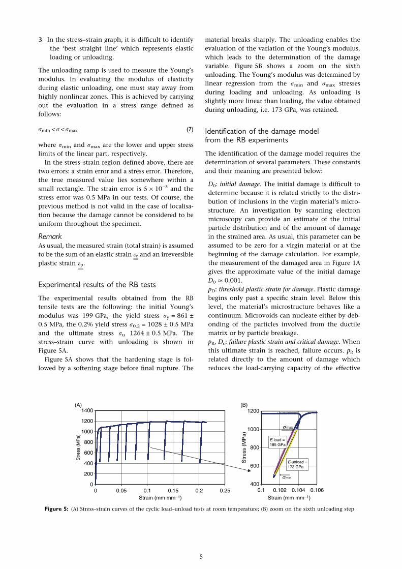
Experimental results of the RB tests

The experimental results obtained from the RB

tensile tests are the following: the initial Young’s

modulus was 199 GPa, the yield stress ry = 861 ±

0.5 MPa, the 0.2% yield stress r0.2 = 1028 ± 0.5 MPa

and the ultimate stress ru 1264 ± 0.5 MPa. The

stress–strain curve with unloading is shown in

Figure 5A.

Figure 5A shows that the hardening stage is fol-

lowed by a softening stage before final rupture. The

material breaks sharply. The unloading enables the

evaluation of the variation of the Young’s modulus,

which leads to the determination of the damage

variable. Figure 5B shows a zoom on the sixth

unloading. The Young’s modulus was determined by

linear regression from the rmin and rmax stresses

during loading and unloading. As unloading is

slightly more linear than loading, the value obtained

during unloading, i.e. 173 GPa, was retained.

Identification of the damage modelfrom the RB experiments

The identification of the damage model requires the

determination of several parameters. These constants

and their meaning are presented below:

D0: initial damage. The initial damage is difficult to

determine because it is related strictly to the distri-

bution of inclusions in the virgin material’s micro-

structure. An investigation by scanning electron

microscopy can provide an estimate of the initial

particle distribution and of the amount of damage

in the strained area. As usual, this parameter can be

assumed to be zero for a virgin material or at the

beginning of the damage calculation. For example,

the measurement of the damaged area in Figure 1A

gives the approximate value of the initial damage

D0 � 0.001.

pD: threshold plastic strain for damage. Plastic damage

begins only past a specific strain level. Below this

level, the material’s microstructure behaves like a

continuum. Microvoids can nucleate either by deb-

onding of the particles involved from the ductile

matrix or by particle breakage.

pR, Dc: failure plastic strain and critical damage. When

this ultimate strain is reached, failure occurs. pR is

related directly to the amount of damage which

reduces the load-carrying capacity of the effective

0

200

400

600

800

1000

1200

1400

0 0.05 0.1 0.15 0.2 0.25Strain (mm mm–1) Strain (mm mm–1)

Str

ess

(MP

a)

400

600

800

1000

1200

0.1 0.102 0.104 0.106

Str

ess

(MP

a)

smin

s max

E-unload =173 GPa

E-load =185 GPa

(A) (B)

Figure 5: (A) Stress–strain curves of the cyclic load–unload tests at room temperature; (B) zoom on the sixth unloading step

5

resisting section critically. In theory, when failure

occurs, the critical damage variable Dc should be

equal to 1. In fact, in almost all experimental

observations on metals, failure occurs before D = 1.

a: damage exponent. This constant carries information

which influences the type of damage evolution and

can be determined from tensile tests. Its value sets the

degree of nonlinearity of the damage evolution law.

For any given pD, pR, D0 and Dc, there is a discrimi-

nating value of a which determines the convexity of

the damage evolution as a function of plastic strain.

If D0 is assumed to be zero, the time integration of

Equation (6) gives:

D ¼ Dcp� pD

pR � pD

� �a

(8)

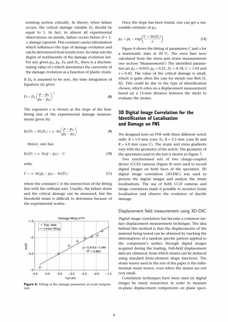
The exponent a is chosen as the slope of the best-

fitting line of the experimental damage measure-

ments given by:

lnðDÞ ¼ lnðDcÞ þ a � ln p� pD

pR � pD

� �(9)

Hence, one has:

lnðDÞ ¼ a � lnðp� pDÞ � C (10)

with:

C ¼ a � lnðpR � pDÞ � lnðDcÞ (11)

where the constant C is the intersection of the fitting

line with the ordinate axis. Usually, the failure strain

and the critical damage can be measured, but the

threshold strain is difficult to determine because of

the experimental scatter.

Once the slope has been found, one can get a rea-

sonable estimate of pD:

pD ¼ pR � expCþ lnðDcÞ

a

� �(12)

Figure 6 shows the fitting of parameters C and a for

a martensitic state at 20 �C. The error bars were

calculated from the stress and strain measurements

(see section ‘Measurements’) The identified parame-

ters are pD = 0.010, pR = 0.21, Dc = 0.18, C = 1.02 and

a = 0.42. The value of the critical damage is small,

which is quite often the case for metals (see Refs [5,

6]). This could be due to the type of identification

chosen, which relies on a displacement measurement

based on a 15-mm distance between the sticks to

evaluate the strains.

3D Digital Image Correlation for theIdentification of Localisationand Damage on FNS

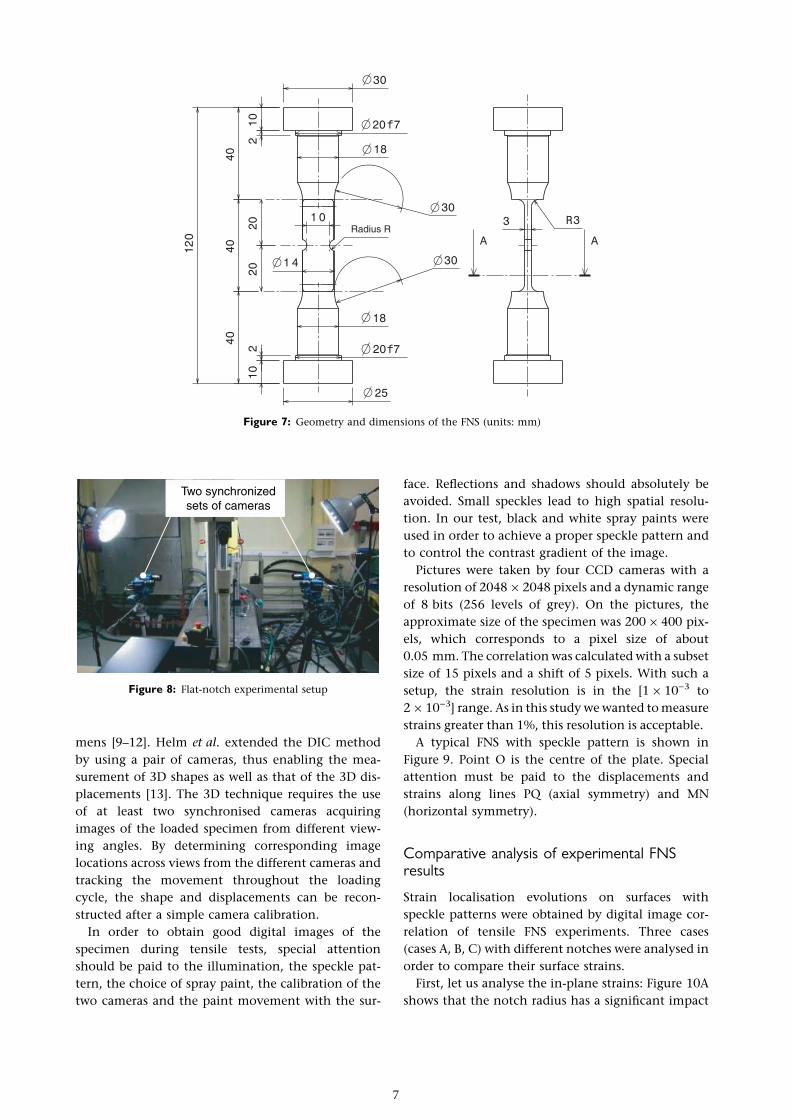
We designed tests on FNS with three different notch

radii: R = 1.0 mm (case A), R = 2.5 mm (case B) and

R = 4.0 mm (case C). The strain and stress gradients

vary with the geometry of the notch. The geometry of

the specimens used in the test is shown in Figure 7.

Two synchronised sets of two charge-coupled

device (CCD) cameras (Figure 8) were used to record

digital images on both faces of the specimen. 3D

digital image correlation (3D-DIC) was used to

process the digital images and analyse the strain

localisations. The use of both CCD cameras and

image correlation made it possible to monitor strain

localisation and observe the evolution of ductile

damage.

Displacement field measurement using 3D-DIC

Digital image correlation has become a common sur-

face displacement measurement technique. The idea

behind this method is that the displacements of the

material being tested can be obtained by tracking the

deformations of a random speckle pattern applied to

the component’s surface through digital images

acquired during the loading. Full-field displacement

data are obtained, from which strains can be deduced

using standard finite-element shape functions. The

strain tensor used in the rest of the paper is the infin-

itesimal strain tensor, even when the strains are not

very small.

Correlation techniques have been used on digital

images by many researchers in order to measure

in-plane displacement components on plane speci-

y = 0.415x –1.046R ² = 0.963

–3

–2.5

–2

–1.5

–4.5 –4.0 –3.5 –3.0 –2.5 –1.5–2.0

ln(D

)

ln(p–pD)

Damage fitting of P1

Exp. dataLinear fitting

Figure 6: Fitting of the damage parameters at room tempera-

ture

6

mens [9–12]. Helm et al. extended the DIC method

by using a pair of cameras, thus enabling the mea-

surement of 3D shapes as well as that of the 3D dis-

placements [13]. The 3D technique requires the use

of at least two synchronised cameras acquiring

images of the loaded specimen from different view-

ing angles. By determining corresponding image

locations across views from the different cameras and

tracking the movement throughout the loading

cycle, the shape and displacements can be recon-

structed after a simple camera calibration.

In order to obtain good digital images of the

specimen during tensile tests, special attention

should be paid to the illumination, the speckle pat-

tern, the choice of spray paint, the calibration of the

two cameras and the paint movement with the sur-

face. Reflections and shadows should absolutely be

avoided. Small speckles lead to high spatial resolu-

tion. In our test, black and white spray paints were

used in order to achieve a proper speckle pattern and

to control the contrast gradient of the image.

Pictures were taken by four CCD cameras with a

resolution of 2048 · 2048 pixels and a dynamic range

of 8 bits (256 levels of grey). On the pictures, the

approximate size of the specimen was 200 · 400 pix-

els, which corresponds to a pixel size of about

0.05 mm. The correlation was calculated with a subset

size of 15 pixels and a shift of 5 pixels. With such a

setup, the strain resolution is in the [1 · 10)3 to

2 · 10)3] range. As in this study we wanted to measure

strains greater than 1%, this resolution is acceptable.

A typical FNS with speckle pattern is shown in

Figure 9. Point O is the centre of the plate. Special

attention must be paid to the displacements and

strains along lines PQ (axial symmetry) and MN

(horizontal symmetry).

Comparative analysis of experimental FNSresults

Strain localisation evolutions on surfaces with

speckle patterns were obtained by digital image cor-

relation of tensile FNS experiments. Three cases

(cases A, B, C) with different notches were analysed in

order to compare their surface strains.

First, let us analyse the in-plane strains: Figure 10A

shows that the notch radius has a significant impact

Figure 7: Geometry and dimensions of the FNS (units: mm)

Two synchronizedsets of cameras

Figure 8: Flat-notch experimental setup

7

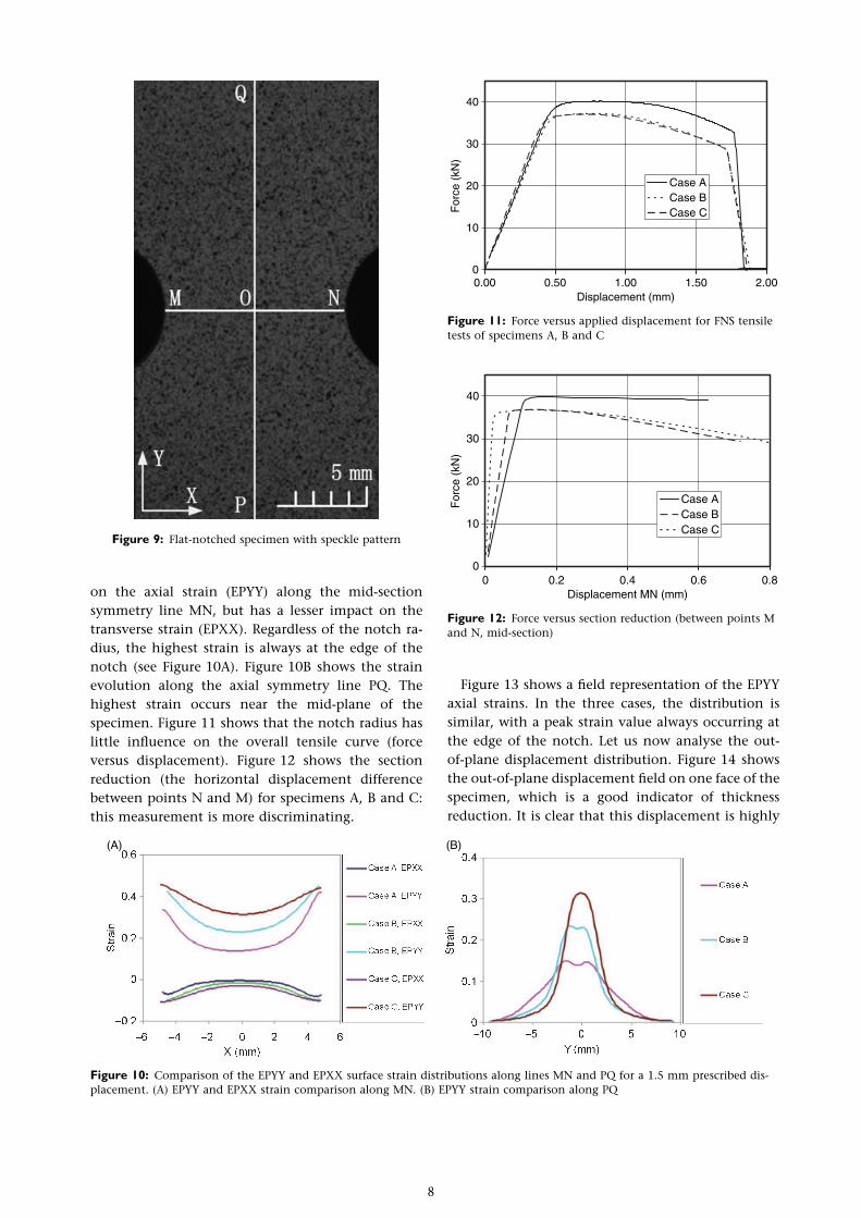
on the axial strain (EPYY) along the mid-section

symmetry line MN, but has a lesser impact on the

transverse strain (EPXX). Regardless of the notch ra-

dius, the highest strain is always at the edge of the

notch (see Figure 10A). Figure 10B shows the strain

evolution along the axial symmetry line PQ. The

highest strain occurs near the mid-plane of the

specimen. Figure 11 shows that the notch radius has

little influence on the overall tensile curve (force

versus displacement). Figure 12 shows the section

reduction (the horizontal displacement difference

between points N and M) for specimens A, B and C:

this measurement is more discriminating.

Figure 13 shows a field representation of the EPYY

axial strains. In the three cases, the distribution is

similar, with a peak strain value always occurring at

the edge of the notch. Let us now analyse the out-

of-plane displacement distribution. Figure 14 shows

the out-of-plane displacement field on one face of the

specimen, which is a good indicator of thickness

reduction. It is clear that this displacement is highly

Figure 9: Flat-notched specimen with speckle pattern

(A) (B)

Figure 10: Comparison of the EPYY and EPXX surface strain distributions along lines MN and PQ for a 1.5 mm prescribed dis-

placement. (A) EPYY and EPXX strain comparison along MN. (B) EPYY strain comparison along PQ

0

10

20

30

40

0.00 0.50 1.00 1.50 2.00Displacement (mm)

For

ce (

kN)

Case ACase BCase C

Figure 11: Force versus applied displacement for FNS tensile

tests of specimens A, B and C

0

10

20

30

40

0 0.2 0.4 0.6 0.8Displacement MN (mm)

For

ce (

kN)

Case ACase BCase C

Figure 12: Force versus section reduction (between points M

and N, mid-section)

8

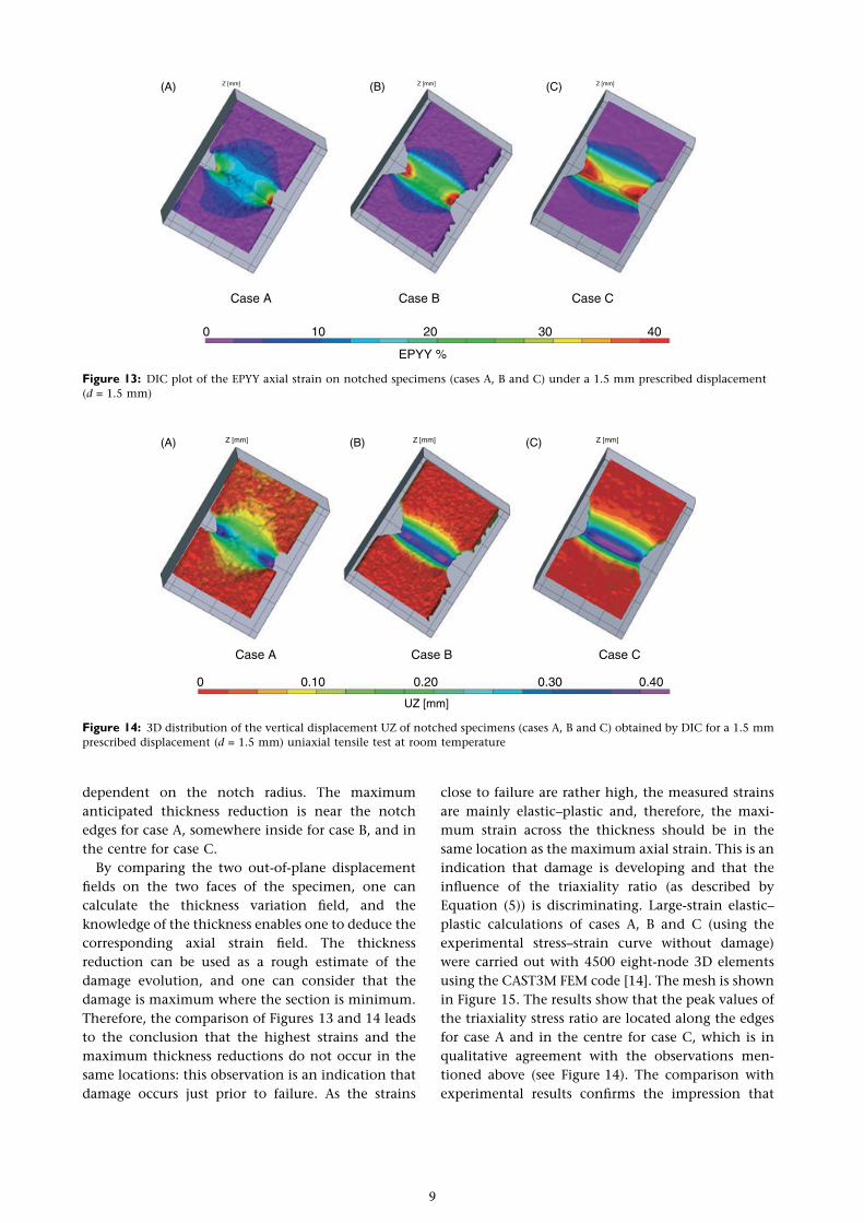
dependent on the notch radius. The maximum

anticipated thickness reduction is near the notch

edges for case A, somewhere inside for case B, and in

the centre for case C.

By comparing the two out-of-plane displacement

fields on the two faces of the specimen, one can

calculate the thickness variation field, and the

knowledge of the thickness enables one to deduce the

corresponding axial strain field. The thickness

reduction can be used as a rough estimate of the

damage evolution, and one can consider that the

damage is maximum where the section is minimum.

Therefore, the comparison of Figures 13 and 14 leads

to the conclusion that the highest strains and the

maximum thickness reductions do not occur in the

same locations: this observation is an indication that

damage occurs just prior to failure. As the strains

close to failure are rather high, the measured strains

are mainly elastic–plastic and, therefore, the maxi-

mum strain across the thickness should be in the

same location as the maximum axial strain. This is an

indication that damage is developing and that the

influence of the triaxiality ratio (as described by

Equation (5)) is discriminating. Large-strain elastic–

plastic calculations of cases A, B and C (using the

experimental stress–strain curve without damage)

were carried out with 4500 eight-node 3D elements

using the CAST3M FEM code [14]. The mesh is shown

in Figure 15. The results show that the peak values of

the triaxiality stress ratio are located along the edges

for case A and in the centre for case C, which is in

qualitative agreement with the observations men-

tioned above (see Figure 14). The comparison with

experimental results confirms the impression that

Case A

0 10 20 30 40

Case B

EPYY %

(A) (B) (C)Z [mm] Z [mm] Z [mm]

Case C

Figure 13: DIC plot of the EPYY axial strain on notched specimens (cases A, B and C) under a 1.5 mm prescribed displacement

(d = 1.5 mm)

Case A

0 0.10 0.20 0.30 0.40

Case B

(A) (B) (C)Z [mm] Z [mm]

UZ [mm]

Z [mm]

Case C

Figure 14: 3D distribution of the vertical displacement UZ of notched specimens (cases A, B and C) obtained by DIC for a 1.5 mm

prescribed displacement (d = 1.5 mm) uniaxial tensile test at room temperature

9

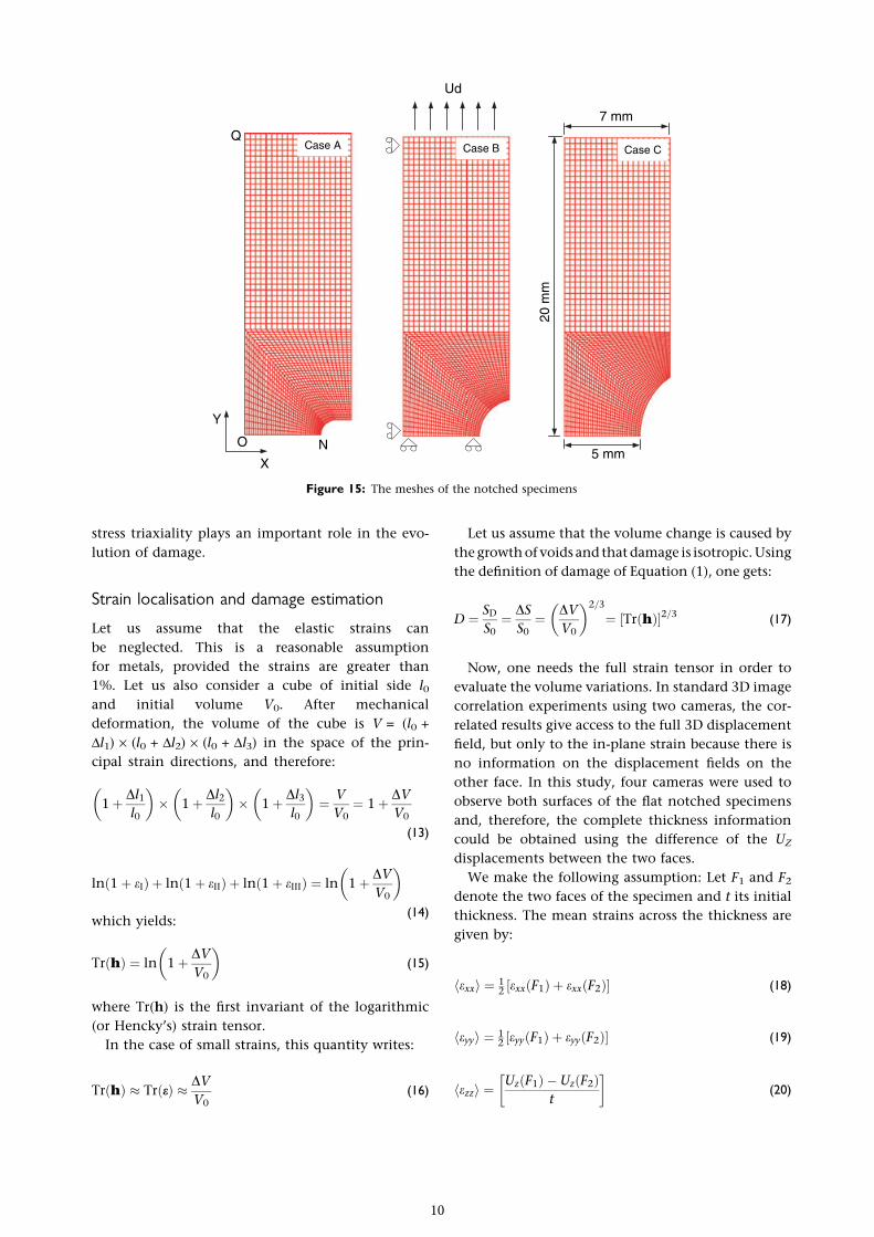
stress triaxiality plays an important role in the evo-

lution of damage.

Strain localisation and damage estimation

Let us assume that the elastic strains can

be neglected. This is a reasonable assumption

for metals, provided the strains are greater than

1%. Let us also consider a cube of initial side l0and initial volume V0. After mechanical

deformation, the volume of the cube is V = (l0 +

Dl1) · (l0 + Dl2) · (l0 + Dl3) in the space of the prin-

cipal strain directions, and therefore:

1þ Dl1l0

� �� 1þ Dl2

l0

� �� 1þ Dl3

l0

� �¼ V

V0¼ 1þ DV

V0

(13)

lnð1þ eIÞ þ lnð1þ eIIÞ þ lnð1þ eIIIÞ ¼ ln 1þ DV

V0

� �(14)

which yields:

TrðhÞ ¼ ln 1þ DV

V0

� �(15)

where Tr(h) is the first invariant of the logarithmic

(or Hencky’s) strain tensor.

In the case of small strains, this quantity writes:

TrðhÞ � TrðeÞ � DV

V0(16)

Let us assume that the volume change is caused by

the growth of voids and that damage is isotropic. Using

the definition of damage of Equation (1), one gets:

D ¼ SD

S0¼ DS

S0¼ DV

V0

� �2=3

¼ ½TrðhÞ�2=3 (17)

Now, one needs the full strain tensor in order to

evaluate the volume variations. In standard 3D image

correlation experiments using two cameras, the cor-

related results give access to the full 3D displacement

field, but only to the in-plane strain because there is

no information on the displacement fields on the

other face. In this study, four cameras were used to

observe both surfaces of the flat notched specimens

and, therefore, the complete thickness information

could be obtained using the difference of the UZ

displacements between the two faces.

We make the following assumption: Let F1 and F2

denote the two faces of the specimen and t its initial

thickness. The mean strains across the thickness are

given by:

hexxi ¼ 12 ½exxðF1Þ þ exxðF2Þ� (18)

heyyi ¼ 12 ½eyyðF1Þ þ eyyðF2Þ� (19)

hezzi ¼UzðF1Þ � UzðF2Þ

t

(20)

X

Y

NO

Ud

Q

7 mm

20 m

m

5 mm

Case A Case B Case C

Figure 15: The meshes of the notched specimens

10

The mean strain tensors given by Equation (18)

and Equation (19) are based on the strains on each

face of the specimen, which can be small or large.

Equation (20) gives the mean strain ezz across the

thickness, which is small. Then, it is consistent to

use the same small strain values for the other two

strain components. One would prefer to have the

large strain value for ezz, which would lead to a

better evaluation near the failure state, but this

value is not easily accessible because in the locali-

sation zone the thickness is no longer constant and

uniform, but changes rapidly as one approaches

failure. This makes the local strain values highly

uncertain. This is the reason why we choose a small

strain value from here on.

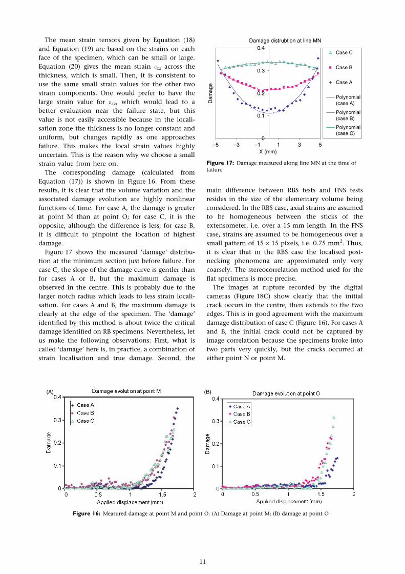
The corresponding damage (calculated from

Equation (17)) is shown in Figure 16. From these

results, it is clear that the volume variation and the

associated damage evolution are highly nonlinear

functions of time. For case A, the damage is greater

at point M than at point O; for case C, it is the

opposite, although the difference is less; for case B,

it is difficult to pinpoint the location of highest

damage.

Figure 17 shows the measured ‘damage’ distribu-

tion at the minimum section just before failure. For

case C, the slope of the damage curve is gentler than

for cases A or B, but the maximum damage is

observed in the centre. This is probably due to the

larger notch radius which leads to less strain locali-

sation. For cases A and B, the maximum damage is

clearly at the edge of the specimen. The ‘damage’

identified by this method is about twice the critical

damage identified on RB specimens. Nevertheless, let

us make the following observations: First, what is

called ‘damage’ here is, in practice, a combination of

strain localisation and true damage. Second, the

main difference between RBS tests and FNS tests

resides in the size of the elementary volume being

considered. In the RBS case, axial strains are assumed

to be homogeneous between the sticks of the

extensometer, i.e. over a 15 mm length. In the FNS

case, strains are assumed to be homogeneous over a

small pattern of 15 · 15 pixels, i.e. 0.75 mm2. Thus,

it is clear that in the RBS case the localised post-

necking phenomena are approximated only very

coarsely. The stereocorrelation method used for the

flat specimens is more precise.

The images at rupture recorded by the digital

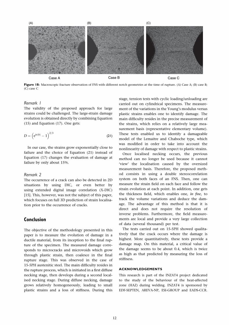
cameras (Figure 18C) show clearly that the initial

crack occurs in the centre, then extends to the two

edges. This is in good agreement with the maximum

damage distribution of case C (Figure 16). For cases A

and B, the initial crack could not be captured by

image correlation because the specimens broke into

two parts very quickly, but the cracks occurred at

either point N or point M.

(A) (B)

Figure 16: Measured damage at point M and point O. (A) Damage at point M; (B) damage at point O

Damage distrubtion at line MN

0

0.1

0.2

0.3

0.4

–5 –3 –1 1 3 5X (mm)

Dam

age

Case C

Case B

Case A

Polynomial(case A)

Polynomial(case B)

Polynomial(case C)

Figure 17: Damage measured along line MN at the time of

failure

11

Remark 1The validity of the proposed approach for large

strains could be challenged. The large-strain damage

evolution is obtained directly by combining Equation

(15) and Equation (17). One gets:

D ¼ etrðhÞ � 1� �2=3

(21)

In our case, the strains grow exponentially close to

failure and the choice of Equation (21) instead of

Equation (17) changes the evaluation of damage at

failure by only about 15%.

Remark 2The occurrence of a crack can also be detected in 2D

situations by using DIC, or even better by

using extended digital image correlation (X-DIC)

[15]. This, however, was not the subject of this paper,

which focuses on full 3D prediction of strain localisa-

tion prior to the occurrence of cracks.

Conclusion

The objective of the methodology presented in this

paper is to measure the evolution of damage in a

ductile material, from its inception to the final rup-

ture of the specimen. The measured damage corre-

sponds to microcracks and microvoids which grow

through plastic strain, then coalesce in the final

rupture stage. This was observed in the case of

15-5PH austenitic steel. The main difficulty resides in

the rupture process, which is initiated in a first diffuse

necking stage, then develops during a second local-

ised necking stage. During diffuse necking, damage

grows relatively homogeneously, leading to small

plastic strains and a loss of stiffness. During this

stage, tension tests with cyclic loading/unloading are

carried out on cylindrical specimens. The measure-

ment of the variations in the Young’s modulus versus

plastic strains enables one to identify damage. The

main difficulty resides in the precise measurement of

the strains, which relies on a relatively large mea-

surement basis (representative elementary volume).

These tests enabled us to identify a damageable

model of the Lemaitre and Chaboche type, which

was modified in order to take into account the

nonlinearity of damage with respect to plastic strains.

Once localised necking occurs, the previous

method can no longer be used because it cannot

‘view’ the localisation caused by the oversized

measurement basis. Therefore, the proposed meth-

od consists in using a double stereocorrelation

system on both faces of an FNS. Then, one can

measure the strain field on each face and follow the

strain evolution at each point. In addition, one gets

the thickness field, which enables one, in fine, to

track the volume variations and deduce the dam-

age. The advantage of this method is that it is

direct and does not require the resolution of

inverse problems. Furthermore, the field measure-

ments are local and provide a very large collection

of data (several thousand) per test.

The tests carried out on 15-5PH showed qualita-

tively that the crack occurs where the damage is

highest. More quantitatively, these tests provide a

damage map. On this material, a critical value of

the damage seems to be about 0.4, which is twice

as high as that predicted by measuring the loss of

stiffness.

ACKNOWLEDGEMENTS

This research is part of the INZAT4 project dedicated

to the study of the behaviour of the heat-affected

zone (HAZ) during welding. INZAT4 is sponsored by

EDF-SEPTEN, AREVA-NP, ESI-GROUP and EADS-CCR.

Case A

(A) (B) (C)

Case B Case C

Figure 18: Macroscopic fracture observation of FNS with different notch geometries at the time of rupture. (A) Case A; (B) case B;

(C) case C

12

We would like to express our gratitude to these organi-

sations for their financial and technical support. We also

thank J. Yang for his contribution to the microscopic

observation. It should finally be mentioned that EADS

kindly provided the 15-5PH stainless steel for testing

purposes.

REFERENCES

1. Germain, P. and Muller, P. (1980) Introduction a la meca-

nique des milieux continus. Masson, France.

2. Rice, J. R. and Tracy, D. M. (1969) On ductile enlargement

of voids in triaxial stress fields. J. Mech. Phys. Solids 17,

210–217.

3. Gurson, A. L. (1977) Continuum theory of ductile rupture

by void nucleation and growth: Part I – yield criteria and

flow rules for porous ductile media. J. Eng. Mat. Tech. 99,

2–5.

4. Kachanov, L. M. (1986) Introduction to Continuum Damage

Mechanics. Martinus, Nijhoff Publisher, Boston, MA,

Dordrecht.

5. Lemaitre, J. and Chaboche, J. L. (1990) Mechanics of Solids

Materials. Cambridge University Press, Cambridge.

6. Lemaitre, J. and Desmorat, R. (2005) Engineering Damage

Mechanics. Springer, Berlin, Heidelberg, New York.

7. Wu, T., Coret, M. and Combescure, A. (2008) Numerical

simulation of welding induced damage and residual stress

of martensitic steel 15-5PH. Int. J. Solids Struct. 45, 4973–

4989.

8. Bonora, N. (1997) A nonlinear CDM model for ductile

failure. Eng. Fract. Mech. 58, 11–28.

9. Touchal, S., Morestin, F. and Brunet, M. (1997) Use of

damage model and method by correlation of digital ima-

ges for the necking detection. 14th Int. Conf. SMIRT, Lyon,

France.

10. Brunet, M. and Morestin, F. (2001) Experimental and

analytical necking studies of anisotropic sheet metals.

J. Mater. Proc. Technol. 112, 214–216.

11. Choi, S. and Shah, S. P. (1997) Measurement of deforma-

tions on concrete subjected to compression using image

correlation. Exp. Mech. 37, 307–313.

12. Wattrisse, B., Chrysochoos, A., Muracciole, J.-M. and

Nemoz-Gaillard, M. (2001) Kinematic manifestations of

localisation phenomena in steels by digital image corre-

lation. Eur. J. Mech. A/Solids 20, 189–211.

13. Helm, J. D., McNeill, S. R. and Sutton, M. A. (1996)

Improved 3D image correlation for surface displacement

measurement. Opt. Eng. 35, 1911–1920.

14. Cast3M, developed by the French CEA, is a computer code

for structural analysis and computational fluids dynamics

by the finite element method. http://www-cast3M.cea.fr

[accessed on 25 December 2008].

15. Rethore, J., Hild, F. and Roux, S. (2008) Extended digital

image correlation with crack shape optimization. Int. J.

Numerical Methods Eng. 73, 248–272.

13