full-journal.pdf - duet
TRANSCRIPT


Dhaka university of engineering & technology, gazipur, banglaDesh
DUET Journal Vol. 3, Issue 1, December 2017
Editorial Board
01. Prof. Dr. Mohammad Zoynal AbedinDean, Faculty of Mechanical Engineering
Editor in Chief
02. Prof. Dr. Md. Khasro MiahDepartment of Civil Engineering
Member
03. Prof. Dr. Md. Nasim AkhtarDepartment of Computer Science and Engineering
Member
04. Prof. Dr. Md. Kamal-Al-HassanDepartment of Physics
Member
05. Prof. Dr. Md. Arefin KowserDepartment of Mechanical Engineering
Member
06. Prof. Dr. Md. Saifuddin FarukDepartment of Electrical and Electronic Engineering
Member
07. Prof. Dr. Fazlul Hasan SiddiquiDepartment of Computer Science and Engineering
Member Secretary

Dhaka university of engineering & technology, gazipur, banglaDesh
DUET Journal Vol. 3, Issue 1, December 2017
Table of Contents
01. Response of River Training Structure against the Changing Flow and Morphology in a Sand Bed Braided River.Mohammad Nazim Uddin, Hao Zhang, Yasuyuki Baba, Hajime Nakagawa, Md. Munsur Rahman
1
02. Effects of Fine Aggregates on the Properties of Pervious Concrete.Md. Suman Mia, Md. Abdus Salam, Md. Bashir Ahmed
9
03. Effects of Curing Methods on the Strength of Concrete.M. A. Rashid, M. N. Islam, M. A. K. Hasan
15
04. Physical and Chemical Effects of Underwater Discharge with a Variation in Solution Conductivity and Input Voltage.Ruma, M Ahasan Habib, M. N. Islam, S. H. R Hosseini, H. Akiyama
23
05. Triple-Stage Actuator System for High Speed Precision Hard Disk Drive Servomechanism.Md. Arifur Rahman, Alamgir Hossain, Utpal Kumar Das, S. M. Mahfuz Alam, Md. Raju Ahmed
29
06. Design and Comparative Analysis of PID Controller for Dual-Stage Hard Disk Drive Servo System.Alamgir Hossain, Md. Arifur Rahman
39
07. NOX Reduction in a Hybrid Plant: Boiler Simulation for Reburning.M. M. Rahman, Md. Arafat Rahman , Md. Awal Khan, Jamal Uddin Ahamed
45
08. Single Degree of Motion Control of a Magnetically Suspended Object Using Analog Controller.Md. Emdadul Hoque, Monjur Mourshed, Fazlur Rashid, Avijit Sarker, Robiul Alam
51
09. Environment Friendly Continuous Flow Gas Generation by Fluidized Bed Rice Husk and Saw Dust Gasifier.Dr. Md. Arefin Kowser, Dr. Hasan Mohammad Mostofa Afroz, Nayeem Md. Lutful Huq, Md. Khaled Khalil
57
10. Receiver Initiated Multi-channel Medium Access Control Protocol for Cognitive Radio Network.Amran Hossain, Sahelee Sultana, Md. Obaidur Rahman
65
11. Automated Intelligent Storytelling.Md. Rabiul Alam, Manik Chandra Sarker, Md. Sajadur Rahman, Fazlul Hasan Siddiqui
75
12. Architecture for Children: Enabling the Cognitive and Physical Development of Vulnerable Children in Orphanages of Bangladesh.Tasniva Rahman Mumu
83
13. Income Increase and Its Impact on Housing Affordability: The Case of Government Employees in Dhaka after Eighth Pay Scale.Joarder Hafiz Ullah, Md. Sabbir Hussain
89
14. Accuracy and efficiency of higher order Serendipity type quadrilateral finite elements using exact integration schemes.M. Borhan Uddin, Tasnimah Jahan, M. S. Karim
95
15. Teaching Listening Skill through Google Classroom: A Study at Tertiary Level in Bangladesh.Mir Md. Fazle Rabbi, AKM Zakaria, Mir Mohammad Tonmoy
103
16. Challenges in Learning English Language Faced by Tertiary Level Engineering Students: A Study in the Context of DUET, BangladeshSanzida Rahman, Fatema Sultana, A. K. M. Zakaria
109

DUET Journal 1 Vol. 3, Issue 1, December 2017
Response of RiveR TRaining sTRucTuRe againsT The changing flow and MoRphology in a sand Bed BRaided RiveR
Response of River Training Structure against the Changing Flow and Morphology in a Sand Bed Braided River
Mohammad Nazim Uddin1*, Hao Zhang2, Yasuyuki Baba3, Hajime Nakagawa3, Md. Munsur Rahman4
1Department of Civil Engg., Dhaka University of Engineering and Technology, Gazipur, Bangladesh 2Agricultural Unit, Natural Sciences Cluster Research and Education Faculty, Kochi University, Japan
3Disaster Prevention Research Institute, Kyoto University, Japan 4Institute of Water and Flood Management, Bangladesh University of Engineering and Technology, Bangladesh
ABSTRACT
The Jamuna is a braided river. The channel boundaries are consisted with fine sand and susceptible to erosion easily. The morphology of the Jamuna is strongly affected by the variable discharge. The morphology of the Jamuna is changed over time. Even after a single flood, the river does not return to its previous morphology and it has to adjust with the changed morphology. During adjustment to its new morphology, erosion at some places and deposition at other places makes the river very dynamic. To protect its bank from erosion different types of structure have been constructed at several locations along the both banks of the Jamuna River. Among them Sirajganj hardpoint (revetment) is one of the robust and most expensive river training structure in Bangladesh. But since its construction the hardpoint has been damaged several times. To investigate the causes of failure of the hardpoint 3-D hydraulic data was measured using ADCP in the dry and flood season. The dry season satellite images have also been used to clarify the failure event. It has been investigated from the present study that the flow pattern around the hardpoint is changed with the morphological change of the river. Oblique flow is generated due to formation and movement of sandbar. It attacked the eastern straight part of the hardpoint. The situations become worsen due to harmonized of several factors with the oblique flow. The factors are shifting of thalweg towards hardpoint, dune movement, riprap failure, development of scour hole and flow slides. The response of the Sirajganj hardpoint against the changing flow and morphology has been investigated in the present paper.
*Corresponding email: [email protected]
1. INTRODUCTION
About 200 years ago the old Brahmaputra has shifted its course towards west of the Madhupur tract that is the present Jamuna River. Since its avulsion the width of this river has been increased in some reaches up to 10 km towards the western direction [2], [6]. The river is flowing on top of a vast alluvial plain. The bed and bank material are consisted with fine sand, which provide least resistance to erosion. The morphology of the Jamuna is strongly affected by the variation of discharge ranging from 2860 m3/sec to 100000 m3/sec [4]. The morphology of the Jamuna changes every year. During adjustment to its new morphology, erosion at some places and deposition at others make the river very dynamic. The river also annually carries a huge amount of suspended load and bed load. The braiding index of this river varies between 2 to 5. The width of the Jamuna River is increased from 1973 to 2002 by about 3.5km from an average 8.3km to about 11.8km. About 800 km2 of the valuable land has been eroded along 220 km of the Jamuna in Bangladesh [11].
The flow processes around a structure is governed by its surrounding morphology. The flow processes is also changed with the change of the morphology [9]. The
response of river training and bank protection structure is dependent on the flow processes. When oblique flow is generated due to formation or movement of sand bar and if it is guided by the sandbar towards the river training structure is dangerous for structural stability of the river training works [10]. Therefore, it is important to analyze flow and morphological change around a river training structure so that the failure event can be handled easily. The response of the Sirajganj hardpoint against changing flow and morphology has been discussed in this paper.
2. METHODOLOGY
For the present study 3-D hydraulic data was measured using Acoustic Doppler Current Profiler (ADCP: 1200 kHz: WH-ADCP Rio Grande by RD Instruments). The ADCP uses the Doppler effect (the change in observed sound pitch that result from relative motion) to measure velocity by transmitting sound at fixed frequency and listening to echoes returning from sound scatters, such as suspended sediment in the water. Global Positioning System (GPS) was used to locate the measuring point. The ADCP was mounted downward with a specially designed plastic boat. The plastic boat with ADCP was

DUET Journal 2 Vol. 3, Issue 1, December 2017
Response of RiveR TRaining sTRucTuRe againsT The changing flow and MoRphology in a sand Bed BRaided RiveR
tied by rope with the country boat. The entire system was connected with a laptop computer for data collection. 3-D velocity, discharge, depth, bed level etc. were measured by this instrument. At a particular location the hydraulic data was recorded by ADCP at different depths. Three sets of hydraulic data around the Sirajgang hardpoint were measured on 22nd and 23rd March in 2008, on 19th March in 2009 and on 19th July in 2009. The bathymetry survey data of different years was collected from Brahmaputra Right Embankment (BRE) specialized division, Bangladesh Water Development Board (BWDB), Sirajganj. The satellite images also were collected from CEGIS for the present study.
3. RESULT AND ANALYSIS
The response of the river training works (Sirajganj hardpoint) has been investigated primarily based on the changing flow and the morphology of consecutive 2008 and 2009 years. Usually the direction of flow is guided by the sandbar. Recently, Rahman et al. [9] has been conducted a study on flow processes in a developing bend downstream of the Sirajganj hardpoint. They have been concluded that the flow processes and flow attacking point is changed with the variation of the water level. Bank erosion and shifting of sand bar also affect flow processes and flow attacking point.
3.1 Change of Morphology
It is earlier stated that the Jamuna is a very dynamic river. Some of the bed forms of height about 15m move at rate about 600m/day towards downstream direction [2]. The satellite images taken after 2007 and 2008 flood seasons (i.e. before 2008 and 2009 flood seasons) are shown in Fig. 1(a) and Fig. 1(b). A significant morphological change has been occurred in 2008 and 2009.
It is found from the satellite images that the confluence of the curved and the straight approach channel was just upstream of the upstream termination of the hardpoint in 2007. It is seen in the satellite image of 2009 that the upstream of the curved channel was dried up due to sediment deposition at location A (Fig. 1b). The curved channel upstream of the Sirajganj hardpoint is almost abandoned. Although this curved channel become active during flood season. Significant morphological change has been occurred in the straight approach channel during 2008 flood season (Fig. 1b). The western part of the S marked parallelogram shaped sand bar (Fig. 1a) has been washed away during 2008 flood season. The width became enlarged of the straight approach channel. A low sand bar B is formed just upstream of the termination of the hardpoint (Fig. 1b). A channel C adjacent to the eastern part of the hardpoint is in developing stage (Fig. 1a). It had no flow during the dry season in 2008. This channel has been fully developed during 2008 flood season. It was found that water was flowing through this channel in March 2009 with depth of flow about 5m.
Fig. 1(a): Satellite image (2007)
Fig. 1(b): Satellite image (2009)

DUET Journal 3 Vol. 3, Issue 1, December 2017
Response of RiveR TRaining sTRucTuRe againsT The changing flow and MoRphology in a sand Bed BRaided RiveR
3.2 Change of Flow Process
The flow processes is changed with the change of the morphology. The flow processes along horizontal and vertical planes in the years 2008 and 2009 have been discussed in this section.
3.2.1 Change of flow processes along the horizontalplane
The flow processes in March 2008 and in March 2009 at depth 1m below the water surface are shown in Fig. 2(a) and Fig. 2(b). The flow processes in March 2008 and in March 2009 at depth 5m below the water surface are shown in Fig. 2(d) and Fig. 2(e). The maximum velocity near the upstream termination was 2m/sec in March 2008. The flow is diverted by the hardpoint and it acts as an extended structure (March 2008). Due to formation sand bar, the upstream approach channel is divided into two approach channels (March 2009). The maximum velocity near the upstream termination was 1.4m/sec in March 2009. The maximum velocity in the eastern approach channel in March 2009 was 1.5m/sec. The downstream channel is also divided into two channels. The reattachment length of the return current was 250m to 300m in March of 2008 and in March 2009. But the reattachment length of the return current was extended more than 600m in August of 2009 (Fig. 2c). The flow obliquely hits the hardpoint just downstream of the reattachment length of the return current. It is found from field measured data that the oblique flow was existed up to 15m depth.
Fig. 2(a): 2-D velocity vectors at depth 1m, March 2008
Fig. 2(b): 2-D velocity vectors at depth 1m, March 2009
Fig. 2(c): 2-D velocity vectors at depth 1m, August 2009
Fig. 2(d): 2-D velocity vectors at depth 5m, 2008

DUET Journal 4 Vol. 3, Issue 1, December 2017
Response of RiveR TRaining sTRucTuRe againsT The changing flow and MoRphology in a sand Bed BRaided RiveR
Fig. 2(e): 2-D velocity vectors at depth 5m, 2009
3.2.2 Changeofflowprocessesalongtheverticalplane
A vertical section is taken along line a-b in Fig. 3(a) in March 2008. The velocity vectors along line a-b (Fig. 3a) are shown in Fig. 3(c) in March 2008. The primary vortex is developed within the scour hole as a result of flow separation at the upstream edge of the scour hole. The primary vortex is the main scouring agent around a structure. The scouring potentiality depends on the flow velocity within the scour hole. The direction of the primary vortex is anti-clockwise in March 2008 (Fig. 3c). Secondary vortex is also generated next to the primary vortex. The direction of the secondary vortex is clock-wise. The vortices observed near the upstream termination are similar to the vortex flow investigated in laboratory through experiment [3], [5], [7]. Again a vertical section is taken along line a-b in Fig. 3(b) in March 2009. The velocity vectors along line a-b (Fig. 3b) are shown in Fig. 3(d) in March 2009. Primary vortex is observed in March 2009. The primary vortex in March 2009 is relatively weaker than that of March 2008. The maximum flow velocity within the primary vortex is about 2m/sec in March 2008. But the maximum velocity within the primary vortex is about 1.4m/sec in March 2009. So the scouring potentiality in March 2009 is significantly reduced than that of March 2008. The reduction of velocity in March 2009 is due to
upstream morphological change. The maximum scour depth in March 2008 was 36.6m due to strong primary vortex within the scour hole. The maximum scour depth in March 2009 was 25m due to significantly decreasing of scouring potentiality of flow.
Fig. 3(a): Vertical section along line a-b in 2008
Fig. 3(b): Vertical section along line a-b in 2009

DUET Journal 5 Vol. 3, Issue 1, December 2017
Response of RiveR TRaining sTRucTuRe againsT The changing flow and MoRphology in a sand Bed BRaided RiveR
Fig. 3(c): Velocity vectors along vertical plane (2008)
Fig. 3(d): Velocity vectors along vertical plane (2009)
3.3 Change of Discharge Intensity and Velocity along Vertical Section
The discharge intensity and velocity between 2008 and 2009 years along a section taken from the upstream termination towards the sandbar have been discussed in this section.
3.3.1 Change of discharge intensity
The maximum discharge intensity near the upstream termination was 47m2/s/m (Table 1) in March 2008. But the maximum discharge intensity was 20m2/s/m (Table 1) at a distance from the upstream termination in March 2009. About 70% and 100% of the total discharge of the Jamuna River was passing through the Sirajganj channel in 2008 and 2009, respectively (Table 2). The variation of discharge intensity in March 2008 (along line a-b Fig. 3a) is shown in Fig. 4(a). The maximum discharge intensity in March 2008 was at a distance from the upstream termination of the hardpoint. The variation of discharge intensity is similar to the experimental result investigated by Rahman [8]. The variation of discharge intensity in March 2009 (along line a-b Fig. 3b) is shown in Fig. 4(b).
The discharge intensity in March 2009 is significantly reduced due to upstream morphological change.
3.3.2 Change of velocity
Two vertical sections are taken along line a-b in Fig. 3(a) and Fig. 3(b) to investigate the variation of velocity between 2008 and 2009. The variation of depth averaged velocity in March 2008 is shown in Fig. 5(a). The maximum depth averaged velocity is observed at a distance from the upstream termination of the hardpoint in 2008. The variation pattern of the depth averaged velocity follows the similar pattern as the discharge intensity which is shown in Fig. 4(a) along the same vertical section. The distribution of the depth averaged velocity (Fig. 5a) follows the similar pattern as investigated in the laboratory
Table 1: Comparison of different parameters in 2008 & 2009
Year 2008 2009Maximum depth of scour (m) 36.6 25.0Maximum velocity (m/sec) 2.0 1.4Maximum discharge intensity (m2/s/m) 47 20

DUET Journal 6 Vol. 3, Issue 1, December 2017
Response of RiveR TRaining sTRucTuRe againsT The changing flow and MoRphology in a sand Bed BRaided RiveR
experiment by Kwan and Melville [7]. Again the variation of depth average velocity in March 2009 along line a-b (Fig. 3b) is shown in Fig. 5(b). It is found that the maximum depth averaged velocity has been significantly reduced in 2009 due to upstream morphological change. Only 25% of the total discharge passes through the western approach channel. Subsequently this discharge passes near the upstream termination of the hardpoint.
Fig. 4(a): Variation of discharge intensity in March 2008
Fig. 4(b): Variation of discharge intensity in March 2009
3.3 Failure of Hardpoint
It is considered that a part of the upstream termination was damaged in September, 2008 due to vortex induced scour and confluence scour (Fig. 6). The primary vortex during 2008 flood season was stronger than that of dry season. The oblique flow is generated in 2009 by the sand bar. This issue has already been discussed in section 3.2.1. The oblique flow attacked the eastern straight part of the hardpoint. The temporal variation of the bed level from 4th February to 11th July, 2009 at a particular point near the failure part of the hardpoint is shown in Fig. 7. It is found that no significant variation of the bed level occurred from 4th February to 28th April. The bed level is slightly raised within the period 28th April to 14th May. No bed level variation is seen from 14th May to 12th June. After that the bed level is rapidly lowered from 12th June up to failure of the hardpoint (i.e. 11th July).
Fig. 5(a): Variation of velocity in March 2008
Fig. 5(b): Variation of velocity in March 2009
Table 2: Discharge passing through the Sirajganj channel in the dry season
Year Total Discharge
Discharge Passing through Sirajganj
Channel23rd March, 2008 4800 m3/sec 3300 m3/sec (70%)
19th March, 2009 4150 m3/sec 4150 m3/sec (100%)

DUET Journal 7 Vol. 3, Issue 1, December 2017
Response of RiveR TRaining sTRucTuRe againsT The changing flow and MoRphology in a sand Bed BRaided RiveR
A vertical section is taken along line k-k normal to the hardpoint (Fig. 8). The variation of bed profile (along line k-k) from 4th February to 11th July is shown in Fig. 9. The bed profile is rapidly lowered from 12th June up to the failure of the hardpoint. The deepest bed level is -11mPWD which was just after one day of the failure of the hardpoint. Although the apron setting and the deepest design scour levels along the straight portion of the hardpoint is (-) 4.2mPWD and (-) 13.25mPWD respectively. In the Jamuna River, the maximum rate of scouring is 5 to 6m per day, 12m in 10 days and 20m in less than one month. The rate of deposition is 3.5m per day, 11m in 3 days and 25m in 50 days [1], [11]. On October
21, 2003, the maximum scour depth in the Jamuna River was 56.75m near the Sailbari Groin. It is easily considered that the developed deepest scour depth before failure of the hardpoint was higher than (-) 11mPWD. The flow slide is occurred from the revetment side and resulting failure of the hardpoint is occurred. The scour hole is filled up by the sliding materials. The catastrophic failure of the hardpoint on 10th July, 2009 is shown in Fig. 10. One important aspect has been investigated from the recent field measurement (August, 2009) that about 5m high dune was passing through the channel adjacent to the hardpoint. The riprap may fail due to repeatedly dune movement.
Finally, it can be concluded from the present study that the oblique flow is generated due to change in morphology. The oblique attacked the straight part of the hardpoint. The sandbar adjacent to the hardpoint is washed away and a channel is developed adjoining the hardpoint. Thalweg is shifted towards hardpoint. It is investigated from the present study that dune with amplitude 5 meter is passed through the channel adjacent to the hardpoint (3 to 4 times per day).
The riprap materials have been undermined into the trough of the dune. The bed level is lowered down about 5m within two weeks (Fig. 9). Almost certainly, flow slide has been occurred from the revetment side towards the scour
Fig. 6: Failure part of the hardpoint September, 2008
Fig. 7: Temporal variation of bed level near the failure part
Jamuna River
KK
Damage Part
Sirajganj Town
471000 471500
Easting (m)
707000
706500
North
ing
(m)
706000
705500472000 472500
Fig. 8: Vertical section along line k-k
Fig. 9: Change of bed profile normal to the failure part
Fig. 10: Failure part of the hardpoint on 10th July, 2009

DUET Journal 8 Vol. 3, Issue 1, December 2017
Response of RiveR TRaining sTRucTuRe againsT The changing flow and MoRphology in a sand Bed BRaided RiveR
hole. It is clarified that the failure of hardpoint is triggered by changing upstream flow and morphology together with dune movement and sudden change of scour depth.
4. CONCLUSION
Flow and morphological changes affect the bank protection structures and vice versa. It has been investigated from the present study that several factors simultaneously affect the structural stability of the hardpoint. The factors are: (i) oblique flow generated by sandbar attacked the hardpoint; (ii) washed away of sandbar adjacent to the hardpoint; (iii) thalweg shifting at the vicinity of the hardpoint; (iv) movement of dune through the channel passing near the hardpoint; (v) riprap failure; (vi) development of scour hole; (vii) flow slides from the hardpoint side. Flow and morphological change in the Jamuna River is inevitable. Therefore, some additional measures should be taken to divert oblique flow from bank protection structure towards the mid-channel.
ACKNOWLEDGMENT
The authors express their gratitude to Disaster Prevention Research Institute (DPRI), Kyoto University, Japan for providing support to this study. Part of the field support by DelPHE Project and JAFS project are also acknowledged.
REFERENCES
[1] BWDB, “Guidelines for River Bank Protection,” Jamuna-Meghna River Erosion Mitigation Project (JMREMP), 2008.
[2] J. M. Coleman, “Brahmaputra river: Channel process and sedimentation,” Sedimentary Geology, Vol. 3, No. 2-3, pp. 129-239, 1969.
[3] S. Dey, and A. K. Barbhuiya, “Flow field at a vertical-wall abutment.” Journal of Hydraulic Engineering, ASCE, Vol. 131, No. 12, pp.1126-1135, 2005.
[4] FAP 24: Morphological characteristics, River Survey Project, Final report, Annex 5, Water Resources Planning Organization, Ministry of Water Resources, Bangladesh, Nov. 1996.
[5] J. K. Kandasamy, “Abutment scour.” Report No. 458, School of Engineering, University of Auckland, Auckland, New Zealand, 1989.
[6] G. J. Klaassen, and K. Vermeer, “Channel characteristics of the braiding Jamuna river,” Bangladesh, International Conference on River Regime, Published by John Wiley & Sons. Ltd, pp. 173-189, 1988.
[7] R. T. F. Kwan and B. W. Melville, “Local scour and flow measurements at bridge abutments,” Journal of Hydraulic Research, Vol. 32, No. 5, pp. 661-673, 1994.
[8] M. M. Rahman, “Studies on deformation process of meandering channels and local scouring around spur-dike-like structures,” PhD thesis, Graduate School of Engineering, Kyoto University, Japan, 1998.
[9] M. M. Rahman, F. Mahmud, H. S. Sarker, M. N. Uddin, M. H. Tuhin, M. A. Rahman, and M. M. Rahman, “Flow processes in an eroding bend fixed with two hardpoint along the braided Jamuna River,” 3rd International Conference on Water & Flood Management (ICWFM-2011), 8th January, 2011.
[10] M. N. Uddin and M. M. Rahman, “Failure of Sirajgang Hardpoint at Changing Hydro-Morphology,” 3rd International Conference on Water & Flood Management (ICWFM-2011), 8th January, 2011.
[11] M. J. Uddin, “RCC spurs in Bangladesh: Review of design, construction and performance,” Msc Thesis, UNESCO-IHE, The Netherlands, 2007.

EffEcts of finE AggrEgAtEs on thE ProPErtiEs of PErvious concrEtE
DUET Journal 9 Vol. 3, Issue 1, December 2017
Effects of Fine Aggregates on the Properties of Pervious Concrete
Md. Suman Mia*, Md. Abdus Salam, Md. Bashir Ahmed
Department of Civil Engineering, Dhaka University of Engineering & Technology, Gazipur, Bangladesh
ABSTRACT
Pervious concrete is highly porous lightweight concrete obtained by replacing or eliminating the fine aggregate from the conventional concrete. The inherent properties of the pervious concrete are low cost due to less cement content, low density, low thermal conductivity and drying shrinkage, no segregation and high capillary movement of water. Due to the presence of large voids, this concrete is used as a permeable material. Pervious concrete does not show the sufficient compressive strength due to permeable material though it needs to prevent storm water runoff from initiating flood and downstream erosion. This study was carried out to enhance the compressive strength of pervious concrete with different percentages of fine aggregate. In addition, the effects of fine aggregate on the compressive strength, permeability and void ratio were also investigated in this study. Three single sizes and one combined size crushed stone were used to make pervious concretes. The specimens were cast by adding 0%, 5% and 10% fine aggregate with the mix proportion 1:6 (Cement: Coarse aggregate) by weight. Water cement ratio was kept constant as 0.35. It has been found that incorporation of fine aggregate in pervious concrete increases the compressive strength and decreases the void ratio and permeability. The optimum fine aggregate content for 1 in. and ¾ in. sizes coarse aggregate was 10%; whereas the fine aggregate content for ½ in. size coarse aggregate was 0%.
*Corresponding email: [email protected]
1. INTRODUCTION
Concrete becomes highly porous to the point when water can flow freely through the concrete. Pervious concrete is a form of concrete that has little or no sand in the mix and has enough cementitious paste adhere with the coarse aggregates while continue the interconnectivity of the voids. It also allows the transfer of both water and air to the root system of trees to flourish even in highly developed areas [1]. The void content of pervious concrete can ranges from 18 to 35% with typical water to cement (w/c) ratio of 0.35 to 0.45 [1, 2]. Infiltration rate of pervious concrete pavement depends on the aggregate size and density of the mixture. Permeability of the pavement is in the range of 200 to 800 cm/h are commonly observed. Permeability more than 2,000 cm/h is readily achievable with lower compressive strength [3, 4]. Flow rates of water through pervious concrete are typically around 480 in./hr (0.13 in./sec), which can be much higher. In Dhaka city the ground water table has downed to 61.18 m. Bangladesh Agricultural Development Corporation (BADC) informs that the ground water of Dhaka city has downed 35 m within last 11 years. According to the WASA, water table of Dhaka city was 11.3 m below the ground in 70th the century. In 80th century it is increased to 20 m. Water table has been decrease by an average depth of 3 m in each year from 1997 to 2007. The 80% people of Dhaka city fulfill their daily demand of water from underground water and another one is the ground of Dhaka city are getting paved or covered by roof due to rapid urbanization [5]. Utilization of pervious concrete
in pavement and other covered areas can minimize these problems. Pervious concrete reduces the runoff from paved area and the expense of necessary drainage system. For this reason popularity of pervious concrete has grown among consultants, architects, planners, environmentalists and engineers. The major ingredients of this concrete are cement, coarse aggregate, water and little or no fine aggregate [6]. Pervious concrete can be designed to attain a compressive strength of 2.8 to 28 MPa but strength 2.8 to 10 MPa are most common [1]. Addition of certain amount of fine aggregate to this concrete generally may reduce the void and increase the compressive strength which may be desirable in certain situation. Pervious concrete is also a lightweight material with density ranging from 1600 kg/m3 to 1900 kg/m3 [7]. Generally the permeability of pervious concrete varies generally between 2-30 mm/s [1]. Meininger [6] established an optimization of 10% - 20% of fine sand to coarse aggregate in pervious concrete and has been shown the increase in compressive strength from 13.80 MPa (2000 psi) to 18.62 MPa (2700 psi). A slight increase in fine particles correlates to decrease in the permeability. In another study Schaefer et al. [8] established a pervious concrete in which the sand to gravel ratio is increased to 8; the mortar bulks up and increases the strength. When sand to gravel ratio increases beyond 8% then the 7 days compressive strength begins to fall. Tennis et al. [9] proposed that, void space decreases with the incorporation of fine aggregates in the mix design of pervious concrete. The size of the coarse aggregate also has an important influence in the properties of pervious concrete. Flores et.al [10] have investigated

EffEcts of finE AggrEgAtEs on thE ProPErtiEs of PErvious concrEtE
DUET Journal 10 Vol. 3, Issue 1, December 2017
that 3/4 in. size of coarse aggregate allows for large void space but reduces workability whereas 3/8 in. size coarse aggregate improves the workability. Recent studies have also reported that pervious concrete with smaller coarse aggregates had higher compressive strength [11]. It was noted that the smaller aggregate sizes allowed for more cementations material to coat around the coarse aggregate and hence allowed for greater contact between the aggregate/binder. Numerous studies have been carried out on pervious concrete. Effects of different water cement ratios, aggregate sizes, fly ash, and fiber on the properties of pervious concrete have been investigated. But limited researches have been found on the use of fine aggregate in pervious concrete. Permeability, water absorption capacity and light weight properties are the main reason of using pervious concrete. This Study summarizes the effects of fine aggregates on the properties of pervious concrete such as compressive strength, permeability and void ratio. In addition, the effects of the sizes of coarse aggregate also studied in this research.
2. EXPERIMENTAL PROGRAMS
2.1 Materials and Methodology
The present investigation addressed the strength, void content and permeability of pervious concrete by varying the percentage of fines. Stone chips were selected as coarse aggregate. 0%, 5% and 10% sand were added to improve the strength of mixes. Cement and coarse aggregate ratio was fixed at1:6. Water cement ratio 0.35 was fixed for mixtures and there was no admixture. The concrete mix consists of ordinary Portland cement as binding materials. Three single sizes 1 in., ¾ in., ½ in. and one combined size crushed stone were used in this study. The single size of coarse aggregate was defined as the size of the sieve on which 100% of aggregate was retained; on to which all pass throw the sieve above. Coarse sand (FM - 2.5) was used as fine aggregate. Under the experimental investigation, physical properties of materials were evaluated according to ASTM Standard [12] and given in Table 1. Experimental program accomplished into three phases. The first phase consists of general tests to determine the physical properties of the ingredients of concrete. The second phase involved casting of different sizes cylindrical concrete specimen in the laboratory and curing for 28 days under normal water. The third phase comprised of the testing of cylindrical specimen for compressive strength, permeability and void ratio.
Table 1: Physical properties of coarse aggregate
PropertiesCoarse aggregate
1 in. ¾ in. ½ in. CombinedDry rodded unit weight (lb/ft3) 95.3 94.2 92.1 99.2Voids (%) 34.77 32.17 33.23 30.21Specific gravity 2.21 2.21 2.21 2.21Absorption 2.1 2.21 2.21 2.21
2.2 Preparation of Specimens
There are 36 (6 in. × 12 in.) concrete cylinders were prepared for compressive strength, 36 cylinders (3 in. × 6 in.) were prepared for void ratio and 36 cylinders (3 in. × 3 in.) were prepared for permeability tests. Mixing procedure was done followed by ASTM C192 Standard [13, 14]. Specimens were compacted by rodding 25 times in three layers.
2.3 Testing of Specimens
The samples were demoulded after 24 hours and then placed in water tanks at room temperature and cured according to ASTM C192 Standard [13, 14]. Before testing, the top surfaces of cylinders were grind smoothly. A typical pervious concrete cylindrical specimen is shown in the Fig.1. The compressive strength of the cylindrical specimen was tested according to ASTM C 39 Standard [13, 14]. Void ratio of pervious concrete was determined for 3 in. x 6 in. cylindrical sample by taking the difference in weight between a sample oven dried and a sample under water [15]. Water is percolating through inter connecting void space of the surface of the pervious concrete which can be shown in Fig. 1. Permeability of pervious concrete was determined using the constant head method. This is composed of 3 in. inner diameter PVC pipe with sufficient drainage facilities. To prevent water leakage along the sides of the sample a flexible sealing gum was used at the outer surface of the sample. The tests were performed using several constant time. The constant time ranged between 15 to 30 seconds.
Fig. 1: A typical pervious concrete cylindrical specimen
3. TEST RESULTS AND DISCUSSIONS
Compressive strength, void ratio and permeability of pervious concrete were tested after 28-days of proper curing. All these properties were varied with the content of fines and different aggregate sizes.

EffEcts of finE AggrEgAtEs on thE ProPErtiEs of PErvious concrEtE
DUET Journal 11 Vol. 3, Issue 1, December 2017
3.1 Compressive Strength
Fig. 2 shows that the compressive strength of pervious concrete increase with the increment of fines content. It is also observed that the concrete with higher single size coarse aggregate have lower compressive strength. Therefore the minimum desired compressive strength i.e., more than 400 psi is achieved by using 0%, 5%, 10% fine content in all cases. This is also attributed that the concrete with larger single size coarse aggregate possesses higher voids resulting the lower compressive strength. In case of combined size coarse aggregate, there are less voids which results in higher compressive strength.
3.2 Void Ratio
Fig. 3 shows the variation of void ratio with the percent of fines in pervious concrete. It is observed that at any case of coarse aggregate of pervious concrete, higher the percentages of fines lower the void ratio. Void content for pervious concrete ranges from 15% to 35% [15]. Results of this study indicate that the void ratio for any size of coarse aggregate is satisfactory for all cases of 0%, 5%, 10% fines. It is also observed that in case of pervious concrete higher size of coarse aggregate leads to higher voids for any content of fines.
0
500
1000
1500
2000
2500
0 5 10% of Fines
1 in. 3/4 in. 1/2 in. Combined
Com
pres
sive s
tren
gth
(psi)
Fig. 2: Compressive strength of pervious concrete
25
30
35
0 5 10
Voi
d ra
tio (%
)
% of Fines
1 in. 3/4 in. 1/2 in. Combined
Fig. 3: Void ratios of pervious concrete
3.3 Permeability
Fig. 4 shows the variation of permeability of pervious concrete with various content of fine aggregate. Permeability decreases with the increase of fine contents. When fines are added to the pervious concrete, pores among the coarse aggregate are getting filled with them which results in less voids. Void leads to a high permeability of pervious concrete. In general, permeability is directly proportional to the void content of pervious concrete. The satisfactory permeability (more than 0.13 in./sec) is achieved for aggregate sizes of 1 in. and ¾ in. with all content of fines and 0% fines for ½ in. size coarse aggregate only. In case of combined size aggregate, it is not satisfactory for any contents of fines. Permeability of pervious concrete is generally between 2-30 mm/s (0.08-1.20 in./sec) [1].
3.4 Correlation Between Compressive Strength, Permeability and Void Ratio
Fig. 5 shows that the compressive strength of pervious concrete decreases with the increase of permeability. This is the results of higher voids among the single sizes coarse aggregates which has left the higher permeability but lower the compressive strength.
0
0.05
0.1
0.15
0.2
0.25
0.3
0 5 10
Perm
eabi
lity
(in./s
ec)
% of Fines
1 in. 3/4 in. 1/2 in. Combined
Fig. 4: Permeability of pervious concrete
0
500
1000
1500
2000
2500
0 0.1 0.2 0.3
)isp( htgnerts evisserpmo
C
Permeability (in./sec)
1 in. 3/4 in. 1/2 in. Combined
Fig. 5: Compressive strength vs. permeability

EffEcts of finE AggrEgAtEs on thE ProPErtiEs of PErvious concrEtE
DUET Journal 12 Vol. 3, Issue 1, December 2017
In Fig. 6, variations of the compressive strength of pervious concrete with void ratio are shown. Void ratio increases with the larger single size of coarse aggregates which possesses lower compressive strength. In case of larger single size coarse aggregate it comprises larger voids; but for the combined size aggregates voids are reduced due to having well graded coarse aggregates. This study indicates that the larger single size coarse aggregate comprises the higher voids but lower the compressive strength.
Fig. 7 shows a general relationship between void ratio and permeability. The figure shows that the higher void ratio leads to higher permeability in all cases of coarse aggregates and fines. It is due to having large voids, which permit to pass water which results in higher permeability. It can be concluded that as the void content increases the permeability also increases.
0
500
1000
1500
2000
2500
25 30 35
)isp( htgnerts evisserpmoC
Void ratio (%)
1 in. 3/4 in. 1/2 in. Combined
Fig. 6: Compressive strength vs void ratio
0
0.1
0.2
0.3
25 30 35
Perm
eabi
lity
(in./s
ec)
Void ratio (%)
1 in. 3/4 in. 1/2 in. Combined
Fig. 7: Permeability vs. void ratio
4. CONCLUSIONS
The study was involved to find the changes the properties of pervious concrete with the change of fines. From this study the following conclusion can be drawn:
• Compressive strength increases with the increment of percentage of fines whereas the permeability and void ratio decreases.
• Void ratio decreases with the increment of percentage of fines which is in expected range.
• Permeability decreases with the decrement of void ratio.
• The optimum fine content for 1 and ¾ inch single size coarse aggregate is found as 10%; whereas for ½ inch is 0% (no fines) and there is no optimum fine content observed for combined aggregate.
ACKNOWLEDGEMENT
The authors acknowledge the financial grants provided by Dhaka University of Engineering &Technology, Gazipur for this study.
REFERENCES
[1] What, Why and How?, Concrete in Practice Series, CIP-38 Pervious Concrete, Silver Spring, Maryland, USA, 2004.
[2] ACI Committee 522, Pervious concrete, ACI International, Farmington Hills, 2006.
[3] E.Z. Bean, W.F. Hunt, D.A. Bidelspach, Evaluation of four permeable pavement sites in eastern North Carolina for runoff reduction and water quality impacts, J. Irrig. Rain. Eng., No. 133, Vol. 6, pp 583-592, 2007.
[4] E.Z. Bean, W.F. Hunt, D.A. Bidelspach, Field survey of permeable pavement surface infiltration rates, J. Irrig. Drain. Eng., No. 133, Vol.3, pp 249-255.
[5] The Daily Ittefaq, 1st page, Sunday, 29 June 2008.
[6] R.C. Meininger, No-Fines Pervious Concrete for Paving, Concrete International, Vol. 10, pp. 20-27, 1998.
[7] K.H. Obla, Pervious Concrete An Overview, The Indian Concrete Journal, pp 9-18, August 2010.
[8] V. R. Schaefer, K. Wang, Suleiman, J. Kevern, Mix Design Development for Pervious Concrete in Cold Weather Climates, Final Report, Center of Transportation Research and Education, Iowa State University, February 2006.
[9] P.D. Tennis, M. L. Leming, D. J. Akers, Pervious Concrete Pavements”, EB302, Portland Cement Association, Skokie, Illinois, 36 pages, 2004.

EffEcts of finE AggrEgAtEs on thE ProPErtiEs of PErvious concrEtE
DUET Journal 13 Vol. 3, Issue 1, December 2017
[10] J. J. Flores, B. Martínez, R. Uribe, Analysis of the Behavior of Filtration vs. Compressive Strength Ratio in Pervious Concrete. Pervious Concrete Symposium Proceedings, USA, 2007.
[11] A. Beeldens, D. Van Gemert, and C. Caestecker, Porous Concrete: Laboratory Versus Field Experience. Proceedings 9th International Symposium on concrete Roads, Istanbul, Turkey, 2003.
[12] ASTM. Annual Book of ASTM Standards. Philadelphia, USA: American Society for Testing and Materials.
[13] A. M. Neville, Properties Concrete, 4th edition, London, Pitman Published Limited, pp. 711-713, 2005.
[14] M. A. Aziz, Engineering Materials, 1st edition, 1973.
[15] Dipesh Teraiya, UtsavDoshi, Piyush Viradiya, Ajay Yagnik, Tejas Joshi., To Develop Method to Find out Permeability Engineering and Technology, Volume: 04 Special Issue: 13and Void Ratio for Pervious Concrete, IJRET: International Journal of Research in Engineering and Technology, 2015.


EffEcts of curing MEthods on thE strEngth of concrEtE
DUET Journal 15 Vol. 3, Issue 1, December 2017
Effects of Curing Methods on the Strength of Concrete
M. A. Rashid1*, M. N. Islam2 and M. A. K. Hasan2
1School of Civil, Environment and Industrial Engineering, Uttara University, Dhaka, Bangladesh2Department of Civil Engineering, Dhaka University of Engineering and Technology, Gazipur, Bangladesh
ABSTRACT
This paper aims at investigating the influences of mainly the curing method on the strength of concrete. Six types of curing method (CM-1: Full submersion of concrete specimens into water; CM-2: Covering the concrete specimens with wet earth; CM-3: Wrapping the concrete specimens with polythene sheet; CM-4: Covering the concrete specimens with gunny sacks and then spraying water on these several times in a day; CM-5: Spraying water on the exposed specimens several times in a day; and CM-6: Concrete specimens left in the open air outside the lab i.e. air curing) which are followed in various practical situations in Bangladesh have been considered. Other parameters considered are types of coarse aggregate, concrete mix ratios, and age of concrete. The water-cement ratio considered was 0.50. A total of 288 nos. of standard concrete cylinders were cast and tested. It has been found that curing method CM-1 gives the highest strength and the curing method CM-6 gives the lowest strength to concretes irrespective of the type of aggregates and the mix ratios considered. Curing methods CM-2 and CM-5 have been found to give slightly higher strengths (4% and 2% respectively) to concretes than those obtained by the CM-6 method. However, the curing methods CM-3 and CM-4 are found to give significantly higher (14%) strength than that obtained by using CM-6 method. The brick aggregate gives higher strengths to concretes than those of the concretes made with stone aggregate. For all the concrete studied, the increase in compressive strength at the age of 90 days over that at 28 days has been found to range from an insignificant value (1%) to a quite large value (48%).
*Corresponding email: [email protected]
1. INTRoduCTIoN
Concrete is the most widely used man-made construction material. It is a stone like material obtained by permitting a carefully proportioned mixture of cement, sand and gravel or other aggregate, and water to harden in forms of the shape and dimensions of the desired structure. The compressive strength of concrete is commonly considered its most valuable property, although, in many practical cases, other characteristics such as durability and permeability may in fact be more important. Nevertheless, strength usually gives an overall picture of the quality of the concrete. Moreover, the strength of concrete is almost invariably a vital element of structural design and is specified for compliance purpose [1].
Curing of concrete is the process of controlling the rate and extent of moisture loss from concrete during cement hydration [2]. It may be needed after concrete has been placed in position thereby providing time for the hydration of the cement to occur. Since the hydration of cement does take time – days, and even weeks rather than hours – curing must be undertaken for a reasonable period of time if the concrete is to achieve its potential strength and durability. Curing may also encompass the control of temperature since this affects the rate at which cement hydrates. The curing period may depend on the properties required of the concrete, the purpose for which it is to be
used, and the ambient conditions, i.e. the temperature and relative humidity of the surrounding atmosphere. Curing is designed primarily to keep the concrete moist, by preventing the loss of moisture from the concrete during the period in which it is gaining strength. Curing may be applied in a number of ways and the most appropriate means of curing may be dictated by the site or the construction method.
The physical properties of concrete depend to a large extent on the extent of hydration of cement and the resultant microstructure of the hydrated cement [3]. Upon coming in contact with water, the hydration of cement proceeds both inward in the sense that the hydration products get deposited on the outer periphery of the cement grain, and the nucleus of un-hydrated cement inside gets gradually diminished in volume. At any stage of hydration the cement paste consist of the product of hydration, the remnant of un-reacted cement, calcium hydro-oxide [Ca(OH)2] and water. The product of hydration forms a random three dimensional network gradually filling the space originally occupied by the water. Accordingly, the hardened cement paste has a porous structure, the pore size varying from very small (4×10⁻¹⁰ m) to very large and are called gel pores. As the hydration proceeds, the deposit of hydration products on the original cement grain makes the diffusion of water to the un-hydrated nucleus more and more difficult and so the rate of hydration decreases with time. Therefore,

EffEcts of curing MEthods on thE strEngth of concrEtE
DUET Journal 16 Vol. 3, Issue 1, December 2017
the development of the strength of concrete, where starts immediately after setting is completed, continue for an indefinite period, though at a rate gradually diminishing with time. Eighty to eighty five percent of the eventual strength is attained in the first 28 days and this strength is considered to be the criterion for the structural design and is called the characteristic strength.
In Bangladesh, depending upon the suitability and availability, different methods are followed for curing of concrete in different structures. Pounding method (blocking water on the surface of cast concrete) is normally used for curing the top surface of flat or near-flat surfaces such as floor slab, pavements, roof slab etc. Structural elements such as footings, pile cap, column below grade etc. are usually covered by soil after few hours/days of their casting. This is done with the view that the curing of these concrete will continue by the damp environment created by the surrounding soil. Sometimes concrete structures such as column, floor slab etc. are wrapped/covered with polythene sheets in order to keep the concrete moist by preventing evaporation of water from it. In some cases, after removing the formwork, concrete elements are wrapped/covered with gunny-sacks and then water is sprayed several times in a day for curing the concrete. This method of concrete curing is usually followed for column, pier, retaining wall and some other vertical structures. On the other hand, exposed side surfaces of floor beams are generally cured by spraying water on the concrete surfaces several times in a day. In some exceptional cases concrete elements are just left exposed in the open air which may be due to the non-availability of curing facilities or some other reasons. However, in all of the above mentioned cases, the representative concrete specimens (cylinder and/or cube) of various concrete elements are normally cured by full submersion of specimens into water. This difference between the curing conditions of real structural element and the representative concrete specimens may yield concretes of different qualities. As a result the strength of the concrete specimens may not represent the strength of the concretes of actual structures.
In Bangladesh, both crushed stone and broken bricks are widely used as coarse aggregates in making concrete. However, due to non-availability and price considerations of stones, the use of broken bricks as coarse aggregate is getting popularity especially in the private sectors. Besides, both the physical and mechanical properties of these two types of aggregates differ significantly. The absorption capacity, as it can influence the extent of concrete curing, of brick aggregates is quite high in comparison to that of stone aggregates. Therefore, the difference between concrete strengths, due to the difference between curing conditions of real structural elements and that of the representative specimens, may be different for concretes made with stone and brick aggregates.
In case of gravel concretes the compressive strength of air cured concrete was reported to be lower by approximately 26% to 36% compared to brick aggregate concretes under
the same curing condition [4]. It was also reported that water curing was better in achieving concrete strength than other types of curing conditions studied.
Effect of the moist curing on the strength of brick aggregate concrete was investigated experimentally by Rahman et al. [5]. It was reported that moist-cured brick aggregate concrete show significant higher compressive strength in comparison with that of the air-cured concrete. An average value of the ratios of the compressive strengths of air-cured concrete to those of moist-cured concrete was found to be 0.74. Also the initial moist curing of 3, 7, 14 and 21 days yielded 67%, 68%, 81% and 89% respectively of the 28 days moist-cured compressive strength (all were tested at 28 days).
Experimental investigation on the effect of curing on the strength of brick aggregate concretes was also done by Ahmad and Amin [6]. They reported that the curing of concrete at any stage is beneficial to overcome the losses due to discontinuity in curing. The delayed curing was found to be helpful even in attaining the desired strength provided that the early age (say 1st one week) curing is not hampered. However, in such cases curing for a longer duration was reported to be required.
So far, no study on the concrete strengths due to the differences in curing condition of real structural concrete elements (considering the different practical cases) and that of representative concrete samples has been reported. This study has, therefore, been aimed at to study the above mentioned issue considering crushed stones and broken bricks as coarse aggregates.
2. EXPERIMENTAL PRoGRAM
In the experimental program a total of 288 standard cylindrical concrete specimens (150×300 mm) have been cast and then tested to get the concrete compressive strength. Four parameters considered were curing method, curing period, type of coarse aggregates, and concrete mix ratio (Table 1). Six types of curing methods of concrete which are usually followed in Bangladesh have been considered as the main parameter. The curing methods considered are:
(i) Full submersion of concrete specimens into water (CM-1).
(ii) Covering the concrete specimens with wet earth (CM-2).
(iii) Wrapping the concrete specimens with polythene sheets (CM-3).
(iv) Wrapping the concrete specimens with gunny sacks and then spraying water on these several times in a day (CM-4).
(v) Spraying water on the exposed specimens at several times in a day (CM-5).
(vi) Concrete specimens left in the open air inside the lab (i.e. air curing) (CM-6).

EffEcts of curing MEthods on thE strEngth of concrEtE
DUET Journal 17 Vol. 3, Issue 1, December 2017
Table 1: Curing methods along with other variables considered in this study
Two types of concrete mix ratio (1:2:4 and 1:1.5:3 by volume), two types of coarse aggregate (brick and stone chips), four types of curing period (7, 14, 28 and 90 days) along with the above mentioned curing methods have been considered in this study (Table 1). Therefore, a total of 2×2×4×6 or 96 mixes of concrete and hence a total of 96×3 or 288 nos. of cylindrical specimens were cast and then tested for concrete compressive strength at the age of specified days. Ordinary Portland cement (Type-I) was used in this experiment. Properties of the cement used are shown in Table 2.
The Properties of fine aggregate and two types of coarse aggregates used in the experiment are presented in Table 3. All coarse aggregates used were 25 mm down-graded. Photographs of coarse and fine aggregates used in this study are shown in Fig. 1. In this study drinking water was used in making concretes.
Required numbers of steel molds each of 150×300 mm size were cleaned using wire brush and then their joints were tightened by nut-bolts. These cleaned molds were placed on firm and leveled floor on concrete laboratory. Lubricating oil (Mobil) was used to smear the inner bottom and side surfaces of the mold for its easy removal after hardening of concrete.
Fig. 1: Photographs of the aggregates used in the study
Fresh concrete was prepared as per designed mix in a mixture machine. Immediately after unloading from mixture machine, the fresh concrete was placed in the mold in three layers and was compacted following the ASTM specifications (ASTM C192/C192M - 02). After placing concrete in the mold, the exposed top surface was trowelled smooth. The fresh concretes in the molds were kept in the laboratory without any disturbance and the specimens were demolded on the following day and cured for specified period of time following the specific curing methods. Photographs of the different types of curing of concrete specimens as performed in the study are shown in Fig. 2 through Fig. 7.
Fig. 2: Curing of concrete by submersion of specimens
into water (CM-1)
Fig. 3: Concrete cylinders placed in the trench for covering
them with wet earth (CM-2)
Fig. 4: Curing of concrete by wrapping the specimens with
polythene sheet (CM-3)
Fig. 5: Concrete cylinders covered with gunny sacks and then spraying water
on them (CM-4)
Fig. 6: Spraying water on specimens which were kept under the open sky (CM-5)
Fig. 7: Concrete specimens left in the open air in the
laboratory (CM-6)
The test cylinders were collected from their specified curing conditions before 24 hours of testing and kept in air-dry condition in the laboratory. Before testing, both the ends of each cylinder were ground by grinding
Table 2: Properties of the cement used in the experiment
Property of cement Test valueNormal consistency 28.6%Initial setting time 3 hr. 0 Min.Final setting time 6 hr. 0 min.Compressive strength (3 days) 25.5 MPaCompressive strength (7 days) 34.3 MPa
Table 3: Properties of fine and coarse aggregates used
Property of materials used Test value of
Sand Stone chips Brick chipsFineness modulus 2.4 7.2 7.4Water absorption (%) 2.0 1.0 6.0Unit weight (Kg/m3 1492 1502 1102

EffEcts of curing MEthods on thE strEngth of concrEtE
DUET Journal 18 Vol. 3, Issue 1, December 2017
machine in order to make the end surfaces smooth and leveled (Fig. 8). Then the measurements for diameter of each specimen were taken using slide calipers. Average of three measurements those at top, middle and bottom were considered in determining the diameter of each of the specimens.
Concrete cylinders were tested in the lab using the 2000 KN capacity Universal Testing Machine (Fig. 9) following the ASTM C39 specifications. At first the test cylinder was placed on the machine’s base platen keeping it vertical and centered on the plate. Then load was applied on the top surface of the specimen. This load was increased gradually until the specimen failed. The crushing load was then recorded.
The crushing load of each of the test specimens was divided by the average cross sectional area of respective cylindrical specimen and was recorded as the crushing/compressive strength of that concrete. Test values of the compressive strengths of all of the concretes along with different parameters are presented in Table 4 and Table 5.
Table 4: Compressive strength of concretes made with stone aggregates
Table 5: Compressive strength of concretes made with brick aggregates
3. ANALYSIS ANd dISCuSSIoN oF TEST RESuLTS
Test data have been analyzed with a view to study the influence of curing methods along with other variables considered on the strength of concrete.
3.1 Influence of the Curing Methods on ConcreteStrength
Fig. 10 and Fig. 11 show the relative influences of curing methods considered in this study on the concrete crushing strength for a wide range of the age of concretes made with stone aggregate and brick aggregate respectively. It is seen that the curing method CM-1 (full submersion of concrete specimens into water) gives higher concrete strength than any other curing method irrespective of the type of aggregates and the concrete mix ratios [except the brick aggregate concrete with a mix ratio of 1:2:4 (Fig. 11a)]. This exceptional case may be due to a comparatively lean concrete mix along with the much higher absorption capacity of brick aggregates.
Fig. 8: Grinding of concrete cylinder’s end surface
Fig. 9: Testing of concrete cylindrical specimen using UTM
(a)
(b)
Fig. 10: Influence of curing methods on the strength of stone aggregate concretes

EffEcts of curing MEthods on thE strEngth of concrEtE
DUET Journal 19 Vol. 3, Issue 1, December 2017
On the other hand, the air curing method CM-6 (concrete specimens left in the open air outside the lab without any curing) gives the minimum strengths to concretes considered. The curing method CM-2 (covering the concrete specimens with wet earth) also gives higher strengths than those of the air-cured concretes [except the stone aggregate concrete with a mix ratio of 1:1.5:3 (Fig. 10b)]. This exceptional case may be due to a comparatively rich concrete mix along with the much lesser absorption capacity of stone aggregates. However, it is seen from Fig. 10b that CM-2 gives almost similar strengths as those of the CM-6 method. Therefore, covering of young concrete with wet earth can give higher strength to a concrete than air curing it.
The curing methods CM-3 (wrapping the concrete specimens with polythene sheet) and CM-4 (covering the concrete specimen with gunny sack and then spraying water on this several times in a day) are seen to be the much influential in giving strengths to concrete. These may be due to the available moisture around the concrete specimens provided by the almost air-tight polythene sheet system and longtime existence of sprayed water on concrete surface because of the coarse gunny sack respectively. The curing method CM-5 (spraying water on the exposed specimens several times in a day) also gives higher strengths than those of the air-cured concretes [except the stone aggregate concrete with a mix ratio of 1:1.5:3 (Fig. 10b)]. This exceptional case may be due to
a comparatively rich concrete mix along with the much lesser absorption capacity of stone aggregates.
A comparative study of the 28-days crushing strengths of concrete cured following the different methods is given in Table 6. Ratios of strength of concrete cured following either of CM-1, CM-2, CM-3, CM-4, and CM-5 to that of the concrete cured by CM-6 method are presented in this table. Mean and Standard Deviation of the ratios are also shown in the same. From Table 6 it is seen that the CM-2 and CM-5 methods of concrete curing give slightly better strengths (an average of 4% and 2% respectively higher) to concrete than those of the air-cured concrete (CM-6). The difference between the strengths of concrete obtained by curing those following CM-3 and CM-4 methods is insignificant. Whereas, both CM-3 and CM-4 method of concrete curing give a significantly higher (14%) strength that obtained by using CM-6 method.
3.2 Influence of the Type Coarse Aggregates onConcrete Strength
Fig. 12 and Fig. 13 show the relative influences of the type of coarse aggregates on the crushing strength for concretes with mix ratio of 1:2:4 and 1:1.5:3 respectively. It is seen from these figures that in most of the cases brick aggregate gives higher strength to concrete than that of the concrete made with stone aggregate irrespective of both the mix ratio and the curing methods considered in this study [except the strengths at 90 days of Fig. 13(d)]. This may be due to the significantly higher absorption capacity of the brick aggregates than that of the stone aggregates. The initially absorbed significant water in the brick aggregates might be used, later on, in hydration of cement and yielded higher strengths to those concretes. The exceptional case of curing method CM-4 to concrete with mix ratio 1:1.5:3 [Fig. 13(d)] may be due to the inadequate compaction of the concretes during casting.
(a)
(b)
Fig. 11: Influence of curing methods on the strength of brick aggregate concretes
Table 6: Ratios of compressive strengths (28 days) obtained following different curing methods

EffEcts of curing MEthods on thE strEngth of concrEtE
DUET Journal 20 Vol. 3, Issue 1, December 2017
Fig. 12: Effects of aggregates on the strength of concrete
(mix ratio = 1:2:4)
Fig. 13: Effects of aggregates on the strength of concrete
(mix ratio = 1:1.5:3)
3.3 InfluenceoftheMixRatioonConcreteStrength
The relative influences of the concrete mix ratios on the crushing strength of concretes made with stone aggregates and brick aggregates are presented in Figs. 14 and Fig.15 respectively. It is seen from these figures that the rich concrete mix (1:1.5:3) gives higher strengths to concrete than those of lean concrete mix (1:2:4) except the two cases (curing method CM-2 for stone aggregate concrete and CM-4 for brick aggregate concrete). These may be due to the inadequate compaction of concretes during casting.
3.4 Concrete Strengths at 7 and 14 days
The ratios of concrete strengths at 7 days to those at 28 days and the ratios of the strengths at 14 days to those at 28 days are presented in Table 7 and Table 8 for the concretes made with stone aggregate and brick aggregate respectively. From the tables it is seen that the concrete continue to increase its strength with its age. The average concrete compressive strength at the age of 7 days is found to be 75% of the strength at 28 days whereas the mean strength at 14 days is found to be 86% of the strength at 28 days irrespective of the aggregates used
Fig. 14: Effects of concrete mix ratio on the strength of
stone aggregate concrete

EffEcts of curing MEthods on thE strEngth of concrEtE
DUET Journal 21 Vol. 3, Issue 1, December 2017
Fig. 15: Effects of concrete mix ratio on the strength of
brick aggregate concrete
Table 7: Gain in compressive strength of stone aggregate concretes at different ages
Table 8: Gain in compressive strength of brick aggregate concretes at different ages
3.5 Increases in Concrete Strength after 28 days
The ratios of concrete strengths at 90 days to those of 28 days are presented in Table 9 and Table 10 for the concretes made with stone aggregate and brick aggregate respectively. It is to be mentioned here that after 28 days no curing was applied to any concrete specimen. From the tables it is seen that the concrete continue to increase its strength with its age even after ending the curing processes considered (28 days) in this study. This increase in concrete strength (at the age of 90 days over that at 28 days) ranges from an insignificant value (1%) to a quite high value (48%). The mean increase in concrete strength is found to be 23% and 18% for concretes made with stone aggregate and brick aggregate respectively.
Table 9: Ratio of concrete (stone aggregate) strength at 90 days to that of 28 days

EffEcts of curing MEthods on thE strEngth of concrEtE
DUET Journal 22 Vol. 3, Issue 1, December 2017
Table 10: Ratio of concrete (brick aggregate) strength at 90 days to that of 28 days
4. CoNCLuSIoNS
Following conclusions can be drawn based on the findings of this study-
(i) Curing method CM-1 (full submersion of concrete specimens into water) gives higher concrete strength than any other curing method irrespective of the type of aggregates and the concrete mix ratios. On the other hand, curing method CM-6 (concrete specimens left in the open air outside the lab i.e. air curing) gives the minimum strengths to concretes considered.
(ii) CM-2 and CM-5 methods of concrete curing do not influence in increasing concrete strengths over those of the concrete under air curing (CM-6).
(iii) The curing methods CM-3 (wrapping the concrete specimens with polythene sheet) and CM-4 (covering the concrete specimen with gunny sack and then spraying water on this several times in a day) are seen to be the much influential parameter in increasing concrete strengths over those of the concrete under air curing (CM-6).
(iv) The brick aggregate concrete is observed to give higher strength than that of the concrete made with stone aggregate.
(v) The rich concrete mix (1:1.5:3) gives higher compressive strength than that of the lean concrete mix (1:2:4) i.e. concrete with higher cement content gives higher compressive strength.
(vi) Irrespective of the coarse aggregates and the mix ratios considered in this study, concrete has been found to achieve around 75% and 86% of its characteristics strength (at 28 days) at the age of 7 days and 14 days respectively.
(vii) The increase in concrete strength, at the age of 90 days over that at 28 days, has been found to range from an insignificant value (1%) to a quite high value (48%). The mean of this increase in concrete strength are 23% and 18% for concretes made with stone aggregate and brick aggregate respectively.
ACKNoWLEdGMENT
The experimental work described was supported by and executed at the Department of Civil Engineering, Dhaka University of Engineering & Technology, Gazipur-1700, Bangladesh. This support is greatly appreciated by the authors.
REFERENCES
[1] A. H. Nilson, D. Drawin, and C. W. Dolan, “Design of Concrete Structures”, Mcgraw-Hill Companies, Inc., New York, 2010.
[2] T. James, A. Malachi, E. W. Gadzama, and V. Anametemfiok, “Effect of Curing Methods on the Compressive Strength of Concrete,” Nigerian Journal of Technology, Vol. 30, No. 3, pp. 14-20, 2011.
[3] [3] M. G. H. Sing, “Handbook on Concrete Mixes,” Bureau of Indian Standards, New Delhi, 2001.
[4] M. R. Aminur, M. R. Harunur, D. C. L. Teo and M. M. Zakir, “Effect of Aggregates and Curing Condition on the Compressive Strength of Concrete with Age,” UNIMAS e-Journal of Civil Engineering, Vol. 1, Issue 2, pp. 1-6, 2010.
[5] M. A. Rahman, S. Chakma, and M. M. Rahman, “Effect of the Moist Curing on the Strength of Brick Aggregate Concrete,” B. Sc. Engineering Thesis, Department of Civil Engineering, DUET, Gazipur, Bangladesh, 2009.
[6] S. Ahmad, and A. F. M. S. Amin, “Effect of Curing Conditions on Compressive Strength of Brick Aggregate Concrete,” Journal of Civil Engineering, The Institution of Engineers, Bangladesh, Vol. CE 26, No. 1, pp. 37-49, 1998.

Physical and chemical effects of Underwater discharge with a Variation in solUtion ...
DUET Journal 23 Vol. 3, Issue 1, December 2017
Physical and Chemical Effects of Underwater Discharge with a Variation in Solution Conductivity and Input Voltage
Ruma1*, M Ahasan Habib2, M. N. Islam3, S.H.R Hosseini4, H. Akiyama4
1Department of EEE, Dhaka University of Engineering & Technology (DUET), Gazipur, Bangladesh 2Dept of IPE, National Institute of Textile Engineering and Research (NITER), Bangladesh
3Department of Chemistry, Dhaka University of Engineering & Technology (DUET), Gazipur, Bangladesh 4Graduate School of Science and Technology, Kumamoto University, Kumamoto 860-8555, Japan
ABSTRACT
Both physical and chemical effects of underwater discharge plasma were investigated in terms of varying solution conductivity and input voltage in a water jacketed glass reactor. The point-plane electrode geometry having a high voltage pulse of positive polarity (0-25kV, 0-1kHz) being generated with a magnetic pulse compression (MPC) pulsed power modulator was used. The discharge propagated along with several streamers branching from the positive electrode to ground electrode in water solution. Initially, the physical appearance of streamer showed a good branching in both 100µS/cm and 500µS/cm conductive solutions, but for 500µS/cm streamer lengths reduced with an increasing pulse number and finally formed a plasma ball with a very narrow branching. A longer length of streamer branching was observed at 23.4kV rather than at 19.4kV of input voltage. The chemical processes of this streamer discharge variation were evaluated by the measurement of H2O2 (hydrogen peroxide) concentration as it is a stable molecule formed mainly due to interaction between discharge plasma and water molecules. The detailed description of both physical and chemical processes involving underwater discharge for a different solution conductivity (100µS/cm, 500µS/cm) and input voltage (23.4kV, 19.4kV) is presented in this paper.
*Corresponding email: [email protected]
1. INTRODUCTION
Over the past decade underwater pulsed electrical discharges have garnered an extensive attention for their several industrial, environmental and biomedical applications including wastewater treatment, disinfection of microorganism, surface modification, nanoparticles and so on [1-5]. Due to a higher permittivity (εr = 81) and density (103 kg/m3) of water, a high electrical field in the order of several MV/cm is necessary to initiate a discharge in water [6-7]. In the presence of a high voltage pulse, a strong electric field is generated at a high voltage needle tip that is strong enough for the breakdown of water to initiate discharge. In most cases, pulsed underwater discharges are generated using the point-plane electrode geometry [8-9], with a positive voltage applied to the point due to its easy discharge initiation. The other electrode configuration such as rod-plate [10], coaxial rod-cylinder, [11], point-mesh [12-13], plane-plane [14], wire-plane [15] has been studied. Many studies have used ac power sources with frequencies up to 100kHz as well as radio frequency or microwave power to generate plasmas in water [16-17]. However, the effects of variation in solution conductivity and input voltage on underwater discharge are not yet well studied. A pulsed power modulator being able to deliver high-voltage pulses with a 25kV and a repetition rate of up to 1kHz was employed in this work.
The discharge can be either in the form of corona or streamer while spark and arc make conductive channels producing high energy electrons in water which can cause ionization, dissociation and/or recombination of water molecules. Through these processes discharge plasma interacts with water molecules to initiate various physical and chemical processes in water such as a strong electric field, an intense UV radiation, shockwaves, and the generation of various active ions such as H, H3O, O, H, reactive radicals such as OH2, O2, OH, and molecular species such as H2, O3, H2O2 [13-18]. Among these species OH radicals have a very strong oxidizing power to inactivate microorganisms or decompose chemical pollutants dissolved in water. Previous study reported the oxidizing power of OH radical is 2.80, while it is 2.42, 2.07 and 1.78 for O radicals, O3 and H2O2, respectively [19]. However, the lifetime of OH radicals is only few microseconds and also it is difficult to measure them quantitatively from discharge water. Therefore, H2O2 is measured as a precursor of OH radicals being generated by discharge plasma in water, because it is mainly formed by recombination of OH radicals and also its dissociation gives OH radicals again in water.
There are several parameters that can affect the radicals or active species formation in the discharged water such as applied voltage, pulse polarity, pulse rise time [10-
Physical and chemical effects of Underwater discharge with a Variation in solUtion ...
DUET Journal 24 Vol. 3, Issue 1, December 2017
11], pulse repetition rate [16-20], electrode configuration, electrode radius curvature [14], solution conductivity, pressure [21], temperature [22-23], as the discharge characteristics are dependent on those parameters. The OH radical density and concentration of H2O2 increased with the applied pulsed voltage of power input [12, 16-20], whereas H2O2 production decreased with an increasing solution conductivity [20], temperature [22] and pH value [23-24]. The concentration of OH and H2O2 was found to vary linearly with the number and length of streamers [25-27]. Though many of these factors influence the physical and chemical processes, their role is not yet well understood. Thus, a further investigation to clarify these aspects is required.
The main objective of this study is to clarify both physical and chemical effects of underwater discharge with the variation in solution conductivity and input voltage. We captured the physical change of discharge condition with parameter variation and also measured the concentration of hydrogen peroxide (H2O2) formed from discharge water to understand chemical efficiency of discharge plasma. Because plasma chemical activity of discharge water mostly depends on the physical characteristics of discharge.
2. EXPERIMENTAL PROCEDURE
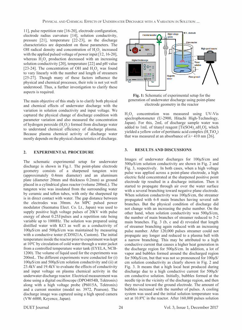
The schematic experimental setup for underwater discharge is shown in Fig.1. The point-plane electrode geometry consists of a sharpened tungsten wire (approximately 0.4mm diameter) and an aluminum plate (diameter 20mm and thickness 0.2mm) as ground placed in a cylindrical glass reactor (volume 200mL). The tungsten wire was insulated from the surrounding water by ceramic and teflon tubes, with only the sharpened tip is in direct contact with water. The gap distance between the electrodes was 30mm. An MPC pulsed power modulator (Suematsu Elect. Co. Lt., Japan) was used to supply positive high voltage pulses of 20kV with pulse energy of about 0.25J/pulses and a repetition rate being variable up to 1000Hz. The solution was prepared using distilled water with KCl as well as a conductivity of 100μS/cm and 500μS/cm was maintained by measuring with a conductive tester (CD5021A, Custom). The initial temperature inside the reactor prior to experiment was kept at 10ºC by circulation of cold water through a water jacket from a controlled temperature water tank (EYELA, NCB-1200). The volume of liquid used for the experiments was 200mL. The different experiments were conducted for (i) 100μS/cm and 500μS/cm solution conductivity and (ii) at 23.4kV and 19.4kV to evaluate the effects of conductivity and input voltage on plasma chemical activity in the underwater discharge reactor. Electrical measurement was done using a digital oscilloscope (DPO4054B, Tektronix) along with a high voltage probe (P6015A, Tektronix) and a current monitor (model no. 3972, Pearson). The discharge image was captured using a high speed camera (VW-6000, Keyence, Japan).
Fig. 1: Schematic of experimental setup for the generation of underwater discharge using point-plane
electrode geometry in the reactor
H2O2 concentration was measured using UV-Vis spectrophotometer (U-2900, Hitachi High-Technology, Japan). For this, 2mL of discharge sample water was added to 1mL of titanyl reagent [Ti(SO4)2.nH2O], which yielded a yellow color of pertitanic acid complex (H2TiO4) that was measured at an absorbance of λ= 410 nm [26].
3. RESULTS AND DISCUSSIONS
Images of underwater discharges for 100µS/cm and 500µS/cm solution conductivity are shown in Fig. 2 and Fig. 3, respectively. In both cases, when a high voltage pulse was applied across a point-plane electrode, a high electric field concentrated at the sharpened positive point electrode tip resulted in a discharge initiation. Then it started to propagate through air over the water surface with a several branching toward negative plane electrode. When solution conductivity was 100µS/cm, the streamer propagated with 6-8 main branches having several sub branches. But the physical condition of discharge did not change with an increasing the pulse number. On the other hand, when solution conductivity was 500µS/cm, the number of main branches of streamer reduced to 5-2 main branches. Fig. 3 (b, c and d) revealed that length of streamer branching again reduced with an increasing pulse number. After 120,000 pulses streamer could not propagate any longer and reduced to a plasma ball with a narrow branching. This may be attributed to a high conductive current that causes a higher heat generation in the discharge region for 500µS/cm. In addition, a lot of vapor and bubbles formed around the discharged region for 500µS/cm, but that was not so pronounced for 100µS/cm solution conductivity as clearly shown in Fig. 2 and Fig. 3. It means that a high local heat produced during discharge due to a high conductive current for 500µS/cm conductive solution. Initially, bubbles formed at the needle tip in the vicinity of the discharge region, and then they moved toward the ground electrode. The amount of bubbles increased with the number of pulses. A cooling system was used and the initial solution temperature was set at 10.8ºC in the reactor. After 160,000 pulses solution

Physical and chemical effects of Underwater discharge with a Variation in solUtion ...
DUET Journal 25 Vol. 3, Issue 1, December 2017
temperature rose up to 40.6ºC and 52.7ºC for a solution conductivity of 100µS/cm and 500µS/cm, respectively.
Images of underwater discharges at 23.4kV and 19.4kV are shown in Fig. 4. It is clear that the length of streamer branching also depends on input voltage, and it was found to be about 15mm and 5-7mm in length at 23.4kV and 19.4kV, respectively.
A typical voltage and current waveforms of underwater discharges for 500µS/cm and 100µS/cm conductive solutions are shown in Fig. 5 and Fig. 6, respectively. It is observed that for 500µS/cm current rose sharply to its peak with amplitude of 25.2A, which only 4.0A for 100µS/cm was. The energy consumed by discharge found to be 97.88mJ and 200mJ for 100µS/cm and 500µS/cm conductive solution, respectively. The conductive current was 2.80A and consumed energy was 34.59mJ at 19.kV of input voltage.
(a) (b)Fig. 2: Images of underwater discharges when solution conductivity was 100µS/cm: for (a) 2,000 pulses and
(b) 120,000 pulses
(a) (b)
(c) (d)Fig. 3: Images of underwater discharges when solution
conductivity was 500µS/cm: for (a) 2,000 pulses, (b) 60,000 pulses, (c) 100,000 pulses and (d) 120,000 pulses
The streamer branching propagated along with a high energy electron forming ionized water molecules in discharge region that lead to a direct and indirect generation of many chemically active species such as OH, O, H, HO2 radicals and H2O2 (hydrogen peroxide), O3, H2, O2 molecular species. But among them OH radicals and H2O2 are considered to be the major active species formed in underwater discharge processes [1-10].
(a) (b)
Fig. 4: Images of underwater discharges for 100µS/cm solution conductivity: at (a) 23.4kV and (b) 19.4kV
In this research, the chemical effects of solution conductivity and input voltage induced by underwater discharge plasma were evaluated through the measurement of H2O2 concentration. We measured H2O2 from the discharge water as a major indicator of the chemical species produced in the discharge reactor. Because H2O2 has a relatively long lifetime than other species (H, OH, O) and also it is easy to measure this quantitatively [27-30]. It is suggested that H2O2 is mainly formed by the recombination of OH radicals that generated through dissociation of water molecules due to discharge plasma or by other probable mechanisms [4, 5-7].
Following reactions are suggested to take place in this process [27-30]:
H2O+e- OH + H………….......……(1)OH +OH H2O2 ………….........……..(2)H2O2 + uv light 2OH …….....................…..(3)H2O2 H2O + O…..…………...….(4)
Other species, such as OH, Haq, OH2, and O also take part in H2O2 generation, but their role is negligible to account for their low concentration as reported by L. Nemcova et al. [30]. Hiroki et al studied 79% of H2O2 formation that can be attributed to OH radicals produced from radiolysis of water and OH radical is the sole precursor of H2O2, as shown in equations 2 and 3 [31] and that quickly decomposes into oxygen atom [32] as shown in equation 4. R. Burlica et al found that H2O2 is quite stable and no change in the absorbance of the sample was observed if left overnight [32].

Physical and chemical effects of Underwater discharge with a Variation in solUtion ...
DUET Journal 26 Vol. 3, Issue 1, December 2017
Fig. 7 shows the effects of solution conductivity on production of H2O2 in underwater discharge reactor. The concentration of H2O2 increased linearly with the number of pulses for 100µS/cm, whereas it reduced for 500µS/cm. Initially concentration of H2O2 steadily increased for 500µS/cm and then reduced after 60,000 pulses. But after that it did not increase significantly up to 160,000 pulses. This is likely due to the fact that for 500µS/cm conductive solution is in contact with plasma having water molecules reduced with an increasing pulse number because of shortening streamer branching. Another likely reason is that the generated H2O2 may be dissociated immediately into OH radicals due to a high localized heat generated in the discharge region.
-15-10-5051015202530
-10
-5
0
5
10
15
20
25
-1.00 1.00 3.005.00
Cur
rren
t (A
)
Vol
tage
(kV
)
Time (µs)
Voltage (kV)
Current (A)
Fig. 5: Voltage and current waveforms of underwater discharge for 500µS/cm solution conductivity
-8
-6
-4
-2
0
2
4
6
8
10
-20
-15
-10
-5
0
5
10
15
20
25
-1.00 0.00 1.00 2.00 3.00 4.00 5.00 Cur
rent
(A)
Vol
tage
(kV
) Voltage (kV)
Current(A)
Fig. 6: Voltage and current waveforms of underwater discharge for 100µS/cm solution conductivity
Fig. 8 shows the effects of input voltage on production of H2O2 in underwater discharge reactor. These results show that concentration of H2O2 linearly increases in both cases, but it was higher at 23.4kV compared to 19.4kV. One possible reason is that a large number of water molecules come in contact with discharge plasma due to an increased streamer length at 23.4kV, whereas a lower number of water molecules come into contact due to a reduced streamer length at 19.4kV (as shown in Fig. 4(a, b). Another reason may be that, streamer heads contain highly energetic electrons that lead to a large number of OH radicals as well as H2O2 at 23.4kV than that at 19.4kV.
0
0.2
0.4
0.6
0.8
1
1.2
0 30000 60000 90000 120000 150000 180000
H2O
2(m
mol
)
Pulse number
100µS/cm
500µS/cm
Fig. 7: The effects of solution conductivity on production of H2O2 in underwater discharge reactor
0
0.2
0.4
0.6
0.8
1
1.2
0 30000 60000 90000 120000 150000 180000
H2O
2 (m
mol
)
Pulse number
23.4 kV19.4kV
Fig. 8: The effects of input voltage on production of H2O2 in underwater discharge reactor
4. CONCLUSION
Physical and chemical effects of underwater discharge were studied with varying solution conductivity and input voltage in a reactor. A magnetic pulse compression (MPC) pulsed-power modulator was used as a pulse source with 0-25kV, 0-1kHz. The experimental results indicate that the physical characteristics of discharge were significantly influenced by the variation in solution conductivity and input voltage. When the solution conductivity was 100µS/cm, physical condition of streamer branching did not change with an increasing pulse number. On the other hand, it was found to reduce in length and finally shrank to a plasma ball for 500µS/cm solution conductivity. A longer streamer length was observed at 23.4kV instead of at 19.4kV. The production of H2O2 was found higher for 100µS/cm rather than that for 500µS/cm solution conductivity, which was higher at 23.4kV than at 19.4kV of input voltage. In addition, a lot of vapor and bubbles formed due to a high heat generated for 500µS/cm solution conductivity with an increasing pulse number while less vapors were observed for 100µS/cm solution conductivity. Finally, it can be concluded that the chemical processes of underwater discharge are directly related to the physical characteristics of discharge.

Physical and chemical effects of Underwater discharge with a Variation in solUtion ...
DUET Journal 27 Vol. 3, Issue 1, December 2017
REFERENCES
[1] B. R. Locke, M. Sato, P. Sunka, M. R. Hoffmann, J.S. Chang, “Electrohydraulic discharge and nonthermal plasma for water treatment”, Ind. Eng. Chem. Res., vol. 20, pp.1-15, 2006.
[2] P. Sunka, “Pulse electrical discharges in water and their applications”, Phys. Plasmas, Vol.8, pp. 2587–2594, 2001.
[3] B R Locke and S. Mededovic, “Analysis and review of chemical reactions and transport processes in pulsed electrical discharge plasma formed directly in liquid water”, Plasma Chem. Plasma Process, Vol. 32, pp. 875–917, 2012.
[4] P. Lukes, B R Locke and J. L. Brisset, “ Aqueous-phase chemistry of electrical discharge plasma in water and in gas–liquid environments Plasma Chemistry and Catalysis in Gases and Liquids”, (Weinheim: Wiley-VCH), pp. 241–307, 2012.
[5] T. J. Lewis, “Breakdown initiating mechanisms at electrode interfaces in liquids”, IEEE Trans. Dielectr. Electr. Insul, Vol. 10, pp. 948–955, 2003.
[6] S. Kanazawa, Y. Ichihashi, S. Wattanabe, S. Akamine, R. Ichiki, T. Ohkubo, T. Sato, M. Kocik and J. Mizeraczyk, “Observation of liquid-gas phase dynamics from pre-breakdown to post-discharge in a single-shot underwater pulsed discharge”, Int. J. Plasma Env. Sci. & Tech, Vol.6, No.1, pp. 49-53, 2012.
[7] S. Mededovic and B.R. Locke, “Side-chain degradation of atrazine by pulsed electrical discharge in water”, Ind. Eng. Chem. Res., 46, pp. 2702-2709, 2007.
[8] Z. Li, S.H.R. Hosseini, T. Ueno, K. Kouno, F. Tanaka, T. Sakugawa, S. Katsuki and H. Akiyama, “Effects of output peaking capacitor on underwater-streamer propagation”, IEEE Trans. Plasma Sci., Vol.37, No.10, pp.1987-1991, 2009.
[9] M. Simek, M. Clupek, V. Babicky, P. Lukes and P. Sunka, “ Emission spectra of a pulse needle-to- plane corona-like discharge in conductive aqueous solutions”, Plasma Sources Sci. Tech., 21, 055031, 2012.
[10] I. V. Lisitsyn, H. Nomiyama, S. Katsuki, and H. Akiyama, “Streamer discharge reactor for water treatment by pulsed power”, American Ins. of Physics, Review of Sci. Instruments, 70, pp. 3457-3462, 2012.
[11] X. Q. Wen, M. Wang, and X. H. Liu, “Effect of Electrode configuration on the wastewater treatment by underwater electrical streamer discharge”, IEEE Trans. on Plasma Sci., Vol. 40, No. 4, pp. 1089-1091, 2012.
[12] C. Yamabe, F. Takeshita, T. Miichi, N. Hayashi and S. Ihara, “Water treatment using discharge on the surface of a bubble in water”, Plasma Process. Polym, 2, pp.246-251, 2005.
[13] M. M. Sein, Z. B. Nasir, U. Telgheder and T. C. Schmidt, “Studies on a non-thermal pulsed corona plasma between two parallel-plate electrodes in water”, J. Phys. D: Appl. Phys. 45, pp.1-9, 2012.
[14] S. Katsuki, H. Akiyama, A. A. Ghazala and K. H. Schoenbach, “Parallel streamer discharges between wire and plane electrodes in water”, IEEE Trans Dielect and Elect Ins, Vol.9, pp. 498-506, 2002.
[15] R. Burlica, M. J. Kirkpatric, B. R Locke, “Formation of reactive species in gliding arc discharges with liquid water”, Journal of Electrostatics, 64, pp. 35-43, 2006.
[16] H. W. Chang and C. C. Hsu, “Plasmas in saline solutions sustained using rectified ac voltages: polarity and frequency effects on the discharge behavior”, J. Phys. D: Appl. Phys., 45 255203, 2012.
[17] P. Baroch, S. Potocky and N. Saito, “Generation of plasmas in water: utilization of a high-frequency, low-voltage bipolar pulse power supply with impedance control”, Plasma Sources Sci. Tech., 20, 034017, 2011.
[18] S. L. Li, S. Hu and H. Zhang, “A novel nanosecond pulsed power unit for the formation of OH in water”, Plasma Sci. Tech., 14, 312–315, 2012.
[19] B. Sun, M. Sato, and J. S. Clements, “Optical study of active species produced by a pulsed streamer corona discharge in water,” J. Electrostatics, vol. 39, no. 3, pp. 189–202, 1997.
[20] K. Kouno, T. Sakugawa, K. Kawamoto, S. H. R. Hosseini, S. Katsuki, and H. Akiyama, M. Hara and Z. Li, “Generation of discharge plasma in water by high repetition rate pulsed power modulator”, IEEE Pulsed Power Conf. (Washington, DC, 28 June–2 July 2009), Vol. 1 and 2 (New York: IEEE), pp. 847–851, 2009.
[21] O. L. Li, N. Takeuchi, Z. He, Y. Guo, K. Yasuoka , J. S. Chang, N. Saito, “Active species generated by a pulsed arc electrohydraulic discharge plasma channel in contaminated water treatments”, Plasma Chem Plasma Process, 11090-011-9346-8, 2012.
[22] P. Lukes , M. Clupek, V. Babicky, M. Simek, I. Tothova, V. Janda, T. Moucha, M. Kordac, “Role of solution conductivity in the electron impact dissociation of H2O induced by plasma processes in the pulsed corona discharge in water”, http://www.ispc-conference.org/ispcproc/papers/391.pdf.

Physical and chemical effects of Underwater discharge with a Variation in solUtion ...
DUET Journal 28 Vol. 3, Issue 1, December 2017
[23] I. Miyamoto, T. Maehara, H. Miyaoka, S. Onishi, S. Mukasa and H. Toyota, “Effect of the temperature of water on the degradation on methylene blue by the generation of radio frequency plasma in water”, J. Plasma Fusion Res. Series, Vol.8, pp. 627-631, 2009.
[24] K.Y shih and B.R. Locke,” Chemical and physical characteristics of pulsed electrical discharge within gas bubbles in aqueous solutions”, Plas. Chem Plas. Process, 30, pp. 1-20, 2010.
[25] S.B. Gupta and H. Bluhm, “The potential of pulsed underwater streamer discharges as a disinfection technique”, IEEE Trans. on Plasma Sci., Vol.36, No.4, pp. 1621-1631, 2008.
[26] S. Mededovic and B.R. Locke, “Platinum catalysed decomposition of hydrogen peroxide in aqueous-phase pulsed corona electrical discharge”, Applied Catalysis B: Environmental 67, pp. 149-159, 2006.
[27] K. Tachibana, Y.Takekata, Y. Mizumoto, H. Motomura and M. Jinno, “Analysis of pulsed discharge within single bubbles in water under synchronized conditions”, Plasma Source Sci. Tech., 20, pp 1-12, 2011.
[28] W. Bian, M. Zhou and L. Lei,” Formation of active species and by products in water by pulsed high-voltage discharge”, Plasma Chem Plasma Process, 27, pp 337-348, 2007.
[29] Y.Z. Wen, H.J. Liu, W.P. Liu and X.Z. Jiang, “Degradation of organic contaminants in water by pulsed corona discharge”, Plasma Chemistry and Plasma Processing, Vol.5, N0.2, pp.137-146, 2005.
[30] L. Nemcova, A. Nikiforov, C. Leys and F. Krcma, “Chemical efficiency of H2O2 production and decomposition of organic compounds under action of DC underwater discharge in gas bubbles”, IEEE Transactions on Plasma Science, Vol.39, No.3, pp.865-870, 2011.
[31] A. Horoki, S.M. Pimblolt and J.A. LaVerne, “Hydrogen peroxide production in the radiolysis of water with high radical scavenger concentrations”, J. Phys. Chem, 6, pp. 9352-9358, 2002.
[32] R. Burlica, K.Y. Shih and B.R. Locke, “Formation of H2 and H2O2 in a water-spray glidding arc nonthermal plasma reactor”, Ind. Eng. Chem. Res, 49, pp. 6342-6349, 2010.

DUET Journal 29 Vol. 3, Issue 1, December 2017
Triple-STage acTuaTor SySTem for HigH Speed preciSion Hard diSk drive ServomecHaniSm
Triple-Stage Actuator System for High Speed Precision Hard Disk Drive Servomechanism
Md. Arifur Rahman*, Alamgir Hossain, Utpal Kumar Das, S. M. Mahfuz Alam, Md. Raju Ahmed
Department of Electrical and Electronic Engineering, Dhaka University of Engineering & Technology,Gazipur, Bangladesh
ABSTRACT
Nowadays, Thermal Fly-height Control (TFC) sliders are used in hard disk drives (HDDs) servo system to drive the Read/Write (R/W) head in the vertical direction to control the distance between the R/W head and the disk surface. Currently, a voice coil motor (VCM) actuator is used as the primary stage and a piezoelectric actuator is used as the secondary stage of a head positioning control in (x-y) lateral direction. To achieve the future generation high capacity HDDs, the TFC slider is employed as thermal position control (TPC) slider. This TPC slider is used as the tertiary stage to control the R/W head in the lateral direction. Several works are being carried out to investigate the feasibility of using the TPC slider as the head-driven tertiary actuator. In this paper, the feasibility of using the TPC slider as a tertiary actuator in a triple-stage HDD is studied through extensive simulation analysis using MATLAB/Simulink.
*Corresponding email: [email protected]
1. InTRoDUCTIon
In a hard disk drive, data is stored by R/W head in circular tracks of magnetic disks where the disks are rotated by a spindle motor. The R/W head is installed on a slider which is attached to the tip of a suspension. The other side of the suspension is attached to an actuator known as voice coil motor (VCM). VCM was the only actuator used in early stage HDDs developed by IBM to control the lateral positioning of R/W head. Currently the storage capacity of the HDD has increased significantly which is almost eight times of the previous capacity [1]. This high data storage capacity demands smaller price-per-bit ratio, which in turn demands higher track density. Higher track density presents a new control challenge for the servo control engineers to design a servo system with precision positioning of R/W head. To overthrow this challenge, a secondary micro-actuator is placed near the R/W head slider for fine positioning.
To control the vertical positioning (fly-height control) of R/W head with respect to the disk surface in vertical direction, a piezo element based actuation was proposed [2]. But this technique was not cost efficient. Another approach of thin-film micro heater was proposed [3], where the heater was installed inside the slider. This method of flying height control (TFC) to reduce the vertical distance between and disk surface are discussed in [4]–[10].
In the head positioning hard disk drive servo system in x-y direction, the overall bandwidth of the system is limited by the mechanical resonance of the actuators. This resonance causes oscillations in the system response which may lead
to instability. Therefore, apart from VCM and secondary actuators, new actuator should be installed as a tertiary stage in the servo system to overcome the limitations of the servo bandwidth. Using the concept of thermal flying-height (TFC) control, a thermal positioning control (TPC) actuator comprised of heaters in a head slider is designed to develop an actuator with positioning accuracy of less than 5 nm. By applying electric power to the TPC actuator, the actuator causes thermal expansion and the R/W head then move in the lateral (x-y) direction. The objective of TPC actuator is to achieve large actuation stroke as well as increase frequency bandwidth. Few works on the TPC actuator in terms of the stroke, the frequency response and the possible bandwidth have been done in [11]-[14].
In this paper, the feasibility of using the TPC slider as the tertiary actuator in a triple-stage HDD is studied through extensive simulation using MATLAB/Simulink. Comprehensive comparative simulation study between single-stage, dual-stage and triple-stage servo systems is done to substantiate the effectiveness of the triple-stage HDD servo system.
2. PLAnT MoDEL
In a single-stage HDD, only a VCM actuator is used for the head positioning. In a dual-stage HDD, a VCM actuator is employed as the primary stage and a piezoelectric micro-actuator is used as the secondary stage. Usually, a Lead-Zirconate-Titanate (PZT) micro-actuator is employed as the secondary stage of a dual-stage HDD. Fig. 1 shows a dual-input single-output (DISO) plant representing the

Triple-STage acTuaTor SySTem for HigH Speed preciSion Hard diSk drive ServomecHaniSm
DUET Journal 30 Vol. 3, Issue 1, December 2017
dual-stage HDD. In a triple-stage HDD, a tertiary actuator is additionally employed in dual-stage HDD. Currently research is on-going to use a TPC slider as the tertiary actuator. Fig. 2 shows a triple-input single-output (TISO) plant representing the triple-stage HDD. Frequency responses of VCM, PZT and TPC actuators are shown in Fig. 3. VCM and PZT actuators have many resonant modes in the high frequency region, where TPC actuator shows no resonance in its frequency response.
++
+
Displacement
DISOControl inputto VCM
Control inputto PZT Secondary
PZT actuator
PrimaryVCM Actuator
Fig. 1: A Dual-stage HDD
+
+
Displacement
Control inputto VCM
Control inputto PZT
Control inputto TPC
TISO
+
+
TertiaryTPC Actuator
SecondaryPZT actuator
PrimaryVCM Actuator
Fig. 2: A Triple-stage HDD
-100
-50
0
50
Mag
nitu
de (
dB)
102 103 104-180
-90
0
90
180
Frequency (Hz)
VCMPZTTPC
Pha
se (
deg)
Fig. 3: Frequency responses of VCM, PZT and TPC actuators
3. ConTRoL ARCHITECTURE
Among the different control architectures [15], decoupled master-slave architecture is used in this work because of its simple structure and efficient performance. Decoupled Master-slave structure has a better sensitivity transfer function than parallel structure. Therefore, DMS has better disturbance rejection efficiency. So this configuration is widely used instead of parallel structure. For each actuator, a notch filter is designed for the resonance compensation and a lag-lead controller or a lag filter is designed for the nominal performance control. Fig. 4, Fig. 5 and Fig. 6 show the control architecture for single-stage, dual-stage and triple-stage HDD servo system, respectively.
Refrence ++
_
DisplacementNominalController
(VCM)
ResonanceCompensator
(VCM)VCM
Actuator
Fig. 4: Single-stage control architecture
Refrence +Nominal
Controller(PZT)
+ ++
+
+
+
+
_
Displacement
Decoupler
PZT Loop
ResonanceCompensator
(PZT)
PZTActuator
NominalController
(VCM)
ResonanceCompensator
(VCM)
VCM Loop
VCMActuator
Fig. 5: Decoupled master-slave control architecture fordual-stage HDD
Refrence +Nominal
Controller(TPC)
ResonanceCompensator
(TPC)
TPCActuator
NominalController
(PZT)
ResonanceCompensator
(PZT)
PZTActuator
+ ++
+
+
+
_
TPC Loop
PZT Loop
Displacement
Decoupler 1
NominalController
(VCM)
ResonanceCompensator
(VCM)
VCMActuator
Decoupler 2+
+
+ +
+
VCM Loop
Fig. 6: Decoupled master-slave control architecture for triple-stage HDD

DUET Journal 31 Vol. 3, Issue 1, December 2017
Triple-STage acTuaTor SySTem for HigH Speed preciSion Hard diSk drive ServomecHaniSm
4. noTCH FILTER
Mechanical resonance of the actuators reduces the gain and phase margin of the overall system. In order to maintain the system stability, the open-loop gain-crossover frequency (i.e. closed-loop bandwidth) of the system has to be reduced. Therefore, resonance of the actuators is to be compensated before designing the nominal controller of the system. One possible method is to use a pre-compensator Notch filter in cascade with the plant model [15]. This approach is known as gain stabilization [16]. Although a low pass filter can be another choice of pre-compensator, however, Notch filter shows better performance over the low pass filter.
A simple notch filter described by the transfer function as follows can be used to compensate a single resonant mode.
where, 1nω is the resonance frequency, 1nζ is the desired
damping ratio, and 1nζ is the damping ratio of the resonant mode. Numerator of the Notch filter transfer function cancels the flexible resonance mode of the actuator. Denominator of the Notch has highly damped complex poles at the resonance frequency or above the resonance frequency which damps the oscillation caused by the resonance.
4.1 notch Filter for VCM Actuator
Frequency response of VCM actuator (Fig. 3) exhibits many resonant modes starting from 3 kHz. Therefore, notch filter is used to reduce the gain at certain resonance frequencies. Fig. 7 and Fig. 8 illustrate the application of the notch filter in VCM actuator. After compensating the resonant modes through notch filter, the VCM actuator model can be approximated by a double integrator model.
102 103 104-100
-50
0
50
100
102 103 104-500
-400
-300
-200
-100
0
Frequency (Hz)
VCMVCM with Notch Filter
Phas
e (d
eg)
Mag
nitu
de (d
B)
Fig. 7: Frequency response of VCM model and VCM model with Notch filter
102 103 104-40
-30
-20
-10
0
Mag
nitu
de (d
B)
102 103 104-450-400-350-300-250-200
Phas
e (d
eg)
Frequency (Hz)
Notch Filter for VCM
Fig. 8: Frequency response of Notch filter for VCM
4.2 notch Filter for PZT actuatorMany resonant modes are also observed in the frequency response of PZT actuator. Therefore, notch filter is used for gain stabilization for each resonant mode of the PZT actuator. Fig. 9 and Fig. 10 illustrate the application of the notch filter in PZT micro-actuator.
102 103 104 105-100
-50
0
50
102 103 104 105-400
-300
-200
-100
0
Phas
e (d
eg)
Frequency (Hz)
PZT PZT with Notch Filter
Mag
nitu
de (d
B)
Fig. 9: Frequency response of PZT model and PZT with Notch filter
102 103 104 105-60
-40
-20
0
102 103 104 105-400
-300
-200
-100
0
Frequency (Hz)
Notch Filter for PZT
Pha
se (d
eg)
Mag
nitu
de (d
B)
Fig. 10: Frequency response of Notch filter for PZT Micro-actuator
2222
2
2111
2
22)(
nnn
nnn
sssssF
ωωζωωζ
++++
=

Triple-STage acTuaTor SySTem for HigH Speed preciSion Hard diSk drive ServomecHaniSm
DUET Journal 32 Vol. 3, Issue 1, December 2017
5. ConTRoLLER DESIGn FoR TRIPLE-STAGE HARD DISK DRIVE
The HDD industry is determined to reach the goal of 10 Terabits per square inch storage density. In order to achieve this goal, track density and bit density should be increased significantly. This demands the reduction of the track width which thereby imposes a challenge of high precision positioning of R/W head. To enhance the positioning accuracy, the closed-loop bandwidth of the servo system should be high enough. Therefore, currently most of the HDDs have a dual-stage servo system where a PZT micro-actuator is used as a secondary actuator to increase the bandwidth of the system. For the future generation high capacity HDDs, the TFC slider is modified as the TPC actuator to be used as the tertiary stage if a triple-stage servo system for ultrafine positioning of the R/W head in lateral direction.
In this work, with a TPC actuator as the tertiary stage, a triple-stage hard disk drive has been designed on simulation platform. Decoupled master-slave (DMS) control architecture is employed here for the triple-stage design which is popular in dual-stage hard disk drive servo system in terms of efficiency and simplicity.
5.1 Controller for VCM Actuator
Based on the Bode stability criterion, the open-loop magnitude plot of the compensated plant model should follow the characteristics as [15]: (a) Low frequency compensated magnitude plot has a high gain above 0 dB and decreases at a rate of -20n dB/decade as the frequency increases, where n is an integer and n ≥ 2; (b) Compensated magnitude plot crosses the unity gain line or 0 dB line with a slope of approximately -20 dB/decade; (c) Compensated high frequency plot has a low gain under 0 dB and decreases with increasing frequency at a rate of -20n dB/decade (n ≥ 2).
In our work, after applying the notch filter the VCM can be modelled as a double integrator rigid-body model. To satisfy the above Bode stability criteria a lag-lead compensator has been designed in this section. To change the slope of -40 dB/decade of the uncompensated nominal plant to -60 dB/decade slope for the compensated plant in the frequencies between 1ω and 2ω , a lag compensator as follows is designed.
1/1/)(
1
2
++
=ωω
sssClag
where, 2ω is a few times higher than 1ω . Similarly to change the slope from -40 dB/decade to -20 dB/decade
in the frequency range between 3ω and 4ω , a lead compensator is designed.
1/1/)(
4
3
++
=ωω
sssClead
where, 4ω is a few times higher than 3ω . The open loop
0-dB crossover frequency vf should lie between 3ω and
4ω . Being a double integrator model, the VCM actuator model has the required high frequency roll off -40 dB/
decade at frequencies higher than 4ω . The combined lag-lead controller is obtained as follows.
)1/()1/()1/()1/()(
41
32
++++
=− ωωωω
sssssC leadlag
)()( sCKsC leadlagVCMVCM −×=
where, vfjsVCMleadlagVCM sGsCK
π2))()(/(1
=− ×= .
GVCM (s) is the transfer function of the VCM actuator. This makes the open loop magnitude plot to cross the 0 dB line
at a frequency vf with a slope of -20 dB/decade. In this
paper, the crossover frequency is chosen as vf =400 Hz
and ,3/3 vf=ω ,34 vf=ω 1 20 ,ω π= .2.5/2 vf=ω
Fig. 11 shows the frequency response of VCM plant, lag-lead controller and VCM plant with lag-lead controller. It is seen that from the frequency response, the VCM plant with controller is closely similar to VCM plant.
-200
-150
-100
-50
0
50
100
Magnitu
de (
dB
)
101
102
103
104
105
106
107
-360
0360
720
10801440
1800
Phase
(deg)
Frequency (Hz)
VCM plantLag-lead controllerVCM plant with lag-lead controller
Fig. 11: Frequency response of lag-lead controller

DUET Journal 33 Vol. 3, Issue 1, December 2017
Triple-STage acTuaTor SySTem for HigH Speed preciSion Hard diSk drive ServomecHaniSm
5.2 Controller for PZT Micro-Actuator
The magnitude plot of the PZT micro-actuator’s frequency response in Fig. 3 shows the constant magnitude response up to 2 kHz. Therefore, PZT micro-actuator can be approximated by a pure gain up to 2 kHz frequency range. Now a lag filter is designed for this PZT actuator. Since, the PZT micro-actuator is expected to work in the high
frequency range, PZT loop crossover frequency mf should
be a few orders of magnitude higher than vf . A lag filter
as follows with the corner frequency of mf is employed as the nominal controller for PZT micro-actuator.
12
1)(+
=s
f
KsC
m
mPZT
πβ
With 1)()(2
=×= mfjsPZTPZT sGsC
π such that micro-actuator
loop crosses 0 dB line with -20 dB/decade slope, where GPZT (s) is the transfer function of the PZT actuator and
mf is the gain crossover frequency.
The frequency response of VCM plant, lag-lead controller and VCM plant with lag-lead controller shown in the Fig. 12. It is observed that from the frequency response, the VCM plant with controller is closely similar to VCM plant.
5.3 Controller for TPC Actuator
From the frequency response of the TPC actuator, it can be seen that it has a first order transfer function model with no resonance. Therefore, an inverse lead compensator followed by a PI compensator has been designed in this
purpose. In order to fix the gain crossover frequency of the open loop response, controller gain KTPC is obtained such that following condition is satisfied.
1)()(2
== tfjsTPCTPCTPC sGsCK
π
where, tf is the gain crossover frequency of TPC loop and GTPC(s) is the transfer function of TPC.
The frequency response of VCM plant, lag-lead controller and VCM plant with lag-lead controller shown in the Fig. 13. It is observed that from the frequency response, the VCM plant with controller is closely similar to VCM plant.
-60
-40
-20
0
20
40
100 101 102 103 104 105-90
-45
0
45
Frequency (Hz)
TPC plantLead-PI controllerTPC plant w ithLead-PI controller
Mag
nitu
de (
dB)
Pha
se (
deg)
Fig. 13: Frequency response of lead-PI controller
Fig. 14 shows the frequency response of each loop. Fig. 15 illustrates the frequency response of single-stage, dual-stage and triple-stage open loop. It can be seen form these figures, that TPC has the maximum crossover frequency as designed. Triple-stage has the maximum crossover frequency, and hence, it has the maximum bandwidth than the dual-stage or single-stage loop control architecture.
5.4 Comparison of Sensitivity and Complementary Sensitivity of Different Control Scheme
The definition of sensitivity transfer function and complementary sensitivity function can be given as follows:
Sensitivity, and
-200
-150
-100
-50
0
50
101 102 103 104 105 106-360
0
360
720
Frequency (Hz)
PZT plantLag controllerPZT plant withlag controllerM
agni
tude
(dB
)P
hase
(deg
)
Fig. 12: Frequency response of lag controller openloopGsS
+=
11)(

Triple-STage acTuaTor SySTem for HigH Speed preciSion Hard diSk drive ServomecHaniSm
DUET Journal 34 Vol. 3, Issue 1, December 2017
Complementary sensitivity, openloop
openloop
GG
sT+
=1
)(.
By analysing the standard feedback configuration it can be concluded that sensitivity, S should be small in order to attenuate disturbances and track references. On the other hand Complementary sensitivity, T should be low in order to filter out measurement errors and/or reduce control energy. But the constraint imposed by the negative feedback configuration .1)()( =+ sTsS However, usually, the spectra of references and disturbances are concentrated on low frequencies, while the spectrum of measurement noise covers a much higher frequency range. Therefore, the controller should be designed in such a way that sensitivity is for low frequency range and complementary sensitivity is low for high frequency range. Fig. 16 illustrates the design procedure [17].
101 102 103 104-100
-50
0
50
100
101 102 103 1040
500
1000
1500
2000
2500
Frequency (Hz)
Tripple-stageDual-stageSingle-stage
Gai
n (d
B)
Phas
e (d
eg)
Fig. 15: Open loop frequency response for triple-stage, dual-stage and single-stage
Gain
1
1/√2
0
ε
ωo ωh
ω
[T(jω)][S(jω)]
Fig. 16: Expected Sensitivity and Complementary sensitivity function
In this work, sensitivity and complementary sensitivity of triple-stage, dual-stage and single-stage control architecture have been studied. Fig. 17 and Fig. 18 respectively show the sensitivity and complementary sensitivity functions of single-stage, dual-stage and triple stage HDD servo systems. In Fig. 14, it has been seen that the triple-stage scheme has the lowest sensitivity for low frequency range although it has the lowest complementary sensitivity for high frequency range. Therefore, triple-stage scheme has the maximum efficiency in terms of disturbance and noise reduction.
101 102 103 104-80
-70
-60
-50
-40
-30
-20
-10
0
10
Frequency (Hz)
Gain
(dB)
Tripple-stageDual-stageSingle-stage
Fig. 17: Sensitivity plot of different control schemes
101 102 103 104-70
-60
-50
-40
-30
-20
-10
0
10
Frequency (Hz)
Gain
(dB)
Tripple-stageDual-stageSingle-stage
Fig. 18: Complementary Sensitivity plot of different control schemes
101 102 103 104-100
-50
0
50
100
Gain
(dB)
101 102 103 104-500
0
500
1000
1500
2000
Phas
e (de
g)
Frequency (Hz)
VCMPZTTPC
Fig. 14: Open loop frequency response of VCM, PZT and TPC

DUET Journal 35 Vol. 3, Issue 1, December 2017
Triple-STage acTuaTor SySTem for HigH Speed preciSion Hard diSk drive ServomecHaniSm
So, in terms of sensitivity analysis it can be concluded that triple-stage can be used as good control architecture.
5.5 Trajectory Tracking Performance Evaluation
For evaluating the relative comparison of tracking of multiple frequency trajectories between different control schemes, a multiple frequency reference trajectory is selected as ).2200sin(4.0)2600sin(2.0)2300sin(5.0 ttt πππ ×+×+×
Fig. 19, Fig. 20 and Fig. 21 have shown the trajectory performance of different architecture. It is seen that Fig. 18 shows superior tracking performance than Fig. 16 and Fig. 18. The standard deviation s of error in each case are calculated and shown in Table 1 by using following equations:
2/1
1
2)(1
1
−
−= ∑
=
n
ii xx
ns
We have determined the percentage improvement of error in each case. We have found 53.68% improvement of error in dual-stage case than single-stage and 70.45% improvement of error in triple-stage than dual-stage. Fig. 22 shows the error signal of each case.
Table 1: Standard Deviation
Sl. no Controller used Standard Deviation
01 Single-stage 0.4646
02 Dual-stage 0.2152
03 Tripple-satge 0.0636
0 0.002 0.004 0.006 0.008 0.01-1.5
-1
-0.5
0
0.5
1
1.5
Time in sec
Out
put R
espo
nse
Output ResponseReference
Fig. 19: Trajectory tracking performance of single-stage control architecture
0 0.002 0.004 0.006 0.008 0.01-1
-0.5
0
0.5
1
1.5
Time in sec
Out
put R
espo
nse
Output responseReference
Fig. 20: Trajectory tracking performance of dual-stage control architecture
0 0.002 0.004 0.006 0.008 0.01-1
-0.8
-0.6
-0.4
-0.2
0
0.2
0.4
0.6
0.8
1
Time in sec
Out
put R
espo
nse
Output ResponseReference
Fig. 21: Trajectory tracking performance of triple-stage control architecture
0 0.002 0.004 0.006 0.008 0.01-1
-0.8-0.6-0.4-0.2
0
0.20.40.60.8
1
Time in sec
Erro
r
Single-stage ErrorDouble-satge ErrorTripple-stage Error
Fig. 22: Error Signal

Triple-STage acTuaTor SySTem for HigH Speed preciSion Hard diSk drive ServomecHaniSm
DUET Journal 36 Vol. 3, Issue 1, December 2017
5.6 Step Response
Fig. 23 illustrates the step response of the triple-stage control architecture. It can be observed that TPC actuator response moves fastest to the set point and then slowly decays to zero. Micro-actuator also behaves in a similar fashion but a little bit slower than the TPC actuator. On the other hand, the VCM actuator response moves to the set point and remains in the steady-state when the TPC, PZT slowly decays to zero.
5.7 Limitations
Some limitations are identified in the design. Designing the hand off frequency is quite difficult which needs more accurate design procedure. Step responses show some oscillations although Notch filter is employed, which might need more deep attenuation. This oscillation may cause some destructive interference which may deteriorate the system performance. Notch filter design by phase stabilization or some other resonance compensation methods might be employed for better response.
6. ConCLUSIon
From the frequency response of the TPC actuator, a good frequency response with no resonance mode is identified. Decoupled master-slave (DMS) control architecture is very much well known in dual-stage hard disk drive industry with its superior performance over the other control structures. This control strategy is applied in this paper for triple-stage hard disk drive servo control design as well. Simulation results substantiate the effectiveness of the control design over the single-stage and dual-stage system.
The VCM actuator should respond to low frequency components of error while the TPC and PZT should
respond to high frequency error signals. As we see from our simulation results of step response and open loop frequency response that VCM has the maximum gain at low frequency range. At high frequencies VCM gain decays much faster than others, and thereby, high frequency response is dominated by TPC and PZT actuators. VCM has little higher gain than PZT in the low frequencies and decays faster than TPC in the high frequencies. Therefore it can be concluded that, low frequency response is largely dominated by VCM actuator and high frequency response is largely dominated by TPC actuator. From thumb rule of design, it is known that the gain of VCM should exceed secondary stage by at least 20 dB below 60 Hz. From the open loop responses of our designs, it can be observed that VCM response is more than 20 dB below 60 Hz than the secondary and the tertiary stage. This establishes the proper design of the proposed control architecture.
Simulation results substantiate the superior performance of triple-stage architecture over the dual-stage or single-stage design, in terms of sensitivity, bandwidth and tracking performance. Therefore, for the next generation ultra-high storage capacity HDDs, triple-stage HDD with a TPC slider as the tertiary actuator can be used effectively. Therefore Triple-stage shows better performance over the dual-stage and single-stage structure in terms of transient response and PES minimization. Literature survey shows the proposed use of TPC actuator for HDD servo system. This paper presents the control scheme for triple-stage HDD which uses TPC as the tertiary actuator. To the best knowledge of the authors, very few works have been done in this field. Therefore, this simulation works would be fruitful for researchers in this field.
ACKnoWLEDGEMEnT
The frequency responses in Fig. 3 are obtained experimentally in Mechatronics and Automation Lab, National University of Singapore (NUS), Singapore. The authors of this paper would like to sincerely thank Department of ECE, NUS, Singapore.
REFEREnCES
[1] Y.-T. Hsia, “The ever shrinking hard disk drive and its components: What are the challenges?” in Int. Symp. Micro-NanoMechatronics and Human Science, Nov. 2006, pp. 1–2.
[2] C. Yeack-Scranton, V. Khanna, K. Etzold, and A. Praino, An active slider for practical contact recording, IEEE Trans. Magn., vol. 26, no. 5, pp. 2478–2483, 1990.
0 1 2 3 4 5 6x 10⁻³
-0.4
-0.2
0
0.2
0.4
0.6
0.8
1
1.2
1.4
1.6
Time (sec)
Out
put
TPCPZTVCMTriple-stage
Fig. 23: Step responses of the TPC, PZT, VCM actuators and the overall triple-stage system

DUET Journal 37 Vol. 3, Issue 1, December 2017
Triple-STage acTuaTor SySTem for HigH Speed preciSion Hard diSk drive ServomecHaniSm
[3] P. Machtle, R. Berger, A. Dietzel, M. Despont, W. Haberle, R. Stutz, G. Binnig, and P. Vettiger, “Integrated microheaters for in-situ flying-height control of sliders used in hard-disk drives,” in The 14th IEEE International Conference on Micro Electro Mechanical Systems (MEMS), pp. 196–199, 2001.
[4] A. Dietzel, R. Berger, P. Machtle, M. Despont, W. Haberle, R. Stutz, G. K. Binnig, and P. Vettiger, “In situ slider-to-disk spacing on a nanometer scale controlled by microheater-induced slider deformations,” Sens. Actuators A, Phys., vol. 100, pp. 123–130, 2000.
[5] M. Suk, K. Miyake, M. Kurita, H. Tanaka, S. Saegusa, and N. Robertson, “Verification of thermally induced nanometer actuation of magnetic recording transducer to overcome mechanical and magnetic spacing challenges,” IEEE Trans. Magn., vol. 41, no. 11, pp. 4350–4352, Nov. 2005.
[6] M. Kurita, J. Xu, M. Tokuyama, K. Nakamoto, S. Saegusa, and Y. Maruyama, “Flying-height reduction of magnetic-head slider due to thermal protrusion,” IEEE Trans. Magn., vol. 41, no. 10, pp. 3007–3009, 2005.
[7] M. Kurita, T. Shiramatsu, K. Miyake, A. Kato, M. Soga, H. Tanaka, S. Saegusa, and M. Suk, “Active flying-height control slider using MEMS thermal actuator,” Microsyst. Technol., vol. 12, no. 4, pp. 369–375, 2006.
[8] S. Song, L. Wang, V. Rudman, D. Fang, K. Stoev, J. Wang, and B. Sun, “Finite element analysis of alternating write-current-induced pole tip protrusion in magnetic recording heads,” IEEE Trans. Magn., vol. 43, no. 6, pp. 2217–2219, 2007.
[9] J. Y. Juang and D. B. Bogy, “Air-bearing effects on actuated thermal pole-tip protrusion for hard disk drives,” ASME J. Tribol., vol. 129, no. 3, pp. 570–578, 2007.
[10] H. Li, M. Kurita, J. Xu, and S. Yoshida, “Iteration method for analysis of write-current-induced thermal protrusion,” Microsyst. Technol., accepted for publication, 2009.
[11] F. Masaru, J. Xu, J. Liu, J. Li, S. Nosaki, H. Otsuki, K. Suzuki, and K. Ono, “Feasibility study of thermal positioning control actuator for hard disk drives,” Microsystem Technologies, pp. 1-6, 2012.
[12] L. Jin, K. Ono, J. Xu, J. Li, and M. Furukawa, “Thermal actuator for accurate positioning read/write element in hard disk drive,” Microsystem Technologies, pp. 1-7, 2012.
[13] A. Takenori, S. Nakamura, M. Furukawa, I. Naniwa, and J. Xu, “Triple-stage-actuator system of head-positioning control in hard disk drives,” APMRC, Digest. IEEE, 2012.
[14] J. P. Yang, C. P. Tan, Z. M. He, N. B. Chong, B. Thubthimthong, and G. K. Lau, “Thermal-mechanical performance of electro-thermally driven micro-actuator for HDDs,” APMRC, Digest. IEEE, 2012.
[15] A. Al Mamun, G. X. Guo, C. Bi, “Hard Disk Drive: Mechatronics and Control,” CRC Press, Taylor & Francis Group, 2007.
[16] G. F. Franklin, J. D. Powell, and M. L. Workman, “Digital Control of Dynamic Systems”, Addison-Wesley Publishing Company, Reading, MA, 3rd edition, 1997.
[17] Lecture notes of Prof. Wang Qing-Guo, “Multivariable Control Systems” EE5102/EE6102, NUS, Singapore.


DUET Journal 39 Vol. 3, Issue 1, December 2017
Design anD Comparative analysis of piD Controller for Dual-stage HarD Disk Drive servo system
Design and Comparative Analysis of PID Controller for Dual-Stage Hard Disk Drive Servo System
Alamgir Hossain* and Md. Arifur Rahman
Department of Electrical and Electronic Engineering, Dhaka University of Engineering & Technology, Gazipur, Bangladesh
ABSTRACT
In modern times, the design and optimization of different control systems for controlling servomechanism of a hard disk drive (HDD) is popular interdisciplinary research area. Dual-stage is a widely used popular control configuration in HDD servo system. In this thesis paper voice coil motor (VCM) actuator and piezo-electric (PZT) micro actuator are used as the primary actuator and secondary actuator, respectively. For these two actuators, different control mechanisms are be used to minimize the error by employing different combinations of PI, PD and PID controllers for primary and secondary actuators. The tuning method is applied on these combinations to obtain the best performance. This paper also proposes the optimized method among these different combinations by analyzing and comparing the results obtained through MATLAB/Simulink simulation.
*Corresponding email: [email protected]
1. InTRoDuCTIon
A HDD is one of the most important medium for data-storage in computers and data-processing. A Hard-Disk Drive (HDD) is a magnetic storage device to record and recover digital information in magnetic disks. This is one of the most important and widely used storage systems. The disks are coated with magnetic materials and rotated at a specific speed. The rotating disks are coupled with read/write heads which are generally attached to an actuator arm. This actuator arm drives the read/write head in the horizontal direction over the disk surfaces. Information bits are recorded in circular rounds known as tracks. Head locating servomechanism has two primary actions in the disk drive systems, one is track seeking and another one is track following [1]. Track seeking is used to move the R/W head to a stated target track from the current track in undermost time using an encompassed control endeavor. During the read/write operation, track following is used to maintain the head close as much as possible to the stated target track. Therefore, data or information bits can be read or written accurately and quickly. In a HDD, the mechanical part of the servo system consists of the voice coil motor (VCM), the suspension and the slider.
The magnetic read/write (R/W) head is fabricated with the slider [2]. The slider is attached to the suspension. It flies over the disk surface maintaining a gap between the slider and disk. The suspension is actuated by the VCM actuator with the slider about a pivot in the middle of the E-block. Early age HDDs use only one actuator, a VCM actuator that plays a vital role to position the R/W head. To achieve the high precision positioning control, the dual-stage
actuator system is widely used. A primary VCM actuator and a secondary actuator are used in dual-stage actuator system. The secondary actuator is a micro actuator installed near the R/W head. This system has been performing competently to achieve superior track densities. As a result, the data capacity of HDDs becomes greater by growing the servo bandwidth [3]. Different control techniques are designed for track following by abounding scientist over the previous years. Nowadays, optimization of these control approaches is the most important research work for obtaining a suitable controller for the dual-stage system to make it acceptable for the mass production. Currently, dual-input single-output (DISO) controller is widely used to analyze of dual-stage HDD servo system [4]-[5]. For controlling servomechanism in a dual-stage HDDs, diverse methods are already designed and optimized that have been described in the revealed articles [6]-[9].
For dual-stage controller, there are three popular configurations: (a) parallel loop configuration, (b) master-slave configuration, and (c) decoupled master-slave configuration [10]. In this work, different combination of PI, PD and PID controllers are used as the primary and secondary controllers.
This paper shows the comparative analysis of output responses for different combination of PI, PD and PID controllers on dual-stage HDD servo system. By using MATLAB and Simulink simulation, we obtain the open-loop bandwidth, gain margin, phase margin, rise time, settling time, and percentage overshoot of each combination and then compare among them to obtain the optimized combination.

Design anD Comparative analysis of piD Controller for Dual-stage HarD Disk Drive servo system
DUET Journal 40 Vol. 3, Issue 1, December 2017
2. PLAnT MoDEL
DISO means dual-input single-output system shown in Fig. 1 where two actuators are used: one is VCM actuator and another one is PZT (Piezoelectric) actuator. The PZT actuator is a micro-actuator that is used as secondary actuator. Control signals from the different controllers are applied to the actuators and system’s combined output is head displacement of a HDD.
Primary Actuator
Secondary Actuator
+
+
+
Displacement
Control Input
Control Input
Fig. 1: Dual-Input Single-Output (DISO) system in HDD
2.1 VCM Model
Voice coil motor actuator may be identified as a double-integrator model which can be expressed as the following form:
Where VK is the gain; VN is equal to the total no. of mechanical resonant modes of VCM actuator. A ∑-type denotes mechanical resonance.
Each resonant mode is represented by three parameters
(and iζ ) as follows,
22 2 ririi
iri ss
AHωωζ ++
=
-100
-50
0
50
Mag
nitud
e (d
B)
102 103 104 105-360
-270
-180
-90
0
90
Phas
e (d
eg)
Bode Diagram
Frequency (Hz)
Resonance compensatorVCMVCM with resonance compensator
Fig. 2: Frequency response of resonance compensator, VCM model and VCM with compensator
Fig. 3 represents the frequency response of a resonant compensator, frequency response of VCM model and frequency response of VCM model with resonance compensator.
It is seen that from the frequency response of VCM model, it has four resonant mode. In this paper two major resonant modes are considered and can be compensate these modes by using notch filter. Other two resonant modes can be neglected since the resonant amplitude is very low.
2.2 PZT Model
A push-pull type of piezoelectric actuator is used in the secondary stage. The secondary actuator (PZT actuator) may be modeled in the following mathematical form:
∑=
×=PN
jjPP RKsG
1)(
Where PK is the gain; PN is equal to the total no. of the mechanical resonant modes of secondary actuator. Each mode can be expressed as,
22 2 pjpjj
ij ss
aRωωζ ++
=
It is seen that from the frequency response of PZT model, it has only one resonant mode and can be compensate this mode by using notch filter. The frequency response of resonance compensator for PZT, PZT model and PZT model with resonance compensator are shown in the Fig. 3.
-80
-60
-40
-20
0
20
103
104
105
106
107
-180
-135
-90
-45
0
45
Bode Diagram
Frequency (Hz)
Resonance compensatorPZTPZT with resonance compensator
Mag
nitu
de (d
B)
Pha
se (d
eg)
Fig. 3: Frequency response of resonance compensator, PZT model and PZT with compensator
∑=
×=VN
iri
VV H
sKsG
12)(

DUET Journal 41 Vol. 3, Issue 1, December 2017
Design anD Comparative analysis of piD Controller for Dual-stage HarD Disk Drive servo system
3. DuAL-InPuT SInGLE-ouTPuT ConTRoLLER
In dual-stage HDD servo system, different controller architecture can be used. The controller parameter of each configuration may be obtained by using following two methods:
(a) Classical loop shaping method and(b) Optimal control in state space. A common design detailed description for controlling servo mechanism of dual-stage HDD is summarized in Table 1.
Table 1: Detailed description for a typical dual-stage controller
Parameters Required valueOpen-loop bandwidth of : >2000 HzPhase margin : >40 degreeGain margin : >6 dBRise time : <0.2 msOvershoot : <20%
In the described actuator system, the inertia of primary stage is large and the bandwidth is low but the range of motion is large. On the other hand, the inertia of secondary stage is lighter and bandwidth is higher but range of motion is small. Due to these conflicting features, our controller must be designed perfectly between these two actuators [10].
+
VCMActuator
+++
+
+
+
+
_
PZT Loop
VCM Loop
DisplacementDecoupler
Reference Input
SecondaryController
(PZT)
ResonanceCompensator
(PZT) PZT
Actuator
PrimaryController
(VCM)
ResonanceCompensator
(VCM)
Fig. 4: Decoupled master-slave control architecture for dual-stage HDD
Figure 4 shows the decoupled master-slave (DMS) controller architecture. In this configuration, the output of secondary controller is feed to input of the primary controller by adding with error signal. For this configuration, the open-
loop transfer function )(sLDMS , the closed-loop transfer
function )(sTDMS and the sensitivity transfer function
)(sSDMS can be expressed as:
,)1()( MMVVMMDMS PCPCPCsL ++=
,)1)(1(
)(MMVV
MMVVMMVVDMS PCPC
PCPCPCPCsT++++
=
,1
11
1)(MMVV
DMS PCPCsS
++=
Where, VC = Primary controller (VCM controller)
MC = Secondary controller (Micro actuator or PZT controller)
VP = Primary actuator (VCM actuator)
MP = Secondary actuator (PZT actuator)
3.1 Simulation Results
All the simulations of dual-stage servo system are done by using MATLAB/Simulink. Fig. 5 shows the relation of output response among three configurations where PI controller used as primary controller and PI, PD, PID controller used as secondary controller respectively. It is seen that from the output response PI-PID combination is better than others. But when used PI-PD controller for dual-stage, the steady state error cannot remove completely. Fig. 6 presents the relation of output response among three configurations where PD controller used as primary controller and PI, PD, PID controller used as secondary controller respectively. It is seen that from the output response PD-PD combination is very fast than others. But the steady state error cannot remove completely.
0 0.005 0.01 0.015 0.02 0.025 0.030
0.2
0.4
0.6
0.8
1
1.2
1.4
Time (ms)
Out
put R
espo
nse
PI-PIPI-PDPI-PID
Fig. 5: Output Response of dual-stage controller where PI as primary controller
Fig. 7 display the relation of output response among three configurations where PID controller used as primary controller and PI, PD, PID controller used as secondary

Design anD Comparative analysis of piD Controller for Dual-stage HarD Disk Drive servo system
DUET Journal 42 Vol. 3, Issue 1, December 2017
controller respectively. It is seen that from the output response PID-PD combination is very fast than others. But the steady state error cannot remove completely. The rise time, settling time and percentage overshoot of each combination of PI, PD and PID controller is obtained from the each output response and mentioned in the Table 3.
From the Fig. 5, Fig. 6 and Fig. 7 it is observed that, the response of primary controller does not effect on output response. Therefore it is seen that the overall response of the dual-stage controller depends on only secondary controller. As a result similar output response gives the same open-loop and close-loop frequency response. Fig. 8 shows the open-loop frequency response of dual-stage architecture where PI, PD and PID controller used as secondary controller respectively. From the open loop frequency responses, bandwidth, phase and gain margin are also determined. When PI is used as secondary controller then the observed value of bandwidth, phase margin and gain margin are 81.1 kHz, ο60 and 88.2 dB respectively. From the time-domain output responses, rise time (3.704 µs), settling time (11.45 µs) and percent overshoot (5.8%) are obtained.
0 0.005 0.01 0.015 0.02 0.025 0.030
0.2
0.4
0.6
0.8
1
1.2
1.4
Time (ms)
Outp
ut R
espo
nse
PID-PIPID-PDPID-PID
Fig. 7: Output Response of dual-stage controller wherePID as primary controller
When PD controller used as secondary controller and PI, PD, PID controller used as secondary controller individually then the system is very fast but cannot remove steady state error properly. In this case the bandwidth is very high. From the open loop frequency response when PD used as secondary controller, bandwidth, phase and gain margin are also determined. When PD is used as secondary controller then the observed value of bandwidth is 483 kHz, phase margin is ο60 and gain margin is 99.5 dB. Rise time (0.491 µs), settling time (1.639 µs) and peak overshoot (16.96%) are also obtained from the output responses.
When PID controller used as secondary controller and PI, PD, PID controller used as secondary controller respectively. From the open-loop frequency response it is seen that, the value of bandwidth is 122 kHz, phase margin is ο60 and gain margin is 109 dB. Rise time (2.336 µs), settling time (9.589 µs) and peak overshoot (6.50%) are also obtained from the output responses. Fig. 9 shows the clos-loop frequency response of dual-stage architecture where PI, PD and PID controller used as secondary controller respectively.
-150
-100
-50
0
50
Mag
nitu
de (d
B)
103
104
105
106
107
108
109
-180
-135
-90
-45
0
Phas
e (d
eg)
Frequency (Hz)
PI in Secondary StagePD in Secondary StagePID in Secondary Stage
Fig. 8: Open loop frequency of different configuration
-150
-100
-50
0
50
Mag
nitu
de (d
B)
103
104
105
106
107
108
109
-180
-135
-90
-45
0
Pha
se (d
eg)
Frequency (Hz)
PI in Secondary StagePD in Secondary StagePID in Secondary Stage
Fig. 9: Close loop frequency of different configuration
0 0.005 0.01 0.015 0.02 0.025 0.030
0.2
0.4
0.6
0.8
1
1.2
1.4
Time (ms)
PD-PIPD-PDPD-PID
Outpu
t Res
pons
e
Fig. 6: Output Response of dual-stage controller where PD as primary controller
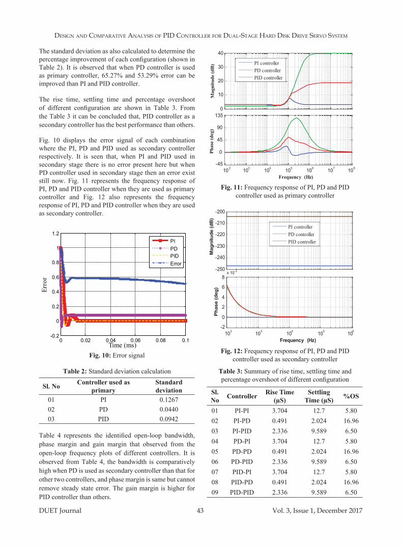
DUET Journal 43 Vol. 3, Issue 1, December 2017
Design anD Comparative analysis of piD Controller for Dual-stage HarD Disk Drive servo system
The standard deviation as also calculated to determine the percentage improvement of each configuration (shown in Table 2). It is observed that when PD controller is used as primary controller, 65.27% and 53.29% error can be improved than PI and PID controller.
The rise time, settling time and percentage overshoot of different configuration are shown in Table 3. From the Table 3 it can be concluded that, PID controller as a secondary controller has the best performance than others.
Fig. 10 displays the error signal of each combination where the PI, PD and PID used as secondary controller respectively. It is seen that, when PI and PID used in secondary stage there is no error present here but when PD controller used in secondary stage then an error exist still now. Fig. 11 represents the frequency response of PI, PD and PID controller when they are used as primary controller and Fig. 12 also represents the frequency response of PI, PD and PID controller when they are used as secondary controller.
0 0.02 0.04 0.06 0.08 0.1-0.2
0
0.2
0.4
0.6
0.8
1
1.2
Time (ms)
Erro
r
PIPDPIDError
Fig. 10: Error signal
Table 2: Standard deviation calculation
Sl. no Controller used as primary
Standard deviation
01 PI 0.126702 PD 0.044003 PID 0.0942
Table 4 represents the identified open-loop bandwidth, phase margin and gain margin that observed from the open-loop frequency plots of different controllers. It is observed from Table 4, the bandwidth is comparatively high when PD is used as secondary controller than that for other two controllers, and phase margin is same but cannot remove steady state error. The gain margin is higher for PID controller than others.
Frequency (Hz)102 103 104 105 106 107 108
-45
0
45
90
1350
10
20
30
40
PI controllerPD controllerPID controller
Mag
nitu
de (d
B)
Phas
e (d
eg)
Fig. 11: Frequency response of PI, PD and PID controller used as primary controller
Frequency (Hz)102 103 104 105 106
-2
0
2
4
6
8x 10⁻³-250
-240
-230
-220
-210
-200
PI controllerPD controllerPID controller
Mag
nitu
de (d
B)
Pha
se (d
eg)
Fig. 12: Frequency response of PI, PD and PID controller used as secondary controller
Table 3: Summary of rise time, settling time and percentage overshoot of different configuration
Sl. no Controller Rise Time
(µS)Settling
Time (µS) %oS
01 PI-PI 3.704 12.7 5.8002 PI-PD 0.491 2.024 16.9603 PI-PID 2.336 9.589 6.5004 PD-PI 3.704 12.7 5.8005 PD-PD 0.491 2.024 16.9606 PD-PID 2.336 9.589 6.5007 PID-PI 3.704 12.7 5.8008 PID-PD 0.491 2.024 16.9609 PID-PID 2.336 9.589 6.50
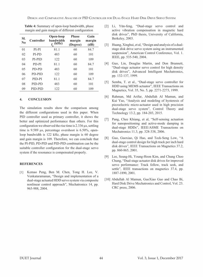
Design anD Comparative analysis of piD Controller for Dual-stage HarD Disk Drive servo system
DUET Journal 44 Vol. 3, Issue 1, December 2017
Table 4: Summary of open-loop bandwidth, phase margin and gain margin of different configuration
Sl. no Controller
open-loop bandwidth
f0 (kHz)
Phase margin
(Degree)
Gain margin
(dB)01 PI-PI 81.1 60 84.702 PI-PD 483 60 10103 PI-PID 122 60 10904 PD-PI 81.1 60 84.705 PD-PD 483 60 10106 PD-PID 122 60 10907 PID-PI 81.1 60 84.708 PID-PD 483 60 10109 PID-PID 122 60 109
4. ConCLuSIon
The simulation results show the comparison among the different configurations used in this paper. When PID controller used as primary controller, it shows the better and optimized performance than others. For this configuration we observed the rise time is 2.336 µs, settling time is 9.589 µs, percentage overshoot is 6.50%, open-loop bandwidth is 122 kHz, phase margin is 60 degree and gain margin is 109. Therefore, we can conclude that the PI-PID, PD-PID and PID-PID combination can be the suitable controller configuration for the dual-stage servo system if the resonance is compensated properly.
REFEREnCES
[1] Kemao Peng, Ben M. Chen, Tong H. Lee, V. Venkataramanan, “Design and implementation of a dual-stage actuated HDD servo system via composite nonlinear control approach”, Mechatronics 14, pp. 965-988, 2004.
[2] Li, Yün-feng, “Dual-stage servo control and active vibration compensation in magnetic hard disk drives”, PhD thesis, University of California, Berkeley, 2003.
[3] Huang, Xinghui, et al, “Design and analysis of a dual-stage disk drive servo system using an instrumented suspension”, American Control Conference, Vol. 1. IEEE, pp. 535-540, 2004.
[4] Guo, Lin, Douglas Martin, and Don Brunnett, “Dual-stage actuator servo control for high density disk drives”, Advanced Intelligent Mechatronics, pp. 132-137, 1999.
[5] Semba, T. et al., “Dual-stage servo controller for HDD using MEMS actuator”, IEEE Transactions on Magnetics, Vol. 35, No. 5, pp. 2271-2273, 1999.
[6] Rahman, Md Arifur, Abdullah Al Mamun, and Kui Yao, “Analysis and modeling of hysteresis of piezoelectric micro-actuator used in high precision dual-stage servo system”, Control Theory and Technology 13.2, pp. 184-203, 2015.
[7] Pang, Chee Khiang, et al, “Self-sensing actuation for nanopositioning and active-mode damping in dual-stage HDDs”, IEEE/ASME Transactions on Mechatronics 11.3, pp. 328-338, 2006.
[8] Guo, Guoxiao, Qi Hao, and Teck-Seng Low, “A dual-stage control design for high track per inch hard disk drives”, IEEE Transactions on Magnetics 37.2, pp. 860-865, 2001.
[9] Lee, Seung-Hi, Young-Hoon Kim, and Chung Choo Chung, “Dual-stage actuator disk drives for improved servo performance: Track follow, track seek, and settle”, IEEE transactions on magnetics 37.4, pp. 1887-1890, 2001.
[10] Abdullah Al Mamun, GuoXiao Guo and Chao Bi, Hard Disk Drive Mechatronics and Control, Vol. 23. CRC press, 2006.

NOX ReductiON iN a HybRid PlaNt: bOileR SimulatiON fOR RebuRNiN
DUET Journal 45 Vol. 3, Issue 1, December 2017
NOX Reduction in a Hybrid Plant: Boiler Simulation for Reburning
M. M. Rahman1*, Md. Arafat Rahman1 , Md. Awal Khan2, Jamal Uddin Ahamed1
1 Department of Mechanical Engineering, CUET, Chittagong, Bangladesh2Department of Mechanical Engineering, Bangladesh Military Academy, Chittagong, Bangladesh
ABSTRACT
Hybrid plants are a possibility to combine a highly efficient diesel engine with a steam boiler connected to a steam turbine and produce electricity with low total NOx emission level. The combustion in the diesel engine with local regions of high temperature produces a large amount of thermal NOx. The exhaust gases from the diesel engine are delivered to the steam boiler. The steam boiler is adapted to the conditions necessary for a reduction of NOx to N2. This gives a combined process with significant reduction of NOx. The architecture and circumstances of NOx reduction in a boiler in a hybrid plant are different from a pure boiler. The objective is not to reduce the amount of nitrogen oxides produced in the boiler but reduce NOx already existing due to the combustion process in a diesel engine. This gives the possibility to implement reburning in the primary zone, i.e. the grate. To determine the NOx level and estimate the overall potential a computer simulation of the boiler was developed. Using low quality biomass a NOx reduction up to 75 percent and an overall efficiency of 45 percent was predicted by the simulation tool. Applying an additional SNCR unit, reducing the nitrogen oxides by another 75 percent, gives a total reduction of 90 percent.
*Corresponding email: [email protected]
1. INTRODUCTION
NOx is one of the major concerns besides CO2 emissions when it comes to reduction of impacts on our environment and human health. Nitrogen oxides contribute to acid rain, water quality deterioration (eutrophication) and particulate matter (PM). Furthermore it is responsible for ground-level ozone (smog) and N2O is a greenhouse gas, which affects the climate change [1][2]. Moreover there is a strong economical incentive for NOx reduction.
NOx is a major problem concerning diesel engines, which is on the other hand economical and ecological reasonable because of their high energy efficiency up to 45 percent [3]. A widespread solution for NOx reduction is secondary treatment with selective catalytic reduction (SCR) or selective non-catalytic reduction (SNCR) by the application of ammonia. The main disadvantage of SCR is the weight, the size and the costs of the catalyst. For instance on ships, space requirement and stability are a big issue and makes the implementation of SCR difficult and expensive [4]. SNCR is more compact but requires complex running conditions as high temperatures and long residence time [5][6]. A well designed gas flow in a steam boiler allows a low NOx level without secondary treatment (Folsom 2001). But combustion of biomass in a steam boiler with a steam turbine gives an electric efficiency of only around 30 percent and this is – compared to the diesel engine – quite low [7].
Thermal NOx is the major source of nitrogen oxides from combustion. The chemical reactions according to the extended Zeldovich mechanisms are [2]
2O N NO N+ ↔ + (1)
2N O NO O+ ↔ + (2)
N OH NO H+ ↔ + (3)
The simulation has been performed to combine both ways in a hybrid plant and get the total efficiency up to the range of a diesel engine and the overall NOx emissions as low as in a boiler. The hybrid plant consists of a diesel engine, which runs on liquid bio fuel and a boiler that is fed with low quality biomass. The application of biomass and liquid bio fuel gives a CO2 neutral solution. The exhaust gases from the diesel engine with a high NOx level are delivered to the boiler. The combustion in the boiler is adjusted to produce a certain amount of NOx reducing agent in a defined stage. NOx is reduced to ordinary N2. A typical basic layout of the plant is shown in Figure 1.
2. REBURNING IN HYBRID PLANT
The architecture and circumstances of NOx reduction in a boiler in a hybrid plant are different from a pure boiler. The objective is not to reduce the amount of nitrogen oxides produced in the boiler but reduce NOx already existing due to the combustion process in a diesel engine. Thus

NOX ReductiON iN a HybRid PlaNt: bOileR SimulatiON fOR RebuRNiNg
DUET Journal 46 Vol. 3, Issue 1, December 2017
nitrogen oxides already exist before entering the boiler while in a conventional setup they are only produced during combustion in the boiler. This gives the possibility to implement reburning in the primary zone, i.e. the grate (Figure 2). The idea is not to use natural gas for reburning, but methane and hydrogen released during combustion, to achieve a CO2 neutral solution. A significant amount of both types of volatiles exist in solid bio-mass.
In conventional boilers this kind of reburning doesn’t occur as NOx is only created due to high temperatures by burning the CH4 and H2. There is almost no coexistence of nitrogen oxides and methane and hydrogen. A sketch of the new layout is shown in Figure 3. Compared to Figure 2 there is no injection of reburning fuel and no separate reburning zone. Primary and reburn zone are integrated on the grate.
diesel engineboiler
liquid bio fuel
airexhaust gas from
solid biomass
air
water
steam
diesel engine
exhaust gassteam turbine
condenser
pump
stack
Fig. 1: Hybrid plant layout
fuel
reburn fuel
secondary air
primary airprimary zone
reburn zone
burnout zone
flue gas
Fig. 2: Boiler with reburn zone
fuel
secondary air
diesel exhaustprimary/reburn zone
burnout zone
flue gas
Fig. 3: Reburning in hybrid plants
3. BOILER SIMULATION
The main focus lies on the chemistry going on in the boiler and trying to understand the chemical reactions taking place during the process of reburning. Doing a simulation the reaction kinetics can be exported.
3.1 Basic Layout and System Modeling
The model of the boiler consists of six reactors. The network is visualized in Figure 4. The inputs are enlisted on the left side: air, biomass and diesel exhaust. Biomass and exhaust gases from the diesel engine are fed to the grate for drying, release/combustion of volatiles and char combustion. In the model those stages are separated. However heat transfer is possible. The calculation focuses most on the reaction of the volatiles with the exhaust gases as reburning of NOx occurs in this step. The secondary combustion is then processed with air. There is no more potential for NOx reduction by feeding exhaust gases as the methane contained in the volatiles is mostly used in the bed (grate). Both heat exchangers are applied to cool down the gases and deliver heat for steam production.
The individual reactors are modeled as stirred. This doesn’t represent reality in detail as it is assumed that concentration of molecules and temperature are the same all over one reaction room. However this gives a first idea about what happens in which zone especially since the main six zones in a boiler are represented.
The calculation itself is transient. This is necessary as the chemical equilibrium will not be obtained and residence time in the different reactors plays a major role for NOx reduction as well as production. History of the reaction, e.g. whether it’s ignited or not, is of importance.
GrateDrying Volatiles Char
Diesel exhaust
Biomass
Heat exchanger 1
Secondary combustionAir
Heat exchanger 2
Stack
Fig. 4: Flow scheme of boiler system model
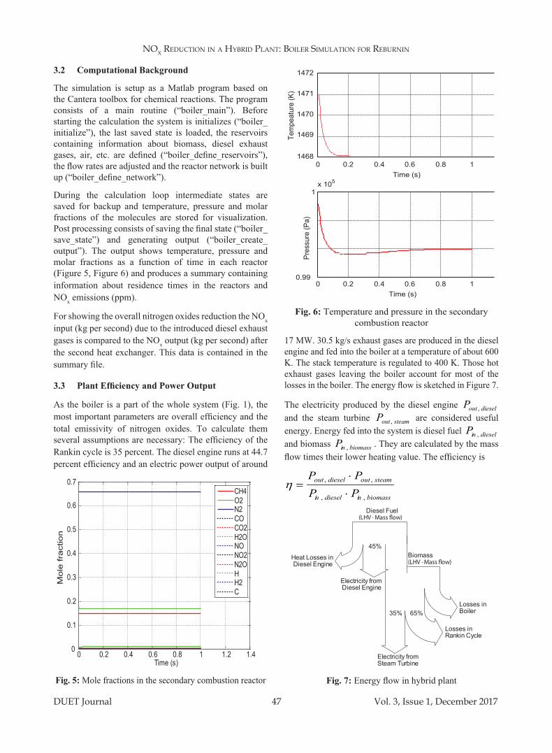
NOX ReductiON iN a HybRid PlaNt: bOileR SimulatiON fOR RebuRNiN
DUET Journal 47 Vol. 3, Issue 1, December 2017
3.2 Computational Background
The simulation is setup as a Matlab program based on the Cantera toolbox for chemical reactions. The program consists of a main routine (“boiler_main”). Before starting the calculation the system is initializes (“boiler_initialize”), the last saved state is loaded, the reservoirs containing information about biomass, diesel exhaust gases, air, etc. are defined (“boiler_define_reservoirs”), the flow rates are adjusted and the reactor network is built up (“boiler_define_network”).
During the calculation loop intermediate states are saved for backup and temperature, pressure and molar fractions of the molecules are stored for visualization. Post processing consists of saving the final state (“boiler_save_state”) and generating output (“boiler_create_output”). The output shows temperature, pressure and molar fractions as a function of time in each reactor (Figure 5, Figure 6) and produces a summary containing information about residence times in the reactors and NOx emissions (ppm).
For showing the overall nitrogen oxides reduction the NOx input (kg per second) due to the introduced diesel exhaust gases is compared to the NOx output (kg per second) after the second heat exchanger. This data is contained in the summary file.
3.3 PlantEfficiencyandPowerOutput
As the boiler is a part of the whole system (Fig. 1), the most important parameters are overall efficiency and the total emissivity of nitrogen oxides. To calculate them several assumptions are necessary: The efficiency of the Rankin cycle is 35 percent. The diesel engine runs at 44.7 percent efficiency and an electric power output of around
17 MW. 30.5 kg/s exhaust gases are produced in the diesel engine and fed into the boiler at a temperature of about 600 K. The stack temperature is regulated to 400 K. Those hot exhaust gases leaving the boiler account for most of the losses in the boiler. The energy flow is sketched in Figure 7.
The electricity produced by the diesel engine dieseloutP , and the steam turbine steamoutP , are considered useful energy. Energy fed into the system is diesel fuel dieselinP , and biomass biomassinP , . They are calculated by the mass flow times their lower heating value. The efficiency is
biomassindieselin
steamoutdieselout
PPPP
,,
,,
⋅
⋅=η
(LHV ∙ Mass �ow)
(LHV ∙ Mass �ow)
Losses in
Losses in
Heat Losses in
Electricity from
Electricity from
Diesel Engine
Diesel Engine
Steam Turbine
Rankin Cycle
Boiler
Diesel Fuel
Biomass45%
35% 65%
Fig. 7: Energy flow in hybrid plant
0 0.2 0.4 0.6 0.8 1 1.2 1.40
0.1
0.2
0.3
0.4
0.5
0.6
0.7
Time (s)
Mole
fra
ctio
n
CH4O2N2COCO2H2ONONO2N2OHH2C
Fig. 5: Mole fractions in the secondary combustion reactor
1472
1471
1470
1469
14680 0.2 0.4 0.6 0.8
Time (s)
Time (s)
1
0.99
Pres
sure
(Pa)
Tem
peat
ure
(K)
x 105
1
0 0.2 0.4 0.6 0.8 1
Fig. 6: Temperature and pressure in the secondary combustion reactor

NOX ReductiON iN a HybRid PlaNt: bOileR SimulatiON fOR RebuRNiNg
DUET Journal 48 Vol. 3, Issue 1, December 2017
4. RESULTS AND DISCUSSION
The results presented here are outcomes of the simulation. Thus one has to accept, that they do not represent reality. The figures are a result of the model. They cannot be more exact than the assumptions and simplifications made. Nevertheless it should be possible to read tendencies and get a rough overview.
4.1 NOx Reduction
A comparison of different types of biomass is presented in Table 1. Biomass feeding is set to 1 kg/s, stoichiometric ratio (lambda) for combustion of volatiles is 0.9 (rich combustion), char combustion is done with an amount of exhaust gas satisfying production of pure CO and secondary combustion runs with a lambda of 1.2 (lean combustion).
In the following wood as a biomass fuel is studied in detail. A variation of the lambda value in the volatiles reactor leads to the following results (Table 2). The other parameters remain unchanged.
Using a stoichiometric ratio of 0.8 for the volatiles, a variation of lambda in the secondary combustion zone is investigated. The outcome is presented in Table 3. Not shown here is that with low lambda values the amount of CO in the exhaust increases.
One can conclude that the type of biomass plays a role for the potential of nitrogen oxides reduction. The total
amount reduced (kg/s) depends on the amount of released hydrogen and methane. As lambda was kept constant the percental reduction was around 60 percent for all types. The stoichiometric ratio for combustion of volatiles is the parameter with the most significant influence. The optimum is around 0.7 for this case.
4.2 Reaction Kinetics
As reburning takes place in the part of the grate where volatiles are released from the biomass, the chemical reactions there – between volatiles and diesel exhaust gas – were investigated. The rates of creation and destruction of species containing nitrogen are summarized in Fig 8. Notice that the y axis is logarithmic. NO and NO2 are reduced. In the grate the destruction rate of nitrogen containing species is a bit higher than the creation rate.
Table 3: NOx reduction for different stoichiometric ratios in the secondary zone
Lambda NOx input NOx output NOx reduction
[kg/s] [kg/s] [%]1.0 0.010752 0.002648 75.41.1 0.010752 0.002821 73.81.2 0.010752 0.002963 72.41.3 0.010752 0.003085 71.31.4 0.010752 0.003191 70.31.5 0.010752 0.003285 69.4
1,00E-06
1,00E-05
1,00E-04
1,00E-03
1,00E-02
1,00E-01
1,00E+00
kmol
/m^3
/s
CreationDestruction
N2
NN
HN
OH
NO
NH
NO
2N
H2 N
HC
NH
NC
OC
NN
CO
NH
3H
CN
ON
2O
HO
CN
H2
CN
HC
NN
Fig. 8: Creation and destruction of species containing nitrogen
Table 1: NOx reduction for different types of biomass
NOx input NOx output
NOx reduction
[kg/s] [kg/s] [%]Wood 0.0119 0.0047 60.5Bagasses 0.0069 0.0023 65.6Rice straw 0.0098 0.0042 57.0Wheat straw 0.0107 0.0040 62.3RDF 0.0066 0.0031 52.2
Table 2: NOx reduction for different stoichiometric ratios for combustion of volatiles
Lambda NOx input NOx output NOx reduction
[kg/s] [kg/s] [%]0.5 0.007132 0.005512 22.70.6 0.008338 0.004282 48.60.7 0.009545 0.002173 77.20.8 0.010752 0.002963 72.40.9 0.011958 0.004719 60.5

NOX ReductiON iN a HybRid PlaNt: bOileR SimulatiON fOR RebuRNiN
DUET Journal 49 Vol. 3, Issue 1, December 2017
The reactions with the 20 highest reaction rates involving a species containing nitrogen are shown in Figure 9. The mechanism for reduction of NOx is complex. As there are more than 90 reactions involved in processing nitrogen it is hard to get an overview of the mechanism. E.g. reaction 2 converts NO into HNO. But this HNO reacts back to NO on different paths (Reaction 3 and 7). The reaction of nitrogen oxide with CH2 and CH to HNCO and HCN seem to be the initial reactions for reburning (Reaction 11 and 17). An important role plays reaction 14. It creates N2 from elementary nitrogen and NO. Elementary nitrogen is primarily produced from NH (Reaction 12).
0,00E+00
2,00E-04
4,00E-04
6,00E-04
8,00E-04
1,00E-03
1,20E-03
1,40E-03
1,60E-03
1,80E-03
CH
2(S)
+ N
2 <=
> C
H2
+ N
2H
+ N
O +
M <
=> H
NO
+ M
HN
O +
H <
=> H
2 +
NO
H +
O2
+ N
2 <=
> H
02 +
N2
N02
+ H
<=>
NO
+ O
HN
O +
O +
M <
=> N
O2
+ M
HN
O +
OH
<=>
NO
+ H
2OH
NC
O +
H <
=> N
H2
+ C
ON
+ O
H <
=> N
O +
HN
CO
+ H
<=>
NH
+ C
OC
H2
+ N
O <
=> H
+ H
NC
ON
H +
H <
=> N
+ H
2N
H2
+ H
<=>
NH
+ H
2N
+ N
O <
=> N
2 +
OC
+ N
O <
=> C
O +
NH
CN
+ O
<=>
NC
O +
HC
H +
NO
<=>
HC
N +
ON
+ C
O2
<=>
NO
+ C
OH
O2
+ N
O <
=> N
O2
+ O
HC
+ N
O <
=> C
N +
O
kmol
/m^3
/s
Fig. 9: Net reaction rates of reactions containing nitrogen
4.3 Efficiency,PowerOutputandEmissions
To calculate the overall efficiency the following settings were applied: The stoichiometric ratio (lambda) for combustion of volatiles is 0.8 (rich combustion), char combustion is done with an amount of exhaust gas satisfying production of pure CO and secondary combustion runs with a lambda of 1.2 (lean combustion). The exhaust gas is taken out at 400 K.
Comparing different kinds of low quality biomass the results presented in Table 4 were obtained. The average value of the total efficiency is in the range of 40 to 45 percent. RDF, having a low heating value and high moisture content, has the lowest performance compared to the other types.
Besides efficiency emissions of NOx in g per MJ of useful energy are important. In order to obtain this value, the mass
flow rate of NOx – measured in kg per second – as well as energy output and total exhaust mass flow is calculated by the simulation tool. Table 5 contains the results both for the pure diesel engine and the boiler exhaust in a hybrid plant.
Table 4: Total efficiencies and total power input and output values
Total eff.
Total power output [MW]
Power output steam turbine/total
Wood 0.43 44 0.61
Bagasse 0.46 43 0.61
Rice straw 0.44 45 0.62
Wheat straw 0.45 45 0.62
RDF 0.40 36 0.52
Table 5: NOx emissions for diesel engine and boiler exhaust gas.
Diesel exhaust gas Boiler exhaust gas
[kg NOx/s]
[g NOx/MJ]
[kg NOx/s]
[g NOx/MJ]
Wood 0.0454 2.660 0.0127 0.2889Bagasse 0.0454 2.660 0.0102 0.2350Rice straw 0.0454 2.660 0.0137 0.3064Wheat straw 0.0454 2.660 0.0124 0.2759
RDF 0.0454 2.660 0.0149 0.4153
Comparing these values to the mean value in Sweden (0.06 g NOx per MJ of useful energy), one can notice that the NOx emissions are still high but the overall reduction is good.
5. CONCLUSIONS
The aim was to find a cheap way to reduce NOx as effective as possible in a hybrid plant. The simulation indicates a reduction of up to 70 percent. Due to practical issues like imperfect mixing a more conservative estimate is 60 percent. The emissions are still high. Thus an additional SNCR could be applied. The costs for the reductant are less than half compared to a configuration without reburning due to reduced amount of NOx in the exhaust of the boiler. A SCR is no alternative. The amount of flue gas remains the same meaning that the size and the costs of the catalyst wouldn’t change. Applying an additional SNCR unit, reducing the nitrogen oxides by another 75 percent, gives a total reduction of 90 percent.

NOX ReductiON iN a HybRid PlaNt: bOileR SimulatiON fOR RebuRNiNg
DUET Journal 50 Vol. 3, Issue 1, December 2017
REFERENCES
[1] U.S. EPA, NOx - How Nitrogen Oxides Affect the Way We Live and Breathe. Site: http://www.epa.gov/air/urbanair/NOx/, last modified 2007-07-23, as accessed 2008-02-02, 2007.
[2] N. Brandt, F. Gröndahl, Miljöeffekter (Environmental effects). KTH, Stockholm, Sweden, 2005.
[3] U.S. DOE EERE, Just the Basics: Diesel Engine. U.S. Department of Energy, Washington, USA, 2003.
[4] Lövblad G., Fridell E., Experiences from use of some techniques to reduce emissions from ships.
Sjöfartsverket and Västra Götalandsregionen Miljönämnden, Gothenburg, Sweden, 2006.
[5] M. Radojevic, Reduction of nitrogen oxides in flue gases, Environmental Pollution 102, pp. 685-689, Elsevier, 1998.
[6] K. Han, C. Lu, Kinetic Model and Simulation of Promoted Selective Non-catalytic Reduction by Sodium Carbonate, Chinese Journal of Chemical Engineering Vol. 15, pp. 512-519, Elsevier, 2007.
[7] R. van den Broek, A. Faaij, A., van Wijk, Biomass Combustion for Power Generation, Biomass and Bioenergy Vol. 11, No. 4, pp. 27I-281, Elsevier, 1996.
Single Degree of Motion Control of a MagnetiCally SuSpenDeD objeCt uSing analog Controller
DUET Journal 51 Vol. 3, Issue 1, December 2017
Single Degree of Motion Control of a Magnetically Suspended Object Using Analog Controller
Md. Emdadul Hoque1*, Monjur Mourshed1, Fazlur Rashid1, Avijit Sarker1, Robiul Alam2
1Department of Mechanical Engineering, Rajshahi University of Engineering and Technology, Rajshahi, Bangladesh
2Refrigeration and Air Condition Technology, Thakurgaon Polytechnic Institute, Thakurgaon, Bangladesh
ABSTRACT
The present study focuses on the control of the single degree of motion (SDF) of a magnetically suspended object using analog controller. To stabilize the maglev system PD controller has been implemented as an active feedback control system. The designed active feedback control system of the PD controller mainly suspends the mass of the object as well as controls its motion. Despite the simplicity and low cost of the eddy current position sensing system, it is able to detect the ball position at a distance of 2-5 mm. The controller circuit has been designed in such a manner to precisely control the electromagnetic field to stabilize the position of the levitated object. The implementation of the PD controller ensure precise control of the system with simplicity in design and relatively low cost.
*Corresponding email: [email protected]
1. INTRODUCTION
In the advanced technological world, the advancement in mechatronics field is momentously captured by magnetic levitation systems. Recently, they are becoming popular because of having hands-on significance in many engineering systems such as high-speed trains for passenger, zero friction magnetic bearings, wind tunnel levitated object in models and vibration isolation [1-3]. In magnetic levitation system, the magnetic force from the electromagnet keeps the object, which is to be levitated, floated in the air-gap against the gravitational force. The force exerted on the levitated object is a function of the current flowing through the coil of the electromagnet and the displacement between the electromagnet and the levitated object. At a certain position of the suspended object, the relation between the magnetic force and the coil current varies depending on the position of the levitated object [4]. As the substance of the levitated object in our designed model is a ferromagnetic ball, the magnetic force is proportional to the square of the coil current [3, 5, and 6]. Magnetic levitation or maglev system itself is very complex due to plant dynamics, the small degree of natural damping in the process, the positioning specifications often required by the application and the open-loop unstable system dynamics from point of view of control engineering. Hence the application of control technologies for use in magnetic levitation systems has become inevitable. For a past couple of decades, a lot of researches have been conducted for the control of magnetic levitation systems. To take care of nonlinearity of the systems, different nonlinear control techniques
such as feedback linearization back stepping and sliding mode control have been applied [3, 4, 6, and 7]. Feedback control is a best way to take care of a magnetic levitation system, though it does not guarantee robustness in the presence of modeling error and disturbances. However in active feedback control system using PID, LQR, H∞, PI control, repetitive controls are extensively used [8, 9]. In this research, a different method of controlling the magnetic force is investigated. PD controller is being used for its simplicity and low cost. Moreover, it makes the system more stable with less consumption of energy as compared to the other processes. Considering the object to move in upward or downward translational direction, i.e. single-degree-of-freedom motion (SDOF), the controller is made enable to control this motion. The steady state condition is realized with this control in which the repulsive or attractive force produced by the electromagnet balance the weight of the suspended mass. Further experimentation reveals the acceptance of the method. The paper is organized as follows: Section 1 introduces the paper; section 2 reveals mathematical modeling of a maglev object. In Section 3, controller is designed. In Section 4, experimental setup is described. Section 5 depicts experimental result and finally, Section 6 concludes the paper.
2. MODELING
2.1 Electromagnetic Force Dynamics
The ball dynamics model of the levitated System is described by the following equation

Single Degree of Motion Control of a MagnetiCally SuSpenDeD objeCt uSing analog Controller
DUET Journal 52 Vol. 3, Issue 1, December 2017
),( xifgmxm −= (1)
Where m is the mass of the steel ball, x is the distance between ball and the electromagnet, f(i, x) is the electromagnetic force that counteracts the weight force (w=mg) to bring the ball in the equivalent position.
The electromagnetic force created for the coil current i is given by using the magnetic energy equation (Faraday’s inductive law and Ampere’s circuit law) in the following form
xdxLdtixif
2)()(),(
2
−=
(2)
Where L is the total inductance of the electromagnet. When the ball comes closer to the electromagnet the total inductance increases. Taking this incremental variation of the total inductance into consideration, equation (2) can be transformed as follows
][2
),( 001
2
xxLL
xddixif +−=
(3)
Where L1 is the inductance of the coil without the levitated object, L0 is the additional inductance caused by the presence of the levitated object and x0 is the air gap at the equilibrium position of the levitated object. The inductance is firmly depends upon the geometry and construction of the electromagnet, and can be experimentally determined.
Now taking the derivative of the inductance with respect to the ball position is given by
200)(
xxL
xdxLd
−=
(4)
Putting this value in Eq. (2), we get
2
200
200
2
2)(
2),(
xixL
xxLixif =−−=
2
2
),(xikxif =
(5)
Where k = 2 00 xL
is the attractive force coefficient for
electromagnet, i is the coil current and x is the mean distance between electromagnet and suspended object. To design a linear control system the non-linear electromagnetic force
),( xif is linearized about an equilibrium position of the levitated object, say x0
...)2()2(),( 30
20
20
02
0
20 +−+=
xiki
xik
xikxif
...),( 10 ++= ffxif (6)
Where, xxx
iiiδδ+=+=
0
0
Where 0i and iδ respectively represent the equilibrium
and incremental values of current, 0x and xδ represent the equilibrium and incremental values of position. In our further analysis, i and x represent the change of current and position from the equilibrium respectively.
2.2 Motion Dynamics
A basic control model is designed based on linearized equation of motion with the assumptions that the displacement of the suspended mass (steel ball) is negligibly small, the nonlinear terms are neglected and the levitated mass m is moving only in the vertical translational direction as shown in the Fig. 1. The equation of motion is given by
wikxkxm is ++= (7)
Where sk is the gap force coefficient, ik is the current force coefficient, w disturbance acting on the suspended
mass, i is the control current. The coefficients sk and
ik are positive. Fig. 2 represents the block diagram for the magnetic levitation system with transfer function. Denoting each Laplace-transform variable by its capital and assuming the initial values to be zero for simplicity, the transfer function representation of equation 7 becomes
))()((1)( 12 sWsIkksm
sX +−
=
Electromagnet
Levitated Object
Displacement Sensor
Controller
PowerAmplifier
x
Fig. 1: Basic model of an active magnetic levitation system

Single Degree of Motion Control of a MagnetiCally SuSpenDeD objeCt uSing analog Controller
DUET Journal 53 Vol. 3, Issue 1, December 2017
))()((1)( 000
2 sWdsIbas
sX +−
=
(8)
Where, m
dmkb
mka is 1,, 000 ===
In current control magnetic suspended system, PD control can be represented as
)()()( sXsPPsI vd +−= (9)
)()()(
sPPsIsX
vd +−=
(10)
)(1
)()(
sPPsIsX
vd +−=
(11)
From this linearized system, )(sX and )(sI represent the change from the equilibrium values of position and current respectively. Hence the negative sign implies that
with an increase in )(sX there will be a decrease in )(sI, and vice versa.
From Eq. (8), (9) and (10)
))()(()(
1)(
)(00
02 sWdsIb
assPPsI
vd
+−
=+
−
)()(
)()(
0002
0
absPbPssPPd
sWsI
vd
vd
−+++−
=
(12)
Again putting the value of, )(sI from Eq. (11) in Eq. (9)
])(})()({[1)( 000
2 sWdsXsPPbas
sX vd ++−−
=
0002
0
)()(
abPsbPsd
sWsX
vd −++=
(13)
3. CONTROLLER DESIGN
Magnetic suspended system can be controlled by various ways. In this paper, PD controller is used to produce active feedback control system.
PD controller can be implemented by any of the followings, such as DSP, PLC, microcontroller and analog circuit. Here the controller is designed based on analog circuit with ‘Op-Amp’ as shown in Fig. 3. The feedback from the sensor is inverted to boost up the voltage, VCE when the object comes close to the sensor. The output is then passed through a proportional circuit to lift object and a derivative circuit to dampen the vibration. After that the output from these two circuits is summed in another circuit and combined with an offset power supply. To amplify the output voltage two bi-polar junction transistors (BJT, BD135) are used to increase the base current of BJT (BC458). So the collector gain of transistor (BC458) is increased and the power input to electromagnet is also amplified.
4. EXPERIMENTAL SETUP
A basic model of single-degree-of-freedom motion magnetic levitation system using PD controller is shown in Fig. 4. The setup consists of a wooden structure which has three stands. One rectangular and two circular plates are set one over another. The middle plate clamps the sensor and the upper plate holds the electromagnet. The height and diameter of the total setup is 23 mm and 11.5 mm. Each stand is round shaped and of 2 mm diameter. Both the top and middle plates are fixed. The sensor is clamped such that its position can be varied by two identical hexagonal nuts when needed. A controller board is attached to the base plate. Wood is being used for low cost and simplicity.
The components of the maglev system include a sensor, an actuator (the electro-magnet), and a controller. The sensor is an inductive displacement sensor with an oscillator which generates AC, induction coil that generates changing magnetic field, and a current sensor. The sensor produces a voltage, vs which is proportional to the position
Reference
Pd + sPv
W+
+ki1
ms2-ksPosition+
_
Fig. 2: Block diagram of a maglev system
Sensor Invertingamplifier
Differentiatingamplifier
Sumamplifier
Sumamplifier
Power amplifier
Volume knob
Volume knob
15 volt supply
Volume knobVR2
VR1
VR3
Fig. 3: Schematic diagram of PD controller for maglev system

Single Degree of Motion Control of a MagnetiCally SuSpenDeD objeCt uSing analog Controller
DUET Journal 54 Vol. 3, Issue 1, December 2017
of the levitated object x (Fig.1), with a gain, say β, which is linear, vs = xβ.
The electromagnet has a winding of 330 turns of 0.644 mm copper wire in 7.6 mm diameter silicon core. It is able to sustain up to 5 Ampere current. The magnetic force developed is given by F= Ni. where N is the number of turns and i is current flow through the winding. Desired force is produced by controlling the current. A steel ball of 1.4 cm diameter and 13.6 gm mass is used as a levitated object. The photograph of the magnetic levitation system is presented in Fig. 5.
5. EXPERIMENTAL RESULTS
A stable magnetic levitation system is developed using a PD controller. The system is suitably controlled by a PD controller. From the experiment, it is observed that the consumption of power of the system is approximately 20-22 watt.
It is considerably low regarding the stability of the system. Fig .5 shows the consumed current by the system versus time. It is seen from the figure that the system is stable using PD controller. Fig. 6 represents a snap of the magnetically suspended object for any instant. Further accuracy of the system can be easily obtained by using precise equipment.
5.1 Sensitivity of the System
The sensitiveness of the system is how the system reacts while functioning under rough condition. The system shows a high notch of sensitiveness with the variation of the distances of the floating object. The output voltages remain in a consistent trend over the various set of data collected while operation is enduring.
Fig. 7 represent that the curve represents almost linear characteristics from 2.5 mm to 5 mm. So the minimum gap between the ball and the sensor should be maintained within the above range. Therefore the reaction of the system when some ferromagnetic material is brought closer to the sensing element is clearly evident by the above curve.
6. CONCLUSION
The maglev system is designed and fabricated. The levitation is successfully established. The single degree-
Fig. 4: Schematic diagram of the developed system
Time (sec.)
Curr
ent (
Am
p.)
1.4
1.2
1
0.8
0.6
0.4
0.2
00 20 40 60 80 100 120 140
Switch on Switch off
Fig. 5: Stability of the designed maglev system
Fig. 6: Realization of maglev system
Fig. 7: Calibration eddy current displacement sensor of the sensor

Single Degree of Motion Control of a MagnetiCally SuSpenDeD objeCt uSing analog Controller
DUET Journal 55 Vol. 3, Issue 1, December 2017
of-freedom motion of the levitated object is controlled manually by tuning the controller gain. The position of the ball can be made stable and varied by regulating the current flow. But with a little energy consumption the stability of the levitated object is confirmed. The successful accomplishment of this venture reveals the feasibility of magnetic levitation for miscellaneous applications. At the same time, supporting loads (levitation), magnetic actuators can apply precision force, dampen vibration and move objects at precise distances all with no contact between surfaces and without friction. In punitive surroundings (corrosive, vacuum, etc.) where conventional mechanical or hydraulic actuators may not survive, this type of actuation can be used readily. It can also operate in extreme clean environments without the threat of generating pollutants from its use. Magnetic actuation can be made a sensible and cost effective solution to numerous engineering problems by using the persistent drift of smaller and cheaper semiconductor devices incorporated with low-cost and low-complexity. Further the maglev system can be developed by adapting microcontroller to the control circuit. The use of microcontroller can make the system more precise and economic. It can also enhance the performance of the control system. The power consumption of the control system can be reduced by using permanent magnet. This system can be made more economical by implementing solar power.
REFERENCES
[1] M. E. Hoque, T. Mizuno, D. Kishita, M. Takasaki, Y. Ishino, “Development of an Active Vibration Isolation System Using Linearized Zero-Power Control With Weight Support Springs”, Journal of Vibration and Acoustics, Vol.132, pp.041006-1~9, 2010.
[2] J. C. Shen, “H∞ control and sliding mode control of magnetic levitation system”, Asian Journal of Control, Vol. 4, No. 3, pp. 333-340, September, 2012.
[3] G. Abbscia, K. Asenso, A. White, Magnetically levitated vertical axis wind turbine, Thesis, Worcester Polytechnic institute, 2010.
[4] Y. S. Lee, J. H. Yang and S. Y. Shim, “A New Model of Magnetic Force in Magnetic Levitation Systems”, Journal of Electrical Engineering & Technology, Vol. 3, No. 4, pp. 584~592, 2008.
[5] M. T. Thompson, “Electrodynamic magnetic suspension models, scaling laws, and experimental results”, IEEE Transaction on Education, Vol. 43, No. 3,2000.
[6] D. Cho, Y. Kato and D. Spilman., “Sliding mode and classical control magnetic levitations systems”, IEEE Control Systems Magazine, Vol. 13, pp. 42-48, 1993.
[7] W.G. Herley and W.H. Wolfle, “Electromagnetic Design of a Magnetic Suspension System”, IEEE Trans. on Educarion., Vol. E-40, pp. 124-130, 1997.
[8] M. E. Hoque, T. Mizuno, M. Takasaki, Y. Ishino, “Application of feed forward control to a vibration isolation system using negative stiffness suspension”, Journal of system design and dynamics, Vol. 05, No. 5, 2011.
[9] E. H. Maslen, G. Schweitzer, Magnetic bearings, theory, design and application to rotating machinery, Springer Berlin Heidelberg, Germany, 2009.
NOMENCLATURE
Symbol Meaning Uniti Control current (Amp)Lmx
InductanceMassControl distance
(H)(gm)(mm)


EnvironmEnt FriEndly Continuous Flow Gas GEnEration by FluidizEd bEd riCE Husk and saw dust GasiFiEr
DUET Journal 57 Vol. 3, Issue 1, December 2017
Environment Friendly Continuous Flow Gas Generation by Fluidized Bed Rice Husk and Saw Dust Gasifier
Dr. Md. Arefin Kowser*, Dr. Hasan Mohammad Mostofa Afroz, Nayeem Md. Lutful Huq, Md. Khaled Khalil
Department of Mechanical Engineering, DUET, Gazipur, Bangladesh
ABSTRACT
Bangladesh is an agriculture based developing country. A huge amount of rice husk is produced from paddy which creates a significant disposal. Although some rice husks are used as fuel for cooking, boiling paddy, electricity generation, and other purposes, but in most of these applications the maximum energy loss occurs due to inefficient burning process. To utilize maximum energy, rice husks should be burned properly. Rice husk gasification is one of the prior solutions where rice husk is burned properly for the utilization of maximum energy. In the present work, a down draught rice husk gasifier is fabricated, where the reactor is constructed to carry out a variety of chemical reaction. In the reactor, air is passed through rice husk at a controlled velocity for the partial combustion which produces a continuous flow of gas of usable form of energy. In this method once the processes is started it can be kept running as long as needed. The burnt solid waste is removed automatically after a certain period. As it gives efficient energy conversion it leaves a less environmental impact. The temperatures at different positions of gasifier are measured by K type thermocouples. The produced gas has been cooled by a radiator to 50°C to measure its flow rate and calorific value. Gasification tests have been conducted with varying air flow rates and fuel feed rates. The typical wall temperature of gasification process was about 400-450°C. The producer gas had an average temperature of 600-800°C and the pick heating value was 3.9MJ/m3 to 4.5MJ/m3.
*Corresponding email: [email protected]
1. INTRoDuCTIoN
Alternative energy sources, like biomass, are among the most attractive field of research now a days. As the availability of the fossil fuels are going down each day, its price is growing high inversely making the domestic as well as for industrial usage in feasible. Moreover, the emission due to production and utilization of the fossil fuels are severely damaging for the environment.
The rice husk, an agricultural by product which is rich with energy content (12 – 18MJ/kg) can be a way of energy recovery for a large number of countries across the world. Round the year and across the globe this is one of the major agricultural waste. About 500 million tons of rice is produced every year [1] of which 20% is assumed to be rice husk [2] that is about 100 million tons. Kandpal et al., 1996 carried out a work for testing the viability and estimated per unit electricity production cost to be 0.05-0.2 USD [3].
Near about 7 million tons of rice husk is produced in Bangladesh every year. However, due to the lack of understanding and inadequate measure in proper utilization of this valuable resource the country is losing a wonderful resource of energy. To reduce the environmental impact many countries have imposed new laws but they are yet to realize the real loss. Nevertheless, these laws have
created even more surplus energy resource, i.e. rice husk, as a renewable energy source [4]. On the other hand these byproducts from agriculture if modified into gaseous or liquid fuels can be proven useful for the agriculture based countries especially those who don’t have conventional energy sources.
Gasifying rice husk means, burning it with limited amount of air. It is found from the previous studies that the gasification of rice husk gives the form of energy that is capable of bluish flame. Using the biomass as a source of energy was started in early 1980s [5]. At that time using combustion and gasification technologies on sunflower hulls, wood residue, and sewage sludge EERC directed several missions. Wood fuel contains minimal heavy metals and extremely low levels of sulfur, hence wood fuel is no threat to acid rain pollution. Usually wood ash is less than 1% of the weight of the wood if moisture content possible to maintained 1 to 2 percent. Sometimes ash may be used in biomass fertilizer production. In the year 1999 Ghaly et al., 1999 [6] used a dual distributor type fluidized bed gasifier for producing fuel gas. A smokeless efficient gasifier was developed in the year 2005 in Myanmar called The Sun Sun Rice Husk Gasifier stove [7]. Alexis TB et al., invented a continuous flow rice husk gasifier in the year 2010. It was designed for thermal applications, such as, cooking, drying etc. [8]. Chidicofan

EnvironmEnt FriEndly Continuous Flow Gas GEnEration by FluidizEd bEd riCE Husk and saw dust GasiFiEr
DUET Journal 58 Vol. 3, Issue 1, December 2017
et al. analyzed technical and economic feasibility and the environmental and social impacts of their gasification project that uses cotton stalk and rice husk [9]. They assessed technical performance and found the electricity efficiency 11.9% for rice husk against 12.6% for cotton. Gominho et al. made an effort to find out the effect of torrefaction which revealed the optimizing guideline for reaction temperature, time etc. They were able to reduce the moisture content and increase the heating value [10].
Thus many Asian countries especially that produces rice, have been working on rice husk gasification. However, this technology is still not well proven and the problems are still arising even in the commercial systems. Further research and development work needs to be undertaken to improve this technology. These projects have the potentials to establish themselves especially in countries where the raw materials are in abundance. This work focuses on the fabrication of a system, i.e. a gasifier that will work below 1000 K and produce syngas. A laboratory scale gasification system was developed and experimental studies have been carried out for optimization. These kind of projects can save a lot of money and time as well as the human effort. These can also give a hand to those who are suffering from employment crisis. Thus this research will enrich our knowledge in rice husk processing in more efficient and economical way. Moreover, the adoption of this technology in many countries simply indicates the significance of its contribution in the advancement of utilizing renewable energy.
This paper is constructed as it begins with the introduction to the system and its background that leads to the objective of the work. After that it describes the methodology that describes the chemical processes, fabrication of the system, operation of different parts, waste handling method etc. and concludes with data acquisition for performance analysis. Then the paper proceeds to results and discussion which deals with different observations, performance analysis, positive and negative aspects of the method etc. and finally it is concluded with the concluding remarks and future recommendations.
2. METHoDoLoGY
A significant amount (20%) of the paddy is rejected from the rice mills which is the rice husk. Thus 132 million tons of rice husk were wasted in the year 2008 mostly by burning them in the open field. Yet the rice husk has an attractive calorific value which can be used by reclaiming it from those waste materials.
2.1 Characteristics of Rice Husk
An inherent quality of the rice husk is that it doesn’t ignite and burn easily and to do that one needs to blow
air through the husk. It also has to more positive qualities that it resists the moisture to get into it and cannot be decomposed with fungal attach. Thus this is often used as a good insulation material.
Silica (SiO2) content in rice husk is very high therefore it decomposes over a long period of time if left alone in the open field.
The rice husk is bulky and dusty which makes it less affordable for handling. Having an angle of repose of about 40°-45° makes it fluent through the feed hoppers.
Because of its low bulk density (70-110 kg/m³, 145 kg/m³ when vibrated or 180kg/m³ in form of pellets) a large storage capacity by volume is required for transport which leads to an uneconomical situation.
As mentioned earlier because of its good calorific value (3410 kcal/kg) it is an attractive option for renewable energy research.
2.2 Fabrication
The gasifier was fabricated using the available materials in Bangladesh so that the system can be constructed at any corner of the country economically. The complete design of rice husk gasifier is shown in Figure 01.
2.3 Reactions in Gasifier
Table 1: Principal chemical reactions in a gasifier
Reaction type Reaction
Combustion C + O2 = CO2
Water gas C + H2O = CO + H2
Water shift reaction CO + H2O = CO2 + H2
Boudouard reaction C + CO2 = 2CO
Methane reaction C + 2H2 = CH4
Fig. 1: Design of the Down Draught Rice husk Gasifier

EnvironmEnt FriEndly Continuous Flow Gas GEnEration by FluidizEd bEd riCE Husk and saw dust GasiFiEr
DUET Journal 59 Vol. 3, Issue 1, December 2017
2.4 Chemical Reaction Occur into Gasification System
There are different reaction zones where different types of reactions take place.
In the oxidation zone:
C + O2 = CO2+ 401.9 kJ/mol (1)H + O2 = H2O + 241.1 kJ/mol (2)
In the reduction zone:
C + CO2 + 164.9 kJ/mol = 2CO (3)C + H2O + 122.6 kJ/mol = CO + H2 (4)CO2 + H2 + 42.3 kJ/mol = CO + H2O (5)C + 2H2 = CH4 (6)CO + 3H2 = CH4 + H2O + 205.9 kJ/mol (7)
Heating value of wood saw dust can be calculated as equation (8)
Heating value per one gm. of fuel= (Heat absorbed by calorimeter - heat released from fuse wire) (8)
= (1900+432) gm ×1 Cal/gm × ∆T-2.3 Cal/cm × 10 cm= 18.72 MJ/kg.∆T = 1.92°C, Unburned wire = 1.5cmExcess air to be obtained from equation (9) % Excess Air = 100 (9)
3. FABRICATIoN
The fabrication consists of preparing and assembling the major parts of the gasifier. It takes different types of metal working, welding, electrical wiring, programming etc.
3.1 Main Components of CFRHG
The lists of main components of gasifier are as follows:1. Feed hopper2. Reactor3. Blowers4. Burner5. Char chamber6. Scraping system7. Data acquisition system8. Support frame
Table 2: Major operational data of CFRHG
Parameter DimensionReactor diameter (cm) 25Startup time (min) 15-25Rice husk consumption (kg/hr) 8Gas temperature (°C) 90-130Air temperature (°C) 20-25Flame temperature (°C) 400-800
Fig. 2 presents the schematic diagram of the gasifier with all components. The gasifier consists of a 25cm diameter and 110cm high reactor. The rice husk is gasified by incomplete combustion. A gravity type feed hopper feeds the reactor which is placed overhead to the reactor while to collect the char a char chamber is placed beneath the reactor. This chamber has another use that is it supplies the combustible gases to the burner. A char separator is placed between the char chamber and the burner for cleaning the gas leaving the reactor. A cyclone separator removes the char with the help of an air injector which is positioned beneath the char chamber. The air needed for the gasification is supplied by a blower.
3.2 Description About Individual Parts
The following sections describe some technical details of the individual parts of the gasifier. However, some of these consists of some smaller components.
3.2.1 Fuel feeding system
The feed hopper is a conical part that serves as the temporary storage for rice husk. It is located on the top of reactor. This device is provided with a door that can be opened for easy disposal of rice husk. The hopper has a capacity of 15kg which is shaped like a funnel, works as a supplier and a reservoir.
3.2.2 Air supply system
Two blowers (7.08m3/min) work as the air supply unit for the reactor. These blowers are accompanied by pressure valve, main valve, bypass valve, and supply pipe. The blower is equipped with 25µ filter to clean the inlet air from dust particles, water etc. The blower-1 is used to supply air to the after burner, while blower-2 is used carry the bed material (char) away.
Fig. 2: Schematic diagram of CFRHG

EnvironmEnt FriEndly Continuous Flow Gas GEnEration by FluidizEd bEd riCE Husk and saw dust GasiFiEr
DUET Journal 60 Vol. 3, Issue 1, December 2017
3.2.3 Start-up system
Like all other start-up systems the start-up burner starts up the initial burning of the rice husk. It works by a spark plug. After the air supply and the ignition systems are turned on the start-up unit comes into play. The rice husk needs to be combusted below 800°C as well as hot spots or localized high temperatures are not expected. Which, unfortunately, in practice (in directly fired furnaces/gasifiers) is not possible. This requires a large grate area and quick dissipation of heat.
3.2.4 Reactor
The operation of the gasifier leads to a very high temperature inside the reactor resulting in much lower amount of CO2, also known as the greenhouse gas. This ranges from 5 to 15% which is almost 50% of the amount produced by direct combustion. Other quantities are; heating value: 1200 to 1400 kcal/m3, black carbon content: 10 to 50 gm/m3, and tar content: 56 to 100 mg/m3.
Fig. 3: Reactor
3.2.5 Char chamber
The char is deposited in char chamber. The temperature in this zone is about 50°C to 87°C. It is produced in the gasifier and is completely black, which is good for soil conditioning. Rice husk contain about 75% organic volatile matter and the balance 25% of the weight of this husk is converted into ash during the burning process which is known as char or rice husk ash (RHA). This RHA in turn contains around 85% - 90% amorphous silica.
3.2.6 Scraper
The scraper is one of the most important elements in this set up. Here it is used to remove the char from the combustion chamber and driven by a dc motor that rotates after every five minutes. It is made of a shaft and a net. The shaft is coupled with a motor by a chain sprocket arrangement. The net should have ability to resist high temperature and the weight of a mass of about 15 to 20 kg. The scrapping system arrangement of the fabricated gasifier is shown in Fig. 4 which includes a motor controlled by timer.
3.2.7 Blower
There are two electric blowers in the system shown in Fig. 5. One blower (blower 1) is used to supply the required air into the combustion chamber so that the husk can burn easily and the other (blower 2) is to remove the char from the scraping zone.
3.2.8 Data acquisition system
A data acquisition (DAQ) system is used for online recording and processing of the data, like temperature and pressure, collected from the gasifier. This system consists of temperature probes, pressure transducers, power supply, microcontroller, personal computer, and signal conditioning extinctions for instrumentation (SCXI). The National Instruments SCXI is a multi-channel signal conditioning and control system for using with personal computers. It is comprised of a chassis that can house a variety of modules for any I/O needs. The SCXI system is programmed with Lab VIEW (Laboratory Virtual Instrument Engineering Workbench), a National Instruments applications software package. A library of functions included in Lab VIEW is used to develop a model for data acquisition, instrument control, data analysis, data presentation and data storage. It collects inlet, outlet, and reactor zone temp., flow rate etc.
Scrapper
Motor
Fig. 4: Scraping system Arrangement
Fig. 5: Blower Arrangement
Blower 1
Blower 2

EnvironmEnt FriEndly Continuous Flow Gas GEnEration by FluidizEd bEd riCE Husk and saw dust GasiFiEr
DUET Journal 61 Vol. 3, Issue 1, December 2017
Fig. 6: The complete setup of fabricated gasifier
Fig. 7: Gas Production from the fabricated gasifier
4. RESuLTS AND DISCuSSIoN
Data collected through the data acquisition system are analyzed from different perspectives to find the better option and to optimize or to suggest some optimization parameter.
4.1. observations
The CFRHG system has been tested successfully in a continuous mode. Continuous operation is accomplished by a very simple method. The feed hopper loaded with
rice husks ensures the continuous supply of raw material to the reactor where the flow is maintained by the gravity. On the other hand the char is removed simultaneously from the char box. Rice husk fuel produced combustible gas within 15 to 25 minutes after ignition. A very positive observation is that no smoke is released by the gasifier while the process goes on. The operation of CFRHG requires only one or two operators which is for loading the raw material and removing the waste. The gas exits the reactor with a temperature ranging from 150° to 270°C. Afterwards the gas is mixed with air preheated to a temperature of 90° to 180°C and supplied to the burner which produces a yellowish-to-bluish flame resulting in a temperature of 400° to 800°C.
4.2 Performance Test
Results of performance test obtained in this research work are presented in following figures. Figure 8–17 show the graphical representations of different characteristic parameters for the gasification system. Fig. 8 shows the calorific value of different types of woods. Where jackfruit shows the highest energy content and teak is second in place.
In Figure 9 moisture and ash contents are portrayed for different woods. Moisture contents are almost same for all of them. However, ash content is maximum in olive, which has negative impact in performance as a fuel.
0
5
10
15
20
25
Calor
ific V
alue (
MJ/k
g)
Type of wood
Fig. 8: Calorific values of sawdust
02468
1012
Moi
sture
/Ash
Con
tent (
%)
Type of Wood
MoistureContent(%)
% of ashcontent
Fig. 9: Moisture and Ash contents of sawdust
Feed Hopper
Controller
Reactor
Reactor
Flame

EnvironmEnt FriEndly Continuous Flow Gas GEnEration by FluidizEd bEd riCE Husk and saw dust GasiFiEr
DUET Journal 62 Vol. 3, Issue 1, December 2017
Teak has the lowest fuel consumption rate, while jackfruit and gamari are moving side by side with good potential as a fuel depicted in Figure 10.
2
3
4
5
6
400 500 600 700 800
Fuel
Con
sum
ptio
n R
ate
(kg/
h)
Inlet Air Velocity (m/s)
Gamari Jack fruitJamboline MahoganyMango OliveRain tree Teak
Fig. 10: Fuel consumption characteristics sawdust
0
5
10
15
20
25
400 500 600 700 800
CO
(ppm
)
Inlet Air Velocity (m/s)
Gamari Jack fruitJamboline MahoganyMango OliveRain tree Teak
Fig. 11: CO content for different sawdust
00.5
11.5
22.5
33.5
400 500 600 700 800
CH
4(p
pm)
Inlet Air Velocity (m/s)
Gamari Jack fruitJamboline MahoganyMango OliveRain tree Teak
Fig. 12: CH4 content in different sawdust.
From fig. 11 to 14, different particle contents (CO, CH4, SO2, and NOx), after gasification, are presented as function of inlet air velocity. All the woods show almost similar characteristics. Mango has the minimum CO
and CH4 content while the others change their positions at different temperatures. Among them jackfruit shows better position. Rain tree has the highest SO2 and NOx at almost all temperature. Again, jackfruit gives minimum SO2, gamari, jamboline, mango, jackfruit, and mahogany gives low NOx.
00.010.020.030.040.050.06
400 500 600 700 800
SO2
(ppm
)
Inlet Air Velocity (m/s)
Gamari Jack fruitJamboline MahoganyMango OliveRain tree Teak
Fig. 13: SO2 content in different sawdust
0
0.02
0.04
0.06
0.08
0.1
400 500 600 700 800
NO
x(p
pm)
Inlet Air Velocity (m/s)Gamari Jack fruitJamboline MahoganyMango OliveRain tree Teak
Fig. 14: NOx vs air inlet velocity for different sawdust.
70
75
80
85
90
400 500 600 700 800
Effic
iency
(%)
Inlet Air Velocity (m/s)Gamari Jack fruitJamboline MahoganyMango OliveRain tree Teak
Fig. 15: Efficiency characteristics for different sawdust

EnvironmEnt FriEndly Continuous Flow Gas GEnEration by FluidizEd bEd riCE Husk and saw dust GasiFiEr
DUET Journal 63 Vol. 3, Issue 1, December 2017
100
150
200
250
300
350
400 500 600 700 800
Tem
pera
ture
(°C
)
Inlet Air Velocity (m/s)Gamari Jack fruitJamboline MahoganyMango OliveRain tree Teak
Fig. 16: Temperature variation with change in inlet air velocity for different sawdust.
In efficiency trend lines in figure 15 mango gives lowest efficiency at all temperature and rain tree is just the opposite of mango. Gamari is the second in command. Figure 16 shows the temperature variation with the variation of inlet air velocity for saw dusts. The produced temperature with the time during gasification is also presented in figure 17 are obtained from bomb calorimeter.
26
27
2829
30
3132
0 5 10 15 20
Tem
pera
ture
°C
Time (min)
Gamari Jack fruitJamboline MahoganyMango OliveRain tree Teak
Fig. 17: Time vs temperature for different sawdust.
In summary, the mango wood should be rejected as a fuel on the contrary jackfruit and teak has a very good potential for future alternative bio-mass fuel. It is evident from the diagram that at lower air inlet speed the performance of the system is more effective.
4.2.1 The positive features of the technology
The mass is converted into chemical energy by the gasifier in a gaseous form which is easy to handle and to supply to various sites.
The operation is convenient for it does not require much attendance and easy control on burning makes it more suitable for sensitive applications like drying and cooking. The system is convenient install in small space thus can be used in a small shop.
The emission of harmful contents such as black carbon, tars, CO2, and other gases are significantly low which makes the system environment friendly.
4.2.2 Advantages of sawdust as fuel
Renewable: Wood fuel has several environmental advantages compared with fossil fuels. Wood can be continually replenished, which leads to a sustainable and dependable supply. However, proper forest management must be practiced to ensure that growing conditions are not degraded during biomass production.
Low carbon emission: There is little net production of carbon dioxide, the major greenhouse gas, from wood combustion. Because the carbon dioxide generated during combustion of wood equals the carbon dioxide consumed during the life cycle of the tree. Transporting the material using petroleum generates excess carbon dioxide.
Minimal metal and Sulphur: Wood fuel contains minimal heavy metals and extremely low levels of Sulphur; wood fuel is no threat to acid rain pollution.
Minimal Ash: Particulate emissions from wood are controllable through standard emission control devices such as bag houses, cyclone separators, and electronic precipitators. Bottom ash is minimal usually wood ash is less than 1% of the weight of the wood and sometimes ash may be used as a fertilizer biomass production.
Low fuel cost: The principle economic advantage of wood burning systems is that wood fuel is usually less expensive than competing fossil fuels. Wood as fuel has several environmental advantages compared with fossil fuels. Wood can be continually replenished, which leads to a sustainable and dependable supply.
5. CoNCLuSIoN
There are seasonal, geographical distribution and other variables in the availability of conventional energy sources in Bangladesh. The CFRHG technology clearly demonstrates that rice husk and saw dust can be efficiently gasified in a continuous mode following the principle of a moving-bed inverted-downdraft technology. The use of scraper eliminates the problem of char clogging during operation.

EnvironmEnt FriEndly Continuous Flow Gas GEnEration by FluidizEd bEd riCE Husk and saw dust GasiFiEr
DUET Journal 64 Vol. 3, Issue 1, December 2017
The technology can provide more benefits to the users, particularly in terms of convenience of operation and cost. It does not require advanced knowledge and high-tech component and equipment for the fabrication; thus, it can easily be built using locally available resources and manpower. It also addresses the environmental aspect, since it is considered a clean technology based on black carbon and CO2 emissions, which are basically low. The by-products can be further used as valuable commodity products for agriculture and construction sectors.
Saw dust is suitable for gasification. Thus eight types of sawdust was used to determine the biomass characteristics of saw dust as solid biomass fuel. The temperature of different zones of gasifier are determined by the thermocouples .The temperature of the drying zone was 75°C–85°C, at temperatures 250°C–500°C, pyrolysis of the biomass fuel starts. A burning (oxidation) zone is formed at the level where oxygen (air) is introduced. Reactions with oxygen are highly exothermic and result in a sharp rise of the temperature up to 800°C–1400°C. The products of the oxidation zone (hot gases and glowing charcoal) move downward into the reduction zone. These reactions are endothermic so the gas temperature decreases (approx. 600°C–700°C). Temperature is maximum in the combustion chamber is 800°C–1400°C and the outer shell temperature of the reactor is about 500°C–700°C. Flame temperature of the gas is 450°C–620°C. The gas temperature is different with different inlet air velocity as shown in Fig. 16. Heating value of different sawdust are different. Heating value of mango wood is lower and the highest is jack fruit while the other samples varies slightly with each other. Chemical analysis shows that combustible gas produced by mango tree is the list while others are almost same with good percentage. When excess air is small in amount, the combustible gas composition is good with stable flame. Finally, it is recommended that less air velocity is required to achieve continuous flow of combustible gas production and better performance of the gasifier.
Experimental value of ash content was different (about 5.7% to 7.69%) for sample of sawdust because of moisture content and combustion efficiency of the gasifier. The principle economic advantage of wood burning systems is that wood fuel is usually less expensive than competing fossil fuels.
5.1 Future Recommendations
The present system is a preliminary one that gives the basic understanding of the method. But to have a commercially viable system it needs farther development
and optimization. The factors that need to be determined for optimized output include;• The rate of air flow for maximum energy output.• The inlet air temperature.• Optimum temperatures at different zones in the
reactor.• Optimum height of different zones in the reactor.• Optimum fuel gas temperature.
REFERENCES
[1] Food and Agriculture Organization. Yearbook Production 1995. Rome: FAO, 1996.
[2] Beagle E. Rice husk conversion to energy. In: Agricultural Services Bulletin, 31. Rome, Italy: FAO, 1978.
[3] T. Kapur, T. Kandpal, and H. Garg, “Electricity Generation from Rice Husk in Indian Rice Mills: Potential and Financial Viability,” Biomass and Bioenergy, Vol. 10, No. 5/6, pp. 393-403, 1996.
[4] A. Boateng, W. Walawender, L. Fan, and C. Chee, “Fluidized-bed steam gasification of rice hull,” Bioresource Technology, Vol. 40, No. 3, pp. 235–239, 1992.
[5] The Energy and Environmental Research Center, “A History of Biomass Experience and Expertise,” EDGE, Vol. 18, No. 1, 2007.
[6] K. Mansaray, A. Ghaly, A. Al-Taweel, F. Hamdullahpur, and V. Ugursal, “Air gasification of rice husk in a dual distributor type fluidized bed gasifier,” Biomass and Bioenergy, Vol. 17, No. 4, pp. 315–332, 1999.
[7] SAN SAN INDUSTRIAL Cooperative, Ltd., (2005) Myanmar. Available: http://www.benergyssic.com/ sansanrice.htm
[8] T. Alexis, A. Daniel, and L. Lucio, “Continuous-flow rice husk gasifier for thermal applications,” 10th PCIERD Regional S&T Fora and Competition February 26, 2010;
[9] G. Chidikofan, M. Sawadogo, Y. Coulibaly, F. Pinta, and J. Pailhes, “Technical and sustainability assessment of power production system based on cotton stalk and rice husk gasification in an isolated area in Burkina Faso,” IEEE, In Renewable Energy Congress (IREC), 2017 8th International, pp. 1-6, 2017.
[10] F. Pinto, J. Gominho, R. André, D. Gonçalves, M. Miranda, F. Varela, and H. Pereira, “Effect of Rice Husk Torre faction on Syngas Production and Quality,” Energy & Fuels, Vol. 31, No. 5, pp. 5183-5192, 2017.

ReceiveR initiated Multi-channel MediuM access contRol PRotocol foR cognitive Radio netwoRk
DUET Journal 65 Vol. 3, Issue 1, December 2017
Receiver Initiated Multi-channel Medium Access Control Protocol forCognitive Radio Network
Amran Hossain*, Sahelee Sultana, Md. Obaidur Rahman
Department of Computer Science and Engineering, Dhaka University of Engineering & Technology, Gazipur, Bangladesh
ABSTRACT
Cognitive Radio Network (CRN) is one of the research area to improve the efficiency of wireless communication. The unlicensed ISM band is used by the users in wireless networks. In CRN at the absence of primary user, the secondary users in different channels can access the licensed bands; thereby Medium Access Control (MAC) protocols for CRN face many challenges to maximize throughput, channel rendezvous amongst the secondary users, maximize data transmission, and minimize delay. A large number of protocols have been proposed for CRN to solve the channel rendezvous problem. However, with respect to few contexts such protocols are still short-off to provide efficient channel rendezvous solution. In this article, a Receiver Initiated Multi-channel (RIM) MAC protocol named as RIM-MAC is proposed exploiting the pseudorandom channel and hopping sequence for channel rendezvous. It is analyzed and implemented through simulation and it provides better performance in terms of different performance metrics.
*Corresponding email: [email protected]
1. INTROduCTION
FCC (Federal Communications Commission) directive involves all radios that use the television whitespace permitted spectrum to request an FCC permitted database before using believed channel [1]. Currently ISM (Industrial, Scientific, Medical) [2] wireless band globally fixed at a frequency spectrum of 2.4 GHz to 2.48 GHz .This frequency band is used by all the Wireless LAN (WLAN), Wireless Personal Area Network (WPAN), Wireless Sensor Network (WSN), Wireless Body Area Network (WBAN) and Wireless Fidelity (Wi-Fi) network users. It is noteworthy that most of the spectrums assigned to television channels, radio channels dividends a huge amount of bandwidth and are kept idle most of the time; whereas wireless network users share a small range of spectrum in 2.4 GHz and 5.0 GHz.
In practical, when there are many wireless users at a time, the network gets congested because of the limited number of channels with less bandwidth. Hence, it is predictable that within a very shorter period of age of coming days this limited bandwidth would not be sufficient to provide better support for the wireless users in terms of quality of service (QoS), throughput, energy consumption and delay. So, the ultimate solution is to find out some alternative. CRN is one of the possible solutions to overcome this problem. Cognitive radio (CR) is an intelligent transceiver, which has ability to automatically detect free or available channels from wireless spectrum and change its transmission parameters enabling more communications to run concurrently. Its transceiver can
perceptively identify which communication channels are being in use and which are not. In fact, CRN is structured with both the secondary user (SU) and primary user (PU) in which, SUs consist CR-enabled radios and the PUs whose radios need not be CR-enabled [3]. Cognitive capability means to the ability to sense opportunities in spectrum where and when channels are not employed by PUs. In CRN, SUs are allowed to utilize free of licensed channels without any harmful interference to PUs [4], [5]. Fig. 1 illustrates the CRN architectural model. In CRN, if two neighbours SUs want to interconnect, both should activate on at least one accessiblemutual channel during a specificintermission of time. Consequently, both the SUs can ascertain each other, exchange control information and negotiate for further data communication using IEEE 802.11 [6] MAC.
In fact, the SUs operates separately on dissimilar channels based on availability (i.e., during the absence of primary users), channel rendezvous seems to be the most challenging issue in CRN [7]. It is observed that, there are different approaches exist for channel rendezvous between two SUs in CRN. Firstly, the common controlchannel (CCC) approach for channelrendezvous [8] that creates bottleneck situation on the CCC.Furthermore, rendezvous scheduling complexity may arise in CCC. Secondly, the channel hopping (CH) approach [9], [10] can be used by the SUs to discover each other on a channel while hopping different channels. In this approachwhen PU is occupied channel(s) gradually, then decrease channel rendezvous rate as well as increase channel rendezvous delay.Thirdly, in message broadcasting approach [10] increases

ReceiveR initiated Multi-channel MediuM access contRol PRotocol foR cognitive Radio netwoRk
DUET Journal 66 Vol. 3, Issue 1, December 2017
message flooding and incurs large delay in discovering SUs. Finally, in synchronization approach [11] nodes are needed to be synchronized; hence synchronous overhead occurs in this approach.
Considering the above mentioned limitations on different channel rendezvous approaches, we have motivated to design an efficient channel rendezvous technique using pseudorandom channel sequence for making channel rendezvous between SUs considering all channels.
Mobile AdHoc Network
Wireless Mesh Network
Wireless Sensor Network
Primary user
Licensed Band-1
Licensed Band-2
Unlicensed Band
Primary Network Cognitive Radio Ad Hoc Network
Spectrum Band
Primary Base Station
Fig. 1: CRN architectural model
The rest of the paper is organized as follows: in Section 2 the background study, problems of existing protocols and motivation are presented. Section 3 provides an overview of proposed RIM-MAC protocol design that describes the system model and details operation of proposed approach. Protocol algorithm design, delay analysis and the performance evaluation of the proposed method are described in Section 4 and 5 respectively, and finally, Section 6 concludes the paper.
2. BACKGROud STudY ANd PROBLEM STATEMENTS ANd MOTIVATION
Till date, a number of MAC protocols have been proposed for CRN to solve the channel rendezvous problem, where the protocols either use any one approach of the followings or make the combinations amongst those; such as- common control channel approach [12]-[15], channel hopping approach [16]-[18], and synchronization approach [11].
2.1 CCC Approach
In CCC approach, selects one frequency channel and all the essential control information is exchanged among the SUs on this channel [12]-[15]. In this approach time is basically divided into two intervals - one is negotiation and another is data exchange interval. When a SU wishes
to communicate with its potential receiver, at first it switchesto the CCC during control interval and attempts to negotiate with its potential receiver using a control packet and then switches to negotiated channel [9] and completes data communication during the data exchange interval. Since, one channel is dedicated as CCC, so it can be less effective because PU may appear at that CCC at any time instance and the all SUs postpone their communication. In addition, bottleneck situation may occur in the CCC when multiple nodes negotiate for rendezvous in a single channel.
2.2 CH Approach
In CH approach [10], [16]-[18] each SU generates a pseudorandom sequence using its own available channels. According to predefined hopping sequence SU switches/hops from one channel to another until finds its neighbour. When two SUs meet on a channel which is common between them, they need to exchange the necessary control information as well as complete their data communication. Hence, we conclude that a large number of iterations are required for channel rendezvous using pseudorandom channel hopping sequence as well as, even after lots of iterations; neighbour discovery of SUs may not be successful if SUs followmutually exclusive pseudorandom sequence [5].
2.3 Synchronization Approach
In synchronization approach [11],time is divided into N number of equal time slots of fixed length. In this approach every slot is used for control signal exchange. After network initialization state, all nodes are synchronized. As a result every node has the information about its neighbors and their corresponding channel sets. When a node wants to communicate, it should interchange the required control signal. Towardsinterchange the control signals it chooses one of the channels common between itself and its neighbor during at the start of specified time slot. Therefore, nodes are needed to be synchronized; hence, synchronization overhead occurs in this approach and increase the rendezvous delay.
Considering the above mentioned constraints of different channel rendezvous approaches, in this paper we have proposed a RIM-MAC protocol for SUs. The proposed method makes a pseudorandom channel sequence according to total number of channels.
Through appropriate simulations and implementations, we have found that our proposed RIM-MAC protocol is better than mentioned protocols with respect to throughput, rendezvous success rate, rendezvous delay, packet transmission rate, energy consumption and average delay.

ReceiveR initiated Multi-channel MediuM access contRol PRotocol foR cognitive Radio netwoRk
DUET Journal 67 Vol. 3, Issue 1, December 2017
3. PROPOSEd RIM-MAC PROTOCOL dESIGN
RIM-MAC is a multichannel asynchronous duty-cycling MAC protocol. It does not require nodes to synchronize. It also does not use common control channel behavior. Each SU node maintains a pseudorandom channel sequence using the standard channel list of ISM band to make channel rendezvous. In this protocol design a beacon packet (i.e., Hello Packet) is considered to exchange all the control information of a SU node. Each SU has a prediction state (i.e., initial state) to learn about receiver’s available channel set, beacon sending time and pseudorandom channel sequence. A sender in RIM-MAC wakes up shortly before the receiver does on the predicted receiver wake up channel, completes the packet transmission and quickly goes back to sleeping state for minimizing idle listening and overhearing.
3.1 Protocol Overview
In RIM-MAC, a node avoids choosing channels that are occupied by PU. In this protocol a SU node independently collects the channel condition information, and when a node wakes up on a channel according to pseudorandom channel sequence to send a beacon, it uses a CCA (Clear Channel Assessment) technique to check and make sure the channel is idle/free before beginning its transmission. If the channel is idle/free, the node sends the beacon and complete data transmission with their potential sender node. If the channel is occupied by PU, the receiver node skips the channel and goes to sleep; and wait on that channel till a cycle time, denoted by TC . Additionally, after waiting the nodes switch to next pseudorandomly chosen channel and repeat the CCA technique and beacon sending method.
3.2 Network Model
Fig. 2 is illustrated as simple CRN model. In this model there are two users such as PU and SU. SUs are mentioned as S (i.e., Sender Node) and R (i.e., Receiver Node). We know that in IEEE 802.11b standard protocol uses only 16 channels. SU can occupy any channel among the standard channel list of ISM band. Here, for simple explanation we have assumed only 5 channels. The PU is mentioned as PS in sender side and PR in receiver side respectively.In sender range PUs are occupied the channel(s) 2 and 3 given in (ci, cj, ck) notation and in receiver range PUs are occupied the channel(s) 3 and 4 given in (ci, cj, ck) notation. Channel(s) not accessed by any PUs are considered as available channel(s) given in {ci, cj, ck} notation. So the available channel(s) set of S is {1, 4, 5} and R is {1, 2, 5}. In the next sections we have used these available channel(s) list for explanation.
3.3 Protocol Operation
RIM-MAC is a multichannel asynchronous duty-cycling MAC protocol. This protocol achieves very high energy efficiency by enabling a sender to precisely and quickly rendezvous with its potential receiver. The design of RIM-MAC is mainly encouraged by the multi-channel EM-MAC [19] protocol for WSN. RIM-MAC protocol operation is categorized into three phases such as-Network Initialization State, Stable Phase and Adaptive Phase which are described in the following sections.
3.3.1 Network Initialization State
Each SU node equipped with a single radio multi-channeltransceiver and can act as a sender or a receiver. The network nodes starts operation with multiple channels and each node maintains pseudorandom channel sequence, receiver’s prediction state, beacon time and available
PS
PS
PR
PR
S R
{1,4,5} {1,2,5}
(3,4)
(4)
(2)
(2,3)OccupiedChannels
by PU
Primary Users inReceiver Side
Primary Users inSender Side
OccupiedChannels
by PUAvailableChannels
Fig. 2: Simple CRN model
channel list for data transmission. The number of channels may vary depending on the availability of PU in a particular channel. Initially it is considered that a node has a packet to send to a receiver but does not have the receiver’s prediction state (i.e., receiver’s available channel list, beacon time and pseudorandom channel sequence). Hence, at the initialization the node having data (i.e., the sender S) starts sensing the first available channel of its own pseudorandom channel sequence. Fig. 3 illustrates the network initialization state of the protocol.
Firstly, the sender checks that if the channel is occupied by any PU, it switches to the next channel of pseudorandom number channel sequence; otherwise, it enlists the channel in its available channel list and waits for receiver’s beacon on that channel. If the sender does not receive beacon from the receiver during its waiting time interval on that channel, then the sender switch to another channel and so on. After receiving the beacon from the receiver, the sender sets a flag in the header of the data packet sent to the receiver, requesting the receiver to embed its prediction state in the following beacon (i.e., the acknowledgement). Thus, the node gets aware of the receiver’s beacon time offset on respective available channels and maintains the same for future data communication. So the receiver

ReceiveR initiated Multi-channel MediuM access contRol PRotocol foR cognitive Radio netwoRk
DUET Journal 68 Vol. 3, Issue 1, December 2017
beacon should be sufficient to ensure that the receiver will visit the channel at least once during this time. Let TC be the cycle time interval of a node and the node wakes-up on different channels using the pseudorandom channel sequence using theTC cycletime interval. However, if the next channel(s) of the pseudorandom channel sequence is occupied by the PU the node stays on its current channel and after elapsing appropriate TC cycle timeinterval(s) it switches to the next available channel. It should be sufficient to ensure that receiver will visit the available channel at least once during this time. So the maximum waiting time of a sender on a channel would be:
Twait =Nch×Tc (1)
Where, TC is the cycle time, and Nch is the total number ofchannels. Based on the overlapping principle [20] it is expected that S would receive the beacon from R and subsequently sends the data packets and complete communication. After waiting timeTWait, if the sender does not receive a beacon from the receiver then the sender switches to the next channel and repeats the waiting process. Furthermore, if the sender is incapable to rendezvous with the receiver after waiting on all channels, the sender presume that the receiver is inaccessible. In contrast, the same node, when acts as a receiver, then it sends the beacon to its potential sender(s) posterior to the waiting time (TWait) for its own receiver’s beacon.
T0 T1 T2 T3 T4
2 3 1 4 5
B
B
B
PU
PU
R:
Time
Cycle
PseudorandomChannel Sequence
Time Interval
S:Waiting Time Period on Channel 1
Time
T0 T1 T2 T3 T4Time Interval
{1,2,5}
{1,4,5}
Tx
Tx
Tx
Tx
Tx
Rx
Fraction of TWait
Channel 1
Channel 2
Channel 3
Channel 4
Channel 5
Legend:Primary User Occupied
B Beacon Transmit
Fig. 3: Network initialization state
3.3.2 Stable State
In the proposed CRN scenario, there would be PUs and SUs, while RIM-MAC mainly focuses on the medium access design for SUs. Every SU node independently decides and maintains its own pseudorandom channel sequence switching behavior, wake-up offsets and available channel list. A sender rendezvous with a receiver on a
particular channel by predicting the receiver’s wake-up channel, wake-up offset and available channels. We denote that a SU Sender as node S and a SU Receiver as node R.Fig. 4 illustrates an example of the operation of proposed RIM-MAC, with time progressing from left to right. As RIM-MAC is a receiver initiated multichannel MAC protocol, a receiver node R first sends a beacon on an available channel (i.e., no primary user is on that channel) according to its generated pseudorandom channel sequence. On the contrary, it is assumed that the sender S is well aware of receiver’s channel sequence, available channel list and beacon time offset on different channels. Hence, the sender S proactively remains on the receiver’s available channel to receive the beacon from node R and consequently sends data to R. As shown in Fig.4, sender S has channel {1, 4, 5} as its available channel list. Now receiver R first scans the channels according to its pseudorandom channel sequence (i.e., 2 3 1 4 5). Thus, on a particular time offset/interval receiver R sends a beacon B to sender S and initiates a communication on available channel 2 during cycle time TC, but on that time sender S is not stayed on that channel because channel 2 is occupied by PU for S. So R does not get any data from sender S. Now R switches to next channel(s) and so on. Here, channels 3 and4 are occupied by PU so receiver skips these channels and switches to next channel. The channel 1 is available to R, so R sends a beacon to sender S on this channel. After receiving the beacon B from R, node S sends the data packet to R. In reply, R sends an acknowledgement beacon B to S to acknowledge the data packet receipt. Moreover, the acknowledgement beacon Bworks as a request for another data packet to be sent to R by the same node S or another sender. In the providing example no other data packet is available, so S and R quickly go back to sleep. After Cycletime TC, R wakes up for the second time on another available channel such as 5 and complete packet transmission with Sand so on. Hence, S has prediction state of R, so S wakes upshortly before predicted time on predicted channel(s) beforedata transmission.
Channel 1
Channel 2
Channel 3
Tx
Rx
R:
Channel 1
Channel 2
Channel 3S:
Primary User Occupied
Primary User Occupied
Primary User Occupied
Primary User Occupied
Time
Legend: Beacon Transmit Beacon Receive
TxRxTxRx
Rx
Rx
Rx
Tx
Tx
Tx
Beacon ACK Transmit Beacon ACK ReciveData ReceiveData Transmit
R stay awake for receive another data packet
S wakes up shortly before predicted time onpredicted channel
T0
Channel 4
TxRx
RxTx
Channel 4
B B
T1 T2 T3 T4
B
Channel 5 B B
TxRx
BDT
B
BDT
B
Cycle
RxTx
Channel 5
Time
{1,2,5}
{1,4,5}
2 3 1 4 5
Time IntervalPseudorandomnumber channel
sequence
DR
DR
B BB
DTB
DR
Fig. 4: RIM-MAC protocol operation scenario

ReceiveR initiated Multi-channel MediuM access contRol PRotocol foR cognitive Radio netwoRk
DUET Journal 69 Vol. 3, Issue 1, December 2017
3.3.3 Adaptive Phase
Fig. 5 and Fig. 6 illustrates the adaptive phase operation. In adaptive phase, we have assumed that after sometimes or next cycle, when available channel list of R is updated with few additional channels due to non-occupation of PUs. In such case,R follows its own pseudorandom channel sequence for sending beacon in the newly added channel(s).
Channel 1
Channel 2
Channel 3
TxRx
R:
Channel 1
Channel 2
Channel 3S:
Primary User Occupied
Primary User Occupied
Primary User Occupied
Time
Legend: Beacon Transmit Beacon Receive
TxRxTxRx
Rx
Rx
Rx
Tx
Tx
Tx
Beacon ACK Transmit Beacon ACK ReciveData ReceiveData Transmit
R stay awake for receive another data packet
S wakes up shortly before predicted time onpredicted channel
T0
Channel 4
TxRx
RxTx
Channel 4
B B
T1 T2 T3 T4
B
Channel 5 B
TxRx
B B
B B
Cycle
RxTx
Channel 5
Time
{1,4,5}
{1,2,4,5}
2 3 1 4 5
B B
B BData
Time IntervalPseudorandomnumber channel
sequenceDR
DT
DR
DT
DT
DRB
B BB BDT DR
Fig. 5: RIM-MAC operation in adaptive phase1
Channel 1
Channel 2
Channel 3
TxRx
R:
Channel 1
Channel 2
Channel 3S: Primary User Occupied
Primary User Occupied
Time
Legend:Beacon Transmit Beacon Receive
TxRxTxRx
Rx
Rx
Rx
Tx
Tx
Tx
Beacon ACK Transmit Beacon ACK ReciveData ReceiveData Transmit
R stay awake for receive another data packet
S wakes up shortly before predicted time on predicted channel
T0
Channel 4
TxRx
RxTx
Channel 4
T1 T2 T3 T4
Channel 5
TxRx
Cycle
RxTx
Channel 5
Time
{1,4,5}
{2,4}
3 1 5 4 2
B B
B BDT
B
Primary User Occupied
Primary User Occupied
Time IntervalPseudorandom number channel
sequence
Primary User Occupied
B
DR
B BB BDT DR
Fig. 6: RIM-MAC Operation in adaptive phase 2
In contrast, it is expected that S will be updated about the changes in available channel list in R through the earlier/later beacons. Thus it can perform data transmission with R in the newly added channel(s). When, available channel list of R is updated with fewer channel(s) due to channel occupation of PUs. In such case, R follows its own pseudorandom channel sequence for sending beacon in the available channel(s) only. Here, as well S will be updated or presume about the changes in available channel list in R. Thus it can perform data transmission with R in the newly added channel(s). Let, after few seconds previous S (i.e., sender S in adaptive pashe1) now acts as R, and its available channel(s) list is {1, 4, 5} and its pseudorandom channel sequence is 31542. Therefore, R follows its own pseudorandom channel sequence and completes the data transmission with another S. Fig. 6 illustrates new adaptive phase operation.
4. PROTOCOL OPERATION ANddELAY ANALYSIS
4.1 Receiver-Initiated Channel Rendezvous Protocol
In this Section, we have designed the proposed receiver and sender operation algorithms (i.e., in pseudo code). The abbreviations of various terms are shown in Table 1 those are used in both algorithms. Receiver and sender operation codes are shown in Table 2 and Table 3 respectively.
Table 1: Abbreviations of terms used in algorithmsTerms Abbreviation
PsRnChSeq PseuduRandomChannelSequenceRanChSeq Random_Channel_SequenceChAvList Check_Available_ListAvList Available_ListCrCh Current_ChannelSeAckB Send_Ack_BeaconACK AcknowledgementCPRChSq ChannelPseuduRandomChannel SequenceBCon Beacon_confirmACKCon Ack_ConfirmRACKB Receive_ACK_BeaconDP Data Packet
4.2 Channel Rendezvous delay Analysis
For channel rendezvous delay analysis, we have considered three cases like: worst case, best case and average case.
4.2.1 Worst case rendezvous delay analysis
If S has no prediction state of R, then S first waits on an available channel until getting the receiver beacon. Let TC be the cycle time interval of a node and the node wakes-up on different channels using the pseudorandom channel sequence using the TC cycle time interval. However, if the next channel(s) of the pseudorandom number sequence

ReceiveR initiated Multi-channel MediuM access contRol PRotocol foR cognitive Radio netwoRk
DUET Journal 70 Vol. 3, Issue 1, December 2017
is occupied by the PU the S stays on its current channel and after elapsing appropriate TC cycle time interval(s), it switches to the next available channel. It should be sufficient to ensure that receiver will visit the available channel at least once during this time. So worst case rendezvous delay would be calculated as follows:
Worst T =Nch×TC (2) waitHere, TC = Cycle time, Nch is the total number of channels.
Table 2: Receiver operation algorithms for channel rendezvous
Algorithm: Receiver Operation (Pseudo Code)1. Begin2. INTEGER I,J,CH,R;3. Beacon B,ACKB;4. PsRnChSeq[R,J]=RanChSeq (CH);5. Available_List[R]=ChAvList (CH);6. WHILE(1)7. IF CrCh is in AvList [R] THEN8. Beacon_confirm=Send_Beacon(B);9. WHILE(1)10. IF Receive_Data THEN11. Ack[i]=SeAckB(ACKB);12. IF Slot Time Elapsed THEN13. Switch to next CPRChSq [R,J];14. END IF15. END IF16. END WHILE17. ELSE18. Switch to next CPRChSq [R,J];19. END IF20. END WHILE21. END
4.2.2 Best case rendezvous delay analysis
In the best case S would get the beacon exactly on its first available channel without wait. So the best case rendezvous delay would be calculated as follows:
BestT ----------- = δ; Where δ→0 (3) Wait
4.2.3 Average case rendezvous delay analysis
Average case rendezvous delay would be calculated as follows:
Average Nch×Tc T ------------------- = δ; Where δ→ -------------------- (4) Wait 2
5. PERFORMACE EVALuATION
We have demonstrated the performance evaluation of proposed RIM-MAC protocol and compare the result with that of a CCC-MAC and SYN-MAC protocols. We have
used our own simulation model developed in Java Platform (NetBeans IDE 7.0) and we have implemented proposed RIM-MAC, CCC-MAC and SYN-MAC protocols and compare the results with among them.In this simulation environment,10 channels are used for modelling licensed channels for PUs and randomly some of the channels made free/unlicensed and set available to the SUs.Maximum 20 nodes are deployed in 500 x 500 m2 area to make variation in number of PU and SU. 10 nodes are chosen randomly as the sources and the other 10 nodes as destinations. The transmission range of each node is set to 250m. In this simulation, 10 simulation cycles are considered, each having a cycle period of 10 seconds. Hence, total simulation time is 100 seconds. Each data packet is considered to cost 1 Joule for single transmission, which is used to calculate energy consumption of each node. In case of data packet transmission failure, 1 Unit (i.e., Second) is assumed, which is used to calculate delay of each node. In simulation, for evaluation the performance of proposed RIM-MAC, SYN-MAC and CCC-MAC, we have considered five performance metrics such as- Throughput, Rendezvous Success Rate, Rendezvous Delay, Packet Transmission Success Rate and Energy Consumption.
Table 3: Sender operation algorithm for channel rendezvous
Algorithm: Sender Operation (Pseudo Code)1. Begin2. INTEGER I,J,CH,S;3. Data Packet P;4. PsRnChSeq[S,J]=RanChSeq (CH);5. AvList[S]=ChAvList (CH);6. WHILE(1)7. IF S has prediction State of R THEN8. IF CrCh is in AvList [S] THEN9. IF Received Beacon B from R THEN10. Data_Confirm[I]= Send_Data(P);11. ACKCon= RACKB(ACKB);12. WHILE (1)13. IF S has another DP(P) THEN14. Data_Confirm[I]= Send_Data(P);15. ACKCon = RACKB (ACKB);16. ELSE17. Switch to Next AvList [S];18. END IF19. END WHILE20. ELSE21. Switch to Next AvList [S];22. END IF23. ELSE24. Wait();25. END IF26. END WHILE27. END

ReceiveR initiated Multi-channel MediuM access contRol PRotocol foR cognitive Radio netwoRk
DUET Journal 71 Vol. 3, Issue 1, December 2017
5.1 Throughput Performance
Fig. 7 shows the aggregated throughput of proposed RIM-MAC with the SYN-MAC and CCC-MAC protocols as the network traffic is increased. The throughput of RIM-MAC is significantly higher than SYN-MAC and CCC-MAC. The main cause for this attitude is that a CCC among all the nodes is not continually available and so many times a connection is not established. Hence, due to these disasters the throughput is meaningfully lower in CCC-MAC. In SYN-MAC when nodes are increased, then synchronization overhead is increased so connection problem and problem of message collaboration among the nodes are increased. So throughput is comparatively lower than the RIM-MAC. In RIM-MAC, there is no control signal shared with among all nodes and hence, nodes are communicated any time any available channel(s). Thus, RIM-MAC has the better throughput from the SYN-MAC and CCC-MAC protocols.
5.2 Rendezvous Success Rate
Fig. 8 demonstrates the results of rendezvous success rate in percent with respect to simulation time for channel rendezvous. In Fig.8, in 1st cycle, rendezvous success rateamong theSUs in RIM-MAC is 100%,in SYN-MAC is100%and in CCC-MAC is 70%, and so
on. After 10th cycle of simulation, it is observed that the rendezvous success rate in RIM-MAC is 60% and steady, and SYN-MAC and CCC-MAC are abrupt. So, it can be concluded that proposed RIM-MAC protocol provides higher rendezvous success rate than the SYN-MAC and CCC-MAC approaches.
5.3 Rendezvous delay Rate
Fig. 9 demonstrates the outcome of rendezvous delay in second with respect to simulation time for channelrendezvous.In Fig. 9, in 1st cycle, rendezvous delay among the SUs inRIM-MAC is 0 (i.e., no delay),in SYN-MACis 1 and in CCC-MAC is 3, and so on. Finally at
10th cycleof simulation, it is observed thatthe rendezvous delay in RIM-MAC is 4 and steady, and SYN-MAC and CCC-MAC are increased. So, it can be concluded that proposed RIM-MAC protocol provides lower rendezvous delay than the SYN-MAC and CCC-MAC approaches.
5.4 Packet Transmission Success Rate
Fig. 10 exhibits the results of packet transmission success rate in percentage with respect to simulation time. In Fig.10,in 1st cycle, packet transmission rate among the SUs in RIM-MAC is 100%, in SYN-MAC is 90% and in CCC-MAC is70% and so on. It is also observe that in10th cycle, the packet transmission success rate in RIM-MAC is 30%, and 20% in SYN-MAC and CCC-MAC respectively.So we can say that RIM-MAC protocol provides higher packet transmission success rate than the SYN-MAC and CCC-MAC protocols.
Fig. 8: Rendezvous success rate with respect to simulation time
Fig. 9: Rendezvous delay with respect to simulation time
Fig.7: Average throughput Vs flow rate

ReceiveR initiated Multi-channel MediuM access contRol PRotocol foR cognitive Radio netwoRk
DUET Journal 72 Vol. 3, Issue 1, December 2017
5.5 Energy Consumption
Fig. 11 illustrates the outcome of energy consumption in second with respect to simulation time. It is observed in RIM-MAC rendezvous success rate and packet transmission success rate is higher than the SYN-MAC and CCC-MAC which are shown in Fig. 8 and Fig. 10 respectively. So it is concluded that the energy consumption in proposed RIM-MAC is higher than the SYN-MAC and CCC-MAC.
6. CONCLuSION
In this paper we have presented a new CRN MAC protocol and channel rendezvous scheme using pseudorandom channel sequence based mechanism for SUs considering all the channels. Proposed RIM-MAC protocol algorithm ensures that maximum number of SUs can make channel rendezvous and successfully complete their data transmission with each other. This protocol automatically eliminates the control channel saturation problem and synchronization overhead. In addition, this protocol increases throughput, maximize channel rendezvous success rate, maximize packet transmission rate and reduces delay.
Fig. 10: Packet transmission success rate with respect to simulation time
Fig. 11: Energy consumption with respect to simulation time
ACKNOWLEdGMENT
This work is supported by the “Research Development Fund” of Dhaka University of Engineering & Technology(DUET), Gazipur and Dr. M. O. Rahman is the corresponding author.
REFERENCES
[1] F. K. Jondral, “Software-defined radio: basics and evolution to cognitive radio,” EURASIP Journal on Wireless Communications and Networking, Vol. 5 No.3, pp. 275-283, 2005.
[2] P. Kolodzy, P. Tenhula, L.V. Wazer, M. Marcus, M. McLaughlin, “Spectrum Policy Task Force Report,” Washington DC, FCC Tech. Rep., 02-155, 2002.
[3] N. Meghanathan, “A survey on the communication protocols and security in cognitive radio networks,” Journal of Communication Networks and Information Security, Vol. 5, No. 1, pp. 19-38, 2013.
[4] I. F. Akyildiz, W. Y. Lee, M. C. Vuran, S. Mohanty, “Next generation dynamic spectrum access /cognitive radio wireless networks: a survey,” Journal of Computer Networks, Vol. 50, No. 13, pp. 2127–2159, 2006.
[5] M. R. Islam, M.A.E. Shakib, M. A. Rahaman, M. O. Rahman, A. S. K. Pathan, “A Neighbour Discovery Approach for Cognitive Radio Network Using Tower of Hanoi(ToH) Sequence Based Channel Rendezvous,” The 5th International Conference on Information and Communication Technology for the Muslim World(ICT4M), pp.1-6, 2014.
[6] G. Bianchi, “Performance analysis of the IEEE 802.11 distributed coordination function,” IEEE Journal on Selected Areas in Communications, Vol. 18, No. 3, pp. 535-547, 2000.
[7] Z. Htike, C. S. Hong, S. Lee, “The Life Cycle of the Rendezvous Problem of Cognitive Radio Ad Hoc Networks: A Survey,” Journal of Computing Science and Engineering, Vol. 7, No. 2, pp. 81-88, 2013.
[8] I.F. Akyildiz, W.Y. Lee, K. R. Chowdhury, “CRAHNs: cognitive radio ad hoc networks,” Journal of Ad Hoc Networks, Vol. 7, No. 5, pp. 810-836, 2009.
[9] Z. Htike, C.S. Hong, “Neighbor Discovery for Cognitive Radio Ad Hoc Networks,” The 7th International Conference on Ubiquitous Information Management and Communication (ICUIMC), Article No. 102, 2013.

ReceiveR initiated Multi-channel MediuM access contRol PRotocol foR cognitive Radio netwoRk
DUET Journal 73 Vol. 3, Issue 1, December 2017
[10] Z. Htike, C.S. Hong, S. Lee, “Cooperative Message Broadcasting in Multichannel Cognitive Radio Ad Hoc Networks,” IEICE Transactions on Fundamentals of Electronics, Communications and Computer Sciences, Vol. E96-A, No.11, pp. 2099-2105, 2013.
[11] Y. R. P. Kondareddy, “Synchronized MAC Protocol for Multi-hop Cognitive Radio Network,” IEEE International Conference on Communications, pp. 3198– 3202, 2008.
[12] X. Zhang, H. Su, “CREAM-MAC: cognitive radio-enabled multichannel MAC protocol over dynamic spectrum access networks,” IEEE Journal of Selected Topics in Signal Processing, Vol. 5, No. 1, pp. 110- 123, 2011.
[13] C. Cordeiro, K. Challapali, “C-MAC: A cognitive MAC protocol for multi-channel wireless networks,” IEEE International Conference on New Frontiers in Dynamic Spectrum Access Networks, DySpan, pp. 147–157, 2007.
[14] B. F. Lo, “A survey of common control channel design in cognitive radio networks,” Journal of Physical Communication, Vol. 4, No. 1, pp. 26–39, 2011.
[15] K. R. Chowdhury, I. F. Akyildiz, “OFDM-Based Common Control Channel Design for Cognitive
Radio Ad Hoc Networks,” IEEE Journal of Mobile Computing, Vol. 10, No. 2, pp. 228-238, 2011.
[16] F. Shih, T. Y. Wu, W. Liao, “DH-MAC: a dynamic channel hopping MAC protocol for cognitive radio networks,” IEEE International Conference on Communications, pp. 1-5, 2010.
[17] J. Shin, D. Yang, C. Kim, “A channel rendezvous scheme for cognitive radio networks,” IEEE Journal on Communications Letters, Vol. 14, No. 10, pp. 954-956, 2010.
[18] L. DaSilva, I. Guerreiro, “Sequence-based rendezvous for dynamic spectrum access,” The 3rd IEEE Symposium on New Frontiers in Dynamic Spectrum Access Networks, pp. 1-7, 2008.
[19] L. Tang, Y. Sun, O. Gurewitz, D. Johnson, “EM-MAC: A Dynamic Multichannel Energy-Efficient MAC Protocol for Wireless Sensor Networks,” The ACM International Conference on Mobile Ad Hoc Networking and Computing, pp. 1-11, 2011.
[20] M. O. Rahman, R. Kamal, C. S. Hong, S. Lee, D. Bang, Y.C, “A light-weight channel rendezvous Scheduling for Multi-channel Medium Access in Sensor Networks,” IEEE International Conference on ICT Convergence, pp. 40-45, 2011.


AutomAted IntellIgent StorytellIng
DUET Journal 75 Vol. 3, Issue 1, December 2017
Automated Intelligent Storytelling
Md. Rabiul Alam, Manik Chandra Sarker, Md. Sajadur Rahman, Fazlul Hasan Siddiqui*
Department of Computer Science and Engineering, Dhaka University of Engineering & Technology, Gazipur, Bangladesh
ABSTRACT
Artificial Intelligence (AI) is a branch of computer science that can think and act like human. AI techniques have been used before to make interactive storytelling in an automated way. Automated intelligent storytelling is a story-based experience in which the sequence of events that unfolds is determined while the player plays, and in an automatic way. Several varied approaches have been taken towards making decisions in interactive storytelling, including chaining together appropriate actor actions, directing scenes toward a dramatic goal, or planning to achieve a learning objective. Automatically generating player-specific actions using automated planning is a way to make a story interactive. In this work, we add different constraints in a story domain to make it more interesting. An automated planner using different heuristics transforms an initial random configuration of the story objects, such as, location, hero, heroine, energy, power, vehicle, flower, etc., into a goal configuration through automatically generating and then executing a sequence of actions of the story. This automatic generation and execution of actions creates suspense in the story, where each player in the story has intelligence to make decisions, and thus it makes the story more entertaining.
*Corresponding email: [email protected]
1. INTRODUCTION
Automated storytelling is a process where storyline is not predetermined. Now a days automated storytelling is a very important part of entertainment in our society and culture. The goal of storytelling is to have some impact on an audience such as educational, entertainment, emotional etc. Most of the automated interactive storytelling systems are based on artificial intelligence (AI) techniques. AI is an area of computer science that emphasizes the creation of intelligent machines that work and react like humans. Classical planning is a technique in the field of AI that is able to solve difficult, meaning computationally expensive and memory hungry, problems. In order to solve by planning techniques a problem need to be modeled consisting of initial states and goal states. Taking those states as inputs, a planning technique devises a plan of actions; successive executions of those actions allow us to achieve goals of the problem.
In this paper, we use planning techniques for automated generation of interactive story as a sequence of actions. The characters of our story are hero, heroine, enemy, girls, peoples, friends, etc. That we have shown in Figure 1. In such story, our main character is a hero who is new in a colony. Initially a hero starts journey from his home then he meets with people, both males and females, and makes friends. Meanwhile some people become enemy of the hero. The hero could make friendship with some female friend who becomes special to him in time. The hero makes someone special according to some characteristics such as what she likes, her education, beauty, smartness, behavior, intelligence, etc. Hero’s friends are very friendly
and helpful. While the goal of the hero is to make friends and special friends (heroines), and save them from threats, the enemies of the hero impede him to achieve his target.
2. BACKGROUND
Planning, in general, is the process of making plans for something. Automated planning, something is denoted as simply planning, is a branch of artificial intelligence that deals with the problems whose solutions are complex and must be discovered and optimized in multidimensional space. We have seen planning used widely in automated interactive storytelling. Automated story telling can be defined as a process where authors access information from audience and make a story that audience want. The Primary goal of storytelling is to have some impact on an audience, be it emotional, educational, or both [4].
Home
Meet poeple
Makefriends
Heroine and
enemies are formed
Heroine is kidnapped by enemies
Battle between hero and enemies
Heroine becomes
free
Fig. 1: An example flow of story telling

AutomAted IntellIgent StorytellIng
DUET Journal 76 Vol. 3, Issue 1, December 2017
2.1 Classical Planning for Story Generation
Classical planning deals with finding a sequence of actions transforming the environment from some initial state to a desired goal state, where the environment is described by propositions. We use domain independent classical planning that holds the following properties: (i) It works in any planning domain, in principle, and (ii) It uses no domain-specific knowledge except the definitions of the basic actions. We use classical planner for our story generation [4]. Classical planner uses a STRIPS-based representation for problem description and searches the state space of states from the initial state, using some heuristic search algorithm applied over the STRIPS formulation. In simple term these heuristics measure the prospect of reaching the goal state from each of the new generated states. A planning process of story generation is as follows: a planner choose an incomplete plan to work on, it has many possibility to make interactive story. A planner is nondeterministic, meaning it applies all strategies and then uses a heuristic function to determine which parts of the story should be expand next. Our planer expand more states as per the expectations of audiences
2.2 The Language of Planning Problems
PDDL (Planning Domain Definition Language) is a recent attempt to standardize planning domain and problem description languages. PDDL contains STRIPS, ADL and more. A PDDL definition consists of two parts: the domain and the problem definition. Because PDDL is very general language and most planners supports only a subset, domains many declare requirements. The most commonly used requirements are – :Strips – the most basic subset of PDDL, consisting of STRIPS only; :Equality – meaning that the domain uses the predicate =, interpreted as equality. :Type – meaning that the domain uses types. :ADL – meaning that the domain uses some or all of ADL(i.e. disjunction and quantifiers in preconditions and goals, quantified and conditional effects).
The domain contains the domain predicates and operators (called actions in PDDL). It may also contain types, constants, static facts and many other things. All parts of an action definition except the name are, according to the spec, optional (although, of course, an action without effects is pretty useless). However, for an action that has no preconditions some planners may require an ”empty” precondition, on the form: Precondition (some planners may also require an empty :parameter list for actions without parameters). In PDDL, the effects of an action are not explicitly divided into “adds” and “deletes”. Instead, negative effects (deletes) are denoted by negation. In a STRIPS domain, an effect formula may consist of added atoms and deleted atoms. In an ADL domain, an effect formula may in addition contain conditional effects and universally quantified formula.
The problem definition contains the objects present in the problem instance, the initial state description and the goal. The initial state description (the: inti section) is simply a list of all the ground atoms that are true in the initial state. All other atoms are definition false. The goal description is a formula of the same form as an action precondition. All predicates used in the initial state and goal description should naturally be declared in the corresponding domain.
2.3 Automated Story
According to Cambridge dictionary, story is a description, either true or imagined, of a connected series of events. We develop an automated story that make an interactive, efficient and twist scenery. Whole story generated depending on author’s (who make planning), Player (Character of this story), audience (who reading this story). In this section we describe goal, property, how to interactive, story event, different type of story, knowledge representation of storytelling, planning of story the basic property of story.
2.4 Primary Goals of Storytelling
To make a story it must achieve some property. Here we discuss property of storytelling. We aim to provide three desirable aspects of interactive entertainment through the telling of interactive stories: enjoyment, Agency, and Reply value.
Goal 1: Maximize Enjoyment
Enjoyment is a measure of the pleasure that a viewer or audience feels whole experiencing a story’s events; the mode of their experience might be reading a novel, watching a movie, or playing a video game.
Goal 2: Maximize Agency
Agency is measure of the viewer’s feeling of having influence over their story experience.
Goal 3: Maximize Replay Value
Replay value measures the viewer’s willingness to experience a story multiple times. Our goal is to make our story more attractive. One of the approaches is suspense, which has been found to contribute to reader enjoyment. We analysis from audience psychological perspective of suspense.
2.5 Properties of Good Interactive Stories
In the previous topic, we discus Goal of storytelling. Next, how might the primary goal of storytelling be achieved? More specifically, what properties must an interactive story have to satisfy these goals? Here we figure out property of good Interactive Stories [4].

AutomAted IntellIgent StorytellIng
DUET Journal 77 Vol. 3, Issue 1, December 2017
Immersion: Immersion is a measure of how engrossed an audience is in the events of their story experience. According to narratology, immersion occurs when the audience identifies strongly with the protagonist of the story. To maintain Flow, the audience’s experience must remain uninterrupted, potential interruptions include unbelievable occurrences, disruptions in presentation, or a cumbersome mode of audience interaction.
Global structure: Global structure describes the degree to which the events of a story are interrelated by causality; a story with strong global structure has highly interrelated events. Mate states that good stories tend to have lots of global structure, and McKee relates that causality drives a story in which motivated actions cause effects that in turn become the causes of yet other effects, thereby interlinking the various levels of conflict in a chain reaction of episodes to the Story Climax, expressing the interconnectedness of reality [4].
Table 1: Six general properties of story events
Property Description
Idea A brief description of the action that occurs.
Actors The people/creatures/forces that either perform some action or are acted upon.
Time The time at which the action begins.
Place The environment(s) in which the action occurs.
Action The changes that actors make to themselves, other actors, or their environment.
Reasons The notions held by actors that prompt their actions.
Plot Consistency: Plot consistency is a measure of the plausibility of the relationships between the events that occur in a story. Property is the part of story that should exist for a good story. We try to our automated story making put all property. In the next section, we describe events of a story.
2.6 Story Event
The Oxford English Dictionary defines “story” as a narrative of real or, more usually, fictitious events, designed for the entertainment of the hearer or reader. Fundamentally, stories are a sequence of events, each of which involves some form of action. In journalism, it is common to report the occurrence of an event by answering each of the following six questions [4]: “Who?”, “What?”, “When?”, “Where?”, “Why?”, and “How?”. Considering the types of facts that result from answering these questions, we propose that events can be well-described by six general properties, as given: For example, consider this event: A Hero kills a villain in a city and free a heroine. In this case, the idea might
be “Rescue from villain”. Actors of the story are hero, heroine and villain, the Place are the city where the hero frees heroine when villain makes a trap to prison heroine; the actions are combat with Villain, Kill, free heroine, annihilate villain, etc.
2.7 Types of Stories
When a story is made by a planner then several types of player specific actions are created, which are shown below:
Linear Stories: To appeal to a wider audience of players, the typical approach is to include elements of game-play from outside the genre. Given the wide range of preferences held by the potential players of a given game, the likely result is that some players will enjoy particular events while other players do not; making the one-size-fits-all strategy of linear stories a problematic approach.
Branching stories: Branching stories, found most often in adventure of Role-Playing games, improve over linear stories by offering a set of story-relevant decisions for the player to make. With each decision, the player can experience an alternative sequence of events, as shown in Figure 2.
Player-created stories: The events forming the stories that players experience are based almost entirely on the actions that they take. Short sequences of events are connected using predefined game rules, and temporally linked together by the player’s choice of actions.
Layered stories: Layered Stories, which combine a linear or branching story with a simulation-based world, have become increasingly common in role-playing games.
Fig. 2: Four common strategies for storytelling: a) Linear, b) Branching, c) Player-created, and d) Layered.
Here nodes show events, edges show predefined connections to subsequent events, and dashed arrows indicate connections that may be created by the player
2.8 Related Work
David James [4] makes a player of interactive quality using PaSSAGE algorithm. An automatic storytelling [6] in sports is shown by trying to learn a mapping between the current state and interesting story that could entertain the viewer, and gather knowledge from the commentary.

AutomAted IntellIgent StorytellIng
DUET Journal 78 Vol. 3, Issue 1, December 2017
The knowledge of past story is stored in the computer database. When comparing between current state and all stories in the database, it could increase cost, or could increase the chance of bad match. For this reason here they compare between current state and subset of the database. An agency-base AI experience manager within interactive storytelling (IS) faces three primary challenges [7]. First, it must accommodate player action consistently with both past events and there story setting. Second, it should preserve authorial goal. Third it should attempt to increase the player’s perception of agency while reducing the number of narrative trajectories that need to be manually authored. It presents new IS setting using both automated planning to accommodate the player’s actions while attaining authorial goal and player modeling to select accommodation based on the player’s gaming style. Invalidate author goal forces automated planner of the Story Director to generate an alternative narrative, called an accommodation, to re enable authorial goals consistently with previous player actions. A method for making decision named delayed authoring [11] views the AI component of an interactive storytelling system as a decision making proxy for the interactive stories authors. Any story decision that is made on-line is delayed for as long as possible, to maximize its chance of being informed by new player information. In this system they use forms of case based reasoning approaches to reuse of story elements.
3. SYSTEM DETAIL
Automate [10] story generation using planning is a process where a story is generated depending on author, player and audience. We used planning for problem solving. The planning process is as follow: A planner chooses an initial state and makes a plan to go from initial state to a goal state. To generate a plan, a planner expands different branches of a search space until it reaches the goal state. An action is executed when its preconditions are satisfied and change the environment by its effects. In this section we discuss the platform of our story and how to generate that story in an interactive and attractive way through planning.
3.1 Story Description
The characters of our story are as follows:
Hero: A Hero is the main character of our story. He travels from place to place, meets people, and makes friends. If someone (villain) makes any trouble (kidnap), he (hero) becomes a militant person. He combats against him (villain) and frees his hostages.
Friends: Those are general characters who makes the story more interactive and twisting.Heroine: Hero makes some friend who may be a lady.
Hero chooses the best one of them as per his choice, who is the heroine.
Villain: Villain is the person who dislikes the hero, and makes trouble to him. The main character is hero, who starts to live a new colony and he does not know others. So he makes a plan to go outside and meets with people. After meeting with them, he classifies those people. The hero only makes friend whose class is nearby to him. According to our problem definition he meets all people. Basically some people act as a friend with him but among them some people act as enemy. Enemies are those people whose character (class) is inverse of hero. That enemy makes trap that eventually twist the plot of the story. In our story there is another character heroine who lives nearby to hero’s colony. Hero not only meets boys but also Girls: Some girl becomes a friend of the hero. Meanwhile hero likes a girl who will be special (heroine) to him. The action of enemy is to make trap for hero which makes the story more romantic and twisting. As a result enemy can kidnap hero’s special friend. After kidnapping, hero makes a plan to free heroine from enemy. So hero first of all goes to this colony and realizes the power of enemy. If hero’s power is greater than enemy’s power then the hero combats with enemy and free his heroine. Otherwise hero makes another plan that turns a new twist in the story. At some stage of the plan hero collects power. Power can be weapon that belongs of his friends. To collect power he also checks his energy. As his heroine is in prison, he has to collect power based on his energy. If he fails to collect power timely, he will die and the story will end up as incomplete. If the hero collects power timely, he’ll go to the colony where enemy captures the heroine.
3.2 Problem Description
Problem definition is written in PDDL. It contains objects, initial state, and goal states. The objects are as follows: location, heroine, peoples, energy, power, vehicle, flower etc.
Initial state: is described by stating the initial position of all people. The path among city locations, and character descriptions are stated in the problem description. The initial configuration of our story is as follows:
Fig. 3: Story objects

AutomAted IntellIgent StorytellIng
DUET Journal 79 Vol. 3, Issue 1, December 2017
Hero lives in citylocation-1. Since hero is new in colony, he has no male or female friend and enemy. Hero likes flower e.g., rose, bally, chameli. Girl-1 lives in city location-3. Girl-1 likes bally, chameli, rose, flowers. Girl-2 lives in city-location-2. Girl-2 likes chameli flower. Girl-3 lives in city-location 5. Girl-3 likes chameli, rose flowers. Girl-4 lives in city-location-4. Girl-4 likes bally, chameli flowers. People-1 lives in citylocation-5, who likes rose, bally flowers. People-2 lives in city location-3, who likes rose, chameli flowers. People-3 lives in city-location-7, who likes chameli flower. People-4 lives in city-location 3, who dislikes all flowers.
• There is a path between city-loc-1 to city-loc-6 with the distance of 10 kilometer, and car as the only transport.
• There is a path between city-loc-1 to city-loc-7 with the distance of 20 kilometer, and plane as the only transport.
• There is a path between city-loc-2 to city-loc-6 with the distance of 15 kilometer, and bus as the only transport.
• There is a path between city-loc-2 to city-loc-5 with the distance of 5 kilometer, and boat as the only transport.
• There is a path between city-loc-3 to city-loc-4 with the distance of 8 kilometer, and plane as the only transport.
• There is a path between city-loc-3 to city-loc-7 with the distance of 25 kilometer, and boat as the only transport.
• There is a path between city-loc-5 to city-loc-4 with the distance of 12 kilometer, and bus as the only transport.
• There is a path between city-loc-5 to city-loc-7 with the distance of 7 kilometer, and boat as the only transport.
• Goal state: After killing enemy hero comes back to citylocation-1.
Fig. 4: Initial state of story
3.3 Domain Description
Domain file describes actions. Action is a process, applying an action transforms one state to another. Below are the action descriptions of our domain file.
• Go-to: The players (Hero, enemy, people, girls and heroine) are moved one place to another place by a vehicle (Bus, car, boat, plane, etc.). The player and vehicle must stand at the same place and must be connected between starting place and ending place by the road. For example hero and car stand at city-location-1 and hero wants to go city-location-6. At first check any road has between city-location-1 to city-location-6. If there is a road between city location-1 to city-location-6 then he goes from city-location-1 to city-location-6.
• Meet-people: Hero goes outside from home and meets peoples in different places. After he meets peoples, the peoples become known to him. At the same time some peoples become enemies of the hero.
• Make-friend: Hero meets with people and knows about each people. Then he makes a friend according to their education, smartness and behavior.
• Select-heroine: Hero meets with many girls and known about her. Now he wants to select special one called heroine. He chooses heroine according their character.
• Energy-Collect: If hero moves one place to another place or does others work (e.g., kills enemy, meets people) then it decreases the energy of hero. If hero’s energy equal to zero then he is dead. But he can collect energy from different way.
• Kidnap: Enemy tries to kidnap a girl who is heroine of hero.
3.4 Story Event Descriptions
We want to make a story set for journey by completing some actions. The story characters are hero, enemy, girls, peoples, friends, heroine etc. At first hero starts journey from the home for finding heroine. He (hero) chooses fiancé according to her characteristics, e.g., what she likes, her education, appearance, smartness, behavior, intelligence etc. He meets people then select who are friend and who are enemy based on some personality. The friends are always helping him and enemy hinder reaching goal. Hero meets with girls and realizes their characteristics. He selects the heroine of his best choice. An enemy explores the heroine of the hero, and if finds the enemy tries to kidnap her, otherwise finds next girl. When enemy kidnaps heroine then the hero tries to kill enemy and free the heroine from the enemy. But if hero wants to kill enemy, need some power. If hero’s power (HP) less then enemy’s power (EM), hero tries to collect power. When hero goes from one place to another that decreases his energy. If energy becomes equal to zero then hero dies. Hero can collect energy from difference activities.

AutomAted IntellIgent StorytellIng
DUET Journal 80 Vol. 3, Issue 1, December 2017
3.5 Heuristics
A heuristic is a technique designed for solving a problem more quickly while classic uninformed methods are too slow. This is achieved by trading optimality, completeness, accuracy, or precision for speed. In a way, it can be considered as a shortcut. A heuristic function, also called simply a heuristic, is a function that ranks alternatives in search algorithms at each branching step based on available information to decide which branch to follow. For example, it may approximate the exact solution. In this section we describe several type of heuristics, which are follow: Casual graph heuristic [Hel(2006)]: The causal graph heuristic provides an estimate of the number of operators needed to reach the goal from a state s in terms of the estimated costs of changing the value of each variable υ that appears in the goal from its value in s to its value in the goal:
hCG (S)= ∑(vϵdom(s*)costϵ (S(V),S*(V))
The costs cost are defined with the help of two structures: the domain transition graphs , which reveal the structure of the domain associated with each variable υ, and the causal graph , which reveals the relation among the variables υ in the problem .
Additive heuristic [9]: The casual graph heuristic is the additive Heuristic. The casual graph heuristic introduced by Helmert is one of the most interesting recent developments in the heuristic search approach to domain independent planning. For the language of , the additive heuristic can be expressed as:
FinishJourney
(Return Home)
Kill enemyFree Heroine
Friend areThere
HP >= VPHP<VPCheck
Power?
CollectPower?
Search nodefor power
collect
Not find
Cannot Find Can Find
Kidnap
Hero come tokill villain
Meetgirl and identify
hero’s fiancs
Enemy
ChoseFriend &Enemy
Friends
Meet withPeople
Meet withGirls
HighestMatch
Heroine
Friend’sFianceKidnap
If Hero’sfiance
kidnaped
Go KidnapCity
Home (Hero)
Fig. 5: Story telling
Where x stands for the atoms for υ V and, and is an estimate of the cost of achieving x from s.
This functional equation approximates the true cost function by assuming that the cost of joint conditions (in goals and effects) is additive. Such sums go away, however, if the goal is a single atom and no condition z features more than one atom. In such a case, the additive heuristic coincides with the max heuristic and both heuristics are optimal.
Context enhanced additive heuristic [5]: This heuristic devises a powerful new technique for satisfying planning (no optimality guarantee), called the context enhanced additive heuristic. That heuristic is based on a formulation of the additive heuristic [2] where fact costs are evaluated relative to particular context states. These state arise from achieving first a pivot condition of each operator, namely the condition referring to the same variable as the operator’s effect.
FF heuristic [9]: Fast Forward, abbreviated FF, was the most successful automatic planner in the AIPS- 2000 planning systems competition. It’s planning trying to attack domain independent planning as heuristic search; the main difficulty lies in the automatic derivation of the heuristic function. For human algorithm designers, a common approach to deriving a heuristic is to relax the problem P at hand into a simpler problem P’, which can be solved efficiently. Facing a search state in P, one can then use the solution length of the same state in P’ to estimate its difficulty.
MAX Heuristic [1]: MAX is more than min. Most work in heuristic search considers problems where a low cost solution is preferred (MIN problems). Max heuristic is complementary setting where a solution of high reward is preferred (MAX problems). Example MAX problems include finding the longest simple path in a graph, maximal coverage, and various constraint optimization problems.
4. EXPERIMENTAL RESULTS
We use planning with different heuristics to generate story actions. Below we compare the results found by applying different heuristics.
Casual graph heuristic measures cost from goal state to current state. So it always goes to a goal state, and also expands very few states. Since it expanded fewer states, it is very time and memory efficient. We know additive heuristic always selects two states and measures cost. It is not goalbased heuristic so it needs larger time and memory than casual graph heuristic. Context enhanced additive heuristic it is a combination of additive and casual graph heuristic. Max heuristic tries to visit largest simplest state.

AutomAted IntellIgent StorytellIng
DUET Journal 81 Vol. 3, Issue 1, December 2017
It is combination of Dijkstra, weighted A*, DFS. It visits maximum state, so it needs huge expansion of states, and therefore, needs more time than other heuristics.
Table 2: Comparing results found by applying several types of heuristics.
Heuristic plan length
plan cost
expand states
search time (sec)
total time (sec)
Peak Mem ory
(KB)Additive heuristic 59 50 22044 8.075 8.09 14620
Context enhanced additive heuristic
38 42 42 0 0 13188
Casual graph heuristic
32 32 76 0 0 7096
FF heuristic 33 33 62 0 0 3056
Max heuristic 37 37 5449K 74.94 74.94 4223MB
4.1 Software Platform
We represent this planning problem in PDDL. The PDDL divided into two parts one is problem file, and another is Domain file: The Problem file contains initial state and goal stale. All variables, predicates, initial and goal configurations are declared in the problem file. The domain file contains action descriptions. Multiple problem files can be associated with one domain file only.
4.2 Components of PDDL Planning
• Objects: In our problem, object are city-locations, peoples, girls, etc.
• Predicate: Properties of objects can be true or false. e.g., (at ?x - locatable ?l - location)
• Action: It is a process that changes the state of the environment. e.g., Move from one place to another place.
• Initial state: Initial state is the state where we describe the initial positions of all people, path among city locations, and character descriptions, e.g., (at hero city-location-1), (at friend1 city location-9), (at friend2 city-location-20), (at heroine city-location-4).
• Goal state: It is the state that we want to achieve, e.g., (Success hero), (at hero city-location-1).
5. CONCLUSION
In this paper we describe automated interactive storytelling, and types of stories. We also provide a comprehensive description on planning techniques and how it can generate a story plan from some knowledge
base. We make a domain file and problem files based on the story plot, which is required to run a planner. We compare different types of heuristics that are applied within the planning technique. In order to make the story interactive, planner makes decisions according to audience’s feedback.
5.1 Future Work
Our current story cannot make conversations between players and cannot represent emotions. It is an area that can be improved in future. Also we would like to make a story according to some user-defined duration. In future, we can generate more interactive story by merging different agents by keep tracking the sequence of generated states.
REFERENCES
[1] Stern, Roni Tzvi, Scott Kiesel, Rami Puzis, Ariel Felner, and Wheeler Ruml. “Max is more than min: Solving maximization problems with heuristic search.” In Seventh Annual Symposium on Combinatorial Search. 2014.
[2] Helmert, Malte. “A Planning Heuristic Based on Causal Graph Analysis.” In ICAPS, vol. 4, pp. 161-170. 2004.
[3] Ramirez, Alejandro, and Vadim Bulitko. “Automated planning and player modeling for interactive storytelling.” IEEE Transactions on Computational Intelligence and AI in Games 7, no. 4 (2015): 375-386.
[4] Thue, David, Vadim Bulitko, and Marcia Spetch. “Making stories player-specific: Delayed authoring in interactive storytelling.” Interactive Storytelling (2008): 230-241.
[5] Helmert, Malte, and Héctor Geffner. “Unifying the Causal Graph and Additive Heuristics.” In ICAPS, pp. 140-147. 2008.
[6] Lee, Minkyo, Daeyeon Kim, Antonio S. Williams, and Paul M. Pedersen. “Investigating the Role of Sports Commentary: An Analysis of Media-Consumption Behavior and Programmatic Quality and Satisfaction.” Journal of Sports Media 11, no. 1 (2016): 145-167.
[7] Ramirez, Alejandro, and Vadim Bulitko. “Automated planning and player modeling for interactive storytelling.” IEEE Transactions on Computational Intelligence and AI in Games 7, no. 4 (2015): 375-386.

AutomAted IntellIgent StorytellIng
DUET Journal 82 Vol. 3, Issue 1, December 2017
[8] Boden, Margaret A. The creative mind: Myths and mechanisms. Psychology Press, 2004.
[9] Hoffmann, Jörg. “FF: The fast-forward planning system.” AI magazine 22, no. 3 (2001): 57.
[10] Moon, David A. “Garbage collection in a large Lisp system.” In Proceedings of the 1984 ACM
Symposium on LISP and functional programming, pp. 235-246. ACM, 1984.
[11] Thue, David, Vadim Bulitko, and Marcia Spetch. “Making stories player-specific: Delayed authoring in interactive storytelling.” Interactive Storytelling (2008): 230-241.

Architecture for children: enAbling the cognitive And PhysicAl develoPment of vulnerAble ...
DUET Journal 83 Vol. 3, Issue 1, December 2017
Architecture for Children: Enabling the Cognitive and Physical Development of Vulnerable Children in Orphanages of Bangladesh
Tasniva Rahman Mumu*
Department of Architecture, Dhaka University of Engineering & Technology , Gazipur, Bangladesh
ABSTRACT
The early stage experience of life has a profound influence on the cognitive and physical development of human being. This is considered as the most sensitive period of life which interacts and modifies the structure and function of developing brain as well as body. ‘Orphanage’ is a long-term (in some cases short-term) institutional and residential facility for the underprivileged children who are in need of supervised care. Living in a place without the affection of parents can never be compromised by anything but the designed space for them should be given special attention and architecture itself should be a fostering tool for the children during their developing process. This paper investigates the possibilities of a child-friendly design approach of residence along with contiguous outdoor area which helps to develop intellectually and physically, increases the adaptability of a new environment and creates a sense of belongingness, abolishing the feelings of disaffection.
*Corresponding email: [email protected]
1. InTRODuCTIOn
A child is never expected to start or continue his/her life journey without the embrace of parents. Unfortunately there are unlucky ones who are forced to go through the journey of life without the affection of parents. Even due to poverty and inability, the parents often cannot raise the child with fundamental needs. These children are reallocated to the orphanages and raised by the government or private fund with basic facilities. There are countless numbers of children living in deplorable condition (orphans, destitute, especially able and poor) in Bangladesh. Being over populated country, the exponential increase of deprived children number is always high. Among 61 million children of Bangladesh 26 million children living below the poverty line (UNICEF 2011). This enormous number of children and the rate of their everyday growth are still alarming for the country. From the nineteen fifties some orphans were reared up, educated and rehabilitated by the Government through establishing the state orphanages which ran by the Primary Education Directorate. In 1944, Bengal Orphan and Widow Act were promulgated for the management of orphanages. Primary Education Directorate was initially responsible to run the state orphanages. Since the inception of the Department of Social Services in 1961, the responsibility of running the state orphanages had been shifted to DSS (Department of Social Service). The Government has given special emphasis on overall development of state orphanages. The concept was to treat the children with family management and providing homely atmosphere for the betterment of their life. Keeping this in mind, the term ‘Sarkari Shishu Sadan’ (Government Child Care) has been changed into
“Sarkari Shishu Paribabar” (State Children Home). This is one of the most important human resource development and poverty alleviation programs of the Government of Bangladesh. A total number of 51,342 orphans have been rehabilitated through this program till date. Though the shelter is provided with all facilities and children are treated according to Article 15 (D) of the Constitution of the Peoples Republic of Bangladesh which envisages the nation’s strong commitment to implement all national and international policies, programs and protocols adapted for the orphans. According to alumni list, successful in career is hardly seen among the inhabitants of these orphanages. Their rehabilitation might only be physical shelter; behavioral and psychological developments are not being considered or they are having lack of confidence. Here raises the question of their rearing up environment and system. The condition of living might create lifelong psychological and behavioral issues. Where they are growing up and how they are being attached with the place and people are also questionable and problematic issue.
This paper aims to analyze children’s reciprocation with residing space which will make them feel affectionate and create the ambiance effecting favorable impact on child growth. Child-friendly yet homely environment and surrounding formation is also a major focus. The roles of architects, designers and policymakers of orphanages are emphasized through this paper.
The structure and analysis of the paper have been made in two parts. First part of the research focuses on the children psychology and the relation of children with the built environment. Here the term ‘child’ indicates human being
Architecture for children: enAbling the cognitive And PhysicAl develoPment of vulnerAble ...
DUET Journal 84 Vol. 3, Issue 1, December 2017
below the age of 18 years (The United Nations Convention on the Rights of the Child). The second part emphasizes on the existing condition of State Children Homes and design guidelines which can be incorporated into children homes to gain child-friendly residential settings.
2. METHODOLOGY
The research is conducted by literature reviews, interviewing children and employee working in children homes, surveying of the existing conditions of orphanages, interviewing the alumnus and after analyzing the outcomes a design guideline is proposed which can be implemented to create the emotional attachment in these residential compounds. A survey has been made in order to document the exact condition of the children homes run by the Government and private organizations. Among 85 branches of state children home, 10 were surveyed extensively (5 boys, 4 girls, 1 having both boys and girls). The selected age group from 6 years to 18 years in the children home varies from needs and experience. In most cases, the basic needs are fulfilled but the designed space for child-friendly environment which will develop them psychologically and help to heal is absent. The present conditions of the alumni of these homes are investigated and the result is below par. The percentage of their being successful in life or career is unsatisfactory. National (SOS Children’s Village) and International Case studies, inspecting the area of present children homes, analyzing child behavioral pattern, child physical and intellectual growth, interviewing children and consulting child psychiatrist, questionnaire, data analysis, previous paper and research work analyzing has been made to conclude this paper.
3. CHILDREn PSYCHOLOGY AnD CHILD FRIEnDLY RESIDEnTIAL SETTInG
Every child has his/her own story, own journey and obscurity. Design of the space depends on how the object is noticed. And how the object is spotted depends on expectations, experience and culture in some cases. Designing residential space for children should consider how they perceive the space and the object in the space. Their perception of space and object depend on their age, as their psychological and physical growth affects the level of understanding. A survey was conducted among 50 children from 2 different children homes. The outcome is quite significant regarding their desire and feeling. Following psychological factors need to be well thought-out while designing built-up space for children.
3.1 Vulnerable Condition of Children
The rise of depression is dramatic with the transition from childhood to adolescence when children develop the ability
of formal operational thought and abstract reasoning, which can remain throughout adulthood. Beck’s theory of depression (BT; Beck, 1987), the Hopelessness theory of depression (HT; Abramson et al., 1989), and the Response Styles theory (RST; Nolen-Hoeksema, 1991) explain general hypothesis how individuals contemplate, interpret and memorize negative life events and experience depression. According to a good deal of research and quantitative synthesis of examining the enormity effect of cognitive vulnerability is more in adolescent than child. It is also theorized that cognitive capacities may become more generalized and rigid across development (Crick and Dodge, 1994; Gotlib and MacLeod, 1997). Further proven hypothesis regarding cognitive vulnerability is depression at young ages is mostly outcome from direct encounter with negative life events. In Beck’s cognitive theory of depression, maladaptive self-schemata that include dysfunctional attitudes, involving themes of loss, inadequacy, failure and worthlessness, constitute the cognitive vulnerability (BT; Beck, 1967, 1987). As stated by Hopelessness theory (HT; Abramson et al., 1989), individuals confronted with a negative life event are expected to develop symptoms of depression. Other possible issues (e.g., neurotransmitters, genetics, etc.) are also responsible for the development of depression. The Response Styles theory indicates how one responds to their depressive symptoms determines the duration of specific symptoms. The basic three response style is considered as rumination, distraction and problem-solving.
These findings are extremely significant for the children living in orphanages. They come from different backgrounds and positioned in one place in orphanages, their situation and life story is dissimilar. Some may have faced negative experience which caused them solemn depression and some may have faced situation which can be defeated and the consequence is different from childhood to adolescence. Children losing parental support develop a fear of loss and imperfectness which result in negative functional attitude. This fear often creates an idea of depending on others; their happiness and value depend on others’ approval. Much evidence indicates that social support buffers against depression when people experience stressful events (Barnett & Gotlib, 1988; Monroe & Hadjiyannakis, Chapter 13). It is more effective for children. The residing space for children should be designed considering the social integration and buffering spaces as well as interactive spaces with the fellows. These layers of interactive spaces (explained in section 4.1) vary upon age and understanding of social activities. Material and emotional support from others helps to prevent hopelessness and create confidence. Material support can be given by the place they reside in, the place with their own belongingness and place of safe shelter.
3.2 Children Psychology
The Mosaic approach is a methodological framework developed by Alison Clark which indicates listening to young children about significant details of their daily

Architecture for children: enAbling the cognitive And PhysicAl develoPment of vulnerAble ...
DUET Journal 85 Vol. 3, Issue 1, December 2017
lives. These details give clear guidelines for architectural features and necessity which young children actually need. Listening to children brings out how important iconography is to them. Sessions with children listening to their life and desire should be considered while designing space for them.
Jean Piaget mentioned that cognitive development is a progressive reformation of mental processes which is the outcome of biological maturity and environmental experience. Children generate an understanding of the world around them and later find the inconsistency between their knowing and experiencing. 3 basic components of Piaget’s cognitive theory: Schemas (building blocks of knowledge): Adaptation processes that enable the transition from one stage to another (equilibrium, assimilation and accommodation). Stages of Cognitive Development: Sensorimotor stage (birth to age 2), Pre-operational stage (from age 2 to age 7), Concrete operational stage (from age 7 to age 11), Formal operational stage (age 11+ - adolescence and adulthood). When the child is approximately 5 to 9 years old, the child starts to comprehend the so called ‘topological l’ relations; nearness, segregation, arrangement, surroundings and succession. (Chawla et al., 2005). In the concrete operational stage the child understands the analytic value of space and circumstance. Formal operation phase is the last stage where child understands the Euclidean spaces and can connect different spatial connection.
Vygotsky emphasized the role of social interaction in the development of cognition. Unlike Piaget’s notion that children development must necessarily precede their learning, Vygotsky argued, “learning is a necessary and universal aspect of the process of developing culturally organized, specifically human psychological function” (1978, p. 90). In other words, social learning tends to proceed (i.e. come before) development.
Kurt Lewin’s indicates the connection between children and their environment sharing dynamic reciprocation. The models of human conduct are basically the result of the fraction and strain that occur between the child and his surroundings. (Chawla et al, 2005).
Werner highlights the fact of relationship that links human activities with the circumstances it is taking place in. According to Werner the improvement occurs in a similar manner and via similar phases, even though the outer circumstances may vary. (Veitch, 2006).
Freud stresses that child development occurs in a fixed anatomical and biological stage and the attitude of a child dealing these stages will have a strong impact on his adulthood.
The theories and findings define that socialization and interaction help children to overcome the helplessness and they become more confident. The way of social interaction
is different according to the age of the children. These can be provided by designed space and space can guide to have desired outcomes.
4. CHILDREn AnD BuILT EnVIROnMEnT
An orphanage works as a shelter for the deplorable children for generally quite long time. They need to feel homely in the place. Adjacent environment along with design elements together can make the attachment with the built form. The more they will get excited about the place and feel closer, the more confident they will become.
4.1 Interactive Spaces
The interaction between two children and interaction in a group of children is different. They need layers of interaction to have the social support and be socialized. Various levels, shape and form of spaces create the interactive spaces more interesting.
Active Spaces for Children: Interactive court, Terrace, Corridor, Staircase, Playground, Dining/Living.
Passive Spaces for Children: Cave spaces, Window sitting, Individual corner.
Fig. 1: A typical section of proposed children living space showing interaction in various levels of the built form and with the outdoor environment. (By author)
4.2 Adaptation and user-Friendliness
The architectural elements and detailed features of regular use need to be accessible by the children. The height of 6 years old and of 18 years old will not be the same; neither their needs nor way of using things are same. The wash basin, water closet, door and window lock, cabinet shelf should be designed considering their height and accessibility. They will feel self-confident doing their own works by themselves and the attachment with the place will amplify.
5. EXISTInG COnDITIOn OF STATE CHILDREn HOMES
Present conditions of the orphanages are not favorable for the growth of children. The shelter is provided but

Architecture for children: enAbling the cognitive And PhysicAl develoPment of vulnerAble ...
DUET Journal 86 Vol. 3, Issue 1, December 2017
hygiene and development issues are not considered. A survey has been conducted among 25 boys and 25 girls and the outcome is quite significant. Requirements of space and perception vary among boys and girls. The need for passive space and active space, colors, light, texture is a common requirement for children. The indicators are defined by the use and activity of children and their interest. How they use a particular space and what attracts them using it was a major concern.
Fig. 2: Poor living state of children (State children home, Jhikargacha, Jessore) photograph by author
Fig. 3: Unhygienic kitchen (State children home, Jhikargacha, Jessore) photograph by author
The survey illustrates that children have a strong perception of desired space and understand the need for various spaces.
Factors Legend boys girls
Fig. 4: Factor Vs Response chart (Survey conducted on 25 boys and girls)
Boys and girls have different perception and need for space. For example, boys are found more active in sharing things and girls are less fervent in sharing things and space.
6. DESIGn FRAMEWORK FOR ORPHAnAGES
As the psychology of children varies according to age and stage of their life, their requirements and desire for space are different. Space requirement for a 6-year-old child is dissimilar from adolescence. The way of sharing, spending time actively and passively differs with the age. Physical factor like height, health is also an issue regarding the perception of space to children.
Fig. 5: Left: Room Arrangement for 6-12 years children (As group). Right: for 13-18 years children (having an
individual corner as they need own spaces)
The built form should meet the need of 6 years as well as 18 years children. According to these findings, the units for children are proposed to divide into two parts, one for children 6-12 years and another for 13-18 years.
Fig. 6: Proposed cluster for 6-12 years children (Illustration by author)

Architecture for children: enAbling the cognitive And PhysicAl develoPment of vulnerAble ...
DUET Journal 87 Vol. 3, Issue 1, December 2017
Providing space which enhances learning to share, Identifying own territory, providing passive spaces- cave space, window sitting helping children to interact and spend own time as well.
Color, texture, lighting and ventilation bring life to the building where they reside. Active spaces-lobby, terrace, corridor, recreational spaces, playground, green court, semi outdoor spaces help children to interact and share with other peers and become socially active. Social activeness and sharing are very important for these children; sharing spaces make them more confident and heal the wound.
Fig. 7: Proposed cluster for 13-18 years children (Illustration by author)
7. COnCLuSIOn
Different design parameters create child friendly environment in their residing space which impact on the bodily, psychologically and societal development of the children in the orphanages. The attachment with the building and surrounding emphasizes on the sense of belongingness and enhance the sagacity of self-identity
which they are lack off. The paper aspires to find a suitable journey of life for the under privileged children where the space and its surrounding will heal their wound and transform their lives in an optimistic way. The architecture itself should be affectionate by providing children responsive spaces. The results and proposal expects that the deprivation of fate may not cause unenthusiastic result in their future and these children grow up as confident citizen of the nation.
REFEREnCES
[1] J. Piaget, The moral judgment of the child. London, Routledge & Kegan Paul, 1932.
[2] J. Piaget, Origins of intelligence in the child, London, Routledge & Kegan Paul, 1936.
[3] J. Piaget, Play, dreams and imitation in childhood, London: Heinemann, 1945.
[4] J. Piaget, Construction of reality in the child, London, Routledge & Kegan Paul, 1957.
[5] J. Piaget, M. T. Cook, The origins of intelligence in children. New York, NY: International University Press, 1952.
[6] J. Piaget, The growth of logical thinking from childhood to adolescence. AMC, 10, 12, 1958.
[7] R. S. Siegler, J. S. DeLoache, N. Eisenberg, How children develop. New York, Worth, 2003.
[8] L. S. Vygotsky, Mind in society: The development of higher psychological processes. Cambridge, MA: Harvard University Press, 1978.
[9] B. J. Wadsworth, Piaget’s theory of cognitive and affective development: Foundations of constructivism. Longman Publishing, 2004.
[10] I. H. Gotlib, C.L. Hammen, Handbook of depression. New York, Guilford, 2002.
[11] SOS Children’s Villages International - A loving home for every child - SOS Children’s Villages International. [online]. Available: http://www.sos-childrensvillages.org
[12] Department of Social Services-Government of the People’s Republic of Bangladesh [online]. Available: http://www.dss.gov.bd


Income Increaseand Its Impact on HousIng affordabIlIty: tHe case of government employees In dHaka ...
DUET Journal 89 Vol. 3, Issue 1, December 2017
Income Increase and Its Impact on Housing Affordability: The Case of Government Employees in Dhaka after Eighth Pay Scale
Joarder Hafiz Ullah* , Md. Sabbir Hussain
Department of Architecture, Dhaka University of Engineering & Technology, Gazipur, Bangladesh
ABSTRACT
Housing affordability in urban area depends on the income of urban households. Changes in income trend have impact on housing affordability. In 2015 government of Bangladesh declared eighth pay scale increasing the salary of government employees which is activated from July 2016. The purpose of the study is to find out whether the current income trend of government employees (grade 6 to grade 9) impacts on housing affordability or not. If impacts then how. Here, in this paper, Mohammadpur, a middle income area of Dhaka, was taken as a case to study. Various types of survey methods such as field survey and structured interviews were used to collect the primary data. Information from secondary sources was also used. It was found that the income increment impacts on housing preference but fails to impact on housing affordability. This paper discussed about this issue and the findings will contribute to better understand the housing affordability of government employees specifically in a middle income area of Dhaka city. It may lead public and private housing providers to take appropriate steps to solve the housing problem of government employees in near future.
*Corresponding email: [email protected]
1. IntrodUctIon
Housing affordability means the ability of a household to afford appropriate housing. Affordability is the one indicator of housing adequacy which is a fundamental human right after food and clothing [1].Conceptualizing and measuring housing affordability is as complex as understanding the causal factors of the housing affordability problem itself [2]. A commonly accepted guideline for housing affordability is a housing cost that does not exceed 30% of a household’s gross income [1].When the monthly carrying costs of a home exceed 30 – 35% of household income, then the housing is considered unaffordable for that household [3].Therefore, household income is a key factor that determines the housing affordability.
Dhaka is the capital of Bangladesh and one of the major megacities in the world [4]. This city approximately accommodates a vast population of over 16 million. For this mammoth population housing is a real need. With very few provision of government housing, the major demand of housing is fulfilled by the private sector both individual providers and real estate developers [5].50% of the total population of the city belongs to middle income group [6].Preceding studies revealed that more than 60% of middle-income population of Dhaka city lives in unaffordable housing condition, and they depend on rental housing. Therefore, study about housing affordability of different groups of middle income population is essential to find out the appropriate housing solution, so that the
housing providers can define ‘affordable housing’ for the middle-income group of the city.
The classification of households based on income in Bangladesh comprise mainly of five types. According to the research of Islam I. the groups are defined as low-income (TK 10,000 or less), lower middle income (TK 30,000-20,000), middle income (TK 60,000-30,000), upper middle-income (TK 1,00,000-60,000) and high income (more than TK 1,00,000) [7].
In 2015, Government of Bangladesh released Eighth Pay Scale which is activated from July 2016 [8].As a result of this the grade 6 to grade 9 government employees who belonged to the lower middle income group before the pay scale declaration are now belong to the middle income group according the above classification. It can be assumed that, naturally, housing affordability of these people should increase. Taking account of this, this paper focuses on two objectives. First, whether this current income trend of government employees (grade 6 to grade 9) has any impact on housing affordability or not. And second, if the current income trend has any impact then how.
2. METHODOLOGY
This paper tends to understand the housing affordability of one specific group of Dhaka dwellers that is the grade6-grade9 government employees, as without knowing correct affordability scenario, the further steps cannot be taken to solve the current housing problem of Dhaka.

Income Increaseand Its Impact on HousIng affordabIlIty: tHe case of government employees In dHaka ...
DUET Journal 90 Vol. 3, Issue 1, December 2017
This research is applied, exploratory and quantitative. To achieve the objectives first of all, relevant literatures were reviewed and fieldworks (i.e. observation, unstructured interviews etc.) were conducted to understand the current (2017) housing affordability status of the middle income dwellers of Dhaka. In next step, a middle income area of Dhaka city was selected randomly for investigation. After that, the study was begun in a quantitative approach focusing government employees (Grade 6-9). Later, income/expenditure analysis was carried out to find out affordability status of owning a house of the government employees using MSXL. Finally, all information was analyzed and findings were determined.
Mohammadpur, which is considered as a middle income area of Dhaka, was selected as to the location of study. Structured interviews were conducted among sixty government employees (grade 6-grade 9) of three different areas of Mohammadpur. Twenty people in each area were selected. The selection criteria were, one, ‘government employee of 9, 8, 7 or 6 grade’, two, must be a tenant. The employees who have investment capability outside of his/her salary such as employees having business, ancestral assets, supportive relatives etc. were not considered. The selection was conducted evaluating the tenants’ list which was collected from Mohammadpur police station. The subjects were asked several questions according to a structured questionnaire. The questionnaire was prepared to find the information that is essential to conduct income/expenditure and preference analysis so that the answer of the objectives can be generated. Additional data were collected from secondary sources such as journal papers, books, newspapers, online resources etc. The collected data were analyzed with the aid of different computer software. Using respondents’ name in data analysis is permitted.
3. oVErVIEW oF StUdY ArEA
Mohammadpur is located immediately adjacent to the affluent areas of Dhanmondi and beside the embankment of the Turag River and covers the south-western periphery of Dhaka. Unlike some parts of Dhaka city, most parts of Mohammadpur was planned in the 1950s. Therefore, it has relatively broad streets and avenues and is connected to Sadar Ghat launch terminus and Gabtali intercity bus terminal by the city protection dam which was developed in 1980’s. Mohammadpur borders Sher-E-Bangla Nagar, a government administrative zone containing many government offices, on the east[9].According to the population census 2011 [10], mostly middle income people live in this area of which a major portion are government employees due to the close proximity to government administrative zones.
According to the field survey (2017) developers and housing providers recommend Mohammadpur as a suitable location for middle income people regarding potential buyers, location, price and payment issues. This
has resulted a real estate construction boom in this area and several residential areas like Mohammadia Housing Society, Baitul Aman Housing Society, Chad Miah Housing, Probal Housing have grown in recent times (2000-present) targeting mostly the middle and upper-middle income people.
3.1 Housing Delivery System
Two types of housing delivery system were found from the field survey and both are multi-ownership housing as single-family house does not conform the affordability limit of the middle-income people of this area. The types are:
a. Co-operativeb. Developer-built
Face to face interviews with both housing providers and buyers revealed that developer-built housing costs much higher than the co-operative housing. The reason behind this phenomenon is the high profit making attitude of the developers. In some cases developers make 100% profit of their investment. That means the selling cost sometimes doubles the development cost (construction+land+services). However, the question remains why people invest for such developer built housing though they know they are paying much more than co-operative built housing? Three reasons could be identified in this. First, the scarcity of land in convenient location. Second, difficulties of construction management especially for job holders. And third, unavailability of appropriate partners. Due to these, people do not have any other choice than to buy readymade developer built apartments from the market.
3.2 Land Value
Land value of this area is determined by assessing three months (July-September 2017) land sale advertisement published in online market places and newspapers. The average land value of this area was found BDT 80,000,00.00 per katha (1 katha = 720 sft) and it is about three times higher than the official land price. (Official land price is BDT 30,000,00.00 as per the data collected from Mohammadpur land sub-register office). This land price is unaffordable for middle income people though this price belongs to medium range comparing to other areas of the city.
3.3 Factors Behind Preferring Mohammadpur
A section in the structured questionnaire was designed to understand why some people prefer Mohammadpur for living and it was asked to the selected samples during the field survey. Following reasons are found after analyzing the data:
a. Type of neighborhood is satisfactory,b. Width of the main road is satisfactory, (min 60 feet)

Income Increaseand Its Impact on HousIng affordabIlIty: tHe case of government employees In dHaka ...
DUET Journal 91 Vol. 3, Issue 1, December 2017
c. Width of the access road is satisfactory, (min 20 feet)d. Surface quality of the main road is good: distance of
the primary road from the area is only 2 KM,e. Low duration of the water logging,f. Market places are available,g. There are several government/private general and
specialized hospitals near the area. (e.g. National Children Hospital, National Heart Diseases Hospital, Sohrawardy Medical College etc.)
h. There are several government/private educational institutes near the area. (e.g. Dhaka residential model college, Saint Joseph school etc.)
i. Good transport communication with CBDs of the city.
Two respondents amongst the sixty, answered, as they belong to Shia Muslim community, prefer to live in Mohammadpur as the Shia mosque of Mohammadpur serves as headquarter of Shia community in Bangladesh.
4. cUrrEnt trEnd oF IncoME
According to the seventh pay scale the basic pay of grade 9 employees started from BDT 11,000 whereas in eighth pay scale it starts from BDT 22,000 plus basic pay’s 50% housing allowance (For Dhaka City Corporation areas) [11]. In this new pay scale the basic pay in every grade increased about double from the preceding one. The following chart shows the current salary situation of government employees (grade 6 to grade 9) comparing to seventh pay scale 2009.
Table 1: Current income trend (in BDT)
Grade 7thNPS 2009 8thNPS 2015 H o u s i n g allowance
Total(Avg.)
6 18,500-19,700 35,500-67,010 50% 60,000
7 15,000-26,200 29,000-63,410 50% 51,000
8 12,000-21,600 23,000-55,470 50% 42,000
9 11,000-20,370 22,000-53,060 50% 34,000
During the face to face interviews with the respondents, who are government employees of different grades of 6 to 9, answered they have no other income source except for the job. It means they only depend on the money they get fromthe salary. Therefore, the further investigation of the objectives of this research is carried out considering the average total income stated above which is determined from the survey. In some cases, it was found that family income is higher than the respondent’s personal income due to having another earning member (i.e. spouse, sibling) in the family. For avoiding complexity in the investigation this research consciously ignored those cases remarking as ‘exceptional’.
5. IMPAct on HoUSInG AFFordABILItY
As per Milligan the term ‘affordable housing’ refers housing that assists households in obtaining and paying for appropriate housing without experiencing undue financial hardship [12]. In contrast to it Stone states that, ‘no housing is affordable unless it is free to some people’, while for some, ‘all housing is affordable, no matter how expensive it is’ [13]. So, affordability measurement is a matter of long debate and certainly a complex process.
Therefore, this paper does not attempt to resolve these long-standing issues regarding affordability measurement. Instead, the paper addresses the ‘changes’ in affordability of the grade6-9 government employees investigating previous affordability state and current state to find out whether they are, according to their housing preference, in affordable condition at present or not. For this, housing expenditure (house rent, maintenance, services) was calculated to compare with income. If the current housing expenditure of each respondent goes beyond 30% of income then it will be considered as unaffordable condition.
To generate the above stated analysis every respondent was asked similar questions during the questionnaire survey. The key questions were:
a. How much is your personal income?b. What is your flat size?c. What is your monthly cost for house rent?d. What is your monthly housing cost (Services&
maintenance)?e. Are you satisfied with your housing expenditure
according to your income?f. What is your previous and current rate of savings?g. What is your future plan to own a house?
The following tables have been prepared in line with the responses by the respondents. As net pay slightly varies employee to employee though they belong to the same grade and it is because of the variations of yearly increment and special increment. Here, in the following tables an average value of the monthly income of each grade is considered and one correspondent from each grade is presented in the tables who earn that average income.
Table 2: Respondents’ monthly income versus housing expenditure (in BDT) in Mohammadia housing society
Nam
e
Gra
de
Mon
thly
in
com
e
Type
of
hous
ing
deliv
ery
Flat
size
(sft
)
Mon
thly
ho
usin
g re
nt
Mr. Hasnat 9 36,000 rental 1100 15,000Mrs. Johora 8 42,000 rental 1100 15,000
Mr. Asif 7 51,000 rental 1200 18,000Mr. Ariful 6 60,000 rental 1250 22,000

Income Increaseand Its Impact on HousIng affordabIlIty: tHe case of government employees In dHaka ...
DUET Journal 92 Vol. 3, Issue 1, December 2017
Table 3: Maintenance cost (in BDT) in Mohammadia housing society
Name Service charge
Flat maintenance charge Other (Driver, maid) Total
Gas bill Electricity bill OtherMr. Hasnat 1,500 950 1,500 1,000 1,000 5,950
Mrs. Johora 1,800 950 1,500 1,200 1,000 6,450
Mr. Asif 1,500 950 1,600 1,000 1,000 6,050
Mr. Ariful 1,500 950 1,700 1,200 1,000 6,350
Table 4: Respondents’ monthly income versus housing expenditure (in BDT) in Chandmia housing
Name Grade Monthly income Type of housing delivery Flat size Monthly housing
rentMr. Kabir 9 36,000 rental 900 12,000
Mrs. Parvin 8 42,000 rental 950 14,000
Mr. Meraj 7 51,000 rental 1000 16,000
Mr. Jaman 6 60,000 rental 1200 17,000
Table 5: Maintenance cost (in BDT) in Chandmia housing
Name Service charge
Flat maintenance charge Other (Driver, maid) Total
Gas bill Electricity bill OtherMr. Kabir 1,000 950 1,500 1,000 800 5,250
Mrs. Parvin 1,000 950 1,500 1,200 800 5,450
Mr. Meraj 1,000 950 1,600 1,000 800 5,350
Mr. Jaman 1,000 950 1,700 1,200 800 5,650
Table 6: Respondents’ monthly income versus housing expenditure (in BDT) in Probal housing
Name Grade Monthly income Type of housing delivery Flat size Monthly housing
rentMr. Masud 9 36,000 rental 800 12,000
Mrs. Nilufar 8 42,000 rental 850 12,000
Mrs. Afroza 7 51,000 rental 900 13,000
Mr. Saha 6 60,000 rental 900 13,000
Table 7: Maintenance cost (in BDT) in Probal housing
Name Service charge
Flat maintenance charge Other (Driver, maid) Total
Gas bill Electricity bill OtherMr. Hasnat 1,000 950 1,500 1,000 800 5,250
Mrs. Johora 1,000 950 1,500 1,200 800 5,450
Mr. Asif 1,000 950 1,600 1,200 800 5,550
Mr. Ariful 1,000 950 1,600 1,300 1000 5,850

Income Increaseand Its Impact on HousIng affordabIlIty: tHe case of government employees In dHaka ...
DUET Journal 93 Vol. 3, Issue 1, December 2017
Table 8: Income versus housing cost (in BDT)
Respondent’ name
Monthly income
(Before 8th pay scale)
Monthly housing cost (Before 8th pay scale)
Housing cost (% of income)
Savings (% of
income)
Current monthly income
Current monthly housing
cost
Current Housing
cost (% of income)
Current savings (% of income)
Mr. Hasnat 18,000 10,000 55% 5% 36,000 20,950 55% 15%Mrs. Johora 23,000 12,000 52% 6% 42,000 21,450 50% 16%Mr. Asif 26,000 12,000 46% 5% 51,000 24,050 47% 16%Mr. Ariful 32,000 16,000 50% 5% 60,000 28,350 46% 18%Mr. Kabir 18,000 11,000 61% 4% 36,000 17,250 47% 16%Mrs. Parvin 23,000 13,000 56% 4% 42,000 19,450 45% 17%Mr. Meraj 26,000 12,000 46% 5% 51,000 21,350 41% 20%Mr. Jaman 32,000 16,000 50% 5% 60,000 22,650 36% 20%Mr. Masud 18,000 9,000 50% 6% 36,000 17,250 47% 15%Mrs. Nilufar 23,000 12,000 52% 5% 42,000 17,450 40% 18%Mrs. Afroza 26,000 12,000 46% 5% 51,000 18,550 35% 20%Mr. Saha 32,000 15,000 46% 4% 60,000 18,850 31% 20%
From the above mentioned tables it is seen that eighth pay scale didn’t make any impact on housing carrying cost of the respondents, it was 45-50% before July 2016 and still it is the same. But, it impacted on housing preference. 90% of the respondents lived in lower income area (e.g. Mirpur, Basila etc.) before the release of eighth pay scale. But now they shifted to Mohammadpur for a comparatively better living. Another remarkable growth is found in the savings rate of the respondents. Previously it was 4-6% of net income but, now it is increased to 15-20% of net income. 80% of the respondents said they are trying to elevate their savings so that after ten years they can buy a piece of land co-operatively in this area. After that they will take a loan from bank for the construction of their co-operative built housing and will repay the loan from housing expenditure which is 45-50% of their income. Other 20% did not show interest to invest for housing here in Mohammadpur, rather they prefer to be transferred to their home towns and invest there for housing as housing is more affordable outside of Dhaka. None of the respondents showed interest to buy developer built flats as those are unaffordable and non-cost-effective to them.
6. concLUSIon
The eighth pay scale perpetrated a remarkable change in the income of government employees. It promoted grade-9-6 government employees to middle income category from lower-middle income category. This impacted on the housing preference of these people but still kept them in unaffordable housing condition. These people can afford rental housing in convenient middle
income area experiencing financial hardship but cannot access their own housing. Therefore, the eighth pay scale failed to impact on housing affordability of government employees in middle income areas of Dhaka, nevertheless, it impacted on savings increment of these people which has an indirect impact on housing affordability if it is forecasted in long term period. Therefore, the housing problem remains the same as before for the government employees. Under the circumstance to solve the housing problem of the government employees as well as middle income people the government should penetrate into housing delivery system by building apartments to break the market monopoly of the real estate developers. As most of the government employees have no other income except the salary the government should give housing loan to its employees with a low rate of interest where the loan would be repaid cutting off the housing allowance. Moreover, the housing allowance should be revised considering the present housing affordability situation in middle income areas of Dhaka. The land price in Dhaka city is getting skyrocketed day by day and so is the cost of building. Study revealed that in Dhaka city between the year 1990 to 2010 the land price escalation is 1833% and the apartment price escalation is 378% [14]. So, to keep housing affordability under the grip of government employees as well as middle income people government should take necessary actions to control the land price hike.
The findings of this study could be different if this study investigated the same issue with same group of people in lower income area like Mirpur, Basila, South Banasree, Badda etc. However, this research followed one logical concept, ‘middle income people live in middle income areas’, and tested the research question in such context.

Income Increaseand Its Impact on HousIng affordabIlIty: tHe case of government employees In dHaka ...
DUET Journal 94 Vol. 3, Issue 1, December 2017
It is clearly understood that the government employee, who has no other income (e.g. Ancestral assets, Business, Bribes, Supportive relatives), it is impossible for them to access own housing with the income only from the salary. Therefore, steps should be taken by both public and private sectors to solve the housing problem of the middle-income government employees of Dhaka immediately.
REFERENCES [2] R. Jahan and A. K. M. A. Kalam, “Measuring Rental
Housing Affordability of Middle-Income Group in Dhaka City,” Journal of Bangladesh Institute of Planners, Vol. 5, pp. 79-91, 2012.
[3] Urban Research Center, “Housing Affordability Literature Review and Affordable Housing Program Audit,” University of Western Sydney, 2008.
[4] P. D. Linneman, F. I. Megbolugbe, “Housing Affordability: Myth or Reality?” Wharton Real Estate Center, University of Pennsylvania, 1992.
[5] World Bank, “Country Assistance Strategy for the People’s Republic of Bangladesh for the Period FY11-14,” pp. 4, 2009.
[6] S. M. Labbib, M. R. Bhuiya, Z. Rahaman, “Location and Size Preference for Apartments in Dhaka and prospect of Real Estate Market,” Bangladesh Research Publication Journal, Vol.9, No.2, pp. 86-97, 2013.
[7] N. Islam, “The Poor Access to Land and Housing in Dhaka,” Paper presented on a Seminar of Dhaka Urban Poor Study of World Bank, Dhaka, 2004.
[8] I. Ishrat and M. Jahur, “Housing for Middle-Income Group of Dhaka: Role of Public and Private Sector,” BRAC University Journal, Vol. XI, No. 2, pp. 17-25, 2016.
[9] Ministry of Finance, Bangladesh Gazette, Service Rules Order no: 369-Act/2015, BG Press, Dhaka, 2015.
[10] Mohammadpur Thana. [online] available: https://en.wikipedia.org/wiki/Mohammadpur_Thana.
[11] Bangladesh Bureau of Statistics, Population and Housing Census 2011. Dhaka, 2011.
[12] Ministry of Finance, Bangladesh Gazette, Service Rules Order no: 369-Act/2015, BG Press, Dhaka, 2015.
[13] V. Milligan, P. Phibbs, K. Fagan and N. Gurran, “A Practical Framework for Expanding Affordable Housing Services in Australia: Learning from Experience,” Final Report No. 65, Australian Housing and Urban Research Institute, 2004.
[14] M. E. Stone, “What is housing affordability? The case for the residual income approach”, Housing Policy Debate, 2006.
[15] REHAB, “A Comprehensive Study on the Real Estate Sector of Bangladesh. Real Estate and Housing Association of Bangladesh, Dhaka, pp. 72, 2012.

ACCURACY AND EFFICIENCY OF HIGHER ORDER SERENDIPITY TYPE QUADRILATERAL FINITE ELEMENTS USING …
DUET Journal 95 Vol. 3, Issue 1, December 2017
Accuracy and Efficiency of Higher Order Serendipity Type Quadrilateral Finite
Elements Using Exact Integration Schemes
M. Borhan Uddin1*, Tasnimah Jahan2, M. S. Karim2
1Department of Mathematics, Dhaka University of Engineering & Technology, Gazipur, Bangladesh
2Department of Mathematics, Shahjalal University of Science & Technology, Sylhet, Bangladesh
ABSTRACT
This paper concentrates to validate the importance of higher order (straight sided) Serendipity type
quadrilateral finite elements. To do so, it incorporates analytical integration schemes along with a fast
algorithm in order to compute element matrices for linear to quartic order serendipity type quadrilateral
elements. Saint-Venant torsion problem is thoroughly studied to substantiate the importance of higher order
elements by calculating the Prandtle stress function values and torsional constants for different cross sections.
Several FEM models for each cross section with elements of different order enable to investigate the desired
importance in obtaining the same accuracy with different computing time. Finally, this note justifies that the
higher order finite elements require less computational effort for obtaining desired accuracy with minimum
computing time and that always ensures a proper balance between accuracy and efficiency of the calculations.
1. INTRODUCTION
In finite element solution procedure, the problem
frequently encountered is to approximate a function that
changes rapidly over a portion of its domain. A common
procedure in such instances is to employ a fine mesh
consisting of large number of lower order (linear/bilinear)
elements [1].
As nodal coordinates are the basic inputs along with the
material properties, large number of elements enforces
huge inputs of nodal coordinates and relation between the
local and global nodes for each element. Then,
computation starts to form element matrices by
evaluating large number of integrals for each element in
the mesh. Hence, employing numerous lower order
elements FEM solution procedures require more
computing time and computer memory as well.
A preferable alternative is to employ fewer number of
higher order elements provided that an efficient algorithm
exist for the generation of element matrices, since
otherwise savings resulting from using fewer (higher
order) elements tend to be offset by the increased cost of
generating element matrices. Further, exact evaluation of
the integrals pertinent in the process increases computing
time very significantly. Therefore, it is an important task
to make a proper balance between accuracy and
efficiency in the FEM solution procedure.
The versatility of the polygonal quadrilateral elements is
well known. Many commercial programs use such
elements up to 1st and 2nd order in the element library and
uses Gaussian quadrature for integration. It is notable that
in conventional FEM procedure the most time consuming
step is the implementation of Gaussian quadrature
scheme to evaluate all the encountered integrals. In
addition to that such routine includes auto mesh
generation employing 1st and 2nd order elements only [5].
This paper concentrates to overcome all the drawbacks
related to the higher order quadrilateral elements up to
quartic order and to test their importance in view of
accuracy and efficiency of calculations.
Finally, prandtle stress function values and torsional
constant calculation for saint-venant torsion problem is
considered for demonstrating the accuracy and efficiency
using developed efficient algorithm to compute the
element matrices for all the elements under consideration
with minimum computational effort and hazard.
2. QUADRILATERAL ELEMENT
A quadrilateral element is considered in the global i.e.
Cartesian coordinate system (x,y) and then transfer it to a
2-square for normalizing in the local parametric
coordinate system ),( which are shown in Fig-1(a-b).
The transformation, which is actually parametric, can be
expressed as,
),(
4
1
i
i
iNxx
and ),(
4
1
i
i
iNyy
(1)
_________________________________
*Corresponding email: [email protected]

ACCURACY AND EFFICIENCY OF HIGHER ORDER SERENDIPITY TYPE QUADRILATERAL FINITE ELEMENTS USING …
DUET Journal 96 Vol. 3, Issue 1, December 2017
where, ),( ii yx represent the nodal coordinate for
41 i in the global Cartesian coordinate system and
the shape function of node i is denoted by ),( iN . For
four node quadrilateral element (NP=4), the shape
functions are
)1)(1(4
1),( iiiN (1a)
where,
)]1,1(),1,1(),1,1(),1,1[(),( ii , 41 i (1b)
2.1 Isoparametric Transformation
Let us choose the field variables, say u, v governing the
physical problem (as in case of linear plane elasticity) for
the isoparametric transformation over the quadrilateral
element as shown in Fig-1(a-b), as:
),(
4
1
i
i
i Nuu
, ),(
4
1
i
i
i Nvv
(2)
where iu , iv refer to unknowns value at node i and
),( iN are the shape functions as define in eq.(1a).
2.2 Subparametric Transformation
For the subparametric transformation over the NP-node
element, we select the field variables u and v (say)
governing the physical problems as:
),(
1
i
NP
i
i Nuu
, ),(
1
i
NP
i
i Nvv
(2a)
where iu , iv refer to unknowns at node i. Here we
consider eight-node (NP=8), 12-node (NP=12), 16-node
(NP=16) serendipity type quadrilateral elements. The
related figures of these elements are given in appendix.
The details discussion about NP=4, 8 node Serendipity
type elements is found in [4]. Similar procedure was
followed for rest of the elements and incorporates with
the developed program for this study without details
discussion here.
3. EXPLICIT FORM OF JACOBIAN
By use of eq.(1) with eq.1(a), the Jacobian of the
transformation can be written explicitly as:
210
yxyxJ (3)
where,
12210 baba , 13311 baba ,
32232 baba (3a)
with
432114
1yyyya
432124
1yyyya
432134
1yyyya
432114
1xxxxb
432124
1xxxxb
432134
1xxxxb
(3b)
The geometrical interpretation of the coefficients
210 ,, of Jacobian thoroughly discussed in [4].
4. GLOBAL DERIVATIVES
The global derivativesx
N i
and
y
N i
can be obtained
by the multiplication of arrays as follows:
Tsii
Js
N
1 (4)
where, for 4-node quadrilateral element (NP=4), the
components of the array si are:
21
12
.1sisi
is CECEA ,
31
13
.2sisi
is CECEA ,
23
32
.3sisi
is CECEA
(4a)
with existence constants
)(4
1432111 iiiiE ,
)(4
1432112 iiiiE
)(4
1432113 iiiiE , for
NPi 1
(4b)
and
1
Therefore, from eq. (4), generally we can write
TsiT
sii
JJs
N
11
yxs , NPi 1 (4c)
2
η 3
1
4
ξ
Fig. 1(b): Normalized
2-square in (ξ, η) space
Y
4
3
2 1
X
Fig. 1(a): Unmapped
quadrilateral in (x, y) space

ACCURACY AND EFFICIENCY OF HIGHER ORDER SERENDIPITY TYPE QUADRILATERAL FINITE ELEMENTS USING …
DUET Journal 97 Vol. 3, Issue 1, December 2017
Where,
For 8-node Serendipity type quadrilateral element
(NP=8) :
qz
qz
qz
qz
qz
qz
qz
qzzq AAAAAAAA ,8,7,6,5,4,3,2,1
22221
For 12-node Serendipity type quadrilateral element
(NP=12):
qz
qz
qz
qz
qz
qzzq AAAAAA ,6,5,4,3,2,1
qz
qz
qz
qz
qz
qz AAAAAA ,12,11,10,9,8,7
23221
3332
For 16-node Serendipity type quadrilateral element
(NP=16) :
qz
qz
qz
qz
qz
qz
qz
qzzq AAAAAAAA ,8,7,6,5,4,3,2,1
qz
qz
qz
qz
qz
qz
qz
qz AAAAAAAA ,16,15,14,13,12,11,10,9
23221
3223433432
if z=s then q=i and if z=t then q=j
and NPji ,1 (4d)
The Jacobian of all considered elements remains same in
this analysis which helps us to utilize the analytical
integration scheme. The coefficient of global derivatives
and corresponding existence constant of 8-node and 12-
node elements was given in [4]. On the same line, the
coefficients of global derivatives of shape functions and
corresponding existence constant for all other considered
elements were derived and incorporated with the
developed program.
5. PRODUCT OF GLOBAL DERIVATIVES
The product of global derivatives and their integration
need to determine in finite element solution procedure
and this is the main and important task as well as time
consuming. Using eq.(4c), we obtain:
TtjT
siji
Jt
N
s
NJ
1 (5a)
Hence, on integration over the domain of a
quadrilateral, we obtain
1
1
1
1
ddt
N
s
NJdxdy
t
N
s
NK
jijiijst
Ttjsiijst ABAK
(5b)
where the symmetric integral matrix is
ddPPJ
BT
1
1
1
1
1
6. INTEGRATION FORMULAE
Eqn. (5b) can also be written, for four node quadrilateral
element (NP=4, N=2), as
llm
m
m
l
llmjits
jiijst fdxdy
t
N
s
NK
,
,
2
0 0
,,,,
21 (6a)
with
ddllm
llm
1
1
1
1 210
,
, 21
for ((l=0,1,2, … … … m), m=0,1,2, … … … N)
where llmjitsf
,,,,
are obtained from the multiplication of
the coefficient of global derivatives. Similarly, one can
obtain for eight-node (N=6), 12-node (N=8) and 16-node
(N=10) quadrilateral element
llm
N
m
m
l
llmjits
ijst fK
,
,0 0
,,,,
21 (6b)
Now, if we expand right hand side of eqn. (6b) and
rearrange all terms, we obtain
lml
N
r
mN
l
lmljits
rN
r
rjist
ijst ffK
,
,
1
0
1
0
,,,,
0,
,0
,0,,
2121 (6c)
or
llm
N
r
mN
l
llmjits
rN
r
rjist
ijst ffK
,
,
1
0
1
0
,,,,
,0
,0
0,,,
2121 (6d)
Clearly equations (6b), (6c), (6d) are identical. But
equation (6c) and (6d) gives us the idea that
)2)(1(2
1 NN integrals in eqn. (6b) can be calculated
in two ways, e.g.
(1) N+1 integrals of the form 0,
, 21
r
for r = 0, 1, 2, …,
N and )1(2
1NN integrals of the form
lml ,
, 21
for ((l = 0, 1, 2, …, N-1-m), m = 0, 1, 2 …, N-1)
and
(2) N+1 integrals of the form r,0
, 21 for r = 0, 1, 2, …,
N and )1(2
1NN integrals of the form
llm ,
, 21
for ((l = 0, 1, 2, …, N-1-m), m = 0, 1, 2…, N-1)
Thus in either ways total
)2)(1(2
1)1(
2
1)1( NNNNN integrals i.e.
llm ,
, 21 for (l = 0, 1, 2 , …, N), (m = 0, 1, 2, …, N) can
be calculated.

ACCURACY AND EFFICIENCY OF HIGHER ORDER SERENDIPITY TYPE QUADRILATERAL FINITE ELEMENTS USING …
DUET Journal 98 Vol. 3, Issue 1, December 2017
Details about of this type of integration evaluation
technique analytically using recursive process were given
in [4]. The following necessary integration formulae for
our analysis are given here without details proof.
Theorem 6.1: If 210 ,, R refer to the functions of
nodal values and satisfy any one of the conditions
021 , 21 ; 021 . Then for any
fixed non-negative integer 0N , the analytical
integration formulae for the integrals llm ,
, 21 for ((l =
0, 1, 2, …, m), m = 0, 1, 2, …,N) are expressed in terms
of the explicit integral expressions.
rrrrr SFEDCBA
r
111
2
0,, )1(
)1(
121
for, r = 0, 1, 2 …, N
via the recursive scheme
mlmlml
mlP,1
,1
,
,03
2
1,
, 212121
),(1
for
((l = 0, 1, 2, …, N-1-m), m = 0, 1, 2,…, N-1)
Where,
210
210ln
A
1
20
B
210
210ln
C
1
20
D
210
210ln
E
210
210ln
F
and
PPr
p
pr
r BDpr
S
0
1
)1(
)1(1
otherwise
evenisprandpifpr
BD pp
0
0)1(
)(2
113 )1(1)1(1
)1)(1(
1),(
ml
mlmlP
Theorem 6.2: If 210 ,, R refer to the functions of
nodal values and satisfy any one of the conditions
021 , 21 ; 021 . Then for any
fixed non-negative integer 0N , the analytical
integration formulae for the integrals llm ,
, 21 for ((l =
0, 1, 2, …, m), m = 0, 1, 2, …, N) are expressed in terms
of the explicit integral expressions.
rrrrr SFEDCBA
r
111
1
,0, )1(
)1(
121
for, r = 0, 1, 2 …, N
via the recursive scheme
1,
,2
,
,03
1
,1
, 212121
),(1 lmlmlm
lmP
for
((l = 0, 1, 2, …, N-1-m), m = 0, 1, 2, …, N-1)
where,
210
210ln
A
2
10
B
)ln(210
210
C
2
10
D
210
210ln
E
210
210ln
F
and
)(
)1(
)1(1
0
1PP
r
p
pr
r BDpr
S
otherwise
evenisprandpifpr
BD pp
0
0)1(
)(2
113 )1(1)1(1
)1)(1(
1),(
ml
mlmlP
Theorem 6.3: If 210 ,, R refer to the functions of
nodal values such that 01 , 02 ; 021 .
Then for any fixed non-negative integer 0N , the
analytical integration formulae for the integrals
llm ,
,0 2for ((l = 0, 1, 2, …, m), m = 0, 1, 2…, N) are
expressible in terms of the explicit integral expressions.
Ar
rr})1(1{
)1(
1 1
2
0,
,0 2
for, r = 0, 1, 2…, N
via the recursive scheme
mlml
mlP,
,03
2
1,
,0 212
),(1
for ((l = 0, 1, 2, …, N-1-m), m = 0, 1, 2, …N-1)
where,
20
20ln
A
113 )1(1)1(1
)1)(1(
1),(
ml
mlmlP
Theorem 6.4: If 210 ,, R refer to the functions of
nodal values such that 01 , 02 . Then for any fixed
non-negative integer 0N , the analytical integration
formulae for the integrals llm ,
0,1for ((l = 0, 1, 2, …,
m), m = 0, 1, 2…, N) are expressible in terms of the
explicit integral expressions.
Ar
rr})1(1{
)1(
1 1
1
,0
0,1
for r = 0, 1, 2…,N

ACCURACY AND EFFICIENCY OF HIGHER ORDER SERENDIPITY TYPE QUADRILATERAL FINITE ELEMENTS USING …
DUET Journal 99 Vol. 3, Issue 1, December 2017
via the recursive scheme
lmlm
lmP,
0,03
1
,1
0, 11
),(1
for ((l = 0, 1, 2…N-1-m), m = 0, 1, 2, …, N-1)
where,
10
10ln
A
113 )1(1)1(1
)1)(1(
1),(
ml
mllmP
Lemma 5.5: If 021 and 00 , then
})1(1}{)1(1{)1)(1(
1
0
,
0,0
llmllm
llm
7. APPLICATION EXAMPLE
To show the application of higher order elements using
the derived formulae in [4], we consider the following
two dimensional boundary value (torsion) problem.
022
2
2
2
y
u
x
u within A (7a)
u = 0 on 1C and 0
u on 2C (7b)
Where, 1C , 2C constitute the cross section boundaries.
7.1 Finite Element Equation
By using the Galerkin weighted residual FE procedure,
we achieve the following finite element equation.
FuK (7.1a)
where the component of matrix [K] and {F} are ji
yyji
xxji KKK ,,, (7.1b)
and
A
i
A
ii dJdNdxdyNF 22 (7.1c)
From eq.(5b) and eq.(4d), we have
xjT
xiji
xx ABAK , , yjT
yiji
yy ABAK , (7.1d)
The calculation of the component of load vectors was
given in [4] for 4, 8-node quadrilateral elements. Using
similar technique, the component of load vector is
calculated and incorporates with the developed program.
7.2 Finite Element Procedure
The following steps are used in the calculation process
(i) Components ijK and iF are obtained for each
element
(ii) Assembling element equations to form global FE
equation for the whole system.
(iii) Impose boundary conditions and solve the global FE
equation for the whole system.
(iv) Calculate the torsional constant k for which
A
i dxdyyxuk ),(2
7.3 Test Example
Three example of solid cross-sections [7] for which either
exact or approximate and also FE solution exists are
presented. A measure of error, KE , is provided when an
exact solution of the torsional constant k is available.
where
exactk
k
kE 1100
For each of the example, computed torsional constant,
error percentage and computing time are presented in
tabular (Table-1, 2, 3) form. The number of elements
increases by taking almost same torsional constant value
for each case to show the importance of higher order
Serendipity type finite elements. Calculated Prandtl stress
function values are plotted in Fig-2(2b, 3b, 4b) for the
considered examples.
Example 1: An equilateral Triangular Cross-section
The cross-section shown in Fig-2a can be subdivided into
three equal parts which are symmetric with each other.
Only one third of the original problem is considered due
to the symmetry for the analysis. u=0 is specified on sides
AD and CD. On the other hand 0
n
u is used at the lines
of symmetry i.e. AB and BC. But stress function values
are plotted in Fig-2b for whole cross-section.
Fig. 2a: An equilateral triangular cross-section
1
A C
D
B
X
Y

ACCURACY AND EFFICIENCY OF HIGHER ORDER SERENDIPITY TYPE QUADRILATERAL FINITE ELEMENTS USING …
DUET Journal 100 Vol. 3, Issue 1, December 2017
Table-1: Computed torsional constant for example-1
NP NE TNP k Ek etime
4 400 441 0.021630017 0.05964 0.8259
4 625 676 0.02163745 0.05964 3.0125
8 20 79 0.021650385 1.15e-3 0.0312
12 16 105 0.021650525 5.04e-3 0.0624
16 12 113 0.021650364 1.25e-3 0.0624
Exact value k=0.021650635
Nomenclature
NP Node number per element
NE Number of elements
TNP Total node points
k Torsional constant
Ek Error percentage
etime Elapse time
Fig. 2b: Prandtl Stress function values
Example 2: A square Cross-section
Fig. 3a: A square cross-section
A square cross-section (Fig-3a), can be subdivided into
eight symmetric isosceles triangles. It can also be
subdivided into four symmetric squares. One fourth of the
square cross-section is considered in this analysis and as
like as the equilateral triangular cross-section, 0
n
u is
enforced at the line of symmetry and u=0 is specified at
the other sides. Prandtl stress function values are plotted
in Fig-3b for whole square cross-section.
Fig. 3b: Prandtl Stress function values
Table-2: Computed torsional constant for example-2
NP NE TNP k Ek etime
4 900 961 0.14051874 0.00445 9.87486
4 625 676 0.14049322 0.02260 2.7300
8 100 341 0.14057649 0.0366 0.03432
12 36 217 0.14057500 0.0355 0.1404
16 9 100 0.14057628 0.03649 0.0468
Exact value k=0.140625
Example 3: A trapezoidal Cross-section
Fig. 4a: A trapezoidal cross-section
Table-3: Computed torsional constant for example-3
NP NE TNP k etime
4 400 441 0.167583875 0.8268
4 625 676 0.167809386 3.0108
8 25 96 0.168073422 0.0468
12 20 128 0.168070032 0.0936
16 16 145 0.167996175 0.0780
A trapezoidal cross-section shown in Fig-4a is considered
as the third example for this study which has no exact
solution. Value of the torsional constant and computing
time are shown in Table-3 for linear to quartic order
Serendipity type quadrilateral finite elements. Fig-4b
represents the stress function values.
Y
X
(0.5, 0.5)
Y
X
(1,1)
(1,0)
(0,1.2)
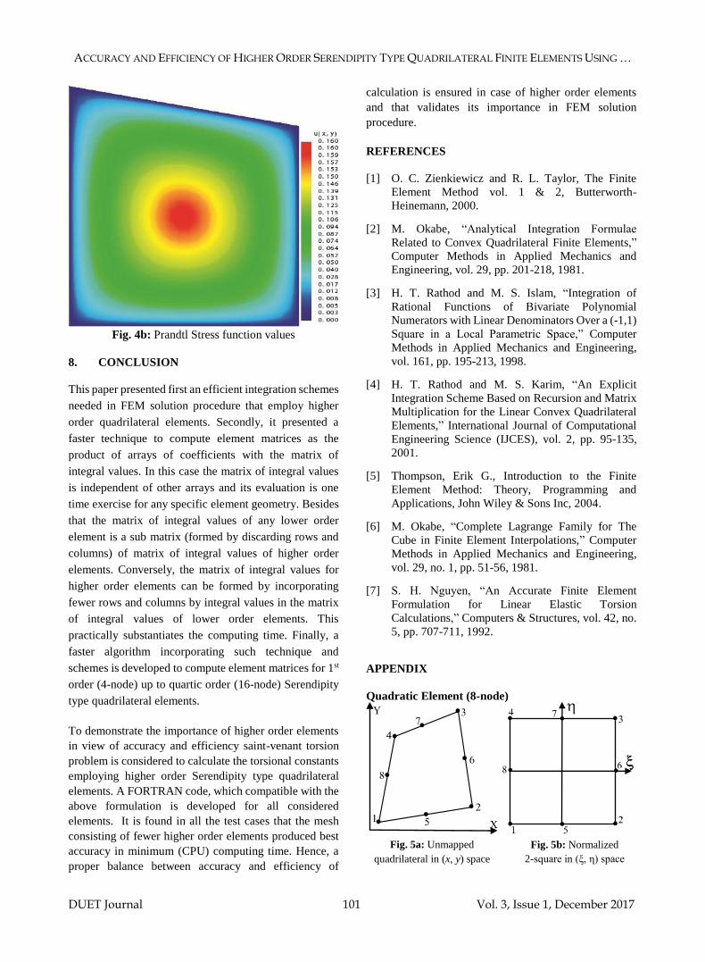
ACCURACY AND EFFICIENCY OF HIGHER ORDER SERENDIPITY TYPE QUADRILATERAL FINITE ELEMENTS USING …
DUET Journal 101 Vol. 3, Issue 1, December 2017
Fig. 4b: Prandtl Stress function values
8. CONCLUSION
This paper presented first an efficient integration schemes
needed in FEM solution procedure that employ higher
order quadrilateral elements. Secondly, it presented a
faster technique to compute element matrices as the
product of arrays of coefficients with the matrix of
integral values. In this case the matrix of integral values
is independent of other arrays and its evaluation is one
time exercise for any specific element geometry. Besides
that the matrix of integral values of any lower order
element is a sub matrix (formed by discarding rows and
columns) of matrix of integral values of higher order
elements. Conversely, the matrix of integral values for
higher order elements can be formed by incorporating
fewer rows and columns by integral values in the matrix
of integral values of lower order elements. This
practically substantiates the computing time. Finally, a
faster algorithm incorporating such technique and
schemes is developed to compute element matrices for 1st
order (4-node) up to quartic order (16-node) Serendipity
type quadrilateral elements.
To demonstrate the importance of higher order elements
in view of accuracy and efficiency saint-venant torsion
problem is considered to calculate the torsional constants
employing higher order Serendipity type quadrilateral
elements. A FORTRAN code, which compatible with the
above formulation is developed for all considered
elements. It is found in all the test cases that the mesh
consisting of fewer higher order elements produced best
accuracy in minimum (CPU) computing time. Hence, a
proper balance between accuracy and efficiency of
calculation is ensured in case of higher order elements
and that validates its importance in FEM solution
procedure.
REFERENCES
[1] O. C. Zienkiewicz and R. L. Taylor, The Finite
Element Method vol. 1 & 2, Butterworth-
Heinemann, 2000.
[2] M. Okabe, “Analytical Integration Formulae
Related to Convex Quadrilateral Finite Elements,”
Computer Methods in Applied Mechanics and
Engineering, vol. 29, pp. 201-218, 1981.
[3] H. T. Rathod and M. S. Islam, “Integration of
Rational Functions of Bivariate Polynomial
Numerators with Linear Denominators Over a (-1,1)
Square in a Local Parametric Space,” Computer
Methods in Applied Mechanics and Engineering,
vol. 161, pp. 195-213, 1998.
[4] H. T. Rathod and M. S. Karim, “An Explicit
Integration Scheme Based on Recursion and Matrix
Multiplication for the Linear Convex Quadrilateral
Elements,” International Journal of Computational
Engineering Science (IJCES), vol. 2, pp. 95-135,
2001.
[5] Thompson, Erik G., Introduction to the Finite
Element Method: Theory, Programming and
Applications, John Wiley & Sons Inc, 2004.
[6] M. Okabe, “Complete Lagrange Family for The
Cube in Finite Element Interpolations,” Computer
Methods in Applied Mechanics and Engineering,
vol. 29, no. 1, pp. 51-56, 1981.
[7] S. H. Nguyen, “An Accurate Finite Element
Formulation for Linear Elastic Torsion
Calculations,” Computers & Structures, vol. 42, no.
5, pp. 707-711, 1992.
APPENDIX
Quadratic Element (8-node)
Fig. 5a: Unmapped
quadrilateral in (x, y) space
Fig. 5b: Normalized
2-square in (ξ, η) space

ACCURACY AND EFFICIENCY OF HIGHER ORDER SERENDIPITY TYPE QUADRILATERAL FINITE ELEMENTS USING …
DUET Journal 102 Vol. 3, Issue 1, December 2017
Cubic Element (12-node)
Quartic Element (16-node)
Fig. 6a: Unmapped
quadrilateral in (x, y) space
Fig. 6b: Normalized
2-square in (ξ, η) space
Fig. 7a: Unmapped
quadrilateral in (x, y) space
Fig. 7b: Normalized
2-square in (ξ, η) space

Teaching LisTening skiLL Through googLe cLassroom: a sTudy aT TerTiary LeveL in BangLadesh
DUET Journal 103 Vol. 3, Issue 1, December 2017
Teaching Listening Skill through Google Classroom: A Study at Tertiary Level in Bangladesh
Mir Md. Fazle Rabbi1*, AKM Zakaria1, Mir Mohammad Tonmoy2
1Department of Humanities and Social Sciences, Dhaka University of Engineering & Technology, Gazipur, Bangladesh 2Department of English, Southeast University, Dhaka, Bangladesh
ABSTRACT
Among the four language skills, ESL learners consider listening skill to be the most difficult one to master. In Bangladesh, both teachers and learners show excuses to avoid this important language skill at elementary, intermediate and tertiary levels. Worldwide teachers are moving towards technological tools in ELT and Google Classroom is one of them. This blended learning platform offers numerous features of Google to enhance teaching-learning process for both teachers and learners. However, nowadays learners at tertiary level are prone to technologies. Considering it as an advantage, this paper demonstrates how a language teacher can facilitate the technophile ESL learners to develop their listening skill in Google Classroom and the impacts it has on students.
*Corresponding email: [email protected]
1. InTRoduCTIon
Using technology in classroom teaching is a new and successful trend in academia. In English Language Teaching (ELT), teachers are leaning towards technology worldwide. Using different technological tools like Computer, Speaker, Microphone, Multimedia projector and Internet has changed the traditional chalk-duster based classroom into a modern ICT based classroom. Recently, different attempts have been taken to promote and support teachers to adopt technology in education. The study of F. Martin, and M.A. Parker states that many online courses are offered; at the same time faculties are adopting synchronous virtual classrooms that enable them to interact with students in real time [1]. The Virtual classroom is a platform of e-learning to cut travel time and costs associated with face to face teacher-centered learning. Google Classroom is a recent addition to virtual classroom, introduced by Google as a feature of G Suite for Education on May 6, 2014 [2]. In this paper, the researchers attempt to exhibit how Google Classroom can be used for teaching listening skill and what the learners opine about their development of listening skill through Google Classroom.
Among the four language skills (reading, writing, listening and speaking) listening skill is the most neglected one to highlight in the context of Bangladesh. In order to stick to the requirement of the curriculum, English teachers of Bangladesh emphasize more on reading and writing skill development irrespective of all levels; primary, secondary and tertiary. Still, at tertiary level learners encounter some speaking activities by means of presentations but listening
skill remains ignored. Teachers tend to show excuses on unavailability of resources thus students development of listening skill in English remains stagnant. Although there is a debate on whether listening skill can be taught or acquired, the researchers have not involved themselves into that. This paper aims to demonstrate how Google Classroom can be used as a learning tool to develop listening skill at tertiary level and what impact does it have on the learners.
The paper is divided into two sections: 1. How Google Classroom works and 2. Impacts of using Google Classroom for teaching listening skill. The first section will introduce Google Classroom and its features. Then it will discuss the facilities and limitations of Google Classroom. However, the second section will discuss the impacts of using Google Classroom. To analyze the impacts, the researchers conduct a study on 40 students. Later their opinions have been recorded through a questionnaire. Finally, the researchers suggest some notions for using Google Classroom for teaching Listening Skill.
2. GooGLE CLASSRooM
2.1 What is Google Classroom
Google Classroom is a recent development of Google for academic institutions to ensure a blended learning platform to simplify creating, distributing and grading assignments in a paperless way [2]. It combines online digital media with traditional classroom methods [3]. Therefore, it is a convenient way for the teachers to engage students online for asking questions, discussing any topic

Teaching LisTening skiLL Through googLe cLassroom: a sTudy aT TerTiary LeveL in BangLadesh
DUET Journal 104 Vol. 3, Issue 1, December 2017
with teacher and classmates and submitting assignments. As S. Iftakhar points out, “Google classroom allows teachers to spend more time with their students and less time on the paperwork, and it is now even better. Google’s latest announcement brings new functionality to Google Classroom. Included in the new functionality is the ability to add more than one teacher, as well as to preparing for classes in advance as well” [4].
2.2 How it Works
Google Classroom is not a well-known platform for many of us. Therefore, a guideline to set up Google Classroom is provided here for clear understanding:
A. Visit classroom.google.com. Earlier Google Classroom was associated with institution based email addresses. Therefore, only teachers and students having institute based domain could use Google Classroom. In March 2017, Google opened Classroom to allow any personal Google users to join classes without the requirement of having a G Suite for Education account, and in April, it became possible for any personal Google user to create and teach a class.
Fig. 1(a): Process of creating a class
B. Click on the “+” button to create your first class. You can find this “+” button next to your email address. Then press on the “Create Class” button.
C. Add a class name and a section, for example, Listening Skill; Section: A
d. You can add details of your class in the “About” tab. You can add a class description and instructions for the students. You can also mention in which room students meet for the traditional classes. Teacher’s email address and Google Drive folder for classroom materials can also be added. You can attach your course outline and lesson plan at the bottom.
Fig. 1(b): Process of creating a class
A. Now students can join the classroom. If they have an institutional Google account it is easier to join. Ask them to log in to Google Classroom through their personal accounts. They have to click the “+” button and it will ask for a class code. Find your class code in the “Stream” tab and inform your students the code they will use to join your classroom.
Fig. 2(a): Process of joining a class
If students do not have the institutional Google account, ask them to create a personal Google account. Collect their Google accounts and invite them to join Google Classroom in “Students” tab. In this case students will not require any class code to join your classroom.
Fig. 2(b): Process of joining a class
2.3: Features of Google Classroom
When the classroom is ready to operate, you will find a “+” button at the right bottom of the screen. You can do the following activities in Google Classroom by clicking on it:
Create announcement: This section is used for announcing any kind of update about the class. You can upload files, Google Drive, videos and web links as class materials as well.

Teaching LisTening skiLL Through googLe cLassroom: a sTudy aT TerTiary LeveL in BangLadesh
DUET Journal 105 Vol. 3, Issue 1, December 2017
Create assignment: This is the most important feature of Google Classroom. Here you can post an assignment which students are to submit within due time. Similar to the announcement section you can upload files, Google Drive, videos and web links. Students can see their assignment in the class “Stream”. They can download the materials and complete their assignments. On the top right, they will see three boxes (Turn In, Comments, and Share). They have select “Turn In”. Then a window will appear to ask them to confirm. They have to click on the blue box labelled “Turn In” to confirm their submission. As a teacher, you will receive an email notification of the submission of the assignment. You will be able to check all the assignments and grade them. Finally, you can return the assignments with your feedbacks and grades.
Create question: This section is very effective to create question for and discuss answers with students. Here students can edit their answers and reply to each other if the teacher permits.
Reuse post: In this section teacher can reuse any important post (announcement, assignment or question) that s/he used earlier in this classroom or another classroom.
2.4 Advantages
Google Classroom has numerous facilities. A few of them are mentioned below:
user friendly: It is very easy to use. As M. Janzen points out, “Google Classroom’s design purposefully simplifies the instructional interface and options used for delivering and tracking assignments; communication with the entire course or individuals is also simplified through announcements, email, and push notifications” [5].
Cloud based: Google Classroom offers more professional and authentic technology to use in learning environment as Google apps represent a significant portion of cloud-based enterprise communications tools used throughout the professional workforce.
Cost free: It does not require any cost to use it. Anyone with or without an institutional Google account can create and join a classroom.
Cell phone friendly: As M. Janzen states, “Mobile access to learning materials that are attractive and easy to interact with is critical in today’s web connected learning environments” [5]. Google Classroom is designed to be quick to respond. It is convenient to be used on any mobile device.
Time saving: Google Classroom saves time both in teachers’ and students’ parts. According to Iftakhar, “It integrates other Google apps like Docs, Slides, Drive and Spreadsheets. Nevertheless, the whole process of administering assignments, grading, formative assessment, and feedback is simplified and streamlined” [4].
2.5 Limitations
Despite various advantages, there are some limitations of Google Classroom. Followings are some of them as mentioned by C. Pappas [6]:
Limited integration options: Google Classroom is not synchronized with Google Calendar or any other calendar. It becomes difficult for the teacher to organize teaching materials and set deadlines for assignments.
Too “googlish”: Pappas defines Google Classroom as too much “googlish”. It is equipped with several buttons which are familiar to Google users only. Therefore, those who are the first time users (students at primary and secondary levels for example) of Google products may get confused or take more time to get accustomed to the icons. Only YouTube is integrated with Google Classroom to help video sharing. Other popular tools like facebook, Slideshare etc. are not built-in with Google Classroom.
no automated updates: Google Classroom does not take the update on activity-feeds automatically. Learners have to refresh on regular basis otherwise, they may miss an important announcement.
Difficult learner sharing: Sharing a document with other classmates is impossible if a student does not become the owner of a document. However, if they become the owner of a document they will need an approval from teacher to share their document.
Editing problems: After creating and distributing assignment, learners become owners of the document. As an owner, they are given the authority to edit it. Eventually, they can delete any part of the assignment if they want, though it occurs accidentally by some notorious students.
no automated quizzes and tests: Google Classroom has no provision for automated quizzes and tests. Therefore it is unable to replace other available Learning Management System (LMS) completely. In most cases, Google Classroom is more appropriate as a blended learning platform than a fully online LMS.
Impersonal: In spite of offering a blended learning platform, it has not integrated other chatting apps like Google Hangouts. Thus, it becomes difficult for online interaction between teachers and learners through Google documents only. Unfortunately, there is no way to have a live chat in Google Classroom; at least, not yet.
3. GooGLE CLASSRooM FoR TEACHInG LISTEnInG SKILL
To observe the impact of Google Classroom for teaching the listening skill, the researchers have formulated the following research design for the study and suggested a few proposals.

Teaching LisTening skiLL Through googLe cLassroom: a sTudy aT TerTiary LeveL in BangLadesh
DUET Journal 106 Vol. 3, Issue 1, December 2017
3.1 Research Methodology
The attempted study is an action research conducted among 40 undergraduate students of Daffodil International University, Bangladesh. The samples are regular 1st year students of BA in English Program. For collecting data, the researchers have employed quantitative research method. Statistical analysis such relative frequencies and percentages of learners-performances have been obtained from four different assignments on listening skill. The researchers have taken extensive support from listenaminute.com for designing research tools. The study has been conducted with a prior permission from the University authority. To conduct the study a classroom titled ‘Listening Skill’ has been created by the researchers in Google Classroom and students have been asked to join. As the students use their Gmail accounts of a similar domain (provided by the University), it is very easy for them to join the classroom. The researchers assign four assignments on listening skill to be submitted on four consecutive weeks. The assignments are simple activities on gap filling while listening. Students are asked to complete each activity every week and answer the following four questions:
i. How many gaps could you fill completely in your first attempt?
ii. How many partial answers (one word or two words, but not the complete answer) could you write in your first attempt?
iii. How many times did you play the audio clip to fill all the gaps completely?
iv. How much time did you take to complete this assignment?
After the fourth week the researchers analyze students’ response to the questions in order to measure whether any individual development occurred in the course of four weeks. The activities have been set considering Krashen’s input hypothesis or (i+1). As Krashen puts it, “The input hypothesis makes the following claim: a necessary (but not sufficient) condition to move from stage i to stage i +1 is that the acquirer understand input that contains i + 1, where “understand” means that the acquirer is focused on the meaning and not the form of the message”[7]. Therefore, the activities are of moderate kinds. Only a few students, with sound listening skill, will be able to fill all the gaps completely in the first attempt. It is likely that students will be able to answer partially in their first attempt, that is, they will not be able to write the three or four words long answers. Moreover, they will need to play the audio clip several times to fill all the gaps completely.
The researchers compare the four assignments of each student to observe their developments (if any). If students’
answers to the four questions show an increase in number from Assignment 1 to Assignment 4, the development is positive. If otherwise, no development occurs.
3.2 Research Findings
The first table shows the number of gaps filled by students in their first attempt. No student could fill 8 gaps in the first three Assignments. However, 8% (4 students) could fill more than 8 gaps in Assignment 4. No one could fill 7 gaps in their first Assignment. 6% (3 students) filled 7 gaps in Assignment 2 and the number increased in the consecutive Assignments. Similarly, 6% (3 students) could fill 6 gaps in Assignment 1 and the percentage increased in the next Assignments. However, 16% (8 students) could fill 5 gaps in the first two Assignments, which increased to 26% (13 students) in Assignment 3 but decreased to 20% (10 students) in Assignment 4. However, the mark of development is noteworthy as the percentages of filling 4 gaps and 3 gaps in the first attempt decrease from Assignment 1 to Assignment 4.
Table 1: Gaps filled by students in their first attempt
Gaps filled by students
A. 1 A. 2 A. 3 A. 4
8+ gaps Nil Nil Nil 8% (4 stu)
7 gaps Nil 6% (3 stu)
10% (5 stu)
14% (7 stu)
6 gaps 6% (3 stu)
8% (4 stu)
16% (8 stu)
18% (9 stu)
5 gaps 16% (8 stu)
16% (8 stu)
26% (13 stu)
20% (10 stu)
4 gaps 38% (19 stu)
32% (16 stu)
28% (14 stu)
22% (11 stu)
3 gaps 40% (20 stu)
34% (17 stu)
20% (10 stu)
18% (9 stu)
A significant development can be observed in case of the partial answers tried by students in their first attempt (Table 2). Less number of partial answers (one word or two words, but not the complete answer) indicates more complete answers. 46% (23 students) attempted 6 partial answers in their first assignment and the percentage decreases up to 24% (12 students) in Assignment 3. A positive sign is that no one attempted 6 partial answers in Assignment 4, which means all students could fill 50% gaps completely in their fourth Assignment. 26% (13 students) could attempt 5 partial answers in Assignment 1 and the number increased to 32% (16 students) in Assignment 2 and Assignment 3. However, the number decreased to 26% (13 students) in Assignment 4. An increase of percentage is observed in case of 4 and 3 partial answers. However, No one could attempt 2 partial answers in the first two Assignments.

Teaching LisTening skiLL Through googLe cLassroom: a sTudy aT TerTiary LeveL in BangLadesh
DUET Journal 107 Vol. 3, Issue 1, December 2017
6% (3 students) and 10% (5 students) attempted 2 partial answers in Assignment 3 and Assignment 4 respectively, pointing a gradual development of students’ performance.
The third table shows the number of times students played the audio clip to complete all the answers. The target is to make students skilled enough to play the audio clip once only to write all the answers completely. In case of Assignment 1 and Assignment 2, no one could write all the ten answers completely by playing the audio clip once only. In Assignment 3 only 4% (2 students) played the clip once and the percentage doubled in case of Assignment 4. An increasing number is observed from Assignment 1 to Assignment 4 in case of playing the clip twice. However, a development of percentage is noticeable in the first two Assignments in case of playing the clip thrice, which fluctuated in Assignment 3 and Assignment 4. The percentage variation is also observed in case of playing the clip 4 times, 5 times and 6 times, which depends on various cognitive and contextual factors.
Table 2: Partial answers tried by students in the first attempt
number of partial answers
A. 1 A. 2 A. 3 A. 4
2 Partial answers Nil Nil 6%
(3 stu)10%
(5 stu)3 Partial answers
8%(4 stu)
12%(6 stu)
14%(7 stu)
28%(14 stu)
4 Partial answers
20%(10 stu)
24%(12 stu)
24%(12 stu)
36%(18 stu)
5 Partial answers
26%(13 stu)
32%(16 stu)
32%(16 stu)
26%(13 stu)
6 Partial answers
46%(23 stu)
32%(16 stu)
24%(12 stu) Nil
Table 3: Number of times audio clip was played to write all the answers completely
Audio clip played A. 1 A. 2 A. 3 A. 4
Once only Nil Nil 4% (2 stu)
8% (4 stu)
Twice 10% (5 stu)
14% (7 stu)
18% (9 stu)
22% (11 stu)
Thrice 12% (6 stu)
18% (9 stu)
14% (7 stu)
20% (10 stu)
4 times 28% (14 stu)
32% (16 stu)
28% (14 stu)
28% (14 stu)
5 times 24% (12 stu)
22% (11 stu)
20% (10 stu) Nil
6 times 18% (9 stu)
10% (5 stu)
16% (8 stu)
22% (11 stu)
7 times 8% (4 stu)
4% (2 stu) Nil Nil
Nevertheless, a substantial improvement can be remarked in Table 4, which demonstrates the time taken by students to complete each Assignment. Less time for doing an assignment shows more competence from the students’ parts. 20% (10 students) took more than 10 minutes to complete Assignment 1. Interestingly, no one took this much time to complete the next Assignments. 16% (8 students) finished Assignment 1 in more than 9 minutes and the percentage increased to 22% (11 students) in case of Assignment 2. No one took this much time to complete the next Assignments. 22% (11 students) and 26% (13 students) completed Assignment 1 and Assignment 2 respectively in more than 8 minutes but no one took this much time for the subsequent Assignments. 24% (12 students) finished Assignment 1 in more than 7 minutes and the percentage increased in case of the next two Assignments. However, no one took more than 7 minutes to finish Assignment 4. An increasing number of percentages are observed in case of completing the Assignments in more than 6 minutes and more than 5 minutes. Although no one could complete their first Assignment in more than 4 minutes, a growing number of percentages are observed in case of subsequent Assignments indicating students’ gradual development.
Table 4: Time taken to complete each assignment
Time(in min) A. 1 A. 2 A. 3 A. 4
3+ Nil 2% (1 stu)
10 % (5 stu)
10% (5 stu)
4+ Nil 6% (3 stu)
12% (6 stu)
22% (11 stu)
5+ 4% (2 stu)
10% (5 stu)
26% (13 stu)
38% (19 stu)
6+ 14% (7 stu)
18% (9 stu)
22% (11 stu)
30% (15 stu)
7+ 24% (12 stu)
16% (8 stu)
28% (14 stu) Nil
8+ 22% (11 stu)
26% (13 stu) Nil Nil
9+ 16% (8 stu)
22% (11 stu) Nil Nil
10+ 20% (10 stu) Nil Nil Nil
3.3 Suggestions
The researchers suggest the following for teaching ‘Listening Skill’ through Google Classroom:
Clear instructions on how to complete the assignments should be provided in the traditional classroom.
One sample assignment should be practised in presence of the teacher.
Formative assessment should be applied so that students feel motivated to do the assignments.
The deadline for submitting the first assignment can be extended, based on students’ demands, as they might find it difficult for the first time.

Teaching LisTening skiLL Through googLe cLassroom: a sTudy aT TerTiary LeveL in BangLadesh
DUET Journal 108 Vol. 3, Issue 1, December 2017
Students should be motivated to be honest in completing their assignments.
4. ConCLuSIon
It has been observed by ELT practitioners that ‘Listening Skill’ is one of the most neglected one among the four language skills because of not having proper training and expertise in positively exploiting the available resources to inculcate listening skill among L2 learners. For this negligence in both teachers’ and students’ parts, Bangladeshi learners are lagging behind in improving their listening skill in English. However, the young generation of today’s world is techno-friendly which is a built-in resource for the ELT practitioners doing research. Considering it as a privilege, this paper shows how Google Classroom can be used as a learning tool to enhance learners’ listening skill. Hence the positive impacts of using Google Classroom for the leaners of tertiary level prove its worth. Finally the paper opens a gateway for further research on using Google Classroom.
REFEREnCES
[1] F. Martin, and M.A. Parker, (2014). “Use of Synchronous Virtual Classrooms: Why, Who, and How?”, MERLOT, Journal of Online Learning and Teaching, Vol. 10, No. 2, pp. 192-210, June 2014.
[2] “Google Classroom”, En.wikipedia.org, 2017. [Online]. Available: https://en.wikipedia.org/wiki /Google_Classroom. [Accessed: 30- Jul- 2017].
[3] “Blended learning”, En.wikipedia.org, 2017. [Online]. Available: https://en.wikipedia.org/wiki/Blended _learning. [Accessed: 30- Jul- 2017].
[4] S. Iftakhar, “Google Classroom: What Works and How?,” Journal of Education and Social Sciences, Vol.3, (Feb), pp. 12-13, 2016.
[5] M. Janzen, “Hot team: Google Classroom”, Teaching and Learning with Technology, 2017. [Online]. Available: http://tlt.psu.edu/2014/12/04/hot-team-google-classroom/. [Accessed: 30- Jul- 2017].
[6] C. Pappas, “Google Classroom Review: Pros And Cons of Using Google Classroom In eLearning – eLearning Industry”, eLearning Industry, 2017. [Online]. Available: https://elearningindustry.com/google-classroom-review-pros-and-cons-of-using-google-classroom-in-elearning. [Accessed: 30- Jul- 2017].
[7] S. Krashen, Principles and Practice in Second Language Acquisition. University of South California: Pergamon Press Inc, 1982.

Challenges in learning english language FaCed by TerTiary level engineering sTudenTs: a sTudy ...
DUET Journal 109 Vol. 3, Issue 1, December 2017
Challenges in Learning English Language Faced by Tertiary Level Engineering Students: A Study in the Context of DUET, Bangladesh
Sanzida Rahman*, Fatema Sultana, AKM Zakaria
Department of Humanities and Social Sciences, DUET, Gazipur, Bangladesh
ABSTRACT
This paper aims at exploring and presenting the English language learning difficulties and challenges, specifically on LSRW skills, encountered by the diploma background BSc engineering students of Dhaka University of Engineering and Technology (DUET), Gazipur, Bangladesh. The study has employed the quantitative research method for data collection. To achieve this aim, a sum of 200 undergraduate engineering students have been randomly chosen for the administration of the survey. The findings of the survey seem to reveal that the students are highly motivated to overcome their problems; henceforth the English Language Teaching (ELT) course design should accommodate both structural and functional aspects of English language. It is also expected that on the basis of these findings, the recommendations made at the end of the paper will immensely help the ELT practitioners in syllabus design, teaching materials, classroom tasks and activities, revising teaching methods, and ultimately promote the students’ academic and professional communication skills.
*Corresponding email: [email protected]
1. InTRoDUCTIon
It has certainly been pronounced that more people use English today than have used any other language in the history of the world [1]. English is the international language par excellence. The use and significance of English language in the present context of Bangladesh cannot be denied because of its enormous implication both in EAP (English for Academic Purpose) and ESP (English for Specific Purpose).Currently, English is accepted as an entity of global communication and proficiency. The English language finds itself at the centre of the paradoxes which arise from globalization. It provides the lingua franca essential to the deepening integration of global service-based economies. It facilitates transnational encounters and allows nations, institutions, and individuals in any part of the world, to communicate their worldview and identities. Though it is the national language of some of the most free market economies driving economic globalization, it is often seen as representing particular cultural, economic, and even religious values [2]. Learning English is viewed as an opportunity to trail better future with prestige especially in increasing literacy rate. In both popular and policy constructs of education, literacy bears a particular “power status”: it is considered necessary for boosting economic, social and political opportunities [3]. Bangladesh is basically a monolingual country. However, its education policy and curriculum mandate English as a compulsory second language because of its global nature [4].
Furthermore, English language learning in the context of ESP, engineering sectors, has turned out to be a
great demand to accomplish the needs of the students to contribute to the new production, new processing, new creation and analysis of the innate requirements of the human beings irrespective of culture, creed, and nation. Engineers require English language skills to understand and go through the knowledge of engineering text to analyze other cultures’ needs, and design products and services to fit those needs [5]. So, engineers do not only need technical knowledge but also need to comprehend and express it orally or by writing reports. Engineering graduates are required to communicate and function effectively both in domestic and international environments (Accreditation Board for Engineering and Technology, 1998-2010). [6] Lack of communication skills only serves to undermine the whole profile and image of the professional engineer. Keeping in mind, 49 government and 387 private polytechnic institutes have been introduced to promote vocational education in Bangladesh [7]. It is found that the students coming from diploma background lack proper guidelines in learning English as they have very limited scope to learn English in their secondary and diploma level and “they maximum come from middle and lower-middleclass family” [7]. Therefore, enrolling themselves into DUET, the students remain in a constant flux in the usage of English Language classes. To the best of our knowledge and experience, students here face troubles in listening speaking, reading, and writing English. Concentrating on the magnitude of English language skills for engineering communication, graduate engineers are expected to achieve English language skills (listening speaking, reading, and writing) to make them eligible for their prospective field.

Challenges in learning english language FaCed by TerTiary level engineering sTudenTs: a sTudy ...
DUET Journal 110 Vol. 3, Issue 1, December 2017
Language is a tool for communication and learning a language includes four basic skills: listening, speaking, reading and writing [8]. It is difficult for the Bangladeshi students, especially diploma students, to learn and master L2 without any challenge. Students learning English encounter a lot of difficulties in respect of materials, setting, motivation, contents not being up to their needs. This paper attempts to investigate the challenges they face and identify the problems in four skills and simultaneously provide remedial measures to successfully acquire the English language Skills.
The paper incorporates a quantitative study using a questionnaire for data collection along with an introduction, literature review, methodology, findings and data analysis, last of all recommendations and conclusions as a general structure of the paper.
2. LITERATURE REvIEw
Many studies have already been carried out on the challenges Engineering graduates encountered while learning English communication skills from different cultural and social contexts. Khanon, [9] studied the difficulties Indian students faced in learning English as a second language. His study revealed that the major barriers behind achieving mastery over English as a second language has been identified as the rural academic and socio-economic background of the students, bilingual method of teaching, negative influence of examination system, education system encouraging learning strategy like memorization; nonetheless pragmatic practice and drills were not imparted in the classroom. He suggested that students must be encouraged, guided and counselled properly by the teachers to improve the condition. Similarly, K. Rajprasit, P. Pratoomrat, & T. Wang [10] carried out a study to measure the perception ability and problems of communication at workplaces having the deficiency in English language proficiency of Thai Undergraduate final year engineering students. Their research findings indicate that Thai engineering students are weak in productive skills like speaking and writing, though of all the four skills, speaking is regarded as the most significant skills. Finally, they suggested realistic communicative situations must be integrated into ESP courses providing needs-based feedback. They further added that ESP courses must be imparted to those students who have a certain level of English language proficiency (generally the intermediate level). But Khader and Shaat’s [11] study reflected different findings which were conducted to examine the reasons of students’ achievement gap in the English language skills by non-English major students in Gaza strip. The findings of the survey result demonstrate that students’ personal factors like gender, age and students’ grade are not regarded as influential in determining the achievement in English language but the external factors like English language
syllabus, the university discipline, the evaluation process, the instructors of English and the linguistics factors of English are considered as important reasons behind the failure in the achievement of English language skills. So, the researchers suggested that the teachers need to be careful to the school level of the students, i.e. students’ yearly assessment process must be reviewed, then students’ university admission system must be reviewed introducing a skill- based test and instructors must be updated by recent TEFL methods and conferences.
In the similar vein, Musa, Lie, and Azman’s [12] review study have focused on the learning difficulties and the pedagogical practice of teaching and learning English language in the classrooms of Malaysia. Their study has intended to demonstrate the reasons of poor achievement in English literacy among Malaysian learners. Based on the study of recent studies, the researchers have suggested that language teaching and learning should be practiced as a meaningful communication integrating it with social context instead of encouraging rote learning of individual isolated learners in the classrooms. In the study, it is also reflected that further research is essential to improve the teaching and learning practice of English language.
The literature review reveals that though many works have been accomplished on the challenges in learning English language skills from different perspectives in different countries, no research has yet been conducted for the development of four skills in an integrated manner for the diploma background BSc students of Dhaka University of Engineering and Technology, Gazipur. Thus, the aim of my study will be to have a close inspection of the students of DUET in terms of their problems and propose an upgraded curriculum for academic and real-life communicative purposes.
3. RESEARCH METHoDoLoGY
This section encompasses the basis of the research process and events related to research design denoting setting, instrument and the method of data collection and data analysis procedure to carry out the present study.
3.1 Population and Respondents
The research was conducted with 200 undergraduate diploma background engineering students pursuing BSc degree in the field of Mechanical Engineering, Civil Engineering, Industrial and Production Engineering, and Architecture at Dhaka University of Engineering and Technology, Gazipur. The respondents were randomly selected who are currently in their 2nd year 1st semester and having both theoretical and lab course on English Language Skills. The native language of all the respondents is Bengali and they all completed English as a compulsory subject in their secondary high school and diploma level.

Challenges in learning english language FaCed by TerTiary level engineering sTudenTs: a sTudy ...
DUET Journal 111 Vol. 3, Issue 1, December 2017
3.2 Instrument and Data Collection
A questionnaire consisting of 21 items has been applied to extract data from 200 undergraduate engineering students of DUET, Gazipur. The items of the questionnaire have been segregated into four sections; namely- Listening skills (Item Nos. 1, 2, 3, and 4), Speaking skills (Item Nos.5, 6, 7, 8, 9, 10, 11, and 12), Reading skills (Item Nos. 13, 14, 15, 16), and lastly writing skills (Item Nos.17, 18, 19, 20, and 21). The questionnaire has been set to unravel the difficulties and challenges that the diploma background BSc engineering students face while learning English in the classroom. The five-point Likert scale [13] from ‘strongly agree (5) to strongly disagree (1) has been employed to develop the questionnaire for the present study.
3.3 Data Analysis
The study employed SPSS program module and M.S excel to analyze data collected through a questionnaire. The findings derived from the detailed analysis of the data are presented in four tables and four bar charts assessing the opinions of the respondents that were employed on a five-point Likert Scale. Subsequently, descriptive statistics and contextual methods were used to analyze the data. The statements were hinted as 5 indicating “Strongly Agree’, 4 ‘Agree’, 3 ‘No Idea’, 2 ‘Disagree ‘and 1 ‘Strongly Disagree’. Finally, the results are presented in four tables and four bar charts showing an average in percentage.
4. FInDInGS AnD DISCUSSIonS
The present study untangles the difficulties or challenge in learning the four skills, by the diploma undergraduate BSc students currently studying in the 2nd year 1st semester at DUET, Gazipur: (a) Listening skills, (b) speaking skills, (3) reading skills, and (d) writing skills. The survey data, collected through a questionnaire, was analyzed using the statistical package, and then percentage wise average result was presented in tables and bar charts incorporating narrative description. Finally, descriptive statistics and contextual methods were applied to interpret the findings of the data. The first section of the questionnaire deals with listening problems of the students from different possible viewpoints which are exposed as obstacles to the understanding of English language efficiently; the second section includes speaking difficulties, students are struggling with, from various perspectives; the third section focuses on reading challenges students encounter obtaining knowledge incessantly; and the fourth section involves the writing difficulty students confront when they are expected to present any reports, or make any technical correspondence, or narrate any general idea. The findings of the study are presented below employing section wise average result in tables and bar chart in accordance with a narrative explanation.
To learn a language effectively, the first and foremost thing required for human beings is the comprehension ability to produce the sound accurately. Hence, listening
capacity is regarded as the prerequisite to learn a language successfully. The following table and bar chart highlight that on average 44% students agree that they have impenetrability in listening skill and only 21.25% students disagree regarding the predicament encountered in listening. It is also observed that 94, 102, and 110 students agree respectively that they have problems in understanding pronunciation and accent of native speakers, complexity in understanding long speech and getting few opportunities to practice.
So, the study reveals that students are conscious of their problems but they do not find it interesting since listening requires rigorous practice for a long period of time. The context of the study suggests that a friendly and interesting learning and practice environment must be provided for the students using different enjoyable games, short film related to teaching goals like pronunciation, intonation, and accent and vocabulary perception along with focusing the meaning.
Speaking is the most significant feature in learning a language. Indeed, oral communication and presentation skills are considered as one of the best career enhancers and the single biggest factor in determining a student’s career success or failure [14]. The data visualized in table and bar chart reflect that 45.88% students agree averagely that they face difficulties in learning speaking skill; while only 7% students only strongly disagree concerning the speaking problem.
Table 1: Listening Skills
Listening Skill Strongly Agree Agree no
idea Disagree Strongly Disagree
Trouble in Pronunciation of Native Speakers
52 94 26 20 8
Complexity in Understanding Long Speech
42 102 8 40 8
Few Opportunities for Practice 34 110 12 32 12
Not Interesting 18 46 14 78 44Average in Percentage 18.25 44 7.5 21.2 9
120100806040200
Strongly AgreeNo OpinionStrongly Disagree
AgreeDisagree
Trouble
in Pron
uncia
tion &
...
Comple
xity i
n ...
Few O
pport
unitie
s for
Practic
e
Not Int
eresti
ng
Average
in Perc
entage
Fig. 1: Listening Skills

Challenges in learning english language FaCed by TerTiary level engineering sTudenTs: a sTudy ...
DUET Journal 112 Vol. 3, Issue 1, December 2017
Table 2: Speaking Skills
Speaking Skills StronglyAgree Agree no
idea Disagree Strongly Disagree
Shyness and Nervousness 70 60 12 34 24
Non-Proficiency 52 118 4 20 6
Inability in Sentence Making
52 108 4 32 4
Vocabulary Limitation 62 92 24 18 4
Way of Improvement 26 104 22 42 6
Problem in Identifying Parts of Speech
54 66 4 44 32
Lack of Adequate Practice
36 120 10 30 4
Average in Percentage 54 66 4 44 32
120100
80604020
0
Strongly AgreeNo OpinionStrongly Disagree
AgreeDisagree
Shyne
ss an
d Nerv
ousne
ss
Non-Prof
icien
cy
Inabil
ity in
Senten
ce Mak
ing
Vocab
ulary
Limita
tion
Pronou
nce P
roblem
Way of
Impro
vemen
t
Problem
in Id
entify
ing ...
Lack of
Adequ
ate Prac
tice
Averag
e in P
ercen
tage
Fig. 2: Speaking Skills
Moreover, data interpretation in the context of different kinds of problems shows that 118 students agree that they are not proficient in speaking, 120 students agree that they have tribulations in identifying parts of speech. In addition, 108 students think that they are not skilled in sentence making and 104 students agree that their poor pronunciation is a problem for them in speaking English fluently. Therefore, it is realized from the study that because of having lack of confidence about speaking proficiency and pronunciation accuracy, students are reluctant to speak English before others. In this regard, students should be motivated and encouraged to increase their exposure using different types of exercises from real life situations like role-play presentations, debate, group discussions etc.
Table 3: Reading Skills
ReadingSkills
Strongly Agree Agree no
idea Disagree Strongly Disagree
Difficulty in Complex Sentence
72 86 14 26 2
Insufficient Vocabulary Knowledge
26 132 22 14 6
Too much Time for Comprehension
40 120 12 24 4
Difficulty in Academic, General & Technical Test
32 88 22 48 10
Average in Percentage 21.25 53.25 8.75 14 2.75
140120100806040200
Strongly AgreeNo OpinionStrongly Disagree
AgreeDisagree
Difficulty in Complex
Sentence S
tructure
Insufficien
t Vocab
ulary Knowled
ge
Too much Time fo
r Compreh
ension
Difficulty in Acad
emic,
General &
Technica
l ...
Average in
Percentag
e
Fig. 3: Reading Skills
Among four skills, reading is perceived as the receptive skill to get, understand and develop knowledge, and ideas prior to making any other productive communication. Here the table and bar chart designate that on average 53% students, the highest percentage of all the average percentage described in this paper, agree that reading is a setback in learning the English language. In this respect, contextual data analysis reveals that 132 (out of 200 students) students agree that they suffer from vocabulary deficiency; whereas 120 (out of 200 students) students suppose that reading takes too much time since they are not used to practicing reading drills. In order to boost up students’ reading capability and comprehension capacity, students and teachers should give effort on reading exercises based on practical life like sports news, technical report, contextual story reading, games like e-mail processing and employing scanning, skimming, differencing, prediction and summarizing technique in a particular context etc.
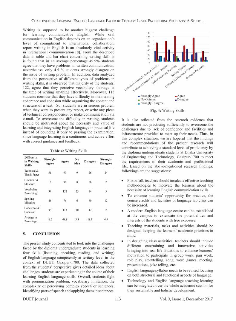
Challenges in learning english language FaCed by TerTiary level engineering sTudenTs: a sTudy ...
DUET Journal 113 Vol. 3, Issue 1, December 2017
Writing is supposed to be another biggest challenge for learning communicative English. While oral communication in English depends on an organization’s level of commitment to international collaboration, report writing in English is an absolutely vital activity in international communication [8]. From the described data in table and bar chart concerning writing skill, it is found that in an average percentage 49.9% students agree that they have problems in written communication; nevertheless, only 4.5 % students strongly disagree on the issue of writing problem. In addition, data analyzed from the perspective of different types of problems in writing skills, it is observed that majority of the students, 122, agree that they perceive vocabulary shortage at the time of writing anything effectively. Moreover, 113 students consider that they have difficulty in maintaining coherence and cohesion while organizing the content and structure of a text. So, students are in serious problem when they want to present any report, or write any piece of technical correspondence, or make communication via e-mail. To overcome the difficulty in writing, students should be motivated about the necessity and value of learning and integrating English language in practical life instead of bouncing it only to passing the examination, since language learning is a continuous and active effort with correct guidance and feedback.
Table 4: Writing SkillsDifficulty in writing Skills
Strongly Agree Agree no
idea Disagree Strongly Disagree
Technical & Thesis Paper 51 90 9 26 24
Grammar & Structure 18 98 8 56 2
Vocabulary Perceiving 34 122 25 14 5
Spelling Mistakes 46 76 6 60 12
Coherence & Cohesion 33 113 10 42 2
Average in Percentage 18.2 49.9 5.8 19.8 4.5
5. ConCLUSIon
The present study concentrated to look into the challenges faced by the diploma undergraduate students in learning four skills (listening, speaking, reading, and writing) of English language competently at tertiary level in the context of DUET, Gazipur-1700. The data collected from the students’ perspective gives detailed ideas about challenges, students are experiencing in the course of their learning English language skills. Overall, students fight with pronunciation problem, vocabulary limitation, the complexity of perceiving complex speech or sentences, identifying parts of speech and applying them in sentences.
140120100
80604020
0
Strongly AgreeNo OpinionStrongly Disagree
AgreeDisagree
Difficulty in Formal,
Technical
& Thesis ...
Problem in Gram
mer & Senten
se Structu
re
Lack of Vocab
ulary Perc
eiving
Spelling Mista
kes
Difficulty in Cohere
nce & Cohesio
n
Average in
Percentag
e
Fig. 4: Writing Skills
It is also reflected from the research evidence that students are not practicing sufficiently to overcome the challenges due to lack of confidence and facilities and infrastructure provided to meet up their needs. Thus, in this complex situation, we are hopeful that the findings and recommendations of the present research will contribute to achieving a standard level of proficiency by the diploma undergraduate students at Dhaka University of Engineering and Technology, Gazipur-1700 to meet the requirements of their academic and professional life. Based on the above-mentioned research findings, followings are the suggestions:
• First of all, teachers should inculcate effective teaching methodologies to motivate the learners about the necessity of learning English communication skills.
• To enhance students’ opportunity for practice, the course credits and facilities of language lab class can be increased.
• A modern English language centre can be established at the campus to extenuate the potentialities and interests of the students with free exposure.
• Teaching materials, tasks and activities should be designed keeping the learners’ academic priorities in mind.
• In designing class activities, teachers should include different entertaining and innovative activities bringing into real-life situations to enhance learners’ motivation to participate in group work, pair work, role play, storytelling, song, word games, meeting, presentations, joke telling, etc.
• English language syllabus needs to be revised focusing on both structural and functional aspects of language.
• Technology and English language teaching-learning can be integrated over the whole academic session for their sustainable and holistic development.

Challenges in learning english language FaCed by TerTiary level engineering sTudenTs: a sTudy ...
DUET Journal 114 Vol. 3, Issue 1, December 2017
REFEREnCES
[1] D. Crystal, English as a global language, Cambridge University Press, Cambridge, 1997.
[2] D. Graddol, English next, British Council, London, pp. 66, 2006.
[3] M. Datta, Bilinguality and literacy: Principles and practice (2nd ed.), Continuum, London, 2007.
[4] MoE. (2010) (Ministry of Education, Bangladesh). National education policy. [Online]. Available: http://www.moedu.gov.bd/.
[5] C. Kaewpet, and S. Sukamolson, “A Sociolinguistic Approach to Oral and Written Communication,” Asian Social Science, Vol. 7, No. 10, pp. 183-187, 2011.
[6] M. J. Reimer, “Investigation into the Development of English and Communication Skills for the Modern Engineer: A Research Scheme,” World Transactions on Engineering and Technology Education, Monash University, Australia, Vol. 1, No. 1, pp. 23-28, 2002.
[7] Juantor Online [online]. Available: http://www.jugantor.com/online/viewers-opinion-/ 2017/03/23/42869
[8] TQI-SEP, BEd, Teaching English: trainers manual, module-1, Teaching Quality in Secondary Education Project: Ministry of Education, Bangladesh, 2006.
[9] R. Kannan, “Difficulties in Learning English as a Second Language,” ESP World, Vol. 5, No. 26, pp. 8-11, 2009.
[10] K. Rajprasit, P. Pratoomrat, and T. Wang, “Perceptions and Problems of English Language and Communication Abilities: A Final Check on Thai Engineering Undergraduates,” English Language Teaching. Canadian Center of Science and Education. Vol. 8, No. 3, pp. 111-120, 2015.
[11] T. K. Khader, and M. Shaat, Reasons Behind Non-English Major University Students’ Achievement Gap in English Language in Gaza Strip from Students’ Perspectives, (2011) Retrieved from www. qou. edu/ english/ . . . / pdfFiles/ khaderKhader. pdf.
[12] N. C. Musa, K.Y. Lie, and H. Azman, “Exploring English Language Learning And Teaching In Malaysia,” GEMA Online™ Journal of Language, Vol.12, No. 1, pp. 35-51, 2012.
[13] R. Likert, “A Technique for the Measurement of Attitudes,” Archives of Psychology, Vo. 22, No. 140, pp. 5-55, 1932.
[14] J. A. Polack-Wahl, “It is time to stand up and communicate,” Proc. 30th ASEE/IEEE Frontiers in Educ. Conf., Kansas City, USA, pp. FIG-16-FIG-21, 2000.
