geographic information systems
TRANSCRIPT

1
OXFORD
Geographic Information Systems
Applications in Natural Resource Management

Second Edition
Geographic Information Systems
Applications in Natural Resource Management
Michael G. Wing
Pete Bettinger
OXFORD UNIVERS ITY PRESS
2
Second Edition
Geographic Information Systems
Applications in Natural Resource Management
Michael G. Wing
Pete Bettinger
OXFORD UNIVERSITY PRESS

OXFORD U:-:lvr RSITV l'Rt'SS
8 Sampson Mews. Suite 204, Don Mills, O lllario M3C OHS www.oupcanada.com
Oxford Uni versiry Press is a department of the Unive rsity of Oxfo rd .
II furt hers (he Unive rsity's objccrivc of excellence in resea rch . scholarship.
and cduc uion by publi shing worldwide in
Oxford New Yo rk
Auckland Cape Town Dar es Salaam Hong Kong Karachi
Kuala LUIll I)Uf Madrid Melbourne Mexico C iry Nairobi New Delhi Shanghai Taipei Toronto
Wi th offices in Argentina Auscria Braz.il C hile Czech Republic France G reece
Guatemala Hungary Italy Japan Poland Portugal Singa pore
South Korea Swirlcrl and T hailand Turkey Ukraine ViclIlam
Oxford is a Hade mark or Oxford Universiry Press
in the UK and in certain other couillfies
rublished in Canada
by Oxfo rd Un iversity Press
Copyri ght @ Oxford Unive rsiTY Press Canada 2008
T he moral rights of the author have been asserted
Database right Oxford Uni versity Press (maker)
Fi rst published 2008
All riglus rese rved. No pari of thi s publication may be reproduced.
sto red in a retrieval system , or transmitt ed , in any form or by any means,
wit hout the prior perm issio n in wri(ing of Oxford University Press.
o r a~ ex pressly perrnill ed by law, o r under terms agreed with the appropriate
reprographics right s organizati on. Etlgui ries concerning reproduction
out side the scope of the above should be scnt to Ihe Right s Department .
Oxford Universiry Press. at the address above.
You must 110 t circulate this book in any OIher bind ing o r cover
and you must impose this sallle condition on any acgu iTer.
Li brary and Archives Canada Cataloguing in Publication
Wing. M ichael G
Geographic information synems: applications in forestry and nafUr.l.1
resources management / M ichael G. W ing & Pele Beninger.- 2nd cd .
Previous cds. by Pete Beninger and Michael G. Wing.
ISBN 978-0- 19-5426 10-6
I . Forests and forestry- Remme sensing. 2. alura.! resources-Remme
sensing. 3. Geographic information systems. I. Ben inger. Pete. 1962- II. Title.
SD387. R4W562008 634.9·028 C2008-902309-9
Cover image: Philip & Karen Smith/Geny Images.
345- 12 11 10
This book is primed on permanent (acid·free) paper e. Printcd in C anada 3
OXFORD SIV I ASITY Pitt's!>
H Sampson Mcw$, Sui rt' 204, Don Mills, Omario M3 OH5 www.oupcanada.com
Oxford University (' ress is a department of the Uni\'cr.)ity of Oxfo rd.
if urthcrs rhe Universiry's objective of excellence in resea rch. scholarship, :md cduc.1.r ion by puhlishing worldwide in
Oxford New York Auckland Cape Town Dar cs Salaam Hong Kong Karach i Kuala Lumpur Madrid Melbourne Mexico Ciry Nairobi
New Delhi Shanghai Taipl·j 1'0(0111'0
\'(Iith oHiees in
AIgcmina Austria Brnil hiJc 7.Cch Republic Fl":1ncc Greece GuatemaJa Hungary IraJy Japan Poland Portugal ingapore South Korea Swirtcrland Thailand Turkey Ukraine Viclnam
Oxford i~ a. lradc m:ak of xford Universiry Press in the UK and in cenain other counrrics
Publi~ht'd in Can:1da by Oxforll Ullivcr!liry Press
opyright @ Oxford Unive rsity Press an:ld:l 2008
The 111 r.tl fight:. of the author have been asscncd
D:uaba.se right Oxford Uni\'crsiry Press (maker)
First published 2008
All righrs rcserw(l. n pari nf tlli s puhlicatioll m3Y be rcproduc~d.
:.wred in a relrleval SY:.fem, or transmiuoo. in any fortn or by any merub.
without the prior permission in writing of Oxford University Press. or 3.) cxprc.ss ly pcrmitlccl hy Jaw. or under terms agre~d with the appropriate
n:prographics rights organization, Enquiries concerning reproduction Ilit sidc the scope of the ahove should IX" :.em to the Ri ghts Depanmel1l .
Oxford Uni\'ersit"y PrC.)$, al lil t address above.
You musl 1101 ircuiale thi.) book in any other binding or cover
and you muSl impose Ihis sallle condirion on :lily :lequirer.
Librnry ~nd Archives Canada Cataloguing in Puhlic:1 lioll
Wing. Mid13d G
Gcogr.tphic information SYSWllS : applications in forestry and n:1IlIral resources management J Michael G. Wing & Pete I3cltinger.-lnd c:d .
Pr('ViollS: t'd<. by Pete Beninger and i\'li chad C. Wing. ISBN 978-0- 19-542610-6
1. Forests and for~try-Remote )cllSing. sensing. J . Geographic information systellls.
2. ;uur.aJ r('~urccs-Rcmou:
I. Beltinger. rete. 1962- II. Title:..
SD387. R4W562008 634.9 '028 C2008-902309-9
Cover image: Philip & KJreu milhfGercy Images.
345 - 121110
This book is primed on permant'nt (ac.id, rree) p:tpt:r c::. .
Primed in Canada
Contents
List of Tables XIV
Preface xv
Part 1 Introduction to Geographic Information Systems. Spatial Databases. and Map Design I
Chapter 1 Geographic Information Systems 2
Objectives 2
What is a Geographic Infonnation System? 3
A Brief History of GIS 4
Why Use GIS in Natural Resource Management Organizations? 7
GIS Technology 8
Data collection processes and inpuc devices 8
Manual map digirizing 10
Scanning 10
Remme sensing II Phologrammerry 13
Field data collection 1 G Dara s[Qrage rechnology 19
D.ta ma nipulation and display 19
O utput Devices 20
Prinrers and ploners 20
Screen displays 21
Graphic images 22
Tabular outpur 22
G IS software programs 22
Summary 24
Applications 24
References 25 4
vi Contents
Chapter 2 GIS Databases: Map Projections, Structures, and Scale 27
Objectives 27
The Shope and Size of the Earth 27
Ellipsoids, Geoids, and Datums 28
The Geographical Coordinate System 30
Map Projections 32
Common Types of Map Projections 33
Planar Coordinate Systems 34
GIS Database Structures 38
Raster data srruc[Ure 38
Sa«llite imagery 38
Digital elev'Hion models 39 Digital orthophotographs 39
Digital raster graphics 40
ar ional Map Accuracy Standards 43
Vector data structure 44
Topology 45
Comparing raster and vector data structures 47
Alternative data S(fuc£ures 4 8
Triangular Irregular Nerwork 48 D ynam ic segmentat ion ofli near nerworks 49
Regions 50
Metadata 50
Obtaining Spatial Data 50
Scale and Resolution of Spatial Databases 51
Summary 51
Applications 52
References 53
Chapter 3 Acquiring, Creating, and Editing GIS Databases 54
Objectives 54
Acquiring GIS Databases 55
Creating GIS Databases 57
Editing GIS Databases 59
Editing anribuccs 60
Editing spatial position 6 1
5
Chapter 4
Checking for missing da,a 62
Checking for inconsistent data 62
Sources of Error in GIS Databases 63
Types of Error in GIS Databases 64
Summary 67
Applications 67
References 70
Map Design 71
Objectives 71
Map Components
Symbology 72
Direction 73
Scale 74
Legend 74
Locational inset
Neadine 76
Annotation 76
Typography 76
72
75
Color and contrast 77
AnciHary information 78
Caveats and disclaimers 79
Map Types 80
Reference maps 80
Thematic maps 81
O,her types of maps 84
The DeSign Loop 85
Common Map Problems 85
Summary 86
Applications 87
References 88
Contents vii
Part 2 Applying GIS to Natural Resource Management 89
Chapter 5 Selecting Landscape Features 90
Objectives 90 6
viii Contents
Selecting Landscape Features from a GIS Database 91
Selecting one feature manually 91
Selecting many features manually 91
Selecting all of the features in a GIS database 92
Select ing none of the features in a GIS database 92
Selecting features based on some database cr iteria 92
Single critcrion queries 94
Multiple criteria queries 94
Selecting features from a previously selected set of features 95
Inverting a selection 97
Example 1: Find the landscape features in one GIS database by using single and mulriple criteria queries and by selecting features from a
previously selected set of features 98
Selecting features within some proximity of other features 99
Example I: Find rhe landscape featu res in one G IS database (har are
inside landscape features (polygons) contai ned in anmher G IS database 99
Example 2: Find rhe landscape fea[tlres in one GIS database that are
close to the landscape features contained within another GIS database 100
Exam ple 3: Find landscape featu res from one G IS darabase that are adjacent ro other landscape featu res in the sa me G IS database 101
Advanced query applications 102
Syntax errors 102
Summary 102
Applications 103
References 105
Chapter 6 Obtaining Infonnation about a Specific Geographic Region 106
Objectives 106
The Process of Clipping Landscape Features 107
Obtaining information about vegetation resources within riparian zones 109
Obtaining information about soil resources within an ownership 110
Obtaining information about roads within a forest III
Obtaining information about streams within a forest I 13
The Process of Erasing Landscape Features I 14
Obtaining information about vegetation resources outside of riparian zones 115
Summary 116
Applications I 16
References 118
7
Chapter 7 Buffering Landscape Features 119
Objectives 119
How a Buffer Process Works 120
Buffering Streams and Creating Riparian Areas 122
Fixed-width buffers 123
Variable-width buffers 123
Buffering Owl Nest Locations 124
Buffering the Inside of Landscape Features 125
Buffering Concentric Rings around Landscape Features 125
Buffering Shorelines 126
Other Reasons for Using Buffering Processes 127
Summary 128
Applications 128
References 130
Chapter 8 Combining and Splitting Landscape Features, and Merging GIS Databases 132
Objectives 132
Combining Landscape Features 132
Contiguous, similar landscape features 135
Contents ix
Multiple spatial rep resentations within a single landscape feature or record 136
Overlapping polygons 137
Splitting Landscape Features 138
Merging GIS Databases 140
Determining how much land area is unrestricted 140
Summary 142
Applications 142
References 143
Chapter 9 Associating Spatial and Non-spatial Databases 144
Objectives 144
Joining Non-spatial Databases with GIS Databases 145
One-to-one join processes 145
One-to-many joins 147
8
x Contents
Many-to-one (or many-to-many) joins 147
Example 1: Determining [he number of hardwood sawm ills in a stare 148
Example 2: Determining sawmill em ploymenr in a counry 149
Joining Two Spatial GIS Databases ISO
Making Joined Data a Permanent Part of the Target (Destination) Table 153
Linking or Relating Tables 153
Summary 154
Applications ISS
References 156
Chapter 10 Updating GIS Databases 157
Objectives 157
The Need for Keeping GIS Databases Updated 158
Example 1: Updating a forest stand GIS database managed by a forest management company 159
Example 2: Updating a streams GIS database managed by a state agency 160
Updating an Existing GIS Database by Adding New Landscape Features 161
Updating a stands GIS database 161
Updating a trails GIS database 162
Updating an Existing GIS Database by Modifying Existing Landscape Features and Attributes 166
Ed_iring the spatial position of landscape features using digitaJ ortbophotographs 166
Updating the tabular 3rrribures using a join process 167
Summary 167
Applications 168
References 169
Chapter 11 Overlay Processes 170
Objectives 170
Intersect Processes 171
Identity Processes 174
Union Processes 175
Incorporating Point and Line GIS Databases into an Overlay Analysis 178
Applying Overlay Techniques to Point and Line Databases 179
Additional Overlay Considerations 180 9
Summary 181
Applications 182
References 183
Contents xi
Chapter 12 Synthesis of Techniques Applied to Advanced Topics 184
Objectives 184
Land Classification 185
Recreation Opportunity Spectrum 188
Habitat Suitability Model with a Road Edge Effect 191
Summary 193
Applications 194
References 19S
Chapter 13 Raster GIS Database Analysis 197
Objectives 197
Digital Elevation Models (DEMs) 197
Elevation Contours 198
Shaded Relief Maps 200
Slope Class Maps 20 I
Interaction with Vector GIS Databases 202
Viewshed Analysis 20S
Watershed Delineation 208
Summary 210
Applications 211
References 212
Chapter 14 Raster GIS Database Analysis II 213
Objectives 213
Raster Data Analysis 213
Raster Analysis Software Parameters 213
Distance Functions 214
Statistical Summary Search Functions 21S
Density Functions 216
10
Summary 181
Applications 182
References 183
Contents xl
Chapter 12 Synthesis of Techniques Applied to Advanced Topics 184
Objectives 184
Land Classification 185
Recreation Opportunity Spectrum 188
Habitat Suitability Model with a Road Edge Effect 191
Summary 193
Applications 194
References 195
Chapter 13 Raster GIS Database Analysis 197
Objectives 197
Digital ElevaHon Models (DEMs) 197
Elevation Contours 198
Shaded Relief Maps 200
Slope Class Maps 20 I
Interarnon with Vector GIS Databases 202
Viewshed Analysis 205
Watershed Delineation 208
Summary 210
Applications 211
References 212
Chapter 14 Raster GIS Database Analysis II 213
Objectives 213
Raster Data Analysis 213
Raster Analysis Software Parameters 213
Distance Funrnons 214
Statistical Summary Search Funrnons 215
Density Functions 216
xii Contents
Raster Reclassification 217
Raster Map Algebra 218
Database Structure Conversions 218
Getting Started with the ArcGIS Spatial Analyst 219
Determining the Most Efficient Route to a Destination 220
Creating a Density Surface for the Number of Trees Per Acre 221
Summary 223
Applications 223
References 224
Part 3 Contemporary Issues in GIS 225
Chapter 15 Trends in GIS Technology 226
Objectives 226
Integrated RasterNector Software 226
Linkage of GIS Databases with Auxiliary Digital Data 227
High Resolution GIS Databases 228
Distribution of GIS Capabilities to Field Offices 229
Web-based Geographic Information Systems 230
Data Retrieval via the Internet 230
Portable Devices to Capture, Display, and Update GIS Data 231
Standards for the Exchange of GIS Databases 231
Legal Issues Related to GIS 232
GIS Interoperability and Open Internet Access 234
GIS Education 234
Summary 235
Applications 235
References 235
Chapter 16 Institutional Challenges and Opportunitie s Related to GIS 237
Objectives 237
Sharing GIS Databases with Other Natural Resource Organizations 237
Sharing GIS Databases within a Natural Resource Organization 239
11
xii Contents
Raster Reclassilication 217
Raster Map Algebra 218
Database Structure Conversions 218
Getting Started with the ArcGIS Spatial Analyst 219
Determining the Most Efficient Route to a Destination 220
Creating a Density Surface for the Number of Trees Per Acre 221
Summary 223
Applications 223
References 224
Part 3 Contemporary Issues in GIS 225
Chapter 15 Trends in GIS Technology 226
Objectives 226
Integrated Raster/Vector Software 226
Linkage of GIS Databases with Auxiliary Digital Data 227
High Resolution GIS Databases 228
Distribution of GIS Capabilities to Field Offices 229
Web-based Geograpruc Information Systems 230
Data Retrieval via the Internet 230
Portable Devices to Capture, Display, and Update GIS Data 231
Standards for the Exchange of GIS Databases 231
Legal Issues Related to GIS 232
GIS Interoperability and Open Internet Access 234
GIS Education 234
Summary 235
Applications 235
References 235
Chapter 16 Institutional Challenges and Opportunities Related to GIS 237
Objectives 237
Sharing GIS Databases with Other Natural Resource Organizations 237
Sharing GIS Databases within a Natural Resource Organization 239
Distribution of GIS Capabilities to Field Offices 240
Technical and Institutional Challenges 241
Benefits of Implementing a GIS Program 243
Successful GIS Implementation 243
Summary 243
Applications 244
References 244
Chapter 17 Certification and Licensing of GIS Users 245
Objectives 245
Current Certification Programs 246
The NCEES Model Law 247
The Need for GIS Certification and Licensing 248
GIS Community Response to Certification and Licensing 249
MAPPS Lawsuit 249
Summary 251
Applications 251
References 251
Appendix A GIS Related Terminology 253
Contents xiii
Appendix B GIS Related Professional Organizations and Journals 260
Appendix C GIS Software Developers 263
Index 264
12
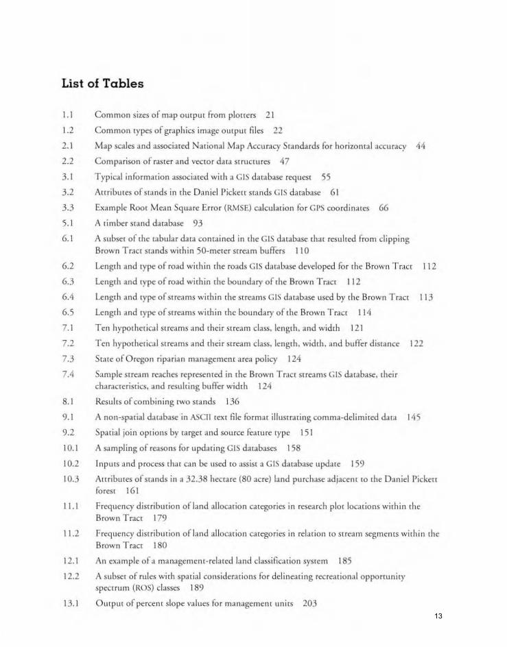
List of Tables
1.1 Common sizes of map Outpur fro m plQners 2 1
1.2 Common rypes of graphics image Output fi les 22
2. 1 Map scales and associated ar ia na! Map Accuracy Standards fo r hori zonta l accu racy 44
2.2 Comparison of raster and vector dara srruc(Ures 47
3.1 Typical informatio n assoc iated with a GIS database request 55
3.2 Auribures of stands in rhe Daniel Pickerr sra nds GIS darabase 6 1
3.3 Exa mple Roor Mea n Square Erro r (RMSE) calcularion fo r Grs coordinares 66
5.1 A rimber srand darabase 93
6. 1 A subser of rhe rabular da,. contained in the GIS database rhar resulred from cl ipping Brown T racr stands within 50-merer stream buffers 110
6.2 Lengrh and rype of road within rhe roads GIS darabase developed fo r rhe Brown Traer I 12
6.3 Lengrh and rype of road with in rhe boundary of ,he Brown T racr I 12
6.4 Length and Type of srrea ms within the SHearns GIS database used by rhe Brown T rac( 11 3
6.5 Length and rype of strea ms within the boundary of rhe Brown T racr 11 4
7 .1 Ten hypmherical streams and their st rea m class. length , and width 12 1
7.2 T en hypor herical streams and their stream class, length, width, and buffer distance 122
7.3 Stale of Oregon riparia n managemem area policy 124
7 .4 Sample stream reaches represenred in the Brown Trdc[ strea ms GIS database, their cha racreristics. and resulring buffer width 124
8. 1 Resul ts of co mbi ning rwo sra nds 136
9.1 A non-spa ri al database in ASCII rexr file fo rmat illustrari ng com ma-del imired data 145
9.2 Spadal join oprions by targer and source fea ture (ype 151
10.1 A sam pling of reasons fo r updat ing GIS databases 158
10.2 I np urs and process thar ca n be used to ass ist a GIS database update 159
10.3 Attribures o r sra nds in a 32.38 hecra re (80 acre) land purchase adjacenr 10 [he Daniel Pickert foresr 16 1
11.1 Frequency distriburion of land allocation categories in resea rch plot locarions within rhe Brown T ract 179
11.2 Frequency disrriburion ofland allocation categories in relarion ro srrea m segmenrs wi thi n the Brown Tract 180
12. 1 An exam ple of a managemenr-related land classi fica rion sysrem 185
12.2 A subset of rules with spatia l co nsiderations fo r delineat ing recreational opportunity specrrum (ROS) classes 189
13. 1 OutpUt of percent slope va lues for managemenr units 203 13
List of Tables
1.1 Common sizes of map OUtP'" from plouers 21
1.2 Common rypes of graph ics image OUtpUt files 22
2.1 Map scales and associa ted ational Map Accu racy Standards fo r horizontal accuracy 44
2.2 Comparison of raster and vector doH3 Stru Ctures 47
3. J TypiC'JJ informarion associated with a GIS d;nabase request 55
3.2 Attributes of sl.lI1ds in rhe Daniel l' ickeoo Stands GIS database 6 1
3.3 Example Roor Mean quare Erro r (R.'v1SE) ealculaoion for GI'S coordinates 66
5.1 A lim ber . t.lnd da tabase 93
6.1 A subS« of the tabular da ta contained in the .IS database that resulted from clipping
Brown T ract stands within 50-meIer stream buffers 110
6.2 Length and rype of road wi thin the roads GIS database developed fo r the Brown Tract 11 2
6.3 Length and rype of road wirhin the boundary of Ihe Brown T raer I 12
6.4 Lengrh and rype of sore.ms within rhe Streams GIS cb rabas. used by Ihe Brown Traer 11 3
6.5 Lenglh and rype of meams withi n the boundary of the Brown T (3Ct I 14
7.1 Ten hyporher i al soreams and rheir meam class. length. and width 12 1
7.2 Ten hypothetical meams and their stream class. lengrh . widd,. and buffer disrancc 122
7.3 State of O regon riparian managemem area policy 124
7.4 Sample stream reaches represented in the Brown Trace strcarns GIS darabase. their characreristics. and n:sulring buffer width 124
8.1 Results or combi ning rwo sta nds 136
9.1 A non-spatial darabase in AS IItcxt file format i1lustr:oti ng com ma-delimited ,bra 145
9.2 Spatial join oprions by mget and sou rce fea rure type 15 1
10.1 A sam pling of reasons for updaring GIS databases 158
10.2 Inpurs and process rim ca n be used to assist a GI database update 159
10.3 Attributes of sm nds in a 32.3 hectare (80 acre) land pur h. < adjacent to the Daniel Pickett foreSt 16 1
I 1.1 Frequency dist ribution or land allocation categories in research plol locacions within rhe Brown T tact 179
11.2 Frequency distribution orla nd allocarion caregorit;S in retll ion to stream segments within tile: Brown T tact 180
12.1 An ex.m pIe of a management-related land c1assiflcarion sYStem 185
12.2 A su bsel of rules wi th sp3rial considerations for deline-J.ling recreational opportunity spectrum (ROS) classes 189
13. 1 O UtPUt of percell[ stope val ut::s for managemem units 203
Preface
T his second edition of Gtogmphic Infonnatioll Sysums: Applications ill Natural Rtsourct
Management is intended for inrroducrory courses in geographic information systems
or computer applications that add ress copies related [0 natural resource management. The emphasis of rhe book is on geographical informacion systems (C IS) app lications in naru ~
fal resource management. GIS lOols are now considered core technologies for natural resource organizations and have become pare of day-co-day activities in many pans of rhe world. In addition , many natural resource programs in higher education require [hat S[U
dents comple[(~ at least one course tha t contai ns significant rrearmenr of GIS. We provide derailed discussions and examples orGIS o perat ions such as querying, buffering, cl ipping, and overlay analysis (and others), as well as background information on the history of GIS,
database creation, editing, acquisition. and map development. The applicarions provided in this book can be extended (0 any region in the world, although the primary emphasis is on North America, as portrayed by numerous examples of natural resource management scenariOS.
The contents of this book were determined largely through our experiences in natural resource management and research, as well as our extensive instructional experience over rhe previous decade. Many applications similar ro (he oncs we present in this book have been performed by natural resource professionals (as well as by the authors) as parr of their
normal job (asks in private o rganizations and public agencies. The goa l of this book is to introduce students, field personnel, biologists, and orher
natural resou rce professionals ro the most common GIS applica tions and principles associated with managing natural resou rces. Therefore, the book focuses mainly on GIS applications r:uher than o n GIS theory. We would be remiss, however, if we did nor provide
some background on the history, technology, and theory that defines GIS. Consequen tly,
the first pan of the book provides a b rief background on many of those areas as well as map development; it is nor all- inclusive. however, as we wish (0 focus rhe text o n GIS
applicarions in natural resource managemenL For a broader rrearmem of GIS concepts. other resources are recommended , including more general GIS books or User Gu ides specific [0 GIS sofrware packages.
Wirh that in mind, who comprises rhe audience of this book? Students. field personnel. biologists. and other natural resource professionals (and their managers) who work in narural resou rce- related fields. but where GIS is perhaps nor their primary job responsibility. People who already serve as GIS analysts, coordinators. or technicians will likely find many of rhe topics presented in this book co be familiar. We rry co focus on topics and applications used common ly by field professionals, [hose rhal are essemial ro their management needs. There are a variety of resources {hat delve deeper into various subject areas of GIS [har will undoubtedly be of va lue to GIS analysts. coordinators. and technicians. In our experiences these resources rare ly consistently focus on narural resource
14
Preface
r-r-his second edition of G~ogrtlphic Infonnatiol1 SysuJns: AppLicatiolls ill NOITlml Rtsourre 1. Mnnagtmt!1lt. is inrended for inrroducrory courses in geographic information systems
or campmer applications Ihat address (opics relared TO narural resource manage-mem. The emphasis of the book is on geogrdphical information systems (G IS) applications in narural resource managemelli. GIS rools are now considered corC' technologies for natural
resource organiZ.1rions and have b«ome parr of daY-fo-day acrivities in many pans of dlC
world. In addirion. many narural resou rce programs in higher education require [hat srudems comple[e at leasl one course rhal comai ns signific.1nt rre'llmem of GIS. We provide derailed discussions and examples of GIS opera rions such as querying, buffering, clipping, and overlay analysis (and 01 hers), as well as background information on the history of GIS. database creation , ediring, acquisition. and map development. T he 3pplicarions provided in rhis book can be exrended to any region in rhe wo rld. although rhe primary emphasis is on Nonh America. 3S portrayed by numerous examples of narural resource management scenarios.
The conreOiS of rhis book were determined largely (hrough our experiences in na[Ural resource management and research. as well as our ex(ensive instructional experience over lhe previous decade. Many appiic.1lions similar to the ones we presenr in this book have been performed by natural resource professionals (as well as by the aurhors) as parr of their
normal job tasks in private organizadons and public ag('ncies. The goal of this book is to introduce Sludent . field personnel. biologists, and other
n31l1ral resource professionals to [he mOSt common GIS applica rions and principles 3SS0-
ciared with managing naturaJ resources. Therefore. the book focuses mainly on GIS applical-ions J'<uher Ihan on GIS theory. We would be remiss, however, if we did not provide some background on the history. technology, and theory that defines GIS. Consequen tly. the first pan of the book provides a brier background on many of those areas as well as map development; it is nOl all- inclusive. however. as we wish (0 focus the [ext on GIS applications in natural resource management. For a broader rreatmem of GIS conceprs. other resources are recommended. including more general ,IS books or User Guides s~cific (0 CI software packages.
With that in mind. who comprises rhe audience of this book? Student.s, field personnel, biologis[s. and other natural resourc(' professionals (and their managers) who work in narural resource-relared fidds. but where GIS is perhaps not (heir primary job responsibil· icy. People who al ready serve as GIS analystS. coordinacors, or technicians wililikdy hnd many of the topics presenred in this book to be F..miliar. We try to focus on topics and applic3t'ions used commonly by fidd professionals, dlOse rhar are essemiallO lhdr man · agemem needs. There are a variecy of resources char delve deeper inro various subjecl areas of GIS rhal will undoubledly be of va lue ro GIS analysrs. coordi mllor . and technicians. In ou r experienc('!\ these resources rarely eonsis[enriy focus 011 naruml resoure('
xvi Preface
applicarions typical [0 field protessionals associated with tederal, stare, p rovincial, or privare narural resource organizations.
To illustrare the applicarions otG IS to narural resource managemelH, we have provided tour sets ot GIS databases. The flrsr ser reterences rhe hypotherical Daniel Picken toresr, one thar may be fa miliar ro {"hose who have taken cou rses in foresr m3nagemenr, as ir is one of the landsca pes used to illustrare managemem alternatives in the book Foust Mfl1Jflgtmt11l (Davis et aI., 2001) . The second set reterences a fictional foresl called the Brown T racr. The Brown Tract represems a more realistic landscape and includes a digi
[al onhophorograph so that users can acrually see rhe resources being managed. The thi rd dara ser represents land uses in Saskarchewan, while rhe founh rep resents milliocarions and counties of the southern US. These databases were derived from acrual GIS data, bur were modified signi fican tly by the authors m make them suitable for li se in th is texr. Each
ot these sets of GIS data can be accessed through a websire hosred by Oregon State University (hrrp:/ /www.foresrry.o regollsrare.edu/gisbook).
Parr 1 provides readers nor on ly with rhe h isrory and development of GIS, bur also with
a common la nguage and perspecrive on GIS. Too otten people us ing GIS have lirrle formal training; instead , they gain knowledge and skills through lrial-and-error applications, shorr courses, o r through other means. We do nor want [0 discourage rhe effons ot seltmOl iva ted CIS users; however, they usually have an abridged perspective on rhe history of GIS, how and why dara srructures are diffe rent, and in other reiared mpies. We hope rhat communication among naruml resource professionals as ir reiares to GIS processes and requests will thus be imp roved with a more thorough perspective, allowing work rasks [0
be accomplished more efficienrly. Pan 2 emphasizes GIS operations and introduces readers ro many ot the most power
ful and commonly lIsed GIS applications in narura l resource ma nagemenr. Each chaprer in Parr 2 inr roduces GIS tech niques, and then provides applications relared to the rechniques. T he concepts introduced in Part 2 are initially related (Q the managemenr and use of vec(Qr GIS darabases. The concepts build upon themselves, and culminare in a synthesis of advanced analyses presemed in chapter 12. Chaprers 13 and 14 provide [rearments of raste r GIS database uses in naru ral resource managemenl.
Parr 3 of rhe book introduces a number of wpies related w the trends in the use ot GIS in narural resource management, {he challenges and opponunities Faced by those o rganiza[ions desiring to use GIS to ass isr in decision-mak ing processes, and the o ngoing and contentious issues relared to cert ification and licensing of GIS users. The appendices ot rhe book provide users wirh a glossary of terms, a summary of organ izations and academic journals associated wirh (he use of GIS, and references (0 lhe developers ot the most com
mon GIS softwa re programs. This book is dedicated (Q those students who have challenged LIS to develop course
wo rk rhat relares directly to rhe GIS tasks (hat they will likely perform as natural resource
managers.
References
Davis. L.S .• Johnson. K.N .• Berringer. P.S .• & Howard. T.E. (2001). Form mOllogelllellf:
To slistain tcological. tconomic, and socifllvfllues (4th ed .). New York: McGraw-H ilI.
15
xvi Preface
applica tions typica l [0 field pro fessionals associated with federal. sta te. provi ncial. or pri
V(ltC' natural resource organizations.
To illustrate the applications of . IS to natural resource management. we have: provided
fOll r sets of GI databases. The first set re ferences the hypotimical Daniel Pickett lo rest. one rhar may be fami liar to those who )ulve taken courses in foresr managemelH. as it is
ont' of the landsca pes lIsed to iliustr.Hc management alrern atives in the book Fort'st Mal/agflllcm (Davis e[ al.. 2001) . The second set references a fictional fores, called the
Brown Trace The Brown Tract representS a more realistic landscape and includes a digi
,al onhopho togrn ph so thar users can acrllally so< the resources being managed . T he third
da(:l Set represems land uscs in askarchewan. while rhe founh represents mill locations
and cou m ies of rhe sourhern U . These databases were derived from aemal GIS data. bur
were modified significantly by dl C' authors to make them suitable fo r use in this tocr. E...1ch of these sets of Gl data can be accessed through a websi(e has red by regan [ate
Univers ity (lmp:llwww.forestry.o tegonstate.edu/gisbook). Parr I provides readers not on ly wirh ,he history and development of GIS. bur also with
a co mmon language and perspecrive on C IS. Too o ften people using GIS have lirrle tor
mal rraining; insre:ld . they gain knowledge and skil ls through Irial-and-erro r applications.
shorr courses, or th rough orher means. \Vlc do nor wam to discourage the efion s of self· ma l iva red GIS IIsers; however. rhey usually have an abridged perspective on the his lOry of
C I . how and why data strucrures are difFerenr. and in other related topics. We hope (hat
com munication among naru ral resource professionals as iI' rda tes ro GIS processes and
rC'1uests will rhus be improved with a mo re rhoro ugh perspecrive. allowi ng work lasks to
be accomplished more efficiently.
Pan 2 emphasizes GIS operarions and inrroduccs r~.ldc rs lO many of the: most power
ful and com monly used GIS applica tions in namral resource ma nagemenr. Each chapu~r
in Pan 2 im roclllces GIS tech niques, and [hen provides applicatio ns related ro rhe tech
niques. The conceprs introduced in Pan 2 are inirially related to the management and use
of vector GIS d:uabases. The concepts build upo n themselves. and culm inate in a symhc~
sis of advanced analyses presented in chaprer 12. C hapters 13 and 14 provide rreat ments
of raster GIS database uses in narural resource m:m agemenr.
Pan 3 of the book introduces a number of ropics relared to rhe rrends in the use of Gl
in na lUra) resou rce management. rhe chaJlenges and oppo rruni lies faced by those organi
'lat io ns desiring to use ,IS to ass isr in dec isio n-making processes, and rhe ongoing and
cOl1len[ious issues related 10 cerriflcarion and licensing of CIS users . The append ices of the
book provide users with :'1 glossary of [erms, a summary of organ iz.u ions and academic
journals associated with Ihe lise of GIS. and references [0 {he devdopers of rhe mOSt com
mon GIS sofrwa re progra ms. Tbis book is dedicated to those studems who have challenged us to d evelop cOll r.se
wo rk thar reiates directly ' 0 [he GIS r .. ks tha t they willlikcly perform .5 narural resource
managers.
References
Davis. L.S .• Johnson. K.N .• Bellinger. r ... & H oward. T.E. (200 1). Form lIIaul/gem",/:
To sustain ~colqgicfll, t rvl/omie, find socia/ llaluts (4(h ed. ). New York: McG raw-HilI.
Part 1
Introduction to Geographic Information Systems, Spatial Databases, and Map Design
W e hope Pa re 1 of GIS AppiicatiollS in Natural Resouras provides readers wirh a com
mo n language and pe rspecrive o n geographic in fo rma t io n sys tems (G IS).
Frequently, people using G IS have li rrle fo rmaJ tra ining, and they ga in rheir knowledge
and skills either through shorr courses or rh rough [hei r own ini{iarive. While these self
mociv3 rcd effo rts 3rc laudable, they lIsually result in an abridged perspecrive on lhe histOry o f GIS. how and why data srrllc{tl res di ffer. and m her related topics. Communicat ion
among naruml resource p rofessionals as it relates [0 GIS processes and requcs[s should be improved with an informed perspecrive of GIS, encouraging work tasks to be accom
plished mo re e ffect ively.
In chapte r I , rhe historical development of GIS and the va rious tools you might use ro
creare C IS da tabases are exa m ined . The focus of chapte r 2 is an essential ropic fo r C IS:
data. C haprer 2 begins by describing the ways in which we ca n quant ify and measure the
Ea rth 's size and shape, and how resulrs from these methods can be incorpo rated inco C IS.
C hapter 2 also includes materia l o n how data can be structured within C IS and outlines
[he options (har a re avai lable fo r t h~e pu rposes. In additio n, some o f rhe more com mon
sources of dara for developing o r augment ing spat ial databases are presented in chapte r 2.
C hapter 3 builds upon the data theme imroduced in chapter 2 by examining how organiza rio ns might acquire or develop darabases, and d iscuss ing issues related ro database ed it
ing and pment ial errors. C hapter 4 delves into ca rtogra phy; o ne of many supporting d is
ci plines from which GIS has evolved bur also one of rhe cemral ways in which C IS resul ts
ca n be comm un icated ro others. In addit ion, chapte r 4 includes a tho rough d iscussio n of
rhe concepts and compo nems that may lead to a successful map. while at the same time identifyi ng some commo n pi tfa lls lO avoid in rhe map crea tion process.
16

Chapter 1
Geographic Information Systems
Geographic Information Systems (G IS) are now core tech
nology fo r many natu ral resource o rganizations and are
also app lied in disciplines throughout society. The initial
applicat ions of GIS that demo nstrated some of rhe power and potential of (his spacial technology, however, were
within namra! resou rce applications (Wing & Beninger,
2003). In one ofrhe firsr papers on the use of GIS in narural resource managemenr, de Sreiguer and Giles (1981)
describe the potenrial uses of GIS in naru ra l resource managemenr. In adapting one of their inrroducrory remarks [0
rhe presenr day, you will find rhe releva nce of GIS ro nar
lIfal resou rce management clearly stared:
A natural resource manager is often ca lled upon to
selecr an area of land to designate as cririca l wildlife habir3r, as a pmenria l area to implemem a timber
harvest, or as an area to recommend a silviculrural
rrear mem, o r to evaluate a landscape under a lterna
rive managemem policies. The manager describes
(0 (he GIS the charac teristics of the ideal a rea in
terms of forest s(fucwrai cond itions, soils, or
(Opography. Within seco nds the manager receives
gra phic and rabu lar informatio n ro loca re the
appropriate manage ment areas, or to compare alre rnative policies. (de Steiguer & G iles, 198 1,
p. 734)
Obviollsly, natura l resource managers ca n perfo rm the
same task of idenrifYi ng appropriate managemenr areas o r
of analyzi ng policies by examining se ts of paper o r mylar maps, bur rhe process beco mes much mo re efficienr 'lOd
accurate when perfo rmed with G IS. Furrher, analyses of
the impact of alternat ive policies are faci litated , allowing
managers {Q consider rhe impacts of d ifferenr policies o r
act ions in a more efficienr manner, usually savi ng time
and money.
For many na[Ural resou rce management o rganiza
tions, G IS has become an irreplaceable rool to assis t in
[he day-to-d ay manage menr of land, wate r, and other
resources. The applica tio ns of GIS vary widely amo ng
o rganiza tions and may range from using GIS primarily as
a mapping tool to lIsing C IS to model pol icy aire rnatives
rhat may impact landscape fearures during rhe nexr 100
years and beyond. Rega rdless of how a narural resource
managemenr o rganizat io n plans to use G IS, understand
ing rhe potential appl ica tions of C IS to na tural resource
managemenr is essenrial for natural resource profession
als. This text is designed to int roduce readers to GIS con
cepts and princi ples and to provide examples of how [0
apply rhis knowledge in a narural resource management
conrex[. The introductory chapler begins by describ ing
the rools and technology thar comprise a GIS, and illus
rrari ng why GIS has beco me so impo rtalll for many
o rganizat ions. A brief hislOry of the evolu tion of G IS and
identification of significanr conrribmors to G IS develop
ment is then provided. Toward the end of this chapter
rhe key compo nent of any successful GIS (sparial dara ) is discussed.
Objectives
This chapter represenrs an introduction to GIS concepts,
roo ls, technology, history, and significant co ntribu rors.
Given that the focus of this book is on rhe appl ications of C IS ro natu ral resource management, what is provided in
(his chap te r is a co ndensed version of these [opics.
17
Nevenheless, ar rhe co nclusion of this chapter, readers
should understand and be able to discllss the perrinent
as peas of the following ropics:
I. [he reasons why GIS use IS prevalenr In natural
resource management.
2 . rhe evolution of the development of GIS technology and key figu res.
3. the common spatial data collecrion tech niques and
input devices rhat are available,
4. the common GIS omput processes thar are rypical in
natural resource managemenr, and
5. rhe broad rypes of G IS sofrwa re rhar are avai lable.
What is a Geographic Information System?
A geographic information system consisrs of the necessary
rools and services ro allow you to collect, organize. manip
ulate, inrerprer, and display geographic information. A GIS is more than JUSt rhe hardware and software familiar (Q
mosr people; it extends to the staff who operate the sysrem, r.he databases, [he physical facilities, and the o rgan i
zational commitmelll necessary ro make it all work. A GIS
can be defined by how it is used (e.g., a land informarion
system, a narural resou rce managemenr information system), by what it contains (sparially distinct features, activ
ities. or events defined as points, lines, polygons. or raster
grid cells), by irs capabilit ies (a powerful set of 1001s for
co llecting. sroring. retrieving. transforming, and displaying
spa rial dara) , or by its role in an organization (a map pro
duction syste m. a spat ial analysis system. a system for
assisting in making decisions regarding basic geograph ic
quesrions such as: Where is it? What is it? Why is it
mere?). The core component of a GIS however is a data
base thar contains a geographic componenr. We wi ll dis
cuss geographic data in more detail shordy.
GIS can also be defined as geographic information science (GIScience). GIScience involves the identification
and srudy of issues that are rdated ro GIS use, affect its
implementation, and that arise from irs applicarion
(Goodchi ld, 1992). In short, GIScience borh encourages
users (0 understand the benefits of GIS technology in pro
viding a powerful set of ana lysis tools and encourages
users ro view rhe technology as pan of a broader discipline rh:H prommcs geographical th inking and problem solving
strategies as being useful to society. The deveiopmem of
GIScience is an outgrowth of the faCt that GIS technology
is avai lable ro more users today than ever before, and that
Chapter 1 Geographic Informafion Systems 3
spatial categorization and analys is is applicable to many
societal issues and problems. Regardless of how a GIS is perceived or used. it is the
imegrar ion of rhe variolls (ools and services rhat leads to
a successful GIS. Although other software programs per
form GIS-like tasks (e.g., darabase management, graphics,
or computer assiSted drafting [CAD) software), a GIS is
unique in its ability (0 allow users ro crC'dtC, maintain.
and analyze geographic o r spat ial data. The term spatial
d ata implies thar a database nor only describes landscape
features (e.g., candidon, composition, structure of
forests), but also includes a geographic reference co where features can be found. A GIS allows you to manipulate
and display spatia l data so that questions regarding a
resource and its conditions can be answered. A GIS. when
used properly, is capable of analyzing a large volume of
spatial data quickly and providing graphical and tabular
results. A GIS stores spatial data in a digital database file;
rhe database file may be referred to using a number of
terms including themes. maps, covers, rabies, layers, or
GIS databases. The terminology for referring to a GIS
database varies depending on the GIS software program
being used and, in some cases, the vers ion of the sofrware
being used. In most GIS software programs, similar land
scape featu res are mainrained in a single GIS database. For
instance. YOli might have a soils GIS database thar con
tains rhe soil characteristics of a landscape, a hydrographic
database [hat shows the locations of rivers and lakes, or a
wildlife GIS database that contains me nest locatio ns of a
single species or a group of species of animals. GIS allows
the integration and simultaneous examination of mulriple
G IS databases through a process described as overlay
analysis. Overlay analyses allow us to determine how fea
tures in one darabase: relate spatially to fearures in another
database, and provide us a powerful means of supporting landscape mapping and investigation. Overlay analysis.
described in further dem il )Her in this book, represenrs
[he essence of whar many co nsider to be {he main role of
GIS in natural resource management: the abiliry to com
b ine tWO or more GIS databases inco a si ngle database (hat
demonstrates {heir spa rial connecriviry.
GIS is related to a number of other Relds and disci
plines, including computer aided drafring (CAD), com
puter carrography. darabase managemem, sraristics, and
remOte sensing. In FaCt, GIS both comains and relies on certain aspects from each of these fields. and thus is closely
related to each of rhem. However, the difference bef\veen GIS and any of these o ther a llied Relds is notable. For
example, most CAD software programs have rudimentary
18
Nevertheless. at the co nclusion of this cha pter. readers
should understand and be able to discuss the perrinent
aspeclS of the following topics:
1. the reasons why GIS usc: is pr~valenl in natural
resource management.
2. the evolution of the development of GIS technology and key figures.
3. the common spatial data collecrion techniques and
inpur devices rhat are available.
4. the common GIS OUlptH processes thar are typical in
narural resource man:lgemellt. and
- rhe broad rypes orGI software tim are avai la ble.
What is a Geographic Information System?
A geog'raphic information sy tern consisrs of the necessary
{ools and services lO allow you to collecr, organize. manip
ulate, interpret. and display geogrJphic information. A GIS
is more {han JUSt tlit': h'lrdware and softwa re hlmiliar to
most people; it extends to lhe staff who operate the system. the dat.bases. the physical fuci lities. and lhe o rgani
zational commirment necessary {O make ir all work. A GI
can be defined by how it is used (e.g .• a land information
sysrcm. a natural resource management information system), by what it comains (spadaJly distincr fearurcs. acriv
iciest or events defined as points. lines. polygons, or raster
grid cells). by its capabiliries (a powerful SCI of tools for
collccling. storing, retrieving. rransforming. and displ:tying
sparial data). or by ils role in an organizarion (~ map pro
duction sysrem. a spadal analysis system. a sysl~m for
assisting in making decisions regard ing basic geographic
questions such as: Where is it? What is il? Why is it (here?). The core component of a GIS however is ... dara
base Ihar conmins a geographic camponelll. We will dis
cuss geographic dara in more detail shordy.
GIS can also be defined as geograph ic information
science (GIScience). GIScience involves the idemiflcation
and srudy of issues that are rdated 10 .1 use, affect ils
implemenr:uion. and lhar arise from iu applic;l(ion
(Goodchild. 1992). In short. GIScience both encourages
lIsers 10 IInderstand the benefits of GIS rechnology in pro
viding a powerful set of ana lysis (ools and encourages
users to view Ihe rechnology as pan of a broader discipline that promotes geogmphiC'JI thinking and problem solvi ng
strJtegies as being useful to sociery. The development of GIScience is an outgrowth of the FaCt rhac GIS technology
is avai lable 10 more users roday than ever before. and [hat
Chapler 1 Geographic Inlormabon Systems 3
sparial categorizarion and analysis is applicable (Q many
societal issues and problems. Regardless of how a GIS is perceived or used. il is (he
inlegralion of Ihe various rools and services ,hat leads (0
a successful GIS. Although other sofrware programs per
form liS-like rasks (e.g., darabase manilgemCnt, graphics.
or compurer ass isred drafting [CAD] sofrwa re). a GIS is
unique in irs abiLiry to allow lIsers to create. maintain,
:lnd analyu geographic or spa rial dara. The term spatial
d ata implies that a database not only describes landscape
fe-dlures (e.g .• condition. composirion. SUUClUre of
forests). bur also includes a geographic reference (0 where
Features can be found. A GIS allows you to manipulare :tnd display sp:nial d:lIa so fllat quesrions regarding a
resource and its conditions am be answered. A GIS. when
used properly. is cap.ble of analyzing a la rge volume of
spa rial data quickly and providing graphical and tabular
results. A GIS stores spa rial data in a digital database file;
the darabase tile may be ref<rred to using a number of {erlllS including (hemes. maps. covers. rabies, layers. or
GIS databases. The: terminology for referring (Q a GIS
darabase varies depending on the GI soFrware program
being used and. in some cases, the: ve rsion of me sofrware
being used. In most .IS software programs. similar landscape fearures are mainraincd in a single ,IS da[abasc. For
insrance. YOli mighr have a soils GIS database that con~
rains rhe soil characterisrics of:1 landscape. it hydrographic
database rhal shows rhe 10C3rions of rivers and lakes. or a
wildlife GIS daraba e Iha( contains the nest ioc31ions of a
single species or a group of species of animals. CIS allows
the integration :lnd simultaneous examination of multiple
GIS databases rhrough a process described as overlay
analysis. Overlay analy~s allow us (0 determine how fea~
(Ures in onc darabase relate spatially (Q fearures in anorher
da rabase, and provide liS <1 powerful means of supporting
landscape mapping and invatigation. Overlay analysis. described in further derail lal er in this book, represems
[he essence of what many consider ro be Ihe main role of
GIS in nalUral resource management: rhe abiliry 10 com
b ine (wo or more Gl databases inlo a si ngle datab~lse I hat
demonsu:ues (heir spatial connccriviry.
GIS is related to a number of other lields dnd disci
pline • including computer aided drafting (CAD). om
pucer cartography. database m<lnagement. srarislics. and
remole sensing. In filet. GIS bolh coma_ins and rdies on cerr .. in aspec(s rrom each of these fields. and thus is closely
related (0 each of them. However. the diflerence between GIS and dny of these orher allied fields is notable. For
example. mosl CAD software programs have rudimentary
4 Part 1 Introduclion to Geographic Information Systems, Spatial Databases, and Map Design
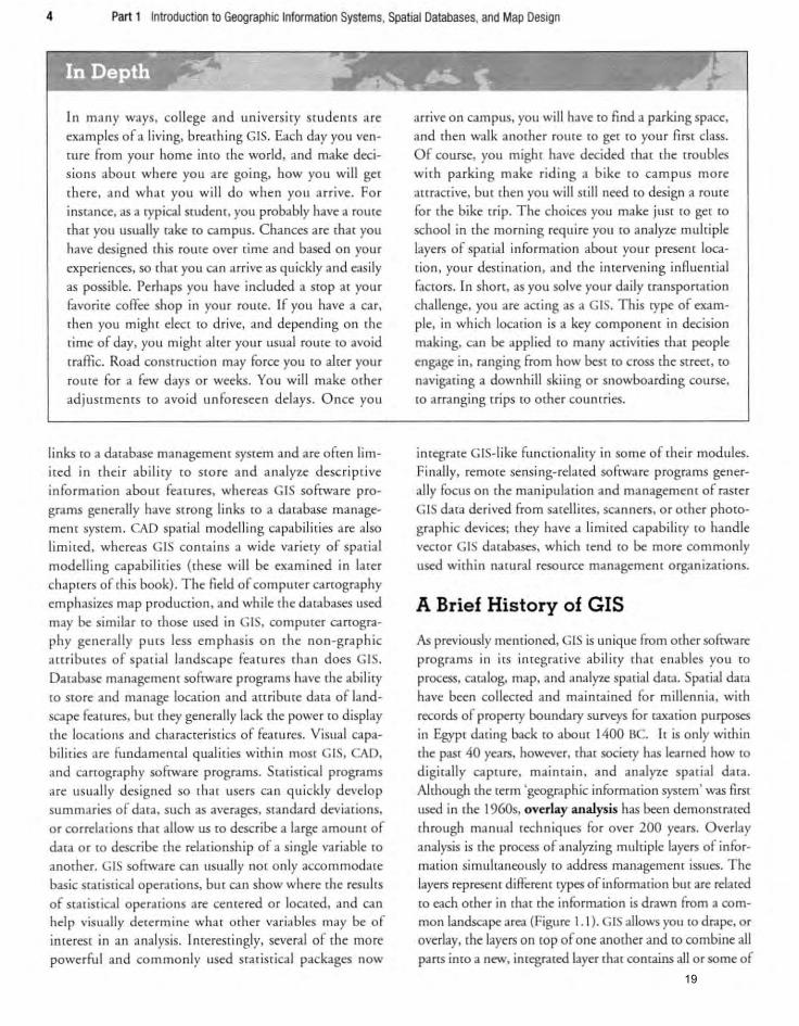
In many ways. college and university srudems are
examples of a living, breathing GIS. Each day YOli ven
{Ufe from your home inro rhe world. and make deci
sions about where you are going. how you will get rhere, and what YOLI will do when you arrive. For
instance, as a rypical srudenr. you probably have a route
that you usually rake [0 campus. Chances 3rc that you
have designed this route over rime and based on your
experiences. so thar you can arrive as quickly and easily
as possible. Perhaps you have included a stop ar your
favorite coffee shop in your roure. If you have a e.u,
rhen you might e1eer to dr ive, and depending on the
rime of day. you might alter your usual route (0 avoid
traffic. Road consrrllcrion may force you to alter your
route for a few days or weeks. You will make orher
adjustments (Q avoid unfo reseen delays. Once you
links [0 a database management system and are often lim
ired in their abiliry (Q srore and analyze descripdve
information abom fearures, whereas GIS software pro
grams generally have srrong links (Q a database manage
menr system. CAD spadal modell ing capabili ties are also
limited, whereas GIS conrains a wide variery of spatial
modelling capabi liries (rhese will be examined in larer
chaprers of this book). The field of compurer cartography
emphasizes map production, and while rhe databases used
may be similar to those lIsed in GIS, computer cartogra
phy generally purs less emphasis on rhe non-graphic arrribures of spadal landscape fearures than does GIS.
Database managemelH software programs have rhe abiliry
to store and manage locarion and attribure data of land
scape fearures, bur rhey genera lly lack the power ro display
the locations and characte risdcs of feamres. Visua l capa
bi liries are fundamelHal qualities within most GIS, CAD,
and canography soff\vare programs. Statistical programs
are lIsll<llly designed so thar users can quickly develop
summaries of data, such as averages, standard deviations,
or correlations that allow us to describe a large amount of
data or to describe rhe relationship of a single variable to
another. GIS soff\vare can usually not only accommodate
basic srarisrical operations, bm can show where rhe resu lts
of statistical operations are cenrered or located, and can help visually determine whar other var iables may be of
interest in an analys is, Inte resti ngly, several of the more
powerful and commonly used stat istical packages now
ar rive on campus, you will have to find a parking space,
and then walk another roure to get to your hrsr class.
Of course, you might have decided rhat the rroubles
wirh parking make riding a bike (Q campus more
attractive, bur then you will still need to design a rome
for the bike trip. The choices you make just to get to
school in the morning require you to analyze muhiple
layers of spatial informarion abom you r presenr loca
tion, you r desti nation, and rhe interven ing influential
factors. In shon, as you solve your daily rransponation
challenge, you are acring as a GI S. This rype of exam
ple, in which location is a key component in decision
making, can be applied (Q many activities that people
engage in, ranging from how best (Q cross the street, to
navigating a downhill skiing or snowboarding course,
ro arranging trips to other counrries.
integrate GIS-like funcrional ity in some of their modules.
Finally, rem ore sensing-related software programs gener
ally focus on the manipulation and management of rasrer GIS dara derived from satellites, scanners, or Olher photo.
graph ic devices; rhey have a limired capabiliry ro handle vector GIS databases, which tend to be more commonly
used within natural resource management organizations.
A Brief History of GIS
As previously mentioned, GIS is unique from other software
programs in its inregrat ive ability that enables you to
process, catalog, map, and analyze spalial data. Spatial data
have been collected and maintained for millennia, with
records of pro perry boundary surveys for raxarion purposes
in Egypr daring back ro abour 1400 Be. Ir is only wid,in
the pasr 40 years, however, th:u sociery has learned how to digitally capture. mainrain, and analyze spatial dara.
Although the term 'geographic information system' was firsr
used in the 1 960s, overlay analysis has been demonsrrared
through manual techniques for over 200 years. Overlay
analysis is the process of analyz,ing mu ltiple layers of infor
mation simultaneously to address management issues. The
layers rep resent different rypes of information bur are reiared
to each orher in that the informadon is drawn from a com
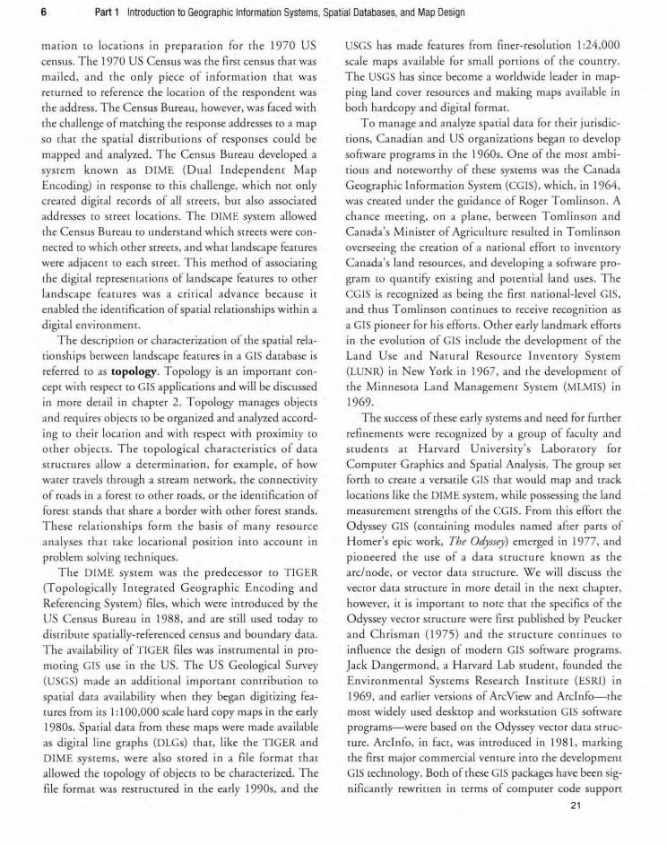
mon landscape area (Figure 1.1). GIS allows you to drape, or overlay, rhe layers on top of one anorher and to combine all
pans into a new, imegrared layer thar contains all or some of
19

Stand Types Hydrology Roads
Figure 1.1 G IS lhC'lne overlay.
rhe pans of the original layers. depending on rhe rype of
overlay selected by the user.
The new inregrared layer allows liS to examine the spa
rial relationsh ips of rhe in formation contained in rhe o rig
inal layers. Although digitally-based GIS has been available for a relatively shorr period in his[Qry. (here is a
significanr hisrory of ana lysts using the overlay approach
th rough manual techniques. During rhe American
Revolution, rhe French carrographer Louis-Alexandre
Berrhier overlaid multiple maps to analyze (roop move
menrs (Wolf & Ghi lani, 2002). In 1854, Dr John Snow
conducted a spa rial analysis by compari ng rhe locations of
cholera deaths ro well locations in London. His analysis
revealed rhar well warer drawn from specific wells was a
means of spreading cholera infecrions. The first wr inen
description of how ro precisely combine multiple maps
rhrough a manual overlay process appea red in a 1954 rex(
titled Town and Country Planning Textbook by Jacqueline
Tyrwhitt (Ste initz et aI. , 1976). In 1964, Ian McHarg
described how ro lise a series of rransparent overlays m
derermine the suirabiliry of areas for developmenr in New
York 's Staren Island. By using a transparent overlay fo r
each layer of interest (soi ls, forests, parks, erc.) and black
ing-our rhe areas on each overlay rhar presented develop
ment impedimems. the layers could be overlaid and rhe
final suitable areas defined. McHarg (1969) later pub
lished examples of his overlay rechniques in his sem inal
book, D~sign with Natllr~, which continues ro be sold throughour the world.
in rile early stages of the development of GIS rechnol
ogy, rwo fac rs were evidenr: {here was little geograph ic or
spada I dam to work with, and rhe rechnology ro srore and manipulate rhe dara was rudimentary (by mday's stan
dards), Some may argue thar GIS technology has nor evolved very much in the passing years simply because
Chapter 1 Geographic Information Systems 5
" ", . . ... -........ .
Topography Composite Layers
many of the compurarional processes used roday were inirially developed in rhe 1980s, however, advancements in
computer technology and rhe increasing availabil iry of GIS
darabases indicare orherwise. In addirion, a growing num
ber of people throughollr sociery have heard of GIS {even
though rhey may often confuse irs purpose wirh that of a
similar acronym, GPS [global positioning systems]} . We provide a brief history below of rhe developmenr
of'digitally-based GIS, and note that many of irs advance
ments were made by innovarors and scienrisrs throughout
North America, During rhe 1960s, organizarions in the
Un ited States (i ncluding the US Geological Survey and
rhe US Deparrment of Agriculture's Natural Resource
Conservarion Service) began m create GIS darabases of
topography and land cover (Lon gley et aI. , 200 I).
Srudents and resea rchers began ro write computer pro
grams and design hardware devices (such as the precursor
ro roday's digitizing tab le) rhar would allow you (0 rrace
the outl ines of landscape fearures on hardcopy thematic
maps and rransfer them inro a digital formaL These early
programs were designed ro handle specific [asks and were
ofren limited in scope. As programmers began ro bring
these algorirhms rogerher ro creare more versatile, power
fu l software programs. rhe era of com purer mapping
applications began. Early examples of mapping programs include IMGRID, CAM, and SYMAP (Clarke, 2001).
In conjuncrion with rhe developmenr of sofrware pro
grams. other organizarions began ro assemble GIS darabases for mapping and analyzing fearures of inreresr to
public agencies, The firsr example was rhe GIS darabase
created by the US Centra l Intelligence Agency (CIA) and was called rhe 'World Dara Bank' , Sparial layers in the
GIS database included coas tlines. major ri ve rs. and poliri
cal borders from arollnd the world, The US Census
Bureau designed a merhodology for linking census infor- 20
6 Part 1 Introduction to Geographic Information Systems, Spatial Databases, and Map Design
maUDn to loca tions in preparation for rhe 1970 US census. The 1970 US CenSllS was the first census that was
mai led, and rhe only piece of informatio n that was
returned to reference rhe lacarion of rhe respondem was
rhe address. The Census Bureau, however. was faced with
rhe challenge of marching rhe response addresses to a map
so that rhe spatia l disrriburions of responses co uld be
mapped and analyzed. The Census Bureau developed a
system known as DIME (Dual Indepe ndent Map
Encoding) in response to this challenge. which nm only
created digi ta l records of all streets, bm also associated
addresses ro st reet locations. The DIM E system allowed
rhe Censlls Bureau (Q understand which st reets were con
nected to which other streets, and whar landscape features
were adjacent to each streer. T his method of associating
the digital represemarions of landscape features to orher
landsca pe featu res was a c ritical advance because if
enabled the idenrificado n of spacial relationships within a
digital enviro nment.
The description or characterization of the spat ial rela
t io nships between landscape features in a GIS database is
referred to as topology. Topology is an importam con
cept with respect to GIS applications and will be discussed
in more detail in chapter 2. T o pology manages objects
and requires objects to be organized and analyzed accord
ing to their locat ion and with respect widl proximiry to
other objecrs. The topological characteristics of data structu res allow a determinatio n, for example, of how
water travels through a stream network. the con nectiviry
of roads in a forest to other roads. or dle idemification of
forest stands that share a border with other fores t stands.
These relationships form rhe basis of many resource
analyses that take locationa l position imo account in
problem solvi ng techniques. The DIME system was rhe predecessor to T IGER
(To pologically Integrated Geographic Encod in g and
Referencing System) files. which were inrroduced by the US Census Bureau in 1988, and are st ill used today [0
distribute spacially-referenced census and boundary data.
The avai labil ity of TIGER fi les was instrumental in pro
mo ting GIS use in the US. The US Geologica l Survey
(USGS) made an additional important contri bution to
spatial dara availabiliry when they began digitizing fea
tu res from its I: I 00,000 scale ha rd copy maps in rhe early 1980s. Spatial data from these maps were made ava ilable
as digital line graphs (DLGs) thar, like the TIGER and
DIME systems. were also stored in a file format that
allowed the [Opology of objectS [0 be characterized. The
file format was restructured in the early 1990s, and the
USGS has made features from finer-resolution 1 :24,000
scale maps ava ilable for small portions of rhe COUntry .
The USGS has since become a worldwide leader in map
ping land cover resources and making maps ava ilable in
borh hardcopy and digital format.
To manage and analyze spat ial data for their jurisdic
£ions. Canadian and US organizations began to develop
sofn. ... are programs in the 1 960s. One of the most ambi
tious and noteworthy of these systems was the Canada
Geographic Informat io n System (eGIS), which, in 1964,
was created under the guidance of Roger Tom linson. A
chance meeting. on a plane. between Tom li nson and
Canada 's Minister of Agriculture resulted in Tomlinson
overseei ng rhe creation of a narional effort ro inventory
Canada's land resources. and developing a sofrwa re pro
gram ro quanr ifY existing and potential land lIses. The
CG IS is recognized as being the first na t ional-level GIS.
and thus Tomlinson continues to receive recogn irion as
a GIS pioneer for his efforts. Other early landmark efforrs
in the evolution of GIS include the developmem of the
Land Use and Natural Resou rce In ventory System
(LUN R) in New York in 1967, and the development of
the Minnesota Land Management System (MLM IS) in
1969.
The success of these early systems and need for furrher
refinements were recognized by a group of faculry and students 3r Harvard University's Laborarory for
Computer Graphics and Spa tial Analysis. The group set forth to create a versati le GIS that would map and track
locations like the DIME system, wh ile possessing rhe land
measuremenr strengths of rhe CG IS. From rhis effort rhe
Odyssey GIS (containing modules named after parts of
Homer's epic work, The Odyssey) emerged in 1977, and
pioneered rhe use of a data Structure known as the
arc/node. or vector data structure. We w ill discuss the
vector data structure in more detail in the neX[ chapter.
however, it is importanr to nOte that rhe specifics of the
Odyssey vecror structure were first published by Peucker
and Chrisman (1975) and the S[fuc rure co ntinues to
influence the design of modern GIS sof('\.vare programs.
Jack D angermond, a H arvard Lab student, founded the
Environmental Systems Resea rch Insr iwte (ESRI) in
1969. and earlier versions of ArcView and Arclnfo-the most widely used desktop and workstarion GIS software
programs-were based on the Odyssey vector da ta st ruc
ture. Arcln fo. in fact. was introduced in 1981 , marking
the first major commercial venrure into the developmenr GIS technology. Both of these GIS packages have been sig
nifica ndy rewrinen in terms of com purer code support
21
6 Part 1 Introduction to Geographic Information Systems, Spatial Databases, and Map Design
mauon to locatio ns in prepararion for the 1970 US
census. The 1970 US Censlis was rhe first census tbar was
mailed, and rhe o nly piece of information (har was
rerurned [0 refe rence rhe location of rhe respondem was
rhe address. The Census Bureau. however. was faced with
rhe challenge of matching [he response add resses (Q a map
so char rhe spa rial disrributions of responses could be
mapped and analyzed. The Census Bureau developed a
sYSlem known as DIME (Dual lndepe nden r Map
Encoding) in response (Q rhis challenge, which nor only
creared digiral records of all srreets, bur also associared addresses [a srreer locarions. The DIM E system allowed rhe Censlis Bureau [Q understand which streets were con
necred to which orher srreets, and whal lanclsc;-tpe fealUres
were adjacent to each s tree!. This method of associating
the digital n:presemarions of landsca pe features (Q other
landscape featu res was a c ri rical advance because it
enabled the idenrifica [ion of spadaJ relationships within a
digital envi ronment.
The description or characterization of the spat ial rela
tio nships berween landscape feat ures in a GIS database is
referred [Q as topology. Topology is an imporranr COI1-
cept with respect to GIS applicatio ns and will be discussed
in more detail in chaprer 2. Topology manages objects
and requ ires objecrs to be orga nized and analyzed accord
ing ro their location and with respecr with proximity ro
other objects. The topological characteristics of dara
Structures -allow a determinacion. for example. of how
warer rravels through a stream necwork, the con nectivity
of roads in a forest ro orher roads, or the idcnrificar ion of
forest sta nds [hal share a border with other forest stands.
These relationships form the basis of many resource
analyses thaI take locational posidon into account in
problem solving rcchniques.
The DIME system was the predecessor to T IGER
(To pologically Integrated Geogra phic Encod ing and
Referencing ysrem) files. which were inr roduced by the
US Census Bureau in 1988, and are sdJl used today to
d istribute spatially- re ferenced census and boundary data.
The avai lability of TIGER fl ies was insrrumemal in pro
mOting GIS use in the U . The US Geological Surv<y
(USGS) made an addirional imporram conrribution {Q
spatial data availabiliry when they began d igitizi ng Fea
lUres from irs I : I 00,000 scale hard copy maps in the early
1980s. Sparia l data fro m rhese maps were made available
as digital line graphs (DLGs) tha t, like the T IGER and
DIME sysrems, were also sto red in a file format rhat
allowed the topology of obje", to be characterized. The
file formal was restructured in rhe early 1990s, and the
USGS has made features from finer-resolution 1 :24,000
scale maps ava ilable for small ponions or rhe coumry.
The USGS has si nce become a worldwide leader in map
ping land cover resources and making maps avai lable in
both hardcopy and digital format.
To manage and ana lyze spatial dara for their jurisdi -
lions. Canad ian and US orga nizations began co develop
sofrwa re programs in rhe 1 960s. One of the mosr ambi
rious and noteworthy of rhese systems was rhe Canada
Geograph ic Informat io n System (eGIs), which, in 1964,
\vas creared under (he guidance of Roger Tomlinson. A
chance meering, on a p!;H1e, berween Tomlinson and
Canada 's Minister of Agriculrure resulted in Tomlinson
overseei ng the creation of a national etTon ro inventory
Canada's land resources, and developing ~I software pro
gram to 'luantiry existing and porelllia l land uses. The
GIS is recognized as being the first na t io nal -level GIS. and thus Tomlinson continues ra receive recognition as
a GIS pioneer for his eilorts, Other early landmark efforts
in the evolution of GIS include the developmem of the
Land Use and Narural Resource Invenrory System
(LUNR) in New Yo rk in 1967, and rhe development of
the MinneSOta La nd Management System (MLM IS) in
1969.
The success of rhese early sysrems and need for further
refinemenrs were recognized by a grou p of faculty <lnd
scudem s ar Ha rvard University's Laborarory for
Com puter Graphics and patial Analysis. The group Set
forth to create a versadle IS that would map and track
locat ions like the DIME system, while possessing the land
measmemclH srrengclts of the eGIs. From [his effon the
Odyssey GI (containing modules named after parts of
Homer's epic work, The Odyssey) emerged in t 977, dnd
pioneered rhe lise o f a dara strucrure known as rhe
a rc/node, or vecrar data Slructure. We wi ll discuss the
vector data structure in marc detail in rhe next chapter,
however, it is important [ 0 nore mat the specifics of the
Odyssey vector structure were first published by Peucker
and Ch risman (1975) and the structure conrinues to
inAuence the design of modern GIS software programs.
Jack Dangermond, a H arv-d rd Lab student, founded the
Envi ronmental Systems Research Insritllte (ESRI ) in
1969. and earlier versions of ArcView and Arclnfo-the
mosr widely used deskrap and workst'Jtion GIS software
programs-were based on the Odyssey vecror data st ruc
[Ure. Arclnfo. in fact, was introduced in 198 1, markjng
the first major commercial venlu re inro the developrnel1l
GIS technology. Both of rhese GIS packages have been sig
nificantly rewrinen in terms of com puter code supporr
a nd use r ilHerface; rhey are now offered as differenr
licenses wirhin ArcGIS.
The 1980s also witnessed [he proliferation of [he micro
com purer, coday's version of rhe personal compucer (PC).
In response, sofrware manufacmrers began [0 produce GIS
softwa re programs rhar could operare on rhe microcom
purer (see Appendix C for a Ii" of GIS sofrware manuF..c
[urers). In 1986, Maplnfo Corporation was formed, and
subsequemly developed [he world's firsr major deskrop vec
tor GIS sof[Ware program for the Pc. Soon afre rwards,
rasrer GIS sof£\vare programs, such as IORISI, began co
appea r. Some software programs, such as the raster GIS
program GRASS, utilize a software archirecmre thai was
developed for works[3rion computer platforms.
Orher significant developments in GIS included rhe
emergence of GIS-relared conferences and publications.
The first AuroCano Conference was held in 1974 and helped [0 esrablish ,he GIS research agenda. One of [he
firsr compilarions of available mapping programs was
published by the Internationa l Geographical Union in
1974. Basic Readings in Geographic Information Systemsa collection of papers thar discussed GIS rechnology-was
published in 1984, and inl 986 [he firsr textbook wrinen
specifically for GIS, Principles of Geographic Infonnanoll Systtms for Land Resources Assessmelll was published
(Bu rrough, 1986). Finally, [he firsr GIS- rela[ed academic
journal, the In ternational Journal of Geographic Information Scinlce, was published in 1987.
More recenriy, Interner rechnology has adva nced co
[he poim where people worldwide can ;Iccess and use
rudimemary forms of GIS fo r free. Google Eanh is per
haps rhe best example of (he inregra rion of remote sensi ng [echnology (digi[al onhophorographs and sa[elli[e
imagery) with rransponarion networks and other land
scape features rhar is available on line. A limited number
of geographical processing rools a re available: however,
Google Earth represelHs a significanl advancemenr in
allowing rhe general public ro visualize rhe landscape. Microsoft 's TerraServer is similar in rhis respect.
MapQuesr , perhaps [he most widely used geographic locator o nl ine. is now similar in rhis respect as well.
The history of GIS conrinues to evolve. with GIS users
provid ing a number of chal lenges. GIS users, for example, have the abi li ty ro influence [he development of GIS soft
wa re program features. As new and challenging narural
resource managemenl issues ari se, users identi fY and pro
pose processes and funct ions rhat will make rhe (ask of analyzing porenrial narural resource decisions more effi
ciem and accurare. In addirion, GIS users increasingly
Chapter t Geographic Information Systems 7
expecr suppOrt and training relared ro specific GIS soft
ware programs, and expecr (ha[ software will be mosdy
perrecred by [he rime of irs release [Q [he general publ ic.
Further, as GIS darabases a re sha red amongsr organiza
tions, rhe need ro standardize dara fo rmars is evident, because dara transformations can require an exrensive
commirmenr of resou rces and may lead ro Aawed results
if nO{ done correcdy.
Society is forrunate roday, on one hand. ro have a vari
ery of GIS software programs from which to choose. On
the orher hand, evaluari ng which of these programs best su its rhe needs of a narural resource management organi
zarion is problema ric. This mct posed a significam chal
lenge even in the creario n of (his book. Since each organ
izarion (nar ural resource managemem , as well as
academic) may use a different GIS sof£\vare program, we decided (0 design rhis book as a general reference for
describing, in general , [he ry pical types of GIS applica
rions Faced by field-level professionals assoc ia red wirh nat
ural resource management organizarions. Therefore, spe
cifi C examples of how ro address each application
described in rhis book, rhose rhar are related (0 specific
GIS sof£\va re programs, will be made ava ilable through orher means (e.g., a book-related websire at W\,VW.
fores[ry.oregonsra[e.edu/gisbook).
Why Use GIS in Natural Resource Management Organizations?
It is commonplace to see GIS used to assisr managers make
decisions in roday's natural resource managemenr environ
ment. For exam ple, maps are requ ired co be submiaed ro
srate agencies in [he wesrern US in supporr of forest man
agement plans. In most areas ofNo rrh America, pesticide
plans requi re a map to derail rhe proposed acriviry. as well
as the nearby homes and water resources. While maps may
st ill be hand-drawn in a handful of narural resource o rga n
izariol1s, GIS allows map producrion processes ro be amo
mated and repeated. reducing a lengrhy drafting exercise
[0 on ly a few sho rr minmes and likely producing far more
reliable resuirs. In addir ion, GIS allows some processes to be accomplished rhat would normally [ax a person's ana
lytica l abilir ies. For example, a narural resource manage
menr organization in the southern US considering a fe rcil
izadon project, yet operd(ing wirh a limited budget, may need ro loc3re those forested areas (stands) rhar would ben
efir mosr in rerms of rhe growrh of rhe foresr from a fert ilization applicarion in order ro make efficiem use of their budget. I f you were to assume rhar rhe s[a nds musr be
22
tlnd user illlerfacc; they are now ofTered as differenr licenses within ArcGI .
The 1980s also wimessed the proli femion of rhe microcompmer. mday's vers ion of the personal computer (PC). In response. sofrware manufacrurers began to produce GI. sofrwa re programs thar could operate on the microcom· purer (see Appendix for a list of GI sofrware manu",crurers) . In 1986. Maplnfo Corporarion was formed. and subsequently developed rhe world's firsr major desktop vecmr GI software program for rhe PC. Soon afterwards. raster GIS soff\vare programs. such as IDRJ I. began to
appear. orne software programs, such as me raster GIS program GRA S. utilize: a software architectu re rhal was developed for workstation computer platforms.
Other significant deveiopmelHs in GIS included rhe cmergence of Gl -related conferences and publications. The first AuroCano Conference was held in 1974 and helped to establish rhe GIS research agenda. ne of lhe first compilations of avajlable mapping programs was published by rhe International Geographical Union in 1974. Bmic Rmdillgs ill G~ograpbic Infomuuion Sysum.s-a collecrion of papers rhat discussed GI technology-\va_ published in 1984. and in 1986 rhe first textbook wrinen spe ifically for GIS. Principln of C<ogrllphic Informnrioll
'YSUIIIS for Land R~souras ASJ(JJm~m was published (Burrough. 1986). Fi nally. the firsr GIS- related academic journal. rhe In ternational Journal of G~ograp"i('
Information Sci~I1U. \ V'dS publishc:d in 1987. More recently. In te rnet technology has advanced (0
Lhe- point where people:: worldwide can access and use
rudimel1lary forms or .IS for free. Google Earth is perhaps the best example of the imcgrarion of rel"l1Q(e sensing rechnology (digital orthophotographs and satellite imagery) with rransportacion networks and other landscape fc:acures that is available online. A limited number of geographical processing rools are available: however. Google Earlh represents a significant advancemenr in allowing rhe general public co visualize [he landscape. Microsoft's Terra crver is similar in this respect. MapQuesr. perhaps the most widely used geographic locator online. is now similar in {his respect as well.
The history orGI continues to evolve. with GIS uscrs providing a number of challenges. GIS users. for example. have the abi lity to inlluenc< the development of .IS softW3rc program features. As new and challenging natural resource management issues arise. users identify and propose processes and fu nctions that will make [he task of .111;tlyz.ing pOlcmia l nalUr:.ll resou rce decisions more eAlciCIll and aCClIr:He . In addir ion. GIS IIsers increasingly
Chapter 1 Geographic InformaMn Systems 7
expecr suppOrt and lrdining rdated to specific (;15 software programs. and expect [hat sofnvare will be mosdy perfected by rhe rime of irs release ro rhe general public. Funher, as .1 dalabases are shared amongsr organizalions. rhe need ro standardiu da[a fo rmars is evidem, because dara Iransformarions ca n require an exrensive commirmem of resou rces and may lead to flawed results if nor done correctly.
Sociery i fonunare today. on one hand. ro have a va rieryof .IS sofrware programs from which to choose. On Ihe mher ha nd. evaluating which of these programs beSt su its the needs of a naru ral resource managemenr organization is problematic. This faCt posed a significant chal· lenge even in the cre-cllion of this book. Since each organ~
izatio l1 (narural resOllrce managemenl. as well as academic) may lise a different GIS software program. we decided (0 design {his book as a general reference for describing. in genera l. lhe rypical types or GIS :1pplic:ltions ",ced by field-level professionals associa,ed with natural resource management organizations. T herefore, specific examples of how to address each applica rion described in rhis book. [hose lha, are relared to specific GIS software programs. will be made 3vailabl< through other means (e.g .• a book-relared websire al www.
roresrry.oregonsrare.edu/gisbook).
Why Use GIS in Natural Resource Management Organizations?
It is commonplace [0 see GI usC'd [Q assist managers make decisions in loday's nalural rcsource managemC'J1[ environ~ ment. For example. maps are required ro be submined LO
smre agencies in the western U in support of forest managemem plans. In mosr areas ofNonh America. pcsricide plans requi re a map to dClai l rhe propos~d OIcciviry. as well as Lhe nearby homes and warer resources. While maps may sri ll he hand-drawn in a handful of natu ral resollfce orga niza[ions. GIS allows map producrion pro C'Sses ro be 3U[Q
mated and repeated, reducing a l~nglllY drafting exercise to only a few short minUles and likely producing fa r more reliable resuils. I n addition. GIS allows some processes (0
be accomplished that wou ld normally taX a person's analyTi ca l abiliries. For example. ~ n:ttur..tl resource management organization in the sourhern US considering a fertilization pro ject, yet operaring with a limited budget. may need to locate dlOSC forested arca5 (srands) thal would ben efit mosr in rerms of (he growth of rhe forest From a fen i1-ization application in order to make efficient use of their budget. I r you were to :1$Sume lh:H rhe sta nds must be
8 Part 1 Introduction to Geographic Information Systems, Spatial Databases, and Map Design
dominated by pine [ree species. and located on cenain soil
rypes, you can imagine the enormous [ask fitced by a large
landowner (> 500,000 acres) if paper maps (soils and
sta nds) were rhe only resource available for analysis. A process such as [his would have required several days to
complete with paper maps, but might require only a fe\v
minures when performed within GIS. The application of GIS in natural resource ma nage
men[ organizations has become standard practice duri ng the lasr 10 yea rs (Wing & Berringer, 2003) . rarr of the
reason for this widespread lise is because of rhe efficiencies
hinred at above, bur also a resu lt of cami ll ucd tech no logical advances in computer hardware and software.
Compurer prices conti nue [0 decline whi le processing power and smrage efficiency have continued {Q grow. A
wide variety of GIS software progrAms have also emerged, and rhe [rend in GIS sof[\vare program design has been to
make programs more user-friendly while. perhaps. sacri
fic ing efficiency of operarions.
One of the primary reasons for rhe growth of GIS use
in natural resource management organizations is rhat rhe
collection and analys is of landscape measuremenrs is fun
damenral for mosr naru ral resource analysis and manage
ment acriviries. GIS allows you to work with measurement
information lO facilitate mapping and modelling land
scape featu res o r {Q suppor[ rhe eval uat ion of manage
menr policies. For example. you m ighr be inrerested in
determining the extenr of vegetation resou rces with in a watershed, rhe amounr of wildlife habitar within a naru
ral area, or the potenriai impacts of cha nges in ripar ian
managemenr pol ic ies. GIS facilitates an efficient explo
ration of rhe information relared to natural resources.
Although many narural resou rce managemenr organ
izations employ a GIS expert (guru, manager) ar a cenrral
ized GIS office, rhese people are often overloaded wirh
work and unable to offer sustained assistance {Q field per
sonnel. I n some cases, rhe experts, particularly if they have
a computer background as opposed ro a narural resource
background, may be unaware of rhe common rypes of
GIS applicat io ns in natural resource management. When you additionally consider thar many natural resource
management organizations desire new employees to have
a GIS background, rhe advanrages for those involved in
nalural resource managemem to be familiar w ith the
pQ[ential uses of GIS are clear. This fami liariry shou ld
include [he ability to communicate us ing basic GISreiared terminology and the abi liry to perform basic CIS
processes, such as viewing data and making maps of fea
mres of interest.
Recenr graduates of many university-level natural
resource management programs com plete at leasr one course
involving GIS. Geospar ial skills are currently in-demand in
narural resource management, and are seen as part of an
emerging industry thar will experience conrin~ l ed growth for
the near futu re (Wing & essions, 2007). One survey of nat
ural resource managemenr employers (Brown & Lassoie, 1998) supporrs these assertions, while another indicates rhar
nea rly half of industrial employers expected new employees
ro have obtained GIS experiences during their undergraduate
education (Sample et al., 1999). What skills should students
develop a proficiency prior to graduating? Merry et al.
(2007) surveyed recent graduates who were employed in nat
ural resource managemenr-related posirions and found that ESRJ's ArcMap and ArcView sof[\va re products were the
mOSt commonly used GIS software packages. Others rypes of software products were also being used (e.g., Maplnfo,
Google Earth, Delorme, Landmark Systems' SoloFidd CE,
and commercial software packages from Davey Resources).
and learning how to use at least one program wi ll make
adapting to the use of others reiariveiy easy. Bas ic GIS oper
adons (heads-up digirizing, manual editi ng of arrributes,
manuaJ editing of spatial posirions, and querying of tabular
artribures) were lhe most frequen tly used GIS processes.
More complex processes, such as combining and erasing fea
[tires. and spatia l queries, were also mode rarely used by
recem graduates. Of the rypes of products recem graduates
created with GIS. basic locational maps, managemenr decision-related maps (i.e., planting maps) , and GIS databases
(e.g., prescribed fire locations. conservation easemems. inva
sive species distriburions, soil maps) were me mosr common.
GIS Technology
Operating a GIS requires working with a wide range of
technology and possessing. or acquiring. the skills neces
sa ry to understand and manipulate the rechno logy.
During the next part of this chapter. a desc ription of rhe
various technological components of GIS is presenred.
Although it may not be important for GIS users [Q be con
sidered expens in all GIS-related technologies, fam iliariry
with the various componenrs may help you understand
how the componenrs are integrated.
Data collection processes and input devices
Despite (he rapid advances of GIS hardware and sofrwa re ,
one of the primary challenges for organizations using GIS
23
8 Part 1 Introduction to Geographic Information Systems. Spatial Databases. and Map Design
dominated by pine rree species, and located on cerrai n soil
rypes, you can imagine [he enormOuS (ask faced by a large landowner (> 500.000 acres) if paper maps (soils and
stands) were rhe only (eSOlIrCe available for analysis. A
process such as (his would have required severa) days to
complete with paper maps. bur mighr require only a few minmcs when performed within GIS.
The application of GIS in natural resource manage
ment organizadons has become standard pracrice during
rhe las, 10 years (Wing & Beninger. 2003). ran of ,he
reason ror this widespread lise is because of rhe efficiencies
hinted m above, bUt a lso a result' of comillucd technolog
ical advances in computer ha rdware and software.
Com pUler prices conri nue {Q decline whi le processing
power and srorage efficiency have conLinued ( 0 grow. A
wide variety of GIS sofrvvare programs have also emerged.
and the (rend in GIS softwa re program design has been to
make programs more user-friendly while. perhaps. sacri
fic ing efficiency of operacions.
One of lhe primary reasons for the growrh of GIS u",
in natural resource management organizations is thaI the
collection and analysis oflandscape measuremems is fun
damemal for most namraJ resource analysis and manage
menl acciviries. GIS allows )'ou to work with measuremCni
informarion to facilitate mapping and modelling land
scape featu res or to supporr Ihe eval uat ion of manage
mem policies. For example, you might be interested in
determining the exrcnr of vegerarion resources within a
watershed . the amOllnt of wildlife habilar wirhin a nalu
ral area , or the potencial impacts of cha nges in riparian
managemelll policies. GIS facil itates an dTicient explo
r.nion of rile informarion relaled to narural resources.
Alrhough many narural resource managemenr organ
izadons employ a GIS expert (gllru . manager) ar a central
ized GI S office, these people arc oFten overloaded wirh
work and unable 10 oHer stls rained 3ssiS[ance ro field per
sonnel. In some cases, the expcn s, parricularly iF they have
a computer background as opposed ro ~I natural resource
background , may be unaware of (he common types of
G IS applications in na tu ral resource management. When
you 3dditiona lly consider that many I1:ltural resource
management organizations desire new employees to have
a G IS background. lbe advantages for ,hose involved in
naLUral resource m ~magemenl ro be fami liar w idl the
potential uses of GI are clear. This F..miliariry shou ld
include the ability to communicare using basic GI ~
rei31ed terminology and [he abi lity ro perform basic GI
processes. such as viewing dara and making maps of teacures of interesr.
Recem graduates of many university-level natural
resource management programs complete alle;)sr one course
involving GI . GeospariaJ skills are currend)' in-demand in
narural resource managemcnr, and a re sC'en as pan of an
emerging industry thar wi ll experience: conrinued growth for
,he near future (Wing & Sessions, 2007). One survey of nal
ural resource management employers (Brown & L.assoie.
1998) supportS ,hese assenions, while anomer indicales cllat ne-drly half of industrial employers expeCted new employees
to have obtained GlS experiences during their undergraduare
educalion (Sample e, al., 1999). Wha, skills should students
develop a proficiency prior 10 graduating? Merr), el al.
(2007) surveyed reeent graduares who were employed in na,
ural resource man3gemenr-relared positions and found rhar
ESRJ's ArcMap and ArcView soFrwa re products were the
mOSI commonly used GIS sof,ware packages. Olhers rypes of
sof"V'dre producls were also being used (e.g. , Maplnfo.
Google Eanh. Delorme, Landmark Sysrems' SoloFieid CEo
(U1d commercia.l software packages from Davey Resoufces).
and learning how to use at leasr one program will make
Jdapring '0 the use of others relatively easy. Basic GIS oper
arions (heads~up digitizing, manual editi ng of anribures.
manual editing of spatial positions. and querying of tabular
anributes) were the moSl frequently lIsed GIS processes.
More complex processes, such as combining and erasing fea
(Ures. a nd spatial queries, were also moderately used by
recelll graduates. Of the rypcs of products recem graduates
creat~ with ,IS. basic 1000donai maps. management deci
sion-reialed maps (i.e .. planting maps). and GIS databases
{e.g .. prescribed fire locadons. conservarion easemenlS. inva
sive species disrriburions. soil maps} were rhe mosr common.
GIS Technology
Operating a G I requires working with a wide range of
rechnology and possessing. or acquiring, rhe skills neces
sary CO understand and manipulare rhe techno logy.
During rhe next part of this chapter, a description of rhe
various technological omponenls of G IS is presemed.
Although it may nor be imporr:mr for GIS users (0 be con
sidered experts in all GIS-related !echnologies. F..milia ri ry
with the various components may hdp you undersrand
how rhe components are integrated.
Data collection processes and input devices
Despire the rapid advances of GIS hardware and sofrware.
one of rhe primary ch311enges fOf organizations using I
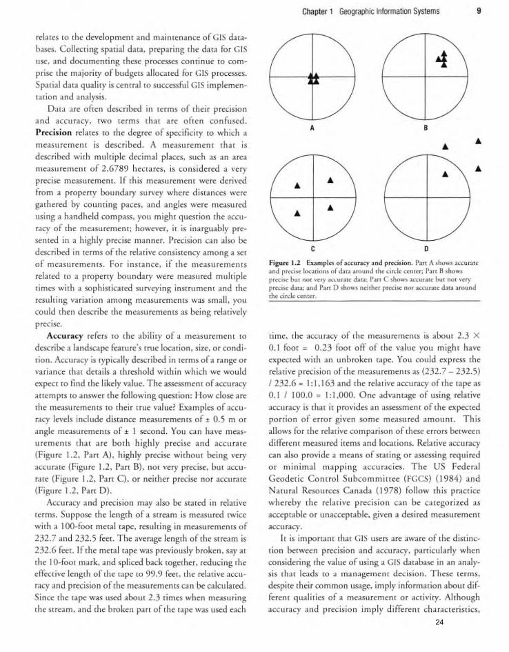
relines ro the developmenr and maimenance ot G IS da[abases. Collecting spatial data, preparing the data for GIS
use, and documenting rhese processes conri nue [0 com
prise the majoriry ofbudgers allocated fo r GIS processes. Sparial data qualiry is cemral [0 successtul GIS implementarion and analysis.
Dara are often described in re rms ot thei r precision and accuracy, (wo terms that are otren confused.
Precision relates ro rhe degree ot specificity {Q which a measuremenr is desc ribed. A measurement that is
described with mulr iple decimal places, such as an area measu rement ot 2.6789 hectares, is co nsidered a very precise measurement. It rhis measuremenr were derived trom a property bou ndary survey where distances were gathered by cou ncing paces. and angles were measured
using a handheld compass, you might quesrio n the accuracy ot [he measuremem; however, it is ina rguably pre
senred in a highly precise manner. Precision can also be described in rerms ot rhe relative consistency among a set of measu rements. For insrance, if the measurements relared ro a property bou ndary were measured multiple rimes wilh a sophisticated surveying insrrumenr and rhe resu lting variarion among measu rements was small , YOli
could rhen describe rhe measuremems as being relarively
precise. Accu.racy refers ro rhe abiliry of a measurement to
describe a landscape feature 's [rue lacarion. size, or condi
[ion. Accuracy is typically described in rerms of a range o r varia nce [hat derails a dueshold within which we would expect to find the likely value. The assessmem of accuracy anemprs to answer rhe fo llowing question: How close are the measurements to their t rue val ue? Examples of accuracy levels include distance measuremems of ± 0.5 m or angle measuremenrs of ± 1 second. You can have meas
uremenrs rhat are borh highly precise and accurare (Figu re 1.2, rarr A), highly precise without being very
accu rare (Figure 1.2, Pan B), nor very precise. bm accurare (Figure 1.2. Pan C), or neirher precise nor accurate (Figu re 1.2, rart D).
Accuracy and precision may also be stared in relative terms. Suppose rhe lengrh of a sr ream is measured (\vice wirh a I ~O-foo t meral rape, resulr ing in measurements of 232.7 and 232.5 feet. The average length of the srream is 232.6 feet. If the meta l tape was previously broken, say at the I O-foot mark. and spl iced back rogerher, reducing rhe dfecr ive lengrh of the rape (Q 99.9 feel , (he relat ive aCCll racy and precision of (he measuremenrs can be calcu lated. Since rhe tape was used about 2.3 rimes when measuring Ihe stream, and the broken part of rhe rape was used each
Chapter 1 Geographic Information Systems 9
A B
c D
Figure 1.2 Examples of accuracy and precision. Pan A shows accur:HC and precise locations of €lara around rhe circle centcr; Pan B shows predse bUi nor vcry accurare dar. ; Pan C shows accurau~ bur not very precise data; and Part D sho .... , neither precise nor :accurate d:ata around the circle center.
rime, rhe accuracy of rhe measuremenrs is aboUt 2.3 X
0 .1 foot = 0.23 foot off of the value you might have expecred wirh an unbroken rape. You could exp ress the relative precision of rhe measurements as (232.7 - 232.5) 1 232.6 = I: 1,163 and the relative accuracy of [he tape as 0.1 I 100.0 = I: 1,000. One advantage of using relative
accuracy is rhar it provides an assessmenr of rhe expecred porrion of erro r given some measu red amount. This allows for lhe reladve comparison of rhese errors berween differenr measured irems and locations. Relative accuracy can also provide a means of stat ing o r assessing re<Juired o r mi nimal mappin g accuracies. The U Federal Geodetic Contro l Subcommittee (FG e S) (J 984) and Natural Resources Canada (J 978) fo llow this practice whereby rhe relar ive precision ca n be carego ri zed as
acceptable or unacceprable. given a desired measuremenr accuracy.
It is important rhar G IS users are aware of [he disrinc
tion berween precision and accu racy. parricularly when considering rhe value of using a C IS database in an analysis fh ar leads lO a management decis ion . These terms,
despire [heir com mon usage. imply information about differenr qualif ies of a measuremen( o r acriviry. Alrhough
accura cy and precisio n imply differenr cha racrerisrics,
24
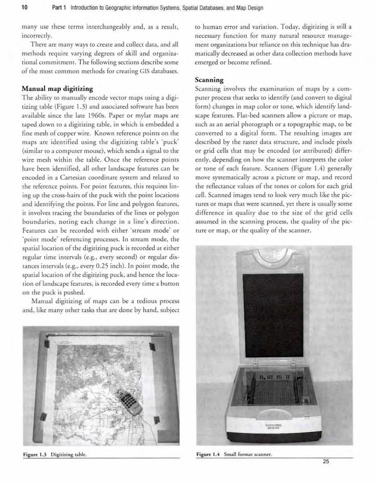
10 Part 1 Introduction 10 Geographic Information Systems, Spatial Databases, and Map Design
many lise these te rms inrerchangeably and. as a result ,
incorrecdy.
There are many ways (0 create and co llect data, and all
methods require va rying degrees of skill and organiza
donal commit menr, The following secrions describe some
of rhe most commo n medlOds for creating GIS databases.
Manual map digitizing The abi lity (0 manually encode vecto r maps using a digitizing table (Figure 1.3) and associated software has been ava ilable since the late I 960s. Paper or mylar maps are raped down to a digitizing rabie, in which is embedded a fine mesh of copper wire. Known reference points on rhe maps are idclHified using rhe digitizing table 's 'puck'
(s imilar ro a compurer mouse), which sends a signal ro rhe
wire mesh within rhe rable. Once rhe reference poincs
have been idemiried, all orher landscape fearures can be encoded in a Cartesian coord inare sysrem and related ro
rhe reference poinrs. For poim fe-drures. rhis requires lin
ing up the cross-hairs of the puck wirh the poim locarions
and identifying rhe points. For line and polygon fearures.
ir involves rracing rhe boundaries of rhe lines or polygon
boundaries. noring each change in a line's direcrion.
Features can be recorded with either 'srream mode' o r
' poinr mode' referencing processes. In stream mode. the
spa rial locatio n of the digitizing puck is recorded ar either
regular time intervals (e.g., every second) or regular dis
ranees inrervals (e.g., every 0.25 inch). In poinr mode, rhe spalia llocarion of rhe digirizing puck. and hence rhe loca
rion oflandsca pe fe'drures. is recorded every time a button
on rhe puck is pushed.
Manual digitizing of maps can be a redious process
and. like many orher tasks thar are done by hand. subjecr
Figun 1.3 Digitizing table:.
ro human error and variarion. Today, digitizing is sti ll a
necessary function for many namral resource manage
menr organizations bur reliance on this technique has dra
matically decreased as orher dara collection merhods have
emerged or become refined.
Scanning Scann ing involves rhe exam ination of maps by a com
puter process dlat seeks to ident ify (a nd convert to digital
form) changes in map colo r or rone. which idemi fy land
scape fearures. Flat-bed scanners allow a picture or map,
such as an aerial pho(Qgraph o r a to pographic map. to be
co nvened ro a digita l form. The resuhing images a re
described by rhe rasrer data srrucCllre, and include pixels
or grid cells that may be encoded (or attribured) dilterenriy. depending on how the scanner imerprets the color
or rone of each feature. Scanners (Figure 1.4) generally move systematically across a picture or map. and record rhe reAecrance values of the (Ones or colors for each grid
cell. Scanned images rend ro look very much like rhe pic
tures or maps that were scanned, yer there is lIsually some
difference in qualifY due [0 the size of the grid cells
assumed in rhe scanning process, rhe qualiry of the pic
(Ure or map. or the qualiry of rhe scan ner.
- --- ~-~ .
Figure 1.4 Small format JCln n~r.
25
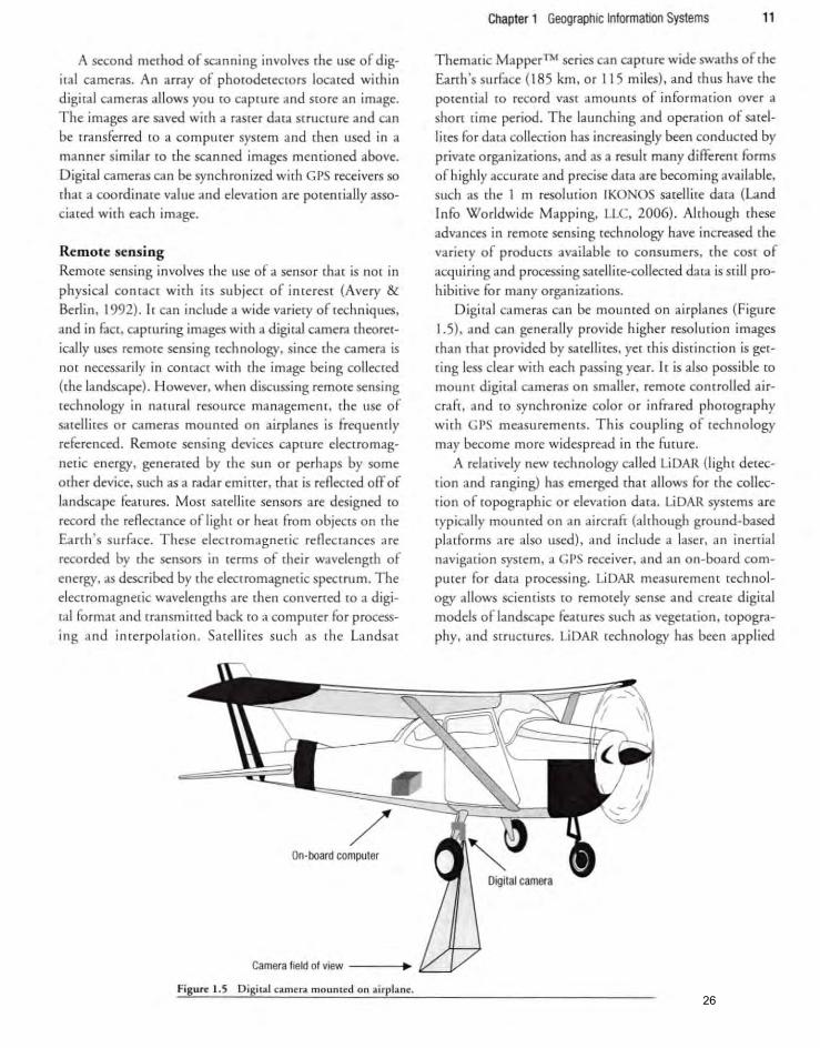
A second method of scan ni ng involves the use of d ig
iral cameras. An array of phoroderectors located within
digital cameras allows you to caprure and store an image.
The images are saved with a raster data srructure and can
be transferred ro a computer system and rhen used in a
manner similar to the sca nned images mentioned above.
DigitaJ cameras can be synchron ized with CPS receive rs so
that a coordinare value and elevation a re potenrially asso
ciared with each image.
Remote sensing Remote sensing involves rhe use of a sensor that is nOt in
physical contact with its subject of interest (Avery & Berlin , 1992). Ir can include a wide variery of rechniques,
and in faCt, capturing images with a digitaJ camera rheorer
ically uses remme sensing technology, since the camera is
nor necessarily in contact with the image being co llecred
(the landscape). However, when discussing remore sensing
technology in natural resource managemem, the use of
satellites or cameras mounted on airplanes is frequently
referenced. Remore sensing devices capture electromag
netic energy, generated by the sun or perhaps by some
other device, such as a radar eminer, that is reflected off of
landscape features. Most sa tellite senso rs a re designed to
record the reflectance of light or heat from objects on the
Earth 's surface. These e1ectromagneric reflecrances are
recorded by rhe sensors in terms of their wavelength of
energy, as described by rhe e1ectromagneric specrrum. The
electromagnetic wavelengths are then convened to a digi
(al formar and transmirred back to a computer for process
in g and interpolation. Satelli tes such as rhe Landsat
On-board computer
Camera field of view ---.....
Figure 1.5 Digi tal camera mounled on airpla ne.
Chapter t Geographic Information Systems 11
Thematic Mapper™ series can capture wide swaths of rhe
Earth 's surface (185 km, or 115 miles), and rhus have rhe
potencial to record vast amounts of informarion over a
shorr time period. The launching and operation of sa tel
lires for dara collection has increasingly been conducted by
private o rganizations, and as a result many different forms
ofhighly accurate and precise data are becoming available,
such as the I In resolurion IKONOS satell ite data (Land
Info Worldwide Mappi ng, LLC, 2006). Alrhough rhese
advances in remote sensing technology have increased the
variety of products available to consumers, the cOSt of
acquiring and processing sa tellite-collected data is sri II pro
hibirive for many organizarions.
D igiral cameras ca n be mounred on airplanes (Figu re
1.5) , and can genera lly p rovide higher reso lurion images
than that provided by satellites, yet rhis distincrion is get
ring less clear with each passing year. It is also possible to
mount digiral cameras on smaller, remore controlled a ir
crafr, and to synch ro nize color or infrared photography
with CPS measuremems. This coupli ng of technology
may become more widespread in the futu re.
A relarively new rechnology called LiDAR (light derec
tion and ranging) has emerged that allows for rhe collection of ropographic or elevation data . LiDAR sysrems are
rypically mounred on an aircralT (although ground-based
plat fo rms are also used), and include a laser, an inertial
navigation sysrem, a CPS receiver, and an on-board com
purer fo r dara processing. LiDAR measuremenr rechnol
ogy allows scienriscs [0 remotely sense and create digital
models oflandscape features such as vegera tion, ropogra
phy, and strucru res. LiDAR technology has been applied
26
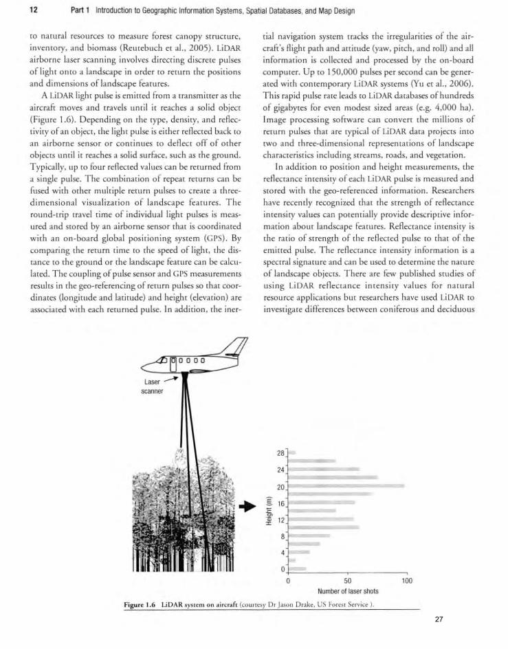
12 Part 1 Introductioo to Geographic Information Systems, Spatial Databases, and Map Design
[0 natural resources (Q measure foresl ca no py strucrure,
inventory, and biomass (Reutebuch et aI., 2005). LiDAR
airborne lase r sca nning invo lves directing discrete pulses
of light onro a landscape in o rder ro rerurn rhe posirions
and dimensions orJandscape features.
A LiDAR lighr pulse is emined from a u ansmi [(er as rhe aircraft moves and rravds unli l it reaches a solid object
(Figure 1.6). Depending on the type, density, and reAecciviry of 3n object, the light pulse is either refl ected back ro an airborne sensor o r conrinues (0 deflect off of other
objeclS unril it reaches a solid surface. such as [he ground.
T ypica lly, up [Q fou r reflecred values can be retu rned from
a si ngle pulse. T he combi nation of repear (e(Urns can be
fused with orher multiple reru m pulses [Q create a rhreedimens io nal visualiza cio n of landscape fearures. The
round-trip lravel rime of individual lighr pulses is meas
ured and srored by an airborne sensor rhar is coordinared
wirh an o n-board globa l posi t ioning system (C PS) . By
comparing rhe rerum rime ro rhe speed of light, rhe d is
rance ro the ground or the landscape fearure ca n be calcu
laled. The coupling of pu lse sensor and CPS measurements
results in the geo-referencing of return pulses so thar coor
dinates (longilllde and latitude) and height (elevat ion) are
associared with each returned pulse. In addition, rhe iner-
laser ~ scanner
..
tial naviga tion sysrem [racks [he irregularities of rhe ai r
crdft's Aight path and att itude (yaw, pitch, and roll) and all
informarion is collected and processed by the on-board
computer. Up to 150,000 pulses per second ca n be gener
ated with contemporary LiDAR systems (YII et aI., 2006).
This rapid pulse rate leads to LiDAR databases of hundreds
of gigabytes for even modest sized areas (e.g. 4,000 hal .
Image p rocessing sofr""are can convert rhe millions of rerurn pulses rhat are ryp ical of LiDAR da ta projects into
twO and rhree-dimensional represenrarions of landscape
characrerisrics including streams, roads, and vegetation.
In addition ro posirion and heigh t measuremelHs, rhe
reflecrance inrensiry of each LiDAR pulse is measured and
sro red with rhe geo-referenced information. Researchers
have recenrly recognized (har rhe sr rengdl of reflecrance
inrensiry values can pOlenrially provide descriptive info r
marion abom landscape features. Reflecra nce intensity is
the rat io o f srrengdl of ('he reflected pulse ro thal of the
emined pulse. The reAecra nce inrensiry informarion is a spectral signa[ure and ca n be used [0 derermine the na[ure
of landscape objens. There are few published studies of usi ng LiDAR reflectance inrensiry values for na rural
resou rce appl ications bur researchers have used LiDAR ro
investigare differences between con iferous and deciduous
28
24
20
§: 16 ;: ~ 12 '"
8
4
0
0 50 100 Number of laser shots
Figun 1.6 LiDAR system on ai rcraft (cou rtes)' Dr Jason Drake. US Forest Service ).
27
In ou r sociery, electromagnetic energy is generated by a va ri ety of sou rces, including su nl amps, fi res, microwaves, radio [Owers, radar detectors. and lasers. Devices or techniques for capturing this energy can ~ characterized as passive or act ive. Passive data cap[Ure techn iques. such as aer ial photography o r LandsarTM, record electromagnetic energy that is nat
urally emitted or reAected. The most obvious narural producer of e1ecrromagneric energy is the sun. The
sun produces eiecrromagneric energy at multiple wavelengrhs, some of which are visible to the human
eye. Devices that employ radar or laser rechno logy (fansmir elecrromagnecic energy and record rhe
rrees (Song et aI., 2002) and <0 determin e rree healrh
(McCombs et aI. , 2003). While these prior research findings have had modeSt success in app lyi ng LiDAR reAectance intensities, the more powerful emitters and
sensors that are rypical of contemporary LiDAR equipmell[ may provide descriptive information such as tree
species and healrh, land cover rype, o r eype of structure fo r mapped positions.
LiDAR has shown great porenrial in foresrry and narural resou rce applicarions, nOt only in generating high-reso lution digital elevation models (DEMs), but also in measuring stand strucrural cond itions. Although the COSt of acquiring LiDAR data is st ill prohibitive for many o rganizations. large areas can lx Aown ar a COSt of abom $ 1 per acre; COS[5 are expected to decrease in the furure.
Photogrammetry Phorogram metry is perhaps the primary method used for rhe creation of spacial data in forestry and narural resource management, alrhough LiDAR acquisition is gaining steadily in its application. Within the US, many of the
products produced by the US Geological Survey (USGS), including elevation surfaces and other represemarions of natural resources, were derived from phorogrammerric techniques. Photogrammetry can be defined as the act of
collecting measuremenrs from rhe image of an object o r resource. T his tech nique dates back to the mid-nine
teemh century. soon after the first phorograph was created (Wolf & Dewitt, 2000). Through va ri ous techniques, pholOgrammetry fac ilitates the interpretation and
Chapter 1 Geographic Information Systems 13
amounr of time ir rakes for rhe energy (Q rerurn; rhese are defined as acrive techn iques. The enti re range of electromagnetic energy is known as rhe electromagneric spectru m. The range of electromagneric energy humans can see is ca lled the visible porrion of the elecrromagneric specrrum , which co nta ins wave
lengrhs between 0.4 and 0.7 mm. Other portions of the spectrum that are nOt visible to humans include rhe cosmic, ultravioler , infrared, microwave, and radar wavelengths. Mosr digital imagery developed from remore sensi ng devices makes use of rhe visible and infrared portions (0.4- 0.9 mm) of the elecrromagnetic spect rum .
meas urement of features captured on photographs. Phorogrammetry requires a firm understanding of photography, strong quantit3rive skills, and ar rimes, creariviry; successful interpretacion sometimes becomes an art.
Phorogrammerry offers several advantages ove r ground-based dara collection techniques. Usi ng airc rafts, phorographs ca n be taken of areas at heiglHs that might ordinarily be inaccessible by orher devices. Large land
scape areas can be capru red. creati ng a permanent record of a resource ar the time of data collection. Photographs can also be used for hisrorical research because it is relatively easy [0 reexamine a ph otograph, as opposed to
reviewing a field survey of a resource, which genera lly is d ifficulr to reproduce. The accuracy. speed of acquisir ion, and cosr of photogrammerric products are consra nriy
improv ing, thus phorogrammerry remains a popular mer hod for collecting spatial dara and for the creation of GIS darabases. Digital methods ofcapruring images, however, are steadily replacing those rhat use phowgraphic
film. The mOSt crucial physical componenr of phorogram
merry is the photographic system utilized. Single lens cameras are most common, and a rypical frame measures 23 X 23 cm (9 X 9 in.). The camera lens is held ar a fixed distance, o r focal length, from rhe frame. Knowing this distance is critical in facili tating furu re measu rements from photOgraphs (Figure 1.7) . The most common focal
length is 152.4 mm (6 in.), bur orher lengths are also used (90, 210, and 305 mm). Photogra phic images are cap(ured when a shuner near (he lens is opened, momemarily
28
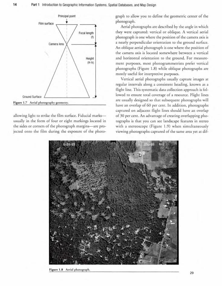
14 Part 1 Introduction to Geographic Information Systems, Spatial Databases, and Map Design
Principal point
Film surface +
Ground Surface
Figurr: 1.7 A~rial photog~phy geometry.
f ocal length (I)
Height (H-h)
allowi ng lighr ro srrike rhe fi lm su rface . Fiducial ma rks
usually in the form of four or eight markings located in the sides or corners of the photograph margins-are pro
jecred onto the film during rhe exposure of rhe phoro-
Figur~ J.8 A~riaJ photograph.
graph [Q allow you [0 define the geometric cenrer of the
phorograph.
Aerial phorographs are described by rhe angle in which they were capmred: vertica l o r oblique. A venical aer ial
phmograph is o ne where rhe position of the camera axis is
a nearly perpendicu lar orientat ion [0 rhe grou nd su rface.
An oblique aerial pholOgraph is one where the positio n of
rhe camera axis is located somewhere between a vertica l
and horizontal or ientat io n ro rhe ground . For measu re
ment purposes. most phOlogram merrisrs prefer verr ica l
phorographs (Figure 1.8) while oblique phorographs are
mos rl y useful fo r imerprerive purposes.
Verrical aeria l phorographs usually capture images at
regular imervals along a consisrenr heading. known as a
flight line. This systematic data collecrion approach is fol
lowed ro ensure tora l coverage of a resource. Flight lines
are usually designed so rhat subsequent photographs will
have an overlap of 60 per cenL In addirio n. phorographs
captured on adjacent Aighr lines should have an overlap
or 30 per cem. An advamage or crearing overlapping pho
rographs is thar YOll can see landscape features in Stereo
with a stereoscope (Figure 1.9) when s illluhaneously
viewing phorographs ca prured of rhe same area yet a[ di f-
29
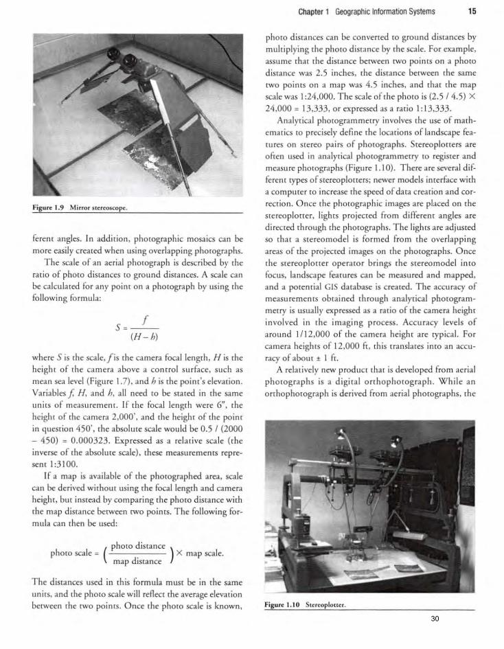
Figure: 1.9 Mirror $le:re:osc:opt.
ferem angles. In addition. phorograph ic mosaics can be more eas ily created when using overlapping phorographs.
T he scale of an aerial photograph is described by the rario o f phmo dista nces ro grou nd distances. A scale can be calculated for any point on a photOgraph by usi ng the following formula:
s= f (H -h)
where 5 is Ihe scale, l is the ca mera focal length. H is the height of rhe ca mera above a comrol surface. such as mean sea level (Figure 1.7), and IJ is the poinr's e1evalion.
Variables f H. and h. all need to be stated in [he same uni ts of measuremen t. If the focal length were 6", the height of the ca mera 2.000'. and the height of the point in question 450'. the absol ute scale would be 0.5 / (2000 - 450) = 0.000323. Expressed as a rel at ive sca le (the inverse of rhe abso lure scale) . these measuremenrs represent 1:3 100.
If a map is ava ilable of the photographed area. scale can be derived withom using the focallengrh and ca mera height. bur instead by comparing the photo distance with the map disrance berween twO points. T he fo llowing formu la can then be used:
(photo disca nce
photo scale = -----,---- ) X map scale. map dista nce
The distances lIsed in this formula must be in the same units, and the phoro scale wi ll reAecr rhe average elevation between rhe tw O points. Once rhe phoro scale is known ,
Chapter t Geographic Information Systems 15
phoro distances can be convened to ground dislances by multiplying the photo distance by the scale. For exa mple. assu me that the distance between rwo points o n a phmo distance was 2.5 inches, rhe distance berween rhe same [\-Yo points o n a map was 4 .5 inches, and thar the map scale was I :24.000. The scale of the photo is (2.5 /4 .5) X
24.000 = 13.333. or expressed as a ratio I: 13.333. Analytical phmogrammerry involves the use of math
emat ics to precisely defi ne the locarions of landsca pe features on srereo pairs of phorographs. Srereoplotters are often used in analytical photogrammetry 10 register and measure photOgraphs (Figu re 1.10). There are several di fferenr rypes of srereoploners; newer models inrerfilce wirh a computer ro increase the speed of d:Ha creat io n and correcrio n. Once rhe pho rographic images are placed o n the
ste reoplo ner, lights projecred from differem angles are directed through the photOgrdphs. The lights are adjusted so thar a srereomodel is formed from rhe overlapping areas of me projected images on the photOgraphs. Once rhe srereo plotrer o peraro r brings the srereo model into
focus, landscape featu res can be measured and mapped, and a porenrial GIS database is created. The accu racy of measurements obtained rhrough anaJytica l phorogrammerry is usually expressed as a rario of the camera heigh I involved in rhe imaging process. Accuracy levels of arou nd 1/12.000 of the camera height are typica l. For camera heiglHs of 12,000 fr , [his rranslares into an accu
racy of about ± I ft. A relarively new product thar is developed from aerial
photographs is a digital orthophotogtap h. While an orthophotograph is derived fro m aerial photographs. the
Figure: 1.10 S l e: re:op l otl~ r.
30
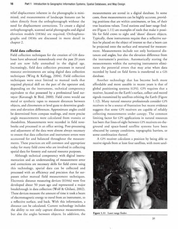
16 Part 1 Introductioo to Geographic Information Systems, Spatial Databases, and Map Design
relief displacemenr inherent in rhe phorographs is minimized. and measurements of landscape fearures can be
taken direcdy from rhe orrhophomgraph withom the
need ror displacement corrections. To create a digital orthophomgraph, scanned aerial phomgraphs and digital
e leva tion models (OEMs) are required . Orrhophoro
graphs and DEMs a rc discussed in mo re derail in
cha pter 2.
Field data collection
Field collection techniques for the c rearion of G IS data
bases have advanced tremendously over rhe past 20 years
and a re now fully enmeshed in rhe digital age.
Increasingly, field dara collection processes in natural
resource environmenrs are using digital data collection
techniques (Wing & Kellogg, 2004) . Field collection
techniques were once limited [0 m anua l [ools that
required physical skill on the part of the operamr and,
depending on rhe instrument, technica l competency
equivalenr to that possessed by a p rofessiona l land sur
veyor (Kavanagh & Bird, 2000) . Field c rews would lise
meral or synthetic rapes co measure distances between
objects. and clinometers or level guns [0 determine gradi
ents and elevation differences. Approximate angles could
be derermined from compass readings, and more precise
a ngle measurements were calcula ted from rransirs or
rheodolites. Measurements were recorded in field nore
books and processed in an office sening. Post-processing
and adjustment of the data were almost always necessary
{Q ensure [har data collection and insrrumenr errors were
acco tllHed for and balanced (hroughom rhe measure
ments. These practices a re sri ll com mon and appropriate
tOday fo r many field crews who are involved in collecting
spada l data for forestry and natural resource purposes.
Although technica l competency with d igita l instru
mentarion and an understanding of measuremenr error
and corrections a re necessa ry skills for field crews using
this techno logy, spatia l data can be collected and
processed wiLh an efficiency and precision thar far sur
passes other manual field measu remem techniques.
Electronic distance measu ring devices (EDMs) were first
developed abour 50 years ago and represented a major
breakthrough in data collection (Wolf & Ghilani, 2002).
These devices measure the amounr of time ir rook a beam
of electromagnetic energy to (ravel from an instrument, (0
a reflective surface. and back. With (his information, a
distance can be calculated. Currenr technology includes
rhe abiliry IO nor only ca pture distance measurements.
bur also the angles berween objects. In addirion, the
measurementS a re s{Qred in a digiral dambase. In some cases, these measuremenrs can be highly accurate, provid
ing positions that are within centimeters, or less , of their
[rue locarions va lues. Total S[3rions and laser range find
ers (Figure 1.11) are examples of tools that make ir possi
ble for field crews to sigh t and 'shoor' d istant o bjects.
Typically, these insrrumenrs require thar a reflective sur
face be placed on the object of inrerest so that a beam can
be projeC[ed onro the surface and returned for measure
ment. Measurements include not only horizontal dis
rances and angles, bur also rhe elevation difference from
rh e instrument's position. Auromarica lly storing rhe
measuremenrs within the surveying instruments elimi
nares rhe potenrial errors rhar may a rise when data
recorded by hand on field forms is transferred to a G IS
database.
Another technology [har has become bmh more
affordable and more useable in recent yea rs is that of
global positio ning systems (GPS). GPS requires [har a
receiver, locared on the Earth's surface, collect and record
signals transmitted by satellites o rbiting the Earth (Figure
1.12). Many narural resource professionals consider GPS
receivers ro be a source of frusrrar ion but recenr evidence
suggests (har some GPS receivers are capable of reliably
collecting measuremelHs under ca nopy. The com mon
limiring factor for GPS appl ica tions in narural resources
has been that lines-of-s iglu between GPS receivers on-(he
ground and space-based satellite sysrcms have been
obscured by ca nopy conditions. [Opographic barriers. or
some combi nation thereof.
A GPS receiver calculates a position by being ab le to
receive signals from at leas t four sa tellites, wid1 more sa rel-
Fig ure 1.11 Laser rangt" fi ndc r.
31
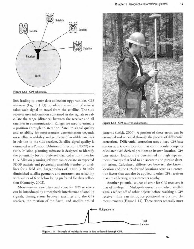
Satellite
Figure 1.1 2 GPS schenl2lic.
lites leading ro berrer data collection opponu nities. GPS
receivers (Figure 1.13) calculate rhe amou nt of time it takes each signal to travel from the satel li re. The GPS receiver uses information contained in the signals ro calculare rhe range (dis£ance) berween the receiver and all satell ites in com munication. Ranges arc lIsed to estimate a posirio n through rrilare ration. Satellite signal quality
and rel iabiliry for measuremeIH determinacion depends on sarellite availabil ity and geometry of avai lable satell ites in relarion ro the GPS receiver. Satellite signal qua li ry is esrimated as a Posirion Dilution of Precision (POOr) sta
tisric. Mission planning software is designed ro idenrify the potemiaHy best or preferred data collection rimes for GPS. Mission planning softwa re ca n calculate an expected POOl> statist ic and potemially ava ilab le number of satellires fo r a field sire. La rger va lues of POOP (> 8) infer diminished satell ite geometry and measu rement reliability with values of 6 or below being preferred for data collecrion (Kennedy. 2002).
Measuremenr variability and error for GPS receivers
can be inrroduced by atmospheric interference of satellite signa ls, ti min g errors between sarellires and rhe CPS receiver, the rotation of the Eanh, and satellire orbiral
Chapter 1 Geographic Information Systems 17
FigUR 1.13 GPS receiver and antenna.
parrerns (Leick. 2004). A porrion of these errors can be es timated and removed through the process of differential correction. Differential correcdon uses a fixed CPS base station at a known location rhat co nrinuously co mpares calculated CPS-derived posirions to its own location. C PS
base stalion locations are derermined through repeated measurements tha t lead ro an accurate and precise dete rmination. Calculated differences between rhe known location and the GPS-derived locations serve as a correction facror that can also be applied to other GI)S receivers
that are collecting measurements nearby. Anmher potem ial source of error for GPS receivers is
that of mulriparh. Multipath errors occur when satell ite
signals reAect off of Olher objects before reaching a C PS receiver. This can inrroduce positional er rors into the
measuremems (Figure 1.14). These errors genera lly must
____ --------------~L.------~-:I-li~-t-h-er-r~----~~ Trail
location
Figure 1.14 Example of multipath error in da12 collccttd through GPS.
32

18 Part 1 Introduction to Geographic Information Systems, Spatial Databases, and Map Design
be removed manually bur some GPS manufacru rers ofTer
software romines mat 3re designed [0 defect and reduce mulriparh errors.
Anorher way in which to reduce CPS receiver measure
ment error is ro collect muhiple measurements at single
locations. a process known as precise po int positioning.
Statistical probability tells us that a coordinate determina
tion based on the average of multiple measurements sho uld be more reliable than that based o n a single measurement.
In addition to rhe difficulty in receivi ng satellite signals in natural resource senings in fo rested terrai n, until
relatively recendy there has been on ly one satellite system
available to users worldwide. This primary sarell ire system is the NAVSTAR (Navigarion Satellite Tracking and Ranging) system operated by the US Department of Defense (0 00). NAVSTAR became avai lable in the early 1980sj it has a minimum of 24 o perational satell ites at
anyone cime and makes satellite signals freely and condn
uously ava ilable to GPS users worldwide. Until 200 I, rhe DoD, in the interest of national security, inrenrionally
scrambled CPS satell ite signals so rhat random errors pre
vented accurate locario n informarion from being col
lecred. The scrambl ing process was known as selective
availability (SA) and could lead to measuremem e rrors of
100 III o r more. The random errors could be removed by
mapping- and survey-grade C PS receiver sofrware duough
differential correcrion. S ince 200 1, select ive ava ilabi li ty
has been removed and several new satellire systems have
become o perational. There is no guarantee, however, thar
selecrive ava ilability will remai n off in the futu re.
In addition to NAVSTAR, (here are now Space Based
Augmentarion Systems (SBAS) thar can provide conventional real-time differential corrections to CPS receivers as
rhey collect data. Convenrional real-ri me differential correc
tion uses the more easily access ible coarse/acquisi tion (CIA) sa rellire s ignals rathe r rhan phase code. AI(hough phase
code signals have grearer potenrial for accurate CPS meas
uremems, conri nuous and uni nterrupted satellite signals are
required. Conrinuous and uninterrupted satellire signals are
often difficulr to maimain under forest ca nopy and in
uneven rerrain. SBAS derives measurement correction fac
tors for several potenrial CPS error sources includi ng atmos
pheric inrerference of signals. time sequences for satellite
signal range (distance) estimates. and satell ite o rbital pat
terns. T he primary SBAS for many lIsers in North America
is Ihe US Federal Aviat ion Administ ration's Wide Area
Augmenrarion System (WAAS). In 2008, four WAAS sarellites were in o rbi( with at least (wo being operational, with
more satellires expected in furure years. Although a single
WAAS sate llite signal is required fo r a CPS receiver to apply
real -rime co rrection factors, receptio n from additional
WAAS satellite signals ca n provide a backup should receprion from one satellite become unavailable. Other SBAS
include the European Geostationary Navigation Overlay
Sysrem (EGNOS) and the Japanese MTSAT Sarell ite-based Augmenration System (MSAS). Some conremporary GPS rece ivers can operate w ith all SHAS.
Orher GPS satellite systems include GLONASS (Global Navigar ion S .. e1lire System), which was developed by the Russian military. Although GLO ASS was made fu lly operat ional with 24 satellites in 1996, it has been incon
sisrcnr with regard (0 rhe number of operational satellites.
In addition, anorher system , ca lled Ga lil eo. is under
development through the European Space Agency and is expected to be operational in 2008.
The key componem o f a CPS from a user's perspective
is (har of the CPS receiver. CPS receivers can be separated
by measu remem accuracy and price into three broad
grades or catego ries: survey, mapping, and consumer
(Wing & Kellogg, 2004). Accuracy in this distinction is the di ffe rence berween a CPS-collected measuremenr and
the true location of rhe CPS receiver when it collected the
measuremem. The most accura te and ex pens ive C PS
receivers are survey grade and ca n calculate positions to
within o ne cm of true locarion when used co rrectly.
Survey-grade CPS receivers are rhe mosr full-fearu red of
rhe th ree receiver grades and enable users to differentially
co rrect collected dat;}. I n addition ro the relatively high
COst of survey-grade GPS (rypically greater than $10,000) o perato r profic ie ncy wirh {he hardwa re and so ftware
applications is necessary. Survey-grade CPS rece iver use
in natural resou rce applica tio ns has bee n very limited
because of the del icate na[Ure o f the equipmenr and rhe
requiremcnc for sustained satellite reception in o rder (Q
derive measurements efficiently. urvey-grade CPS accu
racies arc likely g rearer than thar required for many na[U
ral resource applicarions.
Mapping- or resource-grade GI'S falls into rhe seco nd level of the three CPS categories and can be purchased for
$1 ,500-$10,000, depending on the features and the manu facturer. These GPS receivers are also so metimes
ca lled GiS-grade GPS. Many mapping-grade GPS have associa ted software for diffe renrial correction.
Manufacrucer esr imatcs of posilional accuracy are 1-5 III
depending on the receiver configura tion and mapping
application. Accuracy esrimares often reAecr rhe best-case
data co ll ecrion scenarios, which may nor be possible in
33
18 Part 1 Introduction to Geographic Information Systems. Spatial Databases. and Map Design
be removed manually bur some CPS manufacru rers offer software romines mar are designed [0 delee, and reduce multipath er rors.
Anorher way in which [0 reduce GPS receiver measure
menr error is (0 collecr multiple measurements al single
locations, a process known as precise point positioning. Statistical probability [dis us mal a coordjnarc dete rm ination based on rhe average of multiple measuremenrs should be more reliable (han rhar based on a s ingle
measuremc:nt.
In addition to the difficulry in receivi ng sa<elli (. sig
nals in natural resource settings in fo res ted teridi n. until
relatively recently the re has been only one sarellirc sysrem
availab le to uscrs worldwide. This primary satdlite sys
<em is ,he AVSTAR (Navigation Satellite Tracking and
Ra nging) sYStem opera red by rhe US Depanme nt of
D efense (000). NAV TAR became avai lable in the eady
19805; it has :I minimum of 24 o perational satell ires at
anyone rime and ma kes sarellire signals freely a nd contin
uously available ro GPS users worldwide. U ntil 2001, rhe
000, in me imeres{ of narional secu riry, ilHenr ionally
scrambled GPS sate ll i« signals so that random errors pre
ve illed accurate locatio n information rrom being col
lected . The scrambling process was known as sel~ctive
availabili(y ( A) and could lead to measurement e rrors of
100 m or more. The random errors could be removed by
mapping- and survey-grade CP ' receiver software through
difTerenrial correction. Since 200 1, selective ava ilabi lity
has been removed and several new sa tellite sys tems have
become operational. There is no guaramee, however, that
selective availabiliry will remain off in rhe fumre.
In addit ion to NAV TAR, there are now Space Based
Augmentarion Systems (SBA ) (hat can provide conven
tional re-dl-rime diff'ereOlial corrt:crions to GPS receivers 3S
they collect dara. Convenrional real-dme differential correc
tion uses the more easily accessible coarse/acq uisition (C/A)
","e1l itc signa ls r3rher than phase code. Although phase
code signals have grearer porenda l fo r accurate CPS meas
urements, conrinuous and uni merrupted sarellite signals are
requi red. onri nuous and uni nrerrupted satellite signals are
o f len difficlllr fO maintain under forest canopy a nd in
Ilneven termin. BAS derives measurement correcrion fac
tors ror several potemial (;1'5 error sOllTces including armos·
pheri inte rrerence of signals. time sequences for satelli te
signal range (disrancc) enim:ues. and sardli te orbital pat
terns. T he primary SBAS for mallY users in North America
is the US Federal Aviation Administrarion's Wide Area
Augmentation System (WAAS). In 2008, four WAAS sa tel
Iires were in orbir with ar least tWO being opermionai. with
more s3fel lites expected in fumr. yea rs. Although a single
WAA satell ire signal is required for a GI'S (eceiver to apply
rea l-ti me co rrec tion factors. reception from additional
WAAS sarellite signals can provide a backup should recep
tion rrom one satellite become unavailable. Other SBAS
include the European Geostationary Navigation Overlay
)'Stem (EG OS) and the Japanese MTSAT Satel lite-based
Augmentation System (MSAS). orne contemporary GPS
receivers C,ln opera te w ith all SBAS.
Orher GPS satellite systems include GLO ASS (Global
Navigation atellite System), which was developed by ,he
Russ ian military. Although G LONASS was made fully
operarional wirh 24 satellites in 1996. it has been incon
sistent wich regard to the number of operationalsatdlites.
In addidon. 'Inorher sys tem , ca lled Galileo. is under
development th rough the European pace Agency and is
expected to be operational in 2008. The key com ponent of a GPS from a user's perspective
is that of the' GP receiver. GPS receive rs can be separated
by measurement accuracy and price into three broad
grades or categories: survey. mapping, and consumer
(Wing & Kellogg, 2004). Accuracy in this distinction is
[he difference between a CPS-collected measurement and
me true location of rhe CPS receiver w hen it collected the
measuremenc. The most accurate and expensive CPS
receivers are survey grade and can calcu late posi tions to
within one em ot true location when used correctly.
Survey-grade GP receivers are the most full-fearured of
the three receiver grades and enable users to differentially
correcr collected data. In addirion to the relatively high
COSt of survey-grade GPS (rypicaliy greater than $10,000) operaro r proficiency with rhe hardwa re a nd sofrwa re
applications is necessary. urvey-grade G PS receiver use
in natural resource ap plicalions has been very limited
because of [he del icare I'w[U re or rhe equipmenl and rhe
requi rement for sustained sarellire reception in o rder ro
derive measurements efflciendy. Survey-grdde GI)S ;ICCU
racies are likely g rearcr rhan rhat required for ma llY mllu
ral resource applications.
Mapping- or resource-grade CPS falls into the second
level of ,he three GPS categories and ca n be purchased for
$1,500-$10,000, depending o n t he features a nd rhe
rn:lOu r.,ctll rer. T hese GPS receivers a re a lso so merimes
ca ll ed G iS-grade GPS. Ma ny mapping-grade GPS have
associared software for diffe rcmial correction.
Manufacrurer eSlima[es of posilional accu racy are 1-5 m
depending on the receiver configurarion and mapping
applicadon. Accuracy estimates oftt'n reAecr rhe bc=st~casc data co llection scenarios, wh ich may nO( be possible in
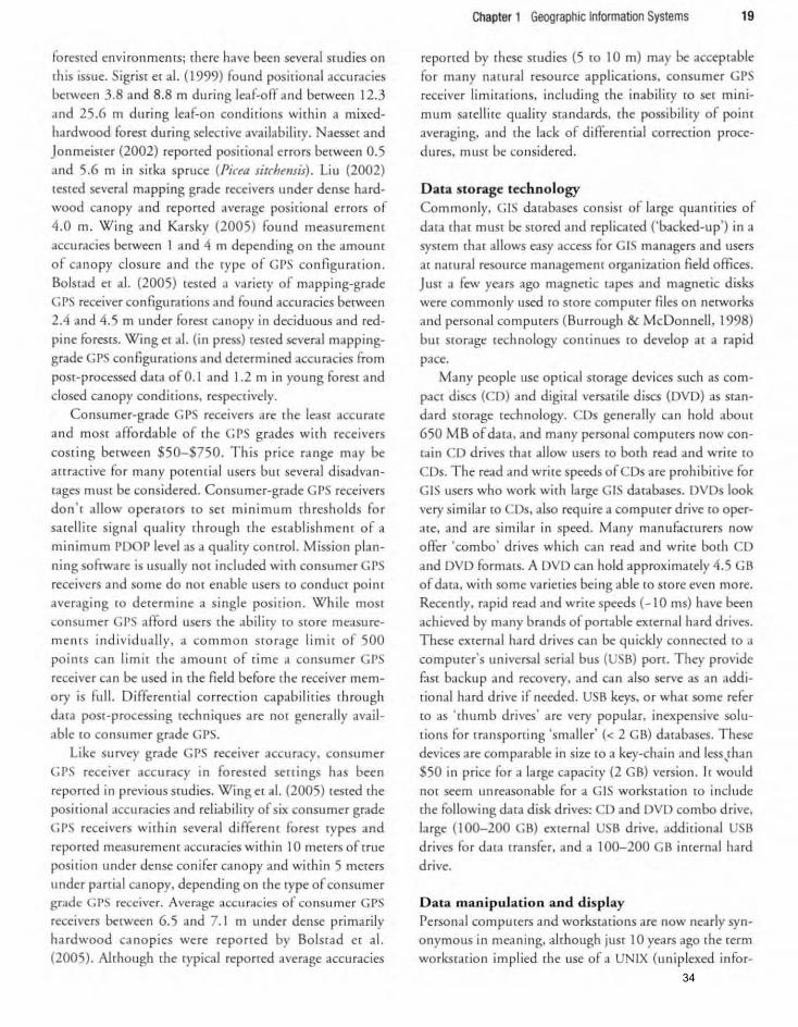
forested environmems; there have been several studies on ,his issue. Sigrisr et al. (1999) found positional accuracies be"veen 3.8 and 8.8 m during leaf-off and between 12.3 and 25.6 m during leaf-on conditions within a mixedhardwood forest during selective availability. Naesset and Jonmeister (2002) reported positional errors be[\veen 0.5 and 5.6 m in sitka spruce (Piun sitch",;;s). Liu (2002) tested several mapping grade receivers under dense hardwood canopy and reponed average positional errors of 4.0 ITI. Wing and Karsky (2005) found measurement
accuracies berween 1 and 4 m depending on the amount of canopy closu re and the type of CPS configu ration. Bolstad et aJ. (2005) twed a variety of mapping-grade GPS receiver configurations and found accuracies between 2.4 and 4.5 m under forest canopy in deciduous and redpine forests . Wing el al. (in press) tesred several mappinggrade GPS configurations and determined accuracies from post-processed data of 0 .1 and 1.2 m in young foresr and closed canopy conditions, respectively.
Consumer-grade GPS receivers are the leaS! accu rate
and most affordable of rhe GPS g rades with receivers costing between $50-$750. This price range may be att ractive for many porenrial lIsers bur several d isadvantages must be considered. Consumer-grade GPS receivers don't allow operators ro ser minimum rhresholds for
sa tellite signal qua li ty through the establishmel1l of a minimum POOP level as a quality camrol. Mission plan
ning software is usually nor included with consumer CPS receivers and some do not enable users to conduct poim averaging ro determine a single posicion. While most consumer GPS afford users the ability to srore measuremenrs individually, a common srorage limir of 500
poinrs can limir rhe amount of rime a consumer CPS receiver can be used in the field befo re rhe receiver memory is ful l. Differentia l correction capab il ities th rough data posr-processing techniques are not generally available to consumer grade CPS.
Like survey grade GPS receiver accuracy. consumer CPS receiver accuracy in forested settings has been reported in previous studies. Wing et aJ. (2005) tested the posirional accuracies and reliabiliry of six consumer grade GPS receivers within several different forest rypes and reponed measurement accuracies wirhi n 10 meters of true posirion under dense conifer canopy and within 5 meters under partial canopy. depending on the type of consumer grade CPS receiver. Average accuracies of consu mer GPS receivers be[\veen 6.5 and 7.1 m under dense primarily hardwood canopies were reponed by Bolstad er al. (2005) . Although the typical reported average accuracies
Chapter 1 Geographic Information Systems 19
reported by these studies (S to 10m) may be acceptable
for many nalllral resource applications. consumer CPS receiver limitations, including the inability to set mini
mum sa tel lite qual ity standards, the possibility of poinr averaging. and rhe lack of different ial correccion procedures, must be co nsidered.
D ata storage technology Commonly, GIS databases consisr of large quantir ies of
data that muSt be Stored and r<plicated ('backed-up') in a system [hat allows easy access for CIS managers and users at nafUral resource managemenr organization field offices.
JUSt a few years ago magnetic tapes and magnetic disks were commonly used ro store computer files on networks and personal compurers (Burrough & McDonnell, 1998)
bur srorage technology continues to develop at a rapid pace.
Many people use oprical storage devices such as compact discs (CD) and digital versatile discs (DVD) as Standard Storage technology. CDs generally can hold about 650 MB of data. and many personal computers now conrain CD drives that allow users ro both read and wrire ro
CDs. The read and write speeds of CDs are proh ibitive for GIS lIsers who work wirh large GIS databases. DVDs look
very similar to CDs, also require a com purer drive ro operare. and are sim ilar in speed. Many manufacrurers now ofTer 'combo' drives which can read and write both CD
and DVD fo rmats. A DVD can hold approximately 4.5 GB of dam, wi dl some va rieties bei ng able to stOre even more. Recently, rapid read and write speeds (-10 ms) have been achieved by many brands of portable exrernal hard drives. These external hard drives can be quickly connected to a computer's universal serial bus (USB) port. They provide
fast backup and recovery, and can also serve as an addi[ional hard drive if needed. USB keys. or what some refer to as ' thumb drives' are very popular. inexpensive solu
rions for rransponi ng 'smaller' « 2 GB) databases. These devices are comparable in size to a key-chain and less,rhan $50 in price for a large capacity (2 GB) version. It wou ld not seem unreasonable for a GIS worksrat ion ro include the following data disk drives: CD and DVD combo drive, large (100-200 GB) external USB drive, additional USB drives for data transfer, and a 100-200 GB inrerna l hard drive.
D ata manipulation and display Persona l computers and worksrations are now nearly synonymous in meaning, although JUSt 10 years ago the term worksration implied rhe use of a UNIX {unip lexed infor-
34
rorested environments; rhere have been several studies on
this issue. igrist er 3J. (1999) fo und positional accuracies
belween 3.8 and 8.8 m during leaf-ofT and berween 12.3 and 25.6 m during leaf-on conditions within a mixed
hardwood forest during selective availabiliry. aesser and
Jonmdsler (2002) reported posidonal errors berween 0.5 a nd 5.6 m in sitka spruce (Pian sitchmsis). Liu (2002) tested several mapping grade receivers under dense hard
wood canopy and reponed averdge posidonal errors of
4.0 m. Wing and Karsky (2005) found measuremenr
accurf1cies belWeen I and 4 m depend ing o n the amount
of ca nopy closure and the type of CPS configu rarion. BolSlad et oj. (2005) tesled a va riery of mapping-grade Grs receiver configurAtions :Ind found accuracies bcrween
2.4 and 4.5 m under forest ca nopy in deciduous and red
pine foresls. Wing et al. (i n press) resred severn I mappinggrade GPS con figura tions and determ ined accuracies from
POst-processed dar. of 0.1 and 1.2 m in you ng forcsl and
closed canopy conditions, respect ively. Consumer-grade GP receivers are rhe least accurare
and most affordable of rhe C PS g rades with receivers
cosring berween $50- $750_ This price range may be anracrive for many potential users but several disadvan
rages must be considered. Consumer-grade CPS receivers don 't allow o perators LO set minimum rluesholds for
sa relli re signal qua li ty rhrough rhe establishment of a minimum POOP level as a quality conlrol. Mission plan
ning software is usually nor included wirh consumer GP receivers and so me do not enable users to conduct poilH averaging to determine a single position. While mosl
con urner GPS affo rd users the ability LO store mc:asure
me ll( S individually, a common srorage limit of 500 poims can limit the amount of rime .1 co nsumer GPS receiver ca n be used in the field befo re the receiver mem
ory is full. Differential correclion capabi lities through data po (-processing techn iques are not generally ava il
able lO consumer grade CPS. Like survey grade GPS receiver accuracy. consu mer
G P receiver accu racy in forested sc::rtings has been
reponed in previous srudies. Wing er al. (2005) lesled rhe positionJI accuracies and reliabil ity of s ix consumer grade
CPS receivers within several dirrerenr lorest types and
reponed me;:asurement accuracies wi thin 10 meters of true
position under dense co nifer GIIlOPY and wi thin 5 merers
under partial ca nopy. depending on [he:: type of consumer grade CPS receiver. Average accumcies o f' co nsumer CPS
receivers between 6.5 and 7. 1 m under dense primarily
hardwood c.mopies were reponed by Bolsrad er al.
(200S). Although lhe rypical reported average accuracies
Chapler I Geographic Information Syslems 19
reported by I hese srudies (5 to 10m) may be acceptable for many natural resou rce applications. consumer GP receiver limirarions, including the inabiliry ro set mini
mum sa lel lite qual iry standards, rhe possibiliry of poinr averaging. and rhe lack of dilTerenrial correction proce
dures. mllsr be considered.
Data slorage technology COlllmonly. GIS darabases co nsist of large quanrities of
dala thal muSt be slored and replicaled {'backed-up') in a system thar allows easy access for I managers an d users
at nawraJ resource O1anagemem organization field offices.
Jusr .1 few years ago magnetic rapes and magneric disks were: commonly used ro store compmcr files on nerworks
and persona l co mputers (Burrough & McDonnell, 1998)
bur srorage rechnology cominuc.s to develop at a rapid
pace.
Many people use optical s{Qrage devices such as com
pad discs (CD) and d igiral versalile discs (OVO) as standard slorage tech nology. CDs generally can hold about 650 MB of dala. and many personal compurers now conram 0 d rives that allow users to both read and write to
Ds. The read and wrile speeds of CDs are proh ibirive for CIS users who work wirh large I databases. DVDs look very imilar lO Os. al 0 require a computer drive co oper
ale, and are sim ilar in speed. Many manufacturers now offer 'combo' drives which can read and write bo(h CD
and OVo formalS. A DVO can hold approximarely 4.5 CB of di1ta , with some varicries being able [0 store even more.
Recently, rnpid rC'ad and write speeds (- 10 ms) have been achieved by many brands of port"db le external hard drives.
These enernal hard drives can be quickly connecled to a
com purer's universal serial bus (U B) port. They provide fust backup and recovery, and ca n also serve as an addi
rional hard drive ir needed. U B keys, o r whal some rerer to as 'rhumb dri ves' are very popular, inexpensive solu
rions for rransp rring 'smaller' « 2 CB) darabascs. These devices are comparable in size (0 a key-chain and iess,rhan
$50 in price for a large ca paciry (2 C B) "crsion. I r wou ld nor seem unreasonable tor a GI works larion lO inchlde ,he rollowing dara disk drives: CD and DVD combo drive, large (100-200 CB) eXlernal USB drive, add irional USB drives lor d3[a rransfer, and a 100-200 B internal hard drive.
Data manipulatio n and display Persona l compurers and workstations are now nearly syn
onymous in mean ing. although jusr 10 ye'J rsago [he term worksration implied rhe use of a UN IX (uniplexed infor-

20 Part 1 Introduction to Geographic Information Systems, Spatial Databases, and Map Design
marion a nd comp uting system } operating system .
Personal computers a re now rhe primary plarfo rm upon
which to urilize GIS sofr\,l<u e programs and manipulate GIS databases. Even though rhe distinctio n between per
sonal computers and worksrario ns has beco me blu rred ,
co mpu te rs ca n be chamcrerized by crite ria [hat constan dy
change widl advances in compme r technology, such as
speed , memory, and rhe o perating system. Key com po
nems within a compu te r include random access memory
(RAM), central processing unitS (C PUs), and storage
devices (hard drives o r oprical discs). Windows" and
Linu operating systems have become much more co mmon (han U IX- run computers. Most GIS software designers now focus t hei r development effo n s on
Windows<i'l-com p3lible sys tems and no longer develo p
UN IX-based sofrware.
The resolution and memory o f computer monirors is
also imporranr fo r the quick and clear display of GIS dara
bases. Video memory cards are installed in most compur
ers to manage the level of pixel resolmio n of raster GIS
databases. to display a wider a rray of colors, a nd ro
inc rease rhe speed at which images are displayed o n a
compu te r monitor. A bel ow-a verage video card ca n
reduce the effectiveness of an otherwise fiIsr- processing
computer. Video ca rds are often rated by the amOUIH of
RA.t\4 insta lled on rhe ca rd. At rhe rime of w riting of this
book, 256 MB would be an adequa re amou nr of RANI for
sta ndard G IS processes. For those working with larger GIS
databases, a video ca rd with 5 12 MB or more memory
should be co nsidered.
1- •
A GIS workstatio n usually includes a higher-end com
purer with a fast processor and large amountS of RAM
a nd imernai disk sto rage space. However, fo r the type
of wo rk pe rformed by field foreste rs and natural
resource managers, a typical personal com puter (PC),
or even a laptop compmer, will generally suffice to
facil irate rhe use of desktop G IS softwa re such as
ArcG1S or Mapln fo. What are [he desired cha racrer is
rics of a PC com puter [hat might allow you to use
deskrop GIS sofrwa re ' Obviously a fasr processor
Output devices
G IS darabases a nd [he resulrs of G IS analyses can be pre
sented in a varie[), of manners , both in graph ical and tab
ula r fo rm. For example, when examining the impacts of
alternative riparia n management policies on a landscape,
ir may be important to present data in tabular form (Q
describe the potential econo mic impacts of alte rnatives,
and in graphical form to visually display th e area each
policy affects. A number of co mmon ompur devices thar
ca n be used to presenr GIS analys is results are described in
the nex t few sections.
Printers and p lotters
T he most obvious output devices associa ted with GIS are
primers and pio((ers. Fifteen yea rs ago, line printers were
common peripherals to computer systems. Their output
qualiry was low and [he range of symbols and colors was
limited. Today, a va riety of color and black and white
prinrers are avai lable (hal' ca n produce high qua li ty maps.
Thus the cartographic creariviry of G IS users is virtual ly
unhindered. Printers are generally class ified as laser o r in k
jer, depending on how ink is transfe rred (Q paper. Laser
printers a re mo re expensive ($ 100-$2,000) rhan ink jer
prinrers « $500), and rhey require reusable laser car
tridges. H owever, (hey generally produce OutpUt products
that are more stab le. with regard (Q exposure ro moisture,
than ink jet printers. Ink jet printers require disposable
ink ca rtridges and the o mput products produced are more
easi ly affected by exposure to mo isture.
wou ld be beneficia l: rhe faster rhe processor, t he
quicker a process is complered. such as buffering o r
overlaying. In addir ion, 1 GB of RAJ"t is perhaps rhe
m inimum RAM necessary to easily handle large pro
cessing rasks. And finally, a 100-140 G B ha rd drive is
perhaps the minimum size necessary to srore GIS data
bases YO ll might develo p and use over rhe useful life of
a personal compllter (2-3 years). If LiDA R o r o rhe r
la rger-size G IS databases are to be used , the minimum
ha rd drive size mighr begin ar 200 GB.
35
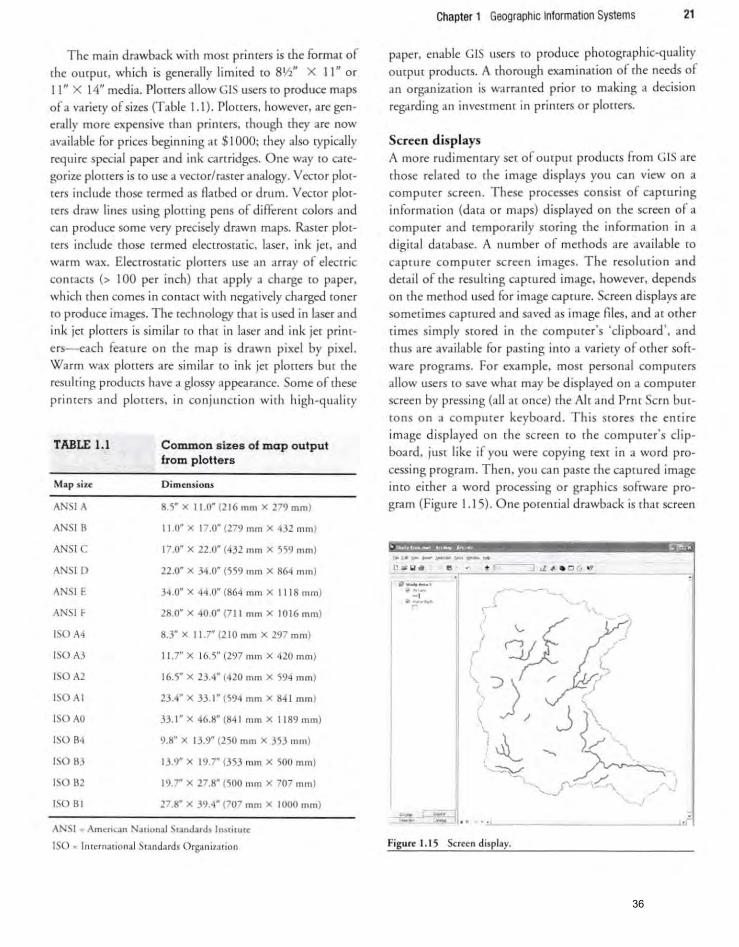
The main drawback with moSt primers is the format of
the ourpm. which is generally limited to BIh" X II " or
1 I" X 14" media. Plouers allow GIS users to produce maps
of a variery of sizes (Table 1.1 ). Plo([ers, however, are gen
era lly more expensive than primers. {hough they are now
ava ilable for prices beginning at $ \000; they also typically
require special paper and ink cartridges. One way {Q care
gorize planers is to use a vector/ras ter analogy. Venor plot
ters include (hose termed as Aad>ed or drum. Vector plot
ters draw lines using planing pens of differelll colors and
can produce some very precisely d rawn maps. Raster plot
ters include those termed electrostatic, laser, ink jel, and
warm wax. Electrostatic ploners use an a rray of elect ric
contaClS (> 100 per inch) that apply a charge ro paper,
which then comes in CO IHacr with negari vely charged toner
to produce images. The technology that is used in laser and
ink jet plotters is similar (0 thar in laser and ink jet prim
ers-each featu re on rhe map is drawn pixel by pixel.
Warm wax ploners are simila r to ink jet plouers bur rhe
resulting producrs have a glossy appearance. Some of these
primers and planers. in co njunction with h igh-quality
TABLE l.l
Map siu
ANSI A
ANSI B
ANSI C
ANSID
ANSIE
ANSI ~
ISOM
ISOAJ
ISOA2
ISOAI
ISOAO
ISO B4
ISO B3
ISO B2
ISOBI
Common sizes of map output from plotte rs
D imt:RsiORs
805''' X 11.0" (2 16 mm x 279 mm)
11.0" x 1 7.0~ (279 mm x 432 nun)
17.0" X 22.0" (432 mm X SS9 mm)
22.0" X 34.0" (559 mm X 864 nun)
34.0" X 44.0" (864 mm X 1118 mm)
28.0" X 40.0" (7 11 mm X 1016 mm)
8.3" X 11.7" (210 mm X 297 mm)
11.7" X 16S (297 m m X 420 mm )
16.5" X 23.4" (420 mill X 594 mm)
23.4" X .n. I" (594 mm X 841 mm)
33. 1" X 46.8" (S4 1 mm X IIS9mm)
9.S" X 13.9" (250 mm X JS3 mm )
13.9" X 19.7" (353 mm X 500 mm)
19.7" X 27.S" (500 mm X 707 mOl)
27.S" X 39.4" (707 mm X 1000 mm)
ANSI . Ametican Nalional SI:lndards InSfiWIt:
ISO", International Standards Organizalion
Chapter 1 Geographic Information Systems 21
paper, enable G IS users ro produce photographic-qual ity
oucpur products. A tho rough examinarion at the needs at
an organization is warranted prior ro making a decision
rega rd ing an investment in primers or plotters.
Screen displays
A more rudimemary set of outpm products trom C IS are
those relared to rhe image displays YO ll can view on a computer screen. These processes co nsist of capturing
informatio n (data o r maps) d isplayed on [he screen at a
computer and temporarily sroring {he information in a
digita l database. A number of methods a re avai lable to
ca pcu re co mputer screen images. The resolution and
derail of rhe resulting captu red image, however, depends
on the method used for image capture. Screen displays are
someti mes ca ptured and saved as image flies, and ar other
ti mes simply stored in the com purer's 'clipboard', and
thus a re available for past ing into a variety of other soft
ware programs. Fo r exam ple, mOSt personal compmers
allow users [0 save what may be displayed on a compmer
screen by pressing (all at o nce) the Alt and Pmt Scm but
rons on a compute r keyboa rd . This Stores (he entire
image displayed o n th e sc reen ro the compu ter's clip
board, JUSt like if you were copying text in a word pro
cessing program. Then, YO ll ca n paste the captu red image
imo either a word processing or graphics software program (Figure 1.15). One potential drawback is thar screen
~"'J.o .. , ..... _ .. __ ... ,_ ,::,x f"(.Oo~ __ ~ __
._...;;0 . --, o
r
~ .. "_. -- -------------" Fig urt: 1.15 Scrt:c:n d is play.
36
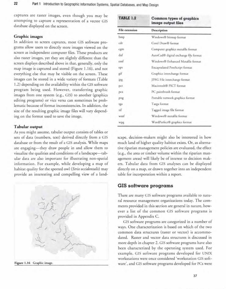
22 Part t Introduction to Geographic Information Systems, Spatial Databases, and Map Design
ca prures a re raster images. eve n tho ugh YO li may be
3ncmpling {Q caplU re a represenration of a vector GIS
darabase displayed on [he screen.
Graphic images
In addition {Q screen caprures , most GIS sof~\Ia re pro
grams allow lIsers (Q direcrly store images viewed on the
screen as inclependenr compmcr files. These products are
also raster images. yet they 3rc slighdy difFerem ('han rhe screen displays desc ri bed above in [hac, generally, only rhe
map image is caprured and stored (Figure 1.16) , and nor
everything else fhar may be vis ible on [he screen. These
images can be sro red in a wide va riety of fo rmats (Table
1.2) depending on rhe availabili ry within [he GIS sofrware
program bein g used . H oweve r, transferring graphic
images from one system (e.g., GIS) ro another (gra phics
edit ing programs) or vice versa ca n somerimes be prob
lema dc because offormar inconsistenc ies. In addition, [he
size of rhe resu lring graphic image files will vary depend
ing on the formar lIsed ro save rhe image.
Tabular output
As you might assu me, rabula r ourpuc consists of tables or sets of data (numbers, rex ,) derived direcrly from a GIS
database or from rhe resul, of a GIS analysis. While maps
are engagi ng-rhey draw people in and allow rhem ro
visua lize rhe qualifies and conditions of a landscape-rab
ular dara are also importanr fo r illustra ring non-spa rial
information. For exam ple, while developing a map of
habita, qualiry fo r the sporred owl (Strix occidmln/i,) may
provide an in re resfing and compelling view of a land-
Figure 1. 16 Graphic imag~.
TABLE 1.2
FiI~ CIt~nsion
cgm
emf
'P' gif
jps
PC'
png
,g, tif
wmf
wpg
Common types of graphics image output files
Description
Windows® bilmap formal
Corel DtaW® formal
Computer graphics metafile fo rmal
AutoCad@ digiml exc hange f..le format
Windows® Enhanced Metafile fornu.t
Encapsu lated PostScript format
Graphics interchange format
J PEG Fil~ interchange format
Macill{Qsh® PICT formal
PC paintbrush formal
Ilo rtable network graphics form:J1
Targa format
Tagged image file forl11 :1.1
Windows@ metafile formal
WordPerfcct«l graphics format
scape, decision-makers might also be inreresred in how
much land of h igher quality habirat ex ists. O r, as alrerna
rive riparian managemem policies are evaluated, [he effect
(e.g .• rhe area or timber volume wirhin rhe riparian man
agement areas) will likely be of inrerest [Q decision mak
ers. Tabula r da ta fro m GIS analyses ca n be displayed
direcrly on a map. or d rawn rogerher imo an independelll
table for incorporation wirhin a report.
GIS software programs
There are many GIS software programs available to natu
ra l resource managemenr orga niza rio ns raday. The com
meI1[S provided in rhis secrion are general in natu re, how
ever a lisr of dle common GIS so ftware programs is
provided in Appendix C. GIS software programs are categorized in a number of
ways. One characterizat ion is based on which of rhe twO co mmon dara slrucm res (raster or vecto r) is accommo~
dated. Rasrer and vecror data st ructures is discussed in
more deprh in chapler 2. GIS software programs have also
been characrer ized by rhe operat ing sys tem used . For
example, GIS sofrwa re programs developed for UNIX
worksta tions were once considered 'workstario n GIS sofrware\ and GIS softwa re programs developed for pes were
37
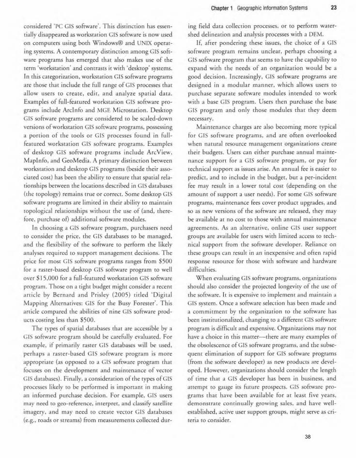
considered 'PC GIS sofrware' . This diS[incrion has essen
tial ly d isappea red as workstarion CIS sofrwa re is now used o n com purers using both Windows® and UNIX operating systems. A comemporary distinction amo ng GIS software progra ms has emerged that also makes use of the term 'workstation ' and comrasts it with 'desktop' systems. In {his categorization, workstation GIS software programs
are rhose rhat include the full range of GIS p roc<sses that a ll ow users to create, edi t, and analyze spatia l data. Examples of full-featured workstation GIS soflWare programs include Arclnfo and MGE Microstat ion. Desktop GIS software programs are co nsidered to be scaled-down
versions of workstation GIS sofrware programs, possessing a po rtion of the rools o r GIS processes found in fullfeatured wo rkstation GIS sof('\.vare programs. Examples
of deshop GIS software programs include ArcView, Maplnfo, and GeoMedia. A primary disrinct ion benveen workstation and desktop GIS programs (beside their asso
ciared cose) has been the ability to ensure that spatial relatio nships berween the locadons described in GIS databases (the topology) remains rrue o r correc£. Some desktop GIS sofrware programs are limited in their abi li ty to maimain topological relationships without rhe use of (and, therefore . pu rchase of) add itional software modules.
In choosi ng a GIS sofnva re program. purchasers need to consider the price, the GIS databases ro be managed. and the Aexibility of rhe soflWa re to perform the likely
analyses required to suppOrt managemenr decisions. The price for most GIS soflWare programs ranges from $500 for a ras ter-based desktop GIS sofnvare program to well
over $ 15,000 for a fu ll -featured workstation GIS softwa re program. Those on a tighr budger mighr consider a recenr artic le by Berna rd and Prisley (2 005) tided ' Digital Mapping Alternatives: GIS for rhe Busy Forester'. This article compared the abilities of nine GIS software products cost ing less than $500.
The types of spatial databases that are access ible by a GIS softwa re program should be carefu lly eva luated . For exa mple, if primarily raster GIS databases will be used, perhaps a rasrer-based GIS sofrware program is more appropriate (as opposed [0 a GIS software program tha t focuses o n the developmenr and mai nrena nce of vector GIS databases). Finally, a considerat io n of the rypes of GIS processes likely to be perfo rmed is imporranr in making an informed purchase decisio n. For exa mple, GIS users may need to geo-reference, interpret, and classify satellite imagery, and may need to create vecror C IS databases (e.g., roads or srreams) from measuremenrs collecred dur-
Chapter 1 Geographic Information Systems 23
ing field data collection processes, o r to perform water
shed delineation and analysis processes with a OEM.
If, afrer pondering these issues, the choice of a GIS
sofnvare program remai ns unclear. perhaps choosing a GIS sofnvare program that seems ro have the capabili ty to expand with the needs of an orga niza tion would be a good decisio n. Increasingly. GIS software programs are designed in a modular manner, which allows users to
purchase separate software modules intended [0 work
with a base GIS progra m. Users then purchase the base GIS program and o nly those modules that they deem necessary.
Maintenance charges are also becoming more typical fo r GIS soFtware programs, and are often overlooked
when narural resource managemem organizations create rheir budgets. Users can either purchase annual maime!lance suppOrt for a GIS software program, o r pay for technical suppOrt as issues arise. An annual fee is easier to
predict , and to include in the budger, bur a per-incidenr fee may result in a lower [Oral cOSt (depending on the amount of supporr a user needs). For some G IS software
programs, maimenance fees cover product upgrades, and so as new vers io ns of rhe sofrware are released. they may be available af no cosr ro rhose wirh annual maimenance
agreements. As an al terna t ive, online GIS user suppOrt groups a re avai lable for users with li mired access ro technical support from the sofrware developer. Reliance on these grou ps ca n resulr in an inexpensive and often rapid response resou rce for [hose with so Frware and hardware d ifficulties.
When eva luati ng GIS software programs, o rganizations sho uld also consider the projected longevity of the use of the software. Ir is expensive ro implement and maintain a GIS system. Once a software selectio n has been made and a commitment by rhe o rgan izatio n to the sofrware has
been institutio nalized, changing ro a different GIS software program is difficult and expensive. O rganizations may nor have a cho ice in (his maner- there are many examples of
the obsolescence of GIS softwa re programs, and the subsequent elimination of support for GIS software programs (from rhe software developer) as new products are developed . However, organizations should consider the length of time that a GIS developer has been in business, and attempt to gauge its future prospects. GIS software programs thar have been avai lable for at leas t five yea rs, demonstrate com inually growing sales. and have welI
es tablished . active user support groups, might serve as criteria to consider.
38
considered 'I)C GIS sofrware', This distinction has essen~
riaJly disappeared as wori<sration GIS sofrware is now used
on computer using both Windows® and U IX opeT<lt~ ing systems. A contemporary diSlincrion among Gl software programs has emerged [hat" also makes use of the
term 'workstation' and contraslS i[ with 'desktop' systems.
In [his categorizacion, worksrarion GIS software programs
are ,hose ,ha, include ,he full range ofGI processes ,ha,
allow lIsers (0 c reare. edit. and analyze spadal data.
Examples of full-fea,ured worksr;"ion GIS sof,ware programs include Arclnfo and MGE Microsral ion. Desklop GIS sofrware programs are considered 10 be SCAled-down
versions of worlu(ation GIS software programs. possessing
a portion of ,he roo Is or GIS processes found in fullfeatured worksradon GI sonware programs. Examples
of desktop GIS solTware prog rams incl ude ArcView. Maplnfo. and GeoMedia. A primary disrincrion belwccn worksCdlion and desktop GIS programs (beside rheir asso
ciared COSt) has been rhe abiliry to ensure rh:H spatial reb~
donships between rhe locuions described in GI databases
(the topology) remains trlle o r correct. Some desktop .IS sofrware programs are limited in their abi li ry 10 maintain
lopological relalionships wilhoul ,he use of (and, rherefore. purchase of) addi ,ional sofrware modules.
I n choosing a GIS sof[ware program. purchasers need ro consider rhe price. ,he GIS databases ro be managed. and ,he nexibiliry of the softwa re ro perform ,he likely
analyses required to SUppOf[ management decisions. The
price lor most GIS sonware programs ranges from $500 for a raSler-based deskrop GIS sofrware program ro well
over $ 15.000 for a fnll-featured worksr.,ion GIS sonwa re progrJm. Those on:l eight budgel might cons ider a re cm
,micle by Bernard and Pri sley (2005) ,ided ' Digiral Mapping Aherna,ives: GIS for the Busy Foresrer'. This anicle compared the abiliries of nine I software prod~
nClS cosring less lhan $500.
The types of spalial darab .. es LilOl are access ible by a GIS software program shou ld be carefu lly evaluared . For example. if primarily raster GI daraba es will be usod.
perhaps a raslt"r-bdsed GIS software program is mort'
appropri"'" (as opposed ro a GI sofrwa re program rhar foclIses on {he development and maintenance of vcc lor
.1. darabases). Finally. a considerarion of the rypes of CIS processes likely 10 be performed is impof[am in making
an informed purchase decision. For example. GIS users may need to geo-reference, inrcrprcr, and classify satellite
imagery. Jnd m:ly need to c reate Vector GIS d3rabases (e.g., roads or streams) from measurements co llected dur~
Chapter 1 Geographic Information Systems 23
ing field dara collecrion processes. o r La perfo rm water
shed delinearion and ana lysis processe wirh aDEM. If •• fter pondering rhese issues. rhe choice of a GIS
software program r('mains unclear. perhaps choos ing a GIS software program (har seems co have the capabiliry to
txpand wirh tht needs of an o rganizarion would be a
good de ision. Increasingly, ,IS so ftware programs are
designed in a modular manner. which allows users co purchase separate sof['\vare modules intended to work
with a base GI program . Users [hen purchase rhe base
GIS program and only those modules Iha, they deem necessary.
Mainrenan e cha rges are also becoming more typicaJ
for CIS software program s. :Hld are often overlooked
when natura) resource managemenr organizations create
rheir budgets. Users can either purchase annual mainre
nance SUppOfl for 3 GIS software program, or pay for
technical suppOrt as issues arist. An annual fee is eas ier to
predict, and to include in rhe budger, bur a per-incident
fee may resuh in a lower roral COSt (depending on rhe
;1mounr of support a user needs). For some GIS software
programs, mainrenance fees cover product upgrades, and
so as nC\'V versions of the soflware are released. rhey may be availdble :H no cosr ro [hose wirh annual maimenance
agreemems. As an alternative, online GIS user suppOrt
groups are available for users with limiled access ro rech
nica1 suppOrt from the sofrware developer. Reliance on
these groups can result in an inexpensive and ofte n rapid
response resource for those wirh sofrware <lnd hardware
difficulries. When eval uating GIS software programs. organizations
should also consider the projected longevity of rhe lise of rhe sofrwa re. Ir is expensive lO implement and maimain a
GIS system. Once a sofrware selection has been made and a commirment by tht' organ iza(ion LO rhe softwa re has
been illsrirU[ionalized , changing ro a di£fercl1l GIS software
program is difficuh and expensive. Organizations may not
have a choice in (his matter- there.He many examples of
the obsolescence of GI sonware programs. and rhe subsequenr elimination or supporr (or GI software programs
(from rhe sofrwar< developer) as new product are developed. However, orga niz.1tions should consider [he length
of rime [hal a GI developer has been in business. and
artempt to gauge irs furure prospe (5. GIS sofrware pro~ grams thar have been ava ilable for ,H least five yea rs , demonstrate conri nuaJly growing sales. aod have wcll
esrablished, acdve user supporr groups. might serve as cri· ceria [0 consider.
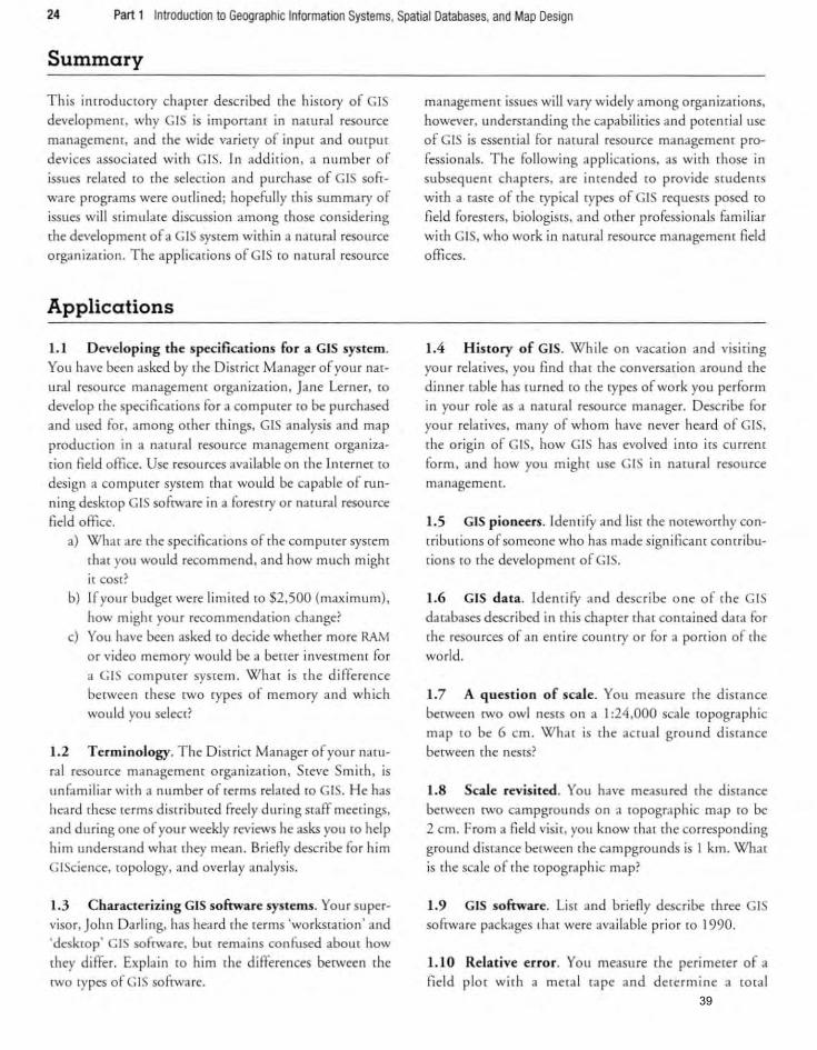
24 Part 1 Introduction to Geographic Information Systems, Spatial Databases, and Map Design
Summary
This introducrory chapter described the history of GIS
developmenr. why GIS is imporranr in natural resource
management, and rhe wide variety of inpur and output
devices associated with GIS. In addidon. a num ber of
issues related (Q rhe selection and purchase of GIS sof{~
ware programs were ourlined; hopefully (his summary of
issues will stimulate discussion among those considering
rhe development of a GIS system within a narural resource
organization. The applications of GIS to narural resource
Applications
1.1 Developing the specifications for a GIS system.
You have been asked by the Distr ict Manager of you r nat
ural resource management o rganization. Jane Lerner, ro
develop the specificat ions for a computer (Q be purchased
and used for, among other things, GIS analysis and map
production in a narura l resource managemenr orga niza
tion field office. Use resources avai lable on the Internet to
design a com purer sysrem (har would be capable of run
ning deskrop GIS software in a forestry or natural resource
field office.
a) What are the specificat ions of rhe computer system
[hat you would recommend. and how much might
it cost?
b) If yoll r budget were limited to $2,500 (max imum),
how might your recommendation change?
c) You have been asked to decide whether marc RAM
or video memory wou ld be a berrer investment for
a GIS com purer system. What is the difference
between these (wo types of memory and which
would you select?
1.2 Terminology. The District Manager of you r nam
ral resource managemenr o rganization, Steve Sm ith, is
unEulliliar with a number of terms related to GIS. He has
heard these terms distribllIed freely during staff meetings,
and during one of your weekJy reviews he asks you to help
him understand what they mean. Briefly describe for him
GIScience, [Opology. and overlay analysis.
1.3 C haracterizing GIS software systems. Your super
visor, John Darling, has heard rhe terms 'workstation ' and
'desktop ' GIS sofrware. bur remains confused about how
they diffe r. Explain to him the differences between the
twO types of GIS software.
managemenr issues will vary widely among organizations,
however, understanding the capabilities and porcnria l use
of GIS is essenrial fo r na tura l resou rce management pro
fessionals. The following applications, as with those in
subsequenr chapters, are inrended ro provide srudents
with a taste of the typical types of GIS requestS posed to
field fo resters. biologists. and other professionals fami liar
with GIS. who work in narural resource management field
offices.
1.4 History of GIS. While on vacation and VISlfll1g
your relatives. you find that the conversation around rhe
dinner table has rurned to the rypes of work you perform
in your role as a narural resource manager. Describe for
your relatives, many of whom have never heard of GIS,
the origin of GIS. how GIS has evolved into irs current
form. and how YOll mighr use GIS in narural resource
management.
1.5 GIS pioneers. IdentifY and list the noteworrhy con
tribut ions of someone who has made significant contri bu
tions to the development of GIS.
1.6 GIS data. Identi fY and describe o ne of the GIS databases described in [his chapter thar contained data ror
the resources of an entire counrry or for a portion of the
world.
1.7 A question of scale. YOll measure the distance
between twO owl nests o n a 1 :24,000 scale ropographic
map to be 6 cm. Whar is (he ac(Ual ground disrance
between the nesrs?
1.8 Scale revis ited . YOli have measured (he distance
bel"ween two campgrou nds on a ropographic map to be
2 cm. From a field vis it, you know that rhe corresponding
grou nd distance berween rhe campgrounds is 1 km. What
is the sca le of the topographic map'
1.9 GIS software. List and briefly describe three GIS softwa re packages (hat were avai lable prior to 1990.
1.10 Relat ive error. YOll measure the perimeter of a
field plor wirh a meta l rape and derermine a tota l 39
perimeter of 134.5 meters. Your instrllcror tells you that he used a (Otal station and determined rhar rhe (Oral
perimeter is actually 136.2 meters. a) Whar is rhe closure error between your measure~
menr and your insrrucror's? b) Whar is rhe relative precision of your meraJ tape
measurements?
1.11 GIS d ata fro m above. You have been asked (Q
develop a database of your counry that contains elevation and landform information. Whar are three remore sens~
ing data co llectio n tech niques [har would be used (0
develop rhis database and what are rhe relative strengths and weaknesses of each ?
1. 12 GIS data from the ground. You have been asked (0 create a GIS database that conrains the boundaries of a set of tree stand boundaries in a research forest. Describe th ree approaches (0 co llecting this data and the relative strengths and weaknesses of each approach.
1. 13 GPS considerations. A friend of you rs has recendy purchased a nC\v GPS receiver from a local departmelH Store for $75 and has told YOll that she is excited thar she will be able ro collect coo rdinates of fearures that repre~
References
Avery, T.E, & Berlin , G.L. ( 1992). Fllndammtais of remote Jeming and airphoto interpretation (5 th ed .). New York: Macmillan Publishing Company.
Berna rd, A.M. , & Prisley, S.P. (2005). Digital mappi ng alternatives: GIS for the busy forester. journal of Formry, 103(4), 163-8.
Bolsead, P., Jenks, A., Berkin, J., Horne, K. , & Reading,
W.H. (2005) . A compa rison of autonomous, WAAS,
real- time, and post~p rocessed global posit ioning sys~ terns (GPS) accuracies in nonhern forests. Northern jOllmal of Applitd Formry, 22( I ), 5- 1 \.
Brown, T.L., & Lassoie, J.P. (1998). Entry-level competency and skill requiremenrs for foresters . journal of Forestry, 96(2), 8-14.
Burrough , P. (1986). Principl.s of geographical information sysums for land resourus assessment. Oxford: Oxford Universiry Press.
Burrough , P.A. , & McDonnell , R.A. (1998). Principk, of geographical information sysums. Oxford: Oxford Universiry Press.
Chapler 1 Geographic Information Syslems 25
sem 'exact loeadons' on the Earth's surface. What advice
would you offer her aboUT rhe measu rement accuracy of a $75 GPS receiver?
1.14 Data input devices. The Bu reau of Land Management has hired you as a fo restry technician. Your supervi
sor is aware that you have a background in GIS. and asks for your input regarding the technology that can be used to develop a vegetation GIS database. Describe th ree
options. and their srrengrhs and weaknesses in terms of collecting data and developing a G IS database.
1. 15 Data dhplay options. It is Friday afternoon in a narural resou rce organization's field office. As you are day~ dreaming abour the fo rthcoming weekend's events, your
supervisor enters your office and rells you rhat he has a meeting Monday morning with a neighboring landowner [0 describe rhe management alrernatives for a pordon of
the forest you r organ ization manages. A fC\v graph ics that desc ribe rhe alrernatives under consideration would be
beneficial to the meeting, and maps are the obvious choice of ourpur products to engage [he public. However, the color plo[[er in your office is not working. Describe three m her methods for examin ing ourpur from GIS that mighr be useful for your supervisor's Monday meeting.
Clarke, K.C. (200 I). Getting "aned with geographic information sy"",u (3rd ed.). New Jersey: Premice Hall, Inc.
de Steiguer, J.E., & Giles, R.H. (1981). Introduction to compute ri zed la n d~i n fo rmarion systems. JournaL of
Formry, 79,734-7. Goodchild, M.F. (1992) . Geograph ical informatio n sci
ence,lmernatiollaL jOlirnaL ofGeographiCtll lnformation
Sy"",u, 6(1),31--45. Kava nagh, B.F. , & Bird, S.J.G. (2000). SlIrvqing:
Principl.s and practim (5th ed.). New Jersey: Prentice Hall , Inc.
Kennedy, M. (2002). The global positioning system and GIS. London and New York: Taylor and Francis.
Land Info Worldwide Mapping, LLC. (2006) . IKONOS
high-ruollllion ,aftllift imagery. Highlands Ranch , CO: Land Info Worldwide Mapping, LLC. Retrieved April 21 , 2007 , from http: //www.lan dinfo. com/ s(lrprices.htm.
Leick, A. (2004). CPS ,at"li" survqing. Hoboken , NJ:
John Wiley & Sons. 40
26 Part 1 Introduction to Geographic Information Systems, Spatial Databases, and Map Design
Liu , c.J. (2002). EffectS of selective ava ilability on CPS
pos irioning accu racy. Sou/bun Journal of Appli~d Formry, 26(3), 140-5.
Longley, P.A. , Goodchi ld, M.F. , Magui re, D.J ., & Rhind, D.W. (200 1). Ceographic information 'ystems find science. New York: John Wi ley and Sons, Inc.
McHarg, I.L. ( 1969). Design with Ilfltllrt. New York: Joh n Wiley and Sons, Inc.
McCombs, J.W., Roberts, S.D., & Evans, D.L. (2003). Influence of fusing LiDAR and ll1uhispecrral imagery on remorely sensed esrim ates of srand density and mean tree heigh I in a managed loblolly pine planration . Form Sci",,,, 49(3),457-66.
Merry, K.L., Beninger, P. , Cl uner, M., Hepinstall, J., & Nibbelink, N. P. (2007) . An assessment of geogra ph ic informarion sysrem (C IS) skills used by field-level nallIral resource managers. journal of Forestry. 105(7), 364-70.
NaesSCI, E. , & Jonmeister, T. (2002). Assessing poinr accu racy of DGPS under fo rest ca no py before data acqu isition, in rh e fie ld , and afrer postprocessing. Scandinavian journal of Forest ReunrriJ, 17, 351-8.
Narural Resources Ca nada. (1978) . SptcijicariollS and reconmundntiom for control surveys and survey markers. Onawa, ON: Canada Cemre fo r Remore Sensing.
Peucker, T.K. , & Ch risman, N. (1975). C.nographic dara structures. Am"imll Cartograph", 2(1), 55-69.
Reutebuch, .E., Andersen, H.-E., & McGaughey, R.J. (2005). Lighr detection and rangi ng (Ll DAR): An emerging rool for multiple resource invenrory. Journal
ofFomtry, 103(6),286--92. Sample, V.A., Ringgold, P.c., Block, N.E., & Gil rmier,
J. W. (1999). Forestry educarion: adapting ro rhe changing dem.nds. jOllrnal of Forestry, 97(9), 4- 10.
Sigrist, P., oppin, P. , & Hermy, M. (1999). Impacr of forest canopy on qualiry and accuracy of CPS measu rements. Imt'rnational Journal of Remou Sensing. 20( 18), 3595-610.
Song, J.- H ., Han, S.- H ., Yu , K., & Kim , Y.-I. (2002) . Assessing rhe possibi li ty of land-cover classifica tion using LIDAR inrensiry data. Inrernational Society of
Phorogram metry and Remore Sensing (ISP RS),
Commission III Symposium. 9-13 September, G raz, Ausrria, Vo!' XXXIV, B-259-62.
Steinitz, c. , Parker, P., & Jordan, L. ( 1976). H anddrawn overlays: Their history and prospecrive uses.
LflIu/scap' Architectllre, 66(5),444-55. US Federal Geoderic Control Committee (FCeS).
(1984). Stalldards alld 'p"ijicariollS for geodetic cOlltrol networks. Rockvi lle. MD: National Geodetic
J nformarion Branch. Wing, M.G., & Berringer, P. (2003). C IS: An updared
primer o n a powerful management tool. Jo urnal of Formry, 101(4),4-8.
Wing, M.G. , & Kellogg, L.D . (2004). Locating and mobile mapping rechniques for forestry applicarions. C,ographic IlIformatioll Scimm, 10(2), 175-82.
Wing, M.G., Eklund , A., & Kellogg, L.D . (2005). onsum er grade global pos itio nin g syste m (CPS)
accuracy and rel iability. jOllmal of Fomtry, 103(4), 169-73.
Wing, M.G ., & Karsky, R. (2006). Srandard and realtime accuracy and reliability of a mapping-grade CPS
in a coniferous western Oregon foresr. Western Journal
of Applied Fomtry, 2 1(4), 222-7. Wi ng, M.G., & Sessions, J. (2007). Geosparial rechnol
ogy education. jOlinUlI of Formry. 105(4), 173-8 . W ing, M.G., Eklund , A., & Karsky, R. (In press).
H orizonra l measuremenr performance of five mappin g-grade GPS rece iver co nfi gllradons in seve ral foresred se((ings. W",,," jOllmal of Applied Fomtry.
Wolf, P.R., & Dewitt, B.A. (2000). EI,mmts of photogrfllllm,try: With applicatiollS ill GIS (3 rd ed.). New York: McGraw-HilI.
Wolf, P.R., & Ghilani, .0. (2002). Elemmtary mrvrying: An introduction to geomntics (1 O[ h ed.). Englewood Cliffs, NJ: Prenrice Hall , Inc.
Yu , X., H yy ppa, J. , Kukko, A. , Malramo, M., & Kaaninen , H. (2006). Cha nge detection techniques fo r canopy height growth measuremems using airborne laser scanner dara. Photogrammetric Engineering
alld Remote S""ing, 72(12), 1339--48.
41
26 Part 1 Introduclion to Geographic Information Systems, Spatial Databases, and Map Design
Liu , ,j. (2002). Effecrs of seleerive availability on GPS positioning accu racy. Sourban Journal of Appli~d Forestry, 26(3), 140- .
Longley, P.A .. Goodchild, M.F., Magui re, D.j .. & Rhind. D.W. (200 1). CeogroplJir illformolioll systems flnd s(i~nct. New York: John Wiley and Sons. Inc.
M Harg. I.L. (1969). Dnigll wi," 1II1I/m. New York: john Wiley and ons. Inc.
Me ombs, j .W., Robe"s, S.D .• & Evans. D.L. (2003). Innuence of fusing LiDAR and multispectral imagery o n remotely sensed eS(im ~HCS of stand dens ity Jnd
mean lfee height in a managed loblolly pine plantation, Form Sci",u. 49(3), 457-66,
Merry. K.L., Berringer. P .• Cluner. M .• Hepinstall. j .• & Nibbelink, N.P. (2007) . An assessment of geographic informalion system (G IS) skills used by field-Ievd na(ural resollrce managers. journal of Forestry, 105(7)'
364-70. Naesset. E .. & jonmeister. T. (2002). Assessing poilll
accuracy ot DGPS under foresr ca nopy before dara
acqui ilion. in th e field. an d after postprocessing.
S{(lIIdi1lllVioll jot/mol of Foml R",orrh. 17. 3 1-8. arural Resources Canada. (1978). Sptcificnli01lS olld rec
OlmlltlldllliollJ for control surll9s Ilnd Sf/TVt] markus.
OWlwa. ON: Canada Centre for Remote Sensing.
Peucker, T,K .. & Chrisman. N. (1975). Cartographic data structures. Americoll Cllrrogrllpher. 2(1), 5--69.
Reutebuch. .E.. Andersen, H.-E., & McG.ughey, R.j. (2005). Ligh t detectio n and ranging (L1DAR): An emerging lool for muhiple resource invclHory.Joumal
ofFomrry, 103(6),286-92. Sample. V.A., Ringgold , P.c.. Block. N.E., & Giltmier.
j.W. (1999). Forestry education: .dapting to the ch.nging demands. jOlmlll1 of Foresrry. 97(9), 4-10.
igrisr, P.. oppin. P .• & Hermy. M. (I 999). Impact or Forest canopy on qualiry and accuracy ofcp. measure
ments. IIIf~r/lllfiolllll journal of Remote ~nsillg. 20( 18). 3595-610.
ong. j.-H .• Han. S.-H .• Yu, K .. & Kim , Y.-I. (2002) . Assessing lhe possibiliry or land-cover classification
using UDAR intensiry dala. IlHern:uional ociery of
Photogrammerry and Remote Sensing (ISI' R5) . Commission 111 ymposium,9-13 eptember, Gra •• Austria, Vol. XXXiV, B-259-62.
teinitz. c., Parke r, P .• & jordan. L. ( 1976) . H anddrawn overlays: Their history and prospective uses.
LOlldSCIlp' IlrriJirechrr,. 66(5) ,444-55. U Federal eodetic Control Committee (FGeS).
(1984). Siamiords I11ld Iptcificoriolll for g,odnic cOlltrol lI<l'work,. Rockville. MD: National Geodetic I nformarion B ... dnch.
Wing, M.G .• & Bettinger. P. (2003). GI : An updated primer on a powerful managemel1l rool. journal of
Fomtry. 101(4),4-8. Wing. M.G., & Kell ogg. L.D. (2004). Locating and
mobile mapping techniques for forestry applic.1rions.
C,ograpiJic IlIformOlioll Srimm. 10(2). I 5--.s2. Wing, M.G .. Eklund , A .• & Kellogg, L.D. (2005).
onsumer grade global positioning system (GI'S) accuracy and reliabili ty. jOllrlllri of Fomtry. 103(4) , 169-73.
Wing, M.G .• & Karsky. R. (2006). Standard and realrime accumey and reliability of a mapping-grade GI'S in a coniferous wes[ern Oregon forest. \Y/~Slem journal of Applied FomlrJ'. 21(4), 222-7.
Wing. M.G .. & Sessions, j. (2007). Geospatialleehnology educllion. jourtlol of Fowtry. 105(4), 173- 8.
Wing, M.G .. Eklund. A .. & K.rsky, R. (In pres ). Horizonta l measurement performance of five mapping-grade CPS receiver co nfigurations in s(,vc:ral fore ted se((ings. \\'It'SltrJI jOlmlol of Appli_d Fomtry.
Wolf. P.R .• & Dewitt, B.A. (2000). Elm,,,,,, of pho-10grfllllllJelry: \\'Iilh applicfllioJlS ill GIS (3rd ed.). New York: McGraw-H ilI.
Wolf. P.R .. & Ghil.n;' .0. (2002) . Elmtmurry ",roryillgo' An iutToduClioll to geolnlllics (I Olh cd.). Engle
wood ClilTs. j: Prentice Hall, Inc. Yu. X,. Hyyppii. j., Kukko. A .. Maltamo, M .. &
Kaarlinen, H. (2006). Change dete rion techniques fo r canopy heighl growrh measurel1lC'I1[S using air
borne laser scanner dat:t. Phologrllmmtfrir Engillt'l'ring fwd RtII,olt Stilling. 72( 12), 1339-48.

Chapter 2
GIS Databases: Map Projections, Structures, and Scale
Objectives
This chaprer imrocluces rhe concepts of map projections
and dara srrucru res. After compiering (his chaprer. readers should have an understanding of the following top ics
rdared ro rhe sr rucru re and composition of GIS darabases:
I . the defi nirion of a map projection, and rhe compo
nents rhat comprise a projeccion.
2. the components and characrcri sri cs of a ras rer dara
structure,
3. the componems and characrerisrics of a vec[Q r clara
structu re,
4. the purpose and srrucrure of meradar3,
5. the likely sources of GIS databases that describe natu
ral resources with in North America,
G. rhe rypes of info rmation available on a typical [OPO
graphic map. and
7. the definirion of scale and reso lmion as rhey relate to
GIS databases.
Perform ing GIS processes and analyses in suppo rt of
natural resource management decisions requires obta ining
and wo rking with spatial databases. Many GIS lIsers find
rhar they spend a grear deal of time and efforr acquiring
and modifying GIS darabases ro ensu re rhar rhe most su itable and approp riate data is being used in subsequenr
analyses. One of the great challenges in working wirh fea
(Ures locared on rhe su rface of the Earth is thar the Earth
is very irregularly shaped, and is in a constant sta re of
change. When you arrempr to create a n.vo-dimensional
represenration of the Earth (as is typically represenred on
maps), rhe Earrh 's irregu larities musr be addressed.
Di fferent map project ions and projecr ion components
have been creared so {hat data from the Earth 's surfa,ce
ca n be displayed on ma ps and othe r fl at su rfaces.
Understanding [har spar ial dara can be represen ted
through any numb<r o f different map projections. and
that data can be transfo rmed from one map projection to
anmher, is a very imponanr component in rhe process of
learning to manage GIS databases successfully. This chap
rer is intended ro introduce readers to commo n GIS dara
base formats, [he ways in which G IS data can be srruc
tured and adjusted to represenr rhe Earth 's surface, and
how GIS databases are documented and described. Some
direction is also prov ided to allow you to begin to think
about sources of GIS databases. although more detailed
trearmem on {his subject is provided in chapter 3.
The Shape and Size of the Earth
GIS software programs are designed to work with data
describing rhe Eanh's featu res. (Q provide merhods fo r
fearu re measurements, and ro allow comparisons of fea
rures of interest. A number of options exist by which you
can collect, structure, and access GIS data. Spatial data users, however, must always be cognizant that represenra
tion of landscape fearures on n.vo-dimensional surfaces.
such as maps or co mputer monitors, are subject to disror
tio n based on the sp herical shape or the Earth. These 42
30 Part 1 Introduction to Geographic Information Systems, Spatial Databases, and Map Design
poi nr loeadons within a datum , rhe greater the potential of rhe darum [Q acr as a reliable surface upon which you
can reference other landscape features.
Hundreds of darums have been developed to describe the Earth, many o f which are specific [ 0 a panicular cou n
try or region. Within Noreh America, [wo darums are prominenr: the arc h American Datum of 1927 ( AD2? ) and rhe Norrh American Darum of 1983 (NA D83). Another, WGS84, is co mmonly used in con
ju ncrion wirh GPS dara collecrion effom. The NAD83 and WGS84 are very si milar, and are sometimes used
interchangeably, although this practice may nor be suitable for applicarions that require high data accu racy levels; rhe NAD83 was designed fo r Norrh America whereas rhe WGS84 rakes a global approach in representing rhe Earlh . Differences berween AD83 and WGS84 are in rhe
neighborhood of 1 co 2 m within rhe conrerminous US. The primary differences berween NAD2? and NAD83
darums are rhe number of longirude and latitude locations (hat were measured (0 creare each darum , and rhe
way in wh ich rhe measured locario ns are referenced (0 rhe
surface of rhe Ea rth . Abour 25,000 poinr locarions were lI sed to creare rhe NAD27 datum , each of which was ref
erenced to a cemrallocarion-the Meades Carde Ranch
located in Kansas. Some 270,000 locations were used (Q
c reate rhe NAD83 datum. Instead of referencing loca rions
to a cemralloca rion on the Earrh 's surface, loeadons are
referenced to the cemer of rhe Ea rth 's mass . The NAD83
datum has become the preferred datum for use in North
America alrhough many GIS databases cominue to con
ra in landscape fearures described by rhe NA D2? datum. Geoids and ellipsoids are ohen associared with a par
ricular datum. For insrance, rhe Cla rke Ellipsoid of 1866 was designed [0 describe rhe landsca pe fea tures of Nonh
Ame rica, and is commonly used in conju ncr ion with rhe
NAD2? darum. Borh GRS80 and WGS84 rake a more global approach and are thus bener sui led for describing
worldwide surFd.ces . Whereas GRS80 is commonly associared wirh NAD83, WGS84 can be rhoughr of as barh an
ell ipsoid and horizomal datum.
D atums are sometimes updared [Q renecr additio nal
comrol measuremems, shifrs in rhe Earrh's landmasses, or
dara co rrecrio ns. When a da tum is updated, the most
recenr year in which data were coHecred is often appended
ro rhe datum name. As an exa mple. AD83/91 would indical< rim rhe NAD83 darum has been adj usted wirh addirional dara rhar were collecred rhrough 199 1. These darum adjusrmenrs are o ften small (on rhe order of cenrimerers, o r
less) and are somerimes referred ro as darum realizatio ns.
Many agencies and organ izations that are involved in
working with spatial dara in onh America use NAD27,
NAD83, o r an adj usred NAD83 darum. A co mmon error among users of GIS, especial ly those who have acqui red
clara from a number of difference sources, is in forgercing
to convert their darabases to a common da(Um. In rerrns
of comparison, in the US, landscape fe-d. rures re ferenced in
barh AD2? and NAD83 will appea r up ro 40 m offser from each other in latitude and as many as 100 m off in
longitude. T hese differences vary by region and may be ha rd to derecr visually when using G IS to view large
resource areas. Th is overs ighr can obviously lead to inac
curate analys is resulrs .
The discussion of da(U ms, {Q rhis poim , has focused
on rhose relared to horizomal surfaces. When worki ng
wim elevation dara, such as a DEM , GIS users musr also be
aware thar darums have also been developed [Q descri be
rhe verrical dimension . A verrical datum allows us ro
derermine where '0' eievarion begins and rhe heighrs of
orher objecrs locared eirher above o r below this poinr. The Narional Geoderic Verrical Darum of 1929 ( GVD29) was esrablished from 26 gauging srarions in
rhe US and Ca nada and was a direcr efTorr in determining
rhe posido n or mean sea level. The Norrh America n
Vert ical Darum of 1988 (NAVD88) used addirional meas
uremenrs from a large number of elevarion pro files (Q c re
ate a single sea level comcol surface. Between 1929 and
1988, over 600,000 km oflevel profiles were com plered,
and changes that had occurred ro ex iring elevation benchmarks were (aken inro accounr. These addirionai meas
uremenrs and adjusrmen rs provided a mo re reliable
mea ns of esrabli shing eleva tion surfaces and fo r rhis rea
son NAVD88 has become (he preferred verrical darum.
Elevarion d ifferences berween NGVD29 and NAVD88 in
rhe US could di ffe r by as much as 1.5 m in some areas.
The Geographical Coordinate System
N ow thar a desc riptio n of [he size and shape or rhe
Earth's surface has been presented, an enrio n is rurned (Q
rhe merhods by w hich landseape fea rures are locared on
rhe Earrh's surface. Rene D escartes. a sevenreenrh-cen
lU ry French marhematician and philosopher, devised one
of rhe fi rsr wrinen methods fo r locaring landscape fe-d
(Ures o n a planar surface. D escarres superi mposed rwo
axes, o rienred perpendicular ro one anorher, with gradations along bot h axes to create equal distance inrervals (Figure 2.4). The horizonral axis is rermed {he x-axis and
43
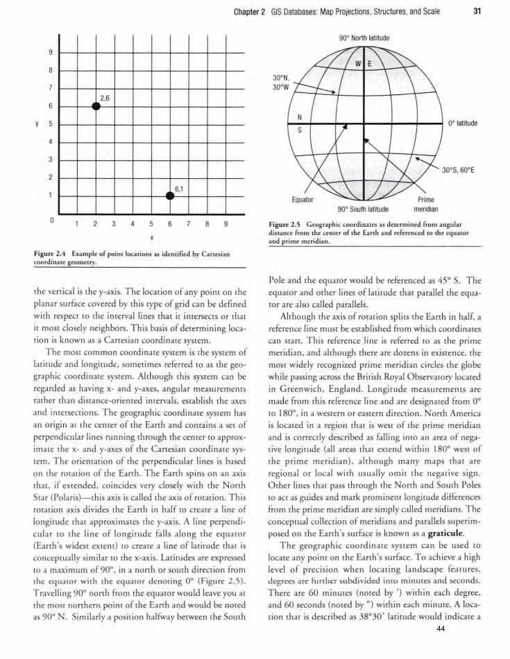
Chapter 2 GIS Databases: Map Projections, Structures, and Scale 31
9
8
7 2,6
6
y 5
4
3
2
6,1
o 2 3 4 5 6 7 8 9
x
Figur~ 2.4 Exampl~ of point locations as idcmtific=d by Cartesian coordinate geometry.
[he ve rr ical is [he y-axis. The (ocarian of any po int o n rhe
planar surface covered by rhis rype of gr id can be defined
wirh respec( to rhe inrerval lines that it inrersec(s or chat ir most closely neighbors. This basis of determining loca
rion is known as a Ca rtes ian coorcl inare sysrem .
The most common coordinate system is rhe sysrem of
larirude and longirude. someti mes refer red ro as rhe geo
graph ic coord inare sys tem . Although [his system can be rega rded as having x- and y-axes. angular measurements
miller than distance-orienred imervals. establish rhe axes
and imcrsecrions. The geographic coordinate sysrem has
an or igi n at rhe cenrer of the Earth and concains a ser of
perpendicular Jines running rhrough the cemer [Q approx
imate the x- and y-axes of rhe Cartes ian coo rd inare sysrem. The o rienrarion of rhe perpendicular lines is based
on the rota rian of rhe Earth . The Earth sp ins on an axis
rhat, if exrended, coi ncides very closely wirh rhe Norrh
Sta r (Polaris}-th is ax is is called the axis of rotarian. Th is
ro rario n axis divides rhe Earrh in half [Q creare a line of
longitude that approximares rhe y-axis. A line perpendi
cu lar to the line o f longitude fa lls a lo ng the equatOr
(Ea rth 's widest exrenr) ro crea re a line of lar itude that is
conceprually si milar ro rhe x-axis. Laritudes are expressed
ro a maxi mum of 90°, in a no[(h or sourh direction from Ihe equaror with the equamr deno[ing 0° (Figure 2.5) .
Trave ll ing 90° norrh from the equaro r would leave YO ll ar
rhe mosr norrhern poi nt of rhe Earth and would be noted
as 90· N. Sim ilarly a position half'vay between the South
90· North lalilude
0" latitude
30' 5,60' E
90' 5001h la1i1ude meridian
Figure 2.5 GC'ogr"phic coordinalC's as determ ined from angular distance from the cenler of the Earth and referenced to the equator and prime meridian.
Pole and rhe equato r would be referenced as 45· S. The
equator and orher lines oflatitude that parallel the equa
tor a re also called parallels.
Altho ugh the axis of roration splits the Earth in half, a
reference line must be established from which coord inares
can srart. This reference line is referred ro as [he prime
meridian, and altho ugh there are dozens in exisrence, rhe
most widely recognized prime meridian circles rhe globe
while passing across the Brirish Royal Observdtory located
in Greenwich, England. Longiwde measuremems a re
made from this reference line and a re designared from 0°
ro 180°, in a wesrern o r easrern di reccion. North America
is locared in a regio n (har is wesr of rhe prime meridian
and is correcrly described as falli ng inro an area o f nega
rive longi tude (a ll areas rhar ex tend wirh in 180° west of
rhe prime meridian) , alrhough many ma ps rhal are
regional o r loca l with lIsually omir rhe negarive s ign.
Other lines tim pass through the Norrh and South Po les
(0 acr as guides and mark prominent longirude differences
from rhe prime meridian are simply called meridians. The
conceprual co llecrion o f meridians and parallels superim
posed on the Ea rth 's surface is known as a grar.icule.
The geogra phi c coo rdina[e system ca n be used to
locate any po int on [he Ea rth 's surFace. To achieve a high
level of precis io n when locating landscape fea rures, degrees are funher subdivided imo minures and seconds.
There are 60 minutes (noted by ') wirhin each degree,
and 60 seconds (nored by") within each minme. A loca
[ion rhar is described as 38°30' laritude would indicare a
44
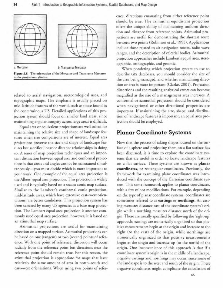
34 Part t Introduction to Geographic Information Systems, Spatial Databases, and Map Design
LZI ~ LL \~
LZ/ \~ L! \~
'\\ II ""'" \. /L/ '\:\ 17 ""'" \. /L/
a. Mercator b. Transverse Mercator
Figure 2.8 Thf: o ricnU.lio n of the Mercator and Tra nsverse MUC2tOr to the p rojection cylinder.
related [Q ae rial navigation. meteorological uses, and
[Opographic maps. The emphasis is usually placed on
mid-Iarlrude features of the world, such as those found in
rhe conterminolls US. Detailed applicarions of this pro
jection system should focus on smaller land areas, since
mainraining angular imegriry across large areas is difficult. Equal area or equ ivalent projections are wel l suited for
mainraining rhe relative size and shape of landscape fea
tures when size comparisons are of imerest. Equal area
projections preserve the siz.e and shape of landscape fea
tu res bur sacrifice linear or d isrance relationships in doing
so. A tenet of map projection techniques and an importam distinction berween equal area and conformal projec
(ions is rhat areas and angles cannor be maimained simul
taneollsly-you mUSt decide which is more important [0
your work. One example of (he equal area projection is
the Albers ' equal a rea projecrion. T his projection is widely
used and is typica lly based on a secam conic map surface.
Similar (0 rhe Lambert's conformal co nic projection.
mid-latitude areas, which have extensive east-wesr orien
[adons, are bener candidates. This projection system has
been selected by many US agencies as a base map projec
tion. The Lambert equal area projection is anomer co m
monly used equal area projection , however, i[ is based on
an az.imuthal map surFace.
Azimurhal projecrions are llseful for maintain ing
direction on a mapped surface. Azimmhal project io ns can
be based on one (ra llgem) or [wo (secam) points of refer
ence. Wirh one poilU of reference. distortion will occur
radially from the reference point but directions near the
reference poim should remain rrue. For this reason, the
az imutha l projectio n is appropriate for maps that have reladvely the same amoum of area in nonh-sourh and
east-west orientations. When using two points of refer-
ence. direcrions emanating from either reference point
should be true. The azimuthal equidistant project ion
offers rhe unique abi lity of maintaining uniform direc
tion and distance from reference poims. Azimuthal pro
jecrions are usefu l for demonstrating the shortest route
between tWO poims (Robinson et aI., 1995). Applications
include those related to air navigation romes, radio wave
ranges, and the description of celestial bodies. Azimuthal
projecrion approaches include Lambert's equal area, stere
ographic, orthographic, and gnomic.
\'Q'hen pondering which projection sysrem ro use to
descr ibe GIS databases , you should consider the size of
the area being managed, and whether maimaining direc
tion o r area is more important (Cla rke, 2001). ProjeClion
distortions and the resulring analytical errors can become
magnified as the size of a management area increases. A
conformal o r azimuthal projection should be considered
when navigational or other directional properties are
importanr. If maimaining the size, shape, and dis rribu
rion oflandscape featu res is important. an equal area pro
jection should be employed.
Planar Coordinate Systems
Now that the process of taking shapes located on the sur
face of a sphere and projecti ng rhem on a flat su rface has
been discussed. it is rime to explore the coordinate sys
tems that are useful in order (0 locare landscape features
on a flat surface. These systems are known as planar
coordinates. or rectangu lar coordi nates. Previously, [he
framewo rk for examining plane coordinates was intro
duced with [he concep( of the Cartesian coordinate sys
[em . Th is same framework appl ies to planar coordina res,
wirh a few minor mod ifications. For example, depending
on the type of planar coordinate systems. coordinates are
sometimes referred to as east in gs or nonhings. An eaSl
ing measu res distance easr of the coordi nate sysrem's ori
gin whi le a northi ng measures distance north of the ori
gin. These are usually specified by following the ' right-up'
approach; easrings are numerically organized so rhal pos
itive measuremems begin ar the o rigin and increase to [he
right (to rhe east) of the origin, while northings a re
numerically o rga n ized so that positive measu rements
begin ar the origin and increase up (to the north) of the
origin. One inconvenience of this approach is rhar if a
coordinate system 's origin is in the middle of a landscape, negarive eas tings and northings may occur, since some of (he landscape is (0 the west' and somh of the origin. These
negative coordinares might complicate the calculation of
45
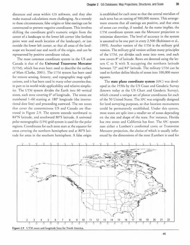
Chapter 2 GIS Databases: Map Projections, Structures, and Scale 35
distances and areas with in GIS softwa re. and rhey also make manual calculations more cha1lenging. As a remedy to these ci rcums[3nces. false origins or False castings can be constructed to prevent nega tive coordinates. This involves shifting rhe coo rdinate grid's numeric origin from the cemcr of a landscape ro rhe lower lefr corner (the fdrrhes( poim west and sourh locatio n o f rhe landscape), o r JUSt
outside rhe lower left corner, so that all areas of rhe landscape are IOC3ted east and north of rhe origi n. and can be represenred by posit ive coordinate va lues.
The most common coordinarc system in the US and Ca nada is that of lhe Universal Transverse Mercato r (UTM). which has even been lI sed to describe rhe surface of Mars (Cla rke, 200 I). T he UTM system has been used
for remOle sensi ng, foresrry, and topographic map applications. and if has been used in many ocher countries duc. in parr co its world-wide applicabili ty and relative simplicity. The UTM system d ivides rhe Earth into 60 vertical
lones, each zone covering 6° oflongirude. The zones 3re numbered I-GO starring at 1800 longirude (rhe inrernadonal dare line) and proceeding eastward. The ren zones lhac cover rhe conterminous US and Canada are illusrrared in Figure 2.9. The system ex rends norrhwa rd (0
84°N iarirude, and sourhward 800 S lari[t1cle. A universal polar stereographic (UPS) grid system is used for the polar regions. Coord inares for each zone scan af rhe equator for areas covering rhe nonhern hemisphere and at 800 S laritude fo r areas in rhe southern hemisphere. A fa lse origin
," ,'<.' ... '.' '.
is established for each zone so that the central meridian of each zone has an easting of 500,000 meters. This arrangemenr ensures rhar all easrings are positive. and that areas of zones can overlap, if needed. As the name implies, the UTM coord inate system uses the Mercaror projection ro minimize distortion. The level of accu racy in the sysrem is assumed ro be one part in every 2,500 (Robinson er aI. , 1995). Another version of the UTM is the military grid
version. The mili ta ry grid version utilizes many princi ples of the UTM, yet divides each zone inro rows, and each row covers 8° oflatirude. Rows are denoted usi ng rhe letters C ro X wirh X occupyi ng the no nhern lati tude between 72° and 84° latitude. The military UTM can be used to further define blocks of zones into 100,000 meter
sq uares. The state plane coordinate system (SPC) was devel
oped in the 1930s by the US Coast and Geoderic Survey (known today as the US C hart an d Geodetic Survey),
which created a unique set of planar coordinates for each of the 50 Uni ted Srates. The SPC was originally designed
fo r land surveying purposes, so that location monumems could be permanently established. Under this system,
mosr stares are spli t inro a smaller set of zones depending on rhe size and shape of rhe stare. For insta nce, Florida has twO zones and Ca lifornia has four. The SPC system uses either a Lambert's conforma l conic or Transverse Mercaror projection , the choice of which is usually influenced by rhe dimensions of the sta le (Lamben is lIsed for
• •
2 3 4 5 6 7 8 9 10 11 12 13 14 15 16 17 18 19 20 21 22
'. .• • FigUJ"~ 2.9 UTM "lon~s and longitud~ lin~s for North Am~rica.
46
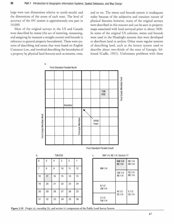
36 Part 1 Introduction to Geographic Information Systems, Spatial Databases, and Map Design
large wcsr-eaS( dimensions relative to north-south) and rhe dimensions of the zones of each srare. The level of
accuracy of rhe SPC system is approximately olle parr in 10,000.
Mosr of rhe o riginal surveys in the US and Canada
were described by metes (rhe act of metering. measuring, and ass igning by measure a straigh t course) and bounds (a reference [0 general property boundaries), These were systems of describing real esrare (hat wefe based on English
ammon Law, and involved describing rhe boundaries of a property by physical land feafllres such as streams, trees,
a. First Standard Parallel North
Baseline
and so on. The metes and bounds sysrem is inadequate
roday because of the subjecrive and transiem narure of physical features; however, many of the original surveys were described in this manner and can be seen in properry maps associated with land surveyed prior ro abom 1830. In some of [he original US colonies. metes and bounds were used in [he Head right systems char were developed [Q distribure land ro setders. Other more regular systems of describing land, such as rhe lorrery system used [0
describe abom two-thirds of the State of Georgia, followed (Cadle. 1991). Unforeseen problems wirh rhese
T2N R3E
I~ c
" Innial ~
:2 a; Point ,. ~ u .s 0:
First Standard Parallel South
b. T2N R3E c. NW 114 , NE 1/4, Seclion 17
6 5 4 3 2 1 NW1I4 NE 1/4 NE 1/4 NE 1/4
7 8 9 10 11 12 NW 114
SW 1/4 SE 1/4
18 17 16 15 14 13 NE 1/4 NE 1/4
19 20 21 22 23 24 N 1/2 SW 1/4
30 29 28 27 26 25 WII2 E 112 SE 114 SE 114
31 32 33 34 35 36 S 112 SW 1/4
Figur~ 2. 10 Origin (a), township (b). and ~ction (c) compon~nu of lh~ Public Land Su("\'~Y Syst~m.
47
Chapter 2 GIS Databases: Map Projections, Structures, and Scale 37
early surveying systems included extensive fraud . survey
ing errors, a lack of consistency in the surveying processes,
hostility fro m nat ives. and remoteness of rhe terrain. As a
resu lt. several rectangular systems of describing land were
proposed, ranging from 6 or 7 square miles to 1,000 o r 2,400 acres each (Ladell , 1993). These rectangular town
ships were meanr CO fac ilitate the development of communities (Stewart, 1979).
Th e recrangular US Public Land Survey System
(PLSS) system was established in 1785 by ,he US
Congress as a national system for the measuremenr and subdividing of public lands. Approximately 75 per cent of the US was su bject to measurement by rhe PLSS. The origina l 13 colonies, which com posed a significant holding, were not included in this system because rhey had
al ready been inventoried through meres and bounds systems. In 1872 a similar sysrem , the Dominion Land
Survey, was creared for adm inisrrarion of the Dominion
Lands of western Canada. The objectives of ,he PLSS and
Dominion Land Survey were ro quanrirariveiy measure
previously non-planed land , c reate land port io ns {hat
could be so ld o r discribured , and provide a means of
recording ownersh ip informatio n. Neirher sysrem is asso
ciared wirh a map projection and therefore neirher o ne
can be considered a coord inate system, ahhough you can
use rhem to specifY the general locar io ns of prope rty
boundaries or other features. These rectangular systems
begin wirh an in iriaJ po inr for a region, province, o r srate
rhro ugh which a prin cipal meridian is asrrollom ica lly derived (Figure 2.10). A baseline is also esrablished, and ir
intersects a principal poine at a righe angle ro the princi
pal meridian. For exam ple. 37 principal points exisr
wirhin (he US . In (he US, at 24-m ile interva ls north and
south of each b .. e1ine, standard parallels are established that extended east and west of the principal meridian
(thus parallel ro rhe baseline). Parallels are numbered, and
are referred to as either being north o r somh from rhe
baseline (e.g., 2nd parallel north or 7th para llel south of a baseline) . Guide meridians were also escabl ished at 24-
mile inrervals easr and west of the principle meridian. The
guide meridians were esrablished astronomically and are
numbered relative ro thei r posicion east o r wesr of rhe
principle meridian (e.g., 4th meridian e'dSt, 8th meridian
west of the princi ple meridian). The grid of meridia ns
and parallels crea tes blocks, each nominally 24 miles square.
Townships are created by fo rming range lines (run
ni ng north and south) and township lines (ru nn ing east
and wesc) boch ar six-mi le imervals. Each [Qwnship is six
mi les squa re, and is fu rther divided ineo secrions. with
each section measuring o ne square milei {here are 36 sec
[ions wirhin a rownship. Sect ions are numbered 1-36
with the 36th sect ion being ar rhe lower riglu-hand cor
ner of a [Qwnship. Sectio ns ca n be appo rrioned in to
smaller componems such as quarter sectio ns. half sectio ns, or quarrer quarrer sections. In {he naming co nven
tion, rhe smaJlesr component is named nrsc, scarr ing with
the porrion of a section rhar a piece of land res ides, then
the rownship, range, and name of the principal meridian.
An example would be the NWI/4, NE 114, Section 17, T2N, R3W , Mt Diablo Meridian. Use of ,he rectangular
systems is limired within GIS to visualizing survey sysrem
themes. but it is likely , especia lly in narural resource
applicar ions, that you will encoumer this system as your
wo rk wirh GIS progresses. T his is particu larl y true fo r
projects that involve properry ownersh ip issues , as most
properry locations and boundaries in areas covered by me
rectangu lar sysLems are described us ing sections, tOwn
sh ips, ranges. and principal meridians. At some po int YO LI
may be required ro re-p roject ow nersh ip boundaries
derived from rhe rectangular sysrems so [hat rhey march
the projectio n systems used in mher GIS databases.
Mismatched map projections have been the bane of
many spa rial analys is effof{s and do ubrless ly, [here are
many published and repof{ed smdy results rhat suffer from th is malady. The likel ihood is ,hat there will be
many future srudies and wrinen products {hat will also
be subject to map projection problems. One of rhe rea
sons fo r projections problems is thar many GIS users are
unaware of the intent of projec tions and fail ro realize
thar there are sub-com ponents, such as coo rdinate systems and datums, which need to be considered when
working with a projection. Anmher contribu tOr to rhis
problem is the inabili ty of many desktOp GIS softwa re programs to manipu late sparial database projections.
Although proj ect io n algo rithms are becoming more common in desktop CIS sofrware programs. they are typ
ica lly more robust in a fu ll -featu red GIS software pro
grams. As a CIS user or analys t, you must be cognizanr of
the projections that are associated wirh spatia l databases.
Wh en obtaining GIS databases , either from wi rhin or
from o U[side an organ ization, it is critical to obtain as
much information as possible abou r rhe structu re of rhe
data , wh ich should at leaSt minimally include info rmarion aoour rhe map projecrion. Information aboU[ spatial
databases ca n be stored in a metadata documenr. We'll
disc llss meradara in more deraillarer in this chaprer bur
turn ou r anemion now to GIS data structu res.
48
Chapter 2 GIS Databases: Map Projections. Structures, and Scale 37
early surveying systems included ex((nsive fraud. surveying errors, a lack of consisrency in the surveying processes, hostil ity from n~tives. and remoteness of the (ccrain. As a resulr, several reCtangular sysrems of describing land wore proposed, ranging from 6 or 7 square miles ro 1,000 or 2,400 acres each (Ladell, 1993). Thes< recrangular lOWI1-ships were meant fO facilitate rhe development of communities (Srew:m, 1979).
The rectangular US Publ ic La nd Survey System (PLSS) system was CSlablished in 1785 by the US Congress as a nalionaJ system for the measuremenl and
subdividing of public lands. Approximarely 75 per cem of the U was subjeCt to measuremenr by rhe PLSS. The
origin.1 13 colonies, which composed a significanl holding, were nor included in [his sysrem because they had
already been invenroried ,hrough meres and bounds syslems. In 1872 a similar system, rhe Dominion Land
urvey. was creared for adminisrration of the Dominion L1nds of weSlern Ca nada. The objec' ives of Ihe PLSS and Dominion Land Survey were [0 quantitatively measure
previously non-planed land. create land pardons th<lr could bc sold or disrribuecd. and provide a means of r~cording ownership information. Neither system is associated wi d1 a map projection and therefore neieher one can be considered a coordinaTe SYSTem , although you can use rh~m to specify [he general locations of pro perry
boundaries or other feacures. These r~clangular systems begin widl an inidal point for a region. provin e, or state through wh ich .1 principal meridian is astronomically derived (Figure 2. I 0). A baseline is also established, and il incersecls a principal point at a righe angle to the principal meridian. For example, 37 principal poin,s exist wilhin Ihe US. In ,he US, at 24-mile inlcrva ls north and sou,h of each baseline, Slandard parallels are eSl3blished that extended e:lst and west of rhe principal meridian (Ihus parallel to the baseline). Parallels are numbered, and :Ire referred to ~lS either being north or south From the basdine (e.g., 2nd parallel norrh or 71h paralld sou lh of a baseline). Guide meridians were also established al 24-mile intervals cast and west of the pri nciple meridian. The guide meridians were established astronomically and are numbered relarive to their posicion east or wesr of the principle meridian (e.g .. 4rh meridian east. 8th meridian west of the principle meridian). The grid of meridi:ans and pa rall els creales blocks, each nominally 24 miles square.
Townships are creared by forming mnge lines (run· ning north and soulh) .md (Ownship lines (running easT . Jnd west) borh :H six-mi le imervals. Each township is six
miles square, and is further divided into sections, with each section measuring one square mile; there are 36 seccions within a wwnship. Seccions are numbered 1-36 with [he 361h secrion being ar ,he lower righr-hand corner of a [Ownship. Sections can be apportioned inca smaller components such as quaner sections. half sections, or quarrer quarter seCTions. In the naming convention, the smallest component is named first, starting with rhe portion of a section thai a piece of land res ides, then the rownship. range, and name of the principal meridian. An example would be Ihe NWII4, NE 114, Sec,ion 17, T2N. R3W, M, Diablo Meridian. Use of [he rec,angular system is limited within CIS to visualizing survey sysrem themes, but it is likely. esp~cia ll y in namra l resource applicadons. that you will encounter th is system as your work wilh GIS progresses. This is particularly (Cue for projects rhat involve property ownership issues. as most properry locarions and boundaries in areas covered by We rectangular systems are described using sections. tOWI1-ships. ranges. and principal merid ians. At some poim you may be reqllired co re~p rojecr ow nership boundaries derived from the recrangular sysrems so [haT (hey match rhe projection systems used in Olher GIS dar-abases.
Misma(ched map projections h3ve been [he b"1I1e of many sparial analysis efrons and doubtlessly, ,here are many publ ished and reported study resules that suffer from Ihis malady. The likelihood is ,ha, rhere will be many furu re sruclies and wrirten products (har will also be subjec, ro map projecrion problems. One of Ihe reasons ror projc rions problems is [hal many GIS users are unaWate of the intent of projections and filii co realize that chere are sub-componellls. such as coordinate ys[CI11S and datums. which ne-cd to bl! considered when working with a projecrion. Another conrriburor (Q This problem is ,he inabiliry or many deskrop GIS soliware programs [0 manipuhne spatia l darabase projections. Although projection .t!gorithms are becoming more common in deskmp ~IS software programs, they are rypically more robuS! in a full-realured GIS sof,ware progr3ms. As a GIS user or ana lyst, you musr be cogniz31H of the projections that are associated wirh spatial databases. \Xlhen obtai ning GI. databases. either from within or from outside an organization. it is critical to obrain as mll h info rmarion as possible aboul the srrucrure of the data . which should at leas[ minimally include informalion .Jbour rhe map projection. Informadon 300m sprlli~1
darabases can be s[Qred in a metadara document. We'll discllss meradar3 in more detail laler in this chapter bur rurn OUt anC'mion no\ .... ro GIS data s(ru turd .
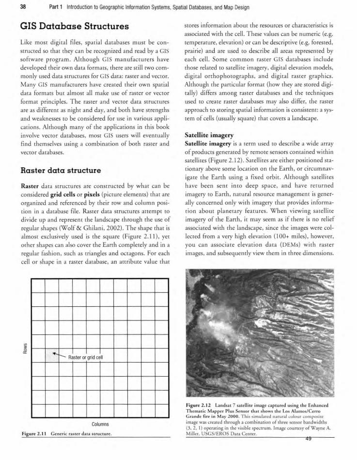
38 Part 1 Introduc1ioo 10 Geographic Informalion Syslems, Spalial Dalabases, and Map Design
GIS Database Structures
Like moS[ digilal fi les, spa(ial databases muS[ be con
S[ruc(ed so rim (hey can be recognized and read by a GIS
software program. Although GIS manufacmre rs have developed the ir own data fo rmats. there are st ill [wo com
monly lIsed data structures for GIS clara: rasrer and vector.
Many GIS manufacrurers have created their own spatial
dam formats bue al most all make lise of ras ter or veeror
formar principles. T he ras te r and vector data structures
are as diffe renr as n ight and day, and borh have strengths
and weaknesses to be considered for use in va rious appli
cations. Ahhough many of the applications in this book involve vector databases, most GIS users will evenrually
find themselves using a combinatio n of both raster and
veem f databases.
Raster data structure
Ras te r dara Strucrures are co nsrructed by whar can be
considered grid cells or pixels (picture dements) that are
organized and referenced by their row and column posi
tion in a darabase file. Raster data st ructures arremp{ (Q
divide up and represenr the landscape duough rhe use of
regu lar shapes (Wolf & Ghilani, 2002). The shape (har is
almost exclusively used is (he square (Figure 2. 11), yer
other shapes can also cover the Earth completely and in a
regular fashion. such as {riangles and octagons. For each
ce ll or shape in a rasrer database. an atrribure va lue [har
... r- Raster or grid cell
Columns
Figure 2.11 G~n~ric ra.Sler dala SlrUClure.
S(Qres information abom the resources or characrerisrics is
associated with rhe cell. These values can be numeric (e.g.
remperam re, e1evarion) o r ca n be descrip tive (e.g. fo rested,
prai rie) and are used to desc ribe all areas represented by
each cell. Some common rasrer GIS databases include
rhose rela red (Q satellire imagery, digiral elevation models.
digi(a l orthophotographs, and digita l raSler graphics.
AI(hough (he particular fo rmal {how they are stored digi
rally} d iffers among raster databases and the tech niques
used to creare raster databases may also diffe r, rhe raster
approach co scoring spatial information is consistem: a sys
rem of cells (usually square) that covers a landsca pe.
Satellite imagery Satellite imagery is a term used ro describe a wide array
of products generated by remore sensors comained widlin satellites (Figure 2.12). Satellites are either posit ioned sta
tio nary above some loca tio n on rhe Ea rrh , o r ci rcumnav
igate (he Earth using a fixed orbit. Although satellites
have been sent inro deep space, and have returned
imagery co Earth. nam ral resource management is gener
ally concerned only wirh imagery rhar provides informa[ion abo ur pla neta ry fearures. When view ing sare ll i[e
imagery of the Earth. ir may seem as if [here is no relief
associared with the landscape. since the images were col
lected from a very high e1evarion (l00+ miles), however,
you ca n assoc iate elevation data (OEMs) w ith raster
images, and subsequently view them in rhree dimensions.
Figure: 2. 12 La nds:H 7 sa te:lli l~ image capmred using Ihe: Enhanced Thema t ic Mapp~r Pl us Sensor that shows the Los AlamoslCe':rro Grande fire': in May 2000. This simulalcd natural colour compositc image was crealcd through a combination of Ihr« ~nsor bandwidths (3, 2, I) operaling in the visiblC' speCIrUIll . Image councsy ofWa)'llC' A. MillC'r. USGS/EROS Data Ontt"r.
49
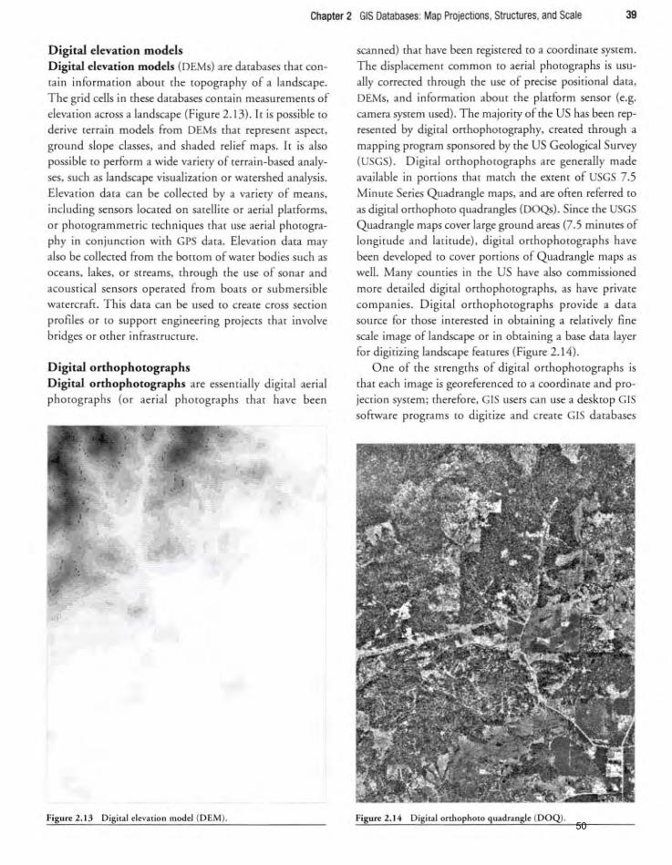
Chapter 2 GIS Databases: Map Projections, Structures, and Scale 39
Digital elevation models Digital elevation models (OEMs) are databases that conmin informacion abol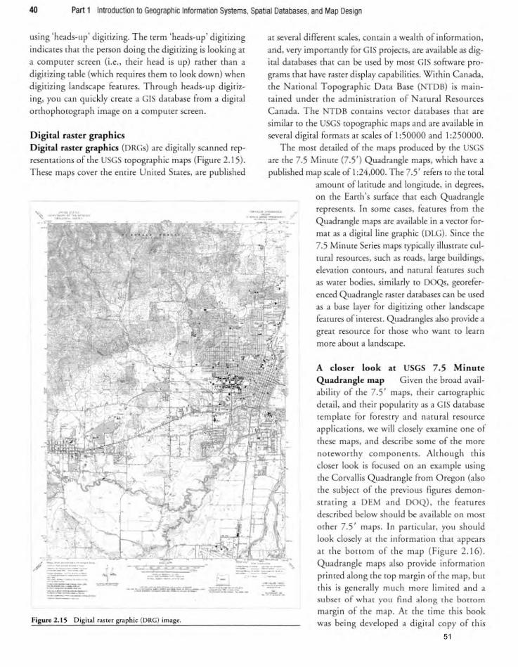
411 Part 1 Introduction to Geographic Information Systems, Spatial Databases, and Map Design
using 'heads-up' digirizing. The rerm 'heads-up' digitizing
indica res that the person doing the digitizing is looking ar a co mpurer screen (i.e., (heir head is up) rather than a
digitizing table (which requires rhem [Q look down) when
digirizing landscape fearures. Through heads-up digirizing, you can quickly creare a GIS darabase from a digiral
orrhophorograph image on a compurer screen .
Digital raster graphics
Digital raster graphics (DRGs) are digirally scanned represemarions of [he USGS topographic maps (Figure 2. I 5).
These maps cover the emire United Scares, are published
Figure: 2. 15 Digi[al raslc: r graphic (ORG) image:.
at several different scales. comai n a wealth of information, and, very importantly for GIS projec[5, are avai lable as digital databases that can be lIsed by most GIS sofrware pro
grams that have raster display capabilit ies. Within Canada. [he Nat ional Topographic Dara Base (NTDB) is main
tained under the adm inistration of Natu ral Resources
Canada. The NTDB contains vecror databases (hat are
similar to rhe USGS ropographic maps and are available in
severa l digital formars ar scales of I :50000 and 1:250000.
The most detailed of [he maps produced by [he USGS are rhe 7.5 Minute (7.5') Quadrangle maps, which have a published map scale of I :24,000. The 7.5' refers [0 [he total
amounr of laritude and longirude, in degrees,
on rhe Earth 's surface rim each Q uadrangle
.. ' ....... -- :..:.-=--~...:-
represenrs. In some cases, fearu res from the
Quadrangle maps are available in a vecror for
mar as a digi,al line graphic (DLG) . Si nce [he
7.5 M inute Series maps typically illustrare cul[Ural resources, such as roads, large buildings.
elevation conrours, and narural features such
as water bodies, similarly ro DOQs, georefer
ellced Quadrangle raster databases can be used
as a base layer for digitizing orher landscape
features ofinreresL Quadrangles also provide a
great resource for rhose who wam ro learn
more about a landscape.
A closer look at USGS 7.5 Minute Quadrangle map Given [he broad avai lability of [he 7.5 ' maps, rheir cartographic
detail. and their populariry as a GIS darabase
template for foresrry and natural reso urce
applic3rions, we will closely examine one of
rhese maps. and describe some of the more
norewonhy components. Alrhough this
closer look is focused on an example using
[he Corvallis Quadrangle from Oregon (also rhe subject of rhe previous figures demon
SHaring a OEM and DOQ), the reatures
described below should be avai lable on most
orher 7.5' maps. In panicular, you should
look closely at rhe information (hat appears
<I, rhe bortom of rhe map (F igure 2. I G) . Quadrangle maps also provide information
primed along rhe rop margin or the map, bur
rhis is generally much more limited and a subser of what YOli find along {he bonom margi n of [he map. A[ [he time this book was being developed a digi[al copy of ,his
51
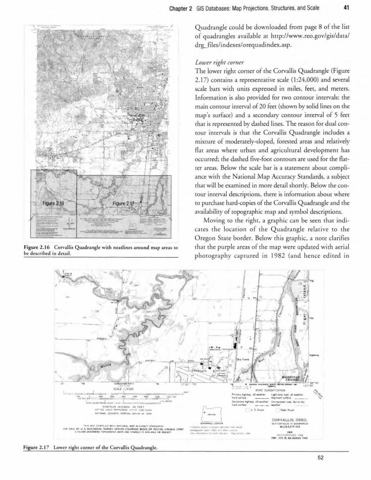
Chapter 2 GIS Databases: Map Projections, Structures, and Scale 41
Figure 2. 16 Corval lis Quad rangle with neatJines around map areas 10
be described in detail.
~
tot<'O"'~ ' .. 'L ..... ' :10 ,tU "" .D .... <~ "'1',_,,,, .. , " ""'" "".~ .... __ "" """oc.o.. 00,· • • ,_
.". ~ .... "" .. .... It ... , .. . ~" ....... _ ,,"U"';' " ... 1>0._ _000 5.0 .... u..L&cOlOGC.OI.~" Dl.....,. 0I:Il0lA00 aont.,OIIIUU ... _ .. _ .- ............ ---.-~.--- .... -~.
Figure 2.1 7 Lower right corner of the Corvall is Quadrangle.
Quadrangle could be downloaded from page 8 of the list
of quadrangles avai lable at Imp:llwww.reo.gov/gis/data/ drg.,files/indexes/orequadindex.asp.
Lower right corner
The lower right corner of the Corvallis Quadrangle (Figure
2.17) contains a representative scale (1 :24,000) and several
scale bars with units expressed in miles. feet. and meters. lnfo rmarion is also provided for (Wo comour inrervals: the main contour inrerval 0(20 feet (shown by solid lines on the map's su rface) and a secondary contour inrervaJ of 5 (eet
that is represented by dashed lines. The reason for dual conlOur intervals is that the Corvallis Quadrangle includes a mixture of moderately-sloped, forested areas and relatively
fl ar areas where urban and agricultural development has occurred; the dashed five-foor contours are lISed for [he flar
rer areas. Below the scale bar is a sraremenr about compliance with the National Map Accuracy Standards, a subjecr rhar will be examined in more derail shoerly. Below the con
tour inrerval descriptions. there is informat ion abom where to purchase hard-copies of [he Corvallis Quadrangle and the availabil ity of topographic map and symbol descriptions.
Moving to rhe right . a graphic ca n be seen that indicates rhe location of rhe Quadrangle relative (Q rhe
Oregon State border. Below [his graphic, a note clarifies (hat [he purple areas of (he map were updated with aerial
photography captured 111 1982 {and hence edited in
, l • I
!, ~ .. , •
~ < ~
~ • :; 1 ' ~
I .. j.
r ,. J : •
~ ' <
. \ r
i .... ... ,,/
""-'J"-'._ l4M .... _._ """_.co _ ____ _ -..,~ .. ..... """ ..--- ..... ., --- ----r-, ' __ I "'~ --
L I CORVALUS.OREO --- __ .... 'r~ - _ .... _--_ .. " 'l) U-JJ-OU __"",".a; .. ____ ... --......... Y,,-- ,-1'toO'<lIIf"o~n,_ - ,,, .. _-
~
1_ .
52
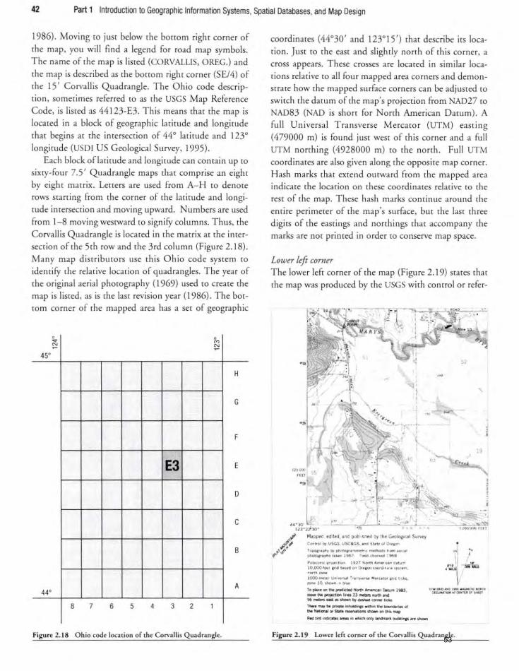
42 Part 1 Introduction to Geographic Information Systems, Spatial Databases, and Map Design
1986). Moving ro JUSt below the bottom right corner of
the map, you will fin d a legend for road ma p symbols.
The name of the map is liSted (CO RVALLIS, OREG.) and
the map is descr ibed as ,he bottom righr corner (SE/4) of rhe 15' Corvallis Quad rangle. The Ohio code description, sometimes referred (Q as rhe USGS Map Reference Code, is liSted as 44 I 23-E3. This means rim the map is
locared in a block of geograph ic lar irude and longitude that begins at rhe intersection of 44° larirude and 1230
longirude (USDI US Geological Survey. 1995).
Each block oflarirude and longirude can comain up ro sixry-fou r 7.5' Quadrangle maps rhar comprise an eigh r by eight matrix . Leners are used from A- H [0 denoce
rows starr ing from rhe corner of rhe latitude and longitude inrersecdon and moving upward. umbers are lIsed from 1- 8 movi ng westwa rd [Q signify columns. Thus, rhe Corvallis Quadra ngle is located in [he matrix at the inrersecrion of rhe 5rh row and the 3rd col umn (Figure 2.18).
Many map disrriburo rs use th is Ohio code system to
idenriry rhe relative location of quadrangles. T he yea r of rhe o riginal aerial ph orography (1969) used to create rhe map is liSted, as is the laSt revision yea r (1986). The bot
rom corner of the mapped area has a set of geographic
, , ~ M ~ ~
45'
H
G
F
E3 E
D
C
B
A 44'
8 7 6 5 4 3 2 I
Figu.rc 2. 18 Ohio codc loca ti on of the Corva.l lis Quadrangle.
coo rdinates (44°30' and 123°15') rhat desc ribe itS loca
rion. JUSt ro the east and slighdy north of (his corner, a cross appears. These crosses are loeared in simila r loca
tions relative [0 all four mapped area corners and demonstrate how the mapped su rface corners can be adjusted [0
switch rhe datum of rhe map's projection from AD27 ro
NAD83 ( AD is short fo r North American Datum). A full Universa l Transverse Merca to r (UTM) casti ng
(479000 m) is found JUSt weSt of this corner and a full
UTM northing (4928000 m) to Ihe north. Fu ll UTM
coordinates are also given along the opposite map corner.
Hash marks [hat extend o utward from {he mapped area
indicate the locat ion on rhese coordinates relative ro rhe
rest of the map. T hese hash ma rks continue around rhe emire peri meter of rhe map's su rface. but the last three
digits of rhe easri ngs and notthings that accompany the marks are nOt primed in order [0 conserve map space.
LOlUty Itft comty The lower lefr corner of the map (Figure 2. t 9) States thar
[he map was produced by (he USGS with control o r reter-
"--":'
1'oIoo<""".,00K1_ 1927 .... "' ........ U"Ie.'~~ 10,()()O<_ .. ..t "" ... a~ 0. ..... <_4,." •• ,.,_. " .. 1 ~ .....
1000 .... .. ' U"..WI • •• • ..... w "' .... tot I~C Uk>. _10_,,101_ T. pIocI __ 1"tId"' .. """", ""-"-' DoIurot 1M.), __ -u. ..... U __ " ._--- .... - .. _-___ ... _--.._ .... --.01 t1-.frUoI_ .. SIt1Oo __ ..... .....
, ( , ,
,.,. ..... __ .. _......,--...... -
,
w- .. .... _ , __ "" _ ... --' .... """ ...... "",.
Figure 2. 19 Lower Itfl corner of Ihe Corvallis Quadrangle. 53

Chapter 2 GIS Oatabases: Map Projections, Structures, and Scale 43
ence points eStablished by [he USGS, US CoaSt and Geode[ic Survey, and [he S,ate of Oregon. Mapped sur
Faces were taken from 1967 ae rial photography and were field checked in 1969. Projection info rmacion is rhen listed and the base su rface is described as a polyconic projection, NAD27, using [he Oregon S,a,e Plane Nonh
Coordinate System. A line follows (Q describe rhe coloring of rhe UTM coordinates that are listed around rhe perime[er of ,he map, and [he UTM zone (10) [hal was used.
Instructions for converting rhe mapped su rface from NAD27 to NAD83 are also given and provide a quanti[a
rive assessmenr of how these twO darums differ in the quadrangle area. This information is useful for porenrial coordinate conversions in a GIS. In addition. the text states
(hat only la ndmark buildings are shown in map areas [hat 3re tinted red . Landmark buildings are those that serve rhe public. have cuimrai or historical significance. or are unusually large in relation to surrou nding buildings.
To [he righ[ of rhese S[3(ements, a graph ic at rhe map's orientation [0 seve raj definirions at norch is shown and text below the graphic explains that the orientation is trom the map's center. The longest nonh line is topped by a Sta r symbol and refers to asrronomic norch. The line to [he left of as tronomic nonh refers to grid nonh (GN) and is oriented 0°13' (0.22°) wesr ot astronomic nor[h. Grid norch is rhe direcrion in which rhe Oregon Stare Plane Coordinare Sysrem is reterenced. The line ro rhe right at asrronomi c north shows rhe magneric declinarion (19° easr), relarive [Q astronomic norrh, thar exiSled in 1986. Since magnetic nonh can Auctuate trom yea r [Q
year (even small daily shifts are also possible), ,he dale of (he measuremenr is imporranr tor those who wish (0 COI1-
ven [heir data to match the map's projection. Geographic coo rdinates appear at rhe sourhwesr cor
ner at rhe mapped su rtace, an d rhe UTM coo rdinate abbrev iations are li sted. A full listing of Stare Plane Coordina[es (NAD27) are liSted and also marked by harch lines to [he nonh (320,000 feet) and eaSt (1,260,000 feet) ot this corner. Full srare plane coordinares are also listed along rhe upper righr corner. Unmarked hash marks around the rest of {he map's perimeter denore gradations of the stare plane coordin ates. Periodically, range and township divisions appear as longer dashed. lines on {he map's surface. Along [he la[i[udinal axis of Figure 2. 19, you can see R. 6 W. and R. 5 W. T his signifies [he d ivi sion berween Range 6 and 5. west of (he reference meridia n (Willamene) rhar was lIsed for crearing rhe PLSS tor Oregon. Larger numbers appea r on the mapped surface and describe the boundaries between secrions and donation land claims (DLCs). As menrioned earlier in this chap-
rer, most of the wesrern US was originally divided according to [he PLSS. The PLSS spli[ regions of [he US in a grid
of townships (approximately six by six mile blocks created by rhe inrersecrions of township and range lines) (hat were created from a reference meridian with townships furrher divided into secrions measuring approximarely one square mile. Section numbers range fro m 1-36 in almost all PLSS
srates rhough you might find an occasional secrion numbered 37 where measurement irregularit ies warranted adjustments to rhe PLSS. Some stares, including Oregon , Florida, and New Mexico, had adopted less rigorous land measu rement systems [hat superseded the PLSS. Through
rhese sysrems, serders could srake cla ims (Q lands and rhese systems were generally referred to as DLCs. DLC bound
aries are numbered. srarring with 37. In general, green shading (gray in the black and while
image of Figure 2.19) is used to represenr foresred or narlIral areas, and no shad ing is used to represent developed areas. Roads. screams, and other cultural and "arural landscape featu res are also visible rhroughour the map.
National Map Accuracy Standards
Accord ing (Q informacion illusrrared in Figure 2. 17. rhe Corvallis Quadrangle map complies with [he Na[ional Map Accuracy Standards ( MAS). The US Bureau of [he Budge[ originally developed these standards in 194 1 so ,hal guidelines wou ld be available for [he establishment of
horizontal and vertical map accuracy a[ multiple scales. The guideli nes were also intended (Q help protect and inform consumers aOOm rhe qualiry of map products rhey acquired. The guidelines assume that organizations claiming adherence ro NMAS guidelines are responsible fo r ensu ring compliance. The NMAS was lasr revised in 1947 (Thompson , 1979) .
The guidel ines (Figure 2.20) provide horizontal accuracy standards for map scales larger [han I :20,000, and for
scales a[ I :20,000 or smaller. For [he larger map scales, no more than 10 per cem ot rhe points verified shall be in error by 1/30th of an inch, as measured on the map su rface . For smaller scale maps, this tolerance is 1/50th of an inch. The Corvallis Quadrangle Falls in the laner category. To resr tor NMAS compliance, locations or elevations from map poims are compared to their acrual measuremems, where locadons or e1evarions have been derived by highly accurare ground surveys. Within these comparisons, only 10 per cem of (he points ca n be in error by more than me tolerance. Table 2.1 describes the tolerances in relation ro some of rhe more common map scales. For [he Corvallis Quadra ngle, [his [hreshold wou ld be 40 feet,
indicating rhar nor more r.han 10 per cem of rhe rested 54
Chapter 2 GIS Databases: Map Projections, Structures, and Scale 43
ence points established by rhe u. G ,U CoaS! a nd Geodetic Survey, and the Srare of Oregon. Mapped surF.rces were raken from 1967 ae rial phorography and were fiel d checked in 1969. Projeclio n info rmarion is then lis red and ci,e base s" rflee is described as a polyconic pro
jection, NAD27, usi ng the Oregon Srare Plane Nonh Coordinal< ystem. A line follows to describe the coloring of {he UTM coordinmes th iU are lisred around [he perime~
rer of the map, and the UTM zone (10) rim was used .
InSHlIcrions fo r convening rhe mapped surface from
NAD27 to NAD83 are also given and provide a quanti tative assessmelH of how these twO datums differ in th t
quadrangle area. This information is usefu l for pOlcnrial coordinate conversions in a GI . In addition. [he [ot( srates Ihat only landmark buildings arc shown in map areas [hat are rimed red. Landmark buildings are [hose dlat serve the public. have cu ltu ral or historical sign iftc3 l1ce. or are unusually large in relarion ra surrounding buildings.
To lhe righl of these Slatemen lS, a graph ic of rhe map's orienrarion m severaJ definidons of nonh is shown and (exl bc:low the graphic explains that the orientation is fro m the map's center. The longest nonh line is lopped by a Sta r symbol and refers to astronom ic nord,. The line [Q the lefr of astronomic norrh refers to grid norrh (GN) and is o riented 0° 13' (0.22°) west of astronomic north.
Grid north is (he dire rion in which rhe Oregon State Plane Coordinate ysrem is referenced. The line to (he right ofast'ronomic north shows the magneric declination (190 east), relative [0 astronomic nonh. [hat existed in 1986. ince magnetic north can AucUlate from ye-A r (0
year (even small daily shifts are also possible), the date of the measurement is important for those who wish [0 convert their data to march rhe map' projection.
Geographic coo rdinates appear ar rhe sourhwest corner of rhe mapped surface. and rhe UTM coo rdinate abbreviations are lisred . A full lisring of Stare Plane Coordinates (NAD27) are listed and also marked by harch lines to lhe norrh (320,000 feer) and eaSt (1,260.000 leer) of this corner. FilII stare plane coordinates are also listed along the upper right co rner. Unmarked hash marks around the resr of the map's perimerer denote gradations of rh e sta re plane coordin ares. Periodicall y. range and township divisions appear as longer dashed lines on the map's surflee. Along the latitudinal axis of Figure 2. I 9, you em see R. 6 W. and R. 5 W. This signifies rhe d ivision between Ra nge 6 and 5. wesr of the reference merid~
ia n (Willamcne) [hat was used for cre-dring the PLSS for Oregon. Larger numbers appear on the mapped surF.rce and describe the boundaries between sections and donarion land claims (OLCs). As menrioned earl ier in this chap-
[(r, mOSt of the western U was originally divided according [0 rhe PIS. The PLS splir regions of lhe U in a grid of rownships (approximately six by six mile blocks created by rhe intersecrions of mwnsh ip and range lines) thar were creared from a reference meridian with townships furrher divided into ections measuring approximately one square mile. ection numbers range fro m 1-36 in almoSt all PI_SS
srares though you might I1nd an occasional section numbered 37 where measurement irregularities warr3IHed adjus[mems to the PI..5S. orne Slares, including Oregon . Florida, and ew Mexico, had adopred less rigorous land measurement sysrems rhat superseded lhe PLSS. Through
these systems, sealers could stake cla ims [Q lands and rhese systems were generally re!erred to as DL . DLe bound
aries are numbered srart ing with 37. In gener. l, green shading (gray in the black and white
image of Figure 2. 19) is used to represen t fo rested o r nar
ural areas. and no shading is used to represeO( developed areas. Roads, streams, and other cultural and natu ral landscape featu res arc also visible throughout [he map.
National Map Accuracy Standards
According to information illustmed in Figure 2. I 7. the orvallis Quadrangle map complies wirh lhe National
Map Accuracy Standa rds (NMAS). The U Bureau of rhe Budger o riginally developed [hese standards in 194 I so that guidelines would be available for [he establishment of
horizontal and verrical map accu racy at multiple scales. The guidel ines were also intended [0 help protect and inform consumers abom the qualiry of map product they acqui red. The guidelines assume thar orga nizations claiming ad herence to NMAS guidelines are responsible for
ensuring compl iance. The MAS was last revised in 1947 (Thompson, 1979).
The guidel ines (Figure 2.20) provide horiwnral accuracy standards for map scales larger [han I :20,000, and for
scales at I :20.000 o r smaller. For lhe larger map scales, no more than 10 per cem of rhe points verified shall be in error by I130r h of an inch. as measured on rhe map surF.ce. For smal ler scale maps, this rolerance is I 150rh of an inch. The Corvallis Quadrangle F.rlls in Lhe latter Cl tegory. To (esr ror NMAS compliance. locations or elevations from map points are compared to their actual measuremems, where locations or elevations have been derived by high ly accurate ground surveys. Within these comparisons, only 10 per cent of the points ca n be in error by more lhan Lhe tolerance. Table 2. I describes rhe tolerances in relation ro some of the more common map scaJes . For the Co rvallis Quadrangle, this threshold would be 40 feer, indicating rhat not more {han 10 per cenr of rhe lested
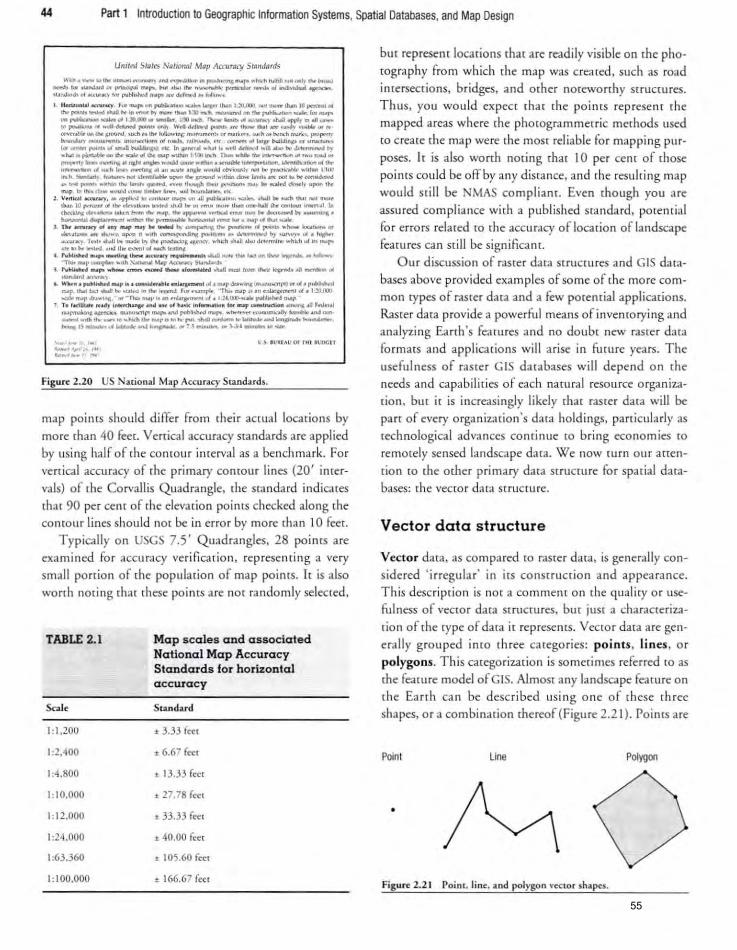
44 Part 1 Introduction to Geographic Information Systems, Spatial Databases, and Map Design
Umlnl Stllt~ NfltlOlUU Map /\((1IMy SIIIIIdllfds
\'oOI. __ "'doo ___ .... pNI .. "''''~'''''I''' .. hIrto'''!,-ill ......... , .... 1>ro.od
..... 100 .u...wcl '" I"'ftCIf"I _"". I>uf .......... "" ...... "'" porunol>r -.. oI ..... idouI .. ...-our40,c!' «j .. ,,,,";v!IlI .... blbhaI .... po..., ~ .. ~.
I . ..... -.1 ~....,. . . ............ OII.....-- ..... 1Mpt I ..... 1-3I.IlUD...,. ........ tlw .. }O ptm'N 01 1hr~_.wloor .. _~ __ l "lC1_1>.-..-..d ....... ~~""""-r> .. ~~...,.,.,. <It 1.lO,cro. -a.... l -,o!nth. ".".. __ .. ---,- .twII""Y"" 00 ..... .. ~.,. ....,..6ffitw,J J"IItIl.. 00II) w" dtm.:.i 1""_ .... ,"'-!Nt ........ '" """""' ...... "",,, •• bIIoOllIN pound. ouch o. """ klIIow...,; _"""",t ... .... 11 ..... """" Of to.·""h .... , .... I""'I"'fn· 10. ... ......., . .-......mIl; _o«tl<>nJ "' ....... ,.oi~ •• "'" --" 011.0 .. buIldlrop ......... ,.. ..... ( .. _.-.ol.....n~ ttc.1n ............ k,otlo .. .,.dftirW'd __ Ioo~_~
"!wl"~"" Ihr,.,. '" Lht .... ...u.. 1100.,.h no ..... hAI rtIr...--- "' ...... 0\l00J Of
~ ...... -... .. ~~ .. .-IJ_ .. Ilhon.omoilIkl~.~~ ..... "'1hoo __ ....... '" -tI rw-. _ .... AI ..... __ ............ Id ob>->ouo.lv _ boo p' ....... bIrt wi,,,," "'-0
nIL ....... ;,,;....,..... _ u,.,.a.f..w.. "f'M .... 5""'tw;! .. iIhon cIo+r 1orIoiI. ~ ""' ... bot ~'II o. _ I"""" ... "'" rho- -'..,.-l "" ... th."'I!h ,,..., ._ .... \ bot __ . 1«.1 dootIj wpon Ihr ... plftlh;.<il..i""-..w«l'llf ............... .... ~ ...
2. V ............ "')' .... "rP'1od •• ru .. _ ""'1" "" .011 poaI.u.-...... """';.,., .li.oii bot.....,. th.I. !WI _
dldnW,..,..,.., .... , .... ...,., ............. ..,>h.oIIbt ................ ltt.tn ' ..... ...uIhe""'lOoninw ... ·.oI tr. ~ .... ..-.- .. ...". 1ft ... ,Iw..,. "'" oPf>M"" wttIC4II ...... _ .... -..",.,.,;1.,.. ~. ~~- .... ,..,..........~ .......... • ... r~~.".,"'"""
). n.. MftI."'Y ., .., ..., .or ... -.II t... """f'U"'I "'" ,.- '" "' ....... ",,,,- Ioc.o_ .. ...... _ ..., ....... n ap. ....... ~II _~ r-- .......... "'"""-'d by ............. ..r 4 hr~
• ", ........ rht. """~ to. nwde l') , .... pn>d ........ ~ .~~ .... "' .. whkh .ho.lI ...... Jo1<'rml ...... hl<h,~ 11> .... 1" _.,l't~ • ...,Uwn_ol...ch1dC!ft,t
L p,.........r .. ,.~ ... u-._..,.""'I-...- oh.oII_dwf..a_ ....... ~ .. "*""" -n.._,,"-rt- ""Ito ~ Moop _4C)'St.t~
, . hlolitoMd..."._ ........ ___ .f~ ohalI_ ""'" '''''''."'''''' _ ...... "'''' _..I""", .. )' •. "' ..... . ,.....;.a,.,., ....... -... ..... ~"'._pJr ... 'Injr (-...-. .... p'l"''''.f'''W'"''td INJ' '''''' *" ...... t. .... ,0<1 '" "'" IfrJ "" ~""""" ·ill .. ""'I' It ... ~.!I"_ 01. I~.tm ••• 01 ....... Ju~, ", .. -0. .... " ~~"...,tup_ ~ . r.!4.00J..c.0Io,.....IIN .... p
7. T. roc\u,OI, nooly I .... rdt.at>s • ....r ... of It.Ml< h.~1oot "" ... ,. c-Irudlooto _ .. 011 r...kt.r "..~ ~ ..... 1>IIiCrif'I .... "" o.nol pu/>Ikht<l-r-. w""'"' ..... ~ ........ __ <mi' _ ......... • ......... _""_rlO ... Io.:F"". _ ......... .......-_~~ ....... ~IS_ ... '"*"-..-J~."'~,-. ... }..J. ~_ ... _
•• _,,..... ,01 , , .. . UIl .. u Of THlluocrr
_'''':'''1'1< _,. ... 1· ,... ·
Figur~ 2.20 US alional Map Accur:.lIcy Slandards.
map points should diffe r from rhei r acmal locadons by
more {han 40 feer. Vertical accuracy srandards are applied by using half of rhe comour inrerval as a benchmark. For
verr ical accu racy of rhe primary COntour lines (20' inrer·
vals) of the Corvallis Quadrangle, the standa rd indicates char 90 per cenr of [he elevation points checked along [he contour lines should nor be in erro r by more [han 10 feer.
Typically on USGS 7.5' Quadrangles, 28 points are examined fo r accuracy verificatio n, representing a very
small portion of rhe population of map poims. h is also worth noti ng thar rhese poims are not randomly selected,
TABLE 2, \
1,1.200
102,400
1,4.800
UO.OOO
1,12,000
1024,000
1,63,360
uoo.OOO
Map scales and associated National Map Accuracy Standards for horizontal accuracy
Standard
:l 3.33 f~~l
:l 6.67 fcel
:l 13.33 feel
.t. 27.78 fcci
.t. 33.33 f~el
J: 40.00 feel
:l 105.60 fC~1
± 166.67 fee l
bur represent locations that are read ily visible on the pho
tography from which the map was created, such as road i nrersections, bridges, and other noreworthy srructures . Th us, you wo uld expect that the po ims represem [he mapped areas where the phorogramme[ric methods used ro crea te the map were [he most reliable for mapping pur
poses. I t is also worth noring rhat 10 per cem of those po ilUS could be off by any distance, and [he resulting map would still be MAS compliant. Even though you are
assured compliance with a published standard, potenrial fo r errors related to the accuracy of locarion of landscape featu res can st ill be signif\canr .
Our discussion of raster data s[rucrures and CIS databases above provided examples of so me of the more common rypes of raster data and a few porenrial applications . Ras[er data provide a powerful means ofinvenrorying and analyzi ng Earrh 's featu res and no doubt new raster dara
fo rmats and applica rions will arise in future years. The usefulness of raste r CIS databases will depend on the needs and capabil iries of each narural resource organization. bur if is increasingly likely that raster data will be parr of every o rganization 's data holdings. parr icularly as technological adva nces conrinue ro b ring economies to remmely sensed landscape data. We now {Urn our atten
tion to the other primary data strucru re fo r sparial databases: the vector data structure.
Vector data structure
Vector dara. as compared to raster data , is generally considered ' irregular ' in irs construction and appearance. T his descrip tio n is nor a co mmenr o n the quality or usefulness of vector data srrucrures. bur JUSt a characreriza
rion of rhe rype of dara it represems. Vecro r data are generally grou ped inro three catego ries: points, lin es, o r polygons. This categorization is sometimes referred (0 as
rhe fearure model of GIS. Almost any landscape feature on rhe Earth ca n be described usin g one of these three shapes. or a combination thereof (F igure 2.21). Points a re
Poin t line Polygon
Figur~ 2.21 Poine . line, and polygon v«to r shapes.
55
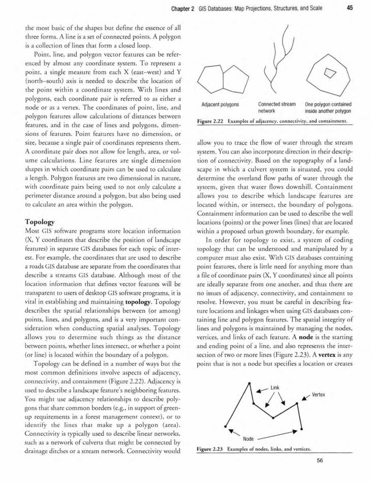
Chapter 2 GIS Databases: Map Projections, Structures, and Scale 45
rhe mOSt basic of rhe shapes btl[ define the essence of all
three fo rms. A line is a set o f connecred paines. A polygon
is a co llection of lines thal form a dosed loop.
Poim. line, and polygon vecror fearures can be refer
enced by almos[ any coordinare system. To represent a poinr, a si ngle measure from each X (east-west) and Y (norch- sourh) axis is needed ro describe rhe location of
rhe poinr wi th in a coo rdina te system. Wi th lines and
polygons. each coordinare pair is referred [0 as either a node o r as a venex. The coo rdinates of poinr, line, and
polygon fearures allow calculations of distances berween
features. and in rhe case o f lines and polygo ns, dimen
sions of featu res. Point features have no dimension, or size, beca use a single pair of coordinares represenrs rhem.
A coord inare pair does nO{ allow for length, area, or vol
um e calc ulatio ns. Line feawres a re singl e dim ensio n
shapes in which coordina[e pairs can be used ro cakulare
a length. Polygon features are rwo dimensional in naru re. wirh coo rdinate pairs being used ro nor only cakulare a
perimeter d isrance a round a polygon. but also being used
ro calculate an area within rhe polygon.
Topology
Most GIS software programs Sto re loca tion informacion
(X, Y coordinates that describe the position of landscape
feam res) in separate GIS dacabases fo r each ropic of inrer
est. For example. the coordi nates that are used ro describe
a roads GIS database are separate from the coordinales char
describe a ",earns GIS database. Although moS( of the
location information thar defi nes vec[Qr feamres will be
rransparent to users of desktop GIS software programs, it is
vital in eS(abl ishing and mai nrai ning topology. Topology
describes the spatial rela tionships between (or among)
poinrs. li nes. and polygons. and is a very important con
siderarion when conducling spatial analyses. Topology
allows you [Q delermine such thin gs as the distance
between points. whether lines intersect, or whether a poi nr
(or line) is located within the boundary of a polygon.
Topology can be defined in a number of ways but the
most common defi nitions involve aspects of adjacency,
connectivity, and conrainmenr (Figure 2.22). Adjacency is
used ro describe a landscape featll re's neighbo ring features.
You might use adjacency relationships to describe poly
gons rhat share common borders (e.g., in support of green
lip requi remenrs in a forest managemenr conrexr). or to identify lhe lines rhal make up a polygo n (a rea).
Connectivity is rypically used (0 describe: linear ner\vorks, such as a network of culverts thar m ight be connected by
drainage d itches or a sr ream network. Connect ivity would
co Adjacent polygons Connected stream One polygon contained
network inside another polygon
Figure 2.22 Exam ples of adjacency, conn~ctivity, and containment.
allow you ro (race rhe fl ow of water (hrough [he stream
system. You can also incorporare direction in [heir descrip
tio n of connectiviry. Based on the topography of a la nd
scape in which a culven system is siruared , you cou ld
determine the overland fl ow paths o f warer rhrough the system, given tha[ water flows downhill. Conrainmenr
allows you (0 describe which landscape features a re
located with in . o r inrersect, the boundary of polygons.
Conrai nmenr in fo rmat ion can be used ro describe (he well
locations (points) or the power lines (lines) that are located
within a pro posed urban growth boundary, for example.
In order for ropology (Q exist. a system of coding
topology thar can be undersrood and manipulated by a
computer must also exist. With GIS darabases co mai ning
point features, there is li[tie need for anythi ng more than
a file of coordi nare pairs (X, Y coordinates) since all points
are idea lly separa te from one another, and thus there a re
no issues of adjacency. co nnectivi ty. and comainmenr ro
resolve. H owever, you must be ca reful in describing fea
ture locations and linkages when using GIS databases con
taining line and polygo n fearures. The spatial integrity of
lines and polygons is mainrained by managing rhe nodes.
ve rtices. and links of each feature. A node is rhe starring
and ending point of a line. and also represents rhe inter
section of twO or more lines (Figure 2.23). A vertex is any
poim rhar is nor a node but specifies a location or creares
¥ Vertex
.........Node ----
Figure 2.23 Examples of nod~$, links. and vertices.
56
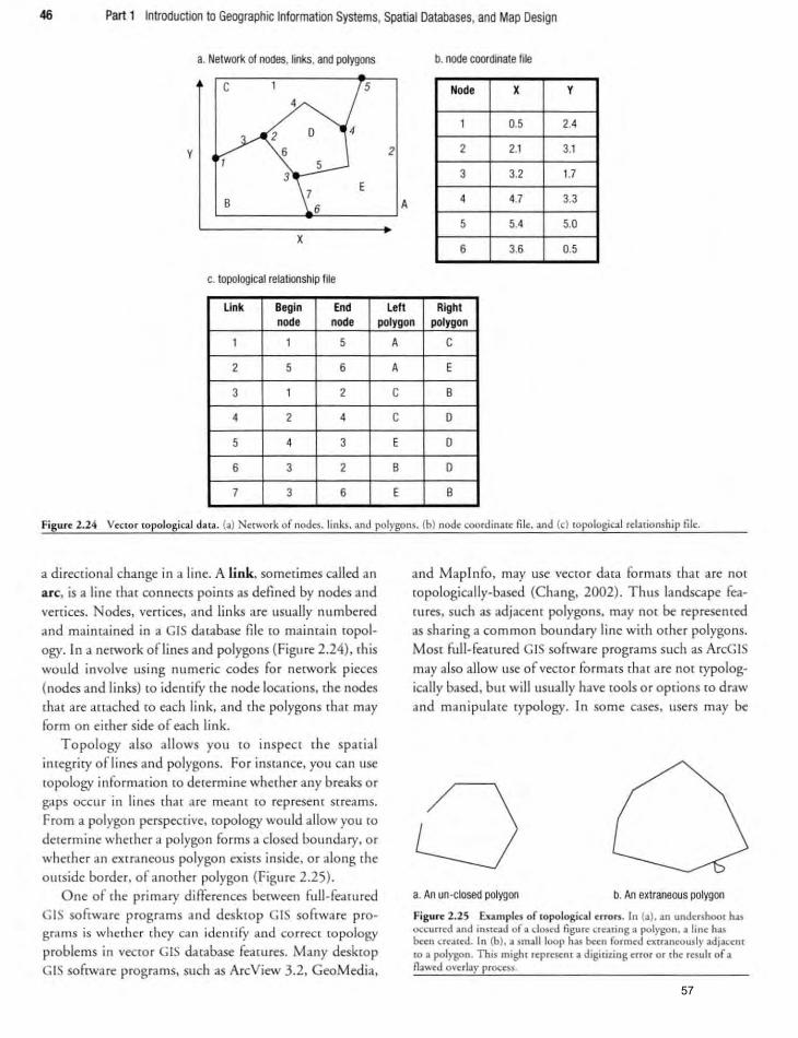
46 Part 1 Introduction to Geographic Information Systems, Spatial Databases, and Map Design
a. Network of nodes, links, and polygons b. node coordinate file
C 5 Node X Y 4
2 0 1 0.5 2.4
Y 6 2 2 2.1 3.1
5 3 3 3.2 1.7
7 E
B 6 A 4 4.7 3.3
5 5.4 5.0 X
6 3.6 0.5
c. topological relationship file
link Begin End Left Righi node node polygon polygon
1 1 5 A C
2 5 6 A E
3 1 2 C B
4 2 4 C 0
5 4 3 E 0
6 3 2 B 0
7 3 6 E B
Figure! 2.24 V~Clor topological data. (a) Network of nodes, links. and polygons. (b) node coordin:lIc fi le, and (el topological rdationship file.
a directional change in a line. A link, sometimes called an
arc, is a line [har connects points as defined by nodes and
verr ices. Nodes, ve rt ices. and lin ks are usually numbered
and mainrained in a C IS database fi le [Q mainrain wpol
ogy. In a network of lines and polygons (Figure 2.24), this
would involve us ing numeric codes fo r network pieces
(nodes and links) to identilY the node locat ions, the nodes
cha r afC attached CO each link, and the polygons that may
fo rm on either side of each link.
Topology a lso allows yo u [Q inspecr rh e spa cial
inregr iry of lines and polygons. For instance, you can li se
topology informarion ro determine wherher any breaks or
gaps occu r in lines that are meant to represent streams.
F rom a polygon perspecrive, topology would allow you [0
dere rmine wherher a polygon forms a closed boundary, o r
whether an exrraneous polygon exisrs inside, or alo ng rhe
outside border, of another polygon (Figure 2.25).
One of the primary differences between full-featured
GIS softwa re programs and desktop GIS software progra ms is whether they can identify and co rrect topology
problems in v<owr GIS database features. Many deskwp
GIS software programs, such as ArcView 3.2, GeoMedia,
and M aplnfo, may use vecto r clara form ars thar are not
topologically-based (Chang, 2002). Thus landscape fea
tures, such as adjacent polygons, may nor be represented
as sharing a common boundary line wirh orher polygons.
Most full-featured GIS software programs such as ArcGIS
may also allow lise of vecro r fo rmars char are nor rypolog~
ica lly based. but will usually have tools or options to draw
and manipulate rypology. I n so me cases, use rs may be
a. An un-closed polygoo b. An extraneous polygon
Figure 2.25 Examplu or lopological urou. In (a). an undershoot has occurred and instead of a closed figure crcat ing a 1>olygon, a line has been crated. In (b), a small loop has been rormed extraneously adjacent to a pol)·gon . This might reprCUllt a digitiz.ing error or the result or a nawed o\'crlay process.
57

Chapter 2 GIS Databases: Map Projections, Structures, and Scale 47
What is topology? Topology, o r topological coding, provides the intelligence in (he data structure relat ive
to the spat ial relationships among landscape feacuces (Lillesand & Kiefer, 2000). For example, in a vector
GIS database containing polygons, topological coding keeps "ack of each line [hat forms each polygon, and
able [0 define their own copological rules. or whether cer
tain topological relationships can be ignored in a specific database. The danger for users of desktop GIS software programs is that some programs will allow users co pro
ceed, without warning, with spatial processes and analyses even though ropological problems exist. Th is condition may lead [Q errors in linear and area measuremenr calcu
lations, or an inabilicy to complete certain spatial operations (hat rely on these dimensions for processing. Users
of desktop GIS sofrware programs may only become aware of (apological problems after careful examination
of GIS databases and associated analyses. or may not notice potential problems altogether.
The point. line. and polygon vecmr data structure provides a method to represent irregularly-shaped Earth features. More often than not. vector GIS databases do nO[
completely cover a landscape of interest (e.g .• a vegetation GIS database may only contain the vegetation located within the ownership boundary of a natu ral resource
management organization. and nOt the vegetation outside of the ownership boundary-<juite different from satellite
imagery or digital orthophotographs), and represent landscape features that are quite diverse (e.g .• polygons of dif
ferent sizes and shapes. rather than a regu lar size and arrangement of pixels). Examples of diverse vecmr databases include road and st ream representations. Both of
these rypes of databases tend to have unique geographic shapes that do not completely occupy a landscape (unless, of course, the ' landscape' is the size of a pothole. or some
pool in a stream). Some poim databases. such as those
that describe timber inventory cruise plots. come close to
a regular arrangement across a landscape. yet they usually deviate from regularity as a result of the sampling method selected for each stand. Point locations of wild life sightings are usually very irregularly distributed across a landscape. Polygons. whether they represent stands of similar trees. soils. or recreation areas. tend to be very irregular in shape. although in areas where the Public Land Survey
the common nodes each line shares with each other
line. In addition, the polygons that are formed on
either side of each line (since polygons may share a boundary defined by a line) are known. Thus with
topology you can understand which forest stands, for
example. are next to which other forest stands.
System or other culturally-based land delineations have
been implemented. some edges of forest stands now seem
to have an aspect of regulariry built into them.
Comparing raster and vector data structures
There are a number of ways in which the differences between vector and raste r GIS data can be described (Table 2.2). Since GIS users will ultimately use databases
representing both structures. and since users sometimes
convert raster to vecCQr data. and vice versa. an illustration of the differences is needed. Therefore. an examination of
a generic dara structure conversion process might be helpfu l to illustrate how the three main rypes of vector data (points, lines, and polygons) might be represented in a
raste r GIS database. The right side of Figure 2.26 also illus trates these three features but demonstrates how they
might be represented in a raste r database structure. The vector representation of points can yield fairly precise
locations, depending on the rype of coo rdinate system used to reference the points. This means that you could
use a GIS to determine with some degree of precision where these points could be located on a map that
TABLE 2.2
Structure complexiry
Location specificiry
Computational efficiency
Data volume
Spatial rcsolu[ion
Comparison of raster and vector data structures
Raster Vector
Simple Complex
Limited Not limited
High Low
High Low
Limited NO(lim iu!"d
Representation of topology Difficult NO( djfficult among feamrcs
58
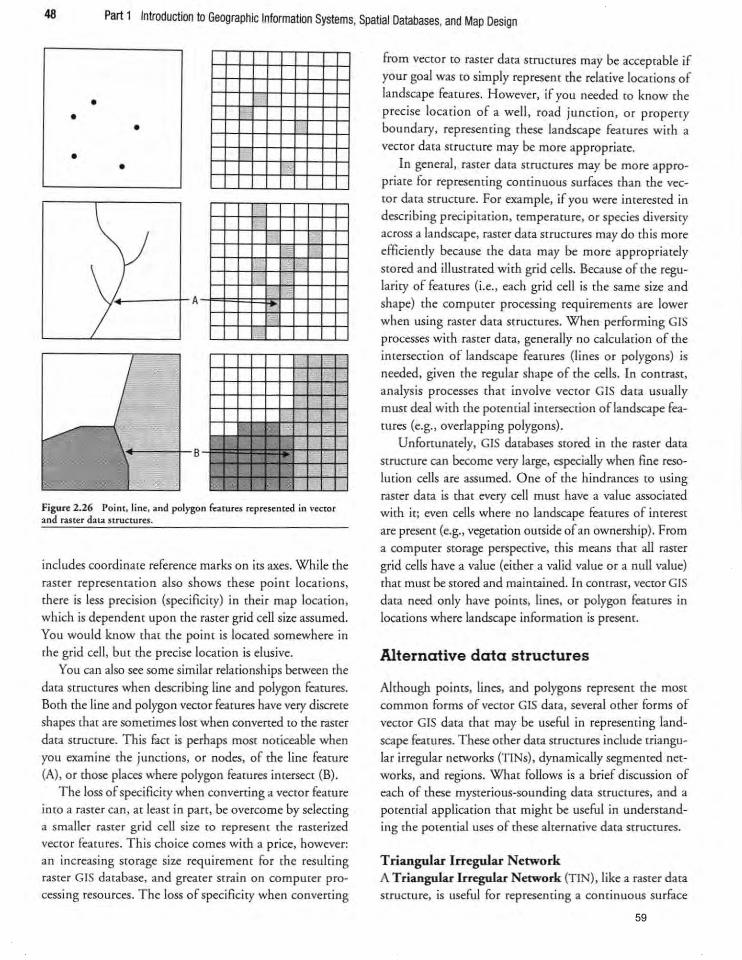
48 Part 1 Introduction to Geographic Information Systems, Spatial Databases, and Map Design
• • •
• •
Figure 2.26 Point, line, and polygon features represen ted in vector and ras ter data StruCtures.
includes coordinate reference marks on its axes. While the
raSter represemation also shows these point locat io ns,
there is less precision (specificity) in their map location, which is dependent upo n the raster grid cell size assumed. You would know that the point is iocared somewhere in
the grid cell . bur the precise locat io n is elusive.
You can also see some similar relationships be[Ween the
data S[rucrures when describing line and polygon features.
Both the line and polygon vector features have very discrete
shapes that are somecimes lost when converted to the raster
data structure. This faCt is perhaps most noticeable when
you examine the junctions. or nodes. of the line featu re (A), or those places where polygon features intersecr (B).
The loss of specificity when converting a vector feature imo a raster can, at least in pan, be overcome by selecting a smaller raSter grid cell size to represent the rasterized vecto r features. This choice comes with a price, however: an increasing storage size requiremem fo r the resuhing raSter GIS database, and greater strain on computer processing resources. The loss of specificity when converting
from vector to raster data structures may be acceptable if your goal was to simply represent the rdative locations of landscape features. However, if you needed to know (he
precise loca tion of a well, road junction, or propeny boundary, representing these landscape features with a
vector da ta structure may be more appropriate .
In general. raster data struCtures may be more appropriate for representing continuous surfaces than the vector data structure. For example, if you were inrerested in describing precipitation, temperature, or species diversity across a landscape, raster data structures may do this more
efficiently because rhe dara may be more appropriately
swred and illustrated with grid cells. Because of the regularity of features (i.e., each grid cell is the same size and
shape) the computer processing requ iremems are lower when using raste r data structures. When performing G IS
processes wi th raste r data, generally no calculation of the intersection of landscape features (lines or polygons) is
needed , given rhe regular shape of the cells. In contrast, analysis processes that involve vector G IS data usually must deal with the potential intersection of landscape fea
tures (e.g., overlapping polygons) .
Unfortunately, GIS databases stored in the raster data structure can become very large, especially when fine reso
lution cells are assumed . One of the hindrances to using raSter data is that every cell must have a value associated with it; even cells where no landscape featu res of interest
are present (e.g., vegetation outside of an ownership). From
a computer storage perspective, this means that all raster grid cells have a value (e ither a valid value or a null value) that must be s[Qred and maintained. In conrrast, vector GIS
data need only have points, lines, o r polygon featu res in locations where landscape information is present.
Alternative data structures
Although points, lines, and polygons represent the most common forms of vector G IS data, several other forms of
vector GIS data that may be useful in representing land
scape features. These other data structures include triangu
lar irregular networks (TINs), dynamically segmenred networks, and regions. What follows is a brief discussion of each of these mysterious-sounding dara structures, and a potential application that might be useful in understanding the potential uses of these ahernarive data structures.
Triangular Irregular Network A Triangular Irregular Network (TIN), like a ras rer data structure, is useful for representing a continuous surface
59
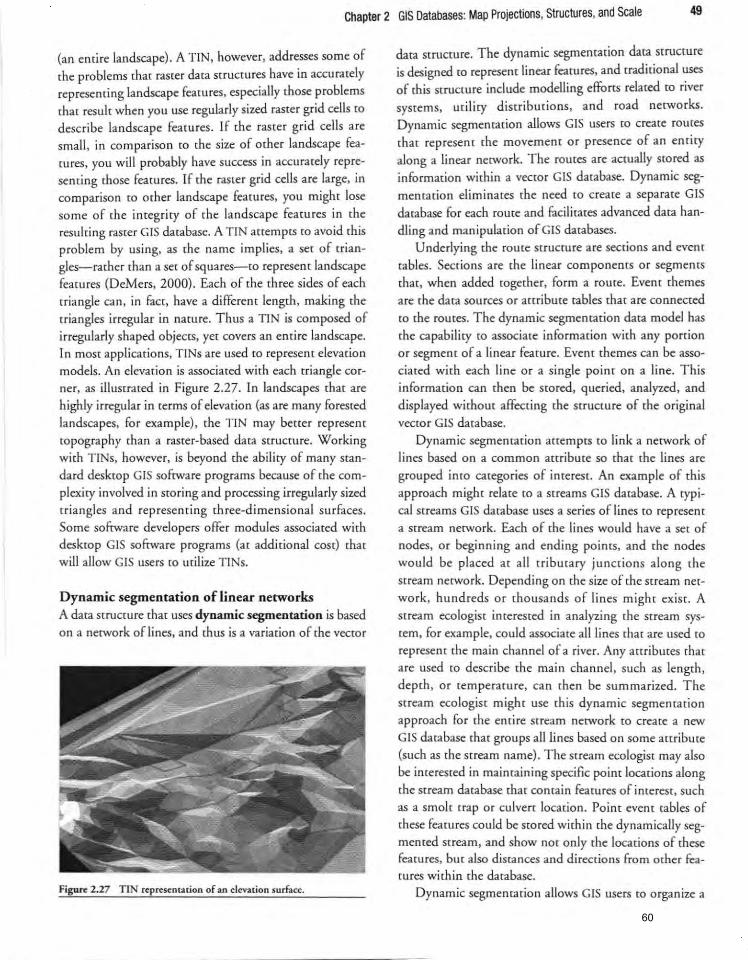
Chapter 2 GIS Databases: Map Projections, Structures, and Scale 49
(an entire landscape). A TIN, however, addresses some of [he problems (hat raster data structures have in accurately
representing landscape feamres , especially those problems that result when you use regularly sized raster grid cells to describe landscape feamres. If the raster grid cells are small. in comparison (Q the size of other landscape fea
tures , you will probably have success in accurately repre
senti ng mose features. If the raster grid cells are large, in comparison co orner landscape features , you might lose
some of {he integrity of [he landscape features in [he resulcing raster GIS database. A TIN attempts to avoid (his
problem by us ing. as the name implies, a set of trian
gles-rather than a set of squares-co represent landscape
features (DeMers, 2000). Each of the th ree sides of each triangle can, in fact, have a different length, making the rriangles irregular in nature. Thus a TIN is composed of
irregularly shaped objects. yet covers an entire landscape.
I n most applications. TINs are used to represent elevation
models. An elevation is associated with each triangle cor
ner, as illustrated in Figure 2.27. In landscapes that are highly irregular in terms of elevation (as are many forested
landscapes, for example), the TIN may berrer represent topography than a raster-based data structure. Working
with TINs, however, is beyond the abili ty of many standard desktop GIS sofrware programs because of the complexity involved in storing and processing irregularly sized
triangles and represent ing three-dimensional surfaces .
Some software developers ofTer modules associated with
desktop GIS sonware programs (at additional cost) that will allow GIS users ro util ize TINs.
Dynamic segmentation of linear networks A data structure that uses dynamic segmentation is based
on a netvlork of lines. and thus is a variation of the vector
Figure 2.27 TIN representation of an elevation surface.
data structure. The dynamic segmentation data structure
is designed to represent linear features. and traditional uses
of this strucrure include moddling efforts related co river
systems. utility distributions, and road networks.
Dynamic segmentat ion allows GIS users co create rOutes
that represent the movement or presence of an endty
along a linear network. The routes are actually stored as
information within a vector GIS database. Dynamic seg
mentation eliminates the need to create a separate GIS
database fo r each route and fucil itates advanced data handling and manipulation of GIS databases.
Underlying the route structure are sections and event
cables. Sections are the li near components or segments
that. when added together. form a route. Event themes
are (he data sources or attribute tables (hat are connected
ro the routes. The dynamic segmentation data model has the capability to associate information with any portion
or segment of a linear feature. Event themes can be asso
cia ted w ith each line or a single point on a line. This
information can then be stored, queried. analyzed. and
displayed without affecting the Structure of the original vecror GIS database.
Dynamic segmentation anempts to link a network of
lines based on a common attribute so that the lines are
grouped into categories of interest. An example of this
approach might relate ro a screams GIS database. A typical Streams GIS database uses a series of lines to represent
a stream netvlork. Each of the lines would have a set of
nodes, or beginning and ending points, and the nodes
wou ld be placed at all tributary junctions along the Stream netvlork. Depending on the size of the stream net
work, hundreds Ot thousands of lines might exist. A stream ecologist interested in analyzing the stream sys
tem. for example, could associate all lines that are used to
represent the main channel of a river. Any anributes that
are used to describe the main channel, such as length,
depth. or temperature, can then be summarized. The
stream ecologist might use this dynamic segmentation
approach for the entire stream netvlork to create a new
GIS database that groups all lines based on some attribute (such as the stream name) . The scream ecologist may also
be interested in maintaining specific point locations along
the stream database that contain features of interest. such
as a smolt trap o r culvert location. Point evenr tables of
these features could be stored within the dynamically segmented stream, and show not only (he locations of these features. but also distances and directions from other fea[Ures within the database.
Dynamic segmentation allows GIS users to organize a
60
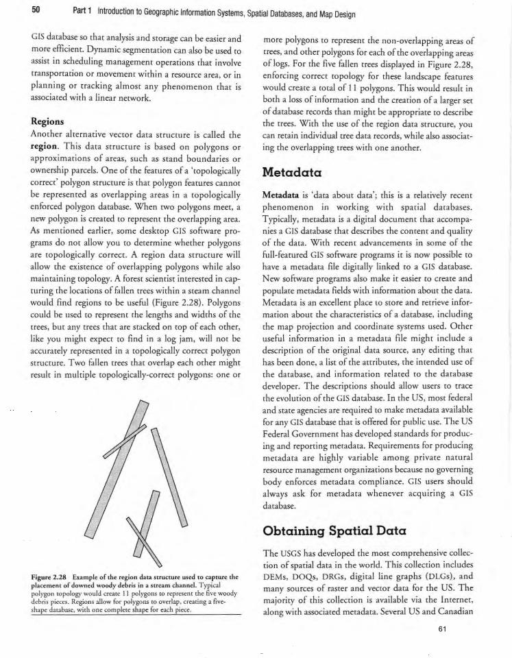
50 Part 1 Introduction to Geographic Information Systems, Spatial Databases, and Map Design
GIS da[3base so that analysis and storage can be easier and more efficient. Dynam ic segmemation can also be used to
ass ist in schedul ing management operations that involve
transportation or movement with in a resource area, or in
planning or tracking almost any phenomenon that is associated w ith a linear network.
Regions
Another alrernarive vectOr data srrucmre is called [he region . This data srrucmce is based on polygo ns or approximat ions of areas, slich as stand boundaries or
ownership parcels. One of the featu res of a ' topologically correct' polygon srruc(Ure is that polygon features can nor be represented as overlapping areas in a topologically
enforced polygon database. When two polygons meet, a new polygon is created. to represent the overlapping area. As mentioned earl ier , some deskrop GIS software pro
grams do not allow you ro determine whether polygons
are topologically correct. A region data structure will
allow (he existence of overlapping polygons while also maimain ing (Opology. A forest scientist interested in cap
turing the locations of Fallen (fees within a steam channel
would find regions to be useful (Figure 2.28) . Polygons could be used co represent the lengths and widths of the trees, bur any trees that are s[3cked on (Op of each other,
like you might expec( co find in a log jam, will not be accu rately represented in a ropologically correct polygon
structure. Two fal len trees that overlap each other might
result in multiple tOpologically-correcc polygons: one or
Figure 2 .28 Example of me region data structure used to capture the placement of downed woody debris in a stream channel. Typical polygon topology would create II polygons (Q represent the: five woody debris pieces . Regions allow for polygons ro overlap. crearing a fiveshape database. with one complete shape for each piece.
more polygons co represent the non-overlapping areas of
trees, and other polygons for each of the overlapping areas of logs. For the five F...llen trees displayed in Figure 2.28, enforcing co rrect ropology for these landscape features
would create a total of II polygons. This would result in both a loss of information and the creation of a larger set
of database records than might be appropriate to describe the trees. With the use of the region data structure, you
can retain individual (fee data records. while also associat
ing the overlapping trees with one another.
Metadata
Metadata is 'data about data'; this is a relatively recent
phenomenon in working with spat ial databases.
Typically, metadara is a digital document that accompa
nies a GIS database that describes the content and quality
of the data. With recent advancements in some of the
full-featured GIS software programs it is now possible to have a metadata file digitally linked to a GIS database. New sofrware programs also make it easier ro create and
populate meradata fields with information about the data.
Metadata is an excellent place to store and retrieve infor
macion about the characteristics of a database. including
the map projection and coordinate systems used. Other
useful information in a metadata file might include a
description of the original data source, any editing that
has been done, a list of the attributes, the intended use of the darabase. and info rmacion related ro the database
developer. The descriptions should allow users [Q trace
the evolution of the GIS database. In the US, most federal and state agencies are required to make mecadaca available
for any GIS dacabase that is offered for public use. The US Federal Government has developed standards for producing and reporting meradata. Requirements fo r producing
metadata are highly variable among private natural
resource management organizations because no governing
body enforces meradata compliance. GIS users should
always ask for metadata whenever acqu ir ing a GIS
database.
Obtaining Spatial Data
The USGS has developed the most comprehensive collection of spatial data in the world. This collection includes OEMs, OOQs, ORGs, digital line graphs (OLGs), and many sources of raster and vector data fo r [he US. The
majority of this co llect ion is available via the Interner,
along with associated meradata. Several US and Canadian
61
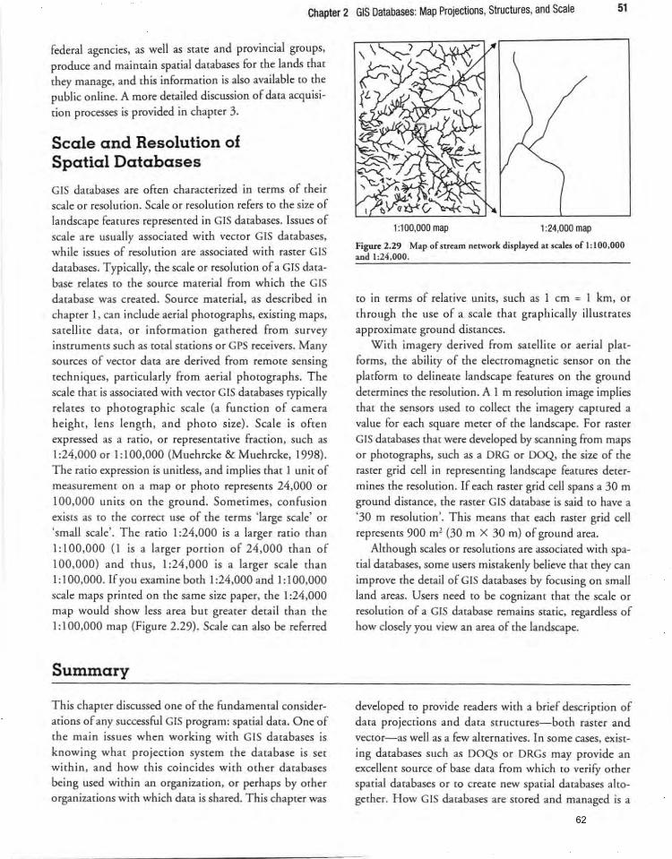
Chapter 2 GIS Databases: Map Projections, Structures, and Scale 51
federal agencies, as well as state and provincial groups,
produce and maintain spacial databases for [he lands that
they manage, and this information is also available to the
public online. A more detailed discussion of data acquisi
tion processes is provided in chapter 3.
Scale and Resolution of Spatial Databases
GIS dacabases are often characterized in terms of their
scale or resolution . Scale or resolU[ion refers [Q [he size of
landscape features represenred in GIS databases. Issues of
scale are usually associated with vector GIS databases.
while issues of resolution are associated with raster GIS databases. Typically, the scale or resolution of a GIS database relates to {he source material from which the GIS
database was created. Source material. as described in
chapter 1, can include aerial phocographs. existing maps.
sate ll ite data. o r information gatheted from survey
instruments such as total stations or GPS receivers. Many
sources of veccor data are derived from remote sensing
techniques, particularly from aerial photographs. The scale that is associated with vector GIS databases typically relates to photographic scale (a function of camera
height, lens length , and photo size) . Scale is often expressed as a ratio, or representative fraction, such as
I :24,000 or 1:100,000 (Muehrcke & Muehrcke, 1998). The ratio expression is unidess, and implies that 1 unit of
measurement on a map or phoco represenrs 24.000 or
100,00D unirs on the ground . Sometimes, confusion exists as to the correct use of the terms 'large scale' o r
'small scale'. The ratio I :24,00D is a larger ratio than 1:100,000 (I is a larger portion of 24,000 than of 100,000) and thus, 1 :24,000 is a larger scale than I: 1 00,000. If you examine both 1 :24,000 and I: I 00,000 scale maps printed on the same size paper, the I :24,ODO map would show less area bur greater detail than the
1: 1 00,000 map (Figure 2.29). Scale can also be referred
Summary
This chapter discussed one of the fundamemal consider
ations of any successful GIS program: spatial data. One of the main issues when working with GIS databases is
knowing what projection system the database is set within, and how this coincides with other databases being used within an organization. or perhaps by other
organizations with which data is shared. This chapter was
1:100,000 map 1 :24,000 map
Figure 2 .29 Map of stream network displayed at scales of 1:100,000 and ' ,24,000.
co in terms of relative units, such as 1 cm = 1 km, or
through the use of a scale [hat graphically illustrates approximate ground distances.
Wi[h imagery derived from satellite or aerial pla<forms, rhe abi lity of the electromagnetic sensor on rhe
platform to delinea<e landscape features on the ground determines the resolution. A I m resolution image implies
that the sensors used [Q colleer the imagery captured a
value for each square meter of the landscape. For raster
GIS databases that were developed by scanning from maps or photographs, such as a DRG or DOQ, the size of the raster grid cell in representing landscape features deter
mines the resolution. If each raster grid cell spans a 30 m ground distance, the raSter GIS database is said co have a
' 30 m resolution '. This means that each raster grid cell represents 900 m' (30 m X 30 m) of ground area.
Although scales or resolutions are associated with spa
rial databases . some users mistakenly believe that they can
improve [he detai l of GIS databases by focusing on small land areas . Users need co be cognizant that the scale or
resolution of a GIS database remains static, regardless of
how closely you view an area of the landscape.
developed to provide readers with a brief description of data projections and data structures-both raster and
veccor-as well as a few alternatives. In some cases, exist
ing databases such as DOQs or DRGs may provide an excellent source of base data from wh ich to verify other spatia l databases or CO create new spatial databases alto
gether. How GIS databases are stored and managed is a
62
52 Part 1 IntroductiOIl to Geographic Information Systems, Spatial Databases, and Map Design
function of the decisions natural resource managers make
regarding rhe purpose and inrenr of use for each GIS database. In many cases, however, YOli have no choice regarding rhe strucmre of GIS darabases. For example, satellite imagery uses a faSter dara Structure whereas veg
erarion and soils darabases acquired from rhe US Foresr Service generally use rhe vec[Qr data structure. In addi
rion, most natural resource organizations use venor data
srruc[U res [0 rep resem management units, roads . and
ocher landscape feamres . Meradara are useful in helping
Applications
2.1. Projection parame te rs . Your supervisor. Steve
Smith, has JUSt learned (hat another natural resource
organization that you intend ro share spatial data with
srores their GIS databases in a projection format that is
different from yours. Steve is unfamiliar with projections,
and asks YOll co provide some background for him. a) Whar is a projecrion? b) Why are projecrions necessary' c) Whar is an ellipsoid? d) What is a geoid' e) What are the major projection rypes, what are their
assumptions, and how have they been used?
2.2 . C hoosing a projection. You've been asked ro rec
ommend either a Lambert or Mercaror projection that
best fits the dimensions of the State or province mat you
live in. a) What is the largest north-south dimension of your
state or province in miles and kilometers?
b) What is the largest west-easr dimension of your
state or province in miles and kilometers?
c) Which of rhe cwo projecrions would YOll choose? d) Defend your projecrion choice.
2.3. Public land survey system. Wirh rhe exceprion of rhe original 13 colonies, several other states, and other
des ignated ownerships, much of the US has been sur
veyed (measured) using rhe PLSS. Significanr areas in Canada have also been surveyed using a similar approach.
Given the broad use of this system and its counterparts in
Nonh America, it is imponant that you understand sev
eral key components.
a) How many square miles (or square kilometers)
would you expect to find in a township?
you determine rhe characteristics of a GIS database.
including rhe projection system used. Finally, under
standing the scale or resolution of GIS databases and thei r
associated landscape fearures is important, as it relates co
the usefulness of a GIS database in assisting with analyses
related ro management decisions. Perhaps an interesting
ropic of conversation over a cup of coffee might be how
well 30 m grid cells obtained from sarellire images porreay forest vegetadon and help you develop management
recommendations.
b) How many acres (or square meters) would you
expect to find in a section?
2.4. GIS data structures. You have been hired as a land management forester for a timber company in the south
ern United States. As a recent college graduate you are
expected to have the most cu rrent knowledge of forest
measu rement and data acquisition techn iques. Your
supervisor, John Delaney, an older forester, is interested
in GIS and is cu rious about database structures. Describe
to him the difference between a raster and vector data
structure. and give an example of a GIS database that
might be designed with each structure.
2.5 Quadrangle challenge. Locare rhe USGS 7.5 m inute Quadrangle that contains your GIS classroom or
work location.
a) Whar is rhe name of rhe quadrangle? b) When was me map originally compiled? c) If rhe map has been updared, when was ir updared? d) Whar is rhe Ohio code descriprion of rhe map? e) When was rhe copography developed? f) How much magnet ic declination existS in the map?
2.6. Resolution and scale. A consulranr has proposed using sarellire imagery co quickly updare rhe foresr resources thar your natu ral resource management organi
zation manages. Some people in your organizarion are
arguing for a complete and fresh phow interpretation of
rhe land base to accomplish (his goal, resulring in a vector
GIS database of the vegetation condition of the landscape.
The differences in resolution and scale are two of me hot
copies when comparing these alternatives . Explain the dif
ference belVv'een resolution and scale. and how they relate
[Q raster and vector data structures.
63
Chapter 2 GIS Databases: Map Projections, Structures, and Scale 53
2.7. Designing GIS databases. You have been hired by a natural resou rce consulting agency [0 develop and maimain a small GIS operation . While your expertise is in
natural resource management, the owners of [he consulrp ing agency were incrigued by your GIS expertise, and have been interested in providing chese services (0 their clients.
You, of course, (Oak the job because it is an opponuniry
to pur your GIS and namral resource management skills
to usc. As a stan, what data Structure might you use to describe the landscape features in the following databases?
a) timber stands g) precipitation
b) screams h) land ownership c) roads i) scream buffers d) inventory plots j) owl locations e) culverts k) owl habitat f) logs in scream
2.8. Map scale and ground distances. You are employed as a field forester for the Ministry of Natural Resou rces , and arc stationed in northern Maniroba. You
References
Cadle, F.W. (1991 ). Georgia land surveying history and law. Athens, GA: The University of Georgia Press.
Chang, K. (2002) . Introduction to geographic information systnm. New York: McGraw-Hili.
Clarke, K.c. (2001). Getting starud with geographic infor
mation systems. Englewood Cliffs, NJ: Prentice Hall, Inc. DeMers, M.N. (2000) . Fundammtals of geographic infor
mation systems. New York: John Wiley and Sons, Inc. Dent, B.D. (1999). Cartography thematic map design .
New York: McGraw·Hili. Ladell, J.L. (1993). They kft their mark: Surveyors and
th~ir role in the settlement of Ontario. Toromo, ON: Oundurn Press.
Lillesand, T.M., & Kiefer, R.W. (2000). Remote smsing
and image interpretation (4 th ed.). New York: John Wiley & Sons, Inc.
Muehrcke, P.c., & Muehrcke, J.O. (1998). Map use:
Reading, analysis, and interpretation (4th ed.). Madison, WI: JP Publications.
have been inventorying timber for the past three hours,
and now it is time for lunch. Your lunch. of course, is located in your truck. The distance you measure on your
map from your current posicion to [he Huck is 12 cm. If the map scale was 1: 12000, how far are you fro m your
£ruck?
2.9. Spatial resolution. The natural resource management agency you work for in [he imermoumain wes[ is
considering [he purchase of 30 m resolmion sa[elli [e
imagery for assiscing in [he managemem of [heir natural resources. How much area, in acres, does a single 30 m grid cell cover? How much area would be covered by a single 100 m resolution grid cell?
2.10. Spatial scale. Your supervisor has asked that you bring a map at the largest map scale possible to your next planning meeting. You have your choice of the following map scales: 1 :24000 or 1: 1 00000. Which map do you bring with you?
Robinson, A.H, Morrison , J.L. , Muehrcke, P.c. , Kimeriing, A.J., & Guptill, S.c. (1995) . Ekmmts of cartography. New York: John Wiley & Sons, Inc.
Snyder, J.P. (1987). Map projectiom-a working manual. Washington, DC: Uni[ed 5ca[es Governmem Priming Office.
Stewan, L.a. (1979). Public land surveys. New York: Arno Press.
Thompson, M.M. (1979) . Mapsfor America (3rd ed. ). Washington, DC: US Government Printing Office.
USDI US Geological Survey. (1995) . Geographic names information system, data users guide 6. RestOn, VA: US Geological Survey. Retrieved January 15,2003, from from: http://mapping.usgs.gov/www/ti/GNIS/gnis_ users-suide_toc.hcrnl .
Wolf, P.R., & Ghilani, C.O. (2002) . Ekmentary survey
ing: An introduction to geomatics (10th ed.). Englewood Cliffs, NJ: Prentice Hall, Inc.
64
Chapter 3
Acquiring, Creating, and Editing GIS Databases
Objectives
This chapter discusses a number of topics related co
acquiring, creating, and edidng GIS databases. Readers should gain an understanding of the opportunities and
challenges associated with the need [Q obtain GIS data from a variety of sou rces. At the conclusion of this chapter, readers should be able to understand and discuss issues related [0:
I . {he acqu isition of GIS databases, panicularly via the Imerner,
2. [he various methods for creari ng new GIS databases,
3. the processes for editing existing GIS databases, and
4. the error types and sources [hat are poremialiy associated with GIS databases.
Acquiring, creating, and editing GIS databases to address rhe needs of natural resource management decisionmaking processes is a continual process. Ideally, narural
resource professionals would have a complete and robust set of GIS databases at their disposal prior to performing an analysis. However. as new and inreresting opportunities to incorporate GIS analysis in decision-making processes arise, the G IS database needs change as well. Four general cases are common in natural resource o rganizations. as rhey relate to the availabi li ty of GIS databases:
1. GIS darabases required for a specific analysis do nor
eXIst.
2. GIS databases exist. bue they were created for other general uses and may not be quite appropriate to
address [he issues related to a specific analysis.
3. GIS databases exist, bue rhey were created for other
specific analyses and are not quire appropriate to
address the issues related to another specific analysis. 4. GIS databases exist, and they are adequate and appro
priate to address the issues of a specific analysis.
Ideally, you would hope that your organization is continually positioned near the fourth case noted above.
However many GIS users find. evenrually, that the first three cases are real , and that time mUSt be spenr acquiring or developing a GIS database. Several options are available
to GIS users faced with having to acquire, create, or edit GIS databases. These options include having someone else create a GIS database (e.g., a GIS contractor) based on maps and other input provided to them, using C PS or some other field-based data collection method to fuc ilitate
the development of a new GIS database, modifYing or
editing an existing C IS database. creat ing a new GIS database by digitizing maps, acquiring a GIS database from the Internet (for example, the National Werlands Invento ry from the US Fish and Wildlife Service [http://weriands.lWs.govl]), o r acquiring a GIS database from mher organizations. The decision [Q pursue one of these strategies will depend on several factors inherent to a person's job. such as the budgetary resources, time constraints. and the skills and computing resources that are available within the natural resource organization.
65
Acquiring GIS Databases
One of the main concerns of natu ral resource managers is locating and acquiring GIS data. Physically receiving the
GIS databases is relatively easy; they can be sen< and received as an email attachment via the Internet or by way of media such as portable USB drives, compact discs (CDs). or DVD disks. GIS databases can be acquired from a variety of clearinghouses. many of which are maintained
and supported by federal, provincial, or state organizations. The US federal government, in fact, is perhaps the larges< source of GIS dara in the world. A variety of federal agencies in the US provide data , and the Manual of Federal Geographic Data Products (US Geological Survey. Federal Geographic Data Committee. 2002) provides a wealth of informacion concern ing rhe agencies from which GIS databases can be acquired. Natural
Resources Canada (Natural Resources Canada. 2007) and the Geography Network Canada (Geography Network Canada. 2007) provide access to many types of geographic data within Canada. Provincial and state agencies. such as rhe Washingcon Depanment of Natural Resources. also d isrribuce a large number of GIS databases
related to the resources of each state. Acquiring GIS databases over the Internet has become
a widely used practice over the past few years. The disad
vantage, however, is that the fo rmat of the data is generally limited to that of the most popularly used data. and may not be directly compatible with some GIS software programs. Agencies that require GIS users {Q make requests for GIS databases may provide a wider variety of products to be acquired, as well as a wider variety of for
mats, depending on the provider. In the case of data
requests, however, the agency may require mat a payment accompany each request. The payment covers the Cost of the media and staff time required to package and deliver the GIS databases; the rates are usually reasonable because public organizations provide the data. People requesting
GIS databases are asked to provide a va riety of information specific to their request (Table 3. I). so that the final product will meet (as closely as possible) their needs without the staff investing extra effort in formatting, re
projecting. or adjusting the GIS databases. As an example of acquiring GIS databases via an
Internet site, rhe Gifford Pinchot N ational Forest (Washington State) maintains a website where a number of GIS databases can be acquired (Gifford Pinchot National Forest. 2007). The Internet site is located at http:// www.fs.fed .us/gpnflforest-research/gis/. By accessing this
Chapter 3 Acquiring. Creating. and Editing GIS Oatabases
TABLE 3.1 Typical information associated with a GIS database request
• G IS database requested
55
• Locarion (Township/Range/Section. Topographic quad indO[ Ohio
code [or nameD
• File format (e.g., Spatial Data Transfer Standard [SOTS] . Ardnfo export format, ESRI shaptfile. Tagged Image File Format [TIF1. Imagine format [IMG], ESRI geodat1lbase)
• Map projection. coordinate system. horizontal and vertical measurement units, and related parameters
• Metadara
• Contact person for questions related to the GIS database
• Delivery method (USB drin. DVD. CD. e·maiI. FTP, ere.)
Database compression format (Zipped. MrSID. TAR, ere.)
Billing information
Product license agreements
website. you will find that all of the vector GIS databases are
available in Arclnfo coverage (ESRI. 2005) expOrt format. Databases can either be downloaded directly from this Interner site, or obtained on a CD-ROM or 8 mm tape.
The COst of obtaining GIS databases on media is $40 (US currency). In addition. some meradara related to each GIS
database can be accessed through the Gifford Pinchot
Nati<;>nal Forest website. The data related to the forest trail system, for example. indicates that the source scale for the GIS database was I :24.000. that it was last updated in 1999, that the projection system is the T ransverse Mercator using the Clarke 1866 spheroid. that the coordinate system
is the UTM system. and that the datum is NAD27. In addition, the me[adata identifies the primary contact person and alerts GIS users [hat some gaps in the trai l system may
exist so that users know to examine the data closely before using i[ to make management decisions.
As you may have no ticed from the Gifford Pinchot example. a variety of GIS databases are available in addi
tion to [he forest trails system, including hydrology, elevation, forest stands, roads, streams, and others. While these GIS database are commonly used to support resource
management on rhe National Forest, they are mainly vector GIS databases. Raster GIS databases. such as digital orrhophotographs, related to a particular landscape are perhaps more difficult to obtain . As mentioned in chap<er I. digital orthophotographs look like aerial photographs but {hey are srored in digital form and are regis
tered to a coordinate and projection system . Raster GIS
66
56 Part 1 Introduction to Geographic Information Systems, Spatial Databases, and Map Design
,. ~ l'_ t ~'In"Depth ' ~1:..1~~<.. '.~ . ..
Reference is made in this book to a number ofInrernet
sites that you can visit for additional informatio n and
resources. The Internet is in a constant state of Aux,
however, and organizations often change website
addresses, or URLs. Since URLs change periodically, you might find that some examples provided in this book have become obsolete. Should you have a problem accessing the URLs we have provided, twO strate
gies can be employed to reach the approptiate address. First, verify that the website address being used
<xactly matches the URL listed in the book. Even the smallest of differences (one incorrect letter, or an extra
space) can resuh in not reaching the appropriate web
site. Second, with a liule ingen uity you can locate the
In ternet sites listed in this book by using an onl ine
search engine. For example, the URL to the Washington Department of Natural Resources
Information Techno logy Division order form has
changed several times since the first edition of th is
book. To locate the most cu rrent version of the order
form, you could anempr an online search similar to
the one oudine below:
databases can also be acqui red via the Internet. The
Minnesota Planning, Land Management Information
Center (2007), for example, maintains a clearinghouse ( http://www.lmic.state.mn.us!chouse!metalong.htmll) where GIS users can access the 'Imagery and Photographs'
How do YOli acqu ire data over the Internet? Usually.
clicking on an Internet link will starr the download
process by presenting a dialog box that asks where the downloaded file should be stored. Another way is to download GIS database files to a computer is to use a
FIP. FTP stands for File Transfer Protocol, and it is a
widely used method of transferring data over the Internet. This method allows you to transfer computer
files to other remote computers. or ro download com
puter fi les from a remote computer. One advantage of
• Search the Inrernet for 'Washington Departmenr of Natural Resources'
- Result: http://www.dnLwa.gov!
• Select 'Publications & Data' from [he list of items on [he DNR main page.
- Result: http://www.dnr.wa.gov/baselpublications. html
• Select 'GIS Data' from the lise of items under
Publications and Data sub-heading - Result: http://www.dnr.wa.gov/dataandmaps!
index.html
• Select the 'Available GIS Data' choice from the available links on the Data page.
- Result: http://www3.wadnr.gov!dnrapp6/data web!dmmatrix.html
At this point, you should be presented with a list of available databases that can be downloaded in an ESRI shapefile format (ESRl, 2005). Thus in four steps, you can reach the currenr website from wh ich spacial da[a
can be accessed from the Washington State DNR.
data category and download county-level digital aerial imagery, including orthophotographs, varying from 1 m to 10m spatial resolution. In add ition, the clearinghouse provides CIS users with some meradar3 related to the digital imagery. You can ascertain from viewi ng meradar3
this process is that PCs are able to communicate w ith
UNIX-based machines, and GIS database file formats are automatically convened into a Windows~-compat
ible format during the transfer process. FTP was once
only ava ilable on a PC th rough a DOS interface, but several low-cost Windows@ applications are available
that simpli fy this process and make additional file transfer or sharing options available. To locate such a utility, try an Internet search using the keywords 'FfP'
and 'Windows' together.
67
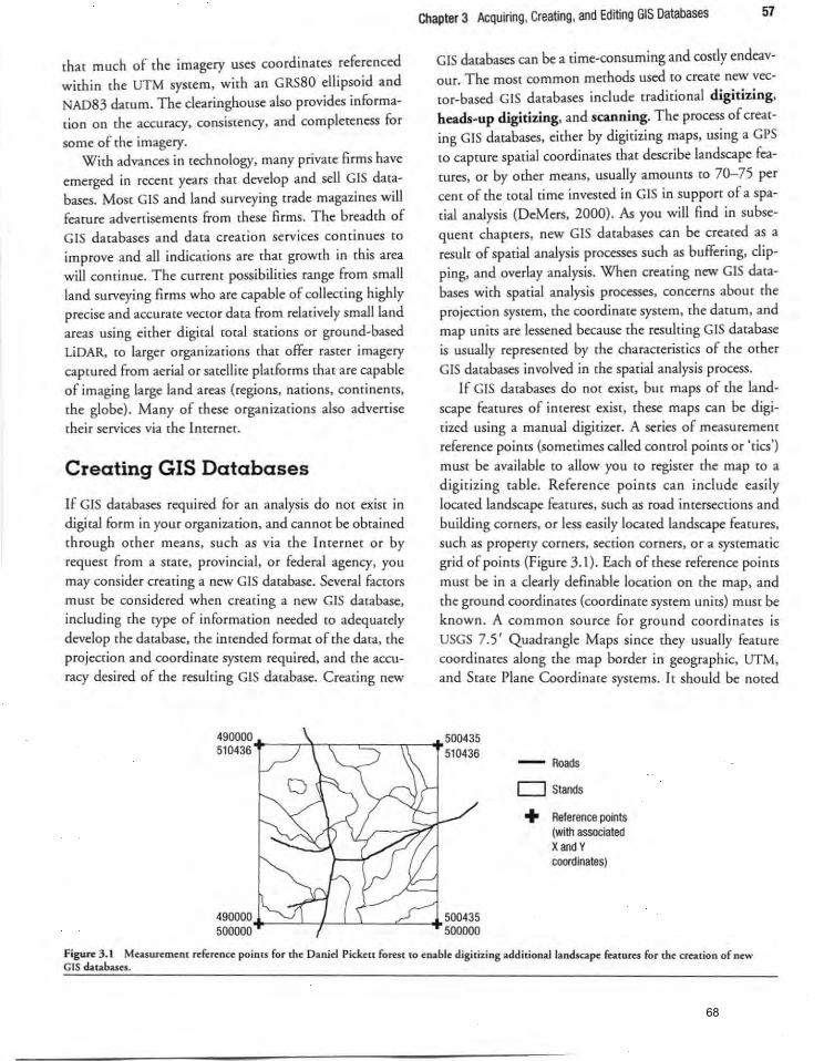
that much of the imagery uses coordinates referenced within the UTM system, with an GRS80 ellipsoid and NAD83 datum. The clearinghouse also provides information on the accuracy, consistency. and completeness for
some of the imagery. With advances in technology, many private firms have
emerged in recent years that develop and sell GIS databases. Most GIS and land surveying trade magazines will fearure advenisements from these firms . The breadth of
GIS databases and daca creation services cont inues (0
improve and all indicacions are that growth in [his area
will continue. The current possibilities range from small
land surveying firms who are capable of collecting highly precise and accurate vector data from relatively small land
areas using either digital tOtal stations or ground-based
LiOAR, to larger organizations that offer raster imagery
captured from aerial or satellite platforms that are capable of imaging large land areas (regions. nations, continents.
the globe). Many of these organizations also advertise their services via the Internet.
Creating GIS Databases
If GIS databases required for an analysis do not exist in digital form in your organization, and cannot be obtai ned
through other means, such as via the Internet or by
request from a state. provincial, or federal agency, you
may consider creating a new GIS database. Several factors
mUSt be considered when creating a new GIS database.
including the type of information needed to adequately develop the database, the intended format of the data, the projection and coordinate system required. and (he accu
racy desired of the resulting GIS database. Creating new
Chapter 3 Acquiring, Creating, and Editing GIS Databases 57
GIS databases can be a time-consuming and costly endeavour. The most common methods used to create new vec
tor-based GIS databases include traditional digitizing,
heads-up digitizing, and scanning. The process of creating GIS databases, either by digitizing maps, using a GPS
to capture spatial coordinates that describe landscape fea
tures, or by other means, usually amounts to 70-75 per
cent of the total time invested in GIS in support of a spa
tial analysis (DeMers, 2000) . As you will find in subsequent chapters. new GIS databases can be created as a
result of spatial analysis processes such as buffering, dipping, and overlay analysis. When creating new GIS databases with spatial analysis processes, concerns about the
projection system, the coordinate system. me datum, and
map units are lessened because the resulting GIS database:
is usually represented by the characteristics of the other GIS databases involved in the spatial analysis process.
If GIS darabases do not exist, but maps of the land
scape featu res of interest exist , these maps can be digi
tized using a manual digitizer. A series of measurement
reference points (sometimes called control points or 'tics')
mUSt be available to allow you to register the map to a
digitizing table. Reference points can include easily located landscape features, such as road intersections and
building corners, or less easily located landscape features, such as property corners, section corners, or a systematic
grid of points (Figure 3.1). Each of these reference points must be in a dearly definable location on the map, and the ground coordinates (coordinate system units) must be
known . A common source for ground coordinates is
USGS 7.5' Quadrangle Maps since they usually feature coordinates along the map border in geographic, UTM,
and State Plane Coordinate systems. It should be noted
490000 500435 510436: +----,-1----c---="--,,,--t 510436
490000, +--=:=...l.-JL....1-L-_c..._+ 500435 500000 5~
- Roads
D Stands
+ Reference points (with associated XandY cOOfdinates)
Figure 3.1 Measurement reference poinu for the Daniel Pickett forest to enable digitizing additional landscape features for the creation of new GIS databases.
68
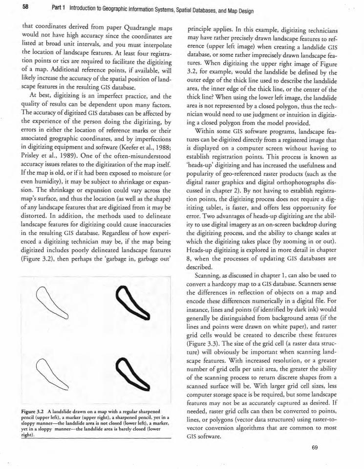
58 Part 1 Introduction to Geographic Information Systems, Spatial Databases, and Map Design
that coordinates derived from paper Quadrangle maps would nor have high accuracy since the coord inates are
listed at broad unit imervals, and you must incerpolare
the location of landscape features. At least four registra~ cion points or rics are required to facilitate the digitizing of a map. Additional reference points, if available, wi ll likely increase the accuracy of the spatial position oflandscape features in the resulting GIS database.
At beSt, digitizing is an imperfect practice. and the quality of results can be dependent upon many factors. The accuracy of digitized GIS databases can be affecred by the experience of the person doing the digitizing, by errors in either the location of reference marks or their
associated geographic coordinates, and by imperfections
in digitizing equipment and software (Keefer et aI., 1988; Prisley et aI., 1989). One of the often-misunderstood accuracy issues relates co the digirizarion of the map itSelf. If the map is old, or if it had been exposed to moisture (or even humidity), it may be subject to shrinkage or expansion. The shrinkage or expansion could vary across the
map's su rEace, and thus the location (as well as the shape) of any landscape features that are digitized from it may be distorted. I n addition, the methods used to delineate landscape features for digitizing could cause inaccuracies
in the resulting GIS database. Regardless of how experienced a digitizing technician may be, if the map being
digirized includes poorly delineared landscape features (Figure 3.2), then perhaps the 'garbage in, garbage out'
Figure 3.2 A landslide drawn on a map with a r~gular sharpen~d p~ncil (upp~r left), a mark~r (upper right), a sharpened pencil, y~t in a sloppy manner- me landslide are:& is not closed (lower left), :& m2rk~r. yet in a sloppy manner-me landslide ar~a is barely closed (Iow~r right).
principle applies. In this example, digitizing technicians
may have rather precisely drawn landscape features to reference (upper left image) when creating a landslide GIS database, or some rather imprecisely drawn landscape fea
tures. When digitizing the upper right image of Figure 3.2, for example, would the landslide be defined by the outer edge of the thick line used to describe the landslide area, the inner edge of the thick line, or the center of the
thick line? When using the lower left image, the landslide area is not represented by a closed polygon, thus the technician would need to use judgment or intuition in digitiz
ing a closed polygon from the model provided. Within some GIS software programs, landscape fea
tures can be digitized directly from a registered image that
is displayed on a computer screen without having {O
establish registration points. This process is known as
'heads-up' digitizing and has increased the usefulness and popularity of goo-referenced raster products (such as the digital raster graphics and digital orthophotographs discussed in chapter 2). By not having {O establish registra
tion poims, the digitizing process does not require a dig
itizing tablet, is faster, and offers less opportunicy for
error. Two advantages of heads-up digitizing are the abil
ity {O use digital imagery as an on-screen backdrop during
the digitizing process, and the ability to change scales at which the digitizing takes place (by zooming in or Out).
Heads-up digitizing is explored in more detail in chapter
8, when the processes of updating GIS databases are described .
Scanning. as discussed in chapter 1, can also be used [0
conven a hardcopy map to a GIS database. Scanners sense
the differences in reflection of objects o n a map and
encode these differences numerically in a digital file. For instance, lines and points (if identified by dark ink) would generally be distinguished from background areas (if [he lines and points were drawn on white paper) , and raster
grid cells would be created to describe rhese features (Figure 3.3). The size of the grid cell (a rasrer data structure) will obviously be important when scann ing land
scape features . With increased resolution, or a greater
number of grid cells per unit area, the greater the ability
of the scanni ng process [0 return discrete shapes from a
scanned surface will be. With larger gr id cell sizes, less computer storage space is be required. bur some landscape featu res may not be as accurately captured as desired. If
needed, raster grid ce lls can then be converted to points. lines, or polygons (vector data structu res) using ras ter-tovecror conversion algorithms that are common to most
GIS software.
69
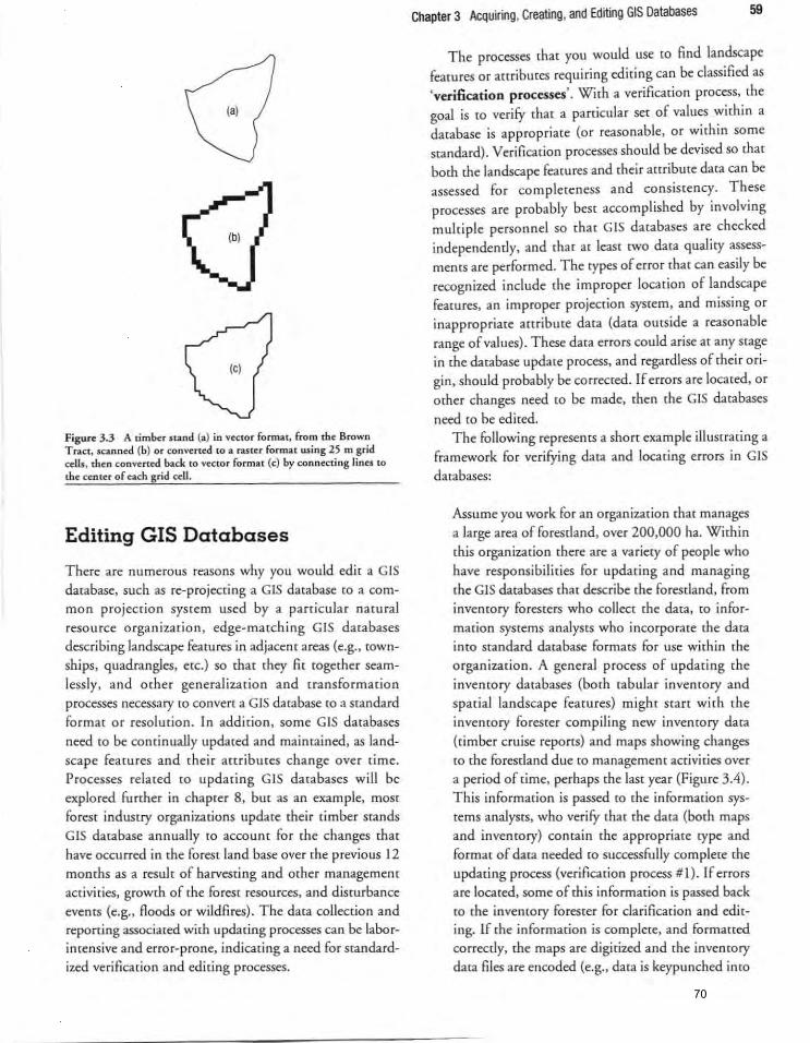
(al
Figure 3.3 A limber stand (a) in vector format. from tbe Brown T ract, scanned (b) or converted to a raster format wing 25 m grid cells, then convcru~d back to vector format (e) by con necting lines to the center of each grid cell .
Editing GIS Databases
There are numerous reasons why you would edit a GIS database, such as re-projecting a GIS database to a common proj ect ion system used by a particular natural resource organization, edge-matching GIS databases describing landscape features in adjacem areas (e.g .• (Qwnships. quadrangles. ece.) so tha[ they fie [oge[her seamlessly, and other generalization and transformation processes necessary to convert a GIS database to a standard format or resolmion. In additio n, some GIS databases
need co be continually updated and maintained, as landscape features and their attributes change over time. Processes rela[ed co upda[i ng G IS da[abases will be explored further in chapter 8, bue as an example, most forest industry organizations update their timber stands G IS da[abase annually co accoune for [he changes [hac have occurred in the forest land base over [he previous 12
months as a result of harvesting and Q[her management activities, growth of the forest reso urces, and disturbance evenes (e.g .• floods or wildfires). The da", collec[ion and repo rting associated with updating processes can be laborimcnsive and error-prone, indicating a need for standard
ized verification and editing processes.
Chapter 3 Acquiring. Creating. and Editing GIS Databases 59
The processes tha[ you would use co find landscape
features or 3nribuces requiring editing can be class ified as 'verification processes'. Wirh a verificadon process, [he
goal is to verify [hat a parricuiar set of values within a database is appropriate (or reasonable, or within some s[andard). Verifica[ion processes should be devised so [hac bo[h [he landscape fea[ures and [heir amibu[e da", can be assessed for completeness and consistency. These processes are probably bes[ accomplished by involving mulciple personnel so [hac G IS da[abases ace checked independently. and [hac a[ lease twO da", qualicy assessmenes are performed. The cypes of error [hac can easily be recognized include [he improper loca[ion of landscape feamres, an improper projection system, and miss ing or
inappropriate attribute data (data o utside a reasonable range of values). These data errors could arise at any stage in the da[abase upda[e process. and regardless of [heir origin. should probably be correc[ed. If errors are loca[ed. or ocher changes need co be made. [hen [he G IS da[abases
need CO be edi[ed. The following represents a shorr example illustrating a
framework for verifying data and locating errors in GIS
databases:
Assume you work for an organizat ion that manages a large area of forestland. over 200.000 ha. Wi[hin {his organization there are a variety of people who have responsibili [ies for upda[ing and managi ng [he GIS da",bases tha[ desc[ibe [he forestland. from inventory foresters who collect (he data. to infor
mation systems analysts who incorporate the data into standard database formats for use within the organization. A general process of updating the
inventory databases (both tabular inventory and spa[ial landscape fea[ures) might S[a[[ wi[h the inventory forester compiling new inventory data
(cimber cruise repons) and maps showing changes to {he forestland due to management accivities over a period of [ime. perhaps [he las[ year (Figure 3.4). This information is passed to the info rmation syscems analyses. who verilY tha[ [he data (boch maps and inventory) contain the appropriate type and forma[ of da[a needed ro successfully comple[e [he upda[ing process (verifica[ion process # 1). If errors are located, some of this information is passed back
to the inventory forester for clarification and editing. If the information is complete. and formatted correctly. the maps are digitized and the invemory da", files are encoded (e.g .• da[a is keypunched ineo
70
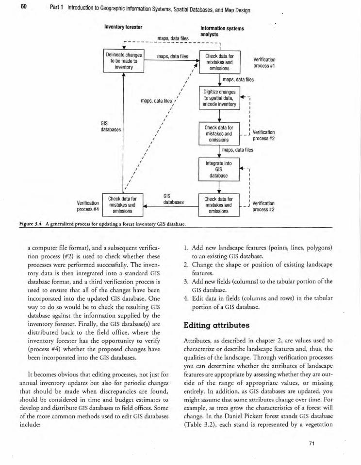
60 Part 1 Introduction to Geographic Information Systems, Spatial Databases, and Map Design
Inventory forester
maps, data files
Information systems analysts
r - ------- -- - - ---- - -- - -, ~ . I
Delineate changes maps, data files to be made to
Check data f(l( Verification process #1 inventory
, maps, data files I , , , , ,
GIS , databases
, , , , , , , , , , , , , , , , , GIS
,. , , , , , , ,
mistakes and omissions
L maps, data files
Digitize changes ~ to spatial data,
encode inventory
! Check data f(l( mistakes and -
omissions
! maps, data f
Integrate into ~ GIS
database
J
-; I I I I I I
J Verification process #2
iles
I I
Verification process #4
Check data for mistakes and databases
Check data for mistakes and J Verification
process #3 -omissions omissions
Figure 3.4 A gc ncraliud process for updating a forest inventory GIS databa.sc.
a compurer file format), and a subsequem verification process (#2) is used to check whether these processes were performed successfully. The inven[Ory data is then integrated into a standard GIS database format, and a third verification process is
used to ensure that all of the changes have been incorporated into the updared GIS database. One way to do so would be to check the resulting GIS database against the information supplied by the inventory forester. Finally, the GIS database(s) are distributed back to the field office, where the inventory forester has the opportunity [0 verify (process #4) whether the proposed changes have been incorporated into the GIS databases.
It becomes obvious that editing processes, not JUSt for annual inventory updates bur also for periodic changes that sho uld be made when discrepancies are found. should be considered in time and budget estimates to develop and distribute GIS databases to field offices. Some of the more common methods used [0 edit GIS databases include:
I. Add new landscape features (points, lines, polygons) [0 an exist ing GIS database.
2. Change the shape or position of existing landscape fe-atures.
3. Add new fields (columns) to the tabular portion of the G IS database.
4. Edit data in fields (columns and rows) in the tabular
portion of a GIS database.
Editing attributes
Attributes, as described in chapter 2, are values used to
characterize or describe landscape fearures and, thus, the qualities of the landscape. Through verification processes
you can determine whether the attributes of landscape features are appropriate by assessing whether they are out
side of the range of appropriate values. or missing entirely. In addition , as GIS databases are updated. you might assume that some attributes change over time. For example, as trees grow the characteristics of a forest will change. In the Daniel Pickett forest stands GIS database (Table 3.2), each stand is represented by a vegetation
71
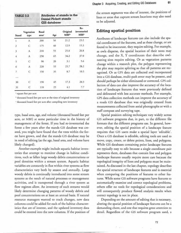
TABLE 3.2 Attributes of stands in the Daniel Pickell s tand. GIS database
Re·
Vegetation BaW O riginal inventoried
Stand "'P' u ... • Age MBF" MBP
A 200 50 21.2 23.2
2 C 175 40 12.9 15.3
3 A 210 55 25.8 26.8
4 A 250 65 34.2 37.0
5 C 90 20 3.1 5.6
6 A 220 55 25.7 28.2
7 C 150 35 8.7 10.5
30 C 190 45 17.3 20.3
3 1 C 110 25 4.1 7.7
• square (ttl ~r acre
h thousand board feet ~r acre at [he dme of original inventory
• thousand board fect per acre afrer compiling new inventory
type, basal area, age, and volume (thousand board feet per acre, or MBF) at some panicuiar time in [he history of management of [he forest. If you had re-inventoried me
forest a few years after the stands GIS database was cre~ ated, you might have found that the trees within the forest have grown, and tha< the stands GIS database may be in need of edicing (as the age, basal area, and volume have likely changed).
Another example might include aquacic habir3r invencories that attempt ro monitor change in habitat conditions. such as fallen large woody debr is concenrcarions or pool densities within a suearn system. Aquatic habitat
variables are consrantly in Aux within river systems as flow characteristics vaty both by season and annually. Large
woody debris is continually introduced into some stream systems as the result of natural processes or management activities, and is cransponed through a river system as flow regimes allow. An inventory of such streams would
likely determine changing patterns of woody debris and pool concemrarions on at least an annual basis. If natural resource managers wanted to track changes, new data
columns could be added for each of the habitat characteristics chat are of imerest. and the updated invemory data could be entered into che new columns. If the position of
Chapter 3 Acquiring, Creating, and Editing GIS Databases 61
the stream segments was also of imerest. [he positions of
lines or areas that capture stream locations may also need
to be adjusted.
Editing spatial position
Attributes of landscape features can also include [he spatiaJ coordinates of the feacures, and as these change, or are
found to be inaccurate, chey require editing. For example,
as owls disperse, the spatial location of their nests may change, and the X, Y coordinates that describe owl
nesting sites require editing. Or as vegetation panerns
change within a research plot, the polygon representing the plot may require splining so that all patterns are recognized. Or as GPS data are collected and incorporated
into a GIS database, multi-pam error may be present, and should perhaps be either eliminated or corrected. GPS collection of data can also improve the accuracy of the loca
tion of landscape features that were previously defined and delineated with less accurate methods. For example,
GPS data collection methods can improve the accuracy of a roads GIS database [hat was originally created from
measurements collected from aerial photographs or with a staff compass and surveying tape.
Spatial position edicing techniques vary widely across GIS software programs due, in part, to the different file formats that the different programs use. In general. how
ever, editing the spatial position of a landscape feature requires chat GIS users make a spatial layer 'editable' . Once a GIS database is editable, edi ting tools are used to
move, copy. create, or delece points. lines, and polygons. While GIS databases containing point landscape features
are typically easy ro edit because a single coordinate pair represents them, databases that comain line and polygon landscape features usuaJly require more care because the topological integrity oflines and polygons must be main
tained. As discussed in the last chapter, topology describes (he spacial structure oflandscape features and is essentiaJ when comparing the positions of features to other features. While some GIS software programs have fearures to auromatically examine and correct topological problems. others offer no rools for topological considerations and will consequently produce flawed analysis results when correct topology is not in place.
Depending on the amoum of editing that is necessary. ahering the spatial position of landscape features can be a demanding chore. and one that requires great attention to detail. Regardless of the GIS software program used, a
72
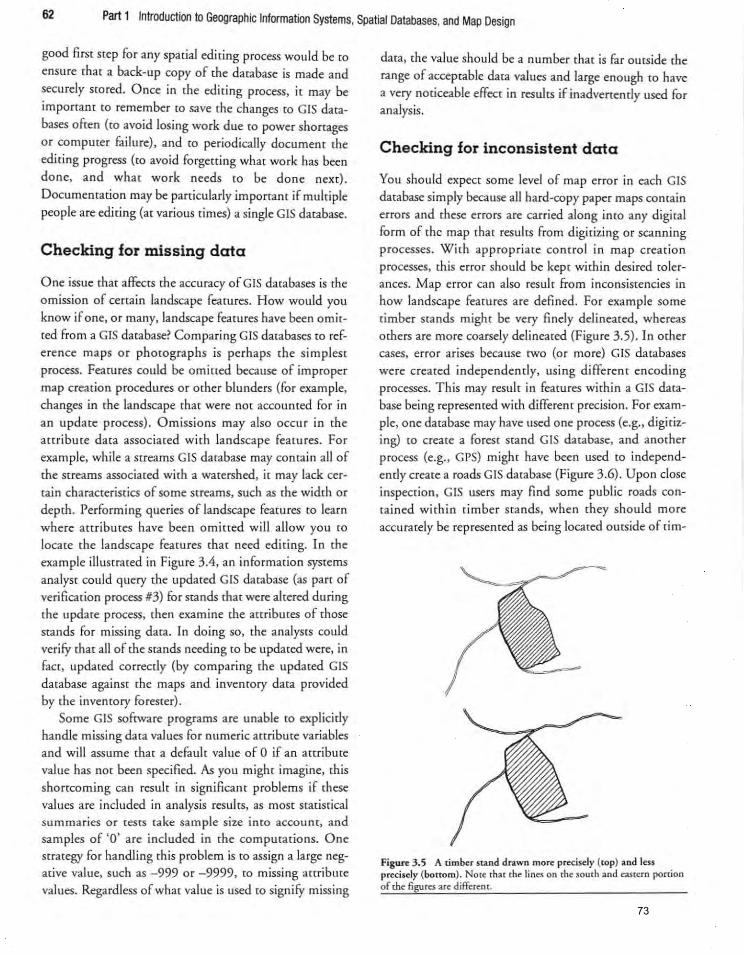
62 Part 1 Introduction to Geographic Information Systems, Spatial Databases, and Map Design
good first step fo r any spacial editing process would be to
ensure that a back-up copy of the database is made and securely srored. Once in the editing process, it may be
imponant to remember to save the changes to GIS databases often (to avoid losing work due [Q power shortages
or computet failure). and to periodically document the editing progress (to avoid forgetting what work has been done. and what work needs to be done next) . Documentation may be particularly important if multiple people are editing (at various times) a single GIS database.
Checking for missing data
One issue that affects the accuracy of GIS databases is the omission of cenain landscape feacuces. How would you
know if one, or many, landscape feacures have been omit
ted from a GIS database? Comparing GIS databases to reference maps or photographs is perhaps [he simplest process. Feacures could be omined because of improper
map creation procedures or other blunders (for example.
changes in the landscape that were not accou nted for in
an update process). Omissions may also occur in the 3nribure data assoc iated w ith landscape features. For
example. wh ile a streams GIS database may contain all of the streams associated with a watershed, it may lack cer
tain characteristics of some streams, such as the width or
depth. Performing queries of landscape features to learn where attributes have been omitted will allow you to
locate the landscape features that need editing. In the
example illustrated in Figure 3.4, an information systems
analyse could query the updated GIS database (as part of verification process #3) for stands that were altered during
the update process, then examine the attributes of those
stands for missing data. In doing so. the analysts could verifY that all of the stands needing to be updated were. in fact. updated correctly (by comparing the updated GIS database against the maps and inventory data provided
by the inventory forester). Some GIS software programs are unable to explicitly
handle missing data values for numeric attribute variables
and will assume that a default value of 0 if an attribute value has not been specified. As you might imagine, this
shortcoming can result in sign ificant problems if these
values are included in analysis resul ts, as most statistical summaries or testS take sample size imo account, and
samples of '0 ' are included in the computations. One
strategy for handling this problem is [Q assign a large negative val ue. such as -999 o r -9999, to missing attribme
values. Regardless of what value is used to signify missing
data. the value should be a number that is far outside the range of acceptable data values and large enough to have a very noticeable effect in results if inadvertendy used for analysis.
Checking for inconsistent data
You should expect some level of map error in each GIS
database simply because all hard-copy paper maps contain errors and these errors are carried along inco any digital
form of the map that results from digitizing or scanning
processes. With app ropriate co ntrol in map creation
processes, this error should be kept within desired toler
ances. Map error can also result from inconsistencies in
how landscape features are defined. For example some
timber stands might be very finely delineated. whereas others are more coarsely delineated (Figure 3.5). In other cases, error arises because rwo (or more) GIS databases
were created independendy, using different encoding
processes. This may result in features within a GIS data
base being represented with different precision. For exam
ple, one database may have used one process (e.g .. digitizing) to create a fo rest stand GIS database. and anmher
process (e.g .• GPS) might have been used to independently create a roads GIS database (Figure 3.6). Upon close inspection. GIS users may find some public roads conta ined w ithin timber sta nds, when they should more
accu rately be represemed as being located outside of tim-
Figure 3.5 A tim~r stand drawn more precisely (tOp) and less precisely (bottom). Note that the lines on the south and ea5[ern portion of the figures are different.
73
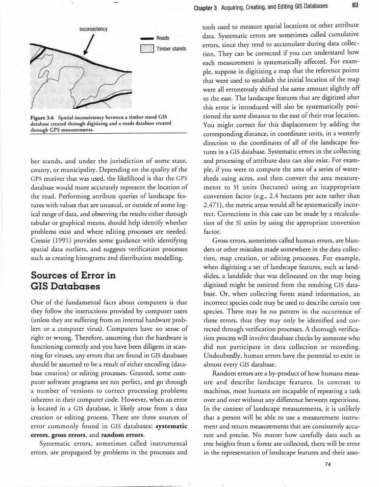
Inconsistency _ Roads
o Timber stands
Figure 3.6 Spatial inconsistency betwttn a timber stand CIS databau: created through digitizing and a roads database created through GPS meuurtments.
ber stands, and under the jurisdiction of some state, county. or municipality. Depending on the quality of the GPS receiver that was used. the likelihood is that the GPS
database would more accurately represent the location of the road. Performing attribute queries of landscape fea{Ures with values that are unusual, or outside of some logical range of data. and observing the results either through tabular or graphical means. should help identify whether problems exist and where editing processes are needed. eressie (1991) provides some gu idance with identifying spatial data outliers, and suggestS verification processes such as creating histograms and distribution modelling.
Sources of Error in GIS Databases
One of the fundamental facts about computers is that they follow the instructions provided by computer users (unless they are suffering from an internal hardware problem or a computer virus). Computers have no sense of right or wrong. Therefore, assuming that the hardware is functioning correcdy and you have been diligent in scanning for viruses. any errors that are found in GIS databases should be assumed to be a result of either encoding (database creadon) or editing processes. Granted. some computer software programs are not perfect, and go through a number of versions to correct processing problems inherent in their computer code. However, when an error is located in a GIS database. it likely arose from a data creation or editing process. There are three sources of error commonly found in GIS databases: systematic errors, gross errors, and random errors.
Systematic errors, sometimes called instrumental errors, are propagated by problems in the processes and
Chapter 3 Acquiring. Creating. and Editing GIS Databases 63
tools used to measure spatial locations or other attribute data. Systematic errors are sometimes called cumulative errors, since they tend to accumulate during data collection. They can be corrected if you can understand how each measurement is systematically affected. For example. suppose in digitizing a map that the reference points that were used to establish the initial location of the map
were all erroneously shifted the same amount slightly ofT to the east. The landscape features that are digitized after this error is introduced will also be systematically positioned the same distance to the east of their true location. You might correct fo r this displacement by adding the corresponding distance, in coordinate units, in a westerly direction to the coordinates of all of the landscape fea[Ures in a GIS database. Systematic errors in the collecting and processing of attribute data can also exist. For example, if you were [Q compute the area of a series of watersheds using acres, and then convert the area measurements to SI units (hectares) using an inappropriate conversion factor (e.g., 2.4 hectares per acre rather than 2.471). the metric areas would all be systematically incor
rect. Corrections in this case can be made by a recalculation of the SI units by using the appropriate conversion factor.
Gross errors, sometimes called human errors, are blunders or other mistakes made somewhere in the data collection, map creation, or editing processes. For example, when digitizing a set of landscape features. such as land
slides. a landslide that was delineated on the map being digitized might be omitted from the resulting GIS data
base. Or, when collecting forest stand information, an incorrect species code may be used to describe cerrain tree species. There may be no pattern in the occurrence of these errors, thus they may only be identified and corrected through verification processes. A thorough verification process will involve database checks by someone who did not participate in data collection or recording. Undoubtedly, human errors have the potencial to exist in almost every GIS database.
Random errors are a by-product of how humans measure and describe landscape features. In contrast to machines, most humans are incapable of repeating a task over and over without any difference between repetitions. In the context of landscape measurements, ic is unlikely that a person will be able to use a measurement instrument and return measurements that are consistently accurate and precise. No maner how carefully data such as tree heights from a forest are collected, there wi ll be error in the representation oflandscape features and their asso-
74

64 Part 1 Introduction to Geographic Information Systems, Spatial Databases, and Map Design
cjared attributes. Chances are that recorded measure
ments will be ar leasr slightly off from rhe [Cue mark due
to (he limitations of vision, musculature, and instrument
se[pup and application. As long as consistent procedures
are followed and no blunders occur, measurements will
tend to be grouped closely around the actual measure
ment, with differences occurring slighdy in all directions.
These types of small errors are called random errors; rhey
remain after all sys tematic errors and blunders are
removed. Random error occurrence does tend to follow
rhe laws of probability, and rhus should be normally dis
tributed in a statisrical sense. The statistical distribution
of repeated measuremems can be estimated in order to
obtain an idea of the variation expected in either the spa
tiallocarion of a landscape feacuee or the associated attrib
ure dara. Through the process of least sq uares adjusr
ments, you can attempt to remove random error from GIS
databases when concern about accu racy issues is high
(Ghilani & Wolf, 2006). More ofren however, in narural
resource management it is assumed that data collection efforts were carried Out diligently with respect to [he accu
racy and precision of measurements, and {hat random
errors rend to cancel each other out. For this reason, random errOfS are sometimes termed compensadng errors.
Two (erms are important when assessing the useful
ness of a G IS database: logical consistency and completeness. Logical consistency is (he term most GIS afi
cionados use co describe how well the relationships of di fferenr types of dara fir rogetlher within a system. In
some cases (his refers to the consistency of the ropological
relationships among GIS databases. For example, when streams are displayed in conjunction with the contour lines of an elevation GIS database. all streams shou ld
What is error? Error can be defined as something produced by misrake or as the difference between rhe
true va lue of a feature and its observed value
(Merriam-Websrer, 2007). How would you know
there was an error in a GIS database? Perhaps by comparing rhe value (o r shape of a landscape fearure)
in a GIS database to what is known as the correct value (or shape of a fearure) from a field survey, pho
cograph, etc. When you consider GIS database erro rs, the goal is to understand three issues: the type of
appear fl ow downhill (as opposed ro uphill) . In orher
cases. logical consistency refers to the anribme dara of a particular GIS database. For example, the dominant tree
species in o ne polygon may be labeled 'Loblolly', whi le in
anorher polygon ir may be labeled 'Loblolly Pine', and in
a rhird, 'Pinus taeda'. Completeness is a term used to
describe rhe types and exrent oflandseape features rhat are
included in a GIS database, and conversely, those that are omitted. For example, in some cases not all types of streams (e.g .• ephemeral streams that only contain flowing water during rain events) are included in a streams GIS database. In add ition, smaHer streams may be omined
because they weren' t apparent in the remotely-sensed da ta that were used co create the database. If only a portion of total number of stream types were included in a streams
GIS darabase, you might conclude that rhe database is not complete.
Types of Error in GIS Databases
Since creating, editing. and acquiring GIS databases may involve many different processes, a variety of errors can
obviously crop up. Some of the more commo n types include those relared to the locacional position of a land
scape fearure, those rela ted co the tabular att ribmes of a landscape feature, and those resulting from compmational problems.
Positional errors simply imply that a landscape feature is locared in the wrong place in a GIS darabase. These errors can arise during GIS database creation processes, such as digitizing or scann ing maps. As mentioned earlier, the digitizing of landscape features requires that a map be registered (Q a set of ground coordinates. How well the
error that exists, the so urce of the erro r, and the extent of the error. All of these relate CO the uncertainty associated with the landscape features contained in a sparial database. Hopefully you have a
high level of confidence in the dara (i.e., uncertainty
regarding the location oflandseape fearures and their
attri butes is minim ized), so that analysis efforts can be used with confidence to positively facilitate decisions made regarding the management of natural resources.
75
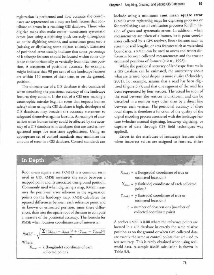
registration is performed and how accu rate the coordinates are represented on a map are both factOrs that contribute to errors in a resulting GIS database. Those who
digitize maps also make errors-sometimes systematic errors (nor using a digitizing puck correctly throughout an enrire digitizing session), and sometimes gross errors (missing or displacing some objects entirely) . Estimates of positional error usually indicate thar some percentage of landscape features should be located within some disrance either horizontally or verticaIly from their true position. A statement of positional accuracy, for example, might indicate that 90 per cent of the landscape features are within 150 meters of their true, or on the ground,
position . The ultimate use of a GIS database is also considered
when describing the positional accuracy of the landscape features rhey contain. If the risk of a GIS user making a catastrophic mistake (e .g., an event that impacts human safety) when using the GIS database is high. developers of GIS databases may broaden the accuracy statement to safeguard themselves against lawsuits. An example of a sit
uation when human safety could be affected by the accuracy of a G IS database is in databases that are used as navigational maps for maritime applications. Using an
appropriate set of comrol standa rds may minimize the amount of error in a CIS database. Control standards can
Root mean square error (RMSE) is a common term used in GIS. RMSE measures the error between a mapped point and its associated true ground position. Commonly used when digitizing a map, RMSE measures the positional error inherent in the registration
points on the hardcopy map. RMSE calculates the squared differences between each reference point and its known or estimated position, sums these differ
ences, than uses the square root of the sum to compute a measure of the positional accuracy. The formula for RMSE when location coordinates are of interest is:
RMSE= n
Where: Xciata.i X (longitude) coordinate of each
collected point i
Chapter 3 Acquiring. Creating. and Editing GIS Databases 65
include using a minimum root mean square error
(RMSE) when registering maps for digitizing processes or for establishing a set of verification processes for elimina
tion of gross and systematic errors. In addition, when measurements ace taken of a featu re, be it point coordi
nates collected by a GPS receiver, linear features such as
scream or trail lengths, or area features sllch as watershed boundaries. a RMSE can be used to assess and repof( differences between collected measurements and the true or
estimated positions of featu res (FGDC. 1998). While the positional accuracy oflandscape features in
a CIS database can be estimated, the uncertainty about
what are termed 'local shapes' is more elusive (Schneider, 2001) . For example. assume that a road has been digitized (Figure 3.7) . and that one segment of the road has been represented by four vertices. The actual location of the road between the vertices is unknown, and can be described in a number ways other than by a direct line
between each vertices. The positional accuracy of these local shapes is therefore a function of the quality of the digital encoding process associated with the landscape feature (whether manual digitizing, heads-up digitizing, or capture of data through GPS field techniques was applied).
Errors in the attributes of landscape features arise when incorrect values are assigned to features. either
Xch«k.i x (longitude) coordinate of true or estimated location i
Ydm .; Y (latitude) coordinate of each collected point i
y (latitude) coordinate of true or estimated location i
n = number of observations (number of collected coordinate pairs)
A perfect RMSE is 0.00 where the reference points are located in a GIS database in exacdy the same relative
position as on the ground or when GPS collected data are exacdy the same as control points that are lIsed to
test accuracy. This is rarely obtained when using realworld data. A sample RMSE calculat ion is shown in Table 3.3.
76
66 Part 1 Introduction to Geographic Information Systems, Spatial Databases, and Map Design
TABLE 3.3 Example of Root Mean Square Error (RMSE) calculation for GPS coordinates
Point
2
3
4
5
GPS-X (m)
477395.3
477399.7
477405.5
477407.5
477406.9
Known-X (m) GPS-Y (m)
477397.2 4934669.5
477398.7 4934677.2
477405.3 4934670.8
477406.9 4934673.9
477405.7 4934670.4
Squared Known-Y (m) Error (m)'
4934671.8 8.90
4934675.2 5.00
4934675.3 20.29
4934671.7 5.20
4934668.5 5.05
Sum of squared crror (ml )!> 44.44
Average squared error sum {m l)e 8.89
Root Mean Squared Error (m)d 2.98
• Squared straight-line differences between CPS coordinates actual known positions: (X-direction error 2 + V-direction error !)
I> Su m of [he squared errors
C Average of the sum of the squared errors: (Sum of squared errors I number of poinu)
d RMSE: Square root of the average of squared errors: (Avt.l'Olge squared error) tI~
through editing processes or through spatial joins (which are discussed in chapter 9), or arise because the attribute data is outdated. Keyboard entry of attribute data can result in attribute data errors, particularly if (he people performing the anribmion processes are nO[ paying close
Digitized road segment
Real-world representation #1
Real-world representation #2
Real-world representation #3
Figure 3.7 Uncertainty of thc local shape of a road scgment (after Schneider, 200 1).
anentian to the quality of their work. As we mentioned earlier, verification processes can range from an examination of primed maps and tabular databases related to the GIS database of interest, to an independent third-party examination of the landscape features a nd associated anribures comained in the resulting G IS database.
Compurational processes can lead to another source of error that can be rather transparent to GIS users. Processes such as general ization. vector-to-raster conversion (or vice-versa), and interpolation cause alterations in the characterization of landscapes. I n vector-faster conversio n. fo r example. vector fearures are converted to raster grid cells. Obviously the size of the resulting grid cells, as discussed in chapter 2, will influence the quality of the landscape features contained in the converted GIS
database. With large grid cells (e.g., 30 m or larger), the curvature of roads and streams could be lost. as well as small (and perhaps important) extensions of polygons. Users of the converted GIS databases would also need to determine whether the spatial resolut ion of the grid cells tha t result after vector-faster conversion is appropriate for the landscape fearures being represented. For example. are 30 m (or larger) grid cells appropriate for representing all roads and streams? Is a 10m resolut ion more appropr iate? The drawback of using a 10 m grid cell resolution is [he relatively large amount of data required-nine times the amount of data contained in a 30 m resolucion database (nine 10m cel ls are contained withi n a single 30 m grid cel l).
77
Ideally, in lieu of starements of error, the processes used to develop GIS databases. such as any transforma
tions and conversions, should be documemoo and made
known co allow users [Q understand the potential direc
tion and magnitude of error associated with subsequenc
GIS analyses. In addition. meradara. such as projection
and coordinate systems, should be made available to allow
Summary
Ultimately, most narural resource managemenc organiza
rions will develop needs rhar will ourgrow rhe capabiliries of their current collection of GIS databases. Acquiring, creating. and editing GIS databases are common processes
encountered by natural resource professionals when they
are in need of data or databases to assist in making man
agement decisions or evaluadng alternacive management
policies. When rhe GIS darabases rhar are available to a natural resource management organizacion are not suitable
Applications
3.1. Acquiring GIS data about Arizona National Forests. Assume you are interested in obtaining informa
tion about the streams related to the Prescott National
Forest in Arizona. The website related to the GIS data is
h rrp:llwww.fs.fed .us/r31 prescorrl gisl i ndex.shrml (USDA Foresr Service, 2007). Based on rhe informarion rhat rhe GIS data s ite provides, what are the ca tego ries that
describe rhe available GIS darabases? In reviewing rhe meradara for rhe 'Fire History' GIS darabase:
a) Whar is rhe purpose of rhe Fire History darabase? b) How were the data creared? c) What datum, projection, and spheroid are used to
represent fires?
d) What data structure is used to represent the fires?
e) What is rhe spa rial extent of rhe fire hisrory darabase in longitude and latitude?
f) Who is rhe primary contact should you have further questions?
Note: Please do not contact the Prescott Forest GIS coor
dinator for answers to these questions.
3.2. Acquiring digital orthophotographs about Massachusetts. Your position as a natural resource con
sultant has allowed you to become involved in a project
Chapter 3 Acquiring, Creating, and Editing GIS Databases 67
users to consider how a GIS darabase was developed. This is, of course, rhe ideal case. For example, rhe GIS darabases used extensively in (his book are void of S[3[emems
of error and of meradara. They were developed as hyporhericallandscapes for students in rhe aurhors' GIS appli
cations courses.
to address a particular cask. acquisition. creation. and edit
ing processes must be considered. Those who simply view
GIS as a sysrem to make maps will likely underesrimare the amount of work required to acquire. create, or edit the
GIS darabases necessary to make rhose maps. In addirion, regardless of how GIS darabases are generared, rhe presence and elimination of errors must be considered, and
will likely require extensive verification processes to ensure
mat the pmential errors are minimized.
situated in Massachusetts. As such. you are interested in
obtaining digital orthophorographs about an area in
Massachusetts . One source of this data might be the
Massachuserrs GIS websire (http: //www.srare.ma. u.1 mgisl) (Commonwealrh of Massachuserrs, Office of Energy and Environmental Affairs, 2007) . Based on whar you can gather from the website:
a) Whar rypes of black and whire digiral orrhophorographic imagery are available?
b) Whar spatial resolurions are available for 1:5000 color orrhophorographic imagery '
c) Whar sparial resol urions are available for 1 :5000 black and whire imagery?
d) What datum and coordinate system are used to
represent these images?
3.3. Data acquisition (1). You have been hired by a private consultant in Washington State to develop a GIS
program . The consultant has a small office, comprised of
only five employees, and is interesred in developing a GIS program thar will urilize desktop GIS software (ArcGIS ArcView, MapInfo, or GeoMedia) and GIS darabases created by other organizations. To get started, you decide
that acquiring base maps describing the counties, towns,
secrion lines, and ownership of rhe Stare is important.
78
68 Part 1 Introduction to Geographic Information Systems. Spatial Databases. and Map Design
a) Is each of these da<abases ava ilable? liS[ any da<abases that are not ava ilable.
b) Wha< S[eps would you have [Q go through to be able <0 download the data?
c) What is the spatial reference of available data?
d) Who would you contact if you had problems downloading the data'
Hint: See Washington Departmenc of Natural Resources 2007a fo r additional info rmation.
3.4. Data acquisition (2) . Assuming you were inter· ested in acqu iring soils GIS databases for 10 rownships in
Washington State from the Washing<on Department of Natural Resources (see Wash ingtOn Deparrmenc of
Namral Resources. 2007b): a) What is the format of the database? b) What are the coordinate units? c) Who is [he contact for more information about the
soils database? d) Where did the soils information come from?
3.5. Data acquisition (3). The Washi ng<on Namral Heritage Program (Washington Department of Namral Resources, 2007c) maintains a GIS database of the highquality terrestrial and wedand ecosystems of the State, as well as locations of rare planes of concern.
a) What groups of professionals are the intended users of the Washing<on Natural Heritage GIS data set?
b) How would you gain access <0 the Washing<on Narural Heritage GIS data set?
c) What data formars are available for the GIS database?
d) Are you allowed <0 display GIS maps of the dataset on {he I ncerner?
3.6. Development of base map for a digitizing contractor. Assume char the standard process within your natural resource managemem organization for updating
G IS databases is to develop hand-drawn maps of the changes des ired, and then to deliver these po tentia l changes to a contractor for digitizing work. In the cemer of the Brown Tract is an open area of land. Assume that the owners of the Brown Tract recently acquired this land. Develop a base map. showing the currenc stands and the current roads. Create a GIS database of fou r tics (reference ma rks) and place them on the map as well, along with thei r assoc iated Xand Y coo rdinates. Print the
map, and then hand-draw the additional timber stands to
be digitized by the contractor. Use the digital orthophotograph associated with [he Brown Tract to hand-draw the new stands.
3.7. Owl locations on the Daniel Pickett forest. The wildlife biologist associated with the Daniel Pickett forest, Kim Dennis, is concerned about the quali ty of the owl nest location GIS database.
a) How could you determine whether the owl nest locations on the Daniel Picken forest are represented as being in the correCt place?
b) What are the coordinates associated with each owl nest location?
3.8. Errors in landscape feature and attribute data. As a user of the Brown Tract GIS databases, you are very imerested in the quali ty of data that each provides. What
might you say about the possible errors in the stands GIS
database features that are located in the fo llowing places? a) X = 1263950; Y = 371726 b) X = 1273647; Y = 363943
3.9. Verification processes. As technology progresses and the capabil ities of field personnel increase (wi th new college courses in GIS, continuin g educa tion co urses, etc.), the co llection and transfer of data can occur with
processes that would seemingly save effort and COSt to an organization. For example, in Figure 3.4 the inventory forester would transfer cruise reports (hard copies) and
maps (hand-drawn) to informatio n system analysts in an annual update process. Several verification processes were noted in an efforr to maintain the consistency and quality of data moving from the field to the information systems deparrment and vice versa.
a) H ow mighr these processes in the flow chart
change if the inventory fo rester were to provide spatial data that was digitized in the field office, and cruise data that was collected with a hand-held data collector?
b) Could the verifica tion responsibilities shift under these circumstances?
3.10. Sources of error. Your supervisor, Steve Smith, is interested in understanding the types of error that may be inherent in GIS databases. Describe fo r Steve the differences between the foHowing three types of error: systematic, random, and gross error.
79
68 Part 1 Introduction to Geographic Information Systems, Spatial Databases, and Map Design
a) Is each of mese databases available? List any databases that are not avai lable.
b) What steps would you have to go mrough [0 be able to download [he data?
c) What is the spatial reference of available data?
d) Who would you contact if you had problems downloading me data?
Hint: See Washington Department ofNarural Resources 2007a for additional info rmation.
3.4. Data acquisition (2) . Assuming you were interested in acquiring soils GIS databases for 10 townships in Washington State from the Washington Department of Natural Resources (see Washington Department of Natural Resources. 2007b) :
a) What is the formar of the database? b) What are (he coordinate units?
c) Who is me comact for more information about the soils database?
d) Where did me soils information come from?
3.5. Data acquisition (3). The Washington Natural Heritage Program (Washington Department of Natural Resources. 2007c) maintains a GIS database of the highqualiry rerresuial and werland ecosystems of the Stare. as
well as locations of r-are plams of concern.
a) What groups of professionals are the intended users of lhe Washington Natural Heritage GIS data set?
b) How would you gain access to the Washington Narural Heritage GIS dara sec?
c) What data formars are available for me GIS database?
d) Are you allowed to display GIS maps of the dataset on (he Incerner?
3.6. Development of base map for a digitizing contractor. Assume that the standard process within your natural resource management organizarion for updating
GIS databases is ro develop hand-drawn maps of the changes desi red, and then [0 deliver these po tential changes [0 a COlHractor for digitizing work. In (he cemer
of the Brown Tract is an open area of land. Assume thar
rhe owners of the: Brown T racr recently acquired this
land. Develop a base: map. showing [he currenc s tands
and the current roads. Create a GIS database of fou r [ics
(reference marks) and place them on the map as well. along wirh their assoc ia[ed X and Y coordinates. Prine [he
map. and then hand-draw the additional [imber srands (Q
be digitized by the contractor. Use the digital orthophocogl"dph associated wirh me Brown Tracr to hand-draw
the new srands.
3.7. Owl locations on tbe Daniel Pickett forest. The wildlife biologist associated with the Daniel Pickett forest. Kim Dennis, is concerned about rhe quality of the owl
nest location GIS database. a) How could you determine whether me owl nest
locarions on rhe Daniel Pickert forese are repre
semed as being in the correcr place?
b) What are [he coordinates associated with each owl
nest locarion ?
3.8. Errors in landscape feature and attribute data. As a user of the Brown Tract GIS databases. you are very inrerested in the quality of data rhat each provides. What
might you say about the possible errors in the srands GIS database features that are located in the following places?
a) X = 1263950; Y = 371726 b) X = 1273647; Y = 363943
3.9. Verification processes. As technology progresses and me capabili ties of field personnel increase (with new college courses in GIS, conrinuing educadon courses)
Ctc.), the collection and transfer of dara can occur with
processes that would seemingly save effort and COSt co an
organizadon. For example. in Figure 3.4 the invencory
foreSter would transfer cruise reports (hard copies) and maps (hand-drawn) to informarion system <1nalysrs in an
annual update process. Several verifkation processes were
nmed in an effort (Q maintain rhe consisrency and quality of data moving from me field [ 0 the information sysrems department and vice versa.
a) How might these processes in the flow chart
c hange if me invemory fo resrer were [Q provide
spatial data that was digitized in the field office. and cruise data that was coUeeted with a hand-held dam coiJector?
b) Could me verification responsibilities shift under these c ircumstances?
3.10. Sources of error. Your supervisor, S teve Smidt , is
interested in undersranding the types of error [hat may be
inherenr in GIS darabases. Describe for Sreve the differ
ences between the following mree rypes of error: systematic, random, and gross error.
3.11. Types of error. Given the inventory updating process oared in Figure 3.4, describe [he sources of error
(posi tional. a[[cibure. comput3rional) that could result at
each step in the process.
3.12. Calculating Root Mean Squared Error: Woodpecker nest GIS database. Assume you are digitizing a map of red-cockaded woodpecker nest cree locations of a
Nacional Forest in Florida. You have four reference marks
that you can use [0 reference the map [Q known coordi
nates. When registering the map you find that the Xdirecrion and V-direction difference berween the reference marks and the acwal known locations are as follows:
Registration X-direction Y.direction Point error (ft) error (ft)
3.526 0.963
2 -2.890 -2.452
3 0.985 -1.987
4 - 1.598 -2.850
Whar is the RMSE, or positional error, associarcd with the
resulting woodpecker nest GIS database?
3.13. Calculating Root Mean Squared Error: Trails GIS database. Assume you are employed by a National Park in Alberta, and are in the process of digirizing a map of trails [har were drawn by the recreadon specialist asso
ciared with che park. On the recreadon specialise's map
chere are six reference marks chat you can use co regisrer
che map [Q known coordinaces. When regiscering che map
you find that the X-direction and Y-direction difference becween the reference marks and (he accual known loca
dons are as follows:
Registration X-direction Y -direction Poine ~rror (m) ~rror (m)
3. 125 - 1.588
2 2.564 -1.992
3 2.548 -2.987
4 1.998 - 2.856
5 1.268 2.857
6 1.489 3.897
Whar is che RMSE, or posidonal error, associ aced. wich [he resulcing cra ils GIS darabase?
Chapter 3 Acquiring, Creating, and Editing GIS Databases 69
3.14 Calculating Root Mean Squared Error: Tree location database. Assume you work as a nacu ral
resource manager in Oregon. and your supervisor is con
cerned about the qualiry of data that you are colleCting wich a GPS receiver. You supervisor has asked you co cal
culate the RMSE between GPS-collected coordinates and coordinates that had been collected by a digital total stacion. Boch secs of coordinates are lisred below.
Total Total
Point GPS-X Station-X GPS-Y Station-Y
4934688.3 4934691.9 477311.7 477309.0
2 4934693.6 4934690.8 477310.5 47731 1.9
3 4934686.9 4934687.0 4773 16.1 4773 13.8
4 4934686.1 4934683.9 4773 12.7 4773 12.7
5 4934678.8 4934682. 1 4773 10.2 477309.0
6 4934680.3 4934683.2 477307.6 477306.0
3.15 Calculating Root Mean Squared Error: Stream gauging stations. Assume chac you are collecdng daca
from a stream survey. A stream ecologisc has given you a
set of GPS coordinates that had been collected from gauging stations locared nexc co a scream. She has also pro
vided a sec of coordinaces from the same gauging scadons
that were collected from LiDAR data. What is the RMSE of che differences between chese secs of coordinaces?
Point GPS-X GPS-Y UDAR-X LiDAR-Y
934681.0 477392.8 934676.6 477402.2
2 934670.8 477405.5 934675.3 477405.3
3 934673.9 477407.5 934671.7 477406.9
4 934670.4 477406.9 934668.5 477405.7
5 934665.8 477399.2 934666.9 477402.1
6 934668. 1 477399.5 934668.6 477398.3
80
70 Part 1 Introduction to Geographic Information Systems, Spatial Databases, and Map Design
References
Commonweal th of Massachusetts, Office of Energy and Environmental Affairs . (2007). Massachusetts g'ographic information sysum. Retrieved April 19,2007, from http://www.state.ma.us/mgisl.
Cressie, N. (1991). Statistics for spatial data. New York: John Wiley & Sons.
DeMers , M.N. (2000). Fundamentals of g,ographic
information systems. New York: John Wiley and Sons, Inc.
Envi ronmental Systems Research Institute. (2005). GIS
topology. Retrieved April 19, 2007, from http://www. es ri .comllibrary/whitepapers/pdfs/gis_topology.pdf.
Federal Geographic Data Commitree (FGDC) . (1998). GeospatiaL positioning accuracy standards. Part 3: National standard fo r spatial data accuracy. Reston , VA: US Geological Survey.
Geography Network Canada. (2007). Data. Retrieved April 27, 2007, from http://www.geographynetwork. ca/datalindex.html.
Ghilani , CD., & Wolf, P.R. (2006). Adjustment computations: Spatial data analysis (4th ed.). New York: John Wiley and Sons, Inc.
G ifford Pi nchot National Forest. (2007). Gifford Pinchot
National Forest geographic infonnation sysums, available data uts. Retrieved April 19, 2007, from http: // www.fs.fed. us/gpn fifo rest -researchl gisl .
Keefer, B.J. , Smith, J.L. , & G regoire, T.G. (1988). Simulating manual digitizing error with sradsricai models. Proceedings, GIS/LiS '88. Falls Church, VA: American Society of Photogrammerric Engineering
and Remote Sensing, American Congress on Surveying and Mapping.
Merriam-Webster. (2007). M"rian- W,bsm onlin, search. Retrieved April 27, 2007, from http://www.m-w.com.
Minnesota Planning. Land Management In fo rmation Center. (2007). LMIC's clearinghouse data catalog. Retrieved April 19, 2007, from http ://www.lmic. Sta te. mn. us! chouse/.
Natural Resources Canada. (2007). Mapping. Retrieved April 19, 2007, from http: //www. nrcan-rncan.gc. cal com/subsu jl mapcar-eng. ph p.
Prisley, S.P., Gregoire, T.G., & Smith , J.L. (1989). The mean and variance of area estimates in an arc-node
geograph ic information sys[em. Photogramm~tric
Enginuring and Remou S,nsing, 55, 1601-12. Schneider, B. (2001) . On the uncertainty of local shape
of lines and surfaces. Cartography and Geographic Information Sciences, 28, 237-47.
USDA Forest Service. (2007). Pmcott National Form: GIS-geographic information sysums. Presco[[, AZ:
USDA Forest Service. Retrieved April 20, 2007, from http://www.fs.fed.us/r3/ prescottl gisl index.sh tml.
US Geological Survey, Federal Geograph ic Data Committee. (2002). Manual offtdual geographic data products. Reston, VA: US Geological Survey.
WashingtOn Department of Natural Resources. (2007a). GIS data. Olympia, WA: Washington Department of Natural Resources. Retrieved April 20, 2007, from http://www.dnr.wa.gov/dataandmaps/index.html.
Washington Department of Natural Resources. (2007b). Avai"'ble GIS data . Olympia, WA: Washington Department of Natural Resources. Retrieved April 20, 2007, from htrp://www3.wadnr.gov/dnrapp6/dara webl dmma[rix.h[ml.
Washington Department of Natural Resoutces. (2007c). Reference desk. Olymipia, WA: Washington Department of Natural Resources. Retrieved April 20, 2007, from http://www.dnr.wa.gov/nhp/refdesk/gis/index.html .
81
Chapter 4
Map Design
Objectives
The common features of maps are described in this chapter. and emphasis is placed on developing those that field professionals can use to present results of GIS analyses or (0 illustrate themes of interest including forest management areas, tree species maps, harvest plans. wildlife habi
tat, and mher narural resource management actions. At the conclusion of this chapter. readers should have acquired a firm understanding of:
I. the main components. or building blocks. of a map; 2. rhe qualities of a map that are imporram in communi
cating information co map users; and 3. the types of maps that can be developed to visually
and quickly communicate information to an audience.
Within the various fields associated with natural resource management, we expect chat maps will be avail
able to illustrate resources and areas that we manage because of the prevalence of GIS use. Maps are amazing tOols that, if constructed properly, have the abili ty to
quickly and clearly communicate a message [Q an audience. Maps are an effective method of communicating spatial relationships among landscape features. Maps are
also engaging-people are drawn to maps. Most GIS software programs provide users the capability to produce sophisticated maps and maps often represent the output
produced by GIS analyses. thus most people mainly tend to associate GIS with map-making activities. Although this association may ignore many of the other analytical capabilities of GIS. the ability to geographically portray the results of an analysis is one of the primary distinguish-
ing characteristics that sets GIS apart from other software
programs. Maps have been part of human civilization for millen
nia and have been used for many purposes, including data storage, navigation, and visualization. Maps have been used to create and sway opinion in many disciplines. including those related to the managemem of natural
resources. In a manner similar to the use of statistics. maps can hold tremendous power over the message that is delivered to an audience and. when created skillfully.
maps can be used to influence people's opinions (Monmonier. 1995. 1996). One of the great dangers pre
sented by maps is that people assume the landscape features represented on maps are accurate ponrayals of the natural resources that they claim to manage. However. maps are. at best, abstractions of the real world, and will usually possess some measure of non-conformity, be it directional or proportional or both, from a set of landscape features . A skilled map-maker will be able to choose
a map projection that best preserves feature qualities (e.g .• area, shape) and that best suits a map's objective. This skill might also include applying strategies for representing data characteristics or qualities through different shapes, colors, or sizes. Understanding that maps must be created and imerpreted with a discerning eye is one of the first steps necessary to becoming a successful mapmaker
or user. Maps usually are two-dimensional representations of
the landscape. although th ree-dimensional maps can be used to show volume o r perspective. Symbols. colors, and text are combined to communicate information and, as with graphs, flow charts, and other diagrams. maps are graphical representations of information. Mapmakers
82
72 Part 1 Introduction to Geographic Information Systems. Spatial Databases. and Map Design
attempt to transmit ideas in a different manner than (hat used by ocher forms of communica(ion. The goal of (he map-making process is co produce a visual display (ha( communicates spatial information to pQ[encial map users. The human brain, with its limited capacity to s(Qre informarion, may be able (Q understand ideas more effectively when supporting concepts are presented graphically on a map (Phillips. 1989). The design of a map can aifec( (he abi lity to communicate spatial information, thus a well
designed map will likely communicate ideas co an audience (e.g .. co-workers and supervisors) more effectively
(han a poorly designed map. Poorly designed maps can lead to misinterpretations and cosdy or inappropriate decisions.
Cartography is the science and art of making maps, and for the bence part of the twentieth century it was a skill developed (hrough ex(ensive experience in making maps by hand. Since (he la(e 1980s when G IS began co be pervasive in namral resource organizations. the vast
majority of maps have been made by non-professional carrographers. This shift is simply because of the access ibiliry and ease of use of GIS sohware. Some people may argue that several of the prescriptive aspects of making maps are no longer necessary (Wood. 2003). However. we would consider our effort to educate readers abom the capabili(ies of GIS less than successful if we failed (0
describe the important aspects of maps, and suggest ways
(0 make maps aesrhecically appealing. When developing maps for others to use, mapmakers
should keep in mind tha( nor all map users will be operating on the same level of competence. In fact, map users can be categorized as experienced, inexperienced, o r reluc(ane (F ranklin. 2001). The de(ail and c1ariry of mapped feacures will likely afTecc how well a map coneribures (0
natural resource management. Within natural resource management, maps should be clear enough for users ro undersrand ewo main (hings: (I) (he land area (ha( me map represents, and (2) the message the map intends to
communicate aboU( the land area. In order to meet these two requirements, a mapmaker needs ro understand:
• (he objec(ive(s) of the map «he message). • (he people who may use ,he map «he audience). • (he da(a (ha( will be displayed in (he map «he in for
mation available), • the use of graphics sohware for displaying map infor
mation, and • the final format of the printed or digital version of the
map «he produc().
The size. shape. and symbology of each componene of a map should reAec( (he likely responses (0 (hese promprs. A variety of common [Ools can be employed (0 make a map both useful for natural resource management purposes and aesrhecically pleasing. The landscape feacures illusuared on a map should include enough landmarks co allow the users to reference themselves to the mapped area. and help navigare (hrough a landscape. Mapmakers should keep ewo importane aspecrs of maps in mind: (I) not everything known about a landscape needs to be displayed on a single map. and (2) co communica(e eifec(ively. maps should focus on displaying a limi(ed number of landscape features. These concepts emphasize that carrographers shou ld focus on characteristics that directly
relate to the map's intended message, and thus they should ensure that other map components do not mask or cloud (he message. The landscape fea(u res primarily emphasized on a map should be (hose associared wi(h (he main intent of the map. For example, on a map devel
oped ro illustrate stream classes. other landscape features. such as roads, timber stands, and soils, should be second
arily emphasized, or omitted from the map ent irely.
Map Components
When developing a map for a natural resource management purpose, several basic components should be con
sidered. These componenrs include (he symbols being used to describe landscape features, a north arrow, the scale. (he legend. and (he quali(ies (fone. size. ere.) of the (ex( (labels and anno(a(ion). In addi(ion. you may find i( necessary to include other components in a map, such as
a description of the mapmaker, the filenames and file loca(ions of (he GIS da(abases used. and map quali(y caveats. Each of these components is briefly discussed below, and it is important ro understand each elemem
before we discuss the common types of maps that can be developed using GIS sofeware programs.
Symbology
Symbology can be (hough( of as (he art of expression. based on symbols (Merriam-Websrer. 2007). A large suire of map symbols has been developed (0 ideneifY and illustrate significant landscape features on maps. Some of (hese symbols (Figure 4. I) were developed as na( ional standards for illustrating landscape features (e.g., conrour lines. hydrologic symbols) found on cerrain widely used maps. such as (he US Geological Survey (opographic
83
72 Part 1 Introduction to Geographic Information Systems, Spatial Databases, and Map Design
attempt ro transmit ideas in a differenr manner than that used by other forms of communication. The goal of the map-making process is to produce a visual display that communicates spa rial information co potential map llsers. The human brain, with irs limited capacity ro Stofe information, may be able to understand ideas more effectively when supporting concepts are presented graphically on a map (Phillips, 1989). The design of a map can affect the ability to communicate spadal information. thus a welldesigned map wi ll likely communicate ideas to an audience (e.g. , co-workers and supervisors) more effectively rhan a poorly designed map, Poorly designed maps can lead to misinterpretations and costly or inappropriate decisions.
Cartography is rhe science and arr of making maps, and for the bc(rer parr of me [wemicrh century it was a skill developed through extensive experience in making maps by hand. Since the late 1980s when GIS began to be pervasive in natural resource organizations. tbe vast majority of maps have been made by non-professional cartographers. This shift is simply because of the accessibility and ease of use of GIS software. Some people may argue that several of the prescriprive aspects of making maps are no longer necessaty (Wood, 2003). However, we would consider our dfoIT to educa.te reade.rs 3bom the capabilities of GIS less ,han successful if we failed to
describe the important aspec[S of maps, and suggest ways
to make maps aesthetically appealing. When developing maps for Q[hers to use, mapmakers
should keep in mind that not all map users will be operating on the same level of competence. In fact, map users can be categorized as experienced. inexperienced. or reluctallt (F ranklin, 2001). The detail and clarity of mapped featu res will likely affeer how well a map conuibutes to
namral resource management. Within natural resource management, maps should be clear enough for users [Q
understand twO main things: (I) the land area thar the map represents, and (2) the message the map intends to communicate abom [he land area. In order to meet these two requ_iremems. a map maker needs to understand:
• the objective(s) of the map (the message), • the people who may use the map (the audience), • the data that will be displayed in the map (the infor
mation available),
• rhe use of graphics software for displaying map information, and
• me final format of the printed or digital version of the map (the product).
The size, shape, and symbology of each component of a map should reAect the likely responses to these promp". A variety of common [ools can be employed to make a map both useful for namral resou rce management purposes and aesthetically pleasing. The landscape features illustrated on a map should include enough landmarks to
allow the users to rderence themselves to [he mapped area, and help navigare through a landscape. Mapmakers should keep two important aspects of maps in mind: (I) not evetything known aboUt a landscape needs to be displayed on a single map, and (2) to communicare effectively, maps should focus on displaying a limired number of landscape features. These concepts emphasiz.e that ca rrographers should focus on characreristics rhar direcdy rel ate ro the map's intended message, and rhus they should ensure that other map components do not mask or cloud the message. The landscape features primarily emphasized on a map should be rhose associared with the main intent of the map. For example, on a map developed to illustrate stream classes) other landscape fearures. such as roads) timber stands, and soi ls. should be second
arily emphasized. or omirred from the map entirely.
Map Components
When developing a map for a natura] resource managemem purpose, several basic components shou ld be con
sidered. These co mponentS include [he symbols being used to describe landscape features, a north arrow, [he scale, the legend, and the qualities (font, size, etc.) of the rext (labels and annmation). In addition, you may find it necessary [Q include other components in a map, such as
a description of the mapmaker, rhe menames and me locations of the GIS databases used, and map qual iry caveats. Each of these components is briefly discussed below, and it is imponant ro understand each e1emem
before we djscuss the common types of maps that can be developed using GIS software programs.
Symbology
Symbology can be thought of as the art of expression, based on symbols (Merriam-Websrer, 2007). A large suire of map symbols has been developed to identifY and iUuscrate significant landscape features on maps. Some of rhese symbols (Figure 4.1) were developed as narional srandards fo r illustrating landscape features (e.g., contOur lines, hydrologic symbols) found on cenain widely used maps, such as the US Geological Survey topographic
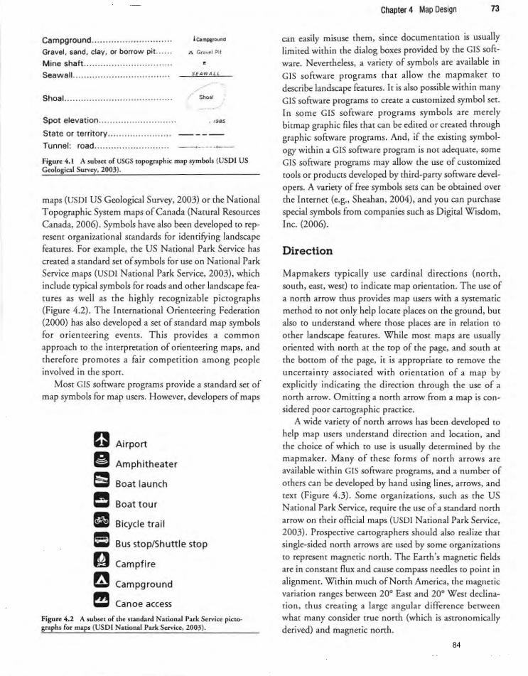
Campground ......... .. ... ..... . .... ..... lc.nqlounI!
Gravel. sand. clay. Of borrow pit ...... .... Grll~t!I?iI
Mine shaft ... .. . ..... ...... ....... ... ..... I!l
Seawall. ... ....... ................... ... .. S£AW" L~
ShoaL ......... ... ........ ........ . ... ...... Shoal
Spot elevation........ .. ............. ..... . mts
State or territory.... ........ ...... ..... -- - ---Tunnel: road...... .... .... .. .... .... ... ~_ £ ... _
Figure 4. 1 A subset of USGS topographic map symbols (USD I US Geological Survey, 2003).
maps (USDI US Geological Survey. 2003) or the National Topographic System maps of Canada (Natural Resources Canada. 2006). Symbols have also been developed to represent organizational standatds for identifying landscape features. For example. the US National Park Service has created a standard set of symbols for use on National Park Service maps (USDI National Park Service. 2003). which
include typical symbols for roads and other landscape features as well as the highly recognizable pictographs (Figure 4.2). The International Orienteering Federation (2000) has also developed a set of standard map symbols
fo r orienteering events. This provides a common approach to the interpretation of o rienteering maps, and therefore promotes a fair competition amo ng people involved in the sporL
Most GIS software programs provide a standard set of map symbols for map users. However. developers of maps
0 Airport
II Amphitheater
e Boat launch
I!J Boat tour ,. Bicycle tra il
El Bus stop/Shuttle stop
g Campfire
~ Campground
!!! Canoe access
Figure: 4.2 A subset of the slanda rd National Park Service pictographs for maps (USDI National Park Service, 2003).
Chapter 4 Map Design 73
can easily misuse them, since documentarion is usually
limited within the dialog boxes provided by the GIS software. Nevertheless, a variety of symbols are available in
GIS software programs that allow the mapmaker to describe landscape features. It is also possible within many
GIS software programs [Q create a customized symbol set. I n so me GIS software programs symbols are merely
bitmap graphic files that can be edited o r created th rough graph ic software programs. And. if the existing symbol
ogy within a GIS sofrware program is nO[ adequate, some GIS software programs may allow the use of customized
tools or products developed by third-party software developers. A variety of free symbols sees can be obtained over
the Internet (e.g .• Sheahan. 2004). and you can purchase special symbols from companies such as Digital Wisdom. Inc. (2006).
Direction
Mapmakers typically use cardinal di rections (north. south, east, west) (Q indicate map orientation. The use of
a north arrow thus provides map users with a systematic
method to not only help locate places on the ground. but also [Q understand where those places are in relation to
ocher landscape features. While most maps are usually oriented with north at rhe tOP of the page, and south at [he bo[{om of the page. it is appropriate to remove the
uncertainty associated with orientation of a map by explicitly indicating the direc(ion through the use of a north arrow. Omitting a north arrow from a map is con
sidered poor cartographic practice. A wide variety of north arrows has been developed to
help map users understand direction and location, and the choice of which to use is usually determined by the mapmaker. Many of these forms of north arrows are available within GIS software programs, and a number of o(hers can be developed by hand us ing lines. arrows. and
text (F igure 4.3). Some organizations. such as the US National Park Service, require the use of a standard north arrow on their official maps (USDI National Park Service, 2003). Prospective cartographers should also realize (har single-sided north arrows are used by some organizations to represent magnetic north . The Earth 's magnetic fields are in constant flux and cause compass needles [Q point in alignment. W ith in much ofNorrh America, the magnetic variation ranges berween 20° East and 20° West declinat ion , thus creating a large angular difference berween what many consider [rue north (which is astronomically derived) and magnetic north.
84
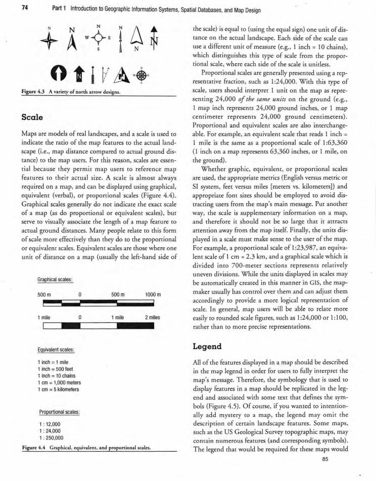
74 Part 1 Introduction to Geographic Information Systems, Spatial Databases, and Map Design
Figure 4.3 A variety of north arrow d~igns.
Scale
Maps are models of real landscapes. and a scale is used to indicate the ratio of (he map features [Q the actual landscape (i.e., map distance compared to actual ground disranee) [0 the map users. For this reason, scales are essencia! beca use they permit map users to reference map
features to their actual size. A sca le is almost always required on a map. and can be displayed using graphical, equivalent (verbal). or proportional scales (Figure 4.4). Graphical scales generally do not indicate the exact scale of a map (as do proponionai or equivalent scales) , but serve to visually associate the length of a map feature to
actual ground distances. Many people relate to this form of scale more effectively than they do to the proportional or equivalem scales. Equivalent scales are those where one
unit of d istance on a map (usually the left-hand side of
Graphical scales:
500m o 500m 1000m - -- -1 mile
Equivalent scales:
1 inch = 1 mile 1 inch = 500 feet 1 inch = 10 chains
o
1 em = 1,000 meters 1 em = 5 kilometers
Proportional scales:
1: 12.000 1 : 24.000 1 : 250,000
1 mile 2 miles
Figure 4.4 Graphical. equivalent. and proportional scales.
the scale) is equal to (using the equal sign) one unit of distance on the actual landscape. Each side of the scale can use a different unit of measure (e.g., 1 inch = 10 chains),
which distinguishes this type of scale from the proportional scale, where each side of the scale is unirless.
Proportional scales are generaIly presented using a representative fraction. such as 1 :24.000. With this type of scale, users should interpret 1 unit on the map as represent ing 24.000 of the same units on the ground (e.g .• 1 map inch represents 24.000 ground inches, or 1 map centimeter represents 24,000 ground centimeters). Proportional and equivalent scales are also interchangeable. For example. an equivalent scale that reads 1 inch =
1 mile is the same as a proportional scale of 1 :63.360 (I inch on a map represents 63.360 inches. or 1 mile, on the ground).
Whether graphic, equivalent , or proportional scales are used, the appropriate metries (English versus metric or
SI system. feet versus miles [meters vs. kilometers)) and appropriate font sizes should be employed to avoid distracring users from the map's main message. Puc another way, the scale is supplementary informacion on a map. and therefore it should not he so large that it auracts attention away from the map itself. Finally, the units dis
played in a scale muSt make sense to the user of the map. For example. a proportional scale of 1 :23.987. an equivalent scale of 1 cm = 2.3 km. and a graphical scale which is divided inro 700-meter sections represents relativdy uneven divisions. While the units displayed in scales may he automaticaHy created in this manner in GIS, the map
maker usually has comrol over them and can adjust them accordingly to provide a mo re logical representation of scale. In general, map users will be able to relate more easily to rounded scale figures. such as 1 :24.000 or 1: 1 00. rather than to more precise representations .
Legend
All of the features displayed in a map should be described in the map legend in order fo r users to fully interpret the map's message. Therefore. the symbology that is used to
display features in a map should be replicated in the legend and associated with some text that defines the symbols (Figure 4.5) . Of course. if you wanted to intentionally add myStery to a map . the legend may omit the description of certain landscape features. Some maps, such as the US Geological Survey topographic maps. may contain numerous features (and corresponding symbols). The legend that would be required for these maps would
85
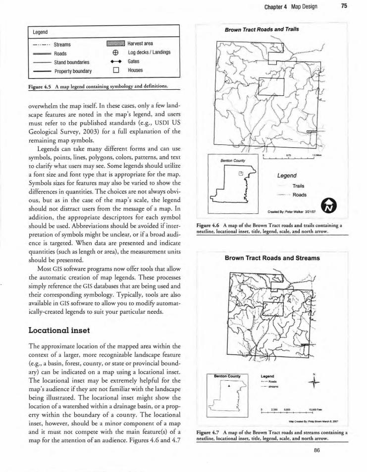
Legend
Streams
Roads
--- Stand boundaries
Property boondary
~ Harvest area
EEl Log decl<s I Landings
........ Gates
o Houses
Figure 4.5 A map legend containing symbology and definitions.
overwhelm the map itself. In these cases, only a few land
scape features are noted in the map's legend. and users must refer to the published standa rds (e.g., USOI US
Geological Survey, 2003) for a full explanation of the
remaining map symbols. Legends can rake many different forms and can use
symbols. points. lines. polygons. colors. pa[(crns. and [ext
co clarify what users may see. Some legends should milize
a font size and font rype (hat is appropriate for the map.
Symbols sizes for features may also be varied to show the
differences in quamiries. The choices are nOt always obvi
ous, but as in the case of the map's scale, [he legend should nor distract users from the message of a map. In
addition , the appropriate descripro[s for each symbol
should be used. Abbreviations should be avoided if inter
pretation of symbols might be unclear, or if a broad audi
ence is targeted. When data are presenred and indicate
quantities (such as length or area). the measurement units
should be presented.
Most GIS sofrware programs now offer [Ools {hat allow
{he automatic creation of map legends. These processes
simply reference the GIS da<abases that are being used and
their corresponding symbology. Typically, [Ools are also
available in GIS software to allow you to modifY aU[Qmat
ica lly-created legends [Q suit your part icular needs.
Locational inset
The approximate location of {he mapped a rea within {he
conrext of a larger, more recognizable landscape feature
(e.g., a basin, forest, counry, o r State or provincial bound
ary) can he indicated on a map using a locational inset.
The locational inset may be exrremely helpful fo r the
map's audience if they are not familiar with the landscape
being illustrated. The locational inset might show the
location of a watershed within a drainage basin, or a prop
erty within the boundary of a county. The locational inset, however, should be a minor component of a map
and it must not compete with the main feature(s) of a map for the attention of an audience. Figures 4.6 and 4.7
Chapter 4 Map Oesign 75
Brown Tract Roads and Trails
............
Legend
Trails
.. Roads
~"' __ ""~, e Figure 4.6 A map of the Brown Tract roads and trails containing a neatline, locational inset, ti tle, legend, scale, and north arrow.
Brown Tract Roads and Streams
,"-nd - .... .. _ .. - ,
+ Benton County
Lr _c-.,.. ..... __ .. JfI07
Figure 4.7 A map of the Brown Tract roads and 5lreams conuining a ncacline. locational insct, title, legcnd. scale, and north arrow.
86
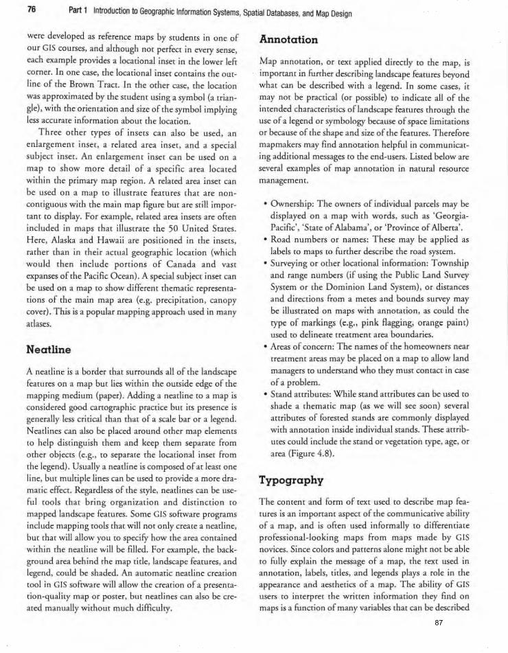
76 Part 1 Introduction to Geographic Information Systems, Spatial Databases, and Map Design
were developed as reference maps by s[Udenrs in one of
our G1S courses, and ahhough not perfect in every sense,
each example provides a loeational inset in [he lower left
corner. In one casc, the loeational inset contains the Out
line of the Brown Traer. In the other case, the location was approximated by the student using a symbol (a triangle), with the orientation and size of the symbol implying less accurate information about the locarion.
Th ree other types of insets can also be used, an enlargement inset, a related area inset , and a special
subject inscr. An enlargement inset can be used on a map co show more detail of a specific area located
within the primary map region . A related area inset can be used on a map [0 illustrate features thac are non
contiguous with the main map figure but are still impor
(3m (Q display. For example. related area insets are often
included in maps thar illumate the 50 Uniced Scaces. Here, Alaska and Hawaii are positioned in [he insets.
rather than in their actual geographic locarion {which
would rhen include pordons of Canada and vast
expanses of the Pacific Ocean}. A special subject inset can be used on a map to show different themadc representa
tions of rhe main map area (e.g. precipitation, canopy
cover). This is a popular mapping approach used in many adases.
Neatline
A neadine is a border that surrounds all of the landscape features on a map hue lies within the ourside edge of rhe
mapping medium (paper). Adding a neadine to a map is considered good canographic practice bur its presence is
generally less crirical than thac of a scale bar or a legend, Nearl ines can also be placed around other map elements
to help disringuish them and keep them separare from other objects (e.g., [0 separate [he loeational inset from
the legend). Usually a neadine is composed of ac least one line, but multiple lines can be used co provide a more dramarie effect. Regardless of the style, nearlines can be use
ful (Oots that bring organization and distinction to
mapped landscape features. Some GIS sofeware programs include mapping tools that will not only create a neadine,
bur that will allow you to speciFy how the area contained within the nearline will be filled. For example, the background area behind [he map tide, landscape features, and
legend, could be shaded. An amomacic neadine creadon tool in GIS sofcware will allow the creation of a presentation-quality map or poster, but neadines can also be cre
ated manually wichouc much difficulty.
Annotation
Map annotation, or tex( applied directly to the map, is
important in further describing landscape features beyond
what can be described with a legend. In some cases, it
may noc be practical (or possible) to indicace all of me intended characterist ics oflandscape features through the
use of a legend or symbology because of space limitations or because of the shape and size of the features. Therefore
mapmakers may find annotation helpful in communicat
ing additional messages to the end-users. Listed below are
several examples of map annotation in natural resource
management.
• Ownership: The owners of individual parcels may be displayed on a map wich words, such as 'GeorgiaPacific', 'Srace of Alabama', or 'Province of Alberta'.
• Road numbers or names: These may be applied as labels to maps to further describe the road system.
• Surveying or other locational information: Township
and range numbers (if using the Public Land Survey System or the Dominion Land System), or distances
and directions from a metes and bounds survey may
be illustrated on maps with annotation, as could the
type of markings (e.g., pink flagging, orange paint) used to delineate treatment area boundaries.
• Areas of concern : The names of the homeowners near
treatment areas may be placed on a map to allow land
managers to understand who they must contact in case
of a problem. • Stand auribures: While stand attributes can be used [Q
shade a thematic map (as we will see soon) several
attributes of forested stands are commonly displayed
with annotation inside individual stands. These attrib
utes could include the stand or vegetation eype, age, or
area (Figure 4.8).
Typography
The content and form of text used to describe map fea
tures is an important aspect of the communicative ability
of a map. and is often used informally to differentiate
professional-looking maps from maps made by GIS novices. Since colors and patterns alone might not be able
co fully explain the message of a map, the texc used in annotation, labels, titles. and legends plays a role in the
appearance and aestherics of a map. The abili ty of GIS users to interpret the written information rhey find on
maps is a function of many variables that can be described
87
76 Part 1 Introduction to Geographic Information Systems, Spatial Databases, and Map Design
were developed as reference maps by Students in one of our GIS cou rses. and ahhough not perfect in every sense.
each example provides a locational inset in [he lower left corner. In one case, the loeational inset contains the our
line of the Brown Tract. In the other case, the location was approximated by the student using a symbol (a triangle). with the orientation and size of the symbol implying less accurate information about rhe lacarion.
Th ree other rypes of insets can also be used. an enlargement inset, a rel ated area inset , and a special
subject inser. An enlargement inset can be used on a
map to show more detail of a speciFic area located within the primary map region. A related area inset can be used on a map [Q illustrate fearu res [hat are nOll p
conriguous wim rhe main map figure but are still impor
tant to display. For example. related area insets are ofren
included in maps rhat illustrate rhe 50 Un ited States. Here. Alaska and Hawaii are posirioned in me insets .
tather than in their actual geographic location (which would then include ponions of Canada and vast expanses of the Pacific Ocean). A special subject inset can be used on a map to show different themadc representa
tions of [he main map area (e.g. precipitation , canopy cover). This is a popular mapping approach used in many
adases.
Neatline
A neadi ne is a border tbat surrounds all of the landscape features on a map but lies within the oU[side edge of me
mapping medium (paper) . Adding a neatline ro a map is considered good cartographic praccice btl[ its presence is
generally less critical than that of a scale bar or a legend. Neatlines can also be placed around other map e1emenrs to help distinguish them and keep them separate from other objects (e.g. , to separare the locadonal inser from
the legend). Usually a nearline is composed of at leasr one line. but multiple lines can be used ro provide a more dramatic effect. RegardJess of the style, nearlines can be use
ful too ls rhat bring organization and disrincrion (0
mapped landscape features. Some GIS software programs include mappi ng [0015 thac will not only create a neadine,
btl( thar will allow you co specifY how the area contained within [he neacline will be filled. For example. the background area behind the map tirle. landscape fearures. and legend, could be shaded. An amomaric nearline crearion tool in GIS sofcware will allow the creation of a presenra[ion-quaJiry map or poster, bur nearlines can aJso be cre
ated manually without much difficulty.
Annotation
Map annoracion, or (ex( applied directly (0 me map, is
important in further describing landscape features beyond whar can be described wich a legend. In some cases, it may not be practical (or possible) to indicate all of the intended characteristics oflandscape features through the use of a legend or symbology beeause of space limitations
or because of the shape and size of the features. Therefore map makers may find annotation helpflll in communicat
ing addi tional messages to [he end-users. Listed below are several examples of map annorarion in natural resource
management.
• Ownership: The owners of individual parcels may be displayed on a map with words. such as 'GeorgiaPacific', 'Scare of Alabama'. or 'Province of Alberta'.
• Road numbers or names: These may be appl ied as labels to maps to further describe the road system.
• Surveying o r other loeational informacion: Township
and range numbers (if using the Public Land Survey System or the Dominion Land System), or distances
and direcdons from a metes and bounds survey may
be illustrated on maps with annotation, as could the
type of markings (e.g .. pink Aagging. orange paint) used to delineate treatment area boundaries.
• Areas of concern: The names of the homeowners near
treatment areas may be placed on a map to allow land managers to understand who they must conract in case
of a problem. • Stand attributes: While stand atrr ibures can be used {Q
shade a thematic map (as we will see soon) several
attributes of forested stands are commonly displayed with annotation inside individual stands. These atuib
Utes could include the stand or vegetar ion eype, age. or
area (Figure 4.8).
Typography
The co ntent and for m of [ext used to describe map features is an imponam aspect of [he communicative abiliry
of a map. and is often used informally to differentiate professional-looking maps from maps made by GIS novices. Since colors and patterns alone might not be able
to fully explain the message of a map. the text used in annotation, labels, tities, and legends plays a role in [he
appearance and aesthetics of a map. The abil ity of GIS users to imerprcr the written information they find on maps is a function of many variables that can be described
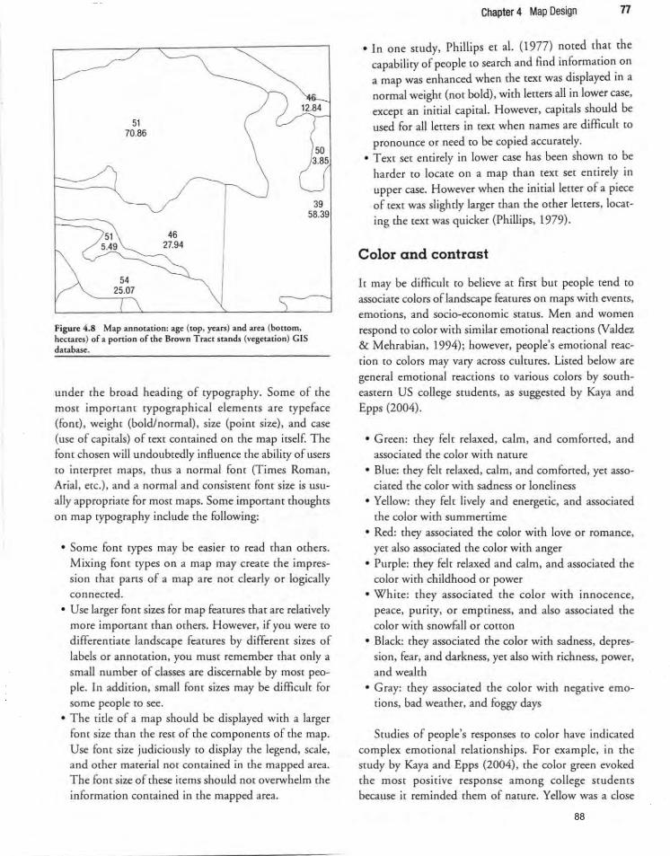
51 70.86
51 46 5.49 27.94
54 25.07
Figure 4.8 Map annotation: age (top, yurs) and area (bottom, hectares) of a ponion of the Brown Tract stands (vegetation) GIS database.
50 3.85
39 58.39
under the broad heading of typography. Some of the most important rypographical elements are typeface (font), weight (bold/normal), size (point size), and case (use of capitals) of text contained on the map itself. The font chosen will undoubtedly inAuence the ability of users to interpret maps, rhus a no rmal font (Times Roman,
Aria], etc.). and a normal and consistent font size is usu
ally appropriate for most maps. Some important thoughts on map typography include the following:
• Some font types may be easier co read than orhers.
Mixing font rypes on a map may create (he impression that parts of a map arc nor clearly or logically connected.
• Use larger font sizes for map fearures mat are relatively morc importam than others. However, if you were (0
differentiate landscape features by differem sizes of labels or annotation, you must remember that only a
small number of classes are discernable by most people. In addition, small font sizes may be difficult for some people to see.
• The tirle of a map should be displayed with a larger font size (han the rest of the components of the map.
Use font size judiciously to display the legend, scale, and Other material not contained in the mapped area. The font size of these items should not overwhelm the information contained in the mapped area.
Chapter 4 Map Design n
• In one study, Phillips et al. (1977) noted that the capability of people to search and find infotmation on a map was enhanced when the text was displayed in a
normal weight (not bold), with letters all in lower case, except an initial capital. However, capitals should be used for all letters in text when names are difficult to
pronounce or need to be copied accurately.
• Text set entirely in lower case has been shown to be
harder to locate on a map than text set entirely in
upper case. However when the initial letter of a piece
of text was slightly larger than the othet letters, locating the text was quicket (Phillips, 1979).
Color and contrast
It may be difficult to believe at first but people tend to
associate colors oflandscape features on maps with events,
emotions, and socio-economic status. Men and women
respond to color with similar emotional reactions (Valdez & Mehrabian, 1994); however, people's emotional reaction [0 colors may vary across cultures . Listed below are
general emotional react ions to various colors by south
eastern US college students, as suggested by Kaya and Epps (2004) .
• Green: they felt relaxed, calm, and comforted, and
associated me color with nature
• Blue: they felt relaxed , calm, and comforted, yet associated the color with sadness or loneliness
• Yellow: they felt lively and energetic, and associated the color with summertime
• Red: they associated the color with love o r romance,
yet also associated the color with anger
• Purple: they felt relaxed and calm, and associated the color with childhood or power
• White: they associated the color with innocence,
peace, purity, or emptiness. and also associated the color with snowfall or conon
• Black: they associated the color with sadness, depression, fear, and darkness, yet also with richness, power,
and wealth • Gray: they associated the color with negative emo
tions, bad weathet, and foggy days
Studies of people's responses to color have indicated
comp lex emotional relationships. For example. in the study by Kaya and Epps (2004), the color green evoked the most positive response among college students
because it reminded them of nacu re. Yellow was a close
88
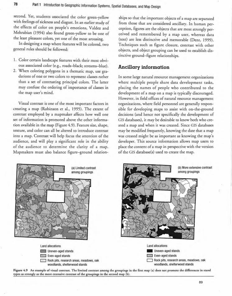
78 Part 1 Introduction to Geographic Information Systems, Spatial Databases, and Map Design
second. Yet, students associated [he color green-yellow with feelings of sickness and disguSt. In an earlier Study of the effects of color on people's emotions, Valdez and Mehrabian (1994) also found green-yellow to be one of the leaS[ pleasant colors, YCt one of the most arousing.
In designing a map where fea tures will be colored, rwo general rules should be followed:
1. Color certain landscape features with their mOSt obvious associated color (e.g., roads-black; screams-blue) .
2. When coloring polygons in a thematic map, use gradarions of one or two colors to represem classes rather
than a set of conrrasting principal colors. The lance may confuse the ordering of importance of classes in the map user's mind.
Visual contrast is o ne of the most important facmrs in
creating a map (Robinson et a1 ., 1995). T he extent of contraSt employed by a mapmaker affects how well one set of in fo rmation is promoted above (he other informa
rion avai lable in the map (Figure 4.9). Feature size, shape, texture, and color can all be altered to introduce contrast
into a map. Contrast will help focus the attemion of (he
audience, and wi ll playa signi ficant role in the abi li ty of the audience co determine the clari ty of a map.
Mapmakers must also balance figure-ground relarion-
(a) limited contrast among groupings
Land allocations
Uneven-aged stands o Even-aged stands o Rock pits, research areas, meadows, oak
woodlands, shelterwood stands
ships so [hat the important objects of a map are separated
from those that are considered ancillary. In human per
ception, figures are the objects that are most strongly per
ceived and remembered by a map user, whereas data (text) are less distinc[ive and memorable (Dene, 1999). Techniques such as figure closure, comrast with other objeccs, and object grouping can be used to escablish distinctive ground-figure relationships.
Ancillary information
In some large namcai resource management organizations
where multiple people share data developmenc [asks, placing the names of people who contribu ted to [he developmene of a map on a map is typical ly discouraged. However, in field offices of narurai resource management
organizations. where field personnel are generally respon
s ible for developi ng maps to ass isc wich on-che-ground decisions (and hence not specifically [he development of GIS databases), it may be desirable to know both who creaced a map and when ic was creaced. Since GIS dacabases
may be modified frequently, knowing the date tha[ a map was creaced mighc be as imponanc as knowing che map's
developer. This sou rce informacion allows map users co
place che coneent of a map in perspeccive w ich che version
of the GIS database(s) used to creace the map.
l and allocations
(b) More extensive contrast among groupings
_ Uneven-aged stands
o Even-aged stands D Rock pits, research areas, meadows, oak
woodlands, shelterwood stands
Figwe 4 .9 An cxaInple of visual contrast. The limited contra.Sf among the groupings in the first map (a) d~s not promote the differences in stand types as stron gly as the more cxtens ive contra$l of the groupings in the second map (b).
89
For example. suppose it is currently September 2008
and you were examining a map developed in June 2007
that represented wildlife habirar across several thousand
acres of a landscape. Assume that the wildlife habitat being
mapped was a funcdon of forest stand conditions, and that
the GIS database describing forest stands had been updated
in December 2007. If the date were displayed on the map
Qune 2007). you would be able to understand that the
qualiry of wildlife habitat illustrated in the map was esti
mated using an earlier version (i .e., not the current version) of the forest inventory data. Withom such informa
tion. you could very likely assume (incorrectly) that the
estimates of wildlife habitat are current.
It is relatively uncommon for mapmakers to provide
the names of the files, projects. or compurcr code (e.g .. macro) used in making the map on the map itself.
However, providing [his informacion would allow you co
readily go back to the GIS darabases or the computer
code. modify some aspect related co the composition of the map. and generate a new version of the map relat ively
quickly. Without such guidance. you may find ir difficult [0 remember how a map was originally constructed, The
map projection might also be provided if the map per
spective is affected by the projecrion system used. This
rype of ancillary information is usually placed in a subor
dinate position on a map. in relation to the other aspects
of a map. and displayed with a relatively small font size.
Caveats and disclaimers
Increasingly. natural resource management organizations
are adding more information to the maps that they pro
duce both to clarifY the accuracy of mapped landscape
features and to clarifY the intended uses of the maps. This
information is important in helping users understand the
appropriate applications of mapped information and in
helping avoid damages and injuries that might result from
improper map use. For example, maps have long served as
vital navigation aids to mariners and pilots. The ability to
safely pilot passengers depends on the quality o f the
mapped information used as a navigational guide. Should
a landscape landmark be misplaced or unidentified. the
consequences to people and veh icles that are navigating with the erroneous data could be disastrous. As you might
imagine. there are other reasons why maps should contain
information related to the quality of data. However. pro
viding this information or deciding not to provide this information is, at least indirectly. a function of [he liti
gious nature of today's society.
Chapter 4 Map Design 79
A map disclaimer is a statement that embodies the
legal position of the mapmaker with respect to map users.
In many cases, the map maker uses a disclaimer to dis
rance himself or herself from any legal responsibiliry for
damages that could result from use of his or her map.
Caveats. similarly. warn others of certain facts in order to
prevent misinterpretat ion of maps. In general. caveats are
less sweeping than disclaimers, and may on ly address cer
tain portions or aspects of a map. Warranties . on the
other hand, are usually written guarantees of the integrity
of a map. and of the mapmaker's responsibiliry for the
repair or replacement of incorrect maps. In practice. dis
claimers and caveats are regularly used. and warranties are
rarely (if ever) used in associarion with maps and GIS databases. Quite often organizations add disclaimers or
caveats to their maps in an attempt to warn users of the
limitations of the map content. In some cases. disclaimers
are noted directly on a map. and in other cases disclaimers
are provided on websites devoted to the distribution of
maps. Pima Couney, Arizona, for exam ple. provides a very thorough disclaimer about its products on a website
(Pima Counry [Arizona] Department of Transportation.
2003). The mai n ideas found in caveats and disclaimers
include:
• rights reserved via copyriglu and permission require-
ments for modificat ion co mapSj
• degree of error found on the mapSj
• suitability for usej
• liability. or responsibility. for errors or omissions (e.g ..
organizations usually assume no responsibility for mis
use of their maps and subsequent losses); and
• contact information (e.g., addresses, phone numbers, e-mail addresses).
Caveats and disclaimers vary in form and content from
organization to organization. Listed below are four
examples.
• Indiana Geological Survey (2007) : The maps on this
web site were compiled by Indiana University, Indiana
Geological Survey. using data believed to be accurate;
however. a degree of error is inherent in all maps. The maps are distributed "AS-IS" without warranties of
any kind. eicher expressed or implied. including bur not limited to warranties of suitability to a particular
purpose or use. No attempt has been made in either the design or production of the maps co define the
limits or jurisdiction of any federal , state, or local gov-
90
80 Part 1 Introduction to Geographic Information Systems, Spatial Databases, and Map Design
ernment. The maps are intended for use only at the published scale. Detailed on-the-ground surveys and hismcical analyses of sites may differ from the maps.'
• USDI Bureau of Land Management (2001), Glennallen, AK: ' In fo rmation displayed on our maps
was derived from multiple sources. OUf maps are only
for graphic display and general planning purposes. Inquiries concerning informacion displayed on our maps, their sources, and intended uses should be directed (0: .. .'
• Orange County (Florida) Property Appraiser (2002) : The Orange County Property Appraiser makes every
effort to produce and publish the most current and accurate informacion possibl e. No warran ties, expressed or implied, are provided for the data herein, its use, or its interpretation. The assessed values are
NOT certified values and therefore are subject to
change before being finalized for ad valorem tax purposes. OCPA's on-line (cadastral) maps are produced for property appraisal purposes, and are NOT surveys. No warranties. expressed or implied, are provided for
[he data therein. its use, o r its interpretation.' • Town of Blacksbu rg (Virginia) (2007), on the
Blacksburg WebGIS si te: 'DISCLAIMER: T he infor
marion contained on this page is NOT [Q be construed or used as a "legal description". Map information is believed to be accu rate but accuracy is nor guaranteed. Any errors or omissions should be
reported to the Town of Blacksburg Geographic Informat ion Systems Office. In no event will the
Town of Blacksburg be liable for any damages, including loss of data, losr profits, business inrerruption. loss of business information or orner pecuniary loss that might arise from the use of this map or the information ir contains.'
Map Types
The type of map thar you develop should be a function
of: (1) the type of data (i.e., point, line, polygon, raster) that is contained in GIS databases, and (2) the message(s) [har you wish to communicate to an audience. For example, if the main GIS database used to create a map contains point features. and you wish to illustrate differences berween the point values. you may want to show the points as dots or graduated symbols (di fferent sizes of points based on the po int att ribute values) . If the main GIS database used ro creare a map contai ns line featu res, you may wam to illustrate the differences in the lines with
di fferent line types. If fearures of interest represent areas, GIS databases containing polygons can be displayed as thematic maps, qua litative area maps. and others. Volumetric databases. such as digital elevation models, can be displayed as gridded fishnet maps, as shaded relief maps. or simply as images with different shades or colors assigned to individual pixels.
If you were interested in illustrating features of a landscape across time, you can develop maps with multiple panels. where each panel would contain a view of the landscape during a differenr time period. In some cases, maps can be animated, as in a short movie. They can also
contain a ' fly through ' ability when viewed. on a computer screen. The next few sections of this chapter describe (he
most common types of maps developed for natural resource managemem purposes in more derail.
Reference maps
Reference maps are those that ill ust rate a number of different landscape features, and mat provide users with a
broad perspective of the landscape. Road maps are one example of reference maps, and may contain not only road types, but also the locations of towns, major rivers. and political boundaries (provinces, states, counties, etc.) that are set among the road system. Maps that display st ream systems or watersheds are another example of reference maps. H ere, you would be able to place a watershed or stream system within the context of a larger geo
graphic area, and thus these maps may also comain the locations of (Owns and political boundaries. Land ownership maps are a third example, and (hese may contain roads, streams, towns, and other features necessary to
place tile land you manages within a larger landscape context. Reference maps are commonly made when you develop management-related activity maps, such as those
for tree planting or locations for new features such as trails o r roads.
The characteristics of reference maps will vary depending on the audience. For example, some reference maps
might display unique landscape features that are essential for high quality recreational experiences. Edwards (200 I)
describes the desirable co ntent and features of fishing maps developed for anglers. It is suggested that these types of reference maps include the complete road system surrounding a fishing area, water depths, access points (Q
water. names of local features, locations of off-limit fishing areas, locations of fishing lodges and places to buy fishing permits, places (Q park vehicles, and, interes tingly,
91
80 Part 1 Introduction to Geographic Information Systems, Spatial Databases, and Map Design
ernmenr. T he maps are intended for use only at the published scale. Detailed on-rhe-ground surveys and hismcica.l analyses of sites may dHfcr from the maps.'
• USDI Bureau of Land Managemenr (2001), Glennallen, AK: 'Informarion displayed on o ur maps
was derived from mulriplc sources. Our maps are only
for graphic disp lay and general plan ning purposes. Inqui ries concerning information d isplayed on our maps, their sources, and intended uses should be directed to: .. .-
• Orange Counry (Florida) Properry Appraiser (2002): The Orange Counry Pro perry Appraiser makes every
effon ro produce and publish the most currem and accurate information possible. No warranties. expressed or implied. are provided lor the dara herein. irs use, or its interpretation. The assessed values are NOT cerrified values and therefore are subject to change before being finalized for ad valorem rax purposes. OCPA's on-line (cadasrral) maps are produced for properry appraisal purposes, and are NOT surveys. No warranties, expressed or implied, are provided for
{he data therein, its use, or its interpretarion.'
• Town of Blacksburg (Virginia) (2007), on rhe Blacksburg WebGIS site: ' DISClAIMER: The informarion comained on rh is page is NOT co be consrrued or used as a "legal description". Map information is believed to be accurate bur accuracy is not guaranteed. Any errors or omissions should be reponed to rhe Town of Blacksburg Geographic
Info rmat ion SyStems Office. In no event will the T own of Blacksburg be liable for any damages, including loss of data, lost profits. business imerrupcion. loss of business information or ocher pecuniary loss [hat might arise from the use of this map or rhe information it comains.'
Map Types
The rype of map thar you develop should be a function of: (I) the rype of dara (i.e., poim. line. polygon. raster) rhar is contained in GIS databases, and (2) the mess.ge(s) rhar you wish to communicate [Q an audience. For exam p
pie, if rhe main GIS database used to create a map contains poinr feat ures, and you wish to illustrate cfjfferences between the point values. you may wanr to show rhe points as dots or graduated symbols (different sizes of poinrs based on rhe paine anribute values). If [he main GIS database used [0 create a map conwns line feacures, you may wane ro illusuare rhe differences in the lines with
differem line cypes. If features of inreresr represent areas, GIS databases conta ining polygons can be displayed as thematic maps, qualitative area maps. and others. Volumetric databases, such as digital elevarion models, can be displayed as gridded fishnet maps, as shaded relief maps, or simply as images with different shades or colors assigned to individual pixels.
If you were inrerested in illust.rating features ofa land
scape across time. you can develop maps with mulriple panels. where each panel would contain a view of the
landscape during a different rime period. In some cases, maps can be animated, as in a short movie. They can also
contain a ' Ay through ' ability when viewed on a compurer screen. The next few sections of this chapler describe the most common rypes of maps developed for natural resource management purposes in more derail.
Reference maps
Reference maps are (hose that il1ustrate a number of different landscape feaOlres, and mat provide users with a
broad perspecrive of the landscape. Road maps are one example of reference maps, and may comain nor only road rypes, bm also the locations of [Owns, major rivers, and poljtical boundaries (provinces, states. counries, etc.) that are set among the road sysrem. Maps that display stream systems or watersheds are another example of reference maps. Here, you would be able to place a watershed or stream sysrem within the concext of a larger geo
graphic area. and thus these maps may also conrain the locations of [Owns and polhical boundaries. Land ownership maps are a third example, and these may comain roads, streams, [Owns, and other featu res necessary to place the land you manages within a larger landscape con[ext, Reference maps are commonly made when you develop managemenr-relared acrivicy maps. such as those
for tree planting or locations for new features such as trails or roads.
The characteristics of reference maps will vary depending on [he audience. For example, some reference maps
might display unique landscape features that are essential for high qualiry recreational experiences. Edwards (2001) descr ibes rhe desirable content and features of fishing maps developed for anglers. Ir is suggested that rhes. rypes of reference maps include the complete road system surrounding a fishing area, water depths, access points to Water, names of local features, locations of off-limit fishing areas. loca tions of fishing lodges and places to buy fish ing permits, places to park vehicles, and, in te restingly.
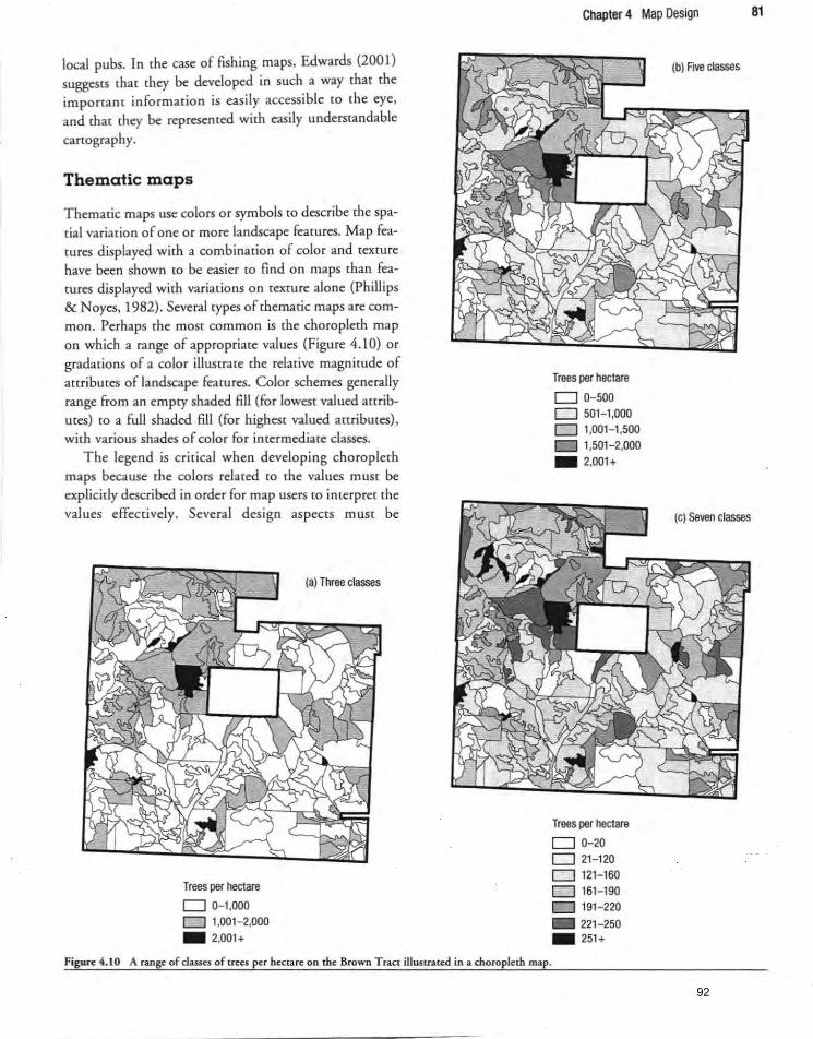
local pubs. In [he case of fishing maps, Edwards (2001) suggests that they be developed in such a way that the imporr3m information is easily accessible to the eye, and that they be represented with easily understandable
carrography.
Thematic maps
Thematic maps use colors or symbols [Q describe the spatial variadon of one or more landscape features. Map features displayed with a combination of color and texture have been shown (0 be easier to find on maps than features displayed with variations on texture alone (Phillips & Noyes, 1982). Several types of thematic maps are common. Perhaps (he most common is the choropleth map on which a range of appropriate values (Figure 4.10) or gradations of a color illustrate [he relative magnicucle of attributes of landscape features . Color schemes generally range from an empty shaded fill (for lowest valued attributes) to a full shaded fill (for highest valued attributes), with various shades of color for intermediate classes.
The legend is crit ical when developing choropleth maps because the colors related (0 the va lues muse be explicitly described. in order for map users (0 interpret [he values effeccively. Several design aspec[s muse be
Trees per hectare
D 0-1 ,000 D 1.001-2.000 _ 2,001+
(a) Three classes
Figure 4 .1 0 A range of classes of trees per hectare on the Brown Tract illustrated in a choroplerh map.
Chapter 4 Map Design 81
Trees per hectare
D 0-500 D 50H.000 D 1,OOH .500 c::J 1,501-2,000 _ 2,001.
Trees per hectare
D 0-20 D 2H20 D 12H60 D 16H90 D 191-220 _ 221-250 _ 251.
(b) Five classes
(c) Seven classes
92
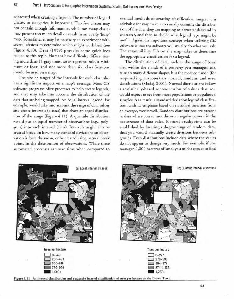
82 Part 1 Introductioo to Geographic Information Systems, Spatial Databases, and Map Design
addressed when creating a legend, The number of legend classes, or categories. is imponanr, Too few classes may
not contain enough informacion, while [00 many classes
may presenr [00 much detail or result in an overly 'busy' map. Sometimes it may be necessary (Q experiment with
several choices co determine which might work beSt (see Figure 4, 10) . Dent (1999) provides some guidelines related to this topic. Humans have difficulty differentiating more than 11 gray [Ones, so as a general rule. a mini
mum or four, and not more (han six, classifications should be used on a map.
The size or ranges of the intervals for each class also has a significant impact on a map's message. MoSt GIS
software programs offer processes to help create legends, and (hey may cake inca account (he distribution of [he data that are being mapped. An equal interval legend, for example. would take into account the range of data val ues
and create intervals (classes) that share an equal disrribution of the range (Figure 4.11) . A quantile diStribution would put an equal number of observations (e.g., polygo ns) into each interval (class). Intervals might also be creared based on how many standard deviations an observar ion is from the mean, or be created using natural break
points in the disrribmion of observations. While these 3momarcd processes can save rime when compared to
Trees per hectare
00-249 o 250-499 0500-749 _ 750-999 _ 1,000+
(a) Equal interval classes
manual methods of creating classification ranges, I( IS
advisable for map makers to visually examine the distribution of the data (hey are mapping to bettcr understand its character, and then to decide what legend type might be useful. Again , an important concept when utilizing GIS
software is that the software will usually do what you ask.
The responsibility !ails on the mapmaker to determine the appropriate classification for a legend.
The diStribution of data, such as the range of basal area within the stands of a property yo u manages, can take on many different shapes. but (he most common (for map-making purposes) are norma1. random. and even distributions (Madej, 2001) . Normal distributions follow a stat iscically-based representacion of va lues thar you
would expect to see from most populations or population
samples. As a result, a standard deviation legend classifica
tion, with its emphasis based on statistical variation from
an average. works well. Random disrribmions are present in data where you cannot discern a regular panern in the
occurrence of data vales. Natural breakpoints can be
established by locating sub-groupings of random data, thus you would manually create divisions between sub
groups. Even disrribmions include data where the va lues
do not appear to change very much . For example. if you
managed 1,000 hectares ofland, you might expect to find
Trees per hectare
00-277 0278-593 o 594-873
874-1 ,236 _ 1,237+
(b) Quantile interval of classes
Figure 4 . 11 An interval cla.uification and a quantile interval classification of trees per hectare on the Brown Tract.
•
93
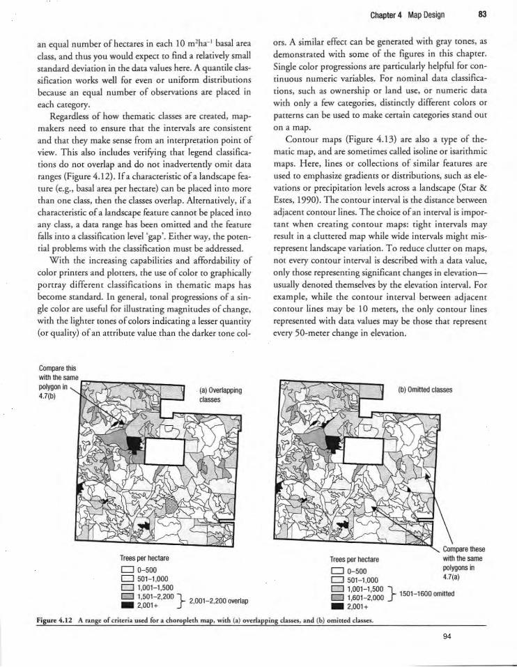
an equal number of hectares in each 10 m' ha- I basal area class. and thus you would expect to find a relatively small standard deviation in the data values here. A quantile classification works well for even or uniform distributions because an equal number of observations are placed in
each category. Regardless of how thematic classes are created. map
makers need to ensure that the intervals are consistent and that they make sense from an interpretation paine of view. This also includes verifYing that legend classifications do not overlap and do not inadvertendy omit data ranges (Figute 4.12). If a characteristic of a landscape feature (e.g .• basal area per hectare) can be placed inro more than one class, then the classes overlap. Alternatively, if a characteristic of a landscape feature cannot be placed inco
any class. a data range has been omitted and the feature Falls into a classification level 'gap'. Either way. the potential problems with the classification must be addressed.
With the increasing capabilities and affordability of color printers and plotters. the use of color to graphically ponray different class ifications in thematic maps has become standard. In general, tonal progressions of a s ingle color are useful for illustrating magnitudes of change, with the lighter (Ones of colo rs indicating a lesser quanc:iry (or quality) of an attribute value than the darker tone col-
Compare this
W"h~e~m.~~~~~~~-r __ ~ polygoo in ' 17"O'...J-' 4.7(b)
Trees per hectare
D 0-500 D 501-1 ,000 D 1,001-1 ,500
(a) Overlapping classes
D 1,501-2.200 } 2001-2200 I _ 2,001 + " over ap
Chapter 4 Map Design 83
ors. A similar effect can be generated with gray tones. as demonstrated with some of the figu res in this chapter.
Single color progressions are particularly helpful for continuous numeric variables . For nominal data classifications. such as ownership or land use, or numeric data
with only a few categories. distinctly different colors or patterns can be used to make certain categories stand out
on a map. Contour maps (Figure 4.13) are also a type of the
made map. and are sometimes called isoline or isarithmic
maps. Here. lines or collections of similar features are used to emphasize gradients or distributions, such as ele
vations or precipitacion levels across a landscape (Star & Estes. 1990). The contour interval is the distance between adjacent contour lines. The choice of an interval is important when creating concour maps: tight intervals may result in a cluttered map while wide intervals might mis
represent landscape variation. To reduce clutter on maps. not every contour interval is described with a data value.
only those representing significant changes in elevationusually denoted themselves by the elevation interval. For example. while the comour interval between adjacent comour lines may be 10 meters, the only comour lines
represented with data values may be those that represent every 50-meter change in elevation.
(b) Omilted classes
Compare1tiese Trees per hectare wtth the same D 0-500 polygons in D 501-1,000 4.7(a)
B ~ :~~~=~',: } 1501-1600omilted _ 2,001+
Figure 4.12 A range of criteria used for a choropleth map, with (a) overlapping classes. and (b) omitted classes.
94
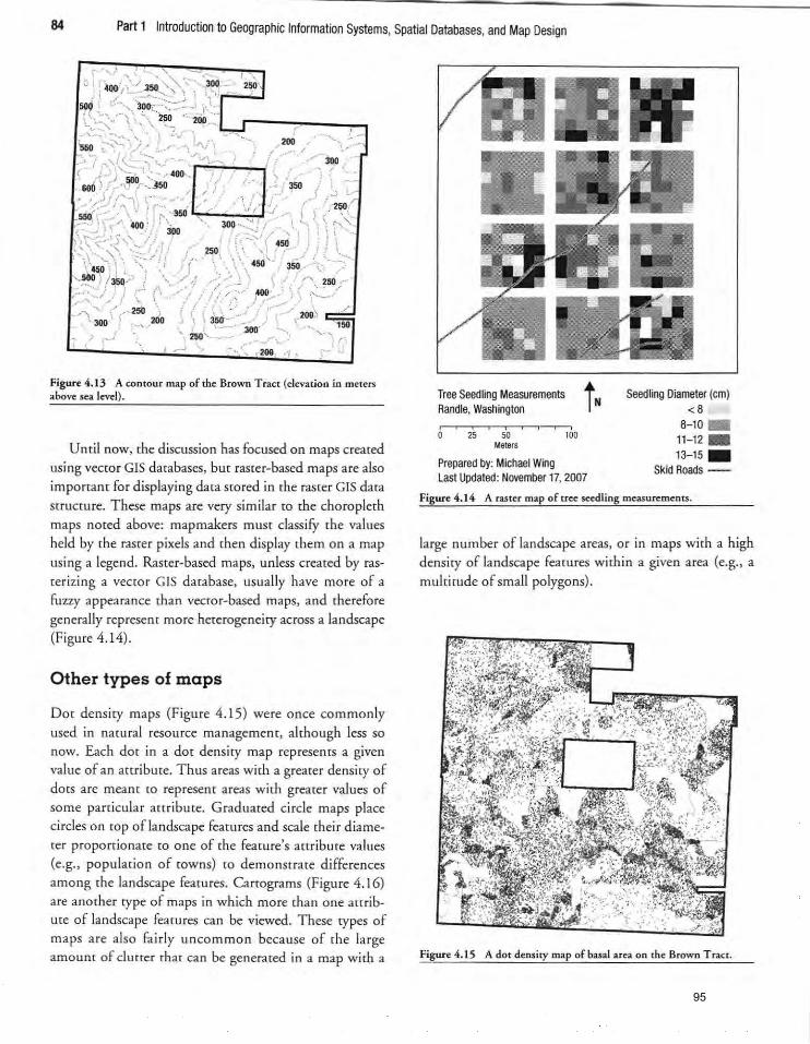
84 Part 1 Introduction to Geographic Information Systems, Spatial Databases, and Map Design
Figure 4.13 A contour map of the Brown Tract (elevation in meters above sea level) .
Until now, the discussion has focused on maps created using vector GIS databases, but raster-based maps are also
important for displaying data stored in the raster GIS data structure. These maps are very similar to the choropierh maps noted above: mapmakers must classify the values held by the rasrer pixels and then disp lay them on a map
using a legend. Raster-based maps, unless created by raste rizing a vector GIS database, usually have more of a hJzzy appearance than vector-based maps. and therefore
generally represenr more hererogeneiry across a landscape (Figure 4 .14).
Other types of maps
Dot density maps (F igure 4.15) were once commonly used in namral resource management, although less so now. Each dor in a dot density map represems a given value of an attribute. Thus areas with a greater density of dots are meam to represent areas with greater values of some particular anribme. Graduated circle maps place ci rcles on top of landscape fearures and scale their diameter proportionate to one of the feature's attr ibute values (e.g.> population of towns) to demonstrate differences among the landscape features. Carrograms (Figure 4 .16) are another type of maps in wh ich more than one an ribme of landscape fearures can be viewed. These types of maps are also fairly uncommon because of the large amount of clutter that can be generated in a map with a
Tree Seedling Measurements + N Randle, Washington II o 25 50
MeIers
Prepared by: Michael Wing last Updated: November 17. 2007
Seedling Diameter (cm) <B
8-10 _ 11- 12 _ 13-15 _
Skid Roads --
Figure 4.14 A raster map of uee seedling measu~ment$ .
large number of landscape areas, or in maps with a high density of landscape features within a given area (e.g .• a
multitude of small polygons).
Figure 4 .15 A dot density map of basal area on the Brown Tract.
95
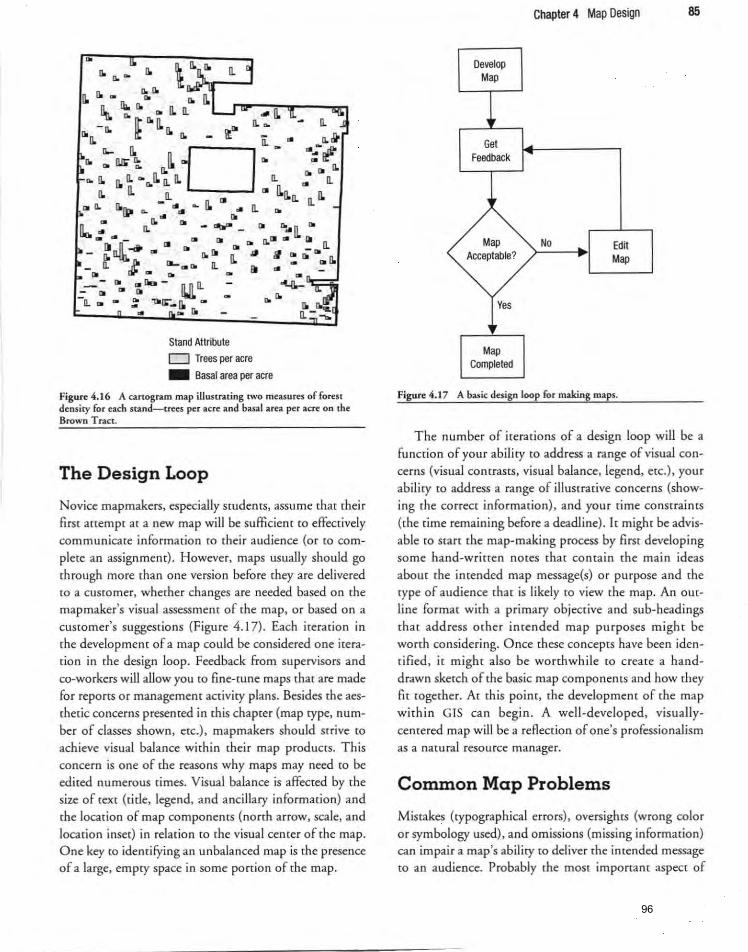
110 .. ~ 110
Stand Attribute
D Trees per acre _ Basal area per acre
Figure 4.16 A cartogram map illustrating two measures offorc$[ density for each stand-trees per acre and basal area per acre on the Brown T net.
The Design Loop
Novice mapmakers, especially students, assume that their first attempt at a new map will be sufficient [0 effectively communicate informacion (Q their audience (or to cam
ple[e an assignmenc). However, maps usually should go through more (han one version before they are delivered to a customer, whether changes are needed based on the mapmaker's visual assessment of (he map. or based on a customer's suggestions (Figure 4.1 7), Each iteration in
the development of a map could be considered one irera[ion in [he design loop. Feedback from supervisors and co-workers will allow you to fine-cune maps that are made
for reports or management activity plans. Besides the aestheric concerns presented in this chapter (map type. number of classes shown, etc.), mapmakers should strive to
achieve visual balance within their map products. This concern is one of {he reasons why maps may need co be edited numerous rimes. Visual balance is affected by {he size of [ex[ (t ide, legend, and ancillary information) and the location of map components (north arrow, scale, and
location inset) in relat ion to the visual center of the map. One key to identifying an unbalanced map is the presence of a large. empty space in some portion of the map.
Develop Map
Get Feedback
Yes
Map Completed
Chapter 4 Map Design 85
No EdH Map
Fig-urc 4. 17 A basic design loop for making maps.
The number of iterations of a design loop will be a function of your abi li ty to address a range of visual concerns (visual contrasts. visual balance. legend. etc.), your abi lity to address a range of illustrative concerns (showing the correct information), and your time constraints
(the time remaining before a deadline) . I[ might be advisable co scan the map-making process by first developing some hand-writren notes that contain the main ideas
about the intended map message(s) or purpose and the rype of audience [hac is likely to view [he map. An outline format wi[h a primary objeccive and sub-headings that address other intended map purposes might be worth considering. Once these concepts have been identified. it might also be worthwhile [Q create a hand
drawn skecch of the basic map componenes and how they fit together. At this poine, the developmene of [he map wi[hin GIS can begin. A well-developed, visuallycentered map will be a reRection of one's professionalism as a natural resource manager.
Common Map Problems
Miscakes (rypographieal errors), oversighcs (wrong color or symbology used), and omissions (missing information) can impair a map's ability to deliver {he imended message to an audience. Probably the most important aspect of
96
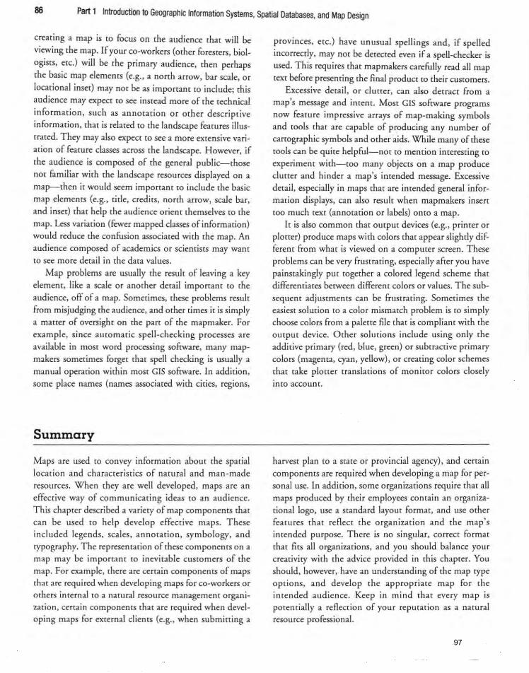
86 Part 1 Introduction to Geographic Information Systems, Spatial Databases, and Map Design
creating a map is co focus on [he audience [hat will be viewing the map. If your co-workers (ocher foreseers, biologists, erc.) will be rhe primary audience, rhen perhaps
the basic map elements (e.g., a north arrow, bar scale. or
locational inset) may not be as importam ro include; [his
audience may expect to see instead more of [he technical
info rmacion, such as annotat ion or Q[her descriptive
informadon, that is related to the landscape feacuces illus
trated. They may also expect [Q see a morc extensive vari
acion of feature classes across the landscape. However, if rhe aud ience is composed of rhe general public-rhose
nor familiar with the landscape resources displayed on a
map- then it would seem imporram {Q include [he basic
map e1emems (e.g .• tide. credits. north arrow, scale bar,
and inset) that help the audience orient themselves to the
map. Less variation (fewer mapped classes of information) would reduce the confusion associated with the map. An
audience composed of academics o r scientists may want to see more detail in the data values.
Map problems are usually rhe resulr of leaving a key
element, like a scale or another detail important to the
audience. off of a map. Sometimes, these problems result
from misjudging the audience, and other times it is simply
a matter of oversight on the part of the mapmaker. For
example, since automatic spell-checking processes are
available in mOSt word processing software, many map
makers somerimes forger thar spell checking is usually a
manual operation within most GIS sofrware. In addition,
some place names (names associated with cities, regions,
Summary
Maps are used to convey information about the spatial
location and cha racteristics of natural and man-made
resources. When they are well developed. maps a re an
effective way of communicating ideas [Q an audience.
This chapter described a variety of map components that
can be used to help develop effecrive maps. These included legends, scales, annotatio n, symbology, and
typography. The representation of rhese components on a
map may be important to inevitable customers of the
map. For example, there are cerrain componentS of maps that are required when developing maps for co-workers or
others internal [Q a natural resource management organization, certain components thar are required when devel
oping maps for external clients (e.g., when submitt ing a
provinces, erc.) have unusual spellings and, if spelled
incorrecdy. may nor be detected even if a spell-checker is used . This requires rhar mapmakers carefully read all map
text before presenting the final product to their customers.
Excessive detail , or clutter, can also detract from a
map's message and intent. Most GIS software programs now feature impressive arrays of map-making symbols
and rools rhar are capable of producing any number of
cartographic symbols and orher aids. While many of rhese
tools can be quite helpful-not to mention interesting to
experiment with-too many objects on a map produce clutter and hinder a map's intended message. Excessive
detail, especially in maps that are intended general infor
mation displays. can also result when mapmakers insert
toO much text (annotation or labels) OntO a map.
It is also common that output devices (e.g., printer or plorrer) produce maps wirh colors rhar appear slightly dif
ferent from what is viewed on a computer screen . These
problems can be very frustrating, especially after you have
painsrakingly pur rogerher a colored legend scheme rhat differentiates between different colors or values. The sub
sequent adjustments can be frustrating. Sometimes the
easiest solution to a color mismatch problem is to simply
choose colors from a palette file that is compliant with the
output device. Other sol utions include using only the
addirive primary (red, blue, green) or subtracrive primary
colors (magenta, cyan, yellow), or creating color schemes
that take plotter translations of monitor colors closely
into account.
harvest plan to a stare or provincial agency), and certain
components are required when developing a map for per
sonal use. In addition, some organizations require that all
maps produced by their employees contain an organiza
tional logo. use a standard layout format, and use other features that reflect the organization and the map's
intended purpose. There is no singular, correct format
rhar firs all organizarions, and you should balance your
creativity with the advice provided in this chaprer. You
should, however, have an understanding of the map rype
options, and develop the appropriate map for the intended audience. Keep in mind that eve ry map is
potentially a reflection of your reputation as a narural resource professional.
97
Applications
4.1. Age class distribution map for the Brown T ract. The manager of rhe Brown T racr, Becky Blaylock, would like you co produce a map char illustrates the age class discribucion of the forest. To complete this exercise, develop
a rhemaric map showing I I age classes: 0-10 years old, 11-20, .... ,91-100, and 100+ years old.
4.2. Tree densiry map for the Brown Tract. Afrer reviewing your previous work, Becky Blaylock would like a map thac illustrates the trees per hectare for vegetation stands contained within the Brown T ract; she needs the
map for an annual reporr chat she is developing. Develop
a thematic map chat classifies the stands by trees per hectare. using five logical classes.
4.3. Owl locations on the Darnel Picketr forest. The wildlife biologisr associared wirh rhe Daniel Picke[[ foresr needs a map chat illustrates the historical spotted owl (StTix occithntalis) nest locations that were known to have
been used in the Forese. Develop a reference map illustrat
ing rhe two nest locations, and annotate rhe map with the
dare of rhe laS[ known sigh[ing of the owls.
4.4. Stream rypes of the Daniel Picketr forest. The hydrologiS[ associared wirh rhe Daniel Picke[[ foreS[ needs a map illustrating the different stream rypes, in o rder CO direct a summer crew co the locat ions he would
like to survey for fish species and habitat conditions. Develop a reference map that iIlusrrarcs the different
scream rypes associated with the Daniel Pickett fo rest.
4.5. Potential harvest unit. The land manager of the Daniel Picken forest is considering a timber sale in unit number 13 on rhe Daniel Picken forese He would like you (0 produce a management map indicating that unit 13 is a proposed harvesr area, and co display rhe road and stream systems in rdarion (0 the uniL
4.6. Brown Tract hiking map . Becky Blaylock, man· ager of rhe Brown Tracr, would like you ro develop a map illumaring rhe crail sysrem, highlighring borh rhe authorized and unauthorized trai ls. Recrearionists who visir rhe fo reS[ wi ll likely use [his map. Develop a refer· enee map that incl udes the road system and the contour lines (wi th associated elevations) as supplementary information.
Chapter 4 Map Design 87
4.7. Culvert installation dates. The road engineer associared wirh the Daniel Picke[[ foresr, Bob Packard, is in the process of developing a culvert replacement plan. He would like you co develop a map illusrraring rhe road system, the culverts, and the culvert installacion dates for
rhe Daniel Pickerr properey.
4 .8. D isclaimers) caveats, and warranties. Imagine
that you work for an agency chat has developed a statewide
streams GIS database. At one of your regular staff meet
ings, rhe discussion shifrs co rhis GIS darabase and the need co add or associate some SOrt of disclaimer, caveat, or war
ranty with the GIS database. During this conversation you
conclude rhar rhe group is very confused abour rhe use of the terms 'disclaimer', 'caveat', and 'warranty'. What guid
ance can you provide co help rhe sraff undersrand rhe differences between the terms, and how the terms might be used in relation to the streams GIS database?
4.9. Map scales. One of your colleagues, Mike Marshall , does nor like rhe eype of scale [har you common ly incorpo rate into your management maps. He
prefers to use another type of scale, and insists that you
use ir as weU . IdenrifY, define, and describe rhe possible advanrages and disadvanrages of rhree eypes of approaches for creating map scales.
4.10. Map development. A sma ll consul ring firm In
Brirish Columbia has recendy hired you, and one of your first assignments is to make management maps for various
planned act ivities on the land managed by your firm.
IdenrifY five irems or objecrs rhar should be placed on almost every map.
4.11. Map legends. The manager of rhe Brown Tracr desires a map illustrating the trees per hecta re for each
stand on the property. There are different approaches for
organizing and displaying sparial dara inro a map legend. a) Whar is a general guideline for choosing rhe num
ber of categories in a legend thar uses gray cones? b) Whar is an equal inrerval legend, and how does ir
display numeric data?
c) What is a quantile distribution legend, and how
does if display numeric data? d) Whar is a srandard devia<ion legend, and how does
it display numeric data?
98

88 Part 1 Introduction to Geographic Information Systems, Spatial Databases, and Map Design
References
Dent. B.D. (1999) . Cartography thematic map design . New York: McGraw-HilI.
Digital W isdom. Inc. (2006). Cartographic symbols & map symbols library. Tappahannock. VA: Digital Wisdom. Inc. Recrieved March 28. 2007. from hnp:llwww.map-symbol.com/sym_lib.htm.
Edwards. D. (2001). Maps for anglers. The Cartographic journal. 38(1).103-6.
Franklin. P. (2001) . Maps for the reluctan t. The Cartographicjourna~ 38(1). 87-90.
Indiana Geological Survey. (2007) . Copyright. map disclaimer. and limitation of warranti~s and liabilities. Bloomington. IN : Indiana Geological Survey. Retrieved March 3. 2007. from hnp:// igs.indiana.edul disclaimer.cfm.
International Orienteering Federation. (2000). Intanational specification for orienuering maps. Radio-katu, Finland: Incernational O rienteering Federation.
Kaya. N .• & Epps. H .H. (2004). Relationship between color and emotion: A study of college students. Co/l'ge Student journal, 38. 396-405.
Madej. J. (2001) . Cartographic dlSign using Arc View GIS. Albany. NY: OnWord Press.
Mecriam-Webster. (2007). Mariam-Webster online search. Retrieved March 28. 2007. from hnp://www. m-w .coml cgi-binl dictionary.
Monmonier. M.S. (1995) . Drawing the line: Tales of maps and cartocontroversy. New York: Henry Holt and Company.
Monmonier. M.S. (1996). How to Lie with maps (2nd ed.). Ch icago. IL: University of Chicago Press.
Natural Resources Canada. (2006). Topographic map symbols-introduction. Ottawa, ON: Nacucal Resources Canada, Earth Sciences Seccoc, Mapping Services Branch. Recrieved March 23. 2007. from hnp:llmaps.nrcan.gc.caltOpo 1 0 I/symbols_e. php.
Orange County (Florida) Propetry Appraiser. (2002) . OCPA
map record inquiry system. Retrieved March 29. 2007. from http://www.ocpafl.orgidocs/disclaimer_map.html.
Phillips. R.J . (1979) . Why is lower case bener? Some data from a search task. Applied Ergonomics. 10.211-14.
Phill ips. R.J. (1989). Ase maps different from other kinds of graphic information? Cartographic journal, 26. 24-5.
Phillips. R.J .• & Noyes. L. (1982). An investigation of visual c1uner in the topographic base of a geological map. Cartographic journal. 19. 122-32.
Phillips. R.J .• Noyes. L.. & Audley. R.J. (1977). The legibility of type on maps. Ergonomics. 20. 671-82.
Pima County (Arizona) Department of Transponacion. (2003). Department disclaimer and me restrictions. T llcson, AZ: Pima COlincy Department of T ransporration, Geographic Information Services Division.
Retrieved March 28. 2007. from http://www.dot. co.pima,az,lls!mapdis,hrm ,
Robinson. A.H. Morrison. J.L. . Muehrcke. P.c. . Kimerling. A.J .• & Gupti ll . S.c. (1995). Elements of cartography. New York: John Wiley & Sons. Inc.
Sheahan. B.T. (2004). The unofficiaL Arc/Info and Arc View symbol page. Victoria. BC: Spatial Solutions. Inc. Retrieved March 28. 2007. from http://www. mapsymbols.com/.
Star. J .• & Estes. J. {I 990) . Geographic information systems: An introduction. Englewood Cliffs. NJ: PrenticeHall. Inc.
Town of Blacksburg (Virginia). (2007). Blacksbu rg WebGIS site. Retrieved March 28 . 2007. from http:// arcims2 . webgis. net/blacksburgl defa ul t.asp.
US DI Bureau of Land Management. (2001). Map disc/aimer. Glennallen. AK: Bureau of Land Management. Retrieved March 28. 2007. from http://www. blm.gov/aklgdo/documents/map_disclaimer.doc.
USDI US Geological Survey. (2003). Part 6 publication symbols. Standards for 1:24.000- and 1:25.000-scale quadrangle maps. Reston. VA: US Geological Survey. Retrieved March 23. 2007. from http://rockyweb. cr. usgs. gov In m ps tdsl ac rodocsl q rna ps/6psym 4 03. pdf.
USDI National Park Service. (2003) . NPS map symbols: Updated March 4. 2003. Retrieved March 27. 2007. from http://www.nps.gov/carto/PDF/symbolsmapl . pdf.
Valdez. P .• & Mehrabian. A. (1994). Effects of color on emotions. journal of ExperimentaL Psychology: Genera~ 123. 394-409.
Wood. D. (2003). Cartography is dead (thank God!). Cartographic Pmpectives. 45.4-7.
99
Part 2
Applying GIS to Natural Resource Management
Pact 2 of rhis book focuses on the GIS applications common to namra) resou rce man
agement organ izatio ns. The majority of data support ing daily GIS use in namral resource management is stored in vectOr GIS databases. although rhe in tegration of vector
and raster GIS databases is becoming increasingly com mon. For example. the development of resource managemem plans may require rhe use of GIS databases representing fo res t stands (polygons), roads and srreams (lines), water sources and wildlife observat ions (points). and topography (raster). T he chapters included in this part of the book present a number of GIS processes such as querying, buffering. clipping. raste r analysis. and simultaneous integratio n of vector and raster GIS databases in an analysis. The ropics increase in complexity wi th each passing chapter. and rhe applications associated with each wpic integrate processes presented in previous chapters. Some advanced wpies are also presented. such as delineating the land classifications of a landscape and delineating the recreation opponunity spectrum classes of a landscape. In panicular, [he raster-oriented chapeers provide examples of advanced analys is techn iques and possibilities.
A variety of processing pathways can be used within GIS co address a si ngle management concern and it is imponant [Q note that there may be more than one processing solut ion for a part icular challenge. While we provide direct ion for the mOSt straightfor
ward processes. students should feel free to be crea tive in their approaches co addressing each application. Finally, some of the applicat ions require students CO think more broadly (beyond GIS) abom how the results of an analysis may affect natural resource management opportunities within a given landscape.
100
Chapter 5
Selecting Landscape Features
Objectives
A variety of methods can be used [Q locate and select
landscape features based on either their attribures or their
proximiry to other feawces. Spatial and attribute reference queries ca n be used [Q select features based on the
informacion scored in attribute rabies (layer database) or
(he spatial location of landscape feacuces. At the conclu
sion of this chapter readers should be /am iliar with, and have a working understanding of:
1. the variety of methods that can be used ro select landscape feawces fro m a GIS database;
2. the meaning of the term 'query', when applied spatially o r referentially; and
3. the methods you can use to develop a description of the resources located on a landscape.
In a reeem annual report to their stockholders. one of
the largesr timber companies in the United States said the
foll owi ng about the use of GIS: 'Our foresters use advanced Geographic Information System (GIS) models to get a picture of timber species. sizes, and age c1assesalong with a multitude of environmental detai ls. from
streams and fis h to wildlife populat ions and habitat' (Plum C reek Timber Co., 2001). This statement recognizes the extent to which GIS is viewed as a valuable man
agement tool and acknowledges the power of GIS to assist in the management of resources. Other natural resource management organizations also rely on GIS to store location information about the natural resources that they
manage (as well as those that they might not manage but
that are important in the management of their property). These o rganizations include public agencies such as the
US Forest Service. the Canadian Forest Service, the US
Park Service, the US Bureau of Land Management. State
and provincial orga nizatio ns, private industriallandown
ers, and those organizations that manage smaller tracts,
such as forestry consu ltants, and university research
forests. Each organization has a different mission, yet each
relies on similar methods fo r storing and organ izing the ir
geographic databases . The methods used to extract infor
mation from these databases are also very similar, and
help provide a picture of the namral resources that they
manage. The chapter emphas izes one of the most com
mon methods of data extraction from a database: the use
of queries . Besides asking questions like 'what is here?' or 'what
type of feature is that?'-the rypes of questions wh ich hold our auenrion in the first part of th is chapter-there
are at least four types of information acquisi tion processes
you can use when asking questions of a GIS database. The
four processes are outlined briefly below, and when we
arrive at the section entitled 'Selecting features based on
some database criteria', we will become engaged in one or
more of these processes. The applications provided at the end of the chapter will further reinfo rce the need for these
acquis ition processes in natural resource management.
1. Obtaining sp"ific focts Is there spotted owl habi tat w ithin the property that is
being managed? Are there any steep hiking trails within the property
being managed?
101
Is ther< any old-growth forest within the property
being managed?
2. Obtaining extended information Besides spotted owl hab itat, what other types of important wildlife habitat are found within the prop
erty bei ng managed? Besides steep hiking trails, what other types of trails are contained within the property being managed?
Besides old-growth forests. what other dassificacions of forest are conta ined within the property being
managed?
3. Obtaining broader information blUed on complrx queries Are there any areas that meet all of the habitat require
ments for all of the species of interest within the prop
erey being managed? Are there any trails that, when combined. provide a relacively easy hiking experience? Are there any forest stands that can be managed co provide both wildlife habitat and timber resources?
4. Obtaining information on resources in limited sup;" Are [here any areas of habitat [hat appear in small quantities across the area being managed?
Are there any trails that provide experiences that occur rarely across the area being managed? Are there any forest stands that represent unique forest types within the area being managed?
Selecting Landscape Features from a GIS Database
As we noted in the introduction to chapter I, natural
resource managers are consistently called upon to describe the condition of a landscape using GIS software programs and GIS databases. Generally speaking, natural resource managers are concerned with understanding where landscape features are located and what characteristic(s) they might have now, have had in the past, or will have in the future. There are at least eight processes you can use to select landscape features from GIS databases:
I . Select one feature {manually}. 2. Select many features {manually}. 3. Select all features (manually or automatically) . 4. Select no features {manually or automatically} .
Chapter 5 Selecting Landscape Features 91
5. Select features based on some criteria . 6. Select features from a previously selected set of features.
7. Switching (inverting) a set of selected features so that
all unselected items become selected. 8. Select features within some proximity of other
features.
Selecting one feature manually
The abi lity to select landscape features using a computer
mouse or digitizing puck is an essential tool for examining or editing individual landscape features in GIS, and for editing tabular data contained in an attribute table. As we
have JUS[ implied, within GIS software programs landscape features can be selected either from the window that presents the spatial display of landscape features, or from the window that presents the associated a[[ ribute table. GIS software programs are either designed to allow users
to select landscape features by default {e.g., Maplnfo} or to provide a well-positioned, easily accessible function (i.e., the 'select features ' tool in ArcMap or the 'select features ' button in ArcYiew 3.3) [hat allows users to manu
ally select individual landscape features. A careful positioning of the computer mouse's cursor over a landscape feature {either in the display of spatial landscape features or in the tabular database} and a simple click of the mouse
will usually do the job. Selected landscape features will normally be colored or shaded differently {in both the spatial display of landscape features and tabular database} from other landscape features in the GIS database of interest, allowing users (0 visually verify what has been
selected. GIS software programs use standard characteristics for displaying selected features, such as the light blue color used by ArcMap or the yellow color used by ArcYiew 3.3 for displaying a selected spatial feature or its attribute record. Some GIS software programs allow users to define the characteristics (i .e., color) of selected spatial features or a[[ributes. and most GIS software will allow users to specify which GIS layers can be 'selectable'. As a resulr, either those layers that are visible in a window are selectable. or those that have been chosen from a list are selectable. Th is ability can make feature selections more efficient and also prevent analysis errors.
Selecting many features manually
There are times when selecting many landscape:: features manually will also be of value in ass isting the develop-
102
92 Part 2 Applying GIS to Natural Resource Management
mem of information (map or data) co facilitate a natural
resoll rce management analysis. The process for selecting multiple landscape features is similar ( 0 the process for
selecting single landscape feamres manually, with the computer mouse playing {he cenrral role. The selection of multiple landscape features can generally be accomplished in one of twO ways:
1. Using the select tool associated with a GIS softwa re program, draw a rectangular box in the window that displays the spatial fearures. Here, you would specifY the location (by clicking and holding down a mouse
button) for one corner of the box. Then, drag the mouse [0 specify the diagonal corner, and release the mouse button.
2. Using [he seiect [001 associated with a GIS software program, select features individually while depressing a key on the computer keyboard (e.g. , the 'shift' key
when using ArcMap). This process can be used in the window that displays the spatial fearuces or in the attribute table.
Each GIS software program may involve a variation (or two) on these techniques. More than likely an alternative
exists that allows users (Q more efficiently select multiple landscape features manually. Fo r example, assume you were interested in selecting vegetation polygons that contained (rees that were, on average, over 100 years of age. Within an attribute table you could sort the vegetation polygon records by their age, either using an ascending (youngest to oldest) or descending (oldest to youngest) sort. This wi ll re-position the vegetation polygon records such that the ones that comain the oldest trees are grouped together. thus facilitating a more efficient manual selec[ion of multiple features. Had you not sorted the records, you would have needed to scroll through [he attribute table to locate records wi th average tree age vallies over 100; this likely would have lead to errors of omission (missed records) and it would not have been an efficient use of your time.
Selecting all of the features in a GIS database
The ability to seleer all landscape features from a G IS
database is a standard process among GIS software programs. In addition, most GIS software programs generally have specific functions to allow users to select all land-
scape features with JUSt one (or a few) c1ick(s) of a mouse ra ther than having to select all the landscape features manually. This ability is useful when summarizing data about all of the landscape featu res in a dambase or when you are considering spatial analysis processes. Some users of G IS prefer to select the landscape features to which the
GIS processes would be applied (all landscape features in this case). rarher than rely 0 11 the common default (if no landscape features are selected, an analysis applies to all landscape features). Another opportunity to select all the features of a GIS database is if you are calculating values for fields in an attribute table. Calculations are usually performed on selected records in a tabular database, so, to
perform a calculacion on all of the records, such as the calculation of some portion of a habitat suitability score for vegetation polygons, you may need to select all of the records as a preliminary step in the process.
Selecting none of the features in a GIS database
T he abil ity to select none of the landscape features in a GIS database (or to ' un-select' o r 'clear' the selection) is also a standard process associated with GIS software programs. Most GIS software programs have specific functions-either menu items or buttons-that allow users to
un-select all landscape features with JUSt one click of a computer mouse (rather than having to un-select all landscape features manually). There are many reasons for wanring to perform this ac tion; one of the most common reasons is to clear previously selected landscape features from a GIS database before performing a spatial process such as buffering. In a buffering process, when no spatial fearures are selected, generally all of the features are used to develop buffers. If one or more features are selected, only the selected features are buffered. It is usually after
viewing the results of a spatial process that you realize you have forgonen to un-select landscape feacures before performing (he operation.
Selecting features based on some database criteria
By now it may be evident that there must be a faster way to select a subset of the enrire set of landscape features mher than having to selec[ [hem manually. Within all GIS
software programs, users have the abi lity CO ask questions, that is, CO develop queries, about the landscape feacures
103
92 Part 2 Applying GIS to Natural Resource Management
menr of inform arion (map or dara) to fac il irate a natural
resource managemeor analysis. The process fo r selecdng mulriple landscape feamces is sim ilar (0 the process for selecting single landscape feamres m an ually, wi th the
compucer mouse playing the central role. The selection of
multiple landscape feamres can generally be accompl ished
in one of rwo ways:
1. Using the seJect tool associated wi th a GIS softwa re
program, draw a reccangular box in rhe window tilar displays the spatial features. Here, you would specilY
the location (by clicking and holding down a mouse
button) for one corner of the box. Then , drag rhe
mouse to specify the diagonal corner, and release the mouse burton.
2. Using the sdect tool associated wirh a GIS soltware
program, sdccr features individually while depressing a
key on the computer keyboard (e.g. , the 'shilt' key
when using ArcMap). This process can be used in rhe
window that displays [he spatial fearu ces or in rhe
arrribur. table.
Each GIS software program may involve a va riation (or
[Wo) o n rhese rechniques. M ore than li kdy an alternat ive
exisrs that allows users to more efficiendy select multiple
la ndscape fearu res manually. For example, assume you
were interested in select ing vegecarion polygons tha t con
tained (rees that were, on average, over 100 years of age.
Within an attribute table you could sore the vegetarian
polygon records by their age, eicher using an ascending
(youngest to oldest) or descending (oldest to youngest)
sorr. This will re·posi rion [he vege tation polygon records
such that the ones that contain the oldest trees are
grouped rogether, thus rncilita ting a more efficient man
ual selection of mulriple features. H ad you not sorted the
records, you would have needed ro scroll th rough the
attribute [able to loca te records wi th average tree age val
ues over 100; [h is likely would have lead {Q errors of om is
sion (missed records) and it would nO[ have been an efficient use of you r time.
Selecting all of the features in a GIS database
The abiliry to sdecl all landscape features from a GIS database is a standard process among GIS software pro
grams. In addition, most GIS software programs generally
have specific funct io ns to allow users to select all land-
seape features with jUst one (or a few) click(s) of a mouse
rather chan having ro selecl all th. landscape featu res
manually. This abiliry is useful when summa rizing data
abour all of the landscape features in a database or when
you are considering spacial analysis processes. Some users
of GIS prefer ro select (he landscape fearures to which rhe
GIS processes would be appl ied (all landscape fearures in
this case), rather than rely on rhe commo n default (if no
landscape fearures are selec<ed, an analysis applies to all
landscape features) . Another opportuniry to selecr all the
fearures of a GIS darabase is if you are calculati ng values
for fi elds in an attribute tab le. Calculations are usually
performed on selected records in a tabular darabase. so, {Q
perform a calculation on all of me records. such as the cal
culation of some portion of a habita t suitabili ty score for
vegetation po lygons, you may need to selecr all of the
records as a prelimina_ry step in the process.
Selecting none of the features in a GIS database
T he abili ty to select none of the landscape features in a
GIS database (or to 'un-sdec[ or 'clear' rhe selection) is
also a standa td process associa ted with GtS software pro
grams. Most GIS soltware programs have specific func
tions-either menu items or buttons-that allow users co un-sdecr all landscape features wirh jUst one click of a
computer mouse (rather rhan having co un-selecr all land
scape featu res manually) . There are many reasons for
wanring (Q perform this anion; one of the most commo n
reasons is [Q clear previollsly selecred landscape featu res
from a GIS darabase before performing a sparial process
such as bu ffering. In a buffering process, when no spa rial
features are selected) genera lly all of the features are used
to develop buffers. If one o r mo re features are selected,
o nly the selected feamres are buffered. h is usually alter
viewing the results ofa spatial process that you real ize you
have forgonen to un-select landscape features before per
forming the operation.
Selecting features based on some database criteria
By now it may be evident that there musr be a faster way
to select a subset of [he ent ire se t of landscape fea tures
rather than having to sdeer rhem manually. Within all GIS software programs. users have the ability to ask questions.
[har is, {Q develop q ueries. ahom the landscape features
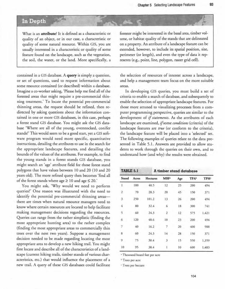
What is an attribute? It is defined as a characteristic or
quality of an object, or in our case, a characreriscic or
quality of some namral resource. Within GIS. you are
usually imeresred in a characteristic or quality of some
feature found on the landscape. such as the vegecarion . the so il , the water, or the land. More specifically, a
contained in a GIS database. A query is simply a question. or set of questions. used co request in fo rmation abom
some resource contained (or described) within a database.
Imagine a co-worker asking. 'Please help me find all of the fo resred areas that might require a pre-commercial thin
ning rrearmem.' To locate the potencial pre-commercial
th in ning areas , the request should be refined, then re
directed by asking questions abour the informacion con
tained in one or more GIS databases, in this case, perhaps
a forest stand GIS database. You might ask the GIS database 'Where are all of the young. overstocked. conifer stands?' This would seem to be a good start. yet a GIS software program wou ld need more specific. quancitative
instructions, detailing the anribuces co use in [he search for
the appropriate landscape feacu res, and detailing the
bounds of the values of [he amibutes. For example, to find the yo ung stands in a forest stands GIS database. you
might search an 'age' anribuce field for those forest stand
polygons [hat have values between 10 and 20 (IO and 20 years old). The more refined query then becomes 'find all of the forest stands where age ~ 10 and age S 20.'
You might ask. 'Why would we need to perform queries?' One reaso n was illuscrated with the need [Q
idencify the potemial pre-commercial th inning areas
there are times when natural resource managers need to
know where certain resources are located to help facili tate
making managemem decisions regarding the resources.
Queries can range from the rather simplistic (finding the
mOSt appropriate huming area) to the rather complex
(finding the most appropriate areas to commercially thin trees over {he next (WO years). Suppose a management
decision needed to be made regarding locat ing the most
appropriate area to develop a new hiking trail. You might
first locate and describe all of the cha racteristics of a land
scape (current hiking crails. timber stands of var ious characteristics, etc.) that would influence the placemem of a
new crail. A query of these GIS databases could facili tate
Chapter 5 Selecting Landscape Features 93
forester might be interested in the basal area, timber vol
ume. or habitat qua/iry of [he srands [hat are delineated on a property. An amibute of a landscape feature can be extended, however, co include its spatial position. size,
perimecer (or length). and even the cype of data it represents (e.g .• point. line. polygon. raster grid cell).
the selection of resources of imerest across a landscape,
and help a managemem team focus o n the more suitable
areas.
In developing GIS queries, you must build a set of criteria to enable a search of database, and subsequently to
enable the selection of appropriate landscape features . For
those more attuned to visualizing processes from a com
puter programming perspective, queries are similar to the
developmem of If stattments. As the auribures of each
landscape are examined. ifsome conditions (criteria) of the
landscape features are true (or conform to the criteria).
the landscape feature will be placed into a 'selected' set. The following examples of queries relate to the data presented in Table 5.1. Answers are provided to allow students to work through the queries o n their own, and to
understand how (and why) the results were obtained.
TABLE S,l A limber stand database
Stand Acra Hectares MBP Ag' TPA' TPW
100 40.5 12 25 200 494
2 70 28.3 20 45 150 371
3 250 101.2 13 26 200 494
4 80 32.4 6 18 300 74 1
5 60 24.3 2 12 575 1,421
6 120 48.6 10 23 200 494
7 40 16.2 7 20 400 988
8 60 24.3 14 28 150 37 1
9 75 30.4 3 15 550 1.359
10 95 38.4 10 600 1,483
• Thousand board ft et ptr acre
h Trees per acre
< T rets per hectare
104
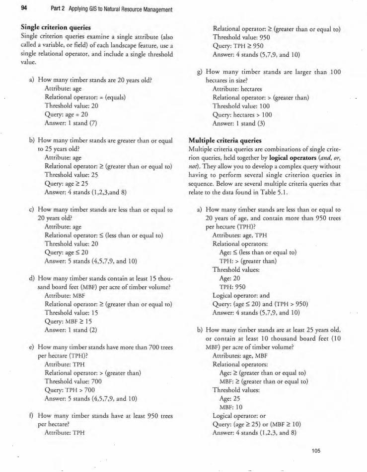
94 Part 2 Applying GIS to Natural Resource Management
Single criterion queries Single criterion queries examine a single attribute (also
called a variable. or field) of each landscape fearure. use a
single relational operator. and include a single threshold value.
a) How many timber stands are 20 years old? A[cciburc: age Relational operator: = (equals) Threshold value: 20
Query: age = 20 Answer: I stand (7)
b) How many timber stands are greater than or equal to 25 years old?
Attriburc: age Relational operator: ~ (greater than or equal to) Threshold value: 25
Query: age ~ 25 Answer: 4 stands (I.2.3.and 8)
c) How many timber stands are less than or equal [Q
20 years old? Attribute: age Relarional operator: S; (less than or equal to) Threshold value: 20
Query: age S; 20
Answer: 5 stands (4.5.7.9. and 10)
d) How many timber stands camain at least 15 thou-
sand board feet (MBF) per acre of timber volume' Amibute: MBF Relational operamc: ~ (greater than o r equal to)
Threshold value: 15 Query: MBF ~ 15 Answer: I stand (2)
e) How many timber stands have more than 700 trees
per hectare (TPH)? Amibute: TPH Relational operawc: > (greater than) Threshold value: 700 Query: TPH > 700 Answer: 5 stands (4.5.7.9. and 10)
f) How many timber stands have at least 950 trees per hectare?
Anribure: TPH
Relational operator: ~ (grearer than or equal to) Threshold value: 950 Query: TPH ~ 950
Answer: 4 stands (5.7.9. and 10)
g) How many timber stands are larger than 100 hectares in size?
Attribute: hectares
Relational operator: > (greater than) Threshold value: 100 Query: hectares > 100 Answer: I stand (3)
Multiple criteria queries Multiple criteria queries are combinations of single crite
rion queries, held together by logical operators (and. or,
not). They allow you to develop a complex query without havi ng to perform several single cr iterion queries in
sequence. Below are several mulriple criteria queries that
relate to the dara found in Table 5.1.
a) How many timber stands are less than or equal to
20 years of age, and contain more than 950 trees per hectare (TPH)?
Attributes: age. TPH Relational operators:
Age: S; (less than or equal to)
TPH: > (greater than) Threshold values:
Age: 20 TPH: 950
Logical operator: and
Query: (age S; 20) and (TPH > 950)
Answer: 4 stands (5.7.9. and 10)
b) How many ti mber stands are at least 25 years old. or contain at least 10 thousand board feet (10
MBF) per acre of timber volume?
Attributes: age. MBF Relational operators:
Age: ~ (greater than or equal to) MBF: ~ (greater than or equal to)
Threshold values: Age: 25 MBF: 10
Logical operator: or
Query: (age ~ 25) or (MBF ~ 10) Answer: 4 stands (I.2.3. and 8)
105
94 Part 2 Applying GIS to Natural Resource Management
Single criterion queries Si ngle criterion queries exami ne a single attribute (also
called a variable, or field) of each landscape featu re, use a si ngle relational operaror, and include a single [hreshold value.
a) How many timber stands are 20 years old? Attribute: age Relational operaror: = (equals) Threshold value: 20 Query: age = 20 Answer: I srand (7)
b) How many timber s[ands are greater than or equal [0 25 years old?
Aucibme: age
Relational oper.ro r: <! (grearer rhan or equal to) Th reshold value: 25 Query: age ~ 25 Answer: 4 stands (I,2,3,and 8)
c) How many limber stands are less rhan or equal ro 20 years old?
Attribute: age
Rela[ional operator: S (less rhan or equal [0)
Threshold value: 20 Query: age S 20 Answer: 5 stands (4,5,7.9. and 10)
d) How many limber "ands conta in ar least 15 thou-sand board feel (MBF) per acre of timber volume?
Amibure: MBF Rela[ional operaro r: <! (greater than or equal to) T hreshold value: 15 Query: MBF ~ 15 Answer: 1 Sland (2)
e) How many timber stands have more than 700 trees
per hectare (TPH) ' Amibute: TPH Relational operator: > (greater than) Threshold value: 700 Query: TPH > 700 Answer: 5 stands (4.5.7.9, and 10)
f) How many dmber srands have at least 950 trees per hectare?
Anribule: TPH
Relational operator: ~ (gn:arer rhan or equal to) Threshold va lue: 950 Query: TPH ~ 950 Answer: 4 stands (5,7,9. and 10)
g) How many tim ber stands are larger than 100 hectares in size?
AttriblHe: hectares Relational operator: > (greater than) Threshold value: 100 Query: hectares > 100 Answer: I stand (3)
Multiple criteria queries Multiple criteria queries are combinations of single crite
rion queries. held rogether by logical operators (and. or, 1/ot). They allow you ro develop a complex query wi thout having [0 perform several single criterio n queries in
sequence. Below are several multiple criteria queries mat
relate to rhe data fou nd in Table 5. !.
a) How many c.imber stands are less than or equal to
20 yea rs of age, and contain more rhan 950 trees per hectare (TPH)?
Attribu(es: age. TPH
Relational operarors:
Age: S (less than or equal to) TPH: > (grea ter than)
Threshold values: Age: 20 TPH: 950
Logical operator: and Query: (age S 20) and (TPH > 950) Answer: 4 srands (5.7,9, and 10)
b) How many ti mber stands are ar least 25 years old, or co ntain at least 10 thousand board feer (10 MBF) per acre of rimber volume?
Attributes: age, MBF Relational operators:
Age: ~ (greater [han or equal to) MBF: ~ (greater than or equal to)
Threshold values: Age: 25 MBF: 10
Logical o peraror: or Query: (age <! 25) or (MBF ~ 10) Answer: 4 stands (I,2.3. and 8)
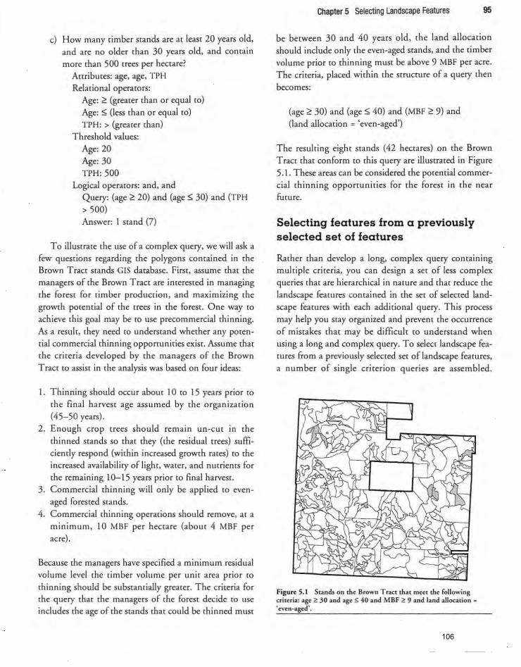
c) How many timber stands are at least 20 years old, and are no older than 30 years old, and contain
more than 500 trees per hectare? Amibutes: age, age, TPH Relational operators:
Age: ;" (greater than or equal to)
Age: S (less than or equal to) TPH: > (greater than)
T hreshold values: Age: 20
Age: 30 TPH: 500
Logical operators: and, and Query: (age;" 20) and (age S 30) and (TI'H > 500) Answer: I srand (7)
To illustrate the use of a complex query, we wi ll ask a few questions regarding the polygons contained in the Brown Tract stands GIS database. First, assume that the managers of the Brown Tract are interested in managing
the forest for timber production, and maximizing the growth potential of (he [fees in the forest. One way ro achieve this goal may be to use precommercial thinning. As a result, (hey need to understand whether any poten
cial commercial thinning opportunities exist. Assume that the criteria developed by the managers of the Brown
Tract [Q assist in (he analysis was based on four ideas:
l. Thinning should occur about 10 to 15 years prior to the fin al harvest age assumed by the organization (45-50 years).
2. Enough crop crees should remain un-cut in the
thinned stands so that they (the residual trees) sufficiently respond (within increased growth rates) to the increased availabili ty of light, water, and nutrients for
the remaining 10-15 years prior to final harvest. 3 . Commercial thinning will only be applied to even
aged forested stands. 4 . Commercial thinning operations should remove, at a
mInimUm, 10 MBF per hectare (abou, 4 MBF per acre).
Because the managers have specified a minimum residual volume level the dmber volume per unit area prior to
thinning should be substantially greater. The criteria for the query that the managers of the forest decide to use includes the age of the stands that could be thinned muSt
Chapter 5 Selecting landscape Features 95
be between 30 and 40 years old, the land allocation should include only the even-aged Stands, and the timber volume prior to thinning must be above 9 MBF per acre.
The criteria, placed within the structure of a query then
becomes:
(age;" 30) and (age S 40) and (MBF ;" 9) and (land allocation = 'even-aged')
The resulting eight stands (42 hectares) on the Brown Tract that conform to this query are illusuated in Figure
5.1. These areas can be considered. the poremial commercial thinning opportun ities for the fo rest in the near
future.
Selecting features from a previously selected set of features
Rather than develop a long, complex query containing multiple criteria. you can design a set of less complex queries that are hierarchical in nature and that reduce the
landscape features contained in the set of selected landscape features with each additional query. This process
may help you stay organized and prevent the occurrence of mistakes that may be difficult to understand when usi ng a long and complex query. To selec, landscape feacures from a previously selected set of landscape features,
a number of single criterion queries are assembled .
Figure 5.1 Stands on the Brown T net that meet the following criteria: age 2: 30 and age :5 40 and MBF 2: 9 and land allocation . 'even-aged' .
106
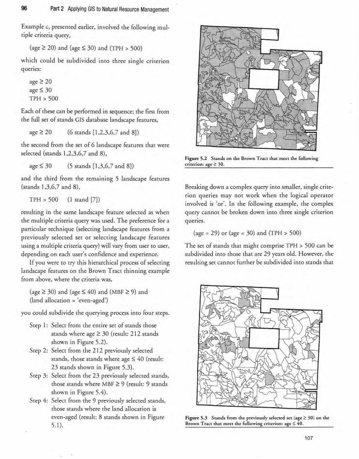
96 Part 2 Applying GIS to Natural Resource Management
Example c, presemed ea rlier. involved the following multiple criteria query,
(age ~ 20) and (age s: 30) and (TPH > 500)
which could be subdivided intO three single criterion quenes:
age ~ 20 age s: 30 TPH > 500
Each of these can be performed in sequence; the first from the full set of stands GIS database landscape features,
age ~ 20 (6 stands [1,2,3,6,7 and 8])
the second from the set of 6 landscape features that were selected (stands 1,2,3,6,7 and 8),
age s: 30 (5 stands [1,3,6,7 and 8])
and the third from the remaining 5 landscape features (stands 1,3,6,7 and 8),
TPH > 500 (I stand [7])
resulting in the same landscape feature selected as when the multiple criteria query was used. The preference for a particular technique (selecting landscape features from a previously selected set or selecting landscape features using a multiple criteria query) wi ll vary from user [0 user,
depending on each user's confidence and experience. If you were co try this hierarchical process of selecting
landscape features on the Brown Tract thinning example from above, where rhe criteria was,
(age ~ 30) and (age s: 40) and (MBF ~ 9) and (land allocation = 'even-aged')
you could subdivide the querying process into four steps.
Step I: Select from rhe entire set of stands those stands where age ~ 30 (result: 212 stands shown in Figure 5.2).
Step 2: Select from the 212 previously selected stands, those stands where age s: 40 (result: 23 stands shown in Figure 5.3).
Step 3: Select from the 23 previously selected stands, those stands where MBF ~ 9 (result: 9 stands shown in Figure 5.4).
Step 4: Select from the 9 previously selected stands, those scands where the land allocation is even-aged (resu le: 8 stands shown in Figure 5.1).
Figure 5.2 Stands on {he Brown Tract that meet the following criterion: age' ~ 30.
Breaking down a complex query into smaller, single crite
rion queries may not work when the logical operawr involved is 'or'. In the following example, the complex query cannor be broken down into rhree single criterion
queries.
(age = 29) or (age = 30) and (TPH > 500)
The set of stands that might comprise TPH > 500 can be subdivided into those that are 29 years old. However, the resulring set cannot further be subdivided into sra nds (har
Figure 5.3 Stands from the previously sciecte'd set (age 2: 30) on the Brown Tract that meet the fo llowing criterion: age S 40.
107
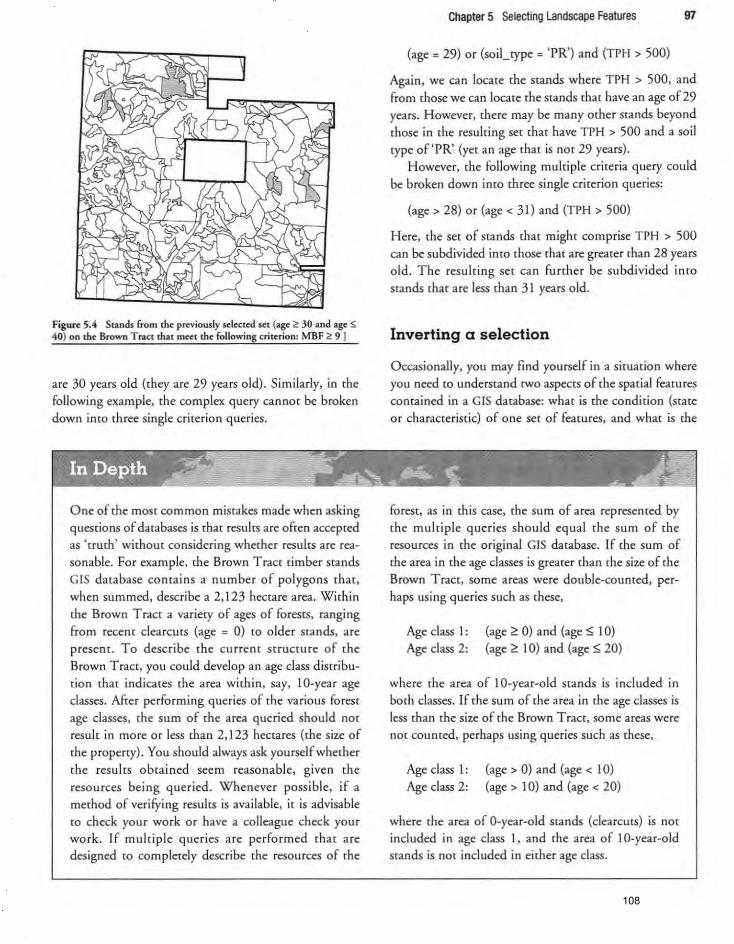
Figure 5.4 Stands &om the previously ~Iected set (age O!: 30 and age :5 40) on the Brown Tract that meet the following criterion: MBF O!: 9]
are 30 years old (they are 29 years old) . Similarly, in the following example, the complex query cannot be broken down into three single criterion queries.
One of the most common mistakes made when asking questions of databases is that results are often accepted as 'truth' without considering whether results are reasonable. For example, the Brown Tract timber scands
GIS database contains a number of polygons that , when summed, describe a 2,123 hectare area. Within the Brown Tract a variety of ages of forests, ranging from recent c1earcuts (age = 0) to older stands. are present. To describe the current structure of the
Brown Tract, you could develop an age class distribution that indicates the area within. say. la-year age classes. After performing queries of the various forest age classes, the sum of the area queried should nor result in more or less than 2,123 hectares (the size of the properry). You should always ask yourself whether the results obtained seem reasonable, given the resources being queried. Whenever possible , if a method of verifying results is available, it is advisable to check your work or have a colleague check your work. If multiple queries are performed that are designed to completely describe the resources of the
Chapter 5 Selecting Landscape Features 97
(age = 29) or (soil_rype = 'PR') and (TPH > 500)
Again, we can locate the stands where TPH > 500, and from those we can locate the stands that have an age of29 years. However. there may be many other stands beyond those in the resulting set that have TPH > 500 and a so il rype of 'PR' (yee an age that is nOt 29 years).
However, the following multiple criteria query could be broken down into three single criterion queries:
(age> 28) or (age < 31) and (TPH > 500)
Here, the set of stands that might comprise TPH > 500 can be subdivided into those that are greater than 28 years old. The resulting Set can furrher be subdivided into stands that are less than 31 years old.
Inverting a selection
Occasionally, you may find yourself in a situation where you need to understand {wo aspects of the spatial features contained in a GIS database: what is the condition (state or characteristic) of one set of features, and what is the
forest, as in this case, the sum of area represented by the multiple queries should equal the sum of the resources in the original GIS database. If the sum of the area in the age classes is greater than the size of the Brown Tract, some areas were double-counted, per
haps using queries such as these,
Age class I: Age class 2:
(age ~ 0) and (age" (0) (age ~ 10) and (age" 20)
where the area of I O-year-old stands is included in both classes. If the sum of the area in the age classes is less than the size of the Brown Tract. some areas were
nor counted. perhaps using queries such as these.
Age class I: Age class 2:
(age> 0) and (age < 10) (age> 10) and (age < 20)
where the area of O-year-old stands (c1earcurs) is not included in age class I , and the area of IO-year-old srands is nor included in either age class.
108
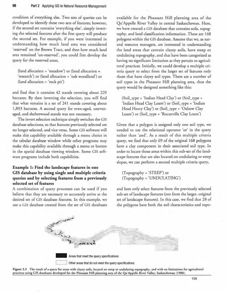
98 Part 2 Applying GIS to Natural Resource Management
condition of everyth ing else. Two sets of queries can be developed to identifY these two sets of features; however, if rhe second set contains 'everything else', simply inverting rhe selected fearures after rhe first query will produce rhe second set. For example, if you were interested in understanding how much land area was considered
'reserved' on the Brown Tract, and rhen how much land area remained 'un-reserved', you could first develop rhe query for rhe reserved areas,
(land allocarion = 'meadow') or (land allocation =
'research') or (land allocation = 'oak woodland') or (land allocation = 'rock pit')
and find that it contains 42 stands covering about 229 hectares. By then inverting the selection, you will find
that what remains is a ser of 241 stands covering abom 1,893 hectares. A second query for even-aged. unevenaged. and shelrerwood stands was not necessary.
The inven selection technique simply switches the GIS database selections, so that featu res previously selected are no longer selected. and vice versa. Some G IS software will make this capability available through a menu choice in the cabular database window while ocher programs may make this capability available through a menu or button in the spatial database viewing window. Some GIS software programs include borh capabi licies.
Example 1: Find the landscape features in one GIS database by using single and multiple criteria queries and by selecting features from a previously selected set of features A co mbination of query processes can be used if you believe that they are necessary to accurately arrive at the desired set of GIS database features. In this example, we use a GIS database created from the set of GIS databases
available for the Pheasant Hill planning area of the QU'Appdle River Valley in central Saskatchewan. Here, we have created a GIS database that contains so il s, topography, and land classification information . There are 168 polygons with in the GIS database. Assume that we, as natural resource managers, are interested in understanding the land areas that contain clayey soils, have steep or undulating topography, and that have been categorized as having no significant lim ita cion as they pertain to agricultural practices. Initially, we could develop a multiple criteria query to select from the larger set of features only those that have clayey soi l types. There are a number of soil types in the Pheasant Hill planning area, thus the query would be designed something like this:
(Soil_type = ' Indian Head Clay') or (Soil_type =
' Indian Head Clay Loam') or (Soil_type = ' Indian Head Heavy Clay') or (Soil_ type = 'Oxbow Clay Loam') or (Soil_type = 'Rocanville Clay Loam')
Given that a polygon is assigned only one soil type. we needed to use the relational operator 'or' in the query rather than 'and'. As a result of this multiple criteria query, we find that only 69 of the original 168 polygons have a clay component in their associated soil type. In order to locate those areas within this sub-set of the landscape features that are also located on undulating or steep slopes. we can perform a second multiple criteria query.
(Topography = 'STEEP') or (Topography = 'UN DULATING')
and here only select features from the previously selected sub-set oflandscape features (not from the larger, original set of landscape features) . In this case, we find that 28 of the polygons have both the soil characteristics and topO-
_ Areas that meet the query specifications
C=:J Other areas that do not meet the query specificatioos
Figure 5.5 The result of a query for areas with dayey soils, located on steep or undulating topography, and with no limitations for agriculrural practices using GIS databases developed for the Pheasant Hill planning area of the Qu'Appelle River Valley, Saskatchewan (1980).
109
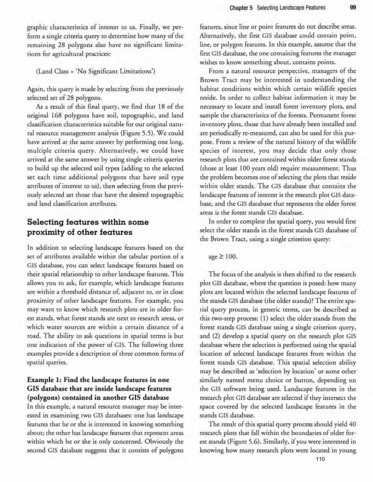
graphic characteriscics of imerest (0 us. Finally. we perform a single criteria query to determine how many of the remain ing 28 polygons also have no sign ificant limitations for agricultural practices:
(Land Class = ' No Significam Limitations)
Again, this query is made by selecting from the previously selecred set of 28 polygons.
As a result of this final query, we find that 18 of the original 168 polygons have soil, topographic. and land classification characteristics suitable for our original natural resource management analysis (Figure 5.5). We could have arrived at the same answer by performing one long. mulciple criteria query. Alternatively. we could have arrived at the same answer by using single criteria queries to build up the selected soil rypes (adding to the selected set each rime additional polygons that have soil rype attributes of interest (Q us). then selecting from the previously selected set those that have the desired topographic and land classification attributes.
Selecting features within some proximity of other features
In addition to selecting landscape features based on the set of attributes available within the tabular portion of a GIS database, you can select landscape features based on their spatial relationship to other landscape features. This allows you to ask. for example. which landscape features are within a threshold distance of. adjacenr roo or in close proximity of other landscape features. For example. you may want to know which research plots are in older forest stands. what forest stands are next to research areas, or which water sources are within a cerrain distance of a road. The abil ity [Q ask questions in spatial terms is but one indication of the power of GIS. The following three examples provide a description of three common forms of spatial queries.
Example 1: Find the landscape features in one GIS database that are inside landscape features (polygons) contamed in another GIS database In this example, a natural resource manager may be ineerested in examining [wo GIS databases: one has landscape features that he or she is ineerested in knowing something about; the orner has landscape features that represent areas within which he or she is only concerned. Obviously the second GIS database suggests that it consists of polygons
Chapter 5 Selecting Landscape Features 99
fearures. since line or poine features do not describe areas. Alternatively. the first GIS database could comain point. line. or polygon features. In this example. assume that the first GIS database, the one containing features the manager wishes to know something about. contains points.
From a natural resource perspective. managers of the Brown Tract may be interested in understanding the habitat conditions within which certain wildlife species reside. In order CO collect habitat information ir may be necessary to locate and install forest inventory plots. and sample the characteristics of the forests. Permanent forest inventory plots. those that have already been instal led and are periodically re-measured. can also be used for this purpose. From a review of the natu ral history of the wildlife species of interest. you may decide thar only those research plots that are contained within older forest stands (those at least 100 years old) require measurement. Thus the problem becomes one of selecting the plots that reside within older stands. T he GIS database that contains the landscape features of interest is the research plot GIS database. and the GIS database that represents the older fo rest areas is the forest stands GIS database.
In order to complete the spatial query. you would first select the older stands in the forest stands GIS database of the Brown Tract, using a single criterion query:
age ~ 100.
The focus of the analysis is then sh ifted to the research plot GIS database. where the question is posed: how many plots are located within the selected landscape features of the stands GIS database (the older stands)? The entire sparial query process, in generic terms, can be described as this two-step process: (I) select the older stands from the forest stands GIS database using a single criterion query, and (2) develop a spatial query on the research plot GIS
database where the selection is performed using the spatial location of selected landscape features from within the fo rest stands GIS database. This spatial selection abiliry may be described as 'selection by location' or some other similarly named menu choice or burton, depending on the GIS software being used. Landscape featu res in the research plot GIS database are selected if they intersect the space covered by the selected landscape features in the stands GIS database.
The result of this spatial query process should yield 40 research plots that fu ll within the boundaries of older forest stands (Figure 5.6). Similarly. if you were interested in knowing how many research plots were located in young
110
graphic characreriscics of imerest to us. Finally, we per
form a single criteria query to determine how many of me remaining 28 polygons also have no significant limica w
dons for agricultural praccices:
(Land Class = 'No Significant Limitations)
Again, this query is made by selecting from the previously
selected set of28 polygons.
As a result of this final query. we lind thar 18 of the
o riginal 168 polygons have soil, topographic, and land
classification characteristics suitable for our original na(U
ral resource managemem analysis (Figu re 5.5). We could
have arrived at the same answer by performing one long,
multiple criteria query. Alternatively. we could have
arrived at the same answer by using single criteria queries
to build up the selected so il rypes (adding to the selecred
ser each time addirional polygons thar have soil rype
attributes of imeres[ (Q us) , then selecting from the previ
ously selected ser rhose thac have the desired ropographic
and land classification amibmes.
Selecting features within some proximity of other features
In addition to selecring landscape fearures based on the
set of attributes available within the tabular portion of a
GIS database, you can select landscape features based on
their spatial relationship to other landscape fearures. This
allows you to ask, for example, whidh landscape fearures
are within a threshold distance of. adjacenr (0, or in close
proximiry of other landscape feamres. For example. you
may wam {Q know which resea rch plots are in older for
est srands. what forest stands are next (0 research areas, or
which water sources are wirhin a certain distance of a
road. The abiliry (0 ask quesdons in spadaJ rerms is bur
one indication of the power of GIS. The following [hree
examples provide a description of three common fo rms of
spadal queries.
Example 1: Find the landscape features in one GIS database that are inside landscape features (polygons) contained in another GIS datahase In rhis example, 3 narural resource manager may be inter
ested in examining (wo GIS databases; one has landscape
features that he o r she is imerested in knowing something
about; the other has landscape features thar represent areas
within which he or she is only concerned. Obviously the
second GIS database sugges" that it consists of polygons
Chapter 5 Selecting Landscape Features 99
fe-drures, since line or point features do nO( describe areas.
A1ternarively. the firsr GIS database could conrain point,
line. or polygon feamres. In this example, assume that the
first G1S database, the one containing feamres the manager
wishes to know something about. contains points.
From a natural resource perspective. managers of the
Brown Tracr may be interested in understanding [he
habitat conditions within which cerrain wildlife species
reside. In order (Q coUee[ habitat information it may be
necessary to locate and install forest inventory plots. and
sample the characteristics of the forests. Pcrmanem forest
inventory plms. rhose that have already been instal led and
are periodically re-measured, can also be used for this pur
pose. From a review of the natural history of rhe wildlife
species of interest, you may decide that only [hose
resea rch plotS thar are contained wirhin older forest s rands
(those ac leaSt 100 years old) require measuremem. Thus
the problem becomes one of selecting the plots that reside
with in older Stands. The GIS database thai contains rhe
landscape fearures of interest is the research plot GIS data
base. and the GIS database that represents the older foreSt
areas is the forest stands GIS database.
In order ro complere the sparial query, you would firSt
select the o lder stands in the forest stands GIS database of
the Brown Tract, using a single criterion query:
age ~ 100.
The focus of the analysis is then shifred to the research
plot GIS darabase. where the question is posed: how many
plots are located within the selecred landscape features of
the srands GIS database (rhe older Stands)? The entire spa
rial query process, in generic terms. can be described as
this two-Step process: (I) select the older stands from the
forest stands G1S database using a si ngle crieerion query,
and (2) develop a spa rial query on rhe researdh plm GIS
daeabase where [he seleceion is performed using the spatial
location of selected landscape features from within the
fo reSt stands GIS database. This spatial selection abiliry
may be described as 'selection by location' or some other
similarly named menu choice or bu([on. depending on
the GIS softwa re being used. Landscape fearures in the
research plot GIS database are selected if they inrersect the
space covered by the selected landscape fearures in the
stands GIS darabase.
The result of this spatial query process should yield 40
research plotS that full within rhe boundaries of older for
est seands (Figure 5 .6) . Similarly, if you were imeresred in
knowing how many research plots were locared in young
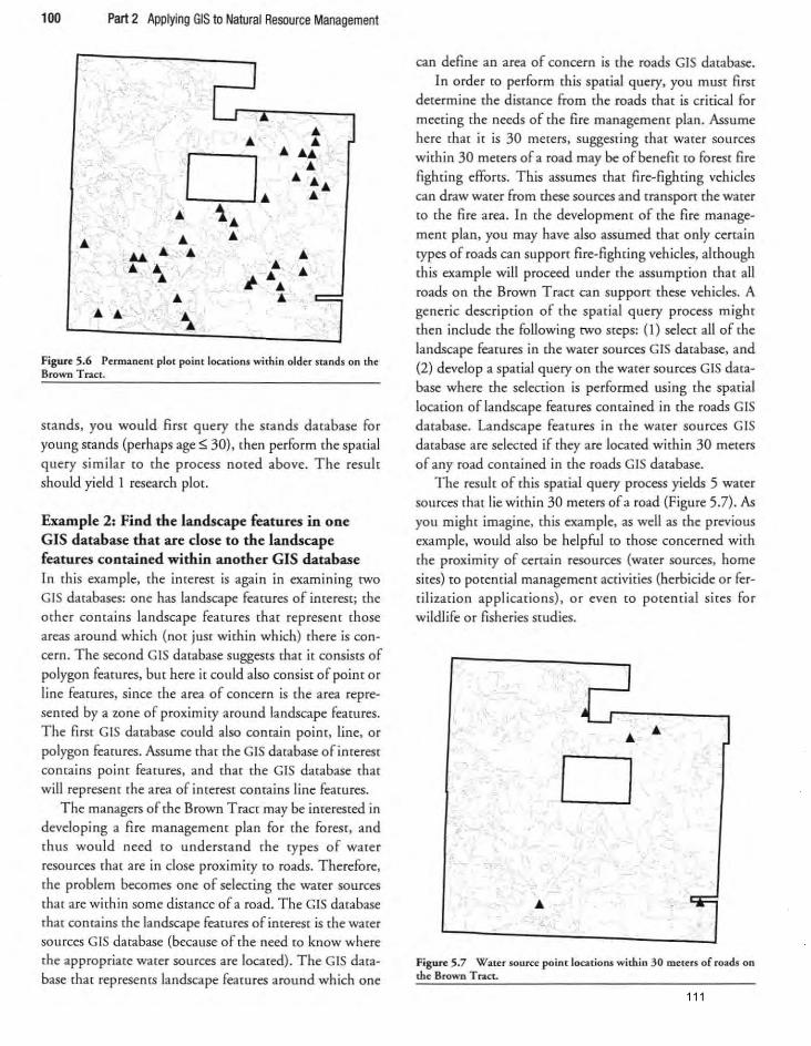
100 Part 2 Applying GIS to Natural Resource Management
Figure 5.6 Permanent plot point locations within older stands on the Brown Tract.
stands. you would first query the stands database for young srands (perhaps age!> 30). then perform the spatial query simila r [0 the process noted above. The result should yield 1 research plot.
Example 2: Find the landscape features in one GIS database that are close to the landscape features contained within another GIS database In this example. the imerest is again in examining two GIS databases: one has landscape feacures of interest; (he other contains landscape features [hat represent those
a reas around which (nor JUSt within which) there is concern. The second GIS dambase suggestS that it consists of polygon features. but here it could also consist of point o r line features. since [he area of concern is the area represented by a zone of proximity arou nd landscape features. The first GIS database could also contain point. line, or
polygon features. Assume that the GIS database of interest contains point features, and that the GIS database that will represenr the area of interest contains line features.
The managers of the Brown Tract may be inrerested in developing a fire management plan for the fores t, and thus would need to understand the types of water resources that are in close proximity to roads. Therefore,
the problem becomes one of selecting the water sou rces rhat are within some distance of a road. The GIS database thar contains the landscape features of interest is the water sources GIS database (because of the need to know where the appropriate water sources are located). The GIS database that represents landscape features around which one
can define an area of concern is the roads GIS database. In order to perform (his spatial query. you muse first
determine the distance from the roads that is cri tical for meering the needs of the fire management plan. Assume here that it is 30 merers, suggesting that water sources within 30 meters of a road may be of benefit to forest fire fighting efforts. This assumes that fi re-fighting vehicles can draw water from these sources and transport the water to the fire area. In the development of the fire manage
menr plan, you may have also assumed that only certain rypes of roads can support fire-fighting vehicles. although th is example will proceed under the assumption that aU roads on the Brown Tract can suppOrt these vehicles. A generic description of the spatial query process might then include the following two steps: (1) select all of the landscape features in the water sources GIS database, and
(2) develop a spatial query on the water sources GIS database where the selection is performed using the spatial location of landscape features con tained in the roads GIS database. Landscape features in the water sources GIS database are selected if they are located within 30 meters
of any road contained in the roads GIS database. The result of this spatial query process yields 5 water
sources that lie within 30 meters of a road (Figure 5.7). As you might imagine, this example, as well as the previous example. would also be helpful to those concerned with the proximity of certain resources (water sources, home sites) to potential management activities (herbicide or fertilization applications) , or even to potential sites for wildlife or fisheries studies.
o
Figure 5.7 Water source point locations within 30 meters of roads on the Brown T tact.
111
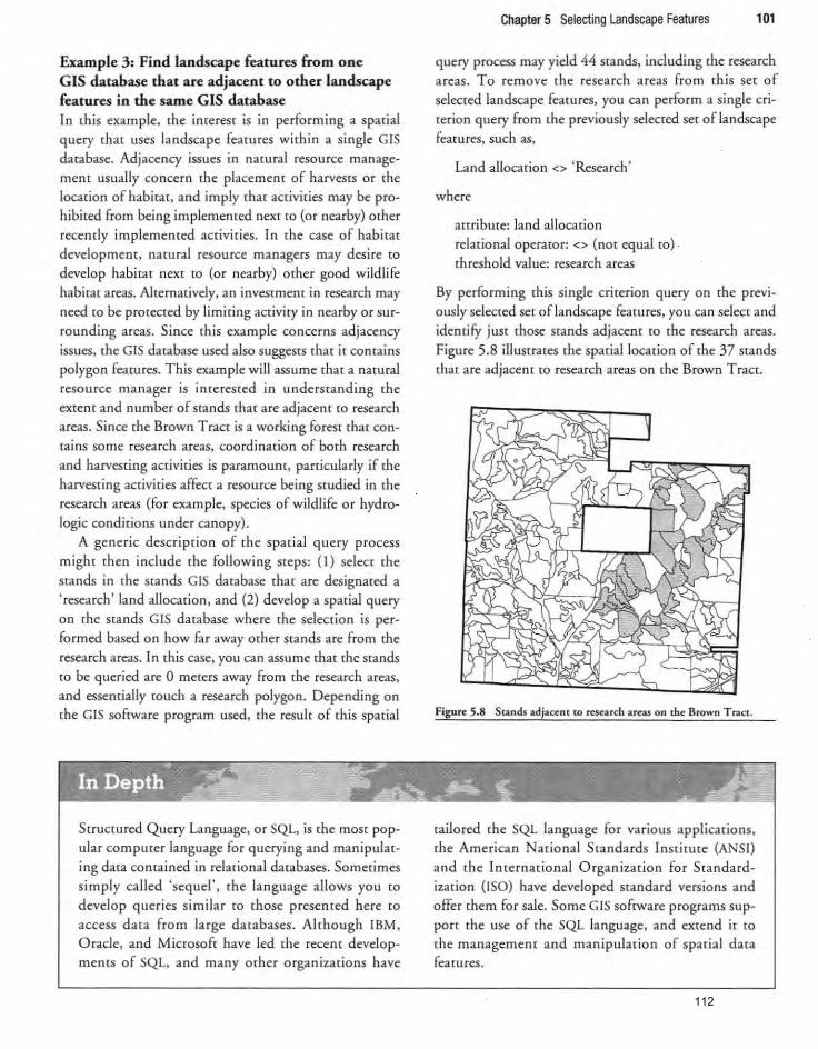
Example 3: Find landscape features from one GIS database tbat are adjacent to otber landscape features in tbe same GIS database In this example, the inrerest is in performing a spatial query that uses landscape features within a single GIS
database. Adjacency issues in natural resource manage
ment usually concern the placemenr of harvests or the location of habitat) and imply that activities may be pro
hibited from being implemented next to (or nearby) other
receody implemented activities. In the case of habitat
development. natural resource managers may desire co
develop habitat next to (or nearby) other good wildlife
habitat areas. Alternativdy. an invesrmem in research may
need co be protected by limiting activity in nearby or sur
rounding areas. Since this example concerns adjacency
issues, the GIS database used also suggests that it conrains
polygon features. This example will assume that a natural
resource manager is interested in understanding the
extenr and number of stands that are adjacent to research
areas. Since the Brown Tract is a working forest that con
tains some research areas, coordination of both research
and harvesting act ivities is paramount. particularly if the
harvesting activities affect a resource being smdied in the
research areas (for example, species of wildlife or hydro
logic conditions under canopy).
A generic description of the spatial query process might then include the following steps: (1) select the
stands in the stands GIS database that are designated a
'research' land allocation, and (2) develop a spatial query
on the stands GIS database where the selection is per
fo rmed based on how far away other stands are from the
research areas. In this case. you can assume that the stands
to be queried are 0 meters away from the research areas,
and essentially touch a research polygon. Depending on
the GIS software program used, the resul , of this spat ial
Structured Query Language, or SQL, is the most pop
ular computer language for querying and manipulat
ing data contained in relational databases. Sometimes
simply called 'sequel ', the language allows you to
develop quer ies similar to those presented here to
access data from large databases. Although IBM ,
Oracle. and Microsoft have led the recent developments of SQL. and many other organizations have
Chapter 5 Selecting Landscape Features 101
query process may yield 44 stands, including the research a reas . To remove the research areas from this set of
selected landscape featu res. you can perform a single cri
terion query from the previously selected set of landscape
feamres. such as,
Land allocation <> 'Research '
where
attribute: land allocation
relational operator: <> (not equal to)
threshold value: research areas
By performing this single criterion query on the previ
ously selected set oflandscape featu res. you can select and
identify JUSt those stands adjacent to the research areas.
Figure 5.8 illustrates the spatial location of the 37 stands
that are adjacent to research areas on the Brown Tract.
Figure 5.8 Stands adjacenllo research areas on the Brown Trace .
tailored the SQL language for various applications. the American Nationa l Standards Institute (ANSi)
and the International Organization for Standard
ization (ISO) have developed standard versions and
offer them for sale. Some GIS software programs sup
POrt the use of the SQL language, and extend it to
the management and manipulation of spatial data
features.
112
102 Part 2 Applying GIS to Natural Resource Management
Advanced Query Applications
Advanced applications of GIS-related database queries have concentrated on limiting the focus of queries only to rhe features inside a spatial or temporal window
defined by the user. In addition to simply providing a summary of rhe resources contained within a specific area, as the user-defined window (location or time frame) sl ides is expanded. or is contracted, the query is updated (Q reflect those features that have left rhe window and those [hat have entered rhe window. Queries can be completely re-evaluated as a window slides (or
otherwise changes). or iteratively evaluated by updating the query by considering only the changes that have occurred (Edelsbrunner & Overmars. 1987; Ghanem et al.. 2007). Dynamic queries can be designed that allow users to adjust questions asked of GIS databases by incorporating slider objec[S in a window rather than ask
in g the user to redefine (by typing) the adj ustmentS needed. For example. a graphical user interface can be
designed to allow users to easily adjust the upper and lower bounds of a quantitative query along a scale, using
a computer mouse (Domingue et al.. 2003). and to provide those results quickly.
Syntax Errors
Syntax errors that occur when developing queries can
Summary
There are a variery of methods you can use (0 select landscape features from a GIS darabase. from using a mouse (0 manually pick the landscape features (0 selecting them with queries. The most common requests of natural resource managers that involve GIS queries include: (1) a map illustrating the landscape features that conform to
some criteria. (2) a GIS database containing only the landscape features that conform to some criteria, and (3) summary statistics of the landscape features that conform
to some criteria. Many of the applications described later in th is book require YOll to develop a map showing some landscape feat ures of interest. and to describe some characteristics of those landscape features. Queries will enable YOli to acco mplish these tasks quickly and efficiently. An important habit to develop is to ask yourself whether the
discourage some users of GIS. MoS[ of these problems occur because brackets or parentheses are missing from a
query; this results in an incomplete query. such as in the
two cases shown below from ArcMap queries.
[Height] >= 50} and ([Age] >= 25
( [Age] >= 25) and ( <= 30 )
(beginning and ending parentheses missing)
{the attribuce 'age' is
missing from the second part of the criteria}
Most software programs require [hat every bracket or
parentheses be balanced, so, if you begin with an opening
bracket or parentheses. you must end with one as well. These parentheses and brackets can also be used to control the order of operations in queries that include mathemarical operations. The dialog boxes that are generally used to help develop queries will assist with the placement of parentheses and brackets as long as the fields. operarors, and values are selected in a logical manner using the computer mouse. Syntax errors usually arise
when a user erases part of a query. then continues with its development (i.e .. through keyboard intervention). Queries with syntax errors usually need manual keyboard intervention to correct the resulting problems. One of the eas iest methods (0 alleviate syntax errors during
queries may be to simply close the query dialog box and begin anew.
results of an analysis (here. a query) are reasonable. It has become very easy in modern GIS software to create spatial and anribute reference queries. and to instantly
receive the results. This ease of use may lead you to
believe that the results should not be questioned. Most GIS programs are designed to perform complex queries provided that the query syntax is correct. H owever, rhey simply provide you with results based on your instructions. and do not have the abili ty to question whether a query was correctly designed. It is therefore important to
be critical of the ourpUt from a query. and to examine whether the results are within the bounds of reason. This will help you to detect errors either in the GIS databases being analyzed or in the methods being used to perform an analysis.
113
Applications
5.1. Daniel Pickett Forest Annual Report. For the AnnuaJ Repof[ ohhe Daniel Pickett forest. you have been asked by Hugh Davenport (DiStrict Forester) to provide some in formation related [Q rhe forest's resources. Me Davenport poses his request as a series of questions:
From the stands GIS database: a) How much area ofland contains forests:S; 20 years
of age? b) How much area of land contains forests > 20 years
of age and:> 40 years of age? c) How much area of land contains forests> 40 years
of age? d) How much area otland contains vegetation type A?
e) How much area ofland contains vegetation type B?
f) How much area of land contains vegetation type C?
g) How much area of land contains average timber
volumes ~ 49.4 MBF (thousand board feet) per hectare (20 MBF per acre)?
h) How much area of land contai ns average timber
volumes ~ 74.1 MBF per hectare (30 MBF per acre)? i) How much area of land contains average timber
volumes ~ 98.8 MBF per hectare (40 MBF per acre)?
From the soils GIS database: a) How much area ofland might have a high response
[0 fenilization?
b) How much area of land might have a medium response to fertilization?
c) How much area ofland might have a low response to ferti lization?
From rhe streams GIS database (map units are feet):
a) How many miles or kilometers of Class 1 streams are
in the database?
b) How many miles or kilometers of Class 2 streams are in the database?
c) How many miles or kilometers of Class 3 streams are
in the database?
d) How many miles or kilometers of C lass 4 streams are
in the database?
e) Why might these values be misleading, and what caveat might you provide to Mr Davenpon?
G raphics for the repon:
a) Develop a histogram of 10-year stand age classes, showi ng the amount ofland in each age class.
Chapter 5 Selecting Landscape Features 103
5.2. Information for a new supervisor of Brown Tract. A new supervisor (Sharon G illman) was recendy selected [Q manage the Brown T mct, and she wanes to get
familiar with the natural resources located mere. She has
asked you to provide some information about the T ract
and j[5 resources:
From the streams GIS database:
a) How many miles or kilometers of fish-bearing, large
streams are in the database?
b) How many miles or kilometers of fish-bearing,
medium streams are in the database?
c) How many miles or kilom<ters of fish-bearing, small streams are: in the database?
d) How many miles or kilom<tm of non-fish bearing, large streams are in the database?
e) How many miles or kilom<lm of non-fish bearing, medium streams are in the database?
J) How many milts or kilom<lm of non-fish bearing, small streams are in the database?
From the roads GIS database: a) How many miles or kilometers of road on (or near)
the Brown T mCt are rock roads?
b) How many milts or kilom<lm of road on (or near) the Brown Tract are dirt roads?
From the soils GIS database: a) How much area ofland of 'PR' soil type is there on
the Brown Tract?
b) How much area of land of 'DN' soil type is there on the Brown Tract?
c) How much area of land of 'WL' soil type is there on the Brown Tract?
From the water sources GIS database:
a) How many beaver pond water sources are on the Brown Tract?
b) How many hydrant sources are on (or near) the
Brown Tract?
c) How many water tank sources are on (or near) the Brown Tract?
From the trails GIS database: a) How many miles or kilometers of authorized trails
are there on the: Brown Tract?
b) How many miles or kilometers of unauthorized
tra ils are there on the Brown Tract?
114
104 Part 2 Applying GIS to Natural Resource Management
c) How many mius or kilom.tm of proposed trails are there on rhe Brown Tract?
5.3. Brown Tract Annual Report. In addition to the requests by Sharon Gi llman to get her acquainted with
some of rhe resources located within and around rhe
Brown Tract. she asks you to supply the following information for the Annual Repon:
a) How much area of land is in even-aged forests? b) How much area of land is in uneven-aged forests?
c) How much area ofland is assigned to the 'research ' category?
d) How much area of land contains board foot volumes ~ 74.1 MBF per hecta re (30 MBF per acre)'
e) How much area ofland has a density of trees ~ 988 per hectare (400 per acre)?
5.4. Annual operating plan, Brown Tract. In order to
develop a budget for management activities next year) rhe
staff of rhe Brown T raet needs information regarding of the amount of land area that can be treated w ith various
silvicuicurai treatments. Through conversations with them. rhe criteria have been narrowed down to rhe
following:
Pre-commercial thinning cand idate stands: a) How much area ofland concains even-aged stands
that are s:; 20 years old and have ~ 988 trees per hectare (400 trees per acre)?
Commercial thinning candidate stands: a) How much area of land contains even-aged stands
that are ~ 30 and s:; 40 years old? b) How much area of land concains even-aged stands
that are ~ 30 and s:; 40 years old. with ~ 494 uees per hectare (200 uees per acre)?
Final harvest candidate stands: a) How much area ofland concains even-aged stands
that are ~ 45 years. s:; 100 years. and have a board foot volume ~ 74. 1 MBF per hectare (30 MBF per acre)?
5.5. Proposed recreation area. You received an e-mail
a few days ago from Erica Douglas, forester, which read:
'We are considering developing a campground or trail system on th e Brown Tract. Are there any sta nds or
groups of stands ~ 150 years old and ~ 25 hectares (6 1.8 acres) in size?' What will your response be?
5.6. Wildlife habitat. A note was placed on your computer's keyboard, from Will Edwards. the Brown Tract wildlife biologiSt, which read: 'Could you perform some queries of the Brown Tract stands database for me? I am
working on some wildlife habitat suitability models. and am incerested in the following:
a) Sharp-sh inned hawk habitat: area of land containing ~ 25 and s:; 50 year old Stands,
b) Cooper's hawk habi tat: area ofland containing ~ 30 and s:; 70 year old Stands.
c) Goshawk habitat: area of land containing ~ 150 year old Stands, and
d) Red tree vole habitat: area ofland containing ~ 195 year old Stands.
Also. could you make me a map of the sharp-shinned hawk habitat?'
5.7. Fire management plan. In preparation for the development of a fi re management plan the district manager of
the Brown Tract is interested in knowing the following:
a) How many water sou rces (all types) are within 30 meters (98.4 feet) of rocked or paved roads?
b) How many pond water sources are within 30 meters
(98.4 feet) of rocked or paved roads?
5.8. Research plots. One of the research sciencists asso
ciated w ith the Brown Tract is interested in measuring a
few of the research plots on the forest, to Study the growth of certain stand types. They want to understand the
following: a) How many research plots are located in research plots
on stands with ages ranging from 30 to 50 years?
b) If the quety were expanded to include Stands with ages ranging from 25 to 50 years. how many research plots would (his query contain?
5.9. Potential Fertilization Project. The managers of the Brown T ract are considering fertilizing all stands that
are aged berween 25 and 40 years old. The managers are not only concerned about the proximity of fertilization
operations to the stream system, bur also to water sources. How many water sources are within 60 meters (196.9
feet) of the stands that could potentially be fertilized'
115
104 Part 2 Applying GIS to Nalural Resource Management
c) How many miks or kilom, ,,n of proposed rra ils are there on the Brown T ract?
5.3. Brown T ract Annual Report. In addition to the requests by Sharon Gillman to get her acquain ted with
some of [he resources located within and around the Brown T racr, she asks you to supply the following informacion for rhe Annual Repon:
a) How much area of land is in even-aged forests? b) How much area of land is in uneven-aged forestS? c) How much area ofland is assigned to the 'research'
category? d) How much area of land contains board foot vol
umes ~ 74. 1 MBF per hectare (30 MBF per acre)? e) How much area ofland has a density of trees ~ 988
per hectare (400 per acre)?
5.4. Annual operating plan, Brown Tract. In order to
develop a budget fo r management activities next year, rhe
staff of the Brown Tract needs informacion regarding of the amount of land area that can be treated with va rious
s il viculrura.l treatments . Through co nve rsations with them. the criteria have been na.rrowed down to [he
followi ng:
Pre-commercial rhinning candidate stands:
a) How much area of land comains even-aged stands
that are S 20 years old and have ~ 988 trees per hectare (400 trees per acre)?
Commercial thinning candidate stands: a) How much area of land contains even-aged stands
that are ~ 30 and S 40 years old? b) How much area ofland contains even-aged stands
rhat are ~ 30 and S 40 years old, with ~ 494 trees per hectare (200 trees per acre)?
Final harvest candidate stands: a) How much area ofland contains even-aged stands
that are ~ 45 years, S 100 years, and have a board foot volume ~ 74.1 MBF per hectare (30 MBF per acre)?
5.5. Proposed recreation area. You received an e-mail
a few days ago from Erica Douglas, forester, which read : 'We are considering developing a campground o r trail
system o n the Brown T fa Ct. Are th ere any smnds o r
groups of stands ~ 150 years old and ~ 25 hecrares (61 .8 acres) in size?' What will your response be?
5.6. Wildlife habitat. A note was placed on your computerS keyboard, from Will Edwards, the Brown Tract wildlife biologist, which read: 'Could you perform some queries of the Brown Tract stands database for me? I am
working on some wildlife habitat suitability models, and am interested in (he following:
a) Sharp-sh inned hawk habitat: area ofland containing ~ 25 and S 50 year old stands,
b) Cooper's hawk habi tat: area ofland containing ~ 30 and S 70 year old srands,
c) Goshawk habitat: area of land containing ~ 150 year old stands, and
d) Red tree vole habitat: area ofland containi ng ~ 195 year old stands.
Also, could you make me a map of the sharp-shinned hawk habitat?'
5.7 . Fire management plan. In preparacion fo r the development of a fire managemem plan the district manager of
the Brown T ract is interested in knowing the fo llowi ng: a) How many water sou rces (a ll types) are within
30 meters (98.4 feet) of rocked or paved roads? b) How many pond water sources are within 30 merers
(98.4 feet) of rocked or paved roads?
5.8. Research plots. One of the research scientistS associa ted with (he Brown T racr is interested in measuring a
few of the research plotS on the forest, to study the growth of certain stand types. They wanr to unde rstand the
following: a) How many research plots are located in research plots
on srands with ages ranging from 30 to 50 years? b) If the query were expanded to include stands with
ages ra nging from 25 to 50 years, how many research plotS would rnis query contain?
5.9. Potential Fertilization Project. The managers of (he Brown Tract are cons idering fen il izing aU stands [hat
are aged berween 25 and 40 years old. The managers are nor only concerned about rhe proxim ity of fertilization
operatio ns to {he stream system, bur also (0 water sou rces . How many water sources are within 60 mecers (I96.9
feet) of the stands that could potentially be fertilized?

References
Domingue. j., Stun, A" Manins, M. , Tan, ] ., Pcrursson,
H .• & Morea. E. (2003). Supporting online shopping (hrough a combination of ontologies and interface metaphors. Intenzational Journal of Human-Computer Studirs. 59. 699-723.
Edelsbrunner. H .• & Overmars. M.H. (1987) . Zooming by repeated range detection. Information ProctIsing Lmers. 24. 413-1 7.
Chapter 5 Selecting Landscape Features 105
Ghanem. T.M .• Hammad. M.A .• Mokbel. M.F .• Aref. W.G .• & Elmagarmid. A.K. (2007). Incremental evaluation of sliding-window queries over dara Streams.
IEEE Transactions on Knowledge and Data Engineering, 19.57-72-
Plum Creek Timber Company. (2001). Plum Creek annual report 2000. Searde. WA: Plum Creek Timber Com pany.
116
Chapter 6
Obtaining Information about a
Specific Geographic Region
Objectives
This chapter is designed co provide readers with examples and applications from namral resource managemem (hat will allow you to analyze the resources contained within
specific geographic regions. Specific geographic regions can be defined in a number of ways, for example, (a) by using query processes (the subject of chapter 5), (b) by using buffer processes (the subject of chapter 7), or (c) through GIS overlay processes (the subject of chapter II). From a land managemen t perspective. there is a wide range of reasons why we would want to understand what is contained within these regions, and we will illustrate a few of these. At the conclusion of this chapter. readers should have acquired knowledge of:
1. how a clipping process works. and what products shou ld be expected when it is used;
2. how an erasing process works. and what products should be expected when it is used; and
3. how to use both clipping and erasing processes CO
obtain information about specific geographic regions. and obtain in format ion that is relevant to natural resou rce management planning.
As natural resource managers, we are often interested in understanding the characteristics of the land resources we manage within . or perhaps outside of, specific geographic areas. For example, if you were to manage riparian areas, where limited amountS of activity can be pre-
scribed. you might be interested in [he type and quantiry of resources within these areas, as well as the type and
quant ity of resources outside these areas-subject to a wider range of managemenr. Understanding the soil conditions within a property is another example. since many soils GIS databases are acquired from governmental organizations. where the coverage of data extends well beyond the boundary of the land you might manage. The twO main GIS processes that can be used to obtain information about a specific geographic region. and hence the focus of this chapter, are the clipping and erasing
processes. To some people. the term 'cl ipping' conjures up
thoughts of American football athletes using an illegal blocki ng maneuver on their opponents; to other people it
conjures up thoughts of snipping pieces of vegetation from a plant. It is also used invariably as both a noun and a verb, such as (a) a way [Q hold something in a tight grip, (b) a device to hold cartridges for a riAe, (c) a single instance or occasion. or (d) the act of cutting (Merriam
Webster, 2007). In a GIS context, a cli pp ing process implies something similar to cutting cookies from a sheet of dough, when baking holiday-related cookies, although nothing is actually baked here. Imagine a landscape rolled our fl at, like a map on a table. If you were to cut our a ponion of the landscape with a pair of scissors, you would have essentially 'clipped' it from the landscape. There are a number of reasons why you would do such a thing. and we will explore some of the more common applications in this chapter.
117
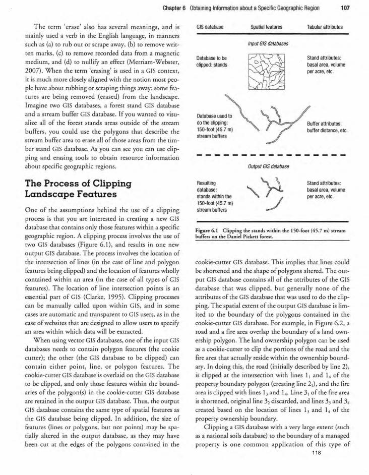
Chapter 6 Obtaining Information about a Specffic Geographic Region 107
The term 'erase' also has several meanings. and is
mainly used a verb in (he English language. in manners such as (a) (Q rub ou( or scrape away. (b) to remove writ
ten marks, (c) co remove recorded data from a magnetic
medium, and (d) to nullifY an effeC( (Merriam-Webster,
2007). When the term 'erasing' is used in a GIS context,
it is much more closely aligned with the notion most people have about rubbing or scraping rhings away: some fea
cures are being removed (erased) from the landscape.
Imagine two GIS databases, a fo resr stand GIS database
and a stream buffer GIS database. If you wanted to visu
alize all of (he forest stands areas oU[side of the stream
buffers, you could use the polygons that describe the stream buffer area co erase all of those areas from the timber stand GIS database. As you can see you can use clipping and erasing tools co obtain resource information
about specific geographic regions.
The Process of Clipping Landscape Features
One of the assumptions behind rhe use of a clipping process is that you are interested in creating a new GIS
database that comains only those features within a specific
geographic region. A clipping process involves the use of
twO GIS databases (Figure 6. I), and results in one new
ourpur GIS database. The process involves the location of
the intersection of lines (in the case of line and polygon
features being clipped) and the location of features wholly
contained within an area (in the case of all rypes of GIS
features), The location of line imersection points is an
essential part of GIS (Clarke, 1995). Cl ipping processes can be manually called upon wirhin GIS, and in some
cases are aurornatic and transparent to GIS users, as in the case of websites that are designed to allow users to specify an area within which data will be extracted.
When using vector GIS databases, one of the input GIS
databases needs [Q comain polygon features «(he cookie
cutter); the other (rhe GIS darabase to be clipped) can
camain either poin t, line, or polygon features. The cookie-cuHer GIS database is overla id on the GIS database to be clipped, and only those features within the bound
aries of the polygon(s) in the cookie-cutter GIS database
are retained in (he output GIS database. Thus, (he output
GIS database contains the same rype of spatial features as
the GIS database being clipped. In addi tion , rhe size of features (lines or polygons. but not points) may be spa
tially ahered in the output database. as they may have been cur a{ (he edges of the polygons contained in the
GIS database
Database to be clipped: stands
Spatial features
Input GIS databases
Database use~dO do the clipping: 150·foot (45.7 m) stream buffers
Resulting database: stands within the 150·foot (45.7 m) stream buffers
Output GIS database
Tabular attributes
Stand attributes: basal area, volume per acre, etc.
Buffer attributes: buffer distance, etc.
Stand attributes: basal area, volume per acre, etc.
Figure 6.1 Clipping the $lands within the 150·foof (45.7 m) sueam buffers on the Daniel Pickett forest.
cookie-curter GIS database. This implies thar lines could
be shorrened and the shape of polygons altered. The out
put GIS database contains all of the attributes of the GIS
database that was clipped, but generally none of the
attributes of the GIS database that was used to do the clip
ping. The spatial extent of the output GIS database is lim
ited to the boundary of rhe polygons contained in rhe
cookie-curter GIS database. For example. in Figure 6 .2. a road and a fire area overlap the boundary of a land own
ership polygon. The land ownership polygon can be used as a cookie-cutter to clip the portions of the road and the
£ire area rhat actually res ide within the ownership bound
ary. In doing this, the road (initially described by line 2),
is clipped at the intersection with lines 11 and 104 of the properry boundary polygon (creating line 2\) , and the fire
area is cl ipped with lines I , and I , . Line 3\ of the fire area
is shortened , original line 3, discarded, and lines 3, and 3, creared based on the location of lines 13 and 1 ~ of rhe
properry ownership boundary. Clipping a GIS database with a very large extent (such
as a national soi ls database) to the boundary of a managed
properry is one common application of this type of 118
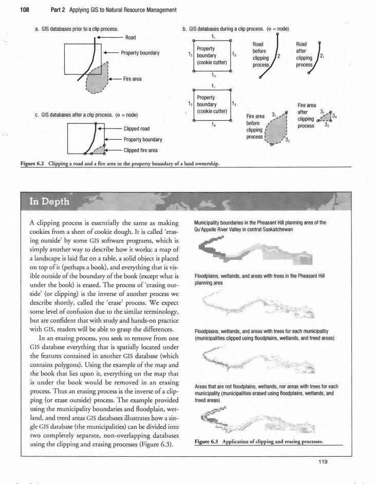
108 Part 2 Applying GIS to Natural Resource Management
a. GIS databases prior to a clip process. +----- Road
<Of-- Property boundary
j __ '1 I
/ ( J'-' Fire area I , • I ..... .. - "
C. GIS databases after a clip process. (0 = node)
i--ll.:l---- Clipped road
Property boundary
Clipped fire area
b. GIS databases during a clip process. (0 = node) 1,
Property 1, boundary I ,
(cookie cutter)
I ,
1,
Properly 1, boundary I ,
(cookie cutter)
I ,
Road belore clipping process
2
31 ... ...... 1 " . Rre area
before , I
clipping,' I I I
process: ./ 3l .... 'tY-, ...
RoadJ after clipping 21 process
Fire area after 3!.'''3 clipping ~ __ ~ 4
process 33
Figure 6.2 Clipping a road and a fire area to tilt: pro~rty boundary of a land ownership.
A clipping process is essenrially the same as making cookies from a sheet of cookie dough. It is called 'eras
ing outside' by some GIS software programs, which is simply another way to describe how ir works: a map of a landscape is laid flat on a table, a solid object is placed on tOP of it {perhaps a book}, and everything that is visible outside of the boundary of the book {except what is under the book} is erased. The process of 'erasing outside' (or clipping) is the inverse of anorher process we
describe shordy, called the 'erase' process. We expect some level of confusion due to the similar terminology,
but are confident that with study and hands-on practice with GIS, readers will be able to grasp the differences.
In an erasing process, you seek to remove from one
GIS database everything that is spatially located under the features conrained in another GIS database (which
contains polygons). Using the example of the map and the book that lies upon it, everything on the map that is under the book would be removed in an erasing
process. Thus an erasing process is me inverse of a clip
ping {or erase outside} process. The example provided using the municipali ty boundaries and floodplain , wet
land. and treed areas GIS databases illustrates how a single GIS database {the municipalities} can be divided into [wo completely separate, non-overlapping databases using the clipping and erasing processes {Figure 6.3}.
MuniCipality boundaries in the Pheasant Hill planning area of the Qu'Appelle River Valley in central Saskatchewan
Floodplains, wetlands, and areas with trees in the Pheasant Hill planning area
Floodplains, wetlands, and areas with trees for each municipality (municipalities clipped using floodplains, wetlands, and treed areas)
Areas that are not floodplains, wetlands, nor areas with trees for each municipality (municipalities erased using floodplains, wetlands, and treed areas)
Figure 6.3 Application of clippi ng and erasing processes.
119
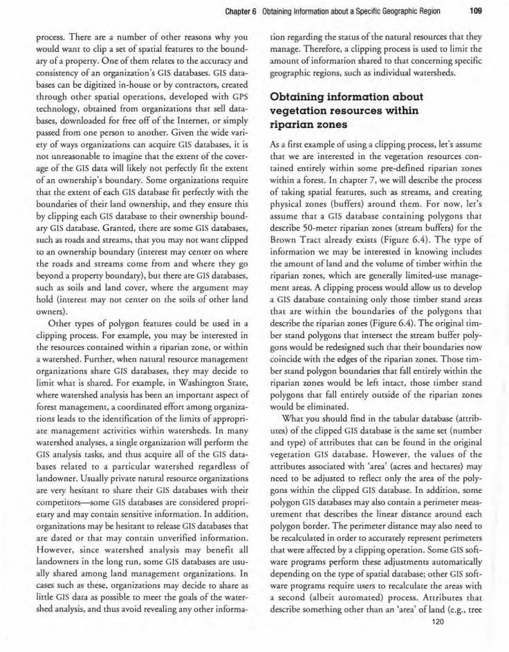
Chapter 6 Obtaining Information about a Spec~ic Geographic Region 109
process. There are a number of other reasons why you would want [0 clip a set of spatial features co the bound
ary of a property. One of them relates to the accuracy and consistency of an organization's GIS databases. GIS databases can be digitized in-house or by comracrocs, created through other spatial operations, developed with GPS
technology, obtained from organizations that sell dacabases, downloaded for free off of the Internet, or simply passed from one person to another. Given the wide va ri ety of ways o rganizacions can acquire GIS databases. it is not unreasonable to imagine that the extent of the coverage of the G IS data wi ll likely not perfectly fit the extent of an ownership's boundary. Some organizations require that the extent of each GIS database fit perfectly with the boundaries of their land ownership, and they ensure this
by clipping each GIS database to their ownership boundary GIS database. Granted, there are some G IS da tabases, such as roads and streams, that you may not want clipped [Q an ownership boundary (interest may center on where [he roads and screams come from and where they go beyond a property boundary), but there are GIS databases, such as soils and land cover, where the argument may hold (interest may not cemer on the soils of other land owners).
Other types of polygon features could be used in a dipp ing process. For example, you may be interested in the resources contained with in a riparian zone, or within a watershed. Further, when natural resource management organizations share GIS databases, rhey may decide to
limit what is shared. For example, in Washington Stare,
where watershed analysis has been an important aspect of foresr management, a coordinated effort among organizations leads to the idemification of the limits of appropriate management activities within watersheds. In many watershed analyses. a single organization will perform rhe G IS analysis tasks, and rhus acqu ire all of the G IS data
bases related to a particular watershed regardless of landowner. Usually private natural resource organizations are very hesitant to share their GIS databases with their competitors-some GIS databases are considered proprietary and may contain sensitive information. In addition, organizations may be hesitant ro release GIS databases that are dated or that may conta in unverified information . However, since watershed analysis may benefit all landowners in the long run, some GIS databases are usually shared among land management organizadons. In cases such as these, organizadons may decide ro share as little GIS data as possible to meet [he goals of the watershed analysis. and thus avoid revealing any other informa-
tion regarding the status of the natural resources thar they manage. Therefore, a clipping process is used ro limit the amount of information shared ro mat concerning specific
geographic regions, such as individual watersheds.
Obtaining information about vegetation resources within riparian zones
As a first example of using a clipping process, let's assume that we are interested in the vegetation resources contained entirely within some pre-defined riparian zones within a fo rest. In chapter 7, we will describe the process of taking spat ial features, such as streams, and creating physical zones (buffers) around them . For now, let's assume that a GIS database containing polygons that describe 50-meter riparian wnes (stream buffers) for the Brown Tract already exists (F igu re 6.4) . The type of information we may be interested in knowing includes the amount of land and the volume of timber within the riparian zones, which are generalJy limited-use management areas. A clipping process would allow us to develop a GIS database containing only those timber stand areas that are within the boundaries of the polygons that describe the riparian zones (Figure 6.4). The original timber stand polygons that intersect the stream buffer polygons would be redesigned such that their boundaries now coincide with the edges of the riparian zones. Those timber stand polygon boundaries that fall entirely with in the riparian zones would be left intact, those timber stand polygons that fall entirely outside of the riparian zones would be e1imina[ed .
What you should find in the tabular database (attrib
utes) of the clipped GIS database is the same set (number and type) of attributes that can be found in the original vegetarion GIS database. However, the values of rhe anributcs associated with 'area' (acres and hectares) may
need to be adjusted to reAect only the area of the polygons within the clipped GIS database. In addition, some polygon GIS databases may also contain a perimeter measuremem that describes the linear distance around each
polygon border. The perimeter distance may also need to
be recalculated in order to accurately represent perimeters that were affected by a clipping operation. Some GIS software programs perform these adjustments auromatically depending on the type of spatial database; other GIS software programs require users to recalculate the areas with a second (albeir automated) process. Arrribures that describe something other than an 'area' of land (e.g., tree
120
Chapter 6 Obtaining Intormation about a Specmc Geographic Region 109
process. There are a number of other reasons why you would wanr to clip a set of spatial fearures (Q the bound
ary of a properry. One of them relates to the accuracy and consistency of an o rganization's GIS databases. GIS databases can be digitized in-house or by contractors, created through other spatial operations, developed with GPS technology. obtained from organizations that seU databases, downloaded for free off of the Internet, or simply passed from one person [0 anomer. Given me wide variery of ways organizations can acquire GIS databases. it is not unreasonable (0 imagine [hat the extent of me coverage of the GIS data wil l likely not perfectly fit the exrenr of an ownership's boundary. Some o rganizations require that the extent of each GIS database lit perfectly with the boundaries of their land ownership, and tbey ensure this
by clipping each GIS database to their ownership boundary GIS database. Granted, there are some GIS da tabases, such as roads and screams, mat you may nO[ want dipped [0 an ownership boundary (interest may ceorer on where the roads and streams come from and where they go beyond a property boundary), but there are GIS databases,
such as soils and land cover, where the argument may hold (interest may not center on the soils of other land owners).
Other rypes of polygon features could be used in a dippi ng process. For example. you may he incercsted in the resources contajned with in a riparian zone. or within
a watershed. Further. when narural resource management organizations share GIS databases, they may decide to limit what is shared. For example, in Washington State,
where watershed analysis has been an important aspect of forese management, a coorciinared dfon among organizations leads to the identification of the limits of appropriate management activities wirhin watersheds. Ln many watershed analyses, a single organization will perform the GIS analysis tasks, and thus acquire all of the GIS data
bases related to a pan.icular watershed regardless of landowner. Usually private namral resource organizadons are very hesitant to share their G IS databases with their competitors-some GI S databases are considered proprietary and may contain sensitive information. In addicion. organizations may be hesitant to release GIS databases that are dated or chat may coma in unverified information . However, since watershed analysis may benefit all landowners in the long run, some GIS dacabases arc usually shared among land management organizations. In cases such as these, organizations may decide to share as lirrle GIS data as possible to meet the goals of the watershed anaJysis. and rhus avoid revealing any other informa-
tjon regarding the starus of the natural resources that they
manage. Therefore, a clipping process is used to limit the amount of information shared to that concerning specific
geographic regions, such as individual watersheds.
Obtaining information about vegetation resources within riparian zones
As a fi rst example of using a clipping process, let's assume that we are iD(~res(ed in [h~ vegetation resources con
tained enti rely within some pre-defined riparian zones within a forest. In chapter 7. we will describe rhe process of taking spat iaJ features, such as Streams, and creating physical zones (buffers) around them. For now, ler's
assume thar a GIS database containing polygons that describe 50-meter riparian wnes (stream buffers) for the Brown Tract already exists (Figure 6.4) . The type of informarion we may be interested in knowing includes the amount of land and the volume of timber within the riparian zones, which are generally limited-use management areas. A clipping process would allow us to develop a GIS database contajning only chose umber stand areas that are within the boundaries of the polygons that describe the riparian zones (Figure 6.4). The original tim
ber stand polygons that intersect the stream buffer polygons would be redesigned such that their boundaries now
coincide with the edges of rhe riparian zones. Those timber stand polygon boundaries that fall entirely within the riparian zones would be left intact . those timber stand
polygons that fitJI entirely outside of the riparian zones would be eliminated.
What you should find in the tabular database (attr ib
Utes) of the clipped GIS database is the same set (number and rype) of attributes thar can be found in the original vegetarion GIS database. However. the values of (he attributes associated with 'area' (acres and hectares) may
need to be adjusted to reAect only the area of the polygons within the clipped GIS database. [n addition, some
polygon GIS databases may also comain a perimeter measuremem that describes [he linear distanc~ around each
polygon border. The perimeter distance may also need to
be recalculated in order to accu rately represent perimerers that were affected by a clipping operation. Some GIS software programs perform these adjustmems automaricaIly
depending on the type of spatial database; other GIS software programs require users to recaJculate the areas with a second (albeit automared) process. Arcributes mar describe something other than an 'a rea ' ofland (e.g., tree
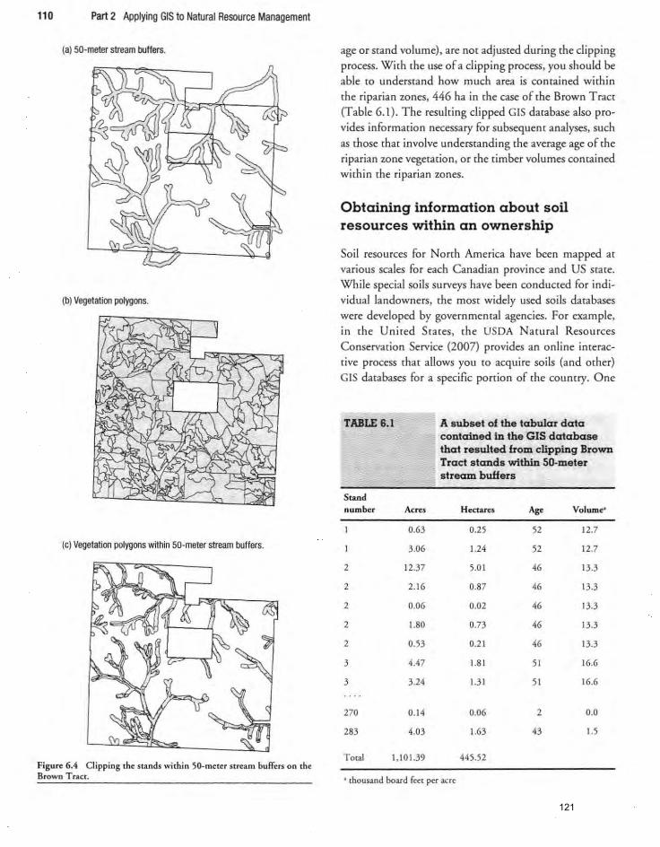
110 Part 2 Applying GIS to Natural Resource Management
(a) so· meter stream buffers.
(b) Vegetation polygons.
age or stand volume). are not adjusted during the dipping
process. With the lise of a dipping process. you should be able ro understand how much area is comained within
the riparian zones, 446 ha in the case of the Brown Tract
(Table 6.1). The resulting dipped GIS database also pro
vides information necessary for subsequem analyses, such
as those that involve understandi ng the average age of the
riparian zone vegetation. or the timber volumes contained
within the riparian zones.
Obtaining information about soil resources within an ownership
Soil resources for North America have been mapped at various scales for each Canadian province and US St3te.
While special soils surveys have been conducted for indi
vidual landowners. the most widely used soils databases
were developed by governmental agencies. For example. in (he United Scates, the USDA Natural Resources
Conservation Service (2007) provides an online inrerac
tive process that allows you to acquire soils (and other)
GIS databases for a specific ponion of the country. One
TABLE 6.1 A subset of the tabular data contained in the GIS database that resulted from clipping Brown Tract stands within SO-meter stream buffers
Stand number Acres Hectares Age Volume'
0.63 0.2; ;2 12.7
(c) Vegetation polygons within 50-meter stream buffers. 3.06 1.24 ;2 12.7
Figure 6.4 Clipping the stands within 50-meter stream buffers on the Brown Tract.
2 12.37
2 2. 16
2 0.06
2 1.80
2 053
3 4.47
3 3.24
270 0.14
283 4.03
To,.] 1,101.39
• thousand board reet per acre
;.01
0.87
0.02
0.73
0.21
1.81
i.31
0.06
1.63
44552
46 13.3
46 13.3
46 13.3
46 13.3
46 13.3
;1 16.6
;1 16.6
2 0.0
43 I.;
121

Chapter 6 Obtaining Information about a Spec~ic Geographic Region 111
product that can be obtained is the soil survey geogtaphic database (SSURGO) for most counties in the US. The majority of SSURGO data were mapped at a 1 :20,000 scale. and the minimum mapping area is 1-2 hectares. This level of detail in the mapping of soils was designed for use by Farmers. landowners. and other natural resource
organizacions. The STA TSGO soils database is another national-level
soils GIS database for the United States (USDA Natural Resources Conservation Service. 2006). However, the STATSGO data is a general soil map, and not as spatially refined as the SSURGO data. STA TSGO was mapped at a 1 :250,000 scale, and the minimum atea mapped is about 600 hectares. This level of detail in mapping soils was designed for broad natural resource planning and management uses.
The National Soil Database of Canada (Agriculture and Agri-Food Canada, 2006) contains databases on soils, landscape features, and climatic data for each Canadia n province. and is the national archive for land resource information collected by federal and provincial field surveys. The GIS databases contained in the National Soil Database range from the more general, mapped at a 1: 1,000,000 scale or smaller (like STATSGO), to the more detailed, mapped at a 1 :20,000 scale or larger (like SSURGO).
Figure 6.5 Soil polygons in me Brown Tract and surrounding at(~a.
Assume.you were to acquire the SSURGO data for the county within which the Brown Tract is located (Figure 6.5). If the managers of the Brown Tract were interested in the eype of soi ls that the Nacucal Resources Conservation Service has delineated for the land that they manage. a dipping process can be used CO obtain that information. In this case, you would use the boundary of the Brown Tract as the polygon theme to perform the clip, and the SSURGO soils database as the theme on which the clip would be performed. The resulting GIS
database provides an indication of (he major types of the SSURGO soils that are being managed on the Brown Tract (Figure 6.6).
Obtaining iruormation about roads within a forest
In the previous examples provided in this chapter, interest was placed on obtaining information aboU[ polygon features (timber stands and soils) that were located within some geographic region . This type of information is informative for land managers, yet it is a1so possible ro
~ Dixonville-Gellatly, steep slopes
t : : : : I Price-MacOunn-RItner complex, steep slopes
• Dbconville-Gellatly, moderats slopes
o Joey silty clay 1oam, Iow slopes
D Jory-Gelderman complex, moderate slopes
D Other soil types
Figw~ 6.6 Major soil types within the boundary of th~ Brown Tract.
122
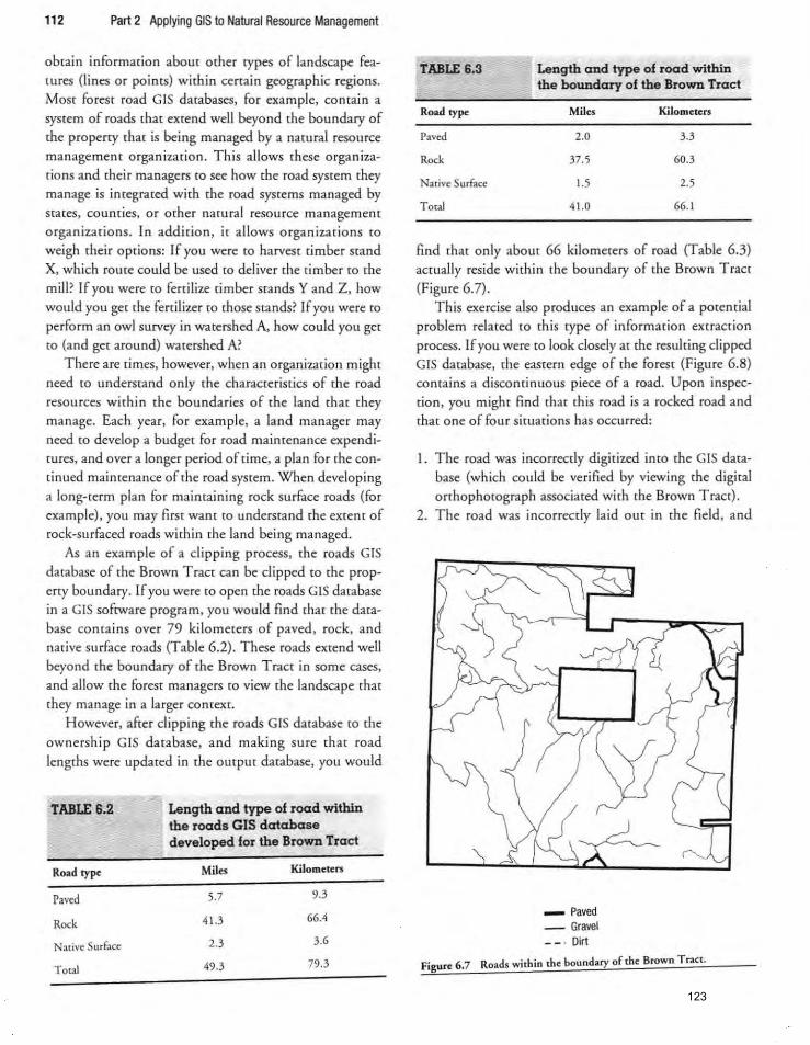
112 Part 2 Applying GIS to Natural Resource Management
obtain information abour other types of landscape feacures (lines or points) within certain geographic regions. Most forest road GIS databases, for example, contain a system of roads that extend well beyond the boundary of the property that is being managed by a nacural resource management organization. Th is allows these organizations and their managers to see how the road system they manage is integrated with the road systems managed by states, counties, or other nacural resource management organizations. In addition, it allows organizations [Q
weigh their options: If you were to harvest timber stand X, which route could be used to deliver the timber to the mill? If you were to fertilize timber stands Y and Z. how would you get the fertilizer to those stands? If you were to
perform an owl survey in watershed A, how could you get to (and get around) watershed A?
There are times, however, when an organization might need to understand only the characteristics of the road resources within the boundaries of the land that they manage. Each year. for example, a land manager may need to develop a budget for road maimenance expend icures, and over a longer period of time. a plan for the continued maintenance of the road system. When developing a long-cerm plan for maintaining rock surface roads (for example), you may first want to understand the extent of rock-surfaced roads within the land being managed.
As an example of a clipping process, the roads GIS database of the Brown Tract can be dipped to the property boundary. If you were to open the roads GIS database in a GIS software program, you would find that the database contains over 79 kilometers of paved. rock. and native surface roads (Table 6.2). These roads extend well
beyond the boundary of the Brown Tract in some cases. and allow the forest managers to view the landscape that they manage in a larger context.
However, after clipping the roads GIS database to the
ownership GIS database. and making sure that road lengths were updated in the output database. you would
TABLE 6.2
Road ty~
Paved
Rock
Native Surface
Total
Length and type of road within the roads GIS database developed for the Brown Tract
Mil .. Kilometers
5.7 9.3
41.3 66.4
2.3 3.6
49.3 79.3
TABLE 6.3 Length and type of road within the boundary of the Brown Tract
Roadrype Miles Kilometers
Paved 2.0 3.3
Rock 37.5 60.3
Native Surface 1.5 2.5
Total 41.0 66. 1
find that only about 66 kilometers of road (Table 6.3) actually reside within the boundary of the Brown Tract
(Figure 6.7). This exercise also produces an example of a potential
problem related to this type of information extraction process. If you were to look closely at the resulting clipped GIS database. the eastern edge of the forest (Figure 6.8) comains a discontinuous piece of a road. Upon inspection, you might find thac chis road is a rocked road and that one of four situarions has occurred:
I. The road was incorrectly digitized into the GIS database (which could be verified by viewing the digital orrhophotograph associated with the Brown Tract).
2. The road was incorrectly laid our in the field. and
_ Paved _ Gravel _ _ . Dirt
Figure 6.7 Roads within the boundary of the Brown Tract.
123
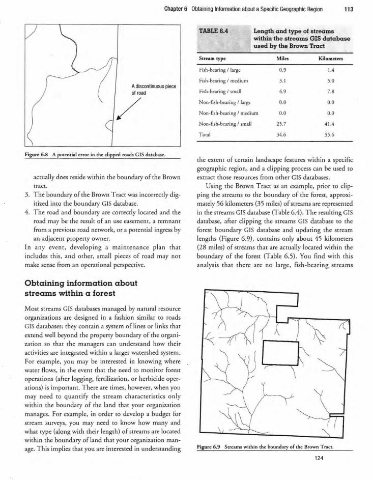
Chapter 6 Obtaining Information about a Specnic Geographic Region 113
A discontinuous piece of road
/ Figure 6.8 A potential error in the clipped roads GIS datab~.
actually does reside within the boundary of the Brown
tracr.
3. The boundary of the Brown Tract was incorrectly dig
itized into the boundary GIS database.
4. The road and boundary are correctly located and the road may be (he result of an use easemem, a remnanc from a previous road network. or a potencial ingress by an adjacent property owner.
In any event, developing a mainrena nce plan that
includes rhis. and ocher, small p ieces of road may not
make sense from an operational perspective.
Obtaining information about streams within a forest
Most sc reams GIS databases managed by natural resource
organizat ions are designed in a fash ion similar to roads
GIS databases: they contain a system oflines or links that
extend well beyond the property boundary of the organi
zat ion so that the managers can understand how their
activities are integrated within a larger watershed system.
For example, you may be interested in knowing where
water flows, in the event that the need to monitor forest operations (after logging, fertilization. or herbic ide oper
ations) is important. There are times. however, when you
may need to quan ti fy the stream characterist ics only
within the boundary of the land that your organization
manages. For example. in order to develop a budget for
stream surveys, you may need to know how many and what rype (along with their length) of streams are located
within the boundary of land that your organization man
age. This implies that you are interested in understanding
TABLE 6.4
Stream type
Fish-Ixaring 1 large
Fish-Ixaring I medium
Fish-Ixari ng I small
Non-fish-bC'aring 1 large
Length and type of streams within the streams GIS database used by the Brown Tract
Miles Kilometers
0.9 1.4
3. 1 5.0
4.9 7.8
0.0 0.0
Non-fish -bearing J medium 0.0 0.0
Non-fish-bearing I small 25.7 41.4
Total 34.6 55.6
the extent of certain landscape features within a specific
geographic region. and a clipping process can be used to
extract those resources from other GIS databases.
Using the Brown Tract as an example. prior to clip
ping the streams to the boundary of the fo rest. approxi
mately 56 kilometers (35 miles) of streams are represented
in the streams GIS database {Table 6.4}. The resulting GIS
database. after clipping the streams GIS database to the
forest boundary GIS database and updating the stream lengths (Figure 6 .9). contains only about 45 kilometers
(28 mi les) of streams that are actually located with in the
boundary of the forest (Table 6.5). You find with this
analysis that (here are no large, fish.bearing streams
Figure 6.9 Streams within the boundary of the Brown Tract .
124
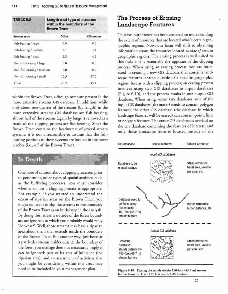
114 Part 2 Applying GIS to Natural Resource Management
TABLE 6.5
Stream typ<
Fish-bearing I large
Fish-bearing I medium
Fish-beari ng I small
Non-fish-bearingJ large:
Length and type of streams within the boundary of the Brown Tract
Mil" Kilometers
0.0 0 .0
2.1 3.4
2.8 4.5
0.0 0.0
Non-fish-lxaring I medium 0.0 0.0
Non-Fis h-bearing I small 23.3 37.5
Tmal 28.2 45.4
within the Brown Tract, although some are present in the more extensive streams GIS database. In addition, while only about one·quartet of the streams (by length) in the more extensive Streams GIS database are fish -bearing, almost half of the streams (again by length) removed as a
result of the clipping process are fish-bearing. Since the Brown Tract contains the headwaters of several stream systems. it is not unreasonable to assume that (he fishbearing portions of these systems are located in the lower reaches (i.e .• off of the Brown Tract).
One note of caution about clipping processes: prior to performing other rypes of spatial analyses. such as the buffering processes, you must consider
whether or nO[ a clipping process is appropriate. For example, if you wanted to understand the extem of riparian areas on the Brown Tract, you
might nor want to clip the st reams to the boundary of rhe Brown Tract as an initial step in the analysis. By doing this, streams outside of rhe forest bound
ary are igno red. to which you probably would reply '50 what?'. Well , those streams may have a riparian area about them that extends inside the boundary of rhe Brown Tract. Put another way. just because a panicular stream resides outside the boundary of the forest you manage does not necessarily imply it can be igno red: part of its area of inAuence (rhe riparian area). and an assessmem of activities mar YOll might be considering within this area. may need to be included in your management plan.
The Process of Erasing Landscape Features
Thus far. our imerest has been centered on understanding the extent of resources that are located within certain geographic regions. Now. our focus will sh ift to obtaining informatio n abour the resources located oZltsid~ of certain geographic regions. The erasing process is well suited to
this task. and is essentially the opposite of the clipping process. When using an erasing process. you are interested in creating a new GIS database that contains landscape features located outside of a speci fic geographic region. Just as with a clipping process, an erasing process involves using two GIS databases as input databases (Figure 6.10). and the process results in one output GIS
database. When using vector GIS databases. one of the input GIS databases (the eraser) needs to comain polygon features; the other GIS database (the database in which landscape fearures will be erased) can contain point. line,
or polygon features. The eraser GIS database is overlaid on the GIS database containing the fearures of interest. and only those landscape features located outside of the
GIS database
Database to be erased : stands
Spatial features
Input GIS databases
Dalabase used~O do the erasing (Ihe eraser): 150-loot (45.7 m) stream buffers
- - -- ------Output GIS database
Resulling
~ database: stands outside the 150-foot (45.7 m) stream buffers
Tabular Attributes
Stand attributes: basal area, volume per acre, etc.
Buffer attributes: buffer distance, etc.
------ ,
Stand attributes: basal area, volume per acre, etc.
Figure 6.10 Erasing the stands within I 50· foot (45 .7 m) stream buffers from tht Danid Picktn stands GIS databast.
125
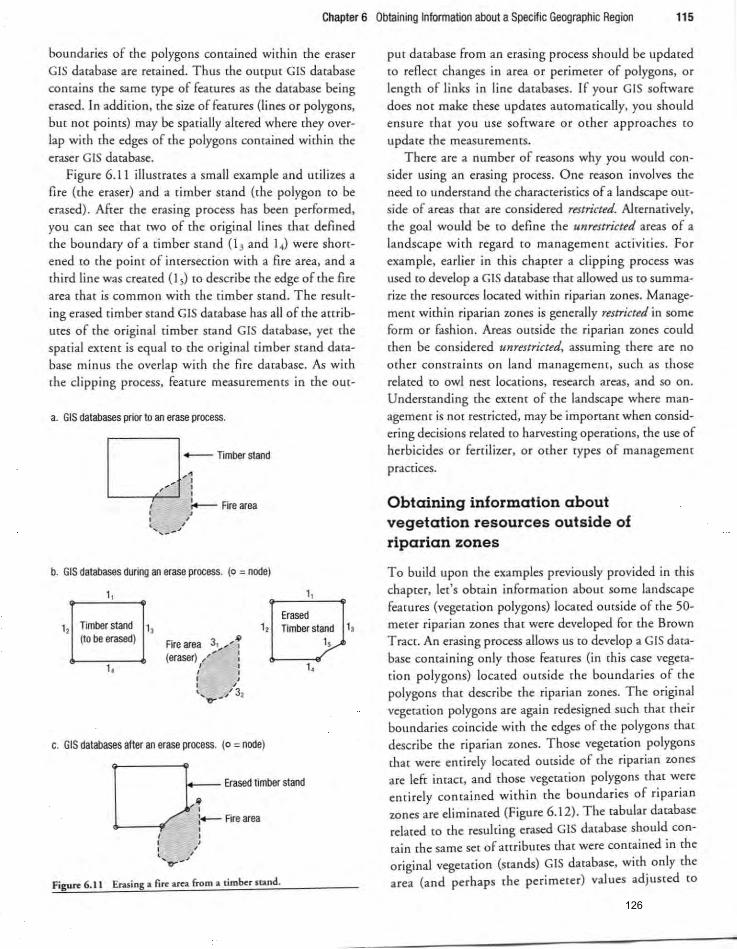
Chapter 6 Obtaining Information about a Specffic Geograph ic Region 115
bou ndaries of the polygons contained within the eraser GIS database are rerained. Thus the output GIS database contains the same type of features as the database being
emsed. In addition, the size of featu res (lines o r polygons, but not points) may be spatially altered where they overlap with the edges of the polygons conta ined within the
ems« GIS database. Figure 6.1 1 illustrates a small example and utilizes a
fire (the eraser) and a timber stand (the polygon to be erased). After the erasing process has been performed, you can see that [WO of the o riginal lines that defined the boundary of a timber stand (l , and I ,) were sho rtened [Q the point of intersection with a fi re area, and a third line was created (J ,) to describe the edge of the fire area tha t is common wi th the timber stand. The resuh
ing erased timber stand GIS database has all of the attributes of the original timber stand GIS database, yee the spacial extent is equal [0 the original cimber stand database minus [he overlap with [he fi re database. As with
[he clipping process, feature measurements in the OU(-
3. GIS databases prior to an erase process.
0 - Timber stand
" , , /" I
, ~ Fire area I , , ' , ' ......... _ /
b. GIS databases during an erase process. (0 = node)
1, 1,
Erased 12 Timber stand 13
(to be erased) Fire area 31 .. ...... ~ 12 Timber stand 13
1,
1, (eraser) /' : , , , , , , , ,
, '3 '"..._" 2
c. GIS databases after an erase process. (0 = node)
,~ , Erased timber stand
:...- Fire area , , ' , ' ' "...- "
, ,
Figure 6.11 Erasing a fire area from a timber 5t:lnd.
1,
put darabase fro m an erasi ng process should be updated (Q reRect changes in area or perimeter of polygons. or length of li nks in line databases. If your GIS software does not make these updates automatically. you shou ld ensu re that you use software or other app roaches (Q
update the measurements. There are a number of reasons why you would con
sider using an erasing process. One reason involves the need to understand the characterist ics of a landscape Out
side of areas that are considered Ttstn·cttd. Alternatively. the goal would be to define the unrestricttd areas of a
landscape with regard to management act ivities. For example. earlier in this chapter a clipping process was used to develop a GIS database that allowed us to summarize the resources located within riparian zones. Management within riparian zones is generally restricted in some fo rm or fashion. Areas outside the riparian zones could then he considered unrestricted, assuming there are no other co nstrai nts on land management, such as those related to owl nest locations, research areas, and so on . Understanding the extent of the landscape where management is not restricted, may be important when considering decisions related [Q harvesring operations, the use of herbicides or fertilizer, or other types of management
practices.
Obtaining information about vegetation resources outside of riparian zones
To build upon the examples previously provided in this chapter, let's obtain information about some landscape features (vegetat ion polygons) loca ted outside of the 50-meter riparian zones that were developed for the Brown Tract. An erasing process allows us to develop a GIS database containing o nly those features (in this case vegetat ion polygo ns) located outs ide the boundaries of the polygons that describe the riparian zones. T he origi nal vegetation polygons are again redesigned such that their boundaries coincide with the edges of the polygons that describe the riparian wnes. Those vegetation polygons that were entirely located outside of the riparian zones are left intact, and those vegetation polygons (hat were ent irely contai ned within the boundaries of riparian zones are eliminated (Figure 6.12). The tabular database related to the resulting erased GIS database should contain the same set of attributes that were contained in the
original vegetat io n (stands) GIS database, with only the area (a nd perhaps the perimeter) values adjusted to
126
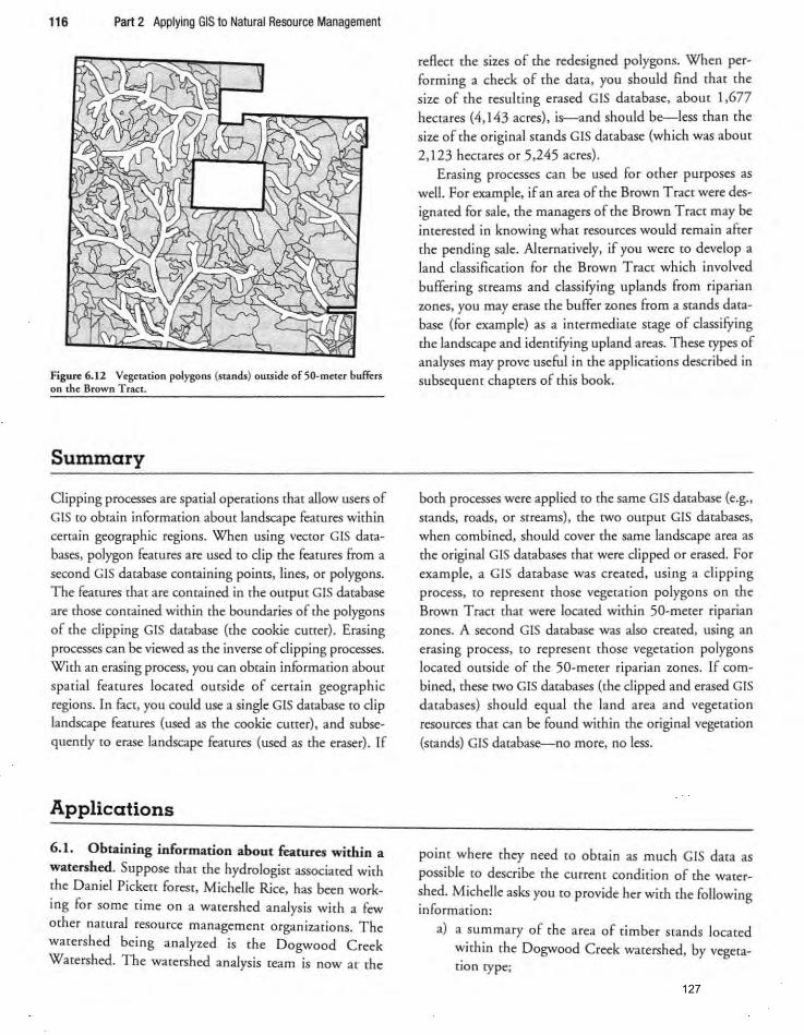
116 Part 2 Applying GIS to Natural Resource Management
Figure 6.12 Vegetation polygons (stands) outside of 50· mcler buffers on the Brown T race.
Summary
Clipping processes are spatial operations that allow users of GIS to obmin information about landscape features within
cercai n geographic regions. When using vec[Qr GIS data
bases, polygon features are used to clip the feacures from a
second GIS database comaining poines, lines. or polygons.
The feacures that are comained in the OUCput GIS database
are those comained within the boundaries of the polygons
of [he clipping GIS database (the cookie cu[(er). Erasing processes can be viewed as the inverse of clipping processes. With an erasing process, you can obtain informadon about
spat ial features located outs ide of certain geographic regions. In fIct. you could use a single GIS database to clip landscape features (used as the cookie cu[(er). and subsequently to erase landscape features (used as the eraser). If
Applications
6.1. Obtaining information about features within a watershed. Suppose that [he hydrologist associated with the Daniel Picke[( forest. Michelle Rice. has been working for some time on a watershed analysis with a few
other natural resource managemem organizations. The watershed being analyzed is the Dogwood Creek Watershed. The warershed analys is team is now ar the
reAeer the sizes of the redesigned polygons. When performing a check of the data. you should find that the size of the resulting erased GIS database. about 1.677 hectares (4.143 acres). is-and shou ld be--less than the size of the original stands GIS database (which was about
2.123 hectares or 5.245 acres) . Erasing processes can be used for other purposes as
well. For example. if an area of the Brown Tract were designaH~d for sale, the managers of the Brown T Tact may be imerested in knowing what resources would remain after the pending sale. Alternatively, if you were co develop a land classification for the Brown Tract which involved buffering streams and classifying uplands from riparian zones, you may erase (he buffer woes from a stands database (for example) as a intermediate stage of classifying
the landscape and identifying upland areas. These types of analyses may prove useful in (he applications described in subsequent chapters of this book.
both processes were applied to [he same GIS database (e.g .• stands, roads, or streams), the twO output GIS databases, when combined, should cover the same landscape area as
the original GIS databases that were clipped or erased. For
example. a GIS database was created, using a clipping
process, to represem those vegetation polygons on the Brown Tract that were located within 50-meter riparian
zones. A second GIS database was also created, using an
erasing process. to represem those vegetation polygons
located outside of the 50-meter riparian zones. If com
bined. these twO GIS databases (the clipped and erased GIS databases) should equal [he land area and vegetation resources thar can be found within the original vegetation
(stands) GIS database--no more. no less.
point where they need to obtain as much GIS data as possible to describe the currenr condition of rhe water
shed. Michelle asks you to provide her with the following informacion:
a) a summary of the area of timber stands located
~ithin the Dogwood Creek watershed. by vege .. -(Ion type;
127
Chapter 6 Obtaining Information about a Spec~ic Geographic Region 117
b) a summary of the length of roads located with in the Dogwood Creek watershed. by road type; and
c) a summary of the length of streams located within the Dogwood Creek watershed. by stream type. In addition, summarize these values in terms of
scream miles per square mile of land. by stream
type.
Develop a shon memo add ressed (Q Ms Rice that details
the resulrs of your analyses.
6.2. Summarizing resources within a management area. Jane Hayes is developing an annual reporr on [he
management of the Daniel Picken forest and has become
very interested in certain aspects of the forest resou rces.
Since she knows that you are becoming proficient with GIS,
she has asked you ro provide some information she feels is necessary for her report:
a) amount of land in each watershed.
b) length of rock road in each watershed.
c) length of dirt road in each watershed. and
d) length of stream classes 1- 3 in each watershed.
In addition, she is imerested in knowing something about the resources that are within 50 merers of the streams.
Using the 50-foot stream buffer provided by the GIS Departmenr, provide the following:
a) area of land within 50 meters of the streams,
b) area of older forest (age ~ 60) with in the 50-meter stream buffers,
c) length of paved road within the 50-meter stream buffers, and
d) length of rock road within the 50-meter stream buffers.
Provide a memo addressed (Q Ms Hayes that details the
results of your analyses. Keep in mind the appropriate
units (perhaps kilometers fo r length rather than meters). and the appropriate precision (to the nearesr 0.1 hectare
or 0.1 kilometer) for this type of report.
6.3. Fertilization possibilities. Within the so ils GIS darab~ of the Daniel Pickerr foresr is an attribute, fer
rresp, which was meant to ind icate the probability of tree
response to fertilization as a functio n of the underlying
soil type. Describe the types of vegetation found in the 'high response' areas using (he following format :
0-20
21-40
41-60
61- 80
80.
A
Vegetation type
8 c
6 .4. Potential sale of watershed for conservation reserve. The managers of the Daniel Pickett forest have been approached by a non-profi t o rganization specializing
in developing and managing conservation reserves. The
non-profit organization is specifically interested in acquir
ing a specific portion of the Daniel Pickett forest-all of the land located in the Trout Creek Watershed. It seems that the non-profit group has been acdve in developing a larger reserve system in the Trout C reek area, and the
Daniel Picken forest just happens to contain the headwa
ters of the watershed. The region manager of the Daniel
Picken forest, Becky Blaylock, is interested in under
standing the effect this land sale may have on the manage
ment plan for the area. She asks you to provide her a before- and after-sale description of the resources, in the
fo llowing format: a) Before-sale conditions (area) of the Daniel Pickett
forest.
Age class
0-20
21- 40
41-60
61 - 80
80.
A
Vegetation type
8 c
b) Alier-sale conditions (area) of the Daniel Pickett forest.
Age class
0-20
21-40
41-60
61- 80
80.
A
Vegetation type
8 c
128
118 Part 2 Applying GIS to Natural Resource Management
In add ition, she has also requested rhe following: c) a map showing the after-sale arrangement of vege
rarion classes (rypes) on rhe Daniel Pickett forest, and
References
Agriculture and Agri-Food Canada. (2006). The national soil database (NSDB). Ottawa, ON: The National Land and Weather In formation Se rvice,
Agriculture and Agri-Food Canada. Retrieved February II , 2007, from http://sis.agr.gc.ca/cansis/ nsdb/intro.html.
Clarke, K.c. (I 995) . Analytical and computl!T cartography.
Upper Saddle River, NJ: Prentice-Hall. Merriam-Webster. (2007). Merriam- Webster online
search. Rerrieved February 4, 2007, from http://www. m-w.com/cgi-bin/diccionary.
d) a brief summary of your opinion of rhe effects of the sale o n the management of the forest,
USDA Natural Resou rces Conservar ion Service. (2006) . US general soil map (STATSGO). Washingwn, DC: Narional Cartography and Geosparial Cemer, USDA Natural Resou rces Conservation Service. Retrieved February II, 2007, from http://www.ncgc.nrcs.usda. gov I p rod uctsl da rasetsl sta tsgo/.
USDA Narural Resources Conservation Service. (2007). Geospatial data gateway. Washington, DC: USDA
Natural Resources Conservation Service. Retrieved February 9. 2007. from http: //datagateway.nrcs.usda. gov/NexrPage.aspx?HitTab= I.
129

Chapter 7
Buffering Landscape Features
Objectives
Chapter 7 is an introduction and examination of GIS
buffering processes. A number of examples and applications are presented in this chapter co provide readers with
experience in several of the common GIS-related tasks in
namral resource management that require the use of a buffering process. At the conclusion of this chapter. read
ers should understand. and be able co discuss, the peninent aspects of:
I. whar bujf<ring spatial landscape features implies; 2. how different buffering techniques can be applied to
point, line, or polygon features; and
3. how buffering can be applied (Q assess alrernarive management policies and to ass ist in making natural
resource managemenr decisions
To someone unfamiliar with [his GIS process. the term
buffering may lead to some confusion. Technically, the noun 'buffer' refers to (a) a device fo r reducing shock when contacted, (b) a means fo r cushioning fluccuations in busi ness activities. (c) a protective barrier, (d) a sub
stance capable of neutralizing both acids and bases. and
(e) a temporary sto rage unit on a computer (Merriam
Web"er, 2007). In GIS appl ications in natural resource management. we generally refer to the buffering process as a method for creating a buffer zone. which is defined
as a land area that delineates separate management activ
ities or emphases. Wirhin GIS, a buffer rone is a polygon that encloses an area within a specific distance from a
point. line. or polygon, and is useful in analyses that
have a proximity criteria (Association for Geographic
Informarion, 1999). The GIS process of buffering usually infers that a
boundary is about to be drawn around some selecred features. There are numerous reasons why you would want to
draw boundaries around selected landscape features in nat
ural resource management. For instance, one of the guid
ing management policies for an organization may suggest
that some management activities may be prohibited within a certa in distance of a stream, a road, a trail. or a
home. Therefore. as a namral resource manager. you may
be interested in the appropriate limits of allowable man
agement activity. As another example, managemenr activ
ities within a certain distance of nesting, roosting. or for
aging sires of a wildlife species of concern may be curtailed during certain times of the year. Therefore. delineating
these 'home ranges' or 'critical habitats' may be an impor
tant aspect of namral resource managemem. In these cases,
you might develop sparial buffers within GIS to identifY resources located within certain distances of important
landscape features (poinrs, lines, or polygons). You mighr also be incerested in examining the potential impacts of rhe policies that suggest the use of buffers. in order to
understand how the objectives of namral resource manage
ment be affected. As you may gather, buffering has been widely used in natural resource managemem to identify
riparian managemenr areas (streamside management zone)
and {Q define areas where management may be restricted
for one reason or another. Yet buffers have also been used
to track and assess the site impacts of logging equipment on soil resources and residual stand conditions (Beninger
er al., 1994; McDonald er .1., 2002) .
130
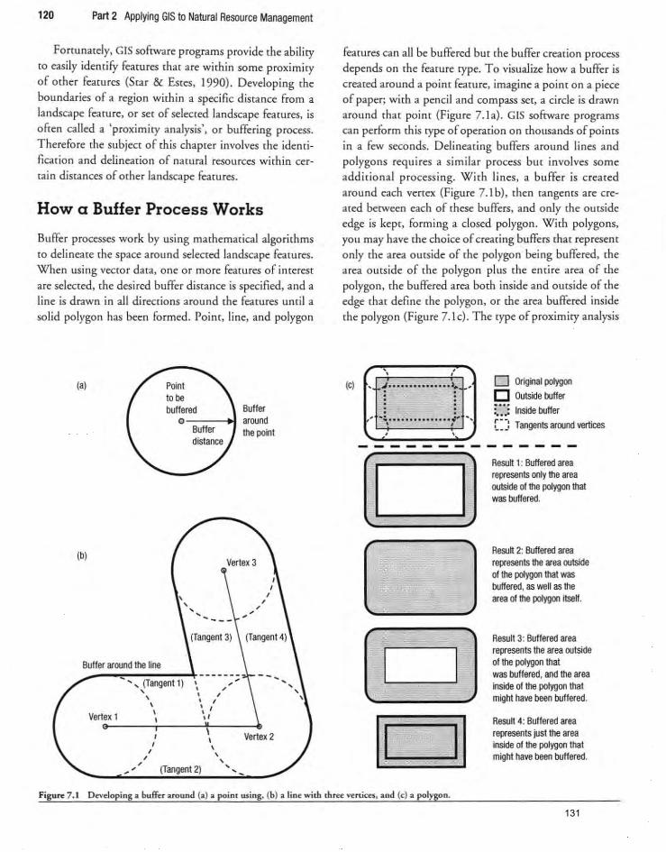
120 Part 2 Applying GIS to Natural Resource Management
Fortunately, GIS software programs provide the ability co easily identify features that are within some proximity of other features (Star & Estes, 1990). Developi ng the boundaries of a region within a specific distance from a
landscape feature, or set of selected landscape features, is
often called a 'proximity analysis', or buffering process.
Therefore the subject of [his chapter involves the identificarion and delineation of natural resources w ithin cer
rain distances of other landscape features.
How a Buffer Process Works
Buffer processes work by using marhemacical algorithms
to delineate the space around selected landscape features.
When using vector data, one or more features of interest
are selected. the desi red buffer distance is specified, and a
line is drawn in all directions around the features until a
solid polygon has been formed . Point , line, and polygon
(a)
(b)
Buffer ---..I around
, , "
the point
Buffer around the line
Vertex 1
"" (Tangent 1) I , '
,
, .. , ,
, ,
\ , \ " , ,
, (Tangent 2)
\ , , , Vertex 2
"
, , , ,
features can all be buffered but the buffer creation process depends on {he feamre rype. To visualize how a buffer is
created around a point feature. imagine a point on a piece
of paper; with a pencil and compass set, a circle is drawn around that point (Figure l .la). GIS software programs can perform this type of operation on thousands of poims
in a few seco nds. Delineating buffers around lines and
polygons requires a similar process bur involves some
additional process ing. With lines. a buffer is created
around each venex (Figu re 7 .1 b)' then tangents are ere
ared between each of these buffers, and only the outside
edge is kept, forming a closed polygon. W ith polygons, you may have the choice of creating buffers that represent only the area outside of [he polygon being buffered, the area outside of the polygon pi us the entire area of the
polygon, the buffered area both inside and outside of the edge that define [he polygon, or the area buffered inside the polygon (Figure l.ic) . The type of proximity analysis
(e) C D Original polygon · . o Outside buffer · . · . · . · . Inside buffer · . ,., .. "':. . ........... ···r ",
[ = =: Tangents around vertices ' . · , ------
D Result 1: Buffered area represents only the area ootside of the polygon that was buffered.
Result 2: Buffered area represents the area outside of the polygon that was buffered, as welt as the area of the polygoo itself.
Result 3: Buffered area represents the area outSide of the polygon that was buffered, and the area inside of the polygon that might have been buffered.
~ Result 4: Buffered area represents just the area inside of the polygon that might have been buffered.
Figure 7 . 1 Developing a buffer around (a) a point lUing, (b) a line with three vertices, and (c) a polygon .
131

that is required will suggest the appropriate 'Ype of buffering process required when polygons are concerned. For example. if you were interested in the type of vegetation within 1.000 meters of a set of polygons chac define cru
cial owl habitat, you would create a buffer outside the sec of polygons. On the other hand, if you were interested in understanding rhe amount ofland chat is associated with a policy chat prevents management activity within 100 meters of the edge of a managed property (to avoid conAict with homes and o ther developed areas oU[side rhe propenyL you would create a buffer inside rhe boundary of the managed proper'Y.
Buffering processes performed on vector GIS data may require some rather complex geometrical calculations. with lines and tangents CO compute, and overlapping areas perhaps merged together. To remove overlapping areas, imersecrion and dissolving processes are used. Buffering processes performed on raster GIS data involve
couming the number of pixels away from selecred or specified pixels.
Buffers used in natural resource managemem can rake on many forms, bur rhe [wo most commonly employed are a conS[(lnt buffer widrh and a variable buffer width. Constant width buffers are the most commonly used
form in natural resource managemem (Bren, 2003), and assume a symmetrical distance around each buffered landscape feature (same distance buffered on each side of a srream, for example) . Variable width buffers assu me that fearures are buffered differently based on some inherem or assumed characteristic, such as stream size. Other rypes of buffers include [hose based on (a) environmentalloading values and (b) other outside influences. Stream buffers based on loading values, for example, might take imo accoum the amoum of area comriburing to an impact. For example. stream reaches that have larger water con
tributing areas might be buffered using a wider buffer width than stream reaches with smaller comribucing areas. These are differem than variable width buffers in thar each section of a stream may be buffered a differem distance based on the size of the watershed that contributes water (Q that secrion of the stream. Buffers based on other outside influences may include stream buffers that take inro accoum the amoum of sunlight that reaches the stream irself. In these cases, buffers on the southerly sides of streams may be wider (han buffers on the
northerly sides of streams (Bren, 2003). As we mentioned, common buffer distances can be
constam (fixed) distances. o r they can vary for each feature in a GIS database based on an att ribute of those
Chapter 7 Buffering Landscape Features 121
fearures . Most GIS sofrware programs can accommodate both buffering approaches. To illustrate these differences, suppose you have a GIS database that includes 10 streams, each of a different stream class (T able 7. I) . With this hyporhetical data, it is assumed that the lower the stream
class number, the la rger (wider) the stream. One task in planning natural resource management
activities may be to delineate riparian buffers around these streams. If a constant buffer distance of, for example. 30 meters is assumed. each stream would be buffered the same distance (30 m). However, many regulations
pertaining to the proximity of management activities around riparian areas require wider buffers around larger Streams, and narrower buffers arou nd smaller streams.
Therefore, distances specific to each landscape feature (each srream reach in rh is example) can be used in the buffer process, to allow the development of variable dis
tance buffers. For example, for each of the 10 streams you could have developed an attribute to describe the appropriate buffer distance (Table 7.2), and use that attribute to guide the buffering process. Readers will examine borh of these buffering assu mptions (constant distance and variable width) in the forthcoming examples as well as in the 'Applications ' section at the end of this chapter.
When buffering mult iple landscape features, a buffer is created around each feature independent of the other features. One option available with most GIS sofrware concerns the handling of the overlapping areas. The choices are [0 retain individual buffer polygons for all features to be buffered (caJled uncomiguous, or non-
TABLE 7.1
Su ....
2
3
4
5
6
7
8
9
10
Ten hypothetical streams and their stream claBs, length, and width
Su .... da>.
Stream length (m)
Streun width (m)
2
2
3
3
3
4
4
5
1000
750
500
450
375
450
400
300
250
275
50
45
10
10
3
3
2
o
132
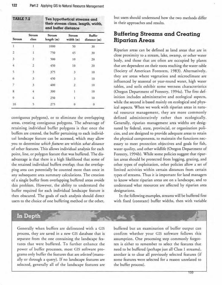
122 Part 2 Applying GIS to Natural Resource Management
TABLE 1.2 Ten hypothetical streams and their stream class, length, width, and buHer distance
Sueam Strum Stream Buff., S ....... d,,, Ie.ngth (m) width (m) distance: (m)
1000 50 30
2 750 45 30
3 2 500 10 20
4 2 450 10 20
5 3 375 3 10
6 3 450 3 10
7 3 400 2 10
8 4 300 10
9 4 250 10
10 5 275 0 0
contiguous polygons), or co eliminate the overlapping
areas, creating contiguous polygons. The advanrage of
retaining individual buffer polygons is tha t once (he
buffers are created, [he buffer perta ining (Q each individ
ual landscape feature can be accessed, which may allow
you [0 determine which fatuus are within what distanu of other fearures. This allows individual analys is for each
point. line, or polygon fearu re that was buffered. The dis
advantage is that there is a high likelihood thar some of
the retained individual buffers overlap; rhus the overlap
ping area can porentially be counted more than once in
any subsequent area summary calculations. The creation
of a single buffer from overlapping buffered areas avoids
this problem. However. the ability CO understand the
buffer required for each individual landscape feature is [hen obscured. The goals of each analysis should direct
users to the choice of one buffering method or the other.
Generally when buffers are delineated with a GIS
process. they are saved in a new GIS database that is
separate from rhe one containing the landscape features that were buffered. To further enhance the
power of buffer processes, most GIS software programs only buffer the features that are selected (manu
a lly or through a query) . If no landscape features are selected, generally all of the landscape features are
but users shou ld understand how the two methods differ in their approaches and results.
Buffering Streams and Creating Riparian Areas
Ripar ian a reas can be defined as land areas that are in
close proximity ro a stream. lake. swamp. or other water body, and those that are often are occupied by plants
that are dependent on their roOtS reaching the water rable
(Society of American Foresters. 1983). Alternatively,
they a re areas where vegetation and microclimate are
inAuenced by seasonal or year-round water. high water tables. and soils exhibir some wetness characrerisrics
(Oregon Department of Forestry, 1994a). The first def
inition includes administrative and ecological aspects.
wh ile the second is based mainly on ecological and physical aspects. When we work with riparian a reas in natu
ral resource management. they are more commonly
defined administratively rather than ecologica lly.
Generally. riparian management area widths are desig
nated by federal . stare. provincial. or organization policies, and are designed ro provide adequate areas ro retain
the physical components. to maintain the functions nec
essary to meet protection objectives and goals for fish.
water quality , and other wildlife (Oregon Department of Forestry, 1994b). While some policies suggest that ripar
ian areas should be protected from logging, grazing. and
other types of exploitation. ocher policies allow a set of
limited activities within certain distances from certain
rypes of streams. Thus it is important for land managers to know where riparian areas are on a landscape. and to
understand whar resources are affected by riparian area
designations.
In the following examples, streams will be buffered first
with fixed (constant) buffer widths. then with variable
buffered but an examination of buffer output can
confirm whether your GIS software follows this
assumption. One processing step commonly forgot
ten is either [Q remember to select the features that
need to be buffered (perhaps just all C lass 1 streams),
another is [Q clear all previously selected features (if some features were selected for a reason unrelated to
the buffer process) .
133
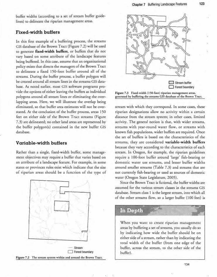
buffer widths (according to a set of stream buffer guide
lines) to del ineate the riparian managemenc areas.
Fixed-width buffers
In this first example of a buffering process, the streams
GIS database of the Brown T ract (Figure 7.2) wi ll be used to generace fiXed-width buffers, o r buffers that do not
vary based on some 3cuiburc of the landscape features being buffered. In this case, assume thar an organizational
policy exis(5 chat directs the managers of the Brown Tract to delineate a fixed )50-foot buffer around all of the
streams. During the buffer process, a buffer polygon will be created around all stream lines in the streams GIS data
base. As noted earl ier, mOSt GIS sofrware programs provide the options of either leaving the buffers as individual
polygons around all stream lines or el iminating the over
lapping areas. H ere, we will illustrate the overlap being eliminated, so that buffer area estimates will not be overstated. At the conclusion of the buffer process, areas 150 feer on either side of (he Brown Tract streams (Figure
7.3) are delineated; no other land areas are represemed by the buffer polygon(s) contained in the new buffer GIS
database.
Variable-width buffers
Ra[her [han a single, fixed-width buffer, some managemem objectives may require a buffer [hat varies based on an auribuce of a landscape feamre. For example, in some S[ates or provinces rules exist which indicate that the size of riparian areas should be a function of the type of
D
"
- Stream D Forest boundary
Figure 7.2 The stream system within and arollnd the Brown Tract.
Chapter 7 Buffering Landscape Features 123
D Stream buffer D Forest boundary
Figure 7.3 Fixed-width (I 50-foot} riparian management areas, generated by buffering the streams GIS database of the Brown Tract.
stream with which they correspond. In some cases, these riparian designarions allow no activity within a cerrain distance from the stream system; in other cases, limited acrivity. The general norian is that, with wider streams,
Streams with year-round warer flow, o r streams with known fish populations, wider buffers are required. Once [he set of buffers is based on the characteristics of the
streams, they are considered variable-width buffers because [hey vary according to the characteristics of each srream. In Oregon, for example, the riparian guidelines require a ) DO-foot buffer around ' large' fish-bearing or
domestic water use streams, and lesser buffer widths around smaller screams (Table 7.3) and streams that are
nO( curren tly fish-bearing or used as sources of domesric water (Oregon State Legislature, 2005) .
Since the Brown Tract is fict ional, the buffer widths are assumed for the various stream classes in rhe streams GIS database. Stream class 1 is the largest srream, inro which all of the other streams flow, so a larger buffer (100 feet) is
When you wanr co create riparian management areas by buffering a set of streams, you usual ly do so by ind icat ing how wide the buffer should be on
either side of a stream, rather than by indicaring the rotal w idth of the buffer (from o ne edge of the
buffer, across the stream, to the other side of rhe buffer).
134
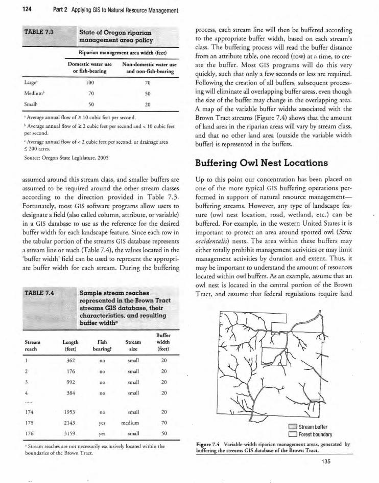
124 Part 2 Applying GIS to Natural Resource Management
TABLE 7.3
Medium"
Small<
State 01 Oregon riparian management area policy
Riparian management area width (feet)
Domestic water we or fish.bearing
100
70
50
Non·domestic water we and non-fish-bearing
70
50
20
• Average annual flow of 2: 10 cubic feet per second.
h Average annual flow of ~ 2 cubic feet per second and < 10 cubic feet
per second.
~ Average annual flow of < 2 cubic fec t per second, or drainage area
s: 200 acres.
Source: Oregon State Legislatu re. 2005
assumed around this st ream class, and smaller buffers are
assumed [Q be required around the other Stream classes according to the direction provided in Table 7.3. Fortunately. most GIS software programs allow users to
des ignate a field (also called column, attribute, or variable) in a GIS database to use as the refe rence for the desired buffer width fo r each landscape feacure. Since each row in the tabular porrion of the streams GIS database represents a Stream line or reach (Table 7.4), the values located in the 'buffer width ' field can be used to represent the appropriate buffer width for each stream. During the buffering
TABLE 7.4 Sample stream reaches represented in the Brown Tract streams GIS database, their characteristics, and resulting buller width-
Buffer
Stream Length Fish Stream width ,each (r.<I) bearing~ size (feet)
362 no small 20
2 176 no small 20
3 992 no small 20
4 384 no small 20
174 1953 no small 20
175 2143 Y" mcdiwn 70
176 3159 Y" small 50
• Stream reaches arc no t necessarily or:clusivcly located within the bou ndaries of rhe Brown T racr.
process, each stream line will then be buffered according to the appropriate buffer width, based on each stream's class. The buffering process will read the buffer distance
from an attribute table, one record (row) at a time. to create the buffer. Most GIS programs will do this very quickly, such that only a few seconds or less are required.
Following the creation of all buffers, subsequent processing will eliminate all overlapping buffer areas, even though [he size of the buffer may change in the overlapping area. A map of the variable buffer widths associated with the Brown Tract streams (Figure 7.4) shows that the amount of land area in the riparian areas will vary by stream class, and that no other land area (outside the variable width buffer) is represented in the buffers.
Buffering Owl Nest Locations
Up to this point our concentration has been placed on one of the more typical GIS buffering operations performed in supporr of natural resource managementbuffering streams. However, any type of landscape feature (owl nest location , road, wetland, etc.) can be buffered. For example, in the western United States it is important to protect an area around spotted owl (Strix
occidtntalis) nests. The area within these buffers may either totally prohibit management activities or may limit management activities by duration and extent. Thus. it
may be imporrant to understand the amounr of resources located within owl buffers. As an example, assume that an owl nest is located in the central portion of the Brown Tract, and assume that federal regulations requi re land
o Stream buffer o Forest boundary
Figure 7 .4 Variable.width riparian management areas, generated by buffering the streams GIS daubue of m e Brown Tract.
135
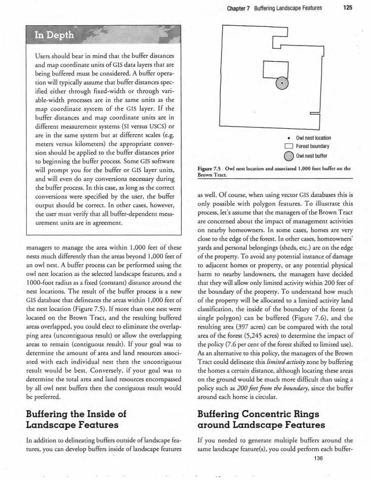
Users should bear in mind that the buffer distances
and map coordinate units of GIS data layers that are being buffered must be considered. A buffer opera
tion will typically assume that buffer distances spec
ified either through fixed-width or through vari
able-width processes are in the same units as the map coordina te system of the G IS layer. If the
buffer distances and map coordinate unics are in
differem measuremenc systems (51 versus USeS) or are in the same system bur at different scales (e .g. meters versus kilometers) the appropriate conversion should be applied to the buffer distances prior
to beginning the buffer process. Some GIS software
will prompt you for the buffer or G IS layer units,
and will even do any conversions necessary during
the buffer process. In th is case, as long as the correct
conversions were specified by the user, the buffer output should be coerceL In other cases, however, the user must verifY that all buffer-dependent meas
urement units are in agreement.
managers to manage the area within 1,000 feet of these
nests much differently than the areas beyond 1,000 feet of
an owl nest. A buffer process can be performed using the owl nest locarion as the selected landscape features, and a 1 ODD-foot radius as a fixed (constant) distance around the
nest locarions. The result of the buffer process is a new GIS database that delineates the areas within 1,000 feet of
the nest location (Figure 7.5). If more than one nest were located on the Brown Tract, and the resulting buffered
areas overlapped, you could elect to eliminate the overlap
ping area (uncontiguous result) or allow the overlapping areas to remain (cont iguous result). If your goal was to
determine the amount of area and land resources associ
ated with each individual nest then the unconriguous resulr would be best. Conversely, if your goal was to determine the toral area and land resources encompassed by all owl nest buffers then the contiguous result would
be preferred.
Buffering the Inside of Landscape Features
In addition to delineating buffers outside oflandseape features, you can develop buffers inside of landscape features
Chapter 7 Buffering Landscape Features 125
• Owl nest location
o Forest boundary o Owl nest buffer
Figure: 7.5 Owl nest location and associated 1,000 fOOl buffer on the Brown Tract.
as well. Of course, when using vector GIS databases this is
only possible with polygon features. To illustrate this
process. let's assume that the managers of the Brown Tract are concerned about the impact of management activities on nearby homeowners. In some cases, homes are very close to the edge of me forest. In orner cases, homeowners'
yards and personal belongings (sheds, etc.) are on the edge
of the property. To avoid any potential instance of damage
to adjacent homes or property, or any potential physical
harm CO nearby landowners. the managers have decided that they will allow only limited activity within 200 feet of
the boundary of the property. To understand how much
of the property will be allocated to a limited activity land
classification, the inside of the boundaty of the forest (a
single polygon) can be buffered (Figure 7 .6) , and the
resulting area (397 acres) can be compared with the total
area of the forest (5,245 acres) to determine the impact of
the policy (7.6 per cent of the forest shifted to limited use) .
As an alternative co this policy. the managers of me Brown Tract could delineate this limited activity zone by buffering
the homes a cenain distance. although locating these areas
on the ground would be much more difficult than using a policy such as 200 feet .from the boundary, since the buffer around each home is circular.
Buffering Concentric Rings around Landscape Features
If you needed to generate multiple buffers around the same landscape fearure(s) , you could perform each buffer-
136
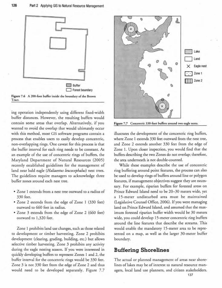
126 Part 2 Applying GIS to Natural Resource Management
o
o Buffer o Forest boundary
Figure 7.6 A 200-foot buffer inside the boundary of the Brown Tract.
ing operation independently using different fixed-width buffer distances. However, the resulting buffers would contain so me areas [hat overlap. Ahernariveiy. if you wanted to avoid the overlap that would ultimately OCCUf
with this method. most GIS sofcware programs contain a process that enables users to easily develop concentric, non-overlapping rings. One caveat for this process is that
the buffer interval for each ring needs to be constanL As an example of the use of concentric rings of buffers. [he
Maryland Deparrmenr of Narural Resources (2005) recently esrablished guidelines for rhe managemenr of land near bald eagle (Haliaeetus lrococephalus) nesr reees. The guidelines require managers [0 acknowledge th ree buffer zones around each nest tree.
• Zone I extends from a nest tree ourward to a radius of 330 feer.
o Zone 2 exrends from rhe edge of Zone 1 (330 feer) ourward to 660 feer in radius.
o Zone 3 exrends from rhe edge of Zone 2 (660 feer) ourward to 1,320 feet.
Zone 1 prohibirs land use changes, such as those relared (Q development or dmber harvesting. Zone 2 proh ibits development (clearing, grading, building, etc.) but allows selective timber harvesting. Zone 3 prohibits any activity during the eagle nesting season. If you were interested in quickly developing buffers to represent Zones 1 and 2, the buffer interval for the concentric rings would be 330 feet. Zone 3 is not 330 feet from the edge of Zone 2 and thus would need to be developed separately. Figure 7.7
D Lake
0 CJ D Land
"-I 0 X Eagle nest 1)\) D Zone'
[)]] Zone 2
\J
Figure 7.7 Concentric 330·foot buff~rs around two agle nests.
illustrates the development of the concentric ring buffers. where Zone 1 extends 330 feet outward from the nest tree.
and Zone 2 extends another 330 feet from rhe edge of Zone J. Upon closer inspection, you would find thar the buffers describing rhe rwo Zones do not overlap; therefore, (he area underneath is nor double-counted.
While these examples describe the use of concentric ri ng buffering around point features. the process can also
be used to develop rings of buffers around line or polygon features. if management objectives suggest they are necessary. For example. ripa rian buffers for forested areas on
Prince Edward Island need to be 20-30 merers wide, ye t a 15-meter undisturbed area must be maintained (Legislative Counsel Office, 2006) . If you were managing land on Prince Edward Island. and assumed that the maximum fo rested riparian buffer width would be 30 meters wide, you could develop I5-meter concentric ring buffers around the line features that describe [he streams. This would enable the mandacory 15-meter area to be represented on a map. as well as the larger 30-meter buffer
boundary.
Buffering Shorelines
The actual or planned management of areas near shorelines of lakes may be of interest to natural resource man
agers. 10caJ land use planners. and citizen stakeholders. 137
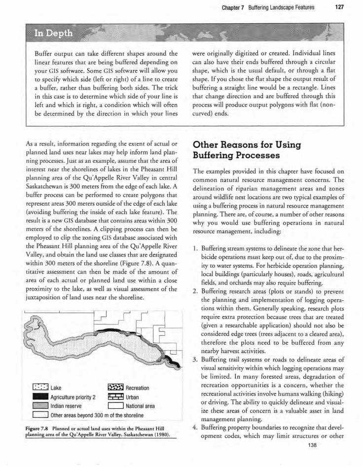
Buffer output can take different shapes around the linear features that are being buffered depending on your GIS software. Some GIS software will allow you to specifY which side (left or right) of a line to create a buffer, rather than buffering both sides. The trick in this case is [0 determine which side of your line is left and which is right , a co ndition which will often he determined by (he direccion in which your lines
As a result, information regarding the extent of actual or
planned land uses near lakes may help inform land planning processes. JUSt as an example. assume that the area of
interest near the shorelines of lakes in the Pheasam Hill planning area of the Qu'Appelle River Valley in cemral Saskatchewan is 300 meters from the edge of each lake. A buffer process can be performed to create polygons that represem areas 300 meters outside of the edge of each lake (avoiding buffering the inside of each lake feature). The result is a new GIS database (hat contains areas within 300 meters of the shorelines. A clipping process can men be employed to clip the zoni ng GIS database associated with the Pheasam Hill planning area of the Qu'Appelle River Valley, and obtain the land use classes that are designated within 300 meters of the shorel ine (Figure 7.B) . A quantitative assessment can then be made of the amount of
area of each actual or planned land use within a close
proximiry to the lake, as well as visual assessment of the
juxtaposition ofland uses near the shoreline.
r=;:] lake ~;, ;~~j Recreation
_ Agriculture priority 2 ~ Urban
[=:J Indian reserve [=:J National area
[=:J Other areas beyond 300 m of the shoreline
Figure 7 .8 Planned or actuaJ land uses within the Pheasant Hill planning aua of the Qu'Ap~l1e River VaJley. Saskatchewan (1980).
Chapter 7 Buffering Landscape Features 127
were originally digitized or created. Individual lines can also have their ends buffered through a circular
shape, which is the usual default, or through a flat shape. If you chose the flat shape the output result of buffering a straight line would be a rectangle. Lines that change direction and are buffered through this process will produce output polygons with flat (noncurved) ends.
Othe r Reasons for Using Buffering Processes
The examples provided in this chapter have focused on common natural resource management concerns. The
delineation of riparian management areas and zones
around wildlife nest locations are twO typical examples of using a buffering process in namral resource management planning. There are, of course, a number of Q[her reasons
why you would use bu ffe ring operations in natural
resource management. including:
1. Buffering stream systems [0 delineate me zone that herbicide operations must keep oU{ of. due co [he proximity to water systems. For herbicide operation planning, local buildings (particularly houses), roads, agricultural fields, and orchards may also require buffering.
2. Buffering research areas (plots or stands) CO prevent
the planning and implementation of logging operadons within them. Generally speaking, research plots
require extra protection because trees rhat are treared
(given a researchable application) should nOt also be considered edge trees (rrees adjacent to a cleared area).
therefore the plots need to be buffered fro m any nearby harvest activities.
3. Buffering trail systems or roads to delineate areas of
visual sensitivity within which logging operations may
be limited. In many forested areas, degradation of
recreacion opporrunides is a co ncern, whether the
recreational activities involve humans walking (hiking)
or driving. The ability to quickly delineate and visualize these areas of concern is a valuable asset in land
management planni ng. 4. Buffering property boundaries to recognize mat devel
opment codes, which may limit structures o r other
138
128 Part 2 Applying GIS to Natural Resource Management
landscape alternations from occurring within a threshold dis,.nce from property lines. are observed. This
may also apply to easements or utility co rridors. which are often subject [0 municipal. county. or provincial
development regulations.
In addition. buffer processes may assist namra! resource managers in evaluating the potential impacts of local for
est regulations. Local forest regulations are generally con
cerned with protecting envi ronmental quality and aesthet
ics, and with safeguarding local government investments
in roads and other infrastructure (Martus et al.. 1995). They are mainly developed as a result of the conflicts that occur with the continuing shift of the human population
Summary
GIS buffering processes are powerful tools that allow you
ro investigate the nearness of landscape elements ro your
feacures ofinteresr. These features of interest can be repre
sented by points. lines. or polygons (as demonstrated here) or by raster grid cells . Buffering processes are spatial oper
ations that allow users of GIS software programs to identifY areas within some proximity of selected landscape feacures .
After landscape features are selected. a zone (a polygon) is delineated around them to represent the buffered area. By
default. if no landscape features are selected. all features are buffered. but you should confirm whether your GIS soft
ware uses this approach. Buffer OUtpUt approaches. such as
contiguous or uncontiguous results. can be customized to
meet analysis objectives. In addition, some GIS software
Applications
7.1. Current Riparian Policy for the Brown Tract. The currell[ organizational policy for the Brown Tract
indicates that the following riparian area buffer widths
should be used in conjunction with management activities:
Class I: 100 feet C lass 2: 75 feet Class 3: 50 feet C lass 4: 40 feet
Becky Blaylock. the Manager of the Brown Tract. wants to know (he 'current situation' with regard to riparian
areas:
from urban to rural settings (Cubbage & Raney. 1987). The types of controls include requiring the development
of forest plans. buffering specific landscape features. and placing restrictions on certain silvicultural practices. For
example. timber harvesting ordinances developed at the
local level are intended to limit site degradation and envi
ronmental qualiry in association wich logging activit ies.
Harvesting operations may be restricted within certain dis
tances of public roads or ocher public resources. therefore
requiring a buffer around these resources. Natural resource
managers may need to identify these buffers in a harvest
plan. and may also be concerned about the cumulative
impact of local regulations on the profitability and feasibility of their management operations.
enables users to specify whether buffers created around
lines have a round or flat shape at the beginning and ending of the line. The resulting buffer GIS databases allow users co visually understand the area that lies within a cer
tain distance from some landscape feacure(s) of interest,
and to quantify the resources contained within the
buffered area. Buffering streams and other resources of
importance (e.g .• owl and red-cockaded woodpecker nest locations) to create limited management zones is a com
mon management objective included in natural resource
management plans. Estimating the impact of these types
of restrictions on natural resource management is impor
tant, and helps landowners investigate the effect of current
and proposed policies.
a) How much area (acres) is located inside the riparian areas?
b) How much area (acres) of each vegetation type is
located inside the riparian areas?
c) How much area (acres) of each vegetation type is loca(ed outside the riparian areas?
d) How much timber volume is located in the ripar
ian areas?
Ms Blaylock also wants you to develop a map that illustrates the stream buffers and includes the roads. streams.
and timber stands. 139

7.2. Proposed Organizational Policy. Becky Blaylock recently 3([cnded a meedng of policy makers, where she
heard rhar rhe riparian rules mighr change. She now needs [Q undersrand rhe paremial impaer of a proposed 125-foot no~harves[ buffer around all streams on [he Brown
T racr. She requem rhe following: a) How much area (acres) is locared inside rhe ripar
ian areas? b) How much area (acres) of each vegerarion 'Ype is
located inside the riparian areas?
c) How much area (acres) of each vegerarion 'Ype is located oU[sicle the riparia n areas?
d) How much timber volume is located in the ripar
ian areas?
Again. Ms Blaylock also wams you [Q develop a map rhar illustrates these stream buffers and that includes the roads.
streams, and timber stands. In addition. she wants you co
develop a memo that describes the diffe rences becween
rhe policy nared in Applicarion 7. 1 and rhe paremial policy noted here.
7.3. Ballot Initiative. A proposed bailor iniriarive. developed by a local conservation group, suggestS that the
following riparian buffer widths may soon be required for the region within which the Brown Tract is situated:
Large. fish-bearing srreams ISO feer Medium. fish-bear ing srreams 100 feer Small. fish-bearing srreams 75 feer Large. non-fIsh-bearing srreams 125 feer Medium, non-fIsh-bearing streams 75 feet
Small. non-fish-bearing srreams 50 feer
As a resulr. Ms Blaylock wams to undersrand rhe following: a) If rhese rules were applied to the Brown Traer. how
much area (acres) would be locared inside rhe riparian areas?
b) If these rules were applied to rhe Brown Traer. how much area (acres) of each vegerarion 'Ype would be located ins ide the riparian areas?
c) If these rules were applied to the Brown Traer. how much area (acres) of each vegetation type would be
located outside the riparian areas?
d) If these rules were applied to rhe Brown Traer. how much rimber volume would be locared in rhe riparian areas?
As before. Ms Blaylock also wants you to develop a map that illustrates these stream buffers and that includes the
Chapter 7 Buffering Landscape Features 129
roads, streams, and timber stands. In addition, she wants
you to develop a memo (hat describes the differences
berween rhe policies nored in Appl icarions 7.1. 7.2. and rhe poremial policy nored here.
7.4. National Forest Riparian Policy. A local Narional Forest uses me following riparian area guidel ines in con
junction with harvesting activities:
Large srreams 250 feer Medium srreams ISO feer Small srreams 100 feer
As wirh rhe arher pol icies. Ms Blaylock wams to undersrand rhe following:
a) If rhese rules were applied to the Brown Traer. how much area (acres) would be locared inside rhe riparian areas?
b) If rhese rules were applied to rhe Brown Traer. how much area (acres) of each vegerarion 'Ype would be located ins ide (he riparian areas?
c) If rhese rules were applied to rhe Brown Traer. how much area (acres) of each vegetation type would be
located outside the riparian areas?
d) If these rules were applied to rhe Brown Traer. how much timber volume would be located in (he ripar
ian areas?
And again. Ms Blaylock also wams you to develop a map that illustrates these stream buffers and that includes the
roads, Streams, and timber stands. In addition, she wants
you to develop a memo that describes the differences
berween rhe policies nored in Applicarions 7.1 . 7.2. 7.3. and rhe porenrial policy nared here.
7.5. Current Owl Buffer Policy. Suppose rhar rhe current pol icy regarding owl nest locations is ro maintain a 1 ~O-acre no-harvest buffer around owl nest site locations.
Develop a memo and a map for Ms Blaylock rhar describes rhe amoum of land (acres) of rhe Brown Traer rhar would be covered by rhe single owl buffer pertain ing ro this property.
7.6. Protection of Research PlotsThousands of research plots have been established across North America ro facil
itate the estimation of the response of forests and wildlife
co a variety of silvicultural treatments. Unfortunately, har
vesting operations are usually implemented independ
ently of research programs. and tOO often the research plots are harvested because the loggers were unaware of
140
7 .2. Proposed Organizational Policy. Becky Blaylock recently attended a meering of policy makers, where she
heard char the riparian rules might change. She now needs to understand the potential impact of a proposed 125-foot no-harvest buffer around all screams on the Brown
Tract. She requestS rhe following: a) How much area (acres) is located inside the ripar
ian areas? b) How much area (acres) of each vegetation type is
located inside tbe riparian areas? c) How much area (acres) of each vegetation type is
located Qucside me riparian areas? d) How much amber volume is located in the ripar
ian areas?
Again, Ms Blaylock also wants you to develop a map that illustrates rhese stream buffers and rhat includes the roads. streams, and timber stands. In addition, she wants you to
develop ;:I memo that describes lhe differences berween me policy noted in Application 7.1 and the potential policy noted here.
7 .3. BaUot Initiative. A proposed ballot initiative, developed by a locaJ conservation group, suggests thar [he fo llowing riparian buffer widths may soon be required for the region within wh ich the Brown Tract is Si(U3red:
Large, fish-bearing streams 150 feet Medium. fish-bearing stteams 100 feet Small. fish-bearing streams 75 feet La rge, non-fIsh-bearing Streams 125 feet Medium, non-fIsh-bearing stteams 75 feet Small, non-fish-bearing streams 50 feet
As a result, Ms Blaylock wants to understand rhe following: a) Ifthese rules were applied to the Brown TraCt, how
much area (acres) would be located inside the riparian areas?
b) If rhese rules were applied to rhe Brown TraCt, how much area (acres) of each vegetation type would be located ins ide the riparian areas?
c) If rhese rules were applied to the Brown T raCI, how much area (acres) of each vegetation type would be located oU[side rhe riparian areas?
d) If these rules were applied to the Brown Tract, how much timber volume would be located in the riparian are-.lS?
As before, Ms Blaylock also wants you to develop a map that illus(rates these Stream buffers and that includes the
Chapter 7 Buffering Landscape Features 129
roads. streams, and timber stands. In addition. she wanrs you [0 develop a memo that describes rhe differenc.es
between the policies noted in Applications 7. 1, 7.2, and the potential pol icy noted here.
7.4. National Forest Riparian Policy. A local National Forest uses the following riparian area guidelines in conjunction with harvesting act ivi ties:
Large Streams 250 feet Med ium Streams 150 feer SmaU streams 100 feet
As wim the other policies, Ms Blaylock wants to understand the following:
a) I f these rules wefe applied (0 the Brown T ract, how much area (acres) would be located inside the riparian areas?
b) If mese rules were applied to the Brown Tract, how much area (acres) of each vegetation type would be located inside rhe riparian areas?
c) If these rules were applied to the Brown T ract. how much area (acres) of each vegetation type would be located outside [he riparian areas?
d) If ,.hese rules were applied to the Brown Tract, how much umber volume would be located in the riparian areas?
And again, Ms Blaylock also wants you to develop a map that illustrates these stream bu ffers and [hat inducles the roads, Streams, and timber stands. In addition, she \Yams you co develop a memo char describes [he differences between the policies noted in Applications 7.1, 7.2. 7.3, and the potential policy noted here.
7.5. Current Owl Buffer Policy. Suppose that the currem policy regarding owl nest locations is to maintain a IOO-acre no-harvest buffer around owl nesl site locations. Develop a memo an d a map for Ms Blaylock that describes rhe amount of land (acres) of me Brown Tract that would be covered by the single owl buffer pertaining to this property.
7.6. Protection of Research PlolS.Thousands of research plots have been established across North America to fac ilitate the estimation of the response of forests and wildlife [0 a variecy of silvicullUral uearmems. Unfortunately. harvesting operations are usually implemented independently of research programs. and tOO often the research plots are harvested because the loggers were unaware of
130 Part 2 Applying GIS to Natural Resource Management
their locarion, and withom the researchers knowing that
the plots were in jeopardy of being destroyed. The resulting loss of the research plot investment (layout, tagging of trees, etc.) may be considerable, and the loss of the opportunity for one final measuremem may be equally as
important. In many organizations, a communication sys[em norifying researchers of potencial impacts ro research
plms has been developed. allowing researchers to either
measure (he plots onc last time, o r CO delineate the
research areas as off-limits to harvesting activities.
Assume that rhe permanenr inventory plots on the
Brown T faCt were designed [0 evaluate {he long-term
growth and yield of the forest properry. Assume further that these plms were designed {Q remain untouched, even
though rhe surrounding forest may be harvested (clearclH
or thinned) . Finally, assume that the plots need to be maintained with a sufficient buffer of trees around them
so that rhe effects (windthrow, increased sunlight, etc.) of
harvesting trees outside the plot (o n the plot's trees) are
min im ized . These plots are circular l/5-acre plots, and
References
Association for Geographic Information. (I999). GIS dic
tionary. Retrieved February 4, 2007, from http: //www.
agi.org.uklbfora /systems/xmlviewerldefau lt.asp 'a rg= DS_AGI_ TRAINART _701_firsttide.xsIl90.
Bettinger, P., Armlovich, D., & Kellogg, L.D. (1994). Evaluating area in logging trails with a geographic infor
mation system. Transactions of the A.s:.1E, 37(4) , 1327-30. Bren , L.J. (2003). A review of buffer strip design algo
rithms. In E.G. Mason and c.J. Perley (Eds .), Procudings of the 2003 ANZ/F Uoint Australia and
N ew Zealand Institute of Forestry) Conference (pp. 32~35) . Retrieved September 5, 2007, from http:// www.forestry.org.nz/articles/ conf2003/Bren. pdf.
Cubbage, F., & Raney, K. (1987). Counry logging and tree protection o rdinances in Georgi a. Sottthern Joumal of Applied Forestry, 11, 7~82.
Legislative Coun sel Office . (2006). Chapter £-9,
Environmental Protection Act. Charlottetown, PE:
Gove rnmem of Prince Edward Island . Retrieved
February 4, 2007, from http: //www.gov.pe.callaw/ statu tesl pd fl e-09 . pdf.
require an additional 100-foot buffer from the edge of the plot boundary to be considered 'protected'. Develop a memo for Becky Blaylock that describes how much land area would be off-limits from harvesting operations
as a resuh of protecting the research plots. Develop a
map of the permanent inventory plots and their buffers.
Include the roads. streams, and timber stands on the
map. In addition. for added protection of the investment in
research , a second 100-foot buffer (for a total of200 feet) could be delineated around the research plots. In this supplemental area we can also assume that the trees in the
buffer are designed to remain untouched, even though
the surro unding forest may be harvested (clearcut or
thinned) . Based on the timber volume contained in the
buffers associated with the first (I OO-foot buffer) and second (200-foot buffer) cases, and a price of$400 per MBF, what is the cost of each case, and therefore what is the
additional cost to require the added protection around
each plot'
Martus, CE., Haney, Jr. , H.L., & Siegel, W.C (1995) . Local forest regulatory ordinances: [rends in the east
ern United States. Journal of Forestry, 93(6), 27-3 1. Maryland Department of Natural Resources. (2005).
Sustainable forest management plan for Chesapeake
forests lands, Chapter 8, Wildlife habitat protection and
management. Annapolis, MD: Maryland D epartment
of Natural Resources, Forest Service. Retrieved
February 4, 2007, from http: //www.dnr.state.md.us/ forests/download/sCmgt_plan_chapters/chapter8cA. pdf.
McDonald, T .P., Carter, E.A., & Taylor, S.E. (2002). Using the global positioning system to map disturbance pa((erns of forest harvesting machinery. Canadian Journal of Forest Research, 32, 310-19.
Merriam-Webster. (2007). Merriam- Webster online
search. Retrieved February 4,2007, from http: //www. rn-w .coml cgi-bi nl dictionary.
Oregon Department of Forestry. (1994a). Oregon forest
practius rules and statutes. Salem. OR: Oregon
Department of Forestry.
141

Oregon Departmem of Forestry. (I994b.) Forest practi« water prouction ruks; Divisions 24 and 57. Salem, OR: Oregon Departmem of Foresrry.
Oregon State Legislatu re. (2005). Chapter 527-imect and disease control; form practices. Rerrieved February 5, 2007, from hrtp:llwww.leg.srare.or.us/ors/527 .hrml.
Chapter 7 Buffering landscape Features 131
Sociery of American Foresrers. (I983) . Terminology offorest scitnct technology practice and products. Be(hesda,
M D: Sociery of American Foresrers. Srar, J., & Esres, J. (1990). Geographical information sys
Urns: An introduction. Englewood Cliffs, NJ: Prenrice Hall.
142
Oregon Deparrmenr of Forestry. (l994 b.) Fomt practict water prouction roks; Divisions 24 and 57. Salem. OR: O regon Deparrmenr of Forestry.
Oregon State Legislarure. (2005). Chapur 527-iIlS«1 and diJ~as~ controL; forest practius. Retrieved February S, 2007. from htrp:llwww.leg.srate.or.us/ors/527.html.
Chapter 7 Buffering landscape Features 131
Sociery of American Foresters. (1983) . Terminology offorest scienct technology praChct and products. Berhesda, M D: Sociery of American Foresrers.
Star. J .. & Estes. J. (1990) . Geographical information systems: An introduction. Englewood Cl iffs. NJ: Prentice Hall.
Chapter 8
Combining and Splitting Landscape Features, and Merging GIS Databases
Objectives
The objecdves of this chapter are to provide readers with
an understanding of rhe opportunities related to, and
potential pitfalls associated with, using a GIS CO combine
and split landscape features . In addition. since merging
twO or more GIS databases rogcrher is similar to combin
ing landscape featu res. another objective is (Q describe rhe
pros and cons associated with this GIS process. After com
pletion of this chapter, readers should have the knowl
edge and ability to understand:
I . why. when . and how YOli might wane to combine
landscape feacures; 2. the reasons for splitting landscape feacures. and the sit
uations where th is process might be appropriate; and
3. why two or more GIS databases might be merged,
and what you would expect co find within a merged database.
In rhe previous chapte rs an emphasis was placed on
understanding how much of a resource (fo r example. the
length of road or an area of land) was located within a cer
tain geographic region. such as within a set of stream
buffers. Queries were used. along with clipping. erasing.
and buffering processes, to determine the size of the resources in question. In performing chese analyses, imer
est was placed only in the end result of the set of GIS
processes performed, a result that most likely included some very precise and accurate, yet perhaps unexpected,
landscape features . For example. as a result of performing
a clipping process, numerous spu rious polygons might
have been createdj polygons so small that it would seem
un reasonable (0 manage the land they represem in a COSt
effective manner (let alone find them on the ground).
In this chapter GIS processes a re imroduced to help
accomplish two goals: (1) clean up GIS databases and (2)
facilitate more efficiem spacial analysis processes. The GIS
processes emphasized relate to combining, spli rting, and
merging landscape features. In introducing these GIS
processes, examples ranging from facilitating wildlife
habitat analysis to estimating unrestricted (from a forest
managemem perspective) areas in a landscape are used to
help readers understand rhe usefulness of these procedures
within a natural resource managemem context.
Combining Landscape Features
Multiple landscape features within a single GIS database
can be combined to produce a single landscape feature.
The combine process generally begins by assessing what
the landscape features of interest have in common. To
make the management of GIS data more efficiem, similar
landscape features could be combined so chat a smaller
number of features are contained in a spatial database. These similarities could be associated with spatial posi
tion (fearures touch one another), or attribute values (they
have the same characterist ics-age, type, ere.). In Figure
8.1, for example, twO polygons are to be combined based on rheir current spatial position-they share an edge.
143
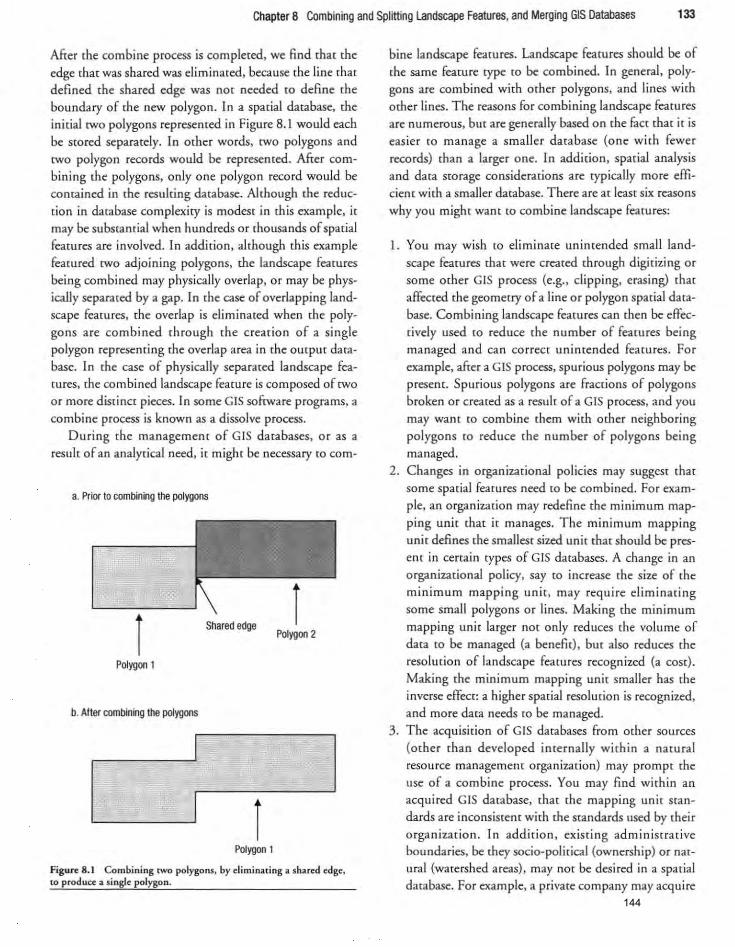
Chapter 8 Combining and Splitting Landscape Features, and Merging GIS Databases 133
After the combine process is completed, we find that the edge that was shared was eliminated. because the line that
defined the shared edge was not needed to define the boundary of the new polygon. In a spatial database, the initial two polygons represented in Figure 8.1 would each be stored separately. In other words, twO polygons and twO polygon records would be represented. After combining the polygons, only one polygon record would be contained in the resulting database. Although the reducrion in database complexity is modest in this example, it may be substantial when hundreds or thousands of spatial features are involved. In addition, although this example featured twO adjoining polygons, the landscape feamres being combined may physically overlap, or may be physically separated by a gap. In the case of overlapping landscape feacuces, the overlap is eliminated when the polygons are combined through the creation of a single polygon represeming the overlap area in the oucpuc database. In the case of physically separated landscape features, the combined landscape feature is composed of two
or more distinct pieces. In some GIS software programs, a
combine process is known as a dissolve process.
During the management of GIS databases, or as a
result of an analytical need, it might be necessary to com-
a. Prior to combining the polygons
r Shared edge
Polygon 2
Polygon 1
b. AHer combining 100 polygons
I
,---------,I r Polygon 1
Figure 8.1 Combining twO polygons. by diminating a shared edge. to produce a single polygon.
bine landscape features. Landscape features should be of the same feature 'Ype to be combined. In general, polygons are combined with other polygons, and lines with other lines. The reasons for combining landscape features
ace numerous, but are generally based on [he fact mar it is
easier [Q manage a smaller database (one with fewer
records) than a larger one. In addition. spacial analysis and data storage considerations are typically more effi
cient with a smaller database. There are at least six reasons
why you might want (Q combine landscape feamces:
l. You may wish to eliminate unintended small land
scape features that were created through digitizing or some other GIS process (e.g., clipping, erasing) that affected the geometry of a line or polygon spatial database. Combining landscape features can then be effectively used to reduce [he number of feamces being managed and can correct unintended feam ces. For
example, after a GIS process, spurious polygons may be present. Spurious polygons are fractions of polygons broken or created as a result of a GIS process. and you
may wanr [0 combine them with other neighboring
polygons to reduce the number of polygons being managed.
2. Changes in organizational policies may suggest that
some spatial features need to be combined. For exam
ple. an organization may redefine the minimum map
ping unit (hat it manages. The minimum mapping
unit defines the smallest sized unit that should be present in certain types of GIS databases . A change in an
organizational policy, say to increase the size of the
minimum mapping unit, may require eliminating
some small polygons or lines. Making the minimum
mapping unit larger not only reduces the volume of data to be managed (a benefit), but also reduces the resolution of landscape features recognized (a COSt).
Making the minimum mapping unit smaller has the
inverse effecc: a higher spacial resolution is recognized,
and more data needs to be managed.
3 . The acquisition of GIS databases from mher sources
(other than developed internally within a natural resource management organization) may prompt the
use of a combine process. You may find within an
acquired GIS database, that the mapping unit stan
dards are inconsistent with the standards used by their
organizat io n. In addition, existing adminisrra d ve boundaries, be they socio-political (ownership) or natlIral (watershed areas), may nO[ be desired in a spatial
database. For example, a private company may acquire 144
134 Part 2 Applying GIS to Natural Resource Management
a GIS database from the US Forest Service. The acquired database may include polygons smaller than what the private company typically manages, suggesr
ing that some landscape features need to be combined [Q adhere to the minimum mapping unie standard chat the company uses. A polygon layer (hat contains watershed boundaries at a sub-regional scale may provide unneeded detail if a regional watershed boundary wi ll suffice. Sub-regional watershed boundaries could be aggregated through a combine process.
4. Comb ining landscape fearures may be necessary because it simply makes sense from a management
perspeccive. For example. in a stands GIS database there may reside two polygons side-by-s ide that describe fo rested areas with trees of similar ages, similar structural conditions. similar sire classes. and similar growth rates. The field personnel responsible for managing these stands might also suggest (hat the two stands would be tceared with similar treatments, at about (he same time. and with similar equipmenc. Thus from a management perspective. combining the
two polygons into a single polygon within a GIS database might make sense.
5. Since landscape features can change in shape and characteristic over rime, managing these changes may sug-
Combining processes must be used in a thoughtful manner. Once landscape features are combined. the topology that describes the resulting landscape feature is altered in the Output database. Should a user decide ro delete the input databases (a common thought once a new database has been created) the orig inal descript ion of the landscape topology is lost. Given this risk, larger natural resource organizations have generally placed the decision to edit and manage GIS databases (where combining landscape features may be necessary) to the person who has been given 'ownership' of the GIS database. All decisions rega rding the development and maintenance of a given GIS database are then the responsibility of the database owner. Other individual users of the GIS database. however. can perfo rm GIS processes. such as combining features, on copies of the original GIS database. However, once performed by someone other than the owner of the
gesr using a combine process. For example. the condition of a road may change due co improvemen(S made (Q ir over rime. A rocked road may become a paved road, a native surface road may become a rocked road.
o r a road of any type may become a decommissioned (obliterated) road. If cond itions of landscape features change, it may seem reasonable to combine those landscape features with other adjacent landscape features of the same stature or condition. A similar example might involve stream network measurements such
as what occurs during a standard watershed analysis project. Field stream crews will visit selected streams
and segregate Stream networks into similar hydrologic or geomorphic categories. or categories related to the surrounding land cover. These groupings are stored in a spat ial database as separate line fearu res with associated dara records containing descriptive information. Some co mbi ning of streams in a GIS database might
be necessary to manage the stream network more efficien tly.
6. It may be appropriate to combine landscape features to facilita te a spatial analysis. For example. co delineate one category of the recreational opportunity spectrum,
we may need co identify the size (area) of contiguous timber stands where rhe average age of rrees is 50 years
database, the altered database is no longer considered the official database of the organization . For example,
John Goheen, a GIS analyst, may be the 'owner' of a roads GIS database within an o rganization. John may then give a copy of this database to Paul Chapman, a field forester. If Paul were to edit the database by combining or splitting roads, the copy of the GIS database that Paul uses will not be considered the official roads GIS database of the organization. even if the database
helps Paul make better management decisions. Can Paul simply provide the edited roads GIS database to John? Certainly. However, John will likely need to ensure that the changes Paul made conform to organizat ional standa rds related to data maintenance, and then subsequently verify that the database does not contain any errors. If John can do these things. the data edited by Paul can be incorporated into the original (and official) roads GIS database.
145
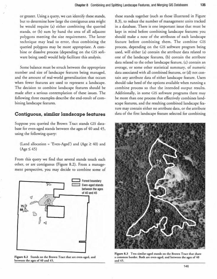
Chapter 8 Combining and Splitting landscape Features, and Merging GIS Databases 135
or greater. Using a query, we can identifY these stands,
but to determine how large the contiguous area might
be would requ ire (a) either combining the queried Stands, or (b) sum by hand the area of all adjacent polygo ns meeting the size requirement. The lance
technique may lead [Q error, rhus co mbining the queried polygons may be more appropriate. A combine or dissolve process (depending on the GIS software being used) would help faci litate this analysis.
Some balance must be struck between the appropriate number and size of landscape features being managed. and the amount of real-world general ization that occu rs when fewer features are used [0 represent a landscape. The decision to combine landscape fearu res should be made after a serious contemplation of these issues. The following three examples describe the end-result of combining landscape features.
Contiguous, similar landscape features
Suppose you queried the Brown Tract Stands GIS database for even-aged srands berween the ages of 40 and 45, using the fo llowing query:
(Land allocation = ' Even-Aged') and (Age ~ 40) and (Age S; 45)
From this query we find that several stands touch each other, or are contiguous (Figure 8.2). From a manage
mem perspective. you may decide to combine some of
c:::J Forest boondary c:::J Even-aged stands
between the ages r ___ ...::Of..:,4o:,;and 45
Figure 8.2 Stands on the Brown Tract that au even-aged. and between the ages of 40 and 45.
these stands together (such as those illustrated in Figure 8.3), co reduce the number of managemem units tracked
in a database. There is one imponam issue thar must be kept in mind before combining landscape features: you should make a note of the attributes of each landscape feature before combini ng them. The combine GIS process, depending on the GIS software program being used. will either (a) comain the a((ribute data related co one of the landscape featutes, (b) comain the attribute data related co the other landscape feature. (c) comain an average. o r some other stat istical summary. of numeric data associated with all combined features. or (d) not contain any anribure data of either landscape feature. Users
should take heed of the options available when running a combine process so that the intended output results. Additionally, in some GIS software programs there may be more than one process that effectively combines land
scape fearures, and the resulting combined landscape feature may contain either no attribute data, o r the attribute data of the firSt landscape feature selected for combining
Figure 8.3 Two similar-aged stands on the Brown T rac{ that share a common border. Both are even-aged. and between the ages of 40 and 45 .
146
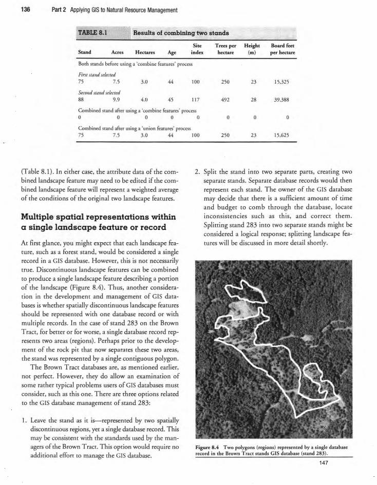
136 Part 2 Applying GIS to Natural Resource Management
TABLE 8.1 Results of combining two stands
Stand Acres Ag. Site
index Trees per
hectare Height
(m) Board feet per hectare
Both stands before using a 'combine features' process
First wmd ulut~d 75 7.5 3.0 44 100 250 23 15.325
&COlli stand u l«ud 88 9.9 4.0 45 11 7 492 28 39.388
Combined stand after using a 'combine features' process 0 0 0 0
Combined stand after using a 'union features' process 75 7.5 3.0 44
(Table 8. I). In either case. the attribute data of the combined landscape feature may need to be edited if the combined landscape feature will represent a weighted average of the conditions of (he original twO landscape featu res .
Multiple spatial representations within a single landscape feature or record
At first glance, you might expect that each landscape fearuee, such as a forest stand, would be considered a si ngle
record in a GIS database. However, this is not necessarily
true. Discontinuous landscape featu res can be combined
co produce a single landscape feature describing a portion of the landscape (Figure 8.4). Thus, another consideration in (he development and management of GIS data
bases is whether sparialJy disconrinuous landscape featu res should be represented with one database record or with multiple records. In the case of nand 283 on the Brown
Tract, for better or for worse, a single database record rep
resents two areas (regions) . Perhaps prior to the develop
ment of the rock pi t that now separates these two areas,
the stand was represented by a single contiguous polygon .
T he Brown Tract databases are, as mentioned earlier,
nOt perfect. However, they do allow an examination of
some rather typical problems users of GIS databases must consider, such as this one. There are three options related
to the GIS database management of stand 283:
1. Leave the stand as it is-represented by twO spatially
discontinuous regions, yet a single database record. This
may be consistent with the standards used by the managers of the Brown Tract. This option would require no additional effort co manage the GIS database.
0 0 0 0
100 250 23 15.625
2 . Split the stand into two separate parts, creating twO
separate stands. Separate database records wou ld then
represent each stand. The owner of the G IS database may decide that there is a sufficient amount of time
and budget to comb through the database, locate inconsiste ncies such as this, and correct them.
Spl itting stand 283 into twO separate stands might be considered a logical response; spli tting landscape fea
(Ures will be discussed in more detail shordy.
Figure 8.4 Two polygons (regions) represen le<l by a single da[abase record in the Brown Tract stands GIS database (stand 283).
147
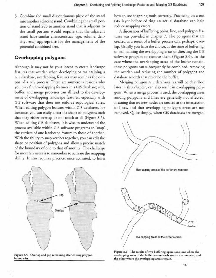
Chapter 8 Combining and Splitting Landscape Features, and Merging GIS Databases 137
3. Combine the small discontinuous piece of the stand into another adjacent stand. Combining the small portion of stand 283 to another scand thar is adjacent to
[he small pardon would require chat (he adjacent
stand have similar characteristics (age. volume. density, ere.) appropriate for the management of (he
potential combined area.
Overlapping polygons
Although it may not be your intent to create landscape fearures that overlap when developing or maintaining a GIS database, overlapping features may resulc as [he OU[
pm of a GIS process. There are numerous reasons why you may find overlapping features in a GIS databasei edit, buffer, and merge processes can all lead to the development of overlapping landscape feacures, especially with GIS software that does nOt enforce ropological rules. When editing polygon feacures within GIS databases, for instance. you can easily affect (he shape of polygons such that they either overlap or not touch at all (Figure 8.5). When editing GIS databases. it is wise co understand the process available within GIS sofrware programs to 'snap'
the verrices of one landscape feature to those of another. With the abiIicy [Q snap vertices together. you can edit the shape or position of polygons and allow a precise match of the boundary of one to that of another. The challenge for most GIS users is to remember to acriva.te the snapping ability. It also requires practice. once activated, to learn
Gap
Overlap
Figure 8.5 Ov~rlap and gap r~maining aft~r ~diting polygon boundarj~s.
how to use snapping tools correctly. Practicing on a test GIS layet before editing an actual database can help reduce snapping errors.
A discussion of buffering point, line, and polygon features was provided in chapter 7. The polygons that are created as a result of a buffer process can, perhaps. over
lap. Usually you have the choice, at the time of buffering, of maintaining the overlapping areas or directing the GIS software program to remove them (Figure 8.6) . In the case where the overlapping areas of the buffer remain,
these polygons can subsequently be combined, removing the overlap and reducing the number of polygons and database records that describe the buffer.
Merging polygon GIS databases, as will be described later in this chapter, can also result in overlapping polygons. When a merge process is used, the overlapping areas
among polygons and lines ate genetally not affected, meaning that no new nodes are created at the intersection of lines, and that overlapping polygon areas are not removed. Quite simply, when GIS databases are merged,
Overlapping areas of the buffer are removed
Overlapping areas of the txJffer remain
Figure 8.6 Th~ results of twO buff~ring operations, on~ wh~r~ th~ oY~rlapping ar~as of th~ buff~r around ~ach str~am ar~ r~moy~d, and th~ oth~r wh~r~ th~ ov~rlapping areas r~majn.
148

138 Part 2 Applying GIS to Natural Resource Management
How would you know whether a polygon GIS database contains overlapping polygons' One method might be to examine very closely the boundaries of each polygon-a tedious process. Another method may be co compare the sum of the area of polygons in
the suspect GIS database with another polygon GIS database of the exact same spadal extent. For example.
if you were concerned about overlapping polygons in the Daniel Pickett forest stands GIS database, you could compare the sum of the area of the stands to [he
area of the boundary GIS database. The extent of the two databases should be exacdy the same: the stands
one set of landscape features is simply laid on top of another sec.
Splitting Landscape Features
The decision (0 use a splitting process general ly arises from some need {Q redefine the topology of spatial data. The word 'split' is defined as a process ro divide or sepa~ rate an item into pares or ponions (Merriam-Webster,
2007) . Within GIS, we use a splitting process to divide polygons and lines (but not points) into smaller pam or portions. Points do not describe areas; however, buffers around points can be spli t because they are polygons.
To illuscrate several reasons for using splining
processes. cons ider the sub-dividing of land ownersh ips
that regularly occurs in many rural and urban areas
throughout Nonh America. Many property owners sub
divide their lands in order to earn revenue or bequeath
property to land stewardship organizations or heirs . Land
ownership records and GIS database are kept by county. provincial. or metropolitan organizations and mUSt be
updated to accurately represent new parcels that result from subdivisions. Spliuing processes are used to separate
parcels from one another and lead to the creation of addi
tional polygons in a GIS property boundary database. As another example involving polygons. imagine a state or province where cleareut size limits are imposed. For
organizations that plan c1earcur activities in these regions. the forest management units represented in their stands
GIS database should probably be smaller in size than the maximum clearcut area allowed. Therefore. these poly-
GIS database should contain polygons that are a subdivision of the ownership defined by the ownership boundary. The stands GIS database has many polygo ns, and the boundary GIS database has only one polygon, yet the sum of the areas should match. You could also choose to combine all polygons within a copy of the stands layer. The area of the resulting combined stands database should also match. If the sum of the areas does not match. either one or more overlap
ping polygons exist in the stands GIS database, or some
gaps exISts between polygons in the stands GIS database.
gons should probably be broken down (split) into smaller management unitS to enable land managers ro plan har
vests mote appropriately (Figure 8.7). In terms of linear
3. l60-acre (64.8 ha) polygon and a stream that will be used to split it Into two smaller polygons
<r---------~- Node of line defining L the polygon
• ~ Stream line used to split ttle polygon / -
__ Polygon to be split
/
b. Resulting two smaller focest management untts after splitting ttle 160·acre (64.8 hal polygon
Polygon 1
Polygon 2
Figure 8.7 A 160-acre (64.8 ha) polygon split along a stream. forming two smaller forest mamlgement units.
149

Chapter 8 Combining and Splitting landscape Features. and Merging GIS Databases 139
fea[l1res, assume mar you are involved with [he planning and maimenance of a road system for a namral resource management organization . Over some period of time, the
scams of a porrion of a woods road may have changed. perhaps from a rocked surface [0 a paved surface (or alternatively, parr of the road was obliterated in a restoration
process). Within the roads GIS database. splitting the line that represents the road at the location of the stams change would seem appropriate, since each resulting piece of the road should be described by different attribute data. The same argument for a sp!iHing process can be used for stream data managemenr. In this case, assume a
recent stream survey identified some differences becween (he GIS data and the acruai stream system. Some stream reaches, fo r example. may have been found [Q be able [Q
support fish populations. yet the GIS data indicates otherwise. In these cases. the various lines that represent
Draw a polygon around one of the nl.lltiple
representations
Stands GIS database
Select the Ofiginal po/ygoo
Clip
Stands GIS database
Remove original polygon from
the stands GIS database
Copy into the stands GIS database the
two portions of the original stand
streams may need to be split to be[(et delineate the capac
ity to suppOrt (or not support) fish populations. The way you go abour spli tting polygons or lines (yet
nor points) varies according to the GIS software program being used. In some GIS software programs. splitting is as easy as drawing a line through a landscape fearure (Figure 8.7). This holds true for polygons or lines that are solid or continuous. However. where a landscape fearure is repre
sented by multiple regions (or objects). and a gap separates these regions (such as that illustrated in Figure 8.4). drawing a line through the gap. without touch ing either of the pieces of the landscape feature . may not result in (he fearure being spli t inro twO separate pieces. In these
cases. a more complex process using combining. clipping. editing. or pasting ptocesses may be more applicable (Figure 8.8). Alrernativeiy. some GIS software programs have processes for convening multipart features to single
Save the original polygon In a
GIS database
One portion of the original
polygon
Erase
portion of the original
polygon
Figure 8.8 A complex process that can be used to split a polygon, initially represented by twO
regions, into twO separate landscape features.
150
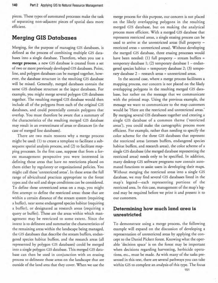
140 Part 2 Applying GIS to Natural Resource Management
pieces. These types of automated processes make the task
of separadng non-adjacent pieces of spacial data more efficient.
Merging GIS Databases
Merging. for the purpose of managing GIS databases. is
defined as the process of combining multiple GIS data
bases into a single database. Therefore, when you use a
merge process, a new GIS darabase is created from a set
of two or more previously developed GIS databases. Point.
line. and polygon databases can be merged together. how
ever, (he database structure in the resulring GIS database
will be mixed. Generally. merged databases contain the same G IS database structure as [he inpU( databases. For
example. you might merge several polygon GIS databases
together. The resulting merged GIS database would then
include aU of the polygons from each of the original GIS databases. and could potentially contain polygons that
overlap. You must therefore be aware (hat a summary of
(he characteristics of the resulting merged GIS database
may result in an overestimate of areas or diS[ances (in (he
case of merged line databases) .
There are two main reasons why a merge process
might be used: (l) to create a template [0 faci litate a sub
sequent spacial analys is process, and (2) to facilitate map
ping processes. In the fi rst case, suppose that from a for
est management perspective yo u were interested in
defin ing those a reas that have no resrrict ions placed on
them either by regulatory or organizational policies. You might call these 'unrest ricted areas'. In rhese areas the full
range of silviculmral practices appropriate to the forest types and the soil and slope condicions can be considered .
T o define rhese unrestricted areas on a map, you might firsr anempt (Q define the restricted areas: those that are
within a cenain distance of the stream system (requiring
a buffer), near some endangered species habitat (requiring
a buffer), o r designated as resea rch areas (requir ing a
query o r buffer). These are the areas within which man
agement may be restricted to some extent. Sin ce the
intent is to delineate and summarize the characteristics of
the remaining areas within the landscape being managed,
the GIS databases that describe the stream buffers. endan
gered species habitat buffers. and the research areas (a ll
represented by polygon GIS databases) could be merged
into a single polygon GIS database. This merged GIS database can then be used in conjunction with an erasing process to delineate those areas on the landscape that are
outside of the land area that they cover. When we use the
merge process for this purpose, our concern is not placed
on the likely overlapping polygons in the resulring
merged GIS da tabase. bur on makin g the analyt ical
process more efficient. With a merged GIS database that
represents restricted areas, a single erasing process can be used to arrive at the unrestricted areas (full property -
restricted areas = unrestricted areas) . Without developing
the merged GIS database. three erasing processes would
have been needed: (I) fu ll property - stream buffers =
temporaty database I; (2) temporary database I - endan
gered species habitat = temporary database 2; (3) tem po
rary database 2 - research areas = unrestricted areas.
In the second case, where a merge process facilitates a
mapping process, ou r concern is not placed o n the likely
overlapping polygons in the resulting merged GIS data
base, but rather on the message that we communicate
with the primed map. Using the previa LIS example, the
message we want to communicate to the map customers
would be ' Here are the rest ricted and unrestricted areas.'
By merging several GIS databases together and creating a
single GIS d atabase of a common theme ('res tr icted
areas'), you could make the canograph ic process mo re efficient. For example, rather than needing to specify the
color scheme for the three GIS databases that represent
the restricted areas (stream buffers, endangered species
habitat buffers. and research areas), the color scheme of a
single GIS database (the merged database representing the
res tricted areas) needs o nly to be specified. In add ition,
many desktop GIS software programs now contain automated fu nctions to assist users in developing thei r maps.
W ithout merging the restr icted a reas inca a single GIS database, we may find several GIS da tabases listed in the
map's legend-each representing portions of the
restricted area. In this case, management of the map's leg
end may be required before we print it and present it to
o ur customers.
Determining how much land area is unrestricted
To demonstrate using a merge process, the following
exa mple will expand on the d iscussion of developing a
representation of unrestricted areas by applying the con
cept to the D aniel Pickett fo rest. Knowing what the operable 'decision space' is on the forest may be important
when decisions regarding harvest ing, herbicide opera
tions, etc., must be made. As with many of the tasks presented in this text, there are several pathways you can take
within GIS to complete an analysis of th is type. The focus 151
140 Part 2 Applying GIS to Natural Resource Management
pieces. These rypes of automated processes make rhe [ask of separaring non-adjacent pieces of spada! data more efficient.
Merging GIS Databases
Merging. for rhe purpose of managing GIS databases. is defined as rhe process of combining multiple GIS databases inco a single database. Therefore, when you use a merge process, a new GIS database is created from a set of two or more previously developed GIS databases. Point. line. and polygon databases can be merged roge<her. how
ever, rhe database structure in rhe resulring GIS database will be mixed. Generally, merged databases contai n the same GIS database strucrure as rhe input databases. For example. you might merge several polygon GtS databases ,oge,her. The resulring me' ged GIS darabase wou ld then
include aU of the polygons from each of the origina l GIS databases. and could potentially contain polygons ,ha, overlap. You must therefore be aware thar a summary of rhe characreristics of the resul'ing merged GIS da",base may result in an overestimate of areas or distances (in rhe case of merged line da,abases).
There arc tWO main reasons why a merge process migh' be used: ( t ) to crea'e a ,empia,e to facili",re a subsequent spatial analys is process, and (2) to faci litate mapping processes. In the first case, suppose that from a for
est management perspective you were interested in defin ing those areas thar have no resrrictions placed on rhem either by regulalOry or organizalional policies. You might call these 'unrestricted areas', ]n these areas the full
range of silvicli lcural pract ices appropriate to the forest types and the soil and slope condirions can be considered. To define these unrestricted areas on a map, you might first attempt {Q define the restricted areas: those that are within a certain disrance of the stream system (requ iring a buffer) . near some endange,ed species habi,a, (,equiring a buffer), o r designated as research areas (requiring a query o r buffer). These are the areas within which manageme nl may be resrr icred to some extent. Since [he intent is (0 delineate and summarize [he characteristics of
the remaining areas within [he landscape being managed, rhe GIS darabases thar describe ,he srream buffers. endangered species habira, buffers. and ,he research areas (all represented by polygon GI databases) could be merged imo a single polygon GIS darabase. Th is merged GIS dalabase can [hen be used in conjunction with an erasing process [0 delineate those areas on rhe landscape that are ourside of the land area that rhey cover. When we use [he
merge process for u,is purpose, our concern is not placed on ,he likely overlapping polygons in lhe resul'ing merged GIS database. bur on making ,he analytical process more efficient. With a merged GIS database ,ha, represents restricted areas, a single erasing process can be lIsed to arrive at the unrestricted areas (full property -restricted areas ~ unrestricted areas) . Witham developing the merged GIS da",base. rh,ee erasing processes would have been needed: (1) full property - srream buffers =
,emporary da,abase I; (2) ,emporary da",base I - endangered species habirar = temporary da",base 2; (3) ,empe
rary dacabase 2 - research areas = unrestricred areas. In the second case, where a merge process faci litares a
mapping process, ou r concern is not placed o n the likely overlapping polygons in rhe resul'ing merged GIS darabase, but rather on rhe message that we communicate with the printed map. Using the previa liS example, the message we want to communicate to the map customers
wouJd be 'Here are the restricted and unrestricted areas.' By merging several GIS da,abases rogether and crea,ing a single GIS database of a common th eme (,restr icted areas'), you could make the carrographic process more efficient. For example, rather than need ing to specify rhe color scheme for rhe rhree GIS da,abases [hat ,epresent
the restricted areas (stream buffers, endangered species habi,a, buffers. and research areas). ,he color scheme of a si ngle GIS dalabase (rhe merged database representing ,he resrric,ed areas) needs only ro be specified. In addition.
many deskcop GIS software programs now contain automated fu ncrions co assist users in developing thei r maps.
Withour merging rhe restricted areas into a single GIS database, we may find severa) GIS databases listed in the map's legend-each representing portions of rhe
restricted area. In rhis case, management of rhe map's legend may be required before we prinr it and present il to our Cllstomers.
Determining how much land area is unrestricted
To demonstrate using a merge process, the following example will expand on the discussion of developing a representation of unrestricted areas by applying [he concep' ro ,he Daniel Pickert forest. Knowing wha, ,he operable 'decision space' is on the forest may be important when decisions regard in g harvesting, herbicide opera(ions, etc., must be made, As with many of the tasks presented in this text, there are severa) pathways you ca n rake wirhin GIS '0 comple,e an analysis of ,his type. The focus
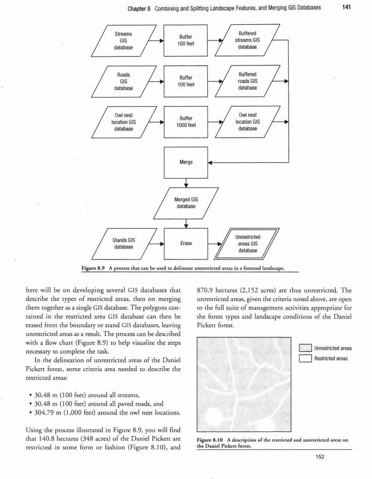
Chapter 8 Combining and Splitting Landscape Features, and Merging GIS Databases 141
Streams GIS
database
Roads GIS
database
Owl nest localion GIS
database
Buffer 100 feel
Buffer 100 feet
Buffer tOD~ feel
Merge
Buffered streams GIS
database
Buffered roads GIS database
Owl nest location GIS
database
Merged GIS dalabase
Stands GIS database
Erase Unrestricted
areas GIS database
Figur~ 8.9 A process that an ~ used to delineate unreuricted areas in a forested landscape.
here will be on developing several GIS databases that describe me types of restricted areas, then on merging them together as a single GIS database. The polygons contained in the restricted area GIS database can then be erased from (he boundary or stand GIS databases, leaving unrestricted areas as a resulr. The process can be described with a flow chart (Figure 8.9) to help visualize the steps necessary [0 complete the task.
In the delineation of unresrricccd areas of the Daniel Pickett forest, some criteria area needed to describe (he restricted areas:
• 30.48 m (J 00 feet) around all stroams, • 30.48 m (J 00 feet) around all paved roads, and • 304.79 m (J ,000 feet) around tho owl nest locations.
Using the process illustrated in Figure 8.9, you will find that 140.8 hectares (348 acres) of tho Danid Pickett are resrricted in some form or fashion (Figure 8.10), and
870.9 hectares (2, I 52 acres) are thus unrestricted. The unrestricted areas, given the crireria noced above, are open to (he full suite of management activities appropriate for
the forest types and landscape conditions of the Daniel Pickett forest.
D Unrestricted areas
D Restricted areas
Figure 8.10 A description of the restricted and unrestricted areas on the Daniel Pickett forest.
152
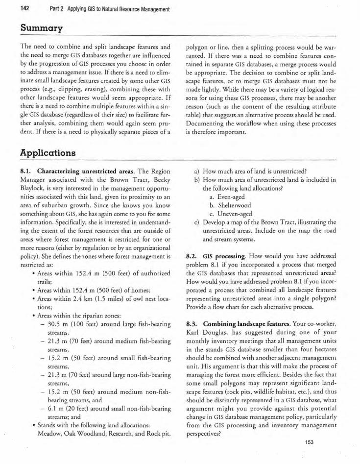
142 Part 2 Applying GIS to Natural Resource Management
Summary
The need to combine and splir landscape fearu res and the need to merge GIS darabases together are influenced by the progression of GIS processes you choose in order ro address a management issue. If there is a need co eliminate small landscape features created by some o ther GIS process (e.g., clipping, erasing), combining rhese wirh
other landscape fearu ces would seem approp riate. If there is a need (Q combine multiple feacures within a single GIS darabase (regardless of rheir size) to fac ilirare fur
ther analysis. combining them would again seem prudent. If rhere is a need ro physically separare pieces of a
Applications
8.1. Characterizing unrestricted areas. The Region Manager associated with the Brown Tract, Becky Blaylock. is very interested in the managemenr oppOrtunities associated with this land, given its proximity ro an
area of suburban growth. Since she knows you know something about GIS, she has again come to you for some information. Specifically, she is interested in understanding the extent of the forest resources that are outside of
areas where fo rest management is restricted for one or more reasons (e ither by regulation or by an organizational policy). She defines rhe zones where fo rest management is
restricted as: • Areas wirhin 152.4 m (500 feer) of aurhor ized
trails;
• Areas wirh in 152.4 m (500 feer) of homes; • Areas wirhin 2.4 km (1 .5 miles) of owl nest loca
tions;
• Areas within the riparian zones: - 30.5 m (100 feer) around large fish-bear ing
streams, 2l.3 m (70 feer) around medium fish-bea ring streams, 15 .2 m (50 feer) around small fish-bearing streams,
- 21.3 m (70 feer) around large non-fIsh-bearing streams,
- 15.2 m (50 feer) aro und medium non-fishbearing streams, and 6.1 m (20 feer) around small non-fIsh-bearing streams; and
• Stands with the following land allocations: Meadow, Oak Woodland, Research, and Rock pir.
polygon or line, rhen a splirring process would be warranted. If there was a need ro combine features con
rained in separate GIS databases. a merge process would be appropriate. The decis ion to combine or spli t landscape feacuces. o r [0 merge GIS databases must not be made lighrly. While rhere may be a variery oflogical reasons for us ing these GIS processes, there may be anocher
reason (such as the contem of the resuhing anribuce table) that suggests an alternative process should be used. Documeming the workAow when using these processes is therefore important.
a) How much area ofland is umestricted? b) How much area of unrestricted land is included in
rhe following land allocarions'
a. Even-aged b. Shelrerwood c. Uneven-aged
c) Develop a map of rhe Brown T racr , illustraring rhe unrestricted areas. Include on the map the road
and stream systems.
8.2. GIS processing. How would you have add ressed
problem 8.1 if you incorporared a process rhar merged the GIS databases that represented unrestricted areas? How would you have addressed problem 8 .1 if you incor
porated a process that combined all landscape features representing unrestricted areas into a single polygon? Provide a Aow chart for each alternative process.
8.3. Combining landscape features . Your co-worker, Ka rl Douglas, has suggeSted during one of your
momhly inventory meetings that all management un its in the stands GIS database smaller than four hectares should be combined with another adjacenr managemenr unie. His argument is that [his will make the process of managing the forest more efficient. Besides the faCt thar
some small polygons may represent sign ifica nt landsca pe fearures (rock pits, wildlife habirar, erc.), and rhus should be disrincrly represenred in a GIS darabase, whar argument might you provide against this potential change in GIS database management policy. particularly from the GIS processing and inventory management perspectives?
153

Chapter 8 Combining and Splitting Landscape Features, and Merging GIS Databases 143
References
Merriam-Websrer. (2007). Mtrriam-W,bsur on/in, search. Retrieved April 28, 2007, from http ://www. m-w .coml cgi-binl dic[ionary.
154

Chapter 9
Associating Spatial and Non-spatial Databases
Objectives
This chapter provides an inrroduction to techniques that
will allow you to associate fea mres in spatially- referenced
GIS databases with data from other sources (other types of
databases) which may not have an explicir spacial refer
ence. Once this chapter has been completed. readers
should have a firm underscanciing of:
l. how (Wo or more databases can be remporarily com
bined withom creating a new database. modifying a
database rabie, or modifying landscape feacuresi
2. what types of GIS processes are available when there is
a need to associate data from different sources;
3 . how non-spacial data can be associated with spatial databases. and how data from one spatial database can
be associated with data of another spatial database; and 4 . what it means to relate (link) two tables, and how this
process is different than joining darabases.
In the last few chapters a concentra rion was placed on taking (WO (or mo re) GIS databases and . with a
process such as erasi ng o r clipping, creating a third (new)
GIS database that featured differenr. o r modified, land
sca pe features. The GIS databases were, in essence, combined in a permanent fashio n in the new database. In th is
chaprer the databases will be combi ned in a way that is
temporary bur that st ill retains each database's o riginal structure (both the spatial structure and attribute table
structu re) . Si nce new landscape features are nOt being
created in th is process. the re is no need to create a new
GIS database; however, this is also possible and we will
discuss this process later in the chapter. To present addi
tional methods of combining databases, two processes of
associa tion will be introduced: the jo in and the relate
(link) processes. The first sect ion of this chapter examines joining data
in non-spacial databases with landscape features in spatial
d atabases. and desc ribes several of the common join
processes you might encounter. The relationship between
the non-spatial data and rhe landscape features is based on a common attribute value found in both da rabases. The
second section of the chapter examines joi ning landscape
features from [wo differen t GIS databases. and how the
relationship between the landscape features in each GIS
database is a fun ction of the location and type (poi nt.
line, or polygon) of the features on the landscape. The
third sectio n of the chapter discusses how you can make
the temporary joined associations among databases per
manenr. The final section of the chapter exam ines relar
ing {linking} features or data from one database to that of another. With a relate process. you can view one of the
related databases. selecr a landscape featu re. then view the
associated related data in the ocher database even rhough
the database will not appear to be physically associated.
Join processes do not follow this approach. but. instead, result in a single database that contains dara from borh
joined databases.
155
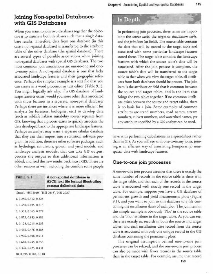
Joining Non-spatial Databases with GIS Databases When you wane [Q join twO databases together the objective is to associate both databases such chat a single data
base resul rs. Therefore, dara from one darabase (in rhis
case a non-spatial database) is transferred to rhe 3ncibucc
rable of rhe other darabase (rhe sparial darabase) . There
are several types of possible associarions when joining
non-spa rial darabases wirh spa rial GIS darabases. The [wo
most common join associations are one-co-one and one
to-many joins. A non-spatial database is one chat lacks associated landscape feacures and their geographic reference. Perhaps the simplest example is a text file chat you
can create in a word processor or text editor (Table 9. I). You mighr logically ask why, if a GIS darabase of land
scape feacures exists, would you store ocher data associated
with those features in a separate. non-spacial database? Perhaps there are instances where it is moce efficient for
analyses (or foresters. biologises. etc.) to develop data
(such as wildlife habirar su irabi liry scores) separare from
GIS, knowing mat a process exists [Q quickly associate the
dara developed back ro rhe appropriare landscape fearures.
Perhaps an analyst may wam a separate tabular da[3base
that they can then import into a statistical software pro
gram. In addition, there are other software packages. such
as hydrologic simularors, growrh and yield models , and
landscape analysis models. that can take GIS output.
process the output so that additional information is
added, and feed rhe new resulrs back imo a GIS. There are
other reasons as well, including the comfort some people
TABLE 9,1 A non.spatial database in AScn text file format illustrating comma-dellmited data
·S r.md ', 'HS12010', 'HSI 20 1;', 'HSI 2020'
1,0.2%, 0.312,0.325
2.0.4;8, 0.49; , 0.516
3,0.333, 0.36;, 0.372
4,0.87;, 0.88;, 0.889
;,0. 12;, 0.215,0.23;
6, 0.468, 0.476, 0.48;
7,0.906,0.908,0.9 11
8,0.648,0.74;,0.7;3
9, 0.378, 0.42;, 0.431
10,0.096,0.102,0.118
Chapter 9 Associating Spatial and Non-spatial Databases 145
In performing join processes, three terms are impor
ram: rhe ,ollrce tabu, the targ't or tk,tination tabu, and rhe join it<m (or field) . The source rable comains
rhe dara rhar will be moved ro the rarger rable and
associated with some part icula r landscape fearu res
srored rhere. The rarger rable comains rhe landscape
fearures with which the source table's data will be
associated. After the join process is complete, the
source table's data will be transferred [Q the target
rable so rhar when you view rhe rarger rabie, all amib
ures from boch darabases should be presem. The join
item is the attribure or field that is common berween
the source and ta rget rabies , and is the irem thar
brings rhe [wo rabies rogether. If no common amib
ute ex.isrs berween the source and target tables. there
is no basis fo r a join. Some examples of common
attributes are stand numbers, road names, stream numbers, culvert numbers, and watershed names, yet
any amibure specified by a GIS analysr can be used.
have with performing calculations in a spreadsheer rather
than in GIS. As you will see with one-to-many joins. join
ing is an efficient way of associating (temporarily) non
spa rial dara wirh landscape feawres.
One-to-one join processes
A one-to-one join process assumes mat mere is exactly the same number of records in the source cable as there is in
the target table, and that each of the records in the source
table is associated with exactly one record in me target
rable. For example, suppose you have a G IS darabase of
permanent growth and yield measurement plots (Figure
9.1), and you want to join to this database to a file con
taining the installation dates of each plot. The join item in
this simple example is obviously 'Plot' in the source table
and the ' Plot' attribute in the target table. A5 you can see,
the re are exacdy six records in both the source and target
tables. and each installation date record from the source table is associated with only one unique record in the GIS
database containing the permanem plo[s.
The original assumption behind one-to-one join processes can be relaxed. and [he one- to-one join process can also be made with fewer records in the source [able
[han in the target [able. For example, assume thar record
156
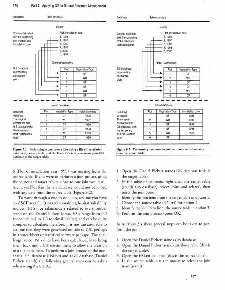
146 Part 2 Applying GIS to Natural Resource Management
Database
Comma-delimited text file containing plot number and Installation date
GIS Database representing permanent plots
Resulting database: The original permanent plot GIS database with the temporary field Mlnstallation date"
Table structure
Plot 1
2
3
4
5
6
Soon;e
r-Plot , Installation dale 1 1998
t--- 2. 1997 3, 1999 4, 1998 5,2000 6, 1999
Target (Destination)
Plol Vegetation Type L...-. 1 OF
2 WH 3 OF 4 OF
5 WH 6 OF
Joined database
Vegetation Type Installation date
OF 1998 WH 1997 OF 1999
OF 1998 WH 2000 OF 1999
Figure 9.1 Performing a one-to-one join usi ng a fi le of installation dates as the source table, and the Danid Pickett permanent piau GIS database as the target table.
6 (Plor 6, insrallarion year 1999) was missing from the source rable. If YOli were to perform a join process using the source and target rabies. a one-to-one join would still occur, yet Plot 6 in the GIS database would not be joined with any data from the sou tee table (Figure 9.2).
To work through a one~to~one join. assume you have an ASCII text file (HSl.rxt) containing habitat suitability ind ices (HSls) for salamanders related to every dmber stand on the Daniel Pickett forest. HSls range from 0.0 (poor habitat) to 1.0 (optimal habitat) and can be quite complex ro calculate; therefore. it is nO[ unreasonable ro assume that they were generared outside of GIS. perhaps in a sp readsheet or stacisdcal sofrware package. The challenge. once HSI values have been calculated. is [0 bring them back into a GIS environment [0 allow the crearion of a thematic map. To perform a join process of the nonspatial HSI database (HSl.rxt) and a GIS database (Daniel Pickett stands) the following general steps can be taken when using ArcG IS 9.x:
Database
Comma·delimited text file containing plot number and installation date
GIS Oatabase representing permanent plots
Resulting database: The original permanent plOt GIS database with the terTij)Orary field -Installation date-
Table structure
Plol 1
2
3
4
5
6
Soon;e
Plot, Installation date 998 .---- 1, 1
2,1997 3,1999 4, 1998 5, 2000
Target (Destination)
Plol Vegetation Type L..,. 1 OF
2 WH 3 OF
4 OF
5 WH 6 OF
Joined database
Vegetation Type Installation dale
OF 1998
WH 1997
OF 1999
OF 1998
WH 2000
OF
Figure 9.2 Performing a one-to-one join with one r«ord missing from the source table.
I. Open the Daniel Pickett stands GIS database (this is the target table).
2. In the table of contentS, right-click the target table (stands GIS database). seiect ' joins and relates' , then seiect [he join option.
3. IdentifY the join item from the target table in option 1. 4. Choose the source table (HSl.rxt) for option 2. 5. IdentifY the join item from the source table in option 3. G. Perform the join process (press OK).
In ArcYiew 3.x these general steps can be taken to per~ form the join:
I. Open the Daniel Pickett stands GIS database. 2. Open the Daniel Pickett stands attribute table (this is
the target table) . 3. Open the HSl.rxt database (th is is the source table) . 4. I n the source table. use the mouse to seieer the join
item (stand).
157
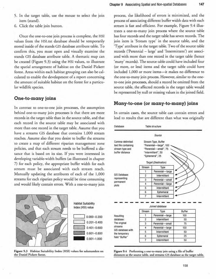
5. In the target table, use the mouse [Q select the join item (stand) .
6. Click the table join button.
Once the one-to-one join process is complete, the HSI values from the HSI.txt database should be temporarily
srored inside of the stands GIS database attribute table. To confirm this, you muSt open and visuaUy examine the stands GIS database attribute table. A thematic map can
be created (Figure 9.3) using the HSI values, to illustrate the spatial arrangement of habitat on the Daniel Pickett forest. Areas with in each habitat grouping can also be calculated to enable the development of a report concerning the amount of suitable habitat on the forest for a particular wi ldli fe species.
One-to-many joins
In COntrast to one-to-one join processes, the assumption behind one-to-many join processes is that there are more records in the target table than in me source table, and that each record in the source table may be associated with more than one record in the target table. Assume that you have a streams GIS database that contains 1,000 stream
reaches. Assume also that you desi re to buffer the Streams to create a map of diffe rent riparian management zone
policies, and that each stream needs to be buffered a disrance that is based on its size. If you were interested in developing variable-width buffers <as illustrated in chapter 7) for each policy, the appropriate buffer width for each stream must be associated with each stream reach. Manually updating the attributes of each of the 1,000 streams for each riparian policy would be time consuming
and would likely contain errors. W ith a one-to-many join
Habitat SUitability Index (HSI) value
CJ 0.000-0.200
CJ 0.201- 0.400
CJ 0.401-0.600
c:::::El!I 0.601- 0.800
_ 0.80H.000
Fi.gure 9.3 Habitat Suitability Index (HSI) valu~s for salamand~rs on the Daniel Pick~tt forest.
Chapter 9 AssoCiating Spatial and Non-spatial Databases t47
process, the likelihood of errors is minimized, and the
process of associaring different buffer width data with each stream is fitst and efficient. For example, Figure 9.4 illus
trates a one-to-many join process where the source table has four records and the targer table has seven records. The join item is 'Stream type' in the source table, and the
'Type' attribure in the target table. Two of the source table records (,Perennial - large' and ' lnterminenr') are associ
ated with more than one record in the ta rget table (hence 'many' records). The source table could have included four
(or more, or less) items and me target table could have included 1,000 or more items-it makes no difference to
the one-to-many join process. However. similar to me oneto-one join processes, should a record be omitted from the source table, the affecred records in the target table would
be represented by null or missing values in the joined field .
Many-to-one (or many-to-many) joins
In certain cases, the source table can contain errors and
lead to results that are different than what was originally
Database
Comma·delimited texl file containing stream type and buffer distance
GIS Oatabase representing permanent plots
Resulting database: The original streams GIS database with the temporary field "Buffer"
Table structure
Stream Type, Buffer · Perennlal-large", loo -Perennial-small". 75 "Intermittent", 50 "Ephemeral ",25
Target (Destination)
Stream Type 1 Perennial-large
2 Intermittent 3
4 Perennial-large 5 Intermittent
6 Ephemeral
7 Intermittent
Joined database
Stream Type
1 Perennial large
2 Intermittent 3 Perennial small
• Perennial large
5 Intermittent 6 Ephemeral
7 Intermittent
Buffer
100
50
75 100
50 25 50
Figure 9.4 P~rformjng a one-to-many join wing a fiI~ of buff~r distances as th~ source tabl~, and streams GIS databas~ as th~ targ~t tabl~.
158
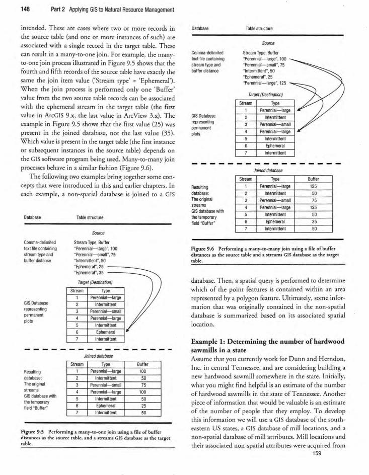
148 Part 2 Applying GIS to Natural Resource Management
intended. These are cases where twO o r more records in
the source table (and one or more instances of such) are associated with a single record in rhe target rable. These can result in a many-tO-one join. For example. the manyto-one join process illustrated in Figure 9.5 shows that rhe
fourth and fifth records of the source cable have exacuy the
same the join item value (,Stream type' = 'Ephemeral') . When rhe join process is performed only one 'Buffer' value from the cwo source table records can be associated
with the ephemeral stream in the target table (the first value in ArcGlS 9.x, the last value in ArcView 3.x). The example in Figure 9.5 shows that the first value (25) was present in the joined database, not the last value (35). Which value is presem in the target table (the first instance or subsequent instances in rhe source table) depends on
the GIS software program being used. Many-to-many join processes behave in a similar fashion (Figure 9.6).
The following two examples bring together some concepts that wefe introduced in (his and earl ier chapters. In each example. a non-spatial database is joined co a GIS
Database
Comma-delimited text file containing stream type and buller distance
GIS Oatabase representing permanent plots
Resulting database: The original streams GIS database with the temporary field "Buffer"
Table structure
Sou",.
Stream Type, Buller "Perennial-large", l00 "Perennial-small ", 75 "Intermittent", 50
"Ephemeral ",25 -====::::::::"Ephemeral ", 35 -
Target (Destination)
Stream Type 1 Perennial-large
2 Intermiltent
3 Perennial-small
4 Perennial-large
5 Intermittent
6 Ephemeral 7 Intermittent
Joined database
Stream Tyll" Buffer 1 Perennial large 100 2 Intermittent 50 3 Perennial .maD 75 4 Perennial large 100 5 Intermittent 50 6 Ephemeral 25 7 Intermittent 50
Figure 9.S Performing a ma ny-to-one join using a file of buffer distances as the source table, and a streams GIS database as the target table.
Oatabase
Comma-delimited text file containing stream type and buffer distance
GIS Database representing permanent plots
Resulting database: The original streams GIS database with the temporary field "Buller"
Table structure
Soun:.
Stream Type, Buller "Perennial-large", l00 "Pereooial-small ", 75 "Intermittent",50 "Ephemeral", 25 "Perennial- large", 125
Target (Destination)
Stream Type
Perennial-large
2 Intermittent 3 Perennial-small
4 Perennial-large
5 Intermittent
6 Ephemeral
7 Intermittent
Joined database
Stream Tyll" 1 Perennial large
2 Intennlttent
3 Perennial small
4 Perennial large
5 Intermittent
6 Ephemeral
7 Intermittent
Butler
125
50 75
125 50
35 50
Figure 9.6 Performing a many- to-many join using a Ale ofbufTer distances as me source table and a streams GIS database as the target table.
database. Then, a spatial query is performed to determine which of the point fearures is contained within an area
represented by a polygon feature. Ultimately, some informarion that was originally contained in [he non-spada I database is summa ri zed based o n its assoc iated spatial locat ion.
Example 1: Determining the number of hardwood sawmills in a state Assume (hat you currently work for Dunn and Herndon, Inc. in centra] Tennessee, and are considering building a new hardwood sawmill somewhere in (he state. Initia lly,
what you might find helpful is an est imate of the number of hardwood sawmills in the state of Tennessee. Another piece of information that would be valuable is an estimate of the number of people that they employ. To develop rhis information we will use a CIS database of the southeastern US states, a GIS database of mill locations, and a non-spa rial database of mill attributes. Mill locat ions and
their associated non-spatial attributes were acquired from 159
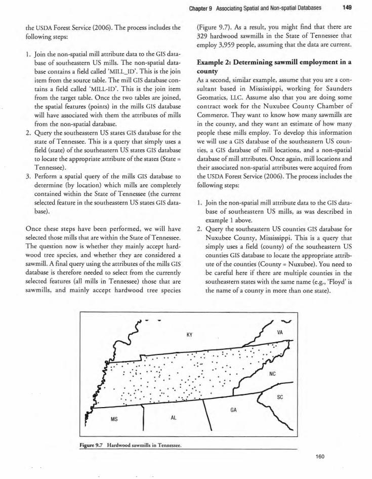
rhe USDA Foresr Service (2006). The process includes rhe fo llowing sreps:
1. Join the non-spatial mill attribute data to the GIS database of southeastern US mills. The non-sparial database comains a field called 'MILL_lD'. This is rhe join item from rhe sou rce rable. The mill GIS database contains a field called 'MILL-lD' . This is the join irem from rhe rarger table. Once the two tables are joined, the spatial features (poims) in the mills GIS database will have associated wirh them rhe attributes of mills from [he non-spatial database.
2. Query rhe southeasrern US srates GIS database for the scate of Tennessee. This is a query that simply uses a field (srate) of the southeastern US "ares GIS darabase to locate the appropriate actcibuce of the scares (State =
Tennessee). 3. Perform a spatial query of rhe mills GIS database to
determine (by location) which mills are completely contained within the Scate of Tennessee (the current
selected feature in the southeastern US states GIS dacabase).
Once these steps have been performed, we will have selected those mills mac are within the Scare of Tennessee. The question now is whether they mainly accept hard
wood [fee species, and whether they are considered a sawmill. A final query using the attribures of the mills GIS database is therefore needed [0 seiect from (he currently
selected features (all mills in Tennessee) those that are sawmills. and mainly accept hardwood reee species
. . . . . . , ' .
. . ' . . '
Chapter 9 Associating Spatial and Non-spatial Databases 149
KY
..
(Figure 9.7) . As a result, you might find that there are 329 hardwood sawm ills in the State of Tennessee that employ 3,959 people, assuming that the data are current.
Example 2: Determining sawmill employment in a county As a second, similar example. assume mat you are a con
sultant based in Mississippi. working for Saunders
Geomacics, LLC. Assume also that you are doing some
CQncract work for the Nuxubee County Chamber of
Commerce. They want (0 know how many sawmills are
in the county, and chey want an estimate of how many
people rhese mills employ. To develop rhis information we will use a GIS database of me southeastern US counfies, a GIS database of mill locations, and a non-spacial
database of mill attributes. Once again. milliocacions and
thei r associated non-spacial attributes were acqui red from
the USDA Forest Service (2006). The process includes the following steps:
1. Join rhe non-spatial mill attribure data (0 the G IS database of southeastern US mills. as was described in
example 1 above. 2. Query the southeastern US counties GIS database for
Nuxubee County, Mississippi . This is a query that
simply uses a field (county) of the sourheastern US counties C IS database [0 locate me appropriate attrib
ute of rhe counties (County = Nuxubee). You need to be careful here if there are muldple counties in the
southeastern scares with me same name {e.g .. 'Floyd' is
(he name of a county in more than one s[a[e).
.: .. . .
". :
MS Al
Figun 9.7 Hardwood sawmills in Tennessee.
160
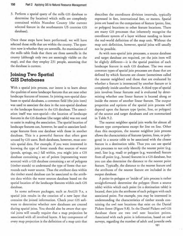
150 Part 2 Applying GIS to Natural Resource Management
3. Perform a spatial query of the mills GIS database [Q
determine (by location) which mills are completely contained within Nuxubee County (the current
selected feature in me southeastern US coumies GIS database).
Once these steps have been performed, we will have selected those mills that are within (he county. The question now is whether they are sawmills. An examination of the mills table finds that there are three sawmills in the
county (although only two are seemingly visible on the map), and that they employ 23 I people, assum ing that the database is currene.
Joining Two Spatial GIS Databases
With a spatial join process. our intent is to learn abour
the qualities of some landscape features that are near other landscape features of imeresr. In joining non-spacial databases [Q spatial databases, a common field (the join item) was used [Q associate the data in the non-spatial database [Q the landscape features in the GIS database. The associ
ation itself was non-spatial-the location of landscape features in the GIS database (the target table) was not used to assist in making the association. The spatia!locarion of landscape fearures can, however, be used (Q associate land
scape fearures from one database with those in another database. This is a powerful feature that often goes unused by GIS users. Both databases, however, mUSt contain spatial data. For example, if you were interested in knowing the type of forest stands that sources of water (ponds, springs, etc.) fall within, you might join a GIS database containing a set of points (representing water sources) with a GIS database containing a set of polygons (t imber stands) to understand the type of forest that surrounds each water source. Thus the attribute data within the timber stand database can be associated to the arr ribute data within the water sources database based on the
spatial location of the landscape features within each GIS database.
In some softwa re packages. such as ArcelS 9.x, a spatial join results in the creation of a new layer that contains the joined info rmation . Check you r GIS software to determine whether new databases 3re created during spatial joins. You should also be aware that spatial joins will usually require that a map projection be associated w ith all involved layers. A key component of every map projection is the definition of a map unit that
describes the coordina te division intervals. typically expressed in feet, international feet, or meters. Spatial joins are based on the comparison of feature (point. line, or polygon) locations to other feature locations. There are many GIS processes that inherently recognize the coordinate system of a layer without needing to know the real-world definition of the map unit. Without the map unir definition, however, sparial joins will usually not be possible.
As with non-spatial join processes, a source database
and target database are required, yet the join item will be slightly different-it is the spatial position of each landscape feature in each GIS database. The [wo most common types of spatial join processes are those that are defined by which features are closest (sometimes called
the nearest neighbor) and those that are evaluated by whether a feature is intersecred by another feature or is completely inside another feature. A third type of spatial join involves linear features and is evaluated by determining whether one linear feature is located along or inside the extent of another linear feature . The outpur
properties and options of the spatial join process will depend upon the feature type (point, line, or polygon) of the source and target databases and are summarized
in Table 9.2 . The nearest neighbor spatial join works for almost all
feature type comparisons except for line on line. Other than this exception, the nearest neighbor join process allows the characteristics of features (points, lines. or polygons) in a source table to be associated with the closest feature in a destination table. Thus you can use spatial join processes to not only identify the nearest point (e.g. tree), line (e.g. road) or polygon (e.g. watershed) feature from all point (e.g., house) features in a GIS database, but you can also determine the distance to the neareSt point
feature . Typ ically. the distance [Q the nearest feature and the anribures of the nearest feature are included in the
Output database. A point-in-polygon or ' inside of join process is rather
straightforward: determine the polygon (from a source table) within which each point (in a destination table) is located, then join the attributes of each polygon with each associated point. For example, you may be interested in understanding the characteristics of t imber stands containing the owl nest locations that exist on the Daniel Pickert forest (Figure 9.8). In the Daniel Pickett owl GIS database there are twO owl nest location points. Associated wirh each point is information, based on owl surveys. regarding the number of adult and juvenile owls
161
150 Part 2 Applying GIS to Nalural Resource Management
3. Perform a spacial query of [he mills GIS dalabase to
de<ermine (by locarion) which mills are completely contained within Nuxubee County (the current selecred feature in the SQUmeasrern US counties GIS database).
Once these Steps have been performed, we will have selected those mills that are within rhe county. The question now is whether they are sawmills. An examination of the mills table finds that there are three sawmills in [he county (al[hough only two are seemingly visible on the map), and that they employ 231 people, assuming that the database is currenL
Joining Two Spatial GIS Databases
With a spatial join process. our imenr is to learn aboul
the qualities of some landscape features that are near other landscape featu res of interest. In joining non-spadaJ databases ro spat ial da[abases, a common field ([he join item) was used [Q associate the data in the non-spatial database to [he landscape features in rhe GIS database. The associalion itself was non-spatia I-the location of landscape fearures in [he GIS database (the target rable) was not used fa ass ist in making the association . The spadallocation of landscape features can, however. be used (Q associate landscape features from one database with those in another database. This is a powerful feam re that often goes unused by GIS users. Both databases, however. must concain spatial data. For example. if you were interested in knowing the rype of torest stands that sources of water (ponds, springs, etc.) fan within, you might join a GIS database containing a set of points (representing water sources) with a GIS database containing a set of polygons (dm ber stands) [0 understand the type of forest that surrounds each water source. Thus rhe anribute data within the timber stand database can be assoc iated to the arnibme dara wirhin the water sources database based on the
sparial locarion of the landscape fea rures within each GIS darabase.
In so me softwa re packages. such as ArcGIS 9.x, a
spatial join results in the creation of a new layer that contains the joined info rmation . C heck you r GIS softwa re CO determine whether new databases are created during spatia l joins. You should a150 be aware that spatial joins will usually requi re that a map projection be associated with all involved layers . A key component of every map projection is the definition of a map unit that
describes the coord inate division inrerva'!s, typically expressed in feer. international fec t, or meters. Spatia l joins are based on the comparison of feamre (poin t, line, or polygon) locadons to other feamre locarions. There are many GIS processes thar inherently recognize the coordinate system of a layer without needing to know [he real-world definition of the map un it. Without the map unit definitio n. however. spatial joins will usually nOI be possible.
As with non-spatial jo in processes. a source database
and rarget database are required. yet the join item wi ll be sligh tly differem-it is the spatial position of each landscape feature in each GIS database. The twO mosr com mon rypes of spat ial join processes are those fhar are defined by which features are closest (sometimes called the neareSt neighbor) and [hose thar are evaluated by whether a feature is intersected by another feature or is completely inside anolher feature . A th ird type of spatial join involves linear features and is evaluated by determining whether one linear feawre is located along or inside the extent of another linear feature. The outpur
properties and options of the spatial join process will depend upon Ihe fearure type (poim, line, or polygon) of the source and target databases and are summarized
in Table 9.2 . The nearesr neighbor spatial join works fo r almost all
feamre type comparisons excepr for line on line. Other
than this except ion. the nearest neighbor join process allows the characrerisrics of features (poinrs. lines, or polygons) in a source table to be associated with the closest feature in a destination table. Thus you can usc spatial join processes ro not only idemifY rhe ne-dtest point (e.g. uee), line (e.g. road) or polygon (e.g. warershed) fearure from all point (e.g., house) features in a GIS database, but you can also determ ine [he distance to the neareSt point
feature. Typ ical ly. the distance to the nearest feature and the anribmes of me nearest feacure are included in the
Output database. A point-in-polygon or 'inside or join process is rather
straightforward: determ ine the polygon (from a source rable) wirhin which each point (in a desrinarion table) is localed, then join the attributes of each polygon with each associated paine For example. you may be interested in understanding rhe characterist ics of (imber sta nds containing [he owl nest locations mat exist on [he Daniel Pickert forest (Figure 9.8). In the Daniel Pickerr owl GIS database [here are twO owl nest location points. Associated with each po int is information, based on owl surveys, regarding the number of adult and juvenile owls
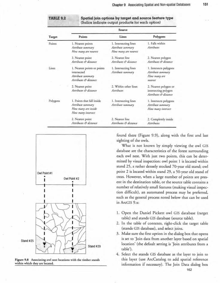
Chapter 9 Associating Spatial and Non-spatial Databases 151
TABLE 9_2 Spatial join options by target and source feature type (Italics indicate output products for each option)
Target
Points
Lilla
Polygons
Owl Point #1
•
•
Stand #25
Poinu
I. Nearest points
Artribuu summary H ow ma,,} a,~ IUllrrSI
2. Nearest point
Attributn &diJlllllU
1. Nearest points o r points
intersected
Attribu/~ summal] Attrihum &-dimmu
2. Nearest poi n t
A ttributn &distallu
I . Poin ts that rail inside
Attrihutr f ummfl,]
How mall) are imitk
How many imm«r
2. Nearest point AllTibutn d- distanu
Owl Poinl#2 • •
Stand #29
Figure 9.8 Associating owl nest locations with the: timber stands withi n which they are located.
1. Intersecting li nes Attrihuu summary How mall) are IU(lreSl
2. Nearest line AttribuUl &diltflllU
I . In tersecting lines
Attribute ru",mary
2. W ithin o ther lines
AltrihuiN
I. Imersecring lines Artribuu sum",ary
2. Nearest line
A ttribum ¢ diuau«
Polygons
I. Falls within AttrihuUl
2. Nearest polygon AttribuU! 6-diJtllfirt
I. In tersects polygons Aurihult' summary How N/ally II"
lIea"st
2. NarcS[ polygon or intersecting polygon Attribuus d- diSlI.m"
I. ImersectS polygons
Attn'buu summary H()w mall] imfl'S«t
2. Compk[dy inside Auribum
fou nd there (Figure 9.9), along with the first and last sighting of the owls.
What is not known by simply viewing the owl GIS dacabase are the characteristics of the forest surrounding each owl nest. With just two points. this can be determined by visual inspection: owl poim 1 is located within stand 25, a rather densely stocked l O-year old stand; owl point 2 is located within stand 29, a 5D-year old stand of trees. However, when a large number of points are presem in me destination table, or the source table comains a number of relatively small features (making visual inspection difficult)' an automated process may be preferred. such as the general process noted below chat can be used in ArcGIS 9.x:
1. Open the Daniel Pickett owl GIS database (target table) and stands GIS database (source table).
2. In the table of contents, right-click the target table (stands GIS database), and seleCt joins.
3. Make sure the first option in the dialog box that opens is set to 'Join data from another layer based on spatial location' (the default setting is 'Join attributes from a table)_
4. Select the stands GIS database as the layer to join to
this layer (use ArcCatalog to add spatial reference information if necessary)_ The Join Data dialog box
162

152 Part 2 Applying GIS 10 Natural Resource Management
Database Table structure
Sourr:e
GIS database representing timber stands
25
: 29 I
A I
A I
. . 260 I 70 I 37.7
: : 200 I 50 I 21.1 "
Target (Destination)
GIS Database representing owl locations
Point
1
2
Ad"1s
2
1
Fledglings Firstsight Lastslght
1 19950618 20070821
0 19980623 20070901 !-
Joined database
Point
1
2
Resulting database: the owl pOints database with the appropriate stand conditions that StXround eacfl point
Adults Fledglings Firstslght
2 1 19950618
1 0 19980623
laslsight SIan<1 Veo_type Basal_area Age Mbl
20070821 25 A 260 70 37.7
20070901 29 A 200 50 21.1
Figure 9.9 Spatially joining the Danid Pickett stanch GIS database with the owl GIS database.
will update to show you the types of feature classes that you are joining, in this case Polygons CO Points.
5. Use the radio or option burron and choose that you
want each point to have the 3([cibures of the polygons [hat 'it fulls inside' ramer (han 'is closest [0 it'.
6. Specify an outpUC location and name for the resulcing joined database.
7. Choose OK to initiate the spatial join.
In ArcView 3.x these general steps can be taken {Q perform the join:
1. Open the Dan iel Pickett owl GIS database (targer table) and stands GIS dat.abase (source table).
2. Open the amibute tables of both GIS databases. 3 . Clear all selecced landscape features in both amibute
tables (to ensure no landscape fearures are selected). 4. With the mouse, click on the join item in the source
table (e.g .• the 'shape' field in ArcYiew) . 5. With the mouse, click on the join item in the target
table (e.g .• the 'shape' field in ArcYiew) . 6. Click the join table bunon to initiate the spatial join
process.
While this example is relatively straightforward, imagine a case where you have several hundred poines. such as research plots. and the goal is to quickly and accurately determine what rype of stand each research plot is located within. A poine-in-polygon join process would seem to be a logical and efficient option to accomplish this goal, and would likely result in fewer errors than a manually driven process.
The spatial join process can also be used to identify the number of features within another point. line. or polygon database that are closest to features within a target database. For example. suppose you had four possible ttail· heads withi n a watershed where you co uld park YOUT
vehicle in order to visit six rain gauges from which YOli
need {Q collect precipitation measurements. Using the trailhead locations (poi nts) as rhe target database. you could spatially join the six rain gauge locations (points) and determine wh ich of the nailheads was closest to the largest number of the six gauges. This would help you at least (Q pick a trai lhead locacion in which to begin your sampling. Another example might include examining a number of watersheds (polygons) and wanting to deter-
163
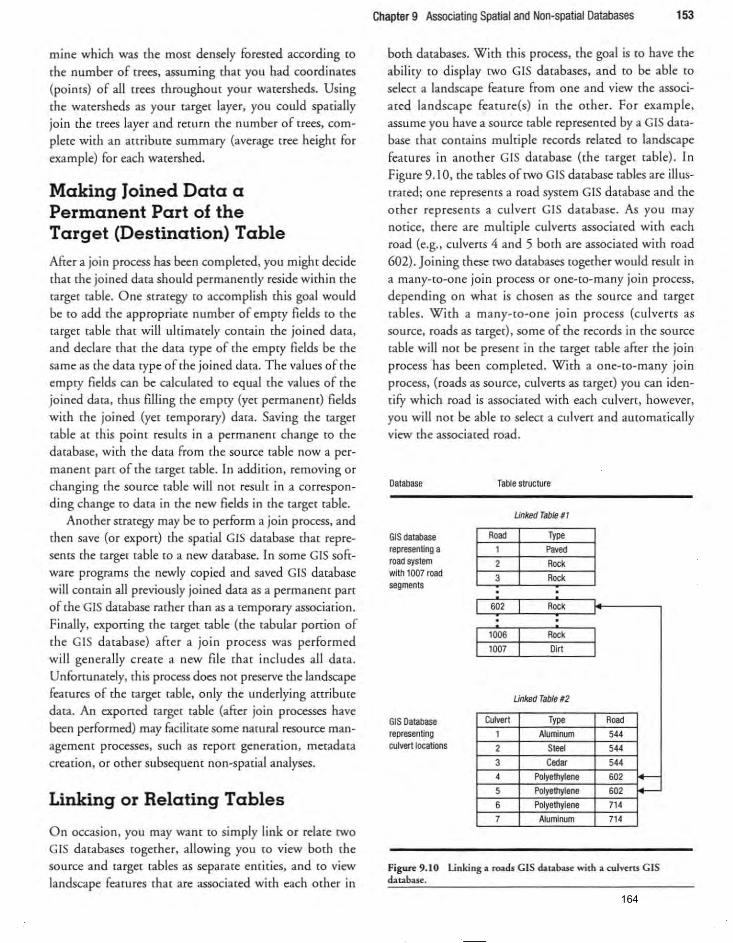
mine which was the most densely forested according to
(he number of uees, assuming that you had coordinates (points) of all trees throughout your watersheds. Using the watersheds as your target layer, you could spatially join the trees layer and return the number of trees, complete with an aruibute summary (average tree height for
example) for each watershed.
Making Joined Data a Permanent Part of the Target (Destination) Table
After a join process has been completed, you might decide that the joined data should permanently reside within the target table. One strategy to accomplish this goal would be to add the appropriate number of empty fields to the target table that will ultimately contain the joined data, and declare that the data type of the empty fields be the same as the data type of the joined data. The va lues of the empty fields can be calculated to equal the values of the joined data, thus filling the empty (yet permanent) fields with the joined (yet temporary) data. Saving the target table at this point results in a permanent change to the database, with the data from the source table now a per
manent pan of the target table. In addirion, removing or changing the source table will not result in a corresponding change to data in the new fields in the target table.
Another suategy may be to perform a join process, and tI,en save (or export) the spatial GIS database that represents the target table to a new database. In some GIS soft
ware programs the newly copied and saved GIS database will contain all previously joined data as a permanent pan of the GIS database rather than as a temporary association. Finally, exporting the target table (the tabular portion of the GIS database) after a join process was performed wi ll generally create a new fil e that includes all data. Unfortunately. this process does not preserve the landscape features of the target table, only the underlying attribute data. An exported target table (after join processes have been performed) may rn.cilitate some natural resource management processes, such as report generation, metadata creation, or other subsequent non-spatial analyses.
Linking or Relating Tables
On occasion, you may want to simply link or relate twO
GIS databases together, allowing you to view both the source and target tables as separate ent ities, and to view landscape features that are associated with each other in
Chapter 9 Associating Spatial and Non-spatial Oatabases 153
both databases. With this process, the goal is to have the abi lity to display twO GIS databases, and to be able to select a landscape feature from one and view the associated landscape feature{s) in the other. For example, assume you have a source table represented by a GIS database that contains multiple records related to landscape featu res in another GIS database (the target table). In Figure 9.10, the tables of twO GIS database tables are illustrated; one represents a road system GIS database and the other represents a culvert GIS database. As you may notice, there are multiple culvertS associated with each road (e.g., culvens 4 and 5 both are associated with road 602) . Joining these twO databases together would result in a manY-CQ-one join process or o ne-to-many join process, depending on what is chosen as the source and target tables. With a manY-(Q-one join process (culverts as
source, roads as targetL some of the records in the source table will not be present in the target table after the join process has been completed . With a one-to-many join process, (roads as source, culvens as target) you can identify which road is associated with each culvert, however, you will not be able to seiect a culvert and automatically view the associated road .
Database
GIS database representing a road system with 1007 road segments
GIS Oatabase representing culvertlocatlons
I
I
Table structure
Unked Table 11
Road Type 1 -2 Rock 3 Rock
602 I Rock
• • 1006
I Rock
1007 Oirt
Linked Table 12
Culvert Type 1 Aluminum
2 SIee1
3 Cedar 4 Polyethylene
5 Polyethylene
6 Polyethylene
7 Aluminum
I
Road 544
544
544
602 -602 -714
714
Figure 9. 10 Linking a roads GIS database with a cuJvcru GIS database.
164
154 Part 2 Applying GIS to Natural Resource Management
Which process-Joining or linking-is more dynamic? Perhaps linking. With linking. you can visualize both the source and target tables. select landscape feamces from either table. and view the
associated links from wither perspective. Further, if
To further illustrate the link or relate process, a general set of steps can be followed in ArcGIS 9.x to associate two GIS databases related (Q the Brown T fact: a culverts data
base (Culverts. txt) and a roads GIS database:
1. Open the Brown Tract roads GIS database and culvens text file.
2. In ,he ,able of contents. right-click the target table (roads GIS database). and select Joins and Relates. then select Relates.
3. Selec, the relate field in the ,arget table. 4. Identify the source table. 5. Select the relate field in the sou rce table. 6. After relating the two databases. perform an identify
process. selecting one of (he roads that are noted in the culvert database. You should be presented with informarion for both the road and the associated culverts along tha, road.
In ArcView 3.x, the following general set of instructions may work to create a link between the roads and the culven databases:
Summary
Join and link processes provide GIS users with a way to
temporary assoc ia te two or more databases. allowing an expansion of the mapping and analysis opportunities within GIS without making permanent changes to the databases. Before utilizing one of these processes you should consider the types of databases available. and the type of association desired (e.g .. one-(O-one, one-to
many. and so o n). In addition. the purpose of the process should be understood. which mighr provide guidance in the choice of a join or link process. For example. you may decide on different courses of action if the purpose is to:
some data are not linked (in either the source or target ,able) they are st ill visible and available for further ana lysis . When a join process is used, source table data not joined with target table data are unavailable
for funher spatial analysis.
1. Open the Brown Tract roads G IS database. 2. Open the roads GIS database attribute ,able (this is the
target table). 3. Open the Culverts. txt file (this is the source table) . 4. Select the link item in the source table (road). 5. Select the link item in the target table (road). 6. Choose Link from ,he Table menu.
At this paim a one-way link becween the roads and culverts databases has been created. The process may need to be repeated with ,he roles reversed (roads GIS database as the source. Culverts.cxt as the target) to create a cwo-way link.
By linking the (wo tables together. you ca n select records in one database (or features in either database), and the landscape features they are associated. with may be selected and highlighted in the other database. For example. after linking together the culvert database with the roads GIS database, you can select one or more culvens. and the roads associated with those culverts may be simul
taneously selected and highlighted in the roads GIS da,abase. In ArcGIS you can view the related data by using the identify tool.
A. Bring together spatial and non-spatial databases to
make thematic maps. B. Funher the abili ty to perform other spatial operations,
such as assoc iating non-spatial stream buffer data with a streams GIS database in order to facilitate a buffer
process. c. Understand the spatial relationship between a sec of
points and other landscape features (through a point
in-polygon process) . D . Understand the association among multiple landscape
features in one database and their counterparts in another database (through a link process).
165
Joining and relating processes often produce databases char are only 'viccually' combined. meaning that no new
databases have been created. but char exist ing informa
rion appears ro be associated either in one [able (with a jo in) or in twO tables (with a relate) . GIS users should recognize mat this temporary condition exiS(5 and that fur
ther acr ian is necessary in order fo r a permanent record of
rhe joined or linked info rmation to be created. The
Applications
9.1. Salamander habitat suitability index. Bob Evans, the Brown Tract's wildl ife biologist/hydrologist, developed some habitat suitabili ty index (HSi) values for a salamander. He suggests joining rhe data provided in 'SAL_HSl.txt ' with the Brown T ract stands GIS database. He then wants you ro answer several questions abour the extenr and spadal distribution of these areas, which are summarized below.
a) How much land area is contained in the 0 .8 [Q 1.0 HSI range?
b) How much land area is contained in the 0.6 to
0.79 HS I range? c) How much land area is contained in the 0.4 [Q
0.59 HSI range?
9.2. Newt habitat suitability index. Bob Evans has also developed some habitat suitabil ity index (HSi) values for a newt. He provided data in the file 'NEWf_HS l. rxr' . After joining the dara with the Brown Tract stands GIS database, please address his needs, which are noted below.
a) Determine how much land area of high quali ty newt habitat (HSI ~ 0.65) is contained with in 100 m of the road system.
b) Determine how much land area of high quality newt habitat (HSI ~ 0.65) is contained withi n 1,000 m of the owl nest site.
c) Determine how much land area of high quality newt habitat (HSI ~ 0.65) is contained in even-aged stands over 50 years of age.
9.3. Sharp-shinned hawk habitat suitability index. In addition to his previously discussed developments, Bob Evans has also developed some habitat suitability index (HSi) estimates for the sharp-shinned hawk covering the years 2010, 2020, 2030, and 2040. His rendeney to provide this data in a texr file continues, and you can fin d it in 'SSHAWK_HSl.txt'. After joining the data with the
Chapter 9 Associating Spatial and Non-spatial Databases 155
exception to this vinuai [esuh is with a spatial join, in which results are usually stored in a new database that conrains all sparially jo ined info rmation. You should
check your software package to determine wherher it fol
lows these OutpUt results in the same way. Regardless of
which process (tabular-based or spatial join) is used to associate two databases. users should track thei r proce
dures and manage the ourpur acco rdingly.
Brown Tract stands GIS database, please address his needs noted below.
a) Determine how much land area of higher quality habitat (0.6-1.0) is contained within the Brown Tract.
b) Prod uce a single map of the sharp-shinned hawk habitar showing HSI values for the years 2010, 2020, 2030, and 2040.
9.4. Water sources and land allocations. John Frewer, a forester associated with the Brown Tract, is interested in knowi ng what types of land allocations the water sou rces were located w ithin. To accomplish this task, perform a
poine- in-polygon operation (or selection by locar ion query), using the water sources as the source table and the stands GIS databases as the target table.
a) How many water sources are located in 'Even-aged' stands on the Brown T ract?
b) What types of water sources are located in unevenaged stands (lisr the water source types)?
c) How many water sources are located in research areas?
9.5. Sawmills in a woodshed. You have recently been hired as a procu rement forester for Chupp and Daughters Sawmill in Floyd County, GA. You need to understand the competit ion for wood in the area. To perform rhis task, use the southeastern counties GIS database, the southeastern mills GIS database, and the mill data DBF fi le. Join the mi ll data DBF file to the southeastern mills GIS database and determine how many sawmills are within 100 miles of Floyd County, GA. The mill locations and non-spatial mill a[cribures can be acquired from the book's website or the USDA Forest Service (2006).
9.6. New mill location. You work for Walker, Avery, and Housron Lumber Company, a company that is
166
156 Part 2 Applying GIS to Natural Resource Management
considering building a new hardwood sawmill mill in Coffee County, AL. They need to understand how much hardwood volume currently exists in (he area
around the county. To perform this task, use rhe southeastern counties GIS database and rhe county volume DBF file.
References
USDA Forest Service. (2006). US wood-using mill locat;0",-2005. Research Triangle Park, NC: USDA Forest Service, Sourhern Research Stadon. Retrieved
April 16, 2007, from http: //www.srs.fs.usda.gov/econ/ data/mills/miIl2005 .htm .
Join the county volume DBF file to the somheastern counties GIS database and determine how much hardwood (soft and hard) volume is conrai ned in the counties that surround, and include, Coffee County. The countylevel can be obtained from the book's website or the USDA Forest Service (2007) .
USDA Forest Service. (2007) . FIA data mart: Download files. St Paul , MN: USDA Fo rest Service, North Central Research Station. Retrieved April 16, 2007, from http ://www.ncrs2 .fs.fed.us/FIADatamart/ fiaclaramarc.aspx/fiadaraman.aspx.
167
Chapter 10
Updating GIS Databases
Objectives
This chapter is designed (Q provide readers with a discussion of GIS processes that should be considered when updacing GIS dacabases. Database updates are necessary when landscapes and associated characteristics. such as
ownership, change. There are a variety of methods you can use to update a GIS database, yet only a few are pre
semed here. The objective of this chapter. therefore. is to
provide an introduction to the poremiai applicarions in (his area. More specifically, at the conclusion of this chap
ter, readers should be able to understand:
I. why GIS databases need to be periodically updated and maintained,
2. what issues might be associated with an update process, and
3. whar GIS processes could be used to physically update a database.
To accomplish these objectives, a discussion of the reasons for updating GIS databases is firsr presented. Two rypes of update processes are then examined, one where new land
scape features are added to an existing GIS database, and
another where me landscape features and attributes in an
exisring GIS database are modified. These cwo examples likely address rhe [WO most common fo rms of GIS darabase updares. This chapter relies heavily on the GIS processes associated with edicing GIS databases. For a
review of these editing processes. please refer to chapter 3 . GIS databases are rarely considered stacic entities: vege
tation conditions change due to human manipulation and
namral disturbances. roads are constructed and obi iter-
ated, and some stream characteristics {pools. sediment, fish
abundance} may change as woody debris moves through the system. Although you may have developed or acquired GIS databases at one point in time. as management needs
or direction change. or as the resources you manage
change, GIS darabases used to describe landscapes must be updated. Table 10. 1 illustrates a number of events that
could occur and affect the landscape being managed, suggesting that the GIS databases used to describe rhe landscape being managed must be updared to reflect changes. Most natural resource management organizations (as well
as data development o rganizations) have created a set of
processes and protocols to guide the updating of GIS databases. Finding and illustrating a standard protocol is.
therefore. difficult because each organization generally will develop the steps they feel are necessary to integrate new
dara within their system of natural resource information.
For example. assume a tract ofland was recendy purchased
by a land management organization. Integrating the forest
stand component of this new tract into a forest stand GIS
database can be accomplished in a number of ways, such
as the three processes described in Figure 10. 1. As database protocols and organization strategies vary from one organ
ization to anomer. there is no one update approach thar will work for every organization .
The users of GIS databases are the ultimate customers
of groups (GIS departments. consultants, agencies) that produce the sparial data. As GIS databases become available, and users begin to explore the usefulness of rhe data for assisting in natural resource management processes. the limitations of [he databases will become evident. The
period of rime from initial GIS database availability to
serious consideration of updates tQ the databases may last 168
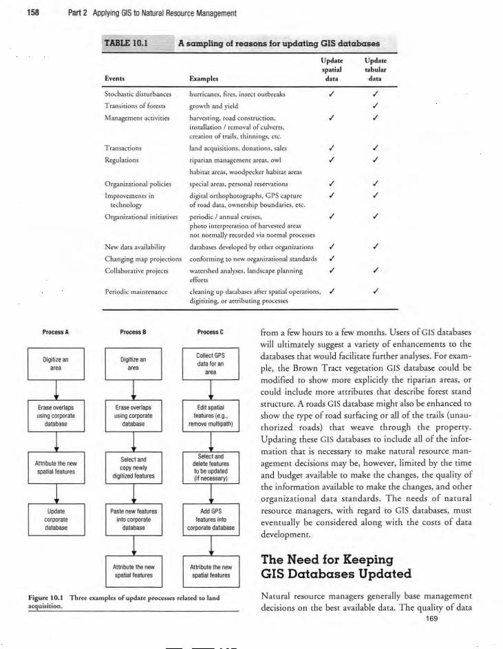
158 Part 2 Applying GIS to Natural Resource Management
Process A
Digitize an area
1 Erase overlaps using corporate
database
1 Attribute the new spatial features
1 Update
COij)Orate database
TABLE 10.1 A sampling 01 reasons lor updating GIS databases
Events
Stochastic disturbances
T ransiriOlls of (orcslS
Management activi ties
T ransacrions
Regulations
Organizational policies
Improvemcnu in technology
Organizational initiatives
New data availabiliry
C hanging map projections
Collaborative projectS
Periodic maintenance
Process B
Digitize an area
1 Erase over131>S using corporale
database
1 Select and copy newly
digitized features
t Paste new features
Inlo corporate database
1 Attribute the new spatialfealures
Update Update spatial tabular
Examples data data
hurricanes. fires. insect outbreaks 01' 01'
growth and yield 01'
harvesting. road consuucrion, 01' 01' insrallalion I removal of culverts. creation of trails. thinnings. NC.
land acquisitions. donations. sales 01' 01'
riparian management areas, owl 01' 01'
habitat areas, woodpecker habitat areas
special areas. personal reservations 01' 01'
digital onhophotographs, GPS captu re: 01' 01' of road data, ownership boundaries, crc.
periodic I annual cruises. 01' 01' photo interpretation of harvested areas not normally recorded via normal processes
databases developed by other organizations 01' 01'
conform ing to new o rganizational standards 01'
watershed analyses. Ia.ndscape planning 01' 01' efforts
cleaning up databases after spatial operations. 01' 01' digitizing, or anributing processes
Process C
Collect GPS data lor an
area
1 Edit spatial
features (e.g., remove muttipath)
1 Select and
delete features to be updated (i l necessary)
1 AddGPS
features Into corporale database
1 Attribute the new spatial features
from a few hours to a few months. Users of GIS databases will ultimately suggest a variety of enhancements to the databases that would facilitate further analyses. For example, the Brown T ract vegetation GIS database could be modified to show more explicitly (he riparian areas, or could include more anributes that describe forest stand structure. A roads GIS database might also be enhanced to
show the type of road surfacing or all of the trails (unauthorized roads) that weave through the property. Updating these GIS databases ro include all of the informarion (hat is necessary to make natural resource management decisions may be, however, limited by the time and budget available ro make the changes, the quality of (he information available to make the changes. and other organizational data standards. The needs of namral resource managers. with regard to GIS databases. must eventually be considered along with (he costs of data development.
The Need for Keeping GIS Databases Updated
Figure 10.1 Three examples of update processes related to land acquisition.
Natural resource managers generally base managemem decisions on the best available data. The quality of data
169
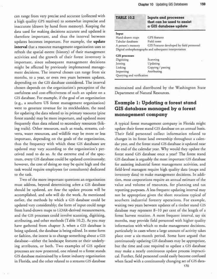
can range from very precise and accurate (collected with a high qual ity GPS receiver) to somewhat imprecise and inaccurate {drawn by hand from memory}. Keeping the data used for making decisions accurate and updated is therefore imponant, and thus the interval between updates becomes important. For example, the update interval that a resource managemem organization uses to
refresh the spatial extent {history} of their management activities and the growth of their forest inventory is imponant, since subsequent management decis ions might be affected by previously implemented managemem decisions. The imerval chosen can range from six momhs. to a year, or even (WO years between updates, depending on the GIS database considered. The interval chosen depends on the organization's perception of the usefulness and cost-effectiveness of such an update on a GIS database. For example, if the goal of an organization (e.g., a southern US forest management organization) were to generate revenue for its stockholders, the need for updating the data related to its primary resource (pine forest stands) may be more important, and updated more frequently than data related to secondary resources (hiking trails). Other resources, such as roads, streams, culvens, water resources, and wildlife may be more or less imporram, depending on the goals of the organization, thus the frequency with which these GIS databases are updated may vary according to the organization's perceived need to do so. At the extreme end of the spectrum. every GIS database could be updated continuously; however, the cost of doing so may be qu ite high and the task would require employees {or consultants} dedicated to the task.
Two ofche more important questions an organization must address, beyond determining when a GIS database should be updated, are how the update process will be accomplished, and who will do the work. As mentioned earlier, the methods by which a GIS database could be updated vary considerably; the fo rm of input cou ld range from hand-drawn maps to LiDAR-derived measurements, and the GIS processes could involve scanning, digitizing. attributing, and other methods {Table 10.2} . As you may have gathered from chapter 3, when a GIS database is being updated, rhe database is being edited. In some form or fashion , the imem is to change something about a GIS database-either the landscape features or their underlying attributes, or both. Two examples of GIS update processes are now presemed, one related to a forest stands GIS database maimained by a forest industry organization in Florida, and the other related to a streams GIS database
TABLE 10.2
Input
Chapter 10 Updating GIS Databases 159
Inputs and processes that can be used to a ssist a GIS database update
Hand-drawn maps GPS features T2bu lar datab2Ses Field nOles A person's memory GIS Features developed by field personnel Digital orthophotographs and subsequent interpretation
GIS processes Digitiring Scanning Joining Updating Linking Copying J p2Sting Importing Attributing Querying and verification
mai ntained and distributed by the Washington State Department of Natural Resources.
Example 1: Updating a forest stand GIS database managed by a forest management company
A typical forest management company in Florida might update their forest stand GIS database on an annual basis. Their field personnel collect information related {Q
changes in irs forest land ownership throughout a calendar year, and the forest stand GIS database is updated near the end of the calendar year. Why would they update the forest stand GIS database once a year? The forest stand GIS database is arguably the most important GIS database for assisting industrial forest management activiries, and field-level managers require high quality data (maps and inventory data) to make managemem decisions. In addition, most corporations require an annual estimate of the value and volume of resources, for planning and tax reporting purposes. A less frequent updating interval may not be appropriate given the short rotacions typical of southern industrial forestry operations. For example, waiting two years between updates of a timber stand GIS database may represent 8-10 per cent of the lengrh of a forest harvest rotation. A more frequent imerval, say six months, may provide field personnel with higher qualiry information with which to make management decisions, particularly in cases where a large amount of activity takes place over a six-month period. Some have argued (hat continuously updating GIS databases may be appropriate. but the: time and cost required to update a GIS database may make a nearly continuous update process impractical. Further, field personnel could easily become confused when faced with a cominuously changing set of GIS data-
170
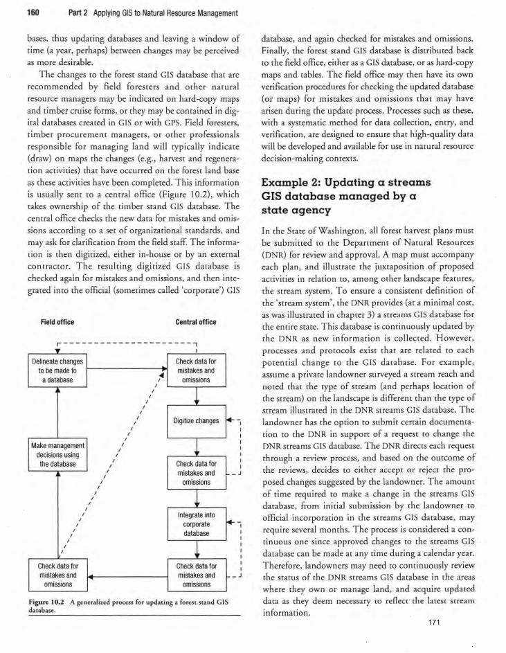
160 Part 2 Applying GIS to Natural Resource Management
bases. thus updating databases and leaving a window of time {a year. perhaps} between changes may be perceived as more des irable.
The changes to the forest stand GIS database that are
recommended by field foreSters and other natural resource managers may be indicated on hard-copy maps and timber cruise forms. or they may be comai ned in d igital databases created in GIS or with GPS. Field foresters. timber procurement managers. or other profess ionals
responsible for managing land will typically indicate {draw} on maps the changes {e.g .• harvest and regeneration activi ti es} that have occurred on [he forest land base
as these act ivit ies have been completed. This informacion is usually sent to a central office {Figure 10.2}. which takes ownership of the timber Stand GIS database. The cemral office checks rhe new data for mistakes and omissions according to a set of organizational standards, and may ask for clarification from the field staff. The information is rhen digitized, either in-house or by an external con n actor. The resuhing digitized GIS database is checked again for mistakes and omissions, and then ime
grated into the official {sometimes called 'corporate} GIS
Field office Central office
r------ ---- ------- ----, .. , Delineate changes Check data for
to be made to ~
mistakes and a database , omissions , ,
L , , , , , Digitize changes ~ , , , ,
~ Make management , , decisions using , the database
, Check data for , , mistakes and r-, , omissions , ,
L , , , , Integrate into , ~ , corporate ,
database , , ~
, , Check data for Check data for mistakes and mistakes and -
omissions omissions
Figurc 10.2 A gcnerali"lcd proces.s for updating a forest stand C IS database.
, , , , , , , , J
-,
, J
database. and again checked for mistakes and omissions. Finally. the forest stand GIS database is distr ibuted back to the field office. either as a GIS database. or as hard-copy maps and tables. The field office may then have itS own
verification procedures for checking the updated database (or maps) fo r m istakes and omissions that may have arisen during the update process. Processes such as these. with a systematic method for data collection. entry, and verification, are designed to ensure that high-qual icy data
will be developed and avai lable for use in natural resource decision-making contexts.
Example 2: Updating a streams GIS database managed by a state agency
In rhe State of Washington, all fo rest harvest plans must be subm itted to the Department of Natu ral Resources
{DNR} for review and approval. A map must accompany each plan, and illustrate the juxtaposition of proposed activities in relation to, among other landscape features, the stream system. To ensure a consistent definition of the 'stream system', the DNR provides (at a minimal COSt, as was illustrated in chapter 3) a streams GIS database for the entire state. This database is conti nuously updated by the DNR as new info rmat ion is co llected. However,
processes and protocols exist that are related [Q each potential change to the GIS database. For example, assume a private landowner surveyed a stream reach and
noted that the type of stream {and perhaps location of the stream} on the landscape is different than the type of stream illustrated in rhe DNR streams GIS database. The landowner has the option to submit certain documentation [Q the DNR in suppOrt of a request to change the DNR streams GIS database. The DNR d irects each request
through a review process, and based on the outcome of the reviews, decides [0 ei ther accept or reject the pro
posed changes suggested by the landowner. The amount of time required to make a change in the streams GIS database, from init ial submission by the landowner to official incorporation in the streams GIS database, may require several months. The process is considered a continuous one since approved changes to [he streams GIS database can be made at any time during a calendar year.
Therefore, landowners may need to continuously review the statuS of the DNR streams GIS database in the areas where they own or manage land, and acquire updated data as they deem necessary to reflect the latest stream
info rmation. 171
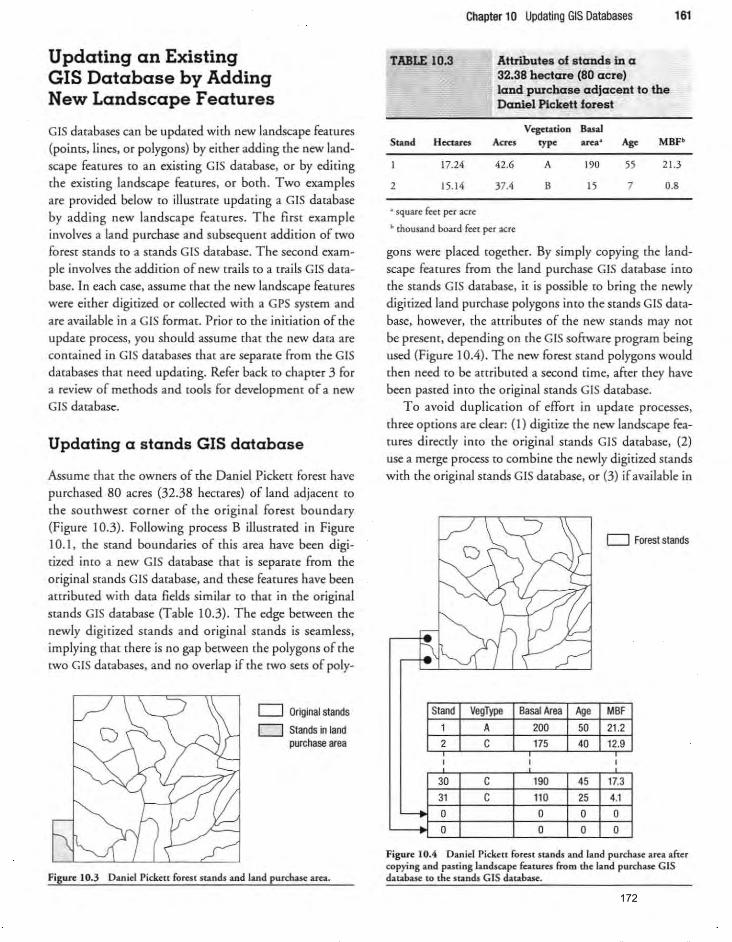
Updating an Existing GIS Database by Adding New Landscape Features
GIS databases can be updated with new landscape features (points. lines. or polygons) by either adding the new landscape features (Q an existing GIS database, or by editing the existing landscape features. or boch . Two examples are provided below to illuStrate updating a GIS database by adding new landscape features . The firSt example involves a land purchase and subsequenr addition of twO
forest stands co a stands GIS database. The second example involves the addition of new trails to a trails GIS database. In each case, assume that the new landscape features
were either digitized or collected with a GPS SYStem and are available in a GIS format. Prior to [he iniciarion of the update process, you should assume that the new data are comained in GIS databases that are separate from the GIS databases that need updating. Refer back to chapter 3 for a review of methods and tools for development of a new GIS database.
Updating a stands GIS database
Assume that (he owners of me Daniel Pickett forest have
pu rchased 80 acres (32.38 hectares) of land adjacent to the southwest corner of the original forest boundary (Figure 10.3). Following process B illuStrated in Figure 10.1. the Stand boundaries of this area have been digitized inco a new GIS database chat is separate from the o riginal stands GIS database. and these features have been attributed wim data fields similar to that in the original stands GIS database {Table 10.3}. The edge between the newly digitized stands and original stands is seamless,
implying that there is no gap between the polygons of the two GIS databases. and no overlap if the two sets of poly-
D Original stands
D Stands in land purchase area
Figure 1 0.3 Dani~1 Pick~[( for~$[ stands and land purchase area.
Chapter 10 Updating GIS Databases 161
TABLE 10.3
Smnd Hectares
2
17.24
15.t4
• squar~ f«t per acr~
Attributes of stands in a 32.38 hectare (80 acre) land purchase adjacent to the Daniel Pickett forest
Vegetation Basal Acus type area" Age MBP
42.6
37.4
A
8
190
15
55
7
21.3
0.8
h thousand board fttt per acr~
gons were placed together. By simply copying the land
scape features from the land purchase GIS database into the stands GIS darabase. it is possible to bring the newly
digitized land purchase polygons into the stands GIS database, however. the attributes of the new stands may not
be present. depending on the GIS software program being used (Figure 1 0.4) . The new fo rest stand polygons would then need to be attributed a second dme, after they have been pasted intO (he original stands GIS database.
To avoid duplication of effort in update processes, three options are clear: (l) digitize the new landscape features directly into the original stands GIS database. (2) use a merge process to combine the newly digitized stands with the origi nal stands GIS database. or (3) if available in
Stand
1
2
30
31
o o
VegType
A
C
c c
Basal Area
200
175
190
110
o o
D Forest stands
Age MBF
50 21.2
40 12.9
45 17.3
25 4.1
o 0 o o
Figur~ 10.4 Daniel Pick~n forest stands and land purchas~ ar~a aft~r copying and pasting landscape fntures from th~ land purch3# GIS datah3# to th~ stands GIS database.
172
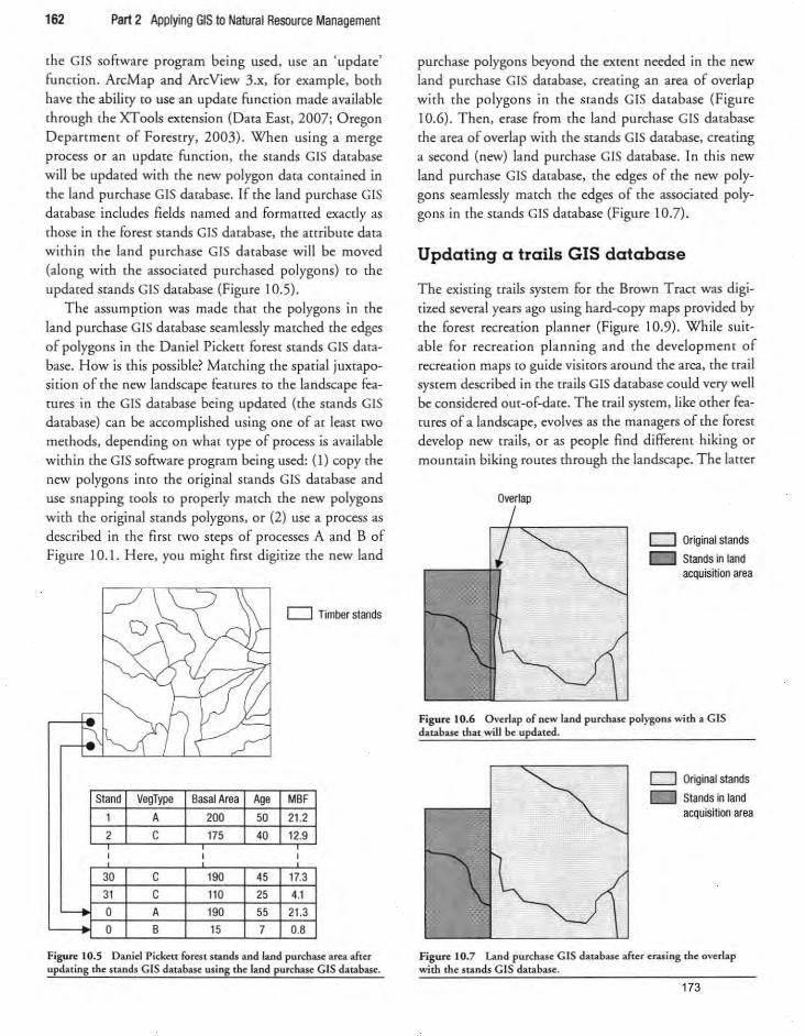
162 Part 2 Applying GIS to Natural Resource Management
rhe GIS software program being used, use an 'updare' funcrion . ArcMap and ArcView 3.x, for example, both
have (he ability to use an update function made available
rhrough the XTools extension (Data Easr, 2007; Oregon Department of Foresrry, 2003). When using a merge process or an update funC[ion, the stands GIS database
will be updared with rhe new polygon dara contained in
the land purchase GIS darabase. If rhe land purchase GIS database includes fields named and formarred exactly as those in the forest stands GIS database, the 3ttrihme data wi[hin [he land purchase GIS da[abase will be moved
(along wi[h rhe associared purchased polygons) to rhe updared srands GIS darabase (Figure 10.5).
The assumprion was made rhac [he polygons in che
land purchase GIS darabase seamlessly marched [he edges of polygons in rhe Daniel Picke" foresr scands GIS da[abase. How is this possible? Matching rhe spacial juxtaposition of the new landscape features to the landscape feacures in [he GIS da[abase being updaced (the stands GIS da[abase) can be accomplished using one of at leasc cwo
mechods, depending on what rype of process is available within the GIS software program being used: (I) copy [he new polygons into the original stands GIS database and
use snapping tools [0 properly match rhe new polygons wi[h the original scands polygons, or (2) use a process as described in the fi rst cwo sceps of processes A and B of Figure 10.1. Here, you might firsc digi[ize the new land
Stand
1
2
30 31
o o
VegType
A
C
c c A
B
Basal Area
200
175
190
110 190
15
D Timber stands
Age MBF
50 21.2
40 12.9
45 17.3
25 4.1
55 21.3
7 0.8
Figu~ 10.5 Daniel Pickett forest stands and land purchase ana after updlUing the stands GIS database wing the land purchase GIS database.
purchase polygons beyond che excent needed in the new land purchase GIS database, creating an area of overlap
with the polygons in [he "ands GIS database (Figure 10.6). Then, erase from [he land purchase GIS da[abase the area of overlap with the stands GIS database, creating
a second (new) land purchase GIS database. In [his new
land purchase GIS database, [he edges of the new polygons seamlessly match the edges of [he associated polygons in the stands GIS database (Figu re 10.7).
Updating a trails GIS database
The existing trails system for the Brown Tract was digi
tized several years ago using hard-copy maps provided by the forest recreation planner (Figure 10.9). While suitable for recreation planning and the development of
recreation maps to guide visitors around the area, the trail syscem described in the [rails GIS database could very well be considered out-of-da[e. The [rail system, like ocher fea[Ures of a landscape, evolves as the managers of the forest
develop new trails, or as people find different hiking or mountain biking rouces through the landscape. The latter
Overlap
D Or~inal stands
Stands in land acquisition area
Figure 10.6 Overlap of new land purchase polygons with a GIS database that will be updated.
D Original stands
o Stands in land acquisition area
Figure 10.7 Land purchase GIS dat:lbasc after erasi ng the overlap with the stands GIS database.
173
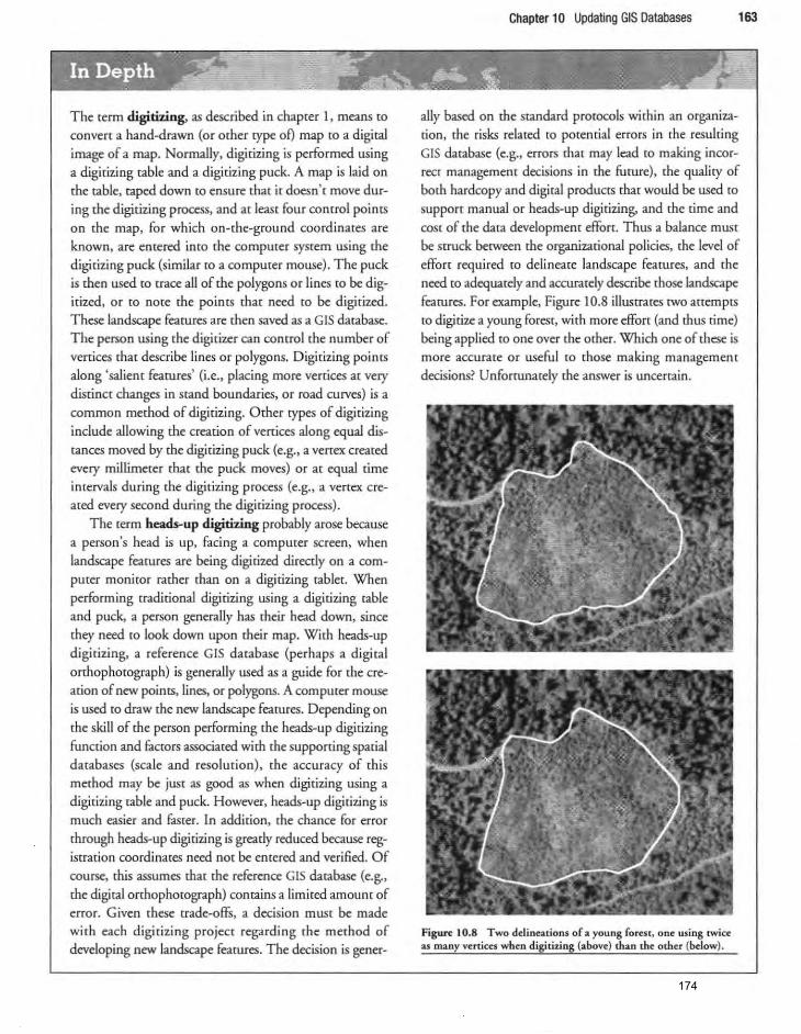
The term digitizing, as described in chapter I. means to
cooven a hand-drawn (or other rype 00 map CO a digical image of a map. Normally. digitizing is performed using a digidzing table and a digitizing puck. A map is laid on the table, taped down to ensure that it doesn'[ move during [he digitizing process. and at least four control points on the map. for which on-the-ground coordinates are known, are emceed imo the compurcr system using the digitizing puck (similar co a computer mouse) . The puck is <hen used ro trace all of <he polygons or lines to be digitized, or (Q nme the poinrs that need ro be digjrited. These landscape features are then saved as a GIS database. The person using the digitizer can control [he number of vertices that describe lines or polygons. Digitizing points along 'salient features' (i .e .• placing more vertices at very distinct changes in stand boundaries. or road cUlVes) is a common method of digitizing. Other types of digitizing include allowing the creation of vertices along equal disranees moved by the digitizing puck {e.g., a venex created every millimeter mat the puck moves} or at equal time intervals during the digitizing process (e.g., a vertex created evety second during <he digitizing process).
The term heads-up digitizing probably arose because a person's head is up. facing a computer screen, when landscape features are being digitized directly on a computer monicor rather than on a digitizing tablet. When performing traditional digitizing using a digitizing table and puck. a person generally has <heir head down. since they need to look down upon their map. With heads-up digitizing, a reference GIS database (perhaps a digital or<hophotograph) is generally used as a guide for the creation of new points. lines, or polygons. A compucer mouse is used to draw the new landscape features. Depending on the ski ll of <he person performing the heads-up digitizing
function and factors associated with the supporting spatial databases (scale and resolution), the accuracy of this method may be just as good as when digitizing using a digitizing table and puck. However, heads-up digitizing is much easier and faster. In addition. the chance for error through heads-up digitizing is greatly reduced because registration coordinares need not be entered and verified. Of course, this assumes that the reference GIS database (e.g., <he digital orthophotograph) contains a limited amount of error. Given these trade-offs, a decision must be made with each digitizing project regarding the method of developing new landscape features. The decision is gener-
Chapter 10 Updating GIS Databases 163
ally based on <he standard protocols within an organization, (he risks relared to potential errors in the resulting GIS database (e.g., errors mat may lead to making incorrect management decisions in the future), the quality of both hardcopy and digital products <hat would be used to
suppon manual or heads-up digitizin~ and the time and cost of the dara development effon. Thus a balance must be struck between <he organizational policies. <he level of
effon required to delineate landscape features, and the need to adequately and accurately describe those landscape
features. For example. Figure 10.8 illustrates twO artempts to digitize a young forest, with more effort (and rhus rime) being applied to one over the other. Which one of these is more accurate or useful ro those making management decisions? Unfortunately the answer is uncenain.
Figure 10.8 Two delineations of a young fores l, one using twice ;u many vertices when digitizing (above) than the other (below).
174
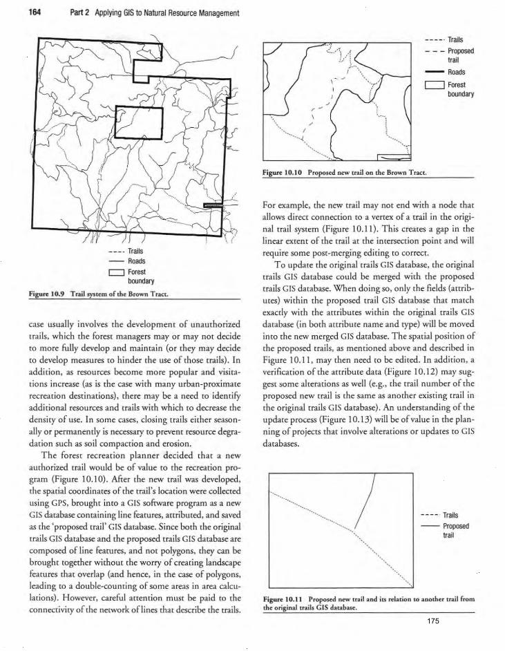
164 Part 2 Applying GIS to Natural Resource Management
--- - Trails -- Roads [:=J Forest
boundary
Figure 10.9 Trail system of the Brown T r:lCL
case usually involves the development of unauthorized tra ils. which the fo rest managers mayor may not decide to more fully develop and mainta in (or they may decide to develop measures to hinder the use of those trails) . In addition, as resources become more popular and visitations increase (as is the case with many urban-proximate recreation destinations), there may be a need CO identify additional resources and trails with which to decrease the density of use. In some cases, closing trails either seasonally or permanently is necessary to prevem resource degra
dation such as soi l compaction and erosion. The forest recreation planner decided that a new
authorized (rail would be of value (0 the recreation program (Figure 10.10). Mor the new trail was developed, the spatial coordinates of the trail's location were collected using GPS, brought into a GIS software program as a new GIS database comaining line features, attributed, and saved as the 'proposed trail' GIS database. Since both the original trails GIS database and the proposed trails GIS database are composed of line features, and not polygons, they can be brought together without the worry of creating landscape featu res that overlap (and hence, in the case of polygons, leading (Q a double-counting of some areas in area calculations). However, careful anention must be paid to the
connectivity of the network of lines that describe the trails .
\. ./
.•..••.. I
'. <" .......
....•.
1
i .. ....... ~ .
\
---- . Trails
- - - Proposed trail
- Roads
CJ Forest boundary
Figure 10.10 Proposed new trail on the Brown Tract.
For example. the new trail may not end with a node that allows direct connection to a vertex of a trail in the origi
nal trail system (Figure 10.1 1). This creates a gap in the linear extent of the trail at the intersection point and will
require some post-merging editing to correct. To update the original trails GIS database, the original
trails GIS database could be merged with the proposed trails GIS database. When doing so, only the fields (attributes) with in the proposed trail GIS database that match exactly with the attributes within the original tra ils GIS database (in both attribute name and type) will be moved into the new merged GIS database. The spatial position of the proposed trails , as mentioned above and described in Figure 10.1 I. may then need to be edited. In addition, a verificat ion of the attribute data (Figure 10.12) may suggest some alterations as well (e.g .• the trail number of the proposed new trail is the same as another existing (rail in the original trails GIS database) . An understanding of the update process (Figure 10.13) will be of value in the planning of projects that involve alterations or updates to GIS
databases.
---- . Trails
-- Proposed
.... , .""',.,.,"
trail
",
....... "',
Figure 10.11 Proposed new trail and iu relation to another trail from the origina1 trails GIS d21abase.
175
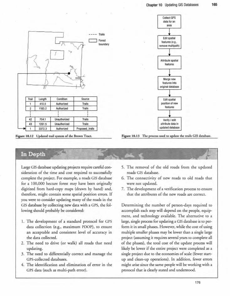
.... < ..
c;. .,,0
---- Traits
c::::::J Fores. boondary
----'.'. ! ;
:~ ~:r, ...
><"'::~:;::"'~(' <./ .: .'
Trail Length Conation Source
410.5 AuthOfized Trails
2 1183.2 AuthOfized Trails
42 704.1 Unauthorized Trails
43 1261.5 Unauthorized Trails
Figure 10.12 Updated trail system of the Brown Tract.
Large GIS database updating projectS require careful con
sideration of the time and COst required to successfully complete the project. For example, a roads GIS database for a 100,000 hectare foresr may have been originally digitized from hard-copy maps (drawn by hand) and, therefore, might contain some spatial position errors. If you were to consider updating many of the roads in the GIS database by collecting new data with a GPS, the following should probably be considered:
I. The development of a sta ndard protocol for GPS data collection (e.g., maxi mum PDOP), to ensure an acceptable and consistent level of accuracy in the data coUected.
2. The need to drive (or walk) all roads that need
updating. 3. The need to differentially correct and manage the
GPS-collected databases. 4. The identification and elimination of error in the
GPS data (such as multi-path error).
Chapter 10 Updating GIS Databases 165
Collect GPS data IOf an
area
~ Edit spatial
leatures (e.g., remove multipalh)
~ Attribute spatial
features
~ Merge new
features into original database
~ Edit spatial
position of new features
~ Verify I edit
allribtJte data In updated database
Figun 10.13 The process used to update the trails G IS database.
5. The removal of the old roads from the updated roads GIS database.
6. The connectivity of new roads [0 old roads that
were not updated. 7. The developmen( of a verification process to ensure
that (he attributes of (he new roads are correct.
Determining the number of person-days required to accomplish each step will depend on the people, equipment, and technology available. The alternative [0 a large, single process fo r updating a GIS database is to perform it in small phases. However, while the COS( of using
multiple smaller phases may be lower than a single large project (assuming it requires several years to complete all of the phases), the total cost of the update process will likely be lower if the entire project were completed as a single project due to the economies of scale (fewer stanup and clean-up operations) . In addition, fewer errors might arise since the same people will be working with a protocol that is clearly stated and understood.
176
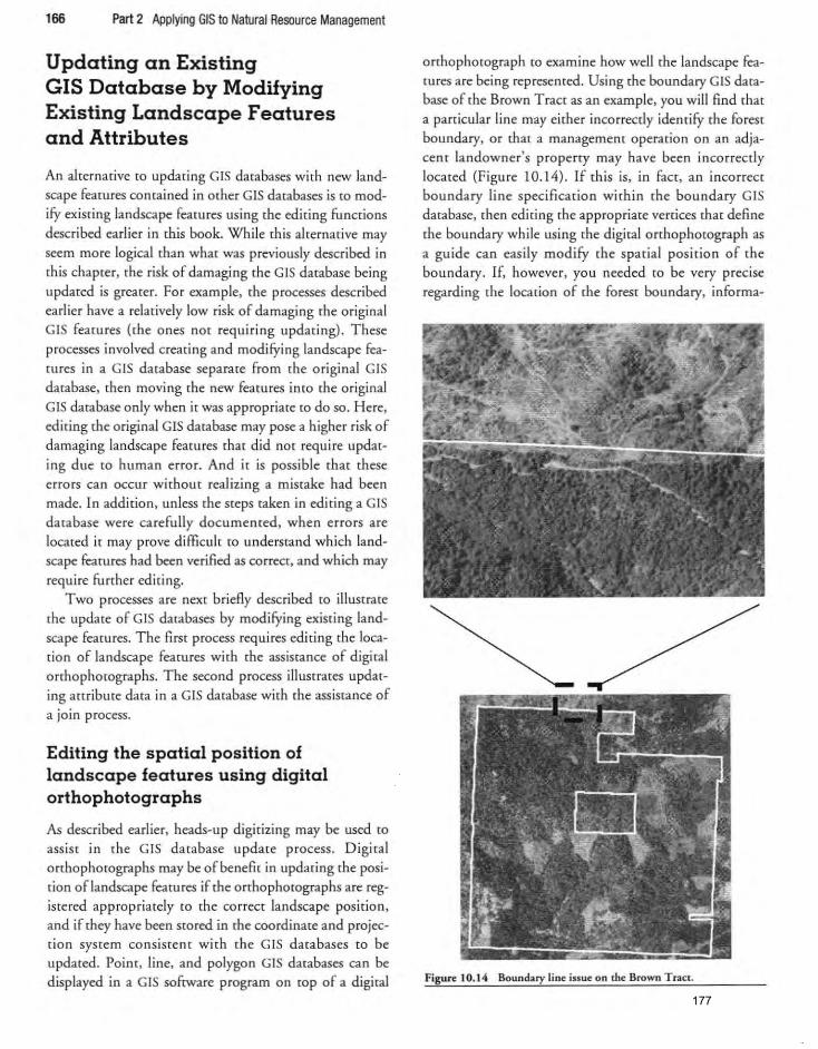
166 Part 2 Applying GIS to Natural Resource Management
Updating an Existing GIS Database by Modifying Existing Landscape Features and Attributes
An alternative to updating GIS databases with new landscape features contained in other GIS databases is [0 modify existing landscape features using [he editing functions described earlier in this book. While this alternative may seem morc logical than what was previously described in
this chapter. the ri sk of damaging the GIS database being updated is grearer. For example. the processes described earlier have a relatively low risk of damaging the original GIS features (the ones not requiring updating). These processes involved creating and modifying landscape fearures in a G IS database separare from the original GIS database, then moving the new features into the original GIS database only when it was appropriate ro do so. Here, editing the original GIS database may pose a higher risk of damaging landscape features thar did not requi re updat
ing due [0 human error. And it is possible that these errors can occur withom realizing a mistake had been made. In addi rio n. unless the steps taken in editing a GIS database were carefully documented, when errors are located it may prove difficult to understand wh ich landscape fearures had been verified as correct, and which may
require furthe r editing. Two processes are next briefly described to illustrate
rhe update of GIS databases by modifying existing landscape features. The first process requires editing the location of landscape features with the assistance of digital
orthophotographs. The second process illustrates updating attribute data in a GIS database with the assistance of
a JOIl1 process.
Editing the spatial position of landscape features using digital orthophotographs
As described earlier. heads-up digitizing may be used to assist in the GIS database update process. Digital orthophotogtaphs may be of benefit in updating the position oflandscape features if the orthophotogtaphs are registered appropriately [Q the correct landscape position, and if they have been stored in the coordinate and projection system consisrent w irh the GIS databases to be updated. Point. line. and polygon GIS databases can be displayed in a GIS software program on top of a digiral
orthophotograph to examine how well rhe landscape fearures are being represented. Using the boundary GIS database of the Brown Tract as an example, you will find that a particular line may either incorrectly ident ify the forest boundary, or that a management operation on an adjacent landowner's property may have been incorrectly located (Figure 10.1 4). If this is. in fact. an incorrect boundary line specification within the boundary GIS database, then editing the appropriate vertices that define the boundary while using the digital orthophotograph as a guide can easily modify the spatial position of the boundary. If. however. yo u needed to be very precise regarding the location of me forest boundary, informa-
Figure 10.14 Boundary line issue on the Brown T raCl.
177
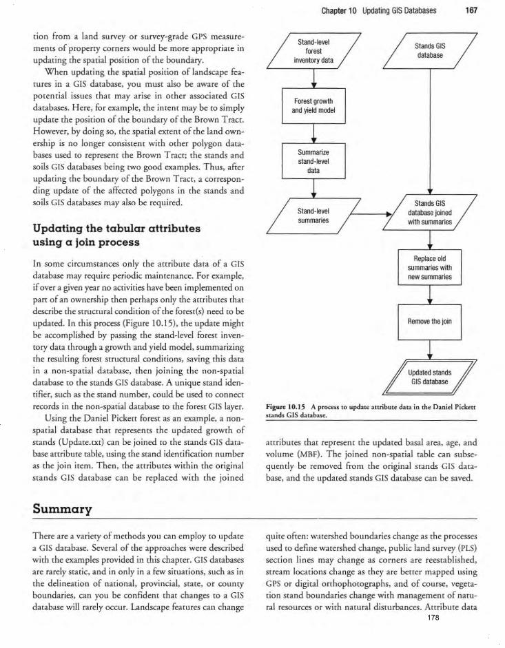
tion from a land surveyor survey-grade GPS measuremems of properey corners would be more appropriate in updating the spatial position of the boundary.
When updating the spacial position of landscape featu res in a GIS database, you must also be aware of the potential issues that may arise in other associated GIS databases. Here, for example, the imem may be to simply update the position of the boundary of the Brown T race. However, by doing so, the spatial extem of the land ownership is no longer consisrem with other polygon databases used to represem the Brown T racti the stands and soils GIS databases being cwo good examples. Thus, afcer updating the boundary of the Brown Tract. a corresponding update of the affecced polygons in the stands and soils GIS databases may also be requi red.
Updating the tabular attributes using a join process
In some circumstances only the attribute data of a GIS database may require periodic maimenance. For example. if over a given year no activities have been implememed on part of an ownership then perhaps only the a[[ributes that describe the structural condition of the forest(s) need [0 be updated. In this process {Figure 1 O.IS}, the update might be accomplished by passing the stand-level forest inven[Ory data through a growth and yield model, summarizing the resulting forest structural conditions. saving this data in a non-spatial database. then joining the non-spatial database to the stands GIS database. A unique stand identifier. such as the stand number. could be used to connect records in the non-spatial database [0 the forest G IS layer.
Using the Daniel Picken forest as an example. a non
spatial database that represents the updated growth of stands {Update. txt} can be joined [0 the stands GIS database attribute table. using the stand identification number as the join item. Then. the anributes within the original stands G IS database can be replaced with the joined
Summary
There are a variery of methods you can employ [0 update a GIS database. Several of the approaches were described with the examples provided in this chapter. GIS databases are rarely static. and in only in a few situations, such as in
the delineation of national. provincial. state. or couney boundaries. can you be con fidem that changes to a GIS database will rarely occur. Landscape features can change
Chapter 10 Updating GIS Databases 167
Stand-level forest
Forest growth and yield model
Summarize stand -level
data
Stands GIS database
Replace old summaries with new summaries
Remove the join
Figure 10.15 A process to update attribute data in the Daniel Pickett stands GIS d:lt.abase.
anributes that represem the updated basal area. age. and volume {MBF} . The joined non-spatial table can subsequently be removed from the original stands GIS database, and the updated stands GIS database can be saved.
quite often: watershed boundaries change as the processes used to define watershed change, public land survey {PLS} sect ion lines may change as corners are reestablished. stream locarions change as they are better mapped using GPS or digital orthophotographs, and of course, vegetation stand boundaries change wi[h management of natural resources or with nacural disturbances. Attribute data
178
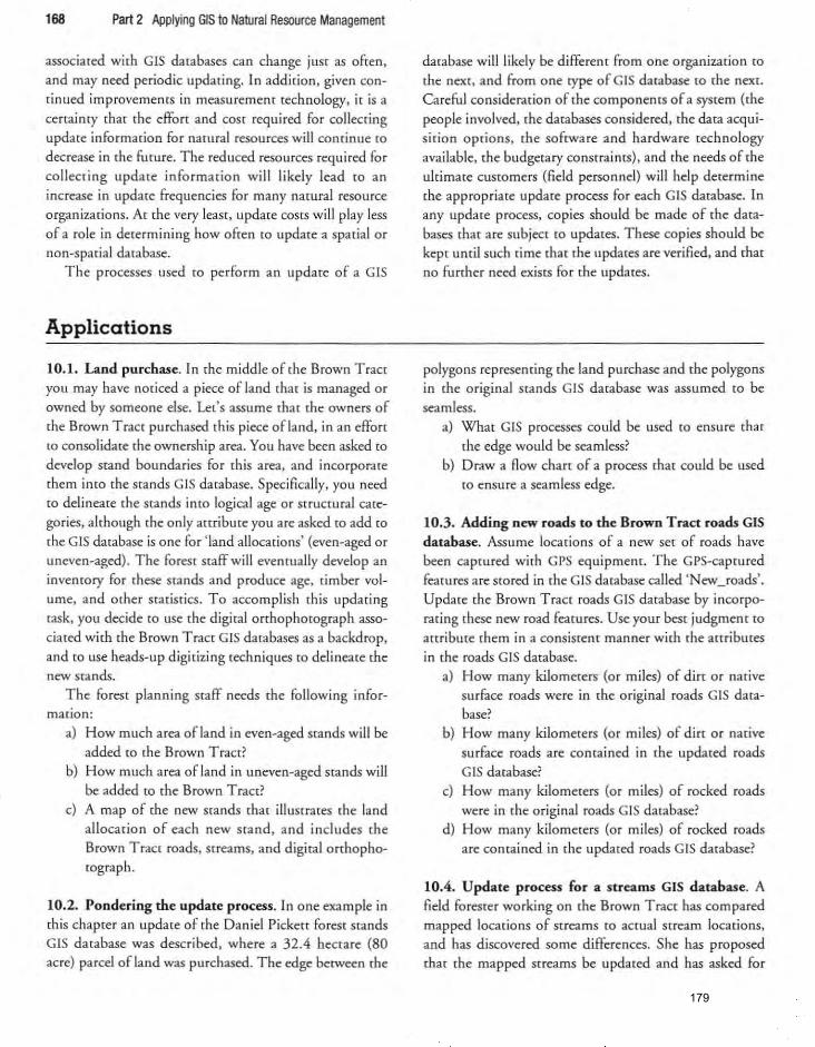
168 Part 2 Applying GIS to Natural Resource Management
associated with GIS databases can change just as often,
and may need periodic updati ng. In addition, given con
tinued improvemenrs in measurement technology, it is a
certainty that the effort and COSt requ ired for collecting update informacion for natural resources will conrinue CO
decrease in the future . The reduced resources required fo r
collecting update information will likely lead to an increase in update frequencies for many natural resource
organizations. At the very least, update COSts will play less
of a role in dererm ining how often to update a spatial or non-spacial database.
The processes used to perform an update of a GIS
Applications
10.1. Land purchase. In the middle of the Brown Tract you may have noticed a piece ofland that is managed or
owned by someone else. Let's assume that the owners of
the Brown T ract purchased this piece ofland, in an effort
to consolidate the ownership area. You have been asked to
develop stand boundaries for this area, and incorporate them into the stands GIS database. Specifically, you need to delineate the stands into logical age or structural cate
gories, although the only attribute you are asked to add to the GIS database is one for ' land allocations' (even-aged or uneven-aged). The forest staff will evemually develop an
inventory for these stands and produce age, timber vol
ume, and other statistics. To accompl ish [his updaring
task, you decide to use the digital orthophotograph associated w ith the Brown Tract GIS databases as a backdrop,
and to use heads-up digicizing techniques to delineate the new stands.
The forest planning staff needs the following information :
a) How much area ofland in even-aged srands will be added to <he Brown Tract?
b) How much area of land in uneven-aged stands will be added to the Brown Tract?
c) A map of the new stands that illumates the land allocation of each new stand, and includes the
Brown Tract roads, streams, and digital orthopho
tograph.
10.2. Pondering the update process. In one example in this chapter an update of (he Daniel Picken forest stands
GIS database was described, where a 32.4 hectare (80 acre) parcel of land was purchased. The edge between (he
database will likely be different from one o rganization [Q
the next, and from one 'Ype of GIS database to the next. Careful cons ideration of the components of a system (the
people involved. the databases cons idered. the data acqu i
sition options. the software and hardware technology
available, the budgetary constraintS), and the needs of the ultimate customers (field perso nnel) will help determine
the appropriate update process for each GIS database. In any update process, copies should be made of the databases that are subject to updates. These copies should be kept until such time that the updates are veri fied, and that
no furthe r need exists for the updates.
polygons representing the land putchase and the polygons in rhe original stands GIS database was assumed to be
seamless. a) What GIS processes could be used to ensure that
the edge would be seamless? b) Draw a Row chart of a process that could be used
to ensure a seamless edge.
10.3. Adding new roads to the Brown Tract roads GIS database. Assume locations of a new set of roads have
been captured with GPS equipment. The GPS-captured features are stored in the GIS database called 'New_roads' . Update the Brown Tract roads GIS database by incorporating these new road features . Use your best judgment to
attribute them in a consistent manner with the attributes
in the roads GIS database. a) How many kilometers (or miles) of dirt or native
surface roads were in the original roads GIS data
base?
b) How many kilometers (or miles) of dirt or native su rface roads are comained in the updated roads
GIS database? c) How many kilometers (or miles) of rocked roads
were in the original roads GIS database? d) How many kilometers (or miles) of rocked roads
are contained in (he updated roads GIS database?
10.4. Update process for a streams GIS database. A field forester working on the Brown Tract has compared
mapped locations of streams to actual stream locations.
and has discovered some differences. She has proposed that the mapped meams be updated and has asked for
179
your guidance in how this process might be accomplished. Describe three options for gathering the data necessary to fuci lirate an update of the streams GIS database. and the merits of each approach.
10.5. Update intervals and approaches. A recreation manager. who has learned of you r geospatial data skills. has asked your advice abou t updating the I O-year-old GIS (fails system. Two trails have been added [0 the system during (he past five years . The recreat ion manager is new
to the area and does not know much about GIS and
related technologies. The trails system is near an urban
cenrer and indications are that use demity is increasing.
Evidence of increasing use density includes a growing number of conflicts being repocted by horseback riders.
dog owners. and hikers throughout the forest. Additional evidence includes an unauthorized trail that is now clearly visible on the landscape. and which shows signs of signifieanr use at one of the primary trailheads.
a) What is an approp riate update interval for trail
information? Defe nd your choice.
b) How wou ld you recommend that any new spatial data be collected?
c) How does any new spat ial and attribute informa
tion collected be integrated into the exisdng GIS trails database?
d) What arrribures of trails would you encourage the recreation manager to collect during field visits co
the trails? Defend you recommendations.
References
Data Easr. (2007). XTools pro. Retrieved April 21, 2007. from http://www.xtoolspro.com.
Chapter 10 Updating GIS Databases 169
10.6. Update tools and approaches. You've been asked to create a spacial data layer representing scructures
(buildings). streams. roads. and watershed boundaries within a relatively small 259-hectare (640 acres) experimental fores( (hat is home to studies on hydrological
observarion and testing. At present, a polygon identifies
the adm inistrative boundary of the experimental forest
and only primary roads and perennial screams are
included in exisring spatial databases. The exisring data was created from hard copy maps at a scale of 1:24.000. You have at your disposal a 1:24.000 digital topographic quadrangle. a 30 m digital elevation model. a I m' resolution digiral orrhophotoquad. a consumer grade GPS. and a tOtal station. To use the rotal station, cwo reference
benchmarks are located within 2.0 km (I.2 miles) of the forest boundaries.
a) What data source andlor inscrumenr would you
use to capture the new spatial information relared
(0 :
I. structures?
ll . secondary roads?
111. smaller streams, including ephemeral streams?
IV. watershed boundaries?
b) Which of the new spatial information sources
described in pan (a) would you incorporate into
existing GIS databases to update them?
c) For the data you identified to be updated into exisring GIS database (described in parr (b». how would you incorporate the new information into
existing GIS databases?
Oregon Deparrmenr of Forestry. (2003). Guide to Xtools extension. Salem, OR: Oregon Department of Foresny.
180
Chapter 11
Overlay Processes
Objectives
One of [he grea< strengths of GIS is the capability to integrate landscape features and attribute information from
more [han one GIS database into a single GIS database. This capability is useful because it allows you to actively investigate and determ ine relationships between land
scape features. Upo n co mpletion of this chapter. readers should have a suffic ient amount of cools in their GIS [001-
box to perform many of the common vector GIS overlay
analyses required of field personnel working in natural resource organizat ions. whether they are employed in
forestty, wildlife, soils, fisheries, or hydrology fields. The objectives of this chapter to provide readers with an intro
duction to three primary rypes of overlay analysis: the
intersect, identity, and union processes. In addition, the
ability of these overlay processes [Q accommodate differ
ent vector feature rypes (point. line, and polygon) is considered. When this chaprer is completed, readers should have obtained knowledge and understanding of:
1. the Outcomes from using an overlay process to accom
pli sh one or more analytical tasks w ith in GIS;
2. the circumstances that help you decide when each of the three overlay processes might be used (0 suppOrt an analysis or research objective; and
3. the differences among the th ree overlay processes, and
between them and other similar GIS processes.
The topics discussed in this chapter relate to spatial
overlay processes. Overlay processes are spatial analysis techniques that involve two or more GIS databases. More
specifically, overlay processes can be used to investigate
and identify spatial relationships becween twO or more
databases. Overlay processes are powerfu l GIS tools and they represent what many consider ro be the essence of
GIS: the ability to integrate and organize information
from multiple spatial data layers into a single database. Overlay processes can be thought of as modell ing techniques that allow us to consider what might occur from
(he inregration of info rmation from multiple sources.
Perhaps the most widely recognized example of pre-G IS (ma nual) overlay analysis is that demonstrared in Ian
McHarg's boo k Design with Nature (I 969). As mentioned earlier in chapter I , this book provided examples
of manual map overlays that were used ro idenrify areas
that were suitable for certa in activities. Design with Nature inspired many people to apply manual overlay techniques for their own analysis needs and to also con
sider developing digital tools (GIS) that might be used to make overlay analysis more precise and efficient.
The topics discussed in rhis chapter relate to spatial
analysis processes that are similar ro merging (chapter 8),
and to obtai ning information about specific geographic
regions (chapter 7) . There are, however, some very dis
tinct differences between the merge process and (he over
lay processes presented in this chapter. When twO (or
more) polygon GIS databases are merged, for example, the resulting GIS database may consist of overlapping poly
gons. The processes presented in this chapter-the inter
sect, identity, and union processes-all result in new out
put GIS databases where the landscape features do not overlap. Overlapping areas and attributes are combined.
in some form or fashion, rhus the potential exists for poly
gons to be splir and combined and their topology reassessed in the result ing GIS database. Calculating the area
181
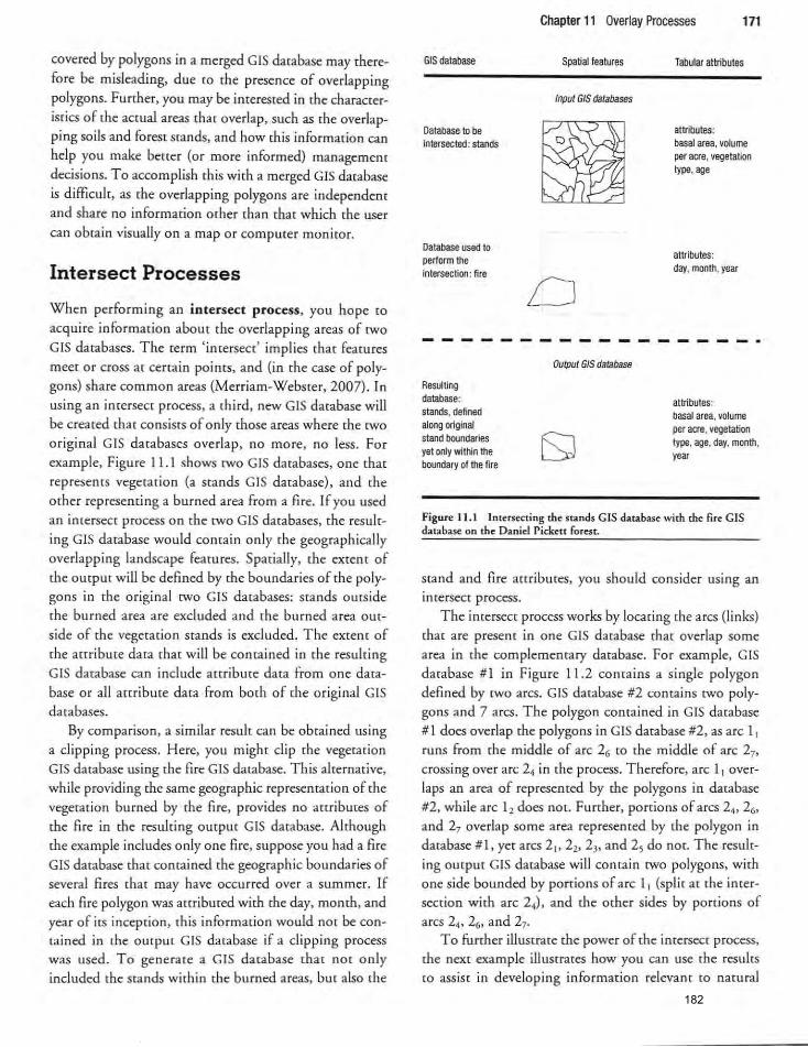
covered by polygons in a merged GIS da",base may therefore be misleading, due to the presence of overlapping polygons. Funher. you may be imerested in the characteristics of rhe actual areas that overlap, such as the overlap
ping soils and forest stands. and how this information can
help you make berrer (or more informed) management decisions. To accomplish this with a merged GIS database is difficult, as the overlapping polygons are independent and share no informadon mher than that which the user
can obtain visually on a map or computer moniroc.
Intersect Processes
When performing an intersect process. you hope to
acquire information about rhe overlapping areas of [wo
GIS databases. The term 'inrersecc' implies (hat features meet or cross at cenain points. and (in the case of polygons) share common areas (Merriam-Webster, 2007). In using an imersect process. a third. new GIS database will be created [hat consists of only those areas where the two
original GIS databases ove rlap, no more, no less. For
example, Figure 11.1 shows rwo GIS databases , one that
represems vegetat ion (a stands C IS database), and the
other representing a burned area from a fire. If you used
an intersect process on the two GIS databases, the result
ing GIS database wou ld conta in only the geographically overlapping landscape features. Spatially, the extent of the output will be defined by the boundaries of the polygons in the original two GIS databases: stands outside
the burned area are excluded and the burned area out
side of the vegetarion stands is excluded. The extent of
the attribute data that will be contained in the resulcing
GIS database can include attribute data from one data
base or all arrribute data from both of the original GIS databases.
By comparison, a similar result can be obtained using
a clipping process. Here, you might clip the vegetation
GIS database using the fire GIS database. This alternative, while providing the same geographic representation of the
vegetat ion burned by the fi re. provides no attributes of
the fire in the resulting output GIS database. Although the example includes only one fire, suppose you had a fire
GIS database that contained the geographic boundaries of several fires that may have occurred over a summer. If
each fire polygon was attributed with the day, month, and year of its inception, this information would not be contained in rhe output GIS database if a clipping process
was used . To generate a GIS database that not only
included the stands within the burned areas, but also the
GIS database
Database to be intersected: stands
Database used to perform the intersectioo: fire
Chapter 11 Overlay Processes 171
Spatial features
Input GIS databases
Tabular attributes
attributes: basal area, volume per acre, vegetation type, age
attributes: day, month, year
------------------Resulting database: stands, defined along original stand boundaries yet only within the boundary of the fire
Output GIS database
attributes: basal area, volume per acre, vegetation type, age, day, month, year
Figure ) ).) Intersecting the stands GIS database with the fire GIS database on the Daniel Pickett forest.
stand and fire attributes. you shou ld consider using an Intersect process.
The intersect process works by locating the arcs (links) that are present in one GIS database that overlap some
area in the complementary database. For example, GIS
database # 1 in Figure I 1.2 contains a single polygon defined by two arcs. GIS database #2 contains twO polygons and 7 arcs. The polygon contained in GIS database #1 does overlap the polygons in GIS database #2, as arc I , runs from the middle of arc 2, to the middle of arc 2" crossing over arc 2<\ in the process. Therefore, arc 11 over
laps an area of represented by the polygons in darabase #2, while arc 12 does not. Further, portions of arcs 24• 26•
and 2, overlap some area represented by the polygon in
database #1, yet arcs 2" 2" 2" and 2, do not. The resulting output GIS database will contain two polygons, with
one side bounded. by portions of arc I I (split at the inter
section with arc 2<\), and the other sides by portions of
arcs 2<\. 26 , and 27 ,
To further illustrate the power of the imersect process,
the next example illustrates how you can use the results [Q assist in developing information relevanr to natural
182
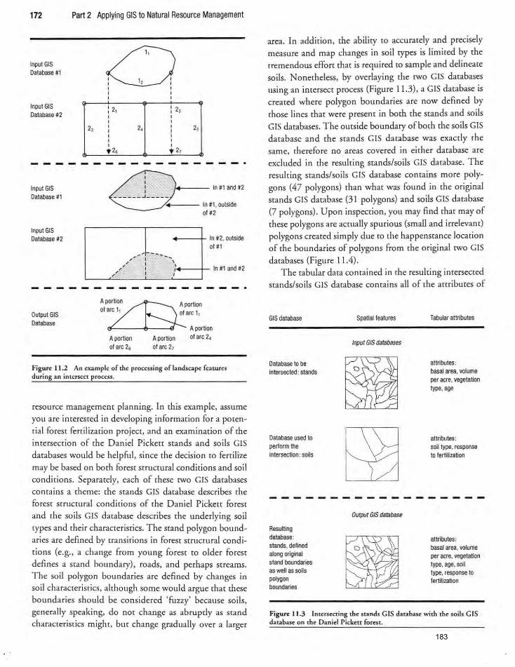
172 Part 2 Applying GIS to Natural Resource Management
Input GIS Database #1
Input GIS Database #2
Input GIS Database #1
Input GIS Database #2
Output GIS Oatabase
2,
~ ~
2,
2.
. 2,
, , , : 22 , , , , , , , . 2,
2,
_~I.o'--- In#l and #2
~ Inl1 , outside 01112
+-- --1- In #2, outside of #1
AP~r,on ola~ olaret , .
A portion
A portion of arc 26
A portion of arc 2,
of arc 2 ~
Figure 11.2 An example of the processing of landscape features during an inH:rsect process.
resource management planning. In this exam ple. assume YO ll are interested in developing information for a poten
tial forest fertilization project, and an examination of the inrersecrion of [he Daniel Picke[[ stands and so ils GIS
databases would be helpful , since the decision to fertilize may be based on both forest srrucrural co nditions and soil conditions. Separately. each of these [\.'10 GIS databases comains a theme: the stands GIS database describes the forest structural conditions of the Daniel Pickett forest and the so ils GIS database describes the underlying soil
types and their characteris tics. The stand polygon boundaries are defined by tra nsitions in forest structural conditions (e.g., a change from young fores t to older forest defines a stand boundary), roads, and perhaps st reams. The soil polygon boundaries are defined by changes in soil character istics, although some would argue that these boundaries should be considered 'fuzzy' because soils, generally speaki ng, do not change as abrupdy as stand characteristics might , bm change gradually over a larger
area. In addition , the ability to accurately and precisely
measure and map changes in soil types is limited by the tremendous effort that is required to sample and del ineate soils. Nonetheless, by overlaying the twO GIS databases
using an intersect process (Figure II.3), a GIS database is created where polygon boundaries are now defined by
those lines that were present in both the stands and soils
GIS databases. The outside boundaty of both the soils GIS database and the stands GIS database was exacdy the same, therefore no areas covered in either database are excluded in the resulting stands/soils GIS database. The
resulting stands/soils GIS database contains more polygons (47 polygons) than what was fo und in the original
stands GIS database (31 polygons) and soils GIS database (7 polygons) . Upon inspection, you may find that may of
these polygons are actually spurious (small and irrelevant) polygons created simply due [Q the happenstance location of the boundaries of polygons from the original twO GIS
databases (Figu re 11.4). The tabular data contained in the resulting intersected
stands/soils GIS database contains all of the anribures of
GIS database Spatial features Tabular attributes
Input GIS databases
Database to be
~ attributes :
Intersected: stands basal area, volume per acre. vegetation type, age
Database used to
~ attributes:
perform the soil type, response intersection: soils to fertilization
------ ------ ------Output GIS database
Resulting database:
§i attributes :
stands, defined basal area, volume along original per acre, vegetation stand boundaries type, age, soil as well as soils type, response to polygon fertilization boundaries
Figure 1l.3 Intersecting the stands GIS database with the soils GIS database on the Daniel Pickett fo rest.
183
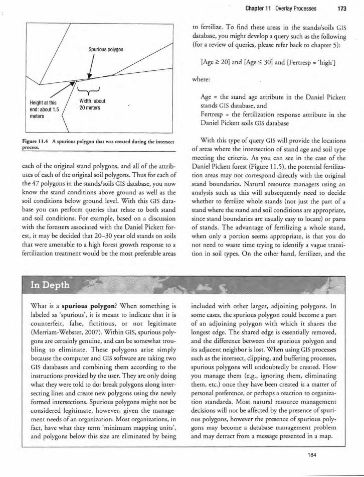
Spurious polygon
-;/jLy--J Height at this end: about 1.5 meters
Width: about 20 meters
Figun 11.4 A spuriow polygoo that was created during the intersect process.
each of the original stand polygons, and all of the attributes of each of the original soil polygons. Thus for each of the 47 polygons in the stands/soils GIS database, you now know the stand conditions above ground as well as the soil conditions below ground level. With this GIS database you can perform queries that rdate to both stand
and soil conditions. For example. based on a discussion with the foreSters associated with the Daniel Pickett foreSt, it may be decided that 20-30 year old Stands on soils that were amenable [Q a high forest growth response [Q a fenilization treatment would be the most preferable areas
What is a spurious polygon? When something is labeled as 'spurious'. it is meant [Q indicate that it is
counterfeit. false. fictitious. or not legitimate (Merriam-WebSter, 2007). Within GIS, spurious polygons are certainly genuine. and can be somewhat troubling to eliminate. These polygons arise simply because the compmer and GIS software are taking two GIS databases and combining them according to the instructions provided by the user. They are only doing what they were told to do: break polygons along intersecting lines and create new polygons using the newly formed intersections. Spurious polygons might nO{ be considered legitimate. however. given the managemem needs of an organization. Most organizations. in fact. have what they term 'minimum mapping units'. and polygons below this size are eliminated by being
Chapter 11 Overlay Processes 173
to ferti lize. To find these areas in the Stands/soils GIS
database, you might develop a query such as the following (for a review of queries, please refer back to chapter 5):
[Age;" 20) and [Age S 30) and [Fertresp = 'high')
where:
Age = the stand age attribute in the Daniel Picke[[ Stands GIS database, and Fenresp = the fertilization response a[[ribute in the Daniel Pickett soils GIS database
With this rype of query GIS will provide the locations of areas where the imersecrion of stand age and soil type meeting the criteria. As you can see in the case of the
Daniel Pickett forest (Figure 11.5), the potential fertilization areas may not correspond directly with the original stand boundaries. Natural resource managers using an analysis such as this will subsequently need to decide whether to fertilize whole Stands (not JUSt the part of a nand where me stand and soil conditions are appropriate. since stand boundaries are usuaIly easy to locate) or pans
of Stands. The advantage of fertiliz ing a whole Stand, when only a portion seems appropriate. is that you do nO{ need to waSte time trying [Q identify a vague transition in soil types. On the other hand, fertilizer, and the
included with other larger, adjoining polygons. In some cases. the spurious polygon could become a part of an adjoining polygon with which it shares the longest edge. The shared edge is essentially removed, and the difference between the spuriolls polygon and its adjacent neighbor is lost. When using GIS processes such as me intersect, clipping. and buffering processes. spu rious polygons will undoubtedly be created. How you manage them (e .g .• ignoring them, elim inat ing them. etc.) once they have been created is a matter of
personal preference. or perhaps a reaction to organization 5[andards. Most natural resou rce management decis ions will not be affected by the presence of spu rious polygons, however the presence of spuriolls polygo ns may become a database management problem and may detract from a message presented in a map.
184
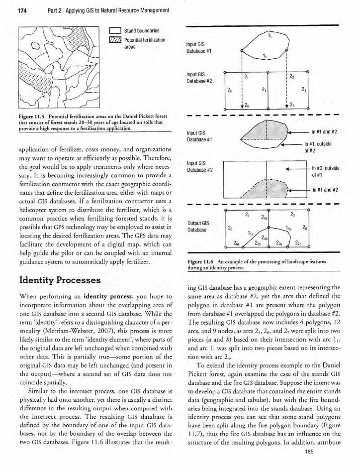
174 Part 2 Applying GIS to Natural Resource Management
CJ Stand boundaries
[-": ....... J Potential fertilization areas
Figure 11.5 Potential fertilization areas on the Daniel Pickett forest that consiSt of forest stands 20-30 years of age located on soils that provide a high response to a fertilil.3tion applic3[ion.
applicado n of fertilizer. costs money. and o rganizations
may want to operate as efficiently as possib le. Therefore,
rhe goal would be [Q apply treatments only where neces
sary. Ie is becoming increasi ngly common [Q provide a
fenilizar ion contraccor with rhe exact geographic coordi
nates that define rhe fertilization area, either with maps or
acrual GIS databases. If a fenilizarion contrac[Qr uses a
hel icopter system to disrribme the fertilizer, which is a
commo n pract ice when fertilizing forested stands, it is
possible that G PS technology may be employed to assist in locating the desired fertilization areas. The GPS data may facilitate the development of a digital map. which can help guide the pilo t or can be coupled with an internal guidance system to autOmatically apply fertil izer.
Identity Processes
When performing an identity process, you hope to
incorporate information about the overlapping area of
one GIS darabase into a second GIS database. While the term 'identiry' refers to a distinguishing character of a per
sonality (Merriam-Webster. 2007). this process is more likely similar ro the term 'identiry element', w here pares of
the o rig inal data are left unchanged when combined with
other data. This is partially true-some portion of the
original GIS data may be left unchanged {and present in the o utput)-where a second set of GIS data does not
co incide spatially .
Si milar to the intersect process, one GIS database is
physica lly laid onto another, yet there is usually a distinct
difference in the resul ting Ol1[Pur when compared w ith the in te rsect process . The resulting GIS database is
defined by the boundary of one of the input GIS databases, not by the boundary of the overlap between the
two GIS databases . Figu re 11 .6 illustrates that the resulr-
Input GIS Database #1
Input GIS Database #2
2,
~ ~ , , , , , , : 21 : 22 , , , , , 2, , , , , , , , , . 2, t 27
2,
--------- --------Input GIS Database #1
Input GIS Database #2
Output GIS Database
, , , , /+-- In #t and #2 __ __ __ .J ___ _ _
'--_ _ -./-'1--- In #1, outside 01#2
+---t- In #2 , outside 01 #1
, ......... :--...... _, ,/; : .~:+--+ In #1 and #2
" I I
2, 2,
Figun~ 11.6 An example of the processing of landscape fea lures during an idenucy process.
ing GIS database has a geogtaphic extent representing the same area as database #2, yet the arcs that defined the
polygon in database # 1 are present where the polygon from database #1 overlapped the polygons in database #2. The resul ti ng GIS darabase now includes 4 polygons. 12 arcs, and 9 nodes , as arcs 24• 26• and 27 were split into twO pieces (a and b) based on their intersection with arc 11>
and arc 11 was split into two pieces based on its intersec
tion w ith arc 24,
To extend the idenriry process exam ple (() the D aniel
Picken forest, again examine the case of the stands GIS
database and the fire GIS database. Suppose the intent was [Q develop a GIS database that contained the entire stands
data (geographic and tabular). but with the fire boundaries being integrated into the stands database. Using an ident ity process you ca n see that some stand polygons
have been split along the fire polygon boundary (Figure 11.7), thus the fire GIS database has an influence on the
structure of the resulting polygons. In addi tio n, 3nribure
185
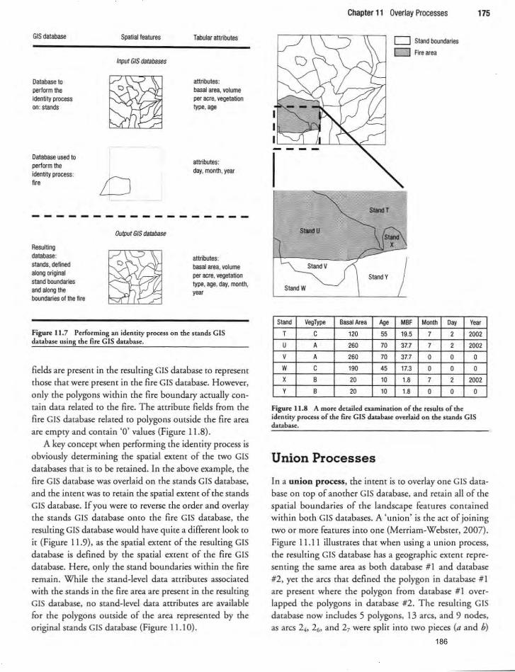
GIS database
Oatabase to perform the identity process Oil : stands
Oatabase used 10 perform the identity process: fire
Spatial features
Input GIS databases
o ------ ------
Output GIS database
Resulting
~ database: stands, defined along original stand boundaries and along the booodaries of the fire
Tabular attributes
attributes: basal area, volume per acre, vegetatiOil type, age
attributes: day, month, year
------
attributes: basal area, volume per acre, vegetation type, age, day, month, ,ear
Figure 11.7 Performing an identity proass on the stands GIS database using the fire GIS database.
fields are present in the resulting GIS database [0 represenr those that were presenc in the fire GIS database. However, only the polygons within the fire boundary actually contain data related [0 the fire. The amibute fields from the fire GIS database related [0 polygons outside the fire area are empry and contain '0' values (Figure 11 .8).
A key concept when performing the identiry process is obviously determining the spatial extent of the [wo GIS databases that is [0 be retained. In the above example, the fire GIS database was overlaid on the stands GIS database, and the incem was [0 rerain the spacial extent of the stands
GIS database. If you were to reverse the order and overlay me stands GIS database onto the fire GIS database, the resulting GIS database would have quite a different look [0
it (Figure 11 .9), as the spatial extent of the resulting GIS database is defined by the spatial extent of the fire GIS database. Here, only the stand boundaries within the fire remain. While the stand-level data anributes associated with the stands in [he fire area are presenr in the resulting GIS database, no stand-level data attributes are available for the polygons outside of the area represented by the original stands GIS database (Figure 1l.l0).
Chapter 11 Overlay Processes 175
Stand V
StandW
Stand VegType Basal Area
T C 120
U A 260
V A 260
W C 190
X B 20 y B 20
StandY
Age
5S
70
70
45
10
10
o Stand bouooaries
D Firearea
MBF Month Day
19.5 7 2
37.7 7 2
31.7 0 0
17.3 0 0
1.8 7 2
1.8 0 0
Year
2002
2002
0
0
2002
0
Figure 11.8 A more detailed examination of the results of the identity process of the fire GIS databue overlaid on the stands GIS database.
Union Processes
In a union process, the intent is to overlay one GIS database on top of another GIS database, and re tain all of the spatial boundaries of the landscape features contained within both GIS databases, A 'union' is the act of joining [wo or more features into one (Merriam-Webster, 2007).
Figure 11.11 illustrates that when using a union process. the resulting GIS database has a geographic extent representing the same area as both database # I and database
#2, yet the arcs that defined the polygon in database # I are present where the polygon from database #1 overlapped the polygons in database #2. The resulting GIS database now includes 5 polygons. 13 arcs, and 9 nodes, as arcs 2 ... 26 • and 27 were split into two pieces (11 and b)
186
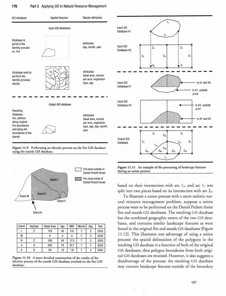
176 Part 2 Applying GIS to Natural Resource Management
GIS database
Database to perform the identity process on: fire
Database used to perform the identity p(ocess: stands
Resulting database: fire, defined along original fire boundaries and along the boundaries of the stands
Spatial features
Input GIS databases
o
output GIS database
Tabular attributes
attributes: day, month, year
attributes: basal area, volume per acre, vegetation type, age
attributes: basal area, volume per acre, vegetation type, age, day, month, year
Figure 11.9 Perfo rming an ide ntity process on the fire GIS database using the n ands GIS database.
Stand M
\ Stand N
Stand VegType Basal Area Age
L C 120 30
M 0 0
N C 190 45
U A 260 70
X B 20 10
MBF
5.6
0
17.3
37.7
1.8
o Fire area outside of Daniel Pickett forest
D Fire area inside 01 Daniel Pickett forest
Month Oay Vear
7 2 2002
7 2 2002
7 2 2002
7 2 2002 7 2 2002
Figure 11 . 10 A more detailed examination of th(' results of the identity process of the standt G IS database overlaid on the fire G IS database.
Input GIS Database "
Input GIS Database .2
2,
~ ~ , , , , , , : 21 : 22 , , , , , 2, , , , , , , , ... 26 ... 27
2,
-------------Input GIS 8: .. ---In#1 and #2 Database" _____ J ____ _
~ In ", outside 01112
Input GIS Database '2
Output GIS Database
+---t- In '2, outside oil'
" " ;---.... ,,' : \~f--+-
./ I In 111 aOO'2
2,
/' Figure 11.11 An example of the processing of landscape features during an union process.
based o n the ir intersection with arc 11. and arc II was split into twO pieces based on its imersection with arc 24,
To illustrate a union process with a more realistic nat
ural resource management problem. suppose a union process were to be performed on the Daniel Picket[ forest fire and stands GIS darabases. The resul ting GIS database has the combined geographic extent of rhe (wo GIS databases, and co ntains similar landscape fea tu res as were
fo und in rhe origi nal fire and stands GIS darabases (Figure I 1.12). This iliumares one adva ntage of using a union process: rhe sparial del inearion of rhe polygons in rhe resul ring GIS database is a fu nction of both of the origi nal GIS databases. thus polygon boundaries from both original GIS databases are retained. However, it also suggests a disadvantage of the process: rhe result ing GIS database may comain landscape features outside of [he boundary
187
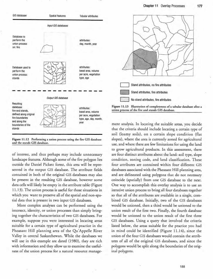
GIS database
Database to perform the union process on: fire
Database used to perform the union process: stands
Resulting database: fire and stands, defined along original fire boundaries and along the boundaries of the stands
Spatial features
Input GIS databases
Output GIS database
Tabular attributes
attributes: day, month, year
attributes: basal area, volume per acre, vegetation type, age
attributes: basal area, volume per acre, vegetation type, age, day, month, year
Figure: 11.12 Performing a union process using the fire GIS database and the stands GIS database.
of interest, and thus perhaps may include unnecessary
landscape features. Although some of the fire polygon lies outside the Daniel Pickett forest, this area will be represented in ,he OUtput G IS database. The attribute fields contained in both of the original GIS databases may also be present in the resulting GIS database, however some
data cells will likely be empty in the attribute table (Figure 11.13). The union process is useful for those situations in which you want to preserve all of the spatial and non-spatial data that is present in twO input GIS databases.
More complex analyses can be performed using the intersect, identity, or union processes than simply bringing together the characteristics of twO GIS databases. For example, suppose you were interested in locating areas suitable for a certain type of agricultural praccice in the Pheasant Hill planning area of the Qu'Appelle River Valley in central Saskatchewan. While the databases we will use in th is example are dated (\980), they are rich with information and they allow us to examine (he usefulness of the union process for a natural resource manage-
Chapter 11 Overlay Processes 1 n
o Stand attributes, no fire attributes
o Stand attributes, fire attributes
o No stand attributes, fire attributes
Figure 11.13 Illustration of completeness of a tabular database after a union process of the fire and stands GIS database.
ment analysis. In locating [he suitable areas, you decide that the criteria should include locating a certain type of soil (loamy soils), on a ce rtain slope condition (flat slopes), where the area is currently wned for agricultural use, and where there are few limitadons for using the land
to grow agricultural produces. In this assessment, there are four distinct anribures about the land: so il type, slope condidon, zoning code, and land classification . These four attributes are comained within four different GIS databases associaeed with the Pheasant Hill planning area, and are delineated using polygons that do noc necessary
coincide (spatially) from one G IS database to the next. One way {Q accomplish this overlay analysis is {Q use an iterative union process to bring all fou r databases together so chat all of the anribures are available in a single, combined GIS database. Initially, two of the GIS databases would be unioned, then a third would be unioned to the union result of the first two. Finally, the fourth database would be unioned to the union result of the first three GIS databases. Using a query thac involved the criteria
listed below, the areas suitable for the praccice you had in mind could be identified (Figure 11.14), since the union of the four GIS databases would contain the attributes of al l of the original GIS databases, and since the polygons would be split along the boundaries of the original polygons.
188
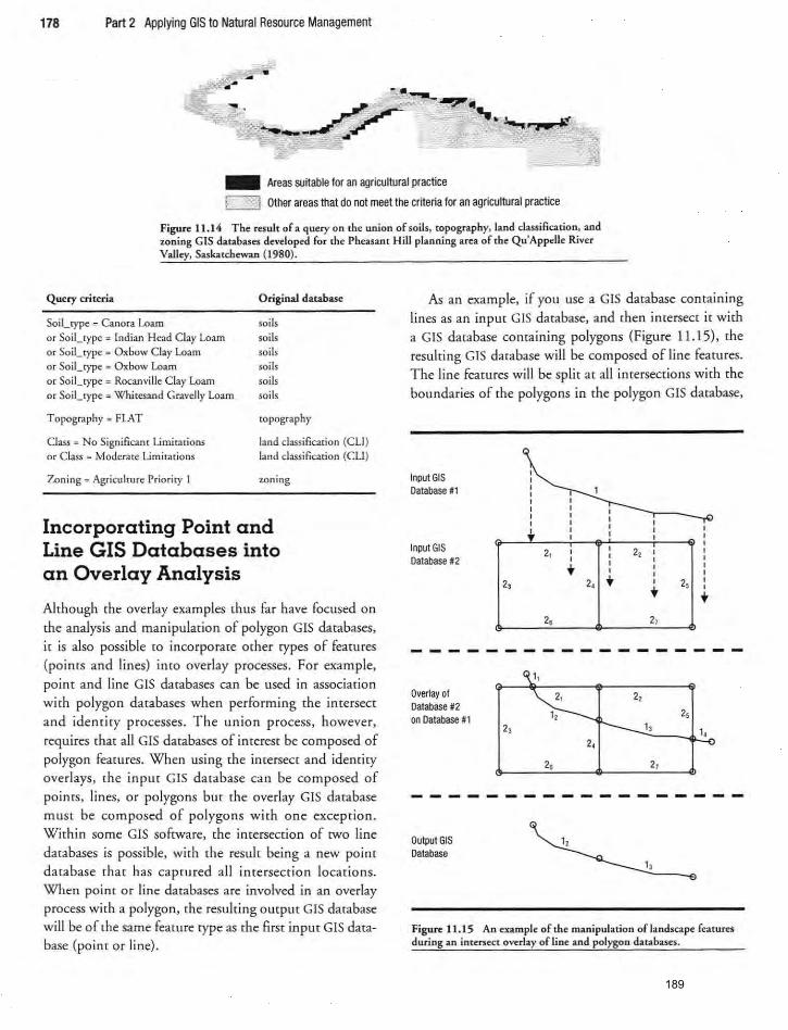
178 Part 2 Applying GIS to Natural Resource Management
- - . -= .. ,pg."
.IiOi'_
_ Areas suitable for an agricultural practice
c=J Other areas that do not meet the criteria for an agricultural practice
Figwe 11.14 The result of a query on the union of soils. topography, land classification, and zoning GIS databases developed for the Pheasant Hill planning area of the Qu'Appclle River Valley. Saskatchewan (1980).
Query criteria
Soil_type ", Canora Loam
or Soil_type ", Indian Head Clay Loam or SoiLrype ,. Oxbow Clay Loam or Soil_rype ,. Oxbow Loam
or Soil_type" Rocanvillc Clay Loam or So il_type II: Whiresand Gravelly Loam
Topography = FLAT
Class" No Significant Limitations or Class", Moderate Limitations
Zoning = Agriculture Priority I
Original database
soils soils soils
soils
soils
soi ls
topography
land classification (eLi) land classification (eLI )
zoning
Incorporating Point and Line GIS Databases into an Overlay Analysis
Although the overlay examples thus fa r have focused on the analysis and manipulation of polygon GIS databases, it is also possible to incorporate other types of features (points and lines) into overlay processes. For example. point and line GIS databases can be used in association with polygon databases when performing the intersect and idemity processes. The union process. however, requires that all GIS databases of interest be composed of polygon features. When using the imersect and identity overlays. the input GIS database can be composed of points, lines, or polygons but the overlay GIS database must be composed of polygons with one exception. With in some GIS software. the intersection of two line databases is possible. with the result being a new point database that has captured all intersection locations. When point or line databases are involved in an overlay process with a polygon. the resulting Output GIS database will be of the same feature type as the first input GIS database (point or line).
As an example. if you use a GIS database containi ng lines as an input GIS database. and then intersect it wi th a GIS database containing polygons (Figure 11. 15), the resulting GIS database wi ll be composed of line features _ The line features will be split at all intersections with the boundaries of the polygons in the polygon GIS database,
Input GIS , ,
Database '1 , , , , , , , .. ,
Input GIS , , 2, , 2, , ,
Database In , , , , • , , , , , ,
2, 2, • , 2, ,
• , •
2. 2,
- - -- - - - -- - --- -1,
Overlay of 2, 2, Database #2
2, on Database.1 1,
2, 1, I ,
2,
2. 2,
--- ---- -- - - - -- -Output GIS Database
1,
Figure 11.15 An example of the manipulation oflandsc.1pe features during an intersect overlay of line and polygon databases.
189
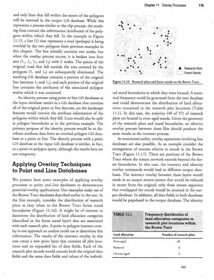
and only lines that full within the extent of the polygons will be retained in the outpUt GIS database. While this
represents a process similar [0 the clip process, the resul t
ing lines contain the information (attributes) of the poly
gons within which they fell. In the example in Figure 11.15, a line (I) that represents a road (perhaps) is being
overlaid by the two polygons from previous examples in this chapter. The line initially comains two nodes, but when the overlay process occurs, it is broken into four
arcs (II' I" 1" and 1. ) with 5 nodes. The pieces of the original road that fall outside the area covered by the polygons (I I and 1, ) are subsequently eliminated. The
resulting GIS database comains a ponico of the original
line (sections 12 and 13), and each portion of the original
li ne contains the anributes of the associated polygon within which it was contained.
An idemity process using point or line GIS databases as
the input database results in a GIS database that concains
all of the original point or line features, yet the landscape
features would contain the 3ucibure information of the polygons within which they fell. Lines would also be split at polygon boundaries as in (he previous example. The primary purpose of the identi ty process would be (Q dis
tribute anribute data from an overlaid polygon GIS data
base (Q a poim or line. T he idenrity process with a point
GIS database as the input GIS database is similar, in fact,
to a point-in-polygon query, although the results here are not temporary.
Applying Overlay Techniques to Point and Line Databases
We presenr here some examples of applying overlay
processes (Q point and line databases (Q demonsuate
potential overlay applications. Our examples make use of
the Brown Tract databases described earlier in the texc. In
the first example, cons ider the distribution of research
plots as they relate to the Brown Tract forest stand
boundaries (Figure 11.16). It might be of interest to
determine rhe distribmion of land allocation categories
(described in the forest stand layer) that are associated
with each research plot. A point in polygon intersect over
lay is one approach an analyst could use to determine this
information . The results of the imersecr overlay in this
case create a new point layer that comains all plot loca
tions and an expanded list of data fields. Each of the research plot records would contain both the original data fields and the same data fields and values of the individ-
Chapter 11 Overlay Processes 179
.. <, 1.'1.
", 1.'. '..-: ".~>
~ Research Plots [:=:J Forest Stands
Figure 11. 16 Research plots and forest stands on the Brown Tract.
ual stand boundaries in which they were located. A statis
t ical frequency could be generated from the new database and could demonstrate the distribution of land alloca
tions conta.ined in the research plot locations (Table
11.1). In this case, the majori ry (48 of 57) of research plots are located in even-aged stands. Given rhe geometry
of the research plots and stand boundaries, an identity
overlay process berween these flies should produce the same results as the inrersect process,
As mentioned earlier, overlay operations involving line
databases are also possible, As an example consider the
arrangement of streams relative (Q stands in the Brown
Tract (Figure 11.17). There are portions of the Brown Tract where the stream network extends beyond the for
est boundaries. In this case, the intersect and identity
overlay commands would lead (Q different output data
bases. The intersect overlay between these layers would
result in an output stream system that would be reduced
in extenr from the original; only those stream segments
that overlapped the stands would be retained in the out
put database. In addition, all data fields in both databases would be populated in the output database. The identiry
TABLE 11.1
Land allocation
Research
Uneven-aged
Frequency distribution of land allocation categories in research plot locations within the Brown Tract
Number of research plots
48
6
3
190
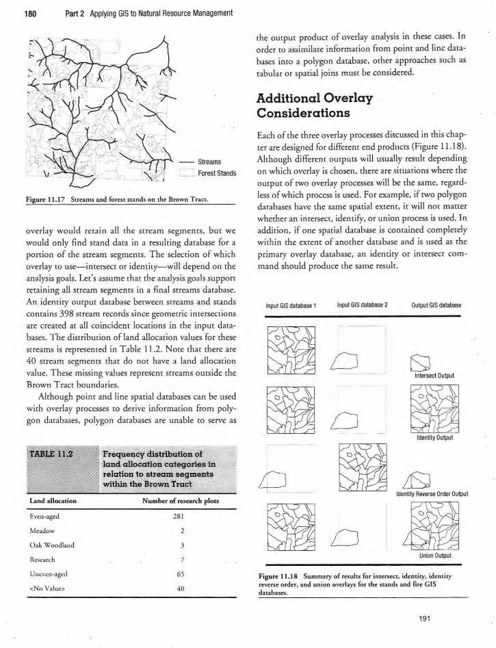
180 Part 2 Applying GIS to Natural Resource Management
-- Streams
Forest Stands
Figure 11.17 Streams and forest stands on the Brown Tract.
overlay would retain all the Stream segments, bur we would only find stand data in a resulting database for a ponioo of [he stream segments. The selection of which
overlay to use-intersect or identity-will depend on the analysis goals. Let'S assume that the analysis goals suppon retaining aU st ream segments in a final streams database. An identity ourpm database between streams and stands contains 398 stream records since geometric intersections are created at all coincident locations in the input databases. The distribution of land allocation values fo r these streams is represented in Table 11.2. Note that there are 40 stream segments that do not have a land allocation
value. These missing values represent streams omside the Brown Tract boundaries.
Although point and line spatial databases can be used with overlay processes to derive information from polygon databases, polygon databases are unable to serve as
TABLE 11.2
Land allocation
Even-aged
Meadow
Oak Woodland
Research
Unevcn·agcd
<No Value>
Frequency distribution of .. land allocation categories ill relation to stream segments within the Brown Tract
Number of research plots
281
2
3
7
65
40
the omput product of overlay analysis in these cases. In order to assimi late information from point and line data
bases into a polygon database, other approaches such as
tabular or spatial joins must be considered.
Additional Overlay Considerations
Each of the three overlay processes discussed in this chap
ter are designed for different end products (Figure 11.18). Although different outputs will usually result depending
on which overlay is chosen, there are situations where the ompm of two overlay processes will be the same, regard
less of which process is used. For example. if two polygon databases have the same spatial extent, it will not matter whether an intersect, identify, or union process is used. In addition, jf one spatial database is contained completely within the extent of another database and is used as the
primary overlay database, an identity or intersect command should produce the same resulr.
Input GIS dalabase 1 Input GIS database 2 Output GIS database
~ 0 bJ Intersect Output
~ 0 ~ Identity Output
0 ~ LlSJ Identity Reverse Order Output
~ 0 ~ Union Output
Figure 11.18 Summary of results for intersect, identity, identity reverse order. and union overlays for the stands and fire GIS databases.
191
The order in which GIS databases are selected for an
overlay process may also have significance on the ompur
database, depending on your GIS software. The identity
overlay will take into accoum (he spatial extent of one of your databases, and reduce other layers (Q the same spatial
extent. For this reason it is imponam (Q recognize how
your soft\vare selects (he inpur database that is used to
determine the idenriry spatial exrenL The union and
intersect overlays. on the other hand. are less discriminat
ing as to the order in which spatial exrencs are considered.
The union output wi ll include the emire spatial extent of
all layers while the intersect OUtput will only include the
common areas. Some GIS sofrware. however, may only
include by default the attributes of the initial input layer
in the outpm database unless the user signifies otherwise.
Depending on your GIS software, you may also be able
co involve more than [Wo layers in an overlay process.
Nthough this ability may be particularly useful for some
applications, the complexity of the Output product will
increase with the number of layers that are involved.
Overlay ompm databases cake into account the topology
Summary
With the conclusion of this chapter you have examined
most of the common vectOr processes available within GIS
software programs. As we have shown in this and previous
chapters, to address natural resource management prob
lems a number of different courses of action can be used,
each utilizing different techniques or different sequences
of GIS processes. For example, the following three
processes might be employed ro develop a summary of
forest resources within owl buffer areas:
I. Buffer owl nest locations. Clip the owl buffer areas
from a stands GIS database. Summarize appropriate
statlS[1cs.
2 . Buffer owl nes( locations. Intersect a stands G IS data
base with the owl buffer GIS database. Summarize
appropriate statistics. 3. Buffer owl nest locations. Overlay a stands GIS data
base on the owl buffer GIS database using an identity
process. Summarize appropriate statisdcs.
The GIS toolbox available to readers of this text, as it
relates [Q vector GIS processes, should now contain a
Chapter 11 Overlay Processes 181
and attr ibutes of all input layers depending on operaror
choices. Bear in mind that overlay processes are complex
operations, particularly when many features are present in
input databases. As such, and depending on computing
resources, some overlay omput databases may take more
time [Q complete than oilie r, less intensive. GIS processes.
Users may have [Q be patient in awaiting overlay ompm
results. Finally. many GIS sofrw-are programs allow users to
select the attribute fields from both the input GIS database
and the polygon overlay GIS database that are ro be carried
into the resulting output GIS database. Often you will find
that selecting a subset of attribute fields for the desired
analysis will reduce the time requirements related to inter
preting and analyzing the results of overlay processes.
Given the considerations expressed above, you should
always carefu lly consider the objectives of your analysis to
dete rmine which overlay process [Q use. In some cases,
knowing whether input vec[Qr databases represent point,
line, or polygon spatial features, or some combination
thereof, will help lead ro an appropriate overlay command
choice.
number of useful rools. The challenge lies in deciding
which tool(s) to use to address each natural resource man
agement issue. The intersect, identity, and union
processes each result in different outcomes, and you need
to match the process to the type of information you
desire. While the union process is restricted to polygon input and outpm databases. point and line vec[Qr data
bases can be used in intersect and identity process. The
intersect process only provides information for features
that overlap. An identity process breaks the featu res con
tained in one GIS database along the lines provided in a
second GIS database, yet retains the full extent of features
contained in the first database. In chis case. some of the
fearures in rhe first database will not contain information
from the second where the features in the second are
absent . The union process also breaks the features con
tained in one GIS database along the lines provided in a
second G IS database, yet retains the full extent of features contained in both databases. Where features overlap, rhe
attributes of both databases will be present in the attrib
Ute rable. Where features did not overlap, only arrributes
from one of the GIS databases will be present.
192
182 Part 2 Applying GIS to Natural Resource Management
Applications
11.1. Fertilization Plan. You have been asked to help develop a fertilization plan for the Brown Traer. In next year's plan of action, the managers of the forest may
consider fert ilizing some forest stands. However, the
managers need [Q know how much area of forest could
be ferr ilized, and what casc co anticipate. After a short discussion with the Brown Tract managers, the follow~
iog criteria for ident ifying potential ferrilization was determined:
• Only stands;:>: 25 years old and $; 35 yea rs old should be considered.
• Only stands on soil types leading to a high fertil ization response should be considered (so il types 'PR' and ' ON').
• Only stands oU[side of a 50~me[er stream buffer
(around all types of streams) should be considered.
The forest managers wam co know the following:
a} How much area of land could be ferti lized, given the criteria noted above?
b} Assuming the forest will develop a contract for the fertilization project, and assuming the contractor
will lise a hel icopter to spread the fenilizer, how
much area of land would you recommend, and
why? Consider the following in your recommenda
tion: (I) Are some of the stands of the appropriate age bisected by (WO or more soil types? (2) Would it be possible fo r the helicopter pilot to recognize these changes from the air? (3) Are some of the areas suggested by the GIS analysis for fertilization
tOO small to be worth rhe effort? (4) Is there a minimum size assumption would you make regarding pocenrial fenilization areas?
c) If the COSt of fertilization was $250 per hectare, what might be the total COSt of the project?
d) How much fenilizer is needed if you expect [0 use
450 kilograms of fert il izer per hectare (about 400 pounds per acre)?
e} Please provide the staff with a map of the potential areas that you are recommending to be fenilized
(from part b above). Include rhe Brown Tracr roads and streams on the map.
11.2. GIS processing (1) . There are a number of processes that can be used to arrive at the info rmation
requested in Application 11.1. For example, you may
have taken advantage of the intersect process, and obvi
ously used a buffer process at some point. To illustrate the
steps raken to accomplish the analysis associated with
Application 11.1 , develop a flow chart similar to the one below (Figure 11 .19) that describes the process you used .
11.3. GIS processing (2). Use a flow chart to describe (WO other (different) processes that could also be used to
generate the same results as those generated for
Application I\,\, You may want to actually perform the process and check your results to see wherher the results
are identical to those obtained in Application I \.\.
11.4 Fire losses. How much forest area, by vegetation
class, burned on the Daniel Picke(( forest during the July 2, 2002 fire? Use the '070202_fire' GIS database to describe the boundary of the fire.
11.5 Operations around research plots. Assume that the managers of the Daniel Picke(( forest have decided to clearcU( sta nd 28. They noticed, JUSt prior to allowing
Vegetation GIS
database
Ouery process
Buffer streams
50 meters
Figure 11 . 19 Hierarchy of intermediate and final GIS databases created in the development of a GIS database describing the older forest vegetation within 50 meters of all streams.
193

loggers to begin operatio ns, that a research plm (number
3) was locared in me srand. If a 100 merer buffer was left around the research plot,
a) How much fo rese area in srand 28 will acwally be clearcur?
b) If rimber values were $400 per rhousa nd board fee< (MBF). whar is the value of rimber thar will remain around rhe research plor [h int: arrribure 'Mbf' represents thousand board feet of timber volume per acre)?
c) What is the djfference in dmber volume and value
between leaving the buffer around the research plor and not leaving me buffer?
d) Develop a map thar describes the vegetation condirions on the forest after the harvesting operation
has comple<ed. Assume rhar rhe 100-merer buffer was maintained around the research plot. I1Jus[rare
References
McHarg. l. (I 969). Design with nature. Garden Ciry. NY: Natura l Hiseory Press.
Chapter 11 Overlay Processes 183
on the map (either with annotation or with a shading scheme) the basal area of all of me stands.
11.6. Integrating streams and vegetation data. Develop a strea ms GIS database fo r (he Brown T ract
where each stream contains the data related to the vegerarion polygon within which it is located. Using this data, develop a thematic map that illustrates one of the vegetation characterisrics of the forest around each stream. In this exercise, change the appearance of the Streams to
illustrate the condit ion of [he forest.
11. 7. Fish bearing streams. a) How many stands in the Brown Tract contain fish
bearing streams? b) How many srands are within 100 merers of fish
bearing streams?
Merriam-Webseer. (2007). Mtrriam- Webster online uarch. Rerrieved April 29. 2007. from hrrp :/Iwww. m-w .coml cgi-binl dictionary.
194
Chapter 12
Synthesis of Techniques Applied to Advanced Topics
Objectives
As you may have found during your various interactions with GIS, there are a number of spatial processes (or mix(Ures and arrangements of methods) that can be used to
find the appropriate solution to a namral resource management problem. As we near the end of Parr II of this book, this chapter seeks (Q integrate and synthesize the
GIS processes introduced in previous chapters. and apply them (Q more complex namral resource management
problems. At the conclusio n of (his chapter, you should be familiar with:
1. how a set of complex management ru les or assumptions can be synthesized into quantitative information [hat can be used in a GIS analysis;
2. how a number of GIS processes can be integrated to
allow you to develop a spatial representation of a value (ecological, econom ic, or social) rhar represems some aspect of a landscape; and
3. how ecological , economic, or social descriptions of a landscape can be developed [Q provide managers and other decision-makers with informat ion regarding the currem sratus of a landscape.
Many of the GIS processes presented in previous chapters can be inregrated to allow users of GIS [Q perform complex landscape analyses. As we progressed through chapters 5 [Q 11, we buih upon GIS processes to show how they may be complementary. For example, query
processes allowed you to quamitatively examllle the results of analyses that required buffering processes (chap
ter 7). In anorher example, clipping and erasing processes were used in tandem to create a new database of select features (chapter 8). Chapter 12 presents some examples of advanced topics in natural resource management for you to consider, and each requires an imegrarion of the GIS
techniques presented in ea rlier chapters. The roo Is acq uired by working through the previous chaprers should be more than adequate to address the problems introduced in th is chapter; rhree rypes of advanced management problems are presented and the 'Applications ' at
the end of the chapter provide an opporruniry for readers to perform similar analyses themselves. Once again, there
are a num ber of paths you can take to ap proach each management problem presented in the app lications section. You should approaeh each problem according to
your preference of methods and techniques. H owever, only one ser of answers to each narural resource manage
ment problem exists, and no maner what process you select, you should ultimately locate the appropriate answers.
We begin with land classification, where separate and
disr incr categories of land are delineated, each suggesting a d ifferent level of natural resource management acriviry wi ll be allowed. Land classifications are, in fact. common starr ing points fo r [he development of land managemenr plans. You may need to use the querying, buffering, erasing, and other GIS processes to parse a land ownership into distinct non-overlapping classes that co mpletely
195
Chapter 12 Synthesis of Techniques Applied to Advanced Topics 185
cover a landscape. A similar problem is then addressed. where a landscape is delineated into Recreacion Oppor~
tunity Spectrum (ROS) classes. ROS classes are designed to describe and emphasize the potencial recreation opportu
nities across a landscape, ranging from primicive recre
ation opporcunicies with few visitors to chose where momrized vehicles and many visirors may be prevalenc.
Again. the querying. buffering. erasing. and other GIS processes may be used to delineate the non-overlapping
ROS classes. Finally. wildlife habitat suitability index measures across a landscape are examined. Here, suitabil
ity is a function of [he condition of the landscape, and
how far each [}'pe of vegetation is from the road system. A hypothetical habitat suitability index is presented to
provide you with a challenging spatial analysis. A number of GIS techniques can be used to develop the habitat suitability index values. including complex mathematical calculations within the attribute table of GIS databases.
In conjunction with these advanced narural resource management problems. we emphasize the use of Row charts to mainrain order in (he analysis process. The flow
charting process may be useful for your own GIS analyses,
as a means of developing a logical approach to addressing management issues. Since many intermediace (cemporary)
GIS databases are created and used. tracking the process of an analysis wich a flow chart may prove co be very useful ,
rhus several examples are provided.
Land Classification
Land can be classified by vegetation. soils. range. habitat. landform (physiography). and other measurable physical or socio-economic characceriscics. Any map chac delin
eaces unique pieces of land can be considered a land clas
sificarion. Land classifications have many pu rposes in nac
ural resource managemenc. from serving as a basis for
assessing che scams ofland resources [0 serving as a frame
work for assessing me local management opportunities
(Frayer et al.. 1978). Land classifications are necessary for providing both policy direction (knowing what types of resources are available) and for assiscing wich policy
implemenracion (knowing where che resources are
located) . Land classification systems are generally based o n landscape characreristics char can be seen and meas
ured. and they ideally would be based on flexible. logical. general. and professionally credible concepts. and th us would be described with a quamifiable set of ru les (Frayer et al.. 1978).
Land classifications can be made from a managemenc
perspeccive where srracificacion of land is based on eco
nomic and managemenr-relaced variables (roads. screams.
erc.) . The example we provide below caprures (he essence
of this type of land classification. Alternatively. land classifications can be made purely from an ecological perspective, using vegecation, soils. wacer, climare. and ocher
physica l variables. The fou r ecological classifications used in Canada are a good example of these. They are designed in a h.ierarchy and range from broader ecozones co smaller
ecodiscriccs. Each of rhe c1assificacions have ecosysrems rhar are predominantly woody vegeracion, and are delin
eaced wichouc regard co commercial va lue (Canadian
Forest Service. 2007). Mosr narural resource managemenr organizarions
establish their management plans with in a land c1assificacion framework. Therefore. one of che inicial sceps in che
development of a managemenc plan is co describe che
resources ([he land) that are managed. and the type of managemenc appropriace [0 each portion of me land base.
After a land classification has been performed. the goals. scracegies, and implemenration of management can be
planned and implememed accordingly. For example. afrer classifying the land base. an organization may decide co
exclude cercain managemenr acrivicies in some areas, limic
the types of activities allowed in other areas. or allow full consideration of silviculrural or operacional activities in
other areas (Table 12. I). For example. the Washington State Parks and Recreation Commission (2006) uses a socio-economic, ecological land classificacion syscem mar
inregraces physical land feacures with porential human
TABLE 12.1
Class I ( R~servcd)
An example of a management-related land classification sys tem
Administratively withdrawn areas (offices and orh~r facili ties related to resource managemem)
Wilderness ar~as Areas of special concern Rock pits Ponds or lakes Viewsheds Other areas where managem~nt activities are precluded
Class 2 (Limit~d management) Riparian ar~as
Visual qualiry corridors around trails Areas designated as buffers around wi ldlife habitat Other areas where management is limi(~d
Class 3 (G~nera1 managemelll) Areas not classi fied as Class I or 2
196
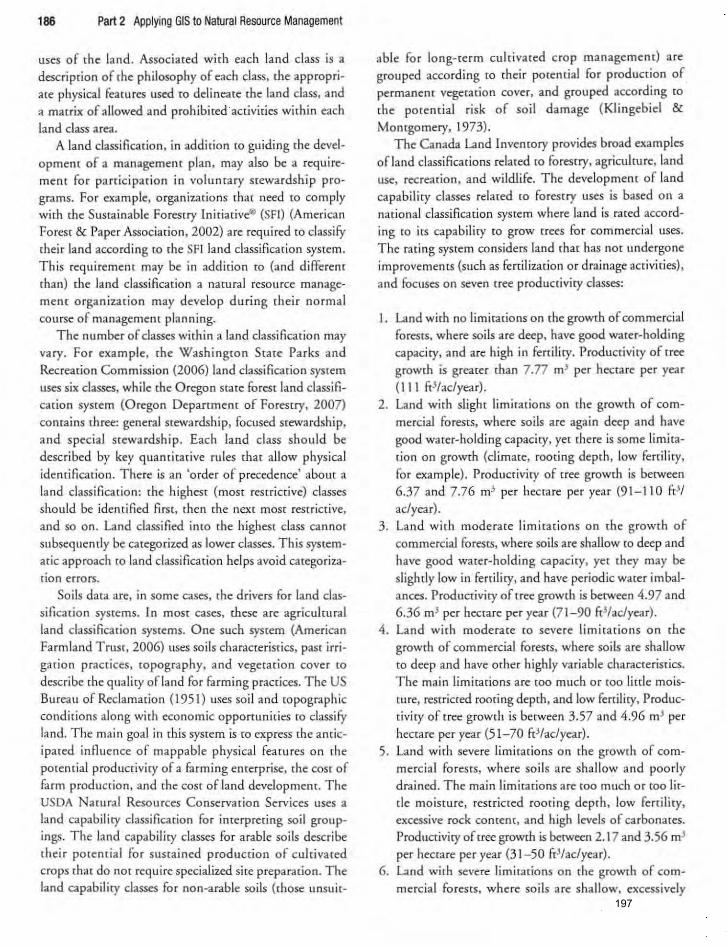
186 Part 2 Applying GIS to Natural Resource Management
uses of the land. Associated w ith each land class is a description of the philosophy of each dass, the appropriate physical featu res used to delineate the land class. and a matrix of allowed and prohibited activities within each
land class area. A land dassification, in addition to guiding the devel
opment of a management plan. may also be a requirement for participation in volunta ry stewardship programs. For example. organizations [hat need ro comply with the Sustainable Forestry In itiative@ (SFJ) (American
Forest & Paper Association , 2002) are required to dassify thei r land according [0 the SF! land classification system. This requirement may be in addirion to {and different
(han) {he land classification a nacura i resource manage
ment organization may develop during their normal
course of management planning. The number of classes withi n a land classification may
vary. For example, the Washington State Parks and
Recreation Commission (2006) land classification system uses six classes, while the Oregon sta te fo rest land classification system (Oregon Department of Forestry, 2007) contains three: general stewardship, focused stewardship, and special stewardship. Each land dass should be described by key quantitative rules that allow physical identification. There is an 'order of precedence' abom a land classificatio n: the highest (most restrictive) classes should be identified first , then the next most restrictive,
and so on. Land classified into the highest class cannor subsequently be catego rized as lower classes. This systematic approach to land classification helps avoid categorization errors.
Soils data are, in some cases, the drivers for land classification systems. In most cases, these are agriculw ral land classification systems. One such system (American Farmland Trust, 2006) uses soils characteristics, past irri
garion practices, (Opography, and vegetation cover to describe the quality ofland for farming practices. The US Bureau of Redamation (195 1) uses soi l and topographic conditions along with economic opporwni t ies to classifY land. The main goal in this system is to express the anticipated influence of mappable phys ical features on the potential productivity of a farm ing enterprise, the cost of fa rm production, and the cost of land developmem. The USDA Natural Reso urces Conservation Services uses a land capability classification for interpreting soil groupings. The land capability dasses for a rable soi ls describe thei r potencial for sustained production of cultivated crops that do not require specialized site preparat ion. The land capability classes for non-arable soils (those unsuit-
able for long-term cultivated crop management) a re grouped according to their potential for production of
permanent vegetation cover, and grouped according to
the potential risk of soil damage (Klingebiel & Montgomery, 1973) .
The Canada Land Inventoty provides broad examples
ofland classifications related to foresny, agriculture, land use, recreation, and wildl ife. The developmenr of land capabil ity classes related to forestry uses is based on a national classification system where land is fated accord
ing to its capability to grow trees for commercial uses. The raring system considers land that has not undergone
improvements (such as fertilization or drainage acrivicies), and focuses on seven tree productivity classes:
1. Land with no limitations on the growth of commercial forests, where soils are deep. have good water-holding capacity, and are high in fertility. Productivity of tree
growth is greater than 7.77 m3 per hectare per year (J 11 ft' /aelyear).
2. Land with slight limitations on the growth of com
mercial forests. where soils are again deep and have good water-holding capacity, yet there is some limitation on growth (dimate, rooting depth, low fertility ,
for example). Productivity of tree growth is between 6.37 and 7.76 m' per hectare per year (9 1-110 ft ' l aelyear).
3. Land with moderate limitat ions on the growth of commercial forests, where soils are shallow ro deep and have good water-holding capacity, yet they may be
slightly low in fertility, and have periodic water imbalances. Productivity of tree growth is between 4 .97 and 6.36 m' per hectare per year (71-90 ft' /ac/year).
4. Land with moderate to severe limitat ions on the growth of commercial fo rests, where soils are shallow to deep and have other highly variable characteristics. The main limitations are roo much or too li ttle mois(Ure, restricted roming depth, and low fertility, Produc
tivity of tree growth is between 3.57 and 4.96 m' per hectare per year (5 1-70 ft'/aelyear).
5. Land with severe limitat ions on the growth of commercial forests , where soils are shallow and poorly drained. The main limitations are roo much or roo little moisture, restricted rooting depth. low fertility, excessive rock content, and high levels of carbonates. Productivity of tree growth is between 2.1 7 and 3.56 m' per hecta re per year (3 1-50 ft' /aelyea r).
6 . Land with severe limitations on the growth of commercial forests. where soils are shallow, excessively
197
186 Part 2 Applying GIS to Natural Resource Management
uses of the land. Associated with each land class is a description of the philosophy of each class. the appropriare physical featu res used to delineate the land class. and a matrix of allowed and prohibieed activities within each
land class area.
A land classificario n, in addition to guiding the development of a management plan. may a]50 be a require
me nt for partic ipation in volu n[ary srewardship pro
grams. For example, organizalions thar need to comply
with the Sustainable Forestry Initiative'" (SFI) (American Forest & Paper Association, 2002) are required to classify thei r land according to the SFI land classification system. This requiremem may be in addidon ro (and different (han) the land c1assificacion a narura! resource manage
menr organizadon may develop during their normal
course of management planning.
The number of classes within a land classification may vary. For example. the Wash ington State Parks and Recreation Commission (2006) land classification system us<os six classes. while the Oregon state forest land classifIcation system (Oregon Department of Forestry. 2007) conrains three: general stewardship, focused stewardship,
and special stewardship. Each land class shou ld be desc ri bed by key quantitative ru les that allow physical identification. There is an 'order of precede nce' abom a
land classificalion: the highest (most restrictive) classes sho uld be identified first, rhen the next most restrictive,
and so on. Land classified into the highest class cannot subsequently be categorized as lower classes. This systemadc approach EO land classification helps avoid categori za
t.ion errors.
Soils data are, in some cases, (he drivers for land clas
sification systems. In most cases, these are agricultural
land classification systems. One such system (American
Farmland Trust, 2006) lISes soils characteristics, past irri
gation practices. topography, and vegetation cover to
describe the quality ofland for farmi ng pcacrices. The U Bureau of Reclamation (195 1) uses soil and ropographic conditions along with econom ic opportunities CO classifY
land. T he mai n goal in this sysrem is ro express the antic
ipated influence of mappable physical features on rhe potential productivity of a farmi ng e nrerprise, the COSt of
farm production. and the cost of land development. The USDA Narural Resources Conservarion Services uses a
land capability classification for inrerprecing soil groupings. The land capabiliry classes fo r arable soils describe their pQ[emial for susrained production of cultivated
crops that do not require specialized si te preparation. The
land capability classes for non-arable soils (those unsuit-
able for long-term cultivated crop management) are
grouped according to their porential for production of
permanent vegetarian cover. and grouped according [0
the potential risk of soil damage (Klingebiel & Montgomery. 1973).
The Canada Land Inventory provides broad examples ofland classificarions related ro forestry. agriculture. land use. recreation, and wildlife. The development of land capabiliry classes related [0 forestry uses is based on a
national classification system where land is rated accord
ing to irs capability [0 grow rrees fo r commercial uses .
T he rating system cons iders land that has nor undergone
improvements (such as fert il ization or dminage accivicies),
and focuses on seven tree productivity classes:
1. Land with no Limitations on [he growth of com mercial
forests, where soils are deep. have good water-holding capaciry. and are high in fertiliry. Productivity of tree grow[h is greater rhan 7 .77 m' per hectare per year
(1 11 fr' /aclyear). 2. Land with slight limitarions on the growth of com
mercial forests, where soils are again deep :tnd have
good water-holding capaciry. yet there is some limitation on growth (dimate. rooting depth. low fertility. for example). Productiviry of tree growth is between 6.37 and 7.76 mJ per hec tare per year (91-1 10 ft'l aclyear).
3. Land with moderate limitations on the growth of
commercial foresrs. where soiJs are shallow co deep and
have good water-holding capaciry, yet they may be slighrly low in ferti~ry. and have periodic water imbalances. Productiviry of tree growth is between 4.97 and 6.3601' per hectare per year (71-90 fr3/aclyear).
4 . Land wirh moderate to severe limitations on the
growth of commercial forests. where soils are shallow
to deep and have other highly variable charactetiStics. The main limitarions are [00 much or roo little mois
ture, restricted roming depch. and low feniliry, Produc
tiviry of tree growth is between 3.57 and 4.96 01 ' per hectare per year (5 1-70 fr' /aclyear).
5. Land w ith severe limi tations o n [he growrh of com
mercial forests, where soi ls are sha llow and poorly
drained. The main limitations are roo much or roo lit
tle mo isture, restricred roming depth , low fertility,
excessive rock coment, and high levels of carbonates.
Productiviry of tree growth is berween 2.1 7 and 3.56 mJ
per hectare per year (31-50 fr' /aclyea r). 6 . Land with severe limitations on the growth of com
mercial fores[s, where soils are shallow, excessively
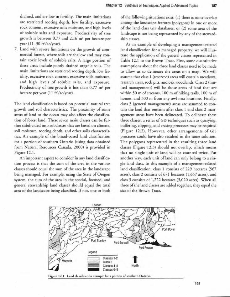
Chapter 12 SyntheSiS of Techniques Applied to Advanced Topics 187
drained, and are low in fertility. The main limitadons are resuicted rooting depth. low fertility, excessive rock content, excessive soils moisture. and high levels of soluble sa lts and exposu re. Productivity of tree growth is between 0.77 and 2.16 m' per hectare per year (11-30 f" /adyear).
7. Land with severe limitations on the growth of commercial forests, where soi ls are shallow and may conta in toxic levels of soluble salts. A large portion of these areas include poorly drained organic soils. The main limitations are restricted rooting depth, low fertility, excessive rock content, excessive soils moisture. and high levels of soluble salts, and exposure. Productivity of tree growth is less than 0.77 m' per hectare per year (1 1 ft3/adyear).
The land classification is based on potential natural tree growth and soil characteristics. The proximity of some areas of land to the ocean may also affect the class ification of forest land. These seven main classes can be fU rther subdivided into subclasses that are based on climate, soil moisture, rooring depth. and orher soils characteristics. An example of the broad-based land classification for a portion of southern Ontario (using data obtained from Natu ral Resources Ca nada, 2000) is provided in Figure 12.1.
An important aspect to consider in any land classification process is that the sum of the area in the various classes should equal the sum of the area in the landscape being managed. For exam ple, using the State of Oregon system, the sum of rhe area in the special, focused, and general stewardship land classes should equal the total area of the landscape being classified. If not, one or both
of the following situations exist: (1) there is some overlap among the landscape features (polygons) in one or more of the land class GIS dacabases, or (2) some area of che landscape is not being represented by any of the stewardship classes.
As an example of developing a management-related land c1assificacion for a managed property, we wi ll illustrare the application of the general classes represented in Table 12.1 to the Brown T ract. First, some quantitative assumptions about the three land classes need to be made to allow us to delinea te rhe areas on a map . We will assume that class 1 (reserved) areas will contain meadows. research areas, rock pits, and oak woodlands. C lass 2 (limited management) will be those areas of land that are within 50 m of streams, 100 m of hiking trails , 100 m of homes, and 300 m from any owl nest locations. Finally, class 3 (general managemenr) areas are assumed to contain the land that remains after class 1 and class 2 management areas have been delineated. To delineate these three classes, a series of GIS techniques such as querying, buffering, clipping, and erasing processes may be requi red (Figure 12.2) . However, other arra ngements of GIS processes could have also resulted in the same solution. The polygons rep resented in the resulting three land classes (Figure 12.3) should not overlap, which means that no single unit of land wi ll be co unted twice. Put another way, each unit of land can only belong to a single land class. In this example of a management-related land classification, class I consists of 229 hectares (567 acres), class 2 consists of671 hecrares (1 ,657 acres) , and class 3 consists of 1,222 hectares (3,020 acres). When all three of the land classes are added togecher, chey equal che size of the Brown Tract.
Port Rowan
Classes 1-2 t Class 3 Classes 4-5 Nor1h Classes 6·8
Figun: l2.. Land d usification cxamplt: for a portion of soumt:rn Ontario.
198
188 Part 2 Applying GIS to Natural Resource Management
(a) Class 1 stewardship areas
0"" process
(e) Class 3 stewardship areas
Erase process
Erase process
(b) Class 2 stewardship areas
Buller process
Buffer process
Buffer process
Buller process
Buffered trails
GIS database
Merge process
Clip process
Eras. process
Figure 12.2 Hierarchy of intermediate and final GIS databases created in one process that facilitates me development of the Brown Tract land classification.
Recreation Opportunity Spectrum
A number of classification processes for outdoor recrearion have been developed, including the Recreacion
Opponunity Spectrum (ROS), carry ing capacity, limits of accep table change. and the Tourism Opportunity Spectrum (Burler & Waldbrook, 1991 ). The latter system
is based on (he Recreation Opportunity Spectrum, and includes aspects of accessibility (i.e., transportation systems) , murism infrastructure, social interaction, and other non-adventure uses. The ROS was developed by the USDA Fo rest Service and the US DI Bureau of Land Management as a tool for managing recreation and
[Quflsm on fede ral land. and for integrating recreation and tourism with other land uses (Clark & Stankey,
1979). ROS is used to describe and identi fy recreational serrings. and to illustrate the likelihood of recreational opportunities along a spectrum that is divided inca several classes. This system combines the physical landscape characteristics of location and access (Q allow you [Q delineate areas of land that may be used for differenc recreational purposes. For exam ple, in the most recent forest plan for the Hi awatha National Forest in norrhern Michigan (US DA Forest Service, 2006) it is suggesred that recreation-rela ted development, activities, management practices, and access will be consistenc with the delineated
199
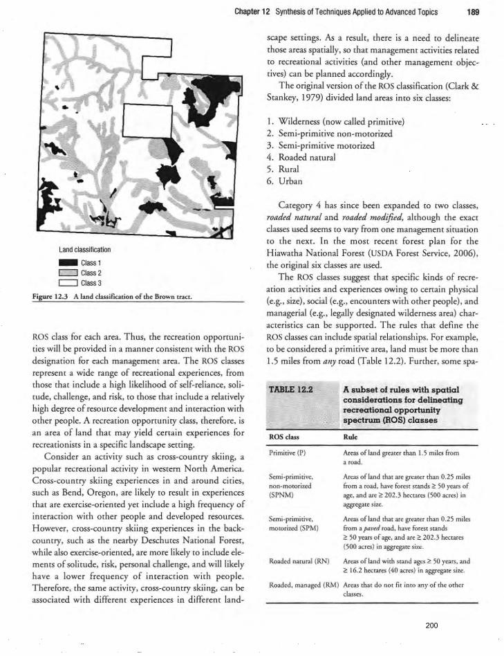
Chapter 12 SyntheSiS of Techniques Applied to Advanced Topics 189
Land classification _ Class 1
c:::::::J Class 2 c:::::::J Class 3
Figw~ 12.3 A land dusification of th~ Brown traCt.
ROS class for each area. Thus. the recreation opportun ities will be provided in a manner consistent with the ROS designation for each management area. The ROS classes represent a wide range of recreational experiences. from rhose rhar include a high likelihood of self-reliance. solitude. challenge. and risk. ro rhose rhar include a relarively high degree of resource development and interaction with
orner people. A recreation opportunity class. therefore. is an area of land that may yield certain experiences for recreationists in a specific landscape setting.
Consider an activiry such as cross-country skiing. a
popular recreational activiry in western North America. Cross-country skiing experiences in and around cities. such as Bend. Oregon. are likely to result in experiences
that are exercise-oriented yet include a high frequency of interaction with other people and developed resources. However. cross-country ski ing experiences in the backcountry. such as the nearby Deschutes National Forest, while also exercise-oriented. are more likely to include elements of solitude. risk. personal challenge. and will likely have a lower frequency of interaction with people. Therefore. the same activity. cross-country skiing. can be associated with different experiences in d ifferent land-
scape settings. As a result. there is a need to delineate
those areas spatially, so that management activities related to recreational activities (and other management objecrives) can be planned accordingly.
The original version of rhe ROS classificarion (Clark & Stankey. 1979) divided land areas into six classes:
I. Wilderness (now called primitive) 2. Semi-primitive non-motorized 3. Semi-primitive motorized 4. Roaded narural 5. Rural 6. Urban
Category 4 has since been expanded to two classes, roaded natural and rooded modified. alrhough me exacr classes used seems to vary from one management situation to the next. In the most recent forest plan for the Hiawarha Narional Forest (USDA Forest Service. 2006).
the o riginal six classes are used.
The ROS classes suggesr rhar specific kinds of recreation activities and experiences owing to certain physical (e.g .• size). social (e.g .• encounters with orher people). and managerial (e.g .• legally designared wilderness area) characterist ics can be supported. The rules that define the
ROS classes can include spatial relationships. For example. to be considered a primitive area, land must be more [han
1.5 miles from any road (Table 12.2). Further. some spa-
TABLE 12-2
ROS class
Primitiv~ (P)
Semi-primitive.
non-momriud (S PNM)
S~mi-primi cive,
motorized (S PM)
Roaded natural (RN)
A subset of rules with spatial consideratioDs for delineating recreational opportunity spectrum (ROS) classes
RuI,
Areas ofland great~r than 1.5 miles from
a road.
Areas of land that ar~ greater than 0.25 mi les
from a road , hav~ forest stands ~ ;0 years of
ag~. and ar~ ~ 202.3 hectares (500 acres) in aggregat~ siu.
Areas of land that ar~ grear~r than 0.25 miles from a pawd road. hav~ forest stands
<!: 50 yeltS of ag~. and are ~ 202.3 hectares
(500 acres) in aggrega[~ size:.
Areas of land with stand ages ~ 50 years. and
2: 16.2 hectares (40 acres) in aggregat~ siu.
Road~d, manag~d (RM ) Ar~as that do nor fit imo any of rh~ other
classes.
200
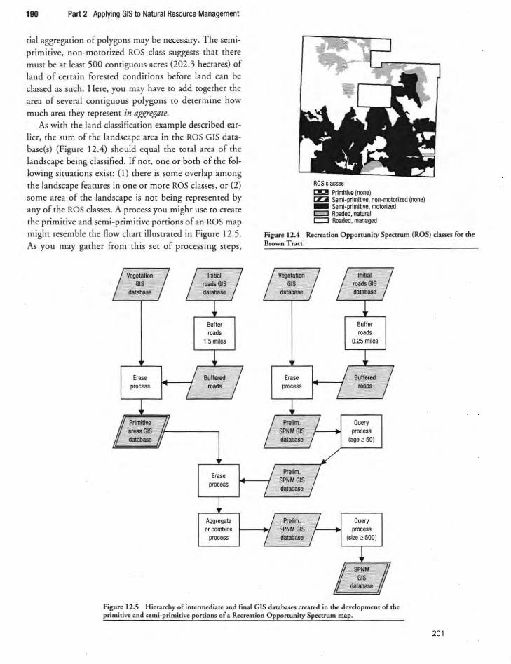
190 Part 2 Applying GIS to Natural Resource Management
[ial aggrega[ion of polygons may be necessary. The semiprimitive, non-motorized ROS class suggestS mat there muse be a[ leas[ 500 comiguous acres (202.3 hec[ares) of land of certain forested conditions before land can be classed as such. Here, you may have co add cogecher [he
area of several contiguous polygons to determine how much area rhey represent in aggregate.
As with rhe land classification example described eacIier, [he sum of [he landscape area in [he ROS GIS da[abase(s) (Figure 12.4) should equal [he co[al area of [he landscape being classified. If no[, one or borh of [he fol
lowing sicu3rions exist: (1) there is some overlap among the landscape fearures in onc or more ROS classes, or (2) some area of rhe landscape is not being represented by any of rhe ROS classes. A process you might use co create the primitive and semi-primitive portions of an ROS map migh[ resemble [he flow chan illusera[ed in Figure 12.5.
As you may gather from this set of processing steps,
Erase process
Buffer roads
1.5 miles
Erase process
Aggregate or combine
process
ROS classes I:J!!!It!!I Primitive (none) rz::::iiiI Semi-primitive, non-motorized (none) _ Semi-primitive, motorized c::J Roaded, natural c:::J Roaded, mCYlaged
Figure 12.4 Recreation OpponunitySpecuum (ROS) classes for the Brown Tract.
Erase process
Buller m.ds
0.25 miles
Query process
(age ~ 50)
Query process
(size :<!: 500)
Figure 12.5 Hieruchy of intermediate and final C IS databases created in the development of the primitive and semi-primitive portions of a Recreation Oppo rtunity S~ctrum map.
201
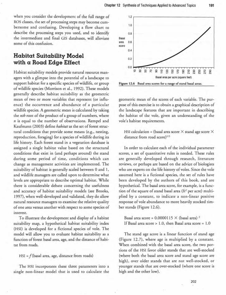
Chapter 12 Synthesis ofTechniques Applied to Advanced Topics 191
when you consider the development of the full range of ROS classes, rhe sec of processing steps may become cum
bersome and confusing. Developing a flow chan to
describe the processing steps you used, and co identify the intermediate and final GIS darabases, will alleviare some of this confusion.
Habitat Suitability Model with a Road Edge Effect
Habitat suitability models provide natural resource managers with a glimpse inca rhe potencial of a landscape co suppOrt habitat for a specific species of wildlife, or group
of wildlife species (Morrison et ai., 1992) . These models generally describe habitat suitability as the geometric mean of two or more variables that represent (or inAu
ence) the occurrence and abundance of a particular
wildlife species. A geomerric mean is calculated by raking rhe nth root of the product of a group of numbers, where
n is equal to rhe number of observations. Rempel and
Kaufmann (2003) define habitat as rhe set of foresr struc(ural conditions that provide some means (e.g. , nesting.
reproduction. foraging) for a species of wildlife during its life history. Each forest stand in a vegetarion database is
assigned a single habitat value based on rhe structural
conditions thar exisr in (and perhaps around) the srand during some period of time. conditions which can
change as management activicies are implemented. The
suirabiliry of habirat is generally scaled becween 0 and I, and wildlife managers are called upon to determine what
levels are appropriate (0 describe optimal habitat. While there is considerable debate concerning the usefulness and accuracy of habitat suitabiliry models (see Brooks, 1997), when well-developed and validated, they do allow natural resource managers (Q examine rhe relative quality
of one area versus another with respect to some species of
inceresc. To illustrate the developmenr and display of a habirar
suitabiliry map, a hypothetical habirat suitabiliry index (HSI) is developed for a fictional species of vole. The model will allow you CO evaluate habitat suitability as a function of foresr basal area, age, and the distance of habitat from roads.
HSI = j(basal area, age, disrance from roads)
The HSI incorporates rhese three paramerers into a
single non-linear model that is used ro calculate rhe
1.2,-----------------,
1.0
0.8
Basal area 0.6 sco<,
0.'
0.2
Basal area per acre (sQuare feet)
Figure 12.6 BanI area scores for a range of stand basal areas.
geometric mean of the scores of each variable. The pur
pose of rhis exercise is to obtain a graphical descriprion of
the landscape features that are important in describing rhe habirar of the vole, given an undemanding of rhe vole's habitat requirements.
HSI calcularion = (basal area score X stand age score X
distance from road score) 113
In order [Q calculate each of the individual parameter
scores, a ser of quantirative rules is needed. These rules
are generally developed rhrough research , lirerature
reviews, or perhaps are based on the advice of biologists
who are experts on rhe life history of voles. Since rhe vole assumed here is a fictional species, the set of rules have
been developed by the authors of rhis book, and are hyporhetical. The basal area score, for example, is a funcrion of rhe square of srand basal area (fr2 per acre) mulriplied by a consrant, ro indicate a non-linear posirive
response of vole abundance to more heavily s[Qcked tim
ber stands (Figure 12.6).
Basal area score = 0.0000 I 15 X (basal area) 2
If Basal area score> 1.0, then Basal area score = 1.0
The stand age score is a linear funccion of stand age
(Figure 12.7), where age is multiplied by a co nsranr. When combined with the basal area score, me [wo por
tions of rhe HSI favor older srands that are well-stocked (where both rhe basal area score and stand age score are
high), over older srands rhat are not well-stocked, or younger srands rhat are over-stocked (where one score is
high and the other low) .
202
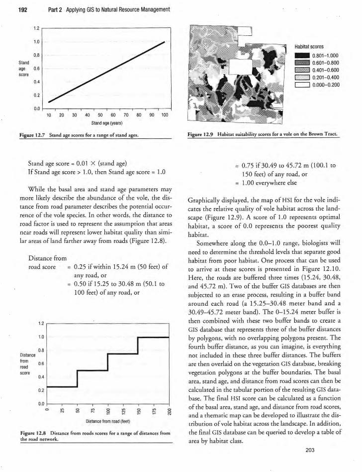
192 Part 2 Applying GIS to Natural Resource Management
1.2
1.0
0.8
Stand a,. 0.6 score
0.4
0.2
0.0 1----,--,----,--,----,--,----,--,----r----1 10 W M ~ W ~ ro W 00 @
Stand age (years)
Figure 12.7 Stand age scores for a range of stand ages.
Scand age score = 0.01 X (scand age) If Scand age score> 1.0, chen Scand age score = 1.0
While the basal area and stand age parameters may more likely describe the abundance of rhe vole, the dis
tance from road parameter describes rhe potential occur
rence of the vole species. In other words , the distance to
road factor is used {Q represent the assumption that areas
near roads will represent lower habitat quality than simi
lar areas of land fa[(her away from roads (Figure 12.8) .
Distance from
road score
1.2
1.0
0.8 Distance from 0.6 road score
D ••
0.2
0.0 0 ~
N
0.25 if wichin 15.24 m (50 feec) of any road, or 0.50 if 15.25 (0 30.48 m (50.1 (0
100 feec) of any road, or
I I
I
Distance from road (feet)
Figure 12.8 Distance from roads scores for a range of distances from the road network.
Habitat scores
_ 0.80H.000 _ 0.601- 0.800
c::J 0.401-0.600 c::J 0.201-0.400 c::J 0.000-0.200
Figwe 12.9 Habitat suitability scores for a vole on the Brown Tract.
0.75 if 30.49 CO 45.72 m (100.1 (0
150 feec) of any road, or I .00 everywhere else
G raphically displayed, che map of HSI for che vole indicates the relative quality of vole habitat across the land
scape (Figure 12.9). A score of 1.0 represen" opcimal
habitat , a score of 0.0 represents the poorest quality
habicar. Somewhere along che 0.0-1.0 range, biologisrs will
need to determine the threshold levels that separate good
habitat from poor habitat. One process that can be used to arrive at these scores is presented in Figure 12.10 .
Here, che roads are buffered chree cimes (15.24, 30.48, and 45 .72 m). Two of rhe buffer GIS databases are chen subjected to an erase process. resulting in a buffer band
around each road (a 15.25-30.48 mecer band and a 30.49-45.72 mecer band). The 0--15.24 mecer buffer is then combined with these MO buffer bands (Q create a
GIS database that represents three of the buffer distances
by polygons, wich no overlapping polygons presem. The fourth buffer distance, as you can imagine. is everything
nor included in chese chree buffer discances. The buffers are then overlaid on the vegetacion GIS database. breaking
vegecacion polygons ac che buffer boundaries. The basal area, stand age. and distance from road scores can then be
calculaced in che cabular ponion of che resulcing GIS dacabase. The final HSI score can be calculaced as a funcrion
of the basal area, stand age, and distance from road scores. and a thematic map can be developed to illustrate the dis
tribution of vole habitat across the landscape. In addition,
che final GIS dacabase can be queried co develop a cable of
area by habicar class. 203
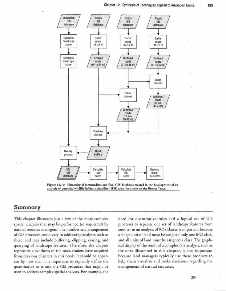
Chapter 12 Synthesis of Techniques Applied to Advanced Topics 193
Iv~m~ I L R_ / I Roa~ I I Roads I GIS GIS GIS GIS da!abase database da!abase database
i ~ ~ ~ Calculate Buffer Buller Buffer basal area roads roads r_
score 15.24m 30.48 m 45.72 m
~ ~ ~ ~ Calculate I( BUllere,,'; I( Buffered III I( Buffered III stand age
(o-~~m) (o-~~ m) roads score (0-45.72 ml
~ Erase
process
Erase ~ process I Bullered I roads
~ (3Q.48-45.7Srn) I Buffered I r_
(15.24-30.48 m)
Combine process
~ Overlay / Road I process / buffers
~ I HSI IL Calculate calculate Develop GIS road HSI mapaf
database II score score HSI scores
Figure 12.10 Hierarchy of intermediate and final GIS d:ltabue$ created in the devdopmcnt of an analysis of potential wildlife habitat suitability (HSI) areas for a vole on the Brown Tract.
Summary
This chapter illustrates juSt a few of [he more com plex spatial analyses that may be performed (or requested) by natural resource managers. The number and arrangemem
of GIS processes could vary in addressing analyses such as these, and may include buffering. clipping, erasing, and querying of landscape features. Therefore. the chapter represents a synthesis of the tools readers have acquired from previous chapters in this book. It should be apparent by now that it is important to explicitly define the quantitative rules and the GIS processes that might be used to address complex spatial analyses. For example, the
need fo r quantirative rules and a logical set of GIS processes [0 separate one set of landscape featu res from another in an analysis of ROS classes is important because a single un it of land must be assigned only o ne ROS class, and all units ofland must be assigned a class. The graphical display of the result of a complex GIS analysis. such as the ones illustrated in this chapter. is also important because land managers rypical ly use these products to help them visualize and make decisions regarding the management of natural resources.
204

194 Part 2 Applying GIS to Natural Resource Management
Applications
12.1 Land classificat ion. Becky Blaylock, manager of
the Brown Tract, wants you to develop a management
related land classification for the forest. She asks you to
develop GIS databases for each of three classes using the
following rules: 1. Special stewardship areas will consist of the follow
ing landscape features: Oak woodlands, Meadows,
and Rock pits. 2. Focused stewardship areas will consist of the follow
ing landscape feamces:
a. streams buffered according co the Oregon State Forest Practices Act (30.48 meters [100 feet]
around large fish-bearing st reams [Size = 'Large'
and Fishbearing = 'Yes], 21.34 meters [70 feet]
arou nd medium fish-bearing streams, 15.24
meters [50 feet] around small fi sh-bea ring
streams, 2 1.34 meters [70 feet] around large
non fish-bearing streams, 15.24 meters [50 feet]
around medium non fish -bearing streams, and
6.10 meters [20 feet] around small non fish
bearing streams);
b. a buffer of 100 meters around all water sources
tha t are not culvert spills or water towers;
c. a buffer of 100 meters around all authorized
(rails; and
d. research areas. 3. General stewardship areas will consist of whatever
land remains.
Do the following:
a) Develop and illustrate a process (How chart) for
accomplishing the task of defining the land classi
ficat ions of the Brown Tract forest according to the
rules listed above.
b) D etermine how much land area is contained in the
special stewardship land classification .
c) Determine how much land area is contained in the
focused stewardship land classification.
d) Determine how much land area is contained in the
general stewardship land classification .
e) Produce a map of the entire Brown Tract, ill ustrat
ing the three land classifications.
As a general strategy, you may want to follow [his process: • Develop a special stewardship GIS database.
• Develop a focused stewa rdship GIS database by
performin g the appropriate buffer and query
processes, and then intersecting these GIS databases.
(Why would you nOt use a merge process here?) • Erase the special stewardship GIS database features
from the focused stewardship GIS database features.
• Erase both the special stewardship GIS database fea
tures and [he focused stewardship GIS database fea
tures from the stands GIS da tabase, creating the
general stewardship GIS database.
12.2 Recreat ion O pportunity Spectrum. The Dimict
Manager associated with the Brown Tracr (Becky
Blaylock) would like you to determine how much area
might be classified in the five recreation opportunity spec
trum (ROS) classes (see T able 12.2) . Based on this subset
of rhe ROS criteria,
a) How much land area is contained in the primitive
class? b) How much land area is contained in the semi
primitive, non-mororized class? c) How much land area is contained in the semi
primitive, motorized class? d) How much land area is contained in the roaded
natu ral class?
e) How much land area is contained in the roaded
managed class? f) Develop a thematic map illustrating the five ROS
classes on the Brown Tract.
g) Draw a flow chart [Q describe the p rocesses lIsed [Q
develop the ROS classes, including the GIS operations and all GIS databases used (original, interme
diate, and final GIS databases).
12.3. Visual quality buffers. You have been asked by
the manager of the Daniel Picken forest [Q evaluate the
potential impact of two proposed organizational policies
for the forest resources found there. It seems that the
owners of the property are becoming very concerned with
the public perception of management on the forest, thus they are interested in the trade-off's associated with alter
native management pol icies.
Policy #1: Buffers next to neighboring landowners.
Assume for this example that even-aged forest manage
ment is practiced across the property. This potential
pol icy suggests that c1earcllt harvesting activities adjacent to neighboring landowners of the Daniel Pickett
forest will be restricted.
205
Chapter 12 Synthesis ofTechniques Applied to Advanced Topics 195
a} If a 50-meter uncut buffer were to be left adjacent co all other property owners, how much land would this require as a volumary contribution [0
rhe pCQ[ecrion of adjacent landowners resources?
b} How much timber volume of vegetation class A would be found in the buffer (vegetation class A is the older timber class. perhaps that which can be harvested in the near- term). and what perce mage
of rhe [Ocal volume in this vegetation class would
be affected?
Policy #2: Buffers next to paved public roads. This potential policy suggeSts that visual quality buffers may be maintained along paved roads within rhe Daniel Pickett forest. These buffers will not be managed. bur rather treated as reserved areas, where har
vesting is precluded. a} If a 50-meter buffer were required around all paved
roads, how much land area would this involve, and
how much timber volume in vegetarion class A would it affect?
b} If the State decided to convert the North-South paved road on the Daniel Pickett foreSt to a highway, and required a 1 DO-meter wide corridor [Q he transferred to State ownership, how much land area would be affected?
c} If bare land values were assumed to be $200 per hecta re. and timber volumes $400 per thousand
References
American Farmland Trust. (2006). Land classification
sysum. Washington. DC: American Farmland Trust. Retrieved February 17. 2007. from http://www. farmland.org/resources/furureisnowllanddassification system.asp.
American Forest & Paper Association . (2002) . Sustainable Fomtry Initiative (SFI)"'. Washington. DC: American Forest & Paper Association. Retrieved December 10.2007. from http: //www.afandpa.org/ ContentfNavigation Menu/ Environment and Recycling! SFIISFl.htm.
Brooks. R.P. (l997). Improving habitat suitabil ity index models. Wildlifi Society Bulletin. 25. 163-7.
Butler. R.W .• & Waldbrook. L.A. (l991). A new planning tool: The tourism opportunity spectrum. JournaL of Tourism Studies. 2(1). 2-14.
board feet (MBF). how much would you ask the Scare [Q compensate [he owners of the Daniel Pickert forest for the loss of this land?
d} If a 30-meter visual quality (i .e .• uncurl buffer was then proposed around the I OO-meter highway corridor, what is the [mal effect [Q the forest resource base, in terms of land area now affected in each vegetation type?
12.4. Habitat suitability index for a vole. The biologist associated with the Daniel Picken forest, Will Edwards. has recently become aware of a vole habi tat suitability model, and is interested in understanding the extenr of vole habitat on the forest. Will asks you to apply the model described in the 'Habitat Suitability Model with a Road Edge Effect' section of this chapter to the Daniel Pickett forest, and m:
a) Calculate the amount of land area on the Daniel
Pickett forest in the following habitat suitabil ity classes: 0.000-0 .200 (low quality). 0.201 -0.400 (low/moderate quality). 0.401-0.600 (moderate qual ity). 0.601-0.800 (moderate/high quality). 0.801-\.000 (high quality).
b} Develop a map illustrating the habitat quality for the vole by suitabi lity class.
c) Draw a flow chart of rhe process yo u used to develop the habitat suitability classes.
Canadian Forest Service. (2007). Ecological land classifications. Onawa. ON: Canadian Forest Service, Natural Resources Canada. Retrieved February 17. 2007. from h up:11 ecosys.d1.scf. rnea n. gc.cal dassifl i n rro_strat_ e. asp.
Clark. R.N .• & Stankey. G.H . (I 979}. The recreation
opportunity spectrum: A framework for planning, management, and research. GeneraL Technical Report PNW-
98. Portland . OR: Pacifi c Northwest Forest and Range Experiment Station, USDA Forest Service.
Frayer. W.E .• Davis. L.S .. & Risser. P.G. (I 978}. Uses of land classification. Journal of Forestry. 76. 647-9.
Klingebiel. A.A .. & Montgomety. P.H. (I 973}. Land capability classification. USDA agricultural handbook 210. Washington. DC: US Government Printing
Office. Retrieved February 17. 2007. from http://
206
196 Part 2 Applying GIS to Natural Resource Management
soils.usda.gov/technical/handbookicontents/partG22p2. html#ex2.
Morrison , M.L. , Marcot, B.G. , & Mannan, R.W. (19 92). Wildlife-habitat relationships: Conupts and applications. Madison. WI : University of Wisconsin Press.
Natural Resources Canada. (2000). Overview o[classification methodology for deurmining land capability for foustry. Ottawa, ON: GeoG racis C li ent Services, Narurai Reso urces Canada. Retrieved August 10, 2007, from http: //geogratis.cgdi.gc.ca/C LI /frames. htm!'
Oregon Department of Forest ry. (2007). Oregon administrative ruiLs, department o/forestry, Division 35. man
agement o[ state forest lands. Salem, OR: Oregon Department of Forestry. Retrieved March 12, 2007, from http://a rcweb.sos.sta te.or.us/ rules/OARS_GOO/ OAR_G29/629_035.html.
Rempel, R.S., & Kaufmann , C.K. (2003) . Spatial modeling of harvest co nsrra inrs on wood supply ve rsus wildlife habi tat objectives. Environmental Manage
ment, 32, 646-59. US Bureau of Reclamation. (195 1). Land classification.
Bureau of reclamation manual vol. V, irrigated land
use, part 2. Denver, CO: US Bureau of Reclamation. USDA Forest Service. (2006). Hiawatha national forest,
2006 forest plan. Milwaukee, WI: USDA Forest Service, Eastern Region. Retrieved February 18,2007, from http://www.fs.fed.us/r9/hiawatha/revision/2006/ ForPlan .pdf.
Washington State Parks and Recreatio n Commission. (2006) . WAC 352-16-020 land classification. Olympia, WA: Washington State Parks and Recreation Commission. Retrieved February 17,2007, from http://www. parks.wa.gov/ plansllowerhoodcanaI/State%20Parks% 20 Land%20Classifications. pdf.
207
196 Part 2 Applying GIS to Natural Resource Management
soils. usda.govltochnicaUhandbookicontents/part622p2. html#ex2.
Morrison. M.L. . Marcot. B.G .• & Mannan. R.W. ( 1992). Wildlife-habitat relationships: Conupts and applications. Madison, WI : Universiry of Wisco nsin Press.
Natural Resources Canada. (2000). Overviewofclassification methodology for determining land capability for forestry . Onawa, ON: GeoGrads Cli enc Services. Nacural Resources Canada. Rerrieved Augus[ 10, 2007. from hrtp: lIgeogratis.cgdi.gc.ca/CLl /frames. html.
Oregon Depareme", of Forestry. (2007). Oregon adminiJtrah'vt! nlus, department offorestry. Division 35. manngeuullt of statt forest lands. Salem , OR: Oregon Depanme", of Fore5[ry. Retrieved March 12. 2007. from h((p: llarcweb.sos.sta te.or.us/rules/OARS_6001 OAR_629/629_035.html.
Rempel. R.S .. & Kaufmann. G.K. (2003). Spatial modding of harvest co nsuainrs on wood supply ve rsus wildli fe habicat objecrives. £Ilvironmeruo/ Management. 32. 646-59.
US Bureau of Reclamation. (1951). Land classification. Bureau of reclamation manull~ vol. V, irrigated land use. part 2. Denver. CO: US Bureau of Reclamation.
USDA Forest Service. (2006). Hiawatha national form. 2006 fomt plan. Milwaukee. WI: USDA Forest Service. Eastern Region. Retrieved February 18.2007. from http://www.fs.fed.us/r9/hiawarhalrevision/2006/ ForPlan .pdf.
Washington Scate Parks and Recrearion Com mission. (2006). WAC 352-16-020 land classification. Olympia. WA: Washington Srate Parks and Recrea(ion Commission. Reuieved Februa.ry 17. 2007. from htrp:/iwww. parks.wa.gov/plans/lowerhoodcanaI/Srare%20Parks% 20Land%20Classificat ions.pdf.
Chapter 13
Raster GIS Database Analysis
Objectives
The skills and techniques you'll learn in this chapter should provide insight inco the examination and applicadon of raster GIS databases for natural resources research,
and how raster GIS databases might be included in suppaning natural resource management decision-making. At the conclusion of this chapter, you should have an understanding of:
1. how landscape comour GIS databases are created from
a OEM;
2. how landscape shaded relief GIS databases are created from a OEM;
3. how slope GIS databases are created from a OEM; 4. how to calculate slope gradients for a linear landscape
feature, such as a road, trail, or stream;
5. how (0 conduct a viewshed analysis for a parrion of a landscape; and
6. how to create a watershed boundary based on digital elevation data.
As mentioned in chapters 1 and 2, there are {Voto gen
eral types of data structures used in GIS coday: vector and
raster. Unci l now, we have focused on vec[Qr GIS data
bases and the GIS operations related to the typical kind of applications performed in natural resource organizat ion
field offices. This chapter now delves into rhe use of raster
GIS databases for namral resource applications. and a few
of the GIS operations that can be performed using them.
An emphasis is placed on how raster GIS databases might
be used in field offices to support natural resource man
agement decisions. Although we will rurn our attemion in
the next chapter to other raster database applications. the
primary raster GIS database that is considered in th is
chapter is a digital elevation model (OEM) . Many difTerem types of landscape information can be cultivated from
a single OEM database.
Digital Elevation Models (OEMs)
As their name implies. OEMs comain information related
to the elevation of a landscape above sea level or relative to
some other datum point. T hey are different than the typ
ical USGS Quadrangle maps discussed in chapter 4, in that they are in digital form. As with other raster GIS databases, each unit on the landscape is typically represented by a landscape-related value (or set to a null or 'no data' value),
and each unit is exactly the same s ize and shape as the
other units (F igure 13.1). The most prevalent OEM databases available in the US are the USGS 30 meter OEMs (US Department of Interior, US Geological Survey, 2007). Within Canada, Natural Resources Canada (2007) provides access to digital topographic data. Raster databases are onen described in terms of their spatial resolu
tion, as in the phrase '30 m OEM'. This infers that each grid cell in the OEM database is 30 m by 30 m in size in terms of on-the-ground area that it represenrs. Many
regions in the US also have 10m OEMs available for areas within federal and state agency administrative boundaries.
In some cases OEMs for states. provinces. or other large
regions can be purchased from commercial entities.
DEMs can be used for a variety of analytical purposes,
bur the most general of these purposes is simply ro view
the rel ief of a landscape. OEMs can use shades of color or gray rones co illustrate differences in e1evadon through a
208

198 Part 2 Applying GIS to Natural Resource Management
Figure 13.1 Ruler grid cells from a digital elevation mode (OEM).
separation and c1assificarion of elevation values . Figure
13.2 illuscrates a gray tone color-shading scheme applied to a 10 m OEM of the Brown Tract, and uses a twelvecategory equal-inrerval classification scheme CO highl ight (he cha nges in elevation. The equal-imerval classificat ion
takes the disrriburion of elevadon data values found
within the 10m OEM and divides it equally into twelve sub-sets of elevat ion ranges. Most GIS software will allow users to define [he number of elevation range categories shown visually. and offer choices for color and gray tone schemes [0 illusrrate distinctions between elevation C3rcgones.
Brown Tract
OEM Values (feet)
D 136-150
0 151 - 200
D 201-25O
D 251 - 300
~301- J50
IH;11 351 -"OO 111 401_ 450
_ 451 -500 _ 501- 550
_551-600
_801-850
_651-700 _ No Data
Figure 13.2 Elevation ca t~ori~ for the Brown Tract using a 10 m OEM.
One notable category rep resented in the legend in Figure 13.2 is the 'No Data' category. This category is necessary because raster GIS data must be stored as a set of grid
cells that combine ro form a rectangular or square shapethe width and height of the image is defined by the number of grid cells. Therefore, when landscape fearures of interest do not match a rectangular shape (e.g., the shape of the Brown Tract) , the grid cells that are nOt associated with [he landscape features of interest are given a nuil , or No Data, value. For example, all of the grid cells that represent areas outside the boundary of the Brown T ract con
tain no data. For mapping purposes, the symbolization
used to display cells with a null value can be assigned a transparent shade. Almost all raster GIS software programs allow the recognition of a null value, yet are designed to ignore this va lue in analytical computations. When performing a multiple GIS database overlay analysis, some raster GIS software programs are also designed ro ignore any cells that overlap null cells in any other GIS database being analyzed. For example, if twO spatially coincident raster databases were overlaid on each orher and any portion of either dacabase comained cells with no darn, any
database resuhing from an overlay or comparative analys is that involved borh databases would also comain no data cells at rhe same locations. This result would occur even if actual values were present in a portion of one of the raster databases. Whi le th is functionality may or may not be appropriate for particular G IS analyses, users should be cognizant of how null values assigned to grid cells will be handled within their selected GIS software program{s).
Elevation Contours
OEMs can be used to create devation contours, or lines that indicate a constant or nearly constam elevation across a landscape. Contour lines are created adjacent ro each other such that elevation represented in even increments, such as every 30, 50, or 100 m. An elevation contour GIS database is usually represemed through a vector dara
srruCture based on a user-defined elevation interval. Contour lines allow YOll to examine the relarive relief of a landscape and to make inferences about landscape ropography ro support managemem decisions. For example. contour intervals can be used ro delineate likely hydrologic drainage patterns and watershed boundaries. When designing road systems, engineers rypically need to keep the slope of each road below some maximum gradient. since slopes too steep will either prevem the movement of certain rypes of veh icles (if the vehicle is travelling uphill),
209
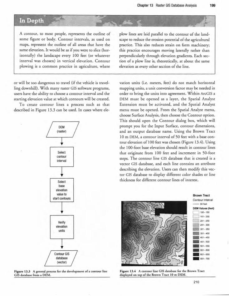
A contour. [Q most people. represents the ou dine of some figure or body. Contour intervals. as used on maps. represent the oudine of all areas thar have the same elevation. It would be as if you were to slice (horizontally) the landscape every 100 feet (or whatever interval was chosen) in verrical elevation. Contour plowing is a common practice in agriculture. where
or will be too dangerous to travel (if the vehicle is travelling downhill) . With many raster GIS software programs, users have the ability [Q choose a contour interval and the starting elevation value at which contours will be created.
To creare contour lines a process such as rhar described in Figure 13.3 can be used. In cases where e1e-
Select contour interval
Setect base
elevation value to
start contours
Verify elevation
units
Figure 13.3 A general process for the development of a contour line GIS database from a OEM.
Chapter 13 Raster GIS Database Analysis 199
plow lines are laid parallel to the contour of the landscape [Q reduce the erosion potential of rhe agricultural practice. This also reduces strain on farm machinery; this practice encourages moving laterally rather than perpendicularly through elevation gradients. Each section of a plow line is. theoretically. at about the same elevation as every other section of the line.
vatlon umts (i.e. meters. feet) do not match horizontal mapping units. a unit conversion factor may be needed in order to bring the units into agreement. Within ArcGIS a OEM must be opened as a layer, the Spatial Analyst Extension must be activated. and the Spatial Analyst menu must be opened. From the Spatial Analyst menu. choose Surface Analysis. then choose the Contour option. This should open the Contour dialog box, which will prompt you for the Input Surface. conrour dimensions, and an output database name. Using the Brown Tracr 10m DEM, a COntour interval of 50 feet with a base contour elevation of 1 00 feet was chosen (Figure 13.4). Using (he 100-foot base elevation should result in comour lines that o riginate from 100 feet and incremem in 50-foot steps. The contour line GIS database that is created is a vector GIS database, and each line contains an att ribute describing the elevation . Users can then modify this vector GIS database to display different color shades or line thickness for differenr contour lines of interest.
Brown Tract
ContoIS Interval
- 50'''' OEM Value. (feet)
0 100- 150
o 1S1-200
W 2{)1 -25O
2S1-lOO _ 301 - 350
_ 351--400
_4()1-~
_.Sl -5OO _ 501-S50
_ 551-600
_ 601-MO
_ 6S1 -700
Figure 13.4 A contour line GIS database for the Brown Tract displayed on top of the Brown Tract 10 m OEM.
210
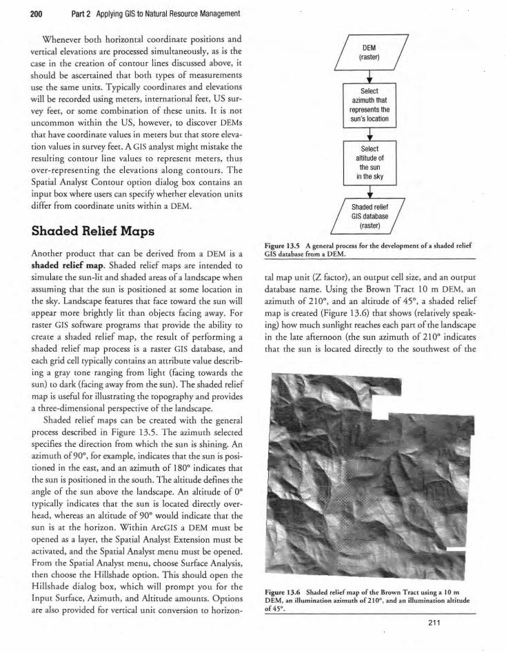
200 Part 2 Applying GIS to Natural Resource Management
Whenever boch horizontal coordinate positions and vertical elevations are processed simultaneously. as is {he
case in the creation of contour lines discussed above. it should be ascenained. [hat both cypes of measurements use rhe same units. TypicaUy coordinates and elevations will he recorded using meters, international feet, US survey feet, or some combination of these units . It is not uncommon within rhe US, however, to discover OEMs chat have coordi nate values in meters bur (hat srore eleva
tion val ues in survey feec. A GIS analyst might mistake rhe resulring contour line va lues (a represent meters, rhus over-representing (he elevat ions alo ng co ntou rs. The
Spac ial Analyst Contour option dialog box conta ins an input box w here users can specify whether elevation units
differ from coordinate units within a OEM.
Shaded Relief Maps
Another product that can be derived from a OEM is a
shaded relief map. Shaded relief maps are intended ro simulate the su n-lit and shaded areas of a landscape when
assuming thar the sun is positioned at some location in
rhe sky. Landscape fearures that face roward the sun will appear more brightly lit than objects facing away. For raster GIS software programs that provide the abiliry co
create a shaded relief map. the resulr of performing a
shaded relief map process is a raster GIS database, and
each grid cell typically contains an attribute value describing a gray cone rangi ng from light (facing cowards rhe
sun) ro dark (f..ci ng away from the sun). The shaded relief map is useful for illustraring rhe ropography and provides a th ree-dimensional perspective of the landscape.
Shaded relief maps can be created with the genera l process described in Figure 13.5. The azimuth selected specifies the d irection from which rhe sun is sh in ing. An
azimuth of 90°, for example, indicates that the sun is posi
tioned in rhe eaSt, and an azimuth of 1800 indicates that
rhe sun is positioned in the south. The altitude defines the
angle of the sun above the landscape. An alti tude of O· typically indicates that the sun is located directly over
head, whereas an altitude of 90· wou ld indicare thar the sun is at the horizon. With in ArcGIS a OEM must be
opened as a layer, the Spatial Analyst Extension must be act ivated, and the Spatial Analyst menu must be opened. From [he Spatial Analyst menu, choose Surface Analys is.
then choose rhe Hillshade option. This should open rhe Hillshade dialog box, which will prompt you for the Input Surface. Azimuth, and Altitude amOunts. Options
are also provided for vertical unit conversion to horizon-
Selecl azimuth that
represents the sun's location
Select altitude of
the sun in the sky
(raslerl
Figure: 13.5 A gene:ral process for the: devdopme:nt of a shade:d re:lie:f GIS database: &om a OEM .
tal map unit (Z factor), an ompur cell size. and an output
database name. Usi ng the Brown T ract 10m OEM, an
azimurh of 210·, and an altitude of 45·, a shaded rel ief map is created (Figu re 13.6) that shows (relatively speaking) how much sunl ight reaches each parr of the landscape in the late afternoon (the su n azimurh of 21 0° indicates
[hat the sun is located directly co the southwest of the
FigllR 13.6 Shade:d relief map of the: Brown Tract using a 10m OEM, an illumination azimuth of 210°, and an illumination altitude of 45°.
211
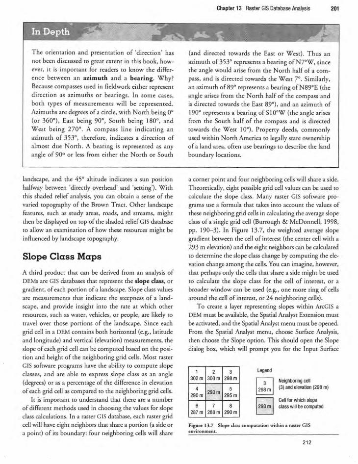
The oriemacion and presentation of 'direction ' has not been discussed co great extent in this book, however, it is important for readers to know the difference between an azimuth and a bearing. Why? Because compasses used in fieldwork either represent
di recdon as azimuths or bearings . In some cases , both types of measurements will be represented. Azimuths are degrees of a circle, with No rth being 0° (or 360°), East being 90°, South being 180°, and West being 270°. A compass line indicating an azimuth of 353°, therefore, indicates a d irect ion of
almost due North. A bearing is represented as any angle of 900 or less from eithet the North or South
landscape, and the 45° altitude indicates a sun position halfway between 'direcdy overhead' and 'setting'). With this shaded relief analysis, you can obtain a sense of the varied ropography of the Brown T ract. Other landscape features. such as study areas, roads, and streams, might [hen be displayed on tOp of the shaded rel ief GIS database to allow an exam ination of how chese resources might be
influenced by landscape tOpography.
Slope Class Maps
A third product that can be derived from an analysis of DEMs are GIS databases that represent the slope class, or gradient, of each portion of a landscape. Slope class values are measurements chat indicate me steepness of a landscape, and provide insight into the rate at which other resources, such as water, vehicles. or people. are likely to travel over [hose portions of [he landscape. Since each
grid cell in a DEM contains both horiwntal (e.g., latitude and longitude) and vertical (elevat ion) measurements, the slope of each grid cell can be computed based on the posit ion and height of the neighboring grid cells. MoSt raster GIS software programs have the abi li ty to compute slope classes. and are able to express slope class as an angle (degrees) or as a percentage of the difference in elevation of each grid cell as compared to the neighboring grid cells.
lr is important to understand that there are a number of different methods used in choosing the values for slope class calculations. In a raster GIS database. each raster grid cell will have eight neighbors that share a portion (a side or a point) of its boundary: fou r neighboring cells will share
Chapter 13 Raster GIS Database Analysis 201
(and directed towards the East or West). Thus an azimuth of 353° represents a bearing of N7°W. since the angle would arise from the North half of a compass, and is directed towards the West r. Similarly, an azimuth of 89° represents a bearing ofN89°E (the angle arises from the North half of the compass and is directed towards the East 89°). and an azimuth of 190° represents a bearing of S I OOW (the angle arises from the South half of the compass and is d irected towards the West 10°). Property deeds, commonly used within North America co legally state ownership of a land area, often use bearings to describe the land boundary locations.
a corner point and four neighboring cells will share a side. Theoretically, eight possible grid cell values can be used to
calculate the slope class. Many raster GIS software programs lise a formula that takes into account me values of these neighboring grid cells in calculating the average slope elass of a single grid cell (Burrough & McDonnell, 1998, pp. 190-3). In Figure 13.7, the weighted average slope gradient between the cell of interest (the center cell with a
293 m elevation) and the eight neighbors can be calculated to determine the slope class change by computing the elevation change among the cells. You can imagine. however. that perhaps only the cells that share a side might be used to calculate the slope class for the cell of interest, or a broader window can be used. (e.g .. one more ring of cells around the cell of interest, or 24 neighboring cells) .
To create a layer representing slopes within ArcGIS a DEM must be available, the Spatial AnalySt Extension muSt be activated, and the Spatial Analyst menu mUSt be opened. From the Spatial Analyst menu, choose Surface Analysis, then choose the Slope option. T his should open the Slope dialog box, which will prompt you for the Input Surface
1 2 302 m 300m
4 293 m 290 m
6 7 287 m 288m
3 298 m
5 295m
8 290 m
Legend
12~m l 1293 m 1
Neighboring cell (3) and elevation (298 m)
Cell lor which slope class will be computed
Figure 13.7 Slope class computation within a raster GIS environment.
212
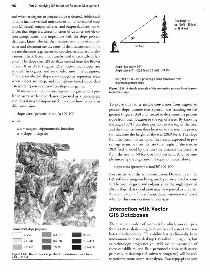
202 Part 2 Applying GIS to Natural Resource Management
and whether degrees or percent slope is desired. Additional options include vertical unit conversion {Q horiwnral map
unit (Z faccoc), Output cell size, and OUtput database name.
G iven [hat slope is a d irect function of distance and eleva
tion comparisons, it is imperative with the slope process
rhat users know whether (he measurement units of coordi
nates and elevations are [he same. If the measurement units ate nO[ the same (e.g. meters for coordinates and feet for elevations), the Z factor input can be used co reconcile differ
ences. T he slope class GIS database created from the Brown Tract 10 m DEM (Figu re 13.8) shows that slopes are repom::d in degrees, and are divided into nine categories. The darker-shaded slope class categories represent areas
where slopes are steep, and the lighter-shaded slope class categories represent areas where slopes are gentle.
Many natural resource management organizations pre
fe r CO work with slope classes expressed as a percentage,
and thus it may be important for CO know how to perform
this conversio n:
slope class (percent) = tan (a) X 100
where
tan = tangent tr igonometric function
0: = slope in degrees
Brown Tract slope (degrees)
0 0-2.3 - 5.3-6.5 -0 2.4-3.8 - 6.6-7.8 -3.9-5.2 - 7.9-9.1 -9.2-10.8
10.9-13.1
13.2- 21.8
Figure 13.8 Brown Tract slope class GIS database' created from aIOmDEM.
50 feet
Angle (degrees) = 30' Angle (percent) = (28.9 feet /50 feet) = 57.7%
Tree height = tan (30') - 50 feet or 28.9 feet
tan (30°) • 100 = 57.7, providing a Quick conversion from degrees to percent slope
Figure 13.9 A simple example of the' con'lo'ersion process from degrttS to percent slope.
T o prove this rather simple conversion from degrees co
percent slope, assume that a person was standing on flat
ground (Figure 13.9) and needed to determine the percent slope from their location to the cop of a tree. By knowing
the angle (30') from their position to the top of the tree, and the distance from their location to the tree, the person
can calculate the height of the tree (28 .9 feet). The slope from the person to the top of the tree, as expressed in per
centage terms, is then the rise (the height of the tree, or
28.9 feet) divided by the run (the distance the person is from the tree, or 50 feet), or 57.7 per cent. And, by simply inserting the angle into the equation noted above,
slope class (percent) = tan(30') X 100
you can arrive at the same conclusion, D epending on (he
GIS sofrware program being used, you may need to con
ven between degrees and rad ians, since the angle reponed
after a slope class calculation may be reported as a radian.
An examination of the software documentation will reveal whether this consideration is necessary,
Interaction with Vector GIS Databases
There are a number of methods by which you can perfo rm a GIS analysis using both vector and raster GIS databases simultaneously. This ability has traditionally been uncommon in many desktop CIS software programs, bur as technology progresses you will see the expansion of
these capabili ties. and field personnel (those with access
primarily to desktop GIS software programs) will be able to perform more complex analyses. Two types of analyses 213
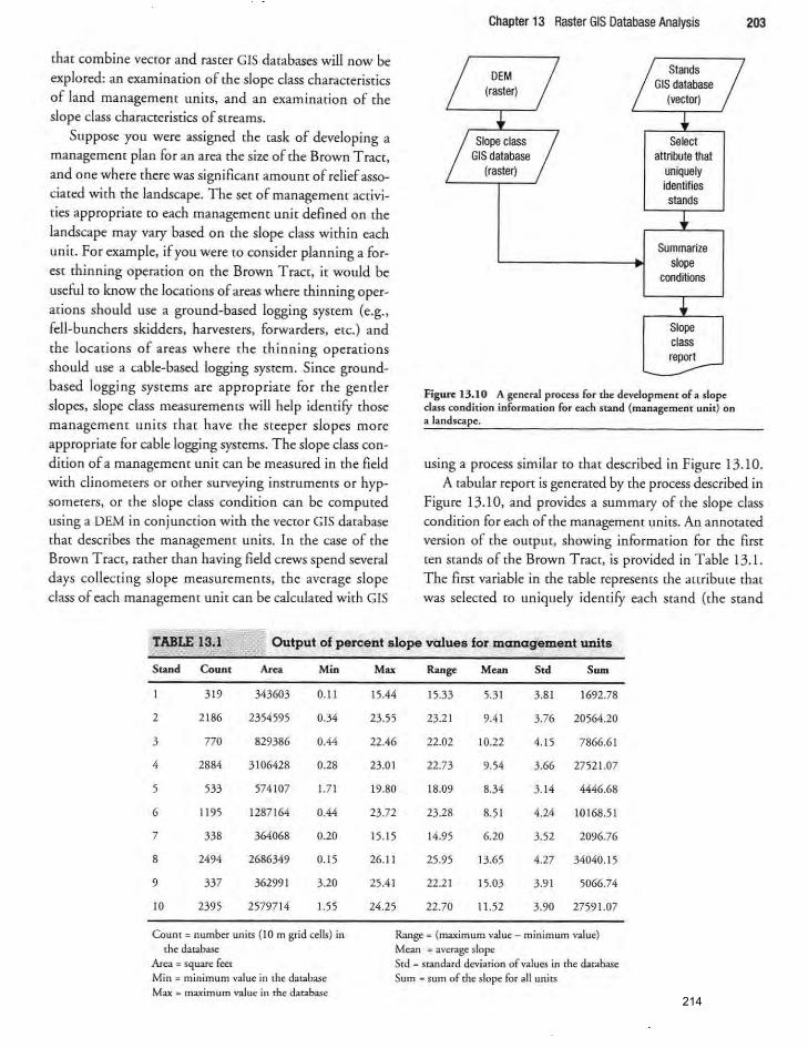
that combine vector and raster GIS databases will now be
explored: an examination of the slope class characteristics of land management units , and an examination of the slope class characteristics of streams.
Suppose you were ass igned rhe rask of developing a management plan for an area the size of the Brown Tract,
and one where there was significant amount of rel ief associated with the landscape. The set of management activities appropriate to each management unit defined on the landscape may vary based on rhe slope class wirhin each unir. For example, if you were to consider planning a for
est thinning operation on the Brown Tract, it would be
useful to know the locations of areas where thinning operarions should use a ground-based logging sysrem (e.g., fell-bunchers skidders, harvesrers, forwarders, ere.) and the locations of areas where the thi nning operations should use a cable-based logging sysrem. Since groundbased logging sysrems are appropriare fo r rhe gender slopes, slope class measuremenrs will help identifY those management units that have the steeper slopes more appropriare for cable logging sysrems. The slope class condition of a management unit can be measured in the field
with clinometers or other surveying instruments or hypsometers, or the slope class condition can be computed using a OEM in conjunction with the vector GIS database that describes the management units. In the case of the Brown Tract, rather than having field crews spend several days collecting slope measurements, the average slope class of each management unit can be calculated with GIS
Chapter 13 Raster GIS Database Analysis 203
Selecl attribute that
uniquely identifies stands
Summarize slope
conditions
Slope class report
FigUJ"~ 13.10 A g~n~ra1 prouss for tb~ developm~nt of a sJop~ class condition information for each stand (manag~m~nt unit) on a landscape.
using a process similar to that described in Figu re 13 .10. A rabular reporr is generared by the process described in
Figure 13.10, and provides a summary of the slope class condition for each of the management units. An annotated vers ion of the output, showing information for the first ten stands of the Brown Tract, is provided in Table 13. 1.
The first variable in the table represents the a((ribure that was selecred ro uniquely identifY each srand (rhe srand
TABLE 13.1 Output of percent slope values for management units
S .... d Count A=- M;" Max Range Mean Std Sum
3 19 343603 0.11 15.44 15.33 5.3 1 3.81 1692.78
2 2186 2354595 0.34 23.55 23.21 9.41 3.76 20564.20
3 770 829386 0.44 22.46 22.02 10.22 4.15 7866.61
4 2884 3 106428 0.28 23.01 22.73 9.54 3.66 27521.07
5 533 574107 1.71 19.80 18.09 8.34 3.14 4446.68
6 1195 1287164 0.44 23.72 23.28 8.51 4.24 10168.51
7 338 364068 0.20 15.15 14.95 6.20 3.52 2096.76
8 2494 2686349 0.15 26. 11 25.95 13.65 4.27 34040.15
9 337 362991 3.20 25.4 1 22.21 15.03 3.9 1 5066.74
10 2395 2579714 1.55 24.25 22.70 11.52 3.90 27591.07
CoUnt:o number units (10 m grid cells) in Range ,. (maximum value - minimum valu~)
the database Mean z averag~ slope Area .. squar~ feet Srd '" standard deviation o f values in [he database Min. minimum valu~ in [h~ da[abas~ Sum = sum of the slope for aU units Max .. maximum valu~ in me darabas~
214
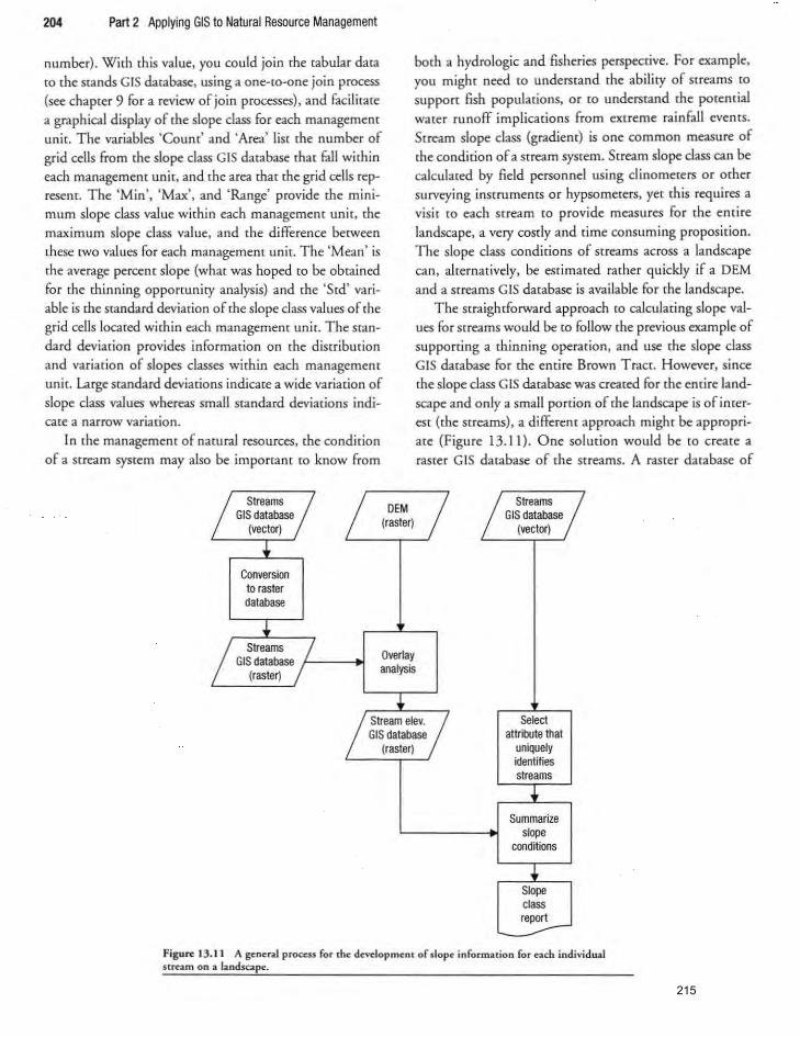
204 Part 2 Applying GIS to Natural Resource Management
number}. With this value, you could join the tabular data
co the stands GIS database. using a one-to-one join process
(see chapter 9 for a review of join processes), and facilitate
a graphical display of the slope class for each managemenr
unit. The variables 'Counr' and 'Area' list the number of
grid cells from the slope class GIS database that F...l1 within
each management unit, and the area mat the grid cells rep
resent. The 'M in', 'Max', and 'Range' provide the minimum slope class value within each management unit, the
maximum slope class value, and the difference becween these [wo values for each management unit. The 'Mean' is
the average percent slope (what was hoped to be obtained
for the thinning opportunity analysis) and the 'Std' variable is me standard deviation of the slope class values of rhe grid cells located within each managemem unic. The stan
dard deviation provides information on rhe disrcibucion and variat ion of slopes classes within each management unit, Large standard deviations indicate a wide variadon of slope class values whereas small standard deviations indicate a narrow varia don.
In the managemenr of namral resources, the condition
of a stream system may also be imporram [0 know from
Conversion to raster database
both a hydrologic and fisheries perspective. For example,
you might need [0 understand the abilicy of Streams to support fish populations, o r to understand the potential
water runoff implicarions from extreme rainfall evems.
Stream slope class (gradient) is one common measure of the condition of a stream system. Stream slope class can be calculated by field personnel using clinometers or other
surveying instruments or hypsometers, yet this requires a visit to each stream to provide measures for the entire landscape, a very costly and time consum ing proposition. The slope class conditions of streams across a landscape
can, alternatively, be estimated rather quickly if a OEM and a streams GIS database is available for the landscape.
The straightforward approach to calculating slope val
ues for streams would be to fo llow the previous example of
supporting a thinning operation. and use the slope class GIS database for the entire Brown Tract. However. si nce the slope class GIS database was created for the entire land
scape and only a small portion of the landscape is of inter
est (the streams), a different approach might be appropri
ate (Figure 13 .1 1). One solution would be to create a
raster GIS database of the streams. A raster database of
Overlay analysis
Select attribute that
uniquely identifies streams
Summarize slope
conditions
Slope class report
Figun: 13.11 A general proces.s for the development of slope inform:uion for each individual stream on a landscape.
215
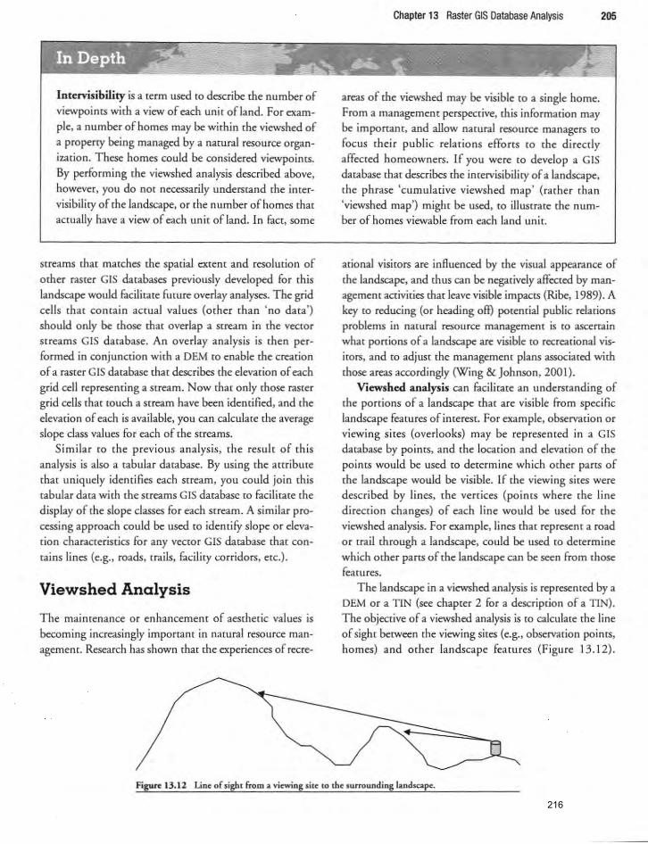
Intervisibility is a term used to describe the number of
viewpoints with a view of each unit of land. For exam
ple, a number of homes may be within the viewshed of
a property being managed by a natural resource organization. These homes could be considered viewpoims.
By performing the viewshed analysis described above. however, you do not necessarily understand the imer
visibility of the landscape. or the number of homes that acmally have a view of each unit of land. In fact, SOffie
streams that matches the spatial extent and resolution of
other raster GIS databases previously developed for this landscape would fucilitate future overlay analyses. The grid cells that contain accuai values (other than 'no data')
should only be those that overlap a stream in the vector screams GIS database. An overlay analys is is then per
formed in conjunction with a OEM CO enable the creation
of a raster GIS database thar describes the elevation of each
grid cell represent ing a stream. Now that only those raster
grid cells that touch a stream have been identified. and the elevation of each is avai lable. you can calculate the average
slope class values for each of the streams.
Si milar to the previous analysis, the result of this
analysis is also a tabular database. By using the attribme
that uniquely identifies each stream. you could join this tabular data with the streams GIS database to facilitate the
display of the slope classes for each stream. A similar processing approach could be used to identifY slope or elevation characteristics for any vector GIS database that con
tains lines (e.g .. roads, trails, facility corridors, etc.) .
Viewshed Analysis
The maintenance or enhancement of aesthetic values is
becoming increasingly important in natural resource man
agement. Research has shown that the experiences of recre-
Chapter 13 Raster GIS Database Analysis 205
areas of the viewshed may be visible to a single home.
From a management perspective, this information may
be impartanr. and allow natural resource managers to
focus thei r public relarions efforts to rhe directly affected homeowners. If you were to develop a GIS database that describes the intervisibility of a landscape. the phrase 'cumulative viewshed map' (rather than
'viewshed map') mighr be used. to illustrate the number of homes viewable from each land unit.
adonal visitors are influenced by the visual appearance of
the landscape. and thus can be negatively affected by managemem activities that leave visible impactS (Ribe. 1989) . A key to reducing (or heading off) potential public relarions problems in natural resource management is to ascertain
what pardons of a landscape are visible to recrearional vis
itors, and to adjust the management plans associated with
those areas accordingly (Wing & Johnson. 2001). Vicwshed analysis can facilitate an understanding of
the portions of a landscape that are visible from specific
landscape features of interest. For example. observation or
viewing si tes (overlooks) may be represented in a GIS database by poinrs. and the location and elevation of the
points would be used to determine which other parts of
the landscape would be visible. If rhe viewing sites were described by lines, the vert ices (points where the line
direction changes) of each line would be used for the viewshed analysis. Fo r example. lines that represent a road
or trail through a landscape. could be used to determine which other parts of the landscape can be seen from those
featu res. The landscape in a viewshed analysis is represemed by a
OEM or a TIN (see chapter 2 for a description of a TIN).
The objective of a viewshed analysis is to calculare rhe line of sight berween the viewing sites (e.g., observation points,
homes) and other landscape features (F igure 13. 12) .
Figure 13.12 Line of sight from a viewing site to the surrounding landscape.
216
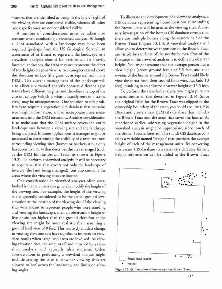
206 Part 2 Applying GIS to Natural Resource Management
Features [hat are identified as being in [he line of sight of the viewing sites are considered visible, whereas all other
landscape feamces are not considered visible. A number of considerations must be taken into
account when conducting a viewshed analys is . Ahhough a OEM associated with a landscape may have been
acquired (perhaps from rhe US Geological Survey), an assessmem of its fitness (Q represent the landscape in a
viewshed analysis should be performed. I n heavily forested landscapes. the OEM may nor represent the effect of tree heights on your view, as [ree canopies extend above
the elevation surface (the ground. as represented in the
OEM) . The current management of rhe landscape will also affect a viewshed analysis because different aged stands have different heights, and therefore [he (Op of rhe current canopy (which is what is usually seen in a scenic view) may be misrepresenced. One solution to this prob
lem is co acquire a vegetation GIS database that contains
tree height information, and [Q incorporate these meas
urements inco the DEM elevations. Another consideration
is to make sure that the DEM surface covers the entire
landscape area between a viewing site and the landscape
being analyzed. In some applicat ions. a managec might be interested in determin ing the visibility of a resoucce from
surrounding viewing sites (homes oc roadways) but only
has access to a OEM that describes the area managed (such
as the OEM for the Brown Tract, as shown in Figure
13.2). To perform a viewshed analysis, i[ will be necessary to acquire a OEM that covers not only the landscape of interest ([he land being managed), but also contains [he areas whece the viewing sites are located.
One consideration in viewshed analyses often ovec
looked is [hat G IS users can generally modify rhe height of the viewing site. For example. the height of the viewing
site is genera lly considered to be the acrual ground-level
elevation at the location of the viewing site. If the viewing
si tes were meant to represent people who were standing
and viewing [he landscape, then an observation height of five or six feet higher than the ground elevation at the
viewing s ite might be more realistic than assuming a
ground level view of 0 feeL This relatively modest change in viewing elevation can have significant impacts on view
shed resules when large land areas are involved. As viewing elevation rises, the amount ofland returned by a view
shed analys is will typically also increase. Orher considerat ions in performing a viewshed analysis might
include sening limits as to how far viewing sites are allowed to 'see' across the landscape. and limits on view
ing angles.
To illumate [he development of a viewshed analysis, a GIS database representi ng home locat ions surrounding
the Brown Tract will be used as the viewing sites. A cur
sory investigation of [he homes GIS database reveals [hat [here are multiple homes along rhe eastern half of [he Brown Tracr (Figure 13.13). A viewshed analysis will allow you to determine what portions of the Brown Tract
are visible by residents of [he n ... rby homes. One of [he first steps in the viewshed analys is is to define the observer
height. You might assume that the average person has a
view height (above ground level) of 5.5 fee<, and [hat owners of [he homes around [he Brown Tract could likely view rhe foreS[ from [heir second Aoor windows (add 10 feet), resulring in an adjusted observer heighr of 15.5 fee<.
To perform the viewshed analys is. you might pursue a
process similar to that described in Figure 13.14. Since [he original OEM for rhe Brown T racr was clipped (0 the ownership boundary of the tract, you could acqu ire USGS
OEMs and creare a new OEM GIS database rhat includes rhe Brown Tract and the areas that cover the homes. As mentioned earlier, addressing vegetarian height in the
viewshed analysis might be appropriate. since much of
[he Brown Tract is foresred . The stands GIS database contains a variable named 'Height' that provides the average
height of each of the management units. By convert ing
this vector GIS database to a raster GIS database format.
height information can be added to the Brown Tract
D Brown tract tocation • Homes
•
• •••• . .. , . ... ..
•••• • • • •
• • •••
Figure 13.13 Locations ofhome.s near the Brown Tr:lci.
• • • •
•
• • •
217

Chapter 13 Raster GIS Database Analysis 207
Create observer height
attribute
OEM (raster)
Overlay analysis
Viewshed analysiS
(raster)
Stands GIS database
Conversion to raster database
GIS database (raster)
Figure 13.14 A general process for the development of a vicwshed analysis for the Brown Tract based on a set of vicwshed sites (nearby homes).
OEM values co get an adjusted elevacion that includes the average tree heights for each management unit contained in the stands GIS database (Figure 13.15). The Spatial Analyst extension within ArcGIS contains a convert menu that offers a 'feamres to raster' utility for this purpose. The dialog box for this option will prompt for the database to be converted and a variable co be represented in the raster (height in this case). Once converted the stand height raster can be added to the DEM ro create a newelevation surface that contains updated elevation data for the Brown Tract and surrounding areas (Figure 13.16).
,
StnI..,{tI) 0-" "..., ..... " ... 81-100 101-120 lZ1-140 141-180 ISHel
"' ''''
After performing the preliminary database development steps, the acmal viewshed analysis can be performed by computing the areas of the landscape that are visible from each home. With in ArcGIS, this can be accomplished by using the Viewshed command. under the Surface Analysis roo Is within the Spatial Analyst extension . A dialog box will open and offer prompts for the inpuc surface (OEM or other modified elevation surface) and observer points (locations from which the input sur-
Figure 13.15 Average tree heights for managemcO( units contained in the Brown Trace stands GIS database.
218

208 Part 2 Applying GIS to Natural Resource Management
Figure 13.16 OEM GIS databuc fo r the Brown Tract and. surrounding areas that includes me :average tree hcighu of the management uniu contained in the stands GIS database.
face will be analyzed). Depending on the size of the DEM,
this processing dme may be lengthy, however, afrer pro
cessing is complete. a raster GIS database is created (hat
illustrates the areas with in and around the Brown Tracr that are visible from the nearby homes (Figure 13.17).
The areas within [he Brown Tract that are vis ible from
Figwc 13.17 Arc:as (dark shade) within and surrounding the Brown Tract that are visible from the ncarby homes.
the nearby homes are located mainly along [he trac[ bor
ders, however a significam amount of land within [he tract boundary is also visible from one or more homes
(a lthough you cannot, from chis analys is determine how
many homes have a view of each piece ofland).
Watershed Delineation
GIS has come to be a standard tool for hydrologic research
and water resource modelling. GIS applicat ions for water
resources are common and vary from simply mapping
water resources (Q sophis ticated analyses that consider
water quality infl uences and [umce water ava ilabi lity
(Wilson et aI., 2000; Marcin e< al., 2005). A primary use
of GIS for water resource managemenr is that of watershed delineation. A watershed can be defined as a land
scape area [hat shares a common drainage. This definition
assumes that if water were able [Q flow freely over a land
scape area, jt would follow a downhill trajectory and exit
(he landscape a rea at a common painr. W atershed bound
aries are commonly used by federal . St3te, and provincial
organizations ro separate a landscape inro smaller man
agemenr areas. In addition, watershed councils-groups
that help (Q determine management acdvities within a
specific watershed-are becoming more common in North America. Some refer {Q watersheds as 'catchmems'
but the intent is rhe same: {Q describe an area according to
the fl ow of water over its surface. The delineation of a
watershed boundary is a func[ion of topography and
changes in landscape relief. You must decide on the scale
of the watershed to be created and have access to topO
graphic information in order to begin delineation. Previous to digi[al GIS and the availabili<y of DEMs,
watersheds were created primarily by using available con
tour maps and using the visual clues provided by comour
shapes to draw or digitize a watershed. boundary. Clues
from contour shapes included saddles. peaks as indicated
by closed COntours, and [he direc[ion of funnel-like con
tour shapes that represent water fl ow paths o r ridges
(Figure 13.18). If existing meam ne<works were present
on the comour map or on additio nal maps, these features
also provided clues as to watershed boundary locations.
The delinea[ion process was usually begun from [he perceived lowest elevation point of the watershed and then
continued uphill , with ,he goal of identifYing the ridge lines that su rrounded a watershed and separated it from
other watersheds. Contour line funnels indicated either water flow paths or ridges. with water flowing from the
bottom of [he funnel (u- or v-shaped end) to the open
219
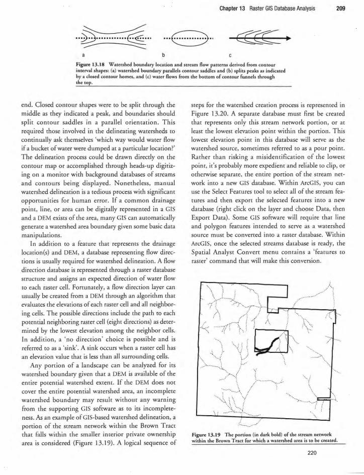
Chapter 13 Raster GIS Database Analysis 209
~ .. ~ ..... ....... ~ .. ::::------:::::
... E) .. a b c
Figure 13.18 Watershed boundary location and Stream flow patterns derived from contour inu:rvai shapes: (a) watcrsh~ bound2.ry parallels contour saddles and (b) splits peaks as indicated by a dosed contour homes, and (e) waler Rows from the bonom of conlour funnels through the tOp.
end. Closed conrour shapes were ro be spl ir rhrough rhe
middle as [hey indicared a peak. and boundaries should
split CQmour saddles in a parallel orientarion. This required those involved in the delineating watersheds co continually ask themselves 'which way would water flow if a bucket of water were dumped at a parcicular location?'
The delinearion process could be drawn direcdy on rhe
coorour map or accompl ished rhrough heads-up digiriz
ing on a monico[ with background databases of streams and contours being displayed . Nonetheless, manual watershed delineation is a tedious process with significant opportunities for human error. If a common drainage point. line. or area can be digitaUy represented in a GIS and a OEM exists of the area. many GIS can automatically generate a watershed area boundary given some basic data manipulations.
In addition to a feature that represems the drainage locarion(s) and OEM. a darabase represeming flow direc
tions is usually required for watershed delineation. A flow direction database is represemed through a raster database structure and assigns an expected direction of water flow to each raster cell. Fortunately, a flow direction layer can usually be creared from a OEM rhrough an a1gorirhm rhar
evaluares rhe e1evarions of each rasrer cell and all neighbor
ing cells. The possible direcrions include rhe parh co each
poreorial neighboring raseer cell (eighr direcrions) as derer
mined by rhe lowese devarion among rhe neighbor cells.
In addition, a 'no direction ' choice is possible and is referred to as a 'sink'. A sink occurs when a raster cdt has
an elevation value mat is less than all surrounding cells. Any ponion of a landscape can be analyzed for irs
watershed boundary given that a OEM is ava ilable of the emire pmential watershed extent. If the OEM does not cover the entire potemial wa[(~:rshed area, an incomplete
watershed boundary may resulr without any warning from rhe supporting GIS software as (Q its incompleteness. As an example of GIS-based warershed delinearion. a
portion of the stream network within (he Brown Tract that falls within the smaller incerior private ownership area is considered (Figure 13. I 9). A logical sequence of
steps for the watershed creation process is represented in Figure 13.20. A separare darabase muse firsr be creared
that represents only this stream network portion, or at
least the lowest elevation point within the porrion. This lowest elevation point in this database will serve as the watershed source, sometimes referred to as a pour point. Rather than risking a misidentification of the lowest point, it's probably more expedient and reliable to clip, or otherwise separate, the ent ire portion of the stream network into a new GIS database. Within ArcGIS, you can use the Select Features tool to select all of the stream features and then export (he selected feawres into a new
da<abase (righr click on rhe layer and choose Dara. [hen
Expon Dara) . Some GIS software will require rhar line
and polygon features intended to serve as a watershed source must be converted inm a raster database, Within ArcGIS, once the selected streams database is ready. the Spatial Analyst Convert menu contains a 'featu res to
raster' command that will make this conversion.
' ... .' :
\~.j 1.,;"; .. ,.'
J
""
··~··· ·'J·····,··.>m \·
.'
Figure 13. 19 The portion (in dark bold) of the stream network within the Brown Trace for which a watershed area is to be created .
220

210 Part 2 Applying GIS to Natural Resource Management
separate Stream sections
of interest
Cooversion to raster database
(raster)
Create Flow direction
database
(raster)
Watershed analysis
Figure 13.20 A general process for the ddineation of a watershed area for a portion of the stream network in the Brown Tract.
The next step is to create a flow direction raster based
on the Brown Tract OEM. This process can be accom
plished wirhin ArcGIS by using rhe rasrer calcularor and flowclirecrion com mand. Assuming that (he extended
OEM for [he Brown Tract is used. (he raster calculator syntax would be ' f]owdirecrion ([browndemex])'. The result of this command should be a temporary raster file
with cells ass igned to one of nine possible values: one for
each direction to the eight neighboring cells and a sink or 'no lower elevation' value. A si nk can be caused by a nat
ural fearure. such as a lake or mher water body with no
surface o utl et, o r can be the result of a OEM error.
Summary
The examples in this chapter have demonstrated several
GIS operations [hat are possible when using raster GIS databases, and have concentrated on [he wealth of oppor
tunities associated with using a OEM. From the basic ele
vation information contained within a DEM, you can gen-
Regardless, it may be necessary to detect and eliminate
sinks within the OEM before flow direcrions can be calcu
lared. Wirhin ArcGIS, rhe fill command can be used to
manipulate porential sinks bur must be run through the
Sparial Analysr Hydrology rools in rho ArcToolbox or rhrough rhe command line inrerface. The fill command will create a new raster with elevation values for sink loca
tions raised to the minimum elevation found in sur
rounding cells. The modified ('filled') rasrer can rhen be
used to calculate flow directions. Once the flow direction
raster is complete, the watershed area can be derived.
Within ArcGIS the raster calculator can be used with rhe
Watershed command to create watershed boundaries. The syntax is 'watershed ([flowraster, streamsecrion])'
where flowraster is the name of the f1owdirection raster
and srreamsection is the name of the raster version of the
portion of the Brown Tract Stream network for which a
warershed will be creared. The warorshed croared should not be very large in co mparison to the Brown Tract
boundary (Figure 13.21 ).
.~.
Figure 13.21 Th~ watersh~d (i n gray) for a portion of the Brown T net stre2m network.
erate contou r lines. a shaded relief image. and a slope clas
sification map. Rasrer GIS databases can be integrated in spatial analyses to calculate slope classes for management units as well as gradiems of streams. and to create a data
base of me viewshed relared to nearby landscape feamres,
221

such as the homes located around the Brown Tract. In addir ion. DEMs can be used to analyze landscape topography and can create additional raster databases to support
watershed delineation . These examples are but a small
Applications
13.1 Shaded relief map. You have been asked by the manager of rhe Brown Tract ro create a shaded relief
map that simulates rhe sun 's lighr on rhe landscape in early morning.
a) What values would YOli use to approximate the sun's azimuth and altitude?
b) Develop a map that illustrates the shaded relief.
13.2 Slope map of the Brown Tract. During one of your monthly planning meetings. it was suggested that a slope map would be of value to the foresters who plan timber sales on the Brown Tract. This map would be of equal value [0 (he recreadon manager, who is interested in
potendal trail systems throughom the forest.
a) Create a slope GIS database of the Brown Tract that has 80 ft con [Our lines that originate from a
300 fr base elevation . b) Develop a map illuStrating the slope classes.
13.3 Viewshed analysis planning. Your supervisor has approached you and asked that you assist in a viewshed
analysis for part of your resource management area. She is
interested in knowing what port ions of your resource
management area are visible from a nearby road. She
needs the information quickly and has asked you to scope our the project with regard to how this mighr be accomplished in GIS (e.g .• what GIS databases are necessary. what processes are necessary, etc.). Provide a brief descrip
rion that lists required GIS databases, techniques, and
potential pitF.Uls of conducting the visibility analysis.
13.4 Road gradient analysis planning. Your supervisor is interested in knowing the average slope gradients of a set of roads within your organization's management area. She has asked you for a one-page description of how this might be accomplished in GIS. Prepare a reporr for her that describes the necessary GIS databases, potential techniques, and considerat ions that would be involved in
using GIS for this purpose.
13.5 Road gradients on the Brown Tract. The forest
Chapter 13 Raster GIS Database Analysis 211
sample of the types of applicat ions that are possible with a single raster GIS database in terms of examining landscape (Opography. We turn our anemion in rhe following chapter to exploring orner poremiai raster data applications.
engineer associated with the Brown Tract has asked you
to calculare road slope gradients (percent slope) for the roads in the Brown Tract using two GIS processing
methods. For the first method. the slopes should be calculared using [he entire DEM available for the landscape. For the second method. the slopes should be calculated using only those raster grid cells that overlap the road
network. The engineer wants to understand the differ
ence, if any, (hat would be observed in the average
slopes gradients when using these two methods. Prepare
a short report to convey this information (0 the forest
engIneer.
13.6 Brown Tract viewshed analysis. The manager of the Brown Tract would like you to develop a viewshed analysis using only those homes located on the north side
of the Brown T racr. Use the assumptions and processes
described in the example provided earlier in this chapter.
How do the viewshed results differ from [hose of the example presented earlier in this chapter?
13.7 Brown Tract watershed analysis. The hydrologiSt for the Brown Tract, Samantha Wasser, has asked for
your help in identifying a watershed for a portion of the Brown Tract stream network. The lowest elevation
stream segment in the portion is identified through a
numeric value of 123 in the stream variable within the
streams database. Develop a watershed for this stream
network portion and report the resulting watershed area
in both acres and hectares.
13.8 Brown Tract beaver watershed analysis. T he Brown Tract manager has asked you to delineate the
watershed area that Aows into a large beaver pond. The
beaver pond location is described in the water sources
database as a point location. Create a warershed for this
point and repOf[ the resulting watershed area in both
acres and hectares.
13.9 Brown Tract stand watershed analysis. The Brown Tract manager has asked you to delineare rhe
222
212 Part 2 Applying GIS to Natural Resource Management
watershed area that flows into a stand inside rhe Forese.
The stand is identified as number 36 with the stand field in rhe Brown T faCt stands database. Create a watershed
for this stand and repon rhe resulting watershed area in
bmh acres and hectares .
13.10 Basic characteristics of the Brown Tract. Becky Blaylock. the manager of rhe Brown T ract, is interested in
some basic knowledge of the landscape. Specifically. she wants to know rhe following:
a) What is rhe m inim um, maximum, average. and
standard deviation of slope (degrees) fo r the Brown Tract?
b) What is rhe m inimum, maximum, average, and
standard deviation of slope (percent) for rhe Brown
T racr?
References
Burrough. P.A .• & McDonnell. R.A. (1998). Principles of geographical information systems. Oxford: Oxford University Press.
Martin. P.H .• LeBoeuf. E.J .• Dobbins. J.P .• Daniel. E.B .• & Abkowirz. M.D. (2005). Interfacing GIS with water resource models: A state-of-the-art review. Journal of the American Water Rtsourus Association, 41 , 1471-87.
Natural Resources Canada. (2007). Mapping. Retrieved May 26. 2007. from hrrp:llwww.nrcan-rncan.gc.cal com/subsuj/mapcar-eng.php.
Ribe. R.G. (1989). The aesthetics of forestry: What has
13.11 Combining raster GIS databases. Wha t is the result when two raster GIS databases are combined. yet
'no dam' values are present in some portions of rhe land
scape in one of the [wo raster GIS databases?
13.12 Highest and lowest elevation stands. Which stand in the Brown Tract is located at (he lowest average elevation?
Which stand is located at the highest average elevation?
13.13 Elevation information for a single stand. What are the average, minimum , and maximum elevations of
the stand described in question 13.9 (stand 36)?
13. 14 Water source elevations. What is the average ele
vation for each of the points described in the water
sou rces database?
emp ir ical preference resea rch taught us? Environmental Managemen t. 13.55-74.
US Department of Interior. US Geological Survey. (2007) . USGS Geographic data download. Retrieved May 26. 2007. from hrrp:lledc2. usgs.gov/geodatal index.php.
Wilson. J.P .• Mitasova. H .• & W right. D.J. (2000). Water resource applications of geographical informa
tion systems. URlSAjouma!, 12(2).61 -79. Wing. M.G .• & Joh nson. R. (2001). Quanti /Ying forest
visibility with spatial data. Environmental Management. 27. 411-20.
223
Chapter 14
Raster GIS Database Analysis II
Objectives
Chapter 14 builds on the previous chapter and further explores raste r data for spatial analysis. Like chapter 13, this chapter also involves [Opographic applications of raster data bue broadens the (reatment of raster data applications. In addition, more technical detail is provided for
raster data processing techniques and analysis. Ar the con
clusion of this chapter, readers should understand and be able (0 converse aOOm:
1. the potential applications of caster data for natural resource problem analysis.
2. how distance functions can be applied to raSter data. 3. the types of statistical summary search functions for
raster data,
4. the capabilities and applications of density operations, 5. raster data reclassification and map algebra processes,
and 6. data structure conversion considerations.
Raster Data Analysis
We further develop raster data analysis in [his chapter by describing some general considerations for raster analysis
working parameters. examples of raster analysis functions. and applications of processing commands for manipulating raster data. We then describe some application examples that make use of select raster funct ions. The raster analysis functions we discuss include distance, statistical sum mary search, and density functions. In some cases, rhe functions can accommodate both vecror and rasrer databases as input. General processing commands cov-
ered in this chapter involve raster reclassification. rasrer map algebra. and data structure conversions. We also provide more detailed information abour the procedures within the world 's most popular GIS software-ArcGISthar can be used for raster analysis. An assumption for rhese procedures is that the Spatia l Analyst software extension for ArcGIS is available. This extension is specifically designed for raster data analysis and provides a set of
menu choices and commands that make some of primary raster capabilities more readily available. If readers are using different raster software (i.e. , Imagine, GRASS. Idrisi , etc.) for their applications, the procedures described in this chapter should provide a template for
applying the functions and analyses that we present.
Raster Analysis Software Parameters
Some raster software will allow you to set working environment parameters that the software will observe during use. These conditions establish resolurion, analysis, ourpur. and other conventions that affect Output raster databases that are created during processing. One of the distinguishing characteristics of raster databases in com
parison to vector data is that they are cypically larger in size in terms of digital storage space. Raster working environment parameters can help constrain raster databases to
specific study areas and resolutions so thar Output files do not become overly large in size. Some raster software will
only create temporary raster databases unless otherwise specified by a user. These remporary raster databases will be removed from the hard drive once the GIS software is closed, which can cause some distress for unsuspecting
224

214 Part 2 Applying GIS to Natural Resource Management
users the nex( time [he software is resrarred. Depending on the raster software, working environment parameters
may need co be reestablished ar rhe beginning of every analysis session.
An important rasrer parameter (Q consider is an anaJy~
sis mask. An analysis mask, as esrablished by rhe dimensions of anQ[her GIS layer. will restrict processing to on ly
those areas coincident within the layer. The extent oprions allow you co further resrricr the areas that will be considered when new raster output is created . Depending on you r software, possible choices include existing layers. spa
rial combinarions of exiscing laye rs. or a bounding ser of
coordinates. In addition to raster databases. vector databases can usually also be used (Q create an analysis mask.
Another critical choice for processing out pm raster databases is cell resolution. Typically, working parameter choices will allow users CO set a designated raster cell resolution for Output databases. This can typically be set [Q
match orher analysis layers. combinations of other layers. user-specified cell resoiurions, or a user-specified set of columns and rows. Sening a cell size and analys is extem
[Q match an existing layer will ensure that our pur raster cells are registered to the existing layer. and that output raster cells from both layers will be coincident and nor offset from one another. These potential parameters described here, and orhers rhar may be available depending on software, can help make raster analys is more efficiem. These choices can help establish a common resolution, analysis area, and output location for raster processing results. The appropriate options should be set prior [Q any raster analysis session.
Distance Functions
Distance functions calculate the measured distance [Q fea
tures of interes(. There are va rious ways of computing distances, ranging from a straight line measurement to more involved approaches (i .e., shorrest paths) that use constraims of moving across a landscape due [Q changes in relief or other impediments. Distance functions can be used to help determine the next closest feature, areas that might be ecologically sensitive because of their proximity to namral features. or the most expedient route to take from one feature to another. Typ ical dista nce funct ions include the straight line, allocation distance, cost weigh red disrance, and shorresr parh (Theobald, 2003).
The stra ight line distance function will create a raster output wim direct (also called Euclidean) distances ro rhe
closest feature. The function can be appl ied to either vecror or raster databases. As an example, consider the water sources poim locations within and around the Brown T racr (Figure 14.1) . Ir mighr be beneficial for emergency response units combating wildfire to know how far away
the closest water sources are located, parriculariy if helicopters will be used (0 carry water from sources to a forest fire and stra ight line distances were of imerest. A distance function cou ld demonstrate relative distances [Q the nearest water source (F igure 14.2) .
An allocat ion distance functio n assigns areas [Q the closest feature. In this case, raSter cells will be assigned a pixel value that recognizes the nearest wne of influence, similar to the vector representation of a Thiessen polygon. A Thiessen polygon is created for each feature in a spatial database and represents the area that each feature is nea res(. In the case of the nine potential water sources, nine allocation zones are identified with each water source hav
ing irs own zo ne of influence (Figure 14.3) . A cost weighted distance function allows for ass igning
different weighting to raster cells that take into account
what is required for a pathway to cross through the cell (Chrisman, 1997). This fill1crion mighr be used ro assess the amount of time needed for water to flow through one end of a srream nerwork to anorher, the relative costs of materials [Q construct or resurface a trail , or resources necessary to develop access ro areas in mountainous te rrain. The COSt weighted function requires that in addition to
I
D
... Water sources
Figure 14. 1 Water source5 in and around the Brown Tract.
225
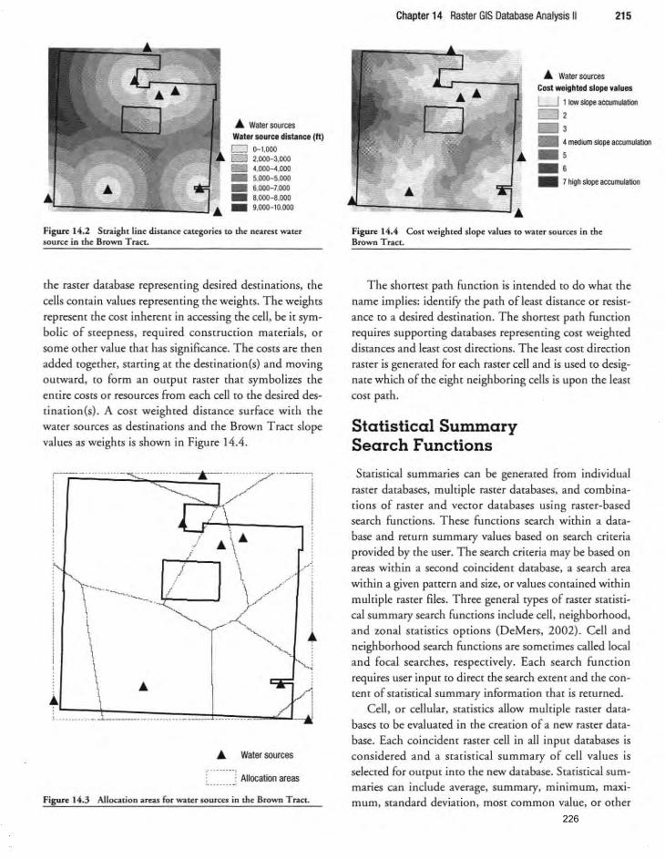
... Waler sources W,t.r source distance (ft) 0 0- 1.000 LIZJ 2.000-3.000 .. 4.000-4.000 _ 5.000-5.000 _ 6.000-7.000 _ 8.000-8.000 _ 9.000-10.000
Figure 14.2 Straight line distance categories to the nearest water source in the Brown T raet.
the raster database representing desired destinations, the cells contain values representing ilie weights. The weights represent the cost inherent in accessing the cell, be it symbolic of steepness. required construction materials, or some other value that has significance. The COStS are then added togecher. start ing at the destination(s) and moving outward. to form an output raster that symbolizes the entire COStS or resources from each cell to the desired des[ination(s) . A cost weighted distance surface wi th the water sources as destinations and the Brown Tract slope values as weights is shown in Figure 14.4 .
,---------- ----- ------- ----- ------A------ ------------- - -- ----,
// I r-''''-o!''/ i
!
... L= _____ = _____ ±:~ __ = ____ = ___ = ______ = _____ = __ _:b ___ = ______ = ____ ...L.L
... Water sources
~ ...... J Allocation areas
Figure 14.3 AJlocation areas for water sources in the Brown Tract.
Chapter 14 Raster GIS Database Analysis II 215
... Water sources Cost weighted slope values
U 1 low slope aco..mu/ation
!2iJ 2
3 _ 4 medium Slope accumulation .' .' • 7h~" _ "",mula""
Figw e 14.4 Cost weighted slope values to water sources in the Brown Tract.
The shortest path function is intended to do what the name implies: identify the path of least distance or resistance to a desired dest ination. The shortest path function requires supporting databases representing cost weighted distances and least cost directions. The least cost direction raster is generated for each raster cell and is used to designate which of the eight neighboring cells is upon the least COSt path.
Statistical Summary Search Functions
Srariscical summaries can be generated from individual raster databases. multiple raster databases. and combinations of raster and vector databases using raste r-based search funccions . These fu nctions search within a database and recurn summary values based on search criteria provided by the user_ The search crireria may be based on areas within a second coincident database, a search area within a given pattern and size, or values comained within multiple raster fi les_ Three general types of raster statistical summary search functions include cell. neighborhood. and zonal statist ics options (DeMers. 2002) _ Cell and neighborhood search functions are sometimes called local and focal searches, respectively. Each search function requires user input to direct the search extent and the con[em of statistical summary information that is returned .
Cell, or cellular, statistics allow multiple raster databases to be evaluated in the creation of a new raster database. Each coincidem raster cell in all input databases is considered and a statist ical summary of cell values is selected fo r output into the new database. Stads[ical summaries can include average. summary, minimum. maximum. standard deviadon. most common value. or other
226
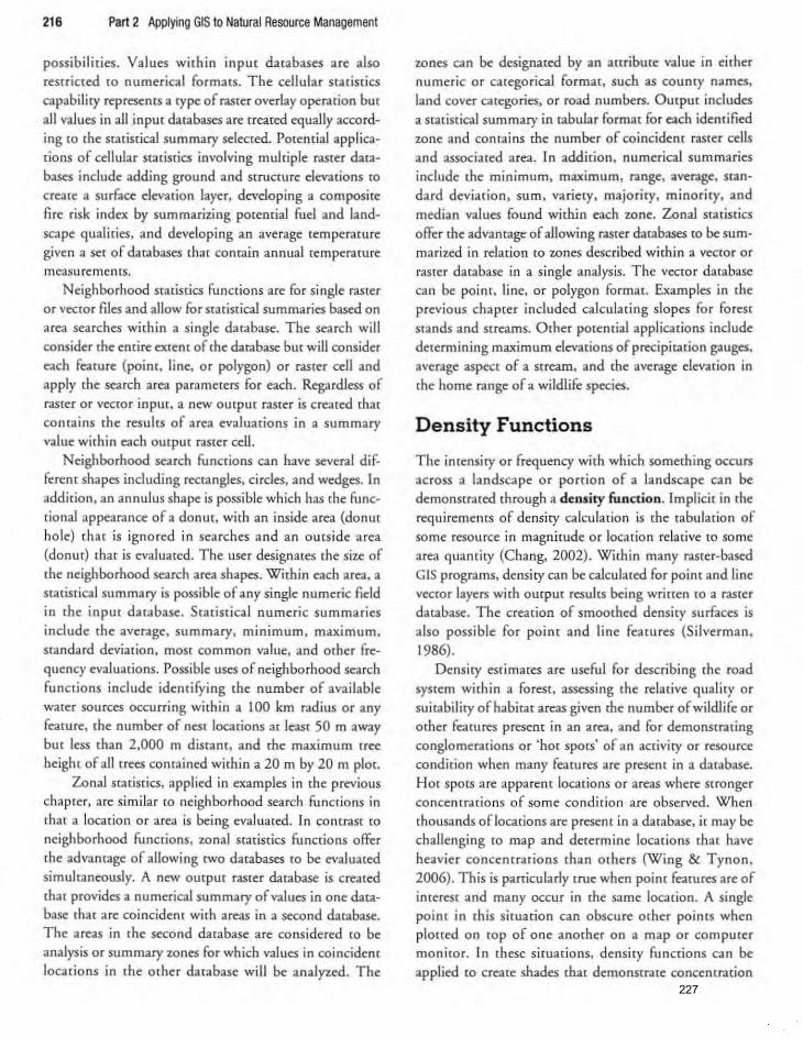
216 Part 2 Applying GIS to Natural Resource Management
possibilities. Values within input darabases are also restricted to numerical formats . The cel lular srar iscics
capability represents a type of raster overlay operation but
all values in all input databases are treated equally according CO [he statist ical summary selected. Potential applica
tions of cellular slatisrics involving multiple raster data
bases include adding ground and structure elevations co
create a surface elevacion layer, developing a composite
fire risk index by summarizing poremial fuel and land
scape qualities. and developing an average temperature
given a set of databases that contain annual temperature
measurements. Neighborhood statist ics funct ions are for single raster
o r vector files and allow for statistical summaries based on
a rea searches within a single database. The search will
consider the entire extent of (he database bur will consider
each feature {point. line, or polygon} or raster cell and
apply the search area parameters for each. Regardless of
raster or vec(Qr input. a new ou tput raster is created that
conrains the results of a rea evaluations in a summary
value within each output raste r cell.
Neighborhood search functions can have several dif
ferenr shapes including rectangles, circles, and wedges. In
addition , an annulus shape is possible which has the func
rional appearance of a donut, with an inside area (donut
ho le) that is ignored in searches and an outside a rea
(donut) that is evaluated. The user designates the size of
the neighborhood search area shapes. Within each a rea, a
statisrical summary is possible of any si ngle numeric field
in the inpur database. Statistical numeric summaries
include rhe average, summa ry. minimum, maximum,
standard deviation, mOSt common value, and other fre
quency evaluations. Possible uses of neighborhood search
functions include identifying the number of available
water sou rces occurring within a 100 km radius or any
feature, the number of nest locations at least 50 m away
but less than 2,000 m disrant. and the maximum tree
height of all trees contained within a 20 m by 20 m plot.
Zonal statistics, applied in examples in rhe previous
chaprer. are similar (Q neighborhood search functions in that a location or area is being evaluated. In cOntrast (Q
neighborhood funccions, zonal statistics functions offer
the advantage of allowing twO databases (Q be evaluated
simultaneously. A new o utput raste r database is created
that provides a numerical summary of values in one database that are coincident with areas in a second database. The areas in the second database are considered (Q be
analys is or summary zones for which values in coincidenr
locatio ns in the other database will be analyzed. The
zones can be designated by an attribute value in either
numeric or categorical format, such as counry names,
land cover categories, or road numbers. Output includes
a statistical summary in tabular format for each idenrified
zone and contains the number of coincident raster cells
and associated a rea. In addition, numerical summaries
include the minimum, maximum, range, average. stan
dard deviation, sum, variety, majority. minoriry, and
median values found within each zone. Zonal statistics
offer the advanrage of allowing raster databases to be sum
marized in relation (Q zones described within a vector or
raster database in a single analysis . The vector database
can be point, line. or polygon format. Examples in the
previous chapter included calculating slopes for forest
stands and streams. Other potential applications include
determining maximum elevations of precipitation gauges.
average aspect of a srream. and the average elevation In
the home range of a wildlife species.
Density Functions
The intensity or frequency with which something occurs
across a landscape or portion of a landscape can be
demonstrated through a density function . Implicit in the
requirements of density calcu lation is the tabulation of
some resource in magnitude or location relative to some
area quantity (Chang. 2002). Within many raster-based
GIS programs. density can be calculated for point and line vector layers with ourput results being written to a ras rer
database. The creation of smoothed densiry surfaces is
a lso possible for point and line featu res (S ilverman,
1986). Density estimates are useful for describing the road
system within a forest. assess ing the relative quali ty or
suitabi lity of habitat areas given the number of wildl ife or
other features present in an area, and for demonstrating
conglomerations or 'hot spots' of an activity or resource
condition when many features are present in a database.
Hot SpOts a re apparent locations or areas where stronger
concentrations of some conditio n are observed. When
thousands of locations are presenr in a database, it may be
challenging ro map and determine locations that have
heavier concentratio ns than o thers (Wing & Tynon ,
2006). This is particularly true when point features are of
interest and many occur in the same location. A si ngle point in this situation can obscure other points when
pioned on top of one another on a map or compurer monitor. I n these situations, density functions ca n be
applied to create shades that demonstrate concentration 227
216 Part 2 Applying GIS to Natural Resource Management
possibilities. Values within input databases arc also restricted to numerical formats. The cellular statistics capabili~ represents a cype of raster overlay operation bur all va lues in all inp"' databases are "eated equally according to the statistical summary selected. Potential applicap
tions of cellular statistics involving multiple raster databases include adding ground and srructure e1evarions (0
creare a surface elevation layer. developing a composite fire risk ind<x by summarizing potential fuel and landscape qualities , and developing an average temperature given a set of databases that con[ain annual temperature
measurements.
Neighborhood statistics functions are for s ingle raster
or vecmr files and allow for statistical summaries based on area searches within a single database. The search will
consider the emire ex;,rem of the database bur will consider
each feature (point, line. or polygon) or rasrer cell and apply [he search area parame«rs for each. Regardless of raster or veccor input, a new Output raner is created that
contains rhe results of area evaluadons in a summary
value within each output raster cell .
Neighborhood search funcdons can have several different shapes including rectangles. circles. and wedges. In addi[ion, an annulus shape is possible which has [he functional appearance of a donut. with an inside area (donut
hole) (hat is igno red in searches and an outside area
(donu,) that is evalua<ed. The user designates the size of ,he neighborhood search area shapes. Within each area, a statisrical summary is possible of any single numeric field in the input database. 5tadsdcal numeric summaries
include me average. summary. minimum . maximu m.
standard deviation. mOSl common value. and other fre
quencyevalua<ions. Possible uses of neighborhood search functions include identifying the number of available
water sources occurring within a 100 km radius or any
feature, the number of nest locacions at least 50 m away
but less than 2,000 m distant, and ilie maximum tree heigh, of al l trees contained wiiliin a 20 m by 20 m plot.
Zonal stadsdcs, applied in examples in the previous
chapl er, are si milar to neighborhood search functions in (hal a locadon or area is being evaluated. In contrast co
neighbo rhood fun ctions, zonal sratistics functions offer
,he advantage of allowing rwo databases to be evalua<ed s imul taneously. A new outpUl raster darabase is created
(hat provides a numerical summary of values in one database that are coincidenr with areas in a second database. The areas in the second database are considered co be
analysis or summary zones for which values in coincident
locat ions in the other da<abase will be analyzed . The
wnes can be designa<ed by an attribute value in either numeric or categorical format , such as county names,
land cover categories, or road numbers. Qurpuc includes
a statistical summary in tabular format for each identified
zone and contains che number of coincident raster cells
and associated area. In addition. numerical summa ries
include me minimum, maximum, range, average. stan
dard deviation) sum, va riety. majority, minority, and
median values found within each zone. Zona] statistics
off'er ilie advantage of allowing ... ster databases ro be summarized in relation to zones described w ithin a veccor or
raSter database in a single analysis. The veccor database can be point, line. or polygon format. Examples in the previous chapcer included calculating s lo pes for forest
srands and streams. Oilier potential applications include determining maximum elevations of precipitation gauges. average aspect of a scream, and me average elevation in
the home range of a wildlife speeies.
Density Functions
The intensity or frequency with which something occurs across a landscape or portion of a landscape can be
demonstrated through a density function . Implicit in the requiremenrs of density calculation is the tabulation of
some resource in magnitude or locat ion relative to some area quantity (Chang, 2002). Wiiliin many raster-based GIS programs. density can be calculated for point and line vecror layers wirh output results being wrinen to a rasrer database. The creation of smoothed density surfaces is
also possible for poinr and line fearures (Silverman, 1986).
Density estimates are useful for describing rhe road
system within a forest. assessing the relative quality or
suitability ofhabirat areas given ilie number of wildlife or other fC'dtures present in an area, and for demonstrating
conglomerations or 'hot spars' of an acriviry or resource
condition when many features are present in a darabase.
Hot SpOts are apparent locations or areas where stronger
concentrations of some condir io n are observed. When
thousands oflocarions are present in a database, ir may be
challenging to map and determine locations rhat have
heavier co ncentrations than others (Wing & Tynon.
2006). This is panicularly true when point features are of interest and many occur in the same location. A single
point in [his sicuacion can obscure other poims when ploned on top of one another on a map or computer monimr. In rhese siruations, density function s can be
applied (0 create shades that demonstrate concentration
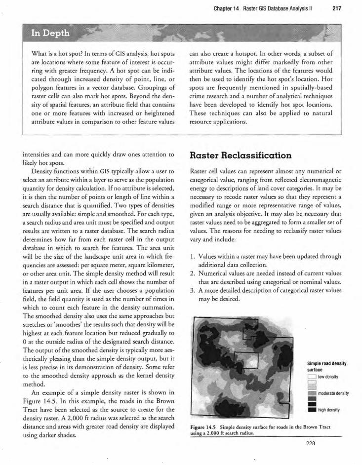
What is a hot spot? In terms of GIS analysis. hot SPOtS
are locadons where some feamre of interest is occurring with greater frequency. A hot SpOt can be indicared through increased density of point, line, or polygon features in a vector database. Groupings of
raster cells can also mark hot spots. Beyond the density of spatial features, an 3nribuce field that contains
one or more features with increased or heightened anribure values in comparison (Q mher feature values
intensities and can more quickly draw ones attemion [0
likely hot Spots. Densicy functions within GIS cypically allow a user to
select an attribute within a layer (0 serve as the population
quamiry for density calculation. If no attribute is selected, it is then the number of points or length of line within a
search distance that is quantified. Two types of densities
are usually available: simple and smoothed. For each cype, a search radius and area unit must be specified. and Outpur
results are wrinen to a raster database. The search radius
determines how far from each raster cell in the output
database in which CO search for features. The area unit
will be the size of the landscape unit area in which fre
quencies are assessed: per square meter, square kilometer,
or other area unit. The simple density method will result
in a raster Output in which each cell shows the number of
features per unit area. If the user chooses a populat ion field, the field quanticy is used as the number of times in which CO count each feature in the density summation.
The smoothed densicy also uses the same approaches but stretches or 'smoomes' the results such that density will be
highest at each feature location but reduced gradually to
D at the outside radius of the designated search distance. The output of the smoothed densicy is cypically more aesthetically pleasing than the simple densicy output, bur it is less precise in its demonstrat ion of density. Some refer
to the smoothed dens icy approach as the kernel dens icy method.
An example of a simple density raster is shown in
Figure 14.5. In this example, the roads in the Brown Tract have been selected as the source to create for the density raster. A 2,000 fe radius was selected as the search
distance and areas with greater road density are displayed
using darker shades.
Chapter 14 Raster GIS Database Analysis II 217
can also create a hotspot. In other words, a subset of
attribu te values might differ markedly from other a([ribure values. The locations of the features would
then be used to identify the hot spot's location. Hot spots are frequently mentioned in spatially-based crime research and a number of analyt ical techniques
have been developed to identify hot SpOt locations. These techniques can also be app lied to natural resource applications.
Raster Reclassification
Raster cell values can represent almost any numerical or
categorical value, ranging from reAected electromagnetic
energy co descriptions ofland cover categories. It may be necessary to recode raster values so that they represent a
modified range or more representative range of values,
given an analysis objective. I t may also be necessary that raster values need co be aggregated to form a smaller set of
values. The reasons for needing to reclassify raster values
vacy and include:
I. Values within a raster may have been updated through
additional data collection .
2. Numerical values are needed instead of current values
that are described using categorical or nominal values .
3. A more detailed description of categorical raster values
may be desired.
Simple road density surface
low dens.,
moderate density -_ high density
Figure 14.5 Simple density surface for roads in the Brown Trac[ wing a 2,000 ft search radius.
228
218 Part 2 Applying GIS to Natural Resource Management
4. Raster values may need [ 0 be rescaled in order [0 sup· pore a single raster analysis.
5. Raster va lues may need co be rescaled in o rder ro support a multiple raster analysis.
Reclassification is differenc from altering the symbology or legend of a raster database for display purposes in that it goes beyond simply altering rhe appearance of a raster database. Regardless of the reasons for reclassifYing a raster database, rhe reclass ification process leads to a new raster database with pixel values ceRecting rhe recoded values. The new raster database and its reclassified values can then be used for mapping and analysis purposes.
Within the ArcGIS Spatial Analyst, a reclassifY command is available. Selecting the reclassifY command will open a dialog box that prompts rhe selection of a raster database, reclassification field , and input cells for reclassification values. By default, this interface will use the exist
ing symbolization used to display the raster. For example. should current raster values be displayed using five ranges or categories, these same five classifications would be displayed on the reclassifY cell options. To select different classifications from which to begin the recoding, the 'classifY' button can be chosen.
Raster Map Algebra
The ability to access and evaluate values within multiple raster databases and output results to a new raster database presents powerful analysis oppormnities. Raster map algebra involves a mathematical evaluation that is applied to one or more raster databases to create a new database
(DeMers, 2002). Mathema, ical evaluations for single raster databases may include adding or multiplying raster cells by a constant value, or applying trigonometric. logarithmic, and other mathematicaJ transformations to raster values. A common example of single raster map algebra might be taking an elevation-based raster and multiplying the elevation values by a conversion facto r to move from one measurement unit to another, such as converting elevation values from meters to feet. Mathematical evalua
tions for multiple raster databases might involve adding or multiplying raster values, comparing mulriple raster databases and remrning the largest value for all coincidental cells, or using raster database values within a formula that capmres landscape processes such as that for water velocity and discharge rates.
Whether one or more raster databases are used, raster
map algebra resulrs in a new raster database that contains the results of the mathematical evaluations specified by the user. Some forms of map algebra can be accomplished through techniques discussed earlier, such as cellular statistics that a llow for statistical summaries to be calcu lated from multiple raster databases. Operations that require mathematical manipulations of single or multiple raste r databases, however, requi re more direct approaches. Within the Spat ial Analyst function of ArcGIS, the raster calculator is provided in support of raster map algebra, and also provides access to additional raster related
funcdons.
Database Structure Conversions
It may be necessary to convert a spatial database from a vector to raster or from a raster to vector data structure for
a variety of reasons. Potential reasons include:
1. supporting a GIS process or ana lysis that only accom
modates vector data. 2. supporting a G IS process or analysis that only accom
modates raster data, 3. sharing data with a colleague who can only access one
data structure type. 4 . meeting the data requirements of a client or funding
organization, and 5. database storage size considerations.
As your work with GIS conti nues. it is likely that you will have to convert spatial data from one srrucmre to another. Regardless of which Structure you are converting to. there are decisions that mUSt be made fo r either (Cansformat ion . The good news is that a second database is typically created through the conversion process. This
usually ensures that if the transformation is unsuccessfut subsequent attempts can be made until a satisfactory product is created.
The creadon of point. line, or polygon features is of interest in converting vector databases to raster. Usually an attribute field is selected as the information to be car
ried into the new raster database. Depending on the software you use, the outpUt raster format might be integer or floating poine. Integer and floating point are the twO primary types of raster data formats supporred within typical GIS software. A key distinction between these twO types is that integer raster databases will usually accommodate
229
218 Part 2 Applying GIS to Natural Resource Management
4. Rascer values may need to be rescaled in order to supP O f[ a single raster analysis.
5. Raster va lues may need to be rescaled in order [Q SUp
porr a mulciple raster analysis.
Reclassi fication is differem from altering the symbology or legend of a raseer database fo r display purposes in that ic goes beyond simply altering the appearance of a raseer dacabase. Regardless of the reasons for reclass ifYing a raster database, the reclassificat.ion process leads to a new raster database with pixel values reflecting the recoded val ues. The new raster database and its reclassi
fied values can then be used for mapping and analysis purposes.
Within the ArcGIS Spatial Analyst. a reclassifY command is available. Selecting the reclassify command will open a dialog box [hat prompts the selecdo n of a raster database. reclassification field. and input cells fo r reclassification values. By default. this interface will use the ex isting symbolization used m display the raster. For example. should current raster values be displayed using five ranges or categories. these same five c1assificacions would be displayed on the reclassifY cel l options. To select different classifications from which to begin the recoding. the 'classifY' butmn can be chosen.
Raster Map Algebra
T he abilicy m access and evaluate values within multiple raster databases and Qurpm results [Q a new raster data
base presents powerful analysis opponunities. Raster map
algebra involves a mathematical evaluation that is applied
to one or mo re raster databases [Q create a new database
(DeMers. 2002). Mathematical evaluations fo r single raster databases may include adding or multiplying raster
cells by a constant value, or applying trigonometric, logarithmic. and other mathemarica1 transformarions co raster
values. A common example of single raster map algebra might be raking an elevation-based raster and multiplying the elevation values by a co nversion factor ro move from
one measurement unit co anomer, such as converting ele
vation values from meters to feet. Mathematical evalua
rions for multiple rascer databases might involve adding or multiplying raster values, comparing muhiple raster
databases and returning the largest value fo r all coinci
demal cells, or using raster database values within a for
mula that captures landscape processes such as thar fo r
warer velocicy and discharge rates.
Whether one or more raster databases are used, rasrer
map algebra results in a new raster database that coma ins the resul" of the mathematical evaluations specified by the user. Some fo rms of map algebra can be accomplished through techniques discussed earlier. such as cellular sta
tistics that aHow for sracisri cal summaries to be calcu lated
from mu ltiple raster databases. Operations that require
mathematical manipulations of single or multiple raster
databases , however. requi re more d irect approaches.
With in the Spatial Analyst function of ArcGIS. the raster calculatOr is provided in suppo rt of raster map algebra.
and also provides access to additional raster related
functions.
Database Structure Conversions
It may be necessary fO convert a spatial database fro m a
vector to raster or from a raster to vec(Or data structure for
a variety of reasons. Potencial reasons incl ude:
I . supporting a GIS process or analysis that on ly accommodates veccor data.
2. supporting a GIS process or analys is that only accom
modares raster data.
3. sharing data with a colleague who can only access one data structure type.
4. meeting the data requirements of a client or funding
organ ization. and
5 . database srorage size considerations.
As your work with GIS conti nues, it is likely that you will have to convert spatiaJ data from one structure to
another. Regardless of which Structure you 3re convening
to, there are decis ions that must be made fo r either trans
formation. The good newS is that a second database is
cypically created through the conversion process. This usually ensures that if the rransformadon is unsuccessful .
su bsequent attempts can be made uncil a satisfactory
product is created .
The creation of point , line, or po lygon features is of
imeresr in conven ing Vec[or databases [Q raster. Usually
an arrribure field is selected as the information (0 be car
ried into the new raster database. Depending on the soli:ware you use. [he OutpUt ras ter format might be imeger or
Roaring point. Integer and Aoat ing poi nt are {he two pri
mary rypes of raster dara formats supported within typical
GIS software. A key distinction between these twO rypes is
that inreger raster databases will usually accommodate
mulriple fields or variables, and can accommodate non
numeric dara. Floating point raster databases are typically used for numeric data that incl udes precis ion. as evi
denced by decimal values. Floating point raSter databases are usually restricted [Q one aruibure value. rather than mulriple. being associated with each raster cell. In some
cases, it may be possible [Q convert a floarin g poin[ raster
database to an integer fo rmat database. or vice versa. bur you must consider what types and formats of data are
intended fo r the final product. In addi tion [Q the attribute field ro carry into the new
raster database. a raSter cel l resolution must also be
selected. T his is a critical choice and it will have a large influence on the specificity of the representation of vector features in the raster database and the scale at which sub
sequent analys is can occur (Mitchell , 2005). Equally important is that this choice will also impact the amount of digital storage space required by the resulting raster database. A smaller cell resolurion will represent vec[Qr features more precisely. but will require more sro rage
space. If a study area is large in size, and analysis goals are oriented more rowards a landscape or regional scale, then a larger cell resoiurion may be an appropriate choice [Q
consider. If a study area is small in size. o r if more detail is desired in the representation oflandscape fea tures, then a smaller cell resolution should be chosen . Increasing a cell resolution by half, however, resul ts in a four-fold increase in the number of raster cells. Keep in mind that
many raster analysis processes will either require or depend on raster databases having the same cell resolution in order to produce reliable outpur results . Raster resam
pIing involves changi ng the resolut ion of an existing raster layer and is a commonly used process among rasterbased GIS users. However. decisions about how cell values are to be treated in the resampled product must be made.
When the resampling of a raster database increases the spatial resolut ion. such as moving from a 30 m [Q a 10m spatial resolution, the value for each resulting cell can be taken from the 'parent' cell directly. When the resampling of a raSter database decreases spatial resolution. such as
moving from a 30 m to a I km resolut ion. the val ue for each cell wi ll require some statisdcal summation of input raster ce lls that contain numeric values. The statistical
summation might be the average or highest value of input cells. For raster databases with categorical values. such as land cover or tree species, the choices will be more limited in how values are resampled. The value in the nearesr or mosr completely coincident cell, o r the most commonly
Chapter 14 Raster GIS Database Analysis II 219
occurring value in cells that will be combined in the out
put product, might be chosen . In moving to a vecror structure from a raster database.
a raster value will need to be selected for (he transforma
t ion product if [he raster supportS multiple fields. A key choice wi ll be the vector feature type for the output database. Users will usually have (Q choose from point, line, or
polygon feature types. The choice of one feature type over another wi ll be a function of the inpur raster database and
analysis objectives.
• Rasterization is the process of creating a rasrer database
from a vector darabase.
• Vectorization is the process of creating a vector data
base from a raster database.
The spat ial resolution of the raster database in either
process may influence the quality of the resulting GIS database (Bettinger et aI., 1996).
Getting Started with the ArcGIS Spatial Analyst
The Spati al Analyst extension software for use with
ArcGIS must be purchased in addition to the base sonware, and will not work independently of the base sonware. The Spatial Analyst extension must be enabled within an open ArcGIS session in order for rhe extension
software to work. As with all ArcGIS extensio ns. the Spatial AnalySt is enabled by selecting [he Tools menu, selecting the Extensions option. and selecting the check box next to the extension . The Spacial Analyst roolbar must then be enabled through either the T oolbar choice under the View menu, or by right clicking on an open location o n one of the menus, then selecting the Spatial Analyst. Once the Spatial Analyst toolbar is avai lable, session parameters ca n be established by accessing the options cho ice at the bottom of the Spatial Analyst menu.
The general options allow you to set your working directory. where newly created raSter databases will be saved. and also the parameters of an analysis mask. The analysis mask can be set to the spat ial dimensions of another GIS layer and processing will only occur in coincident areas. The extent options, avai lable in the second tab of the oprions dialog box, allow you to furthe r customize the
designation of areas considered for raster ourput. Choices include existing layers. spatial combinations of existing layers, or a bounding set o f coordinates. Both vector and
230
mulriple fields or variables, and can accommodate nonnumeric data. Floating point raster darabases are rypically used for numeric clara char includes precision. as evi
denced by decimal values. Floating point raster databases are usually restricted [0 one 3nriburc value. rather lhan mulriple, being associared wim each rasrer cell. In some cases, it may be possible {Q ccnven a fl oating point rasrer
darabase to an integer foemar database. or vice versa, but
you must consider what types and formars of dara are
intended for rhe final producr. In addition to the arrribure field [0 carry inca the new
rasrer database. a raSter cell resoimion must also be selecred. This is a critical choice and ir will have a large influence on the specificiry of me represemarion of vecroc feacures in rhe raster database and the scale at which sub
sequenr analysis can occur (Mirchell, 2005). Equally important is (har this choice will also impacr rhe amounc
of digiral storage space required by me resulting raster darabase. A smaller cell resolution will represent vecmr features more precisely. bur will require morc storage
space. If a study aJea is large in size, and analysis goals are
oriented more towards a landscape or regional scale. men
a larger cell resolution may be an appropriate choice co consider. I f a study area is small in size. or if more detail
is desired in the representation of landscape features, then
a smaller cell resolution should be chosen. Increasing a
cell resolurion by ha lf, however, results in a four-fold increase in the number of raster cells. Keep in mind that
many raster analysis processes will either requ ire or
depend on rasrer databases having the same cell resoludon in o rder to produce reliable ompur resulrs. Raster resam~
piing involves changing rhe resolucion of an exisring
raster layer and is a commonly used process among rasterp
based GIS users. However, decisions abou t how cell va lues are to be [realed in the resampled product must be made.
When me resampling of a raster darabase increases rhe spatial resol ution, such as moving fro m a 30 m (Q a 10 m
spatial resolution. rhe value for each resulring cell can be taken from the 'parenr' cell direcrly. When the resampling of a raster database decreases spatial resolurion, such as
moving from a 30 m to a I km resolution. the value for each cdl will require some s(3tistical summarion of in pur rasrer cells that contain numeric values. T he stat istical
summation migbt be me average or highest value of input cells. For raster databases with categorical values. such as
land cover or tree species, lhe choices will be more limited in how values are resam pled. The value in the nearest or
most completely coincident cell , or the most commonly
Chapter 14 Raster GIS Database Analysis II 219
occu rring value in cel ls mat wi ll be combined in me our
pur producr, might be chosen. tn moving to a vector structure from a raster database,
a raster value will need co be selected for {he transforma
tion producr if rhe raster suppOrtS multiple fields. A key choice will be the vecror fearure rype for the outpur darabase. Users will usually have ro choose from point, line, or polygon fearure rypes. The choice of one feature rype over another wi ll be a function of the input rasrer database and
analysis objectives.
• RasreriZ3tion is the process of crearing a rasrer da[3base
from a vector database.
• Vecwrizacion is the process of creating a vector data
base from a raster database.
The spacial resolution of the raster darabase in eilber
process may influence ri,e quality of the resulting GIS database (Bettinger et a1 ., 1996).
Getting Started with the ArcGIS Spatial Analyst
The Spatia.! Analyst extension sofrwa re for use with
ArcGIS must be purchased in addition ro rhe base software, and wi ll nor work independently of rhe base software. The Sparial Analyst exrension must be enabled within an open ArcGIS session in order for rhe exrension
software to work. As with al l ArcG lS extensions, the
Spatial Analysr is enabled by selecting the Tools menu, selecdng the Extensions option, and selecting the check
box next ro the extension . The Spa rial Analyst roolbar must then be enabled through eirher rhe T oolb.r choice under the View menu, or by right" clicking on an open
location on one of the menus, then selecting the Spatial
Analyst. Once ,he Spatial Analyst toolbar is available, session pa rameters can be established by accessing rhe options choice a[ (he borrom of the Spatial Ana lyst menu .
The general options allow you to set your working direc
cory. where newly created raSter databases will be saved.
and also me paramerers of an analysis mask. The analysis mask can be set [0 the spada! dimensions of another GI S
layer and processing will only occur in coincident areas.
The extent options. available in the second tab of (he
oprions dialog box, allow you to furrher customize me designation of areas considered fo r raster am pul. C hoices include exiSting layers, spatial combinauons of existing
layers. or a bounding set of coordinates. Both vector and

220 Part 2 Applying GIS to Natural Resource Management
raster databases can be used. The cell size options are pro
vided in the third tab of the options dialog box. and can
be used CO establ ish the resolution of Output raSter databases. Settings include other analysis layers. minimum or
maximum area covered by all input databases. and userspecified resolutions. The number of columns and rows in [he raSter can also be chosen . Setting a cell size to
match an existing layer will lead to spatial agreement
berween the layer and any output raster databases. This is
a key choice that can help ensure consistent spatial registration of raster databases, an attribute that helps support
reliable analysis output.
The default raster format with in the Spatial Analyst
extension is an ESRl grid. The grid data structure bears similarities to that of ESRI coverages in terms of transpon, storage, referencing, and naming conventions.
These convemions are nor very forgiving but are manageable given a few ground rules. ESRI grids should be
named using no more than 13 characters and should not stan with a number, should not contain spaces, and
should not use unusual characters such as an ampersand
(&) or dollar symbol. These same rules should be consid
ered for the naming conventions of folders under wh ich
grids are smred. An underscore can be used in place of a
space. JUSt as with an ESRJ coverage, an ESRl grid is actually composed of two folders and all information in both
folders must be stored under the same directOry. For th is
reason. an Ardnfo interchange file with an .eOo file exten
sion is often used to transport ESRJ grids and coverages, much as a common zip file format performs when it is
used to compress and transport multiple files. The majority of the raster analysis and processing
functions described are available under the primary Spatial Analyst menu or within sub-menus. The previous chapter explored the majority of functions available in the surface analysis sub-group. We turn our attention to (WO
examples that involve raster data processing and analysis functions.
Determining the Most Efficient Route to a Destination
Let's assume that the Brown Tract staff would like [Q take
rocky fill material placed in one of the rock pits (described in rhe Brown T racr srands GIS database as Stand 282) and
transpoC[ it to another location near the southeast entrance of the Brown T racr boundary (Figure 14.6). The material will be used to create a new trailhead ro accom-
Brown Tract • Rock pit
• Southeast entrance
- Roads
Figure 14.6 Rock pit, south~ast ~ntr.tnc~. and road 5yst~m in th~ Brown Tract.
modate the growing use within the forest. Mulriple trips with a dump truck will be required and the staff would
like m minimize the impact on the forest road system
during the fill hau ling process. A potential logical
sequence for the GIS operations to support the shortest
path creation is represented in Figure 14.7.
The roads database is in a vector data struCtu re and describes the road surface rype according to one of three
possible values: paved. rocked. or dirt (unpaved). These
values will be used to ass ign a cost to each of the Brown
Tract roads. The idemificarion of the most efficient route will assign costs of I. 5. and 10 to the three road rypes.
respectively. The slopes of the Brown Tract roads will also
be considered in the analysis. Due to the relatively coarse
resolution of the Brown Tract OEM (10 m). road slopes will be divided into three broad categories with COSt val
ues of 1 for mild slopes (< 5 per cent). 5 for moderate
slopes (5-1 0 per cent). and 10 for greater slopes (> 10 per
cent) . Although the choice ofa range between 1 and 10 is
somewhat arbitrary. choosing values from a larger range will help differentiate possible routes more distinctly than
will values from a smaller range. The cwo layers are then
added to each other through raster map algebra to form a
si ngle database with coSt values for each cell. COst weighting and direction are then calculated for the Brown Tract
road ne(Work in order to reach the rock pit. After the support ing databases have been developed a shortesr path
function can be used to identify a preferred transportation route for the fi ll material (Figure 14.8) . Although the
road system represented in the Brown Trace database is not substantially large in extent, many forest and other natural systems have exrensive transportation ne[Works.
231
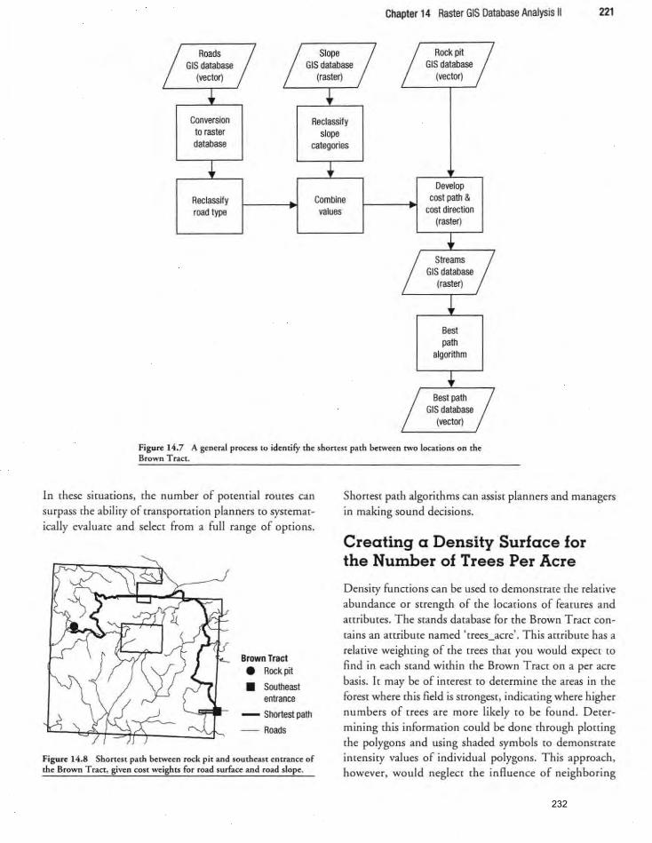
Chapter 14 Raster GIS Database Analysis II 221
Slope Rock pit GIS database GIS database
(vector)
Conversion Reclassify to raster slope database categories
Reclassify Combine road type values
Develop cost path &
cost direction (raster)
Best path
algorithm
(vector)
Figure 14.7 A general process lO identify the shortest path between two locations on the Brown Tract.
In these simations, the number of potenrial fOUCes can surpass (he ability of transportation planners to sysremar· ically evaluate and select from a full range of options.
Brown Tract • Rock pit
• Sootheast entrance
- Shortest path
- Roads
Figure 14.8 Shortest path between rock pit and southC:l$t entrance of the Brown Tract, given cost weights for road surfaa and road slope.
Shorrest path algorithms can assist planners and managers in making sound decisions.
Creating a Density Surface for the Number of Trees Per Acre
Density functions can be used to demonstrate [he relative abundance or strength of the locations of features and anributes, The stands database for the Brown Tract contains an attribute named 'trees_acre', This attribute has a
relative weighting of the trees that you would expect to
find in each stand within the Brown Tract on a per acre
basis. It may be of interest to determine the areas in the forest where this field is strongest, indicating where higher numbers o f trees are more likely to be fou nd. Deter
mining this info rmation could be done through plotting the polygons and using shaded symbols to demonsttate intensity values of individual polygons. This approach, however, would neglect the influence of neighboring
232
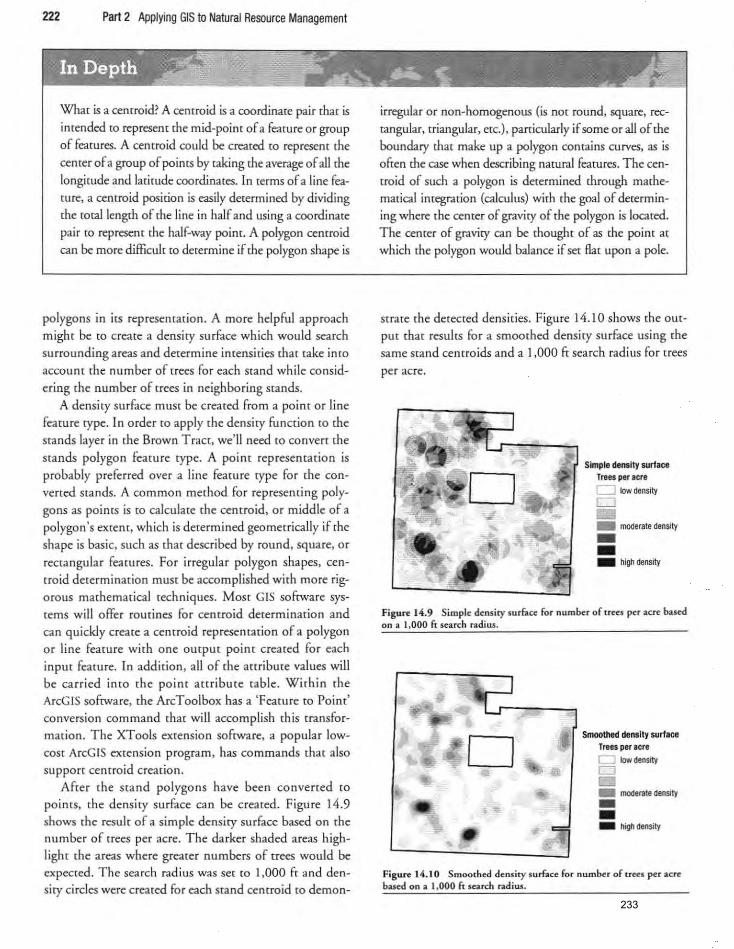
222 Part 2 Applying GIS to Natural Resource Management
What is a centroid? A centroid is a coordinate pair that is intended co represent me mid-point of a feature or group of fe-drures. A centroid could be creatai co represent {he center of a group of points by taking the average of all the longirude and latitude coordinates. In terms of a line feature, a centroid position is easily determined. by dividing the tQ[al length of the line in half and using a coordinate
pair [Q represent the half-way point. A polygon centroid can be more difficult to determine if the polygon shape is
polygons in irs representation . A more helpful approach might be to create a densi ty surface which would search
surrounding areas and determine inrensicies that take into account (he nllmber of trees for each stand while consid
ering the number of trees in neighboring stands.
A density surface must be created from a point or line
feature type. In order [Q apply the density function to the stands layer in the Brown Tract, we'll need ro conven the
stands polygon feamce rype. A point representation is probably preferred over a line feature type for the con
vened stands. A common method for representing poly
gons as poims is {Q calculate the cemroid, or middle of a
polygon's extent, which is determined geometrically if the shape is basic, such as ,hat described by round, square, or
rectangular fearures. For irregular polygon shapes, cen
troid determinat ion must be accomplished with more rig
orous mathematical techniques. Most GIS software sys
tems will offer routines for cemroid determination and
can quickly create a cemroid represemation of a polygon
or line feature with one oUCput point created for each
input feature. In addition, all of the attribute values will be carried into the poim anribuce table. Within [he
ArcGIS software, ,he ArcToolbox has a 'Featu re to Point'
conversion command that will accomplish this cransfor
mation. The XTools extension software, a popular low
COSt ArcGIS extension program, has commands that also
support centroid creation.
After the stand polygons have been converted to
poims, the density surface can be created. Figure 14 .9
shows the resuh of a simple density surface based on the number of trees per acre. The darker shaded areas highlight the areas where greater numbers of crees would be expected. The search rad ius was set to 1,000 ft and den
sity circles were created for each stand cencroid to demon-
irregular or non-homogenous (is not round, square, rec
tangular, triangular, etc.), patricularly if some or all of the
boundaty that make up a polygon contains curves, as is orren the case when describing narural features. The cen
troid of such a polygon is determined through mathematical integration (calculus) with the goal of determining where the center of gravity of the polygon is located.
The center of gravity can be thought of as the point at which the polygon would balance if set flat upon a pole.
strate the detected densities. Figure 14. 10 shows the Output that results for a smoothed density surface using the
same stand centroids and a 1,000 ft search radius for trees
per acre.
Simple density surface Trees per Icre o lOw density
CJ -_ moderate density --_ hIgh density
Figure 14.9 Simple density surface for num~r of trees per acrc based on a 1,000 ft search rndius.
•• i ..
Smoothed density surface Trees per Icre o Iowdenslty CJ II!llI _ moderate density --_ high denslty
Figure 14.10 Smoothed dcns ity sUrhce for num~r of trees per acre based on a 1,000 ft search radius.
233
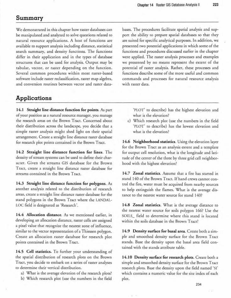
Summary
We demonstrated in (his chapter how raster databases can
be manipulated and analyzed (0 solve questions related [0
natural resource applicadons. A host of functions are
available ro supporc analysis including distance, sracisrica1 search summary. and density functions . The functions
differ in their application and in the types of database structures that can be used for analysis . Omput may be tabu lar, veC(Of, or raster depending on the function .
Several common procedures within most raster-based
software include raster reclass ification, raster map algebra.
and conversion routines between vector and raster dar3-
Applications
14.1 Straight line discance function for points. A!; parr of your position as a natural resource manager. you manage
the research areas on the Brown Tract. Concerned abom
their dimibu<ion across ,he landscape, you decide rhac a simple rasrer analys is mighr shed lighr on rheir spacia l arrangement. Create a straight line dismnce raster database
for research plot pointS conrained in the Brown Tract.
14.2 Straight line distance function for lines. The density of stream systems can be used to define their char
acter. Given the streams GIS database for rhe Brown
Tract , creare a srraight line distance rasrer database for
streams contained in the Brown Trace.
14.3 Straight line dinance function for polygons. A!;
another analysis related {Q the distribution of research
areas, create a straight line distance raster database fo r the
"and polygons in ,he Brown Traer where ,he LANDAL
LOC field is designared as 'Research '.
14.4 Allocation distance. As we mentioned earlier, in
developing an allocation distance, ras ter cells are ass igned
a pixel value that recognize the nearest zone of inAuence,
si milar to the vector representation of a Th iessen polygon.
Create an allocation raSter database for researc h plot
po ints contained in the Brown Tracr.
14.5 Ceu statistics. To furrher you r undersranding of the spatial distribution of research plots on the Brown
Tract, you decide (Q embark on a series of raster analyses
to determine their venical distribution.
a) What is the average elevation of the resea rch plots?
b) Which research plo< (use rhe numbers in rhe field
Chapter 14 Raster GIS Database Analysis II 223
bases. The procedures facilitate spatial analys is and supPOrt ,he abili ty [Q prepare spa,ial daubases so ,har ,hey are su ited for specific analytical purposes. In additio n, we
presented [Wo potential applications in which some of the
functions and procedures discussed earlier in the chapter
were applied. The raster analysis processes and examples
we presented by no means represent the extent of the
porential of raster analysis. Rather, these processes and
functions describe some of the more usefu l and commo n
commands and processes for namra1 resource analys is
with raster data.
' PLOT' to describe) has rhe highesr e1evar ion and what is the elevation?
c) Which research plor (use ,he numbers in ,he field ' PLOT' ro describe) has rhe lowest e1evarion and what is the elevation?
14.6 Neighborhood statistics. Using ,he elevation layer for the Brown Tract as an analys is extent and a template
for Output cell reso lution, what is the longitude and lati
rude of ,he cenrer of rhe ,hree by rhree grid cell neighborhood wirh rhe highest e1evarion'
14.7 Zonal sta,inics. Assume ,har a fire has s<arced in srand 140 of ,he Brown Trace. Ifhand crews canno[Control the fire, water must be acquired from nearby sources
to help extinguish the flames. What is the average dis
tance to the nearest water source for stand 140?
14.8 Zonal statistics . What is the average distance {Q
the nearest water source for so ils polygon 166? Use the
SOILS_ field to determ in e where this stand is located
wirhin the so ils database in the Brown Tracr?
14.9 Density surface for basal area. Crea,e borh a simple and smoorhed density surface for [he Brown Trace stands. Base rhe density upon (he basal area field con
tained with (he stands attribute table.
14.10 Density surface for research plots. Creace borh a simple and smoothed dens ity surface fo r rhe Brown Tract
research plors. Base rhe density upon [he field named 'sl' which contains a numeric value for the site index of each
ploe. 234
224 Part 2 Applying GIS to Natural Resource Management
References
Bettinger, P., G.A. Brndshaw, & Weaver, G.W. (I 996). Effects of geograph ic information system veC[Q f- rasrer
vector data conversion on landscape indices. Canadian journal ofFomt Restarch, 26,1416--25.
Chang, K. (2002) . Introduction to geographic informa
tion systems. New York: McGrnw-Hill. Chrisma n, N . (1997). Exploring geographic information
systems. New York: John Wiley & Sons, Inc. DeMers, M.N. (2002). GIS modeling in raster. New
York: John Wi ley & Sons, Inc.
Mitchell, A. (2005). The ERSI guide to GIS analysis. Volume 2: Spatial 1nf!asurements and stah'sties. Redlands, CA: ERSI Press.
Silverman, B.W. (I986). Density estimation for statistics and data analysis. New York: Chapman and Hall.
Theobald, D.M. (2003). GIS conupts and ArcGlS methods.
Fort Collins, CO: Conservation Planning Technologies. Wing, M.G., & Tynon , J.F. (2006). Crime mappi ng
and spatial analys is in National Forests. Journal of Forestry, 104(6),293- 8.
235

Part 3
Contemporary Issues in GIS
G t!ographic Information Systems: Applications in Natural Rt!sourus Managemt!llt focused
on the background and development of GIS in rart I and delved into GIS applications in Pan 2. In Parr 3. we try [Q provide a glimpse of where GIS use may be heading in
the nea r future. Trying to look ahead and predict what may happen is a difficult task because both GIS-related technology and the society that surrounds it are changing rap
idly. Nonetheless. in chapter 15 we discuss some trends that 3re associated with GIS in
namra1 resource management. These trends are related CO technological developments. rhe
handling and sharing of spatial data, and the legal issues that may impact organizations that use GIS. C hapter 16 makes note of how the increased ava ilability of GIS has trans
formed rhe delivery and struc(Ure of GIS operations in many organizations. Also important in chapter 16 is rhe discussion of possible barriers ro successful GIS impiemenrarion
and how implementation effectiveness can be assessed.
We also consider some of the current challenges within the GIS communicy in Parr 3 .
T he final chapter, chapter 17, examines the on-going and sometimes contentious discus
sion of how the GIS profession should be defined and recognized. There are a number of
other established professions that are also involved with measuring and mapping features
and there has been friction at times in agreeing on me capacity in which certain professions
should apply GIS. Such discussions are evidence that GIS and GIS professionals have an important and necessary ro le in today's society. While many other professions have well
defined activities, competency standards. and governi ng bodies that describe and guide irs
members. the GIS community has only recently developed some initial pathways for cer
tifying GIS competency. Criticism has been leveled toward these initial efforts on the
grounds mat sufficiently rigorous processes to establish competency have not been devel
oped. The discussion ofeIS competency arose initially from concerns voiced. from me land
surveyi ng and engineering communities about the potential for GIS users to perform tra
ditional surveying and measuremenr activities while not actually having professional license as a surveyor or engineer. The final chapter probes the issue of whether GIS users should be licensed. a hot ropic of conversacion particularly when you try to define what a 'professional' GIS user is and what sorts of activicies (hat person is qualified ro perform.
236
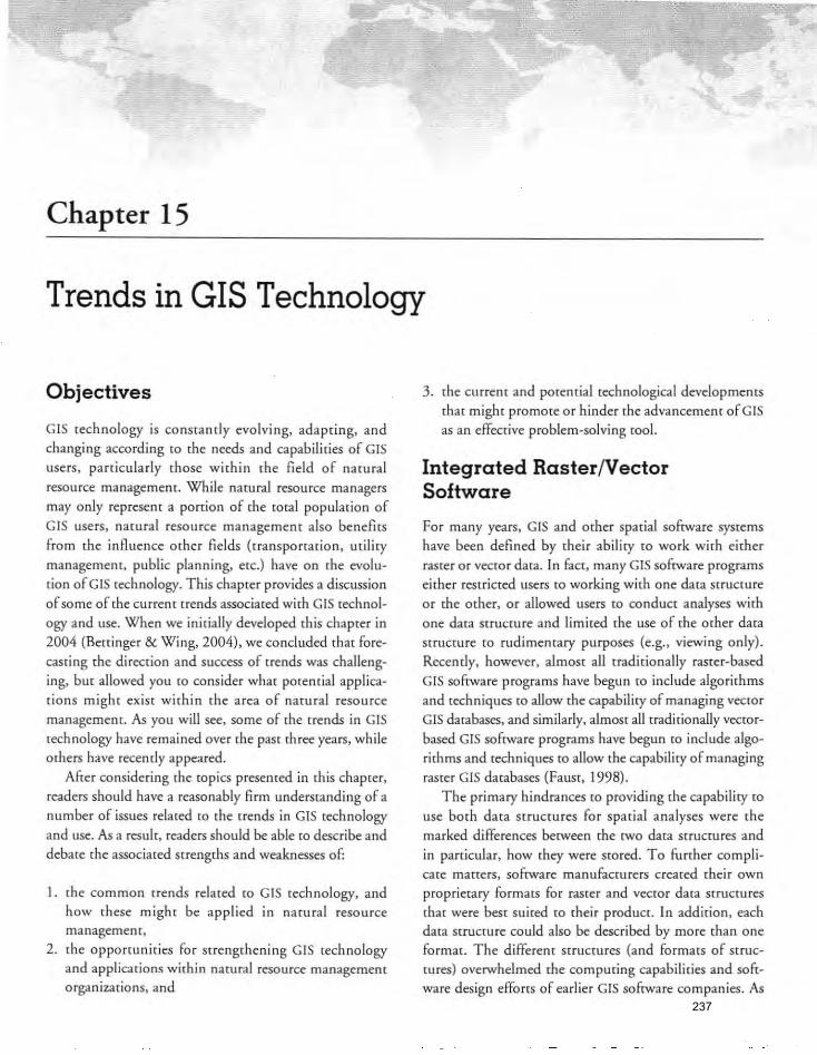
Chapter 15
Trends in GIS Technology
Objectives
GIS technology is constantly evo lving, adapting. and changing according to the needs and capabilities of GIS users , panicularly (hose within the field of namral resou rce management. While namral resource managers
may only represent a portion of the tOtal population of GIS users, natural resource management also benefits from the influence other fields (t ransportatio n, utility
management, public planning, etc.) have on [he evolucion of GIS technology. This chapter provides a discussion of so me of the current trends associated with GIS technol
ogy and use. When we initially developed th is chapter in 2004 (Bettinger & Wing, 2004), we co ncluded that fore
casring the direction and success of trends was challenging, but allowed you [0 consider what potential applications might ex ist within the area of natural resource management. As you will see, some of the trends in GIS
tech nology have remained over the past duee years, while others have recently appeared.
After considering the topics presented in this chapter, readers should have a reasonably firm understanding of a number of issues related to the trends in GIS technology and lise. As a result, readers should be able to describe and debate the associated strengths and weaknesses of:
I. the common trends related ro GIS technology, and how these might be applied in natural resource management,
2. the oppo rrunities for strengthenin g GIS technology and applications within natural resource management o rganizations. and
3. the current and potential technological developments that might promote or hinder the adva ncement of GIS
as an effective problem-solving roo l.
Integrated Raster/Vector Software
For many years, GIS and other spatial software systems have been defined by their ability to wo rk with either
raster or vecror data. In fact, many GIS software programs either rest ricted lIsers ro working with one data structure o r the other, or aiiowed users to conduct analyses with one data strucrure and limited the use of the other data Structure to rudimentary purposes (e.g., viewing only) . Recently, however, almost all traditionally raster-based
GIS software programs have begun to include algorithms and techniques to allow the capability of managing vector GIS databases, and similarly, almost all traditionally vector
based GIS software programs have begun to include algorithms and techniques to allow the capability of managing raSter GIS databases (Faust, 1998).
The primaty hindrances to providing the capability to use both data srrucrures for spacial analyses were {he
marked differences between the twO data structures and in part icular, how they were stored. To further complicate marters, software manufactUrers created their own proprietary formats for raster and vector data structures that were best suited to their product. In addit ion, each data structure could also be described by more than one format. The di ffe rent structures (and formats of srruc~
cures) overwhelmed the computing capabi li t ies and software design efforts of earlier GIS software com panies. As
237
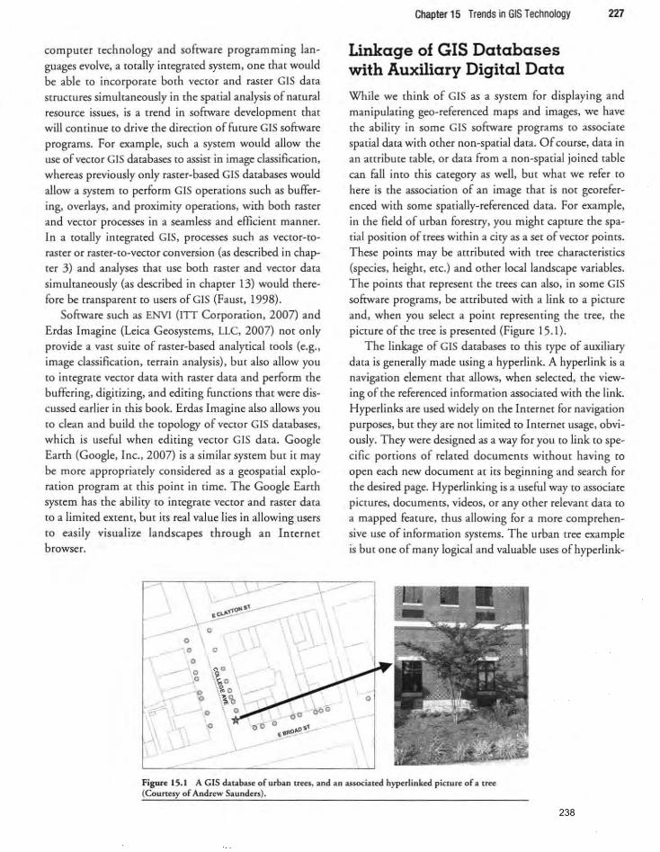
computer technology and software programming languages evolve. a (Orally imegrated system, one that would
be able to incorporate both vecrof and raster GIS data
structures simultaneously in the spatial analysis of natural
resource issues, is a trend in software development that
will continue [0 drive the direction offurure GIS software
programs. For example. such a system would allow the use of vecmr GIS databases (0 assist in image classification,
whereas previously only raster-based GIS databases would allow a system to perform GIS operarions such as buffer
ing. overlays. and proximity operations. with hoth raster
and vector processes in a seamless and efficient manner. In a totally integrated GIS, processes such as vecrof-toraster or raster-[Q-vector conversion (as described in chap
ter 3) and analyses that use both raster and vector data simultaneously (as described in chapter 13) would therefore be transparent to users of GIS (Faust, 1998).
Software such as ENVI (ITT Corporation, 2007) and Erdas Imagine (Leiea Ceosystems, LLC, 2007) not on ly provide a vast suite of raster-based analytical tools (e.g. ,
image classificacion, terrain analysis), bm also allow you
to integrate vec[Qr data with raster data and perform the
buffering, digicizing, and edicing funcrions that were dis
cussed earlier in this book. Erdas Imagine also allows you to clean and build the tOpology of vector GIS databases, which is useful when editing vectOr GIS data. Coogle Earth (Coogle, Inc., 2007) is a similar system but it may be more appropriately considered as a geospatial explo
ration program at this point in rime. The Google Earth
system has the ability to integrate vector and raster data
to a limited extent, but its real value lies in allowing users
to easily visualize landscapes through an Internet
browser.
Chapter 15 Trends in GIS Technology 227
Linkage of GIS Databases with Auxiliary Digital Data
While we think of GIS as a system for displaying and manipulating geo-referenced maps and images. we have
[he ability in some GIS software programs to associate
spatial data with other non-spatial data. Of course, data in
an atuibme [able, or data from a non-spatial joined table
can full into this category as well, but what we refer to
here is the association of an image that is nO( georefer
enced with some spatially-referenced data. For example.
in the field of urban forestry, you might capture the spatial position of (rees within a ciry as a set of vector points.
These points may be attributed with tree characteristics
(species, height, etc.) and other local landscape variables. The points that represent the trees can also. in some CIS
software programs, be atuibuted with a link [Q a picture
and, when you select a point representing (he tree, the
picture of the tree is presented (Figure 15.1). The linkage of GIS databases to this type of auxiliary
data is generally made using a hyperlink. A hyperlink is a navigation element that allows. when selected, [he view
ing of the referenced information associated with the link.
Hyperlinks are used widely on the Internet for navigation
purposes, but they are nO( limited to Internet usage. obvi
ously. They were designed as a way for you to link to specific portions of related documents without having to
open each new document at its beginning and search for
the desired page. Hyperlinking is a useful way to associate pictures. documents, videos, or any other relevanr data to
a mapped feature. thus allowing for a more comprehen
sive use of information systems. The urban tree example
is bur one of many logical and valuable uses ofhyperlink-
Figure 15.1 A GIS database of urban treC$, and an associated hyperlinked picture of a trcc (Courtesy of Andrew Saunders).
238
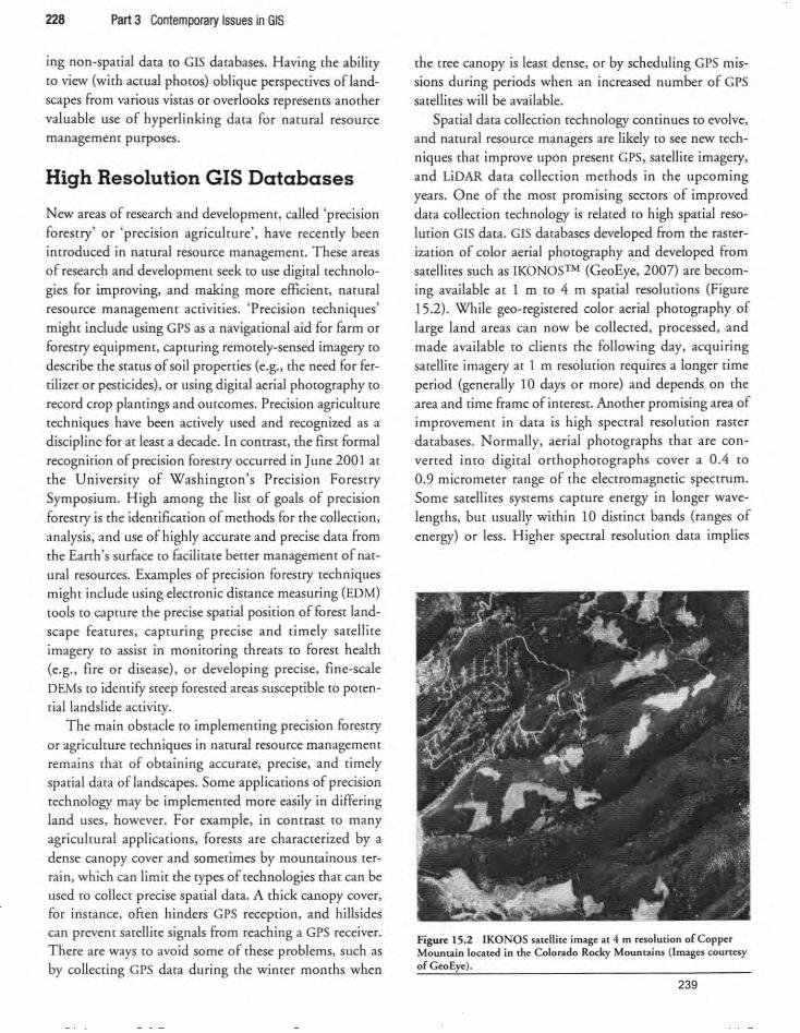
228 Part 3 Contemporary Issues in GIS
ing non-spatial data to GIS databases. Having the abi li ty to view (with actual photos) oblique perspectives of landscapes from various vistas or overlooks represents another
valuable use of hyper/inking data for natu ral resource management purposes.
High Resolution GIS Databases
New areas of research and development, called 'precision
fo restry' or 'p recision agriculture', have recently been introduced in natural resource management. These areas
of research and development seek co use digital technologies for improving, and making more efficient. namral resource management activities. 'Precis ion tech niques' might include using GPS as a navigational aid for farm or
forestry equipment. capturing remotely-sensed imagery co describe the status of soil properties (e.g .• the need for fertilizer or pesticides), or using digital aerial photography to
record crop planrings and outcomes. Precision agriculture
techniques have been actively used and recognized as a
discipline for at least a decade. In contrast. the first formal recognition of precision forestry occurred in June 2001 at
the University of W ashingwn's Precis ion Forescry
Symposium. High among the list of goals of precision forestty is the identification of methods fo r the collection. analys is. and use of highly accurate and precise data from
the Earth's surface w facilitate bener management of nat
ural resources. Examples of precision fo restry techniques
might include using electronic distance measuring (EDM)
(Ools ro capture the precise spatial position of forest land
scape features, capturin g precise and timely satellire
imagery (0 ass ist in monitoring threats (0 forest health
(e.g .• fire or disease). or developing precise. fine-scale DEMs to identify steep forested areas susceptible ro poten
tiallandslide activ ity.
The main obstacle ro implementing precision forestry
or agriculture techniques in natu ral resource management
remains that of obtain ing accurate. prec ise. and timely
spatial data of landscapes . Some applications of precision
technology may be implemented more easily in differing
land uses, however. For example. in COntrast ro many
agricultu ral applicatio ns, forests are characterized by a
dense canopy cover and sometimes by mountainous ter
rain, which can limit the types of technologies that can be used {Q coll eCt precise spatial data. A thick canopy cover,
for instance, often hinders CPS reception. and hillsides can prevent satel lite signals from reaching a CPS receiver. There are ways to avoid some of these problems, such as
by co llect ing CPS data during rhe winrer months when
the tree canopy is least dense. or by scheduling GI'S missions during periods when an increased number of CPS satelli tes will be available.
Spadal data collect ion technology conti nues to evolve.
and natural resource managers are likely to see new tech
niques that improve upon present CPS, satellite imagery,
and LiDAR data collection methods in the upco ming yea rs. One of the most promising secrors o f improved
data collection technology is related to high spatial resolution GIS data. GIS databases developed from the rasterization of color ae rial photography and developed from satelli tes such as IKONOSTM (GeoEye. 2007) are becoming available at 1 m to 4 m spatial resolutions (Figure
15.2). While geo-registered color aerial photography of large land areas can now be collected, processed . and
made avai lable to clients the following day. acquiri ng satell ite imagery at 1 m resolution requires a longer time
period (generally 10 days or more) and depends on the area and time frame of interest. Another promising area of
improvement in data is high speccral resolution raster
databases. Normally. aerial photographs that are converted into digital o rrhophotographs cover a 0.4 to
0.9 micrometer range of the electromagnetic spectrum.
Some satellites systems capture energy in longer wave
lengths. but usually within 10 distinct bands (ranges of energy) or less . Higher spectral resolut ion data implies
FigllR 15.2 IKONOS satellite image at 4 m resolution of Copper Mountain located in the Colorado Rocky Mountains (Imagc.s courtesy of GeoEye).
239
that many mOte bands of enetgy have been captured, and can be used co mo nito r and evaluate the Earm's surface.
AVIRIS (National Aeronautics and Space Administration, 2007) is an example of one such high spectral resolution system, although it has been avai lable for almost 15 years. With this system, 224 bands of data can be captured for a single landscape at one point in time, aIlowing scientists
and managers to use the appropriate spectral reflecrances
for analyzing various nacurai resource management issues.
Still among [he primary concerns of most nam ral
resou rce management organizations is (he COSt related (Q
the acquisi tion of high-resolution spatial data. While initially relat ively high, as new technologies and data sources become available the cost and ava ilability of highresolution GIS databases might be as low as $0.03 per acre. Anomer issue of concern is the data scocage require
ments. H igh-resolutio n images can require mass ive
amounts of computer hard dtive space. Although large hard drives (I 00 GB and above) have become the norm, storage space can be filled quickly as images are gathered and stored digitally.
Managed and integrated properly, high-resolution GIS
databases w ill help facil itate the creation and maintenance
of databases (hat have tremendous potencial for organiza
tions that manage large land areas. These GIS databases can be associated with methods char keep land cover
informacion current, and allow you co conduct temporal
analysis of land cover conditio ns. Two of the challenges
[0 usi ng high-resolution GIS databases wi ll be in deciding how often to acquire new data. and how CO integrate new
GIS databases with existing GIS databases. These challenges are markedly different from those experienced in
the recent past, where most natural resource management
organizations struggled due to a lack of data. Now, the amount of data available to an organization can become overwhelming. The high resolution of these GIS databases w ill also help provide a more accurate representadon of
natural resources, which has typically been one of the
drawbacks of using raSter GIS databases (Faust, 1998) .
Distribution of GIS Capabilities to Field Offices
There are a number of reasons why the use of GIS has.
and cominues (0. spread from a centralized organizational
office to field offices: more and more people are becoming comfortable using GIS. colleges and universities are educating students in the use and application of GIS in natural resources, and natural resource o rganizarions are rec-
Chapter 15 Trends in GIS Technology 229
ognizing that more timely analysis and map products can be obtained if the work is more closely situated co the end user (Bett inger, 1999; Wing & Bettinger, 2003). [n addition, the increased power of computer technologies (speed and memory) and [he advancements made in the operating systems of perso nal computers have both
allowed a wider user base to use GIS technology (Faus[, 1998). Since computer systems are relatively inexpensive
(a GIS workstation can now be purchased for unde r
$2,500) , and GIS software has been developed with end users (e.g., field personnel) in mind, the trend is [Oward a GIS system where, in larger organizations, data develop
ment and maimenance tasks are performed at a cemeal
office, and data analysis and map production tasks are
performed at remote field offices. In smaller organiza
tions, the d istribution of processes may be less clear.
because the distinction between a central office and field
offices may be blurred (or non-existent). In some o rganizations, approved person nel who work
in the field perform the data maintenance tasks . C hanges
to GIS databases can be made at the field office, sent electronically co the cemral office for verification and integration, and eventually passed back to field offices. In systems such as these, o nly one person can be making
changes at each point in time. As a result, data being
edited is 'checked out' (like a library book) umil [he editing has been completed. The transfer of updated information to [he field offices would ideally be instantaneous, but it is not. A delay of 15-30 minutes is required for centralized systems to complete the ir tasks.
The benefits of a distributed GIS system are aimed at enhancing local or field office productivi ty and decisionmaking. Two of the main benefits include a more timely
response co analysis and map productio n needs of field
offices, and a decreased work load on a centralized GIS
office (al lowing more time and effort to be devoted to GIS
database quality and maintenance). Within a distributed
GIS system, clearer channels of communication should
exist, since generally speaking, (he customers (those
requesting maps or analysis) and suppliers (those performing the analysis or making maps) are in the same office (or
perhaps are the same person). This face-eo-face communi
cation is often more effecdve in meecing the goals of a map
or analysis request than communication processes that rely on e-mail or phone ca lls. [n addition , field personnel involved in GIS analysis and map production are likely (0
feel as if they have a greater investmenc in [he GIS program.
and perhaps will develop a greater sense of responsibil iry for maintaining accurare GIS databases (Berringer, 1999) .
240
that many mOte bands of enetgy have been caprured, and can be used to monitor and evaluate the Earth's surface. AV1RIS (National Aeronautics and Space Administration, 2007) is an example of one such high spectral resolution system, although it has been available for almost 15 years. With this system, 224 bands of data can be captured for a single landscape at one point in time. aUowing scientists and managers [0 use the appropriate spectral re£lecrances for analyzing various namrai resource management issues.
Sdll among the primary concerns of most natural resource management organizacions is the COSt related [0
the acquisition of high-resolution spatial data. While initially relatively high , as new technologies and data sources become avai lable the cost and availability of highresolution G IS databases might be as low as $0.03 per acre. Anorher issue of concern is the dara s[Qrage re'luiremenrs. High-resolution images can require massive amounts of computer hard drive space. Although large hard drives (100 GB and above) have become the norm, storage space can be filled quickly as images are ga<hered and stored digitally.
Managed and integrated properly, high-resolution GIS
databases will help facilitate the creation and maintenance of databases mat have tremendous pmential for organizations that manage large land areas. These GIS databases can be associated with methods mar keep land cover informacion currene, and allow you [Q conduct remporai analysis ofland cover conditions. Two of the challenges to usi ng high-resolution GIS databases will be in deciding how often ro acquire new dara, and how (0 imegrare new GIS databases with exisring GIS databases. These challenges are markedly differenr from [hose experienced in the receor pasr, where mosr narural resource managemem organizations Struggled due 10 a lack of data. Now, the amounr of dara avaiJable [0 an organizarion can become overwhelming. The high resolution of these GIS databases will also belp provide a morc: accurale representation of natural resources, which has typically been one of the drawbacks of using raster GIS databases (Fa uS!, 1998).
Distribution of GIS Capabilities to Field Offices
There are a number of reasons why me use of GIS has, and conrinues ro, spread from a cemraliz.ed organizational office to field offices: more and more people are becoming comfortable using GIS. colleges and universiries arc: educadng srudc:ms in the use and application of GIS in nacuraj resources, and namral resource organ izarions are rec-
Chapter 15 Trends in GIS Technology 229
ognizing that more timely analysis and map products can be obtained if the work is more closely situated to the end user (Bettinger, 1999; Wing & Berringer, 2003) . In add irion , rhe increased power of compurer [echnologies (speed and memory) and the advancements made in the operaring systems of personal compurers have borh allowed a wider user base to use GIS technology (Faust, 1998). Since computer systems are relatively inexpensive (a GIS worksrarion can now be purchased for under $2.500), and GIS software has been developed with end users (e.g., field personnel) in mind, the trend is toward a GIS sysrem where, in larger organizacions, dara developmem and maintenance casks are performed at a cemral office, and clara analysis and map production [asks are performed at rem ore field offices. In smaller organizarions, the distriburion of processes may be less dear. because [he distincrion becween a central office and field offices may be blurred (or non-existent).
In some organizations. approved personnel who work in the field perform the data maintenance tasks. Changes to GIS databases can be made at the field office, sent electronically co [he central office for verification and integration, and eventually passed back to field offices. In systems such as these, only one person can be making changes at each point in time. As a result , dara being edited is 'checked out ' (like a library book) until the ed iting has been completed. The transfer of updated information ro the field offices would ideally be instantaneous, but it is not. A delay of 15-30 minutes is required for centraljzed systems co complete [heir rasks.
The benefits of a distributed GIS system are aimed at enhancing local or field office productivity and decisionmaking. Two of me main benefits include a more timely response to analysis and map production needs of field offices, and a decreased work load on a centralized GIS
office (allowing more time and effort to be devoted to GIS
database quality and maintenance). Within a distributed GIS system. dearer channels of communication should exist , since generally speaking, the customers (rhose requesting maps or analysis) and suppliers (those performing the analysis or making maps) are in the same office (or perhaps are the same person). This fuce-to-fuce communication is often more effective in meering rhe goals of a map or analysis request chan communication processes mat rely on e-mail or phone calls. In addition, field personnel involved in GIS analysis and map production are likely to
feel as if rhey have a gre-arer investment in (he GIS program, and perhaps will develop a greater sense of responsibility for maintaining accurate GIS databases (Bettinger, 1999).
230 Part 3 Contemporary Issues in GIS
Given the ongoing technological {software and hardware} advancements related co GIS. and the proliferation
of GIS training, it is highly likely that the distributed GIS model of capabilities wiH continue to grow, and become
more prevalent than the centralized model. At some point, the distributed model may replace the centralized model completely in many organizations. The challenge in man
aging this paradigm shift will be to ensure that organizational prococols and monitoring are in place to protect distributed users from using spatial data improperly.
Web-based Geographic Information Systems
The widespread use of Google Earth has suggested to many that GIS can be both affordable and easy to use across the Internee. Some organizations have recognized
the need to provide GIS data management services over
the Internet as a way [0 more rapidly update databases and provide information to users in the field. Ideally, a natural resource organization would maintain a system where data
being updated by an employee in a field office can be 'checked our' over the Internet and managed (updated or
modified) . While the data is being modified remotely, other users would have the abilicy to view the data, but not
simultaneously modify the data. Once the data has been checked back in, orner users in the organization can then
use the modified data. Overall, [his type of process has the potential for substantially reducing the time required to
traditionally update GIS databases (see chapter 10). However, there may be some data qualicy issues related to
remotely-performed modifications of databases that are
not consistent with organizational standards.
As an example of a system such as this, the Virginia
Department of Forestry has recently implemented the
Integrated Forest Resource Information System (IFRJS).
Many organizations have developed their own Intranet.
These are private, networked computer environments
in which only members within me organization have
access. Imranets look and act like the Internet, and can
range in complexity from the vety simple (a set of folders or subdirectories containing data or other organiza-
The benefits of the system include reduced paper-related processes {e.g., transfer of maps and data to a centralized
office} , and an empowerment of people to adopt and use
new technology at the field level. Users in field offices can update GIS databases using heads-up digitizing, and submit data and repons on progress in managing the state's
forests. Future endeavors include extending the real-dme
capability to hand-held data recorders equipped with GPS technology to all ow an immediate data capture and
update to occur, which can increase the efficiency of map
ping and reporting wildfires, water quality problems, and insect and disease outbreaks. Although the intent of the system is to make administrative functions of state land
managers more efficient, as with the previous discussion,
there may arise some data quality issues related to
remotely-performed modifications of databases that are
not consistent with organizational standards. Only time
will tell whether these advances will result in COSt- and
time-savings and in increased productivity with no sub
stantial reduction in data quality.
Data Retrieval via the Internet
As we discussed in chapter 3, the Internet is becoming a
common source for acquiring GIS databases, GIS meta
data, and other information regarding the acquisition of
GIS databases. In fact, the current popularity and preva
lence of GIS can at least be parely attributed to the Internet. As public agencies began to produce and make
GIS databases available, customers who wanted the data
were often required to pay for the storage medium (tape, co, etc.) and for the time required to place the GIS database{s) on the medium. Since the media had to be mailed to the customer, this process also required a period of sev
eral days (to weeks) before the user could actually use the GIS databases. Presently, most public agencies offer their
tion information) to the sophisticated {those that offer graphical interfaces for access to data, software, or links to other organizational services}. Each of these services is
provided through an internal (co the organization) website. Inrraners are a method that can facilitate a disrrib
ured GIS system within an organization.
241
non-sensitive GIS databases over the Imernet, allowing
GIS users the opportunity to quickly acquire the data at
no COSt. In cases where GIS databases are very large and therefore nO( practical for Imernet transfer (for example, as wirh DOQs or orher high-resol urion rasrer imagery) . public agencies may still require that consumers pay for data transfer COSts. However, data compression software technology conrinues to improve, which reduces the need
for non-Internet transfers. Private organ izations that marker and sel l GIS darabases also allow cusromers ro download the databases from the Internet. In these cases, cus
tomers usually need to be registered w ith rhe private organization because access to the data is restricted.
Portable Devices to Capture, Display, and Update GIS Data
[n rhe pasr decade rhe use of hand-held dara collecrors and personal digiral assisranrs (PDAs) has become quire common for collecting forest inventory data and other attributes oflandscape features. GPS receivers, in faCt, use
hand-held dara collecrors ro allow you ro caprure rhe spatial anributes oflandscape features. Inregration of the two philosophies. allowing you ro collecr sparial locarional information about landscape features and to coliect anribute data, results in positive benefits to a natural resource
management organization. Traditionally, data collected for natural resource inventories would be recorded in a field notebook or on a map, and would requ ire manual dara enrry inro a spreadsheer or GIS darabase (rhrough anributing spatia l landscape features). This manual process is time consuming and presents several opportunities for human error to be incroduced into a GIS database. The integration of digital technologies allows info rmation to be recorded in a computer database while a person is in rhe field. Hand-held dara collecrors and PDAs are able co conneCt to wired or wireless computer systems, allowing rhe dara co be rransferred ro GIS. This grearly exped ires rhe rransfer of field-collecred dara ro a GIS darabase where rhe dara can be analyzed and mapped. This process also removes some of the error opportunities that might occur through rhe manual coding and inputting of clara. Dara collectors also offer users the abil ity to examine maps and
images of landscape fearures as rhey are being measu red. Field personnel can use this heads-up d isplay ro visually determine whether their measurements are in agreement with the landscape features being measu red. Digital orthophotoquads o r digital raster graphics are two com-
Chapter 15 Trends in GIS Technology 231
man GIS darabases rhar can also be used ro visually check measurements, as well as to faci li tate a traverse of rhe
landscape. Hand-held dara collecrors are moderarely expensive
($1.000 ro $5.000). depending on rhe quality of rhe instrument and the functions they allow. POAs are less expensive (around $500). and can be used as dara collectors, but they are generally less rugged and more prone to damage from environmental factors (e .g., rain) and
human error (e.g .• dropping rhe device). Some GIS consulranrs have developed software rhar will run on PDAs. ArcPad (Environmental Systems Research Inst itute, Inc., 2006) is perhaps rhe mosr widely known produce. A growing list of accessories can also be purchased to make POAs more durable and useful in inclement weather and
under other conditions.
Standards for the Exchange of GIS Databases
The deve10pmenr and use of srandards for exchanging GIS databases may seem like a trivial exercise for governmental employees and university researchers, since theorerica1ly dara ((ansferred among US federal governmenr o rganizations (for example) must adhere to federal data srandards (hrrp:llwww.fgdc.gov/srandards) . These srandards specifY dara formars rhar are inrended co facilirare the sharing of spatial data among organizations. Many university researchers also utilize th is protocol (or something very similar) in some cases because they interact with federal granting agencies during the course of research. However, most private natural resource management organizations are not bound by these data standards. Thus acqu isition and modification of GIS databases by private natural resource management organizations proceeds undocumented; transformations
and re-projections regularly occur to allow an integration of rhe acquired GIS darabases inro rhe organizarion's system, since the type and format of data exchanged can vary considerably (Figure 15.3) . Moving co a srandard dara excha nge fo rmat usually suggests that o ne of twO organizational policies will be used: ( I) organizations convert all of the GIS databases currently in use to a standard format, thus avoiding rhe need to convert GIS databases when data exchange processes occur, or (2) organizations convert GIS databases to a standard exchange format on ly when data exchange processes occur. There is a cost associated with both policies, and it is a function of how often
242
non-sensidve GIS databases over the Internet, allowing
GIS users the opportunity [0 quickly acquire the data at no COSt. In cases where GIS databases are very large and therefore nO{ practicaJ for Imernet transfer (for example,
as with OOQs or other high-resolution raster imagery). public agencies may still require that consumers pay for data cransfer costs. However. data compression sofrware technology condnues [0 improve. which reduces me need for non-Inrernet transfers. Privare organizations that market and sell GIS databases also allow customers to download the databases from the lnrernet. In these cases) cus
[Omers usually need ro be regisrered with rhe private organization because access ro the data is restricted.
Portable Devices to Capture, Display, and Update GIS Data
I n the past decade the use of hand-held data collectors and personal digital assistants (POAs) has become quite common for collecting forest inventory dara and other anribures of landscape fearures. G PS receivers, in faCt, use hand-held data collectors [0 allow you [0 capture the spatial attributes of landscape features.lntegradon of the rwo philosophies, allowing you to collect spatial loeational infortflalion aboullandscape features and to collect a([fibute data, results in posirive benefits to a namral resource
management organiz.ation. T radicionaHy. data coUected for narural resource inventories would be recorded in a field notebook or on a map. and would require manual data entry into a sp readsheet or GIS database (through attributing spatial landscape fea(Ures). This manual process is time consuming and presents severaJ opporcunities for human error co be introduced into a GIS database. The integration of digital technologies allows information to be recorded in a computer database while a person is in the field. Hand-held da,a collectors and POAs are able to conneCt to wired or wireless computer systems, allowing ,he data to be transferred to GI . This greatly expedites the transfer of field-collected data to a GIS database where the da,a can be analyzed and mapped. Th is process also removes some of me error opportunities char might occur through ,he manual coding and inputting of data. Da,a coHeetors also offer users the abil iry ro examine maps and
images oflandscape features as they are being measured. Field personnel can use this heads-up display to visually determine whether their measurements are in agreement with the landscape features bei ng measured. Digital onhophotoquads or digital raster graphics are two com-
Chapter 15 Trends in GIS Technology 231
mon GIS databases that can also be used to visually check measurements, as wel l as to faciJir3re a uaverse of {he
landscape. Hand-held data collectors are moderately expensive
($1.000 to $5,000) . depending on the quality of the instrument and the functions they allow. POAs are less expensive (around $500) , and can be used as data collectors. but they are generally less rugged and more prone to
damage from environmental facto rs (e.g. , rain) and human error (e.g., dropping the device). Some GIS consultants have developed sof1ware that will run on POAs. ArcPad (Environmemal Systems Research InstitU[c, Inc. ,
2006) is perhaps the mosr widely known product. A growing IiSl of accessories can also be purchased to make POAs more durable and useful in inclemen, weather and under other conditions.
Standards for the Exchange of GIS Databases
The development and use of standards for exchanging GIS databases may seem like a trivial exercise for governmcnral employees and university researchers, since meoretically data transferred among US federal government organizations (for example) must adhere to federal data standards (J1[[p:llwww.fgdc.gov/standards) . These standards specifY data formats that are intended to facilitate the sharing of spatial data among organizations. Many universiry researchers also urilize this protocol (or something very sim ilar) in some cases because they imeract
with federal granting agencies during the course of research. However, most private namral resource managemenr organizations are not bound by these daca standards. Thus acquisition and modification of GIS databases by private natural resource managemenr
organ izations proceeds undocumenced: transformations and re-projections regularly occur CO allow an integration of the acquired GIS databases into rhe organization's system, since the rype and format of data exchanged can vary considerably (Figure 15.3) . Moving to a standard data exchange formac usually suggescs thac one of cwo organizational policies will be used: (1) organizarions conven all of [he GIS darabases curren dy in use [Q a srandard format. rhus avoiding the need to conven GIS databases when data exchange processes occur, or (2) organizarions convert GIS databases ro a standard exchange format only when dara exchange processes occur. There is a cost associated with both policies, and i, is a function of how often

232 Part 3 Contemporary Issues in GIS
I I
, , , \ I
Siale organizations
, , I
I I \ , , -- -
companies
,
" "
' 4 " I I
" I I
I I I I
\ .. \ \ \ \ \ \ \ \ \ \ \ \ \ \ \ \
Forestry consultants
,
.... -- .... , ' I \
I
Universities
, \ I I
I , ,
....... Federal data standards implied when transferring data
- - .... Other data standards generally used when transferring data
Fi~ 15.3 Datab~ transfu and implied standards among organiutions.
an organizacion perceives that it might exchange data
with orner organizacions. If an o rganization positions irs internal data standard closely to that of the data exchange standard, the cost w ill be minimized when acquiring GIS
databases from. or sharing GIS databases with. federal agencies. If an organization does not plan (Q acquire GIS
databases from, or share them with, federal agencies. the cost of deviating from the federal standard may be minimal.
Even if a natural resource management organization
avoids implementing a data exchange standard a few common data exchange formats are used by other organ
izations. For example. it is not uncommon for public
agencies to make GIS databases available in both ArcInfo export file format (eOO) and ArcView shapefile format. Among com purer-assisted design (CAD) software programs, the DXF (drawing exchange format) format is
commonly used to exchange files. Most GIS software manufacturers recognize that users will need to accommodate data formats designed by other software vendors . For
this reason, it is not unusual for a GIS software program
[Q make ava ilable conversion and integration processes
that make it possible [Q view other GIS database formats.
particularly those (hat are used by the most common GIS
software programs.
Legal Issues Related to GIS
Legal issues confront (he GIS community on several fronts
including issues related to privacy. liability. accessibility,
and licensing. Some of these issues are relatively new,
while others have been associated with GIS since its incep
tion . In either case, the issues will continue to evolve as
GIS sofrware becomes more widely used. Licensing and
certification of GIS professionals is an issue of currene concern to many GIS users and other professionals, and
will be discussed in more detail in chapter 17. Therefore issues related to privacy. liability. and accessibility are presented here.
GIS data is being co llected at an ever-increasing pace,
and used in novel ways as people begin to understand the power of connecting information to spatial position. For
example. some organizations now rely on the ability co relate data abom purchasing decisions with demographic
and location information (Cla rke. 2001). This information is used by businesses to direct mass mailings, CO sug-
243
gest the location of new facilities. and to place phone caUs to porenriai customers in [he evening (Q inquire whether
they may be interested a purchasing a product or service. Although federa l and State legislation exiSts to protect the
privacy of information collected from individuals by public organizations, very little legislation currently exists to
prevent non-public organizations from sell ing or sharing the information that is gathered during regular consumer transactions. GIS has thus enabled organizations to culti
vate business using spatial analyses. In this way. GIS has become a business tool. and like it or nor, an eff'eccive one. As private organizations co ntinue to forge new
ground in the collection, sale. and exchange of spacial data that describes the economic and social behavior of individuals. sociery will be challenged in establishing the laws and regulations that relate to privacy srandards.
In (he US, the federal government and state agencies
have spent millions of dollars of public funds collecting and processing spatial data. The Freedom of Information Act (FOIA) was authorized in 1966 to grant taxpayers the
right to access information related to the functioning of the government (Korte. 1997). Certain rypes of information, such as that related to security and law enforcement investigations, among others, are exempt from the FOIA.
Other types of information, however, must be provided to the person making the request, usually at some minimal cost to cover the cost of processing the data and pro
viding the media upon which the data is exchanged. Most states in the US have developed laws based on the FOIA that also require state governmental agencies to make government information avai lable. Unfortunately, new threats to public safety and national security have emerged in recent years, and have necessitated a closer
scrutiny of the types of government information made available to the public. More than likely, access to certain GIS databases describing such landscape features as water
supplies and power facilities will be curtailed in the future. and access to other GIS databases will be delayed
due to new security protocols. Legal liability issues are associated with circumstances
where a service or product provided by a producer is not sadsfactory to the customer receiving the service or product. Onsrud (I999) identifies twO rypes of liabiliry that
are pertinent to GIS: contractual and tort liability. Contractual liability issues arise when a contract be[Ween
[WO parties has been breached. For a private organization that provides GIS products or services, this might involve a software product not behaving as advertised or a GIS
database that does not adhere to a data accuracy standard.
Chapter 15 Trends in GIS Technology 233
Tort liability issues arise when a party (person or organization) becomes injured (sustains a physical injury, loses business, etc.) as the result of another party's actions or
products. An example might be an accident at sea as a result of using an inaccurate GIS database for navigation.
Private organizations that provide GIS products and services are responsible for adhering ro, and demonstrating, a level of competency associated with their discipline. When others are injured as the result of incompetence,
the organization providing the service or product may be liable for damages. In determining incompetence or negligence, a private organization may be responsible for pro
ducing inaccurate or insufficient data, bue this alone does not prove incompetence. Rather, the courts have sought to establish incompetence by comparing services or products to those that would be produced from an organization that is acting 'reasonably' (Onsrud. 1999).
Government agencies have typically been immune to litigation or responsibility for providing inaccurate spatial data due (0 sovereign immunity. An exceprion is made among agencies that produce goods or services that are
considered discretionary. Discretionary services or prodUCtS have resulted in government agencies being held liable for damages (Korte. 1997).
Bo(h private and public organizations that are involved in providing GIS products and services can act to limi t their liability risk. One method fo r lim iring risk is to
include information or disclaimers [hat accompany a
product in order to describe irs intended use, data accuracy, data reliability, and a wa rning that there may be errors in the data (as described in chapter 4) . Organizations can further protect themselves by ensuring thae all relevant parries have signed a clearly defined contract
for products and services, and that the organization performs the specifics of the contract compeeently. If project requirementS necessitate actions (for example. the development of other products or services) other than what is contained in the original cOntract, the organ ization providing the productS or services should contact the other
panies involved immediately to reach agreement on rhe specifics of the additional produces and services (costS, time frame, etc.) before beginning to develop those products and services (Beardslee. 2002).
Licensing of GIS data products is another legal issue.
and is tied directly to digital rights management (Cary. 2006) . Many organizations require payment for use of data and sof[Ware that they produced and, without payment, organizations using the data risk violating [he terms
of agreements that may have been implicit when the
244
gest rhe location of new facilities, and to place phone calls co porenrial customers in the evening [a inquire whether they may be interested a purchasing a product or service. Although federa l and state legislation exists to protect rhe privacy of information collected from individuals by public organizations. very litt le legis lation currently exists [0
prevem non-public organizations from selling or sharing (he informacion that is gathered during regular consumer
transactions. GIS has mus enabled organizacions [0 cubvate business using spatial analyses. In this way. GIS has become a bl1siness rool , and like if or nor, an effective one. As private organizations co nrinu e (0 forge new ground in the collection. sale. and exchange of spatial data that describes rhe economic and social behavior of individuals, society will be challenged in establishing rhe laws and regulations that relate ro privacy smnclards.
In the US. tbe federal government and state agencies have spent millions of dollars of public funds collecting and processing spacial data. The Freedom of Informacion Act (FOIA) was aurhorized in 1966 to grant taxpayers the right (Q access informacion relared to the functioning of the government (Korte. 1997). Certain types of information. such as mar related to security and law enforcement investigacions. among others, are exempt from the FOIA.
Other types of informacion, however, must be provided [0 the person making the request, usually at some minimal cost (Q cover the cost of processing the data and pro
viding the media upon which rhe data is exchanged. Most states in rhe US have developed laws based on the FOIA
that also require S[3.te governmental agencies (Q make government informadon avai lable. Unfortunately, new
threats to public safety and national security have emerged in recent years. and have necessitated a closer scrutiny of the types of government informacion made available (Q the public. More than likely, access [Q cerrain GIS databases describing such landscape features as water supplies and power facilities will be curtailed in the future. and access to orher GIS databases will be delayed due to new security protocols.
Legal liability issues are associated with circumstances where a service or product provided by a producer is not satisfactory ro the customer receiving the service or produCt. Onsrud (1999) identifies tWO types of liability that are pertinent to GIS: cOIHraCtUaJ and [Ort liability. Contractuall iabiliry issues ar ise when a comracr berween
twO parries has been breached. For a private organization (hat provides .IS products or services, this might involve a software produCt not behaving as advertised or a GIS database mat does not adhere [0 a data accuracy standard.
Chapter 15 Trends in GIS Technology 233
Tort liability issues arise when a party (person or organizacion) becomes injured (sustains a physical injury, loses business. etc.) as the result of another party's actions or
products. An example might be an accident at sea as a result of using an inaccurate GIS database for navigation.
Private organizations that provide GIS products and services are responsible for adheri ng [0, and demonstrating, a level of competency associated with their discipline. When others are injured as the result of incompetence.
the organization providing the service or product may be liable for damages.ln determining incompetence or negligence, a private organization may be responsible for pro
ducing inaccurate or insufficient data, hue this alone does not prove incompetence. Rather, the courtS have sought to establish incompetence by comparing services or products to those that would be produced from an organization ,hat is acting 'reasonably' (On stud, 1999). Governmem agencies have typically been immune to lit
igarion or responsibility for providing inaccurate spatial data due to sovereign immunity. An exception is made among agencies that produce goods or services that are
considered discretionary. Discretionary services or prodUCtS have resulted in government agencies being held liable for damages (Korre. 1997).
Both private and public organizarions that are involved in providing GIS products and services can act to
limit rheir liabil ity risk. One method for limiting risk is to include information or disclaimers that accompany a product in o rder to describe its intended use, data accuracy. data reliabili ty, and a warning that there may be erro rs in rhe data (as desc ri bed in chapter 4) . Organizations can hlfdler protect themselves by ensuring that all relevant parties have signed a clearly defined contraer for products and services, and [hat rhe organization performs the specifics of the contract competently. If project requiremenrs necessitate actions (for example, the developmen [ of other products or services) other than what is con[3.ined in the original contract, the organization providing the products or services should comact the other
parties involved immediately to reach agreement on the specifics of the additionaJ products and services (costS, time frame. etc.) before beginning to develop rhose products and services (Beardslee. 2002).
Licensing of GIS data products is another legal issue, and is tied directly to digital rights management (Cary, 2006). Many organizations require payment for use of dara and software that they produced and. without paymem, organizations using [he data risk violating the terms of agreements that may have been implicit when the

234 Part 3 Contemporary Issues in GIS
information was shared. While the appropriate model for
licensing GIS data is currently being debated, the problem lies with the ease of copying digital data and sharing it with o thers in the absence of an agreemenr (s imi lar to
sharing music files). New types of data sharing arrangements wi ll likely be formulated that are based on limited data sharing licenses. Cary (2006) suggests a system where users of GIS are granted access to certain GIS data based
on the locations of acruallandscape feacures or proximity
CO other featu res . This rype of proximal data sharing
could balance the need for openness (as desired by the user) with the need for confidentiality (as desired by the producer).
GIS Interoperability and Open Internet Access
Interoperabil ity in terms of GIS refers to ability of differen t geospadal insrrumenrs, databases, and techniques to
work together on applications. Inreroperabil iry involves crearing standard terminology. data formats. and software
inrerfaces that are borh recognized and used by organiza
tions involved in geospariaJ applications. T he need for
inreroperabili ry shou ld not be surprising for any disci
pline that becomes popular amo ng a wide number of
potenrial users, such as has been witnessed by the rapid
growth of GIS applications over the past two decades. The rapid growth of GIS gave rise to a number of GIS software inrerfaces and data formats that were proprietary and therefore not designed so that others could easily and freely access and exchange data with the proprietary for
mats. This inabi lity led co frustration among GIS users
and gave rise to the need for GIS interoperability. The Open Geospatial Co nsortium was founded in 1994 (Open Geospatial Consortium, Inc., 2007) and has 34 1 member o rganizations as of2007. The aGe represems a
coalition of both private and public organizations. The
goals of the aGe are to promote public accessibility to
geoprocess ing tools and o ther location-based services.
Sign ificant accomplishments of the aGe include the standardization of terms for GIS features (po inrs, polylines, polygons), the creation of the Geography Markup Language (GML) that provides an open source language for describing spat ial data. and the developmem of stan
dards fo r how geographic data can be requested and accessed from Internet servers (Longley et aI., 2005) . T he aGe has had a profound influence on making geospatial tools and services available to I mernet users and continues
to work on promoting geospatial software accessibil ity.
The aGe will likely continue to develop innovations thar Increase public access to locatio n-based info rmat ion
services.
GIS Education
Attention is likely to increase around the methods and
approaches instructors use [Q teach geosparial ski lls to stu
dents, not only at the university level, but also in high school and within the professional workforce. GIS capabilities are now essential for natural resource organiza
tions, as well as for other disc iplines throughout society
(Wing & Sessions, 2007). The primary tra ining ground for GIS ski lls is currently with in the university sYStem but geospatial skills are also being taught to srudenrs during
e1emenrary school years. In addition. train ing opportuni
ties for in-career professionals appear [Q be growing.
Many disciplines. such as fo restry. engineering, and
surveying have accreditat ion bodies that review and
appraise the curriculums of universities and co lleges that
offer related degrees . The accreditation bodies eithe r
approve the curriculum or repon why it cannot be
accredited and what steps are needed to gain accredita
tion. The accreditation process helps ensure that instruc
tion supporting the necessary knowledge and skills to
enter in to professional disciplines is being delivered
appropriately. The accreditation process helps educational programs become recognized and can be a significant incemive for drawing srudents. No such accred itation
process exists specifically for geospatial technology instruction per se, although some engineering and sur
veying programs focus heavi ly on measuremems and have
accreditation through the American Board of Engineering
Technology (ABET). Currently, a wide variety of methods and approaches are used to teach geospatial ski lls. Th is results in considerable variation in achieved learning Out
comes (Longley et aI., 2005) . A recent publication titled Th, Geographic Information Science and Technology Body of Knowledge (Di Biase et aI. , 2006) has attempted to define critical concepts and ski lls that relate to geographic information science and technology. Written through
extensive collaboration among GlScience researchers and
educators, this work represents an initial attempt to pro
vide a unified description of copies imponant for establishing geospatial ski ll competency. A second edition is planned that will provide additional detail and instructio n that supports key concepts and skills.
245
234 Part 3 Contemporary Issues in GIS
information was shared. While the appropriate model for licensing GIS dara is currencly being debated, the problem lies with the ease of copying digital data and sharing it wi th o[hers in me absence of an agreement (similar (0
sharing music files) . New types of data sharing arrangements wiU likely be formulated that are based on limited dara sharing Licenses. Caty (2006) suggests a system where users of GIS are gramed access to certain GIS data based on (he locations of acmallandscape fearures or proximity
to other fearu res. This type of proximal dara sharing could balance the need for openness (as desired by the user) wirh rhe need for confidentiality (as desired by rhe producer).
GIS Interoperability and Open Internet Access
Interoperability in rerms of GIS refers to ability of different geosparial inSlrumenrs, databases. and techn iques ro work together on applications. Interoperability involves creati ng standard terminology. data formats, and sofrware interfaces that are both recognized and used byorganizations involved in geospatial applicarions. The need fo r interoperability should not be surp rising for any discipline that becomes popu lar among a wide number of potencial users, such as has been wi tnessed by rhe rapid growrh of G IS applications over the past two decades. The rapid growth of GIS gave rise co a number of GIS software interfaces and data formats that were proprierary and therefore not designed so tha t others could easily and freely access and exchange data with the proprietaty formars. This inabili ty led to frustration among GIS users and gave rise co rhe need fo r GIS interoperabil ity. The Open Geospatial Consorrium was founded in 1994 (Open Geosparial Consorrium, Inc., 2007) and has 341 member organizarions as of2007. The aGe represents a coalition of both privare and public organizations. The goals of the aGe are to promore public accessibil ity to
geoprocessing (Ools and other location-based services. Significant accomplishments of the aGe include rhe standardization of rerms for GIS features (poin rs, polylines, polygons), the creation of rhe Geography Markup Language (GML) thar provides an open source language for describing spatial data, and the developmem of standards for how geographic data can be requested and accessed from Interner servers (Longley er aI., 2005). T he aGe has had a profound inAuence on making geosparial rools and services available co Internet users and conti nues
ro work on promoring geosparial software accessibi lity. T he aGe will likely continue to develop in novarions rha[ increase public access co locatio n-based informat ion
services.
GIS Education
Auention is likely to increase around the methods and
approaches instructors use [Q [each geospatial ski lls [0 sru
dents, not only ar the university level, but also in high school and wirhin rhe professional wotkforce. GIS capabiliries are now essential for natural resource organiza
tions, as well as fo r other disciplines throughour society (Wing & Sessions, 2007). The primary training ground for GIS ski lls is cu rrently within the university system but geosparial ski lls are also being taugh[ to students during e1ementaty school years. In addir ion, training opportunities for in-career professionals appear to be growing.
Many disciplines, such as fores[ty, engineering, and surveying have accreditation bodies rhat review and
appraise the curriculums of universities and co lleges that offer related degrees. The accreditation bodies eirher approve the curriculum or repon why if cannor be accredited and what steps are needed (Q gain accreditarion. The accreditation process helps ensu re that insrruc[ion supporring rhe necessaty knowledge and ski lls to
enrer in tO profess ional d isciplines is being delivered appropriarely. T he accreruta[ion process helps educarional programs become recognized and can be a significant incentive for drawing sruden{s. No such accredjtation process exists specifically fo r geospa[ial [echnology instruction per se, although some engineering and surveying programs focus heavily o n measurements and have accredi rarion [hrough the American Board of Engineering Technology (ABET) . Currendy, a wide variety of methods and approaches are used ro [each geospatial skil ls. This results in considerable variation in achieved learning Out
comes (Longley er al ., 2005). A recent publication titled The Ceographic Infomlation Sci",,, and Technology Body of Knowledge (DiBiase er aJ. , 2006) has arremp[ed [0
define critical concep" and skills that reiare co geographic information science and technology. Written through
extensive collaboration among GIScience researchers and educators, this work represents an initial attempt to provide a unified description of topics important for estab· lishing geospatial skill compereney. A second edit ion is planned char wi ll provide additional detail and instructio n that su pporrs key concepts and skills.
Summary
GIS technology is evolving almost as quickly as general computer systems (hardware and software) evolve. People
are thinking about natural resource managemem issues in
ways unimagined juSt a few years ago, and spatial data is facilitating these effons. Natu ral resource management
o rganizations are actively engaged in testing and imple
menting new [Ools for collecting and analyzing spatia l data. Organizations are also making GIS technology available to a large portion ohheir workforce. and me Internet
Applications
14.1 Local regulations regarding GIS distribution. Select an agency in yo ur area (state. province. city ,
coumy, townsh ip, etc .) that uses and mighr distribute GIS
databases. a) What types of GIS databases are publicly avai lable? b) Are the GIS databases available for download over
the I merner? c) What data exchange form ats are available?
d) Is <here a COSt related to acquiring the G IS databases? e) Are there specific laws that relate to GIS database
distribution , and how do they affect your abi li ty (Q
acqu ire GIS data from rhis agency?
14.2 Product liability (1) . Yo u work fo r a private organizat ion that makes GIS databases available to cus
tomers. How might you help prQ[ec( your organization
from liab il ity that could arise from CUS(Qmers that pur
chase your services and products?
14.3 Product liability (2). You work for a public agency that makes spatia l data available to customers.
How might you help protect your organization from lia
bility thar could arise from customers that use you r serv
ices and products?
References
Beardslee, D.E. (2002). Do it! Or, call them before they call you. Proftssional Surveyor, 22(2), 20.
Bettinger, P. (I999). Distributing GIS capabil ities to forestty field offices: Benefits and challenges. Journal of Forestry, 97(6), 22--6.
Chapter 15 Trends in GIS Technology 235
has c reated an efficient avenue [Q make GIS databases
available in a timely manner. These developmems have had a posicive effect on the acceptance and use of C IS. and
encourage furthe r GIS technology development. As GIS
technology and use evolves. however, other issues (pri
vacy. access ibil ity. li ability. etc.) arise that must be
addressed. These issues may require a close examination of policies and practices related to the use of GIS in naru
ral resource managemenr.
14.4 Precision forestry and agriculture. You work for the Bureau of Land Management (BLM) in central Colorado, and your supervisor, Mark Miller, has recently learned of precision forestry and agriculture. He has asked
you how precision techniques might benefit the manage
menr of BLM land in Colorado. Write a brief memo that
out lines the GIS databases, hardware, and sofrware related
to precision techniques. and how rhey might benefit the
management of BLM land in Colorado.
14.5 Distributed GIS. A timber company in the southeastern United States has JUSt hired you as a field forester.
You are eager to use the GIS skills you have learned in college to help yourself (and others) make informed forest managemenr decisions. The timber company has a cen
rraIized GIS deparrmem and five remote field offices and
they are in the midst of developing a system whereby personnel (foresters, biologists, hydrologists, etc.) in field offices (where you are located) can use desktop G IS software to make their own maps and pe rform their own
analyses. What can you do to ensure that the distribution
of responsibilit ies (map development and analysis) to your field office will be successful?
Bettinger, P., & Wing, M.G. (2004). Geographic information sysums: Appfications in forestry and natural resources management. New York: McGraw-Hill, Inc.
Cary, T. (2006). Geospa[ial digita l rights management. Geospatial Solutions, /6(3), 18-2 1.
246
236 Part 3 Contemporary Issues in GIS
Clarke, K.c. (200 I). Getting started with geographic information systems (3rd ed.). Englewood Cl iffs, NJ: Premice-Hall, Inc.
DiBiase, D., DeMers, M. , Johnson, A., Kemp, K., Luck, A., Plewe, B., & Wentz, E. (Eds.). (2006). The geographic information science and technology body of knowledge. Washingwn. DC: University Consortium for Geographic Information Science, Association of American Geographers.
Environmental Systems Research Institute, Inc. (2006). ArcPad - Mobile GIS software for field mapping applications. Redlands, CA: Environmental Systems Research Institute, Inc. Retrieved May 8, 2007, from http: // www.esri.comlsofrware/arcgis/arcpadlindex.html.
Faust, N. (1998) . Raster based GIS. In T.W. Foresman (Ed.), The history of geographic information systems: Perspectives from the pioneers (pp. 59-72). Upper Saddle River, NJ: Prentice-Hall, Inc.
GeoEye. (2007). GeoEye imagery products: IKONOS. Dulles, VA: GeoEye. Retrieved May 9, 2007, from http://www.geoeye.com/prod uctsl i magery/ikonosl default.htm.
Google, Inc. (2007). Google Earth. Mountain View, CA: Google, Inc. Retrieved May 9, 2007, from http: // earrh.google.com.
ITT Corporation. (2007). ENVI- The remote sensing exploitation platform. Boulder, CO: ITT Corporation. Retrieved May 9, 2007, from http: //www .ittvis. com/envil.
Korte, G.B. (1997). The GIS book (4th ed.) . Santa Fe, NM: On Word Press.
Leica Geosystems, LLC. (2007). Erdas Imagine. Norcross, GA: Leica Geosystems LLC. Retrieved May 9, 2007, from http: //gi.leica-geosystems.com/LGISubIx33xO.
aspx. Longley, P.A. , Goodchi ld, M.F., Maguire, D.J., &
Rhind, D.W. (2005). Geographic information ,ystems and science (2nd ed .). Chichester, England: John Wiley & Sons, Inc.
National Aeronautics and Space AdminiStration. (2007). A VlRfS: Airborne visible / infrared imaging spectrometer. Pasadena, CA: National Aeronautics and Space Administration, Jet Propulsion Laboratory, California Institute of Technology. Retrieved May 9, 2007, from http: //aviris.jpl. nasa.gov.
Onsrud, H.J. (1999). Liability in the use of GIS and geographical datasets. In P.A. Longley, M. F. Goodchild, D.J. Maguire, and D.W. Rhind (Eds.), Geographical Information Systems, Volume II (2nd ed.) (pp. 643-52). New York: John Wiley & Sons, Inc.
Open Geospatial Consortium, Inc. (OGe) . (2007). Wayland, MA: Open Geospatial Consortium, Inc. Retrieved May 21, 2007, from http: //www. opengeospatial.org.
Wing, M.G., & Bettinger, P. (2003). GIS: An updated primer on a powerful management (001. Journal of Forestry, 101(4),4-8 .
Wing, M.G., & Sessions, J. (2007) . Geospatial technology education. Journal of Forestry, 105(4), 173-8 .
247
236 Part 3 Contemporary Issues in GIS
Clarke, K.c. (200 I). Getting started with geographic information systems Ord ed.). Englewood Cliffs, NJ: Premice-Hall, Inc.
DiBiase, D., DeMers, M., Johnson, A., Kemp, K., Luck, A., Plewe, B. , & Wenrz, E. (Eds.). (2006). The geographic information science and technology body of knowledge. Washing[Qn, DC: University Consortium for Geographic Information Science. Association of American Geographers.
Environmenral Sysrems Research Institute, Inc. (2006). ArcPad - Mobile GIS software for field mapping applications. Redlands, CA: Environ menraJ Systems Research Instirute, Inc. Retrieved May 8, 2007, from http:// www.esri.com/sofrware/arcgis/arcpadlindex.html.
Faust, N. (1998). Raster based GIS. In T.W. Foresman (Ed.) , The history of geographic information systems: Perspectives ftom the pioneers (pp. 59-72). Upper Saddle River, NJ: Prenrice-Hall, Inc.
GeoEye. (2007). GeoEye imagery prodncts: IKONOS. Dulles, VA: GeoEye. Retrieved May 9, 2007 , from http: //www.geoeye. com /products/ i magery/ikonos/ deFaulr.htm.
Google, Inc. (2007) . Google Earth. Mountain View, CA: Google, Inc. Retrieved May 9, 2007, from http:// earth.google.com.
ITT Corporation. (2007). ENVI-The remote sensing exploitation platform. Boulder, CO: ITT Corporation. Retrieved May 9, 2007. from http://www.ittvis. com/envi/.
Korte. G.B. (1997). The GIS book (4th ed .). Santa Fe. NM: OnWord Press.
Leica Geosystems. LLC. (2007). Erdos Imagine. Norcross. GA. Leica Geosystems LLC. Retrieved May 9. 2007. from http://gi .leica-geosystems.com/LG (Sub I x33xO. aspx.
Longley , P.A .• Goodchild. M.F .• Maguire, D.J. , & Rhind, D.W. (2005). Geographic information systems and science (2nd ed.). Chichester. England: John Wiley & Sons, Inc.
National Aeronautics and Space AdminiStration. (2007). A VIRIS: Airborne visible / inftared imaging spectrometer. Pasadena. CA: Narional Aeronautics and Space
Administration, Jet Propulsion Laboratory. California Insci tute of Technology. Rerrieved May 9, 2007, from http: //aviris. j pI. nasa.gov.
Onsrud, H.J. (I 999) . Liabi lity in the use of GIS and geographical datasets. In P.A. Longley, M. F. Goodchild, D.J. Maguire. and D.W. Rhind (Eds.). G<ographicai Information Systems, Voillme II (2nd ed.) (pp. 643-52). New York: John Wi ley & Sons. Inc.
Open Geospatial Consortium, Inc. (OGe). (2007). Wayland, MA: Open Geospatial Consorcium, Inc. Retrieved May 21. 2007. from http: //www. opengeospadal.org.
Wing, M.G., & Bettinger, P. (2003). GIS: An updated primer on a powerful managemenr [001. Journal of Forestry. 101(4).4-8.
Wing. M.G., & Sessions. J. (2007). GeospaciaJ technology education. journal of Fomtry, 105(4). 173-8.
Chapter 16
Institutional Challenges and Opportunities Related to GIS
Objectives
This chapter offers some thoughts on rhe imegration and
use of GIS within narural resource management organizadons. There are a number of issues related to rhe successful development of a GIS program within an o rganization, and programs in many organ izadons are continuously evolving as people. technology, and organizational struc
[Ures change. At me conclusion of th is chapter, readers
should have an undemanding of a number of issues that relate co rhe challenges facing the implemenracion and use
of GIS in nacural resource managemenr, including:
t. an understanding of rhe potencial challenges mat are ahead for successfu l and efficient GIS applications within and among namra l resource management organIZatiOns;
2. an understanding of the challenges that exist for
organizations thinking of distributing GIS capabilities
to field offices. a move becoming more prevalent as recent natural resource graduates likely will have GIS experience in cou rsework. and exposure or uaining in the field; and
3. an understanding of how to assess the benefit of using GIS. a measurement process that will likely be necessary to develop more efficiem business operacio ns. higher qualiry products. and more timely managemenr decisions.
The development and use of GIS in natural resource
management has evolved considerably in the past 20 years as field foresters. biologists. hydrologists. and other natural resource professionals have become empowered with this technology. and are able to perform many of their own spatial analyses and map production tasks (Wing & Bettinger. 2003). In addition. it is increasingly likely that natural resource professionals wi ll have cou rsework
involving GIS and related geospatial technologies during undergraduate or graduate studies (Wing & Sessions. 2007) . While GIS technology continues to evolve. natural resource management organizations are faced with several lingering issues related to the GIS use. and several nC\v
challenges have arisen with the availability of GIS technology to field offices. Natoli et aJ. (2001) describe a set of
challenges for GIS implementation and use within (mainly) municipal organizations. and Bettinger (J 999) describes some of the challenges associated with implementing a disuibuted GIS system in forestry organiza{ions. This chapter ex{ends the discussion presented by these twO sets of wo rk. and adds to it some additional
points that are relevant to forestry and natural resource management.
Sharing GIS Databases with Other Natural Resource Organizations
As mentioned in chapter 15. one aspect of the use of GIS in natural resource management is the notion mat some GIS databases can be shared among other natural resource
248
238 Part 3 Contemporary Issues in GIS
organizations. The potential to collaborate with other organizations. and rhus the need (0 share GIS data, repre
sents an interesting dynamic that is evolving in narural
resource management. Public organizations. such as rhe USDA Forest Service and the USDI Bureau of Land
Management. provide a wide variety of GIS databases to
rhe public at no COSt; as we discussed in chapter 3. many of rhese databases can be accessed over rhe I nrerner. State-level namral resource management organizations generally provide a more narrow range of GIS databases to the public, if they provide any at all. State-level GIS dacabase clearinghouses, on the ocher hand. generally provide a wide variety of GI S databases (O EMs, digital
orthophotographs, land cover, etc.) to the public at no (or low) cosc, Private natural resource management
o rganizations generally trear their GIS databases as propri
etary-that is, they are not freely ava ilable to the general public (anyone outside of the organization) . W hile the original source of the data for many of the private organ
ization GIS databases may have been a public organization, once the private investment has been made in main
taining and updating the data, concern arises about how the cost can be recouped. and whether competitors may gain insight into the management practices being used
(e.g .. management COSts. productive capacity), thus gaining a competitive edge in the marketplace. Although some may argue that organizations, public and private, should share dara so that more informed decisions can be made for a landscape, the goals and objectives of each organization wi ll guide the development of policies
related to data sharing. As a result, many private natural resource organiza
tions do nO( share GIS databases with those outside of rheir organizarion , unless they can place a value on doing so. There are a number of cases, for example. of private organizarions sharing GIS databases through cooperarive planning and management effons. For example, in Washington State, the Depanment of Natural Resources (WADNR) has taken an ownership role in the development of several state-level databases: roads, streams, and the public land survey to name a few. The WADNR has developed protocols whereby both public and private nat
lIral resource organizations can share their GIS data with rhe WADNR in an effo rt to improve rhe state-level GIS databases. While rhe process is open for contributions of information and knowledge from those more directly tied to the management of particular areas of land. it cOlHains fairly rigid guidelines for contributors. The GIS databases shared with the WADNR, for example. must have been
developed using standards and protocols developed by the WADNR, to maintain the quality of data in the WADNR
distributed GIS databases, and to minimize the costs asso
ciated with updating and managing the state-level GIS
databases. There are also a number of cases where private natural
resource organizations actually have shared data with one another. For example, a number of watershed analyses were conducted in Washington State in the late 1990s. In
performing a watershed analysis, one of the major landowners in the watershed generally coordinates the compilation of the GIS databases associated with the watershed. All other landowners interested in helping
develop the watershed analysis can comribure GIS databases to this 'lead' organization. More than likely, the amount of GIS data shared amongst different private organizations will be limited to a level that is suffic ient to
complete rhe analysis. For example, the spatial extent of
the GIS databases shared will likely be limited to the boundaty of the watershed being analyzed, and the attribute data associa ted with landscape featu res may be
reduced to a small subset of the rotal set of attributes prior to sharing the data. In addition, it is likely that the projection and coordinate systems for each shared GIS database will need to be changed to conform to the system used by the lead organizarion.
An example of multiple public o rganizations joining
tOgether to creare a significant spatial database is the Puget Sound LiDAR consortium (PSLC, 2007). The PSLC
formed in 1999 and now includes metropol itan, academic, couney, state, and federal o rganizat ions. The group's original goal was to use LiDAR to develop public domain high-resolution topographic data initially for significant parts of Washin gtOn. More recendy, public organizarions within Oregon have also joined the PSLC. and large portions ofland in Oregon are also included in
data acquisition plans. Funding has come from the operating budgets of group members and also from grants that members have received co suppOrt landscape hazard mitigation efForrs. This unique collaborative effort will result in LiDAR data being available for most of the population centers in Washington and Oregon , and surrounding lands. The joint efforrs of these organizations have undoubtedly resuhed in significant cosr savings for LiDAR data, particularly in light of the fragmented ownership patterns represented by all groups. Aerial data acquisition is more efficient when continuous swaths of land can be imaged rather than disjoinred sections, which reqUire additional fli ght lines.
249
238 Part 3 Contemporary Issues in GIS
organizations. The potencial to collaborate with other
organizations, and thus the need (Q share GIS data. rep resents an inrerescing dynamic that is evolving in natural resource management. Public organizations. such as the USDA Forest Service and the USDI Bureau of Land
Management. provide a wide variety of GIS databases ro
the public at no COSt; as we discussed in chapter 3 . ma ny
of these databases can be accessed over rhe lorefncr.
State-level natu ral resource management orga.nizarions
generally provide a more narrow range of GI databases
to the public, if they provide any at all. State-level GIS database clearinghouses. on the other hand . generally
provide a wide variery of GIS databases (DEMs, digital
orthophorogrdphs, land cover, etc.) to the public at no (or low) cose. Private namral resource management
organizations general ly [rear their GIS databases as propri
erary-that is, rhey are not freely ava ilable [Q rhe general
public (anyone outside of the organization) . While the original source of the dara for many of the privare organ
ization GIS darabases may have been a public organiza
tion, once me private investmenc has been made in main
taining and updating (he data, concern arises abom how
me cOSt can be recouped, and whether competirors may
gain insight into the management practices being used
(e.g., managemem COStS, productive capaciry), thus gain
ing a competitive edge in the marketplace. Although some may argue that organiz.arions, public and private. should share data so that more informed decisions can be made for a landscape, the goals and objectives of each o rgan ization wi ll guide ,he development of polic ies
related ro da ra sharing.
As a result, many private natural resource o rganiza
tions do nor share GIS databases wim [hose outside of
rheir organizadon, unless they can place a value on doing
so. There are a number of cases, for example, of private
organizations sharing GIS databases through cooperative
planning and management efforts. For example. in
Washington State, the Department ofNarural Resources (WADNR) has taken an ownership role in the development of severn I stare-level databases: roads, Streams, and
the public land survey to name a few. The WADNR has developed protocols whereby both public and private nat
ural resource organizations can share their GIS data with the WADNR in an effort [Q improve [he state-level GIS
databases. While the process is open for contributions of
information and knowledge from those more di recdy tied
to the managemenr of particular areas of land, ir comains Fairly rigid guidelines for co nrributors. The GI databases sha red with the WADNR, for example. must have been
developed using standards and protocols developed by the WADNR, to maintain the qualiry of data in the WADNRdistributed GIS databases, and [Q minimize the costs asso
ciated with updating and managing the state-level GIS
databases. There are also a number of cases where private natural
resource organ izations actually have shared data with one
another. For example. a number of watershed analyses were conducted in Washington State in the late 1990s. In
performing a watershed analys is. one of the major
landowners in the watershed genera lly coo rdi nates the
comp il ation of the GIS databases associated with the
watershed. All other landowners interested in helping develop the watershed analysis can contribute GIS databases to this ' lead' organization. More than likely, the amount of GIS data shared amongst d ifferent private
organizations will be limited to a level that is sufficienr to
complete [he analysis. For example. the spatial exrent of
the GIS databases shared will likely be limited to the boundary of the watershed being analyzed, and the attribute data associa ted with landscape featu res may be
reduced to a small subset of rhe roral set of attributes prior
to sharing the data. In addition, it is likely that the projec[ion and coordinate systems for each shared GIS database
will need to be changed to conform to the sYStem used by
the lead organization. An example of multiple public organizations joining
together ro create a significant spadal database is the Puget Sound LiDAR consortium (PSLC, 2007). The PSLC
fo rmed in 1999 and now includes metropolitan, academic, county, state, and federal o rganizations. The
group's original goal was to use LiDAR to develop public domain high-resolution topographic data initially for significant pans of WashingtOn. More recenrly, public
organizations withi n O regon have also joined the PSLC, and large port ions of land in Oregon are also included in
data acquisition plans. Funding has come from the operating budgets of group members and also from grants that members have received ro suppOrt landscape hazard mit
igation efforts . This unique collaborative effon w ill resulr
in LiDAR data being available fo r moSt of the population centers in Washington and Oregon , and surrounding
lands. The joint efforts of these organizations have
undoubtedly resulted in significant COSt savings for LiDAR data, particularly in ligh' of the fragmented ownership patterns represented by all groups. Aerial data acquisition is more efFicienr when cont inuous swaths ofland can be imaged rather than disjoinred sections. which reqUire
addit ional fl ight lines.
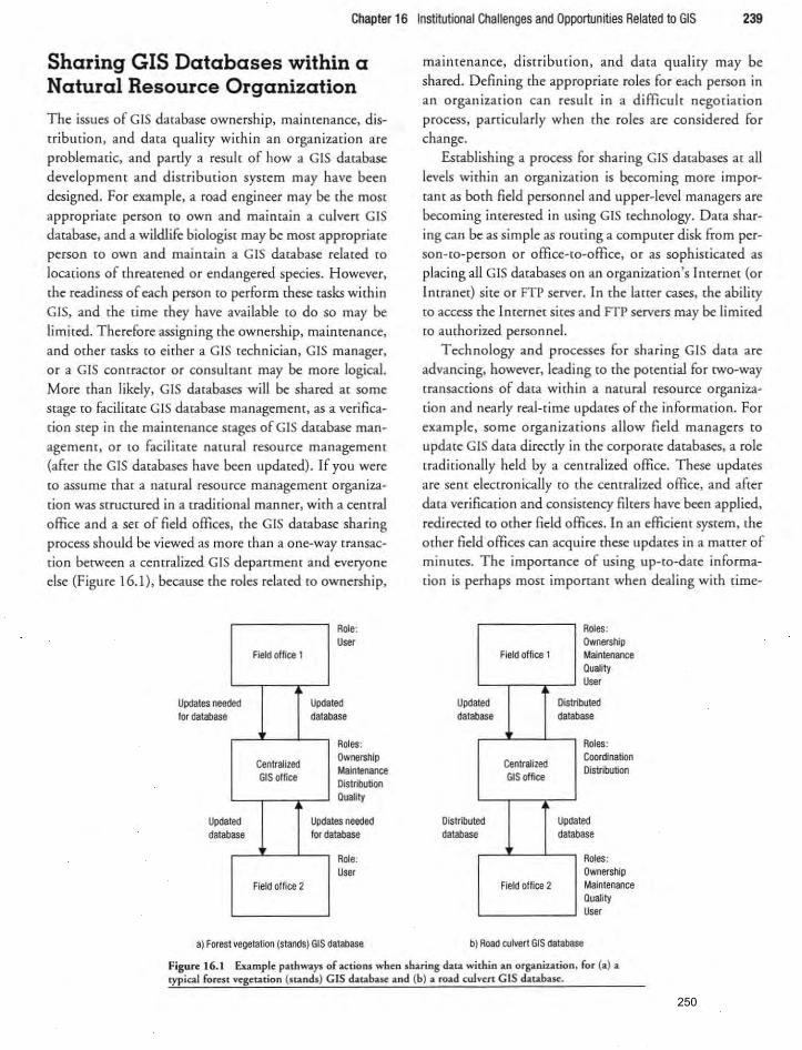
Chapter 16 Institutional Challenges and Opportunities Related to GIS 239
Sharing GIS Databases within a Natural Resource Organization
The issues of GIS database ownership, maintenance, distribution, and data quality within an o rganization are problematic, and partly a result of how a GIS database
development and disuihurion system may have been designed. For example, a road engineer may be the most
appropriate person (0 own and maimain a culverr GIS database, and a wildlife biologist may be most appropriate person to own and maintain a GIS database related to
locations of threatened or endangered species. However, the readiness of each person to perform these tasks within GIS, and the time they have available to do so may be
limited. Therefore ass igning the ownership, maintenance, and mher tasks to either a GIS technician, GIS manager, or a GIS contractor or consuhant may be more logical. More than likely, GIS databases will be shared at some stage to facilitate GIS database management, as a verificacion step in the maintenance stages of GIS database management, or [Q facilitate namral resource managemem
(after the GIS databases have been updated). If you were co assume that a namral resource managemem organizadon was structured in a tradidonal manner, with a cemral
office and a set of field offices, the GIS da tabase sharing process should be viewed as more than a one-way transaction between a cemralized GIS departmem and everyone else (Figure 16.1), because the roles related to ownership,
Updates neede for database
d
I,d Upd, datab as,
Field office 1
Centralized GIS office
Field office 2
Role: Use,
Updat ed as, datab
Updat lorda
Roles : Ownership Maintenance Distribution Ouality
es needed tabas<!
Role: User
a) Forest vegetation (stands) GIS database
maintenance, d istribution, and data quality may be
shared. Defining the appropriate roles for each person in an organ ization can result in a difficult negotiation process, part icularly when the roles are considered for change.
Establishing a process for sharing GIS databases at all levels within an organization is becoming more impor
tant as both field personnel and upper-level managers are becoming interested in using GIS technology. Data sharing can be as simple as routing a com purer d isk from person-to-person or office-to-office, or as sophisticated as placing all GIS databases on an organization's Internet (or Intranet) site or FTPserver. In the laner cases, the ab ili cy
to access the Internet sites and FTPservers may be limited to authorized personnel.
Technology and processes for sha ring GIS data are advancing, however, leading to the potential for two-way transac tions of data within a namraJ resource organization and nearly real-rime updates of the information. For example, some organizations allow field managers [Q
update GIS data directly in the corporate databases, a ro le
tradirionally held by a centralized office. These updates are sent electronically m the centralized office, and after data verification and consistency filrers have been applied,
redi rected to other field offices. In an efficient system, the other field offices can acquire these updaces in a matter of minutes. The importance of using up-m-dare informacion is perhaps most imponant when dealing with rime-
ated Upd database
led Olstribu database
Field office 1
Centralized GIS office
Fjeld office 2
Distri
Rotes : OwnerShip Maintenance Quality User
buted ase datab
Roles: Coordination Distribution
Updal ,d as, d,tab
Roles : Ownership Maintenance Quality User
b) Road culvert GIS database
Figun: 16.1 Example pathWll}'S of actions when sharing data within an orga.niu tion. for (a) a typ ical forest v~getation (stands) GIS database and (b) a road culvert G IS database.
250

240 Part 3 Contemporary Issues in GIS
The following story indicates nor only rhe motivation of field office personnel !O use GIS [<chnology, but also
a residual negative effeer of the abi lity !O share GIS databases with in an organization.
One natural resource managernem organization the authors were famil iar with had a central office where
30- 40 'corporate' GIS databases were mainta ined:
roads, streams, timber scancis, and others. T he organ i
zation had a distributed system. where GIS users in
field offices could access a server and download (copy) rhe GIS darabases !O their field office computers. Field
foreSters, biologiSts, and hydrologisrs subsequently did juSt rhat-rhey copied rhe GIS databases !O rheir personal computers and used [hem fo r a variety of pur
poses related ro rhe management of rhe land. water, wildlife. and recreation resources. Some of these GIS
darabases were even updated with peninenr informa-
sensitive decisions. such as those related [0 wildfire con
trol and suppression. With GIS capabilities now available in hand-held computers, managers in the field can make
more timely and informed decisions when necessary.
Distribution of GIS Capabilities to Field Offices
With rhe development of desktop GIS software the ability of every employee in an organization to use GIS is now
possible. Bettinger (I 999) has noted that the deployment of software and GIS databases to field offices is a significant challenge, and, as nmed in chapter 1 S. that is a trend
that will likely continue. Some of the challenges to naru
ral resource management organizations interested in
imp lemenring a distributed GIS system, as noted by Bettinger (I 999) include:
Where people are concerned • Provide the appropriate training to reduce computer
related anxiety.
• Provide a statemem of purpose behind implementing a distributed system.
• Implement methods to reduce the resistance to
change.
• Provide mmivation ro use the system .
tion that should have been incorporated imo the cor
porate GIS databases. As the d iscussion grew related to
sharing the modified corpo rate GIS databases wirh the
corporate office, it was determ ined that there were
over 1,000 variations of the corporate GIS databases stored across the organization's computer systems.
Each GIS database required Storage space on hard drive
and it was likely that hundreds of megabytes of space were dedicated for th is effort. I n some cases, field personnel believed that their modified version of the cor
porate GIS database was of higher qual ity than other user's versions (even better than the corporate version
of the GIS darabase) . As expected, a number of d iscussions regarding the quality of these mod ified GIS darabases arose, and the process of changing the GIS darabase maintenance policy for the corporate databases
was begun.
Where GIS databases are concerned • Clarify GIS database ownership and mall1tenance
Issues .
• Outl ine data acquisition protocols.
Develop data distribution systems.
• Develop quality control measures.
Where the technology is concerned • Facilitate the acquisition of appropriate hardware and
software.
• Control the purchase, update. and maintenance of
software.
Where the leadership of the organization is concerned • Demonstrate strong suppOrt for the program.
• Make a long-term budgetary commitment to the
program. • Adjust reward systems for added responsibilities of
field managers. • Document the direction and strategic goals for the
system.
Most young profess ionals in natural resource managemem o rganizations will likely be called upon to provide
assistance in the development of maps and GIS databases
to facilitate the day-to-day management of a landscape. 251
Chapter 16 Instrtutiooal Challenges and Opportunrties Related to GIS 241
This is a relatively new job expectation (hat may not ordinarily be placed on [he more seasoned foresters and natural resource professionals. At the onset of a program such
as [his, you should acknowledge [hac i[ adds responsibility [0 [he field manager fo r [he development of his or her own management-related maps. Tasks traditionally per
formed by specialises in a cemralized office will be transferred [0 field offices. This [ransfer of responsibility could lead [0 anxiety on [he parr of field managers, however [he main advantage of the program is in reducing the amount
of time required [0 produce [he produces (maps and analyses) needed CO make management decisions. Once field personnel are sufficiendy rrained and become confident in their abilities. time savings across {he organization should be realized.
Perhaps one of (he most important conuibutions young professionals can make is [Q ask peninem ques
tions about the organization within which they work:
What role do I play in each process [hac involves GIS
databases? How are the GIS databases created or acquired? Who claims ownership ovec the maintenance and disrri p
bu[ion of each GIS database? What [echnology (hardware) is avai lable [0 display [he resul" of an analysis? What [echnology (software) is available [0 perform an analysis? How and when does the organization value GIS analysis
in supporcing management decisions? By asking these questions, you indicate your willingness to understand
how GIS has been implemented within an organization. and imply [hac you understand [hac GIS is a valuable [001 in natural resource management.
Technical and Institutional Challenges
One of the most expensive and time-consuming aspects related [0 using GIS is the effore (hat is required to creatc
a GIS database. Dupl icating previous data collection effores in [he creation of a GIS database should always be avoided, thus a lack of awareness of existing GIS databases
is a serious challenge [0 confront . To prevem duplicating
GIS database development efforts, GIS users within an organization should be made aware of [he types of GIS
databases that the organization can easily access. This
might include GIS database produces [hac were developed internally within an organizadon. GIS databases devel
oped by GIS contractors or land surveyors. or GIS databases that are available through agreements or relationships with other nacural resource management
organizations. Information regarding avai lable GIS data-
bases could be seored in a searchable database or it might be ca[alogued in a less formalized manner. Regardless of how this information is gathered. and stored. personnel in
an organization who use GIS should be able co easily iden[ify and loca[e exiseing GIS databases [hac might facilita[e [he rasks [hac [heir jobs require.
Metadata, or information documenting the specifica[ions and quality oflandscape feacures in a GIS database, have become an important aspect of GIS databases in the
pase decade (Dobson & Durfee, 1999). In order co de[ermine the fitness of a GIS database for a particular use, the
me[ada[a related co me GIS database should be considered. In panicular, when a GIS database is acquired from anomer organization, me me[ada[a should be relied upon co verify [hac [he condition of [he GIS database is what was expected when acqui red. In many instances. however,
little metadata exists to describe the qualities of GIS data
bases. The [wo hypothetical forests used extensively in
this book are prime examples. In faCt, more often than
not you may find [hac GIS databases developed or main[ained by non-federal organizations lack, or have insufficient. metadata. Thus. nacural resource professionals must
be careful when basing decisions on GIS databases where
the level of qualiry is uncertain.
For organizations that are involved in producing and
distributing GIS databases to other natural resource man
agement organizations, guidelines or protocols should be in place that address all aspects related to the distribution of the GIS databases. Without guidel ines. organizations
are likely to be working with an inefficient distribution
syseem, and may be prone co liability problems. Guidelines should include a pricing struccure for all available GIS databases; chis structure will need to reflect the
organization's views on cost recovery. In the case of pub
lic organizations. there may be no need or desire co
recover more than the delivery costs . Some public organ
izarions. however. do utilize contractors to collect and
develop GIS darabases, and may need co recoup some of the COSts of doing so. For most private natural resource
management organizat ions, the pricing struccure w ill
likely need co [eflecr [he accual coses of collecting [he data. Organizations [hat distribute GIS databases will also need co develop a comprehensive liability policy [0 pro[ecr themselves from li[iga[ion. A liability policy will likely need co be [ailored [0 each particular GIS database because the content. accuracy. and uses of databases will vary. A method of providing GIS darabases to cuStomers will also need [0 be identified. As discussed in chapter 15, organizations [hac provide GIS data [0 [he publ ic should make
252
Chapter 16 Inst~utional Challenges and Opportun~les Related to GIS 241
Thls is a relatively new job expectation that may not ordinarily be placed on [he more seasoned foresters and natural resource professionals. At the onset of a program such as this. you should acknowledge that it adds responsibility to the Reid manager for the development of his or her own management-related maps. Tasks tradicionally performed. by specialists in a centralized office will be transferred to Reid offices. This transfer of responsibili ty could lead to anxiety on the part of field managers. however the main advantage of the program is in reducing {he amount of rime required to produce the products (maps and analyses) needed (Q make managemem decisions. Once field personnel are sufficiently trained and become confident in their abilities. time savings across the organizacion should be realized.
Perhaps one of [he most impona.nr contributions young professionals can make is ro ask pertinent quesdons about the organiz.arion within which [hey work: What role do I play in each process thar involves GIS databases? How 3.fe [he GIS databases created or acquired? Who claims ownership over the maintenance and disuibution of each GIS database? What technology (hardware) is avai lable to display the results of an analysis? What technology (software) is available to perform an analysis? How and when does rhe organization value GIS analysis in supporcing management decisions? By asking these questions, you indicate your willingness [0 understand how GIS has been implemenred within an organ izarion, and imply that you understand that GIS is a valuable (001
in narural resource management.
Technical and Institutional Challenges
One of the most expensive and time-consuming aspects related to using GIS is the effon that is required to create a GIS darabase. Duplicating previous data collection efrorts in rhe crearion of a GIS database should always be avoided. thus a lack of awareness of existing GIS databases is a serious chaJlenge to confrom. To prevent duplicating GIS datab.se development efrons. GIS users within an organization should be made aware of the types of GIS databases that (he organization can eas ily access. This might include GIS database products that were developed imernaJly within an organization, GIS databases developed by GIS contractors or land surveyors, or GIS databases that are available through agreements or relationships wiTh other natural resource managemem organizarions. Information regarding avai lable GIS data-
bases could be stored in a searchable database or it might be catalogued in a less formalized manner. Regardless of how ffiis informadon is g:nhered and stored, personnel in an organization who use GIS should be able to easily identifY and locate existing GIS da tabases that might lacilitate the tasks that their jobs require.
Meradara, or informadon documeming [he specifications and quality oflandscape features in a GIS database. have become an important aspect of GIS databases in the past decade (Dobson & Durfee. 1999). In order to derermine the fitness of a GIS database for a particular use. the metadata related to the GIS database should be considered. In particular. when a GIS database is acquired from another organization. the metadata should be relied upon to verifY that the condirion of the GIS database is what was expected when acquired. In many instances, however, Iirde mecadata exises to describe the qualities of GIS databases. The twO hypothetical foresrs used extensively in this book are prime examples. In lact. more often than not you may find that GIS databases developed or maintained by non-federal organizations lack. or have insufficient, mecad:Ha. Thus, natural resource professionals musr be careful when basing decisions on GIS databases where the level of qualiry is uncenain.
For organ izarions that are involved in produci ng and distributing GIS databases [0 orner namral resource management organizations, guidelines or protocols should be in place that address all aspecrs related to the disrriburion of the GIS databases. WithoUt guidelines. organizarions are likely ro be working with an inef-hciem distribution system, and may be prone to liability problems. Guidelines should include a pricing Structure for all avai lable GIS databasesi (his structure will need [0 reAecr [he organization's views on COSt recovery. In me case of publie organizations, {here may be no need or desire to recover more than me delivery costs. Some public organizations, however. do utilize conuacmrs m collecr and develop GIS databases. and may need to recoup some of the coses of doing so. For most private natural resource managemem orga niza tions. rhe pricing srrucrure will likely need to reflect the actual COstS of collecting the dara. O rganizations that distribUte GIS databases will also need to develop a comp rehensive liability policy to protect t11emselves from litigation. A liability policy will likely need to be tailored to each particular GIS database because [he conrent, accuracy. and uses of databases will vary. A method of providing GIS darabases (Q cuStomers will also need [Q be identified. As discussed in chap[er IS, organ izacions that provide GIS data to the public should make
242 Part 3 Contemporary Issues in GIS
GIS databases avai lable in an expedient manner and use cu rrent Internet technologies such as creating new wehsites chat allow users (0 browse darabase offerings and
download both data and metadata. In addition. file transfer protocol (FrP) can be used to make data available. but this data-sharing system is less user-friendly.
For organizations that are nor involved in producing and developing GIS databases for other namrai resource management organizations. the high COSt associated with crearing GIS databases can result in a reluctance [0 share
databases with other organizations. For example. certain GIS databases may contai n sensit ive information. and
might reveal the location of landscape features (such as endangered species nesting locations or archeological sites) that might be disturbed or destroyed should the
locations become public information. Two examples of these GIS databases include the location of endangered species nest sites, and the locacion of genetically-modified [fee field trials. The GIS databases may also comain information about the status oflandscape resources that would be of value to another organization with which it competes, providing the other organization an advantage in the market place. This is clearly importam tOday as the number of land sales has skyrocketed. and potential (a nd
perhaps hostile) investors desire complete information regarding a land asset.
A reluctance on the part of federal public organizations in the US to share or publicize data holdings is that all federal agencies are subject to the Freedom of Information Act (FOIA). FOIA was signed into law in
1966 and later amended in 2002. FOIA makes it possible for individuals (Q request access to federal agency records,
To facilitate a recem landscape analysis research project, a private natural resource managemem organiza
tion agreed to provide a highly detailed GIS database that desc ribed the management units within their
ownership boundaries. The GIS database had been assembled at great COSt and effort, and revealed considerable information abom the natural resources that the private organization managed. The private organization required that a confidentiality agreement be signed prior to making the GIS database available (Q
the research project. As noted in the confidemialicy
except in cases where records are protected from disclosure. These requestS can also be made for spatial databases [hat were produced by federal agencies. In some cases,
spatial databases may comain information that the agency considers to be sensicive or potenrially damaging (Q the resources it manages. One example of sensitive informa
tion might be spatial records of vandalism that occur in public recreation areas. Evidence of high vandalism
occurrence might deter visitors from staying in affected areas, and potemialiy reduce revenue that is gathered from day-use permits. In addition, there may be hesitation to draw additional arremion to 'hot-spotS' of crimi
nal activiry in case the arrenrion may encourage others to
visit these locations our of curiosiry or to cause additional
vandalism. Other hesitations may involve the presence of unusual features, such as special habitat areas, or archeological sites, and the potencial damage that too many visimrs may bring to these areas. For various reasons, federal
agencies may not openly advertise the types of spatial databases that they have produced. A primary hesitation to do so is likely because of the uncertainty of what will happen with the information within the databases should
rhey become widely circulated. Understanding that there are factors that may hinder
an organization's willingness to share a GIS database is
important prior m requesti ng the database. For data of a sensitive nature, it may be possible to enter into a confidentiality agreement to gain access (Q the GIS database. Ultimately, it may be necessary (Q pay a large sum of money ($5.000 to 10.000) for a GIS database. and for
some organizations, it may be difficult m locate the neces
sary budget resources appropriate for this type of purchase.
agreement, access to the GIS database was limited to
the primary scientists of the research project, the sha ring of the GIS database with others was prohibited. and protocols for distribming information drawn from the GIS database were outlined. Without the confidentiality agreement, which facilitated the sharing of the GIS database, knowledge of [he status of resources located within the private natural resource management organization 's ownership would likely have been less accurate, reducing the confidence placed on the landscape analysis results.
253
Chapter 16 Instrtutional Challenges and Opportunities Related to GIS 243
Benefits of Implementing a GIS Program
The decision to implement a GIS program (the entire suite of hardware, software, and personnel related CO the
use of GIS within an organization) can be intimidating for
natural resou rce management organizations. There are
many factors to consider, including investments in soft
ware, hardware, personnel, and CIS databases. Since nat
ural resource management organizations cypically rely on
maps or mapped data to assist in making decisions, GIS
can allow an efficiem storage of maps, and can fac ilitate
the generation of multiple versions of maps in a timely
manner. In addition, GIS allows landscape features to be
measured, analyzed, and integrated with other GIS data
bases in an expedient manner. New technology has pro
vided [he pQ[entiai to convey information [Q field man
agers very quickly. These capabilities, if managed
properly, can allow natural resource management organi
zat ions to make bener management decisions, more accu
rately gauge the effore and cost of potencial namral resource managemem projec(S, and increase the efficiency
of tasks performed by their employees.
Successful GIS Implementation
Saving money, reducing the amount of time spenr in the
office analyzing options. and thus saving resources for Q[her [aSks and management activities are common goals
of namral resource managers. Distributing GIS capabili
ties to field offices has been suggested as one way to
address some of these issues. Successfully implememing
and managing a GIS program can be difficult, as the costs
of implementation and management vary from one
organization to the next. Perhaps the strongest ingredient
for success in implementing a GIS program is in esrablish
ing an organizational commitmenr within the upper lev
els of managemenr of an organization . This commitmenr
needs to view the GIS program as more than JUSt a short
term experimenr that can be discarded after early, d isap
poinring results, since initial GIS products and experi
ences are likely to identify implementation problems.
Unfortunately, upper-level managers tend to be less
Summary
What would the management of natural resources be
like without a few challenges? With the imroduction of
fumiliar with GIS technology than the actual GIS users.
For this reason, GIS users should communicate their sup
porr of GIS in terms that are comp rehensible to the
upper-level managers and help them understand that
when technical difficulties do arise, program implemenra
cion plans must be adjusted. Upper-level managers, in
turn, should promote the G IS program as a way of mak
ing more efficient the tasks required of natural resource
management.
Organizations must also be realistic about the time,
effort, and budgetary resources that individual GIS proj
ects or analyses wi ll require. Proper planning requ ires that
project objectives be clearly defined. Objectives provide a
project mission and ca n help keep personnel focused,
should setbacks occu r. Project objectives a re also impor
tant for establishing standards that allow you to gauge the
success of a GIS project or analys is . Achievement bench
marks are also critical in justifying the continued and
expanded use of GIS within an organization. Allowing
users of GIS to become involved in the planning and
implementation of GIS projects is also importanr, since
they may be among the best qualified to assess whether
GIS can accomplish the appropriate project tasks, which
may lead to an improved level of efficiency in the man
agemenr of natural resources.
Finally, GIS user training is an importanr considera
tion for the success of a GIS program within a natural
resource managemenr organization. Most recenr college
graduates from natural resource programs will likely have
a rudimenrary knowledge of how GIS can ass ist in natural
resou rce management, but will likely lack the level of
experience you gain from using GIS periodically for
actual, on-the-ground, management purposes. To acceler
ate the development of personnel, organizations can pro
vide GIS training inrernaIly, or can allow personnel to
auend cominuing education courses or pursue other
training opportunities. Geospatiai training courses and opportunities appear to be increasing within natural
resource disciplines (Wing & Sessions, 2007). This
investment in continuing education increases the knowl
edge level of personnel and demonstrates an organization 's commitment to its personnel, which hopefully
leads to increases in work efficiency and productiviry.
new computer-related measurement technology and accompanying GIS databases, natural resource manage-
254

244 Part 3 Contemporary Issues in GIS
menr o rganizat ions are facing numerous challenges related to GIS data management. Given that GIS-related technology continues (Q evolve to meet (he increasing
needs of society. an optimistic person might expect that the challenges described in this chapter can be over-
Applications
16.1 Sharing GIS databases with people outside your organization. What issues sho uld a natural resou rce management o rganization address when considering making GIS databases available to other organizations. including perhaps competitors?
16.2 Managing GIS technology. A seaso ned professional (Mary Swarthmore) who manages another department (Accounting) in your natural resource o rganization
is considering a career change. This change will result in Mary managing your organization's GIS department. Mary has never managed a GIS department before, nor
been involved in the creation. acquisition. o r use of GIS databases. She has approached you fo r some advice regarding the tough issues G IS managers face when concerned abom successful implementadon of a GIS program. What might you advise Mary?
16.3 Sharing GIS databases within an organization. You've heard that a colleague in another private natural
References
Bettinger, P. (I999). Distributing GIS capabi lities to fo restry field offices: Benefits and challenges. journal of Fomtry, 97(6), 22-6.
Dobson, J.E., & Durfee, R.C. (I 998). A quarter century of GIS at Oak Ridge National Laboratory. In T.W. Foresman (Ed.), The history of geographic information systems: Perspectives from the pioneers (pp. 231-63). Upper Saddle River, NJ: Prentice-Hall.
Natoli, J.G ., Pelgrin, W.H., Oswald, B. , & Montie, K. (200 1). Geographic Information Systems: The wave of the fmure for information analysis. Public Works, May, 22-9.
come, even as new and va ried issues arise. As we have
noted, many of [he challenges facing the use of GIS within natural resource management organizations are
related to GIS databases, technology, people, and organizational issues .
resource management organization has developed a GIS database that may contain info rmation that could assist you in some part of your job. Under what conditions should you expect your colleague to provide you access to
the GIS database?
16.4 Distributed GIS program. You work for a large integrated forest products company that has a central office and five district offices. The company has been
attempting to shift GIS capabil ities to the field offices by pu rchas ing the appropriate hardware and software resources. and insist ing that field perso nnel (foresters. biologists. managers. and others) use it to make maps associated with their management activities . After twO
years, only one of the five offices has successfully implemented the program.
a) Why do you think the other four offices have been less than successful?
b) Why might the one office have been successfu l?
Puger Sound LiDAR Consortium (PSLC). (2007). Puget Sound Lidar Consortium: Public-domain high-resolution topography for Western Washingron. Retrieved April 23, 2007, from http://pugetsoundlidar.ess.washington. edu/ index.htm.
Wing, M.G., & Bettinger, P. (2003). GIS: An updated primer on a powerful management rool. journal of Forestry, 101(4),4-8.
Wing, M.G., & Sessions, J. (2007). Geospatial technology education. journal of Forestry 105(4), 173-8.
255

Chapter 17
Certification and Licensing
of GIS Users
Objectives
The progressio n of GIS use in natural resource manage
mem has been evolving from development and implementation of systems. to (he distribution of analytical capabilities to field offices, to porting spatial technology into the resource setting. The evolution of GIS can be
viewed from (he perspective of a single organization or
from [he perspective of national or worldwide GIS com
munities. From a global perspective. GIS is facing one of its greatest challenges: mat of implementing certification
and licensing processes to define and recognize 'profes
sio nal' GIS users. In recem years, concerns have been
voiced from the land surveying and engineering communiry regarding the definition of surveying activities and whether GIS practitioners impede upon traditional sur
veying accivities when colleccing o r mapping spatial data
(Gibson, 1999). These concerns have foStered debate among surveyors. engineers. and GIS users regarding the
types of measuremem and analytical activicies that might
be required to competently perform specific accivit ies in
co njunction with the analysis. Thus, in an effon to gain
credibi lity and recognicion among other professions. the
GIS commu ni ty has pondered the issue of cenificatio n
and licensing.
After reading th is chapter and exploring the questions posed in the applications sect ion. students should have
an awareness o f:
1. why certification and licensing of GIS users is being
debated,
2. what organ izations might be relevant in certification
and licensing discussions. and
3. how cenification and licensing issues might affect the
typical GIS user in a natural resource organizacion .
During the last 10 years, one of the primary goals of the GIS comm unity has been to educate other profession
als and the general public about the power and usefulness of GIS beyond its map production capabilities. Many people in natural resource organizations (as wel l as academia)
view GIS only as a map-making tool and may have limited understanding of its analytical power. The American
Society for Photogrammetry and Remote Sensi ng (ASPRS) and the University Consortium for Geographic Information Science (UCGIS) are perhaps the most active groups in educating those who use GIS, as well as the pub
lic, about the capabi lities of GIS. At the ASPRS 2007 Nacional Convemion in Tampa, one AS PRS member was
heard to remark ' If you claim that GIS technology is vital to society you should also promote the need for certifica
tion and licensing among GIS users. ' The UCGIS conducts nadonal meetings rwice a year to identify research and
other act ivi ties that wi ll idencify and promote rhe use of
GIS as a problem-solving tool for society. At a narionai
meeting in June 2000, a member of the UCGIS asked the other delegates. 'Now that everyone seems co know about
GIS , what are we going to do about it ?' These seemingly
innocent observations speak positively about society's growing awareness of GIS while also indicati ng a potent ial
pitfall within natural resou rce managemenr: GIS has been
embraced by natural resource organizations in a way that
256
246 Part 3 Contemporary Issues in GIS
facilitates open use by any professional who might be interested in the technology. Only recently has the GIS community begun co discuss in depth whether professional standards must puc in place to ensure professional
competency for data development. analysis. and other tasks. Given that ocher professions initiated these discus
sions, me leaders and champions of the lise of GIS in nat
ural resource management have found themselves at rimes
in a defensive position when addressing issues related CO
the call for licensing and certification of GIS users. Throughout the US, some professional land surveyors
and engineers have perceived that GIS users were vio lating
state surveying laws when usi ng CPS to coliect spatial
data, and when reponing positional accuracies of collecred measurements. Some of these GPS data collection
activities have actually led to legal disputes, particularly when the collection and mapping of spatial data refercoees land ownership locations. In California, state legis
lation was developed to clarify the activities involving spa
tial data collection (Korte, 1999). These activities full into (wo categories: (1) those that constitute 'land surveying',
and hence require professional licensing, and (2) all other activities, wh ich do not require professional licensing.
Most stares have registration boards mat license and reg
ulate land surveyors and engineers. These boards often
have the ability to interpret existing statutes and laws that
govern the collection and representation of spacial data.
and may also initiate. support. or approve legislation
regarding spatial data collection activities. In addition.
state-level professional land surveying sociecies are active
in promoting or modifYing laws regarding spatial data
collection, and they may occasionally engage political lobbyists to assist in influencing the legislative process.
In contrast to the land surveying and engineering
fields. the GIS community is not direcdy represented or
controlled by a nationally- or state-recognized licensing
board in most cases. There are GIS-related professional
societies at the state or province level but these societies
typically have nOt been in existence for very long. and are
generally nor very active in influencing legislation related to spatial data co llection. The main objective of state-level
and nat iona.l-Ievel GIS societies has been to communicate
information related to the collection. maimenance. and
analysis of GIS databases to inrerested users.
Current Certification Programs
In terms of nationally-recognized GIS certification pro
grams in the US. there are primaril y (wo current options.
The more established and rigo rous of me options is that made by the American Society for Photogrammetty & Remote Sensing (2006). The ASPRS has created a Mapping Scientist certification for GIS users and has also
created certification programs for remote sensing and
photogrammetry. The Mapping Scientist cerrification
requires applicants to develop a statement of accomplish
ments, which are peer-reviewed. and to pass a written
exam. Currently, only about 50 people are certified as Mapping Scientists through the ASPRS. The APSRS has also creared technologist-certifications for GIS, remote
sensing, and photogrammetty. These GIS technologist certifications require less work experience than the
Mapping Scientist and other full certifications (three years as opposed co six) . There are currendy s ix certified
G IS/LIS Technologists. The Urban and Regional Info rmation Systems
Association (URlSA) initiated a GIS professional certification program in 2004 . The GIS Certification Institute
(GISel, 2007) manages the certification program, which results in qual ified applicants becoming recognized as a
certified geographic information systems special ist (GISP).
Three categories of experience must be demonstrated in
order to qualify. The primary experience necessary in
ga ining GISP cert ification is a documented work history
involving GIS and other spatial tools. T he second experience category is an education background that can be sat
isfied by attending conferences and workshops, as well as completing formal education programs or earning certificates. The third category is described as 'contributions'
and includes GIS publications. conference planning or
presentations. and volunteer activities related to GIS.
Ai; of October 2007, there were 1,709 certified GISPs, giving the GISCI program visibility beyond the certification programs of the ASPRS. Although the creation of the GISP certification is noteworthy. the experienced-based
portfolio approach to qualifYing as a GISP lends itSelf to criticism (Longley et aI. , 2005). It remains to be seen whether a certification approach that does not include a
written examination will receive respect and recogn ition
from other professions and disciplines. In addition, there
is no clear method for addressing unprofessional activities
related to GIS, should they occur. Given the emphasis on self-reporting of experience, another issue of discussion is
whether any applicants have been denied GISP status. Many colleges and universities now offer certification
degrees rhat are related to GIS. as well as other spatial data collecrion and analysis rechnologies. however no stan
dards exist for what should be offered in those curricu- 257
246 Part 3 Contemporal'( Issues in GIS
faci li[a[es open use by any professional who might be inreresred in rhe <echnology. Only recently has [he GIS community begun [Q discuss in depth whether professional standards musr put in place (0 ensure professionaJ competency for data development. analysis. and other (asks. Given that o ther profess ions initiated these discus
sions, me leaders and champions o f rhe lise of GIS in nat
uraJ resource managemenr have found themselves at times in a defensive position when addressing issues rdated (0
rhe call for licensing and cerrificarion of GIS users. Throughour rhe US, some professional land surveyors
and engineers have perceived that GIS users were vio lating
scate surveying laws when usi ng GPS [0 collecr spacial
data. and when reporting positional accuracies of col
lecred measurements. Some of these GPS dara collecrion acdviries have acrually led ro legal dispures, parricularly when [he collecrion and mapping of sparial dara references land ownership locado ns. In California, state legis
lation was developed to clarify the accivities involving spa
rial dara collecrion (Korte, 1999). These acriviries fuJI inro [wo caregories: (I) those thar consrim<e ' land surveying', and hence require professional licensing, and (2) all other activ ities. which do nor require professional licensing.
Most states have registration boards (hat license and reg
ulate land surveyors and engineers. These boards often
have rhe abili ty to interprer exis ting starutes and laws that
govern the collection and rcpresemarion of spatial data,
and may also initia te, suppocc, or approve legislat ion
regarding spatial data collection activities. In addition,
state-level professional land surveying societies are active
in promoting or modifying laws regarding spatial dara
collecrion, and they may occasionally engage political lobbyists to assist in influencing the legislative: process.
In contrast to rhe land surveying and engineering
fields, the GIS community is not directly represented or
controlled by a narionally- or state-recognized licensing
board in mosr cases. There are GIS-relared professional societies at the srate o r province level but these societies
typically have nOt been in existence for very long, and are
generally nor very acrive in influencing legislation rdared
to spa rial data collection. The main objective of stare-level
and narional-Ievel GIS socieries has been to communicate
information related to the collection, maintenance, and
analysis of GIS databases (Q interested users.
Current Certification Programs
In terms of nationally-recognized GIS cerr.ification pro
grams in rhe US, there are primarily twO current options.
The more esrablished and rigorous of the oprions is that made by [he American Sociery for Phorogrammerry & Remore Sensing (2006). The ASPRS has crea<ed a Mapping Scientist certification for GIS users and has also
created cen ification programs for remote sensing and
photogram merry. The Mapping Scientisr certification
requires applicants to develop a sratement of accomplish
mems, which are peer-reviewed, and (Q pass a written
exam. Currenrly, only about 50 people are cerrified as Mapping Sciemisrs rhrough rhe ASPRS. The APSRS has also crea red technologist-certifications for GIS, remote
sensing, and phowgrammerry. These GIS rechnologisr certifications require less work experience than the
Mapping Scienrisr and other full certifications (three years as opposed [0 six). There are currently s ix certified
GIS/LIS Technologists. The Urban and Regional Informar ion Sysrems
Associarion (URISA) iniriared a GIS professional certificarion program in 2004. The GIS Certification Innirure (G ISel, 2007) manages rhe cerrification program, which resulrs in qualified applicanrs becoming recognized as a certified geographic informarion sysrems specialisr (GISP). Three categories of experience must ~ demonstrated in
o rder to qualify. The primary experience necessary in
gaining GISP cert ification is a documented work history
involving GIS and orher spa rial rools. The second experience category is an education background (hat can be sat
isfied by arrending conferences and workshops, as well as completing formal education programs o r earning cenifi
cates. The third category is described as 'conuiburio ns'
and includes GIS publications , conference planning or
presentations, and vo lunteer activities related to GIS.
As of October 2007, rhere were 1,709 certified GISPs, giving the GISel program visibiliry beyond [he certificarion programs of rhe ASPRS. Airhough rhe creation of the GISP certification is noteworthy. the experienced-based
portfolio approach ro qualifYing as a GISP lends irself ro criricism (Longley er aI. , 2005). I[ remains ro be seen whether a certification approach rhar does not include a
written examinarion w ill receive respect and recognition
from other profess ions and disciplines. I n addition. there
is no clear merhod. for addressing unprofess ional activicies
reJa<ed to GIS, should [hey occur. Given the emphasis on se lf-reporting of experience, another issue of discussion is
whether any applicants have been denied GISP status.
Many co lleges and universities now offer certification
degrees mar are related ro G IS, as well as other spatial data
collectio n and analysis technologies. however no Stan
dards exist for what should be offered in those curricu-

Besides the current course that you are taking (that
hopefully uses this book), what other GIS courses does your university, college, or community college offer? Although there are many educational instim
tions that offer coursework or curriculum related to
GIS, these programs can look quite different from one instimtion to [he next. At most educacional instim
[io ns, for example, GIS courses are located within the geogra phy department. H owever, special ized GIS cou rses may be found within departments such as
lums. The National Center for Geograph ic Information & Analysis (2000) has produced, and suggested for use, a core curriculum to serve as a foundation fo r studies in GIS. Typically, GIS users can earn a GIS certificate after tWO yea rs of part-time study. While this option does include organized coursework (and perhaps exams to evaluate competency), programs that offer cert ificat ion
degrees lack a recognized set of certification gu idel ines and are generally not accredited by a professional GIS or remote sensing society. As mentioned in chapter 15, the GIS&T Body of Knowledge (DiBiase et aI., 2006) was recently published in o rder to define critical concepts and skills that relate to geographic information science and technology (G IST) . This document was created through the joim efforts of many GIScience researchers and educators, and is an initial attempt to define the skills that you can use to describe geospatial competency. A second edition is intended that will provide detail fo r instructional activities that suppOrt important geospatial concepts and skills.
The NCEES Model Law
The National Council of Examiners for Engineering and Surveying (Ne EES) has developed a set of guidelines described in a Model Law document to help states with licensing issues related co land surveying and engineering (National Council of Examiners for Engineering and Surveyi ng, 2006). The Model Law contai ns reference to GIS activities associated with spacial data collection and use. The Model Law contains 29 sections that are designed to help state boards and other legislative bodies create or amend laws for land surveying and engineering.
Chapter 17 Certification and licensing of GIS Users 247
fishe ries, wildlife, oceanography, forestry , soi ls, rangeland resources, and others. More than likely, GIS courses offered in departments other than geography will provide a different perspective on wha t is
important (Q smdents pursu ing namral resource degrees. If a university or college does not offer courses related co GIS, students can still learn about
the capabilities of GIS through Internet courses, selfstudy of GIS texts, and volunteer wotk with local agencies or government offices.
The fi rst section of the Model Law clarifies the necessity for guidelines by stating that the practices ofland surveying and engineering are a matter of pubic interest. The
decisions made (or recommended) by people employed in these professions can potentially affect the life, health, and property of the general public. Section 2 defines the tasks that are associated with surveying and engineering and no longer refers directly to GIS, as it did in an earl ier version of the Model Law. Section 2 does state that mapping involves the configuration of the Earth's feamres. the subdivision ofland, the location of survey control points, reference points, or property boundaries, and thus people performing 'mapping' are performing the 'Practice of Surveying'. The Model Law suggests that these people should be registered as professional surveyors before engaging in those act ivit ies .
The most d irect pathway co becoming a professional surveyor is to fi rst graduate from an accredited fou r-year college program in engi neering or surveying. Then you must successfully pass an e ight-hour written exam cover
ing surveying fundamentals. Once the fundamentals exam has been successfully passed, four years of surveying experience under the supervision of a licensed surveyor must be accumulated before admittance is allowed to an eight-hour written comprehensive exam covering surveying principles and practice:. Once this comprehensive exam has been successfully passed, and all other state-level requirements are satisfied, you are qualified to become a professiona l land surveyor. Those who grad uate from four-yea r surveying cu rriculums that are not accredited must spend an addirional rwo to four years working in the land survey profession before they can be admitted to the fundamentals exam. T his process of attai ning
258
248 Part 3 Contemporary Issues in GIS
licensing is daunting, and requires a long-term commit
ment on [he pare of poten tial surveyors or others who
w ish to comply with me Model Law. For many cu rrent
natural resource professionals who use GIS. act ive engage
ment in a career combined with family and communiry
commitments offer few realist ic opportunit ies [0 pursue
an engineering degree or to work under the guidance of a
land surveyor.
Earl ier versions of the Model Law definition of surveying that comained direct mention of GIS were criticized as
being (00 stringent and expansive in its descriptio n afG IS
applica tions within surveying activities. Several promi
nent organizations related (0 surveying and GIS co
authored a repan that suggested modifications [0 the Model Law (American Congress on Surveying and
Mapping [ACSM] et aI. , 2001). The report urged the
NeEES to dro p explicit reference to GIS as a data manip
ulation and mapping tool. to refine the definition of sur
veyi ng so that it was less broad, and [0 specifically include
and exclude certain GIS-related accivities in its defini tion
of surveying. The NCEES appears to have acted a( leas t in
parr to these recommendations. Previous to the Model
Law changes. the broader definitions of su rveyi ng created
difficulries for some stares that tried to incorporate the
Model Law's definitions of surveying inco their own state
statutes and regulations (Thurow & Frank, 2001).
The Need for GIS Certification and Licensing
Chief amo ng the argumenr for GIS certifica tio n is an assessment of how GIS activities might impact society's
welfare and safety (Gibson, 1999). The surveying and
engineering professions have long been involved in dete r
mining how best to accurately and precisely collect and
analyze Earrh and structural measurements. Since land
values in North America will likely concinue to increase as
the human population also increases. land areas that are
incorrectly measured can resulr in large monetary losses or
gains for land owners. Knowing the reliabi lity of land
measurements (exp ressed through uncertainty es timates)
will allow land managers ro make bener decisions. While
you may argue that a distinct parr of natural resource data
collection and analytical processes involves quantifying
and expressing the uncertainty that is associated with
those measurements. this quantification is rarely used to rate the reliab ili ty of measu rements collected. Thus the
surveying and engineering professions may be better posi-
tioned to provide information regarding the inherent
uncertainty in land measurements.
Land surveyors are also charged with locating or estab
lishing roads and other utilities such as power lines and
fire hydranrs. Surveyors have argued that it is inappropri
ate for unlicensed surveyo rs to operate CPS equipment for
this purpose since locational errors can potenriaIly affect public safety. In addition, since professional surveyo rs
must absorb the on-going costs associated with maintain
ing licensing and liability insurance, they a re likely to
charge mo re for their services than unlicensed CPS opera
tors. Thus, surveyors have stated that it is unfai r for unli
censed GPS o perators to compete with professional land
surveyo rs in offering these types of d ata collection
servICes. Licensing varies throughout the world and may also
vary by stare o r province. In add ition. it appears that the number of licensed professions is in transicion . In
Canada. professions that require licenses are referred to as
regulated occupations. There are approximately 50 di f
ferenr regulated professio ns in Canada (Government in
Canada, 2007). Within the US, the number of profes
sions thar requ ire a license fo r participario n has been
gradually increasing. Doyle (2007) found that abou(
20 per cem of all professions in rhe US require licensing,
up from abour 5 per cent during the early 1960s. About
50 professions have a regist ration process (hat is recog
nized in all 50 stares. Some people criticize (he licensing
process and claim thar it resulrs in higher prices for serv
ices without an equivalent gai n in the quality of rhe serv
ice or good provided. In additio n. some peo ple see enrry into the profession as being prohibi tively limited once
licensing is in place. While Kle iner (2000) found (hat
incomes from licensed occupations were higher for those
occupations that required more education and training.
faster employment growrh was evidenced in many
licensed professions, such as engineering and law. when
compared to no n-licensed professions. Kle iner (2000)
also reports that empirical evidence addressing whether
licensing results in greater societa l goods. such as increased safety, is currently lacking.
Issues of conrrol and enforcement are additional
aspecrs of licensing and certification . Most stares have
clear definitio ns of what constitutes acceptable surveying
practices. These rules typically cover what clients should
expecr from a professional land surveyor's services, in
terms of producrs. as well as erhical considerations.
Ethical considerarions nOt on ly address the surveyor-
259
248 Part 3 Contemporary Issues in GIS
licensing is daunting, and requires a long-term commit
menr on rhe part of potential surveyors or others who wish to comply with the Model Law. For many current natural resource professionals who use GIS. active engagement in a career combined with family and communiry
commitments offer few realisdc opportuniries to pursue
an engineering degree or to work under rhe guidance of a
land surveyor.
Earlier versions of the Model Law definition of surveying thar contained direct mention of CIS were criticized as
being [00 srringenc and expansive in its description of GIS applications wi thin surveying acrivities. Several prominent organizations related [0 surveying and G1S co
authored a repon that suggested modifications [0 the Model Law (American Congress on Surveying and Mapping [ACSM] et aI., 200 I). The report urged lhe NeEES co drop explicit reference [Q GIS as a data manip
ulation and mapping tool. to refme the definit ion of sur
veying so that i[ was less broad, and ro specifically include and exclude certain GIS-related activities in its definition
or surveying. T he NCEES appears ro have acted a[ leaS[ in pan to these recommendations. Previous to the Model
Law changes, the broader definitions of surveying creared difficulties for some states char tried to incorporate the
Model Law's definitions of surveying into their own state
starutes and regulations (Thurow & Frank, 2001).
The Need for GIS Certification and Licensing
Chief among the argumenr for GIS certification is an
assessment of how GIS activities might impact sociery's
welfare and safery (Gibson, 1999). The surveying and engineering professions have long been involved in deter
mining how best to accllrarcly and precisely collect and
analyze Earth and strucwral measurements. Si nce land
va lues in North America w il i likdy conrinue to increase as
the human popularion also increases, land areas that are
incorrectly measmoo can result in large monetary losses or
gains for land owners. Knowing the reliabiliry of land measurements (expressed through uncertainty estimates)
will allow land managers to make better decisions. While
you may argue that a distinct parr of natural resource data
collection and analytical processes involves quamifying
and expressing the uncertainty that is associated with
those measurements, this quanrification is rarely used to
rate the reliability of measurements collected. Thus the
surveying and engineering professions may be better posi-
tioned to provide information r~garding the inherem
uncertainry in land measurements.
Land surveyors are also charged with Jocaring or estab~
lishing roads and other utilities such as power lines and
fire hydrants. Surveyors have argued [hat it is inappropriate for unlicensed surveyors to operate GPS equipment for
this pu rpose since locational errors can potentially affect
public safery. In addition, since professional surveyors
must absorb rhe on-going costs associated wi th ma i ntain~
ing licensing and liabiliry insurance, they are likely to
charge more fo r their services than unlicensed GPS opera
tors. Thus, surveyors have stated that it is unfair for unl i
censed GPS operaro rs to compere with professional land su rveyors in offering these types of data collection
servIces.
Licensing varies throughout [he world and may also
vary by scate o r province. In addition, it appears that the
number of l icensed professions is in transition . In
Canada, professions mat requ_ire licenses are referred to as
regula red occuparions. There are approxima[e1y 50 different regulated professions in Canada (Govern ment in
Canada, 2007). Within [he US, the number of professions thar require a license for participation has been
gradually increasing. Doyle (2007) found lha[ about 20 per cent of all professions in the US requi re licensing, up from about 5 per cent duri ng the early 1960s. Abou l 50 professions have a registration process that is recog
nized in all 50 srates. Some people criticize the licensing process and claim thal it results in higher prices for services without an equivalent gain in the quality of the serv
ice or good provided. In addition, some people see entry into the profession as being prohibitively limited once
licensing is in place. While Kleiner (2000) found thar incomes from licensed occupations were higher for those
occupations [hat required more education and training,
faster employment growth was evidenced in many
licensed professions, such as engineering and law, when
compared to non-licensed professions. Kleiner (2000) also reports that empirical evidence address ing whether
licensing results in greater societa l goods, such as
increased safety. is currently lacking.
Issues of conrrol and e nforcement are additional
aspects of licensing and certification . Most states have
clea r defi n itions of what constitutes acceptable surveying
pracrices. These ru les rypica lly cover what clients should expect from a profess ional land surveyor's services. in
terms of products. as well as ethical considerations.
Ethical co nsiderations nor only address the surveyor-
client relationsh ip but also offer advice on the professional
relationships that should exist becween surveyors. Most states also have developed a process [0 fac il itate the sub
mirral of complaints against land surveyors. All state licensing boards have the power ro revoke a surveying license if disciplinary infractions occur as a resulr of com
plaines. Th is power encourages most land surveyors [0
become familiar with board rules for professional conduct and [0 adhere to the rules as they engage in survey act ivities. Such rules do not exist in general GIS use in natural resource management.
Crit icism has also been weighed against unlicensed GIS and GPS users due to [he lack of an accredited educational curriculum. Most professions, including forestry and wildlife. have identified an educa[ional and professional background that is necessary for accreditat ion or licensing within their fields. The accred itation process usually suggestS the coursework, minimum competency standards, professional standards, and imegration with other disciplines [hat should be provided to students pursuing degrees in [hose fields (Huxhold. 2002). An accreditation process for G IS could be developed (and perhaps is currently under development). However. the dilemma is thac if you view GIS as a field of study. [he students in [hose cu rricula will graduate with a geography degree. and be considered professional geogra phers. Most natural resource organizations hire biologists, foresters. soils scientists, or other associated professionals. as well as geographers, to assis t in the management of natural resources. These organizations increasingly expect all of thei r personnel to util ize GIS, not JUSt those who have obtained a degree from an accredired geography program.
GIS Community Response to Certification and Licensing
As you might expect. some members of the GIS community have voiced opposition to the suggestion that certa in GIS activit ies be included in the lis t of functions only to
be performed by land surveyors. C riticism has been directed toward the sometimes-broad definitions of land
surveying. and whether GIS databases developed and distributed by public agencies should require management by a licensed surveyor GofFe. 200 1). In addition. some proposals for certificatio n and licensing have also been viewed as exclusionary. and co uld prevenr natural resource professionals from performing the GIS activities that rhey historically performed. Thus the opposirion to
Chapter 17 Certification and Licensing of GIS Users 249
certification and licensing from the natural resource GIS community. largely composed of natural resource managers. bio logists. foresters, and others. is to be expected.
Defining those areas of spatial data collection and mapping that porentially afFecr public welfare and safery is easy in some cases. and challenging in orhers. Clearly. GIS databases used for activ ities such as navigation, locating underground facilities when excavating, or ensuring that property boundaries have been accurately located and used in calcularing land areas. should fall under [he purview of a professio nal land surveyor or enginee r. Activ ities that involve display ing data for illustrative pur
poses, recreatio nal gu ides, or in activit ies that may only affect the person{s) or agency responsible for the associared decision. could perhaps fall ourside [he purview of a professional land surveyor or engineer. Although these examples illustrate distinctions becween activicies chat clearly afFecr public welfare and safery and rhose [har do not, there are many other examples that are less clear and will require furthe r discussion before agreements between the surveying and GIS communities are reached. In cases where mapping products might affect public welfare and safety, several scenarios fo r making map consumers aware of pocenriallimitations have been suggested. Suggestions
include requiring that maps explicicly iden ci fy the source documents, associared metadata, appropriate use of map comenr. and any positional adj usrmenrs Goffe. 2001). Examples of these caveats and disclaimers were introduced in chapter 4. Whether these caveats will continue ro fall short of requiring a certified or licensed G IS professional ro develop the mapping products wi ll likely be an area of discussion.
Finally. and inreresringly. some people have argued that the surveying profession has traditionally not required tra ining in GIS in order to obtain professional surveying cert ification (American Congress on Surveying and Mapping. 1998). For [h is reason. they argue. i[ may not be appropriate fo r land surveyors to manage rhe development. maintenance. and use of GIS databases. However, the current exam syllabi for the national land
surveying exams (borh rhe fundamemal and professional pri nciples and practice) do include GIS and land information systems as potential exam topics .
MAPPS Lawsuit
In June 2006, the Management Associarion for Private Phorogrammerric Surveyors (MAPPS) and rhree other
260
client relationship but also offer advice on the professional relationships chat should exist berween surveyors. Most Sca tes also have developed a process [0 facilitate (he sub
minal of complaincs against land surveyors. All state
licensing boards have the power to revoke a surveying
license if discipl inary infractions occur as a result of com
plainrs. This power encourages most land surveyors to
become familiar with board rules for professiona1 conduct and (Q adhere to the rules as [hey engage in survey activi
ties. Such rules do nor exist in general GIS use in namral
resource management.
Criticism has aJso been weighed agai nst unlicensed
GIS and GPS users due to the lack of an accredi ted educadonal curriculum . Most professions, including forestry
and wildlife, h.ve identified an education. I and professional background [hat is necessary for accredi ta tion or
licensing IlJithin their fields. The accreditation process usu
ally suggests me coursework, minimum competency sran
dards, professional standards, and imegration with other
disciplines that should be provided to students pursuing degrees in those fields (Huxhold, 2002). An accreditation process for GIS could be developed (and perhaps is currently under developmenr). However, me dilemma is rhat
if you view GIS as a field of srudy, the students in those curricula will graduate with a geography degree, and be considered profess ional geographers. Most "amrai
resource organizations hire biologists, foresters, soils sci
entists, or other associated professionals, as well as geogra
phers, to assist in the management of natural resources.
These organizations increasingly expect all of their per
so nnel to ucili1.e GlS. nor just those who have obtained a
degree from an accredited geography program.
GIS Community Response to Certification and Licensing
As you might expect, some members of the GIS community have voiced opposition co the suggestion thar cerrain
GIS activi ries be included in the lis t of funcrions only co
be performed by land surveyors. Criticism has been directed toward the sometimes-broad definitions of land surveying, and whether GIS databases deve.loped and distributed by public agencies should require management by a licensed surveyor Uoffe, 200 1). In addition, some proposals for certifica tion and licens ing have also been
\'iewed as exclusionary. and could prevenr natural
resource professionals from ~rforming the GIS acr iviries
tha t they histor ically performed. Thus the opposition to
Chapter 17 Certffication and Licensing of GIS Users 249
cert ification and licensing from the natural resource G I
communiry, largely composed of narural resource man
agers, biologists. foreseers, and others, is to be expected .
Defining those areas of spatial data collection and
mapping that potentially .ffect public welfure and safety is easy in some cases, and challenging in others. Clearly, GIS databases used for acdviries such as navigation. locat
ing underground Facilities when excavating. or ensuring
that property boundaries have been accurately located and used in calculating land areas, should full under the purview of a professional land surveyor o r engineer.
Acriviries (hat involve displaying data for illustrative pur
poses, recreational gu ides, or in activities [hat may only
.ffect the person{s) or agency responsible for the associated decision, could perhaps fall outside the purview of a professional land surveyor or engineer. Although these examples illusrra te distinct ions between activ it ies [hat
clearly affect public welfare and safety and those that do nor, there are many orher examples rhat are less clear and
will require lUrrher discussion before agreements between
rhe surveying and GIS communities are reached. In cases
where mapping products mighr affect public welfare and safety, several scenarios fo r making map consumers aware
of poremial limitations have been suggested. Suggestions
include requ iring (hat maps explicitly identify me source
documents, associated meradara, appropriate use of map
content, and any positional adjustments Uoffe, 2001). Examples of these caveatS and disclaimers were intro
duced in chapeer 4. Whether these caveats will continue
to fall shon of requiring a certified or licensed GIS professional to develop the mapping products wi ll likely be an area of discussion.
Finally, and interestingly, some people have argued that the surveying profession has traditionally not
required training in GIS in order to obtain professional
surveyi ng cert ification (American Congress on Surveying
and Mapping, 1998). For th is reason, they argue, it may nor be appropriate for land su_rveyors to manage the
developmenr. maimenance. and use of GIS databases.
However, the current exam syllabi fOr rhe narional land
surveying exams (both the fundamental and professional principles and practice) do include GIS and I.nd information systems as poremial exam topics.
MAPPS Lawsuit
In June 2006, rhe Managemenr Associarion for Private
Photogrammetric Surveyors (MAPPS) and three other
250 Part 3 Contemporary Issues in GIS
professional engineering associations filed a lawsu it
against the US government. The lawsuit was fi led on
behalf of the Federal Acquisition Regulation (FAR) Council and is referred to as the MAPPS lawsuit. The actual tide for the lawsuit is MAPPS et at. v. United States
of America. The lawsuit requests changes in interpreta
tion of the 1972 Brooks Act (US Public Law 92-582) which is intended to direct federal government policy in
select ing providers [0 perform architectural. engineering,
and related services. More specifically. the lawsuit seeks
co modify how the selection process for government coo
traccors is evaluated as it relates to mapping activities.
The resulrs of the lawsuit may impact how some US federal agencies award governmenr contracts. The MAPPS
lawsuit has been a considerable concern for many GJS
oriented organizations and has once again fueled the
debate over the definition of activities that can be con
sidered surveying and engineering, which activides influ
ence public welfare and safety, and the appropriate
geospatial certification and licensing requirements. The
participation of prominent organizations on both sides
of the lawsuit is evidence that the MAPPS lawsu it is not
a trivial legal exercise.
Plaintiffs of the MAPPS lawsuit included the American Sociery of Civil Engineers (ASCE). National Sociery of Professional Engineers (NSrE). and Council on Federal Procurement of Architectural and Engineering Services
(COFPAES). The Brooks Act established that price alone should nO( be used in the awarding of government con
tracts to individuals or firms. Instead. Qualificarions
Based Selection (QBS) is to be used. which involves evaluating professional qualifications and experience. in
addition to seeking a 'fair and reasonable' COSt co the gov
ernment, in awa rding contracts. Negotiations for an
acceptable price should begin with the most qualified firm. If negodat ions fail, then negociations should pro
ceed with the second most qualified firm , and so on . The
FAR COllncil applies the rules and laws related to the Brooks Act, and is supposed co ensure that the intentions
of the act are upheld. Although the Brooks Act includes 'surveying and mapping' among the list of architectural and engineering services that it is intended CO cover, fed
eral agencies have not been consistent in their interpreta
cion and adherence to stated protocols. The MAPPS lawsu it seeks to compel the FAR council to more rigorously
interpret and apply the Brooks Act in the select ion of
contractors for surveying and mapping services. In states where licensed surveyors or engi neers are required to per-
form su rveying and mapping activicies. the lawsuit contends that the FAR council should direct that licensed professionals be selected for government cOntracts involv
ing surveying and mapping. The im plications of the MArrs lawsuit are [hen potentially significant given that
many states do nOt draw a clear distinction between sur
veying and mapping in their laws and rules that govern
surveymg. The American Association of Geographers (AAG).
GISCI. Geospatial Information & Technology Association (GITA). VCGIS. and VRISA jointly submitted a briefing to the US District Court in Virginia
(Alexandria Division) that opposed the MAPrs lawsuit (Association of American Geographers. 2007). The brief stated that a successful lawsuit could cause serious con
cern nO( only for the GIS community but also fo r other
related activ ities and professions. Other related activit ies
included GPS data collection, lnrernet mapping, geospa
tial analysis , remote sensing, academic research that
involved mapping, and the broad activities encompassed
within cartography. The briefing claimed that the lawsuit's impact would greatly affect many activities and
industries that involve or rely on mapping activities and
information.
The US District Court ruled against MAPPS in June 2007 and issued a summary judgment in favor of the US Government. The judge in the case stated that the MArps plaintiffs failed to 'establ ish that an injury in fact was suffered by the individual surveyors or their firms'. In order for a case to be tried. a plaintiff (those hling the lawsuit) must establish standing. Standing is indicated by suffering a loss of some sort, be it monetary or otherwise. The
judge found that MAPPS and the other plaintiffS had nOt established sufficienr standing to suppOrt the lawsuir. Alrhough there ate opportunities to appeal the judge's decision, the judge's ruling appears to be strong enough
that an appeal was considered unlikely. There was great uncertainty in determining how a suc
cessful MAPPS lawsuit would have impacted the GIS community and many community members expressed relief
that the lawsuit came to an end. Doubtlessly. there will be similar disputes and uncertainty in the future regarding
licensing that involves (he court system. Although (his
represents a US example of the conAict that has ar isen
with the widespread use of GIS, you could reasonably envision this happening in other countries with an es(ab
lished land records system and regulations rela(ed to engi
neering and land surveying practices.
261
250 Part 3 Contemporary Issues in GIS
professional engineerin g associations filed a lawsuit
aga inst the US governmenr. The lawsuit W<1S filed on behalf of the Federal Acquisirion Regulation (FAR) Council and is referred to as the MAPPS lawsuit. The actual title for tbe lawsuit is MAPPS et al. v. United States of Am(ricft, The lawsuit requests changes in interpretation of the 1972 Brooks Act (US Public Law 92-582) which is intended (0 direct federal government policy in selecti ng providers to perform archi tectural. engineering,
and related serv ices. More specifically, the lawsui t seeks
[0 modify how rhe selection process for government coo
traccors is evaluated as it relates to mapping acriviries.
The resultS of the lawswr may impacr how some US federal agencies award government contractS. The MAPrs lawsuit has been a considerable concern for many GJS
oriented organizations and has once again fueled rhe
debate over the definicion of acdvities that can be con
sidered surveying and engineering, which acriviries inRu
ence public welfare and safery. and the appropriate geospatial cerrificarion and licensing requiremems. The
participation of prominenr o rganizations on both sides
of rhe lawsuit is evidence thal rhe MAPPS lawsui t is nor
a rriviallegal exerc.ise.
Plaintiffs of the MAl'l'S lawsuit included rhe American Sociery of Civil Engineers (ASCE). National Sociery of Professional Engineers (NSPE). and Council on Federal Procurement of Architectural and Engineering Services
(COFPAES). The Brooks Act established that price alone should nO( be used in [he awarding of governmenr con
rracts to individuals o r firms. Instead, Qualificadons
Based Selecrion (QBS) is to be used. which involves evaluating professional qualjficadons and expe rience. in
addirion to seeking a 'fair and reasonable' cosr [0 rhe gov
ernment , in awa rding contracts. Negotiarions for an
acceptable price should begin with the most qualified firm. If negotiations fail , then negoriarions should pro
ceed with the second most qualified firm . and so on . The
FAR Council applies the rules and laws related ro the Brooks Act, and is supposed ro ensure mar the intentions
of rhe acr are upheld. Although rhe Brooks Acr includes 'surveyi ng and mapping' among me list of architectural
and engineering services thar it is intended to cover, fed
eral agencies have nor been cons istent in their interpreta
rion and adherence to stated protocols. The MAl'l'S lawsu it seeks [0 compel the FAR counci l ro more rigorously
inrerpre[ and apply rhe Brooks Act in the selecrion of
contractors for surveying and mapping services. In states
where licensed surveyors or engi neers are required ro per-
form surveying and mapping activicies, the lawsuit con
tends that rhe FAR council should di rect that licensed professionals be selected for government contracts invo lv
ing surveying and mapping. The implicarions of rhe MAPPS lawsuit afe then potentially significanr given thar
many states do nO[ draw a clear distinction berween sur
veying and mapp ing in their laws and rules that govern
surveYing. The American Association of Geographers (MG).
GISCI. Geosparial Information & Technology Associarion (GITA). VCGIS. and VRISA jointly submitted a briefing (0 the US District Court in Virginia
(Alexandria Division) thaL opposed the MAPl'S lawsuit (Association of American Geographers. 2007). The brief stared that a successful lawsuit could cause serious con
cern nm only for rhe GIS commu niry but also fo r mher related act ivities and professions. Other related activities
included GPS data collection, Internet mapping, geospa
tial analysis, remote sensing, academic research that
involved mapping, and the broad activities encompassed
wirhin cartography. The briefi ng claimed thar the lawsuit's impact would greatly affect many activities and
industries that involve or rely on mapping activities and
informacion .
The US Districr Court ruled againsr MAPl'S in June 2007 and issued a su mmary judgment in favor of the US Government. The judge in the case srated that the MAPPS plainrifFs failed to 'establish that an injury in faCt was suffered by rhe individual surveyors or their firms'. In order for a case to be tried. a plaintiff (those filing the lawsuit) must establish standing. Standing is indicared by suffering a loss of some sort, be it monetary or otherwise. The
judge found rhar MAPl'S and the other plaintiffS had nor established sufficienr standing to suppOrt the lawsuit.
Alrhough rhere are opportunities to appeal rhe judge's decision, rhe judge's ruling appears to be strong enough
tllar an appeal was considered unlikely. There was great uncenainry in determining how a suc
cessful MAPl'S lawsuir would have impacted the GIS commun iry and many community members expressed relief
that ti,e lawsuir came ro an end. Doubtlessly. there will be s imilar dispures and uncertainty in the future regarding
licensing that involves the coun system. Although this
represents a US example of the conRicr that has arisen
with the widespread use of GIS. you could reaso nably envision this happening in other counrries with an estab
lished land records system and regulations relared ro engineering and land surveying practices.
Summary
In some circumstances, certification and licensing may be
necessary for those involved in (he developmem and man
agement of GIS databases. to ensure that minimum stan
dards of competency exist and (hat standards 3re being mer in the development. maintenance. and applicacion of
G IS databases. Although many GIS activities related to namral resource managemem may have no bearing on public welfare and safery, some GIS acriviries result in maps or mapped data being sold or made available to the public. and thus may have direct or indirect implicacions on public welfare and safety. GIS has evolved into its own discipline, and is being integrated with other fields of
Applications
17.1. Licensing. Assume that the state or province in
which YOll work is considering the development of a
licensing board to oversee the licensing of GIS users. and
to regulate the use and managemenr of GIS databases
related to your field of namral resource management.
a) What benefits might a licensing board provide for professionals engaged in GIS activities?
b) What disadvantages for GIS users might result from the developmenr of a licensing board?
c) Describe three key dimensions of the licensing
process that the board should develop.
17.2. GIS certification programs. The owners of the Brown Tract have recently become aware that GIS is used
extensively in the management of the fo rese. They are
concerned about the credibility of their land management
team, and have suggested that all employees obtain GIS
certification .
a) What are the potential benefits of GIS certification for GIS users?
b) What are the potential drawbacks of GIS certification for GIS users?
References
Association of American Geographers (MG). (2007) . Amicus Curiae Brief of the Association of American Geographus, GIS Cutification InstituU, Geospatial
Chapter 17 Certification and Licensing of GIS Users 251
study. Guidelines should be developed for determining the experience. educarionaJ background. professional conduct, and cominuing education that defines (he qual ifica
[ions appropriate for those disciplines. Guidelines should
also be developed to define the extent [Q which persons
who are qualified within disciplines can appropriately
develop, manage, and use certain GIS databases. Until a
national certification or licensing program for GIS gains credibility and respect within society, GIS users in namra!
resource fields will find themselves struggling with local or national regularory groups. the legal system, and other
professions for control of GIS activities.
c) What elements would be necessary in order for a GIS certification to be more widely recognized and
respected within society?
17.3. NeEES Mood Law. Does the NeEES Model Law process seem like a reasonable or rational approach to
clarifYing the issue of G IS licensing? Why or why not?
17.4. The need for licensing or certification. Identi fY three GIS or GIS-related activities that could affect public
welfare. and that might suggest that those developing.
maintaining. or using the supporting data should be
licensed or certified.
17.5. GIS community response to certification and
licensing issues. Many professional (foresters. wildlife
biologists. hydrologists. engineers. etc.) working in nat
ural resource management currendy use GIS to ass ist in
making management decisions. Why might they be concerned about the issue of GIS certification and
licensing?
Information 6- Technology Association, University Consortium for Geographic Information Science, and Urban and Regionallnfonnation Systems Association in
262
252 Part 3 Contemporal)' Issues in GIS
opposition to plaintiffs notion for summary judgmt nt. Retrieved on June 6. 2007. from hnp:llwww.aag.org/ Donatellinks.html.
American Congress on Surveying and Mapping (ACSM). (I998). Should surveyors supervise GIS? A CSM
Bulletin. NovemberiDeumber. 26--3 I. American Congress on Surveying and Mapping (ACSM).
American Society of Civil Engineers-Geomatics Division. American Society for Photogrammcrry and Remote Sensing, Management Association for Private Phorogrammecric Surveyors, National Sociery of Professional Surveyors. National States Geograph ic Information Council. & Urban and Regional Information System Association. (2001 ). GIS/LIS addendum to rhe repan of the task Force on the
NCEES Model Law for surveying. Suroeying and Land Infonnation Syswm. 61(1). 24-34.
American Society for PhotOgrammerry & Remote Sensing (ASPRS). 2006. Certification and recertification guidelines for the ASPRS certification program. Bethesda, MD: American Society for Photogrammetry &
Remote Sensing. Retrieved June 7. 2007. from h rtp:l lwww.asprs.org / membership/cenific3rion l certi ficat ion_gu i de lines. h tm I#Certi fied_M a p pin l\Scientist_GIS-LIS.
DiBiase. D .• DeMers. M .• Johnson. A .• Kemp. K .• Luck. A .• Plewe. B .• & Wentz. E. (Eds.). (2006). The geographic information sciena and technology body of knowledge. Washington. DC: University Consortium for Geographic Information Science. Associarion of American Geographers.
Doyle. R. (2007). By the numbers: license to work. Scientific American. February 9. 28.
Gibson . D.W. (1999). Conversion is out. measurement is in-are we beginning the surveying and mapping
era of GIS? Professional SlIroeyor. 19(7). 14- 18. GIS Certification Insritute. (2007) . Are you a GIS practi
tioner or a GIS professional? Retrieved October 5. 2007. from Imp:llwww.gisci.orgl.
Government in Canada. (2007). Types of work. Retrieved October 5. 2007. from hnp:llwww.goingtocanada.gc. calT ypes_oC work_in_ Canada-en.htm.
Huxhold. W.E. (2002). GIS professionals-get a profession! Ceospatial Solutions. 12(2). 58.
Joffe. B.A. (2001). Surveyors and GIS professional reach accord. Suroeying and Land Information Systems. 61(1).
35-6. Kleiner. M. (2000). Occupational Licensing. journal of
Economic Perspectives. 14(4). 189-202. Korte. G .B. (1999) . The current controversy: GIS and
land surveying legislation. Part I . Point of Beginning. 24(6). 70-3.
Longley. P.A .• Goodch ild. M.F .• Magui re. D.J .• & Rhind. D .W . (2005). Ceographic information systems and science (2nd ed.). Ch ichester. England: John Wiley & Sons.
National Council of Examine rs for Engineering and Surveying (NCEES). (2006). Model law. Clemson. SC:
NCEES. National Center for Geographic Information & Analysis
(NCGIA). (2000). The NCGIA core curriculum in GIScience. Sama Barbara. CA: Nationa l Center for Geographic Information & Analysis. Retrieved June 5. 2007. from http://www.ncgia.ucsb.edu/education/ curricula/gisccl.
Thurow. G .• & Frank. S. (200 I). Coming to terms with the Model Law: The search for a definition of surveying in New Mexico. Surveying and Land Information Systems. 61(1).39-43.
263
252 Part 3 Contemporary Issues in GIS
opposition to plaintiffs 11otioll for mmmary jJldgm~llt. Retrieved on June 6, 2007, from Imp:llwww.aag.orgl Donatellinks.html.
American Congress on Surveying and Mapping (ACSM). (t998). Should surveyors supervise GIS? ACSM Bull,tin, NovnnberID,wnber, 26--3 1.
American Congress on Surveying and Mapping (ACSM), American Society of Civil Engineers-Geomatics Division, American Sociery for Photogrammeuy and Remme Sensing, Managemem Association for Private Phocogrammeuic Surveyors, Narional Sociery of Professional Surveyors. National States Geograph ic Information Council, & Urban and Regional Information System Association. (200 1). GIS/LIS addendum CO the report of the task force on the NCEES Model Law for surveying. Surveying and Land Information Sysm"" 61(1), 24-34.
American Society for Phorogrammerry & Remote Sensing (ASPRS). 2006. Certification and reunification guid,lines for Ihe ASPRS certification program. Bethesda, MD: American Sociery for Photogrammerry & Remote Sensing. Retrieved June 7, 2007, from http://www .aspes.o rgl mem beesh i pi cen i ftcat ion I cert i fica t io n_gu idel i nes. h tm I #Certi f1ed_M a p pin &Scientist_G IS-LIS.
DiBiase, D., DeMers, M. , Johnson, A. , Kemp, K., Luck, A., Plewe, B., & Wentz, E. (Eels.). (2006). TIlt gtographic information science and technology body of knowledge. WashingtOn, DC: University Consonium for Geographic Informatio n Science, Associadon of American Geographers.
Doyle, R. (2 007). By [he numbers: license to work. Scientific American, hbruary 9, 28.
Gibson , D.W. (1999) . Conversion is OUt, measurement is in-are we beginning the surveying and mapping
era of GIS? Proftrsional SlIrlltyor, 19(7), 14-18.
GIS Certification Institute. (2007). A" JOu a GIS practitioner or a GIS professional? Retrieved October 5, 2007, from Imp:llwww.gisci.org/.
Government ill Canada. (2007). Types of work. Retrieved October 5, 2007, from Imp:llwww.goingrocanada.gc. carr ypes_oC work_in_ Canada-en.htm.
Huxhold. W.E. (2002). GIS professionals-get a profession! Geospatial Solutions, 12(2),58.
Joffe, B.A. (200 I). Surveyors and GIS professional reach accord. Surveying and Land Information Systems, 6/(1), 35-6.
Kleiner, M. (2000). Occupational Licensing. journal of Economic Perspectives, 14(4), 189-202.
Korte, G.B. (1999). The current controversy: GIS and land surveying legislation, Part 1. Point of Btginning, 24(6), 70-3.
Longley, P.A., Goodchild, M.F ., Maguire, D.J. , & Rhind, D.W. (2005). Geographic information sysmm and scienet (2 nd ed.). Chichester, England : John Wiley & Sons.
National Council of Examiners for Engineering and Surveying (NCEES). (2006). Mod,l law. Clemson, SC: NCEES.
National Center for Geographic Information & Analysis (NCGIA). (2000). The NCGIA core curriwlum in GIScitl1U. Santa Barbara, CA: National Center for Geographic Information & Analysis. Retrieved June 5, 2007, from htrp:llwww.ncgia.ucsb.eclu/educacion/ curricula/gisccl.
Thurow, G ., & Frank, S. (200 I) . Coming [0 terms with the Model Law: The search for a definition of surveying in New Mexico. Survtyillg and Land Infonnation Systems, 61(1),39-43.
Appendix A
GIS Related Terminology
The following represents a brief treatment of [he termi
nology common to all eyp .. of GIS sofcwa re programs and processes. An attempt has been made to avoid [he varia
tions of definitions that rend [0 be more descriptive of [he
processes related to one (or more) particular GIS software
programs. It is important that natural resou rce profes
sionals gain an understanding of a common, generic lan
guage. The lines of communica[ion becween [hose highly versed in GIS and [hose wi[h a cursoey knowledge of GIS need to be clear when making natural resource manage
ment decisions.
Accuracy: The ability of a measuremenr to describe a
landscape feacuce 's [rue locatio n, size, or condition.
Adjacency: A spadal relacionship indicadng which landscape features share boundaries. or are w ith in cenain
discance of other landscape fearures. For example,
adjacency relationships for timber stands may indicare
which stands (Ouch other stands, allowing one to
model green-up requiremems.
Annotation: Text o r strings of characters and numbers
used co describe landscape feamres on a map.
Arc: A single s[[ing of X,Y coordinates (vercices), [hac when connected, form a line. A single line may con
rain many arcs, bur a single arc may only represem one
line. or parr of a line. Arcs have staning and ending
nodes (Q allow analys is of directional travel , such as in
stream systems, where water emers one end of the arc (the starr-node, or 'From-node') and leaves the other end of [he arc (the end node, or 'To-node).
ASCII: American Scandard Code for Informacion lneer-
change. Many eypes of text fi les are commonly referred to as ASCII files; some comain comma-delimited data
(e.g., I , 12, 3.45, 65 .2, 0.45), ochers coneain spacedelimi[ed data (e.g., e.g., I 12 3.45 65.2 0.45), and still others use other delimiters (0 separate individual
pieces of data. See Comma-dtlimited text filt and Space-dtlimited text file.
Attribute: A characteristic of a landscape feacure. A((rihutes can be represented by characters or num
bers (or a combination ofbo[h), and [hey describe various characteristics oflandscape feamres. For example,
the attributes of a timber stand could include the fol
lowing: stand number (or code). basal area, trees per
acre, vo lume per acre, dominam tree species, and so on. The amibmes of a research plo[ (a poine) could include: smdy eype, insta llacio n date, date last remea
sured, dare of nexr remeasure, etc. See Fi~ld.
Azimuth: A degree of a circle, wi[h North being 0° (or 360°), Easc being 90°, South being 180°, and West being 270°.
Azjmuthal project jon: A projeccion system where the
direct ions fro m a centra l point of origin are all
preserved. Bearing: An angle of 90° or less originating from either
[he North or Somh (and direc[ed towards [he Easc or West). Thus an azimuth of 3530 represems a bearing
ofN7°W. Boolean expression: A rype of expression used in a query
o r computer code that requi res a yes or no respo nse. AND, OR, and NOT are the three most common
Boo lean exp ressions. For example, a query us ing a
264
254 Appendix A GIS Related Terminology
Boolean expression could take this form :
stand_age ~ 50 AND land_allocation = 'Even-Aged'
BASIC computer code using a Boolean expression
would look like th is:
If (stand_age ~ 50) AND (land_allocation = 'Even_aged') Then
End if
Buffering (or buffer): A type of spat ial analysis of proxim i[}', where zones of a given distance are generated
around selected landscape feat ures . The result of a
buffering operation is one o r more polygons that rep
resem (he area within a specific distance (fixed. or variable, as defined through an attribute field) around landscape features.
Buffer rone: A set of one or more polygons that represent [he area within a specific distance around landscape
feamces. Cartesian coordinate system: A system that allows one
[Q locate any point on a planar surface divided by a set
of grid lines. Cen: see Grid cell. Character: A single attribute describing a landscape fea
ru re, such as a letter, number, or special symbol. o r a
type of data that indicates the attribute should be considered a piece of text (even though numbers and spe
cial symbols may be val id attributes) . Clipping process: The process of extracting from one
GIS database only those landscape features within the bounds of another GIS database (which could contain a single polygon or a set of polygons) . This is an action that essentially acts like a cookie-currer.
Column: A set of cells in a spreadsheet or database that
are verr ica lly aligned, usually representing a single
anribure of every fearure (reco rd) in the database.
Columns could contain column headers, or terms that
describe the data in the column, or in spreadsheets,
simply be represented by characters such as A, B, C,
etc. Often called ' Fields'; see Field. Related to
'Records'; see Ruord. Combine process: A process of eliminating the shared
edges or intersections between two landscape features. Comma-delimited text file: A text file created in a word
processing system, a text editor, spreadsheet, or database, and saved in a format where commas separate
items. The fo llowing, for example, could indicate
hab itat suitab ili ty index va lues for spec ific timber
stand polygons, with the first item of each line identifying the polygon, and the second item listing the habitat suitability index:
1,0.657 2,0.433 3,0.298
Completeness: A desc ription of the types and extent of landscape fearu res included in a GIS database, and
conversely, those that are omirred.
Conformal projection: A projection system where angles
on the Earth's surface are represented by approxi
mately the same angles on a map. thus the angles related to map fearures are preserved. Therefore. the
scale around any single poinr on a map us ing this pro
jection system is the same in every direction .
Conic projection: A projection system where a cone is
positioned so that it cuts through the Eanh's surface at
one lat irude, and comes Out at another (usua lly the
equator), and mapped features are projected OntO the
cone's surface, based on lines radiating outward from
the center of the Earth. Contour interval: The venica l distance that distingu ishes
neighboring contour lines .
Contour lines: Lines that are connected, and represent
locations of equal elevat ion.
Cy lindrical projection: A project io n system where
mapped features are projected onto a cylinder. then the cylinder is unrolled and the map becomes a planar
surface. Database: A collection of information that is managed
and stored as a single enticy. A spatial database in
cludes information regarding the spatial coordinates
of all of the landscape featu res in the database, as well as information regarding the attributes of each land
scape feature, usua lly in a tabular (spreadsheet) form . Database conversion: The translation of a database from
o ne forma t to ano the r. Fo r example, to conven
ArcView shapefi les to Maplnfo tables would requi re a database conversion.
Datum: A mathematical represenration of the Earth's su r
face fo rmi ng a control surface upon wh ich an ellipsoid
and other location data are referenced.
Destination table: One of twO tables used in a Join operation, the one where the information resides after the join operat ion. In (he case of linking {WO database
tables together, it is the table that is active just before
they are linked. 265
254 Appendix A GIS Related Terminology
Boolean expression could take this fo rm:
stand_age ~ 50 AND land_allocation = 'Even-Aged'
BASIC computer code using a Boolean exp ression
wou ld look like this:
I f (stand_age ~ 50) AN D (land_allocation = ' Even_aged') Then
End if
Buffering (or buffer): A type of spatial analysis of proximity , where zones of a given distance are generated
around selected landscape features . The result of a
buffering operation is one o r more polygons [hat rep~
resem the area within a specific distance (fixed. or v'dri
able, as defined through an amibute field) around la ndscape featu res.
Buffer woe: A set of one o r more polygons that represenT rhe area within a specific distance around landscape
features. Cartesian coordinate system: A system [hat allows one
(Q locate any point on a planar surface divided by a set
of grid lines. Cell: see Grid a ll. Character: A single acrr ibure describing a landscape fea
rure, such as a le[[cr, number, or special symbol, or a
type of data that indicates the amibute should be considered a piece o f text (even though numbers and spe
cial symbols may be valid attributes) . Clipping process: The process of extracting from one
GIS database only those landscape features within the bounds of another GIS database (wh ich could contain a single polygon or a set of polygons) . This is an act ion thal essenrialJy acts like a cookie-currer.
Column: A set of cells in a spreadsheet or database that are vertica lly aligned , usually represeming a s ingle
anribure o f every featu re (record) in the database.
Columns could comain col umn headers, o r terms rhat
describe the data in the column, or in spreadsheers,
s imply be represeIHed by characters such as A, B, C,
etc. Often called ' Fields'; see Field. Related to 'Records'; see Rtcord.
Combine process: A process of eliminating the shared edges or inrersections between rwo landscape features.
Comma-delimited text file: A text me created in a word processing system, a {ext ediror, spreadsheer, o r database, and saved ina formar where commas sepa.rare
irems. The fo llowing, for example, could indicate
habitat suitab ili ty index va lues fo r specific timber stand polygons, with [he firsr item of each line identifying the polygon , and the second item listing the habitat sui tab il ity index:
1,0.657 2,0.433 3,0.298
Completeness: A description of the eypes and extent of landscape features included in a GIS database, and conversely, those that are omitted .
Conformal projection: A projecrion system where angles
o n the Earth's surface are represented by approxi
mately the same angles on a map, thus the angles related to map features are preserved. Therefore. the
scale around any single poinr on a map using this pro
jection system is the same in every direction .
Conic projection: A projection system where a cone is
positioned so that it cutS through the Earth's surface at
one lat itude, and comes o ut at another (usually the
equator) , and mapped features are projected OntO the cone's surface. based o n lines radiating ourward fro m
the cencer of the Earrh.
Contour interval: The verrical distance that distinguishes
neighboring conrour lines.
Contour lines: Lines (hat are connecred. and represent
locat ions o f equal elevation.
Cylindrical projection: A pro jection system where mapped featu res are projected onco a cylinder, then the cylinder is unrolled and the map becomes a planar surface.
Database: A collection of info rmat ion that is managed
and stored as a single entity. A spatial database includes information regarding the spatial coo rdinates of all of the landscape features in the database, as well as information regarding the atuibutes of each land
scape fea ture, usually in a tabular (spreadsheer) form. Database conversion: The translarion of a darabase from
one format to another. For exa mple, to co nvert
ArcView shapefiles to Mapln fa tables would require a database conversion.
Datum: A mathemat ical represenration of the Earth's su r
face forming a control surface upo n which an ellipsoid
and other location data are referenced .
Destination table: One of twO tables used in a Join operation, [he one where [he information resides after che
join operarion. In the case of linking twO darabase rabies together. it is ~e rable [hat is active JUSt before
they are linked.
Digital elevation model (DEM): A GIS database formed offeamres (rypically regularly-spaced as in a grid) [hac contain X.Y as well as Z (elevation) coordinates. Usually i[ represents a [opographic da[abase.
Digital orthophotograph: An image. usually a scanned phocograph. [hac has had removed some of [he displacemenc normally caused during (he aerial phoco
graphic process (tilt. terrain relief) . Digital raster graphics (DRGs): Digi[ally scanned repre
sen[ations of USGS 7.5 Minu<e Series Quadrangle maps.
Digitize (digitizing): To record the X.Y coordina[os of landscape feamres in a compucer file or system as dig
ital data. Digitizing can occur using a digitizing tablet, where maps are raped down, reference points are noted, and featu res (paines, lines, or polygons) are then traced, and their locations in space are known with some level of precision and accuracy. A looser form of digitizing can occur when using the 'heads-up'
technique, where you lise your compuccr's mouse co delineate landscape features on a computer screen, perhaps wi[h a digital orthophocograph as a backdrop. The heads-up cechnique is quicker [han regular digitizing. but usually comes with a COSt reflected in lower
precision or accuracy. or both. Dissolve: To remove the boundaries (arc, lines) between
adjacenc polygons. keying on [he fact [hat some of the polygons have the same value for some 3nrihure. thus [hey should be logically combined.
Dynamic segmentation: A vector data analysis process that cencers on the use of line segments. and attempts to link a nerwork oflines. based on a common attribute, so mat the lines 3re grouped or joined into cate
gories of interest. Easting: A measure of distance east of a coordinate sys
tem 's origin.
Editing: The process of modifying either the spatial shape or location of landscape features, o r the tabular data
that describes the attributes of each landscape feamre.
Elevation contours: Lines that indicate vertical elevation distances. or changes in elevation, across a landscape.
Ellipsoid: A spheroidal figure used co describe the shape of [he Ea"h.
Equal area projection: A projection system where the Earth's features are represented on a map using a constant scaling factor. thus the area of land features is
preserved. Erasing process: The process of extracting from one GIS
database only those landscape features outside the
Appendix A GIS Related Terminology 255
bounds of another GIS da[abase (which could comain a single polygon or a ser of polygons). This is an action that essentially acts like a cookie-cutter with objects outside the cookie-cutter being retained.
Extent: The limits of the locations of all landscape features in a GIS database. Coordinates are used to define the lower-left and upper-right corners of a rectangular area tha[ would include all of the landscape feamres.
Field: As in a[[[ibme field. a column in a tabular da[abase that represents some characteristic of the landscape features in that database. For example. in a polygon database representing timber stands. stand volume. trees per acre, basal area, and dominam species type could all be fields in a [abular database. In an owl location da[abase. a field could be developed co represenc [he firs< sigh[ing. lasc sigh[ing. and number of owls ar certain points on the landscape.
File Transfer Protocol (FTP): A widely used method of transferring data over the Internet, allowing one to transfer computer files to other remote computers, or to download computer fi les from a remore computer.
Fixed-width buffers: Buffers tha[ do no[ vary in size and are applied uniformly co all landscape fea[ures .
Flattening ratio: A ratio used to describe the difference berween the shape of the Earth and a perfecc sphere. described by the relationship (a-b)/a. where a is the equatorial (or semi-major) radius and b is the polar (or semi-minor) radius of [he Earth.
Font: The rype of <ext sryle being used. such as Times New Roman, Arial. or Cour ier. l[ may also represem rypes of symbols commonly used in word processing or graphics programs.
From-node: One of the twO end nodes of a line or arc, the first one of the twO that was digitized. The mher is the to-node.
Geodesy: An area of mathematics that involves determining the precise shape and size of Earth features, as well as positions of features on the Earth's surface.
Geographic Information Science (GIScience) : The identification and study of issues that are related to
GIS use, affect its implementation. and that arise from ics applica[ion (Goodchild. 1992).
Geographic Information System (GIS): A syscem designed to capture, store, edit, manipulate. ana lyze. display, and export data related to geographic features, and includes not only the hardware and software necessary to accomplish these tasks, but also the databases acquired or developed. and the people performing the casks.
266
D igital elevat ion model (DEM): A GIS database formed of fea m res (typically regularly-spaced as in a grid) that contain X.Y as well as Z (elevation) coordinates.
Usually it represents a topographic database. Digital orthophotograph: An image. usually a scanned
photograph. [hat has had removed some of me displacemem normally caused during the aerial photographic process (tilt, terra in relief) .
Digital raster graphics (DRGs) : Digitally scanned representations of USGS 7.5 Minute Series Quadrangle maps.
Digitize (digitizing): To record the X.Y coordinates of landscape features in a compmer file or system as digital data. Digitizing can occur using a digitizing tablet. where maps are raped down. reference points are noted, and feacu res (points. lines, or polygons) are rhen traced . and theif locations in space are known with some level of precision and accuracy. A looser form of digitizing can occur when using the 'heads-up' technique. where you use your compmcr's mouse [Q
delineare landscape feat ures on a com purer screen, perhaps with a digital ormophotograph as a backdrop. The heads-up technique is quicker rhan regular digitizing, but usually comes with a COSt reflected in lower precision or accuracy, or both .
Dissolve: To remove me boundaries (a rc. lines) between adjacenr polygons. keying on the fact that some of the polygons have the same value for some attribme, rhus they should be logically combined.
Dynamic segmentation: A vec[Qr data ana.lysis process that centers 011 the use of line segments, and anempts to link a necwork of lines, based on a common attdb
ute , so that the lines are grouped. or joined into categories of inrerest.
Easting: A measu re of distance east of a coordinate sysrem 's origin.
Editing: The process of modilYing either [he spatial shape or locarion of landscape fearures. or me tabular data ma[ describes the attributes of each landscape fearure.
Elevation contours: Lines that indicate vertical elevation distances. or changes in elevation, across a landscape.
Ellipsoid: A spheroidal figure used ro describe me shape of me Earth.
Equal area projection: A projection system where the Earth's features are represented on a map using a con
scant scaling factor. thus (he area of land features is preserved.
Erasing p rocess: The process of exrracting from one GIS database only those landscape features outside [he
Appendix A GIS Related Terminology 255
bounds of anomer GIS darabase (which could contain a single polygon or a ser of polygons). T his is an action rhat essemiaJly acts like a cookie-curter with objects oucsicle me cookie-cutter being retained.
Extent: The limits of the locations of all landscape features in a GIS database. Coordinates are used [0 define the lower-left and upper-right corners of a rectangular area mat would include all of the landscape fearures.
Field: As in amibure field. a column in a tabular database that represents some characteristic of the landscape features in mat database. For example. in a polygon database representing timber stands, stand volume, trees per acre, basal area, and dominant species type could all be fields in a tabular database. In an owllocation database, a field could be developed to represent the first sighting. last sighting. a.nd number of owls ar certai n points on the landscape.
File T ransfer Protocol (ITP): A widely used memod of transferring data over [he: Internct, allowing one [0
transfer compmer files to orner remote computers, or
[0 download computer fi les fro m a remore computer. Fixed-width buffers: Buffers [hat do nOI vary in size and
are applied uniformly to all landscape fearures. Flattening ratio: A ratio used to describe [he difference
between the shape of [he Earth and a perfect sphere. described by the relationship (a-b) /a. where a is rhe equatorial (or semi-major) radius and b is the polar (or semi-minor) radius of the Earm.
Font: The rype of text style being used. such as Times New Roman, Arial , or Courie r . lr may also represent rypes of symbols commonly used in word processing or graphics programs.
From-node: One of the twO end nodes of a Itne or arc. the first one of the (wo (hat was digitized. The other is the to-node.
Geodesy: An area of mathematics thar involves determ ining the precise shape and size of Earth features. as well as posidons of features on the Earth's surface.
Geographic Information Science (GIScience) : The identification and study of issues that are related to GIS use, affect its implementat ion. and that arise from irs appl ication (Goodchild. 1992).
Geograpb ic Information System (GIS): A system designed to captu re, store, edit, manipulate, analyze.
display. and export data reiated to geograph ic featu res. and includes nor only the hardware and sofTWare necessary to accomplish these tasks. but also the databases acquired or developed. and the people performing the tasks.
256 Appendix A GIS Related Terminology
Geoid: An irregular shape that approximates Earth 's mean sea level perpendicular to the forces of gravity.
Global Positioning System (GPS): A system allowi ng one to locate their position on the Earth's surface by receiving signals from satell ites. The signals are used (Q
calculate a position based on triiarcration. and perhaps differemial correction, processes.
Graticule: The collection of meridians and parallels superimposed on the Earth's surface.
Grid: A geographic database made up of raster features, commonly called grid cells. Can also refer to a graticule.
Grid cell: The smallest unit in a raster database. or pixel.
Usually these are represemed by squaresi however, any regular form that fully covers an area (square. rectangle, triangle, hexagon, polygon, etc.) could be considered a grid cell.
Gross error: Sometimes referred to as human error, it is a blunder or other mistake made somewhere in {he data collection, map creation, or editing processes.
Heads-up digitizing: A method of developing vector GIS
databases (of points, lines, or polygons) where a user
creates landscape features using the com puter's mouse, generally with a rasre r image as a backdrop SO as to draw (or point out) those landscape featu res that are
important. For example, displaying a digital orthophotograph as a backdrop, one might use the computer's mouse to draw roads, or timber stands. This method of dara development is quicker than uaditional digitizing, bur usually less accurate, and does nor require a digitizing table.
Identity process: The acquisition of information within a GIS database concern ing the area represented by another GIS database. Here, like with an intersect process, one GIS database is physically laid onto another, yet the resulting third (new) GIS database is defined by the area of coverage of one of (he input GIS
databases. Intersect process: The acquisition of information con
cerning the overlapping areas of two GIS databases. In uti lizing an intersect p rocess, a third, new GIS database will be created that consists of only those areas where the two original GIS databases overlap, no more, no less.
Intervisibility: A descript ion (from each unit of land's perspective) of the number of viewpo ints that can be seen from a land unit.
Intranet: A network of computers similar to the Internet, except access is limited to a set of authorized people (usually internal to an organ ization).
Join process: A process designed to ei ther (1) associate an external table (wi th no landscape features) to a table of a spatial database using a join item, or (2) to associate
features from one spatial database to another spada) database, using point-in-polygon or nearest neighbor (echniques. When joining tables, the type of join can be a one-to-one join, a one-to-many join, a many-too ne join, or a many-to-few join.
Join item: A field (column) in a tabular database that contains similar information as a field (column) in a
second tabular database. For example, a field in one database may be called 's tand_number' and contain
timber stand numbers, while a field in a second database may be called 'stand' , and again contain timber
stand numbers. While the field names do not have to be the same, the informacion within each field must be similar, such as in this example. where both contain timber stand numbers. The join would then link the
two databases using timber stand number as rhe common element. so data for stand 1234 from one database will be matched with data for stand 1234 in the
second database. Labels: Like annotation, which is text or strings of char
acters and numbers, these are used to describe land
scape features on a map. They usually arise from some anribure field, or column, in the spat ial database's tabular database. where for each landscape feature, a description of that attr ibute (such as srand number,
volume per ac re, trail eype, road eype, etc.) exiscs. Legend: That part of a physical map that contains the
reference informatio n necessary to inrerprer the colors of polygons, and the styles and colors of lines and pOlms.
Line: A str ing ofX,Y coordinares (vertices) that make up a cominuous linear feature. A single line feature (a
road) can comain many small arcs thar are topologically linked at their nodes (end-points), since each arc stans and ends with a node.
Link A line that connects poims, as defined by nodes and vertices (somerimes caIled an arc) .
Link process: A process designed to ei ther assoc iate land
scape features from one database to another database. This process allows the selection and view of landscape features from database, and the inspection of associated (linked) data in the other database. Sometimes called a relate.
Logical consistency: A descrip rion of how well the relat ionships of difFerenr types of data fit together with in a system.
267
256 Appendix A GIS Related Terminology
Geoid: An irregular shape mar approximates Earth's mean sea level perpendicular co the forces of gravicy.
Global Positioning System (GPS): A system allowing
one to locate their position on the Earth's su rface by receiving signals from satellites. T he signals are used to
calculate a posicion based on rrjlarerarion. and perhaps differential correction, processes.
Graticule: The collecrion of meridians and parallels
superimposed on rhe Ea"h's surface. Grid: A geographic database made up of rasrer features,
commonly called grid cells. Can also refer ro a graticule. Grid cell: The smallest unit in a ras ter darabasc. or pixel.
Usually these are represented by squaresi however. any regular fo rm that fully covers an area (square. rectangle, "iangle, hexagon, polygon, erc.) could be considered a grid cell.
Gross error: Sometimes referred [0 as human error, it is a blunder or mher mistake made somewhere in the dara collcedon. map creation, or editing processes.
Heads-up digitizing: A merhod of developing veccor GIS
darabases (of poines, lines, or polygons) where a user
creates landscape features using the com purer's mouse, generally with a raster image as a backdrop so as to draw (or poim our) rhose landscape fearures rhar are
imporram. For example, displaying a digital orrhophotograph as a backdrop, one might use the com purer's mouse to draw roads, or timber stands. T his method of dar a development is quicker than rradirionaJ d.igitiziog, bur usually less accu rate, and does not require a digitizing rable.
Identity process: The acquisition of information within a GIS database concern ing the area represented by another GIS database. Here, like with an incersecc process, one GIS database is physically laid onco anorher, yer rhe resulting ulird (new) GIS database is defined by rhe area of coverage of one of the inpm GIS
darabases.
Intersect process: The acquisition of information concerning rhe overlapping areas of rwo GIS darabases. In
mil iz ing an intersect process, a thi rd. new GIS database wi ll be created chat consists of only those areas wbere the twO original GI databases overlap, no more, no less.
Intervisibility: A descriprion (from each unir of land's perspective) of the number of viewpoints that can be seen from a land unit.
Intranet: A network of compucers similar ro the [nterner, except access is limited to a set of 3urhoriz.ed people (usually inrernal ro an organization).
Join process: A process designed co eirher ( I) associare an exrernal rable (with no landscape feamres) to a rable of a spatial database using a join item, or (2) to associate fearu res from one spatial database to another spatial database. usi ng poinr-in-polygon or nearest neighbor rechniques. When joining ,ables, the 'Ype of join can be a one-repone join. a one-tQ-many join, a manY-(Qone join) or a many-ro-few join .
Join item: A field (column) in a tabular darabase rhar contains similar information as a field (column) in a seco nd tabular database. For example) a field in one database may be called 'stand_number' and contain timber stand numbers, while a field in a second database may be called 'srand', and again contain rimber
srand numbers. While ,he field names do not have to be [he same, the jnformation within each field must be similar, such as in this example. where both contain rimber srand numbers. The join would rhen link rhe
twO databases using timber stand number as the common element. so data for stand 1234 from one darabase will be marched wirh dara for srand 1234 in rhe
second database. Labels: Like annotation) which is text or strings of char
acters and numbers, these are used [Q describe landscape karu res on a map. They usually arise from some anribme field. or column, in rhe spatial database's rabular database. where for each landscape feature. a description of that arrr ibute (such as stand number, volume per acre, trail rype, road eype, etc.) exists.
Legend: TIl.r parr of a physical map thar con rains rhe reference information necessary to interpret [he colors of polygons, and rhe sryles and colors of lines and poims.
Line: A String ofX,Y coordinares (vertices) rhat make up
a cont inuous linear feawre. A si ngle line feature (a road) can contain many small arcs that are ropologically linked ar rheir nodes (end-pointS), since each arc
starts and ends with a node. Linlc A line thar connects poims, as defined by nodes
and vertices (somerimes called an arc). Link process: A process designed [0 eimer assoc iare land
scape features from one database to another database. This process allows the selection and view of landscape feawres from database. and the inspection of associared {linked} dara in rhe other database. Somerimes called a relare.
Logical consistency: A description of how well the relarionships of different 'Ypes of dara fit cogerher wir;,in a system.
Logical operators: The operarors 'and', 'or', and 'not'
that allowing one to develop a complex query without having ro perform several single criterion queries in sequence.
Map scale: T he ratio of map distance £0 ground distance represented on the map. For example, I :250,000 map scale indicates that I un it (inch, perhaps) on a map represents 250,000 units (inches) on the ground represented by the map.
Merge process: A process that creates a single G IS database from a set (or subset) of one or more previouslydeveloped G IS databases. Point, line, and polygon databases can be merged together, however, database types are generally mixed. The resulting merged GIS
database may comain landscape feacures that overlap. Metadata: Data that summarize the characteristics of
databases (or 'data about data). Network: A collection of lines connected via their nodes,
and represeming possible paths from one location to anomer. For example, a stream network would include all of the streams, where the smaller headwater streams
connect to wider streams with more water flow. and so on to rivers, and perhaps the oceans. A road system is another network that is more complex in nacu re. because there may not be a logical Row of traffic from
one road £0 the next. Yet £0 determine optimum paths or alternative roUtes, you would need £0 know which roads connect (Q which orner roads. what types of roads they are, and what restrictions may be placed on them .
Node: One (of two) end-pointS of a line. Northing: A measure of distance nonh of a coordinate
system's origin.
Overlay analysis: The process of analyzing or combining multiple layers of information at one time.
Pan: To slide the viewable image to one side (left, right, up. down, or some combination of these). allowing a view of some portion of the landscape nOt viewable with the previous arrangement. Actively called 'panning,' or 'grabbing' when users are performing this action.
Photogrammetry: T he act of collecting measuremems of landscape features from a image or photograph.
Pixel: The smallest unit in a raster database, or a grid cel l. Formed by combining the twO terms 'picture' and 'element'.
Planar coordinates: X,V coordinates that relate £0. or are positioned on, a planar or horizomal surface.
Plane coordinate system: Rectangular coordinates that reference landscape features as displayed on a flat map of the Earth's surfilce.
Appendix A GIS Related Terminology 257
Point: A single X,Y coordinate that represents a feamre on the landscape (such as a research plot, culvert, owl nest, or spring). These feamres are usually deemed tOO small (by an organization) £0 represent as a line or polygon.
Polygon: A multi-sided, closed spatial object that has an area. Polygons are formed by connecting lines (arcs) until a closed area is formed. They may define the boundaries of timber stands, so ils types, riparian buffers, wildlife habitat, and so on, using a set of logic consistent across the landscape. Squares. triangles, rectangles, and hexagons can be considered polygons. yet the term usually applies to irregularly shaped objects.
Precision: The degree of specificity £0 which a measurement is described. Can also refer to consistency.
Public Land Survey System (PLSS): Established in 1785 by the US Congress as a national system for the measurement and subdividing of public lands. At 24-mile intervals north and south of each baseline, standard parallels are established that extended east and west of the principal meridian. Guide meridians were also established at 24-mile intervals east and west of the principle meridian. The grid of meridians and parallels creates blocks, each nominally 24 miles square.
Townships are created within each block by forming range lines (run ning north and south) and township lines (running easr and west) both at six-mile inter
vals. Each £Ownship is six miles square. Each township is divided into sections, with each section measuring one square mile; there are 36 sections within a £Own
ship. Sections are numbered 1-36 starting at the upper right hand corner of a tOwnship.
Query: To select a subset of landscape features from a la rger set using some selection cri teria. These statementS can include a single piece of logic (stand_age S 40), or multiple pieces of/ogic connected by Boolean operators. For example. suppose you have 10.000 timber stands. and you are interested in those that could be commercially thinned. You could query the GIS
database for those stands of a certa in age, with a query such as (stand_age ~ 30 AND stand_age S 40) . Queries can be rather simple, or quite complex.
Random error: A narural by-product of how one measures and describes landscape featu res. No marter how well maps are developed or data are collected, error will usual ly exist in the representation oflandscape features.
Raster: A data structure based on cells organized in rows and columns. This is a grid-based structure where an entire area is represented by a cell, and a single land-
268
Logical operators: The operarors 'and', 'or', and 'not' rhar allowing one ro develop a complex query wirhour having to perform several single c riterion queries in sequence.
M ap scale: T he ratio of map distance [0 ground disrance
represemed on the map. For example, I :250,000 map scale indicates that I unit (inch, perhaps) on a map represents 250,000 units (inches) on the ground represemed by rhe map.
Merge prOeeM: A process rhat creates a single G IS database from a set (or subset) of one or morc previouslydeveloped GIS databases. Poinr, line, and polygon databases can be merged rogerher. however. database
rypes are generally mixed. The resulting merged GIS dacabase may contain landscape features (hat overlap.
Metadata: Data that summarize the characteristics of databases (or 'data about dara).
Network: A co llection oflines connecred via their nodes,
and representing possible paths from one location to another. For example, a stream ne[Work would include all of the streams, where: the smaller headwater Streams
connect co wider screams with more water Row, and so
on to rivers, and perhaps rhe oceans. A road system is
3.nQ[her network char is more complex in nacu re,
because rhere may not be a logical flow of traffic from one road (Q me next. Yet to determine optimum paths
or alternative routes, you would need to know which
roads connect ro which other roads, what rypes of roads they are, and whar restrictions may be placed on them.
Node: One (of two) end-points of a line. Northing: A measure of diStance norrh of a coordinate
system's origin.
Overlay analysis: The process of analyzing or combining multiple layers of inform ad on at one time.
Pan: To slide rhe viewable image to one side (left, right, up, down. or some combination of these), allowing a
view of some portion of the landscape not viewable wirh the previous arrangement. Actively caHed 'panning,' or 'grabbing' when users are performing (his acrion.
Photogrammetry: The act of collecting mC'.suremenrs of landscape fearures from a image or photograph.
Pixel: The smallest unit in a raSter database, or a grid cel l. Formed by combining the fWO terms 'picture' and
'element' .
Planar coordinates: X,V coordinates that relate co, or are
positioned on, a planar or horizonral surface. Plane coordinate system: Rectangular coordinates that
reference landscape fearures as displayed on a flat map of rhe Earth's surface.
Appendix A GIS Related Terminology 257
Point: A single X,V coordinate that represenrs a feature
on the landscape (such as a research plot, culvert , owl neSt, or spring). These features are usually deemed roo small (by an organization) co represent as a line or
polygon. Polygon: A multi-sided, closed spatial object thar has an
area. Polygons are formed by connecting lines (arcs) u mil a closed area is formed. They may define the boundaries of timber stands, so il s types, riparian buffers, wildlife habitar, and so on, using a set of logic consistent across the landscape. Squares. triangles. rec
tangles, and hexagons can be considered polygons, yer the rerm usually applies to irregularly shaped objects.
Precision: The degree of specificiry to which a measurement is described. Can also refer to consisrency.
Public Land Survey System (PLSS): Established in 1785 by the US Congress as a na<ional system for rhe measurement and subdividing of public lands. At 24-mile intervals north and south of each basel ine, standard pa rallels are established that extended east and west of the principal meridian. Guide meridians were also
established ar 24-mile imervals east and west of the principle meridian. The grid of meridians and parallels creates blocks, each nominally 24 miles square. Townships are creared wirhin each block by forming range lines (running north and sourh) and townsh ip lines (running east and west) both at sLx-mile inrer~
vals. Each township is six miles square. Each township is divided into sections, with each section measuring
one square mile; there are 36 secdons within a town
ship. Secrions are numbered 1-36 sraning at the
upper right hand corner of a township. Query: To selecr a subset of landscape features from a
la rger set using some selection criteria. These state
ments can include a single piece of logic (stand_age $ 40), or multiple pieces of logic connected by Boolean operators. For example, suppose you have 10,000 timber stands, and you are interested in those chat could
be commercially rhinned. You could query rhe GIS
database for those stands of a cenain age. with a query such as (stand_age ~ 30 AND stand_age $ 40). Queries can be ramer simple, or quite. complex.
Random error: A narural by-product of how one measures and describes landscape fearures . No matter how well maps are developed or data are collected, error wiU
usually exist in the representation oflandscape features. Raste r: A data structure based on cells organized in rows
and columns. T his is a grid-based structure where an
entire area is represented by a cell, and a single land-
258 Appendix A GIS Related Terminology
seape fearure (rimber stand. road. research plor) can be represcmed by one or more cell .
Rasterization: The process of converti ng veccoc data to
raster daca. usually by scann ing. Record: Each fearure (poin<. line. or polygon) in a GIS
database is represenred by a record in a tabular data
base. A record is a row in the tabular database, thus each row represems a feamce . Associated with each record arc one or morc fields (columns), which conrain the characrcriscics of each feature.
Region : A data structure that consists of vector features
(lines or polygons). yet allowing overlapping areas. Remotely sensed data: Raster dara acquired by a sensor
(camera, satellite) that is some d istance from the land
scape features being sensed. Root mean square error (RMSE): A measure of the error
between a mapped point and its associated nue ground position. Com mo nly used when assess ing spatial accuracy or digitizi ng a map, RMSE measures the posicional error inherent in the registration points on the hardcopy map.
Satellite imagery: Dara eaprured by a remote sensing device housed in a satellite that is positioned above me Earth's surface. Generally, the data consists of values
representing the relative degree of reflectance of electromagnetic energy in cereain wavelength categories (bands). T he imagery is srored as rasrer dara with a spacial resolution that can range from 1 meter to 1 kilometer.
Scale: The relarionship between a map displayed on a computer screen or printed on a type of media (paper, mylar. ere.). and rhe actual physical dimensions of rhe same area. For example, a township (36 square miles,
or 23.040 acres) drawn on a map where I inch on the paper represents 1 mile on the ground, is displayed at a scale where I inch represenrs 63.360 inches. This scale can rhen be expressed as a fraction (I :63360) or a equ ivalence (l" = I mile).
Scanning: The process of excraccing features from a map
or phorograph and sroring reAeered values generally as a raster database. Line fo llowing and text recognition processes are promising methods for converting analog maps to vector GIS databases.
Secant projection: A projection system where the Earth's surface intersects a map surface in marc than one locat ion.
Selection: A set of one or more landscape features (poinrs. lines. or polygons) from a single GIS darabase. chosen based on a Query or by manual methods
(poin<ing and clicking wirh a com purer mouse). The landscape features selected are usually done so for some reason, perhaps to perform some spacial operation on them (such as buffer some selected screams), or to simply visually inspect those landscape fea tures with
a characteristic ofimerest (such as being curious about where the culverts over 20 years old are located in a
forest). Shaded relief map: A map intended to simulare rhe sun
lir and shaded areas of a landscape when assuming rhar the sun is positioned at some location in the sky.
Slivers: Very small polygons thar resul r during overlay operations (union, identity, intersection) or during clipping or erasing processes. Sometimes these occur when common borders are represented differently,
from separate digitizing processes, and sometimes these occur simply as a result of the spatial process that
was anempred. Slope class : The gradien< of a porrion of a landscape. as
descr ibed by a disriner class (e.g .• 0-10 per een<. 11 - 20 per een<. ere.).
Spaee-delimited text file: A rexr file creared in a word processing system, a text ediror, spreadsheet, or darabase, and saved in a format where items are sepa rated
by blank spaces. The following. for example. could indicate habitat suitability index values for specific timber stand polygons, with the first item of each line identifYing rhe polygon. and rhe second item lisring rhe habitar suitability index:
10.657 20.433 30.298
Spatial database (or data): A database containing some information about an area or landscape, the relacionships among the features in the landscape. and perhaps some tabular or attribute (non-spacial) data abom each feature . T hese databases are usually stored in some known coordi nate system, thus each landscape
feature has one or more spat ial coordinates that defi ne where it exists.
Splitting process: A process of erearing mulriple landscape features from a single landscape feature.
Spurious polygons: Small fractions of polygons ereared as a result of a GIS process.
State plane coordinate system: A coordinate system developed in rhe 1930s by rhe US Coast and Geoderie Survey to create a unique set of planar coordinates for each of rhe 50 United Sures.
269
258 Appendix A GIS Related Terminology
scape feature (timber stand, road, research plOl) can be
represented by one or more cell. Rasterization.: The process of converting veccor data (Q
raster data, usually by scann ing. Record: Each feature (point, line, or polygon) in a GIS
database is represented by a record in a tahu lar data
base. A record is a row in the tabular darabase, thus
each row represents a feacure. Associated with each record are one or more fields (columns), which con
tain (he characteristics of each feature.
Region: A da(3 structure mat consists of vector features
(lines or polygons), yet al lowi ng overlapping areas. Remotely sensed data: Raster data acquired by a sensor
(camera, satellite) that is some distance from the land
scape fearures being sensed. Root mean square error (RMSE): A measure of the error
berween a mapped point and its associated true
ground position. Common ly used when assess ing spacial accuracy or digitizing a map. RMSE measu res d1C
posicional error inherent in the registration poims on
the hardcopy map. SateUite imagery: Data capru red by a remote- sensing
device housed in a satell ite that is positioned above me
Earth's surfuce. Generally, the data consists of values
represeming the relative degree of reAecrance of electromagnetic energy in cenain wavelength categories
(bands). T he imagery is stored as raster data with a spatial resoludon that can range from I meter to I
kilometer.
Scale: The relationsh ip between a map displayed on a
computer screen or primed on a rype of media (paper, mylar, etc.), and the actual physical dimensions of tbe same area. For example, a township (36 square miles ,
or 23,040 acres) drawn on a map where I inch on the paper represems I mile on the ground, is displayed at a scale where I inch represems 63,360 inches. This scale can then be expressed as a fraction (I :63360) or a equivalence (i" = I mile).
Scanning: The process of extracting features from a map
or photograph and storing reAccted values generally as a raster database. Line following and text recognition
processes are promising melhods fo r convening analog maps to vec(Qr GIS databases.
Secant projection: A projection system where the Earth 's surface intersects a map surface in mo re (han one locat ion.
Selection: A set of one o r more landscape fearures (poims, lines, or polygo ns) fro m a single GIS database,
chosen based on a Query or by manual methods
(pointing and clicking with a computer mouse). The landscape features selected are usually done so for some reason, perhaps (0 perform some spatia] opera
tion on them (such as buffer some selected srreams). or
to simply visually inspect those landscape features with
a characteristic of interest (such as being curious about
where the culvens over 20 years old are located in a
fores t). Sbaded relief map: A map intended to sim ulate the slln
li t aod shaded areas of a landscape when assuming thaT the su n is posidoned at some location in the sky.
Slivers: Very small polygons that result during overlay operations (u nion , identi ty. incersecdon) or during
clipping or erasing processes. Sometimes these occur
when common borders are represented differendy,
from sepa rate digitiz ing processes, and sometimes
these occur simply as a result of the spatial process that was attempted.
Slope class: The gradienr of a port ion of a landscape, as described by a distinct class (e.g. , 0-10 per cent, 11 - 20 per cent, etc.).
Space-delimited text file: A text file created in a word processing system, a text edirar, spreadsheet , or data
base, and saved in a format where items are separated
by blank spaces. The fo llowing, for exampl e, could indicate hab irat su i(abili ry index vaJ ues fo r speci fic
timber stand polygons, with the first hem of each line
identifying the polygon, and the second irem listing the habitat suitabil ity index:
10.657 20.433 30.298
Spatial database (or data) : A database containing some information about an area or landscape, the relation
ships among the features in the landscape, and perhaps some tabular or attribute (non-spatial) data about each fea mre. These databases are usually stored in
some known coordinate system, thus each landscape
feature has one or more spat ial coordinates [hat define
where it exists .
Splitting process: A process of creating mult iple landscape features from a single landscape feature.
Spurious polygons: Small fractions of polygons created as a result of a GIS process.
State plane coordinate system: A coordina te system
developed in the 1930s by the US Coast and Geodetic Survey to creare a unique sel of planar coordi nates for
each of the 50 United States.
,
Systematic error: Sometimes referred [0 as instcumencal
error, it is propagated by problems in the processes and [Ools used (0 measure spatial locations or other attribute data.
Tabular data: The data in a GIS database that describe the attributes of each landscape feature. Usually displayed as rows (records) and columns (fields), where each row represents a landscape fearure, and each column repre
sents an attribute of that feature. When displayed, a tabular database often looks as if it is in a spreadsheet.
Tangent projection: A projection system where the Earth's surface (Ouches a map surface at one location
(a tangent). To-node: One of the [wo end nodes of a line or are, the
last one of the twO that was digitized. The other is the from-node.
Topology: An exp ression of the spatial relat ionships among landscape features in a GIS database.
Triangular irregular network (TIN) : A vecto r data model that descri bes the landscape using triangles. Each corner of each triangle is described by a set of values, such as elevation, aspect, and coordinates.
Unjon process: The acquisition of information within
twO GIS databases concerni ng the area represenced by both GIS databases. Here, like with an incersect process, one GIS database is physically laid onto another, yet the resulting th ird (new) GIS database is defined by the area represented by both of the input GIS databases.
Universal Transverse Mercator (lJfM) : The most common coordinate system used in the US, which divides the Eanh into 60 venical zones, each w ne covering 6° oflongitude. The zones are numbered 1- 60 staning at 180· longitude (the international date line) and proceeding eastward.
Update interval: The period of time between the performance of subsequenc update processes on a GIS database.
Update process: The methods used to maintain the cur
rent Status and description of landscape features contained in GIS databases.
References
Goodchild, M.F. 1992. Geographical information science. Internationaljournal o/Geographical information
Spurns. 6(1):31-45.
Appendix A GIS Related Terminology 259
Variable-widtb buffers: Bu ffe rs that vary in size based on some anribu te of the landscape features being buffered.
Vector: A data structure commonly used to represent points, lines, or polygons. This is a coordinate-based structure (nor a regular grid), which may not enrirely fill an area, and each landscape featu re is represented by X,Y coordinate pairs. Attributes can be associated with each feature (point, line, or polygon).
Vectorization: The process of converting rasrer data to vectOr data.
Verification process: The processes that one would use
to find landscape features or attributes requi ring ed iting. With a verificat ion process, the goal is to ensure that a particular set of data is appropriate (or reasonable, or within some standard)
Vertex (Vertices pl.): One of a set ofX,Y coordinates that delineate an arc or line.
Viewshed analysis: The process of understanding the pan ions of a landscape visible from specific landscape features of interest.
X, Y coordinates: A set of values [hat represent a pain[ in
space, relative to the coordinate system be ing employed. A single X,Y coordinate could represent a point featu re. Lines (arcs) are characterized by a series of X,Y coordinates. Polygons are formed by a collection ofl ines (arcs), thus have many X,Y coordinates to
define their shape and posi tion on a landscape. Z coordinate: A th ird value associated with an X,Y coor
dinate usually indicating the elevation of the paine in space above some reference (such as mean sea level) . X,Y coordinates do not necessarily need to have a Z coo rdinate to be usefu l, whereas Z coordinates need their X,Y associates to be of use.
Zoom: To focus more closely on a smaHer or larger area of a spatial database, or to enlarge or make smaller an area of a spatial database, showing more or less detail. Zoom-in refers to focusing more closely on a portion of a spatial database. Zoom-out refers to focusing less closely on a portion of a spatial database.
270

Appendix B
GIS Related Professional
Organizations and Journals Compi/.d by Rongxia (Tiffany) Li
The following is a list of GIS-related professional organization and peer-reviewed journals. We apologize in advance for any om issions. and will gladly add any other o rganizations or journals to the list as they are brought (0
our attention.
Organizations
American Association for Geodecic Surveying. 6 Mont
gomery Village Avenue . Suire #403 Gaithersburg. MD 20879 USA. (h ttp://www.aagsmo.org/)
American Association of Geographers. 1710 Sixteenth Street NW. Washington. DC 20009-3 198 USA. (http: //www.aag.org)
American Congress on Surveying and Mapping. 6 Montgomery Village Avenue. Suite #403 Gaithersburg. MD 20879 USA. (http://www.acsm.net/)
American Geophysical Union. 2000 Florida Avenue NW. Washington. DC 20009-1277 USA. (http:// www.agu.orgl)
American Plan ning Association. 122 S. Michigan Ave.,
Suite 1600 Chicago. IL 60603 I 1776 Massachuserrs Ave .• NW. Washington. DC 20036-1904 USA. (http://www.planning.orgl)
American Society of Landscape Architects. 636 Eye Sueet. NW. Washington. DC 20001-3736 USA. (http: //www.asla.orgl)
American Sociery for Phomgrammercy & Remote
Sensing. 5410 Grosvenor Lane. Suite 210. Bethesda. MD 20814-2160 USA. (http://www.asprs.orgl)
Association of American Geographers. 17 10 16th Street. NW. Washington. DC 20009-3198 USA (http:// www.aag.org/)
British Cartographic Society. BCS Administration. 12 Elworthy Drive. Wellington. Somerset. T A21 9AT. England. UK. (http://www.cartography.org.ukl)
Canadian Association of Geographers. McGill University. Burnside Hall 805 Sherbrooke Sr. West. Room 425. Montreal. Quebec. Canada H3A 2K6 (http://www. cag-acg.ca/en/)
Cartography and Geographic Information Society. 6 Montgomery Village Avenue. Suite #403 Gaithersburg. MD 20879 USA. (http://www.carrogis.orgl)
Geographic and Land Information Society. 6 Montgomery Village Avenue. Suite #403 Gaithersburg. MD 20879 USA. (http://www.glismo.orgl)
Geographical Society of New South Wales. PO Box 162 Ryde NSW 1680. Australia. (http://www.gsnsw.org.aul)
Geosparial Information and Technology Association. 14456 East Evans Avenue. Au rora. CO 80014 USA. (http://www. gita.orgl)
Management Association for Private Photogrammetric Surveyors. 1760 Reston Parkway. Suite 515. Reston. VA 20190 USA. (http://www. mapps.orgl)
271
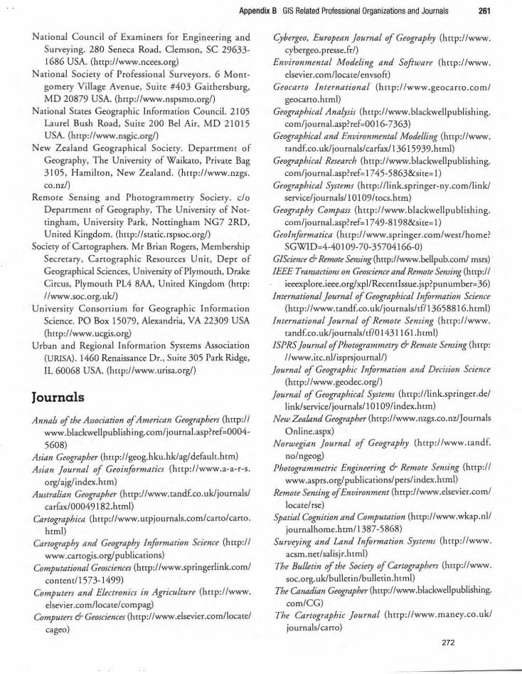
Appendix B GIS Related Professional Organizations and Journals 261
Narional Council of Examiners for Enginee ring and
Surveying. 280 Seneca Road. Clemson. SC 29633-1686 USA. (Imp://www.ncees.org)
National Society of Professional Surveyors . 6 Montgomery Village Avenue. Suite #403 Gaithersburg. MD 20879 USA. (http://www.nspsmo.orgi)
National States Geographic Information Council. 2105 Laurel Bush Road . Suite 200 Bel Air. MD 21015 USA. (http: //www. nsgic.orgl)
New Zealand Geographical Sociery. Department of Geography. The Universiry of Waikaro. Private Bag 3105. Hamilton. New Zealand. (http ://www.nzgs. co.nzl)
Remore Sensing and Phocogrammerry Sociery. c/o Department of Geography. The Universiry of Nottingham. University Park. Nottingham NG7 2RD. United Ki ngdom. (http://static.rspsoc.orgi)
Society of Cartographers. Mr Brian Rogers. Membership Secretary. Canographic Resources Unit, Depr of
Geographical Sciences. University of Plymouth. Drake Circus. Plymouth PL4 8AA. Uni ted Kingdom (http: //www.soc.org.uki)
University Consonium for Geographic Informacion Science. PO Box 15079. Alexandria. VA 22309 USA (http://www.ucgis.org)
Urban and Regional Information Systems Associacion (URlSA) . 1460 Renaissance Dr .• Suite 305 Park Ridge. IL 60068 USA. (http://www.urisa.orgi)
Journals
Annals of th. Association of Am"ican Ceographers (http:// www.blackwellpublishing.com/journaLasp?ref=0004-
5608) Asian Ceograph" (http: //geog.hku.hklag/default.htm) Asian Journal of Ceoinformatics (http ://www.a-a-r-s.
org/ajglindex.htm) Australian C.ographer (http://www.tandf.co.ukljournals/
carfax/00049182.html) Cartographica (http://www.utpjournals.com/carto/carto.
htm1) Cartography and C.ography Information Science (http://
www.cartogis.org/publications) Computational Ceosciences (http://www.springerlink.com/
content/ 1573- 1499) Computm and Electronics in Agricultur< (http ://www.
e1sevier.comlloC3te/compag) Computers 6- GloscilllUS (h [{p: //www.e1sevier.com/loca(e/
cageo)
Cybergeo. European Journal of Ceography (http: //www. cybergeo.presse.fr/)
Environmental Modeling and Softwar< (http ://www. e1sevier.com/loC3(e/envsoft)
Geocarto International (hnp:llwww .geocarro.com/ geocarto.html)
Ceographical Analysis (Imp://www.blackwellpublishing. com/journaLasp?ref=OO 16-7363)
Ceographical and Environmental Modelling (http://www. tandf.co.uk/journals/carfax/13615939.html)
Ceographical Research (Imp://www.blackwellpublishing. com/journaJ.asp?ref= 1745-5863&Site= 1)
Ceographical Systems (http://link.springer-ny.comllink/ service/journals/l 0 1 09Irocs.htm)
Ceography Compass (http://www.blackwellpublishing. com/journaLasp?ref= 1749-8198&site= I)
Ceol nformatica (http ://www.springer.com/west/home? SGWID=4-40 1 09-70-35704166-0)
CIScimce 6-Remote Sensing (http://www.bellpub.com/mses) IEEE Transactions on Ceoscience and Remote Sensing (http://
ieeexplore. ieee.org/xpIiRecenrlssue.jsp?punumber=36) International Journal of GeographicaL Information Science
(http: //www.tandf.co.ukljournalsIrf/13658816.html) International Journal of R.mot( Sensing (http: //www.
tandf.co.ukljournalslrf/O 1431 161.html) ISPRS Journal of Photo gramme try 6- Remote Sensing (http:
Ilwww.itc.nl/isprsjournall) Journal of C.ographic Information and Decision Sci",ce
(http://www .geodec.org/) Journal of Ceographical Systems (http://link.springer.de/
linklservice/journals/l 0 1 09/index.htm) New Zealand C.ographer (http://www.nzgs.co.nzlJournals
Online.aspx) Norwegian Journal of CfOgraphy (http: //www.tandf.
no/ngeog) Photogrammetric Engineering 6- Remote Sensing (http://
www.asprs.org/publicat ions/pers/index.html) Remote Slnsing of Environment (hnp://Wr.vw.clsevier.com/
locate/rse) Spatial Cognition and Computation (http://www.wkap.nl/
journalhome.htm/1387-5868) Surveying and Land Information Systems (http://www.
acsm.net/salisjr.html) The Bulktin of the Soci.ty of Cartographm (http: //www.
soc.org.uklbulletin /bulletin.html) Th. Canadian Ceographer (http://www.blackwellpublishing.
com/CG) The Cartographic Journal (http: //www.maney.co .uk/
journals/carm)
272

262 Appendix B GIS Related Professional Organizations and Journals
The Proftssional Ceographa (http://www.blackwell publishing.com/PG)
Transactions in CIS (http://www.blackwellpublish ing. com/journalsltgis)
Transactions of the fnstitllU of British Ceographers (hnp: Ilwww.blackwellpliblishing.com/journaLasp? ref= 0020-2754&si[<= I)
URISA Journal (http://www.urisa.org/urisajournal)
273
262 Appendix B GIS Related Professional Organizations and Journals
The Proftssiollal Geographtr Omp: llwww.b lackwell publishing.com/PG)
Transactions in GIS (hcrp:llwww.blackwellpublishing. com/journalsitgisl
Transactions of the Imti"''' of BritiJh Geographm (h((p: Ilwww .blackwellpliblishing.com/journal. asp? ref= 0020-2754&si,e= I l
URISA lo.mal (http://www.urisa.org/urisajournal)
Appendix C
GIS Software Developers Compiled by Rongxia (Tiffany) Li
The following is a list of organizacions-governmemal. university, and private-that develop and distribute GIS
related software programs. Included are many of the com
mon GIS software programs as well as contact informa
rion (e.g .• website addresses) for each, however. the list is
not exhaustive. In most cases, GIS software programs
must be purchased either from the developers, or from software diStributOrs, who are nor listed below. Sales representatives associated with (he developers may be able to
direct you to a loeru software distributor. We apologize in
advanee for any omissions, and wiil gladly add any other products to [he list as (hey are brought to our atremian.
GIS Software Program, Distributor, and Website
ArcGIS(Environmental Systems Research Institute, Inc.
[ESRI], 380 New York Street, Redlands, CA 92373-8100 USA) http: //www.esri.eom
Arclnfo (Environmental Systems Research Institute, Inc. [ESRI1 , 380 New York Street, Redlands, CA 92373-8100 USA) http://www.esri .com
ArcYiew (Environmental Systems Research insricuce, Inc.
[ESRI], 380 New York Street, Redlands, CA 92373-8100 USA) http://www.esri.com
ATLAS (Environmental Systems Research Insricute, Inc.
[ESRI], 380 New York Sueet, Redlands, CA 92373-8100 USA) http://www.esri.com
Auro CAD (Aurodesk Media & Emertainmem, Mumbai, 400052, India) http://www.aurodesk.com
ERDAS Imagine (Leica Geosystems Geosparial Imaging, 5051 Peachtree Corners Circle Norcross, GA 30092-2500 USA) http://gi.leica-geosystems.com/LGISubl x33xO.aspx
Geomatica (PC! Geomatics, 50 West Wi lmot Street, Richmond Hill, Omario, Canada, L4B IM5) http: //
. . www.pclgeomancs.com
GeoMedia (lntergraph Corporation, Huntsville, AL 35894 USA) http://www.intergraph.com
GRASS (Geographic Resources Analysis Supporr System) http://grass. i tc.i t
IORISI (Clark Labs, Clark University, 950 Main Street, Worcester, MA 0 I G I 0-1477 USA) hrrp:/Iwww. c1arklabs.org
ILWIS (lmernarional Institute for Geo-Information Science and Earrh Observation, [lTC], 7500 AA Enschede, The Netherlands) http://www.itc.nllilwis/
Manifold System GIS (Manifold Net Ltd., 1945 North Carson Street, Suite 700, Carson City, NY 89701 USA) http://www.manifold.net
Map Info (MapInfo Corporation, One Global View, T roy, NY 12 180-8399 USA) http: //www.map info. com
MGE Products (lmergraph Corporation, 170 Graphics Drive, Madison , AL 35758 USA) hrrp:/Iwww. inrergraph.com
SuperMap GIS (SuperMap GIS Technologies, Inc., 7th Floor, Tower B, Technology Fonune Center, Xueqing Road, Haidian District, Beijing, China, 100085) h[tp: llwww.supermap.com
274
Index
accred itation, 234, 249 accuracy. 9-10; relative, 9 adjacency, 45 Albers' equal area projection, 34
allocation distance function, 214
American Society for Phomgrammerry and Remote
Sensing (ASPRS), 245--{j analysis mask, 214 annotat ion , map. 76 arc: overlay process and, 171; vecroc
data and, 46 ArcGIS, 6--7, 8, 213, 219-20 Arisrode, 28 association: databases and. 144-56 attribure, 38, 49; definition of, 93;
editing, 60-1; errors in, 65--{j; selecti ng, 90-9; updating, 167
AVIRlS,229 axis, 30-1 azimuth, 200-1 azimuchal map projection. 32-4
baseline, 37 bearing, 20 I Bernard, A.M., and Prisley, S.P., 23 Berthier, Louis-Alexandre, 5 Bettinger, P., 237, 240 Boisrad, P., et al., 19 bounds, 36--7 Brooks Act, 250 buffering, 92, 106, 119-31;
concentric rings and, 125-6;
constam/fixed width, 121, 123, 125; individual , 121-2; out pur of, 127; overlapping, 121-2,124,126,137; uncontinguous/non-
concinguous, 121-2; variable width, 121, 123-4, 125
buffer zone, 119
cameras, 11 , 13-14 Canada Geographic Information
Sysrem (CGIS), 6 Canada Land Inventory, 186--7 Cartesian coordinate system, 30-1
canograms, 84 cartography, 3-4, 5, 72; com purer,
3-4, 5; see also maps Cary, T., 234 catchmems,208-10 caveats: maps and, 79-80 cells; see grid ce lls Census Bureau (US), 5--{j Cemral Imelligence Agency (CIA), 5 centroid, 222
certification, 245-52 Clarke Ellipsoid, 30 classification, land, 185-8 clipping process, 106--14 color: DEMs and, 197-8; maps and
77-8,81-2,83 combine process, 132-8, 144 compact discs (CD), 19 completeness, 64 computer aided drafting (CAD)
sohware, 3-4 compurers, personal, 7, 19-20,22-3 conformal map projection, 33-4 conic map projection, 32-4
connectivity,45
containment, 45
COntou r intervals, 4 1, 298-9 COntou r lines, 198-200; watershed
delineation and, 208-9
contrasr: maps and, 77-8 control: datum and, 29-30 coordinate pair. 45 coordinate systems: geographical,
30-2; negative values in, 34-5; planar, 34-7; rectangular, 34-7; vector data and, 45
coSt weighted distance function,
214-15 Cressie, N ., 63 cylindrical map projection, 32-4
Dangermond, J., 6 data: auxiliary, 227-8; collection of,
8-20, 228-9, 231; elevation, 30, 38-9; field collection of, 16--1 9; inconsistent, 62-3;
manipulation and display of, 19-20; missing, 62; output devices and, 20-2; sensitive,
242; data, soils, 186; spatial, 3, 9-10; storage technology and, 19
databases: acquiring, 54-7, 241-2; associating, 144-56; auxiliary
data and, 227-8; clipping, 106--14; combining, 144; conversion of, 218-29;
creating, 10-20,57-9; editing, 59--{j3; erasing and, I 14-16; format of, 55; high resolution, 228-9; joining, 144-53, 154; linking, 144, 153-4; merging, 132,137-8,140-2; official, 134; overlay with point and line, 178-80; ownership of, 239; permanent, 153; proprietary, 109, 238; raster,
275
89. 197-224; relating. 144. 153-4; resolution of. 51. 228-9; scale of. 51; sharing. 237-40; soils. 110-11; sparial. 27-53; temporary. 144; terminology for. 3; updating. 59-63.157-69.229-31. 239-40; vector. 89. 202-5; see also database struc[Ure
database managemem, 3-4
database struc[Ures, 38-50;
alternate. 48-50; conversions
and . 218-19; raster. 38-44. 47-8.49; vector. 38. 44--8. 49
datum. 29-30. 42; vertical. 30 degrees. 31-2 density functions. 216-17. 221 - 2 density surface. 221-2 Oem. B.D .• 82 Descartes. Rene. 30-1 de Steiguer. J.E .• and Giles. R.H .• 2 desrination rable. 145 differential correction, 17
digital elevation model (OEM). 13. 16. 38-9. 197-211
digital line graph (OLG). 6 digital orthophotographs. 15-16.
39-40; updating and. 166-7 digital orthophoto quadrangle
(OOQ). 39. 231 d igiral raster graphics (ORGs).
40-3.231 digital versatile discs (OVO). 19 digitizing. 57-8. 163; 'heads-up'.
40.57.58.163; manual. 10. 57- 8
OIME (Dual Independent Map Encoding). 6
direction, 201; map. 73; flow,
209-10 disclaimers. 233; maps and.
79-80 dissolve process. 133; see also
combine process
distance functions. 214--15, 220-1 dimibutions. 82-3 Dominion Land Survey. 37 Doyle. R .• 248 dynamic segmentation. 49-50
Earth: shape and size of. 27-8 eastings. 34--5 education. GIS. 234. 246-7, 249 Edwards. D .• 80-1 electronic distance measuring
devices (EOMs). 16 elevation, viewing. 206 elevation camours, 198-200 ell ipsoid. 29-30 engineering: v. GIS users, 246.
247-50 ENVI.227 Environmental Systems Research
Institute (ESRI). 6-7. 8 equal area map projection, 33--4 'erasing outside', 108
erasi ng process. 107. 114--16; merging and. 140
Eratosthenes, 28
Erdas Imagine. 227 errors: a[(cibure, 65-6;
compensating. 64; cumulative,
63; database. 59-60. 62-7; definition of. 64; gross. 63; human, 63; instrumental,
63; multipath. 17-18; positional. 64--5; random. 63-4; roer mean square,
65. 66; syntax. 102; sysrema ric, 63
ERSI grid. 220 event themes, 49
Federal Acquisit ion Regulation
(FAR). 250 fiducial marks. 14 field offices: GIS capabilities and.
229-30.239-40 File Transfer Protocol (FTP). 56 flattening ratio, 29
flight line, 14--15 float ing point raster databases,
2 19 Aow direction. 209-10 focal searches. 2 15 font: maps and. 77 Freedom of Information Act
(FOIA). 233. 242 fu nctions. 214-17. 220-2
Index 265
Galileo satellite sYStem. 18 geodesy. 28 Geodetic Reference System of 1980
(GRS80). 29. 30 geographic information science and
technology (G IST). 247 geographic informacion systems
(GIS) : applicarions of. 2. 7-8 ; definition of. 3-4; hiStory of, 4-7; natural resource
management and, 2, 7-8;
technology of. 8-23. 226-36 geographic information systems
specialiSt (G ISP). 246 geographical coordinate system,
30-2 Geography Network Canada. 55 geoid. 29. 30 global posirioning sYStem (G PS) ,
11-13. 16-19; errors in. 17-18; receivers fo r. 18-19
GLONASS (Global Navigation Satellite SYStem). 18
Google Earth. 7. 227 grat icule. 3 1. 32 gray tone: OEMs and. 197-8 grid cells. 38. 48. 217-18; OEMs
and. 197-8; null. 198; size of. 58. 66; slope class and. 201.205
grid cell resolution. 214. 219 grid cell search functions. 215-16
habitat: definition of. 191 ; wildlife. 185, 191-2
habitat suitabil ity index (HSI). 185. 191-2
high resolut ion databases. 228-9 'hot spots'. 216-1 7 hyperlinks. 227-8
identity process. 170. 174-5. 178-8 1
images. graphic. 22 input devices. 10- 20 insets. map. 75-6 Internet: databases and, 55-7; GIS
and. 7. 230-1; open. 234 interoperability. 234
276
266 Index
intersect processes, 170, 171-4. 178- 81
intervals: contour, 41,198-9; maps and, 82-3; update, 159
intervisibility, 205 Intranet, 229
inven selection technique, 97-9
join item/field, 145
jo in process, 144-53, 154; nearest neighbor, 150; non-spatial and spatial databases and, 145- 56; point-in-polygon, 150-1; tabular attributes and, 167
journals, GIS, 7, 261-2
Kaya, N ., and Epps, H.H., 77- 8 Kleiner, M., 248
Lambert conformal conic projection.
33-4,35-6 landmark bui ldings, 43 Landsat Thematic Mapper, II landscape features: contiguous,
similar, 135-6; discontiguous, 136-7; overlapping, 137- 8; selecting, 90- 105
latitude, 31 , 32, 35 legal issues, 232-4 legend: interval , 82- 3; map, 74-5 liability, 232-3, 241 - 2 licensing: data products and,
233-4; professionals and, 246, 247-9
LiDAR (light detection and ranging), 11-l3, 238
line, 44-5, 47 link, 46
link process, 144, 153-4, 171 local searches, 215 ' local shapes', 65 logical consistency, 64 logical operators, 94-5 longitude, 3 1, 32, 35
McHarg, I., 5, 170
Management Association for Private Phorogrammetric Surveyors (MAPPS),249- 50
Manual of Federal Geographic Data Products, 55
maps: ancillary information and.
78-9; ch loropeth, 8 1-2; common problems of, 85-6;
components of, 72- 80; contour, 83; design of, 71-88; design loop and, 85; digitizing of, 10; dot-density, 84;
graduated circle, 84; projeccion and, 27, 28, 32-4, 37; raSterbased, 84; reference, 80-1; scale of, 15, 17; shaded relief, 200-1; slope ciass, 201-2; thematic, 81-4; types of, 80-4
Mapping ScientiSt, 246 mapping unit: joining and, 150;
minimum, 133, 173 MapQuest, 7 Mercaco[ projeccion, 33--4 merge process, 132, 137- 8, 140-2
meridian: prime, 31; principal, 37 Merry, K.L. , et aI. , 8 metadata, 49, 55, 56-7, 67, 241
metes, 36-7 military grid sYStem, 35 minutes. 31 - 2 Model Law, 247-8
Naesser, E., and JonmeiSter, T. , 19 National Council of Exami ners for
Engineering and Surveying (NCEES), 247-8
National Geodetic Venical Datum of 1929 (NGVD29), 30
National Map Accuracy Standards (NMAS), 41, 43-4
National Soil Database of Canada, III
National Topographic Data Base (NTDB),40
Natoli, J. G. , et ai., 237
Natural Resources Canada, 55 NAVSTAR (Navigation Satellite
Tracking and Ranging), 18 neadine, map, 76
neighborhood search funcrions, 215- 16
Newton, Isaac, 28-9
'No Data' categoty, 198
node,45-6 North American Datum of 1927
(NAD27),30 North American Datum of 1983
(NAD83), 30, 42
North American Vertical Darum of
1988 (NAVD88), 30 northings, 34-5
Odyssey GIS, 6 Ohio code system, 42
Onsrud, H.J ., 233 Open Geospatial Consortium, 234 organizations: GIS use and, 237-44;
professional GIS, 260- 1
output devices, 20-2 overlay analysis, 3, 106, 170- 83;
manual, 4-5, 170; null cells
and, 198
parallels: PLSS and, 37 personal digital assistants
(rDAs),231 Peucker, T .K., and Chrisman,
N .,6 Phillips, R.J., et ai. , 77 photogrammetry, 13-16;
analytical, 15 photographs, 13- 16; scale of, 15;
vertical/oblique, 14; see also digital orthophotographs
pixels: raster data and, 38
planar coordinate systems, 34-7 plotters, 20-1 points, 44-5, 47 polygons: overlapping, 137-8;
regions and, 50; spurious.
133, 173; Thiessen, 214;
uncontinguous/non
conringuous. 121-2; vec[Qr
data and, 44-5, 47 Position D ilution of Precision
(PDOr), 17 pour point, 209 precise point positioning. 18 precis ion. 9-10; relative. 9 'precision techniques' , 228-9 printers, 20-1
277
266 Index
imersect processes, 170, 171-4. 178-8 1
imerva ls: contour, 41, 198-9: maps
and, 82-3, update, 159 inrervisibiliry.205 Imranet,229 invert selecdon technique, 97-9
join itemlfield, 145 join process, 144-53, 154, nearest
neighbor, ISO, non-spatial and spatial databases and, 145- 56, point-in-polygon, 150-1, tabular atrributes and, 167
journals, GIS, 7, 261-2
Kaya, N .. and Epps, H.H., 77-8 Kieiner, M., 248
Lamberr conformal conic projection.
33--4,35-6 landmark buildings, 43 Landsat Thematic Mapper, II landscape features: contiguous.
sim ilar, 135-6: discontiguous l
136-7, overlapping, 137- 8, selecting, 90-105
latitude, 31 , 32, 35 legal issues, 232--4 legend: interval, 82-3, map, 74-5 liabiliry, 232-3, 241 - 2 licensing: dara products and,
233--4, professionals and , 246, 247-9
LiDAR (light detecrion and ranging), 11 -13, 238
line, 44-5, 47 link,46 link process, 144, 153--4, 171 local searches, 2 15 'local shapes', 65 logical consisrency, 64 logical operators, 94-5 longirude, 3 1, 32, 35
McHarg, l., 5, 170 Management Association fo r Privare
Phorogrammetric Surveyors
(MArrS),249-50
Manual of Federal Geogtaphic Data Products, 55
maps: anci llary informacion and. 78-9, ch loroperh, 8 1-2; common problems of, 85-6, components of, 72-80, conrour, 83, design of, 71-88; design loop and, 85, digitizing of, 10; dot-densiry, 84, graduated circle, 84; projection and, 27, 28, 32--4, 37; ras<erbased, 84; reference, 80-1, scale of, 15, 17; shaded relief, 200-1; slope class, 201-2; rhematic, 81--4; rypes of, 80--4
Mapping Scientist, 246 mapping unit: joining and, I SO,
minimum, 133, 173 MapQuest,7 Ivterc3co[ projection, 33-4 merge process, 132, 137-8, 140-2 meridian : prime, 31; principal, 37 Merry, K.L., er ai. , 8 meradata, 49, 55, 56-7, 67, 241 meres, 36-7 mili tary gr id system, 35 minutes, 31-2 Model Law, 247-8
Naesser, E., and jonmeisrcr, T ., 19
National Council of Examiners for
Engineering and Surveying (NeEES),247-8
National Geodet ic Verrical Datum
of 1929 (NGVD29), 30 National Map Accuracy Standards
(NMAS), 41, 43--4 National Soil Database of Canada,
III National Topographic Data Base
(NTDB), 40 Natoli, J.G., et al., 237 Natural Resources Canada. 55 NAVSTAR (Navigation Satellite
Tracking and Ranging), 18 neadine, map. 76 neighborhood search func tions)
215- 16 Newmn. Isaac, 28-9
'No Data' category, 198 node, 45-6 North American Datum of 1927
(NAD27),30 North American Datum of 1983
(NAD83), 30, 42 Nonh American Vertical Datum of
1988 (NAVD88), 30 northings, 34-5
Odyssey GIS, 6 Ohio code system, 42 Onsrud, H.J., 233 O pen Geosparial Consortium, 234 organizations: GIS use and, 237-44;
professional GIS, 260-1 o utpU[ devices, 20-2
overlay analysis, 3, 106, 170- 83; manual, 4-5, 170; 111111 cells and, 198
parallels: PLSS and, 37 personal digiral assistams
(PDAs), 231 Peucker. T .K., and Chrisman,
N .,6 Phill ips, R.J., et ai. , 77 photogrammerry, 13-16;
analytical, IS phorographs, 13-16; scale of, IS,
vertical/oblique, 14, see also digital onhophotographs
pixels: rasrer data and. 38 planar coordinate systems. 34- 7 plorrers, 20-1 poinrs, 44-5 , 47 polygons: overlapping, 137-8;
regions and, 50; spurious,
133, 173; Thiessen, 214; u ncon ti nguousl no ncomi nguous. 121-2; vector
data and, 44-5, 47 Posit ion Dilurion of Precision
(PDOP), 17 pour poim, 209 precise paine positioning. 18 precision. 9-1 OJ relative, 9 'precision techniques'. 228-9 primers, 20- 1
privacy: as legal issue. 232-3
projections. map. 27. 2B. 32-4. 37 proximiry analysis, 120; su also
buffering
Public Land Survey System (PLSS). 37.43
public relations. 205 Pythagoras. 2B
Quadrangle maps; see USGS Quadrangle maps
Qualifications-Based Selection (QBS).250
queries. 90-1. 92-102.106; advanced. 102; combinations of. 9B-9; complex. 95; dynamic. 102; hierarchical. 95-7; multiple criteria. 94-5; single criterion. 94. 95-7; spatial. 99- 101
ranges: PLSS and. 37 raster database analysis. 197-224;
software parameters for.
213-14 raster database structure, 38-44,
47-B. 49; vectOr databases and. 202-5
raster map algebra. 21B raster reclassification, 217-18 raster resampling. 219 receivers. GPS. IB-19 Recreational Opponuniry Spectrum
(ROS). IB5. IBB-91 reference points. 57-B reflectance intensity. 12-13
region data system. 49 regions. specific geographic.
106--IB relate process; see link process
femme sensing. 3-4,11-13.38; see also satellite data collection
Rempel. R.S .• and Kaufmann. e.K .. 191
restricted/unrestricted areas, 115.
119.140--1 riparian areas: definicion of, 122 root mean square error (RMSE),
65. 66
satellite data collection. 11-12.
16--17. lB. 3B. 22B-9 scale: map. 74; photOgraphs and
maps. 15 scann ing. 10-11.57. 5B screen displays. 21-2 secant map projection. 33 seconds. 31-2
sections: dynamic segmentation and.
49; PLSS and. 37 selection: landscape fearuces and,
90-105 selective avai lability (SA). IB shaded relief maps. 200-1 shortest path distance function, 215.
220- 1 Sigrist. P .• et al.. 19 sink. 209. 210 slope class. 201-5 snapping. 137 Snow. Dr John. 5 software: computer aided drafting.
3-4; computer mapping. 5; desktOp. 7. 22-3; developers of. 263; GIS. B. 22-3; integrated vectO r/raster. 226-7;
maimenance charges and. 23;
map projecrions and. 37; raster analysis and. 213-14; vector data and. 46-7j workstation.
22-3 soil survey geographic database
(SSURGO). III source table. 145 Space Based Augmemation Systems
(SBAS) . IB Spatial Analyst. 2 13. 219-20 spatial data. 3; quality of. 9-10 specific geographic regions:
definition of. 106; obtaining information about. 106--IB
spectrum. e1ectromagnecic. 13
spli((ing process. 132. 136. 13B-40 standards: data exchange and. 231 - 2 standard deviacions. 204
state plane coordinate system (Spe ).
35-6 statist ical summary search functions,
215-16
Index 267
statistics, 3-4; zonal. 216
STATSGO soils database. III stewardship classes. IB6. IB7 straight line distance function. 214 Structured Query Language
(SQL). 101
surveying: v. GIS users. 246. 247-50 Sustainable Forestry Initiative
(SFI). I B6 symbology. map. 72-3 symax errors: queries and, 102
synthesis: G IS processes and. IB4-96
tables: joining and. 145. 153 tabular output. 22 tangem map projecdon. 33 target table. 145. 153 TerraServer. 7
Thiessen polygon. 214 TIGER (Topologically Integrated
Geographic Encoding and Referencing System). 6
wpology. 6; edit ing. 61-2; vector data and. 45-7
Tourism Opportunity Spectrum, IBB
townships. 37 Triangular Irregular Network
(TIN). 48-9 typography. map. 76--7 Tyrwhi((. Jacqueline. 5
union processes. 170. 175-B. lBO- I universal polar sterographic (ups)
system. 35 Universal Transverse Mercawr
(UTM).33 Universiry Consortium for
Geographic Information
Science (UCGIS). 245 'un-select'. 92 update process, 157-69; reasons
for. 158 Urban and Regional information
Systems Association (URlSA).
246 US Geological Survey (USGS). 6.
39-42.49- 50; 30 meter OEMs. 197; 7.5 Minute Series
278

268 Index
Quadrangle maps, 39-43, 57-B
Valdez, P., and Mehrabian, A., 7B vecto r databases, B9, 202-5 vecto r database struccure, 38,
44-B,49 verification processes. 59-60
vertex, 45-6 viewshed analysis, 205-B
warramies: maps and . 79
watershed delineation , 20B-IO Wide Area Augmenration System
(WMS) , IB Wing, M.G., and Karsky, R., 19
Wing, M.G. , et aI. , 19 workstations, 19-20, 22-3 'World Data Bank', 5
World Geodetic System of 1984 (WDSB4), 29, 30
zonal stat istics, 216
279
268 Index
Quadrangle maps, 39-43, 57-8
Va ldez, P., and Mehrabian, A., 78 vecto r databases, 89, 202-5 vector database struccu re, 38,
44-8,49 verification processes, 59-60
vertex, 45-6 viewshed ana lysis, 205-8
warranries: maps and, 79 warershed delineat ion, 208- 10 Wide Area Augmentarion Sysrem
(WAAS) , 18 Wing, M.G., and Karsky, R., 19
Wing, M.G., er aI. , 19 works rations, 19-20, 22-3 'World Data Bank', 5
World Geodetic System of 1984 (WDS84), 29, 30
zonal sratisrics, 216