advancing geographic information science - gsdi
TRANSCRIPT

Licensed under Creative Commons Attribution 4.0 License
Advancing Geographic Information Science
The Past and Next Twenty Years
EDITED BY
HARLAN ONSRUD and WERNER KUHN
GSDI ASSOCIATION PRESS

Advancing Geographic Information Science: The Past and Next Twenty Years Harlan Onsrud and Werner Kuhn (Editors) Compilation © 2016 by GSDI Association Press / 946 Great Plain Ave. PMB-‐‑194, Needham, MA 02492-‐‑3030, USA This book as a whole and the individual chapters are licensed under the Creative Commons Attribution 4.0 License. Any use of the material contained in the individual chapters in contradiction with the Creative Commons License, Attribution 4.0 requires express permission by the author(s) of the chapter. Front cover photo credit: Sun and Moon Together on the Tay by Ross2085 (CC BY 2.0) Back cover photo credit: Bass Harbor Lighthouse Acadia by Robbie Shade (CC BY 2.0) ISBN 978-0-9852444-4-6
Advancing Geographic Information Science 1
Contents Foreword ...................................................................................................................................... 4 About Editors ................................................................................................................................ 5 Editorial Review Board .............................................................................................................. 6 Introduction ................................................................................................................................. 7
PART ONE: GIScience Contributions, Influences and Challenges CHAPTER 1: Contributions of GIScience over the Past Twenty Years ................................ 9
Egenhofer, Clarke, Gao, Quesnot, Franklin, Yuan and Coleman CHAPTER 2: Technological and Societal Influences on GIScience ................................... 35
Winter, Lopez, Harvey, Hennig, Jeong, Trainor, Timpf CHAPTER 3: Emerging Technological Trends Likely to Affect GIScience in the Next
Twenty Years ....................................................................................................................... 45 Nittel, Bodum, Clarke, Gould, Raposo, Sharma and Vasardani
CHAPTER 4: Emerging Societal Challenges Likely to Affect GIScience in the Next Twenty Years ....................................................................................................................... 59
Ramasubramanian, Couclelis and and Midtbø
PART TWO: Current Research and Reflection in GIScience CHAPTER 5: From Body of Knowledge to Base-Map: Managing Domain Knowledge
through Collaboration and Computation ....................................................................... 65 Ahearn and Skupin
CHAPTER 6: Towards a Theory of GIS Program Management ........................................ 79 Albrecht
CHAPTER 7: Prolegomena for an Ontology of Place .......................................................... 91 Ballatore
CHAPTER 8: Copyright and Alternatives in Access to Scientific Information .............. 105 Campbell
CHAPTER 9: From Observation to Prediction: The Trajectory of Movement Research in GIScience ............................................................................................................................ 123
Dodge CHAPTER 10: Beyond Homeomorphic Deformations: Neighborhoods of Topological
Changes .............................................................................................................................. 137 Dube
2 CHAPTER 11: Mapping Practices in a Digital World ........................................................ 153
Hennig CHAPTER 12: Map Related Experiments Using Oculus Rift: Can low cost VR
technology provide sufficient realism? ......................................................................... 169 Henriksen and Midtbø
CHAPTER 13: Enriching Top-down Geo-ontologies Using Bottom-up Knowledge Mined from Linked Open Data ...................................................................................... 183
Hu CHAPTER 14: Analysis of Dynamic Radiation Level Changes Using Surface Networks
.............................................................................................................................................. 199 Jeong, Wand and Sullivan
CHAPTER 15: Spatial Scene Representation: A Survey and Categorization ................. 213 Lewis
CHAPTER 16: Linked Landmark Data: Toward the Automatic Detection of Landmarks on the Web of Data ........................................................................................................... 227
Quesnot CHAPTER 17: Place Properties .............................................................................................. 243
Vasardani and Winter
PART THREE: Extended Abstracts CHAPTER 18: Spatial Networks in Epidemiological Studies ........................................... 255
Bian CHAPTER 19: Developments Within Geospatial Technologies for the Support of Urban
Sustainability Towards Smart Cities ............................................................................... 259 Bodum
CHAPTER 20: Ontology-based Geo-spatial Knowledge Reasoning System .................. 265 Cui and Bittner
CHAPTER 21: Spatial Preposition Specification for Improved Small Scale Indoor Navigation .......................................................................................................................... 269
Doore CHAPTER 22: Spatiotemporal Autocorrelation Analysis for Pattern Recognition on
Geospatial Big Data .......................................................................................................... 273 Gao
CHAPTER 23: Semantic Challenges for Geographic and Spatial Reasoning .................. 281 Hahmann
CHAPTER 24: Spatial Data and Map Service Development: Mirroring the Path of a Discipline ............................................................................................................................ 287
Hurt

Advancing Geographic Information Science 3
CHAPTER 25: An Ontology-based Geospatial Database for Identifying Geographical Change ................................................................................................................................ 293
Kang, Choi and Bittner CHAPTER 26: Geospatial Resource Management in Disaster Stricken Area in Chile:
GEOSS Approach ............................................................................................................... 301 Lovison-Golob
CHAPTER 27: Using Geo-Spatial Knowledge for Good Governance ............................. 307 Ramasubramanian
CHAPTER 28: Geomorphological Delineation using Computer Vision to Support Automated Mapping ......................................................................................................... 313
Raposo CHAPTER 29: Parallel Cartographic Modelling ................................................................ 319
Shook CHAPTER 30: From Infection Cases to Infection Tree ...................................................... 325
Zhong and Bian SPONSORS .............................................................................................................................. 333

4
Foreword
This book is the result of invited and solicited submissions to an institute on Advancing Geographic Information Science: The Past and Next Twenty Years. A core goal of the institute was to review the research challenges of the past twenty years and discuss emerging challenges of the next twenty.
The summer of 2015 marked the twenty-year anniversary of first of two International Early-Career Scholars Summer Institutes in Geographic Information. These early GIScience conferences were jointly funded by the U.S. National Science Foundation (NSF) and the European Science Foundation (ESF) and held in Wolfe’s Neck Maine in 1995 and at Villa Borsig in Berlin Germany in 1996. The series of continuing Vespucci Institutes arose from and were modeled after the successful institutes held in 1995 and 1996.
In celebration of the success of the early institutes, participants in those institutes invited a new generation of early career scholars to join with them in an anniversary institute. It was co-organized by the Vespucci Initiative and the NCGIA sites of Maine, Buffalo and Santa Barbara and held in Bar Harbor, Maine, 29 June thru July 3, 2015.
As in the past, the participants were equally divided among senior and early career scholars. Senior scholars were invited while early career scholars competed through a paper submission process. The full chapters contained in this book were subjected to a peer refereeing and revision process prior to inclusion in the publication. The review board consisted primarily of scholars that participated in the Institutes twenty years ago.
In keeping with tradition, the Institute supported interactions among senior and early career scholars by (a) utilizing active presentation, discussant and audience sessions, (b) scheduling outdoor activities and social events throughout the week to allow for informal one-on-one and small group discussions and (c) incorporating within the program a research proposal development competition. The program may be viewed at http://giscienceconferences.org/vespucci2015week2/.
We thank the authors of the chapters, the peer review board, and all participants in the Institute for their considerable efforts and constructive criticisms of the ideas and works of each other. We also thank the GSDI Association Press for its willingness to publish this book as a whole and the individual chapters under a Creative Commons Attribution 4.0 License. This allows all to use the materials presented to their own best advantage facilitating the advancement of science.
Harlan Onsrud and Werner Kuhn (Editors)
Advancing Geographic Information Science 5
About Editors Harlan Onsrud is Professor of Spatial Information Science and Engineering in the School of Computing and Information Science at the University of Maine and a research scientist with the National Center for Geographic Information and Analysis (NCGIA). His research and teaching focuses on the analysis of legal, ethical, and institutional issues affecting the creation and use of digital databases and the assessment of the social and societal impacts of spatial and tracking technologies. He is past president and past Executive Director of the Global Spatial Data Infrastructure Association (GSDI), past-president and fellow of the University Consortium for Geographic Information Science (UCGIS), and past Chair of the U.S. National Committee (USNC) on Data for Science and Technology (CODATA) of the National Research Council. He has participated in several U.S. National Research Council studies related to spatial data and services and has been funded as a Fulbright Specialist in Law with assignments in Australia and Germany. Werner Kuhn holds the Jack and Laura Dangermond Endowed Chair in Geography at the University of California, Santa Barbara, where he is professor of Geographic Information Science. He is also the director of the Center for Spatial Studies at the University of California Santa Barbara (UCSB). His main research and teaching goal is to make spatial information and computing accessible across domains and disciplines. Before joining UCSB in late 2013, Kuhn was a professor of Geoinformatics at the University of Münster, Germany, where he led MUSIL, an interdisciplinary semantic interoperability research lab. Kuhn is a leading expert in the area of geospatial semantics and especially known for his work on Semantic Reference Systems as well as on interaction metaphors for Geographic Information Systems. He is a co-founder of the Vespucci Initiative for Advancing Science through Geographic Information and of the COSIT (Conference on Spatial Information Theory) Series.
6
Editorial Review Board Keith Clarke, Geography, University of California-Santa Barbara David Coleman, Geodesy and Geomatics Engineering, University of New Brunswick Helen Couclelis, Geography, University of California-Santa Barbara Massimo Craglia, Joint Research Centre, European Commission Danny Dorling, Oxford University, England Max Egenhofer, Spatial Informatics, University of Maine W. Randolph Franklin, Electrical, Computer and Systems Engineering, Rensselaer
Polytechnic Institute Michael Gould, Esri and Univ Jaume I, Spain Mike Goodchild, Emeritus, Geography, University of California-Santa Barbara Francis Harvey, Geography, University of Minnesota Gerhard Joos, Geoinformatics, University of Applied Sciences, Munich, Germany Xavier Lopez, Oracle David Mark, Geography, University at Buffalo, New York Victor Mesev, Geography, Florida State University Ian Masser, Emeritus Professor, University of Sheffield Terje Midtbø, Norwegian University of Science and Technology Silvia Nittel, Spatial Informatics, University of Maine Dimos N. Pantazis, TEI (Technological Education Institution) of Athens Laxmi Ramasubramanian, Urban Affairs and Planning, Hunter College, City
University of New York Stéphane Roche, Faculté de foresterie, de géographie et de géomatique, Laval
University Jayant Sharma, Oracle Sabine Timpf, Geoinformatics, Geography, University of Augsburg, Germany Tim Trainor, Chief, Geography Division, Census Bureau David Unwin, Emeritus Professor in Geography, Birkbeck, University of London Vít Voženílek, Geoinformatics, Palacký University, Czech Republic Stephan Winter, Geomatics, University of Melbourne, Australia Dawn Wright, Esri May Yuan, Geospatial Information Sciences, University of Texas at Dallas
Advancing Geographic Information Science 7
Introduction
The advancement of geographic information science (GIScience) involves wide ranging facets that intersect with numerous other science domains. The tools and theories of GIScience actively contribute to the advancement of other science domains while at the same time GIScience benefits substantially from the insights gained in working across and among numerous science domains.
The first part of this book consists of several co-authored chapters that look back in time at the progress made by GIScientists over the past twenty years. They also address emerging challenges that should be addressed by GIScientists or by the scientific community as a whole.
At the conference in which the chapters in this book were critiqued and discussed, the sessions in which materials were presented and discussed included those on Semantics and Reasoning, Spatial Relations and Properties, Network and Probabilistic Approaches, Feature Detection and Digital Mapping, Movement and Change, Geo-ontologies for Linked Data, Rethinking Principles and Approaches, Data and Services, and Resource Tracking and Management. However, many scientific breakthroughs within the field have come not from narrowly constrained specialties but from intersections within the discipline and with other disciplines. In this spirit, rather than categorize the contributions to this volume as we did at the recent institute sessions, the editors chose to publish the peer-reviewed articles in this volume in alphabetical order. Extended abstracts are presented in a similar arrangement. In this manner we hope that readers are able to better make connections among thinking and diverse perspectives through these contributions and within the broad field that has come to be known as geographic information science.

8
ADVANCING GEOGRAPHIC INFORMATION SCIENCE: CHAPTER 1
© by the author(s) Licensed under Creative Commons Attribution 4.0 License
9
Contributions of GIScience over the Past Twenty Years
Max J. Egenhofer1, Keith C. Clarke2, Song Gao2, Teriitutea Quesnot3, W. Randolph Franklin4, May Yuan5, and David Coleman6
1School of Computing and Information Science and National Center for Geographic Information and Analysis, 5711 Boardman Hall, University of Maine,
Orono, ME 04469-5711, USA 2Department of Geography, 1720 Ellison Hall, University of California, Santa Barbara,
Santa Barbara, CA 93106-4060, USA 3Centre for Research in Geomatics, Laval University, 1055 Avenue du Séminaire, Pavillon
Louis-Jacques Casault, Quebec City, QC G1V 0A6, Canada 4Department of Electrical, Computer & Systems Engineering, 6026 JEC, Rensselaer Polytechnic
Institute, 110 8th St, Troy, NY 12180, USA 5 School of Economic, Political, and Policy Sciences, The University of Texas at Dallas,
800 W Campbell Road, Richardson, TX 75080-3021, USA 6 Department of Geodesy and Geomatics Engineering, University of New Brunswick,
P.O. Box 4400, E3B 5A3, Fredericton, NB, Canada
Abstract: This paper summarizes the discussions related to the panel “Contributions of GIScientists (or GIScience) over the past Twenty Years” at the 2015 Vespucci Institute. Reflections about the past not only provide an account of what occurred, but also may serve as a basis for comparison when in the future somehow related scenarios arise. Such histories may be detailed enumerations of chronological events or, more analytically, analyses of interactions that enabled or caused specific developments. The purpose of this paper is to account for some key developments in the academic field of geographic information science over the past twenty years (i.e., since 1995) and to assess some of the impact of these developments. The panel in Bar Harbor, moderated by David Coleman, included two invited presentations (by Max Egenhofer and Keith Clarke), and responses by two early career panelists (Song Gao and Teriitutea Quesnot), and by two senior panelists (Randolph Franklin and May Yuan).
Keywords: Emergence of GIScience; short recent history; outlets of GIScience research; publication ranking; selected highlights of GIScience research; contributions to other disciplines; research topics that have disappeared; recently emerging topics.
10 Egenhofer, Clarke, Gao, Quesnot, Franklin, Yuan, and Coleman
1 Introduction Geographic information system (GIS) as the term and concept preceded geographic information science. The term geographic information system is widely attributed to Roger Tomlinson’s Canadian Geographic Information System [88]. The concept spread over its first twenty years to sizeable software systems whose principal goal was to perform computerized mapping. The first Big Book [64] included a chapter by Coppock and Rhind [10], entitled “The History of GIS,” which described primarily the roles of different organizations in developing computerized mapping systems. To contrast this history’s focus on vector representations, Foresman [28] provided a complementary history of GIS from the raster perspective. A third approach—The GIS History Project [62]—aimed at a critical examination of the history of GIS. All these efforts highlight that a single history about geographic information is unlikely to represent fully the many different facets and linkages that geographic information systems have. As this paper focuses on developments since the two International Early Career Summer Institutes in Geographic Information [11, 12], the examination and reflection on geographic information science is limited here to new insights gained since the mid 1990s. This chapter summarizes the main ideas and remarks that emerged from both the panelists (i.e., the authors) and the audience during the first panel session. Specifically, this panel reviewed the emergence of GIScience (Section 2), its recent history (Section 3). Panelists analyzed the proliferation of the terms GIS and GIScience throughout the literature (Section 4) and examined the journal and competitive conferences that are dedicated to GIScience (Section 5) and the most frequently cited articles in some outlets (Section 6). Selected research highlights and contributions to other disciplines are discussed in Sections 7 and 8, respectively. Finally, the change of topics in the research landscape (Section 9) and recently emerging topics (Section 10) are discussed. The chapter closes with conclusions in Section 11.
2 The Emergence of Geographic Information Science The term Geographic Information Science emerged in the early 1990s. Goodchild’s keynote address at the Fourth International Symposium on Spatial Data Handling introduced ideas of some science behind the systems [32]. This approach was very much in response to concerns expressed by Abler [1] that geographic information systems were theory-poor, yet in the long term the success of such a field would require strong theoretical underpinnings. The introduction of a term that distinguished the systems from the science marked the start of this transition. While Goodchild’s initial choice was Spatial Information Science (possibly in line with the Symposium’s name), the longer version of the essay published in the International Journal of Geographical Information Systems (IJGIS), replaced spatial with geographical information science [34]. The minor discrepancy between geographical and geographic had already been addressed by Abler [1] during the emergence of the NCGIA, attributing the difference to the British (geographical) vs. US (geographic) linguistic intricacies and the IJGIS’s preferences (Goodchild’s 1991 keynote at EGIS had used the term Geographic Information Science [33]). Goodchild [36] reflects on twenty years of progress, including these historical accounts in Geographic Information Science. The twenty-one research initiatives of the National Center fro Geographic Information and Analysis (NCGIA), which fuelled much
Contributions of GIScience over the Past Twenty Years 11
research publication in the GIS field between 1988 and 1996, can be seen as a first comprehensive GIS research agenda (www.ncgia.ucsb.edu/research/initiatives.html). Geographic Information Science was quickly adopted as a popular term in academia, as it promotes scientific endeavors beyond technological GIS applications. The broader adoption of geographic information science was evident by the establishment of the (US) university consortium for geographic information science (UCGIS). In 1997, the flagship journal, IJGIS, changed its name from the International Journal of Geographical Information Systems to the International Journal of Geographical Information Science. Then editor-in-chief Peter Fisher highlighted that the name change was only after the 24th character (not counting blanks) so that future volumes would still be most likely shelved in libraries in close proximity, when sorted alphabetically. A few years later, the journal Cartography and Geographic Information Systems also adopted the science term, changing to Cartography and Geographic Information Science. With the initiation of the International Conference on Geographic Information Science in 2000, the term Geographic Information Science gained further prominence within the scientific community, as this biennial conference series caters on the many components of this interdisciplinary field and its intricacies. The conference series’ acronym (GIScience) became a popular way to refer to the field, distinguishing it from its systems (GISs).
3 A Short Recent History of Geographic Information Science
Depending on when one wants to pinpoint the birth of geographic information science, any of its histories may start between 1990 and 1992. The reflection on the early 1990s through mid 2010s captured in this section develops from an earlier focus on a somewhat longer time frame [18] during which the game changers contributed to the formation of geographic information science, such as Vannevar Bush’s As We May Think [5], Tomlinson’s Canadian Geographic Information Systems [88], Tobler’s Computer Movie Simulating Urban Growth [86], Hägerstrand’s Time Geography [46], Dutton’s Symposium on Data Structures for Geographic Information Systems [15], Pat Hayes’s Naive Physics Manifesto [48], Peucker’s TINs [73], Tomlin’s Map Algebra [87], Guttmann’s R-tree [45], and Abler’s vision about the US National Center for Geographic Information and Analysis [1]. Although held only a week prior to Goodchild’s 1990 keynote [32], the NATO Advanced Study Institute on Cognitive and Linguistic Aspects of Geographic Space [66] became the foundation of the cognitive and computational aspects of geographic information science. Together with the Conference on Spatial Information Theory (COSIT) series and the Journal of Spatial Cognition and Computation, a subfield was created that had high impact on geographic information science overall. Twenty-five years later the critique as to whether Las Navas’s Lakoffian credo was more an advancement or an impediment to bringing other approaches on board [7] is up for debate. By 1992 the first traces of micro-sensors started to make an impact on the field as not only GPS-based location (albeit crude at that time) emerged. The Active Badge Location Systems [91] pioneered sensor-based location techniques to track people movement in building complexes. Coupled with the advent of the World-Wide Web, location data can be quickly disseminated across space. Negroponte’s visionary

12 Egenhofer, Clarke, Gao, Quesnot, Franklin, Yuan, and Coleman account of a Being Digital [72] within a society started a novel perspective, also on sharing spatial data digitally, instantaneously. Only shortly afterwards, the visions of location sensors, the Web, and novel space-time interactions came together in the concept of Digital Earth [41]. Access to scientific and cultural data with respect to the sphere would enable global collaboration. In addition, the virtual reality, augmented reality, and visualization technologies more broadly pushed for immersive digital environments. The Virtual LA project [51] added the facet that the traditional map based conveyance of geographic information could be accomplished in a way that allows users to experience space more like they were immersed in that space. In addition, the opportunity of combining photo-realistic renderings of infrastructure with simulations about non-static objects and events started to bring the community outside of its confines. The setting of networked sensors [24] provided the backbone for real-time data collections of distributed phenomena. Geosensor networks [82] highlight the particular challenges that arise with static and mobile sensor colonies that are spatially distributed. The amount, complexity, and diversity of datasets that arise within such geosensor networks have fuelled the contemporary focus on spatial big data [79]. At the beginning of the millennium, the focus shifted towards the meaning of data. The Semantic Web [4] provided a vision that the Web also needs logic in order to make automatic inferences about the data. A critical role in this setting is reserved for ontologies—specifications of conceptualizations [43]. Semantics and ontologies were further specified within the context of geographic information, yielding such concepts as the Geospatial Semantic Web [17] and Ontology-Driven GIS [27]. A new development in the recent history of geographic information science is the concept of volunteered geographic information [35], which puts a focus on spatial data collections that are community-driven rather than conducted and controlled by a single authority. As such volunteered data sets do not necessarily follow a prescribed format, they have the potential of great variability (e.g., quantitative vs. qualitative) and accuracy. Volunteered datasets to which masses of users contribute have the enormous prospectus of timely, up-to-date access to spatial information about phenomena that undergo rapid change.
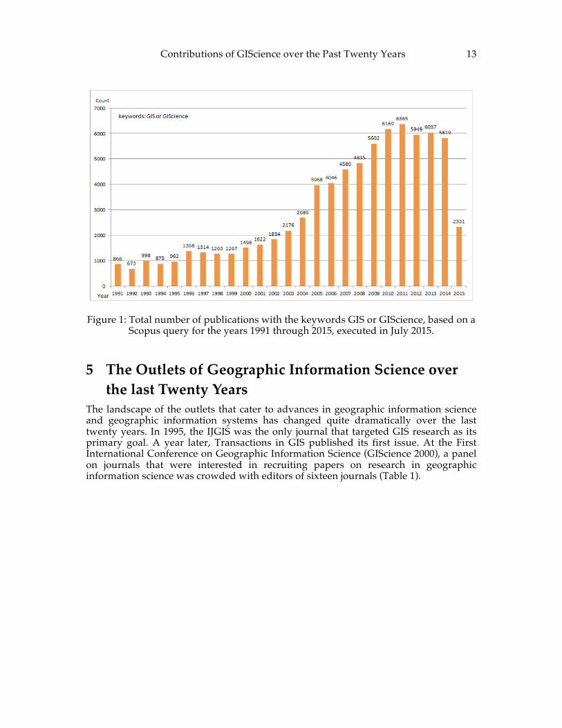
4 Proliferation of the Terms GIS and GIScience The terms GIS and GIScience have become increasingly popular within the scientific world, not only within its own field. In order to quantify such a development, we used Scopus, the abstract and citation database of peer-reviewed literature to query the number of publications that contain the keyword GIS or GIScience between 1991 and 2015 (Figure 1). The annual summary counts reveal for phases:
1. Up to 1995, annual counts were less than 1,000. 2. Between 1996 and 2000 the use of the two terms increases modestly to just
below 1,300. 3. Between 2001 and 2010, the counts essentially quadrupled to rough 6,000
occurrences annually. 4. Since 2010, this count has plateaued at roughly 6,000 annual occurrences of the
terms GIS and GIScience.
Contributions of GIScience over the Past Twenty Years 13
Figure 1: Total number of publications with the keywords GIS or GIScience, based on a Scopus query for the years 1991 through 2015, executed in July 2015.
5 The Outlets of Geographic Information Science over the last Twenty Years
The landscape of the outlets that cater to advances in geographic information science and geographic information systems has changed quite dramatically over the last twenty years. In 1995, the IJGIS was the only journal that targeted GIS research as its primary goal. A year later, Transactions in GIS published its first issue. At the First International Conference on Geographic Information Science (GIScience 2000), a panel on journals that were interested in recruiting papers on research in geographic information science was crowded with editors of sixteen journals (Table 1).
14 Egenhofer, Clarke, Gao, Quesnot, Franklin, Yuan, and Coleman
Table 1: Journals represented at the editors’ panel at GIScience 2000. • Annals of the AAG • Cartographica • Cartography and Geographic Information Science • Computers and Geosciences • Computers, Environment and Urban Systems • Environment and Planning B • Geographic Information Sciences • Geographical Analysis • Geographical Systems • GeoInformatica • Geomatica • International Journal of Geographical Information Science • Networks and Spatial Economics • Spatial Cognition and Computation • Transactions in GIS • URISA Journal A study of GIScience journals, published in 2008 [8], started with 121 journals, reduced them to 84 that were deemed more core to GIScience, ultimately focusing on a subset of 54 in an attempt to rank them. This means the core outlets for GIS and GIScience research more than tripled over eight years. More recently, further reputable outlets have appeared, such as the Journal on Spatial Information Science, ACM Transactions on Algorithms and Systems, Earth Science Informatics, and Open Geospatial Data, Software and Standard. The landscape of regularly scheduled conferences that cater to geographic information science research has seen less volatility. Launching a new journal may be less involved than sustaining a conference series on a regular basis. The global distribution of the events over the last 20 years highlights over the years a focus on Europe and North America. In the mid 1990s, the Spatial Data Handling Symposia (SDH) dominated the field of theoretical contributions to GIS (Section 5.5). Autocarto went into a hiatus in the late 1990s and the AAG meetings included selected sessions related to GIS research. In the early 1990s, two new conferences series adopted the computer scientists’ rigor of fully refereed full papers for conferences with the biennial Symposia on Large Spatial Databases (SSD) and the Conference on Spatial Information Theory (COSIT) (Section 5.2), with proceedings published in Springer’s Lectures Notes in Computer Science series and a single-track conference program. Both established themselves as venues for focused work in specific subfields of geographic information science. The annual ACM Workshops on Geographic Information Systems, which also had a rigorous reviewing system, attracted only small audiences, however. In order to provide a forum for a more encompassing perspective of geographic information science research, the biennial conference series on Geographic Information Science, dubbed GIScience, started in 2000 (Section 5.1). With the formation of ACM SIGPATIAL (Section 5.4)—a Special Interest Group with a focus on the acquisition, management, and processing of spatially-related information—in the early 2000s, ACM GIS became the SIG’s annual meeting of that SIG, drawing large crowds to the presentations of fully refereed papers on systems issues in GIS.
Contributions of GIScience over the Past Twenty Years 15
Specialized meetings with a focus on a subfield of GIScience continue on Spatial Accuracy, Spatial Cognition, GeoComputation (Section 5.6), Web and Wireless GIS, and Digital Earth. Regional GIS meetings (e.g., GISRUK in the UK, AGIT in Austria, GeoInfo in Brazil) complement the conference landscape. The GIScience Conferences portal giscienceconferences.org is a comprehensive archive of these events.
5.1 GIScience The first international conference on Geographic Information Science was held in Savannah (Georgia, USA) in October 2000. It was hosted by NCGIA, UCGIS, and the AAG. This conference aims to bring together GIScience researchers from a wide variety of disciplines, including cognitive science, computer science, engineering, geography, information science, mathematics, philosophy, psychology, social sciences, and statistics. In order to focus on fundamental GIScience advances papers that deal with applications of Geographic Information Systems are systematically discouraged. This multi-track conference brings around 300 researchers every two years. Since of 2002, GIScience has been offering both fully refereed papers as well as extended abstracts that were screened by program committee members. This mixture catered to the different disciplinary preferences in the computational and the geographic fields of GIScience. Paper sessions are usually preceded by workshops and tutorials and followed by a poster session.
5.2 COSIT The initiation of the series of Conferences on Spatial Information Theory (COSIT) was preceded by the international conference “From Space to Territory: Theories and Methods of Spatio-Temporal Reasoning,” which was held in Pisa (Italy) in 1992. It is at times referred as COSIT 0. The first COSIT meeting was held in 1993 as an interdisciplinary biennial European conference on the representation and processing of information about geographic space. COSIT changes its venue every two years, and so far has been held in Australia, Austria, France, Germany, Italy, Switzerland, the UK, and the US. The COSIT conferences cover multiple fields of interests, such as the cognitive aspects of geographic information, the ontology of space, the cartography, and the behavioral geography. COSIT is a single-track conference. It includes a doctoral colloquium, workshops, tutorials, and poster presentations. Full papers have been published in the LNCS series. Between 100 and 130 researchers participate in COSIT every two years.
5.3 AGILE The mission of the Association of Geographic Information Laboratories for Europe (AGILE) is to “promote academic teaching and research on GIS at the European level and to stimulate and support networking activities between member laboratories.” This mission is notably achieved through an annual research conference that systematically takes place in Europe. AGILE’s conference series on Geographic Information Science started in 1998 in Enschede (Netherlands) and clearly became a European reference in the area of GIScience. This conference focuses on research areas related to GIScience, from spatial cognition to geodesign, through health and medical Informatics. Full articles are published in Springer’s Lecture Notes in Geoinformation and Cartography, whereas short papers are included in different electronic proceedings.
16 Egenhofer, Clarke, Gao, Quesnot, Franklin, Yuan, and Coleman 5.4 ACM SIGSPATIAL The ACM SIGSPATIAL International Conferences on Advances in Geographic Information Systems is nowadays a series of symposia and workshops. It brings together researchers and developers specialized in GIS and other systems based on geospatial data. ACM SIGSPATIAL clearly emphasizes the technical aspects of geographic information systems (e.g., algorithms, database systems, and geometric computations). This annual conference is typically sponsored by such companies as ESRI, Google, Oracle, and Microsoft. ACM SIGSPATIAL is organized around paper and demo sessions as well as Ph.D. showcases. Topics addressed during ACM SIGSPATIAL cover numerous research areas (e.g., currently Big Spatial Data, GPU and Novel Hardware Solutions, Spatial Data Analytics, and Web and Real-Time Applications). Proceedings are published by ACM.
5.5 Spatial Data Handling The international symposium on Spatial Data Handling (SDH) began in Zurich (Switzerland) in 1984. It is the key meeting of the International Geographical Union (IGU) Commissions on Geographical Information Science and on Modeling Geographical Systems. SDH is a well-know biennial research forum in the field of GIScience. It brings together geographers, cartographers, computer scientists, and other GIScientists every two years. The latest SDH (16th) was held in Toronto in October 2014 jointly with the ISPRS Technical Commission II Symposium.
5.6 GeoComputation The GeoComputation meeting started in 1996 in Leeds (UK) as an annual conference centered on geographic analysis, statistics, and, modeling, computation algorithms on geospatial data. GeoComputation takes place every alternate year with the GIScience conference since 2002. This is a classic conference where workshops, paper sessions, and poster presentations are proposed.
6 Systematic Analyses of Publications The development of a scientific community relies on many researchers and key players’ contributions to this domain. A past analysis of social and spatial networks aimed at identifying patterns of collaborations among researchers, universities, and institutions in GIScience [2]. The results revealed to what degree individual trajectories (change of affiliations) of researchers impact the formation of a network of the GIScience communities. Citation counts remain a key currency when assessing the impact of research. André Skupin presented a citation analysis of the GIScience literature at the 2008 symposium, which identified Peter Burrough, Mike Goodchild, and Max Egenhofer as the three most-cited researchers in GIScience [36]. These results might be biased, however, because of the bibliographic datasets used in the analysis. In a complementary analysis, Keßler et al. demonstrated how to semantically annotate and interlink bibliographic datasets using Linked Data technology and enable complex queries [49]. One such query showed that by 2012 only seventeen researchers had published full papers at ACM GIS, COSIT, and GIScience conferences, and another five have met this criterion in the meantime (Table 2). Most of them either have a background in computer science or collaborate with computer scientists.
Contributions of GIScience over the Past Twenty Years 17
Table 2: The seventeen researchers who published at least one full paper in each of the three conference series ACM GIS, COSIT, and GIScience by 2012 [52], plus the five who
joined this club by 2015.
Benjamin Adams Krzysztof Janowicz Andrea Rodríguez Christophe Claramunt Christopher B. Jones John Stell Matthew P. Dube Werner Kuhn Egemen Tanin Matt Duckham Lars Kulik Jan Oliver Wallgrün Max J. Egenhofer Ross S. Purves Stephan Winter Leila De Floriani Martin Raubal Michael Worboys Andrew U. Frank Kai-Florian Richter Mark Gahegan Claus Rinner In order to complement the previous review and assessment, we employed two analyses based on 2015 data. The first analysis focuses on the most frequently cited articles in key outlet (Section 6.1). The citation searches focused on two journals and two refereed conferences. The second analysis looked at the development of the most prominent terms used in the publications of a conference series over seven consecutive events (Section 6.2).
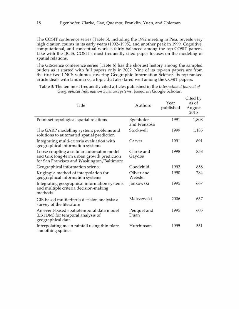
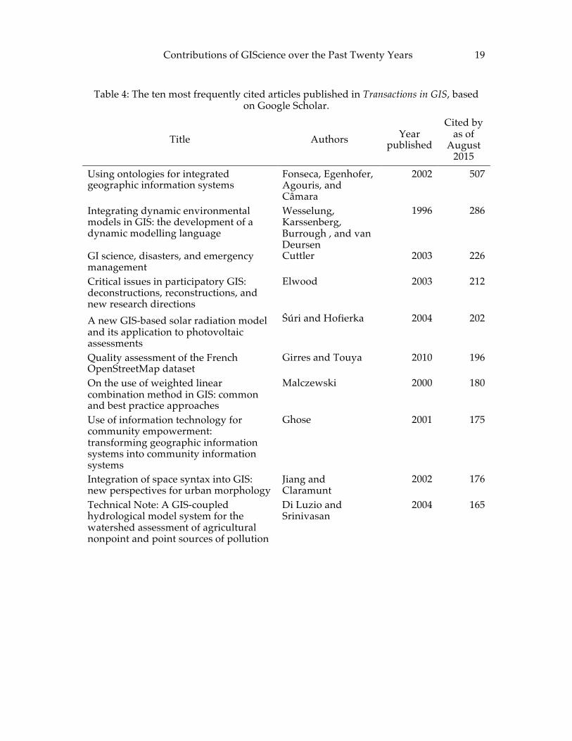
6.1 Most Frequently Cited Papers in Selected GIScience Outlets Occasionally, journal editors have published citation counts of their top-rated articles in editorials of their journal [26, 57]. These counts show that typically, publications must have been disseminated for some time before they collect significant numbers of citations. Also, more dated publications have a greater opportunity to collect more citations. While these side effects seem to favor mostly dated work, novel seminal work often rises quickly into the top of the charts. Here we used Google Scholar to identify the ten most frequently cited articles in five different GIS and GIScience outlets: (1) The International Journal of Geographical Information Science, and its predecessor The International Journal of Geographical Information Systems (IJGIS), (2) Transactions in GIS (TG), (3) the series of conferences on spatial information theory (COSIT), and (4) the GIScience conference series. Among these four samples, the IJGIS citation counts are the highest (Table 3). IJGIS has the longest history of the four (published since 1987) and the highest frequency. Three of its top-ten papers appeared in 1995, the year of the first Young Scholars Institute. Four of the top cited papers appeared in during the pioneering years of geographic information science. Only one of the top ranked papers—a survey article—appeared after 2000. The top-ten articles are mostly methodological, focusing on novel theories and models. IJGIS’s most frequently cited article relates to advances in theory, in particular the modeling of spatial relations, one of the five bullets in the NCGIA solicitation [1]. The top citation counts for TG include an article from the TG’s inaugural issue in 1996, and most of the remainder from the early 2000s (Table 4). A rapidly rising paper from 2010 relates to the emerging theme of volunteered geographic information, while the most frequently cited paper in TG addresses ontologies, one of the topics that are emerged in recent years (Section 10.1). Unlike in the other samples publications, topics related to the geographies of the information society [80] are more prominently represented in TG’s top ten.
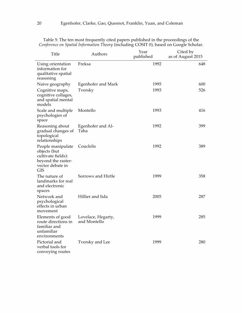
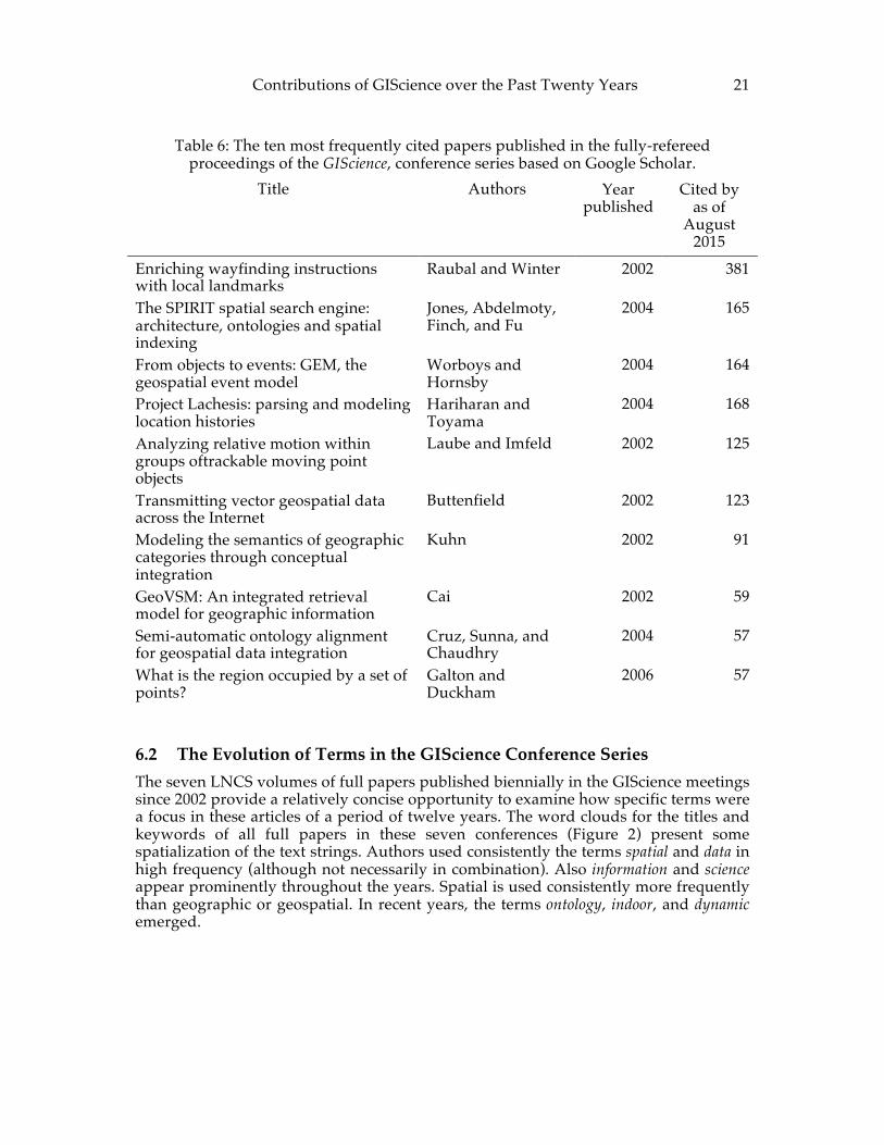
18 Egenhofer, Clarke, Gao, Quesnot, Franklin, Yuan, and Coleman The COSIT conference series (Table 5), including the 1992 meeting in Pisa, reveals very high citation counts in its early years (1992–1995), and another peak in 1999. Cognitive, computational, and conceptual work is fairly balanced among the top COSIT papers. Like with the IJGIS, COSIT’s most frequently cited paper focuses on the modeling of spatial relations. The GIScience conference series (Table 6) has the shortest history among the sampled outlets as it started with full papers only in 2002. Nine of its top-ten papers are from the first two LNCS volumes covering Geographic Information Science. Its top ranked article deals with landmarks, a topic that also fared well among the COSIT papers.
Table 3: The ten most frequently cited articles published in the International Journal of Geographical Information Science/Systems, based on Google Scholar.
Title Authors Year published
Cited by as of
August 2015
Point-set topological spatial relations Egenhofer and Franzosa
1991 1,808
The GARP modelling system: problems and solutions to automated spatial prediction
Stockwell 1999 1,185
Integrating multi-criteria evaluation with geographical information systems
Carver 1991 891
Loose-coupling a cellular automaton model and GIS: long-term urban growth prediction for San Francisco and Washington/Baltimore
Clarke and Gaydos
1998 858
Geographical information science Goodchild 1992 858 Kriging: a method of interpolation for geographical information systems
Oliver and Webster
1990 784
Integrating geographical information systems and multiple criteria decision-making methods
Jankowski 1995 667
GIS-‐‑based multicriteria decision analysis: a survey of the literature
Malczewski 2006 637
An event-based spatiotemporal data model (ESTDM) for temporal analysis of geographical data
Peuquet and Duan
1995 605
Interpolating mean rainfall using thin plate smoothing splines
Hutchinson 1995 551
Contributions of GIScience over the Past Twenty Years 19
Table 4: The ten most frequently cited articles published in Transactions in GIS, based on Google Scholar.
Title Authors Year published
Cited by as of
August 2015
Using ontologies for integrated geographic information systems
Fonseca, Egenhofer, Agouris, and Câmara
2002 507
Integrating dynamic environmental models in GIS: the development of a dynamic modelling language
Wesselung, Karssenberg, Burrough , and van Deursen
1996 286
GI science, disasters, and emergency management
Cuttler 2003 226
Critical issues in participatory GIS: deconstructions, reconstructions, and new research directions
Elwood 2003 212
A new GIS-‐‑based solar radiation model and its application to photovoltaic assessments
Šúri and Hofierka 2004 202
Quality assessment of the French OpenStreetMap dataset
Girres and Touya 2010 196
On the use of weighted linear combination method in GIS: common and best practice approaches
Malczewski 2000 180
Use of information technology for community empowerment: transforming geographic information systems into community information systems
Ghose 2001 175
Integration of space syntax into GIS: new perspectives for urban morphology
Jiang and Claramunt
2002 176
Technical Note: A GIS-coupled hydrological model system for the watershed assessment of agricultural nonpoint and point sources of pollution
Di Luzio and Srinivasan
2004 165
20 Egenhofer, Clarke, Gao, Quesnot, Franklin, Yuan, and Coleman
Table 5: The ten most frequently cited papers published in the proceedings of the Conference on Spatial Information Theory (including COSIT 0), based on Google Scholar.
Title Authors Year published
Cited by as of August 2015
Using orientation information for qualitative spatial reasoning
Freksa 1992 648
Naive geography Egenhofer and Mark 1995 600 Cognitive maps, cognitive collages, and spatial mental models
Tversky 1993 526
Scale and multiple psychologies of space
Montello 1993 416
Reasoning about gradual changes of topological relationships
Egenhofer and Al-Taha
1992 399
People manipulate objects (but cultivate fields): beyond the raster-vector debate in GIS
Couclelis 1992 389
The nature of landmarks for real and electronic spaces
Sorrows and Hirtle 1999 358
Network and psychological effects in urban movement
Hillier and Iida 2005 287
Elements of good route directions in familiar and unfamiliar environments
Lovelace, Hegarty, and Montello
1999 285
Pictorial and verbal tools for conveying routes
Tversky and Lee 1999 280
Contributions of GIScience over the Past Twenty Years 21
Table 6: The ten most frequently cited papers published in the fully-refereed proceedings of the GIScience, conference series based on Google Scholar.
Title Authors Year published
Cited by as of
August 2015
Enriching wayfinding instructions with local landmarks
Raubal and Winter 2002 381
The SPIRIT spatial search engine: architecture, ontologies and spatial indexing
Jones, Abdelmoty, Finch, and Fu
2004 165
From objects to events: GEM, the geospatial event model
Worboys and Hornsby
2004 164
Project Lachesis: parsing and modeling location histories
Hariharan and Toyama
2004 168
Analyzing relative motion within groups oftrackable moving point objects
Laube and Imfeld 2002 125
Transmitting vector geospatial data across the Internet
Buttenfield 2002 123
Modeling the semantics of geographic categories through conceptual integration
Kuhn 2002 91
GeoVSM: An integrated retrieval model for geographic information
Cai 2002 59
Semi-automatic ontology alignment for geospatial data integration
Cruz, Sunna, and Chaudhry
2004 57
What is the region occupied by a set of points?
Galton and Duckham
2006 57
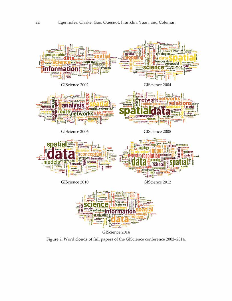
6.2 The Evolution of Terms in the GIScience Conference Series The seven LNCS volumes of full papers published biennially in the GIScience meetings since 2002 provide a relatively concise opportunity to examine how specific terms were a focus in these articles of a period of twelve years. The word clouds for the titles and keywords of all full papers in these seven conferences (Figure 2) present some spatialization of the text strings. Authors used consistently the terms spatial and data in high frequency (although not necessarily in combination). Also information and science appear prominently throughout the years. Spatial is used consistently more frequently than geographic or geospatial. In recent years, the terms ontology, indoor, and dynamic emerged.
22 Egenhofer, Clarke, Gao, Quesnot, Franklin, Yuan, and Coleman
GIScience 2002 GIScience 2004
GIScience 2006 GIScience 2008
GIScience 2010 GIScience 2012
GIScience 2014
Figure 2: Word clouds of full papers of the GIScience conference 2002–2014.
Contributions of GIScience over the Past Twenty Years 23
7 Selected Research Highlights
7.1 Advances in Theory As the core concept of GIScience is to study the science behind the systems, great efforts have been made towards advances in geographic information theories, such as models for spatial relations [19, 21, 29, 42, 74] and uncertainty in geographic data and GIS analysis, which exists in the whole process of data acquisition, geographical abstraction, representation, processing and visualization [94]. The studies of uncertainty help researchers and decision makers make better use of complex, multi-dimensional spatial data with regard to quality control that needs special handling, cleaning, and processing. Fisher discussed the critical causes and conceptual models of uncertainty in spatial data with a number of real-world examples [25]. Methods to visualize uncertainty information on maps were proposed and summarized [60, 62]. Longley et al. suggested five general dimensions of uncertainty in GIS data [59], namely, attribute accuracy, positional accuracy, logical consistency, completeness and lineage. Achievements in this field advance scientific analysis for geographic data.
7.2 The Cognitive World UCGIS’s research challenge on “Cognition of Geographic Information” investigates the understanding of human perception, memory, reasoning and communication toward spatial phenomena. Four of the former NCGIA research initiatives were dedicated to this theme (I2: Languages of Spatial Relations, I10: Spatiotemporal Reasoning in GIS, I13: User Interfaces for GIS, and I21: Formal Models of the Common Sense Geographic Worlds). In the same vein, the NCGIA’s Varenius Project included a specific topic on “Cognitive Models of Geographic Space” [67]. The book The Cognition of Geographic Space [53] and the UCGIS research agenda on Cognition of Geographic Information [71] provide a clear overview of the main contributions done before the establishment of GIScience in 1992. These reviews notably include the concept of cognitive maps [14], theories of human spatial knowledge [78] and its acquisition from direct experience, languages, and maps [84, 85]. Recent advancements in the area of cognitive GIScience fall into the categories of (1) human factors of GIS, (2) geovisualization, (3) navigation systems, (4) cognitive geo-ontologies, (5) geographic and environmental spatial thinking and memory, and (6) cognitive aspects of geographic education [70].
7.3 The Computational World Spatial is special [16]. The storage of geographic data needs handle not only the attributes but also the geometry information. In addition, the rates of geographic data generation were becoming far greater than that of the capabilities for the effective processing, storage, manipulation and analysis of such datasets. Thus new approaches to GIS data models, structures, management, queries and algorithms have been developed in the computational world to advance GIS-based computing and applications [76, 78].
7.4 The Social World The NSF-funded National Center for Geographic Information and Analysis (NCGIA) helped establish a global standard core curriculum in GIS [39]. This NCGIA Core Curriculum was expanded from a set of hard copy lesson plans to various versions of an on-line shared curriculum, which fuelled the teaching of GIS, both within the
24 Egenhofer, Clarke, Gao, Quesnot, Franklin, Yuan, and Coleman discipline as well as the dissemination to many fields that use GIS in their domain analyses. At the same time, the expansion of textbooks at all levels in the field has been extraordinary. An important recent development has been the creation and subsequent improvement of the Geographic Information Science and Technology Body of Knowledge (www.aag.org/bok) [13]. This detailed specification of the core concepts and skill sets necessary for study and proficiency in GIS has influenced the Department of Labor’s job specifications and descriptions, and is now supported by substantial online tools and an online ontology (http://gistbok.org/). In recent years the availability of online social networks and VGI outlets has led to a sub-field of GIS that studies social interactions via the Internet and the World Wide Web, using such tools as the geotags in Flickr, place names in tweets, and geocodes in Foursquare, Google+, and others. These activities often involve “big data” applications over millions or billions of records, challenging the limits of traditional desktop GIS [47].
8 Contributions of GIS to other Disciplines GIS has made contributions to various domains in computer science, such as computational geometry. Geographers, such as at the Census, have been creating tools to process large databases since before the term computational geometry was even used in this context. One GIS contribution is to provide particularly hard problems with large datasets that need workable, fast solutions. An example is label placement on maps. Another contribution within computer science is to the database domain. Spatial data types have been brought into mainstream databases with geospatial data model and query language support (e.g., Geodatabase, Oracle Spatial, PostgreSQL), as well as providing spatial indexing and spatial join methods [44]. However, more research is needed to improve support for network and field data, as well as spatial stream query processing [6, 77, 78]. In addition, the visualization of geographic information also draws a lot of attention from the computer scientists. Research of representation, visualization-computation integration, interfaces, cognitive/usability issues in geovisualization should be addressed in these crosscutting challenges [61]. Efforts have been made to foster a capable and integrated science and engineering community to conquer these challenges. This influence of GIS is in the tradition of mathematics and physics where the big theoretical advances and conceptual unifications respond to applied problems. For example, in physics, Newton's theory of gravity described and unified both the orbit of the moon and the trajectories of small thrown objects. In GIS, the problem of overlaying two maps with almost coincident edges that cause slivers and rounding errors motivates the study of robust geometric algorithms in Computational Geometry. This crosscutting influence has great potential to continue into the future, when various 2D GIS algorithms may extend into 3D. For instance, overlaying maps in GIS in 2D provides techniques that can lead to overlaying 3D triangulations, a new approach that had benefits in the domains of Computer Aided Design and computational fluid dynamics. Countless application domains have benefitted from GIS spatial analysis over the past twenty years. The two Big Books [58, 64] offer detailed accounts for many areas, but more recent advancements continue to ignite new cross-fertilizations, some of which we address here.
Contributions of GIScience over the Past Twenty Years 25
In regional planning and urban studies, GIS has been widely applied as an analysis and modeling tool to support decision-making [93], and as a simulator for urban growth [9]. Advancements in GIS also enabled GeoDesign as an emerging sub-field of landscape architecture that is supported by spatial decision analytical tools and illustrates using science in design as well as design in science [3]. Also, GIScience brings spatial analysis and statistics, as well as other location intelligence components, to facilitate traditional social science research, such as migration, demographics, crime analysis [49], and spatiotemporal access to urban opportunities [56]. In digital humanities, the development of geographic information retrieval spatial search, and digital gazetteer research has contributed to the new form of geolibrary [38]. The scientometrics community also addressed the importance of geospatial components in the scientific analysis of bibliographic data in order to identify institutional and international research collaboration and citation impact patterns [30]. GIS has led the spatial turn in health studies, in which spatial data, analysis, and global health research will be systematically incorporated for creating new discovery pathways in science [75]. This facilitates opportunities for new interdisciplinary research in which GIScientists to collaborate with medical scientists on research funded by the National Institutes of Health.
9 Changes of Topics in the Research Agenda of Geographic Information Science
Over the past twenty years, the research agenda in geographic information science has gone through a variety of iterations (Table 7), starting with Goodchild’s initial list. The University Consortium for Geographic Information Science established in 1996 a list of ten research priorities [89]. The Varenius Project of the National Center for Geographic Information and Analysis [37] concisely formulated three research thrusts—cognitive [67], computational [20], and societal issues [80]. UCGIS updated its research priorities in 2004 and augmented them by another four challenges [63].
26 Egenhofer, Clarke, Gao, Quesnot, Franklin, Yuan, and Coleman
Table 7: Major priorities in GIScience research. Goodchild [34] Data collection and measurement
Data capture Spatial statistics Data modeling and theories of spatial data Data structures, algorithms, and processes Display Analytical tools Institutional, managerial, and ethical issues
UCGIS [89] Research Priorities: Spatial data acquisition and integration Distributed computing Extensions to geographic representations Cognition of geographic information Spatial analysis in a GIS environment Future of the spatial information infrastructure Uncertainty in spatial data Interoperability of geographic information Scale GIS and society
Varenius [37] Strategic Areas for Geographic Information Science Research Cognitive models of geographic space Computational methods for representing geographic concepts Geographies of the information society
UCGIS [63] Research Challenges: Spatial data acquisition and integration Cognition of geographic information Scale Extension to geographic representations Spatial analysis and modeling in a GIS environment Uncertainty in geographic data and GIS-based analysis The future of the spatial information infrastructure Distributed and mobile computing Interoperability GIS and society: interrelation, integration, and transformation
UCGIS [63] Emerging Themes: Geographic visualization Ontological foundations for GIScience Remotely acquired data and information in GIScience Geospatial data mining and knowledge discovery
The major topics and priorities of GIScience research have changed over time. Some of them disappeared or were less developed than other topics, while new topics have also emerged. It is interesting to see how these research topics have been changed with regards to the twenty-one NCGIA research initiatives (http://www.ncgia.ucsb.edu/research/initiatives.html), which focused on the basic research on geographic analysis utilizing GIS and brought all parts of the GIS community to lay out appropriate research agenda. The topics of data modeling and theories of spatial data seem to be well studied with the achievements of vector, raster, and hybrid models in GIS. The geo-atom model, which represents the association
Contributions of GIScience over the Past Twenty Years 27
between space-time point and property, can be taken as one of the generic forms for geographic information representations and combine discrete objects and continuous fields [40]. The research on geospatial data structures and modeling are related to the initiatives of “accuracy of spatial databases” and “multiple representations.”
10 Topics that Recently Emerged in the GIScience Research Agenda
A series of new topics emerged recently in GIScience. Many of the are technology-driven or aimed at the development of new technologies, such as crowd-based solutions; spatial analysis of social media data; high-performance computing and the cloud; open-source solutions and software mashups; web-based mapping applications; location-based services and mobile computing; embedded solutions (e.g., within GPS routing systems), sensor-networks and their integration into real-time GIS; and integration of spatial and temporal processes into GIS functionality. We elaborate on four research threads (Sections 10.1-10.4) that are currently most prominent.
10.1 Ontologies in GIS The study of ontologies in GIS bridges the gap between implementation and human conceptual modeling for representing geospatial phenomena and their analysis. Although it was not listed in the original research initiatives, it did play an increasing role in the series of core GIScience conference topics, as shown in the word cloud visualization of GIScience conference topics (Figure 2). Ontology plays an important role in knowledge organization and information integration. The use of ontologies in GIS development has been widely discussed in related research [27, 68], but relatively few works have addressed the design of the user interface based on semantic integration [55]. Semantic reference systems were suggested for solving semantic interoperability issues, especially to ground geospatial semantics in physical processes and measurements [54]. With the advent of Semantic Web and Linked Data, research on geospatial semantics is valuable for GIScientists interested in semantics research as well as knowledge engineers interested in spatiotemporal data exploration [50**].
10.2 Volunteered Geographic Information The emergence of volunteered geographic information [35] and community mapping engaged the fast growth of the citizen science. The research on credibility, geoprivacy and other societal implication issues become more and more important as the growth of ubiquitous location awareness devices and crowdsourcing studies on geospatial Web [23, 83].
10.3 Spatial Big Data Recently, as the context for geographic research evolves from a data-scarce to a data-rich or big-data environment, a data-driven geography [66] is emerging during the describes that large volumes of data with a geospatial component (including structured, semi-structured, and unstructured data) on various aspects of the environment and society are being created by millions of sensors constantly, in a variety of formats such as remotely sensed imagery, GPS logs, maps, blogs, videos, audios, and photos [31]. This trend sheds new light on spatial modeling and geographic knowledge discovery, and brings about innovative developments in
28 Egenhofer, Clarke, Gao, Quesnot, Franklin, Yuan, and Coleman GIScience. The topic of spatial big data has emerged as one of the research challenges for advancing GIS in a new era.
10.4 CyberGIS With the advancement of representative cloud computing systems, clusters and grids, high performance computing infrastructures have attracted increasing attention for GIScientists and geographers as a way of solving data-intensive, computing-intensive,and access-intensive geospatial problems [92]. The emerging concept of CyberGIS, which synthesizes cyberinfrastructure, spatial analysis, and high-performance computing, provides not only a promising solution to aforementioned geospatial problems as a cloud service but also facilitates a community-driven and participatory approach to achieve scientific breakthroughs across geospatial and other communities [90].
11 Conclusions Twenty years after the first Young Scholars Summer Institute in Geographic Information, we reviewed the advances in the field. The field is still vibrant and continuous to reinvigorate itself with new challenges. Awareness of GIS and Geographic Information Science has increased significantly, and the academic field has matured with a much wider set of outlets for the dissemination of research results. Progress in Geographic Information Science has come through seminal work, but inside and outside of the field, which reflects the interdisciplinary character. Frequently, new technology has required novel approaches to dealing with spatial data and communicating spatial information. Over the last 20 years, the Web and mobile computing have provided unprecedented new opportunities, to which the GIScience research community responded with the development of a plethora of new methods. It is critical that the community is lead by the formulation of big intellectual challenges, like those presented in the NCGIA solicitation [1], and the visions of a geographic information science [34], a Naive Geography [22], a Digital Earth [41], a geospatial semantic web [17], or the volunteered geographic information [35].
Acknowledgments The panelists are grateful to the organizers of the 2015 Vespucci Summer Institute and the Institute’s support provided by the US Bureau of the Census and by ESRI. Max Egenhofer’s work is partially supported by NSF grants IIS- 1016740 and IIS-1527504. Song Gao is supported by a Jack & Laura Dangermond Travel Scholarship and thanks his Ph.D. advisory committee Krzysztof Janowicz, Michael F. Goodchild, and Helen Couclelis from the Department of Geography at the University of California, Santa Barbara. Teriitutea Quesnot is supported by the Social Sciences and Humanities Research Council of Canada (SSHRC) and the Geothink.ca project and he thanks his Ph.D. advisor Stephane Roche from the Geomatics Department at Laval University. Randolph Franklin is supported by the National Science Foundation under Grant No. IIS-1117277. May Yuan’s work is partially supported by NSF grant OCI-0941501. David Coleman’s research is supported by the Natural Sciences and Engineering Research Council of Canada.
Contributions of GIScience over the Past Twenty Years 29
References [1] ABLER, R. F. The National Science Foundation National Center for Geographic
Information and Analysis. International Journal of Geographical Information System 1, 4 (1987) 303–326.
[2] AGARWAL, P., BÉRA, R., AND CLARAMUNT, C. A social and spatial network approach to the investigation of research communities over the World Wide Web. In GIScience 2006: Proceedings of the Fourth International Conference on Geographic Information Science, N. Xiao, M.-P. Kwan, M. Goodchild, S., Eds., (Berlin, 2006), Springer, LNCS vol. 4197, pp. 1–17.
[3] BATTY, M. Defining geodesign (= GIS+ design?). Environment and Planning B: Planning and Design 40, 1 (2013), 1–2.
[4] BERNERS-LEE, T., HENDLER, J., AND LASSILA, O. The semantic web. Scientific American 284, 5 (2001): 28–37.
[5] BUSH, V. As we may think. The Atlantic Monthly. 176, 1 (1945), 101–108. [6] CÂMARA, G., EGENHOFER, M. J., FERREIRA K., ANDRADE, P., QUEIROZ,
G., SANCHEZ A., JONES, J., AND VINHAS, L. Fields as a generic data type for big spatial data. In GIScience 2014: Proceedings of the Eighth International Conference on Geographic Information Science, M. Duckham, E. Pebesma, K. Stewart, and A. Frank, Eds., (Berlin, 2014), Springer, LNCS vol. 8728, pp. 159–172.
[7] CÂMARA, G. Revisiting research agendas in geographic information science, Keynote, Vespucci Week in Advancing GIScience, Bar Harbor, ME, http://www.dpi.inpe.br/gilberto/present/gcamara_vespucci_2015.pptx
[8] CARON, C., ROCHE, S., GOYER, D., AND JATON, A. GIScience journals ranking and evaluation: an international delphi study. Transactions in GIS 12, 3 (2008), 293-321.
[9] CLARKE, K. C., AND GAYDOS. Loose-coupling a cellular automaton model and GIS: long-term urban growth prediction for San Francisco and Washington/Baltimore. International Journal of Geographical Information Science 12, 7 (1998), 699–714.
[10] COPPOCK, J. T., AND RHIND, D. W. The history of GIS. In Geographical Information Systems: Principles and Applications, D.J. Maguire, M.F. Goodchild, and D.W. Rhind, Eds. Longman, 1991, pp. 21–43.
[11] CRAGLIA, M., AND COUCLELIS, H., Eds., Geographic information research: Bridging the Atlantic. Taylor & Francis, 1997.
[12] CRAGLIA, M., AND ONSRUD, H., Eds., Geographic Information Research: Transatlantic Perspectives. CRC Press, 1998.
[13] DIBIASE, D., DEMERS, M., JOHNSON, A., KEMP, K. K., LUCK, A. T., PLEWE, B., AND WENTZ, E. Introducing the first edition of geographic information science and technology body of knowledge. Cartography and Geographic Information Science 34, 2 (2007), 113-120.
[14] DOWNS, R. M., AND STEA, D. Cognitive maps and spatial behavior: process and products. In Image and Environment: Cognitive Mapping and Spatial Behavior, R. M. Downs and D. Stea, Eds. Aldine Press, Chicago, pp. 8-26, 1973.
30 Egenhofer, Clarke, Gao, Quesnot, Franklin, Yuan, and Coleman [15] DUTTON, G. First International Advanced Study Symposium on Topological
Data Structures for Geographic Information Systems, Vol.1-8, Harvard University, Cambridge, MA, 1978.
[16] EGENHOFER, M. J. What's special about spatial?—database requirements for vehicle navigation in geographic space. ACM SIGMOD Record 22, 2 (1993), 398-402.
[17] EGENHOFER, M. J. Toward the semantic geospatial web. In GIS '02: Proceedings of the 10th ACM International Symposium on Advances in Geographic Information Systems (New York, NY, USA, 2002), ACM Press, pp.1–4.
[18] EGENHOFER, M. J. A future history of geographic information science (Keynote), GeoInfo 2014, (Campos do Jordão, Brazil, 2014), http://www.spatial.maine.edu/~max/FutureHistory.mov.
[19] EGENHOFER, M. J., AND FRANZOSA, R. F. Point-set topological spatial relations. International Journal of Geographical Information Systems 5, 2 (1991), 161-174.
[20] EGENHOFER, M. J., GLASGOW, J., GUNTHER, O., HERRING, J. R., AND PEUQUET, D. J. Progress in computational methods for representing geographical concepts. International Journal of Geographical Information Science 13, 8 (1999), 775-796.
[21] EGENHOFER, M. J., AND HERRING, J. R. Categorizing binary topological relations between regions, lines, and points in geographic databases, Tech. Rep., Department of Surveying Engineering, University of Maine, 1990.
[22] EGENHOFER, M. J., AND MARK, D. M. Naive geography. In: COSIT 1995: Proceedings of the International Conference on Spatial Information Theory: A Theoretical Basis for GIS, A. U. Frank and W. Kuhn, Eds. (Berlin, 1995), pp. 1-15.
[23] ELWOOD, S. Geographic information science: emerging research on the societal implications of the geospatial web. Progress in Human Geography 34, 3, 2010, 349–357.
[24] ESTRIN, D., GOVINDAN, R., HEIDEMANN, J., AND KUMAR, S. Next century challenges: scalable coordination in sensor networks. In MobiCom '99: Proceedings of the 5th Annual ACM/IEEE International Conference on Mobile Computing and Networking (New York, NY, USA, 1999), ACM Press, pp. 263–270.
[25] FISHER, P. F. Models of Uncertainty in Spatial Data. Geographical Information Systems 1, (1999), 191–205.
[26] FISHER, P. F. Citations to the international journal of geographical information systems and science: the first 10 years. International Journal of Geographical Information Science 15 (2001), 1–6.
[27] FONSECA, F. T., EGENHOFER, M. J., AGOURIS, P., AND CÂMARA, G. Using ontologies for integrated geographic information systems. Transactions in GIS 6, 3 (2002), 231–257.
[28] FORESMAN, T. W. Ed. The History of Geographic Information Systems: Perspectives from the Pioneers. Prentice Hall, Chicago, 1998.
[29] FRANK, A. U. Qualitative spatial reasoning about distances and directions in geographic space. Journal of Visual Languages & Computing 3, 4 (1992), 343-371.
Contributions of GIScience over the Past Twenty Years 31
[30] FRENKEN, K., HARDEMAN, S., AND HOEKMAN, J. Spatial scientometrics: towards a cumulative research program. Journal of Informetrics 3, 3 (2009), 222–232.
[31] GAO, S., LI, L., LI, W., JANOWICZ, K., AND ZHANG, Y. Constructing gazetteers from volunteered big geodata based on Hadoop. Computers, Environment and Urban Systems (in press).
[32] GOODCHILD, M. F. Spatial Information Science. In Fourth International Symposium on Spatial Data Handling (Zurich, 1990) vol. 1: pp. 3–14.
[33] GOODCHILD, M. F. Progress on the GIS Research Agenda. In EGIS: Proceedings of the Second European GIS Conference (Utrecht: The Netherlands, 1991), EGIS Foundation, pp. 342–350.
[34] GOODCHILD, M. F. Geographical information science. International Journal of Geographical Information Systems 6, 1 (1992), 31–45.
[35] GOODCHILD, M. F. Citizens as sensors: the world of volunteered geography. GeoJournal 69, 4, (2007), 211–221.
[36] GOODCHILD, M. F. Twenty years of progress: GIScience in 2010. Journal of Spatial Information Science 1, (2010), 3–20.
[37] GOODCHILD, M. F., EGENHOFER, M. J., KEMP, K. K., MARK, D. M., AND SHEPPARD, E. Introduction to the Varenius project. International Journal of Geographical Information Science 13, 8 (1999), 731-745.
[38] GOODCHILD, M. F., AND HILL, L. Introduction to digital gazetteer research. International Journal of Geographical Information Science 22, 10 (2008), 1039–1044.
[39] GOODCHILD, M. F., AND KEMP K. K. NCGIA education activities: the core curriculum and beyond. International Journal of Geographical Information Systems 6, no. 4 (1992): 309-320.
[40] GOODCHILD, M. F., YUAN, M., AND COVA, T. J. Towards a general theory of geographic representation in GIS. International Journal of Geographical Information Science 21, 3, (2007): 239–260.
[41] GORE, A. The digital earth: understanding our planet in the 21st century. Australian surveyor 43, 2 (1998), 89–91.
[42] GOYAL, R., AND EGENHOFER, M. J. The direction-relation matrix: a representation of direction relations for extended spatial objects. UCGIS Annual Assembly and Summer Retreat (Bar Harbor, ME, USA, 1997), http://www.spatial.maine.edu/~max/DRM.pdf.
[43] GRUBER, T. R. Toward principles for the design of ontologies used for knowledge sharing. International Journal of Human-Computer Studies 43, 5, (1995), 907–928.
[44] GÜTING, R. H. An introduction to spatial database systems. The VLDB Journal 3, 4, (1994), 357–399.
[45] GUTTMAN, A. R-trees: A dynamic index structure for spatial searching. In SIGMOD '84: Proceedings of the 1984 ACM SIGMOD International Conference on Management of Data (New York, NY, USA, 1984), ACM Press, pp. 47–57.
32 Egenhofer, Clarke, Gao, Quesnot, Franklin, Yuan, and Coleman [46] HÄGERSTRAAND, T. What about people in regional Science? Papers in
Regional Science 24, 1 (1970), 7–24. [47] HAN, S.Y., TSOU M.-H., AND CLARKE, K. C. Do Global Cities Enable Global
Views? Using Twitter to Quantify the Level of Geographical Awareness of US Cities. PloS one 10, 7 (2015).
[48] HAYES, P. J. The naive physics manifesto. In Expert Systems in the Micro-Electronic Age, D. Michie, Ed., Edinburgh University Press, Edinburgh, UK, 1979, pp. 242–270.
[49] HIRSCHFIELD, A., BROWN P., AND TODD, P. GIS and the analysis of spatially-referenced crime data: experiences in Merseyside, UK. International Journal of Geographical Information Systems 9, 2 (1995), 191–210.
[50] JANOWICZ, K., SCHEIDER, S., PEHLE, T., AND HART, G. Geospatial semantics and linked spatio-temporal data—past, present, and future. Semantic Web 3, 4 (2012), 321–332.
[51] JEPSON, W., LIGGETT, R., AND FRIEDMAN, S. Virtual modeling of urban environments. Presence—Teleoperators and Virtual Environments 5, 1 (1995), 72–86.
[52] KESSLER, C., JANOWICZ, K., AND KAUPPINEN, T. Spatial@linkedscience—exploring the research field of GIScience with linked data. In GIScience 2012: Proceedings of the Seventh International Conference on Geographic Information Science, N. Xiao, M.-P. Kwan, M. Goodchild, and S. Shekhar, Eds., (Berlin, 2012), Springer, LNCS vol. 7478, pp. 102–115.
[53] KITCHIN, R., AND M. BLADES. The Cognition of Geographical Space. I. B. Taurus Publishers, 2001.
[54] KUHN, W. Semantic reference systems. International Journal of Geographical Information Science 17, 5 (2003), 405–409.
[55] KUHN, W. Geospatial semantics: why, of what, and how? Journal on Data Semantics III (2005), 1–24.
[56] KWAN, M. P. Gender and individual access to urban opportunities: a study using space–time measures. The Professional Geographer 51, 2 (1999), 210–227.
[57] LEES, B. G. 25 Volumes of the international journal of geographical information science. International Journal of Geographical Information Science 25, 1 (2011), 1–5.
[58] LONGLEY, P. A., GOODCHILD, M. F., MAGUIRE, D. J., AND RHIND, D. W. Geographical Information Systems: Principles, Techniques, Applications and Management. John Wiley & Sons, 1999.
[59] LONGLEY, P. A., GOODCHILD, M. F., MAGUIRE, D. J., AND RHIND, D. W. Geographic Information System and Science. John Wiley & Sons, 2005.
[60] MACEACHREN, A. M. Visualizing uncertain information. Cartographic Perspectives 13 (1992), 10–19.
[61] MACEACHREN, A. M., AND KRAAK, M. J. Research challenges in geovisualization. Cartography and Geographic Information Science 28, 1 (2001), 3–12.
[62] MACEACHREN, A. M., ROBINSON, A., HOPPER, S., GARDNER, S., MURRAY, R., GAHEGAN, M., AND HETZLER, E. Visualizing geospatial information
Contributions of GIScience over the Past Twenty Years 33
uncertainty: what we know and what we need to know. Cartography and Geographic Information Science 32, 3 (2005), 139–160.
[63] MCMASTER, R. B., AND USERY, E. L., Eds. A Research Agenda for Geographic Information Science. CRC Press, 2004.
[64] MAGUIRE, D. J., GOODCHILD, M.F., AND RHIND, D. W., Eds., Geographical Information Systems: Principles and Applications, Longman, 1991.
[65] MARK, D. M., CHRISMAN, N., FRANK, A. U., MCHAFFIE, P. H., AND PICKLES, J. The GIS history project. UCGIS Summer Assembly. Bar Harbor, ME, http://www.ncgia.buffalo.edu/gishist/bar_harbor.html, 1997.
[66] MARK, D. M., AND FRANK A. U. Cognitive and Linguistic Aspects of Geographic Space. Kluwer, NATO ASI Series D, Vol. 63, 1992.
[67] MARK, D. M., FREKSA, C., HIRTLE, S. C., LLOYD, R., AND TVERSKY, B. Cognitive models of geographical space. International Journal of Geographical Information Science 13, 8 (1999), 747-774.
[68] MARK, D. M., SMITH, B., EGENHOFER, M. J., AND HIRTLE, S. C. Ontological foundations for geographic information science. In A Research Agenda for Geographic Information Science, R. B. MacMaster and E. L. Usery, Eds. CRC Press, 2004, pp. 335–350.
[69] MILLER, H. J., AND GOODCHILD, M. F. Data-driven geography. GeoJournal 80, 4 (2015), 449–461.
[70] MONTELLO, D. R. Cognitive research in GIScience: recent achievements and future prospects. Geography Compass 3, 5 (2009), 1824-1840.
[71] MONTELLO, D. R., AND FREUNDSCHUH, S. Cognition of geographic information. In A Research Agenda for Geographic Information Science, R. B. MacMaster and E. L. Usery, Eds. CRC Press, 2004, pp. 61–91.
[72] NEGROPONTE, N. Being Digital. Alfred A. Knopf Inc., 1995. [73] PEUCKER, T. K., FOWLER, R. J., LITTLE, J. J., AND MARK, D. M. The
triangulated irregular network. In American Society of Photogrammetry, Digital Terrain Models Symposium (St. Louis, MO, USA, 1978), pp. 516–540.
[74] RANDELL, D. A., CUI, Z, AND COHN, A. G. A spatial logic based on regions and connection. In KR ‘92: Proceedings of the 3rd International Conference on Principles of Knowledge Representation and Reasoning, B. Nebel, C. Rich, and W. R. Swartout, Eds. (Morgan Kaufmann, 1992), pp. 165-176.
[75] RICHARDSON, D. B., Volkow, N. D., KWAN, M. P., KAPLAN, R., GOODCHILD, M. F., AND CROYLE, R. T. Spatial turn in health research. Science 339, 6126 (2013): 1390.
[76] RIGAUX, P., SCHOLL, M., AND VOISARD, A. Spatial databases: with application to GIS, Morgan Kaufmann, 2001.
[77] RODDICK, J. F., HOEL, E., EGENHOFER, M. J., PAPADIAS, D., AND SALZBERG, B. Spatial, temporal and spatio-temporal databases-hot issues and directions for PhD research. ACM SIGMOD Record 33, 2 (2004), 126–131.
[78] SHEKHAR, S., CHAWLA, S., RAVADA, S., FETTERER, A., LIU, X., AND LU, C. T. Spatial databases—accomplishments and research needs. IEEE Transactions on Knowledge and Data Engineering 11, 1 (1999), 45–55.
34 Egenhofer, Clarke, Gao, Quesnot, Franklin, Yuan, and Coleman [79] SHEKHAR, S., GUNTURI, V., EVANS, M. R., YANG, K. Spatial big-data
challenges intersecting mobility and cloud computing. In MobiDE '12: Proceedings of the Eleventh ACM International Workshop on Data Engineering for Wireless and Mobile Access, (New York, USA, 2012), ACM Press, pp. 1–6.
[80] SHEPPARD, E., COUCLELIS, H., GRAHAM, S., HARRINGTON, J. W., AND ONSRUD, H. J. Geographies of the information society. Cognitive models of geographical space. International Journal of Geographical Information Science 13, 8 (1999), 797-823.
[81] SIEGEL, A. W., AND WHITE, S. H. The development of spatial representations of large-scale environments. Advances in Child Development and Behavior 10 (1975), 9-55.
[82] STEFANIDIS, A., AND NITTEL, S., Eds., GeoSensor Networks. CRC Press, 2004. [83] SUI, D., ELWOOD, S., AND GOODCHILD, M. F., Eds. Crowdsourcing
geographic knowledge: volunteered geographic information (VGI) in theory and practice. Springer, New York, 2012.
[84] TAYLOR, H., AND TVERSKY, B. Spatial mental models derived from survey and route descriptions. Journal of Memory and Language 31, 2 (1992), 261-292.
[85] THORNDYKE, P., AND HAYES-ROTH, B. Differences in spatial knowledge acquired from maps and navigation. Cognitive Psychology 14, 4 (1982): 560-589.
[86] TOBLER, W. R. A computer movie simulating urban growth in the Detroit region. Economic Geography 46 (1970), 234–240.
[87] TOMLIN, C. D. Geographic Information Systems and Cartographic Modeling. Prentice-Hall, 1990.
[88] TOMLINSON, R. F. A geographic information system for regional planning. In: G.A. Stewart (ed.) Symposium on Land Evaluation, Commonwealth Scientific and Industrial Research Organization, Melbourne, Australia, 1968.
[89] UCGIS , Research priorities for geographic information science. Cartography and Geographic Information Science 23, 3 (1996), 115-127.
[90] WANG, S., ANSELIN, L., BHADURI, B., CROSBY, C., GOODCHILD, M. F., LIU, Y., AND NYERGES, T. L. CyberGIS software: a synthetic review and integration roadmap. International Journal of Geographical Information Science 27, 11 (2013), 2122–2145.
[91] WANT, R., HOPPER, A., FALÇAO, V., AND GIBBONS, J. (1992) The active badge location system. ACM Transactions on Information Systems 10, 1 (1992), 91–102.
[92] YANG, C., GOODCHILD, M. F., HUANG, Q., NEBERT, D., RA SKIN, R., XU, Y., BAMBACUS, M., AND FAY, D. Spatial cloud computing: how can the geospatial sciences use and help shape cloud computing? International Journal of Digital Earth 4, 4 (2011), 305–329.
[93] YEH, A. G. Urban planning and GIS. In P. A. Longley, M. F. Goodchild, D. J. Maguire, and D. W. Rhind, Eds., John Wiley & Sons, 2005, pp. 877-888.
[94] ZHANG, J., AND GOODCHILD, M. F. Uncertainty in Geographical Information. CRC Press, 2002.
ADVANCING GEOGRAPHIC INFORMATION SCIENCE: CHAPTER 2
© by the author(s) Licensed under Creative Commons Attribution 4.0 License
35
Technological and Societal Influences on GIScience
Stephan Winter 1, Xavier Lopez 2, Francis Harvey 3, Benjamin D. Hennig 4, Myeong-Hun Jeong 5, Timothy Trainor 6, and Sabine
Timpf7 1 Department of Infrastructure Engineering, The University of Melbourne, Australia
2 Oracle Corp., USA 3 Department of Geography, Environment and Society, University of Minnesota, USA
4 School of Geography and the Environment, Oxford University, UK 5 CyberGIS Center for Advanced Digital and Spatial Studies, UIUC, USA
6 US Census Bureau, Washington DC, USA 7 Department of Geography, University of Augsburg, Germany
Abstract: This paper highlights and critically reflects on some of the most significant technological and societal influences on GIScience over the last 20 years, or since its inception. For the purpose of this book, which in the following chapters begins to sketch out likely paths for future directions of GIScience, one conclusion of this chapter can be taken for granted: In the next 20 years again significant external factors from technology and society will shape GIScience. This paper summarizes the discussions related a panel on the topic at the 2015 Vespucci Institute. The panel in Bar Harbor, moderated by Stephan Winter, included two invited presentations (by Xavier Lopez and Francis Harvey), and responses by two early career panelists (Benjamin D. Hennig and Meyeong-Hun Jeong), and by two senior panelists (Tim Trainor and Sabine Timpf).
Keywords: Geographic information science, spatial information science, spatial information technology, GIS and society, neogeography.
1 Introduction This chapter highlights and critically reflects on some of the most significant technological and societal influences on GIScience over the last 20 years. The question whether, and if so, to what extent, technological and societal influences have impacted on GIScience, or helped shaping GIScience, is worth putting forward and thinking about in a volume that explores challenges for GIScience in the next 20 years.
36 Winter, Lopez, Harvey, Hennig, Jeong, Trainor, and Timpf
The question is a fundamental one. When we consider the last 20 years, it offers us a better vantage of where we stand now and to think about the future. Also, it offers a vantage to reflect on the idea that any science is independent from technological changes or societal impact: Shouldn’t science be the quest for underlying truths or laws that sustain any technological and societal influence? A romantic view, but a common view. We know that GIScience – as many other sciences, but in contrast to logic and mathematics – is an empirical science [19, 7, 8, 9], and empiricism is always driven by technological possibility as well as societal interest. This statement can be observed in physics as much as in geography, and thus holds for GIScience as well. Take privacy as an example. Privacy has come up as an issue on the research agenda only recently, and is a social issue: Technology exposes more and more of our movements, activities and thoughts such that a societal response for privacy protection is needed. As much as this response will apply regulations and legal enforcements, it will also rely on new knowledge and proof of techniques such as encryption and location obfuscation. Where we are will always influence what we know. And yet, also empirical research should reveal over time a body of knowledge that holds over larger periods of time, i.e., is neither bound to particular technology (in times where technologies change so quickly, or innovation rates are exponential, as indicated by Moore’s “Law” [14]), nor to a particular constitution of society. Its “laws” are statements which have been and can always be again confirmed by evidence. For example, research on people’s ability to deal with vague spatial concepts, such as ‘downtown’ or ‘Mt Everest’, or on our ability to represent and reason with this vague knowledge in information systems, should have a considerably longer half-life than on people’s views of where ‘downtown London’, ‘the Alps’ or ‘Mt Everest’ are. Fortunately we know well from geography that different points of view help us gain a better scientific understanding. Critical thinking, instead of taking on one position, considers multiple positions, thus gaining deeper insights and developing more robust solutions. This chapter offers some of these thoughts. It is a result of a panel discussion on technological and societal influences on GIScience at the Vespucci’s Summer Institute in GIScience 2015. The discussion was inspired by two presentations, which are summarized here. However, this chapter transforms this discussion by reflecting on the relationship between society, technology and GIScience as perceived today and felt to impact in the future. For the purpose of this book, one conclusion of this chap- ter can be taken for granted: In the next 20 years again significant technological and societal influences will shape GIScience.
2 The impact of technological change on GIScience Over 500 years ago printing revolutionized the production (technological change) and accessibility (social change) of maps (Fig. 1). About 50 years ago computers became mature enough to allow people such as McHarg [13], Tomlinson [20], Fisher [6], Chris- man [2] and so many others to think about transforming maps for the information age.
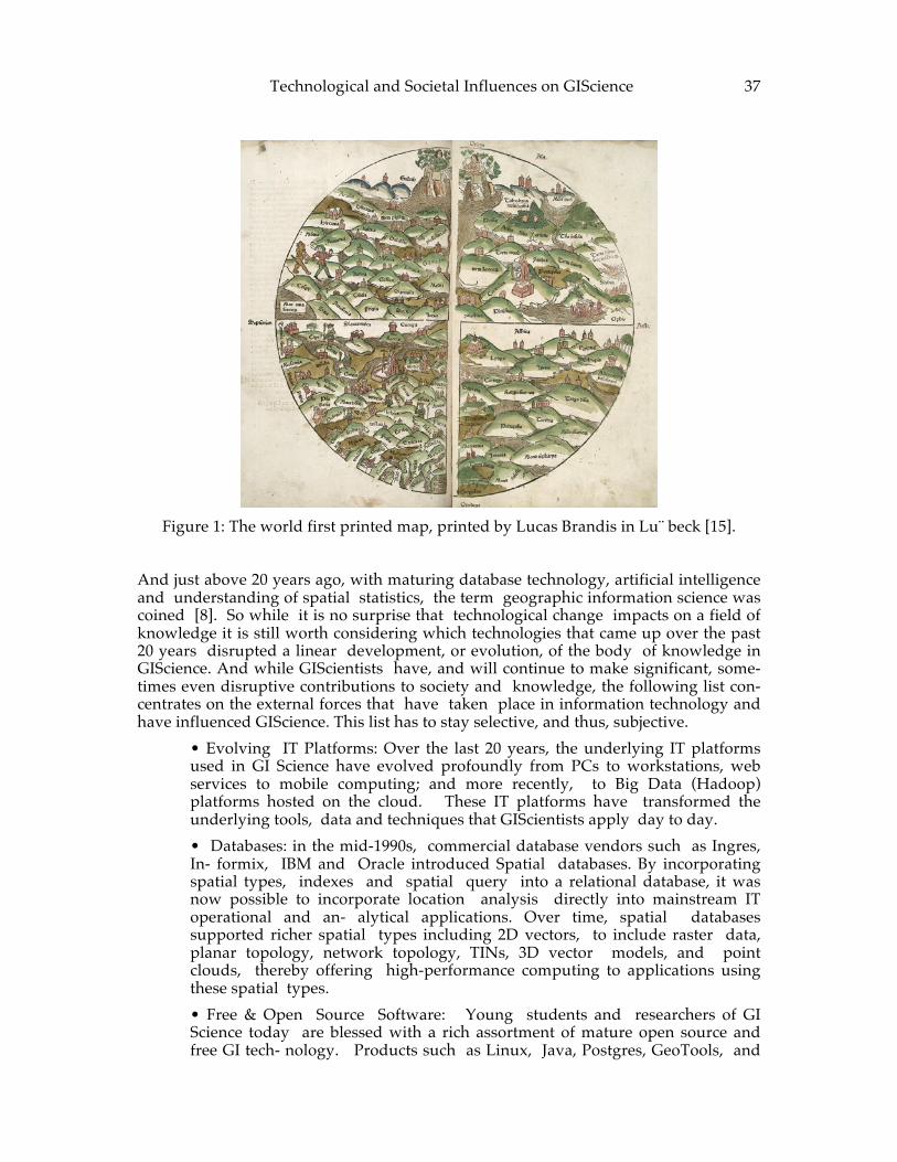
Technological and Societal Influences on GIScience 37
Figure 1: The world first printed map, printed by Lucas Brandis in Lu¨ beck [15].
And just above 20 years ago, with maturing database technology, artificial intelligence and understanding of spatial statistics, the term geographic information science was coined [8]. So while it is no surprise that technological change impacts on a field of knowledge it is still worth considering which technologies that came up over the past 20 years disrupted a linear development, or evolution, of the body of knowledge in GIScience. And while GIScientists have, and will continue to make significant, some- times even disruptive contributions to society and knowledge, the following list con- centrates on the external forces that have taken place in information technology and have influenced GIScience. This list has to stay selective, and thus, subjective.
• Evolving IT Platforms: Over the last 20 years, the underlying IT platforms used in GI Science have evolved profoundly from PCs to workstations, web services to mobile computing; and more recently, to Big Data (Hadoop) platforms hosted on the cloud. These IT platforms have transformed the underlying tools, data and techniques that GIScientists apply day to day. • Databases: in the mid-1990s, commercial database vendors such as Ingres, In- formix, IBM and Oracle introduced Spatial databases. By incorporating spatial types, indexes and spatial query into a relational database, it was now possible to incorporate location analysis directly into mainstream IT operational and an- alytical applications. Over time, spatial databases supported richer spatial types including 2D vectors, to include raster data, planar topology, network topology, TINs, 3D vector models, and point clouds, thereby offering high-performance computing to applications using these spatial types. • Free & Open Source Software: Young students and researchers of GI Science today are blessed with a rich assortment of mature open source and free GI tech- nology. Products such as Linux, Java, Postgres, GeoTools, and
38 Winter, Lopez, Harvey, Hennig, Jeong, Trainor, and Timpf
MapServer are mainstream technologies for GI Scientists and professionals alike. Researchers avail themselves to tools that are easy to acquire, adapt, and use. This was not necessarily the case in the era of commercial desktop GIS. Costs to academic departments have decreased while the range of tooling continues to grow. • Spatial Data Infrastructures: In the 1990s and 2000s, the policy concept of National Spatial Data Infrastructures (NSDI) took hold throughout hundreds of developed and developing countries. National governments, in particular, began to recognize the importance of sharing public sector investments in spatial data broadly across the society and economy. While the promised infrastructures are late in coming – pieces exist but it is not yet a smooth experience –, key activities such as spatial data standards, public dissemination mandates, capacity building, relaxed intellectual property rights, and inter-organizational coordination have been closely studied and influenced by GI Scientists. Today’s political emphasis on ‘open data’, ‘open gov’, and ‘linked open data’ have been enabled by these early efforts to make government spatial data more openly shareable. • Global Positioning System: In May 2000, the U.S. Air Force eliminated ‘selective availability’, the intentional degradation of GPS signals for non-military purposes. This measure improved the precision of GPS signals to about 1 meter, making it feasible to develop broad range of precision surveying, navigation, and mobile location services. The adoption of GPS exploded across all sectors creating new research opportunities for understanding crowd-sourced movement of entities; management and analysis of massive streams of location data; and exploring predictive location behavior based on historical tracking patterns. • Sensor Data Collection: the mainstream use of GPS signals for positioning, cou- pled with the miniaturization of low cost field sensors, ushered in the rapid use of sensor data collection at the turn of the century. Biologists tracked wildlife, trucking companies tracked and regulated the performance of their trucks, meteorologists used stationary sensors in the land, oceans, and atmosphere to monitor the environment. Sensors have crossed over into mainstream consumer use with the release of wearable devices. GI scientists continue to be advanced users of location-enabled sensors, and innovators in the use of Big Data sensor streams. • World Wide Web: The most transformative technology innovation of this last period was the advent of the World Wide Web in 1993. While the Web transformed nearly all sectors of computing, it had a profound impact on the GI community. Before the Web, nearly all work done by GI Scientists was constrained to desk- top systems; after the Web most projects and research is oriented to or exploit the networked nature of the Web. The open standards, formats, and protocols introduced by the W3C, resulted in radical restructuring of how information was transported and published across the Internet. The Web enabled the rapid trans- formation from desktop and client/server platforms to Web Services, creating a foundation for a new class of Web mapping services. • Web Mapping Services: In 1996, Barry Glick, a University of Buffalo Ph.D. graduate working at Donnelley, introduced MapQuest, a ground-breaking Web mapping service using government created data. MapQuest, and later services
Technological and Societal Influences on GIScience 39
from AOL, Microsoft, ESRI, and Google provided mainstream Web users with the power to display maps, search features, geocode addresses, generate driving directions via Web browsers. Over time, these platforms enabled businesses, government agencies and citizens the ability to upload and display their own features on background map tiles. The underlying techniques pioneered by Glick and others - caching of map tiles, in-memory-based routing, crowd-sourced map- ping – continue to make Web mapping services ubiquitous. • Mobile Computing: Between 1999 and 2005, the promise of wireless location- based services (LBS) had been widely promoted. Japanese and European wire- less providers brought early innovation in delivering powerful GPS enabled 3G phones. A constraint to these early mapping services were the proprietary nature of wireless carriers services that also blocked access to Web content. How- ever, by 2006 US carriers had upgraded their 3G networks coinciding with Apple’s release of the iPhone 3G smart phone. This device enabled app developers and users to directly access Web content creating a powerful smart phone plat- form that delivers GI services to nearly every mobile phone user globally. More recently, mobile application environments using HTML5 show promise in solving device-specific constraints within the World Wide Web. • Social media & crowd-sourced data: By mid-2000, a new generation of open source Web and mobile computing services re-invented how mapping content was created. Citizen volunteers, field scientists, activists and amateur mappers began to generate and contribute spatial feature content to a new generation of Web mapping services, like Google Maps, OpenStreetMaps, and DBPedia. Michael Goodchild referred to this phenomena as volunteered geographic information [10]. Within a decade, the use of crowd sourced map data has challenged the role of government and commercial sector in the provisioning of vector map- ping features. • Linked Data: Linked Data is an evolution of by Tim Berners Lee’s Semantic Web vision first introduced in 1999 [1]. Building on W3C standards and Web services, Linked Data focuses on the large scale integration and reasoning of data collections on the Web. Unfortunately, the dearth of formal ontologies, and immaturity of early RDF and SPARQL specifications slowed uptake of the Semantic Web. By 2011 these standards had matured and the availability of open source linking vocabularies, combined with a vast ecosystem of web mapping services, affords an opportunity to realize Tim Berners Lee’s vision of a Web of geospatial features that introduces a potential area of research for GI Science. • From data scarcity to data deluge: Over time – a process rather than a disruptive event – through spatial data infrastructures, open data initiatives and sensor data collection, GIScience is now confronted with unprecedented data volume, variety, and velocity. These advanced technologies not only bring forth computational innovation such as geospatial optimization and simulation, but also yield actionable insight from big data. GIScience therefore seeks today to resolve problems of dealing with and analyzing heterogeneous spatial data, integrating and synthesizing diverse data sources, and orchestrating collaboration, rather than data collection and pre-processing.
40 Winter, Lopez, Harvey, Hennig, Jeong, Trainor, and Timpf
3 Societal influence on GIScience With advancing geospatial technologies, and not least heavily supported by the in- creasing possibilities of the Internet, a revived interest in maps can be observed in recent years. Changing technologies and the revival of public interest in mapping led to the emergence of a large number of untrained cartographers producing maps and geographic data visualizations in the online world as well as contributing to the technological advances themselves. Corresponding to the list above, three underlying social outcomes can be identified immediately:
• Location data becomes mainstream: Map consumption and production moves from specialists to enthusiasts, and into everyday life. • Democratization of tools and services: The combination of open source tools and Web services has broadened the developer base as much as the user base for simple and free mapping tools and apps that create, analyze and exploit spatial data. • Open data initiatives: While free and public domain spatial data has been a feature of the US GI marketplace for a long time, other countries had different policies and values. But over the last two decades also European mapping and statistical agencies have reversed previous restrictive data dissemination policies and are now promoting open data initiatives for selected datasets. The growing availability of government-sourced open data is now driving a range open data services.
The growing availability of map data has made society aware of the limitations of navigation systems geared towards cars, and sparked a (still growing) interest in derivatives of navigation data for bicycles, pedestrians, public transport, wheelchairs or strollers. The drive towards individualized products not only had an impact on type or precision of geographic data but also engendered research on individual cognitive differences in, e.g., wayfinding or map perception. At the same time, prosumers are starting to contribute to datasets and products [10, 18]. However, as the revived interest in geodesign shows, prosumers have the right to expect more of GIScience, especially in terms of integrating the knowledge gained through analyzing and mapping geodata back into the original disciplines such as landscape design, forestry management or navigation. In geography such trends have been identified by speaking of a methods-oriented ‘neogeography’ [21]. Neogeography is understood as combining cartographic techniques and GIS and bridging the gap between users and developers. The more recent field of neocartography1 is seen even more broadly by looking beyond academia and science. It sees the described developments from the perspective of the cartographic community and does not exclude the untrained amateurs from changes in cartography and GIScience.
1 http://neocartography.icaci.org/
Technological and Societal Influences on GIScience 41
4 Perceived Constants With the attempts to define GIScience in the literature (e.g., [8, 12, 11]) also attempts to define its research agenda came along. Thus, one approach to think about constants – challenges that have not gone away – is comparing these research agendas over time: an approach that is not new [12], and perhaps too obvious with a 20 year anniversary [11]. Similarly to research agendas also the evolution of a body of knowledge [4] reveals constants, or core elements. Some challenges that we perceive as significant staying with GIScience are listed in the following paragraphs. Merging disparate data sets on its own is not too difficult. Making them work together seamlessly is more challenging. Tools are beginning to help with that challenge. Data integration means more than joining two or more data sets. Data integration can create new data with new meaning, even if it is not yet clear how this can happen and what are its effects. Over time, spatial data have been made increasingly useful through organized and disciplined standards (metadata), through helpful tools (vendors and open source software), and through increasing amounts of needed, and in some cases, unintended geospatial data (SDIs, VGI). Also over time, the precision and accuracy of geospatial data has increased. Finer and finer resolutions have provided information that allows data exploration at levels significantly greater than 20 years ago, but this trend has not stopped yet. It begs also the question of data quality, a topic that has been well researched and published, but which has not been applied to most of the data that is used. Simple (and sometimes untrue) statements appear in metadata catalogs, but in the end feature-level data quality is needed to be able to answer that question accurately. Once the “goodness” or fitness for use of the pieces can be determined, thenmore general statements about the quality of data sets can be determined. Many phenomena GIScientists study range over several spatial scales. Within geography the range might be smaller than in physics, but it still goes from smaller than a person to the whole world. Although the field is aware of this fact and numerous papers have been written on this topic, there is as yet no definite body of wisdom how to deal with multi-scaled systems or phenomena or how to deal with coupled systems spanning over different levels of scale. Maps and existing approaches to mapping emphasize static properties or geo- graphic forms, whereas geographers and ecologists are often more interested in map- ping the process(es) that produced these forms. While maps (plural) help with this endeavor, the field needs to agree upon a handling of (geo-)process in order to get at the original research questions behind the representation. Mathematical and more recently agent-based simulations have brought a notion of process into the field that differs radically from the notion of a geoprocess – however an integration of these two approaches would ultimately benefit GIScience. Another constant, although an underrated, is ethics. Ethics accounts for the values of our engagements in science and helps formulate our choices, values and responsibilities. In Geographic Information it covers all aspects from what is observed (or not), who has access, for which purposes is it used, and how is it communicated , and concerns system design [16, 17, 3] as much as people building or using these systems [5]. As a constant charge for reflection and responsibility, ethical questions do also change with societal values over time (as they are different between societies).
42 Winter, Lopez, Harvey, Hennig, Jeong, Trainor, and Timpf
5 Relationship between technology, society and GIScience
After reflecting on the opening question – the question whether, and if so, to what extent, technological and societal influence have impacted GIScience, or helped shape GIScience, is worth putting forward and thinking about in a volume that explores challenges for GIScience in the next 20 years – it is quite clear that this chapter scratches the surface of many influences, both of technology and society. It answers the open- ing question positively: the field has been heavily influenced by these external factors. Perhaps what is always going to be most important is not the degree of complete- ness in the reflections, but the degree they enable GIScience to develop and progress through critical thinking. Fast technological progress meant that the field had to adapt the handling of geodata/geoinformation to this progress, from static to streams, from scarce to big, from unstructured to structured and semantically rich data, from vector to raster to linked data. Over this progress it seems that the same questions have been asked repeatedly, always within a different data paradigm, and that we were ever adapting algorithms to these new paradigms. The field thus seldom got to the point to ask what the data was being used for and how to support the ‘handling’ of data in prosumer contexts, illustrating that with technological and societal influences (changes) some questions remain constant.
References [1] BE R N E R S -LE E , T., HE N D L E R , J., A N D LA S S I L A , O. The semantic
web. Scientific American 284, 5 (2001), 34–43. [2] CH R I S M A N , N. Exploring Geographic Information Systems. John Wiley &
Sons, New York, 1997. [3] CR A M P TO N , J. The ethics of GIS. Cartography and Geographic Information
Systems 22, 1 (1995), 84–89. [4] DI BI A S E , D., DE ME R S , M. N., JO H N S O N , A., KE M P, K., TAY L O R
LU C K , A., PL E W E , B., A N D WE N T Z , E. A. Geographic Information Science and Technology Body of Knowledge. Association of American Geographers, Washington, D.C., 2006.
[5] DI BI A S E , D., HA RV E Y, F., GO R A N S O N , C., A N D WR I G H T, D. The GIS professional ethics project: Practical ethics for GIS professionals. In Teaching Geographic Information Science and Technology in Higher Education, D. J. Unwin, K. E. Foote, N. J. Tate, and D. DiBiase, Eds. John Wiley and Sons, Chichester, UK, 2012, pp. 199–209.
[6] FI S H E R , P. F., A N D UN W I N , D. Re-presenting GIS. John Wiley & Sons Ltd, Chichester, 2005.
[7] GO L L E D G E , R. G., A N D AM E D E O , D. On laws in geography. Annals of the Association of American Geographers 58, 4 (1968), 760–774.
[8] GO O D C H I L D , M. F. Geographical information science. International Journal of Geographical Information Systems 6, 1 (1992), 31–45.
Technological and Societal Influences on GIScience 43
[9] GO O D C H I L D , M. F. The validity and usefulness of laws in geographic information science and geography. Annals of the Association of the American Geographers 94, 2 (2004), 300–303.
[10] GO O D C H I L D , M. F. Citizens as sensors: The world of volunteered geography. GeoJournal 69 (2007), 211–221.
[11] GO O D C H I L D , M. F. Twenty years of progress: Giscience in 2010. Journal of Spatial Information Science 1, 1 (2010), 3–20.
[12] MA R K , D. M. Geographic information science: Defining the field. In Foundations of Geographic Information Science, M. Duckham, M. F. Goodchild, and M. F. Worboys, Eds. Taylor & Francis, London, 2003, pp. 3–18.
[13] MC HA R G , I. L. Design with Nature. Natural History Press, Garden City, NY, 1969.
[14] MO O R E , G. E. Cramming more components onto integrated circuits. Electronics Magazine (1965).
[15] NN. Rudimentum noviciorum sive Chronicarum et historiarum epitome. Lucas Bran- dis, Lu¨ beck, 1475.
[16] ON S R U D , H. J. Ethical issues in the use and development of GIS. In Proceedings from GIS/LIS 97 (1997), American Society for Photogrammetry and Remote Sensing and American Congress on Survey and Mapping.
[17] ON S R U D , H. J., A N D LO P E Z , X. Intellectual property rights in disseminating digital geographic data, products and services: Conflicts and commonalities among EU and US approaches. In European Geographic Information Infrastructures: Opportunities and Pitfalls, P. A. Burrough and I. Masser, Eds., vol. 5. Taylor and Francis, London, 1998, pp. 153–167.
[18] RI C H T E R , K.-F., A N D WI N T E R , S. Citizens as database: Conscious ubiquity in data collection. In Symposium on Spatial and Temporal Databases (SSTD), D. Pfoser, Y. Tao, K. Mouratidis, M. Nascimento, M. Mokbel, S. Shekhar, and Y. Huang, Eds., vol. 6849 of Lecture Notes in Computer Science. Springer, Berlin, 2011, pp. 445–448.
[19] SC H L I C K , M. Allgemeine Erkenntnislehre, vol. 1 of Naturwissenschaftliche Monogra- phien und Lehrbu¨ cher. Verlag von Julius Springer, Berlin, 1918.
[20] TO M L I N S O N , R. Thinking About GIS: Geographic Information System Planning for Managers. ESRI Press, Redlands, CA, 2003.
[21] TU R N E R , A. Introduction to Neogeography. O’Reilly, Sebastopol, CA, 2006.

44 Winter, Lopez, Harvey, Hennig, Jeong, Trainor, and Timpf
ADVANCING GEOGRAPHIC INFORMATION SCIENCE: CHAPTER 3
© by the author(s) Licensed under Creative Commons Attribution 4.0 License
45
Emerging Technological Trends likely to Affect GIScience in the Next
Twenty Years Silvia Nittel1, Lars Bodum2, Keith C. Clarke3, Michael Gould4, Paulo
Raposo5, Jayant Sharma6, Maria Vasardani 7 1School of Computing and Information Science, University of Maine, Orono, ME 04469, USA
2Department of Development and Planning, Aalborg University, DK-9000 Aalborg, Denmark 3Department of Geography, UC Santa Barbara, Santa Barbara, CA 93106-4060, USA
4ESRI and University Jaume I, Spain 5Department of Geography, Pennsylvania State University, PA, USA
6Oracle USA Inc., Nashua, NH, USA 7The University of Melbourne, Department of Infrastructure Engineering, Parkville 3010,
Victoria, Australia
Abstract: This article summarizes the discussions related to the panel “Emerging Technological Trends likely to Affect GIScience in the Next 20 Years” at the 2015 Vespucci Institute. The panel in Bar Harbor, moderated by Silvia Nittel, included two invited presentations (by Michael Gould and Lars Bodum), and responses by two early career panelists (Paulo Raposo and Maria Vasardani), and by two senior panelists (Jayant Sharma and Keith Clarke).
Keywords: Technological future developments, real-time sensor streams, decentralized spatial computations, geovisual analytics, geoprivacy, place, user interfaces.
1 Introduction The scope of GIScience is understood in different ways; one of its definitions is the “science of geographic information”. This includes collecting, modelling, understanding, integrating, analysing, and processing geographic information to understand the geographic world around us better. Mark [1] cites another definition from a US National Science Foundation report: “The basic research field that seeks to redefine geographic concepts and their use in the context of geographic information systems.”.
46 Nittel, Bodum, Clarke, Gould, Raposo, Sharma, and Vasardani
Similar to the field of “information science”, geographic information science is influenced by novel technological developments that create new types of data; in geographic information science this includes novel technology of observing the world at different levels of detail, the ability to process data at huge throughput, make results immediately available and share it widely. Novel technologies have contributed to the making of Geographic Information Systems (GIS) since the very beginning. These include raster data processing from remote sensing, geometric data representation and processing from Computer Aided Design (CAD), relational and object/relational database technology from mainstream IT, webmapping borrowed from mainstream web technology, and the list goes on. Novel technology also impacts GIScience and enables or inhibits emerging applications. In this article, we ask a few fundamental questions and attempt to look into a magic ball, predicting which technological developments are most likely to change the landscape of GIS by enabling novel applications and usage of geographic information, and therefore, challenge GIScience to develop new scientific concepts, models and theories.
2 Technological Influences
2.1 Networked Sensors and Real-‐‑time GIS The last two decades have seen unprecedented advances in the development of small-scale sensor devices, inexpensive, small computing platforms and almost ubiquitous wireless communication access [2][3]. While the promise of these technological developments still is mostly harvested in research labs under pilot implementations, its widespread use is one of the significant technological influences that is highly likely to affect GIScience, once platforms are robust, inexpensive and easy to program, and training is wide-spread among students. Today, high school students are programming sensor applications with Arduinos to live streaming data [4][5], and the next generation of college students and scientists will be much more familiar with this technology. This technology will allow us to continuously monitor the world, at much higher spatial and temporal densities than ever before. Furthermore, this information is available for processing or simply visualization in near real-time [6], [7], [8]. While the computing platforms will likely be few and widely used [9]–[11], similar to computer operating systems today, the powerful and at the same time problematic aspect will be a large variety of commercial-off-the-shelf sensor devices for different purposes. Likely, in this Internet-of-Things [12], [13] and sensor web environment, sensor data streams will be widely shared, however, not all will be collected under uniform circumstances, which will pose new challenges for analysis and integration. Sensor nodes will range from stationary sensors, to autonomous vehicles collecting data to even humans acting as sensors. Applications domains are precision agriculture, environmental event detection, extreme weather, personal safety, personal health, medical applications, energy-efficient living, and many others. Overall, one can confidently state that in the next 20 years, GIS will become live, and help to answer new questions such as ‘what is happening near me in real-time?’ or ‘what is happening in geographic space in real-time?’ [7][14][15]. To truly leverage such a ubiquitous sensing infrastructure, research advances are necessary to enable easy access, sharing, and search of this conglomerate of sensor data based on time,
Emerging Technological Trends likely to Affect GIScience in the Next Twenty Years
47
space, parameter(s) and higher-level information such as events and patterns [16]. As WWW technology [17] once enabled a wave of unprecedented information sharing, the creation of an interoperability platform with open source software will enable a similar potential for geographic information, however, also not without drawbacks (e.g. geoprivacy, see Section 2.4). Being able to observe different kinds of new phenomena in geographic space in real-time requires advanced concepts of space-time theory, and software needs to be able to deal with continuous time. Novel algorithms for existing spatio-temporal methods are necessary that can cope with the scale and velocity of these sensor data streams [6]; this will affect analysis, visualization as well as our reaction to the available information.
2.2 Autonomous Data Collection and Analysis Related to real-time sensor data collection is the special domain of vehicles that autonomously move in space, may it be on the ground, in the air or in the water. Several types of autonomous and semi-autonomous vehicles are already in frequent use, such as drones, unmanned aerial vehicles (UAVs), and self-driving cars. Each of these machines collects data about its constantly-changing surroundings, and also interprets these in real-time to make navigation decisions. Many collect data for later analysis. Two of the most pronounced changes to GIScience we expect to see in the near future are an increase in the volume of data collected via autonomously-navigating vehicles, and an increased research focus on automated and distributed interpretation of spatial data. Most data will likely continue to be collected by remote sensors on these vehicles. Geo-computation, using immediately collected data onboard UAVs and the like, will likely prompt a bridging of GIS, remote sensing, photogrammetric, and signal processing methods [18]. An increasing research emphasis on how computer vision methods apply directly to geographic information seems likely in the years to come. Promising methods in use today include geographic object-based image analysis [19], making use of techniques from throughout remote sensing and computer vision [20]. The use of decentralized computing [21], [22] will likely increase, in part as a means to process very large data sets, but also in part to manage distributed collection, storage, and dissemination, and provide localized, and immediate reaction to events. Processing these data will require automated abstraction and generalization [23].
2.3 People as Sensors and Intuitive Geographic Information Systems In the last decade, we have seen large contributions from people to data observation and collection through the rising availability of location-aware technology and smartphones. Volunteer GIS and Citizen Science project make types of data collection feasible that are difficult to collect with automated mechanisms, such as sensors [24]. However, the promise of volunteered information across all sectors of the geographic information economy also mandates the intuitive geographic information capture, exchange and reasoning as emerging fields of research. Such information is especially crucial in emergency management, but also in other functions that depend on the interaction between people and their ‘smart’ environment, such as using a smartphone application, performing a general internet search, or talking to an autonomous vehicle. Place is a central concept in these spatially enabled environments, as the available digital networks, mobility, and modern geo-communication techniques are changing the way people talk about places and interact. Recent approaches to the modern concept of ‘digital environments’ are advocating the place-based networks instead of the areal spaces, especially when it comes to cities [25], [26]. These ideas also challenge
48 Nittel, Bodum, Clarke, Gould, Raposo, Sharma, and Vasardani
the more traditional spatial models of GIS with the layer-cake view of the world, in favor of a networked cupcakes view of a place-based GIS [27]. When it comes to urban intelligence, [25] identify many key contributors—networks, movements and sensors amongst others. It is apparent then that geospatial intelligence is a primary resource and GIScience can aid in the development of social infrastructure and the engagement of non-experts in spatial practices. Mobile positioning technologies can be customized to the individual and provide more user-friendly, intuitive interfaces (see Section 2.6). Accordingly, methods that validate information acquired using these technologies and ensure their integration with other geographic data sources are necessary [28]. GIScience will also play a major role when it comes to supporting the digital dimension of smart environments. In the digital city model, for example, there are multiple, interconnected components of the city’s infrastructure, such as transportation or cadastral, that will require open access to multiple technological platforms that can address the needs of citizens and other private or public companies and organizations [29]. Finally, geo-collaboration and public participation GIS are aspects of the GIScience that can cement the participative dimension of a digital, smart environment [30]. As mentioned before, modern digital spaces will comprise more of networks of places, where places are connected through information fluidity [31]. In these environments, citizens are involved in the production of place-based information, which is self-staged by people’s words and perception. It is important then, that the notion of place is somehow formalized, in order to make it available to GIScience theories and computing systems, as well as for scientific reasoning [32]. Its formalization will improve urban intelligence by allowing participants to decrypt senses of places and their complex relationships, on both physical and digital levels. [33] discusses many of the foundational concepts, such as ontologies related to building platial concepts in GIScience. However, the power that the concept of place has when it comes to describing and understanding societal dynamics comes at the price of bigger complexity when trying to formalize it, especially due to its inherent vagueness (e.g. boundaries, description, localization), more so in digital environments [34].
2.4 Privacy Needs and Control over Data The GIScience of 20 years ago favoured spatially aggregated data (e.g. into census tracts and counties), samples of points and other distributions (e.g. well data, weather stations, pixels) and standard statistical analytical methods based on the Gaussian assumptions of lack of autocorrelation and sample independence. Today, data are “big”, characterized by volume, variety and velocity. This is particularly true of web service data, location based services and social media. This amount of data is expected to multiply, with the exploding use of automated, real-time data collection to be expected in the next 20 years. Today’s typical datasets may have millions of records, be instantaneous in time and include metric and non-metric information, such as text, links and similarity measures. Positional and temporal accuracy and precision are unprecedented, largely because of the success of the various Global Navigation Satellite Systems, particularly the Global Positioning System, and the ubiquity of mobile devices that make use of them, such as smartphones. A consequence of this trend is that individual records can now be associated with unique personal identifying information such as social security numbers, street addresses or precise locations and times. Sensitive geographical information can easily be “reverse geocoded,” meaning that malicious, commercial and law enforcement users can now integrate data to points, to individuals and their behavior [35]. This is particularly
Emerging Technological Trends likely to Affect GIScience in the Next Twenty Years
49
critical in health records, criminal and law enforcement records, when sites need protection (such as children’s schools and homes, endangered species breeding sites, or archaeological remains), or when revealing individual locations would be gross violations of personal privacy [36]. In parallel, GIScience has seen a change in the issue of ownership of geospatial information. Twenty years ago, many geographical datasets remained proprietary--copyrights and patents protected the creators of geographic information. In the United States, important copyright rulings established that facts about the surface of the earth, as represented on maps, were not subject to copyright, only the particular form or organization of their means of management or display. Over time, federal and increasingly state and local governments have used the Freedom of Information Act and the Internet to make public data universally accessible, and not insignificantly to also reduce the costs of distribution to essentially zero. While some detailed street and navigational databases remain protected by patent and copyright, increasingly there is an expectation that such data are also a public good that should be universally available. The growth of online mapping services, volunteered geographic information datasets such as openstreetmap.org and Wikimapia, and government data redistribution clearing houses such as data.gov and geoplatform.gov; plus the placement of huge amounts of satellite data into the public domain (e.g. Landsat) and the rise of Google maps, Apple maps, Here, and other services increasingly mean that people use such open data, almost regardless of ownership. Increasingly, such data are contributed to the public domain, along with the tools to handle and transform them into useful information. The expectation is that in the future most, if not all, detailed geographic information will be in the public domain, accurate and documented, searchable and linked, and that acquisition of such data will be effortless and free. The ubiquity of such data, however, will place the onus of future GIScience on the creation and application of policy and tools for the protection of personal geospatial privacy. The current state of affairs provides no such provision, and has been discussed with some alarm [37], [38]. The status and issues surrounding geoprivacy today are summarized by [39] and [40]. Some recent political reports have examined the implications of big data for privacy, in particular the report “Big Data: Seizing Opportunities, Preserving Values.” This report was the first to acknowledge that big data can “create an asymmetry of power” between data providers and users, and that software now can easily reverse data anonymity. The report reviews the pertinent legal history and key rulings and laws and provides case studies in health care, education, homeland security, and law enforcement. The implications of this report are that the U.S. Constitution’s Fourth amendment protects people, not places; that people are entitled to a “reasonable expectation of privacy”, that there is a need to protect against insider threats, and that consumers have little understanding of the potential loss of privacy, individual and collective. As GIScience moves into the future, these legal implications beg more attention be paid to the legalities of geospatial data and privacy. Current methods of masking and aggregation cannot always protect privacy [41]–[45] and better technical means will be necessary. A current focus on the imagery collected from small drones and UAVs has become the issue of today, but this is really only the tip of the iceberg as far as the future is concerned. GIScience will need to establish principles for determining geospatial privacy rights. Critical to understanding the difference behind geospatial data is that its value depends almost entirely on use. Malicious, illegal or unintended negative consequences for individual privacy are possible once such data are aggregated over time and space. Currently, policy on data privacy has been focused on the consent of
50 Nittel, Bodum, Clarke, Gould, Raposo, Sharma, and Vasardani
the user at the point of data collection. However, there is a spectrum of uses just as there is a spectrum of personal attitudes toward consent for each of these uses. The “who” and the “how” of these unintended uses are important: who needs consent to use the data beyond its original purpose and how will it be used. A first principle of fair geospatial privacy is that individual consent is necessary from each individual to the data user for each and every additional use beyond that for which the data was acquired. Secondly, geospatial data should be used with respect for the rights, dignity, personally identifiable information and identity of the person to whom the data relates—geospatial applications should respect basic human rights. This should include the constitutionally recognized rights of privacy within one’s home or place of residence. Thirdly, it should be recognized that there are tangible benefits, both to individuals, organizations and society, of making available personal geospatial information—the right to enjoy these benefits should be protected against exploitation, illegal activity, and unwarranted denial. The right of the individual to make consensual trade-offs for surrendering privacy in exchange for information benefits should not be denied to that individual.
2.5 Geovisual Analytics We expect that the field of geovisualization and geovisual analytics will be significantly influenced by large and real-time geographic data and the development of inexpensive, novel user interfaces such as head mounted displays.
2.5.1 Geovisual Analytics
Much of the GIS community has focused on geovisualization and geovisual analytics since their introduction [46]. While in other domains such business visual analytics has become a new powerful way to integrate different ways of visualization and statistical analytics to understand data, visualization has always been an integral part of dealing with geographic data. Until recently, geovisualization applications developed throughout academia and private industry have generally focused on large datasets describing past or recent events. A few frequent application areas have been in public health [47]–[49], disaster relief [50], [51], demographic analysis [52], [53], environmental monitoring and climate change [54], [55], and data-rich “smart cities” [56], [57]. The near future is likely to see interest in using geovisualization techniques to analyze these and other themes increase. An intensifying interest in geovisualization seems particularly likely given the increasing ubiquity of sensors and the volumes of data these produce. Geovisualizations of real-time data will probably become more commonplace, particularly in time-sensitive scenarios such as disaster relief, and applications for which real-time data are readily available, such as social media [58] or news events [59].
2.5.2 Novel Geographic Information User Interfaces
Throughout the history of Geographic Information Science, a number of different computer interfaces have been tested and tried out for the visualization of geographic information. Only a few have been successful enough to deliver a result for users that were qualitatively decent. Even though we have lived through almost 50 years of technological development since the first geographic information systems were introduced, the preferable interface is still the 2D flat monitor. First generations came in monochrome versions. In early 1980’s the first personal computers were produced by IBM and others and the hardware included a Colour Graphics Adapter (CGA) that
Emerging Technological Trends likely to Affect GIScience in the Next Twenty Years
51
were able to show 4 colours simultaneously out of a palette of 16 colours. Combining these developments with the immediate fame of the computer mouse and by introducing real graphical user interfaces in the operating systems of personal computing in mid 1980’s, this solution made the way for a real success for the 3:4 ratio computer monitor. With a few changes to the specs, such as the aspect ratio and incredible improvements in the resolution, the speed of the rendering and the number of colours, this interface is still the predominant for most of the geovisualization done today [60]. But what will happen in the future? Will we see alternative computer interfaces get a larger share of the market or will we continue to rely on the flat monitor? Among a long list of more or less successful technologies there are a few interesting technologies that will be discussed in this chapter.
• Stereoscopy • 3D displays • Head Mounted Displays, projected walls and CAVEs (VR) • Mobile screens (touch sensitive screens)
2.5.3 Stereoscopy
Stereoscopy is an old technology that has shown to be very useful for geovisualization purposes. Stereoscopy is the name of the 3D effects that are created when specific technology delivers two different images that present the correct perspective for each eye. These 3D effects can be simulated with modern technologies either by use of active or passive stereo. Active stereo makes use of an emitter that synchronizes the output from the graphics processing unit (GPU) with active shutter-glasses that open and close with a frequency of 60 Hz or more. For professional use, this is still the most popular technology and very reliable to integrate with high performance computer technology. Passive stereo works with polarized glasses where the computer also processes two images but with different polarization so that each eye can focus on the image with the correct perspective. The passive stereo method has gained immense popularity since 2005 after the movie industry adapted the technology and made it a part of their regular market. Stereoscopy will continue to be an important technology for geovisualization purposes, but it will still require specific hardware at both ends (GPUs and glasses) and therefore the use will probably still be limited to image-related purposes. In many of the solutions mentioned later in this chapter, stereoscopy is an important element of the technology in use.
2.5.4 3D Displays
The first few years after 2000 brought out a range of manufacturers of computer displays that came up with new technologies simulating 3D viewing without the use of glasses. This technological development was made possible because of the potential for a real break-through of these solutions in normal TV sets. Even though many producers of 3D TVs made huge investments in this field, the general breakthrough in the market never came. The technology used in the different display types varies from holographic imaging technology to the more common integral imaging technology. There is still a lot of research in this field and 3D displays are still being developed, but it seems to be very difficult to make it into a commercial success. Very few applications within geovisualization have been developed for this type of interface [61].
2.5.5 Head Mounted Displays, projected walls and CAVEs (VR) The combination of geovisualization and Head Mounted Displays (HMD) goes back to the very early years of the developments within Virtual Reality (VR). Even though the
52 Nittel, Bodum, Clarke, Gould, Raposo, Sharma, and Vasardani
term VR was coined much earlier and there were a few experimental success stories such as I. Sutherlands: The Sword of Damocles [62], the real break-through of the technology came much later. Between Sutherlands’ first HMD in 1968 and the generation of commercial VR solutions in the beginning of 1990s there were a few interesting projects that promoted new computer interfaces for the use within geovisualization. The Aspen Movie Map from 1977 was the very first example of a hypermap that showed the possibilities of a videodisc delivering video to the user with reference to a position on the map [63]. Even though the project was ground-breaking in many ways, the interface to the geographic visualisation was still made available through 2D monitors. From 1990 the scientific computer workstations began to be so powerful that it was possible to process several simultaneous images for projected walls. That made the way for new computer interfaces such as the Panorama with three overlapping and digitally stitched images or the famous CAVE from the Electronic Visualization Laboratory (EVL) at University of Illinois at Chicago [64]. The hardware solutions were in some of the applications combined with stereoscopic vision. These immersive VR interfaces – even though they were very expensive – became very popular for a period in history from 1995 until around 2005. In the same period, some of the important scientific progress of geovisualization in VR was made around the world. One of the more prestigious examples came from a team of researchers in Delft, NL, led by Edward Verbree [65], [66]. Another interesting application made possible by the projected walls principle was the GeoWall also created at University of Illinois at Chicago [67]. With a stereoscopic back-projection the wall was used as interface for both regular desktop GIS applications and with more sophisticated high resolution digital earth applications such as Google Earth from Google or iView3D from IVS. An interesting side-kick to the development of projected interfaces is the tangible solutions. The most prominent applications of this type of interface were created by the Tangible Media Group at Media Lab, MIT, led by Hiroshi Ishii. One of the most interesting cases was an application called Urp for urban planning purposes, where changes in the urban terrain model were made with the bare hands and by moving small objects – creating virtual shadows and indicating planning zones and other demarcations [68]. In later years (2013-2015) new hardware solutions have been launched and promoted as possible new interfaces to geovisualization. These are developed with a focus on gaming and are sold directly to end-users. It is still too early to say what kind of impact these cheaper VR solutions will have on the geovisualization domain. Very few tests have been made so far and it still seems like the traditional VR problems occur also with these cheaper products. Among the problems are the difficulties to establish the correct orientation due to the limited viewing angle, and simulation sickness after using the HMD. In both cases the effects caused by these problems have very different individual influences on the users. It means that two users can have two very different experiences using the HMD [67].
2.5.6 Mobile Screens (touch sensitive screens) More focus will be on mobile solutions in the future. Both tablets and phones will become both larger in size and resolution. Tablets will probably attract more attention because they fit the demands of traditional geovisualization users. They will be launched in larger models (>12” and retina) and the direct interface through touch sensitive screens will make it possible to add more functionality to the applications and change the way you manipulate a geovisualization directly or indirectly with your
Emerging Technological Trends likely to Affect GIScience in the Next Twenty Years
53
hands or with a stylus. This will be very interesting for developers of geovisualization applications because of the potential larger markets [69]. Such interfaces can also accommodate modes frequently used by people when trying to communication geographic information, such as sketch elements drawn on a base-map, called sketch-maps [70], and accompanying natural language descriptions [71].
2.5.7 The Future for computer interfaces for geovisualization
There will still be invested considerable amounts of resources into the research field of alternative computer interfaces for geovisualization in the coming years. Especially the distributed systems that works in combination with a tablet or a smartphone will have a real possibility to change the game as it looks today. The easy access to developer tools and the open APIs means that more developers will contribute to the growth in the number of applications. Larger tablets (> 12”) from the hardware producers with new input devices (stylus) and advanced touch sensitivity will make the way for new geovisualization applications. The problems related to the use of stereoscopic HMDs – even those launched as cheaper alternatives these years – seem to remain unsolved and prevent a real breakthrough of VR interface to the geovisualization applications. It seems to be difficult, amounting almost to impossible, to avoid the physical impacts such as simulation sickness from very close focusing and stereoscopic adjustments to the human eyesight. If these effects will not be eliminated, then a break-through of this technology will not take place at all.
3 Conclusions In this article, we have attempted to predict which technological developments are most likely to change the landscape of GIS and challenge GIScience to develop new scientific concepts, models and theories in the next 20 years. Naturally, the future is notoriously difficult to predict, and surprise technological inventions might steer the field into a different direction. However, we are fairly confident to say that we see several likely technologies, that will influence GIScience fundamentally: there are sensors and smart environments, autonomous data collection and in-place processing, availability and searchability of geographic information and the significant problem of geoprivacy, and simpler, more intuitive human computer interfaces for GIS.
References [1] D. Mark, “Geographic Information Science: Critical issues in an emerging
crossdisciplinary research domain.,” J. Urban Reg. Inf. Syst. Assoc., vol. 12, no. 1, pp. 45–54, 2000.
[2] S. Nittel, “A survey of geosensor networks: Advances in dynamic environmental monitoring,” Sensors, vol. 9, no. 7, pp. 5664–5678, 2009.
[3] D. Estrin, L. Girod, G. Pottie, and M. Srivastava, “Instrumenting the world with wireless sensor networks,” in 2001 IEEE International Conference on Acoustics, Speech, and Signal Processing, (ICASSP ’01)., 2001, pp. 2033 – 2036.
[4] L. Sanchez, J. A. Galache, V. Gutierrez, J. M. Hernandez, J. Bernat, A. Gluhak, and T. Garcia, “SmartSantander: The meeting point between Future Internet
54 Nittel, Bodum, Clarke, Gould, Raposo, Sharma, and Vasardani
research and experimentation and the smart cities,” in Future Network & Mobile Summit (FutureNetw), 2011, pp. 1–8.
[5] M. Duckham, X. Zhong, and K. Toohey, “Challenges to Using Decentralized Spatial Algorithms in the Field: The RISERnet Geosensor Network Case Study,” SIGSPATIAL Newletter, Spec. Issue “Geosensor Networks,” vol. 7, no. 2, pp. 14–21, 2015.
[6] S. Nittel, “Real-time Sensor Data Streams,” SIGSPATIAL Newletter, Spec. Issue “Geosensor Networks,” vol. 7, no. 2, pp. 22–28, 2015.
[7] M. Ali, B. Chandramouli, B. S. Raman, and E. Katibah, “Real-time spatio-temporal analytics using Microsoft StreamInsight,” in Proceedings of the 18th SIGSPATIAL International Conference on Advances in Geographic Information Systems - GIS ’10, 2010, pp. 542–543.
[8] S. Nittel, J. C. Whittier, and Qi. Liang, “Real-time Spatial Interpolation of Continuous Phenomena using Mobile Sensor Data Streams,” in SIGSPATIAL’12: Proceedings of International Conference on Advances in Geographic Information Systems (ACM-GIS), 2012.
[9] J. M. Kahn, R. H. Katz, and K. S. J. Pister, “Next Century Challenges : Mobile Networking for ‘ Smart Dust ,’” in Proceedings of the 5th annual ACM/IEEE international conference on Mobile computing and networking, 1999, pp. 271–278.
[10] A. D’Ausilio, “Arduino: A low-cost multipurpose lab equipment,” Behavior Research Methods, vol. 44, no. 2. pp. 305–313, 2012.
[11] Libelium, “Waspmote,” 2015. [Online]. Available: http://www.libelium.com/products/waspmote/. [Accessed: 21-Sep-2015].
[12] L. Atzori, A. Iera, and G. Morabito, “The Internet of Things: A survey,” Comput. Networks, vol. 54, no. 15, pp. 2787–2805, 2010.
[13] N. Gershenfeld, R. Krikorian, and D. Cohen, “The Internet of things.,” Sci. Am., vol. 291, no. 4, pp. 76–81, 2004.
[14] B. Resch, M. Mittlboeck, F. Girardin, R. Britter, and C. Ratti, “Real-Time Geo-awareness – Sensor Data Integration for Environmental Monitoring in the City,” in 2009 International Conference on Advanced Geographic Information Systems & Web Services, 2009, pp. 92–97.
[15] J. Gong, J. Geng, and Z. Chen, “Real-time GIS data model and sensor web service platform for environmental data management,” Int. J. Health Geogr., vol. 14, no. 2, 2015.
[16] D. Wang, E. Rundensteiner, and R. I. Ellison, “Active complex event processing over event streams,” Proc. VLDB Endow., vol. 4, no. 10, pp. 634–645, 2011.
[17] T. Berners-Lee and D. Connolly, “Hypertext Markup Language (HTML),” Internet Engineering Task Force (IETF) Draft, 1993. [Online]. Available: http://tools.ietf.org/html/draft-ietf-iiir-html-00.
[18] S. I. Granshaw and C. S. Fraser, “Editorial: Computer Vision and Photogrammetry: Interaction or Introspection?,” Photogramm. Rec., vol. 30, no. 149, pp. 3–7, 2015.
Emerging Technological Trends likely to Affect GIScience in the Next Twenty Years
55
[19] T. Blaschke, “Object based image analysis for remote sensing,” ISPRS J. Photogramm. Remote Sens., vol. 65, no. 1, pp. 2–16, 2010.
[20] F. Turek, “Machine Vision Fundamentals, How to Make Robots See,” NASA Tech Briefs Mag., vol. 35, no. 6, pp. 60–62, 2011.
[21] A. Stefanidis and S. Nittel, GeoSensor Networks. CRC Press, Inc., 2004. [22] M. Duckham, Decentralized Spatial Computing; Foundations of Geosensor
Networks. Springer, 2013. [23] D. Burghardt, C. Duchêne, and W. Mackaness, Abstracting Geographic
Information in a Data Rich World:Methodologies and Applications of Map Generalisation. Springer, 2012.
[24] E. Paulos, R. Honicky, and B. Hooker, “Citizen science: Enabling participatory urbanism,” in Urban Informatics: community Integration and Implementation, 2008, pp. 1–16.
[25] M. Batty, K. W. Axhausen, F. Giannotti, A. Pozdnoukhov, A. Bazzani, M. Wachowicz, G. Ouzounis, and Y. Portugali, “Smart cities of the future,” Eur. Phys. J. Spec. Top., vol. 214, no. 1, pp. 481–518, Dec. 2012.
[26] H. Chourabi, S. Walker, J. R. Gil-Garcia, S. Mellouli, K. Nahon, T. A. Pardo, and H. J. Scholl, “Understanding smart cities: An integrative framework.,” in 45th Hawaii International Conference on System Science (HICSS), 2012, 2012, pp. 2289–2297.
[27] S. Roche, “Geographic information science II: Less space, more places in smart cities,” Prog. Hum. Geogr., May 2015.
[28] M. F. Goodchild and L. Li, “Assuring the quality of volunteered geographic information,” Spat. Stat., vol. 1, pp. 110–120, May 2012.
[29] S. Roche, “Geographic Information Science I: Why does a smart city need to be spatially enabled?,” Prog. Hum. Geogr., vol. 38, no. 5, pp. 703–711, Oct. 2014.
[30] P. A. Johnson and R. E. Sieber, “Situating the Adoption of VGI by Government,” in Crowdsourcing Geographic Knowledge, D. Sui, S. Elwood, and M. Goodchild, Eds. Springer Netherlands, 2013, pp. 65–81.
[31] W. J. Mitchell, City of Bits. MIT Press, 1996. [32] M. Vasardani and S. Winter, “Place Properties,” in Andvancing Geographic
Information Science, H. Onsrud and W. Kuhn, Eds. GSDI Press, 2015. [33] W. Kuhn, “Core concepts of spatial information for transdisciplinary research,”
Int. J. Geogr. Inf. Sci., vol. 26, no. 12, pp. 2267–2276, Jul. 2012. [34] C. B. Jones, R. S. Purves, P. D. Clough, and H. Joho, “Modelling vague places
with knowledge from the Web,” Int. J. Geogr. Inf. Sci., vol. 22, no. 10, pp. 1045–1065, 2008.
[35] M. P. Armstrong, G. Rushton, and D. L. Zimmerman, “Geographically masking health data to preserve confidentiality,” Stat. Med., vol. 18, no. 5, pp. 497–525, 1999.
[36] M. Duckham and L. Kulik, “Location privacy and location-aware computing,” in Dynamic & mobile GIS: Investigating change in space and time, J. Drummond, R.
56 Nittel, Bodum, Clarke, Gould, Raposo, Sharma, and Vasardani
Billen, E. Joao, and D. Forrest, Eds. Boca Raton, FL, USA: CRC Press, Inc., 2006, pp. 34–51.
[37] M. Monmonier, Spying with Maps: Surveillance Technologies and the Future of Privacy. Chicago: University of Chicago Press, 2002.
[38] J. E. Dobson and P. F. Fisher, “Geoslavery,” IEEE Technol. Soc. Mag., vol. 22, no. 1, 2003.
[39] K. D. Pomfret, “Summary of Location Privacy in the United States. in,” in Geographic Data and the Law: Defining New Challenges, K. Janssen and J. Crompvoets, Eds. Leuven University Press.
[40] L. A. Shanley, R. Burns, Z. Bastian, and E. S. Robson, “Tweeting Up a Storm The Promise and Perils of Crisis mapping,” Photogramm. Eng. Remote Sens., no. October 2013, pp. 865–879, 2013.
[41] A. R. Beresford and F. Stajano, “Location privacy in pervasive computing,” IEEE Pervasive Comput., vol. 2, no. 1, pp. 46–55, 2003.
[42] M.-P. Kwan, I. Casas, and B. Schmitz, “Protection of Geoprivacy and Accuracy of Spatial Information: How Effective Are Geographical Masks?,” Cartographica: The International Journal for Geographic Information and Geovisualization, vol. 39, no. 2. pp. 15–28, 2004.
[43] M. Leitner and A. Curtis, “A first step towards a framework for presenting the location of confidential point data on maps—results of an empirical perceptual study,” Int. J. Geogr. Inf. Sci., vol. 20, no. 7, pp. 813–822, 2006.
[44] K. El Emam and F. K. Dankar, “Protecting Privacy Using k-Anonymity,” J. Am. Med. Informatics Assoc., vol. 15, no. 5, pp. 627–637, 2008.
[45] K. L. Olson, S. J. Grannis, and K. D. Mandl, “Privacy protection versus cluster detection in spatial epidemiology,” Am. J. Public Health, vol. 96, no. 11, pp. 2002–2008, 2006.
[46] A. M. MacEachren, How Maps Work: Representation, Visualization and Design, vol. 81. 1995.
[47] K. Khan, J. Arino, W. Hu, P. Raposo, J. Sears, F. Calderon, C. Heidebrecht, M. Macdonald, J. Liauw, A. Chan, and M. Gardam, “Spread of a novel influenza A (H1N1) virus via global airline transportation.,” The New England journal of medicine, vol. 361, no. 2. pp. 212–214, 2009.
[48] H. Luan and J. Law, “Web GIS-Based Public Health Surveillance Systems: A Systematic Review,” ISPRS Int. J. Geo-Information, vol. 3, no. 2, pp. 481–506, 2014.
[49] A. C. Robinson, A. M. MacEachren, and R. E. Roth, “Designing a web-based learning portal for geographic visualization and analysis in public health,” Health Informatics Journal, vol. 17, no. 3. pp. 191–208, 2011.
[50] K. Charvat, P. Kubicek, V. Talhofer, M. Konecny, and J. Jezek, “Spatial Data Infrastructure and Geovisualization in Emergency Managemento Title,” in Resilience of Cities to Terrorist and other Threats, H. J. Pasman and I. A. Kirillov, Eds. Springer, 2008, pp. 443–473.
[51] B. Tomaszewski, Geographic Information Systems (GIS) for Disaster Management. Boca Raton, FL, USA: CRC Press, Inc., 2014.
Emerging Technological Trends likely to Affect GIScience in the Next Twenty Years
57
[52] R. T. Schuermann and T. E. Chow, “Geovisualization of Local and Regional Migration Using Web-mined Demographics,” Int. Arch. Photogramm. Remote Sens. Spat. Inf. Sci., vol. XL, no. 2, pp. 93–97, 2014.
[53] A. Skupin and R. Hagelman, “Visualizing demographic trajectories with self-organizing maps,” Geoinformatica, vol. 9, no. 2, pp. 159–179, 2005.
[54] W. Luo, Z. Chang, L. Kong, R. Link, M. Hejazi, L. Clarke, and R. Maciejewski, “Web-Based Visualization of the Global Change Assessment Model,” in Workshop on Visualisation in Environmental Sciences (EnvirVis), 2015.
[55] R. E. Roth, C. Quinn, and D. Hart, “The Competitive Analysis Method for Evaluating Water Level Visualization Tools,” in Modern Trends in Cartography, A. Vondrakova, J. Brus, and V. Vozenilek, Eds. Springer, 2014, pp. 241–256.
[56] J. Dykes, G. Andrienko, N. Andrienko, V. Paelke, and J. Schiewe, “Editorial - GeoVisualization and the Digital City,” Computers, Environment and Urban Systems, vol. 34, no. 6, pp. 443–451, 2010.
[57] G. Sagl, B. Resch, and T. Blaschke, “Contextual Sensing: Integrating Contextual Information with Human and Technical Geo-Sensor Information for Smart Cities,” Sensors, vol. 15, no. 7, pp. 17013–17035, 2015.
[58] M.-H. Tsou, “Research Challenges and Opportunities in Mapping Social Media and Big Data,” Cartogr. Geogr. Inf. Sci., vol. 42, no. sup1, pp. 70–74, 2015.
[59] D. J. Peuquet, A. C. Robinson, S. Stehle, F. A. Hardisty, and W. Luo, “A Method for Discovery and Analysis of Temporal Patterns in Complex Event Data,” Int. J. Geogr. Inf. Sci., vol. 29, no. 9, pp. 1588–1611, 2015.
[60] T. L. Nyerges, D. M. Mark, R. Laurini, and M. J. Egenhofer, Cognitive Aspects of Human-Computer Interaction for Geographic Information Systems. Kluwer Academic Publishers, 1995.
[61] D. Fattal, Z. Peng, and T. Tran, “A multi-directional backlight for a wide-angle, glasses-free three-dimensional display,” Nature, vol. 495, pp. 348–351, 2013.
[62] I. E. Sutherland, “A head-mounted three dimensional display,” in Proceedings of the December 9-11, 1968, fall joint computer conference, part I on - AFIPS ’68 (Fall, part I), 1968, p. 757.
[63] A. Lippman, “Movie-maps: An application of the optical videodisc to computer graphics,” ACM SIGGRAPH Comput. Graph., vol. 14, no. 3, pp. 32–42, 1980.
[64] C. Cruz-Neira, D. Sandin, and T. DeFanti, “Surround-screen projection-based virtual reality: the design and implementation of the CAVE,” Proc. SIGGRAPH ’93, pp. 135–142, 1993.
[65] E. Verbree, G. van Maren, R. Germs, F. Jansen, and M.-J. Kraak, “Interaction in virtual world views-linking 3D GIS with VR,” International Journal of Geographical Information Science, vol. 13, no. 4. pp. 385–396, 1999.
[66] M.-J. Kraak, G. Smets, and P. Sidjanin, “Virtual Reality, The New 3-D Interface for Geographical Information Systems,” in Spatial Multimedia and Virtual Reality, 1999, pp. 131–136.
[67] S. Henriksen and T. Midtbø, “Investigation of Map Orientation by the Use of Low-Cost Virtual Reality Equipment,” in ies Lecture Notes in Geoinformation
58 Nittel, Bodum, Clarke, Gould, Raposo, Sharma, and Vasardani
and Cartography, C. R. Sluter, C. B. M. Cruz, and P. M. L. de Menezes, Eds. Springer, 2015, pp. 75–88.
[68] J. Underkoffler and H. Ishii, “Urp: A luminous-tangible workbench for urban planning and design,” in Proceedings of the SIGCHI conference on Human factors in computing systems: the CHI is the limit, 1999, pp. 386–393.
[69] J. Doellner, “Service-Oriented Geovisualization for Geodesign,” in Proceedings of Digital Landscape Architecture, 2014, pp. 43–45.
[70] E. E. Boschmann and E. Cubbon, “Sketch Maps and Qualitative GIS: Using Cartographies of Individual Spatial Narratives in Geographic Research,” Prof. Geogr., vol. 66, no. 2, pp. 236–248, 2014.
[71] I. Schlaisich and M. J. Egenhofer, “Multimodal Spatial Querying: What People Sketch and Talk About,” in in 1st International Conference on Universal Access in Human-Computer Interaction, 2001, pp. 732–736.
ADVANCING GEOGRAPHIC INFORMATION SCIENCE: CHAPTER 4
© by the author(s) Licensed under Creative Commons Attribution 4.0 License
59
Emerging Societal Challenges Likely to Affect Geographic Information Science in the Next Twenty Years
Laxmi Ramasubramanian1, Helen Couclelis2, and Terje Midtbø3 1 Department of Geography, Hunter College, CUNY, New York City, NY, USA
2 Department of Geography, 1720 Ellison Hall, University of California, Santa Barbara, Santa Barbara, CA 93106-4060, USA
3 Norwegian University of Science and Technology
Abstract: This paper summarizes the discussions related to the panel “Emerging Societal Challenges Likely to Affect GIScience in the Next Twenty Years” at the 2015 Vespucci Institute. Among major drivers of change are likely to include demography, urbanization, climate, and digital technologies. The panel in Bar Harbor, moderated by Laxmi Ramasubramanian, included two invited presentations (by Helen Couclelis and Terje Midtbø), and responses by two early career panelists (James Campbell and Jeon-Young Kang), and by two senior panelists (Aileen Buckley and Stéphane Roche).
Keywords: Societal challenges, demography, urbanization, climate, digital technologies.
1 Introduction The objective of Panel 4 was aptly summarized in its title; however, most panel participants tacitly acknowledged that the task of predicting the societal changes and challenges relevant to geographic information science in the next two decades was too ambitious. Both invited speakers thus chose to considerably narrow the scope of their remarks in order to encourage a more focused discussion. In their presentations, Terje Midtbø and Helen Couclelis both loosely adopted a ‘social construction of technology’ (SCOT) perspective, which emphasizes the tight recursive coupling between societal change and technological change, and the inability to predict the outcomes of the resulting complex feedback processes. By doing so, the speakers sidestepped any ambition to develop an inventory of relevant future societal changes and challenges. Indeed, Midtbø implied that attempting to do so would be akin to making predictions by peering into a crystal ball. Couclelis made a similar point concerning even those societal trends that are already on the horizon. Still, it was easy
60 Ramasubramanian, Couclelis, and Midtbo for the seven panel members to agree on the fact that most future societal changes and challenges relevant to GIScience and technologies are likely to stem from a small number of already well-established domains of global significance. Four of these broad and interconnected areas that are the sources of more specific drivers of change are: demography, urbanization, climate, and digital technologies.
1.1 Demography The world’s population is projected to continue growing rapidly in the next twenty years. However, population growth is predicted to occur unevenly, with much of Europe and Japan facing population declines, while parts of Africa and Asia are experiencing significant increases. A consequence of these population declines already observed and anticipated in many developed countries will be an altered age structure with disproportionately large (and growing) population percentages being above 65 years of age.
1.2 Urbanization The world is becoming increasing urban and already, since about 2006, over half of the world’s population lives in cities. This trend is set to continue in the next twenty years, with the majority of the earth’s population eventually living in a city or an urban exclave adjoining a major city. Rapid urban growth has impacts on infrastructure, food systems, public health, and governance, while cities in parts of the world where populations are declining still have to deal with crumbling and obsolete infrastructure. In some regions, trans-border immigration increases urbanization pressures.
1.3 Climate Global climate changes are apparent, and while a general warming trend across the planet is predicted, regional-level changes are much less well understood, complicating prediction and political action. Seasonal variations are likely to intensify (hotter summers, colder winters) with severe weather events increasingly creating natural disasters (fires, floods, dust storms) and other challenges for human habitation. Coastal communities, where the majority of the earth’s populations lives, are likely to be vulnerable to increased sea-level rise and more frequent flooding.
1.4 Digital Technologies We have already witnessed the rise of a generation of people who were born and have reached adulthood in a world where most everything depends on technology. These first digital natives and all those who will follow will live lifestyles that take for granted a seamless interface and round-the-clock communion with the digital world and its hardware peripherals. Distinguishing needs from fads, providing and keeping up to date the necessary technological infrastructure, safeguarding security, safety and equity, and anticipating the most critical societal changes will not be simple. While this is currently true primarily of technologically advanced countries, the rest of the world is not far behind.
Emerging Societal Challenges Likely to Affect Geographic Information Science in the Next Twenty Years
61
2 Societal Challenges
2.1 The importance of data Central to the SCOT perspective is the notion that societal needs can lead to the development of new technology, just as existing technology can be harnessed toward the resolution of new societal challenges. Either way, at any point in time, the available data play a critical role in forging the connection between technology and society. In his presentation titled “Twenty Years from Today…” Terje Midtbø stressed that data constitute a third integral part of the society-technology dialectic. He then gave examples of societal challenges that are likely to affect GI science contributions over the next twenty years, provided that the necessary data can be obtained in the quantity, quality, and locational accuracy needed. These examples are representative of the drivers of change stemming from the four broad problem domains mentioned above. Older populations: People especially in western countries are living longer but not without the burdens of old age. Among other things, the elderly and disabled more generally would benefit from better indoor navigation possibilities. Despite ongoing efforts to map interior spaces, there is still a lack of indoor navigational technology that can compete with the outdoor satellite systems when it comes to availability, standardization and accuracy. To this end better models of the indoor environment are needed that can become the basis for visualizations specifically tailored to people with reduced sight or mobility, and for other approaches to navigational guidance using auditory or tactile cues. Such methods would be part of what has been called ‘welfare technology’, and most of these would require constant streams of live data that can only be provided by networks of sensors. Bioengineering is another field that largely depends on sensors that are built in, or are in close connection with the human body. Thanks to emerging bioengineering technologies, parts of the body and its functions will be able to be repaired, replaced or extended with the help of artificial sensors, restoring sight, hearing, the sense of touch or smell, etc. These built-in “tools” could extend the functionality of the human body past the frailties of old age or trauma. For example, a navigational implant may interact with a suitable model of the world and help people move safely and efficiently in both indoor and outdoor environments. Safer mobility in urban areas and beyond: Safer and more efficient mobility is supported by the development of autonomous vehicles and vessels. There is much ongoing work on making cars safer to reduce human injuries and loss of life as well as economic losses. Car accidents are usually caused by human failure, and by making cars autonomous the expectation is that the number of accidents will be greatly reduced. There is also ongoing research on how to make ships autonomous in order to make conveyance of goods more cost-effective and to reduce very costly losses of both cargo and vessels. Research and development in both these areas is undertaken by big industries, and in both cases geographic information methods and data are essential. Appropriate models must be built and algorithms for handling different situations must be developed, but again, models and algorithms are of little use without live streams of geocoded data. Natural disasters: New ways of monitoring natural hazards through the use of sensor networks will also play an increasing role when it comes to public safety. Pilot projects show that it is now possible to issue accurate, localized early warnings for a number of
62 Ramasubramanian, Couclelis, and Midtbo different natural disasters, such as floods, landslides and earthquakes, whether caused by climate change or not. Knowledge that such technological capabilities exist creates demands from local communities for more sensors and more monitoring of potential dangerous phenomena in close proximity. The promise and problem of sensors. The technological developments mentioned above would help mitigate several already existing and emerging societal challenges. They also clearly challenge GI science itself to come up with new ways of thinking as well as with new tools. But the fact that these developments all depend on nearly ubiquitous networks of sensors gives pause. Monitoring everything can easily turn into surveillance of everyone. Will we be tracking every human being, whether outdoors or indoors, while monitoring city traffic, or the unsteady slope behind your house, or when checking for possibly accident-causing toys left behind on grandmother’s floor? For most people this sounds absurd. We do not want this kind of surveillance. Nevertheless, where should the balance be struck between providing needed societal services and protecting people's’ privacy? There will certainly be some critical ethical boundaries to be debated and defined.
2.2 The importance of flexibility and adaptive capacity Following Terje Midtbø, Helen Couclelis presented a paper entitled “Faster Horses”: emerging societal challenges and GI science. The title refers to a quote attributed to Henry Ford, speaking of his game-changing Model T car: “If you had asked people what they wanted, they would have said ‘faster horses’”. The point is that people have difficulty predicting disruptive innovations, even if related ‘emerging trends’ had been visible for quite some time, as was the case with the diffusion of the automobile. Even harder to predict are emerging societal trends with respect to their implications for geographic information science. The principle of the ‘social construction of technology’ (SCOT) mentioned earlier, which posits a dialectical relationship between technological development on the one hand and societal transformation on the other, makes prediction futile. Being the sum of theoretical perspectives on a class of software tools, GI science is a prime example of this dynamic: the tools must be adapted to the changing use needs, but changing use needs challenge the possibilities afforded by the tools at any one time. Furthermore, GI science is evolving based on field-internal trends as well as on wider technological and societal influences, making it impossible at this point to tell whether this evolution will be at the rather mundane wolf-to-dog scale, or whether, within the 20-year time horizon considered, it will perhaps yield something quite extraordinary such as the dinosaur-to bird transformation. For the purposes of this presentation Couclelis chose a rather narrow but realistic illustration of the problem: GI science in relation to emerging societal trends that will likely challenge metropolitan governments in the industrialized world in the next couple of decades. There are two main aspects to this discussion The first aspect concerns the local governments - traditional major users of GI technologies - that must serve the evolving needs of urban life and society; the second aspect has to do with the new technological and other developments that affect urban life modes and societal relations. In standard urban geography and planning taxonomies, the aspects of urban life for which local governments are responsible fall into the following seven domains: home, work, commerce, health, education, recreation, and transportation/ communication. This classification served urban planning and services well as long as there was a reliable correspondence between the spaces (urban land uses) on the one hand, and the placing and timing of activities on the other. But the convenient symmetry between where you are and what you are doing started disintegrating once
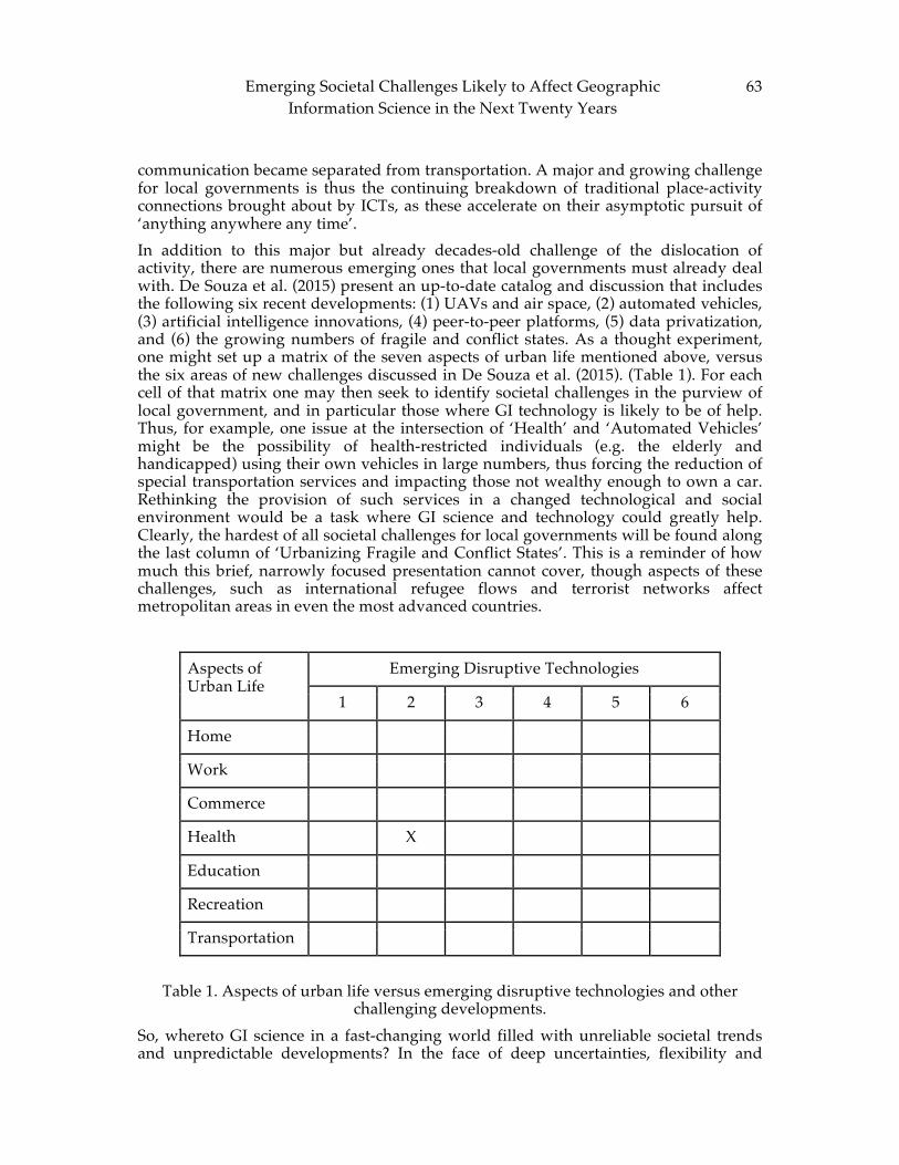
Emerging Societal Challenges Likely to Affect Geographic Information Science in the Next Twenty Years
63
communication became separated from transportation. A major and growing challenge for local governments is thus the continuing breakdown of traditional place-activity connections brought about by ICTs, as these accelerate on their asymptotic pursuit of ‘anything anywhere any time’. In addition to this major but already decades-old challenge of the dislocation of activity, there are numerous emerging ones that local governments must already deal with. De Souza et al. (2015) present an up-to-date catalog and discussion that includes the following six recent developments: (1) UAVs and air space, (2) automated vehicles, (3) artificial intelligence innovations, (4) peer-to-peer platforms, (5) data privatization, and (6) the growing numbers of fragile and conflict states. As a thought experiment, one might set up a matrix of the seven aspects of urban life mentioned above, versus the six areas of new challenges discussed in De Souza et al. (2015). (Table 1). For each cell of that matrix one may then seek to identify societal challenges in the purview of local government, and in particular those where GI technology is likely to be of help. Thus, for example, one issue at the intersection of ‘Health’ and ‘Automated Vehicles’ might be the possibility of health-restricted individuals (e.g. the elderly and handicapped) using their own vehicles in large numbers, thus forcing the reduction of special transportation services and impacting those not wealthy enough to own a car. Rethinking the provision of such services in a changed technological and social environment would be a task where GI science and technology could greatly help. Clearly, the hardest of all societal challenges for local governments will be found along the last column of ‘Urbanizing Fragile and Conflict States’. This is a reminder of how much this brief, narrowly focused presentation cannot cover, though aspects of these challenges, such as international refugee flows and terrorist networks affect metropolitan areas in even the most advanced countries.
Aspects of Urban Life
Emerging Disruptive Technologies
1 2 3 4 5 6
Home
Work
Commerce
Health X
Education
Recreation
Transportation
Table 1. Aspects of urban life versus emerging disruptive technologies and other challenging developments.
So, whereto GI science in a fast-changing world filled with unreliable societal trends and unpredictable developments? In the face of deep uncertainties, flexibility and
64 Ramasubramanian, Couclelis, and Midtbo adaptive capacity are key. Rather than striving to meet some specific research agenda, GI science must be rethought so as to be able to evolve, adapt to, and anticipate emerging needs and circumstances. This way GI science could be what it should be, at all times: user-oriented, problem centered, and multi-perspectival.
3 Discussion and Conclusions The discussants and commentators on the panel emphasized the need to avoid focusing on hypothetical problems and be pragmatic about the use and value of GI science to address serious and immediate concerns. They recommended the systematic consideration of both basic human needs (e.g., at the level of individuals and small groups) but also of more complex social needs (e.g., at the level of urban management, participation in government and governance). Both Roche and Buckley emphasized the need for GI scientists to work collaboratively with other disciplines, arguing that the GI science contribution was circumscribed and unique to the problem at hand. Campbell reminded the group about the need to engage with ethical considerations seriously, as each of these societal challenges and their resolution using different types of theoretical framings, methodological considerations, and data sources created their own sets of ethical challenges. Participants on the panel as well as the audience seemed divided between those who argued that the GI science community has a responsibility to propose new tools and solutions to help intervene through action – i.e. offer our expertise to serve society, and others who wondered whether such thoughts and beliefs were simply an act of hubris. The discussion was lively, but ultimately inconclusive. It is a foregone conclusion that the world is changing and will continue to do so in the next twenty years under the drivers of demographic shifts, rapid urbanization, climate change, and technological developments, among others. In particular, the advent of the Internet and the geoweb have resulted in advances that empower individuals greatly. However, major geo-political and societal divides persist or are being intensified by these technologies, ensuring that developments and innovations are not distributed evenly. The role that GI Scientists can and should play is far from clear, with many in this scholarly community viewing themselves as fairly narrow, subject matter experts, qualified to participate in collaborative problem solving endeavors, rather than being creators, advocates, or influencers of science-driven and evidence-based policy change. Regardless of their particular positionalities, all GI Scientists must be clear-eyed about the social and ethical implications of their work.
References [1] Desouza, K, Swindell, D, Smith, K.L, Sutherland, A, Fedorschak, K, and C.
Coronel, 2015. Local government 2035: Strategic trends and implications of new technologies. Issues in Technology Innovation, No. 27, May 2015. Washington, D.C: The Brookings Institution. http://www.brookings.edu/research/papers/2015/05/29-local-government-strategic-trends-desouzaxx
ADVANCING GEOGRAPHIC INFORMATION SCIENCE: CHAPTER 5
© by the author(s) Licensed under Creative Commons Attribution 4.0 License
65
From Body of Knowledge to Base-Map: Managing Domain Knowledge
through Collaboration and Computation
Sean C. Ahearn 1and André Skupin 2 1 Center for Advanced Research of Spatial Information, Department of Geography, Hunter
College, New York, NY 10065 USA 2 Center for Information Convergence and Strategy, Department of Geography, San Diego State
University, San Diego, CA 92182, USA
Abstract: This paper describes a body of knowledge technological implementation for domain knowledge management. The system enables collaboration, exploration, and exploitation of domain knowledge through a front-end visual wiki, an ontology-driven knowledge base and Web services. The service-based architecture enables applications that allow knowledge artifacts to be related to domain concepts through inference and such relationships to be visualized. Essential to the design and operation of the system are such notions as reference system and base map borrowed from traditional mapping. This includes the idea of a domain base map onto which any domain artifact can be projected. We hypothesize that this type of system may break to down traditional boundaries, such as between educators, students, researchers, and professionals.
Keywords: Ontology, knowledge domains, reference systems, base maps, visualization, wiki, collaboration, body of knowledge.
1 Introduction There is a critical need to improve the construction and dissemination of knowledge within and across the many communities that constitute a knowledge domain. Scientific research, academic education, technical training, and professional practice are driven by seemingly disparate concerns, and there tends to be little interaction between these sub-communities. As a result, cutting-edge research is often slow to transition into professional practice, while educational activities and materials often do not represent the current state of research and practice. Similar inefficiencies
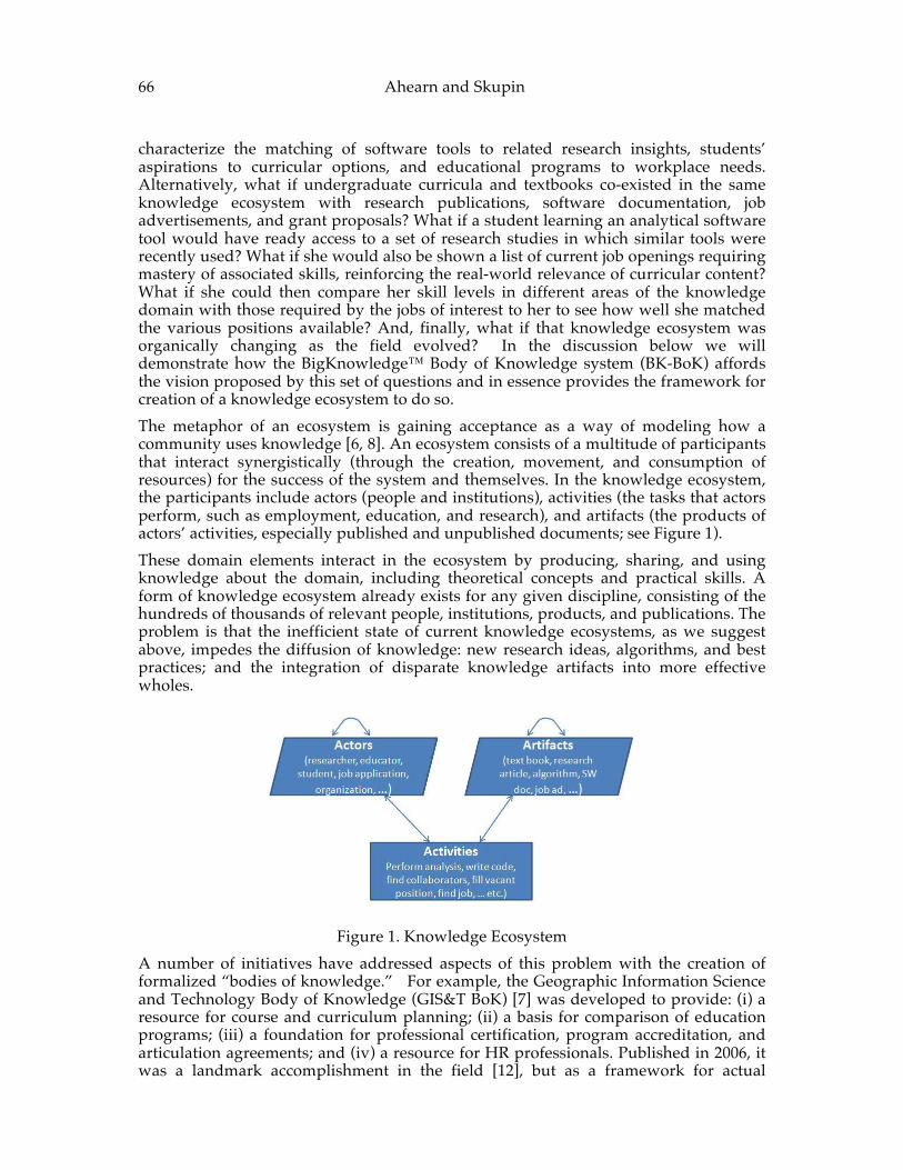
66 Ahearn and Skupin characterize the matching of software tools to related research insights, students’ aspirations to curricular options, and educational programs to workplace needs. Alternatively, what if undergraduate curricula and textbooks co-existed in the same knowledge ecosystem with research publications, software documentation, job advertisements, and grant proposals? What if a student learning an analytical software tool would have ready access to a set of research studies in which similar tools were recently used? What if she would also be shown a list of current job openings requiring mastery of associated skills, reinforcing the real-world relevance of curricular content? What if she could then compare her skill levels in different areas of the knowledge domain with those required by the jobs of interest to her to see how well she matched the various positions available? And, finally, what if that knowledge ecosystem was organically changing as the field evolved? In the discussion below we will demonstrate how the BigKnowledge™ Body of Knowledge system (BK-BoK) affords the vision proposed by this set of questions and in essence provides the framework for creation of a knowledge ecosystem to do so. The metaphor of an ecosystem is gaining acceptance as a way of modeling how a community uses knowledge [6, 8]. An ecosystem consists of a multitude of participants that interact synergistically (through the creation, movement, and consumption of resources) for the success of the system and themselves. In the knowledge ecosystem, the participants include actors (people and institutions), activities (the tasks that actors perform, such as employment, education, and research), and artifacts (the products of actors’ activities, especially published and unpublished documents; see Figure 1). These domain elements interact in the ecosystem by producing, sharing, and using knowledge about the domain, including theoretical concepts and practical skills. A form of knowledge ecosystem already exists for any given discipline, consisting of the hundreds of thousands of relevant people, institutions, products, and publications. The problem is that the inefficient state of current knowledge ecosystems, as we suggest above, impedes the diffusion of knowledge: new research ideas, algorithms, and best practices; and the integration of disparate knowledge artifacts into more effective wholes.
Figure 1. Knowledge Ecosystem
A number of initiatives have addressed aspects of this problem with the creation of formalized “bodies of knowledge.” For example, the Geographic Information Science and Technology Body of Knowledge (GIS&T BoK) [7] was developed to provide: (i) a resource for course and curriculum planning; (ii) a basis for comparison of education programs; (iii) a foundation for professional certification, program accreditation, and articulation agreements; and (iv) a resource for HR professionals. Published in 2006, it was a landmark accomplishment in the field [12], but as a framework for actual
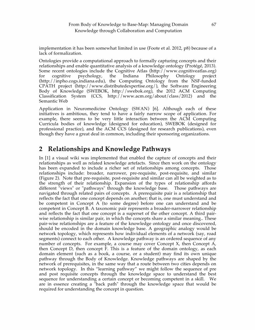
From Body of Knowledge to Base-‐‑Map: Managing Domain Knowledge through Collaboration and Computation
67
implementation it has been somewhat limited in use (Foote et al. 2012, p8) because of a lack of formalization. Ontologies provide a computational approach to formally capturing concepts and their relationships and enable quantitative analysis of a knowledge ontology (Protégé, 2013). Some recent ontologies include the Cognitive Atlas (http://www.cognitiveatlas.org) for cognitive psychology, the Indiana Philosophy Ontology project (http://inpho.cogs.indiana.edu), the Computing Ontology from the NSF-funded CPATH project (http://www.distributedexpertise.org/), the Software Engineering Body of Knowledge (SWEBOK, http://swebok.org), the 2012 ACM Computing Classification System (CCS, http://www.acm.org/about/class/2012) and the Semantic Web Application in Neuromedicine Ontology (SWAN) [6]. Although each of these initiatives is ambitious, they tend to have a fairly narrow scope of application. For example, there seems to be very little interaction between the ACM Computing Curricula bodies of knowledge (designed for education), SWEBOK (designed for professional practice), and the ACM CCS (designed for research publications), even though they have a great deal in common, including their sponsoring organizations.
2 Relationships and Knowledge Pathways In [1] a visual wiki was implemented that enabled the capture of concepts and their relationships as well as related knowledge artefacts. Since then work on the ontology has been expanded to include a richer set of relationships among concepts. Those relationships include: broader, narrower, pre-requisite, post-requisite, and similar (Figure 2). Note that pre-requisite, post-requisite and similar can all be weighted as to the strength of their relationship. Expansion of the types of relationship affords different "views" or "pathways" through the knowledge base. Those pathways are navigated through related pairs of concepts. A prerequisite pair is a relationship that reflects the fact that one concept depends on another; that is, one must understand and be competent in Concept A (to some degree) before one can understand and be competent in Concept B. A taxonomic pair represents a broader-narrower relationship and reflects the fact that one concept is a superset of the other concept. A third pair- wise relationship is similar pair, in which the concepts share a similar meaning.. These pair-wise relationships are a feature of the knowledge ontology and once discovered, should be encoded in the domain knowledge base. A geographic analogy would be network topology, which represents how individual elements of a network (say, road segments) connect to each other. A knowledge pathway is an ordered sequence of any number of concepts. For example, a course may cover Concept X, then Concept A, then Concept D, then concept F. This is a feature of the domain ontology, as each domain element (such as a book, a course, or a student) may find its own unique pathway through the Body of Knowledge. Knowledge pathways are shaped by the network of prerequisites, in the same way that a route between two cities depends on network topology. In this “learning pathway” we might follow the sequence of pre and post requisite concepts through the knowledge space to understand the best sequence for understanding a certain concept or becoming competent in a skill. We are in essence creating a "back path" through the knowledge space that would be required for understanding the concept in question.
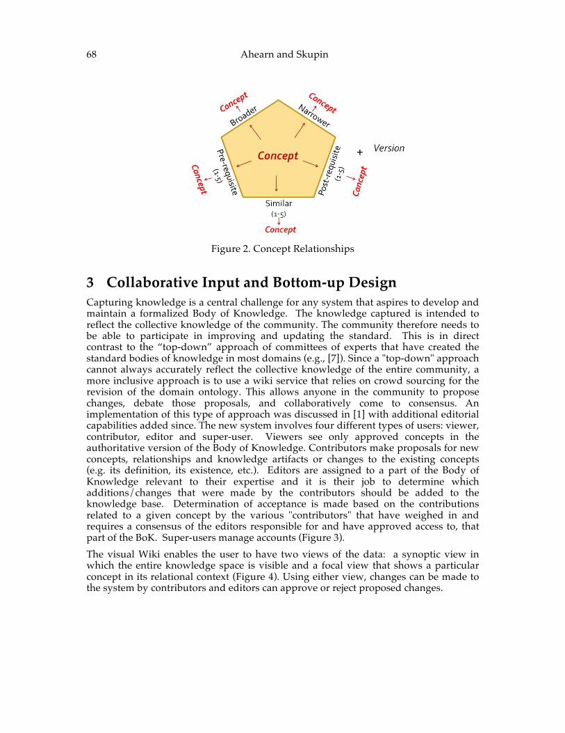
68 Ahearn and Skupin
Figure 2. Concept Relationships
3 Collaborative Input and Bottom-‐‑up Design Capturing knowledge is a central challenge for any system that aspires to develop and maintain a formalized Body of Knowledge. The knowledge captured is intended to reflect the collective knowledge of the community. The community therefore needs to be able to participate in improving and updating the standard. This is in direct contrast to the “top-down” approach of committees of experts that have created the standard bodies of knowledge in most domains (e.g., [7]). Since a "top-down" approach cannot always accurately reflect the collective knowledge of the entire community, a more inclusive approach is to use a wiki service that relies on crowd sourcing for the revision of the domain ontology. This allows anyone in the community to propose changes, debate those proposals, and collaboratively come to consensus. An implementation of this type of approach was discussed in [1] with additional editorial capabilities added since. The new system involves four different types of users: viewer, contributor, editor and super-user. Viewers see only approved concepts in the authoritative version of the Body of Knowledge. Contributors make proposals for new concepts, relationships and knowledge artifacts or changes to the existing concepts (e.g. its definition, its existence, etc.). Editors are assigned to a part of the Body of Knowledge relevant to their expertise and it is their job to determine which additions/changes that were made by the contributors should be added to the knowledge base. Determination of acceptance is made based on the contributions related to a given concept by the various "contributors" that have weighed in and requires a consensus of the editors responsible for and have approved access to, that part of the BoK. Super-users manage accounts (Figure 3). The visual Wiki enables the user to have two views of the data: a synoptic view in which the entire knowledge space is visible and a focal view that shows a particular concept in its relational context (Figure 4). Using either view, changes can be made to the system by contributors and editors can approve or reject proposed changes.
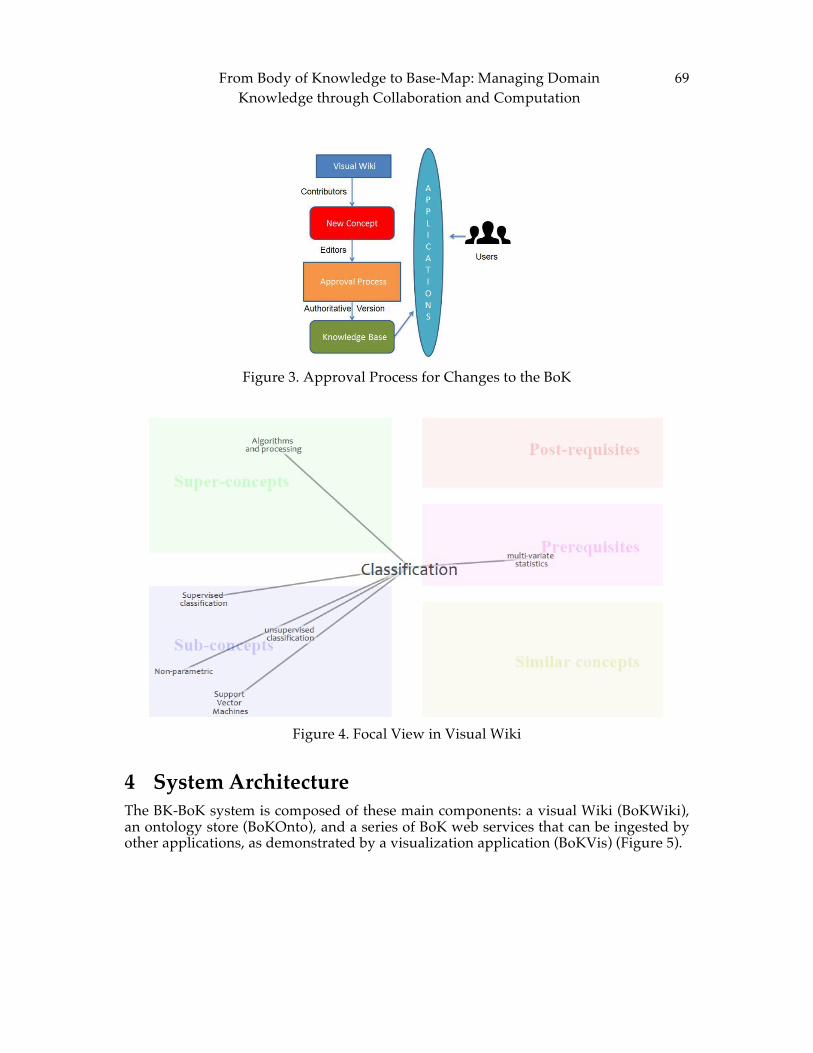
From Body of Knowledge to Base-‐‑Map: Managing Domain Knowledge through Collaboration and Computation
69
Figure 3. Approval Process for Changes to the BoK
Figure 4. Focal View in Visual Wiki
4 System Architecture The BK-BoK system is composed of these main components: a visual Wiki (BoKWiki), an ontology store (BoKOnto), and a series of BoK web services that can be ingested by other applications, as demonstrated by a visualization application (BoKVis) (Figure 5).
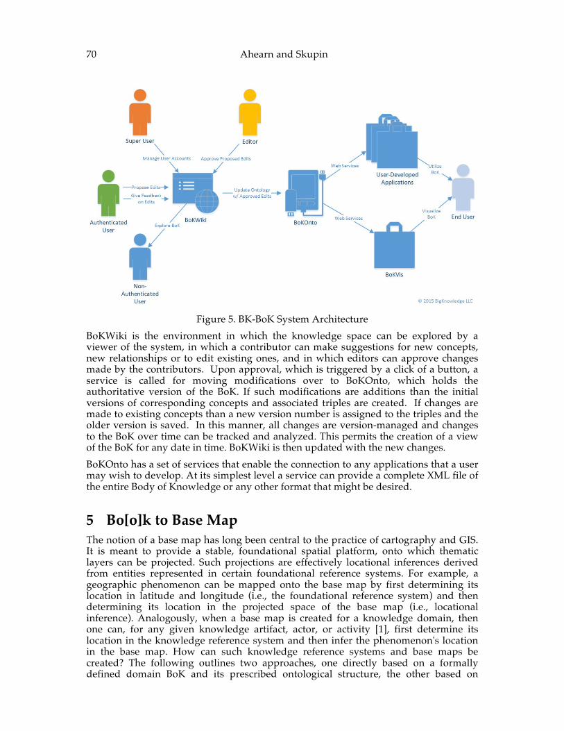
70 Ahearn and Skupin
Figure 5. BK-BoK System Architecture
BoKWiki is the environment in which the knowledge space can be explored by a viewer of the system, in which a contributor can make suggestions for new concepts, new relationships or to edit existing ones, and in which editors can approve changes made by the contributors. Upon approval, which is triggered by a click of a button, a service is called for moving modifications over to BoKOnto, which holds the authoritative version of the BoK. If such modifications are additions than the initial versions of corresponding concepts and associated triples are created. If changes are made to existing concepts than a new version number is assigned to the triples and the older version is saved. In this manner, all changes are version-managed and changes to the BoK over time can be tracked and analyzed. This permits the creation of a view of the BoK for any date in time. BoKWiki is then updated with the new changes. BoKOnto has a set of services that enable the connection to any applications that a user may wish to develop. At its simplest level a service can provide a complete XML file of the entire Body of Knowledge or any other format that might be desired.
5 Bo[o]k to Base Map The notion of a base map has long been central to the practice of cartography and GIS. It is meant to provide a stable, foundational spatial platform, onto which thematic layers can be projected. Such projections are effectively locational inferences derived from entities represented in certain foundational reference systems. For example, a geographic phenomenon can be mapped onto the base map by first determining its location in latitude and longitude (i.e., the foundational reference system) and then determining its location in the projected space of the base map (i.e., locational inference). Analogously, when a base map is created for a knowledge domain, then one can, for any given knowledge artifact, actor, or activity [1], first determine its location in the knowledge reference system and then infer the phenomenon's location in the base map. How can such knowledge reference systems and base maps be created? The following outlines two approaches, one directly based on a formally defined domain BoK and its prescribed ontological structure, the other based on
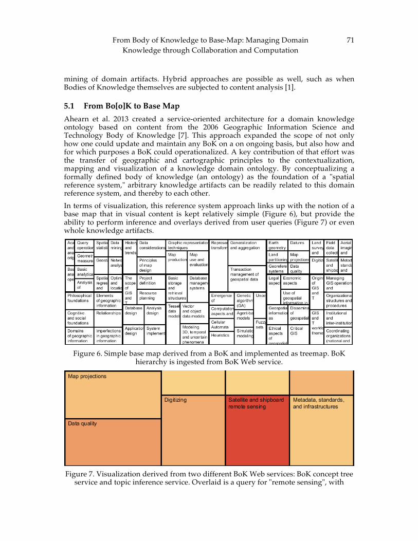
From Body of Knowledge to Base-‐‑Map: Managing Domain Knowledge through Collaboration and Computation
71
mining of domain artifacts. Hybrid approaches are possible as well, such as when Bodies of Knowledge themselves are subjected to content analysis [1].
5.1 From Bo[o]K to Base Map Ahearn et al. 2013 created a service-oriented architecture for a domain knowledge ontology based on content from the 2006 Geographic Information Science and Technology Body of Knowledge [7]. This approach expanded the scope of not only how one could update and maintain any BoK on a on ongoing basis, but also how and for which purposes a BoK could operationalized. A key contribution of that effort was the transfer of geographic and cartographic principles to the contextualization, mapping and visualization of a knowledge domain ontology. By conceptualizing a formally defined body of knowledge (an ontology) as the foundation of a "spatial reference system," arbitrary knowledge artifacts can be readily related to this domain reference system, and thereby to each other. In terms of visualization, this reference system approach links up with the notion of a base map that in visual content is kept relatively simple (Figure 6), but provide the ability to perform inference and overlays derived from user queries (Figure 7) or even whole knowledge artifacts.
Figure 6. Simple base map derived from a BoK and implemented as treemap. BoK
hierarchy is ingested from BoK Web service.
Figure 7. Visualization derived from two different BoK Web services: BoK concept tree
service and topic inference service. Overlaid is a query for "remote sensing", with
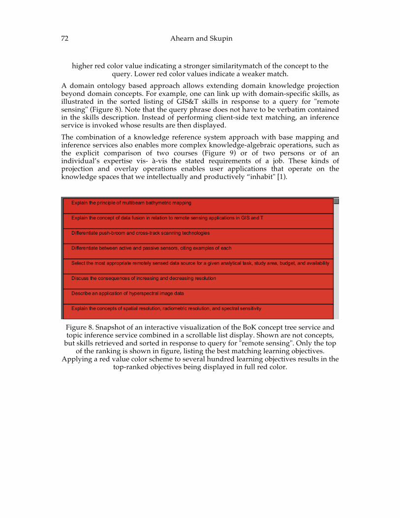
72 Ahearn and Skupin
higher red color value indicating a stronger similaritymatch of the concept to the query. Lower red color values indicate a weaker match.
A domain ontology based approach allows extending domain knowledge projection beyond domain concepts. For example, one can link up with domain-specific skills, as illustrated in the sorted listing of GIS&T skills in response to a query for "remote sensing" (Figure 8). Note that the query phrase does not have to be verbatim contained in the skills description. Instead of performing client-side text matching, an inference service is invoked whose results are then displayed. The combination of a knowledge reference system approach with base mapping and inference services also enables more complex knowledge-algebraic operations, such as the explicit comparison of two courses (Figure 9) or of two persons or of an individual’s expertise vis- à-vis the stated requirements of a job. These kinds of projection and overlay operations enables user applications that operate on the knowledge spaces that we intellectually and productively “inhabit" [1).
Figure 8. Snapshot of an interactive visualization of the BoK concept tree service and topic inference service combined in a scrollable list display. Shown are not concepts,
but skills retrieved and sorted in response to query for "remote sensing". Only the top of the ranking is shown in figure, listing the best matching learning objectives.
Applying a red value color scheme to several hundred learning objectives results in the top-ranked objectives being displayed in full red color.
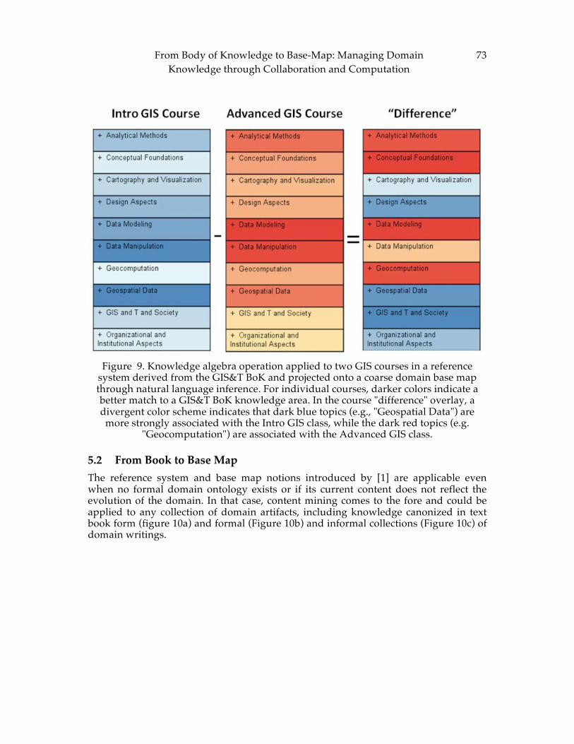
From Body of Knowledge to Base-‐‑Map: Managing Domain Knowledge through Collaboration and Computation
73
Figure 9. Knowledge algebra operation applied to two GIS courses in a reference
system derived from the GIS&T BoK and projected onto a coarse domain base map through natural language inference. For individual courses, darker colors indicate a better match to a GIS&T BoK knowledge area. In the course "difference" overlay, a divergent color scheme indicates that dark blue topics (e.g., "Geospatial Data") are
more strongly associated with the Intro GIS class, while the dark red topics (e.g. "Geocomputation") are associated with the Advanced GIS class.
5.2 From Book to Base Map The reference system and base map notions introduced by [1] are applicable even when no formal domain ontology exists or if its current content does not reflect the evolution of the domain. In that case, content mining comes to the fore and could be applied to any collection of domain artifacts, including knowledge canonized in text book form (figure 10a) and formal (Figure 10b) and informal collections (Figure 10c) of domain writings.
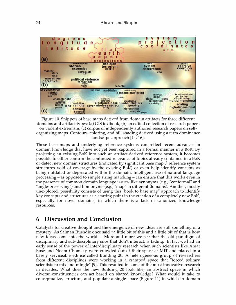
74 Ahearn and Skupin
Figure 10. Snippets of base maps derived from domain artifacts for three different
domains and artifact types: (a) GIS textbook, (b) an edited collection of research papers on violent extremism, (c) corpus of independently authored research papers on self-
organizing maps. Contours, coloring, and hill shading derived using a term dominance landscape approach [14, 16].
These base maps and underlying reference systems can reflect recent advances in domain knowledge that have not yet been captured in a formal manner in a BoK. By projecting an existing BoK into such an artifact-derived reference system, it becomes possible to either confirm the continued relevance of topics already contained in a BoK or detect new domain structures (indicated by significant base map / reference system structures void of coverage by the existing BoK) or even help identify concepts as being outdated or deprecated within the domain. Intelligent use of natural language processing – as opposed to simple string matching – can ensure that this works even in the presence of common domain language issues, like synonyms (e.g., "conformal" and "angle-preserving") and homonyms (e.g., "map" in different domains). Another, mostly unexplored, possibility consists of using this "book to base map" approach to identify key concepts and structures as a starting point in the creation of a completely new BoK, especially for novel domains, in which there is a lack of canonized knowledge resources.
6 Discussion and Conclusion Catalysts for creative thought and the emergence of new ideas are still something of a mystery. As Salman Rushdie once said “a little bit of this and a little bit of that is how new ideas come into the world”. More and more we see that the old paradigm of disciplinary and sub-disciplinary silos that don’t interact, is fading. In fact we had an early sense of the power of interdisciplinary research when such scientists like Amar Bose and Noam Chomsky were crowded out of their space at MIT and placed in a barely serviceable edifice called Building 20. A heterogeneous group of researchers from different disciplines were working in a cramped space that "forced solitary scientists to mix and mingle" [9]. This resulted in some of the most innovative research in decades. What does the new Building 20 look like, an abstract space in which diverse constituencies can act based on shared knowledge? What would it take to conceptualize, structure, and populate a single space (Figure 11) in which in domain
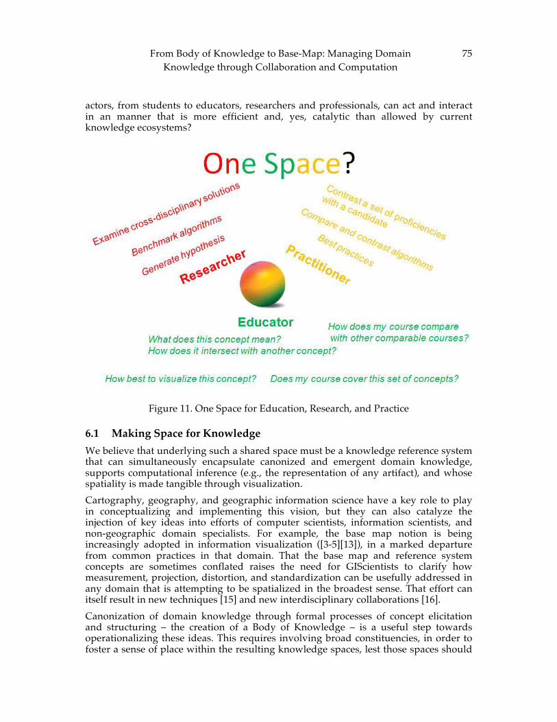
From Body of Knowledge to Base-‐‑Map: Managing Domain Knowledge through Collaboration and Computation
75
actors, from students to educators, researchers and professionals, can act and interact in an manner that is more efficient and, yes, catalytic than allowed by current knowledge ecosystems?
Figure 11. One Space for Education, Research, and Practice
6.1 Making Space for Knowledge We believe that underlying such a shared space must be a knowledge reference system that can simultaneously encapsulate canonized and emergent domain knowledge, supports computational inference (e.g., the representation of any artifact), and whose spatiality is made tangible through visualization. Cartography, geography, and geographic information science have a key role to play in conceptualizing and implementing this vision, but they can also catalyze the injection of key ideas into efforts of computer scientists, information scientists, and non-geographic domain specialists. For example, the base map notion is being increasingly adopted in information visualization ([3-5][13]), in a marked departure from common practices in that domain. That the base map and reference system concepts are sometimes conflated raises the need for GIScientists to clarify how measurement, projection, distortion, and standardization can be usefully addressed in any domain that is attempting to be spatialized in the broadest sense. That effort can itself result in new techniques [15] and new interdisciplinary collaborations [16]. Canonization of domain knowledge through formal processes of concept elicitation and structuring – the creation of a Body of Knowledge – is a useful step towards operationalizing these ideas. This requires involving broad constituencies, in order to foster a sense of place within the resulting knowledge spaces, lest those spaces should
76 Ahearn and Skupin remain "foreign lands" even for domain insiders. Wikification is a key strategy for capturing the breadth of domain concepts and for generation buy-in from the community. Another requirement is for the resulting knowledge structures to be made accessible to domain services, from human resource management to coordination of research activities. If a BoK is to form the sustainable heart of a domain knowledge ecosystem, then it has to be accessible through a variety of means and for many purposes, from knowledge management to exploration and analytics. The BK-BoK system discussed in the article provides such a framework, since it provides a front- end visual wiki (BokWiki), an ontology-driven knowledge base (BoKOnto), and a service-based architecture for enabling applications.
6.2 Putting Domain Knowledge to Work for Education Almost without exception, most BoKs have typically been created with the explicit and exclusive goal of supporting tasks in education, especially curricular planning. This has included efforts in the GIS&T domain [10-12]. Though [1] presented a vision significantly expanded beyond this, education and training is an arena where an overtly knowledge-centric approach to integration of actors, artifacts, and activities, including an elaboration of canonized and emergent practices, shows particular promise. A range of novel education applications can be envisioned, involving numerous elements of higher and vocational education, from faculty and administrators to students and the learning infrastructure, such as courseware. An operationalized domain knowledge reference system allows breaking down traditional barriers in the knowledge ecosystem. What if the theory-laden, long-term approaches of education and the hands-on, short-term view of training could be represented in a single space? What if core concepts could be explicitly linked to hands-on tools and real-world practices? For example, how could students quickly find mappings between the concept of "functional distance," a GIS software tool for computing "cost distance," and a map of hospital service areas published by a county health and human services agency? Other types of mappings supported by a reference system and base map approach include course articulation and course equivalency, which can now be represented in overtly spatial terms, by identifying overlaps and gaps. The explicit linking of concepts, skills, tools, and literature through ontological relationships allows tracking students' progress in a number of ways. For example, instructors could project individual performance results into the knowledge space to identify which tasks students found especially challenging and take note of the associated concepts. This would create a whole new dynamic in pedagogy: interactive, expansive, and comprehensive. The ability to project learning outcomes into a common space also allows comparison of different instructional modes, such as traditional lecture-lab approaches versus the various forms of flipped learning [2].
References [1] Ahearn, S.C., Icke, I., Datta, R., DeMers, M.N. Plewe, B., and Skupin, A. (2013)
Re-engineering the GIS&T Body of Knowledge. International Journal of Geographical Information Science 27(11), 2227-2245.
[2] Bishop, J.L. and Verlerger, M.A. (2013) The Flipped Classrom: A Survey of the Research. ASEE Annual Conference and Exposition, June 23-26, 2013, Atlanta, Georgia.
From Body of Knowledge to Base-‐‑Map: Managing Domain Knowledge through Collaboration and Computation
77
[3] Börner, K. (2010) Atlas of Science: Visualizing What We Know. MIT Press. [4] Börner, K. (2015) Atlas of Knowledge: Anyone Can Map. MIT Press. [5] Chen, C., Cribbin, T., Macredie, R., and Morar, S. (2002) Visualizing and Tracking
the Growth of Competing Paradigms. Journal of the American Society for Information Science and Technology 53(8): 678-689.
[6] Ciccarese, Elizabeth Wu, Gwen Wong, Marco Ocana, June Kinoshita, Alan Ruttenberg, and Tim Clark (2008). The SWAN biomedical discourse ontology, Journal of Biomedical Informatics 41:739–751.
[7] DiBiase, David, Michael Demers, Ann Johnson, Karen Kemp, Ann Taylor Luck, Brandon Plewe, and Elizabeth Wentz, eds. (2006) Geographic Information Science and Technology Body of Knowledge. Assocation of American Geographers.
[8] Foote, Kenneth E., et al. "GIS&T in higher education: Challenges for educators, opportunities for education." Teaching geographic information science and technology in higher education (2012): 3-15.
[9] Gao, Yong, June Kinoshita, Elizabeth Wu, Eric Miller, Ryan Lee, Andy Seaborne, Steve Cayzer, Tim Clark (2006) SWAN: A distributed knowledge infrastructure for Alzheimer disease research, ScienceDirect, Web Semantics: Science, Services and Agents on the World Wide Web, 4:222-228.
[10] Lehrer, J. (2012) GROUPTHINK: The Brainstorming Myth. The New Yorker 87(46): 22-27.
[11] Prager, S., and Plewe, B. (2009) Assessment and Evaluation of GIScience Curriculum using the Geographic Information Science and Technology Body of Knowledge, Journal of Geography in Higher Education, 33: 46-69.
[12] Prager, S. (2011) Using the GIS&T Body of Knowledge for Curriculum Design: Different Design for Different Contexts. In: Unwin, D.J., Foote, K.E., Tate, N.T., and DiBiase, D. (Eds.) Teaching Geographic Information Science and Technology in Higher Education. Chichester, UK: John Wiley & Sons, Ltd. 63-80.
[13] Rip, Frans (2008) GIS&T Body of Knowledge: basis for e-learning, certification and curriculum planning? Proceedings of the Eleventh Annual AGILE Conference.
[14] Skupin, A. (2000). From metaphor to method: Cartographic perspectives on information visualization. In IEEE Symposium on Information Visualization (InfoVis 2000), IEEE: 91-97.
[15] Skupin, A. (2004) The World of Geography: Visualizing a Knowledge Domain with Cartographic Means. Proceedings of the National Academy of Sciences. 101 (Suppl. 1): 5274-5278.
[16] Skupin, A. (2009). Discrete and continuous conceptualizations of science: Implications for knowledge domain visualization. Journal of Informetrics, 3(3): 233-245.
[17] Skupin, A., Biberstine, J. R., and Börner, K. (2013). Visualizing the topical structure of the medical sciences: a self-organizing map approach. PloS ONE, 8(3), e58779.

78 Ahearn and Skupin
ADVANCING GEOGRAPHIC INFORMATION SCIENCE: CHAPTER 6
© by the author(s) Licensed under Creative Commons Attribution 4.0 License
79
Towards a Theory of GIS Program Management
Jochen Albrecht Department of Geography, Hunter College, CUNY, 695 Park Ave, New York, NY 10065, USA
Abstract: After a brief flurry of monographs on business and organizational aspects of GIS in the 1990s, little attention has been paid to a systematic approach in support of GIS Program management. Most existing efforts in both public and private enterprises are based on anecdotal evidence. This chapter outlines a range of research questions and the beginning efforts to study modern GIS management practices and help develop a body of knowledge that can be used for the accreditation of GIS Programs and the certification of GIS Program managers.
Keywords: Enterprise GIS, strategic planning, cost benefit evaluation, human resources, funding, governance, capability maturity model, management competency model.
1 Introduction GIS has grown up. We do not need to explain the acronym anymore; everybody knows what it is and everybody seems to be using it. Or so they thinki. Text books of the late 20th century spent a lot of time defining GIS; definitions that show little resemblance to how GIS users in 2015 understand GIS. Many current GIS applications are as easy to use as writing an email on a mobile device and the end user is well-shielded from the 'S' in GIS, the system that was all-important in the definitions of the 1990s. This chapter aims to provide academic support for the people who build and maintain such systems; not the programmers who help us to create ever faster indexes on unstructured data but the people who build the infrastructure that the easy to use applications depend on. Every organization that has multiple GIS users has de facto a GIS Program [1]. If the users get their work done and are not aware of the business unit that allows them to do their work, then this means that the program manager does her job well. If on the other hand every GIS project starts from scratch and the only institutional memory is buried in the heads of those who did other GIS projects before, then the tool that constitutes GIS is clearly not used to its highest potential. This chapter aims to rectify this all-too-
80 Albrecht common situation by providing an analysis of best practices. Even in organizations that have an official GIS Program manager, this person more often than not has reached their position by seniority and learned by trial and error what works and what doesn't [2]. As mature as GIS is from a technical perspective [3], GIS Program management is still haphazard [4] and the best a GIS Program manager could do up to now is to talk to peers in a social network built over decades of professional experience [5]. The professionalization of GIS has made good progress [6]. GIS certificates, both academic and vendor-driven abound and several professional organizations have developed their own set of certifications for GIS technicians [7-10]; i.e., the bottom strung of a hierarchy of GIS professionals [11]. There is, or at least has not been, a corresponding body of knowledge for higher level GIS professionals or managers, which is surprising given that there are thousands of GIS departments in the United States alone. King County’s (Seattle) GIS department, for instance, has 28 staff and spends over $5 million to support some 35 business units throughout the county [12]. Running such a unit could be seen as a public administration [13] or more generally a management science [14] task. But similar to GIScience being different from general information science [15], the body of knowledge in support of a GIS Program is different and needs to be codified. This necessity is underlined by the creation of the GIS Management Institute (GMI) that requires a scientific foundation for its accreditation of GIS Programs and the certification of GIS Program managers [16].
2 The Widening Gap between Bodies of Knowledge There was a wave of interest in the fledgling GIScience literature on organizational and management aspects of GIS in the late 1990s [17-20] that has barely been kept alive in later years by vendor-sponsored monographs [21, 22]. But things have understandably since changed with respect to technology (from client-server to PC to web services) as well as the role of GIS in many organizations. The better academic departments are doing a good job teaching GIS project management [23] but there is only one school in the United States that offers a degree in GIS Management [24]. In spite of the flurry of publications in the 1990s, GIScience has not been acknowledged in the world of business schools [25]. At the same time, new standards [26 -28] have been widely adopted in the business community but are virtually unknown in the academic world. The PMI defines program management as “the application of knowledge, skills, tools, and techniques to a program to meet the program requirements and to obtain benefits and control not available by managing projects individually”, [27, p. 6]. The scope of programs is hence beyond the sum of individual projects and includes training, operations and maintenance activities. All this applied to GIS Programs as well. Two dimensions are useful to keep in mind when there is confusion about the differences between projects and programs:
• Uncertainty; well-managed projects generally have a low level of uncertainty associated with them. This starts with project specification and improves as a project moves towards its goal. Programs, on the other hand do not start out with a well-defined scope and require continuous adjustment. In extreme cases, a successful project may still be abandoned because its program context has changed.
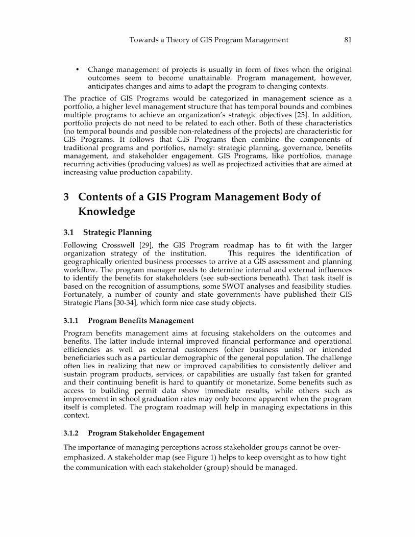
Towards a Theory of GIS Program Management 81
• Change management of projects is usually in form of fixes when the original outcomes seem to become unattainable. Program management, however, anticipates changes and aims to adapt the program to changing contexts.
The practice of GIS Programs would be categorized in management science as a portfolio, a higher level management structure that has temporal bounds and combines multiple programs to achieve an organization’s strategic objectives [25]. In addition, portfolio projects do not need to be related to each other. Both of these characteristics (no temporal bounds and possible non-relatedness of the projects) are characteristic for GIS Programs. It follows that GIS Programs then combine the components of traditional programs and portfolios, namely: strategic planning, governance, benefits management, and stakeholder engagement. GIS Programs, like portfolios, manage recurring activities (producing values) as well as projectized activities that are aimed at increasing value production capability.
3 Contents of a GIS Program Management Body of Knowledge
3.1 Strategic Planning Following Crosswell [29], the GIS Program roadmap has to fit with the larger organization strategy of the institution. This requires the identification of geographically oriented business processes to arrive at a GIS assessment and planning workflow. The program manager needs to determine internal and external influences to identify the benefits for stakeholders (see sub-sections beneath). That task itself is based on the recognition of assumptions, some SWOT analyses and feasibility studies. Fortunately, a number of county and state governments have published their GIS Strategic Plans [30-34], which form nice case study objects.
3.1.1 Program Benefits Management
Program benefits management aims at focusing stakeholders on the outcomes and benefits. The latter include internal improved financial performance and operational efficiencies as well as external customers (other business units) or intended beneficiaries such as a particular demographic of the general population. The challenge often lies in realizing that new or improved capabilities to consistently deliver and sustain program products, services, or capabilities are usually fast taken for granted and their continuing benefit is hard to quantify or monetarize. Some benefits such as access to building permit data show immediate results, while others such as improvement in school graduation rates may only become apparent when the program itself is completed. The program roadmap will help in managing expectations in this context.
3.1.2 Program Stakeholder Engagement
The importance of managing perceptions across stakeholder groups cannot be over-‐‑ emphasized. A stakeholder map (see Figure 1) helps to keep oversight as to how tight the communication with each stakeholder (group) should be managed.
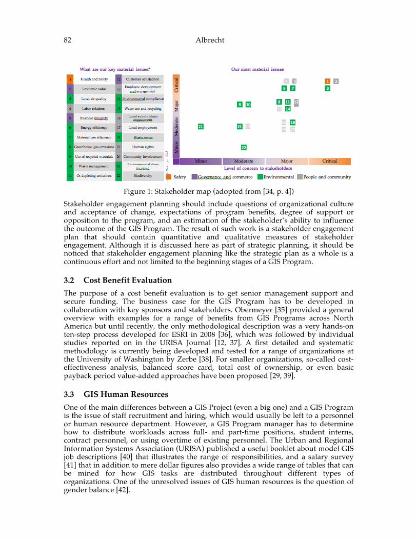
82 Albrecht
Figure 1: Stakeholder map (adopted from [34, p. 4])
Stakeholder engagement planning should include questions of organizational culture and acceptance of change, expectations of program benefits, degree of support or opposition to the program, and an estimation of the stakeholder’s ability to influence the outcome of the GIS Program. The result of such work is a stakeholder engagement plan that should contain quantitative and qualitative measures of stakeholder engagement. Although it is discussed here as part of strategic planning, it should be noticed that stakeholder engagement planning like the strategic plan as a whole is a continuous effort and not limited to the beginning stages of a GIS Program.
3.2 Cost Benefit Evaluation The purpose of a cost benefit evaluation is to get senior management support and secure funding. The business case for the GIS Program has to be developed in collaboration with key sponsors and stakeholders. Obermeyer [35] provided a general overview with examples for a range of benefits from GIS Programs across North America but until recently, the only methodological description was a very hands-on ten-step process developed for ESRI in 2008 [36], which was followed by individual studies reported on in the URISA Journal [12, 37]. A first detailed and systematic methodology is currently being developed and tested for a range of organizations at the University of Washington by Zerbe [38]. For smaller organizations, so-called cost- effectiveness analysis, balanced score card, total cost of ownership, or even basic payback period value-added approaches have been proposed [29, 39].
3.3 GIS Human Resources One of the main differences between a GIS Project (even a big one) and a GIS Program is the issue of staff recruitment and hiring, which would usually be left to a personnel or human resource department. However, a GIS Program manager has to determine how to distribute workloads across full- and part-time positions, student interns, contract personnel, or using overtime of existing personnel. The Urban and Regional Information Systems Association (URISA) published a useful booklet about model GIS job descriptions [40] that illustrates the range of responsibilities, and a salary survey [41] that in addition to mere dollar figures also provides a wide range of tables that can be mined for how GIS tasks are distributed throughout different types of organizations. One of the unresolved issues of GIS human resources is the question of gender balance [42].
Towards a Theory of GIS Program Management 83
3.3.1 From Geospatial Technology Competency to Geospatial Management Competency
The US Department of Labor released in 2010 a nine-tiered geospatial technology competency model that specifies foundational, industry-wide, industry sector-specific, and finally occupation-specific competencies [43] (see Figure 2). It then contracted with URISA to develop a geospatial management competency model for the top tier of this pyramid [44]. It specifies 74 essential competencies and 18 competency areas that characterize the work of most successful managers in the geospatial industry. Its purpose is to guide individual professional development, to help people in move up or over in an organization or industry, to help educators and trainers develop curricula that address workforce needs, to inform development of interview protocols, as requirements for professional certification, and as criteria for academic program accreditation and articulation.
Figure 2: Geospatial competency model (adopted from [43, 44])
84 Albrecht 3.4 Financial Planning and Management
3.4.1 Costs
GIS Programs are often funded through line-items in the general fund—allocated through the organization’s budgeting process. In addition to funds allocated through the normal budgeting process in an organization, there are often other funding sources such as special funds or capital funds (for road or utility improvements) that are managed separate from the general fund. Among program management one can distinguish traditional project costs from those that are more often seen as “fixed costs” such as system infrastructure, tech support, application development, or finance management. We are used to projects to have costs overruns. These will have to be buffered in the larger context of the GIS Program – something that puts GIS Program managers into a difficult position, where she has to defend herself in all directions. Flexibility gained from a wider range of staffing options (including the secondment of employees from other departments) goes a long way to create such buffers.
3.4.2 Outsourcing
An increasingly popular option for minimizing long term costs is the notion of outsourcing and contracting. Web services cover potentially more and more of the above mentioned fixed costs. In addition, needs assessment, field work, and many data maintenance tasks are now seen as areas that do not require in-house expertise. The difficult part here is that outsourcing does not relinquish the organization from its role to manage and oversee the work, and to take overall responsibility for it. With increased reliance on outside vendors and contractors comes the issue of procurement. Traditionally the realm of a purchasing department, this is a prime example for where spatial is special, i.e., the expertise for running the complete workflow from the preparation of specifications and requests for information / qualifications / proposals / bids to review and contract preparation should lie within the GIS Program [29]. The need to incorporate legal counsel may cause this externalization of costs to become a rather drawn-out process. It is therefore the responsibility of the GIS Program manager to develop and maintain a good working relationship with the vendor/contractor.
3.5 The Technological Environment
3.5.1 Enterprise GIS
GIS Program management and enterprise GIS go hand in hand. An enterprise GIS without GIS Program management is unconceivable and the latter would be overkill if there is no wide adoption of GIS throughout the organization. The notion of an enterprise GIS assumes that multiple if not many business units are using GIS.
3.5.2 Components of a GIS Architecture
Although many businesses do not have a formal GIS architecture, enterprise GIS benefit immensely from an organized conceptual framework that enables the description and guides the construction and operation of complex GIS implementations. There is a large body of literature on architectural reference models and best practices [45, 46].
Towards a Theory of GIS Program Management 85
A solid architectural design is robust enough to cope with ever changing environments and demands. Examples for relatively recent demands that distinguish GIS architectures from general IT trends are: wireless data acquisition including real-time GPS/GNSS, “Open GIS” from desktop clients to web portals, web services and crowd- sourcing, coping with big data like LiDAR, CAD-GIS integration. Compared with most other business applications, GIS puts a much higher demand on the expertise and computational prowess of the IT infrastructure, which may in some instances cause the general IT department to be subsumed under the GIS Program. Given the above mentioned demands, enterprise GIS tend to put a much higher strain on security, database administration, and user support than traditional IT departments are used to. Even the development of technical standards (in-house as well as outside all the way up to the International Standards Organization (ISO)) requires faster training and continuing education cycles.
3.5.3 Maintaining the In-‐‑house GIS Database
GIS projects are usually not expansive enough to warrant the development of guidelines for data quality. It is therefore at the GIS Program level, that organization- wide data quality specifications should be developed and enforced. The FGDC has developed a widely accepted base standard [47], which may, however, have to be expanded to fit the mission of the enterprise. It is in this context worthwhile to consult further standards developed by ISO [48] and the Open Geospatial Consortium. The GIS Program manager is responsible for defining an enterprise-wide set of automated and manual checks both during (quality control) and after data editing (quality assurance). In some instances, this still involves data capture itself, but for most GIS programs, standardized procedures will have to be developed that ascertain that editing and analysis procedures are documented well enough to be reproducible.
3.6 GIS Program Governance
3.6.1 Reporting Structures and Responsibilities
Following directly from the previous section, a well-managed GIS Program has policies and practices for each of the categories listed in Table 1. These should be developed on a consensus basis and reviewed/revised on a regular basis.
Table 1: Categories of GIS Program Policies (adopted from [29]).
86 Albrecht 3.6.2 Legal Issues
Except for health and financial institutions, few other IT managers have to deal as many legal concerns as the GIS Program manager. In the widest sense, these have to do with access to and distribution of geographic information. Legal authority for access to public records is granted in the United States by the federal freedom of information act [49] that are augmented by state laws and local regulations such as right-to-know laws and sunshine acts. This is balanced by both security concerns and the threat of liability suits. A FGDC study [50] showed that security concerns are usually over-emphasized and that most of non-classified information is available through multiple pathways. Liability concerns are more difficult to deal with because the range of possible aggravations is so large. Reliability questions though are easiest to address by placing data into the public domain, which absolves authorities from almost any responsibility for inaccuracies [51] – but this contradicts another tenet of GIS Program management: to cover one’s costs through revenues [52]. Interagency agreements for cost and data sharing carry their own rules and should be adhered to if for no other reason than that it would erode trust if partners do not act in sync. With the transition from product to service delivery, the legal territory becomes ever more uncertain to the GIS manager because service providers usually exclude liability in case of service changes and traditional data backup procedures become obsolete.
4 GIS Capability Maturity Model (GISCMM) The GIS Management Institute developed a tool to assess levels of capability and maturity of an organization’s GIS operations [53]. The model was originally developed with a focus on local governments but is intended to be applicable to any enterprise GIS. The notion of a capability maturity model was originally developed by the Software Engineering Institute [54]. The capability maturity model is based on the characteristics of the organization’s approach to individual defined processes. These processes are usually defined as: Level 1 – Ad hoc (chaotic) processes-typically in reaction to a need to get something
done. Level 2 – Repeatable processes–typically based on recalling and repeating how the
process was done the last time. Level 3 – Defined process–the process is written down (documented) and serves to
guide consistent performance within the organization. Level 4 – Managed process–the documented process is measured when performed and
the measurements are compiled for analysis. Changing system conditions are managed by adapting the defined process to meet the conditions.
Level 5 – Optimized processes–The defined and managed process is improved on an on-going basis by institutionalized process improvement planning and implementation. Optimization may be tied to quantified performance goals.
The National States Geographic Information Council (NSGIC) identified in 2010 seven categories for which GIS capability maturity should be measured: (1) people, (2) data, (3) processes, (4) policy, (5) strategy, (6) technology, and (7) legal [55]. Within these
Towards a Theory of GIS Program Management 87
seven categories, the GMI chose to assess GIS organizations’ maturity on a 7-point scale in 56 specific detailed characteristics based on their current implementation of each characteristic. The GIS Capability Maturity Model assumes two broad areas of GIS operational development: enabling capability and execution ability. Enabling capability can be thought of as the technology, data, resources, and related infrastructure to support typical enterprise GIS operations. Enabling capability includes GIS management and professional staff. However, the ability (execution capability) of the staff to utilize the enabling technology at its disposal is subject to a separate assessment as part of the model.
5 Conclusions This chapter outlines a range of aspects in which the management of GIS projects and programs differ. The latter is a relatively undeveloped research area. Efforts to build a scientific foundation for program management practices just started with the development of a thorough return on investment study across a multitude of organization types [38]. Similarly, the data created by hundreds of organizations, who are as of 2015 conducting a GISCMM-based assessment will provide the foundation to build a generalizable body of knowledge for GIS Program management. Together with an analysis of best practices as identified, for example, through 35 years of peer review for the Exemplary Systems in Government Award [56], we are inching towards a theory of GIS Program Management
References [1] PETERS, P. Building a GIS. ESRI Press, Redlands, CA, 2008. [2] TOMLINSON, R. Thinking about GIS. ESRI Press, Redlands, CA, 2011. [3] ONSRUD, H. AND PINTO, J. Evaluating correlates of GIS adoption success and
the decision process of GIS acquisition. URISA Journal, 5, 1 (1993), 18-39. [4] BABINSKI, G: URISA Develops the Geospatial Management Competency Model
(GMCM) for USDOLETA. In Proceedings of WURISA GIS Conference 2012 (Tacoma, WA), http://www.waurisa.org/conferences/2012/presentations/05 Greg Babinski URISA Helps Develop the USDOL Geospatial Management Competency.pdf.
[5] OBERMEYER, N. The maturation of a profession. Cartography and Geographic Information Science, 34, 2 (2007), 129-132, DOI: 10.1559/152304007781002280.
[6] MCMASTER, R AND HARVEY, F. Geographic Information Science and Society. In Manual of Geospatial Science and Technology, J Bossler, Ed. CRC Press, Boca Raton, FL, 2010, ch 33, pp. 653-668.
[7] WIKLE, T. An examination of job titles used for GIScience professionals. In Geospatial Technologies and Advancing Geographic Decision Making, D Albert, Ed. IGI Global, Hershey, PA, 2012, ch 6, pp. 66-81 DOI: 10.4018978-1-4666-0258-8.ch006.
[8] JOHNSON, A. UCGIS Body of Knowledge, proposed and unanticipated benefits and possible future initiatives. In Proceedings seventh European GIS Education Seminar 2010 (Serres, Greece). http://eugises.eu/proceedings2008/johnson.pdf.
88 Albrecht [9] TRINDER, J. Competency standards, a measure of the quality of a workforce.
Proceedings 37th ISPRS Congress, Commission VI, WG VI/5, http://www.isprs.org/proceedings/xxxvii/congress/6a_pdf/5_wg-vi-5/01.pdf.
[10] PRAGER, S AND PLEWE, B. Assessment and evaluation of GIScience curriculum using the geographic information science and technology body of knowledge. Journal of Geography in Higher Education, 33, sup1 (2009), 46-69, DOI: 10.1080/03098260903034012.
[11] LUKINBEAL, C AND MONK, J. Master's in Geographic Information Systems Programs in the United States: Professional Education in GIS and Geography. The Professional Geographer, 67, 2 (2015), pp. xxx, DOI: 10.1080/00330124.2014.983630.
[12] BABINSKI, G. FUMIA, D. REYNOLDS, T, SINGH, P., SCOTT, T. AND ZERBE, R. An Analysis of Benefits From the Use of Geographic Information Systems by King County, Washington. 2012.
[13] SHAFRITZ, J. Classics of Public Administration. Wadsworth Publishing, Boston, 2012.
[14] DRUCKER, P. The Practice of Management. Harper Collins, 1954. [15] GOODCHILD, M. Twenty years of progress: GIScience in 2010. Journal of Spatial
Information Science, 1 (2010), 3-20. doi:10.5311/JOSIS.2010.1.2. [16] BUTLER, A. URISA starts the task of reorganizing for the future. The GIS
Professional, 252, 6-16. [17] CAMPBELL, H AND MASSER, I. GIS and Organizations. Taylor & Francis,
London, 1995. [18] HUXHOLD, W. AND LEVINSOHN, A. Managing Geographic Information
System Projects. Oxford University Press, New York, 1995. [19] FRANK, AU. Geographic information business in the next century. Proceedings
of Third Joint European Conference on Geographical Information, JEC-GI’97, Vienna, Vol. 1, pp: 13-22IOS Press.
[20] OBERMEYER, N AND PINTO, J. Managing Geographic Information Systems. Guilford Press, London, 2008.
[21] THOMAS, C AND OSPINA, M. Measuring Up: The Business Case for GIS. Redlands: ESRI Press, 2004.
[22] PETERS, D. System Design Strategies. ESRI Press, Redlands, CA, 2015. http://wiki.gis.com/wiki/index.php/System_Design_Strategies_Preface.
[23] GIS Project Management. Course home page for GEOG 584 as part of their online MGIS Program, 2015. https://www.e-education.psu.edu/geog584/l1_p7.html.
[24] SCOTT, M. Master of Science in GIS Management. Salisbury University, 2015, http://www.salisbury.edu/geography/msgism/docs/GIS_MS_Brochure_2011. pdf.
[25] DOUGLAS, B. Achieving Business Success with GIS. John Wiley, 2008. DOI: 10.1002/9780470985595.
[26] PMI. The standard for portfolio management. Program Management Institute, 2013.
Towards a Theory of GIS Program Management 89
[27] PMI. The standard for program management. Program Management Institute, 2013.
[28] PMI. A guide to the project management body of knowledge. Program Management Institute, 2013.
[29] CROSWELL, P. The GIS Management Handbook. Frankfort, KY: Kessey Dewitt Publications, 2009.
[30] WESTCHESTER COUNTY. Strategic Plan 2012. Department of Information Technology, Geographic Information Systems. http://giswww.westchestergov.com.
[31] APPLIED GEOGRAPHICS. State of New York Geographic Information System (GIS) Strategic Plan. NY State Office of Cyber Security and Critical Infrastructure Coordination, 2008.
[32] CITY OF ALEXANDRIA. Geographic Information Systems (GIS) Five-Year Strategic Plan 2013-2017. Department of Planning and Zoning, GIS Division, 2012.
[33] COUNTY OF LOS ANGELES. Enterprise Geographic Information Systems 2009 – 2012 Strategic Plan. Los Angeles Enterprise GIS, 2009
[34] APERAM. Sustainability Report 2013. Luxembourg. http://www.aperam.com/uploads/pdf/Sustainability/Aperam Sustainability Report 2013.pdf.
[35] OBERMEYER, N. Measuring the Benefits and Costs of GIS, In Geographical, Information Systems, Vol. 2, Management Issues and Applications, Abridged (M.F. Goodchild, P.A. Longley, D.J. Maguire, and D. W. Rhind (Eds.), pp. 255-264, John Wiley & Sons, 2005.
[36] MAGUIRE, D., KOUYOUMIJAN, V. And SMITH, R. The Business Benefits of GIS: An ROI Approach. Redlands: ESRI Press, 2008.
[37] JOFFE, B. Estimating GIS Return on Investment the Empirical Way. URISA Journal, 27, 1, pp. 2015.
[38] ZERBE, R. International GIS Return on Investment Study. URISA Journal, 27, 2, (in print).
[39] LONGLEY, P., GOODCHILD, M, MAGUIRE, D. AND RHIND, D. Geographic Information Systems and Science. John Wiley & Sons, 2005.
[40] BUTLER, A. Model GIS Job Descriptions. URISA, 2013. [41] URISA. 2014 Salary Survey for IT/GIS Professionals. URISA, 2015. [42] MAZUR, L. AND ALBRECHT, J. Women in GIS. The URISA Journal, 27, 2, (in
print). [43] DOLETA. Geospatial Technology Competency Model. US Department of Labor,
Employment and Training Administration, 2010 [44] URISA. Geospatial Management Competency Model. URISA GIS Management
Institute, 2012. [45] FGDC. Geospatial Profile of the Federal Enterprise Architecture. 2009.
90 Albrecht [46] NASCIO. Enterprise Architecture Program Toolkit 3.0. National Association of
State Chief Information Officers, 2004. [47] FGDC. Content Standard for Digital Geospatial Metadata. Federal Geographic
Data Committee, 2000. [48] FGDC. ISO Metadata Resources. Federal Geographic Data Committee, 2012. [49] US HOUSE OF REPRESENTATIVES. A Citizen's Guide on Using the Freedom of
Information Act and the Privacy Act of 1974 to Request Government Records. United States House of Representatives, 2012.
[50] FGDC. Guidelines for Providing Appropriate Access to Geospatial Data in Response to Security Concerns. Federal Geographic Data Committee, 2005.
[51] ROSNAY, M AND JANSSEN, K. Legal and Institutional Challenges for Opening Data across Public Sectors: Towards Common Policy Solutions. Journal of Theoretical and Applied Electronic Commerce Research, 9, 3, (online). DOI: 10.4067/S0718-18762014000300002.
[52] CROSWELL, P. AND WERNHER, A. GIS Program Revenue Generation and Legal Issues in Public Sector Organizations. URISA, 2004.
[53] GIS Management Institute. Geospatial Capability Maturity Model. URISA GMI, 2013.
[54] PAULK, M, WEBER, C, CURTIS, B. AND CHRISSIS, M. The Capability Maturity Model: Guidelines for improving the software process. Addison-Wesley, 1995.
[55] NSGIC. Statewide Geospatial Maturity Assessment Model. National States Geographic Information Council, 2010.
[56] URISA. Exemplary Systems in Government Award. URISA, 2015. http://www.urisa.org/clientuploads/directory/Documents/ESIG/ESIG Award Winners.pdf
ADVANCING GEOGRAPHIC INFORMATION SCIENCE: CHAPTER 7
© by the author(s) Licensed under Creative Commons Attribution 4.0 License
91
Prolegomena for an Ontology of Place Andrea Ballatore
Center for Spatial Studies, Department of Geography, 1720 Ellison Hall, University of California, Santa Barbara, Santa Barbara, CA 93106-4060, USA
Abstract: The computational representation of place is one of the key research areas for the advancement of geographic information science (GIScience), bridging the gap between place-based human cognition and experience, and space-centered information systems. While many conceptual schemas, vocabularies and ontologies contain some notion of place, the concept is either left implicit or articulated in widely diver- gent ways. Because of its ubiquity, an ontological clarification of place seems overdue. Adopting the perspective of ontology engineering, and not that of philosophical Ontology, this article paves the way towards the formalization of a place ontology in two steps. First, it provides a critical survey of how this concept is currently represented from lightweight vocabularies to formal ontologies. Second, it presents a set of prolegomena for a place ontology which would overcome the limitations of current approaches. Acknowledging the cultural dependency of place, I argue that such an ontology should be seen as a module positioned between foundational and domain ontologies. This place ontology would provide (i) a conceptual tool to support the modeling of place in any domain, and (ii) a widely applicable ontology, whose deployment would increase the interoperability of datasets, particularly in the context of Linked Data.
Keywords: Place ontology, place semantics, geo-semantics, Linked Data, ontology engineering.
1 Introduction Place occupies a pivotal role in human cognition, language, and knowledge representation. This highly polysemic and vague notion is constantly used to structure, ground, and connect other entities. Social and cultural processes create, shape and destroy places, objects move across places, transport and communication networks interconnect places, experiences and memories are situated in places. In this sense, places are not merely backgrounds or containers of processes, but they have been long recognized as entities with distinctive characteristics which deserve investigation [10]. Although it might unwarranted to discern a ‘placial turn,’ recent trends in geography [3], GIScience [26], and philosophy [9], are reaffirming the
92 Ballatore centrality of place in human affairs, while acknowledging its elusiveness and multiple meanings. In fact, despite our intuitive grasp of its meaning in different contexts, place resists formalization and dwells uncomfortably in our information systems. Focusing on the computational representation of place in information systems, re- markable ambiguity exists about its content and relations [12]. Widely different approaches to modeling place can be observed in existing knowledge bases and ontologies [6]. While spatial grounding, typically through spatial reference systems, enjoys a high degree of standardization, place is seen as too vague and culturally-dependent to provide a stable reference frame. In general, place is rarely given an explicit representation, and is modeled either as domain-specific tessellation (e.g., electoral districts, census tracts, and counties), or as toponyms linked to footprints, as in gazetteers. My contention is that this state of affairs is problematic, as it misses the potential of place as a connector between heterogeneous data spaces. In this article, I critically survey the models of place that can be found in existing ontologies, ranging from lightweight, semantic networks, to more formal ontologies, focusing on the context of Linked Data. Recurring issues and ontological flaws in such cases are identified. Subsequently, I identify advantages and drawbacks to the development of place ontology, arguing that such an ontology would help the modeling process of geographic information across domains. A successful place ontology should operate between the level of abstract space and the level of domain-specific, culturally defined concepts which vary widely across information communities, providing an intelligible layers between (ideally) stable geographic coordinates and culturally defined, elusive, context-dependent entities. To find concrete applications, a place ontology should avoid the ‘scope creep’ problem by taking a quasi-foundational approach, and without venturing in domain- specific semantic fields. Prolegomena to such a place ontology are identified and dis- cussed, as well as some counter-arguments, as a step preliminary to its formalization. To design such a place ontology, fundamental questions need to be addressed: What is wrong with the representation of place (or lack thereof) in current data spaces? What is invariant in all entities that informally fall under the ‘place’ umbrella? What are the essential themes through which places are classified in different information communities? What are the relationships of place with relatively well-defined ontological categories such as ‘spatial regions’, and with GIScience core concepts, such as objects and fields? The remainder of this article tries to propose some answers.
2 Representing place in the Semantic Web Central to human cognition and experience, notions of place emerges in various forms in online schemas, lightweight ontologies, and vocabularies in Semantic Web [6]. Linked Data is emerging as a prominent paradigm to structure, merge, and share geospatial data [17], and geography is a key element to ground and inter-connect entities. This section surveys how the concept is defined and formalized in existing linked datasets, starting from lightweight vocabularies, and then moving to formal ontologies.
Prolegomena for an Ontology of Place 93
2.1 Place in vocabularies and semantic networks Schema.org. In this lightweight ontology, designed to annotate web pages with micro-formats, place is defined as “Entities that have a somewhat fixed, physical extension.”1 The concept takes a business-oriented view, stating that place has phone number and an address, as well as customer reviews. At the same time, place is subsumed by landforms and administrative areas, which indeed are not businesses – famously, Mountain has a fax number. Place has several sub-types, branching out to 197 concepts, including AdministrativeArea, CivicStructure, and LandmarksOrHistorical- Buildings. The ontology expresses containment through containedIn, and geographic grounding through property geo. DBpedia. In this project, place is represented both as instance, and as a class. Place qua instance2 corresponds to a Wikipedia page, describing place encyclopedically. By contrast, place qua class3 is part of the DBpedia ontology, and is used to structure other concepts. This class, described as “immobile things or locations,” is very central in the DBPedia ontology, and is used as a domain in more than 200 properties in other classes. The class is the range of about 200 properties, including informal spatial relations (locatedInArea), and obscure properties resulting from noise in the data such as red ski piste number and president of the general council. Place has a hierarchy of 135 subclasses, ranging from very general and vague concepts (e.g. NaturalPlace) to very specific ones (e.g. LunarCrater). The top level of the hierarchy includes WineRegion, ArchitecturalStructure, HistoricPlace, Monument, Mountain, MountainPass, NaturalPlace, PopulatedPlace, ProtectedArea, SiteOfSpecialScientificInterest, SkiArea, WorldHeritageSite, SportFacility, HotSpring, SkiResort, and Community. Oddly, Mountain is not a subclass of NaturalPlace. OpenStreetMap. This popular crowd-sourced cartographic project takes an administrative view of place, defining it as “populated settlements, including city, town, village, suburbs, neighborhoods and hamlets etc and also unoccupied identifiable places ranging from very large (continents and oceans) down to very small features.”4 The term is specialized to settlements using concepts from the British administrative context, including place=city, place=town, and place=hamlet. Points and polygons can be tagged as places. Because of its intrinsic ambiguity, the term is occasionally used to describe features that do not fit other terms, such islands (place=island) and seas (place=sea). The same term can be found in linked data projects OSM Semantic Net- work5 and LinkedGeoData,6 both based on OpenStreetMap [5]. GeoNames. The GeoNames ontology7 re-uses the place class from schema.org to model the feature classes at the core of the project. The Feature class subsumes place,
1 http://schema.org/Place 2 http://dbpedia.org/resource/Place 3 http://dbpedia.org/ontology/Place 4 http://wiki.openstreetmap.org/wiki/Key:place 5 http://spatial.ucd.ie/lod/osn/term/k:place 6 http://linkedgeodata.org/ontology/Place 7 http://www.geonames.org/ontology
94 Ballatore and represents all features in the gazetteer, and has simple relations, including located in, nearby features, neighbor features, children features, and parent feature. Features are grouped into Classes, and classified into 690 Codes, representing a wide variety of specific place types, such as logging camp and asphalt lake. ConceptNet. In MIT’s semantic network ConceptNet5, place is a node that is connected to other concepts through labeled edges such as isA and relatedTo. e.g. city → isA → place.8 Unlike lightweight ontologies, place has relations related to human purpose (e.g. place → UsedFor → eat to meet friend). No formal semantics is defined for the spatial or non-spatial relations between place and its neighbors. WordNet. Because of its polysemy, the term ‘place’ belongs to 16 different noun synsets and to 16 verb synsets in WordNet. Excluding the metaphorical/idiomatic meanings, the two noun meanings relevant to this discussion are defined as follows: (#1) “topographic point, place, spot (a point located with respect to surface features of some region) ‘this is a nice place for a picnic’; ‘a bright spot on a planet;’ ” This synset9 has highly idiosyncratic hyponyms, such as rendezvous, hiding place, and solitude, i.e. a “solitary place.” By contrast, the second synset is defined as: (#2) “place, property (any area set aside for a particular purpose) ‘who owns this place?’; ‘the president was concerned about the property across from the White House.’ ” Oddly, this synset has only four hyponyms, including sanctuary, and hatchery. Despite these limitations, WordNet can be used as a common ground to inter-link vocabularies [5]. Other lightweight ontologies. The Places Ontology10 is a vocabulary containing 50 classes that describe natural features and man-made structures. The vocabulary includes spatial relations in, overlaps, bounded by. Similarly, the BBC News ontology11 contains a generic class place, used to described events reported in the stories, without formal semantics. Start-up Factual published a large vocabulary of place categories as part of their Global Places product.12 This vocabulary contains about 460 categories, largely based on the US Yellow Pages. Drawing on WordNet, GeoNames, and DBpedia, the PlaceVocabulary13 provides a vocabulary of 1,800 place types [4].
2.2 Place in formal ontologies OSGB Buildings and Places ontology. This ontology was designed in 2008 the British Ordnance Survey to model cadastral data, described as “buildings and places that are topographically relevant, i.e. which are sufficiently important to be recognized and recorded by Ordnance Survey surveyors.”14 The OWL model contains 678 classes with 1,770 axioms, including mereological, and topological relations, as well as specifications of activities and purposes. For example, the place subclass ‘castle’ has a part Building, has historic purpose Defense, and has a part Defensive Wall. Similarly, a ‘cattery’ is described as follows: “Every Cattery is a kind
8 http://conceptnet5.media.mit.edu/web/c/en/place 9 http://wordnet.rkbexplorer.com/id/synset-‐‑topographic point-‐‑noun-‐‑1 10 http://purl.org/ontology/places 11 http://www.bbc.co.uk/ontologies/news 12 http://www.factual.com 13 https://github.com/andrea-‐‑ballatore/PlaceVocabulary 14 http://data.ordnancesurvey.co.uk/ontology
Prolegomena for an Ontology of Place 95
of Place. Every Cattery has purpose Housing of Cats. Every Cattery has part a Building that has purpose Housing of Cats.” OpenCyc. In the OpenCyc project, the Place15 concept is a synonym to point, site, and spot. The definition of the concept is more formal than any of the previous ontologies, and is summarized as follows: “A specialization of EnduringThing Localized (q.v). Each instance of Place is a spatial thing which has a relatively permanent location. Thus, in a given micro-theory, each Place is stationary with respect to the frame of reference of that micro-theory.” This concept is a type of enduring thing localized, site, spatial thing, thing that is not a perceptual agent, thing that is not someone, underspecified location. In the project’s documentation, the difference between place and locations is defined as follows: “An important specialization of EnduringThing Localized is Place (q.v.). The salient distinction between places (instances of Place) and locations (instances of EnduringThing Localized) is that places are assumed to have relatively permanent locations, whereas locations need not have permanent locations. Thus, from the perspective of someone standing on a beach, the crest of a breaking wave can be a location at which foaming is occurring (thus an EnduringThing Localized), but it cannot be such a place (i.e. it cannot be an instance of Place).”16 OpenCyc is organized in micro-theories, and place is important to several of them, particularly to the definition of agency with respect to geo-political regions. In the knowledge base, geopolitical-entities can be viewed through two different micro-theories. In a physical geography micro-theory, geopolitical-entities are clearly distinguished from the regions they control. In these cases, the TerritoryFn function is used to demarcate the land mass (a geopolitical region) of a geopolitical entity. By contrast, in a dualist geography micro-theory, geopolitical entities are viewed as being both agents and land masses. UMBEL Reference Concept Ontology. In this interoperability project, there is an elaborate attempt to model place.17 Several concepts that subsume place are defined following OpenCyc micro-theories.
• PopulatedPlace: “A Place or area with clustered or scattered buildings and a permanent human population, including cities, settlements, towns, and villages. It does not include Locales.” • Place NonAgent: “(Non-agent-like place) A collection of places which are not agent-like. Some things can be both places and exhibit agency; e.g., the City- OfMiamiFL is a region in Florida State, and it also can enter into agreements with other cities (see GeopoliticalEntity). Each instance of Place NonAgent is a Place that does NOT have any agency, e.g., LakeErie and OuterSpace.” • GeographicPlace: “(Site that is also a geographical thing) Point that is also a geographical thing, place that is also a geographical thing, spot that is also a geo- graphical thing.”
15 http://sw.opencyc.org/concept/Mx4rvVjTtJwpEbGdrcN5Y29ycA 16 http://sw.opencyc.org/concept/Mx4ro3lluGJHQdiVxrZReHS-‐‑jQ 17 http://umbel.org/umbel/sc/Place
96 Ballatore
• HumanlyOccupiedSpatialObject: “(Places occupied by humans) A specialization of InanimateObject. Each instance of HumanlyOccupiedSpatialObject is a place that humans occupy. Instances include both movable things, such as cars and ships, and things having a more or less permanent location, such as houses or office buildings.” • GeopoliticalEntity: “A specialization of Organization and of LegalAgent and of GeographicalAgent; instances of this collection control GeographicalRegions. Each instance of GeopoliticalEntity includes a governing body, but is more than just that governing body.” • GeographicalRegion: “a tangible spatial region that includes some piece of the surface of a planet (usually PlanetEarth), and may be represented on a map of the planet.”
A “super type” that aggregates many classes is Geopolitical,18 defined as “Named places that have some informal or formal political (authorized) component. Important subcollections include Country, IndependentCountry, State Geopolitical, City, and Province.” Through a geographic module, UMBEL is connected to the GeoNames ontology.19 DOLCE. While the DOLCE [11] foundational ontology has no direct representation of place, the CommonSenseMapping ontology, based on DOLCE, contains a rather sophisticated formalization of place and its related concepts [19, pp. 230-1].20 This conceptualization hinges on the distinction between physical and non-physical places:
• physical-place: subclass of non-agentive-physical-object that subsumes all places. • geographical-object: subclass of physical-place with geographic coordinates. • non-physical-place: subclass of non-agentive-figure “for non-physical (i.e. socially- or cognitively-constructed) places.” Non-physical places (e.g. Italy) are the hypostasis (i.e. figurative representation) of some physical-place. • geographical-place: subclass of non-physical-place. It is a hypostasis of some geographical-object. • political-geographic-object: subclass of geographical-place, “conventionally accepted by a community.” The class has the meronomical property geographic-part-of. • country: subclass of political-geographic-object.
Other formal ontologies. The Basic Formal Ontology (BFO)21 distinguishes between an ontology for continuants that captures a state of affairs at a given time (SNAP), and an ontology for occurrents such as processes and events (SPAN). According the authors of BFO, place is a sub-class of a SNAP substantial entity. Places are a kind of site, but can also be geo-artifacts. For example, the term ‘London’ can refer to “London-as- site (‘John lives in London’) and London-as-geoartifact (‘John admired London
18 http://umbel.org/umbel#Geopolitical 19 http://techwiki.umbel.org/index.php/UMBEL -‐‑ Annex J 20 http://www.loa-‐‑cnr.it/ontologies/CommonSenseMapping# 21 http://www.ifomis.org/bfo
Prolegomena for an Ontology of Place 97
from the air ’)” [13, p. 164]. However, the distinction is not further clarified and formally expressed. In the General Formal Ontology (GFO),22 developed by the Onto-Med Research Group, place is not specified. Its fundamental classes include Spatial regions, constructed on Topoids, i.e. connected compact regions of space with boundaries. The Suggested Upper Merged Ontology (SUMO)23 purports to be a standardized foundational ontology, and includes a number of domain ontologies. In SUMO, place is spuriously formalized through classes PlaceDescriptor, PlaceAddress, PlaceID, PlaceOf- Commerce, and PlaceOfWorship.
3 Prolegomena for an ontology of place The previous section surveyed the conceptualization of place in actual artifacts, from lightweight vocabularies to formal ontologies. Here, I argue that we need a new ontology of place to clarify the conceptual confusion that dominates the field. The goals of such an ontology are:
1. Provide an intermediate conceptual layer between foundational ontologies such as DOLCE and domain ontologies. 2. Allow the coherent articulation of multiple viewpoints on the same place. 3. Design a general tool to model places in different domains, aiming at a cross- cultural conceptualization. 4. Facilitate the integration of heterogeneous representations of place across academic disciplines, such as geography, economics, medicine, and history. 5. Model non-integrated aspects of place such as provenance, affordances, and social roles.
To frame our work towards these goals, I outline a minimal set of prolegomena, motivating reasons to construct such an ontology.
3.1 3.1 Why a place ontology? Many counter-arguments can be formulated to deny the need for a place ontology. To date, simple models have been used to describe places in GISs. For example, gazetteers have traditionally relied on associations of the form <place name, place type, geometry>, where geometry is either a point or a polygon. While this approach is indeed sufficient in many context, it has several drawbacks: (i) it cannot express multiple viewpoints on the same place; (ii) it relies on a fixed typology of places, usually a taxonomy; (iii) it is not easy to integrate with other conceptualizations. As shown in Section 2, a concept or a class called ‘place’ is present, in one form or another, in the vast majority of existing geographic vocabularies and ontologies. The many different ways used to model this concept suggest that each of these efforts rely on some implicit, common-sensical notion of place. The ubiquity and obscurity of
22 http://www.onto-‐‑med.de/ontologies/gfo 23 http://www.ontologyportal.org
98 Ballatore the concept calls for an ontological work of clarification, ideally resulting in a usable conceptual modeling tool that would enable many communities to specify and share their places of interest. Other objections might come from the area of new generation, semantic gazetteers [16], and from the feature type and points of interest (POIs) ontologies, which are receiving attention in GIScience [14] and by the Open Geospatial Consortium (OGC).24 Similarly, microformats such as RDFa and Microdata aim at providing minimal mech- anisms to specify places in unstructured web pages. The fundamental difference between our proposal and existing ontologies lies in the attempt of going beyond culture- and domain-specific places. While these approaches provide lists of culturally- bound place types, such as mountain, restaurant, and music store, we aim at identifying and formalizing fundamental aspects of place, supporting the design of place in do- main ontologies. One final objection might be the possibility of over-engineering place, adding an unwarranted layer of complexity in the model, without reaping tangible benefits. This objection is perhaps the most serious, and is certainly a major issue that hinders the adoption of foundational ontologies. To mitigate the risk of over-engineering, my ap- proach aims at showing that simpler models of place have many implicit assumptions, which result in difficulties in the long run. To achieve this goal, the next sections out- line the prolegomena for such a place ontology.
3.2 Place cognition and place engineering A fundamental difference to grasp in relation to place research is the distinction be- tween place cognition and place engineering. The former approach aims at under- standing how humans understand and conceptualize place, using methodologies from cognitive science and psychology. In this framework, place is one of the key geo- graphic concepts that has been targeted for clarification with respect to cognate concepts such as region, neighborhood, location, space, district and area [2]. In their linguistic analysis of the term ‘place’ in English, Bennett and Agarwal [7] identify four categories of place-related expressions: (i) count nouns (i.e. place types), (ii) locative property (e.g. ‘in London,’ ‘on the hill,’ ‘by the sea-side’), (iii) place names (e.g. ‘Lon- don,’ ‘England’), and (iv) definite descriptions (e.g. nominal expressions referring to places). The authors acknowledge that their attempt to formulate a logical theory of place clashed with the term’s vagueness, polysemy, and variety of modes through which it is used in natural language. Even in academic debates, unexamined notions of place are often used as a synonym to spatial or spatio-temporal region, relying on the commonsensical meaning of the term, making a precise definition difficult if not impossible. Geographers often refer to it as a spatial unit of analysis, as in case of demography or political science. From a philosophical perspective, Casati and Varzi’s major mereotopological analysis [8] uses the term ‘place’ extensively, both as a noun and as a verb, carefully avoiding to define it. As fundamental assumptions about what place is and how it relates to cognate concepts, a complete formal theory of place seems a rather unlikely development.
24 http://www.opengeospatial.org/projects/groups/poiswg
Prolegomena for an Ontology of Place 99
My proposal, by contrast, falls within the area that can be defined place engineer- ing, i.e. the modeling of the concept in computational systems to support its representation, processing, and retrieval. As well as the place vocabularies and ontologies discussed in Section 2, ontologies of place have attracted interest in the context of geographic information retrieval [15, 21, 1]. In many works, however, the term ‘place ontology’ is not used in sense intended in this paper, but refers to culturally-specific taxonomies of place types (e.g. city, town, etc.), without formalizing their ontological commitments. Assuming a skeptical position regarding the possibility of reaching a wide, transdisciplinary agreement on place, I believe that a place ontology should provide conceptual tools to help design places in domain ontologies, increasing their interoperability. In this sense, a place ontology should be inclusive, taking into account the multi-faceted representations of the concept across disciplines, and distilling their underlying commonalities.
3.3 Cultural and linguistic dependence of place One of the reasons that make place difficult to formalize is its cultural and linguistic dependence. Entities that are commonly referred to as places are deeply embedded in a specific cultural context. Typically, place types present in the Anglo-American world are proposed as universal, such as in the case of schema.org and similar projects, which results in ‘scope creep,’ i.e. the attempt to create all-encompassing, universal place types, which are hard to use outside the borders of the English-speaking world. Moreover, even within the same large national and linguistic contexts, different information communities can have radically different understandings of commonsensical terms. Examples of these issues abound both in traditional, top-down ontologies and classifications devised by professional geographers and in crowd-sourced projects such as OpenStreetMap (OSM). Depending on the context, place types such as ‘city,’ ‘park,’ ‘field,’ and ‘restaurant’ can refer to very different concepts, and therefore should be modeled as part of domain ontologies. As Smith and Mark [24] pointed out, any of these categorizations rely on a “degree of human-contributed arbitrariness on a number of different levels, and it is in general marked by differences in the ways different languages and cultures structure or slice their worlds” (p. 312). The research program of ethnophysiography focuses precisely on these aspects, particularly for landforms [18]. Based on these considerations, a place ontology should avoid the explicit model- ing of such domain-specific place concepts. I maintain that a place ontology should provide a foundational, shared platform to facilitate the modeling and integration of diverging conceptualizations of place, rather than forcing a standardization that appears politically oppressive and, incidentally, to be doomed to fail. A crucial element in this context is the possibility of expressing multiple views on a place, formalizing the provenance of a place concept, i.e. the information community that generated it. For this purpose, the PROV-O ontology can represent a promising starting point.25
25 http://www.w3.org/TR/prov-‐‑o
100 Ballatore 3.4 Place in time Much discussions about place hinge on the issue of the definition of its boundaries, which are often vague, mutable, and highly subjective. However, place is often modeled without taking into account its temporal dimension. New places are relentlessly created, while existing places are updated, re-defined, and some disappear as a result of human and natural disasters. Hence, in principle, a place ontology should be able to model the temporal dimension of place, to capture its changes in a coherent framework, as happens in historical gazetteers. The lack of place temporality results in considerable confusion. For example, ‘Rome’ as the capital of the Roman Empire and ‘Rome’ as the capital of the current Italian Republic are the same atemporal in- stance of a City in DBpedia, which renders it useless for reasoning purposes. Indeed, some applications (e.g., historical analysis) and some place types (e.g., businesses) need an explicit temporal dimension for places more than others. The Linking Open Descriptions of Events (LODE) ontology constitutes a promising model to handle the temporal dimension of place and its complex relationship with events [23].
3.5 Social roles of place As geographers in the humanistic tradition point out, place originates from the attribution of human meanings to regions of physical space [25]. The representation of place in ontologies usually conflates the social and the physical dimension, e.g. a shopping mall qua set of trading activities and a shopping mall qua collection of buildings and infrastructure. A common problem, particularly visible in OSM, occurs when the same physical structure is devoted to different activities, and when the activities change. Modeling confusion arises, for instance, when a building originally designed and used as a hospital in Victorian times currently hosts private apartments, shops, and a hotel. Clarifying the distinction between the physical structure and social roles of place might help the maintainability and re-usability of complex place-related data. To achieve this, physical and natural objects need to be associated with their social roles through appropriate relations, representing what patterns of social interaction occurs there. To tackle the complex nature of these relations, a starting point is offered by Masolo et al. [20], in their formal analysis of socially constructed entities and roles. Acknowledging the relational nature of place, specific anti-rigid roles can be fleshed out based on human geographic perspectives, e.g. power relations between physical space and agents, through property, ownership, and control relations.
3.6 Place and scale The intuitive notion of place includes entities located at different scales, ranging from a room (‘my bedroom’) to continents (‘Africa’). Scale, intended as phenomenon scale, influences the characteristics of place, constraining how they can be perceived, experienced, and conceptualized. An ecological view aims at modeling place through the lens of the influential theory of affordances by Gibson [22]. Place, in its combination of physical and social structures, can enable (‘afford’) specific activities for human actors. While affordances are certainly a promising way to conceptualize part of human-scale places, such as venues, restaurants, parks, and barbers, they seem less useful for large- scale places that cannot be experienced in a holistic way. Cities, seas and countries can indeed be depicted as wholes in aerial photographs and maps, but are experienced directly only in human-scale fragments, and their
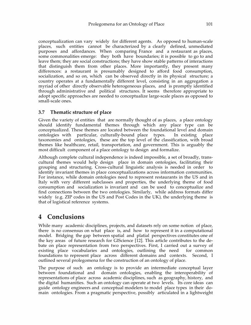
Prolegomena for an Ontology of Place 101
conceptualization can vary widely for different agents. As opposed to human-scale places, such entities cannot be characterized by a clearly defined, unmediated purposes and affordances. When comparing France and a restaurant as places, some commonalities emerge: they both have boundaries; it is possible to go to and leave them; they are social constructions; they have show stable patterns of interactions that distinguish them from other places. More importantly, they present many differences: a restaurant is presumably designed to afford food consumption, socialization, and so on, which can be observed directly in its physical structure; a country operates at a fundamentally different level, consisting in an aggregation a myriad of other directly observable heterogeneous places, and is promptly identified through administrative and political structures. It seems therefore appropriate to adopt specific approaches are needed to conceptualize large-scale places as opposed to small-scale ones.
3.7 Thematic structure of place Given the variety of entities that are normally thought of as places, a place ontology should identify fundamental themes through which any place type can be conceptualized. These themes are located between the foundational level and domain ontologies with particular, culturally-bound place types. In existing place taxonomies and ontologies, these are the top level of the classification, with broad themes like healthcare, retail, transportation, and government. This is arguably the most difficult component of a place ontology to design and formalize. Although complete cultural independence is indeed impossible, a set of broadly, trans-cultural themes would help design place in domain ontologies, facilitating their grouping and structuring. Cross-cultural linguistic analysis is needed in order to identify invariant themes in place conceptualizations across information communities. For instance, while domain ontologies need to represent restaurants in the US and in Italy with very different subclasses and properties, the underlying theme of food consumption and socialization is invariant and can be used to conceptualize and find connections between the two ontologies. Similarly, while address formats differ widely (e.g. ZIP codes in the US and Post Codes in the UK), the underlying theme is that of logistical reference systems.
4 Conclusions While many academic disciplines, projects, and datasets rely on some notion of place, there is no consensus on what place is, and how to represent it in a computational model. Bridging the gap between spatial and platial perspectives constitutes one of the key areas of future research for GIScience [12]. This article contributes to the de- bate on place representation from two perspectives. First, I carried out a survey of existing place vocabularies and ontologies, outlining the need for common foundations to represent place across different domains and contexts. Second, I outlined several prolegomena for the construction of an ontology of place. The purpose of such an ontology is to provide an intermediate conceptual layer between foundational and domain ontologies, enabling the interoperability of representations of place across academic disciplines, such as geography, history, and the digital humanities. Such an ontology can operate at two levels. Its core ideas can guide ontology engineers and conceptual modelers to model place types in their do- main ontologies. From a pragmatic perspective, possibly articulated in a lightweight
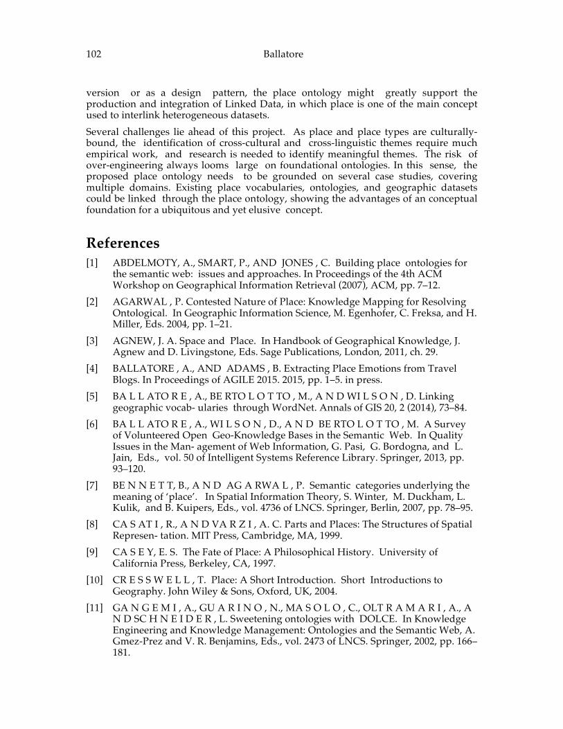
102 Ballatore version or as a design pattern, the place ontology might greatly support the production and integration of Linked Data, in which place is one of the main concept used to interlink heterogeneous datasets. Several challenges lie ahead of this project. As place and place types are culturally- bound, the identification of cross-cultural and cross-linguistic themes require much empirical work, and research is needed to identify meaningful themes. The risk of over-engineering always looms large on foundational ontologies. In this sense, the proposed place ontology needs to be grounded on several case studies, covering multiple domains. Existing place vocabularies, ontologies, and geographic datasets could be linked through the place ontology, showing the advantages of an conceptual foundation for a ubiquitous and yet elusive concept.
References [1] ABDELMOTY, A., SMART, P., AND JONES , C. Building place ontologies for
the semantic web: issues and approaches. In Proceedings of the 4th ACM Workshop on Geographical Information Retrieval (2007), ACM, pp. 7–12.
[2] AGARWAL , P. Contested Nature of Place: Knowledge Mapping for Resolving Ontological. In Geographic Information Science, M. Egenhofer, C. Freksa, and H. Miller, Eds. 2004, pp. 1–21.
[3] AGNEW, J. A. Space and Place. In Handbook of Geographical Knowledge, J. Agnew and D. Livingstone, Eds. Sage Publications, London, 2011, ch. 29.
[4] BALLATORE , A., AND ADAMS , B. Extracting Place Emotions from Travel Blogs. In Proceedings of AGILE 2015. 2015, pp. 1–5. in press.
[5] BA L L ATO R E , A., BE RTO L O T TO , M., A N D WI L S O N , D. Linking geographic vocab- ularies through WordNet. Annals of GIS 20, 2 (2014), 73–84.
[6] BA L L ATO R E , A., WI L S O N , D., A N D BE RTO L O T TO , M. A Survey of Volunteered Open Geo-Knowledge Bases in the Semantic Web. In Quality Issues in the Man- agement of Web Information, G. Pasi, G. Bordogna, and L. Jain, Eds., vol. 50 of Intelligent Systems Reference Library. Springer, 2013, pp. 93–120.
[7] BE N N E T T, B., A N D AG A RWA L , P. Semantic categories underlying the meaning of ‘place’. In Spatial Information Theory, S. Winter, M. Duckham, L. Kulik, and B. Kuipers, Eds., vol. 4736 of LNCS. Springer, Berlin, 2007, pp. 78–95.
[8] CA S AT I , R., A N D VA R Z I , A. C. Parts and Places: The Structures of Spatial Represen- tation. MIT Press, Cambridge, MA, 1999.
[9] CA S E Y, E. S. The Fate of Place: A Philosophical History. University of California Press, Berkeley, CA, 1997.
[10] CR E S S W E L L , T. Place: A Short Introduction. Short Introductions to Geography. John Wiley & Sons, Oxford, UK, 2004.
[11] GA N G E M I , A., GU A R I N O , N., MA S O L O , C., OLT R A M A R I , A., A N D SC H N E I D E R , L. Sweetening ontologies with DOLCE. In Knowledge Engineering and Knowledge Management: Ontologies and the Semantic Web, A. Gmez-Prez and V. R. Benjamins, Eds., vol. 2473 of LNCS. Springer, 2002, pp. 166–181.
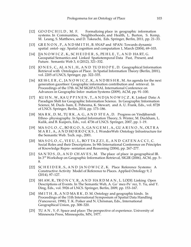
Prolegomena for an Ontology of Place 103
[12] GO O D C H I L D , M. F. Formalizing place in geographic information systems. In Communities, Neighborhoods, and Health, L. Burton, S. Kemp, M. Leung, S. Matthews, and D. Takeuchi, Eds. Springer, Berlin, 2011, pp. 21–33.
[13] GR E N O N , P., A N D SM I T H , B. SNAP and SPAN: Towards dynamic spatial ontol- ogy. Spatial cognition and computation 1, March (2004), 69–103.
[14] [JA N O W I C Z , K., SC H E I D E R , S., PE H L E , T., A N D HA RT, G. Geospatial Semantics and Linked Spatiotemporal Data Past, Present, and Future. Semantic Web 3, 4 (2012), 321–332.
[15] JO N E S , C., AL A N I , H., A N D TU D H O P E , D. Geographical Information Retrieval with Ontologies of Place. In Spatial Information Theory (Berlin, 2001), vol. 2205 of LNCS, Springer, pp. 322–335.
[16] KE SS L E R , C., JA N O W I C Z , K., A N D BI S H R , M. An agenda for the next generation gazetteer: Geographic information contribution and retrieval. In Proceedings of the 17th ACM SIGSPATIAL International Conference on Advances in Geographic Infor- mation Systems (2009), ACM, pp. 91–100.
[17] KU H N , W., KA U P P I N E N , T., A N D JA N O W I C Z , K. Linked Data: A Paradigm Shift for Geographic Information Science. In Geographic Information Science, M. Duck- ham, E. Pebesma, K. Stewart, and A. U. Frank, Eds., vol. 8728 of LNCS. Springer, Berlin, 2014, pp. 173–186.
[18] MA R K , D. M., TU R K , A. G., A N D ST E A , D. Progress on Yindjibarndi Ethno- physiography. In Spatial Information Theory, S. Winter, M. Duckham, L. Kulik, and B. Kuipers, Eds., vol. 4736 of LNCS. Springer, 2007, pp. 1–19.
[19] MA S O L O , C., BO R G O , S., GA N G E M I , A., GU A R I N O , N., OLT R A M A R I , A., A N D HO R R O C K S , I. WonderWeb: Ontology Infrastructure for the Semantic Web. Tech. rep., 2001.
[20] MA S O L O , C., VI E U , L., BO T TA Z Z I , E., A N D CAT E N A C C I , C. Social Roles and their Descriptions. In 9th International Conference on Principles of Knowledge Repre- sentation and Reasoning (2004), pp. 267–277.
[21] SA N TO S , D., A N D CH AV E S , M. The place of place in geographical IR. In 3rd Workshop on Geographic Information Retrieval, SIGIR (2006), ACM, pp. 5–8.
[22] SC H E I D E R , S., A N D JA N O W I C Z , K. Place Reference Systems: A Constructive Activity Model of Reference to Places. Applied Ontology 9, 2 (2014), 97–127.
[23] SH AW, R., TR O N C Y, R., A N D HA R D M A N , L. LODE: Linking Open Descriptions of Events. In The Semantic Web, A. Go´ mez-Pe´ rez, Y. Yu, and Y. Ding, Eds., vol. 5926 of LNCS. Springer, Berlin, 2009, pp. 153–167.
[24] SM I T H , B., A N D MA R K , D. M. Ontology and geographic kinds. In Proceedings of the 11th International Symposium of Spatial Data Handling (Vancouver, 1998), T. K. Poiker and N. Chrisman, Eds., International Geographical Union, pp. 308–320.
[25] TU A N , Y.-F. Space and place: The perspective of experience. University of Minnesota Press, Minneapolis, MN, 1977.

104 Ballatore [26] WI N T E R , S., KU H N , W., A N D KR U¨ G E R , A. Guest Editorial: Does
Place have a Place in Geographic Information Science? Spatial Cognition & Computation 9 (2009), 171–173.
ADVANCING GEOGRAPHIC INFORMATION SCIENCE: CHAPTER 8
© by the author(s) Licensed under Creative Commons Attribution 4.0 License
105
Copyright and Alternatives in Access to Scientific Information
James Campbell School of Computing and Information Science and National Center for Geographic Information
and Analysis, 5711 Boardman Hall, University of Maine, Orono, ME 04469-5711, USA
Abstract: As more and more spatially-referenced data are generated, as more and more papers are written based on those data, and as software programs are written to exploit that data, the issue of copyright becomes an increasingly important context within which Geographic Information Science practitioners work. Those who seek to find and use spatially-related information, and those who produce such information, are working within, and sometimes constrained by, copyright law. The tension between the limitations on open access to scientific information due to copyright, and the traditional mores of science that depend on open access, are more evident than ever in the digital age. A brief review of limiting trends in copyright in the United States over the past four decades shows that limitations of access to information have generated responses, including new alternatives to strict copyright. GIS practitioners, both as users and as generators of scientific information, are wise to be aware not only of copyright provisions but of alternatives that are becoming available to traditional copyright.
Keywords: Copyright, information access, open access, licenses, data access.
1 Introduction As more and more spatially-referenced data are generated, as more and more papers are written based on those data, and as software programs are written to exploit that data, the issue of copyright becomes an increasingly important context within which Geographic Information Science practitioners work.1 In this paper, we look at the context of copyright as it exists today and its effect on access to scientific information and data, including spatially-referenced information. This article examines the expansion of copyright and its effects on access to information over the past 40 years, reactions to that expansion, and some current efforts on the part of government, research funders, academic institutions, and some aspects of civic society to offer alternatives to traditional copyright in order to make
106 Campbell scientific information more widely accessible on a free basis. The focus is primarily on US copyright law, with some mention of differing contexts in other jurisdictions, e.g., the European Union’s sui generis regulations conferring protection of facts in some circumstances. However, with negotiations underway for new agreements such as the proposed Trans Pacific Partnership, the TransAtlantic Trade and Investment Partnership, and the Trade in Services Agreement that will have a major impact intellectual property rights, it is likely that there will be more rather than less conformity of copyright regimes internationally since copyright conformity is a major emphasis in what has been revealed to date through drafts of these secret negotiations. In this situation, the US context can be informative beyond its domestic borders.
2 The Enclosure of the Information Commons In the United States, copyright is a socially granted right in the U.S. Constitution that establishes a “bargain” between creators and the larger society: “To promote the Progress of Science and useful Arts, by securing for limited Times to Authors and Inventors the exclusive Right to their respective Writings and Discoveries” (Article 1, Section 8). Creators get an “exclusive Right” to exploit the value of their work in economic terms for “limited Times,” and society gets the benefit of having that work available for everyone to use and, after “limited Times,” to build on directly. For about the first 180 years of U.S. history, copyright law worked quite well to pursue this Constitutional goal. One reason for this general success was the law; another was the technology needed to violate copyright in any significant way. As Lawrence Lessig observes, in an atmosphere in which the technological burden is heavy, the legal burden may be light. [1] In the U.S., historically, not all creators asserted copyright on their works. From 1800-1976, only about 25% of works were copyrighted. Copyright owners had to affirmatively renew their copyrights to extend the length of protection, and only about 3% chose to do so. This may be because about 97% of copyrighted works exhaust their commercial potential within five years. [2] From 1976 on, however, there has been a sea change in copyright law, and a parallel change in the technological environment in which copyrighted materials are distributed. This confluence of changes in law and technology has led to a concern that the balance implicit in the copyright “bargain” has shifted, and that law and technology have now placed the rights of copyright owners far above those of users of copyrighted material, and of society as whole. What has changed since 1976, and why is there such concern that this change adversely affects the information commons? For the purposes of this discussion, the “information commons” consists of any information that a potential user of that information does not have to obtain explicit prior permission to use. “Information,” in this sense, encompasses creative as well as informative works expressed in any tangible medium, including digital media. It also includes data per se, including spatially-referenced data. Information commons materials include any work in the public domains well as works that are under copyright but for which the copyright owners have given prior permission for use, usually under specific conditions. The conditions attached to Creative Commons licenses are examples of these “some rights restricted” conditions of use.
Copyright and Alternatives in Access to Scientific Information 107
With this description of the information commons in place, we return to the question: What has changed since 1976, and why is there such concern that this change will adversely affect the information commons? To answer that question, we must briefly highlight recent key changes in law, in technology, and in the convergence of the two that give rise to concerns that the information commons is, in James Boyle’s terminology, being “enclosed.” [3] We will then look at responses to this perceived enclosure, with a focus on recent initiatives designed to make information available with minimal or no use restrictions.
2.1 Changes in Law and Technology Three elements in U.S. copyright law have changed in recent decades: the necessity for claiming copyright; the term of copyright protection; and the role of government in protecting copyright in a digital environment. A fourth element, the scope of what copyright covers, is also under discussion in the U.S. We examine each element in turn.
2.2 The Claim of Copyright Prior to 1978, those who wished to obtain copyright protection for a work had the affirmative obligation to register that work with the Registrar of Copyright and assert ownership in order to benefit from the protections available through copyright law. That requirement changed in the Copyright Act of 1976, which went into effect January 1, 1978. Since then, copyright exists the moment any original work is fixed in a tangible medium, whether registered with the Copyright Office or not. As a result, simply finding a copyright owner can now be a huge challenge. In the year 1930, to take one example, over 10,000 books were published. In the year 2000, 176 of those titles were still in print. In 2013, according to the International Publishers Association, 304,912 books were published in the U.S. [4], and they have copyright protection for at least 70 more years. Yet, historically, almost 97% of published works exhaust their potential for economic return within five years. That may be why, when copyright extensions had to be affirmatively applied for, only 3% of copyrighted works applied for and had their copyright protection extended. [2] Others who wished to use those formerly copyrighted works were then free to do so with no restrictions, or in the case of the small percentage of copyrighted works whose copyright was extended, potential users could easily ascertain who owned the copyright, and for how long the period of protection ran. Contrast this with the situation which a potential user of a work created since 1978 faces. A user who would like to build upon a certain work 50 years hence (or even 10 years hence) may have no way of knowing who the copyright owner is or how to contact that owner to ask permission. In such a scenario, it is unlikely that a potential user will risk using the copyrighted work without prior permission, and will simply decide not to use the work at all. On the face of it, this may not seem like a cultural calamity: after all, the future user can simply create something entirely new. However, even a moment’s reflection will point out the potential harm to the larger culture that this situation can cause. For example, suppose that the public domain had not been available to the Disney company. Would society have had any of the tremendously successful re-creations of Pinocchio, Aladdin, or dozens of other public domain stories in the film format that today’s adults grew up with, or would today’s children have access to animated versions of The
108 Campbell Velveteen Rabbit and a host of other previously copyrighted works in the Rabbit Ears series? Since the term of copyright in the U.S. is so long, and since it is no longer necessary to claim or register a copyright, the U.S. now faces a serious “orphan works” problem. Orphan works are works that are presumably under copyright but for which no copyright owner can be found to ask for permission to use a work. The problem has become so acute that in 2005, Senators Hatch and Leahy requested that the Registrar of Copyrights study the problem, take testimony, and issue a report. The Registrar did so and the report she issued contained a number of recommendations as well as suggested language for legislation to amend the copyright law to deal with the problem of “orphan works.” [5] While bills have been submitted in Congress to make the use of orphan works less risky for subsequent users who make good faith efforts to find a copyright owner but are unable to do so, none have made much progress and orphan works remain a serious limitation for those who wish to use or build on past works.
2.3 The Term of Copyright Protection Congress first granted copyrighted works protection for a period of 14 years. For most of U.S. history, this term length, augmented by a possible extension of another 14 years if applied for, was the norm. The period of copyright duration began to grow in the 20th century: the term of copyright was extended 11 times in 40 years culminating in the Sonny Bono Copyright Term Extension Act (CTEA) of 1997. The CTEA extended the term of copyright to an author ’s lifetime plus 70 years; or, for works in which copyright is held by a company, for 90 years from publication or 120 years from creation if the work was not published. For a rock musician or a young author or a student researcher who creates a work at age 20 and lives an average lifespan, the work would be under copyright protection for about 130 years under current U.S. law. Not surprisingly, some have questioned whether a term of protection of 100+ years constitutes a grant of protection “for limited Times” or “promotes the Progress of Science and the useful Arts” as the Constitution directs. The CTEA extension of copyright protection, and its philosophical implications, have been challenged in court, and the courts have essentially deferred to Congress in deciding what the proper definition of “limited Times” may be (Eldred v. Ashcroft 2003). As it stands, therefore, the length of copyright protection in the U.S. is that contained in the Sonny Bono Copyright Term Extension Act.
2.4 The Role of Government in Protecting Copyright Until recently, enforcement of copyright has been a civil matter in which a copyright owner who felt her rights had been violated would sue the alleged violator for damages and other, usually injunctive, relief. But in the digital age, this is changing, and changing fast. In the past decade, the U.S. government has taken a much more active role in copyright enforcement, and in some cases has extended the legal definition of copyright violation to the criminal realm. The major piece of legislation in this effort has been the Digital Millennium Copyright Act (DMCA). The DMCA prohibits providing tools or even information that would enable circumventing any type of technological protection, usually referred to as DRM or “Digital Rights Management,” devised by copyright
Copyright and Alternatives in Access to Scientific Information 109
owners to limit access to their digital works. Not only does the act allow anyone harmed by violation of the act’s provisions to sue, it also makes willful violation for profit a felony. In 2008, Congress passed the Prioritizing Resources and Organization for Intellectual Property Act (PRO-IP) of 2008 that, among other things, created a “Copyright Czar” in the Executive Branch, and dramatically increased penalties for copyright infringement. Other government actions, while not specifically focused on copyright per se, have also had a significant impact on the overall health of the information commons. Governments allocate scarce public resources such as spectrum space in broadcasting. They also regulate competition through anti-trust and similar regulation. The past two decades in the U.S., and, in fact, throughout the world, has seen an unprecedented increase in the concentration of copyright ownership and in the ownership of channels of distribution for copyrighted works due in large part to changes in government regulations and/or policies. The results have been dramatic. As of 2003 in the U.S., 80% of music for retail sale was distributed by only five companies, and 70% of the major radio markets were controlled by four companies. Of the 91 "major" televisions networks (including cable), 80% are owned by six companies, and 75% of prime time programming is owned by the networks. [6] This concentration of ownership of copyrighted materials and of the channels to distribute those materials has significant repercussions on the information commons. Access to a large portion of culturally important copyrighted material now lies in the hands of a relatively few owners. Those owners are in a powerful quasi-monopolistic position to control use of that material through technologically enforced licensing provisions, provisions that often are at odds with traditional user rights such as fair use and first sale. This situation is becoming more and more prevalent as more publications are being distributed in digital form. This is particularly noticeable in the world of academic journals where a decade long trend of consolidation has led to a half dozen large corporations controlling access to scholarly journals, and more and more journals being available in only digital format. Predictably, the price increase for scholarly publications taken as a whole have significantly exceeded the rate of inflation for over a decade at a time when library budgets have been generally decreasing. The result is more limited access to journals and scholarly works both on campus and off.
2.5 Scope of Copyright Protection Under U.S. law, copyright protection can only be extended to works that exhibit some degree of originality. Simple facts or even the obvious arrangement of facts cannot be protected under U.S. copyright law. A simple alphabetical listing of place names, for example, or an alphabetical lists of names and telephone numbers does not reach the threshold of originality needed for copyright protection even though the bar for that originality is not high. In the words of Justice Sandra Day O'Connor, it requires but “a modicum of creativity.” [7] Facts per se may be in the public domain in the U.S., but it does not take a great deal of “creativity” to make a collection of facts copyrightable. In the area of geography and mapping, for instance, the geographic objects themselves are facts. How they are arranged in a map using various graphic symbols, colors, and other “nonfactual” modalities that offer a variety of ways to represent those facts, may qualify as original enough to merit copyright protection even if the facts themselves do
110 Campbell not. Similarly, non-obvious categorization and arrangements of facts in tables or other database forms may also be original enough to merit protection. Any public records generated by the federal government do not fall under copyright protection since in the United States the Copyright Act specifically excludes the federal government itself from claiming copyright in materials it produces. This includes everything from weather reports to court decisions to data on water purity to testimony before congressional committees. All material generated directly by federal government employees is in the public domain. Under the Freedom of Information Act, access to some federal government generated information may be limited by concerns for security or other political considerations but may not be limited because of copyright ownership by government. Recently, there have been efforts that would have the effect of eroding components of the public domain in the U.S. The European Union now includes databases of facts as works that can gain protection, either through copyright or through a sui generis designation, and similar bills have been introduced in the U.S. Congress in recent years (e.g., HR 3261, HR 3872 in the 108th Congress, and others since). If bills of this type were to be enacted into law in the future, facts collected and arranged in even obvious ways could fall under copyright protection in the U.S. This type of sui generis database protection scheme in the European Union has not, in the view of The Royal Society, been a good thing for science.
Advances of technology and commercial forces have led to new IP [Intellectual Property] legislation and case law that unreasonably and unnecessarily restrict freedom to access and to use information. This restriction of the commons in the main IP areas of patents, copyright and database right has changed the balance of rights and hampers scientific endeavour. In the interests of society, that balance must be rectified. [8]
In the United States, there are two factors under copyright law that provide some utility to users of copyrighted materials in the face of the expansion of the scope of copyright: First Sale and Fair Use. First Sale simply means that once a person purchases a lawful physical copy of a work, e.g., a book, an academic journal, a CD, or other copyrightable work, the copyright owner no longer exerts any control over that copy. The purchaser may loan the item, give it away, or even sell it since in none of those transactions is a copy of the work made. It is the First Sale doctrine that makes libraries and video rental stores possible in the U.S. As more and more sales of books and music become digital, however, licensing rather than selling is becoming more common, even for personal purchases, thus minimizing the effect of the First Sale doctrine since no sale technically took place. Some scholars are beginning to argue that many licenses actually should be considered as sales, e.g., those that allow unlimited use by the licensee. [9] Even the Registrar of Copyright has raised the question of whether a marketplace in which everything digital is licensed is the most desirable one for America's economic future. [10] These are, however, still only questions and courts to date have held that licenses trump First Sale rights. Fair Use enables use of copyrighted materials for certain purposes without the copyright owner ’s permission. The difficulty with Fair Use from the perspective of potential users is that Fair Use is a defense, not a right. A user may cite Fair Use as a defense if a copyright owner
Copyright and Alternatives in Access to Scientific Information 111
sues for violation of copyright. Although there is a four element test to help determine whether a particular use constitutes Fair Use, no one really knows if a use is a Fair Use until a judge’s gavel falls. Lawrence Lessig once joked that “Your Fair Use right is your right to hire a lawyer.” Nonetheless, Fair Use does provide some elasticity in an otherwise tightly bound U.S. copyright law.
2.6 Brief Summary of Changing Laws and Technology Since the term of copyright is now so long, since DRM cannot be legally circumvented under the DMCA, and since the copyright holder can impose license conditions that restrict or remove traditional user First Sale rights under copyright law, and then enforce those license provisions through the use of DRM, Pamela Samuelson has suggested that DRM might more accurately be described as “digital restrictions management.” [11] And, indeed, that is the way that many view the current situation in copyright in the U.S.: as a situation in which law and technology have combined to radically alter the traditional balance between copyright owners and users of copyrighted materials in favor of copyright owners. Those who view the current copyright landscape in this way are reacting, and it is to the range and forms those reactions are taking that we now turn our attention.
3 Reactions to Enclosure of the Commons As it became clear that the Sonny Bono Copyright Extension Act and the Digital Millennium Copyright Act were altering the copyright landscape in an unprecedented way in today’s digital environment, those who found this landscape alteration undesirable or unacceptable began to respond. Responses took a variety of forms and approaches to addressing the problem of “enclosure.” We classify the responses for the purposes of this review as:
• Legislate • Litigate • Legally re-interpret • Create alternatives
We examine them in turn.
3.1 Legislate In the U.S., no bills have been introduced in the Congress over the past decade designed to specifically counteract the automatic grant of copyright, or to shorten its statutory duration. There are however, examples of bills introduced to mitigate the effects of the CTEA in recent sessions of Congress, and to temper the effects of DRM technologies that copyright owners are increasingly using to control access to their digital products, technologies that are currently protected from circumvention under the DMCA. While it is unlikely at this time that the periods of copyright protection codified into law through the Sonny Bono Copyright Term Extension Act will be reduced, given both World
112 Campbell Intellectual Property Organization treaty obligations and the tenor of Congress, some legislative initiatives have been brought forward that, had they been successful, would have ensured that only those works whose owners actually wish to utilize copyright over the full term provided in the CTEA would receive the full term of copyright protection. Rep. Zoë Lofgren, for example, twice introduced The Public Domain Enhancement Act (108th and 109th Congresses). It would have required copyright owners who wish to continue to enjoy copyright protection to affirmatively assert their copyright after 50 years by paying a small registration fee of one dollar. Absent that assertion, copyright would expire after 50 years. While the bill attracted some co-sponsors, it went nowhere. Another of the “enclosing” laws, the DMCA, has had a number of consequences that were not intended, according to testimony that led to passage of the act. Some businesses, for example, have attempted to use threats of suits or prosecution based on Sections 1201(a)(1), 1201(a)(2), and 1201(b) of the DMCA to stifle reporting of shortcomings in their products (e.g., HP and Microsoft). Others, such as SONY, have attempted to stifle competition, and Lexmark invoked the DMCA in suing and actually obtaining an injunction against Static Control Components, a company that sold aftermarket cartridges for Lexmark printers. That injunction stood for almost a year before being vacated in October of 2004 by the Sixth Circuit Court of Appeals, which later also ruled against Lexmark’s DMCA violation claims. [12] The process took years to conclude and had a large impact on innovation and competition in the printer ink industry until it was resolved. This example, others like it, and examples of the DMCA being applied against consumers in ways that do nothing to thwart large scale digital “piracy,” which was Congress’s avowed intent in passing the DMCA, alarmed some in Congress, and led to the introduction of bills that were intended to rectify some of the imbalances that the sponsors felt the DMCA has created in favor of copyright owners. Rep. Zoë Lofgren, for example, twice introduced the BALANCE Act, which is designed to make legal in the digital realm what has been – and remains – a user ’s legal rights under copyright law in the paper realm. This proposed legislation, according to its sponsors, would have made traditional fair use and first sale rights available in the digital domain, and allow a user who has lawfully obtained a copy of a digital work to defeat DRM restrictions that interfered with exercising those rights. The bill, in plain language, got nowhere in any Congressional session. In its absence, courts have continued to rule that any kind of copy made in the process of transfer, even if only one copy exists at the end of the process, is a violation of copyright. [13] In short, in the U.S., no legislative initiatives to ameliorate the effects of changes in law and in technology as they affect access to information have had any success up to the beginning of the first session of the 114th Congress in 2015.
3.2 Litigate While some were pursuing legislative remedies, others felt that recent changes in copyright law violated the spirit and letter of the U.S. Constitution. They mounted legal challenges to provisions of both the CTEA and to the Copyright Act of 1976, which made copyright protection automatic.
Copyright and Alternatives in Access to Scientific Information 113
In Eldred v. Ashcroft, the lead plaintiff, Eric Eldred, made available on his web site, and in other fashions, works that had entered the public domain. Some of those works had their copyright terms extended retroactively by the CTEA. Eldred asserted he had standing in the case since his work and livelihood was directly impacted by the CTEA. He claimed in the suit that the CTEA was unconstitutional (1) because it violated the “limited Times” clause in the Constitution, and (2) because it constrained free speech. The case went all the way to the Supreme Court, where it lost by a 7-2 vote. The majority found that the Constitution granted Congress the duty to determine what “limited Times” meant, and that the Court should defer to Congress’s judgment. Justice Breyer, one of the dissenters, had long argued against the extension of copyright: “Taken as a whole, the evidence now available suggests that, although we should hesitate to abolish copyright protection, we should equally hesitate to extend or strengthen it.” [14], and he continued that argument in his dissent. On the free speech issue, the Court held that the act did not change the “traditional contour of copyright,” and that any free speech concerns raised by the act could be dealt with through copyright’s traditional established safeguards, e.g., Fair Use. While those who sought to have the CTEA declared unconstitutional failed to achieve that goal, others felt that elements of the Supreme Court’s Eldred decision strengthened the case for asserting that a combination of recent changes in copyright law did, in aggregate, affect the “traditional contour of copyright” for a certain class of works, and therefore that these laws essentially created a situation which required “further first amendment scrutiny.” That was the approach taken by plaintiffs in Kahle v. Ashcroft (original name: case as decided in 2007 is Kahle v. Gonzales). However, this suit gathered no traction and was dismissed by the Ninth Circuit, as was a similar case in the D.C. Circuit Court, Luck’s Music v. Ashcroft. A third suit addressed the extension of copyright term as well as first amendment issues from another perspective. It focuses on another “enclosing” copyright issue, that of restoring copyright protections for works, in this case foreign works, that had already entered the public domain. In the words of the original complaint:
This is an action to challenge the constitutionality of Congress’s attempt to remove and radically deplete the supply of literary and artistic works from the public domain…Congress’s dramatic expansion of the term of copyright [in the CTEA] has been accompanied by an even more radical depletion of works from the public domain. On December 8, 1993, Congress amended the Copyright Act to recognize for the first time in the history of our copyright law a general provision that purports to “restore” copyrights – retroactively – in numerous works that heretofore had indisputably been in the public domain for failure to satisfy the requirements of the Copyright Act. [15]
Although this suit was not dismissed. The Tenth Circuit court held that, indeed, Congress’s removal of works from the public domain that were already part of the public domain reached the Supreme Court’s definition of changing the “traditional contour of copyright,” and remanded the case to the district court for trial. The government, defendant in the trial, requested an en banc hearing by the entire 10th Circuit bench. That request was denied. In April, 2009, the District Court for the District of Colorado granted a motion for summary judgment in Golan v. Holder, accepting the change in the “traditional contour of copyright” argument. In the words of the plaintiff’s attorneys: “It is the first time a
114 Campbell court has held any part of the Copyright Act violates the First Amendment and the first time any court has placed specific constitutional limits on the government's ability to erode the public domain.” [16] That decision was later reversed by the Tenth Circuit Court of Appeals. The plaintiffs appealed to the Supreme Court which affirmed the Tenth Circuit's decision and held that the government did not exceed its authority in removing the formally public domain works from the public domain Like the legislative initiatives mentioned above, court challenges to extensions of copyright have universally failed. Prospects for relief through Congress or the courts, at the moment, do not seem bright.
3.3 Legally Re-‐‑Interpret Underlying any legal statute concerning intellectual property, and thus copyright, is a set of assumptions about what “property” actually is. Laws such as the DMCA have emerged because the forms of property have changed in the digital age, while the conceptualization of the nature of property has not. Consumption, excludability, costs of replication, and other characteristics of physical property may not apply in the same way to intellectual property as they do to physical property, yet recent legislation and court decisions seem to assume they do. In the last two decades, and particularly in the past decade, some scholars have argued that intellectual property and physical property such as land are not the same thing. Therefore, they argue, the set of assumptions underlying laws governing intellectual property in a digital environment should not be based on the analogy of physical property but rather on some other model more reflective of the nature of intellectual property itself. As Wesley Hohfeld has famously pointed out, intellectual property claims are claims between people [17], not, as earlier legal commentators described, claims of people on something inanimate but tangible such as land. Why this upwelling of legal theory with respect to intellectual property now? Simply put, the need did not exist as urgently before. Until 1976, using the model of physical property as the basis for copyright law worked reasonably well. “Excludability” had to be claimed through copyright registration, which only a minority of creators sought to assert, and that excludability was tempered by First Sale and Fair Use rights of users of the intellectual property. Economically, there were significant burdens encountered in large scale copyright violation. Any type of large scale violation of copyright required a significant investment, for example, in printing press equipment or video and film duplication equipment. In this environment, the analogy to physical property, despite the clear differences in intellectual property (e.g., it is non-rivalrous), worked well enough. And then came digital and the Internet. The economic burdens of making perfect copies and distributing them widely almost completely disappeared. At the same time, the technology to enable creators to exclude potential users from the use of their works – supported by civil and criminal law – became widely available. Now the differences between physical property and intellectual property were thrown into sharp contrast, and legal and economic theorists such as Robert Heverly began to respond.
We think of information as property; law and economic structures, we argue, make it so. But this should not be the end of our inquiry. If we believe information is property, we must ask: What kind of property is information?”[18]
Copyright and Alternatives in Access to Scientific Information 115
Recent theorists have approached an answer to this question in a variety of ways. Heverly, for example, concludes that “information is not a private property regime: it is a semicommons” which, in his analysis, reflects the “dynamic relationship and interdependence of private and common property interests.” P2P file sharing, for example, represents such an interdependence. On the one hand, P2P sharing of music may have a negative economic impact on a copyright owner by reducing some potential sales of a piece of music; on the other hand, the exposure and “word of mouth” available through P2P file sharing has a positive economic impact and increases sales and thus income for the same owner. [19] In fact, some music companies are actually using P2P file sharing activity statistics to promote future “hit songs” to radio stations. They are doing this promotion through third parties in order not to dilute their claims of harm due to copyright infringement, since music companies are simultaneously suing those who distribute copyrighted music through P2P networks. Leaving aside the contradiction involved in these apparently conflicting activities, this example is precisely the type of interdependence that Heverly posits as a characteristic of a semicommons model of property. Jacqueline Lipton asserts that there is nothing wrong with viewing information as property in the traditional sense, as long as property rights and obligations are viewed in a holistic manner. Problems arise when there is an imbalance in the rights and obligations of property owners: “the problem can be re-cast in terms of the ‘absolutism’ of information property rights…” [19] Lipton argues that even physical property rights are not absolute, and neither should information property rights be. Her point is that “where a government has created, or supported the creation of private rights in information, it should be prepared to create and support concurrent public duties.” Lipton shares a conclusion, if not the process of arriving at that conclusion, with Mark Lemley. He quotes with approval the view of the Supreme Court of Canada in Compo Co. Ltd. V. Blue Crest Music Inc.:
copyright law is neither tort law nor property law in classification, but is statutory law. It neither cuts across existing rights in property or conduct nor falls in between rights and obligations heretofore existing in the common law. Copyright legislation simply creates rights and obligations upon the terms and in the circumstances set out in the statute. [20]
In short, Lemley argues that intellectual property is sui generis and needs to be envisioned as such when crafting legislation to define appropriate economic rights, characteristics, and obligations rather than to use terms of “inapposite economic analysis borrowed from the very different case of land.” All of these legal scholars find the root of the enclosure problem with respect to information to lie in the legal assumptions underlying the legislative and judicial analysis of the nature of intellectual property. They, as well as others [e.g., 15, 21, 22, 23, 24, 25, 26, 27, 28] propose alternative legal and economic analyses that, in their views, would go a long way toward reducing or eliminating at least some of the legal aspects of the enclosure of the information commons. Fair Use has traditionally been the balancing mechanism in the copyright social contract. However, in the eyes of some scholars, the advent of works in digital form along with technological DRM protections have weighted that balance heavily on the side of rightsholders to the detriment of Fair Uses on the part of consumers.
The more technology reflects only one set of interests, however, the more it departs from the law, which conceptualizes copyright as a balancing of
116 Campbell
interests, with the ultimate goal of fostering both creative expression and broad public availability of creative works. The result has been a perverse scenario nowhere commanded by the Copyright Act or the DMCA, in which technological measures have been al- lowed to override the fair use doctrine. [29)
This is not simply a theoretical problem, nor one confined to the United States. Lynne Brindley, CEO of the British Library stated in 2007 that: It seems to me, as CEO of the British Library and therefore representing the researcher in part, that the balance that is referred to here, between private rights and public domain, between free competition and monopoly rights - is not working; it is being undermined by a number of things from our perspective including:
• A restrictive use of new technology (Digital Rights Management) • Poor or outmoded legislation (i.e. too complex, increasing durations and harmonising durations ever upward, etc) • The public interest aspects of copyright being undermined and made irrelevant by private contract. [30]
The issue has become widespread enough to involve the policy making bodies of some of the largest scholarly organizations in the world. For example, The Public Policy Council of the ACM in its “USACM Policy Recommendations on Digital Rights Management” recommended that:
Because lawful use (including fair use) of copyrighted works is in the public’s best interest, a person wishing to make lawful use of copyrighted material should not be prevented from doing so. As such, DRM systems should be mechanisms for reinforcing existing legal constraints on behavior (arising from copyright law or by reasonable contract), not as mechanisms for creating new legal constraints. Appropriate technical and/or legal safeguards should be in place to preserve lawful uses in cases where DRM systems cannot distinguish lawful uses from infringing uses. [31]
Not surprisingly, legal scholars have begun to re-think approaches to Fair Use in the digital age as well suggesting approaches that, in their views, would help to reestablish balance between rightsholders and users. [32] Armstrong, for example, proposes a regime of what he refers to as "Fair Circumvention” of DRM technologies. Reichman, Dinwoodie and Samuelson propose a “Reverse Notice and Takedown Regime” under the DMCA in which those who would assert a claim to legally circumvent DRM for Fair Use purposes notify rightsholders they intended to take such circumvention steps, and rightsholders would have 14 days to object. [33] The details of these proposals are not the issue here. What is of import is the effort to reinterpret law to reflect the changes in the social contract that digital technologies have made possible. Another stream of quasi-legal thought focuses not on definitions of intellectual property nor on the empirical economic, political, or legal validity of arguments in support of copyright extension. Rather these arguments assert that access to information is a right, based upon ethical principles as well as charters and statements of rights such as those authored by treaty organizations such as the Universal Declaration of Human Rights (Articles 19 and 27) as well as numerous non-governmental organizations such as the Library Bill of Rights of the American Library Association. Drawing on these and similar national and international declarations, some scholars, such as Kay Mathiesen, have argued that “the right to access is not
Copyright and Alternatives in Access to Scientific Information 117
merely a liberty right but also a welfare right. That is, individuals’ information rights place duties on governments to provide access to information.” [34] At this point in time, these legal and moral speculations and theories remain speculations only and have to date had no real impact on access to information. However, they serve to provide a counterbalance, albeit a weak one at present, to the ongoing efforts of copyright owners to assert greater and greater control over copyrighted information in a culture that is increasingly digital.
3.4 Create Alternatives In the absence of legislative or legal remedies, some have sought to leverage existing copyright law to realize goals of more open access that legislative proposals and law suits have not so far been able to accomplish. This type of response encourages creators to forego some rights available under copyright law while retaining others. The desired effect is to widen the amount of material available in the information commons, if not in the public domain per se.
3.4.1 GNU General Public License.
There is ample precedent for this tactic. Free and Open source software has been released for over two decades under the GNU General Public License (GPL) or one of many “open source” variants. This class of licenses uses copyright law to license the use of copyrighted works under much less restrictive terms than exist under normal copyright conditions. So, for example, a work licensed under the GPL mandates that no charge can be made for the work itself (although charges for duplicating or distributing copies can be levied); that users are free to copy or modify the work as they see fit but that if any such modifications are made to the work, those modifications also must be made available under the same licensing terms as the original work. [35] Creators use the GPL and its many derivatives and variants, such as the Berkeley Software Distribution (BSD) license, mostly in licensing free or open source software. However, similar licensing approaches can also apply to other types of copyrighted works such as text or music or photographs or motion pictures or datasets. The GNU Free Documentation License, for example, was the license underlying the text on Wikipedia for many years, one of the most popular sites on the World Wide Web, although Wikipedia has now brought its licensing terms into compliance with Creative Commons licenses.
3.4.2 Creative Commons.
Several of those who had been involved in some of the litigation summarized above decided that, while it was necessary to continue to challenge in court the validity of laws limiting access, something needed to be done at once to create alternatives to the closing off of the commons they felt was underway, and the Creative Commons was born. The Creative Commons extends and broadens the “some rights reserved” approach of the GPL to licenses that creators can apply to a wide variety of creative works. The same digital technology that has made it possible for copyright owners to impose restrictive licenses on works in digital form also allows copyright owners to offer much
118 Campbell less restrictive licenses for which users do not have to seek prior permission to use, as long as users adhere to the conditions set out in the license. Typically, those conditions are much more liberal than those that obtain under copyright law per se. For example, Creative Commons offers a set of conditions that creators may choose to apply one or more of to their works to create a license. Creative Commons takes whatever conditions the creator indicates she wishes to attach to her work, and creates a legal license that the creator attaches to the work. The license comes in three forms: human readable (a general description of the license terms in common language), lawyer readable (a legal language license), and machine readable. The creator indicates that the work is licensed under a Creative Commons license, and provides a link to the Creative Commons website where the specifics of the license are laid out for any potential user to view. As long as the user conforms to those conditions of use, there is no need to track down the copyright owner and obtain specific permission to use the work. While these Creative Commons licenses do expand access to information in a commons spirit, the works are licensed under copyright and the licenses chosen draw their force and enforceability from copyright law. None of these licenses has yet had its validity fully tested in court in the U.S. although there are instances of courts in other countries upholding the validity of the Creative Commons licenses. Some creators are uncomfortable with having their work under copyright for 70 years after their deaths. For these creators, the Creative Commons also offers a “Founder ’s Copyright” option. This option limits a creator ’s claim to copyright to 14 years, the original grant of copyright in the U.S., after which time the work enters the public domain. Creators may also choose to simply affirmatively donate their copyright to the public domain immediately, and Creative Commons provides a mechanism for doing that as well. U.S. law makes no specific provision for this type of dedication so the Creative Commons dedication is as close as a creator can come. Before 1976, a work entered the public domain unless copyright was registered. Now, as noted above, it is necessary to specifically disavow copyright ownership for a work to be considered in the public domain. In the years since Creative Commons licenses have become available, creators have applied Creative Commons licenses to an estimated 880 million works as of mid 2014, and the rate of use has been growing steadily. While Creative Commons supporters do not pretend that this is more than a small percentage of created works on the Internet, they do assert that it is important to have a legal channel available for those who wish to contribute to the expansion of the information commons, even if not to the public domain itself. Alternative licensing schemes such as those employed by Creative Commons or the Open Source software movement do create a mildly competing economic model to traditional markets in copyrighted material. Creators under these alternative licensing systems do not generally attempt to capture the entire value of their work but choose instead to reserve only some value for themselves. Some universities are incorporating Creative Commons licenses into their institutional structures. Stanford University, for example, no longer requires that theses and dissertations be microfilmed. Now they are simply made available electronically under Creative Commons licenses. Open access publishing initiatives go even further and actually create an alternative model of academic publishing that competes directly in the market for academic scholarship.
Copyright and Alternatives in Access to Scientific Information 119
3.4.3 Open Access Publishing.
Scientific progress depends on scientists having wide ranging access to scientific information. The same confluence of forces that has adversely affected the information commons in general has adversely affected the scientific commons, according to many in the scientific community and the communities of information professionals who serve them. While there are over 24,000 scientific journals currently published by 2000+ publishers [36], fewer than half a dozen large publishers own or control the distribution of a large majority of those journals, including a majority of the intellectually most important ones. These publishers are in a quasi-monopolistic position and have been raising prices in excess of increases in the rate of inflation for two decades. During the past decade, publishers also have increasingly migrated their publications to digital form, in many cases abandoning paper publishing altogether. Once their products are in digital form, publishers are in a position to impose technologically enforceable licensing controls, and most have done so. One result of this technologically enforceable quasi-monopolistic position is entirely predictable under capitalistic economic theory. Publishers, unfettered by competition, have bundled many titles into packages in a “take it or leave it” fashion, and have unilaterally set price points to maximize profits. The strategy has worked: the industry reported profit margins of 40% in the middle of the first decade of the 21st Century [37] and while profits may have declined somewhat since, they are still in very healthy double digit territory. Academic publishers pay nothing for the articles they publish. Scholars who submit articles for publication are typically university faculty who are being paid to do research and for whom publication is part of the research process. Publishers pay nothing for the peer reviewers for the same reason. This “free labor,” combined with an increasingly non-print distribution environment, reduces costs dramatically. When combined with a near monopolistic pricing ability, these advantages result in enviable profit margins. They have also resulted in an increasing tide of customer resentment. Scholarly libraries have had to continually cut back on journal purchases and/or reduce monograph purchases in order to attempt to keep up with rising journal prices. In many libraries, journal purchases now make up two-thirds or more of acquisition costs, with only one third going for books and other materials. Since scholars typically sign over copyright to publishers, some scholars have found themselves in the ironic position of not being able to legally provide copies of articles they have authored, and which they provided to publishers for free, to their students because their libraries can no longer afford to purchase the journals the articles were published in. In this environment, libraries and librarians began to react, as did a host of non- governmental and professional organizations. One of the clearest statements of their view of the recent situation with respect to academic publishing is included in this description of SPARC:
Scholarly Publishing and Academic Resources Coalition is an alliance of academic and research libraries and organization working to correct market dysfunctions in the scholarly publishing system…Its strategies expand competition and support open access to address the high and rising cost of
120 Campbell
scholarly journals, especially in science, technology, and medicines—a trend which inhibits the advancement of scholarship. [37]
SPARC, as well as many other organizations, encourages the development of open access journals, publications that make their articles available to the public at no cost to the user, and that typically allow the user to make copies in digital form, and often confer a wider set of usage rights. And those efforts have had some notable success. The Directory of Open Access Journals (DOAJ) lists over 10,000 peer-reviewed open access journals containing nearly 1.2 million articles of which over 600,00 are searchable at the article level as of February of 2015. This is a small proportion of the articles published in scientific, technical, and medical journals each year, to say nothing of journals in other fields. Still, open access is becoming a serious, if still small, market force, and other forces are amplifying the impact of open access initiatives. Funders as well as government agencies are beginning to take notice of the effect of limitations on access to information on scholarship and learning. In the U.S., the National Institutes of Health (NIH) require that all research results generated through NIH funding be made available to the public in an open access repository within a year of publication. Bills that would extend such mandates to other federal agencies have been introduced in both houses of several recent Congresses but none have to date passed. However, in the U.S., a provision in the Consolidated Appropriations Act of 2014 requires federal agencies in Labor, Health and Human Services, and Education with research budgets of over $100 million to provide public access within 12 months of publication in a peer-reviewed journal to research resulting from projects they fund. Private funders are also promoting open access. The Welcome Trust, a major funder of research in the United Kingdom, has mandated that articles resulting from research it funds be placed in an open repository. Some research institutes, such as the The Howard Hughes Medical Institute, have made open access mandatory for research conducted by their employees. The Max Planck Institute in Germany is encouraging its many research employees to make their work open access as well. Faculty Senates and other policy setting bodies in educational institutions in this country and abroad including major institutions such as MIT, Harvard, and Stanford as well as over 30 other U.S. universities and colleges have voted to make open access mandatory for their faculty members. There are many important obstacles for open access publishing to overcome to be a full- fledged market alternative to commercial academic publishing, including building sustainable economic models and changing the culture of academia to value open access and traditional publication credits equally when considering tenure and promotions. Nonetheless, open access scholarly publishing is already having an effect on the marketplace and, through market mechanisms, has already begun to expand the information commons.
4 Summary and Conclusions There are tensions in the balance of copyright as established in the U.S. Constitution, and these tensions are even more obvious in the digital age. Access to data, research studies, academic papers, and other information in GIS, as in all scientific disciplines today, can be complicated. While copyright itself has evolved to be more restrictive in terms of access to information, there are offsetting though not yet completely countervailing forces pushing for less restrictive and more open access to information and data. GIS researchers, authors, and software writers are wise to understand
Copyright and Alternatives in Access to Scientific Information 121
copyright and alternatives to copyright. As researchers, such understanding can lead to more and better access to information needed for their work. As authors, such understanding can help authors to choose copyright options that best serve their purposes and make their work as widely known as possible.
References [1] Lessig, L. Building the Creative Commons.
http://www.uwm.edu/Dept/SOIS/about/news/events/index.htm, 2004. [2] Lessig, L. Free Culture: How Big Media Uses Technology and the Law to Lock
Down Culture and Control Creativity. Penguin Press, New York, 2004. [3] Boyle, J. The Second Enclosure Movement and the Construction of the Public
Commons. Law and Contemporary Problems 66, 33 (2003), 33-75. [4] International Publishers Association. 2014. Annual Report 2013-2014. http://
www.internationalpublishers.org/images/reports/2014/IPA-annual-report-2014.pdf, 2014.
[5] Registrar of Copyrights. Report on Orphan Works. United States Copyright Office, Washington, 2006.
[6] Lessig, L. 2003. The Future of Ideas and Code and Other Laws of Cyberspace. 13th Annual Conference on Computers, Freedom & Privacy. http://www.cfp2003.org/cfp2003/ program.html, 2003.
[7] Feist Publications, Inc. v. Rural Tel. Service Co., 499 U.S. 340 (1991). [8] The Royal Society. Keeping Science Open: the Effects of Intellectual Property
Policy on the Conduct of Science. http://www.royalsoc.ac.uk/document.asp?tip=0&id=1374, 2003.
[9] Asay, C. D.“Kirtsaeng and the First-Sale Doctrine’s Digital Problem,” Stanford Law Review Online, volume 66, http://www.stanfordlawreview.org/online/kirtsaeng-and-first-sale-doctrines-digital-problem, 2013.
[10] Pallante, M. A. The Next Great Copyright Act. Columbia Journal of Law and the Arts. 36, 3 (2013), 315-344.
[11] Samuelson, P. DRM {and, or, vs.} the Law. Communications of the ACM. 46, 4 (2003), 41-45.
[12] Lexmark International, Inc. v. Static Control Components, Inc., 387 F.3d 522 (6th Cir. 2004)
[13] Capitol Records, LLC v. ReDigi, Inc. 2013 [14] Breyer, S. The Uneasy Case for Copyright: A Study of Copyright in Books,
Photocopies, and Computer Programs. Harvard Law Review. 84, 2 (1970), 281-351.
[15] Golan v. Ashcroft, now Golan v. Holder, 132 S. Ct. 873, 2012 [16] Falzone, A. URAA Held Unconstitutional.
http://cyberlaw.stanford.edu/node/6149. 2009.
122 Campbell [17] Hohfeld, W. N. Fundamental Legal Conceptions As Applied in Judicial
Reasoning. Yale University Press, New Haven, 1964 (copyright 1946). [18] Heverly, R. A. The Information Semicommons. BTLJ. 18, (2003), 1127-1189. [19] Lipton, J. Information Property: Rights and Responsibilities. Fla. L. Rev. 56, 1
(2004), 140. [20] Lemley, M. Property, Intellectual Property, and Free Riding. Stanford Law and
Economics Olin Working Paper No. 291, 2004. [21] McCarty, L. T. Ownership: A Case Study in the Representation of Legal
Concepts. Artificial Intelligence and Law. 10, (2002), 1-3. [22] Lunney, G. S., Jr. Reexamining Copyright’s Incentives-Access Paradigm.
Vanderbilt Law Review. 49, (1996), 483-656. [23] Pessach, G. Reciprocal Share-Alike Exemptions in Copyright Law. Cardozo Law
Review. 30, 3 (2008), 101-150. [24] Sohn, G. B. Six Steps to Digital Copyright Sanity: Reforming a Pre-vcr Law for a
Youtube World. New Media and Marketplace of Ideas Conference, 2007. [25] Sprigman, C. Reform(aliz)ing Copyright. Stanford Law Review. 56, 2 (2004), 485-
568. [26] Samuelson, P. Preliminary Thoughts on Copyright Reform. Utah Law Review.
2007, 3 (2007), 551-571. [27] Boldrin, M. and Levine, D. K. The Case Against Intellectual Property. American
Economic Review Papers and Proceedings. 92 (2002), 209-212. [28] Parchomovsky, G. and Weiser, P. J. Beyond Fair Use. Cornell Law Review. 96, 1
(2010), 91-137. [29] Armstrong, T. K. Digital Rights Management and the Process of Fair Use.
Harvard Journal of Law and Technology. 20, 1 (2006), 49-121. [30] Brindley, Lynne. Balance in IP “Not working”.
http://legacy.earlham.edu/~peters/fos/2007_12_02_fosblogarchive.html, 2007. [31] ACM US Public Policy Council. USACM Policy Recommendations on Digital
Rights Management. ACM, 2006. [32] Armstrong, T. K. Fair Circumvention. Brooklyn Law Review. 74, 1 (2008), 1-50. [33] Reichman, J. H., Dinwoodie, G. B., and Samuelson, P. 2007. A Reverse Notice and
Takedown Regime to Enable Public Interest Use of Technically Protected Copyrighted Works. Berkeley Technology Law Journal. 22 (2007), 981-1060.
[34] Mathiesen, K. Access to Information as a Human Right. iConference 2009. http://ssrn.com/abstract=1264666, 2009.
[35] St. Laurent, A. M. Understanding Open Source & Free Software Licensing. O’Reilly,Cambridge MA, 2004.
[36] ÓhAnluain, D. 2004. Calls for Open Access Challenge Academic Journals. Online Journalism Review. http://www.ojr.org:80/ojr/stories/121004ohanluain, 2004.
[37] Scholarly Publishing and Academic Resources Coalition (SPARC) 2006. What Is SPARC? http:/ /www.arl.org/sparc/ about/index.html, 2006.
ADVANCING GEOGRAPHIC INFORMATION SCIENCE: CHAPTER XX
© by the author(s) Licensed under Creative Commons Attribution 4.0 License
123
From Observation to Prediction: The Trajectory of Movement Research in
GIScience Somayeh Dodge
School Department of Geography and Environmental Studies University of Colorado, Colorado Springs, USA
Abstract: Movement is a key to understanding the underlying mechanisms of dynamic processes. Over the past two decades, the availability of an unprecedented amount of movement observations at fine spatial and temporal granularities has resulted in substantial advances in different areas of movement research in GIScience and other related disciplines. This article describes a continuum encapsulating essential elements of movement research. The study of movement involves development of concepts and methods to transform movement observations to knowledge of the behavior of moving phenomena under known conditions. This knowledge is then used to calibrate simulation models to predict movement and behavioral responses in varying environmental conditions. The article highlights significant achievements, existing gaps, and potential future directions of the trajectory of movement research across this continuum in GIScience.
Keywords: Movement analysis, movement, behavior, movement observations, environment, geographic context, trajectory analysis, movement research.
1 Introduction Movement is essential to almost all organisms and spatiotemporal processes. Movement as “a change in the spatial location of the whole individual in time” [37, p.19052] results from complex states and behaviors of moving entities. Movement occurs in space and time across multiple scales and through an embedding context which influences how entities move. The importance of spatiotemporal aspect of movement has attracted a wide range of studies in Geographic Information Science (GIScience). Movement research is important in many areas of science and technology, such as movement ecology, environmental studies, behavioral studies, epidemiology, and
124 Dodge transportation, to name but a few [17]. Movement ecology aims at understanding local movement and global migration patterns of animals and their space utilization patterns [23, 13]. Trajectory analysis plays a key role in behavioral and social sciences, urban and transportation planning to study human mobility and activity pat- terns [21, 45, 39, 46]. Movement analysis is essential in public health and epidemiology to model disease spread in space and time, and estimate human exposure to pollution or infectious diseases [43, 20, 33]. The advent of inexpensive and ubiquitous positioning technologies has triggered a wealth of interdisciplinary research collaborations among developers of methods and domain experts. Demsar et al. [11] provides a comprehensive review of recent developments in movement analysis and visualization methodologies resulting from such collaborations between ecologists and experts from GIScience. Over the past two decades, the study of movement has gained significant momentum in GIScience [28, 32, 29]. Although movement research crosses many disciplinary boundaries (e.g. movement ecology, behavioral studies, transportation, information science, human health), this article mainly focuses on the trajectory of movement re- search in GIScience. The main contribution of this article is the introduction of a new and overarching framework to illustrate the continuum of research that enables us to understand movement and its underlying processes. For each element, the article portrays the strengths and existing gaps in the current state of research, and provides some suggestions as where the research should be heading in the future. One of the key suggestions is that the field should be heading more towards the development of informed models to predict the future behavioral responses of spatiotemporal phenomena to environmental changes. The remainder of this article is organized as follows: Section 2 introduces a continuum encapsulating the key elements of movement research. Section 3 describes the components of movement and their associations to one another. Section 4 discusses GIScience methods for understanding movement. Section 5 reviews simulation and predictive models for movement, which have received less attention in the past from the community. Section 6 summarizes the natural progression of movement research over the past twenty years, and discusses a proposal for future directions of the research and issues that need to be taken into considerations.
2 Movement Research Continuum Figure 1 illustrates a continuum encapsulating fundamental areas of movement re- search, which are tightly linked to one another. Study of movement entails two inter- connected strands of research for (1) understanding movement processes (the right side of Figure 1); and (2) modeling behavior of moving phenomena and prediction of their responses to environmental changes (the left side of Figure 1). These two processes are tightly connected and feed into each other, often through a validation procedure on the basis of real movement observations.
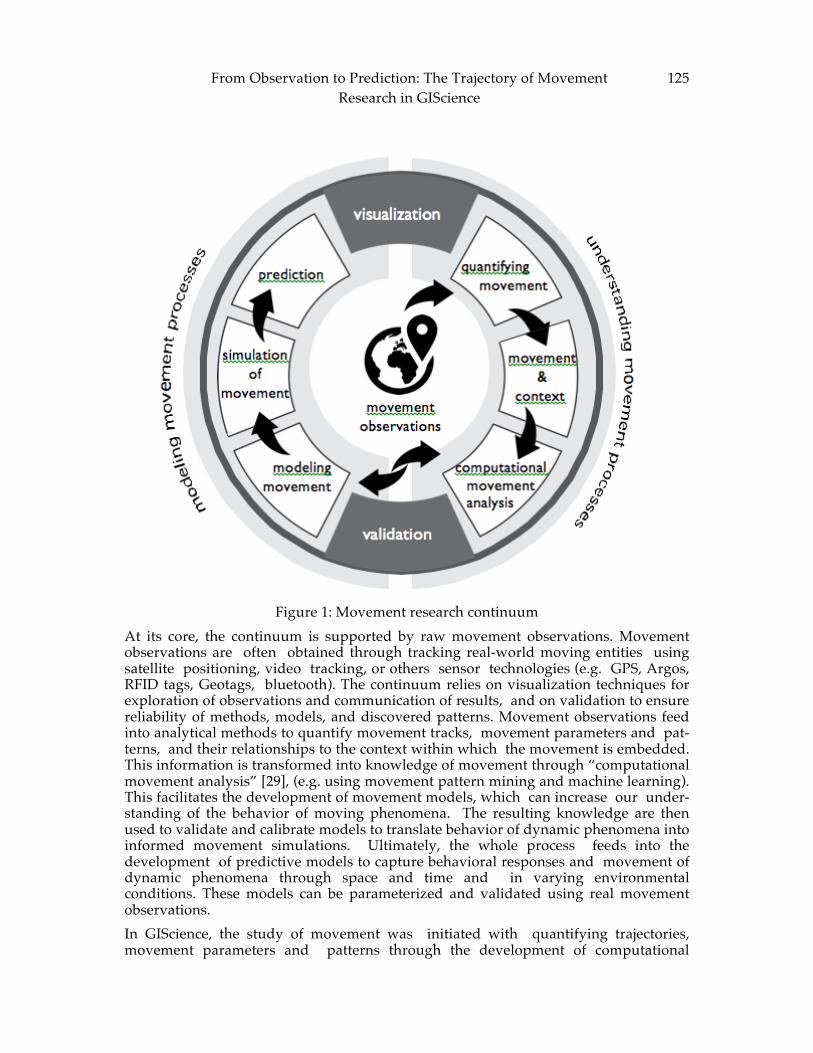
From Observation to Prediction: The Trajectory of Movement Research in GIScience
125
Figure 1: Movement research continuum
At its core, the continuum is supported by raw movement observations. Movement observations are often obtained through tracking real-world moving entities using satellite positioning, video tracking, or others sensor technologies (e.g. GPS, Argos, RFID tags, Geotags, bluetooth). The continuum relies on visualization techniques for exploration of observations and communication of results, and on validation to ensure reliability of methods, models, and discovered patterns. Movement observations feed into analytical methods to quantify movement tracks, movement parameters and pat- terns, and their relationships to the context within which the movement is embedded. This information is transformed into knowledge of movement through “computational movement analysis” [29], (e.g. using movement pattern mining and machine learning). This facilitates the development of movement models, which can increase our under- standing of the behavior of moving phenomena. The resulting knowledge are then used to validate and calibrate models to translate behavior of dynamic phenomena into informed movement simulations. Ultimately, the whole process feeds into the development of predictive models to capture behavioral responses and movement of dynamic phenomena through space and time and in varying environmental conditions. These models can be parameterized and validated using real movement observations. In GIScience, the study of movement was initiated with quantifying trajectories, movement parameters and patterns through the development of computational
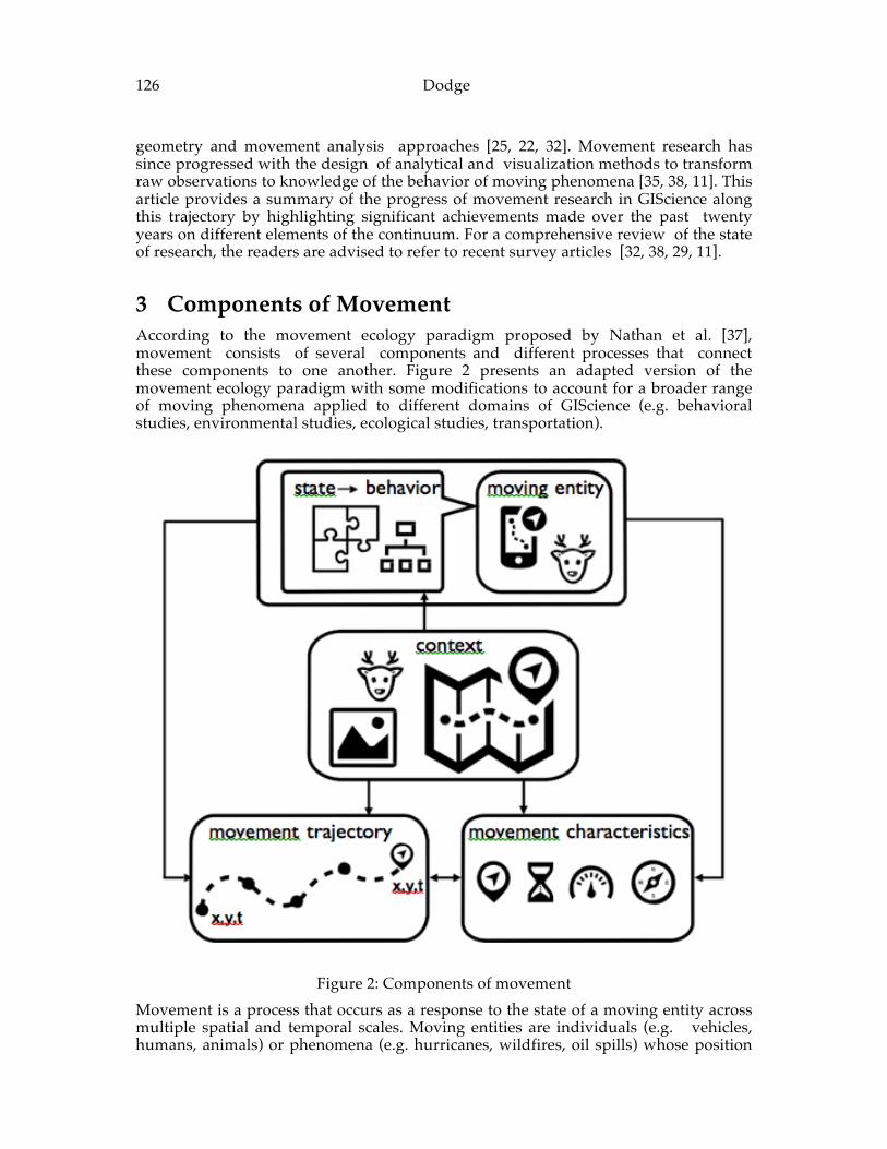
126 Dodge geometry and movement analysis approaches [25, 22, 32]. Movement research has since progressed with the design of analytical and visualization methods to transform raw observations to knowledge of the behavior of moving phenomena [35, 38, 11]. This article provides a summary of the progress of movement research in GIScience along this trajectory by highlighting significant achievements made over the past twenty years on different elements of the continuum. For a comprehensive review of the state of research, the readers are advised to refer to recent survey articles [32, 38, 29, 11].
3 Components of Movement According to the movement ecology paradigm proposed by Nathan et al. [37], movement consists of several components and different processes that connect these components to one another. Figure 2 presents an adapted version of the movement ecology paradigm with some modifications to account for a broader range of moving phenomena applied to different domains of GIScience (e.g. behavioral studies, environmental studies, ecological studies, transportation).
Figure 2: Components of movement
Movement is a process that occurs as a response to the state of a moving entity across multiple spatial and temporal scales. Moving entities are individuals (e.g. vehicles, humans, animals) or phenomena (e.g. hurricanes, wildfires, oil spills) whose position
From Observation to Prediction: The Trajectory of Movement Research in GIScience
127
changes over time. The state of an entity either emerges from intrinsic properties of the individual (e.g. being hungry or readiness to move) or is influenced by the context (i.e. presence of a pray or predator for animals, daily schedule for humans, rise in sea surface temperature for development of hurricanes). The context includes influencing external factors such as the geography and physiography in which the movement takes place, environment and ambient attributes, transportation network, and presence of other moving agents in the vicinity. The entity’s state leads to a behavior (e.g. hunting, patrolling, going to work, hurricane intensification). The state and resulting behavior determine the characteristics and capacities of movement (e.g. speeds, directions, accelerations, path sinuosity), which are highly influenced by context. Accordingly, the trajectory of a movement (i.e. a spatiotemporal path that is composed of a time-ordered sequence of coordinates) is driven by behavior and context. When more than one entity is involved in the process, their collective movements are driven by the interactions between the entities and their dynamics [19]. This collective behavior is also influenced by other contextual parameters in space and time.
4 Understanding Movement Processes Movement observations are signals of real-world moving entities. These signals carry important information pertaining to behavior of these entities. To gain insights into movement processes it is necessary to develop methods to analyze these signals, identify patterns (i.e. regularities and structure) in movement datasets, and assess how they are influenced by their environment [12]. These insights then contribute to modeling, simulation, and ultimately prediction of movement (see Figure 1).
4.1 Quantifying Movement The availability of fine resolution movement observations has facilitated GIScience with the development of effective methods to quantify the geometric properties of movement trajectories, their derivatives (e.g. speeds, acceleration, path sinuosity), and associated movement patterns [12]. These methods enable us to gain an understand- ing of the fundamental elements of movement and its patterns. This is indispensable as a basis for the development of computational and analytic techniques to extract knowledge from movement observations [17]. In many applications, studying movement characteristics of entities is more relevant than simply the geometry of their movement paths, as they convey the physical and biological notions of movement [16]. This information leads to insight into the semantics of trajectories, underlying mechanisms of movement, and the behavior of organisms.
4.2 Movement and Context Movement is often driven by the characteristics of its embedding spatiotemporal con- text; the surrounding environment and the the nature of space (i.e. geographic and physiography) that the object is moving through. This includes external factors that influence a dynamic process at a specific time scale (moment or duration). Context can be characterized into different types such as networks (e.g. roads), obstacles (e.g. lakes, rivers), and landscapes, (e.g. land cover, vegetation, terrain), ambient attributes (e.g. weather conditions), and presence of other agents (e.g. interactions) [6]. These parameters can trigger a specific behavior (e.g. hunting, patrolling, walking, biking) and hence they can enable or limit movement as a consequence of that behavior. For
128 Dodge instance, a tiger patrols a soft boundary of its home range more often than a boundary with rigorous terrain characteristics [2]. Therefore, movement observations alone cannot describe all mechanisms behind movement processes. In order to correctly identify patterns and their causes, and understand behaviors of moving phenomena it is essential to relate movement to its physical environment. Context has been an important part of GIScience studies which have dealt with characterizing geospatial phenomena based on the geographic context of their neigh- boring space [44, 18, 8]. Thus far context has been considered as a static snapshot of the neighboring space and spatiotemporal context (i.e. context that changes over time) has received less attention. Although GIScience has been very successful in both quantification of movement and modeling geographic context, the link between movement, behavior, and context has largely been ignored. This also has been identified as a current limitation of GIScience studies on movement [30], and as an important aspect of the future agenda of movement research [38]. Recently, a few studies have tackled the quantification of such connections and interactions [4, 14, 6, 13, 36]. This area still requires a lot of attention in future studies to increase our understanding of the relationships between movement and its spatiotemporal context, and to learn how environment influences the behavior and accordingly drives movement processes.
4.3 Computational Movement Analysis The term computational movement analysis was coined by P. Laube [29] and is defined as “computational techniques for capturing, processing, managing, structuring, and ultimately analyzing data describing movement phenomena”. In GIScience, a large number of studies have pioneered innovative computational movement analysis approaches for quantitative assessment of movement trajectories and their similarities [7, 15], mining movement patterns [28], clustering analysis [26], segmentation and classification of trajectories [16], to name but a few. According to recent reviews on the progress of these methods in GIScience [22, 32], most advances in this area have taken place in data mining and machine learning techniques for the detection of movement patterns in moving individuals or groups. The proposed techniques aim at finding structures and associations in movement datasets, by seeking commonalities and arrangements in the geometric specifications of trajectories or in the variation of their movement parameters in space and time [15]. The above publications not only document the significant progress of computational movement analysis in GIScience over the past twenty years, they also highlight the fact that so far environmental factors and geographic context have largely been ignored in the development of methods as well as in analyses. Integrating context and characteristics of the neighboring space in computational movement analysis seems inevitable and a logical step forward for future studies.
4.4 Visualization of Movement Visualization is a powerful tool in data science for data exploration and discovery of hidden patterns by giving structure to complex datasets through aggregations and cartographic processes. In movement research, visualization and animations enable collaboration among scientists of different domains to find common grounds to discuss movement observations, observe and interpret known patterns, discover unknown structures, and generate scientific hypotheses. Together with validation, visualization constitutes the backbone of the whole movement research continuum (Figure 1) be- cause it communicates the outcomes of computational techniques,
From Observation to Prediction: The Trajectory of Movement Research in GIScience
129
simulations, and predictive models in meaningful and effective ways by portraying the connections between movement and its context. Visualization can also support the validation process by facilitating the interpretation of results and providing real-time feedback for examining movement simulations. Geographic visualization and visual analytic techniques developed to this date mainly provide a complex representation of spatiotemporal phenomena that is not intuitive [3]. These techniques are often based on the three dimensional Ha¨gerstrand’s space-time-cube representation [27, 10] or hierarchical structures of treemaps [40]. Al- though these static representations can be effective for a small number of trajectories, they are cognitively very complex, particularly, when a large number of long trajectories are involved. Animations have proven to be an efficient medium, specially when communicating movement to scientists of other disciplines [49]. GIScience community should seek to develop more effective ways of communicating patterns in movement datasets using simple, dynamic, and interactive visualization approaches. Context re- mains to be an inevitable and integral part of future movement visualization tools [31].
5 Modeling Movement Processes In analyzing trajectories the assumption is that entities move freely in a landscape and without constraints. This assumption ignores the internal state of moving individual (i.e. movement strategies and decisions) and its behavior, as well as how it interacts with its physical environment and other dynamic phenomena. It is therefore essential to develop effective modeling and simulation approaches that capture the complexity of movement and behavior of individuals as they relate to the environment in which they move, the other individual with whom they interact and their responses to varying environments [1].
5.1 Modeling and Simulation of Movement Movement models are “simplified representation of real world” movement processes, which can be used “to explore, to understand better, or to predict” the behavior of such process [9]. These models are generated based on a set of assumptions on the states and behaviors of moving phenomena and their relationships with their embedding context. In GIScience, the time geography approaches have provided a basis for modeling the space-time settings of movement (i.e. space-time path, prism, and station) mainly for human activity patterns by taking the uncertainty of observations into ac- count [24, 34, 48, 42]. Approaches to date mainly consider movement capacities (i.e. max speed, time budget) when modeling the use of space. However, as mentioned earlier, these models need to be enriched with contextual parameters for a more realistic representation of movement processes. Thus far only a few studies have proposed such inclusive agent-based modeling of movement processes [2, 1, 5, 45]. This area still has room for growth in the future of GIScience research. Traditionally, simulation models have been used to generate a set of artificial movement trajectories to test known scientific hypotheses about the behavior of movement processes. Future research should strengthen simulation models for
130 Dodge prediction purposes based on quantitative analysis of real movement observations, and through an iterative calibration process.
5.2 Prediction Our universe is dynamic and changing over time. Any change in the environment can have an impact on the behavior of organisms. Also peculiarities in the behavior of moving phenomena could give us cues about environmental changes. In order to predict future responses to changes and varying environmental conditions, it is critical to translate our understanding of movement processes (i.e. from the right side of the continuum in Figure 1) to inform and calibrate predictive models. As a natural progression of movement research in GIScience, we need to develop predictive mod- els to assess how movement processes are changing over time and how future environmental changes impact these processes. Future simulation models should equip scientists with tools to assess how changes of any movement components (Figure 2) influence the susceptibility of the whole system over time. We now have available resources (i.e. valuable observations of real world movement processes and environmental information) and a solid foundation on which to generate effective and integrated simulation models enabling reliable prediction of movement and system outcomes/imbalances.
6 Discussion: Moving from Observations to Predictions In the past, direct observation of moving individuals was the most frequently used approach to quantify movement [47]. Following the rapid growth in movement observations owing to tremendous advances in positioning technologies, analytical methods have enabled GIScientists to increase their understanding of movement of dynamic phenomena and their associated behavior. However, the investigation of the interactions between moving phenomena with one another and with the physical environment through is lacking. What is required is more research on context-sensitive analytical techniques and simulation models. The GIScience community has made significant contribution to the understanding of movement (i.e. transforming movement observations to knowledge of behavior). These approaches have yet to inform us about how movement is affected by changes in the environment or how behavioral changes influence movement (i.e. derive movement from behavior and context). Still, questions such as to what extent movement observations convey information on the underlying behavior of moving phenomena? to what degree geographic and environmental contexts influence these behaviors? how susceptible are these behaviors to environmental changes? to what extent changes in the behavior of moving phenomena indicate changes in the environment? remain unanswered. In summary, GIScience has been successful in the past at extracting patterns and structures from raw movement observations. However, the community should strengthen its capacities to transform raw movement observations to behavior through informed models by incorporating contextual parameters and interactions with environment (i.e. the right side of the continuum in Figure 1). This knowledge should then inform simulation models in order to predict changes in movement in response to changes in environmental conditions (i.e. the left side of the continuum in Figure 1). En route to this goal, several important issues require careful considerations in future directions of movement studies in GIScience, which are summarized as follows: Temporal scales and granularity of movement: Movement is often reduced to a series of spatial positions in most existing methods, with little attention paid to the
From Observation to Prediction: The Trajectory of Movement Research in GIScience
131
temporal scales of movement and observation granularities. Geometric movement analysis techniques often disregard temporal information of trajectories (i.e. temporal resolution and frequencies). Future analytical techniques should take into account the temporal granularity of observations, temporal frequencies of movement patterns, and the sequential structure of trajectories [23, 30, 41]. Movement processes across scale: Movement processes form across different scales in space and time. In order to gain insights into hierarchical structures in movement processes, it is essential to explore movement patterns, their formation mechanisms, and their associations across a range of local to global scales [17, 30]. Movement uncertainty: Uncertainty is a fundamental and unavoidable issue in modeling, simulation, and prediction of movement. As noted in [9], “epistemic un- certainty”, which includes “process errors, measurement errors, random individual and temporal effects, uncertainty about initial conditions”, greatly affects models and resulting predictions. GIScience has been very successful in modeling measurement errors and making adjustments for locational errors and their propagations through the analysis [48, 42]. Future research should emphasize the effect of uncertainty on modeling and predictions of changes in movement processes. Evaluation and calibration of models through observations and domain expert knowledge: Future studies should evaluate the strengths and shortcomings of GI- Science computational approaches to movement research. Recent studies have shown that GIScience can benefit through interdisciplinary research collaborations [11]. Future movement research should embrace multidisciplinary collaborations to develop informed models by applying domain expert knowledge to effectively evaluate and calibrate models. A number of important research gaps in computational movement analysis are summarized in [29]. These challenges include handling big movement data, bridging the semantic gap between low-level movement observations and extracted patterns and structures obtained from the analyses, safeguarding individual’s privacy specifically in analyzing human mobility, and generating smart mobile applications through autonomous and decentralized spatial computing.
7 Conclusions This article presented a continuum of movement research to summarize previous studies and future directions of movement research in GIScience. The continuum organizes movement research in two overarching sections: (1) understanding of movement processes and (2) modeling movement processes. This article discussed the main highlights of GIScience research across this continuum and suggested a proposal for future directions of movement studies. GIScience to date has made significant contribution to this area through the development of data-driven computational movement analysis techniques and time geography approaches to quantify movement and space use patterns. Still methods to investigate the connections between movement and its context, and interactions between moving individuals lags behind. The GIScience community should embrace interdisciplinary collaborations with domain experts (e.g. ecologists, health scientists, etc.) to advance its capacities by developing reliable methodologies which are grounded in thorough knowledge of the dynamic phenomena and parametrized through real movement observations. Movement research in GIScience should progress towards the development of
132 Dodge informed simulations and predictive models to better understand the behavior of moving phenomena and assess their susceptibility to environmental changes. Issues such as working with large and real time movement datasets, privacy issues, influence of scale and granularity, uncertainty in movement observations and models, visualization of dynamic phenomena remain as important technical and scientific challenges for further research.
Acknowledgements The author wishes to thank Sean C. Ahearn (CUNY – Hunter College) for his valuable input and review of this paper, and Timothy F. Trainor (US Census Bureau), May Yuan (University of Oklahoma), and Stephan Winter (University of Melbourne) for their constructive feedback at the 2015 Vespucci Institute on Advancing Geographic Information Science: The Past and Next Twenty Years.
References [1] S. C. Ahearn and J. L. D. Smith. Modeling the interaction between humans and
animals in multiple use forests: a case study of Panthera tigris. In D. Maguire, M. Goodchild, and M. Batty, editors, GIS, Spatial Analysis, Modeling, chapter 18, pages 387–403. ESRI, Redlands, California, 2005.
[2] S. C. Ahearn, J. L. D. Smith, A. R. Joshi, and J. Ding. TIGMOD: an individual- based spatially explicit model for simulating tiger/human interaction in multiple use forests. Ecological Modelling, 140(1-2):81–97, 2001.
[3] G. Andrienko, N. Andrienko, P. Bak, D. Keim, and S. Wrobel. Visual Analytics of Movement. Springer, 2013.
[4] G. Andrienko, N. Andrienko, and M. Heurich. An event-based conceptual model for context-aware movement analysis. International Journal of Geographical Information Science, 25:1347–1370, 2011.
[5] D. A. Bennett and W. Tang. Modelling adaptive, spatially aware, and mobile agents: Elk migration in Yellowstone. International Journal of Geographical Information Science, 20(9):1039–1066, 2006.
[6] M. Buchin, S. Dodge, and B. Speckmann. Similarity of trajectories taking into account geographic context. Journal of Spatial Information Science, 9(9):101–124, 2014.
[7] M. Buchin, A. Driemel, M. van Kreveld, and V. Sacrista´ n. An Algorithmic Frame- work for Segmenting Trajectories based on Spatio-temporal Criteria. In Proceedings of the 18th SIGSPATIAL International Conference on Advances in Geographic In- formation Systems, GIS ’10, pages 202–211, New York, NY, USA, 2010. ACM.
[8] K. C. Clarke and L. J. Gaydos. Loose-coupling a cellular automaton model and GIS: long-term urban growth prediction for San Francisco and Washing- ton/Baltimore. International Journal of Geographical Information Science, 12(7):699–714, 1998.
[9] O. David and G. L. W. Perry. Spatial Simulation: Exploring Pattern and Process. Wiley-Blackwell, 2013.
From Observation to Prediction: The Trajectory of Movement Research in GIScience
133
[10] U. Demsˇar and K. Virrantaus. Space–time density of trajectories: exploring spatio-temporal patterns in movement data. International Journal of Geographical Information Science, 24(10):1527–1542, 2010.
[11] U. Demsˇar, K. Buchin, F. Cagnacci, K. Safi, B. Speckmann, N. Van de Weghe, D. Weiskopf, and R. Weibel. Analysis and visualisation of movement: an inter- disciplinary review. Movement Ecology, 3(1), 2015.
[12] S. Dodge. Exploring Movement Using Similarity Analysis. PhD thesis, University of Zurich, 2011.
[13] S. Dodge, G. Bohrer, K. Bildstein, S. C. Davidson, R. Weinzierl, M. J. Bechard, D. Barber, R. Kays, D. Brandes, J. Han, and M. Wikelski. Environmental drivers of variability in the movement ecology of turkey vultures (cathartes aura) in north and south america. Philosophical Transactions of the Royal Society of London B: Bio- logical Sciences, 369(1643), 2014.
[14] S. Dodge, G. Bohrer, R. Weinzierl, S. C. Davidson, R. Kays, D. Douglas, S. Cruz, J. Han, D. Brandes, and M. Wikelski. The environmental-data automated track annotation (Env-DATA) system: linking animal tracks with environmental data. Movement Ecology, 1(1):3, 2013.
[15] S. Dodge, P. Laube, and R. Weibel. Movement Similarity Assessment Using Sym- bolic Representation of Trajectories. International Journal of Geographic Information Science, 26(9):1563–1588, 2012.
[16] S. Dodge, R. Weibel, and E. Forootan. Revealing the Physics of Movement: Com- paring the Similarity of Movement Characteristics of Different Types of Moving Objects. Computers, Environment and Urban Systems, 33(6):419–434, Nov. 2009.
[17] S. Dodge, R. Weibel, and A.-K. Lautenschu¨ tz. Towards a Taxonomy of Movement Patterns. Information Visualization, 7(3-4):240–252, Aug. 2008.
[18] D. H. Douglas. Least-cost path in gis using an accumulated cost surface and slopelines. Cartographica: The International Journal for Geographic Information and Geovisualization, 31(3):37–51, 1994.
[19] A. Galton. Dynamic Collectives and their Collective Dynamics. In Spatial In- formation Theory, Lecture Notes in Computer Science, volume 3693, pages 300–315. Springer, 2005.
[20] M. L. Glasgow, C. B. Rudra, E.-H. Yoo, M. Demirbas, J. Merriman, P. Nayak, C. Crabtree-Ide, A. A. Szpiro, A. Rudra, J. Wactawski-Wende, and Others. Using smartphones to collect time–activity data for long-term personal-level air pollution exposure assessment. Journal of Exposure Science and Environmental Epidemiology, 2014.
[21] M. C. Gonza´ lez, C. a. Hidalgo, and A.-L. Baraba´ si. Understanding individual human mobility patterns. Nature, 453(7196):779–82, June 2008.
[22] J. Gudmundsson, P. Laube, and T. Wolle. Computational Movement Analysis. In W. Kresse and D. M. Danko, editors, Springer Handbook of Geographic Information, chapter 22, pages 725–741. Springer, Berlin-Heidelberg, Berlin, 2012.
[23] M. Holyoak, R. Casagrandi, R. Nathan, E. Revilla, and O. Spiegel. Trends and Missing Parts in the Study of Movement Ecology. Proceedings of the
134 Dodge
National Academy of Sciences of the United States of America, 105(49):19060–5, Dec. 2008.
[24] K. Hornsby and M. Egenhofer. Modeling Moving Objects over Multiple Granularities. Annals of Mathematics and Artificial Intelligence, 36(1):177–194, 2002.
[25] S. Imfeld. Time, Point and Space- Towards a Better Analysis of Wildlife Data in GIS. PhD thesis, Universitaet Zuerich, 2000.
[26] S. Kisilevich, F. Mansmann, M. Nanni, and S. Rinzivillo. Spatio-temporal clustering. Springer, 2010.
[27] M.-J. Kraak. The space-time cube revisited from a geovisualization perspective. In Proc. 21st International Cartographic Conference, pages 1988–1996, 2003
[28] P. Laube. Progress in Movement Pattern Analysis. In B. Gottfried and H. K. Aghajan, editors, Behaviour Monitoring and Interpretation - Ambient Assisted Living, volume 3 of Behaviour Monitoring and Interpretation – BMI - Smart Environments, pages 43–71. IOS Press BV, 2009.
[29] P. Laube. Computational Movement Analysis. Springer Briefs in Computer Science. Springer International Publishing, 1 edition, 2014.
[30] P. Laube and R. Purves. How fast is a cow? Cross-scale analysis of movement data. Transactions in GIS, 15(3):401–418, 2011.
[31] A.-K. Lautenschu¨ tz. Assessing the relevance of context for visualizations of movement trajectories. PhD thesis, University of Zurich, 2011.
[32] J. a. Long and T. a. Nelson. A review of quantitative methods for movement data. International Journal of Geographical Information Science, 27(2):292–318, 2013.
[33] Y. Lu and T. Fang. Examining Personal Air Pollution Exposure, Intake, and Health Danger Zone Using Time Geography and 3D Geovisualization. ISPRS International Journal of Geo-Information, 4(1):32–46, 2014.
[34] H. J. Miller. A Measurement Theory for Time Geography. Geographical Analysis, 4(2):63–45, Jan. 2005.
[35] H. J. Miller and J. Han. Geographic Data Mining and Knowledge Discovery. Taylor & Francis Group, second edition, 2009.
[36] J. A. Miller. Towards a better understanding of dynamic interaction metrics for wildlife: a null model approach. Transactions in GIS, 19(3):342–361, 2015.
[37] R. Nathan, W. M. Getz, E. Revilla, M. Holyoak, R. Kadmon, D. Saltz, and P. E. Smouse. A Movement Ecology Paradigm for Unifying Organismal Movement Research. Proceedings of the National Academy of Sciences of the United States of America, 105(49):19052–9, Dec. 2008.
[38] R. S. Purves, P. Laube, M. Buchin, and B. Speckmann. Moving beyond the point: An agenda for research in movement analysis with real data. Computers, Environment and Urban Systems, 47(0):1– 4, 2014.
[39] S. Sang, M. OKelly, and M.-P. Kwan. Examining Commuting Patterns: Results from a Journey-to-work Model Disaggregated by Gender and Occupation. Urban Studies, 48(5):891–909, 2011.
From Observation to Prediction: The Trajectory of Movement Research in GIScience
135
[40] A. Slingsby, J. Dykes, and J. Wood. Using treemaps for variable selection in spatio- temporal visualisation. Information Visualization, 7(3-4):210–224, 2008.
[41] A. Soleymani, J. Cachat, K. Robinson, S. Dodge, A. Kalueff, and R. Weibel. Inte- grating cross-scale analysis in the spatial and temporal domains for classification of behavioral movement. Journal of Spatial Information Science, 8(8):1–25, 2014.
[42] Y. Song and H. J. Miller. Simulating visit probability distributions within planar space-time prisms. International Journal of Geographical Information Science, 28(1):104–125, Jan. 2014.
[43] C. N. Theophilides, S. C. Ahearn, E. S. Binkowski, W. S. Paul, and K. Gibbs. First evidence of West Nile virus amplification and relationship to human infections. International Journal of Geographical Information Science, 20(1):103–115, 2006.
[44] C. D. Tomlin. Cartographic Modelling, 1991. [45] P. M. Torrens, A. Nara, X. Li, H. Zhu, W. a. Griffin, and S. B. Brown. An
extensible simulation environment and movement metrics for testing walking behavior in agent-based models. Computers, Environment and Urban Systems, 36(1):1–17, 2012.
[46] C. P. Tribby, H. J. Miller, C. M. Werner, K. R. Smith, and B. B. Brown. Assessing built environment walkability using activity-space summary measures. Journal of Transportation and Land Use, 0(0):1–21, 2015.
[47] P. Turchin. Quantitative Analysis of Movement: Measuring and Modeling Population Redistribution in Animals and Plants. Sinauer Associates, Sunderland, MA, USA,1998.
[48] S. Winter and Z.-C. Yin. The elements of probabilistic time geography. GeoInformatica, 15(3):417–434, Apr. 2010.
[49] G. Xavier and S. Dodge. An Exploratory Visualization Tool for Mapping the Relationships between Animal Movement and the Environment. In Proceedings of the 2nd ACM SIGSPATIAL Workshop on MapInteraction, pages 36–42, 2014.

136 Dodge
ADVANCING GEOGRAPHIC INFORMATION SCIENCE: CHAPTER 10
© by the author(s) Licensed under Creative Commons Attribution 4.0 License
137
Beyond Homeomorphic Deformations: Neighborhoods of
Topological Changes Matthew P. Dube
School of Computing and Information Science, University of Maine, Orono, Maine 04469, USA
Abstract: The past 20 years has seen the vast growth of the field of qualitative spatial reasoning. While qualitative formalisms have been developed to identify topologically similar binary relations from the point-of-view of the 9-intersection, one of the most important pieces of the spatial reasoning puzzle is in that of the conceptual neighborhood graph. Conceptual neighborhood graphs remain restricted to homeomorphic deformations of regions. In this paper, topological changes to the structure of an object are considered, such as that of hole formation and separation generation. This paper lays the groundwork for neighborhoods of non-homeomorphic deformations, a necessity in a sensor world.
Keywords: Topological spatial reasoning, topological changes, conceptual neighbourhood graph, complex regions, spatial queries
1 Introduction Qualitative spatial reasoning is a topic that developed dramatically over the last 20 years. Dominated by sound formalisms for qualitative spatial relations, in particular binary topological relations [16][31], it has expanded into automated abstract inferences without a need for exact geometric representations, including reasoning about spatial similarities. The majority of such approaches assume changes in the objects’ locations and shapes, yet they rely on the preservation of the objects’ topological structure. For instance, in such reasoning, regions may change their sites or footprints, but they otherwise remain holed or hole-free, separated or separation-free. This paper lays the foundation for non-homeomorphic deformations between objects, a necessity in a world driven by sensor technologies. In other words, how do topological structure changes change object relations? Within a single object, a topological change represents simply a transformation of that single object in one of many ways [23][30]: topology preserving changes, such as the
138 DUBE changes exhibited by a receding or advancing glacier, hole forming changes, such as the creation of an oxbow lake or a loss of coverage within a sensor network, separation forming changes, such as a natural disaster dividing an ecosystem or the historical acquisition of territory such as Seward’s Folly, hole removing changes, such as sea level rise, separation removing changes, such as countries declaring independence from a colonial power or the reunification of Germany, or any combination of such changes. Relation changes occur between a pair of objects [15][19] or between a collection of objects [2][25][26] when the topological or mereotopological interactions between the objects change vis à vis some formalism such as the 9-intersection [17], the 9+-intersection [24], or the region connection calculus [31]. These changes ultimately reflect the similarity between distinct topological states. Such changes have been modelled through the conceptual neighborhood graph [19]. A simple example of a relation change is the movement of the moon’s shadow across the Earth during a solar eclipse relative to political boundaries. As the Earth rotates “beneath” the shadow, the moon’s shadow moves relative to the objects on the Earth, potentially changing basic topological relations on its surface. Spatial query languages are reliant upon the conceptual neighborhood graph in a key operation: nearest neighbor matching. In such instances where the particular result cannot be found in the database, a nearest neighbor match is declared when the distance within the conceptual neighborhood graph is minimized [12]. To effectively execute such a match requires knowledge not just of topology preserving changes (or combinations thereof) [11], but also requires knowledge of what happens when a dynamic object is allowed to change its topological structure. While Liu and Schneider [30] have attempted to explain how to convert from one topological structure to another through a state transition graph, the impact upon the relations themselves has not been studied past the level of their determination as a possibility for complex regions [27][33]. In this paper, the study of conceptual neighbors is moved from the realm of topology preserving changes to the realm of topology modifying changes using the approach of typed relations. While researchers have considered type-independent conceptual neighborhood graphs [4], conceptual neighborhood graphs within simple types [11][14][15][20], or even context-based conceptual neighborhood graphs [5], complex relations have not been studied through the approach of typed relations other than the environments holed region to simple region [18] and holed region to holed region [37], but even in those cases, the neighborhoods are based on topology preserving deformations. The remainder of this paper is structured as follows. In Section 2, the basics of topological structure changes within an object are presented. In Section 3, the basics of topological relation changes between objects are presented. In Section 4, the impact of first order topology modifying changes is addressed, identifying the transition from simple regions to such object types as holed region, self-merging region, separated region, and self-splitting region, and the corresponding effect upon the relation to a second simple region. In Section 5, the impact of second order topology modifying changes is addressed, resulting in regions with multiple holes, multiple separations, and regions with a hole and a separation together, and the corresponding effect upon the relation. Section 6 considers if second order topology modifying changes are closed, namely that the execution of yet another operation upon the relations of that type results in additional connections in the neighborhood. Section 7 provides conclusions and calls for future study.
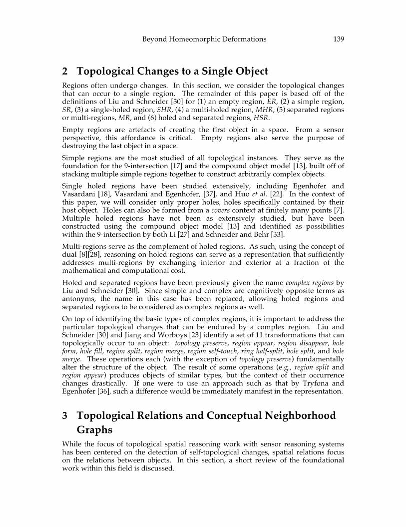
Beyond Homeomorphic Deformations 139
2 Topological Changes to a Single Object Regions often undergo changes. In this section, we consider the topological changes that can occur to a single region. The remainder of this paper is based off of the definitions of Liu and Schneider [30] for (1) an empty region, ER, (2) a simple region, SR, (3) a single-holed region, SHR, (4) a multi-holed region, MHR, (5) separated regions or multi-regions, MR, and (6) holed and separated regions, HSR. Empty regions are artefacts of creating the first object in a space. From a sensor perspective, this affordance is critical. Empty regions also serve the purpose of destroying the last object in a space. Simple regions are the most studied of all topological instances. They serve as the foundation for the 9-intersection [17] and the compound object model [13], built off of stacking multiple simple regions together to construct arbitrarily complex objects. Single holed regions have been studied extensively, including Egenhofer and Vasardani [18], Vasardani and Egenhofer, [37], and Huo et al. [22]. In the context of this paper, we will consider only proper holes, holes specifically contained by their host object. Holes can also be formed from a covers context at finitely many points [7]. Multiple holed regions have not been as extensively studied, but have been constructed using the compound object model [13] and identified as possibilities within the 9-intersection by both Li [27] and Schneider and Behr [33]. Multi-regions serve as the complement of holed regions. As such, using the concept of dual [8][28], reasoning on holed regions can serve as a representation that sufficiently addresses multi-regions by exchanging interior and exterior at a fraction of the mathematical and computational cost. Holed and separated regions have been previously given the name complex regions by Liu and Schneider [30]. Since simple and complex are cognitively opposite terms as antonyms, the name in this case has been replaced, allowing holed regions and separated regions to be considered as complex regions as well. On top of identifying the basic types of complex regions, it is important to address the particular topological changes that can be endured by a complex region. Liu and Schneider [30] and Jiang and Worboys [23] identify a set of 11 transformations that can topologically occur to an object: topology preserve, region appear, region disappear, hole form, hole fill, region split, region merge, region self-touch, ring half-split, hole split, and hole merge. These operations each (with the exception of topology preserve) fundamentally alter the structure of the object. The result of some operations (e.g., region split and region appear) produces objects of similar types, but the context of their occurrence changes drastically. If one were to use an approach such as that by Tryfona and Egenhofer [36], such a difference would be immediately manifest in the representation.
3 Topological Relations and Conceptual Neighborhood Graphs
While the focus of topological spatial reasoning work with sensor reasoning systems has been centered on the detection of self-topological changes, spatial relations focus on the relations between objects. In this section, a short review of the foundational work within this field is discussed.
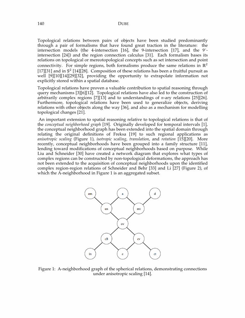
140 DUBE Topological relations between pairs of objects have been studied predominantly through a pair of formalisms that have found great traction in the literature: the intersection models (the 4-intersection [16], the 9-intersection [17], and the 9+-intersection [24]) and the region connection calculus [31]. Each formalism bases its relations on topological or mereotopological concepts such as set intersection and point connectivity. For simple regions, both formalisms produce the same relations in ℝ! [17][31] and in 𝕊! [14][28]. Composition of these relations has been a fruitful pursuit as well [9][10][14][29][32], providing the opportunity to extrapolate information not explicitly stored within a spatial database. Topological relations have proven a valuable contribution to spatial reasoning through query mechanisms [3][6][12]. Topological relations have also led to the construction of arbitrarily complex regions [7][13] and to understandings of n-ary relations [25][26]. Furthermore, topological relations have been used to generalize objects, deriving relations with other objects along the way [36], and also as a mechanism for modelling topological changes [21]. An important extension to spatial reasoning relative to topological relations is that of the conceptual neighborhood graph [19]. Originally developed for temporal intervals [1], the conceptual neighborhood graph has been extended into the spatial domain through relating the original definitions of Freksa [19] to such regional applications as anisotropic scaling (Figure 1), isotropic scaling, translation, and rotation [15][20]. More recently, conceptual neighborhoods have been grouped into a family structure [11], lending toward modifications of conceptual neighborhoods based on purpose. While Liu and Schneider [30] have created a network diagram that explores what types of complex regions can be constructed by non-topological deformations, the approach has not been extended to the acquisition of conceptual neighborhoods upon the identified complex region-region relations of Schneider and Behr [33] and Li [27] (Figure 2), of which the A-neighborhood in Figure 1 is an aggregated subset.
Figure 1: A-neighborhood graph of the spherical relations, demonstrating connections under anisotropic scaling [14].
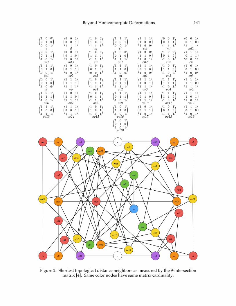
Beyond Homeomorphic Deformations 141
1 0 00 1 00 0 1
0 0 10 0 11 1 1
1 0 01 0 01 1 1
1 1 10 0 10 0 1
1 1 11 0 01 0 0
0 0 10 1 11 1 1
0 0 10 1 01 1 1
e d in ct em mt mt1 0 0 10 1 11 0 1
0 0 10 1 01 0 1
1 0 01 1 01 1 1
1 0 00 1 01 1 1
1 0 01 1 01 0 1
1 0 00 1 01 0 1
1 1 10 1 10 0 1
mt2 mt3 cB cB1 cB2 cB3 cv 1 1 10 1 00 0 1
1 0 10 1 10 0 1
1 0 10 1 00 0 1
1 1 11 1 01 0 0
1 1 10 1 01 0 0
1 0 11 1 01 0 0
1 0 10 1 01 0 0
cv1 cv2 cv3 en en1 en2 en3 0 0 10 1 01 0 0
1 1 11 1 11 1 1
1 0 11 1 11 1 1
1 1 10 1 11 1 1
1 1 11 0 11 1 1
1 1 11 1 11 0 1
1 1 11 1 01 1 1
a ov ov1 ov2 ov3 ov4 ov5 1 0 11 1 11 0 1
1 0 11 1 01 1 1
1 0 10 1 11 1 1
1 1 10 1 11 0 1
1 1 10 1 01 1 1
1 1 11 1 01 0 1
1 1 11 0 11 0 1
ov6 ov7 ov8 ov9 ov10 ov11 ov12 1 1 11 0 01 1 1
1 1 10 0 11 1 1
1 0 11 0 11 1 1
1 0 11 1 01 0 1
1 0 10 1 11 0 1
1 0 10 1 01 1 1
1 1 10 1 01 0 1
ov13 ov14 ov15 ov16 ov17 ov18 ov19
1 0 10 1 01 0 1
ov20
Figure 2: Shortest topological distance neighbors as measured by the 9-intersection matrix [4]. Same color nodes have same matrix cardinality.
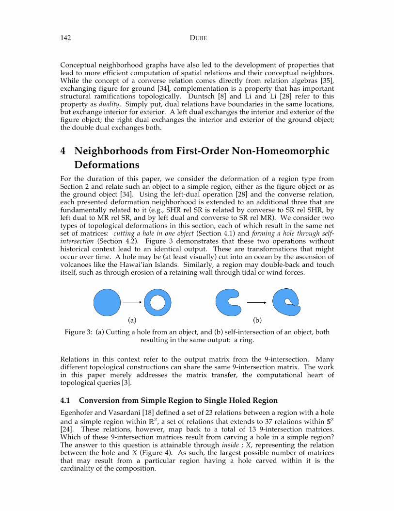
142 DUBE Conceptual neighborhood graphs have also led to the development of properties that lead to more efficient computation of spatial relations and their conceptual neighbors. While the concept of a converse relation comes directly from relation algebras [35], exchanging figure for ground [34], complementation is a property that has important structural ramifications topologically. Duntsch [8] and Li and Li [28] refer to this property as duality. Simply put, dual relations have boundaries in the same locations, but exchange interior for exterior. A left dual exchanges the interior and exterior of the figure object; the right dual exchanges the interior and exterior of the ground object; the double dual exchanges both.
4 Neighborhoods from First-‐‑Order Non-‐‑Homeomorphic Deformations
For the duration of this paper, we consider the deformation of a region type from Section 2 and relate such an object to a simple region, either as the figure object or as the ground object [34]. Using the left-dual operation [28] and the converse relation, each presented deformation neighborhood is extended to an additional three that are fundamentally related to it (e.g., SHR rel SR is related by converse to SR rel SHR, by left dual to MR rel SR, and by left dual and converse to SR rel MR). We consider two types of topological deformations in this section, each of which result in the same net set of matrices: cutting a hole in one object (Section 4.1) and forming a hole through self-intersection (Section 4.2). Figure 3 demonstrates that these two operations without historical context lead to an identical output. These are transformations that might occur over time. A hole may be (at least visually) cut into an ocean by the ascension of volcanoes like the Hawai’ian Islands. Similarly, a region may double-back and touch itself, such as through erosion of a retaining wall through tidal or wind forces.
(a) (b)
Figure 3: (a) Cutting a hole from an object, and (b) self-intersection of an object, both resulting in the same output: a ring.
Relations in this context refer to the output matrix from the 9-intersection. Many different topological constructions can share the same 9-intersection matrix. The work in this paper merely addresses the matrix transfer, the computational heart of topological queries [3].
4.1 Conversion from Simple Region to Single Holed Region Egenhofer and Vasardani [18] defined a set of 23 relations between a region with a hole and a simple region within ℝ!, a set of relations that extends to 37 relations within 𝕊! [24]. These relations, however, map back to a total of 13 9-intersection matrices. Which of these 9-intersection matrices result from carving a hole in a simple region? The answer to this question is attainable through inside ; X, representing the relation between the hole and X (Figure 4). As such, the largest possible number of matrices that may result from a particular region having a hole carved within it is the cardinality of the composition.
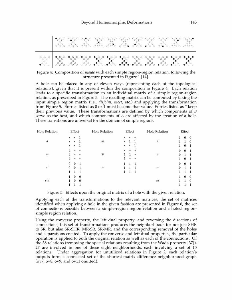
Beyond Homeomorphic Deformations 143
Figure 4: Composition of inside with each simple region-region relation, following the
structure presented in Figure 1 [14]. A hole can be placed in any of eleven ways (representing each of the topological relations), given that it is present within the composition in Figure 4. Each relation leads to a specific transformation to an individual matrix of a simple region-region relation, as prescribed in Figure 5. The resulting matrix can be computed by taking the input simple region matrix (i.e., disjoint, meet, etc.) and applying the transformation from Figure 5. Entries listed as 0 or 1 must become that value. Entries listed as * keep their previous value. These transformations are defined by which components of B serve as the host, and which components of A are affected by the creation of a hole. These transitions are universal for the domain of simple regions. Hole Relation Effect Hole Relation Effect Hole Relation Effect
d ∗ ∗ 1∗ ∗ 1∗ ∗ 1
mt ∗ ∗ ∗∗ 1 1∗ ∗ 1
a 1 0 01 1 01 0 1
in 1 ∗ ∗1 ∗ ∗1 ∗ ∗
cB ∗ ∗ ∗1 1 ∗1 ∗ ∗
e 0 0 10 1 11 0 1
ct 0 0 10 0 11 1 1
ov 1 1 11 1 11 1 1
cv 0 0 10 1 11 1 1
em 1 0 01 0 01 1 1
en 1 0 01 1 01 1 1
Figure 5: Effects upon the original matrix of a hole with the given relation. Applying each of the transformations to the relevant matrices, the set of matrices identified when applying a hole in the given fashion are presented in Figure 6, the set of connections possible between a simple-region region relation and a holed region-simple region relation. Using the converse property, the left dual property, and reversing the directions of connections, this set of transformations produces the neighborhoods for not just SHR to SR, but also SR-SHR, MR-SR, SR-MR, and the corresponding removal of the holes and separations created. To apply the converse and left dual properties, the particular operation is applied to both the original relation as well as each of the connections. Of the 38 relations (removing the special relations resulting from the Wada property [37]), 27 are involved in one of these eight neighborhoods, each involving a set of 15 relations. Under aggregation for unutilized relations in Figure 2, each relation’s outputs form a connected set of the shortest-matrix difference neighborhood graph (ov7, ov8, ov9, and ov11 omitted).
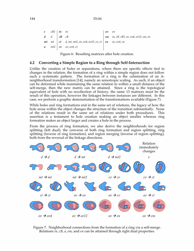
144 DUBE
e cB2 in in ov ov
d d cB cB em in, cB, cB2, ov, ov4, ov12, em, en
mt mt ct d, mt, mt2, ov, ov4, ov12, cv, ct en ov, ov4, en
a mt2 cv ov, ov4, cv
Figure 6: Resulting matrices after hole creation.
4.2 Converting a Simple Region to a Ring through Self-‐‑Intersection Unlike the creation of holes or separations, where there are specific effects tied to changes in the relation, the formation of a ring within a simple region does not follow such a systematic pattern. The formation of a ring is the culmination of an A-neighborhood transformation [14], namely an anisotropic scaling. As such, if an object can be deformed while maintaining the same relation to within a small distance of the self-merge, then the new matrix can be attained. Since a ring is the topological equivalent of hole with no recollection of history, the same 13 matrices must be the result of this operation, however the linkages between instances are different. In this case, we perform a graphic demonstration of the transformations available (Figure 7). While holes and ring formations end in the same set of relations, the legacy of how the hole arose within the object changes the structure of the transition substantially. None of the relations result in the same set of relations under both procedures. This assertion is a testament to hole creation making an object smaller whereas ring formation makes an object larger and creates a hole in the process. From the process of ring formation, we also derive the neighborhoods for region splitting (left dual), the converse of both ring formation and region splitting, ring splitting (inverse of ring formation), and region merging (inverse of region splitting), both from the reversal of the linkage directions.
Relation immediately
changes d à d d à mt d à mt2 e
mt à mt mt à mt2 cv à cv cv à ct
ct à ct ov à ov ov à cv ov à ct
ov à ov4 ov à ov12 ov à en ov à em
Figure 7. Neighborhood connections from the formation of a ring via a self-merge.
Relations in, cB, a, em, and en can be attained through right dual properties.
Beyond Homeomorphic Deformations 145
As also seen in Figure 6, the changes under ring formation also form connected sets after aggregation of non-used relations ov7, ov8, ov9, and ov11.
5 Neighborhoods for Second-‐‑Order Non-‐‑Homeomorphic Deformations
Section 4 considered the transitions that resulted from making a single change to a simple region. In this section, we consider deformations upon these deformations, what we term second order non-topological deformations. Second order non-topological deformations lead to such object types as MHR, MSR, and CR. At the level of second order deformations, a hole and a ring are the same basis, and similarly a separation and a split are the same basis. The operations themselves, however, are not equivalent as previously demonstrated. We will only consider second order deformations as occurring to a previously deformed region, not to a simple region opposite a previously deformed region. This application is saved for future work. Similarly, we will only consider second order deformations formed under the insertion of a hole, the creation of a separation, or the splitting of a hole.
5.1 Adding Extra Holes (or Adding Extra Separations) Like for simple disks, the insertion of a hole with a particular relation to B will have the same effects as it did in Figure 5. As such, to accomplish the mapping, we must determine which matrices can have an additional hole inserted in a particular topological relation to B. Simply put, a hole can be placed in A wherever A’s components will allow it relative to B (Figure 8), having always an impact on A’s interior, but in some cases having further impacts. Applying the transformations in Figure 5 to the relations from Figure 8 produces the viable matrices that arising from the insertion of a second hole into A for a SHR – SR relation. These relations are shown in Figure 9. While additional relations are connected to one another, the set of relations is closed under hole formation solely and under separation generation solely. This closure property suggests that under one type of complexity, only a small set of matrices are available. While the type of complexity can be exchanged, the small set of matrices is equivalent in size and only differs by the converse property or the dual properties. The connections established in Figure 9 can be converted in much the same way as single holed relations were converted to single separations and their converses. Using this powerful transformation produces the relation between simple regions and multiple-holed regions, n-separations to simple regions (n > 2), and its converse. Like their predecessors, these connections are again closed under neighborhood aggregation over relations ov7, ov8, ov9, and ov11.
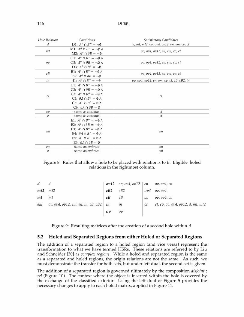
146 DUBE Hole Relation Conditions Satisfactory Candidates
d D1: 𝐴! ∩ 𝐵! = ¬∅ d, mt, mt2, ov, ov4, ov12, en, em, cv, ct
mt M1: 𝐴! ∩ 𝐵! = ¬∅ ∧ M2: 𝐴! ∩ 𝜕𝐵 = ¬∅ ov, ov4, ov12, en, em, cv, ct
ov O1: 𝐴! ∩ 𝐵! = ¬∅ ∧ O2: 𝐴! ∩ 𝜕𝐵 = ¬∅ ∧ O3: 𝐴! ∩ 𝐵! = ¬∅
ov, ov4, ov12, en, em, cv, ct
cB B1: 𝐴! ∩ 𝐵! = ¬∅ ∧ B2: 𝐴! ∩ 𝜕𝐵 = ¬∅ ov, ov4, ov12, en, em, cv, ct
in I1: 𝐴! ∩ 𝐵! = ¬∅ ov, ov4, ov12, en, em, cv, ct, cB, cB2, in
ct
C1: 𝐴! ∩ 𝐵! = ¬∅ ∧ C2: 𝐴! ∩ 𝜕𝐵 = ¬∅ ∧ C3: 𝐴! ∩ 𝐵! = ¬∅ ∧ C4: 𝜕𝐴 ∩ 𝐵! = ∅ ∧ C5: 𝐴! ∩ 𝐵! = ∅ ∧ C6: 𝜕𝐴 ∩ 𝜕𝐵 = ∅
ct
cv same as contains ct e same as contains ct
em
E1: 𝐴! ∩ 𝐵! = ¬∅ ∧ E2: 𝐴! ∩ 𝜕𝐵 = ¬∅ ∧ E3: 𝐴! ∩ 𝐵! = ¬∅ ∧ E4: 𝜕𝐴 ∩ 𝐵! = ∅ ∧ E5: 𝐴! ∩ 𝐵! = ∅ ∧ E6: 𝜕𝐴 ∩ 𝜕𝐵 = ∅
em
en same as embrace em a same as embrace em
Figure 8. Rules that allow a hole to be placed with relation x to B. Eligible holed
relations in the rightmost column.
d d ov12 ov, ov4, ov12 en ov, ov4, en mt2 mt2 cB2 cB2 ov4 ov, ov4 mt mt cB cB cv ov, ov4, cv em ov, ov4, ov12, em, en, in, cB, cB2 in in ct ct, cv, ov, ov4, ov12, d, mt, mt2
ov ov
Figure 9: Resulting matrices after the creation of a second hole within A.
5.2 Holed and Separated Regions from either Holed or Separated Regions The addition of a separated region to a holed region (and vice versa) represent the transformation to what we have termed HSRs. These relations are referred to by Liu and Schneider [30] as complex regions. While a holed and separated region is the same as a separated and holed regions, the origin relations are not the same. As such, we must demonstrate the transfer for both sets, but under left dual, the second set is given. The addition of a separated region is governed ultimately by the composition disjoint ; rel (Figure 10). The context where the object is inserted within the hole is covered by the exchange of the classified exterior. Using the left dual of Figure 5 provides the necessary changes to apply to each holed matrix, applied in Figure 11.
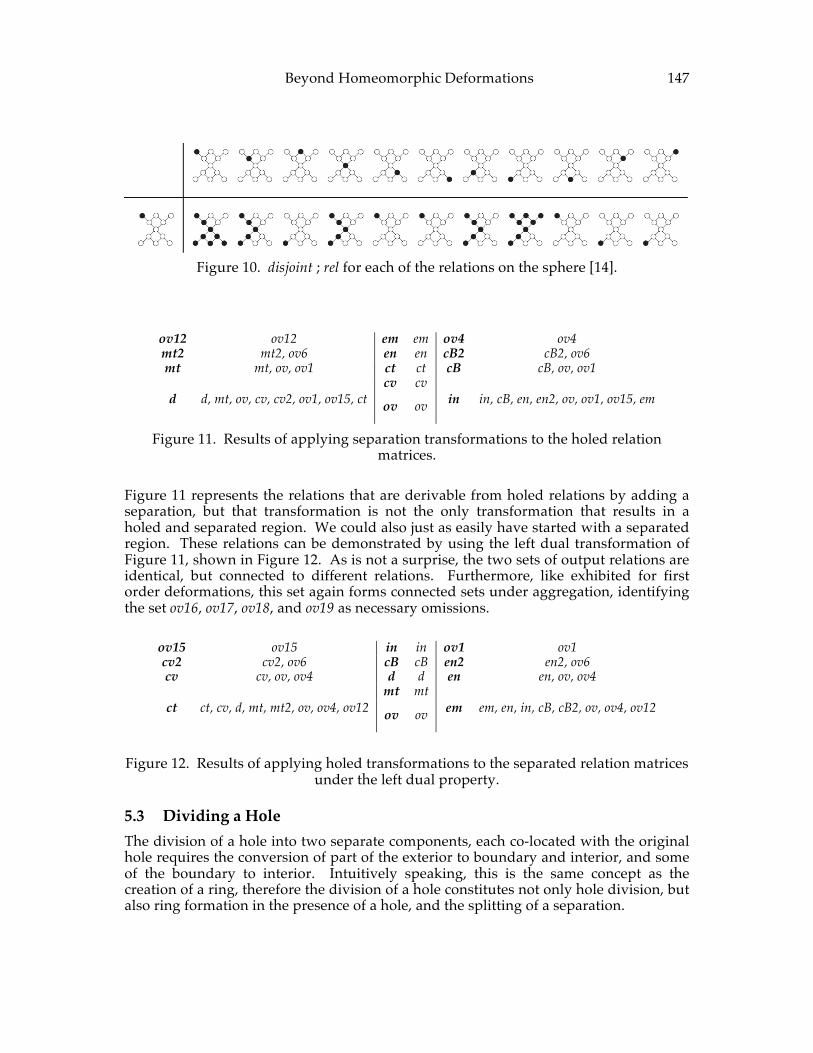
Beyond Homeomorphic Deformations 147
Figure 10. disjoint ; rel for each of the relations on the sphere [14].
ov12 ov12 em em ov4 ov4 mt2 mt2, ov6 en en cB2 cB2, ov6 mt mt, ov, ov1 ct ct cB cB, ov, ov1
d d, mt, ov, cv, cv2, ov1, ov15, ct cv cv
in in, cB, en, en2, ov, ov1, ov15, em ov ov
Figure 11. Results of applying separation transformations to the holed relation matrices.
Figure 11 represents the relations that are derivable from holed relations by adding a separation, but that transformation is not the only transformation that results in a holed and separated region. We could also just as easily have started with a separated region. These relations can be demonstrated by using the left dual transformation of Figure 11, shown in Figure 12. As is not a surprise, the two sets of output relations are identical, but connected to different relations. Furthermore, like exhibited for first order deformations, this set again forms connected sets under aggregation, identifying the set ov16, ov17, ov18, and ov19 as necessary omissions.
ov15 ov15 in in ov1 ov1 cv2 cv2, ov6 cB cB en2 en2, ov6 cv cv, ov, ov4 d d en en, ov, ov4
ct ct, cv, d, mt, mt2, ov, ov4, ov12 mt mt
em em, en, in, cB, cB2, ov, ov4, ov12 ov ov
Figure 12. Results of applying holed transformations to the separated relation matrices
under the left dual property.
5.3 Dividing a Hole The division of a hole into two separate components, each co-located with the original hole requires the conversion of part of the exterior to boundary and interior, and some of the boundary to interior. Intuitively speaking, this is the same concept as the creation of a ring, therefore the division of a hole constitutes not only hole division, but also ring formation in the presence of a hole, and the splitting of a separation.
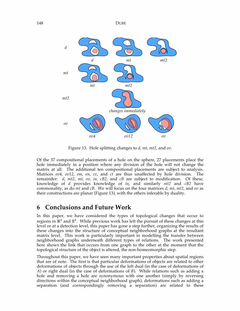
148 DUBE
d
d mt mt2
mt
mt mt2
mt2
changes immediately
ov
ov4 ov12 ov
Figure 13. Hole splitting changes to d, mt, mt2, and ov.
Of the 37 compositional placements of a hole on the sphere, 27 placements place the hole immediately in a position where any division of the hole will not change the matrix at all. The additional ten compositional placements are subject to analysis. Matrices ov4, ov12, em, en, cv, and ct are thus unaffected by hole division. The remainder: d, mt2, mt, ov, in, cB2, and cB are subject to modification. Of these, knowledge of d provides knowledge of in, and similarly mt2 and cB2 have commonality, as do mt and cB. We will focus on the four matrices d, mt, mt2, and ov as their constructions are planar (Figure 13), with the others inferable by duality.
6 Conclusions and Future Work In this paper, we have considered the types of topological changes that occur to regions in ℝ! and 𝕊!. While previous work has left the pursuit of these changes at this level or at a detection level, this paper has gone a step further, organizing the results of these changes into the structure of conceptual neighborhood graphs at the resultant matrix level. This work is particularly important in modelling the transfer between neighborhood graphs underneath different types of relations. The work presented here shows the link that occurs from one graph to the other at the moment that the topological structure of the object is altered, the non-homeomorphic step. Throughout this paper, we have seen many important properties about spatial regions that are of note. The first is that particular deformations of objects are related to other deformations of objects through the use of the left dual (in the case of deformations of A) or right dual (in the case of deformations of B). While relations such as adding a hole and removing a hole are synonymous with one another (simply by reversing directions within the conceptual neighborhood graph), deformations such as adding a separation (and correspondingly removing a separation) are related to these
Beyond Homeomorphic Deformations 149
operations. Using the left dual and the converse operations, knowledge of the matrices that result from adding a hole to A can be used to create removal of a hole, addition of a separation, removal of a separation (all in A), and by converse can be used to create the same deformations within the object B. On top of these deformations, deformations such as ring formation, object splitting, ring splitting, and object merging are all related to one another in a similar manner. This paper used these fundamental properties to streamline the process of full identification. Another interesting insight with regard to hole formation and ring formation is that the two deformations result in the same output set of matrices (as each forms a hole in the end), but the manner in which the corresponding simple region relations are connected to these output relations in either case is not equivalent. This assertion is not a large surprise, but is rather important to note. The history and context of hole formation is very important in this light. Similarly, a region that divides is different contextually than a region that spawns a separation. These differences are the result of two concepts: A-neighborhood deformations that lead to rings or splits, and secondly, the semantics of ring formation versus hole formation. Ring formation is in addition to the object (a composition with covers), whereas hole formation is a composition with inside. Both relations (part of a larger converse family under generalization) lead to vastly different inferences, and thus vastly different connections to simple region parents. For second order deformations and beyond, the historical legacy of hole formation or ring formation is inconsequential as the output structures are identical. After considering the deformations in this paper, 29 of the 38 matrices proposed by Li [27] (excluding the Wada property) have been accounted for within a conceptual neighborhood graph setting. The other nine matrices thus are the result of the combination of holes and separations in both A and B, a set of deformations not accounted for in this paper. To complete the process of this work requires the study of the relation between complex objects A and B, not just the relation between a single complex object and a simple region. These missing relations are ov3, ov7, ov8, ov9, ov11, ov16, ov17, ov18, and ov19. The Wada relations are ov20, mt3, en3, cB3, and cv3. Furthermore, under aggregation of these 14 relations, the conceptual neighbors from the particular non-homeomorphic changes are all neighbors within the shortest-distance neighborhood graph, the suggested prototype for neighborhood graphs [4]. Apart from the additional construction of neighborhood graphs is the insight that the type of relation matters in deformation neighborhoods. If an object is a simple region and a separation is added to it, a set of 13 matrices result. Similarly, if an object is a holed region and a separation is added to the holed region, a set of 16 matrices result. Type thus is instrumental in understanding the qualitative possibilities that deformation provides. This knowledge is critically important for the advancement of spatial information systems in a world where complexity is becoming evermore the normal expectation. Since underlying formalisms for query models in geographic information systems are mostly topological in nature [3], types of regions that can share a 9-intersection matrix represent a fundamental need for addressing the type to better equip nearest-neighbor matching procedures. A sensor world makes us slave to such a phenomenon, but the world itself has always operated in this manner. Moving beyond homeomorphism is the next step to a more advanced world of spatial intelligence systems that can respond to the needs of a dynamic information world. From a practical perspective, these deformations are imperative to understand our dynamic world. One need only conceive of structures that might be weakened or strengthened by holes or separations in a measurement (such as heat’s expanding and contractive effects on metals) to see that systems in the future could see dramatic
150 DUBE impact from non-homeomorphic changes. These changes are just as important as the simpler changes of Freksa [19] and Egenhofer and Al-Taha [15], but are much harder to fully comprehend and formally define relative to existing topological formalisms. While the 9+-intersection can manage the interactions after the fact or in a static environment [24], it is ill equipped to model the change in a dynamic fashion.
Acknowledgments The author wishes to gratefully acknowledge his advisor Max J. Egenhofer for support and guidance through the process of effective dissemination. The author also gratefully acknowledges support under a Michael J. Eckardt Dissertation Fellowship from the University of Maine under the Maine Economic Investment Fund.
References [1] ALLEN, J. Maintaining knowledge about temporal intervals. Communications
of the ACM 26,11 (1983): 832-843. [2] BRUNS, T., AND EGENHOFER, M. Similarity of Spatial Scenes. In Seventh
International Symposium on Spatial Data Handling (Delft, The Netherlands, 1996), Springer-Verlag, pp. 31-42.
[3] CLEMENTINI, E., SHARMA, J., AND EGENHOFER, M. Modelling topological spatial relations: strategies for query processing. Computer Graphics 18,6 (1994): 815-822.
[4] DUBE, M. An embedding graph for 9-intersection topological spatial relations. Masters Thesis, University of Maine (2009).
[5] DUBE, M., AND EGENHOFER, M. Establishing similarity across multi-granular topological-relation ontologies. In Quality of Context (Stuttgart, Germany, 2009), Springer, pp. 98-108.
[6] DUBE, M., AND EGENHOFER, M. Surrounds in partitions. In Proceedings of the 22nd ACM SIGSPATIAL International Conference on Advances in Geographic Information Systems (Dallas, TX, USA, 2014), ACM Press, pp. 133-142.
[7] DUBE, M., EGENHOFER, M., LEWIS, J., STEPHEN, S., AND PLUMMER, M. Canton regions: a model for complex objects in geographic partitions. In Conference on Spatial Information Theory (Santa Fe, NM, USA, 2015), Springer (in press).
[8] DUNTSCH, I. A tutorial on relation algebras and their applications in spatial reasoning. At Conference on Spatial Information Theory (1999): pp. 25-29.
[9] DUNTSCH, I., WANG, H., AND MCCLOSKEY, S. A relation-algebraic approach to the region connection calculus. Theoretical Computer Science 255,1 (2001): 63-83.
[10] EGENHOFER, M. Deriving the composition of binary topological relations. Journal of Visual Languages and Computing 5,2 (1994): 133-149.
[11] EGENHOFER, M. The family of conceptual neighborhood graphs for region-region relations. In Geographic Information Science (Zurich, Switzerland, 2010), Springer, pp. 42-55.
Beyond Homeomorphic Deformations 151
[12] EGENHOFER, M. Query processing in spatial-query-by-sketch. Journal of Visual Languages and Computing 8,4 (1997): 403-424.
[13] EGENHOFER, M. A reference system for topological relations between compound spatial objects. In Advances in Conceptual Modeling – Challenging Perspectives (2009), Springer, pp. 307-316.
[14] EGENHOFER, M. Spherical topological relations. Journal on Data Semantics III 2 (2005): 25-49.
[15] EGENHOFER, M., AND AL-TAHA, K. Reasoning about gradual changes of topological relationships. In Theories and Methods of Spatio-Temporal Reasoning in Geographic Space (Pisa, Italy, 1992), Springer, pp. 196-219.
[16] EGENHOFER, M., AND FRANSOZA, R. Point-set topological spatial relations. International Journal of Geographical Information Science 5, 2 (1991), 161–174.
[17] EGENHOFER, M., AND HERRING, J. A mathematical framework for the definition of topological relationships. In Fourth International Symposium on Spatial Data Handling (Zurich, Switzerland, 1990), Springer, pp. 803-813.
[18] EGENHOFER, M., AND VASARDANI, M. Spatial reasoning with a hole. In Conference on Spatial Information Theory (Melbourne, Australia, 2007), Springer, pp. 303-320.
[19] FREKSA, C. Temporal reasoning based on semi-intervals. Artificial Intelligence 54,1 (1992): 199-227.
[20] GOODAY, J., AND COHN, A. Conceptual neighbourhoods in spatial and temporal reasoning. In European Conference on Artificial Intelligence (Amsterdam, The Netherlands, 1994).
[21] HORNSBY, K., AND EGENHOFER, M. Identity-based change: a foundation for spatio-temporal knowledge representation. International Journal of Geographical Information Science 14,3 (2000): 207-224.
[22] HUO, L., OUYANG, J., AND LIU, D. A Model for Representing Topological Relations between Regions with Holes. In 1st IEEE International Conference onInformation Science and Engineering (Nanjing, China, 2009), IEEE, pp. 1147-1150.
[23] JIANG, J., AND WORBOYS, M. Event-based topology for dynamic planar objects. International Journal of Geographical Information Science 23,1 (2009): 33-60.
[24] KURATA, Y. The 9+-intersection: a universal framework for modelling topological relations. In Geographic Information Science (Park City, UT, USA, 2009), Springer, 181-198.
[25] LEWIS, J., DUBE, M., AND EGENHOFER, M. The Topology of Spatial Scenes in ℝ!. In Conference on Spatial Information Theory (Scarborough, United Kingdom, 2013), Springer, pp. 495-515.
[26] LEWIS, J., AND EGENHOFER, M. Oriented regions for linearly conceptualized features. In Geographic Information Science (Vienna, Austria, 2014), Springer, 333-348.
152 DUBE [27] LI, S. A complete classification of topological relations using the 9-intersection
method. International Journal of Geographical Information Science 20,6 (2006): 589-610.
[28] LI, S. AND LI, Y. On the complemented disk algebra. The Journal of Logic and Algebraic Programming 66,2 (2006): 195-211.
[29] LI, S. AND YING, M. Region connection calculus: its models and composition table. Artificial Intelligence 145,1 (2003): 121-146.
[30] LIU, AND SCHNEIDER, M. Tracking continuous topological changes of complex moving objects. In Proceedings of the 2011 ACM Symposium on Applied Computing (Taichung, Taiwan, 2011), ACM Press, pp. 833-838.
[31] RANDELL, D., CUI, Z., AND COHN, A. A spatial logic based on regions and connection. In Knowledge Representation 92 (Cambridge, MA, USA, 1992), Morgan Kauffmann, pp. 165-176.
[32] RENZ, J., AND NEBEL, B. On the complexity of qualitative spatial reasoning: a maximal tractable fragment of the region connection calculus. Artificial Intelligence 108,1 (1999): 69-123.
[33] SCHNEIDER, M., AND BEHR, T. Topological relationships between complex spatial objects. ACM Transactions on Database Systems 31,1 (2006): 39-81.
[34] TALMY, L. Cognitive semantics: an overview. In Handbook of Semantics: An International Handbook of Natural Language Meaning (2011), pp. 622-642
[35] TRYFONA, N., AND EGENHOFER, M. Consistency among parts and aggregates: a computational model. Transactions in GIS 1,3 (1996): 189-206.
[36] VASARDANI, M., AND EGENHOFER, M. Single-holed regions: their relations and their inferences. In Geographic Information Science (Park City, UT, USA, 2008), Springer, pp. 337-353.
[37] YONEYAMA, K. Theory of continuous sets of points. Tohoku Mathematical Journal 11, 12 (1917): 43-158.
ADVANCING GEOGRAPHIC INFORMATION SCIENCE: CHAPTER 11
© by the author(s) Licensed under Creative Commons Attribution 4.0 License
153
Mapping Practices in a Digital World Benjamin D. Hennig
School of Geography and the Environment, University of Oxford, Oxford, OX1 3QY, United Kingdom
Abstract: Current GIS and mapping techniques are highly technologically driven. With advances in the capabilities especially of online mapping platforms but also advanced geovisualization applications for considerably enhancing digital maps, the map has turned into an advanced digital product that goes far beyond the capabilities of a printed paper map. However, digital mapping practices often remain a mere technical challenge while the wider implications of this digital turn for cartographic practice is less discussed. What is needed is a new approach to rethinking cartographic principles in the digital era.
Keywords: Neocartography, digital mapping, computer cartography, cartographic principles, GIS, online, interne.
1 Introduction The advent of digital technology and the internet has led to the question being asked of how maps can be visualised beyond the traditional paper map. GIS-derived maps make great use of digital technology in the process of their creation, and their great potential to get new perspectives on the world using highly advanced techniques can only be exploited because of the most recent advances in digital technology. Therefore, the question remains whether digital technology beyond its analytical power may also be able to provide new means of cartographic practice to show maps in the digital world. Changing technologies have a considerable impact on cartography. Several technological revolutions marked important steps in the practice and process of creating maps. Mechanical, optical and photo-chemical technologies changed the way maps were produced. Then, the discovery of electronic capabilities made a new dimension in map production accessible: Not only were most of the design techniques transferred to digital platforms, but also the possibility to deal with huge amounts of data that can hardly be analysed by a single person enables cartographers to find new ways of handling data for cartographic visualisation [32].
154 Hennig This paper puts the issue of cartographical principles into the main focus and discusses in this context what role cartography can play in the digital world and the internet age about thirty years after digital technology has become widely used in cartographic practice with personal computers having become much more affordable in the 1980s [23]. This discussion is framed by a reflection on current digital mapping techniques. Based upon that, exemplary suggestions for directions of cartographic research and practice are made that take the implications of digital and web technology into account. This is also illustrated on some simple examples that link cartographic principles and their technical realisation. The following remarks are not intended to give a complete overview of developments in digital mapping (see [9] for an extensive compilation of relevant works in the field). The main emphasis is put on the aspect of cartographic principles to demonstrate and propose future perspectives for digital mapping beyond what is currently done.
2 Digital Mapping Techniques
2.1 Geospatial analysis and geovisualization Geospatial analysis has become a standard operation in data processing. It is not only a necessity given the huge amount of data which many geospatial sciences are working with, but also a result of growing data availability and increasing computing power. The pivotal element in this process often is the geographic information system (GIS), which brings data together and allows performing a large number of geospatial analyses. Many new techniques find their way in GIS applications fairly quickly. Programming interfaces allow a highly specialized customization of these applications and the integration of particular algorithms and techniques in the process of geospatial analysis. The main purpose of using GIS software is the execution of spatial analysis and the integration of various geospatial-related data. Mapping and cartography are subordinate elements in these applications. Although maps can be designed using a set of design options, these capabilities are rudimentary. This is a weak point of using GIS for geospatial analysis while at the same time aiming for good cartographic practice or looking for innovative visual mapping approaches. Map results derived from GIS software often lack that design component that is essential to convey a message or tell a story with a map beyond the sole purpose of putting data on a map display [21]. Drawing visually appealing maps starts with the way in which data is analysed and how results from this spatial analysis come out of that process. This process of spatial and statistical data processing is essential for the mapping results, but the outcome of the techniques is only a first step that results in a rough draft that needs particular cartographic treatment before it can be seen as a more understandable and as such also more meaningful cartographic representation of the processed data. Visualisation concepts are thus as essential as the underlying methodologies themselves, which makes cartographic concepts so valuable and their outcome a key component of geographic visualisation. The emergence of geovisualization as a sub-discipline of the so-called GIScience is a result of advances in the field. The debate about whether GIScience can be seen as a scientific discipline for itself or only as a powerful technology of scientific visualisation is ongoing [4]. Most important in this rapidly evolving field is that
Mapping Practices in a Digital World 155
digital methods of advanced data analysis and data visualisation play a crucial role in the understanding of ever growing amounts of data. New techniques are not only different ways of looking at data, but are central elements in the process of understanding geographic information. Here, geovisualization connects to the very fundamental elements cartographic research, and with others may lead to the assumption that cartographic practice is part scientific research as well (for instance part of a communications science [28]). I do not want to argue for or against the perceptions of cartography and GIScience as scientific disciplines, although I see them as an integral part of geographical methods. As such research on new geovisualizations (cartographic or else) is part of the scientific advance in geographical science. Anyway, the spectrum of GIS- and cartography- related research is too broad to be categorised in one discipline only or to be linked to only one discipline. As a matter of course all these advances could not be made without a solid geographic background in mind. As pointed out by many before me, GIS is not the magic black box that produces meaningful results of geospatial analysis and creates stunning images [12, 29, 33]. It is the user who influences that process considerably and needs the knowledge about the methods and the science behind the data. The only problem is that often there is a gap between those who are capable of advancing technology and those who are capable of advancing science. With the recent trends and advances in geovisualization, visualising geospatial data has left the domain of cartography, and maps or map-related visuals have become only one option to show geographical information. The line between digital cartography and data visualisation has vanished. Visual designers as well as geographical information science researchers see maps as one of many ways to make sense of data and information. Despite the boom in data visualisation in the digital world, advances in cartographic visualisation in academic geography remain limited. Kessler & Slocum [21] make the disconcerting finding of an overall low quality of map design in an analysis of thematic maps in two major geographical academic journals. They argue that geography as a core discipline of mapping should embrace map design as a vital component of geographic education, and that good practice of mapping needs to be actively promoted and easy to perform. Digital technology can be one part of that process that reduces the barriers to create better maps with new and easier to use tools that do not require the advanced skills that are needed to perform more complex geospatial analysis.
2.2 Mapping tools There are a growing number of tools for digital mapping and geovisualization outside GIS environments that do not require the corresponding technical knowledge about the use of geodata and GIS techniques. The range of tools is widespread and contain different degrees of complexity and specialisation of currently available visualisation environments. Many other resources exist, and the developments and advances in this field are very dynamic. Other digital mapping tools include specialised but easy to use resources that solve specific cartographic tasks. The examples shown in Figure 1 demonstrate the range of tools and resources that have become available with digital technology. These are targeted at users who produce maps in the common map design environments, such as Adobe InDesign. All applications have basic cartographic
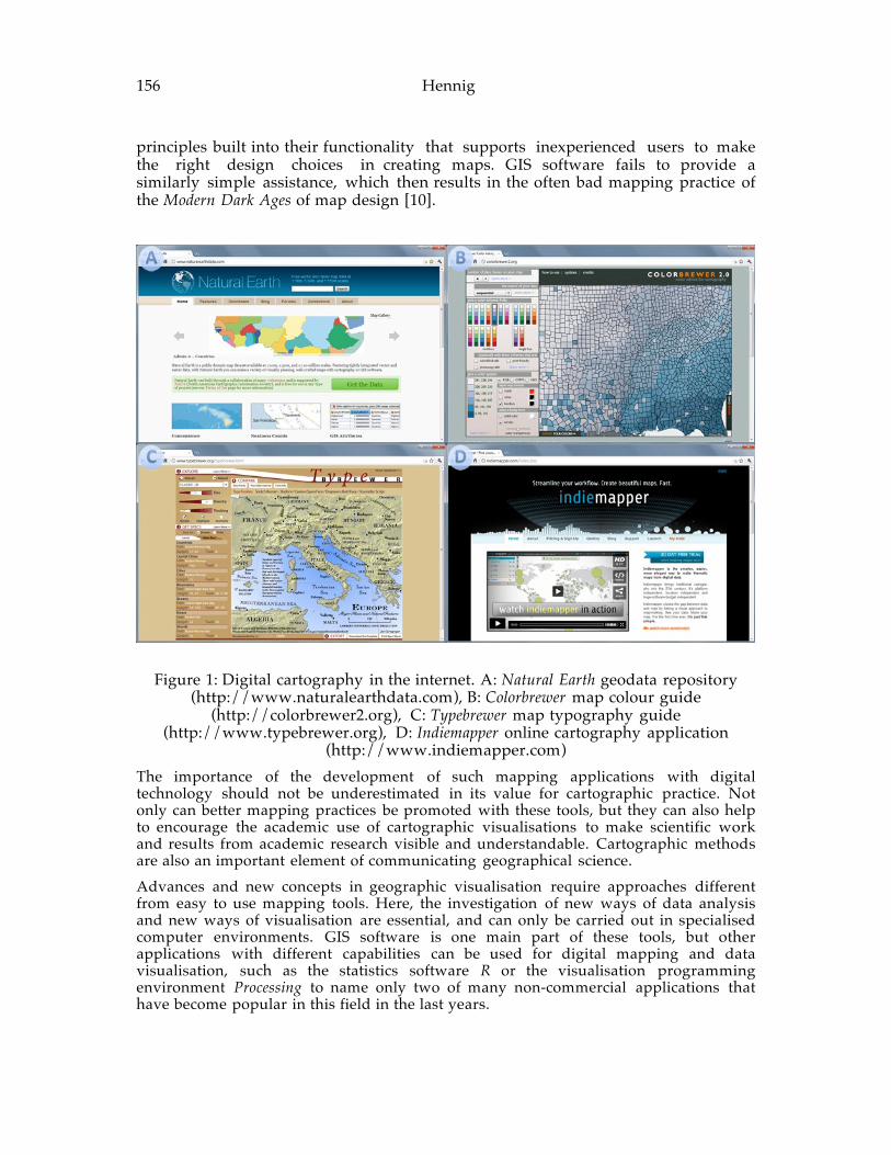
156 Hennig principles built into their functionality that supports inexperienced users to make the right design choices in creating maps. GIS software fails to provide a similarly simple assistance, which then results in the often bad mapping practice of the Modern Dark Ages of map design [10].
Figure 1: Digital cartography in the internet. A: Natural Earth geodata repository (http://www.naturalearthdata.com), B: Colorbrewer map colour guide
(http://colorbrewer2.org), C: Typebrewer map typography guide (http://www.typebrewer.org), D: Indiemapper online cartography application
(http://www.indiemapper.com) The importance of the development of such mapping applications with digital technology should not be underestimated in its value for cartographic practice. Not only can better mapping practices be promoted with these tools, but they can also help to encourage the academic use of cartographic visualisations to make scientific work and results from academic research visible and understandable. Cartographic methods are also an important element of communicating geographical science. Advances and new concepts in geographic visualisation require approaches different from easy to use mapping tools. Here, the investigation of new ways of data analysis and new ways of visualisation are essential, and can only be carried out in specialised computer environments. GIS software is one main part of these tools, but other applications with different capabilities can be used for digital mapping and data visualisation, such as the statistics software R or the visualisation programming environment Processing to name only two of many non-commercial applications that have become popular in this field in the last years.
Mapping Practices in a Digital World 157
3 The Role of Maps in Digital Publishing The recent advances in digital mapping demonstrate how digital technology has become a standard element in the process of creating maps in manifold ways. This applies to the traditional cartographic practices that are nowadays often performed using graphic design software such as Macromedia Freehand or Adobe Illustrator. Here, principles of map design are generally transferred to the digital world, and basic cartographic principles are used as in the non-digital process of creating a map. In this context, digital technology mainly has the role of reducing the manual work and simplifying and automating the work stages. Digital technology has also become a routine element in analysing and generating scientific raw data for a map or a geovisualisation, which is then finalised in the design software and dedicated mapping tools, or which is further visualised in new visualisation environments such as Processing. The degree of expertise that is needed to create maps is slowly declining, with new tools becoming available that allow map making following basic cartographic principles also for less experienced users. Advanced cartographic works, however, remain part of the work for trained experts. Computers play a crucial role in the task of analysing and visualising data in novel ways or using new approaches, which require expert knowledge to be realised. Many mapping techniques were impossible to realise without present-day computing power. The digital turn in cartography thus has not led to a simplification of the process of making maps, but has enabled new dimensions of data analysis and new ways to visualise that data. Often the result of using digital technology in the mapping process remains some form of paper map, which still is seen as the ultimate final product of the cartographic visualisation process. Even if the final map remains a digital entity that is only used on a computer screen, it is treated as being a paper map, and the screen only resembles the paper. This is a widespread phenomenon in digital media. Digital equivalents of analogue products are often oriented in their appearance to the real world, resulting in the creation of effects that resemble a physical product. A paramount example of this is the visual page turning effect in digital books on portable computers. Publishers are struggling with adapting to new media concepts that embrace the capabilities of advancing digital technology, which at present can be described as an experimental phase of creating innovative new concepts for media on digital devices. One key problem is to find new applications that enhance the usability or add value to digital media. Current attempts of that often fail because they do not add significant value [5, 11,15]. What is described here is a general issue that affects the publishing scene more than it perhaps affects cartography as a discipline. Nevertheless, it reveals a gap in cartographic research ever since digital technology arrived in the discipline: While cartographic practice was translated into digital techniques, and geospatial analysis was introduced to the spectrum of (geo)scientific methods [26] – arguably resulting in the creation of GIScience as a discipline between geosciences, cartography and informatics – the map as a publishing product itself has changed little. Mobile mapping applications and GPS-technology are part of geospatial research that does not focus on the map itself or on visualisation problems. Here basic
158 Hennig mapping principles here have been conducted by pragmatic and technology-led decisions, which have often been initially set by technology companies rather than geovisualisation research. Most research in this field currently focuses on advancing database structures and queries, and analytical algorithms that better connect the increasing amount of geospatial information [3]. Geovisualisation in these digital map products has only become more relevant with advancing display capabilities that include more complex information, with the aim to improve the visualisations towards a more realistic appearance (rather than alternative concepts of visualising complex data). Despite being in the centre of the visualisation of the information shown in mobile mapping applications, the map itself as a cartographic element plays a subordinate role, while major efforts are put into the analytical capabilities [22, 25, 26]. Online maps and cartographic geovisualisations in the internet move maps away from their static character towards interactive and versatile multimedia products. Maps in the internet are widely used and appear in diverse forms. The development of GoogleMaps and OpenStreetMap both date back to the years 2004/05. GoogleMaps quickly gained high user numbers, which was further encouraged by the implementation of interfaces to allow the integration into external websites and the combination with external datasets. OpenStreetMap took longer to attract a wider perception, because the initial phase included the compilation of a geodatabase, which GoogleMaps could just acquire from commercial providers of geodata. Meanwhile, there is no significant difference in data quality for many parts of the world, and in some regions OpenStreetMap even provides more data than GoogleMaps [2, 31, 36]. The direction of these services is largely driven by technological advances that Google implements in its platform(s). Google increasingly adds functionalities that aim to make an online replica of the world. The recent additions of live traffic information and similar services appear to help the Google mapping platform remain successful in the digital world, significantly influencing the way online maps are created and consumed. OpenStreetMap follows a different direction that is not driven monetary considerations. It is more open to user input and therefore relies on individual projects that push the technical progress ahead. The increasing implementation of OpenStreetMap in scientific applications may turn OpenStreetMap into a non- commercial alternative to integrating scientific data in dynamic and interactive mapping environments [36]. The web interfaces of GoogleMaps and OpenStreetMap are very similar in terms of cartographic capabilities. Some basic cartographic principles, as different levels of detail at changing scales, colour schemes for the major geographic features and other elements are well integrated in these platforms. Advantages of the digital world include the large degree of interactivity using simple navigation tools to zoom in and out, and pan the map inside the display window. In terms of usability, these mapping services are major improvements to earlier online mapping attempts in the late 1990s and the first years of the 21st century, which were in very experimental stages of development with sluggish interfaces. These examples hardly exist anymore, not least because of the possibility to integrate GoogleMaps, OpenStreetMap, and other web mapping services into self-made map projects. Further advanced cartographic elements or new cartographic practices are less prevalent so far. The user adaption of maps based on online mapping services remains very limited to adding new layers on the basemaps, and depicting basic
Mapping Practices in a Digital World 159
geometric elements such as lines or points in form of the infamous (but customisable) pushpins to depict locations. Cartographic design for this additional information lies in the hand of the user who creates map mashups, but is nevertheless limited to what general digital mapping tools provide. Digital map design principles are extensively discussed in cartographic literature (see e.g. [1, 16, 17, 18, 19, 35]). Topics focus on specific design guidelines for digital technology and the investigation of cartographic principles in relation to the specific technological configurations. Issues such as screen typography, colour rendition, and map navigation tools to simplify the user interaction are among the well discussed issues that solve some of the key problems in transferring existing cartographic practice to the (not so) new digital environments [19]. Problematic remains their implementation in some of the most commonly used and mainly technology-driven web mapping services. More open projects such as OpenStreetMap are more progressive in this regard, also because their ties with academic research and GIScience are much closer and the prime interest is not commercial. Digital mapping in the online world shows a divided picture. Online maps are largely based on digital mapping services that serve as a fundament for the actual mapping and provide the main framework for controlling and visualising the topic of interest. Improvements that benefit from digital technology include considerable technical advances of the underlying geographical databases, and the improved capabilities to interact with maps by moving them around, changing scales, showing dynamic changes in animated form, or interactively selecting the relevant information. These are capabilities that mark clear advances over static (and therefore printed) maps. On the other hand, the standards upon which these digital interfaces and usability are based are largely set by commercially driven decisions to extend the capabilities of digital mapping platforms, rather than well-considered choices on the best practices and most elegant forms of visualisation. Online maps still resemble to a great degree paper maps, with a little bit more interactivity, but otherwise with all the concepts of the analogue world translated into the digital world – sometimes better, sometimes worse, just like good and bad maps in the offline world. Online maps are currently a major focus of the developments in digital mapping, and the underlying more technically oriented GIS-related areas of research in this field are major subjects of methodological advances in this field (see e.g. [1, 23, 25]). Work on more cartography-oriented practices of digital mapping and new approaches that focus on maps as a publishing product like outlined (e.g. [17, 34]) are less common fields of cartographic research.
4 Creating Maps using Web Technology
4.1 The advent of digital technology in mapping The examples of the use of maps in contemporary digital platforms demonstrate how using computer technology considerably enhances the value of maps. Cartographic practice is an indispensable foundation for these new technologies. Principles of cartography and mapping techniques are the underlying common ground of these innovations, and the emergence of the field of geovisualisation finds its manifestation in these new digital mapping platforms [24, 25]. Although
160 Hennig taken for granted in most industrialised societies – as is the internet in general – these techniques have only become available less than a decade ago, many of which we use today are even much younger. Before that, digital mapping was generally more focused on experimenting with the multimedia capabilities of the first multitasking operating systems. First maps as digital media products were developed for a small group of people and not the wider public. Home computers only became a standard configuration in many households and in education in the 1990s, but did not immediately become a primary source for media consumption [23]. The first digital mapping products in the 1990s were often complementary to existing publications, such as an additional CD-ROM that accompanied textbooks, or similar extras for printed atlases [8, 32]. The main aim was an additional incentive for buying, or multimedia products were targeted at people exploring the new technologies. These early digital mapping products were less the inevitable move of map products away from paper form to digital, but rather an early explorative phase of a wider trend to create multimedia content for the new media devices that started to occupy the mass markets. Media consumption on digital devices has accelerated in recent years [6, 30]. Digital media has not yet replaced traditional publishing. Books, newspapers, magazines and their likes still outnumber their likes on digital devices. But their profits are falling sharply, while digital content has started to be a major source for consuming news and other content, including maps and map-like visualisations. It may not be a daring assumption that the majority of maps nowadays are consumed in digital form. Satnav systems (replacing paper maps), location based services on mobile phones (replacing maps in guidebooks, and guidebooks themselves), online route planners (replacing the road atlas), and many other of these examples introduced before are these new digital maps that people consume. Content created by the new mapmakers (who often have no cartographic training) published online is widely consumed solely online. If their likes are used in analogue media, they often have a digital origin, which is where the majority of their audience has accessed them (not least because of their more widespread and immediate availability). What is needed to enhance the value of digitally published maps are new ways of visualising and presenting them. New forms of map presentation in the digital world need to make optimum use of technical capabilities, and new approaches should be as unconstrained as possible to create a map that can be consumed regardless of the specific nature of the digital platform or device on which the map is accessed. Cartographers produced analogue maps so that the final product can be printed in a book, in a magazine, on a poster, and in many other similar ways. Traditional cartographic practices are suitable for all these ways of publishing, because their analogue nature does not allow much innovation in this regard. The same products can be used in digital media, but that remains an incomplete map product that makes use of digital technology. The maps published in the Worldmapper project for example face similar problems and demonstrate this dilemma. The maps on the project’s website (www.worldmapper.org) are produced with very recent technological advances using state of the art GIS methods, but the end product is a static map that works on screen as it does on printed paper. The website itself makes some use of digital technology by providing additional material and allows accessing all relevant data, but the maps that stand in the centre of the project remain static.
Mapping Practices in a Digital World 161
What is needed apart from the technological advances is a standardisation of rules for digital cartographic practice that go beyond the mere translation of existing principles. The principles for digital mapping need to be extended by new, very basic concepts of designing and creating digital maps. The development of new principles obviously has to be oriented on technical capabilities, but should not be driven by them and has to be formulated outside the specific ways of technical realisation. Just as there are principles defined for the creation of map elements, symbols, colours, without explaining how these are implemented using pen and paper or using a design software, there should be new principles defined for digital maps that become part of the toolbox for digital cartographers. Cartographic practices for digital publishing platforms must be examined and defined in a way that they can be realised in different ways and using different tools and applications, therefore must not be restricted to the capabilities of a specific software or hardware platform. They should be independently applicable and make use of the new capabilities of digital devices. Cartographic textbooks try to consider the most recent trends by adding sections about web mapping and virtual environments (e.g. [4, 26]). Often these are already out-dated at the time of print, and quickly need to be adjusted if not rewritten. HTML5 and the recent more serious attempts to monetise digital publishing products may change this, which is why for cartography it could prove valuable to look into these technologies to provide innovative concepts for publishing maps in the digital world.
4.2 Examples of digital mapping with HTML5 and jQuery To demonstrate in a very basic manner how HTML5 in combination with an extension by JavaScript libraries can improve digital maps and help to define new principles for digital cartography, I looked at some basic applications that can be used to enhance the digital presentation of the gridded cartograms from my own geospatial research [14]. These two examples are clearly technology-driven realisations of what is possible (and commonly used) in online mapping, but the actual aspect of translating these two examples into some more general principles are the key points that are relevant. The realisation of such principles will always require an adequate technical solution, while the underlying principles could be defined much more general than it is being done at the moment. All concepts developed in this section can be applied to a basic HTML5 project that works online as well as offline and is not restricted to be used as an internet website, but as a digital map product that can be integrated in other forms of digital publishing. Looking back at my own research on cartograms [14], creating an animation to demonstrate the transition between a conventional map and a cartogram or two versions of a cartogram is time consuming and can be highly technical. An alternative concept would be the interactive presentation of the original and the transformed state of the map where the map reader can use an interactive slider element to switch between the two maps. This can also be a useful way to compare two different states presented in a map. A functionality that overlays two maps and lets the map reader interactively switch between them is an interactive image slider (Figure 2). The slider is a simple example of how the basic design capabilities of the jQuery library [20] can be exploited for digital map displays. The resulting digital map has a substantial added value that embraces the digital technology. Rather
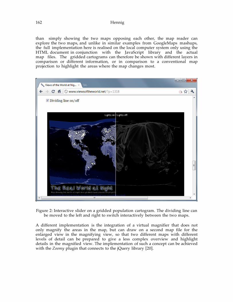
162 Hennig than simply showing the two maps opposing each other, the map reader can explore the two maps, and unlike in similar examples from GoogleMaps mashups, the full implementation here is realised on the local computer system only using the HTML document in conjunction with the JavaScript library and the actual map files. The gridded cartograms can therefore be shown with different layers in comparison or different information, or in comparison to a conventional map projection to highlight the areas where the map changes most.
Figure 2: Interactive slider on a gridded population cartogram. The dividing line can be moved to the left and right to switch interactively between the two maps.
A different implementation is the integration of a virtual magnifier that does not only magnify the areas in the map, but can draw on a second map file for the enlarged view in the magnifying view, so that two different maps with different levels of detail can be prepared to give a less complex overview and highlight details in the magnified view. The implementation of such a concept can be achieved with the Zoomy plugin that connects to the jQuery library [20].
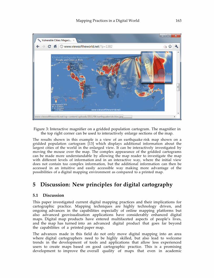
Mapping Practices in a Digital World 163
Figure 3: Interactive magnifier on a gridded population cartogram. The magnifier in the top right corner can be used to interactively enlarge sections of the map.
The results shown in this example is a view of an earthquake risk map shown on a gridded population cartogram [13] which displays additional information about the largest cities of the world in the enlarged view. It can be interactively investigated by moving the mouse over the map. The complex appearance of the gridded cartograms can be made more understandable by allowing the map reader to investigate the map with different levels of information and in an interactive way, where the initial view does not contain too complex information, but the additional information can then be accessed in an intuitive and easily accessible way making more advantage of the possibilities of a digital mapping environment as compared to a printed map.
5 Discussion: New principles for digital cartography
5.1 Discussion This paper investigated current digital mapping practices and their implications for cartographic practice. Mapping techniques are highly technology driven, and ongoing advances in the capabilities especially of online mapping platforms but also advanced geovisualisation applications have considerably enhanced digital maps. Digital map products have entered multifaceted aspects of people’s lives, and the map has turned into an advanced digital product that goes far beyond the capabilities of a printed paper map. The advances made in this field do not only move digital mapping into an area where digital cartographers need to be highly skilled, but also lead to welcome trends in the development of tools and applications that allow less experienced users to create maps based on good cartographic practice. This is a promising development to improve the overall quality of maps that even in academic
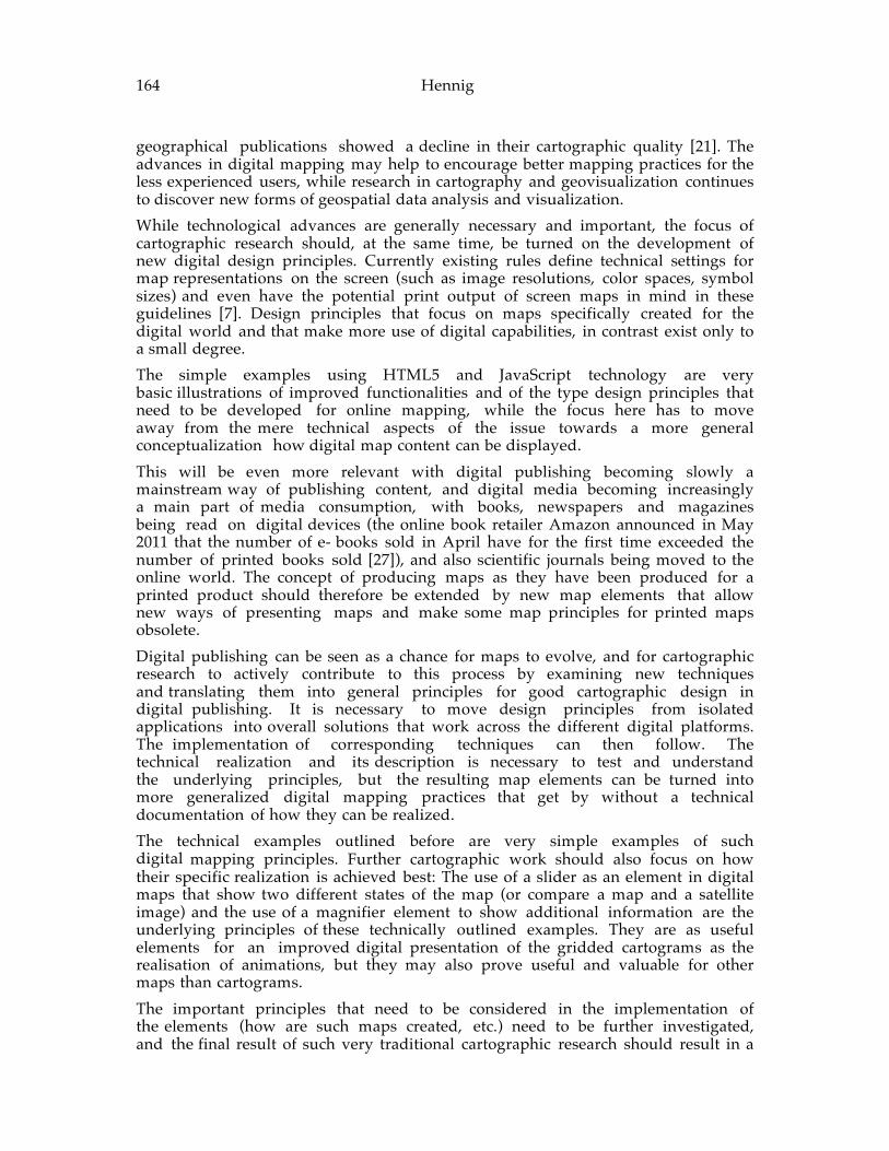
164 Hennig geographical publications showed a decline in their cartographic quality [21]. The advances in digital mapping may help to encourage better mapping practices for the less experienced users, while research in cartography and geovisualization continues to discover new forms of geospatial data analysis and visualization. While technological advances are generally necessary and important, the focus of cartographic research should, at the same time, be turned on the development of new digital design principles. Currently existing rules define technical settings for map representations on the screen (such as image resolutions, color spaces, symbol sizes) and even have the potential print output of screen maps in mind in these guidelines [7]. Design principles that focus on maps specifically created for the digital world and that make more use of digital capabilities, in contrast exist only to a small degree. The simple examples using HTML5 and JavaScript technology are very basic illustrations of improved functionalities and of the type design principles that need to be developed for online mapping, while the focus here has to move away from the mere technical aspects of the issue towards a more general conceptualization how digital map content can be displayed. This will be even more relevant with digital publishing becoming slowly a mainstream way of publishing content, and digital media becoming increasingly a main part of media consumption, with books, newspapers and magazines being read on digital devices (the online book retailer Amazon announced in May 2011 that the number of e- books sold in April have for the first time exceeded the number of printed books sold [27]), and also scientific journals being moved to the online world. The concept of producing maps as they have been produced for a printed product should therefore be extended by new map elements that allow new ways of presenting maps and make some map principles for printed maps obsolete. Digital publishing can be seen as a chance for maps to evolve, and for cartographic research to actively contribute to this process by examining new techniques and translating them into general principles for good cartographic design in digital publishing. It is necessary to move design principles from isolated applications into overall solutions that work across the different digital platforms. The implementation of corresponding techniques can then follow. The technical realization and its description is necessary to test and understand the underlying principles, but the resulting map elements can be turned into more generalized digital mapping practices that get by without a technical documentation of how they can be realized. The technical examples outlined before are very simple examples of such digital mapping principles. Further cartographic work should also focus on how their specific realization is achieved best: The use of a slider as an element in digital maps that show two different states of the map (or compare a map and a satellite image) and the use of a magnifier element to show additional information are the underlying principles of these technically outlined examples. They are as useful elements for an improved digital presentation of the gridded cartograms as the realisation of animations, but they may also prove useful and valuable for other maps than cartograms. The important principles that need to be considered in the implementation of the elements (how are such maps created, etc.) need to be further investigated, and the final result of such very traditional cartographic research should result in a
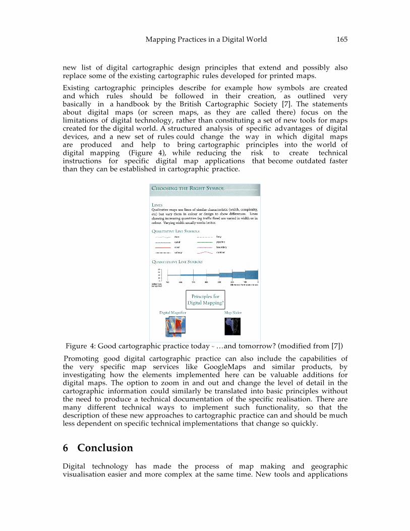
Mapping Practices in a Digital World 165
new list of digital cartographic design principles that extend and possibly also replace some of the existing cartographic rules developed for printed maps. Existing cartographic principles describe for example how symbols are created and which rules should be followed in their creation, as outlined very basically in a handbook by the British Cartographic Society [7]. The statements about digital maps (or screen maps, as they are called there) focus on the limitations of digital technology, rather than constituting a set of new tools for maps created for the digital world. A structured analysis of specific advantages of digital devices, and a new set of rules could change the way in which digital maps are produced and help to bring cartographic principles into the world of digital mapping (Figure 4), while reducing the risk to create technical instructions for specific digital map applications that become outdated faster than they can be established in cartographic practice. Figure 4: Good cartographic practice today -‐‑ …and tomorrow? (modified from [7])
Promoting good digital cartographic practice can also include the capabilities of the very specific map services like GoogleMaps and similar products, by investigating how the elements implemented here can be valuable additions for digital maps. The option to zoom in and out and change the level of detail in the cartographic information could similarly be translated into basic principles without the need to produce a technical documentation of the specific realisation. There are many different technical ways to implement such functionality, so that the description of these new approaches to cartographic practice can and should be much less dependent on specific technical implementations that change so quickly.
6 Conclusion
Digital technology has made the process of map making and geographic visualisation easier and more complex at the same time. New tools and applications
166 Hennig have a great potential to lower the obstacles for inexperienced users to create better maps, and can also encourage the general use of cartographic visualisations to illustrate geographical research. New digital developments and web applications are promising steps towards a better use of cartographic practice that previously required a solid theoretical and technical background to be achieved in specialised mapping environments. Digital technology has also extended our capabilities to visualise large amounts of data by digital processing methods. For achieving that, a number of new tools and applications have emerged in the last years. They specialise in the different tasks of statistical analysis and visualisation, which allows more and more advanced geovisualisation concepts and new forms of working with data outside the domain of informatics and pure computer sciences. The perspective of new concepts being integrated into common mapping tools for normal users is an essential part in the process of new visualisation techniques and should always be an objective for new techniques. This allows the broader acceptance and wider use by non-experts, while specialised visualisation algorithms that remain not (or badly) integrated in common mapping tools, will less likely succeed as successful geovisualisation concepts despite their promising capabilities. Digital technology has also changed the way we consume maps, which so far is often neglected in the development of digital mapping applications. Therefore, it may also be essential to extend cartographic practice into the digital domain and to look at new ways of presenting maps in digital environments. Creating new cartographic principles and hence novel rules can be a major challenge to move digital mapping from an innovative but highly technical and very fragmented entity towards an integrated part of cartographic practices, and move digital mapping (not opposed to but still in contrast to GIS or GIScience) towards being part of a cartography for the 21st century.
Acknowledgments
Part of this research was made possible by the generous funding provided by the Leverhulme Trust.
References [1] ASCHE, H. AND HERRMANN, C. Web.Mapping 2. Heidelberg: Wichmann,
2003. [2] BENNETT, J. OpenStreetMap. Birmingham, Packt Publishing, 2010. [3] BERNARD, L., J. FITZKE AND WAGNER, R. Geodateninfrastruktur.
Grundlagen und Anwendungen. Heidelberg, Wichmann, 2004. [4] CARTWRIGHT, W. Advancing global cartography and GIScience. The
Cartographic Journal, 48 2 (2011), 81-85. [5] CHAPMAN, N. AND CHAPMAN, J. Digital multimedia. Edinburgh: Wiley,
2009.
Mapping Practices in a Digital World 167
[6] COULDRY, N. AND MCCARTHY, A. Mediaspace: place, scale and culture in a media age. Abringdon, Routledge, 2004.
[7] DARKES, G. AND SPENCE M. Cartography - an introduction. London, The British Cartographic Society, 2008.
[8] DENT, B. D. Cartography: thematic map design. Boston: William C Brown, 1999. [9] DODGE, M., R. KITCHIN AND PERKINS, C. The map reader. Chichester:
[9] Wiley-Blackwell, 2011. [10] FRIENDLY, M. A brief history of data visualisation. In Handbook of data
visualisation, C. Chen, W. Härdle and Unwin, A., Eds. Berlin / Heidelberg: Springer, 2008, pp. 15-56.
[11] GRAHAM, G. AND SMART A. The regional-newspaper industry supply chain and the internet. Supply Chain Management, 15 3 (2010), 196-206.
[12] GUERIN, S. M. Peeking into the black box: some art and science to visualizing agent-based models. In Proceedings of the 36th conference on Winter simulation (Orlando, FL, 2004).
[13] HENNIG, B. D. Gridded cartograms as a method for visualising earthquake risk at the global scale. Journal of Maps, 10 2 (2014), 186-194.
[14] HENNIG, B.D. Rediscovering the World: Map Transformations of Human and Physical Space. Heidelberg / New York / Dordrecht / London, Springer, 2013.
[15] HIRST, M. News 2.0: Can journalism survive the internet? Sydney: Allen & Unwin, 2011.
[16] JENNY, B. Geometric distortion of schematic network maps. Bulletin of the Society of Cartographers SoC, 40 (2006), 15-18.
[17] JENNY, B., H. JENNY AND RÄBER, S. 2008. Map design for the internet. In International perspectives on maps and the internet, ed. M. P. Peterson, 31-48. Berlin/Heidelberg/New York: Springer, 2008.
[18] JENNY, B., T. PATTERSON AND L. HURNI, L. Flex projector: interactive software for designing world map projections. Cartographic Perspectives, 59 (2008), 12-27.
[19] JENNY, H., A. NEUMANN, B. JENNY AND HURNI, L. A WYSIWYG interface for user-friendly access to geospatial data collections. In Preservation in Digital Cartography, ed. M. Jobst, 221-238. Berlin / Heidelberg / New York, Springer, 2010.
[20] JQUERY PROJECT jQuery API. http://docs.jquery.com/Main_Page (last accessed 2015-03-01).
[21] KESSLER, F. C. AND SLOCUM, T. A. Analysis of thematic maps published in two geographical journals in the twentieth century. Annals of the Association of American Geographers, 101 2 (2011), 292-317.
[22] KIM, B. AND JEONG, S. A comparison of algorithms for origin-destination matrix generation on real road networks and an approximation approach. Computers and Industrial Engineering, 1 56 (2009), 70-76.
168 Hennig [23] KORDUAN, P. AND ZEHNER M. L. Geoinformation im Internet:
Technologien zur Nutzung raumbezogener Informationen im WWW. Heidelberg, Wichmann, 2008.
[24] KRAAK, M.-J. From geovisualisation toward geovisual analytics. The Cartographic Journal, 45 3 (2008), 163-164.
[25] KRAAK, M. J. AND ORMELING, F. Cartography: visualisation of geospatial data. Boston, MA, Pearson Education, 2010.
[26] LONGLEY, P. A., M. F. GOODCHILD, D. J. MAGUIRE AND D. W. RHIND, D. W. Geographic information systems and science. New York, NY: John Wiley & Sons, 2011.
[27] MILLER, C. C. AND BOSMAN, J. E-books outsell print books at Amazon. http://www.nytimes.com/2011/05/20/technology/20amazon.html?_r=1ANDs cp=2ANDsq=amazonANDst=cse (last accessed 2015-03-01).
[28] MORRISON, J. L. The science of cartography and its essential processes. International Yearbook of Cartography, 16 (1976), 84-97.
[29] POORE, B. S. The open black box: the role of the end-user in GIS integration. The Canadian Geographer, 47 1 (2003), 62-74.
[30] POSTER, M. Consumption and digital commodities in the everyday. Cultural Studies, 18 2 (2004), 409-423.
[31] RAMM, F., J. TOPF AND CHILTON, S. OpenStreetMap: using and enhancing the free map of the world. Cambridge, UIT, 2010.
[32] ROBINSON, A. H., J. L. MORRISON, P. C. MUEHRCKE, A. J. KIMERLING AND GUPTILL, S. C. Elements of cartography. New York, NY, Wiley & Sons, 1995.
[33] SCHUURMAN, N. The ghost in the machine: spatial data, information and knowledge in GIS. Canadian Geographer, 47 1 (2003), 1-4.
[34] SWIENTY, O. Attention-guiding geovisualisation. A cognitive approach of designing relevant geographic information. PhD thesis. München, Technische Universität, 2008.
[35] TURNER, A. J. Introduction to Neogeography. Sebastopol, CA, O'Reilly Media, 2006.
[36] ZIPF, A. OpenStreetMap - Datenqualität und Potentiale der Nutzung mit OpenGIS Diensten in 2D und 3D. In GIS-Report 2010/11, B. Harzer, Ed. Karlsruhe, Bernhard Harzer Verlag, 2010, pp. 33-58.
ADVANCING GEOGRAPHIC INFORMATION SCIENCE: CHAPTER 12
© by the author(s) Licensed under Creative Commons Attribution 4.0 License
169
Map Related Experiments Using Oculus Rift: Can low cost VR
technology provide sufficient realism? Steffen Pøhner Henriksen and Terje Midtbø
Norwegian University of Science and Technology, Trondheim, Norway
Abstract: In the last years a new kind of virtual reality equipment has emerged. Low cost head mounted displays (HMD) like “Oculus Rift DK1” are intentionally made for the gaming industry. However, the technology opens for a much wider range of use. If the recreation of the real world is adequate it might be possible to explore human experience and behavior in a spatial environment more efficiently. This paper looks closer into different aspects with using Oculus Rift for experiments where map navigation is in focus. Limitations in the present version of the actual device are discussed and general challenges when using virtual reality is studied in an experiment. This includes simulator sickness and the user’s experiences of presence in the virtual world. This study concludes that interactions with the device during the user’s motions still need improvements to make the equipment adequate for map related experiments.
Keywords: Virtual reality, Oculus Rift, map navigation, presence in VR
1 Introduction Even before the computers were able to handle digital models, mechanical equipment was constructed in order to recreate the impression of the real world [3, 20]. However, when we are talking about VR today it is about software and digital models handled by special input and output equipment connected to a computer. Output devices are responsible for presentation of the virtual environment to the user. There are several types of output devices, from Binocular Omni Orientation Monitor (BOOM) [4] to more advanced Computer Assisted Virtual Environment (CAVE) outfit (virtual reality room) and Head-Mounted Displays (HMDs) [6, 7]. The selection of input devices is even more diverse. Of course we have general input devices as mouse and joystick, however wireless game controllers, sometimes equipped with motion sensors (for example Nintendo Wii) or followed by camera sensor (for example Playstation Move), may be more applicable. Finally we have input devices that are developed for VR like
170 Henriksen and Midtbø wired gloves, built in motion sensors in HMDs and walking interfaces as Virtuix Omni [3, 20, 33]. Several of these input devises may also include haptic output to the user. New and low cost virtual reality devices have showed promising performance compared to more advanced equipment used in virtual reality research some years ago [35]. Virtual reality used together with geospatial data is able to give a realistic virtual environment. In research activities can all variables in the virtual world be controlled and a detailed registration of the behaviour of the test subjects may be available for studies. Hence, it is our prediction that we will see an increased use of virtual reality devises for map related research in the future. In this work we have explored peoples experience when finding their ways through a virtual environment by the use of maps. Various orientations of the map were tested during the experiment. The ultimate goal of virtual reality is to give the opportunity to step into a virtual world which feels as real as our own. This is called presence. Presence is the key to directly transfer results gathered in the virtual world to real world scenarios. Presence in virtual reality refers to the subjective experience of being in the virtual world and having the feeling that it is real, while you are actually situated in another place [34]. [2] phrase the definition of presence as ``a cognitive state which occurs when the brain processes and makes sense of the myriad of stimulus information impinging upon the human sensory systems''. In this paper answers in a questionnaire is indicating the level of presence for the participants in the experiment. In the experiment related to this paper human subjects were moving inside a “spatial environment”. It has been shown that spatial abilities measured with the SBSOD questionnaire correlates with the performance in wayfinding tasks [11, 28]. Hence, it is possible that people showing good spatial abilities might perform better when navigating in the virtual environment. Many people experience simulator sickness, similar to motion sickness, when using VR equipment [14, 22, 27]. The degree of simulator sickness varies from person to person, and some may not feel any discomfort. The symptoms induced are often grouped into nausea, oculomotor, discomfort and disorientation [22] and include general discomfort, apathy, drowsiness, headache, disorientation, fatigue, pallor, sweating, salvation, stomach awareness, nausea and vomiting [18]. Kennedy and Fowlkes [15] state that simulator sickness is polysymptomatic and may best be described as a syndrome. The cause of simulator sickness is hard to isolate, and many factors come to play as described by [18], but the mismatch between the vestibular system and the visual system is a major factor according to [13]. How familiar the participants are with computer games can also affect the end result and metrics, as virtual reality applications can resemble computer games. The movement system used to control the virtual world in this paper is a gamepad. This may add to the feel of playing a computer game, and give those familiar with such equipment an advantage. The relationship between performance in the virtual environment and how often the participants play computer games is hence studied. This paper strives to answer these questions: 1. Which problems are prominent when using Oculus Rift for studying the map orientation performance?
2. Can we learn something about how factors as simulator sickness, good spatial abilities or videogame experience influence on map related experiments by the use of Oculus Rift?
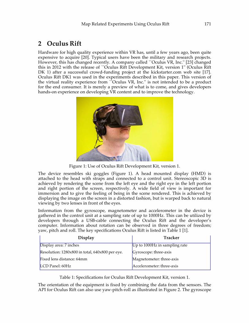
Map Related Experiments Using Oculus Rift 171
2 Oculus Rift Hardware for high quality experience within VR has, until a few years ago, been quite expensive to acquire [20]. Typical users have been the military and research projects. However, this has changed recently. A company called ``Oculus VR, Inc.'' [23] changed this in 2012 with the release of ``Oculus Rift Development Kit, version 1'' (Oculus Rift DK 1) after a successful crowd-funding project at the kickstarter.com web site [17]. Oculus Rift DK1 was used in the experiments described in this paper. This version of the virtual reality experience from ``Oculus VR, Inc.'' is not intended to be a product for the end consumer. It is merely a preview of what is to come, and gives developers hands-on experience on developing VR content and to improve the technology.
Figure 1: Use of Oculus Rift Development Kit, version 1.
The device resembles ski goggles (Figure 1). A head mounted display (HMD) is attached to the head with straps and connected to a control unit. Stereoscopic 3D is achieved by rendering the scene from the left eye and the right eye in the left portion and right portion of the screen, respectively. A wide field of view is important for immersion and to give the feeling of being in the scene rendered. This is achieved by displaying the image on the screen in a distorted fashion, but is warped back to natural viewing by two lenses in front of the eyes. Information from the gyroscope, magnetometer and accelerometer in the device is gathered in the control unit at a sampling rate of up to 1000Hz. This can be utilized by developers through a USB-cable connecting the Oculus Rift and the developer’s computer. Information about rotation can be observed in three degrees of freedom; yaw, pitch and roll. The key specifications Oculus Rift is listed in Table 1 [1].
Display Tracker Display area: 7 inches Resolution: 1280x800 in total, 640x800 per eye. Fixed lens distance: 64mm LCD Panel: 60Hz
Up to 1000Hz in sampling rate Gyroscope: three-axis Magnetometer: three-axis Accelerometer: three-axis
Table 1: Specifications for Oculus Rift Development Kit, version 1. The orientation of the equipment is fixed by combining the data from the sensors. The API for Oculus Rift can also use yaw-pitch-roll as illustrated in Figure 2. The gyroscope
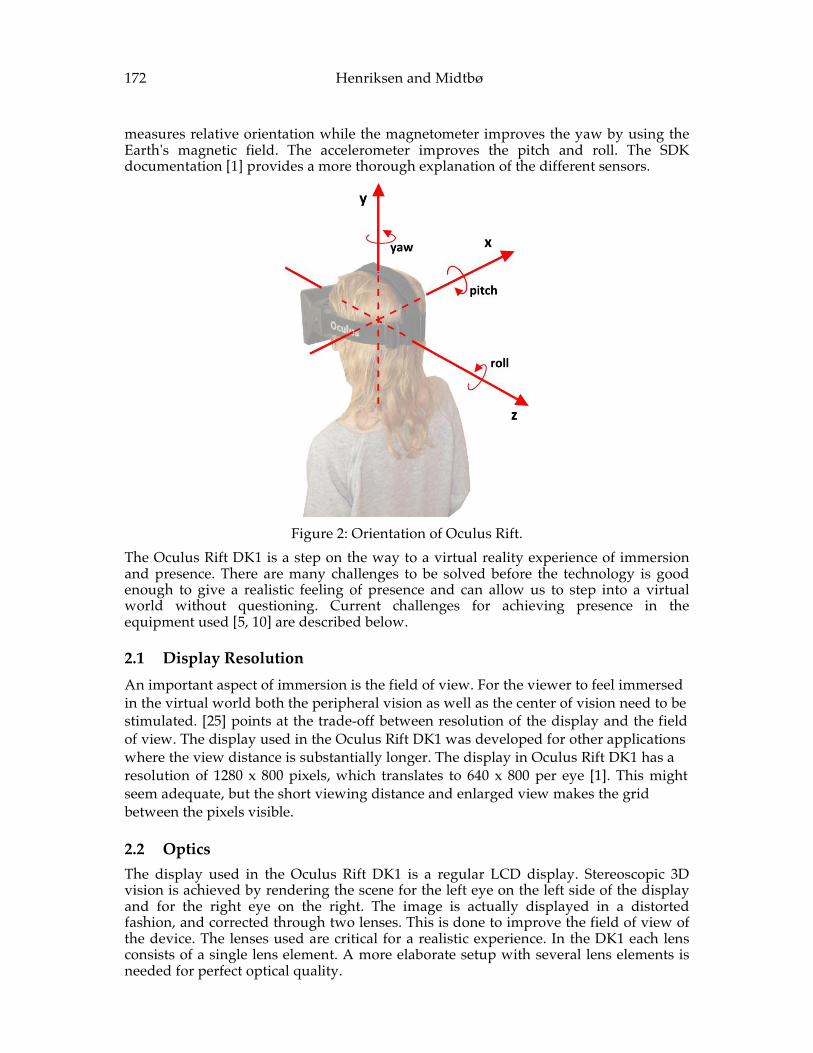
172 Henriksen and Midtbø measures relative orientation while the magnetometer improves the yaw by using the Earth's magnetic field. The accelerometer improves the pitch and roll. The SDK documentation [1] provides a more thorough explanation of the different sensors.
Figure 2: Orientation of Oculus Rift.
The Oculus Rift DK1 is a step on the way to a virtual reality experience of immersion and presence. There are many challenges to be solved before the technology is good enough to give a realistic feeling of presence and can allow us to step into a virtual world without questioning. Current challenges for achieving presence in the equipment used [5, 10] are described below.
2.1 Display Resolution An important aspect of immersion is the field of view. For the viewer to feel immersed in the virtual world both the peripheral vision as well as the center of vision need to be stimulated. [25] points at the trade-off between resolution of the display and the field of view. The display used in the Oculus Rift DK1 was developed for other applications where the view distance is substantially longer. The display in Oculus Rift DK1 has a resolution of 1280 x 800 pixels, which translates to 640 x 800 per eye [1]. This might seem adequate, but the short viewing distance and enlarged view makes the grid between the pixels visible.
2.2 Optics The display used in the Oculus Rift DK1 is a regular LCD display. Stereoscopic 3D vision is achieved by rendering the scene for the left eye on the left side of the display and for the right eye on the right. The image is actually displayed in a distorted fashion, and corrected through two lenses. This is done to improve the field of view of the device. The lenses used are critical for a realistic experience. In the DK1 each lens consists of a single lens element. A more elaborate setup with several lens elements is needed for perfect optical quality.
Map Related Experiments Using Oculus Rift 173
The Oculus Rift DK1 comes with three sets of lenses. These lenses can correct eye sight to a certain degree. One lens assumes perfect vision, but the other to can correct near sight and far sight, respectively.
2.3 Persistence Persistence is the time each pixel remains lit on the head mounted display. In the real world the information we see through our eyes is always correct. When viewing a display, the frame does not update at an infinite speed. Between each frame update the previous frame is still present before the next one is presented. In this time in between frames, information which is not updated is shown. This often leads to motion sickness as we try to interpret the wrong information [24]. More specifically, a visual system called vestibulo-ocular reflex (VOR), responsible to stabilize the visual impression on the retina during head movement, are affected [9]. The effect is experienced as a motion blur when the user moves its head. Motion blur is also present when objects are moving relative to the user. One solution to this problem is to use a low persistence display such as OLED. This display does not wait for the next image to be ready before switching to a new colour of the pixel, but can turn off the pixels between frames. In this way no incorrect information is sent to the brain, and the experience is more comfortable.
2.4 Latency A computer display simulates motion by displaying images in series. How often this image updates affects how smooth we experience the motion. A display conveying a virtual reality needs a fast refresh rate for realistic animations. The Oculus Rift DK1 uses a 60Hz display. This may not be enough for a perfect realistic experience. In addition we need computer hardware capable of rendering frames to match the display refresh rate. As the refresh rate increases, the number of pixels needed to be rendered per second rises. When the level of detail in the scene is expected to be higher, the requirements of powerful computer graphics hardware are even tougher. ``Motion-to-last-photon'' latency is a common term in VR terminology. It describes the time it takes for the photons from the display to hit your retina after a movement was made. Keeping this latency low is the key to immersion and the experience of being present in a virtual world. If the latency is too large the human perceptual system will tell us that we are looking at rendered images not reality. One important factor affecting the latency is tracking the movement of the equipment. To minimize the latency a prediction paradigm is established. Developers use the sensors to record information of a previous point in time, and use software algorithms to predict where the next movement is going to be.
2.5 Positional Tracking A VR system needs a tracking system. The tracking system detects the user’s point of view for updating the display. The system needs to respond to the user’s action quickly for a realistic experience. Oculus Rift DK1 tracks head movement in three degrees of freedom and update sensory information at a rate up to 1000 Hz [1]. Yaw, pitch and roll are registered and made available for the application. The tracking is also predicted in software to further speed up the process. All in all is this sampling rate sufficient for a satisfying experience as the bottleneck in the system lies elsewhere. However, the human head moves in space as well, not just turns. We crouch, lean
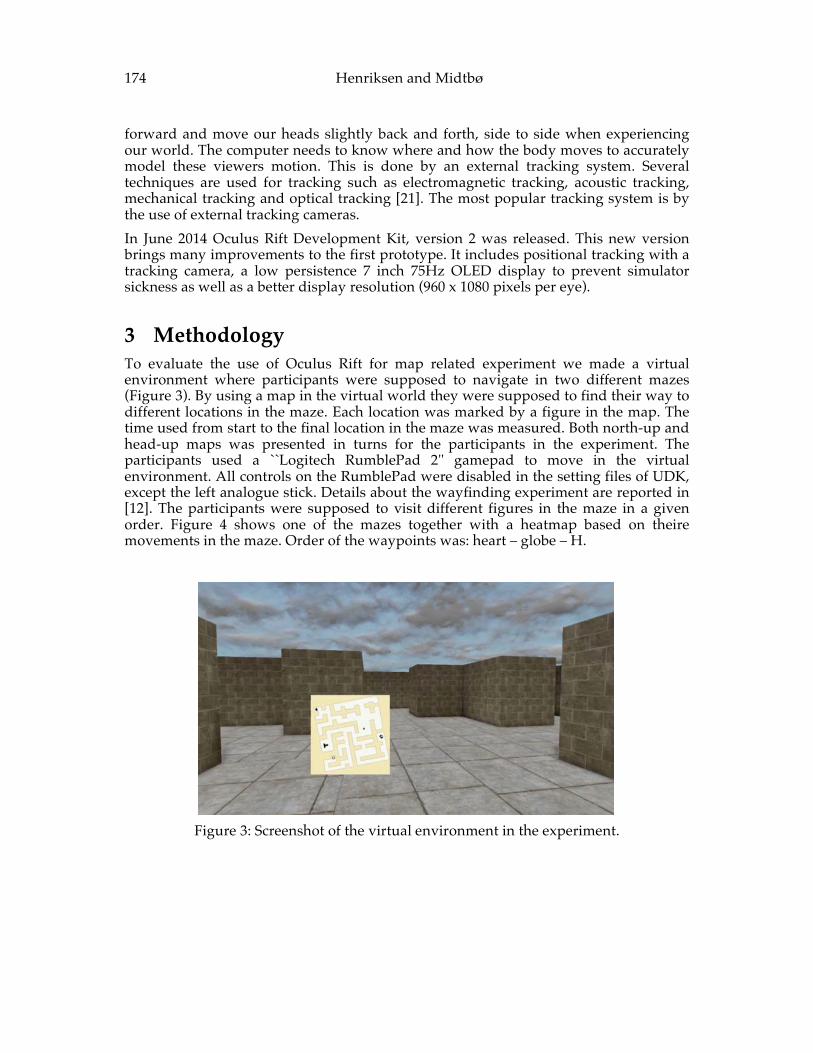
174 Henriksen and Midtbø forward and move our heads slightly back and forth, side to side when experiencing our world. The computer needs to know where and how the body moves to accurately model these viewers motion. This is done by an external tracking system. Several techniques are used for tracking such as electromagnetic tracking, acoustic tracking, mechanical tracking and optical tracking [21]. The most popular tracking system is by the use of external tracking cameras. In June 2014 Oculus Rift Development Kit, version 2 was released. This new version brings many improvements to the first prototype. It includes positional tracking with a tracking camera, a low persistence 7 inch 75Hz OLED display to prevent simulator sickness as well as a better display resolution (960 x 1080 pixels per eye).
3 Methodology To evaluate the use of Oculus Rift for map related experiment we made a virtual environment where participants were supposed to navigate in two different mazes (Figure 3). By using a map in the virtual world they were supposed to find their way to different locations in the maze. Each location was marked by a figure in the map. The time used from start to the final location in the maze was measured. Both north-up and head-up maps was presented in turns for the participants in the experiment. The participants used a ``Logitech RumblePad 2'' gamepad to move in the virtual environment. All controls on the RumblePad were disabled in the setting files of UDK, except the left analogue stick. Details about the wayfinding experiment are reported in [12]. The participants were supposed to visit different figures in the maze in a given order. Figure 4 shows one of the mazes together with a heatmap based on theire movements in the maze. Order of the waypoints was: heart – globe – H.
Figure 3: Screenshot of the virtual environment in the experiment.
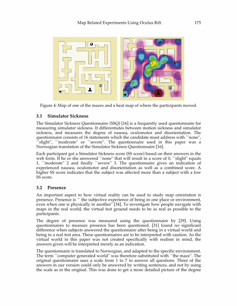
Map Related Experiments Using Oculus Rift 175
Figure 4: Map of one of the mazes and a heat map of where the participants moved.
3.1 Simulator Sickness The Simulator Sickness Questionnaire (SSQ) [16] is a frequently used questionnaire for measuring simulator sickness. It differentiates between motion sickness and simulator sickness, and measures the degree of nausea, oculomotor and disorientation. The questionnaire consists of 16 statements which the candidate must address with ``none'', ``slight'', ``moderate'' or ``severe''. The questionnaire used in this paper was a Norwegian translation of the Simulator Sickness Questionnaire [16]. Each participant got a Simulator Sickness score (SS score) based on their answers in the web form. If he or she answered ``none'' that will result in a score of 0, ``slight'' equals 1, ``moderate'' 2 and finally ``severe'' 3. The questionnaire gives an indication of experienced nausea, oculomotor and disorientation as well as a combined score. A higher SS score indicates that the subject was affected more than a subject with a low SS score.
3.2 Presence An important aspect to how virtual reality can be used to study map orientation is presence. Presence is `` the subjective experience of being in one place or environment, even when one is physically in another'' [34]. To investigate how people navigate with maps in the real world, the virtual test ground needs to be as real as possible to the participants. The degree of presence was measured using the questionnaire by [29]. Using questionnaires to measure presence has been questioned. [31] found no significant difference when subjects answered the questionnaire after being in a virtual world and being in a real test area. These questionnaires are to be interpreted with caution. As the virtual world in this paper was not created specifically with realism in mind, the answers given will be interpreted merely as an indication. The questionnaire is translated to Norwegian, and adapted to the specific environment. The term ``computer generated world'' was therefore substituted with ``the maze''. The original questionnaire uses a scale from 1 to 7 to answer all questions. Three of the answers in our version could only be answered by writing sentences, and not by using the scale as in the original. This was done to get a more detailed picture of the degree
176 Henriksen and Midtbø of presence felt by the participants. It made it easier for the participants to convey their experience, although the results are harder to measure objectively.
3.3 Spatial Abilities The spatial abilities of a person are known to affect how easily mental rotation is done [8], and navigating with north-up maps require mental rotation as explained in the introduction. Individual differences in spatial ability can be measured by psychometric tests or self-report measures. Psychometric tests include mental rotation of different shapes and solving small navigational problems [32]. However, self-report measures have been found to be sufficient [11]. In this paper a translated version of the Santa Barbara Sense of Direction Scale (SBSOD) [11] was used to measure individual differences in spatial ability. The questionnaire was translated to Norwegian and made available through a computer. One statement was added to the standard SBSOD. Studies have shown a correlation between spatial abilities, gender and how familiar the test subject is to computer games [19, 26]. Since the movements in the virtual environment in the experiment were done with a game controller, it may favour subjects familiar with such a controller. The statement ``I often play video games'' was added to study this correlation further, and to judge whether computer game experience and/or spatial abilities affected the result.
3.4 Experiment For the experiment it is important to use adequate computer equipment in order to make the Oculus Rift perform at a maximum refresh rate of 60Hz. In our experiment a computer including an Intel i7-3720QM @ 2,6Ghz processor, 16 GB of memory and a NVIDA Quadro K4000M 12GB GDDR5 solved this issue. 27 subjects (5 female and 22 men) participated in the experiment. The youngest was 17 and the oldest 70 years old. However, 4 of the females and 18 of the men were between 20 and 28 years. The experiment went as follows:
1. The participant was introduced to the study and its purpose. He or she was informed of the tasks to be solved and in which order. 2. The risk of simulator sickness was conveyed and the SBSOD questionnaire was answered. 3. The head-mounted display, gamepad and test area was adjusted to fit the participant and validated as the participant experienced a simple virtual environment. The movement pattern using the gamepad was shown and learned before proceeding. 4. The time was measured when the participant completed two mazes run- through each, one using a north-up map and by a head-up map. The run- through was aborted if a participant was affected by strong discomfort. 5. The simulator sickness questionnaire was answered. 6. The presence questionnaire was answered.
During the experiment most participants managed to stand in the range of the wires connecting the head-mounted display to the computer. However, there were times were participants needed correction because they moved away from the starting position. They started walking in the real world when using the gamepad. This interrupted the trial and it felt unnatural for the participants to be moved in the real
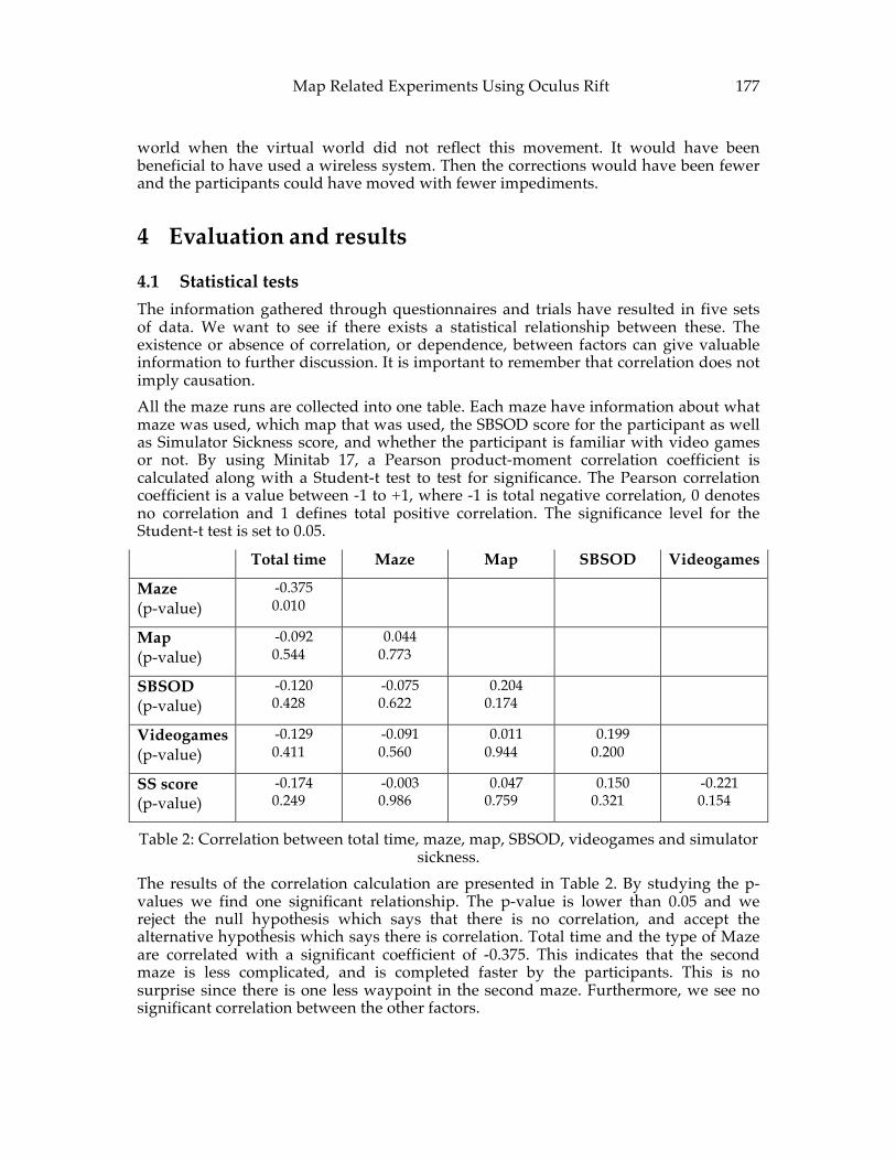
Map Related Experiments Using Oculus Rift 177
world when the virtual world did not reflect this movement. It would have been beneficial to have used a wireless system. Then the corrections would have been fewer and the participants could have moved with fewer impediments.
4 Evaluation and results
4.1 Statistical tests The information gathered through questionnaires and trials have resulted in five sets of data. We want to see if there exists a statistical relationship between these. The existence or absence of correlation, or dependence, between factors can give valuable information to further discussion. It is important to remember that correlation does not imply causation. All the maze runs are collected into one table. Each maze have information about what maze was used, which map that was used, the SBSOD score for the participant as well as Simulator Sickness score, and whether the participant is familiar with video games or not. By using Minitab 17, a Pearson product-moment correlation coefficient is calculated along with a Student-t test to test for significance. The Pearson correlation coefficient is a value between -1 to +1, where -1 is total negative correlation, 0 denotes no correlation and 1 defines total positive correlation. The significance level for the Student-t test is set to 0.05. Total time Maze Map SBSOD Videogames
Maze (p-value)
-0.375 0.010
Map (p-value)
-0.092 0.544
0.044 0.773
SBSOD (p-value)
-0.120 0.428
-0.075 0.622
0.204 0.174
Videogames (p-value)
-0.129 0.411
-0.091 0.560
0.011 0.944
0.199 0.200
SS score (p-value)
-0.174 0.249
-0.003 0.986
0.047 0.759
0.150 0.321
-0.221 0.154
Table 2: Correlation between total time, maze, map, SBSOD, videogames and simulator sickness.
The results of the correlation calculation are presented in Table 2. By studying the p- values we find one significant relationship. The p-value is lower than 0.05 and we reject the null hypothesis which says that there is no correlation, and accept the alternative hypothesis which says there is correlation. Total time and the type of Maze are correlated with a significant coefficient of -0.375. This indicates that the second maze is less complicated, and is completed faster by the participants. This is no surprise since there is one less waypoint in the second maze. Furthermore, we see no significant correlation between the other factors.
178 Henriksen and Midtbø 4.2 Simulator sickness Two of 27 participants aborted the trial due to a feeling of discomfort. The Simulator Sickness Questionnaire shows large individual differences. The average score was 31.2 with a standard deviation of 31.45. The scores range from 0 as the lowest score to 130.9 for the highest. Several participants said they were affected by light simulator sickness after the first maze, but reported that they felt better after the second maze.
4.3 Presence Both quantifiable data and text was collected from the presence questionnaire. The mazes were not designed to be perfectly realistic. Few landmarks and details are in the mazes, which are basically just walls and a floor. However, the questionnaire can give hints to how the virtual environment was experienced by the participants. One question was to be answered using a scale from 1 to 7. It sounded ``Please rate your sense of being in the virtual environment, on a scale of 1 to 7, where 7 represents your normal experience of being in a place''. The average result was 4.88 with an estimate of the standard deviation of 1.34. Two questions were to be answered with only two choices. 20 of 27 answered that when they think back to the experience, they remember the virtual environment as a place they have visited rather than a series of images. 25 of 27 answered that they had the strongest sense of being in the maze rather than somewhere else. The text answers seem to be diverse. Some people experience the virtual environment as very real, others are aware of the simulation during the whole trial. When answering the question: ``to what extent were there times during the experience when the virtual environment was the reality'' some commented the poor graphical quality, others said that the movement in the virtual environment felt unnatural and broke presence. Most experienced the visual impression as real, but factors such as sound and haptics reminded them of where they really were. It was often mentioned that it always felt like a computer game, and that the gamepad used for movement contributed to this feeling. Eight participants answered with phrases similar to ``it felt real all the time''. The answers to the question ``How often did you think to yourself that you were actually in the virtual environment?'' was polarized. 17 answered that they were aware of being in a virtual environment through the whole trial. At the same time 8 of the participants answered the opposite; that they were not aware of being in a virtual environment. As shown the results from the presence questionnaire are quite diverse, and it is hard to see a common trend. How realistic the virtual environment used in the trials is quite different from person to a person, and there were no signs that this depended on the personal characteristics like sex or age.
5 Discussion During the trial a gamepad was used as input device. This may have clouded the end result since those who were familiar with the gamepad used less time to move around corners. Participants with the slowest times did often got stuck when turning corners, and needed to back up and turn before walking forward and around the corner. A more natural way of moving in the virtual world would have been preferred. By adding positional tracking, the subjects could have moved more freely and natural.
Map Related Experiments Using Oculus Rift 179
These tracking systems often have a limited range and subjects can only move within a radius of a few meters. This can be improved by increasing the speed of movement in the virtual world. In this way the subject can explore large virtual environments, but remain in a small place [30]. Another option is an omni-directional treadmill like the Virtuix Omni [33]. The Omni lets the user move in all directions, by using special shoes which slide down from a curved floor while you are held in place with a harness. No significant correlation was found based on the total time and SBSOD score registered in the trials, although this was expected. It is possible that factors not considered in this paper are affecting the end result, and hide the expected result. Two of 27 participants aborted the trial due to strong discomfort. An average Simulator Sickness score of 32.00, and just two scores of 0, indicate that simulator sickness is an important factor to consider. Most participants experienced some degree of discomfort. But the correlation of SS score and total time shows no relationship between the performance in the mazes and the level of simulator sickness experienced. The movement system may be an important factor in inducing simulator sickness. Some participants reported that the mismatch between the movement experienced in the virtual environment and the real world made them dizzy and disoriented. This mismatch may have felt unnatural as the vestibular system sensed no motion but the visual system did. All actions done in the real world which is not reflected in the virtual world, particularly related to movement, might induce simulator sickness. If results collected using virtual environments are to be directly transferable to the real world, then the virtual world needs to feel real, and participants in trials needs to feel presence. To achieve this, the experiment must be designed specifically with VR in mind from the beginning, and include all sensory inputs. As both VR content frameworks are getting better, and the hardware is improving, it is expected that presence will be easier to achieve. On a scale from 1 to 7 the participants in our experiment gave an average score of 4.88 for the virtual world to be real. Furthermore, no participant gave a score indicating that the virtual world felt as real as reality. A minimalistic approach to details in the virtual environment may have contributed to this, as well as the movement system. Nevertheless, the hardware needs to be improved to achieve presence. Still, the results were not black and white. As with all results presented in this paper those regarding presence also show great individual differences. Some participants said it felt real all the time, while others thought of it as a computer game. The map was displayed to the user in a way that may have impacted presence. The map was placed floating in the air on the left side of their field of view. A more natural path would have been displaying it as a real map when looking down. The map could have been held by hands, mimicking how the participant would hold a real map. This would require extensive developing and was not prioritized in the time frame available for this paper.
6 Conclusions and further work Map related experiments in virtual reality depend on a realistic representation of the virtual world. Likewise it is crucial that all motions are apprehended as it is anticipated and that interaction with the equipment is natural for the user. Oculus Rift has still some challenges with respect to this. The motion system was reported as unnatural, and made the feeling of being in the virtual environment more like a videogame. The presence questionnaires showed great individual differences. Oculus Rift DK2 meets
180 Henriksen and Midtbø some of these challenges by introducing a display with better resolution, a better response time as well as lower persistence. During the experiment two participants aborted the trials due to a high level of discomfort. The Simulator Sickness Questionnaire revealed that most participants felt symptoms, but the severity varied. No correlation between simulator sickness and performance was found and concluding from this that the Oculus Rift Dk1 is suitable for trails as those conducted in this paper. Nevertheless, the movement system was questioned by participants and may have been a source to the induced simulator sickness. Through multiple questionnaires the spatial abilities, familiarity with computer games, the level of simulator sickness and feeling of presence were registered among the participants. These factors, along with the total time, which map that was used, and in which maze the trail was conducted, were included in a correlation analysis. The correlation analysis showed no significant correlation between the factors other than the total time and which maze used. All results collected in this paper show large variation and individual differences. Since peoples experience of VR is very different from person to person it is very difficult to extract clear answers from an experiment that engaged a relative small group of participants. Some find it very realistic while others do not share the same feelings. The degree of simulator sickness also varied greatly as with the total time registered in the mazes.
References [1] ANTONOV, M., MITCHELL, N., REISSE, A., COOPER, L., LA VALLE, S. AND
KATSEV, M. 2013. SDK Overview, SDK Version 0.2.5. Oculus VR. [2] BARFIELD, W., ZELTZER, D., SHERIDAN, T. AND SLATER, M. 1995. Presence
and performance within virtual environments. Virtual environments and advanced interface design. (1995), 473–513.
[3] BOAS, Y. 2013. Overview of Virtual Reality Technologies. Interactive Multimedia Conference, Southhampton, January 8th 2013.
[4] BOLAS, M.T. 1994. Human factors in the design of an immersive display. Computer Graphics and Applications, IEEE. 14, 1 (1994), 55–59.
[5] BURDEA, G. AND COIFFET, P. 2003. Virtual reality technology. Presence: Teleoperators and virtual environments. 12, 6 (2003), 663–664.
[6] CRUZ-NEIRA, C. 1993. Virtual reality overview. SIGGRAPH’93 (1993). [7] CRUZ-NEIRA, C., SANDIN, D.J., DEFANTI, T.A., KENYON, R.V. AND HART,
J.C. 1992. The CAVE: Audio Visual Experience Automatic Virtual Environment. Commun. ACM. 35, 6 (Jun. 1992), 64–72.
[8] DARKEN, R.P. AND CEVIK, H. 1999. Map usage in virtual environments: Orientation issues. Virtual Reality, 1999. Proceedings., IEEE (1999), 133–140.
[9] VAN DER STEEN, J. 2009. Vestibulo-Ocular Reflex (VOR). Encyclopedia of Neuroscience. Springer. 4224–4228.
[10] DURLACH, N.I., MAVOR, A.S. 1994. Virtual reality: scientific and technological challenges. National Academies Press. ISBN: 978-0-309-05135-4
Map Related Experiments Using Oculus Rift 181
[11] HEGARTY, M., RICHARDSON, A.E., MONTELLO, D.R., LOVELACE, K. AND SUBBIAH, I. 2002. Development of a self-report measure of environmental spatial ability. Intelligence. 30, 5 (2002), 425–447.
[12] HENRIKSEN, S.P. AND MIDTBØ, T. 2014. Investigation of map orientation by the use of low cost virtual reality equipment. (Accepted for publication).
[13] HETTINGER, L.J., BERBAUM, K.S., KENNEDY, R.S., DUNLAP, W.P. AND NOLAN, M.D. 1990. Vection and simulator sickness. Military Psychology. 2, 3 (1990), 171.
[14] KENNEDY, R., LILIENTHAL, M., BERBAUM, K., BALTZLEY, D. AND MCCAULEY, M. 1989. Simulator sickness in US Navy flight simulators. Aviation, Space, and Environmental Medicine. 60, 1 (1989), 10–16.
[15] KENNEDY, R.S. AND FOWLKES, J.E. 1992. Simulator sickness is polygenic and polysymptomatic: Implications for research. The International Journal of Aviation Psychology. 2, 1 (1992), 23–38.
[16] KENNEDY, R.S., LANE, N.E., BERBAUM, K.S. AND LILIENTHAL, M.G. 1993. Simulator sickness questionnaire: An enhanced method for quantifying simulator sickness. The international journal of aviation psychology. 3, 3 (1993), 203–220.
[17] KICKSTARTER: https://www.kickstarter.com/. Accessed: 2014-05-12. [18] KOLASINSKI, E.M. 1995. Simulator Sickness in Virtual Environments. DTIC
Document. Technical Report 1027. U.S. Army Research Institute. [19] LISI, R.D. AND CAMMARANO, D.M. 1996. Computer experience and gender
differences in undergraduate mental rotation performance. Computers in Human Behavior. 12, 3 (1996), 351 – 361.
[20] MAZURYK, T. AND GERVAUTZ, M. 1996. Virtual Reality - History, Applications, Technology and Future. Institute of Computer Graphics and Algorithms, Vienna University of Technology.
[21] MEYER, K., APPLEWHITE, H.L. AND BIOCCA, F.A. 1992. A survey of position trackers. Presence: Teleoperators and Virtual Environments (ISSN 1054-7460), vol. 1, no. 2, p. 173-200. (1992), 173–200.
[22] MOURANT, R.R. AND THATTACHERRY, T.R. 2000. Simulator sickness in a virtual environments driving simulator. Proceedings of the Human Factors and Ergonomics Society Annual Meeting (2000), 534–537.
[23] OCULUS RIFT: http://www.oculusvr.com?>. Accessed: 2014-05-12. [24] PELI, E. 1995. Real vision & virtual reality. Optics and Photonics News. 6, 7 (1995),
28. [25] PIANTANIDA, T.P., BOMAN, D.K., LARIMER, J.O., GILLE, J. AND REED, C.
1992. Studies of the field-of-view/resolution tradeoff in virtual-reality systems. SPIE/IS&T 1992 Symposium on Electronic Imaging: Science and Technology (1992),448–456.
[26] QUAISER-POHL, C., GEISER, C. AND LEHMANN, W. 2006. The relationship between computer-game preference, gender, and mental-rotation ability. Personality and Individual Differences. 40, 3 (2006), 609 – 619.
[27] REGAN, C. 1995. An investigation into nausea and other side-effects of head- coupled immersive virtual reality. Virtual Reality. 1, 1 (1995), 17–31.
182 Henriksen and Midtbø [28] SKUNDERGARD, K., KIRSH, D. AND DAHLBÄCK, N. 2012. Maps in the Head
and Maps in the Hand. CogSci 2012 (2012), 2339–2344. [29] SLATER, M., USOH, M. AND STEED, A. 1994. Depth of presence in virtual
environments. Presence. 3, 2 (1994), 130–144. [30] STEINICKE, F., BRUDER, G., JERALD, J., FRENZ, H. AND LAPPE, M. 2010.
Estimation of detection thresholds for redirected walking techniques. Visualization and Computer Graphics, IEEE Transactions on. 16, 1 (2010), 17–27.
[31] USOH, M., CATENA, E., ARMAN, S. AND SLATER, M. 2000. Using presence questionnaires in reality. Presence: Teleoperators and Virtual Environments. 9, 5 (2000), 497–503.
[32] VANDENBERG, S.G. AND KUSE, A.R. 1978. Mental rotations, a group test of three-dimensional spatial visualization. Perceptual and motor skills. 47, 2 (1978), 599–604.
[33] VIRTUIX OMNI: 2013. http://www.virtuix.com/. Accessed: 2014-05-12. [34] [34] WITMER, B.G. AND SINGER, M.J. 1998. Measuring presence in virtual
environments: A presence questionnaire. Presence: Teleoperators and virtual environments. 7, 3 (1998), 225–240.
[35] YOUNG, M.K., GAYLOR, G.B., ANDRUS, S.M. AND BODENHEIMER, B. 2014. A Comparison of Two Cost-differentiated Virtual Reality Systems for Perception and Action Tasks. Proceedings of the ACM Symposium on Applied Perception (New York, NY, USA, 2014), 83–90.
ADVANCING GEOGRAPHIC INFORMATION SCIENCE: CHAPTER 13
© by the author(s) Licensed under Creative Commons Attribution 4.0 License
183
Enriching Top-down Geo-ontologies Using Bottom-up Knowledge Mined
from Linked Open Data Yingjie Hu and Krzysztof Janowicz
STKO Lab, Department of Geography, University of California Santa Barbara, Santa Barbara, CA 93106, USA
Abstract: Geo-ontologies provide formal specifications on geographic concepts, and can be embedded into geographic information systems to support automatic reasoning. Traditionally, geo-ontologies are often developed through a top-down approach in which a group of experts collaboratively decide the formalization of the ontologies. While such an approach captures valuable expert knowledge, the resulted geo- ontologies could be biased or miss certain useful properties. The fast evolving Linked Open Data (LOD) cloud offers a large amount of structured data contributed by not only authoritative agencies but also the general public. With the diverse perspectives and the structured data organization, the LOD cloud possesses knowledge which could be used to enrich top-down geo-ontologies. This paper proposes a workflow to mine bottom-up geographic knowledge from the LOD cloud. We describe each step of this workflow, and conduct an experiment using a dataset from the LOD cloud to learn a geographic concept port city. An evaluation has also been performed, and the result indicates that the workflow can extract useful knowledge for enriching top-down geo-ontologies.
Keywords: Geo-ontology, ontology engineering, concept learning, Linked Open Data, Semantic Web, semantics, DBpedia.
1 Introduction Geo-ontologies provide formal specifications on geographic concepts, and have been discussed in a variety of GIScience studies. As concept mediators, geo-ontologies can enhance the semantic interoperability among heterogeneous data and distributed systems. For example, Fonseca et al. (2002) proposed an architecture which used ontologies as an essential component to integrate different geographic information (GI) systems [8]. In the domain of environmental monitoring, Pundt and Bishr (2002) developed an ontology to
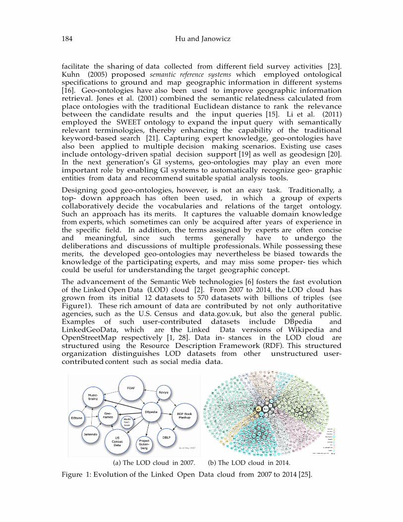
184 Hu and Janowicz facilitate the sharing of data collected from different field survey activities [23]. Kuhn (2005) proposed semantic reference systems which employed ontological specifications to ground and map geographic information in different systems [16]. Geo-ontologies have also been used to improve geographic information retrieval. Jones et al. (2001) combined the semantic relatedness calculated from place ontologies with the traditional Euclidean distance to rank the relevance between the candidate results and the input queries [15]. Li et al. (2011) employed the SWEET ontology to expand the input query with semantically relevant terminologies, thereby enhancing the capability of the traditional keyword-based search [21]. Capturing expert knowledge, geo-ontologies have also been applied to multiple decision making scenarios. Existing use cases include ontology-driven spatial decision support [19] as well as geodesign [20]. In the next generation’s GI systems, geo-ontologies may play an even more important role by enabling GI systems to automatically recognize geo- graphic entities from data and recommend suitable spatial analysis tools. Designing good geo-ontologies, however, is not an easy task. Traditionally, a top- down approach has often been used, in which a group of experts collaboratively decide the vocabularies and relations of the target ontology. Such an approach has its merits. It captures the valuable domain knowledge from experts, which sometimes can only be acquired after years of experience in the specific field. In addition, the terms assigned by experts are often concise and meaningful, since such terms generally have to undergo the deliberations and discussions of multiple professionals. While possessing these merits, the developed geo-ontologies may nevertheless be biased towards the knowledge of the participating experts, and may miss some proper- ties which could be useful for understanding the target geographic concept. The advancement of the Semantic Web technologies [6] fosters the fast evolution of the Linked Open Data (LOD) cloud [2]. From 2007 to 2014, the LOD cloud has grown from its initial 12 datasets to 570 datasets with billions of triples (see Figure1). These rich amount of data are contributed by not only authoritative agencies, such as the U.S. Census and data.gov.uk, but also the general public. Examples of such user-contributed datasets include DBpedia and LinkedGeoData, which are the Linked Data versions of Wikipedia and OpenStreetMap respectively [1, 28]. Data in- stances in the LOD cloud are structured using the Resource Description Framework (RDF). This structured organization distinguishes LOD datasets from other unstructured user-contributed content such as social media data.
(a) The LOD cloud in 2007. (b) The LOD cloud in 2014.
Figure 1: Evolution of the Linked Open Data cloud from 2007 to 2014 [25].
Enriching Top-‐‑down Geo-‐‑ontologies Using Bottom-‐‑up Knowledge Mined from Linked Open Data
185
The LOD cloud presents a valuable resource from which bottom-up knowledge could be mined to enrich the top-down geo-ontologies. The value of the LOD cloud can be seen in two folds. First, with many different data contributors, datasets on the LOD cloud reflect the diverse perspectives of people towards the same concepts and entities, and therefore can be exploited to enrich the knowledge from the limited number of participating experts. Second, the structured data from the LOD cloud enables knowledge to be extracted as a structured manner (e.g., in the form of property and property-value) which is often desired for an already formalized top-down geo- ontology. However, mining knowledge from the LOD cloud demands suitable methods, since improper approaches (e.g., using a natural language processing method based on the bag of words model) may simply break the links among data instances and convert the structured data back to an unstructured manner. This paper is an effort towards extracting bottom-up knowledge from the LOD cloud. The contributions of this work are as follows:
• Developed a workflow that mines knowledge about geographic concepts from the structured Linked Open Data. • Demonstrated the use of the workflow by applying it to a sample dataset from DBpedia and an example top-down geo-ontology. • Designed a preliminary experiment to evaluate the extracted bottom-up geo- graphic knowledge.
The remainder of this paper is organized as follows. Section 2 reviews related work on geo-ontology engineering, and provides some background on Linked Data and DBpedia. Section 3 presents the workflow developed to extract geographic knowledge from Linked Open Data. In section 4, we employ the proposed workflow to mine knowledge from DBpedia, and perform a preliminary evaluation on the extracted knowledge. Finally, section 5 summarizes this work and discusses future directions.
2 Related work The value of geo-ontologies has long been recognized by the GIScience community, and the history can be traced back to 1998 when a NCGIA specialist meeting was held in Maine [22]. Unlike the ontology discussed in philosophy, geo-ontologies are closer to those in computer science, which are designed to help machines turn data into sharable knowledge [4, 10]. Different from ontologies in other domains (e.g., bioinformatics), geo-ontologies focus on achieving better understanding of the geo- graphic world and facilitating the implementation of conceptually sound GI systems [26]. Since the 1998 meeting, a lot of studies have been devoted to developing geo- ontologies. Smith and Mark (2001) investigated the conceptualization of non-expert subjects on geospatial phenomenon, and derived an ontology of geographical categories [27]. Frank (2003) designed a 5-tier ontology for spatio-temporal databases, which starts from the observations in the physical world and completes at the knowledge of cognitive agents [9]. Kuhn (2009) proposed to develop ontologies with a minimal but firm grounding in
186 Hu and Janowicz reality [17], and Scheider et al. (2009) formalized this grounding process [24]. Focusing on geographic information constructs, Coucle- lis (2010) developed a hierarchical framework with the user intentionality on one end and the existence of information on the other [5]. Janowicz (2012) proposed an observation-driven ontology engineering framework which aims at deriving ontological primitives from observation data [13]. Recently, there are also an increasing number of geo-ontologies developed through joint community efforts during a series of Geo-Vocabulary Camps (GeoVocamps) [11]. This work was influenced by these pre- vious studies. However, it focuses on extracting bottom-up geographic knowledge from Linked Open Data to enrich top-down geo-ontologies, which has been rarely examined so far. The growth of the LOD cloud brings a large amount of structured spatiotemporal data, and is changing the ways of publishing, searching, and sharing geographic information [14, 18]. The term Linked Data has two folds of meanings that are often used interchangeably. On the one hand, it refers to a set of principles recommended by W3C for publishing data on the Semantic Web. On the other hand, it represents the data which are structured and published following these principles. Among the many datasets on the LOD cloud, DBpedia is a central hub, which provides information about more than 4.58 million entities (many of which are geographic places) [3]. The content of DBpedia originates from Wikipedia, and each Wikipedia article has a corresponding DBpedia page. As a result, DBpedia inherits many great features of Wikipedia. For example, Wikipedia articles are contributed by 25, 271, 668 users (http://en.wikipedia.org/wiki/Wikipedia:Statistics, retrieved in May 2015), and accord- ingly, DBpedia data obtain the diverse perspectives from the huge number of people. Meanwhile, a lot of data on Wikipedia have their original sources from authoritative agencies. For example, by examining the Wikipedia page of San Francisco, one can find that the data about the city’s land and water areas come from U.S. Census, while the elevation data are from U.S. Geological Survey. Unsurprisingly, DBpedia also inherits these valuable authoritative data. Since new content is being constantly added to Wikipedia, DBpedia updates its data periodically to synchronize with Wikipedia. Categorization systems are frequently used by datasets on the LOD cloud to group similar instances. Different from some LOD datasets that employ pre-defined categorization schemata, Wikipedia allows voluntary contributors to create customized categories and to classify entities into these categories. For example, there exists a category called Port cities and towns of the United States Pacific coast (see http://en.wikipedia.org/ wiki/Category:Port cities and towns of the United States Pacific coast) which contains cities, such as San Francisco and Los Angeles. According to Wikipedia, the intention of these categories is to “group together pages on similar subjects”. To some degree, the categorization result is similar to the data that Smith and Mark (2001) collected in [27]. In their experiment, non-expert human subjects were asked to give examples for geographic categories, whereas Wikipedia invites users to perform categorization tasks on the Web. DBpedia inherits these customized categories and the classification results from Wikipedia. In this work, we make use of the data instances under specific geographic categories to discover the properties which differentiate the instances that are in a category from those that are not.
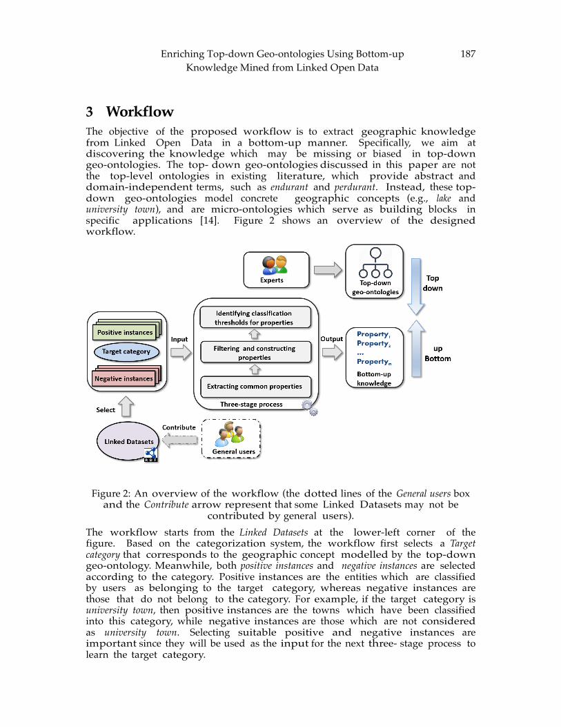
Enriching Top-‐‑down Geo-‐‑ontologies Using Bottom-‐‑up Knowledge Mined from Linked Open Data
187
3 Workflow The objective of the proposed workflow is to extract geographic knowledge from Linked Open Data in a bottom-up manner. Specifically, we aim at discovering the knowledge which may be missing or biased in top-down geo-ontologies. The top- down geo-ontologies discussed in this paper are not the top-level ontologies in existing literature, which provide abstract and domain-independent terms, such as endurant and perdurant. Instead, these top-down geo-ontologies model concrete geographic concepts (e.g., lake and university town), and are micro-ontologies which serve as building blocks in specific applications [14]. Figure 2 shows an overview of the designed workflow.
Figure 2: An overview of the workflow (the dotted lines of the General users box and the Contribute arrow represent that some Linked Datasets may not be
contributed by general users). The workflow starts from the Linked Datasets at the lower-left corner of the figure. Based on the categorization system, the workflow first selects a Target category that corresponds to the geographic concept modelled by the top-down geo-ontology. Meanwhile, both positive instances and negative instances are selected according to the category. Positive instances are the entities which are classified by users as belonging to the target category, whereas negative instances are those that do not belong to the category. For example, if the target category is university town, then positive instances are the towns which have been classified into this category, while negative instances are those which are not considered as university town. Selecting suitable positive and negative instances are important since they will be used as the input for the next three- stage process to learn the target category.
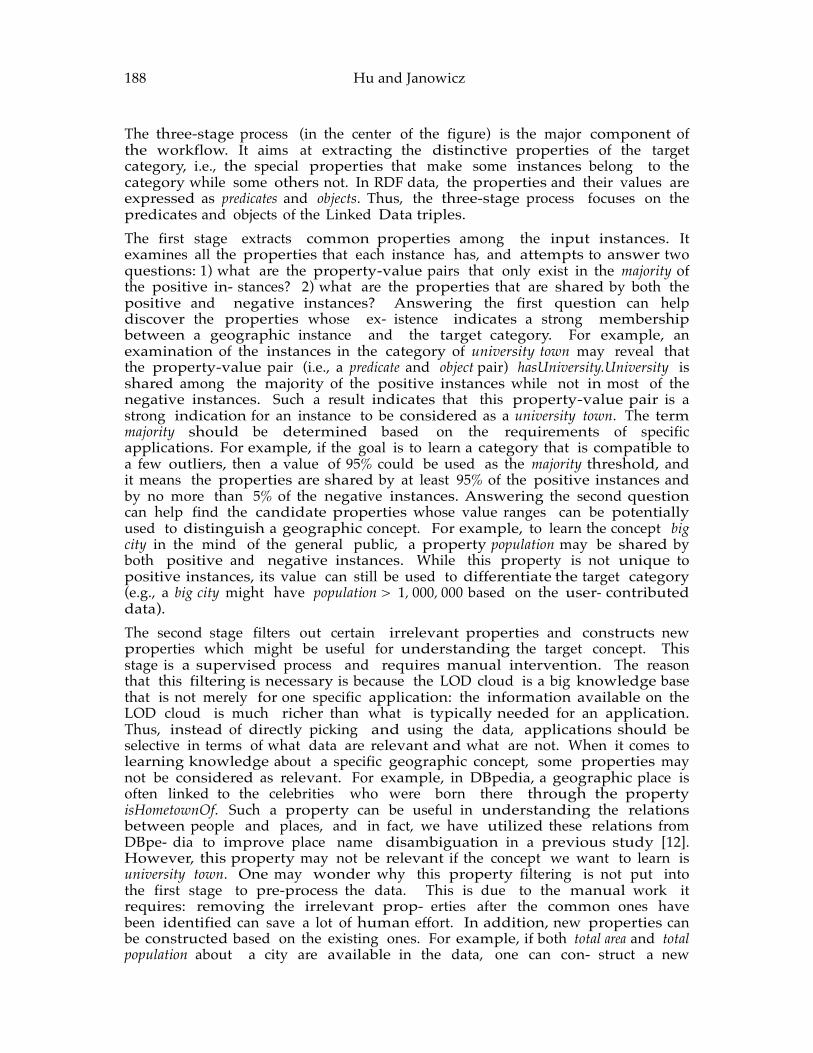
188 Hu and Janowicz The three-stage process (in the center of the figure) is the major component of the workflow. It aims at extracting the distinctive properties of the target category, i.e., the special properties that make some instances belong to the category while some others not. In RDF data, the properties and their values are expressed as predicates and objects. Thus, the three-stage process focuses on the predicates and objects of the Linked Data triples. The first stage extracts common properties among the input instances. It examines all the properties that each instance has, and attempts to answer two questions: 1) what are the property-value pairs that only exist in the majority of the positive in- stances? 2) what are the properties that are shared by both the positive and negative instances? Answering the first question can help discover the properties whose ex- istence indicates a strong membership between a geographic instance and the target category. For example, an examination of the instances in the category of university town may reveal that the property-value pair (i.e., a predicate and object pair) hasUniversity.University is shared among the majority of the positive instances while not in most of the negative instances. Such a result indicates that this property-value pair is a strong indication for an instance to be considered as a university town. The term majority should be determined based on the requirements of specific applications. For example, if the goal is to learn a category that is compatible to a few outliers, then a value of 95% could be used as the majority threshold, and it means the properties are shared by at least 95% of the positive instances and by no more than 5% of the negative instances. Answering the second question can help find the candidate properties whose value ranges can be potentially used to distinguish a geographic concept. For example, to learn the concept big city in the mind of the general public, a property population may be shared by both positive and negative instances. While this property is not unique to positive instances, its value can still be used to differentiate the target category (e.g., a big city might have population > 1, 000, 000 based on the user- contributed data). The second stage filters out certain irrelevant properties and constructs new properties which might be useful for understanding the target concept. This stage is a supervised process and requires manual intervention. The reason that this filtering is necessary is because the LOD cloud is a big knowledge base that is not merely for one specific application: the information available on the LOD cloud is much richer than what is typically needed for an application. Thus, instead of directly picking and using the data, applications should be selective in terms of what data are relevant and what are not. When it comes to learning knowledge about a specific geographic concept, some properties may not be considered as relevant. For example, in DBpedia, a geographic place is often linked to the celebrities who were born there through the property isHometownOf. Such a property can be useful in understanding the relations between people and places, and in fact, we have utilized these relations from DBpe- dia to improve place name disambiguation in a previous study [12]. However, this property may not be relevant if the concept we want to learn is university town. One may wonder why this property filtering is not put into the first stage to pre-process the data. This is due to the manual work it requires: removing the irrelevant prop- erties after the common ones have been identified can save a lot of human effort. In addition, new properties can be constructed based on the existing ones. For example, if both total area and total population about a city are available in the data, one can con- struct a new
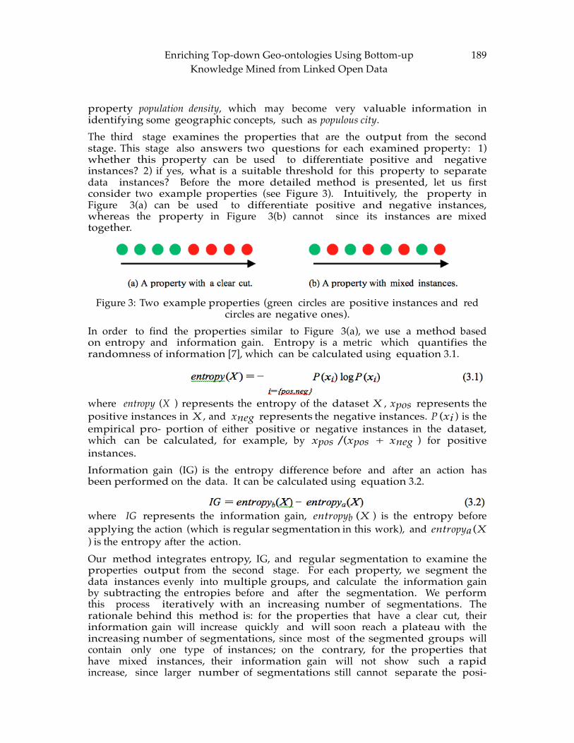
Enriching Top-‐‑down Geo-‐‑ontologies Using Bottom-‐‑up Knowledge Mined from Linked Open Data
189
property population density, which may become very valuable information in identifying some geographic concepts, such as populous city. The third stage examines the properties that are the output from the second stage. This stage also answers two questions for each examined property: 1) whether this property can be used to differentiate positive and negative instances? 2) if yes, what is a suitable threshold for this property to separate data instances? Before the more detailed method is presented, let us first consider two example properties (see Figure 3). Intuitively, the property in Figure 3(a) can be used to differentiate positive and negative instances, whereas the property in Figure 3(b) cannot since its instances are mixed together.
Figure 3: Two example properties (green circles are positive instances and red
circles are negative ones). In order to find the properties similar to Figure 3(a), we use a method based on entropy and information gain. Entropy is a metric which quantifies the randomness of information [7], which can be calculated using equation 3.1.
where entropy (X ) represents the entropy of the dataset X , xpos represents the positive instances in X , and xneg represents the negative instances. P (xi ) is the empirical pro- portion of either positive or negative instances in the dataset, which can be calculated, for example, by xpos /(xpos + xneg ) for positive instances. Information gain (IG) is the entropy difference before and after an action has been performed on the data. It can be calculated using equation 3.2.
where IG represents the information gain, entropyb (X ) is the entropy before applying the action (which is regular segmentation in this work), and entropya (X ) is the entropy after the action. Our method integrates entropy, IG, and regular segmentation to examine the properties output from the second stage. For each property, we segment the data instances evenly into multiple groups, and calculate the information gain by subtracting the entropies before and after the segmentation. We perform this process iteratively with an increasing number of segmentations. The rationale behind this method is: for the properties that have a clear cut, their information gain will increase quickly and will soon reach a plateau with the increasing number of segmentations, since most of the segmented groups will contain only one type of instances; on the contrary, for the properties that have mixed instances, their information gain will not show such a rapid increase, since larger number of segmentations still cannot separate the posi-
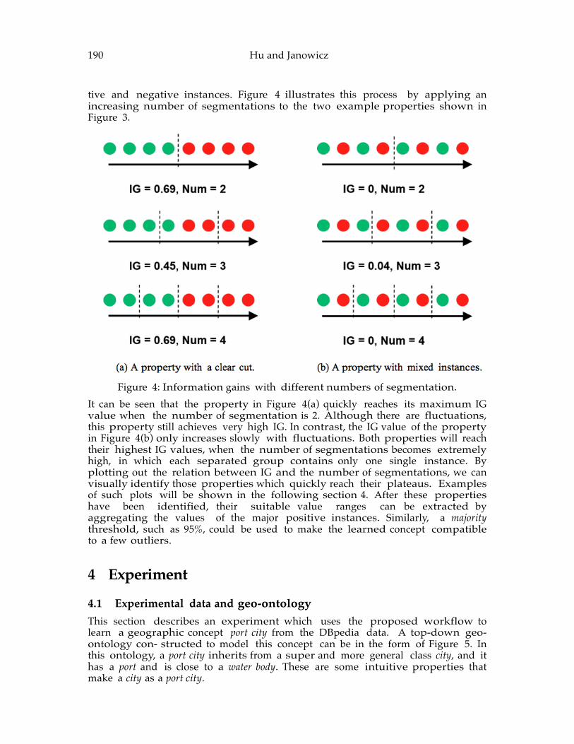
190 Hu and Janowicz tive and negative instances. Figure 4 illustrates this process by applying an increasing number of segmentations to the two example properties shown in Figure 3.
Figure 4: Information gains with different numbers of segmentation.
It can be seen that the property in Figure 4(a) quickly reaches its maximum IG value when the number of segmentation is 2. Although there are fluctuations, this property still achieves very high IG. In contrast, the IG value of the property in Figure 4(b) only increases slowly with fluctuations. Both properties will reach their highest IG values, when the number of segmentations becomes extremely high, in which each separated group contains only one single instance. By plotting out the relation between IG and the number of segmentations, we can visually identify those properties which quickly reach their plateaus. Examples of such plots will be shown in the following section 4. After these properties have been identified, their suitable value ranges can be extracted by aggregating the values of the major positive instances. Similarly, a majority threshold, such as 95%, could be used to make the learned concept compatible to a few outliers.
4 Experiment
4.1 Experimental data and geo-‐‑ontology This section describes an experiment which uses the proposed workflow to learn a geographic concept port city from the DBpedia data. A top-down geo-ontology con- structed to model this concept can be in the form of Figure 5. In this ontology, a port city inherits from a super and more general class city, and it has a port and is close to a water body. These are some intuitive properties that make a city as a port city.
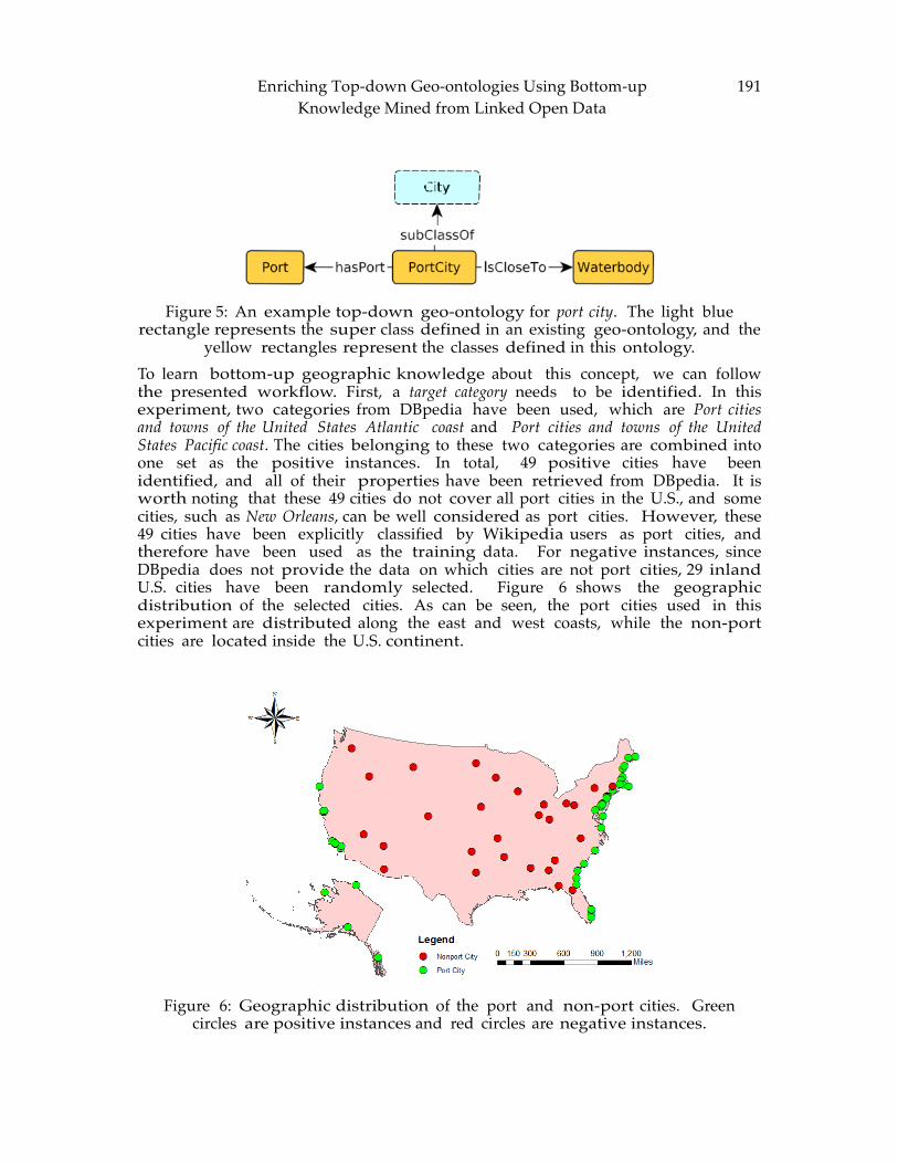
Enriching Top-‐‑down Geo-‐‑ontologies Using Bottom-‐‑up Knowledge Mined from Linked Open Data
191
Figure 5: An example top-down geo-ontology for port city. The light blue
rectangle represents the super class defined in an existing geo-ontology, and the yellow rectangles represent the classes defined in this ontology.
To learn bottom-up geographic knowledge about this concept, we can follow the presented workflow. First, a target category needs to be identified. In this experiment, two categories from DBpedia have been used, which are Port cities and towns of the United States Atlantic coast and Port cities and towns of the United States Pacific coast. The cities belonging to these two categories are combined into one set as the positive instances. In total, 49 positive cities have been identified, and all of their properties have been retrieved from DBpedia. It is worth noting that these 49 cities do not cover all port cities in the U.S., and some cities, such as New Orleans, can be well considered as port cities. However, these 49 cities have been explicitly classified by Wikipedia users as port cities, and therefore have been used as the training data. For negative instances, since DBpedia does not provide the data on which cities are not port cities, 29 inland U.S. cities have been randomly selected. Figure 6 shows the geographic distribution of the selected cities. As can be seen, the port cities used in this experiment are distributed along the east and west coasts, while the non-port cities are located inside the U.S. continent.
Figure 6: Geographic distribution of the port and non-port cities. Green
circles are positive instances and red circles are negative instances.
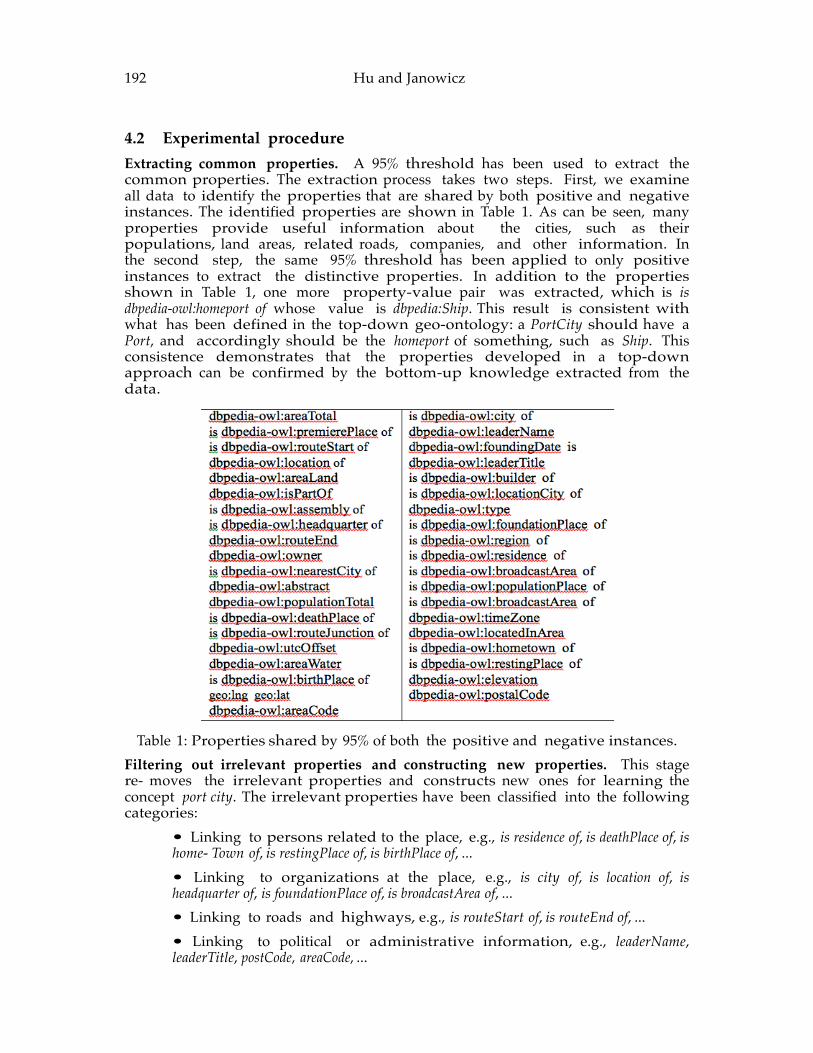
192 Hu and Janowicz 4.2 Experimental procedure Extracting common properties. A 95% threshold has been used to extract the common properties. The extraction process takes two steps. First, we examine all data to identify the properties that are shared by both positive and negative instances. The identified properties are shown in Table 1. As can be seen, many properties provide useful information about the cities, such as their populations, land areas, related roads, companies, and other information. In the second step, the same 95% threshold has been applied to only positive instances to extract the distinctive properties. In addition to the properties shown in Table 1, one more property-value pair was extracted, which is is dbpedia-owl:homeport of whose value is dbpedia:Ship. This result is consistent with what has been defined in the top-down geo-ontology: a PortCity should have a Port, and accordingly should be the homeport of something, such as Ship. This consistence demonstrates that the properties developed in a top-down approach can be confirmed by the bottom-up knowledge extracted from the data.
Table 1: Properties shared by 95% of both the positive and negative instances.
Filtering out irrelevant properties and constructing new properties. This stage re- moves the irrelevant properties and constructs new ones for learning the concept port city. The irrelevant properties have been classified into the following categories:
• Linking to persons related to the place, e.g., is residence of, is deathPlace of, is home- Town of, is restingPlace of, is birthPlace of, ... • Linking to organizations at the place, e.g., is city of, is location of, is headquarter of, is foundationPlace of, is broadcastArea of, ... • Linking to roads and highways, e.g., is routeStart of, is routeEnd of, ... • Linking to political or administrative information, e.g., leaderName, leaderTitle, postCode, areaCode, ...
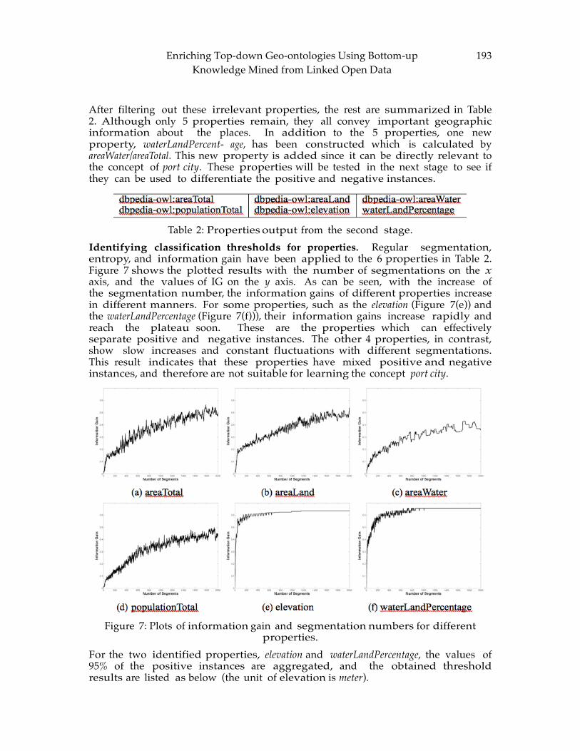
Enriching Top-‐‑down Geo-‐‑ontologies Using Bottom-‐‑up Knowledge Mined from Linked Open Data
193
After filtering out these irrelevant properties, the rest are summarized in Table 2. Although only 5 properties remain, they all convey important geographic information about the places. In addition to the 5 properties, one new property, waterLandPercent- age, has been constructed which is calculated by areaWater/areaTotal. This new property is added since it can be directly relevant to the concept of port city. These properties will be tested in the next stage to see if they can be used to differentiate the positive and negative instances.
Table 2: Properties output from the second stage.
Identifying classification thresholds for properties. Regular segmentation, entropy, and information gain have been applied to the 6 properties in Table 2. Figure 7 shows the plotted results with the number of segmentations on the x axis, and the values of IG on the y axis. As can be seen, with the increase of the segmentation number, the information gains of different properties increase in different manners. For some properties, such as the elevation (Figure 7(e)) and the waterLandPercentage (Figure 7(f))), their information gains increase rapidly and reach the plateau soon. These are the properties which can effectively separate positive and negative instances. The other 4 properties, in contrast, show slow increases and constant fluctuations with different segmentations. This result indicates that these properties have mixed positive and negative instances, and therefore are not suitable for learning the concept port city.
Figure 7: Plots of information gain and segmentation numbers for different
properties. For the two identified properties, elevation and waterLandPercentage, the values of 95% of the positive instances are aggregated, and the obtained threshold results are listed as below (the unit of elevation is meter).
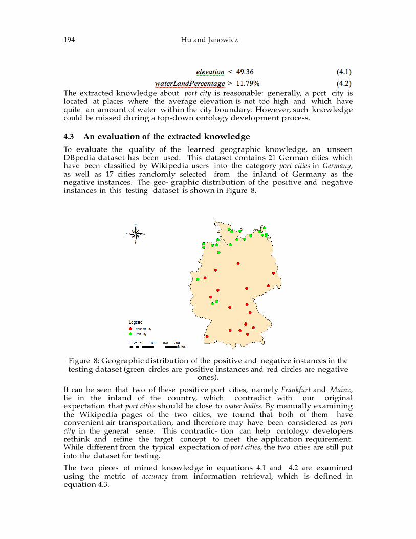
194 Hu and Janowicz
The extracted knowledge about port city is reasonable: generally, a port city is located at places where the average elevation is not too high and which have quite an amount of water within the city boundary. However, such knowledge could be missed during a top-down ontology development process.
4.3 An evaluation of the extracted knowledge To evaluate the quality of the learned geographic knowledge, an unseen DBpedia dataset has been used. This dataset contains 21 German cities which have been classified by Wikipedia users into the category port cities in Germany, as well as 17 cities randomly selected from the inland of Germany as the negative instances. The geo- graphic distribution of the positive and negative instances in this testing dataset is shown in Figure 8.
Figure 8: Geographic distribution of the positive and negative instances in the testing dataset (green circles are positive instances and red circles are negative
ones). It can be seen that two of these positive port cities, namely Frankfurt and Mainz, lie in the inland of the country, which contradict with our original expectation that port cities should be close to water bodies. By manually examining the Wikipedia pages of the two cities, we found that both of them have convenient air transportation, and therefore may have been considered as port city in the general sense. This contradic- tion can help ontology developers rethink and refine the target concept to meet the application requirement. While different from the typical expectation of port cities, the two cities are still put into the dataset for testing. The two pieces of mined knowledge in equations 4.1 and 4.2 are examined using the metric of accuracy from information retrieval, which is defined in equation 4.3.
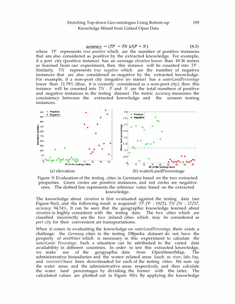
Enriching Top-‐‑down Geo-‐‑ontologies Using Bottom-‐‑up Knowledge Mined from Linked Open Data
195
where TP represents true positive which are the number of positive instances that are also considered as positive by the extracted knowledge. For example, if a port city (positive instance) has an average elevation lower than 49.36 meters as learned from our experiment, then this instance will be counted into TP . Similarly, TN represents true negative which are the number of negative instances that are also considered as negative by the extracted knowledge. For example, if a non-port city (negative in- stance) has a waterLandPerventage lower than 11.79% (thus, it is correctly considered as a non-port city), then this instance will be counted into TN . P and N are the total numbers of positive and negative instances in the testing dataset. The metric accuracy measures the consistency between the extracted knowledge and the unseen testing instances.
(a) elevation (b) waterLandPercentage Figure 9: Evaluation of the testing cities in Germany based on the two extracted properties. Green circles are positive instances, and red circles are negative
ones. The dotted line represents the reference value based on the extracted knowledge.
The knowledge about elevation is first evaluated against the testing data (see Figure 9(a)), and the following result is acquired: TP /P : 19/21, TN /N : 17/17, accuracy: 94.74%. It can be seen that the geographic knowledge learned about elevation is highly consistent with the testing data. The two cities which are classified incorrectly are the two inland cities which may be considered as port city for their convenient air transportations. When it comes to evaluating the knowledge on waterLandPercentage, there exists a challenge: the Germany cities in the testing DBpedia dataset do not have the property of areaWater which is necessary in this experiment to calculate the waterLand- Percentage. Such a situation can be attributed to the varied data availability in different countries. In order to test this extracted knowledge, we make use of the geographic data from OpenStreetMap. The administrative boundaries and the water- related areas (such as river, lake, bay, and reservoir) have been downloaded for each of the testing cities. We sum up the water areas and the administrative areas respectively, and then calculate the water land percentages by dividing the former with the latter. The calculated values are plotted out in Figure 9(b). By applying the knowledge
196 Hu and Janowicz waterLandPercentage > 11.79% to the testing cities, we obtain the following result: TP /P : 17/21, TN /N : 17/17, accuracy : 89.47%.
5 Conclusions and future work Geo-ontologies can play an even more important role in developing the next genera- tion’s intelligent GIS by enabling the systems to automatically recognize geographic concepts from data and recommend suitable tools. While a top-down approach has often been used to develop geo-ontologies, such an approach may be biased towards the knowledge of the participants or miss some useful properties. The fast growth of the Linked Open Data cloud provides a valuable resource for deriving knowledge in a bottom-up manner. Such knowledge can then be used to enrich and complement the top-down geo-ontologies. This paper presents a workflow for mining bottom-up geographic knowledge from Linked Open Data. Based on both positive and negative instances of a target concept, this workflow identifies the common properties, filters irrelevant information, and extracts suitable thresholds. An experiment has been con- ducted, in which the workflow has been used to extract knowledge about a geographic concept port city from a DBpedia dataset. We evaluate the extracted knowledge using an unseen dataset, and the evaluation result shows a good consistency between the learned knowledge and the testing cities. While DBpedia has been used as the data source in the experiment, the proposed workflow can also be applied to other LOD datasets, such as Freebase. The performance of the proposed workflow depends on the availability and qual- ity of the training data which contain the target category, the positive instances, and the negative ones. While we obtained our data from the Wikipedia categorization system in this work, other approaches could also be used. For example, traditional human participant experiments could be employed to elicit the typical instances of a target category. The derived instance memberships can then be embedded into the presented workflow, and combined with the LOD datasets to mine bottom-up knowl- edge. Alternatively, one can create the target category on Wikipedia, encourage online users to classify instances based on this category, and then harvest the data. While the latter approach might require less human effort and thus better scale up, traditional human participant tests provide more information about the background of the participants (e.g., age and gender), and therefore can provide a more representative data sample. The presented research can also be extended in several directions. First, our experiment so far has examined the applicability of the proposed workflow using one geographic concept. While fair performance has been observed, it is still necessary to investigate some additional concepts to understand the merits and limitations of the proposed workflow more thoroughly. Such investigation could also help quantify the degree of improvement that our workflow can bring to existing top-down geo- ontologies. Second, the evaluation experiment indicates that the port cities in the U.S. are similar to the port cities in Germany in terms of their elevations and water land percentages. This result is intriguing since some geographic concepts (e.g., mountain and hill) may be conceptualized differently in different countries. Thus, it would also be interesting to examine which concepts are more regionally sensitive and which others are more stable across different geographic areas.
Enriching Top-‐‑down Geo-‐‑ontologies Using Bottom-‐‑up Knowledge Mined from Linked Open Data
197
References [1] AU E R , S., BI Z E R , C., KO B I L A R O V, G., LE H M A N N , J., CY G A N I A K , R., A N D IV E S ,
Z. DBpedia: A nucleus for a web of open data. In The semantic web. Springer, 2007, pp. 722–735.
[2] BI Z E R , C., HEAT H , T., A N D BE R N E R S -LE E , T. Linked data - the story so far. International Journal on Semantic Web and Information Systems 5, 3 (2009), 1–22.
[3] BI Z E R , C., LE H M A N N , J., KO B I L A R O V, G., AU E R , S., BE C K E R , C., CY G A N I A K , R., A N D HE L L M A N N , S. Dbpedia-a crystallization point for the web of data. Web Semantics: science, services and agents on the world wide web 7, 3 (2009), 154–165.
[4] CO U C L E L I S , H. Ontology, epistemology, teleology: triangulating geographic in- formation science. In Research trends in geographic information science. Springer, 2009, pp. 3–15.
[5] CO U C L E L I S , H. Ontologies of geographic information. International Journal of Geographical Information Science 24, 12 (2010), 1785–1809.
[6] EG E N H O F E R , M. J. Toward the semantic geospatial web. In Proceedings of the 10th ACM international symposium on Advances in geographic information systems (2002), ACM, pp. 1–4.
[7] FL A C H , P. Machine learning: the art and science of algorithms that make sense of data. Cambridge University Press, 2012.
[8] FO N S E C A , F. T., EG E N H O F E R , M. J., AG O U R I S , P., A N D CA M A R A , G. Using ontologies for integrated geographic information systems. Transactions in GIS 6, 3 (2002), 231–257.
[9] FR A N K , A. U. Ontology for spatio-temporal databases. Springer, 2003. [10] GU A R I N O , N. Formal ontology in information systems: Proceedings of the first inter-
national conference (FOIS’98), June 6-8, Trento, Italy, vol. 46. IOS press, 1998. [11] HU , Y., JA N O W I C Z , K., CA R R A L , D., SC H E I D E R , S., KU H N , W., BE R G -CR O S S
, G., HI T Z L E R , P., DE A N , M., A N D KO L A S , D. A geo-ontology design pattern for semantic trajectories. In Spatial Information Theory. Springer, 2013, pp. 438–456.
[12] HU , Y., JA N O W I C Z , K., A N D PR A S A D , S. Improving wikipedia-based place name disambiguation in short texts using structured data from dbpedia. In Proceedings of the 8th workshop on geographic information retrieval (2014), ACM New York, NY, pp. 1–8.
[13] JA N O W I C Z , K. Observation-driven geo-ontology engineering. Transactions in GIS 16, 3 (2012), 351–374.
[14] JA N O W I C Z , K., SC H E I D E R , S., PE H L E , T., A N D HA RT, G. Geospatial seman- tics and linked spatiotemporal data–past, present, and future. Semantic Web 3, 4 (2012), 321–332.
[15] JO N E S , C. B., AL A N I , H., A N D TU D H O P E , D. Geographical information retrieval with ontologies of place. In Spatial information theory (2001), Springer, pp. 322–335.
198 Hu and Janowicz [16] KU H N , W. Geospatial semantics: why, of what, and how? In Journal on
Data Semantics III. Springer, 2005, pp. 1–24. [17] KU H N , W. Semantic engineering. In Research trends in geographic information
sci- ence. Springer, 2009, pp. 63–76. [18] KU H N , W., KA U P P I N E N , T., A N D JA N O W I C Z , K. Linked data-a paradigm
shift for geographic information science. In Geographic Information Science. Springer, 2014, pp. 173–186.
[19] LI , N., ERV I N , S., FL A X M A N , M., GO O D C H I L D , M., A N D ST E I N I T Z , C. Design and application of an ontology for geodesign. Revue internationale de geomatique, 22 (2012), 145–168.
[20] LI , N., RA S K I N , R., GO O D C H I L D , M., A N D JA N O W I C Z , K. An ontology-driven framework and web portal for spatial decision support. Transactions in GIS 16, 3 (2012), 313–329.
[21] LI , W., YA N G , C., NE B E RT, D., RA S K I N , R., HO U S E R , P., WU , H., A N D LI , Z. Semantic-based web service discovery and chaining for building an arctic spatial data infrastructure. Computers & Geosciences 37, 11 (2011), 1752–1762.
[22] PE U Q U E T, D., SM I T H , B., A N D BR O G A A R D , B. O. The ontology of fields. Tech. rep., National Center for Geographic Information and Analysis, 1998.
[23] PU N D T, H., A N D BI S H R , Y. Domain ontologies for data sharing–an example from environmental monitoring using field gis. Computers & Geosciences 28, 1 (2002), 95–102.
[24] SC H E I D E R , S., JA N O W I C Z , K., A N D KU H N , W. Grounding geographic categories in the meaningful environment. In Spatial Information Theory. Springer, 2009, pp. 69–87.
[25] SC H M A C H T E N B E R G , M., BI Z E R , C., JE N T Z S C H , A., A N D CY G A N I A K , R. Linking open data cloud diagram, http://lod-cloud.net/, 2014.
[26] SM I T H , B., A N D MA R K , D. M. Ontology and geographic kinds. In Proceedings of the Tenth International Symposium on Spatial Data Handling, T. Poiker and N. Chris- man, Eds. Simon Fraser University, 1998, pp. 308–320.
[27] SM I T H , B., A N D MA R K , D. M. Geographical categories: an ontological investi- gation. International journal of geographical information science 15, 7 (2001), 591–612.
[28] STA D L E R , C., LE H M A N N , J., HO FFN E R , K., A N D AU E R , S. Linkedgeodata: A core for a web of spatial open data. Semantic Web 3, 4 (2012), 333–354.
ADVANCING GEOGRAPHIC INFORMATION SCIENCE: CHAPTER 14
© by the author(s) Licensed under Creative Commons Attribution 4.0 License
199
Analysis of Dynamic Radiation Level Changes Using Surface
Networks Myeong-Hun Jeong1, Shaowen Wang1, and Clair J. Sullivan 2
1 CyberGIS Center for Advanced Digital and Spatial Studies, CyberInfrastructure and Geospatial Information Laboratory, Department of Geography and Geographic
Information Science, National Center for Supercomputing Applications, University of Illinois at Urbana-Champaign, Champaign, IL, 61820, USA
2 Department of Nuclear, Plasma, and Radiological Engineering, University of Illinois at Urbana-Champaign, Champaign, IL, 61820, USA
Abstract: The Fukushima nuclear accident reminds us of severe risk of radioactive substances. Citizen scientists voluntarily collect and share radiation data using geo- tagged sensors for radiation preparedness. However, radiation levels are affected by a number of factors including for example weather conditions, naturally occurring radioactive materials (NORM), and large marble structures. It is therefore difficult to determine whether a higher radiation level comes from a normal variation in back- ground or not. This research analyzes the radiation changes using surface networks that can be used to characterize complex surfaces. A new algorithm has been developed to identify salient peaks and their hills by merging insignificant peaks recursively. Salient peaks and their hills are converted into graphs. The structural similarities of graphs were compared over time. The radiation measurements in the city of Koriyama, Japan were analyzed as a case study. The results demonstrated that structural analysis of dynamic radiation levels revealed stable changes, while numeric analysis of radiation levels presented statistically significant differences. This method is able to detect radiation level changes irrespective of background variations.
Keywords: Surface networks, structural similarities, graph indices, radiation levels.
1 Introduction Radiation levels have been a subject of major debate after a nuclear disaster – Fukushima Daiichi accident – released substantial contamination into our environments. Citizen scientists, as it came to be known, started gathering and sharing environmental radiation levels using mobile detectors (e.g., Geiger
200 Jeong, Wang, and Sullivan counters) across the world due to awareness of health effects. In particular, the non-profit organization such as Safecast has been building a radiation sensor network from crowd-sourced data. Its data points have been over 25 million at the end of 2014 [1]. While an immense number of radiation sensors quantify the levels of radiation in our environment, it is difficult to understand accurate radiation levels due to back- ground variations [29, 18]. For example, some regions have naturally occurring radioactive materials (NORM); weather such as precipitation causes the increase of back- ground levels, or background levels have a tendency to increase as a result of the presence of large marble structures. It is challenging to predict whether the amplitude of the count rate is due to the possible release of radioactive materials or not. However, looking beyond direct background effects on radiation levels, this paper investigates how the structure of regions of higher count rates have changed as time varies. We assume if radioactive materials are continually stable, the structure of the regions of higher count rates would have similar patterns, irrespective of background fluctuations. In this paper, the regions of higher count rates are represented by surface networks, consisting of critical points (peaks, pits, and passes) and critical lines (ridges and channels) [24, 25]. We particularly focus on salient peaks and their hills such as catchments areas. Salient peaks are connected by edges. Such a graph between sub- sequent time steps have been analyzed and compared using graph structural analysis techniques [26]. The structural analysis can provide dynamic radiation level changes without knowing accurate background variations. In the reminder, the following section starts by discussing the previous computations of surface networks and structural similarity measurements between surface networks. Section 3 describes the data processing for parsing and filtering radiation data set. Section 4 provides a surface network algorithm presented in this study. In addition, this section provides the information about analysis methods. Section 5 presents evaluations of structural analysis. The results confirm the effectiveness of the approach, discussed in Section 6. Finally, the conclusions and future works are drawn in Section 7.
2 Background This paper utilizes spatial reasoning for identifying radiation level changes. The radia- tion level changes may be identified by using cluster analysis from a group of radiation measurements. However, it is difficult to separate radiation measurements appropri- ately because radiation levels are floating at even the same location due to background effects. In this paper, radiation measurements are converted to raster maps. The radiation scalar fields (i.e., raster maps) are characterized by surface networks. The regions of higher count rates are represented as peaks and their hills on the surface network. The structural similarity of surface networks are compared in order to infer radiation level changes. Surface networks originate from the work of [6, 17], which do not describe the Earth’s surface as hills and valley, but also propose relations between the number of peaks, pits, and passes. In a later, Morse theory uses differential
Analysis of Dynamic Radiation Level Changes Using Surface Networks
201
,y ) ,y
topology generally to define surface networks [19]. Morse theory pertains to the relationship between the shape of the space and functions on defined on the space. If the derivative of a height function z = f (x, y) equals to zero at a point (x0, y0), this point (x0, y0) is called a
critical point, if and only if the determinant of the Hessian matrix ( fxx (x0 ,y0 ) fxy (x0
,y0 ) ) yx 0 0 yy 0 0
is not zero, where fxx, fxy , fyx, fyy are partial derivatives of the height function, z [16]. There are broadly two approaches to construct surface networks from continuous surfaces to discrete data structures: explicit and implicit cell complexes. Explicit cell complexes can be regarded as triangulations. The critical points are extracted from the triangular mesh by comparing values with adjacent points [30] or piecewise linear functions [10, 8]. Illicit cell complexes make use of a grid such as raster-based DEMs [23, 35]. We use a grid configuration of each radiation measurements (i.e., a raster map). In particular, we focus on the detection of peaks and their hills because our purpose is to identify regions of higher count rates. The hills of peaks are called as Morse complexes [8]. One example for using Morse complex is to analyze and track burning structures [3]. Based on a raster map, there are several ways to identify critical points. [23] use local comparisons between eight direct neighbo rs. Local comparisons are known to identify spurious critical points due to continuity constraints [27]. [34, 35] uses bi- quadratic interpolation as well as geomorphological parameters, which help to re- move spurious critical points. However, geomorphological parameters (e.g., slope and curvature) can not guarantee that all peaks are identified due to the violation of geomorphological parameters’ constraints, although geomorphological approach is good at removing spurious critical points. The regions of higher does rates are important in our application. In such context, this paper presents a new algorithm for identifying salient critical points (i.e., peaks) in a radiation scalar field using prominence (i.e., the relative height difference between adjacent peaks) and horizontal distance (i.e., distance between adjacent peaks). Our approach recursively removes insignificant peaks. In terms of measuring similarity between surface networks, there is very few re- search on the structural analysis of surface networks. One example is to calculate structural similarity index for the analysis of urban population surfaces [21]. In the first step, identified surface networks are generalized by removing peaks that have the minimum difference in height with associated passes. Critical points are then sorted based on the height. Sorted critical points are continually deleted until there is only one peak left. During this process, structural similarity index is given if two surface networks are isomorphic. However, this approach is ill-suited to our problem in the sense that background fluctuations lead to different radioactive levels in spite of the same count rates in reality.
202 Jeong, Wang, and Sullivan Another approach is to use graph theoretic indices (e.g., density or connectivity) to analyze the surface and its changes over time [12]. However, graph theoretic indices are not enough to characterize radiation level changes because a network connectivity can be different without significant radiation level changes. None of approaches en- countered are directly applicable to our problems. Therefore we adapt graph similarity measurement techniques for quantifying the similarity of surface networks. There are a broad range of applications in graph similarity scoring and matching techniques: chemical structures [14, 32], social media [5, 20], web searching [2, 9] or medical diagnostics [28]. In summary, this paper provides a new algorithm to identify salient peaks among spurious peaks. In addition, the structural similarity of surface and its changes are measured using graph similarity scoring and measuring techniques. We demonstrate that this approach can provide global radiation level changes without accurate back- ground measurements.
3 Data processing Based on our previous literature review, we will now proceed with data processing for the analysis of radiation level changes. We acquired experimental radiation data set from Safecast in February, 2015. The data size is over 26 million records and over 3 GB as a csv file format. The experimental area was selected in Japan because citizen scientists have been gathering substantial numbers of radiation measurements across Japan. Our experimental region is the city of Koriyama that is 82km away from Fukushima Daiichi nu- clear power station (i.e., WGS84 bounds are 140.32564, 37.36191, 140.40993, 37.43678). We gathered all measurements each month in 2013. Thus, there are twelve data set for the city of Koriyama. In order to analyze a large volume of data, we exploited Apche Pig and Hadoop. The former is a programming language designed to ease the development of distributed applications for analyzing large volumes of data. The later can be thought of distributed computing framework designed for processing large distributed data [22]. By using Pig and Hadoop, we can derive experimental data set with ease and speed. Finally, all measurements per month are converted into raster maps using Empirical Bayesian Kriging (EBK). EBK is well known to have smaller prediction uncertainty and the ability to filter out measurement errors [15]. These interpolation maps have been used as the cornerstone for identifying surface networks as well as analysing radiation level changes.
4 Surface networks In this section, we explore a new algorithm to identify peaks and their hills in a radiation scalar field. Further, the analysis methods are presented: how well surface net- works reflect the radiation measurements; numerical summaries of surface networks’ structure; and structural similarity of surface and its changes over time.
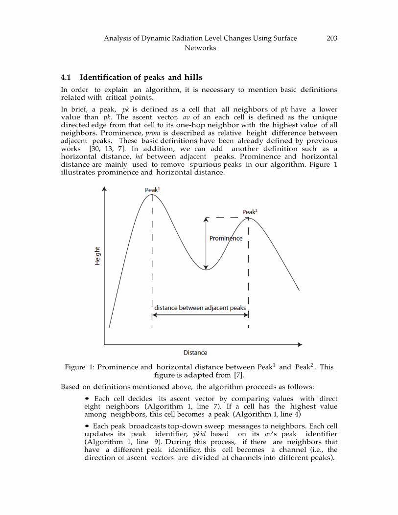
Analysis of Dynamic Radiation Level Changes Using Surface Networks
203
4.1 Identification of peaks and hills In order to explain an algorithm, it is necessary to mention basic definitions related with critical points. In brief, a peak, pk is defined as a cell that all neighbors of pk have a lower value than pk. The ascent vector, av of an each cell is defined as the unique directed edge from that cell to its one-hop neighbor with the highest value of all neighbors. Prominence, prom is described as relative height difference between adjacent peaks. These basic definitions have been already defined by previous works [30, 13, 7]. In addition, we can add another definition such as a horizontal distance, hd between adjacent peaks. Prominence and horizontal distance are mainly used to remove spurious peaks in our algorithm. Figure 1 illustrates prominence and horizontal distance.
Figure 1: Prominence and horizontal distance between Peak1 and Peak2 . This
figure is adapted from [7]. Based on definitions mentioned above, the algorithm proceeds as follows:
• Each cell decides its ascent vector by comparing values with direct eight neighbors (Algorithm 1, line 7). If a cell has the highest value among neighbors, this cell becomes a peak (Algorithm 1, line 4) • Each peak broadcasts top-down sweep messages to neighbors. Each cell updates its peak identifier, pkid based on its av’s peak identifier (Algorithm 1, line 9). During this process, if there are neighbors that have a different peak identifier, this cell becomes a channel (i.e., the direction of ascent vectors are divided at channels into different peaks).
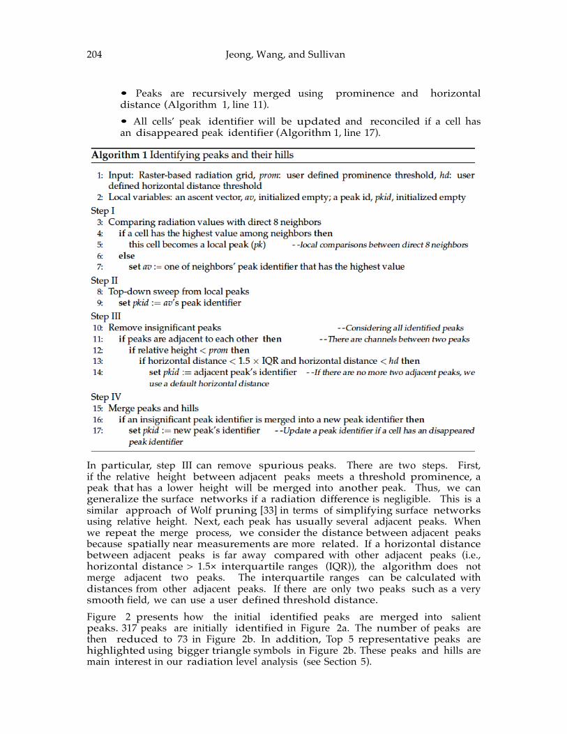
204 Jeong, Wang, and Sullivan
• Peaks are recursively merged using prominence and horizontal distance (Algorithm 1, line 11). • All cells’ peak identifier will be updated and reconciled if a cell has an disappeared peak identifier (Algorithm 1, line 17).
In particular, step III can remove spurious peaks. There are two steps. First, if the relative height between adjacent peaks meets a threshold prominence, a peak that has a lower height will be merged into another peak. Thus, we can generalize the surface networks if a radiation difference is negligible. This is a similar approach of Wolf pruning [33] in terms of simplifying surface networks using relative height. Next, each peak has usually several adjacent peaks. When we repeat the merge process, we consider the distance between adjacent peaks because spatially near measurements are more related. If a horizontal distance between adjacent peaks is far away compared with other adjacent peaks (i.e., horizontal distance > 1.5× interquartile ranges (IQR)), the algorithm does not merge adjacent two peaks. The interquartile ranges can be calculated with distances from other adjacent peaks. If there are only two peaks such as a very smooth field, we can use a user defined threshold distance. Figure 2 presents how the initial identified peaks are merged into salient peaks. 317 peaks are initially identified in Figure 2a. The number of peaks are then reduced to 73 in Figure 2b. In addition, Top 5 representative peaks are highlighted using bigger triangle symbols in Figure 2b. These peaks and hills are main interest in our radiation level analysis (see Section 5).
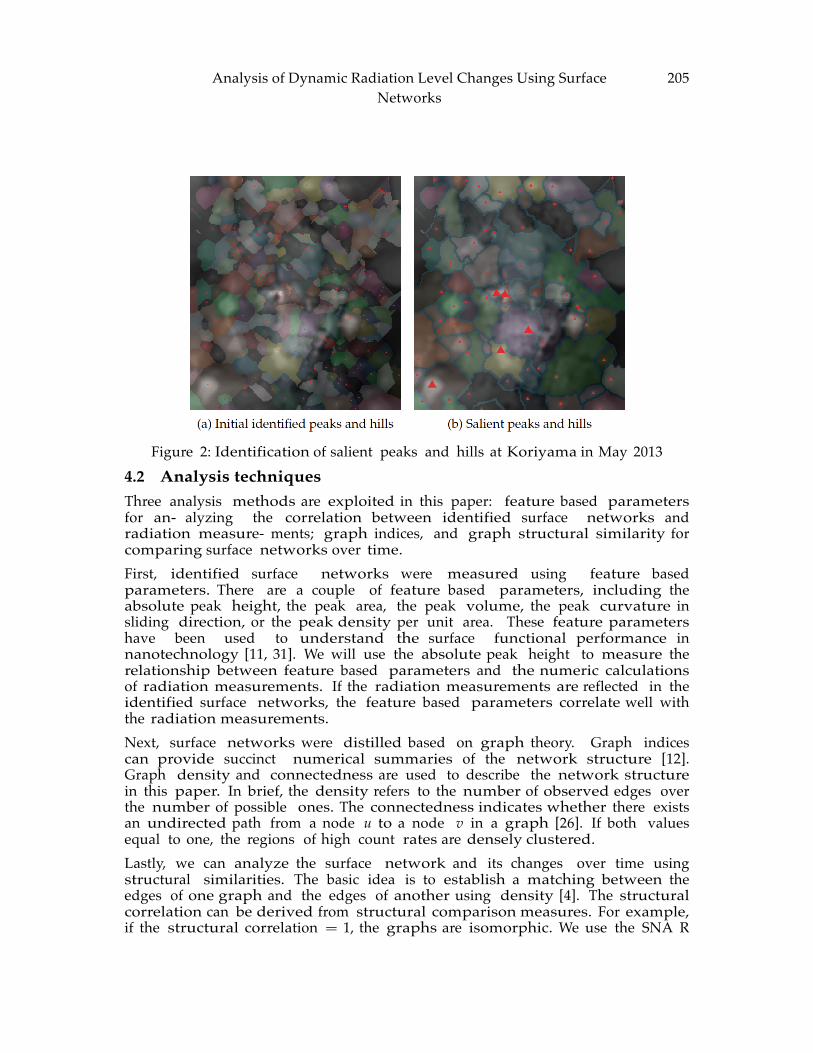
Analysis of Dynamic Radiation Level Changes Using Surface Networks
205
Figure 2: Identification of salient peaks and hills at Koriyama in May 2013
4.2 Analysis techniques Three analysis methods are exploited in this paper: feature based parameters for an- alyzing the correlation between identified surface networks and radiation measure- ments; graph indices, and graph structural similarity for comparing surface networks over time. First, identified surface networks were measured using feature based parameters. There are a couple of feature based parameters, including the absolute peak height, the peak area, the peak volume, the peak curvature in sliding direction, or the peak density per unit area. These feature parameters have been used to understand the surface functional performance in nanotechnology [11, 31]. We will use the absolute peak height to measure the relationship between feature based parameters and the numeric calculations of radiation measurements. If the radiation measurements are reflected in the identified surface networks, the feature based parameters correlate well with the radiation measurements. Next, surface networks were distilled based on graph theory. Graph indices can provide succinct numerical summaries of the network structure [12]. Graph density and connectedness are used to describe the network structure in this paper. In brief, the density refers to the number of observed edges over the number of possible ones. The connectedness indicates whether there exists an undirected path from a node u to a node v in a graph [26]. If both values equal to one, the regions of high count rates are densely clustered. Lastly, we can analyze the surface network and its changes over time using structural similarities. The basic idea is to establish a matching between the edges of one graph and the edges of another using density [4]. The structural correlation can be derived from structural comparison measures. For example, if the structural correlation = 1, the graphs are isomorphic. We use the SNA R
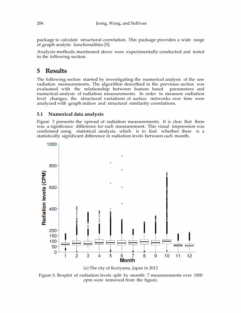
206 Jeong, Wang, and Sullivan package to calculate structural correlation. This package provides a wide range of graph analytic functionalities [5]. Analysis methods mentioned above were experimentally conducted and tested in the following section.
5 Results The following section started by investigating the numerical analysis of the raw radiation measurements. The algorithm described in the previous section was evaluated with the relationship between feature based parameters and numerical analysis of radiation measurements. In order to measure radiation level changes, the structural variations of surface networks over time were analyzed with graph indices and structural similarity correlations.
5.1 Numerical data analysis Figure 3 presents the spread of radiation measurements. It is clear that there was a significance difference for each measurement. This visual impression was confirmed using statistical analysis, which is to find whether there is a statistically significant difference in radiation levels between each month.
(a) The city of Koriyama, Japan in 2013
Figure 3: Boxplot of radiation levels split by month: 7 measurements over 1000 cpm were removed from the figure.
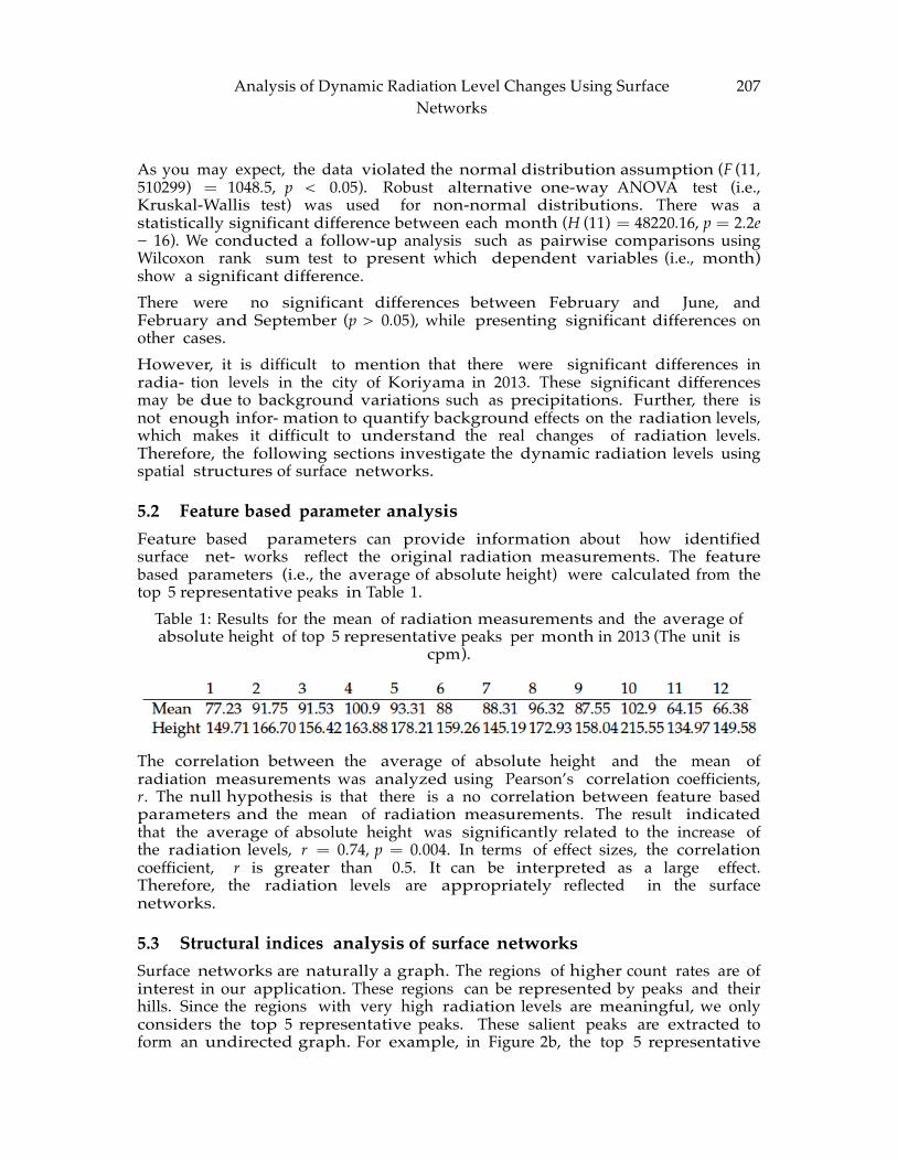
Analysis of Dynamic Radiation Level Changes Using Surface Networks
207
As you may expect, the data violated the normal distribution assumption (F (11, 510299) = 1048.5, p < 0.05). Robust alternative one-way ANOVA test (i.e., Kruskal-Wallis test) was used for non-normal distributions. There was a statistically significant difference between each month (H (11) = 48220.16, p = 2.2e − 16). We conducted a follow-up analysis such as pairwise comparisons using Wilcoxon rank sum test to present which dependent variables (i.e., month) show a significant difference. There were no significant differences between February and June, and February and September (p > 0.05), while presenting significant differences on other cases. However, it is difficult to mention that there were significant differences in radia- tion levels in the city of Koriyama in 2013. These significant differences may be due to background variations such as precipitations. Further, there is not enough infor- mation to quantify background effects on the radiation levels, which makes it difficult to understand the real changes of radiation levels. Therefore, the following sections investigate the dynamic radiation levels using spatial structures of surface networks.
5.2 Feature based parameter analysis Feature based parameters can provide information about how identified surface net- works reflect the original radiation measurements. The feature based parameters (i.e., the average of absolute height) were calculated from the top 5 representative peaks in Table 1.
Table 1: Results for the mean of radiation measurements and the average of absolute height of top 5 representative peaks per month in 2013 (The unit is
cpm).
The correlation between the average of absolute height and the mean of radiation measurements was analyzed using Pearson’s correlation coefficients, r. The null hypothesis is that there is a no correlation between feature based parameters and the mean of radiation measurements. The result indicated that the average of absolute height was significantly related to the increase of the radiation levels, r = 0.74, p = 0.004. In terms of effect sizes, the correlation coefficient, r is greater than 0.5. It can be interpreted as a large effect. Therefore, the radiation levels are appropriately reflected in the surface networks.
5.3 Structural indices analysis of surface networks Surface networks are naturally a graph. The regions of higher count rates are of interest in our application. These regions can be represented by peaks and their hills. Since the regions with very high radiation levels are meaningful, we only considers the top 5 representative peaks. These salient peaks are extracted to form an undirected graph. For example, in Figure 2b, the top 5 representative
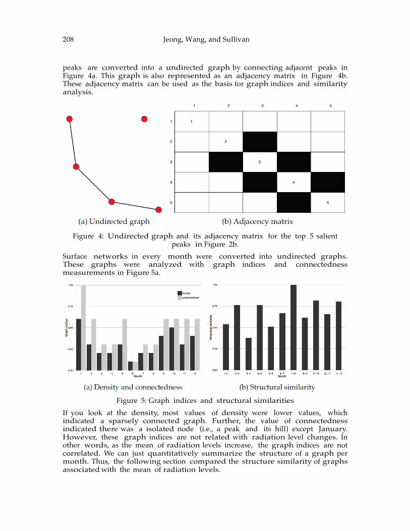
208 Jeong, Wang, and Sullivan peaks are converted into a undirected graph by connecting adjacent peaks in Figure 4a. This graph is also represented as an adjacency matrix in Figure 4b. These adjacency matrix can be used as the basis for graph indices and similarity analysis.
Figure 4: Undirected graph and its adjacency matrix for the top 5 salient
peaks in Figure 2b. Surface networks in every month were converted into undirected graphs. These graphs were analyzed with graph indices and connectedness measurements in Figure 5a.
Figure 5: Graph indices and structural similarities
If you look at the density, most values of density were lower values, which indicated a sparsely connected graph. Further, the value of connectedness indicated there was a isolated node (i.e., a peak and its hill) except January. However, these graph indices are not related with radiation level changes. In other words, as the mean of radiation levels increase, the graph indices are not correlated. We can just quantitatively summarize the structure of a graph per month. Thus, the following section compared the structure similarity of graphs associated with the mean of radiation levels.
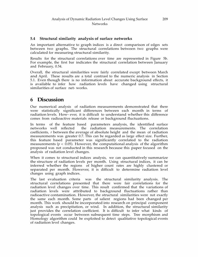
Analysis of Dynamic Radiation Level Changes Using Surface Networks
209
5.4 Structural similarity analysis of surface networks An important alternative to graph indices is a direct comparison of edges sets between two graphs. The structural correlations between two graphs were calculated for measuring structural similarity. Results for the structural correlations over time are represented in Figure 5b. For example, the first bar indicates the structural correlation between January and February, 0.54. Overall, the structural similarities were fairly correlated except between March and April. These results are a total contrast to the numeric analysis in Section 5.1. Even though there is no information about accurate background effects, it is available to infer how radiation levels have changed using structural similarities of surface net- works.
6 Discussion Our numerical analysis of radiation measurements demonstrated that there were statistically significant differences between each month in terms of radiation levels. How- ever, it is difficult to understand whether this difference comes from radioactive materials release or background fluctuations. In terms of the feature based parameters analysis, the identified surface networks well reflected the radiation measurements. The correlation coefficients, r between the average of absolute height and the mean of radiation measurements was greater 0.7. This can be regarded as large effect size. Further, this feature based parameter was significantly correlated to the radiation measurements (p < 0.05). However, the computational analysis of the algorithm proposed was not conducted in this research because this paper focused on the analysis of radiation level changes. When it comes to structural indices analysis, we can quantitatively summarize the structure of radiation levels per month. Using structural indices, it can be inferred whether the regions of higher count rates are highly clustered or separated per month. However, it is difficult to determine radiation level changes using graph indices. The last evaluation criteria was the structural similarity analysis. The structural correlations presented that there were fair correlations for the radiation level changes over time. This result confirmed that the variations of radiation levels were attributed to background fluctuations rather than radioactive contamination. However, the structural similarities were not exactly the same each month. Some parts of salient regions had been changed per month. This work should be incorporated into research on principal component analysis such as precipitation, or wind. In addition, the structural similarity just provides the correlation coefficient. It is difficult to infer what kinds of topological events occur between subsequent time steps. Tree morphism and Homology algorithm could be exploited to detect qualitative topological events of radiation level changes.
210 Jeong, Wang, and Sullivan
7 Conclusions This paper has demonstrated how radiation level changes can be identified using the structural similarities of surface networks. The structural similarities over time pro- vide fair correlations for the radiation level changes, even though the numerical analysis indicates there are statistically significant differences for radiation levels. The approach presented in this paper has taken a key step in addressing back- ground effects in radioactive engineering. This research is part of a larger project to detect the illicit movement of nuclear materials with big data. The structural analysis can be used efficiently to monitor illicit nuclear materials, irrespective of background fluctuations.
Acknowledgments This work was supported in part by the U.S. National Science Foundation (grant numbers: 0846655, 1047916, and 1443080) and the Defense Advanced Research Projects Agency (grant number: N66001-14-1-4043). The views, opinions, and findings contained in this article are those of the authors and should not be interpreted as representing the official views or policies, either expressed or implied, of the National Science Foundation, the Defense Advanced Research Projects Agency or the Department of Defense.
References [1] Safecast. http://blog.safecast.org. [Online; accessed 04-March-2015]. [2] BL O N D E L , V. D., GA J A R D O , A., HE Y M A N S , M., SE N E L L A RT, P., A N
D VA N DO O R E N , P. A measure of similarity between graph vertices: Applications to synonym extraction and web searching. SIAM review 46, 4 (2004), 647–666.
[3] BR E M E R , P., WE B E R , G., PA S C U C C I , V., DAY, M., A N D BE L L , J. Analyzing and tracking burning structures in lean premixed hydrogen flames. IEEE Transactions on Visualization and Computer Graphics 16, 2 (2010), 248–260.
[4] BU T T S , C., A N D CA R L E Y, K. Multivariate methods for interstructural analysis. Casos working paper, Carnegie Mellon University., 2001.
[5] BU T T S , C. T. Social network analysis with sna. Journal of Statistical Software 24, 6 (2008), 1–51.
[6] CAY L E Y, A. On contour and slope lines. Philosophical Magazine Series 4 18, 120 (1859), 264–268.
[7] CH A U D H RY, O. Z., A N D MA C K A N E S S , W. A. Creating mountains out of mole hills: Automatic identification of hills and ranges using morphometric analysis. Transactions in GIS 12, 5 (2008), 567–589.
[8] DA N O VA R O , E., DE FL O R I A N I , L., PA PA L E O , L., A N D VI TA L I , M. A multi- resolution representation for terrain morphology. In Geographic Information Science, M. Raubal, H. Miller, A. Frank, and M. Goodchild, Eds., vol. 4197 of Lecture Notes in Computer Science. Springer, Berlin Heidelberg, 2006, pp. 33–46.
Analysis of Dynamic Radiation Level Changes Using Surface Networks
211
[9] DE H M E R , M., ST R E I B , F. E., ME H L E R , A., KI L I A N , J., A N D MU H L H A U S E R , M. Application of a similarity measure for graphs to web-based document structures. In International Conference on Data Analysis ICA (2005).
[10] ED E L S B R U N N E R , H., HA R E R , J., A N D ZO M O R O D I A N , A. Hierarchical Morse Smale complexes for piecewise linear 2 manifolds. Discrete and Computational Geometry 30 (2003), 87–107.
[11] HAO, Q., BIANCHI, D., KAESTNER, M., AND REITHMEIER, E. Feature based characterization of worn surfaces for a sliding test. Tribology International 43, 5 (2010), 1186–1192.
[12] HU , Y., MI L L E R , H. J., A N D LI , X. Detecting and analyzing mobility hotspots using surface networks. Transactions in GIS 18, 6 (2014), 911–935.
[13] JE O N G , M.-H., DU C K H A M , M., MI L L E R , H., KE A LY, A., A N D PE I S K E R , A. De- centralized and coordinate-free computation of critical points and surface net- works in a discretized scalar field. International Journal of Geographical Information Science 28, 1 (2014), 1–21.
[14] KA Z I U S , J., NI J S S E N , S., KO K , J., BA C K , T., A N D IJ Z E R M A N , A. P. Substructure mining using elaborate chemical representation. Journal of Chemical Information and Modeling 46, 2 (2006), 597–605.
[15] KR I V O R U C H K O , K. Spatial statistical data analysis for GIS users. Esri Press Redlands, CA, USA, 2011.
[16] MAT S U M O TO , Y. An Introduction to Morse Theory, vol. 208. American Mathemati- cal Society, USA, 2002.
[17] MA X W E L L , J. C. On hills and dales. Philosophical Magazine Series 4 40 (1870), 421–427.
[18] ME R C I E R , J.-F., TR A C Y, B., D ’AM O U R S , R., CH A G N O N , F., HO FF M A N , I., KO R - PA C H , E., JO H N S O N , S., A N D UN G A R , R. Increased environmental gamma-ray dose rate during precipitation: A strong correlation with contributing air mass. Journal of environmental radioactivity 100, 7 (2009), 527–533.
[19] MI L N O R , J. Morse Theory. Princeton University Press, 1969. [20] MU R ATA , T., A N D MO R I YA S U , S. Link prediction of social networks based
on weighted proximity measures. In IEEE/WIC/ACM international conference on Web Intelligence (2007), IEEE, pp. 85–88.
[21] OK A B E , A., A N D MA S U YA M A , A. A method for measuring structural similarity among activity surfaces and its application to the analysis of urban population surfaces in japan. In Topological Data Structures for Surfaces : An Introduction for Geographical Information Science (2004), S. Rana, Ed., Willey, pp. 103–120.
[22] PA S U P U L E T I , P. Pig Design Patterns. Packt Publishing Ltd, 2014. [23] PE U C K E R , T. K., A N D DO U G L A S , D. H. Detection of surface-specific points
by local parallel processing of discrete terrain elevation data. Computer Graphics and image processing 4, 4 (1975), 375–387.
[24] PFA LT Z , J. L. Surface networks. Geographical Analysis 8, 1 (1976), 77–93.
212 Jeong, Wang, and Sullivan [25] RA N A , S. Topological Data Structures for Surfaces. John Wiley & Sons, Ltd.,
Chichester, UK, 2004. [26] SA M ATO VA , N. F., HE N D R I X , W., JE N K I N S , J., PA D M A N A B H A N , K., A N
D CH A K R A B O RT Y, A. Practical Graph Mining with R. CRC Press, 2013. [27] SC H N E I D E R , B., A N D WO O D , J. Construction of metric surface networks
from raster-based dems. In Topological Data Structures for Surfaces : An Introduction for Geographical Information Science, S. Rana, Ed. Willey, 2004, pp. 53–70.
[28] SH A R M A , H., AL E K S E Y C H U K , A., LE S K O V S K Y, P., HE L LW I C H , O., AN A N D , R., ZE R B E , N., A N D HU F N A G L , P. Determining similarity in histological images using graph-theoretic description and matching methods for content-based image retrieval in medical diagnostics. Diagn Pathol 7 (2012), 134.
[29] SU L L I VA N , C. J. Nuclear forensics driven by geographic information systems and big data analytics. In Proc. the Institute for Nuclear Materials Management on Infor- mation Analysis Technologies, Techniques and Methods for Safeguards, Nonproliferation and Arms Control Verification Workshop (2014), pp. 273–286.
[30] TA K A H A S H I , S., IK E D A , T., SH I N A G AWA , Y., KU N I I , T. L., A N D UE D A , M. Algo- rithms for extracting correct critical points and constructing topological graphs from discrete geographical elevation data. Computer Graphics Forum 14, 3 (1995), 181–192.
[31] TI A N , Y., WA N G , J., PE N G , Z., A N D JI A N G , X. A new approach to numerical characterisation of wear particle surfaces in three-dimensions for wear study. Wear 282 (2012), 59–68.
[32] WA L E , N., WAT S O N , I. A., A N D KA RY P I S , G. Comparison of descriptor spaces for chemical compound retrieval and classification. Knowledge and Information Systems 14, 3 (2008), 347–375.
[33] WO L F, G. W. Knowledge diffusion from giscience to other fields: The example of the usage of weighted surface networks in nanotechnology. International Journal of Geographical Information Science 28, 7 (2014), 1401–1424.
[34] WO O D , J. The geomorphological characterisation of digital elevation models. PhD the- sis, University of Leicester, 1996.
[35] WO O D , J. Modelling the continuity of surface form using digital elevation models. In Proc. 8th international Symposium on Spatial Data Handling (1998), IGU Commission of GIS New York, pp. 725–736.
ADVANCING GEOGRAPHIC INFORMATION SCIENCE: CHAPTER 15
© by the author(s) Licensed under Creative Commons Attribution 4.0 License
213
Spatial Scene Representation: A Survey and Categorization
Joshua A. Lewis School of Computing and Information Science, 5711 Boardman Hall, University of Maine,
Orono, ME 04469-5711, USA
Abstract: In modeling a geographic reality, one identifies the participating objects and captures the relations that exist between them. This process results in the creation of a spatial scene. Spatial scenes can take on many forms: the chosen embedding space has implications on which types of objects one represents and the set of possible relations between them. Further restricting the set of represented objects to suit a specific need provides additional focus; considering just points, lines, regions, or a combination of objects are some of the many possibilities. Furthermore, the types of relations captured are often the centerpiece of any qualitative depiction: does one care only about intersections, does sequence matter, or dimension? This survey seeks to categorize some of the ways in which a spatial scene can be captured, and provides a perspective where research can be seen in the wider context of choices one makes.
Keywords: Spatial reasoning, points, lines, regions, complex objects, holes, separations, spatial scenes.
1 Introduction There are many models for representing spatial scenes. A spatial scene is a collection of objects and their spatial arrangement [5, 32, 35, 37]. Models of spatial scene representation will be considered with respect to the embedding space, the objects represented, and the topological relations between those objects. While domain specific surveys illustrate a wide range of theories concerning qualitative topological representation [6, 11, 12, 27], this work aims to illustrate the process of constructing or selecting a topological model, touching on the implications of choices encountered along the way. In such a fashion the body of work represented herein can be seen within a larger context, spanning the last two decades of thought on such issues, beyond simply grouping research into singular categories. For instance, a model may work within a specific embedding space, or it might be modified by this choice. The objects modeled may vary, based on this decision, or
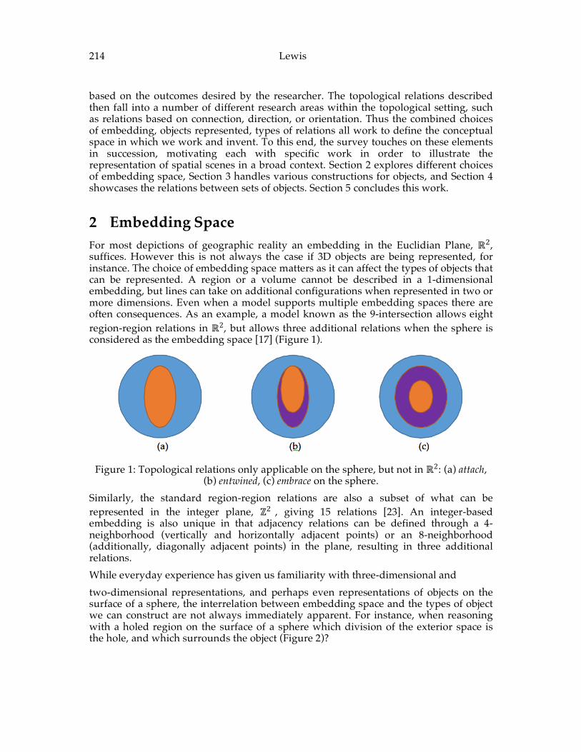
214 Lewis
based on the outcomes desired by the researcher. The topological relations described then fall into a number of different research areas within the topological setting, such as relations based on connection, direction, or orientation. Thus the combined choices of embedding, objects represented, types of relations all work to define the conceptual space in which we work and invent. To this end, the survey touches on these elements in succession, motivating each with specific work in order to illustrate the representation of spatial scenes in a broad context. Section 2 explores different choices of embedding space, Section 3 handles various constructions for objects, and Section 4 showcases the relations between sets of objects. Section 5 concludes this work.
2 Embedding Space For most depictions of geographic reality an embedding in the Euclidian Plane, ℝ2, suffices. However this is not always the case if 3D objects are being represented, for instance. The choice of embedding space matters as it can affect the types of objects that can be represented. A region or a volume cannot be described in a 1-dimensional embedding, but lines can take on additional configurations when represented in two or more dimensions. Even when a model supports multiple embedding spaces there are often consequences. As an example, a model known as the 9-intersection allows eight region-region relations in ℝ2, but allows three additional relations when the sphere is considered as the embedding space [17] (Figure 1).
Figure 1: Topological relations only applicable on the sphere, but not in ℝ2: (a) attach,
(b) entwined, (c) embrace on the sphere. Similarly, the standard region-region relations are also a subset of what can be represented in the integer plane, ℤ2 , giving 15 relations [23]. An integer-based embedding is also unique in that adjacency relations can be defined through a 4- neighborhood (vertically and horizontally adjacent points) or an 8-neighborhood (additionally, diagonally adjacent points) in the plane, resulting in three additional relations. While everyday experience has given us familiarity with three-dimensional and two-dimensional representations, and perhaps even representations of objects on the surface of a sphere, the interrelation between embedding space and the types of object we can construct are not always immediately apparent. For instance, when reasoning with a holed region on the surface of a sphere which division of the exterior space is the hole, and which surrounds the object (Figure 2)?
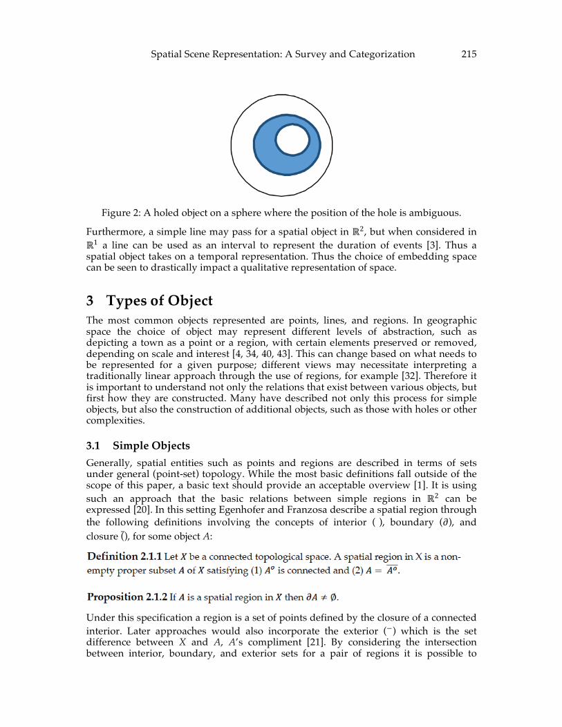
Spatial Scene Representation: A Survey and Categorization 215
Figure 2: A holed object on a sphere where the position of the hole is ambiguous.
Furthermore, a simple line may pass for a spatial object in ℝ2, but when considered in ℝ1 a line can be used as an interval to represent the duration of events [3]. Thus a spatial object takes on a temporal representation. Thus the choice of embedding space can be seen to drastically impact a qualitative representation of space.
3 Types of Object The most common objects represented are points, lines, and regions. In geographic space the choice of object may represent different levels of abstraction, such as depicting a town as a point or a region, with certain elements preserved or removed, depending on scale and interest [4, 34, 40, 43]. This can change based on what needs to be represented for a given purpose; different views may necessitate interpreting a traditionally linear approach through the use of regions, for example [32]. Therefore it is important to understand not only the relations that exist between various objects, but first how they are constructed. Many have described not only this process for simple objects, but also the construction of additional objects, such as those with holes or other complexities.
3.1 Simple Objects Generally, spatial entities such as points and regions are described in terms of sets under general (point-set) topology. While the most basic definitions fall outside of the scope of this paper, a basic text should provide an acceptable overview [1]. It is using such an approach that the basic relations between simple regions in ℝ2 can be expressed [20]. In this setting Egenhofer and Franzosa describe a spatial region through the following definitions involving the concepts of interior ( ), boundary (𝜕), and closure (), for some object A:
Under this specification a region is a set of points defined by the closure of a connected interior. Later approaches would also incorporate the exterior (−) which is the set difference between X and A, A’s compliment [21]. By considering the intersection between interior, boundary, and exterior sets for a pair of regions it is possible to
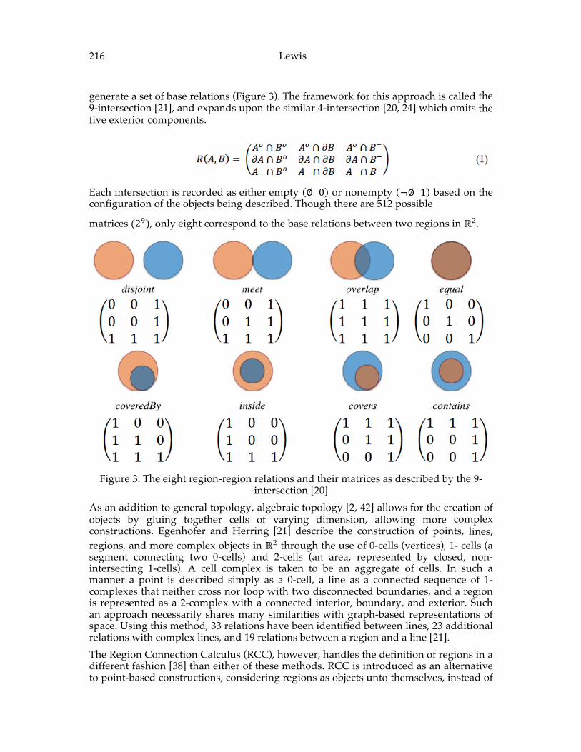
216 Lewis
generate a set of base relations (Figure 3). The framework for this approach is called the 9-intersection [21], and expands upon the similar 4-intersection [20, 24] which omits the five exterior components.
Each intersection is recorded as either empty (∅ 0) or nonempty (¬∅ 1) based on the configuration of the objects being described. Though there are 512 possible
matrices (29 ), only eight correspond to the base relations between two regions in ℝ2.
Figure 3: The eight region-region relations and their matrices as described by the 9-
intersection [20] As an addition to general topology, algebraic topology [2, 42] allows for the creation of objects by gluing together cells of varying dimension, allowing more complex constructions. Egenhofer and Herring [21] describe the construction of points, lines, regions, and more complex objects in ℝ2 through the use of 0-cells (vertices), 1- cells (a segment connecting two 0-cells) and 2-cells (an area, represented by closed, non-intersecting 1-cells). A cell complex is taken to be an aggregate of cells. In such a manner a point is described simply as a 0-cell, a line as a connected sequence of 1- complexes that neither cross nor loop with two disconnected boundaries, and a region is represented as a 2-complex with a connected interior, boundary, and exterior. Such an approach necessarily shares many similarities with graph-based representations of space. Using this method, 33 relations have been identified between lines, 23 additional relations with complex lines, and 19 relations between a region and a line [21]. The Region Connection Calculus (RCC), however, handles the definition of regions in a different fashion [38] than either of these methods. RCC is introduced as an alternative to point-based constructions, considering regions as objects unto themselves, instead of
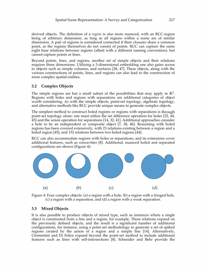
Spatial Scene Representation: A Survey and Categorization 217
derived objects. The definition of a region is also more nuanced, with an RCC-region being of arbitrary dimension, as long as all regions within a scene are of similar dimension. A pair of regions is considered connected if their closures share a common point, as the regions themselves do not consist of points. RCC can capture the same eight base relations between regions (albeit with a different naming convention), but cannot capture points or lines. Beyond points, lines, and regions, another set of simple objects and their relations requires three dimensions. Utilizing a 3-dimensional embedding one also gains access to objects such as simple volumes, and surfaces [28, 47]. These objects, along with the various constructions of points, lines, and regions can also lead to the construction of more complex spatial entities.
3.2 Complex Objects
The simple regions are but a small subset of the possibilities that may apply in ℝ2. Regions with holes and regions with separations are additional categories of object worth considering. As with the simple objects, point-set topology, algebraic topology, and alternative methods like RCC provide unique means to generate complex objects. The simplest method to construct holed regions or regions with separations is through point-set topology alone: one must utilize the set difference operation for holes [32, 44, 45] and the union operation for separations [14, 32, 41]. Additional approaches consider a hole to be an independent or composite object [7, 38, 46]. Reasoning with holed regions has been covered extensively, with 23 relations existing between a region and a holed region [45], and 152 relations between two holed regions [44]. RCC can also accommodate regions with holes or separations, and its extensions cover additional features, such as concavities [8]. Additional, nuanced holed and separated configurations are shown (Figure 4):
Figure 4: Four complex objects: (a) a region with a hole, (b) a region with a fringed hole,
(c) a region with a separation, and (d) a region with a weak separation.
3.3 Mixed Objects It is also possible to produce objects of mixed type, such as instances where a single object is constructed from a line and a region, for example. These relations expand on the previously defined objects, and the result is a significant number of additional configurations, for instance, using a point-set methodology to generate a set of spiked regions created by the union of a region and a simple line [14]. Alternatively, Clementini and Di Felice expand beyond the point-set method to include additional features such as lines with self-intersections [8]. Schneider and Behr provide the
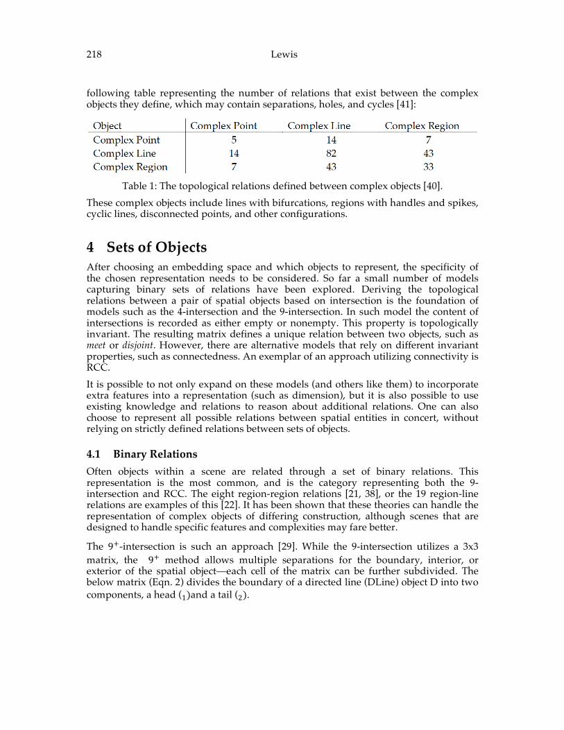
218 Lewis
following table representing the number of relations that exist between the complex objects they define, which may contain separations, holes, and cycles [41]:
Table 1: The topological relations defined between complex objects [40].
These complex objects include lines with bifurcations, regions with handles and spikes, cyclic lines, disconnected points, and other configurations.
4 Sets of Objects After choosing an embedding space and which objects to represent, the specificity of the chosen representation needs to be considered. So far a small number of models capturing binary sets of relations have been explored. Deriving the topological relations between a pair of spatial objects based on intersection is the foundation of models such as the 4-intersection and the 9-intersection. In such model the content of intersections is recorded as either empty or nonempty. This property is topologically invariant. The resulting matrix defines a unique relation between two objects, such as meet or disjoint. However, there are alternative models that rely on different invariant properties, such as connectedness. An exemplar of an approach utilizing connectivity is RCC. It is possible to not only expand on these models (and others like them) to incorporate extra features into a representation (such as dimension), but it is also possible to use existing knowledge and relations to reason about additional relations. One can also choose to represent all possible relations between spatial entities in concert, without relying on strictly defined relations between sets of objects.
4.1 Binary Relations Often objects within a scene are related through a set of binary relations. This representation is the most common, and is the category representing both the 9- intersection and RCC. The eight region-region relations [21, 38], or the 19 region-line relations are examples of this [22]. It has been shown that these theories can handle the representation of complex objects of differing construction, although scenes that are designed to handle specific features and complexities may fare better.
The 9+-intersection is such an approach [29]. While the 9-intersection utilizes a 3x3 matrix, the 9+ method allows multiple separations for the boundary, interior, or exterior of the spatial object—each cell of the matrix can be further subdivided. The below matrix (Eqn. 2) divides the boundary of a directed line (DLine) object D into two components, a head (1 )and a tail (2 ).
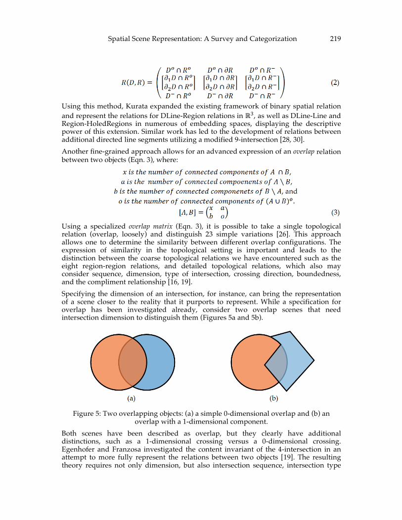
Spatial Scene Representation: A Survey and Categorization 219
Using this method, Kurata expanded the existing framework of binary spatial relation and represent the relations for DLine-Region relations in ℝ3, as well as DLine-Line and Region-HoledRegions in numerous of embedding spaces, displaying the descriptive power of this extension. Similar work has led to the development of relations between additional directed line segments utilizing a modified 9-intersection [28, 30]. Another fine-grained approach allows for an advanced expression of an overlap relation between two objects (Eqn. 3), where:
Using a specialized overlap matrix (Eqn. 3), it is possible to take a single topological relation (overlap, loosely) and distinguish 23 simple variations [26]. This approach allows one to determine the similarity between different overlap configurations. The expression of similarity in the topological setting is important and leads to the distinction between the coarse topological relations we have encountered such as the eight region-region relations, and detailed topological relations, which also may consider sequence, dimension, type of intersection, crossing direction, boundedness, and the compliment relationship [16, 19]. Specifying the dimension of an intersection, for instance, can bring the representation of a scene closer to the reality that it purports to represent. While a specification for overlap has been investigated already, consider two overlap scenes that need intersection dimension to distinguish them (Figures 5a and 5b).
Figure 5: Two overlapping objects: (a) a simple 0-dimensional overlap and (b) an
overlap with a 1-dimensional component. Both scenes have been described as overlap, but they clearly have additional distinctions, such as a 1-dimensional crossing versus a 0-dimensional crossing. Egenhofer and Franzosa investigated the content invariant of the 4-intersection in an attempt to more fully represent the relations between two objects [19]. The resulting theory requires not only dimension, but also intersection sequence, intersection type
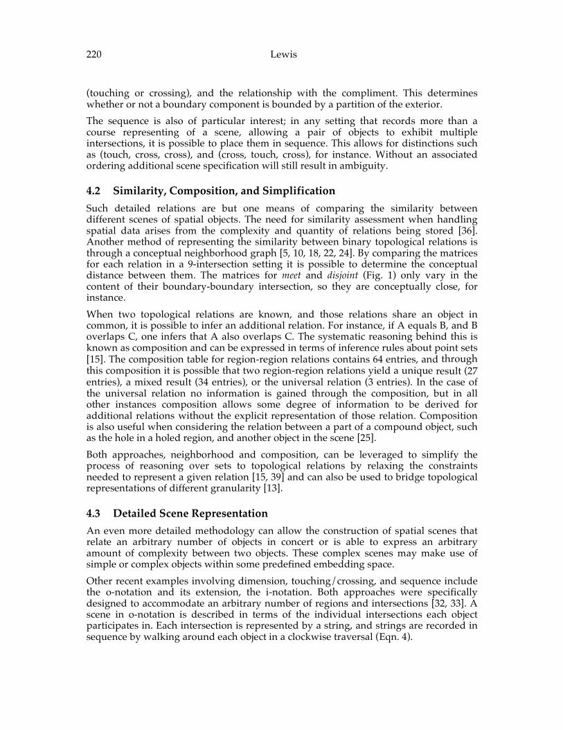
220 Lewis
(touching or crossing), and the relationship with the compliment. This determines whether or not a boundary component is bounded by a partition of the exterior. The sequence is also of particular interest; in any setting that records more than a course representing of a scene, allowing a pair of objects to exhibit multiple intersections, it is possible to place them in sequence. This allows for distinctions such as (touch, cross, cross), and (cross, touch, cross), for instance. Without an associated ordering additional scene specification will still result in ambiguity.
4.2 Similarity, Composition, and Simplification Such detailed relations are but one means of comparing the similarity between different scenes of spatial objects. The need for similarity assessment when handling spatial data arises from the complexity and quantity of relations being stored [36]. Another method of representing the similarity between binary topological relations is through a conceptual neighborhood graph [5, 10, 18, 22, 24]. By comparing the matrices for each relation in a 9-intersection setting it is possible to determine the conceptual distance between them. The matrices for meet and disjoint (Fig. 1) only vary in the content of their boundary-boundary intersection, so they are conceptually close, for instance. When two topological relations are known, and those relations share an object in common, it is possible to infer an additional relation. For instance, if A equals B, and B overlaps C, one infers that A also overlaps C. The systematic reasoning behind this is known as composition and can be expressed in terms of inference rules about point sets [15]. The composition table for region-region relations contains 64 entries, and through this composition it is possible that two region-region relations yield a unique result (27 entries), a mixed result (34 entries), or the universal relation (3 entries). In the case of the universal relation no information is gained through the composition, but in all other instances composition allows some degree of information to be derived for additional relations without the explicit representation of those relation. Composition is also useful when considering the relation between a part of a compound object, such as the hole in a holed region, and another object in the scene [25]. Both approaches, neighborhood and composition, can be leveraged to simplify the process of reasoning over sets to topological relations by relaxing the constraints needed to represent a given relation [15, 39] and can also be used to bridge topological representations of different granularity [13].
4.3 Detailed Scene Representation An even more detailed methodology can allow the construction of spatial scenes that relate an arbitrary number of objects in concert or is able to express an arbitrary amount of complexity between two objects. These complex scenes may make use of simple or complex objects within some predefined embedding space. Other recent examples involving dimension, touching/crossing, and sequence include the o-notation and its extension, the i-notation. Both approaches were specifically designed to accommodate an arbitrary number of regions and intersections [32, 33]. A scene in o-notation is described in terms of the individual intersections each object participates in. Each intersection is represented by a string, and strings are recorded in sequence by walking around each object in a clockwise traversal (Eqn. 4).
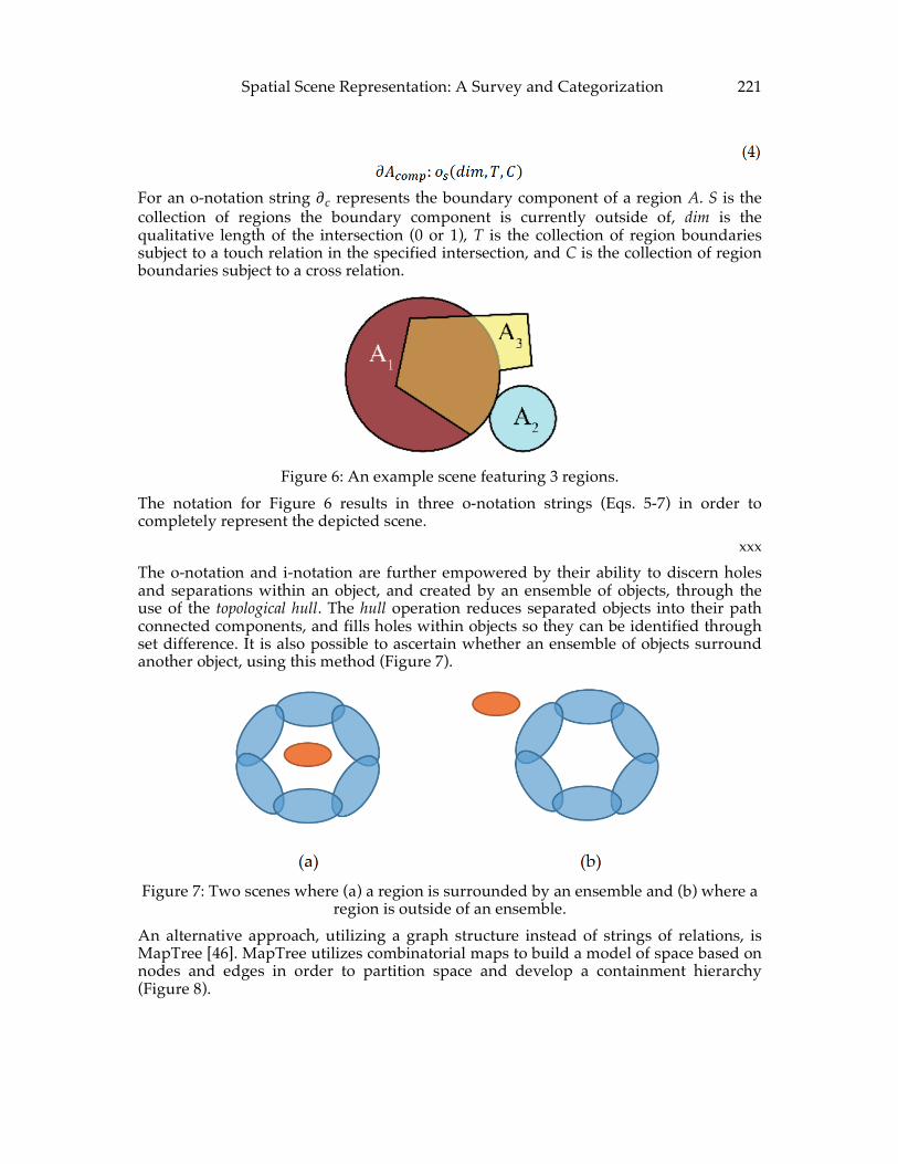
Spatial Scene Representation: A Survey and Categorization 221
For an o-notation string 𝜕𝑐 represents the boundary component of a region A. S is the collection of regions the boundary component is currently outside of, dim is the qualitative length of the intersection (0 or 1), T is the collection of region boundaries subject to a touch relation in the specified intersection, and C is the collection of region boundaries subject to a cross relation.
Figure 6: An example scene featuring 3 regions.
The notation for Figure 6 results in three o-notation strings (Eqs. 5-7) in order to completely represent the depicted scene.
xxx
The o-notation and i-notation are further empowered by their ability to discern holes and separations within an object, and created by an ensemble of objects, through the use of the topological hull. The hull operation reduces separated objects into their path connected components, and fills holes within objects so they can be identified through set difference. It is also possible to ascertain whether an ensemble of objects surround another object, using this method (Figure 7).
Figure 7: Two scenes where (a) a region is surrounded by an ensemble and (b) where a
region is outside of an ensemble. An alternative approach, utilizing a graph structure instead of strings of relations, is MapTree [46]. MapTree utilizes combinatorial maps to build a model of space based on nodes and edges in order to partition space and develop a containment hierarchy (Figure 8).
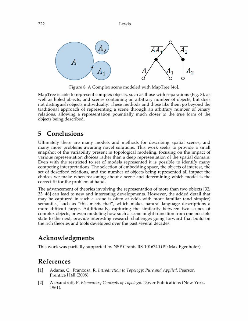
222 Lewis
Figure 8: A Complex scene modeled with MapTree [46].
MapTree is able to represent complex objects, such as those with separations (Fig. 8), as well as holed objects, and scenes containing an arbitrary number of objects, but does not distinguish objects individually. These methods and those like them go beyond the traditional approach of representing a scene through an arbitrary number of binary relations, allowing a representation potentially much closer to the true form of the objects being described.
5 Conclusions Ultimately there are many models and methods for describing spatial scenes, and many more problems awaiting novel solutions. This work seeks to provide a small snapshot of the variability present in topological modeling, focusing on the impact of various representation choices rather than a deep representation of the spatial domain. Even with the restricted to set of models represented it is possible to identify many competing interpretations. The selection of embedding space, the objects of interest, the set of described relations, and the number of objects being represented all impact the choices we make when reasoning about a scene and determining which model is the correct fit for the problem at hand. The advancement of theories involving the representation of more than two objects [32, 33, 46] can lead to new and interesting developments. However, the added detail that may be captured in such a scene is often at odds with more familiar (and simpler) semantics, such as “this meets that”, which makes natural language descriptions a more difficult target. Additionally, capturing the similarity between two scenes of complex objects, or even modeling how such a scene might transition from one possible state to the next, provide interesting research challenges going forward that build on the rich theories and tools developed over the past several decades.
Acknowledgments This work was partially supported by NSF Grants IIS-1016740 (PI: Max Egenhofer).
References [1] Adams, C., Franzosa, R. Introduction to Topology: Pure and Applied. Pearson
Prentice Hall (2008). [2] Alexandroff, P. Elementary Concepts of Topology. Dover Publications (New York,
1961).
Spatial Scene Representation: A Survey and Categorization 223
[3] Allen, J. F. Maintaining Knowledge about Temporal Intervals. Communications of the ACM, 26(11), (1983), 832-843.
[4] Barkowsky, T., Latecki, L., Richter, K. Schematizing Maps: Simplification of Geographic Shape by Discrete Curve Evolution. In: Freksa, C., Brauer, W., Habel, C., Wender, K. (eds.) Spatial Cognition II, (2000), 41–53.
[5] Bruns, T. and Egenhofer, M. Similarity of Spatial Scenes. Seventh International Symposium on Spatial Data Handling. Delft, The Netherlands (1996) pp. 31-42.
[6] Chen, J., Cohn, A. G., Liu, D., Wang, S., Ouyang, J., and Yu, Q. A Survey of Qualitative Spatial Representations. The Knowledge Engineering Review, 30, (2015), pp. 106-136.
[7] Clementini, E., Di Felice, P., and Califano, G. Composite Regions in Topological Queries. Information Systems 20(7), (1995), 579-594.
[8] Clementini, E. and Di Felice, P. A Model for Representing Topological Relationships Between Complex Geometric Features in Spatial Databases. Information Sciences 90(1-4), 121-136 (1996)
[9] Cohn, A. G. A Hierarchical Representation of Qualitative Shape Based on Connection and Convexity. In Spatial Information Theory A Theoretical Basis for GIS, Springer Berlin Heidelberg. (1995) pp. 311-326.
[10] Cohn, A., Bennett, B., Gooday, J., Gotts, N. Qualitative Spatial Representation and Reasoning with the Region Connection Calculus. GeoInformatica 1(3), (1997) 275-316.
[11] Cohn, A., Hazarika, S.: Qualitative Spatial Representation and Reasoning: An Overview. Fundamenta Informaticae 46(1-2), (2001) 2-32.
[12] Cohn, A., Renz, J.: Qualitative Spatial Representation and Reasoning. In: van Hermelen, F., Lifschitz, V., Porter, B. (Eds.) Handbook of Knowledge Representation, pp. 551-596 (2008)
[13] Dube, M. P., and Egenhofer, M. J. Establishing similarity across multi-granular topological–relation ontologies. In Quality of Context, Springer Berlin Heidelberg,(2009) pp. 98-108).
[14] Egenhofer, M. A Reference System for Topological Relations between Compound Spatial Objects. In: Heuser, C., Pernul, G. (Eds.) Advances in Conceptual Modeling—Challenging Perspectives, ER 2009 Workshops, Lecture Notes in Computer Science Vol. 5833, (2009) pp. 307-316.
[15] Egenhofer, M. J. Deriving the Composition of Binary Topological Relations. Journal of Visual Languages and Computing, 5(2), (1994) 133-149.
[16] Egenhofer, M. J. Query Processing in Spatial-Query-by-Sketch. Journal of Visual Languages and Computing, 8(4), (1997) 403-424.
[17] Egenhofer, M. J. Spherical Topological Relations. Journal on Data Semantics III, (2005) pp. 25-49.
[18] Egenhofer, M. J., and Al-Taha, K. K. Reasoning about Gradual Changes of Topological Relationships. In Theories and methods of spatio-temporal reasoning in geographic space, Springer Berlin Heidelberg. (1992) pp. 196-219.
224 Lewis
[19] Egenhofer, M. J. and Franzosa, R. D. On the Equivalence of Topological Relations. International Journal of Geographical Information Systems 9(2), (1995) 133–152.
[20] Egenhofer, M., Franzosa, R.: Point-Set Topological Spatial Relations. International Journal of Geographical Information Systems 5(2), (1991) 161-174.
[21] Egenhofer, M. J. and Herring, J. Categorizing Binary Topological Relationships between Regions, Lines and Points in Geographic Database. Technical report, University of Maine (1991).
[22] Egenhofer, M. J., and Mark, D. M. Modelling Conceptual Neighbourhoods of Topological Line-Region Relations. International journal of geographical information systems, 9(5), (1995) 555-565.
[23] Egenhofer, M. J. and Sharma, J. Topological Relations Between Regions in R2 and Z2. In Proceedings of the Advances in Spatial Databases, Third International Symposium, SSD’93, Singapore, June 23–25. Lecture Notes in Computer Science 692, Springer (1993) 316–336.
[24] Egenhofer, M. J., Sharma, J., and Mark, D. M. A critical Comparison of the 4- intersection and 9-intersection Models for Spatial Relations: Formal Analysis. In AUTOCARTO). McMaster R. and Amrstrong M. (eds.), Minneapolis, MN, (1993) pp. 1-11.
[25] Egenhofer, M. J. and Vasardani, M. Spatial Reasoning with a Hole. In Proceedings of the Spatial Information Theory, 8th International Conference, COSIT 2007, Melbourne, Australia, September 19–23. Lecture Notes in Computer Science 4736, Springer, (2007) pp.303–320.
[26] Galton, A. Modes of Overlap. Journal of Visual Languages and Computing 9(1), (1998) pp.61-79.
[27] Galton, A. Spatial and Temporal Knowledge Representation. Earth Science Informatics 2(3), (2009) 169-187.
[28] Kurata, Y. From three-dimensional topological relations to contact relations. In Developments in 3D Geo-Information Sciences. Springer Berlin Heidelberg (2010) pp. 123-142.
[29] Kurata, Y.: The 9+-Intersection: A Universal Framework for Modeling Topological Relations. In: Cova, T., Miller, H., Beard, K., Frank, A., Goodchild, M. (eds.) Geographic Information Science. Park City, UT, LNCS 5266, Springer (2008) 181-198.
[30] Kurata, Y., Egenhofer, M.: The Arrow Semantic Interpreter. Spatial Cognition and Computing 8, 4, (2008) 306–332.
[31] Kurata, Y., Egenhofer, M.: The Head-Body-Tail Intersection for Spatial Relations Between Directed Line Segments. In: Raubal, M., Miller, H., Frank, A., Goodchild, M. (eds.) Geographic Information Science, Münster, Germany, LNCS 4197, (2006) 269–286.
[32] Lewis, J., Dube, M., Egenhofer, M. The Topology of Spatial Scenes in R2. In: Tenbrink, T., Stell, J., Galton, A., Wood, Z. (eds.) Spatial Information Theory COSIT ’13, Scarborough, UK, LNCS 8116, (2013) 495-515.
Spatial Scene Representation: A Survey and Categorization 225
[33] Lewis, J. A., and Egenhofer, M. J. Oriented regions for linearly conceptualized features. In Geographic Information Science, Springer Berlin Heidelberg (2014) pp. 333-348.
[34] Morehouse, S.: GIS-Based Map Compilation and Generalization. In: Müller, J. C., Lagrange, J., Weibel, R. (eds.) GIS and Generalization: Methodology and Practice. Taylor&Francis, Bristol, PA (1995) pp. 21–30.
[35] Nedas, K. A., Egenhofer, M. J. Spatial‐Scene Similarity Queries.Transactions in GIS, 12(6), (2008) 661-681.
[36] Nedas, K. A., Egenhofer, M. J.. Spatial similarity queries with logical operators. In Advances in Spatial and Temporal Databases, Springer Berlin Heidelberg (2003) pp.430-448.
[37] Papadimitriou, C. H., Suciu, D., Vianu, V. Topological Queries in Spatial Databases. In Proceedings of the fifteenth ACM SIGACT-SIGMOD-SIGART symposium on Principles of database systems, ACM (1996) pp. 81-92.
[38] Randell, D., Cui, Z., Cohn, A.: A Spatial Logic Based on Regions and Connection. In: Third International Conference on Knowledge Representation and Reasoning, (1992) pp. 165-176.
[39] Rodríguez, M. A., Egenhofer, M. J., Blaser, A. D. Query Pre-Processing of Topological Constraints: Comparing a Composition-Based with Neighborhood- Based Approach. In Advances in Spatial and Temporal Databases, Springer Berlin Heidelberg (2003) pp. 362-379.
[40] Ruas, A., Lagrange, J.: Data and Knowledge Modelling for Generalization. In: Müller, J., Lagrange, J., Weibel, R. (eds.) GIS and Generalization: Methodology and Practice. Taylor&Francis, Bristol, PA, (1995) pp. 73–90.
[41] Schneider, M., Behr, T. Topological Relationships between Complex Spatial Objects. ACM Transactions on Database Systems 31(1), (2006) 39-81.
[42] Spanier, E. Algebraic Topology (McGraw-Hill Book Company, New York, 1966). [43] Timpf, S., Volta, G., Pollock D., Egenhofer, M. A Conceptual Model of
Wayfinding Using Multiple Levels of Abstraction. In: Frank A., Campari, I., Formentini, U. (eds.) Theories and Methods of Spatio-Temporal Reasoning in Geographic Space, Pisa, Italy, LNCS 639, (1992) 348–367.
[44] Vasardani, M. Egenhofer, M. J. Comparing Relations with a Multi-Holed Region. In Proceedings of the Spatial Information Theory, 9th International Conference, COSIT 2009, Aber Wrac’h, France, September 21–25. Lecture Notes in Computer Science 5756, Springer (2009) 159–176.
[45] Vasardani, M. Egenhofer, M. J. Single-Holed Regions: Their Relations and Inferences. In Proceedings of the Geographic Information Science, 5th International Conference, GIScience 2008, Park City, UT, USA, September 23–26. Lecture Notes in Computer Science 5266, Springer (2008) 337–353.
[46] Worboys, M. The Maptree: A Fine-Grained Formal Representation of Space. In: Xiao, N., Kwan, M., Goodchild, M., Shekhar, S. (eds.) Geographic Information Science. Columbus, OH, LNCS 7478, (2012) pp. 298-310
[47] Zlatanova, S. On 3D topological relationships. In Database and Expert Systems Applications, IEEE (2000), pp. 913-919.

226 Lewis
ADVANCING GEOGRAPHIC INFORMATION SCIENCE: CHAPTER 16
© by the author(s) Licensed under Creative Commons Attribution 4.0 License
227
Linked Landmark Data: Toward the Automatic Detection of Landmarks
on the Web of Data Teriitutea Quesnot
Center for Research in Geomatics, Laval University, 1055 Avenue du Se minaire, Pavillon Louis-Jacques Casault, Quebec City, QC G1V 0A6, Canada
Abstract: Providing relevant landmark-based route instructions remains a crucial challenge in the field of spatial cognitive engineering. Firsts automatic landmark detection systems emerged in the early 2000’s and usually relied on a heavy desktop architecture. Landmarks were usually detected through a Geographic Information System connected to a database that contained some points of interest (POIs) potentially useful for navigation. This approach is not suitable for a web deployment, let alone a cloud computing one. The advent of Web 2.0 and Volunteered Geographic Information allowed researchers to move beyond the boundary of POIs. Indeed, place-based information shared by social web users are richer than POI databases and now easily accessible through APIs. However, it is important to keep in mind that the landmark- ness is a relative characteristic per se. Its measure primarily depends on the configuration of the environment, the surrounding objects, and the context of navigation. Yet, fixing those issues by relying on data stored into isolated databases remains quite complex. In this way, I explain here the main reasons why I am convinced that the slow-growing sphere of linked data is worth to be explored to overcome this gap.
Keywords: Landmarks, linked data, open data, RDF, wayfinding, web of data.
1 Introduction The use of location-based services (LBS) became commonplace in everyday life. Among these services, navigational aid systems are constantly accessed by mobile device users. For instance, the Google Maps application siphoned off 54% of world smartphone users in 2013 (against 44% for Facebook) [1]. This growing consumption and produc- tion of spatial data is an opportunity now taken to understand urban dynamics and improve the management of the next generation of cities; commonly named Smart Cities. Specifically, the smart
228 Quesnot mobility, which is one of the main intrinsic characteristics of a smart city, is defined by the three following aspects: the accessibility of urban places and services, the presence of sustainable transport systems, and the availability of relevant (spatial) information for communication systems [2]. In this context, mobility is not only a matter of transportation. Helping people to better read the environment to quickly reach a destination is a major concern. To address this need, navigational aid systems should ideally be compatible with human spatial communication and reasoning. In order to match as accurately as possible with users’ ”mental maps”, these LBS have to include landmarks inside traditional street name-based instructions. Indeed, research that investigated the role of landmarks found that their inclusion inside route instructions helps people to better memorize itineraries and orient themselves[3]. Those findings date from the early 2000’s but one can notice that current web map- ping services (e.g. Google Maps) do not provide such information in their verbal instructions. Actually, designing a system that automatically identify relevant land- marks (ALDS) is harder than it looks. I attempt to support this statement in the fol- lowing section through a brief state of art around the concept of landmark. In addition, landmarks are necessarily extracted from data. To my knowledge, all the solutions pro- posed for the automatic detection of landmarks rely on the exploitation of data that come from isolated databases. This approach implies several limits that I summarize in the third section. Since the measure of the landmarkness needs to establish links be- tween data, I do argue that research in the area of ALDS should address the potential of linked data. I notably propose a first approach for identifying landmarks through the web of data in the final section.
2 Landmarks Within the Field of GIScience
2.1 A Brief History of Landmarks In his work on the imageability of the city in the early sixties, Lynch clearly formalized the concept of landmark [4]. According to him, a landmark is a feature that is sufficiently prominent to be memorized by individuals and recalled when necessary. Specifically, it is a visual marker that gives global orientation information to travelers. In 1975, Siegel and White proposed a theory of the acquisition of human spatial knowledge called Landmark-Route-Survey [5]. Their sequential theory suggests that landmarks constitute the base of human spatial knowledge. In this manner, they appear before the route and survey knowledge in the spatial learning process. In the same vein, Golledge proposed his theory of anchor points. He suggests that landmarks, which are included within each individual’s cognitive map, are hierarchically structured according to three levels [6]. The first one embraces primary land- marks, which are highly familiar places such as homes and workplaces. The second level includes often visited venues such as marketplaces, whereas the third one gathers rarely practiced places (e.g. a venue visited during vacations) together. Research conducted between the 80’s and 90’s focused on the concept of points of reference and the assessment of cognitive distances. In the late 90’s, Lovelace et al. categorized land- marks according to their locations [7]. More precisely, the authors proposed four types of
Linked Landmark Data: Toward the Automatic Detection of Landmarks on the Web of Data
229
landmarks: (i) on-route points, which unlike (ii) off-route points, are used by travelers to ensure the route control, (iii) choice points, which unlike (iv) potential choice points, are located around an intersection where a turn is scheduled in the itinerary. Finally, Sorrows and Hirtle proposed a single typology of landmarks based on three distinct categories [8]. According to them, the characteristics of a landmark are essentially visual, structural, and cognitive. More precisely, visual landmarks are similar to Lynch’s landmarks. They are visually remarkable and highly visible from a long distance. Structural landmarks are associated with advantageous positions such as the intersection of major streets. Finally, cognitive landmarks (also described as semantic landmarks) are outstanding because of their historical and cultural significance or their atypical function (e.g. a monument surrounded by offices). They also are highly meaningful for the traveler (i.e. subjective landmarks). Raubal and Winter adapted Sorrows and Hirtle’s landmark typology when they formalized their first formal model of landmark saliencies applied to the facades of buildings [9].
2.2 Major Findings Around Landmark Saliencies The measure of visual salience is crucial since our attention is instinctively grabbed by objects visually prominent. Actually, travelers tend to unintentionally pick-up and store distinctive useful objects while traveling [10]. An important thing to keep in mind is that visual salience remains a relative property. For instance, a red house - which is a color known to grab attention - surrounded by other red houses will obviously not stand out from the scene. However, the main ”advantage” of such salience is that the factors that contribute to its significance are quite similar from one observer to another [11]. Therefore, the computation of the visual salience can be easily done by relying on specific attributes such as the color of the object, its area and height, and its proximity to road (cf. [9, 12, 13, 14]). In addition, Winter introduced the notion of advance visibility by assuming that buildings highly visible from a long distance tend to grab travelers’ attention [15]. The author proposed to combine the visibility coverage of the buildings and their orientation compared to the road. Research around structural salience aimed at locating the ideal position of the land- mark when a turn is required. Researchers clearly focused on landmark candidates located at decision points (i.e. Lovelace et al.’s choice points) since references to landmarks in people’s route instructions are quite higher from those areas [7]. Specifically, Klippel and Winter significantly enriched Raubal and Winter’s model [16]. According to them, venues located before the intersection and along the same direction as the turn are ideal structural landmarks. Those assumptions have already been empirically sup- ported [17, 14]. Recently, Quesnot and Roche additionally found that the side where travelers move compared to the road also influences the landmark selection process. Indeed, the travelers’ field of view varies according to this parameter and obviously interferes in the selection of landmarks while moving along the road. The example of the red houses single-handedly summarizes the concept of cognitive landmarks. Indeed, a red house surrounded by other houses of the same color will not really grab the observer ’s attention, unless he is familiar with this particular house. In this way, unlike visual and structural saliencies,
230 Quesnot semantic salience is based on subjective features often recognized by a small group of people or even one per- son. Measuring this salience is therefore more complex than the two other saliencies. Consequently, this measure has been limited for a while to specific indicators, i.e. the historical and cultural significance of a place (e.g. [9]), its function (e.g. [12]), its name brevity, and its ubiquity and familiarity (e.g. [13]). With the advent of Volunteered Geo- graphic Information (VGI) [18], researchers extended the notion of cognitive salience by adding the social aspect (cf. [19]). Cognitive landmarks remained a theory-based suggestion until recently. Their usefulness is now empirically supported (cf. [20, 14]).
2.3 Automatic Landmark Detection Systems GIScientists relied on the conceptual framework previously explained to design systems that automatically detect landmarks (ALDS). They notably used Raubal and Winter ’s formal model of landmarkness to reach this goal ([9]). Concretely, ALDS are usually based on a route knowledge approach. They provide to travelers relevant landmarks along an itinerary, especially at each decision point (i.e. where a turn is scheduled). The landmark extraction is divided into three main steps. The first one consists of performing a neighborhood analysis at each decision point. Once potential landmark candidates selected, an analysis of their attributes is then performed. The last step consists in the selection of the outlier, i.e the candidate of which attributes stand out the most from the others [19]. Two main generations of ALDS succeeded. The first one typically relied on a GIS that was connected to a spatial database. This database contained geographic features with sufficient attributes to compute landmark saliencies. I consider the solution proposed by Elias et al. as the first generation of ALDS ([12]). Thanks to a cadastral database, they got an access to several building properties (e.g. size, height, orientation to road, etc.) for performing relevant salience scores. In this case, they selected the outlier by using Quilan’s ID3 algorithm. Actually, this approach was limited to a GIS associated with a single computer. Therefore, it was not suitable for a web deployment. The second generation of ALDS attempted to overcome this gap by exploiting web map servers (e.g. Geoserver) and web map client (e.g. OpenLayers). These technologies allow developers to display geographic features on a web map, but also - and most importantly - to perform several spatial queries just as a GIS would do. Regarding the second generation of ALDS, the work of Duckham et al. [13] remains the most representative example. They assigned a landmarkness score to each top-level category associated with a set of 170,000 POIs (e.g. Gas station). Their algorithm, named Core Landmark Navigation Model, was implemented on the Australian route service Whereis. By relying on the pre-established landmarkness scores, this platform was able to pick-up relevant landmarks from the POI database. Until its recent update, Whereis was the only wayfinding platform that provided landmark-based route instructions. Although these solutions remain a significant achievement in the field of spatial cognitive engineering, they still suffer from several drawbacks. Sadeghian and Kantardzic [21] listed six shortcomings that affect ALDS: (1) ALDS focus on objective at- tributes and neglect the subjective ones; (2) those systems work on the assumption that the salience factors are all equivalent whereas it is not the case (see [14]); (3) they only focus on buildings and ignore other types of object (e.g. trees); (4) ALDS only provide landmarks at decision
Linked Landmark Data: Toward the Automatic Detection of Landmarks on the Web of Data
231
points whereas both on-route and off-route landmarks are also useful (see [7]); (5) the issue of ”false landmarks” is not addressed, and (6), experiments carried out to assess the reliability of the ALDS remain perfectible. It is important to notice that half of the listed issues is directly linked to the data used to measure the landmarkness (issues 1, 3, and 5). Exploiting relevant data is crucial in the automatic landmark detection context. Thus, I will briefly review in the following section the main (geographic) data that can be harvested to perform meaningful salience scores and to extract reliable landmarks accordingly.
3 Using Geographic Data for Landmark Extraction
3.1 Proprietary Data Most of the spatial data that can be used for the automatic detection of landmarks are currently more closed than open. These proprietary data are now accessible through application programming interfaces (APIs) but their usages are restricted at the same time. Obviously, the purpose of this subsection is not to provide an exhaustive list of these restrictions. Instead, I will focus here on three companies that provide a large part of the geographic data that could be efficiently used to detect landmarks, namely: Google, Foursquare, and Facebook. Google launched Google Map Maker in June 2008. This service allows Internet users to enrich the entire database of Google Maps. Like OpenStreetMap (OSM), contributors are able to add points, lines, polygons, and specify basic information (e.g. the name of the entity, its category, etc.). The main difference between the two platforms is that once created, the geographic data becomes an exclusive property of Google. Moreover, data freshly produced are systematically verified by Google before any on- line publishing. Plus, they are not retrievable from the Google API. Indeed, Google only proposes to download them from a hyperlink. For the moment, data from 64 countries are available; of which 62 are located in Africa and South-East Asia (the two remaining are Haiti and Chile). In parallel, Google proposes to retrieve useful information about its georeferenced places (e.g. name, location information, address, phone number, review ratings, etc.) through the Google Places API. These data are useful for computing both visual and structural salience scores. Unfortunately, information related to Google Plus check-ins cannot be harvested. Furthermore, the copy and the export of the data are highly restricted. Specifically, saving the content to a third party service or use it to create a personal database is strictly prohibited by the Terms of Service of the API. The Location-Based Social Network (LBSN) Foursquare was created in 2009. The company launched Swarm in 2014, a complementary platform that now hosts the en- tire geosocial component of Foursquare (especially the check-in feature). The database of Foursquare currently contains 65 million of venues. It is constantly enriched by a community of 55 million of users who have published more than 7 billion of check- ins. Useful data about venues can be easily harvested through the Foursquare API. The location information of the venue,
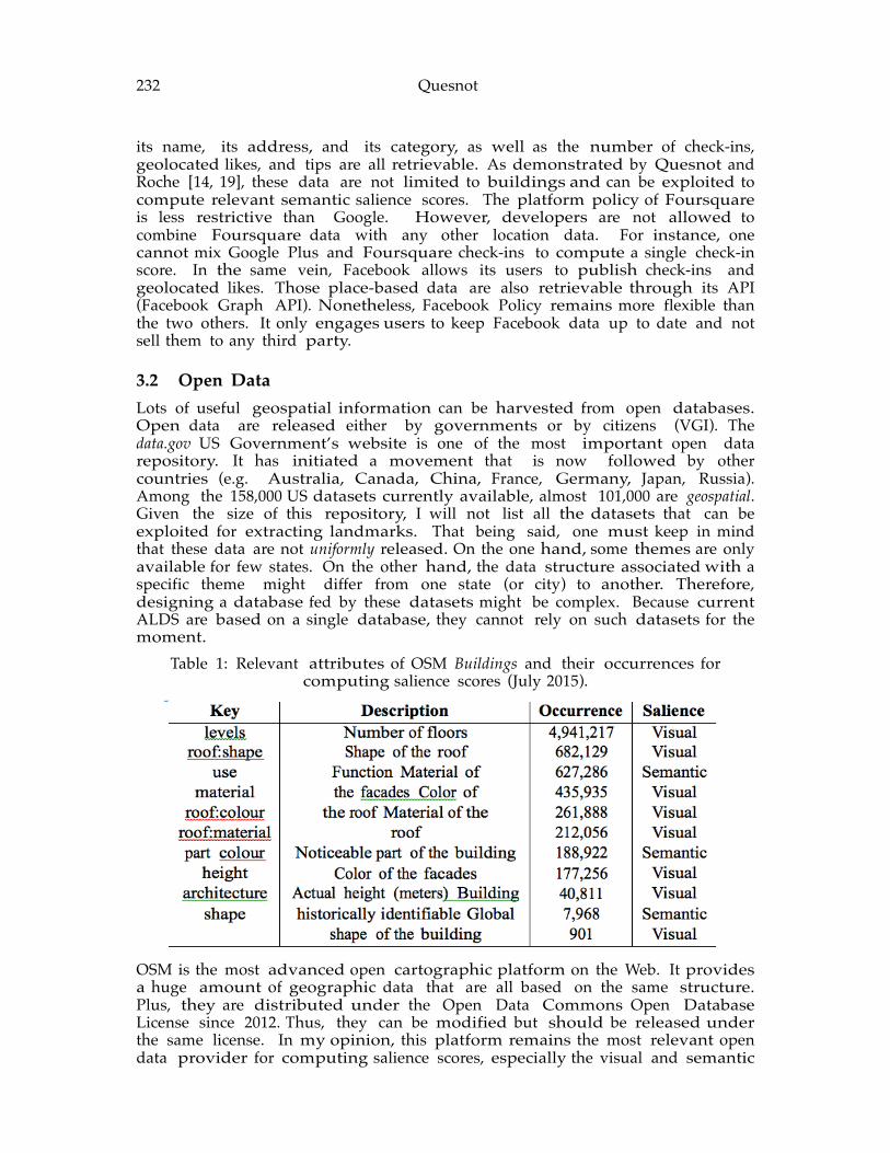
232 Quesnot its name, its address, and its category, as well as the number of check-ins, geolocated likes, and tips are all retrievable. As demonstrated by Quesnot and Roche [14, 19], these data are not limited to buildings and can be exploited to compute relevant semantic salience scores. The platform policy of Foursquare is less restrictive than Google. However, developers are not allowed to combine Foursquare data with any other location data. For instance, one cannot mix Google Plus and Foursquare check-ins to compute a single check-in score. In the same vein, Facebook allows its users to publish check-ins and geolocated likes. Those place-based data are also retrievable through its API (Facebook Graph API). Nonetheless, Facebook Policy remains more flexible than the two others. It only engages users to keep Facebook data up to date and not sell them to any third party.
3.2 Open Data Lots of useful geospatial information can be harvested from open databases. Open data are released either by governments or by citizens (VGI). The data.gov US Government’s website is one of the most important open data repository. It has initiated a movement that is now followed by other countries (e.g. Australia, Canada, China, France, Germany, Japan, Russia). Among the 158,000 US datasets currently available, almost 101,000 are geospatial. Given the size of this repository, I will not list all the datasets that can be exploited for extracting landmarks. That being said, one must keep in mind that these data are not uniformly released. On the one hand, some themes are only available for few states. On the other hand, the data structure associated with a specific theme might differ from one state (or city) to another. Therefore, designing a database fed by these datasets might be complex. Because current ALDS are based on a single database, they cannot rely on such datasets for the moment.
Table 1: Relevant attributes of OSM Buildings and their occurrences for computing salience scores (July 2015).
OSM is the most advanced open cartographic platform on the Web. It provides a huge amount of geographic data that are all based on the same structure. Plus, they are distributed under the Open Data Commons Open Database License since 2012. Thus, they can be modified but should be released under the same license. In my opinion, this platform remains the most relevant open data provider for computing salience scores, especially the visual and semantic
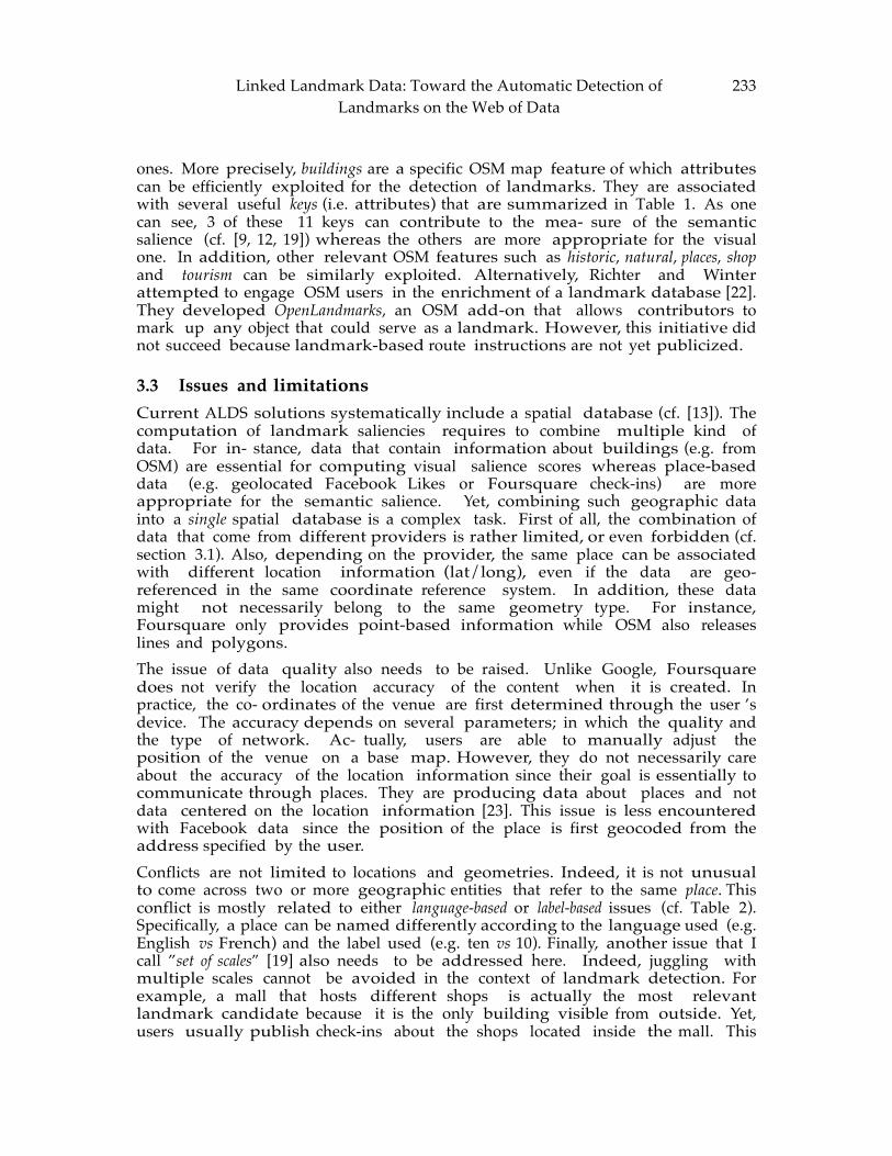
Linked Landmark Data: Toward the Automatic Detection of Landmarks on the Web of Data
233
ones. More precisely, buildings are a specific OSM map feature of which attributes can be efficiently exploited for the detection of landmarks. They are associated with several useful keys (i.e. attributes) that are summarized in Table 1. As one can see, 3 of these 11 keys can contribute to the mea- sure of the semantic salience (cf. [9, 12, 19]) whereas the others are more appropriate for the visual one. In addition, other relevant OSM features such as historic, natural, places, shop and tourism can be similarly exploited. Alternatively, Richter and Winter attempted to engage OSM users in the enrichment of a landmark database [22]. They developed OpenLandmarks, an OSM add-on that allows contributors to mark up any object that could serve as a landmark. However, this initiative did not succeed because landmark-based route instructions are not yet publicized.
3.3 Issues and limitations Current ALDS solutions systematically include a spatial database (cf. [13]). The computation of landmark saliencies requires to combine multiple kind of data. For in- stance, data that contain information about buildings (e.g. from OSM) are essential for computing visual salience scores whereas place-based data (e.g. geolocated Facebook Likes or Foursquare check-ins) are more appropriate for the semantic salience. Yet, combining such geographic data into a single spatial database is a complex task. First of all, the combination of data that come from different providers is rather limited, or even forbidden (cf. section 3.1). Also, depending on the provider, the same place can be associated with different location information (lat/long), even if the data are geo- referenced in the same coordinate reference system. In addition, these data might not necessarily belong to the same geometry type. For instance, Foursquare only provides point-based information while OSM also releases lines and polygons. The issue of data quality also needs to be raised. Unlike Google, Foursquare does not verify the location accuracy of the content when it is created. In practice, the co- ordinates of the venue are first determined through the user ’s device. The accuracy depends on several parameters; in which the quality and the type of network. Ac- tually, users are able to manually adjust the position of the venue on a base map. However, they do not necessarily care about the accuracy of the location information since their goal is essentially to communicate through places. They are producing data about places and not data centered on the location information [23]. This issue is less encountered with Facebook data since the position of the place is first geocoded from the address specified by the user. Conflicts are not limited to locations and geometries. Indeed, it is not unusual to come across two or more geographic entities that refer to the same place. This conflict is mostly related to either language-based or label-based issues (cf. Table 2). Specifically, a place can be named differently according to the language used (e.g. English vs French) and the label used (e.g. ten vs 10). Finally, another issue that I call ”set of scales” [19] also needs to be addressed here. Indeed, juggling with multiple scales cannot be avoided in the context of landmark detection. For example, a mall that hosts different shops is actually the most relevant landmark candidate because it is the only building visible from outside. Yet, users usually publish check-ins about the shops located inside the mall. This
234 Quesnot issue remains quite complex to bypass because the system is not aware of the relationship between the shops and the mall.
Table 2: Label-based and language-based issues: the example of the Le Jules Verne restaurant (Paris). Facebook data were harvested through the Graph
API V2.3 on April, 3rd 2015.
To conclude, it is important to remember that landmarks are far from being limited to a place in its wholeness. Indeed, any observable item (e.g. small objects or specific parts of buildings) might be used as a landmark while navigating. For instance, this could be a remarkable signboard, a flag, or any other noticeable signs associated with a venue. OSM provides such type of information but to my best knowledge, it remains the only reliable source.
4 Exploring the Web of Data to Detect Landmarks
4.1 What Are (Geo)Linked (Open) Data? Nelson’s hypertext concept was notably applied by Berners-Lee when he invented the World Wide Web by linking documents on the Internet. The architecture of the web is composed of three interrelated components: (1) HTTP (Hypertext Transfer Protocol) is a way among others to ensure the communication between web browsers and servers, (2) HTML (Hypertext Markup Language) is the common representation language of the web documents, which are (3) identified and located by URLs (Unified Resource Locator). The initiative of linked data explores both the techniques and the technologies that can be used to link, structure, and publish data on the web. Concretely, URLs are used to locate and identify documents that exist on the web. In the field of linked data, URIs (Universal Resource Identifier) are used to identify on the web any entity that exists elsewhere (e.g. a person, a building, etc.). The main objective is to link together entities identified by their URIs so anyone can reuse them. Resources on the web of data need to be identified but also represented. RDF (Resource Description Framework) is a language and a model used to reach that goal. Once published, linked data can be accessed by using a query language named SPARQL (Sparql Protocol And RDF Query Language). Also, reasoning about the links between data and their semantics remains crucial. In this way, RDF-S (Schema) and OWL (Web Ontology Language) are both languages used to design ontologies. Finally, PROV is used to produce structured metadata in order trace the origin of the linked data. In this context, the open data movement is closely related to the initiative of linked data. Obviously, proprietary data can also be linked, but the ideal would be that linked data remain open at the same time. According to Berners-Lee, a ”good” linked open data should be: (1) available on the web under an open licence, (2) available as machine-readable structured data, and (3) as non-proprietary formats. In addition, he recommends users to (4) use open standards
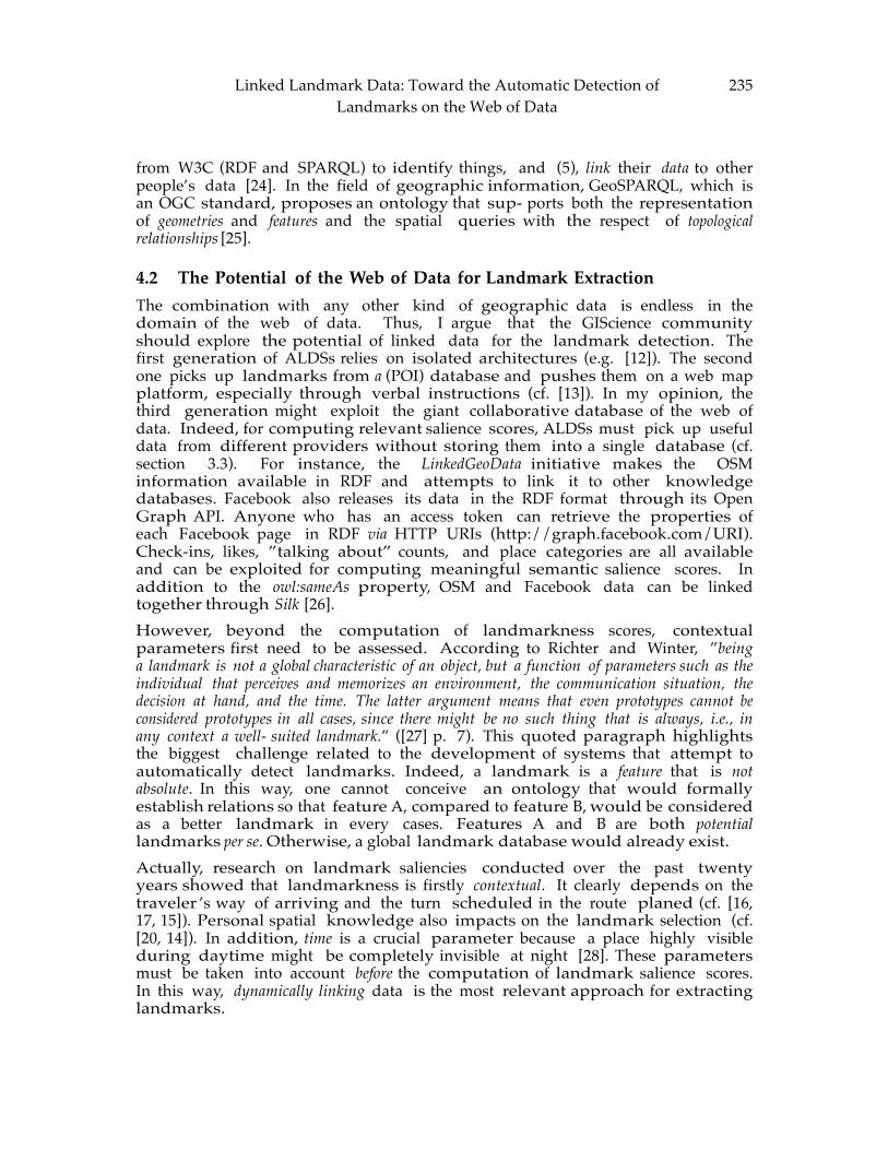
Linked Landmark Data: Toward the Automatic Detection of Landmarks on the Web of Data
235
from W3C (RDF and SPARQL) to identify things, and (5), link their data to other people’s data [24]. In the field of geographic information, GeoSPARQL, which is an OGC standard, proposes an ontology that sup- ports both the representation of geometries and features and the spatial queries with the respect of topological relationships [25].
4.2 The Potential of the Web of Data for Landmark Extraction The combination with any other kind of geographic data is endless in the domain of the web of data. Thus, I argue that the GIScience community should explore the potential of linked data for the landmark detection. The first generation of ALDSs relies on isolated architectures (e.g. [12]). The second one picks up landmarks from a (POI) database and pushes them on a web map platform, especially through verbal instructions (cf. [13]). In my opinion, the third generation might exploit the giant collaborative database of the web of data. Indeed, for computing relevant salience scores, ALDSs must pick up useful data from different providers without storing them into a single database (cf. section 3.3). For instance, the LinkedGeoData initiative makes the OSM information available in RDF and attempts to link it to other knowledge databases. Facebook also releases its data in the RDF format through its Open Graph API. Anyone who has an access token can retrieve the properties of each Facebook page in RDF via HTTP URIs (http://graph.facebook.com/URI). Check-ins, likes, ”talking about” counts, and place categories are all available and can be exploited for computing meaningful semantic salience scores. In addition to the owl:sameAs property, OSM and Facebook data can be linked together through Silk [26]. However, beyond the computation of landmarkness scores, contextual parameters first need to be assessed. According to Richter and Winter, ”being a landmark is not a global characteristic of an object, but a function of parameters such as the individual that perceives and memorizes an environment, the communication situation, the decision at hand, and the time. The latter argument means that even prototypes cannot be considered prototypes in all cases, since there might be no such thing that is always, i.e., in any context a well- suited landmark.” ([27] p. 7). This quoted paragraph highlights the biggest challenge related to the development of systems that attempt to automatically detect landmarks. Indeed, a landmark is a feature that is not absolute. In this way, one cannot conceive an ontology that would formally establish relations so that feature A, compared to feature B, would be considered as a better landmark in every cases. Features A and B are both potential landmarks per se. Otherwise, a global landmark database would already exist. Actually, research on landmark saliencies conducted over the past twenty years showed that landmarkness is firstly contextual. It clearly depends on the traveler ’s way of arriving and the turn scheduled in the route planed (cf. [16, 17, 15]). Personal spatial knowledge also impacts on the landmark selection (cf. [20, 14]). In addition, time is a crucial parameter because a place highly visible during daytime might be completely invisible at night [28]. These parameters must be taken into account before the computation of landmark salience scores. In this way, dynamically linking data is the most relevant approach for extracting landmarks.
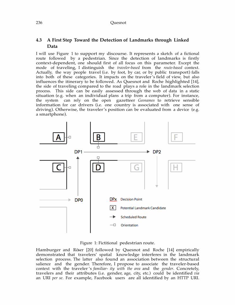
236 Quesnot 4.3 A First Step Toward the Detection of Landmarks through Linked
Data I will use Figure 1 to support my discourse. It represents a sketch of a fictional route followed by a pedestrian. Since the detection of landmarks is firstly context-dependent, one should first of all focus on this parameter. Except the mode of traveling, I distinguish the traveler-based from the route-based context. Actually, the way people travel (i.e. by foot, by car, or by public transport) falls into both of these categories. It impacts on the traveler ’s field of view, but also influences the itinerary to be followed. As Quesnot and Roche highlighted [14], the side of traveling compared to the road plays a role in the landmark selection process. This side can be easily assessed through the web of data in a static situation (e.g. when an individual plans a trip from a computer). For instance, the system can rely on the open gazetteer Geonames to retrieve sensible information for car drivers (i.e. one country is associated with one sense of driving). Otherwise, the traveler ’s position can be evaluated from a device (e.g. a smartphone).
Figure 1: Fictitional pedestrian route.
Hamburger and Roser [20] followed by Quesnot and Roche [14] empirically demonstrated that travelers’ spatial knowledge interferes in the landmark selection process. The latter also found an association between the structural salience and the gender. Therefore, I propose to associate the traveler-based context with the traveler ’s familiar- ity with the area and the gender. Concretely, travelers and their attributes (i.e. gender, age, city, etc.) could be identified via an URI per se. For example, Facebook users are all identified by an HTTP URI.
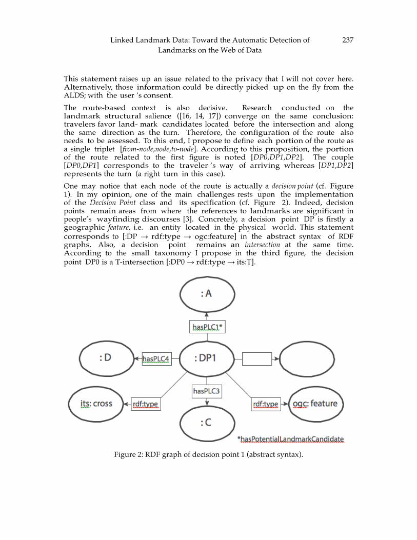
Linked Landmark Data: Toward the Automatic Detection of Landmarks on the Web of Data
237
This statement raises up an issue related to the privacy that I will not cover here. Alternatively, those information could be directly picked up on the fly from the ALDS; with the user ’s consent. The route-based context is also decisive. Research conducted on the landmark structural salience ([16, 14, 17]) converge on the same conclusion: travelers favor land- mark candidates located before the intersection and along the same direction as the turn. Therefore, the configuration of the route also needs to be assessed. To this end, I propose to define each portion of the route as a single triplet [from-node,node,to-node]. According to this proposition, the portion of the route related to the first figure is noted [DP0,DP1,DP2]. The couple [DP0,DP1] corresponds to the traveler ’s way of arriving whereas [DP1,DP2] represents the turn (a right turn in this case). One may notice that each node of the route is actually a decision point (cf. Figure 1). In my opinion, one of the main challenges rests upon the implementation of the Decision Point class and its specification (cf. Figure 2). Indeed, decision points remain areas from where the references to landmarks are significant in people’s wayfinding discourses [3]. Concretely, a decision point DP is firstly a geographic feature, i.e. an entity located in the physical world. This statement corresponds to [:DP → rdf:type → ogc:feature] in the abstract syntax of RDF graphs. Also, a decision point remains an intersection at the same time. According to the small taxonomy I propose in the third figure, the decision point DP0 is a T-intersection [:DP0 → rdf:type → its:T].
Figure 2: RDF graph of decision point 1 (abstract syntax).
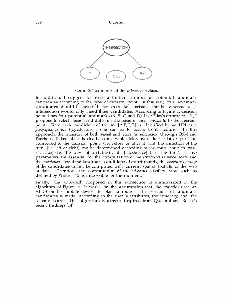
238 Quesnot
Figure 3: Taxonomy of the Intersection class.
In addition, I suggest to select a limited number of potential landmark candidates according to the type of decision point. In this way, four landmark candidates should be selected for cross-like decision points whereas a T-intersection would only need three candidates. According to Figure 1, decision point 1 has four potential landmarks (A, B , C, and D). Like Elias’s approach [12], I propose to select those candidates on the basis of their proximity to the decision point. Since each candidate of the set [A,B,C,D] is identified by an URI as a geographic feature ([ogc:feature]), one can easily access to its features. In this approach, the measure of both visual and semantic saliencies through OSM and Facebook linked data is clearly conceivable. Moreover, their relative position compared to the decision point (i.e. before or after it) and the direction of the turn (i.e. left or right) can be determined according to the route couples [from-node,node] (i.e. the way of arriving) and [node,to-node] (i.e. the turn). Those parameters are essential for the computation of the structural salience score and the orientation score of the landmark candidates. Unfortunately, the visibility coverage of the candidates cannot be computed with current spatial toolkits of the web of data. Therefore, the computation of the advance visbility score such as defined by Winter [15] is impossible for the moment. Finally, the approach proposed in this subsection is summarized in the algorithm of Figure 4. It works on the assumption that the traveler uses an ALDS on his mobile device to plan a route. The selection of landmark candidates is made according to the user ’s attributes, the itinerary, and the salience scores. This algorithm is directly inspired from Quesnot and Roche’s recent findings [14].
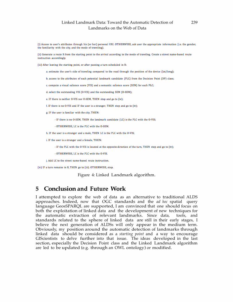
Linked Landmark Data: Toward the Automatic Detection of Landmarks on the Web of Data
239
Figure 4: Linked Landmark algorithm.
5 Conclusion and Future Work I attempted to explore the web of data as an alternative to traditional ALDS approaches. Indeed, now that OGC standards and the ad hoc spatial query language GeosSPARQL are supported, I am convinced that one should focus on both the exploitation of linked data and the development of new techniques for the automatic extraction of relevant landmarks. Since data, tools, and standards related to the sphere of linked data are still in their early stages, I believe the next generation of ALDSs will only appear in the medium term. Obviously, my position around the automatic detection of landmarks through linked data should be considered as a starting point and a way to encourage GIScientists to delve further into that issue. The ideas developed in the last section, especially the Decision Point class and the Linked Landmark algorithm are led to be updated (e.g. through an OWL ontology) or modified.
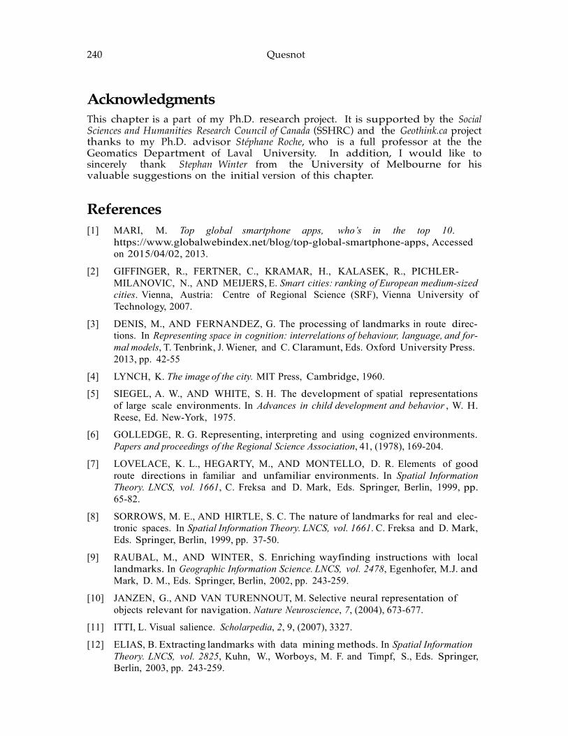
240 Quesnot
Acknowledgments This chapter is a part of my Ph.D. research project. It is supported by the Social Sciences and Humanities Research Council of Canada (SSHRC) and the Geothink.ca project thanks to my Ph.D. advisor Stephane Roche, who is a full professor at the the Geomatics Department of Laval University. In addition, I would like to sincerely thank Stephan Winter from the University of Melbourne for his valuable suggestions on the initial version of this chapter.
References [1] MARI, M. Top global smartphone apps, who’s in the top 10.
https://www.globalwebindex.net/blog/top-global-smartphone-apps, Accessed on 2015/04/02, 2013.
[2] GIFFINGER, R., FERTNER, C., KRAMAR, H., KALASEK, R., PICHLER- MILANOVIC, N., AND MEIJERS, E. Smart cities: ranking of European medium-sized cities. Vienna, Austria: Centre of Regional Science (SRF), Vienna University of Technology, 2007.
[3] DENIS, M., AND FERNANDEZ, G. The processing of landmarks in route direc- tions. In Representing space in cognition: interrelations of behaviour, language, and for- mal models, T. Tenbrink, J. Wiener, and C. Claramunt, Eds. Oxford University Press. 2013, pp. 42-55
[4] LYNCH, K. The image of the city. MIT Press, Cambridge, 1960.
[5] SIEGEL, A. W., AND WHITE, S. H. The development of spatial representations of large scale environments. In Advances in child development and behavior , W. H. Reese, Ed. New-York, 1975.
[6] GOLLEDGE, R. G. Representing, interpreting and using cognized environments. Papers and proceedings of the Regional Science Association, 41, (1978), 169-204.
[7] LOVELACE, K. L., HEGARTY, M., AND MONTELLO, D. R. Elements of good route directions in familiar and unfamiliar environments. In Spatial Information Theory. LNCS, vol. 1661, C. Freksa and D. Mark, Eds. Springer, Berlin, 1999, pp. 65-82.
[8] SORROWS, M. E., AND HIRTLE, S. C. The nature of landmarks for real and elec- tronic spaces. In Spatial Information Theory. LNCS, vol. 1661. C. Freksa and D. Mark, Eds. Springer, Berlin, 1999, pp. 37-50.
[9] RAUBAL, M., AND WINTER, S. Enriching wayfinding instructions with local landmarks. In Geographic Information Science. LNCS, vol. 2478, Egenhofer, M.J. and Mark, D. M., Eds. Springer, Berlin, 2002, pp. 243-259.
[10] JANZEN, G., AND VAN TURENNOUT, M. Selective neural representation of objects relevant for navigation. Nature Neuroscience, 7, (2004), 673-677.
[11] ITTI, L. Visual salience. Scholarpedia, 2, 9, (2007), 3327.
[12] ELIAS, B. Extracting landmarks with data mining methods. In Spatial Information Theory. LNCS, vol. 2825, Kuhn, W., Worboys, M. F. and Timpf, S., Eds. Springer, Berlin, 2003, pp. 243-259.
Linked Landmark Data: Toward the Automatic Detection of Landmarks on the Web of Data
241
[13] DUCKHAM, M., WINTER, S., AND ROBINSON, M. Including landmarks in routing instruction. Journal of Location Based Services, 4, 1, (2010), 28-52.
[14] QUESNOT, T., AND ROCHE, S. Quantifying the significance of semantic land- marks in familiar and unfamiliar environments. In Spatial Information Theory. LNCS, vol. 9368, Fabrikant, S.I., Raubal, M., Bertolotto, M., Davies, C., Freund- schuh, S., Bell, S., Eds. Springer, Berlin, 2015 (in press).
[15] WINTER, S. Route adaptive selection of salient features. In Spatial Information Theory. LNCS, vol. 2825, Kuhn, W., Worboys, M. F. and Timpf, S., Eds. Springer, Berlin, 2003, pp. 349-361.
[16] KLIPPEL, A., AND WINTER, S. Structural salience of landmarks for route direc- tions. In Spatial Information Theory. LNCS, vol. 3693, Cohn, A. G. and Mark, D. M., Eds. Springer, Berlin, 2005, pp. 347-362.
[17] RO SER, F., HAMBURGER, K, KRUMNACK, A., AND KNAUFF, M. The struc- tural salience of landmarks: results from an on-line study and a virtual environ- ment experiment. Journal of Spatial Science, 57, 1, (2012), 37-50.
[18] GOODCHILD, M. F.. Citizens as sensors: the world of volunteered geography. GeoJournal, 4, (2007), 211-221.
[19] QUESNOT, T., AND ROCHE, S. Measure of landmark semantic salience through geosocial data streams. ISPRS International Journal of Geo-Information, 4, 1, (2015), 1-31.
[20] HAMBURGER, K. AND RO SER, F. The role of landmark modality and familiarity in human wayfinding. Swiss Journal of Psychology, 73, 4, (2014), 205-213.
[21] SADEGHIAN, P., AND KANTARDZIC, M. The new generation of automatic landmark detection systems: challenges and guidelines. Spatial Cognition & Com- putation, 8, (2008), 252-287.
[22] RICHTER, K. F., AND WINTER, S. Harvesting user-generated content for seman- tic spatial information: the case of landmarks in OpenStreetMap. In Proceedings of the Surveying & Spatial Sciences Biennial Conference. Wellington, NZ, 2011, pp. 75-86.
[23] QUESNOT, T., AND ROCHE, S. Platial or locational data? Toward the charac- terization of social location sharing. In Proceedings of the 48th Annual Hawaii Inter- national Conference on System Sciences. IEEE Computer Society Press, Washington, DC, 2015, pp. 1973-1982.
[24] BERNERS-LEE, T. Linked data. http://www.w3.org/DesignIssues/LinkedData.html, Accessed on 2015/04/02, 2009.
[25] BATTLE, R. AND KOLAS, D. Enabling the geospatial semantic web with par- liament and GeoSPARQL. Semantic Web - On linked spatiotemporal data and geo- ontologies, 3, 4, (2012), 355-370.
[26] VOLZ, J., BIZER, C., GAEDKE, M., AND KOBILAROV, G. Discovering and main- taining links on the web of data. In The Semantic Web - ISWC 2009. LNCS vol. 5823, Bernstein, A., Karger, D. R., Heath, T., Feigenbaum, L., Maynard, D., Motta, E., and Thirunarayan, K., Eds. Springer, Berlin, 2009, pp. 650-665.

242 Quesnot [27] RICHTER, K. F. AND WINTER, S. Landmark: GIScience for intelligent services
Springer, Cham (Switzerland), 2014.
[28] WINTER, S., RAUBAL, M., AND NOTHEGGER, C. Focalizing measures of salience for wayfinding. In Map-based Mobile Services, Meng, L., Reichenbacher, T., and Zipf, A., Eds. Springer, Heidelberg, 2005, pp. 125-139.
ADVANCING GEOGRAPHIC INFORMATION SCIENCE: CHAPTER 17
© by the author(s) Licensed under Creative Commons Attribution 4.0 License
243
Place Properties Maria Vasardani and Stephan Winter
Department of Infrastructure Engineering, The University of Melbourne, Parkville, Victoria 3010, Australia
Abstract: Place and space were antagonists in geographic information science for a long time, but not anymore. Place, it is argued here, is a location (in an environment, not in an empty space) with properties that give it ‘shape and character’ and which enable conversations about place. To realize this argument, place can be characterized by Alexander’s theory of centres, where 15 structural properties that characterize a whole are assembled. This paper investigates these properties and their relationship to place by identifying theories within geographic information science that can be employed for their formalization. We argue therefore that we already have some tools to observe these properties for characterizing places, while many traditional issues with modeling place – for example, their typical lack of crisp boundaries, their subjective notion, and their reliance on context – may no longer pose a problem.
Keywords: Place, wholeness, centres, spatial cognition, spatial concept formalization.
1 Introduction Philosopher Jeff Malpas argues that “…place is such a central and ubiquitous concept across so many disciplines […] in the arts, humanities and social sciences in the twenty-first century” [40]. Indeed, place is an important term in the disciplines of geography and Geographic Information Systems (GISs) as well. While it is a key geographical concept, place with its non-‐‑quantifiable character has in the past largely escaped GISs, which since their inception, represent and manipulate measurable features in spatial form. However, and due to recent technological advances, the importance of the concept of place in everyday life is evident and ever growing. The merging of mapping software and social media apps provides constant streams of information about where people or things are, in what is in essence information about ‘place’. Think for example of Foursquare: a popular app whose premise is based entirely on the concept of place. The resurface of the importance of place in GIS has not gone unnoticed by GIS scholars. Sui and Goodchild debate that:
“Formalizing place in the GIS context will be both interesting and challenging; until recently, place has been off the intellectual radar screen of GIScientists, many of whom appear to use the two terms place and space somewhat
244 Vasardani and Winter
interchangeably […], yet in GIScience, we still do not have an overarching theory of place or how to work with the concept.”[3, pg. 1744]
The above-stated realisation asserts that no matter how ubiquitous in its use - as a word that people use daily in the English-speaking world- place is not well defined in academic terms. While fundamental in many disciplines, it is a concept planted in common sense, thus evoked in many different ways. Tim Cresswell in his book ‘Place: an introduction’ offers a wide coverage of the different definitions of place and its centrality in both everyday life and interdisciplinary academic endeavour [12]. Definitions of the word place go as far back as Aristotle and Plato, who introduced the terms chora and topos—what in a free English translation one would think of as region and place, respectively—with the second term being the obvious root of geographic terms such as topography and topology. However, each discipline, including GIScience, provides different definitions of the concept of place, none of which seems to be all-‐‑encompassing given its commonsensical nature. In this work we pose the following question: Rather than focusing on an all-‐‑encompassing definition of the concept of place, can we, instead, provide a set of ‘properties of place’, which would allow its formalization and realization in different contexts and applications in GIS? To start answering this question, we go back to Malpas’ [41] approach of interdisciplinarity not as a featureless mélange of research related to place, but rather as research which has, in a sense, its own topography—locations with properties that give them ‘shape and character’ and which enable conversations about place. Fittingly then, our approach combines theories from GIScience with a toolset borrowed from the field of architecture: the theory of centres [2]. In this theory, Alexander assembles 15 structural properties that characterize a whole (see Table 1)—wholeness, in this theory is any living order or structure that exists in things and which people can feel. Such felt orders are factual and independent of individual cognition. These 15 properties can help generate a variety of ‘good’ patterns with this so-‐‑called living structure [23, 50]. As an architect, Alexander developed the theory of centres in an effort to make shared values and human senses part of science. He believed that existing science based on the positivists’ mechanical view of the world, cannot layout a scientific foundation for architecture, whose goal should be to create structures and places where life can be sustained and people can feel connected to.
Table 1 Alexander's 15 Properties of Wholeness [2]
Observing these 15 properties through GIScience lenses, one can see that most, if not all of them, can be immediately identified as properties that already exist in theories developed for formalizing place in the discipline. In the remaining of this paper, we examine these theories and analyse how these 15 properties already correspond to characteristics of places. Our aim is to create a dialogue within GIScience for
Place Properties 245
developing a set of place properties, with which any place can be uniquely identified in various contexts, depending on the domain of the properties’ values. Such a properties set frees GIScientists from adhering to a specific definition of the concept of place, which would necessarily need to change according to different application fields.
2 Properties of Places Much like Christaller developed central-‐‑place theory in geography [11], concerned with the size and distribution of central places (or settlements) within a system in an effort to explain how central places of different sizes are located in relation to, and affecting each other, Alexander’s theory of centres [2] attempts to measure the degree of life in structures by the number of fundamental structural properties they comprise. The notion of centres, therefore, is an important one in any such framework concerning the spatial organization of elements. Having this concept in mind, the remaining of this section discusses how some of Alexander’s 15 properties of wholeness can be already identified in place related theories in GIScience and can, therefore, be used to uniquely characterize and perhaps formalise places.
2.1 Levels of scale Formations within and across places can exhibit different scales. Place attachment is a term used to describe the emotional ties people experience with places of different scale [38], such as their room/residence [7, 16], neighbourhood, suburb, city [37], region, or country, places such as landscapes [29], forests, lakes, summer houses [53], or beaches etc. Apart from place attachment, terms such as place identity, sense of place, place satisfaction and others are used to name people’s relations with places of different scale, and it is still debatable whether the concept itself is a multi or single dimensional one (for a review see [16]). However, what is perhaps more interesting in our discussion is the fact that scale is one of the fundamental place properties, which affects people’s cognition and perception of their surrounding environment and as a result, their place attachment. For example, there is evidence of a curvilinear relationship between scale of place and strength of place attachment. When places of three different scales where measured, i.e. home, neighbourhood, and city, emotional attachment was shown stronger at the two extremes, home and city than to the midpoint of the scale where neighbourhood is typically found [21] (see [38] for a review of empirical case studies on the effect of place scale on place attachment). In GIScience and geography there is no shortage of research on mathematical models of scale in natural or artificial structures, from nature’s self-‐‑organization [4, 10], to fractal theory and ht-‐‑indices of geographic phenomena and cities [5, 19, 26, 36], to scale of topological patterns of street networks [24], or general accounts of scale in geography and GIS [18, 43]. So whether the domain is geography, sociology, urban planning, humanistic geography, architecture or philosophy, scale is one of the fundamental properties of place, expressed in a plethora of models and terminologies in a variety of contexts, and one that affects people’s perception and sense of place.
2.2 Strong centres, contrast, boundaries, gradients, non-‐‑-‐‑separateness, deep interlock and ambiguity.
As has been already stated, at the heart of Alexander’s theory is the concept of the existence of centres in any living structure. We argue that the existence of centres is
246 Vasardani and Winter also at the heart of the place properties set. In any ‘place’ formation, there exists at least one, and in most cases multiple centres of varying sizes, which support each other. This concept is clear in the central-place theory in geography [11] and its later modifications [8, 30]. However, when dealing with centres in geographic reality, one has to consider the notions of membership (i.e., belonging to a centre vs. not part of the centre), gradient membership (a more fuzzy interpretation of belonging and not- belonging), as well as boundaries. Therefore, the properties of gradients and boundaries are also studied together with the centres property. Places such as metropolitan areas, wetlands, and cultural regions have gradual boundaries in contrast to places with well-defined boundaries such as buildings. There are many models for representing and reasoning with geographic objects with either crisp or gradient boundaries. The latter are mostly based on fuzzy sets [3, 55], rough sets [1, 13, 45], or supervaluation [6, 34] to deal with gradient and boundaries (for a collection of edited papers see also Burrough and Frank’s book [9]). Recently, there have been attempts within the GIScience community to explain structures in verbal place descriptions and to localize features without committing to boundaries, crisp or otherwise. Winter and Freksa [54] use contrast sets to capture sufficiency of places by explicating their contrast to other places, based on the claim that cognition and communication about places in spatial environments is a matter of perceiving one place as sufficiently different from another. Contrast, a fundamental principle in sensing and understanding [17], and one of the organizing principles of perception in Gestalt theory, focuses on the core instead of the fridges of concepts. No matter how one chooses to represent and reason with places, however, it is clear that centres, boundaries and contrast are properties utilized in human perception to recognize and differentiate one place from another. Places are hardly ever perceived as separate entities that exist in isolation. Rather, people recognize them as collections of entities and the relations between them, and in relations with other places. Even map sketches, the graphical externalizations of places as they are perceived and stored in memory, represent configurations of places and relations between them. These relations exist in various granularities and hierarchies, and exist within and across places. Freksa and Barkowsky [14] argue that what type of entities and relations people will choose is task-dependent. Therefore places exhibit the property of non-separateness as relations between within-place centres or across different places. These relations strengthen the ties between centres in places, as each one gets support from centres of equal or lesser size around it and equally supports larger centres. As a whole then, the entities that form a place and places them selves, exhibit centres, that can be contrasted to each other, may have distinct boundaries or gradients that create harmonious transitions between contrasting centres and they all belong to the same whole structure, experiencing what Alexander calls deep interlock and ambiguity. In Gestalt theory, this is the figure‑ground reversal phenomenon, where distinct parts of a whole interpenetrate each other and create ambiguity in visual perception [52], just like the layout of the building blocks and the spaces between them in a city. When observed as a whole, these various distinct parts blend, creating ambiguity from a visual perception point, but are ultimately experienced as a ‘place’ in human cognition. As an example, think of a city with its central district and the local suburban centres. Within these various size centres exist other centres such as public transport stations, malls, stadiums, parks and centres for various other activities. Between all these exist relations in the forms of street networks and paths. Similarly, the city itself is connected with other cities via land, air and water pathways that form together larger metropolitan areas and countries. The centre of each hierarchical level and granularity
Place Properties 247
has borders, some of them distinct, some others gradient, but together they blend in, creating non-separated places. Considering this example, one can clearly distinguish the resemblance of this group of properties with many of the five elements of Lynch’s mental maps [39]. Nodes and districts are equivalent to smaller (local) and larger centres, while edges relate to perceived boundaries, especially explicit ones such as riverbanks. And then of course, the connections or relations between them are represented as paths such street networks and other travel channels.
2.3 Good shape, local symmetries, echoes, roughness, alternating repetitions, positive space
These six properties together all deal with the internal structural organization of place elements, which give each place its distinctive, yet familiar identity. They are all perceived in human cognition both at the conscious and subconscious levels and mostly described qualitatively in natural language place descriptions. These properties are, however, mathematical in nature and can, therefore, easily lend themselves to formalization. In particular, they adhere to fractal theory and self-‐‑similarity and they are responsible for the patterns that make various places look similar, but yet distinct. Local symmetries are experienced in both natural and artificial places where different foci create symmetrical neighbourhoods around them. Alternating repetitions are common in places with self-‐‑similarity patterns such as coastal places or forests. Positive spaces are what differentiate the figure from the ground in Gestalt theory and they are usually associated with the convex footprints of spatial features especially in the built environment, vs. the background space that surrounds them. This pattern is evident in the layout of a city for example [25]. Roughness has to do with the irregularities and imperfections in any place configuration, as the result of organic generative process of development that do not adhere to perfect geometric symmetries. This development pattern is most common in the expansion of most neighbourhoods and cities around the world, where urban sprawl for example does not follow strict geometric alignments, but depends on other factors such as accessibility, demand due to increasing popularity of place, and others. Then the property of good shape of a place is the result of the cumulative good shape of its parts, such that if the individual centres and their surroundings are characterized by good shape by experiencing a few or all the aforementioned properties, then a place as the sum of its parts is also in good shape. Finally, echo is the property of a place when its whole structure is reminiscent of another place, or the sense of familiarity that people some times experience in a place, even when they visit it for the first time, due to its similarity with other places of similar properties. Echoes can be internal, as similarity of the elements within a place, or external, characterizing a place as a whole when compared with other places. While, to the best of our knowledge, there are no current models for the potential formalization of this subgroup of mathematical, in nature, properties, Jiang’s hierarchical graph for modelling the 15 wholeness properties [25] is a good starting point, even though the author does not specify how, in this model, each of these properties is distinctly measured. The existence of patterns in this group of properties brings in mind spatio-temporal image schemata and how they capture common structures from people’s repeated experiences of properties such as containment, linkage or contact [27, 35]. The regularity and recurrent patterns or shapes identified in schemata make them good candidates for formalizing local symmetries, echoes and alternating repetitions. In fact, Kuhn’s work [31] on ontologies of spatio-temporal phenomena, which uses image schemata for their spatial nature and their ability to
248 Vasardani and Winter allow conceptual mappings and to construct abstract categories, could be a good first step toward such formalisations.
2.4 Void, simplicity and inner calm Finally, the property of void is the one that exists in all places, natural and artificial, rural or urban, in micro-‐‑ or macro-‐‑scales. It is that of empty space, a requirement for any place configuration through which people can move around, where space is not completely filled. It is also one of the properties that allows for people to use each place according to their needs at any given context. Take parks for example, maybe one of the place categories where void is an obvious property. It is also one of the properties of parks that make them so attractive to people. The void, emptiness or openness of the space in such places allows for its creative and individualized use, be it for recreation, sport, a meeting, or a picnic among others. And inherently related with the void is also the property of simplicity and inner calm. This property is a more abstract one perhaps, but one well understood and agreed upon, nonetheless, when describing places of preference, of which it more often than not, is a characteristic. It abides to the notion that simplicity offers a feeling of calmness, or that places function better when they are not overloaded with elements or functions, or both. Think of the words one uses when describing shopping malls. Usually, and depending on the previous experiences, expressions such as ‘crowded’, ‘busy’, ‘difficult to navigate through’, ‘confusing’, or ‘tiring’, often appear in the descriptions for such places where many needs and many functions are attempted to be accommodated, such as shopping for various categories, eating, resting, recreation and others in one single place. On the contrary, places where categories of functions, or to use a word closer affiliated with theories in GIScience, of affordances are kept to a minimum, experience a higher degree of simplicity and inner calm.
3 Discussion Our basic premise in this paper has been that the concept of place, rather than defined in a precise manner that is bound to be different according to application domain and context, can rather be identified via a set of properties that are encoded in it, much like philosophers argue that abstract concepts can be identified by the properties they encrypt [49]. Recently, Jiang [25] also used Alexander’s theory in order to ‘capture the nature of space’ in hierarchical graphs, from nations to buildings. Jiang argues along the same line that these properties are helpful to understand (and in the future formalize) patterns in space. Jiang, in the end, is more focussed on the structure of a graph of centres, providing ht-indices from which number of centres and level of scale can be identified, but is not concerned much with how the rest of the properties could be measured. We leave the question for specific measures deliberately open: we can think of a range of alternative measures, and of different agencies using different measures for the same properties.
Accordingly, this paper addresses this identified gap of a higher-‐‑level discussion of the phenomenon itself: places characterized by properties. This ontological rather than quantitative approach should allow comparing patterns / places when they are described by different agencies, or when they are used in different communication contexts. As revealed in Turk and Mark’s study [42] of how people categorize place elements in an Australian indigenous language vs. in English, there are fundamental differences at the basic levels of conceptual systems in different backgrounds and languages, supporting the idea that people may use a variety of categories for the same
Place Properties 249
geographic elements. We argue that by not defining places, but rather describing them using a set of properties, we do not have to adhere to equivalent categories between different groups. Instead we postulate that it suffices to provide an agreed upon understanding of the value range of each property between the different domains or communication contexts. An approach by a theory of centres is also relating and supported by other work. One is Kuhn’s [32] postulate of spatial core concepts. These concepts are formed by location, neighbourhood, field, object and network. He identifies location as relation, not a property: “All location descriptions express spatial relations between figures to be located and chosen grounds” (p. 2271). This view of a figure on a ground is compatible with strong centres, positive space and contrast, and further supported by his neighbourhood, which he calls the “natural companion concept to location” (also p. 2271). “When grounds become salient, as in the case of places, they tend to be thought of as ‘locations’ in the sense of objects” (p. 2271). Object “implies boundedness, but this does not mean that the object’s boundaries need to be known or even knowable” (p. 2272), linking to Alexander’s boundaries, and Kuhn’s network, capturing the relationships between objects, closes the loop to Alexander’s non-separateness. Another suggested ontological approach to place has been built from affordance [28, 33, 46]. Affordance theory [15] adds an interesting view to this discussion, because it takes a stance from an individual’s perception, capabilities and intentions, in contrast to Jiang’s search for universal measures. Applying an approach grounded in affordances the above properties by Alexander finally get contextualized. A place, characterized by these properties, will be different between individuals, and even for an individual at different times (intentions). For example, in “let’s meet at the market” the market is not an objective, positivist object, but a concept in the mind of the speaker (which could be described by the above properties) and in the mind of the listener (which could be described by the above properties, but potentially differently). Further expanding this example, “let’s meet at the market” will most likely lead to a different description of market, used here with the intention of meeting, i.e., calling for a strong center point, compared to “at the market you can find produce from all over the region”, used with the intention of shopping, i.e., calling for levels of scale (a place of places) and alternating repetition (many stalls).
4 Conclusions This paper attempts to fill a gap in GIScience: it approaches places as ‘locations with properties’ that give them ‘shape and character’, and along the way points to a range of existing, but disconnected knowledge in GIScience that, combined together, provides a powerful tool to capture this elusive, subjective, and context-‐‑dependent concept. The framework for combining this knowledge has been provided by Alexander’s theory of centres. This theory formulated 15 properties (of centres, or of wholeness) that this paper transferred to geographic places, namely from a GIScience perspective, not from a philosophical or human geography perspective. This transfer provides sufficient links to scattered knowledge to fill the properties with meaning in this particular context of place. The paper focuses decidedly on the concept of place, a concept of emerging interest in GIScience. It does so in contrast to other work, e.g., Jiang’s study whether space can be characterized by measures of these 15 properties. We deliberately do not commit to particular measures, arguing that in different context different measures of particular
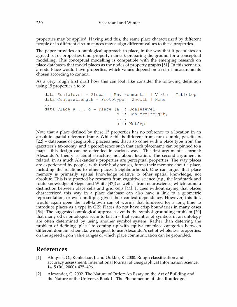
250 Vasardani and Winter properties may be applied. Having said this, the same place characterized by different people or in different circumstances may assign different values to these properties. The paper provides an ontological approach to place, in the way that it postulates an agreed set of properties (and property names), preparing the ground for a conceptual modelling. This conceptual modelling is compatible with the emerging research on place databases that model places as the nodes of property graphs [51]. In this scenario, a node Place would have properties, which values depend on a set of measurements chosen according to context. As a very rough first draft how this can look like consider the following definition using 15 properties a to o:
Note that a place defined by these 15 properties has no reference to a location in an absolute spatial reference frame. While this is different from, for example, gazetteers [22] – databases of geographic placenames, that also come with a place type from the gazetteer’s taxonomy, and a georeference such that each placename can be pinned to a map – this design can be defended in various ways. The first argument is formal: Alexander’s theory is about structure, not about location. The second argument is related, in as much Alexander’s properties are perceptual properties: The way places are experienced by people, with their body senses, forms their memory about a place, including the relations to other places (neighbourhood). One can argue that place memory is primarily spatial knowledge relative to other spatial knowledge, not absolute. This is supported by research from cognitive science (e.g., the landmark and route knowledge of Siegel and White [47]) as well as from neuroscience, which found a distinction between place cells and grid cells [44]. It goes without saying that places characterized this way in a place database can also have a link to a geometric representation, or even multiple, given their context-dependency. However, this link would again open the well-known can of worms that hindered for a long time to introduce places as a type in GIS: Places do not have crisp boundaries in many cases [54]. The suggested ontological approach avoids the symbol grounding problem [20] that many other ontologies seem to fall in – that semantics of symbols in an ontology are often determined by using another symbol system. Rather than deferring the problem of defining ‘place’ to coming up with equivalent place categories between different domain schemata, we suggest to use Alexander’s set of wholeness properties, on the agreed upon value ranges of which place communication can be grounded.
References [1] Ahlqvist, O., Keukelaar, J. and Oukbir, K. 2000. Rough classification and
accuracy assessment. International Journal of Geographical Information Science. 14, 5 (Jul. 2000), 475–496.
[2] Alexander, C. 2002. The Nature of Order: An Essay on the Art of Building and the Nature of the Universe, Book 1 - The Phenomenon of Life. Routledge.
Place Properties 251
[3] Altman, D. 1994. Fuzzy set theoretic approaches for handling imprecision in spatial analysis. International Journal of Geographical Information Systems. 8, 3 (May 1994), 271–289.
[4] Bak, P. 1996. How Nature Works. Springer New York. [5] Batty, M. and Longley, P. 1994. Fractal cities: a geometry of form and function.
Academic Press Professional, Inc. [6] Bennett, B. 2001. Application of Supervaluation Semantics to Vaguely Defined
Spatial Concepts Spatial Information Theory. D. Montello, ed. Springer Berlin / Heidelberg. 108–123.
[7] Bonaiuto, M., Aiello, A., Perugini, M., Bonnes, M. and Ercolani, A.P. 1999. Multidimensional perception of residential environment quality and neighborhood attachment in the urban environment. Journal of Environmental Psychology. 19, 4 (1999), 331–352.
[8] Bradford, M.G. and Kent, W.A. 1977. “Central place theory: Christaller’s model.” Human Geography: Theories and their Applications. Oxford University Press. 6–27.
[9] Burrough, P.A. and Frank, A. 1996. Geographic Objects with Indeterminate Boundaries. CRC Press.
[10] Buttenfield, B.P. 1989. Scale-‐‑Dependence And Self-‐‑Similarity In Cartographic Lines. Cartographica: The International Journal for Geographic Information and Geovisualization. 26, 1 (Oct. 1989), 79–100.
[11] Christaller, W. 1966. Central places in southern Germany. Prentice-‐‑Hall. [12] Cresswell, T. 2014. Place: An Introduction. John Wiley & Sons. [13] Duckham, M., Mason, K., Stell, J. and Worboys, M. 2001. A formal approach to
imperfection in geographic information. Computers, Environment and Urban Systems. 25, 1 (Jan. 2001), 89–103.
[14] Freksa, C. and Barkowsky, T. 1996. On the relation between spatial concepts and geographic objects. Geographic objects with indeterminate boundaries. P.A. Burrough and A. Frank, eds. Taylor and Francis, London. 109–121.
[15] Gibson, J. 1977. The theory of affordances In RE Shaw & J. Bransford (eds.) Perceiving, Acting, and Knowing. Lawrence Erlbaum Associates.
[16] Giuliani, M.V. 2003. Theory of Attachment and Place Attachment. (2003), 137–170.
[17] Goodale, M.A. and Milner, A.D. 1992. Separate visual pathways for perception and action. Trends in Neurosciences. 15, 1 (Jan. 1992), 20–25.
[18] Goodchild, M.F. 2011. Scale in GIS: An overview. Geomorphology. 130, 1-‐‑2 (Jul. 2011), 5–9.
[19] Goodchild, M.F. and Mark, D.M. 1987. The Fractal Nature of Geographic Phenomena. Annals of the Association of American Geographers. 77, 2 (Jun. 1987), 265–278.
[20] Harnad, S. 1990. The symbol grounding problem. Physica D: Nonlinear Phenomena. 42, 1-3 (Jun. 1990), 335–346.
252 Vasardani and Winter [21] Hidalgo, M.C. and Hernández, B. 2001. Place attachment: Conceptual and
empirical questions. Journal of Environmental Psychology. 21, 3 (2001), 273– 281. [22] Hill, L. 2006. Georeferencing: The Geographic Associations of Information. MIT
Press. [23] Ishikawa, S. and Silverstein, M. 1977. A Pattern Language: Towns, Buildings,
Construction. Oxford University Press. [24] Jiang, B. 2007. A topological pattern of urban street networks: universality and
peculiarity. Physica A: Statistical Mechanics and its Applications. 384, 2 (2007), 647–655.
[25] Jiang, B. 2015. Wholeness as a Hierarchical Graph to Capture the Nature of Space. arXiv:1502.03554 [nlin, physics:physics]. (Feb. 2015).
[26] Jiang, B. and Yin, J. 2014. Ht-Index for Quantifying the Fractal or Scaling Structure of Geographic Features. Annals of the Association of American Geographers. 104, 3 (May 2014), 530–541.
[27] Johnson, M. 1987. The Body in the Mind: The Bodily Basis of Meaning, Imagination, and Reason. The University of Chicago Press.
[28] Jordan, T., Raubal, M., Gartrell, B. and Egenhofer, M.J. 1998. An Affordance‑Based Model of Place in GIS. 8th Int. Symposium on Spatial Data Handling (SDH’98) (1998), 98–109.
[29] Kaltenborn, B.P. and Bjerke, T. 2002. Associations between landscape preferences and place attachment: A study in Røros, Southern Norway. Landscape Research. 27, 4 (2002), 381–396.
[30] King, L. 1984. Central Place Theory. Sage, Beverly Hills [31] Kuhn, W. 2007. An Image-Schematic Account of Spatial Categories. Spatial
Information Theory. S. Winter, M. Duckham, L. Kulik, and B. Kuipers, eds. Springer Berlin Heidelberg. 152–168.
[32] Kuhn, W. 2012. Core Concepts of Spatial Information for Transdisciplinary Research. International Journal of Geographical Information Science. 26, 12 (2012), 2267–2276.
[33] Kuhn, W. 2001. Ontologies in support of activities in geographical space. International Journal of Geographical Information Science. 15, 7 (2001), 613–631.
[34] Kulik, L. 2001. A Geometric Theory of Vague Boundaries Based on Supervaluation. Proceedings of the International Conference on Spatial Information Theory: Foundations of Geographic Information Science (London, UK, UK, 2001), 44–59.
[35] Lakoff, G. 1987. Women, Fire, and Dangerous Things - What Categories Reveal about the Mind. The University of Chicago Press.
[36] Lam, N.S.N. and Quattrochi, D.A. 1992. On the issues of scale, resolution, and fractal analysis on the mapping sciences. Professional Geographer. 44, 1 (Feb. 1992), 88–98.
[37] Lewicka, M. 2008. Place attachment, place identity, and place memory: Restoring the forgotten city past. Journal of Environmental Psychology. 28, 3 (2008), 209–231.
Place Properties 253
[38] Lewicka, M. 2010. What makes neighborhood different from home and city? Effects of place scale on place attachment. Journal of Environmental Psychology. 30, 1 (Mar. 2010), 35–51.
[39] Lynch, K. 1960. The Image of the City. MIT Press. [40] Malpas, J. Place Research Network. Progressive Geographies, 2010.
http://progressivegeographies.com/2010/11/04/place-research-network/. Accessed: 2015-02-26.
[41] Malpas, J. Thinking Topographically: Place, Space, and Geography, 2013, Jeff Malpas. http://jeffmalpas.com/wp-content/uploads/2013/02/Thinking- Topographically-Place-Space-and-Geography.pdf Accessed: 2015-02-26.
[42] Mark, D.M. and Turk, A.G. 2003. Landscape Categories in Yindjibarndi: Ontology, Environment, and Language. Spatial Information Theory. Foundations of Geographic Information Science. W. Kuhn, M.F. Worboys, and S. Timpf, eds. Springer Berlin Heidelberg. 28–45.
[43] Montello, D.R. 2001. Scale in geography. International Encyclopedia of the Social and Behavioral Sciences. N.J. Smelser and B. Baltes, eds. 13501–13504.
[44] Moser, E.I., Kropff, E. and Moser, M.-B. 2008. Place Cells, Grid Cells, and the Brain’s Spatial Representation System. Annual Review of Neuroscience. 31, 1 (2008), 69–89.
[45] Pawlak, Z. Rough sets. International Journal of Computer and Information Sciences. 11, 341–356.
[46] Scheider, S. and Kuhn, W. 2010. Affordance-based categorization of road network data using a grounded theory of channel networks. International Journal of Geographical Information Science. 24, 8 (2010), 1249–1267.
[47] Siegel, A.W. and White, S.H. 1975. The development of spatial representations of large-scale environments. Advances in Child Development and Behavior. H.W. Reese, ed. New York: Academic Press.
[48] Sui, D. and Goodchild, M. 2011. The convergence of GIS and social media: challenges for GIScience. International Journal of Geographical Information Science. 25, 11 (2011), 1737–1748.
[49] Swoyer, C. and Orilia, F. 2014. Properties. The Stanford Encyclopedia of Philosophy. E.N. Zalta, ed.
[50] Thompson, D.W. 1992. On Growth and Form. Cambridge University Press. [51] Vasardani, M., Timpf, S., Winter, S. and Tomko, M. 2013. From Descriptions to
Depictions: A Conceptual Framework. Spatial Information Theory - Proceedings of 11th International Conference, COSIT 2013, Scarborough, UK, September 2-‐‑6, 2013. T. Tenbrink, J. Stell, A. Galton, and Z. Wood, eds. Springer International Publishing. 299–319.
[52] Wagemans, J., Elder, J.H., Kubovy, M., Palmer, S.E., Peterson, M.A., Singh, M. and von der Heydt, R. 2012. A Century of Gestalt Psychology in Visual Perception I. Perceptual Grouping and Figure-Ground Organization. Psychological bulletin. 138, 6 (Nov. 2012), 1172–1217.

254 Vasardani and Winter [53] Williams, D.R. and McIntyre, N. 2001. Where heart and home reside: changing
constructions of place and identity. Trends 2000: Shaping the Future (September 17-20, 2000). 392–403.
[54] Winter, S. and Freksa, C. 2012. Approaching the Notion of Place by Contrast. Journal of Spatial Information Science. 2012, 5 (2012), 31–50.
[55] Zadeh, L.A. 1965. Fuzzy sets. Information and Control. 8, (1965), 338–353.
ADVANCING GEOGRAPHIC INFORMATION SCIENCE: CHAPTER 18
© by the author(s) Licensed under Creative Commons Attribution 4.0 License
255
Spatial Networks in Epidemiological Studies
Ling Bian Department of Geography, University at Buffalo, Amherst, NY 14068, USA
Extended Abstract
1 Introduction This discussion attempts to formalize the spatial network model, as an alternative to the social network model, in epidemiological studies. Conceptual issues discussed include the composition of spatial networks, representation of their dynamics, and the application challenges of spatial networks. Network-based models have received increasing interest in epidemiological research in recent years [1, 2, 3, 4]. Communicable diseases spread across space and time as a consequence of human interaction and mobility. The interactions between individuals at a location facilitate infections within a local network. The mobility of individuals between locations connects the local networks into a population-wide network and spreads infection throughout an area over time.
2 Social Networks and Spatial Networks A network consists of nodes and links. The properties of their individual nodes and links, along with the topology of the network, determine its ability to transmit various tangible or intangible properties across it, including diseases. Mostly motivated by the need to identify the pathways of disease transmission between individuals, most current network models are focused on a human–network where individuals are nodes and the social contacts between them are links. Location and time characteristics associated with individuals are treated as attributes of the nodes. The spatial and temporal dynamics of an epidemic are a secondary property and cannot be analyzed directly without first analyzing the social network. Disease transmission is inherently a spatial and temporal process. An alternative to the social network model is a spatial network model where locations are treated as nodes and the mobility of infection cases between locations as edges. The spatial network can
Bian
256
easily represent the spatial and temporal dynamics of the transmission process and address spatially oriented issues, such as the pathway, speed, direction, and extent of disease ‘flow’ in an epidemic. Individuals and their characteristics, such as infection vulnerability and health outcome, are attributes of the location nodes and are considered a secondary property of the spatial network. The distinction between a social network model and a spatial network model can draw upon the analogy of the difference between Eulerian vs. Lagrangian views of motion [5]. In the Lagrangian view, the focus is on a moving object (e.g. a moving individual), while the background environment (e.g. urban street or within-building settings) moves with the object. In the Eulerian view, the focus is on a fixed frame in space, while objects move around within the frame. In the context of spatial representation, the social network model is most analogous to a Lagrangian view of motion. The individual of interest, as a node in the network, is in the center of space. The background environment, i.e. in this case the local network around the individual, changes with the individual spatially and temporally. This model is best suited for estimating the individualized vulnerability and health outcomes in a networked population. In contrast, the spatial network model is more similar to a Eulerian view of motion. A network is fixed in space, while infection cases move around within the network. This model is more effective in representing the spatial temporal dynamics of an epidemic in a network-formed environment. Properties of individual nodes, links, and the topology of the network can be measured and expressed at different scales by a rich set of parameters and analytical tools. These include those that measure the position, role, clustering, and structure of individual nodes, clusters of nodes, and the entire network. These tools are rooted in graph theory and have been enriched by social network studies through the past decades. They are intended to study social relationships and influences and are not intended for spatial analysis. Currently in health studies, these measurements are mostly applied to social networks. For a given population and area, the social network and spatial network have distinct node properties, link properties, and network topology. Presently, social networks are the predominant model to simulate disease transmission in health studies. Only in the past decade has the spatial network been explicitly presented and distinguished from the social network [1]. Spatial networks and their associated challenges and opportunities have been much less studied.
3 Criteria of Spatial Networks A spatial network does not guarantee spatial analysis. Having spatially oriented features, such as location and mobility, explicitly represented as the nodes and links of a network seems to be a necessary, but not a sufficient condition to define spatial networks. Summarized from the literature, there seem to be three levels of approaches to the utility of spatial network. The simplest level is to treat a spatial network as a social network. The network has a spatial form but does not support spatial analysis. The set of parameters and analytical tools commonly used to analyze social networks are applied to the spatial network. It is possible that for this type of analysis that the network data are collected by geographic location or region, making it impossible to build a social network. The
Spatial Networks in Epidemiological Studies
257
subsequent analysis must deal with a spatially formed network while its spatial characteristics are not a concern. The second level of utility of a spatial network exploits the spatially explicit information of a network in order to directly address spatial questions. In addition to the basic analysis, such as transmission pathways, speed, direction, and extent of disease flow, many other spatial characteristics, such as spatial dependence in the flow, have been explored [6]. This type of analysis requires additional, spatially oriented tools beyond the existing tools offered by conventional social network analysis. The third level of utility of spatial network requires spatial constraints in addition to representing locations as nodes and mobility as links. Most typically, the location of nodes or the length of links must be associated with a cost or reward [7]. Thus far, this is the most restricted definition of a spatial network. Many flows show spatial dependence or the distance decay effect, but not all do. This rather restricted definition raises further questions regarding the criteria of a spatial network model, the advantages and limitations of the spatial network model, and its relationship with the social network model. These issues warrant further investigations.
References [1] Eubank S, Guclu H, Kumar V S A, Marathe M V, Srinivasan A, Toroczkai T, and
Wang N 2004 Modeling disease outbreaks in realistic urban social networks. Nature 429: 180–83.
[2] Ferguson N M, Cummings D A T, Fraser C, Cajka J C, Cooley P C, and Burke D S 2006 Strategies for mitigating an influenza pandemic. Nature 442: 448–52.
[3] Salathé M, Kazandjieva M, Lee J W, Levis P, Feldman M W, and Jones J H 2010 A high-resolution human contact network for infectious disease transmission. Proceedings of National Academy of Science 107: 22020–25.
[4] Bian L, Huang Y, Liang M, Lim E, Lee G, Yang Y, Cohen M, and Wilson D 2012 Modeling individual vulnerability to communicable diseases - a framework and design. Annals of the Association of American Geographers 102(5): 1016-1025.
[5] Maidment D R 1993 GIS and hydrologic modeling. In Environmental Modeling with GIS, M.F. Goodchild and L.T. Steyaert, Eds. Oxford University Press, New York, 1993, pp. 147–167.
[6] [Guo D 2008 Regionalization with Dynamically Constrained Agglomerative Clustering and Partitioning (REDCAP). International Journal of Geographical Information Science 22(7): 801-823.
[7] Barthélemy M 2011 Spatial networks, Physics Reports 499(1–3): 1-101.

Bian
258
ADVANCING GEOGRAPHIC INFORMATION SCIENCE: CHAPTER 19
© by the author(s) Licensed under Creative Commons Attribution 4.0 License
259
Developments Within Geospatial Technologies for the Support of
Urban Sustainability Towards Smart Cities
Lars Bodum Department of Development and Planning, Aalborg University, Vestre Havnepromenade 5,
9000 Aalborg, Denmark
Extended Abstract
Abstract: Four important environmental and societal challenges are identified and investigated within this presentation. In each of the four areas, examples of technologies that can support and enhance the sustainability of the urban environment that were invented and in some cases implemented (most of them in Denmark) are discussed.
Keywords: Urbanization, urban sustainability, smart cities, geospatial technologies, water management, waste management, energy management, 3D object orientation, mobility management, CityGML.
1 Introduction Urbanization is a growing phenomena and more than 54% of the World population in 2015 lives in urban areas. This number is expected to grow to 66% in 2050 according to the United Nations (UN). This means that more than 2.5 billion will be added to the urban population in 2050 with more than 90% of the growth related to Asia and Africa [16]. To be able to deal with this intense growth and to handle the environmental and societal challenges coming from this scenario, it is important to prepare our cities for this invasion. There is a need for technologies that can enhance and support the urban sustainability. These technologies are to a certain degree the same technologies that many developers, authorities and other organisations today promote for the course of transforming our urban areas to smart cities. Geospatial solutions are in many ways
260 Bodum the facilitator of these technologies and works as the cornerstone of the documentation, distribution and services coming from smart cities. The technology behind the mapping of almost any kind of infrastructure of an urban area has gone from printed 2D paper maps with an update frequency of several years to a live map of the current service situation in 3D sometimes incorporated with live video from the location. In this abstract four important environmental and societal challenges have been selected and investigated. Examples of technologies that can support and enhance the sustainability of the urban environment in each of these four areas invented and in some cases implemented (most of them in Denmark) will be shown. In each of the problem areas presented there will be a specific focus on the use of geospatial technology as a tool for monitoring, collecting or spreading information. This is also what is normally called a spatial data infrastructure (sdi).
2 Water Management Water management is important from a supply perspective, but it is also important to know how your water grid is performing or to give the citizens incentives to save water in the daily household. On a global level the 2030 Water Resources Group (2030WRG) expect the demand for fresh water to grow in every part of the world. This will lead to water scarcity and the need for technologies that can help maintain a sustainable water supply situation [1]. Some cities around the world have already had a long and successful tradition for saving water. In Copenhagen they successfully cut the yearly water consumption from 100 million m3 in the late 1970’s to 55 million m3 in 2014 [9]. This has been achieved through a combination of an active policy towards each individual household and better knowledge about the grid. By increasing and taxing the price and installing meters in every household the city managed to communicate their strategy of seriously cutting the consumption of water from 170 litres per capita in 1987 to 108 litres per capita in 2010. At the same time another smart technology was introduced in the form of intelligent water pumps that monitors the actual water consumption through grid use patterns and remote sensors and thereafter automatically adjusts the water pressure accordingly using an algorithm developed by the Danish company Grundfos [8,9]. This reduces both water and electricity consumption by up to 20% and prolongs the lifetime of the pipes. The information related to each individual part of the water grid (age of the pipes, number of consumers and total consumption of water) helps to plan the renovation of the grid. Each year up to 1% of the total grid is changed and that corresponds to approximately 6.8 km of pipes. This renovation has helped to reduce the total loss of water in the grid to just 7%, which is very low compared to other urban areas [9].
3 Waste Management Waste management will become more important than ever because of the urban growth. There are two dominant factors that determine the amount of waste from a society. First it is the population size and second it is the consumption patterns of that society. There is no doubt that the population growth will happen in countries where a rise in the Gross Domestic Product per Capita (GDP/c) also should be expected. The global average GDP/c around 2050 is expected to be fourfold of the present [13]. The amounts of waste generated will therefore grow, which again will call for innovative solutions to the problem of getting rid of the waste. Where the bad news is the amount of waste, the good news is that a global rise in the GDP/c will also automatically lead to more advanced solutions to the waste management. Globally there are two trends in
Developments Within Geospatial Technologies for the Support of Urban Sustainability Towards Smart Cities
261
the innovation of waste management. The first is the reservation of larger land fills near urban areas and organised with a combination of sorting in different types of waste and in some cases also complemented with a large incineration plant for the type of waste that can be burned and used for energy production (heat and/or electricity). This will most likely be the chosen technology in the majority of urban areas in Africa, Asia and the Americas. The greater City of Copenhagen, which is predicted to increase to around 1.35 million citizens in 2020, have decided to cut the number of incineration plants to two and the newest of them (under construction until 2017), called Amager Bakke, is planned to deal with 400,000 tons of waste every year. The plant will at this capacity yearly deliver 444,000 MWh (18% of the total yearly electricity consumption) and 5,240 TJ in heating (15% of the total yearly heating demand) for the larger urban area. The most interesting part of the design of the incineration plant, and the reason why Amager Bakke has become famous is due to the fact that the outside of the plant will work as a year-round alpine ski slope for the support of the experience economy. Even though this modern facility is still under construction, the long-term goal for Denmark will be to phase out fossil fuels by 2050. That means also a close of all incineration plants in Denmark because 33% of the waste burned there is categorized as fossil fuel due to the large amount of plastic materials in the garbage. The second trend in waste management is the rise in recycling. According to the waste plan from the Danish Government the share of recycling should be 50% by 2020 [14]. This is an ambitious goal and it will only be possible to reach this by using advanced technology to sort out organic/biological waste, plastics and other materials. That is one part of the recycling plan and this alone will claim huge economic investments. The other part is the contribution from the public. Every household is supposed to start the recycling at home through reducing the total amount of household waste and begin to see each wasted item as a resource that could be used again maybe in the same household or maybe in another household. There are two major technological trends that can support the effort of increasing the recycling. The first trend is closely related to the theory behind the Internet of Things (IoT). By using tags of some sort and make a geospatial reference, it suddenly becomes interesting to follow items that once were in your possession. One example of this technology is the Tales of Things project from CASA [5]. The main idea of that project was to tag things and combine it with personal tales about the things. Then it was possible to follow the things in time and space. New projects are regularly launched with the same type of idea. The other dominant technology trend in recycling is a combination of joint ownership and rental sharing. Through dedicated websites or through social media, users can either offer a joint ownership of specific equipment or rent out their machines, silverware or clothes. There are even sites where you can swap your goods for other things and thereby completely renew your possessions. This way the use of equipment, which normally has a low usage percentage, becomes much more efficient and eventually will lead to a lower consumption rate in society. Needless to say an important technology behind this boom in IoT have been the easy access to geospatial information and the help users get to navigate between each other through online maps and driving directions. This trend is a part of a global transition towards sharing economy [6] (sometimes also referred to as the collaborative economy), which again is a part of the movement towards circular economy [3].
262 Bodum
4 Energy Management Energy management is traditionally the first association that comes to mind when the talk is about smart cities. The smart grid technology has an enormous potential and lives from the dream of making distribution of energy (electricity and heat) more intelligent. If you are able to control production of energy directly from input generated by the consumers (or the appliances of consumers), then it becomes much more efficient to live in an urban area. This will also allow urban planners to come up with better alternatives to the traditional energy management, which for many countries mainly are based on fossil fuel or nuclear driven plants. In a future sustainable energy management the smart grid evolves to become a smart energy system [12]. The object-orientation of a 3D city model will also provide an important tool for the future and the combination of 3D geometry of the city and detailed information of the energy transmission network will provide enough information to reduce both the energy and heat consumption of individual households and also generate the correct mix of production of electricity and heat from renewable energy sources. The city of Frederikshavn in the northern part of Denmark announced itself as EnergyCity in early 2005 and with ambitions of becoming 100% renewable energy dependent before 2015. Even though they failed to succeed, they learned a lot during the years of the project and one of the main technological elements was the use of an object-oriented 3D city model used for visualisation of the energy system and for the interactive modelling of this in both space and time [11]. One of the big challenges in energy management of the future is the transition of heating and cooling of domestic housing from individual electricity based systems to integrated systems supplied from e.g. district heating and/or cooling produced with a combination of biomass, wind, solar and heat pumps. The energy that comes out of industrial production from e.g. water-cooling can be used as a renewable source of energy and reduce both the carbon footprint and the costs in an urban area. One of the largest data centres in Europe is planned to be build by Apple in a rural location in Jutland, Denmark. From 2016, when construction of the centre is planned to begin, this facility will only be powered from renewable energy sources (wind, water, solar) and at the same time the excess heat from the centre will be transmitted to the nearby city of Viborg (60,000 inhabitants) to cover the district heating demand in that urban environment [4].
5 Mobility Management Mobility Management is an important element of a smart and sustainable city. The traffic congestions of modern cities are both environmental unsustainable and a threat to the future climate. In some cases the best policy against private car traffic is taxation. There are many examples of this in Europe. The congestion zones in London, Oslo and Stockholm are good examples of this policy. In line with this are more active technologies where cars are taxed through registration of their whereabouts. The road-pricing systems and other adaptive traffic control systems require very efficient mapping and tracking technologies [2]. But when it comes to providing future cities with hope of a more clean and less congested traffic situation, the only effective solution is to design the inner part of cities for pedestrians, cyclists and public transport solutions such as busses powered by non-emission fuels, light-rail and metro-systems [7]. It is very important for future cities to use geospatial technologies in smart manner, which means as a supporting technology for those people who are living, using, working and visiting the city.
Developments Within Geospatial Technologies for the Support of Urban Sustainability Towards Smart Cities
263
6 Conclusions Can these environmental and societal challenges be connected to the development of a future geospatial data infrastructure in smart cities? At Open Geospatial Consortium (OGC) they have launched a white paper on Smart Cities with the title Spatial Information Framework [15]. The purpose of the white paper is to promote the value of geospatial information for use within the framework of smart cities. A lot of technological solutions are already at hand and combined with the principles of theopen information technology standards this could open the way for new solutions in a future where organisations, authorities, public and private companies together with the citizens all feed the information systems. They both feed them and subscribe to the many different solutions and services that keep them updated about the city and how it performs. This is done with a reference to the long list of relevant indicators that constantly measures the performance of cities and the quality of life in the city. A great deal of these indicators is also indicators that would be used to find out how the city performs in relation to sustainability. When it comes to the platform for integration of the many different data types and processing of the private and public geospatial databases the most obvious choice will be the CityGML standard provided by OGC [10]. Developed continuously over the last 10 years, this standard has shown itself to be robust and future-proof both in relation to the diversity in spatial modelling but also in relation to the complex semantic modelling of cities.
References [1] 2030 Water Resources Group.2030 Water Resources Group.
http://www.2030wrg.org/. [2] Agerholm, N. and Olesen, A.V.Adaptive Traffic Control Systems in a
mediumsized Scandinavian city. I E T Intelligent Transport Systems, (2015). [3] Andersen, M.S.An introductory note on the environmental economics of the
circular economy. Sustainability Science 2, 1 (2007), 133–140. [4] Apple.Press Info - Apple to Invest €1.7 Billion in New European Data Centres.
2015. https://www.apple.com/pr/library/2015/02/23Apple-to-Invest-1-7- Billion-in-New-European-Data-Centres.html.
[5] Barthel, R., Leder Mackley, K., Hudson-Smith, A., Karpovich, A., de Jode, M., and Speed, C.An internet of old things as an augmented memory system. Personal and Ubiquitous Computing 17, 2 (2013), 321–333.
[6] Gansky, L.The Mesh: Why the Future of Business Is Sharing. Penguin Books, New York, 2010.
[7] Gehl, J.Cities for People. IslandPress, Washington DC., 2010. [8] Grundfos.Grundfos Demand Driven Distribution part II. 2012.
https://youtu.be/Wcx64gS0dYM. [9] Grundfos.Smart cities secure water supplies while risks loom. 2014.
http://www.grundfos.com/about-us/news-and-press/news/smart-citiessecure-water-supplies-while-risks-loom.html.
264 Bodum [10] Gröger, G. and Plu mer, L.CityGML – Interoperable semantic 3D city models.
ISPRS Journal of Photogrammetry and Remote Sensing 71, (2012), 12–33. [11] Kjems, E. and Bodum, L.Object Oriented Visualization of Urban Energy
Consumption. Proceedings of 11th conference on Computers in Urban Planning and Urban Management, ESRI Press (2009).
[12] Lund, H.Renewable Energy Systems. Academic Press, 2014. [13] Mavropoulos, A.Waste management 2030+. Waste Management World, 2010.
http://www.waste-management-world.com/articles/print/volume-11/issue-2/features/waste-management-2030.html.
[14] Miljøministeriet.Danmark uden affald. 2013. http://mim.dk/arbejdsomraader/danmark-uden-affald-ii/danmark-udenaffald/.
[15] Open Geospatial Consortium.Smart Cities Spatial Information Framework. 2015. [16] United Nations, Department of Economic and Social Affairs, Population
Division.World Urbanization Prospects: The 2014 Revision, Highlights (ST/ESA/SER.A/352). 2014.
ADVANCING GEOGRAPHIC INFORMATION SCIENCE: CHAPTER 20
© by the author(s) Licensed under Creative Commons Attribution 4.0 License
265
Ontology-based Geo-spatial Knowledge Reasoning System
Kejin Cui1, Thomas Bittner1,2,3 1 Department of Geography, State University of New York at Buffalo, Buffalo, NY 14260, USA 2 Department of Philosophy, State University of New York at Buffalo, Buffalo, NY 14260, USA 3 National Center for Geographic Information and Analysis (NCGIA), State University of New
York at Buffalo, Buffalo, NY 14260, USA USA
Extended Abstract
1 Introduction Ontological modeling [18] has been widely applied in current GIScience. For example, ontology can be used in analyzing natural language information to describe human activities [16]. When focusing on a specific geographic processes, an ontological model can be created to describe casual-like relationships amongst states, events and processes [2]. Ontological analysis can also be used in classifying geographic features [8]. Ontology describes an entity based on its attribute and its relationship with other entities, and its reasoning is based on logic [18]. Thus, when more and more pieces of knowledge are added into the ontology, a logic based formal model can be formed, which can also be seen as a network composed by different logic chains. From this logic network formal model, more knowledge can be discovered by reasoning. This paper presents a conceptual system model to integrate many aspects of geo-spatial knowledge, including geographic categories, geographic process, geographic representation, qualitative spatial reasoning, then introduces how to apply this reasoning system in those four aspects.
2 Title Potential areas to apply the reasoning system are as follows:
2.1 Geographic categories In ontological analysis of geographic concepts, a cognitive study was presented to distinguish the relationships among different geographic categories [20]. Also a
266 Cui and Bittner semantic reference system was developed to describe relations between sub-concept and super-concept in hydrological modeling [1]. To further analyze geographic concepts, more relationships need to be considered. For instance, the concepts “Island” can be classified as “Continental Island” and “Oceanic Island”. So we can create a relation of “Lie on” between “Continental Island” and “Continental Shelve”, and also between “Ocean” and “Oceanic Island”. We can also build a relation that “Continental Island” and “Oceanic Island” are mutual exclusive. Therefore, by adding more relationships and attributes, the semantic power of the ontology model is enhanced, and more potential relationships amongst geographic concepts can be found.
2.2 Geographic process In macro perspective, ontology modeling in earth system sciences is a potential area. In current research, the concept of system has been widely applied in climate change [15] and ecology study [3]. In this context, the system is divided by many components. Each component has some state attributes or variables, and each component can interact with other components with relationships such as “positive coupling” or “negative coupling”. Thus, this characteristics of systems makes it appropriate to apply ontological modeling. However, when applying ontology in earth systems, two problem need to be discussed. First, in a system, the relationships between states in different components can be linear, logarithmic, exponential, or some more complex function curves. How can ontology modeling deal with the quantitative relations like that? Second, in a system, several couplings can form a feedback loop, and then how can ontology reason the possible result in a feedback loop? These questions need to be answered in future. In micro perspective, focusing on a small geographic phenomena, ontological modeling can be applied to describe casual relationships amongst states, events and processes [2]. Then based on the result of spatial data mining, we can get the value of spatial variables with its probability and the associated rules between different variables. By apply this information into designed ontology model, we can find which direction of casual relationship for this geographic process. On the other hand, qualitative process theory [9], which was a form of ontology, was developed to simulate physical processes. This idea in modeling physical processes can also be applied in describing geography processes. There are also two problems to be solved. Firstly, compared with physical phenomena, which only has physical variables, geographic processes need to deal with spatial variables plus its location and time. This will enhance the complexity of ontological modeling. Secondly, after modeling, one can test the sensitivity of spatial variables by changing their values, spatial range, or time scale. Then how this sensitivity analysis should be done in the reasoning system is also a question.
2.3 Geographic representation Geographic representation is a research topic on how to use appropriate data model or method for spatial analysis in different conditions [12]. Discrete-object and continuous-field conceptualizations are two key perspective of geographic representation [13]. Much attention is focusing on the essence, distinction and unifying of field and object models, such as Geo-atom [14], General Field[17], and Object-field[6]. Methods to extend field-view and object-view with temporal attributes are also developed [21]. On the other hand, formal logic model has
Ontology-‐‑based Geo-‐‑spatial Knowledge Reasoning System 267
been applied to describe object and field representation with their relationships [12]. So the next step will be using ontology-based logic model to describe the relationships between object and field geographic representation according to the achievements above.
2.4 Qualitative spatial reasoning (QSR) Qualitative spatial reasoning is a research field on how to provide calculi which allow a machine to represent and reason with spatial entities without resort to the traditional quantitative techniques, such as computer graphics [5]. Many achievements have been made to identify spatial relations such as topology [7], direction [11], distance [10], and shape [4]. Since QSR uses logic to reason new information, it can be easily integrated into the ontological systems discussed above. Firstly, it can be a key part in spatial analysis, and it can enhance the power of analysis functions [20]. Second, in sensitivity analysis of ontological models for geographic processes, QSR can be applied to answer what will happen if the spatial relations among two or more entities changes. Third, it can also be integrated into geographic representation models to identify the potential relationship between object and field models. For example, Egenhofer’s nine-intersection [7] can be defined on raster data to create a hybrid raster model [20].
3 Conclusions This paper discusses the design of ontology-based reasoning system for geo-spatial knowledge. Potential applications in four major areas are discussed. New knowledge can be discovered by reasoning from one area, or combination of knowledge from different areas. For example, knowledge in geographic concepts and geographic processes can be integrated together to discover the function of different geographic concepts in their corresponding geographic processes. Knowledge in geographic representation and geographic process can also be linked to identify which data model is the best one to describe the specific geographic phenomena. Thus, future work will be designing reasoning systems based on different geo-spatial problems.
References [1] BIAN, L., AND HU, S. Identifying components for interoperable process models
using concept lattice and semantic reference system. International Journal of Geographical Information Science 21, 9(2007), 1009-1032.
[2] BLEISCH, S., DUCKHAM, M., GALTON, A., LAUBE, P., AND LYON, J. Mining candidate causal relationships in movement patterns. International Journal of Geographical Information Science, 28, 2(2014), 363-382.
[3] BROWN, M. T. A picture is worth a thousand words: energy systems language and simulation. Ecological Modelling 178, 1(2004), 83-100.
[4] CLEMENTINI, E., AND DI FELICE, P. (1997). A global framework for qualitative shape description. GeoInformatica 1, 1(197), 11-27.
[5] COHN, A. G., AND HAZARIKA, S. M. Qualitative spatial representation and reasoning: An overview. Fundamenta Informaticae 46, 1(2001), 1-29.
268 Cui and Bittner [6] COVA, T. J., AND GOODCHILD, M. F. Extending geographical representation
to include fields of spatial objects. International Journal of Geographical Information Science 16, 6(2002), 509-532.
[7] EGENHOFER, M. J., AND FRANZOSA, R. D. Point-set topological spatial relations. International Journal of Geographical Information System 5, 2(1991), 161-174.
[8] FENG, C. C., AND BITTNER, T. Ontology‐based Qualitative Feature Analysis: Bays as a Case Study. Transactions in GIS 14, 4(2010), 547-568.
[9] FORBUS, K. D. Qualitative process theory. Artificial intelligence 24, 1(1984), 85-168.
[10] FRANK, A. U. Qualitative spatial reasoning about distances and directions in geographic space. Journal of Visual Languages & Computing 3, 4(1992), 343-371.
[11] FRANK, A. U. Qualitative spatial reasoning: Cardinal directions as an example. International Journal of Geographical Information Science 10, 3(1996), 269-290.
[12] GALTON, A. A formal theory of objects and fields. In Spatial Information Theory(2001), 458-473. Springer Berlin Heidelberg.
[13] GOODCHILD, M. F. Geographical data modeling. Computers & Geosciences 18, 4(1992), 401-408.
[14] GOODCHILD, M. F., YUAN, M., AND COVA, T. J. Towards a general theory of geographic representation in GIS. International journal of geographical information science 21, 3(2007), 239-260.
[15] KUMP, L. R., BRANTLEY, S. L., AND ARTHUR, M. A. Chemical weathering, atmospheric CO2, and climate. Annual Review of Earth and Planetary Sciences 28, 1(2000), 611-667.
[16] KUHN, W. Ontologies in support of activities in geographical space. International Journal of Geographical Information Science 15, 7(2001), 613-631.
[17] LIU, Y., GOODCHILD, M. F., GUO, Q., TIAN, Y., AND WU, L. Towards a General Field model and its order in GIS. International Journal of Geographical Information Science 22, 6(2008), 623-643.
[18] SMITH, B. Ontology, 2003. [19] SMITH, B., AND MARK, D. M. Geographical categories: an ontological
investigation. International journal of geographical information science 15, 7(2001), 591-612.
[20] WINTER, S., & FRANK, A. U. Topology in raster and vector representation. GeoInformatica 4, 1(2000), 35-65.
[21] YUAN, M. Representing complex geographic phenomena in GIS. Cartography and Geographic Information Science 28, 2(2001), 83-96.
ADVANCING GEOGRAPHIC INFORMATION SCIENCE: CHAPTER 21
© by the author(s) Licensed under Creative Commons Attribution 4.0 License
269
Spatial Preposition Specification for Improved Small Scale Indoor
Navigation Stacy A. Doore
NCGIA and School of Computing and Information Science, University of Maine, 5711 Boardman Hall, University of Maine, Orono, ME 04469-5711, USA
Extended Abstract
Abstract: Improving natural language descriptions of scenes and spatial localization of objects in indoor environments is critical to creating effective dialogue-based indoor navigation systems. One approach is to map context-based natural language (NL) classifications directly to concepts in a linguistically-motivated spatial ontology to generate NL spatial expressions. However, this approach may oversimplify important aspects of spatial prepositions and their context dependencies based on assumptions made about the relative weight given to the spatial configuration vs. functional interaction and the relationships between these two factors. This pilot study explores the influence of multiple factors in an existing scene description dataset in order to better understand spatial preposition semantics within indoor scene descriptions. Future work will investigate rules to allow for multi-level semantic detail and spatial preposition substitutions to improve semantic flexibility and precision in indoor navigation systems.
Keywords: Indoor spatial data models, navigation systems, spatial context, spatial prepositions, spatial linguistic analysis, spatial networks.
1 Introduction Spatial concepts expressed in prepositions and other elements of language are relatively imprecise in describing non-metric qualitative regions, distances and directions. Likewise, most spatial terms are dependent on various aspects of context for their interpretation. The question about how to best specify context dependencies inherent in the interpretation and use of spatial prepositions attempts to resolve the “basic question” regarding the nature of spatial prepositions [8, 10]. In some cases,
270 Doore spatial prepositions can be characterized as strictly an expression of ‘spatial configuration’, while in other cases, they express a ‘functional interaction’ between two objects in space [8]. Spatial expression form and interpretation are also highly impacted by culture and native language of the observer [9]. Indoor space presents unique challenges for navigation support as it differs in scales, dimensions and structural boundaries from outdoor spaces. The aim of this research is to determine what types of formal ontological structures might enhance existing frameworks used for reasoning in indoor space through NL scene description analysis. The result of this analysis will provide more information about the context cues used in indoor settings, which can then be specified and formalized in a ‘helper’ ontology for existing frameworks. The expected contribution is a ‘smart’ thesaurus to support spatial preposition usage in NL descriptions of indoor space.
2 Related Work A number of researchers have conducted experiments using spatial prepositions such as in, on, over and beside [2, 4]. These studies concluded that knowledge about how objects interact with each other contributes to the representation of functional relations, which, in turn, determines prepositional usage; and extrageometric factors contribute to models of spatial preposition use and comprehension. In most cases, the primary usage of prepositions is ‘spatial configuration’ versus interaction function, however, there are questions about our current ability to capture the functional as easily as spatial [8]. Spatial ontologies have been evaluated for inter-annotator reliability and spatial logics using a number of spatial language corpora [1,3,5]. However, most studies focused on the validation of spatial semantics over identification of spatial vs. function factors based on context. Other studies used an unrestricted NL parser to convert descriptions into spatial triples and a 2D spatial property graph using spatial annotation and formal models [7,11]. Their approach differed in its focus on outdoor space as opposed to indoor space. In related work [6], indoor scene descriptions were analyzed for word frequency and spatial object relations but were not formally mapped to a spatial linguistic annotation schema. These analyses also did not distinguish between moveable objects versus boundary structures (i.e., walls or floor).
3 Pilot Study Indoor scene description data from a previous study [6] was converted to corpus style utterances and annotated using spatial linguistic ontology concepts [1,7]. The data were analyzed using a variety of linguistic and spatial network analysis methods to identify semantic patterns, spatial structures, and context dependencies. Finally, an additional analysis was conducted to extract evidence of anthropomorphic aspects and spatial vs. functional roles [10]. The number of utterances and number of spatial triples used in each description showed substantial consistency. Moveable objects dominated the trajectory position and boundary structures were most frequently employed in the landmark position in the extracted spatial triples and the spatial prepositions on, about, and in were the most frequently referenced relations. Linguistic differences were detected between room descriptions based on small contextual shifts. In the first setting, observers were more likely to use an intrinsic relative perspective (“you”) and move through the description in either a dominant near/far or far/near access pattern. In the second
Spatial Preposition Specification for Improved Small Scale Indoor Navigation
271
setting, observations did not begin from an intrinsic perspective but instead SpSpatial preposition specification for improved indoor navigation 3 from the right side of the observer. There was little evidence of entities described according to their functional roles over simple spatial configurations. Both test rooms exhibited spatial networks of a similar size and density and patterns of connectivity between specific objects/structures as well as groups of objects/structures. The spatial preposition on was used most frequently and almost exclusively in the Contact sense (e.g., TR (mobile object) on LM (structure)) rather than the Support sense. Semantically similar spatial prepositions were mapped to complex primitives in order to better understand the level of detail necessary to constrain or expand spatial relations based on user comprehension, perception limits and task dependencies. In some cases, simple spatial expressions may be sufficient to construct a simple cognitive model, however, a more complex task (object location or navigation) the relation may require more detail.
4 Discussion Preliminary results suggest scene description studies need to consider both moveable and fixed structural objects within indoor settings to fully capture the range of object relations within built environments. This study suggests that indoor navigation NL models might benefit from a set of rules that build spatial descriptions from spatial triples of moveable objects as trajectors, boundary structures as landmarks and relations based on semantic similarity (i.e. spatial relation thesaurus). There is also some evidence that rules could guide the classification and grouping of object/structures as well as account for latent functional properties. Additional questions raised by this study include:
• What level of semantic clarity is lost or gained when one spatial preposition is selected as the spatial relation vs. a semantic synonym? • What critical factors influence user spatial expression choice/preference within different types of indoor environments (small scale vs large scale)? • To what degree are user expression choices task dependent? Is using the most linguistically appropriate or correct spatial preposition important in some tasks but not others?
Future work will include additional human subject experiments to test native English speakers choice/preference of scene descriptions generated from rules based on the findings of the pilot study. These experiments will address the questions above in a variety of settings such as a 3D virtual indoor space, small and large scale indoor spaces, and in task based indoor scenarios. A practical application of this work is the creation of classification and organization rules for a NL scene description system. This type of system could be used in conjunction with image capture and interpretation systems designed for indoor environments, analogous to current mobile device GPS and NL navigation assistants for outdoor space.
272 Doore
References [1] BATEMAN, J., HOIS, J., ROSS, R., AND TENBRINK, T. A linguistic ontology of
space for natural language processing. Artificial Intelligence 174 (2010), 1027- 1071.
[2] COVENTRY, K., Function, geometry and spatial prepositions: Three experiments. Spatial Cognition and Computation 1 (1999) 145-154.
[3] ELAHI, M., SHI, H. BATEMAN, J., EBERHARD, K. AND SCHEUTZ, M. Classification of localization utterances using a spatial ontology. In Proceedings of the International Workshop on Place related knowledge acquisition research (P-KAR’2012) pp. 13-18.
[4] EVANS, V. A Unified Account of Polysemy within LCCM Theory. 157 (2015) Lingua. 100-123.
[5] HOIS, J. Inter-annotator agreement on a linguistic ontology for spatial languagea case study for GUM-Space In 7th International Conference on Language Resources and Evaluation.(LREC’10) pp. 3464-3469. ELRA.
[6] KESAVAN, S. Indoor scene knowledge acquisition using natural language descriptions. Master’s thesis University of Maine , Orono, Maine. (2013).
[7] KORDJAMSHIDI, P., VAN OTTERLO, M., AND MOENS, M. Spatial role labeling: Towards extraction of spatial relations from natural language. ACM Transactions on Speech and Language Processing, 8, 3, (2011). 1-36.
[8] LANGACKER, R. Reflections on the functional characterization of spatial prepositions. CORELA - Numéros thématiques | Espace, Préposition, Cognition. (2010). http://corela.edel.univ-poitiers.fr/index.php?id=999
[9] SMITH, B. AND MARK, D. Do mountains exist? Towards an ontology of landforms. Environment and Planning B (Planning and Design) 30, 3, (2003). 411– 427.
[10] VANDELOISE, C. (2006) Are there spatial prepositions? In Space in Languages: Linguistic Systems and Cognitive Categories, M. Hickmann and S. Robert, Eds. John Benjamins, Philadelphia, 2006. 139-154.
[11] VASARDANI, M., TIMPF, S.,WINTER, S. AND TOMKO, M., From descriptions to Depictions: A conceptual framework. In T. Tenebrink, J.G. Stell, A. Galton and Z. Wood Eds. Conference on Spatial Information Theory, Proceedings of COSIT 2013. 8116, (2013). 299-319) Heidelberg: Springer Verlag.
ADVANCING GEOGRAPHIC INFORMATION SCIENCE: CHAPTER 22
© by the author(s) Licensed under Creative Commons Attribution 4.0 License
273
Spatiotemporal Autocorrelation Analysis for Pattern Recognition on
Geospatial Big Data Song Gao
Department of Geography, University of California, Santa Barbara, 1832 Ellison Hall, UC Santa Barbara, CA93106-4060, USA
Extended Abstract
Abstract: Expeditions on the spatiotemporal analytical techniques can contribute to the future development of space-time GIS and thus play an important role in GIScience. In this research, we investigate three statistical measures which extend the classic spatial association indices for the spatiotemporal autocorrelation analysis (STAA). Experiments are conducted using large-scale mobile phone data in a city. The spatial order of weighted matrix was found to have more significant effects than the temporal neighbors on influencing the autocorrelation strength of hourly phone-call patterns. The analytical methods introduced in this paper can be applied in other geospatial datasets (e.g., infectious diseases, crimes, and GPS tracks) for facilitating data mining and knowledge discovery in geoinformatics and social sciences.
Keywords: Space-time, spatiotemporal analytics, spatiotemporal visualization, spatiotemporal autocorrelation analysis, geospatial big data..
1 Introduction Despite that humans have keen ability to discover patterns hidden in small-scale data; they may find it difficult for large-scale data that often vary over both space and time. Researchers have made great effort on spatial data mining and spatiotemporal visual analytics to raise the cognitive ceilings which often prevent the interpretation of large-scale geospatial datasets. Recently, with the widespread use of location-awareness devices, it is possible to collect large-scale location-awareness datasets, such as mobile phone data, GPS-enabled taxi trajectories, and social media data, for sensing complex human activities and human-environment interactions. Although human movements and activities may vary over time across different regions, the observed activity
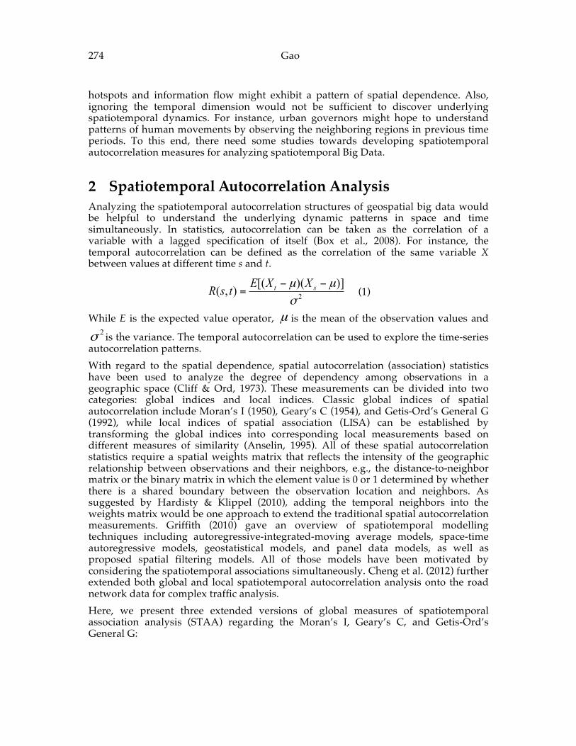
274 Gao
hotspots and information flow might exhibit a pattern of spatial dependence. Also, ignoring the temporal dimension would not be sufficient to discover underlying spatiotemporal dynamics. For instance, urban governors might hope to understand patterns of human movements by observing the neighboring regions in previous time periods. To this end, there need some studies towards developing spatiotemporal autocorrelation measures for analyzing spatiotemporal Big Data.
2 Spatiotemporal Autocorrelation Analysis Analyzing the spatiotemporal autocorrelation structures of geospatial big data would be helpful to understand the underlying dynamic patterns in space and time simultaneously. In statistics, autocorrelation can be taken as the correlation of a variable with a lagged specification of itself (Box et al., 2008). For instance, the temporal autocorrelation can be defined as the correlation of the same variable X between values at different time s and t.
2
)])([(),(σ
µµ −−= st XXEtsR (1)
While E is the expected value operator, µ is the mean of the observation values and 2σ is the variance. The temporal autocorrelation can be used to explore the time-series
autocorrelation patterns. With regard to the spatial dependence, spatial autocorrelation (association) statistics have been used to analyze the degree of dependency among observations in a geographic space (Cliff & Ord, 1973). These measurements can be divided into two categories: global indices and local indices. Classic global indices of spatial autocorrelation include Moran’s I (1950), Geary’s C (1954), and Getis-Ord’s General G (1992), while local indices of spatial association (LISA) can be established by transforming the global indices into corresponding local measurements based on different measures of similarity (Anselin, 1995). All of these spatial autocorrelation statistics require a spatial weights matrix that reflects the intensity of the geographic relationship between observations and their neighbors, e.g., the distance-to-neighbor matrix or the binary matrix in which the element value is 0 or 1 determined by whether there is a shared boundary between the observation location and neighbors. As suggested by Hardisty & Klippel (2010), adding the temporal neighbors into the weights matrix would be one approach to extend the traditional spatial autocorrelation measurements. Griffith (2010) gave an overview of spatiotemporal modelling techniques including autoregressive-integrated-moving average models, space-time autoregressive models, geostatistical models, and panel data models, as well as proposed spatial filtering models. All of those models have been motivated by considering the spatiotemporal associations simultaneously. Cheng et al. (2012) further extended both global and local spatiotemporal autocorrelation analysis onto the road network data for complex traffic analysis. Here, we present three extended versions of global measures of spatiotemporal association analysis (STAA) regarding the Moran’s I, Geary’s C, and Getis-Ord’s General G:
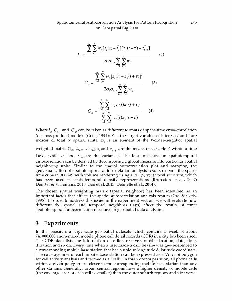
Spatiotemporal Autocorrelation Analysis for Pattern Recognition on Geospatial Big Data
275
∑∑
∑∑
= =+
=+
=
−+−
= N
i
N
jijtt
N
itjti
N
jij
st
w
ztzztzwI
1 1
1
__
1])(][)([
τ
τ
σσ
τ (2)
∑∑
∑∑
= =+
= =
+−
= N
i
N
jijtt
N
iji
N
jij
st
w
tztzwC
1 1
1
2
1
2
)]()([
τσσ
τ (3)
∑∑
∑∑
= =
= =
+
+
= N
iji
N
j
N
iji
N
jij
st
tztz
tztzwG
1 1
1 1
)()(
)()(
τ
τ (4)
Where stI , stC , and stG can be taken as different formats of space-time cross-correlation (or cross-product) models (Getis, 1991); Z is the target variable of interest; i and j are indices of total N spatial units; wij is an element of the k-order-neighbor spatial
weighted matrix (1st, 2nd,…, kth); _
tz and _
τ+tz are the means of variable Z within a time lagτ , while tσ and τσ +t are the variances. The local measures of spatiotemporal autocorrelation can be derived by decomposing a global measure into particular spatial neighboring units. Similar to the spatial autocorrelation plot and mapping, the geovisualization of spatiotemporal autocorrelation analysis results extends the space-time cube in 3D GIS with volume rendering using a 3D (x; y; t) voxel structure, which has been used in spatiotemporal density representations (Brunsdon et al., 2007; Demšar & Virrantaus, 2010; Gao et al. 2013; Delmelle et al., 2014). The chosen spatial weighting matrix (spatial neighbor) has been identified as an important factor that affects the spatial autocorrelation analysis results (Ord & Getis, 1995). In order to address this issue, in the experiment section, we will evaluate how different the spatial and temporal neighbors (lags) affect the results of three spatiotemporal autocorrelation measures in geospatial data analytics.
3 Experiments In this research, a large-scale geospatial datasets which contains a week of about 74, 000,000 anonymized mobile phone call detail records (CDR) in a city has been used. The CDR data lists the information of caller, receiver, mobile location, date, time, duration and so on. Every time when a user made a call, he/she was geo-referenced to a corresponding mobile base station that has a unique longitude & latitude coordinate. The coverage area of each mobile base station can be expressed as a Voronoi polygon for call activity analysis and termed as a “cell”. In this Voronoi partition, all phone calls within a given polygon are closer to the corresponding mobile base station than any other stations. Generally, urban central regions have a higher density of mobile cells (the coverage area of each cell is smaller) than the outer suburb regions and vice versa.
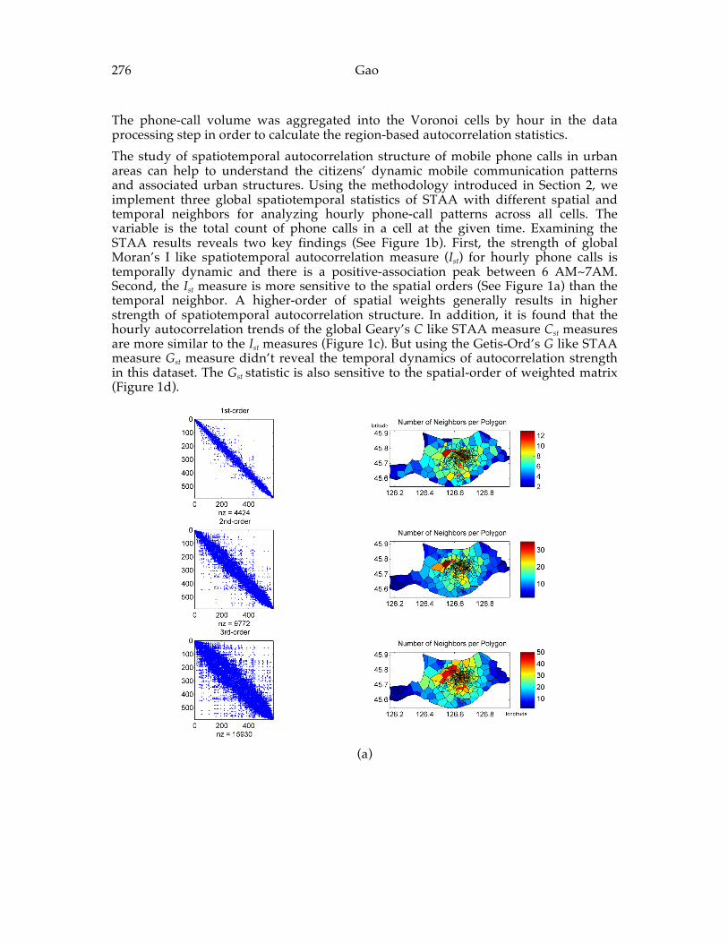
276 Gao
The phone-call volume was aggregated into the Voronoi cells by hour in the data processing step in order to calculate the region-based autocorrelation statistics. The study of spatiotemporal autocorrelation structure of mobile phone calls in urban areas can help to understand the citizens’ dynamic mobile communication patterns and associated urban structures. Using the methodology introduced in Section 2, we implement three global spatiotemporal statistics of STAA with different spatial and temporal neighbors for analyzing hourly phone-call patterns across all cells. The variable is the total count of phone calls in a cell at the given time. Examining the STAA results reveals two key findings (See Figure 1b). First, the strength of global Moran’s I like spatiotemporal autocorrelation measure (Ist) for hourly phone calls is temporally dynamic and there is a positive-association peak between 6 AM~7AM. Second, the Ist measure is more sensitive to the spatial orders (See Figure 1a) than the temporal neighbor. A higher-order of spatial weights generally results in higher strength of spatiotemporal autocorrelation structure. In addition, it is found that the hourly autocorrelation trends of the global Geary’s C like STAA measure Cst measures are more similar to the Ist measures (Figure 1c). But using the Getis-Ord’s G like STAA measure Gst measure didn’t reveal the temporal dynamics of autocorrelation strength in this dataset. The Gst statistic is also sensitive to the spatial-order of weighted matrix (Figure 1d).
(a)
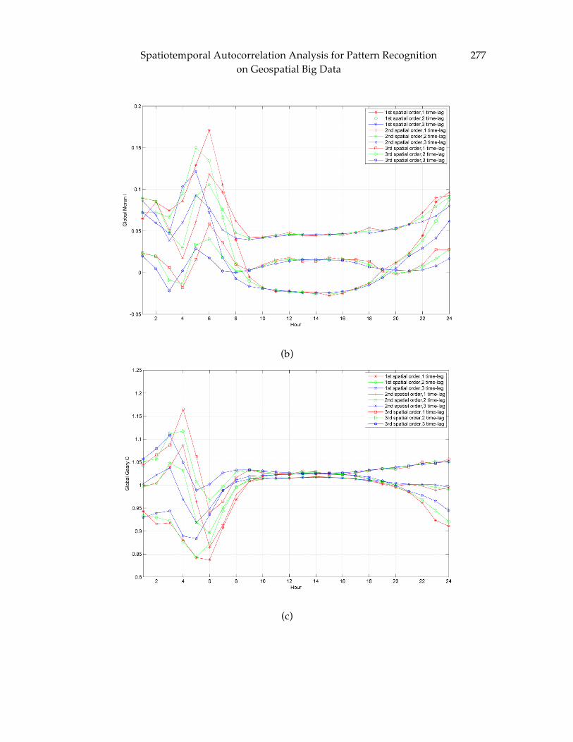
Spatiotemporal Autocorrelation Analysis for Pattern Recognition on Geospatial Big Data
277
(b)
(c)
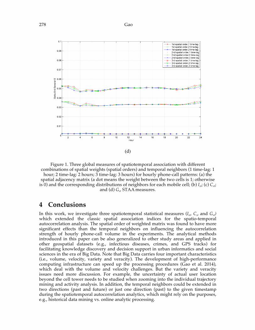
278 Gao
(d)
Figure 1. Three global measures of spatiotemporal association with different combinations of spatial weights (spatial orders) and temporal neighbors (1 time-lag: 1
hour; 2 time-lag: 2 hours; 3 time-lag: 3 hours) for hourly phone-call patterns: (a) the spatial adjacency matrix (a dot means the weight between the two cells is 1; otherwise
is 0) and the corresponding distributions of neighbors for each mobile cell; (b) Ist; (c) Cst; and (d) Gst STAA measures.
4 Conclusions In this work, we investigate three spatiotemporal statistical measures (Ist, Cst and Gst) which extended the classic spatial association indices for the spatio-temporal autocorrelation analysis. The spatial order of weighted matrix was found to have more significant effects than the temporal neighbors on influencing the autocorrelation strength of hourly phone-call volume in the experiments. The analytical methods introduced in this paper can be also generalized to other study areas and applied in other geospatial datasets (e.g., infectious diseases, crimes, and GPS tracks) for facilitating knowledge discovery and decision support in urban informatics and social sciences in the era of Big Data. Note that Big Data carries four important characteristics (i.e., volume, velocity, variety and veracity). The development of high-performance computing infrastructure can speed up the processing procedures (Gao et al. 2014), which deal with the volume and velocity challenges. But the variety and veracity issues need more discussion. For example, the uncertainty of actual user location beyond the cell tower needs to be studied when zooming into the individual trajectory mining and activity analysis. In addition, the temporal neighbors could be extended in two directions (past and future) or just one direction (past) to the given timestamp during the spatiotemporal autocorrelation analytics, which might rely on the purposes, e.g., historical data mining vs. online analytic processing.

Spatiotemporal Autocorrelation Analysis for Pattern Recognition on Geospatial Big Data
279
References [1] ANSELIN, L. Local indicators of spatial association—LISA Geographical analysis
27.2 (1995): 93-115. [2] BOX, G. E., JENKINS, G. M., AND REINSEL, G. C. Time series analysis:
forecasting and control. John Wiley & Sons, 2008. [3] BRUNSDON, C., CORCORAN, J. AND HIGGS, G. Visualising space and time in
crime patterns: A comparison of methods. Computers, Environment and Urban Systems 31.1 (2007): 52-75.
[4] CHENG, T., HAWORTH J., AND WANG J.Q. Spatio-temporal autocorrelation of road network data. Journal of geographical systems 14.4 (2012): 389-413.
[5] CLIFF, A. D., AND ORD, J. K. Spatial autocorrelation (Vol. 5). London: Pion, 1973.
[6] DELMELLE, E., DONY, C., CASAS, I., JIA, M., AND TANG, W. Visualizing the impact of space-time uncertainties on dengue fever patterns." International Journal of Geographical Information Science 28.5 (2014): 1107-1127.
[7] DEMŠAR, U., AND VIRRANTAUS, K. Space–time density of trajectories: exploring spatio-temporal patterns in movement data. International Journal of Geographical Information Science 24.10 (2010): 1527-1542.
[8] GAO, S., HU YJ, JANOWICZ, K., AND MCKENZIE, G. A spatiotemporal scientometrics framework for exploring the citation impact of publications and scientists. In Proceedings of the 21st ACM SIGSPATIAL International Conference on Advances in Geographic Information Systems, pp. 204-213. ACM, 2013.
[9] GAO, S., LI, L., LI, W., JANOWICZ, K., AND ZHANG, Y. Constructing gazetteers from volunteered big geo-data based on Hadoop. Computers, Environment and Urban Systems, doi:10.1016/j.compenvurbsys.2014.02.004
[10] GEARY, R. C. The contiguity ratio and statistical mapping. The incorporated statistician (1954): 115-146.
[11] GETIS, A., AND ORD, J. K. The analysis of spatial association by use of distance statistics. Geographical analysis 24.3 (1992): 189-206.
[12] GRIFFITH, D. A. Modeling spatio-temporal relationships: retrospect and prospect. Journal of Geographical Systems 12.2 (2010): 111-123.
[13] HARDISTY, F., AND KLIPPEL, A. Analysing spatio-temporal autocorrelation with LISTA-Viz. International Journal of Geographical Information Science 24.10 (2010): 1515-1526.
[14] MORAN, P. AP. Notes on continuous stochastic phenomena. Biometrika (1950): 17-23.
[15] ORD, J. K., AND GETIS, A. Local spatial autocorrelation statistics: distributional issues and an application. Geographical analysis 27.4 (1995): 286-306.

280 Gao
ADVANCING GEOGRAPHIC INFORMATION SCIENCE: CHAPTER 23
© by the author(s) Licensed under Creative Commons Attribution 4.0 License
281
Semantic Challenges for Geographic and Spatial Reasoning
Torsten Hahmann School of Computing and Information Science and National Center for Geographic Information
and Analysis, 5711 Boardman Hall, University of Maine, Orono, ME 04469-5711, USA
Extended Abstract
1 Semantics and Ontologies in GI Science Over the last 20 years, semantics, and ontologies as specific tools for capturing semantics, have played an increasingly significant role in Geographical Information Science as predicted in some early work [8, 9]. Since then much progress has been made in analyzing, understanding, and formally describing common geographic features, such as mountains and rivers [3, 22], and the foundational spatial relationships that underlie common sense descriptions of geographic space in the sense of [8], including qualitative relations that capture topology, direction, or shape (see [18] for an overview). This has significantly advanced the realization of a "Naïve Geography" [8], envisioned as consisting of two complementary sources:
(1) the cognitive and linguistic approach, investigating the terminology people use for spatial concepts; and (2) the formal approach concentrating on mathematically based models, which can be implemented on a computer.
Much of the ontological research in GI Science can be thought of as being guided by this idea of a naïve geography necessary for formalizing (in a computer-accessible representation) and automating the kind of common sense spatial reasoning that humans accomplish effortlessly.
2 Changing Requirements for Semantics of Geographic Terms But since 1995, the requirements for semantically-enabled geographic representations have significantly evolved, due to the explosion in available geographic data for which semantics are needed in order to not only access and find the data, but also to support
282 Hahmann
the increasingly automated selection, comparison, integration, and reasoning about the data. Examples include high-precision Lidar data of Earth surface as well as detailed land-use and transportation network data, and volunteered data about both natural and artificial (engineered) geographic features. This wealth of data has stretched the limits of simple common sense spatial reasoning that relies on fairly small, hand-crafted representations of spatial knowledge as common in the literature on Qualitative Spatial Reasoning [7, 18]. Instead, data-driven approaches { foremost machine learning { are now considered the holy grail of spatial intelligence. While early work using machine learning approaches tried to do without semantics by recognizing patterns in data or by integrating heterogeneous data sources without knowledge or respect of the underlying semantics, the results are incomprehensible to humans and thus offer little insights into how geographic objects or features are classified. Consequently, recent work on semantics for geographic terms has focused on injecting semantics into these data-driven approaches in order to obtain more meaningful and human-understandable results. Most notably, work on geographic data within the realm of the \Semantic Web" has focused on developing data standards for geographic data and on general patterns applicable to many data sources to facilitate integration and semantically conformant reasoning. However, much of the analysis and formalization of the necessary semantics has remained on a fairly general level by trying to accommodate all possible linguistic senses (meanings/uses/interpretations) of spatial relationships such as \in contact", \contains", \inside", \meets", or \overlaps", and of geographic terms such as \stream" or \mountain" instead of formally disambiguating between them. We believe that even more rigorous analysis, disambiguation, and formalization of semantics for spatial and geographic terms is needed { not necessarily for enabling data standardization and exchange, but for selecting appropriate senses of a specific uses of spatial and geographic terms. Human spatial and geographic language is highly ambiguous and dependent on specific contexts [1]; the more important it is to more precisely understand all the different senses and contextual conditions in which a specific spatial term is used1. We will outline three promising and interrelated challenges that need to be addressed to support semantically richer (semi-)automated geographic data integration and more sophisticated geographic reasoning and spatial intelligence. These critical challenges are motivated by the barriers/limitations we have encountered in our own attempts and closely related work [14, 15, 16, 21] about more sophisticated geographic representations of water bodies and water flows. They include:
1. Complementing semantics of two-dimensional abstract spatial concepts by semantics of physically-based spatial concepts, which requires a fuller integration of the vertical spatial dimension; 2. Developing computational spatial semantics separate from, yet in close relationship to, semantics of linguistic/cognitive uses of spatial terms as formalized in, e.g., [1]; 3. Developing computational ways to reason with multiple conceptualizations of space, in particular with different dimensional abstractions of physical/geographic space.
While this may go beyond narrower definitions of what constitutes geographic reasoning, which could be described as cartographic reasoning, we believe these are necessary for computationally solving many common sense spatial reasoning tasks that humans easily accomplish. The second and third challenge in particular
Semantic Challenges for Geographic and Spatial Reasoning 283
emphasize the computational aspects of semantics of geographic and spatial terms as opposed to the linguistic/cognitive aspects. The remainder will explain the three challenges in more detail.
2.1 Complementing Semantics of Two-‐‑Dimensional Spatial Concepts by Semantics of Physically-‐‑Based Spatial Concepts
This challenge aims at expanding the scope of na�ve geography by eliminating two assumptions from [8], namely the restriction of na�ve geography to essentially two (or 2 1/2) dimensions and the related assumption that for the purposes of na�ve geography the Earth is flat. The reason for this expansion is that the third, vertical dimension encodes much of the physics that governs space, such as when things stay put in place or fall, or where water collects and flows. To address this challenge, pure geographic (abstract spatial) knowledge must be joined with basic hydrographic, hydrologic, geologic, and physical knowledge, thereby enriching the spatial terms grounded in a two-dimensional abstraction of space by what the terms mean with respect to the physical terrain. First attempts such as [14, 15, 16, 21] are promising, but still need richer, explicit semantics that encodes what terrain features such as peaks and pits, ridge and slope lines, and channels in terms of what is \cartographically" (two-dimensionally) and physically possible or impossible: Where can these features be located and how do they spatially and physically relate to one another?
2.2 Developing Computational Spatial Semantics Traditionally, the emphasis of ontological work within GI Science has been on representing the exterior reality [9], which manifests itself in geographic terminology and language, as opposed to ontologies that create a digital reality. However, nowadays the digital reality is often more important than the exterior reality: what is not represented in a digital representation (such as a database, a digital map, or a collection of observations) of the world does, for many purposes, not exist: a stream that is not recorded is usually not called a stream and an unnamed mountain or mountain peak is not explicitly displayed as a peak on a map. However, if we understand the semantic intricacies and possible distinctions of terms such as \stream", \peak", or \mountain" to such a level of detail that we can encode them in a computer-understandable representation, we can also design corresponding algorithms to automatically extract them from digital representations such as the USGS National Map. Such extraction algorithms already exist, but their semantics is not explicitly represented outside the algorithms, so that the semantics of the extracted features remain detached from the implied semantics that underlie the algorithms. But developing algorithms based on explicit representations of the semantics of geographic features, we would no longer need to rely on humans to label these features as we currently do and we would no longer need to try to guess or infer which sense of a term such as \stream" or \mountain" was originally meant { the algorithms' underlying semantics are explicit about it. This would complement the currently applied techniques used to extract features, such as roads, buildings, or surface water from satellite or areal imagery by computationally identifying and describing more subtle geographic features. While these descriptions may not always match human descriptions, at least they are uniformly applied and thus comparable across the landscape. A prime example of how this could be accomplished could be set by linking the recently developed parallel treatment of various notions of spatial
284 Hahmann
containment/surrounding from [2, 15]. Their explicit linkage could yield linguistically grounded formal models of relations that express some form of spatial containment or surrounding.
2.3 Developing Computational Ways to Reason with Multiple Spatial Conceptualizations
This challenge is closely related to the observation that people often use multiple conceptualizations of space in different contexts or even simultaneously [8]. This seems to be one of least understood and maybe most complicated aspects of human spatial and geographic reasoning, which has not yet been addressed satisfactorily. The related observation that humans often use multiple levels of detail in different contexts or simultaneously is now much better understood, thanks to work such as [4, 5, 20]. However, these two aspects must be treated in unison: different conceptualizations of space are often tied to specific scales at which they are applied. This is exhibited most clearly in how humans conceptualize geographic features dimensionally different based on application or required level of detail. For example, finding a route from A to B can be accomplished using a fairly coarse representation, whose nest elements are individual segments between intersections of the road networks, without any information about the width of the road or the change in elevation. But for finding a hiking route, the elevation may contain critical information that needs to be incorporated as a third dimension. Equally, when planning a route for an oversized truck, the width of roads is important, requiring not just a linear but a full three-dimensional model that incorporates distances, width and height clearance above the roads. As one prerequisite for this challenge, formal spatial semantics for these dimensionally varying conceptualizations of space are necessary. Early explorations of the role of dimension in spatial relations [19, 6, 10, 11] showed some promise but were not further pursued. In recent work, we picked up this line of research [17, 13] and showed that cognitive simple yet powerful sets of relations that respect and incorporate the different dimensions of spatial features can be formally defined and hold significant potential for modeling the ubiquitous geographic features represented using point, vector/line, or polygonal/region representations.
References [1] Bateman, J. A., Hois, J., Ross, R., and Tenbrink, T. A linguistic ontology of space
for natural language processing. Artif. Intell. 174, 14 (2010), 1027{1071. [2] Bennett, B., Chaudhri, V., and Dinesh, N. A vocabulary of topological and
containment relations for a practical biological ontology. In Conf. on Spatial Inf. Theory (COSIT-13) (2013), Springer.
[3] Bennett, B., Mallenby, D., and Third, A. An ontology for grounding vague geographic terms. In Conf. on Formal Ontology in Inf. Systems (FOIS-08) (2008).
[4] Bittner, T. Granularity in reference to spatio-temporal location and relations. In Florida Artif. Intell. Research Society Conf. (FLAIRS-15) (2002), pp. 466{470.
[5] Bittner, T., and Smith, B. A theory of granular partitions. In Foundations of Geographic Information Science, M. Duckham, M. F. Goodchild, and M. F. Worboys, Eds. Taylor & Francis, 2003, pp. 124{158.
Semantic Challenges for Geographic and Spatial Reasoning 285
[6] Clementini, E., Di Felice, P., and van Oosterom, P. A small set of formal topological relationships suitable for end user interaction. In Symp. on Large Spatial Databases (SSD'93) (1993), LNCS 692, Springer, pp. 277{295.
[7] Cohn, A. G., and Renz, J. Qualitative Spatial Representation and Reasoning. In Handbook of Knowledge Representation, F. van Harmelen, V. Lifschitz, and B. Porter, Eds. Elsevier, 2008.
[8] Egenhofer, M. J., and Mark, D. M. Naive Geography. In Conf. on Spatial Inf. Theory (COSIT-95) (1995), LNCS 988, Springer, pp. 1{15.
[9] Frank, A. U. Spatial Ontology: A Geographical Information Point of View. In Spatial and Temporal Reasoning, O. Stock, Ed. Kluwer, 1997, pp. 135{154.
[10] Galton, A. Taking dimension seriously in qualitative spatial reasoning. In Europ.Conf. on Artif. Intell. (ECAI-96) (1996), pp. 501{505.
[11] Gotts, N. M. Formalizing commonsense topology: the INCH calculus. In Int. Symp. On Artif. Intell. and Math. (1996), pp. 72{75.
[12] Gruninger, M., Hahmann, T., Hashemi, A., Ong, D., and Ozgovde, A. Modular first-order ontologies via repositories. Applied Ontology 7, 2 (2012), 169-209.
[13] Hahmann, T. A Reconciliation of Logical Representations of Space: from Multidimensional Mereotopology to Geometry. PhD thesis, Univ. of Toronto, Dept. of Comp. Science, 2013.
[14] Hahmann, T., and Brodaric, B. The void in hydro ontology. In Conf. on Formal Ontology in Inf. Systems (FOIS-12) (2012), IOS Press, pp. 45{58.
[15] Hahmann, T., and Brodaric, B. Kinds of full physical containment. In Conf. on Spatial Inf. Theory (COSIT-13) (2013), Springer.
[16] Hahmann, T., Brodaric, B., and Gr�uninger, M. Interdependence among material objects and voids. In Conf. on Formal Ontology in Inf. Systems (FOIS-14) (2014), IOS Press. Conf. on Formal Ontology in Inf. Systems (FOIS-14). 4
[17] Hahmann, T., and Gr�uninger, M. A na�ve theory of dimension for qualitative spatial relations. In Symp. on Logical Formalizations of Commonsense Reasoning (CommonSense 2011) (2011), AAAI Press.
[18] Hahmann, T., and Gr�uninger, M. Region-based Theories of Space: Mereotopology and Beyond. In Qualitative Spatio-Temporal Representation and Reasoning: Trends and Future Directions, S. M. Hazarika, Ed. IGI, 2012, pp. 1{62.
[19] McKenney, M., Pauly, A., Praing, R., and Schneider, M. Dimension-refined topological predicates. In Conf. on Advances in Geographic Information Systems (GIS-05) (2005), ACM, pp. 240{249.
[20] Rector, A., Rogers, J., and Bittner, T. Granularity, scale and collectivity: When size does and does not matter. J. Biomed. Inform. 39 (2006), 333{349.
[21] Sinha, G., Mark, D., Kolas, D., Varanka, D., Romero, B. E., Feng, C.-C., Usery, L. E., Liebermann, J., and Sorokine, A. An ontology design pattern for surface water features. In 8th Int. Conf. on Geographic Information Science (GIScience 2014) (2014).
[22] Smith, B., and Mark, D. M. Do mountains exist? Towards an ontology of landforms. Environment and Planning B 30, 3 (2003), 411{428.

286 Hahmann
ADVANCING GEOGRAPHIC INFORMATION SCIENCE: CHAPTER 24
© by the author(s) Licensed under Creative Commons Attribution 4.0 License
287
Spatial Data and Map Service Development: Mirroring the Path of a
Discipline Indy Hurt
Mapzen – need address
Extended Abstract
1 Introduction Today’s web map services are developed by collections of software engineers, database engineers, content and sourcing teams, data scientists, cartographers, geographers, planners, researchers, and editors. There are clear parallels between research themes that have developed over time in the discipline of geography and the development of web map services. Some challenges and criticisms that accompanied periods of geography continue to manifest themselves. The compressed timeline associated with web map development can amplify some challenges while advancing technologies and globalism can eliminate others. More cross-pollination between industry and academia could prove to be a fruitful partnership with respect to addressing challenges. To succeed, the academy must be up to the challenge of preparing students for these opportunities. Open source development enables transparency, while open data aims to encourage community around a shared resource. There are some barriers associated with the current reward system in academia that make it difficult to participation in the agile software development commonly associated with open source software [1]. While traditional publishing track records currently dominate the tenure-track review process, the overall number of tenure positions is declining [2, 3]. Graduate students are taking notice and considering other career opportunities for this and may other reasons [4].
2 Trajectory of Map Services Web map services are advancing rapidly, fueled by an ever-growing list of players. In 2016, MapQuest’s web service celebrates a 20-year anniversary. Google Maps celebrated 10 years in 2015. OpenStreetMap reached this same milestone in 2014.
288 Hurt
Other notable services include Nokia’s Here, and Microsoft’s Bing Maps both changing hands entirely or in part in 2015 with a consortium of German car makers [5] and ride share app Uber [6], respectively. TomTom and Apple Maps have a data partnership while both maintain independent web map services. Russian search engine Yandex also offers a global map service; while countless other web map services like Géoportail, MapMyIndia, and Arealis provide specialized local content. Global web map services are an interesting subset. A common first step to building one begins with a data model that can be populated with spatial and tabular data. A web map service might be a series of services that work collectively to provide various types of routing, flexible search able to return addresses and features, personal reminders, display of personalized data, and other useful location based features. Reminiscent of classical geography identified as the period between 600 BC and 1770 AD, today’s players focus on general and regional geography as the foundation for their service when they enter the playing field. This is commonly referred to as the basemap. One significant challenge during the classical geography period revolved around limitations in mobility. While mobility is not as much of a challenge today, collecting and maintaining the fundamental basemap data on a global scale presents new challenges. A comprehensive map of the world grows in complexity with each added theme of information. Errors in sparsely populated areas garner as much visibility and potential negative publicity as any other area. Examples include routes that end in the middle of nowhere [7], routes to points of interest that end at residential addresses [8, 9], and numerous examples of missing localities or inaccurate representations of borders and place names [10, 11]. A fierce competition is on to secure market share, and a significant component to winning the hearts and minds of users is the ability to continuously present accurate reliable spatial data. Unfortunately, the users are most concentrated in economically viable regions leaving other areas without a user base to demand rich content. Public participatory GIS and volunteered geographic information efforts have made contributions in this area. While some of these efforts suffer from data quality issue [12], the Humanitarian OpenStreetMap Team continues to address feedback and supports further development of rich content during and long after crisis events [13]. The era of modern geography, characterized as the period between 1770 and 1970, ushered in the dawn of university geography departments. This time period, strengthened by standardized empirical observations, took place alongside the period of the Enlightenment. A strong emphasis on the value of science has filtered its way into the map service development activities of today, but not just any science. Today’s activities revolve around data science specifically targeted towards big data. With web map services, there are opportunities for geographers and other spatially oriented domain experts to conduct the kinds of analyses they have been doing for years, just on a much larger scale [14]. Is today’s spatial data analytics the reincarnation of the quantitative revolution of the 1950’s and 1960’s? There are some interesting similarities. The quantitative revolution saw analysis conducted with tools and data that were not easily accessible to the general population. Desktop and web based GIS software environments with graphical user interfaces were not yet developed. Big data is similarly inaccessible to store on a personal computer, most cannot be accessed freely in the cloud, and it cannot be manipulated without a reasonable amount of technical skill. For this reason, data scientists often double as software engineers. They contribute to a large code-
Spatial Data and Map Service Development: Mirroring the Path of a Discipline
289
base, build web applications, store and retrieve large datasets, and employ statistical methods with proprietary and open source tools. Data that individuals contribute in the form of data logs from sensors onboard personal devices remain an incomprehensible mystery to most. These logs help drive analysis and improvements to maps in many ways. They uncover patterns, reveal collective behaviors, and help businesses target goods and services more effectively in ways that are often tied to profitability. Large spatial data providers like TomTom boast probe data consisting of 6 trillion data points with an additional 6 billion new data points collected every day from their community of users and other sources [15]. Applications like Waze initially turned street data acquisition into a game. As the user base grew, users voluntarily agreed to share personal tracking information to improve traffic and routing analytics. These closed systems provide a traffic service in exchange for the data, but users have no way to download and process their own personal data. As the commodification of web map services continues to grow, an effort to identify exploitative activity around the collection and dissemination of spatial data and services remains an important area of inquiry. Acceptance of terms of service agreements does not mean that privacy is dead. Data from the Pew Research Center indicates that people do care about privacy and how their personal data is used [16]. Critical GIS was the response to the quantitative revolution, and this history continues to repeat itself. Through publications and continued scholarship, the Friday Harbor meetings of 1993 and 2014 lend voices to issues that remain prominent today. The 1993 meeting was sponsored by the NCGIA and was organized by Nick Chrisman, John Pickles, Tom Poiker and Eric Sheppard [17]. Notable publications from the 1993 meeting include Ground Truth: the social implications of Geographic Information Systems edited by John Pickles, and a special issue of Cartography and GIS featuring papers from the meeting. The 2014 meeting returned to Friday Harbor to revisit these topics and renew engagement between the scholars of critical GIS and quantitative spatial analysis. Humanist, Marxist, feminist, poststructuralist, postcolonial, antiracist, and queer geographers cautioned against quantitative geography and its inability to effectively address several areas of concern that could not be understood from a purely mathematical approach [18]. We could be turning the page. The open source community is attracting a broader audience by putting data back in the control of contributors. Open source analysis tools are becoming easier to use. While access to cloud computing still comes at a cost, the cost is declining at a rate of 33% each year and data storage costs are declining at a rate of 38% each year [19]. Amazon Web Services has made all Landsat 8 scenes from 2015 available through a joint effort with the U.S. Geological Survey and NASA. Could the opportunity for individuals to capture, access, and analyze the extensive amount of personal data they generate also become accessible in the same manner? Advanced technical skill sets are still key to interpreting information in an endless supply of data, but the potential to overcome this barrier is easier to imagine. GIS went through a similar transformation, and continues to become more accessible.
3 Conclusion The similarities between the evolution of the discipline of geography and the trajectory of individual web map services are evident. Entities embark on the task of building a basemap. This stage is dominated by data discovery of regional geographies.
290 Hurt
Simultaneously or in close succession, services are built on top of the basemap. These services include real time traffic, transit, multi-modal routing, spatially oriented personalized advertising, location sharing, and many others. Data collected from onboard sensors enhance these services while bringing privacy concerns to the surface. Data scientists sift through an endless sea of data looking for patterns and opportunities. The individuals contributing the data are often far removed from the analysis and decisions being made as a result of the analysis. These activities lend strength to critical GIS discussions and the support of a more equitable distributed system. Are we closer to this goal than we were 20 years ago? Arguably yes, we are, based on the advances in the development and distribution of open source data and tools. The final piece of the puzzle requires more inroads into the development process. Geographers familiar with critical GIS research themes and statistical methods specific to spatial data have a lot to contribute to the fast paced industry growing around web map services. Software engineers with computer science backgrounds are dominating the landscape of web map service development. Opportunities to change this must start with earlier engagement between geographers, computer scientists, and designers. While software engineering skills are highly valuable, it should not be a requirement for participation. The ability to communicate with software engineers presents a tremendous amount of value. Application building benefits from the cohesive relationship between both software engineering and design.
4 References [1] Sui, D., Opportunities and Impediments for Open GIS. Transactions in GIS, 2014.
18(1): p. 1-24. [2] Jaschik, S. The Disappearing Tenure-Track Job. 2009 5/12/2009 [cited 2015
8/27/2015]; Available from: https://www.insidehighered.com/news/2009/05/12/workforce.
[3] Kezar, A. and D. Maxey. The Changing Academic Workforce. 2013 [cited 2015 8/27/2015]; Available from: http://agb.org/trusteeship/2013/5/changing-academic-workforce.
[4] Mason, M.A., M. Goulden, and K. Frasch, Why graduate studetns reject the fast track. Academe, 2009. 95(1): p. 11-16.
[5] Bartz, D. German carmakers win U.S. antitrust approval to buy Nokia maps. 2015 9/2/2015 [cited 2015 9/10/2015]; Available from: http://www.reuters.com/article/2015/09/02/us-nokia-here-automakers-antitrust-idUSKCN0R21SO20150902.
[6] Wilhelm, A. Uber Acquires Part of Bing's Mapping Assets, Will Absorb Around 100 Microsoft Employees. 2015 6/29/2015 [cited 2015 9/10/2015]; Available from: http://techcrunch.com/2015/06/29/uber-acquires-part-of-bings-mapping-assets-will-absorb-around-100-microsoft-employees/ - .acdjk8:yvg4.
[7] Thompson, N. Apple Maps flaw could be deadly, warn Australian police. 2012 12/11/2012 [cited 2015 8/12/2015]; Available from: http://www.cnn.com/2012/12/10/tech/apple-maps-australia-flaw/.
[8] Burnham, K. 6 Memorable Google Maps Mishaps. 2011 7/27/2011 [cited 2015 8/12/2015]; Available from: http://www.cio.com/article/2405903/internet/6-memorable-google-maps-mishaps.html - slide2.
Spatial Data and Map Service Development: Mirroring the Path of a Discipline
291
[9] Reed, B. Apple's iOS Maps pushes woman to brink of madness. 2014 2/28/2014 [cited 2015 8/12/2015]; Available from: http://bgr.com/2014/02/28/worst-apple-maps-mistakes/.
[10] Sutter, J. Google Maps border becomes part of international dispute. 2010 11/5/2010 [cited 2015 8/12/2015]; Available from: http://www.cnn.com/2010/TECH/web/11/05/nicaragua.raid.google.maps/.
[11] Reed, B. Apple, Google map apps inflame international feud between Japan and Korea over tiny disputed island. 2012 11/4/2012 [cited 2015 8/12/2015]; Available from: http://bgr.com/2012/11/04/apples-maps-app-korea-japan-island-dispute/.
[12] American Red Cross, OpenStreetMap Damage Assessment Review Typhoon Haiyan (Yolanda) Interim Report. 2014, American Red Cross: American Red Cross. p. 8.
[13] Soden, R. and L. Palen, From Crowdsourced Mapping to Community Mapping: The Post-earthquake Work of OpenStreetMap Haiti, in COOP 2014 - Proceedings of the 11th International Conference on the Design of Cooperative Systems, 27-30 May 2014, Nice (France), C. Rossitto, et al., Editors. 2014, Springer International Publishing. p. 311-326.
[14] Wright, D., Have I Been a Data Scientist from the Start?, in Esri Insider. 2015, Esri: Esri.
[15] TomTom. Custom Probe Counts - Traffic density information for location-based analysis. 2012 6/2012 [cited 2015 9/9/2015]; Available from: http://www.tomtom.com/lib/doc/licensing/I.CPC.EN.pdf.
[16] Madden, M. Privacy and Cybersecurity: Key findings from Pew Research. 2015 [cited 2015 8/1/2015]; Available from: http://www.pewresearch.org/key-data-points/privacy/.
[17] Craig, W., T. Harris, and D. Weiner. Empowerment, Marginalization and Public Participation GIS. Report of Varenius Workshop 1998 2/1/1999 [cited 2015 9/8/2015]; Available from: http://www.ncgia.ucsb.edu/varenius/ppgis/PPGIS98_rpt.html.
[18] Kwan, M.-P. and T. Schwanen, Quantitative Revolution 2: The Critical (Re)Turn. The Professional Geographer, 2009. 61(3): p. 283-291.
[19] Hagel, J. KPCB Internet Trends 2014. [SlideShare] 2014 5/28/2014 [cited 2015 9/9/2015]; Available from: http://www.slideshare.net/kleinerperkins/internet-trends-2014-05-28-14-pdf.

292 Hurt
ADVANCING GEOGRAPHIC INFORMATION SCIENCE: CHAPTER 25
© by the author(s) Licensed under Creative Commons Attribution 4.0 License
293
An Ontology-based Geospatial Database for Identifying Geographical
Change Jeon-Young Kang1, Jinmu Choi2, Thomas Bittner1
1 Department of Geography, University at Buffalo, NY, USA 2 Department of Geography, Kyung Hee University, Seoul, South Korea
Extended Abstract
Abstract: This paper aims to explore the spatiotemporal change of administrative units of Seoul. We built a domain ontology for administrative units of Seoul based on BFO 2.0, and integrated the ontology with geospatial database. In particular, formal ontology was used to clarify administrative units, their properties, and their relative processes. Formal relations of spatiotemporal changes were considered, as well. The ontology-based geospatial database can contribute to identifying geographical changes over time via SPARQL.
Keywords: Geographical Changes, BFO 2.0, Formal Ontology, Geospatial Database.
1 Introduction Geographical entities change over time, so do their appearance and/or properties. Interestingly, administrative units in new urban areas, which look static at first glance, also undergo changes over time; some units are expanded, shrank, destroyed, and newly established. These changes may give a rise to change units’ properties (e.g., name, postcode, area) and parthood relations to others. Geospatial database and formal ontology have been used to identify and trace such changes. Geospatial databases play an important role in recording changes of geometry through time. Recorded changes then can be accessed by using spatiotemporal queries [5, 11, 12]. Geospatial database also serves to keep track of the identity of geographical entities that may undergo significant changes (e.g., merge, split) [10]. Formal ontology has been used to clarify specifications of geographical entities and their changes over time by providing classification schemes for entities, their relationships to others, as
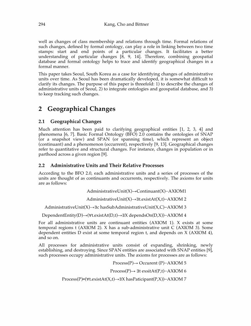
294 Kang, Cho and Bittner
well as changes of class membership and relations through time. Formal relations of such changes, defined by formal ontology, can play a role in linking between two time stamps: start and end points of a particular changes. It facilitates a better understanding of particular changes [8, 9, 14]. Therefore, combining geospatial database and formal ontology helps to trace and identify geographical changes in a formal manner. This paper takes Seoul, South Korea as a case for identifying changes of administrative units over time. As Seoul has been dramatically developed, it is somewhat difficult to clarify its changes. The purpose of this paper is threefold: 1) to describe the changes of administrative units of Seoul, 2) to integrate ontologies and geospatial database, and 3) to keep tracking such changes.
2 Geographical Changes
2.1 Geographical Changes Much attention has been paid to clarifying geographical entities [1, 2, 3, 4] and phenomena [6, 7]. Basic Formal Ontology (BFO) 2.0 contains the ontologies of SNAP (or a snapshot view) and SPAN (or spanning time), which represent an object (continuant) and a phenomenon (occurrent), respectively [9, 13]. Geographical changes refer to quantitative and structural changes. For instance, changes in population or in parthood across a given region [9].
2.2 Administrative Units and Their Relative Processes According to the BFO 2.0, each administrative units and a series of processes of the units are thought of as continuants and occurrents, respectively. The axioms for units are as follows:
AdministrativeUnit(X)→Continuant(X)−AXIOM1
AdministrativeUnit(X)→∃t.existAt(X,t)−AXIOM 2
AdministrativeUnit(X)→∃c hasSubAdministrativeUnit(X,C)−AXIOM 3
DependentEntity(D)→(∀t.existAt(D,t)→∃X dependsOn(D,X))−AXIOM 4 For all administrative units are continuant entities (AXIOM 1). X exists at some temporal regions t (AXIOM 2). X has a sub-administrative unit C (AXIOM 3). Some dependent entities D exist at some temporal region t, and depends on X (AXIOM 4), and so on. All processes for administrative units consist of expanding, shrinking, newly establishing, and destroying. Since SPAN entities are associated with SNAP entities [9], such processes occupy administrative units. The axioms for processes are as follows:
Process(P)→ Occurent (P)−AXIOM 5
Process(P)→ ∃t exsitAt(P,t)−AXIOM 6
Process(P)≡(∀t.existAt(X,t)→∃X hasPaticipant(P,X))−AXIOM 7
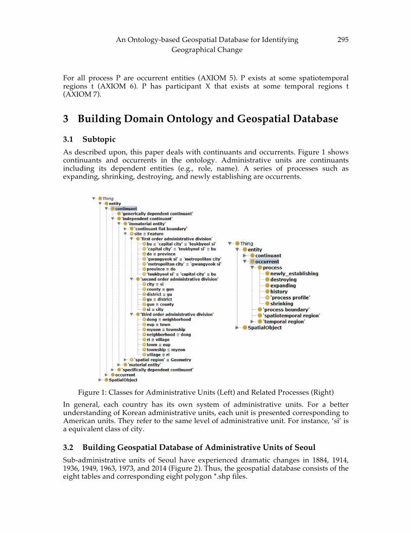
An Ontology-‐‑based Geospatial Database for Identifying Geographical Change
295
For all process P are occurrent entities (AXIOM 5). P exists at some spatiotemporal regions t (AXIOM 6). P has participant X that exists at some temporal regions t (AXIOM 7).
3 Building Domain Ontology and Geospatial Database
3.1 Subtopic As described upon, this paper deals with continuants and occurrents. Figure 1 shows continuants and occurrents in the ontology. Administrative units are continuants including its dependent entities (e.g., role, name). A series of processes such as expanding, shrinking, destroying, and newly establishing are occurrents.
Figure 1: Classes for Administrative Units (Left) and Related Processes (Right) In general, each country has its own system of administrative units. For a better understanding of Korean administrative units, each unit is presented corresponding to American units. They refer to the same level of administrative unit. For instance, ‘si’ is a equivalent class of city.
3.2 Building Geospatial Database of Administrative Units of Seoul Sub-administrative units of Seoul have experienced dramatic changes in 1884, 1914, 1936, 1949, 1963, 1973, and 2014 (Figure 2). Thus, the geospatial database consists of the eight tables and corresponding eight polygon *.shp files.
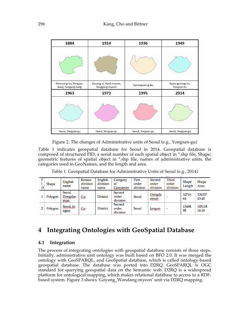
296 Kang, Cho and Bittner
Figure 2. The changes of Administrative units of Seoul (e.g., Yongsan-gu) Table 1 indicates geospatial database for Seoul in 2014. Geospatial database is composed of structured FID; a serial number of each spatial object in *.shp file, Shape; geometric features of spatial object in *.shp file, names of administrative units, the categories used in GeoNames, and the length and area.
Table 1. Geospatial Database for Administrative Units of Seoul (e.g., 2014)
4 Integrating Ontologies with GeoSpatial Database
4.1 Integration The process of integrating ontologies with geospatial database consists of three steps. Initially, administrative unit ontology was built based on BFO 2.0. It was merged the ontology with GeoSPARQL, and GeoSpatial database, which is called ontology-based geospatial database. The database was ported into D2RQ. GeoSPARQL is OGC standard for querying geospatial data on the Semantic web. D2RQ is a widespread platform for ontological mapping, which makes relational database to access to a RDF-based system. Figure 3 shows ‘Goyang_Wondang-myeon’ unit via D2RQ mapping.
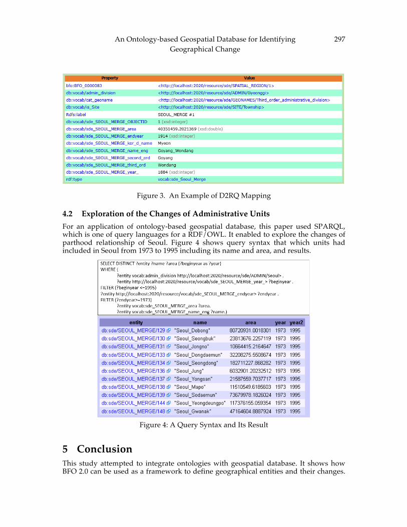
An Ontology-‐‑based Geospatial Database for Identifying Geographical Change
297
Figure 3. An Example of D2RQ Mapping
4.2 Exploration of the Changes of Administrative Units For an application of ontology-based geospatial database, this paper used SPARQL, which is one of query languages for a RDF/OWL. It enabled to explore the changes of parthood relationship of Seoul. Figure 4 shows query syntax that which units had included in Seoul from 1973 to 1995 including its name and area, and results.
Figure 4: A Query Syntax and Its Result
5 Conclusion This study attempted to integrate ontologies with geospatial database. It shows how BFO 2.0 can be used as a framework to define geographical entities and their changes.
298 Kang, Cho and Bittner
It finds out in what ways ontology-based geospatial database can be utilized in tracing geographical changes through time. This study carried out spatiotemporal exploration as well. The approach of this study contributes to formally identifying administrative units’ changes over time, and supporting such changes.
References [1] BITTNER, T. From top-level to domain ontologies: Ecosystem classifications as a
case study, Spatial Information Theory, (2007), 61-77. [2] BITTNER, T., DONNELLY, M. AND SMITH, B. A Spatio-temporal ontology for
geographic information integration, International Journal of Geographical Information Science 23, 6 (2009), 765-798.
[3] BITTNER, T. On the integration of Regional Classification and Delineation Systems into The National Map, Catographica: The International Journal for Geographic Information and Geovisualization 45, 2 (2010), 127-139.
[4] BITTNER, T. Vagueness and the trade-off between the classification and delineation of geographic regions-an ontological analysis, International journal of Geographical information Science 25, 5 (2011), 825-850.
[5] CHOI, J., SEONG, J. C., KIM, B., AND USERY, L. Innovations in Individual Feature History Management- The Significance of Feature-based Temporal Model. GeoInformatica 12 (2008), 1-20.
[6] GALTON, A. Space, Time, and the Representation of Geographical Reality. TOPOI 20, (2001), 173-187
[7] GALTON, A. On What Goes On: The Ontology of Processes and Events, Formal Ontology in Information Systems. In FOIS ’06: Proceedings of the 4th International Conference on Formal Ontology in Information Systems (Baltimore, MD, USA, 2006), IOS Press, pp. 4-11
[8] GANGEMI, A. GUARINO, N., MASOLO, C., OLTRAMARI, A. AND SCHNEIDER, L., Sweetening Ontologies with DOLCE, AI Magazine 23, 3 (2003), 13-24
[9] GRENON, P. AND SMITH, B. SNAP and SPAN: Towards Dynamic Spatial Ontology, Spatial Cognition and Computation 4, 1 (2004), 69-103.
[10] HORNSBY, K. AND EGENHOFER, M. J. Identity-based change: a foundation for spatio-temporal knowledge representation, International journal of Geographical Information Science 14, 3 (2000), 207-224.
[11] KAUPPINEN, T., VAATAINEN, J. AND HYVONEN, E. Creating and Using Geospatial Ontology Time Series in a Semantic Cultural Heritage Portal, In ESWC ’08: Proceedings of the 5th European Semantic Web Conference (Tenerife, Canary Islands, Spain, 2008), Springer Berlin Heidelberg, pp.110-123
[12] SENGUPTA, R. AND YAN, C. A hybrid spatio-temporal data model and structure (HST-DMS) for efficient storage and retrieval of land use information, Transactions in GIS 8, 3 (2004), 351-366.
[13] SMITH, B., ALMEIDA, M., BONA, J., BROCHHAUSEN, M., CEUSTER, W., COURTOT, M., DIPERT, R., GOLDFAIN, A., GRENON, P., HASTINGS, J., HOGAN, W., JACUZZO, L., JOHANSSON, I., MUNGALL, C., NATALE, D.,

An Ontology-‐‑based Geospatial Database for Identifying Geographical Change
299
NEUHAUS, F., ROVETTO, A.P.R., RUTTENBERG, A., RESSLER, M., SCHULZ, S. Basic Formal Ontology 2.0 Draft, (2012)
[14] WORBOYS, M. F. Modelling and Changes and Events in Dynamic Spatial Systems with Reference to Socio-economic Units. In Life and Motion of Socio-Economic Units, ESF GISDATA series, A. U. Frank, J. Raper, and J.-P. Cheylan, Eds. Taylor and Francis, London, 2001, pp. 129-138

300 Kang, Cho and Bittner
ADVANCING GEOGRAPHIC INFORMATION SCIENCE: CHAPTER 26
© by the author(s) Licensed under Creative Commons Attribution 4.0 License
301
Geospatial Resource Management in Disaster Stricken Area in Chile:
GEOSS Approach Lucia C. Lovison-Golob
Afriterra Foundation, 400 Commonwealth Avenue, Boston, 02425, MA, U.S.A.
Extended Abstract
Abstract: The management of geospatial resources in Chilean areas stricken by disasters within GEOSS (Global Earth Observations System of Systems), a framework of content providers and a source of decision-support tools for geospatial data users, is presented. The GEO (Global Earth Observations) program, to which GEOSS belongs, encompasses nine societal benefit areas, one being the disasters area. The Architecture Implementation Pilot (AIP- GEOSS) project for disasters in Chile allows geospatial data and their associated metadata to be accessed, searched, and discovered through a geoportal, based on a distributed service-oriented architecture (SOA), called GEOSS Common Infrastructure (GCI). The project involves the following research areas: data sharing and collaboration among people, management of large volumes of data, their ontologies and models, as well as inclusion of geospatial data from Earth observation sensors into augmented reality, disaster robotics, and virtual reality applications as a means to reduce societal vulnerability to disasters.
Keywords: GEOSS (Global Earth Observations System of Systems), disasters, geospatial products, and interoperable web services.
1 Introduction The GEO (Global Earth Observations) program, to which GEOSS (Global Earth Observations System of Systems) belongs, started in 2005 and encompasses nine societal benefit areas: agriculture, biodiversity, climate, disasters, ecosystems, energy, health, water, and weather. The Chile Architecture Implementation Pilot (AIP-GEOSS) project covers one of the societal benefit areas, with several disaster scenarios in Chile, and involves the capacity-building of technical experts to decrease the vulnerability of
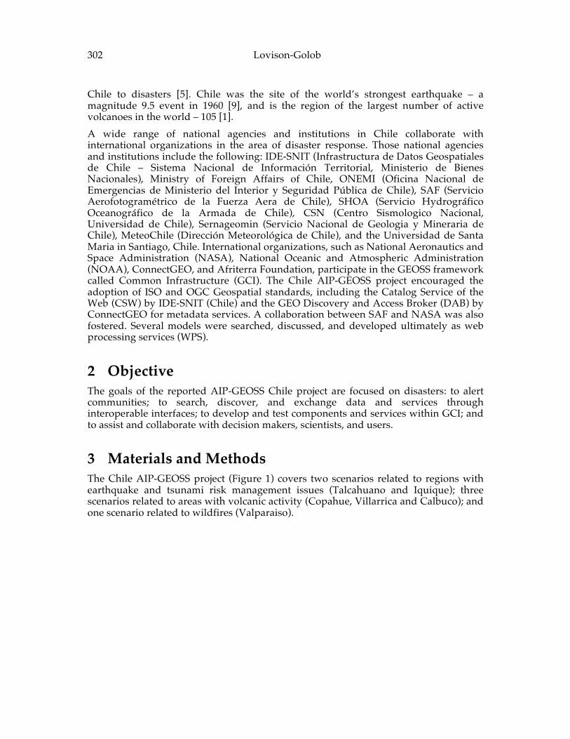
302 Lovison-‐‑Golob
Chile to disasters [5]. Chile was the site of the world’s strongest earthquake – a magnitude 9.5 event in 1960 [9], and is the region of the largest number of active volcanoes in the world – 105 [1]. A wide range of national agencies and institutions in Chile collaborate with international organizations in the area of disaster response. Those national agencies and institutions include the following: IDE-SNIT (Infrastructura de Datos Geospatiales de Chile – Sistema Nacional de Información Territorial, Ministerio de Bienes Nacionales), Ministry of Foreign Affairs of Chile, ONEMI (Oficina Nacional de Emergencias de Ministerio del Interior y Seguridad Pública de Chile), SAF (Servicio Aerofotogramétrico de la Fuerza Aera de Chile), SHOA (Servicio Hydrográfico Oceanográfico de la Armada de Chile), CSN (Centro Sismologico Nacional, Universidad de Chile), Sernageomin (Servicio Nacional de Geologia y Mineraria de Chile), MeteoChile (Dirección Meteorológica de Chile), and the Universidad de Santa Maria in Santiago, Chile. International organizations, such as National Aeronautics and Space Administration (NASA), National Oceanic and Atmospheric Administration (NOAA), ConnectGEO, and Afriterra Foundation, participate in the GEOSS framework called Common Infrastructure (GCI). The Chile AIP-GEOSS project encouraged the adoption of ISO and OGC Geospatial standards, including the Catalog Service of the Web (CSW) by IDE-SNIT (Chile) and the GEO Discovery and Access Broker (DAB) by ConnectGEO for metadata services. A collaboration between SAF and NASA was also fostered. Several models were searched, discussed, and developed ultimately as web processing services (WPS).
2 Objective The goals of the reported AIP-GEOSS Chile project are focused on disasters: to alert communities; to search, discover, and exchange data and services through interoperable interfaces; to develop and test components and services within GCI; and to assist and collaborate with decision makers, scientists, and users.
3 Materials and Methods The Chile AIP-GEOSS project (Figure 1) covers two scenarios related to regions with earthquake and tsunami risk management issues (Talcahuano and Iquique); three scenarios related to areas with volcanic activity (Copahue, Villarrica and Calbuco); and one scenario related to wildfires (Valparaiso).
Geospatial Resource Management in Disaster Stricken Area in Chile: GEOSS Approach
303
Figure 1 -- Testing areas of the Architecture Implementation Pilot of the Global Earth Observation System of Systems (AIP-GEOSS) in Chile.
On February 27, 2010, a magnitude 8.8 earthquake struck Talcahuano and generated a 2.30-meter tsunami. About 500 people were killed, and about $30 billion in damage was caused [5]. In Iquique, a magnitude 8.2 earthquake occurred on April 1, 2014, triggered a 2.1-meter tsunami, but only partially ruptured the seismogenic fault [3] . Volcanic activity occurred in Copahue on May 27, 2013, and additional volcanic activity was observed in October and December 2014; the Villarrica volcano erupted on March 3, 2015, causing mudslides and snow melts near Pucon; and the Cabulco volcano started to erupt on April 22, 2015, after about 41 years of dormancy [7]. This volcanic activity resulted in the evacuation of about 3,000 people living within a 25-kilometer radius from the volcano in the south rim of Copahue; about 3,500 people from Villarrica, although about 15,000 people living in rural areas near Villarrica suffered from water shortages; and about 4,000 people in a 20-kilometer radius around the Calbuco volcano. The wildfires in Valparaiso adversely impacted several endemic flora and fauna and, in May 2015, covered an area of about 11,428 hectares [6]. About one year earlier, on April 15, 2014, wildfires in urban Valparaiso killed at least 16 people.
4 Discussion The life cycle of risk management for disasters areas is characterized by three phases: prevention, response, and recovery. In the Chile AIP-GEOSS project, these three phases
304 Lovison-‐‑Golob
of disasters are considered within a GEOSS framework for metadata and geospatial data. For each area, four levels of alerts are used: green, yellow, amber, and red. At the amber alert level, the mobilization of people exposed to a disaster is triggered, and people are evacuated. The Chilean emergency agency, ONEMI, makes broadcasts of alerts and notifications using all means, including radio, VHF, and social media. The Chile AIP-GEOSS project was established to suggest more effective approaches for making alerts in relation to the scale and type of disasters. For example, the AIP-GEOSS project has recommended that alerts include the visualization of the geospatial data, with the adoption of geospatial standards, and with a basic map of the disaster event. The Chile AIP-GEOSS project works on four main subareas: increasing people skills and knowledge in the geospatial field, developing metadata, imagery, and models. In addition, the project works to improve harmonization and increase integration of geospatial data. In fact, these data are originally in different types and formats dependent on the different sensor characteristics, and are afterwards converted into interoperable web services through standard interfaces. The project also estimates the hazards in the test areas and includes socio-economic data and services. These aspects are very important in relation to the rapid urbanization of once remote regions. The goal of this project is to prove that service oriented architecture (SOA) can be successfully and effectively applied to disaster areas, and to reduce the disaster risks for the benefit of societies in a rapid changing environment. Furthermore, Chile AIP-GEOSS focuses on the research that needs to be undertaken to address disaster response models for wild fires; and for estimating volcanic risk. With respect to seismic and tsunami risks, the Chile AIP-GEOSS project includes prevention, response, and recovery policies and scenarios. In the prevention phase, the major emphasis is on capacity building, while in the response phase of the disaster cycle, mobilization starts with alerts and notifications, followed by the increasing mobilization of all resources at local, regional, national and international level. Depending of the type of disaster, there it will be necessary to classify as soon as possible the affected areas as total or partial losses, and to designate the shelter areas. With respect to volcanic risk, more research needs to be undertaken on evaluating the timing and exact location of the hazard, whether an eruption, ash cloud, mudslide, or episode of lake acidification, and on assessing the vulnerability of urban and rural populations. In this way, decisions can be made about the extent of the area to be evacuated and the duration of the evacuation. For urban and rural populations, the project plans to use the population density grid and the urban settlement points with the 2010 census for Chile [4, 5]. The goal of this effort is to estimate the web services and geospatial products that need to be registered to GEOSS Common Infrastructure (GCI) in order to reduce the magnitude of disaster risks and to suggest additional policies for managing disaster responses. Ultimately, the Chile AIP-GEOSS project will develop applications and services useful in responding to disaster events, some already available at the Group on Earth Observations geoportal [2]. Future activity of the Chile AIP-GEOSS project for disasters will probably be part of an initiative for Disaster Risk Reduction and the Sustainable Development Goals (SDGs), which will be lead by the Japanese government as part of the post-2015 development agenda, and will involve other countries in the Americas. Part of the Chile AIP-GEOSS project is to address the parameters needed to measure different GEOSS activities for each type and scale of disaster. While many governments, non-profit and academic organizations as well as private entities will
Geospatial Resource Management in Disaster Stricken Area in Chile: GEOSS Approach
305
focus on providing data and services in case of disasters to users through networks such as internet and radio, people will see during the upcoming decades, especially in the private sector, the offering of Virtual Reality (VR) devices and services, such as Facebook Oculus, Google Cardboard, Microsoft HoloLens, Sony Morpheus, and China’s Baofeng Mojing. Chile AIP-GEOSS project already shows the direction, although needs to integrate the data and services from “humanitarian” drones, as demonstrated in the 2015 Nepal earthquake [8], in order to provide more timely and comprehensive data and services for humanitarian actions and decision making. The project also shows the increased need for GIScience to implement augmented reality applications, such as GEOSS-type applications with a graphic layer added to a map or an image on mobile devices, such as Google and/or SONY glasses.
5 Conclusions The effort of the Chile AIP-GEOSS project for disaster risk reduction will benefit not only Chile but also other countries stricken by disasters. So far, the Chile AIP-GEOSS project has resulted in strengthening the knowledge and skills of disaster relief experts while respecting cultural differences, in developing better policies in the management of disasters, and in developing and sharing geospatial resources and associated metadata to decrease the vulnerability of potential victims and property. In the future, pilot projects will be focused on building more geospatial applications and products, on managing increasingly large volumes of data and on including geospatial data from Earth observation sensors within a framework, currently represented by GEOSS, into augmented reality, disaster robotics, and virtual reality applications as a means to reduce our vulnerability to disasters worldwide. GIScience can nurture knowledge and skills of people who increasingly will not have a formal education on the management of geospatial data and products. For example, there is an increasing number of mobile users who want to manage their imagery even during a disaster: these people wants both to develop maps and applications with a geospatial component, and to generate themselves geospatial data. For more technical people, GIScience needs to focus on developing new ontological, spatio-temporal, software architecture models that also take into account privacy; on proposing and testing integration and analysis of big volumes of data, while experimenting with new technology and sensors.
References [1] GLOBAL VOLCANISM PROGRAM, http://volcano.si.edu/reports_weekly.cfm
(last accessed 2015-05-09). [2] GROUP ON EARTH OBSERVATIONS,
http://www.geoportal.org/web/guest/geo_home_stp (last accessed 2015-05-09).
[3] HAYES, G.P, HERMAN, M.W., BARNHART, W.D., FURLONG, K.P., RIQULME, S., BENZ, H.M., BERGMAN, E., BARRIENTOS, S., EARLE, P.S., AND SAMSONOV, S. Warning signs of the Iquique earthquake. Nature, 512 (2014), 295-298.
306 Lovison-‐‑Golob
[4] ISTITUTO NACIONAL DE ESTADISTICAS, http://www.ine.cl/canales/chile_estadistico/familias/censos.php (last accessed 2015-05-09).
[5] LOVISON L., L. PARODI, A. MONETT, P. DUEŃAS, S. FRYE, S. NATIVI, and M. SANTORO, A GEOSS Architecture Implementation Pilot Project for Disasters in Chile, submitted to PE & RS, (2015) ASPRS.
[6] ONEMI, http://www.onemi.cl/incendio-en-valparaiso/(last accessed 2015-05-09).
[7] SERNAGEOMIN, http://www.sernageomin.cl/volcan.php?iId=3 (last accessed 2015-05-09).
[8] SKY NEWS, https://www.youtube.com/watch?v=WwIw1-voHKQ&ab_channel=SkyNews (last accessed 2015-05-09).
[9] U.S. GEOLOGICAL SURVEY, http://earthquake.usgs.gov/earthquakes/world/events/1960_05_22_articles.php (last accessed 2015-05-09).
ADVANCING GEOGRAPHIC INFORMATION SCIENCE: CHAPTER 27
© by the author(s) Licensed under Creative Commons Attribution 4.0 License
307
Using Geo-Spatial Knowledge for Good Governance
Laxmi Ramasubramanian CUNY Institute for Sustainable Cities, Hunter College, City University of New York,
695 Park Avenue, Room 1217 HE, New York, NY
Extended Abstract
Abstract: Although GIS applications to support collaborative planning and problem solving have greatly expanded information access and individual empowerment, the democratizing power of GIS continues to create new contradictions and tensions as it continues to be deployed across institutional settings. Both technical and non-technical barriers limit the use of geo-spatial knowledge in engaging ordinary citizens to participate in real world planning and policy-making. In addition, participatory processes themselves have moved online, further complicating how geospatial technologies and methods are used. The abstract highlights some of these contradictions and challenges GIScientists to develop better tools for participatory planning both in face-to-face and online settings.
Keywords: Participatory GIS, co-production, community, empowerment.
1 Introduction The process of engaging citizens in planning and policy-making is fraught with difficulties. In the United States, as citizen participation has become more institutionalized, it has become disconnected from its original goals of increasing access and larger questions of social justice and is often used to fulfil procedural obligations or requirements [2, 7]. From the outset, many GIScience scholars have proposed and demonstrated the use of GIS principles, methods and geo-visualization to explain (and solve) complex socio-spatial problems. A smaller cohort of scholars has examined the social, political, and institutional aspects of GIS use in different realworld settings [1, 4, 5]. In addition to the academic discourse [6, 11], a Community of Practice (CoP) loosely defined as Public Participation-GIS (PPGIS) has also emerged [10]. Both academics and practitioners aligned with this CoP have emphasized the
308 Ramasubramanian
democratizing power of GIS while highlighting some of the contradictions associated with its use. Nearly twenty years after the first discussions about GIS and Society debates [3], some of the tensions associated with GIS use in democratic decision-making have been resolved at the same time that new contradictions have emerged. This extended abstract examines some of these contradictions and suggests some directions for future research in this area. In particular, the focus of this abstract is planning and policymaking across spatial scales in big cities, wherein planning includes city management and heterarchic governance processes.
2 GIS and the Rise of Accidental Activists Over the past decade, geo-visualization and communications technologies have created a virtual space for accidental activists. The phrase, “there’s an app for that” is more than a cute tagline – it exemplifies how individuals are using their creative abilities and technological prowess to identify and create new niche markets. The power of an application like See, Click, Fix for instance, is situated in its promise of immediate gratification in practical and emotional terms. The end user with a smart phone can vent or complain about something that disturbs their sense of well-being while navigating their everyday urban environment. The application is designed for reporting of non-emergency issues such as potholes or non-functioning street lights. End users can demand accountability from a variety of government agencies with a single click of a button and feel personally empowered because they are able to act for themselves and their fellow citizens, albeit, with minimal effort. Both practising planners and GIS experts recognize See, Click, Fix, as one of the many examples of planning apps that use the power of GIS, GPS, as well as digital photo/videography to solve urban problems. The app, its purpose, and its deployment offer a lot of promise allowing citizens and responsible government agencies to quickly identify trouble spots and distribute scare resources in a timely manner. But, if one pauses to consider the issue a little longer, more difficult questions emerge, highlighting some of the contradictions created by the new ubiquitous, all pervasive, yet invisible, GIS. See, Click, Fix represents only one particular aspect of planning and should not be confused with the complexity of the planning enterprise as a whole. Some questions that need to be answered include: Who has access to skills or the expertise to use See, Click, Fix? Does personal information provided by the end user (knowingly or unknowingly) get recorded and stored? Will it be used to keep track of end users? Are government agencies more sensitive to complaints about certain types of problems? Are they more responsive to problems that occur in certain locations? Are digital tools being developed only to make our citizens hyper-aware about the failures of government (when things don’t work)? If so, what are the consequences? For instance, a recent NYC council hearing on the shooting death of an unarmed man by a police officer in a public housing complex cited neglect of routine maintenance on NYCHA (NYC public housing) properties. In these situations, does it demoralize members of a particular segment of public to realize that they can complain and complain about some problems and nothing will get fixed? Alternatively, does it make them believe the popular American refrain that government itself is somehow the problem? More importantly, how do these and other digital tools shape the larger democracy project that is presently being shaken and transformed in a myriad of ways that are both exhilarating and confusing?
Using Geo-‐‑Spatial Knowledge for Good Governance 309
3 Community Empowerment Remains Elusive Goal The past two decades have seen rapid shifts in GIS adoption and use in different institutional settings, coupled with changes in the production, consumption, and use of GIS-data. While hyper-connected netizens use their “smart” phones to write emails, send text messages, “tweet”, update their FaceBook profiles, and use the built-in GPS systems to find their way around strange cities and towns, low-skilled workers looking for work in the service sector will find that their jobs are far away from their places of residence; their commutes are long; and that the kind of work they do precludes tele-commuting. In the quest to find affordable housing and transportation or dependable child care options, these workers know that there is very little to be gained from getting onto a computer, even if they had access to one. At the most, these workers could find out bus routes and schedules, but the service on the ground is unlikely to be prompt or reliable. It can be argued that GIS-based decisions have done little to overcome deep and enduring barriers of race, class, gender, age, and privilege. It is true that in 2015, societies around the world have made great strides in providing data access. We operate in a data-rich environment which can be mined because of cheap computing power. However, information access does not automatically encourage participation or civic engagement. Participation takes motivation, commitment, time, specialized skills, and above all, trust or confidence that the act of participating will make a difference in the resolution of the problem. Geo-spatial tools developed for the public to encourage them to be involved in planning or policymaking are still not the norm. The dominant tools or apps are focused on recreation, gaming, or adventure, and have limited benefit in addressing socio-spatial inequalities. Government-funded tool developments such as the Climate Resilience Toolkits are actually not easily used in community conversations. Sophisticated geodesign software extensions such as CommunityViz have a steep learning curve and typically require skilled experts to conduct and explain the analyses to citizens. Twenty years on, the most rigorous spatial analysis techniques, the fanciest computers, and the best data are still no match to combat institutional inertia, interdepartmental rivalries, and other non-technical barriers to successful GIS implementation to solve community problems.
4 The Challenge to the GIScientists The origins of geospatial science are grounded in a set of beliefs about planning and policy-making. Chief among them is the value placed on examining problems holistically, within particular spatial and temporal contexts. Geospatial science research has also valued the analysis of diverse types of data and information. Last but not the least, is the belief among geospatial scientists that decisions made using GIS can ensure transparency and accountability. As geospatial science and technologies have grown and matured, the early ideals of the GIScientists are finally coming to fruition. The new genre of geospatial tools are user friendly and accessible, increasing opportunities for active citizen involvement. Citizens in the USA, western Europe, as well as many other countries of the global south have become sophisticated consumers of information and producers of highly localized data and information about their own neighborhoods and communities. Rather than accept the results for “official” studies, today’s citizens are more likely to use social networks to assemble and gather data to confirm or refute official analyses
310 Ramasubramanian
and make rational counter-arguments when necessary. Citizen activism is now educational and affordable. It appears to empower individuals more than groups, but there is progress being made [9]. Yet, the nature of planning and policy-making is changing, with much of the “work” moving online. The emphasis in government-led planning is on e-participation and the idea that there are highly customized approaches to engaging different publics – a laudable goal. Technical (manipulating the technologies) and non-technical (group communication) skills associated with the use of online tools affect e-participation. Citizens require some technical skills to participate in processes that actively use information technologies and their by-products such as maps or graphic renderings. At the local level, the absence of technical skills is often countered through a well designed group process that is educational and informative. In many instances, group processes with marginalized communities use popular education techniques. In small groups, an individual’s lack of a particular technical skill (for example, reading a land use plan) can create some collaborative moments as other participants explain and share their understanding, thereby fulfilling one of the goals of a participatory decision making process, i.e., to develop the capacity of the participants to organize, analyze, and discuss concepts to the level required by the particular endeavor in which they are involved. It is unclear how this problem will be managed with physically dispersed population that may come together only virtually (e.g., through site-to-site video conferences). It is reasonable to speculate that inter-personal and group communication skills are critical in facilitating and managing e-participation processes. The staff in planning agencies has to be trained to meet the new demands and challenges associated with e-participation. While techno-enthusiasts abound, the technology cannot be used to drive the planning process. Thus, the facilitator (agency staff person or hired consultant) must be able to determine the needs of the planning process and identify the appropriate technology to suit that purpose. A technical expert unable to speak the language of community groups further compounds these problems, which results in the breakdown of already fragile participatory processes [8]. It may be reasonable to explore the idea of a set of principles that should be included in e-participation applications for planning. E-participation applications should:
1. use stable technologies and be available free or at low cost to end users; 2. be easily understandable to potential users; 3. recognize and accommodate different levels of technical and spatial literacy, specifically allowing for individual users to learn at their own pace; 4. allow citizens to “interact” with the data with as much freedom as possible in order to generate different scenarios and alternatives, wherein the underlying models and formulas governing application design can also be scrutinized; 5. include the capability for citizens to download data and analyses from the official planning organization’s website to their own computers. 6. include the capability for citizens to upload their own data sets. Application must allow upload of photographs, audio clips, video, sketch maps, or computer-rendered designs;
Using Geo-‐‑Spatial Knowledge for Good Governance 311
7. link scenario developments, wherever possible, to outcomes and impact assessments that can be described in quantitative and qualitative terms; 8. contain robust context-sensitive help that facilitates peer to peer information sharing and assistance in real-time; and, 9. allow and support extensive archiving and documentation.
References [1] ELWOOD, S. Information for Change: The social and political impacts of
Geographic Information Technologies, PhD dissertation, Department of Geography, University of Minnesota. Available from University of Minnesota Libraries, 2000.
[2] INNES, J., AND. BOOHER, D. Reframing Public Participation: Strategies for the 21st century, Planning Theory & Practice, 5, 4 (2004), pp. 419-436
[3] HARRIS, T., AND WEINER, D. GIS and Society: The Social Implications of How People, Space, and Environment are represented in GIS. Scientific Report for the Initiative 19 Specialist Meeting, March 2-5, 1996, South Haven, Minnesota
[4] MASSER, I., AND ONSRUD, H (Eds.) Diffusion and Use of Geographic Information Technologies. (Dordrecht, Netherlands, 1993), Kluwer
[5] NYERGES, T., COUCLELIS, H., AND MCMASTER, R (Eds) The SAGE Handbook of GIS and SOCIETY, (London, England, 2010), Sage
[6] OBERMEYER, N. The Evolution of Public Participation GIS, Cartography and GIS, 25, 2 (1998), pp.65-66
[7] RAMASUBRAMANIAN, L., AND QUINN, A. Visualizing Alternative Urban Futures: Using Spatial Multimedia to Enhance Community Participation and Policymaking, in M. Campagna (Ed.). GIS and Sustainable Development. (Florida, USA, 2006), CRC Press, pp. 467-486
[8] RAMASUBRAMANIAN, L. Nurturing community empowerment: Participatory decision-making and community-based problem solving using GIS, in Onsrud, H. and M. Craglia (Eds.) Geographic Information Research: Transatlantic Perspectives. (London, England, 1999), Taylor & Francis, pp. 87-102
[9] RAMSUBRAMANIAN, L. GIS and Public Participation, (Heidelberg, Germany, 2010), Springer
[10] SAWICKI, D., & PETERMAN, D, 2002. Surveying the extent of PPGIS practice in the United States, in Craig, W, T. Harris & D. Weiner (Eds.) Community Participation and Geographic Information Systems (New York, NY, USA, 2002), Taylor & Francis, pp. 17-36
[11] SIEBER, R. Public Participation GIS: A Literature Review and Framework, Annals of the Association of American Geographers, 96,3 (2006), pp. 491-507

312 Ramasubramanian
ADVANCING GEOGRAPHIC INFORMATION SCIENCE: CHAPTER 28
© by the author(s) Licensed under Creative Commons Attribution 4.0 License
313
Geomorphological Delineation using Computer Vision to Support
Automated Mapping Paulo Raposo
Department of Geography, The Pennsylvania State University, University Park, Pennsylvania 16802, USA
Extended Abstract
Abstract: This article presents an automated workflow for finding generalized areas of relatively rough terrain using GIS, remote sensing, and computer vision techniques, taking a digital elevation model (DEM) as input. The method supports automated delineation of morphometrically self-similar areas as polygons and is demonstrated here using a portion of the Sahara Desert exhibiting large sand dunes, modeled in ASTER GDEM data.
Keywords: Geomorphometry, DEMs, terrain roughness, computer vision, segmentation, polygonization, labeling.
1 Introduction Cartography has always benefitted from the evolution of graphic media, with clear examples seen in the invention of the printing press and, much later, computerization. Map media continue to evolve, seen in today’s proliferation of location-aware smartphones. Maps and spatial data in the coming decades will take forms afforded by computational innovations. We predict that spatial data will be stored in increasingly decentralized repositories, and that it will increasingly not be stored at all, but generated on an immediate, as-needed basis from distributed sensor networks. Automated cartography of instantaneously synthesized data with become more and more important, as will computer or artificial intelligence (AI) interpretation of geography. While basic automated maps made today are of arguably passable quality (say, for GPS receivers used in car navigation), the methods programmed into GIS systems for producing instantaneous maps will have to improve to deal with the increase in diversity, resolution, and complexity we can expect from future data. GIS
314 Raposo need to be better able to deal with fundamental cartographic modelling and design issues such as generalization, topological consistency, legibility, and feature detection. These challenges parallel many of those seen by researchers in computer vision, and methods used in that field seem promising for application in geographic information science (GIScience). We present an automated workflow for finding generalized areas of relatively rough terrain using GIS, remote sensing, and computer vision techniques, taking a digital elevation model (DEM) as input. Specifically, we derive surface roughness and segment this image using mean-shift segmentation [11], a robust, non parametric, mode-seeking, iterative classification algorithm developed in information theory and adapted to pixel data in the computer vision context [7]. Our method allows for automated delineation of morphometrically self-similar areas as polygons. We believe this ability is useful in numerous applications, particularly with respect to computer-automated navigation (e.g., polygonal patches of rough land can be detected and avoided by computer navigation applications using simple point-in-polygon tests). The method also helps in a common contemporary map making problem, being the delineation of landforms [10] such as rock formations, mountain ranges, or canyons, as polygons. Having such areas polygonized is advantageous over points or lines in that automated label-placing algorithms are given greater legitimate, spatial flexibility [16, 2, 19]. Our method is automated using Python scripting in an open-source desktop GIS environment using The Geospatial Data Abstraction Library (GDAL version 1.7.0), Orfeo Tool Box (version 4.4), and QGIS (version 2.8.1), and is demonstrated here in a portion of the Sahara Desert exhibiting large sand dunes, modelled in ASTER GDEM data.
2 Background Strong methodological similarities exist between raster GIS, remote sensing, and computer vision analyses. Image content can vary considerably between the fields in aspects including subject, acquisition method, and geometry (e.g., orthoimages vs. perspective images). Still, because analysis in all fields begins with pixels, analytical problems and algorithms nearly always take the form of mathematical calculations on fields of regularly-spaced values, taking the spatial relations between values as important context [12, 4, 3, 1]. For example, many GIS or remote sensing analysis procedures involve the “reclassification” of pixels (e.g., different kinds of land cover), while many computer vision procedures perform image “segmentation” to differentiate pixels in figure-ground relationships in a scene. Similarly, both fields make use of kernel operations on the premise that local pixels influence the variable being calculated at the pixel in question because their nearness, whether on the Earth’s surface or in the visual scene, makes them important to the model. Geomorphometry and terrain generalization procedures to date have increasingly bridged methodological gaps between GIScience and related computer graphics fields. Several studies have presented methods for identifying landforms and classifying landscapes using DEM data [6, 18, 14, 8]. Other studies have devised and reviewed various derivative surfaces or surface parameters that can be used to characterize a surface [15, 17, 21, 20]. Methods in geomorphometry typically deal directly with elevation and its first and second derivatives in the vertical and horizontal directions (i.e., slope, profile curvature, aspect, plan curvature) [9].
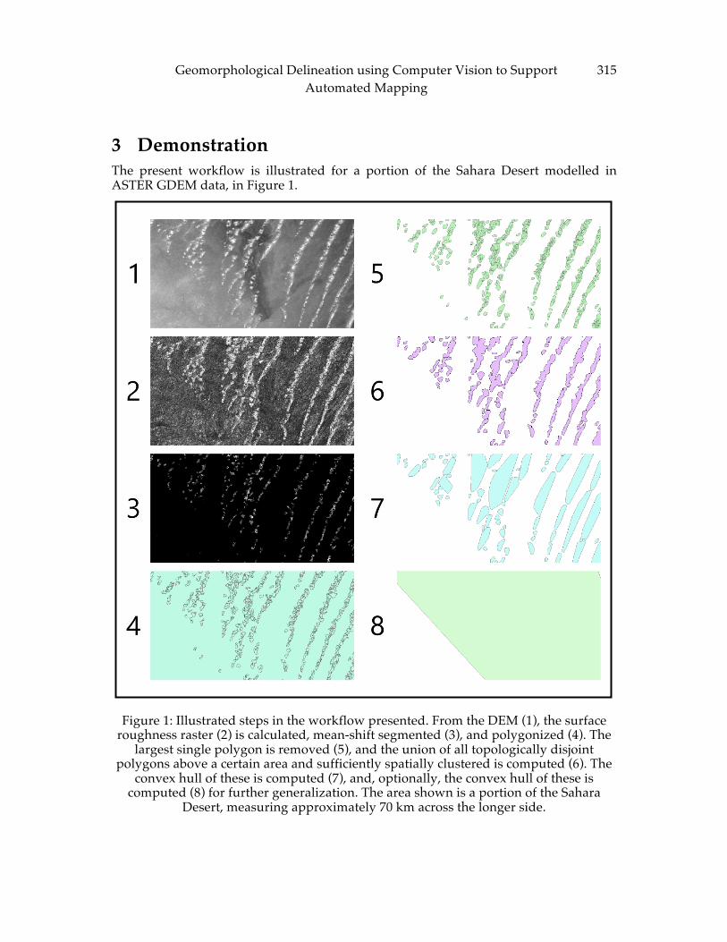
Geomorphological Delineation using Computer Vision to Support Automated Mapping
315
3 Demonstration The present workflow is illustrated for a portion of the Sahara Desert modelled in ASTER GDEM data, in Figure 1.
Figure 1: Illustrated steps in the workflow presented. From the DEM (1), the surface roughness raster (2) is calculated, mean-shift segmented (3), and polygonized (4). The
largest single polygon is removed (5), and the union of all topologically disjoint polygons above a certain area and sufficiently spatially clustered is computed (6). The
convex hull of these is computed (7), and, optionally, the convex hull of these is computed (8) for further generalization. The area shown is a portion of the Sahara
Desert, measuring approximately 70 km across the longer side.
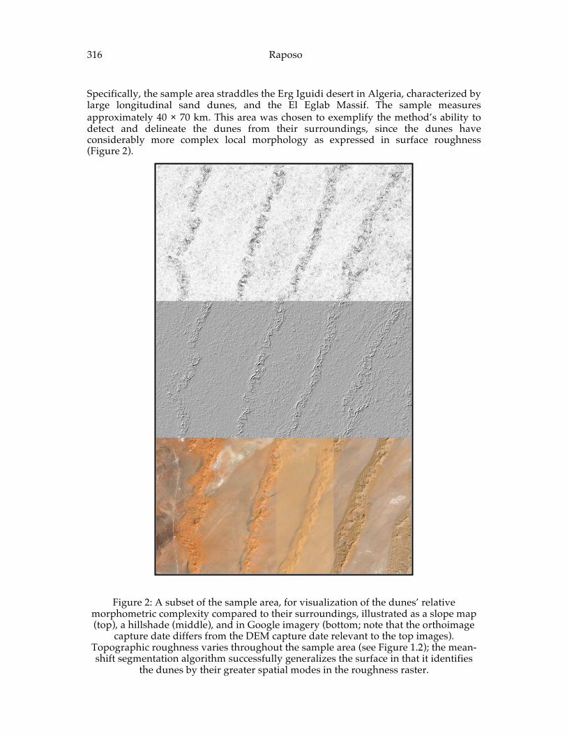
316 Raposo Specifically, the sample area straddles the Erg Iguidi desert in Algeria, characterized by large longitudinal sand dunes, and the El Eglab Massif. The sample measures approximately 40 × 70 km. This area was chosen to exemplify the method’s ability to detect and delineate the dunes from their surroundings, since the dunes have considerably more complex local morphology as expressed in surface roughness (Figure 2).
Figure 2: A subset of the sample area, for visualization of the dunes’ relative morphometric complexity compared to their surroundings, illustrated as a slope map (top), a hillshade (middle), and in Google imagery (bottom; note that the orthoimage
capture date differs from the DEM capture date relevant to the top images). Topographic roughness varies throughout the sample area (see Figure 1.2); the mean-shift segmentation algorithm successfully generalizes the surface in that it identifies
the dunes by their greater spatial modes in the roughness raster.
Geomorphological Delineation using Computer Vision to Support Automated Mapping
317
Processing begins with generating surface roughness [20] using the gdaldem module of GDAL (Figure 2.1 and 2.2). Next, the roughness raster is segmented using the mean shift algorithm implemented in Orfeo ToolBox (Figure 1.3). The segmented (i.e., clustered) raster is polygonized (Figure 1.4) in QGIS such that each unique, contiguous region identified in the raster with a unique integer is given its own polygon, with individual features permitted to exist across multiple polygons (i.e., features are multi-part). The largest single polygon feature, representing the most common topographic roughness in the sample area and therefore the “ground” as opposed to the “figure”, is removed from the polygon set (Figure 1.5). The remaining polygons are thresholded for area and proximity to other polygons (i.e., spatial clustering), and these have their convex hulls calculated. These hulls are unified into a single union polygon (Figure 1.6), and this multi-part polygon is dissolved into individual feature polygons for each topologically disconnected polygon. The convex hulls of the remaining polygons are computed (Figure 1.7), yielding generalized footprints of where anomalously rough terrain occurs in the sampled landscape. A further level of generalization of the rough area is achieved if the convex hull that surrounds the previous hull polygons is computed (Figure 1.8). The use of convex hulls ensures that dunes are “over-identified”, meaning some portions of polygonized “dunes” do not exhibit the same membership to a local statistical mode as identified by the mean-shift algorithm. While convex hulls are one way to simplify the geometry of an object, they may not always be geographically appropriate. The described workflow can be easily implemented with other derivative surfaces such as slope, openness [21], sky view factor [13, 5], terrain ruggedness index, or topographic position index [20], among others. These derived surfaces should be mathematically normalized, whether intrinsically or otherwise, so that the analysis is not as sensitive to the distribution of values in the sampled surface.
References [1] ATKINSON, P. M. (2004). Resolution Manipulation and Sub-Pixel Mapping. In S.
M. De JONG & F. D. Van der MEER (Eds.), Remote Sensing Image Analysis: Including The Spatial Domain (pp. 51-70). Boston: Kluwer Academic Publishers.
[2] BAE, W. D., ALKOBAISI, S., NARAYANAPPA, S., VOJTECHOVSKY, P., and BAE, K. "Optimizing map labeling of point features based on an onion peeling approach." Journal of Spatial Information Science 2. (2011) pp. 3-28.
[3] BLASCHKE, T., LANG, S., and HAY, G. J., Eds. Object-Based Image Analysis: Spatial Concepts for Knowledge-Driven Remote Sensing Applications. Lecture Notes in Geoinformation and Cartography, Springer, (2008).
[4] BLASCHKE, T. and STROBL, J. "What's Wrong With Pixels? Some Recent Developments Interfacing Remote Sensing and GIS." Geo-Informations-Systeme 14,6 (2001). pp. 12-17.
[5] BOEHNER, J. and ANTONIC, O. Land-Surface Parameters Specific to Topo-Climatology. Geomorphometry - Concepts, Software, Applications. Developments in Soil Science. T. Hengl and H. Reuter, Elsevier. 33 (2009) pp. 195-226.
318 Raposo [6] BOLONGARO-CREVENNA, A., TORRES-RODRIGUEA, V., SORANI, V.
FRAME, D., and ORTIZ, M. A. "Geomorphometric Analysis for Characterizing Landforms in Morelos State, Mexico." Geomorphology 67 (2005) pp. 407-422.
[7] CHENG, Y. "Mean Shift, Mode Seeking, and Clustering." IEEE Transactions on Pattern Analysis and Machine Intelligence 17,8 (1995) pp. 790-799.
[8] COBLENTZ, D., PABIAN, F., and Prasad, L. "Quantitative Geomorphometrics for Terrain Characterization." International Journal of Geosciences 5 (2014) pp. 247-266.
[9] EVANS, I. S. (1972). General Geomorphometry, Derivations of Altitude and Descriptive Statistics. In R. J. CHORLEY (Ed.), Spatial Analysis in Geomorphology (pp. 17-90). New York: Harper & Row Publishers.
[10] EVANS, I. S. “Geomorphometry and Landform Mapping: What is a Landform?” Geomorphology 137 (2012) pp. 94-106.
[11] FUKUNAGA, K. and HOSTETLER, L. "The Estimation of the Gradient of a Density Function, with Applications in Pattern Recognition." IEEE Transactions on Information Theory 21,1 (1975) pp. 32-40.
[12] HARALICK, R. M. "Statistical and Structural Approaches to Texture." Proceedings of the IEEE 67 (1979) pp. 45-69.
[13] HANTZSCHEL, J., GOLDBERG, V., and BERNHOFER, C. "GIS-Based Regionalization of Radiation, Temperature and Coupling Measures in Complex Terrain for Low Mountain Ranges." Meteorological Applications 12,1 (2005) pp. 33-42.
[14] IWAHASHI, J. and PIKE, R. J. "Automated Classifications of Topography from DEMs by an Unsupervised Nested-Means Algorithm and a Three-Part Geometric Signature." Geomorphology 86 (2007) pp. 409-440.
[15] MARK, D. M. "Geomorphometric Parameters: A Review and Evaluation." Geografiska Annaler, Series A, Physical Geography 57,3/4 (1975). pp. 165-177.
[16] MARKS, J. and SHIEBER, S. The computational complexity of cartographic label placement. Cambridge, MA, Harvard University, (1991).
[17] PIKE, R. J. "The Geometric Signature: Quantifying Landslide-Terrain Types from Digital Elevation Models." Mathematical Geology 20,5 (1988) pp. 491-511.
[18] PRIMA, O. D. A., ECHIGO, A., YOKOYAMA, R., and YOSHIDA, T. "Supervised Landform Classification of Northeast Honshu from DEM-derived Thematic Maps." Geomorphology 78 (2006) pp. 373-386.
[19] RYLOV, M. A. and REIMER, A. W. "A Comprehensive Multi-criteria Model for High Cartographic Quality Point-Feature Label Placement." Cartographica 49,1 (2014) pp. 52-68.
[20] WILSON, M. F. J., O'CONNELL, B., BROWN, C., GUINAN, J. C., and GREHAN, A. J. "Multiscale Terrain Analysis of Multibeam Bathymetry Data for Habitat Mapping on the Continental Slope." Marine Geodesy 30 (2007) pp. 3-35.
[21] YOKOYAMA, R., SHIRASAWA, M., and PIKE, R. J. "Visualizing Topography by Openness: A New Application of Image Processing to Digital Elevation Models." Photogrammetric Engineering & Remote Sensing 68,3 (2002) pp. 257-265.
ADVANCING GEOGRAPHIC INFORMATION SCIENCE: CHAPTER 29
© by the author(s) Licensed under Creative Commons Attribution 4.0 License
319
Parallel Cartographic Modeling Eric Shook
High-Performance Computing and GIS Laboratory, Department of Geography, Kent State University, Kent, OH 44242, USA
Extended Abstract
1 Introduction The increasing volume, velocity, and variety of big spatial data combined with rapid technological advancements has motivated computational geographers and Geographic Information Scientists (GIScientists) to increasingly adopt parallel and high-performance computing (HPC) approaches. Yet, despite years of well-received research in the areas of Geoinformatics, GeoComputation, (Geo)Spatial Cyberinfrastructure, and CyberGIS, we still lack a general methodology—free from technical jargon and computational details—that captures the complex process of leveraging HPC infrastructures to solve spatial problems [1, 2, 8, 10]. This article establishes Parallel Cartographic Modeling as a general methodology for parallelizing spatial data processing, which extends the widely adopted spatial data processing methodology, cartographic modeling [7]. Cartographic modeling—one of many spatial data processing methodologies— consists of three primary components: procedures, layers, and locations; and two primary operators: operations and functions. For brevity, this article briefly reviews the primary components and operators defined as part of cartographic modeling, which will be used to describe parallel cartographic modeling. Interested readers are referred to a seminal text on cartographic modeling for further details [7]. Locations serve as the element unit of cartographic space in cartographic modeling. Map layers contain one or more locations. Functions provide data processing capabilities for cartographic modeling and are generally applied to each location in a map layer as part of an operation. Operations are applied to map layers to generate new map layers. Operations are generally classified as local, focal, zonal, and global based on which spatially proximate locations are used to calculate new values in a map layer ranging from the location itself (local) to all locations (global). An ordered set of operations is referred to as a procedure and is often visualized as a flowchart. While cartographic modeling is a flexible methodology for spatial data processing, the current suite of components and operators is ill suited for capturing parallel spatial data processing.
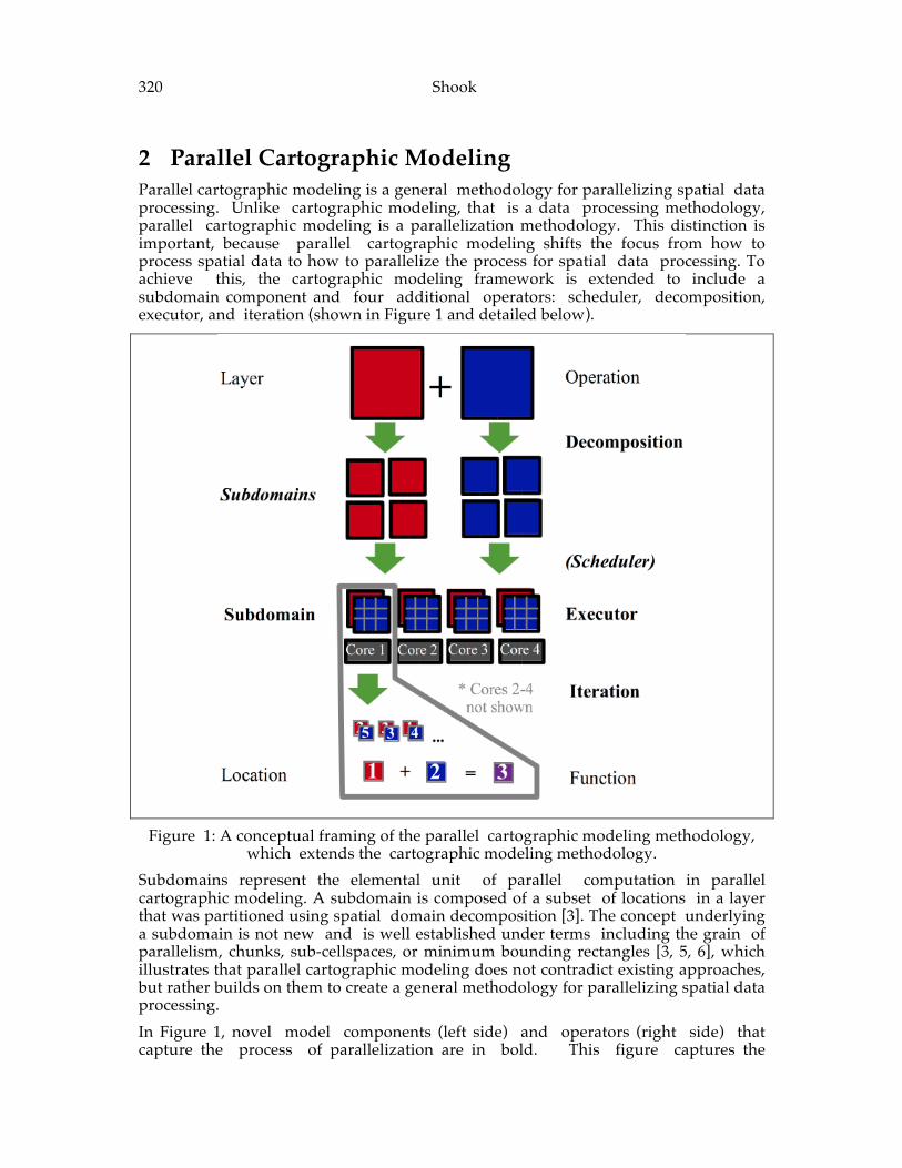
320 Shook
2 Parallel Cartographic Modeling Parallel cartographic modeling is a general methodology for parallelizing spatial data processing. Unlike cartographic modeling, that is a data processing methodology, parallel cartographic modeling is a parallelization methodology. This distinction is important, because parallel cartographic modeling shifts the focus from how to process spatial data to how to parallelize the process for spatial data processing. To achieve this, the cartographic modeling framework is extended to include a subdomain component and four additional operators: scheduler, decomposition, executor, and iteration (shown in Figure 1 and detailed below).
Figure 1: A conceptual framing of the parallel cartographic modeling methodology, which extends the cartographic modeling methodology.
Subdomains represent the elemental unit of parallel computation in parallel cartographic modeling. A subdomain is composed of a subset of locations in a layer that was partitioned using spatial domain decomposition [3]. The concept underlying a subdomain is not new and is well established under terms including the grain of parallelism, chunks, sub-cellspaces, or minimum bounding rectangles [3, 5, 6], which illustrates that parallel cartographic modeling does not contradict existing approaches, but rather builds on them to create a general methodology for parallelizing spatial data processing. In Figure 1, novel model components (left side) and operators (right side) that capture the process of parallelization are in bold. This figure captures the
Parallel Cartographic Modeling 321
methodological process of parallel cartographic modeling from the Sum operation applied to two layers, to functions processing individual locations (in parallel). At the core of parallel cartographic modeling is a novel component called a subdomain that serves as the elemental unit of parallel computation. Using subdomains, it is straightforward to capture the entire processing spectrum from serial data processing (decomposing a layer into a single subdomain) to completely parallel processing (decomposing a layer with N locations into N subdomains). Schedulers manage the parallel execution of a procedure, which may include scheduling (1) two operations simultaneously (i.e. task-level parallelism); (2) the processing of multiple subdomains simultaneously (i.e., data-level parallelism as seen in Figure 1); or (3) both (i.e. data-task hybrid parallelism [5]). Schedulers, in conjunc- tion with the rest of the framework, can be used to overcome challenges concerning HPC infrastructures (e.g., load-balancing, network bandwidth limitations, or memory constraints) or spatial problems (e.g., complex spatial or temporal dependencies). Decomposition operators partition a layer into one or more subdomains (see Figure 1). Certain spatial problems or computational infrastructures may align themselves to certain decomposition strategies (see [3] for discussion), which may be guided by computational intensity representations to balance computational work- loads [8]. Parallel cartographic modeling does not favor or restrict any particular strategy whether row, column, recursive-bisection, quadtree, or a novel strategy. Executors handle the execution of a function to process locations in a subdomain. Just as functions process locations and operations process layers, executors process subdomains. In essence, executors serve as a boundary of separation between parallel processing in the form of schedulers and decomposition and spatial data processing in the form of functions. This separation, using subdomains as the elemental unit of parallel computation, enables parallel cartographic modeling to simultaneously support parallel computing optimizations such as data-task hybrid parallelism as well as serial algorithmic optimizations for spatial-data processing. Iteration operators control the order in which locations in a subdomain are processed by a function. Iteration orderings, as part of algorithmic optimizations, may help exploit data localities inherent in spatial data to improve utilization of disk, memory, or CPU cache thus improving performance [2, 9]. Numerous iteration orderings for rasters (e.g., row-prime), points (e.g., point quadtrees), and polygons (e.g., R-trees) have been proposed and could be used in parallel cartographic modeling [9]. Parallel cartographic modeling follows the tradition of cartographic modeling as being more a re-organization of existing ideas rather than all new ideas. Similarly, it captures the process of parallelization without being designed for a specific HPC infrastructure thus enabling it to be implemented in a variety of computational settings for spatial problem solving.
3 Case Study A novel computing language named the Parallel Cartographic Modeling Language (PCML) has been developed based on the parallel cartographic modeling framework presented here. PCML is an open source language developed in Python that is freely available for download at the code hosting site GitHub (see https://github.com/ HPCGISLab/pcml for further details and PCML code). This language was used in a
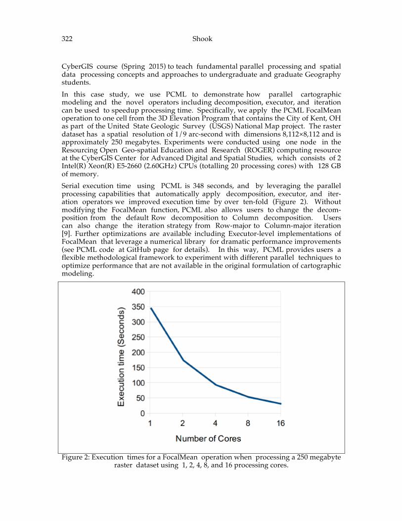
322 Shook
CyberGIS course (Spring 2015) to teach fundamental parallel processing and spatial data processing concepts and approaches to undergraduate and graduate Geography students. In this case study, we use PCML to demonstrate how parallel cartographic modeling and the novel operators including decomposition, executor, and iteration can be used to speedup processing time. Specifically, we apply the PCML FocalMean operation to one cell from the 3D Elevation Program that contains the City of Kent, OH as part of the United State Geologic Survey (USGS) National Map project. The raster dataset has a spatial resolution of 1/9 arc-second with dimensions 8,112×8,112 and is approximately 250 megabytes. Experiments were conducted using one node in the Resourcing Open Geo-spatial Education and Research (ROGER) computing resource at the CyberGIS Center for Advanced Digital and Spatial Studies, which consists of 2 Intel(R) Xeon(R) E5-2660 (2.60GHz) CPUs (totalling 20 processing cores) with 128 GB of memory. Serial execution time using PCML is 348 seconds, and by leveraging the parallel processing capabilities that automatically apply decomposition, executor, and iter- ation operators we improved execution time by over ten-fold (Figure 2). Without modifying the FocalMean function, PCML also allows users to change the decom- position from the default Row decomposition to Column decomposition. Users can also change the iteration strategy from Row-major to Column-major iteration [9]. Further optimizations are available including Executor-level implementations of FocalMean that leverage a numerical library for dramatic performance improvements (see PCML code at GitHub page for details). In this way, PCML provides users a flexible methodological framework to experiment with different parallel techniques to optimize performance that are not available in the original formulation of cartographic modeling.
Figure 2: Execution times for a FocalMean operation when processing a 250 megabyte
raster dataset using 1, 2, 4, 8, and 16 processing cores.
Parallel Cartographic Modeling 323
4 Concluding Discussion As we reflect on the past and look toward the future of GIScience [4], it is pertinent to recognize that the rapid shift in technologies empowering much of GIScience introduces both opportunities and challenges for future research. While it can be challenging to look beyond the excitement of new systems including heterogeneous architectures, graphic processing units (GPUs), and many-core accelerators, the GIScience community has an opportunity to advance the science by surveying the rapidly shifting computational and geographical information landscape to identify new trends and approaches in spatial problem solving. Parallel cartographic modeling is one step in this scientific pursuit that captures the commonalities rather than uniqueness of parallel spatial data processing, which can be used to illustrate the general process and fundamental concepts underlying many parallel GIS.
5 Acknowledgments Parallel cartographic modeling grew as a generalization of two interrelated projects. I would like to acknowledge Shaowen Wang, Michael Hodgson, Babak Behzad, and Kiumars Soltani for the original conception, design, and development of a PCML developed in C++ and for helping me extend that original work. I also acknowledge Zhengliang Feng for assistance in developing the Python-based PCML mentioned in the article. I appreciate the informative and engaging discussions with these individuals that helped lead to the creation of parallel cartographic modeling. This work used the Resourcing Open Geo-spatial Education and Research (ROGER) computing resource, which is supported by National Science Foundation grant number ACI-1429699.
References [1] AB R A H A RT, R., A N D SE E , L. GeoComputation. CRC Press, 2014. [2] AR M S T R O N G , M. Geography and computational science. Annals of the
Association of American Geographers 90, 1 (2000), 146–156. [3] DI N G , Y., A N D DE N S H A M , P. Spatial strategies for parallel spatial
modelling. International Journal of Geographical Information Systems 10, 6 (1996), 669–698.
[4] GO O D C H I L D , M. F. Twenty years of progress: GIScience in 2010. Journal of Spatial Information Science, 1 (2010), 3–20.
[5] GU A N , Q., A N D CL A R K E , K. A general-purpose parallel raster processing programming library test application using a geographic cellular automata model. International Journal of Geographical Information Science 24, 5 (2010), 695–722.
[6] QI N , C., ZH A N , L., ZH U , A., A N D ZH O U , C. A strategy for raster-based geocomputation under different parallel computing platforms. International Journal of Geographical Information Science 28, 11 (2014), 2127–2144.
[7] TO M L I N , C. GIS and Cartographic Modeling. Esri Press, 2013.

324 Shook
[8] WA N G , S. A cyberGIS framework for the synthesis of cyberinfrastructure, GIS, and spatial analysis. Annals of the Association of American Geographers 100, 3 (2010), 535–557.
[9] WO R B O Y S , M., A N D DU C K H A M , M. GIS: a computing perspective. CRC press, 2004.
[10] YA N G , C., RA S K I N , R., GO O D C H I L D , M., A N D GA H E G A N , M. Geospatial cyberinfrastructure: past, present and future. Computers, Environment and Urban Systems 34, 4 (2010), 264–277.
ADVANCING GEOGRAPHIC INFORMATION SCIENCE: CHAPTER 30
© by the author(s) Licensed under Creative Commons Attribution 4.0 License
325
From Infection Cases to Infection Tree Shiran Zhong and Ling Bian
University at Buffalo, the State University of New York
Extended Abstract
1 Introduction The diffusion of communicable diseases, such as Influenza Like Illness (ILI) is caused by interactions with the infectious at a place, while a population-wide propagation is the consequence of human mobility between places (Eubank et al. 2004; Salathé et al. 2010). Recently, an increasing effort has been devoted to developing models to understand spatial and temporal patterns of disease diffusion (Ferguson et al. 2006; Bian et al. 2012). These studies are mostly designed in either of the following two perspectives: spatial analysis in a static time frame (Gomes et al. 2014) or temporal analysis on aggregated spatial data, such as classic Susceptible-Infectious-Recovered (SIR) models (Anderson and May 1991). It is a common understanding that disease transmission processes are dynamic both spatially and temporally, but little research has focused on the analysis of spatial and temporal interactive patterns in disease transmissions. The objectives of this study are twofold. Firstly, we construct an infection tree by mining the spatial and temporal co-occurrence information embedded in discrete ILI cases. Secondly, we identify “super-spreaders” and “super-receivers” from the infection tree in the context of spatial and temporal interactive transmission processes. The simultaneous accounting for both the spatial and temporal dynamics should reveal the processes observed during actual epidemics.
2 Study Area and Data The study area is a metropolitan area in Midwest China. The dataset used for this study consists of 4,315 anonymous cases; each was clinically diagnosed as ILI during a 73 day period between September 1 - November 12. Each case is associated with a residential address (detailed to the level of residential community), a workplace (location identified to the census block group level in the U.S.), and the symptom onset date (self- reported at diagnosis). In this study, possible interactions occur among family members, colleagues, or neighbors who live within the same residential
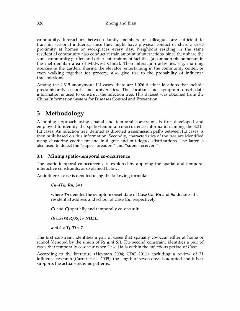
326 Zhong and Bian
community. Interactions between family members or colleagues are sufficient to transmit seasonal influenza since they might have physical contact or share a close proximity at homes or workplaces every day. Neighbors residing in the same residential community also conduct certain amount of interactions, since they share the same community garden and other entertainment facilities (a common phenomenon in the metropolitan area of Midwest China). Their interaction activities, e.g. morning exercise in the garden, sharing the elevator, entertaining in the community center, or even walking together for grocery, also give rise to the probability of influenza transmissions. Among the 4,315 anonymous ILI cases, there are 1,026 distinct locations that include predominantly schools and universities. The location and symptom onset date information is used to construct the infection tree. This dataset was obtained from the China Information System for Diseases Control and Prevention.
3 Methodology A mining approach using spatial and temporal constraints is first developed and employed to identify the spatio-temporal co-occurrence information among the 4,315 ILI cases. An infection tree, defined as directed transmission paths between ILI cases, is then built based on this information. Secondly, characteristics of the tree are identified using clustering coefficient and in-degree and out-degree distributions. The latter is also used to detect the “super-spreaders” and “super-receivers”.
3.1 Mining spatio-‐‑temporal co-‐‑occurrence The spatio-temporal co-occurrence is explored by applying the spatial and temporal interactive constraints, as explained below: An influenza case is denoted using the following formula:
Cn=(Tn, Rn, Sn), where Tn denotes the symptom onset date of Case Cn; Rn and Sn denotes the residential address and school of Case Cn, respectively. Ci and Cj spatially and temporally co-occur if: (Ri!Si)∩( Rj!Sj) ≠ NULL, and 0 < Tj-Ti ≤ 7.
The first constraint identifies a pair of cases that spatially co-occur either at home or school (denoted by the union of Ri and Si). The second constraint identifies a pair of cases that temporally co-occur when Case j falls within the infectious period of Case. According to the literature (Heyman 2004; CDC 2011), including a review of 71 influenza research (Carrat et al. 2005), the length of seven days is adopted and it best supports the actual epidemic patterns.
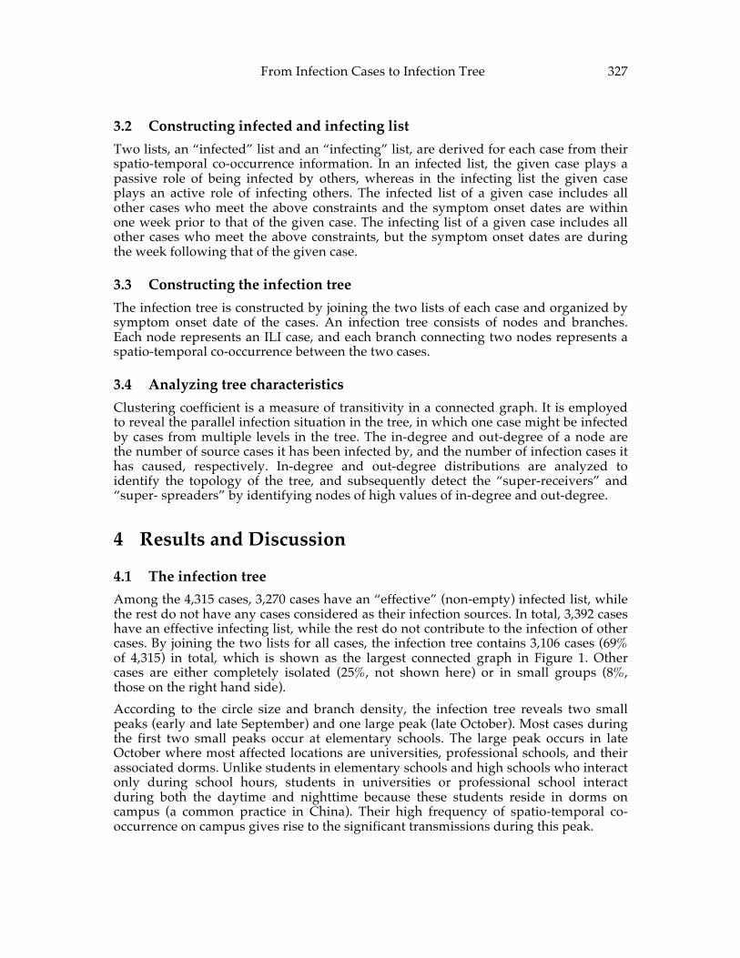
From Infection Cases to Infection Tree 327
3.2 Constructing infected and infecting list Two lists, an “infected” list and an “infecting” list, are derived for each case from their spatio-temporal co-occurrence information. In an infected list, the given case plays a passive role of being infected by others, whereas in the infecting list the given case plays an active role of infecting others. The infected list of a given case includes all other cases who meet the above constraints and the symptom onset dates are within one week prior to that of the given case. The infecting list of a given case includes all other cases who meet the above constraints, but the symptom onset dates are during the week following that of the given case.
3.3 Constructing the infection tree The infection tree is constructed by joining the two lists of each case and organized by symptom onset date of the cases. An infection tree consists of nodes and branches. Each node represents an ILI case, and each branch connecting two nodes represents a spatio-temporal co-occurrence between the two cases.
3.4 Analyzing tree characteristics Clustering coefficient is a measure of transitivity in a connected graph. It is employed to reveal the parallel infection situation in the tree, in which one case might be infected by cases from multiple levels in the tree. The in-degree and out-degree of a node are the number of source cases it has been infected by, and the number of infection cases it has caused, respectively. In-degree and out-degree distributions are analyzed to identify the topology of the tree, and subsequently detect the “super-receivers” and “super- spreaders” by identifying nodes of high values of in-degree and out-degree.
4 Results and Discussion
4.1 The infection tree Among the 4,315 cases, 3,270 cases have an “effective” (non-empty) infected list, while the rest do not have any cases considered as their infection sources. In total, 3,392 cases have an effective infecting list, while the rest do not contribute to the infection of other cases. By joining the two lists for all cases, the infection tree contains 3,106 cases (69% of 4,315) in total, which is shown as the largest connected graph in Figure 1. Other cases are either completely isolated (25%, not shown here) or in small groups (8%, those on the right hand side). According to the circle size and branch density, the infection tree reveals two small peaks (early and late September) and one large peak (late October). Most cases during the first two small peaks occur at elementary schools. The large peak occurs in late October where most affected locations are universities, professional schools, and their associated dorms. Unlike students in elementary schools and high schools who interact only during school hours, students in universities or professional school interact during both the daytime and nighttime because these students reside in dorms on campus (a common practice in China). Their high frequency of spatio-temporal co-occurrence on campus gives rise to the significant transmissions during this peak.
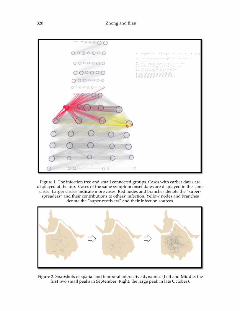
328 Zhong and Bian
Figure 1. The infection tree and small connected groups. Cases with earlier dates are displayed at the top. Cases of the same symptom onset dates are displayed in the same
circle. Larger circles indicate more cases. Red nodes and branches denote the “super- spreaders” and their contributions to others’ infection. Yellow nodes and branches
denote the “super-receivers” and their infection sources.
Figure 2. Snapshots of spatial and temporal interactive dynamics (Left and Middle: the first two small peaks in September. Right: the large peak in late October).
From Infection Cases to Infection Tree 329
4.2 Clustering coefficient The average clustering coefficient of 0.33 (Figure 3) illustrates the transitivity in the infection tree, which implies parallel infections among cases across multiple levels of the infection tree. If Case i contributes to the infection of Cases j and k, Case k might be the victim of both Case i and j if it spatially and temporally co-occurs with Case j. Thus, the possibility of Case k being infected is increased due to multiple parallel infection sources.
Figure 3. The clustering coefficient distribution of tree nodes.
4.3 In-‐‑degree and out-‐‑degree distribution Both in-degree and out-degree distributions of the infection tree follow a power law distribution (Figures 4a. "=1.93, p-value from the Kolmogorov-Smirnov test =0.93; Figures 4b "=1.83, p-value from the Kolmogorov-Smirnov test =0.73). In the case of in-degree, a large number of cases (58%) are probably infected by less than ten cases. A few cases at the tail are probably infected by more than 100 cases, and thus are the “super-receivers”.
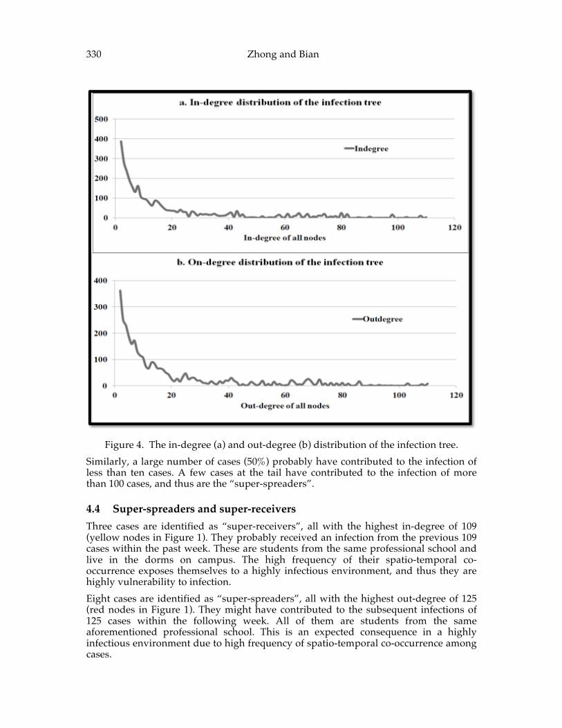
330 Zhong and Bian
Figure 4. The in-degree (a) and out-degree (b) distribution of the infection tree. Similarly, a large number of cases (50%) probably have contributed to the infection of less than ten cases. A few cases at the tail have contributed to the infection of more than 100 cases, and thus are the “super-spreaders”.
4.4 Super-‐‑spreaders and super-‐‑receivers Three cases are identified as “super-receivers”, all with the highest in-degree of 109 (yellow nodes in Figure 1). They probably received an infection from the previous 109 cases within the past week. These are students from the same professional school and live in the dorms on campus. The high frequency of their spatio-temporal co-occurrence exposes themselves to a highly infectious environment, and thus they are highly vulnerability to infection. Eight cases are identified as “super-spreaders”, all with the highest out-degree of 125 (red nodes in Figure 1). They might have contributed to the subsequent infections of 125 cases within the following week. All of them are students from the same aforementioned professional school. This is an expected consequence in a highly infectious environment due to high frequency of spatio-temporal co-occurrence among cases.
From Infection Cases to Infection Tree 331
5 Conclusion The spatial and temporal interactive patterns that are reconstructed in this study are critical to improve our understanding of transmission dynamics of communicable diseases. Although not all individuals who have symptoms will visit hospitals to be included in the dataset, the spatial and temporal trend derived from the data available for this study is representative of the epidemic in retrospective.
References [1] Anderson, R. M., & May, R. M. (1991). Infectious diseases of humans (Vol. 1).
Oxford: Oxford university press. [2] Bian, L., Huang, Y., Mao, L., Lim, E., Lee, G., Yang, Y., ... & Wilson, D. (2012).
Modeling individual vulnerability to communicable diseases: A framework and design. Annals of the Association of American Geographers,102(5), 1016-1025.
[3] Carrat, F., Vergu, E., Ferguson, N. M., Lemaitre, M., Cauchemez, S., Leach, S., & Valleron, A. J. (2008). Time lines of infection and disease in human influenza: a review of volunteer challenge studies. American journal of epidemiology, 167(7), 775-785.
[4] Centers for Disease Control and Prevention (CDC). "The 2009 H1N1 pandemic: summary highlights, April 2009–April 2010." Website: http://www. cdc. gov/h1n1flu/cdcresponse. htm, Accessed on August 2 (2011)
[5] Ferguson, N. M., Cummings, D. A., Fraser, C., Cajka, J. C., Cooley, P. C., & Burke, D. S. (2006). Strategies for mitigating an influenza pandemic. Nature,442(7101), 448-452.
[6] Eubank, S., Guclu, H., Kumar, V. A., Marathe, M. V., Srinivasan, A., Toroczkai, Z., & Wang, N. (2004). Modelling disease outbreaks in realistic urban social networks. Nature, 429(6988), 180-184.
[7] Gomes, M. F., y Piontti, A. P., Rossi, L., Chao, D., Longini, I., Halloran, M. E., & Vespignani, A. (2014). Assessing the international spreading risk associated with the 2014 West African Ebola outbreak. PLOS Currents Outbreaks.
[8] Heyman, D. L. (2004). Control of Communicable Diseases Manual. American Public Health Association. Washington, DC.
[9] Salathé, M., Kazandjieva, M., Lee, J. W., Levis, P., Feldman, M. W., & Jones, J. H. (2010). A high-resolution human contact network for infectious disease transmission. Proceedings of the National Academy of Sciences, 107(51), 22020-22025.

332 Zhong and Bian
ADVANCING GEOGRAPHIC INFORMATION SCIENCE
333
Sponsors The following sponsors made substantial contributions in support of the institute on Advancing Geographic Information: The Past and Next Twenty Years and towards the production of this volume.
Esri has been dedicated to the building and use of geographic information systems (GIS) for more than 40 years. As the world leader in GIS with over 1.5 million users, Esri offers innovative solutions allowing the creation, visualization, analysis, and presentation of information for better decision making. Esri's open, standards-based, and interoperable GIS platform provides the foundation for modernizing production cartography, building essential data sets and geoweb services, and deploying metadata catalogs. Esri GIS solutions allow highly diverse sectors to get the geographic advantage. To learn more, please visit esri.com
United States Census Bureau, Census Division. Geography is central to the work of the Census Bureau, providing the framework for survey design, sample selection, data collection, tabulation, and dissemination. Geography provides meaning and context to statistical data. Given the diversity of the nation's population, economic activities, and geographic areas, use of the latest and best geographic methodologies is critical to the Census Bureau’s ability to serve as the leading provider of statistical and geospatial data. To learn more, please visit http://www.census.gov/geography.html