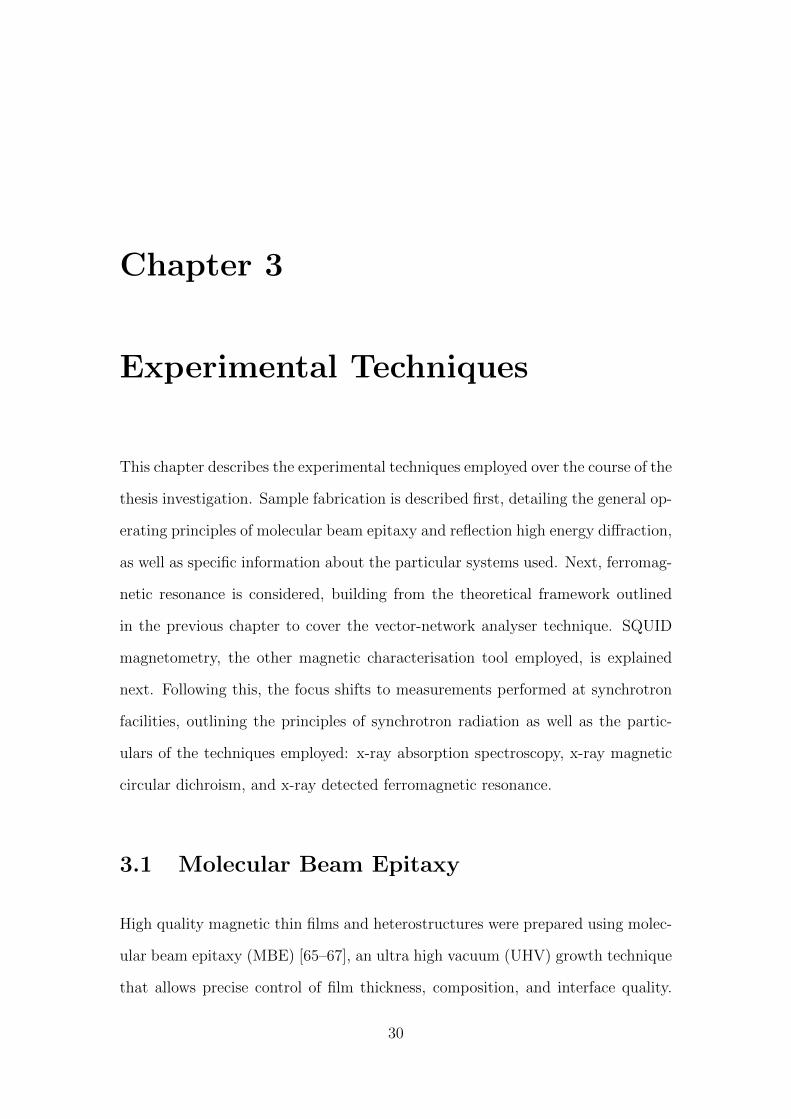
Tailoring of Magnetic Anisotropyand Interfacial Spin Dynamics

Alexander Baker

Wadham College

University of Oxford

A thesis submitted for the degree of

Doctor of Philosophy

Hilary 2016

Abstract

Spin transfer in magnetic multilayers offers the possibility of a new generation

of ultra-fast, low-power spintronic devices. New ways to control the resonance

frequency and damping in ultrathin films are actively sought, fuelling study of

the precessional dynamics and interaction mechanisms in such samples. One ef-

fect that has come under particular scrutiny in recent years is the spin-transfer

torque, wherein a flow of spins entering a ferromagnet exerts a torque on the

magnetisation, inducing precession. A flow of spin angular momentum is usually

generated through a spin-polarised electrical current, but a promising alternative

is the pure spin current emitted by a ferromagnet undergoing ferromagnetic reso-

nance (FMR). This allows spins to be transferred without a net charge flow. The

physics of the generation, transmission and absorption of pure spin currents is a

developing field, and holds great promise for both industrial applications and as

a means to study fundamental physical phenomena in exotic materials.

This thesis presents an investigation into the magnetodynamics of ferromagnetic

thin films and heterostructures grown by molecular beam epitaxy and studied us-

ing vector-network analyser ferromagnetic resonance (VNA-FMR), x-ray magnetic

circular dichroism, vibrating sample magnetometry and x-ray detected ferromag-

netic resonance (XFMR). Particular attention is paid to the anisotropy of damping

processes that occur in thin films, and the different coupling mechanisms that can

exist across non-magnetic spacer layers in spin valves and magnetic tunnel junc-

tions.

It is first shown that the static and dynamic magnetic properties of thin Fe films

can be effectively tailored by dilute doping with Dy impurities, which introduces

a sizeable anisotropy of Gilbert damping. The mechanism underlying this effect is

discussed, as is the concurrent modification of the spin and orbital contributions

to the magnetic moment.

ii

The focus then turns to magnetodynamics of ferromagnetic films coupled across

a nonmagnetic spacer layer, examining how different materials permit different

interactions. First, an insulating MgO layer is used to separate the FM layers; it

is found that this attenuates a spin current in under 1 nm, but permits a static

interaction for at least 2 nm. XFMR measurements are used to ascertain the

different contributions of the two interactions, and shed light on their interplay.

Next, the same techniques are applied to spin valves with a spacer layer of the

topological insulator (TI) Bi2Se3. TIs are the subject of much attention in the

physics community, as they hold the potential for dissipationless transport, ex-

tremely high spin-orbit torques, and a host of novel physical effects. Here, their

ability to absorb and transmit a pure spin current is studied, testing their suit-

ability for incorporation into existing device schemata. VNA-FMR measurements

confirm that the TI functions as an efficient angular momentum sink. XFMR

measurements, however, demonstrate the presence of a weak interaction between

the two ferromagnets, able to persist up to at least 8 nm, and possibly mediated

by the topological surface state.

Finally, the angle-dependence of spin pumping through a Cr barrier is examined,

finding that a strong anisotropy of spin pumping from the source layer can be

induced by an angular dependence of the total Gilbert damping parameter in

the spin sink layer. VNA-FMR measurements show that anisotropy is suppressed

above the spin diffusion length in Cr, which is found to be 8 nm, and is independent

of static exchange coupling in the spin valve. XFMR results confirm induced

precession in the spin sink layer, with isotropic static exchange and an anisotropic

dynamic exchange.

Taken together, these studies provide an insight not only into the magnetisation

dynamics of thin films (and ways to modify them) but a demonstration of the

power of ferromagnetic resonance techniques, and their applicability across ma-

terials and concepts. The results offer valuable information on the transmission

and absorption of spin currents by different materials, and several mechanisms by

which enhanced spin torques and angular control of damping may be realized for

next-generation spintronic devices.

iii

For Meghan

This is not a story of incredible heroism, or merely the narrative of a cynic; at

least I do not mean it to be. It is a glimpse of several lives that ran parallel for a

time, with similar hopes and convergent dreams. – Ernesto Guevara

iv

Acknowledgements

A thesis is by its nature a collaborative endeavour, and I have been extremely

fortunate as regards the company in which I have found myself. Anything of

merit contained within these pages can be attributed to the exceptional colleagues,

collaborators, and friends I have had along the way; any mistakes are entirely my

own.

First thanks must, of course, go to my supervisors: Professors Thorsten Hesjedal

and Gerrit van der Laan. They have guided my research at macro and micro

levels, provided me with innumerable opportunities to learn, and been excellent

company to boot. Thorsten is to be thanked in particular for training me in the

operation of the LaMBE in the Clarendon. We spent many hours struggling with

its peculiarities and personality quirks, it is probably remarkable that all three

of us are still standing at the end of it. Gerrit has been a constant source of

advice and aid on beamtimes, and discussions with him on the subject of static

and dynamic interactions lead directly into the work presented in chapters 6 and

8. For this and so much more, my thanks to both of them.

Throughout my research, Dr. Adriana Figueroa-Garcia has provided incomparable

support. Whether it be improving our measurement kit, advising me on how to

interpret and present data, or chasing down problems at 2 am on a beamtime, I

could not have asked for a more supportive post-doc to work with. I must also

thank Dr. Leigh Shelford, who first taught me the fundamentals of FMR, and

who provided excellent company on many XFMR beamtimes.

The staff of beamline I10 have allowed me to make it a home from home. Dr. Paul

Steadman, Dr. Alexey Dobrynin, Dr Peter Bencok, and Dr. David Burn have pro-

vided able and friendly assistance, as well as letting me use their SQUID-VSM.

Mark Sussmuth must be singled out from this group, for his peerless technical sup-

port and good humour. At the ALS in Berkeley, Prof. Elke Arenholz, Dr. Padraic

Shafer and Dr. Alpha N’Diaye always had huge smiles and were willing to help

v

at the most unsociable hours. For their assistance on XFMR beamtimes, I must

also thank Dr. Stuart Cavill, Chris Love, Dr. Gavin Stenning, and Rob Valkass.

I also thank the staff of I05, in particular Dr. Moritz Hoesch and Jon Riley, for

hosting the µ-MBE in their rooms and helping with numerous maintenance tasks.

In the office and the lab I have shared the travails with some good friends: (Dr.)

Liam Collins-McIntyre, Shilei Zhang, Piet Schonherr, Liam Duffy and (Dr.) Sara

Harrison. Always standing by with a helping hand or a joke, I could not have

asked for better labmates. Though I was not there as much as I would have liked,

the fine people of the Clarendon lab were likewise excellent company at coffee

and tea, and took the bizarre confections I brought in with, if not actual relish,

good-humoured resignation.

I must thank my parents, Deb and Adrian, for their varied and unstinting support,

and for instilling what work ethic I can claim to have. Finally, I thank Meghan

for her unquestioning and unequalled support in so many ways, and for being so

understanding of the fractured schedule my studies have required me to keep. I

could not have done this without her, and would not care to have tried.

vi

Contents

1 Introduction 1

1.1 Magnetism of Thin Films and Heterostructures . . . . . . . . . . . 1

1.2 Why Ferromagnetic Resonance? . . . . . . . . . . . . . . . . . . . . 3

1.3 Outline of the Thesis . . . . . . . . . . . . . . . . . . . . . . . . . . 5

2 Theoretical Background 7

2.1 Basic Energy Terms of Ferromagnetism . . . . . . . . . . . . . . . . 7

2.1.1 Exchange Energy . . . . . . . . . . . . . . . . . . . . . . . . 9

2.1.2 Demagnetisation Energy . . . . . . . . . . . . . . . . . . . . 10

2.1.3 Magnetocrystalline Anisotropy Energy . . . . . . . . . . . . 11

2.1.4 Zeeman Energy . . . . . . . . . . . . . . . . . . . . . . . . . 12

2.2 Magnetisation Dynamics . . . . . . . . . . . . . . . . . . . . . . . . 12

2.2.1 The Landau-Lifshitz-Gilbert Equation . . . . . . . . . . . . 13

2.2.2 Equilibrium Orientation of Magnetisation . . . . . . . . . . 14

2.2.3 The Resonance Condition . . . . . . . . . . . . . . . . . . . 16

2.2.4 Static Exchange Coupling . . . . . . . . . . . . . . . . . . . 18

2.3 Magnetisation Damping . . . . . . . . . . . . . . . . . . . . . . . . 19

2.3.1 Gilbert Damping . . . . . . . . . . . . . . . . . . . . . . . . 19

2.3.2 Non-Gilbert Damping . . . . . . . . . . . . . . . . . . . . . 20

2.3.3 Spin Pumping . . . . . . . . . . . . . . . . . . . . . . . . . . 21

2.4 X-Ray Magnetic Circular Dichroism . . . . . . . . . . . . . . . . . . 25

2.4.1 Sum Rules . . . . . . . . . . . . . . . . . . . . . . . . . . . . 26

3 Experimental Techniques 30

3.1 Molecular Beam Epitaxy . . . . . . . . . . . . . . . . . . . . . . . . 30

3.1.1 Reflection High Energy Electron Diffraction . . . . . . . . . 37

3.2 Vector-Network Analyser Ferromagnetic Resonance . . . . . . . . . 40

3.3 SQUID Vibrating Sample Magnetometry . . . . . . . . . . . . . . . 43

3.4 X-Ray Magnetic Circular Dichroism . . . . . . . . . . . . . . . . . . 46

vii

3.5 X-Ray Detected Ferromagnetic Resonance . . . . . . . . . . . . . . 48

4 Engineering of Magnetic Properties using Rare Earth Dopants 54

4.1 Motivation . . . . . . . . . . . . . . . . . . . . . . . . . . . . . . . . 54

4.2 Sample Fabrication . . . . . . . . . . . . . . . . . . . . . . . . . . . 56

4.3 Magnetometry and Magetocrystalline Anisotropy Parameters . . . . 58

4.4 Angle-Dependent Gilbert Damping . . . . . . . . . . . . . . . . . . 60

4.5 Determination of Spin and Orbital Magnetic Moments . . . . . . . 63

4.6 Conclusion . . . . . . . . . . . . . . . . . . . . . . . . . . . . . . . . 65

5 Micromagnetic Modelling of Coupled Magnetodynamics 67

5.1 Motivation . . . . . . . . . . . . . . . . . . . . . . . . . . . . . . . . 67

5.2 OOMMF . . . . . . . . . . . . . . . . . . . . . . . . . . . . . . . . . 68

5.2.1 Simulating FMR . . . . . . . . . . . . . . . . . . . . . . . . 69

5.2.2 Isolated Layers . . . . . . . . . . . . . . . . . . . . . . . . . 70

5.2.3 Coupled Layers . . . . . . . . . . . . . . . . . . . . . . . . . 71

5.3 Determination of the AC Magnetic Susceptibility Tensor . . . . . . 76

5.3.1 Dynamic Susceptibility of an Isolated Layer . . . . . . . . . 76

5.3.2 Modelling Dynamic and Static Exchange . . . . . . . . . . . 81

5.4 Conclusion . . . . . . . . . . . . . . . . . . . . . . . . . . . . . . . . 85

6 Suppression of Spin Pumping by an Insulating Barrier 87

6.1 Motivation . . . . . . . . . . . . . . . . . . . . . . . . . . . . . . . . 87

6.2 Sample Fabrication . . . . . . . . . . . . . . . . . . . . . . . . . . . 88

6.3 Static Exchange Coupling . . . . . . . . . . . . . . . . . . . . . . . 89

6.4 Structural Characterisation of the MgO Barriers . . . . . . . . . . . 92

6.5 VNA-FMR Measurements of Gilbert Damping . . . . . . . . . . . . 94

6.6 Layer Resolved Magnetodynamics . . . . . . . . . . . . . . . . . . . 97

6.7 Conclusion . . . . . . . . . . . . . . . . . . . . . . . . . . . . . . . . 100

7 Spin Pumping in Topological Insulators 102

7.1 Motivation . . . . . . . . . . . . . . . . . . . . . . . . . . . . . . . . 102

7.1.1 What is a Topological Insulator? . . . . . . . . . . . . . . . 104

7.2 Sample Fabrication . . . . . . . . . . . . . . . . . . . . . . . . . . . 106

7.3 Coupling Across a Topological Insulator . . . . . . . . . . . . . . . 109

7.3.1 Gilbert Damping as a Function of TI Thickness . . . . . . . 109

7.3.2 Layer-Resolved Magnetodynamics . . . . . . . . . . . . . . . 112

7.4 Anti-Damping Torques from Simultaneous Resonance . . . . . . . . 117

viii

7.4.1 Vector Network Analyser Measurements . . . . . . . . . . . 119

7.4.2 Layer-Resolved Measurements . . . . . . . . . . . . . . . . . 122

7.5 Temperature Dependence of Spin Pumping . . . . . . . . . . . . . . 124

7.6 Conclusion . . . . . . . . . . . . . . . . . . . . . . . . . . . . . . . . 126

8 Anisotropy Imprinting Through Spin Pumping 128

8.1 Motivation . . . . . . . . . . . . . . . . . . . . . . . . . . . . . . . . 128

8.1.1 Angular Control of Spin Pumping . . . . . . . . . . . . . . . 129

8.2 Sample Fabrication . . . . . . . . . . . . . . . . . . . . . . . . . . . 131

8.3 Determining the Static Exchange . . . . . . . . . . . . . . . . . . . 131

8.4 Spin Pumping Through a Cr Barrier . . . . . . . . . . . . . . . . . 136

8.4.1 Attenuation of a Pure Spin Current in Cr . . . . . . . . . . 137

8.4.2 Angular Dependence of Spin Pumping . . . . . . . . . . . . 137

8.5 Layer-Resolved Magnetodynamics . . . . . . . . . . . . . . . . . . . 141

8.6 Conclusion . . . . . . . . . . . . . . . . . . . . . . . . . . . . . . . . 145

9 Conclusion 147

9.1 Summary of Results . . . . . . . . . . . . . . . . . . . . . . . . . . 148

9.2 Perspective and Outlook . . . . . . . . . . . . . . . . . . . . . . . . 150

A Derivation of the AC Magnetic Susceptibility with Static

and Dynamic Exchange Coupling 152

B List of of Abbreviations and Acronyms 159

C Publications Arising from this Work 161

References 164

ix

List of Figures

2.1 Diagram of Thin Film Coordinate System . . . . . . . . . . . . . . 9

2.2 Schematic of Precession of Magnetisation . . . . . . . . . . . . . . 13

2.3 Magnetic Susceptibility Across Resonance . . . . . . . . . . . . . . 17

2.4 Illustration of Spin Pumping . . . . . . . . . . . . . . . . . . . . . . 22

2.5 Schematic of the X-ray Magnetic Circular Dichroism Effect . . . . . 27

3.1 Photographs of the LaMBE . . . . . . . . . . . . . . . . . . . . . . 33

3.2 Photograph of the µ-MBE . . . . . . . . . . . . . . . . . . . . . . . 34

3.3 Cutaway view of the µ-MBE growth chamber . . . . . . . . . . . . 35

3.4 Picture of an Effusion cell . . . . . . . . . . . . . . . . . . . . . . . 36

3.5 Diagram of an Electron Beam Evaporator . . . . . . . . . . . . . . 37

3.6 Schematic of a RHEED Gun . . . . . . . . . . . . . . . . . . . . . . 38

3.7 RHEED Patterns of Co50Fe50 . . . . . . . . . . . . . . . . . . . . . 40

3.8 Schematic of VNA-FMR Setup . . . . . . . . . . . . . . . . . . . . 41

3.9 Photographs of the Portable Octupole Magnet System . . . . . . . 42

3.10 Example Kittel Curves . . . . . . . . . . . . . . . . . . . . . . . . . 44

3.11 SQUID-VSM Operating Principle . . . . . . . . . . . . . . . . . . . 45

3.12 Schematic of the XFMR Experimental Setup . . . . . . . . . . . . . 50

4.1 RHEED Images of Thin Fe Film Doped with Dy . . . . . . . . . . . 57

4.2 XRD Measurement of a Thin Fe Film Doped with Dy . . . . . . . . 58

4.3 Hystersis Loops of Dy-doped Fe Thin Films . . . . . . . . . . . . . 59

4.4 Angular Dependence of Resonance Field for Dy-doped Fe . . . . . . 60

4.5 Angular Variation of Gilbert Damping for Dy-doped Fe . . . . . . . 61

4.6 XAS and XMCD Spectra for Dy-doped Fe . . . . . . . . . . . . . . 64

4.7 Calculated Spin and Orbital Moments as a Function of Dy Content 65

5.1 Precession of Magnetisation and Associated FMR Spectrum . . . . 70

5.2 Micromagnetic Simulation of a CoFe Film . . . . . . . . . . . . . . 71

5.3 FMR Spectrum of a Weakly Coupled CoFe/NiFe Bilayer . . . . . . 72

x

5.4 Kittel Curves for a CoFe/NiFe Bilayer . . . . . . . . . . . . . . . . 73

5.5 FMR Spectra of an Exchange-Coupled CoFe/NiFe Bilayer . . . . . 74

5.6 Resonances Plotted Across the Depth of the Bilayer . . . . . . . . . 75

5.7 Dynamic Susceptibility of an Iron Thin Film . . . . . . . . . . . . . 79

5.8 Static Coupling: Amplitude and Phase of Precession . . . . . . . . 83

5.9 Dynamic Coupling: Amplitude and Phase of Precession . . . . . . . 84

5.10 Combined Effects of Static and Dynamic Coupling . . . . . . . . . . 85

6.1 Hysteresis loops of Trilayers with MgO Spacers . . . . . . . . . . . 90

6.2 XMCD Hysteresis loops of Trilayers with MgO Spacers . . . . . . . 91

6.3 Static Exchange Coupling in MgO Trilayers . . . . . . . . . . . . . 92

6.4 Structural Characterisation of the MTJs . . . . . . . . . . . . . . . 94

6.5 Gilbert Damping as a Function of MgO Thickness . . . . . . . . . . 95

6.6 Amplitude and Phase of Precession for tMgO = 1 nm . . . . . . . . 97

6.7 Amplitude and Phase of Precession for tMgO = 2 nm . . . . . . . . 99

7.1 Bandstructure of a Topological Insulator . . . . . . . . . . . . . . . 105

7.2 Ferromagnet-Topological Insulator-Ferromagnet Heterostructure . . 107

7.3 Angular Dependence of Resonance of TI-FM Heterostructure . . . . 108

7.4 Gilbert Damping as a Function of TI layer Thickness . . . . . . . . 111

7.5 Precession of Ni Magnetisation Across Resonance at 4 GHz . . . . . 113

7.6 Amplitude and Phase of Precession for tTI = 4, 8 nm . . . . . . . . 114

7.7 Amplitude and Phase of Precession for tTI = 20 nm . . . . . . . . . 115

7.8 Evolution of Overlapping Resonances . . . . . . . . . . . . . . . . . 118

7.9 Outline of Fitting of Overlapping Resonances. . . . . . . . . . . . . 120

7.10 Resonant Linewidths as a Function of Mode Separation: VNA-FMR 121

7.11 Overlapping Resonances Measured by XFMR . . . . . . . . . . . . 123

7.12 Resonant Linewidths as a Function of Mode Separation: XFMR . . 124

7.13 Gilbert Damping as a Function of Temperature . . . . . . . . . . . 126

8.1 Hysteresis Loops of Cr Spin Valves . . . . . . . . . . . . . . . . . . 132

8.2 XMCD Hysteresis Loops of Cr Spin Valves . . . . . . . . . . . . . . 133

8.3 Example Kittel Curves of Cr Spin Valves . . . . . . . . . . . . . . . 134

8.4 Fitted VNA-FMR Data of Cr Spin Valves . . . . . . . . . . . . . . 136

8.5 Spin Pumping as a Function of Cr Thickness . . . . . . . . . . . . . 138

8.6 Decay Gilbert Damping Along the Easy and Hard Axes . . . . . . . 139

8.7 Gilbert Damping as a Function of External Field Angle . . . . . . . 140

8.8 Amplitude and Phase of Precession for tCr = 1 nm . . . . . . . . . 142

xi

8.9 Angle-Resolved Phase of Precession of CoFe for tCr = 1 nm . . . . . 143

8.10 Fitted Phase Variation Across Resonance . . . . . . . . . . . . . . . 144

xii

Chapter 1

Introduction

1.1 Magnetism of Thin Films and Heterostruc-

tures

Throughout the twentieth century electronic devices revolutionised our way of life

and lead to a heady pace of technological change. More recently the demand

for ever-faster device operation and ever-greater memory capacity has driven the

magnetics community to search for new physical concepts and device schemata

that exploit them. Leaving behind “electronics”, technologies based on the charge

of the electron, the emerging paradigm is “spintronics” [1, 2], technologies incor-

porating the spin of the electron, a quantum property that promises faster, more

stable and ever smaller devices.

Perhaps the first true spintronic innovation was the discovery of giant magnetore-

sistance (GMR) in 1988 [3, 4], earning Albert Fert and Peter Grunberg the 2007

Nobel prize. Together with the subsequent discovery of tunneling magnetoresis-

tance in magnetic tunnel junctions (MTJs) [5], the first spin valve read heads and

magnetic random access memory (MRAM) devices were developed [6, 7]. Data

1

storage has been revolutionised by these concepts, as the drive for miniaturisa-

tion leads to ever-greater information densities. A wide variety of mechanisms

to write data have been proposed, including heat assisted MRAM [8] and mag-

netic switching [9, 10], but perhaps the most promising is the use of spin-transfer

torque (STT) [11–13]. When a spin polarised current is passed through a magnet,

the interaction of the angular momentum of the flowing electrons with the static

magnetisation exerts a torque, inducing precession. If this torque is sufficiently

large it can reverse the magnetisation, rewriting stored data [10]. This provides

one motivation for the study of magnetodynamics and interfacial spin dynamics

in heterostructures.

A second motivation arises from the need for faster and faster write operations. As

the speed of device operation increases to the GHz range, the magnetic relaxation

properties of the system become important [14,15]. Energy loss mechanisms aris-

ing from spin orbit coupling [14], sample imperfections [16, 17], interactions with

impurities or dopants [18, 19], and even the ejection of spins into neighbouring

layers must be considered [20–23]. High quality thin film samples are required

for such studies, as they allow experiments to access the intrinsic properties of

such processes in a controlled environment. The use of single crystal samples also

allows one to study the angular variation of damping mechanisms, studying how

they can relate to the lattice, the co-ordination of defects or the magnetocrys-

talline anisotropy [16]. Comparatively little work exists to date on such effects,

but if the anisotropy of damping can be tailored it offers new possibilities for de-

vice optimisation, as well as revealing deeper information about the underlying

magnetic relaxation mechanisms.

This thesis presents an investigation of the magnetodynamics of thin films grown

by molecular beam epitaxy (MBE) and studied by vector-network analyser fer-

romagnetic resonance (VNA-FMR), x-ray magnetic circular dichroism (XMCD),

2

vibrating sample magnetometry (VSM) and x-ray detected ferromagnetic reso-

nance (XFMR). High quality samples consisting of single layers or trilayers based

on ferromagnet – non-magnet – ferromagnet structures were grown on MgO (001)

substrates. These samples were used to study coupling across non-magnetic bar-

riers, paying attention to how they can be modified, and the angle-dependent

damping processes that arise.

Throughout this research the goal has been to study how the anisotropy of mag-

netodynamics might be manipulated, and how two magnetic layers separated by

a spacer layer interact and influence one another. Though they appear separate

concepts, they can be studied in the same way, and by the final chapter it will

be shown that they can come together to yield valuable insights into spin transfer

and coupled magnetodynamics. While the research has been conducted from a

perspective of basic science, aiming to understand the fundamental physics driv-

ing the observations, every effort has been made to ensure that work is directed

in technologically relevant channels, and to contextualise the findings in their po-

tential for device applications.

1.2 Why Ferromagnetic Resonance?

It is important to consider not just why this investigation was performed, but

also why a specific approach was chosen. Here, broadband VNA-FMR was widely

used as both a standard characterisation technique to check the quality of samples,

and as a detailed probe of magnetodynamics and spin transfer. The question is

then what advantages are unique to broadband FMR over, for example, SQUID

magnetometry (which is employed here in a supportive role) [24], inverse spin Hall

effect (ISHE) [25,26] or magnetotransport techniques [27]?

The key advantage offered by broadband FMR is its versatility. Few other tech-

3

niques can offer such powerful characterisation of both static and dynamic mag-

netic properties [28], especially when the extension of x-ray detection is incorpo-

rated [15,29]. Further, it does not require patterning of samples into measurement

geometries such as Hall bars, or the application of electrical contacts to the sample

surface. In this way, VNA-FMR has a high-throughput, is non-destructive and

uses samples with other standard characterisation techniques.

When studying the coupling mechanisms between magnetic layers in a heterostruc-

ture, the choice of technique also determines which interactions are accessible.

While many magnetic measurement techniques can detect the presence of a static

coupling, for example through a change in the shape of the hysteresis loop [30]

or a shift in resonance field [31, 32], the dynamic interaction of spin pumping oc-

curs when the magnetic layer is precessing, most commonly when the resonance

condition is fulfilled [22]. FMR-based techniques such as VNA-FMR, or ISHE

are therefore required. ISHE is a sensitive technique, as in measuring the volt-

age induced by the absorption of spins it is a direct probe of the presence of

spin pumping [25, 33]. VNA-FMR, in contrast can only indirectly measure spin

pumping, and does not provide layer-specific information as it averages over the

whole stack. This limitation is alleviated, however, by performing XFMR [29,34].

This technique will be explored in more detail in section 3.5, but in brief it uses

an experimental configuration similar to VNA-FMR, in combination with a syn-

chrotron light source, to perform a time-resolved version of x-ray magnetic circular

dichroism. This allows layer-resolved measurements of the amplitude and phase

of precession. The high degree of temporal and spatial resolution yields infor-

mation unavailable to few other techniques, allowing, for example, separation of

different coupling mechanisms [15,28,32,35] or clean measurements of overlapping

resonances [15,28].

Broadband FMR is a technique in which conceptual and experimental simplicity

4

are combined with with high sensitivity and straightforward extension to more ad-

vanced measurements. It is well-suited to study the effects of magnetic anisotropy

on magnetodynamics, offering insights into how these traits might be tailored and

optimised towards spintronic applications. It allows precise determination of the

strength and nature of coupling mechanisms in magnetic heterostructures and,

by extension into XFMR, the interfacial spin dynamics induced by long-range

interactions.

Beyond VNA-FMR, other characterisation techniques were employed to confirm

findings or provide additional information. By measuring hysteresis loops, VSM

provides an alternative measure of saturation magnetisation and coupling in tri-

layers [28, 30], as well as probing magnetocrystalline anisotropy. A significant

portion of the research presented here was conducted at synchrotrons, sources

of intense, coherent light of tunable energy and polarisation [36]. This affords

an element-specific probe of magnetisation through XMCD [37, 38], as well as

allowing determination of the relative contributions of spin and orbital angular

momentum [39,40].

1.3 Outline of the Thesis

The investigation presented in this thesis focuses on methods to manipulate the

anisotropy and spin transfer properties of ferromagnetic thin films and heterostruc-

tures. The aim is to present a comprehensive, multi-technique study of the spin

dynamics of a variety of systems, utilising both lab and synchrotron methods to

develop a thorough understanding of the underlying physics. All samples were

grown by the author (with the exception of the topological insulator layers used

in chapter 7) using molecular beam epitaxy. The primary technique employed

throughout the research was ferromagnetic resonance, used to determine both

5

static and dynamic magnetic properties, with particular attention paid to Gilbert

damping and spin pumping in spin valves. The work is presented as a series of

individual projects, linked by the common theme of magnetodynamics and spin

transfer.

Chapter 2 gives an introduction to the pertinent theory, paying particular atten-

tion to the mechanisms underlying ferromagnetic resonance and the spin pumping

effect, along with a more general background on magnetism in thin films and the

x-ray magnetic circular dichroism effect. Building on this foundation, chapter

3 details the experimental techniques used to fabricate and study the samples.

Chapter 4 concerns a study of how dilute Dy doping of Fe thin films can mod-

ify the angular dependence of Gilbert damping. Chapter 5 gives further detail

on the modelling used throughout the thesis, in particular how exchange-coupled

multilayers can be simulated. From this, chapter 6 studies the coupled magneto-

dynamics of ferromagnetic layers separated by a thin MgO barrier, studying the

suppression of spin pumping by an insulating layer. Chapter 7 is dedicated to a

study of spin pumping in the novel materials class of topological insulators, aim-

ing to exploit the exotic surface state. Chapter 8 takes elements from all previous

chapters to present evidence of angle-dependent spin pumping in spin valves with

a Cr interlayer. Finally, chapter 9 provides a summary of the work to date, and

presents an outlook onto the prospects and challenges suggested by the findings.

6

Chapter 2

Theoretical Background

This chapter outlines the fundamental theoretical concepts that underpin both

the physical phenomena and the experimental techniques employed to investigate

them. Later chapters will build upon this foundation to fit particular requirements,

but the information presented here applies to all aspects of the work. First, the en-

ergy terms associated with ferromagnetic thin films are discussed, outlining their

origins and effects. With this grounding, the equation of motion for ferromag-

netic resonance is introduced and explained, paying particular attention to the

resonance condition. Damping processes are considered, with particular atten-

tion being paid to spin pumping, which features prominently in several chapters.

Finally, the x-ray magnetic circular dichroism effect is discussed, including the

magneto-optical sum rules that allow determination of spin and orbital contribu-

tions to the total magnetic moment.

2.1 Basic Energy Terms of Ferromagnetism

Before describing the dynamic properties of the magnetisation, it is instructive to

consider the contributions towards the total energy, and their microscopic origin.

7

As in bulk samples one must take into account the Zeeman, exchange and magne-

tocrystalline anisotropy energies, but in thin films the demagnetisation tensor and

interface effects are also important. The definition of a “thin” film is somewhat

loose, but it can be said to be bounded from below by the magnetic exchange

length, lex. Films below this are more commonly termed “ultra-thin”, and act as

a single macrospin. The exchange length is given by [41]:

lex =

(2A

µ0M2s

)1/2

, (2.1)

where A is the exchange constant of the magnetic material and Ms the saturation

magnetisation. In Co, for example, lex = 3.5 nm. The maximum thickness of

a “thin” film is harder to define, but a practical definition can be reached by

considering the fabrication techniques employed in film growth. The films studied

in this work are grown by molecular beam epitaxy (MBE), which usually has a

growth rate of < 0.1 A/s. Therefore, in order to conserve time and preserve film

quality, films are typically t < 100 nm, and often much less.

To find the total energy associated with magnetism in the film we sum over the

individual contributions, as:

Etot = Eex + Edemag + Eanis + EZeeman + ... , (2.2)

with the energy terms here being exchange, demagnetisation, anisotropy and Zee-

man energies, respectively. Contributing energies are chosen based on the nature

of the sample; other terms, such as interlayer exchange or exchange bias, can be

included in the same way.

8

y [010]

z [001]

x [100]

H

θH

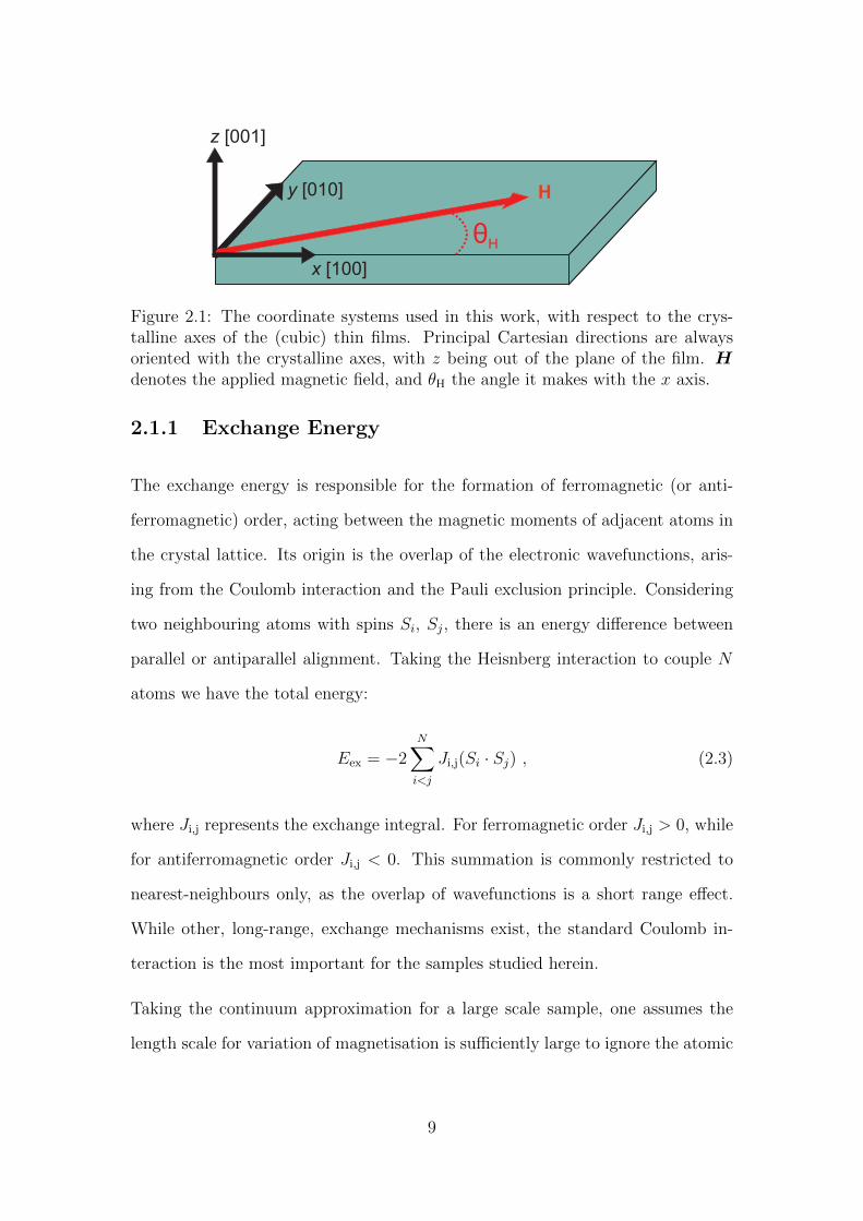
Figure 2.1: The coordinate systems used in this work, with respect to the crys-talline axes of the (cubic) thin films. Principal Cartesian directions are alwaysoriented with the crystalline axes, with z being out of the plane of the film. Hdenotes the applied magnetic field, and θH the angle it makes with the x axis.

2.1.1 Exchange Energy

The exchange energy is responsible for the formation of ferromagnetic (or anti-

ferromagnetic) order, acting between the magnetic moments of adjacent atoms in

the crystal lattice. Its origin is the overlap of the electronic wavefunctions, aris-

ing from the Coulomb interaction and the Pauli exclusion principle. Considering

two neighbouring atoms with spins Si, Sj, there is an energy difference between

parallel or antiparallel alignment. Taking the Heisnberg interaction to couple N

atoms we have the total energy:

Eex = −2N∑i<j

Ji,j(Si · Sj) , (2.3)

where Ji,j represents the exchange integral. For ferromagnetic order Ji,j > 0, while

for antiferromagnetic order Ji,j < 0. This summation is commonly restricted to

nearest-neighbours only, as the overlap of wavefunctions is a short range effect.

While other, long-range, exchange mechanisms exist, the standard Coulomb in-

teraction is the most important for the samples studied herein.

Taking the continuum approximation for a large scale sample, one assumes the

length scale for variation of magnetisation is sufficiently large to ignore the atomic

9

structure. The total energy is then obtained by the integral:

Eex =A

Ms

∫V

(∇M )2dV , (2.4)

where the exchange constant A = nJS2/a, with a the lattice constant, S the

magnitude of the spin, and n a factor arising from crystal structure.

2.1.2 Demagnetisation Energy

The magnetic dipole interaction is a long range effect: the interaction of each

magnetic moment with the dipole field of every other magnetic moment. The

demagnetising field arises from the divergence of the overall magnetisation, and

is largest in the case when the local magnetisation is aligned perpendicular to the

edge of the sample, creating a magnetic pole. The energy of the demagnetising field

is reduced through the formation of magnetic domains in the material. Though it

is rather weaker than the exchange interaction, its long range makes it important,

and in the confined geometries of thin films its effects are considerable. The

interaction tends to oppose the formation of a uniform magnetic state, hence its

name, and has the form:

Edemag = −µ0

2

∫V

M ·HdemagdV , (2.5)

with Hdemag the demagnetising field, and the integration running over the whole

sample volume, V . Determining Hdemag is in general challenging, requiring nu-

merical integration. Fortunately, analytical solutions exist in the case of homo-

geneously magnetised ellipsoids where Hdemag = -N ·M , and this can be used

to approximate a thin film. Here N is the (dimensionless) demagnetising tensor,

which controls orientation and strength of the demagnetising field. This tensor

can be diagonalised when the magnetisation is along one of the principal axes, and

10

the sum of the diagonal elements satisfies Nxx + Nyy + Nzz = 1. For an infinite

thin film in the x − y plane the diagonal elements are Nxx ≈ Nyy ≈ 0, Nzz ≈ 1,

effectively constraining the magnetisation to lie in the plane of the film, unless

there is a significant external field or perpendicular magnetic anisotropy.

2.1.3 Magnetocrystalline Anisotropy Energy

The magnetisation in a crystalline ferromagnet has preferred orientations, termed

the easy axes, due to the spin-orbit interaction. The spin moment of the electron

couples to the orbital moment, whose symmetry is determined by the underlying

symmetry of the lattice. This causes certain crystallographic directions to be

more energetically favourable than others. All ferromagnetic materials discussed

in this thesis have a cubic crystal structure, leading to a four-fold anisotropy with

a typical easy axis in the [100] direction, and a hard axis in the [110] direction. An

additional in-plane uniaxial (two-fold) anisotropy can also arise due to chemical

interactions with the substrate or mechanical strain during growth. Furthermore,

the reduced symmetry at an interface enhances the spin-orbit interaction, and

can also lead to an out-of-plane uniaxial anisotropy, which in certain cases leads

to films having their easy axis of magnetisation oriented out of the plane. The

magnetocrystalline anisotropy energy is:

Eanis = −K‖C

2(α4

x + α4y)−

K⊥C2α4z −K

‖U

(n ·M)2

M2s

−K⊥Uα2z , (2.6)

where αx,y,z are the direction cosines with respect to the [100], [010], and [001]

axes, and K‖C , K⊥C , K

‖U , K⊥U are the in-plane and out-of-plane cubic and unixial

anisotropy constants, respectively. In all cases in this work it is sufficient to

consider the in-plane components, as magnetisation is confined to the plane of the

film.

11

2.1.4 Zeeman Energy

In the presence of an external magnetic field, H , an energy term arises due to the

interaction of the magnetization and the external field:

EZeeman = −µ0

∫V

M ·H . (2.7)

The Zeeman energy acts to align the magnetic field and the magnetisation, and is

the parameter that is most readily varied in typical FMR experiments.

2.2 Magnetisation Dynamics

In a ferromagnetic resonance experiment a time dependent field with frequency

typically in the GHz range is used to excite precession in a ferromagnetic material,

while a static bias field combined with internal fields of the material defines an

equilibrium orientation of magnetisation. When studying FMR we are primarily

concerned with the resonance frequency, which relates to the internal energy of the

system, and the resonance linewidth, which is governed by energy loss mechanisms.

The combination of different energy terms discussed in the previous section leads

to an effective field [14]:

Heff = − 1

µ0

∇MEtot , (2.8)

the functional derivative of the total energy with respect to the magnetisation.

This is the effective field which drives FMR, linking the resonance frequency to

the different energetic contributions within the sample. Such magnetodynamics

are described by the Landau-Lifshitz-Gilbert (LLG) equation [42].

As the central technique of this thesis, the following sections examine the the-

oretical concepts of FMR in greater detail. First, the LLG is introduced and

12

Heff

M

- xM Heff

M

- xM Heff

Without damping With damping

HeffM x d /dtM

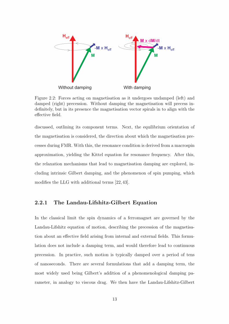
Figure 2.2: Forces acting on magnetisation as it undergoes undamped (left) anddamped (right) precession. Without damping the magnetisation will precess in-definitely, but in its presence the magnetisation vector spirals in to align with theeffective field.

discussed, outlining its component terms. Next, the equilibrium orientation of

the magnetisation is considered, the direction about which the magnetisation pre-

cesses during FMR. With this, the resonance condition is derived from a macrospin

approximation, yielding the Kittel equation for resonance frequency. After this,

the relaxation mechanisms that lead to magnetisation damping are explored, in-

cluding intrinsic Gilbert damping, and the phenomenon of spin pumping, which

modifies the LLG with additional terms [22,43].

2.2.1 The Landau-Lifshitz-Gilbert Equation

In the classical limit the spin dynamics of a ferromagnet are governed by the

Landau-Lifshitz equation of motion, describing the precession of the magnetisa-

tion about an effective field arising from internal and external fields. This formu-

lation does not include a damping term, and would therefore lead to continuous

precession. In practice, such motion is typically damped over a period of tens

of nanoseconds. There are several formulations that add a damping term, the

most widely used being Gilbert’s addition of a phenomenological damping pa-

rameter, in analogy to viscous drag. We then have the Landau-Lifshitz-Gilbert

13

equation [42,44]:

dm

dt= −γ [m×Heff ] + α

[m× ∂m

∂t

], (2.9)

with γ the gyromagnetic ratio, m is the unit magnetisation vector of the ma-

terial, Heff the effective magnetic field (through which the various energy terms

discussed in section 2.1 enter the equation), and α the dimensionless Gilbert damp-

ing parameter. Note that this form of the damping preserves the length of the

magnetisation vector, making it unsuitable for describing damping mechanisms

such as two magnon scattering. Damping is discussed in more detail in section

2.3.

2.2.2 Equilibrium Orientation of Magnetisation

In order to determine the FMR frequency one must first identify the equilibrium

orientation of the magnetisation. When the external bias field is aligned along

an easy axis the magnetisation and field are collinear, but this is not in general

the case. Rather, the internal fields of the sample can lead to a canting of the

magnetisation away from the bias field; a misalignment of several degrees is pos-

sible. This is important not just when calculating the resonance frequency, but

also when determining precessional damping. The effect of field dragging caused

by magnetisation canting leads to an angle-dependent contribution to the total

damping within a sample.

To determine the equilibrium condition of the magnetisation we minimise the free

energy, F , such that:

∂F

∂φ= 0 , (2.10)

where φ is the in-plane angle.

14

For the case of a cubic system, with the magnetisation confined to the plane of

the film at an angle φM, this is:

∂F

∂φ= µ0MH sin[φM−φH]−KU sin[2(φM−φU)]+

1

2KC sin[4(φM−φC)] = 0 , (2.11)

where φH is the angle of the external field, φC the angle of the magnetocrystalline

cubic easy axis, and φU the angle of the magnetocrystalline uniaxial easy axis. Here

M and H are the magnitudes of the magnetisation and external field, respectively,

KU|| the in-plane two-fold (uniaxial) anisotropy constant and KC the in-plane

four-fold (cubic) anisotropy constant. This equation must be solved numerically,

or one can instead make the substitution ∆φ = φM− φH, the misalignment of the

magnetisation from the external field, then expand in terms of ∆φ. Discarding

terms above those linear in the expansion of ∆φ, one arrives at:

∆φ ≈ KC sin[4(φM − φC)]− 2KU sin[2(φM − φU)]

−2µ0MH − 4KC cos[4(φM − φC)] + 4KU cos[2(φM − φU)]. (2.12)

Retaining terms up to second order in ∆φ this is the quadratic formula:

∆φ ≈ −b+√b2 − 4ac

2a,

a = −4KC sin[4(φM − φC)]− 2KU sin[2(φM − φU)] ,

b = 2KC cos[4(φM − φC)]− 2KU cos[2(φM − φU)] + µ0MH ,

c =1

2KC sin[4(φM − φC)]−KU sin[2(φM − φU)] , (2.13)

which can be solved to find the equilibrium condition of the magnetisation.

15

2.2.3 The Resonance Condition

The condition for ferromagnetic resonance is derived using the macro-spin ap-

proximation, wherein all spins are assumed to undergo coherent precession. This

approach implicitly neglects the contribution of the exchange interaction to the

magnetisation dynamics. Further, it is not strictly true that all spins precess

coherently in a material undergoing FMR, particularly in the case of coupled mul-

tilayers or patterned samples. However, this approximation is very useful as it

allows the resonance condition to be derived using a simple variational approach

that captures the key features of FMR.

In the case of small perturbations, and including a correction for Gilbert damping,

the resonance frequency is found using [45]:

(ω

γ

)2

=1 + α2

[M sin(θ)]2

[∂2F

∂θ2

∂2F

∂φ2−(∂2F

∂θ∂φ

)2], (2.14)

with γ = gµB/h the gyromagnetic ratio. Again restricting the magnetisation to

lie in-plane, this reduces to [14,45,46]:

(ω

γ

)2

=(1 + α2

) [µ0M + µ0H cos [φM − φH] +

KC

2M(3 + cos [4 (φM − φC)]) +

KU

M(1− cos [2 (φM − φU)])

][µ0H cos [φM − φH] +

2KC

M(cos [4 (φM − φC)])−

2KU

Mcos [2 (φM − φU)]

]. (2.15)

This is the Kittel equation [47], which is used to extract material parameters from

the resonant fields measured in an FMR experiment.

An alternative approach to determining the resonance condition is to use harmonic

solutions of a linearised version of the LLG to find the AC magnetic susceptibility

16

-10 -5 0 5 10

Susceptibili

ty (

arb

. units)

H - H (mT)res

Imaginary

Real

MixedHres

DH

H

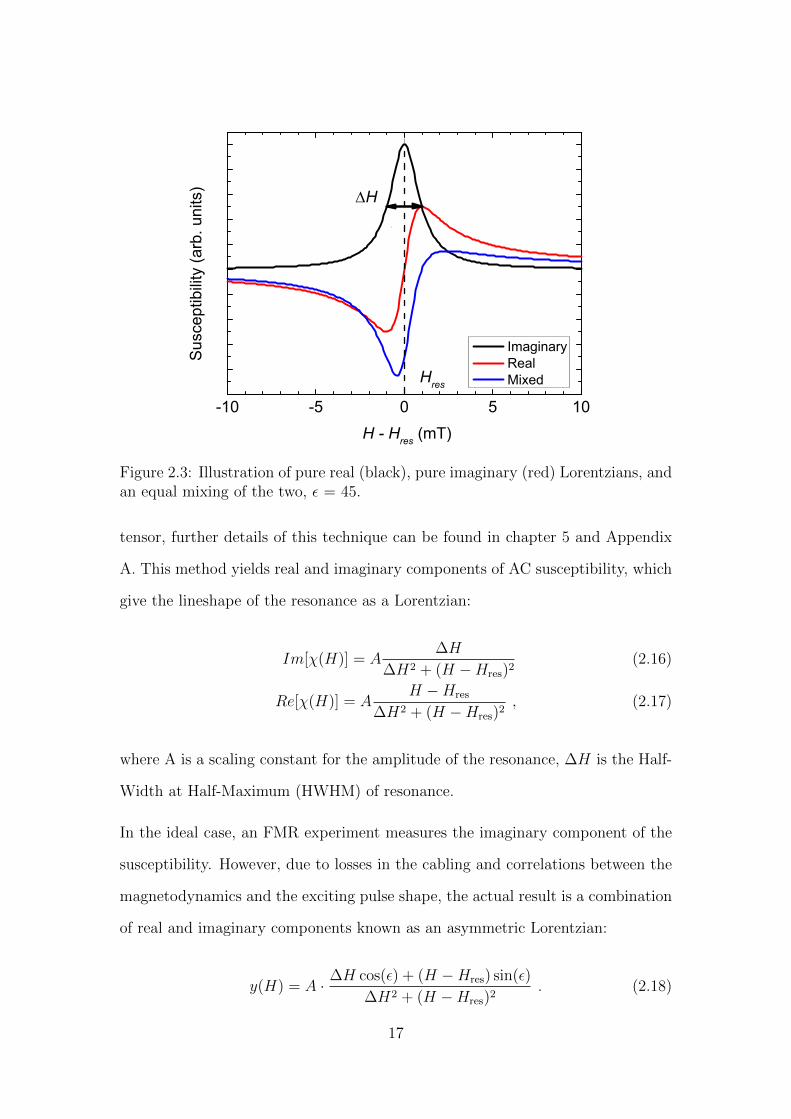
Figure 2.3: Illustration of pure real (black), pure imaginary (red) Lorentzians, andan equal mixing of the two, ε = 45.

tensor, further details of this technique can be found in chapter 5 and Appendix

A. This method yields real and imaginary components of AC susceptibility, which

give the lineshape of the resonance as a Lorentzian:

Im[χ(H)] = A∆H

∆H2 + (H −Hres)2(2.16)

Re[χ(H)] = AH −Hres

∆H2 + (H −Hres)2, (2.17)

where A is a scaling constant for the amplitude of the resonance, ∆H is the Half-

Width at Half-Maximum (HWHM) of resonance.

In the ideal case, an FMR experiment measures the imaginary component of the

susceptibility. However, due to losses in the cabling and correlations between the

magnetodynamics and the exciting pulse shape, the actual result is a combination

of real and imaginary components known as an asymmetric Lorentzian:

y(H) = A · ∆H cos(ε) + (H −Hres) sin(ε)

∆H2 + (H −Hres)2. (2.18)

17

Here ε is the mixing angle: for ε = 0 the resonance is purely the imaginary

component, while for ε = π2

it is purely real.

2.2.4 Static Exchange Coupling

The static interlayer exchange coupling is a general term for any interaction that

acts to (anti-)align the magnetisations of the two layers in a spin valve. Examples

of such interactions include Ruderman-Kittel-Kasuya-Yosida (RKKY), superex-

change, Neel or orange peel coupling, and direct exchange through a discontinuous

spacer layer. In the case of the Cr spin valves studied in chapter 8, for example,

the coupling between the two magnetic layers is RKKY, wherein conduction elec-

trons provide an interaction mechanism through the hyperfine interaction with

the nuclear spins. The presence of a static interaction modifies the LLG equation

with an additional term [32,35]:

−∂mi

∂t= mi ×

[γiH i

eff + βiM jsm

j − αi0∂mi

∂t

], (2.19)

where β is the interlayer exchange, and i, j index magnetic layers. The interlayer

exchange is defined as [31,35,48]:

βi =Aex

M isdi

cos(φiM − φjM), (2.20)

with Aex the interlayer exchange constant, d the thickness of the magnetic layer,

and φM the equilibrium orientation of magnetisation. The sign of Aex determines

whether the interaction favours parallel (positive) or antiparallel (negative) align-

ment.

18

2.3 Magnetisation Damping

The study of magnetic relaxation processes in thin films and nanoscale devices

has become increasingly important in recent years, spurred by the interest in phe-

nomena such as spin-transfer torques and vortex core dynamics [6,49]. Relaxation

of the excited magnetic state can proceed by a number of different mechanisms,

including coupling to the crystal lattice [14], dissipation into the magnetic sub-

system through two magnon scattering [17, 50], and spin pumping [22, 43]. The

resonance linewidth functions as a sensitive probe of damping, and many studies

have examined the interplay of layer structure, crystal quality and magnetisation

alignment in determining the precessional damping [51–54].

Broadly speaking, damping processes can be separated into two types - Gilbert

and non-Gilbert. Gilbert-type damping processes preserve the length of the mag-

netisation vector, as they do not redistribute energy within the magnetic sub-

system. More pragmatically, they depend linearly on microwave frequency. Ex-

amples of such processes include phonon drag, itinerant electron processes and

spin-pumping. Non-Gilbert damping processes preserve only the z-component of

the magnetisation vector, and their magnitude has a non-linear frequency depen-

dence. An important example of non-Gilbert damping is two magnon scattering,

wherein the k = 0 magnon, the FMR mode, scatters into degenerate magnon

states with k 6= 0.

2.3.1 Gilbert Damping

The resonance linewidth, ∆H, has both intrinsic (Gilbert) and extrinsic (non-

Gilbert) contributions, and is given by [55]

∆H =4πf

γα + ∆H0 , (2.21)

19

with α the (dimensionless) Gilbert damping parameter and ∆H0 the extrinsic

broadening. Gilbert damping in pure metals is primarily caused by the spin orbit

interaction, scattering the excitations from phonons or magnons [56]. Ultimately,

this mechanism allows transfer of energy from the spin subsystem of the sample

to the lattice. There are several mechanisms by which it may be enhanced, for

example, through the introduction of rare earth impurities [19,57,58], the presence

of an adjacent rare earth layer [59], or through spin pumping, wherein angular

momentum is pumped out of an on-resonance ferromagnetic layer [21].

2.3.2 Non-Gilbert Damping

Extrinsic broadening in equation (2.21) arises from imperfections in the sample, for

example magnetic inhomogeneities, or the presence of defects that break trans-

lational symmetry. Extrinsic damping processes typically do not conserve the

magnitude of the magnetisation vector. Perhaps the most important non-Gilbert

damping mechanism is two magnon scattering, wherein the k=0 magnon that

is the FMR mode scatters from a defect within the sample to form degenerate

magnon states with k 6= 0 [16]. For this to occur, the spin wave dispersion must

allow for the formation of degenerate states. Further, the character of the spin

waves that can be excited is determined by the distribution of the defects that act

as scattering centres within the sample. The wavelength of the excited spin waves

is related to the length scale of the defects – long wavelength spin waves require

the presence of defects on the order of hundreds of nanometres. Two magnon

scattering has a non-linear frequency dependence, and can have a significant in-

plane angular variation, depending on the co-ordination of scattering sites within

the magnetic layer [17, 54]. Its contribution was found to be negligible in the

structures studied in this thesis, and will not be discussed further.

20

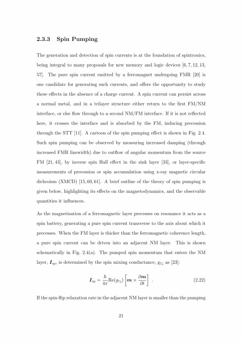
2.3.3 Spin Pumping

The generation and detection of spin currents is at the foundation of spintronics,

being integral to many proposals for new memory and logic devices [6, 7, 12, 13,

57]. The pure spin current emitted by a ferromagnet undergoing FMR [20] is

one candidate for generating such currents, and offers the opportunity to study

these effects in the absence of a charge current. A spin current can persist across

a normal metal, and in a trilayer structure either return to the first FM/NM

interface, or else flow through to a second NM/FM interface. If it is not reflected

here, it crosses the interface and is absorbed by the FM, inducing precession

through the STT [11]. A cartoon of the spin pumping effect is shown in Fig. 2.4.

Such spin pumping can be observed by measuring increased damping (through

increased FMR linewidth) due to outflow of angular momentum from the source

FM [21, 43], by inverse spin Hall effect in the sink layer [33], or layer-specific

measurements of precession or spin accumulation using x-ray magnetic circular

dichroism (XMCD) [15, 60, 61]. A brief outline of the theory of spin pumping is

given below, highlighting its effects on the magnetodynamics, and the observable

quantities it influences.

As the magnetisation of a ferromagnetic layer precesses on resonance it acts as a

spin battery, generating a pure spin current transverse to the axis about which it

precesses. When the FM layer is thicker than the ferromagnetic coherence length,

a pure spin current can be driven into an adjacent NM layer. This is shown

schematically in Fig. 2.4(a). The pumped spin momentum that enters the NM

layer, Isp, is determined by the spin mixing conductance, g↑↓ as [23]:

Isp =h

4πRe(g↑↓)

[m× ∂m

∂t

]. (2.22)

If the spin-flip relaxation rate in the adjacent NM layer is smaller than the pumping

21

Magnon

Spin current

Ma

gn

etisa

tio

n

(a) Spin pumping out of a magnetic layer

(b) Spin pumping in a trilayer structure

Ferromagnet Normal metal

Spin current

Ma

gn

etisa

tio

n

Ma

gn

etisa

tio

n

FM1 NM FM2

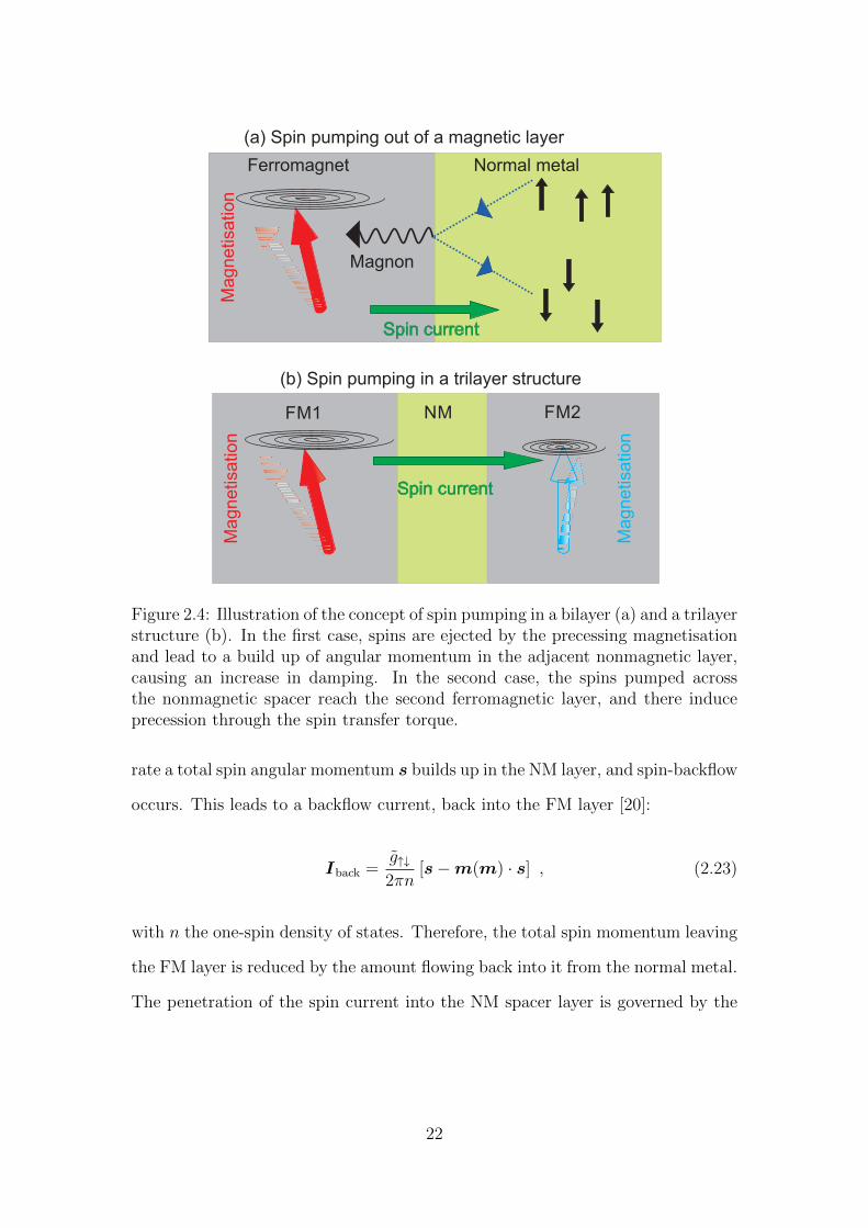
Figure 2.4: Illustration of the concept of spin pumping in a bilayer (a) and a trilayerstructure (b). In the first case, spins are ejected by the precessing magnetisationand lead to a build up of angular momentum in the adjacent nonmagnetic layer,causing an increase in damping. In the second case, the spins pumped acrossthe nonmagnetic spacer reach the second ferromagnetic layer, and there induceprecession through the spin transfer torque.

rate a total spin angular momentum s builds up in the NM layer, and spin-backflow

occurs. This leads to a backflow current, back into the FM layer [20]:

Iback =g↑↓2πn

[s−m(m) · s] , (2.23)

with n the one-spin density of states. Therefore, the total spin momentum leaving

the FM layer is reduced by the amount flowing back into it from the normal metal.

The penetration of the spin current into the NM spacer layer is governed by the

22

scattering lifetimes of conduction electrons, and is given by [22]:

δsp = D · τsf = vF

√τsfτm/3 , (2.24)

where D is the diffusion coefficient in the normal metal, vF the Fermi velocity in

the NM layer, and τsf and τm the NM layer’s spin-flip and momentum scattering

times, respectively.

The increased flow of spin momentum out of the FM layer acts as an additional

channel for energy loss, leading to an increase in damping. This damping is linear

with resonant frequency, and can thus be described in the same terms as Gilbert

damping. The contribution to total damping due to spin pumping can be isolated

by comparison with bare FM layers. In a FM/NM system the spin-pumping

contribution to damping is [23]:

αsp =

[1−

(1 + e−2kd)12vF(

Dk + 12vF + e−2kd

) (12vF −Dk

)]

× gµB

4πMs

g↑↓1

d, (2.25)

where k = 1/δsp and d the thickness of the FM layer. As the thickness of the NM

layer increases, the spin current that it can absorb also increases, in turn increasing

damping in the FM. However, once tNM > δsp, αsp saturates to its maximum value.

In the case of a FM1/NM/FM2 structure, the second FM layer acts as a spin sink

for the spin current driven out of the first FM layer. The absorbed spin current

exerts a torque on the static magnetisation in FM2, which can lead to precession

of magnetisation even when the resonance condition is not met. Figure 2.4(b)

shows this process schematically. The addition of a second scattering interface

and a high-efficiency spin sink modifies the spin pumping equations significantly.

23

In this case the LLG becomes [15]:

−∂mi

∂t= mi ×

[γiH i

eff − (αi0 + αiii)∂mi

∂t

]+ αiijm

j × ∂mj

∂t, (2.26)

where the subscript denotes the magnetic layer number, αi0 the intrinsic Gilbert

damping parameter, αiii damping due to angular momentum pumped out of layer

i, and αiij (anti-)damping due to angular momentum driven into layer i from layer

j. The anti-damping torque is only significant when both layers are simultaneously

on-resonance, otherwise ∂M j/∂t ≈ 0 and its effects are negligible.

The additional damping in a trilayer is defined as [62]:

αsp =

[1−

[(Dk + 1

2vF

)+ e−2kd

(Dk − 1

2vF

)]12vF(

Dk + 12vF

)2+ e−2kd

(Dk − 1

2vF

)2

]

× gµB

4πMs

g↑↓1

d, (2.27)

which, in the limit of ballistic transport, simplifies to [15]:

αsp =gµB

4πMg↑↓

1

d. (2.28)

Damping is highest when the spin current can cross the spacer layer and be ef-

ficiently absorbed by the second FM layer. As the thickness of the spacer layer

increases the spin pumping decreases due to increasing backflow. The increase in

damping reaches its minimum value when the spacer layer is thicker than the spin

coherence length, and no current reaches FM2 [23].

24

2.4 X-Ray Magnetic Circular Dichroism

X-ray Magnetic Circular Dichroism (XMCD) is a powerful tool for chemical and

magnetic characterisation, capable of identifying, for example, atomic valences,

site occupation and spin and orbital moments through application of the much

celebrated sum rules (see section 2.4.1). The absorption of light by a material is

governed by its wavelength and the available energy level transitions within the

sample. X-ray absorption spectra (XAS) measurements are performed by sweeping

the energy of the x-ray photons and observing the regions of maximum absorption,

when the incident light corresponds to a given core-level transition in the atoms.

These regions are known as absorption edges, and are typically referred to in

the spectroscopic notation, e.g. L2,3,M4,5 etc. In this way XAS and XMCD are

element-selective techniques, as each edge corresponds uniquely to one element.

This can be exploited to probe specific layers in a magnetic heterostructure.

In the 3d transition metals that are the central subject of this thesis, the L2,3

edge corresponds to the transition from spin-split 2p 12, 32

core states to the 3d

valence states. When the incident x-rays are circularly polarised there is an extra

selection rule, ∆mj = ±1, which results in a different transition probability for

left- and right-circularly polarised light into the unoccupied states valence band.

This effect is comparable to the Faraday or Kerr effects, but much stronger as the

spin-orbit interaction is larger in the core level than in the optical region, at tens

of eV, compared to less than 100 meV [38]. In this way, the transition probability

depends on both the helicity of the incoming light and the magnetic state of the

illuminated material. The XMCD is defined as the difference between two XAS

measurements performed with opposite magnetisations or x-ray helicities, as:

XMCD(E) = µ−(E)− µ+(E) , (2.29)

25

where µ−(E) and µ+(E) are the absorption coefficients with left and right circu-

larly polarized light, respectively, as a function of incident photon energy. The

XMCD is therefore sensitive to the difference in the density of empty states with

different spin moment.

To understand XMCD, it is instructive to consider a two-step approach, in a mo-

noelectronic atomic picture [63]: in a 3d metal, the 2p core state is spin split with

j = 3/2 (L3) and j = 1/2 (L2), with the spin and orbital angular moments having

parallel and antiparallel coupling, respectively. When absorbing an x-ray photon

with helicity ±1, the helicity vector is parallel (antiparallel) to the 2p orbital an-

gular moment. There is therefore a preferential excitation of electrons of spin up

(down) direction. The excited electron then moves to an unoccupied state in the

3d valence band. In a magnetic material the density of states in the 3d band is

different for the two spin orientations. This process is illustrated schematically

in Fig. 2.5. As the transition probability is related to the available states, the

resulting XMCD spectrum has a net negative L3 and positive L2 peak. In this

way, absorption of light depends upon the helicity of the incident light and the

magnetisation of the sample: reversing either will reverse the XMCD spectrum.

The intensity of the XMCD effect scales as the dot product of the magnetisa-

tion vector and the polarisation vector of the x-rays, thus if the magnetisation is

perpendicular to the beam direction no XMCD is observed.

2.4.1 Sum Rules

One of the most powerful aspects of XMCD is its ability to independently deter-

mine spin and orbital contributions to total magnetic moment, through the use of

the sum rules. Originally derived by Thole et al. [40] and Carra et al. [39], they

relate the area under the XAS and XMCD spectra to the spin, mS = −2µB〈SZ〉/h

26

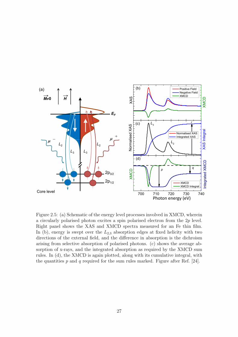
(a)

H

EF

M0

XA

S

Positive Field Negative Field XMCD

L3

XM

CD

Normalised XAS Integrated XAS

No

rma

lise

d X

AS (c)

XA

S In

teg

ral

r

(b)

2p3/2

2p1/2

Core level

L2

L3

L2

L3

700 710 720 730 740

L2

No

rma

lise

d X

AS

(d)

XA

S In

teg

ral

XM

CD

XMCD XMCD Integral

pq

Inte

gra

ted

XM

CD

Photon energy (eV)

Figure 2.5: (a) Schematic of the energy level processes involved in XMCD, whereina circularly polarised photon excites a spin polarised electron from the 2p level.Right panel shows the XAS and XMCD spectra measured for an Fe thin film.In (b), energy is swept over the L2,3 absorption edges at fixed helicity with twodirections of the external field, and the difference in absorption is the dichroismarising from selective absorption of polarised photons. (c) shows the average ab-sorption of x-rays, and the integrated absorption as required by the XMCD sumrules. In (d), the XMCD is again plotted, along with its cumulative integral, withthe quantities p and q required for the sum rules marked. Figure after Ref. [24].

27

and orbital, mL = −µB〈LZ〉/h magnetic moments. These necessary integrals are:

p =

∫L3

(µ− − µ+)dE

q =

∫L3

(µ− − µ+)dE +

∫L2

(µ− − µ+)dE (2.30)

r =

∫L3+L2

(µ− + µ+)dE .

In practical terms p and q are the XMCD integrals over the L3 and the combined L3

+ L2 edges, respectively, and r the integral over the sum of positive and negative

field spectra over the L3 + L2 edges. Figure 2.5 shows the cumulative integrals of

the XAS and the XMCD, indicating typical definitions for the extraction of p, q, r.

A background that takes into account transitions into higher states or into the

continuum must be subtracted before calculating r. This is usually approximated

by a hyperbolic step function at each absorption edge [64].

The sum rule for orbital moment is expressed as:

mL

nh= −4

3

q

r, (2.31)

with nh the number of holes. In the case of the spin sum rule, one must also

consider the dipolar term, mD, which depends on the inter-atomic dipole operator,

〈TZ〉. However, in the case of undistorted cubic symmetry it is normal to assume

that the angle averaged 〈TZ〉 is much less than mS. The sum rule for spin moment

is then:

mS

nh= −2

(3p− 2q

r

). (2.32)

It is also common to consider the ratio of spin to orbital moments, as it is inde-

pendent of nh:

mL

mS

=1

(9/2)(p/q)− 3. (2.33)

28

As it is non-trivial to determine nh, values of mL and mS are commonly expressed

as magnetic moment per d-hole, along with the mL/mS ratio.

29

Chapter 3

Experimental Techniques

This chapter describes the experimental techniques employed over the course of the

thesis investigation. Sample fabrication is described first, detailing the general op-

erating principles of molecular beam epitaxy and reflection high energy diffraction,

as well as specific information about the particular systems used. Next, ferromag-

netic resonance is considered, building from the theoretical framework outlined

in the previous chapter to cover the vector-network analyser technique. SQUID

magnetometry, the other magnetic characterisation tool employed, is explained

next. Following this, the focus shifts to measurements performed at synchrotron

facilities, outlining the principles of synchrotron radiation as well as the partic-

ulars of the techniques employed: x-ray absorption spectroscopy, x-ray magnetic

circular dichroism, and x-ray detected ferromagnetic resonance.

3.1 Molecular Beam Epitaxy

High quality magnetic thin films and heterostructures were prepared using molec-

ular beam epitaxy (MBE) [65–67], an ultra high vacuum (UHV) growth technique

that allows precise control of film thickness, composition, and interface quality.

30

The concept is based on assembling a crystal through direct deposition of con-

stituent atoms, achieving superior purity through the use of ultrahigh vacuum

conditions and low energy deposition [68–70]. MBE has been extensively applied

to the synthesis and investigation of a wide range of materials [71], including com-

plex oxides [72], semiconductor devices [73], and magnetic tunnel junctions [74].

The technique allows unmatched thickness and composition control, and it can be

applied to thin-film structures both close to [75] and far away [76] from thermo-

dynamic equilibrium. MBE is therefore an indispensable tool at the forefront of

materials research and surface science.

As a UHV technique MBE requires a sophisticated chamber design to maintain

pressures better than 1×10−9 Torr, and to allow operation of growth, characteri-

sation and sample manipulation in this environment. Such pressures are typically

achieved through the use of turbomolecular pumps, aided by a liquid nitrogen

cryoshroud, which reduces the kinetic energy of free gas molecules to further re-

duce the chamber pressure. UHV is required due to the extremely low growth

rates employed in MBE, which are often less than 0.1A/s. Strict control of cham-

ber pressure throughout growth limits the impurities that are incorporated into

the film during growth, which is beneficial from the standpoint of both chemical

purity and crystalline order.

Three MBE systems were used over the course of this thesis: the Lanthanide

MBE (LaMBE) in the Clarendon lab, Oxford [77]; the micro-MBE (µ-MBE) [78]

on beamline I05 at Diamond Light Source; and a chalcogenide MBE in the Re-

search Complex at Harwell. The LaMBE is a venerable Balzers UMS 630 sys-

tem, equipped with three effusion cells and three electron-beam evaporators, with

a quartz crystal microbalance for growth rate calibration, and a reflection high

energy electron diffraction (RHEED) system for sample characterisation during

growth. The µ-MBE is a newly developed system (Createc Fischer) that was

31

installed and commissioned over the course of this thesis. It houses 8 high tem-

perature effusion cells, a beam flux monitor for growth rate calibration and a

miniaturised RHEED. The topological insulator layers used in chapter 7 were

grown in a dedicated chalcogenide MBE. However, this system was not operated

by the author, and for further details the interested reader is referred to Ref. [79].

Despite several technical differences between the systems, the core operating prin-

ciples are the same. Aside from noting which system was used for which sample

series, no great distinction will be drawn between them.

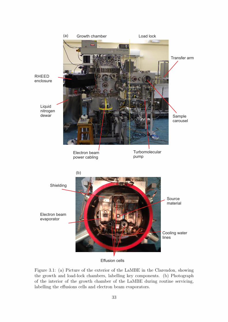
The LaMBE is shown in Fig. 3.1, and is composed of two chambers: a load-lock

and growth chamber. New substrates are mounted on holders and introduced to

the system at the load lock, which has a storage carousel for up to 6 samples. Due

to its comparatively small volume, the load lock can be pumped to a pressure of

5×10−8 Torr in about 12 hours. From here, samples are transferred to the growth

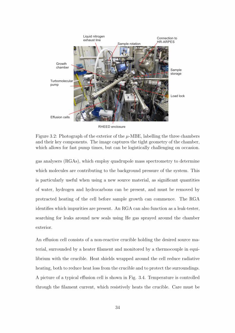
chamber using the manipulator arm. The exterior of the µ-MBE is shown in Fig.

3.2. It is composed of three chambers: a load-lock and growth chamber (a cutaway

is shown in Fig. 3.3) as in the case of the LaMBE, but with an additional sample

storage chamber with a carousel for up to 12 samples. The load-lock in this case

is much smaller, capable of reaching 5×10−8 Torr in a mere 30 minutes, thanks

to the use of an integrated heating lamp to desorb water. Only one sample at a

time can be introduced in this manner. From here the sample is transferred to the

storage chamber, which also provides an interface with the preparation chamber

of the HR-ARPES branchline [80].

The substrate is affixed to a sample holder by means of tantalum clips or a vacuum

compatible bonding agent such as indium, ensuring good thermal contact with the

holder. The holder is designed to facilitate transfer of the sample through the UHV

environment, using manipulator arms in conjunction with storage racks.

In addition to capacitance pressure gauges, both chambers are fitted with residual

32

Growth chamber Load lock

RHEEDenclosure

Liquidnitrogendewar

Turbomolecularpump

Transfer arm

Samplecarousel

Electron beampower cabling

(a)

Effusion cells

Electron beamevaporator

Shielding

Cooling waterlines

Sourcematerial

M

(b)

Figure 3.1: (a) Picture of the exterior of the LaMBE in the Clarendon, showingthe growth and load-lock chambers, labelling key components. (b) Photographof the interior of the growth chamber of the LaMBE during routine servicing,labelling the effusions cells and electron beam evaporators.

33

Growthchamber

Samplestorage

Load lock

RHEED enclosure

Turbomolecularpump

Liquid nitrogenexhaust line

Sample rotation

Effusion cells

Connection toHR-ARPES

Figure 3.2: Photograph of the exterior of the µ-MBE, labelling the three chambersand their key components. The image captures the tight geometry of the chamber,which allows for fast pump times, but can be logistically challenging on occasion.

gas analysers (RGAs), which employ quadrupole mass spectrometry to determine

which molecules are contributing to the background pressure of the system. This

is particularly useful when using a new source material, as significant quantities

of water, hydrogen and hydrocarbons can be present, and must be removed by

protracted heating of the cell before sample growth can commence. The RGA

identifies which impurities are present. An RGA can also function as a leak-tester,

searching for leaks around new seals using He gas sprayed around the chamber

exterior.

An effusion cell consists of a non-reactive crucible holding the desired source ma-

terial, surrounded by a heater filament and monitored by a thermocouple in equi-

librium with the crucible. Heat shields wrapped around the cell reduce radiative

heating, both to reduce heat loss from the crucible and to protect the surroundings.

A picture of a typical effusion cell is shown in Fig. 3.4. Temperature is controlled

through the filament current, which resistively heats the crucible. Care must be

34

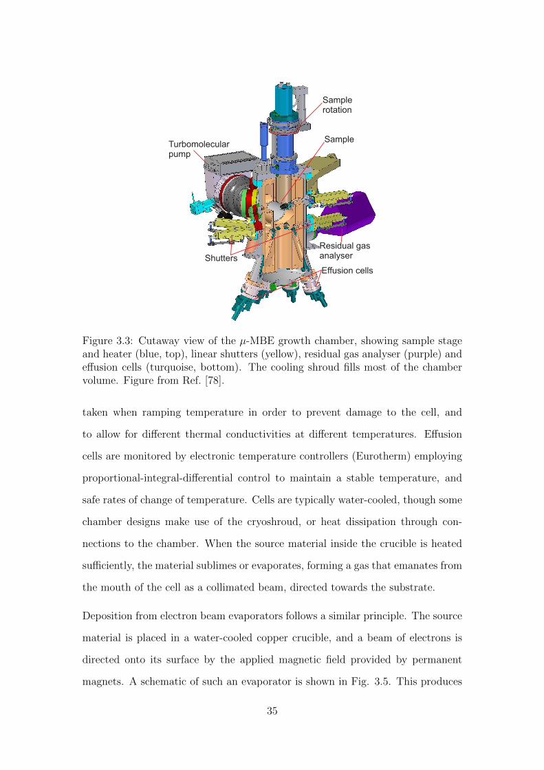
Turbomolecularpump

Samplerotation

Shutters

Effusion cells

Sample

Residual gasanalyser

Figure 3.3: Cutaway view of the µ-MBE growth chamber, showing sample stageand heater (blue, top), linear shutters (yellow), residual gas analyser (purple) andeffusion cells (turquoise, bottom). The cooling shroud fills most of the chambervolume. Figure from Ref. [78].

taken when ramping temperature in order to prevent damage to the cell, and

to allow for different thermal conductivities at different temperatures. Effusion

cells are monitored by electronic temperature controllers (Eurotherm) employing

proportional-integral-differential control to maintain a stable temperature, and

safe rates of change of temperature. Cells are typically water-cooled, though some

chamber designs make use of the cryoshroud, or heat dissipation through con-

nections to the chamber. When the source material inside the crucible is heated

sufficiently, the material sublimes or evaporates, forming a gas that emanates from

the mouth of the cell as a collimated beam, directed towards the substrate.

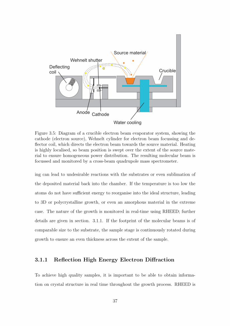
Deposition from electron beam evaporators follows a similar principle. The source

material is placed in a water-cooled copper crucible, and a beam of electrons is

directed onto its surface by the applied magnetic field provided by permanent

magnets. A schematic of such an evaporator is shown in Fig. 3.5. This produces

35

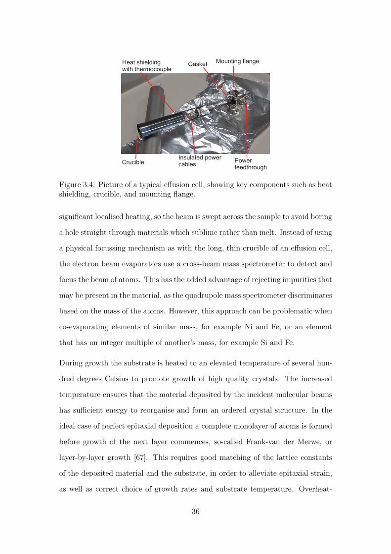
Crucible

Heat shieldingwith thermocouple

Mounting flange

Powerfeedthrough

Gasket

Insulated powercables

Figure 3.4: Picture of a typical effusion cell, showing key components such as heatshielding, crucible, and mounting flange.

significant localised heating, so the beam is swept across the sample to avoid boring

a hole straight through materials which sublime rather than melt. Instead of using

a physical focussing mechanism as with the long, thin crucible of an effusion cell,

the electron beam evaporators use a cross-beam mass spectrometer to detect and

focus the beam of atoms. This has the added advantage of rejecting impurities that

may be present in the material, as the quadrupole mass spectrometer discriminates

based on the mass of the atoms. However, this approach can be problematic when

co-evaporating elements of similar mass, for example Ni and Fe, or an element

that has an integer multiple of another’s mass, for example Si and Fe.

During growth the substrate is heated to an elevated temperature of several hun-

dred degrees Celsius to promote growth of high quality crystals. The increased

temperature ensures that the material deposited by the incident molecular beams

has sufficient energy to reorganise and form an ordered crystal structure. In the

ideal case of perfect epitaxial deposition a complete monolayer of atoms is formed

before growth of the next layer commences, so-called Frank-van der Merwe, or

layer-by-layer growth [67]. This requires good matching of the lattice constants

of the deposited material and the substrate, in order to alleviate epitaxial strain,

as well as correct choice of growth rates and substrate temperature. Overheat-

36

Wehnelt shutter

CathodeAnode

Deflectingcoil Crucible

Source material

Water cooling

e-

Figure 3.5: Diagram of a crucible electron beam evaporator system, showing thecathode (electron source), Wehnelt cylinder for electron beam focussing and de-flector coil, which directs the electron beam towards the source material. Heatingis highly localised, so beam position is swept over the extent of the source mate-rial to ensure homogeneous power distribution. The resulting molecular beam isfocussed and monitored by a cross-beam quadrupole mass spectrometer.

ing can lead to undesirable reactions with the substrates or even sublimation of

the deposited material back into the chamber. If the temperature is too low the

atoms do not have sufficient energy to reorganise into the ideal structure, leading

to 3D or polycrystalline growth, or even an amorphous material in the extreme

case. The nature of the growth is monitored in real-time using RHEED; further

details are given in section. 3.1.1. If the footprint of the molecular beams is of

comparable size to the substrate, the sample stage is continuously rotated during

growth to ensure an even thickness across the extent of the sample.

3.1.1 Reflection High Energy Electron Diffraction

To achieve high quality samples, it is important to be able to obtain informa-

tion on crystal structure in real time throughout the growth process. RHEED is

37

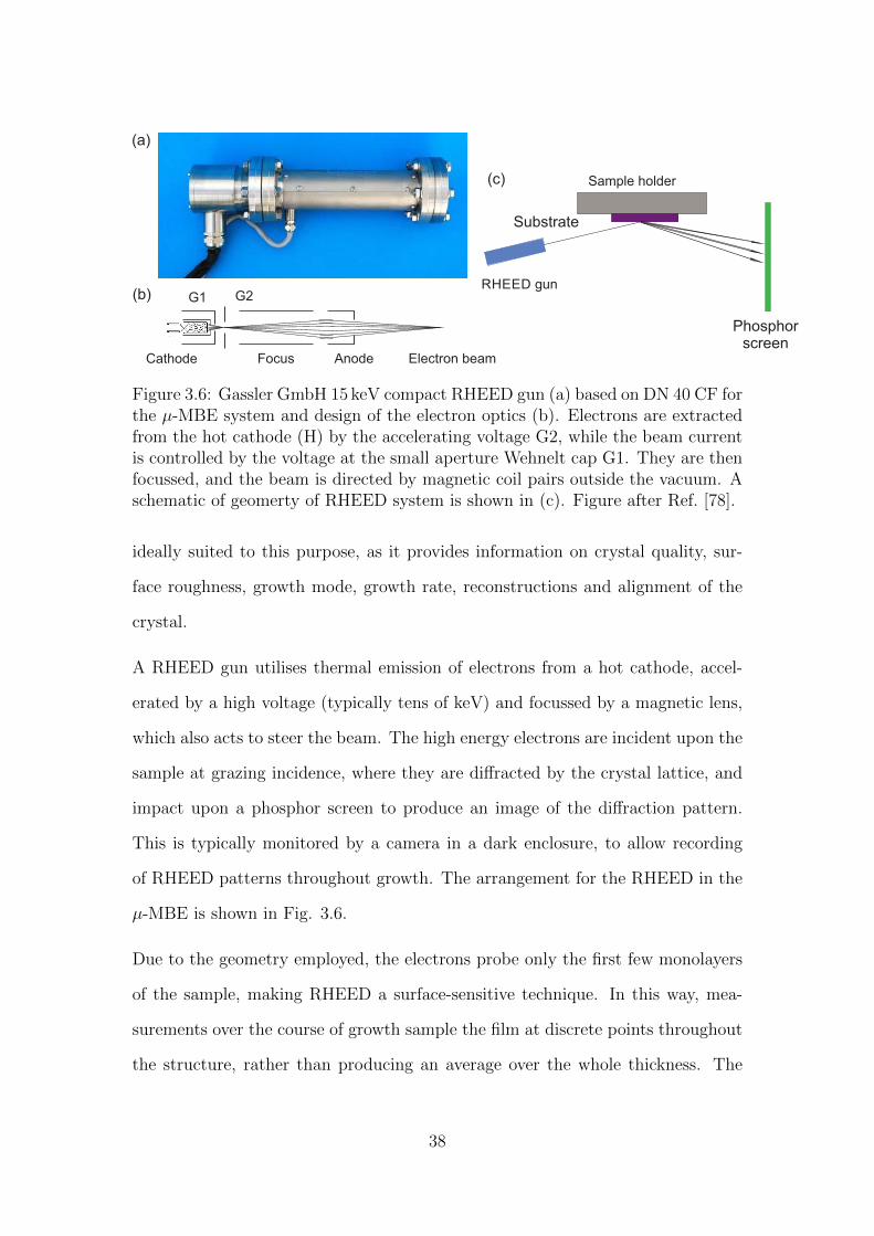
(c) Sample holder

RHEED gun

Substrate

Phosphorscreen

(a)

(b)

Anode Electron beamFocusCathode

G1 G2

Figure 3.6: Gassler GmbH 15 keV compact RHEED gun (a) based on DN 40 CF forthe µ-MBE system and design of the electron optics (b). Electrons are extractedfrom the hot cathode (H) by the accelerating voltage G2, while the beam currentis controlled by the voltage at the small aperture Wehnelt cap G1. They are thenfocussed, and the beam is directed by magnetic coil pairs outside the vacuum. Aschematic of geomerty of RHEED system is shown in (c). Figure after Ref. [78].

ideally suited to this purpose, as it provides information on crystal quality, sur-

face roughness, growth mode, growth rate, reconstructions and alignment of the

crystal.

A RHEED gun utilises thermal emission of electrons from a hot cathode, accel-

erated by a high voltage (typically tens of keV) and focussed by a magnetic lens,

which also acts to steer the beam. The high energy electrons are incident upon the

sample at grazing incidence, where they are diffracted by the crystal lattice, and

impact upon a phosphor screen to produce an image of the diffraction pattern.

This is typically monitored by a camera in a dark enclosure, to allow recording

of RHEED patterns throughout growth. The arrangement for the RHEED in the

µ-MBE is shown in Fig. 3.6.

Due to the geometry employed, the electrons probe only the first few monolayers

of the sample, making RHEED a surface-sensitive technique. In this way, mea-

surements over the course of growth sample the film at discrete points throughout

the structure, rather than producing an average over the whole thickness. The

38

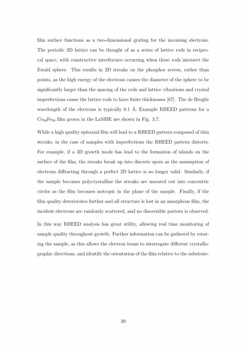
film surface functions as a two-dimensional grating for the incoming electrons.

The periodic 2D lattice can be thought of as a series of lattice rods in recipro-

cal space, with constructive interference occurring when these rods intersect the

Ewald sphere. This results in 2D streaks on the phosphor screen, rather than

points, as the high energy of the electrons causes the diameter of the sphere to be

significantly larger than the spacing of the rods and lattice vibrations and crystal

imperfections cause the lattice rods to have finite thicknesses [67]. The de Broglie

wavelength of the electrons is typically 0.1 A. Example RHEED patterns for a

Co50Fe50 film grown in the LaMBE are shown in Fig. 3.7.

While a high quality epitaxial film will lead to a RHEED pattern composed of thin

streaks, in the case of samples with imperfections the RHEED pattern distorts.

For example, if a 3D growth mode has lead to the formation of islands on the

surface of the film, the streaks break up into discrete spots as the assumption of

electrons diffracting through a perfect 2D lattice is no longer valid. Similarly, if

the sample becomes polycrystalline the streaks are smeared out into concentric

circles as the film becomes isotropic in the plane of the sample. Finally, if the

film quality deteriorates further and all structure is lost in an amorphous film, the

incident electrons are randomly scattered, and no discernible pattern is observed.

In this way RHEED analysis has great utility, allowing real time monitoring of

sample quality throughout growth. Further information can be gathered by rotat-

ing the sample, as this allows the electron beam to interrogate different crystallo-

graphic directions, and identify the orientation of the film relative to the substrate.

39

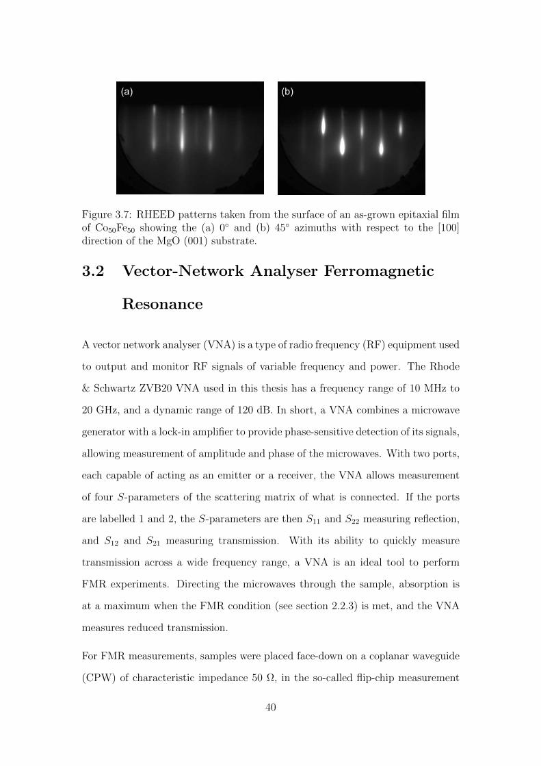
(a) (b)

Figure 3.7: RHEED patterns taken from the surface of an as-grown epitaxial filmof Co50Fe50 showing the (a) 0 and (b) 45 azimuths with respect to the [100]direction of the MgO (001) substrate.

3.2 Vector-Network Analyser Ferromagnetic

Resonance

A vector network analyser (VNA) is a type of radio frequency (RF) equipment used

to output and monitor RF signals of variable frequency and power. The Rhode

& Schwartz ZVB20 VNA used in this thesis has a frequency range of 10 MHz to

20 GHz, and a dynamic range of 120 dB. In short, a VNA combines a microwave

generator with a lock-in amplifier to provide phase-sensitive detection of its signals,

allowing measurement of amplitude and phase of the microwaves. With two ports,

each capable of acting as an emitter or a receiver, the VNA allows measurement

of four S-parameters of the scattering matrix of what is connected. If the ports

are labelled 1 and 2, the S-parameters are then S11 and S22 measuring reflection,

and S12 and S21 measuring transmission. With its ability to quickly measure

transmission across a wide frequency range, a VNA is an ideal tool to perform

FMR experiments. Directing the microwaves through the sample, absorption is

at a maximum when the FMR condition (see section 2.2.3) is met, and the VNA

measures reduced transmission.

For FMR measurements, samples were placed face-down on a coplanar waveguide

(CPW) of characteristic impedance 50 Ω, in the so-called flip-chip measurement

40

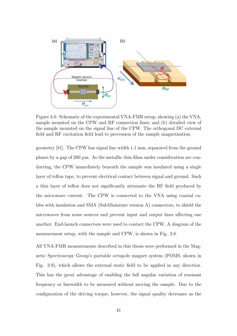
M

HRF

Hext

Sample

extH

HRF

(a) (b)

Magnet vacuumchamber

Figure 3.8: Schematic of the experimental VNA-FMR setup, showing (a) the VNA,sample mounted on the CPW and RF connection lines; and (b) detailed view ofthe sample mounted on the signal line of the CPW. The orthogonal DC externalfield and RF excitation field lead to precession of the sample magnetisation.

geometry [81]. The CPW has signal line width 1.1 mm, separated from the ground

planes by a gap of 200 µm. As the metallic thin films under consideration are con-

ducting, the CPW immediately beneath the sample was insulated using a single

layer of teflon tape, to prevent electrical contact between signal and ground. Such

a thin layer of teflon does not significantly attenuate the RF field produced by

the microwave current. The CPW is connected to the VNA using coaxial ca-

bles with insulation and SMA (SubMiniature version A) connectors, to shield the

microwaves from noise sources and prevent input and output lines affecting one

another. End-launch connectors were used to contact the CPW. A diagram of the

measurement setup, with the sample and CPW, is shown in Fig. 3.8.

All VNA-FMR measurements described in this thesis were performed in the Mag-

netic Spectroscopy Group’s portable octupole magnet system (POMS, shown in

Fig. 3.9), which allows the external static field to be applied in any direction.

This has the great advantage of enabling the full angular variation of resonant

frequency or linewidth to be measured without moving the sample. Due to the

configuration of the driving torque, however, the signal quality decreases as the

41

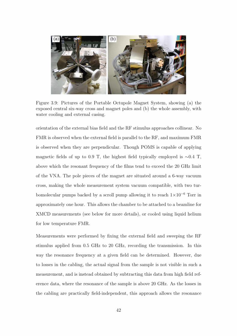
(a) (b)

Figure 3.9: Pictures of the Portable Octupole Magnet System, showing (a) theexposed central six-way cross and magnet poles and (b) the whole assembly, withwater cooling and external casing.

orientation of the external bias field and the RF stimulus approaches collinear. No

FMR is observed when the external field is parallel to the RF, and maximum FMR

is observed when they are perpendicular. Though POMS is capable of applying

magnetic fields of up to 0.9 T, the highest field typically employed is ∼0.4 T,

above which the resonant frequency of the films tend to exceed the 20 GHz limit

of the VNA. The pole pieces of the magnet are situated around a 6-way vacuum

cross, making the whole measurement system vacuum compatible, with two tur-

bomolecular pumps backed by a scroll pump allowing it to reach 1×10−6 Torr in

approximately one hour. This allows the chamber to be attached to a beamline for

XMCD measurements (see below for more details), or cooled using liquid helium

for low temperature FMR.

Measurements were performed by fixing the external field and sweeping the RF

stimulus applied from 0.5 GHz to 20 GHz, recording the transmission. In this

way the resonance frequency at a given field can be determined. However, due

to losses in the cabling, the actual signal from the sample is not visible in such a

measurement, and is instead obtained by subtracting this data from high field ref-

erence data, where the resonance of the sample is above 20 GHz. As the losses in

the cabling are practically field-independent, this approach allows the resonance

42

to be identified. By putting together many measurements of transmission as a

function of frequency at different fields, a field-frequency-transmission map show-

ing the Kittel curves of the resonance can be built up, examples of such maps are

shown in Fig. 3.10. While the VNA can be calibrated to remove the effects of the

cabling, the necessity for the whole arrangement to be both vacuum compatible

and portable makes this rather impractical. However, a significant improvement in

data quality can be obtained by changing the approach. At a fixed frequency, the

data quality of transmission as a function of external field is much better. Rather

than requiring the frequency to be fixed and field to be swept (a much more

time consuming process), high quality data can be obtained from field-frequency-

transmission maps simply by searching for resonant field at a fixed frequency. This

also makes determination of Gilbert damping from linewidth mathematically more

convenient. Details of the procedure to extract resonance field and linewidth can

be found in section 2.2.3. A series of such measurements performed at different

angles of the applied magnetic field allows the anisotropy parameters of the film

to be determined, using the Kittel equation, equation (2.15).

3.3 SQUID Vibrating Sample Magnetometry

A magnetometer measures the magnetisation of a material, as a function of tem-

perature and applied external field. A vibrating sample magnetometer (VSM)

operates by oscillating the sample under test within a set of pick up coils, wherein

a current is induced proportional to the magnetisation. The sensitivity of a VSM

is directly related to how accurately the voltage can be measured. A SQUID-

VSM uses a superconducting quantum interference device (SQUID) for this pur-

pose, providing an extremely sensitive probe of magnetisation. A diagram of the

SQUID-VSM operating principle is shown in Fig. 3.11. The superconducting mea-

43

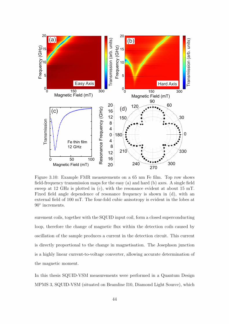
0 50 100

Magnetic Field (mT)

Fe thin film

12 GHz

0

30

6090

120

150

180

210

240270

300

330

4

8

12

16

20

0

4

8

12

16

20Re

so

na

nce

Fre

qu

en

cy (

GH

z)

Fre

quency (

GH

z)

Magnetic Field (mT)

20

15

10

5

03001500

Easy Axis

Magnetic Field (mT)

Fre

quency (

GH

z)

(c) (d)

(b)(a)

Hard Axis

Tra

nsm

issio

n

Tra

nsm

issio

n (

arb

. u

nits) 20

15

10

5

03001500

Tra

nsm

issio

n (

arb

. u

nits)

Figure 3.10: Example FMR measurements on a 65 nm Fe film. Top row showsfield-frequency transmission maps for the easy (a) and hard (b) axes. A single fieldsweep at 12 GHz is plotted in (c), with the resonance evident at about 15 mT.Fixed field angle dependence of resonance frequency is shown in (d), with anexternal field of 100 mT. The four-fold cubic anisotropy is evident in the lobes at90 increments.

surement coils, together with the SQUID input coil, form a closed superconducting

loop, therefore the change of magnetic flux within the detection coils caused by

oscillation of the sample produces a current in the detection circuit. This current

is directly proportional to the change in magnetisation. The Josephson junction

is a highly linear current-to-voltage converter, allowing accurate determination of

the magnetic moment.

In this thesis SQUID-VSM measurements were performed in a Quantum Design

MPMS 3, SQUID-VSM (situated on Beamline I10, Diamond Light Source), which

44

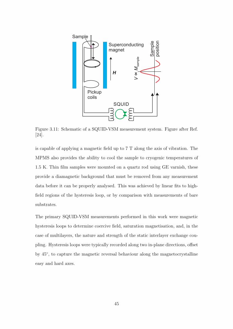
H

Superconductingmagnet

Sample

Pickupcoils

SQUID

V M

sam

ple

Sam

ple

positio

n

Figure 3.11: Schematic of a SQUID-VSM measurement system. Figure after Ref.[24].

is capable of applying a magnetic field up to 7 T along the axis of vibration. The

MPMS also provides the ability to cool the sample to cryogenic temperatures of

1.5 K. Thin film samples were mounted on a quartz rod using GE varnish, these

provide a diamagnetic background that must be removed from any measurement

data before it can be properly analysed. This was achieved by linear fits to high-

field regions of the hysteresis loop, or by comparison with measurements of bare

substrates.

The primary SQUID-VSM measurements performed in this work were magnetic

hysteresis loops to determine coercive field, saturation magnetisation, and, in the

case of multilayers, the nature and strength of the static interlayer exchange cou-

pling. Hysteresis loops were typically recorded along two in-plane directions, offset

by 45, to capture the magnetic reversal behaviour along the magnetocrystalline

easy and hard axes.

45

3.4 X-Ray Magnetic Circular Dichroism

XMCD is an element- and site-specific probe of magnetic order, utilising circu-

larly polarised synchrotron radiation at tunable energies. The theoretical back-

ground for the technique is described in section 2.4; this section will concentrate

on practical aspects of performing the technique. XMCD measurements used in

this thesis were performed at two synchrotrons: beamline I10 of Diamond Light

Source (DLS) and beamline 6.3.1 of the Advanced Light Source (ALS). These are

soft-xray beamlines, with a maximum energy on the order of 1.5 keV. The x-rays

are easily attenuated, and all measurements must be performed at UHV.

A synchrotron is a machine that accelerates electrons to nearly the speed of light,

whereupon they are directed into an orbit within a central storage ring and kept at

a constant velocity. The storage ring is at ultra-high vacuum, and uses quadrupole

and sextupole magnets to steer and focus the electron beam. Once in the ring,

electrons can circulate for an extended period of time, typically on the order of

hours.

A charged particle will emit radiation when it is accelerated, according to the

relativistically-correct Lienard-Wiechert potential [36]. In a synchrotron this is

used to produce high-intensity x-rays of a particular wavelength. There are two

main methods for this process. In the first case, when the electrons encounter

a curved section of the storage ring their path is altered by dipole (or bending)

magnets; the resulting acceleration causes them to emit light. In the second case,

an insertion device is placed on one of the straight sections of the ring, and uses

an array of magnets to produce a periodic field that causes the electrons to oscil-

late perpendicular to the direction of travel. The periodicity of the perturbation

correlates with the wavelength of the emitted light, when the Lorentz contraction

of the relativistic electrons and the Doppler shift is taken into account. Insertion

46

devices use constructive interference of the emitted light to produce a beam of

much higher intensity than bending magnets. In either case, the x-rays emitted

from the electrons are directed out from the storage ring and into the beamline,

which passes the light through a monochromator, focussing mirrors and diagnos-

tics before reaching the experimental hutch, where the measurement equipment is

situated.

The absorption of x-rays by the sample can be measured in several ways. In to-

tal electron yield (TEY) mode electrical contact is made to the sample surface

and the photoelectrons generated by the incident photons measured. Due to the

limited electron escape depth TEY is a surface-sensitive technique, with a probe

depth in the soft x-ray regime typically on the order of ∼3-5 nm. The XMCD

sum rules [38–40] can be readily applied to TEY data, making it a popular de-

tection mechanism. Fluorescence yield (FY) mode uses a photodiode placed in

the measurement chamber to measure photons emitted as electrons of lower bind-

ing energy fill the vacated core hole. It offers a significantly deeper probe depth

than TEY, interrogating the entire profile of thin film samples. Unfortunately,

FY amplitude is low in the soft x-ray region of the transition metal L2,3 edges,

and can be limited by geometrical considerations in chamber design. Finally, x-ray

excited optical luminescence of the substrate offers an attractive detection method

for suitable substrates. In this technique, x-rays that pass through the film are

absorbed by the substrate, wherein the recombination of trapped excitons leads to

emission of visible light. The MgO substrates widely used for growth of magnetic

heterostructures have a particularly strong optical emission line, visible even to

the naked eye. Placing a photodiode directly behind the sample therefore permits

measurement of the film’s XAS, as the intensity of x-rays reaching the substrate

is dictated by the absorption within the film.

XMCD measurements on beamline 6.3.1 of the ALS use a 2 T electromagnet, where

47

the beam pipe passes through the pole pieces of the magnet, giving a field parallel

to the beam. Beamline 6.3.1 uses a bending magnet, and is capable of fast energy

scanning to quickly acquire XAS measurements at a fixed polarisation. XMCD is

performed by reversing the magnetic field direction and repeating the XAS. The

beamline is optimised for a single polarisation (usually circular negative), thereby

achieving almost 100 % polarisation. XMCD measurements on beamline I10 at

DLS use the Magnetic Spectroscopy Group’s portable octupole magnet system,

mounted behind the RASOR scattering chamber. POMS can apply a field of up

to 0.9 T in any direction for short periods, with 0.5 T continuous field. In the

case of I10, XMCD measurements were performed by reversing the magnetic field

at every energy point.

3.5 X-Ray Detected Ferromagnetic Resonance

While VNA-FMR is a versatile characterisation tool, it is somewhat limited in that

it provides a measurement over the whole sample. While this is not a problem

when studying a single layer, it can be troublesome for the case of magnetic

heterostructures such as spin valves, as it is unable to separate contributions from

individual layers. This drawback can be addressed by combining the dynamic

sensitivity of FMR with the element- (and thus layer-) selectivity of XMCD to

perform x-ray detected ferromagnetic resonance (XFMR) [15,29,34].

The electrons in a storage ring of a synchrotron do not propagate in a continuous

beam, rather they travel in bunches of a given pulse width. The x-rays delivered

to the beamline have a repetition rate correlated to the arrival of bunches at the

insertion device. At both Diamond and the ALS this repetition rate is 499.65 MHz,

with a pulse width of 30 ps and 70 ps, respectively. Stroboscopic measurements

of magnetisation dynamics can therefore be performed at integer multiples of this

48

frequency; enabling time-dependent precession of magnetisation to be determined

at the picosecond timescale.

Static XMCD is defined as the difference between the two x-ray absorption spectra

recorded with the helicity vector of the circular polarization parallel and antipar-

allel respectively to an external magnetic field [38]. The XMCD signal is propor-

tional to the projection of the helicity vector, which is along the beam direction, k,

onto the magnetisation M , such that IXMCD ∝ k ·M . XMCD spectra generated

by reversing either the magnetic field or the circular polarisation are equivalent.

In XFMR, the energy and polarisation of the incoming light are fixed, and small

oscillations of the magnetisation as the material undergoes FMR are measured by

monitoring IXMCD.

The sample is mounted on a CPW and driven by an applied RF field while under

a static external field. At Diamond POMS is used (on beamline I10) to apply the

magnetic field, while at the ALS the vector magnet on beamline 4.0.2 is used [82].

The use of a vector magnet is especially convenient, as it allows static XMCD to be

measured with Hext parallel to the x-ray beam, and XFMR to be measured with

Hext orthogonal to the beam and RF field, which is required for phase-resolved

XFMR. A schematic of the measurement setup and detection circuit is shown in

Fig. 3.12.

There are two approaches to measure XFMR, the time-averaged longitudinal ge-

ometry [34, 84], and the time-resolved transverse geometry [29]. Longitudinal

XFMR detects the shortening of the magnetisation vector along the direction of

the x-ray beam as the sample is driven at the FMR condition. It detects a signal

of magnitude ∆Mz = M0[1− cos θ] ≈ 12M0θ

2, with θ the cone angle of precession.

The advantage of such a time-averaged measurement is that it does not require

synchronising with the x-ray arrival, and can thus be performed at any frequency.

It is useful when measuring overlapping resonances, but does not offer the more

49

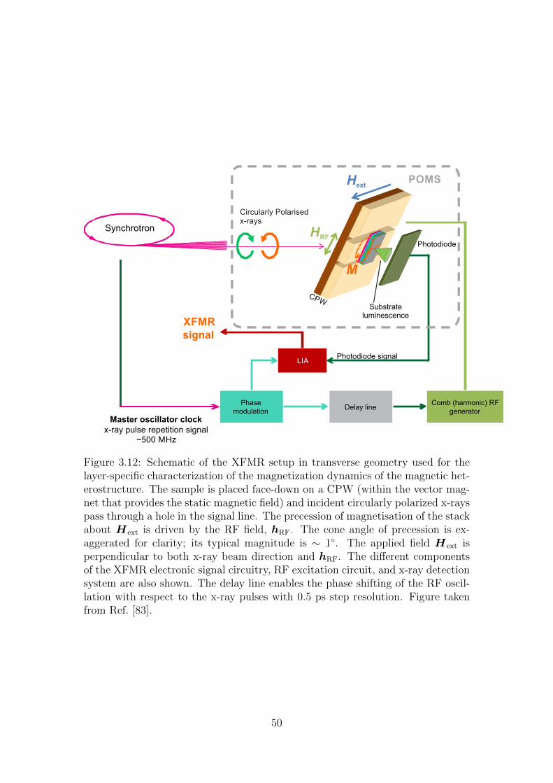
Synchrotron

Delay line

Master oscillator clock

x-ray pulse repetition signal~500 MHz

Comb (harmonic) RF

generator

Phase

modulation

LIA

Photodiode

Substrateluminescence

Photodiode signal

CPW

XFMR

signal

M

HRF

HextPOMS

Circularly Polarisedx-rays

Figure 3.12: Schematic of the XFMR setup in transverse geometry used for thelayer-specific characterization of the magnetization dynamics of the magnetic het-erostructure. The sample is placed face-down on a CPW (within the vector mag-net that provides the static magnetic field) and incident circularly polarized x-rayspass through a hole in the signal line. The precession of magnetisation of the stackabout Hext is driven by the RF field, hRF. The cone angle of precession is ex-aggerated for clarity; its typical magnitude is ∼ 1. The applied field Hext isperpendicular to both x-ray beam direction and hRF. The different componentsof the XFMR electronic signal circuitry, RF excitation circuit, and x-ray detectionsystem are also shown. The delay line enables the phase shifting of the RF oscil-lation with respect to the x-ray pulses with 0.5 ps step resolution. Figure takenfrom Ref. [83].

50

detailed phase information available to time-resolved measurements.

Throughout this work, time-resolved XFMR was employed as it provides greater

insight into the precessional dynamics. In this geometry Hext is applied perpen-

dicular to the incident x-ray beam, and variation in IXMCD probes the oscillating

component of the Larmor precession with magnitude My = M0 sin θ ≈ M0θ, a

factor of 2/θ larger than that in the longitudinal geometry. On resonance, θ is

typically 0.6, meaning that the dynamic XMCD observed is approximately 1%

of that observed in static measurements. Measurements are performed at close to

grazing incidence, in order to maximise the projection of magnetisation precession

along the direction of the beam.

For the stroboscopic measurements, the RF excitation must be a harmonic of the

x-ray pulse frequency, limiting the available frequencies. The higher harmonics are

provided by a comb generator (Atlantic Microwave) driven by the master oscillator

of the synchrotron. Typical frequencies used in the measurements are 4, 8 and

10 GHz. A programmable delay line is used to phase-shift the delay between

RF excitation (pump) and x-ray pulse arrival (probe), with a step resolution of

∼0.5 ps. However, the practical limit on step size is given by the jitter on the

RF signal, which is usually ∼3 ps. Coupled with increasing power losses at higher

frequencies, this imposes an upper limit on excitation frequencies of 12 GHz.

XMCD is detected by x-ray excited optical luminescence of the substrate, using a

photodiode mounted directly behind the sample. Lock-in amplifier (LIA) detection

of the time-varying signal is necessary to be able to measure the small amplitude

of precession, using a LIA while modulating the phase of the driving RF through

180. In this way the LIA measures the XMCD between opposite points on the

cone of precession, ensuring the largest possible signal.

The x-rays are incident upon the sample through a small hole drilled in the signal

51

line of the CPW. The x-ray beam has an incidence angle of 35 with respect to

the plane of the sample, ensuring that the XMCD probes in-plane precession.

Smaller incidence angles would yield a larger signal, but are impractical as such

rotation causes the footprint of the beam to be larger than the hole, or to be

partially blocked by the CPW itself. Unlike VNA-FMR measurements, where the

CPW is insulated beneath the sample, the film surface is in direct contact with

both the signal and ground in XFMR. This maximises RF power delivered to the

sample, thereby maximising cone angle and resulting XMCD. Connecting signal

and ground in such a manner causes considerable microwave losses, particularly

at high frequencies. This is not a serious concern, however, as long as cone angle

of precession is maximised at the desired frequency.

Two types of measurement are possible in the transverse geometry. In the first,

termed a field scan, the delay between RF excitation and x-ray arrival is fixed,

while the magnetic field strength is swept. The delay is increased by one quarter

oscillation, and the field sweep is repeated. This measures the real and imaginary

components of transverse susceptibility, from which phase and amplitude of pre-

cession can be determined. This approach is used when the dynamic XMCD signal

is large. In the second method, termed a delay scan, the static field is fixed and

the delay is swept, producing a sine curve of precession of magnetisation. Ampli-

tude and phase of precession can be obtained directly by fitting this curve. The

field is then changed, and the process repeated, in steps over the resonance con-

dition. This method is much more time consuming than field scans, but enables

significantly weaker signals to be measured. With phase and amplitude of pre-

cession across resonance the relative contributions of each layer to the resonances

can be determined, observing induced precession in the nominally off-resonance

layer. Further, modelling of the AC magnetic susceptibility tensor allows the sep-

arate contributions of Gilbert damping and spin pumping damping to be directly

52

measured, more details of which can be found in section 5.

53

Chapter 4

Engineering of Magnetic

Properties using Rare Earth

Dopants

4.1 Motivation

The development of spintronic devices utilising spin transfer torque requires a

mechanism for robust manipulation of both the static and dynamic properties of

ferromagnetic (FM) thin films [6,7,57]. One attractive route for such optimisation

is the use of rare earth (RE) dopants, which can significantly increase the Gilbert

damping parameter of the film [85–87]. Due to the antiferromagnetic coupling of

the RE impurities to the host lattice [88], there is an accompanying reduction in

saturation magnetization (Ms) [18,87]. Much effort has been expended to develop

this approach, from the perspective of device applications as well as fundamen-

tal investigations [18, 85–88]. Woltersdorf et al. [58] showed that the increase in

damping can be explained by the “slow relaxing” RE impurity model developed

by van Vleck and Orbach [89], whereby transitions between the exchange-split 4f

54

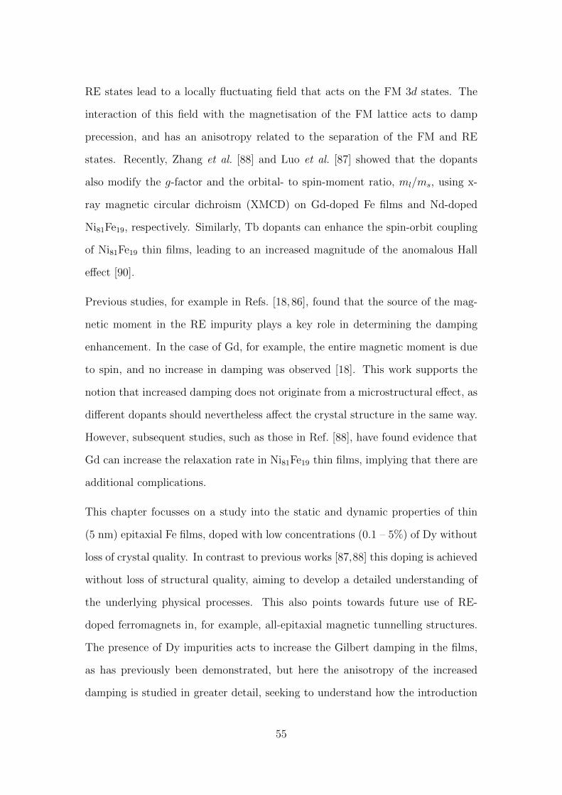
RE states lead to a locally fluctuating field that acts on the FM 3d states. The

interaction of this field with the magnetisation of the FM lattice acts to damp

precession, and has an anisotropy related to the separation of the FM and RE

states. Recently, Zhang et al. [88] and Luo et al. [87] showed that the dopants

also modify the g-factor and the orbital- to spin-moment ratio, ml/ms, using x-

ray magnetic circular dichroism (XMCD) on Gd-doped Fe films and Nd-doped

Ni81Fe19, respectively. Similarly, Tb dopants can enhance the spin-orbit coupling

of Ni81Fe19 thin films, leading to an increased magnitude of the anomalous Hall

effect [90].

Previous studies, for example in Refs. [18, 86], found that the source of the mag-

netic moment in the RE impurity plays a key role in determining the damping

enhancement. In the case of Gd, for example, the entire magnetic moment is due

to spin, and no increase in damping was observed [18]. This work supports the

notion that increased damping does not originate from a microstructural effect, as

different dopants should nevertheless affect the crystal structure in the same way.

However, subsequent studies, such as those in Ref. [88], have found evidence that

Gd can increase the relaxation rate in Ni81Fe19 thin films, implying that there are

additional complications.

This chapter focusses on a study into the static and dynamic properties of thin

(5 nm) epitaxial Fe films, doped with low concentrations (0.1 – 5%) of Dy without

loss of crystal quality. In contrast to previous works [87,88] this doping is achieved

without loss of structural quality, aiming to develop a detailed understanding of

the underlying physical processes. This also points towards future use of RE-

doped ferromagnets in, for example, all-epitaxial magnetic tunnelling structures.

The presence of Dy impurities acts to increase the Gilbert damping in the films,

as has previously been demonstrated, but here the anisotropy of the increased

damping is studied in greater detail, seeking to understand how the introduction

55

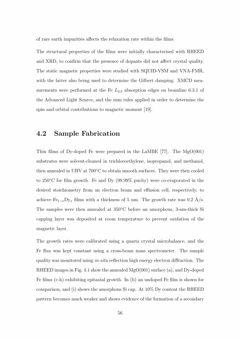
of rare earth impurities affects the relaxation rate within the films.

The structural properties of the films were initially characterised with RHEED

and XRD, to confirm that the presence of dopants did not affect crystal quality.

The static magnetic properties were studied with SQUID-VSM and VNA-FMR,

with the latter also being used to determine the Gilbert damping. XMCD mea-

surements were performed at the Fe L2,3 absorption edges on beamline 6.3.1 of

the Advanced Light Source, and the sum rules applied in order to determine the

spin and orbital contributions to magnetic moment [19].

4.2 Sample Fabrication

Thin films of Dy-doped Fe were prepared in the LaMBE [77]. The MgO(001)

substrates were solvent-cleaned in trichloroethylene, isopropanol, and methanol,

then annealed in UHV at 700C to obtain smooth surfaces. They were then cooled

to 250C for film growth. Fe and Dy (99.99% purity) were co-evaporated in the

desired stoichiometry from an electron beam and effusion cell, respectively, to

achieve Fe1−xDyx films with a thickness of 5 nm. The growth rate was 0.2 A/s.

The samples were then annealed at 350C before an amorphous, 3-nm-thick Si

capping layer was deposited at room temperature to prevent oxidation of the

magnetic layer.

The growth rates were calibrated using a quartz crystal microbalance, and the

Fe flux was kept constant using a cross-beam mass spectrometer. The sample

quality was monitored using in-situ reflection high energy electron diffraction. The

RHEED images in Fig. 4.1 show the annealed MgO(001) surface (a), and Dy-doped

Fe films (c-h) exhibiting epitaxial growth. In (b) an undoped Fe film is shown for

comparison, and (i) shows the amorphous Si cap. At 10% Dy content the RHEED

pattern becomes much weaker and shows evidence of the formation of a secondary

56

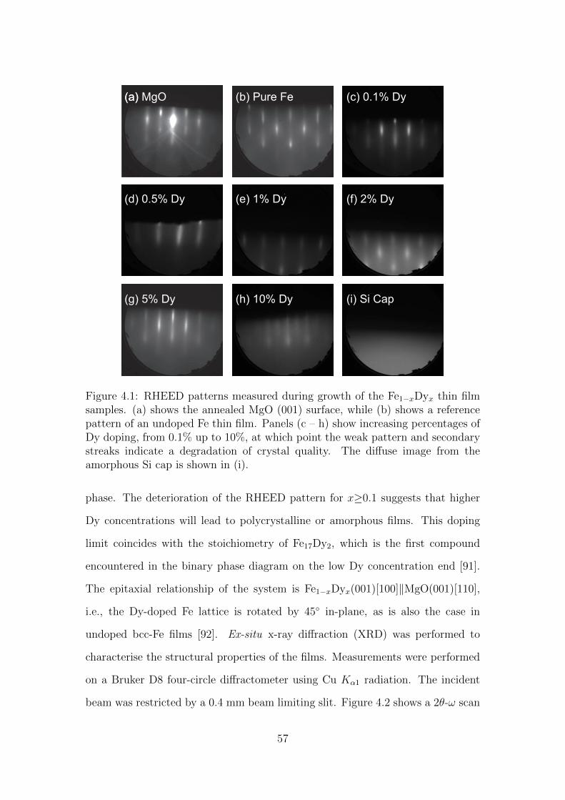
(a) (b) Pure Fe (c) 0.1% Dy

(d) 0.5% Dy (e) 1% Dy (f) 2% Dy

(g) 5% Dy (h) 10% Dy (i) Si Cap

(a) MgO

Figure 4.1: RHEED patterns measured during growth of the Fe1−xDyx thin filmsamples. (a) shows the annealed MgO (001) surface, while (b) shows a referencepattern of an undoped Fe thin film. Panels (c – h) show increasing percentages ofDy doping, from 0.1% up to 10%, at which point the weak pattern and secondarystreaks indicate a degradation of crystal quality. The diffuse image from theamorphous Si cap is shown in (i).

phase. The deterioration of the RHEED pattern for x≥0.1 suggests that higher

Dy concentrations will lead to polycrystalline or amorphous films. This doping

limit coincides with the stoichiometry of Fe17Dy2, which is the first compound

encountered in the binary phase diagram on the low Dy concentration end [91].

The epitaxial relationship of the system is Fe1−xDyx(001)[100]‖MgO(001)[110],

i.e., the Dy-doped Fe lattice is rotated by 45 in-plane, as is also the case in

undoped bcc-Fe films [92]. Ex-situ x-ray diffraction (XRD) was performed to

characterise the structural properties of the films. Measurements were performed

on a Bruker D8 four-circle diffractometer using Cu Kα1 radiation. The incident

beam was restricted by a 0.4 mm beam limiting slit. Figure 4.2 shows a 2θ-ω scan

57

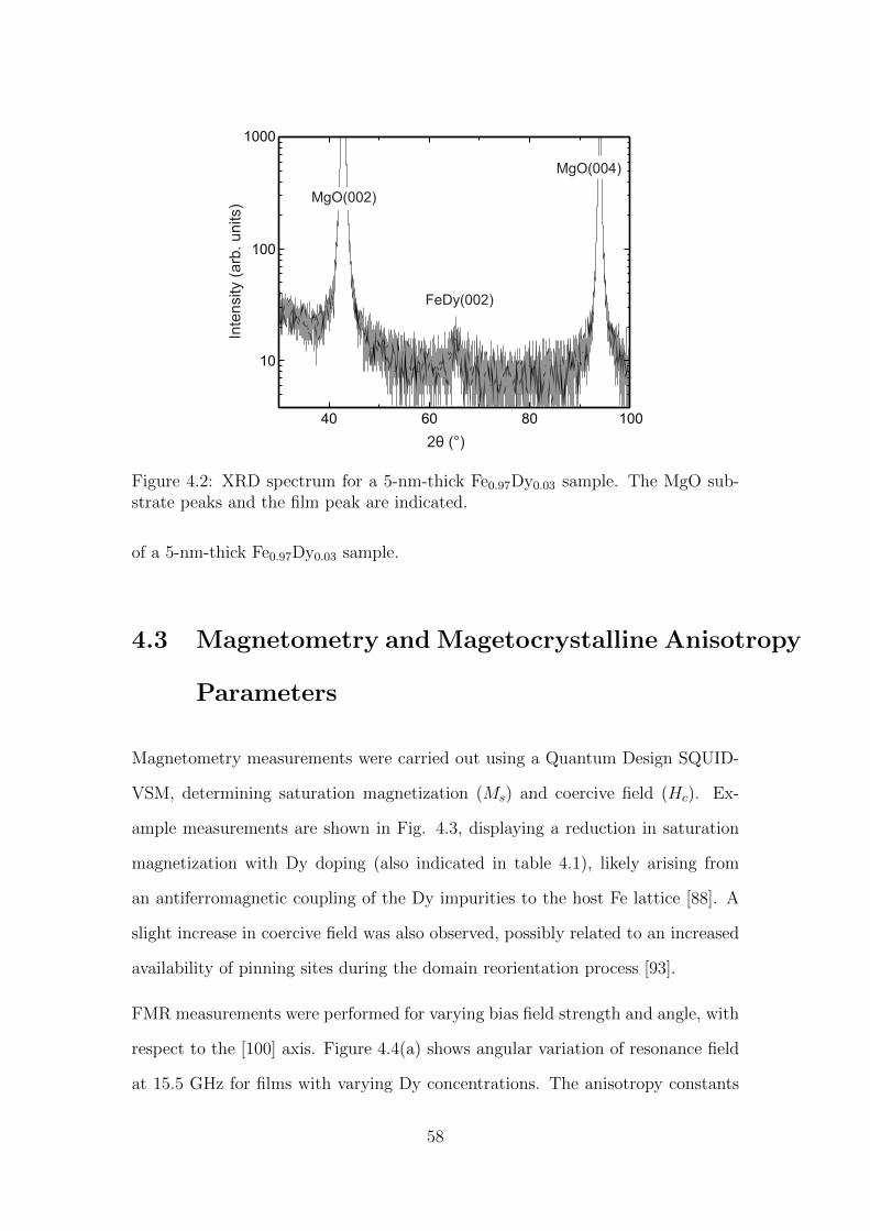
Inte

nsity (

arb

. units)

2 (°)θ

40 60 80 100

10

100

1000

MgO(002)

FeDy(002)

MgO(004)

Figure 4.2: XRD spectrum for a 5-nm-thick Fe0.97Dy0.03 sample. The MgO sub-strate peaks and the film peak are indicated.

of a 5-nm-thick Fe0.97Dy0.03 sample.

4.3 Magnetometry and Magetocrystalline Anisotropy

Parameters

Magnetometry measurements were carried out using a Quantum Design SQUID-

VSM, determining saturation magnetization (Ms) and coercive field (Hc). Ex-

ample measurements are shown in Fig. 4.3, displaying a reduction in saturation

magnetization with Dy doping (also indicated in table 4.1), likely arising from

an antiferromagnetic coupling of the Dy impurities to the host Fe lattice [88]. A

slight increase in coercive field was also observed, possibly related to an increased

availability of pinning sites during the domain reorientation process [93].

FMR measurements were performed for varying bias field strength and angle, with

respect to the [100] axis. Figure 4.4(a) shows angular variation of resonance field

at 15.5 GHz for films with varying Dy concentrations. The anisotropy constants

58

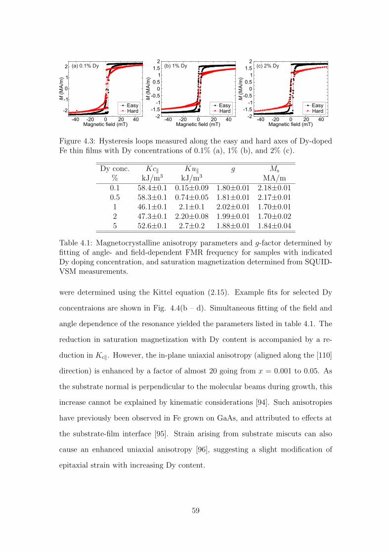
(b) 1% Dy

-2

-1.5

-1

-0.5

0

0.5

1

1.5

2

EasyHard

-40 -20 0 20 40Magnetic field (mT)

(a) 0.1% Dy

-2

-1

0

1

2

M(M

A/m

)

EasyHard

-40 -20 0 20 40Magnetic field (mT)

(c) 2% Dy

-40 -20 0 20 40Magnetic field (mT)

EasyHard

-2

-1.5

-1

-0.5

0

0.5

1

1.5

2

M(M

A/m

)

M(M

A/m

)

Figure 4.3: Hysteresis loops measured along the easy and hard axes of Dy-dopedFe thin films with Dy concentrations of 0.1% (a), 1% (b), and 2% (c).

Dy conc. Kc‖ Ku‖ g Ms

% kJ/m3 kJ/m3 MA/m0.1 58.4±0.1 0.15±0.09 1.80±0.01 2.18±0.010.5 58.3±0.1 0.74±0.05 1.81±0.01 2.17±0.011 46.1±0.1 2.1±0.1 2.02±0.01 1.70±0.012 47.3±0.1 2.20±0.08 1.99±0.01 1.70±0.025 52.6±0.1 2.7±0.2 1.88±0.01 1.84±0.04

Table 4.1: Magnetocrystalline anisotropy parameters and g-factor determined byfitting of angle- and field-dependent FMR frequency for samples with indicatedDy doping concentration, and saturation magnetization determined from SQUID-VSM measurements.

were determined using the Kittel equation (2.15). Example fits for selected Dy

concentraions are shown in Fig. 4.4(b – d). Simultaneous fitting of the field and

angle dependence of the resonance yielded the parameters listed in table 4.1. The

reduction in saturation magnetization with Dy content is accompanied by a re-

duction in Kc‖. However, the in-plane uniaxial anisotropy (aligned along the [110]

direction) is enhanced by a factor of almost 20 going from x = 0.001 to 0.05. As

the substrate normal is perpendicular to the molecular beams during growth, this

increase cannot be explained by kinematic considerations [94]. Such anisotropies

have previously been observed in Fe grown on GaAs, and attributed to effects at

the substrate-film interface [95]. Strain arising from substrate miscuts can also

cause an enhanced uniaxial anisotropy [96], suggesting a slight modification of

epitaxial strain with increasing Dy content.

59

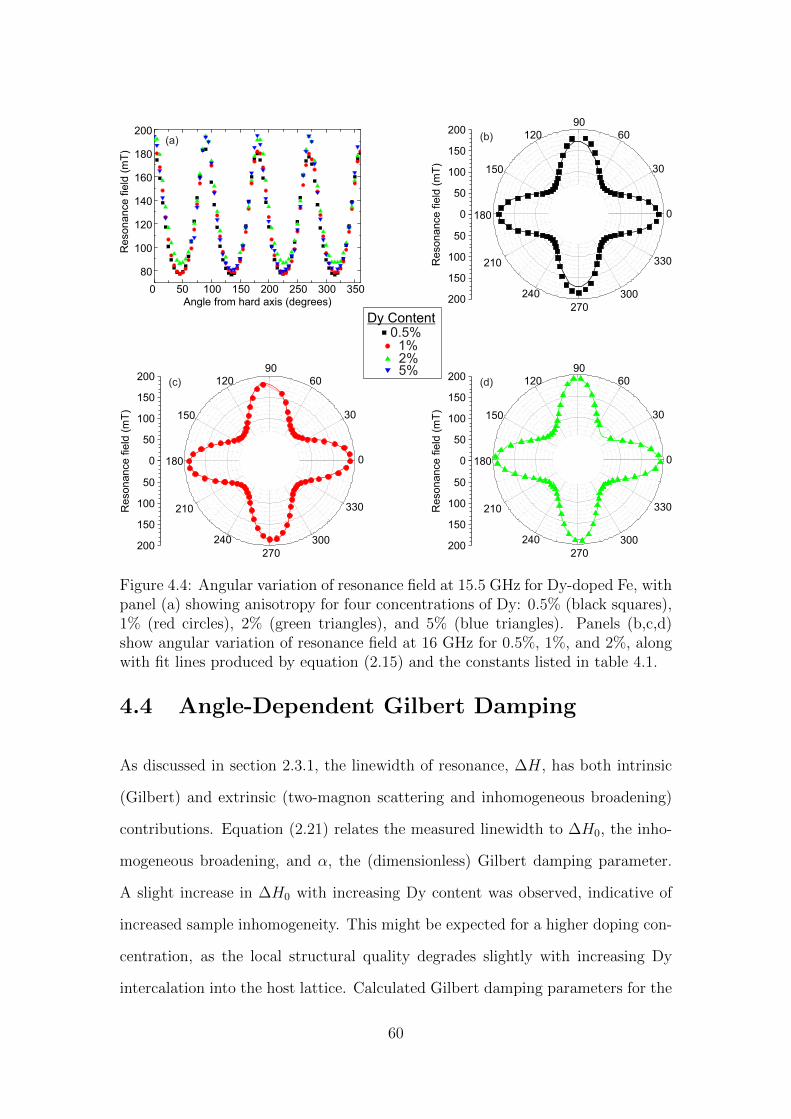
Dy Content0.5%

1%2%5%

80

100

120

140

160

180

200R

esonance

field

(m

T)

0 50 100 150 200 250 300 350Angle from hard axis (degrees)

(a)

0

50

100

150

200

50

100

150

200

Resonance

field

(m

T)

0

30

60

90

120

150

180

210

240

270

300

330

(b)

0

50

100

150

200

50

100

150

200

Resonance

field

(m

T)

0

30

60

90

120

150

180

210

240

270

300

330

(d)

0

30

60

90

120

150

180

210

240

270

300

330

0

50

100

150

200

50

100

150

200

Resonance

field

(m

T)

(c)

Figure 4.4: Angular variation of resonance field at 15.5 GHz for Dy-doped Fe, withpanel (a) showing anisotropy for four concentrations of Dy: 0.5% (black squares),1% (red circles), 2% (green triangles), and 5% (blue triangles). Panels (b,c,d)show angular variation of resonance field at 16 GHz for 0.5%, 1%, and 2%, alongwith fit lines produced by equation (2.15) and the constants listed in table 4.1.

4.4 Angle-Dependent Gilbert Damping

As discussed in section 2.3.1, the linewidth of resonance, ∆H, has both intrinsic

(Gilbert) and extrinsic (two-magnon scattering and inhomogeneous broadening)

contributions. Equation (2.21) relates the measured linewidth to ∆H0, the inho-

mogeneous broadening, and α, the (dimensionless) Gilbert damping parameter.

A slight increase in ∆H0 with increasing Dy content was observed, indicative of

increased sample inhomogeneity. This might be expected for a higher doping con-

centration, as the local structural quality degrades slightly with increasing Dy

intercalation into the host lattice. Calculated Gilbert damping parameters for the

60

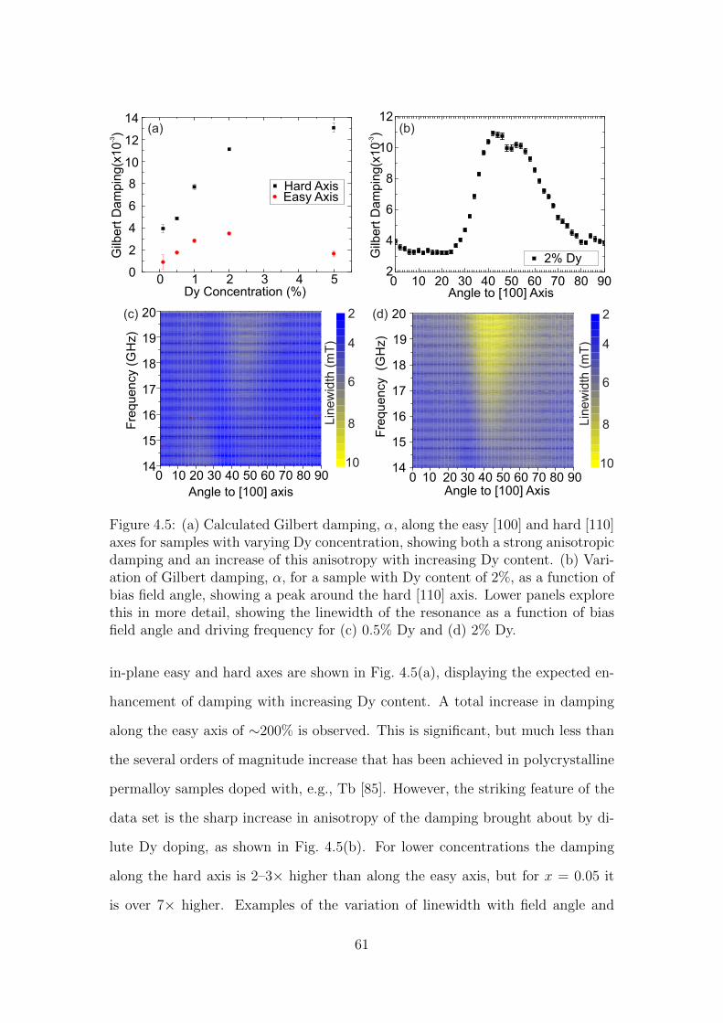
Lin

ew

idth

(m

T)

10

2

8

6

4

0 10 20 30 40 50 60 70 80 9014

15

16

17

18

19

20

Angle to [100] Axis

Fre

quency (G

Hz)

0 10 20 30 40 50 60 70 80 9014

15

16

17

18

19

20

Angle to [100] axis

Fre

quency (

GH

z)

Lin

ew

idth

(m

T)

10

2

8

6

4

(c)

0 1 2 3 4 50

2

4

6

8

10

12

14

Hard AxisEasy Axis

Gilb

ert

Dam

pin

g(x

10

)-3

Dy Concentration (%)

(a)

(d)

(b)

0 10 20 30 40 50 60 70 80 90

2% Dy

Angle to [100] Axis

Gilb

ert

Dam

pin

g(x

10

-3)

2

4

6

8

10

12

Figure 4.5: (a) Calculated Gilbert damping, α, along the easy [100] and hard [110]axes for samples with varying Dy concentration, showing both a strong anisotropicdamping and an increase of this anisotropy with increasing Dy content. (b) Vari-ation of Gilbert damping, α, for a sample with Dy content of 2%, as a function ofbias field angle, showing a peak around the hard [110] axis. Lower panels explorethis in more detail, showing the linewidth of the resonance as a function of biasfield angle and driving frequency for (c) 0.5% Dy and (d) 2% Dy.

in-plane easy and hard axes are shown in Fig. 4.5(a), displaying the expected en-

hancement of damping with increasing Dy content. A total increase in damping

along the easy axis of ∼200% is observed. This is significant, but much less than

the several orders of magnitude increase that has been achieved in polycrystalline

permalloy samples doped with, e.g., Tb [85]. However, the striking feature of the

data set is the sharp increase in anisotropy of the damping brought about by di-

lute Dy doping, as shown in Fig. 4.5(b). For lower concentrations the damping

along the hard axis is 2–3× higher than along the easy axis, but for x = 0.05 it

is over 7× higher. Examples of the variation of linewidth with field angle and

61

frequency are shown in Fig. 4.5(c,d). The relatively sharp peak in the damping

around the hard axis does not match the angular dependence that would be ex-

pected for other anisotropic damping processes, such as the smooth sine curve of

two-magnon scattering [17].

The enhanced damping of such RE-doped films has its origin in the coupling of the

Dy 4f electrons to the Fe 3d electrons mediated through the RE 5d orbitals. This

interaction is anisotropic, however, so that the populations of the 4f states vary as

the 3d moments undergo FMR, leading to a time-varying field due to the Dy relax-

ation time. Anisotropic damping enhancement has previously been observed in low

temperature measurements of bulk YIG doped with rare earth atoms such as Tb

or Y [97,98]. The linewidth was found to reduce along orientations corresponding

to near-crossings of the energy levels of the host lattice and the RE impurity [99].

This suggests that the increased anisotropy of damping originates from the same

process as the damping enhancement itself, i.e., anisotropic coupling of the 4f -5d

orbitals. The importance of using high quality, epitaxially grown samples is clear

in this case; it allows a detailed study of angular dependence that is simply not

possible with polycrystalline films. Further, it limits the role of defects (which

can lead to inhomogeneous broadening) or other microstructural effects as crystal

quality is preserved across the whole series. It is therefore important to study

the effect this interaction has on the host Fe lattice in more detail, in order to

determine whether the effects of the Dy are limited to the interatomic 5d states,

or if the character of 3d moments themselves is changed.

62

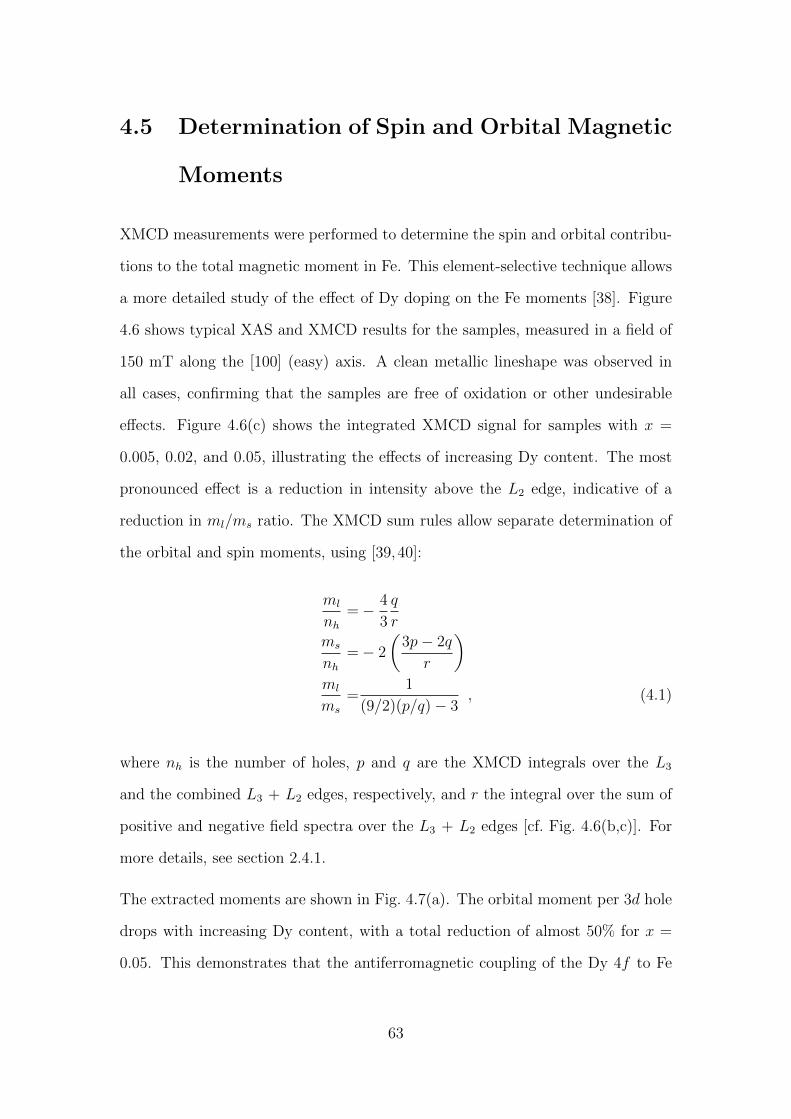
4.5 Determination of Spin and Orbital Magnetic

Moments

XMCD measurements were performed to determine the spin and orbital contribu-

tions to the total magnetic moment in Fe. This element-selective technique allows

a more detailed study of the effect of Dy doping on the Fe moments [38]. Figure

4.6 shows typical XAS and XMCD results for the samples, measured in a field of

150 mT along the [100] (easy) axis. A clean metallic lineshape was observed in

all cases, confirming that the samples are free of oxidation or other undesirable

effects. Figure 4.6(c) shows the integrated XMCD signal for samples with x =

0.005, 0.02, and 0.05, illustrating the effects of increasing Dy content. The most

pronounced effect is a reduction in intensity above the L2 edge, indicative of a

reduction in ml/ms ratio. The XMCD sum rules allow separate determination of

the orbital and spin moments, using [39,40]:

ml

nh=− 4

3

q

r

ms

nh=− 2

(3p− 2q

r

)ml

ms

=1

(9/2)(p/q)− 3, (4.1)

where nh is the number of holes, p and q are the XMCD integrals over the L3

and the combined L3 + L2 edges, respectively, and r the integral over the sum of

positive and negative field spectra over the L3 + L2 edges [cf. Fig. 4.6(b,c)]. For

more details, see section 2.4.1.

The extracted moments are shown in Fig. 4.7(a). The orbital moment per 3d hole

drops with increasing Dy content, with a total reduction of almost 50% for x =

0.05. This demonstrates that the antiferromagnetic coupling of the Dy 4f to Fe

63

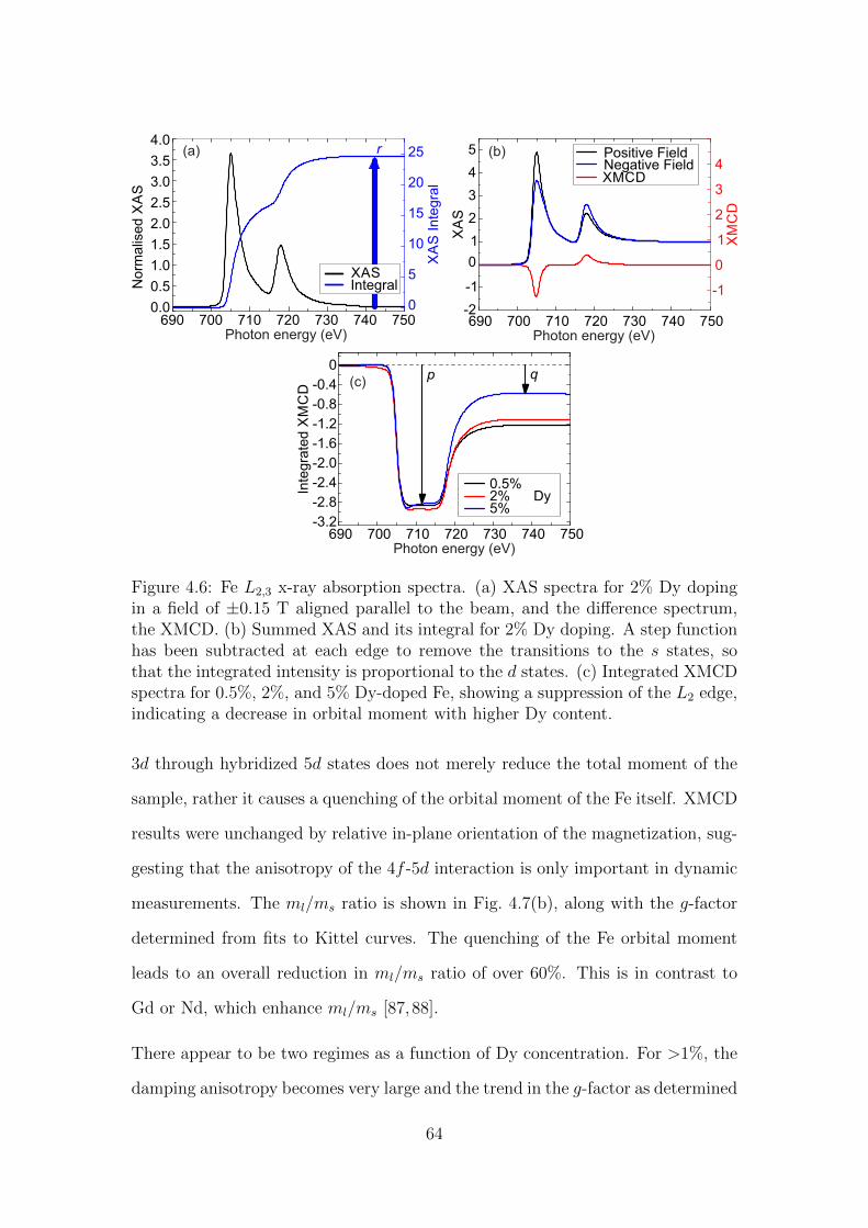
690 700 710 720 730 740 750-3.2

-2.8

-2.4

-2.0

-1.6

-1.2

-0.8

-0.4

0

Inte

gra

ted

XM

CD

0.5%2% Dy5%

p q(c)

Photon energy (eV)

-2

-1

0

1

2

3

4

5

XA

S

Positive FieldNegative FieldXMCD

-1

0

1

2

3

4

XM

CD

(b)

690 700 710 720 730 740 750Photon energy (eV)

0.0

0.5

1.0

1.5

2.0

2.5

3.0

3.5

4.0

XASIntegralN

orm

alis

ed

XA

S

0

5

10

15

20

25

XA

SIn

tegra

l

r(a)

690 700 710 720 730 740 750Photon energy (eV)

Figure 4.6: Fe L2,3 x-ray absorption spectra. (a) XAS spectra for 2% Dy dopingin a field of ±0.15 T aligned parallel to the beam, and the difference spectrum,the XMCD. (b) Summed XAS and its integral for 2% Dy doping. A step functionhas been subtracted at each edge to remove the transitions to the s states, sothat the integrated intensity is proportional to the d states. (c) Integrated XMCDspectra for 0.5%, 2%, and 5% Dy-doped Fe, showing a suppression of the L2 edge,indicating a decrease in orbital moment with higher Dy content.

3d through hybridized 5d states does not merely reduce the total moment of the

sample, rather it causes a quenching of the orbital moment of the Fe itself. XMCD

results were unchanged by relative in-plane orientation of the magnetization, sug-

gesting that the anisotropy of the 4f -5d interaction is only important in dynamic

measurements. The ml/ms ratio is shown in Fig. 4.7(b), along with the g-factor

determined from fits to Kittel curves. The quenching of the Fe orbital moment

leads to an overall reduction in ml/ms ratio of over 60%. This is in contrast to

Gd or Nd, which enhance ml/ms [87, 88].

There appear to be two regimes as a function of Dy concentration. For >1%, the

damping anisotropy becomes very large and the trend in the g-factor as determined

64

m mL S- ratiog factor

Dy content (%)0 1 2 3 4 5

0.04

0.06

0.08

0.10

0.12

0.14

0.16

0.18

m/ m

ls

1.8

1.9

2.0

FM

Rfa

cto

rg

(b)

0.016

0.020

0.024

0.028

0.032

0.036

0.040

0.044m

l/N

h

0.22

0.26

0.30

0.34

0.38

0.42

ms/ N

h

(a)

Dy content (%)0 1 2 3 4 5

Figure 4.7: (a) Orbital and spin moments per hole as a function of Dy dopantpercentage. A suppression of ml and slight enhancement of ms with increasing Dyis observed. (b) Comparison of ml/ms ratio as determined by element-selectiveXMCD, and the g-factor, as determined by FMR.

by FMR follows the ml/ms ratio. This most likely arises as the proximity of the

Dy increases the spin-orbit interaction of the Fe. For <1% Dy the anisotropy is less

pronounced and the ml/ms is significantly reduced, while the g-factor generally

follows the trend, but at a much smaller rate. A possible cause is that the influence

of the low concentration of Dy is insufficient to increase the Fe orbital moment,

yet is still able to affect the FMR, through the effective field exerted by these

slow-relaxing impurities.

4.6 Conclusion

This chapter has examined the modification of static and dynamic properties of

ultrathin Fe films through dilute Dy doping. Crystal quality was preserved up

to 5% Dy content, as determined by RHEED and XRD. It was found that the

introduction of RE dopants reduces the saturation magnetisation of the film, most

likely through antiferromagnetic coupling to the host Fe lattice, and that the cu-

bic magnetocrystalline anisotropy parameter was similarly reduced. The uniaxial

anisotropy parameter increased, however, perhaps as a result of epitaxial strain or

hybridisation with the substrate. The Gilbert damping was enhanced by a factor

65

of three with increasing Dy content, as has been observed with many other RE-

doped thin films. Using high quality MBE-grown samples allowed a detailed study

of the anisotropy of the increased Gilbert damping, which has heretofore received

only limited interest. A strong anisotropy of the damping develops, driven by the

anisotropic interaction between the Dy 4f and interatomic 5d states, characteris-

tic of the slow relaxing impurity model. This orientation dependence is important

when considering spin-torque assisted magnetization reversal, or similar spintronic

processes. Element-specific measurements showed that the Dy also modifies the

properties of the Fe lattice itself, significantly reducing the orbital moment, and

with it the ml/ms ratio. These results show that the interaction between FM films

and RE dopants are more significant than previously anticipated, and demonstrate

the possibility of fine-tuning magnetic properties of films for spintronic applica-

tions. More detailed calculations are required to elucidate the link between the

increased Gilbert damping and modified orbital moment. A more detailed study

of the temperature dependence of such effects could provide this information, as

damping due to RE impurities has previously been observed to have a maximum

at about 80 K, but how the anisotropy or spin and orbital moments are affected

remains an open question. The techniques and results presented here show ex-

ploratory power of the combination of VNA-FMR and synchrotron radiation as

tools to characterise the dynamic properties of thin films, as well as the nuanced

role that growth, composition and exchange interactions can have on magnetody-

namics. Later chapters will take these ideas further, studying spin transfer and

coupling mechanisms that arise when two ferromagnets are in close proximity, as

well as showing the profound insights that a combination of FMR and XMCD,

XFMR, can offer.

66

Chapter 5

Micromagnetic Modelling of

Coupled Magnetodynamics

5.1 Motivation

The field of computational micromagnetics is an expanding area of study that

bridges the pure physics and device engineering communities, offering valuable

insights into the behaviour of magnetic structures at the nanoscale, where experi-

mental data is difficult to obtain due to the length scales involved, to understand

complicated time-resolved magnetodynamics [100], or where analytical theory can

not be applied. Here, it has been employed to gain a greater insight into the

layer-resolved magnetodynamics of the heterostructures.

This chapter outlines the approach for conducting FMR simulations in the Na-

tional Institute of Standards and Technology’s (NIST) object-oriented micromag-

netic framework (OOMMF) [101], discussing the case of isolated layers, finite-size

effects and the insights offered by modelling of coupled layers. It then outlines in

broad detail the approach for calculation of the AC susceptibility tensor, and how

67

this yields data comparable to XFMR measurements. The effects of static and

dynamic exchange on the coupled magnetodynamics of spin valves are discussed,

with particular reference to how their competition can distort phase features. With

this foundation, it is then possible to move on to experimental measurements of

such spin valve samples.

5.2 OOMMF

The first modelling approach employed was OOMMF: this package employs the

finite difference approach to create a mesh of cuboids across a sample, then solves

the LLG to compute the time evolution of magnetisation for a point at the cen-

tre of each cuboid. This makes OOMMF fast and well suited for samples of a

regular geometry (such as thin films), but poor for objects with curves or sharp

points. As OOMMF is a mature software package, its results are generally reli-

able, and it accurately incorporates effects such as magnetocrystalline anisotropy,

static exchange coupling through the Ruderman-Kittel-Kasuya-Yosida (RKKY)

interaction and magnetodynamics for FMR. When simulating FMR, this method

yields the amplitude and phase of precession at a fixed field for a wide frequency

range, with a spatial resolution governed by the exchange length and the spatial

discretisation chosen by the user. It is somewhat limited, however, as it does not

offer support for the spin pumping effect, which is a key consideration in many of

the systems studied in this thesis. Nevertheless, OOMMF is a valuable tool when

investigating ferromagnetic resonance [100,102–105].

The most computationally expensive step in micromagentic is calculation of the

demagnetising field.Analytical formulae only exist for uniformly magnetised ellip-

soids, therefore OOMMF must numerically calculate the long-range demagnetisa-

tion field for every point in the mesh at every time step. This is, naturally, a

68

time-consuming process that places practical limits on the size of the simulated

objects. Furthermore, when simulating magnetic heterostructures of out-of-plane

(z) dimension ∼20 nm, the in-plane dimensions (x − y) must be several orders

of magnitude larger, to preserve the thin-film behaviour of the demagnetisation

tensor. Therefore, to achieve manageable simulation times a simplifying approx-

imation is employed. The magnetisation is restricted to vary only with z, i.e.

for a given slice within the depth-profile of the film the magnetization acts as a

macrospin, and the film appears as a chain of spins in the z direction only. In

this way, the number of points calculated by OOMMF is significantly reduced, and

the simulation closely matches the thin-film approximation employed in the Kittel

equation [equation (2.15)].

5.2.1 Simulating FMR

The simplest method to simulate FMR is to perturb the system and record the

magnetisation dynamics as precession is damped away. If the perturbation is

chosen correctly, the precession of magnetisation is composed of a sum of the

supported normal modes. Resonance frequencies and corresponding modes can

then be extracted by performing the Fourier transform on the recorded data.

When performing these simulations, the system was first prepared in a uniformly

magnetised state by being allowed to relax under a static external field applied

along the x direction. Next, a sinc ( sin(t)t

) pulse is applied out of the plane of the

film used to excite precession of magnetisation over a given frequency range. The

time evolution of the system was recorded over a period of 20 ns, over which time

the magnetisation precession is described by sine curves of frequencies matching

the normal (FMR) modes of the system, convoluted with a decaying exponential

damping term due to energy loss. Fourier transforming the resulting data yields

an FMR spectrum. Only the y-component of magnetisation is important in this

69

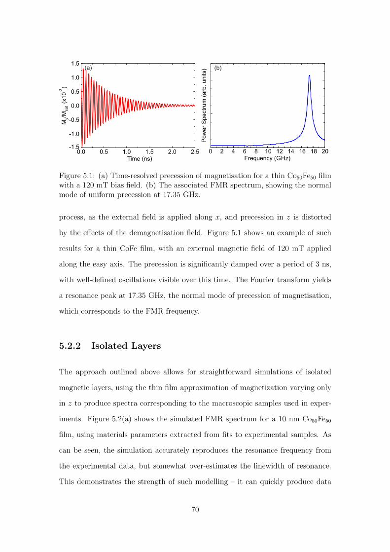
0.0 0.5 1.0 1.5 2.0 2.5

M/M

(x1

0)

ysa

t

-3

Time (ns)

(a)

-1.5

-1.0

-0.5

0.0

0.5

1.0

1.5

0 2 4 6 8 10 12 14 16 18 20

Po

we

r S

pe

ctr

um

(a

rb.

un

its)

Frequency (GHz)

(b)

Figure 5.1: (a) Time-resolved precession of magnetisation for a thin Co50Fe50 filmwith a 120 mT bias field. (b) The associated FMR spectrum, showing the normalmode of uniform precession at 17.35 GHz.

process, as the external field is applied along x, and precession in z is distorted

by the effects of the demagnetisation field. Figure 5.1 shows an example of such

results for a thin CoFe film, with an external magnetic field of 120 mT applied

along the easy axis. The precession is significantly damped over a period of 3 ns,

with well-defined oscillations visible over this time. The Fourier transform yields

a resonance peak at 17.35 GHz, the normal mode of precession of magnetisation,

which corresponds to the FMR frequency.

5.2.2 Isolated Layers

The approach outlined above allows for straightforward simulations of isolated

magnetic layers, using the thin film approximation of magnetization varying only

in z to produce spectra corresponding to the macroscopic samples used in exper-

iments. Figure 5.2(a) shows the simulated FMR spectrum for a 10 nm Co50Fe50

film, using materials parameters extracted from fits to experimental samples. As

can be seen, the simulation accurately reproduces the resonance frequency from

the experimental data, but somewhat over-estimates the linewidth of resonance.

This demonstrates the strength of such modelling – it can quickly produce data

70

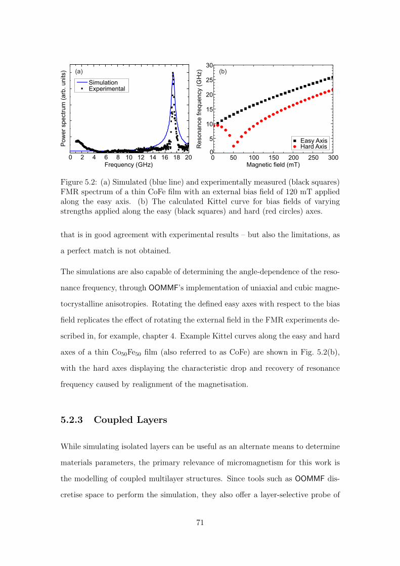
0 50 100 150 200 250 3000

5

10

15

20

25

30

Easy AxisHard AxisR

esonance fre

quency (

GH

z)

Magnetic field (mT)

(b)

0 2 4 6 8 10 12 14 16 18 20

Pow

er

spectr

um

(arb

. units)

Frequency (GHz)

(a)

SimulationExperimental

Figure 5.2: (a) Simulated (blue line) and experimentally measured (black squares)FMR spectrum of a thin CoFe film with an external bias field of 120 mT appliedalong the easy axis. (b) The calculated Kittel curve for bias fields of varyingstrengths applied along the easy (black squares) and hard (red circles) axes.

that is in good agreement with experimental results – but also the limitations, as

a perfect match is not obtained.

The simulations are also capable of determining the angle-dependence of the reso-

nance frequency, through OOMMF’s implementation of uniaxial and cubic magne-

tocrystalline anisotropies. Rotating the defined easy axes with respect to the bias

field replicates the effect of rotating the external field in the FMR experiments de-

scribed in, for example, chapter 4. Example Kittel curves along the easy and hard

axes of a thin Co50Fe50 film (also referred to as CoFe) are shown in Fig. 5.2(b),

with the hard axes displaying the characteristic drop and recovery of resonance

frequency caused by realignment of the magnetisation.

5.2.3 Coupled Layers

While simulating isolated layers can be useful as an alternate means to determine

materials parameters, the primary relevance of micromagnetism for this work is

the modelling of coupled multilayer structures. Since tools such as OOMMF dis-

cretise space to perform the simulation, they also offer a layer-selective probe of

71

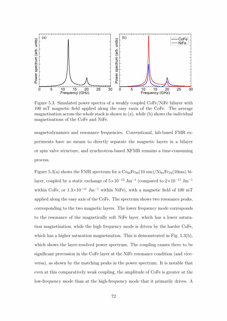
0 5 10 15 20 25 30

Pow

er

sp

ectr

um

(arb

. u

nits)

Frequency (GHz)

(a) CoFeNiFe

0 5 10 15 20 25 30Frequency (GHz)

Pow

er

spe

ctr

um

(a

rb.

un

its) (b)

Figure 5.3: Simulated power spectra of a weakly coupled CoFe/NiFe bilayer with100 mT magnetic field applied along the easy eaxis of the CoFe. The averagemagnetisation across the whole stack is shown in (a), while (b) shows the individualmagnetisations of the CoFe and NiFe.

magnetodynamics and resonance frequencies. Conventional, lab-based FMR ex-

periments have no means to directly separate the magnetic layers in a bilayer

or spin valve structure, and synchrotron-based XFMR remains a time-consuming

process.

Figure 5.3(a) shows the FMR spectrum for a Co50Fe50(10 nm)/Ni81Fe19(10nm) bi-

layer, coupled by a static exchange of 5×10−13 Jm−1 (compared to 2×10−11 Jm−1

within CoFe, or 1.3×10−11 Jm−1 within NiFe), with a magnetic field of 100 mT

applied along the easy axis of the CoFe. The spectrum shows two resonance peaks,

corresponding to the two magnetic layers. The lower frequency mode corresponds

to the resonance of the magnetically soft NiFe layer, which has a lower satura-

tion magnetisation, while the high frequency mode is driven by the harder CoFe,

which has a higher saturation magnetisation. This is demonstrated in Fig. 5.3(b),

which shows the layer-resolved power spectrum. The coupling causes there to be

significant precession in the CoFe layer at the NiFe resonance condition (and vice-

versa), as shown by the matching peaks in the power spectrum. It is notable that

even at this comparatively weak coupling, the amplitude of CoFe is greater at the

low-frequency mode than at the high-frequency mode that it primarily drives. A

72

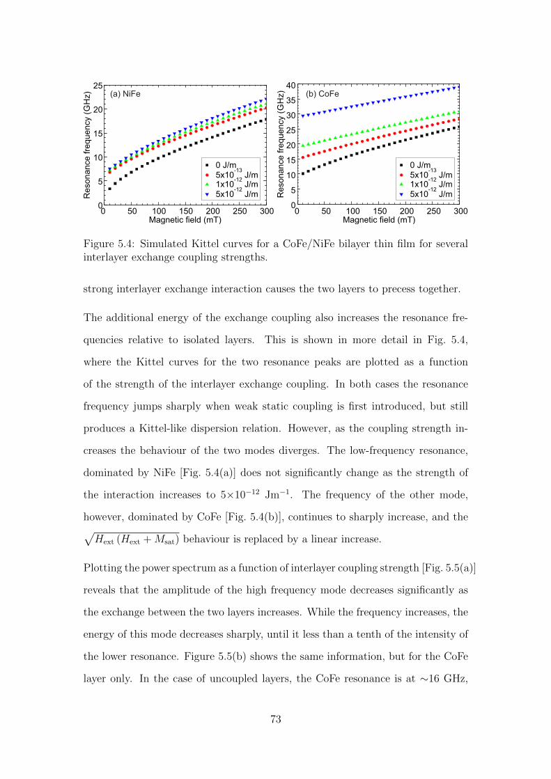
0 J/m

5x10 J/m-13

1x10 J/m-12

5x10 J/m-12

0 50 100 150 200 250 3000

5

10

15

20

25R

eso

na

nce

fre

qu

en

cy (

GH

z)

Magnetic field (mT)

(a) NiFe

0

5

10

15

20

25

30

35

40

Re

so

na

nce

fre

qu

en

cy (

GH

z)

0 50 100 150 200 250 300Magnetic field (mT)

(b) CoFe

0 J/m

5x10 J/m-13

1x10 J/m-12

5x10 J/m-12

Figure 5.4: Simulated Kittel curves for a CoFe/NiFe bilayer thin film for severalinterlayer exchange coupling strengths.

strong interlayer exchange interaction causes the two layers to precess together.

The additional energy of the exchange coupling also increases the resonance fre-

quencies relative to isolated layers. This is shown in more detail in Fig. 5.4,

where the Kittel curves for the two resonance peaks are plotted as a function

of the strength of the interlayer exchange coupling. In both cases the resonance

frequency jumps sharply when weak static coupling is first introduced, but still

produces a Kittel-like dispersion relation. However, as the coupling strength in-

creases the behaviour of the two modes diverges. The low-frequency resonance,

dominated by NiFe [Fig. 5.4(a)] does not significantly change as the strength of

the interaction increases to 5×10−12 Jm−1. The frequency of the other mode,

however, dominated by CoFe [Fig. 5.4(b)], continues to sharply increase, and the√Hext (Hext +Msat) behaviour is replaced by a linear increase.

Plotting the power spectrum as a function of interlayer coupling strength [Fig. 5.5(a)]

reveals that the amplitude of the high frequency mode decreases significantly as

the exchange between the two layers increases. While the frequency increases, the

energy of this mode decreases sharply, until it less than a tenth of the intensity of

the lower resonance. Figure 5.5(b) shows the same information, but for the CoFe

layer only. In the case of uncoupled layers, the CoFe resonance is at ∼16 GHz,

73

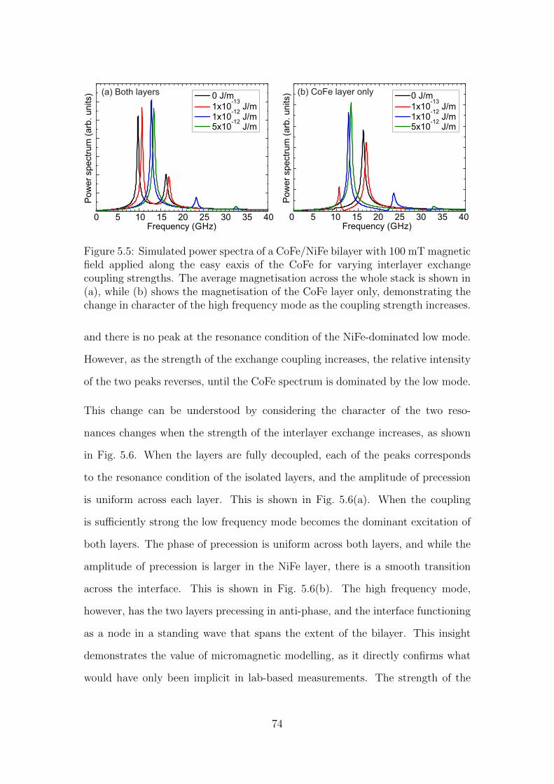
0 5 10 15 20 25 30 35 40Frequency (GHz)

Po

we

r sp

ect

rum

(a

rb.

un

its) 0 J/m

-13 1x10 J/m

-12 1x10 J/m

-12 5x10 J/m

(a) Both layers

0 5 10 15 20 25 30 35 40Frequency (GHz)

Po

we

r sp

ect

rum

(a

rb.

un

its) (b) CoFe layer only 0 J/m

-13 1x10 J/m

-12 1x10 J/m

-12 5x10 J/m

Figure 5.5: Simulated power spectra of a CoFe/NiFe bilayer with 100 mT magneticfield applied along the easy eaxis of the CoFe for varying interlayer exchangecoupling strengths. The average magnetisation across the whole stack is shown in(a), while (b) shows the magnetisation of the CoFe layer only, demonstrating thechange in character of the high frequency mode as the coupling strength increases.

and there is no peak at the resonance condition of the NiFe-dominated low mode.

However, as the strength of the exchange coupling increases, the relative intensity

of the two peaks reverses, until the CoFe spectrum is dominated by the low mode.

This change can be understood by considering the character of the two reso-

nances changes when the strength of the interlayer exchange increases, as shown

in Fig. 5.6. When the layers are fully decoupled, each of the peaks corresponds

to the resonance condition of the isolated layers, and the amplitude of precession

is uniform across each layer. This is shown in Fig. 5.6(a). When the coupling

is sufficiently strong the low frequency mode becomes the dominant excitation of

both layers. The phase of precession is uniform across both layers, and while the

amplitude of precession is larger in the NiFe layer, there is a smooth transition

across the interface. This is shown in Fig. 5.6(b). The high frequency mode,

however, has the two layers precessing in anti-phase, and the interface functioning

as a node in a standing wave that spans the extent of the bilayer. This insight

demonstrates the value of micromagnetic modelling, as it directly confirms what

would have only been implicit in lab-based measurements. The strength of the

74

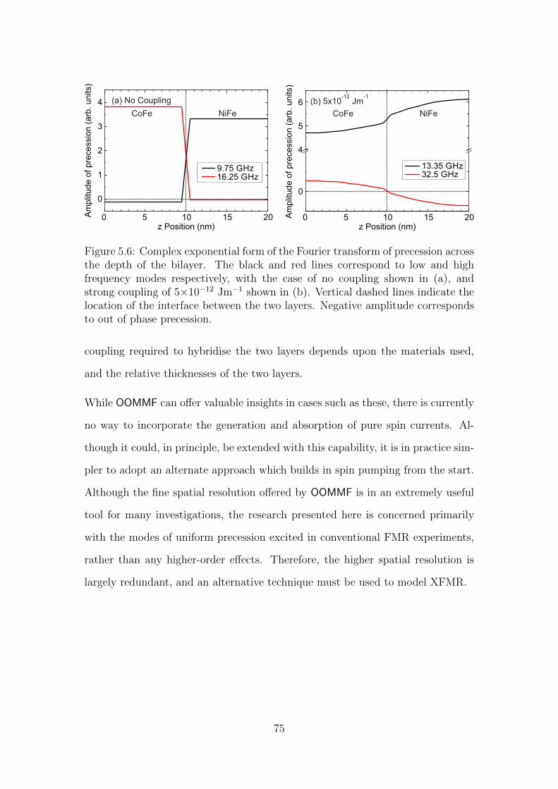
0 5 10 15 20

0

1

2

3

4

9.75 GHz16.25 GHz

Am

plit

ude o

f pre

cessio

n (

arb

. units)

z Position (nm)

CoFe NiFe

0

4

5

6

13.35 GHz32.5 GHz

0 5 10 15 20z Position (nm)

CoFe NiFe

Am

plit

ude o

f pre

cessio

n (

arb

. units)

(a) No Coupling (b) 5x10 Jm-12 -1

Figure 5.6: Complex exponential form of the Fourier transform of precession acrossthe depth of the bilayer. The black and red lines correspond to low and highfrequency modes respectively, with the case of no coupling shown in (a), andstrong coupling of 5×10−12 Jm−1 shown in (b). Vertical dashed lines indicate thelocation of the interface between the two layers. Negative amplitude correspondsto out of phase precession.

coupling required to hybridise the two layers depends upon the materials used,

and the relative thicknesses of the two layers.

While OOMMF can offer valuable insights in cases such as these, there is currently

no way to incorporate the generation and absorption of pure spin currents. Al-

though it could, in principle, be extended with this capability, it is in practice sim-

pler to adopt an alternate approach which builds in spin pumping from the start.

Although the fine spatial resolution offered by OOMMF is in an extremely useful

tool for many investigations, the research presented here is concerned primarily

with the modes of uniform precession excited in conventional FMR experiments,

rather than any higher-order effects. Therefore, the higher spatial resolution is

largely redundant, and an alternative technique must be used to model XFMR.

75

5.3 Determination of the AC Magnetic Suscep-

tibility Tensor

The second modelling approach was chosen to address the need for a layer-resolved

model of magnetisation dynamics that incorporates both static and dynamic ex-

change. To achieve this, the LLG was modified to include the required coupling

mechanisms, then solved using a macrospin approximation and linearising in time.

From this, the AC magnetic susceptibility tensor can be determined, yielding the

amplitude and phase of precession at a fixed frequency for a range of fields, with

a spatial resolution suitable only to separate the two layers. It is a fast calcu-

lation, but cannot offer the detailed spatial information that OOMMF does, nor

does it truly reproduce the time-resolved magnetodynamics. However, it matches

measured XFMR data closely, which offers the same information, at the same

spatial resolution. Furthermore, calculations can be run extremely quickly, which

is useful for the large parameter space afforded by systems with both static and

dynamic coupling, alongside magnetocrystalline anisotropies and damping terms

within the layers.

5.3.1 Dynamic Susceptibility of an Isolated Layer

The dynamic (AC) susceptibility tensor relates the response of the magnetisa-

tion of a material to a time-varying perturbation, giving the real and imaginary

components of the precession of magnetisation. From this, the amplitude and

phase of precession can be determined. The tensor is found using a solution of the

Landau-Lifshitz Gilbert equation:

−∂m∂t

= m×[γHeff − α

∂m

∂t

], (5.1)

76

with m the magnetisation vector, Heff , the effective field and α the Gilbert damp-

ing. This derivation uses the co-ordinate system outlined in Fig. 2.1, a thin film

with z oriented out of the plane, an effective fieldHeff composed ofHext andHanis

oriented along x, an RF field h(t) oriented along y, and Hdemag oriented along

z. The magnetic field is homogeneous, and the magnetisation of the thin layer

behaves as a macrospin with the equilibrium orientation aligned with Heff along

x. Since h(t) Hext,Hanis, the perturbations are small and the magnetisation

vector m can be approximated:

m = x+myy +mzz, (5.2)

The effective field is:

Heff = (Hext +Hanis)x+ h(t)y −Msmzz. (5.3)

Substituting these definitions into the LLG yields:

0 = my

(Ms − α

∂mz

∂t

)−mz

(h− α∂my

∂t

)−1

γ

∂my

∂t= mz(Hext +Hanis −Ms) +

α

γ

∂mz

∂t

−1

γ

∂mz

∂t=

(h+

α

γ

∂my

∂t

)+my(Hext +Hanis), (5.4)

with γ the gyromagnetic ratio, and α the Gilbert damping. These equations are

then linearised by disregarding products of m, h, and using harmonic solutions of

the form m(t) = m exp(−iωt), h(t) = h exp(−iωt). This yields the following pair

77

of equations:

0 =− iω

γmy +mz

(Hext +Hanis −Ms − α

iω

γ

)h =−my

(Hext +Hanis + α

iω

γ

)+iω

γmz. (5.5)

Which can be written in matrix form as:0

h

=

− iωγ

Ha

−Hbiωγ

my

mz

, (5.6)

where:

Ha = Hext +Hanis −Ms − αiω

γ

Hb = Hext +Hanis + αiω

γ. (5.7)

This can be succinctly written as h = Am, and since m = χh, the susceptibility

tensor, χ, is found by inverting the matrix, A. As the microwave field is aligned

purely in y, only χyy is required for modelling purposes. χyy is in general a

complex number, with the real part giving the portion of the oscillation that is

in phase with the driving frequency, and the imaginary part being the component

that is out of phase by 90. Thus the amplitude and phase of χyy correspond to

the transmission of microwaves as measured by VNA-FMR, or the amplitude and

phase of precession of magnetisation as measured by XFMR.

Figure 5.7 shows the results of modelling of a thin Fe film, with the magnetic

field applied along the magnetocrystalline easy and hard axes. The peaks in

amplitude of precession in Fig. 5.7(a) correspond to the peaks in absorption of

microwave power observed in VNA-FMR. Several features are notable here. First,

the hard axis has two resonance peaks at 4 GHz, due to the reorientation of the

78

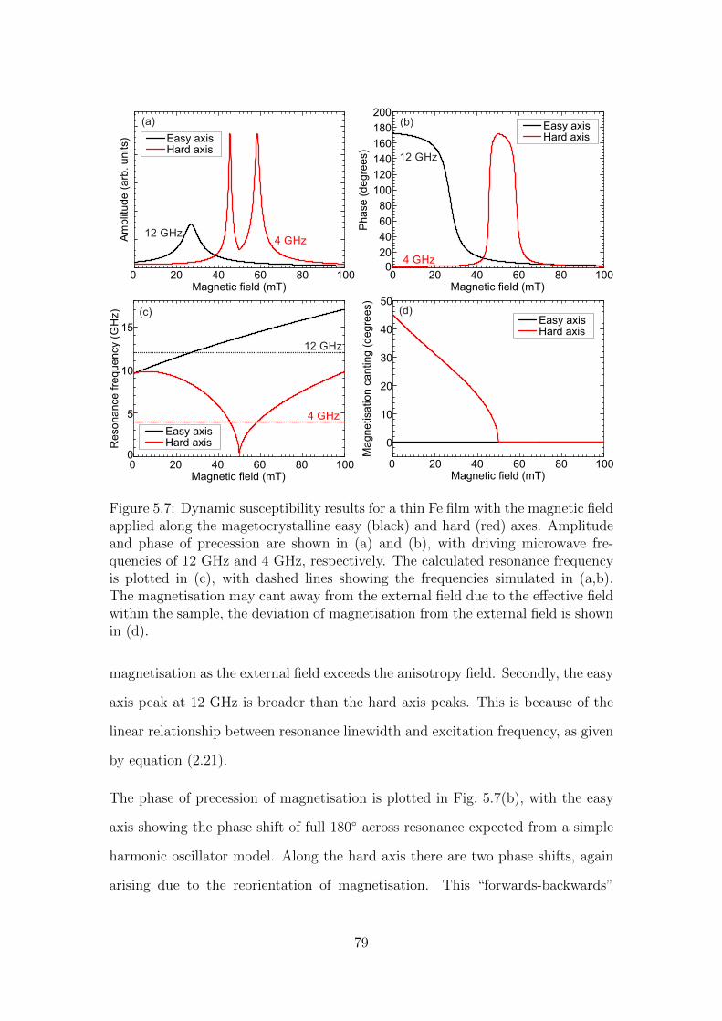
0 20 40 60 80 100

Am

plit

ud

e (

arb

. u

nits)

Magnetic field (mT)

Easy axisHard axis

(a)

0

20

40

60

80

100

120

140

160

180

200

Ph

ase

(d

eg

ree

s)

0 20 40 60 80 100Magnetic field (mT)

Easy axisHard axis

(b)

0

10

20

30

40

50

Ma

gn

etisa

tio

n c

an

tin

g (

de

gre

es)

0 20 40 60 80 100Magnetic field (mT)

Easy axisHard axis

(d)

0

5

10

15

Re

so

na

nce

fre

qu

en

cy (

GH

z)

0 20 40 60 80 100Magnetic field (mT)

Easy axisHard axis

(c)

12 GHz

4 GHz

12 GHz4 GHz

12 GHz

4 GHz

Figure 5.7: Dynamic susceptibility results for a thin Fe film with the magnetic fieldapplied along the magetocrystalline easy (black) and hard (red) axes. Amplitudeand phase of precession are shown in (a) and (b), with driving microwave fre-quencies of 12 GHz and 4 GHz, respectively. The calculated resonance frequencyis plotted in (c), with dashed lines showing the frequencies simulated in (a,b).The magnetisation may cant away from the external field due to the effective fieldwithin the sample, the deviation of magnetisation from the external field is shownin (d).

magnetisation as the external field exceeds the anisotropy field. Secondly, the easy

axis peak at 12 GHz is broader than the hard axis peaks. This is because of the

linear relationship between resonance linewidth and excitation frequency, as given

by equation (2.21).

The phase of precession of magnetisation is plotted in Fig. 5.7(b), with the easy

axis showing the phase shift of full 180 across resonance expected from a simple

harmonic oscillator model. Along the hard axis there are two phase shifts, again

arising due to the reorientation of magnetisation. This “forwards-backwards”

79

phase feature always occurs along a hard axis, though if the peak separation

is small the feature is compressed, and may not complete the full 180 shift.

This can make interpretation of XFMR data rather challenging, and renders the

classification of a resonance as an “optic” or “accoustic” mode complicated.

Figure 5.7(c) shows the Kittel curves for the thin Fe film calculated from the

prefactor of the inverse susceptibility matrix. At zero applied magnetic field the

results along both axes agree. The curves diverge as the magnetic field increases,

and the external field begins to compete with the anisotropy field. Examining

the kink in the hard axis data yields an anisotropy field of ∼50 mT. The equilib-

rium orientation of magnetisation was calculated by minimising the free energy

derivative, equation (2.10), and is plotted in Fig. 5.7(d). Along the easy axis the

magnetisation is always collinear with the field, however along the hard axis the

rotation of magnetisation can be easily observed.

This illustrates the benefits of this modelling approach: it quickly produces re-

sults that correspond well to experimental findings, and gives a good breadth of

information by returning susceptibility, resonance condition and canting angle si-

multaneously. Further, as it is a direct simulation of an ideal FMR experiment,

one does not have to worry about shape effects, choice of initial perturbation or

time discretisation. However, the very fact that it is an idealised FMR experi-

ment means that there are some shortcomings; it assumes a perfect microwave

excitation, infinitely sharply defined crystalline axes, and homogeneous magnetic

field. Further, its spatial resolution is limited to a macrospin approximation of

each layer, as it has no way of dealing with the magnetisation variations within

a ferromagnet. In this respect it is inferior to OOMMF. However, as this is the

same level of spatial resolution obtained by XFMR, this drawback is less impor-

tant. Therefore, for its versatility, speed and ease of use, and close correspondence

to experimental techniques, determination of the dynamic susceptibility is the

80

preferred modelling approach.

5.3.2 Modelling Dynamic and Static Exchange

The magnetic heterostructures studied in the following chapters are based on the

spin valve or tunnel junction concept: two ferromagnets separated by a thin non-

magnetic barrier, that may be conducting or insulating. For a suitable barrier

thickness and material, two coupling mechanisms exist. Dynamic coupling (intro-

duced in section 2.3.3) occurs when the magnetisation of one or both of the layers

is in motion, and proceeds through the indirect interaction of spin pumping. The

mathematical formulation of spin pumping is discussed in more detail in section

2.3.3. The dynamic interaction modifies the LLG with the addition of damping

and anti-damping terms, which codify the additional linewidth of resonance due

to loss of angular momentum, and the induced precession caused by absorption of

angular momentum.

Static coupling was introduced in section 2.2.4, recall the definition [31,35]:

βi =Aex

M isdi

cos(φiM − φjM), (5.8)

with Aex the interlayer exchange constant, d the thickness of the magnetic layer,

and φM the equilibrium orientation of magnetisation. The sign of Aex determines

whether the interaction favours parallel (positive) or antiparallel (negative) align-

ment.

With the addition of these two coupling mechanisms, the LLG for a trilayer system

81

becomes [35]:

−∂mi

∂t= mi ×

[γiH i

eff + βiM jsm

j − (αi0 + αiii)∂mi

∂t

]+ αiijm

j × ∂mj

∂t, (5.9)

where superscripts denote magnetic layer, and H ieff is the effective field acting on

layer i. The intrinsic Gilbert damping is αi0, while αimn are spin source (m = n)

and spin sink (m 6= n) terms. This equation is solved in the same manner as in

section 5.3.1. For full details of the derivation and associated assumptions, refer

to appendix A.

The presence of these coupling mechanisms alters the magnetodynamics of the on-

and off-resonance layer. The static coupling shifts the resonant field of both layers,

as it functions as an additional field term in the Kittel equation. Spin pumping,

on the other hand, broadens the resonances by providing an additional energy loss

mechanism. However, the most important change is the precession induced in the

off-resonance layer, wherein the exchange interactions transfer energy between the

two layers. This leads to changes in both the phase and amplitude of precession,

with the phase being the more sensitive probe.

Figure 5.8 shows the off-resonance precession induced at 7 GHz in a 5 nm Co50Fe50

layer, coupled to a 5 nm Ni81Fe19 layer by the static interaction. The shifts in

resonance frequency relative to the resonance of an isolated NiFe layer (dashed

black line) are due to the increased energy in the system from the static interaction.

A (weak) interaction of 1×10−6 Jm−2 has little effect, leading to an almost flat

line across the resonance. When this is increased to 1×10−5 Jm−2 there is a weak

bipolar feature in the amplitude, and a unipolar feature in the phase, along with

a shift in resonance frequency of about ∼5 mT. If the same coupling strength

is used, but the interaction is made antiferromagnetic, the resonance shifts in

82

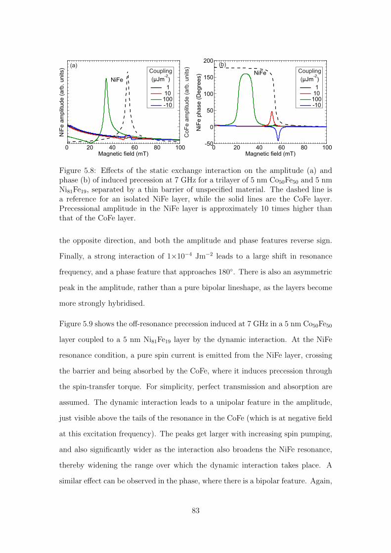
0 20 40 60 80 100

NiFe

Magnetic field (mT)

NiF

e a

mp

litu

de

(a

rb.

un

its)

Co

Fe

am

plit

ud

e (

arb

. u

nits)(a)

-50

0

50

100

150

200

NiF

e p

ha

se

(D

eg

ree

s)

0 20 40 60 80 100Magnetic field (mT)

NiFe

-10100101

Coupling

(μJm )-2

(b)

-10100101

Coupling

(μJm )-2

Figure 5.8: Effects of the static exchange interaction on the amplitude (a) andphase (b) of induced precession at 7 GHz for a trilayer of 5 nm Co50Fe50 and 5 nmNi81Fe19, separated by a thin barrier of unspecified material. The dashed line isa reference for an isolated NiFe layer, while the solid lines are the CoFe layer.Precessional amplitude in the NiFe layer is approximately 10 times higher thanthat of the CoFe layer.

the opposite direction, and both the amplitude and phase features reverse sign.

Finally, a strong interaction of 1×10−4 Jm−2 leads to a large shift in resonance

frequency, and a phase feature that approaches 180. There is also an asymmetric

peak in the amplitude, rather than a pure bipolar lineshape, as the layers become

more strongly hybridised.

Figure 5.9 shows the off-resonance precession induced at 7 GHz in a 5 nm Co50Fe50

layer coupled to a 5 nm Ni81Fe19 layer by the dynamic interaction. At the NiFe

resonance condition, a pure spin current is emitted from the NiFe layer, crossing

the barrier and being absorbed by the CoFe, where it induces precession through

the spin-transfer torque. For simplicity, perfect transmission and absorption are

assumed. The dynamic interaction leads to a unipolar feature in the amplitude,

just visible above the tails of the resonance in the CoFe (which is at negative field

at this excitation frequency). The peaks get larger with increasing spin pumping,

and also significantly wider as the interaction also broadens the NiFe resonance,

thereby widening the range over which the dynamic interaction takes place. A

similar effect can be observed in the phase, where there is a bipolar feature. Again,

83

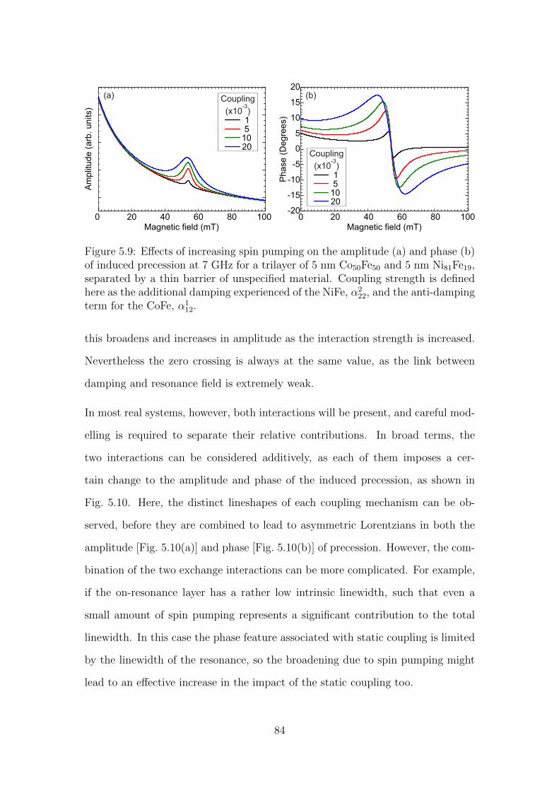
0 20 40 60 80 100

Am

plit

ud

e (

arb

. u

nits)

Magnetic field (mT)

-20

-15

-10

-5

0

5

10

15

20

Ph

ase

(D

eg

ree

s)

0 20 40 60 80 100Magnetic field (mT)

15

1020

Coupling

(x10 )-3

15

1020

Coupling

(x10 )-3

(a) (b)

Figure 5.9: Effects of increasing spin pumping on the amplitude (a) and phase (b)of induced precession at 7 GHz for a trilayer of 5 nm Co50Fe50 and 5 nm Ni81Fe19,separated by a thin barrier of unspecified material. Coupling strength is definedhere as the additional damping experienced of the NiFe, α2

22, and the anti-dampingterm for the CoFe, α1

12.

this broadens and increases in amplitude as the interaction strength is increased.

Nevertheless the zero crossing is always at the same value, as the link between

damping and resonance field is extremely weak.

In most real systems, however, both interactions will be present, and careful mod-

elling is required to separate their relative contributions. In broad terms, the

two interactions can be considered additively, as each of them imposes a cer-

tain change to the amplitude and phase of the induced precession, as shown in

Fig. 5.10. Here, the distinct lineshapes of each coupling mechanism can be ob-

served, before they are combined to lead to asymmetric Lorentzians in both the

amplitude [Fig. 5.10(a)] and phase [Fig. 5.10(b)] of precession. However, the com-

bination of the two exchange interactions can be more complicated. For example,

if the on-resonance layer has a rather low intrinsic linewidth, such that even a

small amount of spin pumping represents a significant contribution to the total

linewidth. In this case the phase feature associated with static coupling is limited

by the linewidth of the resonance, so the broadening due to spin pumping might

lead to an effective increase in the impact of the static coupling too.

84

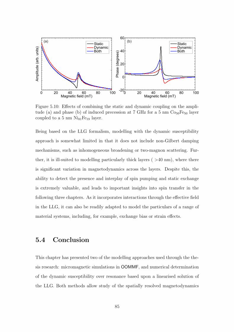
0 20 40 60 80 100-20

0

20

40

60

Ph

ase

(d

eg

ree

s)

Magnetic field (mT)

StaticDynamicBoth

Am

plit

ud

e (

arb

. u

nits)

0 20 40 60 80 100Magnetic field (mT)

StaticDynamicBoth

(a) (b)

Figure 5.10: Effects of combining the static and dynamic coupling on the ampli-tude (a) and phase (b) of induced precession at 7 GHz for a 5 nm Co50Fe50 layercoupled to a 5 nm Ni81Fe19 layer.

Being based on the LLG formalism, modelling with the dynamic susceptibility

approach is somewhat limited in that it does not include non-Gilbert damping

mechanisms, such as inhomogeneous broadening or two-magnon scattering. Fur-

ther, it is ill-suited to modelling particularly thick layers ( >40 nm), where there

is significant variation in magnetodynamics across the layers. Despite this, the

ability to detect the presence and interplay of spin pumping and static exchange

is extremely valuable, and leads to important insights into spin transfer in the

following three chapters. As it incorporates interactions through the effective field

in the LLG, it can also be readily adapted to model the particulars of a range of

material systems, including, for example, exchange bias or strain effects.

5.4 Conclusion

This chapter has presented two of the modelling approaches used through the the-

sis research: micromagnetic simulations in OOMMF, and numerical determination

of the dynamic susceptibility over resonance based upon a linearised solution of

the LLG. Both methods allow study of the spatially resolved magnetodynamics

85

of thin film magnetic heterostructures, without requiring a synchrotron or simi-

lar complex experimental techniques. Further, through their implementations of

static coupling mechanisms, they enable identification of the character of reso-

nances in coupled systems. While OOMMF offers finer spatial discretisation, and

thereby examination of the distribution of energy across the magnetic layer at the

resonance condition, it currently lacks the ability to simulate spin pumping offered

by calculations of the dynamic susceptibility. This modelling of magnetodynam-

ics, and the introduction of coupling terms to the resonance condition, will prove

crucial in the coming three chapters, which deal with trilayer structures. The

separation of the effects of intrinsic damping, spin pumping, and static exchange

is essential to develop a detailed understanding of coupled magnetodynamics.

86

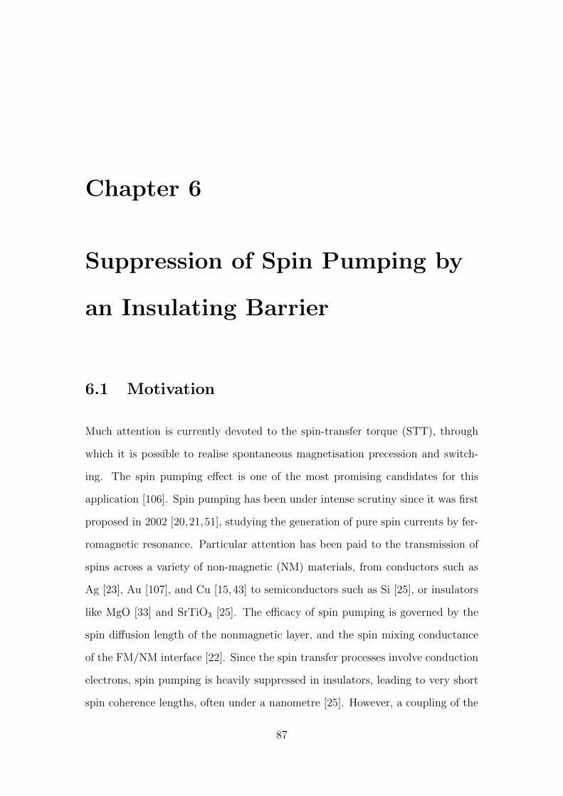
Chapter 6

Suppression of Spin Pumping by

an Insulating Barrier

6.1 Motivation

Much attention is currently devoted to the spin-transfer torque (STT), through

which it is possible to realise spontaneous magnetisation precession and switch-

ing. The spin pumping effect is one of the most promising candidates for this

application [106]. Spin pumping has been under intense scrutiny since it was first

proposed in 2002 [20,21,51], studying the generation of pure spin currents by fer-

romagnetic resonance. Particular attention has been paid to the transmission of

spins across a variety of non-magnetic (NM) materials, from conductors such as

Ag [23], Au [107], and Cu [15, 43] to semiconductors such as Si [25], or insulators

like MgO [33] and SrTiO3 [25]. The efficacy of spin pumping is governed by the

spin diffusion length of the nonmagnetic layer, and the spin mixing conductance

of the FM/NM interface [22]. Since the spin transfer processes involve conduction

electrons, spin pumping is heavily suppressed in insulators, leading to very short

spin coherence lengths, often under a nanometre [25]. However, a coupling of the

87

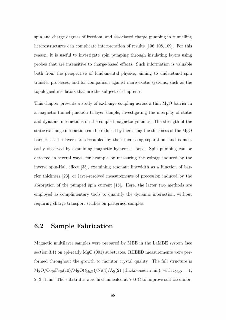
spin and charge degrees of freedom, and associated charge pumping in tunnelling

heterostructures can complicate interpretation of results [106, 108, 109]. For this

reason, it is useful to investigate spin pumping through insulating layers using

probes that are insensitive to charge-based effects. Such information is valuable

both from the perspective of fundamental physics, aiming to understand spin

transfer processes, and for comparison against more exotic systems, such as the

topological insulators that are the subject of chapter 7.

This chapter presents a study of exchange coupling across a thin MgO barrier in

a magnetic tunnel junction trilayer sample, investigating the interplay of static

and dynamic interactions on the coupled magnetodynamics. The strength of the

static exchange interaction can be reduced by increasing the thickness of the MgO

barrier, as the layers are decoupled by their increasing separation, and is most

easily observed by examining magnetic hysteresis loops. Spin pumping can be

detected in several ways, for example by measuring the voltage induced by the

inverse spin-Hall effect [33], examining resonant linewidth as a function of bar-

rier thickness [23], or layer-resolved measurements of precession induced by the

absorption of the pumped spin current [15]. Here, the latter two methods are

employed as complimentary tools to quantify the dynamic interaction, without

requiring charge transport studies on patterned samples.

6.2 Sample Fabrication

Magnetic multilayer samples were prepared by MBE in the LaMBE system (see

section 3.1) on epi-ready MgO (001) substrates. RHEED measurements were per-

formed throughout the growth to monitor crystal quality. The full structure is

MgO/Co50Fe50(10)/MgO(tMgO)/Ni(4)/Ag(2) (thicknesses in nm), with tMgO = 1,

2, 3, 4 nm. The substrates were first annealed at 700C to improve surface unifor-

88

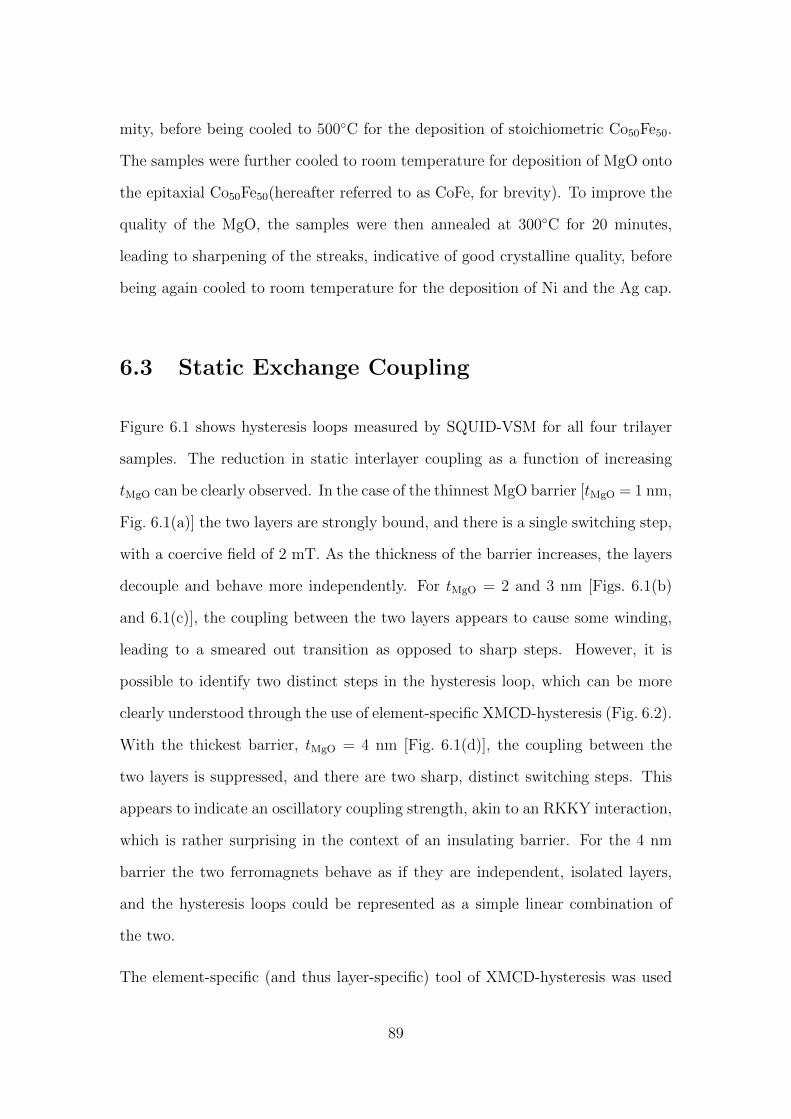
mity, before being cooled to 500C for the deposition of stoichiometric Co50Fe50.

The samples were further cooled to room temperature for deposition of MgO onto

the epitaxial Co50Fe50(hereafter referred to as CoFe, for brevity). To improve the

quality of the MgO, the samples were then annealed at 300C for 20 minutes,

leading to sharpening of the streaks, indicative of good crystalline quality, before

being again cooled to room temperature for the deposition of Ni and the Ag cap.

6.3 Static Exchange Coupling

Figure 6.1 shows hysteresis loops measured by SQUID-VSM for all four trilayer

samples. The reduction in static interlayer coupling as a function of increasing

tMgO can be clearly observed. In the case of the thinnest MgO barrier [tMgO = 1 nm,

Fig. 6.1(a)] the two layers are strongly bound, and there is a single switching step,

with a coercive field of 2 mT. As the thickness of the barrier increases, the layers

decouple and behave more independently. For tMgO = 2 and 3 nm [Figs. 6.1(b)

and 6.1(c)], the coupling between the two layers appears to cause some winding,

leading to a smeared out transition as opposed to sharp steps. However, it is

possible to identify two distinct steps in the hysteresis loop, which can be more

clearly understood through the use of element-specific XMCD-hysteresis (Fig. 6.2).

With the thickest barrier, tMgO = 4 nm [Fig. 6.1(d)], the coupling between the

two layers is suppressed, and there are two sharp, distinct switching steps. This

appears to indicate an oscillatory coupling strength, akin to an RKKY interaction,

which is rather surprising in the context of an insulating barrier. For the 4 nm

barrier the two ferromagnets behave as if they are independent, isolated layers,

and the hysteresis loops could be represented as a simple linear combination of

the two.

The element-specific (and thus layer-specific) tool of XMCD-hysteresis was used

89

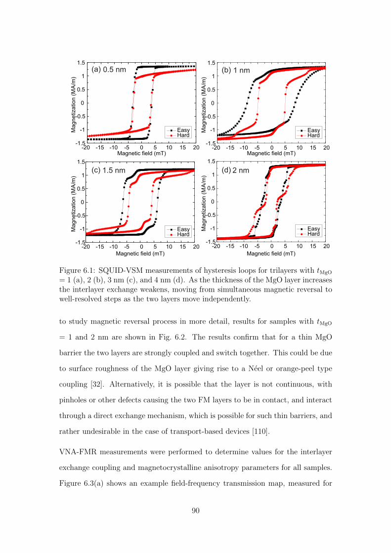
(b)

(d)

1 nm

2 nm

-20 -15 -10 -5 0 5 10 15 20

Ma

gn

etiza

tio

n (

MA

/m)

EasyHard

-1.5

-1

-0.5

0

0.5

1

1.5

-20 -15 -10 -5 0 5 10 15 20

Ma

gn

etiza

tio

n (

MA

/m)

EasyHard

-1.5

-1

-0.5

0

0.5

1

1.5

Magnetic field (mT)

Magnetic field (mT)

Magnetic field (mT)

(a) 0.5 nm

-20 -15 -10 -5 0 5 10 15 20

Ma

gn

etiza

tio

n (

MA

/m)

EasyHard

-1.5

-1

-0.5

0

0.5

1

1.5

(c) 1.5 nm

Magnetic field (mT)

-20 -15 -10 -5 0 5 10 15 20

Ma

gn

etiza

tio

n (

MA

/m)

EasyHard

-1.5

-1

-0.5

0

0.5

1

1.5

Figure 6.1: SQUID-VSM measurements of hysteresis loops for trilayers with tMgO

= 1 (a), 2 (b), 3 nm (c), and 4 nm (d). As the thickness of the MgO layer increasesthe interlayer exchange weakens, moving from simultaneous magnetic reversal towell-resolved steps as the two layers move independently.

to study magnetic reversal process in more detail, results for samples with tMgO

= 1 and 2 nm are shown in Fig. 6.2. The results confirm that for a thin MgO

barrier the two layers are strongly coupled and switch together. This could be due

to surface roughness of the MgO layer giving rise to a Neel or orange-peel type

coupling [32]. Alternatively, it is possible that the layer is not continuous, with

pinholes or other defects causing the two FM layers to be in contact, and interact

through a direct exchange mechanism, which is possible for such thin barriers, and

rather undesirable in the case of transport-based devices [110].

VNA-FMR measurements were performed to determine values for the interlayer

exchange coupling and magnetocrystalline anisotropy parameters for all samples.

Figure 6.3(a) shows an example field-frequency transmission map, measured for

90

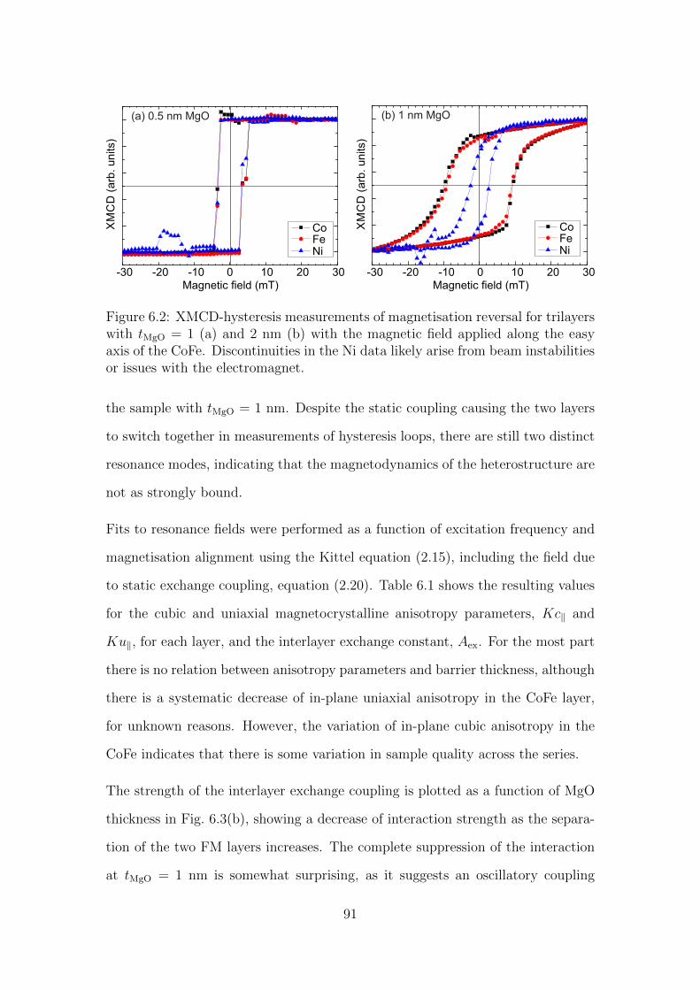
-30 -20 -10 0 10 20 30

XM

CD

(arb

. units)

Magnetic field (mT)-30 -20 -10 0 10 20 30

XM

CD

(arb

. units)

Magnetic field (mT)

CoFeNi

(a) 0.5 nm MgO

CoFeNi

(b) 1 nm MgO

Figure 6.2: XMCD-hysteresis measurements of magnetisation reversal for trilayerswith tMgO = 1 (a) and 2 nm (b) with the magnetic field applied along the easyaxis of the CoFe. Discontinuities in the Ni data likely arise from beam instabilitiesor issues with the electromagnet.

the sample with tMgO = 1 nm. Despite the static coupling causing the two layers

to switch together in measurements of hysteresis loops, there are still two distinct

resonance modes, indicating that the magnetodynamics of the heterostructure are

not as strongly bound.

Fits to resonance fields were performed as a function of excitation frequency and

magnetisation alignment using the Kittel equation (2.15), including the field due

to static exchange coupling, equation (2.20). Table 6.1 shows the resulting values

for the cubic and uniaxial magnetocrystalline anisotropy parameters, Kc‖ and

Ku‖, for each layer, and the interlayer exchange constant, Aex. For the most part

there is no relation between anisotropy parameters and barrier thickness, although

there is a systematic decrease of in-plane uniaxial anisotropy in the CoFe layer,

for unknown reasons. However, the variation of in-plane cubic anisotropy in the

CoFe indicates that there is some variation in sample quality across the series.

The strength of the interlayer exchange coupling is plotted as a function of MgO

thickness in Fig. 6.3(b), showing a decrease of interaction strength as the separa-

tion of the two FM layers increases. The complete suppression of the interaction

at tMgO = 1 nm is somewhat surprising, as it suggests an oscillatory coupling

91

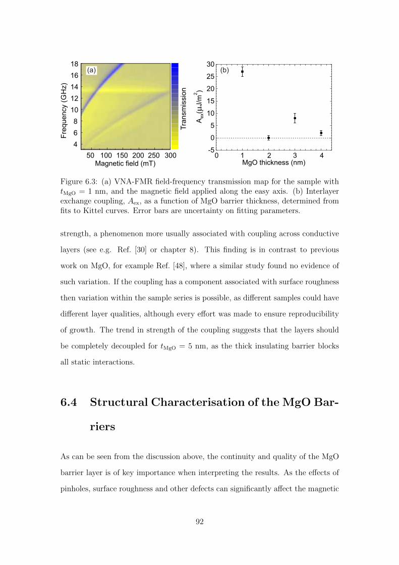
A(

J/m

)e

xm

2

0 1 2 3 4-5

0

5

10

15

20

25

30

MgO thickness (nm)

(b)

4

6

8

10

12

14

16

18F

requency (

GH

z)

50 100 150 200 250Magnetic field (mT)

300

Tra

nsm

issio

n

(a)

Figure 6.3: (a) VNA-FMR field-frequency transmission map for the sample withtMgO = 1 nm, and the magnetic field applied along the easy axis. (b) Interlayerexchange coupling, Aex, as a function of MgO barrier thickness, determined fromfits to Kittel curves. Error bars are uncertainty on fitting parameters.

strength, a phenomenon more usually associated with coupling across conductive

layers (see e.g. Ref. [30] or chapter 8). This finding is in contrast to previous

work on MgO, for example Ref. [48], where a similar study found no evidence of

such variation. If the coupling has a component associated with surface roughness

then variation within the sample series is possible, as different samples could have

different layer qualities, although every effort was made to ensure reproducibility

of growth. The trend in strength of the coupling suggests that the layers should

be completely decoupled for tMgO = 5 nm, as the thick insulating barrier blocks

all static interactions.

6.4 Structural Characterisation of the MgO Bar-

riers

As can be seen from the discussion above, the continuity and quality of the MgO

barrier layer is of key importance when interpreting the results. As the effects of

pinholes, surface roughness and other defects can significantly affect the magnetic

92

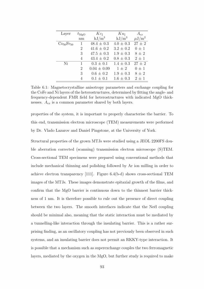
Layer tMgO Kc‖ Ku‖ Aexnm kJ/m3 kJ/m3 µJ/m2

Co50Fe50 1 48.4 ± 0.3 4.0 ± 0.3 27 ± 22 41.6 ± 0.2 3.2 ± 0.2 0 ± 13 47.5 ± 0.3 1.9 ± 0.3 8 ± 24 43.4 ± 0.2 0.8 ± 0.3 2 ± 1

Ni 1 0.3 ± 0.1 1.4 ± 0.3 27 ± 22 0.04 ± 0.09 1 ± 2 0 ± 13 0.6 ± 0.2 1.9 ± 0.3 8 ± 24 0.1 ± 0.1 1.6 ± 0.3 2 ± 1

Table 6.1: Magnetocrystalline anisotropy parameters and exchange coupling forthe CoFe and Ni layers of the heterostructures, determined by fitting the angle- andfrequency-dependent FMR field for heterostructures with indicated MgO thick-nesses. Aex is a common parameter shared by both layers.

properties of the system, it is important to properly characterise the barrier. To

this end, transmission electron microscope (TEM) measurements were performed

by Dr. Vlado Lazarov and Daniel Pingstone, at the University of York.

Structural properties of the grown MTJs were studied using a JEOL 2200FS dou-

ble aberration corrected (scanning) transmission electron microscope (S)TEM.

Cross-sectional TEM specimens were prepared using conventional methods that

include mechanical thinning and polishing followed by Ar ion milling in order to

achieve electron transparency [111]. Figure 6.4(b-d) shows cross-sectional TEM

images of the MTJs. These images demonstrate epitaxial growth of the films, and

confirm that the MgO barrier is continuous down to the thinnest barrier thick-

ness of 1 nm. It is therefore possible to rule out the presence of direct coupling

between the two layers. The smooth interfaces indicate that the Neel coupling

should be minimal also, meaning that the static interaction must be mediated by

a tunnelling-like interaction through the insulating barrier. This is a rather sur-

prising finding, as an oscillatory coupling has not previously been observed in such

systems, and an insulating barrier does not permit an RKKY-type interaction. It

is possible that a mechanism such as superexchange couples the two ferromagnetic

layers, mediated by the oxygen in the MgO, but further study is required to make

93

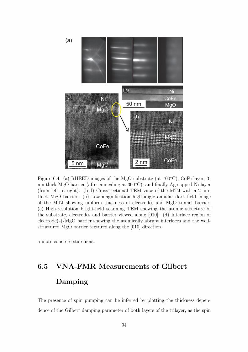
CoFe

MgO

Ni

MgO

Ni

MgO

CoFe( )c

CoFe

Ni

MgO

( )d

2 nm5 nm

50 nm

( )b

( )a

Figure 6.4: (a) RHEED images of the MgO substrate (at 700C), CoFe layer, 3-nm-thick MgO barrier (after annealing at 300C), and finally Ag-capped Ni layer(from left to right). (b-d) Cross-sectional TEM view of the MTJ with a 2-nm-thick MgO barrier. (b) Low-magnification high angle annular dark field imageof the MTJ showing uniform thickness of electrodes and MgO tunnel barrier.(c) High-resolution bright-field scanning TEM showing the atomic structure ofthe substrate, electrodes and barrier viewed along [010]. (d) Interface region ofelectrode(s)/MgO barrier showing the atomically abrupt interfaces and the well-structured MgO barrier textured along the [010] direction.

a more concrete statement.

6.5 VNA-FMR Measurements of Gilbert

Damping

The presence of spin pumping can be inferred by plotting the thickness depen-

dence of the Gilbert damping parameter of both layers of the trilayer, as the spin

94

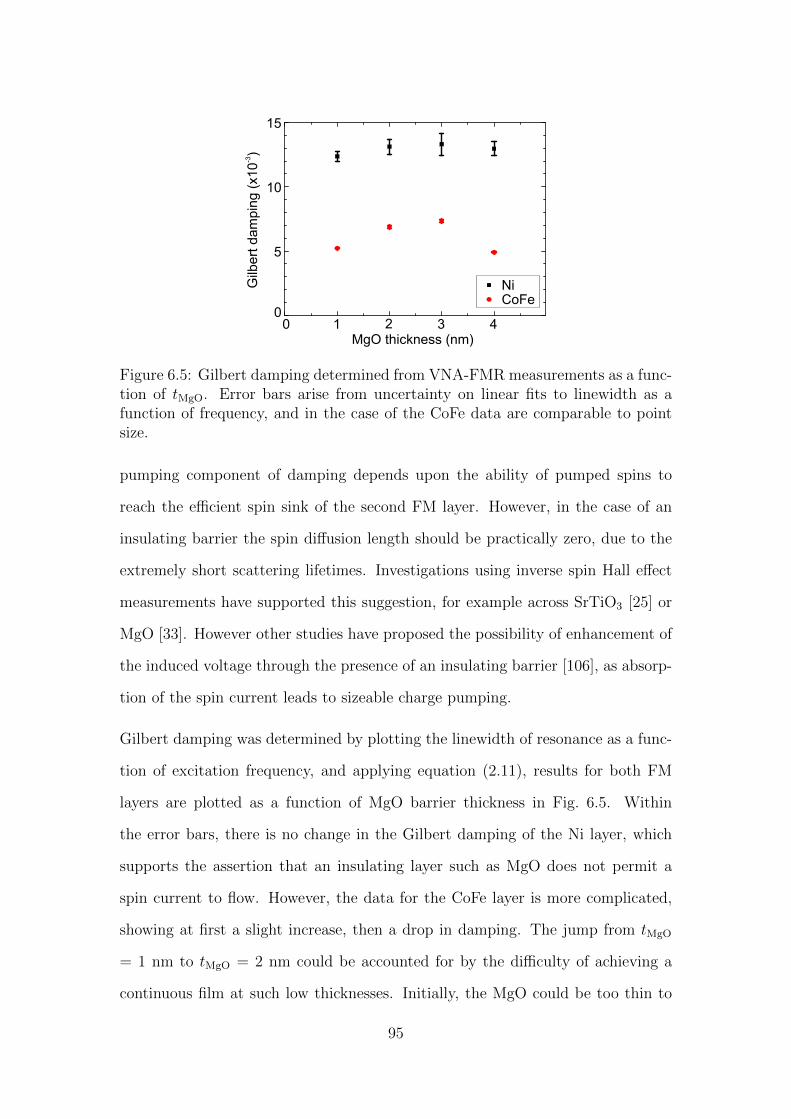
0 1 2 3 40

5

10

15

NiCoFe

Gilb

ert

dam

pin

g (

x10

)-3

MgO thickness (nm)

Figure 6.5: Gilbert damping determined from VNA-FMR measurements as a func-tion of tMgO. Error bars arise from uncertainty on linear fits to linewidth as afunction of frequency, and in the case of the CoFe data are comparable to pointsize.

pumping component of damping depends upon the ability of pumped spins to

reach the efficient spin sink of the second FM layer. However, in the case of an

insulating barrier the spin diffusion length should be practically zero, due to the

extremely short scattering lifetimes. Investigations using inverse spin Hall effect

measurements have supported this suggestion, for example across SrTiO3 [25] or

MgO [33]. However other studies have proposed the possibility of enhancement of

the induced voltage through the presence of an insulating barrier [106], as absorp-

tion of the spin current leads to sizeable charge pumping.

Gilbert damping was determined by plotting the linewidth of resonance as a func-

tion of excitation frequency, and applying equation (2.11), results for both FM

layers are plotted as a function of MgO barrier thickness in Fig. 6.5. Within

the error bars, there is no change in the Gilbert damping of the Ni layer, which

supports the assertion that an insulating layer such as MgO does not permit a

spin current to flow. However, the data for the CoFe layer is more complicated,

showing at first a slight increase, then a drop in damping. The jump from tMgO

= 1 nm to tMgO = 2 nm could be accounted for by the difficulty of achieving a

continuous film at such low thicknesses. Initially, the MgO could be too thin to

95

form a continuous layer, resulting in pinholes or islands that cause direct contact.

In this case, the magnetodynamics of the layers are more complicated, as hybridi-

sation of the interface region can lead to modification of the relaxation rate. With

a continuous layer, separate behaviour of the layers is restored. However, TEM

measurements (Fig. 6.4) showed that the barrier is smooth and continuous even

for tMgO = 1 nm, so any such interaction must occur across the insulating layer,

rather than bypassing it due to imperfections.

In the case of the lower damping for the thickest layer, it is challenging to provide

a conclusive explanation. A drop in damping with increasing interlayer thickness

is usually indicative of spin pumping, but it is unclear why the damping increases

before this point. It is unlikely to be related to a structural change in the CoFe,

as this is the bottom layer of the heterostructure. RHEED measurements dur-

ing growth, and TEM performed afterwards, gave no indication of a variation in

crystal quality that could explain this change either, and despite some variation

in magnetic parameters across the series there is nothing to explain the change in

damping.

Several points should be noted when considering these results. Firstly, measure-

ments on comparable bare CoFe layers yielded a Gilbert damping of ∼3×10−3.

This suggests that whether or not it is able to transmit a spin current, the MgO

does at least absorb some of the spins pumped by the precessing magnetisation

of the CoFe. Secondly, the increase of damping up to tMgO = 3 nm is not large,

especially when compared to the spin pumping damping in Cr spin valves (chapter

8) or the changes induced by doping with rare earths (chapter 4).

Unfortunately, these indirect measurements of spin transfer using VNA-FMR are

unable to provide a conclusive determination of the presence of spin pumping

within the heterostructures. Therefore, XFMR was performed to investigate the

system further, using the layer-resolved technique to establish a clearer picture of

96

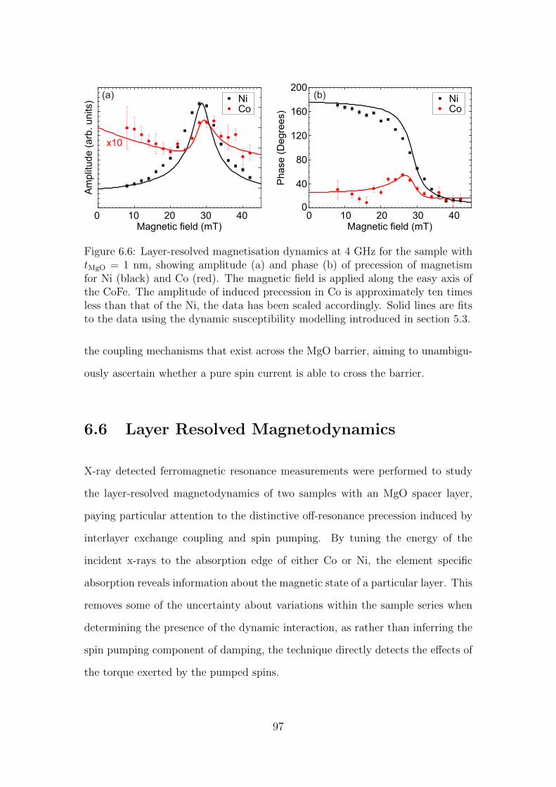
0 10 20 30 400

40

80

120

160

200

Ph

ase

(D

eg

ree

s)

NiCo

(b)NiCo

Am

plit

ud

e (

arb

. u

nits)

(a)

0 10 20 30 40Magnetic field (mT)

x10

Magnetic field (mT)

Figure 6.6: Layer-resolved magnetisation dynamics at 4 GHz for the sample withtMgO = 1 nm, showing amplitude (a) and phase (b) of precession of magnetismfor Ni (black) and Co (red). The magnetic field is applied along the easy axis ofthe CoFe. The amplitude of induced precession in Co is approximately ten timesless than that of the Ni, the data has been scaled accordingly. Solid lines are fitsto the data using the dynamic susceptibility modelling introduced in section 5.3.

the coupling mechanisms that exist across the MgO barrier, aiming to unambigu-

ously ascertain whether a pure spin current is able to cross the barrier.

6.6 Layer Resolved Magnetodynamics

X-ray detected ferromagnetic resonance measurements were performed to study

the layer-resolved magnetodynamics of two samples with an MgO spacer layer,

paying particular attention to the distinctive off-resonance precession induced by

interlayer exchange coupling and spin pumping. By tuning the energy of the

incident x-rays to the absorption edge of either Co or Ni, the element specific

absorption reveals information about the magnetic state of a particular layer. This

removes some of the uncertainty about variations within the sample series when

determining the presence of the dynamic interaction, as rather than inferring the

spin pumping component of damping, the technique directly detects the effects of

the torque exerted by the pumped spins.

97

Figure 6.6 shows the amplitude and phase of precession at 4 GHz for each layer

in the sample with tMgO = 1 nm, with the magnetic field applied along the easy

axis of the CoFe. The resonance in the Ni layer can be clearly seen, with a peak

in amplitude at 28 mT. Precession is also induced in the off-resonance CoFe layer;

the resulting dynamic XMCD signal is approximately ten times smaller than that

of the Ni. The phase feature in the Co has a magnitude of about 40, and is

predominantly unipolar in character. Taken together with the bipolar shape of

the Co amplitude variation, this indicates that the static interaction is primarily

responsible for induced precession in the Co, as would be expected following the

VNA-FMR measurements.

Solid lines in Fig. 6.6 are fits to the data using the dynamic susceptibility modelling

outlined in section 5.3 and appendix A. The values of static exchange coupling

and magnetocrystalline anisotropy determined in section 6.3 were used to calcu-

late the expected amplitude and phase of precession for each layer. In order to

reproduce the slightly distorted features in the Co, a dynamic interaction had to

be introduced, accounting for 50% of the total Gilbert damping in the Ni layer,

and assuming perfect transmission of spins. This modifies the shape of the Co

features, mixing a small amount of unipolar feature into the bipolar lineshape of

the amplitude, and vice-versa in the phase. With this included the model repro-

duces the experimental data, although it underestimates the linewidth of the Ni

mode. This is because it does not include inhomogeneous (non-Gilbert) broaden-

ing, which can be a major contribution to the linewidth at low frequencies. The

measurement of a small component of dynamic interaction shows that a suitably

thin MgO barrier will permit a spin current to flow.

Figure 6.7 shows the amplitude and phase of precession at 4 GHz for each layer

in the sample with tMgO = 2 nm, with the magnetic field applied along the easy

axis of the CoFe. As with the tMgO = 1 nm case outlined above there is a well-

98

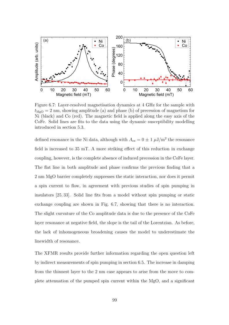
NiCo

0 10 20 30 40 50 60

Am

plit

ud

e (

arb

. u

nits)

Magnetic field (mT)

(a)

0

40

80

120

160

200

Ph

ase

(d

eg

ree

s)

0 10 20 30 40 50 60Magnetic field (mT)

NiCo

(b)

Figure 6.7: Layer-resolved magnetisation dynamics at 4 GHz for the sample withtMgO = 2 nm, showing amplitude (a) and phase (b) of precession of magnetism forNi (black) and Co (red). The magnetic field is applied along the easy axis of theCoFe. Solid lines are fits to the data using the dynamic susceptibility modellingintroduced in section 5.3.

defined resonance in the Ni data, although with Aex = 0 ± 1 µJ/m2 the resonance

field is increased to 35 mT. A more striking effect of this reduction in exchange

coupling, however, is the complete absence of induced precession in the CoFe layer.

The flat line in both amplitude and phase confirms the previous finding that a

2 nm MgO barrier completely suppresses the static interaction, nor does it permit

a spin current to flow, in agreement with previous studies of spin pumping in

insulators [25, 33]. Solid line fits from a model without spin pumping or static

exchange coupling are shown in Fig. 6.7, showing that there is no interaction.

The slight curvature of the Co amplitude data is due to the presence of the CoFe

layer resonance at negative field, the slope is the tail of the Lorentzian. As before,

the lack of inhomogeneous broadening causes the model to underestimate the

linewidth of resonance.

The XFMR results provide further information regarding the open question left

by indirect measurements of spin pumping in section 6.5. The increase in damping

from the thinnest layer to the 2 nm case appears to arise from the move to com-

plete attenuation of the pumped spin current within the MgO, and a significant

99

reduction in the static interaction between the two layers. With the insulating

barrier blocking the transmission of spins, there is no dynamic interaction. This

is in line with previous studies of similar samples [25,33]; but here the separation

of different coupling effects permitted by XFMR provides a deeper understanding

of the magnetodynamics of such systems.

6.7 Conclusion

This chapter has presented the first in a series of studies of coupled magnetisation

dynamics in trilayer structures, investigating the interplay of static and dynamic

coupling mechanisms. Here, an insulating MgO barrier was used to suppress both

interactions, in a sample structure based on the magnetic tunnel junction archi-

tecture. Layer-resolved measurements of magnetodynamics show that for a thin

spacer layer both static exchange and spin pumping are present, leading to cou-

pled precession of the two magnetic layers, and simultaneous switching at a low

coercive field of 2 mT. As the barrier thickness increases the interaction between

the magnetic layers is weakened. In particular, the pure spin current driven by

ferromagnetic resonance is attenuated by as little as 1 nm of MgO, as the low scat-

tering lifetimes and lack of conduction electrons leads to an extremely short spin

diffusion length [25,33]. This was indicated by the lack of systematic variation of

Gilbert damping as a function of tMgO, and confirmed by XFMR measurements.

Analysis of the Kittel curves of resonance shows that static exchange is also sup-

pressed at 2 nm, but this appears to be a result of an oscillatory coupling strength,

rather than complete decoupling of the two layers, as a weak interaction is also

observed up to 4 nm. Aside from the tMgO = 2 nm case, Aex generally decreases as

a function of tMgO, suggesting that 5 nm of MgO would completely separate the

two magnetic layers. The mechanism behind this coupling is currently unknown,

100

however, as the RKKY interaction that typically drives an oscillatory strength

should not exist in an insulating layer such as MgO. Moreover, the effect cannot

be explained away as arising from structural changes or imperfections in the MgO

barrier, as TEM shows that this layer is smooth and continuous across the whole

series. It is clear that this surprising result merits further investigation, seeking

to understand the origin of the varying interaction strength.

These results demonstrate how the coupling between magnetic layers can be ma-

nipulated through choice of barrier material and thickness, and illustrate the dif-

fering regimes of static and dynamic coupling that can be thus attained. The

ability of MgO to quickly suppress a spin current was confirmed, and in more

general terms it was shown that a trivial insulator can very effectively decouple

ferromagnetic layers. Furthermore, the co-operative effects of static and dynamic

were studied, showing how they can co-operatively transfer energy between layers

during ferromagnetic resonance. The following chapters build on these themes,

aiming in particular to study spin pumping in more detail and develop a deeper

understanding of static and dynamic coupling.

101

Chapter 7

Spin Pumping in Topological

Insulators

7.1 Motivation

The exciting physics of topological insulators (TIs) has been under intense study

since their theoretical prediction [114] and experimental verification [115–117].

Recently, they were shown to display the quantum anomalous Hall effect after

doping with magnetic impurities [118], and are proposed to host image magnetic

monopoles and the giant magneto-optical effect [119–122]. In the prototypical

three-dimensional TI Bi2Se3 a large spin-orbit interaction leads to a band inver-

sion in the bulk and the formation of topologically protected surface states (TSS),

with fully spin-polarised counter-propagating conduction channels that are robust

against scattering from non-magnetic impurities [123]. Spin-momentum locking

suggests the possibility of very long spin-flip scattering lifetimes and the ability

to generate ultra-high spin-orbit torques [124–126]. It has been predicted that

the TSS can exert a torque on spins in a neighbouring ferromagnet (FM) through

exchange coupling [127]. However, in order to realise these prospects the magneto-

102

dynamics of the TSS must be studied and such TI-FM heterostructures fabricated.

While angle-resolved photo-emission spectroscopy (ARPES) has been extremely

successful at identifying TIs [116, 117], transport measurements are hampered by

to large bulk conductivities that make unambiguously identifying the surface state

challenging [128,129]. It is therefore beneficial to apply a wider range of techniques

to the study of TIs, aiming to focus more closely on the spin degrees of freedom

present in the TSS.

FMR offers an attractive means to investigate the coupling of ferromagnets to TIs,

using the pure spin current emitted at the resonance condition to probe the bulk

and surface state. In VNA-FMR the enhanced damping due to this loss of angular

momentum can be studied, while XFMR allows detection of coupling across a TI

spacer layer in a spin-valve-like structure. The application of this technique to

TIs is quite naturally suggested by the similarity between the spin-locked surface

state of a TI and the separation of angular momentum and charge flow that

takes place in a pure spin current. Recently, studies of such effects have begun

to emerge through electrical transport and inverse spin-Hall effect measurements

[126, 130, 131], demonstrating the great potential of TIs for incorporation into

spintronic devices such as spin valves.

This chapter describes a series of experiments designed to assess the spintronic po-

tential of TIs, using Co50Fe50(30 nm)/Bi2Se3(x nm)/Ni81Fe19(30 nm) heterostruc-

tures with x = 4...20 nm (materials are also referred to as CoFe, BiSe, and NiFe,

for brevity). Studies of the thickness dependence of interactions between the two

FM layers were used to separate the contributions of bulk and surface conduction

through the TI. Measurements of anti-damping terms that arise for overlapping

resonances were performed to isolate the presence of spin pumping in the het-

erostructures, as opposed to other coupling mechanisms. Finally, the temperature

dependence of the Gilbert damping was measured, as transport measurements

103

have shown that conduction through the bulk of a TI can be frozen out at low

temperatures.

7.1.1 What is a Topological Insulator?

Topological insulators are materials in which a bulk band inversion leads to the

formation of a surface state protected by time reversal symmetry, wherein electrons

are spin-locked and back-scattering events are forbidden. It is important to note

that this novel state is not a surface property, rather its existence is a direct

consequence of the bulk band structure. Only a brief overview of TIs and their

study is presented here, the interested reader is referred to, for example, Refs.

[36,79].

The band inversion that drives the fundamental properties of TIs has its origin in

the strong spin-orbit interaction of such materials. Considering a simple picture,

imagine a material with a separated conduction (CB) and valence (VB) band, in

the case of a direct band gap at the centre of the Brillouin zone. In a conventional

material the CB has positive parity, while the VB has negative character. The

spin-orbit interaction lifts the degeneracy of the p level of the VB, giving rise to

j = 3/2, j = 1/2 states. With sufficiently strong splitting, the j = 3/2 state moves

above the s state of the CB, leading to a parity inversion and the creation of a

TI. An image of the bandstructure of a TI is shown in Fig. 7.1(a). The ”normal”

ordering of bands must be restored at the junction of a TI with a conventional

material. This means that the bands must cross the Fermi energy at the interface,

leading to the formation of two metallic states that are topologically protected. In

the surface state the direction of an electron’s travel is determined by its spin, and

they travel without resistance as any scattering event would require reversal of the

spin. This is not possible without the presence of spin scattering defects, such as

magnetic impurities. A diagram of these protected states is shown in Fig. 7.1(b).

104

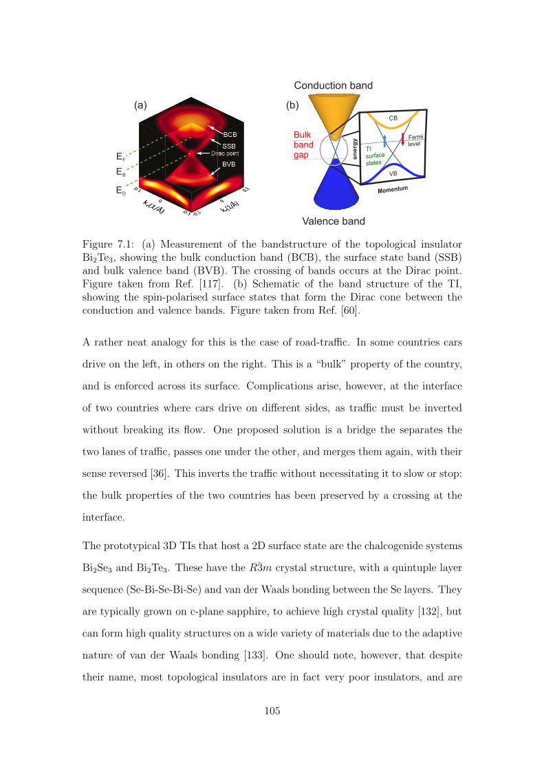
Bulkbandgap

Valence band

Conduction band

EF

EB

ED

(a) (b)

Figure 7.1: (a) Measurement of the bandstructure of the topological insulatorBi2Te3, showing the bulk conduction band (BCB), the surface state band (SSB)and bulk valence band (BVB). The crossing of bands occurs at the Dirac point.Figure taken from Ref. [117]. (b) Schematic of the band structure of the TI,showing the spin-polarised surface states that form the Dirac cone between theconduction and valence bands. Figure taken from Ref. [60].

A rather neat analogy for this is the case of road-traffic. In some countries cars

drive on the left, in others on the right. This is a “bulk” property of the country,

and is enforced across its surface. Complications arise, however, at the interface

of two countries where cars drive on different sides, as traffic must be inverted

without breaking its flow. One proposed solution is a bridge the separates the

two lanes of traffic, passes one under the other, and merges them again, with their

sense reversed [36]. This inverts the traffic without necessitating it to slow or stop:

the bulk properties of the two countries has been preserved by a crossing at the

interface.

The prototypical 3D TIs that host a 2D surface state are the chalcogenide systems

Bi2Se3 and Bi2Te3. These have the R3m crystal structure, with a quintuple layer

sequence (Se-Bi-Se-Bi-Se) and van der Waals bonding between the Se layers. They

are typically grown on c-plane sapphire, to achieve high crystal quality [132], but

can form high quality structures on a wide variety of materials due to the adaptive

nature of van der Waals bonding [133]. One should note, however, that despite

their name, most topological insulators are in fact very poor insulators, and are

105

rather closer to narrow bandgap semiconductors, with a typical gap on the order

of 300 meV.

7.2 Sample Fabrication

Samples were prepared using MBE, sources were calibrated using a quartz crys-

tal microbalance and beam-flux monitor. First, the MgO substrate was annealed

at 700C to clean the surface and reduce the surface roughness. Next, 30 nm

of Co50Fe50 was co-evaporated from Fe and Co electron-beam evaporators. The

substrate temperature was held at 300C during this stage. Strong streaks and

kikuchi lines were observed by RHEED, indicative of high crystalline quality. Sam-

ples were then transferred into a chalcogenide MBE for growth of the Bi2Se3 layers.

Growth of the TI layers was performed by Liam Collins-McIntyre, according to

growth protocols developed during his study of thin film topological insulators,

see e.g. Refs. [79,132,133]. The Co50Fe50 surface was again annealed at 300C to

ensure the surface was high quality; this was checked by RHEED before growth.

The Bi and Se were then evaporated from Knudsen cells for stoichiometric growth

of Bi2Se3. Substrate temperature was 200C. RHEED patterns reveal the forma-

tion of a crystalline mosaic domain pattern. Bi2Se3 thickness was varied between

4 - 20 nm. The samples were then transferred back to the LaMBE chamber, and

a top FM layer of Ni81Fe19 (30 nm) deposited at room temperature (∼300 K), to

avoid damaging the Bi2Se3 layer structure. This leads to polycrystalline Ni81Fe19,

which is desirable as it ensures fully isotropic magnetic behaviour. Samples were

then capped with 5 nm Cu, to prevent oxidation. Samples were grown with an

interlayer thickness of tTI = 4, 6, 8, 16, 20 nm.

The static magnetic properties of the films were characterised using VNA-FMR;

example field-frequency transmission maps along the easy and hard axes are shown

106

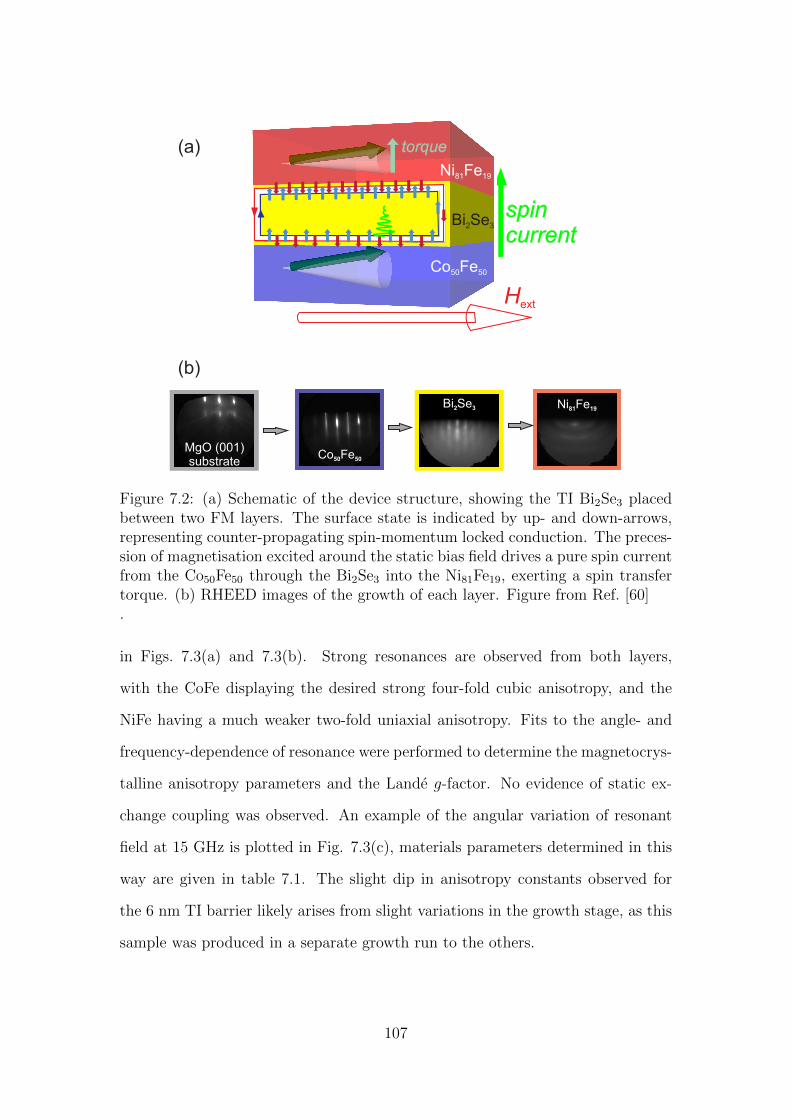
Co Fe50 50

MgO (001)substrate

Ni Fe81 19

Bi Se2 3

spincurrent

Bi Se2 3

Ni Fe81 19

Co Fe50 50

torque

Hext

(a)

(b)

Figure 7.2: (a) Schematic of the device structure, showing the TI Bi2Se3 placedbetween two FM layers. The surface state is indicated by up- and down-arrows,representing counter-propagating spin-momentum locked conduction. The preces-sion of magnetisation excited around the static bias field drives a pure spin currentfrom the Co50Fe50 through the Bi2Se3 into the Ni81Fe19, exerting a spin transfertorque. (b) RHEED images of the growth of each layer. Figure from Ref. [60].

in Figs. 7.3(a) and 7.3(b). Strong resonances are observed from both layers,

with the CoFe displaying the desired strong four-fold cubic anisotropy, and the

NiFe having a much weaker two-fold uniaxial anisotropy. Fits to the angle- and

frequency-dependence of resonance were performed to determine the magnetocrys-

talline anisotropy parameters and the Lande g-factor. No evidence of static ex-

change coupling was observed. An example of the angular variation of resonant

field at 15 GHz is plotted in Fig. 7.3(c), materials parameters determined in this

way are given in table 7.1. The slight dip in anisotropy constants observed for

the 6 nm TI barrier likely arises from slight variations in the growth stage, as this

sample was produced in a separate growth run to the others.

107

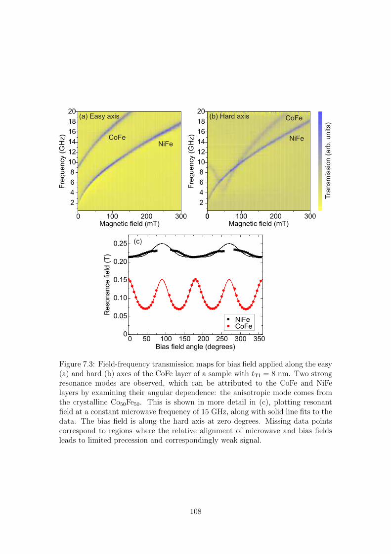
0 50 100 150 200 250 300 3500

0.05

0.10

0.15

0.20

0.25

NiFeCoFe

Resonance

field

(T

)

Bias field angle (degrees)

0 100 200 300

2

4

6

8

10

12

14

16

18

20

Magnetic field (mT)

Fre

quency (

GH

z)

0

2

4

6

8

10

12

14

16

18

20

Fre

quency (

GH

z)

(c)

(a) Easy axis (b) Hard axis CoFe

NiFeCoFe NiFe

Tra

nsm

issio

n (

arb

. units)

0 100 200 300Magnetic field (mT)

Figure 7.3: Field-frequency transmission maps for bias field applied along the easy(a) and hard (b) axes of the CoFe layer of a sample with tTI = 8 nm. Two strongresonance modes are observed, which can be attributed to the CoFe and NiFelayers by examining their angular dependence: the anisotropic mode comes fromthe crystalline Co50Fe50. This is shown in more detail in (c), plotting resonantfield at a constant microwave frequency of 15 GHz, along with solid line fits to thedata. The bias field is along the hard axis at zero degrees. Missing data pointscorrespond to regions where the relative alignment of microwave and bias fieldsleads to limited precession and correspondingly weak signal.

108

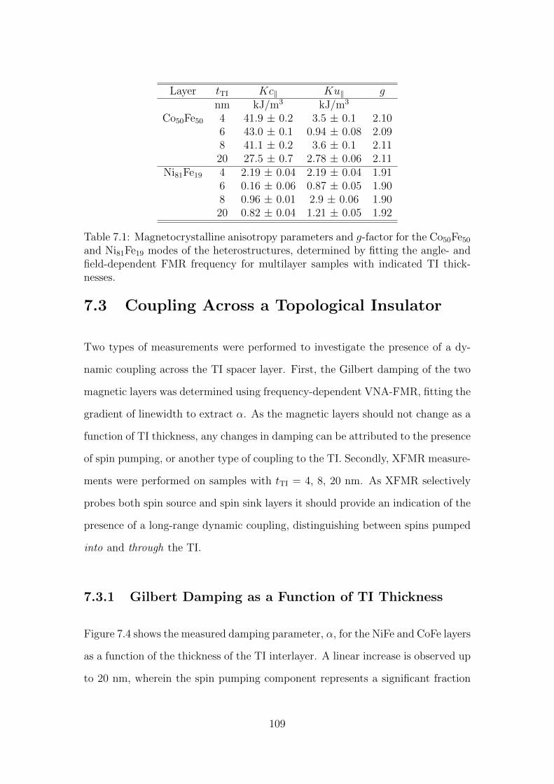
Layer tTI Kc‖ Ku‖ gnm kJ/m3 kJ/m3

Co50Fe50 4 41.9 ± 0.2 3.5 ± 0.1 2.106 43.0 ± 0.1 0.94 ± 0.08 2.098 41.1 ± 0.2 3.6 ± 0.1 2.1120 27.5 ± 0.7 2.78 ± 0.06 2.11

Ni81Fe19 4 2.19 ± 0.04 2.19 ± 0.04 1.916 0.16 ± 0.06 0.87 ± 0.05 1.908 0.96 ± 0.01 2.9 ± 0.06 1.9020 0.82 ± 0.04 1.21 ± 0.05 1.92

Table 7.1: Magnetocrystalline anisotropy parameters and g-factor for the Co50Fe50

and Ni81Fe19 modes of the heterostructures, determined by fitting the angle- andfield-dependent FMR frequency for multilayer samples with indicated TI thick-nesses.

7.3 Coupling Across a Topological Insulator

Two types of measurements were performed to investigate the presence of a dy-

namic coupling across the TI spacer layer. First, the Gilbert damping of the two

magnetic layers was determined using frequency-dependent VNA-FMR, fitting the

gradient of linewidth to extract α. As the magnetic layers should not change as a

function of TI thickness, any changes in damping can be attributed to the presence

of spin pumping, or another type of coupling to the TI. Secondly, XFMR measure-

ments were performed on samples with tTI = 4, 8, 20 nm. As XFMR selectively

probes both spin source and spin sink layers it should provide an indication of the

presence of a long-range dynamic coupling, distinguishing between spins pumped

into and through the TI.

7.3.1 Gilbert Damping as a Function of TI Thickness

Figure 7.4 shows the measured damping parameter, α, for the NiFe and CoFe layers

as a function of the thickness of the TI interlayer. A linear increase is observed up

to 20 nm, wherein the spin pumping component represents a significant fraction

109

of the total damping, indicating a large transfer of angular momentum to the TI.

It is important to compare this result with other materials. As discussed before,

damping in trilayers normally drops exponentially with spacer thickness [23], as

scattering within the non-magnetic (NM) layer is a much less efficient sink for

angular momentum than absorption by a second ferromagnet. This trend is seen,

for example, in the Cr spin valves studied in chapter 8. Here, however, damping

increases with TI thickness, suggesting not only that the TI is a very efficient spin-

sink, but that the pure spin current can penetrate several nanometres into the TI.

If the spacer layer does not transmit spins the damping saturates as soon as a

continuous layer is formed, as shown in chapter. Here, the consistently increasing

damping suggests that the spin current can penetrate some distance into the TI,

which is a more efficient spin sink than the second FM layer. One interpretation

is that while it is possible to drive a spin current into the TI, recovering that

pumped angular momentum at the second interface is more difficult. As a spin

current is driven into the TSS a spin imbalance develops, which is converted to

a charge current [126]. The scattering of such conduction electrons within the

bulk of the TI could then provide a mechanism for efficient absorption of pumped

angular momentum. Therefore, a thicker TI leads to a higher Gilbert damping,

as a thinner layer still allows some spin backflow into the on-resonance FM layer.

Another interpretation can arise when considering the form of equation (2.27),

which yields the spin pumping damping in a trilayer structure. The spin diffusion

length in a nonmagnetic material is determined by its Fermi velocity, and the spin-

flip and momentum scattering lifetimes. In most materials the spin-flip scattering

lifetime (τsf ) is longer than the momentum scattering lifetime (τm), yielding an

exponential decay of damping with increasing spacer layer thickness. If the τm >

τsf , however, the sense of the resulting exponential reverses and the damping

increases with increasing spacer layer thickness, as observed here. This effect

110

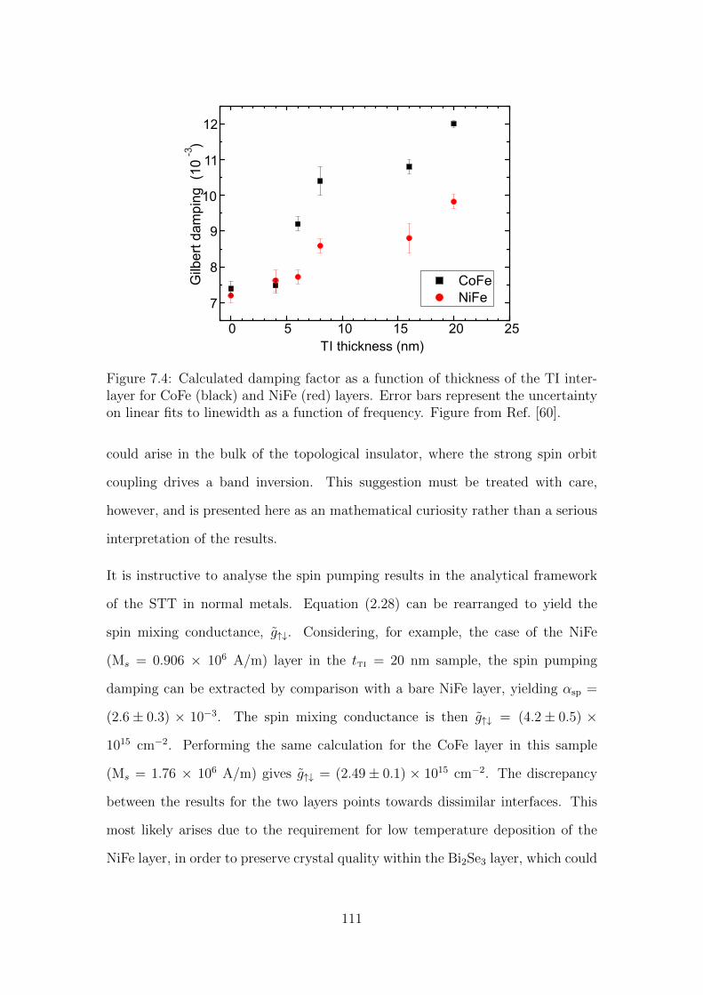
Gilb

ert

da

mp

ing

(1

0

)-3

0 5 10 15 20 25

7

8

9

10

11

12

CoFe

NiFe

TI thickness (nm)

Figure 7.4: Calculated damping factor as a function of thickness of the TI inter-layer for CoFe (black) and NiFe (red) layers. Error bars represent the uncertaintyon linear fits to linewidth as a function of frequency. Figure from Ref. [60].

could arise in the bulk of the topological insulator, where the strong spin orbit

coupling drives a band inversion. This suggestion must be treated with care,

however, and is presented here as an mathematical curiosity rather than a serious

interpretation of the results.

It is instructive to analyse the spin pumping results in the analytical framework

of the STT in normal metals. Equation (2.28) can be rearranged to yield the

spin mixing conductance, g↑↓. Considering, for example, the case of the NiFe

(Ms = 0.906 × 106 A/m) layer in the tTI = 20 nm sample, the spin pumping

damping can be extracted by comparison with a bare NiFe layer, yielding αsp =

(2.6± 0.3) × 10−3. The spin mixing conductance is then g↑↓ = (4.2± 0.5) ×

1015 cm−2. Performing the same calculation for the CoFe layer in this sample

(Ms = 1.76 × 106 A/m) gives g↑↓ = (2.49± 0.1) × 1015 cm−2. The discrepancy

between the results for the two layers points towards dissimilar interfaces. This

most likely arises due to the requirement for low temperature deposition of the

NiFe layer, in order to preserve crystal quality within the Bi2Se3 layer, which could

111

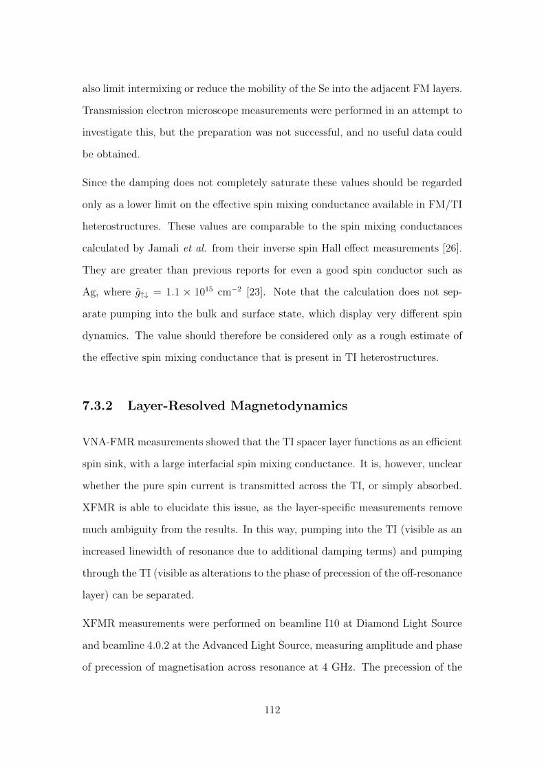
also limit intermixing or reduce the mobility of the Se into the adjacent FM layers.

Transmission electron microscope measurements were performed in an attempt to

investigate this, but the preparation was not successful, and no useful data could

be obtained.

Since the damping does not completely saturate these values should be regarded

only as a lower limit on the effective spin mixing conductance available in FM/TI

heterostructures. These values are comparable to the spin mixing conductances

calculated by Jamali et al. from their inverse spin Hall effect measurements [26].

They are greater than previous reports for even a good spin conductor such as

Ag, where g↑↓ = 1.1 × 1015 cm−2 [23]. Note that the calculation does not sep-

arate pumping into the bulk and surface state, which display very different spin

dynamics. The value should therefore be considered only as a rough estimate of

the effective spin mixing conductance that is present in TI heterostructures.

7.3.2 Layer-Resolved Magnetodynamics

VNA-FMR measurements showed that the TI spacer layer functions as an efficient

spin sink, with a large interfacial spin mixing conductance. It is, however, unclear

whether the pure spin current is transmitted across the TI, or simply absorbed.

XFMR is able to elucidate this issue, as the layer-specific measurements remove

much ambiguity from the results. In this way, pumping into the TI (visible as an

increased linewidth of resonance due to additional damping terms) and pumping

through the TI (visible as alterations to the phase of precession of the off-resonance

layer) can be separated.

XFMR measurements were performed on beamline I10 at Diamond Light Source

and beamline 4.0.2 at the Advanced Light Source, measuring amplitude and phase

of precession of magnetisation across resonance at 4 GHz. The precession of the

112

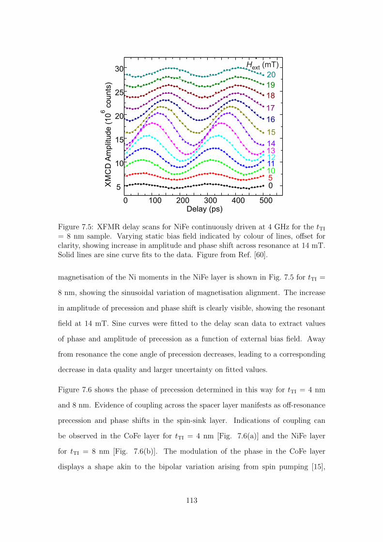
5000 100 200 300 400

5

10

15

20

25

30

XM

CD

Am

plit

ud

e (

10

co

un

ts)

6

Delay (ps)

20

19

18

17

16

15

141312111050

Hext (mT)

Figure 7.5: XFMR delay scans for NiFe continuously driven at 4 GHz for the tTI

= 8 nm sample. Varying static bias field indicated by colour of lines, offset forclarity, showing increase in amplitude and phase shift across resonance at 14 mT.Solid lines are sine curve fits to the data. Figure from Ref. [60].

magnetisation of the Ni moments in the NiFe layer is shown in Fig. 7.5 for tTI =

8 nm, showing the sinusoidal variation of magnetisation alignment. The increase

in amplitude of precession and phase shift is clearly visible, showing the resonant

field at 14 mT. Sine curves were fitted to the delay scan data to extract values

of phase and amplitude of precession as a function of external bias field. Away

from resonance the cone angle of precession decreases, leading to a corresponding

decrease in data quality and larger uncertainty on fitted values.

Figure 7.6 shows the phase of precession determined in this way for tTI = 4 nm

and 8 nm. Evidence of coupling across the spacer layer manifests as off-resonance

precession and phase shifts in the spin-sink layer. Indications of coupling can

be observed in the CoFe layer for tTI = 4 nm [Fig. 7.6(a)] and the NiFe layer

for tTI = 8 nm [Fig. 7.6(b)]. The modulation of the phase in the CoFe layer

displays a shape akin to the bipolar variation arising from spin pumping [15],

113

Am

plit

ude (

arb

. units)

NiCo

(a) 4nm TI

NiCo

0 10 20 30 40 50 60 700

40

80

120

160

200

Phase (

Degre

es)

Magnetic field (mT)

(c)

Am

plit

ude (

arb

. units) Ni

Co

(b) 8nm TI

NiCo

0 10 20 30 40 50 60 700

40

80

120

160

200

Phase (

Degre

es)

Magnetic field (mT)

(d)

Figure 7.6: Amplitude (top row) and phase (bottom row) of precession of mag-netisation for Ni81Fe19(black) and Co50Fe50(red) layers at 4 GHz driving frequencyfor tTI = 4 nm and 8 nm [(a,c) and (b,d), respectively]. The drop and recoveryin phase across the Co mode is caused by the superposition of the two modes,corresponding to canted and collinear magnetisation, as can be seen in Fig. 7.3.Error bars arise from uncertainty on fits to the time-resolved precession, see Fig.7.5. Solid lines are fits to the data using the model presented in section 5.3 andparameters from VNA-FMR measurements. The model does not account for re-duced XFMR signal due to magnetisation canting, and thus over-estimates thelower branch fo the CoFe resonance.

but is rather weak, perhaps due to scattering in the TI layer suppressing spin

pumping. There is no corresponding variation of amplitude, due to the thick FM

layers employed (30 nm) being much larger than the typical penetration depth of

a pure spin current into an FM (∼2 nm). The phase of precession is, however,

a much more sensitive probe and can be used to detect the presence of a weak

coupling. Result from the modelling approach outlined in section 5.3 and values

for magnetocrystalline anisotropy and spin pumping determined by VNA-FMR

measurements provide only an approximate fit to the off-resonance precession.

While there are indeed phase variations akin to those predicted, the model under-

114

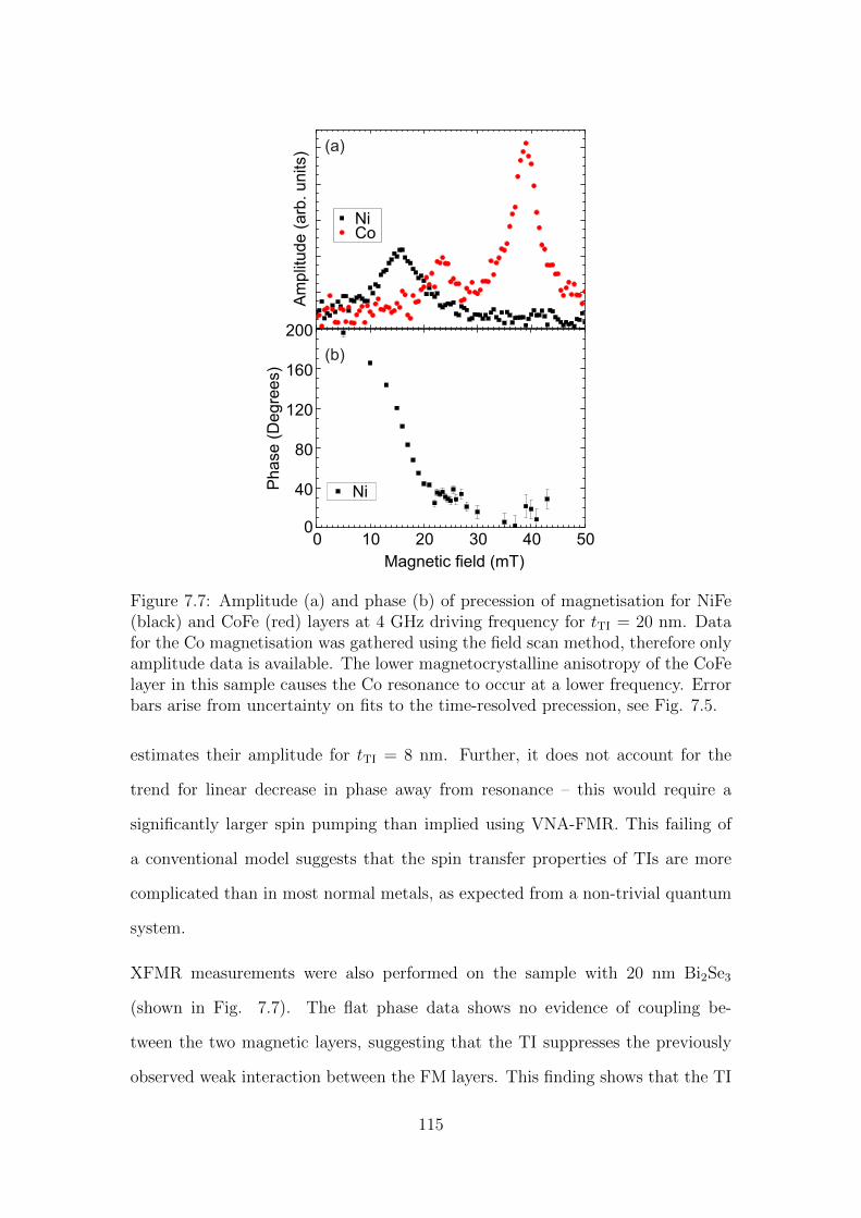
NiCo

Am

plit

ude (

arb

. units)

0 10 20 30 40 500

40

80

120

160

200

Phase (

Degre

es)

Magnetic field (mT)

Ni

(a)

(b)

Figure 7.7: Amplitude (a) and phase (b) of precession of magnetisation for NiFe(black) and CoFe (red) layers at 4 GHz driving frequency for tTI = 20 nm. Datafor the Co magnetisation was gathered using the field scan method, therefore onlyamplitude data is available. The lower magnetocrystalline anisotropy of the CoFelayer in this sample causes the Co resonance to occur at a lower frequency. Errorbars arise from uncertainty on fits to the time-resolved precession, see Fig. 7.5.

estimates their amplitude for tTI = 8 nm. Further, it does not account for the

trend for linear decrease in phase away from resonance – this would require a

significantly larger spin pumping than implied using VNA-FMR. This failing of

a conventional model suggests that the spin transfer properties of TIs are more

complicated than in most normal metals, as expected from a non-trivial quantum

system.

XFMR measurements were also performed on the sample with 20 nm Bi2Se3

(shown in Fig. 7.7). The flat phase data shows no evidence of coupling be-

tween the two magnetic layers, suggesting that the TI suppresses the previously

observed weak interaction between the FM layers. This finding shows that the TI

115

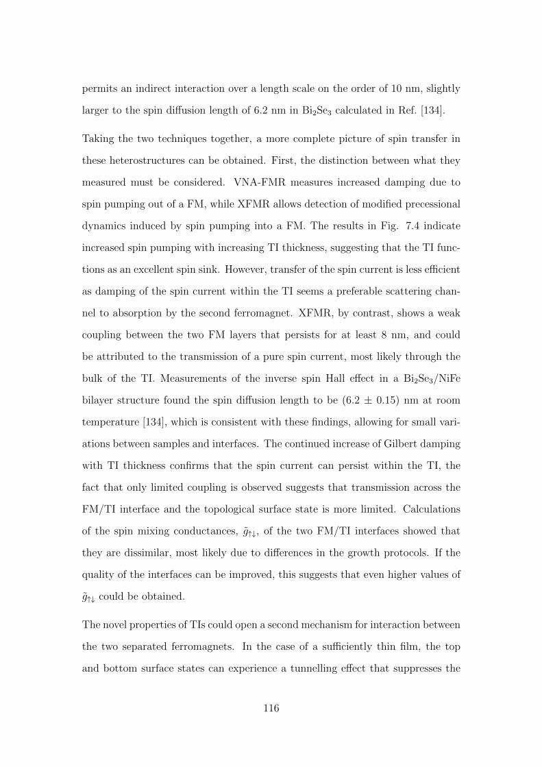
permits an indirect interaction over a length scale on the order of 10 nm, slightly

larger to the spin diffusion length of 6.2 nm in Bi2Se3 calculated in Ref. [134].

Taking the two techniques together, a more complete picture of spin transfer in

these heterostructures can be obtained. First, the distinction between what they

measured must be considered. VNA-FMR measures increased damping due to

spin pumping out of a FM, while XFMR allows detection of modified precessional

dynamics induced by spin pumping into a FM. The results in Fig. 7.4 indicate

increased spin pumping with increasing TI thickness, suggesting that the TI func-

tions as an excellent spin sink. However, transfer of the spin current is less efficient

as damping of the spin current within the TI seems a preferable scattering chan-

nel to absorption by the second ferromagnet. XFMR, by contrast, shows a weak

coupling between the two FM layers that persists for at least 8 nm, and could

be attributed to the transmission of a pure spin current, most likely through the

bulk of the TI. Measurements of the inverse spin Hall effect in a Bi2Se3/NiFe

bilayer structure found the spin diffusion length to be (6.2 ± 0.15) nm at room

temperature [134], which is consistent with these findings, allowing for small vari-

ations between samples and interfaces. The continued increase of Gilbert damping

with TI thickness confirms that the spin current can persist within the TI, the

fact that only limited coupling is observed suggests that transmission across the

FM/TI interface and the topological surface state is more limited. Calculations

of the spin mixing conductances, g↑↓, of the two FM/TI interfaces showed that

they are dissimilar, most likely due to differences in the growth protocols. If the

quality of the interfaces can be improved, this suggests that even higher values of

g↑↓ could be obtained.

The novel properties of TIs could open a second mechanism for interaction between

the two separated ferromagnets. In the case of a sufficiently thin film, the top

and bottom surface states can experience a tunnelling effect that suppresses the

116

formation of the true topological surface state [135, 136]. In the case of Bi2Se3

this thickness is 6 nm. When this is the case, direct communication between the

top and bottom interfaces should be possible, negating the presence of the bulk

entirely. Since surface roughness or other imperfections can cause the surface

state to retreat [137], it is possible that this direct interaction is responsible for

the coupling observed for tTI = 4 nm and 8 nm, while the distinct states at tTI

= 20 nm do not allow this. In this interpretation, the increased Gilbert damping

stems from spin pumping into the bulk, while the interaction observed in XFMR

stems from direct coupling across the TI.

7.4 Anti-Damping Torques from Simultaneous

Resonance

While the VNA-FMR and XFMR measurements performed in the previous sec-

tion showed that the TI layer can absorb a spin current, they did not provide a

conclusive answer as to the nature of the coupling between the two ferromagnetic

layers. While a dynamic interaction through spin pumping is a likely candidate,

another interaction mediated by the topological surface state is also a possibility.

Another experimental approach is therefore required to provide more information

as to the origin of the interaction shown in Fig. 7.6.

The additional damping caused by spin pumping arises due to the loss of energy

when spins are pumped out of the on-resonance layer. In the same way, this

outflow of energy can induce precession in the off-resonance layer, through the

spin transfer torque, when it is absorbed. These effects enter the LLG (equa-

tion (2.26)) as the damping and anti-damping constants αspii and αspij , respectively.

However, if both layers are simultaneously on-resonance then the anti-damping

from the incoming spin current can partially compensate the additional damping

117

50 100 150 200Magnetic field (mT)

Tra

nsm

issio

n (

arb

.un

its)

50 100 150 200Magnetic field (mT)

Tra

nsm

issio

n (

arb

.un

its)

50 100 150 200Magnetic field (mT)

Tra

nsm

issio

n (

arb

.un

its)

50 100 150 200Magnetic field (mT)

Tra

nsm

issio

n (

arb

.un

its)

(a) 9 GHz (b) 9.5 GHz

(c) 10 GHz (d) 11 GHz

Figure 7.8: VNA-FMR data for a sample with tTI = 8 nm, showing the changein resonance field as a function of excitation frequency. The modes completelyoverlap at 9 GHz (a), making it difficult to separate individual contributions tolinewidth and amplitude. They move apart as frequency increases (b,c), and arefully resolved at 11 GHz (d). Black squares are data points, solid lines are fits tothe data using two asymmetric Lorentzians.

from the outgoing spin current. Experimentally, this is observed as a decrease in

resonance linewidth as the separation of the resonances of the two layers approach

one another. In heterostructures with a strong magnetocrystalline anisotropy it

is possible to use the angular dependence of the resonance condition to alter the

separation of the two resonances, and identify signs of spin pumping. This tech-

nique is made somewhat more complicated by the difficulty of obtaining accurate

fits to the overlapping Lorentzians of two resonances in close proximity. This is

illustrated in Fig. 7.8. Furthermore, spin pumping is not the only source of angu-

lar variation of resonant linewidth: mosaic broadening and two magnon scattering

can also play a role. Nevertheless, this technique can offer valuable insights into

the relaxation processes of spin valves.

118

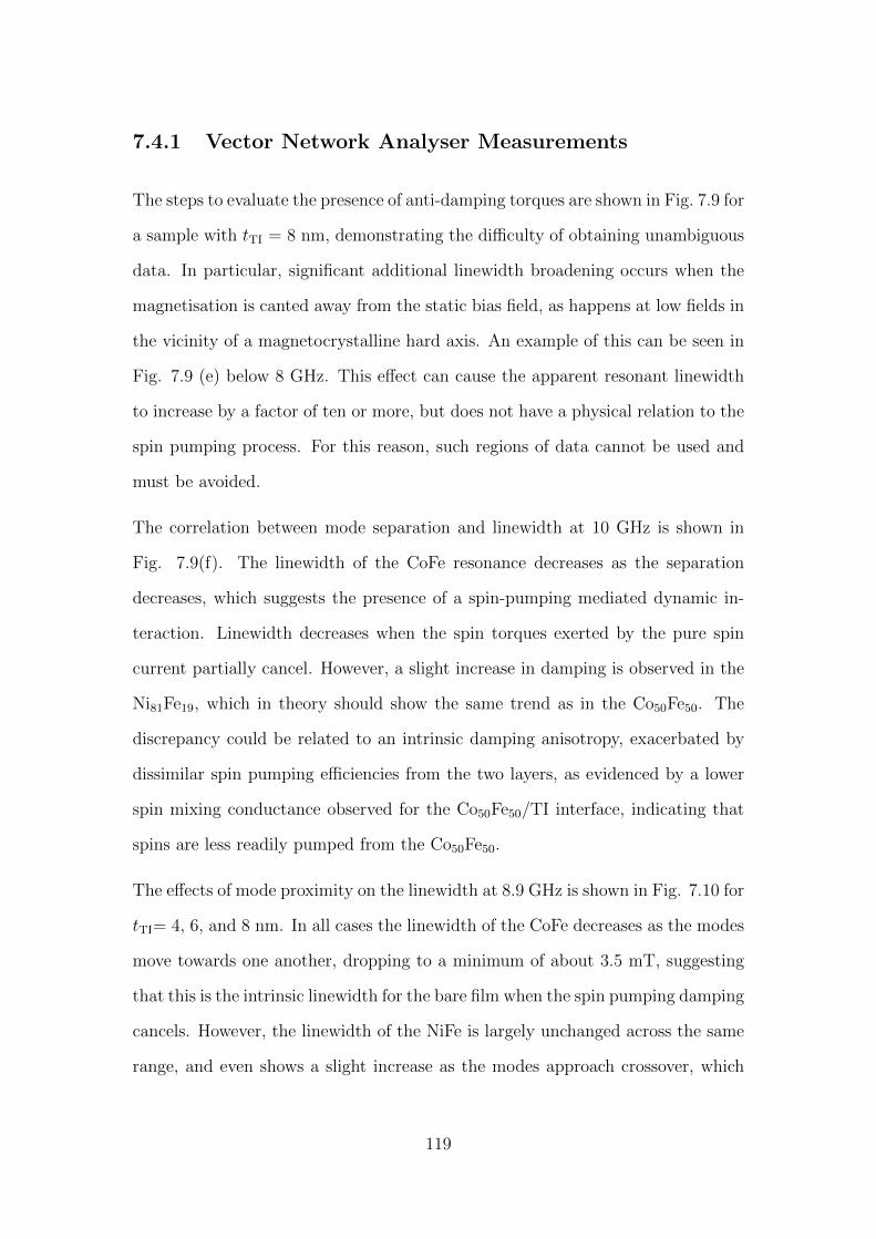
7.4.1 Vector Network Analyser Measurements

The steps to evaluate the presence of anti-damping torques are shown in Fig. 7.9 for

a sample with tTI = 8 nm, demonstrating the difficulty of obtaining unambiguous

data. In particular, significant additional linewidth broadening occurs when the

magnetisation is canted away from the static bias field, as happens at low fields in

the vicinity of a magnetocrystalline hard axis. An example of this can be seen in

Fig. 7.9 (e) below 8 GHz. This effect can cause the apparent resonant linewidth

to increase by a factor of ten or more, but does not have a physical relation to the

spin pumping process. For this reason, such regions of data cannot be used and

must be avoided.

The correlation between mode separation and linewidth at 10 GHz is shown in

Fig. 7.9(f). The linewidth of the CoFe resonance decreases as the separation

decreases, which suggests the presence of a spin-pumping mediated dynamic in-

teraction. Linewidth decreases when the spin torques exerted by the pure spin

current partially cancel. However, a slight increase in damping is observed in the

Ni81Fe19, which in theory should show the same trend as in the Co50Fe50. The

discrepancy could be related to an intrinsic damping anisotropy, exacerbated by

dissimilar spin pumping efficiencies from the two layers, as evidenced by a lower

spin mixing conductance observed for the Co50Fe50/TI interface, indicating that

spins are less readily pumped from the Co50Fe50.

The effects of mode proximity on the linewidth at 8.9 GHz is shown in Fig. 7.10 for

tTI= 4, 6, and 8 nm. In all cases the linewidth of the CoFe decreases as the modes

move towards one another, dropping to a minimum of about 3.5 mT, suggesting

that this is the intrinsic linewidth for the bare film when the spin pumping damping

cancels. However, the linewidth of the NiFe is largely unchanged across the same

range, and even shows a slight increase as the modes approach crossover, which

119

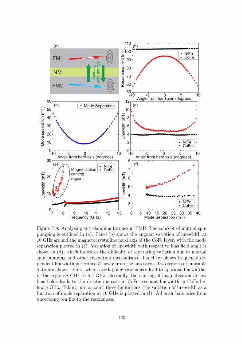
-10 -5 0 5 1050

60

70

80

90

100

110

Re

son

an

ce fi

eld

(m

T)

Angle from hard axis (degrees)

-10 -5 0 5 100

10

20

30

40

50

60

Mode Separation

Mo

de

se

pa

ratio

n (

mT

)

Angle from hard axis (degrees)-10 -5 0 5 100

2

4

6

8

10

12

Lin

ew

idth

(m

T)

Angle from hard axis (degrees)

Mutu

al S

pin

Pum

pin

g

FM1

FM2

NM

0 5 10 15 20 25 30 35 40

3

4

5

6

7

8

Lin

ew

idth

(m

T)

Mode Separation (mT)

(a)

(c)

(e)

(b)

(d)

(f)

7 8 9 10 11 12 130

10

20

30

Lin

ew

idth

(m

T)

Frequency (GHz)

Magnetisation cantingregion

NiFe CoFe

NiFe CoFe

NiFe CoFe

NiFe CoFe

Figure 7.9: Analysing anti-damping torques in FMR. The concept of mutual spinpumping is outlined in (a). Panel (b) shows the angular variation of linewidth at10 GHz around the magnetocrystalline hard axis of the CoFe layer, with the modeseparation plotted in (c). Variation of linewidth with respect to bias field angle isshown in (d), which indicates the difficulty of separating variation due to mutualspin pumping and other relaxation mechanisms. Panel (e) shows frequency de-pendent linewidth performed 5 away from the hard axis. Two regions of unusabledata are shown. First, where overlapping resonances lead to spurious linewidths,in the region 8 GHz to 8.5 GHz. Secondly, the canting of magnetisation at lowbias fields leads to the drastic increase in CoFe resonant linewidth in CoFe be-low 8 GHz. Taking into account these limitations, the variation of linewidth as afunction of mode separation at 10 GHz is plotted in (f). All error bars arise fromuncertainty on fits to the resonances.

120

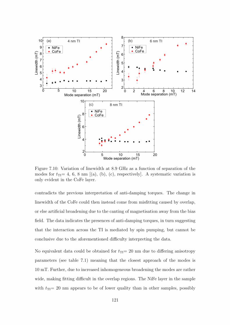
0 5 10 15 20

3

4

5

6

7

8

9

10

Lin

ew

idth

(m

T)

Mode separation (mT)

NiFeCoFe

4 nm TI(a)

0 2 4 6 8 10 12 142

3

4

5

6

7

8

Lin

ew

idth

(m

T)

Mode separation (mT)

NiFeCoFe

(b) 6 nm TI

Lin

ew

idth

(m

T)

0 5 10 15 202

4

6

8

10

Mode separation (mT)

NiFeCoFe

(c) 8 nm TI

Figure 7.10: Variation of linewidth at 8.9 GHz as a function of separation of themodes for tTI= 4, 6, 8 nm [(a), (b), (c), respectively]. A systematic variation isonly evident in the CoFe layer.

contradicts the previous interpretation of anti-damping torques. The change in

linewidth of the CoFe could then instead come from misfitting caused by overlap,

or else artificial broadening due to the canting of magnetisation away from the bias

field. The data indicates the presences of anti-damping torques, in turn suggesting

that the interaction across the TI is mediated by spin pumping, but cannot be

conclusive due to the aforementioned difficulty interpreting the data.

No equivalent data could be obtained for tTI= 20 nm due to differing anisotropy

parameters (see table 7.1) meaning that the closest approach of the modes is

10 mT. Further, due to increased inhomogeneous broadening the modes are rather

wide, making fitting difficult in the overlap regions. The NiFe layer in the sample

with tTI= 20 nm appears to be of lower quality than in other samples, possibly

121

due to interdiffusion with the Bi2Se3 layer, or else problems with stoichiometry

during growth. It is also possible that the surface roughness of the Bi2Se3 increases

significantly for thicker films, leading to a poor quality NiFe film. The problem of

fitting in overlap regions is partially addressed by measuring with XFMR.

7.4.2 Layer-Resolved Measurements

XFMR offers a solution to some of the problems inherent in measuring overlapping

resonances, as its element-selectivity ensures that only one layer is measured at

a time. Further, it is less sensitive to magnetisation canted away from the bias

field, due to reduced projection along the x-ray beam in turn reducing the dynamic

XMCD signal. The first results gathered in this way are shown in Fig. 7.11, where

the amplitude of precession of magnetisation is shown around resonance for tTI =

4 nm. The anisotropy of the CoFe layer is used to tune the relative position of

the two layers. The move from overlapping resonances to a separation of ∼10 mT

causes the linewidth to increase by approximately 15%, although the lower data

quality of the CoFe leads to large uncertainty on the fit. Nevertheless, a reduction

in linewidth is observed in the NiFe layer, indicative of anti-damping arising form

mutual cancellation of spin pumping.

Further results of separation-dependent linewidth at 8 GHz for samples with tTI

= 8 nm and tTI = 20 nm, are plotted in Fig. 7.12. The data show a narrowing

of resonant linewidth with decreasing mode separation for tTI = 8 nm, though as

with the VNA-FMR measurements, only in the CoFe layer. This suggests that

the linewidth narrowing previously observed is a genuine effect, perhaps stemming

from simultaneous spin pumping.

XFMR overcomes the difficulties previously presented by the increased linewidth

of the NiFe mode in the tTI = 20 nm sample, allowing measurements of the two

122

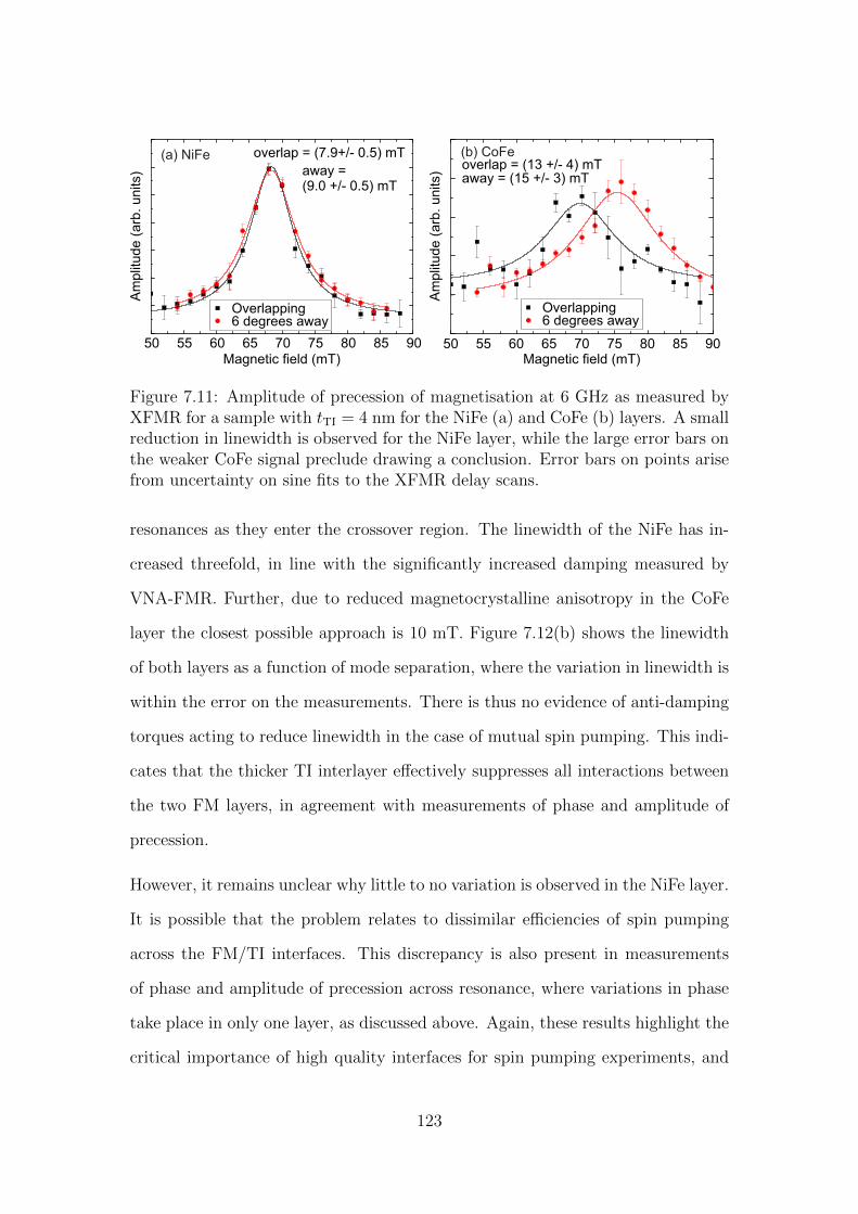
50 55 60 65 70 75 80 85 90

Overlapping6 degrees away

Am

plit

ud

e (

arb

. u

nits)

Magnetic field (mT)

overlap = (7.9+/- 0.5) mT

away =(9.0 +/- 0.5) mT

(a) NiFe

50 55 60 65 70 75 80 85 90

overlap = (13 +/- 4) mTaway = (15 +/- 3) mT

Am

plit

ud

e (

arb

. u

nits)

(b) CoFe

Overlapping6 degrees away

Magnetic field (mT)

Figure 7.11: Amplitude of precession of magnetisation at 6 GHz as measured byXFMR for a sample with tTI = 4 nm for the NiFe (a) and CoFe (b) layers. A smallreduction in linewidth is observed for the NiFe layer, while the large error bars onthe weaker CoFe signal preclude drawing a conclusion. Error bars on points arisefrom uncertainty on sine fits to the XFMR delay scans.

resonances as they enter the crossover region. The linewidth of the NiFe has in-

creased threefold, in line with the significantly increased damping measured by

VNA-FMR. Further, due to reduced magnetocrystalline anisotropy in the CoFe

layer the closest possible approach is 10 mT. Figure 7.12(b) shows the linewidth

of both layers as a function of mode separation, where the variation in linewidth is

within the error on the measurements. There is thus no evidence of anti-damping

torques acting to reduce linewidth in the case of mutual spin pumping. This indi-

cates that the thicker TI interlayer effectively suppresses all interactions between

the two FM layers, in agreement with measurements of phase and amplitude of

precession.

However, it remains unclear why little to no variation is observed in the NiFe layer.

It is possible that the problem relates to dissimilar efficiencies of spin pumping

across the FM/TI interfaces. This discrepancy is also present in measurements

of phase and amplitude of precession across resonance, where variations in phase

take place in only one layer, as discussed above. Again, these results highlight the

critical importance of high quality interfaces for spin pumping experiments, and

123

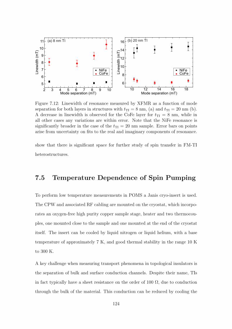
2 3 4 5 6 7 8 9 10

5

6

7

8

9

10

11

Lin

ew

idth

(m

T)

Mode separation (mT)

(a) 8 nm TI

NiFeCoFe

10 12 14 16 18

6

8

10

12

14

16

Lin

ew

idth

(m

T)

Mode separation (mT)

(b) 20 nm TI

NiFeCoFe

Figure 7.12: Linewidth of resonance measured by XFMR as a function of modeseparation for both layers in structures with tTI = 8 nm, (a) and tTI = 20 nm (b).A decrease in linewidth is observed for the CoFe layer for tTI = 8 nm, while inall other cases any variations are within error. Note that the NiFe resonance issignificantly broader in the case of the tTI = 20 nm sample. Error bars on pointsarise from uncertainty on fits to the real and imaginary components of resonance.

show that there is significant space for further study of spin transfer in FM-TI

heterostructures.

7.5 Temperature Dependence of Spin Pumping

To perform low temperature measurements in POMS a Janis cryo-insert is used.

The CPW and associated RF cabling are mounted on the cryostat, which incorpo-

rates an oxygen-free high purity copper sample stage, heater and two thermocou-

ples, one mounted close to the sample and one mounted at the end of the cryostat

itself. The insert can be cooled by liquid nitrogen or liquid helium, with a base

temperature of approximately 7 K, and good thermal stability in the range 10 K

to 300 K.

A key challenge when measuring transport phenomena in topological insulators is

the separation of bulk and surface conduction channels. Despite their name, TIs

in fact typically have a sheet resistance on the order of 100 Ω, due to conduction

through the bulk of the material. This conduction can be reduced by cooling the

124

sample to low temperatures, freezing out conduction channels aside from those in

the topologically protected surface state. Indeed, the first measurements of the

quantum anomalous Hall effect in a ferromagnetically doped TI were performed

at 30 mK [118]. It is thus important to study how the measurements of spin

pumping in the FM-TI heterostructures are affected by temperature. The spin

pumping process is dependent upon the spin flip and momentum scattering life-

times, so should be sensitive to bulk transport. Spin pumping into the surface

state, however, should not be affected by a change in temperature.

The temperature dependence of damping in ferromagnets must also be considered,

as the various processes that contribute to energy dissipation can each be affected

differently. For example, the additional damping due to the presence of slow re-

laxing impurities (see chapter 4) increases as the temperature decreases, as the

population of the 4f levels of the rare earth impurity ions depends strongly upon

temperatures [58]. Similarly, the scattering of itinerant electrons in the ferromag-

net is enhanced at lower temperatures, leading to an increased damping [14,138].

Temperature dependent measurements were performed on two samples (tTI =

4 nm and tTI = 8 nm), which were mounted for VNA-FMR in the standard flip-

chip geometry. Field-frequency transmission maps were recorded with the bias

field aligned along the easy axis, in the temperature range 10 K to 300 K. The

Gilbert damping was then determined from the frequency dependence of resonant

linewidth, according to equation (2.21). The results are shown in Fig. 7.13.

While there are weak indications of a variation of Gilbert damping with tempera-

ture, no pattern of increasing or decreasing damping emerges. The NiFe layers in

the two samples appear to show opposite trends, with a slight decrease in damping

at low temperatures for tTI = 4 nm, and a slight increase for tTI = 8 nm, but in

both cases the variation is extremely slight, even comparable to the uncertainty on

the data points. The data for the CoFe layers has larger measurement uncertainty,

125

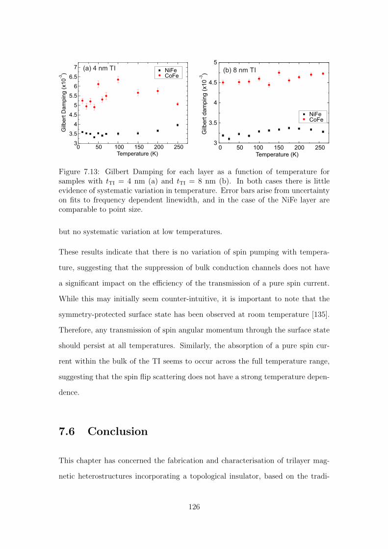
0 50 100 150 200 2503

3.5

4

4.5

5

5.5

6

6.5

7NiFeCoFe

Gilb

ert

Da

mp

ing

(x1

0)

-3

Temperature (K)

(a) 4 nm TI

NiFeCoFe

(b) 8 nm TI

0 50 100 150 200 250Temperature (K)

3

3.5

4

4.5

5

Gilb

ert

da

mp

ing

(x1

0)

-3

Figure 7.13: Gilbert Damping for each layer as a function of temperature forsamples with tTI = 4 nm (a) and tTI = 8 nm (b). In both cases there is littleevidence of systematic variation in temperature. Error bars arise from uncertaintyon fits to frequency dependent linewidth, and in the case of the NiFe layer arecomparable to point size.

but no systematic variation at low temperatures.

These results indicate that there is no variation of spin pumping with tempera-

ture, suggesting that the suppression of bulk conduction channels does not have

a significant impact on the efficiency of the transmission of a pure spin current.

While this may initially seem counter-intuitive, it is important to note that the

symmetry-protected surface state has been observed at room temperature [135].

Therefore, any transmission of spin angular momentum through the surface state

should persist at all temperatures. Similarly, the absorption of a pure spin cur-

rent within the bulk of the TI seems to occur across the full temperature range,

suggesting that the spin flip scattering does not have a strong temperature depen-

dence.

7.6 Conclusion

This chapter has concerned the fabrication and characterisation of trilayer mag-

netic heterostructures incorporating a topological insulator, based on the tradi-

126

tional spin valve device architecture. Through VNA-FMR and XFMR, the spin

dynamics of this novel heterostructure have been studied, aiming to understand the

spin transfer processes mediated by the TI. Varying the thickness of the TI spacer

layer, it was observed that the TI functions as an efficient angular momentum

sink. XFMR measurements, however, confirmed the presence of a weak interac-

tion between the two ferromagnets, able to persist for at least 8 nm, and possibly

mediated by the topological surface state. The maximum spin mixing conductance

of the Co50Fe50/TI interace was calculated to be g↑↓ = (2.49± 0.1) × 1015 cm−2,

while that of the Ni81Fe19/TI interface was g↑↓ = (4.2± 0.5)× 1015 cm−2, compa-

rable with that of a good spin conductor such as Ag.

To study the coupling in more detail, measurements of resonance linewidth were

performed as a function of bias field angle. By bringing the resonances of the

two layers into close proximity, it was possible to observe anti-damping torques

that lead to a narrowing of linewidth, a characteristic of spin pumping. This sug-

gets that the interaction across the TI is a dynamic exchange mediated by spin

pumping, as opposed to a self-coupling of the surface state or a similar unusual

mechanism. Temperature dependent measurements of Gilbert damping showed

no significant variation down to 10 K, indicating that a suppression of the bulk

conduction channels of the TI does not fundamentally alter its spin-transfer prop-

erties.

These results show the great potential of TIs for device applications, as these effects

can be observed at room temperature and low magnetic fields, as well as being a

fertile ground for investigation of fundamental physical phenomena. Further work

is required to improve understanding of the FM/TI interface and separate bulk

and surface conduction, but these initial results show that FMR is a valuable tool

to develop greater understanding of this new materials class.

127

Chapter 8

Anisotropy Imprinting Through

Spin Pumping

8.1 Motivation

This chapter details an investigation into the spin transfer properties of Cr, study-

ing how the static and dynamic exchange interactions can be controlled in spin

valves with Cr interlayers. While the oscillatory nature of the static interaction in

such systems is well known (see, for example, Refs. [30,139]), interest in spin pump-

ing in Cr has developed in recent years [61,140]. Furthermore, mechanisms for an-

gular control of spin pumping have started to recieve more attention [53,141–143],

as a way to fine tune applications of spintronic devices and to gain a deeper un-

derstanding of spin transfer in magnetic multilayers. The investigation outlined

here aims to combine a study of angular control of spin pumping with a detailed

examination at how static and dynamic coupling can compete and combine to

modify the magnetodynamics of spin valves.

Spin valve samples were fabricated by MBE, with one magnetic layer being epitax-

128

ial, with well-defined magnetocrystalline easy and hard axes (Co50Fe50) and the

other being polycrystalline, resulting in isotropic magnetic behaviour (Ni81Fe19).

The thickness of the Cr interlayer was varied between 1 nm and 10 nm, tun-

ing the strength of both the static and dynamic interactions. SQUID-VSM and

VNA-FMR are used to quantify the strength and nature of the static interaction,

as it changes from preferring parallel to antiparallel alignment. Analysis of the

change in resonance linewidth as a function of Cr thickness reveals the presence

of spin pumping, while the angular variation of the linewidth is used to determine

the anisotropic component of the dynamic interaction. Finally, XFMR is used to

measure the layer-resolved precessional dynamics, showing how the angular vari-

ation of spin pumping modifies the spin transfer torque experienced by the layer

absorbing the pure spin current.

8.1.1 Angular Control of Spin Pumping

Gilbert damping can have a large anisotropy, as discussed in the case of the doped

films discussed in chapter 4. Aside from the additional damping induced by rare

earth impurities, several other contributions are possible, including two-magnon

scattering [50], wherein the uniform FMR mode scatters into higher order ex-

citations, mosaic broadening due to sample inhomogeneities [17, 50, 144], and

anisotropic Gilbert damping arising due to canting of magnetisation away from

the applied magnetic field [17].

Spin pumping can also have a pronounced angular dependence, making unambigu-

ous determination of the origin of any anisotropy of Gilbert damping rather chal-

lenging. The most prominent mechanism by which an anisotropy of spin pumping

can arise is a misalignment of the magnetisation of the two magnetic layers in the

heterostructure [53, 141, 145]. The absorption of the pumped angular momentum

is more efficient when the two layers are aligned antiparallel, as compensation of

129

the pumped angular momentum drops [142]. For the same reason, spin pumping

tends to be larger when the modes precess in anti-phase as angular momentum

compensation again drops. Therefore, it is theoretically possible to modulate the

damping further by switching the optical/acoustic character of the resonances of

the two layers [146]. This can be achieved in trilayers with a sufficiently strong

static coupling to transfer precession between the two layers, and suitable mag-

netocrystalline anisotropy to change which modes occur at high or low frequency.

However, layer-resolved measurements of amplitude and phase of precession cast

some doubt on this interpretation, as the modulation of phase along a hard axis

makes straightforward interpretation of the character of the resonances difficult.

It has also been suggested that stray fields from domain walls in the spin sink layer

can provide an effective dipolar field that acts as an additional damping term on

the precession of the free layer [143].

Another possible cause of an apparent angular variation of spin pumping, distinct

from those outlined above, is the presence of anti-damping torques from mutual

spin pumping [107]. This effect was studied in topological insulator spin valves

in section 7.4. As spin pumping drives angular momentum out of the spin source

layer, and into the spin sink layer, it has both damping and anti-damping charac-

teristics. When the resonance fields of the two layers are well separated the source

layer experiences only damping, and the sink layer only anti-damping. However,

in the case where both layers are simultaneously on resonance, both experience

both damping and anti-damping effects, leading to partial or total compensation

of the pumped spin angular momentum, and corresponding apparent reduction in

Gilbert damping. Thus, for broad resonances with a significant angular variation,

points of near crossing can also lead to an angular variation of linewidth, as the

in-plane anisotropy of the resonant field causes the separation of the modes to

decrease as a function of the angle of the applied magnetic field. One can see that

130

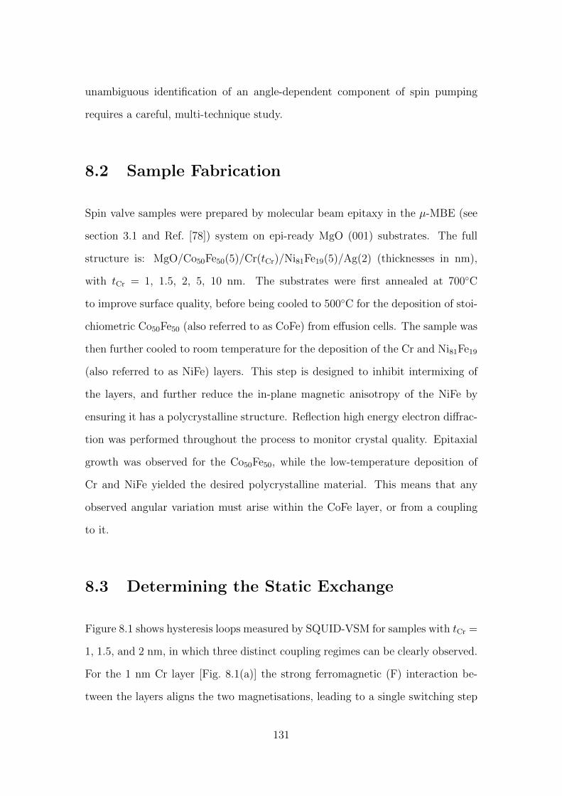
unambiguous identification of an angle-dependent component of spin pumping

requires a careful, multi-technique study.

8.2 Sample Fabrication

Spin valve samples were prepared by molecular beam epitaxy in the µ-MBE (see

section 3.1 and Ref. [78]) system on epi-ready MgO (001) substrates. The full

structure is: MgO/Co50Fe50(5)/Cr(tCr)/Ni81Fe19(5)/Ag(2) (thicknesses in nm),

with tCr = 1, 1.5, 2, 5, 10 nm. The substrates were first annealed at 700C

to improve surface quality, before being cooled to 500C for the deposition of stoi-

chiometric Co50Fe50 (also referred to as CoFe) from effusion cells. The sample was

then further cooled to room temperature for the deposition of the Cr and Ni81Fe19

(also referred to as NiFe) layers. This step is designed to inhibit intermixing of

the layers, and further reduce the in-plane magnetic anisotropy of the NiFe by

ensuring it has a polycrystalline structure. Reflection high energy electron diffrac-

tion was performed throughout the process to monitor crystal quality. Epitaxial

growth was observed for the Co50Fe50, while the low-temperature deposition of

Cr and NiFe yielded the desired polycrystalline material. This means that any

observed angular variation must arise within the CoFe layer, or from a coupling

to it.

8.3 Determining the Static Exchange

Figure 8.1 shows hysteresis loops measured by SQUID-VSM for samples with tCr =

1, 1.5, and 2 nm, in which three distinct coupling regimes can be clearly observed.

For the 1 nm Cr layer [Fig. 8.1(a)] the strong ferromagnetic (F) interaction be-

tween the layers aligns the two magnetisations, leading to a single switching step

131

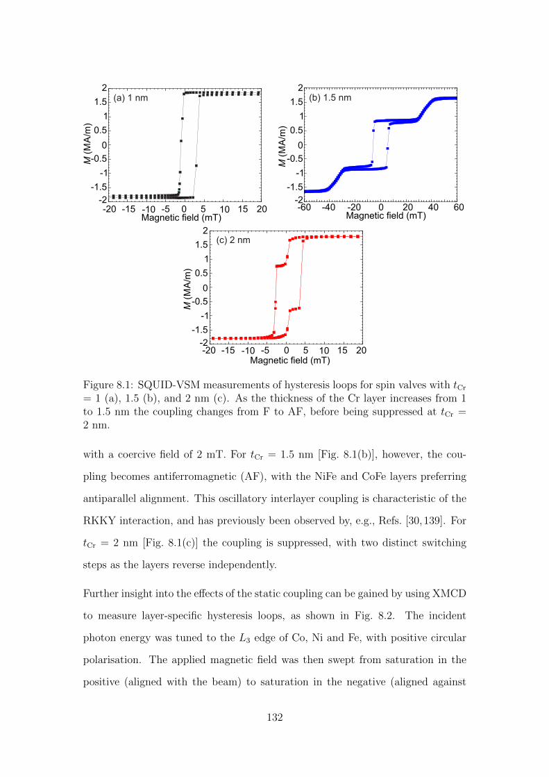
-20 -15 -10 -5 0 5 10 15 20Magnetic field (mT)

-2

-1.5

-1

-0.5

0.5

1

1.5

2

M(M

A/m

)

0

(c) 2 nm

-20 -15 -10 -5 0 5 10 15 20-2

-1.5

-1

-0.5

0.5

1

1.5

2M

(MA

/m)

0

(a) 1 nm

Magnetic field (mT)-60 -40 -20 0 20 40 60

-2

-1.5

-1

-0.5

0.5

1

1.5

2

M(M

A/m

)

Magnetic field (mT)

0

(b) 1.5 nm

Figure 8.1: SQUID-VSM measurements of hysteresis loops for spin valves with tCr

= 1 (a), 1.5 (b), and 2 nm (c). As the thickness of the Cr layer increases from 1to 1.5 nm the coupling changes from F to AF, before being suppressed at tCr =2 nm.

with a coercive field of 2 mT. For tCr = 1.5 nm [Fig. 8.1(b)], however, the cou-

pling becomes antiferromagnetic (AF), with the NiFe and CoFe layers preferring

antiparallel alignment. This oscillatory interlayer coupling is characteristic of the

RKKY interaction, and has previously been observed by, e.g., Refs. [30,139]. For

tCr = 2 nm [Fig. 8.1(c)] the coupling is suppressed, with two distinct switching

steps as the layers reverse independently.

Further insight into the effects of the static coupling can be gained by using XMCD

to measure layer-specific hysteresis loops, as shown in Fig. 8.2. The incident

photon energy was tuned to the L3 edge of Co, Ni and Fe, with positive circular

polarisation. The applied magnetic field was then swept from saturation in the

positive (aligned with the beam) to saturation in the negative (aligned against

132

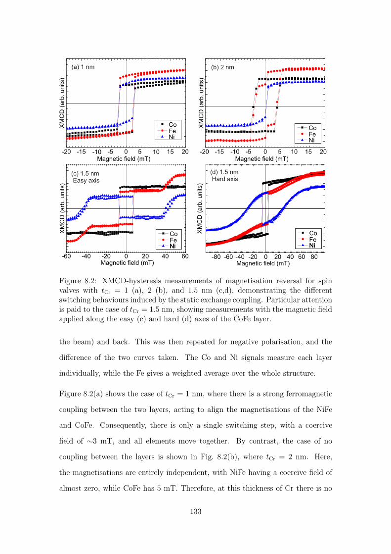
XM

CD

(arb

. units)

-20 -15 -10 -5 0 5 10 15 20Magnetic field (mT)

(a) 1 nm

CoFeNi

-20 -15 -10 -5 0 5 10 15 20Magnetic field (mT)

(b) 2 nm

CoFeNi

XM

CD

(arb

. units)

XM

CD

(arb

. units)

CoFeNiNi

-60 -40 -20 0 20 40 60Magnetic field (mT)

(c) 1.5 nmEasy axis

-80 -40 0 40 80Magnetic field (mT)

(d) 1.5 nmHard axis

CoFeNiNi

XM

CD

(arb

. units)

-60 -20 20 60

Figure 8.2: XMCD-hysteresis measurements of magnetisation reversal for spinvalves with tCr = 1 (a), 2 (b), and 1.5 nm (c,d), demonstrating the differentswitching behaviours induced by the static exchange coupling. Particular attentionis paid to the case of tCr = 1.5 nm, showing measurements with the magnetic fieldapplied along the easy (c) and hard (d) axes of the CoFe layer.

the beam) and back. This was then repeated for negative polarisation, and the

difference of the two curves taken. The Co and Ni signals measure each layer

individually, while the Fe gives a weighted average over the whole structure.

Figure 8.2(a) shows the case of tCr = 1 nm, where there is a strong ferromagnetic

coupling between the two layers, acting to align the magnetisations of the NiFe

and CoFe. Consequently, there is only a single switching step, with a coercive

field of ∼3 mT, and all elements move together. By contrast, the case of no

coupling between the layers is shown in Fig. 8.2(b), where tCr = 2 nm. Here,

the magnetisations are entirely independent, with NiFe having a coercive field of

almost zero, while CoFe has 5 mT. Therefore, at this thickness of Cr there is no

133

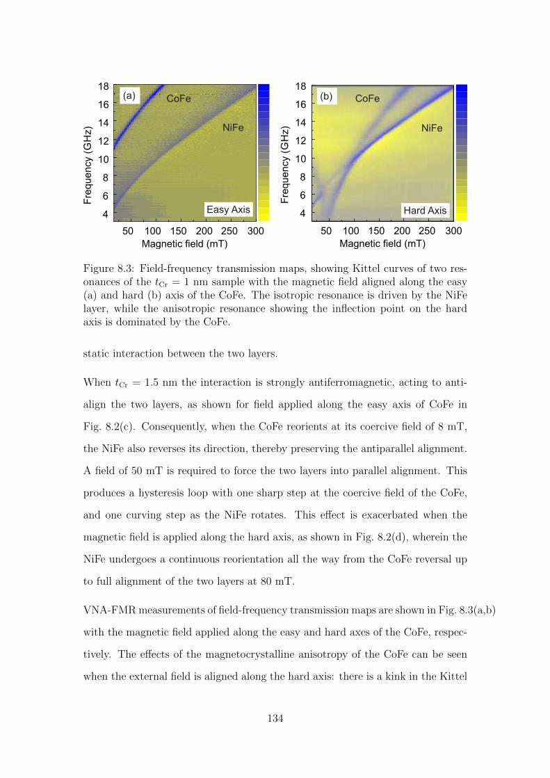
50 100 150 200 250

Magnetic field (mT)

300

4

6

8

10

12

14

16

18F

req

ue

ncy (

GH

z)

CoFe

NiFe

Easy Axis

(a)

4

6

8

10

12

14

16

18

Fre

quency (

GH

z)

CoFe

NiFe

50 100 150 200 250

Magnetic field (mT)

300

(b)

Hard Axis

Figure 8.3: Field-frequency transmission maps, showing Kittel curves of two res-onances of the tCr = 1 nm sample with the magnetic field aligned along the easy(a) and hard (b) axis of the CoFe. The isotropic resonance is driven by the NiFelayer, while the anisotropic resonance showing the inflection point on the hardaxis is dominated by the CoFe.

static interaction between the two layers.

When tCr = 1.5 nm the interaction is strongly antiferromagnetic, acting to anti-

align the two layers, as shown for field applied along the easy axis of CoFe in

Fig. 8.2(c). Consequently, when the CoFe reorients at its coercive field of 8 mT,

the NiFe also reverses its direction, thereby preserving the antiparallel alignment.

A field of 50 mT is required to force the two layers into parallel alignment. This

produces a hysteresis loop with one sharp step at the coercive field of the CoFe,

and one curving step as the NiFe rotates. This effect is exacerbated when the

magnetic field is applied along the hard axis, as shown in Fig. 8.2(d), wherein the

NiFe undergoes a continuous reorientation all the way from the CoFe reversal up

to full alignment of the two layers at 80 mT.

VNA-FMR measurements of field-frequency transmission maps are shown in Fig. 8.3(a,b)

with the magnetic field applied along the easy and hard axes of the CoFe, respec-

tively. The effects of the magnetocrystalline anisotropy of the CoFe can be seen

when the external field is aligned along the hard axis: there is a kink in the Kittel

134

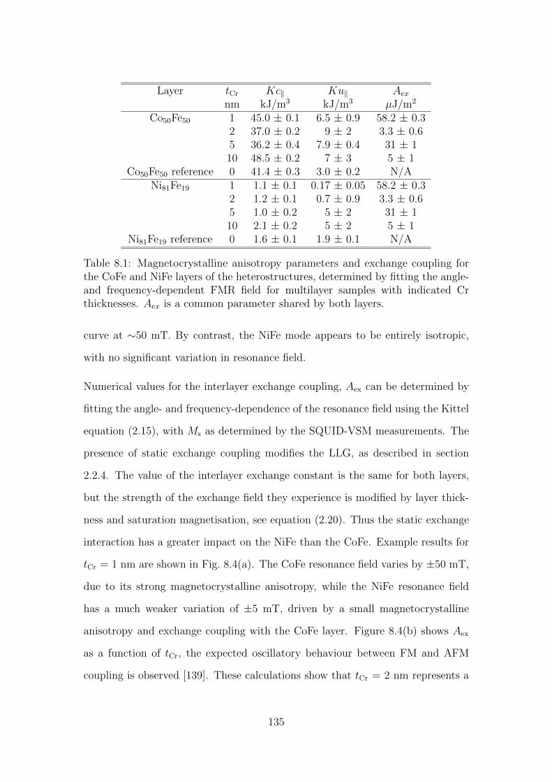
Layer tCr Kc‖ Ku‖ Aexnm kJ/m3 kJ/m3 µJ/m2

Co50Fe50 1 45.0 ± 0.1 6.5 ± 0.9 58.2 ± 0.32 37.0 ± 0.2 9 ± 2 3.3 ± 0.65 36.2 ± 0.4 7.9 ± 0.4 31 ± 110 48.5 ± 0.2 7 ± 3 5 ± 1

Co50Fe50 reference 0 41.4 ± 0.3 3.0 ± 0.2 N/ANi81Fe19 1 1.1 ± 0.1 0.17 ± 0.05 58.2 ± 0.3

2 1.2 ± 0.1 0.7 ± 0.9 3.3 ± 0.65 1.0 ± 0.2 5 ± 2 31 ± 110 2.1 ± 0.2 5 ± 2 5 ± 1

Ni81Fe19 reference 0 1.6 ± 0.1 1.9 ± 0.1 N/A

Table 8.1: Magnetocrystalline anisotropy parameters and exchange coupling forthe CoFe and NiFe layers of the heterostructures, determined by fitting the angle-and frequency-dependent FMR field for multilayer samples with indicated Crthicknesses. Aex is a common parameter shared by both layers.

curve at ∼50 mT. By contrast, the NiFe mode appears to be entirely isotropic,

with no significant variation in resonance field.

Numerical values for the interlayer exchange coupling, Aex can be determined by

fitting the angle- and frequency-dependence of the resonance field using the Kittel

equation (2.15), with Ms as determined by the SQUID-VSM measurements. The

presence of static exchange coupling modifies the LLG, as described in section

2.2.4. The value of the interlayer exchange constant is the same for both layers,

but the strength of the exchange field they experience is modified by layer thick-

ness and saturation magnetisation, see equation (2.20). Thus the static exchange

interaction has a greater impact on the NiFe than the CoFe. Example results for

tCr = 1 nm are shown in Fig. 8.4(a). The CoFe resonance field varies by ±50 mT,

due to its strong magnetocrystalline anisotropy, while the NiFe resonance field

has a much weaker variation of ±5 mT, driven by a small magnetocrystalline

anisotropy and exchange coupling with the CoFe layer. Figure 8.4(b) shows Aex

as a function of tCr, the expected oscillatory behaviour between FM and AFM

coupling is observed [139]. These calculations show that tCr = 2 nm represents a

135

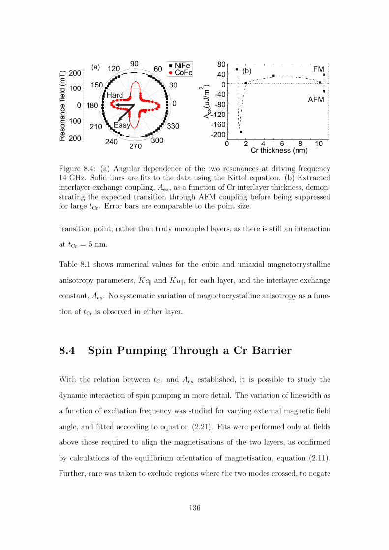
0

100

200

100

200Re

son

an

ce fi

eld

(m

T)

0

30

6090

120

150

180

210

240270

300

330

NiFeCoFe

(a)

0 2 4 6 8 10-200

-160

-120

-80

-40

0

40

80

AFM

2A

(mJ/

m)

ex

Cr thickness (nm)

FM

(b)

Hard

Easy

Figure 8.4: (a) Angular dependence of the two resonances at driving frequency14 GHz. Solid lines are fits to the data using the Kittel equation. (b) Extractedinterlayer exchange coupling, Aex, as a function of Cr interlayer thickness, demon-strating the expected transition through AFM coupling before being suppressedfor large tCr. Error bars are comparable to the point size.

transition point, rather than truly uncoupled layers, as there is still an interaction

at tCr = 5 nm.

Table 8.1 shows numerical values for the cubic and uniaxial magnetocrystalline

anisotropy parameters, Kc‖ and Ku‖, for each layer, and the interlayer exchange

constant, Aex. No systematic variation of magnetocrystalline anisotropy as a func-

tion of tCr is observed in either layer.

8.4 Spin Pumping Through a Cr Barrier

With the relation between tCr and Aex established, it is possible to study the

dynamic interaction of spin pumping in more detail. The variation of linewidth as

a function of excitation frequency was studied for varying external magnetic field

angle, and fitted according to equation (2.21). Fits were performed only at fields

above those required to align the magnetisations of the two layers, as confirmed

by calculations of the equilibrium orientation of magnetisation, equation (2.11).

Further, care was taken to exclude regions where the two modes crossed, to negate

136

the effect of anti-damping due to simultaneous resonance.

8.4.1 Attenuation of a Pure Spin Current in Cr

Measurements of spin pumping damping as a function of tCr are shown in Fig. 8.5

for the CoFe and NiFe layers, with the magnetic field applied along the easy axis

of the CoFe. A decrease in damping for both layers with increasing Cr thickness

is observed, indicative of spin pumping. This arises as spins pumped from the

precessing ferromagnetic layer are unable to reach the efficient spin sink of the

second FM, instead scattering in the spacer layer or flowing back to the spin

source, where they are absorbed and exert an anti-damping torque.

The spin pumping damping is more significant in the NiFe layer, but both lay-

ers show the expected exponential drop in spin pumping as the thickness of the

interlayer increases. Fits to extract the spin diffusion length were performed us-

ing equation (2.27), using the Drude model for the Fermi velocity in Cr (vF =

1.56×10−6 ms−1), which yields a spin diffusion length of 8 nm. This is somewhat

less than the 13 nm reported by Du et al. using inverse spin Hall effect measure-

ments [140], but some variation between sample series is to be expected, with the

nature of the interfaces and crystallinity of the materials themselves playing a key

role. It should be noted that this approach implicitly assumes perfect transmission

of spins in the case of a 1 nm Cr barrier, but as it proved impossible to fabricate

a continuous Cr layer below this thickness, the data set could not be extended.

8.4.2 Angular Dependence of Spin Pumping

Further information can be obtained by considering the angle-dependence of spin

pumping in the Cr spin valves. Figure 8.6 shows the Gilbert damping as a function

of tCr for both layers, measured with the magnetic field applied along the easy and

137

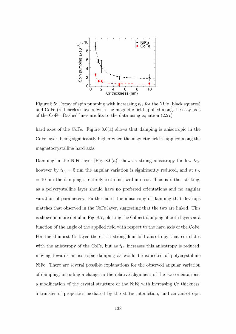
NiFeCoFe

0

2

4

6

8

10

2 4 6 8 10Cr thickness (nm)

Spin

pum

pin

g(x

10 )

-3

0

Figure 8.5: Decay of spin pumping with increasing tCr for the NiFe (black squares)and CoFe (red circles) layers, with the magnetic field applied along the easy axisof the CoFe. Dashed lines are fits to the data using equation (2.27)

hard axes of the CoFe. Figure 8.6(a) shows that damping is anisotropic in the

CoFe layer, being significantly higher when the magnetic field is applied along the

magnetocrystalline hard axis.

Damping in the NiFe layer [Fig. 8.6(a)] shows a strong anisotropy for low tCr,

however by tCr = 5 nm the angular variation is significantly reduced, and at tCr

= 10 nm the damping is entirely isotropic, within error. This is rather striking,

as a polycrystalline layer should have no preferred orientations and no angular

variation of parameters. Furthermore, the anisotropy of damping that develops

matches that observed in the CoFe layer, suggesting that the two are linked. This

is shown in more detail in Fig. 8.7, plotting the Gilbert damping of both layers as a

function of the angle of the applied field with respect to the hard axis of the CoFe.

For the thinnest Cr layer there is a strong four-fold anisotropy that correlates

with the anisotropy of the CoFe, but as tCr increases this anisotropy is reduced,

moving towards an isotropic damping as would be expected of polycrystalline

NiFe. There are several possible explanations for the observed angular variation

of damping, including a change in the relative alignment of the two orientations,

a modification of the crystal structure of the NiFe with increasing Cr thickness,

a transfer of properties mediated by the static interaction, and an anisotropic

138

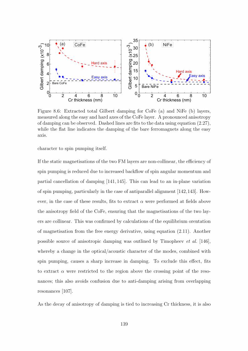
(b)

Gilb

ert

dam

pin

g(x

10 )

-3

0

5

10

15

20

25

30

35

Bare NiFe

Easy axisHard axis

NiFe

0 2 4 6 8 10Cr thickness (nm)

0

2

4

6

8

10

Bare CoFe

0 2 4 6 8 10Cr thickness (nm)

(a) CoFe

Hard axis

Easy axis

Gilb

ert

dam

pin

g(x

10 )

-3

Figure 8.6: Extracted total Gilbert damping for CoFe (a) and NiFe (b) layers,measured along the easy and hard axes of the CoFe layer. A pronounced anisotropyof damping can be observed. Dashed lines are fits to the data using equation (2.27),while the flat line indicates the damping of the bare ferromagnets along the easyaxis.

character to spin pumping itself.

If the static magnetisations of the two FM layers are non-collinear, the efficiency of

spin pumping is reduced due to increased backflow of spin angular momentum and

partial cancellation of damping [141, 145]. This can lead to an in-plane variation

of spin pumping, particularly in the case of antiparallel alignment [142,143]. How-

ever, in the case of these results, fits to extract α were performed at fields above

the anisotropy field of the CoFe, ensuring that the magnetisations of the two lay-

ers are collinear. This was confirmed by calculations of the equilibrium orentation

of magnetisation from the free energy derivative, using equation (2.11). Another

possible source of anisotropic damping was outlined by Timopheev et al. [146],

whereby a change in the optical/acoustic character of the modes, combined with

spin pumping, causes a sharp increase in damping. To exclude this effect, fits

to extract α were restricted to the region above the crossing point of the reso-

nances; this also avoids confusion due to anti-damping arising from overlapping

resonances [107].

As the decay of anisotropy of damping is tied to increasing Cr thickness, it is also

139

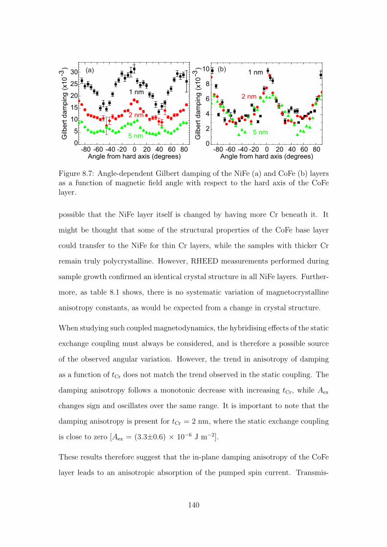
-80 -60 -40 -20 0 20 40 60 80Angle from hard axis (degrees)

Gilb

ert

da

mp

ing

(x1

0

)

-3

(a)

0

5

10

15

20

25

30

1 nm

2 nm

5 nm0

2

4

6

8

10

-80 -60 -40 -20 0 20 40 60 80Angle from hard axis (degrees)

(b)1 nm

2 nm

5 nm

Gilb

ert

da

mp

ing

(x1

0

)

-3

Figure 8.7: Angle-dependent Gilbert damping of the NiFe (a) and CoFe (b) layersas a function of magnetic field angle with respect to the hard axis of the CoFelayer.

possible that the NiFe layer itself is changed by having more Cr beneath it. It

might be thought that some of the structural properties of the CoFe base layer

could transfer to the NiFe for thin Cr layers, while the samples with thicker Cr

remain truly polycrystalline. However, RHEED measurements performed during

sample growth confirmed an identical crystal structure in all NiFe layers. Further-

more, as table 8.1 shows, there is no systematic variation of magnetocrystalline

anisotropy constants, as would be expected from a change in crystal structure.

When studying such coupled magnetodynamics, the hybridising effects of the static

exchange coupling must always be considered, and is therefore a possible source

of the observed angular variation. However, the trend in anisotropy of damping

as a function of tCr does not match the trend observed in the static coupling. The

damping anisotropy follows a monotonic decrease with increasing tCr, while Aex

changes sign and oscillates over the same range. It is important to note that the

damping anisotropy is present for tCr = 2 nm, where the static exchange coupling

is close to zero [Aex = (3.3±0.6) × 10−6 J m−2].

These results therefore suggest that the in-plane damping anisotropy of the CoFe

layer leads to an anisotropic absorption of the pumped spin current. Transmis-

140

sion of the spin current at the Cr/CoFe interface is then modified by the same

mechanism that leads to anisotropic damping within the CoFe layer. The highest

spin pumping damping is achieved when the static magnetisation is aligned with

the direction of maximum damping in the CoFe, which in this case matches the

magnetocrystalline hard axis. Damping is maximized along the hard axis as most

of the pumped spins are absorbed by the CoFe, which acts as a spin sink for the

pure spin current ejected from the on-resonance NiFe layer. Along the easy axis,

the spin current is partially reflected at the Cr/CoFe interface and returns to the

NiFe, where it is re-absorbed and exerts an anti-damping torque on the precessing

magnetisation. This raises the possibility of fine control of spin pumping through

modification of sink layer damping parameters and engineering of the NM/FM

interfaces.

8.5 Layer-Resolved Magnetodynamics

A deeper insight into the anisotropy of damping can be gained by performing layer

resolved measurements of precession. XFMR allows determination of not only the

spin pumping out of the spin source layer, but also the absorption of the pure spin

current by the spin sink layer, through determination of off-resonance precession

induced by the spin transfer torque. Further, through modelling of the phase of

precession it is possible to separate the effects of static exchange, Gilbert damping

and spin transfer torque.

Figure 8.8 shows the layer-resolved amplitude and phase of precession at 4 GHz

across the NiFe resonance for tCr = 1 nm, with the magnetic field applied along

the easy axis of the CoFe. The resonance field is at 14 mT, with the expected

phase shift of almost 180 across the resonance in the NiFe. The CoFe also shows

a weak peak in the amplitude, and a phase shift of approximately 90 across the

141

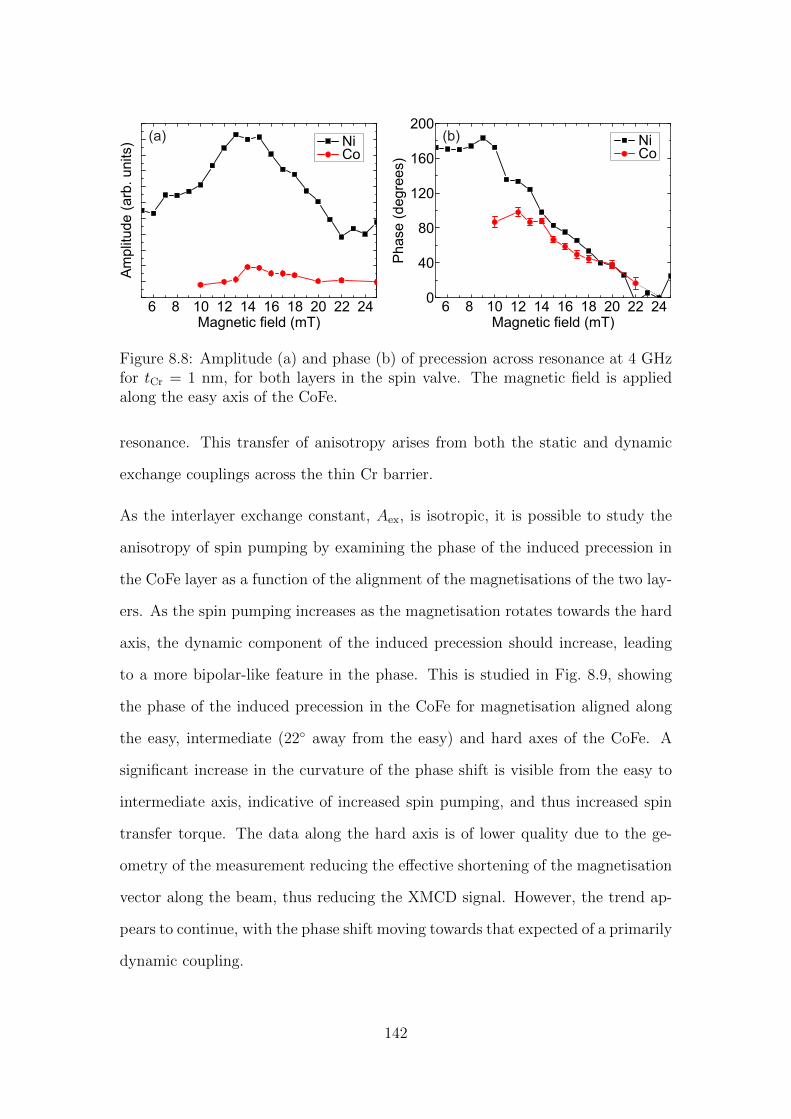
6 8 10 12 14 16 18 20 22 24

Am

plit

ud

e (

arb

. u

nits) Ni

Co

0

40

80

120

160

200

Ph

ase

(d

eg

ree

s)

NiCo

6 8 10 12 14 16 18 20 22 24

(a) (b)

Magnetic field (mT)Magnetic field (mT)

Figure 8.8: Amplitude (a) and phase (b) of precession across resonance at 4 GHzfor tCr = 1 nm, for both layers in the spin valve. The magnetic field is appliedalong the easy axis of the CoFe.

resonance. This transfer of anisotropy arises from both the static and dynamic

exchange couplings across the thin Cr barrier.

As the interlayer exchange constant, Aex, is isotropic, it is possible to study the

anisotropy of spin pumping by examining the phase of the induced precession in

the CoFe layer as a function of the alignment of the magnetisations of the two lay-

ers. As the spin pumping increases as the magnetisation rotates towards the hard

axis, the dynamic component of the induced precession should increase, leading

to a more bipolar-like feature in the phase. This is studied in Fig. 8.9, showing

the phase of the induced precession in the CoFe for magnetisation aligned along

the easy, intermediate (22 away from the easy) and hard axes of the CoFe. A

significant increase in the curvature of the phase shift is visible from the easy to

intermediate axis, indicative of increased spin pumping, and thus increased spin

transfer torque. The data along the hard axis is of lower quality due to the ge-

ometry of the measurement reducing the effective shortening of the magnetisation

vector along the beam, thus reducing the XMCD signal. However, the trend ap-

pears to continue, with the phase shift moving towards that expected of a primarily

dynamic coupling.

142

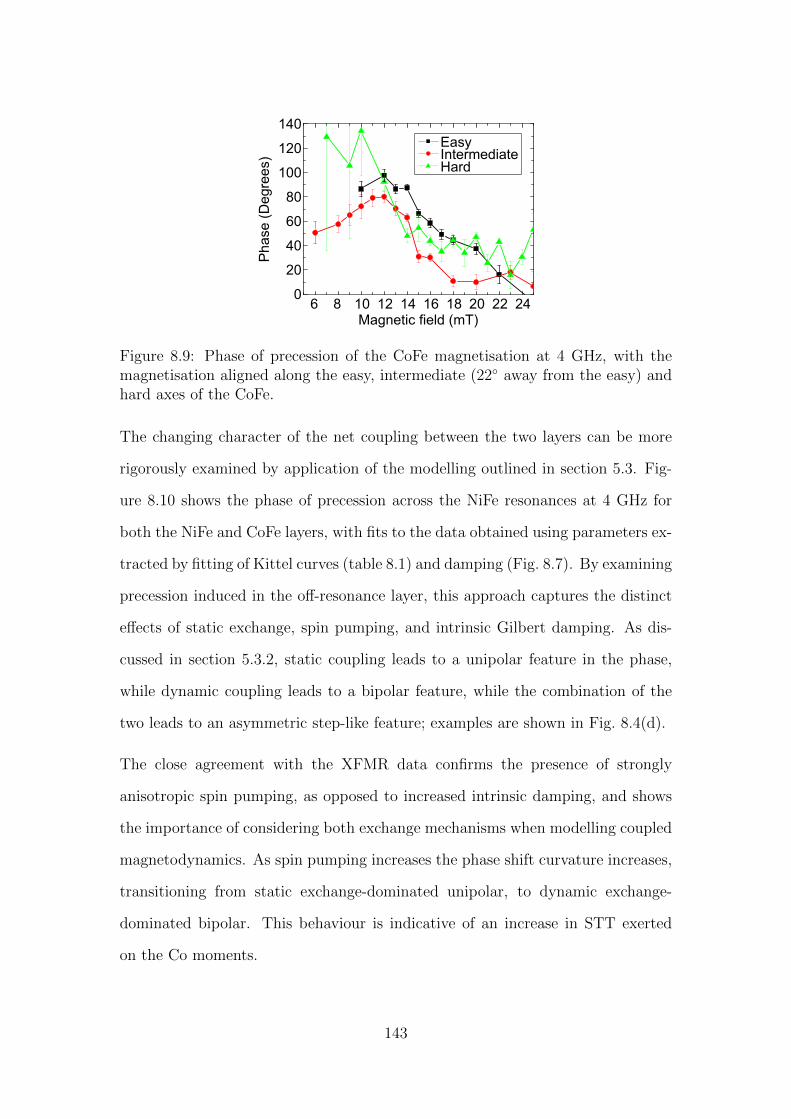
6 8 10 12 14 16 18 20 22 240

20

40

60

80

100

120

140

Phase (

Degre

es)

Magnetic field (mT)

EasyIntermediateHard

Figure 8.9: Phase of precession of the CoFe magnetisation at 4 GHz, with themagnetisation aligned along the easy, intermediate (22 away from the easy) andhard axes of the CoFe.

The changing character of the net coupling between the two layers can be more

rigorously examined by application of the modelling outlined in section 5.3. Fig-

ure 8.10 shows the phase of precession across the NiFe resonances at 4 GHz for

both the NiFe and CoFe layers, with fits to the data obtained using parameters ex-

tracted by fitting of Kittel curves (table 8.1) and damping (Fig. 8.7). By examining

precession induced in the off-resonance layer, this approach captures the distinct

effects of static exchange, spin pumping, and intrinsic Gilbert damping. As dis-

cussed in section 5.3.2, static coupling leads to a unipolar feature in the phase,

while dynamic coupling leads to a bipolar feature, while the combination of the

two leads to an asymmetric step-like feature; examples are shown in Fig. 8.4(d).

The close agreement with the XFMR data confirms the presence of strongly

anisotropic spin pumping, as opposed to increased intrinsic damping, and shows

the importance of considering both exchange mechanisms when modelling coupled

magnetodynamics. As spin pumping increases the phase shift curvature increases,

transitioning from static exchange-dominated unipolar, to dynamic exchange-

dominated bipolar. This behaviour is indicative of an increase in STT exerted

on the Co moments.

143

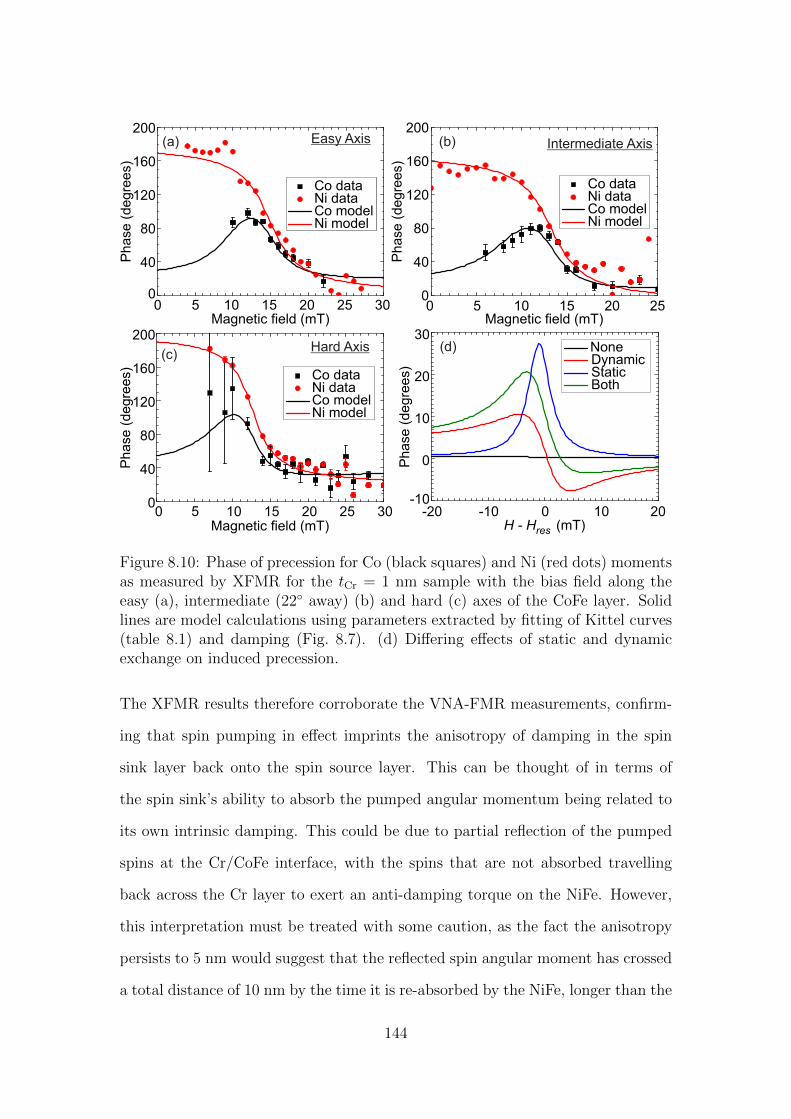
(d)

-20 -10 0 10 20-10

0

10

20

30

Ph

ase

(d

eg

ree

s)

H - Hres

(mT)

NoneDynamicStaticBoth

Hard Axis(c)

0 5 10 15 20 25 300

40

80

120

160

200

Ph

ase

(d

eg

ree

s)

Co dataNi dataCo modelNi model

(b) Intermediate Axis

0 5 10 15 20 250

40

80

120

160

200

Ph

ase

(d

eg

ree

s)

Co dataNi dataCo modelNi model

(a) Easy Axis

0 5 10 15 20 25 300

40

80

120

160

200P

ha

se

(d

eg

ree

s)

Co DataNi DataCo ModelNi Model

Co dataNi dataCo modelNi model

Magnetic field (mT)

Magnetic field (mT)

Magnetic field (mT)

Figure 8.10: Phase of precession for Co (black squares) and Ni (red dots) momentsas measured by XFMR for the tCr = 1 nm sample with the bias field along theeasy (a), intermediate (22 away) (b) and hard (c) axes of the CoFe layer. Solidlines are model calculations using parameters extracted by fitting of Kittel curves(table 8.1) and damping (Fig. 8.7). (d) Differing effects of static and dynamicexchange on induced precession.

The XFMR results therefore corroborate the VNA-FMR measurements, confirm-

ing that spin pumping in effect imprints the anisotropy of damping in the spin

sink layer back onto the spin source layer. This can be thought of in terms of

the spin sink’s ability to absorb the pumped angular momentum being related to

its own intrinsic damping. This could be due to partial reflection of the pumped

spins at the Cr/CoFe interface, with the spins that are not absorbed travelling

back across the Cr layer to exert an anti-damping torque on the NiFe. However,

this interpretation must be treated with some caution, as the fact the anisotropy

persists to 5 nm would suggest that the reflected spin angular moment has crossed

a total distance of 10 nm by the time it is re-absorbed by the NiFe, longer than the

144

calculated spin diffusion length in Cr. It could be, rather, that the process is more

akin to tunnelling magnetoresistance, where the transmission probability from the

initial states is determined by the available final states. Further work is required

to conclusively determine the origin of this surprising result. Nevertheless, the

implications for device optimisation through engineerable anisotropies and tun-

ing of sink layer damping parameters are profound, suggesting several avenues of

enquiry through which to further develop the technique of anisotropy imprinting.

8.6 Conclusion

This chapter has presented a multitechnique study of static and dynamic coupling

in Cr spin valves, showing how the strength of both interactions can be modified

by varying the Cr thickness. The preferred relative orientation can be tuned

to aligned (tCr = 1, 5 nm) or anti-aligned (tCr = 1.5 nm), while the layers are

decoupled for a careful choice of a crossing point between the two regimes, and

for suitably thick Cr (tCr = 2, 10 nm). The dynamic interaction of spin pumping

follows the expected exponential decay with increasing Cr thickness, and fits to

the data yield a spin coherence length of 8 nm. The most important finding of this

investigation, however, is that spin pumping from the polycrystalline NiFe layer

is anisotropic, with an in-plane angular dependence that follows the anisotropy of

Gilbert damping within the epitaxial CoFe layer. This anisotropy is unaffected by

the strength or character of the static exchange coupling, but is suppressed as tCr

exceeds the spin diffusion length in Cr.

This anisotropy imprinting appears to originate in angle-dependent transmission

and reflection of spins at the Cr/CoFe interface. XFMR measurements confirm the

angular variation of the spin pumping, through measurements of the precession

induced in the CoFe layer by on-resonance NiFe. The spin transfer torque exerted

145

by the pumped spins increases in strength as the magnetisation rotates from the

easy axis of the CoFe to the hard axis. Modelling of the data using parameters

extracted from VNA-FMR measurements yields good fits to the data, confirming

the validity of this interpretation.

These surprising results suggest several routes to further optimise spintronic de-

vices, for example through engineering angular dependence of damping through

nanoscale patterning or strain control of magnetocrystalline anisotropy parameters

and crystal structure. Further, if modification of the sink layer damping increases

the effective spin pumping, techniques such as dilute rare earth doping, as exam-

ined in chapter 4, could be used to further increase the efficiency of spin transfer.

While a detailed theory of the origin and limitations of the anisotropy imprinting

is still lacking, this study makes clear the benefits of a multi-technique, layer-

resolved approach to magnetodynamics, and again underlines the importance of

high-quality thin films to gain a deep insight into fundamental physical processes.

It is hoped that these findings will lead to new concepts in both basic science and

practical applications of spin transfer in magnetic multilayers.

146

Chapter 9

Conclusion

This thesis has presented a study of the magnetoydnamics of thin films and het-

erostructures, exploring mechanisms by which magnetic relaxation can be modi-

fied. Particular attention was paid to the development of angular control of damp-

ing, and the role of interfacial couplings. To this end, a multi-technique approach

has been employed, combining the lab-based methods of FMR and SQUID-VSM

with the synchrotron techniques of XMCD and XFMR. Findings have included the

discovery of highly anisotropic damping in Dy-doped Fe, the study of the injection

of a pure spin current into a topological insulator and the imprinting of damping

anisotropy across a thin Cr barrier. These results have diverse implications for the

field of spintronics, as they offer several ways to optimise devices, and shed new

light on established spin transfer phenomena. Future work on these topics should

travel in two directions, firstly aiming to build on the new understanding of physi-

cal phenomena that has been developed and, secondly, working to incorporate the

findings into devices with practical applications.

147

9.1 Summary of Results

Chapter 4 detailed a study of dilute Dy doping of Fe thin films, without loss of

crystal quality. The use of rare earth metals as dopants in thin ferromagnetic films

has been well-studied over the past decade, and shown to lead to a significant en-

hancement of Gilbert damping through the mechanism of slow-relaxing impurities.

However, there is comparatively little work on high quality samples, and next to

no studies have considered the angle-dependence of magnetic relaxation. Here, it

was shown that as the Dy content increases from 0.1 % to 5 % the Gilbert damping

increases by a factor of 3, and develops a significant anisotropy of damping when

comparing the magnetocrystalline easy and hard axes. Application of the XMCD

sum rules showed that this change is accompanied by a quenching of the orbital

moment, and overall reduction in the ratio of orbital to spin moments. These

results provide a demonstration of a method for angular engineering of Gilbert

damping, and a further test of the slow-relaxing impurity model for RE-doped

FM films.

From chapter 6 the focus shifted from single FM layer to trilayer structures, study-

ing the coupling mechanisms that arise for FM layers separated by a thin NM

barrier. Co50Fe50/MgO(x)/Ni structures were fabricated by MBE, with x = 0.5,

1, 1.5, 2 nm. It was found that the insulating MgO barrier permits a weak static

interaction between the two FM layers, but suppresses the dynamic interaction of

spin pumping in under 1 nm. SQUID-VSM hysteresis measurements showed the

shift from strongly coupled layers switching together to isolated layers switching

independently. However, for all but the thinnest barrier no transfer of precessional

amplitude was observed, indicating that the static and dynamic behaviour of the

layers is rather different.

Chapter 7 studies the spin transfer dynamics of the novel materials class of topo-

148

logical insulators. In TIs, the large spin-orbit coupling of the bulk leads to a band

inversion, and surface states that are topologically protected and robust against

backscattering from non-magnetic impurities, making them of great interest for

spintronic applications. VNA-FMR studies showed that they have great capac-

ity to absorb angular momentum, in line with other work that has shown they

can exert a large spin-orbit torque. However, XFMR found evidence of an inter-

action between the ferromagnetic layers, across 8 nm of TI, a surprising result,

particularly when compared to the results from MgO, or literature studies of in-

sulators and semiconductors. The nature of this interaction was initially unclear,

but measurements of the anti-damping torques that arise when both layers are

on resonance suggested that a pure spin current is able to persist across the TI

barrier. This study was the first of its kind, investigating spin transfer in a TI spin

valve architecture, and showcased the rich physics that occurs at the FM-TI inter-

face. That these effects are all observable at room temperature further reinforces

the appeal of TIs for device applications.

Chapter 8 combines the twin themes of spin transfer and angular control of magne-

todynamics, studying the coupled motion of Co50Fe50/Cr(tCr)/Ni81Fe19 trilayers

as a function of tCr. Depending on the barrier thickness, the layers experience

a strong ferromagnetic or anti-ferromagnetic coupling, and are completely sepa-

rated for a sufficiently thick barrier. FMR measurements revealed a significant

anisotropy of spin pumping from the NiFe layer, arising from an anisotropy of

Gilbert damping in the CoFe layer. This anisotropy is unaffected by the strength

or character of the static exchange coupling, but is suppressed as tCr exceeds the

spin diffusion length in Cr, which was found to be 8 nm. A possible explana-

tion for this unexpected effect is anisotropic transmission and reflection of spins

at the Cr/CoFe interface. Layer-resolved measurements of induced precession in

the CoFe at the NiFe resonance at 4 GHz confirm this observation, revealing the

149

competition between static and dynamic exchange that occurs in such spin valves.

These results shed new light on the increasingly important topic of the anisotropic

generation and detection of spin currents. Furthermore, they suggest the possibil-

ity of further control of spin pumping through magnetisation alignment, as well

as suggesting new concepts to manipulate spin pumping, through modification of

the damping mechanisms in the spin sink layer.

9.2 Perspective and Outlook

In reviewing the incidents of this research, though unconscious of intentional omis-

sions, it is nevertheless sensible to consider the suggestions for new studies the

findings imply, and their place in the wider field. For example, in the case of

Dy-doped Fe films it was found that increasing dopant concentration lead to a

quenching of the orbital moment. However, studies on Nd or Gd found the re-

verse to be true, suggesting that the location of the dopant within the lanthanide

series is important, even if they all produce the same effect on the Gilbert damp-

ing. This of course merits further study, particularly in the case of Tb, where

some of the highest damping enhancements to date has been achieved.

Similarly, the work on spin transfer in TIs represents only the beginning of the

effort to understand and functionalise these exciting new materials, bringing them

out of the laboratory and into devices. This is currently an area of intense study,

in particular magnetotransport studies, so it is anticipated that the field will be

unrecognisable in five years, when compared to the snapshot captured here. Future

work in this theme should aim to improve the fabrication of such devices, and to

explore the effects of using other TI layers, such as Bi2Te3 or Sb2Te3.

A new thrust in spintronic research is the aim to incorporate antiferromagnets

into devices, as their compensated magnetic moments are minimise stray fields

150

and offer superior thermal stability. Unfortunately, the resonance frequencies of

such antiferromagnets are typically on the order of THz, and thus outside the

range of the FMR techniques employed here. Synthetic antiferromagnets formed

of anti-aligned ferromagnetic layers, however, combine the benefits of natural an-

tiferromagnets with the ease of use of ferromagnets, and can be achieved easily,

making them an excellent testbed for such spin transfer phenomena. The antifer-

romagnetically coupled Cr spin valve presented in chapter 8 is one such synthetic

structure, and in itself merits significant further study. Initial XFMR results have

shown sharp phase jumps associated with magnetic reversal, and that the preces-

sion induced by this coupling is in anti-phase. While these findings are outside

the scope of this thesis, they represent a natural extension of the work conducted

here, and an excellent lead-in to a new field of research.

151

Appendix A

Derivation of the AC Magnetic

Susceptibility with Static and

Dynamic Exchange Coupling

This appendix provides an outline of the derivation of the equations for AC mag-

netic susceptibility of a structure with two ferromagnetic layers, coupled by both

static exchange coupling and dynamic exchange driven by spin pumping. These

equations were used to model the amplitude and phase of precession of magneti-

sation measured by XFMR.

The derivation is based upon the modified form of the LLG equation including spin

pumping, as outlined in, for example, Heinrich et al. [107] and static exchange, as

provided by Arena et al. [32]. The derivation itself closely follows that outlined

in Appendix 3 of Max Marcham’s PhD thesis [35], but does not require that the

magnetisation be aligned along a magnetocrystalline easy axis, explicitly including

both cubic and uniaxial magnetocrystalline anisotropies.

We consider two ferromagnetic layers, denoted 1 and 2, with magnetic parameters

152

KiU, Ki

C, M is , and γi, the in-plane uniaxial and cubic magnetocrystalline anisotropy

parameters, saturation magnetisation and gyromagnetic ratio, respectively. The

static coupling between the two layers is defined as [31,32]:

βi =Aex

M isdi

cos(φiM − φjM) (A.1)

with di the thickness of the magnetic layer.

From this starting point, we write the LLG:

−∂mi

∂t= mi ×

[γiH i

eff + βiM jsm

j − (αi0 + αiii)∂mi

∂t

]+ αiijm

j × ∂mj

∂t, (A.2)

where superscripts denote magnetic layer, and H ieff is the effective field acting on

layer i. The intrinsic Gilbert damping is αi0, while αimn are spin source (m=n) and

spin sink (m 6= n) terms.

We use the co-ordinate system outlined in Fig. 2.1, a thin film with z oriented out

of the plane, external field H0 oriented along x and RF field h(t) oriented along y.

Both layers are free (unpinned) with their own cubic and uniaxial magnetocrys-

talline anisotropy axes, which are not necessarily aligned. All in-plane angles are

defined relative to φ1C . As before, static magnetisations are not necessarily aligned

with φH , their position is instead found by minimizing the free energy. We take

the thin film approximation, Nxx = Nyy = 0, Nzz = 1, and therefore include the

demagnetisation field, H idemag = −mi

z as part of the general anisotropy field H ianis

for simplicity. Finally, we note that for completeness one should also include the

imaginary components of the spin mixing conductance, δmn, but these are typically

negligible so are neglected here.

FMR is driven by energy supplied by the effective field, which in this formulation

153

is written as:

H ieff = H0 +H i

anis + h(t). (A.3)

Writing individual components explicitly:

H0 = H0 cos(φiM − φH)x , (A.4)

h(t) = h(t)y , (A.5)

H ianis = H i

xx+H iyy +H i

z z . (A.6)

The anisotropy field has components:

Hx =KC

2M4s

[M3

x(cos 4(φM − φC) + 3)− 3m2xmy sin 4(φM − φC)

+ 3mxm2y(1− cos 4(φM − φC)) +m3

y sin 4(φM − φC)]

+KU

M2s

[mx(1 + cos 2(φM − φU))−my(sin 2(φM − φU)] (A.7)

Hy = − KC

2M4s

[m3x sin 4(φM − φC)− 3m2

xmy(1− cos 4(φM − φC))

− 3mxm2y(1 + sin 4(φM − φC))−m3

y(cos 4(φM − φC) + 3)]

−KU

M2s

[mx(sin 2(φM − φU)−my(1− cos 2(φM − φU))] (A.8)

Hz =−Msmz +2KC

M4s

m3z . (A.9)

We now re-write the LLG component-wise, calculating the cross products as re-

154

quired:

− 1

γi∂mi

x

∂t=mi

y

(H ieff,z + βiM j

smjz −

αi0 + αiiiγi

∂miz

∂t

)−mi

z

(H ieff,y + βiM j

smjy −

αi0 + αiiiγi

∂miy

∂t

)−αiijγi

(mjy

∂mjz

∂t−mj

z

∂mjy

∂t

)(A.10)

− 1

γi∂mi

y

∂t=mi

z

(H ieff,x + βiM j

smjx −

αi0 + αiiiγi

∂mix

∂t

)−mi

x

(H ieff,z + βiM j

smjz −

αi0 + αiiiγi

∂miz

∂t

)−αiijγi

(mjz

∂mjx

∂t−mj

x

∂mjz

∂t

)(A.11)

− 1

γi∂mi

z

∂t=mi

x

(H ieff,y + βiM j

smjy −

αi0 + αiiiγi

∂miy

∂t

)−mi

y

(H ieff,x + βiM j

smjx −

αi0 + αiiiγi

∂mix

∂t

)−αiijγi

(mjx

∂mjy

∂t−mj

y

∂mjx

∂t

)(A.12)

At this point, we make the small angle approximation to linearise the equations.

As the static magnetisation is aligned along x, and the oscillations about this

direction are small, we can rewrite:

m = x+my(t)y +mz(t)z (A.13)

where my(t), mz(t)Ms. Note, also, that as mx is constant in time:

∂mx

∂t= 0 . (A.14)

155

Making this linear approximation, we can cancel terms that are nonlinear in my(t),

mz(t), h(t):

0 = miy(H

ieff,z + βiM j

smjz)−mi

z(Hieff,y + βiM j

smjy) (A.15)

− 1

γi∂mi

y

∂t=mi

z(Hieff,x + βiM j

s )

−(H ieff,z + βiM j

smjz −

αi0 + αiiiγi

∂miz

∂t

)+αiijγi∂mj

z

∂t(A.16)

− 1

γi∂mi

z

∂t=

(H ieff,y + βiM j

smjy −

αi0 + αiiiγi

∂miy

∂t

)−mi

y

(H ieff,x + βiM j

s

)−αiijγi∂mj

y

∂t(A.17)

The next step is to expand out the H ieff terms. This leads to unwieldy expressions,

so we define:

Beff =H0 cos(φM − φH) +Ms

+KC

2Ms

[3 + cos 4(φM − φC)] +KU

Ms

[1 + cos 2(φM − φU)] (A.18)

Heff =H0 cos(φM − φH)

+2KC

Ms

cos 4(φM − φC) +2KU

Ms

cos 2(φM − φU) (A.19)

Note that these terms can also be used to write the resonance condition, as dis-

156

cussed in section 2.2: (ω

γ

)2

= BeffHeff |Hres(A.20)

evaluated at the resonance frequency. This is equivalent to equation (2.15). With

these definitions we expand the H ieff terms and linearise the results, to yield:

− 1

γi∂mi

y

∂t=mi

z

[Beff + βiM j

s

]+αi0 + αiiiγi

∂miz

∂t

−βiM jsm

jz +

αiijγi∂mj

z

∂t(A.21)

− 1

γi∂mi

z

∂t=mi

y

[Heff − βiM j

s

]− αi0 − αiii

γi∂mi

y

∂t

−βiM jsm

jy +

αiijγi∂mj

y

∂t+ h . (A.22)

Now we seek harmonic solutions to these equations, using the form m(t) =

m exp(−iωt), h(t) = h exp(−iωt):

0 =miz

(Beff + βiM j

s − (αi0 + αiii)iω

γi

)−mj

z

(βiM j

s − αiijiω

γi

)− iω

γimiy (A.23)

hmis = −mi

y

(Heff + βiM j

s + (αi0 + αiii)iω

γi

)+mj

y

(βiM j

s − αiijiω

γi

)+iω

γimiz . (A.24)

Thus far we have considered only one layer, so we now exploit symmetry of i↔ j

157

interchange to write out the matrix form of the linearised coupled equations:

0

h

0

h

=

− iωγ1

H1a 0 H1

c

−H1b

iωγ1−H1

c 0

0 H2c − iω

γ2H2

a

−H2c 0 −H2

biωγ2

m1y

m1z

m2y

m2z

(A.25)

where:

H ia = Beff + βiM j

s − (αi0 + αiii)iω

γi

H ib = Heff + βiM j

s + (αi0 + αiii)iω

γi

H ic = αiij

iω

γi− βiM j

s , (A.26)

which gives the relation between the microwave field and the magnetisation dy-

namics:

hM s = Am . (A.27)

We can therefore see that A is the inverse magnetic susceptibility tensor:

A−1hM s = χhM s = m . (A.28)

Thus it is possible to calculate desired components of the AC magnetic suscepti-

bility tensor by calculating the inverse of the matrix A. This was performed in

Python, yielding the complex susceptibility. The amplitude of this complex num-

ber is directly proportional to the amplitude of precession of magnetisation, while

the phase gives the phase of precession relative to the driving microwave field.

158

Appendix B

List of of Abbreviations and

Acronyms

AC Alternating Current

AF Anti-Ferromagnetic (in the context of exchange coupling)

ALS Advanced Light Source

ARPES Angle Resolved Photo-Emission Spectroscopy

BiSe Bi2Se3

CB Conduction Band

CoFe Co50Fe50

CPW Coplanar Waveguide

DC Direct Current

DLS Diamond Light Source

F Ferromagnetic (in the context of exchange coupling)

FM Ferromagnet (in the context of a ferromagnetic material or layer)

FMR Ferromagnetic Resonance

FY Fluorescence Yield

GMR Giant Magnetoresistance

HWHM Half Width Half Maximum

ISHE Inverse Spin Hall Effect

LaMBE Lanthanide Molecular Beam Epitaxy (machine)

159

LIA Lock In Amplifier

LLG Landau-Lifshitz-Gilbert (equation)

MBE Molecular Beam Epitaxy

MSG Magnetic Spectroscopy Group

MTJ Magnetic Tunnel Junction

MRAM Magnetic Random Access Memory

µ-MBE micro-Molecular Beam Epitaxy (machine)

NiFe Ni81Fe19

NM Non-Magnetic (in the context of non-magnetic material or layer)

OOMMF Object-Oriented Micromagnetic Framework [101]

POMS Portable Octupole Magnet System

QCM Quartz Crystal Microbalance

RE Rare Earth

RF Radio Frequency

RGA Residual Gas Analyser

RHEED Reflection High Energy Electron Diffraction

RKKY Ruderman-Kittel-Kasuya-Yosida (interaction)

SQUID Superconducting Quantum Interference Device

STT Spin Transfer Torque

TEY Total Electron Yield

TI Topological Insulator

TMR Tunnelling Magnetoresistance

TSS Topological Surface State

UHV Ultra-High Vacuum

VB Valence Band

VNA Vector Network Analyser

VSM Vibrating Sample Magnetometer

XAS X-ray Absorption Spectroscopy

XFMR X-ray Detected Ferromagnetic Resonance

XMCD X-ray Magnetic Circular Dichroism

XRD X-ray Diffraction

160

Appendix C

Publications Arising from this

Work

The following publications have arisen in full, or in part, as a result of the work

conducted over the course of this thesis research.

Anisotropic Absorption of Pure Spin Currents ; AA Baker, AI Figueroa, CJ Love,

SA Cavill, T Hesjedal, G van der Laan; Phys. Rev. Lett. 117 047201 (2016)

Enhanced Curie temperature of Cr-doped Bi2Se3 thin films by magnetic-proximity

effect ; AA Baker, AI Figueroa, K. Kummer, LJ Collins-McIntyre, G van der Laan,

T Hesjedal; Phys. Rev. B. 92 094420 (2015)

Tailoring of magnetic properties of ultrathin epitaxial Fe films by Dy doping ;

AA Baker, AI Figueroa, G van der Laan, T Hesjedal; AIP Advances. 5 077117

(2015)

Spin pumping in Ferromagnet Topological Insulator Ferromagnet Heterostructures ;

AA Baker, AI Figueroa, LJ Collins-McIntyre, G van der Laan, T Hesjedal; Scien-

tific Reports. 5 7097 (2015)

161

An ultra-compact, high-throughput molecular beam epitaxy growth system; AA Baker,

W Braun, G Gassler, S Rembold, A Fischer, T Hesjedal; Rev. Sci. Instrum. 86,

043901 (2015)

Spin pumping through a topological insulator probed by x-ray detected ferromag-

netic resonance; AI Figueroa, AA Baker, LJ Collins-McIntyre, G van der Laan,

T Hesjedal; J. Magn. Magn. Mater.. in press doi:10.1016/j.jmmm.2015.07.013

(2015)

X-ray magnetic circular dichroism on La2/3Ca1/3Mn0.97Fe.03O3 thin films AI Figueroa,

GE Campillo, AA Baker, JA Osorio, OL Arnache, G van der Laan Superlattice

Microst 87 42 (2015)

Study of Dy-doped Bi2Te3: thin film growth and magnetic properties SE Harrison,

LJ Collins-McIntyre, SL Zhang, AA Baker, AI Figueroa, AJ Kellock, A Pushp,

SS Parkin, JS Harris, G van der Laan, T Hesjedal J. Phys.: Condens. Matter 27

245602 (2015)

Universal Magnetic Hall Circuit Based on Paired Spin Heterostructures S Zhang,

AA Baker, J-Y Zhang, G Yu, S Wang, T Hesjedal; Adv. Elec. Mater. 1 6 (2015)

Modelling ferromagnetic resonance in magnetic multilayers: Exchange coupling

and demagnetisation-driven effects ; AA Baker, CS Davies, AI Figueroa, LR Shelford,

G van der Laan, T Hesjedal; Journal of Applied Physics 115 17D140 (2014)

Three dimensional magnetic abacus memory ; S-L Zhang, J Zhang, AA Baker, S

Wang, G Yu, T Hesjedal; Scientific Reports 4 (2014)

Engineering of BiSe nanowires by laser cutting ; P Schonherr, AA Baker, T Hes-

jedal, P Kusch, S Reich; EPJ Applied Physics 66 10401 (2014)

Magnetic Cr doping of Bi2Se3: Evidence for divalent Cr from x-ray spectroscopy ;

AI Figueroa, G van der Laan, LJ Collins-McIntyre, S-L Zhang, AA Baker, SE

162

Harrison, P Schonherr, G Cibin, and T Hesjedal; Physical Review B 90 134402

(2014)

X-ray magnetic spectroscopy of MBE-grown Mn-doped Bi2Se3 thin films ; LJ Collins-

McIntyre, MD Watson, AA Baker, SL Zhang, AI Coldea, SE Harrison, A Pushp,

AJ Kellock, SSP Parkin, G van der Laan and T Hesjedal; AIP Advances 4 127136

(2014)

Study of Gd-doped Bi2Te3 thin films: Molecular beam epitaxy growth and magnetic

properties ; SE Harrison, LJ Collins-McIntyre, S Li, AA Baker, LR Shelford, Y

Huo, A Pushp, SSP Parkin, JS Harris, E Arenholz, G van der Laan and T Hesjedal

J. Appl. Phys. 115, 023904 (2014)

163

References

[1] S. A. Wolf, D. D. Awschalom, R. A. Buhrman, J. M. Daughton, S. vonMolnar, M. L. Roukes, A. Y. Chtchelkanova, and D. M. Treger, Science294, 1488 (2001).

[2] S. A. Wolf, A. Y. Chtchelkanova, and D. M. Treger, IBM J. Res. Dev. 50,101 (2006).

[3] M. N. Baibich, J. M. Broto, A. Fert, F. N. Van Dau, F. Petroff, P. Etienne,G. Creuzet, A. Friederich, and J. Chazelas, Phys. Rev. Lett. 61, 2472 (1988).

[4] G. Binasch, P. Grunberg, F. Saurenbach, and W. Zinn, Phys. Rev. B 39,4828 (1989).

[5] S. Yuasa and D. D. Djayaprawira, J. Phys. D: Appl. Phys. 40, R337 (2007).

[6] J. C. Sankey, Y.-T. Cui, J. Z. Sun, J. C. Slonczewski, R. A. Buhrman, andD. C. Ralph, Nat. Phys. 4, 67 (2008).

[7] J. A. Katine and E. E. Fullerton, J. Magn. Magn. Mater. 320, 1217 (2008).

[8] I. L. Prejbeanu, M. Kerekes, R. C. Sousa, H. Sibuet, O. Redon, B. Dieny,and J. P. Nozieres, J Phys: Cond. Matt. 19, 165218 (2007).

[9] J. Slaughter, Annu. Rev. Mat. Res. 39, 277 (2009).

[10] A. D. Kent and D. C. Worledge, Nat. Nanotechnol. 10, 187 (2015).

[11] M. D. Stiles and A. Zangwill, Phys. Rev. B 66, 014407 (2002).

[12] N. Locatelli, V. Cros, and J. Grollier, Nat. Mater. 13, 11 (2014).

[13] S. Urazhdin, V. E. Demidov, H. Ulrichs, T. Kendziorczyk, T. Kuhn,J. Leuthold, G. Wilde, and S. Demokritov, Nat. Nanotechnol. 9, 509 (2014).

[14] G. Woltersdorf. Spin-pumping and two-magnon scattering in magnetic mul-tilayers. PhD thesis, Simon Fraser University, (2004).

[15] M. K. Marcham, L. R. Shelford, S. A. Cavill, P. S. Keatley, W. Yu, P. Shafer,A. Neudert, J. R. Childress, J. A. Katine, E. Arenholz, N. D. Telling,G. van der Laan, and R. J. Hicken, Phys. Rev. B 87, 180403 (2013).

[16] G. Woltersdorf and B. Heinrich, Phys. Rev. B 69, 184417 (2004).

164

[17] K. Zakeri, J. Lindner, I. Barsukov, R. Meckenstock, M. Farle, U. vonHorsten, H. Wende, W. Keune, J. Rocker, S. S. Kalarickal, K. Lenz,W. Kuch, K. Baberschke, and Z. Frait, Phys. Rev. B 76, 104416 (2007).

[18] W. Bailey, P. Kabos, F. Mancoff, and S. Russek, IEEE Trans. Magn. 37,1749 (2001).

[19] A. A. Baker, A. I. Figueroa, G. van der Laan, and T. Hesjedal, AIP Adv.5, 077117 (2015).

[20] A. Brataas, Y. Tserkovnyak, G. E. W. Bauer, and B. I. Halperin, Phys. Rev.B 66, 060404 (2002).

[21] Y. Tserkovnyak, A. Brataas, and G. E. W. Bauer, Phys. Rev. B 66, 224403(2002).

[22] Y. Tserkovnyak, A. Brataas, G. E. W. Bauer, and B. I. Halperin, Rev. Mod.Phys. 77, 1375 (2005).

[23] B. Kardasz and B. Heinrich, Phys. Rev. B 81, 094409 (2010).

[24] A. I. Figueroa. Magnetic Nanoparticles: A Study by Synchrotron Radiationand RF Transverse Susceptibility. Springer, (2014).

[25] C. H. Du, H. L. Wang, Y. Pu, T. Meyer, P. M. Woodward, F. Y. Yang, andP. C. Hammel, Phys. Rev. Lett. 111, 247202 (2013).

[26] M. Jamali, J. S. Lee, J. S. Jeong, F. Mahfouzi, Y. Lv, Z. Zhao, B. K. Nikolic,K. A. Mkhoyan, N. Samarth, and J.-P. Wang, Nano Lett. 15, 7126 (2015).

[27] L. Liu, T. Moriyama, D. C. Ralph, and R. A. Buhrman, Phys. Rev. Lett.106, 036601 (2011).

[28] A. A. Baker, A. I. Figueroa, C. J. Love, S. A. Cavill, T. Hesjedal, andG. van der Laan, Phys. Rev. Lett. 116, 047201 (2016).

[29] D. A. Arena, Y. Ding, E. Vescovo, S. Zohar, Y. Guan, and W. E. Bailey,Rev. Sci. Inst. 80, 083903 (2009).

[30] A. Azevedo, C. Chesman, S. M. Rezende, F. M. de Aguiar, X. Bian, andS. S. P. Parkin, Phys. Rev. Lett. 76, 4837 (1996).

[31] G. B. G. Stenning, L. R. Shelford, S. A. Cavill, F. Hoffmann, M. Haertinger,T. Hesjedal, G. Woltersdorf, G. J. Bowden, S. A. Gregory, C. H. Back,P. A. J. de Groot, and G. van der Laan, New J. Phys. 17, 013019 (2015).

[32] D. A. Arena, E. Vescovo, C.-C. Kao, Y. Guan, and W. E. Bailey, Phys. Rev.B 74, 064409 (2006).

[33] O. Mosendz, J. E. Pearson, F. Y. Fradin, S. D. Bader, and A. Hoffmann,Appl. Phys. Lett. 96, 022502 (2010).

[34] J. Goulon, A. Rogalev, F. Wilhelm, N. Jaouen, C. Goulon-Ginet, G. Goujon,J. Ben Youssef, and M. Indenbom, J. Exp. Theor. Phys. 82, 696–701 (2005).

165

[35] M. Marcham. Phase-Resolved Ferromagnetic Resonance Studies of ThinFilm Ferromagnets. PhD thesis, University of Exeter, (2012).

[36] E. Beaurepaire, H. Bulou, L. Joly, and F. Scheurer. Magnetism and Syn-chrotron Radiation: Towards the Fourth Generation Light Sources. Springer,(2013).

[37] G. van der Laan and A. I. Figueroa, Coord. Chem. Rev. 277, 95 (2014).

[38] G. van der Laan, J. Phys.: Conf. Ser. 430, 012127 (2013).

[39] P. Carra, B. Thole, M. Altarelli, and X. Wang, Phys. Rev. Lett. 70, 694(1993).

[40] B. T. Thole, P. Carra, F. Sette, and G. van der Laan, Phys. Rev. Lett. 68,1943 (1992).

[41] G. S. Abo, Y. K. Hong, J. Park, J. Lee, W. Lee, and B. C. Choi, IEEETrans. Magn. 49, 4937–4939 (2013).

[42] B. Heinrich and J. A. C. Bland. Ultrathin Magnetic Structures II: Measure-ment Techniques and Novel Magnetic Properties. Springer, (1994).

[43] S. Mizukami, Y. Ando, and T. Miyazaki, Phys. Rev. B 66, 104413 (2002).

[44] T. L. Gilbert, Phys. Rev. 100, 1243 [Abstract Only] (1955).

[45] M. Farle, Rep. Prog. Phys. 61, 755 (1998).

[46] F. Hoffman. Magnetic anisotropies of (Ga,Mn)As films and nanostructures.PhD thesis, Universitat Regensburg, (2010).

[47] C. Kittel, Phy. Rev. 73, 155 (1948).

[48] A. Caprile, A. Manzin, M. Coisson, M. Pasquale, H. W. Schumacher,N. Liebing, S. Sievers, R. Ferreira, S. Serrano-Guisan, and E. Paz, IEEETrans. Magn. 51, 1 (2015).

[49] T. A. Ostler, R. Cuadrado, R. W. Chantrell, A. W. Rushforth, and S. A.Cavill, Phys. Rev. Lett. 115, 067202 (2015).

[50] G. Woltersdorf, M. Buess, B. Heinrich, and C. H. Back, Phys. Rev. Lett.95, 037401 (2005).

[51] Y. Tserkovnyak, A. Brataas, and G. E. W. Bauer, Phys. Rev. Lett. 88,117601 (2002).

[52] M. Tokac, S. A. Bunyaev, G. N. Kakazei, D. S. Schmool, D. Atkinson, andA. T. Hindmarch, Phys. Rev. Lett. 115, 056601 (2015).

[53] T. Chiba, G. E. W. Bauer, and S. Takahashi, Phys. Rev. B 92, 054407(2015).

[54] K. Lenz, H. Wende, W. Kuch, K. Baberschke, K. Nagy, and A. Janossy,Phys, Rev. B 73, 144424 (2006).

166

[55] S. S. Kalarickal, P. Krivosik, M. Wu, C. E. Patton, M. L. Schneider, P. Ka-bos, T. Silva, and J. P. Nibarger, J. Appl. Phys. 99, 093909 (2006).

[56] B. Heinrich, R. Urban, and G. Woltersdorf, J. Appl. Phys. 91, 7523 (2002).

[57] Z. Diao, Z. Li, S. Wang, Y. Ding, A. Panchula, E. Chen, L.-C. Wang, andY. Huai, J. Phys.: Condens. Matter 19, 165209 (2007).

[58] G. Woltersdorf, M. Kiessling, G. Meyer, J.-U. Thiele, and C. H. Back, Phys.Rev. Lett. 102, 257602 (2009).

[59] M. K. Marcham, W. Yu, P. S. Keatley, L. R. Shelford, P. Shafer, S. A.Cavill, H. Qing, A. Neudert, J. R. Childress, J. A. Katine, E. Arenholz,N. D. Telling, G. van der Laan, and R. J. Hicken, Appl. Phys. Lett. 102,062418 (2013).

[60] A. A. Baker, A. I. Figueroa, L. J. Collins-McIntyre, G. van der Laan, andT. Hesjedal, Sci. Rep. 5, 7907 (2015).

[61] R. Kukreja, S. Bonetti, Z. Chen, D. Backes, Y. Acremann, J. A. Katine,A. D. Kent, H. A. Durr, H. Ohldag, and J. Stohr, Phys. Rev. Lett. 115,096601 (2015).

[62] C. Burrowes, B. Heinrich, B. Kardasz, E. A. Montoya, E. Girt, Y. Sun, Y.-Y.Song, and M. Wu, Appl. Phys. Lett. 100, 092403 (2012).

[63] G. Schutz, M. Knulle, R. Wienke, W. Wilhelm, W. Wagner, P. Kienle, andR. Frahm, Zeitschrift fur Physik B Condensed Matter 73, 67.

[64] C. T. Chen, Y. U. Idzerda, H.-J. Lin, N. V. Smith, G. Meigs, E. Chaban,G. H. Ho, E. Pellegrin, and F. Sette, Phys. Rev. Lett. 75, 152 (1995).

[65] C. T. Foxon and J. Orton. Molecular Beam Epitaxy: A Short History.Oxford University Press, USA, (2015).

[66] B. A. Joyce, Rep. Prog. Phys. 48, 1637 (1985).

[67] R. Farrow. Molecular Beam Epitaxy: Applications to Key Materials. Noyes,(1995).

[68] A. Y. Cho, J. Appl. Phys. 41, 2780 (1970).

[69] W. P. McCray, Nat. Nanotechnol. 2, 259 (2007).

[70] J. R. Arthur, Surf. Science 500, 189 (2002).

[71] M. Henini, editor. Molecular Beam Epitaxy — From Research to Mass Pro-duction. Elsevier, (2013).

[72] H. Y. Hwang, Y. Iwasa, M. Kawasaki, B. Keimer, N. Nagaosa, andY. Tokura, Nat. Mater. 11, 103 (2012).

[73] R. Dingle, A. C. Gossard, and W. Wiegmann, Phys. Rev. Lett. 34, 1327(1975).

167

[74] J. Faure-Vincent, C. Tiusan, E. Jouguelet, F. Canet, M. Sajieddine, C. Bel-louard, E. Popova, M. Hehn, F. Montaigne, and A. Schuhl, Appl. Phys. Lett.82, 4507 (2003).

[75] F. Katmis, R. Calarco, K. Perumal, P. Rodenbach, A. Giussani, M. Hanke,A. Proessdorf, A. Trampert, F. Grosse, R. Shayduk, R. Campion, W. Braun,and H. Riechert, Cryst. Growth & Design 11, 4606–4610 (2011).

[76] D. J. Eaglesham, J. Appl. Phys. 77, 3597–3617 (1995).

[77] W.-X. Ni, J. O. Ekberg, K. B. Joelsson, H. H. Radamson, A. Henry, G.-D.Shen, and G. V. Hansson, J. Cryst. Growth 157, 285 (1995).

[78] A. A. Baker, W. Braun, G. Gassler, S. Rembold, A. Fischer, and T. Hesjedal,Rev. Sci. Inst. 86, 043901 (2015).

[79] L. Collins-McIntyre. Transition-Metal Doped Bi2Se3 and Bi2Te3 TopologicalInsulator Thin Films. PhD thesis, University of Oxford, (2015).

[80] C. Thomas, P. Dudin, and M. Hoesch, Opt. Commun. 359, 171 (2016).

[81] J.-M. L. Beaujour, A. D. Kent, D. W. Abraham, and J. Z. Sun, J. Appl.Phys 103, 07B519 (2008).

[82] E. Arenholz and S. O. Prestemon, Rev. Sci. Inst. 76, 083908 (2005).

[83] A. I. Figueroa, A. A. Baker, L. J. Collins-McIntyre, T. Hesjedal, andG. van der Laan, J. Magn. Magn. Mater. 400, 178 (2015).

[84] G. Boero, S. Mouaziz, S. Rusponi, P. Bencok, F. Nolting, S. Stepanow, andP. Gambardella, New J. Phys. 10, 013011 (2008).

[85] S. E. Russek, P. Kabos, R. D. McMichael, C. G. Lee, W. E. Bailey,R. Ewasko, and S. C. Sanders, J. Appl. Phys. 91, 8659 (2002).

[86] S. G. Reidy, L. Cheng, and W. E. Bailey, Appl. Phys. Lett. 82, 1254 (2003).

[87] C. Luo, Z. Feng, Y. Fu, W. Zhang, P. K. J. Wong, Z. X. Kou, Y. Zhai, H. F.Ding, M. Farle, J. Du, and H. R. Zhai, Phys. Rev. B 89, 184412 (2014).

[88] W. Zhang, S. Jiang, P. K. J. Wong, L. Sun, Y. K. Wang, K. Wang, M. P.de Jong, W. G. van der Wiel, G. van der Laan, and Y. Zhai, J. Appl. Phys.115, 17A308 (2014).

[89] J. H. Van Vleck and R. Orbach, Phys. Rev. Lett. 11, 65 (1963).

[90] M. Li, Z. Shi-Ming, M. Jun, and J. Yong, Chin. Phys. B 24, 017101 (2015).

[91] A. S. van der Goot and K. H. J. Buschow, J. Less-Common Met. 21, 151(1970).

[92] C. M. Boubeta, J. L. Costa-Kramer, and A. Cebollada, J. Phys.: Condens.Mater. 15, R1123 (2003).

[93] H. Song, L. Cheng, and W. E. Bailey, J. Appl. Phys. 95, 6592 (2004).

168

[94] Y. Park, E. E. Fullerton, and S. D. Bader, Appl. Phys. Lett. 66, 2140 (1995).

[95] M. Brockmann, M. Zolfl, S. Miethaner, and G. Bayreuther, J. Magn. Magn.Mater. 198, 384 (1999).

[96] Q.-F. Zhan, S. Vandezande, K. Temst, and C. van Haesendonck, New J.Phys. 11, 063003 (2009).

[97] B. H. Clarke, Br. J. Appl. Phys. 18, 727 (1967).

[98] J. F. Dillon Jr and J. W. Nielsen, Phys. Rev. Lett. 3, 30 (1959).

[99] A. G. Gurevich, A. N. Ageev, and M. I. Klinger, J. Appl. Phys. 41, 1295(1970).

[100] P. S. Keatley, V. V. Kruglyak, A. Neudert, E. A. Galaktionov, R. J. Hicken,J. R. Childress, and J. A. Katine, Phys. Rev. B 78, 214412 (2008).

[101] M. J. Donahue and D. G. Porter. Interagency Report NISTIR 6376. NationalInstitute of Standards and Technology, Gaithersburg, MD.

[102] V. V. Kruglyak, P. S. Keatley, A. Neudert, R. J. Hicken, J. R. Childress,and J. A. Katine, Phys. Rev. Lett. 104, 027201 (2010).

[103] T. Pramanik, U. Roy, M. Tsoi, L. F. Register, and S. K. Banerjee, J. Appl.Phys. 115, 17D123 (2014).

[104] A. A. Baker, C. S. Davies, A. I. Figueroa, L. R. Shelford, G. van der Laan,and T. Hesjedal, J. Appl. Phys. 115, 17D140 (2014).

[105] R. Meckenstock, I. Barsukov, O. Posth, J. Lindner, A. Butko, and D. Spod-dig, Appl. Phys. Lett. 91, 2507 (2007).

[106] T. Moriyama, R. Cao, X. Fan, G. Xuan, B. K. Nikolic, Y. Tserkovnyak,J. Kolodzey, and J. Q. Xiao, Phys. Rev. Lett. 100, 067602 (2008).

[107] B. Heinrich, Y. Tserkovnyak, G. Woltersdorf, A. Brataas, R. Urban, andG. E. Bauer, Phys. Rev. Lett. 90, 187601 (2003).

[108] Y. Tserkovnyak, T. Moriyama, and J. Q. Xiao, Phys. Rev. B 78, 020401(2008).

[109] J. Xiao, G. E. W. Bauer, and A. Brataas, Phys. Rev. B 77, 180407 (2008).

[110] J. Ventura, J. M. Teixeira, J. P. Araujo, J. B. Sousa, P. Wisniowski, andP. P. Freitas, Phys. Rev. B 78, 024403 (2008).

[111] L. Lari, S. Lea, C. Feeser, B. W. Wessels, and V. K. Lazarov, J. Appl. Phys.111, 07C311 (2012).

[112] S. G. Wang, R. C. C. Ward, T. Hesjedal, X.-G. Zhang, C. Wang, A. Kohn,Q. L. Ma, J. Zhang, H. F. Liu, and X. F. Han, J. Nanosci. Nanotechnol. 12,1006 (2012).

169

[113] D. L. Li, Q. L. Ma, S. G. Wang, R. C. C. Ward, T. Hesjedal, X.-G. Zhang,A. Kohn, E. Amsellem, G. Yang, J. L. Liu, J. Jiang, H. X. Wei, and X. F.Han, Sci. Rep. 4 (2014).

[114] C. L. Kane and E. J. Mele, Phys. Rev. Lett. 95, 146802 (2005).

[115] B. A. Bernevig, T. L. Hughes, and S.-C. Zhang, Science 314, 1757 (2006).

[116] Y. L. Chen, J. G. Analytis, J.-H. Chu, Z. K. Liu, S.-K. Mo, X. L. Qi, H. J.Zhang, D. H. Lu, X. Dai, Z. Fang, S. C. Zhang, I. R. Fisher, Z. Hussain,and Z.-X. Shen, Science 325, 178 (2009).

[117] Y. L. Chen, J.-H. Chu, J. G. Analytis, Z. K. Liu, K. Igarashi, H.-H. Kuo,X. L. Qi, S. K. Mo, R. G. Moore, D. H. Lu, M. Hashimoto, T. Sasagawa,S. C. Zhang, I. R. Fisher, Z. Hussain, and Z. X. Shen, Science 329, 659(2010).

[118] C.-Z. Chang, J. Zhang, X. Feng, J. Shen, Z. Zhang, M. Guo, K. Li, Y. Ou,P. Wei, L.-L. Wang, Z.-Q. Ji, Y. Feng, S. Ji, X. Chen, J. Jia, X. Dai, Z. Fang,S.-C. Zhang, K. He, Y. Wang, L. Lu, X.-C. Ma, and Q.-K. Xue, Science 340,167 (2013).

[119] X.-L. Qi, R. Li, J. Zang, and S.-C. Zhang, Science 323, 1184–1187 (2009).

[120] W.-K. Tse and A. H. MacDonald, Phys. Rev. Lett. 105, 057401 (2010).

[121] J. R. Williams, A. J. Bestwick, P. Gallagher, S. S. Hong, Y. Cui, A. S.Bleich, J. G. Analytis, I. R. Fisher, and D. Goldhaber-Gordon, Phys. Rev.Lett. 109, 056803 (2012).

[122] D. Kong, Y. Chen, J. J. Cha, Q. Zhang, J. G. Analytis, K. Lai, Z. Liu,S. S. Hong, K. J. Koski, S.-K. Mo, Z. Hussain, I. R. Fisher, Z.-X. Shen, andY. Cui, Nature Nanotech. 6, 705 (2011).

[123] J. E. Moore, Nature 464, 194 (2010).

[124] M. H. Fischer, A. Vaezi, A. Manchon, and E.-A. Kim, arXiv preprintarXiv:1305.1328 (2013).

[125] Y. Fan, P. Upadhyaya, X. Kou, M. Lang, S. Takei, Z. Wang, J. Tang, L. He,L.-T. Chang, M. Montazeri, G. Yu, W. Jiang, T. Nie, R. N. Schwartz,Y. Tserkovnyak, and K. L. Wang, Nat. Mater. 13, 699 (2014).

[126] Y. Shiomi, K. Nomura, Y. Kajiwara, K. Eto, M. Novak, K. Segawa, Y. Ando,and E. Saitoh, Phys. Rev. Lett. 113, 196601 (2014).

[127] T. Yokoyama, J. Zang, and N. Nagaosa, Phys. Rev. B 81, 241410 (2010).

[128] Z. Ren, A. A. Taskin, S. Sasaki, K. Segawa, and Y. Ando, Phys. Rev. B 82,241306 (2010).

[129] C. H. Li, O. M. J. van‘t Erve, J. T. Robinson, Y. Liu, L. Li, and B. T.Jonker, Nat. Nanotechnol. 9, 218 (2014).

170

[130] J. Tian, I. Childres, H. Cao, T. Shen, I. Miotkowski, and Y. P. Chen, SolidState Commun. 191, 1 (2014).

[131] A. R. Mellnik, J. S. Lee, A. Richardella, J. Grab, P. J. Mintun, M. H.Fischer, A. Vaezi, A. Manchon, E.-A. Kim, N. Samarth, and D. C. Ralph,Nature 511, 449 (2014).

[132] L. J. Collins-McIntyre, S. E. Harrison, P. Schonherr, N.-J. Steinke, C. J.Kinane, T. R. Charlton, D. Alba-Veneroa, A. Pushp, A. J. Kellock, S. S. P.Parkin, J. S. Harris, S. Langridge, G. van der Laan, and T. Hesjedal, Euro-phys. Lett. 107, 57009 (2014).

[133] L. J. Collins-McIntyre, W. Wang, B. Zhou, S. C. Speller, Y. L. Chen, andT. Hesjedal, Phys. Status Solidi B 252, 1334 (2015).

[134] P. Deorani, J. Son, K. Banerjee, N. Koirala, M. Brahlek, S. Oh, and H. Yang,Phys. Rev. B 90, 094403 (2014).

[135] Y. Zhang, K. He, C.-Z. Chang, C.-L. Song, L.-L. Wang, X. Chen, J.-F. Jia,Z. Fang, X. Dai, W.-Y. Shan, S.-Q. Shen, Q. Niu, X.-L. Qi, S.-C. Zhang,X.-C. Ma, and Q.-K. Xue, Nature Phys. 6, 584 (2010).

[136] M. Brahlek, N. Koirala, M. Salehi, N. Bansal, and S. Oh, Phys. Rev. Lett.113, 026801 (2014).

[137] G. Wu, H. Chen, Y. Sun, X. Li, P. Cui, C. Franchini, J. Wang, X.-Q. Chen,and Z. Zhang, Sci. Rep 3, 1233 (2013).

[138] V. Kambersky, Phys. Rev. B 76, 134416 (2007).

[139] R. Topkaya, M. Erkovan, A. Ozturk, O. Ozturk, B. Aktas, and M. Ozdemir,J. Appl. Phys. 108, 023910 (2010).

[140] C. Du, H. Wang, F. Yang, and P. C. Hammel, Phys. Rev. B 90, 140407(2014).

[141] T. Taniguchi and H. Imamura, Phys. Rev. B 76, 092402 (2007).

[142] X. Joyeux, T. Devolder, J.-V. Kim, Y. G. De La Torre, S. Eimer, andC. Chappert, J. Appl. Phys. 110, 063915 (2011).

[143] R. Salikhov, R. Abrudan, F. Brussing, K. Gross, C. Luo, K. Westerholt,H. Zabel, F. Radu, and I. Garifullin, Phys. Rev. B 86, 144422 (2012).

[144] J. Lindner, K. Lenz, E. Kosubek, K. Baberschke, D. Spoddig, R. Mecken-stock, J. Pelzl, Z. Frait, and D. Mills, Phys. Rev. B 68, 060102 (2003).

[145] J.-V. Kim and C. Chappert, J. Magn. Magn. Mater 286, 56 (2005).

[146] A. A. Timopheev, Y. G. Pogorelov, S. Cardoso, P. P. Freitas, G. Kakazei,and N. A. Sobolev, Phy. Rev. B 89, 144410 (2014).

171