JOURNAL OF RESEARCH of the National Bureau of Standards - B. Mathematica l Sciences Vol. 77B, Nos. 3 & 4, July- December 1973

Tables and Graphs of the Stable Probability Density Functions *

Donald R. Holt

Institute for Basic Standards, National Bureau of Standards, Boulder, Colorado 80302

and

Edwin l. Crow

Institute for Telecommunication Sciences, Office of Telecommunications, Boulder, Colorado 80302

(May 4, 1973)

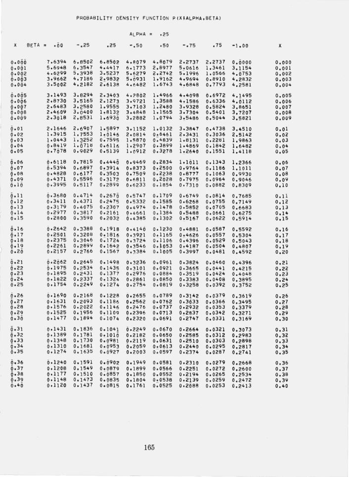
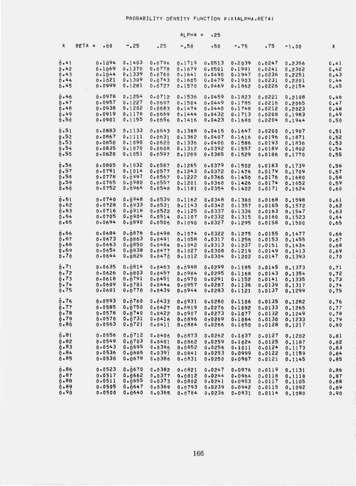
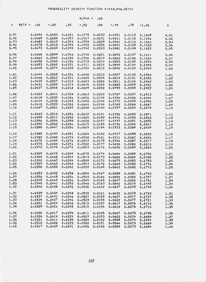
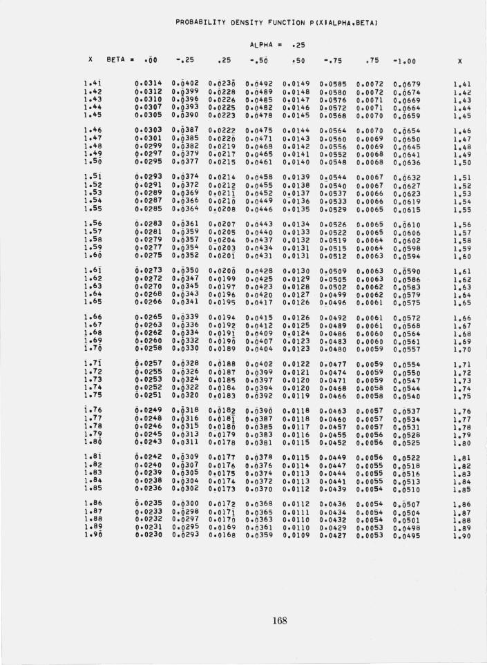
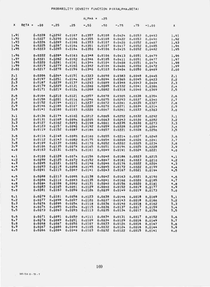
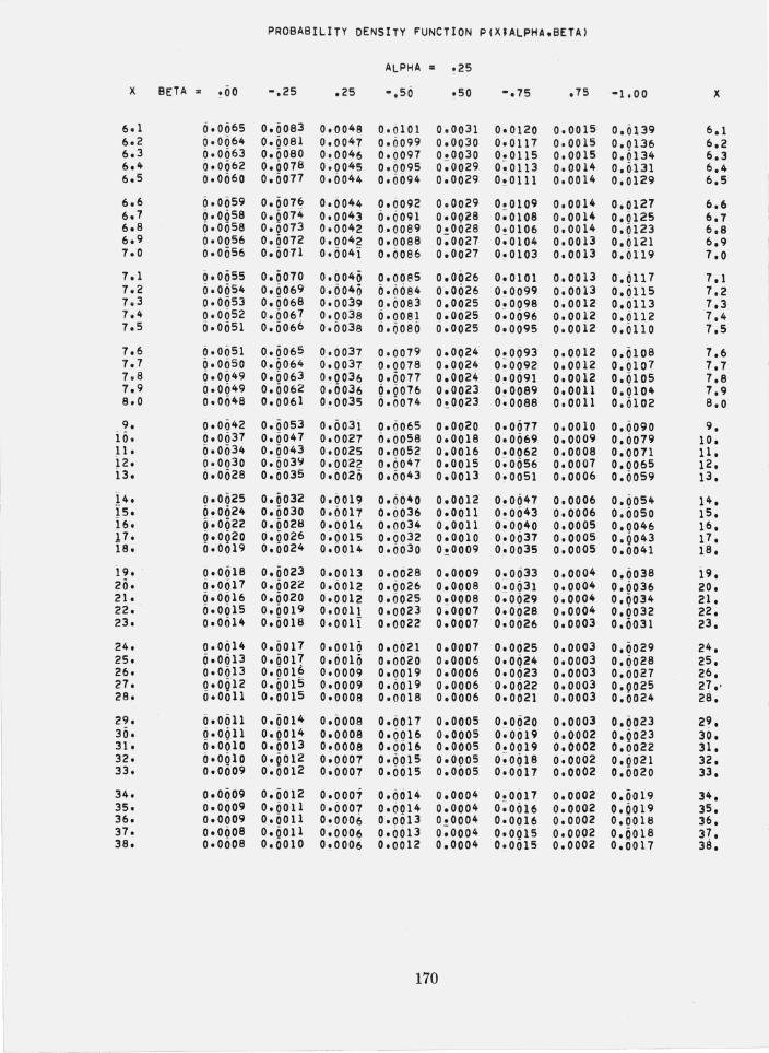
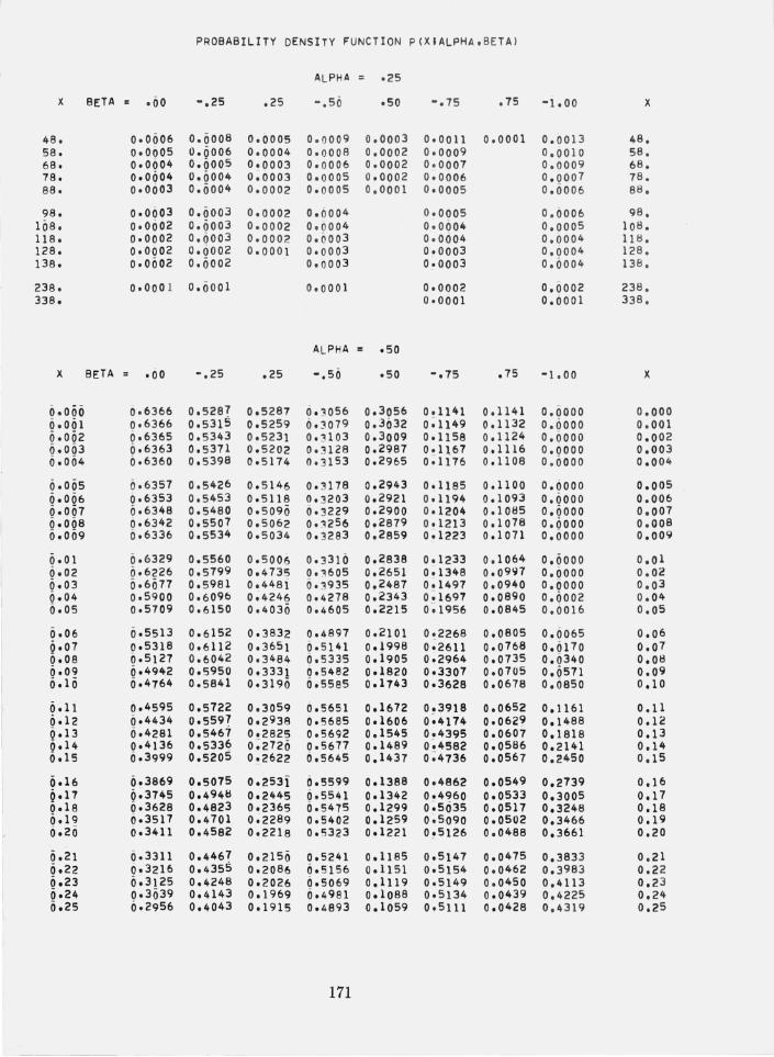
Four-decimal -place tables are presented of the probabi lity density fun ction p(x; a, {3) of the stable distribution [or a = 0.25(.25)2.00, {3 = - 1.00(.25)1.00, and nonnegative x in steps varying by factors of 10 from 0.001 to 100 such that interpo lation is possible , the tabulation being terminated where p(x; a, {3) falls to 0.0001. The largest such va lue of x is 338, for a= 0.25, {3 =- 1.00. Graphs of p(x; a, {3) are also provided for essentially the above va lues of a and {3. The methods of ca lc ulation ([rom the characte ri s ti c fun ction), checking, and interpolation with res pect to x , {3 , and (to some extent ) a are described. The most important properti es of stable distributions are summarized . Some app lica­tions are cited. A selected bib liography with 9] items is included.

Key words: Accuracy; app rox imations; asymptotic expa nsion; Cauc hy distribution ; c harac teris ti c fun ction; closed form s; contour; convergence; curves; distribution [unct ion; e rror; Fourier transform; infinite series; interpolation ; limit distribution ; normal distribution; polynomials; probability dens it y function; quadrature; stable distribution; sums of independent random variables; tables; truncation.

Contents Page

1. Introduction ' .. .. .. .... ... ...... .. . .. . . ..... . ... .. ... .. ......................... .. .. .. ..... ........... . ..... ......... .. ................ _.. 144 2. Definition and properties o[ stable distributions... .... .... .. ............. ... .. ........... ...... . ....... ... ... . ........ .............. 144 3. Applications of stable distributions. ...................... .. ...... ...... .. .. .. .. .... .. . .. ... .... ... .............. . .............. . ..... .. 150 4. Approximation o[ the stable densi ty p(x; a, {3) . .... . .................. ............ .... ......... ........ .. ..... .................... 151 5. Further asymptotic expansions of p(x; a, {3) ... ... .. ..... ... .............. ............ ..... . ................... .. .............. .... 155 6. Preparation of tables... . ......................... ....... . ....... . ... ... ....................... .......... ........... ....... .. .. .. ..... . 156 7. Checking the tables.... . .. .... ............ . .... . .. ... ....... .. . ..... ........... .. .... .. .............. . .......................... ... . .. ...... 156 8. Interpolation .... ... .... ................. .. ......... . .. ...... .. .................... ......... .. .. ........ ..................... ......... ......... 157 9. Truncation points (X,.) ....................................... ..... .... ............................. . .. .... ..... ......... ... ............. .. . 159

10. Computation of the stable (cumu lat ive) distribution function P(x; a, {3) ............ .... ... ........ ..... .................. .. . 159 11. Selected bibliography.... ..... .... . . ......... ... .. ... ........................... ................... ..... ... .. . ... .... .. .. ........... ........ 161

11.1. Theory of stable distributions............. ....... ... .... ...... .... . .. . ..... .. ... .. ... ......... ...... .. .. .. .... .. ..... .. ..... 161 11.2. Applications of stable distributions.. .......... ...... .. .. . ...... . ........ .... ............... ................ .. .... ...... .. 162 11.3. Numerical analysis ....... . .... ............. ..... ..... ........................ ... . . . ... . .. ..... ......... ... ........ .. . 163 11.4. Tables of or related to stable distributions................... .. .. .......... ... .......... . ........................... .... 164

12. Tables of the stable probabi lity density fun ction s......... .. .. .... . .......... ....... ... .. ................. .. ... ...... .. .. .. ........ 165 13. Graphs of the stable probability density fun ctions.. ...... ............................. .. ......................... .... ...... ........ 194

AMS Subject Classificution: 60 - 00. *The paper was begun when the second aut hor was employed by the National Bureau of Standards, continued while he worked for the Environme ntal Sc ie nce

Services Administration (now National O ceanic and Atmospheric Administ ration), and completed under the Office of Telecomm unications , all in Boulder, Colorado.

143

1. Introduction

The stable distributions have provided a fascinating and fruitful area of research for probability theorists and models of value in physics , astronomy, economics, and comm unications theory. The symmetric stable distributions were introduced by Cauchy in 1853 [4],1 and one of them is well known by his name. The general class was studied systematically by Paul Levy in the early 1920's [I8a, 19]. If two independent real random variables with the same shape or type of distribution are combined linearly and the distribution of the resulting random variable has the same shape, the common dis tribution (or its type, more precisely) is said to be stable. The normal, or Gaussian, distribution is the best-known example.

Th e inspiration for systematic research on stable distributions was the desire to generalize the celebrated Central Limit Theorem, which states that under fairly general conditions, the distribution func tion (df) of the sum of n independent random variables approaches (when standardized to constant median and scale) the normal df as n becomes infinite. It was known that the mean of n independent observations from a Cauchy distribution has the same distribution as a single observation , which is thus also the limit distribution as n ~ IX) and not covered by the Central Limit Theore m. It can be shown that all limit distributions of sums of independent random variables must be stable [Levy, 19; Gnedenko and Kolmogorov , 11].

The restricti ve condition of stabi lity enabled A. Ya. Khintchine and Levy in 1936 [see 11, p. 164] to d ri e the general form for the characteristic function (cf, the Fourier transform of the p obability de nsit y function (pdf)) of a stable distribution. However, the pdf itself is not known in closed form except for the normal and Cauchy types and one other type (see sec. 2.13).

The considerable interest in stable distributions makes a general set of tables of the densities and distribution fun ctions highly desirable. A table of pdf's for characteristic exponent a = 1.1(.1)1.9, 1.95, 1.99 was given by Mandelbrot and Zarnfaller in 1961 [88]. Fama and Roll [85] published tables of th e df's and fractiles of standardized symmetric stable distributions for characteristic exponent a = 1.0(.1)1. 9(.05)2.0 (as well as formulas and tables for estimatin g the parameters). Here we present four-decimal-place tables (sec. 12) of the standardized pdfp(x; a, (3) for a= 0.25(.25)2 .00, f3 = - 1.00(.25)1. 00, and nonnegative x in steps varying by factors of 10 from 0.001 to 100 such that interpolation is possible. The tabulation is terminated where p(x; a, (3) first falls to 0.0001 , correct to the fourth decimal place. The largest such value of x is 338, for a = 0.25, f3 =-1.00. Graphs of p(x; a, (3) are also provided for the above values of a and f3 (sec. 13). The methods of calculation, checking, and interpolation are desc ribed in detail (secs. 4- 8). Proba­bilities may be calculated from the tables by Simpson's Rule (sec. 10).

The theory and properties of stable distributions have been systematically presented by Lukacs [23, 24], Gnedenko and Kolmogorov [11], and Feller [44], but a brief statement, without proofs , of the most important properties, taken from these sources , especially [24], is given in section 2 for convenience. Some applications are noted in section 3. An extensive selec ted bibliog­raphy is included (sec. 11).

2. Definition and Properties of Stable Distributions

2.1. Definition.

The (cumulative) distribution function (df), P (x), of a r eal random variable X is the proba­bility that X is less than or equal to the real number x:

P(x) == Prob [X :s::: x], -IX) <x <+ IX) .

I Figures in brackets indicat e the Jjl eralure refe rences 011 pages 161 - 164.

144

(The definition of a random variable is omitted, being outside the sco pe of thi s paper.)

2.2. Definition.

Th e proba bility density function (pelf), of X is (when it ex is ts or, equivale ntly, when P (x)

is absolutely continuous) the derivative of the df:

p(x) == P' (x) == dP/dx, - 00 < x < + 00 .

2.3. Definition.

The characteristic function (cf) of X is the Fourier-Stieltjes transform of the df:

-oo< t<+ oo,

when p (x) exis ts.

2.4. The df, pdf (when it exists) , and cf are alternative and equivalent ways of describin g a proba­bility distribution, and it is at tim es convenie nt and sufficient to say " distribution " rather than df, pdf, or cf. When the pdfp(x) exists ,

1 f '" p(x) = - e- iX1cp(t)dt. 27T -00

2.5. Definition.

If X, and X 2 are two ind epend ent random variables with d/,s PI (x ) and Pdx) and c/,s CP I (t) a nd CP z (t), the n the df P( x) of the sum X == X 1 + X2 is given by the convolution of P I (x) and Pdx):

The correspondin g cf is cp(t) = CPI (t)CPz(t).

2.6. Definition .

Two df' s P(x) and Q(x) are of the same type if th ere exist a postive c and real d such that the relation Q(x) = P(( x - d )/c ) holds for aU x.

2.7. Definiti on .

A df P(x) (or any df of the same type as P(x» is stable if to eve ry C I > 0 , C2 > 0 and real d I , d z there correspond a positive c and real d such that

145

for all x. An equivalent condition for P (x) to be stable is the following: If XI and X2 are independent random variables with the df P(x), then the df of clX 1+ CtXt is of the same type as P(x) for every CI > 0, C2 > 0. Stability is really a property of the type of distribution rather than of any single distribution , but we may attribute it conveniently to a df, a pdf, or a cf also, just as we speak of the normal distribution when we mean the normal type.

2.8. A cfep(t) is stable if and only if it has the form

ep(t) = exp {idt -I ct 1"[1 + i,8(t /1 t I )w( I t I, a)]}

where - 00 < d < + 00, c ~ 0, 0< O':S; 2, -1 :S; ,8 :s; 1, and

ltan (7m/2) w(ltl,O')=

(2/7T) log I t I

for a =1= 1

for 0'=1.

(Here c is the scale parameter as in Fama and Roll [85] but not as in Lukacs [23, 24]. If the c of Lukacs is denoted by c', then c' = c".) The constant a is called the characteristic exponent.

(Unfortunately th e above definitions of w produce the heavier tail of the pdf in the positive x direc· tion for 0'= 1 and in the negative x direc tion for a =1= 1. Thus there is an apparent inconsistency in the tables and graphs.)

2.9. Degenerate distribution.

If c= 0, the stable cf reduces to that of the degenerate (improper) distribution with df

2.10. Normal distribution.

10, x < d P(x) =

1, x ~ d.

If 0'=2, the stable cf reduces to that of the normal distribution with mean d and variance 2c2 (independent of the value of ,8).

2.11. Cauchy distribution.

If 0'= 1 and ,8= 0, the stable cf reduces to that of the Cauchy distribution with median d , semi·interquartile range c, and pdf

For c = 1 and d = O this reduces to the Student t pdf with 1 degree of freedom.

2.12. The cfof the standardized variable (X-d)/cfor c> O is of the form in section 2.8 with d=O and c=l. Hereafter (except in sees. 2.24 and 2.28) we therefore take d=O and c=l and write the pdf of the standardized variable, by section 2.4, as

1 f ro p(x; 0',,8) =- e- t" cos [xt+,8t"w(t, O')]dt. 7T 0

146

2.13. ex = ~, f3 =- 1.

The n the stable cf corresponds to th e pdf

{(27T) - 1/2x - 3/2e - I/(2x)

p(x; t, -1) = o

for x > 0

for x ~ O.

This is the pdf of the reciprocal of a chi·square variable with 1 degree of freedom. It is also of Type V in the Pearson system of frequency curves. No stable distributions with pdf's that are elementary functions other than the four above are known.

2.14. Higher transcendental/unctions .

The stable densities for several rational values of ex can be represented in terms of higher transcendental functions as follows:

ex

1/3

2/3 2/3 3/2

1/2

f3

1

arbitrary

Principal/unction involved Macdonald fun ction (modified Besse l fun ction of third kind) KI /3(X) [38]

Whittaker fun ction WI /t, 1/6(X) [38; 39; 69, p. 505]

w(z) as shown in (7.1)- (7 .3) below

2.15. pC- x; ex, - f3) = p(x; ex, f3) .

Hence we tabulate p(x; ex, f3) only for nonn egative values of x.

2.16. Continuity.

All stable df's are absolutely continuous. AJl stable pdf's are continuou s.

2.17. R egularity.

The stable pdf's with ex ~ 1 are regular (analytic) for all real x and are entire functions except for the Cauchy distributions. The stable pdf's with a < 1 have the form

p(x; a, f3) = 1 (l/x)<P I (x- a)

(l/ix I)<p t (lxi - a)

where <PI (z) and <P2 (z) are entire functions.

2.18. Derivatives.

for x> 0

for x < 0

Derivatives of the stable pdf's with respect to x of all orders exist for all real x. They are bounded according to

I a"p(x; ex, f3) I ~ ~ r (n+ 1). ax" 7Ta ex

147

2.19. U nimodality.

All stable pdf's are unimodal.

2.20. Symmetry.

A stable pdf is symmetrical if and only if {3 = O.

2.21. Convergent infinite series.

The stable pdf's have convergent infinite series representations. Let x > 0 , 'rJ = {3 tan (Trex/2) , r= (l + 'Y/2) - I/ (2a), and y= - (2/Tr) arctan TJ. Then the pdf of the standardized variable evaluated at the abscissa rx is , for 0 < ex < 1,

1 00 (-I)k - l . . [kTr ] p(rx; ex, (3)=-L k

' r(ak+l)x- a k sm -2 (a+y) ,

Trrx k = 1 •

and for 1 < ex ~ 2,

1 00 (-I)k - ' (k) [kTr ] p(rx;ex,{3)=-L k'

r -+1 xksin 2-(ex+y)' TrrX k = 1 • ex ex

A series in powers of x exists for a = 1, but the coefficients are expressed only as complicated integrals.

2.22. Asymptotic series.

Asymptotic series are available for x in the neighborhood of 0, + 00, or - 00 and exhaustive ranges of values of ex and {3. In particular the first n terms of the first series in section 2.21 is an asymptotic approximation for x ~ + 00 and 1 < a < 2. Likewise the first n terms of the second series in section 2.21 is an asymptotic approximation for x ~ 0 and 0 < a < 1. (Note the interchange in the ranges of a from those for convergence in sec. 2.21.)

2.23. x = 0, a =t= 1.

By changes of variable in section 2.12 with x = 0 and a =t= 1 we obtain gamma functions and consequently

with y as in section 2.21. In particular

. 1 (1) ( Try)I/Q p(o · ex , (3) =- r - cos-, Trex a 2

p(o; ex, 0) =~ r (!); Tra a

p(O;a, ± l) = O, a < l;

148

Try cos 2ex'

2.24. Interrelation for a and a* = l/a.

It is convenient to consider a stable pdf of the nonstandardized variable Y=X/c, where c=[cos(1Ty/2)]I/a with y as in section 2.21. Let l <a";;: 2, a*=I/a, y*=(y+a - l) /a, and P aY (y) be the pdf ofY. Then for y > 0

2.25. Z ero values of pdf's.

If 0 < a < 1 and y = - a, then it follows from the first form ula in section 2.21 th at

p(x; a, 1) =0 for x > O.

From section 2.15

p(x; a, - 1) = 0 for x < 0 and 0 < a < 1.

2.26. Infinite divisibility.

A stable cf is infinitely divisible; i. e ., for every positive intege r n it can be expressed as the nth power of some cf. Equivalently we can say that for every positive integer n a stable df can be expressed as the n· fold convolution of some df.

2.27. Moments .

The absolute moment of order I) of a df P(x) is defined as

when p (x) exists. Every stable df with characteristic exponent a with 0 < a < 2 has finite absolute moments of all orders I) with 0 < I) < a, whereas all absolute moments of order I) ~ a are infinite. Thus the normal df's are the only stable df's with finite variance. The mean exists for 1 < a";;: 2, but neither the mean nor the variance exists for 0 < a";;: 1.

2.28. Location and scale parameters of a linear combination.

If Xl. X 2 , • •• , XI! are independent random variables with stable distributions of the same type (and therefore with the same a and {3), location parameters dl. d 2 , ••• , d n , and scale paramo eters c l. C2, • , C n respectively, then the linear combination

" Y= L a;Xj, aj ~ 0, 1= 1

149

has, from sections 2.3, 2.5, and 2.8, the location parameter

n

d= L aidi i=1

and scale parameter c given by

i = 1

The last equation is familiar for a = 2, the normal distribution, but is not so well known for other a. In particular, if all d i = d I, Ci = CI, and ai = 1/ n, so that Y is the sample mean X, then

C] c= . 1'

Vn a = 2 (normal)

a = 1 (Cauchy if (3 = 0)

1 a = 2 (Pearson Type V if (3 = - 1)

Thus the scale parameter (as well as the entire distribution) for a = 1 is the same for X as for X I, - 1

but the scale parameter of X for a = 2 (and aU other a < 1) increases without limit as n ~ 00.

2.29. Importance in limit distributions.

Let Z I, Z 2,· . " Z II, ••• be independent and identically distributed random variables. Let

1 n Vn=s L Zi-AII,

II ;= 1

n = 1,2 , ... ,

where AI, A 2 , ••• and 8 1,82 , •• • , Hi > 0, are sequences of constants. A well·known Central Limit Theorem states that if the Zi have a finite variance then the sequence of df's of the VII con· verges to the standardized normal df for suitable choices of the A i and 8 i. The normal df is not the only possible limit df for the Vn in general, however: In order that a df be the limit df of a sequence of df's of V" it is necessary and sufficient that it be a stable df.

3. Applications of Stable Distributions

Beyond the pervasive occurrence of the normal distribution in practice as well as in theory , the primary interes t in the stable distributions arises in probability theory as a result of their remarkable th eoretical properties. However, they have also been applied in a wide variety of scien· tific fields , as indicated by the substantial but quite incomplete appended bibliography on applica­tions. Feller's Volume II [44] discusses applications to the gravitational field of stars (Holts mark distribution, a = 3/2; cf. Holtsmark, [48]), first-passage times in Brownian motion (a = 1), diffusion theory, and economics.

Benoit Mandelbrot has discussed many applications in economics, including the distributions of income and of speculative prices and relating stable distributions to the well-known Pareto distributions [53-59, 61, 63]. He has also found stable distributions in biology [51 ,62], psychology

150

[52], and electrical engineering [60]. The occurrence in economics or business is also discussed by Press [66], Roll [67], Teichmoeller [68], Granger and Orr [47], and Fielitz and Smith [4S].

The interes t in economics led to the tabulation of the cdf's and fractiles of the symmetric stable distributions for ()'= 1.0 (.1) 2.0 by Fama and Roll [85] and to estimation of parameters and tests of hypotheses by them [86] and by Press [28]. A manuscript including the cdf's for certain asym· metric stable distributions (f3= -1 (.2S)0) for ()'= 1.1 (.2) 1.9,2.0, as well as graphs of the corre­s ponding pdf's for ()'= 1.1 (.4) 1.9, has just been sent to us by M. J. Cross [84].

The infinite divisibility of the stable distributions accounts for their occurre nce in the theory of s tochastic processes with stationary indepe ndent increm ents; see Feller [44, Vol. II] , Kolmogorov and Sevast'yanov [SO] , Kac [14], Berman [41] , Getoor [10]; Greenwood [12], Kesten [IS, 49 1, and Lukacs [2S].

Other occurrences in electrical engineering are indica ted by Dobru shin [42] and by Ovsevic a nd Yaglom [65].

4. Approximation of the Stable Density P(Xi a, fJ)

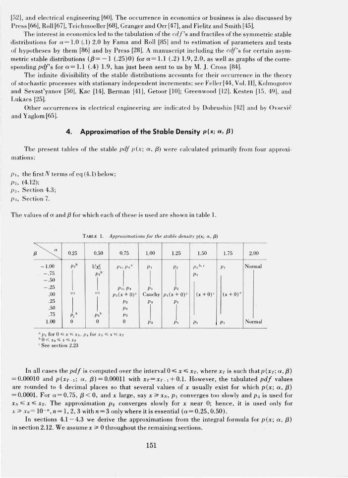
The present tables of the stab le pdf p(x; ()', (3) were calc ulated primarily from four approxi· mations:

PI, the firs tN terms of eq (4. 1) below; P2, (4.12); Pa , Section 4.3; P4, Section 7.

The values of ()' and f3 for which each of these is used are s hown in table 1.

TABLE 1. Approximations for the stable density p(x; n , f3)

~ 0.25 0.50 0.75

- 1.00 P2b l /;f, PI, P4 a

- .75 b '

I P2

-.50

I - .25 p" p. .00 (e) (e) P2(X * o) e .25

I b I

P2 .50 P2 .75 P2 I P2b P2

1.00 0 0 0

a PI for 0 '" x '" X.v, P. for x .v '" x '" X7' b 0 < Xo '" x '" X'f

e See section 2.23

1.00 1.25 1.50

PI

PI' P:l.b . c

I PI

PI P2 Cauchy PI(X * o) e (x * o) e

p" PI

I I P3 PI PI

1.75 2.00

PI Norm al

(x * 0) e

PI Normal

In all cases the pdf is computed over the interval 0,,;; x,,;; XT, where XT is such thatp(xT; ()', (3) =0.00010 and P(XT - I; ()', (3)=O.OOOll with XT=XT- I+O.1. However, the tabulated pdf values are rounded to 4 decimal places so that several values of x usually exist for which P (x; ()', (3) = 0.0001. For ()' = 0.75 , f3 < 0, and x large, say x "'" XN, PI converges too slowly and P4 is used for XN";; x ,,;; XT. The approximation P2 converges slowly for x near 0; hence, it is used only for x"'" Xo= lO - n , n = 1,2,3 with n = 3 only where it is essential «()'= 0.2S, 0.50).

In sections 4.1- 4.3 we derive the approximations from the integral formula for p(x; ()', (3) in section 2.12. We assume x"'" 0 throughout the remaining sections.

151

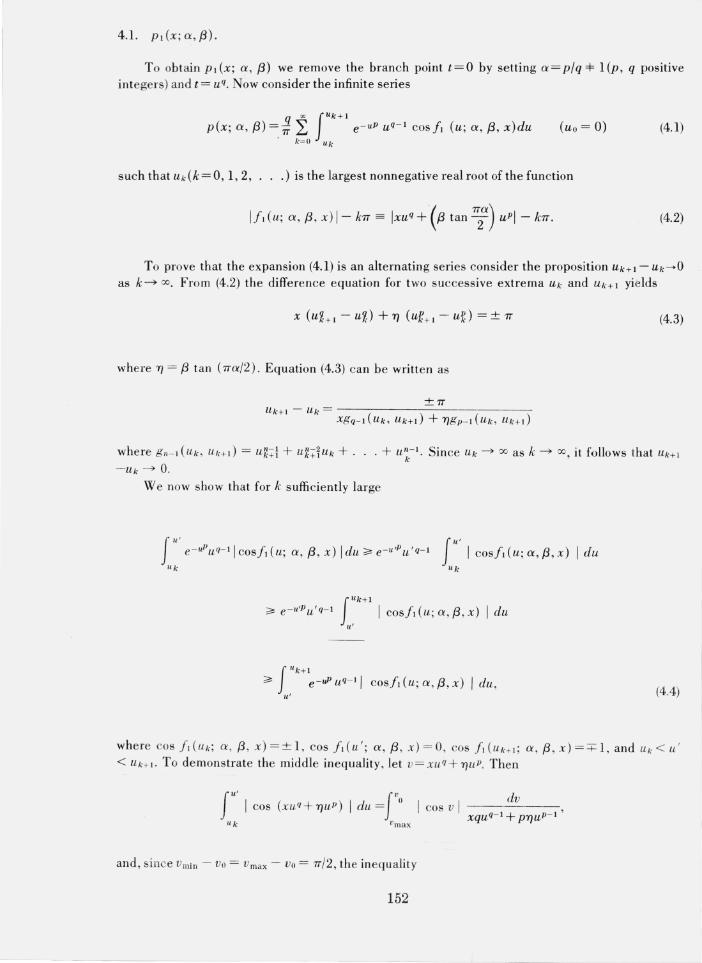
4.1. PI(x;a, {3 ) .

To obtain P I (x ; a , {3) we remove the branch point t = 0 by setting a = pi q +- 1 (p , q positive integers) and t = uq. Now consider the infinite series

q " j U k+ l p(x; a , {3) =,1i L e- uP UQ - I COS!I (u ; a , {3, x)du

k =O Uk

(U O = 0) (4.1)

such that Uk (k = 0, 1,2, . . .) is the largest nonnegative real root of the function

(4.2)

To prove that the expansion (4.1) is an alternatin g series consider the proposition Uk +l- Uk ..... O as k~ 00. F rom (4.2) the difference equation for two successive extrema Uk and Uk +1 yields

(4.3)

where TJ = {3 tan (1Ta/2) . Equation (4.3) can be written as

where gn- I ( Uk , Uk+ d = u~+ l + U~+TUk + . . . + Un- I . Since Uk ~ 00 as k ~ 00 , it follows that Uk+1 k

- Uk ~ O.

We now show that for k sufficiently large

J"' I cos!l(u;a,{3 , x) I du Uk

JUk+1

~ e-u'Pu'q- 1 I COS!I ( u ; a, {3 , x ) I du u'

(4.4)

where cos !I (U k; a , {3 , x) =± 1, cos ! I ( u '; a, {3 , x) = 0, cos !I ( U k+I; a , {3 , x ) ==t= 1, and U k < u ' < Uk+ l . To de monstrate the middle inequality, le t v = xuq+ TJ uP. Then

jU' I cos (xuq+ TJUP ) I du = fo Uk Vmax

and, since Vmin - Vo = Vrnax - Vo = 1T/2, the inequality

152

- ----- -----------

dv I cosvl ----------­xquq- I + PTJUP- I '

is true. Thus (4.4) is es tablished. S ince both the integrand and the interval Uk+ 1 - Uk approach zero as k ~ 00 , so also does the k th term of the seri es (4 .1).

Similarly when 0' = 1 we have the infinit e series

1 " Jtk + 1 P (x; 1, /3) =; L e - t cosh (t ; /3 , x )dt

k = 0 t k

( to = O) (4.5)

such that tk is the largest nonnegative real r oot of the equation

(k = O, 1, .. . ). (4.6)

It is easy to show that t k + 1 - tk ~ 0 as k ~ 00 b)l substituti ng the expansion

into the difference equation

He nce we have

Since tk ~ 00 as k ~ 00, it follows th at t"+ 1 - t A-~ O. The fact that (4.5) is a n alte rnatin g se ries follows in the same way as in establishing (4.4). The approximation PI (x; 0', f3) is the truncation of (4.1) and (4.5) to N terms with the Nth te rm

the first term not greate r than 10 - 5 in magnitude.

The zeros Uk and tk are computed via the Newton-Raphson (NR) and False Posi tion (FP) root-finding procedures. T he NR procedure is used in the following cases , for which the necessary sign conditions ce rtainly hold :

3 0' = 2' - 1 < /3 < 0

7 0'= 4> /3 < 0

o < Xu < x ,s; X T .

In the remaining cases the FP procedure is applied.

153 507-714 0 - 73 - 6

Determining the initial values, say Uk ,O and tk,o, for the NR and FP procedures in the presence of arbitrary fixed (x, a, j3) requires a little care. For the NR procedure the following initial values were used:

UO(Xi) = 0, Uk ,O(XO) = 1 (k = 1,2, ' ,), (4.7)

(i=O,I, .. . )

where Uk (x;) is the root of eq (4.2) with x = Xi.

A table of initial values for the FP procedure is available on request. We denote the kth integral of (4.1) (i.e., not including the factor q/w) by T k, normalize the inter·

val of integration to [- 1, 1], and approximate Tk• by 48-point Legendre-Gaussian quadrature. Hence, the quadrature representation becomes

48

Th· ='= Ah· L HjWJh-: le - wf, cos (XWJk + 7jWYk), j=1

where Hj and Vj are Gaussian weights and abscissas respectively [79, p. 30].

(4.8)

The approximation for (4.5) parallels the approximation for (4.1); hence we omit that formulation. Although the approximation p, (x; a, f3) may be used for any given (a, j3, x), experience showed

that the other approximations below required less computer time for the desired accuracy over certain ranges of a, j3 , x as shown in table 1.

Consider the contour integral

WI f exp [- wa + i(xw +7jw a ) ] dw c

(a=l=l) (4.9)

taken on the path in figure 1. Along the taxis (4.9) reduces to p (x; a, j3) in the limit as E ~ 0 and R ~ 00. The integral along

C" say II, is bounded by

1111:;;;; R { /2 exp [-Ra(cos aO+7j sin aO) -xR sin O]dO. (4.10)

Hence, I, ~ 0 as R ~ 00, The contribution on C 2 goes to zero as the branch point is approached, and consequently, equating real parts yields

(4.11 )

where D, ~ 0 is sufficient for the integral to converge (D, > ° for x= 0).

154

Employin g the transformation tl !Q= u in (4.11 ), applying 48-point Legendre-Gaussian quadra­ture between each extre mum pair of the fun ction sin D2Ui' and normalizing the jth interval to [- 1, 1] yields the approxim ation

P2 (x ; a, f3) =; (2~Jq!P ~ Clk {~ HjZJk-:1 . exp {- [x (2~J!P ZJk + ~;: Z)k.]} sin ~ Z)k (4.12)

where

k= 1, 2, . . . , N ,

CIO=CZO=t,

Hj and Vj are Gaussian weights and abscissas respectively, and N is determined so th at the N th term is the firs t term not greater than 10- 5 in magnitude.

4.3 P3(X; I , f3) .

Using a differe nt contour integration, Skorohod [32 , p. 161] obtained a useful altern ati ve integral form ula for a = 1:

1 t OO p (x; 1, f3 )=- exp [-xu - (2 /1T)f3ulnu] sin [(l+f3)u] du. 1T 0

(4. 13)

The a pproxim ation P3(X; 1, f3) is obtained by applying the 48-point Legend re-Gaussian quadrature fo rmula to each term of the convergent altern atin g se ries arising from (4. 13) whe n it is divided at successive extre ma of sin (l + f3 )u.

5. Further Asymptotic Expansions of p(x; a, fJ)

A double seri es expansion of the product exp (- Dlte<) sin D2 t e< in (4.11 ), an interchange of integration a nd summation, and the application of Watson's le mma yields

) 1 ~ ~ (-l) k+ l DkD21 +! f[(k+2l+1)a+l] ( ;;6 1) p{x;a , f3 - ; k~0 ,~ok!(2l+1) ! I 2 X( J.-+2 1+ J) e<+ 1 a (5.1 )

as x~ 00 .

Expanding the integrand of (4.13) yields

P (x; 1, (3) = 1[ (l + f3) ( 00 e- X1 tdt - 2f3 (1 + f3) ( oo e- X1t2 In dt 1T Jo 1T Jo

(5.2)

155

With the aid of integral tables [74, pp. 576-578] we obtain the incomplete asymptotic expansion

+ [1;; 2 (1 + f3){ [ t/I ( 4) - In x)2 + ~ (2, 3) } - (1 + 13) 3 ] x\

+ [8(1 + 13)313 [t/I(5) -In x] - 25~3 (1 + f3){ [t/I(5) -lnx)3 7T 7T

1 + [2t/1 (5) - 3 In x H (2, 4) - 2 ~ (3, 4) } ] 5' x ~ CXl, X

(5.3)

which is valid for 13 > o. The symbols t/I and ~ represent the digamma and generalized Riemann zeta functions

dlnf(z) '" 1 t/I(z)= dz and~(z,q)= L ( +n)z·

I/ = () q

6. Preparation of Tables

To tabulate pdf values computer -programs were prepared from the various approximations. Since values of the pdf were both printed and punched, the two sets of values were compared to safeguard against mechanical errors. In the vicinity of the maximum of each pdf we employed a variable mesh size in the x direction which depended on Idp(x; a, f3)/dxl. Hence, for a""::: t, ~x=O.OOI, 0.01, or 0.1; for a=i, ~x=O.Ol or 0.1; and for a ~ 1, ~x=O.l. On the pdf tails most of the original values with a mesh size ~x= 0.1 were discarded in favor of linear interpolation with steps ~x= 1, 10, or 100. Consequently, after reading all pdf values into the computer , we deleted unnecessary values, rounded the remaining ones to four decimal places , and punched the results on cards. After some trial and error the appended printout (reduced in size) was ob· tained from the punched cards.

7. Checking the Tables

In addition to the previous cross checking, the appropriate approximations, closed forms, and special values were compared. We also made spot checks by using

(a) Pl(X; 1,13) overf3>O;

(b) P5(X; J. f3) over 13 > 0, for large values of x near XT;

(c) P4(X; a, 13) over a =1= 1, 13 < 1 for large values of x near XT;

(d) P6(X; a, 13) over a =1= 1, for values of x near 0.

Approximation P5(X; 1,13) is the truncation of the asymptotic expansion (5.3), two terms of which were generally required for agreement with the tabulated pdf values. The approximations P4(X; a, f3) and P6 (x; a, 13) are the truncations of the first and second expansions of section 2.21 reo spectively. (See sec. 2.22 for asymptotic properties of the two expansions of sec. 2.21.)

156

By use of the followin g eq uations of V. M. Zolotarev [38, p. 166], an additional check is availab le for a = t. He showed that

(7.1)

where 1+,8-i(1-,8)

z= 2v'2x

(7.2)

By setting w(z) =u(p,-q) + iv(p , - q) and z=p-iq we obtain

( 1) 1 [ " 1 - ,82 1 - ,82 2 ] p x;-,,8 =- (2X)-3/2e-{3 /(2X) (1+,8) cos--+(l-,B) sin---- (qu-pv) . 2 171/2 4x 4x lTX

(7.3)

Karpov [78] tabulates u and v from w(pe ilJ ) . Checking of several tabulated pdf values correspond­ing to ,8 = 0.25 and ,8 = 1 reveals no error in our tables greater than 10- 4 •

Many of the tabulated values of p (x; 1.5, ± 1) were checked with values found in a report by Mandelbrot and Zarnfaller [88] ; no discrepancy was found. A check is also available from Fama and Roll 's [851 4-place table of cdf's for,8= 0 and a= 1.0(0.1)2.0; see section 10.

To detect blunders which escaped the preceding checks, pdf values from the punched cards were subjected to differencing of orders 1 through 12. Mille r [80"1 states that blunders may occur when sixth and tenth difference magnitudes greater than 22 and 300 respectively appear. Using this technique un covered several entries which were Dbvious ly erroneous.

8. Interpolation

8.1 Interpolation with respect to x.

To reduce the size of the table of pdf values it is necessary to establish appropriate degree interpolation polynomials over certain intervals of x for each p (x; a, ,8). We justify this interpola­tion by noting the analytic properties of p (x; a, ,8).

For a;:;: 1, (except a=1 and ,8 = 0), p(x; a,,8) is an entire function of xfsec. 2.171. Hence, a sequence of interpolating polyn omials {PII (x)} con verges uniformly to p (x; a, ,8) over a given closed interval [71]. For a < 1, Idp(x; ct, ,8)/dxl becomes large at or near x= O. Therefore, inter­polation over [0 , xs], for some small Xs is difficult. However, away from x=O, p(x; a, ,8) is an analytic func tion even for a < 1 [23], so that some {PI! (x)} provides interpolation for p (x; a, ,8) for x > Xs.

The Lagrange interpolation polynomial for n equally spaced abscissas x," and corresponding ordinates fA- is represented by

f(xo+ph) = L AA'(p)fA-+R II - 1 (7.4) A-

where the index k is defined via the inequalities

-t(n - 2) :,;:; k :,;:; n/2 (neve n),

The coeffi cients AI.'(p) are defined in [69, p.878] and tabulated in [69, pp. 900-913]. We computed a sample of 150-300 pdf values with ,1x = 0.01 (in contrast with ,1x = 0.1 for the tabu­lated pdf values) around the maximum of each c urve for a ;:;: 1 and applied the Lagrange formula

157

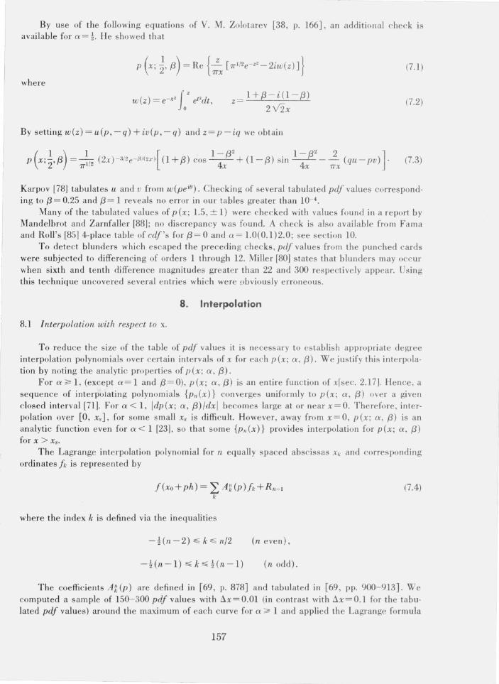
with n=2(1)8; p=O.l, 0.5, 0.9; h=O.l; and sliding intervals beginning with 0.00, 0.01, 0.02, .... The interpolated points were compared with the computed points and all errors (E) were tallied and classified according to the magnitudes:

(b) 10-4 > lEI ::?; 0.5(10- 4 ), (c) 0.5(10-4 ) > lEI. An example below (table 2) illustrates this scheme: a = 1, /3 = - 0.25, 154 points starting at x = 0.00, i.e., 0.00 ~ x ~ 1.53.

TABLE 2

p Degree of Number of Interval containing Number of Interval containin g

interpolation errors in (a) errors in (a) e rrors in (b) errors in (b)

0.1 2 to 7a 0 0 -0.5 2 8 [0.57, 0.72] 36 [0.45, 0.88] 0.5 3 to 7 0 0 0.9 2 0 1 0.9 3 to 7 0 0

a That is, each degree from 2 to 7 was used, and none of the formulas yielded any errors.

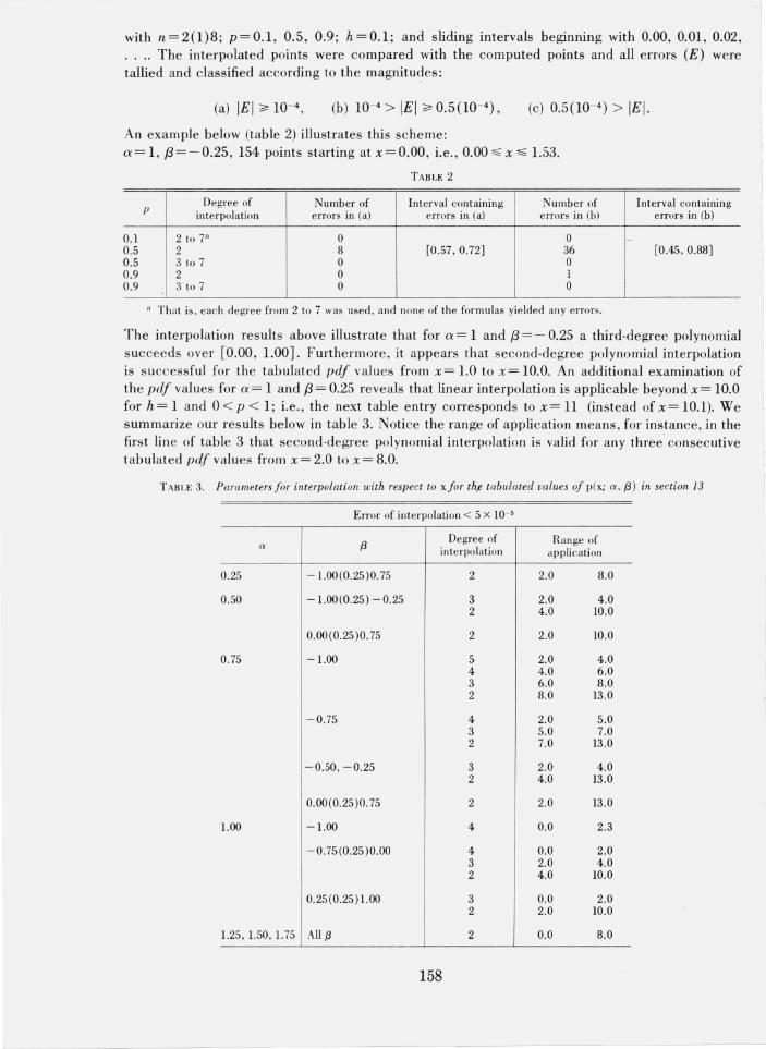
The interpolation results above illustrate that for a = 1 and /3 = - 0.25 a third-degree polynomial succeeds over [0.00, 1.00]. Furthermore, it appears that second-degree polynomial interpolation is successful for the tabulated pdf values from x = 1.0 to x = 10.0. An additional examination of the pdf values for a = 1 and /3 = 0.25 reveals that linear interpolation is applicable beyond x = 10.0 for h= 1 and 0 < P < 1; i.e ., the next table entry corresponds to x= 11 (instead of x= 10.1). We summarize our results below in table 3. Notice the range of application means , for instance, in the first line of table 3 that second-degree polynomial interpolation is valid for any three consecutive tabulated pdf values from x = 2.0 to x = 8.0.

TABLE 3. Parameters for interpolation with respect to x for thl! tabulated values of p(x; a , (3) in section 13

Error of interpolation < 5 X 10- 5

a f3 Degree of Range of

inte rpolation application

0.25 -1.00(0.25)0.75 2 2.0 8.0

0.50 -1.00(0.25) - 0.25 3 2.0 4.0 2 4.0 10.0

0.00(0.25 )0. 75 2 2.0 10.0

0.75 -1.00 5 2.0 4.0 4 4.0 6.0 3 6.0 8.0 2 8.0 13.0

-0.75 4 2.0 5.0 3 5.0 7.0 2 7.0 13.0

-0.50 , -0.25 3 2.0 4.0 2 4.0 13.0

0.00(0.25 )0. 75 2 2.0 13.0

1.00 -1.00 4 0.0 2.3

- 0.75 (0.25 )0.00 4 0.0 2.0 3 2.0 4.0 2 4.0 10.0

0.25 (0.25) 1.00 3 0.0 2.0 2 2.0 10.0

1.25, 1.50, 1.75 All f3 2 0.0 8.0

158

8.2. Interpola tion with respect to f3.

The accuracy of polynomial interpolation with res pect to f3 was estim ated from the re mainder formulas for Lagrangian interpolation in the Handbook of Mathematical Functions [69, sec. 25.2, pp. 878- 879]. The accuracy was also tested by extensive application of Lagrangian interpolation to the tabulate d pdf values using the interval on f3 of 0.50 to interpolate the pdf values at the mid­points of intervals and co mparing with the corresponding tabulated values. We conclude that:

(a) p(x ; a, (3) can be obtained accurate to 3 or 4 decimal places (DP) by at least one of 2-,3-, or 4-point Lagrangian interpolation with respect to f3 (using coefficients given in the Handbook [69, table 25.1 , pp. 900- 903]) for all f3 for the tabulated a's and any x not too near to 0.0.

(b) Higher than 4-point interpolation may not necess arily improve the accuracy since higher­order differences often do not decrease in magnitude.

(c) p(O; 0', (3) for (0', (3) not in the table should always be calculated from the closed formula, section 2.23 (not applicable for 0' = 1).

Rule (a) cannot be eas ily s tated more quantitatively. For sufficiently large x linear interpolation with res pect to f3 yields 4 DP acc uracy (i. e., within 1 unit in the 4th DP). As x decreases , higher­degree interpo lation is required for the sa me accuracy. For exa mple, for 0' = 0.25 linear inte rpola­tion yields 4 DP accuracy for x ~ 1.00 but cu bic is in ge neral needed (and is suffi c ient) for x = 0.10. For 0'= 1 quadratic interpolation yields 4 DP accuracy for x ~ 2.0, but only 3 DP can be attain ed for x = 0.5, even if c ubic or quartic interpo la tion is used.

8.3. I nterpolation with respect to 0' .

Interpolation with respect to 0' was investi gated in the same way as th at with res pect to f3. Unfortunately the results are mostly negative because there a re as many ~s three local max im a with res pect to 0' for tab ul ated values of f3 =1= 0 and x_ We co nclude that:

(a) For f3 = 0, lin ear quadratic, or c ubi c interpolat ion with res pect to 0' yields 3 DP accuracy [or x ~ 1.0.

(b) For f3 =1= 0 quadratic interpolation may yie ld 2 DP or 3 DP accuracy for 0' > 1.50, but inte rpolation is unre li able for 0' < 1.50.

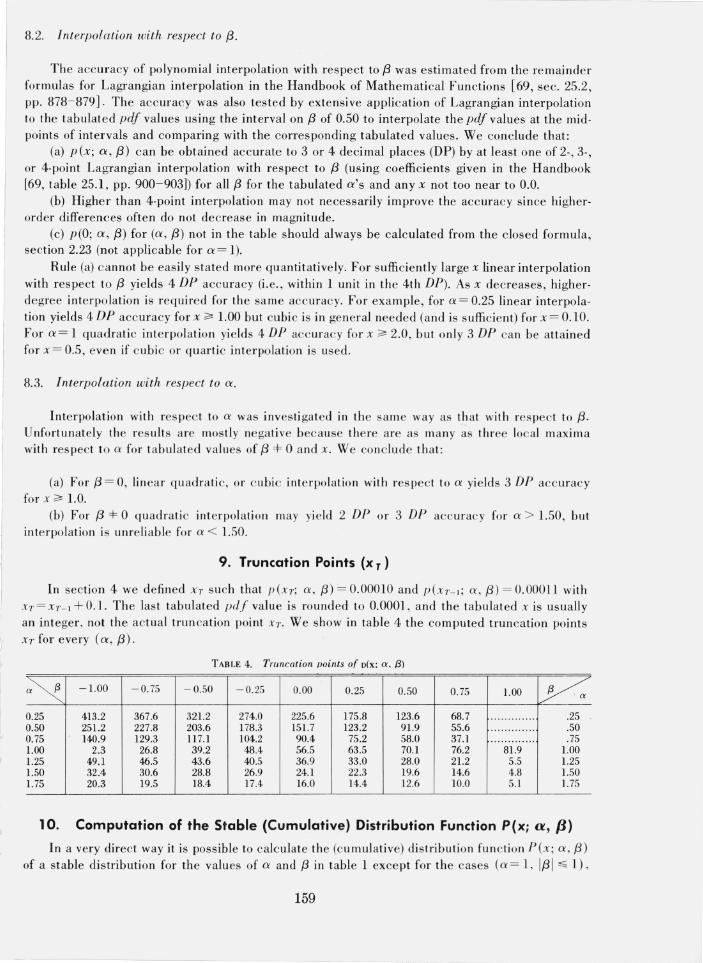
9. Truncation Points (x T )

In section 4 we defin ed XT such that P( XT; 0', (3 ) = 0.00010 and P( XT- l; 0' , (3) = 0.0001l with x'/' = XT - l + 0.1. Th e last tabulated pdf value is rounded to 0.0001 , and the tabulated x is usually an integer , not th e actual trun cation point x,/, . We show in table 4 the co mputed trun cation points x'/' for every (a, (3 ).

TABLE 4. Truncation points of pix: a , {3)

~ -1.00 -0.75 - 0.50 - 0.25 0.00 0.25 0.50 0.75 1.00 y< 0.25 413.2 367.6 321.2 274.0 225.6 175.8 123.6 68.7 . . . . . . . . . . . . . .25 0.50 251.2 227.8 203.6 178.3 151.7 123.2 91.9 55.6 ...... . .. . .. . .50 0.75 140.9 129.3 117.1 104.2 90.4 75.2 58.0 37.1 .. .. ...... ... .75 1.00 2.3 26.8 39.2 48.4 56.5 63.5 70.1 76.2 81.9 1.00 1.25 49.1 46.5 43.6 40.5 36.9 33.0 28.0 21.2 5.5 1.25 LSO 32.4 30.6 28.8 26.9 24.1 22.3 19.6 14.6 4.8 1.50 1.75 20.3 19.5 18.4 17.4 16.0 14.4 12.6 10.0 5. 1 1.75

10. Computation of the Stable (Cumulative) Distribution Function P(x; a, Il) In a very direct way it is possible to calculate the (cumulative) distribution fun ction P(x; 0', (3)

of a stable distribution for the values of 0' and f3 in table 1 except for the cases (0' = I, 1f31 ,;;; 1) ,

159

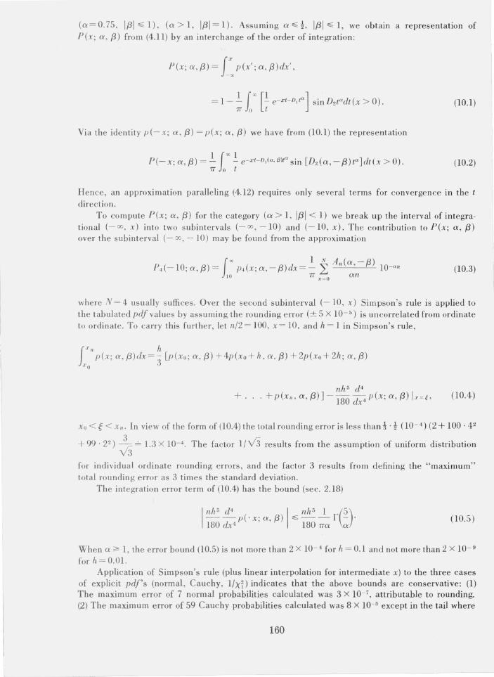
(a=0.75, 1131';:;1), (a>l, 1131=1). Assuming a.;:;t, 113 1';:;1, we obtain a representation of P(x; a, f3) from (4.11) by an interchange of the order of integration:

P(x;a,f3)= f"p(x l ;a,f3)dx l,

=l - l.f '" [le - xt - D,ta ] sin D2tadt(x>0). 7r 0 t

Via the identity p(- x; a, 13) = p(x; a, 13) we have from (10.1) the representation

1 f '" 1 P(-x; a, f3) = - - e-xt- D ,(a,{3)ta sin [D2 (a ,-f3) ta ]dt(x > 0), 7r 0 t

(10.1)

(10.2)

Hence, an approximation paralleling (4.12) requires only several terms for convergence in the t

direction. To compute P(x; a, f3) for the category (a> 1, 1131 < 1) we break up the interval of integra·

tional (- 00, x) into two subintervals (-00, -10) and (-10, x). The contribution to P(x; a, 13) over the subinterval (- 00 , - 10) may be found from the approximation

f'" 1 N A,,(a, - f3) P4 (-10; a, f3) = P4(X; a, - f3)dx = - L lO- a "

10 7r 11 = 0 an (10.3)

where N = 4 usually suffices. Over the second subinterval (-10, x) Simpson's rule is applied to the tabulated pdf values by assuming the roundi ng error (± 5 X 10- 5 ) is uncorrelated from ordinate to ordinate. To carry this further, let n/2 = 100, x = 10, and h = 1 in Simpson's rule,

Jx " h p(x ; a , f3)dx = - [p(xo; a, f3) + 4p(xo+ h, a, f3) + 2p(xo+ 2h; a, f3)

Xo 3

(l0.4)

Xo < ~ < XII' In view of the form of (10.4) the total rounding error is less than t . t (10 - 4) (2 + 100 .42

+ 99.22 ) ~ == 1.3 X 10- 4 . The factor 1/V3 results from the assumption of uniform distribution V3

for individual ordinate rounding errors , and the factor 3 results from defining the "maximum" total rounding error as 3 times the standard deviation.

The integration error term of (10.4) has the bound (sec. 2.18)

I nh 5 d 4 I nh 5 1 (5) --p('x;a,f3) .;:; - -f - . 180 dx 4 180 7ra a

(l0.5)

When a ~ 1, the error bound (10.5) is not more than 2 X 10- 4 for h = 0.1 and not more than 2 X 10- 9

for h = 0.01 . Application of Simpson's rule (plus linear interpolation for intermediate x) to the three cases

of explicit pdf's (normal , Cauchy, l/Xn indicates that the above bounds are conservative: (1) The maximum error of 7 normal probabilities calculated was 3 X 10- 7, attributable to rounding. (2) The maximum error of 59 Cauchy probabilities calculated was 8 X 10- 5 except in the tail where

160

the steps in x become 10, and then the maximum error was 3 X 10- 4 • (3) The maximum error of twelve l/xH 0' = 0.5, (3 = -1) probabilities was 1.3 X 10-5 for x in steps of 0.01 and 3.6 X 10 - 5 for x in steps of 0.1.

Values of cd/for 0'=1.5, {3 = 0, as well as the above ones for 0'= 1, {3 = 0 and 0'=2, were derived for comparison with Fama and Roll' s [85] 4-place table for cdf' s for (3 = 0 and 0' = 1.0(0.1 )2.0. In 39 comparisons there was only one difference (3) greater than 1 in the 4th place.

The rather dense grid of values of x, as fine as 0.00l for the largest pdf values , is an important contributor to the accuracy of calculation of probabilities. We conclude from the above that prob­abilities can be calculated by Simpson's rule plus linear interpolation with maximum error of 3 X 10- 4 for 0' ~ 1. For 0' < 1 we have no rigorous error bound and the errors tend to be larger than for 0' ~ 1, but calculated probabilities may well have satisfactory accuracies comparable to those above.

The authors thank Garney Hardy 2 and Matthew Lojko 3 of NBS for computer programming support. Stephen Jarvis , Jr. , and John Sopka of NBS were especially helpful in their encourage­ment of this project.

11. Selected Bibliography

A few listed works, FeIle r 's books in particular, may have materi al in more th an one of the following four ca tegories , but each is li sted only once. Several Russian papers have English trans lation s in "Selec ted Translations in Mathematical Sta ti sti cs and Probability", published for the Institute of Mathematical S tatistics by the American Mathematical Society, Providence, Rhode Island . Th ese are iden tified be low as AMS·IMS.

11 .1. Theory of Slable Dis!ri bILlions

[1) Bergstrom, H., On some expa nsions of stable distribution functions , Ark. Mat. 2, 375- 378 (1952). [2] Be rgstriim, H., On distribution fun ctions with a limiting stable distribution fun ction, Ark. Mat. 2,463- 474 (1953). [3J Bergstriim, 1-1 ., Eine Theorie der stabilen Verteilungsfunktionen , Arch. Math. , Karl s ruhe 4, 380-391 (1953). [4) Cauchy, A. Oeuvres Completes, 1st se r. , 12, Su r les resultats moyens d'observa tions de meme nat.ure, et sur les

resultats les probables. 94- 104; Sur la probabilite des erreurs qui a ffec tent des resultats moyens d'observations de meme nature , 104- 114, Ga uthie r·Vill ars, Paris (1900). (Originals in C. R. Acad. Sci. Paris 37,198 (A ug. 8 , 1853) and 264 (Aug. 15, 1853)).

15] Chao, C. J., Explicit formula for the stable law of distribution (C hinese. English summary), Acta Math. Sinica 7, 63 - 78 (1953). English ve rsion in Sci. Sinica 7,565- 581.

[6] Cramer, H., On the approximation to a stable probability distribution, pp. 70- 76 in Studies in Mathematical Analysis and Related To pi cs: Essays in Honor of George Polya, ed. G. Szegii et a /. (S tanford University Press, 1962).

[71 Darling, D. A. , The maximum of sum s of stable random variables, Trans. Amer. Math. Soc. 83,164- 169 (1956). [8) Fe rguson, T . 5 . , A representation of th e symmetric bivariate Cauchy distribution, Ann. Math. Statis. 33,1256- 1266

(1962). [91 Fisz, M. , Infinitely divi sible di stributions: Recent results and applications, Ann. Math. Statis. 33,68- 84 (1962).

[10) Getoor , R. K. , The asymptotic distribution of the number of zero free intervals of a stable process , Trans. Amer. Math. Soc. 106, 127- 138 (1963).

rIl) Gnedenko, B. V., and Kolmogorov, A. N., Limit Distributions for Sums of Independent Random Variables , Chap. 7, English translation with notes by K. L. Chung (Addison-Wesley Publishing Co., Reading, Mass., 1954, revised 1968).

[12) Greenwood, P. E., The variation of a stable path is stable, Z. Wahrscheinlichkeitstheorie verw. Geb. 14,140- 148 (1969).

[13) Ibragimov, 1. A., and Chernin, K. E., On the unimodality of stable laws , Theor. Probability App/. 4,417- 419 (1959). [14] Kac, M., Some remarks on stable processes with independent increments , pp. 130- 138 in Probability and Statistics,

The Harald Cramer Volume , ed. U. Grenander (John Wiley & Sons, New York , 1959). [15] Kesten, H., A convolution equation and hitting probabilities of single points for processes with stationary independent

increments, Bull. Amer. Math. Soc. 75, 573- 578 (1969). [16) Kimbleton , S. R., A simple proof of a random stable limit theorem, J. App/. Prob. 7, 502 - 504 (1970). [17) Laha, R. G., On a characterization of the stable law with finit e expectation, Ann. Math. Sta ti st. 27,187- ]95 (1956). [181 Lamperti , J., Probability, A Survey of the Mathematical Theory, Secs. 16- 17 (W. A. Benjamin , Tnc. New York. 1966).

~ Now wi th O ffice of Telecommuni ca tions, Houlder , Colorado. :1 No w with Nation al Oceanic and Atmosphe ri c Adm in is tratio n . Boulder , Colo rad o.

161

[18aJ Levy, P ., Theorie des erreurs. La loi de Gauss et les lois exceptio nelles, Bull. Societe Math. France 52,49- 85 (1924). See also C. R. Acad. Sci. Paris 174,855- 857 (1922) and 176, 1118- 1120 (1923).

[19] Levy, P., Calcul des probabilites, Part II, Chap. 6 (Gauthier·Villars, Paris, 1925). [20] Levy, P., Theorie de I'addition des variables aleatoires, Secs. 30,57- 63 (Gauthie rs·Villars, Paris , 1937; 2nd rev. ed.,

1954). [21] Linnik, Yu. V., On stable probability laws with exponent less than one (Russian), Dok!. Akad. Nauk SSSR 94,619-621

(1954). [22J Loeve, M. , Probability Theory (D. Van Nostrand Co., Princeton, N.J., 3rd ed., 1963). [23] Lukacs, E., Characteristic Functions, Chapter 5 (Hafner Publishing Co., New York, 1960; 2nd rev. ed., 1970). [24] Lukacs, E., Stable distributions and their characteristic fun ctions, Jahresbericht der Deutschen Math.·Vereinigung

71,84- 114 (1969). [25] Lukacs, E., A characterization of stable processes, J. App!. Prob. 6,409- 418 (1969). [26] Menon, M. V., A characterization of the Cauchy distribution , Ann. Math. Statist. 33, 1267- 1271 (1962). [27] Pitman , E.]. G., and Williams, E. J ., Cauchy·distributed functions of Cauchy variates, Ann. Math. Statist. 38,916- 918

(1967). [28] Press, S. ]., Estimation in univariate and multivariate stable distributions , J . Amer. Statist. Assoc. 67,842- 846 (1972). [29] Prohorov, Yu. V., and Rozanov, Yu. A., Probability Theory, 186- 189 (Springer·Verlag, New York, 1969). [30] Sakovich, G. N., A single form for the conditions for attraction to stable laws, Theor. Probability App!. I, 322- 325

(1956). [31] Shimizu, R., Certain class of infinitely divisible charac teristic functions, Ann. Inst. Statist. Math. 17,115- 132 (1965). [32] Skorohod, A. V. , Asymptotic formulas for stable distribution laws (Russian), Dok!. Akad. Nauk SSSR 98, 731 - 734

(1954). English translation, AMS·IMS I, 157- 161 (1961). [33] Skorohod , A. V. , On a theorem concerning stable distributions (Russian), Uspehi Mat. Nauk (N.S.) 9,189- 190 (1954).

English translation , AMS·IMS I, 169- 170 (1969). [34] Tucker, H. G., Convolutions of distribution s attracted to stable laws, Ann. Math. Statist. 39,1381- 1390 (1968). [35] WintrIer, A., On the stable distribution laws , Amer. J . Math. 55,335- 339 (1933). [36] Wintner, A., The singularities of Cauchy's distributions, Duke Math. J. 8, 678- 681 (1941). [37] Wintner, A., Cauchy's stable distributions and an "explicit formula" of Mellin, Amer. J. Math. 78,819- 861 (1956). [38] Zolotarev, V. M., Expression of the density of a stable distribution with exponent a greater than one by means of a

frequency with exponent lla (Russian), Dok!. Akad. Nauk SSSR 98, 735- 738 (1954). English translation, AMS· IMS I, 163- 167 (1961).

[39] Zolotarev, V. M., On analytic properties of stable probability laws (Russian), Vestnik Leningrad. Univ. II, 49-52 (1956). English translation , AMS·IMS I, 207- 211 (1961).

[40] Zolotarev, V. M., Mellin·Stieltjes transforms in probability theory, Theor. Probability App!. 2, 433- 460 (1957).

J 1.2. Applications of Stable Distributions

[41] Berman, S. M., A general arc sine law and its application to diffusion processes (Abstract), Notices of Ame r. Math. Soc. 10, 567 (1963).

[42] Dobrushin, R. L., A statistical problem arising in the theory of detection of signals in the presence of noise in a multi· channel system and leading to stable distribution laws , Theor. Probability App!. 3, 161- 173 (1958).

[43] DuMouchel, W. H., Stable distributions in statistical inference, Ph. D. dissertation , Dept. of Statistics, Univ. of Con· necticut (1971).

[44] Feller, W., An Introduction to Probability Theory and Its Applications , Vol I: Sec. III.7 (3rd ed. , 1968); Vol. II: Secs. IT.4e-h; Ill. le-f; VI. 1-2,10, 13; IX. 8; X. 7; XI. 5; XIII. 6-7; XVII. 4-6, 11, 12 (1966, 2nd ed., 1971) (John Wiley & Sons , Inc., New York).

[45] Fielitz, B. D. , and Smith, E. W. , Asymmetric stable distributions of stock price changes,]. Amer. Statist. Assoc. 67, 813- 814 (1972).

[46] Good, I. 1.. The real stable characteristic functions and chaotic acceleration, ]. Roy. Statist. Soc. Ser. B 23, 180- 183 (1961).

[47] Granger, C. W. ]. , and Orr, D., " Infinite variance" and research strategy in time series ana lysis, J . Amer. Statist. Assoc. 67, 275 - 285 (1972).

[48] Holtsmark, J. , Uber die Verbreiterung von Spektrallinien, Annalen der Physik 58, 577- 630 (1919). [49] Kesten, H. , On a theorem of Spitzer and Stone and random walks with absorbing barriers, II!. J . Math. 5,246-266

(1961). [50] Kolmogorov , A. N. , and Sevast'yanov, B. A., The calculation of fin a l probabilities for branching random processes,

Dok!. Akad. Nauk SSSR 56, 783- 786 (Russian) (1947). [51J Mandelbrot, B. , La distribution de Willis·Yule, relative au nombre d'especes dans les genres taxonomiques, C. R.

Acad . Sci. Paris 242,2223 - 2226 (1956). [52] Mandelbrot, B., Les lois stati stiques macroscopiques du comportement (role de la loi de Gauss et des lois de Paul

Levy), Psychologie Francaise 3,237-249 (1958).

162

[53J Mandelbrot , 8., Variables et processus stochastiques de Pareto-Levy et la repartition des revenus, I & II , C. R. Acad. Sci. Paris 249,613- 615 and 2153- 2155 (1959).

[54J Mandelbrot, B., The Pareto · Levy law and the distribution of income, Internal. Econ. Rev. 1, 79-106 (1960). [55] Mandelbrot, 8. , Stable Paretian random fun ctions a nd the multiplicative variation of income, Econometrica 29,

517- 543 (1961). [56J Mandre lbrut , B. , Sur certains prix speculatifs: fait s empiriques et modele base sur les pro cessus stables additifs de

Paul Levy, c. R. Acad. Sci . Paris 254, 3968- 3970 (1962). [57] Mandelbrot , B. , The stable Paretian income distribution, when the apparent exponent is near two , Internal. Econ.

Rev. 4, Ill - lIS (1963). [58] Mandelbrot , B., New methods in statistical econom ics, J. Political Economy 71,421- 440 (1963). [59J Mandelbrot , 8. , The variation of certain speculative prices , J. Business Univ. Chicago 36, 394- 419 (1963). [60] Mandelbrot, B., Some noises with l/f spectrum, a bridge between direct current and white noise, IEEE Trans. Info.

Th. IT-13, 289-298 (1967). [61J Mandelbrot , B., The variation of some other speculative prices, J. Business Univ. Chicago 40, 393- 413 (1967). [62] Mandelbrot, B., and Gerstein, G. 1., Random walk models for the spike activity of a single neuron , Biophysical J. 4,

41 - 68 (1964). [63] Mandelbrot, B., and Taylor, H. M., On the distribution of stock price differences, Operations Res. 15 , 1057- 1062

(1967). [641 Nahman, N. S., A discussion on the transient analysis of coaxial cables considering high-frequency losses, IRE Trans.

Circuit Th. CT- 9, 144-152 (1962). (See p. 148, eq. 19). ) [65] OvseviC, 1. A., and Yaglom , A. M. , Monotonic transfer processes in homogeneous long line s, Izv. Akad. Nauk SSSR

Otd. Tehn. Nauk, No.7 , 13- 20 (Russian)(1954). [66] Press, S. J., A compound events model for security prices, J. Business 40,317- 335 (1968). [67] Roll , R., The efficient market model applied to U.S. Treasury bill rates , Doctora l dissertation, Graduate School of

Business, Univ. of Chicago (1968). [68] Teichmoeller , J., A note on the distribution of stock price changes, J. Amer. S tati st. Assoc. 66,282- 284 (1971 ).

11.3. Numerical Analysis

[69] Abramowitz, M., and Stegun , I. A., Handbook of Mathematical Functions , Nat. Bur. S tand. (U.S.), AplJl. Math. Ser. 55 (1964); 9th printing, 1970.

[70] Berezin, 1. S., and Zhidkoy, N. P. , Computing Methods (Pe rgamon Press, Addison Wes ley Pub. Co. , Reading, Mass. , 1965). Chap. 1, Errors; Chap. 2, Sec. 14, The Use of Interpolation in Comput ing Tables.

[71] Davis, P. ]., Interpolation and Approximation, pp. 81 - 82 , (Blaisdell Pub. Co. , New York , 1963). [72] de Balbine, G., and Franklin , J. N., The calculation of Fourier integrals , Math. of Computation 20, 570-589 (1966). [73] Fox. L., The Use and Construction of Mathemati cal Tables, Nat. Physical Lab. Mathematical Tables, Vol. 1 (H. M.

Stationery Office, London, 1956). [74] Gradshteyn, 1. S. , and Ryzhik , 1. M. , Tables of Integrals, Series , and Produ cts (Academic Press, New York , 1965). (75] Hildebrand , F. B., Introduc tion to Numerical Analysis (McG raw-Hill Book Co., Inc. , New York, 1956), p. 449. [76] Hurwitz , H. , Jr., and Zweifel, P. F., Numerical quadrature of Fourier transform integrals , Math. Tables and Other

Aids to Compo 10,140- 149 (1956). [77] Hurwitz , H. , Jr. , Pfeiffer, R. A. , and Zweifel, P. F. , Numerical quadrature of Fourier transform integrals, II, Math.

Tables and Other Aids to Compo 13,87- 90 (1959).

[78] Karpov, K. A., Tables of the Function w= e- " f Z eX' dx in the Complex Domain (Pergamon Press, Macmillan , New (l

York, 1965). [79] Love, C. H. , Abscissas and Weights for Gaussian Quadrature for N=2 to 100 and N=125, 150, 175,200, Nat. Bur.

Stand. Monograph 98 (U.S. Government Printing Office, Washington , 1966). [80] Miller, J. C. P. , Checking by differences- J, Math. Tables and Other Aids to Compo 4,3-11 (1950). [81] Nuttall , A. H. , Nume rical Evaluation of Cumulative Probability Distribution Functions Directly From Characteristic

Functions (Navy Underwater Sound Lab., New London , Conn. , Aug. lI , 1969). [82] Ralston , A., A First Cou rse in Numerical Analysis (McGraw· Hili Book Co., New York, 1965). Table checking by dif·

ferences , pp. 50-52 and Exs. 12, 13, pp. 69-70.

11.4. Tables df or Related to Stable Distributions

[83] Bol'shev, 1. N., Zolotarev, V. M., Kedrova, E. S. , and Rybinskaya, M. A. , Tables of cumulative fun ctions of one·sided stable distributions , Theor. Probability Appl. 15, 299-309 (1968). Cdf's for (3 =± 1, a = 0.1 (0.1) 1.0, but with scale factors different from ours that make co mparison difficult. We did not achieve a check in facl.

[84] Cross, M. J., Tables of the finite ·mean nonsymmetric stable distributions as computed from their convergent and asymptotic series. Unpublished manu script , 39 pp. (1973). Cdf for a= 1.1(.2)1.9,2.0; (3 =- 1(.25)0. Graphs of pdf for a = 1.1(.4)1.9; (3 = - 1(.25)0.

163

---:

[85] Fama, E. F., and Roll , R. , Some properties of symmetric stable distributions, 1. Amer. Statist. Assoc. 63,817-836 (1968). Includes cdf's and fractiles, a= 1.0(0.1)2.0.

[86J Fama, E. F. , and Roll, R., Parameter estimates for symmetric stable distributions, 1. Amer. Statist. Assoc. 66,331-338 (1971). Includes tables of distributions of estimators.

[87] Harter, H. L. , New Tables of the Incomplete Gamma·Function Ratio and of Percentage Points of the Chi·Square and Beta Distributions, Aerospace Research Labs., USAF (U.S. Government Printing Office, Washington, 1964). For cdf for a = 0.5, f3 = - 1.

[88] Mandelbrot, B. , and Zarnfaller, F ., Five Place Tables of Certain Stable Distributions , IBM Research Report RC-421 (IBM Research Center, Yorktown, N.Y. , Dec. 31,1959). Pdf for f3= 1 and a= 1.01,1.05,1.1(0.1)1.9,1.95,1.99.

[89] Nationsl Bureau of Standards, Table of Arctan x, Applied Math. Series 26 (U.S. Government Printing Office, Wash· ington, 1953). Cdffor a = 1, f3 = 0.

[90] National Bureau of Standards, Tables of Normal Probability Functions, Applied Math. Series 23, (U.S. Government Printing Office, Washington, 1953).

164

-- 1

PROBABILITY DENSITY FUNCTION P(XIALPHA.BETA)

ALPHA = .25

X BETA ,. .00 -.25 .25 -.50 .50 -.75 .75 -1.00 X

0.000 7.6394 6.8502 6.8502 4.8079 4.8079 2.2737 2.2737 0.0000 0.000 0.001 5.6948 6.3547 4.4417 601773 2.8977 5.0616 1.3461 3.1154 0.001 0.002 4.6299 5.3938 3.5237 5.6279 2.2742 5~1996 1.0566 4.0753 0.002 0.003 3.9662 4.7186 2.9832 5.6931 1.9162 4.9694 0.8910 4.2832 0.003 0.004 3.5002 4.2182 2;6138 4.6482 - 1.6743 4~6848 0.7H3 4.2581 0.004

0.005 3.1493 3.8294 2.3403 4.2802 1.4966 4.4098 0.6972 4.1495 0.005 Q.OQ6 2.8730 3.5165 2.1273 3.9721 1.3588 4.1586 0.6336 4.0112 0.006 0.007 2.6483 3.2580 1.9555 3.7103 1.2480 3~9328 0.5824 3.8651 0.007 0.008 2~4609 3.6400 1.8132 3.4848 1.1565 3~7304 0.5401 3.7207 0.008 0.009 2.3018 2.8531 1;6930 3.2882 1.0794 3!5486 0.5044 3.5821 0.009

0.01 2.1646 2.6907 1.5897 3.1152 1.0132 3.3847 0.4738 3.4510 0.01 0.02 1.3915 1.7553 1.0146 2.08 14 0.6461 2.3431 0.3036 2.5142 0.02 0.03 1.0443 1.3252 0;7595 1.5870 0:4839 1.8131 0.2281 1.9863 0.03 0.04 6.8419 1.6711::1 0.6116 1.2907 0.3899 1.4869 0.1842 1.6482 0.04 6.05 0.7678 0.9029 0.5139 1.0912 0.3278 1!2640 0.1551 1.4118 0.05

0.06 6.6118 0.7815 0.4440 0.9469 0.2834 1.1011 0.1343 1.2366 0.06 0.07 0.5394 0.6897 0.3914 0.8373 0.2500 0.9764 0.1186 1.1011 0.07 0.08 0.4828 0.6177 0:3503 0.7509 0;2238 0~8777 0.1063 0.9930 0.08 0.09 0.4371 0.5596 0.3172 0.6811 0.2028 0.7975 0.0964 0.9046 0.09 0.10 6.3995 0.5117 0.2899 0.6233 0.1854 0.7310 0.0882 0.8309 0.10

0.11 6.3680 0.4714 0.2670 0.5147 0.1709 0.6749 0.0814 0.7685 0.11 0.12 6.3411 0.4371 0.2475 0.5332 0.1585 0.6268 0.0755 0.7149 0.12 6.13 0.3179 0.4075 0.2307 0.4974 0.1478 0.5852 0.0705 0.6683 0.13 6.14 0.2977 0.3817 0.2161 0.4661 0.1384 0.5488 0.0661 0.6275 0.14 6.15 0.2800 0.3590 0.2032 6.4385 0.1302 0!S167 0.0622 0.5914 0.15

6.16 0.2642 0.3388 0.1918 0.4146 0.1230 0!4881 0.0587 0.5592 0.16 0.17 0.2501 0.3208 0.1816 0.3921 0.1165 0.4626 0.0557 0.5304 0.17 0.18 0.2375 0.3046 0:1724 0.3724 0.1106 0~4396 0.0529 0.5043 0.18 0.19 6.2261 0.289~ 0.1642 0.3546 0·t Q53 0;4187 0.0504 0.4807 0.19 0.20 6.2157 0.2766 0.1567 0.3384 O. 005 0~3997 0.0481 0.4592 0.20

0.21 0.2062 0.2645 0.1498 0.3236 0.0961 0.3824 0.0460 0.4396 0.21 6.22 6.1975 0.2534 0.1435 0.3101 0.0921 0.3665 0.0441 0.4215 0.22 6.23 0.1895 0.2431 0.1317 0.2976 0.0884 0.3519 0.0424 0.4048 0.23 0.24 0.1822 0.2337 0.1324 0.2861 0.0850 0.3383 0.0408 0.3895 0.24 6.25 0.1754 0.2249 0;1274 0.2754 0~0819 0.3258 0.0392 0.3752 0.25

6.26 6el690 0.2168 Oel228 0.2655 0.0789 0.3142 0.0379 0.3619 0.26 0.27 0.1631 0.2093 0.1186 0.2562 0.0762 0.3633 0.0366 0.3495 0.27 0.28 0.1576 0.2022 0.1146 0.2476 0.0737 0.2932 0.0353 0.3379 0.28 0.29 0.1525 0. ].956 0.11 09 0.2396 0.0713 0.2837 0.0342 0.3271 0.29 6.30 0.1477 0.1894 0; 1014 6.2320 0.0691 0:2747 0.0331 0.3169 0.30

0.31 0.1431 0.1836 0.1041 0.2249 0.0670 0.2664 0.0321 0.3073 0.31 0.32 0.1389 0.1781 0.1010 0.2182 0.0650 0.2585 0.0312 0.2983 0.32 6.33 6.1348 0.1730 0;098i 0.2119 0.0631 0~2510 0.0303 0.2898 0.33 Q.34 6.1310 0.1681 0.6953 0.2059 0.0613 0.2440 0.0295 0.2817 0.34 0.35 0;1274 0.1635 0.6927 0.2003 0:0597 0~2374 0.0287 0.2141 0.35

0.36 6.1240 0.1591 0.6902 0.1949 0.0581 0.2310 0.0279 0.2668 0.36 6.37 0.1208 0.1549 0.0879 0.1899 0.0566 0.2251 0.0272 0.2600 0.37 0.38 0.11 77 0.1510 0;6857 0.1850 0.0552 0.2194 0.0265 0.2534 0.38 6.39 6.1148 0.1473 0.0835 0.1804 0.0538 0.2139 0.0259 0.2472 0.39 6.40 0; 1120 0.1437 0.6815 001761 0:0525 0.2088 0.0253 0.2413 0.40

165

PROBABILITY DENSITY FUNCTION P(XIALPH,\.BETAI

ALPHA " .25

X BETA " .00 ".25 .25 ".50 .50 ".15 .75 "1.00 X

0.41 0.1 09 4 0.1403 0.0796 0.1719 0.0513 0.2039 0.0247 0.2356 0.41 0.42 0.1069 0.1370 0.0178 0.1679 0.0501 001991 0.0241 0.2302 0.42 0.43 0.1044 0.1339 0.0760 001641 0.0490 0.1947 0.0236 0.2251 0.43 0.44 0.1021 0.1309 0.6743 001605 0.0479 0.1903 0.0231 0.2201 0.44 0.45 0.0999 001281 0.6727 0.1570 0.0469 0.1862 0.0226 0.2154 0.45

0.46 6.0978 0.1254 0.0712 0.1536 0.0459 0.1823 0.0221 0.2108 0.46 0.47 0.0957 0.1227 0.0697 0.1504 0.0449 0.1785 0.0216 0.2065 0.41 0.48 0.0938 0.1202 0.6683 0.1474 0.0440 0.1748 0.0212 0.2023 0.48 0.49 0.0919 0.11713 0~0669 0.1444 0.0432 0;1713 0.0208 0.1983 0.49 0.50 0.0901 0.1155 0.0656 0.1416 0.0423 001680 0.0204 0.1944 0.50

0.51 0.0883 001133 0.0643 0.1388 0.0415 0.1647 0.0200 0.1907 0.51 0. 52 0.0867 001111 0.0631 0.1362 0.0407 001616 0.0196 0.1871 0.52 0.53 0.0850 0.1090 0.0620 0.1336 0.0400 001 586 0.0193 0.1836 0.53 0.54 0.0835 001070 0;6608 001312 0.0392 001557 0.0189 0.1802 0.5'+ 0.55 0.0820 0.1051 0.0597 0.1288 0.0385 001 529 0.0186 0.1770 0.55

0.56 0.0805 0.1032 0.0587 0.1265 0.0379 001502 0.0183 0.1739 0.56 0.57 0.0791 0.1014 0.0517 0.1243 0.0372 001476 0.0179 0.1709 0.57 0.58 0.0778 0.0997 0.6567 001222 0.0366 0.1450 0.0176 0.1680 0.58 0.59 0·0765 0.0980 0.0557 0.1201 0.0360 001426 0.0174 0.1652 0.59 0.60 0.0752 0.0964 0.0548 0.1181 0.0354 001402 0.0171 0.1624 0.60

0. 6 1 0.0740 0.0 948 0.6539 0.1162 0.0348 0.1380 0.0168 0.1598 0.61 0.62 0.0728 0.0933 0.0531 0.1143 0.0342 0.1357 0.0165 0.1572 0.62 0.63 0·0716 0.0911l 0.0522 0.1125 0.0337 0.1336 0.0163 0.1547 0.63 0.64 0.0705 0.6904 0.0514 0.1107 0.0332 0.1315 0.0160 0.1523 0.64 6.65 0.0694 0.0890 0.0506 0.1090 0.0327 0.1295 0.0158 0.1500 0.65

6.66 0.0684 0.0876 0.0498 0.1074 0.0322 001275 0.0155 0.1477 0.66 0.67 0.0673 0.0863 0.049j 0.1058 0.0317 001256 0.0153 0.1455 0.67 0.68 6.0663 0.0850 0;0484 0.1042 0.0313 001237 0.0151 0.1434 0.68 0.69 0.0654 0.0838 0.0417 0.1027 0.0308 0.1219 0.0149 0.1413 0.69 0. 7 0 0.0644 0.0826 0.0470 0.1012 0.0304 0.1202 0.0147 0.1393 0.70

0. 71 0.0635 0.0814 0.0463 0.0998 0.0299 0.li85 0.0145 0.1373 0.71 0.72 0.0626 0.0803 0.0457 0.0984 0.0295 0.1,168 0.0143 0.1354 0.72 0.73 6.0618 0.0791 0;0451 0.0970 0.0291 001152 0.0141 0.1335 0.73 0.14 0.0609 0.0781 0.0444 0.6957 0.0287 0~1136 0.0139 0.1317 0.74 6.75 0.0601 0.0770 0.0439 0.0944 0.0283 0.1121 0.0137 0.1299 0.75

0. 7 6 6.0593 0.0760 0.0433 0.6931 0.0280 0.1106 0.0135 0.1282 0.76 0.17 6.0585 0.0750 0.0427 0.ii919 0.0276 0.1092 0.0133 0.1265 0.77 6.78 0.0578 0.0740 0;0422 0.0907 0.0273 0.1077 0.0132 0.1249 0.78 Q.7~ 6.0570 0.0731 0.0416 Q.0896 0.0269 0.1064 0.0130 0.1233 0.7<,1 0.80 0.0563 0.0721 0.0411 0.0884 0;0266 0~1650 0.0128 0.1217 0.80

0. 8 1 0.0556 0.0712 0.0406 0.0873 0.0262 0.1037 0.0127 0.1202 0.81 0.82 0.0549 0.0703 0.0401 0.0862 0.0259 0.1024 0.0125 0.1187 0.82 0.83 6.0543 0'0695 0.0396 0.6852 0.0256 0.1011 0.0124 0.1173 0.83 6.84 0.0536 0.0686 0.0391 0.0841 0.0253 0.0999 0.0122 0.1159 0.84 0. 85 0.0530 0.0671l 0~0386 0.0831 0;0250 0~0987 0.0121 0.1145 0.85

0.86 0.0523 0.0670 0.6382 0.0821 0.0247 0.0976 0.0119 0.1131 0.86 6.87 0.0517 0.Q662 0.0377 0.0812 0.0244 0.0964 0.0118 0.1118 0.87 0.88 6.0511 0.0655 0.0373 0.6802 0.0241 0.0953 0.0111 0.1105 0.88 0.89 0.0505 0.0647 0.6369 0.0793 0.0239 0.0942 0.0115 0.1092 0.89 6.90 0.0500 0.0640 0;0365 0.0784 0.0236 0.0931 0.0114 0.1080 0.90

166

J

PROBABILITY DENSITY FUNCTION P(XIALPHA.BETA)

ALPHA = .25

X BETA .00 -.25 .25 -.50 .50 -.15 .15 -1.00 X

0. 9 1 0.0494 0.0633 0.036i 0.0175 0.0233 0.0921 0.0113 0.1068 0.91 0.92 0.0489 0.0626 0.0351 0.0161 0.0231 0.0911 0.0112 0.1056 0.92 0.93 0.0483 0.0619 0.03!)3 0.0158 0.0228 0.0901 0.0110 0.1044 0.93 0.94 0.0478 0.0612 0.0349 0.0750 0.0226 0.0891 0.0109 0.1033 0.94 0.95 0.0473 0.060 5 0.0345 0.0742 0.0223 0.0881 0.0108 0.1022 0.95

0.96 0.0468 0.0599 0.034 2 0.0734 0.0221 0.0872 0.0107 0.1011 0.96 0.97 0.0463 0.0593 0.0338 0.0726 0.0219 0.0862 0.0106 0.1000 0.97 0.98 0.0458 0.0586 0;0334 0.0718 0.0216 0.0853 0.0105 0.0990 0.98 0.99 0.0453 0.0580 0.033i 0.0711 0.0214 0.0845 0.0104 0.0980 0.9\1 1.00 0.0449 0.057 4 0:0328 0.0704 0.0212 0.0836 0.0103 0.0969 1.00

1 .01 0.0444 0.0568 0.0324 0.0696 0.0210 0.0827 0.0102 1 0.0960 1.01 1.02 0.0440 0.0563 0.0321 0.0689 0.0208 0.0819 0.0101 0.0950 1.02 1.03 0.0435 0.0557 0.0318 0.0683 0.0206 0.0811 0.0100 0.0940 1.03 1.04 0.0431 0.0552 0.0315 0.0616 0.0204 0.0803 0.0099 0.0931 1.04 1.05 0.0427 0.054~ 0.0312 0.0669 0.0202 0;0795 0.0098 0.0922 1.05

1.06 0.0423 0.0541 0.0309 0.0663 0.0200 0.0787 0.0097 0.0913 1.06 1.07 0.0418 0.0535 0.0306 0.0656 0.0198 0.0780 0.0096 0.0904 1.07 1.08 0.0414 0.0 53 0 0.0303 0.0650 0.0196 0.0172 0.0095 0.0896 1.08 1.09 0.0410 0.0525 0.0300 0·0644 0.0194 0.0765 0.0094 0.0887 1.09 1 • 10 0.0401 0.0521 0.0297 0.0638 0:0192 0;0757 0.0093 0.0879 1.10

1 • 1 i 0.0403 0.051~ 0.0294 0.0632 0.0191 0.0750 0.0092 0.0811 1.11 1.12 0.0399 0.0511 0.0292 0.0626 0.0189 0.0744 0.0092 0.0863 1.12 1.13 0.0396 0.0506 0:0289 0.0620 0.0187 0.0731 0.0091 0.0855 1.13 1.14 0.0392 0.0502 0.028(, 0.0615 0.0185 0.0730 0.0090 0.0847 1.14 1.15 0.0388 0.049? 0.0284 0.0609 0.0184 0.0123 0.0089 0.0839 1.15

1.16 0.0385 0.0493 0.028i 0.0604 0.0182 0.0717 0.0088 0.0832 1.16 1.17 0.0382 0.048tl 0.0279 0.0598 0.0181 0.0711 0.0087 0.0824 1.17 1 • 18 0.0378 0.048 4 0.0276 0.0593 0.0179 0.0104 0.0087 0.0817 1.18 1.19 0.0375 0.0480 0.0274 0.0588 0.0117 0.0698 0.0086 0.0810 1.19 1.20 0.0372 0.0476 0.0272 0.0583 0.0176 0.0692 0.0085 0.0803 1.20

1.21 0.0369 0.0472 0.0269 0.0518 0.0174 0!0686 0.0085 0.0796 1.21 1.22 0.0365 0.0468 0.0261 0.0573 0.!0173 0.0680 0.0084 0.0789 1.22 1.23 0.0362 0.0463 0.0265 0.0568 0.0172 0.0675 0.0083 0.0783 1.23 1.24 0.0359 0.0460 0.0262 0.0563 0.0170 0.0669 0.0082 0.0716 1.24 1.25 0.0356 0.0456 0.0260 0.0558 0.0169 0.0663 0.0082 0.0710 1.25

1.26 6.0353 0.0452 0.0258 0.0554 0.0167 0.0658 0.0081 0.0763 1.26 1.27 0.0350 0.0448 0.0256 0.0549 0.0166 0.0652 0.0080 0.0751 1.27 i.28 0.0348 0.0445 0.0254 0.0545 0.0165 0~0647 0.0080 0.0751 1.28 1.29 0.0345 0.0 44 1 0.0252 0.0 5 40 0.0163 0.0642 0.0079 0.0745 1.29 1.30 6.0342 0.04 38 0.025 0 0.0536 0.0162 0.0637 0.0078 0.0739 1.30

1.31 0.0339 0.04 3 4 0.0248 0.0532 0.0161 0.0632 0.0078 0.0733 1.31 1.32 0.0337 0.0 4 31 0.0246 0.0527 0.0159 0.0621 0.0071 0.0727 1.32 1.33 0.0334 0.04 27 0;0244 0.0523 0.0158 0;0622 0.0071 0.0721 1.33 1.34 0.0331 0.0424 0.0242 0.0519 0.0157 0.0611 0.0076 0.0716 1.34 1.35 0.0329 0.0421 0.024 0 0.0515 0.0156 0.0612 0.0076 0.6710 1.35

1.36 0·0326 0.041 7 0.0239 0.0511 0.0155 0 .. 0601 0.0075 0.0105 1.36 1.31 0.0324 0.041 4 0.0237 0.0501 0.0153 0.0603 0.0074 0.0699 1.37 1.38 0.0321 0.0411 0.0235 0.0504 0.0152 0.0598 0.0074 0.6694 1.38 1.39 0.0319 0.040tl 0.0233 0.1)500 0.0151 0.0594 0.0073 0.0689 1.39 1.40 0.0317 0.0 4 05 0.023i 0.0496 0.0150 0.0589 0.0073 0.0684 1.40

167

PROBABILITY DENSITY FUNCTION PIXJALPHA.BETAl

ALPHA = .25

X BETA • .00 -.25 .25 -.50 ! 50 -.75 .75 -1.00 X

1.4i 6.0314 0.0402 0.0230 0.0492 0.0149 0.0585 0.0072 0.0679 1.41 1.42 6.0312 0.6399 0.6228 0.6489 0.0148 0.0580 0.0072 0.0674 1.42 1.43 0.0310 0'Q39~ 0.0226 0.0485 0.0147 0.0576 0.0071 0.0669 1.43 1.44 0.0307 0.0393 0.0225 0.6482 0;0146 0.0572 0.0071 0.0664 1.44 1.45 0.0305 0.0390 0.0223 0.0478 0.0145 0.0568 0.0070 0.0659 1.45

1.46 0.0303 0.0387 0.0222 0.0475 0.0144 0.0564 0.0070 0.0654 1.46 1.47 0.0301 0.0385 0.0226 0.0471 0.0143 0.0560 0.0069 0.0650 1.47 1.48 0.0299 0.0382 0.0219 0.0468 0.0142 0.0556 0.0069 0.0645 1.48 1.49 6.0297 0.0379 0;0217 0.0465 0.0141 0~0552 0.0068 0.0641 1.49 1.50 6.0295 0.0371 0.0215 0.0461 0.0140 0.0548 0.0068 0.6636 1.50

1.5i 6!0293 0.6374 0.0214 0.0458 0.0139 0!0544 0.0067 0.6632 1.51 1.52 6.0291 0.6372 0.0212 0.6455 0.0138 0.0540 0.0067 0.0627 1.52 1.53 0.0289 0.0369 0.0211 0.0452 0.0137 0.0537 0.0066 0.0623 1.53 1.54 6~0287 0.0366 0;0216 0.6449 0;0136 0!0533 0.0066 0.0619 1.54 1.55 0.0285 0.636~ 0!0208 0.0446 0.0135 0.0529 0.0065 0.0615 1.55

1.56 0.0283 0.6361 0.0207 0.0443 0.0134 0.0526 0.0065 0.6610 1.56 1.57 6.0281 0.6359 0.0205 0.0440 0.0133 0~0522 0.0065 0.0606 1.57 1.58 0.0279 0.6357 0.0204 0.0437 0.0132 0;0519 0.0064 0.0602 1.58 1.59 6.0277 0.635 4 0;0203 0.0434 0.0131 0~0515 0.0064 0.6598 1.59 1.66 0.0275 0.0352 0.0201 0.0431 0.0131 0~0512 0.0063 0.6594 1.60

1.61 0.0273 0.6350 0.0206 0.0428 0.0130 0.0509 0.0063 0.0590 1.61 1.62 0~0272 0.0347 0.0199 0.0425 0.0129 0;0505 0.0063 0.6586 1.62 1.63 0.0270 0.6345 0.6197 0.0423 0.0128 0.0502 0.0062 0.0583 1.63 1.64 6.0268 0.0343 0.0196 0.6420 0~0127 0.0499 0.0062 0.6579 1.64 1.65 0.0266 0.0341 0~0195 0.0417 0.0126 0!0496 0.0061 0.0575 1.65

1.66 0.0265 0.0339 0.0194 0.0415 0.0126 0.0492 0.0061 0.0572 1.66 1.67 6.0263 0.0336 0.0192 0.0412 0.0125 0.0489 0.0061 0.6568 1.67 1.68 6~0262 0.6334 0.019i 0.0409 0.0124 0.0486 0.0060 0.0564 1.68 i.69 6.0260 0.0 332 0~619ij 0.6407 0;0123 0.0483 0.0060 0.6561 1.69 1.70 0;0258 0.0330 0.0189 0.6404 0.0123 0;0480 0.0059 0.0557 1.70

i.7i 0.0257 0.0328 0.6188 0.0402 0.0122 0.0477 0.0059 0.6554 1.71 1.72 6.0255 0.6326 0.6187 6.6399 0.0121 0.0474 0.0059 0.0550 1.72 1.73 6.0253 0.632~ 0.0185 0.0397 0.0120 0.0471 0.0059 0.0547 1.73 1.74 6.0252 0'0 322 0.0184 0.0394 0.0120 0.0468 0.0058 0.6544 1.74 1.75 0!0251 0.0320 0.!O183 0.0392 0.0119 0.0466 0.0058 0.0540 1.75

i.76 0.0249 0.031 8 0.0182 0.0390 0.0118 0.0463 0.0057 0.0537 1.76 1.17 6.0248 0.0316 0.6181 0.6387 0.011B 0.0460 0.0057 0.0534 1.71 i.78 0.0246 0.0315 0.0180 0.03B5 0.0117 0.0457 0.0057 0.0531 1.78 1.79 6;0245 0.0313 0;6179 0.03B3 0.0116 0.0455 0.0056 0.0528 1.79 1.80 O!0243 0.0311 0.0178 0.03Bl 0.0115 0.0452 0.0056 0.0525 1.BO

1.Bi 0.0242 0.0309 0.0177 0.0378 0.0115 0.0449 0.0056 0.0522 1.Bl 1.82 0.0240 0.0307 0.0176 0.6376 0.0114 0.0447 0.0055 0.0518 1.B2 1.83 6.0239 0.0305 0.0175 0.0374 0.0113 0.0444 0.0055 0.0516 1.B3 1.84 6·0238 0'0 304 0;0174 0.0372 0.0113 0.0441 0.0055 0.6513 1.84 1.85 0.0236 0.0302 0!0173 0.6370 0.0112 0;0439 0.0054 0.0510 1.B5

1.86 0.0235 0.0300 0.01!2 0.0368 0.0112 0!0436 0.0054 0.0507 1.B6 i.87 6·0233 0·0298 0.Q17i 0.Q365 0.0111 0.0434 0.0054 0.0504 1.B7 1.88 0.0232 0.0297 0.0170 0.0363 0.0110 0.0432 0.0054 0.0501 1.B8 1.B9 6 ~ 0231 0.6295 0.0169 0.0361 0.0110 0.0429 0.0053 0.0498 1.B9 1.90 0.0230 0.029~ 0.0168 0.0359 0.0109 0.0427 0.0053 0.0495 1.90

168

PROBABILITY DENSITY FUNCTION P(XIALPHA,BETA)

ALPHA = .25

X BETA = .60 ·.25 .25 ·.56 .50 -.75 .75 -1.00 X

1.91 0.0228 0~Q292 0.0167 0.0357 0.0108 0.0424 0.0053 0.0493 1.91 1.92 6.0227 0.0290 0.0166 0.0355 0.0108 0.0422 0.0053 0 . 0490 1.92 1.93 0.0226 0.6289 0.0165 0.0353 0.0107 0.0420 0.0052 0.0487 1.93 1.94 6.0225 0.Q287 0.0164 0.0351 0.0107 0.0417 0.0052 0.0485 1.94 1.95 6.0223 0.0285 0.0164 0.0350 0.0106 0.0415 0.0052 0.0482 1.95

1.96 0.0222 0.6284 0.0163 0.0348 0.0106 0.0413 0.0051 0.0479 1.96 1.97 0.0221 0.6282 0.0162 0.6346 0.0105 0.0411 0.0051 0.0471 1.97 1.98 6.0220 0.6281 0.0161 0.0344 0.0104 0.0408 0.0051 0.0474 1.98 1.99 0.0219 0.027~ 0.0160 0.0342 0.0104 0.0406 0.0050 0.0472 1.99 2.00 6.0217 0.6278 0.0159 0.03 4 0 0.0103 0.0404 0.0050 0.0469 2.00

2.1 0.0206 0.0264 0.0151 0.6323 0.0098 0.0383 0.0048 0.0445 2.1 2.2 6.0197 0.0251 0.0144 0.0307 0.0094 0.0365 0.0045 0.0423 2.2 2.3 6.0187 0.6239 0.0137 0.0293 0.0089 0.0348 0.0043 0.0404 2.3 2.4 0.0179 0.0229 0.0131 0.0280 0:0085 0.0332 0.0041 0.0386 2.4 2.5 6.0171 0.0219 0.0126 0.0268 0.0082 0.0318 0.0040 0.0369 2.5

2.6 0.0164 0.0210 0.6121 0.0257 0.0078 0.0305 0.0038 0.6354 2.6 2.7 6.0158 0.Q201 0.0116 0.0246 0.0075 0~0293 0.0037 0.0340 2.7 2.8 6.0152 0.0194 0.0111 0.0237 0.0072 0.0281 0.0035 0.0327 2.8 2.9 0.0146 0.0186 0.0107 0.0228 0:0070 o .!0271 0.0034 0.0314 2.9 3.0 0.0141 0.6180 0.0103 0.0220 0.0067 0.0261 0.0033 0.0303 3.0

3.1 6.0136 0.6174 0.0100 0.0212 0.0065 0.0252 0.0032 0.0292 3.1 3.2 0.0131 0.0168 0.6096 Q·0205 0.0063 0~0243 0.0030 0.0282 3.2 3.3 6.0127 0.0162 0.0093 0.0198 0.0061 0!0235 0.0030 0.0273 3.3 3.4 0.0123 0.0157 0~6090 0.0192 0.0059 0.0228 0.0029 0.6264 3.4 3.5 0.0119 0.6152 0.0087 0.0186 0.0057 0.0221 0.0028 0.0256 3 ~ 5 3.6 0.0116 0.0148 0.0085 0.0180 0.0055 0.0214 0.0027 0.6248 3.6 3.7 0.0112 0.0143 0.0082 0.0175 0.0054 0.0208 0.0026 0.0241 3.7 3.8 0.0109 0.0139 0.0080 0.0170 0.0052 0.0202 0.0025 0.0234 3.8 3.9 0.0106 0.0135 0.0078 0.0165 0.0051 0~0196 0.0025 0.0228 3.9 4.0 0.0103 0.0131 0.6076 0.0161 0.0049 0.0191 0.0024 0.0221 4.0

4.1 0.0100 0.0128 0.0074 0.0156 0.0048 0!0186 0.0023 0.0215 4.1 4.2 0.0098 0.ij125 0.0012 0.6152 0.00 47 0.0181 0.0023 0.9 210 4.2 4.3 6.0095 0.0121 0.0070 0.01~8 0.0046 0;0176 0.0022 0.0204 4.3 4.4 0·OQ93 0.Q11 8 0.6068 0.0145 0;0045 0;0172 0.0022 0.0199 4.4 4.5 0.0091 0.0115 0.0067 0.6141 0.0043 0.0167 0.0021 0.0194 4.5

4.6 0.00 88 0.0113 0.0065 0.0138 0.0042 0.0163 0.0021 0.0190 4.6 4.7 0.00 8 6 0.0110 0.00b3 6.0135 0.0041 0.0160 0.0020 0.0185 4.7 4.8 0.0084 0.6108 0.0062 0.0131 0.0040 0.0156 0.0020 0.0181 4.8 4.9 0.0683 0.010 5 0.006i 0.0129 0;0640 0~0152 0.0019 0.6177 4.9 5.0 6.0081 0.0103 0.0059 0.0126 0.!0039 0.0149 0.0019 0.0173 5.0

5.1 0.0079 0.0101 0.6058 0.0123 0.0038 0.0146 0.0018 0.0169 5.1 5.2 0.0077 0.0098 0.00 57 0.Oi2Q 0.0037 ' 0.0143 0.0018 0.0166 5.2 5.3 0.0676 0.009~ 0.0056 0.0118 0.0636 0.0146 0.0018 0.0162 5.3 5.4 o ~ 0074 0.0095 0.0054 0.0115 0.0036 0~0137 0.0017 0.0159 5.4 5.5 0.0073 0.0093 0.6053 0.0113 0.0035 0.0134 0.0017 0.0156 5.5

5.6 0.0671 0.0091 0.00 52 0.0111 0.0034 0.0131 0.0017 0.0152 5.6 5.7 0.007 0 0.0089 0.00 51 0.0109 0.0034 0.0129 0.0016 0.0149 5.7 5.8 0.0068 0.0087 0.0050 0.6107 0.0033 0;0126 0.0016 0.0147 5.8 5.9 0.0067 0.0086 0;0049 0.6105 0.0032 0;0124 0.0016 0.0144 5.9 6.0 0.0666 0.608 4 0;0049 0.6103 0.0032 0;0122 0.0015 0.0141 6.0

169

507·714 0 - 73 - 7

PROBAB ILI TV DENSITY F'UNCTION P(XIALPHA,BETAl

ALPHA = .25

X BETA .. !OO -.25 .25 -.56 .50 -.15 .75 -1.00 X

6.1 6.0065 0.0083 0.0048 0.0101 0.0031 0.0120 0.0015 0.0139 6.1 6.2 0.0664 0.0081 0.0047 0.6099 0.0030 0.0117 0.0015 0.0136 6.2 6.3 0.0063 0.0080 0.0046 6.0091 0.0030 0.0115 0.0015 0.0134 6.3 6.4 6.0062 0.0018 0;0045 0.6095 0;0029 0~0113 0.0014 0.0131 6.4 6.5 0.0060 0.0071 0.0044 0.6094 0.0629 0! 0111 0.0014 0.0129 6.5

6.6 0.0059 0.001~ 0.0044 0.0092 0.0029 0!0109 0.0014 0.0127 6.6 6.7 0.00 58 0.0074 0.0043 6.6091 0.0028 0.0108 0.0014 0.0125 6.7 6.8 0.0058 0.0073 0.0042 0.6089 0.0628 0.0106 0.0014 0.0123 6.8 6.9 0.0056 0.0072 0.0042 0.0088 0~0027 0;0104 0.0013 0.0121 6.9 7.0 0.00 56 0.0071 0.0041 0.0086 0.0021 0.0103 0.0013 0.0119 7.0

1.1 0.0055 0.0070 0.0040 0.0085 0.0026 0.0101 0.0013 0.0117 7.1 7.2 0.0054 0.6069 0.00 40 6.6084 0.0626 0~0099 0.0013 0.0115 7.2 7.3 0.0053 0.0068 0.0039 0.0083 0.0025 0~0098 0.0012 0.0113 7.3 7.4 0.0052 0.006 7 0.0038 6.0081 0.0025 0~0096 0.0012 0.0112 7.4 7.5 0.0051 0.0066 0.0038 6.6080 0.0025 0.0095 0.0012 0.0110 7.5

7.6 0.0051 0.0065 0.0037 0.0019 0.0024 0.0093 0.0012 0.0108 7.6 7.7 0.0050 0.0064 0.0037 0.0018 0.0024 0;0092 0.0012 0.0107 7.7 7.8 0.0049 0.0063 0.0036 0.6077 0.0024 0;0091 0.0012 0.0105 7.8 1.9 0.0049 0.0062 0;0036 0.0676 0.0023 0.0089 0.0011 0.6104 1.9 8.0 0.0048 0.0061 0!0035 0.0074 0!0623 0~0088 0.0011 0.0102 8.0

9. 0.0042 0.0053 0.003i 0.6065 0.0020 0.0077 0.0010 0.0090 9. io. 6.0037 0.0047 0.0021 6.0058 0.0018 0.0069 0.0009 0.6079 10. 11. 0.0034 0.0043 0.0025 0.0052 0.0016 0.0062 0.0008 0.0071 11. 12. 0.0030 0.003<J 0.0022 6.0047 0.0015 0~0656 0.0007 0.0065 12. 13. 6.0028 0.0035 0.602ii 0.6043 0.0013 0.0051 0.0006 0.0059 13.

14. 0.0025 0.0032 0.0019 0.6040 0.0012 0.0041 0.0006 0.0054 14. 15. 6.0024 0.0030 0.6017 0.0036 0.0011 0;0643 0.0006 0.0050 15. 16. 0~0022 0.0028 0.0016 0.6034 0.0011 0.0040 0.0005 0.0046 16. 17. Q.OQ20 0.Q026 0;6015 0.0032 0.0010 0~0031 0.0005 0.Q043 17. 18. 0.0019 0.0024 0.0014 0.0030 0!0009 0.0035 0.0005 0.0041 18.

19. 0.0018 0.0023 0.0013 0.0028 0.0009 0.0033 0.0004 0.0038 19. 20. 0.0017 0.0022 0.6012 6.6026 0.0008 0!OQ31 0.0004 0.6036 20. 21. 6.0016 0.6020 0.0012 0.6025 0.0008 0.0029 0.0004 0.0034 21. 22. 6.0615 0.0019 o.ooli 0.0023 0;0001 0.0028 0.0004 0.0032 22. 23. 0.0014 0.0018 0.0011 0.0022 0.0601 0.0026 0.0003 0.0031 23.

24. 0.0014 0.0017 0.6010 0.0021 0.0007 0.0025 0.0003 0.0029 24. 25. 0.0013 0.0017 0.0010 0.0020 0.0006 0.0024 0.0003 0.0028 25. 26. 0.0013 0.0016 0.0009 0.0019 0.0006 0.0023 0.0003 0.0027 26. 27. 0.0012 0.0015 0.0009 0.0019 0.0006 0;0022 0.0003 0.0025 27., 28. 0.0011 0.0015 0.0008 0.0018 0.0006 0.0021 0.0003 0.0024 28.

29. 0.0011 0.001 4 0.0008 0.0011 0.0005 0.0020 0.0003 0.0023 29. 30. 6.0011 0.0014 0.0008 0.0016 0.0005 0.0019 0.0002 0.0023 30. 31. 0.0010 0.0013 0.0008 0.0016 0.0005 0!0019 0.0002 0.0022 31. 32. 0.0010 0'0 012 0~0001 0·0015 0.0005 0.0618 0.0002 0.0021 32. 33. 0.0009 0.0012 0.0001 0.0015 0.0005 0~0011 0.0002 0.0020 33.

34. 0.0009 0.0012 0.0001 0.0614 0.0004 0.0011 0.0002 0.0019 34. 35. 0.0609 0.0011 0.0001 0.0014 0.0004 0;0016 0.0002 0.0019 35. 36. 0.0609 0.0011 0.0006 0.0013 0.0004 0.0016 0.0002 0.0018 36. 37. 0.0608 0.0011 0.0006 0.0013 0;0004 0.0015 0.0002 0.li018 37. 38. 0.0008 0.0010 0.0006 0.0012 0.0004 0.0015 0.0002 0.0011 38.

170

PROBABILITY DENSITY FUNCTION P(XIALPHA.BEU )

ALPHA = .25

X BETA .. .60 -.25 .25 -.56 .50 -.75 .75 -1.00 X

48. 0.0606 0.6008 0.0005 0.0009 0.0003 0.0011 0.0001 0.00 13 4B. 58. 0.0005 0.6006 0.0004 0.0008 0.0002 0.0 009 0.0010 58. 68. 0.0604 0.6005 0.0003 0.0006 0.0002 0.0007 0.0009 68. 78. 0.0604 0.ii004 0~0003 0.0005 0.0002 0.0006 0.0007 78. 88. 0.0003 0.0004 0.0002 0.0005 0.0001 0.0005 0.0006 8B.

98. 0.0603 0.0003 0.0002 0.6004 0.0005 0.0006 98. 108. 0.0002 0.0003 0.0002 0.0004 0.0604 0.0005 108. li8. 0.0002 0.0003 0.0002 0.0003 0.0604 0.0004 118. 128. 0.0002 0.0002 0.0001 0.0003 0.0003 0.0004 128. 138. 0.0602 0.0002 0.00 03 0.0003 0.6004 138.

238. 0.0001 0.0001 0.0 001 0.0002 0.6002 238. 338. 0.0001 0 .0001 338 .

ALPHA = .50

X BETA :: .60 -. 25 .25 -.56 .50 -.75 .75 -1.00 X

6.006 0.6366 0.5287 0.5287 6.3056 0.3056 0.1141 0.1141 0.6000 0.000 0.061 0.6366 0.5315 0.5259 6.3079 0.3032 0;1149 0.1132 0.6000 0.001 0.002 6.6365 0.5 343 0.5231 0.3103 0.3009 0.1158 0.1124 0.6000 0.00 2 0.063 0.6363 0.5371 0.5202 0.3128 0.2987 0.1167 0.1116 0.0 000 0.003 6.004 0.6360 0.5398 0.5174 0.3153 0.2965 o ~ 1176 0.11 08 0.0000 0.004

6.005 0.6 357 0.5426 0.5146 0. 3 178 0.2943 001185 0.1100 0.6000 0.005 0.006 0.6353 0.5453 0.5118 0.3203 0.2921 0.11 94 0.1093 0.0000 0.006 0.007 0.6348 0.5480 0.5090 6.3229 0.2900 0.1204 0.1085 0.0000 0.007 0.008 0.6342 0.5507 0.5062 0.3256 0.2879 0.1213 0.1078 0.0000 0.008 0.069 0.6336 0.5534 0.5034 0.3283 0.2859 0.1223 0.1071 0.0000 0.009

6.01 6.6329 0.5560 0.5006 0.3310 0.2838 0.1233 0.1064 0.0000 0.01 0.02 0.6226 0.5799 0.4735 0.1605 0.2651 0.1348 0.09c,J7 0.0000 0.02 0.03 0.6077 0. 5 981 0.4481 (i.:1 935 0.2487 0~1497 0.0940 0.0000 0.03 0.04 0.5900 0.6096 0.4246 0.4278 0.2343 0 '~1697 0.0890 0.0002 0. 04 6.05 0.5709 0.6150 0.4030 0.4605 0.2215 O '~ 1956 0.0845 0.0016 0.05

6.06 0.5513 0.6152 0.3832 0.4897 0.2101 0!2268 0.0805 0.6065 0.06 0.07 0.5318 0.6112 0.3651 0.5141 0.l998 0.2611 0.0768 0.0170 0.07 0.08 0.5127 0.6042 0.3484 6.5335 0.1905 0.2964 0.0735 0.0340 0.08 0.09 0. 4942 0.5950 0.3331 6.5482 0.1820 0.3307 0.0705 0.6571 0.09 0.10 6.4764 0.5841 0.3190 6.5585 0.1743 0.3628 0.0678 0. 0850 0.10

0.11 0.4595 0.5722 0.3059 0.5651 0.1672 0.3918 0.0652 0.1161 0.11 0.12 6.4434 0.5597 0.2 938 0.5685 0.1606 0.4174 0.0629 0.1488 0.12 0.13 0.4281 0.5467 0.2825 0.5692 0.1545 0.4395 0.0607 0.1818 0.13 6.14 0.4136 0.5336 0~2720 0.5677 0.1489 0~4582 0.0566 0.2141 0.14 0.15 0.3999 0.5205 0 !. 2622 0.5645 0.1437 0 ; 4736 0.0567 0.2450 0.15

0.16 0.3869 0.5075 0.2531 0.5599 0.1388 0.4862 0.0549 0.2739 0.16 Q.17 0.3745 0.4941:1 0.2445 0.5541 0.1342 0.4960 0.0533 0.3005 0.17 o.la 0.3628 0.4823 0.2365 0.5475 0.1299 0~5035 0.0517 0.3248 0.18 0.19 0.3517 0.4701 0.2289 0.5402 0.1259 0.5090 0.0502 0.3466 0.19 6.20 0.3411 0.4582 0.2218 0.5323 0.1221 0!5126 0.0488 0.3661 0.20

0.21 0.3311 0.4467 0.21 5 0 0.5241 0.1185 0.5147 0.0475 0.3833 0.21 0.22 6.3216 0.4355 0.2086 0.5156 0.1151 0.5154 0.0462 0.3983 0.2 2 0.23 0.3125 0.4248 0.2026 0.5069 0.1119 0.5149 0.0450 0.4113 0.2 3 0.24 0.3039 0.4143 0.1969 6.4981 0.1088 0.5134 0.0439 0.4225 0.24 0.25 0.2956 0.4043 0.1915 0.4893 0.1059 0.5111 0.0428 0 .4319 0.25

171

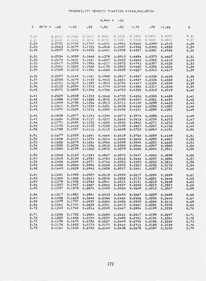
PROBABILITY DENSITY FUNCTION P(XIALPHA,BETA)

ALPHA = .50

X 8ETA .60 -. 25 .25 -.50 .50 -.75 .75 -1.00 X

o. 26 o. 2 87 8 0 . 39 46 o. 186 3 0 . 48 05 0.103 2 O. 5 08 0 O. 041 8 0.43 9 8 O. 26

O. 27 0.2803 0 .385 2 0.1 8 14 O. 47 18 O. 1006 0.5044 O. 040 8 O. 446 3 O. 27 0.28 0 .2731 0.3762 0.1767 0 .4631 0.0981 0.5002 0.03"'9 0.4515 0.28 0.29 0.2663 0.3674 0.1723 0.4546 0.0957 0.4956 0.03"'0 0.4555 0.2'" 0.36 0.2597 0.3590 0.1680 0.4461 0.0935 0.4907 0.0381 0.4586 0.30

6.31 0.2534 0. 35 09 0.1646 0.4378 0.0913 0.4854 0.0373 0.4607 0.31 0.32 6.2474 0.343 1 0.160i 0.4297 0.0892 0 .4800 0.0365 0.4619 0.32 0.33 0.2417 0.3356 0. 1564 0.42 17 0.0872 0.4743 0.0357 0.4625 0.33 0.34 0.2361 0.3283 0.1528 0.4139 0.0853 0.4685 0.0350 0.4624 0.34 0.35 0.2308 0.3212 0.1494 0.4062 0.0835 0.4627 0.0343 0.4617 0.35

0.36 6.2257 0.3144 0.1461 0.1988 0 . 0817 0.4567 0.0336 0.4605 0.36 0.37 0.2208 0.3079 0.1430 0.1915 0.0801 0.4507 0.0330 0.4589 0.37 6.38 0.2161 0.3015 0.1399 0.3843 0.0784 0. 4447 0.0324 0.4569 0.38 0.39 0.2115 0.2954 0.1370 0.3774 0.0769 0.4386 0.0317 0.4545 0.3'" 0. 4 0 0.2ii71 0.2895 0.1342 0.3706 0.0753 0.4326 0.0312 0.4518 0.40

0.41 6.2029 0.2838 0.1315 0.3640 0.0739 0.4266 0.0306 0.4489 0.41 6.42 6.1988 0.2782 0.1289 0.3576 0.0725 0.4207 0.0301 0.4457 0.42 6.43 6.1949 0.2728 0.1264 0.3513 0.0711 0.4148 0.0295 0.4423 0.43 6 .44 0.1911 0.2676 0.1239 0.3451 0.0698 0.4089 0.0290 0.4387 0.44 0.45 0.1874 0.2 626 0.1216 0.3392 0.0686 0.4031 0.0285 0.4351 0.45

0. 4 6 6.1838 0.2577 0.1193 0.3334 0.0673 0.3974 0.0280 0.4312 0.46 0. 47 0.1804 0 .2530 0.1171 0.:"1271 0.0662 0.3918 0.0276 0.4273 0.47 6.48 6.1771 0.2484 0.11 5 0 ~.3222 0.0650 0.3862 0.0271 0.4233 0.48 0. 49 0 .17 39 0.2440 0.1130 o.:n 68 0.0639 0.3807 0.0267 0.4192 0.49 0.56 0.1708 0.23 97 0.1110 0.3115 0.0628 0.3753 0.0263 0.4151 0.50

0. 5 1 0.1677 0.2355 0.109i 0.3064 0.0618 0.3700 0.0259 0.4109 0.51 0.52 0.1648 0.2314 0.1072 0.3014 0.0608 0.3648 0.0255 0.4067 0.52 0.53 001620 0.2275 0.1054 0.2966 0.0598 0.3596 0.0251 0.4025 0.53 0. 5 4 0.1592 0.2236 0.1036 0.2918 0.0589 0.3546 0.0247 0.3983 0.54 0. 55 6.1566 0.2199 0.1020 6.2872 0.0579 0.3496 0.0244 0.3941 0.55

0.56 0.1540 0.2163 0.1003 0.2827 0.0570 0.3447 0.0240 0.3898 0.56 0.57 0.1515 0.2128 0.0987 0.2783 0.0562 0.3400 0.0237 0.3856 0.57 6.58 0.1490 0.2094 0.6971 0.2740 0.0553 0.3353 0.0233 0.3814 0.58 0. 59 6.1466 0.2060 0.0956 0.2698 0.0545 0.3307 0.0230 0.3772 0.59 0. 6 0 0.1443 0.2028 0.0942 0.2658 0.0537 0.3261 0.0227 0.3731 0.60

0.61 0.1421 0.i996 0.0927 0.2618 0.0529 0.3217 0.0224 0.3689 0.61 6.62 0.1399 0.1966 0.0913 0.2579 0.0522 0.3173 0.0221 0.3648 0.62 6.63 6.1378 0.1936 0.6900 0.2541 0.0514 0.3131 0.0218 0.3608 0.63 0.64 0.1357 0.1907 0.0887 0.2504 0.0507 0.3089 0.0215 0.3567 0.64 0. 65 0.1337 0.1878 0.0874 0.2468 0.0500 0.3048 0.0212 0.3527 0.65

6.66 0.1317 0.1851 0.0861 0.2433 0.0493 0.3007 0.0209 0.3488 0.66 0.67 0.1298 0.1823 0.0849 0.2398 0.0486 0.2968 0.0206 0.3449 0.67 0.68 0.1279 0.1797 0~0837 0.2364 0.0480 0.2929 0.0204 0.3410 0.68 0.69 0.1261 0.177i 0.0825 0.2331 0.0473 0.2891 0.0201 0.3372 0.69 0. 7 0 001243 0.1746 0.0814 0.2299 0.0467 0.2854 0.0199 0.3335 0.70

0.71 0.1226 0.1722 0. 0803 0.2268 0.0461 0.2817 0.0196 0.3297 0.71 0.72 0.1209 0.1698 0.0792 0.2237 0.0455 0.2781 0.0194 0.3261 0.72 0.73 0.1192 0.1675 0.0782 0.2207 0.0449 0.2746 0.0192 0.3224 0.73 0.74 0.1176 0.1652 0.0172 0.2171 0.0444 0.2712 0.0189 0.3189 0.74 0.75 6.11 61 0.1630 0.0762 0.2149 0;0438 0.2678 0.0187 0.3153 0.75

172

PROBAB I LI TV DENS I TY FUNCTI ON P(XIALPHA,BETA)

ALPHA .50

X BETA .00 -.25 .25 -.50 .50 -.75 .75 -1.00 X

0. 7 6 0.1145 0.1608 0.0752 0.2120 0.0433 0.2645 0.0185 0.3119 0.76 0.17 0.1130 0.1587 0.0742 0.2093 0.0427 0.2612 0.0183 0.3 084 0.77 0.78 0.1116 0.1566 0.0733 0.2066 0.0422 0.2580 0.0181 0.3051 0.78 0.79 0.1101 001546 0.0724 0.2039 0.0417 0.2549 0.0179 0.3017 0.79 0.80 0.1087 0.1526 0.0715 0.2014 0.0412 0.2518 0.0177 0.2984 0.80

0.81 0.1074 0.1506 0.0706 0.1988 0.0408 0.2488 0.0175 0.2952 0.81 0.82 001060 0.1487 0.0697 0.1964 0.0403 0.2458 0.0173 0.2920 0.82 0. 8 3 601 047 0.1469 0.0689 0.1939 0.0398 0.2429 0.0171 0.2888 0.83 0.84 001034 0.1450 0.0681 0.1915 0.0394 0.2400 0.0169 0.2857 0.84 0.85 0.1022 0.1433 0.0673 0.1892 0.0389 0.2372 0.0167 0.2827 0.85

0.86 0.1009 0.1415 0.0665 0.1869 0.0385 0.2345 0.0165 0.2797 0.86 0.87 0.0997 001398 0.0657 0.1847 0.0380 0.2318 0.0164 0.2767 0.87 0.88 0.0986 001381 0.6650 0.1825 0.0376 0.2291 0.0162 0.2738 0.88 0.89 6.0974 001365 0.064;> 0.1803 0.0372 0.2265 0.0160 0.2709 0.89 6.90 0.0963 001349 0.0635 0.1782 0.0368 0.2240 0.0159 0.2681 0.90

0. 9 1 0.0951 0.1333 0.0628 0.1762 0.0364 0.2215 0.0157 0.2653 0.91 0.92 0.0941 00131tl 0.0621 0.1741 0.0360 0.2190 0.0156 0.2625 0.92 0. 9 3 0.0930 0.1303 0.0614 0.1722 0.0356 0.2166 0.015 4 0.2598 0.93 0.94 6.0920 0.128tl 0.0607 0.1702 0.0353 0.2142 0.0152 0.2572 0.94 6.95 0.0909 0.1273 0.060i 0.1683 0.0349 0.2118 0.0151 0.2545 0.95

0.96 0.0899 001259 0.0594 0.1664 0.0346 0.2095 0.0149 0.2519 0.96 0.97 0.0889 001245 0.0588 0.1646 0.0342 0.2073 0.0148 0.2494 0.97 0. 98 0.0880 0.1231 0~0582 0.1628 0.0338 0.2051 0.0141 0.2469 0.98 0. 9 9 6.0870 0.1218 0.0576 0.1610 0.0335 0.2029 0.0145 0.2444 0.99 1.00 0.0861 0.1205 0.0570 0.1592 0.0332 0.2007 0.0144 0.2420 1.00

1 .01 0.0852 0.1192 0.0564 0.1515 0.0328 0.1986 0.0142 0.2396 1.01 1.02 0.Ofl43 001179 0.0558 0.1558 0.0325 0.1965 0.0141 0.2372 1.02 1.03 0.0834 001166 0.0553 0.1542 0.0322 0.1945 0.0140 0.2349 1.03 1.04 0.0825 0.1154 0.0547 0.1526 0.0319 0.1925 0.0139 0.2326 1.04 1.05 0.0817 0.1142 0.0541 0.1510 0.0316 0.1905 0.0131 0.2303 1.05

1.06 0.0809 0.1130 0.053 6 0.1494 0.0313 0.1886 0.0136 0.2281 1.06 1.07 0.0801 0.i1l8 0.0531 001479 0.0310 0.1867 0.0135 0.2259 1.07 1.08 0.0792 0.1107 0.0526 0.1463 0.0307 0.1848 0.0133 0.2237 1.08 1.09 0·0785 001096 0.052 1 0.1449 0.0304 0.1830 0.0132 0.2216 1.09 1.10 0.0777 001085 0.0516 0.1434 0.0301 0.1812 0.01::11 0.2195 1 .10

1.11 0.0769 0.1074 0.051 i 0.1420 0.0299 0.1794 0.0130 0.2174 1 .11 1.12 0.0762 0.1063 0.0506 0.1405 0.0296 001776 0.0129 0.2154 1.12 1 • 13 0.0754 001053 0.050i 0.1391 0.0293 0.1759 0.0128 0.2134 1.13 1.14 0.0747 0.i042 0.0496 0.1378 0.0291 0.1742 0.0127 0.2114 1.14 1.15 0.0740 001032 0.0492 0.1364 0.0288 0.1725 0.0126 0.2094 1.15

1.16 0.0733 0.1022 0.0487 0.1351 0.0285 0.1708 0.0125 0.2075 1.16 1.17 0.0726 001012 0.0483 0.1338 0.0283 0.1692 0.0123 0.2056 1.17 1.18 0.0719 001003 0.0478 0.1325 0.0280 001676 0.0122 0.2037 1.18 1.19 0.0713 0.0993 0.0474 0.1313 0.0278 0.1660 0.0122 0.2019 1.19 1.20 0.0706 0.098~ 0.0 47 0 0.1300 0.0276 0.1645 0.0121 0.2001 1.20

1.2i 0.0699 0.0 975 0.0466 0.1288 0.0273 0.1630 0.0120 0.1983 1.21 1.22 0.0693 0.0966 0.0462 0.1276 0.0271 001615 0.0119 0.1965 1.22 1.23 0.0687 0.0 957 0.6458 001264 0~0269 001600 0.0118 0.1948 1.23 1.24 0.0681 0.0948 0.0454 0.1253 0.0266 0.1585 0.0117 0.1930 1.24 1.25 0.0675 0.0 940 0.0450 0.1241 0.0264 0.1571 0.0116 0.1913 1.25

173

PROBABILITY DENSITY FUNCTION P(XIALPHA,BETA)

ALPHA = .50

X BETA • .00 -.25 .25 -.50 !50 -.75 .75 -1.00 X

1.26 0.0669 0.0931 0.6446 0.1230 0.0262 0!1557 0.0115 0.1897 1.26 1.27 0.0663 0.0923 0.6442 0.1219 0.0260 0.1543 0.0114 0.1880 1.27 1.28 0.0657 0.0914 0.6438 0.1208 0.0258 0.1529 0.0113 0.1864 1.28 1.29 0.0651 0.0906 0.0435 0.1197 0.0256 0.1515 0.0112 0.1848 1.29 1.36 0.0646 0.0898 0.0431 0.1186 0.0254 0.1502 0.0111 0.1832 1.30

1.31 0·0640 0.0891 0.6421 0.1176 0.0252 0.1489 0.0110 001816 1.31 1.32 0.0635 0.0883 0.6424 0.1166 0.0250 0.1476 0.0110 0.1801 1.32 1.33 0.0629 0.0875 0.6420 0.1156 0.0248 0;1463 0.0109 0.1786 1.33 1.34 0.0624 0.0868 0.6417 0.1146 0.0246 0.1451 0.0108 0.1771 1.34 1.35 0.0619 0.0860 0;6414 0.1136 0;0244 0~1438 0.0107 0.1756 1.35

1.36 6.0614 0.0853 0.0410 0.1126 0.0242 0!1426 0.0106 0.1741 1.36 i .37 0.0608 0.6846 0.0401 0.1116 0.0240 0.1414 0.0106 0.1727 1.37 1.38 0.0603 0.083'" 0;0404 0.1107 0.0238 0;1402 0.0105 0.1713 1.38 1.39 6.0599 0.0832 0.6406 0.1097 0.0236 0;1390 0.0104 0.1699 1.39 1.40 0.0594 0.0825 0.0397 0.1088 0.0235 0~1379 0.0103 0.1685 1.40

1.4i 0.0589 0.08 18 0.0394 0.1079 0.0233 0.1367 0.0103 0.1671 1.41 1.42 0.0584 O. (j811 0.6391 0.1070 0.0231 001356 0.011)2 0.1658 1.42 1.43 0.0580 0.080!:i 0.0388 0.1062 0.0229 0~1345 0.0101 0.1645 1.43 1.44 0.0575 0.0798 0.6385 0.1053 0.0228 0.1334 0.0100 0.1631 1.44 1.45 6.0570 0.0792 0.6382 6.1044 0;0226 0.1323 0.0100 0.1618 1.45

1.46 6.0566 0.0785 0.6379 0.1036 0.0224 0.1312 0.0099 0.1606 1.46 1.47 6.0562 0.077'" 0.0376 0.1028 0.0223 0.1302 0.0098 0.1593 1.47 1.48 0.0557 0.0773 0.6373 0.1019 0.0221 0.1292 0.0098 0.1580 1.48 1.49 6.0553 0.0767 0!037i 0.1011 0.0219 0.1281 0.0097 0.1568 1.49 1.50 0.0549 0.0 761 0.0368 0.1003 0~O218 o ~ 1271 0.0096 0.1556 1.50

1.51 0.0544 0.6755 0.6365 0.6995 0.0216 0.1261 0.0096 0.1544 1.51 1.52 0.0540 0.0749 0.0363 0.0988 0.0215 0.1251 0.0095 0.1532 1.52 1.53 6.0536 0.Q743 0.6360 6.0980 0.0213 0.1242 0.0094 0.1520 1.53 1.54 0.0532 0.0738 0.6357 0.0972 0.0212 0.1232 0.0094 0.1509 1.54 1.55 6.0528 0.0732 0~0355 0.0965 0.0210 0.1223 0.0093 0.1497 1.55

1.56 0.0524 0.6727 0.0352 0.0957 0.0209 0.1213 0.0092 0.1486 1.56 1.57 6.0521 0.0721 0!0350 0.0950 0.0207 0.1204 0.0092 0.1475 1.57 1.58 0.0517 0.0716 0.0347 6.0943 0.0206 0·1195 0.0091 0.1464 1.58 1.59 0.0513 0.6710 0.0345 0.0936 0.0205 0.li86 0.0091 0.1453 1.5\/ 1.60 0.0509 0.670 5 0~0342 0.6929 0.0203 0.1177 0.0090 0.1442 1.60

1.61 0.0506 0.6700 0.0346 0.0922 0.0202 0.1168 0.0089 0.1431 1.61 1.62 0.0502 0.6695 0.0337 0.0915 0.0200 0.1159 0.0089 0.1421 1.62 1.63 0.0498 0'0 69 0 0.0335 0.0908 0.0199 0.1151 0.0088 0.1411 1.63 1.64 6.0495 0.0685 0.0333 0.6902 0.0198 0.1142 0.0088 0.1400 1.64 1.65 6.0491 0.0680 0.633i 0.6895 0;0197 0.1134 0.0087 0.1390 1.65

1.66 0.0488 0.6675 0.6328 0.6889 0.0195 0.1126 0.0087 0.1380 1.66 1.67 6.0485 0.0670 0.6326 0.6882 0.0194 0.1118 0.0086 0.1370 1.67 1.68 0.0481 0.0665 0~0324 0.0876 0.0193 0.1109 0.0086 0.1360 1.68 1.69 0.0478 0.0661 0.0322 0.6869 0.0191 0.1101 0.0085 0.1351 1.69 1.70 0.0475 0.065~ 0.0319 0.0863 0.0190 0~1094 0.0084 0.1341 1.70

1.7i 0.0471 0.0651 0.0317 0.6857 0.0189 0.1086 0.0084 0.1332 1.71 1.72 6.0468 0.6647 0.0315 0.0851 0.0188 0.1078 0.0083 0.1322 1.72 1.73 0.0465 0.0642 0.0313 0.0845 0.0186 0.1071 0.0083 0.1313 1.73 1.74 6.0462 0.0638 0.0311 0.6839 0.0185 0.1063 0.0082 0.1304 1.74 1.75 6.0459 0.6634 0.0309 0.6833 0.0184 0.1656 0.0082 0.1295 1.75

174

--- -

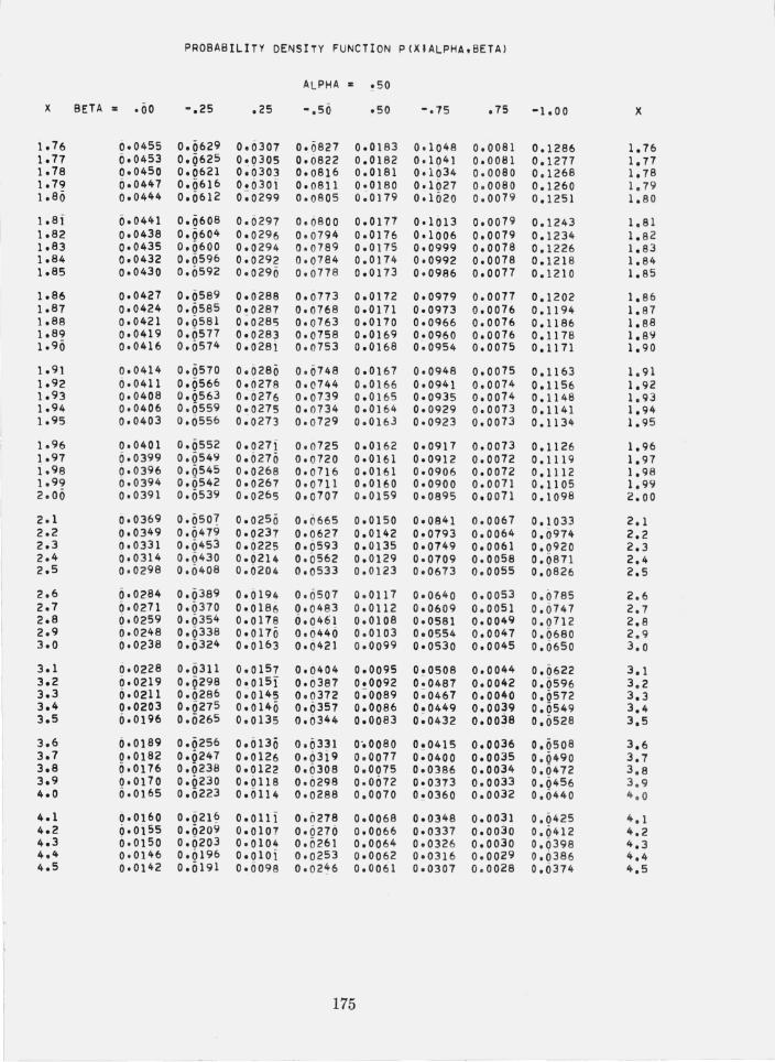
PROBABILITY DENSITY FUNCTION P(XIALPHA.8ETA)

ALPHA = .50

X BETA" .00 -.25 .25 -.50 .50 -.75 .75 -1.00 X

1.76 6.0455 0.0629 0.0307 0.0827 0.0183 0.1048 0.0081 0.1286 1.76 1.17 6.0453 0.0625 0.0305 0.6822 0.0182 001041 0.0081 0.1277 1.77 1.78 6.0450 0.0621 0~6303 0.0816 0.0181 0.1034 0.0080 0.1268 1.78 1.79 6.0447 0.0616 0.6301 0.08i1 0.0180 001627 0.0080 0.1260 1.79 1.80 0.0444 0.0612 0;0299 0.0805 o ~ 0 179 001620 0.0019 0.1251 1.80

1.8i 6.0441 0.0608 0.0297 0.0800 0.0177 0.1013 0.0019 0.1243 1.81 1.82 0.0438 0.0604 0.0296 0 .0794 0.0176 001006 0.0019 0.1234 1.82 1.83 0.0435 0.0600 0.0294 0.0789 0.0175 0.0999 0.0018 0.1226 1.83 1.84 0.0432 0.0596 0.0292 0.0784 0.0174 0.0992 0.0018 0.1218 1.84 1.85 0.0430 0.0592 0.0290 0.0778 0.0173 0.0986 0.0077 0.1210 1.85

1.86 0.0421 0.0589 0.0288 0.0773 0.0172 0.0979 0.0011 0.1202 1.86 1.87 0.0424 0.0585 0.0287 0.0168 0.0171 0.0973 0.0016 0.1194 1.87 1.88 0.0421 0.0581 0;0285 0.0163 0.0170 0.0966 0.0016 0.1186 1.88 1.89 0.0419 0.0577 0.0283 0.0758 0.0169 0.0960 0.0016 0.1178 1.89 1.90 0.0416 0.0574 0.028i 0.0753 0.0168 0 ~ 0954 0.0015 0.1171 1.90

1.91 0.0414 0.0570 0.6280 0.0748 0.0161 0.0948 0.0015 0.1163 1.91 1.92 6.0411 0.0566 0.0278 0.0744 0.0166 0.0941 0.0074 0.1156 1.92 1.93 0.0408 0.0563 0.6276 0.0739 0.01 65 0.0935 0.0074 0.1148 1.93 1.94 0.0406 0.0559 0.0275 0.0134 0.0164 0.0929 0.0073 0.1141 1.94 1.95 0.0403 0.0556 0.0273 0.0129 0.0163 0.0923 0.0073 0.1134 1.95

1.96 0.0401 0.0552 0.0271 0.0725 0.0162 0.0917 0.0073 0.1126 1.96 1.97 0.0399 0.0549 0.6270 0.0720 0.0161 0.0912 0.0072 0.1119 1.97 1.98 0.0396 0.ij545 0.0268 0.0116 0.0161 0.0906 0.0072 0.1112 1.98 1.99 0.0394 0.0542 0.0267 0.0711 0.0160 0.0900 0.0011 0.11 05 1.99 2.00 0.0391 0.0539 0.0265 0.0107 0.0159 0.0895 0.0071 0.1098 2.00

2.1 0.0369 0.050 7 0.025ii 0.6665 0.0150 0.0841 0.0067 0.1033 2.1 2.2 0.0349 0.0479 0.0237 0.0627 0.0142 0.0793 0.0064 0.0974 2.2 2.3 0.0331 0.0453 0.0225 0.6593 0.0135 0.0749 0.0061 0.0920 2.3 2.4 0.0314 0.0430 0.0214 0.6562 0.0129 0.0709 0.0058 0.0871 2.4 2.5 0.0298 0.0408 0.0204 0.0533 0.0123 0.0673 0.0055 0.0826 2.5

2.6 0.0284 0.0 389 0.0194 0.6507 0.0117 0.0640 0.0053 0.0785 2.6 2.7 6.0271 0.0370 0.618 6 0. 0483 0.0112 0.0609 0.0051 0.0147 2.7 2.8 0.0259 0.6354 0.0178 0.0461 0.0108 0.0581 0.0049 0.0712 2.8 2.9 6.0248 0.0338 0.0170 0.0440 0.0103 0.0554 0.0047 0.0680 2.9 3.0 6.0238 0.0 32 4 0.0163 0.6421 0.0099 0.0530 0.0045 0.0650 3.0

3.1 6.0228 0.0311 0.0151 0.0404 0.0095 0!0508 0.0044 0.0622 3.1 3.2 0.0219 0.ij298 0.01 51 0.0387 0.0092 0.0487 0.0042 0.0596 3.2 3.3 6.0211 0.0286 0;0145 0.0372 0;0089 0 ; 0467 0.0040 0.0572 3.3 3.4 0.0203 0.027 5 0.01 4 0 0.6357 0.0086 0.0449 0.0039 0.0549 3.4 3.5 6.0196 0.0265 0.0135 0.6344 0.0083 0;0432 0.0038 0.0528 3.5

3.6 6.0189 0.0256 0.61 3 0 0.0331 0-.0080 0!0415 0.0036 0.0508 3.6 3.7 0.0182 0.0247 0.0126 0.0319 0.0077 0.0400 0.0035 0.0490 3.7 3.8 6.0176 0.0238 0.0122 0.0308 0.0075 0.0386 0.0034 0.6472 3.8 3.9 0.0170 0.0230 0.6118 0.0298 0.0072 0.0373 0.0033 0.0456 3.9 4.0 6.0165 0.0223 0.6114 0.0288 0.0070 0!0360 0.0032 0.0440 4 .0

4.1 0.0160 0.021 6 0.0111 0.0278 0.0068 0.0348 0.0031 0.0425 401 4.2 0.0155 0.0209 0.0107 0.0276 0.0066 0.0337 0.0030 0.0412 4.2 4.3 6.0150 0.0203 0.0104 0.0261 0.0064 0.0326 0.0030 0.0398 4.3 4.4 0·0146 0.6196 o.oloi 0.0253 0.0062 0.0316 0.0029 0.6386 4.4 4.5 0.0142 0.0191 0.ii098 0.02~6 0.0061 0.0307 0.0028 0.0374 4.5

175

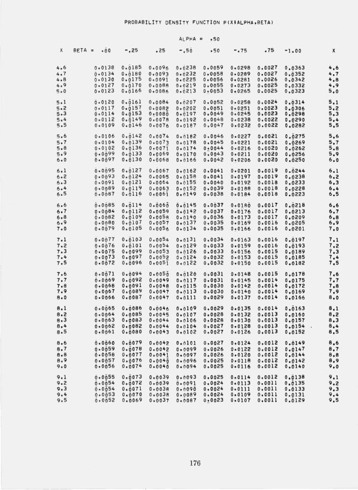
PROBAB I LI TV DENSITY FUNCTION P(XIALPHA.BETAl

ALPHA = .50

X BETA :: .00 -.25 .25 -.50 .50 -.75 .75 -1.00 X

4.6 0.0138 0.0185 0.0096 0.0238 0.0059 0.0298 0.0027 0.0363 4.6 4.7 0.0134 0.0180 0 . 0093 0.0232 0.0058 0.0289 0.0027 0.0352 4.7 4.8 0.01 30 0.0175 0 .0 091 0.0225 0.0056 0.0281 0.0026 0.0342 4.8 4.9 0.0127 0.0170 0.0088 0.0219 0.0055 0.0273 0.0025 0.0332 4.9 5.0 0.0123 0.0166 0.0086 0.0213 0,-0053 0,-0265 0.0025 0.0323 5.0

5.1 0.0120 0.0161 0.0084 0. 0207 0.0052 0.0258 0.0024 0.0314 5.1 5.2 0.0117 0.Q157 0.008 2 0.0202 0.0051 0.0251 0.0023 0.0306 5.2 5.3 0.0114 0.0153 00.0080 0.0197 0.0049 0;0245 0.0023 0.0298 5.3 5.4 0.0112 0.0149 0.0078 0.0192 0.0048 0.0238 0.0022 0.0290 5.4 5.5 0.0109 0.0146 0.0076 0.0167 0.0047 0,-0232 0.0022 0.0282 5.5

5.6 0.0106 0.0142 0.0 074 0.0162 0.0046 0.0227 0.0021 0.0275 5.6 5.7 0.0104 0.013~ 0.0073 0.0178 0.0045 0.0221 0.0021 0.0269 5.7 5.8 0.0102 0.0136 0.0071 0.0174 0.0044 0.0216 0.0020 0.0262 5.8 5.9 0.00 99 0.0133 0;0069 0.0170 0~0043 0.0211 0.0020 0.0256 5.9 6.0 0.00 97 0.0130 0.0068 0.0166 0.0042 0! 0206 0.0020 0.0250 6.0

6.1 0.0095 0.0127 0.0067 0.0162 0.0041 0.0201 0.0019 0.0244 6.1 6.2 0.0093 0.0124 0.0065 0.0158 0.0041 0.0197 0.0019 0.0238 6.2 6.3 0.009 1 0.0121 0.0064 0. 0155 0.0040 0.0192 0.0018 0.0233 6.3 6.4 0.0089 0.611 9 0.0063 0.0152 0.0039 0.0188 0.0018 0.0228 6.4 6.5 0.0087 0.011~ 0,-00 61 0.0149 0.0038 0.0184 0.0018 0.0223 6.5

6.6 0.0085 0.011~ 0.0060 0.0145 0.0037 0.0180 0.0017 0.0218 6.6 6.7 0.0084 0.0112 0.0059 0.01 42 0.0037 0~0176 0.0017 0.0213 6.7 6.8 6.0682 0.0109 0.0058 0.0140 0.0036 0.0173 0.0017 0.0209 6.8 6.9 0.0080 0.010 7 0.0057 0.0137 0.0035 0.0169 0.0016 0.0205 6.9 7.0 0.0079 0.610 5 0.00 56 0.0134 0.0035 00. 0166 0.0016 0.0201 7.0

7.1 0.0077 0.0103 0.0054 0.0131 0.0034 0.0163 0.0016 0.0197 7.1 7.2 0.00 76 0.0101 0.0054 0.0129 0.0033 0.0159 0.0010 0.0193 7.2 7.3 0.0075 0.0099 0.0053 0.0126 0.0033 0.0156 0.0015 0.Q189 t.3 7.4 0.0073 0.0097 0.00 52 6.0124 0.0032 0~0153 0.0015 0.0185 7.4 7.5 0.0072 0.0096 0.00 51 0.0122 0.0032 0.0150 0.0015 0.0182 t.5

7.6 0.0071 0.0094 0.0050 0.0120 0.0031 0.0148 0.0015 0.0178 7.6 7.7 0.0069 0.0092 0.0049 0.0117 0.0031 0.0145 0.0014 0.a175 t.7 7.8 0.0008 0.0091 0.0048 0.0115 0.0030 0~0142 o.OOH 0.0172 7.8 7.9 6.0067 0.0089 0.0047 0.0113 0.0030 0.0140 0.0014 0.0169 7.9 8.0 0.0066 0.0087 0,-0047 0.0111 0.0029 0.0137 o.OOH 0.0166 8.0

8.1 6.0065 0.0086 0.00 46 0.0109 0.0029 0.0135 0.0014 0.0163 8.1 8.2 0.00 64 0.0085 0.0045 0.6107 0.0028 0.0132 0.0013 0.0160 8.2 8.3 6.0063 0.0083 0.0044 0.0106 0.0028 0.0130 0.0013 0.i)l57 8.3 8.4 0.0062 0.0082 0.0044 0.0104 0.0027 0.0128 0.0013 0.0154 8.4 8.5 0.0061 0.0080 0.0043 0.0102 0.0027 0.Oi26 0.0013 0.0152 8.5

8.6 0.0060 0.0079 0.0042 0.0101 0.0027 0.0124 0.0012 0.0149 8.6 8.7 0.00 59 0'Q078 0.0042 0.0099 0.0026 0.0122 0.0012 0.Q147 8.7 8.8 6.00 58 O. 0077 0.0041 0.il097 0.0026 0.0120 0.0012 0.0144 8.8 8.9 0.0057 0.007 6 0.00 46 0.0096 0.0025 0.0118 0.0012 0.0142 8.9 9.0 0.0056 0.0074 0.0040 0.0094 0.0025 0.0116 0.0012 0.0140 9.0

9.1 0.00 55 0.0073 0.0039 0.0093 0.0025 0.0114 0.0012 0.0138 9.1 9.2 0.0054 0.0072 0.0039 0.0091 0.0024 0~0113 0.0011 0.0135 9.2 9.3 0.0054 0.0071 0.0038 0.6090 0.0024 0.0111 0.0011 0.0133 9.3 9.4 0.0053 0.0070 0.0038 0.0069 0.0024 0.0109 0.0011 0.0131 9.4 9.5 0.00 52 0.0069 0.0037 0.0087 0!0023 0.0107 0.0011 0.0129 9.5

176

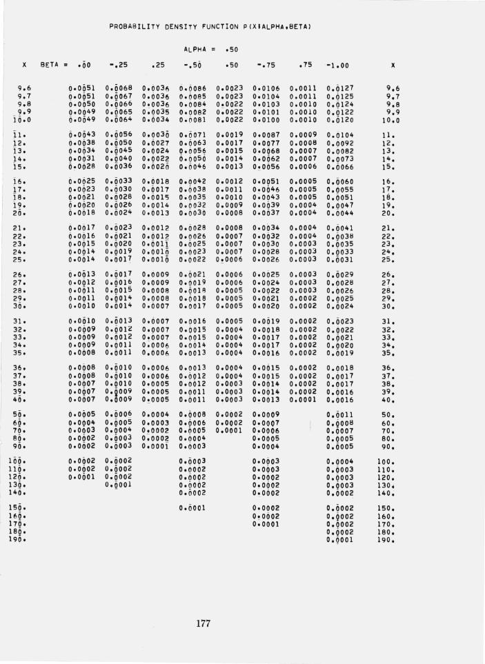
- 1

PROBABILITY DENSITY FUNCTION P(XIALPHA,BETA)

ALPHA = .50

X BETA = .60 -.25 .25 -.50 .50 -.75 .75 -1.00 X

9.6 0.0651 0.606B 0.003(, 6.6086 0.0023 0.0106 0.0011 0.0127 9.6 9.7 0.0051 0.6067 0.6036 0.0085 0.0023 0.0104 0.0011 0.0125 9.7 9.8 6.0050 0.6066 0.0036 0.0084 0.0022 0.0103 0.0010 0.6124 9.8 9.9 0.00 49 0.0065 0;0035 0.0082 0~0022 0.0101 0.0010 0.0122 9.9

io.o 6.00 49 0.606 4 0.0034 0.(i081 0.0022 0.0100 0.0010 0.0120 10.0

11. 6.00 43 0.6056 0.0036 0.6071 0.0019 0.0087 0.0009 0.0104 11. i2. 0.0038 0.6050 0.0027 0.0063 0.0017 0.0077 0.0008 0.0092 12. 13. 0.0634 0.0045 0.6024 0.6056 0.0015 0.0068 0.0007 0.6082 13. 14. 0.0031 0.0040 0.6022 6.0056 0.0014 0.0062 0.0007 0.0073 14. is. 0.0028 0.6036 0.0020 0.604 6 0.0013 0..0056 0.0006 0.6066 15.

16. 0.0025 0.0033 0.0018 0.0042 0.0012 0.0051 0.0005 0.0060 16. i7. 0.0623 0.6030 0.6017 0.0038 0.0011 0.0046 0.0005 0.6055 17. 18. 6.0021 0.6028 0.001'5 0.0035 0.0010 0~0043 0.0005 0.0051 18. i9. 0.0020 0.0026 0.0014 0.0032 0.0009 0.0039 0.0004 0.6047 19. 20. 0.0018 0.602 4 0.0013 0.0030 0.0008 0.0637 0.0004 0.0044 20.

21. 0.0617 0.6023 0.0012 0.6028 0.0008 0.0034 0.0004 0.0041 21. 22. 6.0016 0.6021 0.0012 0.0026 0.0007 0.0032 0.0004 0.003!! 22. 23. 0.0615 0.0020 0.6011 0.0025 0.0007 0.0030 0.0003 0.0035 23. 24. 0.0014 0.0019 0.0010 0.6023 0.0007 0.0028 0.0003 0.0033 24. 25. 0.0014 0.0017 0.0010 0.6022 0!0006 0.0026 0.0003 0.0031 25.

26. 6.0013 0.0017 0.0009 0.0021 0.0006 0.0025 0.0003 0.0029 26. 27. 0.0612 0.0016 0.0009 0.6019 0.0006 0.0024 0.0003 0.0028 27. 28. 0.0011 0.0015 0.0008 0.0011'1 0.0005 0.0022 0.0003 0.0026 28. 29. 0.0011 0.001 4 0.0008 0.60 18 0.0005 0.0021 0.0002 0.6025 29. 30. 0.0010 0.001 4 0.6007 0.0017 0.0605 0.0620 0.0002 0.6024 30.

31. 0.0010 0.ii013 0.6007 0.0016 0.0005 0.0019 0.0002 0.0023 31. 32. 0.0009 0.0012 0.0007 0.0015 0.0004 0.0018 0.0002 0.0022 32. 33. 0.0009 0.0012 0.0007 0.6015 0.0004 0.0617 0.0002 0.6021 33. 34. 0.0009 0.0011 0 ; 0006 0.0014 0.0004 0.0617 0.0002 0.0020 34. 35. 0.0608 0.0011 0.600(, 0.0013 0.0004 0.0016 0.0002 0.0019 35.

36. 0.0008 0.6010 0.0006 0.0013 0.0004 0.0015 0.0002 0.0018 36. 37. 0.0608 0.0010 0.0006 0.0012 0.0004 0.0015 0.0002 0.0017 37. 38. 0.0007 0.0010 0.0005 0.0012 0.0003 0.0014 0.0002 0.6017 38. 39. 0.0007 0'2 009 0.0005 0.6011 0.0003 0.0014 0.0002 0.0016 39. 40. 0.0007 0.0009 0!0005 0.6011 0.0003 0!0013 0.0001 0.0016 40.

5ii. 0.0005 O.OOO~ 0.0004 0.6008 0.0002 0.0009 0.0011 50. 69' 0.0004 0.0005 0.0003 0.6006 0.0002 0.0007 0.000 8 60. 70. 0.0003 0.0004 0.0002 0.0005 0.0001 0.0006 0.0007 70. 80. 0.0002 0.6003 0~0002 0.0004 0~0005 0.0005 80. 90. 0.0602 0.0003 o.oooi 0.0003 0.0004 0.0005 90.

100. 0.0002 0.0002 0.0003 0.0003 0.0004 100. 11 6. 0.0002 0.0002 0.6062 0.0603 0.0003 11 O. 120. 0.0001 0.0002 0.0002 0.0002 0.0003 120. 130. O'QOOI 0.0062 0.0602 0.0003 130. 140. 0.6002 0~0002 0.0002 140.

ISO. 0.6001 0.0002 0.0002 ISO. 160. 0.0002 0.Q002 160. 170. 0;0001 0.0002 170. 180. 0.0002 180. 190. O.QOOI 190.

177

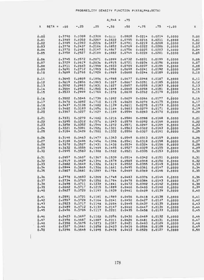
PROBABILITY DENSITY FUNCTION P(XIALPHA,BETA)

ALPHA = .75

X BETA = ,00 -.25 .25 -.50 !50 -.75 .75 -1.00 X

0.00 0.3790 0.2308 0.2308 0.0808 0.0808 0.0214 0.0214 0.0000 0.00 0.01 0.3789 0.2350 0.2267 0.0822 0.0795 0.0216 0.0211 0.0000 0.01 0.02 0.3785 0.2393 0.2226 6.0837 0.0781 0.0219 0.0208 0.0000 0.02 0.03 0.3778 0.2437 0.2186 0.0852 0.0769 0.0222 0.0206 0.0000 0.03 0.04 0.3770 0.2481 0.2147 0.0867 0.0756 0.0225 0.0203 0.0000 0.04 0.05 0.3758 0.2527 0.2109 0.0882 0.0744 0.0228 0.0201 0.0000 0.05

0.06 6.3745 0.2572 0.2071 0.0899 0.0732 0.0231 0.0199 0.0000 0.06 0.07 0.3729 0.2619 0.2034 0.0915 0.0721 0.0234 0.0196 0.0000 0.07 0.08 0.3711 0.2665 0.1999 0.0933 0.0709 0.0237 0.0194 0.0000 0.08 0.09 0.3691 0.2712 0~1963 0.0950 0~0698 0.0241 0.0192 0.0000 0.09 0.10 0.3669 0.2760 0.1929 0.0969 0.0688 0!0244 0.0189 0.0000 0.10

o.li 0.3645 0.2808 0.1896 0.0988 0.0677 0.0248 0.0187 0.0000 0.11 0.12 0.3619 0.2856 0.1863 0.1007 0.0667 0.0251 0.0185 0.0000 0.12 0.13 0.3592 0.2903 0.183i 0.1 027 0.0657 0.0255 0.0183 0.0000 0.13 0.14 0.3564 0.2951 0;1800 0.1 048 0.0648 0~0258 0.0181 0.6000 0014 0.15 0.3533 0.2999 0.1769 001070 0.0638 0.0262 0.0179 0.0000 0015

0.16 0.3502 0.3046 0.1739 0.1092 0.0629 0.0266 0.0177 0.0000 0.16 0.17 0.3470 0.3092 0.1710 0 .111 5 0.0620 0.0270 0.0175 0.0000 0.17 0.18 0.3437 0.3138 0.1682 0.1139 0.0611 0.0275 0.0173 0.0000 0.18 0.19 0.3402 0.3183 0.1654 0.1164 0.0603 0.0279 0.0171 0.0000 0.19 0.20 0.3367 0.3227 0.1627 001189 0.0594 0.0283 0.0170 0.0000 0.20

0.2i 0.3331 0.3270 0.1600 0.1216 0.0586 0.0288 0.0168 0.0000 0.21 0.22 0.3295 0.3312 0.1574 0.1243 0.0578 0.0292 0.0166 0.0000 0.22 0.23 0.3258 0.3352 0.1549 0.1272 0.0571 0.0297 0.0164 0.0000 0.23 0.24 0.3221 0.3391 0~1524 0.1301 0.0563 0.0302 0.0163 0.0000 0.24 0.25 0.3184 0.3428 0.150ii 0.1332 0.0556 0.0307 0.0161 0.0000 0.25

0.26 0.3146 0.3463 0.1477 0.1363 0.0548 0.0313 0.0159 0.0000 0.26 0.27 0.3108 0.3496 0.1454 6.1396 0.0541 0.0318 0.0158 0.0000 0.27 0.28 0.3070 0.3527 0.1431 0.1430 0.0534 0.0324 0.0156 0.0000 0.28 0.29 0.3632 0.3556 0.1409 0.1465 0;0527 0.0329 0.0155 0.0000 0.29 0.30 0.2995 0.3583 0.1388 0.1502 0.0521 0.0335 0.0153 0.0000 0.30

0.31 0.2957 0.3607 0.1367 0.1539 0.0514 0.0342 0.0151 0.0000 0.31 0. 32 0.2919 0.3629 0.1346 0.1578 0.0508 0.0348 0.0150 0.0000 0.32 0.33 6.2882 0.3649 0.1326 0.1619 0.0502 0.0355 0.0149 0.0000 0.33 0.34 0.2844 0.3666 0.1306 001661 0.0495 0.0361 0.0147 0.0000 0.34 0.35 0.2807 0.3681 0!1287 0.1704 0.0489 0.0369 0.0146 0.0000 0 . 35

0.36 0.2770 0.3693 0.1269 0.1748 0.0483 0.0376 0.0144 0.0000 0.36 0.37 0.2734 0.3703 0.1250 6.1794 0.0478 0.0384 0.0143 0.0000 0.37 0.38 0.2698 0.3711 0.1232 0.1841 0.0472 0.0392 0.0142 0.0000 0.38 0. 39 0.2662 0.3717 0.1215 6.1889 0.0466 0.0400 0.0140 0.0000 0.39 0.40 0.2627 0.3720 0.1197 0.1939 0 ! 0461 0.0409 0.0139 0.0000 0.40

0.41 0.2591 0.3721 0.1181 0.1989 0.0456 0.0418 0.0138 0.0000 0.41 0.42 0.2557 0.3720 0.1164 0.2041 0.0450 0.0427 0.01:17 0.0000 0.42 0.43 0.2523 0.3717 0.1148 0.2094 0.0445 0~0437 0.0135 0.0000 0.43 0.44 0.2489 0.3712 0.1132 0.2147 0.0440 0~0447 0.0134 0.6000 0.44 0.45 0.2456 0.3706 0.1117 0.2201 0!0435 0.0458 0.0133 0.0000 0.45

0.46 0.2423 0.3697 0.1102 0.2256 0.0430 0.0469 0.0132 0.0000 0.46 0.47 6.2390 0.3687 0.1087 6.2311 0.0426 0.0481 0.0131 0.6000 0.47 0.48 0.2358 0.3675 0.1073 0.2367 0.0421 0.0493 0.0129 0.0000 0.48 0.49 0.2327 0.3661 0.1058 0.2423 0.0416 0.0506 0.0128 0.0000 0.49 0. 5 0 0!2296 0.364§ 0.1045 6.2478 0.0412 0~0520 0.0127 0.0000 0.50

178

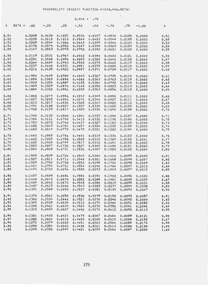
l PROBABILITY DENSITY FUNCTION P(XIALPHA.BETA) I

ALPHA .75

X BETA .00 -.25 .25 -.50 .50 -.75 .75 -1.00 X

0.51 0.2265 0.3630 001031 0.2534 0.0407 0.0534 0.0126 0.0000 0.51 0.52 0.2235 0.3612 0.1018 0.2589 0.0403 0.0549 0.0125 0.0000 0.52 0.53 0.2205 0.3594 001004 0.2643 0.0399 0.0566 0.01~4 0.0000 0.53 0.54 6.2176 0.3574 0.0992 0.2697 0.0395 0.0583 0.0123 0.0000 0.54 0.55 0.2147 0.3553 0.0979 0.2750 0.0390 0.0601 0.0122 0.0000 0.55

0.56 0.2119 0.3531 0.0967 0.2802 0.0386 0.0620 0.0121 0.0000 0.56 0.57 0.2091 0.3508 0.0955 0.2853 0.0382 0.0 640 0.0120 0.0000 0.57 0.58 0.2064 0.3484 0.0943 0.2902 0.0378 0.0662 0.0119 0.0000 0.58 0. 59 0.2037 0.3460 0.0931 0.2951 0.0375 0 .0685 0.0118 0.0000 0.59 0.60 0.2010 0.3435 0.0920 0.2997 0~0371 0.0709 0.0117 0.0000 0.60

0.61 0.1984 0.3409 0.0909 0.3043 0.0367 0.0735 0.0116 0.0000 0.61 0.62 0.1959 0.3383 0.0898 0.':1086 0.0363 0.0763 0.0115 0.0000 0.62 0.63 0.1933 0.3356 0.0887 0.3128 0.0360 0.0792 0.0114 0.0000 0.63 0.64 0.1909 0.3329 0.0876 0.,168 0.0356 0 .0823 0.0113 0.0000 0.64 0.65 0.1884 0.3302 0.0866 0.3205 0.03~3 0.0856 0.0112 0.0000 0.65

0.66 0.1860 0.3274 0.0856 0.":!242 0.0349 0.0890 0.0111 0.0000 0.66 0.67 0.1837 0.3245 0.0846 0.:;l276 0.0346 0.0927 0.0111 0.0000 0.67 0.68 0.1813 0.3217 0.0836 0.3308 0.0343 0.0965 0.0110 0.0000 0.68 , 0.69 0.1791 0.3188 0.082 7 0.3337 0.0339 0.1005 0.0109 0.0000 0.69 0.70 0.1768 0.3159 0.0817 0.3365 0.0336 001046 0.0108 0.0000 0.70

0.71 0.1746 0.3130 0.0808 0.3391 0.0333 0.1090 0.0107 0.0000 0.71 0.72 0.1724 0.3101 0.0799 0.3415 0.0330 001136 0.0106 0.0000 0.7 2 0.73 001703 0.3072 0.0790 0.3437 0.0327 001183 0.0105 0.0000 0. 73 0.74 0.1682 0.3043 0.0781 0.3457 0.0324 0.1232 0.0105 0.0000 0.74 0.75 0.1662 0.3014 0.0772 6.;475 0.0321 0.1282 0.0104 0.0000 0.75

0. 76 0.1642 0.2985 0.0764 0.3491 0.0318 0.1334 0.0103 0.0000 0.76 0.77 0.1622 0.2955 0.0755 0.3505 0.0315 0.1387 0.0102 0.0001 0.17 0.7A 0.1602 0.2926 0.0747 0.,517 0~0312 0.1441 0.0102 0.0002 0.78 0.79 0.1583 0.2897 0.6739 0.3527 0.0309 001496 0.0101 0.0002 0.79 0.80 0.1564 0.2868 0.0731 0.3536 0.0307 0.1553 0.0100 0.0004 0.80

0. 8 1 0.1545 0.2839 0. 0724 0.3543 0.0304 001610 0.0099 0.0005 O.Bl 0.82 0.1527 0.2811 0.0716 0.3548 0.0301 0.1668 0.0099 0.0007 0.82 0.83 0.1509 0.2782 0~0708 0.3552 0.0298 0~1726 0.0098 0.0009 0.83 0.84 0.1491 0.2754 0.0701 0.3554 0.0296 0.1784 0.0097 0.0012 0.84 0. 85 0.1474 0.2726 0.0694 0.,555 0.0293 0.1843 0.0097 0.0015 0.85

0.86 0.1457 0.2698 0.0686 0.3554 0.0291 001902 1 0.0096 0.0020 0.86 0.87 0.1440 0.2670 0.0679 6.3552 0.0288 0.1961 0.0095 0 .0025 0.87 0. 8 8 0.1424 0 .2642 0.0672 0.3548 0.0286 0.2019 0.0095 0.0031 0.88 0.89 0.1407 0.261 5 0. 0666 0.:;l543 0.0283 0.2077 0.0094 0.0038 0.89

;> 0. 9 0 0.1391 0.2588 0.0659 0.3537 0.0281 0;2i35 0.0093 0.0047 0.90

0. 9 1 0.1376 0.2561 0.0652 0.3530 0.0279 0!2192 0.0093 0.0051 0.91 0.92 0.1360 0.2534 0.06 46 0.3521 0.0276 0.2248 0.0092 0.0069 0.92 0. 9 3 0.1345 0.2508 0.0639 0.3512 0.0214 0.2304 0.0091 0.0082 0.93 0.94 0.1330 0.2481 0.0633 0.:;l502 0.0272 0.2358 0.0091 0.0096 0.94 0. 9 5 0.1315 0.2455 0.0627 0.3490 0.0270 0.2412 0.0090 0.0113 0.95

0.96 0.1301 0.2430 0.0621 0.3478 0.0267 0.2464 0.0089 0.0131 0.96 0.97 0.1286 0.2404 0 .0615 0.3465 0.0265 0.2515 0.0089 0.0152 0.97 0. 98 0.1272 0.2379 0.0609 0.:,\451 0.0263 0.2564 0.0088 0.0174 0.98 0.99 0.1259 0.2354 0 .0603 0.3436 0.0261 0.2 6 13 0.0088 0.0199 0.99 1.00 0.1245 0.2330 0.0597 0.'1421 0.0259 0.2660 0.0087 0.0226 1.00

179

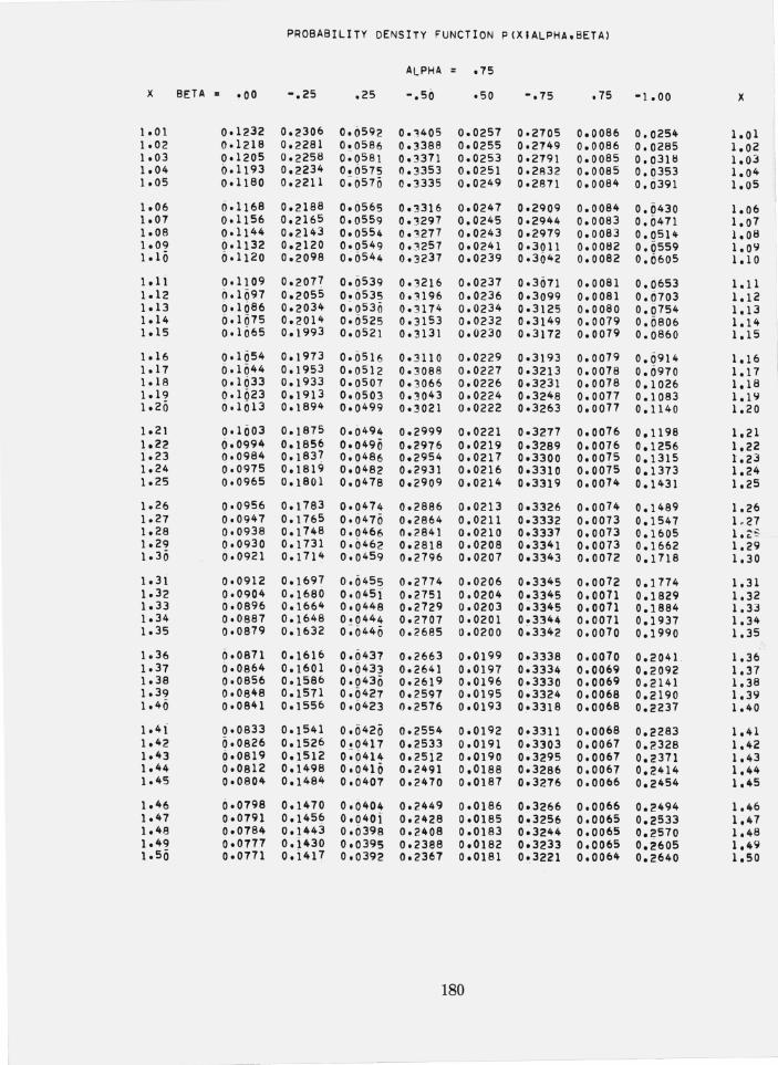
PROBABILITY DENSITY FUNCTION

ALPHA = .75

X BETA " ·00 -.25 .25 -.50 .50

1.01 0.1232 0.2306 0.6592 0.,405 0.0257 1.02 0.1218 0.2281 0.0586 0.3388 0.0255 1.03 0.1205 0.2258 0~0581 0.3371 0.0253 1.04 0.1193 0.2234 0.6575 0.3353 0.0251 1.05 001180 0.2211 0;6570 0.3335 0.0249

1.06 0.1168 0.2188 0.0565 0.33i6 0.0247 1.07 001156 0.2165 0.0559 0.3297 0.0245 1.08 0.1144 0.2143 0.0554 6.3277 0.0243 1.09 001132 0.2120 0.0549 0.3257 0.0241 1.10 001120 0.2098 0.6544 6.3237 0.0239

1.11 0.1109 0.2077 0.0539 0.3216 0.0237 1.12 0.109 7 0.2055 0.0535 0.3196 0.0236 1.13 001086 0.2034 0~0530 0.3174 0.0234 1.14 001075 0.2014 0.0525 0.3153 0.0232 1.15 0.1065 0.1993 0.0521 0.3131 0.0230

1.16 001054 0.1973 0.0516 0.3110 0.0229 1.17 0010 44 0.1953 0.0512 0.3088 0.0227 1.18 001033 0.1933 0.0507 0.3066 0.0226 1.19 001023 0.1913 0.0503 0.3043 0.0224 1.20 001013 001894 0.0499 0.3021 0.0222

1.21 001003 0.1875 0.0494 0.2999 0.0221 1.22 0.0994 0.1856 0.0490 0.2976 0.0219 1.23 0.0984 0.1831 0.0486 0.2954 0.0217 1.24 0.0975 001819 0.0482 0.2931 0.0216 1.25 0.0965 0.1801 0.0478 0.2909 0.0214

1.26 0.0956 0.1783 0.0474 0.2886 0.0213 1.27 0.0947 0.1765 0.0470 0.2864 0.0211 1.28 0.0938 0.1748 0.0466 0.2841 0.0210 1.29 6.0930 0.1731 0.6462 0.2818 0.0208 1.30 0.0921 001714 0.0459 0.2796 0.0207

1.31 0.0912 0.1697 0.0455 0.2774 0.0206 1.32 0.0904 0.1680 0.045i 0.2751 0.0204 1.33 0.0896 0.1664 0.0448 0.2729 0.0203 1.34 0.0887 0.1648 0.0444 0.2707 0.0201 1.35 0.0879 0.1632 0~O440 0.2685 0.0200

1.36 0.0871 0.1616 0.0437 0.2663 0.0199 1.37 0.0864 Ool60i 0.0433 0.2641 0.0197 1.38 0.0856 001586 0~6430 0.2619 0.0196 1.39 6.0848 001571 0.0427 0.2597 0.0195 1.40 0.0841 O. i 556 0.0423 0.2576 0.0193

1.41 0.0833 o • 1541 0.6420 0.2554 0.0192 1.42 0.0826 Ool52~ 0.0417 0.2533 0.0191 1.43 0.0819 0.1512 0;6414 0.2512 0.0190 1.44 0.0812 0.1498 0.0410 0.2491 0.0188 1.45 0.0804 0.1484 0.0407 0.2470 0.0187

1.46 6.0798 0.1470 0.0404 0.2449 0.0186 1.47 0.0791 0.1456 0.0401 0.2428 0.0185 1.48 6.0784 0.1443 0.0398 0.2408 0.0183 1.49 0.0777 O. i 430 0.0395 0.2388 0.0182 1.50 0.0771 0.i417 0.0392 0.2367 0.0181

180

L - --.---

P(XIALPHA.BETA)

-.75 .75

0.2705 0.0086 0.2749 0.0086 0.2791 0.0085 0.2832 0.0085 0.2871 0.0084

0.2909 0.0084 0.2944 0.0083 0.2979 0.0083 0.3011 0.0082 0.3042 0.0082

0.3671 0.0081 0.3099 0.0081 0.3125 0.0080 0.3149 0.0079 0.3172 0.0079

0.3193 0.0079 0.3213 0.0078 0.3231 0.0078 0.3248 0.0077 0.3263 0.0017

0 •. 3271 0.0076 0.3289 0.0076 0.3300 0.0075 0.3310 0.0075 0.3319 0.0014

0.3326 0.0074 0.3332 0.0073 0.3337 0.0073 0.3341 0.0073 0.3343 0.0072

0.3345 0.0072 0.3345 0.0011 0.3345 0.0011 0.3344 0.0071 0~3342 0.0070

0.3338 0.0010 0.3334 0.0069 0.3330 0.0069 0.3324 0.0068 0~3318 0.0068

0~3311 0.0068 0.3303 0.0067 0.3295 0.0067 0.3286 0.0067 0.3276 0.0066

0.3266 0.0066 0.3256 0.0065 0~3244 0.0065 0.3233 0.0065 0.3221 0.0064

-1.00

0.0254 0.0285 0.0318 0.0353 0.6391

0.0430 0.0471 0.0514 0.0559 0.0605

0.0653 0.0703 0.6754 0.0806 0.0860

0.0914 0.0970 0.1026 0.1083 0.1140

0.1198 0.1256 0.1315 0.1373 0.1431

0.1489 0.1547 0.1605 0.1662 0.1718

0.1774 0.1829 0.1884 0.1937 0.1990

0.2041. 0.2092 0.2141 0.2190 0.2237

0.2283 0.2328 0.2371 0.2414 0.2454

0.2494 0.2533 0.2570 0.2605 0.2640

X

1.01 1.02 1.03 1.04 1.05

1.06 1.07 1.08 1.0'1 1.10

1.11 1.12 1.13 1.14 1.15

1.16 1.17 1.18 1.1'1 1.20

1.21 1.22 1.23 1.24 1.25

1.26 1.27 1.~S 1.29 1.30

1.31 1.32 1.33 1.34 1.35

1.36 1.37 1.38 1.39 1.40

1.41 1.42 1.43 1.44 1.45

1.46 1.47 1.48 1.49 1.50

I _J

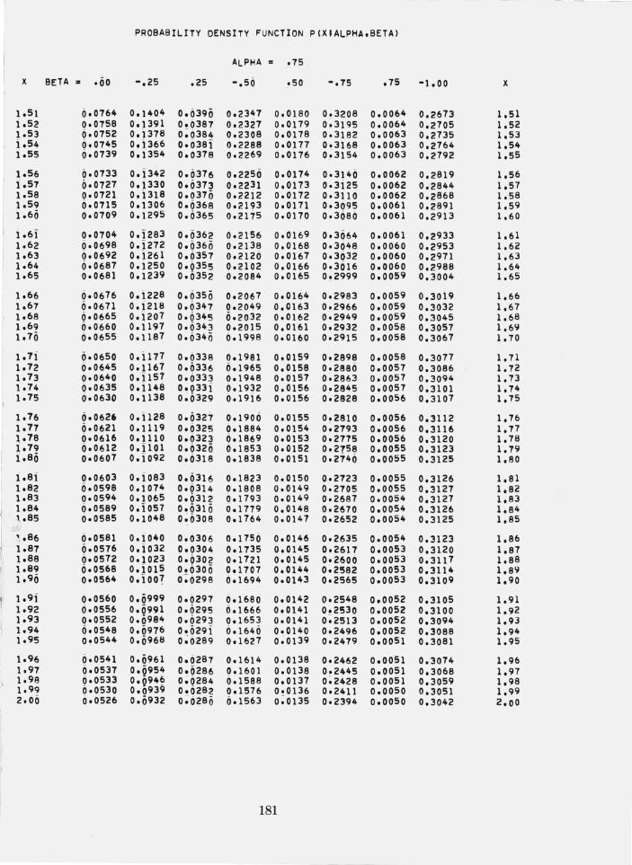
PROBABILITY DENSITY FUNCTION P(XIALPHA.BETA)

ALPHA .. .75

X BETA :II .00 -.25 .25 -.56 .50 -.75 .75 -1.00 X

1.51 0.0764 0.1404 0.6390 0.2347 0.0180 0!3208 0.0064 0.2673 1.51 1.52 0.0758 0.1391 0.0387 0.2327 0.0179 0.3195 0.0064 0.2705 1.52 1.53 6.0752 0.1378 0;6384 0.2308 0.0178 0.3182 0.0063 0.2735 1.53 i.54 6.0745 0.i366 0.038i 0.2288 0.0177 0.3168 0.0063 0.2764 1.54 1.55 6.0739 0.1354 0.0378 0.2269 0.0176 0.3154 0.0063 0.2792 1.55

1.56 6.0733 0.1342 0.0376 0.2250 0.0174 0.3146 0.0062 0.2819 1.56 i.57 0.0727 0.i330 0.0373 0.2231 0.0173 0.3i25 0.0062 0.2844 1.57 1.58 0.0721 0.i318 0.0370 0.2212 0.0172 0.3110 0.0062 0.2868 1.58 1.59 6.0715 0.1306 0.0368 0.2193 0.0171 0.3095 0.0061 0.2891 1.59 1.60 0.0709 0.1295 0.6365 0.2175 0.0170 0.3686 0.0061 0.2913 1.60

1.61 0.0704 0.1283 0.0362 0.2156 0.0169 0.3064 0.0061 0.2933 1.61 1.62 6.0698 0.1272 0.0360 0.2138 0.0168 0.3048 0.0060 0.2953 1.62 1.63 6.0692 0.1261 0.6357 0.2120 0.0167 0.3632 0.0060 0.2971 1.63 1.64 6.0687 0.1250 0'0 35 5 0.2102 0.0166 0.3016 0.0060 0.2988 1.64 1.65 0.0681 0.1239 0.0352 6.2084 0.0165 0!2999 0.0059 0.3004 1.65

1.66 0.0676 0.i228 0.6350 0.2067 0.0164 0.2983 0.0059 0.3019 1.66 1.67 0.0671 0.1218 0.0347 0.2049 0.0163 0.2966 0.0059 0.3032 1.67 1.68 6.0665 0.1207 0.6345 6.2032 0.0162 0.2949 0.0059 0.3045 1.68 1.69 0.0660 0.1197 0.6343 0.2015 0.0161 0.2932 0.0058 0.3057 1.69 1.70 6.0655 0.1187 0.634 0 0.1998 0.0160 0.2915 0.0058 0.3067 1.70

1.7i 6.0650 O. i 177 0.0338 0.1981 0.0159 0.2898 0.0058 0.3077 1.71 1.72 0.0645 0.1161 0.6336 6.1965 0.0158 0.2886 0.0057 0.3086 1. 72 1.73 0.0640 0.1157 0.6333 6.1948 0.0157 0~2863 0.0057 0.3094 1. 73 1.74 0.0635 0.1148 0.0331 0.1932 0.0156 0.2845 0.0057 0.3101 1.74 1.75 0.0630 0.1138 0;6329 0.19i6 0.0156 0.2828 0.0056 0.3107 1.75

1.76 6.0626 0.1128 0.0327 0.1900 0.0155 0!2810 0.0056 0.3112 1.76 1.17 0.0621 0.1119 0.6325 0.1884 0.0154 0.2793 0.0056 0.3116 1.77 1.78 6.0616 0.1110 0.6323 6.1869 0.0153 0.2775 0.0056 0.3120 1.78 i.79 6.0612 0.1101 0.0320 0.1853 0.0152 0·215~ 0.0055 0.3123 1.79 i.86 0.0607 O.i:OQ2 0.6318 0.1838 0.0151 0.2740 0.0055 0.3125 1.80

1.81 0.0603 0.i083 0.6316 0.1823 0.0150 0.2723 0.0055 0.3126 1.81 1.82 ii.0598 001074 0.6314 0.1808 0.0149 0.2705 0.0055 0.3127 1.82 1.83 0.0594 0.1065 0.6312 0.1793 0.0149 0.2687 0.0054 0.3127 1.83 1.84 0.0589 0.1051 0.6316 0.1719 0.0148 0.2670 0.0054 0.3126 1.84 ,.85 6.0585 o .}048 0~6308 0.1764 0.0147 0.2652 0.0054 0.3125 1.85

' . • 86 6.0581 0.1040 0.0306 0.1756 0.0146 0.2635 0.0054 0.3123 1.86 1.87 6.0576 0.1032 0.0304 0.1735 0.0145 0.2617 0.0053 0.3120 1.87 1.88 6.0572 0.1023 0.6302 0.1721 0.0145 0.2600 0.0053 0.3117 1.88 1.89 6.0568 0.1015 0.!0300 0.1707 0.0144 0.2582 0.0053 0.3114 1.89 1.90 0.0564 0.100? 0.0298 0.1694 0.0143 0.2565 0.0053 0.3109 1.90

1.91 0.0560 0.6999 0.{)297 6.1680 0.0142 0.2548 0.0052 0.3105 1.91 1.92 0.0556 0.6991 0.0295 0.1666 0.0141 0.2530 0.0052 0.3100 1.92 1.93 0.0552 0.6984 0.0293 0.1653 0.0141 0~2513 0.0052 0.3094 1.93 1.94 6.0548 0.0976 0.6291 0.1646 0.0140 0.2496 0.0052 0.3088 1.94 1.95 6.0544 0.0 968 0~0289 0.1627 0~0139 0~2479 0.0051 0.3081 1.95

1.96 6.0541 0.6961 0.6287 0.1614 0.0138 0.2462 0.0051 0.3074 1.96 1.97 6.0537 0'0954 0.6286 0.1601 0.0138 0.2445 0.0051 0.3068 1.97 1.98 6.0533 0'Q94~ 0~6284 0.1588 0.0137 0~2428 0.0051 0.3059 1.98 1.99 0.0530 0.0939 0.6282 0.1576 0.0136 0.2411 0.0050 0.3051 1.99 2.00 6.0526 0.6932 0~0280 6.1563 0~0135 0.2394 0.0050 0.3042 2.00

181

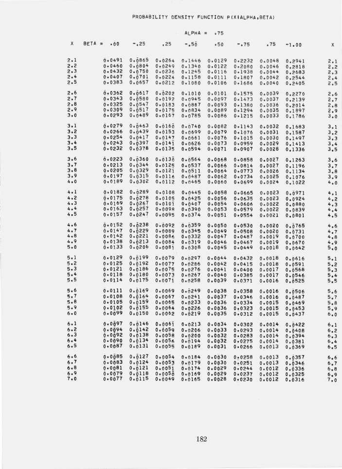
PROBABILITY DENS tTY FUNCT! ON P(XIAL PHA,BETA)

ALPHA :: .75

X BETA ,. .00 -.25 .25 ·.50 .50 ·.75 .75 -1 .00 X

2.1 0.0491 0.0865 0.0264 0.1446 0.0129 0.2232 0.0048 0.2941 2.1 2.2 0.0460 0.0804 0.0249 0.1340 0.0122 0.2080 0.0046 0.2818 2.2 2.3 0.0432 0.0750 0~0236 0.1245 0.0116 0.1938 0.0044 0.2683 2.3 2.4 0.0407 0.0701 0.0224 0.1158 0.0111 0.1807 0.0042 0.254 4 2.4 2.5 0.0383 0.0657 0.0212 6.1080 0.0106 0~1686 0.0040 0.2405 2.5

2.6 0.0362 0.0617 0.0202 0.101 0 0.0101 001575 0.0039 0.2270 2.6 2.7 0.0343 0 .0580 0.0192 0.0945 0.0097 0.1473 0.0031 0.2139 2.1 2.8 0.0325 0.Q541 0.0183 0.ii887 0.0093 0.1380 0.0036 0.2014 2.8 2.9 0.0309 0.0511 0.0175 0.0834 0.0089 0.1294 0.0035 0.1891 2.9 3.0 0.0293 0.0489 0 .016 7 0.0785 0.0086 0~1215 0.0033 0.1186 3.0

3.1 0.0279 0 .0463 0.0160 0.0740 0.0 082 0.1143 0.0032 0.1683 3.1 3.2 0.0266 0.0439 0.0153 0 .0699 0.0079 0.1076 0.0031 0.1581 3.2 3.3 0~0254 0.0411 0.0147 0.0661 0.0076 0.1015 0.0030 0.1497 3.3 3.4 0.0243 0.0391 0.0141 0.0626 0.0073 0.0959 0.0029 0.1413 3.4

, 3.5 0.0232 0.0318 0.0135 0.0594 0.0071 0.0901 0.0028 0.1336 3.5

3.6 0.0223 0.0360 0.0130 0.0564 0.0068 0.0858 0.0027 0.1263 3.6 3.7 0.0213 0 .0344 0.0125 0.0537 0.0066 0.0814 0.0027 0.1196 3.7 3.8 0.0205 0.0329 0.012i 0.0511 0.0064 0.0773 0.0026 0.1134 3.8 3.9 0.0197 0.031 5 0.0116 0.0487 0.0062 0.0734 0.0025 0.1076 3.9 4.0 0~O189 0.0302 0.0112 0.0465 0.0060 0~O699 0.0024 0.1022 4.0

4.1 0.0182 0.0289 0.0108 0.0445 0.0058 0.0665 0.0023 0.0971 4.1 4.2 0.0175 0.0278 0.0105 0.ii425 0.0056 0 . 0635 0.0023 0.0924 4.2 4.3 6.0169 0.0261 o.oloi 0.0407 0.0054 0 ;06 06 0.0022 0.0880 4.3 4.4 0.0163 0.0257 0.0098 0 .0 390 0.0053 0.0579 0.0022 0.0839 4.4 4.5 0.0157 0.0241 0.0095 0.0374 0.0051 0.0554 0 .002 1 0.6801 4.5

4.6 0.0152 0.0238 0 .0092 6'0359 0.0050 0.0530 0.0020 0.0765 4.6 4.7 0.0147 0.0229 0.0089 0.0345 0.0049 0.0508 0.0020 0.0731 4.7 4.8 0.0142 0.0221 0.0086 0.0332 0.0047 0 ; 0487 0.0019 0.0100 4.8 4.9 0.0138 0.0213 0.0084 0.0319 0.0046 0.0467 0.0019 0.0670 4.9 5.0 0.0133 0.020 6 0.008] 0.0308 0.0045 0~0449 0.0018 0.0642 5.0

5.1 0.0129 0 .01 99 0.0079 0.0297 0.0044 0.0432 0.0018 0.0616 5.1 5.2 0.0125 0 .01 92 0.0017 0.0286 0.0042 0.0415 0.0018 0.0591 5.2 5.3 0.0121 0.0186 0.0015 0 .0216 0.0041 0.0400 0 . 0017 0.0568 5.3 5.4 0.0118 0.0180 0.0013 0.0267 0.0040 0.0385 0.0017 0.0546 5.4 5.5 0.0114 0.0175 0. 0071 6.0258 0.0039 0.0371 0.0016 0.0525 5.5

5.6 0.0111 0 .0 169 0.0069 0.ij249 0.0038 0.0358 0 . 0016 0.6506 5.6 5.7 0.0108 0.0164 0.0067 0.0241 0.0037 0.0346 0.0016 0.0487 5.7 5.8 0.0105 0 . 015~ 0.0065 0.0233 0.0036 0~0334 0.0015 0.0469 5.8 5.9 0.0102 0.0155 0.0064 0.0226 0.0036 0!0323 0.0015 0.0453 5.9 6.0 6.00 99 0.0150 0.0062 0.0219 0.0035 0.0312 0.0015 0.0437 6.0

6.1 0.0097 0.0146 0.0061 0.0213 0.0034 0.0302 0.0014 0.0422 6.1 6.2 0.0094 0.0142 0.0059 0.0206 0.0033 0.0293 0.0014 0.Q408 6.2 6.3 0~0092 0.0138 0~0058 0.0200 0.0032 0.0283 0.0014 0.0394 6.3 6.4 0.0090 0.013~ 0.0056 0.0194 0.0032 0.0275 0.0014 0.0381 6.4 6.5 0.00 87 0.0131 0.0055 0.0189 0.0031 0.0266 0.0013 0.0369 6.5

6.6 0.0085 0.0121 0.0054 0.0184 0.Oii30 0! 0258 0.0013 0.0357 6.6 6.1 0.0083 0.0124 0.0053 0.0179 0.0030 0.0251 0.0013 0.0346 6.7 6.8 0.0081 0.0121 0.60 51 6.0114 0.0029 0~0244 0.0012 0.0336 6.8 6.9 0.0079 0.0 118 0.0050 0 . 0169 0.0029 0.0237 0.0012 0.0325 6.9 7.0 6.0677 0.011 5 0.0049 0.0165 0.0028 0.0230 0.0012 0.0316 7.0

182

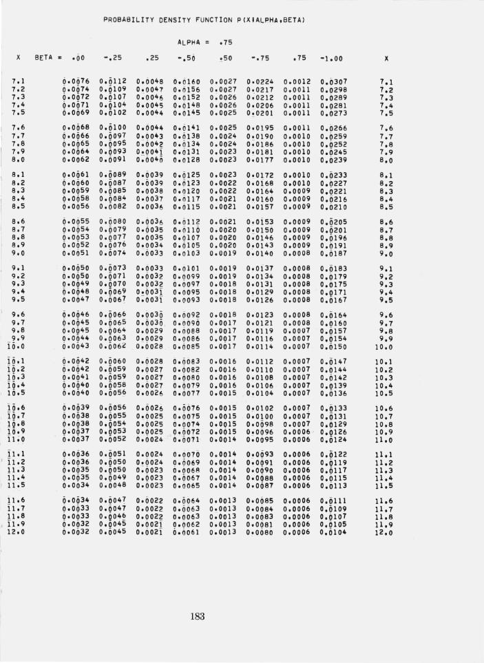
PROBABILITY DENSITY FUNCTION P(XIALPHA.BETA)

ALPHA = .75

X BETA .. .00 -.25 .25 -.50 ! 50 -.75 .75 -1.00 X

7.1 0.00 76 0.0112 0.6048 6.0160 0.0027 0.0224 0.0012 0.0307 7.1 7.2 0.0074 0.010 9 0.0047 0.0156 0.0027 0.0217 0.0011 0.0298 7.2 7.3 6.0072 0.0107 0~0046 0.0152 0.0026 0~0212 0.0011 0.0289 7.3 7.4 6.0071 0.010 4 0.0045 0.614B 0.0026 0.0206 0.0011 0.Q2Bl 7.4 7.5 6.0069 0.0102 0.0044 0.6145 0.0025 0!0201 0.0011 0.0273 7.5

7.6 0.0068 0.0100 0.6044 0.0141 0.0025 0.0195 0.0011 0.0266 7.6 7.7 0.0066 0.0097 0.0043 0.0138 0.0024 0!0190 0.0010 0.0259 7.7 7.8 6.0(j65 0.0095 0~6042 0.0134 0.0024 0.0186 0.0010 0.0252 7.8 7.9 6.0064 0.0093 0.0041 0.0131 0.0023 0.0181 0.0010 0.0245 7.9 8.0 6.0062 0.009i 0;60 40 0.0128 0.0023 0.0177 0.0010 0.0239 8.0

8.1 0.0061 0.0089 0.0039 0.0125 0.0023 0.0172 0.0010 0.0233 8.1 8.2 0.0060 0.0087 0.0039 0.0123 0.0022 0.0168 0.0010 0.0227 8.2 8.3 6.0659 0.0085 0.0038 0.(1l20 0.0022 0.0164 0.0009 0.0221 8.3 8.4 0.00 58 0.008 4 0.0037 0.0117 0.0021 0.0160 0.0009 0.0216 8.4 8.5 6.0056 0.0082 0~0036 0.0115 0.0021 0.0157 0.0009 0.0210 8.5

8.6 0.00 55 0.0080 0.60 36 0.0112 0.0021 0.oi53 0.0009 0.0205 8.6 8.7 0.0054 0.0079 0.0035 0.0110 0.0020 0·0150 0.0009 0.0201 8.7 8.8 6.0053 0.6077 0.0035 0.6107 0.0020 0;0146 0.0009 0.0196 8.8 8.9 6.00 5 2 0.0076 0.0034 0.0105 0.0020 0.0143 0.0009 0.0191 8.9 9.0 0.0051 0.0074 0.0033 0.0103 0.0019 0~0140 0.0008 0.0187 9.0

9.1 0.0050 0.0073 0.0033 0.0101 0.0019 0.0137 0.0008 0.0183 9.1 9.2 0.0050 0.0071 0.0032 0.0099 0.0019 0.0134 0.0008 0.0179 9.2 9.3 0.0049 0.0070 0.0032 0.0097 0.0018 0.0131 0.0008 0.0175 9.3 9.4 0.00 48 0.0069 0.0031 0.0095 0.0018 0.0129 0.0008 0.0171 9.4 9.5 6.0047 0.006 7 0~003i" 0.0093 0.0018 0 ; 0126 0.0008 0.0167 9.5

9.6 0.0046 0.0066 0.0036 0.0092 0.0018 0.0123 0.0008 0.0164 9.6 9.7 0.0045 0.0065 0.0030 . 0.0090 0.0017 0.0121 0.0008 0.0160 9.7 9.8 6.0045 0.0064 0.0029 0.6088 0.0017 0.0119 0.0007 0.0157 9.8 9.9 0.0044 0.6063 0.0029 0.0086 0.0017 0.0116 0.0007 0.0154 9.9

16.0 6.0643 0.606 2 0;0028 0.6085 0.0617 0.0114 0.0007 0.0150 10.0

iii .1 0.00 42 0.6060 0.6028 0.00e3 0.0016 0.0112 0.0007 0.0147 10.1 16.2 0.0042 0.6059 0.0027 0.0082 0.0016 0.0110 0.0007 0.0144 10.2 16.3 6.0041 0.0059 0.6027 0.0080 0.0016 0.0108 0.0007 0.0142 10.3 10.4 0.00 4 0 0.0058 0.0027 0.0079 0.0016 0.0106 0.0007 0.0139 10.4 16.5 0.0640 0.6056 0.0026 0.0077 0.0015 0~0104 0.0007 0.0136 10.5

iO.6 0.0639 0.0056 0.602(, 0.0076 0.0015 0.0102 0.0007 0.0133 10.6 iO.7 0.0638 0.0055 0.0025 0.0075 0.0015 0.0100 0.0007 0.0131 10.7 16.8 6.0038 0.Q054 0;6025 0.0074 0.0015 0.009B 0.0007 0.0129 10.8

I 10.9 0.0037 0.0053 0.0025 0.0072 0.0615 0.0096 0.0006 0.0126 10.9 11.0 0.0637 0.0052 0.6024 0.0071 0.0014 0~0095 0.0006 0.0124 11.0

11 • 1 0.0636 0.0051 0.0024 0.0076 0.0014 0.0093 0.0006 0.0122 11.1 11.2 6.0036 0.0050 0.0024 0.0069 0.0014 0~0091 0.0006 0.0119 11.2 11.3 6.0635 0.6050 0;6023 0.0068 0.0014 0;0090 0.0006 0.0117 11.3 11.4 0.00 35 0.6049 0.0023 0.0067 0.0014 0.0088 0.0006 0.0115 11.4 11.5 6.0034 0.0048 0.6023 0.6065 0.0014 0.0087 0.0006 0.0113 11.5

i1.6 0.0034 0.0047 0.0022 0.6064 0.0013 0.0085 0.0006 0.6111 11.6 i 11.7 0.0033 0.0047 0.0022 0.0063 0.0013 0.0084 0.0006 0.0109 11.7

11.8 0.0633 0.604~ 0.0022 6.0063 0~0013 0.0083 0.0006 0.Cll07 11.8 11.9 0.00 3 2 0.0045 0.002i 0.6062 0.0013 0.0081 0.0006 0.0105 11.9 12.0 6.0032 0.0045 0.0021 0.6061 0.0013 0.0080 0.0006 0.0104 12.0

183

----_.-

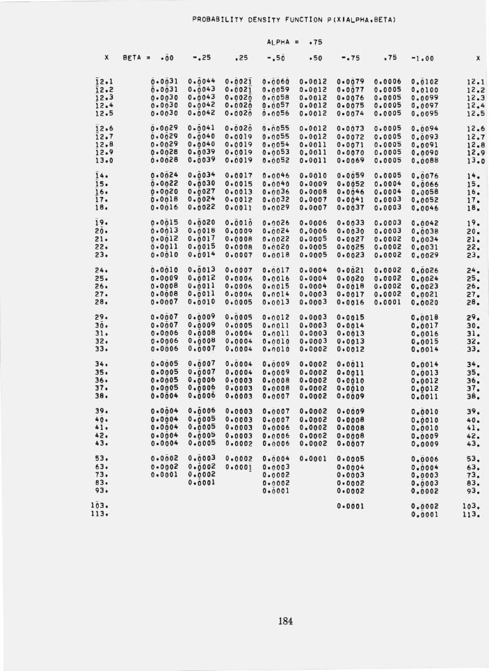
PROBABILITY DENSITY FUNCTION P(XIALPHA.BETAI

ALPHA = .75

X BETA " .00 -.25 .25 -.50 .50 -.75 .75 -1.00 X

12.1 0.00 3 1 0.0044 0.0021 0.0060 0.0012 0.0079 0.0006 0.0102 12.1 12.2 0.0031 0.0043 0.0021 0.6059 0.0012 0.0077 0.0005 o.i)lOO 12.2 12.3 0.0030 0.0043 0.0020 0.0058 0.0012 0.0076 0.0005 0.0099 12.3 1

12.4 0.00 30 0.0042 0.0020 0.6057 0.0012 0.0075 0.0005 0.0097 12.4 12.5 0.0630 0.0042 0.6020 6.0056 0.0012 0.0674 0.0005 0.0095 12.5

12.6 0.0629 0.0041 0.0020 6.ii055 0.0012 0.0073 0.0005 0.0094 12.6 12.7 0.0029 0.0040 0.0019 0.0055 0.0012 0.0072 0.0005 0.0093 12.7 12.8 0.0029 0.0040 0.6019 0.0054 0.0011 0.0071 0.0005 0.0091 12.8 12.9 0.0028 0.6039 0.0019 0.6053 0.0011 0.oi)70 0.0005 0.0090 12.9 13.0 0.0628 0.6039 0.6019 0.6052 0.0011 0.0069 0.0005 0.0088 13.0

14. 6.0024 0.6034 0.6017 0.0046 0.0610 0.0059 0.0005 0.0076 14. 15. 0.0022 0.0030 0.0015 0.0040 0.0009 0.0652 0.0004 0.0066 15. 16. 6.0020 0.6027 0~0013 0.6036 0.0008 0.0646 0.0004 0.0058 16. 17. 0.0018 0.6024 0.0012 0.6032 0.0007 0.004 1 0.0003 0.0052 17. 18. 6.0616 0.0022 0.0011 0.0029 0.0007 0.0637 0.0003 0.0046 18.

19. 0.0015 0.0020 0.0010 0.0026 0.0006 0.0633 0.0003 0.6042 19. 20. 0.0613 0.6018 0.0009 0.0024 0.0606 0.0030 0.0003 0.6038 20. 21. 6.0612 0.6017 0.6008 0.6022 0.0005 0.0027 0.0002 0.6034 21. 22. 0.0611 0.60US 0.6008 0.6020 0.0005 0.0025 0.0002 0.0031 22. 23. 6.0610 0.001 4 0.0007 0.6018 0.0005 0.0623 0.0002 0.0029 23.

24. 6.0010 0.6013 0.0007 0.0017 0.0004 0.0621 0.0002 0.0026 24. 25. 0.0009 0.0012 0.0006 0.0016 0.0004 0.0020 0.0002 0.0024 25. 26. 0.0008 0.6011 0.0006 0.0015 0.0004 0.0018 0.0002 0.6023 26. 27. 0.0008 0.6011 0.000/\ 0.0014 0.0003 0.0617 0.0002 0.0021 27. 28. 0.0607 0.6010 0.6005 0.0013 0.0003 0.0016 0.0001 0.0020 28.

29. 0.0607 0.6009 0.6005 0.0012 0.0003 0.0015 0.0018 29. 30. 0.0007 0.6009 0.6005 0.0011 0.0003 0.0014 0.0017 30. 31. 0.0006 0.6008 0.0004 0.0011 0.0003 0.0013 0.0016 31. 32. 0.0606 0.6008 0.0004 0.6010 0.0003 0.0613 0.0015 32. 33. 0.0006 0.6007 0.0004 o.iiOl(j 0.0002 0.0012 0.0014 33.

34. 6.0005 0.6007 0.0004 0.6009 0.0002 0.0011 0.0014 34. 35. 0.0605 0.6007 0.0004 0.0009 0.0002 0.0611 0.0013 35. 36. 0.0605 0.6006 0.6003 0.6008 0.0002 0.0010 0.0012 36. 37. 0.0005 0.6006 0;0003 0.6008 0.0002 0.0010 0.0012 37. 38. 0.0004 O.600~ 0.0003 0.0007 0.0002 0.0009 0.6011 38.

39. 0.0604 0.0006 0.0003 0.6007 0.0002 0.0009 0.0010 39. 4Q. 0.0004 0.6005 0.0003 0.6007 0.0002 0.0008 0.QOI0 40. 41. 0.0004 0.6005 0.0003 0.6006 0.0002 0.0008 0.0010 41. 42. 0.0004 0.6005 0.0003 0.0006 0.0602 0.0008 0.6009 42. 43. 0.0004 0.6005 0.0002 0.6006 0.0002 0.0007 0.0009 43.

53. 0.0602 0.0003 0.0002 0.6004 0.0001 0.0005 0.0006 53. 63. 0.0602 0'Q002 o.oooi 0.6003 0.0004 0.0004 63. 73. 0.0001 0.0002 0.0002 0.0003 0.0003 73. 83. 0.0001 0.6002 0.0002 0.0003 83. 93. 0.0001 0.0002 0.0002 93.

103. 0.0001 0.0002 103. 113. 0.0001 113.

184

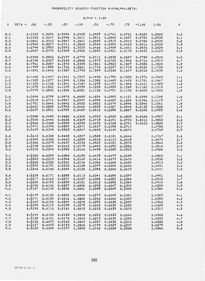
PROBABILITY DENSITY FUNCTION P(XIALPHA.BETA) l ALPHA = 1.00

X BETA .00 -.25 .25 -.50 .50 -.15 .15 -1.00 1.00 X

0.0 0.3183 0.3096 0.3096 0.2925 0.2925 0.2161 0.2161 0.2622 0.2022 0.0 0.1 0.3152 0.3141 0:2999 0.3011 0.2B14 0.2B49 0.2651 0.2102 0.2532 0.1 0.2 0.3061 0.3143 0.2861 0.3061 0.2685 0.2915 0.2543 0.2168 0.2434 0.2 0.3 0.2920 0.3017 0.2111 0.3069 6.2545 0.2954 0.2423 0.2814 0.2332 0.3

, 0.4 0.2144 0.2953 0.2543 0.3025 0.2400 0.2958 0.2301 0.2836 0.2228 0.4 0.5 0.2541 0.2176 0;:2369 0.2926 0.2254 0.2921 0.2178 0.2836 0.2123 0.5

0.6 0.2340 0.2562 0.2191 0.2172 0.2111 0.2838 0.2051 0.2189 0.2020 0.6 0.1 0.2136 0.2321 0.2030 0.2568 0.191~ 0.2105 001940 0.2110 0 .. 191~ 0.1 0.8 0.1941 0.2081 001812 0.2325 6.1841 0.2523 0.1821 0.2588 0.1 820 0.8 0.9 0.1159 001855 0.1124 0.2061 0.1116 0.2291 0.1119 0.2424 0.1126 0.9 1.0 0.1591 0.1640 0;1581 0.1193 0. ! 599 0.2036 001611 0.2218 0.1035 1 .0

1.1 0.1440 0.1441 0.1461 0.1537 0.1490 0.1154 001520 001914 0.1549 1.1 1.2 0.1305 001217 0.1346 0.1306 0.1389 001469 0.1430 0.1101 0.1461 1.2 1.3 0.1183 0.1130 0.1241 0.1107 0.1295 0.1191 0.1344 0.1411 0.1389 1.3 1.4 0.1015 001002 001145 0.0939 0.1208 0.0955 001265 0.1120 0.1315 1.4 1.5 0.(i919 0.0892 00105B 0.0801 0.1128 0.0151 001190 0.0845 0.1246 1.5

1.6 0.0894 0.0798 0.0919 0.0689 0.1054 0.0589 0.1121 0.0599 o.l1eo 1.6 1.1 0.~818 0.0716 0.0901 0.0597 0.0986 0.0465 001056 0.03 9 6 0.111 9 1.1 1.8 0.6751 0.0646 0~0842 0.0522 0.0923 0.0314 0.0996 0.024 0 0.1061 1.8 1.9 0.0691 0.0585 0;0183 0.0460 0.0865 0.0301 0.0940 0.0132 0.1006 1.9 2.0 0.0631 0.0531 0"!0129 0.0409 0.0812 0.0258 0.0881 0.0065 0.0?55 2.0

2.1 0.~588 0.0485 0.0680 0.0365 0.0163 0.0220 0.0838 0.0028 0.0901 2.1 2.2 0'0 545 0.0444 0 '.0636 0.0329 6.0118 0.0191 0.0793 0.0016 0.0862 2.2 2.3 0'2 506 0.0408 0.0595 0.0298 0.0616 0.0168 0.0151 0.0003 0.0t!20 2.3 2.4 0.c 411 0.0376 0.0551 0.0211 6.0637 0.0150 0.0111 0.0180 2.4 2.5 0.0439 0.0348 0;0523 0.0241 0.0602 0.0134 0.0674 0.0742 2.5

2.6 0.0410 0.0322 0.0492 0.0221 0.0568 0.0121 0.0640 0.0101 2.6 2.1 0.0384 0.0300 0.0463 0.0209 0.0538 0.0110 0.0608 0.0674 2.1 2.8 0.0360 0.0219 0.0431 0.0193 0.0509 0.0101 0.0578 0.0643 2.8 2.9 0.0338 0.0261 0.0412 0.0119 0.0483 0.0092 0.0550 0.0614 2.9 3.0 0.0318 0.0244 0.0390 0.0166 0.0458 0.0085 0.0523 0.0586 3.0

3.1 0.0300 0.0229 0.0369 0.0155 0.0435 0.0019 0.0499 0.0560 3.1 3.2 0'0283 0.0215 0.0349 0.0145 0.0414 0.0013 0.0416 0.0!:i36 3.2 3.3 0.0268 0.0202 0;0331 0.0136 0.0394 0.0068 0.0454 0.0513 3.3 3.4 0'0253 0.0191 0~0315 0.0128 0.0375 0.0064 0.0434 0.0491 3.4 3.5 0.0240 0.0180 0.0299 0.0120 6.0358 0.0060 0.0415 0.0411 3.5

3.6 0.0228 0.0111 0.0285 0.0113 0.0341 0.0056 0.0391 0.0451 3.6 3.1 0'2 211 0.0162 o ~ 0211 0.0101 0.0326 0.0053 0.0380 0.0433 3.1 3.8 0'0206 0.0153 0.0259 0.0101 0.0312 0.0050 0.0364 0.0416 3.8 3.9 0'0 196 0.0146 0~0241 0.0096 Q.Q298 0.0041 0·6349 0.039 9 3.9 4.0 0'0181 0.0139 0 ;: 0236 0.0091 0.0285 0.0045 0.0335 0.0384 4.0

4.1 0.0119 0.0132 0.0226 0.0086 0.0273 0.0042 0.0321 0.0369 4.1 4.2 0'0111 0.0126 0.0216 0.00:~2 6.0262 0.0040 0.0309 0.0355 4.2 4.3 0'2 163 0.0120 0.0201 0.0018 0.0252 0.0038 0.0291 0.0342 4.3 4.4 0'0156 0.0115 0 ;: 0199 0.0015 O.Oc42 0.0036 0.0285 0.0~29 4.4 4 . 5 0.0150 0.0110 0!0191 0.0012 6.0232 0.0035 0.0215 0.0311 4.5

4.6 0.0144 0.0105 0.0183 0.0068 0.0223 0.0033 0.0264 0.0306 4.6 4.7 0'0138 0.0101 0.0116 0.0065 6.0215 0.0032 0.0255 0.0295 4.1 4.8 0'0132 0.0091 0;0169 0.0063 0.0201 0.0030 0.0246 0.0285 4.8 4.9 0'2 121 0.0093 0~0163 0.0060 0.0199 0.0029 0.Q23 7 0.OZ15 4~9 5.0 0'0122 0.0089 0 ! 0151 0.0058 0.0192 0.0028 0.0228 0.0266 5.0

185

507-71 4 0 - 73 - 8

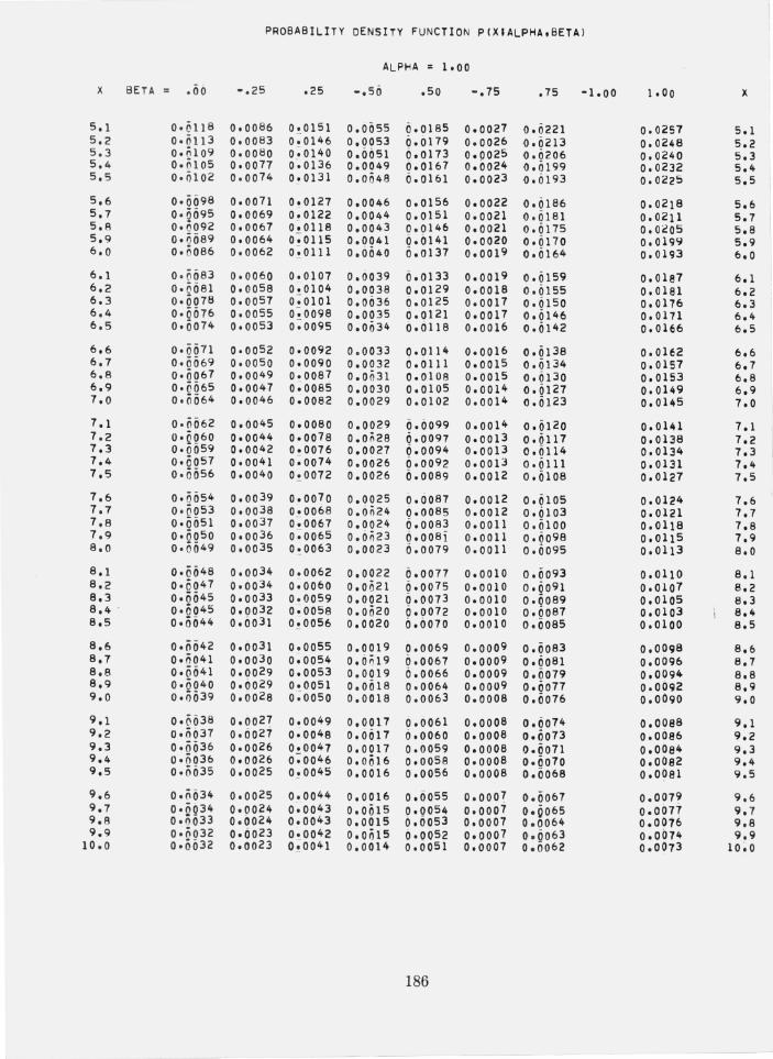
P~OBABlLITY DENSITY FUNCTION P(XIALPHA,BETA)

ALPHA = 1.00

X BETA .00 -.25 .25 -.50 .50 -.75 .75 -1.00 1.00 X

5.1 O.Q11B 0.0086 0, .. 0151 0.0055 0.0185 0.0027 0.0221 0.0257 5.1 5.2 0·0113 0.0083 0.0146 0.0053 0.0179 0.0026 0.0213 0.0248 5.2 5.3 0.~109 O.OOtlO 0 ~ 0140 0.0051 0.0173 0.0025 0.0206 0.0240 5.3 5.4 0.0105 0.0077 o ~ 0 136 0.0049 0.0167 0.0024 0.ii199 0.0232 5.4 5.5 0.0102 0.0074 0!0131 0.0048 0.0161 0.0023 0.0193 0.0225 5.5

5.6 0'0098 0.0071 0.0127 0.0046 0.0156 0.0022 0.0186 0.0218 5.6 5.7 0.§095 0.0069 0.0122 0.0044 0.0151 0.0021 0.0181 0.0211 5.7 5.8 0.0092 0.0067 0~0118 0.0043 0.0146 0.0021 0.0175 O.OCOS 5.8 5.9 0.ii089 0.0064 0~0115 0.0041 0.0141 0.0020 0.0170 0.0199 5.9 6.0 0' 0086 0.0062 0,! 0111 0.0040 6.0137 0.0019 0.0164 0.0193 6.0

6.1 0 '0083 0.0060 0.0107 0.0039 6.0133 0.0019 0.0159 0.0187 6.1 6.2 0'0081 0.0058 0.0104 0.0038 0.0129 0.0018 0.0155 0.0181 6.2 6.3 0.0078 0.0057 0 ~ 0101 0.0036 6.0125 0.0017 0.0150 0.0176 6.3 6.4 0'0676 0.0055 0~0098 0.0035 0.0121 0.0017 0.0146 0.0171 6.4 6.5 O. ii074 0.0053 0:0095 0.0034 0.0118 0.0016 0.0142 0.0166 6.5

6.6 0·0071 0.0052 0.0092 0.0033 0.0114 0.0016 0.0138 0.0162 6.6 6.7 0.0069 0.0050 0.0090 0.0032 0.0111 0.0015 0.0134 0.0157 6.7 6.8 0'0067 0.0049 0.0087 0.0 031 0.0108 0.0015 0.0130 0.0153 6.8 6.9 0'0065 0.0047 0:0085 0.0030 0.0105 0.0014 0.0127 0.0149 6.9 , 7.0 0.0064 0.0046 0.0082 0.0029 0.0102 0.0014 0.0123 0.0145 7.0

7.1 0 .0 062 0.6045 0.0080 0.0029 0.6099 0.0014 0.0120 0.0141 7.1 7.2 0.QQ60 0.0044 0.0078 0.On28 6.0097 0.0013 0.0117 0.0138 7.2 7.3 0 .0 059 0.0042 0.0076 0.0027 0.0094 0.0013 0.0114 0.0134 7.3 7.4 0'0057 0.0041 0:0074 0.0026 0.0092 0.0013 0.0111 0.0131 7.4 7.5 0. 0056 0.0040 0!.0072 0.0026 0.0089 0.0012 0.0108 0.0127 7.5

7.6 0. 0054 0.0039 0.0070 0.0025 0.0087 0.0012 0.0105 0.0124 7.6 7.7 0'0053 0.0038 0.0068 0.0024 6.0085 0.0012 0.0103 0.0121 7.7 7.8 0'0051 0.0037 0.0067 0.0024 0.0083 0.0011 0.0100 0.0118 7.8 7.9 0.QQ50 0.0036 0: 0065 0.0023 0.008i 0.0011 0.0098 0.0115 7.9 8.0 0· 0 049 0.0035 0,,- 0063 0.0023 0.0079 0.0011 0.0095 0.0113 8.0

8.1 0.0048 0.0034 0.0062 0.0022 0.0077 0.0010 0.0093 0.0110 8.1 8.2 0'0047 0.6034 0.0060 0.0 021 0.0075 0.0010 0.00 9 1 0.0107 8.2 8.3 0'0045 0.0033 0 . 0059 0.0021 0.0073 0.0010 0.0089 0.0105 8.3 8.4 - 0 ' 0045 0.0032 0~0058 0.0020 0.0072 0.0010 0.6087 0.0103 8.4 8.5 0.0044 0.0031 0! 0056 0.0020 0.0070 0.0010 0.0085 0.0100 8.5

8.6 0.ii042 0.0031 0.0055 0.0019 0.0069 0.000 9 0.0083 0.0098 8.6 8.7 0. ii 041 0.0030 0~0054 0.6~19 0.0067 0.0009 0.6081 0.0096 8.7 8.8 0.0041 0.0029 0.0053 0.0019 0.0066 0.0009 0.0079 0.0094 8.8 8.9 0'0040 0.0029 0.0051 0.0018 0.0064 0.0009 0.0077 0.0092 8.9 9.0 0.ii039 0.0028 0~0050 0.0018 0.0063 0.0008 0.0076 0.0090 9.0

9.1 0. 56 38 0.0027 0.0049 0.0017 0.0061 0.0008 0.0074 0.0088 9.1 9.2 0.0037 0.6027 0~0048 0.0017 0.0060 0.0008 0.0073 0.0086 9.2 9.3 0'0036 0.0026 0.0047 0.0017 0.0059 0.0008 0.0071 0.0084 9.3 9.4 0'0036 0.0026 0:0046 0.0016 0.0058 0.0008 0.0070 0.0082 9.4 9.5 0.0635 0.0025 0! 0045 0.0016 0.0056 0.0008 0.0068 0.0081 9.5

9.6 0.0034 0.0025 0.0044 0.0016 0.0055 0.0007 0.0067 0.007~ 9.6 9.7 0'29 34 0.0024 0.0043 0.0015 0.0054 0.0007 O.Q065 0.0077 9. 7 9.8 O.e033 0 . 0024 0.0043 0.0015 0.6053 0.0007 0.0064 0.0076 9.8 9.9 0.ii032 0.0023 0.0042 0.0015 0.0052 0.0007 O.Q063 0.0074 9.9

10 .0 0.0632 0.0023 0! 0041 0.0014 0.0051 0.0007 0.0062 0 . 0073 10~0

186

- ---

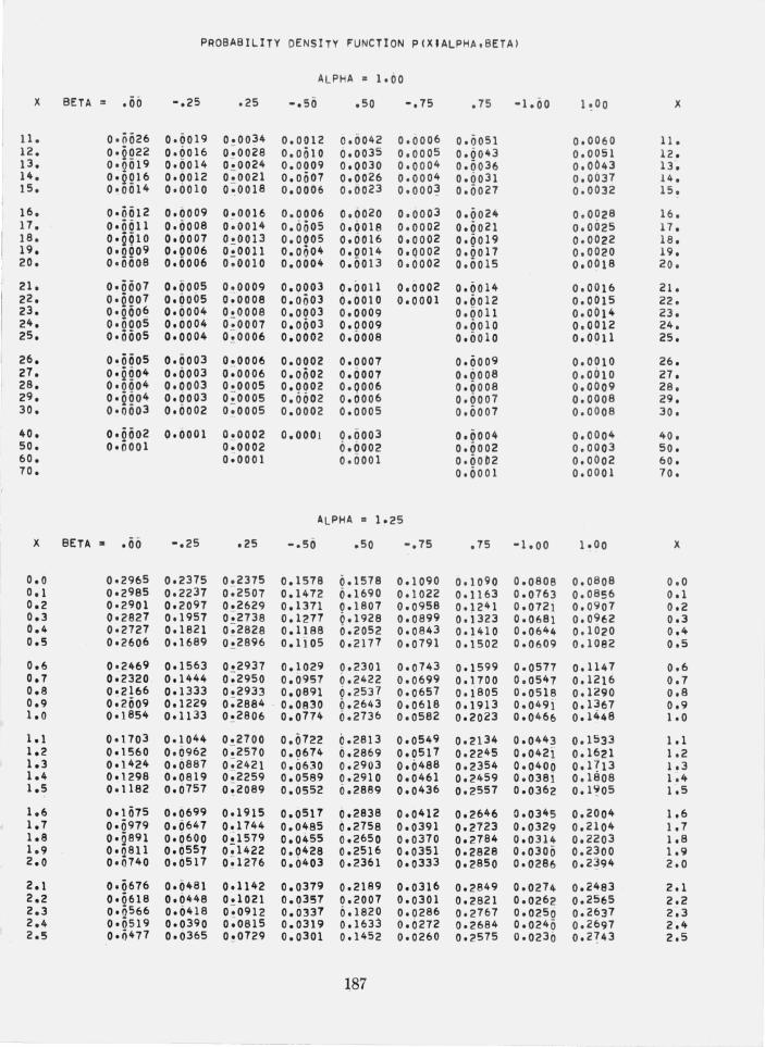
PROBABILITY DENSITY FUNCTION P(XIALPHA.BETA)

ALPHA z: 1.00

X BETA :: .00 -.25 .25 -.50 .50 -.75 .75 -1.00 1!00 X

11. 0,0026 0.0019 0!0034 0.0012 0.0042 0.0006 0.0051 0.0060 11. 12. 0.0022 0.0016 0.0028 0.0010 0.0035 0.0005 0.0043 0.0051 12. 13. 0.0019 0.0014 0~0024 0.0009 0.0030 0.0004 0.0036 0.0043 13". 14. 0.QQ16 0.0012 0~0021 0.0007 0.0026 0.0004 0.0031 0.0037 !4. IS. 0'0014 0.0010 0~0018 0.0006 0.0023 O.OOO~ 0.0027 0.0032 IS.

16. 0.0012 0.0009 0.0016 0.0006 0.6020 0.0003 0.0024 0.0028 16. 17. 0'0011 0.0008 0.0014 0.0505 0.0018 0.0002 0.0021 0.0025 17. 18. 0'29 10 0.0007 0!0013 0.0005 0.0016 0.0002 0.0019 0.0022 18. 19. 0'2Q09 0.0006 0.0011 0.000 4 0.0014 0.0002 0.0017 0.0020 19. 20. 0·0008 0.0006 0~0010 0.0004 0.0013 0.0002 0.0015 0.0018 20.

21. 0'0007 0.0005 0!0009 0.0003 0.0011 0.0002 0.0014 0.0016 21. 22. 0~Q007 0.0005 0.0008 0.0503 6.0010 0.0001 0.0012 0.0015 22. 23. 0'000 6 0.0004 0;0008 0.0003 0.0009 0.0011 0.0014 23. 24. 0'QQ05 0.0004 0~0007 0.0003 0.0009 0.0010 0.0012 24. 25. 0'0005 0.0004 0;: 0006 0.0002 0.0008 0.0010 0.0011 25.

26. 0.5005 0.0003 0 "~0006 0.0002 0.0007 0.0009 0.0010 26. 27. 0'QQ04 0.0003 0.0006 0.0002 0.0007 0.0008 0.0010 27. 28. 0'QQ04 0.0003 0.0005 0.0002 0.0006 0.0008 0.0009 28. 29. 0.QQ04 0.6003 0~0005 0.0602 0.6006 0.0007 0.0008 29. 30. 0.0003 0.0002 0;: 0005 0.0002 0.0005 0.0007 0.0008 30.

40. 0.0002 0.6001 0.0002 0.0001 0.0003 0.0004 0.0004 40. SO. O.QOOI 0;0002 0.0002 0.0002 0.0003 50. 60. O~OOOI 0.0001 0.0002 0.0002 60. 70. 0.0001 0.0001 70.

ALPHA = 1.25

X BETA .. .00 -.25 .25 -.50 .50 -.75 .75 -1.00 1!00 X

0.0 0.2965 0.2375 0.2375 0.1578 0.1578 0.1090 0.1090 0.0808 0.0808 0.0 0.1 0.2985 0.2237 0 ~ 2507 0.1472 0.1690 0.1022 0.1163 0.0763 0.0856 0.1 0.2 0.2901 0.2097 0.2629 0.1371 0.1807 0.0958 0.1241 0.072i 0.0907 0.2 0.3 0.2827 0.1957 0;2738 0.1277 0.1928 0.0899 0.i323 0.0681 0.0962 0.3 0.4 0.2727 0.1821 0;2828 0.1188 0.2052 0.0843 0.1410 0.0644 0 . 1020 0.4 0.5 0.2606 0.1689 0;: 2896 0.li05 0.2171 0.0791 0.1502 0.0609 0.1082 0.5

0.6 0.2469 001563 0.2937 0.1029 0.2301 0.0743 0.1599 0.0517 0.1147 0.6 0.7 0.2320 0.1444 0:2950 0.0957 0.2422 0.0699 0.1700 0.0547 0.1216 0.7 0.8 0·2166 0.1333 0.2933 0.0891 0.2537 0.0657 0.1805 0.05i8 0.1290 0.8 0.9 0.2009 0.1229 0:2884 . 0.0830 0.2643 0.0618 0.1913 0.049i 0.1367 0.9 1.0 0~1854 0.1133 0!2806 0.0774 6.2736 0.0582 0.2023 0.0466 0.1448 1.0

1.1 0.1703 0.1044 0.2700 0.0722 0.2813 0.0549 0.2134 0.0443 0.1 533 1 .1 1.2 0.1560 0.0962 0;2570 0.0674 0.2869 0.0517 0.2245 0.0421 0.1621 1.2 1.3 0.1424 0.0887 0~2421 0.0630 0.2903 0.0488 0.2354 0.0400 0.1?13 1.3 1.4 0.1298 0.0819 0;2259 0.0589 0.2910 0.0461 0.2459 0.0381 0.1808 1.4 1.5 0.1182 0.0757 0;2089 0.0552 6.2889 0.0436 0.2557 0.0362 0.1'!05 1.5

1.6 0.1075 0.0699 0.1915 0.0517 0.2838 0.0412 0.2646 0.0345 0.2004 1.6 1.7 0.0979 0.0647 0.1744 0.0485 0.2758 0.0391 0.2723 0.0329 0.2104 1.7 1.8 0'0891 0.0600 0;1579 0.0455 0.2650 0.0370 0.2784 0.0314 0.2203 1.8 1.9 0.Q811 0.0557 0~1422 0.0428 0.2516 0.0351 0.2828 0.0300 0.2300 1.9 2.0 0'0740 0.0517 0;1276 0.0403 0.2361 0.0333 0.2850 0.0286 0.2~94 2.0

2.1 0.0676 0.0481 0.1142 0.0379 0.2189 0.0316 0.2849 0.0274 0.2483 2.1 2.2 0'Q618 0.0448 0.1021 0.0357 0.2007 0.0301 0.2821 0.0262 0.2565 2.2 2.3 0.0566 0.0418 0~0912 0.0337 0.1820 0.0286 0.2767 0.0250 0.2637 2~3 2.4 0.0519 0.0390 0~0815 0.0319 0.1633 0.0272 0.2684 0.02 40 0.2697 2.4 2.5 0.ij477 0.0365 0!0729 0.0301 0.1452 0.0260 0.2575 0.02 30 0.2?43 2.5

l87

PROBABILITY DENSITY FUNCTION P(XIALPHA.BETA)

ALPHA = 1.25

X BETA = .00 -.25 .25 -.50 .50 -.75 .75 -1.00 1.00 X

2.6 0.0440 0.0342 0.0653 0.0285 6.1281 0.0248 0.2440 0.0220 0.2172 2.6 2.7 0.0406 0.0321 0.0587 0.0270 0.1123 0.0236 0.2282 0.021i 0.2782 2.7 2.8 0.0 375 0.0301 0;0528 0.0256 0.098 0 0.0226 0.2106 0.0203 0.2770 2.8 2.9 0.0348 0.0283 0~0476 0.0243 0.0852 0.0215 0.1917 0.0195 0.2734 2.9 3.0 0.0323 0.0267 0;0431 0.0231 0.0140 0.0206 0.1720 0.0187 0.2674 3.0

3.1 0.0300 0.0251 0.0391 0.0220 6.0643 0.0197 0.1522 0.0180 0.2588 3.1 3.2 0.0280 0.0237 0.0356 0.0209 0.0559 0.0189 001327 0.0173 0.2476 3.2 3.3 0.0261 0.0224 0~0325 0.0199 0.0488 0.0181 0.1142 0.0166 0.2340 3.3 3.4 0·0244 0.0212 0;0298 0.0190 0.0427 0.0173 0.0971 0.0160 0.2182 3.4 3.5 0.0228 0.0201 0~0273 0.0181 0.0376 0.0166 0.0816 0.0154 0.2005 3.5

3.6 0.0214 0.0190 0.0251 0.0173 0.0333 0.0160 0.0679 0.0149 0.1813 3.6 3.7 0.0201 0.in80 0.0232 0.0165 0.0296 0.0153 0.0562 0.0143 0.1612 3.7 3.8 0.0189 0.0171 0;0215 0.0158 0.0264 0.0147 0.0463 0.0138 0.1407 3.8 3.9 0'2 178 0.0163 0.0199 0.0151 0.0237 0.0142 0.0382 0.0133 0.1203 3.9 4.0 0.0168 0.0155 0!0185 0.0145 0.0213 0.0136 0.0315 0.0129 0.1007 4.0

4.1 0.0158 0.0148 0.0172 0.0139 0.0193 0.0131 0.0262 0.0124 0.0824 4.1 4.2 0'0150 0.0141 0.0161 0.0133 0.0176 0.0126 0.0219 0.0120 0.0657 4.2 4.3 0.0142 0.0134 0;0150 0.0128 6.0161 0.0122 0.0186 0.0116 0.0 5 10 4.3 4.4 0.0134 0.0128 0;0141 0.0123 0.0147 0.0117 0.0159 0.0113 0.0385 4.4 4.5 0.0128 0.6123 0;0132 0.0118 0.0135 0.0113 0.0137 0.0109 0.0282 4.5

4.6 0.0121 0.6117 0.!0124 0.0113 0.0125 ~.010~ 0.0120 0.0105 0.0200 4.6 4.7 0.Q115 0.0112 0.0117 0.0109 0.0116 .0105 0.0106 0.0102 0.0137 4~7 4.8 0'Q110 0.0108 0;0110 0.0105 0.0107 0.0102 0.0094 0.0099 0.0090 4.8 4.9 0'0105 0.0103 0;0104 0.0101 o.inoo 0.0098 0.0085 0.00 9 6 0.0057 4.9 5.0 0'0100 0.009~ 0;0099 0.0097 0.009~ 0.0095 0.0077 0.0093 0.0035 5.0

5.1 0.0095 0.0095 0.0093 0.0094 0.0087 0.0092 0.0069 0.0090 0.0020 5.1 5.2 0.0091 0.6091 0;0089 0.0090 0.0082 0.0089 0.0063 0.0087 0.0011 5.2 5.3 0.QQ87 0.6088 0.0084 0.00 87 0.6071 0.0086 0.0058 0.0085 0.0006 5.3 5.4 0.0083 0.0085 0;0080 0.0084 0.6072 0.0084 0.0054 0.0082 0.0003 5.4 5.5 0.0080 0.0081 0;0076 0.0081 6.0068 0.0081 0.0050 0.0080 0.0001 5.5

5.6 0.0077 0.0078 0!0072 0.6079 0.0064 0.0078 0.0046 0.00 78 5.6 5.7 0.0073 0.0075 0.0069 0.0076 0.6061 0.6076 0.00 43 0.00"16 5.7 5.8 0.0671 0.0073 0;0066 0.0074 0.0057 0.0074 6.00 4 0 0.0073 5.8 5.9 0.0068 0.0070 0~0063 0.0071 6.0054 0.0072 0.0037 0.0071 5.9 6.0 0.6665 0.0068 0;0060 0.0;;69 6.0052 0.0069 0.0035 0.0069 6.0

601 0.6063 0.0065 0.0058 0.0067 0.6049 0.0068 0.0033 0.0668 6.1 6.2 0.6060 0.0063 0;0055 0.0065 6.0047 0.0065 0.0031 0.0066 6.2 6.3 0!QQ58 0.0061 0;0053 0.0063 0.0044 0.0064 6.6029 0.0064 6.3 6.4 0·0056 0.0059 0;0051 0.0061 0.0042 0.0062 0.0028 0.0062 6 ~4 6.5 0.0654 0.0057 0;00 49 0.0059 6.0040 0.0060 0.0026 0.0061 6.5

6.6 0.0052 0.0055 0.0047 0.0057 0.0039 0.605~ 0.0025 0.005 9 6.6 6.7 0'2 050 0.0054 0~0045 0.0056 0.0037 0.0057 0.0024 0.0058 6.7 6.8 0.QQ49 0.0052 0;0043 0.0054 0.0035 0.0055 0.6022 0.0056 6.8 6.9 0.004 7 0.6050 0.0042 0.6053 0.6034 0.0054 0.0021 0.0055 6.9 7.0 0.0645 0.6049 0;0040 0.6051 0.0032 0.O05~ 0.6020 0.0053 7.0

7.1 0.0044 0.0047 0.0039 0.0050 6.0031 0.0051 0.0019 0.0052 7.1 7.2 0.§ij42 0.0046 0.0038 0.0048 0.0030 0.0050 0.6018 0.0051 7.2 7.3 0·0041 0.0045 0;0036 0.6047 6.6029 0.0049 0.0018 0.0056 7 .3 7.4 0.0040 0.0043 0.0035 0.0046 0.0028 0.0047 0.0017 0.0049 7.4 7.5 0.0639 0.0042 0!0034 0.004 5 0.0027 0.0046 0.6016 0.004 7 7.5

188

L

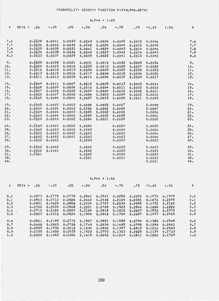
PROBABILITY DENSITY FUNCTION P(XIALPHA,BETA)

ALPHA = 1.25

X BETA = .00 -.25 .25 -.56 .50 -.75 .75 -1.0 0 1.00 X

7.6 0'0038 0.0041 0.0033 0.0043 0.0026 0.0045 0.0015 0.00 46 7.6 7.7 0.0636 0.0040 0.0032 0.0~42 0.0025 0.0044 0.0015 0.0045 7.7 7.8 0.0035 0.6039 0.0031 0.0041 0.6024 0.0043 0.0014 0.0044 7.8 7.9 0.0634 0.6038 0;;0030 0.0040 6.0023 0.0042 0.0014 0.0043 7.9 8.0 0'0033 0.0037 0!0029 0.0039 0.6022 0.0041 0.0013 0.004 2 8.0

9. 0.0025 0.6028 0.0021 0.0031 6.()016 0.0032 0.0009 0.0034 9. 10. 0'2Q20 0.0023 0;0016 0.0025 6.6012 0.002~ 0.0007 0.0028 10. 11. 0.0016 0.0018 0 ;; 0013 0.0020 0.0009 0.0022 0.0005 0.0023 11 • 12. 0'2Q13 0.0015 0.0010 0.0017 0.0008 0.0018 0.0004 ~.0020 12. 13. 0·0011 0.()013 0;;0009 0.0014 0.0006 0.0015 0.0003 • 0017 13 •

14. 0.0009 0.0011 0.0007 0.0012 0.0005 0.0013 0.0003 0.0014 14. IS. 0'000 8 0.0009 0.0006 0.0010 0.0004 0.0011 0.0002 0.0012 15. 16. 0.ii007 0.0008 0.0005 0.0009 0.0004 0.0010 0.0002 0.0011 16. 17. 0.ii006 0.0007 0.0005 0.0008 0.6003 0.0009 0.0002 0 .001 0 17. 18. 0.0005 0.0006 0.0004 0.0007 0.0003 0.0008 0.0001 0 .0009 18.

19. 0.0005 0.0005 0.0003 0.0006 0.0002 0.0007 0.0008 19. 20. 0.ii004 0.0005 0.0003 0.6;;06 0.0002 0.0006 0.0007 20. 21. 0'0004 0.0004 0.0003 0.0005 0.()002 0.0006 0.0006 21. 22. 0'QQ03 0. 0004 0; 0002 0.0005 0.0002 0.0005 0.0006 22. 23. 0.0003 0.0003 0.0002 0.0004 0.0001 0.0005 0.0005 23.

24. 0.0003 0.0003 0.0002 0.0004 0.0004 0.0005 24. 25. 0. ii0 02 0.0003 0.0002 0.0003 0. 0004 0.0004 25. 26. 0.ii002 0.0003 0.0002 0.0003 0.0003 0.0004 26. 27. 0'QQ02 0.0002 0.0001 0.Oii03 0.0003 0.0004 27. 28. 0·0002 0.0002 0.0003 0.0003 0.0003 28.

29. 0.0002 0.0002 0.00 02 0.0003 0.0003 29. 30. 0.0002 0.0001 0.Oii02 0.0003 0.0003 30. 31. 0.;;001 0.0002 0 .6 002 0.0003 31. 38. 0.6001 ~'Q001 0.0002 38. 48. 0.0001 48.

ALPHA = 1.50

X BETA :: . 00 -.25 .25 -.56 .50 -.75 .75 -1.00 1.00 X

0.0 0.2873 0.2778 0.2778 0.2541 0.2541 0.2252 0.2252 0.1975 0.1975 0.0 001 0.2863 0.2712 0.2828 0.2442 6.2630 0.2144 0.2356 0.1872 0.2078 0~1 0.2 0.2831 0.2629 0.2858 0.2334 0.2707 0.2034 0.2455 001770 0.2180 0.2 0.3 0·2780 0.2533 0:2868 0.2221 6.2769 001923 6.2546 0.1669 0.2280 0.3 0.4 . 0.2710 0.2426 0.2857 0.2104 0.2815 0.1812 0.2627 001572 0.2375 0.4 0.5 0.2623 0.2310 0 :! 2824 0.1986 0.2843 001704 0.2697 0.1477 0 .246 5 ' 0.5

0.6 0.252 1 0. 2189 0!2772 0.1867 6.2851 001598 0.2754 0.1386 0.2548 0.6 0.7 0.2408 0.2063 0.2700 0.1749 0.2839 0.1495 0.2795 0.1299 0.2621 0.7 0.8 0.2285 0.1936 0 ;'-2 610 0.1634 0.2806 001397 0.2819 0 .1 216 0.26 8 3 0.8 0.9 0.2155 0.1808 0.2505 0.1522 0.2753 0.1303 0.2825 0.1137 0.2733 0.9 1.0 0.2020 0. 1683 0:2386 0.1415 0.2680 0.1214 0.2811 0.1062 0. 2 169 1 .0

189

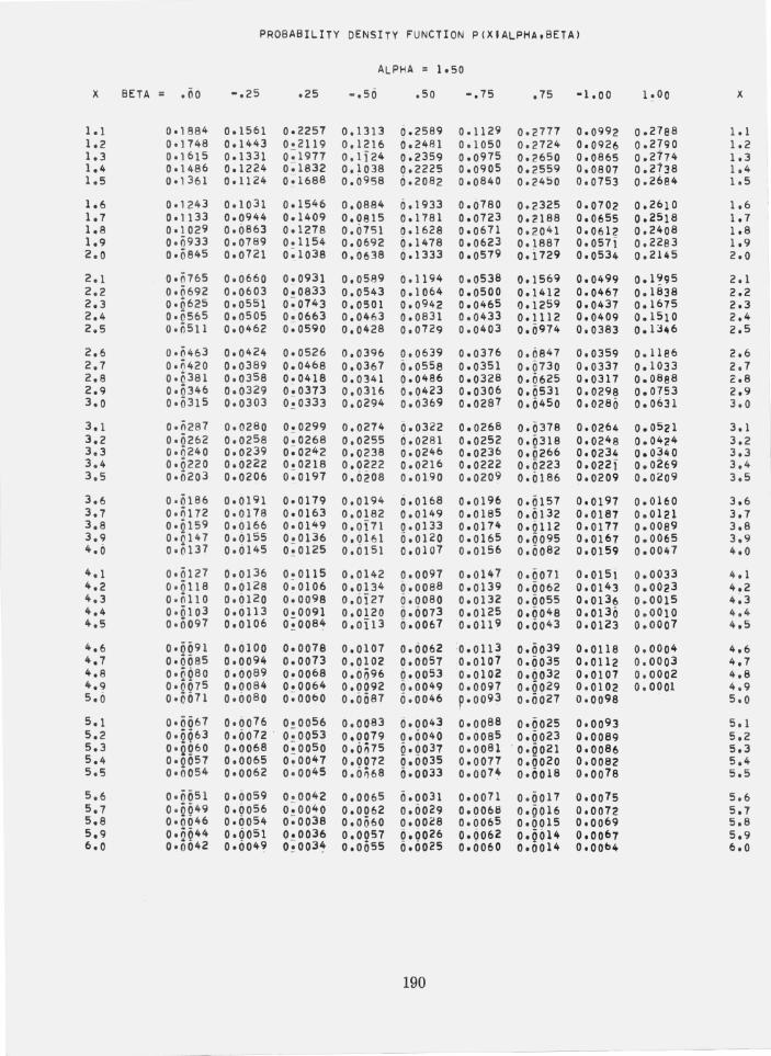
PROBABILITY DENSITY FUNCTION P(XIALPHA,BETAl

ALPHA = 1.50

X BETA = .00 -.25 .25 -.56 .50 -.75 .75 -1.00 1.00 X

1.1 0.1884 0.1561 0.2257 0.1313 0.2589 001129 0.2777 0.0992 0.2788 1.1 1.2 0.1748 0.1443 0.2119 0.1216 6.2481 0.1050 0.2724 0.0926 0.2790 1.2 1.3 0.1615 0.1331 0~1977 0.1124 0.2359 0.0975 0.2650 0.0865 0.2774 1.3 1.4 0.1486 0.1224 0;1832 0.1038 0.2225 0.0905 0.2559 0.0807 0.2738 1.4 1.5 0.1361 0.1124 0~1688 0.0958 6.2082 0.0840 0.2450 0.0753 0.2684 1.5

1.6 0.1243 0.1031 0.1546 0.0884 6.1933 0.0780 0.2325 0.0702 0.2610 1.6 1.7 0.1133 0.0944 0.1409 0.0815 0.1781 0.0723 0.2188 0.0655 0.2 518 1.7 1.8 0.1029 0.0863 0.1278 0.0151 0.1628 0.0671 0.2041 0.0612 0.2408 1.8 1.9 0.0933 0.0789 0.11 54 0.0692 0.1478 0.0623 0.1887 0.0571 0.2283 1.9 2.0 0.0845 0.0121 0~1038 0.0638 6.1333 0.0579 0.1729 0.0534 0.2145 2.0

201 0.0765 0.0660 0.0931 0.0589 0.1194 0.0538 0.1569 0.0499 0.1~95 2.1 2.2 0.0692 0.0603 0.0833 0.0543 0.1064 0.0500 0.1412 0.0467 0.1838 2.2 2.3 0'0625 0.0551 0;0143 0.0501 0.0942 0.0465 0.1259 0.0437 0.1615 2.3 2.4 0.0565 0.0505 0.0663 0.0463 0.0831 0.0433 001112 0.0409 0.1510 2.4 2.5 0.i)511 0.0462 0~0590 0.0428 0.0729 0.0403 0.0974 0.0383 0.1~1+6 2.5

2.6 0'01+63 0.0424 0.0526 0.0396 0.0639 0.0376 0.6847 0.0359 0.1186 2.6 2.7 0.0420 0.0389 0.0468 0.0361 0.0558 0.0351 0.0730 0.0337 0.1033 2.1 2.8 0'0 381 0.0358 0.0418 0.0341 0.0486 0.0328 0.0625 0.0317 0.0888 2.8 2.9 0.0346 0.0329 0~0373 0.0316 0.0423 0.0306 0.0531 0.0298 0.0753 2.9 3.0 0'0315 0.0303 0;.0333 0.0294 0.0369 0.0287 0.6450 0.0286 0.0631 3.0

3.1 0.0287 0.0280 0!0299 0.0274 6.0322 0.0268 0.6378 0.0264 0.0521 3.1 3.2 0.0262 0.0258 0.0268 0.0255 0.0281 0.0252 0.0318 0.024 8 0.042 4 3.2 3.3 0'0240 0.0239 0;0242 0.0238 0.021+6 0.0236 0.6266 0.0234 0.0340 3.3 3.4 0'0220 0.0222 0.0218 0.0222 0.0216 0.0222 0.0223 0.0221 0.0269 3.4 3.5 0.0203 0.0206 o ~ 0 197 0.6208 0.0190 0.0209 0.0186 0.0209 0.0209 3.5

3.6 0 . 5186 0.0191 0.0179 0.0194 0.0168 0.0196 0.0157 0.0191 0.0160 3.6 3.7 0'0172 0.0178 0.0163 0.0182 0.0149 0.0185 0.0132 0.0181 0.0121 3.7 3.8 0.Q159 0.0166 0.0149 0.0171 0.0133 0.0174 0.0112 0.0171 0.0089 3.8 3.9 0'2 147 0.0155 0.0136 0.0161 6.0120 0.0165 0.0095 0.0161 0.0065 3.9 4.6 0'0137 0.6145 0;0125 0.0151 0.0107 0.0156 0.0082 0.0159 0.001+7 4.0

4.1 0.0127 0.0136 0!01l5 0.0142 0.0097 0.0147 0.6071 0.015j 0.0033 4.1 4.2 0.0118 0.0128 0.0106 0.0134 0.0088 0.0139 0.0062 0.0143 0.002 3 4.2 4.3 0 .0 110 0.6120 0.0098 0.6127 6.0080 0.0132 0.0055 0.01 36 0.0015 4.3 4.4 0.Q103 0.0113 0.0091 0.0120 0.6073 0.0125 0.0048 0.0136 0.0010 4.4 4.5 0.0097 0.0106 0;:00 84 0.0113 6.0067 0.0119 0.00 43 0.0123 0.0007 4.5

4.6 0.5091 0.6100 0.0078 0.0107 0.6062 0.0113 0.0039 0.0118 0.0004 4.6 4.7 0'0085 0.0094 0.0073 0.0102 0.0057 0.0107 0.0035 0.0112 0.0003 4.7 4.8 0.0680 0.6089 0.0068 0.00 96 6.0053 0.0102 0.00 32 0.0101 0.0002 4.8 4.9 0.0075 0.0084 0!0064 0.0092 0.6049 0.0091 0.0029 0.0102 o • 0001 4.9 5.6 0'0071 0.0080 O.OObO 0.0081 6.0046 p.0093 0.0027 0.0098 5.0

Sol 0'0067 0.0076 0·0056 0.0083 6.0043 0.0088 0.0025 0.0093 5.1 5.2 0'0663 0.6072 · 0~0053 0.0079 0.6040 0.0085 0.0023 0.0089 5.2 5.3 0.QQ60 0.0068 0;0050 0.6575 6.0037 0.0081 · 0.6021 0.0086 5.3 5.4 0.0057 0.6065 0 ~004 7 0.0072 0.0035 0.0077 0.0020 0.0082 5.4 5.5 0.0054 0.0062 0;0045 0.0~68 0.0033 0.0014 0.0018 0.0078 5.5

5.6 0.5051 0.6059 0.0042 0.0065 0.0031 0.0071 0.0017 0.00 75 5.6 5.7 0'Q9 49 0.6056 0~0040 0.0062 0.0029 0.0068 0.0016 0.0012 5.1 5.8 0'0046 0.6054 0;0038 0.0(;60 0.0028 0.0065 0.0015 0.0069 5.8 5.9 0'2944 0.6051 0.0036 0.0051 6.0026 0.6062 0.6014 0.0067 5.9 6.0 0'0042 0.0049 0;:003~ 0.0055 0.6025 0.0060 0.0014 0.00b4 6.0

190

---...

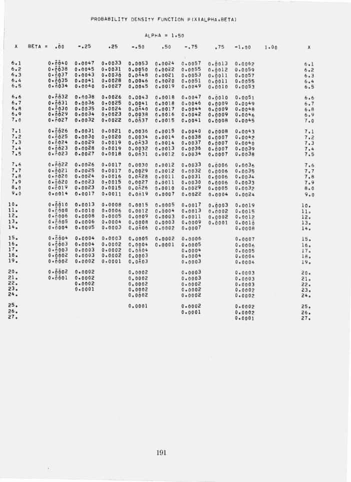
PROBAB I LI TV DENSITY FUNCTION P(XIALPHA,BETA)

ALPHA = 1.50

X BETA = .00 -.25 .25 -.50 .50 -.75 .75 -1.00 1.00 X

6.1 0.0040 0.0047 0.0033 0.0053 0.0024 0.0057 0.0013 0.00 62 6.1 6.2 0'0038 0.0045 0.0031 0.0050 0.0022 0.0055 0.0012 0.0059 6.2 6.3 0.0637 0.0043 0.0030 0.0~48 6.6021 0.0053 0.0011 0.0057 6.3 6.4 0.0035 0.6041 0.0028 0.0046 0.0020 0.0051 0.0011 0.0055 6.4 6.5 0.0634 0.0040 0~0027 0.0045 0.0019 0.6049 0.0010 0.0053 6.5

6.6 0.;;032 0.0038 0.0026 0.0043 0.0018 0.0047 0.0010 0.0051 6.6 6.7 0.0031 0.0036 0.0025 0.0041 0.0018 0.0046 0.0009 0.0049 6.7 6.8 0'0630 0.6035 0~0024 0.0040 0.0017 0.0044 0.0009 0.00 48 6.8 6.9 0.0029 0.0034 0.0023 0.0038 0.0016 0.0042 0.0009 0.00 46 6.9 7.0 0.5027 0.0032 0~0022 0.6037 0.0015 0.0041 0.0008 0.0045 7.0

7.1 0'0026 0.0031 0.0021 0.0036 0.0015 0.0040 0.0008 0.00 43 7. 1 7.2 0.0025 O.OO~O 0.0020 0.0034 0.6014 0.0038 0.0007 0.00 42 7.2 7.3 0.n024 0.6029 0~0019 0.6n33 0.0014 0.0037 0.6007 0.00 4 6 7.3 7.4 0'0623 0.6028 0.0019 0.0032 0.0013 0.0036 0.0007 0.0039 7.4 7.5 0.';023 0.0027 0;0018 0.0031 0.0012 0.0034 0.0007 0.0038 7.5

7.6 0.ii622 0.0026 0.0017 0.0030 0.0012 0.0033 0.0006 0.00 36 7.6 7.7 0.0621 0.0025 0.0017 0.0029 0.0012 0.0032 0.6006 0.0035 7.7 7.8 0.ii620 0.0024 0~0016 0.Oii28 0.0011 0.0031 0.6006 0.00 34 7.8 7.9 0.0020 0.0023 0~0015 0.0027 0.6011 0.0030 0.0006 0.0033 7.9 8.0 0.0019 0.0023 0~0015 0.0026 0.0010 0.0029 0.6005 0.0032 8.0 9.0 0'0014 0.0017 0.0011 0.0619 0.0007 0.0022 0.0004 0.0024 9.0

10. 0.0610 0.0013 0.0008 0.0015 0.0005 0.0017 0.0003 0.0019 10. 11. 0.0008 0.0010 0.0006 0.0012 0.6004 0.0013 0.0002 0.0015 11. 12. 0.ii006 0.0008 0;0005 0.0009 0.0003 0.0011 0.0002 0.0012 12. 13. 0.0005 0.0006 0~0004 0.0008 0.0003 0.0009 0.0001 0.0010 13. 14. 0'0004 0.0005 0.0003 0.0006 0.0002 0.0007 0.0008 14.

15. 0.0004 0.0004 0.0003 0.0005 0.0002 0.0006 0.0007 15. 16. 0'0003 0.0004 0.0002 0.0004 0.0001 0.0005 0.0006 16. 17. 0.;;003 0.0003 0.0002 0.on04 0.000 4 0.0005 17. 18. 0.0002 0.0003 0.0002 0.0003 0.0004 0.0004 18. 19. 0'0602 0.0002 0.0001 0.0003 0.0003 0.0004 19.

20. 0.0002 0.0002 0.0002 0.0003 0.0003 20. 21. 0.0001 0.0002 0.0002 0.0003 0.0003 21. 22. 0.0002 0.0002 0.0002 0.0003 22. 23. 0.0001 0.0002 0.0002 0.0002 23. 24. 0.0002 0.0002 0.0002 24.

25. 0.0001 0.0002 0.0002 25. 26. 0.0001 0.0002 26. 27. 0.0001 27.

191

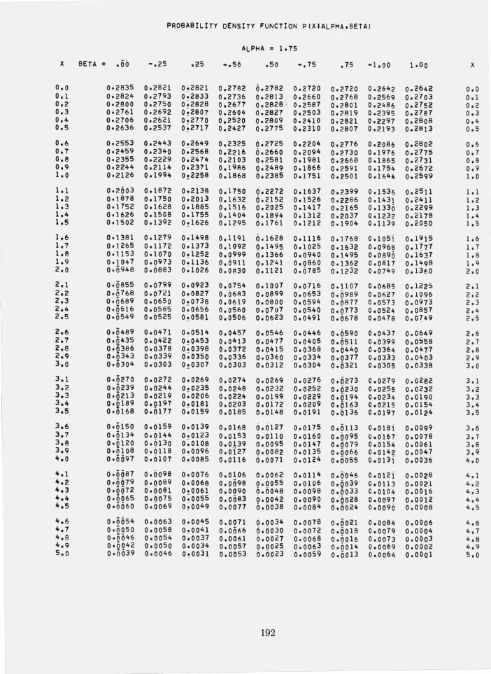
PROBABILITY DENSITY FUNCTION P(XIALPHA.BETA)

ALPHA = 1.75

X BETA = .00 -.25 .25 -.50 .50 -.75 .75 -1.00 1.00 X

0.0 0.2835 0.2821 0!2821 0.2782 0.2782 0.2720 0.2720 0.2642 0.2642 0.0 O. 1 0.2824 0.2193 0.2833 0.2136 0.2813 0.2660 0.2168 0.2569 0.2703 0.1 0.2 0.2800 0.2750 0~2828 0.2677 0.2828 1 0.2581 0.2801 0.2486 0.2152 0.2 0.3 0.2161 0.2692 0;2801 0.2604 0.2827 0.2503 0.2819 0.2395 0.2787 0.3 0.4 0.2706 0.2621 0;2710 0.2520 0.2809 0.2410 0.2821 0.2291 0.2808 0.4 0.5 0·2636 0.2537 0;2717 0.2427 0.2715 0.2310 0.2807 0.2193 0.2813 0.5

0.6 0.2553 0.2443 0.2649 0.2325 6.2725 0.2204 0.2776 0.2086 0.2802 0.6 0.7 0.2459 0.2340 0~2568 0.2216 0.2660 0.2094 0.2730 0.1976 0.2175 0.7 0.8 0.2355 0.2229 0~2474 0.2103 0.2581 0.1981 0.2668 0.1865 0.2731 0.8 0.9 0.2244 0.2114 0.2371 0.1986 0.2489 0.1866 0.2591 0.1754 0.2672 0.9 1.0 0.2126 0.1994 0!2258 0.1868 0.2385 0.1 751 0.2501 0.1644 0.2599 1 .0

1.1 0.2003 0.1872 0.2138 0.1750 0.2272 0.1631 0.2399 0.1536 0.2511 1 • 1 1.2 0.1878 0.1750 0~2013 0.1632 0.2152 0.1526 0.2286 0.1431 0.2411 1.2 1.3 0.1752 0.1628 0~1885 0.1516 0.2025 0.1417 0.2165 0.1330 0.2299 1.3 1.4 001626 0.1508 o ~ 1755 0.1404 0.1894 0.1312 0.2037 0.1232 0.2178 1.4 1.5 0.1502 0.1392 0!1626 0.1295 0.1761 0.1212 001904 0.1139 0.2050 1.5

1.6 0.1381 0.1279 0.1498 0.1191 0.1628 0.1116 o .176B 0.1051 0.1 9 15 1 .6 1.7 0.1265 0.1172 0~1373 0.1092 0.1495 0.1025 0.1632 0.0968 0.1177 1 .7 1.8 0.1153 0.1070 0.1252 0.0999 0.1366 0.0940 0.1495 0.089 0 0.1631 1.8 1.9 0.1047 0.0973 0;1136 0.0911 0.1241 0.0860 0.1362 0.0817 0.1498 1.9 2.0 0.~948 0.0883 0~1026 0.0830 0.1121 0.0785 001232 0.0149 0.1360 2.0

2.1 0.0855 0.0799 0.0923 0.0754 0.1001 0.0116 001107 0.0685 0.1225 2.1 2.2 0.Q16 8 0.6721 0.0827 0.0683 0.0899 0.0653 0.0989 0.0627 0.1096 2.2 2.3 0'0689 0.6650 0~0738 0.0619 0.0800 0.0594 0.0817 0.0573 0.0973 2.3 2.4 0.0616 0.0585 0;0656 0.0560 0.0707 0.0540 0.0773 0.0524 0.0857 2.4 2.5 0'0549 0.0525 0;' 0581 0.0506 0.0623 0.0491 0.0618 0.0478 0.0749 2.5

2.6 0'0489 0.0471 0.0514 0.0457 0.0546 0.0446 0.0590 0.0437 0.0649 2.6 2.7 6'2 435 0.0422 0.0453 0.0413 0.0477 0.0405 0.0511 0.0399 0.0558 2.7 2.8 0'2 386 0.0378 0;0398 0.0372 0.0415 0.0368 0.0440 0.0364 0.0471 2.8 2.9 0'2 343 0.6339 0;0350 0.0336 0.0360 0.0334 0.0317 0.0333 0.0403 2.9 3.0 0'0304 0.0303 0!0307 0.0303 0.0312 0.0304 0.0321 0.0305 0.0338 3.0

3.1 0.0210 0.0212 0.0269 0.0274 0.0269 0.027~ 0.0273 0.0279 0.0282 3.1 3.2 0.0239 0.0244 0.0235 0.0248 0.0232 0.0252 0.0230 0.0255 0.0232 3.2 3.3 0'2 213 0.0219 0;0206 0.0224 0.0199 0.0229 0.0194 0.0234 0.0190 3.3 3.4 0'2 189 0.0197 0.0181 0.0203 0.0172 0.0209 0.0163 0.0215 0.0154 3.4 3.5 0·0168 0.0177 0;0159 0.0185 0.0148 0.0191 0.0136 0.0197 0.0124 3.5

3.6 0.0150 0.0159 0.0139 0.0168 0.0127 0.0115 0.0113 0.018i 0.0099 3.6 3.7 0'2 134 0.0144 0;0123 0.0153 0.0110 0.0160 0.0095 0.0167 0.0078 3.7 3.8 0'2 120 0.(il30 0;0108 0.0139 0.0095 0.0147 0.Oi)79 0.0154 0.0061 3~8 3.9 0.0108 0.6118 0.0096 0.0127 0.0082 0.0135 0.0066 0.0142 0.0047 3.9 4.0 0.0097 0.0107 0;0085 0.0116 6.0071 0.0124 0.6055 0.01 3 1 0.0036 4.0

4.1 0.0087 0.0098 0.0076 0.0106 0.0062 0.0114 0.6046 0.012j 0.0028 4.1 4.2 0.0079 0.0089 0.0068 0.0098 0.0055 0.0106 0.Q039- 0.0113 0.0021 4.2 4.3 0'0672 0.0081 0~0061 0.0090 0.0048 0.0098 0.0033 0.0104 0.0016 4.3 4.4 0.0065 0.0075 0;0055 0.0683 0.0042 0.0090 0.6028 0.0097 0.0012 4.4 4.5 0.0060 0.6069 0; 00 49 0.0077 0.0038 0.0084 0.0024 0.0090 0.0008 4.5

4.6 0.0054 0.0063 0.0045 0.0071 0.0034 0.0078 0.0021 0.0084 0.0006 4.6 4.7 0.6050 0.0058 0.0041 0.6666 0.0030 0.0072 0.0018 0.0019 0.0004 4.7 4.8 0.0046 0.0054 0;0037 0.0061 0.0027 0.0068 0.6016 0.0073 0.0003 4.8 4.9 0.QQ42 0.0050 0.0034 0.0057 0.0025 0.006~ 0.6014 0.0069 0.0002 4.9 5.0 0.0039 0.0046 0.0031 0.0053 6.0023 0.0059 0.0013 0.0064 0.0001 5.0

192

L

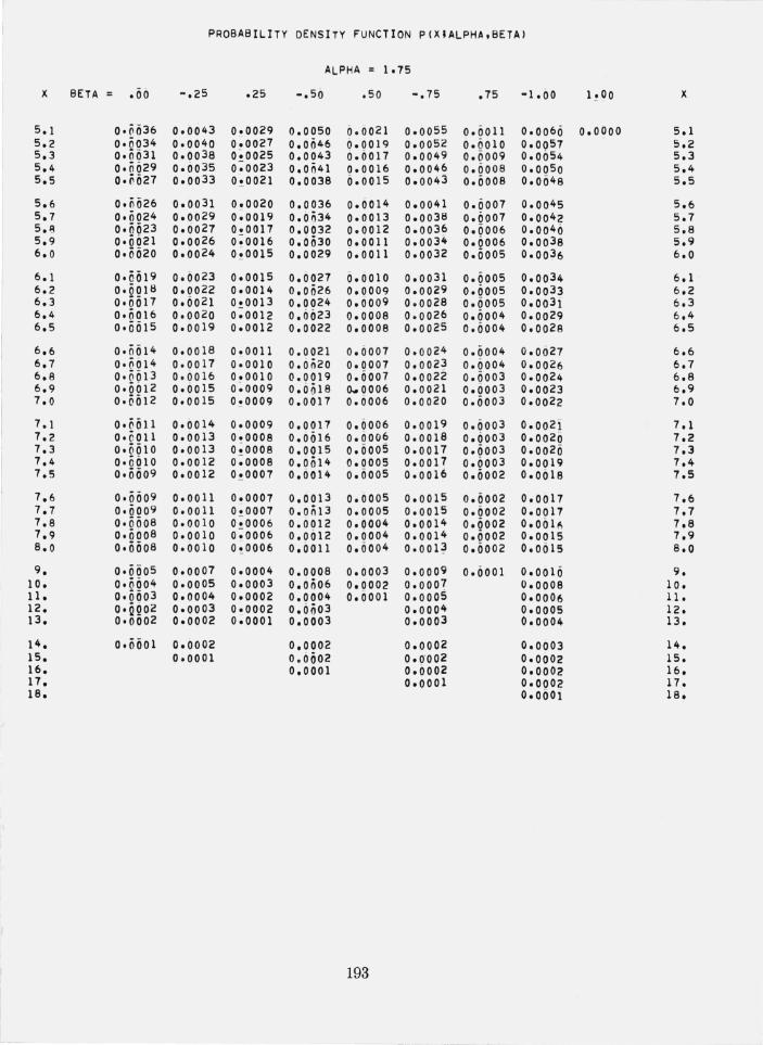
PROBABILITY DENSITY FUNCTION P(XIALPHA,BETA)

ALPHA = 1.75

X BETA .00 -.25 .25 -.50 .50 -.75 .75 -1.00 1!00 X

5.1 0.n036 0.0043 0.0029 0.0050 0.0021 0.0055 0.0011 0.0060 0.0000 5.1 5.2 0.QQ34 0.0040 0~0027 0.0046 0.0019 0.0052 0.0010 0.0057 5.2 5.3 0.0031 0.003B 0~0025 0.0043 0.0017 0.0049 0.0009 0.0054 5.3 5.4 0.0029 0.0035 0~0023 0.0041 0.0016 0.0046 0.0008 0.00 5 0 5.4 5.5 0.0027 0.0033 0!0021 0.0038 0.0015 0.0043 0.0008 0.0048 5.5

5.6 0.0026 0.0031 0!0020 0.0036 0.0014 0.0041 0.0007 0.0045 5.6 5.7 0.0024 0.0029 0.0019 0.0~34 0.0013 0.0038 0.0007 0.00 42 5.7 5.8 0.0023 0.0027 0.0017 0.0032 0.0012 0.0036 0.0006 0.0046 5.8 5.9 0.0021 0.0026 0;0016 0.0030 0.0011 0.0034 0.0006 0.0038 5.9 6.0 0.0020 0.0024 0; 0015 0.0029 6.0011 0.0032 0.0005 0.00 36 6.0

6.1 0.0019 0.0023 0.0015 0.0027 0.0010 0.0031 0.0005 0.0034 6.1 6.2 0.0018 0.0022 0.0014 0.0026 0.0009 0.0029 0.0005 0.0033 6.2 6.3 0.0017 0.0021 0!0013 0.0024 0.0009 0.0028 0.0005 0.00 31 6.3 6.4 0.ii016 0.0020 0.0012 0.0023 0.0008 0.0026 0.0004 0.0029 6.4 6.5 0.ii015 0.0019 0.0012 0.0022 0.0008 0.0025 0.0004 0.0028 6.5

6.6 0.0014 0.0018 0.0011 0.0021 0.0007 0.0024 0.0004 0.0027 6.6 6.7 0.~014 0.0017 0.0010 0.0020 0.0007 0.0023 0.0004 0.0026 6.7 6.8 0'0013 0.0016 0.0010 0.0019 0.6007 0.0022 0.0003 0.0024 6.8 6.9 0.0012 0.0015 0~0009 0.00 18 0...0006 0.0021 0.6003 0.0023 6.9 7.0 0.0012 0.0015 0! 0009 0.0017 0.0006 0.0020 0.0003 0.0022 7.0

7.1 0'0011 0.0014 0.0009 0.0017 0.6006 0.0019 0.0003 0.0021 7.1 7.2 0.6011 0.0013 0!0008 0.6016 0.0006 0.0018 0.0003 0.0020 7.2 7.3 0.0010 0.0013 0!0008 0.0015 0.0005 0.0017 0.0003 0.0020 7.3 7.4 0.QQ10 0.0012 0.0008 0.0014 0.0005 0.0017 0.0003 0.0019 7.4 7.5 0.0009 0.0012 0!0007 0.0014 0.0005 0.0016 0.0002 0.0018 7.5

7.6 0.0009 0.0011 0.0007 0.0013 0.0005 0.0015 0.0002 0.0017 7.6 7.7 0.0009 0.0011 0!0007 0.On13 0.0005 0.0015 0.0002 0.0017 7.7 7.8 0.ii008 0.0010 0.0006 0.0012 0.0004 0.0014 0.0002 0.001~ 7.8 7.9 0.0608 0.0010 0;0006 0.0012 0.0004 0.0014 0.0002 0.0015 7.9 8.0 0.0008 0.0010 0 ;' 0006 0.0011 0.0004 0.001~ 0.0002 0.0015 8.0

9. 0.0005 0.0007 0.0004 0.0008 0.0003 0.0009 0.6001 0.0010 9. 10. 0'QQ04 0.0005 0.0003 0.0006 0.0002 0.0001 0.0008 10. 11. 0.0003 0.0004 0.0002 0.0004 0.0001 0.0005 0.0006 11. 12. 0'220 2 0.0003 0.0002 0.0003 0.0004 0.0005 12. 13. 0.0002 0.0002 0.0001 0.0003 0.0003 0.0004 13.

14. 0.0001 0.0002 0.0002 0.0002 0.0003 14. 15. 0.0001 0.Oii02 0.0'002 0.0002 15. 16. 0.0001 0.0002 0.0002 16. 17. 0.0001 0.0002 17. 18. o.oooi 18.

193

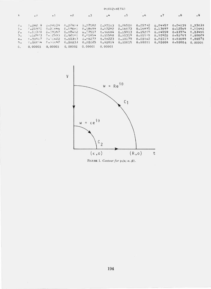
p(X;2"lE.TAl

x • (! • 1. - :2 .3 .4 .S . F, .7 .8 .9

(1 . ~ . 28~ . 9 d " d139 !1 . 279 ? '1 o. 7 582 C.?71 03 0.26501) 0.25? '~2 0 .249 57 0.24039 O .2303 ~ 1 • ·' . 2 ] 970 0 · >'.46 Q.1 9 6 ;'! O. 8489 0 .17282 0 .] 60 73 0.141<75 0.13697 0.12549 0 .11440 2 . !' • 1 ~ ) 3 ,2> (I . 9J6 7 0 . 0 8 412 iJ . 7517 1) . '166Cl4 0.05913 0.OS2 !'S 0.(>4559 0·03974 0.034'+6 3 . ') . 0 ;.:9l3 0 . 2~ :> 3 0 .n2p<I r; .' . 1 8:'4 O. ()lS68 i).n131 9 0.011 6 5 a. nono 0~OO761 0 .00629 4. (' . OO!)]7 ~; . ·2 422 0 .003 43 0 . 0277 0 . 1)02 23 0 . J0 179 0.00142 0.001D 0.00089 n.ooo7o S • 1! .on () ') 4 n. ':, :) n4? n .ouo33 n. 0 0 25 G.no019 0.00015 0.00011 0.00008 (J.nooa 6 0.00005 6. O. 00003 0.00003 O. 00002 O. 00001 O. 00001

v

w s e i 8

(E ,0) ( R ,0 ) t

FIG URE 1. Contour for P2(X; a, f3).

194

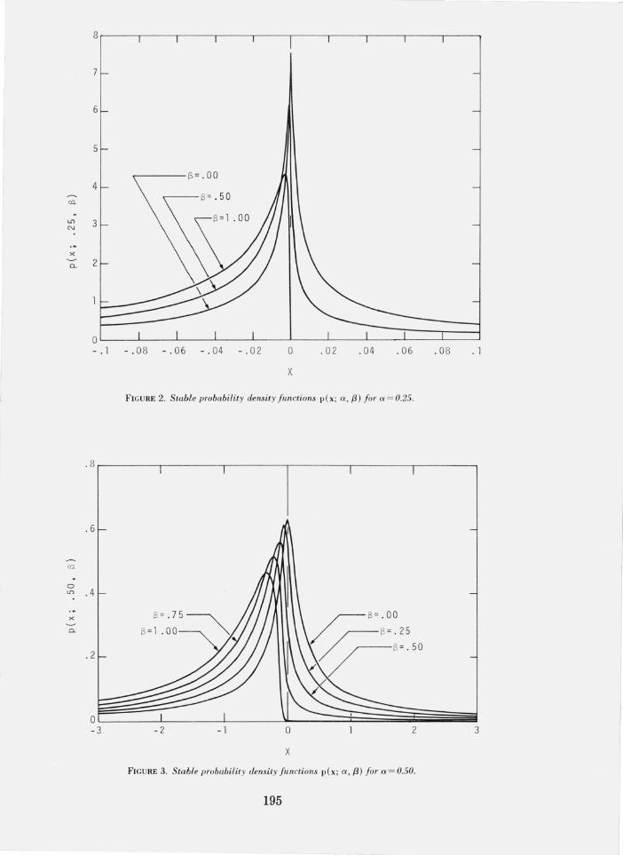
Cl

OL-__ ~ ____ -L ____ -L ____ ~ ____ L-__ ~ ____ -L ____ J-____ L-__ ~

- . 1 - . 08 - .06 -. 04 -. 02 o

X

.02 .04 . 06

FI GU RE 2. Stable probability density functions p(x; a, f3) for a = 0.25 .

.08 .1

. 8 ,--------.--------.--------,,--------.--------.--------.

. 6

Ln .4

x S=.OO D-

.2

- 2 - 1 o 2 3

X

FIGURE 3. Stable probability density functions p(x ; a, f3 ) for a = 0.50.

195

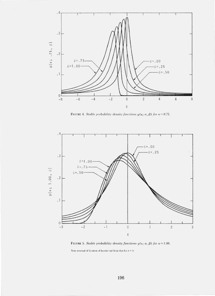
.4.-----.------,,-----,-------.-----,------.------,------,

.3

ill

L!)

..... .2

x S=.OO ~

~;~550 D-

.1

/

Oc===r===~ __ ~~-L~=±~~~~~ __ - 8 -6 -4 - 2 o 2 4 6 8

x

FIGURE 4. Stable probability density functions p{x; a, f3) for a = 0.75 .

. 4.---.----.----.---.----.----.---.----.----.---.----.---.

.3

g .2

.1

-2 - 1 o 2 3

x

FIGURE 5. Stable probability density functions p{x; a , f3) for a = 1.00.

Note reversal of location of heavier tail from that for 0' =F 1.

196

-- -- - - -

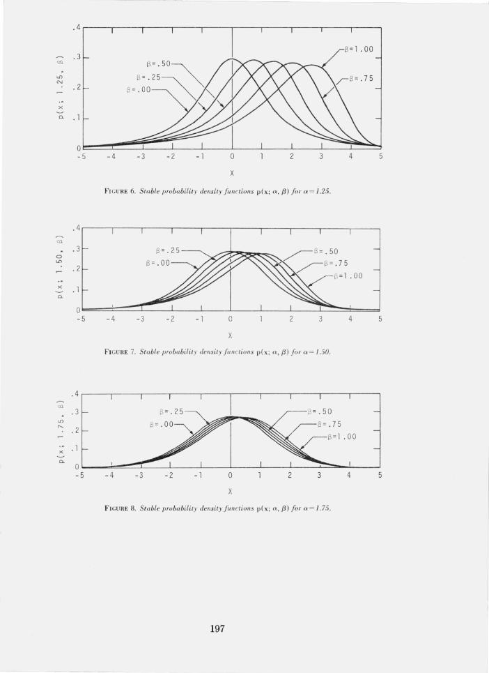
~ .4 I

8= 1 .00 .3

ill

B ~B ;;~ L.O N

.2 8 =.00 '"

><

0- . 1

x

fI GU RE 6. Stable probability density j unctions p (x; a, (3) jor a = 1.25 .

. 4 ill

. 3 0 L.O

.2

>< . 1 0-

0 - 5 -4 -3 - 2 - 1 0 2 3 4 5

x

F IGURE 7. Stable probability dens ity junctions p( x; a , (3) jor a = J .50 .

. 4 <:Q.

. 3 Lf)

r--. .2

>< . 1

0-

0 - 5 - 4 - 3 - 2 - 1 0 2 3 4 5

X

FICU RE 8. Stable probability density j unctions p (x; a , (3 ) jor a = 1.75.

197

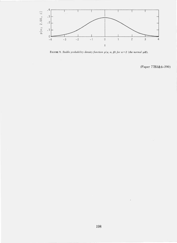
'l

.4 ill

.3 CJ CJ

.2 N

x .1 <>-

0 -4 -3 -2 - 1 0 2 3 4

X

FIGURE 9. Stable probability density function p{x; a, (3) for a = 2 (the normal pdf).

(Paper 77B3&4-390)

198