Synthesis of Timed Asynchronous CircuitsChris J. Myers and Teresa H. -Y. MengComputer Systems LaboratoryStanford UniversityStanford, CA 94305Appeared in IEEE Trans. VLSI Systems in June 1993

AbstractIn this paper we present a systematic procedure to synthesize timed asynchronous circuits using timing con-straints dictated by system integration, thereby facilitating natural interaction between synchronous and asyn-chronous circuits. In addition, our timed circuits also tend to be more e�cient, in both speed and area, com-pared with traditional asynchronous circuits. Our synthesis procedure begins with a cyclic graph speci�cationto which timing constraints can be added. First, the cyclic graph is unfolded into an in�nite acyclic graph.Then, an analysis of two �nite subgraphs of the in�nite acyclic graph detects and removes redundancy in theoriginal speci�cation based on the given timing constraints. From this reduced speci�cation, an implementa-tion that is guaranteed to function correctly under the timing constraints is systematically synthesized. Withpractical circuit examples, we demonstrate that the resulting timed implementation is signi�cantly reduced incomplexity compared with implementations previously derived using other methodologies.1 IntroductionThe design of timed asynchronous circuits has recently gained much attention because of the increasing needfor asynchronous circuits in mixed synchronous/asynchronous environments. Inherent in these environmentsare timing constraints (gate, wire, and environment delay information) which circuits must satisfy andcan exploit to optimize the implementation. Existing asynchronous design techniques either cannot handlesystems with timing constraints, or do not fully utilize the information contained in them. This paperpresents a methodology to synthesize asynchronous circuits that utilizes timing constraints throughout thesynthesis procedure. As a result, our timed circuits retain the same behavior with less circuit complexitythan earlier implementations.Many methodologies have been proposed for the synthesis of speed-independent circuits [1] [2] [3] [4].Speed-independent circuits are very robust since they are guaranteed to work independent of the delaysassociated with their gates, but they can be overly conservative when timing constraints are known. Timedcircuits, on the other hand, are only guaranteed to work if the delays fall in the range given in the timingconstraints of the speci�cation. Utilizing these timing constraints, we trade robustness to variations in delaysfor signi�cant reductions in circuit complexity.Speed-independent circuits are restricted to interfaces where their environment only changes inputs inresponse to changes of outputs. Inputs from a synchronous circuit often do not satisfy this restriction. Inorder to address this problem, fundamental mode synthesis methods have been used [5] [6] [7] [8], whichassume the environment will wait long enough for the circuit to stabilize before inputs are changed. Timinganalysis must be performed after synthesis, and appropriate delays may need to be added to guarantee thatthis requirement is satis�ed. Since these methods limit the concurrency within a circuit and do not fullyutilize available timing constraints, they may result in circuits that are larger and slower than necessary.0This research was supported by an NSF fellowship, ONR Grant no. N00014-89-J-3036, and research grants from the Centerfor Integrated Systems, Stanford University and the Semiconductor Research Corporation, Contract no. 92-DJ-205.The authors are with the Department of Electrical Engineering, Stanford University, Stanford, CA 94305.1

Methods have been proposed to use timing constraints to synthesize timed circuits [9] [10]; however, mosttechniques apply timing constraints after synthesis only to verify that hazards do not exist. If hazards aredetected, delay elements are added to avoid them, degrading the performance of the implementation. It wasshown in [4] that the more conservative speed-independent model while resulting in somewhat larger circuitsactually produces faster circuits compared with the timed circuits described in [10]. This surprising resultcan be attributed to the fact that these timed circuits often need to have delay elements added to the criticalpath to remove hazards.Our synthesis procedure uses the timing constraints at the outset to enhance performance while min-imizing circuit complexity. In several practical examples, we show that signi�cant reductions in circuitcomplexity (measured in terms of literal count needed for the implementation) as compared to previousdesigns can be achieved using very conservative timing constraints. In particular, in a memory managementunit designed for use with a real asynchronous microprocessor [11] [12], the circuit complexity is reducedby over 50 percent over the speed-independent implementation. Circuit performance is also enhanced, notonly because we have reduced circuit area and do not use delay elements, but also because we are able tosynthesize a more concurrent speci�cation without adding state variables. An example of a DRAM controllerto be used with a synchronous processor and DRAM array is presented to illustrate a design that cannot bedone speed-independently. Circuit complexity is also reduced as compared to previous fundamental modedesigns [13] [7].This paper contains �ve sections. Section 2 describes our speci�cation language and timing analysisalgorithm. Section 3 discusses our synthesis procedure. Section 4 presents several practical examples.Section 5 gives our conclusions.2 Timing Analysis on Timed Speci�cationsA wide variety of methodologies for speci�cation of asynchronous circuits have been proposed. They can beroughly grouped into three classes: language based, such as communicating sequential processes (CSP) [1];graph based, such as signal transition graphs (STG) [2]; and �nite-state machine based, such as burst-modestate machines (BSM) [6]. At a high-level, CSP provides a very concise representation for large designssuch as the microprocessor described in [11]. It is well suited for non-deterministic behavior, but it can bedi�cult to specify concurrency within a process. On the other hand, STG provides a good representationof concurrency within a process, but it is cumbersome to use for large designs and cannot specify arbitrarynon-deterministic behavior. Neither of these representations are good for specifying asynchronous circuitsin a synchronous environment. BSM has been successfully used for such applications [13], which was madepossible by assuming fundamental mode as opposed to the other two speci�cations which use the speed-independent model. None of these speci�cation methods incorporates timing constraints.We chose to use a speci�cation language, the event-rule (ER) system [14], which is easily derivable fromCSP, STG, and BSM and incorporates timing constraints. It is shown in [14] that speci�cations that are notdisjunctive or non-deterministic can be directly transformed into an ER system. A speci�cation is disjunctiveif there exists a transition in the speci�cation that is speci�ed to occur after either one transition or another,but it does not have to be preceded by both. A speci�cation is non-deterministic if the circuit behavior isdetermined by a choice made by either the environment or the circuit. Derivation of ER systems from eachspeci�cation method described above (i.e., CSP, STG, and BSM) is illustrated through an example. Whileour synthesis procedure does not presently allow non-deterministic speci�cations, it is shown, by way ofan example, that some non-deterministic speci�cations can be transformed into deterministic speci�cationswhich can then be synthesized.In order to synthesize timed circuits, timing analysis must be used on the ER system speci�cationto deduce timing information necessary to detect redundancy in the speci�cation from the given timingconstraints. More speci�cally, in timed circuits, the timing information needed is the minimumand maximumdi�erence in time between any two events (i.e., signal transitions) in a circuit speci�cation. Polynomial-timealgorithms have been developed [15] [16] to determine the di�erence in time between any two events in anacyclic graph. Circuit speci�cations, however, are normally cyclic. Therefore, to apply these algorithms tocircuit synthesis, these results must be expanded to handle cyclic speci�cations. Recently, an algorithm hasbeen proposed that �nds these time di�erences in cyclic graphs in exponential-time [17]. In this paper, we2

propose instead a polynomial-time heuristic algorithm which is su�cient for our purposes. Our algorithmunfolds the cyclic graph into an in�nite acyclic graph and then examines only two �nite acyclic subgraphsof the in�nite graph to determine a su�cient bound on the time di�erence between two events.2.1 Event-Rule SystemThe ER system was introduced in [14] for performance analysis of asynchronous circuits. It was modi�ed toincorporate bounds on the timing constraints and introduced as a speci�cation language for timed circuitsin [18]. An ER system is composed of a set of atomic actions, events, and the causal dependencies betweenthem, rules, and it can be compactly represented using an event-rule (ER) schema.2.1.1 EventsAn event is de�ned as \ : : :an action which one can choose to regard as indivisible|it either has happenedor has not : : :" [19]. In circuits, events are transitions of signals from one value to another. There are twotransitions associated with each signal s in a speci�cation, namely, s " where " denotes that the signal s ischanging from a low to high value, and s # where # denotes that the signal s is changing from a high to lowvalue.2.1.2 RulesA rule is a causal dependency between two events. Each rule is composed of an enabling event, an enabledevent, and a bounded timing constraint. Informally, a rule states that the enabled event cannot occur untilthe enabling event has occurred. If two rules enable the same event then that event cannot occur until bothenabling events have occurred. This causality requirement is termed conjunctive.The bounded timing constraint places a lower and upper bound on the timing of a rule. A rule is said tobe satis�ed if the amount of time which has passed since the enabling event has exceeded the lower boundof the rule. A rule is said to be expired if the amount of time which has passed since the enabling event hasexceeded the upper bound of the rule. An event cannot occur until all rules enabling it are satis�ed. Anevent must always occur before every rule enabling it has expired. Since an event may be enabled by multiplerules, it is possible that the di�erence in time between the enabled event and some enabling events exceedsthe upper bound of their timing constraints, but not for all enabling events. These timing constraints arethe same as the max constraints described in [15] and the type 2 arcs described in [16].Finding timing constraints for a speci�cation is not a trivial task. Rules can be categorized into envi-ronment rules (i.e., the enabled event is a transition of an input signal) and internal rules (i.e., the enabledevent is a transition of a state variable or output signal). Timing constraints for environment rules can bedetermined from interface speci�cations or datapath delay estimates. For internal rules, the problem is muchmore di�cult since the timing constraints cannot be known until the circuit is synthesized, but the circuitcannot be synthesized without given timing constraints. To solve this problem, the designer should estimatethe maximumdelay for the gates in the library to be used and set the upper bound of the timing constraintin each internal rule to this value. The lower bound of the timing constraint should usually be set to 0 sinceoptimizations could potentially reduce the gate to nothing more than a wire. After a circuit is generated, itshould be analyzed using a timing analysis tool to verify that the timing constraints used are correct. If thecircuit violates the timing constraints, it must be resynthesized with more conservative timing constraints(larger upper bounds in this case). In order to avoid resynthesis, conservative values should be used fortiming constraints on internal rules at the outset. In the design of interface circuits and other controllers,inputs often are from o�-chip or from a datapath. In these cases, the lower bound of the timing constrainton environment rules is large compared with the upper bound of the timing constraints on internal rules.Therefore, a conservative estimate for internal gate delays does not signi�cantly a�ect the complexity of thetimed implementation.2.1.3 Event-Rule SchemaAn ER system can be speci�ed using an ER schema and initialization information described in the nextsubsection. An ER schema de�nes a cyclic constraint graph which is a weighted marked graph in which the3

vertices are the events, the arcs are the rules, the weights are the bounded timing constraints, and the initialmarking is given by the value of ". Each rule of the form he; f; "; � i is represented in the graph with anarc connecting the enabling event e to the enabled event f . The arc is weighted with the bounded timingconstraint � . In other words, each rule corresponds to a graph segment, e �! f (or e �!� f when the rule isinitially marked, i.e., " = 1). A cyclic constraint graph is similar to a STG in which timing constraints havebeen added to the arcs. The ER schema is de�ned more formally as follows:De�nition 2.1 (Event-Rule Schema) An event-rule schema is a pair hE0; R0i where E0 is a �nite set ofevents, and R0 is a �nite set of rules. Each rule is denoted as he; f; "; � i, where e and f are two events, " isde�ned to be 1 if the rule has an initial marking and 0 otherwise, and � = [l; u] where l is the lower boundand u is the upper bound of the timing constraint on the rule.As an example, a SCSI protocol controller, originally speci�ed with a STG [20], is speci�ed by its cyclicconstraint graph as shown in Figure 1. An example of a rule in this constraint graph is between the twoevents q # and rdy #, which is of the form hq #; rdy #; 0; [0; 5]i.Our synthesis procedure requires that each event in an ER schema is uniquely identi�ed. This led to therestriction in [18] of only one rising and one falling transition of each signal per cycle in the speci�cation. Toremove this restriction in this paper, each occurrence of the rising and falling transition in a cycle is given aunique name. For example, a signal s speci�ed to rise and fall twice in a cycle, is renamed to s1 for the �rstrising and falling transitions and s2 for the second. These events are treated separately during the timinganalysis; however, they are recombined during synthesis as illustrated in an example later.Another requirement is that the cyclic constraint graph is well-formed. A cyclic constraint graph is well-formed if it is strongly connected, every cycle has the sum of the " values along the cycle greater than orequal to 1, and for every event there exists a cycle including the event in which the sum of the " values isequal to 1 [17]. Many speci�cations are not well-formed, but such speci�cations can often be synthesized bytransforming them into ones which are well-formed as shown later in an example.2.1.4 Event-Rule SystemTo construct the ER system, the cyclic constraint graph is transformed into an in�nite acyclic constraintgraph. Each event in the ER schema is mapped onto an in�nite number of event occurrences, each corre-sponding to a di�erent occurrence of that event. The rules are similarlymapped. Thus, in the in�nite acyclicconstraint graph, each rule occurrence he; f; i; "; � i corresponds to a graph segment, he; i � "i �! hf; ii. Theoccurrence-index i is used to denote each separate occurrence of an event or rule in the ER schema. The�rst occurrence has i = 0, and i increments with each following occurrence. The occurrence-index o�set" is the di�erence in the occurrence-index of the enabled event f and the enabling event e. For each ruleoccurrence, the value of the occurrence-index o�set " is the same as the value of the initial marking " for thecorresponding rule in the ER schema.A special reset event is added to the set of events in order to model the reset of the circuit. For eachinitially marked rule (i.e., " = 1) with enabled event f , a reset rule is added between the reset event andthe event f . This rule models special timing constraints on the initial occurrence of the event f . E�ectively,the acyclic constraint graph is constructed by cutting the cyclic constraint graph at the initial marking andunfolding the graph an in�nite number of cycles. The result is an ER system as de�ned below:De�nition 2.2 (Event-Rule System) Given the event-rule schema hE0; R0i, de�ne an event-rule system tobe a pair hE;Ri where each event occurrence he; ii in E where i � 0 represents an occurrence of an evente in E0, and each rule occurrence he; f; i; "; � i in R where i � " is an occurrence of a rule he; f; "; � i in R0.The event hreset; 0i is added to E. For each rule in R0 in which " = 1, a rule of the form hreset; f; 0; 0; �0iis added to R.The speci�ed circuit behavior is de�ned by simulating the acyclic constraint graph using the timed �ringrule given below:De�nition 2.3 (Timed Firing Rule) Given that t(hf; ii) is the exact time of the event occurrence hf; ii, itcan take on any value within the bound de�ned in terms of the times of the event occurrences that enable it.4

The bound can be given as follows:maxhe;f;i;";�i2Rft(he; i � "i) + lg � t(hf; ii) � maxhe;f;i;";�i2Rft(he; i � "i) + ugA subgraph of the unfolded in�nite acyclic constraint graph for the SCSI protocol controller is shown inFigure 2. An example of a rule occurrence in this ER system is between the two event occurrences hq #; 0iand hrdy #; 0i, which is of the form hq #; rdy #; 0; 0; [0;5]i. According to the timed �ring rule, the eventoccurrence hrdy #; 0i cannot occur until both the event occurrences hq #; 0i and hgo "; 0i have occurred, andit must occur before 5 time units have elapsed since both the event occurrences occurred.2.2 Timing AnalysisIn order to transform an ER system speci�cation into a timed circuit, our synthesis procedure requires atiming analysis algorithm to determine the minimum and maximum time di�erence between any two events.We have developed an e�cient polynomial-time timing analysis algorithm to determine a su�cient estimateof these time di�erences based on only two �nite subgraphs of the in�nite acyclic constraint graph.2.2.1 Worst-Case Time Di�erenceA time di�erence is a bound in the amount of time between two event occurrences (see De�nition 2.4). Theworst-case time di�erence is a bound on the minimum and maximum di�erence in time between two eventsfor any occurrence (see De�nition 2.5).De�nition 2.4 (Time Di�erence) Given two event occurrences, hu; i � ji and hv; ii, and the occurrence-index o�set between them j where j � 0, the time di�erence between these two event occurrences is thestrongest bound [Li; Ui] such that: Li � t(hv; ii) � t(hu; i� ji) � UiDe�nition 2.5 (Worst-Case Time Di�erence) Given two events, u and v, and the occurrence-index o�setbetween them j where j � 0, the worst-case time di�erence between these two events, [L;U ], is:L = mini�j fLig and U = maxi�j fUig;where [Li; Ui] is the time di�erence for each occurrence of u and v with o�set j (as de�ned in De�nition 2.4).2.2.2 Algorithm to Estimate Worst-Case Time Di�erenceIn our ER systems, a pair of events has an in�nite number of occurrences; however, it is possible to analyzea �nite number of occurrences to �nd a su�cient estimate of the worst-case time di�erence as de�ned inDe�nition 2.6.De�nition 2.6 (Estimate of the Worst-Case Time Di�erence) Given the worst-case time di�erence [L;U ]between two events, an estimate of the worst-case time di�erence is any [L0; U 0] such that L0 � L and U 0 � U .Given two events u and v and an occurrence-index o�set between them j, Algorithm 2.3 determines anestimate of the worst-case time di�erence between them by constructing two �nite acyclic subgraphs to beanalyzed by Algorithm 2.2. The �rst subgraph includes only events and rules with indices i � 1 and i forsome arbitrary value of i > 0. A source event is added to this subgraph, and each rule with " = 1 and withindex i � 1 is replaced with a rule from the source event to the enabled event with a timing constraint of[0;1]. This construction guarantees that no timing assumptions are made about previous cycles which arenot modeled in our �nite graph. For the special case when i = 0, another subgraph is constructed whichincludes only events and rules with i = 0. We prove later that the analysis of these two subgraphs yields anestimate of the worst-case time di�erence.These two subgraphs are acyclic and �nite so the algorithms described in [15] and [16] can be used to�nd the time di�erence between any two event occurrences hu; i� ji and hv; ii in these graphs. The function5

MaxDi� (de�ned recursively in Algorithm 2.1 [16]) is used to �nd the upper bound of the time di�erenceUi. MaxDi� is also used to �nd the minimum time di�erence Li since MinDi�(hu; i � ji; hv; ii) = (�1) �MaxDi�(hv; ii; hu; i� ji) [15] [16]. The estimate of the worst-case time di�erence returned by Algorithm 2.3is the minimum of the lower bounds and the maximum of the upper bounds of the time di�erences for theith and 0th occurrence. In our synthesis procedure, only time di�erences with values of j = 0 or j = 1 areof interest, so this algorithm does not produce a tight bound for j > 1. Also, since the worst-case timedi�erence is only de�ned over values of i where i � j, the 0th occurrence only needs to be considered if j = 0.Finally, since this algorithm is called repeatedly in the synthesis procedure, the graphs are created only oncefor a given circuit, and once a time di�erence is calculated for a particular pair of event occurrences, it isstored in a table such that it need not be recalculated.Algorithm 2.1 (Find Max Time Di�erence in an Acyclic Graph)int MaxDi�(acyclic graph G; event occurrences hu; i� ji, hv; ii) fmaxdi� = maxhe;v;i;";�evi2RfMaxDi�(G; hu; i� ji; he; i� "i) + uevg;If there is a path from hv; ii to hu; i� ji thenmaxdi� = minf minhe;u;i�j;";�eui2RfMaxDi�(G; he; i� j � "i; hv; ii) + leug;maxdi�g;Return(maxdi�);gAlgorithm 2.2 (Find Time Di�erence in an Acyclic Graph)bound TimeDi�(acyclic graph G; event occurrences hu; i� ji, hv; ii) fLi = (�1) �MaxDi�(G; hv; ii; hu; i� ji);Ui = MaxDi�(G; hu; i� ji; hv; ii);Return([Li; Ui]);gAlgorithm 2.3 (Find Estimate of the Worst-Case Time Di�erence in a Cyclic Graph)bound WCTimeDi�(ER system hE;Ri; events u; v; occurrence-index o�set j) fIf (j > 1) then Return([�1;1]);Else fConstruct subgraph G from hE;Ri using only events and rules with indices i � 1 and ifor an arbitrary i > 0 and exclude rules with enabling event hreset; 0i;Add event hsource; i� 1i to graph G;For each rule of the form he,f ,i � 1,1,� i in graph G, replace it with hsource,f ,i � 1,0, [0;1]i;[Li; Ui] = TimeDi�(G; hu; i� ji; hv; ii);If (j == 1) then Return([Li; Ui]);Else fConstruct subgraph G0 from hE;Ri using only events and rules with index i = 0;[L0; U0] = TimeDi�(G0; hu; 0i; hv; 0i);L0 = min(Li; L0);U 0 = max(Ui; U0);Return([L0; U 0]);g g gFor the example shown in Figure 2, the estimate of the worst-case time di�erence found by Algorithm 2.3between the two events rdy # and q # with occurrence-index o�set j = 0 is the bound [15; 55]. This meansthat rdy # always occurs at least 15 units of time after q #, but no more than 55 units of time after q #.2.2.3 Proof of CorrectnessTheorem 2.1 shows that the bound for the ith occurrence, [Li; Ui], found in Algorithm 2.3 is an estimate forall i > 0. Therefore, combining this with the actual time di�erence for i = 0 results in an estimate of theworst-case time di�erence.Theorem 2.1 Algorithm 2.3 determines an estimate of the worst-case time di�erence between two events.6

Proof: In order to show that Algorithm 2.3 returns an estimate of the worst-case time di�erence, wemust show that the following inequalities hold: L0 � L and U 0 � U (from De�nition 2.6). If j > 1 thenAlgorithm 2.3 returns [L0; U 0] = [�1;1] which trivially satis�es De�nition 2.6. If j = 1 then it returns[L0; U 0] = [Li; Ui]. If j = 0 then Algorithm 2.3 returns L0 = min(L0; Li) and U 0 = max(U0; Ui). Since[L0; U0] is an actual time di�erence for the 0th occurrence, we only need to show that [Li; Ui] always yieldsan estimate for i > 0. A maximum time di�erence is calculated recursively in terms of other maximum timedi�erences (see Algorithm 2.1). Therefore, when calculating Ui using subgraph G, one of two cases mayoccur. Its value may be independent of maxdi� values for events not in graph G (i.e., events with indices lessthan i � 1). If this is the case, then Ui = mini�1fUig. On the other hand, if it depends on time di�erencesof earlier events not in graph G, then just before MaxDi� falls o� the end of the graph, it will call eitherMaxDi�(G; hsource; i� 1i; hf; i� 1i) (1) or MaxDi�(G; hf; i� 1i; hsource; i� 1i) (2). Since the rule betweenhf; i � 1i and hsource; i � 1i has timing constraint [0;1], (1) will return 1, and (2) will return 0. If graphG were extended to include another cycle, the rule between hsource; i� 1i and hf; i� 1; i would be replacedwith a rule of the form he; f; i � 1; 1; � i. Now, MaxDi�(G; he; i � 2i; hf; i� 1i) would be called which wouldreturn a value less than or equal to1, or MaxDi�(G; hf; i�1i; he; i�2i) would be called which would returna value less than or equal to 0 (note this second case is never positive because from the ordering de�ned bythe rule, we know that e always occurs before f). This relationship continues to hold if the graph is extendedan in�nite number of cycles. Since the value found for case (1) and for case (2) is greater than that foundif graph G is extended back further, and since the maximum time di�erence is calculated by adding thesevalues to values found on the rest of the graph, we know that the value calculated for Ui using graph G willbe less than or equal to the actual value of Ui for i > 1. Therefore, U 0 � U , and we can similarly show thatL0 � L. Thus, Algorithm 2.3 gives an estimate of the worst-case time di�erence.2.2.4 Complexity of the AlgorithmCalculating the time di�erence of each pair of events using the MaxDi� algorithm has complexity O(v � e)where v is the number of vertices and e is the number of arcs in the graph [15]. Let jE0j and jR0j be thenumber of events and rules, respectively, in the cyclic constraint graph representation. The largest graphwhich Algorithm 2.3 analyzes has 2jE0j vertices and 2jR0j arcs. Therefore, using Algorithm 2.3 to calculateestimates for all time di�erences has complexity O(jE0j � jR0j).2.2.5 Extensions to Find a Better EstimateIf either the bound is not tight enough or there is interest in �nding worst-case time di�erences of eventsacross more than one cycle (i.e., j > 1), the algorithm can be extended by increasing the size of the subgraphswhich Algorithm 2.3 analyzes. Assuming subgraph G is enlarged to contain c cycles (c = 2 in Algorithm 2.3),the algorithm is modi�ed in the following ways:1. Construct subgraph G using only events and rules with indices i � (c � 1); : : : ; i where i > (c� 2).2. Construct subgraph G0 using only events and rules with indices i � (c� 2).3. If j � (c� 2) then using graph G0, �nd [Lj ; Uj]; : : : ; [L(c�2); U(c�2)].4. L0 = min(Li; Lj ; : : : ; L(c�2)) and U 0 = max(Ui; Uj; : : : ; U(c�2)).In the modi�ed algorithm, estimates of worst-case time di�erences with j � (c � 1) can now be found.Theorem 2.1 can easily be extended to show that the modi�ed algorithm returns an estimate of the worst-casetime di�erence. It is also easy to show that the complexity of the modi�ed algorithm is O(cjE0j � cjR0j).2.2.6 Termination of the AlgorithmIn order to avoid unnecessary calculations, the algorithm can be modi�ed to check if extending the size of thesubgraphs analyzed (i.e., increasing c) is helpful. To do this, the algorithm is modi�ed to return a best-caseestimate, [Lbest; Ubest], in addition to the worst-case estimate, [L0; U 0], where Lbest = min(Lj ; : : : ; L(c�2))and Ubest = max(Uj ; : : : ; U(c�2)). Given the actual worst-case time di�erence is [L;U ], it is easily shown7

that these estimates satisfy the inequalities: L0 � L � Lbest and Ubest � U � U 0. If tightening thebound to [Lbest; Ubest] would not result in less circuitry than [L0; U 0], then it is not worth increasing c. Infact, if Lbest = L0 and Ubest = U 0, then the actual worst-case time di�erence [L;U ] has been found. Ingeneral, increasing c does not guarantee that the exact bound [L;U ] can always be found, but in all thecircuit examples that we synthesized, Algorithm 2.3 (i.e., c = 2) either found the exact bound or at least asu�ciently tight bound to detect all redundancies.3 Synthesis ProcedureGiven an ER system speci�cation, we apply our timing analysis algorithm to derive an optimized timedcircuit implementation. The synthesis procedure has three steps. The �rst step is to detect and removeredundant rules from the speci�cation. The second step is to construct a reduced state graph. The third stepis to derive a circuit implementation from the reduced state graph.3.1 Removing Redundant RulesThe �rst step in the synthesis procedure is to detect and remove redundant rules in the timed speci�cation.Since each internal rule results in a literal in the implementation in order to ensure the behavior speci�edby the rule, if it is determined that this behavior is guaranteed without the rule (i.e., the rule is redundant)then the literal can be removed from the implementation resulting in a smaller circuit.3.1.1 Redundant RulesA rule is redundant in the timed speci�cation if its omission does not change the behavior speci�ed by thetimed �ring rule. This is de�ned more formally as follows:De�nition 3.1 (Redundant Rule) A rule he; f; i; "; � i is redundant for all i � " if the bound on the time ofthe event occurrence hf; ii with the rule removed as de�ned below:maxhe;f;i;";�i2RNRft(he; i � "i) + lg � t(hf; ii) � maxhe;f;i;";�i2RNRft(he; i � "i) + ugwhere RNR = R � fhe; f; i; "; � i j i � "g is the same as the bound speci�ed in the timed �ring rule (seeDe�nition 2.3).3.1.2 Algorithm for Detecting Redundant RulesIf there are multiple rules enabling an event, then it is possible that some of them are redundant. Al-gorithm 3.1 checks each rule by using Algorithm 2.3 to �nd an estimate of the worst-case time di�erencebetween the enabled and enabling event. We prove later that if the lower bound of this estimate is largerthan the upper bound of the timing constraint on the rule, then the rule is redundant.Algorithm 3.1 (Find Redundant Rules)set FindRed(ER system hE;Ri) fRNR = R;For each rule of the form he,f ,i,",� i where � = [l; u] f[L0; U 0]=WCTimeDi�(hE;Ri; e; f; ");If (L0 > u) then RNR = RNR � fhe; f; i; "; � i j i � "g;gReturn(RNR);g The SCSI protocol controller example depicted in Figure 2 has four events that are enabled by multiplerules: req #, rdy #, req ", and q ". For the rule, hq #; rdy #; i; 0; [0; 5]i, Algorithm 2.3 estimates the worst-casetime di�erence between the two events rdy # and q # to be the bound [15; 55]. Since the lower bound ofthis time di�erence, 15, is greater than the upper bound of the timing constraint on the rule, 5, the rule isfound to be redundant. In other words, the rule between the events q # and rdy # can be removed withoutchanging the speci�ed behavior. Further analysis �nds this to be the only redundant rule.8

3.1.3 Proof of CorrectnessDe�nition 3.1 de�ned a redundant rule as a rule which could be removed from the ER system withoutchanging the behavior speci�ed by the timed �ring rule. By applying transformations to the timed �ringrule, Theorem 3.1 proves that Algorithm 3.1 �nds redundant rules.Theorem 3.1 Algorithm 3.1 �nds redundant rules.Proof: (by contradiction) Given a rule he; f; i; "; � i sati�es the condition set forth in Algorithm 3.1 tobe redundant (i.e., L0 > u), assume that it is not redundant. In that case, there exists a value of i such thatone of the following is true:t(he; i � "i) + l � t(hf; ii) or t(hf; ii) � t(he; i� "i) + u:(from De�nitions 2.3 and 3.1). Now, subtract t(he; i� "i) from each element:l � t(hf; ii) � t(he; i� "i) or t(hf; ii) � t(he; i � "i) � u:These are instances of a worst-case time di�erence, so they are bounded by [L;U ],L � l � t(hf; ii) � t(he; i� "i) � U or L � t(hf; ii) � t(he; i � "i) � u � U:(from De�nition 2.5). Since L0 returned by Algorithm 2.3 is an estimate of the worst-case time di�erence(from Theorem 2.1), L0 � L (from De�nition 2.6). Also, L0 > u (from Algorithm 3.1) and u � l (fromDe�nition 2.2), so the following inequalities hold:l � u < L0 � L � l or u < L0 � L � u:Thus, we have a contradiction in each case.3.2 Finding the Reduced State GraphIn order to generate a circuit implementation, many methodologies transform a higher-level speci�cationinto a state graph so that Boolean minimization techniques can be applied [2] [3]. Essentially, a state graphis a graph in which the vertices are bitvectors and the arcs are signal transitions. Each bitvector speci�es thebinary value of every signal in the system when the system is in that state. In our method, timing analysisis utilized to generate a reduced state graph which often has signi�cantly fewer states than a state graphgenerated without considering timing constraints. Since the size of the state graph and the complexity of thecircuitry are strongly correlated, our method often results in simpler circuitry compared with other methodsthat do not fully utilize timing constraints.3.2.1 Reduced State GraphTypically, a state graph is speci�ed as a set of states and a set of transitions between states [2] [3]. Algo-rithm 2.3 can be utilized to detect states that can never be reached, resulting in a reduced state graph. Theseunreachable states are removed from the set of states, and the transitions leading to them are removed fromthe set of transitions. It is not always possible to infer from the reduced state graph all enabled transitions,since a transition can be enabled in a particular state without an arc leading from it to a state where thattransition has occurred. Although the transition cannot occur in the next state, the fact that it has beenenabled is needed during synthesis. To solve this problem, a reduced state graph is fully characterized by aset of states that contain information on enabled transitions as described in De�nition 3.2. Each such stateis a vertex in the reduced state graph, and these vertices are connected by arcs as described in De�nition 3.3.De�nition 3.2 (State) Each state S is of the form S = s1; : : : ; sk; : : : ; sn, where n is the number of signalsin the speci�cation. Each state bit sk has the value: 0 if the signal sk is low, R if the signal sk is low butenabled to rise, 1 if the signal sk is high, and F if the signal sk is high but enabled to fall. The functionVAL[sk] = 0 if sk = 0 or R and VAL[sk] = 1 if sk = 1 or F .De�nition 3.3 (Reduced State Graph) A reduced state graph is a graph in which its vertices are states andthe arcs are allowed transitions between states. There exists an arc from state S to state S0 if there exists asignal sk, such that for all l 6= k, VAL[s0l] = VAL[sl], and either sk = R and VAL[s0k] = 1, or sk = F andVAL[s0k] = 0. 9

3.2.2 Constrained Token FlowThe reduced state graph is derived using constrained token ow described in Algorithm 3.3. This is similarto token ow which is used for �nding state graphs as described in [3] [2]. The algorithm begins with theinitial marking of the constraint graph which is de�ned as the set of rules enabled by reset. The functionFindState is then used to �nd the state as de�ned in De�nition 3.2 for the marking. Given a marking, anevent is enabled if all rules which enable that event are in the marking. If in a marking more than one eventis enabled, all possible event sequences need to be generated. With timing constraints, it may be possiblethat one of the enabled events is always preceded by another, in which case the function Slow, implementedin Algorithm 3.2, is used to check if an enabled event is slower than some other enabled event. If so, theoccurrence of the slower event is postponed. The result is that some states are no longer reachable, yieldinga reduced state graph. Note that if the function Slow is changed to always return FALSE then the resultingstate graph is the same as generated using regular token ow.Algorithm 3.2 (Check If Event Is Slow)boolean Slow(ER system hE;Ri; event occurrence hu; ki; marking M) fFor each event hv; li that is enabled in M where u 6= v,If (l � k) then f[L0; U 0]=WCTimeDi�(hE;Ri; u; v; l� k);If (U 0 < 0) then Return(TRUE)g Else f[L0; U 0]=WCTimeDi�(hE;Ri; v; u; k� l);If (L0 > 0) then Return(TRUE)gReturn(FALSE);gAlgorithm 3.3 (Find Reduced State Graph)set FindRSG(ER system hE;Ri) finitial marking = frules in R of the form hreset; f; 0; 0; �0ig;set of markings = finitial markingg;present state = FindState(hE;Ri, initial marking);set of states = fpresent stateg;While (set of markings 6= ;) fTake marking from set of markings (i.e., set of markings = set of markings� fmarkingg );For each enabled event hf; ii in marking fIf not (Slow(hE;Ri; hf; ii;marking)) then fnew marking = marking� frules in marking of the form he; f; i; "; � ig+ frules in R of the form hf; g; i+ "; "0; � 0ig;present state = FindState(hE;Ri; new marking);If (present state 62 set of states) then fset of states = set of states+ fpresent stateg;set of markings = set of markings+ fnew markingg;g g g gReturn(set of states);g Using this algorithm on the SCSI protocol controller with the function Slow replaced with FALSE (i.e.,ignoring the timing constraints), the state graph obtained contains 20 states as shown in Figure 3a. If thetiming constraints are considered, a reduced state graph is derived which contains 16 states as shown inFigure 3b.3.3 Derivation of a Circuit ImplementationSeveral methods exist which transform a state graph into a circuit implementation such as those describedin [2] [3] [4]. We present a method similar to guard strengthening described in [21] but derive the circuit10

implementations from a state graph. A guard is a conjunction of signals and their negations. When thisconjunction evaluates to true, the transition it is guarding can occur. The reason this method is called guardstrengthening is that it starts with weak guards (i.e., the guard may evaluate to true in states in which thetransition it is guarding should not occur) to which signals are added to strengthen them.3.3.1 Finding the Enabled StateThe �rst step is to determine the enabled state for the transitions on each signal. The enabled state for atransition is the value of each signal in all states in which that transition is enabled to occur. This providesinformation on which signals are stable during a particular transition, and thus, can be used to strengthenthe guard for that transition. This is de�ned more formally in De�nition 3.4. Algorithm 3.4 shows how theenabled state for each transition can be found from the reduced state graph.De�nition 3.4 (Enabled State) For each transition sk ", the enabled state is of the form Qk" = qk";1, : : : ,qk";l, : : : , qk";n, where n is the number of signals in the speci�cation. Each qk";l is determined as follows:if in all states where sk = R, VAL[sl] = 0 then qk";l = 0; if in all states where sk = R, VAL[sl] = 1 thenqk";l = 1; otherwise, qk";l = X. The enabled state for the transition sk # is similarly de�ned.Algorithm 3.4 (Find Enabled State)array FindES(ER system hE;Ri; set set of states) fFor each signal sk, Qk" = Qk# = unde�ned; : : : ; unde�ned;For each state and each signal sk in each stateIf (sk == R) thenFor each signal slIf (qk";l == unde�ned) then qk";l = VAL[sl];Else if (qk";l 6= VAL[sl]) then qk";l = X;Else if (sk == F ) thenFor each signal slIf (qk#;l == unde�ned) then qk#;l = VAL[sl];Else if (qk#;l 6= VAL[sl]) then qk#;l = X;Return(Q);g In the SCSI protocol controller, the enabled state for the transition req " is 0X000, since there are twostates 0FR00 and 00R00 where the transition req " is enabled to occur. In this case, both the state graphand the reduced state graph give the same enabled state. However, for the transition rdy ", if the stategraph is used, the enabled state is X0001, but if the reduced state graph is used, the enabled state is 10001.Therefore, using timing constraints, the enabled state can contain less uncertainty.3.3.2 Detecting and Resolving Con ictsThe next step is to check for con icts in each state. A con ict occurs when the weak guard evaluates to truein a particular state, but in that state the signal is enabled to change or has changed to the opposite value.This either results in interference, where a signal is being both pulled high and low at the same time, or itcan result in a mis�ring, where a transition occurs in a state in which the signal should remain stable. Bothcases represent circuit hazards and must be prevented.The non-redundant rules are used to construct the weak guards for each transition. To prevent a con ict,context signals are added to a weak guard to guarantee that the transition being guarded cannot occur in theparticular problem state. A signal can be used as a context signal if it is stable in the enabled state for thetransition, and its value in the enabled state is di�erent from that in the problem state. For each transition,a table is constructed where the columns are the con ict problem states, and the rows are the signals whichcan be chosen to solve each problem. An outline of the basic procedure is described in Algorithm 3.5. Thefunction Problem determines if a set of rules is su�cient to prevent a given transition from occurring in aparticular state. The function Solution checks if a signal or its negation can be used to prevent a transitionfrom occurring in a given state. 11

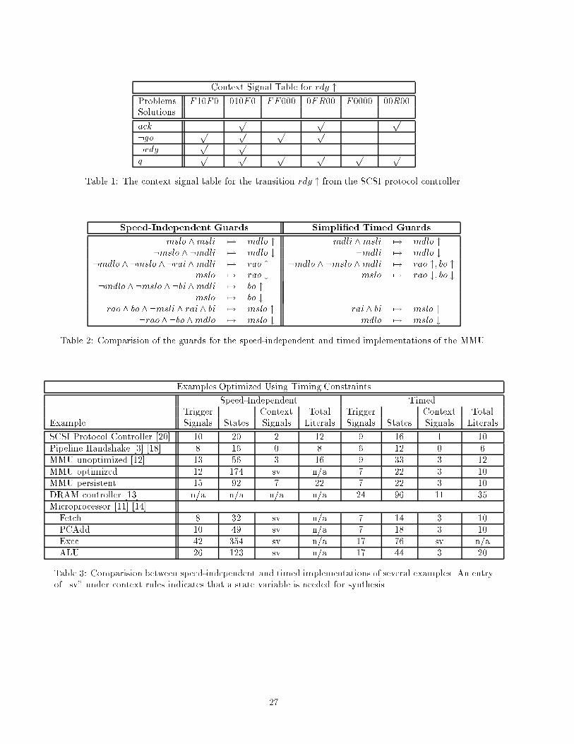
Algorithm 3.5 (Find Con icts)array FindConf(ER system hE;RNRi; set set of states; array Q) fFor each state S and each signal sk in SIf ((sk == F or sk == 0) and (Problem(S; sk "; frules in RNR of the form he; sk "; i; "; � ig))) thenFor each signal sl , if (Solution(S; qk";l)) then Ck"[sl; S] = TRUE;Else If ((sk == R or sk == 1) and (Problem(S; sk #; frules in RNR of the form he; sk #; i; "; � ig)))then For each signal sl , if (Solution(S; qk#;l)) then Ck#[sl; S] = TRUE;Return(C);g In the SCSI protocol controller, the transition req " has the weak guard :ack ^ :rdy. Using this guardand the state graph shown in Figure 3a, there is a con ict with the state 000R1. This problem state iscompared with the enabled state for req ", 0X000, as determined earlier. The only signal which can bechosen to solve this problem is :q. Using the reduced state graph in Figure 3b, the state 000R1 is notreachable, so there is no con ict. Thus, the guard is not strengthened with :q, and the timing constraintshave again helped reduce the complexity of the implementation.3.3.3 Finding an Optimal CoverDetermining which context signals to use to optimally solve all con icts constitutes a covering problem, whichis solved by treating the table of con ict problems and possible solutions as a prime implicant table [22].Thus, for each transition, a prime implicant table is solved using the procedure outlined in Algorithm 3.6.The function Choose essential rows determines if a problem has only one possible solution. If so, the signalassociated with that solution is added to the guard and all problems solved by this signal are removed fromthe table. The function Rm dominating columns detects if solving a problem implies another will be solved,and if so, removes the second problem. The function Rm dominated rows checks if one solution solves allthe same problems that another solution does and more, and if so, removes the second solution. If there isonly one remaining problem to solve, the function Solve essential columns solves it, and, if possible, does soby selecting a signal which provides symmetry between guards for the rising and falling transition.This procedure is repeated until all problems are solved, or the number of problems solved is no longerdecreasing. At the end of the procedure, all problems may not be resolved if the table is cyclic, in which casethe remaining problems can be solved by inspection or a branching method [22] implemented in the functionSolve remaining problems.Algorithm 3.6 (Find Optimal Cover)set FindCover(ER system hE;RNRi; array C) fRC = ;;For each transition t fWhile ((NumProb(Ct) > 0) and (NumProb(Ct) is decreasing)) do fRC = RC + Choose essential rows (Ct);Rm dominating columns (Ct);Rm dominated rows (Ct);RC = RC + Solve essential columns (hE;RNR +RCi; Ct);gIf (NumProb(Ct) > 0) then RC = RC + Solve remaining problems (hE;RNR + RCi; Ct);gReturn(RC);g Returning to our example, in the reduced state graph, there are still con icts associated with the transitionrdy ". A table of problems and possible solutions is shown in Table 1. In this table, there is an essential rowsince the �fth column can only be solved by choosing q. Strengthening the guard with this signal solves allthe problems. 12

3.3.4 A Complex Gate ImplementationFor each output signal s the trigger signals (i.e., those given in the rules) and the context signals (i.e., thoseadded to solve con icts) for s " are implemented in series in a pullup network, and similarly, the signals neededfor s # are implemented in series in a pulldown network. The resulting circuit is a state-holding elementcalled a generalized C-element [1]. The complex gate implementations for both the speed-independent andthe timed versions of the signal req from the SCSI protocol controller are shown in Figure 4, with the guardsthat are being implemented. If a signal appears only in the pullup, but not in the pulldown, then it isannotated with a \+". If a signal appears only in the pulldown then it is annotated with a \-". Otherwise,the signal has no annotation. A static CMOS implementation for each element is also shown in �gure 4.Since signal :q was not needed in the guard for req " for the timed implementation, the resulting circuitryneeds two less transistors. Similarly, since the rule hq #; rdy #; i; 0; [0; 5]i is found to be redundant, the signal:q is not used in the guard for the transition rdy #, and two transistors are saved there as well.3.4 ExceptionsThroughout the synthesis procedure, there are various exception conditions which can occur if the procedure�nds that it has a speci�cation for which it cannot derive an implementation. Each is brie y described herewith suggestions on how to modify the speci�cation to solve the problem, but a general solution for timedcircuits is still an open area of research.3.4.1 Complete State Coding ViolationA timed speci�cation violates the complete state coding property if in the reduced state graph, two stateshave the same binary value, but di�erent transitions on non-input signals are enabled in each state (seeDe�nition 3.5). To solve this problem, state variables are usually added to the speci�cation.De�nition 3.5 (Complete State Coding Property) A reduced state graph has the complete state coding prop-erty if for any two states S and S0 either there exists a signal sk such that VAL[sk] 6= VAL[s0k], or for allnon-input signals sk, sk = s0k.3.4.2 Persistency ViolationAfter the enabled state is found, the synthesis procedure veri�es that the timed speci�cation is persistent [2][3] as de�ned below. While in general the persistence property is not a necessary requirement for synthesis[4], it is required to use the enabled state approach. Persistence problems can be solved by either addingstate variables or persistence rules [2] [3].De�nition 3.6 (Persistence) For each rule of the form he; f; i; "; � i in the set of non-redundant rules RNR,if event e is a rising transition on the signal sk and the enabled state Qf of event f has qf;k = 1, then evente is persistent. If event e is a falling transition on the signal sk and the enabled state has qf;k = 0, thenevent e is persistent.3.4.3 Unresolvable Con ictsFinally, it is possible that there may be no available context signal to resolve a con ict. This problem maybe caused by a potential context signal which is non-persistent [4]. To solve this problem, state variables areagain added.3.5 Putting It All TogetherThe entire synthesis procedure neglecting exceptions can be given as follows:Algorithm 3.7 (Automated Timed Asynchronous Circuit Synthesis)circuit ATACS(ER system hE;Ri) fRNR = FindRed(hE;Ri); 13

RSG = FindRSG(hE;Ri);Q = FindES(hE;Ri; RSG);C = FindConf(hE;RNRi; RSG;Q);RC = FindCover(hE;RNRi; C);Circuit = FindCircuit(hE;RNR + RCi);Return(Circuit);g4 ExamplesThis section describes two practical examples: a memory management unit (MMU) and a DRAM controller.The MMU is derived from a CSP speci�cation, and it is used to illustrate the complexity reduction of timedcircuits compared to speed-independent circuits. The DRAM controller is derived from a BSM speci�cation,and it is used to demonstrate how timed circuits can be used in a synchronous environment.4.1 Memory Management UnitThe �rst example is a MMU designed for use with a 16-bit asynchronous microprocessor [11]. The originalimplementation was derived using Martin's synthesis method [12]. The basic operation of the MMU is toconvert a 16-bit memory address to a 24-bit real address. There are six possible cycles that the MMUcontroller can enter, depending on data from the environment. For simplicity, the design of only one cycle isdiscussed: memory data load. A simpli�ed block diagram is shown in Figure 5 in which only signals involvedin this cycle are depicted.4.1.1 From CSP to a Timed Speci�cationThe high-level CSP speci�cation for the memory data load cycle is: �[MDl ! (RA k B);MSl;MDl] (see[12]). This speci�cation is initially transformed into the following handshaking expansion:�[[mdli ^:rai]; rao "; [:bi]; bo "; [rai^ bi ^ :msli];mslo "; [msli];mdlo "; rao #; bo #; [:mdli];mslo #;mdlo #];which is then converted to the constraint graph shown in Figure 6.The transformation from CSP to a handshaking expansion is not unique. A more concurrent constraintgraph shown in Figure 7 also satis�es the high-level CSP speci�cation. This speci�cation is simply a reshuf- ing [1] of the earlier one. This reshu�ing is not considered in [12] because it results in a complete statecoding violation [2]. This means that the more concurrent speci�cation cannot be implemented withoutadding state variables. Adding state variables not only changes the speci�cation, but can also add extracircuitry and/or delay to the implementation. This cost often outweights the bene�t of the higher degree ofconcurrency. This particular problem can also be solved by adding persistence rules, but this can reduce theconcurrency in the speci�cation. If conservative timing constraints are also added, the reduced state graphof the more concurrent speci�cation shown in Figure 7 does not have a complete state coding violation, andthus, it can be implemented without adding state variables or persistence rules. To make the speci�cation inFigure 7 persistent, three arcs are added to the constraint graph as shown in Figure 8; the speci�cation cannow be implemented speed-independently. As shown later, the speed-independent implementation is stillmore complex than the original implementation derived from the speci�cation in Figure 6.4.1.2 Speed-Independent vs. Timed ImplementationA speed-independent and a timed implementation of the speci�cation shown in Figure 8 are compared. Forthe timed implementation, the timing constraints used are depicted in Figure 8. The lower bound of thetiming constraint on mdli " states that the processor does not issue memory requests faster than every 30ns.The lower bound of the timing constraint on msli " states that the DRAM access time takes at least 30ns.Both of their upper bounds are in�nite since the processor could choose never to do a load, or the interfacecould choose never to process the request. The reseting of the acknowledgement (i.e., mdli # and msli #)is assumed to be somewhat faster, and must occur within 5 to 30ns of the reset of the request. The other14

numbers were obtained from SPICE simulations of the datapath circuitry for a 0:8�m CMOS process. Thecomparator, denoted bi, has a delay of between 2:5 to 13ns, and the registers, denoted rai, have a delay ofbetween 2 to 9ns depending on temperature, voltage, and processing variations. All output signals have adelay of 0 to 1ns where 1ns was found to be the maximum delay of the gates in the library used.In the MMU speci�cation, there are �ve events with multiple rules enabling them: rao ", bo ", mslo ",mslo #, and mdlo #. Timing analysis determines that at least one rule associated with each event isredundant. In all, 6 of the 15 rules on output signals in the original speci�cation are redundant. Thisincludes the 3 persistence rules. To determine which context signals must be added, the �rst step is todetermine the reduced state graph and the enabled state for each signal using the timing constraints. Astate graph generated without any timing constraints results in 92 states while the reduced state graph onlyhas 22 states. Using the reduced state graph, the timed implementation needs 5 context signals as opposedto 7 needed for the speed-independent implementation.After adding context signals to our original speci�cation, 22 literals (note that we de�ne a literal to bea signal in a guard) are required for a speed-independent implementation as shown in Table 2. The timingconstraints reduce the circuit to only 10 literals. Thus, our circuit complexity is reduced by over 50 percentusing conservative timing constraints. A complex gate implementation for both is shown in Figure 9. Notethat this reduction is possible not only because of removing redundant literals, but also because the gateneeded for implementing rao and bo can be shared after the optimizations.4.2 DRAM ControllerOur next example is a DRAM controller which is an interface between a microprocessor and a DRAM array.This example is interesting for two reasons. It is an asynchronous design in a synchronous environment,and it is an example which includes non-deterministic behavior (i.e., input choice) which can be synthesizedby transforming it into a deterministic speci�cation. The DRAM controller has three possible modes ofoperation: read, write, and refresh. A block diagram for the entire DRAM controller is shown in Figure 10.The design of the refresh cycle is discussed in detail in the next subsection to illustrate how synchronousinputs can be incorporated into an asynchronous design. The three cycles are combined to illustrate synthesisof a speci�cation with non-determinism and multiple occurrences of events in a single cycle.4.2.1 From Burst-Mode to Timed Speci�cationOur speci�cation is derived from a burst-mode speci�cation shown in Figure 11 [13]. The speci�cation of therefresh cycle is converted to the constraint graph shown in Figure 12. Notice that this constraint graph is notwell-formed (i.e., it is not strongly connected), so our timing analysis procedure cannot be applied directly.To solve this problem, the dashed arcs in Figure 13 are added to the constraint graph. For this example,these new ordering rules are chosen to make the speci�cation satisfy the fundamental mode assumption (i.e.,outputs must occur before inputs can change). For example, the transition rfip " must occur before c #, soa rules is added between them. The timing constraints for these rules are [0; 0] which means that only theordering of the two events is important and not the time di�erence between them.In general, an ordering rule can be added between two events if the enabling event is guaranteed bythe timing constraints to always precede the enabled event by at least the amount of time given in theupper bound of the ordering rule. In other words, the rule must be declared redundant using the timinganalysis, since it is not actually enforced with circuitry. If this is the case, the implementation synthesizedis valid; otherwise di�erent ordering rules need to be chosen. If no ordering rules can be found to make thegraph well-formed, then our procedure cannot derive an implementation which can satisfy the given timingconstraints. Currently, these ordering rules must be added before the synthesis procedure can be applied,but future research will incorporate �nding appropriate ordering rules into the procedure.4.2.2 Burst-Mode vs. Timed ImplementationThe implementation of a timed version of the DRAM controller is compared with implementations from twoburst-mode design styles [13] [7]. For our timed implementation, the timing constraints used for the refreshcycle are depicted in Figure 13 [23]. These timing constraints are derived assuming the environment is asdepicted in Figure 10, and the controller is being used with a 68020/30 running at 16 to 20 MHz.15

The implementation of the refresh cycle is considered �rst. As before, the �rst step is to determine whichrules in the speci�cation are redundant. All 7 of the ordering rules added to make the graph well-formed arefound to be redundant. In addition, the rules from a # to ras " and rfip # are also redundant. Next, thesynthesis procedure derives a reduced state graph with 16 states. Using this reduced state graph and thenon-redundant rules, one context signal is needed for the implementation. In all, 7 literals are needed forthe implementation of the two output signals in the refresh cycle, rfip and ras.The implementation of the complete DRAM controller is non-deterministic; i.e., the environment canchoose to do a refresh cycle, a write cycle, or a read cycle. Our timing analysis algorithm cannot analyzespeci�cations with non-determinism directly. To solve this problem, the speci�cation is converted to a longcycle going through a refresh, a write, and a read cycle sequentially as illustrated in Figure 14. In thisexample, since each cycle always returns to the same state before the next cycle is chosen, all possiblebehaviors are modeled.The resulting cyclic constraint graph has multiple occurrences of the same event in a cycle. For example,the transition ras " now occurs three times in a single cycle. Each event which occurs multiple times isgiven a unique name for each occurrence, and these events are noted to be on the same signal. For example,the three occurrences of ras " are replaced with ras1 ", ras2 ", and ras3 ". These events will be treatedseparately during timing analysis, but together during synthesis.The same procedure described earlier is used to �nd redundant rules and the reduced state graph. Whendetermining the enabled state, the multiple occurrences of an event are considered together. For example,when determining the enabled state for the transition we #, there is a state where dtack1 = F and dtack2 = 1,and another state where dtack1 = 0 and dtack2 = 1. Therefore, in the enabled state for we #, both dtack1and dtack2 are set to X. To �nd con icts, the individual occurrences of the same event are used, but todetermine context signals, only the merged value is available. For example, ras can only be used as a contextsignal if ras1, ras2, and ras3 all qualify as context signals.This procedure leads to the implementation of the DRAM controller shown in Figure 15. Note thatalthough some of the gates are shown with multiple levels, they are all actually implemented as single complexgates. For example, a dynamic gate implementing cas is shown in Figure 16. Our �nal implementation has35 literals (41 literals if the gate for dtack and selca are not shared). A locally-clocked implementation asreported in [13] used 62 literals and 1 state variable. A 3-D implementation as reported in [7] used 46 literalsand 1 state variable. Our implementation did not need a state variable.4.3 Other ResultsThe synthesis procedure described in this paper has been fully automated in a CAD tool which transforms awell-formed ER system speci�cation into a complex gate implementation. All results reported in this paperwere compiled using this program, and they appear tabulated in Table 3.Additional examples in this table are parts of an asynchronous microprocessor described in [11], andtheir speci�cations are taken from [14]. All of the microprocessor speci�cations need state variables for aspeed-independent implementation; however, three of the four can be implemented without state variablesif conservative timing constraints are added.The timed implementation for the MMU controller and the refresh cycle of the DRAM controller havebeen veri�ed using Burch's timed circuit veri�er [24] [25] to be hazard-free under the given timing constraints.Here, hazard-freedom is de�ned to mean that no transition once enabled to occur can be disabled withoutit occurring.5 Conclusions and Future ResearchWe have proposed a new methodology for the speci�cation of timed asynchronous circuits, the event-rulesystem, and developed a timing analysis algorithm to deduce timing information su�cient for the synthesis oftimed circuits. A synthesis procedure based on our timing analysis algorithm has been constructed to detectand remove redundancy in the speci�cation and to produce a reduced state graph. From the reduced stategraph, our procedure systematically derives a complex gate implementation. Our results indicate that byusing conservative timing constraints, our synthesis procedure can signi�cantly reduce a circuit's complexity.16

While reducing circuit area, we also increase circuit performance, not only because smaller circuits switchfaster but also because we are able to synthesize more concurrent speci�cations than can often be consideredpractical using other design styles. Finally, we have applied our technique to the synthesis of asynchronouscircuits in a mixed synchronous/asynchronous environment.At present, our synthesis procedure requires a well-formed, deterministic ER system speci�cation. Whilewe have shown through an example how these restrictions can be relaxed, a systematic method has not yetbeen incorporated into our synthesis procedure. In the future, we plan to incorporate transformations tomake a speci�cation well-formed into the synthesis procedure. We also plan to generalize our timing analysisalgorithm to handle non-deterministic behavior. The third direction for future work is develop a procedurefor adding state variables to a timed speci�cation to resolve exceptions: complete state coding violations,persistency violations, and unresolvable con icts. This problem is not as straightforward as it sounds becauseadding state variables changes the speci�cation, and thus may invalidate earlier timing analysis. Therefore,techniques used for adding state variables in other methodologies may not be directly applicable. Also, whilewe are able to verify our designs to be hazard-free, verifying that they satisfy a speci�cation has not yet beencompleted and will be addressed in the future. Finally, we intend to apply our technique to larger examples,and implement the IC design of interesting timed circuits to better assess the area and performance gain.AcknowledgmentsThe authors would especially like to thank Professor David Dill of Stanford University who dedicated con-siderable amount of time in assisting us in formalizing our work. We would also like to thank Peter Beerel ofStanford University for his invaluable comments on numerous versions of this manuscript. Our thanks alsogo to Dr. Jerry Burch of Stanford University for verifying several of our designs. The authors would also liketo thank Professors Steve Burns and Gaetano Borriello of the University of Washington and their studentsfor many valuable discussions on timing analysis and the synthesis of timed circuits. Finally, we would liketo express our appreciation of the work done in Professor Alain Martin's group at the California Instituteof Technology, for their insight in the design of asynchronous circuits. Their assistance in deriving thespeci�cation and speed-independent implementation of the MMU example is also gratefully acknowledged.References[1] Alain J. Martin. \Programming in VLSI: From Communicating Processes to Delay-Insensitive VLSICircuits". In C.A.R. Hoare, editor, UT Year of Programming Institute on Concurrent Programming.Addison-Wesley, 1990.[2] Tam-Anh Chu. Synthesis of Self-Timed VLSI Circuits from Graph-theoretic Speci�cations. PhD thesis,Massachusetts Institute of Technology, 1987.[3] Teresa H.-Y. Meng, Robert W. Brodersen, and David G. Messershmitt. \Automatic Synthesis of Asyn-chronous Circuits from High-Level Speci�cations". IEEE Transactions on Computer-Aided Design,8(11):1185{1205, November 1989.[4] Peter A. Beerel and Teresa H. Y. Meng. \Automatic Gate-Level Sythesis of Speed-Independent Cir-cuits". In Proceedings IEEE 1992 ICCAD Digest of Papers, pages 581{586, 1992.[5] S.H. Unger. Asynchronous Sequential Switching Circuits. New York: Wiley-Interscience, 1969. (re-issuedby Robert E. Krieger, Malabar, 1983).[6] Steven M. Nowick and David L. Dill. \Synthesis of Asynchronous State Machines Using a Local Clock".In International Conference on Computer Design, ICCD-1991. IEEE Computer Society Press, 1991.[7] K. Y. Yun, D. L. Dill, and S. M. Nowick. \Synthesis of 3D Asynchronous State Machines". In Interna-tional Conference on Computer Design, ICCD-1992. IEEE Computer Society Press, 1992.[8] Al Davis, Bill Coates, and Ken Stevens. \The Post O�ce Experience: Designing a Large AsynchronousChip". In Proceedings of the Twenty-Sixth Annual Hawaii International Conference on System Sciences,pages 409{418. IEEE Computer Science Press, 1993.[9] Gaetano Borriello and Randy H. Katz. \Synthesis and Optimization of Interface Transducer Logic". InProceedings IEEE 1987 ICCAD Digest of Papers, pages 274{277, 1987.17

[10] L. Lavagno, K. Keutzer, and A. Sangiovanni-Vincentelli. \Algorithms for Synthesis of Hazard-FreeAsynchronous Circuits". In Proceedings of the 28th ACM/IEEE Design Automation Conference, 1991.[11] A. J. Martin, S. M. Burns, T. K. Lee, D. Borkovi�c, and P. J. Hazewindus. \The Design of an Asyn-chronous Microprocessor". In Decennial Caltech Conference on VLSI, pages 226{234, 1989.[12] Chris J. Myers and Alain J. Martin. \The Design of an Asynchronous Memory Management Unit".Technical Report CS-TR-92-25, California Institute of Technology, 1992.[13] S. M. Nowick, K. Y. Yun, and D. L. Dill. \Practical Asynchronous Controller Design". In InternationalConference on Computer Design, ICCD-1992. IEEE Computer Society Press, 1992.[14] Steve Burns. Performance Analysis and Optimization of Asynchronous Circuits. PhD thesis, CaliforniaInstitute of Technology, 1991.[15] Kenneth McMillan and David L. Dill. \Algorithms for Interface Timing Veri�cation". In InternationalConference on Computer Design, ICCD-1992. IEEE Computer Society Press, 1992.[16] P. Vanbekbergen, G. Goossens, and H. De Man. \Speci�cation and Analysis of Timing Constraints inSignal Transition Graphs". In Proceedings of the European Design Automation Conference, 1992.[17] T. Amon, H. Hulgaard, G. Borriello, and S. Burns. \Timing Analysis of Concurrent Systems". TechnicalReport UW-CS-TR-92-11-01, University of Washington, 1992.[18] Chris Myers and Teresa H.-Y. Meng. \Synthesis of Timed Asynchronous Circuits". In InternationalConference on Computer Design, ICCD-1992. IEEE Computer Society Press, 1992.[19] Glynn Winskel. \An Introduction to Event Structures". In Linear Time, Branching Time and PartialOrder in Logics and Models for Concurrency. Noordwijkerhout, Norway, June 1988.[20] Tam-Anh Chu. Private Communication, July 1991. Tam-Anh Chu is with Cirrus Logic.[21] Alain J. Martin. \Formal Program Transformations for VLSI Circuit Synthesis". In E.W. Dijkstra,editor, UT Year of Programming Institute on Formal Developments of Programs and Proofs. Addison-Wesley, 1989.[22] Edward J. McCluskey. Logic Design Principles with Emphasis on Testable Semicustom Circuits.Prentice-Hall, Englewood Cli�s, NJ, 1986.[23] Ken Yun. Private Communications, 1992. Ken Yun is a graduate student at Stanford University.[24] Jerry R. Burch. \Modeling Timing Assumptions with Trace Theory". In 1989 International Conferenceon Computer Design: VLSI in Computers and Processors, pages 208{211. IEEE Computer SocietyPress, 1989.[25] Jerry R. Burch. Trace Algebra for Automatic Veri�cation of Real-Time Concurrent Systems. PhDthesis, Carnegie Mellon University, 1992.18

Figure 1: The cyclic constraint graph for a SCSI protocol controller (courtesy of [17]).

Figure 2: A subgraph of the in�nite acyclic constraint graph for the SCSI protocol controller.19

Figure 3: (a) State graph for the SCSI protocol controller. (b) Reduced state graph for the SCSI protocolcontroller.

Figure 4: (a) Speed-independent implementation of req. (b) Timed implementation of req.20

Figure 5: Block diagram for part of the MMU controller.

Figure 6: The cyclic constraint graph speci�cation for the unoptimized MMU.21

Figure 7: The cyclic constraint graph speci�cation for the optimized MMU.

Figure 8: The cyclic constraint graph speci�cation for the persistent MMU.22

Figure 9: (a) Speed-independent implementation of the MMU controller. (b) Timed implementation of theMMU controller.

Figure 10: Block diagram for the DRAM controller (courtesy of [12]).23

Figure 11: The burst-mode speci�cation for the DRAM controller (courtesy of [12]).

Figure 12: The constraint graph speci�cation for refresh cycle of DRAM controller.24

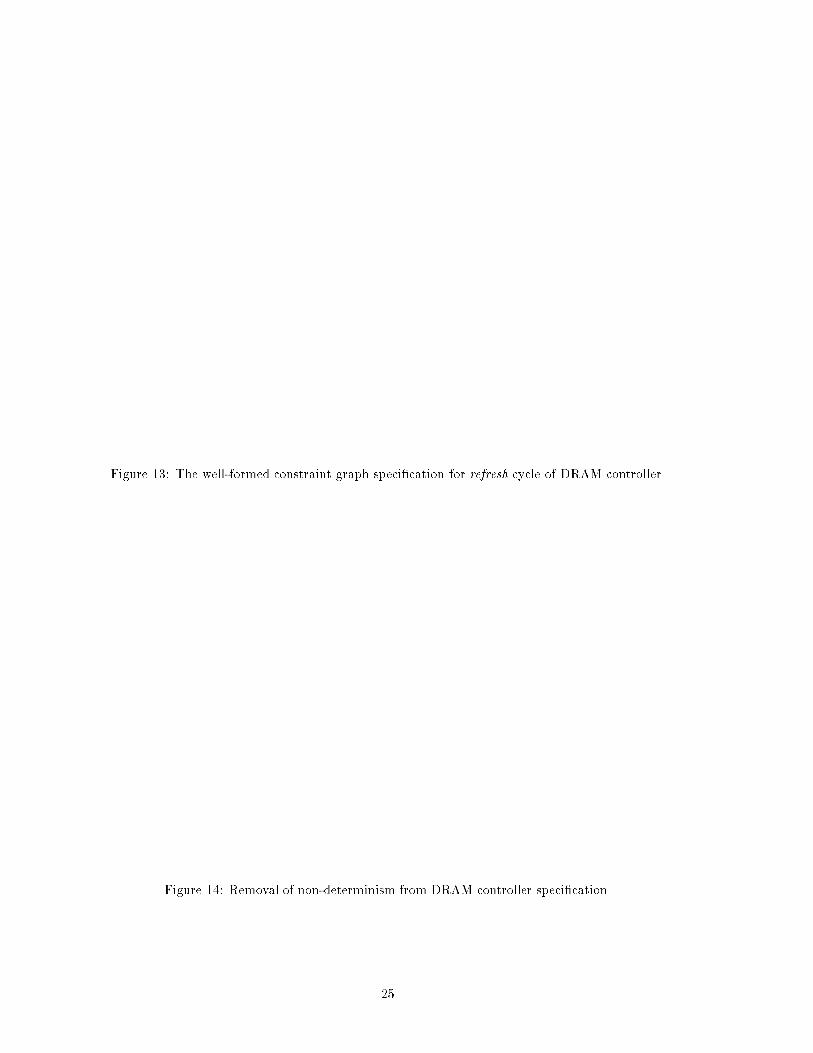
Figure 13: The well-formed constraint graph speci�cation for refresh cycle of DRAM controller.

Figure 14: Removal of non-determinism from DRAM controller speci�cation.25

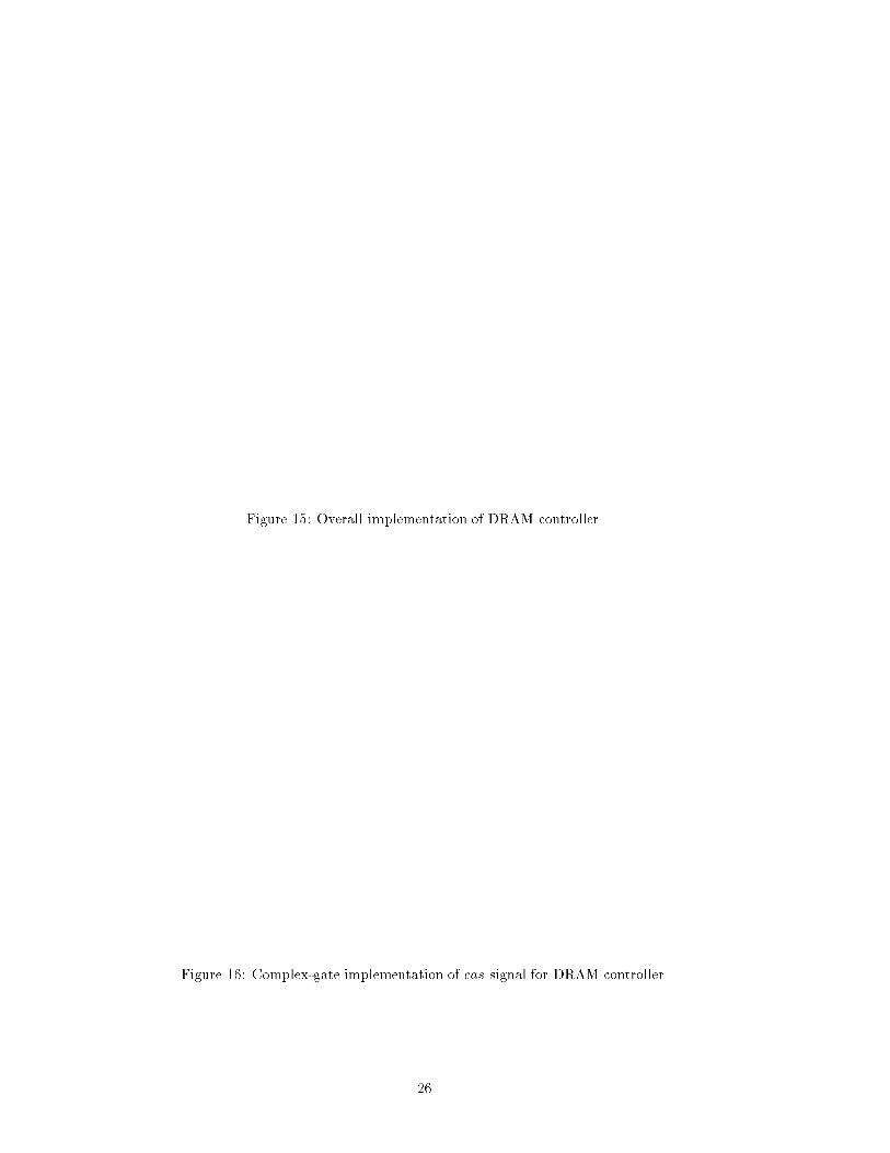
Figure 15: Overall implementation of DRAM controller.

Figure 16: Complex-gate implementation of cas signal for DRAM controller.26

Context Signal Table for rdy "Problems F10F0 010F0 FF000 0FR00 F0000 00R00Solutionsack p p p:go p p p p:rdy p pq p p p p p pTable 1: The context signal table for the transition rdy " from the SCSI protocol controller.Speed-Independent Guards Simpli�ed Timed Guardsmslo ^msli 7! mdlo " mdli ^msli 7! mdlo ":mslo ^ :mdli 7! mdlo # :mdli 7! mdlo #:mdlo ^ :mslo ^ :rai ^mdli 7! rao " :mdlo ^ :mslo ^mdli 7! rao "; bo "mslo 7! rao # mslo 7! rao #; bo #:mdlo ^ :mslo ^ :bi ^mdli 7! bo "mslo 7! bo #rao ^ bo ^ :msli ^ rai ^ bi 7! mslo " rai ^ bi 7! mslo ":rao^ :bo ^mdlo 7! mslo # mdlo 7! mslo #Table 2: Comparision of the guards for the speed-independent and timed implementations of the MMU.Examples Optimized Using Timing ConstraintsSpeed-Independent TimedTrigger Context Total Trigger Context TotalExample Signals States Signals Literals Signals States Signals LiteralsSCSI Protocol Controller [20] 10 20 2 12 9 16 1 10Pipeline Handshake [3] [18] 8 16 0 8 6 12 0 6MMU unoptimized [12] 13 56 3 16 9 33 3 12MMU optimized 12 174 sv n/a 7 22 3 10MMU persistent 15 92 7 22 7 22 3 10DRAM controller [13] n/a n/a n/a n/a 24 96 11 35Microprocessor [11] [14]Fetch 8 32 sv n/a 7 14 3 10PCAdd 10 49 sv n/a 7 18 3 10Exec 42 354 sv n/a 17 76 sv n/aALU 26 123 sv n/a 17 44 3 20Table 3: Comparision between speed-independent and timed implementations of several examples. An entryof \sv" under context rules indicates that a state variable is needed for synthesis.27

List of Figures1 The cyclic constraint graph for a SCSI protocol controller (courtesy of [17]). : : : : : : : : : : 192 A subgraph of the in�nite acyclic constraint graph for the SCSI protocol controller. : : : : : : 193 (a) State graph for the SCSI protocol controller. (b) Reduced state graph for the SCSI protocolcontroller. : : : : : : : : : : : : : : : : : : : : : : : : : : : : : : : : : : : : : : : : : : : : : : : 204 (a) Speed-independent implementation of req. (b) Timed implementation of req. : : : : : : : 205 Block diagram for part of the MMU controller. : : : : : : : : : : : : : : : : : : : : : : : : : : 216 The cyclic constraint graph speci�cation for the unoptimized MMU. : : : : : : : : : : : : : : 217 The cyclic constraint graph speci�cation for the optimized MMU. : : : : : : : : : : : : : : : : 228 The cyclic constraint graph speci�cation for the persistent MMU. : : : : : : : : : : : : : : : : 229 (a) Speed-independent implementation of the MMU controller. (b) Timed implementation ofthe MMU controller. : : : : : : : : : : : : : : : : : : : : : : : : : : : : : : : : : : : : : : : : : 2310 Block diagram for the DRAM controller (courtesy of [12]). : : : : : : : : : : : : : : : : : : : : 2311 The burst-mode speci�cation for the DRAM controller (courtesy of [12]). : : : : : : : : : : : 2412 The constraint graph speci�cation for refresh cycle of DRAM controller. : : : : : : : : : : : : 2413 The well-formed constraint graph speci�cation for refresh cycle of DRAM controller. : : : : : 2514 Removal of non-determinism from DRAM controller speci�cation. : : : : : : : : : : : : : : : 2515 Overall implementation of DRAM controller. : : : : : : : : : : : : : : : : : : : : : : : : : : : 2616 Complex-gate implementation of cas signal for DRAM controller. : : : : : : : : : : : : : : : : 2628

List of Tables1 The context signal table for the transition rdy " from the SCSI protocol controller. : : : : : : 272 Comparision of the guards for the speed-independent and timed implementations of the MMU. 273 Comparision between speed-independent and timed implementations of several examples. Anentry of \sv" under context rules indicates that a state variable is needed for synthesis. : : : 27

29