sustainable workforce scheduling in construction program management

Sustainable workforce scheduling inconstruction program managementL Florez

1, D Castro-Lacouture

1� and AL Medaglia2

1Georgia Institute of Technology, Atlanta, GA, USA; and

2Universidad de los Andes, Bogota,

Colombia

The multimode resource-constrained project scheduling problem (MRCPSP) deals with the schedulingof a set of projects with alternative requirements of renewable and non-renewable resources. Solutions tothe MRCPSP usually consider objectives in terms of cost and time. However, social objectives relatedwith the workforce may impact the performance of projects and affect program sustainability goals. Toaccount for this new social input, this paper extends the MRCPSP and proposes a new multiobjectivemixed-integer programming model. The proposed solution method uses an a priori lexicographicordering of the objectives, followed by an e-constraints approach. The model is illustrated with a casestudy of a construction program.

Journal of the Operational Research Society (2013) 64, 1169–1181. doi:10.1057/jors.2012.164

Published online 12 December 2012

Keywords: construction; project management; integer programming; scheduling

Introduction

Project scheduling is an important task in project manage-

ment (Hartmann and Briskorn, 2010). The selection of

resources and the harmonization of their work make

project scheduling crucial for the success of a construction

project for both the owner and contractor (Jaskowski and

Sobotka, 2006). The classical resource-constrained project

scheduling problem (RCPSP) deals with the scheduling

of a given set of projects considering renewable and non-

renewable resource constraints. Renewable resources

(Jaskowski and Sobotka, 2006) such as workers and

machines are available every period during the planning

horizon while non-renewable resources such as budget are

available only at the beginning of the planning horizon and

are consumed as projects are executed. Optimal schedules

usually mean that evaluation criteria such as time and cost

are met (Jaskowski and Sobotka, 2006). However, the

project scheduling problem currently lacks a method that

helps decision-makers to optimally schedule projects while

considering social sustainability measures that may benefit

workers as well as the program manager and owner.

Social sustainability is an opportunity to achieve better

standards of living and increase the well being of people

(Alwaer and Clements-Croome, 2010) by implementing

practices that can be maintained in time. These practices

promote the development of socially responsible ways to

manage people by considering people’s needs and expecta-

tions. A number of studies have identified criteria to pro-

mote social sustainability (Labuschagne et al, 2005; Ugwu

and Haupt, 2005; Singh et al, 2007; Alwaer and Clements-

Croome, 2010; Fernandez-Sanchez and Rodriguez-Lopez,

2010; Tahir and Darton, 2010). Social sustainability is

achieved in a project when factors such as its duration

(Ramos and Caeiro, 2010), geographical location (Ramos

and Caeiro, 2010), impact on stakeholders (Fernandez-

Sanchez and Rodriguez-Lopez, 2010), safety (Ugwu and

Haupt, 2005), design process (Alwaer and Clements-

Croome, 2010), and employment generation (Labuschagne

et al, 2005) are considered. In order to achieve social sus-

tainability when planning and scheduling projects, pro-

gram managers need tools that can help them assess their

performance (Fernandez-Sanchez and Rodriguez-Lopez,

2010). Indicators are metrics to measure performance

across a range of sustainable principles (Singh et al, 2009).

Indicators help visualize phenomena and highlight trends

(Singh et al, 2009) and can provide useful evidence to

support project management (Fernandez-Sanchez and

Rodriguez-Lopez, 2010).

In this paper, we aim to assist program managers and

decision-makers when dealing with the challenge of plann-

ing a construction program to achieve social sustainability

by developing a multiobjective mixed-integer program that

schedules projects and assigns workers. A construction

program is defined as a set of projects with the ability of

sharing resources among them (Reiss, 1996). A schedule

Journal of the Operational Research Society (2013) 64, 1169–1181 © 2013 Operational Research Society Ltd. All rights reserved. 0160-5682/13

www.palgrave-journals.com/jors/

�Correspondence: D Castro-Lacouture, School of Building Construction,

Georgia Institute of Technology, 280 Ferst Drive, 1st Floor, Atlanta, GA

30332, USA.

E-mail: [email protected]

provides a coherent process that includes all operations to

allocating resources while satisfying all constraints (Pinedo,

2005). Note that the model does not schedule the different

tasks or activities within a project; it assumes that the

schedule for the tasks (with precedence relations) is known

in advance. To account for social sustainability, one of the

objectives of the model is to maximize labour stability,

while simultaneously considering cost and time objectives.

The model includes both renewable (machines and work-

ers) and non-renewable (financial capital) resource con-

straints to address realistic scenarios experienced by the

program manager. In addition, the model determines

detailed working patterns, that is, the time periods when

workers are using certain skills, as well as the best time

when they need to be hired, fired, or shift between skills.

This paper is organized as follows. We first provide

a review of the project scheduling literature as well as

objectives that achieve social sustainability. Then, we pre-

sent the optimization model and the solution strategy,

followed by an illustration of the operation of the model

on a case study of a construction program. Finally, we con-

clude the paper and outline opportunities for future

research.

Literature review

In the RCPSP, each activity has a single execution mode,

that is, both the activity duration and its resource require-

ments are fixed and known in advance. There are several

approaches to solve the RCPSP. Li and Willis (1993)

presented a heuristic approach to schedule projects and

evaluate the cost/time trade-off when implementing re-

planning of activities. Zhu et al (2005) developed a mixed-

integer program to schedule projects when a disruption is

presented and the activities need to get on track at the

minimum cost and deviation from the original schedule.

Jaskowski and Sobotka (2006) proposed an evolutionary

algorithm to minimize the schedule duration, while con-

sidering limited accessibility of renewable resources. A

review of variants and extensions of the RCPSP can be

found in Hartmann and Briskorn (2010).

An extension of the RCPSP is the multimode resource-

constrained project scheduling problem (MRCPSP), which

considers that projects can be executed in different modes.

Each mode represents an alternative combination of

renewable and non-renewable resources and the quantities

employed to fulfil a given project (Zhang et al, 2006). The

corresponding project duration is a function of the quanti-

ties of resources used, that is, a project can be accelerated

by increasing the quantities coming into operation

(Hartmann, 2001). The methodologies for solving the

MRCPSP that have been proposed include various

approaches. For instance, Zhang et al (2006) proposed a

methodology based on particle swarm optimization (PSO)

in which the solution is represented in terms of priority and

mode combination of projects. Sprecher and Drexl (1998)

proposed a branch and bound methodology with an

enumeration scheme that increases the efficiency of the tree

exploration. Hartmann (2001) proposed a genetic algo-

rithm using two local search methods to deal with the

feasibility problem of the MRCPSP and to improve the

schedules. El-Rayes and Moselhi (2001) proposed a

dynamic programming approach, which is focused on

crews that can be allocated in multiple modes. Recently,

Palacio (2010) proposed a mixed-integer program to solve

the MRCPSP with minimum and maximum time lags.

None of these methods, as implemented, help decision-

makers schedule projects in order to maximize their social

sustainability performance while still meeting cost and time

requirements.

Labour in construction

People are an organization’s most valuable asset and this is

especially true in relatively labour intensive industries such

as construction (Loosemore et al, 2003). In construction,

labour costs on a project may account for 30–50% of the

total project costs (Adrian, 1987). However, project

management strategies have focused on planning opera-

tions without attention being paid to the human resource

factor (Belout, 1998). In the construction industry, the lack

of opportunities for training and career growth result in

high turnover rates while construction companies have

difficulties maintaining and recruiting construction work-

force (Gomar et al, 2002). People, unlike other resources,

have their own needs and requirements beyond the

financial compensation for their work. Workers place a

great value on requirements such as involvement, respect,

and sense of personal growth (Lingard and Sublet, 2002).

Because of their needs and requirements, workers may

represent the most difficult resource for organizations to

manage, but when managed effectively can bring consider-

able benefits (Loosemore et al, 2003). For instance, a

project that offers continual employment allows contrac-

tors to not only use workers more efficiently and at lesser

cost, but also helps generate a sense of commitment to the

job from the workers (MacKenzie et al, 2010). At the same

time, an increase in employment duration may help train

workers and resolve the skills shortage problem within the

construction industry (Gomar et al, 2002; Srour et al, 2006;

MacKenzie et al, 2010). Projects receive greater loyalty

from their workers and better productivity where condi-

tions are set to provide improved career opportunities and

more equitable workplace environments (Loosemore et al,

2003). By considering their needs and expectations,

construction projects may not only benefit current workers

but may also help attract other workers and be sustainable

over time.

1170 Journal of the Operational Research Society Vol. 64, No. 8

Multiskilling

Construction is a labour intensive as well as craft-based

activity and the behaviour of people has a direct impact on

the performance of construction projects (Lill, 2008). The

poor image of the construction industry is partially due to

the lack of opportunities for training and career growth

resulting in high turnover rates (Gomar et al, 2002). A

contributing factor for this problem is the single-skill strategy

amply used in construction (Burleson et al, 1998). This

strategy is characterized by the irregularity of the workload

(Lill, 2008) and fluctuations of workforce that lead to

workers facing the problem of short employment duration,

frequent layoffs, and periods of unemployment between jobs

(Gomar et al, 2002). Because of the discontinuity of job

assignments (El-Rayes and Moselhi, 2001) and the feeling of

purposelessness due to idle time in the job site, the single-skill

strategy impacts the attitude of workers. Workers believe

that there is lack of respect and opportunities for training,

factors that act to lower the overall craft efficiency (Gomar

et al, 2002) and workers’ general satisfaction (Lill, 2008).

Additionally, workers’ variations make it difficult to distri-

bute and coordinate crews, which leads to delays and rework

(Burleson et al, 1998). Therefore, sustainable development in

the construction industry has to consider not only building

technologies and materials but also respectful and consider-

ate labour management strategies (Lill, 2008). One of such

strategies is multiskilling.

Multiskilling is a labour technique in which workers are

able to perform several trades. With multiskilling, workers

may have longer employment durations, continuity of job

assignments, and reduced idle time (Gomar et al, 2002). The

benefits of multiskilling include increases in productivity,

quality, and continuity of work as well as safer worksites

and flexibility to managers in assigning tasks (Burleson

et al, 1998; Gomar et al, 2002). Furthermore, multi-skilled

workers have a broader variety of skills that makes them

adaptable to unforeseen activities and allows the manager

more flexible utilization of their capacities (Lill, 2008). An

extensive work has been carried out to solve multiskilling

decisions and project scheduling problems. Jun and

El-Rayes (2010) developed a model to optimally plan and

schedule multiple shifts in construction projects using three

modules to retrieve input data, develop shift schedules, and

identify optimal trade-offs between project criteria in

different shifts. Hyari et al (2010) developed an optimization

model to assign multi-skilled workers with the purpose of

minimizing total labour project costs. Wongwai and

Malaikrisanachalee (2011) proposed a heuristic algorithm

for multi-skilled resource scheduling in which substitution of

resources is allowed. Srour et al (2006) developed a linear

program model that provides a strategy for training and

hiring workers to satisfy schedule requirements. However,

there is no method that quantifies the social sustainability

performance of scheduling.

Labour stability indicator

From the above definition of multiskilling and based on

social indicators from previous studies (Labuschagne et al,

2005; Singh et al, 2007; Ramos and Caeiro, 2010), we

developed an indicator to measure social performance of

projects. The indicator defined as labour stability quantifies

the project’s capability of maintaining a stable crew work-

force. Stabilizing the workforce may result in an increase in

employment duration and job continuity. To account for

this social indicator, two alternatives of labour stability

are proposed. The first alternative minimizes the maximal

labour fluctuation, that is, minimizes the largest change

on the number of workers between any pair of consecutive

periods. The second alternative minimizes the sum of

fluctuations, that is, minimizes the absolute variation

of workers along the planning horizon (a linear proxy of

variance).

Optimization model and solution strategy

The proposed model smoothes the allocation of workers

to the project schedule to avoid drastic measures while

maintaining a stable workforce. The proposed model is

based on the one by Medaglia et al (2008), which was later

extended by Palacio (2010) for the MRCPSP/max (with

time lags). Despite the fact that some building blocks

are shared, modelling labour stability brings several new

elements and challenges into the model that makes it

unique on its own.

Model formulation

The formulation includes the set of projects I, the set of

machines N, the set of workers J, and the set of skills

among all workers R. The set Jr contains the workers with

skill r, and conversely, the set Rj contains the skills of

worker j. The set Mi represents the available execution

modes for project i.

The model also includes parameter T representing the

length of the planning horizon. Parameters chire, cfire, cshift,

and cjwage represent the cost of hiring a worker, the cost of

firing a worker, the cost of switching a worker across

different skills, and the wage (per period of time) of worker

j, respectively. The earliest and latest starting times for

project i are represented by parameters ti� and ti

þ ,respectively. Parameter bt represents the available budget

for time t. The lifespan of project i if executed in mode m is

denoted by vim. Parameter cikminv represents the investment

cost in project i in period k in mode m. The number of

machines n needed by project i in period k in mode m is

given by parameter qnikm, while the number of workers

with skill r needed by project i in period k in mode m is

given by parameter drikm. The availability of machines n in

time t is denoted by pnt. The binary parameter ajt takes the

L Florez et al—Sustainable workforce scheduling in construction program management 1171

value of 1 if worker j is available in period t; it takes the

value of 0, otherwise.

The structural binary variable yitm takes the value of 1 if

project i is scheduled to start at time t in mode m; it takes

the value of 0, otherwise. In addition, the (auxiliary) binary

variable xiktm takes the value of 1 if period k of project i

executed in modem is scheduled in time t; it takes the value

of 0, otherwise. For the assignment of workers, the binary

variable wjrt takes the value of 1 if worker j works in skill r

at time t; it takes the value of 0, otherwise. The binary

variable hjt takes the value of 1 if worker j is hired at the

beginning of time t, it takes the value of 0, otherwise. The

binary variable fjt takes the value of 1 if worker j is fired at

the beginning of time t; it takes the value of 0, otherwise.

The binary variable sjt takes the value of 1 if worker j shifts

skills between times t�1 and t; it takes the value of 0,

otherwise. Variable �wt represents the amount of labour

working in the scheduled projects at time t (where �w0 � 0).

The auxiliary variables �c labourt and �c inv

t denote the labour

and investment cost incurred at time t, respectively. Vari-

able dthire represents the workers hired in time t (ie, increase

of labour between times t�1 and t) and variable dtfire

represents the workers fired in time t (ie, decrease of labour

between times t�1 and t). The decision variable Cmax

represents the completion time of the latest project in the

schedule. The decision variable D represents the largest

labour difference from time t�1 to time t (in any given pair

of consecutive time periods). The proposed multiobjective

mixed-integer program follows:

min f1 ¼ Cmax ð1Þ

min f2 ¼XTt¼1

clabourt þ cinvt

� �ð2Þ

min f3 ¼f 13 ¼ Dor

f 23 ¼PTt¼1

dhiret þ dfiret

� �8>><>>:

ð3Þ

subject to,

CmaxX tþ vi;m � 1� �

� yi;t;m;

i 2 I ;m 2Mi; t ¼ t�i ; . . . ;min tþi ;T � vi;m þ 1� �

ð4Þ

Xm2Mi

Xmin tþi;T�vi;mþ1f g

t¼t�i

yi;t;m ¼ 1; i 2 I ð5Þ

Xvi;mk¼1

xi;k;tþk�1;m ¼ vi;m� yi;t;m;

i 2 I ;m 2Mi; t ¼ t�i ; . . . ;min tþi ;T � vi;m þ 1� �

ð6Þ

Xi2I

Xm2Mi

Xvi;mk¼1

qn;i;k;m�xi;k;t;mppn;t;

n 2 N; t ¼ 1; . . . ;T

ð7Þ

Xr2Rj

wj;r;tp1; j 2 J; t ¼ 1; . . . ;T ð8Þ

Xi2I

Xm2Mi

Xvi;mk¼1

dr;i;k;m� xi;k;t;mpXj2Jr

aj;t�wj;r;t;

r 2 R; t ¼ 1; . . . ;T ð9Þ

clabourt ¼Xj2J

�chire� hj;t þ cfire� fj;t þ cshift� sj;t:

þXr2Rj

cwagej �wj;r;t

�; t ¼ 1; :;T ð10Þ

cinvt ¼Xi2I

Xm2Mi

Xvi;mk¼1

cinvi;k;m�xi;k;t;m; t ¼ 1; . . . ;T ð11Þ

cinvt þ clabourt pbt; t ¼ 1; . . . ;T ð12Þ

�wt ¼Xj2J

Xr2Rj

wj;r;t; t ¼ 1; . . . ;T ð13Þ

�wt ¼ �wt�1 þ dhiret � dfiret ; t ¼ 1; . . . ;T ð14Þ

dhiret pD; t ¼ 1; . . . ;T ð15Þ

dfiret pD; t ¼ 1; . . . ;T ð16Þ

hj;t þ fj;tp1; j 2 J; t ¼ 1; . . . ;T ð17ÞXr2Rj

wj;r;t ¼hj;t; j 2 J; t ¼ 1 ð18Þ

Xr2Rj

wj;r;t ¼Xr2Rj

wj;r;t�1þhj;t � fj;t;

j 2 J; t ¼ 2; . . . ;T

ð19Þ

wj;r 0 ;t�1 þX

r2Rjn r 0f gwj;r;t � 1psj;t;

j 2 J; r0 2 Rj; t ¼ 2; . . . ;T

ð20Þ

yi;t;m 2 0; 1f g;i 2 I ;m 2Mi; t ¼ t�i ; . . . ;min tþi ;T � vi;m þ 1

� �ð21Þ

xi;k;tþk�1;m 2 0; 1f g;i 2 I ;m 2Mi; k ¼ 1; . . . ; vi;m;

t ¼ t�i ; . . . ;min tþi ;T � vi;m þ 1� �

ð22Þ

wj;r;t 2 0; 1f g; j 2 J; r 2 Rj; t ¼ 1; . . . ;T ð23Þ

hj;t; fj;t; sj;t 2 0; 1f g; j 2 J; t ¼ 1; . . . ;T ð24Þ


�wt; dhiret ; dfiret 2 Z1þ; t ¼ 1; . . . ;T ð25Þ

D;Cmax 2 Z1þ ð26Þ

clabourt X0; t ¼ 1; . . . ;T ð27Þ

cinvt X0; t ¼ 1; . . . ;T ð28Þ

The model pursues three objectives: minimizes the total

execution time when scheduling all projects in (1),

minimizes the total labour and investment costs over the

planning horizon in (2), and maximizes labour stability.

The latter objective is achieved by either minimizing the

maximal labour fluctuation—see f31 in (3)—or by minimiz-

ing the sum of fluctuations—see f32 in (3). The group of

constraints in (4) sets Cmax to the completion time of the

latest project in the schedule. The set of constraints in (5)

guarantees that every project is executed in any given

mode. The set of constraints in (6) activates the corre-

sponding x variables when a given project is scheduled at a

given time and mode. The set of constraints in (7)

guarantees that the schedule does not exceed the machines

available at any given time along the planning horizon. The

set of constraints in (8) forces a worker to use at most one

skill at any given time. The group of constraints in (9)

guarantees that at any time, the available workforce is able

to fulfil the demand of labour with a given skill. The labour

and investment costs in time t are defined by expressions

(10) and (11), respectively. The group of constraints in (12)

guarantees that the investment cost plus the labour cost do

not exceed the available budget at any given time. The

expression in (13) denotes the labour working in

time t. Note that these workers might not be available

(eg, on vacation), but they are hired. The set of constraints

in (14) accounts for the labour fluctuation between

consecutive time periods t�1 and t. The bound constraints

in (15) and (16) define the largest labour fluctuation. The

set of constraints in (17) guarantees that firing and hiring

events are mutually exclusive (when they happen). Note

that constraints (18) and (19) trigger a firing event if a given

worker j works in time t�1, but not in time t; while they

trigger a hiring event if a given worker does not work in

time t�1, but does in time t. The group of constraints in

(20) indicates if a given worker shifts skills from time t�1to time t. Variable-type constraints (21), (22), (23), and (24)

define variables y,x,w, h, f, and s as binary. Constraints

(25) and (26) define variables �w, dhire, dfire, D, and Cmax as

non-negative integers. Finally, constraints (27) and (28)

account for the non-negativity of �c labourt and �c inv

t .

Solution strategy

To solve the multiobjective mixed-integer program defined

by (1)–(28), we used an a priori lexicographic ordering of

the objectives (Steuer, 1989) followed by an e-constraints

approach (Chankong and Haimes, 1983). In contrast to

methods designed to unveil a whole set of non-dominated

solutions (ie, construction programs), the proposed inter-

active approach narrows the solutions to only those with a

good compromise of objectives (Alves and Clımaco, 2007).

In summary, our solution approach first gives top priority

to the completion time of the projects, followed by mini-

mizing the overall cost, and finally, it achieves labour

stability without deteriorating too much the previously

attained objectives. A similar solution approach has been

successfully applied to solve multiobjective mixed-integer

optimization models arising in the context of locating

new neighbourhood parks in a city (Sefair et al, 2011)

and restructuring the Colombian coffee supply network

(Villegas et al, 2006).

The solution strategy is divided into three phases (see

Figure 1). In the first phase, the objective f1 is optimized in

isolation, subject to constraints (4)–(28), referred as to the

solution space O. The optimal value for this first phase is

denoted by f �1. Note that while minimizing completion

time, there are no costs involved in the objective f1.

Without being a minimum-cost schedule, it is possible, for

instance, that the shift variables sj, t in constraint (20) might

activate without being absolutely necessary, thus giving rise

to a more expensive schedule. By incorporating the second

phase, we find a schedule with the same completion time,

but with a tighter cost that penalizes, among other things,

useless shifts (penalized by cshift). In the second phase, we

find a tighter solution in terms of cost by optimizing f2,

subject to the same set of constraints that define solution

space O. Aside from minimizing cost, we want a

construction program that does not take longer than the

schedule found earlier in the first phase. Thus, we enforce

the following additional constraint:

Cmaxpf �1 ð29Þ

The optimal value for this second phase is denoted by f �2.Then, in the third phase, we optimize either one of the two

versions of labour stability, without a significant sacrifice on

the optimal completion time or the total overall cost. If we

optimize f 31, we make as small as possible the largest labour

fluctuation; but, if we decide to optimize f 32, we make as

small as possible the sum of absolute fluctuations. In the

third phase, aside from the constraints that define the solu-

tion space O, we enforce constraints to limit the compro-

mise on the completion time and overall cost as follows:

Cmaxpf �1 1þ a1ð Þ; a1 2 ½0; 1� ð30Þ

XTt¼1

clabourt þ cinvt

� �pf �2 1þ a2ð Þ; a2 2 ½0; 1� ð31Þ

The constraint shown in (30) guarantees that the

new total completion time is at most a1% away from


the best time given by f �1, where a1 represents the

maximum allowable deterioration of objective (1).

On the other hand, the constraint shown in (31)

guarantees that the labour and investment costs are

at most a2% away from the minimum overall cost given

by f �2, where a2 represents the maximum allowable

deterioration of the objective (2). In other words, in

the third phase we find a construction program that

minimizes either f 31 or f 3

2, allowing some tolerable

deterioration in the completion time and overall cost

defined by parameters a1 and a2, defined by the decision-

maker.

Model extensions

We could further extend the mathematical program

defined in (1)–(28) to incorporate additional considera-

tions. For instance, in some contexts, projects might be

subject to precedence relations (Medaglia et al, 2008).

Let the set of precedence relations between projects be

Input parameters:

Projects and modesResource requirementsAvailability of resourcesWorkers (skills and costs)Planning horizonEarliest and latest starting times

Optimization procedure

SolutionOK?

no

Time (makespan)constraint

yes

Project Ganttchart

Project resourceconsumption

Workersassignment


SolutionOK?

no

Cost and timeallowable

deteriorations

Minimizing time

Maximizing laborstability


SolutionOK?

Labor stability

no

Start

yes

yes

End

Ph

ase

1P

has

e 3

Ph

ase

2

Minimizing cost

-----

-

Figure 1 Flow diagram of the solution strategy.


denoted by A, that is, if project iAI precedes project i0AI,

then (i, i0)AA. In other words, it is required for project

iAI to be completed before project i0AI starts. The

following set of constraints enforces the precedence

relations between projects:

yi 0;t 0;m 0pXm2Mi

Xmin tþi;t 0�vimf g

t¼t�i

yi;t;m 0 ; ði; i 0Þ 2 A;m0 2Mi 0 ;

t0 ¼ t�i 0 ; . . . ;min tþi 0 ;T � vi 0;m 0 þ 1� �

ð32Þ

We now show how the assumption of having fixed

resources can be easily relaxed, leading to a more flexible

model that handles (automatically) the addition of

resources at some expense. Let lnt represent the marginal

cost of adding machines of type n at time t, and variable Dnt

denote the additional amount of machines n at time t. To

accommodate this change to the base model defined by

(1)–(28), we replace Equations (7) and (11) by the following

equations:

Xi2I

Xm2Mi

Xvi;mk¼1

qn;i;k;m�xi;k;t;mppn;t þ Dn;t;

n 2 N; t ¼ 1; . . . ;T ð33Þ

cinvt ¼Xi2I

Xm2Mi

Xvi;mk¼1

cinvi;k;m�xi;k;t;m þXn2N

Dn;tln;t;

t ¼ 1; . . . ;T ð34Þ

Similarly, the model could be further extended to

subcontract or add additional resources, including labour.

Case study: scheduling a construction program

To illustrate how the solution strategy works, let us

consider a construction program comprised of 10 projects.

Assume each project ranges from 5000m2 to 8000m2 in

area and is about 10-11 storeys high. The projects’ sched-

ule and duration of activities are known in advance.

The dates of completion of the projects are obtained

from each particular owner. Based on these dates

and considering technical requirements, the earliest

and latest times for each project are determined. The

planning horizon is 36 time periods, that is, the program

manager has to schedule the projects so that they are all

completed at the latest in time period 36. For the case

study, using the cost of shifting a worker (Burleson et al,

1998), administrative costs of hiring and firing (Srour

et al, 2006), workers’ wages (RSMeans, 2012) and costs

of construction crews (RSMeans, 2012), the proportion

between costs was calculated to forecast the costs for the

model. Costs were divided by a factor of 100. We

considered one-skill workers and multi-skilled workers

(two or three skills). Based on the skill groupings in

Burleson et al (1998), three skills and thus three wages

are considered: general support (USD 5), mechanical

(USD 7), and civil/structural (USD 8). No electrical

work is considered. The wage for multi-skilled workers is

the largest among the groupings. The number of skills

and the number of machines required in each period of

time were generated randomly, ranging from zero to

three. Based on the number of workers and machines

required by the projects, the availability of machines and

workers was determined. The supply had variations in

Table 1 Value of the objectives for the 10-project construction program case study

Objective function

Minimizetime (Phase 1)

Minimizecost (Phase 2)

Minimize maximalfluctuation (Phase 3)

Minimize sum offluctuations (Phase 3)

Completion time 30 (100%) 30 (100%) 31 (103.33%) 31 (103.33%)Total expense USD 13025 (142.47%) USD 9142 (100%) USD 9321 (101.96%) USD 9315 (101.89%)Maximal fluctuation 14 (466.67%) 15 (500%) 3 (100%) 9 (300%)Sum of fluctuations 123 (351.43%) 52 (148.57%) 48 (137.14%) 35 (100%)

1 2 3 4 5 6 7 8 9 10 11 12 13 14 15 16 17 18 19 20 21 22 23 24 25 26 27 28 29 30 31 32 33 34 35 36

p1p2p3p4p5p6p7p8p9p10

ProjectTime period

Figure 2 Schedule for the third phase (maximal fluctuation).


the number of resources per time period, reflecting

changing availability of workers due to vacation or

machine capacity due to maintenance.

For the first phase, the program manager considers as

the top-priority criterion the completion time. Thus, when

the completion time (1) is minimized subject to constraints

(4)–(28), the optimal solution is that the projects are

finished in 30 time periods. This solution accounts for a

total expense across the projects of USD 13025, a maximal

labour fluctuation of 14 workers, and a sum of fluctuations

of 123. In other words, there is a change of 14 workers

between two consecutive periods and a total of 123 hires

and/or fires along the planning horizon. For the second

phase, the program manager wants to find a tighter

solution in terms of cost, without deteriorating the mini-

mum completion time attained in the first phase. Hence,

the right-hand side of constraint (29) is equal to 30. When

the labour and investment costs (2) are minimized subject

to constraints (4)–(29), then the total expense across

the projects is USD 9142 (a 29.8% cost reduction), the

maximal labour fluctuation is 15 workers, and the sum of

fluctuations is 52.

For the third phase, the manager wants to maximize

labour stability, but still wants the construction program to

be tight in terms of time and cost. Thus, he/she determines

a value of a1 equal to 5% and a value of a2 equal to 2%,

meaning that a deterioration of up to 5% of the com-

pletion time and 2% of the labour and investment costs are

allowed, respectively. Hence the right-hand side of con-

straint (30) is equal to 31.5 and the right-hand side of

constraint (31) is equal to 9324.84. To achieve labour

stability, the manager minimizes the maximal labour

fluctuation or alternatively minimizes the sum of fluctua-

tions (3). When the maximal labour fluctuation is mini-

mized, subject to constraints (4)–(28) and constraints (30)

and (31), the maximal labour fluctuation is three workers.

Note that this solution accounts for a total expense of

USD 9321, a completion time of 31 time periods, and a

sum of labour fluctuations of 48. A second version of

labour stability can be accomplished by minimizing the

absolute sum of fluctuations, that is, an expression that

shares the same spirit of variance, but linearly. This second

version is solved under the same conditions as that of

maximal labour fluctuation, that is, subject to constraints

(4)–(28), (30) and (31), and values of a1¼ 5% and a2¼ 2%,

respectively. When the sum of labour fluctuations is

minimized, the maximal labour fluctuation is nine workers

and the sum of fluctuations is 35. Note that this solution

accounts for a total expense of USD 9315 and a comple-

tion time of 31 time periods. Table 1 shows the results for

the three phases in terms of the objectives sought. Note

that values in bold in the table denote the objective being

optimized.

Table 1 also shows the results relative to the best

achievable value for each objective. For instance, when

minimizing the maximal fluctuation, the decision-maker

can achieve an optimal value of maximal fluctuation equal

to three, accepting a 1.96% degradation in the expenses.

To illustrate the results and show how the model would

assist program managers when planning and scheduling a

construction program, the solutions of the third phase

(maximizing labour stability) were displayed in several

figures. Figure 2 shows the optimal timing of the projects

when the model minimizes the maximal labour fluctuation

(3). For instance, Project 1 should start in time period 5

under mode 2 and will be finished in time period 17, while

Project 2 should start in time period 7 under mode 1 and

will be finished in time period 19. Note that the completion

time of the latest project in the schedule (Project 7) is time

1 2 3 4 5 6 7 8 9 10 11 12 13 14 15 16 17 18 19 20 21 22 23 24 25 26 27 28 29 30 31 32 33 34 35 36

p1

p2

p3

p4

p5

p6

p7

p8

p9p10

ProjectTime period

Figure 3 Schedule for the third phase (sum of fluctuations).

0

1

2

3

4

5

6

7

8

9

10

1 2 3 4 5 6 7 8 9 101112131415161718192021222324252627282930313233343536

Use

Periods

Figure 4 Crane usage in the optimal schedule.


period 31. Thus, starting in time period 4 (Project 9) all the

projects are completed by time period 31. As shown in

Figure 2, the model only allows go-no-go decisions, that is,

projects cannot be partially funded and once they are in

progress are not interrupted.

Figure 3 shows the optimal timing of the projects when

the model minimizes the sum of fluctuations (4). Note that

the completion time of the latest project in the schedule

(Project 7) is time period 31. However, comparing this

schedule with that shown in Figure 2, the program starts in

time period 1 (Project 1). In other words, when minimizing

the sum of fluctuations, the program is extended in three

periods of time compared with the program when

minimizing the maximal labour fluctuation.

The optimal timing of the projects is also solved for

the case there are no multi-skilled workers available. When

the model minimizes the maximal labour fluctuation, the

solution is that the total completion time is 33 time periods.

This solution accounts for a total expense across the

projects of USD 9530, a maximal labour fluctuation of 4,

and a sum of fluctuations of 52. Under the same conditions

(no multi-skilled workers), when the model minimizes the

1 2 3 4 5 6 7 8 9 10 11 12 13 14 15 16 17 18 19 20 21 22 23 24 25 26 27 28 29 30 31 32 33 34 35 36

1

2

3

4

5

6

7

8

9

10

11

12

13

14

15

16

17

18

19

20

21

22

23

24

25

26

27

28

29

30

Skill 1 Skill 2 Skill 3

WorkerPeriods

Figure 5 Report per worker (maximal fluctuation).


sum of fluctuations, the total completion time of the

projects is 33 time periods. This solution accounts for a total

expense of USD 9516, a maximal labour fluctuation of 12,

and a sum of fluctuations of 40. For both cases, when using

single-skilled workers, the program is extended in two

periods compared with the program when using multi-

skilled workers. Furthermore, the maximal fluctuation and

the sum of fluctuations increase by 33.3 per cent and 14.3

per cent, respectively. As can be seen from above, the use of

multi-skilled workers minimizes the number of fires, reduces

the completion time, and allows the program manager to

maintain a stable workforce along the planning horizon.

Figure 4 illustrates the use of cranes under the opti-

mal solution for the first alternative in the third phase,

minimizing the maximal fluctuation. The crane utilization

helps determine the level of usage of this resource and

whether there is a shortage or excess. This result may be used

to hire additional resources or readjust the initial budget.

Figure 5 illustrates the working pattern for each worker

when the objective is to minimize the maximal fluctuation.

For instance, worker 2 is hired at the beginning of time

period 5 and uses skill 1 until time period 36. Note that

worker 2 is not fired and works until the end of the planning

horizon. Worker 2 is a single skilled worker, so it does not

shift skills and just uses skill 1. On the other hand, worker 5

is a multi-skilled worker, qualified in skill 1, skill 2, and skill

3. Worker 5 is hired at the beginning of time period 4 and

uses skill 2, works with skill 2 until he/she is shifted in time

period 13 to use skill 3. In time period 17, he/she shifts again

0123456789

101112131415161718192021222324252627

1 2 3 4 5 6 7 8 9 10 11 12 13 14 15 16 17 18 19 20 21 22 23 24 25 26 27 28 29 30 31 32 33 34 35 36

Number of workers

1 skill 2 skills 3 skills

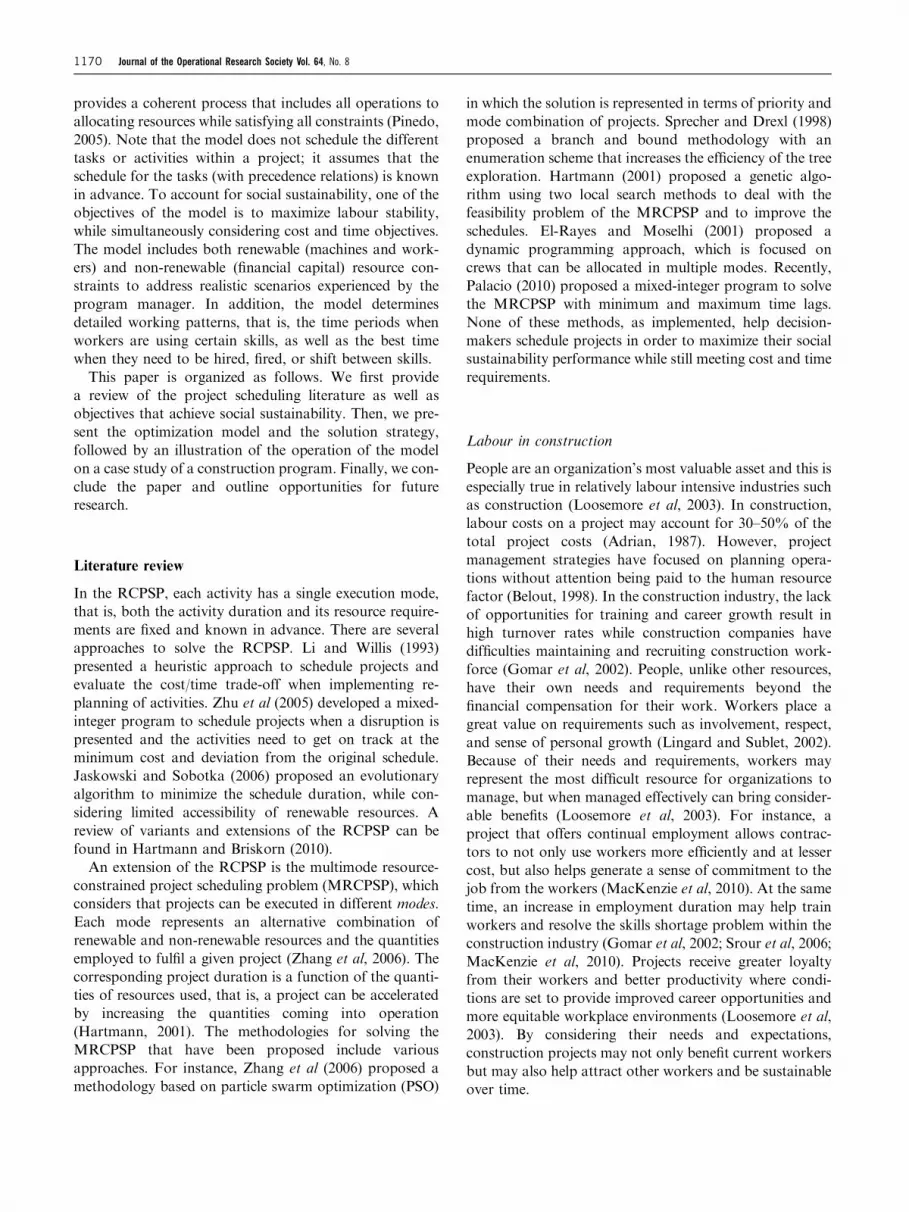
Figure 6 Number of workers by skill (maximal fluctuation).

0

5

10

15

20

25

30

1 2 3 4 5 6 7 8 9 10 11 12 13 14 15 16 17 18 19 20 21 22 23 24 25 26 27 28 29 30 31 32 33 34 35 36

Periods

Phase 2 Phase 3 ( max fluctuation)

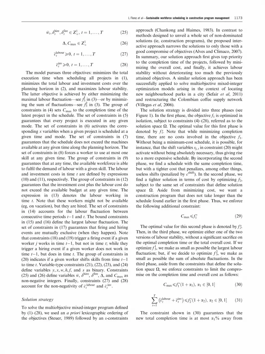
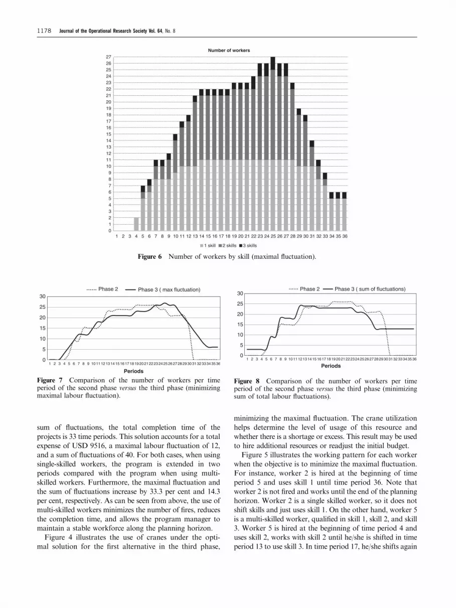
Figure 7 Comparison of the number of workers per timeperiod of the second phase versus the third phase (minimizingmaximal labour fluctuation).

0

5

10

15

20

25

30

1 2 3 4 5 6 7 8 9 101112131415161718192021222324252627282930313233343536

Periods

Phase 2 Phase 3 ( sum of fluctuations)

Figure 8 Comparison of the number of workers per timeperiod of the second phase versus the third phase (minimizingsum of total labour fluctuations).


to skill 2 and works until time period 36, when he/she is

fired. Note that although worker 5 is qualified in three skills,

he/she only uses two skills. Also, note that the report shows

when a worker is hired, fired, and shifted and the time

periods when each worker uses a skill. Workers 4, 12, and 29

are not hired during the planning horizon.

Figure 6 illustrates the number of workers by skill when

minimizing the maximal labour fluctuation. For instance,

in time period 15, the program uses 22 workers. That is, 11

single-skilled workers (50%), 10 multi-skilled workers with

two skills (45%), and one multi-skilled worker with three

skills (5%).

Figure 7 graphically compares the number of workers

per time period of the second and third phase (maximal

labour fluctuation). In the second phase, the projects were

scheduled to minimize cost and time, resulting in a maximal

labour fluctuation of 15 workers. The fluctuation of 15 is the

result of firing 15 workers in time period 31 as shown in

Figure 7. In the third phase (maximal labour fluctuation),

the solution is a maximal change of three workers between

any pair of consecutive time periods. Note that the slope is

equal to 3 between time periods 4 through 7 and time

periods 27 through 31. That is, three workers are hired in

time periods 5–7 and three workers are fired in time periods

28–31. Also, note that in phase 2 all workers are fired after

the last project is completed (time period 31), while in phase

3 some workers are kept until the end of the planning

horizon (time period 36). The difference between the costs

of fire (USD 15) and wage (USD 8) for a worker led to the

results shown in Figure 7.

Similarly, Figure 8 graphically compares the number of

workers per time period of the second and third phase (sum

of fluctuations). In the second phase, the projects were

scheduled to minimize cost and time, resulting in 52

fluctuations. This is the result of 52 hiring and firing events.

In the third phase (sum of fluctuations), the solution is

35 fluctuations. Note that in this alternative, a total of 13

workers are kept at the end of the planning horizon (time

period 36). As shown in Figure 7, the objective of mini-

mizing the maximal labour fluctuation resulted in a total

of 21 fires and six workers at the end of the planning

horizon (period 36). On the other hand, the objective of

minimizing the sum of fluctuations resulted in 11 fires

and 13 workers at the end of the planning horizon, as

shown in Figure 8. This trade-off between number of

fires and number of workers allows decision-makers to

consider their preferences and identify which solution

best suits their needs.

Finally, Figure 9 graphically compares the compro-

mise solution at the end of phase 3 with those of phase

1 and phase 2 where each criterion is optimized in

isolation. Each radial axis represents a single criterion

and each point reflects the percentage of the best

possible value achieved at each phase. Note that for

the completion time and total cost, the compromise

solution obtained in the three phases is close to 100%.

The solution to maximal fluctuation comprises the sum

of fluctuations by 137% of the best value while the

solution to sum of fluctuations comprises the maximal

fluctuation by 300% of the best value.

The solution process for the three phases using single-

skilled workers took 52 s (in average), while the solution

using multi-skilled workers took about 10.5min (in average).

The experiments in this section were performed on a Lenovo

X201 Tablet with 4GB of RAM, Intel Core i7 running at

1.729GHz (with 2 cores), on a 64-bit Microsoft Windows 7

Enterprise Edition operating system. The algorithm was

implemented in Mosel version 3.2.2 and the mixed-integer

optimization models were solved using Xpress-MP Optimi-

zer version 22.01.04.

0%

100%

200%

300%

400%

500%

Phase 1 Phase 2

Phase 3 (max fluctuation) Phase 3 (sum of fluctuations)

Sumof fluctuations

Completion time

Total expense

Maximal fluctuation

Figure 9 Comparison of the compromise solution at the end of phase 3 versus the solutions to phase 1 and phase 2.


Conclusions and future work

The project scheduling problem in construction has been

tackled in the literature using several methods. These

methods have considered evaluation criteria such as time,

cost, and quality to develop optimal schedules for

construction projects. However, the construction industry

is moving towards sustainability, requiring projects to

additionally include sustainable factors. Social sustainabil-

ity is one of such factors.

To measure the social sustainability performance of

project scheduling, we propose a new indicator denoted

labour stability. We proposed two alternatives to model

labour stability. The first alternative minimizes the max-

imal fluctuation of workers, whereas the second alternative

minimizes the sum of the fluctuations. By maximizing

labour stability, the objective is to increase the extent of use

of workers in the jobsite and job continuity.

A multiobjective mixed-integer programming model was

developed to allocate workers and schedule projects. We

illustrated the application of the model in a case study of a

construction program of 10 projects. The decision-makers

were able not only to determine the optimal starting times

for each of the projects, but also to identify working pat-

terns for each of the workers, usage levels of the machines,

and investment and labour costs.

The proposed solution strategy included three phases

that allow the decision-maker to include his/her preferences

and reveal trade-offs between objectives. In the first phase,

projects were scheduled with the objective of minimizing

completion time. Then, in the second phase, the objective

was to minimize cost without allowing deterioration of the

optimal completion time attained in the first phase. Finally,

in the third phase, the objective was to maximize labour

stability, allowing some deterioration in the time and cost

objectives.

The development of optimal schedules while considering

social sustainable practices contributes to determining

actions and formulating strategies to prevent social burdens

in an attempt to make program management more

sustainable. Following this study, the idea is to formulate

a more holistic set of sustainability performance indicators

that cover other social aspects as well as the environmental

dimensions. By doing so, a wider scope of goals can be

achieved, including those beyond social sustainability.

References

Adrian JJ (1987). Construction Productivity Improvement. Elsevier:New York.

Alves MJ and Clımaco J (2007). A review of interactive methodsfor multiobjective integer and mixed-integer programming.European Journal of Operational Research 180(1): 99–115.

Alwaer H and Clements-Croome DJ (2010). Key performanceindicators (KPIs) and priority setting using the multi-attributeapproach for assessing sustainable intelligent buildings. Buildingand Environment 45(4): 799–807.

Belout A (1998). Effects of human resource management on projecteffectiveness and success: Toward a new conceptual framework.International Journal of Project Management 16(1): 21–26.

Burleson RC, Haas CT, Tucker RL and Stanley A (1998).Multiskilled labor utilization strategies in construction. Journalof Construction Engineering and Management 124(6): 480–489.

Chankong V and Haimes YY (1983). Multiobjective DecisionMaking: Theory and Methodology. North-Holland: New York.

El-Rayes K and Moselhi O (2001). Optimizing resource utilizationfor repetitive construction projects. Journal of ConstructionEngineering and Management 127(1): 18–27.

Fernandez-Sanchez G and Rodriguez-Lopez F (2010). A metho-dology to identify sustainability indicators in constructionproject management—Application to infrastructure projects inSpain. Ecological Indicators 10(6): 1193–1201.

Gomar JE, Haas CT and Morton DP (2002). Assignment andallocation optimization of partially multiskilled workforce.Journal of Construction Engineering and Management 128(2):103–109.

Hartmann S (2001). Project scheduling with multiple modes: Agenetic algorithm. Annals of Operations Research 102(1–4):111–135.

Hartmann S and Briskorn D (2010). A survey of variants andextensions of the resource-constrained project scheduling pro-blem. European Journal of Operational Research 207(1): 1–14.

Hyari K, El-Mashaleh M and Kandil A (2010). Optimal assign-ment of multiskilled labor in building construction projects.International Journal of Construction Education and Research6(1): 70–80.

Jaskowski P and Sobotka A (2006). Scheduling constructionprojects using evolutionary algorithm. Journal of ConstructionEngineering and Management 132(8): 861–870.

Jun HJ and El-Rayes K (2010). Optimizing the utilization ofmultiple labor shifts in construction projects. Automation inConstruction 19(2): 109–119.

Labuschagne C, Brent AC and Van Erck RPG (2005). Assessingthe sustainability performances of industries. Journal of CleanerProduction 13(1): 373–385.

Li RKY and Willis RJ (1993). Resource constrained schedulingwithin fixed project durations. Journal of the OperationalResearch Society 44(1): 71–80.

Lill I (2008). Sustainable management of construction labour. In:Zavadskas EK, Kaklauskas A and Skibniewski MJ (eds).Proceedings of the 25th International Symposium on Automationand Robotics in Construction ISARC-2008, Vilnius Lithuania,Vilnius: Technika, pp 864–875.

Lingard H and Sublet A (2002). The impact of job andorganisational demands on marital or relationship satisfactionand conflict among Australian civil engineers. ConstructionManagement and Economics 20(6): 507–521.

Loosemore M, Dainty A and Lingard H (2003). Human ResourceManagement in Construction Projects: Strategies and OperationalApproaches. Spon Press: London.

MacKenzie S, Kilpatrick AR and Akintoye A (2010). UKconstruction skills shortage response strategies and an analysisof industry perceptions. Construction Management and Economics18(7): 853–862.

Medaglia AL, Hueth D, Mendieta JC and Sefair JA (2008).A multiobjective model for the selection and timing of publicenterprise projects. Socio-Economic Planning Sciences 42(1):31–45.


Palacio JD (2010). On the multi-mode resource-constrained projectscheduling problem with minimum and maximum time lags(MRCPSP/max) via mixed-integer programming. MSc Thesis(in Spanish), Universidad de los Andes.

Pinedo ML (2005). Planning and Scheduling in Manufacturing andServices. Springer: New York.

Ramos TB and Caeiro S (2010). Meta-performance evalua-tion of sustainability indicators. Ecological Indicators 10(2):157–166.

Reiss G (1996). Programme Management Demystified: ManagingMultiple Projects Successfully. E & F Spon: London.

RSMeans (2012). RSMeans reed construction data. http://rsmeans.reedconstructiondata.com/, accessed on 23 March 2012.

Sefair JA, Molano A, Medaglia AL and Sarmiento OL(2011). Locating neighborhood parks with a lexicographicmulti-objective optimization method. In: Michael PJ (ed).Community-Based Operations Research: Decision Modelingfor Local Impact and Diverse Populations. International Seriesin Operations Research & Management Science, Springer:New York, Vol. 167, Part 2, pp 143–171.

Singh RK, Murty HR, Gupta SK and Dikshit AK (2007).Development of composite sustainability performance indexfor steel industry. Ecological Indicators 7(2): 565–588.

Singh RK, Murty HR, Gupta SK and Dikshit AK (2009). Anoverview of sustainability assessment methodologies. EcologicalIndicators 9(2): 189–212.

Sprecher A and Drexl A (1998). Multi-mode resource-constrainedproject scheduling by a simple, general and powerful sequencingalgorithm. European Journal of Operational Research 107(2):431–450.

Srour IM, Haas CT and Morton DP (2006). Linear programmingapproach to optimize strategic investment in the constructionworkforce. Journal of Construction Engineering and Management132(11): 1158–1166.

Steuer R (1989). Multiple Criteria Optimization: Theory, Computa-tion and Application. Krieger: Malabar, FL.

Tahir AC and Darton RC (2010). The process analysis method ofselecting indicators to quantify the sustainability performance ofa business operation. Journal of Cleaner Production 18(16–17):1598–1607.

Ugwu OO and Haupt TC (2005). Key performance indicators forinfrastructure sustainability—A comparative study betweenHong Kong and South Africa. Journal of Engineering, Designand Technology 3(1): 30–43.

Villegas JG, Palacios F and Medaglia AL (2006). Solution methodsfor the bi-objective (cost-coverage) unconstrained facility loca-tion problem with an illustrative example. Annals of OperationsResearch 147(1): 109–141.

Wongwai N and Malaikrisanachalee S (2011). Augmented heuristicalgorithm for multi-skilled resource scheduling. Automation inConstruction 20(4): 429–445.

Zhang H, Tam CM and Li H (2006). Multimode project schedulingbased on particle swarm optimization. Computer-Aided Civil andInfrastructure Engineering 21(2): 93–103.

Zhu G, Bard JF and Yu G (2005). Disruption managementfor resource-constrained project scheduling. Journal of theOperational Research Society 56(4): 365–381.

Received April 2012;accepted November 2012 after one revision


sustainable workforce scheduling in construction program management

Documents