support-vector-machine-based reduced-order model for limit cycle oscillation prediction of nonlinear...

Hindawi Publishing CorporationMathematical Problems in EngineeringVolume 2012, Article ID 152123, 12 pagesdoi:10.1155/2012/152123

Research ArticleSupport-Vector-Machine-Based Reduced-OrderModel for Limit Cycle Oscillation Prediction ofNonlinear Aeroelastic System

Gang Chen,1 Yingtao Zuo,2 Jian Sun,1 and Yueming Li1

1 State Key Laboratory for Strength and Vibration of Mechanical Structures, School of Aerospace,Xi’an Jiaotong University, Xi’an, Shannxi 710049, China

2 School of Aeronuatics, Northwestern Polytechnical University, Xi’an, Shannxi 710072, China

Correspondence should be addressed to Yingtao Zuo, [email protected]

Received 25 June 2011; Accepted 3 November 2011

Academic Editor: Hamdy Nabih Agiza

Copyright q 2012 Gang Chen et al. This is an open access article distributed under the CreativeCommons Attribution License, which permits unrestricted use, distribution, and reproduction inany medium, provided the original work is properly cited.

It is not easy for the system identification-based reduced-order model (ROM) and even eigenmodebased reduced-order model to predict the limit cycle oscillation generated by the nonlinearunsteady aerodynamics. Most of these traditional ROMs are sensitive to the flow parametervariation. In order to deal with this problem, a support vector machine- (SVM-) based ROMwas investigated and the general construction framework was proposed. The two-DOF aeroelasticsystem for the NACA64A010 airfoil in transonic flow was then demonstrated for the new SVM-based ROM. The simulation results show that the new ROM can capture the LCO behavior ofthe nonlinear aeroelastic system with good accuracy and high efficiency. The robustness andcomputational efficiency of the SVM-based ROM would provide a promising tool for real-timeflight simulation including nonlinear aeroelastic effects.

1. Introduction

Aeroelasticity is the science concerned with the fluid-structure interaction including the iner-tial, elastic, and aerodynamic forces. The prediction of aeroelastic instability in the transonicregime plays a very important role in the definition of the flight envelope for many high-performance aircraft. For example, flutter and limit cycle oscillation (LCO) are the majornonlinear aeroelastic unstable phenomena, which are very dangerous to the aircraft structure.With the development of computational aeroelasticity, the nonlinear aeroelastic response canbe accurately predicted by the high-fidelity physics-based CFD/CSD couple solver. However,the use of multistep time domain calculations for each aircraft state is computationallyexpensive and provides limited insight into the dependence of the parameters on the type

2 Mathematical Problems in Engineering

of response in the vicinity of the instability boundary. In order to reduce the expensivecomputational cost, a novel conception called reduced-order model (ROM) based on high-fidelity physics model has been put forward in recent years. ROM seeks to capture thedominant nonlinear behavior of the aeroelastic system by constructing a simplemathematicalrepresentative model, which is very convenient to be used in conceptual design, control, anddata-driven systems [1].

Different approaches for reduced-order modeling of aerodynamic systems have beeninvestigated, including linearization about a nonlinear steady-state flow data-driven modelsuch as Volterra theory of nonlinear systems [2] and linear model fitting ARMA model [3],representation of the aerodynamic system in terms of its eigenmodes such as POD method[4, 5], and representation of the nonlinear aerodynamic system using the nonlinear dynamictheory [6]. Many approaches for constructing linear flow and aeroelastic ROMs have beendeveloped and shown to produce good numerical results that comparewell with high-fidelitynonlinear solvers. Most aeroelastic phenomena such as flutter and gust response can be dealwith these ROMs based on the dynamically linearized equation. However, unfortunately,some important strong nonlinear dynamic phenomena such as LCO cannot be simulatedby the small disturbance solvers. For modeling the cases where the amplitude of the flowperturbation is large, the ROMs based dynamically nonlinear solvers are required. Thomaset al. proposed a new nonlinear HB/ROMwhich can predict the LCO of the NLR 7301 airfoilaeroelastic model very well in the transonic regime [7]. Badcock et al. put forward a fullynonlinear ROM construction method based on bifurcation theory, which can predict LCOvery well [8]. Recently, we also proposed a new dynamically nonlinear NPOD/ROM, whichenables the rapid modeling of nonlinear unsteady flows for the prediction and control ofLCO [9, 10]. These recently developed high-order ROMs for LCO simulation are much morecomplex than traditional ROMs and are also not easy to realize in code.

Nonlinear system-identification-based ROMs have been widely used to predict thetransonic flutter boundary such as Volterra series [11, 12] and neural network approaches [13,14]. Because of the high efficiency and simplicity, it is an attractive idea to predict the LCO bysystem-identification-based ROMs. Neural networks have been widely applied in nonlinearsystem identification because of the ability of self-learning, strong parallel processing,and fault tolerance [15, 16]. There are also successful applications in the LCO predictionof the airfoil aeroelastic model [17, 18]. However, the disadvantages of getting stuckinto local minima, over-fitting, and low generalization performance prevent the practicalapplication of these methods. Recently, support vector machine introduced by Vapnik [19]has become a promising tool for solving nonlinear regression problems including nonlinearsystem identification. SVM is a newly emerging technique for learning relationships indata within the framework of statistical learning theory and structural risk minimization.Relying on statistical learning theory which enables learning machines to generalize well tounseen data, SVM has been significantly highlighted in the areas of system identificationand parameter estimation [20, 21]. In comparison with neural networks, SVM has stricttheory and mathematical foundation. It does not have the problem of local optimizationand dimensional disaster and can achieve higher generalization performance for smallsamples.

In this study, we develop an SVM-based ROM for predicting the LCO induced bythe nonlinear aerodynamics with high efficiency and good accuracy. Firstly, we gave abrief introduction about the regression SVM machine; secondly, we proposed a generalconstruction framework of the SVM-based ROM for the aeroelastic system; finally, wedemonstrated the ROM by the two-DOF NACA 64A010 airfoil aeroelastic model in detail.

Mathematical Problems in Engineering 3

2. Support Vector Machine-Based Nonlinear System Identification

The basic idea of SVM theory is to map the data to a higher-dimensional feature space vianonlinear mapping functions and then do the linear regression in this space. SVM-basednonlinear system identification approaches have taken advantage of both the kernel trick andthe well-developed SVR algorithmic implementations [19, 22].After introducing ε-insensitiveloss function, SVMs extend to the regression case, named support vector regression (SVR),whose key idea is to replace regression line with a ε-tube. Geometrically, the samples locatedoutside this tube will not be considered in regression model. The goal of SVR is to find adecision function f(x)which has at most ε deviation from actually obtained observations andat the same time is as flat as possible. Therefore, in the process of minimizing the empiricalerrors, SVRs also try to maximize the generalization ability.

Based on statistical learning theory, SVRs can be applicable especially to small-samplelearning problems. Here, we give a brief summary of SVR. Given an input-output data set{(x1, y1), . . . , (xl, yl)} ⊂ Rd × R, such as the time response series of the unsteady aerodynamiccoefficient of the aeroelastic system, SVR can be formulated as [19]

minw,b,ξ,ξ∗

12‖w‖2 + C

l∑

i=1

(ξi + ξ∗i

)

subject to

⎧⎪⎪⎨

⎪⎪⎩

yi − 〈w,Φ(xi)〉 − b ≤ ε + ξi

〈w,Φ(xi)〉 + b − yi ≤ ε + ξ∗iξi, ξ

∗i ≥ 0, i = 1, 2, . . . , l,

(2.1)

where the w is the weighting vector and ε-insensitive loss function is defined as

L(yi, f(xi)

)=

{0, if

∣∣yi − f(xi)∣∣ ≤ ε

∣∣yi − f(xi)∣∣ − ε, otherwise.

(2.2)

The slack variables ξi, ξ∗i determine the sample’s deviation from ε-tube, and the regularizationparameterC > 0 determines the trade-off between empirical risk and generalization term andpunishes the samples which violate the ε-tube. Applying the method of Lagrange multipliersto (2.1), equation (2.1) is transformed into the following equation:

L(w, b, α) =12‖w‖2 + C

l∑

i=1

(ξi + ξ∗i

) −l∑

i=1

(ηiξi + η∗

i ξ∗i

)

−l∑

i=1

αi

(ε + ξi − yi + 〈w,Φ(xi)〉 + b

)

−l∑

i=1

α∗i

(ε + ξ∗i + yi − 〈w,Φ(xi)〉 − b

),

(2.3)

where αi, α∗i are the introduced Lagrange multipliers and denoted by α

(∗)i .


After calculating the partial derivatives of L(w, b,α) with respect to (w, b, ξi, ξ∗i ), the

dual optimization problem can be obtained as follows [23]:

minα,α∗

12

l∑

i,j=1

(a∗i − αi

)(a∗j − αj

)⟨Φ(xi),Φ

(xj

)⟩+ ε

l∑

i=1

(a∗i + αi

) −l∑

i=1

yi

(a∗i − αi

)

s.t.l∑

i=1

(a∗i − αi

)= 0, 0 ≤ αi, a

∗i ≤ C, i = 1, 2, . . . , l.

(2.4)

Equation (2.4) is a quadratic programming problem. After calculating the values of αand α∗ for all samples, the decision function is obtained as follows:

f(x) =l∑

i=1

(αi − a∗

i

)K(xi, x) + b. (2.5)

In (2.5), only some samples come with nonzero α(∗), which is called the supportvector and provide sparsity. Moreover, K(xi, x) = 〈Φ(xi),Φ(xj)〉 is kernel function whichonly depends on dot products between observations xi and xj and does not have to knownonlinear mapping Φ explicitly. Any function satisfying Mercer’s condition can be used asthe kernel function. The widely used kernel functions are including polynomial kernel, theGaussian kernel, and Radial Basis kernel. From the implementation point of view, trainingSVM is equivalent to solving a linearly constrained quadratic programming problem withthe number of variables twice that of the training data points. Many effective optimizationalgorithms were proposed for solving the regression problem such as the solution pathalgorithm [24, 25].

3. SVM-Based Reduced-Order Model for Aeroelastic System

3.1. Numerical Couple Simulation Method ofthe Nonlinear Aeroelastic System

The full-coupled nonlinear semi-discrete aeroelastic equation is given as

(A(u)w),t + F(w,u, v) = 0,

Mv,t + f int(u, v) = fext(u,w).(3.1)

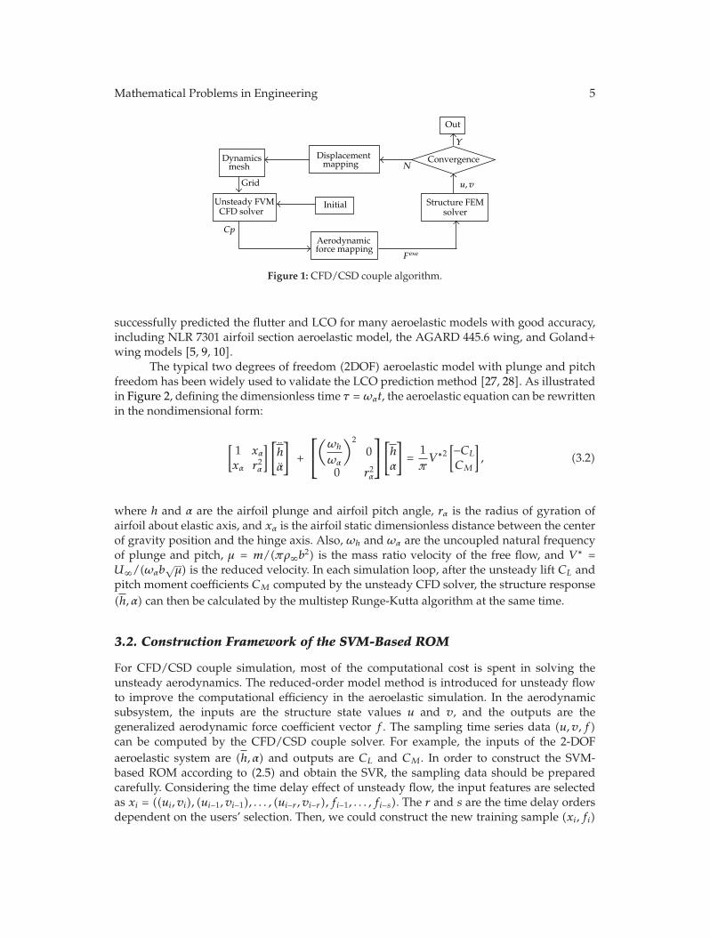
Equations (3.1) represent the fluid and structure dynamics, respectively, where w isconservative flow field value, F is flow flux residual,A is flow cell volume, u is the structuralgeneral displacement, v is structure general displacement derivatives, M is mass matrix,and f int is structure inner force. Also, fext is the aerodynamic force acting on the structurewhich is dependent on the flow state values and the structure state values. Many kindsof accurate CFD/CSD couple numerical algorithms have been developed to predict theresponse of structure and aerodynamics simultaneously [26]. The procedure of the popularloosely couple numerical simulation algorithm is illustrated in Figure 1. A general multiblockstructure mesh-based CFD/CSD loosely coupled solver was developed by the authors and


Dynamicsmesh

Aerodynamicforce mapping

Structure FEMsolver

Displacement mapping

Initial

Grid

Unsteady FVMCFD solver

u, v

Convergence

Out

Y

N

Cp

Fexe

Figure 1: CFD/CSD couple algorithm.

successfully predicted the flutter and LCO for many aeroelastic models with good accuracy,including NLR 7301 airfoil section aeroelastic model, the AGARD 445.6 wing, and Goland+wing models [5, 9, 10].

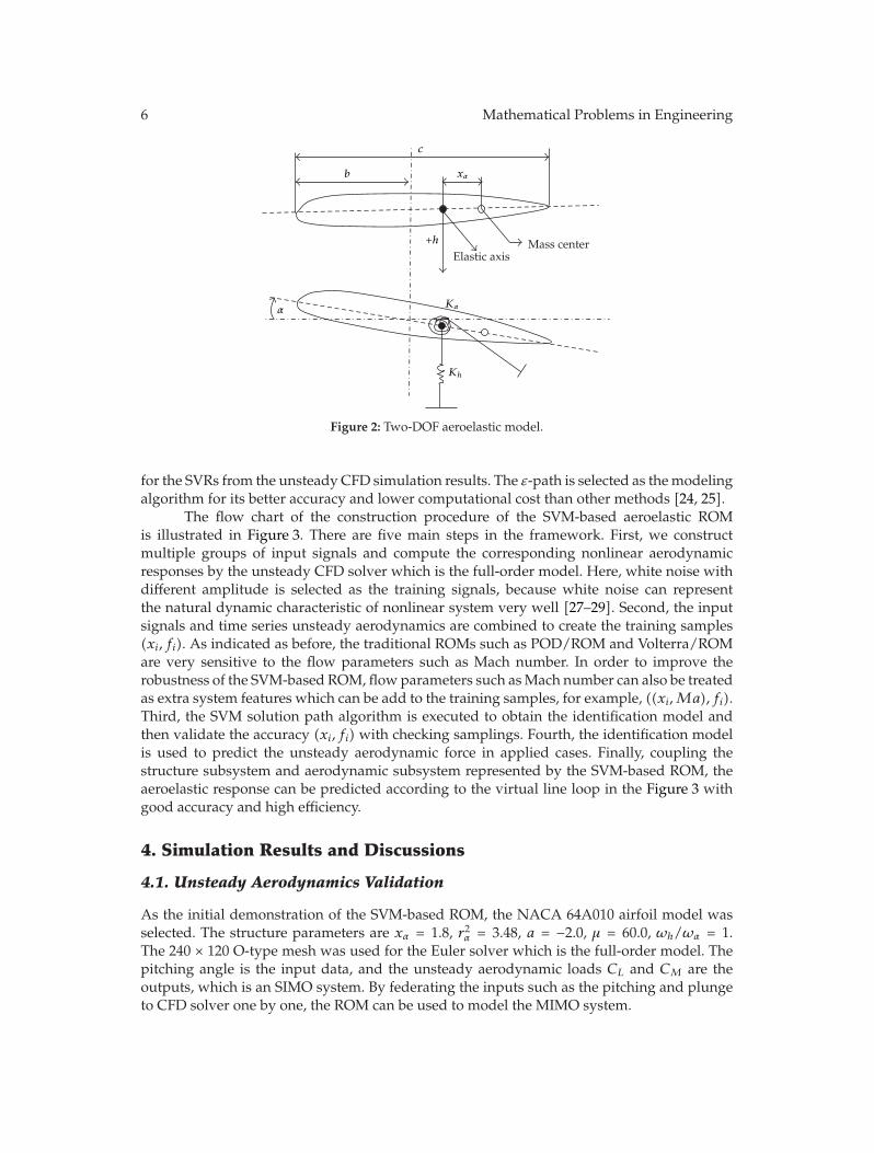
The typical two degrees of freedom (2DOF) aeroelastic model with plunge and pitchfreedom has been widely used to validate the LCO prediction method [27, 28]. As illustratedin Figure 2, defining the dimensionless time τ = ωαt, the aeroelastic equation can be rewrittenin the nondimensional form:

[1 xα

xα r2α

][hα

]+

⎡

⎣

(ωh

ωα

)2

0

0 r2α

⎤

⎦[hα

]=

1πV ∗2

[−CL

CM

], (3.2)

where h and α are the airfoil plunge and airfoil pitch angle, rα is the radius of gyration ofairfoil about elastic axis, and xα is the airfoil static dimensionless distance between the centerof gravity position and the hinge axis. Also, ωh and ωα are the uncoupled natural frequencyof plunge and pitch, μ = m/(πρ∞b2) is the mass ratio velocity of the free flow, and V ∗ =U∞/(ωαb

√μ) is the reduced velocity. In each simulation loop, after the unsteady lift CL and

pitch moment coefficients CM computed by the unsteady CFD solver, the structure response(h, α) can then be calculated by the multistep Runge-Kutta algorithm at the same time.

3.2. Construction Framework of the SVM-Based ROM

For CFD/CSD couple simulation, most of the computational cost is spent in solving theunsteady aerodynamics. The reduced-order model method is introduced for unsteady flowto improve the computational efficiency in the aeroelastic simulation. In the aerodynamicsubsystem, the inputs are the structure state values u and v, and the outputs are thegeneralized aerodynamic force coefficient vector f . The sampling time series data (u, v, f)can be computed by the CFD/CSD couple solver. For example, the inputs of the 2-DOFaeroelastic system are (h, α) and outputs are CL and CM. In order to construct the SVM-based ROM according to (2.5) and obtain the SVR, the sampling data should be preparedcarefully. Considering the time delay effect of unsteady flow, the input features are selectedas xi = ((ui, vi), (ui−1, vi−1), . . . , (ui−r , vi−r), fi−1, . . . , fi−s). The r and s are the time delay ordersdependent on the users’ selection. Then, we could construct the new training sample (xi, fi)


Elastic axisMass center

b

c

α

xα

+h

Kh

Kα

Figure 2: Two-DOF aeroelastic model.

for the SVRs from the unsteady CFD simulation results. The ε-path is selected as themodelingalgorithm for its better accuracy and lower computational cost than other methods [24, 25].

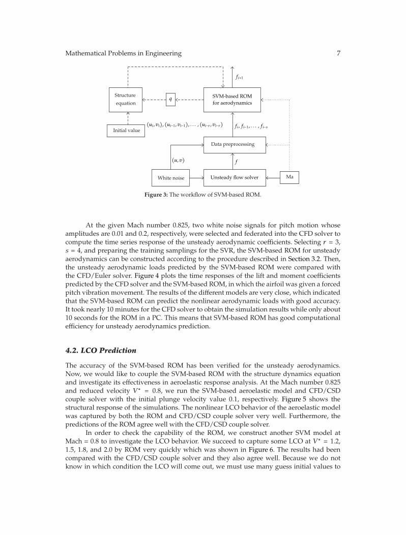
The flow chart of the construction procedure of the SVM-based aeroelastic ROMis illustrated in Figure 3. There are five main steps in the framework. First, we constructmultiple groups of input signals and compute the corresponding nonlinear aerodynamicresponses by the unsteady CFD solver which is the full-order model. Here, white noise withdifferent amplitude is selected as the training signals, because white noise can representthe natural dynamic characteristic of nonlinear system very well [27–29]. Second, the inputsignals and time series unsteady aerodynamics are combined to create the training samples(xi, fi). As indicated as before, the traditional ROMs such as POD/ROM and Volterra/ROMare very sensitive to the flow parameters such as Mach number. In order to improve therobustness of the SVM-based ROM, flow parameters such asMach number can also be treatedas extra system features which can be add to the training samples, for example, ((xi,Ma), fi).Third, the SVM solution path algorithm is executed to obtain the identification model andthen validate the accuracy (xi, fi) with checking samplings. Fourth, the identification modelis used to predict the unsteady aerodynamic force in applied cases. Finally, coupling thestructure subsystem and aerodynamic subsystem represented by the SVM-based ROM, theaeroelastic response can be predicted according to the virtual line loop in the Figure 3 withgood accuracy and high efficiency.

4. Simulation Results and Discussions

4.1. Unsteady Aerodynamics Validation

As the initial demonstration of the SVM-based ROM, the NACA 64A010 airfoil model wasselected. The structure parameters are xα = 1.8, r2α = 3.48, a = −2.0, μ = 60.0, ωh/ωα = 1.The 240 × 120 O-type mesh was used for the Euler solver which is the full-order model. Thepitching angle is the input data, and the unsteady aerodynamic loads CL and CM are theoutputs, which is an SIMO system. By federating the inputs such as the pitching and plungeto CFD solver one by one, the ROM can be used to model the MIMO system.


Structure

equation

White noise

Initial value

Ma

Data preprocessing

fi+1

SVM-based ROMfor aerodynamics

Unsteady flow solver

q

f

fi, fi−1, · · · , fi−sui, vi

,ui−1, vi−1

, · · · ,

ui−r , vi−r

u, v

Figure 3: The workflow of SVM-based ROM.

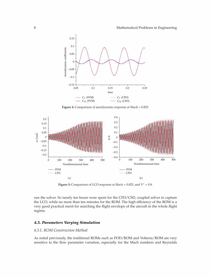
At the given Mach number 0.825, two white noise signals for pitch motion whoseamplitudes are 0.01 and 0.2, respectively, were selected and federated into the CFD solver tocompute the time series response of the unsteady aerodynamic coefficients. Selecting r = 3,s = 4, and preparing the training samplings for the SVR, the SVM-based ROM for unsteadyaerodynamics can be constructed according to the procedure described in Section 3.2. Then,the unsteady aerodynamic loads predicted by the SVM-based ROM were compared withthe CFD/Euler solver. Figure 4 plots the time responses of the lift and moment coefficientspredicted by the CFD solver and the SVM-based ROM, in which the airfoil was given a forcedpitch vibration movement. The results of the different models are very close, which indicatedthat the SVM-based ROM can predict the nonlinear aerodynamic loads with good accuracy.It took nearly 10 minutes for the CFD solver to obtain the simulation results while only about10 seconds for the ROM in a PC. This means that SVM-based ROM has good computationalefficiency for unsteady aerodynamics prediction.

4.2. LCO Prediction

The accuracy of the SVM-based ROM has been verified for the unsteady aerodynamics.Now, we would like to couple the SVM-based ROM with the structure dynamics equationand investigate its effectiveness in aeroelastic response analysis. At the Mach number 0.825and reduced velocity V ∗ = 0.8, we run the SVM-based aeroelastic model and CFD/CSDcouple solver with the initial plunge velocity value 0.1, respectively. Figure 5 shows thestructural response of the simulations. The nonlinear LCO behavior of the aeroelastic modelwas captured by both the ROM and CFD/CSD couple solver very well. Furthermore, thepredictions of the ROM agree well with the CFD/CSD couple solver.

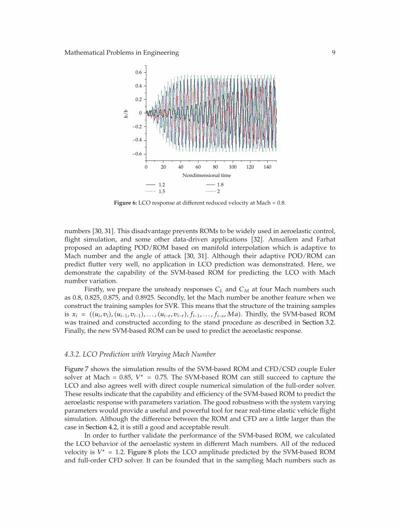
In order to check the capability of the ROM, we construct another SVM model atMach = 0.8 to investigate the LCO behavior. We succeed to capture some LCO at V ∗ = 1.2,1.5, 1.8, and 2.0 by ROM very quickly which was shown in Figure 6. The results had beencompared with the CFD/CSD couple solver and they also agree well. Because we do notknow in which condition the LCO will come out, we must use many guess initial values to


0.05 0.1 0.15 0.2 0.25−0.15

−0.1

−0.05

0

0.05

0.1

0.15

Aer

odyn

amic

coe

ffici

ents

time

CL (SVM)CM (SVM)

CL (CFD)CM (CFD)

Figure 4: Comparison of aerodynamic response at Mach = 0.825.

0

0

100 200 300 400 500

−0.2

−0.15

−0.1

−0.05

0.05

0.1

0.15

0.2

α/(r

ad)

Nondimensional time

SVMCFD

(a)

0 100 200 300 400 500

Nondimensional time

SVMCFD

−0.4

−0.3

−0.2

−0.1

0

0.1

0.2

0.3

0.4

h/b

(b)

Figure 5: Comparison of LCO response at Mach = 0.825, and V ∗ = 0.8.

run the solver. So nearly ten hours were spent for the CFD/CSD, coupled solver to capturethe LCO, while no more than ten minutes for the ROM. The high efficiency of the ROM is avery good practical merit for searching the flight envelope of the aircraft in the whole flightregime.

4.3. Parameters Varying Simulation

4.3.1. ROM Construction Method

As noted previously, the traditional ROMs such as POD/ROM and Volterra/ROM are verysensitive to the flow parameter variation, especially for the Mach numbers and Reynolds


0 20 40 60 80 100 120 140

−0.6

−0.4

−0.2

0

0.2

0.4

0.6

Nondimensional time

1.21.5

1.82

h/b

Figure 6: LCO response at different reduced velocity at Mach = 0.8.

numbers [30, 31]. This disadvantage prevents ROMs to be widely used in aeroelastic control,flight simulation, and some other data-driven applications [32]. Amsallem and Farhatproposed an adapting POD/ROM based on manifold interpolation which is adaptive toMach number and the angle of attack [30, 31]. Although their adaptive POD/ROM canpredict flutter very well, no application in LCO prediction was demonstrated. Here, wedemonstrate the capability of the SVM-based ROM for predicting the LCO with Machnumber variation.

Firstly, we prepare the unsteady responses CL and CM at four Mach numbers suchas 0.8, 0.825, 0.875, and 0.8925. Secondly, let the Mach number be another feature when weconstruct the training samples for SVR. This means that the structure of the training samplesis xi = ((ui, vi), (ui−1, vi−1), . . . , (ui−r , vi−r), fi−1, . . . , fi−s,Ma). Thirdly, the SVM-based ROMwas trained and constructed according to the stand procedure as described in Section 3.2.Finally, the new SVM-based ROM can be used to predict the aeroelastic response.

4.3.2. LCO Prediction with Varying Mach Number

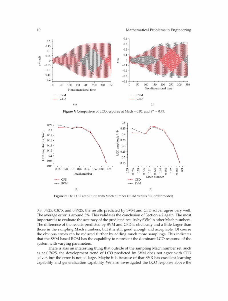
Figure 7 shows the simulation results of the SVM-based ROM and CFD/CSD couple Eulersolver at Mach = 0.85, V ∗ = 0.75. The SVM-based ROM can still succeed to capture theLCO and also agrees well with direct couple numerical simulation of the full-order solver.These results indicate that the capability and efficiency of the SVM-based ROM to predict theaeroelastic response with parameters variation. The good robustness with the system varyingparameters would provide a useful and powerful tool for near real-time elastic vehicle flightsimulation. Although the difference between the ROM and CFD are a little larger than thecase in Section 4.2, it is still a good and acceptable result.

In order to further validate the performance of the SVM-based ROM, we calculatedthe LCO behavior of the aeroelastic system in different Mach numbers. All of the reducedvelocity is V ∗ = 1.2. Figure 8 plots the LCO amplitude predicted by the SVM-based ROMand full-order CFD solver. It can be founded that in the sampling Mach numbers such as


0 50 100 150 200 250 300 350

−0.2

−0.15

−0.1

−0.05

0

0.05

0.1

0.15

0.2α

/(r

ad)

Nondimensional time

SVMCFD

(a)

0 50 100 150 200 250 300 350−0.4

−0.3

−0.2

−0.1

0

0.1

0.2

0.3

0.4

Nondimensional time

SVMCFD

h/b

(b)

Figure 7: Comparison of LCO response at Mach = 0.85, and V ∗ = 0.75.

0.76 0.78 0.8 0.82 0.84 0.86 0.88 0.90.06

0.08

0.1

0.12

0.14

0.16

0.18

0.2

0.22

Mach number

CFDSVM

LC

O a

mpl

itud

eα

/(r

ad)

(a)

0.75

0.76

5

0.78

0.79

5

0.81

0.82

5

0.84

0.85

5

0.87

0.88

5

0.9

0.15

0.2

0.25

0.3

0.35

0.4

0.45

0.5

Mach numberCFDSVM

LC

O a

mpl

itud

eh

/b

(b)

Figure 8: The LCO amplitude with Mach number (ROM versus full-order model).

0.8, 0.825, 0.875, and 0.8925, the results predicted by SVM and CFD solver agree very well.The average error is around 5%. This validates the conclusion of Section 4.2 again. The mostimportant is to evaluate the accuracy of the predicted results by SVM in other Mach numbers.The difference of the results predicted by SVM and CFD is obviously and a little larger thanthose in the sampling Mach numbers, but it is still good enough and acceptable. Of coursethe obvious errors can be reduced further by adding much more samplings. This indicatesthat the SVM-based ROM has the capability to represent the dominant LCO response of thesystem with varying parameters.

There is also an interesting thing that outside of the sampling Mach number set, suchas at 0.7625, the development trend of LCO predicted by SVM does not agree with CFDsolver, but the error is not so large. Maybe it is because of that SVR has excellent learningcapability and generalization capability. We also investigated the LCO response above the


Mach number 0.9, but the SVM model fail to capture the LCO. It seems that the aeroelasticsystem runs into divergence or convergence from the simulation of the full-order solver. It isobviously and reasonable that no data-driven model can do everything.

It takes about 1 hour for the CFD solver to capture the LCO response, but it is no morethan one minutes for the SVM-based ROM to predict the same response. The computationalefficiency of ROM is obvious, which is very important to the near real-time flight dynamicsimulation and flight controller design. The fast prediction of the system response withgood accuracy is one of the most important factors to realize these challenge applicationssuccessfully.

5. Conclusion

An SVM-based reduced-order model was developed for fast prediction of the response of thenonlinear aeroelastic system. We proposed a general construction framework for the SVM-based ROM. The two-dimensional aerofoil aeroelastic system was used to demonstrate thecapability and performance of the ROM in detail. The simulation results show the capability,accuracy, and high efficiency of the SVM-based ROM for the LCO prediction. The SVM-basedROM can also fairly predict the LCO response of the 2DOF aeroelastic model with the Machnumber variation. The robustness of the SVM-based ROM with varying flow parametersprovides a useful tool for real-time flight simulation of flexible vehicle. Further researchwill focus on developing new training methods and improving the accuracy of the ROM,especially for the cases with parameters variation.

Acknowledgments

This work was supported by the National Natural Science Foundation of China (10902082,91016008), New Faculty Research Foundation of XJTU, and the Fundamental Research Fundsfor the Central Universities (xjj20100126). The first author acknowledges W. T. Mao for thediscussion of SVM algorithms. All the authors thank H. N. Agiza and the reviewers for theirgood comments.

References

[1] D. J. Lucia, P. S. Beran, andW. A. Silva, “Reduced-order modeling: new approaches for computationalphysics,” Progress in Aerospace Sciences, vol. 40, no. 1-2, pp. 51–117, 2004.

[2] W. A. Silva and R. E. Bartels, “Development of reduced-order models for aeroelastic analysis andflutter prediction using the CFL3Dv6.0 code,” Journal of Fluids and Structures, vol. 19, no. 6, pp. 729–745, 2004.

[3] J. Y. Kwak, W. Hong, S. J. Shin, I. Lee, J. W. Yim, and C. Kim, “CFD-Based aeroelastic analysis ofthe X-43 hypersonic flight vehicle,” in Proceedings of the 39th Aerospace Sciences Meeting and Exhibit(AIAA ’01), 2001.

[4] K. C. Hall, J. P. Thomas, and E. H. Dowell, “Proper orthogonal decomposition technique for transonicunsteady aerodynamic flows,” AIAA Journal, vol. 38, no. 10, pp. 1853–1862, 2000.

[5] G. Chen, Y.-M. Li, G.-R. Yan, M. Xu, and X.-A. Zeng, “A fast aeroelastic response prediction methodbased on proper orthogonal decomposition reduced order model,” Journal of Astronautics, vol. 30, no.5, pp. 1765–1769, 2009 (Chinese).

[6] K. J. Badcock andM. A. Woodgate, “Fast prediction of transonic aeroelastic stability and limit cycles,”AIAA Journal, vol. 45, no. 6, pp. 1370–1381, 2007 (Chinese).

[7] J. P. Thomas, E. H. Dowell, and K. C. Hall, “Using automatic differentiation to create a nonlinearreduced-order-model aerodynamic solver,” AIAA Journal, vol. 48, no. 1, pp. 19–24, 2010.


[8] K. J. Badcock, S. Timme, and S. Marques, “Transonic aeroelastic simulation for instability searchesanduncertainty analysis,” Progress in Aerospace Sciences, vol. 47, pp. 392–423, 2011.

[9] G. Chen, Y. Li, and G. Yan, “A nonlinear POD reduced order model for limit cycle oscillationprediction,” Science China, vol. 53, no. 7, pp. 1325–1332, 2010.

[10] G. Chen, Y.-M. Li, and G.-R. Yan, “Limit cycle oscillation prediction and control design methodfor aeroelastic system based on new nonlinear reduced order model,” International Journal ofComputational Methods, vol. 8, no. 1, pp. 77–90, 2011.

[11] D. E. Raveh, “Identification of computational-fluid-dynamics based unsteady aerodynamic modelsfor aeroelastic analysis,” Journal of Aircraft, vol. 41, no. 3, pp. 620–632, 2004.

[12] W. A. Silva, “Simultaneous excitation of multiple-input/multiple-output CFD-based unsteadyaerodynamic systems,” Journal of Aircraft, vol. 45, no. 4, pp. 1267–1274, 2008.

[13] F. D. Marques and J. Anderson, “Identification and prediction of unsteady transonic aerodynamicloads by multi-layer functionals,” Journal of Fluids and Structures, vol. 15, no. 1, pp. 83–106, 2001.

[14] K. L. Lai, K. S. Won, E. P. C. Koh, and H. M. Tsai, “Flutter simulation and prediction with CFD-basedreduced-order model,” in Proceedings of the 47th AIAA/ASME/ASCE/AHS/ASC Structures, StructuralDynamics and Materials Conference (AIAA ’06), pp. 5229–5245, Newport, RI, USA, May 2006.

[15] S. Srivastava, M. Singh, M. Hanmandlu, and A. N. Jha, “Identification of nonlinear systems usingwavelets and neural network,” IETE Journal of Research, vol. 52, no. 4, pp. 305–313, 2006.

[16] E. Marcelo, A. K. S. Johan, and D. M. Bart, “Kernel based partially linear models and nonlinearidentification,” IEEE Transactions on Automatic Control, vol. 50, no. 10, pp. 1602–1606, 2005.

[17] M. R. Johnson and C. M. Denegri, “Comparison of static and dynamic artificial neural networks forlimit cycle oscillation prediction,” in Proceedings of the 42nd AIAA/ASME/ASCE/AHS/ASC Structures,Structural Dynamics and Exhibit Technical Papers (AIAA ’01), pp. 793–800, April 2001.

[18] O. Voitcu and Y. S. Wong, “An improved neural network model for nonlinear aeroelastic analysis,”in Proceedings of the 44th AIAA/ASME/ASCE/AHS/ASC Structures, Structural Dynamics, and MaterialsConference (AIAA ’03), pp. 825–835, April 2003.

[19] V. N. Vapnik, “An overview of statistical learning theory,” IEEE Transactions on Neural Networks, vol.10, no. 5, pp. 988–999, 1999.

[20] I. Goethals, K. Pelckmans, J. A. K. Suykens, and B. DeMoor, “Subspace identification of Hammersteinsystems using least squares support vector machines,” IEEE Transactions on Automatic Control, vol. 50,no. 10, pp. 1509–1519, 2005.

[21] Z. Lu and J. Sun, “Non-Mercer hybrid kernel for linear programming support vector regression innonlinear systems identification,” Applied Soft Computing Journal, vol. 9, no. 1, pp. 94–99, 2009.

[22] I. Witten and E. Frank, Data Mining Practical Machine Learning Tools and Techniques, Elsevier, 2005.[23] A. J. Smola and B. Scholkopf, “A tutorial on support vector regression neurocolt,” Tech. Rep., Royal

Holloway College, London, UK, 1998.[24] G. Wang, D. Y. Yeung, and F. H. Lochovsky, “A new solution path algorithm in support vector

regression,” IEEE Transactions on Neural Networks, vol. 19, no. 10, pp. 1753–1767, 2008.[25] W. Mao, G. Yan, and L. Dong, “Weighted solution path algorithm of support vector regression based

on heuristic weight-setting optimization,” Neurocomputing, vol. 73, no. 1–3, pp. 495–505, 2009.[26] R. Kamakoti and W. Shyy, “Fluid-structure interaction for aeroelastic applications,” Progress in

Aerospace Sciences, vol. 40, no. 8, pp. 535–558, 2004.[27] J. P. Thomas, E. H. Dowell, and K. C. Hall, “Nonlinear inviscid aerodynamic effects on transonic

divergence, flutter, and limit-cycle oscillations,” AIAA Journal, vol. 40, no. 4, pp. 638–646, 2002.[28] W. Mao, D. Hu, and G. Yan, “A new SVM regression approach for mechanical load identification,”

International Journal of Applied Electromagnetics and Mechanics, vol. 33, no. 3-4, pp. 1001–1008, 2010.[29] M. Anna, B. D. P. Andrea, and J. Schoukens, “Nonlinear system identification by means of Svms:

choice of excitation signals,” in Proceedings of the 16th TC4 International Symposium, Exploring NewFrontiers of Instrumentation andMethods for Electrical and ElectronicMeasurements (IMEKO ’08), Florence,Italy, September 2008.

[30] D. Amsallem and C. Farhat, “Interpolation method for adapting reduced-order models andapplication to aeroelasticity,” AIAA Journal, vol. 46, no. 7, pp. 1803–1813, 2008.

[31] D. Amsallem, J. Cortial, and C. Farhat, “Toward real-time computational-fluid-dynamics-basedaeroelastic computations using a database of reduced-order information,” AIAA Journal, vol. 48, no.9, pp. 2029–2037, 2010.

[32] P. Hu, M. Bodson, and M. Brenner, “Towards real-time simulation of aeroservoelastic dynamics for aflight vehicle from subsonic to hypersonic regime,” in Proceedings of the Atmospheric Flight MechanicsConference and Exhibit (AIAA ’08), Honolulu, Hawaii, USA, August 2008.

support-vector-machine-based reduced-order model for limit cycle oscillation prediction of nonlinear...

Documents