subsonic phase transition waves in bistable lattice models with small spinodal region
TRANSCRIPT
Subsonic phase transition waves
in bistable lattice models with small spinodal region
Michael Herrmann∗, Karsten Matthies†, Hartmut Schwetlick‡, Johannes Zimmer§
January 21, 2013
Abstract
Phase transitions waves in atomic chains with double-well potential play a fundamental role inmaterials science, but very little is known about their mathematical properties. In particular, theonly available results about waves with large amplitudes concern chains with piecewise-quadraticpair potential. In this paper we consider perturbations of a bi-quadratic potential and prove thatthe corresponding three-parameter family of waves persists as long as the perturbation is smalland localised with respect to the strain variable. As a standard Lyapunov-Schmidt reductioncannot be used due to the presence of an essential spectrum, we characterise the perturbationof the wave as a fixed point of a nonlinear and nonlocal operator and show that this operator iscontractive in a small ball in a suitable function space. Moreover, we derive a uniqueness resultfor phase transition waves with certain properties and discuss the kinetic relation.
Keywords: phase transitions in lattices, kinetic relations,heteroclinic travelling waves in Fermi-Pasta-Ulam chains
MSC (2010): 37K60, 47H10, 74J30, 82C26
1 Introduction
Many standard models in one-dimensional discrete elasticity describe the motion in atomic chainswith nearest neighbour interactions. The corresponding equation of motion reads
uj(t) = Φ′(uj+1(t)− uj(t))− Φ′(uj(t)− uj−1(t)) , (1)
where Φ is the interaction potential and uj denotes the displacement of particle j at time t.Of particular importance is the case of non-convex Φ, because then (1) provides a simple dy-
namical model for martensitic phase transitions. In this context, a propagating interface can bedescribed by a phase transition wave, which is a travelling wave that moves with subsonic speed andis heteroclinic as it connects periodic oscillations in different wells of Φ. The interest in such waves isalso motivated by the quest to derive selection criteria for the naıve continuum limit of (1), which isthe PDE ∂ttu = ∂xΦ′(∂x). For non-convex Φ, this equation is ill-posed due to its elliptic-hyperbolicnature, and one proposal is to select solutions by so-called kinetic relations [AK91, Tru87] derivedfrom travelling waves in atomistic models.
Combining the travelling wave ansatz uj(t) = U(j − ct) with (1) yields the delay-advance-differential equation
c2R′′(x) = ∆1Φ′(R(x)), (2)
∗[email protected], Universitat des Saarlandes†[email protected], University of Bath‡[email protected], University of Bath§[email protected], University of Bath
1
arX
iv:1
206.
0268
v2 [
mat
h-ph
] 1
8 Ja
n 20
13
where R(x) := U(x + 1/2) − U(x − 1/2) the (symmetrised) discrete strain profile and ∆1F (x) :=F (x+ 1)−2F (x) +F (x−1). Periodic and homoclinic travelling waves have been studied intensively,see [FW94, SW97, FP99, Pan05, EP05, Her10] and the references therein, but very little is knownabout heteroclinic waves. The authors are only aware of [HR10, Her11], which prove the existence ofsupersonic heteroclinic waves, and the small amplitude results from [Ioo00]. In particular, there seemsto be no result that provides phase transitions waves with large amplitudes for generic double-wellpotentials.
Phase transition waves with large amplitudes are only well understood for piecewise quadraticpotentials, and there exists a rich body of literature on bi-quadratic potentials, starting with [BCS01a,BCS01b, TV05]. For the special case
Φ(r) = 12r
2 − |r| , Φ′(r) = r − sgn(r) (3)
the existence of phase transition waves has been established by two of the authors using rigorousFourier methods. In [SZ09] they consider subsonic speeds c sufficiently close to 1, which is the speedof sound, and show that (2) admits for each c a two-parameter family of waves. These waves haveexactly one interface and connect different periodic tail oscillations, see Figure 2 for an illustration.
In this paper we allow for small perturbations of the potential (3) and show that the three-parameter family of phase transition waves from [SZ12] persist provided that the perturbation issufficiently localised with respect to the strain variable r.
A related problem has been studied in [Vai10]. There, a piecewise quadratic family of potentialsis considered such that the stress-strain relationship is continuous and trilinear, with a small spinodalregion. Travelling wave solutions are shown to obey a relation of residuals in the Fourier represen-tation, which is then approximately solved numerically. The regularity of the perturbed potential islower than that of the class of perturbations considered here, so strictly speaking the results do notoverlap. However, in spirit the settings are close and indeed the numerical evidence [Vai10, Fig. 4,bottom right panel] is in good in agreement with our findings: there is an one-sided asymptoticallyconstant solution, and the tail behind the interface oscillates with slightly different amplitude fromthat related to (3). The range of velocities considered in [Vai10] is larger than the one studied here.
Our approach is in essence perturbative and reformulates the travelling wave equation with per-turbed potential in terms of a corrector profile S, i.e., we write R = R0 + S, where R0 is a givenwave corresponding to the unperturbed potential. The resulting equation for the corrector S can bewritten as
MS = A2G(S) + η , (4)
where η is a constant of integration and A,M, G are operators to be identified below. More precisely,M is a linear integral operator which depends on c and G a nonlinear superposition operator involvingR0. The analysis of (4) is rather delicate since the Fourier symbol ofM has real roots, which impliesthat 0 is an inner point of the continuous spectrum of M. In particular M is not a Fredholmoperator in the function spaces we considered here, so a standard bifurcation analysis from δ = 0 viaa Lyapunov-Schmidt reduction is impossible.
In our existence proof, we first eliminate the corresponding singularities and derive an appropriatesolution formula for the linear subproblem. Afterwards we introduce a class of admissible functionsS and show that the properties of A and G guarantee that A2G(S) is compactly supported andsufficiently small. These fine properties are illustrated in Fig. 5 and allow us to define a nonlocal andnonlinear operator T such that
MT (S) = A2G(S) + η(S)
holds for all admissible S with some η(S) ∈ R. This operator T is contractive in some ball of anappropriately defined function space, so the existence of phase transitions waves is granted by thecontraction mapping principle, see Lemma 14. Moreover, the properties of M and G imply that ourfixed point method for S yields all phase transition waves R that comply with certain requirements,see Proposition 17.
2
Our existence result yields – for each c from an interval of subsonic velocities – a genuine two-parameter family of solutions to (2) but it is not clear whether all these phase transition waves arephysically reasonable. In the literature, one often employs selection criteria to single out a uniquephase transition wave for each speed c. One selection criterion is the causality principle, which inour case selects waves with non-oscillatory tails in front of the interface; see [Sle01, Sle02, TV05]and Remark (v) following the Main Theorem 3. These waves can also be observed in numericalsimulations of atomistic Riemann problems with non-oscillatory initial data [HSZ12].
Below we tailor our perturbation method carefully in order to show persistence of the tail oscil-lations in front of the interface. In particular, for each small δ and any given c we obtain exactly onewave that propagates towards an asymptotically constant state. The other solutions are oscillatoryfor both x→ −∞ and x→ +∞, and satisfy the entropy principle – which is less restrictive than thecausality principle – as long as the oscillations in front of the interface have smaller amplitude thanthose behind; see [HSZ12] for more details and a discussion of the different versions of Sommerfeld’sradiation condition. It is not known whether waves with tail oscillations on both sides of the inter-face are dynamically stable or can be created by Riemann initial data. As usual, however, one mightexpect that travelling waves resemble dynamical solutions of more complex situations in a temporaland spatial window. Candidates are cascades of moving phase interfaces in chains with multi-wellpotential or other types of macroscopically self-similar waves.
We also emphasise that phase transition waves satisfy Rankine-Hugoniot conditions for the macro-scopic averages of mass, momentum, and total energy [HSZ12], which imply nontrivial restrictionsbetween the wave speed and the tail oscillations on both sides of the interface. Although these con-ditions do not appear explicitly in our existence proof, they can (at least in principle) be computedbecause the tail oscillations are given by harmonic waves, see again Fig. 2. For general double-wellpotentials, however, it is much harder to evaluate the Rankine-Hugoniot conditions and thus it re-mains unclear which tail oscillations can be connected by phase transition waves. Closely related tothe jump condition for the total energy is the kinetic relation, which specifies the transfer betweenoscillatory and non-oscillatory energy at the interface and determines the configurational force thatdrives the wave. In the final section we discuss how the kinetic relation changes to leading orderunder small perturbations of the potential (3).
We now present our main result in greater detail.
1.1 Overview and main result
We study an atomic chain with interaction potential
Φδ(r) = 12r
2 −Ψδ(r) , Ψδ(0) = 0 ,
where Ψ′δ is a perturbation of Ψ′0 = sgn in a small neighbourhood of 0. The travelling wave equationtherefore reads
c2R′′ = 41
(R−Ψ′δ(R)
)(5)
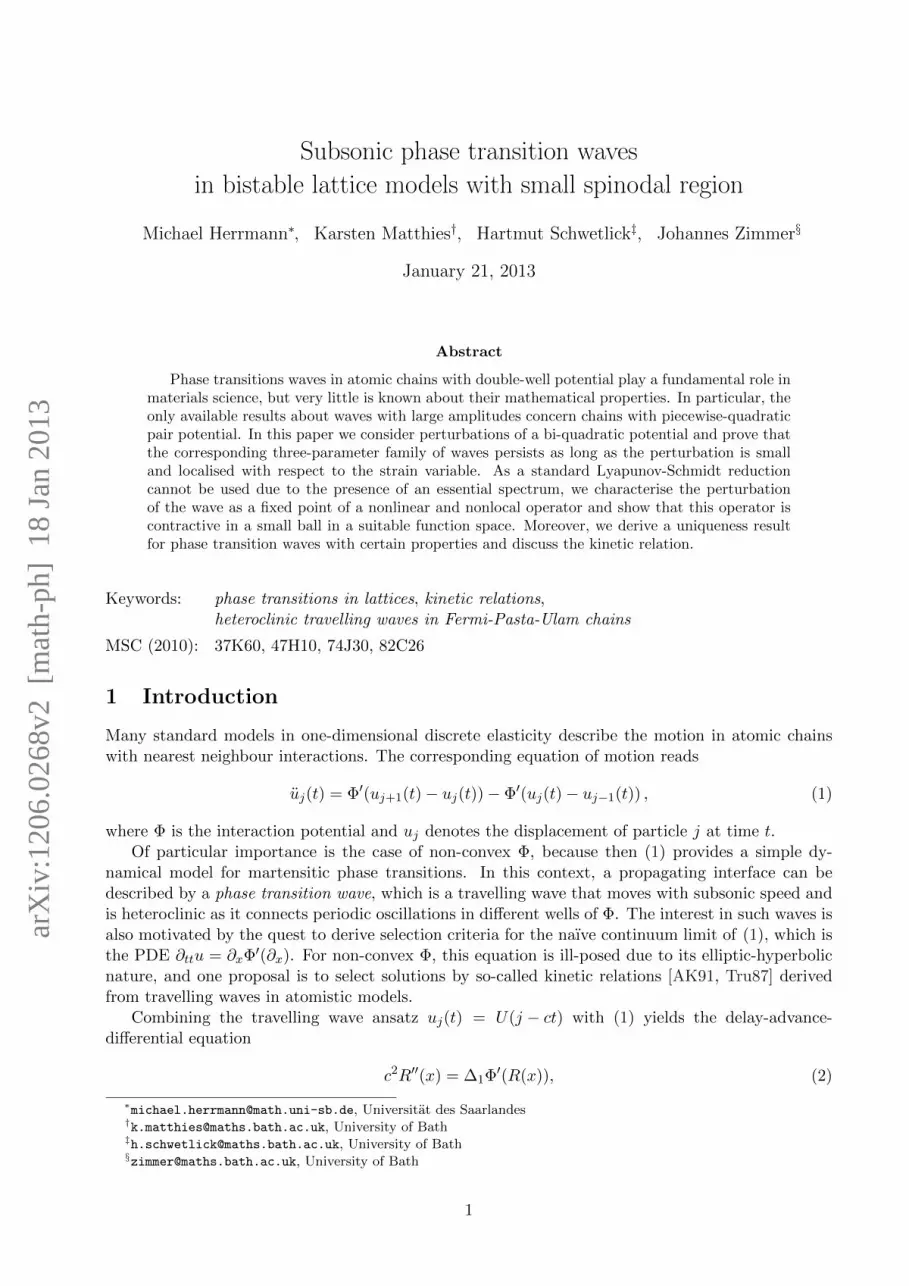
and depends on the parameters c and δ. In order to show that (5) admits solutions for small δ werely on the following assumptions on Ψ′δ, see Figure 1 for an illustration.
Assumption 1. Let (Ψδ)δ>0 be a one-parameter family of C2-potentials such that
(i) Ψ′δ coincides with Ψ′0 outside the interval (−δ, δ),
(ii) there is a constant CΨ independent of δ such that∣∣Ψ′δ(r)∣∣ ≤ CΨ ,∣∣Ψ′′δ (r)∣∣ ≤ CΨ
δ.
for all r ∈ R.
3
The quantity
Iδ := 12
∫R
(Ψ′δ(r)−Ψ′0(r)
)dr
plays in important role in our perturbation result as it determines the leading order correction.Notice that our assumptions imply
Iδ = 12
∫ δ
−δΨ′δ(r) dr = −1
2(Φδ(+1)− Φδ(−1)) and hence |Iδ| ≤ CΨδ .
As already mentioned, the case δ = 0 has been solved in [SZ09]. The main result can be summarisedas follows.
Proposition 2 ([SZ09], Proof of Theorem 3.11 and [SZ12], Theorem 1). There exist 0 < c0 < 1such that for every c ∈ [c0, 1), there exists a two-parameter family of solutions R0 ∈W2,∞(R) to thetravelling wave equation (5) with δ = 0. This family is normalised by R0(0) = 0 and can be describedas follows:
(i) There exists a unique travelling wave R0 such that
R0(x)x→+∞−−−−−→ r+
c
R0(x)− α−c(
cos (kcx)− 1)− β−c sin (kcx)
x→−∞−−−−−→ r−c
for some constants r±c , kc, α−c , and β−c depending on c.
(ii) There exists an open neighbourhood Uc of 0 in R2 such that for any (α, β) ∈ Uc the functionR0 = R0 + α
(cos (kc·)− 1
)+ β sin (kc·) is a travelling wave with
(a) ‖R0‖∞ ≤ D0
(1− c2
)−1,
(b) R0(x) > r0 for x > x0 and R0(x) < −r0 for x < −x0 ,
(c) R′0(x) > d0 for |x| < x0
for some constants x0, r0, d0, and D0 depending on c0.
r
rr
0(r)
+ +
(r)
+ 12
12
+1
1
Figure 1: Sketch of Ψ′δ and Φδ for δ = 0 (grey) and δ > 0 (black). Since Φ0 is symmetric, −Iδ is justhalf the energy difference between the two wells of Φδ.
The main result of this article can be described as follows.
Theorem 3. For all c1 ∈ (c0, 1) there exists δ0 > 0 such that for any 0 < δ < δ0, any speedc0 < c < c1, and any given wave R0 as in Proposition 2 there exists a solution R to (5) with
R = R0 − Iδ + S,
where Iδ = O(δ) and the corrector S ∈W2,∞(R)
4

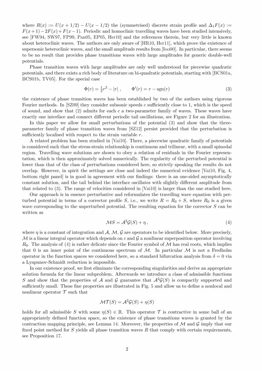
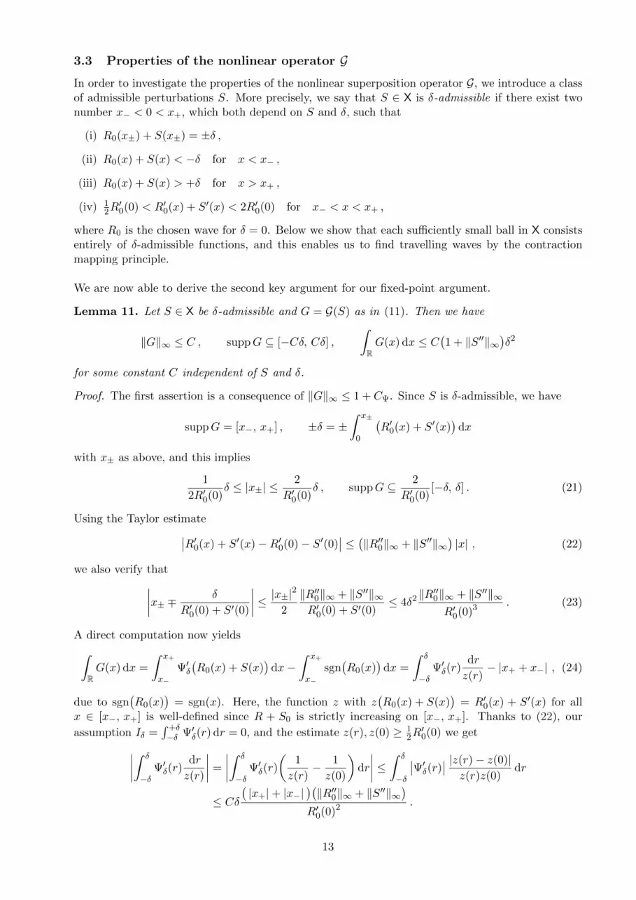
graph of R
Figure 2: Sketch of the waves for δ = 0 (grey) and δ > 0 (black) as provided by our perturbationresult; the shaded region indicates the spinodal interval [−δ, +δ], where Ψ′δ differs from Ψ′0. Bothwaves differ by the constant Iδ = O(δ) and a small corrector S of order O
(δ2), which is oscillatory for
x < 0 but asymptotically constant as x→ +∞. The tail oscillations of both waves do not penetratethe spinodal region and are generated by harmonic waves with wave number kc. For each admissibleδ and c there exists exactly on wave that satisfies the causality principle as it is non-oscillatory forx→ +∞.
(i) vanishes at x = 0,
(ii) is non-oscillatory as x→ +∞, i.e., the limit limx→+∞ S(x) is well defined,
(iii) admits harmonic tail oscillations for x → −∞, that means there exists constants a− and d−such that limx→−∞ S(x)− a−R0(x+ d−) is well defined,
(iv) is small in the sense of
‖S‖∞ = O(δ2), ‖S′‖∞ = O(δ), ‖S′′‖∞ = O(1).
Moreover, the solution R with these properties is unique provided that δ is sufficiently small.
More detailed information about the existence and uniqueness part of our result are given inProposition 15 and Proposition 17, respectively. We further mention:
(i) Since the travelling wave equation is invariant under
c −c, R(x) R(−x),
there exists an analogous result for −1 < c 0.
(ii) Different choices of c and R0 provide different waves R, see Section 4.
(iii) The travelling wave equation (5) is, of course, invariant under shifts in x but fixing R0 and Sat 0 removes neutral directions in the contraction proof.
(iv) All constants derived below depend on c1 and c0 but for notational simplicity we do not writethis dependence explicitly. It remains open whether δ0 can be chosen independently of c1.
(v) The causality principle selects those solutions with cgr < cph and cgr > cph for all oscillatoryharmonic modes ahead and behind the interface, respectively, where, cgr and cph are the groupand the phase velocity. For nearest neighbour chains with interaction potential Φ0 and wavespeed c sufficiently close to 1, Proposition 2 yields
cph = c = a(kc) = k−1c Ω(kc) > cgr = Ω′(kc)
on both sides of the interface, where Ω(k) = 2 sin (k/2) is the dispersion relation [SCC05,HSZ12]. The causality principle therefore selects the solution R0 as it is the only wave havingno tail oscillations ahead of the interface. Since our perturbative approach changes neither thewave speed c nor the wave number kc in the oscillatory modes (but only the amplitude behindthe interface and, of course, the behaviour near the interface), we conclude that Theorem 3provides for each δ and c exactly one wave that complies with the causality principle.
5
(vi) The surprisingly simple leading order effect, that is the addition of −Iδ to R0, implies thatthe kinetic relation does not change to order O(δ). Notice, however, that the kinetic relationdepends on the choice of R0, cf. [SZ12].
This paper is organised as as follows. In Section 2 we reformulate (5) in terms of integral operatorsA and M and show that it is sufficient to prove the existence of waves for the special case Iδ = 0.Section 3 concerns the existence of correctors S. We first establish an inversion formula for Mwhich in turn enables us to define an appropriate solution operator L to the affine subproblemMS = A2G+ η with given G. Afterwards we investigate the properties of the nonlinear operator Gand prove the contractivity of the fixed point operator T . In Section 4 we establish our uniquenessresult and conclude with a discussion of the kinetic relation in Section 5.
2 Preliminaries and reformulation of the problem
In this section we reformulate the travelling wave equation (5) in terms of integral operators andshow that elementary transformations allow us to assume that Iδ = 0 holds for all δ > 0.
2.1 Reformulation as integral equation
For our analysis it is convenient to reformulate the problem in terms of the convolution operator Aand the operator M defined by
(AF )(x) :=
x+1/2∫x−1/2
F (s) ds , MF := A2F − c2F .
The travelling wave equation can then be stated as
MR = A2Ψ′δ(R) + µ . (6)
Lemma 4. A function R ∈ W2,∞(R) solves the travelling wave equation (5) if and only if thereexists a constant µ ∈ R such that (R, µ) solves (6).
Proof. By definition of A, we have d2
dx2A2 = 41. Equation (5) is therefore, and due to the definition
of M, equivalent to
(MR)′′ = P ′′ , P := A2Ψ′δ(R) . (7)
The implication (6) =⇒ (5) now follows immediately. Towards the reversed statement, we integrate(7)1 twice with respect to x and obtain MR = P + λx + µ, where λ and µ denote constants ofintegration. The condition R ∈ L∞(R) implies MR, Ψ′δ(R), P ∈ L∞(R), and we conclude thatλ = 0.
2.2 Properties of the operators A and M
Some of our arguments rely on Fourier transform, which we normalise as follows
F (k) =1√2π
∫ReikxF (x) dx , F (x) =
1√2π
∫Re−ikxF (k) dk .
Using standard techniques for the Fourier transform in the space of tempered distributions we readilyverify the following assertions.
6
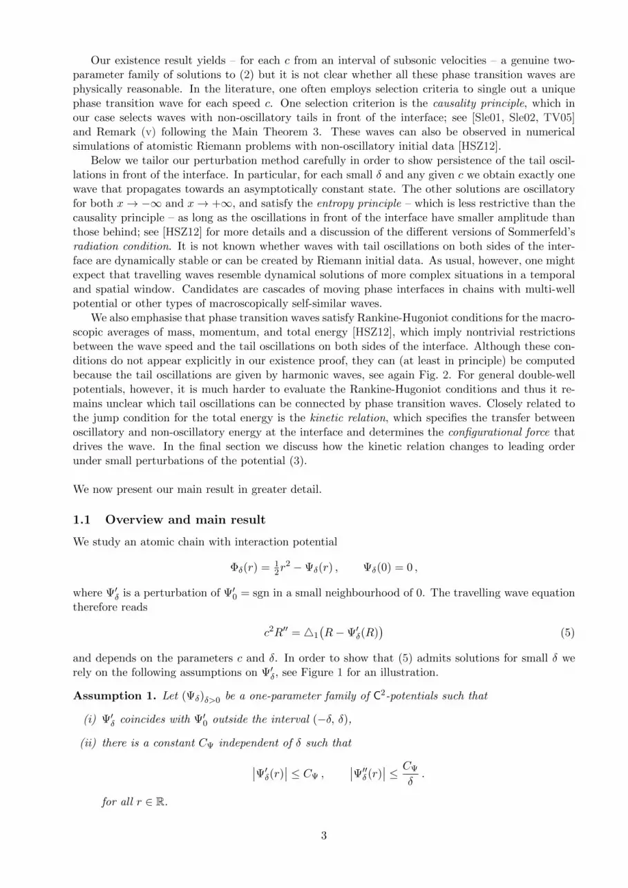
graph of |a|
1
|c|
+1010
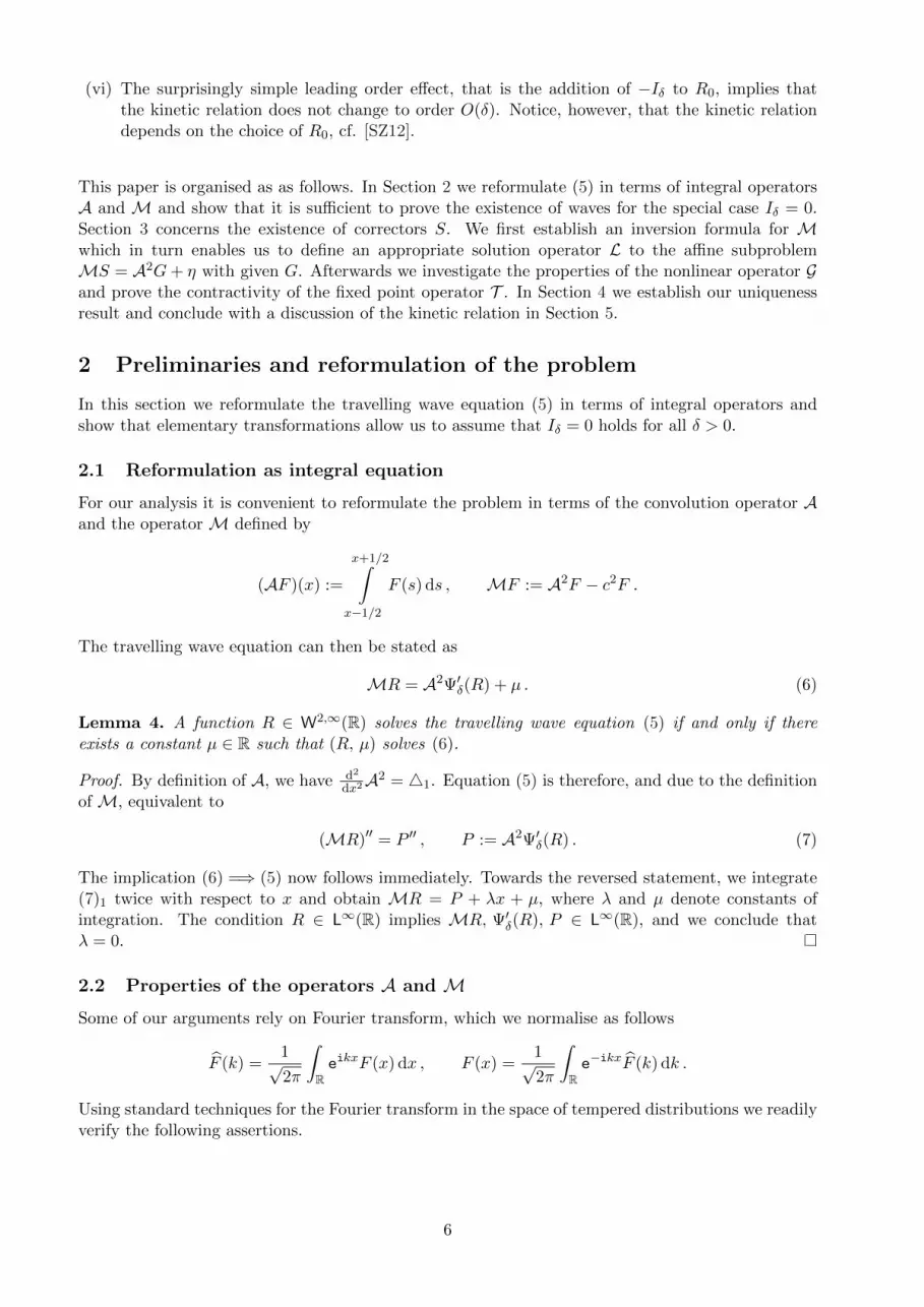
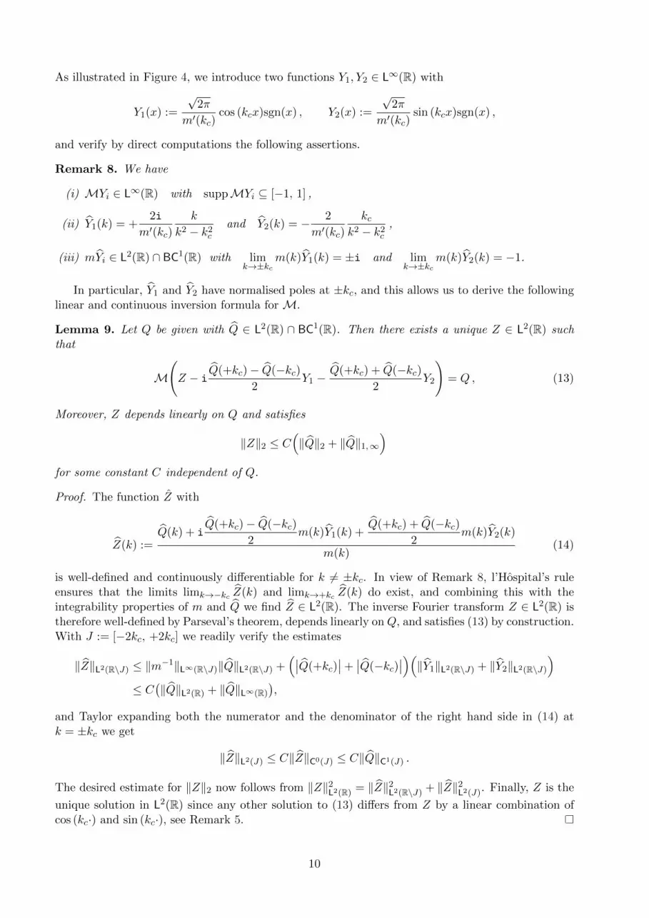
Figure 3: The the real roots of the symbol function m are the solutions to |a(k)| = |c|.
Remark 5. The operators A and M diagonalise in Fourier space and have symbols
a(k) =sin (k/2)
k/2and m(k) = a(k)2 − c2 ,
respectively. In particular, we have
M cos (kc·) = 0 , M sin (kc·) = 0 , M1 = 1− c2 ,
for any real root kc of m, and
F ∈ span
cos (kc·), sin (kc·) : m(kc) = 0, kc > 0
for any tempered distribution F with MF = 0.
The set of real roots of m depends strongly on the value of c, see Figure 3. In what follows weonly deal with positive and near sonic speed c, that means c / 1, for which m has two simple realroots.
We next summarise further properties of the operator A and recall that the Sobolev space W1, p(R)is for any 1 ≤ p ≤ ∞ continuously embedded into BC(R).
Lemma 6. For any 1 ≤ p ≤ ∞ we have A : Lp(R)→W1,p(R) ⊂ BC(R) with
‖AF‖p ≤ ‖F‖p , ‖(AF )′‖p ≤ 2‖F‖p , ‖AF‖∞ ≤ ‖F‖p (8)
for all F ∈ Lp(R), where (AF )′ = ∇F := F(·+ 1
2
)− F
(· − 1
2
). Moreover, suppF ⊆ [x1, x2] implies
suppAF ⊆ [x1 − 12 , x2 + 1
2 ].
Proof. Let 1 ≤ p < ∞ and F ∈ Lp(R). The definition of A ensures that AF has in fact the weakderivative ∇F , and this implies the estimate (8)2 via ‖∇F‖p ≤ 2‖F‖p. Using Holder’s inequality wefind ∣∣(AF )(x)
∣∣p ≤ ∫ x+1/2
x−1/2
∣∣F (s)∣∣p ds
and integration with respect to x yields (8)1. We also infer that∣∣(AF )(x)
∣∣ ≤ ‖F‖p holds for allx ∈ R, and this gives (8)3. Finally, the arguments for p = ∞ are similar and the claimed relationbetween suppF and suppAF is a direct consequence of the definition of A.
2.3 Transformation to the special case Iδ = 0
The key observation that traces the general case Iδ 6= 0 back to the special case Iδ = 0 is that anyshift in Ψ′δ can be compensated by adding a constant to R.
7
Lemma 7. The family (Ψδ)δ>0 defined by
δ = δ(1 + CΨ), Ψ′δ(r) = Ψ′δ(r − Iδ)
satisfies Assumption 1 with constant CΨ = CΨ(1 + CΨ) as well as
Iδ = 12
∫R
Ψ′δ(r)−Ψ′0(r) dr = 0 for all δ > 0.
Moreover, each solution (R, µ) to the modified travelling wave equation
MR = A2Ψ′δ(R) + µ (9)
defines a solution (R, µ) to (6) via R = R− Iδ and µ = µ−(c2 − 1
)Iδ and vice versa.
Proof. Due to |Iδ| ≤ CΨδ and our definitions we find Ψ′δ(r) = Ψ′0(r) at least for all r with |r| ≥ δ, as
well as ∣∣∣Ψ′δ(r)∣∣∣ ≤ CΨ ≤ CΨ ,
∣∣∣Ψ′′δ(r)∣∣∣ ≤ CΨ
δ=CΨ
δ
1 + CΨ
1 + CΨ=CΨ
δfor all r ∈ R .
We also have
Iδ = 12
∫R
(Ψ′δ(r − Iδ)−Ψ′0(r)
)dr = 1
2
∫R
(Ψ′δ(r)−Ψ′0(r + Iδ)
)dr
= 12
∫R
(Ψ′δ(r)−Ψ′0(r)
)dr + 1
2
∫R
(Ψ′0(r)−Ψ′0(r + Iδ)
)dr = Iδ − Iδ = 0 .
Finally, the equivalence of (6) and (9) is obvious.
3 Existence of phase transition waves
In this section, we show that each phase transition wave for Ψ0 persists under the perturbationΨ0 Ψδ, provided that δ is sufficiently small. To this end we proceed as follows.
(i) We fix c ∈ [c0, c1] with 0 < c0 < c1 < 1 as in Proposition 2 and Theorem 3. Then there exists aunique solution kc > 0 to a(kc) = c, and this implies m(±kc) = 0, m′(±kc) 6= 0, and m(k) 6= 0for k 6= ±kc. All constants derived below can be chosen independently of c but are allowed todepend on c0 and c1.
(ii) Thanks to Proposition 2 and Lemma 4, we fix (R0, µ0) from the two-parameter family ofsolutions to the integrated travelling wave equation (6) for δ = 0 and given c. Recall that R0
is normalised by R0(0) = 0.
(iii) In view of Lemma 7, we assume that Iδ = 0 holds for all δ > 0. To avoid unnecessarytechnicalities we also assume from now on that δ is sufficiently small.
In order to find a solution (R, µ) to the integrated travelling wave equation (6) for δ > 0, we furthermake the ansatz
R = R0 + S , µ = µ0 + η ,
and seek correctors (S, η) such that
MS = A2G+ η , G = G(S) . (10)
Here, the nonlinear operator G is defined by
G(S)(x) = Ψ′δ(R0(x) + S(x)
)−Ψ′0
(R0(x)
). (11)
8
In order to identify a natural ansatz space X for S, we first remark that the smoothing properties ofA, see Lemma 6, imply S ∈W2,∞(R). Notice, however, that R = R0+S is in general more regular dueto the smoothness of Ψδ. More precisely, (6) combined with Ψδ ∈ Ck(R) yields R ∈ Ck+1(R). We alsoimpose the normalisation condition S(0) = 0 in order to eliminate the non-uniqueness that resultsfrom the shift invariance of the travelling wave equation (6). In fact, without this constraint anycorrector S provides a whole family of other possible correctors via S = S(·+ x0) +R0(·+ x0)−R0
with x0 = O(δ2).A key property of our existence and uniqueness result is that R has only harmonic tail oscillations
with wave number kc and that both R and R0 share the same tail oscillations for x → +∞. Thecorrector S is therefore non-oscillatory in the sense that S(x) converges as x → +∞ to some well-defined limit σ. In summary, we seek solutions (S, η) to (10) with S ∈ X and η ∈ R, where
X :=S ∈W2,∞(R) : S(0) = 0 , σ = lim
x→+∞S(x) exists
is a closed subspace of W2,∞(R) and hence a Banach space.
3.1 Inversion formula for M
Our first task is to construct for givenG a solution (S, η) to the affine equation (10)1. In a preparatorystep, we therefore study the solvability of the equation
MF = Q (12)
using the Fourier transform for tempered distributions, whereQ ∈ L∞(R) is some given function. Thisproblem is not trivial because the symbol function m has two simple roots at ±kc, or, equivalently,because 0 is an element of the continuous spectrum of M corresponding to a two-dimensional spaceof generalised eigenfunctions. We are therefore confronted with the following two issues in Fourierspace:
(i) F is uniquely determined only up to elements from the space
spanδ−kc(k) , δ+kc(k)
,
which contains the Fourier transforms of all bounded kernel functions of M.
(ii) F exhibits – at least for generic Q with Q(±kc) 6= 0 – two poles at ±kc and is hence notLebesgue integrable in the vicinity of ±kc. In particular, the dual pairing between F and aSchwartz function is defined in the sense of Cauchy principal values only.
The non-uniqueness is actually an advantage because it allows us to select solutions with particularproperties; see the proof of Lemma 10, where we add an appropriately chosen kernel function toensure non-oscillatory behaviour for x→ +∞. Concerning the non-integrable poles at ±kc, we splitF into a two-dimensional singular part and a remaining regular part, and show that any solution Fto (12) belongs to some Lebesgue space provided that Q is sufficiently regular.
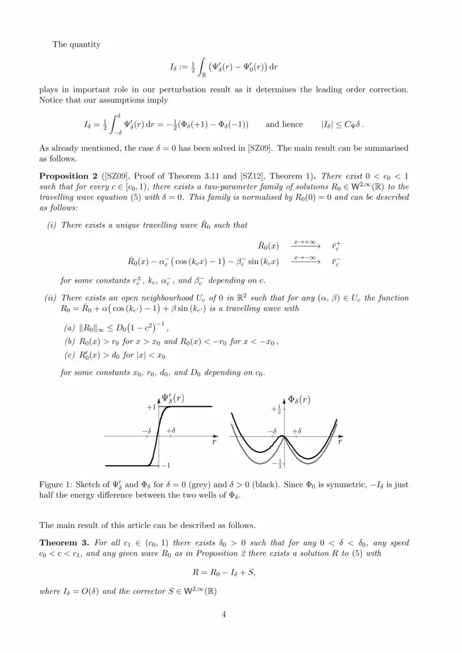
graph of Yi graph of MYi graph of
bYi
+kc5.0
5.0 kc1.0
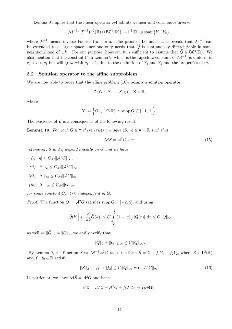
Figure 4: Properties of Y1 (grey) and Y2 (black).
9
As illustrated in Figure 4, we introduce two functions Y1, Y2 ∈ L∞(R) with
Y1(x) :=
√2π
m′(kc)cos (kcx)sgn(x) , Y2(x) :=
√2π
m′(kc)sin (kcx)sgn(x) ,
and verify by direct computations the following assertions.
Remark 8. We have
(i) MYi ∈ L∞(R) with suppMYi ⊆ [−1, 1] ,
(ii) Y1(k) = +2i
m′(kc)
k
k2 − k2c
and Y2(k) = − 2
m′(kc)
kck2 − k2
c
,
(iii) mYi ∈ L2(R) ∩ BC1(R) with limk→±kc
m(k)Y1(k) = ±i and limk→±kc
m(k)Y2(k) = −1.
In particular, Y1 and Y2 have normalised poles at ±kc, and this allows us to derive the followinglinear and continuous inversion formula for M.
Lemma 9. Let Q be given with Q ∈ L2(R) ∩ BC1(R). Then there exists a unique Z ∈ L2(R) suchthat
M
(Z − i
Q(+kc)− Q(−kc)2
Y1 −Q(+kc) + Q(−kc)
2Y2
)= Q , (13)
Moreover, Z depends linearly on Q and satisfies
‖Z‖2 ≤ C(‖Q‖2 + ‖Q‖1,∞
)for some constant C independent of Q.
Proof. The function Z with
Z(k) :=Q(k) + i
Q(+kc)− Q(−kc)2
m(k)Y1(k) +Q(+kc) + Q(−kc)
2m(k)Y2(k)
m(k)(14)
is well-defined and continuously differentiable for k 6= ±kc. In view of Remark 8, l’Hospital’s ruleensures that the limits limk→−kc Z(k) and limk→+kc Z(k) do exist, and combining this with theintegrability properties of m and Q we find Z ∈ L2(R). The inverse Fourier transform Z ∈ L2(R) istherefore well-defined by Parseval’s theorem, depends linearly onQ, and satisfies (13) by construction.With J := [−2kc, +2kc] we readily verify the estimates
‖Z‖L2(R\J) ≤ ‖m−1‖L∞(R\J)‖Q‖L2(R\J) +(∣∣Q(+kc)
∣∣+∣∣Q(−kc)
∣∣)(‖Y1‖L2(R\J) + ‖Y2‖L2(R\J)
)≤ C
(‖Q‖L2(R) + ‖Q‖L∞(R)
),
and Taylor expanding both the numerator and the denominator of the right hand side in (14) atk = ±kc we get
‖Z‖L2(J) ≤ C‖Z‖C0(J) ≤ C‖Q‖C1(J) .
The desired estimate for ‖Z‖2 now follows from ‖Z‖2L2(R) = ‖Z‖2L2(R\J) + ‖Z‖2L2(J). Finally, Z is the
unique solution in L2(R) since any other solution to (13) differs from Z by a linear combination ofcos (kc·) and sin (kc·), see Remark 5.
10
Lemma 9 implies that the linear operator M admits a linear and continuous inverse
M−1 : F−1(L2(R) ∩ BC1(R)
)→ L2(R)⊕ span
Y1, Y2
,
where F−1 means inverse Fourier transform. The proof of Lemma 9 also reveals that M−1 canbe extended to a larger space since one only needs that Q is continuously differentiable in someneighbourhood of ±kc. For our purpose, however, it is sufficient to assume that Q ∈ BC1(R). Wealso mention that the constant C in Lemma 9, which is the Lipschitz constant ofM−1, is uniform inc0 < c < c1 but will grow with c1 → 1, due to the definition of Y1 and Y2 and the properties of m.
3.2 Solution operator to the affine subproblem
We are now able to prove that the affine problem (10)1 admits a solution operator
L : G ∈ Y 7→ (S, η) ∈ X× R ,
where
Y :=G ∈ L∞(R) : suppG ⊆ [−1, 1]
.
The existence of L is a consequence of the following result.
Lemma 10. For each G ∈ Y there exists a unique (S, η) ∈ X× R such that
MS = A2G+ η . (15)
Moreover, S and η depend linearly on G and we have
(i) |η| ≤ CM‖A2G‖∞ ,
(ii) ‖S‖∞ ≤ CM‖A2G‖∞ ,
(iii) ‖S′‖∞ ≤ CM‖AG‖∞ ,
(iv) ‖S′′‖∞ ≤ CM‖G‖∞.
for some constant CM > 0 independent of G.
Proof. The function Q := A2G satisfies suppQ ⊆ [−2, 2], and using
∣∣∣Q(k)∣∣∣+
∣∣∣∣ ddk Q(k)
∣∣∣∣ ≤ C2∫−2
(1 + |x|
)|Q(x)| dx ≤ C‖Q‖∞
as well as ‖Q‖2 = ‖Q‖2, we easily verify that
‖Q‖2 + ‖Q‖1,∞ ≤ C‖Q‖∞ .
By Lemma 9, the function S := M−1A2G takes the form S = Z + f1Y1 + f2Y2, where Z ∈ L2(R)and f1, f2 ∈ R satisfy
‖Z‖2 + |f1|+ |f2| ≤ C‖Q‖∞ = C‖A2G‖∞ . (16)
In particular, we have MS = A2G and hence
c2Z = A2Z −A2G+ f1MY1 + f2MY2 .
11

The functions MY1, MY2 are supported in [−1, +1], see Remark 8, and G ∈ Y combined withLemma 6 implies that A2G vanishes outside of [−2, +2]. For |x| ≥ 2 we therefore find
c2∣∣Z(x)
∣∣ =∣∣(A2Z
)(z)∣∣ ≤ (∫ x+1/2
x−1/2
((AZ)(s)
)2ds
)1/2x→±∞−−−−−−→ 0 ,
thanks to Holder’s inequality and since Lemma 6 implies AZ ∈ L2(R). By definition of M, Q, andS we also have
c2S = −A2G+A2S = −A2G+A2(Z + f1Y1 + f2Y2
), (17)
and Lemma 6 ensures that
‖A2Z‖∞ ≤ ‖Z‖2 , ‖A2Yi‖∞ ≤ ‖Yi‖∞ .
Combining these estimates with (16) and (17), we arrive at S ∈ L∞(R) with
‖S‖∞ ≤ C‖A2G‖∞ .
Moreover, differentiating the first identity in (17) with respect to x, we get
c2S′ = ∇(−AG+AS
), c2S′′ = ∇∇
(−G+ S
),
where the discrete differential operator ∇ is defined as ∇U = U(·+ 1
2
)− U
(· − 1
2
), cf. Lemma 6.
This implies
‖S ′‖∞ ≤ C‖AG‖∞ , ‖S ′′‖∞ ≤ C‖G‖∞
thanks to ‖A2G‖∞ ≤ ‖AG‖∞ ≤ ‖G‖∞ and ‖AS‖∞ ≤ ‖S‖∞. Since S does not belong to X, wenow define
S(x) := S(x)− S(0)− f1
√2π
m′(kc)
(cos (kcx)− 1
)− f2
√2π
m′(kc)sin (kcx) (18)
as well as
η :=(1− c2
)(f1
√2π
m′(kc)− S(0)
), (19)
and observe that S ∈ X and (15) hold by construction. Moreover, S and η depend linearly on Gand the above estimates for f1, f1 and S provide the desired estimates for both S and η. Finally,the uniqueness of (S, η) is a direct consequence of S ∈ X and Lemma 5.
Notice that the solution (S, η) to (10)1 is unique only in the space X×R and that further solutionbranches exists due to the nontrivial kernel functions ofM. For instance, replacing (18) and (19) by
S(x) := S − S(0) , η := −(1− c2
)S(0)
we can define an operator
L : G ∈ Y →(S, η
)∈ X× R , X :=
S ∈W2,∞(R) : S(0) = 0
, (20)
which provides another solution to the affine problem (10)1. The corresponding corrector S, however,does in general not belong to X as it is oscillatory for both x→ −∞ and x→ +∞.
We emphasise that the three-parameter family of travelling waves R = R0+S, which we constructbelow by fixed points arguments involving L, is – at least for sufficiently small δ – independent ofthe details in the definition of L. The reason is, roughly speaking, that changing L is equivalent tochanging R0, see the discussion at the end of Section 4. However, choosing X×R as image space for Lprovides more information on the resulting family of travelling waves: The existence of limx→+∞ S(x)reveals that for each c there exists one wave R = R0 + S that complies with the causality principleas it is non-oscillatory for x→ +∞.
12
3.3 Properties of the nonlinear operator G
In order to investigate the properties of the nonlinear superposition operator G, we introduce a classof admissible perturbations S. More precisely, we say that S ∈ X is δ-admissible if there exist twonumber x− < 0 < x+, which both depend on S and δ, such that
(i) R0(x±) + S(x±) = ±δ ,
(ii) R0(x) + S(x) < −δ for x < x− ,
(iii) R0(x) + S(x) > +δ for x > x+ ,
(iv) 12R′0(0) < R′0(x) + S′(x) < 2R′0(0) for x− < x < x+ ,
where R0 is the chosen wave for δ = 0. Below we show that each sufficiently small ball in X consistsentirely of δ-admissible functions, and this enables us to find travelling waves by the contractionmapping principle.
We are now able to derive the second key argument for our fixed-point argument.
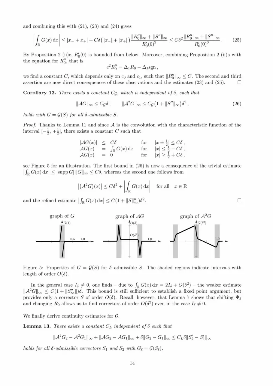
Lemma 11. Let S ∈ X be δ-admissible and G = G(S) as in (11). Then we have
‖G‖∞ ≤ C , suppG ⊆ [−Cδ, Cδ] ,∫RG(x) dx ≤ C
(1 + ‖S′′‖∞
)δ2
for some constant C independent of S and δ.
Proof. The first assertion is a consequence of ‖G‖∞ ≤ 1 + CΨ. Since S is δ-admissible, we have
suppG = [x−, x+] , ±δ = ±∫ x±
0
(R′0(x) + S′(x)
)dx
with x± as above, and this implies
1
2R′0(0)δ ≤ |x±| ≤
2
R′0(0)δ , suppG ⊆ 2
R′0(0)[−δ, δ] . (21)
Using the Taylor estimate∣∣R′0(x) + S′(x)−R′0(0)− S′(0)∣∣ ≤ (‖R′′0‖∞ + ‖S′′‖∞
)|x| , (22)
we also verify that∣∣∣∣x± ∓ δ
R′0(0) + S′(0)
∣∣∣∣ ≤ |x±|22
‖R′′0‖∞ + ‖S′′‖∞R′0(0) + S′(0)
≤ 4δ2 ‖R′′0‖∞ + ‖S′′‖∞R′0(0)3 . (23)
A direct computation now yields∫RG(x) dx =
∫ x+
x−
Ψ′δ(R0(x) + S(x)
)dx−
∫ x+
x−
sgn(R0(x)
)dx =
∫ δ
−δΨ′δ(r)
dr
z(r)− |x+ + x−| , (24)
due to sgn(R0(x)
)= sgn(x). Here, the function z with z
(R0(x) + S(x)
)= R′0(x) + S′(x) for all
x ∈ [x−, x+] is well-defined since R + S0 is strictly increasing on [x−, x+]. Thanks to (22), our
assumption Iδ =∫ +δ−δ Ψ′δ(r) dr = 0, and the estimate z(r), z(0) ≥ 1
2R′0(0) we get∣∣∣∣∫ δ
−δΨ′δ(r)
dr
z(r)
∣∣∣∣ =
∣∣∣∣∫ δ
−δΨ′δ(r)
(1
z(r)− 1
z(0)
)dr
∣∣∣∣ ≤ ∫ δ
−δ
∣∣Ψ′δ(r)∣∣ |z(r)− z(0)|z(r)z(0)
dr
≤ Cδ(|x+|+ |x−|
)(‖R′′0‖∞ + ‖S′′‖∞
)R′0(0)2 .
13
and combining this with (21), (23) and (24) gives∣∣∣∣∫RG(x) dx
∣∣∣∣ ≤ |x− + x+|+ Cδ(|x−|+ |x+|
)‖R′′0‖∞ + ‖S′′‖∞R′0(0)2 ≤ Cδ2 ‖R′′0‖∞ + ‖S′′‖∞
R′0(0)3 . (25)
By Proposition 2 (ii)c, R′0(0) is bounded from below. Moreover, combining Proposition 2 (ii)a withthe equation for R′′0 , that is
c2R′′0 = ∆1R0 −∆1sgn ,
we find a constant C, which depends only on c0 and c1, such that ‖R′′0‖∞ ≤ C. The second and thirdassertion are now direct consequences of these observations and the estimates (23) and (25).
Corollary 12. There exists a constant CG, which is independent of δ, such that
‖AG‖∞ ≤ CGδ , ‖A2G‖∞ ≤ CG(1 + ‖S′′‖∞
)δ2 , (26)
holds with G = G(S) for all δ-admissible S.
Proof. Thanks to Lemma 11 and since A is the convolution with the characteristic function of theinterval [−1
2 , +12 ], there exists a constant C such that
|AG(x)| ≤ Cδ for |x± 12 | ≤ Cδ ,
AG(x) =∫RG(x) dx for |x| ≤ 1
2 − Cδ ,AG(x) = 0 for |x| ≥ 1
2 + Cδ ,
see Figure 5 for an illustration. The first bound in (26) is now a consequence of the trivial estimate∣∣∫RG(x) dx
∣∣ ≤ |suppG| ‖G‖∞ ≤ Cδ, whereas the second one follows from
∣∣(A2G)(x)∣∣ ≤ Cδ2 +
∣∣∣∣∫RG(x) dx
∣∣∣∣ for all x ∈ R
and the refined estimate∣∣∫
RG(x) dx∣∣ ≤ C(1 + ‖S‖′′∞)δ2.
0.5 1.0
O(1) O() O(2)
graph of Ggraph of AG graph of A2G
1.0O(2)
1.0
Figure 5: Properties of G = G(S) for δ–admissible S. The shaded regions indicate intervals withlength of order O(δ).
In the general case Iδ 6= 0, one finds – due to∫RG(x) dx = 2Iδ + O(δ2) – the weaker estimate
‖A2G‖∞ ≤ C(1 + ‖S′′∞‖)δ. This bound is still sufficient to establish a fixed point argument, butprovides only a corrector S of order O(δ). Recall, however, that Lemma 7 shows that shifting Ψδ
and changing R0 allows us to find correctors of order O(δ2) even in the case Iδ 6= 0.
We finally derive continuity estimates for G.
Lemma 13. There exists a constant CL independent of δ such that
‖A2G2 −A2G1‖∞ + ‖AG2 −AG1‖∞ + δ‖G2 −G1‖∞ ≤ CLδ‖S′2 − S′1‖∞
holds for all δ-admissible correctors S1 and S2 with G` = G(S`).
14
Proof. According to Lemma 11, there exists a constant C, such that G`(x) = 0 for all x with |x| ≥ Cδ.For |x| ≤ Cδ, we use Taylor expansions for S1 − S2 at x = 0 to find
|S2(x)− S1(x)| ≤ ‖S′2 − S′1‖∞ |x| ,
where we used that S2(0)− S1(0) = 0. Combining this estimate with the upper bounds for Ψ′′δ gives∣∣G2(x)−G1(x)∣∣ ≤ C
δ
∣∣S2(x)− S1(x)∣∣ ≤ C‖S′2 − S′1‖∞
for all |x| ≤ Cδ, and this implies the desired estimate for ‖G2 −G1‖∞. We also have
‖A2G2 −A2G1‖∞ ≤ ‖AG2 −AG1‖∞ ≤ |supp (G2 −G1)| ‖G2 −G1‖∞ ≤ Cδ‖G2 −G1‖∞ ,
and this completes the proof.
3.4 Fixed point argument
Now we have prepared all ingredients to prove that the operator
T := PS L G
admits a unique fixed point in the space
Xδ :=S ∈ X : ‖S‖∞ ≤ C0δ
2 , ‖S′‖∞ ≤ C1δ , ‖S′′‖∞ ≤ C2
.
Here, PS denotes the projector on the first component, that means PS(S, η) = S, and the constantsCi are defined by
C2 := CM(1 + CΨ), C1 := CMCG , C0 := CMCG(1 + C2) .
Notice that any fixed point of T provides a solution to (10) and vice versa.
Lemma 14. For all sufficiently small δ, the operator T has a unique fixed point in Xδ.
Proof. Step 1: We first show that each S ∈ Xδ is δ-admissible provided that δ is sufficiently small.According to Proposition 2, there exist positive constants r0, x0, and d0 such that∣∣R0(x)
∣∣ ≥ r0 for |x| > x0 , d0 < R′0(x) for |x| < x0 ,
and combining the upper estimate for ‖R0‖∞ with the equation for R0 we find ‖R′′0‖∞ ≤ D2 for someconstant D2. We now set
δ0 :=1
2min
d0
2D2d0
+ C1
, x0d0,
√r0
C0, r0
, xδ :=
2
d0δ
and assume that δ < δ0. For any x with |x| ≤ xδ ≤ x0, we then estimate∣∣R′0(x) + S′(x)−R′0(0)∣∣ ≤ D2xδ + C1δ ≤
(2D2d0
+ C1
)δ ≤ 1
2d0 <12R′0(0) ,
and this gives 12R′0(0) ≤ R′0(x) + S′(x) ≤ 3
2R′0(0). Moreover, xδ ≤ |x| ≤ x0 implies
∣∣R0(x) + S(x)∣∣ ≥ ∣∣∣∣∫ x
0R′0(s) ds
∣∣∣∣− ‖S′‖∞ |x| ≥ (d0 − C1δ) |x| > 12d0 ·
2
d0δ = δ ,
whereas for |x| > x0 we find ∣∣R0(x) + S(x)∣∣ ≥ r0 − C1δ
2 ≥ 12r0 ≥ δ .
15
Using
x− := maxx : R0(x) + S(x) ≤ −δ , x+ := minx : R0(x) + S(x) ≥ +δ ,
we now easily verify that S is δ-admissible.Step 2: We next show that T (Xδ) ⊂ Xδ for all δ < δ0. Since each S ∈ Xδ is δ-admissible, Corollary
12 yields
‖AG(S)‖∞ ≤ CGδ , ‖A2G(S)‖∞ ≤ CG(1 + C2)δ2
and ‖G(S)‖∞ ≤ 1 + CΨ holds by definition of G and Assumption 1. Lemma 10 now provides
‖T (S)‖∞ ≤ CMCG(1 + C2)δ2 = C0δ2 ,
‖T (S)′‖∞ ≤ CMCGδ = C1δ ,‖T (S)′′‖∞ ≤ CM(1 + CΨ) = C2 ,
and hence T (S) ∈ Xδ.Step 3: We equip Xδ with the norm ‖S‖# = ‖S‖∞ + ‖S′‖∞ + δ‖S′′‖∞, which is, for fixed δ,
equivalent to the standard norm. For given S1, S2 ∈ Xδ, we now employ the estimates from Lemma10 and Lemma 13 for S = S2 − S1 and G = G(S2)− G(S1). This gives
‖T (S2)− T (S1)‖# ≤ CM(‖A2G(S2)−A2G(S1)‖∞ + ‖AG(S2)−AG(S1)‖∞ + δ‖G(S2)− G(S1)‖∞
)≤ CMCLδ‖S′2 − S′1‖∞ ≤ CMCLδ‖S2 − S1‖# ,
and we conclude that T is contractive with respect to ‖·‖# provided that δ < 1/(CMCL). The claimis now a direct consequence of the Banach Fixed Point Theorem.
The previous result implies the existence of a three-parameter family of waves that is parametrisedby the speed c ∈ [c0, c1] and by R0, where R0 can be regarded as parameter in the two-dimensionalL∞-kernel of M.
Proposition 15. Suppose that Iδ = 0 for all δ. Then there exists δ0 > 0 with the following property:For any δ < δ0, each c ∈ [c0, c1], and any R0 as in Proposition 2 there exists an δ-admissible
S ∈ Xδ ∩
(L2(R)⊕ span
1, Y1 −
√2π
m′(kc)cos (kc·) , Y2 −
√2π
m′(kc)sin (kc·)
).
such that R = R0 +S and solves the travelling wave equation (6) for some µ. In particular, we haveR(0) = 0, the limits
limx→−∞
(R(x)− α− cos (kcx)− β− sin (kcx)
)and lim
x→+∞
(R(x)−R0(x)
)are well-defined for some constants α−, β− depending on c and R0, and the estimates
R(x) ≤ −δ for x ≤ −Cδ , R(x) ≥ +δ for x ≥ +Cδ (27)
hold for some constant C > 0 independent of c and R0.
Proof. For given c and R0, Lemma 14 provides a unique fixed point S ∈ Xδ of T , which solves
MS = A2G(S) + η
for some η ∈ R, and this implies that R = R0 + S is in fact a travelling wave. Moreover, byconstruction – see the proof of Lemma 10 – we also have
S = Z + λ+ f1
(Y1 −
√2π
m′(kc)cos (kc·)
)+ f2
(Y2 −
√2π
m′(kc)sin (kc·)
)for some constants f1, f2 and λ and a function Z ∈ L2(R) with Z(x)→ 0 as x→ ±∞. The claims onthe asymptotic behaviour as x→ ±∞ now follow immediately since R0 has harmonic tails oscillationswith wave number kc. Finally, the fixed point S is δ-admissible – see the proof of Lemma 14 – andthis implies the validity of (27) due to 0 ≤ x+,−x− ≤ Cδ.
16
Notice that Proposition 15 yields a genuine three-parameter family in the sense that differentchoices of the parameters c and R0 correspond to different tail oscillations for x → +∞ and henceto different waves R = R0 + S. This finishes the existence proof of Theorem 3.
4 Uniqueness of phase transition waves
In this section we establish the uniqueness result of the Theorem 3 by showing that the familyprovided by Proposition 17 contains all phase transition waves that have harmonic tails oscillationsfor x→ +∞ and penetrate the spinodal region in a small interval only.
Lemma 16. Let κ > 12 be given and suppose that Iδ = 0 for all δ. Then there exists δκ > 0 such
that the following statement holds for all 0 < δ < δκ: Let (R1, µ1) and (R2, µ2) be two solutions tothe travelling wave equation (6) with speed c ∈ [c0, c1] such that
Ri ∈W2,∞(R) , µi ∈ R , Ri(0) = 0
and
Ri(x) ≤ −δ for x ≤ −δκ , Ri(x) ≥ +δ for x ≥ +δκ
for both i = 1 and i = 2. Then, R1 and R2 are either identical or satisfy
R1(x)−R2(x)− α+
(cos (kcx)− 1
)− β+ sin (kcx)− γ+
x→+∞−−−−−→ 0
for some constants γ+ and (α+, β+) 6= (0, 0).
Proof. For given R1, R2, there exist constant µ1, µ2 ∈ R such that
M(R2 −R1) = A2G+ µ2 − µ1 , G := Ψ′δ(R2)−Ψ′δ(R1) .
By assumption and due to the bounds of Ψ′′δ we also find G(x) = 0 for |x| ≥ δκ as well as∣∣G(x)∣∣ ≤ C
δ|R2(x)−R1(x)| ≤ Cδκ−1‖R′2 −R′1‖∞ for |x| ≤ δκ ,
and this implies
‖AG‖∞ ≤ |suppG| ‖G‖∞ ≤ Cδ2κ−1‖R′2 −R′1‖∞ .
Moreover, Lemma 10 provides S ∈ X as well as η ∈ R such that
MS = A2G+ η , ‖S′‖∞ ≤ Cδ2κ−1‖R′2 −R′1‖∞.
In particular, we have
A2G =M(R2 −R1 −
(1− c2
)−1(µ2 − µ1)
)=M
(S −
(1− c2
)−1η).
Since the space of bounded kernel functions for M is spanned by sin (kc·) and cos (kc·), we concludethat there exist constants α+ and β+ such that
R2(x)−R1(x) = S(x)− σ + α+(1− cos (kcx)) + β+ sin (kcx) + γ+ ,
where σ := limx→+∞ S(x) and γ+ :=(1− c2
)−1(µ2 − µ1 − η) + σ − α+. In case of α+ = β+ = 0 we
therefore find
‖R′2 −R′1‖∞ = ‖S′‖∞ ≤ Cδ2κ−1‖R′2 −R′1‖∞ ,
and combining this with R1(0) = R2(0) we get R2 = R1 for all sufficiently small δ.
17

Proposition 17. Suppose that Iδ = 0 for all δ and that κ with 12 < κ < 1 is fixed. Then there exists
δκ with 0 < δκ ≤ δ0 such that the following statement holds for all 0 < δ < δκ: Let R be a travellingwaves with speed c ∈ [c0, c1] such that the limit
limx→+∞
(R(x)−R0(x)
)is well-defined for some R0 from Proposition 2 and such that
R(x) ≤ −δ for x ≤ −δκ , R(x) ≥ +δ for x ≥ +δκ.
Then R belongs to the family of waves provided by Proposition 15.
Proof. Let R0 +S be the travelling wave from Proposition 15. By construction, R−R0−S convergesas x → +∞ and for all sufficiently small δ we also have Cδ ≤ δκ. Lemma 16 applied with R1 = Rand R2 = R0 + S therefore implies R = R0 + S.
With Proposition 15 and Proposition 17 we have established our existence and uniqueness resultin the special case that Iδ = 0 holds for for all δ. The corresponding result for the general case isthen provided by Lemma 7.
We finally mention a particular consequence of our uniqueness result, namely that the familyfrom Proposition 15 does not depend on the particular choice of the solution operator L to the affineproblem (10)1. At a first glance, this might be surprising since the operator T and hence each fixedpoint surely depend on L. We can, however, argue as follows. Suppose we would choose in the proofof Lemma 10 another reasonable solution operator L (for instance, the operator from (20) that doesnot involve any kernel function of M). Repeating all arguments from Section 3 we then find – forany given δ, c, and R0 – a different corrector S ∈ W2,∞(R). In general, this corrector S does notconverge as x→ +∞ but satisfies
S(0) = 0 , ‖S‖∞ ≤ Cδ2 , ‖S′‖∞ ≤ Cδ , ‖S′′‖∞ ≤ C
for some constant C that is independent of c, R0, and δ. Moreover, we also have
S ∈ L2(R)⊕ span
1, Y1, Y2, cos (kc·), sin (kc·)
that means the tail oscillations of S for both x→ −∞ and x→ +∞ are again harmonic waves withwave number kc. Adding a suitable linear combination of 1 − cos (kc·) and sin (kc·) to R0 we canconstruct another wave R0 such that R0 and R0 + S have the same tails oscillations as x → +∞.This function R0 is, at least for small δ, also a travelling wave for the unperturbed problem andhence among the family of waves provided by Proposition 2. We can therefore use R0 instead of R0
in order to define the operator G. Theorem 10, which relies on the oscillation-preserving operator L,then provides a corrector S that converges as x → +∞, and from Lemma 16 we finally infer thatR0 + S = R0 + S because both waves have, by construction, the same tail oscillations for x→ +∞.We therefore conclude, at least for small δ, that changing L does not alter the family of travellingwaves but only its parametrisation by R0.
5 Kinetic relations
We finally show that the kinetic relation does not change to order O(δ). To this end we denote byRδ a travelling wave solution to (2) as provided by Theorem 3. The corresponding configurationalforce, cf. [HSZ12], is then defined by Υδ := Υe,δ −Υf,δ with
Υe,δ := Φδ(rδ,+)− Φδ(rδ,−) , Υf,δ :=Φ′δ(rδ,+) + Φ′δ(rδ,−)
2
(rδ,+ − rδ,−
),
where the macroscopic strains rδ,± on both sides of the interface can be computed from Rδ via
rδ,± = limL→∞
1
L
∫ +L
0Rδ(±x) dx .
18

Lemma 18. Let Rδ be a travelling wave from Theorem 3, and R0 the corresponding wave for δ = 0.Then we have Υδ = Υ0 +O(δ2).
Proof. By construction, we know that the only asymptotic contributions to the profile Rδ are due toR0 − Iδ plus a small asymptotic corrector of order O(δ2) from span
1, Y1, Y2
. This implies
rδ,± = r0,± − Iδ +O(δ2) .
As r0,± and rδ,± are both larger than δ we know that
Ψ′δ(rδ,±) = ∓1 = Ψ′0(rδ,±) .
Thus, we conclude
Φ′δ(rδ,±) = rδ,± ∓ 1 = Φ′0(r0,±)− Iδ +O(δ2) ,
and hence
Υf,δ = Υf,0 − Iδ(r0,+ − r0,−) +O(δ2) .
Moreover, we calculate
Υe,δ =
∫ rδ,+
rδ,−
Φ′δ(r) dr =
∫ rδ,+
rδ,−
(r −Ψ′δ(r)−Ψ′0(r) + Ψ′0(r)
)dr
=
∫ rδ,+
rδ,−
Φ′0(r) dr −∫ rδ,+
rδ,−
(Ψ′δ(r)−Ψ′0(r)
)dr
= Φ0(rδ,+)− Φ0(rδ,−)− 2Iδ = 12(rδ,+ − 1)2 − 1
2(rδ,− + 1)2 − 2Iδ
= 12(r0,+ − Iδ − 1)2 − 1
2(r0,− − Iδ + 1)2 − 2Iδ +O(δ2)
= 12(r0,+ − 1)2 − 1
2(r0,− + 1)2 − Iδ(r0,+ − 1− r0,− − 1)− 2Iδ +O(δ2)
= Υe,0 − Iδ(r0,+ − r0,−) +O(δ2) .
Subtracting both results gives Υδ = Υ0 +O(δ2), the desired result.
Acknowledgement
The authors gratefully acknowledge financial support by the EPSRC (EP/H05023X/1).
References
[AK91] Rohan Abeyaratne and James K. Knowles. Kinetic relations and the propagation of phaseboundaries in solids. Arch. Rational Mech. Anal., 114(2):119–154, 1991.
[BCS01a] Alexander M. Balk, Andrej V. Cherkaev, and Leonid I. Slepyan. Dynamics of chains withnon-monotone stress-strain relations. I. Model and numerical experiments. J. Mech. Phys.Solids, 49(1):131–148, 2001.
[BCS01b] Alexander M. Balk, Andrej V. Cherkaev, and Leonid I. Slepyan. Dynamics of chains withnon-monotone stress-strain relations. II. Nonlinear waves and waves of phase transition.J. Mech. Phys. Solids, 49(1):149–171, 2001.
[FP99] Gero Friesecke and Robert L. Pego. Solitary waves on FPU lattices. I. Qualitative prop-erties, renormalization and continuum limit. Nonlinearity, 12(6):1601–1627, 1999.
[FW94] Gero Friesecke and Jonathan A. D. Wattis. Existence theorem for solitary waves onlattices. Comm. Math. Phys., 161(2):391–418, 1994.
19
[Her10] Michael Herrmann. Unimodal wavetrains and solitons in convex Fermi-Pasta-Ulam chains.Proc. Roy. Soc. Edinburgh Sect. A, 140(4):753–785, 2010.
[Her11] Michael Herrmann. Action minimising fronts in general FPU-type chains. J. NonlinearSci., 21(1):33–55, 2011.
[HR10] Michael Herrmann and Jens D. M. Rademacher. Heteroclinic travelling waves in convexFPU-type chains. SIAM J. Math. Anal., 42(4):1483–1504, 2010.
[HSZ12] Michael Herrmann, Hartmut Schwetlick, and Johannes Zimmer. On selection criteria forproblems with moving inhomogeneities. Contin. Mech. Thermodyn., 24:21–36, 2012.
[Ioo00] Gerard Iooss. Travelling waves in the Fermi-Pasta-Ulam lattice. Nonlinearity, 13(3):849–866, 2000.
[EP05] J. M. English and Robert L. Pego. On the solitary wave pulse in a chain of beads. Proc.Amer. Math. Soc., 133(6): 17631768, 2005.
[Pan05] Alexander Pankov. Travelling waves and periodic oscillations in Fermi-Pasta-Ulam lat-tices. Imperial College Press, London, 2005.
[SW97] Didier Smets and Michel Willem. Solitary waves with prescribed speed on infinite lattices.J. Funct. Anal., 149(1):266–275, 1997.
[SZ09] Hartmut Schwetlick and Johannes Zimmer. Existence of dynamic phase transitions in aone-dimensional lattice model with piecewise quadratic interaction potential. SIAM J.Math. Anal., 41(3):1231–1271, 2009.
[SZ12] Hartmut Schwetlick and Johannes Zimmer. Kinetic Relations for a Lattice Model of PhaseTransitions. Arch. Ration. Mech. Anal., 206(2):707–724, 2012.
[SCC05] Leonid I. Slepyan, Andrej Cherkaev, and Elena Cherkaev. Transition waves in bistablestructures. II. Analytical solution: wave speed and energy dissipation. J. Mech. Phys.Solids, 53(2):407436, 2005.
[Sle01] Leonid I. Slepyan. Feeding and dissipative waves in fracture and phase transition. I. Some1D structures and a square-cell lattice. J. Mech. Phys. Solids, 49(3):469511, 2001.
[Sle02] Leonid I. Slepyan Models and phenomena in fracture mechanics. Foundations of Engi-neering Mechanics, Springer-Verlag, Berlin, 2002.
[Tru87] Lev Truskinovsky. Dynamics of nonequilibrium phase boundaries in a heat conductingnon-linearly elastic medium. Prikl. Mat. Mekh., 51(6):1009–1019, 1987.
[TV05] Lev Truskinovsky and Anna Vanchtein. Kinetics of martensitic phase transitions: latticemodel. SIAM J. Appl. Math., 66(2):533553, 2005.
[Vai10] Anna Vainchtein. The role of spinodal region in the kinetics of lattice phase transitions.J. Mech. Phys. Solids, 58(2):227–240, 2010.
20