structural equation modeling and ecological experiments

Real World Ecology

ShiLi Miao l Susan CarstennMartha NungesserEditors

Real World Ecology

Large-Scale and Long-Term Case Studiesand Methods

Foreword by Stephen R. Carpenter

1 3

Editors

ShiLi MiaoSouth Florida WaterManagement District

West Palm BeachFL, [email protected]

Susan CarstennHawaii Pacific UniversityKaneohe, [email protected]

Martha NungesserSouth Florida WaterManagement District

West Palm BeachFL, [email protected]

ISBN 978-0-387-77916-4 e-ISBN 978-0-387-77942-3 (Softcover)ISBN 978-0-387-77941-6 e-ISBN 978-0-387-77942-3 (Hardcover)DOI 10.1007/978-0-387-77942-3

Library of Congress Control Number: 2008941656

# Springer ScienceþBusiness Media, LLC 2009All rights reserved. This workmay not be translated or copied in whole or in part without the writtenpermission of the publisher (Springer Science+BusinessMedia, LLC, 233 Spring Street, NewYork,NY 10013, USA), except for brief excerpts in connection with reviews or scholarly analysis. Use inconnection with any form of information storage and retrieval, electronic adaptation, computersoftware, or by similar or dissimilar methodology now known or hereafter developed is forbidden.The use in this publication of trade names, trademarks, service marks, and similar terms, even if theyare not identified as such, is not to be taken as an expression of opinion as to whether or not they aresubject to proprietary rights.

Printed on acid-free paper

springer.com

To our mothers, whose love and supportwe appreciate.

Foreword

Ecology is not rocket science – it is far more difficult (Hilborn and Ludwig1993). The most intellectually exciting ecological questions, and the ones mostimportant to sustaining humans on the planet, address the dynamics of large,spatially heterogeneous systems over long periods of time. Moreover, therelevant systems are self-organizing, so simple notions of cause and effect donot apply (Levin 1998). Learning about such systems is among the hardestproblems in science, and perhaps the most important problem for sustainingcivilization. Ecologists have addressed this challenge by synthesis ofinformation flowing from multiple sources or approaches (Pickett et al. 2007).Some major approaches in ecology are theoretical concepts expressed inmodels, long-term observations, comparisons across contrasting systems, andexperiments (Carpenter 1998). These approaches have complementarystrengths and limitations, so findings that are consistent among all of theseapproaches are likely to be most robust.

Ecosystem data are noisy. There are multiple sources of variability, such asexternal forcing, endogenous dynamics, and our imperfect observations. Thusit is not surprising that statistics have played a central role in ecologicalinference. However, with few exceptions the statistical approaches availableto ecologists have been imported from other disciplines and were designed forproblems that are simpler than the ones that ecologists face routinely. If youneed to cut a board and all you have is a hammer, you might try pounding onthe board until it breaks. Such a misapplication of force resembles some uses ofstatistics in ecology. But the metaphor is not quite right. It would be moreaccurate to say that ecosystem and landscape ecologists need to create andcompare multifaceted models for large-scale processes, whereas the readilyavailable tools were designed for testing null models that are usually trivial orirrelevant for this family of ecological questions.

The mismatch between the needs of scientists and the availability ofstatistical tools is acute in the analysis of ecosystem experiments. Ecosystemexperiments have been an important contributor to ecological science for morethan 50 years (Likens 1985, Carpenter et al. 1995). While humans havemanipulated ecosystems since at least the beginnings of agriculture, if notlonger, deliberate experiments for learning about ecosystems are traced to

vii

limnology in the 1940s (Likens 1985). The earliest whole-lake manipulationslacked reference systems, and so sometimes it was difficult to determine whetherchanges in the ecosystems were caused by the manipulations or by otherenvironmental factors. In 1951, Arthur Hasler and his students divided anhour-glass shaped lake with an earthen dam, thereby creating two basins,Paul and Peter lakes. Peter Lake was manipulated, while Paul Lake served asan unmanipulated reference ecosystem (Johnson and Hasler 1954). The use of areference or ‘‘control’’ ecosystem was a pathbreaking innovation (Likens 1985).It allowedHasler and his students to separate the effects of the manipulations ofPeter Lake from those of the environmental variability that affected both lakes(Stross and Hasler 1960, Stross et al. 1961). As a result of their experiences asstudents of Hasler, Gene Likens andWaldo Johnsonwere inspired to create twoof the most influential centers of ecosystem experimentation in the world, theHubbard Brook Ecosystem Study (Likens 2004) and the Experimental LakesArea (Johnson and Vallentyne 1971).

Most ecosystem experiments involve spatially extensive systems (oftenobserved at several spatial extents) over long time spans. Such experiments posestatistical challenges that cannot be handled by the methods of laboratory scienceor small agricultural plots (Carpenter 1998). It is not possible to substitute small-scale experiments run for short periods of time, because results of such experimentsdo not predict dynamics at spatial and temporal scales relevant to ecosystemscience or to management (Carpenter 1996, Schindler 1998, Pace 2001). Instead,we must perform our studies at the appropriate scales – possibly at multiplescales. Then, we must learn how to learn from noisy observations of transient,heterogeneous, and non-replicable systems. This is a daunting challenge.

Thus many ecologists have broken free of the constraints of older statisticalmethods in order to explore new alternatives that seem better-adapted to theworld of large-scale ecological change. The method of multiple workinghypotheses (Chamberlain 1890) is now explicit in many ecological papers.Multiple hypotheses are expressed as quantitative models and confrontedwith data (Burnham and Anderson 1998, Hilborn and Mangel 1997). Newapproaches are explored for long-term monitoring data (Stow et al. 1998).Experiments are designed for critical tests of multiple alternative models toaddress fundamental questions about ecological dynamics (Dennis et al. 2001,Wootton 2004). Comparisons of multiple models are providing new insightsabout long-term field observations of big systems (Ives et al. 2008). These arebut a few selections from a diverse and rapidly growing literature. This newphase of ecological research is turbulent and subject to rapid intellectualprogress. Some of the emerging practices are nonstandard and are themselvesobjects of inquiry. Some approaches are tried, found wanting, and abandoned.New approaches are introduced frequently. It is an era of creativity, innovation,discarding of mistakes, and selection among alternatives – in a nutshell, a timeof rapid evolution by the discipline.

The volume before you presents a sampling of case studies and synthesesfrom this fertile field of research. The authors and editors aim to improve our

viii Foreword

tools for ecological inference at scales that are relevant for fundamentalunderstanding, as well as for management of ecosystems and landscapes. Thebook conveys the excitement and novelty of emerging approaches for learningabout large-scale ecological changes.

Stephen R. CarpenterMadison, WI

References

Burnham, K.P. and D.R. Anderson. 1998. Model Selection and Inference. Springer-Verlag,N.Y., USA.

Carpenter, S.R. 1996. Microcosm experiments have limited relevance for community andecosystem ecology. Ecology 77: 677–680.

Carpenter, S.R. 1998. The need for large-scale experiments to assess and predict theresponse of ecosystems to perturbation. pp. 287–312 in M.L. Pace and P.M. Groffman(eds.), Successes, Limitations and Frontiers in Ecosystem Science. Springer-Verlag, N.Y.,USA.

Carpenter, S.R., S.W. Chisholm, C.J. Krebs, D.W. Schindler, and R.F. Wright. 1995. Eco-system experiments. Science 269: 324–327.

Chamberlain, T.C. 1890. The method of multiple working hypotheses. Science 15: 92–96.Dennis, B., R.A. Desharnais, J.M. Cushing, S.M. Henson, and R.F. Costantino. 2001.

Estimating chaos and complex dynamics in an insect population. Ecological Monographs71: 277–303.

Hilborn, R. and D. Ludwig. 1993. The limits of applied ecological research. EcologicalApplications 3: 550–552.

Hilborn, R. and M. Mangel. 1997. The Ecological Detective. Princeton University Press,Princeton, N.J., USA.

Ives, A.R., A. Einarsson, V.A.A. Jansen, and A. Gardarson. 2008. High-amplitude fluctua-tions and alternative dynamical states of midges in Lake Myvatn. Nature 452: 84–87.

Johnson, W.E. and A.D. Hasler. 1954. Rainbow trout population dynamics in dystrophiclakes. Journal of Wildlife Management 18: 113–134.

Johnson, W.E. and J.R. Vallentyne. 1971. Rationale, background, and development ofexperimental lake studies in northwestern Ontario. Journal of the Fisheries ResearchBoard of Canada 28: 123–128.

Levin, S.A. 1998. Ecosystems and the biosphere as complex adaptive systems. Ecosystems 1:431–436.

Likens, G.E. 1985. An experimental approach for the study of ecosystems. Journal of Ecology73: 381–396.

Likens, G.E. 2004. Some perspectives on long-term biochemical research from the HubbardBrook Ecosystem Study. Ecology 85: 2355–2362.

Pace, M.L. 2001. Getting it right and wrong: extrapolations across experimental scales.pp. 157–177 in R.H. Gardner, W.M. Kemp, V.S. Kennedy and J.E. Peterson (eds.).Scaling Relations in Experimental Ecology. Columbia University Press, NY, USA.

Pickett, S.T.A., J. Kolasa, and C. Jones. 2007. Ecological Understanding. Academic Press,Burlington, Massachusetts, USA.

Schindler, D.W. 1998. Replication versus realism: The need for ecosystem-scale experiments.Ecosystems 1: 323–334.

Stow, C.A., S.R. Carpenter, K.E. Webster, and T.M. Frost. 1998. Long-term environmentalmonitoring: some perspectives from lakes. Ecological Applications 8: 269–276.

Foreword ix

Stross, R.G. and A.D. Hasler. 1960. Some lime-induced changes in lake metabolism. Limnol-ogy and Oceanography 5: 265–272.

Stross, R.G., J.C. Neess and A.D. Hasler. 1961. Turnover time and production of theplanktonic crustacean in limed and reference portions of a bog lake. Ecology 42:237–245.

Wootton, T. 2004. Markov chain models predict the consequences of ecological extinctions.Ecology Letters 7: 653–660.

x Foreword

Contents

1 Introduction – Unprecedented Challenges in Ecological Research:

Past and Present . . . . . . . . . . . . . . . . . . . . . . . . . . . . . . . . . . . . . . . . 1ShiLi Miao, Susan Carstenn and Martha Nungesser

2 Structural Equation Modeling and Ecological Experiments . . . . . . . . 19James B. Grace, Andrew Youngblood and Samule M. Scheiner

3 Approaches to Predicting Broad-Scale Regime Shifts Using

Changing Pattern-Process Relationships Across Scales . . . . . . . . . . . 47Debra P. C. Peters, Brandon T. Bestelmeyer, Alan K. Knapp,Jeffrey E. Herrick, H. Curtis Monger and Kris M. Havstad

4 Integrating Multiple Spatial Controls and Temporal Sampling

Schemes To Explore Short- and Long-Term Ecosystem Response

to Fire in an Everglades Wetland . . . . . . . . . . . . . . . . . . . . . . . . . . . . 73ShiLi Miao, Susan Carstenn, Cassondra Thomas, Chris Edelstein,Erik Sindhøj and Binhe Gu

5 Bayesian Hierarchical/Multilevel Models for Inference

and Prediction Using Cross-System Lake Data . . . . . . . . . . . . . . . . . 111Craig A. Stow, E. Conrad Lamon, Song S. Qian,Patricia A. Soranno and Kenneth H. Reckhow

6 Avian Spatial Responses to Forest Spatial Heterogeneity

at the Landscape Level: Conceptual and Statistical Challenges . . . . . 137Marie-Josee Fortin and Stephanie J. Melles

7 The Role of Paleoecology in Whole-Ecosystem Science . . . . . . . . . . . 161Suzanne McGowan and Peter R. Leavitt

8 A Spatially Explicit, Mass-Balance Analysis of Watershed-Scale

Controls on Lake Chemistry . . . . . . . . . . . . . . . . . . . . . . . . . . . . . . . 209Charles D. Canham and Michael L. Pace

xi

9 Forecasting and Assessing the Large-Scale and Long-Term

Impacts of Global Environmental Change on Terrestrial Ecosystems

in the United States and China . . . . . . . . . . . . . . . . . . . . . . . . . . . . . . 235Hanqin Tian, Xiaofeng Xu, Chi Zhang, Wei Ren,Guangsheng Chen, Mingliang Liu, Dengsheng Luand Shufen Pan

10 Gradual Global Environmental Change in the Real World

and Step Manipulative Experiments in Laboratory and Field:

The Necessity of Inverse Analysis. . . . . . . . . . . . . . . . . . . . . . . . . . . . 267Yiqi Luo and Dafeng Hui

11 Ecology in the Real World: How Might We Progress?. . . . . . . . . . . . 293James B. Grace, Susan Carstenn, ShiLi Miao and Erik Sindhøj

Index . . . . . . . . . . . . . . . . . . . . . . . . . . . . . . . . . . . . . . . . . . . . . . . . . . . . . 303

xii Contents

Contributors

Brandon T. Bestelmeyer U.S. Department of Agriculture, Jornada ExperimentalRange, Jornada Basin Long TermEcological Research Program, Las Cruces, NM88003-0003, USA, [email protected]

Charles D. Canham Cary Institute of Ecosystem Studies, Millbrook, NY12545 USA, [email protected]

Steve R. Carpenter University of Wisconsin, Center for Limnology, Madison,WI 53706 USA, [email protected]

Susan M. Carstenn Hawai’i Pacific University, College of Natural Sciences,Kaneohe, Hawaii 96744 USA, [email protected]

Guangsheng Chen Auburn University, School of Forestry and WildlifeSciences, Ecosystem Science and Regional Analysis Laboratory, Auburn, AL36849, USA [email protected]

Chris Edelstein City of Griffin, Stormwater Department, 100 S Hill St.,Griffin, GA 30224 USA, [email protected]

Marie-Josee Fortin University of Toronto, Department of Ecology andEvolutionary Biology, Toronto, Ontario, Canada M5S 3G5,[email protected]

James B. Grace U.S. Geological Survey, National Wetlands Research Center,Lafayette, LA 70506 USA, [email protected]

Binhe Gu South Florida Water Management District, Everglades Division,West Palm Beach, FL 33406 USA, [email protected]

Kris M. Havstad U.S. Department of Agriculture, Jornada ExperimentalRange, Jornada Basin Long Term Ecological Research Program, Las Cruces,NM 88003-0003, USA, [email protected]

Jeffrey E. Herrick U.S. Department of Agriculture, Jornada ExperimentalRange, Jornada Basin Long Term Ecological Research Program, Las Cruces,NM 88003-0003, USA, [email protected]

xiii

Dafeng Hui Tennessee State University, Department of Biological Sciences,

Nashville, TN 37209 USA [email protected]

Alan K. Knapp Colorado State University, Graduate Degree Program in

Ecology and Department of Biology, Fort Collins, CO 80524, USA,

[email protected]

E. Conrad Lamon Duke University, Nicholas School of the Environment and

Earth Sciences, Levine Science Research Center, Durham, NC 27708 USA,

[email protected]

Peter R. Leavitt University of Regina, Department of Biology, Regina, SK,

Canada S4S 0A2, [email protected]

Mingliang Liu Auburn University, School of Forestry and Wildlife Sciences,

Ecosystem Science and Regional Analysis Laboratory, Auburn, AL 36849,

USA, [email protected]

Dengsheng Lu Auburn University, School of Forestry and Wildlife Sciences,



Yiqi Luo University of Oklahoma, Department of Botany/Microbiology,

Norman, OK 73019 USA, [email protected]

Suzanne McGowan University of Nottingham, School of Geography,

University Park, Nottingham, NG7 2RD, UK,

[email protected]

Stephanie J. Melles University of Toronto, Department of Ecology and

Evolutionary Biology, Toronto, Ontario, Canada M5S 3G5,

[email protected]

ShiLi Miao South Florida Water Management District, STA Management

Division, 3301 Gun Club Road, West Palm Beach, FL 33406 USA,

[email protected]

H. Curtis Monger New Mexico State University, Department of Plant and

Environmental Sciences, Las Cruces, NM 88003-8003, USA,

[email protected]

Martha Nungesser South Florida Water Management District, Everglades

Division, 3301 Gun Club Road, West Palm Beach, FL 33406 USA,

[email protected]

Michael L. Pace Department of Environmental Sciences, University of

Virginia, Charlottesville, VA 22904-4123, USA, [email protected]

Shufen Pan Auburn University, School of Forestry and Wildlife Sciences,



xiv Contributors

Debra P. C. Peters USDA-ARS, Jornada Experimental Range, New MexicoState University, Las Cruces, NM 88003-0003 USA, [email protected]

Song S. Qian DukeUniversity, Nicholas School of the Environment and EarthSciences, Durham, NC 27708 USA, [email protected]

Kenneth H. Reckhow Duke University, Nicholas School of the Environmentand Earth Sciences, A317 Levine Science Research Center, Durham, NC 27708USA, [email protected]

Wei Ren Auburn University, School of Forestry and Wildlife Sciences,Ecosystem Science and Regional Analysis Laboratory, Auburn, AL 36849,USA, [email protected]

Samule M. Scheiner National Science Foundation, Division of EnvironmentalBiology, Arlington, VA 22230, USA, [email protected]

Erik Sindhøj Swedish University of Agricultural Sciences (SLU), Faculty ofNatural Resources and Agricultural Sciences, SE-750 07 Uppsala, Sweden,[email protected]

Particia A. Soranno Department of Fisheries and wildlife, Michigan stateUniversity, East Lansing, MI 48824, USA, [email protected]

Craig A. Stow NOAA Great Lakes Environmental Research Laboratory,Aquatic Ecosystem Modeling, Ann Arbor, MI 48105-2945 USA,[email protected]

Cassondra R. Thomas TBE Group, West Palm Beach, FL 33411, USA,[email protected]

Hanqin Tian Auburn University, School of Forestry and Wildlife Sciences,Auburn, AL 36849, USA, [email protected]

Xiaofeng Xu Auburn University, School of Forestry and Wildlife Sciences,Auburn, AL 36849, USA, [email protected]

Andrew Youngblood La Grande Forestry and Range Sciences Laboratory, LaGrande, Oregon 97850-3368 USA, [email protected]

Chi Zhang Auburn University, School of Forestry and Wildlife Sciences,Auburn, AL 36849, USA, [email protected]

Contributors xv

Chapter 1

Introduction – Unprecedented Challenges

in Ecological Research: Past and Present

ShiLi Miao, Susan Carstenn and Martha Nungesser

1.1 Unprecedented Challenges in Ecological Research

The focus of ecological research has been changing in fundamental ways as the

need for humanity to address large-scale environmental perturbations and global

crises increasingly places ecologists in the limelight. Ecologists are asked to explain

and help mitigate effects from local to global scale issues, such as climate change,

wetlands loss, hurricane devastation, deforestation, and land degradation. The

traditional focus of ecology as ‘‘the study of the causes of patterns in nature’’ (e.g.,

Tilman 1987) has shifted to a new era in which ecological science must play a

greatly expanded role in improving the human condition by addressing the

sustainability and resilience of socio-ecological systems (Millennium Ecosystem

Assessment 2003, Palmer et al. 2004). In the twenty-first century, scientists study-

ing ecological science are required not only to understand mechanisms of ecosys-

tem change and develop new ecological theories but also to contribute to a future

in which natural and human systems can coexist sustainably on the Earth

(Carpenter and Turner 1998, Hassett et al. 2005). This unprecedented challenge

demands that ecologists link science to planning, decision- and policy-making,

forecasting ecosystem states, and evaluating ecosystem services and natural capital

(Carpenter et al. 1998, Clark et al. 2001b). To realize these goals, ecologists must

expand temporal and spatial scales of research, develop novel design approaches

and analytical tools that meet the demands of this increasingly complex milieu,

and provide education and training in using these tools.Ecological research began with observational field studies, then moved to

experimentation, at which time the difficulty of isolating and controlling the

variables that influence ecosystems became apparent (McIntosh 1985). In

response, ecologists tried to reproduce systems on a smaller spatial scale using

microcosms and mesocosms, where the influence of variables could be system-

atically isolated, controlled, and tested (Forbes 1887, Beyers 1963, Hutchinson

S. Miao (*)South Florida Water Management District, STA Management Division, 3301 GunClub Road, West Palm Beach, FL 33406, USAe-mail: [email protected]

S. Miao et al. (eds.), Real World Ecology, DOI 10.1007/978-0-387-77942-3_1,� Springer ScienceþBusiness Media, LLC 2009

1

1964, Abbott 1966, 1967). Emphases on whole ecosystem studies followedTansley (1935) and H.T. Odum and E. P. Odum’s ecosystem concepts (Odumand Odum 1955, Odum 1955) have been pursued for over half a century byecologists working in a wide array of ecosystems including forests (Edmisten1970, Likens et al. 1970, Beier and Rasmussen 1994), lakes (Schindler 1971, 1973,Carpenter 1996, Vitousek et al. 1997, Carpenter 1998, Lamon III et al. 1998),deserts (Schlesinger 1990, Havstad et al. 2006), grasslands (Risser and Parton1982, McNaughton and Chapin 1985), estuaries (Martin et al. 1990, Martin etal. 1994), and wetlands (Odum et al. 1977, Woodwell 1979, Likens 1985,Niswander and Mitsch 1995, Mitsch et al. 1998). From the persistent effortsof ecologists, including ecosystem and landscape ecologists, ecosystem sciencehas developed into a well-established and diverse discipline that bridges thegap between fundamental research and applied problem solving (Carpenterand Turner 1998, Schindler 1998, Turner 2005). However, these and otherstudies collectively revealed critical issues for the advancement of ecology:multiple scales of spatial and temporal extent and variability, complex inter-actions, and system feedbacks.

Ecologists must now reach beyond focusing on simple systems with fewvariables to addressing complex ecosystems and landscapes with many uncon-trolled variables operating across multiple spatial and temporal scales(Carpenter 1996, Peters et al. 2008). Conceptually, these ideas are illustratedin Fig. 1.1. Traditional ecological studies have focused largely on small-scale,short-term questions that can be addressed by replicated designs and statis-tical null hypothesis testing. Statistical tools for these questions are wellunderstood and widely applied. These studies have tried to define causalrelationships and develop ecological theories that lead to greater understand-ing of natural systems. The applicability of these approaches to providegreater understanding is limited by space, time, complexity, and the abilityto replicate the study sites. However, many of the statistical techniques (in thetoolbox on the left, Fig. 1.1) used to design and analyze these studies are nottransferable to large-scale ecological research, as it generally encompasseslarge spatial scales, long temporal scales, and high complexity including feed-backs and nonlinear dynamics resulting in statistical uncertainty. New toolshave been and continue to be developed to address the demands for analyticalprocedures that support predictions of future ecological conditions, policydevelopment, environmental management and sustainability, and assessingenvironmental impacts, but refinement is needed for both experimental designand analysis.

To some ecologists, it has become apparent that many classical statisticalapproaches developed in other fields, such as randomized block design andanalysis of variance, no longer fit the scope and objectives of large-scale andlong-term ecosystem and landscape studies (Carpenter 1998, Grace et al. Chap-ters 2 and 11, Canham and Pace Chapter 8). Increasingly, ecologists question theappropriateness of null hypothesis testing in impact assessment and ecosystemrestoration (Carpenter 1998, Green et al. 2005, Stephens et al. 2006). There is an

2 ShiLi Miao et al.

increasing call for a paradigm shift in statistical methodology (McBride et al.1993, Maurer 1998, Germano 1999, Johnson 1999, Anderson et al. 2000,McBride 2002), and leadership is urgently needed to ask appropriate questions,design better studies, and develop analytical practices for ecological research intoday’s world.

In this volume, we offer our experience in design and analysis to meet thechallenges and find solutions to large-scale and long-term ecological researchissues. In each case study, alternative designs and/or analytical approachesare applied to research where replication was not practical, incorporatingtemporal and spatial scaling, and other challenges of non-traditional research(Table 1.1).

Large-scale ecological research

Temporal

Spatial

Complexity

Uncertainty

Many tools

Fewer tools

TraditionalEcology

-Understand causes &

develop theories

-Focus on natural systems

-Null hypothesis testing

-Small scale, short term

-Predictions, policy, management,

& sustainability

–Natural & manipulated systems

-Impact assessment

-Large scale, long term

SEMBACI

Bayesian

Multi-scale

Randomization

Meanstest

VariancepartitioningCorrelation

Independence

Fig. 1.1 We propose a modified paradigm for ecology that encompasses a much broaderphysical and temporal scale than traditionally taught ecology, requiring a very differentapproach to analysis and design of experiments. The approach is similar to that of theGordian knot, known in mythology as a seemingly intractable problem that can be solvedby a bold stroke. The problems addressed are those involving management, sustainability,policy, impact assessment, and predictions based upon issues that encompass large spatialscales, long temporal scales, complexity, and uncertainty that render traditional, null hypoth-esis based studies irrelevant. New experimental designs and analytical tools are required toaddress these questions. Traditional ecology, in contrast, focuses on smaller-scale, short-termquestions that can be addressed by replicated designs and statistics that test a null hypothesis.Statistical tools for these questions are well understood and widely addressed, and while somemay be applicable to these non-traditional approaches, most are generally inappropriate forthese complex and difficult ecological questions

1 Introduction – Unprecedented Challenges in Ecological Research 3

Table1.1

Highlightsofninecase-studychapters

includingecologicalissues,system

s,scales,andtheirdesignandanalyticalfeatures

Analyticalapproach

ChapterAuthors

Ecological

issues

System

sScales

Response

variablesor

Parameters

Disturbance

Designor

Statistical

issue

Statistical

modeling

Conceptual

orEmpirical

modeling

2Grace

&Youngblood

Fire&

forest

managem

ent

Forest

Multiple

spatial

Vegetation

&pine

bark

beetle

Pulse

Partitioning

variance

vs

ecological

understanding

Structural

equation

modelling

3Peterset

al.

Regim

eshift

grasslandto

shrublands

Grassland

Cross-scale

Nativeplant

cover,

density,&

spatial

distribution

Press

Cross-scale

design

Quantile

regression

Sim

ulation,

Cellular

automata

4Miaoet

al.

Fire&

ecosystem

restoration

Wetland

Multiple

temporal

&spatial

Water,soil,

&vegetation

total

phosphorus

Pulse;

Press

Multiple-scale

design&

asymmetric

sampling

schem

e

Moving

regression

vs.ANOVA

5Stowet

al.

Ecosystem

managem

entLake

Multiple

temporal

&spatial

Watercolumn

chlorophylla

&total

phosphorus

Press

Multi-level,

cross-system

inference

&prediction

Bayesian

hierarchical

models

6Fortin

&Melles

Avian

response

toforestloss

Forest

Large-scale

pattern

Ovenbird

Press

Interplayof

data

acquisition,

resolution&

spatial

structure

scales

Univariate

4 ShiLi Miao et al.

Table1.1

(continued)

Analyticalapproach

ChapterAuthors

Ecological

issues

System

sScales

Response

variablesor

Parameters

Disturbance

Designor

Statistical

issue

Statistical

modeling

Conceptual

orEmpirical

modeling

7McG

owan

&Leavitt

Climate

change,

fisheries,&

lake

managem

ent

Lake

Multiple

temporal

&spatial

Sedim

ents,

isotopes,

pigments,

water,

quality,&

salm

on

Multiple

Retrospective

analysis

Synchrony,

variance

partitioning,

timeseries,&

correlations

explicit

spatial

contrasts

8Canham

&Pace

Watershed

nutrient

loading

Watersheds

&Lake

Linkages

between

scales

Chem

ical

constituents

Press

Identifying

model

parameters

Spatial

regression

Empirical

9Tianet

al.

Human-

induced

changes

&Scaling

Forest,

grassland,

cropland

Regional

(US&

China)

Carbonstorage

&flux

Press

Extrapolation;

assessm

ent;

prediction

Integrated

regional

modelling

10

Luo&

Hui

Climate

Change

Telexstrial

Ecosystem

Multiple

Photosynthesis;

Cpartitioning

&respiration

Stepv.

Gradual

Prediction

Inverse

analysis


1.2 Major Developments of Alternative Experimental Designs

The evolution of alternative design approaches started in the middle of the

twentieth century and continues today. Non-replicated experimental design,

such as paired treatment and control or reference, dates back to 1948, when

Hasler and his colleagues (Hasler et al. 1951) experimented with two lakes in

Chippewa County, Wisconsin; one lake was experimentally manipulated

(limed) and the other served as a control or reference. The paired treatment–

control design was applied by Likens and his colleagues to study forested

ecosystem processes and associated aquatic ecosystems on a watershed scale

at the Hubbard Brook Experimental Forest in New Hampshire (Bormann et al.

1968, Likens 1985 and references therein). Later, Box and Tiao (1965, 1975b)

developed the Before–After (BA) design to assess the effects of new environ-

mental laws and a new freeway on Los Angeles air-pollution levels, after which it

was applied to other air pollution studies (Hilborn and Walters 1981, Morrisey

1993). The BA design has no ‘‘control,’’ therefore it cannot eliminate the possi-

bility that an effect may have resulted from something other than the studied

impacts or treatments. To address this shortcoming, Green (1979) recommended

sampling both an impact and a control site before and after a disturbance, i.e.,

Before–After-Control-Impact (BACI), as an appropriate design for environmen-

tal assessment, emphasizing the necessity of the control site.Some approaches to BACI were criticized by Hurlbert (1984) because of

potential problems in statistical inference arising from the lack of independent

replicates, both spatial and temporal, which was termed ‘‘pseudoreplication.’’

Though Hurlbert’s argument was countered for the specific issue of ‘‘pseudor-

eplication in time’’ (Stewart-Oaten et al. 1986), the central premise of the paper

stimulated a discussion among ecologists, statisticians, and editors of ecological

journals that has highlighted limitations in both classical statistical inference

and ecological experimentation (Carpenter 1990, Hargrove and Pickering 1992,

Carpenter 1996).Furthermore, some scientists developed the Before–After-Control-Impact

Paired Series design (BACIPS), which estimates not only the spatial variability

of data collected from a treatment and control but also the temporal variability

of the data (Bernstein and Zalinski 1983, Stewart-Oaten et al. 1986). The

BACIPS design was further developed through theoretical and practical appli-

cations and summarized in a book edited by Osenberg and Schmitt (1996) and

in a monograph by Stewart-Oaten and Bence (2001). In spite of continued

improvements, the BACIPS design has not been enthusiastically received.

One reason hindering BACIPS wide-scale acceptance and application is that

it requires extensive sampling both before and after the treatment or impact,

and often these data are not available. Nonetheless, various modified non-

replicated designs have continued to emerge including Beyond BACI (Under-

wood 1992, 1993, 1994) and multiple BACI (MBACI) (Keough and Quinn

2000). In an attempt to increase statistical rigor, the Beyond BACI design

6 ShiLi Miao et al.

employs multiple randomly selected control locations, and the MBACI designincludes both multiple controls and multiple treatment sites. Non-replicateddesigns have received limited acceptance for environmental monitoring and arevirtually ignored by scientists in experimental ecological fields.

The BACI design and its more recent modifications have considerablyimproved the power and sensitivity of statistical procedures to detect impactsby minimizing the confounding effects imparted by natural variation andfactors other than experimental manipulation. This design has been used inboth the design of environmental assessments (Stewart-Oaten et al. 1992) andecosystem evaluation studies (Anderson and Dugger 1998). For example, thelargest river restoration project in the world, Florida’s Kissimmee RiverRestoration Project, incorporates ecological monitoring studies that useBACI- and BACIPS-like sampling designs to evaluate restoration success(Bousquin et al. 2005).

More recently, Legendre et al. (2002) considered whether spatial autocorrela-tion effects could be eliminated by varying the design of field surveys and byconducting stochastic simulations to evaluate which design provides the greateststatistical power. In addition, multi-scale experimental designs have emerged as apowerful tool for identifying the mechanisms underlying ecosystem change. Ellisand Schneider (1997) integrated Control/Impact (CI) and BACI designs along anenvironmental gradient to detect the spatial extent and varying magnitude ofenvironmental impacts. Petersen et al. (2003) proposedmulti-scale experiments incoastal ecosystems. Peters et al. (Chapter 3) applied a design incorporatingmultiple interacting scales to assess pattern and mechanisms of woody speciesencroachment into grasslands, and Miao et al. (Chapter 4) applied MBACIdesigns to assess ecological impacts of repeated fires on wetland ecosystemrestoration. Moreover, Barnett and Stohlgren (2003) and Hewitt et al. (2007)demonstrated the effectiveness and required spatial extent of a monitoring pro-gram by applying a multi-scale nested sampling design to assess local andlandscape-scale heterogeneity of plant species richness. They argued that spatialand temporal nesting increased cost-effectiveness of assessing cumulative effectsof diffuse impacts and numerous point sources. These studies demonstrate thatecologists have gradually realized that rather than struggle with controlling orminimizing spatial and temporal variations, they should incorporate and accountfor variation as well as natural history and other prior knowledge, includinglong-term monitoring data (Peters et al. 2006, Hewitt et al. 2007, Miao et al.Chapter 4).

1.3 Major Developments of Alternative Analytical Approaches

The development of non-replicated experimental designs has paralleled thedevelopment of alternative statistical analyses in the 1970s and 1980s, withadvances in one providing impetus to the other. Alternative experimental


designs such as BA, BACI, or BACIPS require analyzing time–series datawithin one site or comparing unreplicated impact and control sites. Interven-tion Analysis (Box and Tiao 1975a) based on a BA design used a mixedautoregressive moving average model and maximum likelihood estimates formodel parameters to detect an effect resulting from a disturbance. Further-more, Randomized Intervention Analysis (RIA), based on Monte Carlo simu-lations, was applied to detect whether an impacted ecosystem changed relativeto a control ecosystem, while considering serial correlation within the time-series data (Carpenter et al. 1989). These methods were employed because thedata did not meet classical statistical assumptions of an ordinary t-test: normal-ity, constant variance, and independence. BACI designs, t-tests, or ANOVAmodels, with or without modifications for variance allocation, were appliedafter designing a sample scheme that would avoid serial correlation among thedata and ascertaining whether the assumption of independence was met (Smith2002). A t-test was proposed by Stewart-Oaten and Bence (2001) for theBACIPS design, while an asymmetric ANOVA was recommended by Under-wood (1993, 1994) for the Beyond BACI design. However, an ecologist’sstatistical tools must move beyond the ANOVA paradigm (Grace et al.Chapters 2 and 11) to maximize our understanding of ecological systems andprocesses and identify the mechanisms that underlie ecosystem change, ratherthan simply accepting or rejecting a null hypothesis.

Contemporary statistical tools such as maximum likelihood, meta-analysis,information theory, Bayesian statistics, structural equation modeling (SEM),and inverse analysis, readily applied in other scientific fields including conser-vation biology, wildlife management, meteorology, and paleoecology areincreasingly applied to ecology (Clark et al. 2001a, Holl et al. 2003, Pugeseket al. 2003, Grace et al. 2005, Green et al. 2005, Hilty et al. 2006, Hobbs andHilborn 2006). Likelihood methods are extremely flexible when identifying bestfit parameters, including strongly skewed and non-normal data (Aguiar andSala 1999, Pawitan 2001, Hobbs and Hilborn 2006), allowing both linear andnonlinear models to fit to data. The likelihood approach also provides a basisfor meta-analysis, information theory, and Bayesian analyses. Meta-analysisincorporates disparate, albeit carefully selected experimental data includingpseudoreplicated studies, into a statistical statement of cumulative knowledge(Hedges and Olkin 1985, Hunt and Cornelissen 1997, Gurevitch et al. 2001).Bayesian statistics have received more attention than the others as a result ofpersistent efforts by a group of leading ecologists including Reckhow (1990),Ellison (1996, 2004), Lamon and Stow (2004), Clark (2005), and McCarthy(2007). Bayesian statistical models are designed to incorporate informationfrom multiple sources to explicitly use results of previous studies as well ascurrent experiments, observations, or manipulations. This multi-source featureallows relatively wide application for resource management and policy deci-sions. Bayesian models offer distinct advantages over classical null hypothesistesting. They provide a posterior probability distribution for the model para-meters which potentially can be used to support a wide range of decisions

8 ShiLi Miao et al.

that apply multiple decision criteria and prediction function testing, whileapproaches used in classical null hypothesis testing are much more constrained.

Structure Equation Model (SEM) is essentially a multivariate extension ofregression and correlation analyses derived from the original concept of pathanalysis (Grace et al. Chapter 2). It is a powerful tool for inferring cause andeffect relationships in the absence of experimental manipulation (Pugesek et al.2003, Grace 2006) and therefore offers a more comprehensive, efficient, andeffective framework than the traditional ANOVA-based experimentalapproaches for learning about processes from data (Grace et al. Chapter 2).Inverse analysis is an approach that focuses on data analysis to estimate para-meters and their variability in order to evaluate model structure and informa-tion content of data. Overall, novel experimental design and analyticalapproaches such as those mentioned above are capable of addressing thecomplexity and uncertainty of large-scale ecosystem studies.

1.4 Ongoing Issues

These developments in design and analysis are not yet mainstream in ecologicalstudies. In 1990, Carpenter and others contributed to a special edition of thejournal Ecology in which they called for developing non-replicated experimen-tal design and novel statistical analyses. In the 10 years (1990–2000) followingCarpenter’s appeal for development of new statistical methods, relatively fewpapers used BACI, BACIPS, MBACI, and similar approaches, with that num-ber increasing slightly from 2000 to 2006. Since 1990, over 140 papers appearedin refereed journals that used a version of these methods: 42% in the USA, 19%in Australia–New Zealand, and 18% in Europe. Studies using BACI or one ofits variants were conducted most frequently in aquatic ecosystems (marine34%, freshwater 29%) while only 12% were conducted in forests. Fifty-threepercent included animals (19% fisheries and 14% birds). Use of these analyticaltechniques was most common for impact assessment (53%) and managementissues (11%), thoughmore typical research questions (14%)were also reported.Surprisingly, only 13% of the articles addressed restoration and habitatimprovement. Because this survey was conducted for scientific papers search-able online, this review is likely incomplete, and there may be a bias againstsome of the earlier research.

Numerous reasons exist for the lag in acceptance of alternative design andanalytical approaches. First of all, ecologists traditionally have been trained todesign field experiments using randomized complete block design or orthogonaldesigns with systematic or random sampling, particularly when prior knowl-edge about spatial structure and patterning of the system does not exist.Additionally, ecologists have long relied on a relatively narrow set of statisticaltechniques to ask questions that can be answered using existing statisticalframeworks (Grace et al. Chapter 2). Hobbs and Hilborn (2006) pointed out


that ‘‘There is danger that questions are chosen for investigation by ecologists tofit widely sanctioned statistical methods rather than statistical methods beingchosen to meet the needs of ecological questions.’’ It is clear that students needexperience conducting both traditional and novel analyses, but their professors,well versed in traditional analytical methods, are often not sufficiently experi-enced to engage their students in the use of novel approaches. Finally, estab-lished journals and their editors may shy away from reporting non-replicateddesigns and their associated data analyses because they, too, must obtainreviews from scientists who are most comfortable with classical approaches.

As part of our efforts to design a large-scale ecosystem study in the FloridaEverglades, we (Miao and Carstenn 2005) attempted to integrate ecologicalresearch and management needs four years ago to advance the field of ecosys-tem ecology. In the process, we were confronted by many, if not most, of thedesign and analytical challenges addressed in this book. Echoing the concernsof the 1990 Ecology Special Feature, we organized a symposium for the 2006Ecological Society of America (ESA) Annual Conference to share our andothers’ experiences with integrating new statistical approaches into the designand analysis of large-scale and long-term ecosystem and landscape studies.Following the ESA Symposium and a Frontiers in Ecology and the Environmenteditorial (Miao and Carstenn 2006), we heard repeatedly from eminent andjunior scientists alike that there is not only a need to change techniques but alsoa need for guidance and examples of ‘‘how to change.’’ In this book, we haveunited a group of scientists who have been working in the field of ecology fordecades to present the ecological issues, challenges, novel solutions, and impli-cations of their research.

1.5 Major Features of the Book

This book fills a unique niche in ecological methodology. It is neither a statis-tical book nor an experimental design book. Instead, it is a "how-to" bookintegrating design, analysis, and interpretation of large-scale and long-termcase studies based on real-world ecological issues. Authors have emphasizedtheir thought processes, communicating why they applied particular experi-mental designs and/or analytical approaches to answer their research questions.In doing so, each case study begins with issue identification; includes experi-mental design, analysis, and interpretation; and concludes with appropriatemanagement recommendations. Each chapter emphasizes the reasoning behindthe approach rather than simply the results of an experiment, giving eachchapter a flavor very different from scientific journals. It offers a unique andrich ‘‘behind the scenes’’ learning experience to readers that they usually do notgain from scientific journal articles covering the same topics. This educationalaspect encourages multiple readings of chapters where the approachmay not befamiliar.

10 ShiLi Miao et al.

Overall, the structure of the book is broken into design, analysis, and

modeling. The book offers an array of alternative perspectives and options

for the design and analysis of large-scale and long-term ecological studies

(Table 1.1). Grace et al. (Chapter 2) critique conventional experimental prac-

tices that use ANOVA-based experimental approaches and strongly recom-

mend rethinking the dominant role of ANOVA in ecological studies. ANOVA

models (including their derivatives ANCOVAandMANOVA) have dominated

ecological analyses and are often considered to be the preferred model for

analyses. Overemphasized in the biological sciences, they are poorly suited to

the analysis of systems. For example, one striking characteristic of the ANOVA

approach is its use of ‘‘replications.’’ In this book, authors from diverse back-

grounds and ecological fields have shown that formany large-scale and long-term

studies including watersheds, wetlands, fire, global climate change, landscape

regime shifts, and paleoecology (Table 1.1), replication of ecosystem and land-

scape disturbances or treatments is neither possible nor desirable under real-

world circumstances (Schindler 1998). Alternatives better suited to the study of

multi-process system models deserve more attention (Grace et al. Chapter 2). It

is time for large-scale ecological studies to develop alternatives rather than

just applying replication and randomization to cope with system variation

(Carpenter 1990, Hewitt et al. 2001, Hewitt et al. 2007, Miao et al. Chapter 4).

For example, Canham and Pace (Chapter 8) employed an inverse approach to

asking research questions about processes and answered their questions using

an alternative modeling approach. They argue that instead of focusing on

‘‘statistical significance’’ of an effect of a manipulative experiment, ecosystem

ecologists and/or resource managers should address the questions of where,

when, and most importantly, how much a system was affected by the manip-

ulation. Traditionally, ecologists and hydrologists have devoted enormous

efforts to the intensive direct measurement of one or a few variables, yet these

data provide little insight into predicting whole system performance. An inverse

approach which asks ‘‘what would the rate of the process have to be given the

data available’’ uses readily measured variables (e.g., lake chemistry) to model

processes, then predicts process responses to changing variables.Another unique feature of this book is that it not only stimulates scientific

aspirations for alternative novel approaches but also provides diverse solutions

to individual problems in research design, statistical analysis, and modeling

approaches to assess ecological responses to natural and anthropogenic distur-

bances at ecosystem and landscape levels. Several chapters present readers with a

clear picture of steps taken by the authors to move beyond the dilemmas they

faced and overcame obstacles by linking design and analytical techniques. For

example, Peters et al. (Chapter 3) outlined amulti-scale experimental designwith

relevant analytical techniques to examine the key processes influencing woody

plant encroachment from fine to broad scales. Miao et al. (Chapter 4) applied

multi-scale spatial controls to contend with variation arising from system spatial

structure and asymmetric temporal sampling schemes for response variables


which operate at different biological organization levels, thereby revealing bothshort- and long-term fire effects on a wetland ecosystem.

In addition to design, several chapters provide solid arguments and examplesof alternative statistical methods to solve real-world problems, particularlythose related to spatial and temporal variation. For example, Grace and col-leagues (Chapter 2) applied SEM to two field experimental studies, plantdiversity in coastal wetlands and the effects of thinning and burning on delayedmortality in Ponderosa pine forests. They illustrated how the application ofSEM to ecological problems, especially large-scale studies, can contribute to thescientific understanding of natural systems. Stow and his colleagues (Chapter 5)advocate a popular cross-system approach for large-scale ecological inferencein limnological studies (Cole et al. 1991). They developed several alternativemultilevel Bayesian models for chlorophyll a concentrations and total phos-phorus concentrations, and suggested that working in a Bayesian frameworkprovides measures of uncertainty that can be used to evaluate the probabilitythat management objectives will be achieved under differing strategies. FortinandMelles (Chapter 6) analyzed spatial responses of avian bird species to forestspatial heterogeneity at the landscape level. They addressed data acquisition,resolution, spatial structure, and statistical analyses; identified statistical chal-lenges that emerged while analyzing spatially autocorrelated data; and pro-posed a series of widely applicable analytical steps to help determine whichspatial and numerical methods best estimated species’ responses to changes inforest cover at the regional scale. McGowan and Leavitt (Chapter 7) high-lighted the role of paleoecology in ecosystem science by demonstrating how themodes and causes of ecological variation can be identified by analysis of longtime series (100–1000s year) using numerous statistical approaches, includingecosystem synchrony, variance partitioning analysis, and explicit spatial con-trasts among lakes. These retrospective studies were used to generate clearmanagement options for pressing environmental issues such as sustainablefisheries, management, and climate change.

Modeling efforts have been widely recognized and accepted for scaling-uptraditional experiments and solving management problems. However, mostcurrent modeling approaches are still constrained when ecological and man-agement issues are addressed on regional spatial scales and/or long temporalscales (King 1991, Tian et al. 1998, Tian et al. Chapter 9). Canham and Pace(Chapter 8) present a new approach to analyzing the linkages between water-sheds and lakes based on a simple, spatially explicit, watershed-scale model oflake chemistry. Their modeling approach provides a means to test questionson regional scales using the power of data from large numbers of watershedsthat produce robust parameter estimates and comparisons of models. Tianand others (Chapter 9) attempted to predict the growth of plants, animals, andecosystems in the future when climate, CO2, and other factors will likely differgreatly from today. They employed an integrated regional modeling approachto effectively reorganize data collected on multiple scales to make them con-sistent with the study scale while preventing information loss and distortion.


Luo and Hui (Chapter 10) applied inverse analysis to Duke Forest Free Air

CO2 Enrichment (FACE) experimental data demonstrating that uncertainty

in both parameter estimations and carbon sequestration in forest ecosystems

can be quantified. They argued that inverse analysis will play a more impor-

tant role in global change ecology. The combination of forward and inverse

approaches allows us to probe mechanisms underlying ecosystem responses to

global change. Finally, Grace et al. (Chapter 11) presents a framework to

describe how different types of analyses depend on the amount of data avail-

able and the amount of knowledge about mechanisms. The flexibility of model

analysis procedures proposed permits a greater integration of process with

data than up to this point, suggesting at least one way forward for the study of

large-scale systems.A further innovation of this book is that the authors present a comprehen-

sive framework for ecological problem solving using new and recently pub-

lished data (e.g., Chapters 4 and 6) rather than summaries of previously

published research. Each chapter addresses the development of one or more

new methodologies and their underlying philosophies to an extent that cannot

usually be addressed adequately in a typical journal article. For each chapter,

the methods are the primarymessage while the case study is the context in which

the authors present their methods. This approach is intended to help researchers

design and analyze their own work using similar methods by clearly connecting

the challenges of ecological research, the limitations of traditional statistical

paradigms, and the goals and purposes of scientific investigations.Moreover, all chapters of the book were subjected to rigorous anonymous

peer review. The chapters were first reviewed by the three editors, revised, and

then submitted to two or three external reviewers to assure an extensive peer-

review process. These reviews ensure more extensive critiques and editing than

many journal articles receive.Overall, from our unique perspectives, the authors of this book illustrate

howwe, as ecologists, can effectively address ecological questions under spatial,

temporal, and budgetary constraints while using defensible quantitative but

non-traditional techniques. The authors highlight successful case studies that

use novel approaches to address large-scale or long-term environmental inves-

tigations. This collection of case studies showcases innovative experimental

designs, analytical options, and interpretations currently available to theoreti-

cal and applied ecologists, practitioners, and biostatisticians. These case studies

begin to address the challenges that ecologists increasingly face in understand-

ing and explaining large-scale, long-term environmental change.

Acknowledgement We thank the South Florida Water Management District for supportingthe Fire project that stimulated our investigation of the issues that eventually inspired us topursue collaboration on this book, and for support for the book project. We also thankHawaii Pacific University for providing release time for S. Carstenn. We appreciate C. Stow’sgenerous contribution of his time for reviewing and raising important questions, J. Grace’senthusiastic support and discussion of statistical issues, critical comments from S. Carpenter


and P. Leavitt on earlier drafts of this chapter, and S. Bousquin, D. Peters, B. Bestelmeyer,and A. Knapp for providing some references.

References

Abbott, S. 1966. Microcosm studies of estuarine waters: The replicability of microcosms.Journal of Water Pollution Control Federation 1:258–270.

Abbott, S. 1967. Microcosm studies of estuarine waters: The effects of single doses of nitrateand phosphate. Journal of Water Pollution Control Federation 2:113–122.

Aguiar, M. R. and O. E. Sala. 1999. Patch structure, dynamics and implications for thefunctioning of arid ecosystems. Trends in Ecology and Evolution 14:273–277.

Anderson, D. H. and B. D. Dugger. 1998. A Conceptual Basis for Evaluating RestorationSuccess. American Wildlife and Natural Resource Conference, Lake Placid, FL.

Anderson, D. R., K. P. Burnham, and W. L. Thompson. 2000. Null hypothesis testing:problems, prevalence, and an alternative. The Journal ofWildlifeManagement 64:912–923.

Barnett, D. T. and T. J. Stohlgren. 2003. A nested-intensity design for surveying plantdiversity. Biodiversity and Conservation 12:255–278.

Beier, C. and L. Rasmussen. 1994. Effects of whole-ecosystem manipulations on ecosysteminternal processes. Trends in Ecology and Evolution 9:218–223.

Bernstein, B. B. and J. Zalinski. 1983. An optimum sampling design and power tests forenvironmental biologists. Journal of Environmental Management 16:35–43.

Beyers, R. J. 1963. The metabolism of twelve aquatic laboratory microcosms. EcologicalMonographs 33:255–306.

Bormann, F. H., G. E. Likens, D. W. Fisher, and R. S. Pierce. 1968. Nutrient loss acceleratedby clear cutting of a forest ecosystem. Science 159:882–884.

Bousquin, S. G., D. H. Anderson, D. J. Colangelo, and G. E. Williams. 2005. Introductionto baseline studies of the channelized Kissimmee River. Establishing a Baseline: Pre-Restoration Studies of the Channelized Kissimmee River 1:1.1–1.19.

Box, G. E. P. and G. C. Tiao. 1965. A change in level of a nonstationary time series.Biometrika 52:181–192.

Box, G. E. P. and G. C. Tiao. 1975a. Intervention analysis with applications to economic andenvironmental problems. Journal of the American Statistical Association 70:70–79.

Box, G. E. P. and G. C. Tiao. 1975b. Intervention analysis with applications to economic andenvironmental problems. Journal of the American Statistical Association 70:70–79.

Carpenter, S., N. F. Caraco, D. L. Correll, R. W. Howarth, A. N. Sharpley, and V. H. Smith.1998. Nonpoint pollution of surface waters with phosphorus and nitrogen. EcologicalApplications 8:559–568.

Carpenter, S. R. 1990. Large-scale perturbations: Opportunities for innovation. Ecology71:2038–2043.

Carpenter, S. R. 1996. Microcosm experiments have limited relevance for community andecosystem ecology. Ecology 77:677.

Carpenter, S. R. 1998. The need for large-scale experiments to assess and predict the responseof ecosystems to perturbation. Pages 287–312 inM. L. Pace and P. M. Groffman, editors.Limitations and frontiers in ecosystem science. Springer-Verlag.

Carpenter, S. R., T. M. Frost, D. Heisey, and T. K. Kratz. 1989. Randomized interventionanalysis and the interpretation of whole-ecosystem experiments. Ecology 70:1142–1152.

Carpenter, S. R. and M. G. Turner. 1998. At last: A journal devoted to ecosystem science.Ecosystems 1:1–5.

Clark, D. A., S. Brown, D. W. Kicklighter, J. Q. Chambers, J. R. Thomlinson, J. Ni, andE. A. Holland. 2001a. Net primary production in tropical forests: an evaluation andsynthesis of existing field data. Ecological Applications 11:371–384.


Clark, J. S. 2005. Why environmental scientists are becoming Bayesians. Ecology Letters8:2–14.

Clark, J. S., S. R. Carpenter, M. Barber, S. Collins, A. Dobson, J. A. Foley, D. M. Lodge,M. Pascual, R. Pielke Jr., W. Pizer, C. Pringle, W. V. Reid, K. A. Rose, O. Sala,W. H. Schlesinger, D. H. Wall, and D. Wear. 2001b. Ecological forecasts: An emergingimperative. Science 293:657–660.

Cole, J., G. Lovett, and S. Findlay, editors. 1991. Comparative analyses of ecosystems:patterns, mechanisms and theories. Springer-Verlag.

Edmisten, J. 1970. Studies of Phytolacca icosandra. Pages D183–188 in H. T. Odum andR. F. Pigeon, editors. A Tropical Rainforest. U.S. Atomic Energy Commission, OakRidge, Tennessee.

Ellis, J. I. and D. C. Schneider. 1997. Evaluation of a gradient sampling design for environ-mental impact assessment. Environmental Monitoring and Assessment 48:157–172.

Ellison, A. M. 1996. An introduction to Bayesian inference for ecological research andenvironmental decision-making. Ecological Applications 6:1036–1046.

Ellison, A. M. 2004. Bayesian inference in Ecology. Ecology Letters 7:509–520.Forbes, S. A. 1887. The lake as a microcosm. Bulletin of the Science Association of Peoria

15:537–550.Germano, J. D. 1999. Ecology, statistics, and the art of misdiagnosis: The need for a paradigm

shift. Environmental Reviews 7:167–190.Grace, J. B., editor. 2006. Structural equation modeling and natural systems. Cambridge

University Press, Cambridge.Grace, J. B., L. K. Allain, H. Q. Baldwin, A. G. Billock, W. R. Eddleman, A. M. Given,

C. W. Jeske, and R. Moss. 2005. Effects of prescribed fire in the coastal prairies of Texas.USGS Open File Report 2005–1287.

Green, J. L., A. Hastings, P. Arzberger, F. J. Ayala, K. L. Cottingham, K. Cuddington,F. Davis, J. A. Dunne, M.-J. Fortin, L. Gerber, and M. Neubert. 2005. Complexity inecology and conservation: Mathematical, statistical, and computational challenges.BioScience 55:501–510.

Green, R. H. 1979. Sampling Design and Statistical Methods for Environmental Biologists.John Wiley & Sons, University of Western Ontario.

Gurevitch, J., P. S. Curtis, and M. H. Jones. 2001. Meta-analysis in ecology. AdvancedEcological Research 32:199–247.

Hargrove, W. W. and J. Pickering. 1992. Pseudoreplication: A sine qua non for regionalecology. Landscape Ecology 6:251–258.

Hasler, A. D., O. M. Brynildson, and W. T. Helm. 1951. Improving conditions for fish inbrown-water bog lakes by alkalization. Journal of Wildlife Management 15:347–352.

Hassett, B., M. Palmer, E. Bernhardt, S. Smith, J. Carr, and D. Hart. 2005. Restoringwatersheds project by project: trends in Chesapeake Bay tributary restoration. Frontiersin Ecology and the Environment 3:259–267.

Havstad, K.M., L. F.Huenneke, andW.H. Schlesinger, editors. 2006. Structure and functionof a Chihuahuan Desert ecosystem: the Jornada Basin Long Term Ecological Researchsite. Oxford University Press, Oxford.

Hedges, L. V. and I. Olkin. 1985. Statistical methods for meta-analysis. Academic Press,Orlando, Florida, USA.

Hewitt, J. E., S. E. Thrush, and V. J. Cummings. 2001. Assessing environmental impacts:Effects of spatial and temporal variability at likely impact scales. Ecological Applications11:1502–1516.

Hewitt, J. E., S. F. Thrush, P. K. Dayton, and E. Bonsdorff. 2007. The effect of spatial andtemporal heterogeneity on the design and analysis of empirical studies of scale-dependentsystems. The American Naturalist 169:398–408.

Hilborn, R. and C. J. Walters. 1981. Pitfalls of environmental baseline and process studies.Environmental Impact Assessment Review 2:265–278.


Hilty, L. M., P. Arnfalkb, L. Erdmannc, J. Goodmand, M. Lehmanna, and P. A. Wagera.2006. The relevance of information and communication technologies for environmentalsustainability – A prospective simulation study. Environmental Modelling and Software21:1618–1629.

Hobbs, N. T. and R. Hilborn. 2006. Alternatives to statistical hypothesis testing in ecology:A guide to self teaching. Ecological Applications 16:5–19.

Holl, K. D., E. E. Crone, and C. B. Schultz. 2003. Landscape restoration: Moving fromgeneralities to methodologies. BioScience 53:491–502.

Hunt, R. and J. H. C. Cornelissen. 1997. Components of relative growth rate and theirinterrelations in 59 temperate plant species. New Phytologist 135:395–417.

Hurlbert, S. H. 1984. Pseudoreplication and the design of ecological field experiments.Ecological Monographs 54:187–211.

Hutchinson, B. E. 1964. The lacustrine microcosm reconsidered. American Science52:334–341.

Johnson, D. H. 1999. The insignificance of statistical significance testing. Journal of WildlifeManagement 63:763–772.

Keough, J. M. and G. P. Quinn. 2000. Legislative vs. practical protection of an intertidalshoreline in Southeastern Australia. Ecological Applications 10:871–881.

King, D. A. 1991. Correlations between biomass allocation, relative growth rate and lightenvironment in tropical forest saplings. Functional Ecology 5:485–492.

Lamon, E. C. and C. A. Stow. 2004. Bayesian methods for regional-scale lake eutrophicationmodels. Water Research 38:2764–2774.

Lamon III, E.C., S.R.Carpenter, andC.A. Stow. 1998. Forecasting PCB concentrations inLakeMichigan Salmonids: A dynamic linear model approach. Ecological Applications 8:659–668.

Legendre, P., M. R. T. Dale, M.-J. Fortin, J. Gurevitch, M. Hohn, and D. Meyers. 2002. Theconsequences of spatial structure for the design and analysis of ecological field surveys.Ecography 25:601–615.

Likens, G. E. 1985. An experimental approach for the study of ecosystems: The Fifth TansleyLecture. Journal of Ecology 73:381–396.

Likens, G. E., F. H. Bormann, N.M. Johnson, D.W. Fisher, andR. S. Pierce. 1970. Effects offorest cutting and herbicide treatment on nutrient budgets in the Hubbard Brookwatershed-ecosystem. Ecological Monographs 40:23–47.

Martin, J. H., K. H. Coale, K. S. Johnson, S. E. Fitzwater, R. M. Gordon, S. J. Tanner,C. N. Hunter, V. A. Elrod, J. L. Nowicki, T. L. Coley, R. T. Barber, S. Lindley,A. J. Watson, K. Van Scoy, C. S. Law, M. I. Liddicoat, R. Ling, T. Stanton, J. Stockel,C. Collins, A. Anderson, R. Bidigare, M. Ondrusek, M. Latasa, F. J. Millero, K. Lee,W. Yao, J. Z. Zhang, G. Friederich, C. Sakamoto, F. Chavez, K. Buck, Z. Kolber,R. Greene, P. Falkowski, S. W. Chisholm, F. Hoge, R. Swift, J. Yungel, S. Turner,P. Nightingale, A. Hatton, P. Liss, and N. W. Tindale. 1994. Testing the iron hypoth-esis in ecosystems of the equatorial Pacific Ocean. Nature 371:123–129.

Martin, J. H., M. Gordon, and S. Fitzwater. 1990. Iron in Antarctic waters. Nature345:156–158.

Maurer, B. A. 1998. Research: Ecology-Ecological science and statistical paradigms at thethreshold. Science 279:502–503.

McBride, G. B. 2002. Statistical methods helping and hindering environmental science andmanagement. Journal of Agricultural Biological and Environmental Statistics 7:300–305.

McBride, G. B., J. C. Loftis, and N. C. Adkins. 1993. What do significance tests really tell usabout the environment? Environmental Management 17:423–432.

McCarthy, M. A., editor. 2007. Bayesian Methods for Ecology, Cambridge.McIntosh, R. P. 1985. The background of ecology: Concept and Theory. Cambridge

University Press, Cambridge.McNaughton, S. J. and F. S. Chapin, III. 1985. Effects of phosphorus nutrition and defolia-

tion on C4 graminoids from the Serengeti Plains. Ecology 66:1617–1629.


Miao, S. and S. Carstenn. 2006. A new direction for large-scale experimental design andanalysis. Frontiers in Ecology 4:227.

Miao, S. L. and S. Carstenn. 2005. Assessing long-term ecological effects of fire and naturalrecovery in a phosphorus enriched Everglades wetlands: cattail expansion phosphorusbiogeochemistry and native vegetation recovery. . West Palm Beach, Florida.

Millennium Ecosystem Assessment. 2003. Ecosystems and human well-being. MillenniumEcosystem Assessment.

Mitsch, W. J., X. Wu, R.W. Nairn, P. E. Weihe, N. Wang, R. Deal, and C. E. Boucher. 1998.Creating and restoring wetlands: a whole-ecosystem experiment in self-design. BioScience48:1019–1030.

Morrisey, D. J. 1993. Environmental impact assessment—a review of its aims and recentdevelopments. Marine Pollution Bulletin 26:540–545.

Niswander, S. F. and W. J. Mitsch. 1995. Functional analysis of a two-year-old created in-stream wetland: Hydrology, phosphorus retention, and vegetation survival and growth.Wetlands 15:212–225.

Odum, E. P. and H. T. Odum. 1955. Trophic structure and productivity of a windward coralreef community on Eniwetok Atoll. Ecological Monographs 35:291–320.

Odum, H. T. 1955. Trophic structure and productivity of Silver Springs, Florida. EcologicalMonographs 27:55–112.

Odum, H. T., K. C. Ewel, W. J. Mitsch, and J. W. Ordway. 1977. Recycling treated sewagethrough cypress wetlands. Pages 35–67 in F. M. D’Itri, editor. Wastewater Renovationand Reuse. Marcel Dekker, New York.

Osenberg, C. W. and R. J. Schmitt, editors. 1996. Detecting ecological impacts caused byhuman activities. Academic Press, Inc., San Diego, CA.

Palmer, M., E. Bernhardt, E. Chornesky, S. Collins, A. Dobson, C. Duke, B. Gold,R. Jacobson, S. Kingsland, R. Kranz, M. Mappin, M. L. Martinez, F. Micheli,J. Morse, M. Pace, M. Pascual, S. Palumbi, O. J. Reichman, A. Simons, A. Townsend,and M. Turner. 2004. Ecology for a crowded planet. Science 304:1251–1252.

Pawitan, Y. 2001. In all likelihood: Statistical modeling and inference using likelihood.Oxford Scientific Publications, Oxford, UK.

Peters, D. P. C., B. T. Bestelmeyer, J. E. Herrick, H. C. Monger, E. Fredrickson, andK. M. Havstad. 2006. Disentangling complex landscapes: new insights to forecastingarid and semiarid system dynamics. BioScience 56:491–501.

Peters,D. P. C., P.M.Groffman,K. J.Nadelhoffer,N. B.Grimm, S. L. Collins,W.K.Michener,and M. A. Huston. 2008. Living in an increasingly connected world: a framework forcontinental-scale environmental science. Frontiers in Ecology and the Environment 6:229–237.

Petersen, J. E., W. M. Kemp, R. Bartleson, W. R. Boynton, C.-C. Chen, J. C. Cornwell,R. H. Gardner, D. C. Hinkle, E. D. Houde, T. C. Malone, W. P. Mowitt, L. Murray,L. P. Sanford, J. C. Stevenson, K. L. Sunderburg, and S. E. Suttles. 2003. Multiscaleexperiments in coastal ecology: Improving realism and advancing theory. BioScience53:1181–1197.

Pugesek, B. H., A. von Eye, and A. Tomer, editors. 2003. Structural Equation Modeling:Applications in Ecological and Evolutionary Biology. Cambridge University Press,Cambridge.

Reckhow, K. H. 1990. Bayesian inference in non-replicated ecological studies. Ecology71:2053–2059.

Risser, P. and W. J. Parton. 1982. Ecological analysis of a tallgrass prairie: Nitrogen cycle.Ecology 63:1342–1351.

Schindler, D. W. 1971. Carbon, nitrogen, phosphorus and the eutrophication of freshwaterlakes. Journal of Phycology 7:321–329.

Schindler, D. W. 1973. Experimental approaches to liminology – an overview. Journal of theFisheries Research Board of Canada 30:1409–1413.


Schindler, D. W. 1998. Replication versus realism: The need for ecosystem-scale experiments.Ecosystems 1:323–334.

Schlesinger, W. L. 1990. Evidence from chronosequence studies for a low carbon-storagepotential of soils. Nature 348:232–234.

Smith, E. P. 2002. BACI design. Pages 141–148 in A. H. El-Shaarawi and W. W. Piegorsch,editors. Encyclopedia of Environmetrics.

Stephens, P. A., S. W. Buskirk, and C. Martınez del Rio. 2006. Inference in ecology andevolution. Trends in Ecology and Evolution 22:192–197.

Stewart-Oaten, A. and J. R. Bence. 2001. Temporal and spatial variation in environmentalimpact assessment. Ecological Monographs 71:305–339.

Stewart-Oaten, A., J. R. Bence, and C. W. Osenberg. 1992. Assessing effects of unreplicatedperturbations: no simple solutions. Ecology 73:1396–1404.

Stewart-Oaten, A., W. Murdoch, and K. R. Parker. 1986. Environmental impact assessment:‘‘Pseudoreplication’’ in time? Ecology 67:929–940.

Tansley, A. G. 1935. The use and abuse of vegetational concepts and terms. Ecology16:284–307.

Tian, H., C. A. Hall, and Y. Qi. 1998. Modeling primary productivity of the terrestrialbiosphere in changing environments: Toward a dynamic biosphere model. CriticalReviews in Plant Sciences 15:541–557.

Tilman, D. 1987. Secondary succession and the pattern of plant dominance along experi-mental nitrogen gradients. Ecological Monographs 57:189–214.

Turner, M. G. 2005. Landscape ecology in North America: Past, present, and future. Ecology86:1967–1974.

Underwood, A. J. 1992. Beyond BACI: The detection of environmental impacts on popula-tions in the real, but variable, world. Journal of ExperimentalMarine Biology and Ecology161:145–178.

Underwood, A. J. 1993. The Mechanics of Spatially replicated sampling programs to detectenvironmental impacts in a variable world. Australian Journal of Ecology 18:99–116.

Underwood, A. J. 1994. On Beyond BACI: Sampling designs that might reliably detectenvironmental disturbances. Ecological Applications 4:3–15.

Vitousek, P. M., J. Aber, R. W. Howarth, G. E. Likens, P. A. Matson, D. W. Schindler,W. H. Schlesinger, andG. D. Tilman. 1997. Human alteration of the global nitrogen cycle:Causes and consequences. Issues in Ecology 1:1–16.

Woodwell, G. M. 1979. Leaky ecosystems: Nutrient fluxes and succession in the pine barrensvegetation. Pages 333–343 in R. T. T. Forman, editor. Pine Barrens: Ecosystem andLandscape. Academic Press, Inc., New York, NY.


Chapter 2

Structural Equation Modeling and Ecological

Experiments

James B. Grace, Andrew Youngblood and Samule M. Scheiner

2.1 Introduction

Practicing ecologists are generally aware that the conventional approaches to

experimental design and analysis presented in standard textbooks fall short of

satisfying their scientific aspirations (Carpenter 1990, Miao and Carstenn

2006). It is the thesis of this chapter that an alternative framework, structural

equation modeling (SEM), provides both a perspective for seeing some of the

limitations of conventional procedures and also suggests expanded possibilities

for the design and analysis of experiments. In our presentation, we will first

provide a brief description of SEM. Our emphasis shall be on a few key

distinctions that help us to describe the essential features of SEM that separate

it from other methods. Second, we will examine the analysis of variance

(ANOVA) model from the perspective of SEM. We believe that SEM provides

a good point of contrast for better understanding the strengths and weaknesses

of ANOVA. Following this material, we describe two experimental studies: one

conducted in coastal wetlands and another conducted in low elevation interior

coniferous forests. In these examples, we first consider the challenges that large-

scale ecological experiments can pose to traditional analysis methods such as

ANOVA. We then derive approaches to analyzing the data in these studies

using SEM. Finally, we end the chapter by discussing the potential for SEM to

contribute to the design and analysis of ecological experiments.Before launching into a discussion of SEM and ANOVA, we would like to

make an important distinction that generally applies to our topic. Above we

used the phrase ‘‘scientific aspirations.’’ We believe that it is important to

recognize that there is a difference between our scientific aspirations and the

statistical procedures that may be used in pursuit of those aspirations. Text-

books dealing with statistics in general and experimental statistics in particular

seem to imply that we are interested in a very limited set of scientific goals and

J.B. Grace (*)US Geological Survey, National Wetlands Research Center, Lafayette, Louisiana70506, USAe-mail: [email protected]


19

that these goals can be achieved through the procedures for data analysis theypresent. Further, statistical procedures for the design and analysis of experi-mental studies are often presented in the form of protocols or prescriptions.Such presentations imply that somehow the process of scientific inquiry issatisfied through the application of, say, a factorial random block design. Webelieve that this codification of science through statistical protocols has been soinfluential in ecology that its limitations are invisible to many people. We agreewith Abelson (1994) that the idea that fixed statistical protocols somehow leadautomatically to scientific learning is misguided. Our presentation of methods isdesigned to illustrate the scientific structure of statistical models and, thereby,clarify the roles that univariate and structural equation models can play inexperimental studies.

2.2 What Is Structural Equation Modeling?

SEM in its modern form represents a scientific framework that uses statisticalprocedures to further our learning about causal processes (Bollen 1989, Grace2006). Importantly, SEM is not a fixed procedure, but instead involves a highlyflexible modeling methodology. A great variety of statistical techniques andtools have been and can be used in the process of estimating parameters andevaluating models. What has been constant since its roots in path analysis(Wright 1921) has been SEM’s emphasis on addressing questions about causalprocesses (as opposed to being focused on selecting a parsimonious set ofpredictors). SEM techniques have evolved substantially over time, and usersof this methodology have been quick to incorporate new statistical techniquesas they become available. For the past several decades, SEM applications haverelied heavily on maximum likelihood procedures. Recent innovations inMarkov Chain Monte Carlo procedures and Bayesian estimation are availableto SEM practitioners and have been incorporated into some SEM softwarepackages (Arbuckle 2007, Lee 2007).

What essential features distinguish SEM from other analysis frameworksand modeling approaches? In this chapter, we will specifically contrast SEMwith univariate modeling methods such as ANOVA. In general, the implica-tions of SEM for science are made clear by considering some of its characteristicfeatures (Table 2.1). One feature is that at a fundamental level, the ‘‘structural’’part of SEM refers to the objective of learning about causal processes fromdata. This ambitious goal has contributed to some of the distinctive features ofSEM practice, which include (a) tests of mediation (defined and illustratedbelow) and the study of indirect effects, (b) sequential learning, and (c) theuse of latent (unmeasured) variables. The first of these, testing for mediationand the study of indirect effects, is one of the most distinctive features of SEM.The second of these, sequential learning, is characteristic of SEM in the degreeto which it plays a central role in the modeling process. Third, the ability of

20 J.B. Grace et al.

SEM to incorporate and evaluate latent variables is another major capability ofthe methodology.

An additional characteristic of SEM is that it is a member of the family oftechniques known as graphical models. The use of diagrams to graphicallyrepresent the structure of models was invented by mathematicians interestedin representing causal relationships (Borgelt and Kruse 2002). In graphicalmodels, the flow of causation is more intuitively represented than can beachieved simply using sets of simultaneous equations (Pearl 2000). It shouldbecome readily apparent in this chapter how graphical representation of modelshelps to convey the scientific logic associated with SEMs.

A simple example can be used to illustrate the role of theory and the conceptsof mediation and sequential learning. In a study of chaparral vegetation recov-ery after wildfires, Grace and Keeley (2006) observed a negative relationshipbetween the age of the shrubland stand that burned and the degree of post-firerecovery (Fig. 2.1A). An association between the ages of a shrubland standsprior to burning and the degree of vegetative recovery after fire contains thetemporal elements needed to plausibly support an interpretation of causalinfluence. But, what, we may ask, is the basis for such an influence? In SEMpractice, we seek to understand relationships through intervening variables.The authors hypothesized that the basis for the relationship in Fig. 2.1Awas because older stands had more fuel to burn and, therefore, sustainedmore severe fires. This hypothesis implies a second model that is shown inFig. 2.1B. A test of mediation involves solving both models A and B, andthen evaluating the equation

gnet ¼ g11 � b21 (2:1)

where gnet is the net effect of stand age on recovery, g11 is the effect of standage on fire severity, and b21 is the effect of fire severity on recovery. Analysis ofthese relationships by Grace and Keeley (2006) showed the condition in

Table 2.1 Some attributes of structural equation modeling

Is a scientific framework, not a specific statistical technique

Flexible method for representing a wide range of models

Requires support from theoretical knowledge

A graphical modeling method

Involves the concept of mediation

Emphasizes the study of pathways to learn about causal processes

Relies on sequential learning (hypothesize -> test -> refine hypothesis -> retest) to buildconfidence in interpretation

Evaluates theoretically specified models rather than null-hypotheses

Often involves the inclusion of latent variables

Sheds light into the simultaneous functioning of multiple processes, contributing to a system-level understanding

2 Structural Equation Modeling and Ecological Experiments 21

equation (2.1) to be satisfied, which supports the interpretation that older

stands affected recovery through their more severe fires.It should be pointed out that alternative outcomes might have been found. If

either g11 or b21 had been found to not represent significant effects, it would

have been concluded that fire severity did not mediate the effect in Fig. 2.1A. If

both g11 and b21 were deemed significant, but the condition in equation (2.1)

was not met, then that would imply an additional, separate process whereby

recovery was influenced by stand age (as shown in Fig. 2.1C). Grace andKeeley

(2006) considered that older stands might have also possessed seed banks that

were depleted by the passage of time (compared to younger stands). Such a

process would imply an additional effect g21 that would be expected to have a

negative sign. Since the condition in equation (2.1) held, the conclusion was

drawn that the operation of an additional process was not detectable in this

case.The above example shows how theoretical knowledge can be combined

with evaluations of mediation to evaluate possible causal interpretations

based on the relationships in the data. Through this process, net relation-

ships are partitioned into a network of direct and indirect pathways, each

representing separate processes. Additional characteristics of SEM listed in

Table 2.1 are illustrated in later sections where examples are presented in

more detail.

Fig. 2.1 Models illustrating the concept of mediation. (a) Model representing the net effect ofstand age on post-fire recovery. (b) Model testing whether fire severity mediates (or explains)relationship in Model A. (c) Alternative model in which fire severity does not completelyexplain effects of stand age on recovery


2.3 The Univariate Model and Analysis of Variance

The univariate model is a logical point of comparison for structural equationmodels. For the purposes of this chapter, the collection of univariate modelsassociated with ANOVA procedures will be of special interest. It is fair to saythat ANOVA models (including ANCOVA, analysis of covariance) currentlyplay a dominant role in ecological studies. One of our objectives in this chapteris to put ANOVA models into perspective through comparison with structuralequation models.

Our emphasis on ANOVA in this chapter is based in large part on theinfluence this model continues to have on the practice of ecology. At the mostfundamental level, ANOVA has been of importance to ecologists, as with othernatural scientists, because of an interest in drawing confident inferences.Through the efforts of Sir Ronald Fisher (1956) and the suggestions of JerzyNeyman and Egan Pearson (Neyman 1976), the concept of controlled, manip-ulative experiments in combination with a focus on null hypothesis testing hascome to represent to many the gold standard of statistical procedures in thenatural sciences.

In addition to providing a means of analyzing the data from experimentalstudies, ANOVA models are closely associated with the topic of experimentaldesign. Strictly speaking, the issues of design and analysis are somewhat sepa-rate. However, in practice, they are often linked, primarily because they areoften taught together as a set of protocols. For most practicing ecologists whoare not statistical specialists, what they are taught (or advised to do) is to designtheir studies in such a fashion that the data are appropriate for ANOVA,ANCOVA, or MANOVA (multivariate analysis of variance). This typicallymeans (1) establishing replicate experimental units with high homogeneity andsimilarity, (2) manipulating a few factors with a small number of levels for eachfactor to permit replication of each treatment combination, and (3) usingcovariates, blocking, or physical control to remove the effects of environmentalcontext from the analysis. This is, of course, an oversimplification, andadvanced biometricians will see the above list as ignoring the important caseof response-surface, regression-based designs. Still, we believe the above to be afair description of typical training and applications by many practitioners,particularly when emphasis is placed on understanding differences betweenmeans.

For the sake of illustration, let us consider a single-factor experiment with asingle covariate.We can represent such a situation in the univariate framework as

yij ¼ �þ b1xi þ b2cij þ b3xicij þ "ij; (2:2)

where y is a response of interest across i treatments and j replicates of eachtreatment, � is the intercept, x is a treatment variable, b1 is the effect that thetreatment has on y, c is a covariate, b2 is the effect of the covariate on y, b3 is the


interactive effect of the treatment and covariate, and "ij represents the error ofprediction for y. There are several variants of this equation possible, depending

on the number of treatments, whether treatments have fixed or random effects,

and how we choose to model treatment effects (e.g., if the treatment is nominal

or ordered categorical).There is, of course, nothing inherently wrong with the ANOVA approach to

experimental studies. However, we believe it is important for ecologists to

realize that there are opportunities to address additional questions beyond

those easily evaluated using ANOVA. Oversimplifying a bit, the ANOVA

framework is well suited for the study of net effects of select factors, but limited

in its capacity to accommodate certain complexities that we will discuss in this

chapter. In this chapter, we will use several different approaches to explain and

illustrate why we make these contentions. Our main points, however, are

summarized in Table 2.2.The concept of variance partitioning (the analysis of variances) is based on

the premise that treatments and covariates are orthogonal or uncorrelated

(Fig. 2.2A). The assumption of orthogonality between treatments and covari-

ates is required if we are to partition variance so as to uniquely ascribe effects to

individual factors (it is perhaps worth noting that the interaction terms in such

models are not orthogonal to the main factors, however). When treatments and

covariates are correlated, it means that a portion of the variance explanation for

our y variable is shared between x1 and c (see Grace and Bollen 2005 for a

discussion of this concept). The burden of achieving orthogonality, as required

for ANOVA and ANCOVA, falls on the study design, and as we shall discuss, a

special set of circumstances in which treatment manipulations express them-

selves consistently across replicates. If factors affecting y (including treatments

and covariates) are intercorrelated, the concept of variance partitioning

becomes inappropriate because variance explanation cannot be partitioned

cleanly. How is one to analyze experimental data if not through variance

partitioning? The answer lies in the realization that regression is a more general

framework for statistical modeling and one that canmore readily accommodate

correlated factors (Cohen 1968). In order to accommodate correlated factors, a

regression approach replaces an emphasis on comparingmeans and on variance

partitioning with an emphasis on regression/path coefficients and the estima-

tion of model parameters. Regression/path coefficients can be seen as para-

meters that describe processes rather than particular outcomes (slopes rather

Table 2.2 Limitations associated with ANOVA univariate models commonlyused in the natural sciences

Historically has emphasized means rather than process parameters

Built on premise of uncorrelated (orthogonal) factors

Best suited for studying isolated effects, one or a few at a time

Encourages limited representation of sample space and particularly narrow environmentalconditions

Historically has been linked to null hypothesis testing


than means) (Pedhazur 1997). Regression, and SEM by extension, involves aparameter-based approach to analyze data that more naturally accommodatesituations where factors are correlated.

It is useful for us to consider under what circumstances we might expectexperimental studies to involve important covariates that correlate with treat-ments. There is always an unlucky situation that can occur where an importantcovariate happens to correlate with a particular treatment. However, there is animportant category of circumstances in which covariates are generated by thetreatments themselves. One such circumstance is when treatment applicationsare not uniformly expressed within experimental units. Let us take the exampleof a study involving prescribed fire as a case where treatment manipulationsmight not be expressed consistently across experimental units. Imagine a num-ber of experimental units such as field plots (in forest, grassland, or shrubland)that are subjected to three prescribed fire treatments (1) no fire, (2) dormantseason fire, and (3) growing season fire. It is nearly a universal feature ofburning across landscapes that fire behavior is variable. In particular, it canvary temporally as weather conditions vary throughout a day or from day today.We can also expect it to vary from season to season, and this can further beinfluenced by differing fuel conditions, which can vary significantly over shorttime periods and even more dramatically among seasons. It would be verynatural in such circumstances for the investigators to adjust for the variationamong plots in actual fire effects, by measuring things such as the completenessor severity of burns that took place. We might find, for example, that dormantseason burns were consistently hot and complete, while growing season burnsweremore variable because they occur when fuels have greater variability in fuelmoisture. In such a case, the covariate ‘‘completeness of burn’’ would correlatewith the season of burn and, therefore, violate the assumptions of ANCOVA.Figure 2.2B represents such a case.

Fig. 2.2 (a) Graphicalpresentation of an analysisof covariance model, wherey is a response of interest, x1is a treatment factor, and c isa covariate that isuncorrelated with thetreatment factor. Theinteractive effect of x1 and cis signified by the jointarrows. (b) Structuralequation model, in whichmediating conditionsgenerated by the treatmentscan be included in the model


Another major feature associated with conventional experimental designs isthe focus on one or a few factors of interest and a desire to keep other environ-mental factors as constant as possible. Indeed, it seems that the more theenvironmental conditions can be forcibly controlled, for example through theuse of laboratory or other artificial conditions, the more the assumptions andpurpose of ANOVA can be met. It is, in essence, this gradation from artificial,controlled conditions to natural, less controlled conditions that is the focus ofthis book. Many practicing ecologists view the emphasis that conventionalexperimental procedures and the assumptions of ANOVA place on orthogon-ality of factors and homogeneity of experimental units as something to beovercome and not something to be quietly accepted.

One can ask what it is about conventional designs and analyses that tend tocause an emphasis on the study of a few processes? Actually, there are a numberof contributing factors. An emphasis on understanding mean differencesamong treatments, for example, promotes designs that require numerous repli-cates in order to lend precision to these point estimates. Such replicated designsmake multi-factor studies replicate-hungry, placing logistic demands on experi-ments. Another important issue is that variance partitioning leads to analyticalresults in the form of ANOVA tables in which multi-factor studies can yieldsignificant multi-way interactions. Below we shall compare the presentation ofresults from ANOVAs to those from SEM to illustrate the differences inperspective resulting from the two approaches. For now, we simply note thatfinding multi-way interactions using ANOVA is often less instructive than theresearcher might wish. We should also point out that the design of multi-factorexperiments commonly creates physical conditions (and a structuring of thedata) in which interactions are conspicuous. Collectively, these things meanthat often ANOVA results tend to feel very specific and less comprehensive thanoften wished by scientists desiring to understand the mechanistic processescontrolling systems.

Overall, the act of comparing mean responses to manipulations through thepartitioning of variances (characteristic of ANOVA) involves a different mind-set than does the estimation of treatment effects on regression or path coeffi-cients (characteristic of regression or SEM approaches). The former tends toencourage the researcher to cover a narrower range of environmental condi-tions and to replicate intensively rather than extensively. Unreplicated, regres-sion-based designs, in which experimental factors are treated as continuousvariables, provide a greater opportunity to represent a larger volume of samplespace and are encouraged by the SEM approach. By adopting such anapproach, one not only comes closer to studying the system as a whole, butalso positions themselves to accomplish what ecologists often say they wish toaccomplish – to provide information that will help us to predict the futurebehavior of systems.

There is at least one additional characteristic of conventional applications ofANOVA procedures that stand in contrast to SEM. Historically, ANOVA hasbeen framed in terms of null hypothesis testing. There is currently an active


discussion on the merits of null hypothesis testing across many fields of study(Harlow, Mulaik and Steiger 1997, Guthery et al. 2005). This topic is bothinteresting and important; however, it is beyond our purpose to consider it herein any depth. As will be demonstrated in the examples that follow, SEMpractice is based on the study of a priori, theoretically justified models, notthe rejection of null models of no effect. This perspective is consistent with itsfoundations in likelihood statistics.

Ultimately, we believe that consideration of the SEM perspective leads oneto the conclusion that typical ANOVA approaches and their influence onexperimental studies has resulted in the codification of a methodology that isnot well suited for the study of systems, but instead, more appropriate forisolating the effects of individual processes. In the following sections, we willillustrate the alternatives provided by SEM.

2.4 SEM Example #1: The Factors Controlling Plant Diversity

in Coastal Wetlands

This first example will serve the purpose of allowing a fairly simple comparisonof SEM to traditional ANOVA results. In this example, we will describe a studythat was designed with SEM in mind and for which the experimental designmatches the analyses in a straightforward way. The results of this study, whichaddressed the question of what factors control patterns of plant diversity incoastal wetlands, have been summarized in several papers (Gough and Grace1998a, 1998b, 1999). The presentation will be brief and the reader is referred tothe references mentioned if interested in more details.

2.4.1 Background

This study was inspired by the desire to understand the multi-process controlof plant species diversity. As characteristic of most ecological topics, the studyof diversity has emphasized the derivation and evaluation of a whole host ofsimple theories based on one or a few processes. As Palmer (1994) has pointedout, there are over 100 theories/models/hypotheses that have been proposed toexplain patterns of diversity, and there has been little consolidation and resolu-tion of ideas until recently (Grace 1999, Scheiner and Willig 2006). The reasonthat ecologists have placed so much emphasis on studies of individual mechan-isms can be traced to the dominating influence of the univariate paradigm (andthe above-described features of ANOVA) in biology (Grace 2006, Chapter 12).In this study of coastal wetlands, the overall goal was the identification of thesystem of factors controlling plant diversity. This involved the manipulation offour major factors based on insights obtained from a previous nonexperimentalSEM study of the same geographic area (Grace and Pugesek 1997).


2.4.2 Methods

The experimental design for this study involved four factors of interest: (1) salinity,(2) herbivory, (3) flooding, and (4) soil nutrient enrichment. The experimental unitwas a 0.33m-diameter plot. Salinity wasmanipulated by planting or transplantingsods in fresh versus brackish marshes. Herbivory was manipulated using exclo-sures that excluded mammalian herbivores (nutria, muskrats, hogs, rabbits, anddeer). Flooding was manipulated by lowering or elevating sods by 10 cm. Soilfertility was manipulated by applying nutrients or native sediments. Each indivi-dual sod was exposed to some combination of salinity, herbivory, flooding, andsoil fertility treatment. Therewere a total of 254 plots and the studywas allowed toproceed for three growing seasons before final measurement of above-groundbiomass. Measurements of environmental conditions including soil salinity, soilelevation, soil carbon and nitrogen, and visually apparent disturbance were alsotaken at the end of the study. For further details regarding the methodology, seeGough and Grace (1999).

2.4.3 Results

The analysis of such an experiment can be approached from either an ANOVAor a SEM framework and the results from both analyses were published by theauthors. Here we present a sample of results from the two approaches forillustrative purposes. Table 2.3 reproduces the results from the repeated mea-sures ANOVA published in Gough and Grace (1998a). The main effects con-spicuous in this table are (1) enrichment, fencing, and salinity effects (loss ofspecies) intensified over time, (2) there was an overall decline in species richnessdue to enrichment, and (3) richness was lower in brackish marsh than in freshmarsh. Certainly there was much gleaned by examining graphs of means andtheir differences in conjunction with this table of ANOVA results beyond thisbrief summary of statistical findings.

SEM was used by Gough and Grace (1999) to represent the combinedinfluences of manipulated and covarying factors (Fig. 2.3). In that paper, theyalso compared the values of species richness predicted from a prior nonexperi-mental SEM analysis with those observed from the experimental manipula-tions. Here we focus briefly on just a few of the main interpretations from theSEM results and again refer those interested in more details to the originalpaper.

As seen in the SEM diagram (Fig. 2.3), latent variables were used to repre-sent certain conceptual entities. ‘‘Richness’’ or species richness was estimatedfrom a single indicator (sden), the number of species observed in a plot at theend of the study. ‘‘Disturbed’’ refers to the disturbance regime of a plot, whichwas indicated by a single measure of visually apparent disturbance at the end ofthe study. The direction of arrows (from latent to indicator) follows the


Fig. 2.3 Structural equation model results presented by Gough and Grace (1999) with minormodification (kind permission obtained from Ecology)

Table 2.3 Source table for repeated measures ANOVA of species richness from GoughandGrace (1998a). Note that marsh represents the salinity effect, fencing the herbivory effect,and enrichment the soil fertility effect

Source df MS F P

Marsh 1 1805.03 124.38 0.0001

Fence 1 0.17 0.01 0.91

Marsh � fence 1 1.78 0.12 0.73

Replicate (marsh � fence) 28 14.51 � �Enrichment 2 20.49 3.98 0.02

Marsh � enrichment 2 2.24 0.43 0.65

Fence � enrichment 2 15.66 3.04 0.06

Marsh � fence � enrichment 2 5.04 0.98 0.38

Error 55 5.15 � �Time 6 66.89 51.56 0.0001

Time � marsh 6 5.36 2.46 0.03

Time � fence 6 4.05 1.86 0.09

Time � marsh � fence 6 3.76 1.72 0.12

Time � replicate (marsh � fence) 168 2.18 � �Time � enrichment 12 3.53 2.72 0.002

Time � marsh � enrichment 12 1.13 0.87 0.58

Time � fence � enrichment 12 1.73 1.33 0.20

Time�marsh� fence� enrichment 12 0.73 0.56 0.87

Error (time) 330 1.30 � �


convention of a L!M (latent to manifest) relationship (Grace and Bollen2008), where the observed variable reflects the causal influence of an underlying(latent) process. In Fig. 2.3, ‘‘Biomass’’ refers to the standing communitybiomass (live and dead) that was harvested at the end of the study. Twoindicators (measured biomass in grams per meter squared and the square ofthe biomass value) were used to represent biomass effects on richness in apolynomial equation, because the observed relationship was found to be unim-odal. In this case, the diagram follows the convention of a M!L (manifest tolatent) relationship because the abstract concept (Biomass) arises from a collec-tion of measured entities (mass and mass squared). ‘‘Abiotic’’ in the modelrepresents the collective effects of abiotic factors (salinity, flooding, and othersoil properties such as spatial variations in soil organic content) on richness andbiomass production.

It should be pointed out that there are certain approximations in this model.All pathways are approximated as linear effects, except the one from biomass tospecies richness, which is a second-order modal relationship. Also, while thepath coefficients are unbiased, the standard errors associated with those para-meters may be slightly underestimated because certain features of the sampledesign (e.g., nesting) were ignored. From a likelihood perspective (in contrast toa null hypothesis perspective), this poses little problem for our interpretations.Also, it should be noted that the use of standardized coefficients, as was done inthis paper, is an approximation that should be interpreted carefully (see Graceand Bollen 2005 for a succinct discussion of this issue).

2.4.4 Discussion

The SEM results presented in Fig. 2.3 are presumed to summarize the effects ofvarious mechanisms. The focus in this model is on explaining spatial variationin species richness, and each direct or indirect pathway represents a distinctprocess. For example, the indirect path Disturbed!Biomass!Richness repre-sents the effect of disturbance on species richness mediated by influences onstanding biomass. In contrast to this, the pathway Disturbed!Richness repre-sents an effect of disturbance on richness that is independent from biomass. Asdiscussed previously with reference to Fig. 2.1, the interpretations of directpathways are unevaluated, since no test of mediation has been performed. Inthis example, the authors suspected that the direct path from disturbed torichness represented a morphological influence of disturbance on plant form,but certainly other processes could be involved.

There is a great deal we could infer from Fig. 2.3 and it is beyond ourscope here to give a complete presentation. However, for illustrative pur-poses, we consider the various components behind the effects of fencing onrichness (Table 2.4). There are three pathways in our model that lead fromfencing to richness. Perhaps the most conceptually obvious is the pathway


Fenced!Disturbed!Biomass!Richness. Slightly less obvious is the path-

way Fenced!Disturbed!Richness, which may involve a selective loss of

species from herbivory. The third pathway is the direct one, Fenced!Richness. The mechanism behind this path is a bit of a mystery and there

are several possible candidates. None of these three pathways is terribly

strong in this case, though all contain links deemed to be statistically sig-

nificant. Of further interest is that these three pathways, whereby fencing

influences richness, are largely offsetting when taken all together. The con-

cept of total effect in structural equation models refers to the net influence of

several pathways. In this case, we can see (Table 2.4) that the three pathways

from Fenced to Richness add up to�0.19+ 0.074+ 0.100=�0.016, whichwe can see from the ANOVA results in Table 2.3, is indistinguishable from a

value of zero (i.e., nonsignificant). While the ANOVA results only provide

an assessment of the net effect, the SEM results yield both the net effect and

the various components. In this case, as is typical in our experience, ANOVA

results fail to reveal the wealth of information about underlying processes

that can be extracted using SEM. Further, the form of information provided

by the SEM analysis seems much more naturally suited to an understanding

of system function.

Table 2.4 List of pathways and inferred processes involved in the relationship betweenfencing and species richness in Fig. 2.3. Pathway strength is calculated from the product ofthe individual path coefficients along the pathway

Pathway Inferred process Strength

Fenced!Richness Effect of fencing on richness independentof influences mediated throughdisturbance or biomass. Perhaps aselective loss of species via herbivory.

–0.19

Fenced!Disturbed!Richness Fencing effect on richness caused byreduced disturbance yet unrelated tobiomass reduction.

0.074

Fenced!Disturbed!Biomass!Richness

Fencing effect on richness caused byreduced disturbance and subsequentreduction in biomass.

0.100

Net effect of Fenced onRichness

Averages across offsetting processes. �0.016

Fenced!Disturbed Reduction in plot-level disturbanceresulting from fencing.

�0.31

Disturbed!Biomass Degree of reduction in biomass resultingfrom disturbance.

�0.49

Biomass!Richness Degree to which richness varied withbiomass. Since relationship is firstincreasing and then decreasing(unimodal), this is a nonlinear effect.

0.65 (+/�),net effectpositive

Disturbed!Richness Reduction in richness from disturbancethat is not proportional to reduction inbiomass. Could be selective mortalityof herbivory-intolerant species.

�0.24


2.5 SEM Example #2: The Effects of Forest Treatments

on Post-fire Mortality in Ponderosa Pine

The next example presented in this chapter is one that confronts some of the

bigger challenges associated with large-scale ecological experiments. In parti-

cular, we deal here with the situation where experimental units are very large,

and treatment manipulations have heterogeneous effects. The study was part of

a national Fire and Fire Surrogate (FFS) study (see http://frames.nbii.gov/ffs).

The FFS study involved a network of 13 study sites in forests of the contiguous

U.S. and sought to evaluate thinning and prescribed burning treatments

designed to reduce fuels and restore historical forest structures. The work

reported here is from the northeastern Oregon site, which is dominated by

ponderosa pine (Pinus ponderosa) and Douglas-fir (Pseudotsuga menziesii).

The information for the following presentation was taken from Youngblood

et al. (in press). Additional information about this study and resulting

changes in stand structure, understory vegetation, and fuelbed characteristics

can be found in Youngblood et al. (2006) and Youngblood et al. (2008),

respectively.

2.5.1 Background

It is generally believed that prior to the 20th century, dry conifer forests in the

western US were subjected to frequent, low to mixed-severity fires (Agee 1993,

Youngblood et al. 2004). These fires, which were likely most prevalent during

seasonal dry periods, selected against fire-intolerant species, prevented heavy

fuel buildup and maintained an open forest structure with a widely spaced

overstory of large trees, a sparse woody understory, and an abundant herbac-

eous fine-fuel layer (Wickman 1992, Arabas, et al. 2006). Following decades of

altered fire regimes, these forests now commonly possess quite different char-

acteristics, including greater accumulation of woody fuels, more ladder fuels, a

substantially higher understory tree density, and as a result, conditions con-

ducive to a greater risk of catastrophic fires. Contributors to these changes are

thought to include fire exclusion, livestock grazing, selective timber harvests of

fire-intolerant species, and changes in climate (Bergoffen 1976, Steele et al.

1986, Dolph et al. 1995, Arno et al. 1997).One component of this system that contributes to both forest dynamics and

fire conditions is a guild of bark beetles that attack both large and small trees.

Fires have been shown to attract at least some species of bark beetles and to

increase tree susceptibility to beetle damage (de Groot and Turgeon 1998,

McCullough et al. 1998, Parker et al. 2006). Mortality from bark beetles that

occurs during outbreaks can also contribute to fire-promoting conditions by

increasing woody fuel mass (Youngblood et al. in press). As a consequence,


delayed tree mortality following fire from bark beetles is an integral part of the

picture when considering forest management in these systems.In recent decades, awareness of the importance of altered forest structure to

fire risk has led to ambitious national programs that seek to apply management

treatments so as to reduce fire risk. Federal legislation and initiatives relating to

these interests include the National Fire Plan, the 10-Year Comprehensive

Strategy, the Healthy Forests Initiative, and the Healthy Forests Restoration

Act of 2003. These activities promote large-scale fuel reduction efforts and the

restoration of forest structure and ecological characteristics. Most commonly,

selective removal of smaller trees, either by mechanical thinning or prescribed

burning (or both), has been recommended as an approach to the problem. This

is to be accomplished, though, with a minimal impact on the large trees in the

overstory. Themain objective of the FFS study was to evaluate the effectiveness

of these kinds of treatments and also to consider any potentially adverse side

effects, such as mortality of large trees from post-treatment beetle invasions.

2.5.2 Field Methods

This study was conducted in the BlueMountains of northeastern Oregon, USA.

The study area, broadly defined, covers approximately 10,000 ha and occurs

within an elevation range of 1,000–1,500 m. Because of the dissection of forest

by ravines and valleys, most contiguous stands in this area are less than 200 ha

in size. Previous timber harvests have resulted in the forest overstory being

composed primarily of 70 to 100-year-old trees of ponderosa pine and Douglas

fir, with scattered survivors from the previous populations. Significant recruit-

ment of trees into the understory had occurred in the decades preceding the

study. More information about site history and study methodology can be

found in Youngblood et al. (2006).The experimental units in this study were forest stands 10 – 20 ha in size.

The reason that units this large were used was because of a desire to examine

operational-scale activities representative of those that would occur in routine

management applications. The experimental units included in the study were

randomly selected from a population of possible candidate sites with similar

topographic features and forest stand structure. The four treatments applied

were (1) no manipulation, (2) thin, which was a single entry thinning of

understory trees, (3) burn, which involved a single prescribed burn, and (4)

thin + burn, with thinning taking place shortly before burning. Treatments

were allocated to experimental units using a completely random design, with

four replicate units per treatment and a total of 16 units in the study. The study

was established in 1998, with mechanical thinning treatments being applied

that same year. Burning treatments were applied in September 2000 and

sampling continued through 2004.


In 1998, prior to treatment applications, permanent 0.04 ha sampling plotswere established within the units, since a complete sampling of the 180 hacontained within the units was deemed infeasible. Plots were located across asystematic grid of sample points spaced 50 m apart and � 50 m from the unitboundaries. Because units varied in size, the number of plots per unit variedfrom 10 to 30. Within all sample plots, all trees � 1.37 m in height wereinventoried by species, noted as live or dead, and their height and diameter atbreast height were measured. Individual trees were examined for signs of barkbeetle attack. Trees with external indications of bark beetle attack were taggedand numbered. Dead trees were autopsied by removing portions of the bark toidentify any signs of characteristic beetle damage. The most common barkbeetles and wood borers found in the study included the following: the westernpine beetle (Dendroctonus brevicomis), mountain pine beetle (D. ponderosae),red turpentine beetle (D. valens), pine engraver (Ips pini), Douglas-fir beetle(D. pseudotsugae), Douglas-fir engraver (Scolytus unispinosus), flatheadedwood borer (Buprestidae), and roundheaded borer (Cerambycidae). Therewere numerous other bark beetles found during the inventory, but none thatcontributed substantially to tree death. New mortality found post-treatmentthat was associated with scorched trees having no sign of fresh beetle damagewas attributed to the fire. Post-treatment tree inventories were conductedfollowing treatment applications in 2001 and 2004.

As part of the study, a large number of additional variables were measured.These included measures of (1) fuelbed characteristics and mass, (2) fire tem-peratures, (3) fire severity, and (4) physical damage to trees. Additional detailsrelating to these measurement procedures can be found in Youngblood et al. (inpress).

2.5.3 Univariate Analyses

ANOVA was considered for analyzing unit-level tree mortality. As illustratedin Fig. 2.4,, mortality rates ascribed to specific causes were highly variable at theunit level, indicative of a binomial process with a low probability of mortality.The observed high level of variability for mortality responses at the unit levelwas examined, and it was determined that the low probability of beetle-causedmortality combined with the large amount of within-unit heterogeneity in fireeffects made standard, unit-level analysis inappropriate/ineffective for thisstudy. For this reason, data were summarized at the plot level for analysis.Again, ANOVA was considered for analysis of mortality as a function oftreatment types using the plot-level data (n¼ 380 plots). In all treatmenttypes, mortality at the plot level was evidenced as a low probability binomialprocess, characterized by a high percentage of plots having zero mortalityvalues. To simplify the problem, the authors collapsed tree size classes intotwo categories, small trees (< 25 cm dbh) and larger trees (� 25 cm dbh), and


then performed a frequency table analysis. Fisher’s exact test (Zar 1984) wasused in the frequency table analysis because of the small numbers of non-zeroobservations for some causes of mortality.

2.5.4 Structural Equation Modeling

This study is a dramatic example of a case where the experimental manipula-tions of ‘‘thinning’’ and ‘‘burning’’ represent broad dichotomous terms belying amuch greater range of actual variation in the intervening causal factors poten-tially influencing mortality. Conventional ANOVA analyses in this case ascribenet results to the particular thinning treatment and the particular burn eventdescribed in the methods of Youngblood et al. (in press). Based on only suchanalyses, we have little capacity to extrapolate to any thinning treatment otherthan the one performed (set to achieve a particular final density) and no set ofburn conditions other than those that occurred in that brief window of time.The designers of the study had the foresight to measure in some detail causalagents that might mediate the effects of thinning and burning on tree mortality(despite the fact that these covariates do not qualify as suitable for use in anANCOVA to isolate the effect of the manipulations, as seen in Fig. 2.2).

Youngblood et al. (in press) chose to focus their SEM on trees exposed tofire and to deal only with ponderosa pine. This decision was based on thefinding that virtually all of the beetle-caused mortality occurred in burned or

Fig. 2.4 Illustration of thevariation in the unit-leveltree mortality observed forone of the most commonbark beetle species, thewood borer (Youngbloodet al. in press)


thinned and burned units (as did, of course, all fire-related tree mortality) and

because there was little mortality in Douglas-fir. The authors also decided that

the plot-level data weremore appropriate for capturing the process-level events.

The authors began the SEM process by developing a conceptual model repre-

senting the processes hypothesized to connect treatment manipulations to tree

mortality (Fig. 2.5). The logic expressed in the conceptual model was that the

combination of thinning with burning may influence fuel loads, which in turn

would potentially affect fire temperatures (which measure fire intensity) and

fire severities (which measure the amount of impact). Of great interest was the

possibility that the degree of fire severity might influence the incidence of beetle-

caused and other mortality. Trees were grouped into large and small size classes

to correspond with the management objectives of reducing densities of small-

diameter trees while preserving large trees. In addition to the above-described

cascade of effects from treatment ! fuels ! fire intensity ! fire severity !mortality, it was recognized that additional processes could be at work. For

example, there could be treatment effects on fire intensity and fire severity not

related to fuel loads, such as from the piling of downed fuels associated with the

thinning treatment. Also, it was considered possible that tree mortality could

relate to fire intensity in ways not entirely explained by fire severity. For

example, intense fires could generate more smoke, which might attract beetles

from further away, even if individual trees were only lightly scorched.For the specification of the actual structural equation model(s) to be exam-

ined, a first consideration was how tomodel the binomial response of mortality.

Mortality itself was observed to be an occasional, stochastic event, and as a

Fig. 2.5 Conceptual model representing hypothesized relationships among factor contribut-ing to delayed conifer mortality following burning (from Youngblood et al. in press)


result, inherently unpredictable. It was decided that what was of primaryinterest was tomodel the probability ofmortality. To accomplish this, mortalityvariables were specified using a probit transformation (Muthen and Muthen2007). This approach essentially presumes that beneath the dichotomous eventsof dying or surviving lies a continuous probability of mortality operating as alatent process. In such a formulation, the model essentially represents how theprobabilities of mortality vary with treatment and mediating conditions. Toaccommodate the high degree of nonnormality of the responses, the softwareused (Mplus in this case, Muthen and Muthen 2007) employs a weighted leastsquares estimation procedure.

A second statistical issue that the authors addressed was to adjust for the factthat plots were nested within units. The nesting of plots within units does notaffect the parameter estimates (e.g., path coefficients) themselves. However, itcan bias the sizes of the standard errors of the parameters. This was handledwithin Mplus by accounting for the hierarchical nature of the data using themethods of Hox (2002). Additional details regarding the statistical procedurescan be found in Youngblood et al. (in press).

2.5.5 SEM Results

Results indicated that mortality of both large and small trees related to fireseverity (Fig. 2.6). For small trees, the estimated probabilities of death fromboth pine engraver beetles and wood borers were substantially higher wherefires were severe. Mortality from other causes included both deaths from fireitself and also an increased chance of death where trees were physicallydamaged prior to burning. The curved, double-headed arrows on the rightside of the mortality boxes in Fig. 2.6 represent the influences of unmeasuredagents that caused mortalities to be positively correlated. For large trees, therewas little death ascribed solely to fire (the mortality from other causes) and itwas unrelated to any of the predictors. Mortality from wood borers and fromwestern pine beetles was strongly increased by severe fires. Note that a fullunderstanding of the results requires reference to the magnitudes of responsesand not just the relationships presented in Fig. 2.6. For our purposes, however,we ignore those additional considerations (although they are addressed inYoungblood et al. in press).

Two forms of fire severity were found to contribute tomortality in this study:severe scorching of the ground surface and direct charring of the tree boles(Fig. 2.6). In this model, the authors chose to present the combined influences offire severity from these two different causes so as to reduce the complexity of thepresentation. The technique used to represent the combined influences of fireseverity was compositing (Grace and Bollen 2008), which is a handy capabilityof SEMwhenworking with concepts such as fire severity (and fuel type) that aremultifaceted. As for the rest of the model, it was found that fire severity was


related to measured fire temperatures, which was in turn related to the com-bined effects of 100-hour fuels (mass of woody fuels between 2.54 and 7.62 cm indiameter) and 1000-hour fuels (mass of woody fuels greater than 7.62 cm indiameter). Finally, the 100-hour fuel load was higher in units where mechanicalthinning preceded burning. Overall, mortality was found to be more likelywhere fires were most severe and fires tended to be more severe in units wherethinning increased fuel loads prior to burning.

2.5.6 Implications of Findings

Examination of unit-level mortality patterns revealed very clearly that a sim-plistic consideration of treatment effects onmortality was inadequate (Fig. 2.4).For example, while some thin + burn units showed high levels of mortalityfrom wood borers, other similarly treated units did not. Also, there were unitssubjected to burning without thinning that experienced more mortality thansome of the thin+ burn units. We can certainly expect that if we were to repeat

Fig. 2.6 Structural equation model results for large and small ponderosa pine mortality (fromYoungblood et al. in press). Rectangles represent observed variables while hexagons representcomposites summarizing the effects of multiple predictors on individual responses. Pathcoefficients presented are standardized values. R2 values represent the estimated varianceexplained in underlying continuous mortality probabilities based on model relationships


the experiment many times, we would find variation in tree response at the levelof the sample unit to be significant. It would take a huge number of suchexperiments, we imagine, to obtain a broad enough sample of thinning treat-ments (with different degrees of thinning under different forest conditions) andburns (under different conditions) to achieve much generality at the level of thetreatment type. Using the plot-level data, we were able to take advantage ofthe heterogeneity in actual conditions within units to shed some light on theprocesses of importance.

In this particular example, there are some important implications of thesefindings for science applications. Of particular value is the fact that there are noimportant, major pathways directly from the treatment variable to responsesother than the 100-hour fuels. This means that the treatment variable ‘‘drops outof the model’’ in the sense that we have an explanation for what the thin + burntreatment did (increase 100-hour fuels) and we have a basis for discussing ourfindings that does not deal in terms of the specific thinning and burning treat-ments that were conducted. For example, since we recognize the predominantrole of fire severity in influencing mortality, management practices can bedesigned around fire severity targets. In conditions where fuels indicate thepotential for high severity fires, burning techniques and the judicious selectionof burn times might be used to lower burn intensity near large trees. In any event,we feel that this application of SEM improved both the ability to extract infor-mation about the system and the ability to obtain information that can be used topredict future outcomes.

2.6 The Potential Utility of SEM in Experimental Studies

2.6.1 The Challenge of Exploring the Processes Behind Net Effects

Modern principles of experimental design and analysis developed from a desireto obtain unambiguous interpretations about causal factors (Salsburg 2001).Manipulation of treatment factors, physical control of nontreatment factors,randomization, replication, and null hypothesis testing have all been carefullyconsidered by a generation of statisticians. The purpose of these procedures isto convince even a skeptical person that a specific causal process operates(Mayo 2004). To accomplish this, factors must be isolated and assumed to beuncorrelated to one another.

The SEM tradition shares with the biometric tradition of using ANOVA toanalyze results from controlled experimental studies a desire to understandcauses. SEM practice does not reject the above-mentioned elements of experi-mental procedures, but rather, views the ANOVA-based experimental philoso-phy as a special case that lives within a broader body of possible objectives andemphases. In virtually any analysis of experimental data, there is a potentialrole for ANOVA in establishing the net effects. However, we think that


following such analyses with the evaluation of SE models can advance ourevaluation of mechanisms behind the responses.

Within SEM practice, there are additional alternatives for addressing causa-tion that are not a part of the ANOVA approach. One is the critical role playedby path models, which permit causal interpretations to be evaluated and multi-ple causal pathways to be partitioned. All these originate from the test ofmediation (see Fig. 2.1), which is absent from the ANOVA framework(Fig. 2.2A versus B). The ANOVA-based approach precludes testing causalinterpretations because mediating causes are not evaluated.

A second basis for complementarity between the SEM and ANOVA per-spectives is the desirability of working with fully orthogonal models. There issubstantial agreement about the value of isolating treatments from confound-ing background conditions. Part of the tension that exists here between theaspirations of field ecologists and ANOVA-based approaches comes from thelack of recognition that ANOVA is best suited for studying individual processeswhen we do not wish to extrapolate to the behavior of whole systems. Take forexample microcosm studies where small containers of organisms are used assurrogates for ecological communities. Studies conducted under such condi-tions (which are often viewed to be ideal for ANOVA designs and analyses) arecapable of establishing the validity of processes in principle. That does not meanthat their outcomes extrapolate directly to natural systems (though they mayextrapolate in concept). Understanding the behavior of whole systems requiresa consideration of multiple, interacting processes. As we have shown in thischapter, univariate models are not designed for evaluating hypotheses aboutsystems, and even when experiments are conducted under field conditions,ANOVA-based studies generally fail to reflect the natural importance of pro-cesses (Grace et al. 2007). The microcosm study based on anANOVA approachsuffers doubly from both the limits of the univariate model and from theartificiality of the conditions. From the SEM perspective, it is highly desirableto allow many parts of the system to freely intercorrelate during experiments soas to retain some degree of naturalness for the results. In our second example,we argued that the authors gained understanding by including measures of thecascading set of mediating responses (such as fuels, fire temperatures, and fireseverity) despite the fact that these covariates correlated strongly with thetreatments. It is the flexibility of the SEM framework that permits such inter-correlated factors to be included in models. We feel this enhances the scientist’sability to discern the effects and importance of underlying causal processescompared to what can be achieved within the ANOVA framework.

A third characteristic of SEM is the emphasis on estimating path coefficientsrather than partitioning variances and expressing results in terms of differencesamong group means. This is not to say that the study of fixed (versus random)factors and the analyses of mean differences are not possible within SEM,because they are (Grace 2006, Chapter 5). However, the user of SEM aspiresto permit interpolation and even extrapolation where possible. Path coefficientssupport this aspiration. Among the many merits derived from estimating path


coefficients instead ofmeans and their standard errors is that all the samples in astudy contribute to the estimate of each coefficient. Estimation of path coeffi-cients encourages a broad sampling of conditions that expands sample spaceand reveals relationships.

A fourth characteristic of SEM is the reliance on sequential hypothesistesting. While sequential hypothesis testing may occur within an ANOVAenvironment, it receives greater emphasis with SEM. As mentioned earlier,beyond the most exploratory applications, SEM practice involves (1) develop-ment of competing a priori hypotheses expressed as models, (2) evaluation ofthose models, (3) refinement of hypotheses and models, and (4) retesting ofmodels with new data. In SEM, we place limited emphasis on the conclusionsdrawn from a single study; rather, the emphasis is on consistency at large. Also,progressively refined models that seek to understand direct paths by includinghypothesized mediating variables is another common element of SEM practice.Taken together, we can see that one of our goals in SEM is to build under-standing through sequential studies. Again, this is not unique to SEM practice,though its emphasis is quite a bit stronger because SE models are able to bringalong the knowledge gained from previous studies in the form of the structure ofthe prior models used in the next study.

2.6.2 Technical Issues Associated with Using SEMin Experimental Studies

In this treatment, we have ignored many important points relating to technicalissues. This has been deliberate because (1) the objective of the book in whichthis chapter resides is to speak to ecologists, not statisticians and (2) SEM is ascientific framework and from that perspective technical issues can be viewed asan ongoing process of invention and refinement. Omitted from our discussionhas been the multiple-group methodology routinely implemented in SEM soft-ware that is very well suited to evaluating experimental data. In multi-groupanalysis, SE models are evaluated across groups (e.g., across males and femalesor across populations). This framework permits both an easy approach tocomparing model parameters across groups, and it automates the evaluationof interactions involving grouping variables. Several examples of multi-groupSEM have now been developed in the ecological sciences (e.g., Grace and Jutila1999, Tonsor and Scheiner 2007).

While SEM provides a framework for specifying and evaluating models, itdoes not guarantee that all the important statistical issues are addressed (nordoes it inhibit the proper formulations either). A main strength of SEM is itsflexibility. At the same time, this flexibility means that it is not feasible topresent to users some limited set of protocols for its use (as is often done withANOVA). Experiments frequently impose a whole set of characteristics on thedata when they involve nested designs, split-plot arrangements, blocking, and


the like. Most such features actually do not influence the parameter estimates,but they do influence the standard errors for the parameters and require someconsiderations. The estimation tools and techniques included in specializedSEM software frequently permit the accommodation of many technical issues(Grace 2006). Recently, the development of Markov Chain Monte Carlo(MCMC) methods in conjunction with Bayesian estimation procedures hasopened the door to substantial refinements in statistical modeling (Congdon2001). This allows users to specify hierarchical models more easily, to accom-modate nonnormal processes more readily, and to relax many of the assump-tions that have restricted analyses in SE models (Lee 2007). From a SEMperspective, many discussions of such things as null hypothesis testing versusmodel selection and Bayesian versus frequentist inference are important statis-tical details to be addressed. From the viewpoint of using data to enhancescientific understanding, we emphasize the differences between univariate mod-els and structural equation models.

2.7 Summary

As Kuhn (1970) pointed out, paradigm shifts from one view of the world toanother are not easily accomplished. Two events are required before a shiftoccurs: (1) a demonstration that the new paradigm has certain advantages and(2) a realization of the limitations of the existing paradigm. While SEM hasbecome accepted as a means of learning from nonexperimental data in thenatural sciences (e.g., Grace 2008), we believe its acceptance as a frameworkfor experimental studies will require a bit of a paradigm shift because theANOVA perspective is so entrenched. In this paper, we attempt to demonstratesome of the advantages of using SEM in experimental studies. To emphasizewhy we think a change in practice is needed, we also point out what we believeto be weaknesses of the ANOVA-based approach. In practice, both ANOVAand SEM can contribute to our analysis of experimental data.

While a growing number of ecologists are coming to recognize the value ofSEM for experimental studies, there remain many (especially biometricians)who seem resistant to recognizing the limitations of variance partitioning andunivariate models such as ANOVA for the study of systems. Since the profes-sional biometricians tend to be the ones who teach most University courses inapplied statistics, we appear at the moment to be deeply entrenched in a limitedparadigm. We view this as a transitional condition. In fact, SEM is widelyaccepted for use in experimental studies in the human sciences while approachessuch as ANOVA are viewed as simplistic approximations (Hair et al. 1995). It isour hope that explicit presentations of the issues, as attempted in this chapter,along with persistence in applications and illustrations, will permit SEM tobecome sufficiently established so that it can contribute to the study of large-scale and long-term studies to its full potential.


Acknowledgments We thank ShiLi Miao, Craig Stow, Beth Middleton, Jack Waide, and twoanonymous reviewers for helpful comments and suggestions on an earlier version of themanuscript. The use of trade names is for descriptive purposes only an does not implyendorsement by the US Government. This manuscript is based in part on work done bySMS while serving at the National Science Foundation. The views expressed in this paper donot necessarily reflect those of the National Science Foundation or the United StatesGovernment.

References

Abelson, R.P. 1995. Statistics as Principled Argument. Hillsdale, New Jersey: LawrenceErlbaum Publishers

Agee, J.K. 1993. Fire Ecology of Pacific Northwest Forests. Washington, D.C.: Island PressArabas, K.B., K.S. Hadley, and E.R. Larson. 2006. Fire history of a naturally fragmented

landscape in central Oregon. Canadian Journal of Forest Research 36:1108–1120.Arbuckle, J.L. 2007. Amos 7.0 User’s Guide. Chicago, Illinois: SPSS Inc.Arno, S.F., H.Y. Smith, and K.A. Krebs. 1997. Old growth ponderosa pine and western larch

stand structures: influences of pre-1900 fires and fire exclusion. USDA Forest ServiceResearch Paper INT-RP-495.

Bergoffen, W.W. 1976. 100 years of federal forestry. USDA Forest Service AgricultureInformation Bulletin 402.

Bollen, K.A. 1989. Structural equations with latent variables. New York: John Wiley & SonsBorgelt, C. and R. Kruse. 2002.Graphical Models. New York: John Wiley & SonsCarpenter, S.R. 1990. Statistical analysis of ecological response to large-scale perturbations.

Ecology 71:2037.Cohen, J. 1968. Multiple regression as a general data-analytic system. Psychological Bulletin

70:426–443.Congdon, P. 2001. Bayesian statistical modeling. New York: John Wiley & Sonsde Groot, P., and J.J. Turgeon. 1998. Insect-pine interactions. In Ecology and Biogeography

of Pinus. (ed.) D.M. Richardson, pp. 354–380. Cambridge: Cambridge University PressDolph, K.L., S.R. Mori, andW.W. Oliver. 1995. Long-term response of old-growth stands to

varying levels of partial cutting in the eastside pine type. Western Journal of AppliedForestry 10:101–108.

Fisher, R.A. 1956. Statistical Methods and Scientific Inference. Edinburgh: Oliver and BoydGough, L. and J.B. Grace. 1998a. Herbivore effects on plant species density at varying

productivity levels. Ecology 79:1586–1594.Gough, L. and J.B. Grace. 1998b. Effects of flooding, salinity, and herbivory on coastal plant

communities, Louisiana, United States. Oecologia 117:527–535.Gough, L. and J.B. Grace. 1999. Predicting effects of environmental change on plant species

density: experimental evaluations in a coastal wetland. Ecology 80:882–890.Grace, J.B. 1999. The factors controlling species density in herbaceous plant communities: an

assessment. Perspectives in Plant Ecology, Evolution and Systematics 2:1–28.Grace, J.B. 2006. Structural equation modeling and natural systems. Cambridge: Cambridge

University Press.Grace, J.B. 2008. Structural equation modeling for observational studies. Journal of Wildlife

Management 72:14–22.Grace, J.B. and K.A. Bollen. 2005. Interpreting the results from multiple regression and

structural equation models. Bulletin of the Ecological Society of America 86:283–295.Grace, J.B. and K.A. Bollen. 2008. Representing general theoretical concepts in structural

equation models: the role of composite variables. Environmental and Ecological Statistics15:191–213.


Grace, J.B. and H. Jutila. 1999. The relationship between species density and communitybiomass in grazed and ungrazed coastal meadows. Oikos 85:398–408.

Grace, J.B., and J.E. Keeley. 2006. A structural equation model analysis of postfire plantdiversity in California shrublands. Ecological Applications 16:503–515.

Grace, J.B. and B. Pugesek. 1997. A structural equationmodel of plant species richness and itsapplication to a coastal wetland. American Naturalist 149:436–460.

Grace, J.B., T.M., Anderson, M., Smith, E., Seabloom, S., Andelman, G., Meche, E.,Weiher, L.K., Allain, H., Jutila, M., Sankaran, J., Knops, M.E. Ritchie, andM.R. Willig. 2007. Does species diversity limit productivity in natural grassland com-munities. Ecology Letters 10:680–689.

Guthery, F.S., L.A., Brennan, M.J., Peterson, and J.J. Lusk. 2005. Information theory inwildlife science: critique and viewpoint. Journal of Wildlife Management 69:457–465.

Hair, J.F., Jr., R.E., Anderson, R.L., Tatham, and W.C.Black. 1995. Multivariate DataAnalysis. Fourth Edition, Englewood Cliffs, NJ: Prentise Hall.

Harlow, L.L., S.A., Mulaik, and J.H. Steiger (eds.). 1997. What If There Were No Signifi-cance Tests? Mahwah, NJ: Lawrence Erlbaum Associates Publishers.

Hox, J. 2002. Multilevel Analysis. Mahwah, NJ: Lawrence Erlbaum Associates Publishers.Kuhn, T.S. 1970. The Structure of Scientific Revolutions. Second Edition, Chicago:

University of Chicago Press, Chicago.Lee, S.Y. 2007. Structural EquationModeling: A Bayesian Approach. NewYork: JohnWiley

and Sons.Mayo,D.G. 2004. An error-statistical philosophy of evidence. pp 79–118, In: Taper,M.L. and

S.R. Lele (eds.) 2004. The nature of scientific evidence. Chicago: University of ChicagoPress.

McCullough, D.G., R.A. Werner, and D. Neumann. 1998. Fire and insects in northern andboreal forest ecosystems. Annual Review of Entomology 43:107–127.

Miao, S.L. and S.M. Carstenn, 2006. A new direction for large-scale experimental design andanalysis. Frontiers in Ecology and the Environment 4:227.

McCarthy, M.A. 2007. Bayesian methods for ecology. Cambridge: Cambridge UniversityPress.

Muthen, L.K. and B.O. Muthen. 2007. Mplus user’s guide. Third Edition. Los Angeles, CA:Muthen and Muthen.

Neyman, J. 1976. Tests of statistical hypotheses and their use in studies of natural phenomena.Communications in Statistics and Theoretical Methods 8:737–751.

Palmer, M.W. 1994. Variation in species richness: towards a unification of hypotheses. FoliaGeobotanic Phytotaxa Praha, 29:511–530.

Parker, T.J., K.M. Clancy, and R.L. Mathiasen. 2006. Interactions among fire, insects andpathogens in coniferous forests of the interior western United States and Canada.Agricultural and Forest Entomology 8:167–189.

Pearl, J. 2000. Causality. Cambridge: Cambridge University Press.Pedhazur, E.J. 1997. Multiple regression in behavioral research. Third Edition, New York:

Wadsworth Press.Salsburg, D. 2001. The lady tasting tea. New York: Henry Holt & Company.Scheiner, S.M. and M.R. Willig. 2006. Developing unified theories in ecology as exemplified

with diversity gradients. American Naturalist 166:458–469.Steele, R., S.F. Arno, and K. Geier-Hayes. 1986. Wildfire patterns change in central Idaho’s

ponderosa pine-Douglas fir forest. Western Journal of Applied Forestry 1:16–18.Tonsor, S.J. and S.M. Scheiner. 2007. Plastic trait integration across a CO2 gradient in

Arabidopsis thaliana. American Naturalist 169:E119–140.Wickman, B.E. 1992. Forest health in the Blue Mountains: The influence of insects and

disease. USDA Forest Service General Technical Report PNW-GTR-295.Wright, S. 1921. Correlation and causation. Journal of Agricultural Research 10:557–585.


Youngblood, A., T.Max, andK. Coe, 2004. Stand structure in eastside old-growth ponderosapine forests of Oregon and northern California. Forest Ecology and Management199:191–217.

Youngblood, A., K.L.Metlen, andK. Coe. 2006. Changes in stand structure and compositionafter restoration treatments in low elevation dry forests of northeastern Oregon. ForestEcology and Management 234:143–163.

Youngblood, A., C.S. Wright, D. Ottmar, and J.D. McIver. 2008. Changes in fuelbedcharacteristics and resulting fire potentials after fuel reduction treatments in dry forestsof the Blue Mountains, northeastern Oregon. Forest Ecology and Management In press.

Youngblood, A., J.B. Grace, and J.D. McIver. in press. Delayed conifer mortality after fuelreduction treatments: interactive effects of fuels, fire intensity, and bark beetles. EcologicalApplications.

Zar, J.H. 1984. Biostatistical Analysis. Englewood Cliffs, New Jersey: Prentice Hall.


Chapter 3

Approaches to Predicting Broad-Scale Regime

Shifts Using Changing Pattern-Process

Relationships Across Scales

Debra P. C. Peters, Brandon T. Bestelmeyer, Alan K. Knapp, Jeffrey E. Herrick,

H. Curtis Monger, and Kris M. Havstad

3.1 Introduction

Shifts from one ecosystem state to another with dramatic consequences for

ecosystem organization and dynamics are increasing in frequency and extent as

a result of anthropogenic global change (Higgens et al. 2002, Foley et al. 2003,

Scheffer and Carpenter 2003). Ecosystem state changes (i.e., regime shifts) have

been well-documented for a number of different systems, from lakes (Carpenter

2003) to oceans (Beaugrand 2004), coral reefs (McCook 1999), and grasslands

(Rietkerk and van de Koppel 1997). Ecosystem state changes are usually

characterized by a shift in dominant species that persists through time. For

example, shifts in dominant fish species in lakes can result in significant changes

in prey populations (Magnuson et al. 2006), and shifts to woody plant dom-

inance in grasslands result in increased rates of erosion and land degradation

(Schlesinger et al. 1990). Ecosystem state changes can also occur with changes in

the production of a single species in association with modification of one or

more biophysical processes (e.g. Howes et al. 1986). In many cases, ecosystem

state changes are ‘‘ecological surprises’’ in that they are observed and confirmed

after they occur. These surprises result from our inability to understand the full

suite of mechanisms driving and maintaining these shifts. New approaches are

needed to improve our understanding and to allow the detection and prediction

of impending ecosystem state changes, in particular those that impact the

delivery of goods and services to human populations.Experimental and analytical approaches designed to detect and predict

ecosystem state changes must enhance our understanding of cross-scale inter-

actions and elucidate the role of these interactions in determining ecosystem

thresholds (the level or magnitude of an ecosystem process that results in a

sudden or rapid change in ecosystem state).

D.P.C. Peters (*)USDA ARS, Jornada Experimental Range, Jornada Basin Long Term EcologicalResearch Program, Las Cruces, NM 88003-0003, USAe-mail: [email protected]


47

Critical thresholds are often crossed during or following a state change suchthat a return to the original state is difficult or seemingly impossible(Bestelmeyer 2006). Here, we define thresholds as points in time where a changein an environmental driver results in a discontinuous increase or decrease in therate of a process and the resultant change in a state variable (Peters et al. 2004a,Groffman et al. 2006). Thresholds can occur either in the environmental driver,the rate of a process or a state variable. Thresholds indicate that a change ina dominant process has occurred and that distinct exogenous drivers or endo-genous positive feedbacks are governing rates of change (Scheffer et al. 2001,Peters et al. 2004a). Feedbacks tend to maintain a state, and it is often thechange in these feedbacks and the resultant alteration in pattern–process rela-tionships that differentiate a regime shift from a reversible ecosystem changethat is not maintained through time (Carpenter 2003, Peters et al. 2007). Forexample, shifts from grasslands to woodlands can be maintained for hundredsof years by positive feedbacks between woody plants and soil properties. Oncecritical thresholds in surface soil properties are crossed, soil water availabilityis modified to promote woody plant growth and limit the establishment ofgrasses; thus promoting the maintenance of woodlands. These state changedynamics are differentiated from successional dynamics following disturbancesthat remove the vegetation without major changes to soil properties (e.g.,wildfire). Critical thresholds in soil properties do not exist following thesedisturbances; thus a return to grass dominance through a succession of speciesis possible.

In some cases, state changes are driven by processes at one spatial ortemporal scale interacting with processes at another scale (Carpenter andTurner 2000, Gunderson and Holling 2002, Peters et al. 2007). For example,the Dust Bowl of the 1930s in the US resulted from interactions among broad-scale patterns of extremely low rainfall, landscape-scale patterns in the numberand spatial arrangement of abandoned agricultural fields, and fine-scale pat-terns in plant mortality, which resulted in shifts from vegetated to bare statesthroughout the Central Great Plains (Peters et al. 2004a). Observations at singleor even multiple, independent scales would have been insufficient to predictsuch cross-scale interactions that ultimately generated the emergent behaviorcharacterized as an ecosystem state change (Michener et al. 2001). Detailedmonitoring of vegetation on small plots during the 1930s was insufficient toaccount for the spatial extent and rate of loss of vegetation being driven bylandscape- and broader-scale processes, on a continental-scale (Weaver andAlbertson 1940).

Approaches that explicitly account for thresholds and cross-scale interac-tions are expected to improve our understanding of the mechanisms drivingecosystem state changes and to allow more informed predictions of impendingchanges (Ludwig et al. 2000, Diffenbaugh et al. 2005, Bestelmeyer et al. 2006b).Alternatively, downscaling the effects of broad-scale drivers on fine-scale pat-terns can, under some conditions, improve understanding of key ecologicalprocesses driving these patterns. Extrapolating information about fine-scale

48 D.P.C. Peters et al.

processes to broad scales can be used, under some conditions, for predictingresponses through time and space. Previous studies have described hierarchical,multi-scale approaches to improve both understanding and prediction (e.g.,Wiens 1989, Stohlgren et al. 1997, Petersen et al. 2003). Our approach considersthe interactions and feedbacks in patterns and processes across land areas froman ecosystems perspective that links different kinds of data across spatial andtemporal scales. Most studies of cross-scale interactions have documentedchanging patterns in vegetation through time and across space, and thenassumed changing patterns resulted from changing ecological processes (Peterset al. 2004a). However, an approach that combines pattern analyses withexperimental manipulation of processes and simulation modeling of rates ofecosystem change under different drivers is needed to tease apart the role ofdrivers and processes in determining patterns at different scales.

We had three objectives: (1) to describe an experimental approach thatwould identify changing pattern–process relationships across scales and thedominant processes within a scale that drive and maintain state changes interrestrial systems; (2) to describe statistical approaches for detecting andpredicting state changes; (3) to apply these approaches to broad-scale shiftsfrom grasslands to woody plant dominance in the Chihuahuan Desert, but theyare applicable to the United States and globally. Our approach built on existingmethods that examined multiple scales hierarchically, and combined observa-tion, manipulation, and simulation modeling (e.g., Wiens 1989, Petersen et al.2003, Stohlgren et al. 1997). However, our approach included three new com-ponents: (1) an explicit focus on stratification of the landscape by variation indrivers, in addition to the more common approach of stratifying by underlyingenvironmental (e.g., soils, landuse) and biotic (vegetation cover, species com-position) heterogeneity, (2) experimental manipulations of drivers at multiplescales, and (3) sufficient levels of manipulation to allow thresholds to bedetected and examined.

3.2 The Shrinking Grasslands: Woody Plant Encroachment

into Perennial Grasslands

Woody plant encroachment is a pervasive problem throughout perennial grass-lands globally (Scholes and Archer 1997, Briggs et al. 2005, Knapp et al. 2008).In the United States alone, 220–330 million ha of non-forested land either haschanged or is changing from a grassland to a woodland (Houghton et al. 1999,Pacala et al. 2001). The consequences of a grassland to woodland ecosystemstate change are consistent among grassland types: local ecosystem propertiesare modified, including primary production, biodiversity, and rates and pat-terns of nutrient cycling (Schlesinger et al. 1990, Ricketts et al. 1999, Huennekeet al. 2002, Briggs et al. 2005, Knapp et al. 2008). Regional to global processesare altered, including transport of dust to the atmosphere, redistribution of

3 Approaches to Predicting Broad-Scale Regime Shifts 49

water to the oceans and groundwater reserves, and feedbacks to weather (Jaffee

et al. 2003, McKergow et al. 2005, Pielke et al. 2007).This state change is occurring in most grassland types located along a

precipitation gradient from the xeric desert grasslands in the Southwest to the

mesic tallgrass prairie in the central Great Plains and the barrier islands along

the Atlantic coast (Archer 1994, Briggs et al. 2005, Young et al. 2007), and along

a temperature gradient from warm deserts to alpine meadows and arctic tundra

(Marr 1977, Shaver et al. 2001, Epstein et al. 2004). Woody plant encroachment

most often involves increases in cover and density of native or non-native

shrubs or small trees and loss of perennial grasses. At the dry end of the

gradient, the size and density of bare soil patches and concentration of soil

resources under sparse woody plants increases to create a landscape that is more

arid and desert-like (i.e., desertification). At the wet end of the gradient, woody

plant encroachment results in an increase in leaf area of woody plants, but no

increase in bare ground (i.e., afforestation; Briggs et al. 2005).During an ecosystem state change from grassland to woodland, the funda-

mental unit of change is the individual, either a grass or woody plant. Adjacent

grass- and woody plant-dominated communities have a dynamic transition

zone or ecotone that consists of individual plants and patches of plants. The

location of the ecotone shifts through time and space as ecological driving

forces fluctuate to favor either grasses or woody plants (Peters et al. 2006b).

Historical evidence of a grassland–woodland transition zone that has shifted

repeatedly at large spatial and long temporal scales – a tension zone – comes

from the paleorecord in the central United States (Grimm 1983) and in the

Chihuahuan Desert based on packrat middens (Van Devender 1990), carbon

isotopes (Monger et al. 1998) , and fossil pollen (Hall 2005). However, during an

ecosystem state change, environmental drivers reach a threshold in magnitude

or rate of change that favors woody plant encroachment, woody plants disperse

into the grassland, germinate and become established (Peters et al. 2006d). In

many cases, woody plants modify the water, light, and nutrient conditions of

their microsites to create a positive feedback that promotes their persistence

(Schlesinger et al. 1990, Lett andKnapp 2003,McCarron andKnapp 2003, Lett

et al. 2004). Successful individuals, by producing seed or through vegetative

reproduction, can increase the density of woody plants throughout the transi-

tion zone. A broad-scale state change results when woody plants coalesce into

patches that then dominate the cover of the community at the landscape scale

(Peters et al. 2006b).On some soil types (e.g., sandy soils in arid systems), when a threshold density

of woody plants is reached, a change from biotic (e.g., competition, dispersal) to

abiotic control (i.e., wind erosion) takes place. Upon reaching the threshold, the

shift from grassland to woodland occurs rapidly (years to decades) (Peters et al.

2004a). Because encroachment by woody plants often results in changes to

surface soil properties, a state change can be documented by a combination of

changes in vegetation dominance and soil properties (Bestelmeyer et al. 2006a).


It is the change in soil properties and the positive feedbacks with the vegetationthat may determine the irreversibility of the system (Davenport et al. 1998).

Although shifts from grasslands to woodlands occur over a very large anddiverse area that includes much of the continental United States, there is acommon set of drivers and processes that determine these ecosystem dynamics(Fig. 3.1). The relative importance of specific drivers and processes varies in eachcase; however, the suite of possibilities that determine changing pattern–processrelationships across scales is similar. Drivers, such as climate, provide both thespatial and temporal context for finer-scale dynamics, and can interact withfiner-scale drivers to influence state change dynamics across scales (Fig. 3.1). Atthe grassland regional scale, drivers include climate (precipitation, temperature)and atmospheric properties (e.g., nitrogen deposition, carbon dioxide levels,solar radiation) (Bahre and Shelton 1993, Archer et al. 1995, Polley et al. 2002,Knapp et al. 2008) as well as the regional pool of species and their dispersalattributes (Ricklefs 1987). Multi-year drought is the broad-scale driver mostoften implicated in desertification, whereas extended wet periods can increasethe rate of afforestation in more mesic environments (Humphrey 1958, Grimm1983, Briggs et al. 2005).

As the spatial scale of resolution decreases to the landscape, additional driversbecome important, such as patterns of livestock grazing, fire, land use, soils, andgeomorphology, which interact with climate variability at multiple time scales(Lyford et al. 2003, Monger and Bestelmeyer 2006). In general, broad-scaledrought (xeric systems) or wet periods (mesic systems) combine with landscape-scale variation in intensity and frequency of livestock grazing (xeric systems) andfire (mesic systems) to promote woody plant expansion (Schlesinger et al. 1990,Briggs et al. 2005). At the fine scale of individual plants, patterns in life historytraits (e.g., lifespan, drought and grazing tolerance, water- and nitrogen-useefficiency) influence a plant’s ability to respond to micro-site conditions.

Processes follow a similar hierarchy of scales. At the finest scale of indivi-duals, recruitment, competition for resources vertically in the soil profile, andmortality of grasses and woody plants as well as plant-soil feedbacks areimportant to local dominance (Brown and Archer 1989). As the scale of interestincreases to the landscape and region, additional processes become importantthat redistribute resources and propagules horizontally. Transport vectors (i.e.,water, wind, animals, humans, and disturbance) redistribute water, soil, nutri-ents, and seeds, and act to connect adjacent or non-contiguous spatial units(Ludwig et al. 2005; 2007, Fredrickson et al. 2006, Okin et al. 2006). We definecontagious processes as those processes that connect spatial units at the same ordifferent scales via transport vectors (Peters et al. 2008).

Because of the explicit linkages among scales, the importance of contagiousprocesses can only be understood with studies of multiple interacting scales. Forexample, seeds can be dispersed long distances (tens of kilometers) by birds andother vectors to initiate fine-scale woody plant invasion in non-contiguous areas(Chambers et al. 1999, Lyford et al. 2003). Thus, construction of livestockexclosures, designed to alter local scale processes of herbivory on seedlings, can


be ineffective in delaying or stopping the advancement of woody plants if large

numbers of seeds are dispersed bywind and small animals or if seeds were already

in the soil seed bank at the time of exclosure construction (Peters et al. 2006a).

Fig. 3.1 Conceptual diagram of key patterns in drivers and processes associated with grass-land to woodland transitions along a precipitation gradient that includes desertification(xeric) and afforestation dynamics (mesic). Pattern–process relationships at three major scalesare shown that influence shifts from grasslands to woodlands (dashed arrows): regional-,landscape-, and plant-scale. For each scale, patterns in drivers are denoted byD and processesare denoted by P. Dynamics at any given scale are hierarchical and determined by interactionswith the next higher and lower scale in the hierarchy. In addition, regional-scale drivers caninfluence plant-scale dynamics directly. In most cases, similar drivers and processes areimportant across the precipitation gradient. The exceptions are: (a) drought is a key broad-scale driver for desertification whereas afforestation is affected by periods of high rainfall, and(b) fire is more important in mesic than xeric areas


3.3 Limits of Current Approaches

In spite of decades-old recognition that scale and spatial heterogeneity are

important, there is little systematic understanding of how to design cross-

scale studies (Viglizzo et al. 2005, Bestelmeyer et al. in review). Traditional

approaches to studying landscapes tend to blend areas of ecologically signifi-

cant heterogeneity at particular spatial scales and to emphasize randomness

within a scale. Fine-scale heterogeneity may be acknowledged, but only certain

kinds and scales of heterogeneity are recognized as sufficiently important by the

investigator to be sampled. Observer perception that a particular process is

important often dictates the scale of interest and the associated sampling design

(Wiens 1989). For example, broad climate zones used to examine the effects of

drought on grassland to woodland conversion either ignore fine-scale variation

in soil properties or stratify by these properties at the landscape or regional scale

(Charney et al. 1975, Claussen 1997, Martin and Asner 2005). These designs

ignore variation in the distribution of patches within a landscape that may be

critical to predicting shifts from grasslands to woodlands (Kefi et al. 2007,

Scanlon et al. 2007).Within climate zones, random sampling is typically used and heterogeneity is

ignored. If heterogeneity is important to understanding ecosystem dynamics,

then random sampling can lead to under-sampling of relatively small areas that

have a proportionately greater effect on the process of interest. Experimental

manipulations, especially those that are intensive and long-term, focus by

necessity on relatively few areas and represent selected components of spatial

heterogeneity. The results of these focused studies are often over-generalized to

the larger suite of conditions that are too costly to explore directly. Further-

more, spatial stratification is most often based on patterns in the environment

(e.g., soils, vegetation) and ignores variability in transfer processes that redis-

tribute resources and propagules (Peters et al. 2004b). Contagious processes

require a spatially explicit approach that considers spatial heterogeneity and

accounts for the transport of material and seeds among spatial units at the same

and different scales (Peters et al. 2004b).Similarly, the temporal scale of studies has often been limited. Studies of

state changes have emphasized short-term (year to decade-long) studies of

pattern–process relationships performed at different stages of the regime

shift. The complete state change is seldom directly observed, but presumably

the data collected are related to causes of the shift. Thresholds (especially

grassland–woodland transitions) often take a long time to develop (e.g.,

30–50 years; Peters et al. 2004a). There are few examples in which ecosystem

drivers and processes have been assessed, monitored or evaluated before,

during and after reaching a threshold. In most cases, thresholds are observed

using analyses of historical data where key processes driving threshold beha-

vior have been inferred (e.g., Peters et al. 2004a). Space for time substitutions

have also been used to infer long term dynamics that can not be observed


directly, although applicability of space-for-time substitutions has been ques-tioned (Hargrove and Pickering 1992).

3.4 Cross-Scale Approach

Similar challenges in design and analysis of studies exist for grassland–woodlandtransitions occurring throughout the precipitation and temperature gradients inthe US which must be accounted for in any experimental approach (Fig. 3.1).These challenges include: (1) high spatial and temporal heterogeneity in environ-mental drivers and conditions, and vegetation across a hierarchy of interactingscales, (2) threshold behavior with positive feedbacks that result in a persistentshift in dominance and change in ecosystem state, and (3) the importance ofspatial context and connections among spatial units via contagious processes,such as seed dispersal.

We propose that a general design for a cross-scale approach tograssland–woodland transition would include the following steps: (1) identifypatterns in broad-scale drivers, (2) determine hierarchical structure of thespatial units, (3) stratify and map the focal region based on these spatial unitsand environmental gradients, (4) sample and correlate attributes across stratawithin each spatial scale, (5) perform experimental manipulations of pattern–process relationships within key strata, and (6) use simulation modeling toinvestigate possible interactions between broad- and fine-scale drivers.Although each step has been conducted in previous studies, either individuallyor in combination with one or more other steps, the synthesis of all six steps intoone approach is novel, in particular for understanding state changes associatedwith woody plant expansion. With such general approaches, we can explain orevaluate the potential for ecosystem change under a broader array of circum-stances than is currently possible. We describe this approach using a case studyfrom the Southwestern US.

3.5 Case Study: State Changes in the Chihuahuan Desert

A multi-scale sampling approach was used to improve understanding andprediction of grassland–woodland transitions in the northern ChihuahuanDesert. Landscapes of southern New Mexico exemplify arid and semiaridregions of the world where perennial grasslands have transitioned to xerophy-tic, unpalatable shrubs over the past 150 years (Gibbens et al. 2005). In the1980s and 1990s, most studies of ecosystem state changes focused on theimportance of plant-scale processes and the vertical and horizontal redistribu-tion of resources among individual grasses, shrubs, and bare interspaces(Wright and Honea 1986, Schlesinger et al. 1990). The studies revealed that asgrasslands degrade and shrubs invade, bare soil patches increase in spatial


extent. Wind and water transport soil nutrients from bare areas to shrubs,where they accumulate to form ‘‘islands of fertility’’ maintained by positiveplant–soil feedbacks. These plant-scale results were linearly extrapolated toexplain state changes at broad scales (Schlesinger et al. 1990). More recently,the importance of spatial processes (e.g., seed dispersal) and redistribution ofresources (water, nutrients) within and among patches of plants and largerlandscape units have been recognized as influencing spatial and temporalvariation in grassland–shrubland transitions (Peters et al. 2006a). Transportvectors (wind, water, animals, humans) act to move materials (seeds, propa-gules) and nutrients (nitrogen, water) within and among spatial units to result inpatterns that can not be explained using a nonspatial, point-based approach.

For example, recent analyses show that redistribution of water from upslopelocations to playas during high rainfall events can explain both high and lowvalues of aboveground net primary production (ANPP) that likely depend ontiming of the excess water relative to plant growth (Fig. 3.2a; from Peters et al.2006a). Excess water that precedes the growing season can result in extremelylarge values of ANPP, whereas large amounts of water during the growingseason can result in very small values of ANPP as a result of standing water thatkills plants. In another example, spatially explicit, plant-based sampling thataccounted for small arroyos where water accumulates and moves downslopewas required to locate remnant grass plants in a shrubland (Fig. 3.2b; Peterset al. 2006c). Random sampling or sampling stratified by dominant vegetationcharacteristics likely would have missed the few plants found on average(0.1 grass/m2) in this area. Because these grasses can be used as source plantsfor restoration, the locally, concentrated plants related to heterogeneous redis-tribution of water are more important to measure than the average valueobtained from random sampling.

A recognition of the complexity of landscapes led to the need for a multi-scale approach to understand how changing pattern–process relationshipsacross scales influence the rate and pattern of these transitions. Of particularinterest is how plant-scale processes associated with individual grasses andshrubs influence spatial processes, resource redistribution among spatialunits, and broad-scale drivers (e.g.., rainfall, temperature) to influence statechanges from grasslands to shrublands. We focus on the role of three factors indetermining these transitions: (1) spatial variation in environmental drivers(e.g., soil properties, geomorphology, weather), (2) the extent to which resourcedistribution is modified by patch structure interacting with transport vectorsand environmental drivers, and (3) the extent to which changes in patch struc-ture overwhelm within-patch processes (e.g., competition). These factors areexamined within the temporal context of known historic legacies and measure-ments of environmental drivers (Peters et al. 2006a). This approach is designedto test the following hypothesis: as connectivity in bare patches increases, therate and magnitude of material transfer that connects bare soil patches via windand water increases. A threshold level of connectivity among bare patches(based on their size and spatial arrangement) is reached where the transfer of


Fig. 3.2 Examples of the importance of transport vectors to landscape-scale dynamics.(a) Aboveground net primary production (ANPP) is not always related to rainfall on thesite. Redistribution of water during wet years can create flooding events that either lead tohigher (circles) or lower (arrow) than expected values depending on the timing of the excesswater relative to plant growth. Redrawn from Peters et al. (2006a) with kind permission fromBioScience. (b) Low average density (0.1 plant/m2) of the historically dominant perennialgrass, Bouteloua eriopoda, is a misleading value when plants are restricted to arroyos thatreceive additional water during rain events. These remnant plants can provide seed andvegetative propagules for revegetation in systems that are currently dominated by shrubs.Redrawn from Peters et al. (2006c) with kind permission from Rangeland Ecology andManagement Journal


materials among patches increases nonlinearly. Because of positive feedbacksbetween bare ground connectivity and shrub dominance, the spatial extent ofshrub dominance also increases nonlinearly, and resource losses from thesystem are escalated across increasing scales.

A pattern analysis of historical aerial photos and satellite images that startedin the 1930s in southernNewMexico, USA provides support for this hypothesis(Peters et al. 2004a). Images show grasslands became dominated by woodyplants through time, but the change in area dominated by woody plantsincreased nonlinearly with three distinct thresholds (Fig. 3.3). These thresholdslikely occurred with a change in the dominant process driving shrub invasionand grass loss. The first threshold (T1) occurred at the point in time whentransport of woody plant seeds into the area was the dominant process. Thisintroduction phase was followed by a phase where patch expansion throughseedling establishment was the dominant process. This shift in dominant pro-cess occurred at a second threshold (T2) where the slope of the line is smallerthan during the introduction phase. The patch expansion phase lasted until themid-1980s. At that time, the number and spatial arrangement of bare soilpatches accompanying woody plant expansion was sufficient for another shiftin dominant process to wind erosion and deposition (Okin et al. 2005). A thirdthreshold (T3) was crossed with this shift in dominant process, and the rate ofincrease in woody plant-dominated area increased dramatically. A large areabecame dominated by coppice dunes centered on individual woody plantswithin 10 years.

Processes associated with these changes in patterns between the 1930s andpresent were surmised based on previous studies and past experience (e.g., Schle-singer et al. 1990). The connectivity hypothesis of changing pattern–processrelationships is now being directly tested at the Jornada Basin Long TermEcological Research (JER) site located in the northern Chihuahuan Desert ofsouthern New Mexico, USA (32.58 N, 106.88 W, 1188 m a.s.l.) (Fig. 3.4a). Thecross-scale approach to test this hypothesis is as follows. The study began in 2007,thus our results are preliminary and limited for Steps 3–5.

3.5.1 Step 1. Identify patterns in broad-scale drivers

We first identified the key broad-scale drivers for our system (wind, water)based on past experience and studies conducted at the JER (Havstad et al.2006), and then determined the patterns in these drivers that can be used tostratify the landscape in Step 2. Landscape stratification is most often con-ducted using vegetation, soil, climate or topography. Here, we focus on spatialvariability in drivers that influence state change dynamics in arid systems: windthat causes soil movement associated with desertification and water redistribu-tion that influences plant success. In our initial analyses, we used satelliteimages and aerial photos to qualitatively determine broad-scale spatial


variability in the effects of wind and water on resource redistribution(Fig. 3.4b). Data collected as part of the research project were used to confirmthe quantitative characterizations of patterns in these drivers.

Wind: Patterns in sand deposition follow the prevailing winds from themajor source of sand (Rio Grande) to the northeast across the JER (windarrows; Fig. 3.4b). Sand deposition is less spatially extensive in the southernpart of the JER, presumably because the Dona Ana Mountains obstruct windflow. Thus, initial pattern analyses of sand deposition suggest that the JER canbe divided into two general regions based on the effects of strong wind (northand central) and weak wind (south). Because sand deposition is determined byboth wind speed and a sand source, long-term measurements of both windspeed and sand movement are needed to create a map of the effects of windacross the JER. These measurements were initiated as part of the multi-scaledesign.

Fig. 3.3 In southern New Mexico, cover of woody plants (mesquite) has increased throughtime with three thresholds associated with different dominant processes: T1 was associatedwith the introduction and establishment of woody plants (1912–1928), T2 occurred whenpatch expansion processes were driving woody plant dynamics (1929–1988), and T3 occurredwhen wind erosion and deposition overwhelmed biotic processes to become the dominantprocesses determining woody plant dominance (1989–2004). Redrawn from Peters et al.(2004a)


Water: The spatial extent of the Jornada Basin is sufficiently large

(200,000 ha) that rainfall is spatially variable across the Basin (Wainwright

2006); however, this variation is small (<50 mm/year rainfall; Peters et al.

2006e) relative to the redistribution of water along arroyos visible on high-

resolution aerial photos (Fig. 3.4c). In general, the JER can be divided into

areas containing arroyos that redistribute rainfall from the San Andres Moun-

tains in the east and the Dona Ana Mountains in the southwest to lower

elevations (water arrows; Fig. 3.4b), and relatively flat areas without broad-

scale redistribution of rainfall. Stream gauges and small flumes distributed

throughout the JER are being used to characterize the amount of water redis-

tribution in these different areas such that a quantitative analysis can be used in

the future to differentiate variability in the effects of water.

Fig. 3.4 (a) Location of the Jornada in southern New Mexico, USA where mean annualprecipitation over the past 80 years is 24 cm, and average monthly maximum temperaturesrange from 138C in January to 368C in June. (b) Satellite image showing spatial variation inwind redistribution of soil particles, primarily from the southwest to the northeast (windarrows). The southeastern part of the Jornada is blocked from sand movement by the DonaAna Mountains, but has high redistribution of water from the mountains in the east (SanAndres) and west (Dona Ana) to the basin (water arrows). (c) Redistribution of water from themountains to lower elevations by arroyos is visible in close up images


Wind and water: The resulting qualitative map of broad-scale drivers showsthree main areas of the Jornada based on the relative importance of wind andwater: (1) high wind, low water, (2) high wind, high water; and (3) low wind,high water (Fig. 3.4b). Interestingly, a transition zone occurs in the central tosouthern Jornada Basin where these two drivers either act in opposite directions(wind SW toNE; water NE to SW) or water operates fromwest to east or east towest. These patterns in broad-scale drivers provide an opportunity to evaluatetheir relative importance through landscape stratification followed by observa-tions, experimental manipulation, and modeling in the steps below.

3.5.2 Step 2. Identify hierarchical levels of spatial units

The next step is to identify hierarchical levels of spatial units and delineategradients or discrete unit classes (e.g., digital climate, landforms, soils, patchtypes/ecotones) using existing maps coupled to high-resolution remote sensingand novel analytical approaches, such as the use of object-oriented imageclassification, to map patterns at user-defined scales (e.g., Laliberte et al.2007). Fine-grained patch distinctions and gradients that are difficult to detectin imagery at any scale can be complemented by field observations. Identifyinghierarchical levels is a step that is often used in multi-scale studies (e.g., Wiens1989). In our study, we identified four major hierarchical levels of spatial unitsbased on previous research (Fig. 3.5; Peters et al. 2006a): (a) individual plantsand associated bare interspaces, (b) patches or groups of plants and interspaces,(c) ecological sites or landscape units, and (d) soil-geomorphic units. The land-scape unit (i.e., either a grassland or shrubland) is the spatial scale at which statechanges in vegetation are often defined; thus, the landscape unit containedwithin a larger soil-geomorphic unit was the area of interest in the next stepof stratification and mapping.

3.5.3 Step 3. Stratify and map the areas of interest

We used maps of landforms, soils, and vegetation to determine the location ofour broadest hierarchical level, the soil-geomorphic unit, of which there arefour on the JER (Monger et al. 2006): (1) the basin floor sand sheet (SS) on flat(<1% slope) loamy sands dominated by upland grasses and shrubs, primarilyhoney mesquite, (2) the piedmont slope (bajada) sand sheet on loamy sandsdominated by honey mesquite, (3) the piedmont slope (bajada) (P) on silty andgravelly soils currently dominated by shrubs (creosotebush) with grasses in theunderstory, and (4) the transition zone (TZ) on low-gradient (<1% slope) loamysoils located between the sand sheet and piedmont slope bajada, and oftencharacterized by banded vegetation patterns that commonly occur in aridregions on gently sloping terrain (Tongway et al. 2001) (Fig. 3.6a). Each


geomorphic unit exhibits variation in vegetation and soils across a hierarchy of

scales (Fig. 3.5), and contains similar landscape units defined by topography

(uplands, slopes, playas) and vegetation (grasslands, shrublands). However, the

geomorphic units differ with respect to: (1) the two physical transport vectors

(wind, water) at broad scales and all three vectors (including animals) at multi-

ple, finer scales, and (2) feedbacks between spatial variation in patch structure

and the other system elements.Aerial photos were used to document patch structure within each of three of

the geomorphic units (SS, TZ, P) and to assess how this patch structure changes

Fig. 3.5 Spatial hierarchy of arid systems includes four major scales: (d) the basin floor sandsheet soil-geomorphic unit consists of (c) two landscape units (grasslands, shrublands), eachof which contains (b) patches of plants and bare interspaces; (a) each patch consists ofindividual plants and an associated bare interspace shown on aerial photo and close up photo


(b)

Fig. 3.6 (a) Location of four geomorphic units at the Jornada: patterns in soil and vegetationdiffer based on enlarged images for three of the units. (b) Changes in pattern from 1937 to 2003in randomly selected 500 m� 500 m areas within each of three geomorphic units derived fromaerial photos using Erdas Imagine and APACK software. The basin floor sand sheet (SS)decreased in vegetated area, yet increased in average patch size. The transition zone (TZ)decreased in vegetated area and patch size. The piedmont slope (bajada) (P) did not change invegetated area, yet decreased in patch size. The piedmont slope sand sheet was not analyzed


through time (Fig. 3.6b). In general, different patterns were found through timefor each geomorphic unit. Total vegetated cover decreased and average patcharea increased for the SS whereas both total cover and patch area decreased forthe TZ. The piedmont slope (P) decreased in average patch area with littlechange in total vegetated cover.

Data were collected to stratify each geomorphic unit into the next smallerlevel of landscape units. Patterns of vegetation and surface soil features of eachlandscape unit were quantified using high-resolution aerial imagery from avariety of sources, including unmanned aerial vehicles (UAVs; ground resolu-tion of ca. 5 cm), aircraft images (ca. 25 cm ground resolution), and high-(60–70 cm QuickBird; 1 m IKONOS) and low-resolution (15–30 m resolutionASTER and Landsat) satellite data. Patches of bare ground and vegetationwere extracted separately for all imagery and compared to show how landscapemetrics for each patch type change with spatial scale. Field measurements werestrategically employed to validate image interpretation. Each landscape unitwas internally stratified based on levels of connectivity in bare soil patchesdetermined from image analyses and spatial analysis software (Bestelmeyeret al. 2006a), and broad-scale patterns in water and wind vectors was quantifiedfrom a sensor network being developed as part of Step 1.

3.5.4 Step 4. Sample and correlate attributes

Field sampling of vegetation and soil was conducted within each landscape unitto document relationships both within and among patches. Sampling acrosseach spatial unit (landscape or patch) in a ‘‘snapshot’’ fashion was used toquantify how patterns and processes underlying transitions vary between spa-tial units, and to ask how spatial context within the broader-scales affects theserelationships. This approach is a relatively simple way to measure cross-scaleeffects. One example is to ask how erosion rates vary between patch types with75% grass cover and 25% grass cover, and how this difference, in turn, isaffected by the occurrence of these patch types in landscape units containingsoils of high versus low erodibility, that, in turn, occur in soil-geomorphic unitsof high versus low wind speed.

3.5.5 Step 5. Experimental manipulations of drivers

The next step called for conducting experimental manipulations in conditionsidentified from step 4 as critical to state change dynamics. For example,replicate intensive study sites were selected within each landscape unit torepresent a range of broad-scale drivers, in this case, high versus low wind,and a range of connectivity in resource redistribution levels (high to low) at finerscales, as determined from the pattern analyses in Step 3. Manipulations of


patch structure were used to either increase or decrease bare ground connectiv-

ity. Areas of high bare ground cover were manipulated by adding structures to

mimic grass/shrub effects to disrupt connectivity by wind and water transport

processes. Areas with low bare ground connectivity were manipulated by

removing plants to increase bare ground connectivity and movement of soil

by wind. Replicated non-manipulated areas serve as controls. Spatially distrib-

uted soil collectors are used within each study site to quantify the scale, direc-

tion, and rate of material transport by wind throughout each site through time.

Data are collected in adjacent downwind areas to quantify connectivity among

replicates and adjacent landscape and geomorphic units. Vegetation (cover,

composition, spatial distribution) and soil properties are measured through

time.

3.5.6 Step 6. Simulation modeling of responses

Simulation models can be used to investigate possible interactions between

broad- and fine-scale drivers using a broader combination of environmental

conditions than possible experimentally (e.g., Rastetter et al. 2003, Urban

2005). Model simulations can be conducted by modifying broad- and fine-

scale drivers independently and in combination, and multiple regression ana-

lyses can be used to determine the relative importance of each driver. Models

can also be used to push the system to novel conditions, such as directional

changes in climate, and to determine the susceptibility of different patch types

to regime shifts (Peters 2002).Simulation modeling subsequently integrated with results from existing and

planned field and greenhouse studies can be used to: (1) identify key processes

and interactions driving ecosystem dynamics, (2) develop new testable hypoth-

eses and guide experimental designs, and (3) predict future conditions under

alternative management and climatic scenarios. Models of horizontal transport

processes (wind, water, animal) are being linked with a vegetation–soil water

dynamics model to simulate transfer of materials both within and among

spatial units across a range of scales (Fig. 3.7). Modeling experiments will be

designed to: (1) identify and assess plant-soil-water-nutrient interactions to

determine their importance and the nature of limitations, co-limitations, con-

tingencies, and feedbacks mechanisms, (2) determine the extent to which

accounting for cross-scale interactions can improve predictions of ecosystem

dynamics across a range of environmental conditions and management scenar-

ios, (3) determine the conditions under which fluxes of water and windborne

material between plants and interspaces at fine scales can cascade to impact

ecosystem dynamics at broader scales, and (4) the conditions where broad scale

drivers begin to overwhelm or constrain fine-scale processes.


3.6 Analytical Approaches to Identifying and Predicting Regime

Shifts

There is an important role for conventional statistics to analyze data generatedfrom hierarchically structured or spatially structured sampling. The key to suchanalysis lies in linking inferences gained from broad-scale, pattern-based studieswith embedded fine-scale, mechanistic studies to identify transitions. For exam-ple, traditional statistics can be used to determine if nonlinearities detected inpattern–process relationships at fine scales (e.g., between grass cover and ero-sion rate or shrub establishment rate) translate to differences in the occurrenceof alternative states at broad spatial and temporal scales. In addition, statisticalanalyses can be used to determine if the following criteria have been met toidentify the presence and type of regime shift (from Scheffer and Carpenter2003): (1) Is there a discrete step function or intervention in the time series?(2) Does the response variable have a bimodal or multi-modal distribution? (3)Is there a different functional relationship in different regimes? (4) Given

Materials of transportTransport models

water HydrologyWindAnimal

LU: Banded vegetationGU: transition zone

Transfers within and among landscape units (LU) andgeomorphic units (GU)

LU: Creosotebush shrublandsGU: Piedmont slope (bajada)

GU: basin floor sand sheetmesquite shrublandsLU: Upland grasslands;

Vegetation-soilwater model

seedssoil particleslitternutrients

Fig. 3.7 Simulation models of vegetation and soil processes at the scale of individual plantsand patches are being linked with transport models of wind, water, and animals to simulatethe transfer of materials (water, seeds, soil particles, litter, and nutrients) both within andamong landscape units (LU; e.g., upland grasslands) and geomorphic units (GU; e.g., basinfloor sand sheet). Specific materials and transport vectors can differ for each landscape unitand geomorphic unit


different starting conditions, will the system go to different stable states? (5)Does the system shift to an alternative state when perturbed? (6) Does thesystem have a different trajectory when the forcing function increases comparedto when it decreases? (7) Does the second derivative of the time series have peaksthat indicate nonlinearities?

There are also a variety of novel statistical approaches to deal with pattern(survey) data gathered at multiple scales that show promise in predicting regimeshifts (e.g., Lichstein et al. 2002, Keitt and Urban 2005). Three non-traditionalapproaches warrant discussion here.

First, quantile regression offers the ability to examine relationships across arange of quantiles of a dataset, especially at the limits of the ‘data cloud’ thatoften result when limiting factors (such as soils and climate) structure data (i.e.,5–10% and 90–95%; Cade and Noon 2003). Quantile regression is especiallyuseful when the distribution of a response variable (e.g., grass cover) on envir-onmental gradients in a reference state at a particular scale is obscured by eventsthat cause transitions to alternative states (Bestelmeyer et al. in review). Forexample, deviations away from an upper limit to the data (defined by sites in areference state) may be caused by transitions and disjunct clouds of points thatrepresent alternative states.

Second, variability in temporal data may also indicate transitions. Risingvariance in time series data of key proximate variables underlying transitionsmay provide a useful means of predicting transitions (Brock and Carpenter2006). Increasing variability in grass cover (possibly detected at several scales)or erosion rates with variations in climate may similarly herald an increased riskof a transition to woodland-dominated state (see also Viglizzo et al. 2005 forother approaches).

Third, changes in the size distribution of vegetated or bare soil patches maybe warning signs of an impending regime shift in arid systems. Cellular auto-mata modeling suggests that transitions between patch types defined by simplerules can lead to a predictable departure from the power-law behavior ofgrasslands (Kefi et al. 2007, Scanlon et al. 2007). Field observations of changingdistribution of bare soil patches with increasing soil degradation that leads totransition to woody plant dominance support these theoretical analyses(J.E. Herrick unpublished data).

3.7 Conclusions

State changes from grasslands to woodlands provide the context for develop-ment of a multi-scale experimental approach combined with simulation model-ing and statistical analyses to examine the key processes influencing thesedynamics. This approach is sufficiently general to be applied to other systemswhere drivers and responses interact across scales, either with or without a statechange (e.g., Scheffer et al. 2001, Allen 2007,Willig et al. 2007). In addition, this


approach is relevant to broader questions regarding changes in global ecology,

such as: how and under what conditions do dynamics and decisionsmade at fine

scales influence dynamics at broader scales and how and under what conditions

do broad-scale dynamics overwhelm fine-scale processes to influence landscape

patterns? Addressing these questions is becoming increasingly important as

ecologists expand the scope and spatial extent of interest beyond individual

sites to regions, continents, and the globe (Peters et al. 2008). Existing and

emerging networks of sites, such as the Long Term Ecological Research net-

work (www.lternet.edu), the National Ecological Observatory Network

(www.neoninc.org), AmeriFlux (public.ornl.gov/ameriflux), and the National

Atmospheric Deposition Program (nadp.sws.uiuc.edu), are collecting observa-

tional and experimental data primarily at the site scale, yet are charged with

addressing broad-scale questions. These networks necessitate a multi-scale

approach such as the one described here.

Acknowledgments This study was supported by National Science Foundation awards toLTER programs at the Jornada Basin at New Mexico State University (DEB 0618210) andthe Konza Prairie at Kansas State University (DEB 0218210). We thank Barbara Nolen forassistance in figure preparation. We thank Greg Okin, Tony Parsons, John Wainwright, AlRango, Ed Fredrickson, Laurie Abbott, Osvaldo Sala, Steve Archer, Rhonda Skaggs, andHeather Throop for helpful discussions. We thank the reviewers and editors for helpfulcomments on the manuscript.

References

Allen, C.D. 2007. Interactions across spatial scales among forest dieback, fire, and erosion innorthern New Mexico landscapes. Ecosystems 10:797–808.

Archer, S. 1994. Woody plant encroachment into south-western grasslands and savannas:rates, patterns and proximate causes. In Ecological implications of livestock herbivory inthe West, ed. M, Vavra, W. Laycock, and R. Pieper, pp. 13–68. Denver, CO: Society ofRangeland Management.

Archer, S.R., Schimel, D.S., and E.H. Holland. 1995. Mechanisms of shrubland expansion:land use, climate or CO2? Climate Change 29:91–99.

Bahre, C.J., and M.L. Shelton. 1993. Historic vegetation change, mesquite increase, andclimate in southeastern Arizona. Journal of Biogeography 20:489–504.

Beaugrand, G. 2004. The North Sea regime shift: evidence, causes, mechanisms and conse-quences. Progress in Oceanography 60:245–262.

Bestelmeyer, B.T. 2006. Threshold concepts and their use in rangeland management andrestoration: the good, the bad, and the insidious. Restoration Ecology 14:325–329.

Bestelmeyer, B.T., Trujillo, D.A., Tugel, A.J., and K.M. Havstad. 2006b. A multi-scaleclassification of vegetation dynamics in arid lands: what is the right scale for models,monitoring, and restoration? Journal of Arid Environments 65:296–318.

Bestelmeyer, B.T., Tugel, A.J., Peacock, G., Robinett, D., Shaver, P.L., Brown, J.R., Herrick,J.E., Sanchez, H., and K.M. Havstad. A cross-scale sampling strategy to develop ecolo-gical land classifications coupled to State-and-Transition models. Rangeland Ecology andManagement (in review).


Bestelmeyer, B., Ward, J., Herrick, J.E., and A.J. Tugel, A.J. 2006a. Fragmentation effects onsoil aggregate stability in a patchy arid grassland. Rangeland Ecology and Management59:406–415.

Briggs, J.M., Knapp, A.K., Blair, J.M., Heisler, J.L., Hoch, G.A., Lett, M.S., andJ.K. McCarron. 2005. An ecosystem in transition: causes and consequences of theconversion of mesic grassland to shrubland. BioScience 55:243–254.

Brock, W.A., and S.R. Carpenter. 2006. Variance as a leading indicator of regime shift inecosystem services. Ecology and Society 11(2):9. [online] URL: www.ecologyandsociety.org/vol11/iss2/art9/ .

Brown, J.R., and S. Archer. 1989. Woody plant invasion of grasslands: establishment ofhoney mesquite (Prosopis glandulosa var. glandulosa) on sites differing in herbaceousbiomass and grazing history. Oecologia 80:19–26.

Cade, B.S. and B.R. Noon. 2003. A gentle introduction to quantile regression for ecologists.Frontiers in Ecology and Environment 1:412–420.

Carpenter, S.R. 2003. Regime shifts in lake ecosystems: pattern and variation. InternationalEcology Institute, 21385 Oldendorf/Luhe, Germany.

Carpenter, S.R., and M.G. Turner. 2000. Hares and tortoises: Interactions of fast and slowvariables in ecosystems. Ecosystems 3:495–497.

Chambers, J.C., Vander Wall, S.B., and E.W. Schupp. 1999. Seed and seedling ecology ofpinon and juniper species in the pygmy woodlands of western North America. BotanicalReview 65:1–38.

Charney, J.G., Stone, P.H., and W.J. Quirck. 1975. Drought in the Sahara: a biogeophysicalfeedback mechanism. Science 187:434–435.

Claussen, M. 1997. Modeling biophysical feedback in the African and Indian Monsoonregion. Climate Dynamics 13:247–257.

Davenport, D.W., Breshears, D.D., Wilcox, B.P. and C.D. Allen. 1998. Viewpoint: sustain-ability of pinon-juniper ecosystems – a unifying perspective of soil erosion thresholds.Journal of Range Management 51:231–240.

Diffenbaugh, N.S., Pal, J.S., Trapp, R.J., and F.Giorgi, F. 2005. Fine-scale processes regulatethe response of extreme events to global climate change. ProceedingsNational Academy ofSciences 102:15774–8.

Epstein, H.E., Beringer, J., Gould, W.A., Lloyd, A.H., Thompson, C.D., Chapin, F.S. III,Michaelson, G.J., Ping, C.L., Rupp, T.S., and D.A. Walker. 2004. The nature of spatialtransitions in the arctic. Journal of Biogeography 31:1917–1933.

Foley, J.A., Coe, M.T., Scheffer, M., and G. Wang. 2003. Regime shifts in the Sahara andSahel: interactions between ecological and climatic systems in Northern Africa. Ecosys-tems 6:524–539.

Fredrickson, E.L., Estell, R.E., Laliberte, A., and D.M. Anderson. 2006. Mesquite recruit-ment in the Chihuahuan Desert: historic and prehistoric patterns with long-term impacts.Journal of Arid Environments 65:285–295.

Fredrickson, E.L. Havstad, K.M., Estell, R., and P. Hyder. 1998. Perspectives on desertifica-tion: Southwestern United States. Journal of Arid Environments 39:191–207.

Gibbens, R.P., McNeely, R.P., Havstad, K.M., Beck, R.F., and B. Nolen. 2005. Vegetationchanges in the Jornada Basin from 1858 to 1998. Journal of Arid Environments61:651–668.

Grimm, E.C. 1983. Chronology and dynamics of vegetation change in the prairie-woodlandregion of southern Minnesota, U.S.A. New Phytologist 93:311–350.

Groffman, P.M., Baron, J.S., Blett, T., Gold, A.J., Goodman, I., Gunderson, L.H., et al.2006. Ecological thresholds: the key to successful management or an important conceptwith no practical application? Ecosystems 9:1–13.

Gunderson, L., and C. Holling, Eds. 2002. Panarchy: understanding transformations inhuman and natural systems. Island Press, Washington DC.


Hall, S.A. 2005. Ice Age vegetation and flora of New Mexico. New Mexico Museum ofNatural History and Sciences Bulletin 28:171–183.

Hargrove, W.W., and J. Pickering. 1992. Pseudoreplication: a sine qua non for regionalecology. Landscape Ecology 6:251–258.

Havstad, K.M., Huenneke, L.F., and W.H. Schlesinger, Eds. 2006. Structure and function ofa Chihuahuan Desert ecosystem: the Jornada Basin Long Term Ecological Research site.Oxford University Press: Oxford.

Higgens, P.A.T., Mastrandrea, M.D., and S.H. Schneider. 2002. Dynamics of climate andecosystem coupling: abrupt changes and multiple equilibria. Philosophical TransactionsRoyal Society of London B. 357:647–655.

Houghton, R.A., Hackler, J.L., and J.T. Lawrence. 1999. The U.S. carbon budget: contribu-tions from land-use change. Science 285:574–578.

Howes, B.L., Dacey, J.W.H., and D.D. Goehringer. 1986. Factors Controlling the GrowthForm of Spartina alterniflora: feedbacks Between Above-Ground Production, SedimentOxidation, Nitrogen and Salinity. Journal of Ecology 74:881–898.

Huenneke, L.F., Anderson, J.P., Remmenga,M., andW.H. Schlesinger. 2002.Desertificationalters patterns of aboveground net primary production in Chihuahuan ecosystems. GlobalChange Biology 8:247–264.

Humphrey, R.R. 1958. The desert grassland: a history of vegetational change and an analysisof causes. Botanical Review 24:193–252.

Jaffe, D.,McKendry, I., Anderson, T., and H. Price. 2003. Six ‘‘new’’ episodes of trans-Pacifictransport of air pollutants. Atmospheric Environment 37:391–404.

Kefi, S., Rietkerk, M., Alados, C.L., Pueyo, Y., Papanastasis, V.P., ElAich, A., and P.C. deRuiter. 2007. Spatial vegetation patterns and imminent desertification in Mediterraneanarid ecosystems. Nature 449:213–217.

Keitt, T.H. and D.L. Urban. 2005. Scale-specific inference using wavelets. Ecology86:2497–2504.

Knapp, A.K., Briggs, J.M., Collins, S.L., Archer, S.R., Bret-Harte, M.S., Ewers, B.E., Peters,D.P.C., Young, D.R., Shaver, G.R., Pendall, E., andM.B. Cleary. 2008. Shrub encroach-ment in North American grasslands: shifts in growth form dominance rapidly alterscontrol of ecosystem carbon inputs. Global Change Biology 14:615–623.

Laliberte, A.S., E.L. Fredrickson, and A. Rango. 2007. Combining decision trees withhierarchical object-oriented image analysis for mapping arid rangelands. Photogram-metric Engineering and Remote Sensing 73:197–207.

Lett, M.S. and A.K. Knapp. 2003. Consequences of shrub expansion in mesic grassland:resource alterations and graminoid responses. Journal of Vegetation Science14:487–496.

Lett,M.S., Knapp, A.K., Briggs, J.M., and J.M. Blair. 2004. Influence of shrub encroachmenton aboveground net primary productivity and carbon and nitrogen pools in a mesicgrassland. Canadian Journal of Botany 82:1363–1370.

Lichstein, J., T. Simons, S. Shriner, and K. Franzreb. 2002. Spatial autocorrelation andautoregressive models in ecology. Ecological Monographs 72:445–463.

Ludwig, J.A., Bartley, R., Hawdon, A., and D. McJanner. 2007. Patchiness effects sedimentloss across scales in a grazed catchment in north-east Australia. Ecosystems 10:839–845.

Ludwig, J.A., Wiens, J.A., and D.J. Tongway. 2000. A scaling rule for landscape patches andhow it applies to conserving soil resources in savannas. Ecosystems 3:84–97.

Ludwig, J.A., Wilcox, B.P., Breshears, D.D., Tongway, D.J., and A.C. Imeson. 2005. Vegeta-tion patches and runoff-erosion as interacting processes in semiarid landscapes. Ecology86:288–297.

Lyford, M.E., Jackson, S.T., Betancourt, J.L., and S.T. Gray. 2003. Influence of landscapestructure and climate variability on a late Holocene plant migration. Ecological Monographs73:567–583.


Magnuson, J.J., Kratz, T.K., and B.J. Benson. 2006. Long-term dynamics of lakes in thelandscape: long-term ecological research on North Temperate lakes. Oxford UniversityPress, Oxford.

Marr, J.W. 1977. The development and movement of tree islands near the upper limit of treegrowth in the southern Rocky Mountains. Ecology 58:1159–1164.

Martin, R.E., and G.P. Asner. 2005. Regional estimate of nitric oxide emissions followingwoody encroachment: linking imaging spectroscopy and field studies. Ecosystems8:33–47.

McCarron, J.K. and A.K. Knapp. 2003. C3 shrub expansion in a C4 grassland: positive post-fire responses in resources and shoot growth. American Journal of Botany 90:1496–1501.

McCook, L.J. 1999. Macroalgae, nutrients, and phase shifts on coral reefs: scientific issuesand management consequences for the Great Barrier Reef. Coral Reef 18:357–367.

McKergow, L.A., Prosser, I.P., Huges, A.O., and J. Brodie. 2005. Sources of sediment to theGreat Barrier Reef World Heritage Area. Marine Pollution Bulletin 51:200–211.

Michener, W.K., Baerwald, T.J., Firth, P., Palmer, M.A., Rosenberger, J.L., Sandlin, E.A.,and H. Zimmerman. 2001. Defining and unraveling complexity. BioScience 51:1018–23.

Monger, H.C., and B.T. Bestelmeyer. 2006. The soil-geomorphic template and biotic changein arid and semiarid ecosystems. Journal of Arid Environments 65:207–218.

Monger, H.C., Cole, D.R., Gish, J.W., and T.H. Giordano. 1998. Stable carbon and oxygenisotopes in Quaternary soil carbonates as indicators of ecogeomorphic changes in thenorthern Chihuahuan Desert, USA. Geoderma 82:137–172.

Monger, H.C., Mack, G.H., Nolen, B.A., and L.H. Gile. 2006. Regional setting of theJornada Basin. Pages 15–43 In Havstad, K.M., Huenneke, L.F., and W.H. Schlesinger,eds. Structure and function of a Chihuahuan Desert ecosystem: the Jornada Basin LongTerm Ecological Research site. Oxford University Press, Oxford.

Okin, G.S., Gillette, D.A., and J.E. Herrick. 2006. Multi-scale controls on and consequencesof aeolian processes in landscape change in arid and semi-arid landscapes. Journal of AridEnvironments 65:253–275.

Pacala, S.W., Hurtt, G.C., Baker, D., Peylin, P., Houghton, R.A., Birdsey, R.A., Heath, L.,Sundquist, E.T., et al. 2001. Consistent land- and atmosphere-based U.S. carbon sinkestimates. Science 292:2316–2320.

Peters, D.P.C. 2002. Plant species dominance at a grassland-shrubland ecotone: an individual-based gap dynamics model of herbaceous and woody species. Ecological Modelling 152:5–32.

Peters, D.P.C., Bestelmeyer, B.T., Herrick, J.E., Monger, H.C., Fredrickson, E., and K.M.Havstad. 2006a. Disentangling complex landscapes: new insights to forecasting arid andsemiarid system dynamics. BioScience 56:491–501.

Peters, D.P.C., Bestelmeyer, B.T., and M.G. Turner. 2007. Cross-scale interactions andchanging pattern-process relationships: consequences for system dynamics. Ecosystems10:790–796.

Peters, D.P.C., Gosz, J.R., Pockman, W.T., Small, E.E., Parmenter, R.R., Collins, S.L., andE. Muldavin. 2006b. Integrating patch and boundary dynamics to understand and predictbiotic transitions at multiple scales. Landscape Ecology 21:19–33.

Peters, D.P.C., Groffman, P.M., Nadelhoffer, K.J., Grimm, N.B., Collins, S.L., Michener,W.K., and M.A. Huston. 2008. Living in an increasingly connected world: a frameworkfor continental-scale environmental science. Front. Ecol. Environ 6:229–237.

Peters, D.P.C., I. Mariotto, K.M. Havstad, and L.W. Murray. 2006c. Spatial variation inremnant grasses after a grassland to shrubland state change: implications for restoration.Rangeland Ecology and Management 59:343–350.

Peters, D.P.C., Pielke, R.A. Sr, Bestelmeyer, B.T., Allen, C.D., Munson-McGee, S., andK.M. Havstad. 2004a. Cross scale interactions, nonlinearities, and forecasting cata-strophic events. Proceedings of the National Academy of Sciences 101:15130–15135.


Peters, D.P.C., Urban, D.L., Gardner, R.H., Breshears, D.D., and J.E. Herrick. 2004b.Strategies for ecological extrapolation. Oikos 106:627–636.

Peters, D.P.C., J. Yao, and J.R. Gosz. 2006d. Woody plant invasion at a semiarid-aridtransition zone: importance of ecosystem type to colonization and patch expansion.Journal of Vegetation Science 17:389–396.

Peters, D.P.C., J. Yao, L.F. Huenneke, K.M. Havstad, J.E. Herrick, A. Rango, and W.H.Schlesinger. 2006e. A framework and methods for simplifying complex landscapes toreduce uncertainty in predictions. Pages 131–146. In: J. Wu, B. Jones, H. Li, and O.L.Loucks, eds. Scaling and uncertainty analysis in ecology: methods and applications.Springer, Dordrecht, The Netherlands.

Petersen, J.E., Kemp, W.M., Bartleson, R., Boynton, W.R., Chen, C., Cornwell, J.C.,Gardner, R.H., Hinkle, D.C., Houde, E.D., Malone, T.C., Mowitt, W.P., Murray, L.,Sanford, L.P., Stevenson, J.C., Sundberg, K.L., and S.E. Suttles. 2003. Multiscale experi-ments in coastal ecology: improving realism and advancing theory. BioScience53:1181–1197.

Pielke, R.A. Sr, Adegoke, J., Beltran-Przekurat, A., Hiemstra, C.A., Lin, J., Nari, U.S.,Niyogi, D., and T.E. Nobis. 2007. An overview of regional land-use and land-coverimpacts on rainfall. Tellus DOI: 10.1111/j.1600-0889.2007.00251.x

Polley, H.W., Johnson, H.B., and C.R. Tischler. 2002. Woody plant invasion of grasslands:evidence that CO2 enrichment indirectly promotes establishment of Prosopis glandulosa.Plant Ecology 164:85–94.

Rastetter, E.B., Aber, J.D., Peters, D.P.C. Peters, and D.S. Ojima. 2003. Using mechanisticmodels to scale ecological processes across space and time. BioScience 53:1–9.

Ricketts, T.R., Dinerstein, E., Olson, D.M., and Loucks, C.J., et al. 1999. Terrestrial Ecor-egions of North America: A Conservation Assessment. Island Press, Washington DC.

Ricklefs, R.E. 1987. Community diversity: relative roles of local and regional processes.Science 235:167–171.

RietkerkM., and J. van de Koppel. 1997. Alternate stable status and threshold effects in semi-arid grazing systems. Oikos 79:69–76.

Scanlon, T.M., Caylor, K.K., Levin, S.A., and I. Rodriguez-Iturbe. 2007. Positive feedbackspromote power-law clustering of Kalahari vegetation. Nature 449:209–211.

Scheffer, M., and S.R. Carpenter. 2003. Catastrophic regime shifts in ecosystems: linkingtheory to observation. Trends in Ecology and Evolution 18:648–656.

Scheffer,M., Carpenter, S.R., Foley, J.A., Folke, C., and B.Walker. 2001. Catastrophic shiftsin ecosystems. Nature 413:591–596.

Schlesinger, W.H., Reynolds, J.F., Cunningham, G.L., Huenneke, L.F., Jarrell, W.H.,Virginia, R.A., and W.G. Whitford. 1990. Biological feedbacks to global desertification.Science 247:1043–1048.

Scholes, R.J., and S.R. Archer. 1997. Tree-grass interactions in savannas. Annual Review ofEcology and Systematics 28:517–544.

Shaver, G.R., Bret-Harte, M.S., Jones, M.H., Johnstone, J., Gough, L., Laundre, J., and F.S.Chapin. 2001. Species composition interacts with fertilizer to control long-term change intundra productivity. Ecology 82:3163–3181.

Stohlgren, T.J., Chong, G.W., Kalkhan,M.A., and L.D. Schell. 1997.Multiscale Sampling ofPlant Diversity: Effects of Minimum Mapping Unit Size. Ecological Applications7:1064–1074.

Tongway, D.J., Valentin, C., and J. Seghieri. 2001. Banded Vegetation Patterning in Arid andSemi-arid Environments: Ecological Processes and Consequences for Management. Eco-logical Studies No. 149, Springer Verlag, New York, 243 pp.

Urban, D.L. 2005. Modeling ecological processes across scales. Ecology 86:1996–2006.Van Auken, O.W. 2000. Shrub invasions of North American semiarid grasslands. Annual

Review of Ecology and Systematics 31:197–215.


VanDevender, T.R. 1990. Late Quaternary vegetation and climate of the ChihuahuanDesert,United States and Mexico. Pages 104–133 In: Betancourt, J.L., Van Devender, T.R., andP.S. Marton, eds. Packrat middens: the last 40,000 years of biotic change. University ofArizona Press: Tucson, AZ, USA.

Viglizzo, E.F., Pordomingo, A.J., Buschiazzo, D., andM.G. Castro. 2005. A methodologicalapproach to assess cross-scale relations and interactions in agricultural ecosystems ofArgentina. Ecosystems 8:546–558.

Wainwright, J. 2006. Climate and climatological variation in the Jornada Basin. Pages 44–80In: Havstad, K.M., Huenneke, L.F., andW.H. Schlesinger, eds. Structure and function ofa Chihuahuan Desert ecosystem: the Jornada Basin Long Term Ecological Research site.Oxford University Press: Oxford.

Weaver, J.E., and F.W. Albertson. 1940. Deterioration of Midwestern ranges. Ecology21:216–236.

Wiens, J.A. 1989. Spatial Scaling in Ecology. Functional Ecology 3:385–397.Willig, M.R., Bloch, C.P., Brokaw, N., Higgens, C., Thompson, J., and C.R. Zimmerman.

2007. Cross-scale responses of biodiversity to hurricane and anthropogenic disturbance ina tropical forest. Ecosystems 10:824–838.

Wright, R.A., and J.H. Honea. 1986. Aspects of desertification in southern New Mexico,USA: soil properties of a mesquite duneland and a former grassland. Journal of AridEnvironments 11:139–145.

Young, D.R., Porter, J.H., Bachmann, C.M., Shao, G., Fusina, R.A., Bowles, J.H., Korwan,D., and T. Donato. 2007. Cross-scale patterns in shrub thicket dynamics in the Virginiabarrier complex. Ecosystems 10:854–863.


Chapter 4

Integrating Multiple Spatial Controls

and Temporal Sampling Schemes To Explore

Short- and Long-Term Ecosystem Response

to Fire in an Everglades Wetland

ShiLi Miao, Susan Carstenn, Cassondra Thomas, Chris Edelstein,

Erik Sindhøj and Binhe Gu

4.1 Introduction

Ecologists, natural resource managers, and policy makers have faced the neces-

sity of applying the findings of ecological research to solving real world pro-

blems resulting from both natural disasters and anthropogenic disturbances. In

response, new disciplines in ecology have emerged, such as ecosystem, land-

scape, and restoration ecology. These disciplines and others reflect a critical

paradigm shift in ecological research from classical small-scale mechanistic

experiments to large-scale studies which attempt to integrate ecosystem com-

plexity, landscape processes, and multiple response variables (Legendre 1993,

Carpenter et al. 1995, Carpenter et al. 1998, Clark et al. 2001, Simberloff 2004,

Melbourne and Chesson 2005). Ecological experimental design has progressed

(Legendre et al. 2002, Petersen et al. 2003, Hewitt et al. 2007, Miao and

Carstenn 2006, Miao et al. Chapter 1, Peters et al. Chapter 3) by recognizing

and addressing ecosystem heterogeneity across spatial and temporal scales and

incorporating response variables operating at multiple levels of biological

organization (e.g., individuals, population, communities, and ecosystems)

into design and analysis. While advances in large-scale and long-term ecological

studies have been heralded, deliberately incorporating ecological complexity

into experimental design is still in its infancy (Hewitt et al. 2007) in part because

of the shortcomings of traditional analytical methods in dealing with complex-

ity (Miao et al. Chapter 1, Grace et al. Chapter 2).Experimentation at the ecosystem scale is a powerful approach to understanding

the linkages among processes operating at multiple scales (Likens 1985, Carpenter

et al. 1995,Clark et al. 2001,Mitsch andDay2004).Ecosystemexperiments are field

studies incorporating multiple spatial and temporal scale including most, if not all

S. Miao (*)South FloridaWaterManagementDistrict, TAManagementDivision, 3301GunClubRoad, West Palm Beach, FL 33406, USAe-mail: [email protected]


73

major ecological processes (Carpenter et al. 1995,Mitsch andDay 2004). However,increasing the spatial and temporal scales of an experiment in turn increases theextent of natural variation encompassedby the experiment.Furthermore, the extentof spatial variation is relative to the response variable. For example, in a nutrient-enriched wetland the variation in hydrology over space and time is much greaterthan the variation in vegetation. Therefore, it is important to link spatial variationand process response-scale when designing an ecosystem study.

Traditionally, scientists addressed increased spatial variability at largerscales by increasing the number of replicates; however, replication of large-scale ecosystem disturbances is not always feasible, logistically or financially,and might even be considered undesirable in many real-world circumstances(Carpenter 1990, 1996, Schindler 1998). Many contemporary designs and ana-lytical approaches for nonreplicated experiments originated from experimentsconducted as early as 1948 whenHasler and his colleagues applied a Treatment/Control or Reference approach (Hasler et al. 1951). In the decades to follow,these approaches were gradually refined and resulted in Intervention Analysis(IA; Box and Tiao 1965, 1975), Before–After (BA; Green 1979), RandomizedIntervention Analysis (RIA; Carpenter et al. 1989), Impact–Control (IC;Pickett 1989) and Before–After Control–Impact (BACI; Stewart-Oaten 1996c).

Site selection is critical to accounting for spatial variability and detectingtreatment impacts in nonreplicated experimental designs and will influence therobustness of ecological generalizations. Currently, there is no consensus on therequirements for selecting controls in a field study, neither what constitutes anideal control nor howmany control sites are best suited for detecting a responseto a treatment. Underwood (1991) proposed that increasing the number ofcontrols would increase the likelihood of correctly detecting a response totreatment. He further suggested that the location and similarity among controlsites was not critical for detecting treatment impact, as long as a sufficientnumber of controls were selected and all controls fell within the expectedrange of natural variability (Underwood 1993, 1994). Thus, controls shouldbe randomly located and increasing the number of control sites should reducevariability in the data and more accurately estimate parameter values, therebyincreasing the likelihood of detecting a response. Yet, other scientists havesuggested that control and treatment sites should be similarly influenced byfactors affecting system changes and therefore display similar temporal trajec-tories, i.e., control and treatment sites should be highly correlated in the absenceof a treatment (Osenberg and Schmitt 1996, Stewart-Oaten 1996c). Hewitt et al.(2001) carried this argument further and concluded that the greater the correla-tion between control and treatment sites in the absence of the treatment, thegreater the chance of detecting treatment effects. Accordingly, controls shouldbe selectively located to maximize the covariation between the control andtreatment site, as described for Before-After-Control-Impact Paired Series(BACIPS) analysis (Stewart-Oaten 1996c, Urquhart et al. 1998).

Increasing the number of controls in nonreplicated ecosystem experimentshas been argued to increase the inferential robustness of the BACI design

74 S. Miao et al.

(Underwood 1993, 1994, Conquest 2000, Hewitt et al. 2001, Hewitt et al. 2007).Based on this assumption, Underwood (1993, 1994) presented an asymmetricalmultiple-control BACI design (Beyond BACI), and Keough and Quinn (2000)proposed a multiple-control and multiple-impact BACI (MBACI) design.Other scientists, however, claimed that using multiple controls in the BACImodel would hinder impact detection (Stewart-Oaten 1996c). Hewitt et al.(2001) went on to demonstrate that each successive control location added tothe BACI model decreased the likelihood of detecting the impact. Ultimately,the logistical and financial limitations precluding experimental replicationlimit our ability to replicate regardless of whether we are replicating thecontrol or the treatment; therefore, experimental results suggesting that repli-cation may actually hinder impaction detection deserve further attention.

The potential for treatment effects extending beyond the borders of thetreatment site (heretofore called regional effects or responses), such as down-stream or downwind effects from a treatment, complicates appropriate treat-ment and control site selection. Most contemporary nonreplicated designs andassociated analytical approaches focus primarily on temporal effects of a dis-turbance to the treatment site and do not address spatial questions, such as thedistance from the disturbance that effects can be detected or the magnitude andduration of the regional responses. For example, the influence of flowing waterand wind on downstream post-fire nutrient transport in riverine and wetlandsystems must be included when evaluating the effects of fire on aquatic systems.Ecologists and resource managers must account for unexpected or undesirableregional responses to management activities as part of comprehensive ecosys-tem management plans.

Addressing temporal variation is another challenge for experimental designand data analyses of ecosystem-scale studies. Temporal variation can resultfrom daily, seasonal, and annual cyclical influences, but is also a function ofscale-related processes, biological organizational levels, and feedback loops;each requires a unique sampling regime for adequate detection. The more scalesat which processes occur and are measured, the more sampling schemesrequired. Temporal sampling schemes that are optimal for detecting responsevariables at longer temporal scales (months and years) are not necessarilyadequate for detecting those at shorter temporal scales (hours or days). Simi-larly, optimal sampling schemes designed to detect pulsed responses are notlogistically or economically practical over long periods of time, particularlywhen disturbances can generate both ‘‘pulsed’’ (short-duration) and ‘‘press orsustained’’ (long-duration) effects and responses (Bender et al. 1984, Under-wood 1989). Thus, a single balanced sampling strategy, defined as an equalnumber of control and treatment samples, equal intervals between samples, andequal sampling duration, that is often required by traditional analyticalapproaches may not be suitable for an ecosystem-scale study. Instead, imbal-anced temporal sampling schemes are needed with high frequency samplingevents to detect pulsed responses and low frequency sampling events to detectseasonal and long-term trends. Not only do the sampling interval, frequency,

4 Integrating Multiple Spatial Controls and Temporal Sampling Schemes 75

and duration need to vary to detect responses at different time scales, but alsothey must vary by system response variables examined.

While incorporating spatial variation and imbalanced temporal samplingschemes into the design of large-scale ecosystem studies makes ecological sense,it significantly complicates data analysis. Many analytical procedures requireequal variance, equal sampling intervals, and equal sampling duration, all ofwhich are not practical when attempting to reach an integrated understandingof ecosystem response at multiple scales. Moreover, existing analyticalapproaches for assessing effects of environmental disturbances within a non-replicated design are largely designed to capture sustained treatment effectsfrom long-term datasets. For example, time-series analysis may seem ideal forevaluating the onset, duration, and magnitude of an ecosystem response overtime; however, it requires a long sequence of data collected at equal intervals,which would likelymiss pulsed effects or include such a large number of samplesas to be economically infeasible. Although the Beyond BACI approach usingmultiple controls was proposed to address both pulsed and sustained impacts ofenvironmental disturbances (Underwood 1993, 1994), it was still based on equalsampling numbers and durations both before and after a disturbance. Thus,other scientists have suggested using linear regression to detect differences intemporal trends among sites by using the slope of the regression as the responsevariable (Gotelli and Ellison 2004, Murtaugh 2007). This regression approachrequires replicate treatment, controls, and slope estimates for conducting eithera t-test or an ANOVA and is therefore not appropriate for nonreplicateddesign. However, if no replicates are available the slopes among the sites canbe compared using a test for homogeneity of slope or ANCOVA. Each of theseanalyses is based on different assumptions and is useful for detecting sustainedeffects, but none of these approaches are applicable for data that demonstratepulsed response patterns. Therefore, there is an urgent need to refine anapproach that will facilitate analyses of nonreplicated repeated measures dataexhibiting both pulsed and sustained responses at multiple spatial and temporalscales.

Recently, Hewitt et al. (2007) suggested that researchers needed to embracevariation and incorporate it into experiments designed to detect and understandchanges in variability (Thrush et al. 1998, Thrush et al. 1999, Hewitt et al. 2001).The present study is one of only a few empirical studies that have deliberatelyaddressed the incorporation of multiple spatial and temporal scales into theirdesign and analysis. We address this issue from a case-study perspective usingour ongoing empirical study investigating the effects of a prescribed surfacefire on the recovery of a nutrient-enriched and Typha domingensis (cattail)-dominated wetland ecosystem within the Florida Everglades. Our main objec-tives were to illustrate the following: (1) the integration of variability within andamong multiple-spatial and temporal scales into design, experimental setup,and temporal sampling schemes; (2) the application of control sites at multiplespatial scales; and (3) novel, yet simple, analytical approaches to detect pulsedand sustained fire effects and system responses.

76 S. Miao et al.

4.2 Rationale of a Large-Scale Fire Project

In northern portions of the Everglades, decades of increased phosphorus

(P) loading, altered hydrology, and disrupted fire regimes have led to the

degradation of the historical topography and the replacement of historical

vegetation with dense monotypic stands of cattails. Recent management

efforts, such as reduced nutrient loading to the Everglades through the

creation of Stormwater Treatment Areas (STAs), Best Management Prac-

tices (BMPs) for agriculture, and partially restored hydrology (Chimney and

Goforth 2001), were thought to eventually lead to natural recovery of the

eutrophic areas. However, there was little understanding of processes and

time scale involved in recovery of these areas. Therefore, the 2003 Long

Term Plan for Achieving Water Quality Goals in the Everglades

Protection Area and Tributary Basins (LTP; Burns and McDonnell 2003),

an amendment to the Everglades Forever Act, required large-scale research

into restoration options that may ‘‘accelerate’’ recovery of nutrient-enriched

areas of the Everglades. The key emphasis of the LTP was accelerating the

decline of dense stands of cattail and the return of historical Everglades

vegetation.Vegetation restoration is a major goal and approaches to accelerating recov-

ery must contend with the approximately 20 cm thick layer of P-enriched soil, a

legacy of past nutrient loading. Several approaches to large-scale cattail

removal include herbicide application, mechanical removal, and fire. Given

that fire is a natural forcing function in the Everglades, one could surmise it is

a more ecologically sensitive approach than chemical or mechanical removal.

The role of fire in creation and maintenance of the historic Everglades was

recently reviewed (Miao and Carstenn 2005, and references therein); however,

fire’s ability to shift species composition and reduce cattail domination in the

nutrient-enriched areas has yet to be rigorously investigated in the Everglades.

Therefore, an empirical field study (the Fire project) driven by legislated

environmental restoration goals was initiated to assess the use of repeated

prescribed fires as a management tool to drive an ecosystem state change,

thereby reducing the competitive advantage of cattail, and facilitating

re-establishment of historical species, i.e., fire-induced accelerated recovery.This ecosystem restoration study is investigating the potential role of fire in

halting and reversing the transition from sawgrass to cattail in nutrient enriched

areas of the Everglades. Three overall hypotheses guide the project. First, while

single fires have been shown to facilitate cattail growth, at least temporarily

(Ponzio et al. 2004), multiple prescribed fires may provide a recurrent distur-

bance and accelerate the decline of cattail communities. Second, natural recov-

ery of the eutrophic wetlands, a response to improved water quality due to the

STAs and BMPs, may follow similar long-term trajectories as fire-induced

accelerated recovery, but each would progress at a different rate. Last, acceler-

ated recovery trajectories may reflect response variable pulses (e.g., surface


water P concentrations, cattail biomass and others) of diminishing magnitudefollowing each subsequent fire.

4.3 Spatial Features of the System Studied

Foreknowledge of the natural history and spatial structure of the Evergladeswas essential to understanding the multiple organizational-, temporal- andspatial-scales of major driving forces and ecosystem processes affected byfire. This provided the necessary insight for the design of a study that woulddetect ecosystem response to prescribed fire and determine the magnitudeand ecological significance of the response. The Fire project was conducted inthe northern Everglades (Fig. 4.1) in Water Conservation Area 2A (WCA2A), which is an impounded wetland with a distinct nutrient enrichmentgradient extending from the north along the Hillsboro Canal, where waterenters WCA 2A, southward about 10 km (Davis and Ogden 1994). Theenrichment gradient was classified into three distinct ecological zones: ahighly P-enriched area (H) dominated by monotypic cattail stands; a mod-erately P-enriched area (M) composed of a cattail and sawgrass mixed com-munity; and a reference area (R) which was considered unenriched with lowwater and soil P concentrations and characterized by sawgrass ridges andopen water sloughs dominated by Nymphaea odorata (water lily). Two trans-ects (E and F) were established in 1994 for long-term monitoring of waterquality, soil nutrient concentrations, and plant communities within the threezones (Fig. 4.1). Data from this ongoing monitoring study were used to assesstemporal and spatial variability of multiple response variables and influencedthe design of the Fire project (Miao and Carstenn 2005). A priori poweranalysis of the data collected at the transect monitoring stations indicatedthat, depending on the response variable, between 13 and 90 replicates wererequired for a classical block design using a two-way ANOVA to detect a30% (� ¼ 0.05; � ¼ 0.2) change in the response variable (unpublished data).Spatial replication required for a classical replicated experimental designexceeded that which could be efficiently and effectively implemented from aphysical, financial, and logistical perspective. Furthermore, limited siteaccess and the infrastructure construction and maintenance required to con-duct sample collections via airboat and helicopter further limited our abilityto replicate. These along with other constraints convinced us to pursue anonreplicated experimental design.

While there was evidence of a north-south nutrient gradient in water, soil,and vegetation resulting from a long history of nutrient enriched runoff, therealso existed a short-term (days to weeks) east-west variation in water qualityand water depth. Surface water inputs to WCA 2A from three main watercontrol structures located along the Hillsboro Canal (Fig. 4.1) influencedwater quantity and quality in WCA 2A. Under certain conditions, surface

78 S. Miao et al.

water loading intoWCA 2A differed greatly from east to west even between thetwo transects. For example, during extreme weather conditions, control struc-tures were used to move large quantities of water into or out of water conserva-tion areas within the Everglades to avert urban flooding. Events such as these

Fig. 4.1 The study area included the experimental plots in the highly enriched (H), moderatelyenriched (M), and reference (R) regions along a nutrient gradient inWaterConservationArea 2A(WCA2A).Eachof thesixplotshavea300�300mboundarywith the samelayout;oneupstream,three within plot (C1, C2 andC3), and two downstream sampling stations at 25 and 100m


periodically resulted in localized preferential flows which lead to hydraulic andnutrient loading differences among areas that normally had similar surfacewater characteristics. For a study proposed to span a large spatial area andevaluate short- and long-term ecosystem responses to fire, the east–west varia-tion had to be accounted for at a finer temporal scale in the overall design andanalysis.

4.4 Overall Experimental Design Incorporating Ecosystem

Spatial and Temporal Features

We integrated several common nonreplicated designs along a gradient of nutri-ent enrichment and vegetation dominance into the Fire project (Fig. 4.1).Briefly, two paired plots adjacent to sampling stations on the long-term mon-itoring transects were established. One pair of plots (H1 and H2) was estab-lished in the highly P-enriched areas, a second pair (M1 and M2) in themoderately P-enriched areas. Two additional plots (Rc, cattail-dominated,and Rs, sawgrass-dominated) were located in the reference area (Fig. 4.1).The eastern plots in the enriched zones, H2 and M2, were subjected to fireand the western plots, H1 and M1 (approximately 2.4 km west of the burnedplots), served as controls or covariates. The two unburned plots, hereaftercalled distant controls, are similar to the ‘‘controls’’ used in typical BACI orBACIPS designs. Neither Rc nor Rs were burned; instead, they were usedprimarily as benchmarks for comparing natural and accelerated recovery tra-jectories. As a result, this overall design strategy consists of Control/Impact(H1 vs H2; M1 vs M2), Reference/Impact (Rc vs H2; Rc or Rs vs M2), BACI(H1 vs H2; M1 vs M2), BACIPS (H1 vs H2; M1 vs M2 incorporating fireproject and long-term monitoring data), and Beyond BACI (H2 vs H1, M1, Rcand Rs; M2 vs H1, M1, Rc and Rs). This multi-faceted design provides anopportunity to compare strengths and limitations of existing analytical designsand contributes to the development of novel analytical approaches for thesedesigns using real-world datasets. In the present chapter, we focus on theresults from the paired plots (H1 and H2) established in the highly nutrient-enriched area.

All six plots were 300 m � 300 m and four of the six contained six samplingstations: one 25 m upstream of the plot, three within, and two downstream(25 m and 100 m; Fig. 4.1). The reference plots did not have upstream anddownstream sampling stations because they were not subjected to fire. Thethree within-plot sampling stations captured small-scale spatial variation; theupstream station served as an adjacent control for water quality parameters.The two downstream stations were used to assess the regional effects of fireimpacts beyond the burned areas, a critical issue for evaluating ecosystem-scaleresponses to fire. Incorporating the second spatial control directly adjacentto the treatment plot (25 m upstream) was critical for assessing pulsed

80 S. Miao et al.

effects of fire on water quality parameters. Moreover, depending on theresponse variable analyzed, the six sampling stations of the distant controlwere used independently or in combination to test hypotheses related to thenumber of controls used in the analysis of a BACI design (Underwood 1993,1994, Hewitt et al. 2001, Hewitt et al. 2007).

Planning and implementing data collection, analysis, and interpretation ofprocesses operating at different spatial and temporal scales were challenging andexacerbated by the interplay of feedbacks between processes. The initial chal-lenge was determining which response variables captured the system’s responseto fire across abiotic, individual, population, and community organizationallevels. The next challenge was to hypothesize which response variables wouldexperience the immediate effects of fire, and which response variables woulddisplay delayed ecosystem responses following the fire. These hypothesizedecosystem response scenarios were imperative to designing appropriate tem-poral sampling schemes. Immediate impacts were defined as those alterationsin response variables that occurred during or immediately after the fire(Fig. 4.2A). Delayed ecosystem responses were defined as alterations in responsevariables that occurred any time other than immediately after the fire (Fig. 4.2B).Immediate and delayed responses could be either directly caused by the fire, orindirectly caused by changes in processes or parameters or a function of internalecosystem feedbacks and therefore would vary by response variable. In fact, someresponse variables demonstrated both immediate responses to the fire and a delayedresponse (Fig. 4.2C). There were some processes and variables for which noresponse to the treatment was detected (Fig. 4.2D). Regardless of whether immedi-ate or delayed, a response that continued over a long period of time (months, years)was referred to as a sustained effect or response and a short duration response (days,weeks) was defined as a pulsed effect or response (Fig. 4.2E).

System response variables operating at different organizational levelsoften differ greatly in onset and duration of response; therefore a classicaltemporally balanced sampling approach did not meet the objectives of ourstudy. Sampling schedules became complex as we attempted to capture bothshort-term pulsed and long-term sustained responses of the critical variables.Figure 4.2E and Table 4.1 define the extensive and intensive samplingschemes for each of the multiple response variables under investigation.Extensive sampling was intended to detect seasonal and long-term trendsand was conducted monthly, bimonthly or quarterly. The intensive samplingscheme, however, was intended to detect pulsed effects and included hourly,daily, and weekly sampling. Similar to BACI designs reported elsewhere, alldata collected before the fire were referred to as ‘‘Before’’ data, and all datacollected after the fire were referred to as ‘‘After’’ data. In contrast to theBACI temporal sampling scheme, the unique goal of the imbalanced sam-pling scheme used in this study was to distinguish a ‘‘Response’’ period withinthe After period, defined as the total time elapsed from the onset of an effector response until a response variable’s return either to pre-fire conditions(Table 4.1) or to a new equilibrium. As a result, the After fire period was


Fig. 4.2 Hypotheticalscenarios of disturbanceimpacts and ecosystemresponses to fire. The solidand broken lines representtwo hypothetical measuredresponses of a particularparameter. The solid linerepresents an immediate anddelayed pulse responsefollowed by recovery in (A)and (B), respectively. Thebroken line represents animmediate and delayedsustained response in (A)and (B), respectively, (C)represents possiblecombinations of parameterresponses, (D) represents nomeasured response of aparameter, and (E) showsvisually that if pulsedresponses are anticipatedsampling intensity shouldincrease to measure thepulse. The dots in (E)represent sampling events

82 S. Miao et al.

Table

4.1

Extensiveandintensivesamplingschem

esformultiple

ecosystem

parametersandprocesses

inacattail-dominatedFloridaEverglades

wetlandalongwiththeonsetanddurationofecosystem

response

toprescribefire.E

xtensivesamplingintervalswereintended

tomonitorseasonaland

long-term

trends.Intensivesamplingschem

esweredesigned

todetectpulsed

eventsfrom

theprescribed

fire.F

ortheintensivesamplingfrequency,‘‘d’’

refersto

days,‘‘m

’’to

months,‘‘p

re’’to

samplescollectedwithin

2weekspriorto

thefire,and‘‘p

ost’’to

anytimeperiodafter

thefire.‘‘N

R’’refersto

no

response

detectedand‘‘T

BD’’meansto

‘‘tobedetermined’’followingadditionalresearch

Samplingfrequencies

Responsesto

fire

Ecosystem

parameters

Extensive

Intensive

Onset

Duration

Surface

water

Phosphorus(TP,TDP,SRP)

Monthly

Hourlyfor2dpre

and9dpost

<1d

7d

TKN,TDKN,TC,DIC

Monthly

Hourlyfor2dpre

and9dpost

NR

NR

pH

Monthly

30min

for2dpre

and9dpost

<30min

<3w

Tem

p(logger

data)

Hourly

Hourlyfor2dpre

and9dpost

<1d

>1y

Dissolved

Oxygen

(DO)

Monthly

30min

for2dpre

and9dpost

4d

>1y

Pore

water

Phosphorus(TDP,SRP)

Monthly

Days2,9&

20

<2d

6m

TDKN

Monthly

Days2,9&

20

NR

NR

pH

Monthly

Days2,9&

20

NR

NR

Tem

pMonthly

Days2,9&

20

<2d

6m

Periphyton

Biomass

Annual

Pre,1and3m

post

<1m

>3m

Nutrients(TCa,TC,TOC,TN)

Annual

Pre,1and3m

post

<1m

>3m

Soilfloc

Nutrients(TP,Oslen

P,TC,TN,TS)

Quarterly

Pre,weeks2,3and5post

NR

NR

IPfractionation

Annually

Pre,weeks2and5post

NR

NR

TFe

Quarterly


<3w

<5w

TCa

Pre

andweek2post

<2w

>2w


Table4.1

(continued)

Samplingfrequencies

Responsesto

fire

Ecosystem

parameters

Extensive

Intensive

Onset

Duration

Soilprofile(0-5cm

)

Nutrients(TP,Oslen

P,TC,TN,TS)

Quarterly


NR

NR

IPfractionation

Annually

Pre,weeks2and5post

NR

NR

TFe

Quarterly


<3w

<5w

TCa

Pre

and2weekspost

<2w

>2w

Tem

p(logger

data)

Hourly

Hourly

<1d

NR

Soilprofile(0-30)

Nutrients(TP,TC,TN)

Annually

——

NR

NR

Redox

Quarterly

2dpre

and1,3,7,10&

11dpost

NR

NR

Vegetation

Communitybiomass

&nutrients:

Live

Leafbiomass

Quarterly

Pre,1d,1and5m

<1d

>1y

Leafnutrients(TP,TN,TC)

Quarterly

Pre,1d,1and5m

<1m

<5m

Rootbiomass

Quarterly

Pre,1and5m

<1m

<1y

Rhizomebiomass

Quarterly

Pre,1and5m

<5m

<1y

RootandrhizomenutrientsTP

Quarterly

Pre,1and5m

<1m

<5m

TN

Quarterly

Pre,1and5m

<1m

>5m

TC

Quarterly

Pre,1and5m

NR

NR

Shootbase

biomass

Quarterly

Pre,1and5m

<1m

<1y

Shootbase

nutrients(TP,TN,TC)

Quarterly

Pre,1and5m

NR

NR

Dead

Leafmass

Quarterly

Pre,1d,1and5m

<1m

>1y

LeafnutrientsTP

Quarterly

Pre,1d,1and5m

<1m

<5m

TN

Quarterly

Pre,1d,1and5m

<5m

>5m

TC

Quarterly

Pre,1d,1and5m

NR

NR

Belowgroundmass

Quarterly

Pre,1and5m

<5m

>1y

Belowground(TP,TN,TC)

Quarterly

Pre,1and5m

NR

NR

84 S. Miao et al.

Table4.1

(continued)

Samplingfrequencies

Responsesto

fire

Ecosystem

parameters

Extensive

Intensive

Onset

Duration

Communityproduction

LeafAreaIndex

Weekly

Quarterly

<1d

>1y

Litterproduction

Monthly

Monthly

<1d

>1y

Communitystructure Soilseed

bank

Quarterly

Pre

and2dayspost

<2d

TBD

Transect

vegetation

Annual

——

TBD

TBD

Aerialphotography

Annual

Pre,3d,3,4and5m

post

TBD

TBD

Populationdem

ograph

Cattaildensity

Quarterly

Weeks1,2,3and4

<1d

6m

Meanplantsize

Quarterly

Pre,1d,1and5m

<1d

>1y

Individualplant

Leafheightgrowth

Quarterly

Weeks1,2,3and4

<1d

>5m

Rootgrowth

Bi-monthly

——

TBD

TBD

Plantdecomposition

Bi-monthly

——

TBD

TBD

Environmentalparameters

Windspeed

2minutes

2minutes

<1d

1y

Waterdepth

——

——

NR

NR

Ash

Nutrients(TP,PO

4,TN,TC,NH

4,NO

3)

——

Immediately

post-fire

<1d

2w

pH

——

Immediately

post-fire

<1d

2w


divided into Response and Recovered periods of different lengths dependingon the response pattern of the variable. In general, extensive samplingregimes were implemented during the Before and After periods to monitorpre-fire conditions, sustained responses to fire, and eventual system recovery,while intensive sampling schemes were nested within the extensive samplingscheme directly after the fire (Fig. 4.2E).

Based on our foreknowledge of the Everglades, as well as general ecologicaland biological principles, multiple temporal scales were established for thearray of ecosystem variables in Table 4.1. For example, surface water wascollected on an hourly basis for several days immediately before and after thefire, while soil was collected once pre-fire and approximately bimonthly post-fire. The organizational level of each response variable influenced the intensivesampling frequency. Leaf growth and plant density (individual and populationlevels) were sampled weekly post-fire, while biomass (community level) wassampled at 1 day, 1 month, and 5 months post-fire. Intensive sampling wasconducted primarily during the first month after the fire.

Stochastic temporal events often confound data analysis. The probability ofconfounding events increases with spatial and temporal scales; therefore, spa-tial and temporal scales are an important consideration when selecting controllocations. This was ourmotivation formonitoring response variables exhibitingrapid and slow turnover with adjacent (upstream) and distant control sites,respectively. Indeed, a confounding event was detected with our intensivepost-fire sampling of surface water quality variables (Fig. 4.3). Two distincttemporal trajectories were found at the distant and upstream controls (Fig.4.3). Surface water total phosphorus (SWTP) at the upstream control wasstable during post-fire intensive sampling, while the distant control SWTPexhibited a pulsed increase. This suggests that the distant plot experienced aperturbation at the time of the prescribed fire treatment. Although the timing(including onset and duration) of the event at the distant control was similar tothe prescribe fire, it occurred two days after the fire and increased slower thanat the burned plot, not reaching its peak until five days after the fire. On theother hand, the SWTP of the burned plot increased instantaneously followingthe fire, reaching its peak within one day after the fire and then decreasingsharply (Fig. 4.3). The SWTP pulse at the distant control was most likely the

Fig. 4.3 (continued) Temporal trends in eight selected ecosystem parameters characteristic ofdifferent temporal scales or turnover times. The first panel includes data collected before theprescribed fire conducted on July 25, 2006. The second panel includes data collected from July25 to August, 2006. The third panel includes data collected from August 26 2006 throughSeptember 2007. Note the difference in the X-axis scale among panels. Monthly intervals areused in panels 1 and 3 whereas panel 2 used 2 day intervals. Floc refers to unconsolidated peat.Sample sizes of all parameters were given in Table 4.1

86 S. Miao et al.

Fig. 4.3 (continued)


result of a large water release into WCA 2A from the Hillsboro Canal. Thishydrological event increased spatial and temporal variation between the dis-tant control and the burned plot to such a degree that the distant control wasinappropriate for distinguishing fire effects for many rapidly respondingvariables.

Differences in SWTP, between the two controls and the burned plot, resultingfrom differential hydrologic loading can be elucidated with our year-long dataset. The coefficients of correlation of SWTP were 0.67 (p ¼ 0.01) between theburned plot and the distant control, but 0.95 (p< 0.001) between the burned andthe upstream control, suggesting that the SWTP at the upstream control trackedthe burned plot better than the distant control. The same was also true forsurface water pH (SWpH); correlation coefficients between the distant andburned plots were 0.60 (p¼ 0.01) and 0.73 (p< 0.001) for the upstream andburned plots. However, there was minimal difference in correlation of pore watertotal dissolved phosphorus (PWTDP) between the distant control and burnedplots (0.87; p< 0.01) and the upstream control and burned plots (0.89; p< 0.01).In addition, we conducted single-control BACI-ANOVA and BACIPS t-test(Table 4.2) for SWTP, SWpH, and PWTDP using the distant control andupstream control separately. The results showed that the likelihood of detectingSWTP and SWpH impacts increased using the upstream plot as the control,whereas both control locations detected significant fire impacts for PWTDP(Table 4.2). In this particular case, proximity of the upstream control to theburned plot reduced the confounding factor of water quantity differences at ourdistant control site during the time of the impact allowing us to detect fire effectson surface water variables. When response variables are temporally or spatiallyvariable, strong correlations between a specific control and treatment site may bethe best criterion for choosing which control site to use for detecting an effect.

Furthermore, we took advantage of our integrated design and real-worlddataset to address the effects of control number on a BACI model designed todetect fire impacts. Several models, single control/single impact BACI-ANOVA, Beyond BACI-ANOVA using multiple control sites, and BACIPSt-test (Stewart-Oaten 1996c), were selected to test for fire’s effect on SWTP,SWpH, and PWTDP (Table 4.2). The models examined the distant control, theupstream control, and the two downstream sites using their Recovered perioddata only. For the single- and multiple-control BACI-ANOVA models, twoterms, fire effects and temporal variation, were collectively used to detect fireeffects. There were four control scenarios, each with an Upstream and Distantcontrol comparison. The first scenario, with a single control, compared eitherthe Upstream or the Distant control to the burned plot using either BACI-ANOVA (Table 4.2; case 1 and 2) or BACIPS models (Table 4.2; cases 8 and 9).In both cases, fire impacts on surface water variables were detected using theUpstream control only. An impact on PWTDP was detected with a BACI-ANOVA using either control. The second scenario examined the ability of twocontrols to detect an impact (Table 4.2; cases 3 and 4), the third scenarioexamined the effect of three controls (Table 4.2; cases 5 and 6), and the fourth

88 S. Miao et al.

Table4.2

P-values

usingBACI,Beyond-BACI,andBACIPSt-teststo

testforsensitivityofthenumber

andlocationofcontrolsites

usingsurface

and

pore

waterparameters.Thefourcontrolsitesincluded

aDistantcontrol(2.4

km

west),anUpstream

control(25m

north),andtw

oDownstream

controls(25m

and100m

south)oftheburned

plot(see

Fig.4.1forspatiallocations).D

ownstream

siteswereanalyzedascontrolsonlyafter

parameters

hadreturned

topre-fireconditionsbasedonmovingregressions.TheremainingcomparisonswerebasedontheBefore–Response

periodasdefined

inTable4.3.Boldfacedp-values

weresignificantat�¼0.05.Samplesizesforthetw

oDownstream

andUpstream

sitesweren=

1,whiletheBurned

and

Distantplotsweren=

3.Surface

watertotalphosphorus(SWTP)andpore

watertotaldissolved

phosphorus(PWTDP)werelogtransform

ed

Plots

SWTP

Surface

waterpH

PWTDP

Model

Control

Impact

Fire

effect

Tem

poral

variation

Fire

effect

Tem

poral

variation

Fire

effect

Tem

poral

variation

SingleControl/Im

pact

BACI-ANOVA

1.Distant

Burned

plot

0.618

0.112

0.266

0.001

0.013

0.889

2.Upstream

Burned

plot

0.026

0.121

0.036

0.002

0.041

0.996

MultipleControl/Im

pact

BACI-ANOVA

3.Distant,Upstream

Burned

plot

0.605

0.519

0.919

0.022

0.190

0.113

4.Upstream,25m

Downstream

Burned

plot

0.660

0.756

0.846

0.051

0.347

0.104

5.D

istant,25m

Downstream

100m

Downstream

Burned

plot

0.373

0.652

0.892

0.826

0.593

0.307

6.Upstream,25m

Downstream

100m

Downstream

Burned

plot

0.511

0.684

0.884

0.155

0.204

0.662

7.Distant,Upstream,

25m

Downstream

100m

Downstream

Burned

plot

0.464

0.500

0.780

0.921

0.588

0.564

BACIPS

8.Distant

Burned

plot

0.781

–0.202

–0.176

–

9.Upstream

Burned

plot

0.045

–0.030

–0.544

–


scenario (Table 4.2; case 7) considered four control sites together (the twodownstream sites were used as control sites only after response parametershad returned to pretreatment values). Regardless of whether the Distant orUpstream control was used, none of the combinations of more than one controlwere able to detect fire impacts. This was especially interesting for the PWTDPsince individually both the Distant and Upstream controls were able to detectimpacts with the BACI-ANOVAmodel. Our results suggest that increasing thenumber of controls increases background variability, which inhibits the abilityto detect a treatment effect. Hewitt et al. (2001) reported similar results andattributed their finding to dissimilarities between controls and impact sites overtime. Thus, to assess environmental impacts using a BACI design, control sitesmust be in proximity to each other and the impact site (Osenberg and Schmitt1996) and display similar temporal trajectories in the absence of a treatment(Stewart-Oaten 1996c).

The validity of this conclusion may, of course, depend on the parametermeasured and the variability of the study area. A more holistic interpretationcould be that well-matched, single control/impact comparisons were the mostsensitive methods for detecting an effect, while multiple control/impact com-parisons were better suited for examining the magnitude of the response incomparison to overall ecosystem variability. For example, as assessed using theupstream control, fire did impact SWTP and P moved downstream; however,this event was not outside the range of normal ecosystem variability, becausethe release of P-enriched water from theHillsboro Canal intoWCA2A caused asimilar magnitude P peak at the distant control. Our results demonstrated thatalthough multi-spatial scale controls are necessary for placing the magnitudeand duration of an impact within context of natural ecosystem variation,adding more controls may reduce impact detection.

4.5 Applying Moving Regressions to Determine Onset and

Duration of Fire Impacts and Magnitude of Ecosystem

Responses

As mentioned above, one of the underlying assumptions of a nonreplicateddesign is that treatment and control plots are similarly influenced by factorsaffecting system change (Stewart-Oaten 1996b). Thus, a quantitative relation-ship should exist between each response variable measured at the control andtreatment sites before a disturbance. Furthermore, if the relationship changesafter the disturbance, then it is not unreasonable to attribute the change to thedisturbance. A regression or correlation depicting differences in this relation-ship before and after a disturbance is a useful analysis only if the change in therelationship is sustained. When a trend changes with time, as is the case withpulsed events, multiple estimates based on data from sequential time intervalsare necessary to detect the change. Trends in time series data are sometimes

90 S. Miao et al.

analyzed using a moving average, a method for smoothing a time series byaveraging a fixed number of consecutive data points (Box and Tiao 1975). Theaverage ‘‘moves’’ over time in that each data point of the series is sequentiallyincluded in the averaging, while the oldest data point in the span of the averageis removed. A similar approach, moving regression (not average), was appliedto generate a series of linear regressions, in which each data point of the serieswas sequentially included in the regression, while the oldest data point in thespan of the regression was removed. The resulting series thus depicts how therelationship changes over time.

To generate the first in a series of regressions, the first four data points in thetime series were used. For the second regression in the series, the first data pointwas removed and the fifth data point was added; maintaining n=4 for eachregression. This continued until a series of regressions had been modeled usingall the data available. Slopes and intercepts among the series of regressions werevisually compared and grouped by similarity of linear features into Before,Response, andRecovered periods. Once the periods were established, the slopesand intercepts of the three periods were (Table 4.3) then compared usingANCOVA to determine whether significant differences existed betweenperiods.

For our study, the series of control vs. impact regressions were usefulparticularly for those variables exhibiting strong correlative relationshipsbetween the treatment and control sites before the fire. Thus, we applied thisregression approach to the SWTP relationship between the treatment andcontrol sites during the Before period; this relationship is depicted as a solidblack line (n¼ 4) in Fig. 4.4A. For example, the slope of the relationshipbetween SWTP (Fig. 4.4A) at the control and treatment site increased lessthan 24 h after the fire (Response) and then returned to the pre-fire slope within9 days (Recovered). Changes in the slope of the relationship between SWpH(Fig. 4.4B) at the control and treatment sites were not as clear. A significantrelationship existed between SWpHat the control and treatment sites before thefire (p¼ 0.03; r2¼ 0.58). Although the slope increased less than 30 min after thefire (Response) and remained greater throughmost of the first week post-fire, atwhich time SWpH slope gradually became negative (Delayed response) beforereturning to a slope similar to pre-fire (Recovered), none of relationships weresignificant (p > 0.05). The lack of significance may simply be a reflection ofsystem variability or inadequate sample size, or perhaps this indicates thesystem is still responding. Pore water TDP (Fig. 4.4C) responded similarly toSWTP including a brief Response period followed by a return to conditionssimilar to the Before period. Again these relationships were not significantlydifferent (p > 0.05). The regression relationship between soil temperature(Fig. 4.4D) at the control and treatment sites differed before and after the fireand had not recovered even after one year.

For those variables not exhibiting strong correlations between treatmentand control plots, e.g., live leaf biomass, dead leaf biomass, and cattail density(Fig. 4.4E, F, G, H) before the fire another regression approach was used. The


Table 4.3 Slopes and Y-intercepts of surface water, pore water, and soil response variables.Surface water total phosphorus (TP) and pH; pore water total dissolved phosphorus (TDP);soil temperature, and unconsolidated peat (floc TP) measured at the burned plot wereregressed against the control data. Live and dead leaf biomass and cattail density deltas(difference between the response variable measured at the burned and control plots) wereregressed against time. Two or three response periods, Before, Response, andRecovered, wereidentified depending on the parameter. The Before time period started on July 1, 2005 and ranthrough July 24, 2006. The Response period coincided with the onset of the fire or immedi-ately after depending on the response variable and ended when the response variable could nolonger be distinguished from pre-fire conditions. The recovery period began when theresponse period ended. Control data used for each regression was dependent upon theresponse variable (1Burned plot regressed against upstream control, 2burned plot regressedagainst distant control and 3delta calculated by subtracting the burned plot from the distantcontrol and regressed against time)

Time period SlopeSlopep value Y intercept

Y interp value Power r2 N

Surface water TP1

Before 1.64 0.001 1.68 0.91 0.96 0.98 5

Response 7.38 0.01 �407.75 0.06 0.77 0.7 8

Recovered 1.44 0.02 �14.95 0.6 0.65 0.61 8

Surface water pH1

Before 0.48 0.03 3.7 0.02 0.61 0.58 8

Response 1 2.18 0.63 �8.16 0.8 0.07 0.06 6

Response 2 �0.22 0.81 8.78 0.21 0.04 0.01 7

Recovered 0.35 0.2 4.78 0.02 0.24 0.1 17

Pore water TDP1

Before 2.72 0.09 33.05 0.6 0.33 0.82 4

Response 3.2 0.08 99.66 0.15 0.36 0.85 4

Recovered 3.28 0.004 �32.97 0.32 0.87 0.84 7

Soil temperature2

Before 0.83 <0.0001 3.29 0.02 1 0.91 12

Response 1 <0.0001 1.23 0.07 1 0.96 50

Floc TP2

Before 0.48 0.7 906 0.65 0.04 0.09 4

No response 0.03 0.97 1592.06 0.25 0.03 0.001 5

Leaf biomass3

Before 1.27 0.28 �300.62 0.21 0.15 0.52 4

Response 0.96 0.07 �559.95 0.01 0.43 0.73 5

Dead leaf mass3

Before 2.74 0.13 �529.08 0.13 0.26 0.75 4

Response 0.14 0.89 �936.34 0.03 0.03 0.01 5

Cattail density3

Before 0.02 0.44 �6.65 0.23 0.1 0.21 5

Response 0.29 0.2 �10.3 0.05 0 0.91 3

Recovered 0.02 0.21 �7.39 0.05 0.22 0.29 7

92 S. Miao et al.

dependent variable, the differences (delta; Osenberg et al. 1994, Stewart-Oaten1996a, 1996c, 2003) between the parameter measured at the treatment andcontrol sites, was regressed against time. Soil floc TP did not show any responseto the fire. Although there is no doubt that fire affected both live and dead leafbiomass, no significant differences (p > 0.5) in the delta-time relationship weredetected between the Before and After periods. The data suggest that theserelationships may still be responding. The delta-time relationship for stemdensity, on the other hand, demonstrated both a response, although not statis-tically significant, and a recovery to pre-fire deltas within one year. TheResponse period differed in duration among response variables. Plant densityappears to have recovered within 7 months, whereas live and dead leaf biomassand soil temperature were still in the Response period 1 year post-fire.

After distinguishing between the Before, Response, and Recovered periodsusing moving regression analyses, we conducted a standard regression usingprediction intervals to assess fire impacts Fig 4.4. The prediction intervaldistinguishes between observed and expected values in the dependent variable,which can lead to the discovery of outliers caused by measurement errors, lackof homogeneity of samples, or samples that exhibit a treatment effect (Sokaland Rohlf 1981). We calculated 95% prediction intervals for the regressionbetween the burned plot and the control after combining the Before andRecovered period data (Fig. 4.5A, B, C, D). All data collected during the Beforeand Recovered (open symbols) periods for these four parameters fell within the95% prediction interval, while many data points collected during the Responseperiod (Fig. 4.5A, B, C, D;We suggest closed symbols) were located beyond theupper bound of the prediction intervals. All data points falling within thebounds of the 95% prediction intervals represented expected values given the

Fig. 4.4 (continued) Regression analyses of eight ecosystem parameters reflecting turnovertimes ranging from days to months or years. Moving regressions were used to determinetransition from Response period (a difference between burned and control) to Recoveredperiod (no longer a difference between control and burned plot). The independent variable isthe response variable measured at the control and the dependent variable is the responsevariable measured at the burned plot for surface water TP, pH and porewater total dissolved P(TDP), soil temperature, and unconsolidated peat (floc) TP. Control data used for eachregression was dependent upon the response variable. For surface water variables, the burnedplot was regressed against the upstream control; for soil variables, the burned plot wasregressed against the distant control. Live and dead leaf biomass and cattail density deltas(difference between the response variable measured at the burned and control plots) wereregressed against time. Time on the X-axis represents the number of days in each of theindividual moving average regression periods. Thick black lines represent the pre-fire condi-tions while long dashed lines represent the direct effect time period; short dashed lines representthe indirect response time and a dotted line represents recovery to pre-fire conditions. Beforethe fire n¼ 5 for surface water TP, pH and density; n¼ 4 for pore water TDP, floc TP and liveand dead leaf biomass; and n¼12 for soil temperature. After the fire n¼ 4 for surface water TPand plant density; n¼ 6 for pH; n¼ 8 for pore water TDP; n¼ 13 for soil temperature; and n¼3 for floc TP and live and dead leaf biomass


Surface Water TP (µg L–1)

Upstream control

Bu

rned

plo

t

0

100

200

300

Surface Water pH

Upstream control0 100 200 300 6.5 7.0 7.5 8.0

Bu

rned

plo

t

6.5

7.0

7.5

8.0

Before Immediate response Delayed response Recovered

Soil Temperature (oC)

Distant control

Bu

rned

plo

t

15

20

25

30

Floc TP (g kg-1)

Distant control

Bu

rned

plo

t

0

500

1000

1500

2000

No responseNo response

Pore Water TDP (µg L–1)

Upstream control

Bu

rned

plo

t

0

100

200

300

Leaf Biomass

Days

Del

ta o

f b

urn

ed -

dis

tan

t co

ntr

ol

–800

–600

–400

–200

0

200

Dead Leaf Mass

Days

Del

ta o

f b

urn

ed -

dis

tan

t co

ntr

ol

–1500

–1000

–500

0

500

Cattail Density

Days

15 20 25 30

0 500 1000 1500 2000

0 100 200 300

0 100 200 300 400 500

0 100 200 300 400 500 0 100 200 300 400 500

Del

ta o

f b

urn

ed -

dis

tan

t co

ntr

ol

–15

–10

–5

0

5

BA

C

FE

HG

D


94 S. Miao et al.

Surface Water TP (µg L–1)

Upstream control

Bu

rned

plo

t

0

100

200

300

Surface Water pH

Upstream control

6.5

7.0

7.5

8.0

8.5

Soil Floc TP (g kg–1)

Distant control

0.0

0.5

1.0

1.5

2.0Leaf Biomass (g m–2)

Distant control

0

200

400

600

800

1000

Dead Leaf Mass (kg m–2)

Distant control

0.0

0.5

1.0

1.5

2.0

Plant Density(# m–2)

Distant control

0

5

10

15

20

25

Soil Temperature (oC)

Distant control

15

20

25

30Pore Water TDP (µg L–1)

Upstream control

0 100 200 300 6.5 7.0 7.5 8.0

0.0 0.5 1.0 1.5 2.0 0 200 400 600 800 1000

0.0 0.5 1.0 1.5 2.0 0 5 10 15 20 25

15 20 25 300 100 200 300

0

100

200

300

Before & recoveredResponse95% Prediction interval

A

C

E

G

B

D

F

H



variation of the data, whereas those lying beyond the upper or lower bounds of

the predict interval represent responses that may be attributable to fire.In addition to regression analysis, we conducted a BACI-ANOVA and

compared analyses using the After period and the Response period only.

BACI-ANOVA detected significant fire effects on all variables except live leaf

biomass and plant density using the Before-Response period but did not detect

any significant effects when the entire After period was considered (Table 4.4).

Significant temporal variation was found in the BACI-ANOVA using the

Before–After period for SWTP and SWpH, due largely to the pulsed responses

these variables exhibited following the fire. Increased variation during the After

period masked the pulsed responses and resulted in no significant fire impacts

Fig. 4.5 (continued) Linear regressions with 95% prediction intervals for eight ecosystemparameters representing different temporal scales or turnover times measured before the fireand after the variable had recovered (open circles) at the control and burned plot. Theindependent variable was the response variable measured at the control plot and the depen-dent variable is the response variable measured at the burned plot. Solid circles represent theresponse variable measured at the control plot after the fire regressed against the responsevariable measured at the burned plot on the same date. A regression line was included only if itwas significant at alpha <.05.

Table 4.4 P-values of a three-factor BACI-ANOVA, Site (control vs. impact), Period (Beforevs. After), and Time nested within Period, testing for fire effect and temporal variation foreight ecosystem variables. The model was run twice for each variable using two samplingperiods determined by moving regressions in Table 4.3, Before–Response and Before–After.The ‘‘Response’’ period defined as when the parameter was different from the Before periodbased onmoving regressions, while the ‘‘After’’ period included the entire time period after fire(1 year for this study) regardless of variable response. The Response period differed induration among parameters. The surface water total phosphorus (SWTP) response periodwas 7 days; surface water pH was 1 month; pore water total dissolved phosphorus (PWTDP)was 2 months; plant density was 7 months; whereas live and dead leaf biomass and soiltemperature were still in Response period 1 year post-fire. Soil floc TP did not respond to fire.SWTP, pH, and PWTDP analyses used the Upstream as the control site, whereas soil andvegetation analyses used the Distant control site. Boldfaced p-values were significant at�¼ 0.05. Sample sizes for the Upstream control was n¼ 1, while the Burned plot and Distantcontrol were n¼ 3. Surface water TP and pore water TDP were log-transformed, whiletemperature was Box-Cox Y transformed

Variables

Before–Response Before–After

Fire effect Temporal variation Fire effect Temporal variation

SWTP 0.026 0.121 0.797 0.000

pH 0.036 0.002 0.816 0.000

PWTDP 0.041 0.996 0.631 0.997

Soil temperature 0.000 0.976 – –

Floc TP – – 0.913 0.249

Leaf live biomass 0.421 0.494 – –

Leaf dead biomass 0.018 0.842 – –

Plant density 0.420 0.286 0.523 0.574

96 S. Miao et al.

detected for these response variables (Table 4.4), a typical case of Type I error.Obviously, the magnitude and duration of a pulsed response would influence theability of an ANOVAmodel to detect an impact if the model was based solely onthe Before–After temporal periods. Thus, we encourage investigators to evaluategraphs of the response variables and utilize regressions to identify the responsephase within the After period prior to running the BACI-ANOVA models. Alldata collected after the impact or treatment should not be routinely combinedinto a single period if short-term, pulsed impacts and responses are to be detected.

4.6 Approaches to Determining the Onset and Duration of

Downstream Impacts of Fire

The potential for regional effects of a localized impact raises a number of criticalissues for experimental design and analytical approaches. Many disturbances,such as air pollution, non-point source agricultural runoff, point-source indus-trial pollution, oil spills, and wildfires, potentially affect regions downwind ordownstream of the areas directly affected by the disturbance. While regionaleffects that extend beyond the immediate vicinity of the disturbance shoulddiminish with distance, they are nonetheless relevant to evaluating ecosystemresponse. A nonreplicated research design permits the reallocation of resourcesfrom replicating the disturbance to addressing the question of potential regionaleffects. For example, what is the magnitude, duration, and distance from adisturbance at which effects can be detected, and how many sampling stationsare necessary to capture the full regional impact of the disturbance? Essentially,an experimental design intended to detect regional effects of an impact is thereverse of the Beyond BACI design (Underwood 1993). Whereas the BeyondBACI design includes one treatment and multiple controls, the ‘‘regionaleffects’’ design includes at least one control and multiple impacted sites. Theimpacted sites are not replicate treatments sites; they all experience the effects ofthe treatment to varying degrees as a function of distance from the treatment.Using SWTP as an example, we applied the same approaches previously used toassess fire effects, descriptive statistics, regression, BACI-ANOVA, andBACIPS, to explore downstream post-fire effects during the response period.

Surface water TP delta values between the upstream control plot and the twodownstream sampling stations (25 and 100 m) showed a pulsed response thatquickly returned to pre-fire levels and had a similar pattern as the burned plot(Fig. 4.6A). The SWTP deltas of both the burned plot and the downstream plotsexperienced two peaks only a few days apart. The first peak at the downstreamsites occurred one day after the peak within the burned plot. A few days later,shortly after a rain, a second SWTP delta peak occurred in the burned plot. Ashcaught on the litter and leaves that were not consumed by the fire was likelywashed into the surface water by rain. As with the first peak, this effect at thedownstream sites was also delayed one day and did not occur at the upstream


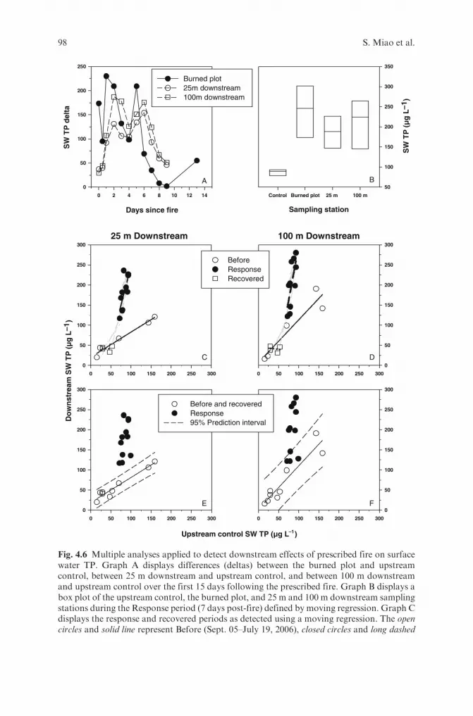
100 m Downstream

0 50 100 150 200 250 300

0

50

100

150

200

250

300

0 50 100 150 200 250 300

0

50

100

150

200

250

300

Sampling station

Control Burned plot 25 m 100 m

SW

TP

(µ

g L

–1)

50

100

150

200

250

300

350

Upstream control SW TP (µg L–1)

0 50 100 150 200 250 300

0

50

100

150

200

250

300

Before and recoveredResponse95% Prediction interval

Days since fire

0 2 4 6 8 10 12 14

SW

TP

del

ta

0

50

100

150

200

250

Burned plot25m downstream100m downstream

25 m Downstream

0 50 100 150 200 250 300

Do

wn

stre

am S

W T

P (

µg

L–1

)

0

50

100

150

200

250

300

BeforeResponseRecovered

A

DC

B

FE

Fig. 4.6 Multiple analyses applied to detect downstream effects of prescribed fire on surfacewater TP. Graph A displays differences (deltas) between the burned plot and upstreamcontrol, between 25 m downstream and upstream control, and between 100 m downstreamand upstream control over the first 15 days following the prescribed fire. Graph B displays abox plot of the upstream control, the burned plot, and 25 m and 100 m downstream samplingstations during the Response period (7 days post-fire) defined by moving regression. Graph Cdisplays the response and recovered periods as detected using a moving regression. The opencircles and solid line represent Before (Sept. 05–July 19, 2006), closed circles and long dashed

98 S. Miao et al.

control. While the SWTP delta peaks of the downstream pulses were delayedand slightly less than the burned plot pulse, the duration of the downstreamdelta pulse was several days longer (Fig. 4.6A and Table 4.1).

Moreover, the downstream data were regressed against the upstream (adja-cent) control to determine the Response and Recovered period (Fig. 4.6C andD). The Before period regressions were characterized by positive slopes betweenthe upstream control and the 25 and 100 m downstream stations. The coeffi-cients of variations were 0.62 (p¼ 0.002) and 1.07 (p¼ 0.02) respectively. TheseBefore slopes were significantly different from the Response period slopes, butwere not different from the slopes of the Recovered period. Once the Responseand Recovered periods were determined for each downstream station, the meanSWTP during the Response period were calculated for at the burned plot, 25 mdownstream, 100 m downstream, and upstream (240 � 68, 188 � 43, 213 � 61,and 88 � 8 mg TP L�1, respectively) (Fig. 4.6B). In addition, simple regressionsof each response period and their 95% prediction intervals were calculated (Fig.4.6E and F). For both downstream stations, all sampling points during theResponse period fell outside of the 95% prediction interval of the Before andRecovered combined regression.

Finally, using the Before and Response periods established by regressionanalysis, several BACI-ANOVA models and BACIPS t-tests were used toexplore downstream post-fire nutrient pulse effects at two downstream sites.Downstream sites were analyzed as separate impacted sites, and also averagedtogether as one impacted site (Table 4.5). Several interesting results becameobvious after completing these different combinations of statistical analyses.First, regardless of whether the BACI-ANOVA or BACIPS t-tests were used, asignificant SWTP pulse was detected when compared to the upstream controlwhereas the pulse was considered insignificant when compared to the distantcontrol or the burned plot. Second, using the upstream control, the singlecontrol/impact model BACI-ANOVA detected downstream post-fire SWTPeffects regardless of whether the two downstream plots were analyzed as sepa-rate impacted sites, or averaged together.

Using the burned plot for comparison allowed us to determine the similarityof the burned plot’s SWTP concentration with downstream plots. The p-valuesfor the BACI-ANOVA and BACIPS models comparing the burned and

Fig. 4.6 (continued) line represent Response (July 25–Aug. 3, 2006) and open squares anddotted line represents the Recovered (Sept. 6–Aug. 1, 2007) time period. The grey lines in bothgraphs are for the individual moving regression lines that were originally used in determiningthe Before, Response and Recovered time periods. The dark regression lines are calculatedfrom the grouping of the moving regression data points. For both the 25 and 100 m down-stream graphs, the upstream control is on the x-axis and the downstream impacted plot is onthe y-axis. Graph D presents the simple regression between the upstream control (x-axis) andthe downstream (y-axis); the data collected during the Before and Recovered periods aredisplayed as open symbols; the Response are represented by solid symbols


downstream plots were large and insignificant (p values ranged from 0.551 to0.979), indicating the increase in SWTP in the downstream plots could not bedistinguished from the increase in the burned plot (Table 4.5). Overall, firecaused an immediate increase in SWTP within the burned plot and P wastransported at least 100 m downstream of the burned plot. Again, definingthe response period using a series of regressions was critical for statistical

Table 4.5 P-values of BACI-ANOVA and BACIPS t-test analyses of the downstream effectsof fire on surface water total phosphorus concentrations. Downstream plots were analyzedseparately (25 m downstream or 100 m downstream) and in combination (25 m downstreamand 100 m downstream). The analyses used the Before–Response period defined in Table 4.3.Bolded p-values are significant at�¼ 0.05. Sample sizes for the two downstream and upstreamcontrol were n ¼ 1, whereas for Burned and Distant control were n ¼ 3

Model Control ImpactFireeffects

Temporalvariation

Spatialvariation

Single control/impact BACIANOVA

Upstreamcontrol

25 m downstream 0.032 0.041 �100 m downstream 0.008 0.122 �Total downstream 0.008 0.226 �

Distantcontrol

Total downstream 0.890 0.007 �

Burned plot 25 m downstream 0.551 0.041 �100 m downstream 0.815 0.035 �Total downstream 0.665 0.002 �

Single control/multi-impactBACI ANOVA

Upstreamcontrol

25 m and 100 mdownstream

0.061 0.021 0.103

Burned, 25 m and100 mdownstream

0.051 0.008 0.017

Burned and Totaldownstream

0.214 0.087 0.084

Distantcontrol


0.641 0.014 0.223

Burned, 25 m and100 mdownstream

0.715 0.003 0.088


0.751 0.057 0.191

BACIPS Upstreamplot

25 m downstream <0.001 � –

100 m downstream <0.001 – –


<0.001 – –

Total downstream <0.001 – –

Distant plot Total downstream 0.104 – –

Burned plot 25 m downstream 0.863 – –

100 m downstream 0.979 – –

Total downstream 0.918 – –

MBACI ANOVA DistantandUpstream


0.326 0.017 0.131

100 S. Miao et al.

validation of detecting impacts in a nonreplicated design. Increasing the num-ber of impact sites seemed to increase temporal variability in the data, which ledto reduced impact detection sensitivity, as was the case with multiple controlsites.

The results reported in sections 4.5 and 4.6 suggest that the regressionapproach was more effective than ANOVA for detecting the effects of fire.The BACI-ANOVA determined only whether there was an impact, whileregression provided information on the onset, duration, or recovery of theresponse variable. Although ANOVA may represent a contemporary method,we believe that using regression has additional advantages in large scale studies.Regression avoids the necessity of having to subjectively categorize continuousvariables (i.e., After, Response, or Recovered) to construct the ANOVAmodeland possibly toss away hard-earned information. One major advantage ofanalyses of continuous variables is that measures of potentially importantsources of variation can be easily incorporated and variability can then beseparated into that associated with the main variable of interest, other mea-sured variables, and noise, allowing clearer identification of effects (Hewittet al. 2007). In our study, the regression analyses addressed spatial variationby regressing response variables at the impact sites against the same variables atthe control sites and fire effects by evaluating changes in slope between Beforeand After and/or among the Before, Response and Recovered periods. Theregression models were not confounded by variation; instead, the variationbenefited the analyses. By comparing slopes rather than just mean responses,we were able to detect emerging patterns and properties in the landscape. Inaddition to slope comparisons, the simple regressions also provided predictionintervals for detecting impact effects. Furthermore, the moving regressionanalysis defined intervals including the onset and duration of the response,neither of which could be accomplished by BACI-ANOVA, thereby avoiding aType I error, particularly for the disturbances creating pulsed effects.

4.7 Ecosystem Synthesis: Fire Effects on Wetland

Phosphorus Pools

While detailed analyses are necessary to assess specific effects of prescribed fire,synthesis of key system responses is the ultimate goal of ecosystem-scale studies.Fire’s effect on a cattail community in the highly enriched area is shown in asimplified depiction in Fig. 4.7A. Based on this, we developed a conceptualmodel of TP pools (g TPm�2) for the major wetland components studied at oursite (Fig. 4.7B) to give an overview of ecosystem response to fire for one year.The data used in this analysis were based primarily on Fig. 4.3 and Table 4.1.

The fire consumed most of the aboveground dead leaves, but only a smallportion of the live leaf biomass. Combustion converted previously organic-bound P in the biomass to inorganic P in the ash. Soluble components of the ash


Peri

phyt

on

(0

)

Pea

t(2

0.36

)

Sur

face

Wat

er (

0.02

)

Por

eW

ater

(0.0

2)

AG

Liv

ing

Bio

mas

s

(0.

62)

Floc

cule

nt D

etri

tus

(

2.86

)

BG

Dea

d B

iom

ass

(0

.31)

BG

Liv

ing

Bio

mas

s

(0.

67)

AG

Dea

d B

iom

ass

(0

.57)

B

Peri

phyt

on(0

.01)

Peat

(19.

99)

Surf

ace

Wat

er(0

.004

)

Pore

Wat

er(0

.03)

AG

Liv

ing

Bio

mas

s(0

.66)

Floc

cule

ntD

etri

tus

(3.2

4)

BG

Dea

dB

iom

ass

(0.7

5)

BG

Liv

ing

Bio

mas

s(0

.53)

AG

Dea

dB

iom

ass

(0.3

5)

Perip

hyto

n

(0)

Pea

t(2

0.62

)

Surf

ace

Wat

er (0

.03)

Por

eW

ater

(0.0

5)

AG

Liv

ing

Bio

mas

s

(0.4

3)

Floc

cule

nt D

etrit

us (

2.13

)

BG

Dea

d B

iom

ass

(0

.71)

BG

Liv

ing

Bio

mas

s

(0.2

7)

AG

Dea

d B

iom

ass

(0.

14)

Perip

hyto

n(0

.05)

Peat

(19.

94)

Surf

ace

Wat

er(0

.04)

Pore

Wat

er(0

.06)

AG

Liv

ing

Bio

mas

s(0

.22)

Floc

cule

ntD

etrit

us(2

.90)

BG

Dea

dB

iom

ass

(0.8

9)

BG

Liv

ing

Bio

mas

s(0

.42)

AG

Dea

dB

iom

ass

(0.8

5)

A

Fig.4.7

(continued)

102 S. Miao et al.

dissolved upon entering the water and SWTP increased immediately; however,

the SWTP pulse only lasted about 10 days (Fig. 4.3). The SWTP pool was

greatest one month after the fire, but this was likely the consequence of a large

release of water into WCA 2A since SWTP increased simultaneously at the

distant control. During the SWTP pulse following the fire, plant regrowth and

periphyton production at the burned plot were minimal indicating these pro-

cesses contributed little to the quickly diminishing SWTP after the fire. Pore

water TDP (PWTDP) increased after the fire; however, it remained elevated

long after SWTP returned to pre-fire concentrations, suggesting that processes

other than P fluxing below-ground were responsible for the sustained increase

in PWTDP. Calcium-bound P concentrations increased in the floc and top few

cm of soil immediately after the fire; however, this accounted for a relatively

small portion of the TP pulse after the fire and the change in soil TP was notsignificant (unpublished data). One day after the fire, a SWTP pulse was

detected at both downstream sampling locations, while upstream SWTP did

not change. Themagnitude of the downstream pulse was slightly less than in the

burned-plot pulse, yet the duration was one day longer. Considering the down-

stream pulse together with the other processes discussed above suggests that the

bulk of P released by the fire was transported downstream by water and as ash

in the air.Live leaves were generally not consumed in the fire, but were scorched by the

heat and died (Fig. 4.7A). These newly dead leaves had greater nutrient con-

centrations than naturally senesced cattail leaves, explaining the TP increase in

the aboveground dead biomass pool one month post-fire when the dead leaf

litter mass was less than before the fire. Fire opened the canopy, which allowedmore light to reach the soil surface and increased soil and water temperatures

even one year after the fire. Periphyton production was noted two weeks after

the fire in response to increased light and was still greater than pre-fire or

control after one year. Cattail leaves began growing soon after the fire and

Fig. 4.7 (continued) (A) Chronological pictorial illustrating the fire impacts and temporalresponses of three main ecosystem components (water quality, soil biogeochemistry, andvegetation dynamics) to a prescribed fire in a cattail-dominated wetland. Arrows indicateincreases ("), no change (!), or decreases (#) in the corresponding parameter. Green cattailleaves indicate live leaves; light blue leaves at 1 day after the fire represent the live leaves thatwere scorched and killed by the fire but not consumed, and the brown leaves represents thegeneral dead leaf litter. (B) Temporal changes in a conceptual model of relevant wetlandecosystem total P (g m–2) pools and transfer pathways in the air, surface water, and soil after aprescribed fire. Each of the four models corresponded to each of the time periods in A. AGand BG stands for above and below ground respectively. The red AG pool 1 day after the firerepresents the scorched leaves not consumed by the fire. Pore water TDP pools were estimatedto a depth of 30 cm based samples taken from the 15–25 cm depth range and measured soilbulk density profiles. The Peat TP pools were to a depth of 30 cm. Only the top 5 cm weremeasured on the 1 day and 1 month after the fire, and therefore we assumed the 5–30 cm layerto be similar to the before fire sample.


within one month the TP of the aboveground biomass pool was 50% of pre-firepool, even though live leaf biomass was less than 20% Fig 4.7B. This seemed tobe due to significantly greater TP concentrations in new leaves compared toolder leaves collected before the fire (unpublished data). One-year after the fire,the aboveground biomass TP pool had recovered and was similar to before thefire; however, aboveground dead leaf TP was still 40% less than pre-fire.

Pulsed and sustained responses of the belowground biomass TP pools weremore difficult to determine, so some of the results and conclusions stated herewere theoretically derived. Fire caused direct mortality of approximately 60%of cattail ramets (Sindhøj andMiao, submitted) which would have resulted in adecrease in the TP pool of belowground live biomass and a subsequent increasein the TP pool of belowground dead biomass. The relatively large TP increase inthe belowground live biomass one month after the fire was attributed mostly tothe belowground components of new ramets, which accounted for over 50% ofindividual cattail plants at this time (Sindhøj and Miao, submitted) and shouldhave greater nutrient concentrations compared to older plants, as describedabove for the leaves. By the end of the first year, TP of the belowground livebiomass had almost recovered to pre-fire levels, but there was still more thantwice as much TP in the belowground dead biomass than before the fire. Thisinput of belowground dead biomass that could result in increased long-term Pstorage belowground may be offset by increased peat surface temperatures thatcould enhance decomposition and accelerate nutrient cycling, so it is unclearwhether fire will lead to increased long-term storage of nutrients below-ground.

Overall, fire resulted in a SWTP pulse of short duration at the burned site.Downstream transport of the fire-released P exceeded 100 m and the total extentof downstream transport remains unknown. However, taking multiple factorsinto consideration (e.g., the short TP pulse, no increase in soil TP, and highbackground TP level), it appears that P mobilized from prescribed fires at thescale investigated in this study would not exceed variations in P transport result-ing from other system-wide events, processes or perturbations. Furthermore,while cattail populations had almost recovered after one year, community struc-ture still exhibited impacts which would affect ecosystem processes.

4.8 Summary

Large-scale ecosystem restoration presents unprecedented challenges, for whichcurrent methods of ecological research and analysis are not well-prepared, indi-cating a need for a paradigm shift in experimental design and analysis that addressspatial- and temporal-scales and variances. At the same time, ecosystem restora-tion projects provide an ideal framework for ecologists to question, investigate,and develop important ecological theory and philosophy. Driven by a legislativemandate to restore the historical vegetation in nutrient enriched areas of theEverglades, we designed and implemented the ecosystem-scale Fire project toinvestigate the effects of fire on wetland ecosystem structure and function and to

104 S. Miao et al.

address issues related to nonreplicated experimental design and analysis. Preli-minary data analysis of the Fire project’s initial years clearly shows the challengesand benefits of integrating multiple spatial scales and unbalanced temporaldesigns for detecting responses to fire amid large-scale natural variability.

Replication of ecosystem-scale environmental disturbances or treatments isoften not possible or desirable under real world circumstances. While thereshould be no moral or ethical reasons to limit control site replication, financial,and logistical restraints to replication in general are often a reality. The Fireproject demonstrated that a few carefully chosen controls at multiple spatialscales (such as adjacent and distant controls) provided analytical flexibility.Considering spatial structure of the system studied and multiple ecosystemresponse variables operating at different temporal scales, we suggest that atleast one carefully chosen control site should closely co-vary with the impact siteto maximize the potential for impact detection for variables with rapid responsetimes, and one control site should be ecologically similar but separated at agreater spatial scale providing a context of natural ecosystem variability forvariables with relatively longer response times. Thus, we echo Carpenter’s(1990) recommendation that ‘‘resources that could be invested in duplicates[minimal replication] might be better spent on more detailed mechanisticanalyses conducted within the context of a large-scale experiment.’’

Purposely selecting controls at the spatial scales of major system driving forcesseemed an effective approach to simultaneously detect a fire impact at a smallscale while placing themagnitude of the impact in the context of natural variationat a larger scale. However, it may be argued that this approach is perilously closeto predetermining one’s results, i.e., choosing a control that will show theintended effect. Continuing with this argument, it is recommended that usingdifferent controls yields different results and therefore multiple random controlsare required to ensure analytical rigor and robustness. These are rational andelegant arguments from the traditional ecological paradigm and directly relate tothe inferential power of nonreplicated large-scale ecological studies. Inference,however, is not always necessarily the goal of ecosystem restoration or distur-bance studies. One fundamental difference between null hypothesis testing andlarge-scale ecosystem restoration or disturbance studies is the former merelyseeks to determine whether an impact has occurred, whereas the later seeksto elucidate the direction, duration, relevance, and magnitude of the impact(Canham and Pace, Chapter 8). Foreknowledge of the systems studied, thepotential scales of impacts, and the forcing functions behind natural variationshould shape experimental design adequately to detect and quantify impacts. Inthis study, fire did cause a nutrient pulse in surface waters; however, it was indeedno greater than the overall natural long-term temporal variability of the system.In addition, the multiple spatial control design had advantages to assess post-firedownstream nutrients effects, a critical issue in aquatic and wetland systems.

The multiple, unbalanced design of temporal sampling schemes for responsevariables operating at different biological organization scale is important whenassessing both short- and long-term effects on a whole ecosystem. When pulsed


responses are anticipated, sampling regimes should be adjusted accordingly tocapture the changes even at the expense of not meeting standard statisticalassumptions. This strategy, however, requires the development of a wide rangeof novel analytical tools that encompass the assessment of ecosystem compo-nents operating at different spatial and temporal scales.

The two regression approaches, moving and simple regressions, outlinedhere appear to effectively determine ecosystem response characteristics suchas direction (increase, decrease, or no change), onset, duration, and magnitude.For both regressions, data collected at the control site were defined as theindependent variable and the data from the impact site as the dependentvariable. The moving regression identifies the onset and duration of impacts,i.e. Before, Response or Recovered periods. After which a simple regression canelucidate the slopes, confidence and prediction intervals, and scatter of indivi-dual data points sampled at specific times during these periods. Overall, thesetwo regression-analysis models incorporate spatial (Control and Impact) andtemporal (Before andResponse) variation in a correlative context and eliminatemany analytical challenges of dealing with variation in nonreplicated design.However, accurate use of these regression models requires that both Controland Impact sites are sampled at the same time.

These regression models also advanced our insights into the ecological con-text of the After period. In the BACI literature, the system response period isrepresented by the entire After period and is solely decided by the timing of thetreatment. Analyzing ecosystem response according to these assumptions limitsthe likelihood of impact detection when pulsed effects occur. Clearly, wideningthe After period definition to include both Response and Recovered periodsenhances the applicability of both BACI and BACIPS comparisons and con-sequently reduces the likelihood of a Type I error. While common graphicalanalysis of data may obviously indicate a response, the regression approachesoffer statistical support for the characterization of Before, Response, andRecovered periods of disturbance impacts and provide an overall frameworkfor further analysis of system responses. We will continue to investigate theapplication of regression approaches from other analytic tools to address newissues that arise along with our ongoing Fire project.

Acknowledgments We thank the South Florida Water Management District for supportingthe Fire project and Hawaii Pacific University for providing release time for S. Carstenn. Wegreatly appreciate many former (D. Pisut, H. Chen, J. Creasser, D. Salembier, M. Tapia, andD.Condo) and current members (Robert Johnson, Christina Stylianos, D. Monette) of theFire project team who conducted field samplings. We thank C. Stow, D. Hui, J. Hewitt, J.Grace, S. Hill, M. Nungesser and D. Drum for their valuable comments on early drafts of thechapter. S.L. Miao contributed to overall idea, structure, and preparation of the manuscript;S.Carstenn contributed to analysis of moving regression and manuscript preparation; C.Thomas conducted BACI-ANOVA analyses related to control similarity and control num-bers for detecting fire impacts; C. Edelstein was responsible for field setup and sampling, datamanagement and figure and table creation; E. Sindhøj developed the model for nutrient poolanalysis used in the synthesis section and contributed to manuscript preparation; and BinheGu contributed to the development of the nutrient pool analysis.

106 S. Miao et al.

References

Bender, E. A., T. J. Case, and M. E. Gilpin. 1984. Perturbation experiments in communityecology: theory and practice. Ecology 65:1–13.

Box, G. E. P. and G. C. Tiao. 1965. A change in level of a nonstationary time series.Biometrika 52:181–192.

Box, G. E. P. and G. C. Tiao. 1975. Intervention analysis with applications to economic andenvironmental problems. Journal of the American Statistical Association 70:70–79.

Burns and McDonnell. 2003. Everglades Protection Area Tributary Basins Long-Term Planfor Achieving Water Quality Goals. South Florida Water Management District, WestPalm Beach, FL.

Carpenter, S., N. F. Caraco, D. L. Correll, R. W. Howarth, A. N. Sharpley, and V. H. Smith.1998. Nonpoint pollution of surface waters with phosphorus and nitrogen. EcologicalApplications 8:559–568.

Carpenter, S. R. 1990. Large-scale perturbations: Opportunities for innovation. Ecology71:2038–2043.

Carpenter, S. R. 1996. Microcosm experiments have limited relevance for community andecosystem ecology. Ecology 77:677.

Carpenter, S. R., S. W. Chisholm, C. J. Krebs, D. W. Schindler, and R. F. Wright. 1995.Ecosystem experiments. Science 269:324–327.

Carpenter, S. R., T. M. Frost, D. Heisey, and T. K. Kratz. 1989. Randomized inter-vention analysis and the interpretation of whole-ecosystem experiments. Ecology70:1142–1152.

Chimney, M. J. and G. Goforth. 2001. Environmental impacts to the Everglades ecosystem: ahistorical perspective and restoration strategies. Water Science and Technology 44:93–100.

Clark, J. S., S. R. Carpenter, M. Barber, S. Collins, A. Dobson, J. A. Foley, D. M. Lodge, M.Pascual, R. Pielke Jr., W. Pizer, C. Pringle, W. V. Reid, K. A. Rose, O. Sala, W. H.Schlesinger, D. H.Wall, and D.Wear. 2001. Ecological forecasts: an emerging imperative.Science 293:657–660.

Conquest, L. L. 2000. Analysis and interpretation of ecological field data using BACI designs:discussion. Journal of Agricultural, Biological and Environmental Statistics 5:293–296.

Davis, S. M. and J. C. Ogden. 1994. Toward ecosystem restoration. Pages 769–796 in S. M.Davis and J. C. Ogden, editors. Everglades: The Ecosystem and Its Restoration. St. LuciePress, Delray Beach, Florida, USA.

Gotelli, N. J. and A. M. Ellison. 2004. A Primer of Ecological Statistics. Sinauer Associates,Sunderland, MA.

Green, R. H. 1979. Sampling Design and Statistical Methods for Environmental Biologists.John Wiley & Sons, University of Western Ontario.

Hasler, A. D., O. M. Brynildson, W. T. Helm. 1951. Improving conditions for fish in brown-water bog lakes by alkalization. Journal of Wildlife Management 15:347–352.

Hewitt, J. E., S. E. Thrush, and V. J. Cummings. 2001. Assessing environmental impacts:effects of spatial and temporal variability at likely impact scales. Ecological Applications11:1502–1516.

Hewitt, J. E., S. F. Thrush, P. K. Dayton, and E. Bonsdorff. 2007. The effect of spatial andtemporal heterogeneity on the design and analysis of empirical studies of scale-dependentsystems. The American Naturalist 169:398–408.

Keough, J. M. and G. P. Quinn. 2000. Legislative vs. practical protection of an intertidalshoreline in Southeastern Australia. Ecological Applications 10:871–881.

Legendre, P. 1993. Spatial autocorrelation: trouble or new paradigm? Ecology 74: 1659–1673.Legendre, P., M. R. T. Dale, M.-J. Fortin, J. Gurevitch, M. Hohn, and D. Meyers. 2002. The

consequences of spatial structure for the design and analysis of ecological field surveys.Ecography 25:601–615.


Likens, G. E. 1985. An experimental approach for the study of ecosystems: The Fifth TansleyLecture. Journal of Ecology 73:381–396.

Melbourne, B. A. and P. Chesson. 2005. Scaling up population dynamics: integrating theoryand data. Oecologia 145:179–187.

Miao, S. and S. Carstenn. 2006. A new direction for large-scale experimental design andanalysis. Frontiers in Ecology 4:227.

Miao, S. L. and S. Carstenn. 2005. Assessing Long-TermEcological Effects of Fire andNaturalRecovery in a Phosphorus Enriched Everglades wetlands: Cattail Expansion PhosphorusBiogeochemistry and Native Vegetation Recovery. West Palm Beach, Florida.

Mitsch, W. J. and J. W. Day Jr. 2004. Thinking big with whole-ecosystem studies andecosystem restoration- a legacy of H.T. Odum. Ecological Modeling 178:133–155.

Murtaugh, P. A. 2007. Simplicity and complexity in ecological data analysis. Ecology 88:56–62.Osenberg, C. W. and R. J. Schmitt, editors. 1996. Detecting Ecological Impacts Caused by

Human Activities. Academic Press, Inc., San Diego, CA.Osenberg, C. W., R. J. Schmitt, S. J. Holbrook, K. E. Abu-Saba, and A. R. Flegal. 1994.

Detection of environmental impacts: natural variability, effect size, and power analysis.Ecological Applications 4:16–30.

Petersen, J. E., W. M. Kemp, R. Bartleson, W. R. Boynton, C.-C. Chen, J. C. Cornwell, R. H.Gardner, D. C. Hinkle, E. D. Houde, T. C. Malone, W. P. Mowitt, L. Murray, L. P.Sanford, J. C. Stevenson, K. L. Sunderburg, and S. E. Suttles. 2003. Multiscale experimentsin coastal ecology: improving realism and advancing theory. BioScience 53:1181–1197.

Pickett, S. T. A. 1989. Space-for-time substitution as an alternative to long-term studies.Pages 110–135 inG.E.Likens, editor. Long-term studies in ecology. Springer-Verlag,NewYork.

Ponzio, K. J., S. J. Miller, and M. A. Lee. 2004. Long-term effects of prescribed fire onCladium jamaicense crantz and Typha domingensis pers. densities. Wetlands Ecology andManagement 12:123–133.

Schindler, D. W. 1998. Replication versus realism: The need for ecosystem-scale experiments.Ecosystems 1:323–334.

Simberloff, D. 2004. A rising tide of species and literature: a review of some recent books onbiological invasions. BioScience 54:247–254.

Sindhøj, E. and S. Miao. Submitted. Recovery dynamics and underlying mechanisms ofTypha domingensis communities following fire in a highly- and moderately-nutrientenriched Everglades wetland Ecosystem Restoration.

Sokal, R., R. and F. J. Rohlf. 1981. Biometry. 2nd edition. W.H. Freeman and Company,New York.

Stewart-Oaten, A. 1996a. Goals in environmental monitoring. Pages 17–27 in R. J. Schmittand C.W. Osenberg, editors. Detecting Ecological Impacts: Concepts and Applications inCoastal Habitats. Academic Press, Inc.

Stewart-Oaten, A. 1996b. Problems in the analysis of environmental monitoring data. Pages109–131 in R. J. Schmitt and C. W. Osenberg, editors. Detecting Ecological Impacts:Concepts and Applications in Coastal Habitats. Academic Press, San Diego.

Stewart-Oaten, A. 1996c. Problems in the analysis of environmental monitoring data. Pages109–131 in R. J. Schmitt and C. W. Osenberg, editors. Detecting Ecological Impacts:Concepts and Applications in Coastal Habitats. Academic Press, Inc.

Stewart-Oaten, A. 2003. Using Before-After-Control Impact in Environmental Assessment:Purpose, Theoretical Basis, and Practical Problems. Coastal Research Center, MarineScience Institute, University of California, Santa Barbara, California.

Thrush, S. F., J. E. Hewitt, V. J. Cummings, P. K.Dayton,M. Cryer, S. J. Turner, G. Funnell,R. Budd, C. Milburn, and M. R. Wilkinson. 1998. Disturbance of the marine benthichabitat by commercial fishing: impacts at the scale of the fishery. Ecological Applications8:866–879.

Thrush, S. F., S. M. Lawrie, J. E. Hewitt, and V. J. Cummings. 1999. The problem of scale:uncertainties and implications for soft-bottom marine communities and the assessment of

108 S. Miao et al.

human impacts. Pages 185–210 in J. S. Gray, editor. Biogeochemical Cycling and SedimentEcology. Kluwer Academic, Netherlands.

Underwood, A. J. 1989. The analysis of stress in natural populations. Biological Journal ofthe Linnean Society 37:51–78.

Underwood, A. J. 1991. Beyond BACI: experimental designs for detecting human environ-mental impacts of temporal variations in natural populations. Australian Journal ofFreshwater Research 42:569–587.

Underwood, A. J. 1993. The Mechanics of Spatially replicated sampling programs to detectenvironmental impacts in a variable world. Australian Journal of Ecology 18:99–116.

Underwood, A. J. 1994. On beyond BACI: sampling designs that might reliably detectenvironmental disturbances. Ecological Applications 4:3–15.

Urquhart, N. S., S. G. Paulsen, and D. P. Larsen. 1998. Monitoring for policy-relevantregional trends over time. Ecological Applications 8:246–257.


Chapter 5

Bayesian Hierarchical/Multilevel Models

for Inference and Prediction Using

Cross-System Lake Data

Craig A. Stow, E. Conrad Lamon, Song S. Qian, Patricia A. Soranno and

Kenneth H. Reckhow

Abbreviations AIC – Akaike’s Information Criterion, ANOVA – Analysis of

Variance, BCART – Bayesian classification and regression tree, BIC –

Bayesian Information Criterion, CART – Classification and Regression

Tree, DIC –Deviance Information Criterion, LIL – Log Integrated likelihood,

MCMC – Markov Chain Monte Carlo, MLE – Maximum Likelihood Esti-

mator, SBC – Schwarz’s Bayesian criterion, TP – Total phosphorus

5.1 Introduction

Cross-system studies are commonly used for large-scale ecological inference

(Cole et al. 1991). Many processes change slowly within a particular ecosystem,

thus long time periods can be required to measure how changes in one process

may influence changes in another. By using data frommany systems researchers

essentially substitute space for time, assuming commonality among the systems

being compared. Comparing characteristics among systems helps researchers

identify patterns that provide clues for understanding ecosystem function,

generate testable hypotheses, and isolate cause–effect relationships.In limnology, cross-system studies have been widely applied, in part because

lakes are relatively discrete ecosystems with tangible boundaries, making their

properties straightforward to evaluate and compare. Additionally, many

important lake attributes, such as trophic status, can be well-approximated by

a small number of quantitative measures. In the 1960s and 1970s cross-system

lake comparisons were influential in resolving the limiting nutrient debate. The

work of Richard Vollenweider, in particular, popularized this approach, and

led to nutrient loading concepts that are still widely applied in aquatic ecosys-

tem management (Vollenweider 1968, 1969, 1975, 1976).

C.A. Stow (*)NOAA Great Lakes Environmental Research Laboratory, 2205 CommonwealthBlvd., Ann Arbor, MI 48105, USAe-mail: [email protected]


111

Early efforts to quantify relationships among lakes may have been largely adhoc; electronic calculators were not widely available until the mid-1970s andaccess to fast computers was limited. Thus, even relatively simple models likelinear regression and ANOVA were tedious to compute for more than a smallnumber of observations. With the increasing availability of fast, inexpensivecomputing power researchers began to use cross-system lake data to developmathematical relationships useful for quantifying limnological processes and tobuild models for decision-making (Reckhow and Chapra 1983).

The use of cross-system data for lake-model development has also beenfostered by a general lack of extensive long-term data from individual lakes.However, individual lake behavior can be idiosyncratic – highly dependent onfeatures such as the landscape setting in which the lake is located (Stow et al.1998). Thus, models developed from cross-system data may not accuratelycapture the behavior of a particular lake. Because management decisions aretypically made on a lake-by-lake basis, it is arguably preferable to constructlake-specific models to support management actions such as Total MaximumDaily Loads (National Research Council 2001). Nevertheless, with some excep-tions (Stow et al. 1997, Lathrop et al. 1998), relatively few lakes have beensufficiently well-monitored to provide adequate data for individual modeldevelopment. This is particularly true in lake-rich states in the US and otherregions of the world where limited resources prohibit intensive data collectionon more than a few lakes.

Additionally, data representing a range of conditions are necessary to assessthe functional form of amodel and estimate model parameters. Individual lakesin approximately steady-state conditions are unlikely to generate data of suffi-cient variance for accurate model estimation even over long time periods. Insuch cases extrapolation beyond the observed conditions may be required topredict the likely changes that will occur under alternative management actions,resulting in considerable predictive uncertainty. Thus, even if many years ofdata are available for a particular lake, augmenting the lake-specific data withdata from other lakes can increase predictive accuracy for the lake underconsideration.

Building models for prediction from cross-system data is based on the suppo-sition that the relationship between the response and predictor variables is thesame for all the lakes used to estimate the model. While this presumption is neverexactly correct, most modelers implicitly hope that it is close enough to the truthto make useful inferences and decisions. A popular strategy to increase thelikelihood of similar behavior is to group lakes based on common attributes.Features used to categorize lakes have included lake type (natural vs. reservoir),geographic setting, and geomorphology (Canfield and Bachman 1981, Reckhow1988, Malve and Qian 2006) and models based on such groupings are then usedfor individual lake forecasts (Hession et al. 1995). The goal of this strategy is to‘‘borrow’’ information from other similar lakes to increase the accuracy of pre-diction for a particular lake, so that the risk of making a bad decision isacceptably low.

112 C.A. Stow et al.

But are models developed from a cross-section of lakes sufficiently accurate

to make good management decisions for an individual lake? Moreover, how

uncertain can a model be and still be useful for effective management decision-

making? The answer to these questions is context specific, depending on the

stakes associated with the pending decisions. If the consequences of a poor

decision are not very severe, high model uncertainty may not matter much.

Alternatively, in high-stakes decision situations, models with large uncertainties

may not differentiate the likely outcomes of one management alternative from

another, providing little basis for selecting a management option.Given a choice of models, a decision-maker is likely to use the model with the

lowest uncertainty. A model that provided correct forecasts 98% of the time

would be a clear choice over one that was accurate only 75% of the time. With

98% accuracy, management actions could be chosen based only on the societal

value of the consequences of those actions. A model with higher uncertainty

may still be informative, but applying this model requires decision-makers to

hedge their decisions by considering a range of possible outcomes, based on

knowing how uncertain the model is. Therefore, while uncertainty may arise

from a lack of knowledge, quantified uncertainty provides information that is

useful for both picking the best model and applying that model for decision

support.Often, however, decision-makers are given models or model results with no

supporting information regarding uncertainty – providing an illusion of preci-

sion (Pappenberger and Beven 2006). How is this information useful for high-

stakes decisions?Uncertainty is typically expressed as a probability statement. The term

probability has several interpretations; the most widely appreciated is the

long-term relative frequency of a particular event. Coin-flipping is a common

example of this probability notion. The probability of flipping a coin and

obtaining ‘‘heads’’ is approximately 50% – meaning that if a coin is flipped

enough times approximately 50% of those flips will result in the coin landing

heads-side up. Another interpretation of probability is that it represents a

degree-of-belief (Winkler 2003). If an individual is presented with a coin and

asked the probability that the coin will land heads-side up when flipped, it is

likely that the response will be: ‘‘approximately 50%’’. In this instance there is

no long-term relative frequency involved, in fact the coin has not been flipped

even once yet. The response ‘‘50%’’ represents the respondent’s degree-of-belief

that the coin will land heads-side up. This belief is based on prior experience

resulting in knowledge of what usually happens when a coin is flipped. If the

respondent had reason to believe that they were being tricked with a coin that

had been engineered to produce heads they might indicate 90 or 95%. Thus, the

degree-of-belief notion of probability is a quantification of the confidence an

individual has in the occurrence of a particular result.These two notions of probability are not mutually exclusive; in fact they can

be reconciled using Bayes theorem:

5 Bayesian Hierarchical/Multilevel Models for Inference and Prediction 113

pð�jyÞ ¼ pð�Þfðyj�ÞR� pð�Þfðyj�Þd�

(5:1)

The interpretation of Bayes theorem is that prior beliefs (those held beforethe experiment), represented by p(�), are combined with new information fromthe experiment, contained in the likelihood function, which is represented by

f( y | �), to obtain posterior beliefs, represented by p(� | y). For most practicalapplications, the denominator on the right side of the equation can be regardedas a scaling constant and essentially ignored.

If, for example, before flipping a coin we believed that the probability ofheads was 50%, and in our experiment of 100 flips we obtained 50 heads and 50

tails our belief would be unchanged; the posterior belief would be the same asthe prior belief. If, however, the coin-flipping experiment resulted in 95 heads itis likely that our posterior belief in the probability of heads would move toward95%, depending on whether or not we thought the 95 head outcome was typical

or accidental.While Bayesian approaches have been known in ecology and the environ-

mental sciences for some time (Reckhow 1990), they are being increasingly used(Ellison 2004), in part because they have only become practically feasible sincethe widespread availability of fast, inexpensive computers. Many models areanalytically intractable in a Bayesian context, particularly nonlinear models or

models with more than just a few parameters to be estimated. Using a Bayesianapproach in such cases was virtually impossible until recently. But the advent ofcheap computing has fostered the development of algorithms that provideprecise numerical approximations for most problems, making the routine

application of Bayes theorem a practical option.Bayesian approaches are not new; their use predates what are often referred

to as ‘‘frequentist’’ or ‘‘classical’’ methods, which were developed in the early-mid 1900s (Salsburg 2001). Classical approaches are what most ecologists havebeen trained in since the 1960s, and usually involve setting up a null hypothesis,then performing a ‘‘significance test’’ to evaluate the validity of the null hypoth-

esis. Many textbooks present classical methods as a coherently conceivedapproach to scientific inference, and their application has become deeplyengrained in ecology. Thus, many ecologists perceive them to be inviolaterules that govern the way science is properly conducted, and finding ‘‘signifi-

cant’’ results has become an end in itself rather than a means to an end. In fact,classical significance testing arose from a somewhat rocky fusion of two con-trasting schools of thought, contributing to considerable confusion amongapplied scientists when interpreting their results, as p-values and significance

levels are often interpreted to be synonyms (Hubbard and Bayarri 2003,Hubbard and Armstrong 2006).

Working in a Bayesian framework offers distinct advantages over a classicalnull hypothesis testing framework. A Bayesian approach provides a posteriorprobability distribution for the model parameters, p(� | y), which indicates the


relative probabilities of all possible values of �, conditional on the observeddata, y. This posterior distribution can be used to support a wide range ofdecisions applying many possible decision criteria. Predictions for y are madeby evaluating the model over the entire posterior parameter distribution, result-ing in a predictive probability distribution for future y values.

Classical null hypothesis testing approaches are muchmore constrained. Thedecision to be made is to either accept or reject an a priori null hypothesis, andthe decision criterion is chosen to minimize the chance of accepting a false nullhypothesis. Acceptance or rejection of the null hypothesis is based on a p-value,which is the probability of obtaining results at least as extreme as the observeddata, conditional on the null hypothesis being true. Many researchers findp-values (symbolically expressed as p(� y | �) where � is typically zero) confus-ing, often misinterpreting them to convey the same information as a posteriordistribution.

Bayesian approaches are sometimes disparaged as subjective because of theneed to provide prior information regarding parameter values (Dennis 1996),but in fact modelers often fix parameters at specific values based on precedent,published literature values, or expert-judgment, and this practice is rarelycriticized. Bayes theorem offers modelers considerably more flexibility. If aparameter value is well-known then a fixed value can be used, but if the modelerhas very little prior information regarding a parameter value, or wants theposterior distribution to be determined by the data, then a non-informative orvague prior distribution can be chosen. Non-informative priors typically have alarge variance, thus they convey minimal information about the value of amodel parameter. Alternatively, semi-informative priors, with intermediatevariances, can be used for parameters that are not known precisely, but arelikely to be within a limited range (Stow and Scavia 2008). In any case, priorspecification in Bayes theorem is explicit, allowing other researchers the oppor-tunity to evaluate the sensitivity of model-based inferences to the choice ofthe prior.

5.2 Multilevel/Hierarchical Models

Although lake management decisions are usually made on a lake-by-lake basis,the scientific information for such decisions is often based on cross-systemdata. On one hand, a model developed using data from multiple lakes willalmost certainly be less accurate for a specific lake, because the model repre-sents the average of the lakes. On the other hand, a model based only on lake-specific data will have a large uncertainty because of the small lake-specificsample size. Multilevel models provide a rigorous framework to systematicallycombine information from several sources and appropriately weight the group-specific or lake-specific information depending on the degree of similarity toother groups or lakes in the data set.


In a multilevel model, parameters representing individual lakes, or groups oflakes, are given a probability structure. For example, within a lake, observa-tions of a response variable, such as chlorophyll a concentration, exhibit a lake-specific mean, and a certain level of within-lake variability. If the within-lakevariability is expected to be similar for lakes belonging to the same group, thenthe between-lake variability can be expressed in terms of the variability amongthe lake-specific means. This variability among lake-specificmeans can bemodeled with a normal (or other) distribution and the parameters of thisdistribution can be estimated from the cross-system data. In some cases, obser-vations may be nested – there may be distinct basins within lakes, lakes withinsimilar groups, groups within a region, etc., and the probability model captur-ing each of these levels of variability assumes a hierarchical configuration.

To explain the difference between the multilevel approach and more tradi-tional approaches, we use a simple example of estimating lake-specific means ofa response variable. Mathematically, we would model this between and within-lake variability using a model similar to an ANOVA model

yij � Nð�i; �2Þ; (5:2)

where yij is the jth observation from the ith lake, �i is the mean of the ith lakeand �2 is the variance of the observations. When individual lakes are modeledseparately, each �i is estimated to be a lake-specific mean. When cross-systemdata are used, all lakes implicitly share the samemean. Themultilevel approachis a compromise between these two extremes. It treats each individual lake as aseparate entity, but the lake-specific means are structured to share the sameprior distribution:

�i � Nð�; t2Þ; (5:3)

where � and t2 are the mean and variance, respectively, of the �i. By using ashared prior distribution of all lake-specific means, the multilevel model resultsin at least two improvements over more conventional approaches: first, theshared prior distribution provides a connection between individual lakes.Because of the common prior, the lake specific means are now estimated as aweighted average of individual lake mean and the overall mean.

��i ¼ni �

2��

�yi þ ð1 t2�Þ�yall

ni �2=ð Þ þ 1 t2=ð Þ (5:4)

The weights are determined by individual lake sample size (ni), individual lakevariance (�2), and the variance among lake-specific means (t2). When thesample size of a lake is large, the multilevel estimated lake specific mean willbe close to the sample mean. When the sample size is small, the multilevelestimated lake specific mean will be close to the overall mean. If there are no


data from a lake, the multilevel estimate of the lake specific mean is the overallmean. In addition to the sample size, the multilevel estimate also considers thelevels of between and within lake variances. If the between-lake variance (t2) ishigh, the weight on overall mean will be small, individual lake mean will beweighted heavier, and vice versa. This partial pooling of the cross-system dataallows system specific estimates without requiring a large sample size for eachsystem. Second, by pooling data frommultiple lakes, the uncertainty associatedwith lake-specific prediction is reduced. If we refer to the cross-systemapproach, where data from multiple lakes are pooled, as complete pooling ofall lakes, and refer to the separate analysis of individual lake approach as nopooling, the multilevel modeling approach is called partial pooling of the data.By partial pooling, we balance the information from individual lakes and theoverall average from all lakes. The individual lake data are more variable (moreuncertain) while the overall average is less variable (more certain).

Compared to the separate lake means, the multilevel-based estimates ofindividual lake means are pulled towards the overall mean. Lakes with largersample sizes are pulled less, while lakes with smaller sample sizes will be pulledmore to the overall mean. This pulling (also known as Bayesian shrinkage)represents a form of information discounting. If a lake with few observations,or a large variance, has a mean chlorophyll a concentration that is much higherthan the overall mean of all the lakes, we are likely to doubt the validity of theanomalously high estimate. The multilevel estimate provides a sensible way ofdiscounting the information that is less trustworthy. This is consistent with theway that Bayes theorem pools information from different sources. The informa-tion represented in the overall mean can be seen as the prior for an individuallake, while data from the lakes are treated as observations. Under the hierarch-ical framework, prior distributions are typically needed for the model parametersthat are of secondary interest, thus their influence on the parameters of primaryinterest is indirect and often minimal. In our case, we need to supply priordistributions for the mean of group means of model coefficients and the withinand between group standard deviations of model coefficients. When there aremany groups, the mean of group means is of less interest and we usually do nothave much information on the within and between group standard deviations ofmodel coefficients. As a result, non-informative priors are used.

The multilevel approach can be readily extended to more complex modelswhere the variable of interest is a linear or nonlinear function of one or morepredictor variables, with unknown model parameters. In our example, lakechlorophyll a concentration is the variable of interest and we model the log ofchlorophyll a as a simple linear function of the log of total phosphorus con-centration. The multilevel model partially pools the group data by introducingcommon prior distributions for model coefficients. With this approach, themodel structure is:

logðChlaÞik � Nð�ik; t2Þ (5:5a)


and

�ik ¼ �k þ �k logðTPikÞ; (5:5b)

ak � Nð�; �2�Þ; (5:5c)

�k � Nð�; �2�Þ; (5:5d)

where log (Chla)ik is the natural log of chlorophyll a concentration from lake i ingroup k, �ik is the mean of the ith lake in group k, t2 is the variance of log(Chla)at a given value of log(TP) (assumed to be the same for all lakes), �k and �k arethe intercept and slope parameters, respectively, for group k, a is the mean ofthe �ks, b is the mean of the �ks, and �

2� and �

2� are the respective variances of

the �ks and �ks.Computing a multilevel model can be done in either a Bayesian or non-

Bayesian context. The non-Bayesian implementation is usually referred to as arandom, fixed, or mixed-effect model. Typical random, fixed, and mixed-effectmodels use a maximum likelihood estimator (MLE) producing a result similarto a Bayesian model using vague prior distributions for �2, a, b, �2�, and �2�.However, estimating the variances can be difficult usingMLEwhen the numberof lakes or number of groups is small (single digit). The Bayesian method ismore flexible, especially when proper prior information is available. A Baye-sian implementation of multilevel modeling is typically calculated usingMarkov chain Monte Carlo (MCMC) simulation (Qian et al. 2003) and canreadily be programmed in WinBUGS (Lunn et al. 2000) which is a free down-loadable software. Multilevel/hierarchical models are similar in concept torandom coefficient and empirical Bayes models which have been previouslydemonstrated with cross-system lake data (Reckhow 1993, Reckhow 1996).They can be very useful for organizing ecological data and have been used tosynthesize information in a cross-system data set of Finnish lakes (Malve andQian 2006).

5.3 Finding Groups in Data

As noted earlier, lake water quality models may be classified by the level ofpooling used in the estimation of their parameters, and have historically eitherbeen developed in a lake-specific context (no pooling) or from a cross-systemstudy (complete pooling). The simple linear structure of a regressionmodel doesnot always apply to an entire cross-system dataset in the complete poolingsituation. There are many reasons that this may be true for lake water qualitydata, including factors such as regional and local differences in climate, geol-ogy, morphometry, land use, land cover, and food web structure. An openquestion with regard to partially pooled lake models is ‘‘How do we determinewhich of the above mentioned factors to use to create lake groups for pooling?’’


In some situations, a natural hierarchical structure is present in the data andmay be exploited for the purpose of assigning lakes to groups for pooling. Lakesoccur in watersheds, watersheds in ecoregions, etc. These are categorical orfactor variables, in which observations take multiple discrete values or levelswith in each factor. In such instances, it may be of interest to determine if one ormore levels of the factor may be combined to reduce model complexity. Further,there may be thresholds, or change points, along the axes of continuous variablesthat may be used to define groups (above/below threshold) for pooling.

Chipman et al. (2002) provide an algorithm to obtain models that may betterdescribe simple structure in cross-system data, by sub-setting the data and thenfitting separate sub-models for each subset. We used Bayesian Treed models(Chipman et al. 2002) to determine if model predictive performance could beimproved by fitting our simple linear regression model to subsets of cross-system lake data. Bayesian CART and Bayesian Treed models are bothenhancements to the more familiar Classification and Regression Tree(CART) procedure (Breiman et al. 1984). Bayesian TreedModels select subsetsof observations on partitions of the matrix of predictor variables for whichlinear models are estimated. Further, they identify subsets of the predictorvariables for which linear model performance is improved as measured bypredictive log integrated likelihood (LIL). Chipman et al. (2002) provide fulldetails regarding Bayesian Treed models.

Use of Bayesian CART (Chipman et al. 1998) and Bayesian Treed models(Chipman et al. 2002) allows predictors to work together in a nonlinear, non-additive fashion by virtue of their tree-based structure, because the disjointpartitions on the predictor space provide for global non-linearity and non-additivity, even though model structure may be locally linear (and additive).We begin our discussion of methods with a general discussion of tree basedmethods, followed by a more specific description of Bayesian CART andBayesian Treed models.

5.3.1 Tree-Based Models

Tree-based models are useful for classification and regression problems inwhich the analyst cannot (or does not want to) specify a priori, the form ofimportant interactions between explanatory (or independent) variables (Clarkand Pregibon 1992). Tree models are easy to interpret, invariant to monotonetransformations of the predictors, and able to capture interaction effects amongthe independent variables (non-additivity). Tree-based models made their firstappearance in the statistical literature due to Sonquist and Morgan (1964).Much of their recent development is due to the work of Breiman et al. (1984).Because they are a computationally intensive procedure, their use has grownconcurrently with the advent of the personal computer. Clark and Pregibon(1992) provide a description of classification and regression trees, along with


examples. Classification and regression trees have been used in numerousecological studies (e.g., Magnuson et al. 1998, Lamon and Stow 1999, Qianand Anderson 1999). Bayesian Treed Models have been used with cross sec-tional data to link nutrients to chlorophyll a concentrations in lakes of thecontinental U.S. (Lamon and Stow 2004, Freeman et al. 2008), and in Finnishlakes (Lamon et al. 2008).

To fit a regression tree, the algorithm begins with the root (or parent) node.The root node contains all the observations and their associated variability. Thedata are split by binary recursive partitioning into increasingly homogeneoussubsets until within-node variability is below some user-specified value. Aterminal node is one that cannot be split further according to the user specifiedrules. Terminal nodes are also called leaves, consistent with the tree analogy.For every split made, the algorithm uses all unique values along the axes of eachpredictor variable as candidate values for splitting the dataset.

The process starts by defining the deviance of the root node (all of the data) as:

Dð�Þ ¼Xðyi��Þ2 (5:6)

where yi are the observations within the node and � is the nodemean. Then eachcandidate predictor variable is examined to find a point that splits the responsevariable into two new nodes, a left and right, where:

Dð�LÞ ¼

Xðyi��LÞ2 (5:7a)

and

Dð�RÞ ¼

Xðyi��RÞ2 (5:7b)

are the deviances of the left (�L) and right (�R) nodes. The split that maximizesthe deviance reduction, defined as:

�Dð�Þ ¼ Dð�Þ � fDð�LÞ þDð�RÞg (5:8)

is chosen, and the process begins again at the left and right nodes. The result isanalogous to a dichotomous key where successive choices are made regardingthe value of the response variable, based on predictor characteristics.

A comparison to ANOVA provides some qualitative insight into the CARTprocedure. ANOVA attempts to answer the question ‘‘Is the mean responsedifferent among the various levels of the chosen factors?’’ (Chambers et al.1992). CART searches for the levels of the factors (as defined by splits) thathave different means, and does not restrict the search to additive, globallylinear models. When there is just one predictor variable, tree models are stepfunctions, and with two predictors the partitions of a tree model may be plottedon a bivariate plot of the pair of predictor variables.


Some limitations of the method include the fact that it results in discontinu-ities at the partition boundaries rather than providing smooth transitionsbetween partitions, as well as the inability to provide good approximations tolinear and additive functions. Uncertainty regarding selection of the predictorvariable upon which to partition the data, as well as the value at which to makethe split once the variable is chosen, is dealt with in CARTmodels only one nodeat a time. This decision is based on maximizing �D. Because �D is calculatedconsidering only the current node and the resulting daughter nodes, there may bea split of the current node that yields a less than maximum �D in the twodaughter nodes, but provides a much better (i.e., larger) �D in subsequent splits.

5.3.1.1 Bayesian CART and Bayesian Treed Models

These limitations are addressed using the Bayesian approach to the classifica-tion and regression tree algorithm (Chipman et al. 1998, Chipman et al. 2002).Instead of the binary recursive partitioning approach of conventional CARTmodels, Bayesian CART (BCART) uses MCMC methods to explore the treestructure. The MCMC approach is computationally more demanding than therecursive partitioning used by conventional CART, but produces trees of loweroverall deviance.

The difference between BCART and Bayesian Treed models is the specifica-tion of the end node model. BCART (and conventional CART) uses the meanof y value in each leaf as the end node model, while a Bayesian Treedmodel usesa simple linear regression. By using a richer structure on the terminal nodes, wetransfer model structure from the tree to the terminal nodes. We thereforeexpect smaller, more interpretable trees to result.

It is difficult to find the ‘‘best’’ tree using any tree-based method. Theconventional approach to this problem is to use a ‘‘greedy’’ algorithm to‘‘grow’’ a tree, then ‘‘prune’’ it back to avoid overfitting, as in conventionalCART. These greedy algorithms usually grow a tree by sequentially choosingsplitting rules for nodes based on maximizing some fitting criterion (Chipmanet al. 1998). This approach produces a sequence of trees, all of which arerefinements of the previous tree in the sequence severely limiting the explorationof all possible trees. In contrast, the Bayesian approach to CART consists of aprior specification and stochastic search (Chipman et al. 1998), exploring amuch richer set of candidate trees. The Bayesian Treed models presented herewere fit using software available by download free of charge: (http://faculty.chicagogsb.edu/robert.mcculloch/research/code/CART/index.html).

5.4 Comparing Models

Several criteria have been proposed for use in model comparison and selection.Many proposed criteria have a component that quantifies goodness of modelfit, along with a component that penalizes model complexity. Among these


criteria are the Akaike Information Criterion (AIC, Akaike 1973), the BayesianInformation Criteria (BIC, Schwarz 1978), and the Deviance InformationCriterion (DIC, Spiegelhalter et al. 2002). The goodness of fit component forall these make use of the deviance, D(y,�) ¼ –2log[ p(y|�)], where y is responsedata associated with a parameterized model, � are the parameters of that model,and p(y|�) is the likelihood. Note that the likelihood is associated with a specificset of data, y. For this reason, criteria that are based on deviance (and therefore,on the likelihood) should be based on the same data y for all models considered.

The Akaike Information Criterion (AIC) is calculated with the formula

AIC ¼ Dðy; �Þ þ 2p; (5:9)

where p represents the number of parameters in the fitted model. Note that thepenalty, 2p, increases with increasing complexity (number of model para-meters), and a model with a lower AIC is preferred over a model with a largerAIC.

The Bayesian Information Criterion, also known as Schwarz’s Bayesiancriterion (SBC), is calculated according to the formula

BIC ¼ Dðy; �Þ þ p� logðnÞ; (5:10)

where p again represents the number of parameters and n the number ofobservations in the fitted model. As with AIC, a model with a lower BIC ispreferred over a model with a larger BIC. Functions for calculation of AIC andBIC are readily available in the R statistical graphics package.

In the context of a Bayesian hierarchical model, the number of inde-pendent parameters included in the model is difficult to determine, whichmakes the use of AIC or BIC problematic. DIC has been proposed formodel comparison in this context. Spiegelhalter et al. (2002) show that theeffective number of parameters in a complex hierarchical model, pD, can becomputed as

pD ¼ Dðy;�Þ �Dðy; ��Þ: (5:11)

The first term on the right is the mean deviance of the model using all of ourestimates (samples) of �, and the second term on the right is the deviance of themodel using only the mean value of our estimate of � (mean of our samples).The deviance information criterion is then

DIC ¼ Dðy;�Þ þ pD: (5:12)

As with the other criteria, a lower value of DIC is preferred over a higher value.Spiegelhalter et al. (2002) offer guidelines for using DIC to compare competingmodels similar to those suggested by Burnham and Anderson (1998) for


interpretation of differences in AIC between models, such that models within

1–2 of the ‘‘best’’ deserve further consideration and 3–7 have considerably less

support. Calculation of DIC is relatively simple in MCMC, and a function for

calculating DIC is implemented in WinBUGS.

5.5 Our Analyses

The goal of our analysis is to illustrate the utility of Bayesian and multilevel

approaches for constructing models using cross-system data. This particular

model is developed to help managers assess target phosphorus concentrations

in lakes where data may be sparse. We used data from 382 Michigan lakes and

reservoirs (� 0.20 km2), with public access, sampled by the MI-Department of

Environmental Quality (Fig. 5.1). Water data were collected from each lake on

a single date during the summer stratified season (July–September) for chlor-

ophyll a, Secchi depth, total phosphorus, total nitrogen, alkalinity, chloride,

dissolved silica, and true water color. We separated the lakes into two types:

natural lakes (lakes with or without a water control structure on it, but with

little change in water level), and reservoirs (lakes that were created by damming

of a river with a range in water residence time of several days to years). We also

characterized each lake by surface area, shoreline development factor (ratio of

shoreline perimeter to the perimeter of a circle of area equal to the lake), average

depth, and catchment area defined as the cumulative catchment (including all

connected upstream lakes and streams). Finally, we included ecoregion

Fig. 5.1 Study area with locations of the 382 Michigan lakes


classifications including Omernik Level III ecoregion (Rohm et al. 2002), GreatLakes Basin, and landscape position (Martin and Soranno 2006).

Overall, the data exhibit an approximately linear relationship between logof chlorophyll a concentration and log of total phosphorus concentration,though there is considerable scatter about a simple regression line fit to thedata (Fig. 5.2). This residual scatter will lead to increased uncertainty in themodel parameter estimates and predictions, thus, it may be advantageous tosubset the data into logical groups that reduce the scatter.We present the resultsfrom three models: a completely pooled model with no groups; a model withfour groups based on Omerniks ecoregion; and a model with two groups basedon the results from a Bayesian Treed analysis.

5.5.1 Completely Pooled Model

Our first model, using complete data pooling, is analogous to the simple linearregression model:

logðchlaÞ ¼ �þ � logðTPÞ þ " (5:13)

" � Nð0; �2Þ (5:13a)

where log(chla) is the natural log of the chlorophyll a concentration, log(TP) isthe natural log of the total phosphorus concentration, � and � are the interceptand slope parameters, respectively, each to be estimated from the data, and " is

Fig. 5.2 Log Chlorophyll a as a function of log Total Phosphorus for the 382 Michigan lakes


an additive model error term that is normally distributed with mean ¼ 0 and

variance ¼ �2 where �2 is also estimated from the data.To estimate this model using Bayes theorem requires specification of three

prior distributions, one for each of the model parameters, �, �, and �2. For thisexample, we programmed WinBUGS using non-informative priors so that the

results would not be influenced by information outside of the data. For both �and �, we used a normal prior distribution with mean ¼ 0 and variance ¼10,000, and for 1/ �2 we used a gamma prior with scale and shape parameters

both ¼ 0.001. Variances in WinBUGS are specified by their inverses (hence the

use of 1/ �2 which is referred to as the precision) and gamma distributions are a

common non-informative prior for the precision. This choice has some caveats

as we will illustrate in our second example model.Because we used non-informative priors, the resulting posterior densities for

� and � (Fig. 5.3) convey information closely analogous to what would be

obtained using a classical approach for a simple linear regression model. The

important difference, however, is that rather than confidence intervals, which

cannot be used to infer the probability of any particular result, we can make

intuitive probability statements from these posterior distributions. Summary

statistics for �, for example, indicate that the mean and median of �’s posteriorare both –0.55 and the standard deviation of the posterior is 0.16 (Table 5.1).

The 2.5 and 97.5 percentiles indicate that there is a 95% probability, given this

model and these data, that � has a value between �0.86 and �0.23. Similar

inference can be made for �, and �, as well as for predictions of chlorophyll a inboth the log and natural metrics.

Fig. 5.3 Parameter estimates and Chlorophyll predictive distribution for the fully pooledmodel. The circle represents the estimated mean, the thick black line is the 50% credibleinterval and the thin black line is the 95% credible interval

Table 5.1 Summary statistics for completely pooled model

Quantity mean median sd 2.5% 97.5%

� �0.55 �0.55 0.16 �0.86 �0.23� 0.69 0.69 0.06 0.57 0.81

� 0.82 0.81 0.03 0.76 0.88

Log predicted chlorophyll a 1.17 1.17 0.82 �0.42 2.79

Predicted chlorophyll a 4.50 3.23 4.4 0.66 16.3

DIC 930.2


Figure 5.3 also depicts a predictive distribution for chlorophyll a at alog TP value of 2.5 (the mean value of the data – chosen for convenience).At this log TP value chlorophyll a has 95% probability of being between0.66 and 16.3 mg/L (Table 5.1). The distribution exhibits a right skew andmedian and mean values of 3.23 and 4.50 mg/L, respectively, illustratingthe separation of the mean and median that occurs when models estimatedunder a log-transformation are retransformed back to the natural metric(Stow et al. 2006).

5.5.2 Ecoregion Model

Our second model has four groups based on Omernik’s ecoregion (Rohm et al.2002). Ecoregion might be considered a reasonable a priori basis for assigninggroups, assuming that the ecoregion designation implies features consistentwith distinctions in lake behavior. In this case, the model is

logðchlaÞ ¼ �j þ �j logðTPÞ þ " (5:14)

" � Nð0; �2Þ (5:14a)

where j ¼ 1–4 with 175, 27, 179, and only 1 lake in groups 1–4, respectively(note: 1–4 correspond to ecoregions 50, 51, 56, and 55, respectively). A hier-archical structure results by imposing normal prior distributions on the �j and�j with respective means �� and �� and respective variances �2� and �2�. Both�� and �� were assigned non-informative priors, normal distributions withmean ¼ 0 and variance ¼ 10,000, while the priors for 1/�2� and 1/�2� weregamma with both scale and shape parameters ¼ 0.001. Note that though eachecoregion has a distinct intercept and slope, a common variance, �2, wasassigned. We also used a gamma prior with scale and shape parameters ¼0.001 for 1/ �2. Additionally, to remove the correlation between the interceptsand slopes we centered the predictor variables, log TP, on their respectivemeans, a step that aids convergence of the algorithm.

Though the means differ, the resultant posterior distributions for �1–4

exhibit considerable overlap (Fig. 5.4) as do the posterior distributions for�1–4 (Fig. 5.4), and the respective summary statistics for these parametersconfirm these similarities among the group-specific parameters (Table 5.2).Predictive distributions for chlorophyll a (using a log TP value of 2.5) ineach ecoregion also overlap (Fig. 5.5) with similar summary statistics(Table 5.2).

Additionally, a comparison of the summary statistics for the posteriordensity of � from the fully pooled model (Table 5.1) and the ecoregionmultilevel model (Table 5.2) reveals that they are almost identical.Together, this body of evidence suggests that the ecoregion multilevel


model might not represent much improvement over the fully pooled model(Tables 5.1 and 5.2). However, respective DICs of 930.2 and 926.0 for thefully pooled and ecoregion-based models indicate that a slight advantage isconferred by the more complex structure of this particular multilevelmodel. While this should not be interpreted to mean that the ecoregion-based model is a better forecasting tool, it does imply that the ecoregionmodel does somewhat better at predicting the existing data set than thefully pooled model does.

Although the ecoregion-based multilevel model does not represent amajor improvement over the fully pooled model, it does illustrate somepotentially important capabilities of multilevel models. In this model,

Fig. 5.4 Parameterestimates for the ecoregionmultilevel model. The circlerepresents the estimatedmean, the thick black line isthe 50% credible intervaland the thin black line is the95% credible interval

Fig. 5.5 Chlorophyll apredictive distribution forthe ecoregion multilevelmodel. The circle representsthe estimated mean, thethick black line is the 50%credible interval and the thinblack line is the 95% credibleinterval


ecoregion group 4 (ecoregion 55) contains data from only one lake; there-fore the group 4 parameters are based on extremely sparse group-specificdata. This is possible because partial pooling in multilevel estimationpermits information sharing among the groups. In this case, considerableinformation is borrowed from the other groups to estimate the group 4parameters. Thus, multilevel models represent a powerful approach toestimate group specific, or in this example even lake specific models withlimited group or lake specific information. However, there are someimportant caveats associated with this capability, some of which are subtle.Conceptually, it seems apparent that estimating a model with one or onlya few observations could be risky, particularly if the observations representunusual circumstances for that group or lake. And because this is arelatively new approach, it has not been extensively applied and tested toevaluate whether it provides better predictions in this particular context.But in addition, Gelman (2006) warns that some non-informative priorsfor the variance can actually be quite informative when groups containsparse data or when there are only a few groups in the multilevel model. Insuch instances, Gelman (2006) recommends using a uniform prior for �instead of a gamma prior for 1/ �2 to ensure that the prior is truly non-informative. When this change is made the differences, in this instance, areslight, but worth noting.

With the new non-informative prior, the estimated means and mediansfor �1�4 and �1�4 differ slightly (Table 5.3) from those resulting from thegamma prior (Table 5.2) while � is essentially unchanged. However, thestandard deviation of �4 increases from 0.72 (Table 5.2) to 1.14 (Table5.3). The overall change in the parameter distributions is visually moreapparent by comparing Figs. 5.4 and 5.6. As a result of the increaseduncertainty in �4, the width of the 95% credible interval for a prediction

Table 5.2 Summary statistics for ecoregion model – gamma prior

Quantity Mean Median Sd 2.5% 97.5%

�1 �0.20 �0.20 0.23 �0.64 0.22

�2 �0.71 �0.72 0.38 �1.43 0.06

�3 �1.04 �1.04 0.30 �1.64 �0.45�4 �0.77 �0.72 0.72 �2.41 0.61

�1 0.55 0.55 0.09 0.37 0.74

�2 0.72 0.72 0.16 0.41 1.00

�3 0.86 0.86 0.11 0.65 1.07

�4 0.76 0.74 0.26 0.29 1.38

� 0.81 0.81 0.03 0.75 0.86

Predicted chlorophyll a 1 4.25 3.13 4.06 0.74 14.08




DIC 926.0


of chlorophyll a also increases for group 4, while the prediction for groups

1–3 change little (Table 5.3 and Fig. 5.7). Thus this example illustrates that

the gamma prior, in groups with few observations, tends to be somewhat

informative and may cause the parameter and predictive uncertainty to be

under-estimated in those groups. Additionally, the DIC goes up from

926.0 using the gamma prior (Table 5.2) to 926.5 with the uniform prior

(Table 5.3), indicating that the improved performance of the ecoregion-

based model relative to the completely pooled model (DIC=930.2, Table

5.1), may have been slightly overstated.

Fig. 5.6 Parameterestimates for the ecoregionmultilevel model, using auniform prior distributionfor sigma. The circlerepresents the estimatedmean, the thick black line isthe 50% credible intervaland the thin black line is the95% credible interval

Fig. 5.7 Chlorophyll apredictive distribution forthe ecoregion multilevelmodel, using a uniform priordistribution for sigma. Thecircle represents theestimated mean, the thickblack line is the 50% credibleinterval and the thin blackline is the 95% credibleinterval


5.5.3 Bayesian Treed Model

The Bayesian Treed model search resulted in the following tree structure:

Secchi ≤ 2.7

n = 159log chla = –0.86 + 0.89 × log TP

n = 223log chla = 0.24 + 0.26 × log TP

This tree structure indicates that the 382 lakes in the data set can be partitionedinto two groups, 159 with a secchi depth of � 2.7 meters and 223 with a secchidepth of > 2.7 meters, and that these two groups differ in their log chlorophylla:log TP relationship (Fig. 5.8). This outcome is consistent with resultspresented by Webster et al. (2008) which showed that regression modelspredicting chlorophyll a from TP are improved with water color (a strongdeterminant of secchi depth) included as a predictor variable.

Using this result we developed the model:

logðchlaÞ ¼ �j þ �j logðTPÞ þ " (5:15)

" � Nð0; �2Þ (5:15a)

where j = 1–2, with 159 and 223 lakes in groups 1 (turbid) and 2 (clear),respectively. We built a multilevel model, using these two groups, in a manneranalogous to the structure used for the ecoregion-based model. For this exam-ple we, again, centered the predictor variables, log TP, on their respective means

Table 5.3 Summary statistics for ecoregion model – uniform prior

Quantity Mean Median sd 2.5% 97.5%

�1 �0.17 �0.16 0.21 �0.56 0.23

�2 �0.70 �0.7 0.41 �1.51 0.15

�3 �1.12 �1.14 0.30 �1.70 �0.50�4 �0.85 �0.80 1.14 �3.1 1.1

�1 0.55 0.55 0.09 0.37 0.74

�2 0.72 0.72 0.16 0.41 1.01

�3 0.86 0.86 0.11 0.65 1.07

�4 0.76 0.74 0.26 0.29 1.38

� 0.81 0.81 0.03 0.75 0.87





DIC 926.5


(note this may cause the parameter estimates to differ slightly from those

depicted in the displayed tree) and used a uniform prior for � instead of the

gamma prior on 1/�2.In this case, a comparison of the parameter posterior distributions indicates

that �1 and �2 have dissimilar means (Table 5.4) andminimal overlap (Fig. 5.9).

Similarly, the posterior distributions for �1 and �2 overlap minimally (Fig. 5.9)

which is confirmed by comparing their respective means and standard devia-

tions (Table 5.4). The mean value of � in this model = 0.75 (Table 5.4), a

reduction from 0.82 and 0.81 (Tables 5.1 and 5.3) for the fully pooled and

ecoregion-based models, suggesting a better fit to the data. This is supported by

aDIC of 874.6 (Table 5.4) as compared to DIC values of 930.2 and 926.5 for the

first two models. Based on this evidence, the secchi depth-based model

Fig. 5.8 Log Chlorophyll a as a function of log Total Phosphorus for the turbid lakes (n=159, circles, steeper line) and clear lakes (n=223, plus signs, less steep line)

Fig. 5.9 Parameterestimates for the multilevelmodel based on secchidepth, identified with theBayesian Treed Modelsearch. The circle representsthe estimated mean, thethick black line is the 50%credible interval and the thinblack line is the 95% credibleinterval


suggested by the Bayesian Treed results appears to be the best model, among

those tested, for these data.But is there a practical importance to these secchi depth-based differences,

and how would using this model result in decisions that differ from decisions

based on the fully pooled model? Suppose, for example, we are charged with

evaluating whether or not a log TP concentration of 2.5 (12.2 mg/L in the

natural metric) is sufficient to meet a state chlorophyll a criterion of 10 mg/L.Guidance provided by the U.S. Environmental Protection Agency suggests that

numerical criteria should be regarded as an acceptable 90th percentile, recog-

nizing that ambient concentrations vary spatially and temporally (U.S. Envir-

onmental Protection Agency 2000). Thus, to answer this question, we need to

evaluate if these models differ in predicting whether the probability of exceeding

10 mg/L chlorophyll a is greater than 10%.Both the mean and median predicted chlorophyll a values for secchi groups

1 and 2 are well below 10 mg/L (Table 5.4), as are the mean and median values

for the fully pooled model (Table 5.1). Considering only these values of central

tendency, which is often done in practice, would result in the conclusion that

both models support the notion that 12.2 is an acceptable target TP concen-

tration to meet the chlorophyll a criterion. Further, chlorophyll a predictive

distributions for groups 1 and 2 from the secchi depth-based model exhibit

considerable uncertainty, signifying a wide range of possible chlorophyll a

values. They also display considerable overlap (Fig. 5.10) suggesting minimal

differentiation of predicted outcomes. However, the probability of exceeding

10 mg/L for group 1 is �12% while for group 2 this probability is �3%. The

fully pooled model, on the other hand, predicts an 8% probability that

chlorophyll a will exceed 10 mg/L at a 12.2 mg/L TP level. Thus, according to

the fully pooled model 12.2 mg/L is an acceptable target TP concentration for

all lakes, while the secchi-based model indicates that only lakes in group 2 will

meet that criterion at this TP concentration. Based on the much lower DIC

value for the secchi-based model we would likely place more credence in this

model’s predictions.Suppose, however, we want to evaluate a lake for which secchi depth mea-

surements are not readily available, so that groupmembership is unclear. Using

Table 5.4 Summary statistics for secchi model – uniform prior

Quantity Mean Median sd 2.5% 97.5%

�1 �0.86 �0.87 0.32 �1.46 �0.23�2 0.24 0.243 0.19 �0.14 0.60

�1 0.87 0.88 0.11 0.65 1.08

�2 0.27 0.27 0.081 0.12 0.44

� 0.75 0.75 0.03 0.70 0.81



DIC 874.6


the fully pooled model this would not be a problem, because knowing groupmembership is unnecessary. But the preferred model in this case is the secchi-based model and there are two possible parameter sets available – which ofthese is more appropriate for a lake with unknown group membership?

In principle, the answer to this question is that we would use the hyper-parameters, which are defined by the prior distributions on �j and �j. Inpractice, Gelman and Hill (2007) warn that, with only two groups, the hyper-parameters will not be well-estimated and are likely to be overly variable. Thus,the advantage of a two-group multilevel model is limited in this respect. For-tunately, at least for this example, secchi depth is probably the easiest limnolo-gical measurement to obtain.

5.6 Summary

Our example illustrates some advantages as well as some limitations of usingBayesian multilevel models for inference and prediction with cross-system lakedata. Multilevel modeling is a rigorous basis for partial pooling of informationamong similar, but non-identical groups, and Bayesian approaches provide aframework for uncertainty analysis, an important ingredient for environmental

Fig. 5.10 Chlorophyll a predictive distribution for multilevel model based on secchi depth,identified with the Bayesian TreedModel search. The circle represents the estimatedmean, thethick black line is the 50% credible interval and the thin black line is the 95% credible interval


decision support. The explicit inclusion of quantified uncertainty, expressedprobabilistically, provided by Bayesian predictive distributions, underscoresthe reality that model predictions are probably better regarded as testablehypotheses rather than forecasts of the future.

The importance of models and their limitations were explicitly recog-nized in the development of the Adaptive Management concept (Holling1978, Lee 1993). Adaptive Management views environmental stewardshipas an ongoing process; models offer guidance for decision-making, andmanagement actions serve as an ecosystem-scale experiment to learn moreabout system behavior. Measuring the response of the ecosystem to thismanagement experiment supplies data to confirm and update the modeland refine future projections. The adaptive process is not well-facilitatedby the rather static view of classical null hypothesis-testing in whichdecisions are limited to accept or reject. However, these ideas are consis-tent with Bayesian inference, and Bayes theorem provides a rigorousframework for model updating and refinement to implement the AdaptiveManagement paradigm.

References

Akaike, H., 1973. Information theory and an extension of the maximum likelihood principle,In Proc. 2nd Int. Syp. Information Theory (eds. B.N. Petrov and F. Csaki), pp. 267–281.Budapest: Akademiai Kiado.

Breiman, L., J. H. Friedman, R. A. Olshen, and C. J. Stone. 1984. Classification andRegression Trees. Chapman & Hall. New York, NY.

Burnham, K. P., and D. R. Anderson. 1998. Model Selection and Inference, New York:Springer.

Canfield, D. E., and R. W. Bachmann. 1981. Prediction of total phosphorus concentrations,chlorophyll a, and secchi depths in natural and artificial lakes. Canadian Journal ofFisheries and Aquatic Sciences 38: 414–423.

Chambers, J. M., A. E. Freeny, and R. M. Heiberger 1992. Analysis of Variance: designedexperiments, in /Statistical Models in S/, J. M. Chambers and T. J. Hastie (eds.), Wads-worth and Brooks/Cole Advanced Books and Software, Pacific Grove, California.

Chipman, H. A., E. I. George, and R. E. McCulloch. 1998. Bayesian CART model search.Journal of the American Statistical Association 93: 935–948.

Chipman, H. A., E. I. George, and R. E. McCulloch. 2002. Bayesian treed models. MachineLearning 48: 299–320.

Clark, L. A., and D. Pregibon, 1992. Tree Based Models, in Statistical Models in S, J. M.Chambers and T. J. Hastie (eds.), Wadsworth and Brooks/Cole Advanced Books andSoftware, Pacific Grove, California.

Cole, J., G. Lovett, and S. Findlay (eds.). 1991. Comparative analyses of ecosystems: patterns,mechanisms and theories. Springer-Verlag. 375 pp.

Dennis, B. 1996. Discussion: Should ecologists become Bayesians? Ecological Applications 6:1095–1103.

Ellison, A. M. 2004. Bayesian inference in ecology. Ecology Letters 7: 509–520.Freeman, A. M., E. C. Lamon, and C. A. Stow. 2008. Regional nutrient and chlorophyll a

relationships in lakes and reservoirs: A Bayesian TREED model approach. EcologicalModelling. in press.


Gelman, A. 2006. Prior distributions for variance parameters in hierarchical models. BayesianAnalysis 1: 515–533.

Gelman, A., and J. Hill. 2007. Data Analysis Using Regression and Multilevel/HierarchicalModels, Cambridge University Press, NY.

Hession, W. C., D. E. Storm, S. L. Burks, M. D. Smolen, R. Lakshminarayanan, andC. T. Haan. 1995. Using Eutromod with a GIS for establishing total maximum dailyloads to Wister Lake, Oklahoma. Pages 215–222 in K. Steele, editor. Animal Waste andthe Land-Water Interface. Lewis, Boca Raton.

Holling, C. S. ed. 1978. Adaptive Environmental Assessment andManagement. JohnWiley &Sons. NY.

Hubbard, R., andM. J. Bayarri. 2003. Confusion over measures of evidence (p’s) versus errors(�’s) in classical statistical testing. American Statistician 57: 171–178.

Hubbard, R., and J. S. Armstrong. 2006. Why we don’t really know what ‘‘statistical signifi-cance’’ means: A major educational failure. Journal of Marketing Education 28: 114–120.

Lamon E. C., O. Malve, and O-P. Pietilainen. 2008. Lake classification to enhance predictionof eutrophication endpoints in Finnish lakes, Environmental Modeling and Software. 23:947–948.

Lamon, E. C., andC.A. Stow. 1999. Sources of variability inmicrocontaminant data for LakeMichigan salmonids: Statistical models and implications for trend detection. CanadianJournal of Fisheries and Aquatic Sciences 56, Supplement 1: 71–85.

Lamon, E. C., and C. A. Stow. 2004. Bayesian methods for regional-scale lake eutrophicationmodels. Water Research 38: 2764–2774.

Lathrop, R. C., S. R. Carpenter, C. A. Stow, P. A. Soranno, and J. C. Panuska. 1998.Phosphorus loading reductions needed to control blue-green algal blooms in Lake Men-dota. Canadian Journal of Fisheries and Aquatic Sciences 55: 1169–1178.

Lee, K. N. 1993. Compass and Gyroscope. Island Press. Washington, DC.Lunn, D. J., A. Thomas, N. Best, and D. Spiegelhalter. 2000. WinBUGS - A Bayesian

modelling framework: Concepts, structure, and extensibility. Statistics and Computing10: 325–337.

Magnuson J. J., W.M. Tonn, A. Banerjee, J. Toivonen, O. Sanchez, M. Rask. 1998. Isolationvs. extinction in the assembly of fishes in small northern lakes. Ecology 79: 2941–2956

Malve, O., and S. S. Qian. 2006. Estimating nutrients and chlorophyll a relationships inFinnish lakes. Environmental Science & Technology 40: 7848–7853.

Martin, S. L., and P. A. Soranno. 2006. Defining lake landscape position: Relationships tohydrologic connectivity and landscape features. Limnology and Oceanography 51:801–814.

National Research Council. 2001. Assessing the TMDLApproach toWater QualityManage-ment. National Academy Press, Washington, D.C.

Pappenberger, F., and K. J. Beven. 2006. Ignorance is bliss: Or seven reasons not to useuncertainty analysis. Water Resources Research 42. Article number W05302.

Qian, S. S., C. A. Stow, and M. E. Borsuk. 2003. On Monte Carlo methods for Bayesianinference. Ecological Modelling 159: 269–277.

Qian, S. S., and C. W. Anderson. 1999. Exploring factors controlling the variability ofpesticide concentrations in the Willamette River Basin using tree-based models. Environ-mental Science & Technology 33: 3332–3340.

Reckhow, K. H. 1988. Empirical-models for trophic state in SoutheasternUnited-States lakesand reservoirs. Water Resources Bulletin 24: 723–734.

Reckhow, K. H. 1990. Bayesian-inference in non-replicated ecological studies. Ecology 71:2053–2059.

Reckhow, K. H. 1993. Random coefficient model for chlorophyll nutrient relationships inlakes. Ecological Modelling 70: 35–50.

Reckhow, K. H. 1996. Improved estimation of ecological effects using an empirical Bayesmethod. Water Resources Bulletin 32: 929–935.


Reckhow, K. H., and S. C. Chapra. 1983. Engineering approaches for lake management,Volume 1: Data Analysis and Empirical Modeling. Butterworth Publishers. Boston.

Rohm C.M., J. M. Omernik, A. J. Woods, and J. L. Stoddard. 2002. Regional characteristicsof nutrient concentrations in streams and their application to nutrient criteria develop-ment. Journal of the American Water Resources Association 38: 213–239.

Salsburg, D. 2001. The Lady Tasting Tea. Henry Holt and Company. NY.Schwarz, G., 1978. Estimating the dimension of a model, Annals of Statistics 6:461–464.Sonquist, J. N., and J. N.Morgan. 1964. TheDetection of Interaction Effects.Monograph 35,

Survey Research Center, Institute for Social Research, University of Michigan, AnnArbor, MI.

Spiegelhalter, D. J., Best, N. G., Carlin, B. P., and van der Linde, A., 2002. Bayesian measuresof model complexity and fit. Journal of the Royal Statistical Society, Series B 64: 583–639.

Stow, C. A., S. R. Carpenter, andR. C. Lathrop. 1997. A Bayesian observation error model topredict cyanobacterial biovolume from spring total phosphorus in Lake Mendota, Wis-consin. Canadian Journal of Fisheries and Aquatic Sciences 54: 464–473.

Stow, C. A., S. R. Carpenter, K. E.Webster, and T.M. Frost. 1998. Long-term environmentalmonitoring: Some perspectives from lakes. Ecological Applications 8: 269–276.

Stow, C. A., K. H. Reckhow, and S. S. Qian. 2006. A Bayesian approach to retransformationbias in transformed regression. Ecology 87: 1472–1477.

Stow, C. A., and D. Scavia. 2008. Modeling Hypoxia in the Chesapeake Bay: Ensembleestimation using a Bayesian hierarchical model. Journal of Marine Systems. In press.

U.S. Environmental Protection Agency. 2000. Nutrient Criteria Technical GuidanceManual,Lakes and Reservoirs. Office of water. EPA 822-B00-001.

Vollenweider, R. A. 1968. The Scientific Basis of Lake and Stream Eutrophication withParticular Reference to Phosphorus and Nitrogen as Eutrophication Factors. TechnicalReport DAS/DSI/68.27. OECD, Paris.

Vollenweider, R. A. 1969. Possibilities and limits of elementary models concerning the budgetof substances in lakes. Archiv fur Hydrobiologie 66: 1–36.

Vollenweider, R. A. 1975. Input-output models with special reference to the phosphorusloading concept in limnology. Schweizerische Zeitschrift fur Hydrologie 37: 53–84.

Vollenweider, R. A. 1976. Advances in defining critical loading levels for phosphorus in lakeseutrophication. Mem. Ist. Ital. Idrobiol. 33:53–83.

Webster, K. E., P. A. Soranno, K. S. Cheruvelil, M. T. Bremigan, J. A. Downing, P. Vaux, T.Asplund, L. C. Bacon, and J. Connor. 2008. An empirical evaluation of the nutrient colorparadigm for lakes. Limnology and Oceanography. 53:1137–1148.

Winkler, R. L., 2003. An Introduction to Bayesian Inference and Decision, Second Edition,Probabilistic Publishing, Gainesville, FL, USA.


Chapter 6

Avian Spatial Responses to Forest Spatial

Heterogeneity at the Landscape Level: Conceptual

and Statistical Challenges

Marie-Josee Fortin and Stephanie J. Melles

6.1 Introduction

Forest ecosystems are increasingly fragmented directly by human activities,

such as agriculture, forestry, transportation networks (Forman et al. 2003)

and urbanization (Fahrig 2003, Melles et al. 2003). These practices interact

with additional indirect anthropogenic impacts on biodiversity such as climate

change (Thomas et al. 2004), pollution, and species homogenization (Olden

2006). These global disturbances can cause local extirpation and global species

extinction (Gaston 2003). While land-use change fragments, or completely

destroys species habitat, climate change modifies, shifts, reduces, and destroys

the amount of habitat available to species (Pyke 2004). The major types of land-

use change that affect species’ survival include those that alter land cover,

reducing suitable habitat (e.g., from forest to crop land or urban areas), and

those that fragment species’ habitat (e.g., road networks), increasing mortality

rates and constraining animal movements (Forman et al. 2003). Climate change

can affect both the size of a species’ geographical range through range expan-

sion and contraction as well as the limits of a species’ geographic distribution by

shifting their boundaries (Parmesan 1996, Jetz and Rahbek 2002, Gaston 2003,

Fortin et al. 2005). Habitat alteration resulting from manifold global changes

occurs at several spatial scales and has the potential to negatively impact wild-

life diversity and species persistence.To help conserve species, we need to understand how species respond to

landscape spatial heterogeneity at multiple spatial scales. This implies that it is

necessary to study species spatial responses to habitat loss and fragmentation

locally (Belisle et al. 2001) and regionally (Kerr and Cihlar 2004). The local

distribution of a species is the end result of composite processes, including

population demographics, behavioral traits, and physiological tolerances.

These processes create inherent spatial patterns that result from biotic factors,

M.-J. Fortin (*)Department of Ecology andEvolutionaryBiology,University of Toronto, 25Harbord St.,M5S 3G5, Toronto, Ontario, Canadae-mail: [email protected]


137

referred to as spatial autocorrelation, and abiotic factors, referred to as spatialdependence (Fortin and Dale 2005, Wagner and Fortin 2005). Spatial auto-correlation and spatial dependence are always confounded and the only way totease them apart is to undertake intensive field work (Belisle 2005, Ewers andDidham 2006). When the underlying abiotic and biotic processes are unknown,spatial structure is typically referred to as spatial autocorrelation regardless ofits source and this is the convention that we will use. At the regional scale, thegeographic distribution of a species is often most strongly related to physicalcharacteristics such as climate, habitat availability, and landuse (i.e., spatialdependence is most apparent at large scales).

The goal of this chapter is to explore the relationship between the spatialdistribution of ovenbirds (Seiurus aurocapilla) and a gradient of forest cover ona regional scale. To do so, we first summarize the conceptual and statisticalchallenges that emerge with spatially autocorrelated data. We then use a seriesof spatial statistics to determine the inherent spatial structure of the data.Equipped with these findings, two regression methods are highlighted, geogra-phically weighted regression (GWR) and regression kriging (RK), to comparehow they account for spatial autocorrelation and the insights they provide.Spatial autocorrelation is a feature that can be captured in a model to provide abetter understanding of the relationships within an ecosystem.

6.2 Conceptual and Statistical Issues

6.2.1 Several Processes: Several Spatial Scales Versus Sub-regions

Without a process there would be no pattern. But what is a spatial patternexactly? The term ‘‘spatial pattern’’ has several connotations ranging from thepresence of structure to spatial heterogeneity (i.e., a non random spatialarrangement of quantitative or qualitative data in a repeating or characteristicway). The notion of spatial heterogeneity is better contrasted, however, withspatial homogeneity, which is in turn quite rare and more of a conceptual nullmodel than something that exists in reality (Fischer and Lindenmayer 2007).Spatial heterogeneity, like stationarity, is a concept that depends on scale(Fortin and Dale 2005). At large extents and coarse resolutions, a patternmay appear to be homogeneous, whereas at small extents and finer spatialresolutions, heterogeneity emerges. Ironically, in the absence of pattern thereis no spatial, or temporal scale, so examination of the end result of a process,i.e., analysis of a spatial pattern, helps to determine the spatial scale of thatprocess (Dungan et al. 2002).

When several processes act together, what is the resulting spatial pattern? Onone hand, the processes can interact to create non-additive spatial patternscharacteristic of non-stationary processes. Stationarity implies that the under-lying process(es) are constant across the entire region of interest and therefore

138 M.-J. Fortin and S.J. Melles

that the species–environment relationship does not change with location orscale (Fortin and Dale 2005). Most modeling approaches that account forresidual spatial autocorrelation assume that the underlying processes are sta-tionary, such that parameter values are constant over the study area (Fortin andDale 2005). While it is impossible to test directly whether or not an underlyingprocess is stationary, it is possible to examine and map model residuals acrossthe region of interest. If there is a heterogeneous variance structure to theresiduals, or they are otherwise non-normal, then this structure often indicatesthat the assumption of stationarity is violated. In this case, it may be necessaryto subdivide the data into spatially homogeneous subregions in terms ofmean or variance so that each subregion can be analyzed separately (seeSection 6.4.2).

On the other hand, if we are lucky, the resulting spatial pattern is additive(i.e., the sum of patterns generated by each process), such that there are largescale trends due to environmental gradients, patches resulting from speciesdispersal, and some random noise. Additive spatial patterns can be analyzedby removing or detrending the effects of each key spatial pattern in dependentand independent variables (if appropriate) and then quantifying the relation-ships using the residuals (Fortin and Gurevitch 2001). For example, a largescale trend due to an environmental gradient can be removed. If some spatialpattern remains in the residuals, i.e., if patches are present, then the data can bedetrended again with another type of structure (quadratic, cubic, etc.) so thatonly random noise remains.While in theory detrending is an elegant solution, inpractice it is difficult to be certain that only information about the trend and noother patterns were removed. This is the reason that, in the absence of priorknowledge or hypothesis about the process(es) and their resulting pattern,several authors recommend avoiding detrending the data (Osborne andSuarez-Seoane 2002, Fortin and Dale 2005). In general, spatial autocorrelationin the dependent variable should not be viewed as a problem that needs to becorrected prior to analysis. Effectively, spatial autocorrelation typicallyincludes the variation that we are most interested in understanding and model-ing. However, autocorrelation in the residuals is often overlooked, resulting inmisleading inference using classical parametric estimators and statistical tests.

Another way to analyze spatially autocorrelated data is to treat space as apredictor (Dray et al. 2006). To do so, spatial autocorrelation is decomposedusing a Fourier spectral decomposition approach (Legendre and Legendre 1998)or a wavelet approach (Keitt and Urban 2005). Both of these approaches requirecomplete coverage of evenly spaced data. Uneven or sparsely sampled data thatis not on a regular grid (i.e., incomplete coverage) can be analyzed using principalcoordinates of neighbor matrices (Borcard and Legendre 2002, Borcard et al.2004, Dray et al. 2006), spatial eigenvector mapping (Griffith and Peres-Neto2006) or nested kriging (Wackernagel 2003, Bellier et al. 2007). In either case (i.e.,with or without complete spatial coverage data), when the region under study islarge, the number of sampled locations is usually immense, such that decom-position methods will generate as many spatial predictors as there are samples. It

6 Avian Spatial Responses to Forest Spatial Heterogeneity 139

is therefore necessary to determine the relevant spatial scales based either on apriori hypotheses of the key processes or statistical methods (Keitt and Urban2005, Dray et al. 2006, Bellier et al. 2007).

6.2.2 Which Methods?

It is important to select appropriate statistical method(s) when the data arespatially autocorrelated (Dale and Fortin 2002, Dungan et al. 2002, Fortin andDale 2005). Spatial statistics, however, cannot discriminate between inducedspatial dependence (i.e., marginal autocorrelation due to environmental gradi-ents) and inherent spatial autocorrelation (i.e., conditional autocorrelation dueto species dispersal). Only prior knowledge and hypotheses tests of the under-lying processes responsible for spatial patterns can help to differentiate them.

Spatial exploratory data analysis is a crucial first step that helps to determinethe scale(s) of the pattern(s), which in turn aid in the selection of appropriatestatistical methods.Most, if not all, ecological data show some degree of spatialautocorrelation due to the inherent spatial structure of biotic and inducedabiotic processes (Wagner and Fortin 2005). In such circumstances, the inde-pendent variable (e.g., forest cover gradient) in a parametric linear regression,like ordinary least squares regression, may not capture all the spatial structureof the dependent variable (e.g., species abundance) such that the residuals stillhave some degree of spatial autocorrelation, i.e., they are not independent. Thislack of residual independence violates the assumption of parametric statisticsthat errors should be independent (Dale and Fortin 2002). Residual autocorre-lation is a problem for many classical estimators that are conditioned on theassumption of independence because if the assumption is not met (or nearlymet) then the properties of the estimators, on which inference is based, may nothold and parameter significance can be inflated. However, it is the presence ofspatial pattern(s) that can lead to greater understanding and insights about thedata and the underlying processes that generate them (Fortin and Dale 2005).

We need, therefore, to use models that can explicitly account for spatialautocorrelation present in the data, either by modeling the spatial structure orby removing it. Several spatially explicit methods (e.g., conditional autoregres-sive models, simultaneous autoregressive models) that account for autocorre-lated residuals are available (Keitt et al. 2002, Lichstein et al. 2002, Guisan andThuiller 2005, Austin 2007, Dormann et al. 2007). There is also a family ofmethods (e.g., CART, random forest, boosted regression) that can deal withnon-stationarity such as the regression tree approaches (Hastie et al. 2001,De’Ath 2002, Elith et al. 2006) and Bayesian spatial methods (Clark andGelfand 2006, Diggle and Søren 2006, Latimer et al. 2006).

Here, we compare and contrast two spatial methods which may be of parti-cular interest to ecologists: regression kriging, RK (Odeh, McBratney andChittleborough 1995, Hengl et al. 2004, Hengl et al. 2007), and geographically


weighted regression, GWR (Fotheringham et al. 2002). We show how the results

of these spatially explicit modeling methods compare with an aspatial equivalent(ordinary linear regression by least squares). We have selected to highlight these

two spatially explicit methods for a few reasons: (1) they do not require data withcontinuous spatial coverage and therefore they are spatially flexible, and (2) each

of these methods has its own particular advantages, which will become clear inour examination of the case study below.

6.3 Case Study: Distribution of S. aurocapilla in Relation

to Forest Cover

For conservation reasons, it is becoming increasingly important to understand

how species respond to changes in the environment over a large region. Ouroverall goal here is to understand how the spatial distribution of the ovenbird is

affected by a forest cover gradient in southern Ontario, Canada. To do this,we need first to explore the statistical and spatial characteristics of forest cover

and bird abundance data separately (Section 6.4). Once these characteris-tics have been determined, appropriate statistics can be used to quantify the

relationship between species distribution, abundance patterns, and forest cover(Section 6.5).

6.3.1 Study Area

Southern Ontario has undergone a process of deforestation over the last cen-

tury and a half, which has resulted in a gradient of forest cover. Our case studyarea covers southern Ontario (�428 to 468N and 738 to 838W, Fig. 6.1). This

area consists of three main ecoregions characterized by differences in climaticvariables and vegetation: Lake Erie-Lake Ontario, Lake Simcoe-Rideau, andGeorgian Bay. The geographical range limits for several species occur in south-

ern Ontario, and climate warming is expected to have an impact on many ofthese species distributions (Bowman et al. 2005, Melles 2007). Monitoring the

distributions of species at regional scales will therefore play an important role infuture conservation efforts. Extreme southern Ontario in the Lake Erie-Lake

Ontario region is highly fragmented by agricultural lands, urbanization, andexurban development. The remaining and predominantly deciduous forest

cover in this region ranges from 0.25 to 42.2% cover per 10�10 km squares(Fig. 6.1, Melles 2007). Here we use sampling units of 10�10 km squares to

match the Atlas bird data (see below). In the rest of southern Ontario, south ofthe Canadian Shield, mixed deciduous and coniferous forests occur, fragmen-

ted by urban centers. This creates a gradient of forest cover in southern Ontarioboth from west to east and from south to north (Fig. 6.1).


6.3.2 Bird Data

Our model species, S. aurocapilla, is a neotropical migrant warbler that nests onthe ground and has an insectivorous diet. This species was selected because it is

Fig. 6.1 (a)Map of Canadawhere the study area in southernOntario is shown in black. (b) Studyarea extent showing the mean number of ovenbirds observed per point count (proportionalcircles) and percent forest cover (grey shade squares) per Atlas square 10�10 km (n ¼ 1359)


a mature forest obligate that is sensitive to forest loss and forest fragmentation(e.g., Burke and Nol 1998). Ovenbirds breed in mature deciduous, mixeddeciduous, and coniferous forests throughout eastern North America, rangingfrom the eastern deciduous forests of the United States to the Boreal forests ofCanada. The habitat preferences of S. aurocapilla span all three of the ecor-egions in southern Ontario.

Data reflecting the distribution and abundance of S. aurocapilla in southernOntario were acquired from the Ontario Breeding Bird Atlas (OBBA) project(Ontario Breeding Bird Atlas Interim Database, Bird Studies Canada et al.2006a). The OBBA was designed to assess the current distribution and abun-dance of bird species in Ontario at a 10�10 km spatial resolution. The Atlas is avolunteer-based, province-wide survey of breeding birds, conducted over a5-year period (Cadman et al. 1987, Bird Studies Canada et al. 2006b). Thefirst Ontario bird Atlas was initiated in 1981, covering the years 1981–1985, andthe Atlas project is repeated every 20 years. We selected the most recent Atlas,covering the years 2001–2005 because these are the best available data torepresent the current distribution and abundance of S. aurocapilla, and becausecorresponding land cover data were available for a roughly comparable timeperiod (1991–1998). OBBA birds were surveyed aurally by volunteers for 5 minintervals at specified randomly selected points along road-side (and some off-road) locations within 10�10 km squares. Point count sampling was designedto attain a representative sample of the different habitat types present in eachAtlas square. Both a limited radius (100 m) and an unlimited radius point countmethodology were followed with a minimum interpoint distance of 250 m. Weselected 100 m distance counts for relative abundance in this applicationbecause ovenbird song carries quite far and we wanted to reduce the potentialof counting the same birds twice. In addition, the number of birds detectedwithin 100 m should be less affected by observer skill and hearing than unlim-ited distance counts (Bird Studies Canada et al. 2006b). The target number ofcounts per square for the Atlas was set at 25 and in southern Ontario almostevery 10�10 km square was covered with at least 20 h of volunteer survey effort(1678 squares). Following Atlas protocol (Bird Studies Canada et al. 2006b),only those squares with at least 10 point counts were included in our analysis(n ¼ 1359) because mean abundance estimates per square did not change muchwith additional point counts. Point counts were conducted by volunteers duringthe early morning peak singing period in fair weather conditions (Bird StudiesCanada et al. 2006b).

6.3.3 Forest Spatial Heterogeneity

Percent forest cover was determined from the most recent, publicly availablelandcover dataset for the province of Ontario derived from LANDSAT TMremotely sensed data (25 m grid resolution) recorded between 1986 and 1997


(OMNR 1991–1998). The majority of satellite data frames were recorded in theearly 1990s (OMNR 1991–1998). Forested habitat included all coniferous,deciduous, and mixed woodland categories of the landcover data, but sparselyforested cover classes (<30% forested) were excluded because this type of forestis not suitable for ovenbirds.

There are some inherent problems with using landcover classes based onremotely sensed imagery to estimate forest cover. First, these data often haveclassification errors and uncertainties that are not accounted for. Landcover andother remotely sensed data are typically classified aspatially, resulting in imagespeckling and urban cells classified in the middle of forested areas. Classificationerrors may be particularly high in urban settings. Therefore, areas that are oftenchanging most quickly due to development pressure could have the largest errors(Langford et al. 2006). Second, forest stands are interspersed with a matrix ofurban development, agriculture, grasslands, and different types of land uses.Thus, the matrix has a heterogeneous composition as well and this suggests thatall forest cover cells are not alike because the surrounding matrix habitat mayaffect bird–environment relationships. Third, increasing forest cover tends to benegatively correlated with forest fragmentation (i.e., isolation, configuration,edge effects), but not necessarily linearly so (Drolet et al. 1999). Forest config-uration affects species dispersal behaviors with different species responding indissimilar ways to the same forest configurations. Some species are more sensi-tive to forest fragmentation than others, demonstrating threshold like declines inpopulation abundance and occurrence (Betts et al. 2006) Finally, the landcoverdata were determined 10 years or more prior to the Atlas data collection. Thislack of temporal overlap is often inevitable. In this case, these are the onlycurrently available forest cover data that cover the entire study area.

All of these aspects affect the estimation of forest loss and the relationshipbetween forest cover and bird distribution, but in order to quantify these effects,we would need data at a much finer resolution than an Atlas square. The OBBAwas designed to estimate the current distribution of S. aurocapilla within10�10 km squares, thus it is at this resolution that we will consider deforesta-tion in our analyses. We acknowledge that this is a simplification and that theinsights made are limited because we do not have information on other relevantprocesses and sources of error. But for the purpose of demonstrating spatialanalyses, they will help to characterize and quantify the spatial relationshipsbetween variables over the region.

6.3.4 Resolution and registration issues

Investigations into relationships between species and their environment onlarge spatial scales require large amounts of data summarizing the spatialprocesses of interest, often collected from differing sources and observed atdisparate spatial resolutions. It is often difficult to match the scale of the


response variable with the process of interest at an appropriate extent andresolution for analysis. Here, we are interested in the question of how thedistribution of S. aurocapilla changes along a principal gradient of forestcover; however, bird and landcover data were available as point referencedand areal data, respectively. One solution to this spatial misalignment problemis to average the point-referenced data to the area level creating a commonsupport for both variables. Because the bird Atlas project was designed toprovide a representative sample of birds in Ontario within each 10�10 kmsquare, the variable of interest was an estimate of mean relative abundanceover all point counts within each square. The centroid of each Atlas square wasused to represent its spatial position. Converting the point count to an arealestimate of relative abundance effectively averages out some of the variation inthe underlying continuous spatial process represented by the original pointcount data. If we were interested in modeling the process represented by thepoint count data, a more correct approach would be to model the aggregationof points within a square using spatial integrals (e.g., block kriging; Journel andHuijbregts 1978). Block kriging is computationally more expensive, but pro-vides a more accurate estimation of the spatial error.

The Universal Transverse Mercator (UTM) projection was used to mapAtlas squares during the first and second Atlas. This projection and those likeit (e.g., Lambert Conformal Conic projections in meters) provide a moreaccurate depiction of spatial distances on the ground than longitude andlatitude coordinate systems that show relative position on the globe. TheUTM projection divides the earth into zones; each zone is six degrees of long-itude wide. Ontario, given its size, encompasses three UTM zones. A problemwhich arises from this is that Atlas squares on either side of zone lines havetruncated triangle or ‘sliver’ shapes. The problem of sliver squares in thisdataset was addressed by aligning and summarizing the two datasets to ensurethat only one Atlas centroid occurred per landcover square (by averaging theoccasional squares with two points). We acknowledge that potential smoothingerrors were introduced at this stage. Yet a full uncertainty and error analysis isbeyond the scope of this chapter. There are still disappointingly few investiga-tions addressing how these types of registration issues affect inferences made inlarge scale ecological studies. This example highlights the need for researchersto be cognizant of practical issues such as map projections and datum duringthe design and analysis of data collected on large spatial scales and fromdisparate sources.

6.4 Spatial Exploratory Data Analysis

We perform two types of analyses to determine: (1) the degree of spatialautocorrelation (Section 6.4.1) and (2) the presence of spatially homogeneoussubregions (Section 6.3.2).


6.4.1 Spatial Statistics

To determine the spatial properties of the data, global spatial autocorrelationcan be computed using Moran’s I coefficient (Fortin and Dale 2005). Thiscoefficient is in essence the equivalent in space to Pearson’s correlation coeffi-cient where the relationship is not between two variables but rather between thevalues of a variable with itself at different sampling locations, spaced at a givenspatial interval known as a distance lag or distance class ‘‘d ’’. As with a correla-tion coefficient, Moran’s I is standardized; hence positive spatial autocorrelationis indicated by positive values (usually ranging from 0 to � 1), and negativespatial autocorrelation by negative ones (usually ranging from 0 to��1). In theabsence of spatial autocorrelation, the expected value is slightly negative andclose to zero (E Ið Þ ¼ � n� 1ð Þ�1). For a given d distance lag, Moran’s I is:

Iðd Þ ¼ 1

Wðd Þ

� �Pn

i¼1i 6¼j

Pn

j¼1j 6¼i

wijðd Þ xi � �xð Þ xj � �x� �

1n

Pn

i¼1xi � �xð Þ2

� � ; (6:1)

wherewij (d ) is the connectivity (or weight) matrix for the distance class d,whichindicates whether a pair of sampling locations are in the same distance class; xiand xj are the values of the variable x at sampling location i and j; �x is the meanvalue of the variable;W (d ) is the sum of the wij (d ), i.e., the number of pairs ofsampling locations per distance class; and n is the number of sampling locations.A plot ofMoran’s I coefficient for each distance class is known as a correlogramand the shape of a correlogram can be informative of the type of spatial pattern(Fortin and Dale 2005). The term ‘‘global’’ is used to stress two properties ofMoran’s I: it is computed using all the sampling locations of the study underinvestigation, and therefore the value of each coefficient is an average value ofspatial autocorrelation for the entire area (i.e., all sampling locations). Thisaverage implies that coefficient values do not represent a specific location inspace but rather a statistical property of the data that is related to the spatialpattern. With our case study data, both forest cover and bird occurrencecorrelograms show a strong significant trend as the values range from highlypositive at short distance intervals to negative at large distance intervals(Fig. 6.2a). Global and local (Section 6.4.2) Moran’s I values were compu-ted using PASSaGE (Pattern Analysis, Spatial Statistics and Geographic Exeg-esis) package software version 2 (developed by Dr. M. Rosenberg: http://www.passagesoftware.net).

The global degree of spatial autocorrelation can also be quantified using thesemivariance function �ðhÞ, which provides an estimate of how a variablechanges in space. Unlike Moran’s I, the semivariance is usually not standar-dized (but can be) and therefore has the same units as the variable of interest.Low values of semivariance (i.e., close to zero) indicate low spatial variance


(i.e., a high degree of spatial autocorrelation), and as the distance increases

between sampling points, the semivariance often increases as well. When the

semivariance reaches a plateau, this indicates that the distance between sam-

pling locations has no effect on the spatial variance. The distance at which this

occurs is called the ‘‘range’’; below the range, a variable is spatially autocorre-

lated, and beyond the range, values of the variable can be considered spatially

independent (i.e., they lack spatial autocorrelation). A plot of semivariance

values against distance is called a variogram and like the correlogram can

provide insights into the spatial patterns in the data (Fortin and Dale 2005).

Both Moran’s I and semivariance values can be affected by the statistical

distribution of the data (Fortin and Dale 2005). When the data are skewed, as

is the case for both bird occurrences (Fig. 6.2b) and forest cover (Fig. 6.2c), a

Fig. 6.2 (a) GlobalMoran’s I of forest cover (squares) andmean number of ovenbirds (circles)in anAtlas square 10�10 km (n¼ 1359). Solid symbols indicate significantMoran’s I values atp � 0.05. (b) Histogram of mean number of ovenbirds in an Atlas square 10�10 km (n ¼1359).


transformation of the data is often recommended to approximate a symmetric,

Gaussian, distribution (Journel and Huijbregts 1978).

6.4.2 Delimiting Spatially Homogeneous Subregions

Ecologists who study species distributions over large spatial scales (e.g., states,

provinces, continents) are often aware that the assumption of stationarity is

unrealistic because dispersal patterns and the relationship between a species and

its environment are likely to change with changes in ecotypes (e.g., eastern

deciduous to boreal forests) and in land use (e.g., predominantly agricultural

to predominantly forested). Yet there are few methods that can deal with non-

stationarity (Osborne et al. 2007, see also Sections 6.3.4 and 6.4). This is why it

is important to delineate spatially homogeneous subregions in terms of the

major processes acting on them or subregions where parameter values (e.g.,

mean, variance) are more or less constant. Such homogeneous subregions can

be delineated using edge and boundary detection algorithms, spatial cluster

methods (Fortin and Drapeau 1995, Fortin and Dale 2005), or local spatial

statistics (Philibert et al. 2008).When the data are regularly spaced in a grid-like fashion, several edge

detectors are available to determine boundaries (Jacquez et al. 2000, Csillag

et al. 2001, Fortin and Dale 2005). The most effective ones are the multiscale

detectors, such as wavelets (Csillag and Kabos 2002) or scale-space edge detec-

tors (Faghih and Smith 2002). These techniques require complete spatial cover-

age, which is not the case in our study dataset due to the presence of lakes and

incomplete sampling effort (Fig. 6.1). Therefore we used a lattice-wombling

approach (Jacquez et al. 2000), which is a local edge detector that computes the

magnitude of the rate of change among quantitative values of the four adjacent

locations. Locational uncertainties can be taken into account using a randomi-

zation procedure that converts the rates of change into boundary membership

values (Jacquez et al. 2000, Jordan et al. 2008).To determine potential boundaries in our study area, we used all forest cover

squares (i.e., forest cover ranging from 0 to 100%) to better identify the spatial

properties of forest cover. Using this method, forest cover (Fig. 6.3a) showed

two spatially homogeneous subregions of low boundary membership values

(less than 0.153) in the southwest and in the northeast separated by a subregion

with high boundary membership values (0.377–0.781). Boundary membership

values for the ovenbird (Fig. 6.3b) resembled forest cover boundaries

(0.401–0.797). Areas that lack any boundary membership value represent

areas outside the study area (i.e., in the Great lakes) or areas that were excluded

from the analysis (Fig. 6.1). The lattice-wombling and boundary membership

values were computed using BoundarySeer (developed by TerraSeer Inc.:

http://www.terraseer.com).


Another way to identify spatial variability in the data is to use local spatial

statistics (Anselin 1995, Fortin and Dale 2005, Jetz et al. 2005, Philibert et al.

2008). Local spatial statistics can be used as exploratory tools to statistically

characterize the local spatial variability of a pattern (Boots 2002). Unlike global

Moran’s I, local Moran’s I (Anselin 1995) computes spatial autocorrelation at

each sampling location based on neighbouring values within a local neighbour-

hood search. Significance can be determined using randomization procedures

or by transforming the local Moran’s I values into their standardized corre-

sponding z values (for mathematical detail, see Anselin 1995, Fortin and Dale

2005). Local Moran’s I should be interpreted in a slightly different way than

global Moran’s I: positive z values can be due to values around i, and at i, that

are larger (positive deviation) or smaller (negative deviation) than the average;

negative z values indicate deviation from the average as well, but with negative

local Moran’s I the value at location i is of a different sign than its neighbours;

and values close to zero imply that local deviation from the global average is

very small.The maps of local Moran’s z values for each Atlas square were based on a

local neighbourhood search of radius 30 km (Fig. 6.4). These local Moran’s z

value maps for both the ovenbird and forest cover data depict patterns that

concur with the regionalization found in the boundary analysis (Fig. 6.3). Two

subregions with high positive z values (� 1.96) were identified, separated by a

subregion with few significant values (i.e., z values between �1.96 and 1.96).

There were very few negative z values. The local Moran’s I values were com-

puted using PASSaGE package software version 2.The local Getis statistic, G, is another local spatial statistic that can be used

to determine spatially homogeneous areas (Getis and Ord 1996, Boots 2002,

Philibert et al. 2008). As with localMoran’s I, local Getis measures the degree of

spatial association for each sampling location as the ratio of local averages

Fig. 6.3 Boundary likelihood probabilities based on lattice-Womble rates of change (a)percent forest cover and (b) mean number of ovenbirds by Atlas square 10�10 km (n¼ 1359)


(both at and around a location) to the global average of the variable of interest

for the entire study area. In essence, local Getis calculates a local spatial moving

average allowing the detection of local spatial clusters of high (hot spots) and

low values (cold spots).Standardized localG values are shown in Fig. 6.5. It is now apparent that the

two subregions in our case study, which were also detected using boundary

statistics and local Moran’s I (Figs. 6.3 and 6.4) have different local G proper-

ties: the southern subregion is a ‘cold spot’ (with lowG values) and the northern

subregion is a ‘hot spot’ (with highG values). The localG values were computed

using the spdep package for R (Bivand 2006).

Fig. 6.4 Local Moran’s I (reported as z-scores) computed using a 30 km radius searchwindow on (a) percent forest cover and (b) mean number of ovenbirds by Atlas square10�10 km (n ¼ 1359)

Fig. 6.5 Local Getis (reported as z-scores) computed using a 30 km radius search window(a) on percent forest cover and (b) mean number of ovenbirds by Atlas square 10�10 km(n¼ 1359)


6.5 Spatially Explicit Regression Methods

In this section, we outline and compare the performance of ordinary leastsquares regression and spatially explicit methods (i.e., regression kriging and

geographical weighted regression) by analyzing model residuals for the pre-sence of spatial pattern. The ordinary least squares regression was conductedin R (R Development Core Team 2007). The gstat package for R (Pebesma2004) was used to perform RK, and the GWR 3 package was used for GWR

(Charlton and Fotheringham 2004).In ordinary least squares regression, OLS, the relationship between the

dependent variable Y and the independent explanatory variables X can beassessed using the following equation, written in matrix notation:

Y ¼ �Xþ "; (6:2)

where � is a vector of parameter coefficients for intercept and explanatoryvariables X to be estimated, and e is a random error term assumed to benormally distributed.

OLS regression approaches (including multiple linear regression) assume

that the errors are independent and normally distributed, which is often notthe case when the dependent variable is based on species count data. Speciescount data are often, but not necessarily, highly skewed, and the distributionwill be truncated at zero (as with our bird data Fig. 6.2b) because there are no

negative counts. This can result in non-normally distributed residuals. Onesolution to this problem is to transform the dependent variable logarithmically(ln(y+1) and to fit the regression model using the transformed variable. Oftenthere is evidence of remaining spatial autocorrelation in the residuals of such a

model even after data transformations (Henebry 1995). For our case study, theOLS regression was performed on the ln(mean overbirds+1) data. Forest coverwas logit transformed (ln( p/1–p)), where p is the proportion of cover. Theoverall R2 for this OLS regression was 0.43.

There are several ways to compute residuals. The most commonly used

residuals with linear models are: (1) raw residuals (observed minus expected),(2) Pearson’s residuals, and (3) deviance residuals (Myers et al. 2002). In somecases, i.e., with grouped or count data in Logistic or Poisson regression, the rawresiduals are technically not appropriate because the variance of yi depends on

the number of observations within each group (Myers et al. 2002). If residualsare to be examined in further statistical analysis, then care must be taken toensure that the statistical properties of those residuals meet the assumptions offurther analyses. Whether or not it is appropriate, for example, to transform

residuals in order to meet normality assumptions in complementary analyses isan open question and an important area for future research.

Residual analysis (e.g., mapping the residuals and computing globalMoran’s I statistics) can provide insight into model lack of fit or violations of


assumptions. This is definitely the case for our data as the map of the OLS

residuals (Fig. 6.6a) revealed that high negative residuals were clustered in the

southern part of Ontario where forest cover was lowest, and high positive

residuals were predominant in the northern part of the study area where forest

cover was highest. The spatial pattern remaining in the residuals was confirmed

by the presence of positive spatial autocorrelation in the residuals up to 210 m,

as indicated by the correlogram of Moran’s I (Fig. 6.6). Spatially structured

residuals may be related to four main factors:

1. missing an important environmental predictor in the model;2. unaccounted for biotic processes or predictor variables;3. incorrect model specification;4. smoothing effects resulting from changes in scale (in terms of both grain and

spatial extent).

In our case, the most likely reason for residual spatial pattern is that the study

area contains sub-regions, which were identified by the spatial partitioning

methods highlighted earlier (Figs. 6.3, 6.4, and 6.5). To explicitly account for

this, the data can be partitioned and analyzed separately within each subregion.

But how do spatially explicit regression methods, such as RK and GWR, deal

with these kinds of data?Regression krigingis known as a linear mixed spatial modeling technique

(Zhang et al. 2005, Hengl 2007) because it combines regression with spatial

interpolation of the regression residuals (Hengl et al. 2004, Hengl et al. 2007).

Some authors reserve the termmixedmodel for models that include amixture of

both fixed and random effects in addition to the mean and error terms (Searle

1997), and thus RK may be more accurately described as a hybrid modeling

Fig. 6.6 (a) Standardized OLS regression residuals (sometimes known as internally studen-tized residuals) and (b) associated global Moran’s I values for residuals of the regressionbetween ln(mean overbirds+1) and forest cover, (ln( p/1–p)), where p is proportion cover.Solid circles indicate significant Moran’s I values


approach because it includes only fixed linear effects and a spatially autocorre-lated error term. In any case, a combination of techniques has been shown toresult in better predictions than either approach alone (e.g., Zhang et al. 2005).Another strong point of RK is that the method apparently allows for theanalysis of more complex forms of regression (e.g., Poisson regression, logisticregression, and the use of categorical or continuous data) along with separatemodeling of the residual as a stationary random spatial function (Hengl et al.2007). Moreover, residual interpolation does not require that the analyst haveprior knowledge or hypotheses about the underlying causes of autocorrelation,which is often the case in models of species–environment relationships on largespatial scales. Thus, RK accepts incomplete knowledge of the underlyingresidual processes and models uncertainty in the system by means of a spatiallyautocorrelated stochastic residual (Hengl et al. 2007).

In RK, the underlying model is initially the same as for OLS, ðY ¼ X� þ "Þ;but predictions are made by modeling remaining spatial variation in the resi-dual error term e using an isotropic (i.e., equal in all directions) or anisotropicvariogram model with zero mean and a covariance function that depends onlyon the distance between pairs of points. Typical forms used to model theresidual variogram are Gaussian, spheroid, and exponential models (thesemodels are also used to estimate covariance functions or correlation functions;Wackernagel 2003, Dormann et al. 2007). Interpolation of regression residualsis then performed by finding the kriging weights l as determined by thesemivariance or variogram model of the residuals:

Y^¼ XT �

^þ�T"; (6:3)

The regression parameter estimates b�p are estimated from the sample byOLSor preferably by generalized least squares (GLS) estimation techniques, whichaccount for residual spatial correlation (Hengl et al. 2004):

b�gls ¼ ðXT��1XÞ�1XT��1Y; (6:4)

where � (sigma) is the n � n variance–covariance matrix of the residuals. It isimportant to realize that estimation of GLS residuals is an iterative process thatfirst involves parameter estimation by OLS because before the regression isperformed, the residuals are unknown. To find the OLS parameter estimates,the identity matrix (I, with ones on the diagonal and zeroes elsewhere in thematrix) is used in place of �. After estimation of parameter estimates by OLS,the covariance function of the residuals is used to obtain new GLS parameterestimates (Fig. 6.7). Arguably, these estimates should then be used to recomputethe residuals, and so forth until convergence (Hengl et al. 2007). HoweverKitanidis (1993) showed that a single iteration to compute the residual vario-gram may be adequate (Hengl et al. 2007). Even so, the conditions under whichthis is true have not been fully explored. For a more detailed description of RK


and its mathematical similarities to other methods like universal kriging or

kriging with a trend model, see Hengl et al. (2004). The overall R2 for our

ovenbird and forest cover case study using RK was 0.68 (Fig. 6.7a), which was

an improvement over the non-spatial OLS approach (Fig. 6.6, R2 ¼ 0.43).

Moreover, the spatial distribution of the standardized cross-validation resi-

duals for RK (z-scores) were more evenly distributed than standardized OLS

residuals in the northern part of the study area.Geographically weighted regression is one of the few currently available

modeling approaches that was designed to account for a species–environment

relationship that varies with location (Fotheringham et al. 2002, Shi et al. 2006,

Osborne et al. 2007). GWR permits the parameter estimates to vary locally as

the distance between points is taken into account during the estimation of

regression coefficients (Hengl 2007):

b�gls ¼ ðXTWXÞ�1XTWY; (6:5)

Fig. 6.7 (a) Standardized cross-validation residuals of regression kriging (z-scores). OveralladjustedR2 for this hybrid spatial method was 0.68, an improvement over the OLSR2 of 0.43.(b) Geographical weighted regression R2 and (c) Standardized geographical weighted regres-sion residuals (internally studentized residuals)


W is a matrix of weights determined using some form of distance decay, usually aGaussian kernel using either a fixed or adaptive bandwidth (i.e., local neighbour-hood search radius; Shi et al. 2006, Hengl 2007). For our case study, GWR wascomputed using a Gaussian kernel and a fixed bandwidth of 30 km. The resultantR2 values ranged from 0.190 to 0.819 according to location. The map of GWRresiduals was similar to the corresponding map for RK, and residuals weresparsely distributed in the northern part of the study area (Fig. 6.7b). Note thesimilarities between b�gls parameter estimation by generalized least squares inRK and estimation of the weighted regression coefficients in GWR (Equations6.4 and 6.5). Indeed, GLS estimation of the regression parameters in RKis a special case of geographically weighted regression, where the weights aredetermined more objectively by accounting for residual spatial correlation(Hengl 2007). This explains the similarities in the mapping of residuals betweenthe results of our case study for RK and GWR (Figs. 6.7a and 6.7c).

The advantage of RK is that it provides a single set of regression parametersfor the entire region, which are calculated by taking the marginal autocorrelationof the data into account. The advantage of GWR is that it helps to visualizedifferent sub-regions in the data, and GWR models these subregions withdifferent sets of parameter values. Overall, GWR is a good way to explorespatially regionalized data in search of missing spatial variables or an inappropri-ate functional model form, while RK is more appropriate for hypothesis testingacross the region. This is because with RK, the degrees of freedom available fortesting model significance do not vary over the study area as they do with GWR.Conversely, the advantage in RK of having a single set of regression parameterscan also be considered a disadvantage because the results of GWR indicated thatour study area had subregions with different parameter values, which was alsosuggested by our local spatial analyses of the area (Section 6.4.2).

6.6 Conclusion

Analysis of ecological data over large regions requires the exploration of notonly the statistical, but also the spatial properties of the data. With informationfrom preliminary global spatial analyses, researchers can better determinewhich methods they should use to evaluate species–environment relationships.For this case study, we limit our consideration to a few non-spatial and spatialmethods which we feel are versatile and robust enough to be of use in a varietyof cases. Regardless of the analytical method selected, we suggest that residualanalysis is a key step that can improve our understanding of mechanisms forunexplained spatial autocorrelation. Residual spatial autocorrelation can high-light where our knowledge about the system is uncertain. The informationprovided by analysis of the residuals is why we caution against detrendingdata when insufficient knowledge of the underlying processes is available.Removing a spatial pattern in these cases without understanding the underlying


mechanisms can result in a loss of essential information about the processesbeing studied. It is better to use spatially explicit regression methods that canmodel the marginal autocorrelation directly.

In our case study, residual analysis of the OLS regression showed significantspatial autocorrelation. Hence this non-spatial regression method was not ableto fully capture the spatial pattern in ovenbird abundance, indicating thatfactors other than forest cover play a role in determining the species’ spatialdistribution. Spatially explicit methods were better able to account for thespatial pattern in ovenbird distribution over the entire region in differentways. With RK, residual spatial autocorrelation was modeled with a single(spherical) variogram and sampling locations within the range of autocorrela-tion were predominantly used to estimate the spatial component. Given thatRK assumes the residual variogram is constant across the entire study area ofsouthern Ontario, this method is more similar to other global statistical meth-ods such as regression. Using GWR, the spatial pattern was modeled by allow-ing the regression coefficients to vary locally. In this case, a constant kernel wasused and therefore a similar number of neighbors were included for localparameter estimation across the entire study area. A varying kernel bandwidthis also possible with GWR (Shi et al. 2006), which could be more appropriatedfor spatial exploration purposes. Recall that RK resulted in an overall R2 of0.68, indicating that 68 percent of the variation in mean ovenbird abundanceper Atlas square was explained by this hybrid model; in contrast, GWRexplained more variation in ovenbird abundance in some areas of the studyarea (R2¼ 0.82), but not in others (R2¼ 0.19); and the increase in fit was at theexpense of having several local equations.

What insights can be gleaned from these results? The standardized cross-validation residuals of RK were spatially not that different from standardizedGWR residuals (Fig. 6.7), but the varyingR2 values in GWRmay provide someinsight into areas where broad scale forest cover is not the most importantpredictor variable. Local fragmentation effects or other environmental vari-ables may be playing a role here. This could justify initiating a more detailedfield study in these areas to test some more direct hypotheses.

Both spatially explicit regression methods require data rich sample distribu-tions with adequate spatial coverage. Indeed, in order to fit regression coeffi-cients that vary in space (GWR), there must be an adequate number of sampleswithin theGWRkernel. As suchGWRmay be prone to overfitting the data andit is not clear how many degrees of freedom are available for testing modelsignificance. Regression coefficients calculated using GWR depend on positionand for this reason GWR may be more useful as an exploratory tool ratherthan for hypothesis testing (Dormann et al. 2007). While RK may be moreappropriate for hypothesis testing, it assumes a constant variance–covariancestructure of residuals across the entire region, which may not be a realisticassumption in many large scale ecological studies.

Finally, regardless of the method used, determining the relative importanceof biotic processes responsible for spatial autocorrelation requires data


collected on multiple spatial scales. Without such data it is difficult, if not

impossible, to determine if residual structure is the result of missing a spatially

dependent environmental predictor or if residual structure is related to a

spatially autocorrelated biotic process. Data on relevant biotic processes

include information on species behavior, competition, and predation, which

are available only at fine spatial scales over small extents.

Acknowledgments Ontario Provincial Landcover Data has been supplied under license byMembers of The Ontario Geospatial Data Exchange. Thanks to the official sponsors of theOntario Breeding Bird Atlas (Bird Studies Canada, Canadian Wildlife Service, Federation ofOntario Naturalists, Ontario Field Ornithologists, and Ontario Ministry of NaturalResources) for supplying Atlas data, and to the thousands of volunteer participants whogathered data for the project. We gratefully acknowledge the assistance of Trevor Middel forreading and editing previous versions of this chapter. A very special thanks to RandyMcVeigh for discussions, analytical support, and assistance with preparing figures. Thanksalso to colleagues at Wageningen and Utrecht University for discussions that helped to shapesome of the ideas presented herein. Finally we would like to acknowledge the help of the fouranonymous reviewers whose comments greatly improved the quality of this chapter.

References

Anselin, L. 1995. Local indicators of spatial association – LISA. Geographical Analysis27:93–115.

Austin, M. 2007. Species distribution models and ecological theory: A critical assessment andsome possible new approaches. Ecological Modeling 200:1–19.

Belisle, M. 2005. Measuring landscape connectivity: The challenge of behavioral landscapeecology. Ecology 86:1988–1995.

Belisle, M., A. Desrochers, and M.-J. Fortin. 2001. Influence of forest cover on the move-ments of forest birds: A homing experiment. Ecology 82:1893–1904.

Bellier, E., P. Monestiez, J.-P. Durbec, and J.-N. Candau. 2007. Identifying spatial relation-ships at multiple scales: Principal coordinates of neighbour matrices (PCNM) and geos-tatistical approaches. Ecography 30:385–399.

Betts, M., G. J., Forbes, A. W. Diamond, and P.D. Taylor. 2006. Independent effects offragmentation on forest songbirds: An organism-based approach. Ecological Applications16:1076–1089.

Bird Studies Canada, Canadian Wildlife Service, Ontario Nature, Ontario Field Ornitholo-gists and Ontario Ministry of Natural Resources. 2006a. Ontario Breeding Bird AtlasInterim Database, 31 July 2006.

Bird Studies Canada, Canadian Wildlife Service, Ontario Nature, Ontario Field Ornitholo-gists and Ontario Ministry of Natural Resources. 2006b. Ontario Breeding Bird AtlasWebsite. http://www.birdsontario.org/atlas/atlasmain.html.

Bivand, R. 2006. Implementing spatial data analysis software tool in R. Geography Analysis38:23–40.

Boots, B. 2002. Local measures of spatial association. Ecoscience 9:168–176.Bowman, J., G. L. Holloway, J. R. Malcolm, K. R. Middel, and P. J. Wilson. 2005. Northern

range boundary dynamics of southern flying squirrels: Evidence of an energetic bottle-neck. Canadian Journal of Zoology 83:1486–1494.

Borcard, D., and P. Legendre. 2002. All-scale spatial analysis of ecological data by means ofprincipal coordinates of neighbour matrices. Ecological Modeling 153:51–68.


Borcard, D., P. Legendre, C. Avois-Jacquet, and H. Tuomisto. 2004. Dissecting the spatialstructure of ecological data at multiple scales. Ecology 85:1826–1832.

Burke, D. M., and E.Nol, E. 1998. Influence of food abundance, nest-site habitat, and forestfragmentation on breeding ovenbirds. Auk 115:96–104.

Cadman,M.D., P. F. J. Eagles, F.M.Helleiner, Federation of Ontario Naturalists, and LongPoint Bird Observatory. 1987. Atlas of the Breeding Birds of Ontario. University ofWaterloo Press, Waterloo, Ontario.

Charlton, M. and S. Fotheringham. 2004. National Center for Geocomputation, NationalUniversity of Ireland. Maynooth, Ireland.

Clark, J. S. and A. Gelfand (editors). 2006. Hierarchical Modeling for the EnvironmentalSciences: Statistical Methods and Applications. Oxford University Press, New York.

Csillag, F., and S. Kabos. 2002. Wavelets, boundaries, and the spatial analysis of landscapepattern. Ecoscience 9:177–190.

Csillag, F., B. Boots, M.-J. Fortin, K. Lowell, and F. Potvin. 2001. Multiscale characteriza-tion of boundaries and landscape ecological patterns. Geomatica 55:291–307.

Dale,M. R. T., andM.-J. Fortin. 2002. Spatial autocorrelation and statistical tests in ecology.Ecoscience 9:162–167.

De’Ath, G. 2002. Multivariate regression trees: A new technique for modeling species-envir-onment relationships. Ecology 83:1105–1117.

Diggle, P., and L. Søren. 2006. Bayesian geostatistical design. Scandinavian Journal ofStatistics 33:53–64.

Dormann, C. F., J. M. McPherson, M. B. Araujo, R. Bivand, J. Bolliger, G. Carl, R. G. Davies,A. Hirzel, W. Jetz, W. D. Kissling, I. Kuhn, R. Ohlemuller, P. R. Peres-Neto, B. Reineking,B. Schroder, F. M. Schurr, and R. Wilson. 2007. Methods to account for spatial autocorrela-tion in the analysis of species distributional data: A review. Ecography 30:609–628.

Dray, S., P. Legendre, and P. Peres-Neto. 2006. Spatial modeling: A comprehensive frame-work for principal coordinate analysis of neighbour matrices (PCNM). Ecological Mod-eling 196:483–493.

Drolet, B., A. Desrochers, and M.-J. Fortin. 1999. Effects of landscape structure on nestingsongbird distribution in a harvested boreal forest. The Condor 101:699–704.

Dungan, J. L., S. Citron-Pousty, M. Dale, M.-J. Fortin, A. Jakomulska, P. Legendre,M. Miriti, and M. Rosenberg, 2002. A balanced view of scaling in spatial statisticalanalysis. Ecography 25:626–640.

Elith, J., C. H. Graham, R. P. Anderson, M. Dudik, S. Ferrier, A. Guisan, R. J. Hijmans,F. Huettmann, J. R. Leathwick, A. Lehmann, J. Li, L. G. Lohmann, B. A. Loiselle,G. Manion, C. Moritz, M. Nakamura, Y. Nakazawa, J. M. Overton, A. T. Peterson,S. J.Phillips, K. Richardson, R. Scachetti-Pereira, R. E. Schapire, J. Soberon, S. Williams,M. S. Wisz, and N. E. Zimmermann. 2006. Novel methods improve prediction of species’distributions from occurrence data. Ecography 29:129–151.

Ewers, R. M., and R. K. Didham. 2006. Confounding factors in the detection of speciesresponses to habitat fragmentation. Biological Reviews 81:117–142.

Faghih, F., and M. Smith. 2002. Combining spatial and scale-space techniques for edgedetection to provide a spatially adaptive wavelet-based noise filtering algorithm. IEEETransactions on Image Processing 11:1069–1071.

Fahrig, L. 2003. Effects of habitat fragmentation on biodiversity. Annual Review of EcologyEvolution and Systematics 34:487–515.

Fischer, J., and D. B. Lindenmayer. 2007. Landscape modification and habitat fragmenta-tion: A synthesis. Global Ecology and Biogeography 16:265–280.

Forman, R. T. T., D. Sperling, J. A. Bissonette, A. P. Clevenger, C. D. Cutshall, V. H. Dale,L. Fahrig, R. France, C. R. Goldman, K. Heanue, J. A. Jones, F. J. Swanson, T. Turrentine,andT.C.Winter. 2003.RoadEcology: Science and Solutions. IslandPress,Washington,D.C.

Fortin, M.-J., and M. R. T. Dale. 2005. Spatial Analysis: A Guide for Ecologists. CambridgeUniversity Press, Cambridge.


Fortin, M.-J., and P. Drapeau. 1995. Delineation of ecological boundaries: Comparison ofapproaches and significance tests. Oikos 72:323–332.

Fortin, M.-J., and J. Gurevitch. 2001. Mantel tests: spatial structure in field experiments. In:Scheiner, S.M., and J. Gurevitch (editors). Design and Analysis of Ecological Experi-ments. Second edition. Oxford University Press, New York.

Fortin,M.-J., T. H. Keitt, B. A.Maurer,M. L. Taper, D.M. Kaufman, and T.M. Blackburn.2005. Species ranges and distributional limits: Pattern analysis and statistical issues. Oikos108:7–17.

Fotheringham, A. S., C. Brunsdon, and M. E. Charlton. 2002. Geographically WeightedRegression: The Analysis of Spatially Varying Relationships. Wiley, Chichester.

Gaston, K. J. 2003. The Structure and Dynamics of Geographic Ranges. Oxford, OxfordUniversity Press.

Getis, A., and J. K. Ord. 1996. Local spatial statistics: An overview. In Longley, P., and M.Batty (editors). Spatial Analysis: Modeling in a GIS Environment. pp. 261–277. Cam-bridge, GeoInformation International.

Griffith, D. A., and P. R. Peres-Neto. 2006. Spatial modeling in ecology: The flexibility ofeigenfunction spatial analyses in exploiting relative location information. Ecology87:2603–2613.

Guisan, A., andW. Thuiller. 2005. Predicting species distribution: Offering more than simplehabitat models. Ecology Letters 8:993–1009.

Hastie, T., R. Tibshirani, and J. Friedman. 2001. The Elements of Statistical Learning: DataMining, Inference, and Prediction. Springer.

Henebry, G. M. 1995. Spatial model error analysis using autocorrelation indexes. EcologicalModeling 82:75–91.

Hengl, T. 2007. A practical guide to geostatistical mapping of environmental variables. JRCScientific and Technical Reports. European Commission, Joint Research Centre,Luxemburg.

Hengl, T., G. B. M. Heuvelink, and D. G. Rossiter. 2007. About regression-kriging: Fromequations to case studies. Computers and Geosciences 33:1301–1315.

Hengl, T., G. B.M.Heuvelink, and A. Stein. 2004. A generic framework for spatial predictionof soil variables based on regression-kriging. Geoderma 120:75–93.

Jacquez, G. M., S. L. Maruca, and M.-J. Fortin. 2000. From fields to objects: A review ofgeographic boundary analysis. Journal of Geographical Systems 2:221–241.

Jetz, W., and C. Rahbek. 2002. Geographic range size and determinants of avian speciesrichness. Science 297:1548–1551.

Jetz, W., C. Rahbek, and J. W. Lichstein. 2005. Local and global approaches to spatial dataanalysis in ecology. Global Ecology and Biogeography 14:97–98.

Jordan, G. J., M.-J. Fortin, and K. P. Lertzman. 2008. Spatial pattern and persistence ofhistorical fire boundaries in southern interior British Columbia. Environmental andEcological Statistics (online).

Journel, A., and C. Huijbregts. 1978. Mining geostatistics. Academic Press, London.Keitt, T. H., and D. L. Urban. 2005. Scale-specific inference using wavelet. Ecology

86:2497–2504.Keitt, T. H., O. N. Bjørnstad, P. M. Dixon, and S. Citron-Pousty. 2002. Accounting for

spatial pattern when modeling organism-environment interactions. Ecography25:616–625.

Kerr, J. T., and J. Cihlar. 2004. Patterns and causes of species endangerment in Canada.Ecological Applications 14:743–753.

Kitanidis, P. 1993. Generalized covariance functions in estimation. Mathematical Geology25:525–540.

Langford, W., S. E. Gergel, T. G. Dietterich, and W. Cohen. 2006. Map misclassification cacause large errors in landscape pattern indices: Examples from habitat fragmentation.Ecosystems 9:474–488.


Latimer, A. M., S. Wu, A. E. Gelfand, and J. A. Silander Jr. 2006. Building statistical modelsto analyze species distributions. Ecological Applications. 16:33–50.

Legendre, P., and L. Legendre. 1998. Numerical Ecology. 2nd English edition., ElsevierScience BV, Amsterdam.

Lichstein, J. W., T. R. Simons, S. A. Shriner, and K. E. Franzreb. 2002. Spatial autocorrela-tion and autoregressive models in ecology. Ecological Monographs 72:445–463.

Melles, S. J. 2007. Effects of forest connectivity, habitat availability, and intraspecific bioticprocesses on range expansion: Hooded warbler (Wilsonia citrina) as amodel species. Ph.D.Thesis, Department of Ecology and Evolution, University of Toronto.

Melles, S., S. Glenn, and K. Martin. 2003. Urban bird diversity and landscape complexity:Species–environment associations along a multiscale habitat gradient. Conservation Ecol-ogy 7(1):5. [online] URL: http://www.consecol.org/vol7/iss1/art5/.

Myers, R. H., D. C. Montgomery, and G. G. Vining. 2002. Generalized Linear Models. NewYork: John Wiley & Sons, Inc.

Odeh, I. O. A., A. B. McBratney, and D. J. Chittleborough. 1995. Further results onprediction of soil properties from terrain attributes: Heterotopic cokriging and regres-sion-kriging. Geoderma 67:215–226.

Olden, J. D. 2006. Biotic homogenization: A new research agenda for conservation biogeo-graphy. Journal of Biogeography 33:2027–2039.

Ontario Ministry of Natural Resources (1991–1998) Ontario Provincial Landcover DataBase.

Osborne, P. E., G. M. Foody, and S. Suarez-Seoane. 2007. Non-stationarity and localapproaches to modeling the distributions of wildlife. Diversity and Distribution13:313–323.

Osborne, P. E., and S. Suarez-Seoane. 2002. Should data be partitioned spatially beforebuilding large-scale distribution models? Ecological Modeling 157:249–259.

Parmesan, C. 1996. Climate and species range. Nature 382:765–766.Pebesma, E. J. 2004. Multivariable geostatistics in S: The gstat package. Computers and

Geosciences 30:683–691.Philibert, M. D., M.-J. Fortin, and F. Csillag. 2008. Spatial structure effects on the detection

of patches boundaries using local operators. Environmental and Ecological Statistics(online).

Pyke, C. R. 2004. Habitat loss confounds climate change impacts. Frontiers in Ecology andthe Environment 2:178–182.

R Development Core Team. 2007. R: A language and environment for statistical computing.R Foundation for Statistical Computing, Vienna, Austria. ISBN 3-900051-07-0, URLhttp://www.R-project.org.

Searle, S. R. 1997. Linear Models. New York: John Wiley & Sons Inc.Shi, H., E. J. Laurent, J. LeBouton, L. Racevskis, K. R. Hall, M. Donovan, R. V. Doepker,

M. B. Walters, F. Lupi, and J. Liu. 2006. Local spatial modeling of white-tailed deerdistribution. Ecological Modeling 190:171–189.

Thomas, C. D., A. Cameron, R. E. Green, M. Bakkenes, L. J. Beaumont, Y. C. Collingham,B. F. N. Erasmus, M. Ferreira de Siqueira, A. Grainger, L. Hannah, L. Hughes,B. Huntley, A. S. van Jaarsveld, G. F. Midgley, L. Miles, M. A. Ortega-Huerta,A. T. Peterson, O. L. Phillips, and S. E. Williams. 2004. Extinction risk from climatechange. Nature 427(6970):145–148.

Wackernagel, H. 2003. Multivariate Geostatistics. Kindle Edition.Wagner, H. H., andM.-J. Fortin. 2005. Spatial analysis of landscapes: concepts and statistics.

Ecology 86:1975–1987.Zhang, L., J. H. Gove, and L. S. Heath. 2005. Spatial residual analysis of six modeling

techniques. Ecological Modeling 186:154–177.


Chapter 7

The Role of Paleoecology in Whole-Ecosystem

Science

Suzanne McGowan and Peter R. Leavitt

7.1 Introduction

Paleoecological analyses provide exceptionally long time series of population

abundance, community composition, environmental variability, ecosystem sub-

sidies, and temporal variability that can uniquely inform and guide ecosystem

managers and scientists conducting whole-ecosystem experiments (Battarbee

1999, Smol and Cumming 2000, Battarbee et al. 2005, Willis and Birks 2006).

Although retrospective time series can be selective or biased representations

of the underlying ecological or environmental processes, such biases are often

predictable (Cuddington and Leavitt 1999), such that fossil records retain

many essential time series characteristics of the original processes (e.g., rate of

change, mode of variation, diversity, non-linear events, etc.). In general, paleoe-

cological processes are most informative when investigators seek to quantify

temporal variability and its controls within and among ecosystems. In particu-

lar, retrospective analyses can quantify baseline conditions, rates of departure

from expected ecosystem states, threshold or tipping-point transitions, the

presence of alternative stable states, and changes in the nature of variability

(CV, range, etc.) – in essence, any measure of temporal variability which

would otherwise be deemed as deviation from ‘natural’ state of the ecosystem(Cottingham et al. 2000, Scully et al. 2000, McGowan et al. 2005a). Because

many changes in ecosystem properties develop over decades to centuries due to

slow variation in direct (e.g., flux of energy and water to lake surface) or indirect

effects of climate (e.g., mass transfer among ecosystems), paleoecological

analyses are unique in their ability to place natural and anthropogenic distur-

bance into a context of baseline ecosystem variability, both through considered

selection of contrasting ecosystems (e.g., lakes in clear-cut and undisturbed

forests; Scully et al. 2000) and through state-of-the-art time series analyses

(e.g., variance partitioning analysis, spectral analysis, etc.; Cumming et al. 2002).

S. McGowan (*)School of Geography, University of Nottingham, University Park, Nottingham,NG7 2RD, UKe-mail: [email protected]


161

This chapter illustrates the potential of retrospective studies to inform, guide,

and refine ecosystem experimentation and management using case studies

derived from paleoecological studies of freshwater lakes. The transfer of energy,

water, and dissolved substances to the lake ensures that these sites integrate

ecological and environmental information derived from aquatic, terrestrial and

atmospheric sources. In particular, through the action of gravity, mass accu-

mulates in an orderly fashion in lake sediments, usually following the law of

superposition (deepest is oldest). Paleolimnoligsts recover, isolate, quantify and

analyse all or part of these sediments to yield biased but interpretable time series

lasting years tomillennia, potentially with annual or better temporal resolution,

and with many of the statistical properties most desired for numeric analysis or

modelling (e.g., Stewart-Oaten and Murdoch 1986). Although similar archives

exist for other ecosystems such as tree rings, ancient food caches, soil profiles,

geological stratigraphy, ice cores, etc., we focus here on three case histories from

lake ecology that illustrate unique insights derived from paleoecology.Paleoecological analysis of lake ecosystems has been advanced in the past

30 years by critical developments in analytical chemistry (e.g., mass spectro-

scopy and spectrometry, liquid chromatography), species taxonomy (e.g.,

diatoms), and statistics (e.g., multivariate analyses, weighed averaging models,

time series analyses, Bayesian statistics, neural networks), each of which has

improved investigators’ ability to identify the causes and consequences of

temporal variability arising from continuous or sudden forcing by climate

and humans. For example, stable isotopes are now commonly used to identify

change in the flux and cycling of nitrogen ( N) and carbon (C) (Leavitt et al.

2006), while improved understanding of algal and invertebrate taxonomy, as

well as decompositional processes forming fossil records (taphonomy), allow

quantitative reconstruction of past fish populations and vertebrate predation

regimes from sedimentary records of invertebrate remains (Jeppesen et al.

2001). Similarly, weighted-averagingmodels have allowed increasingly accurate

reconstruction of the mean and variance of key regulatory variables, including

nutrients that control eutrophication (Bennion et al. 1996), ionic content that

reflects drought histories (Fritz et al. 1991, Laird et al. 2003), and dissolved

organic matter content and C flux (Philibert et al. 2003), while new neural

network approaches seem poised to increase the accuracy of retrospective

studies (Racca et al. 2007). In all instances, effective use of lake sediments

depends on accurate determination of sediment age (chronology), and explicit

recognition of the potential limitations of both age determinations and tem-

poral resolution of deposits (due to pre- and post-depositional mixing). The

case studies that follow will demonstrate how many issues that limit the use

and interpretation of whole-lake experiments can be resolved by the use of

paleolimnological approaches, often in combination with modern monitoring

or mass-balance studies, and by careful site selection and application of

advanced numerical analyses (variance partitioning analysis, synchrony analy-

sis and time series analysis).

162 S. McGowan and P.R. Leavitt

7.2 Case History 1 – Sources of Temporal Variability

in Greenlandic Lake Ecosystems

The development of lakes through time ( lake ontogeny) is driven by diverse

agents (e.g., climate, geology, ecological processes, humans) acting through

both direct forcing (receipt of energy or mass by the lake) and indirect mechan-

isms that alter the interaction between lakes and their watersheds (e.g., vegeta-

tion development, depletion of geological and edaphic resources, groundwater

hydrology) (O’Sullivan 2004), as well as ecological processes operating within

individual lakes. Implicit in this idea is that external processes dictate or con-

strain the pathway of ecosystem ontogeny, with additional development arising

from lake infilling that changes the presence and proportion of biologicalhabitats, biogeochemical cycles, and species persistence. Unfortunately, to

date, the links between external drivers (and their interactions) and lake trajec-

tory through time have not been well defined (Engstrom et al. 2000), in part due

to difficulties in disentangling the effects of multiple forcing mechanisms, many

of which take centuries to millennia to develop and interact in unpredictable

ways with landscape disturbance (e.g., extreme events). In this study, we aimed

to overcome these challenges by using sediment sequences covering the past

6800 years in lakes from an area of southwest Greenland that is devoid of

anthropogenic disturbance. In selecting undisturbed sites and using a combina-

tion of numerical analyses, our objectives were to quantify the natural mechan-

isms underlying lake ontogeny in the absence of human effects.The area around Kangerlussuaq (Danish name Søndre Strømfjord; 66859 N;

51806 W; Fig. 7.1) has a geologically homogeneous terrain composed of hills ofgentle relief (relative relief ca. 200 m, maximum altitude ca. 450 m). The terres-

trial vegetation is scrub and heathland including Betula nana, Salix glauca,

Vaccinium spp. and Empetrum nigrum (Bocher 1949). Among the numerous

lakes in this area are a number of closed-basin sites (no surface outflow) with

elevated salinity (conductivity 1500–4000 mS cm�1) that are sensitive to present

climatic variation (Anderson et al. 2001), and which lie in catchments that are

thought to have been influenced by changes in temperature and precipitation

over the past millennia (McGowan et al. 2003). Regional summers are short and

temperate (mean �10.58C), winters are long and cold (mean –188C), and there

are low levels of precipitation (150 mm year�1) (Hasholt and Søgaard 1978). In

most cases, elevated lake-water salinity arises because annual evaporation (and

sublimation) exceeds precipitation, and lakes aremaintained as a result of runoff

that also transfers dissolved substances to the lake basin. However, superim-posed over this general trend, lake salinity fluctuates among years, with higher

ionic content during warmer and drier periods, and lower conductivity during

humid intervals. Lake ontogeny in this region, therefore, is expected to be

mediated by variations in the flux of energy, water and dissolved salts that

have both long-term, directional trends (baseline), and shorter-term cyclic,

threshold or aperiodic variability (disturbance). Because these chemical and

7 The Role of Paleoecology in Whole-Ecosystem Science 163

thermal changes are known to strongly regulate species composition and abun-

dance in high-latitude lakes, analysis of historical changes in the fossil record

of algal community composition and production using pigment biomarkers

(Leavitt and Hodgson 2001) should provide important insights into the nature

and mechanism of ecosystem change.Modern limnological studies demonstrate that the biota of saline lakes

respond to changes in climate via a number of mechanisms. At present, several

lakes exhibit chemical stratification by depth (termed meromixis) in which

dense saline waters are overlain by more ion-poor freshwaters (Anderson

et al. 2000). Photosynthetic biota are usually limited to the well-lit surface

Fig. 7.1 Map of (A)WestGreenland, (B) the Søndre Strømfjord region and (C) the area in whichBraya Sø and Lake SS6 are located (the dashed line indicates the limits of the lake catchments).Source: McGowan et al. (2008) with permission from the Journal of Paleolimnology


waters, although several species of phototrophic sulphur bacteria predominatealong the strong salinity gradient (e.g., a 25% change in specific conductivity inBraya Sø over 1 m depth) separating upper and lower water bodies. Changes inthe influx of freshwaters are thought to enhance the separation between salinedeep and fresh surface waters by increasing the density difference between them.Second, because changes in water balance affect lake depth and the degree ofinundation of nearshore land, changes in climate also affect biotic compositionand production by altering the proportion of benthic and planktonic (sus-pended) habitats (Stone and Fritz 2006). Third, changes in atmospheric tem-perature alter the timing and extent of ice cover, as well as the phenology ofspecies replacement during the short growing seasons. Ice cover may affectbiota in saline Greenlandic lakes by preventing turbulent mixing (suspension ofheavy biota), light penetration (habitat for algal and bacterial growth), andnear-surface water chemistry by exclusion of salts from ice (osmotic environ-ment). Unfortunately, while all mechanisms undoubtedly influence lake biota,little is known of their importance in regulating lake ontogeny, or if the relativeimportance of individual controls change over millennia.

To address these issues, we used paleoecological analysis of algal species(diatoms) and biochemical fossils ( pigments) to quantify the relative importanceof temperature, salinity and the passage of time on the abundance and composi-tion of lake autotrophs. We focused on salinity because modern limnologicalsurveys and experiments suggest that it is the principle factor explaining algalvariability among lakes (Ryves et al. 2002), temperature because of its role inregulating ice cover and because of our interest in the effects of global warming,and time because we anticipated that some slowly developing but immeasurablecontrolmechanisms (e.g.,mineralization of geological deposits to supply nutrientsand dissolved ions) may vary predictably over centennial or millennial timescales.

7.2.1 Methodological Approach

We used basic and well-tested paleolimnological techniques to quantify theunique and interactive effects of salinity, temperature and the passage of timeon lake ontogeny, but paid particular attention to the sampling design andsubsequent numerical analyses. Sediment cores covering the last >6800 years(entire Holocene sequence is ca. 8000 years in this region) were recovered fromlakes in the Kangerlussuaq region (McGowan et al. 2003, McGowan, et al.2008). At all sites, accelerator mass-spectrometric (AMS) analysis of 14C activityin the organic matter of lake sediments was used to establish the tentative age ofdeposits at a number of depth intervals within the sediment cores (McGowanet al. 2003). In addition, historical variation in autotrophic production wasestimated by using high performance liquid chromatography to quantifychanges in the sedimentary concentrations of chlorophyll and carotenoidpigments from diverse groups of algae and phototrophic bacteria (Fig. 7.2)


(a)

(b)

(c)

(d)

(e)

Fig. 7.2 Time series of response variables ( pigments a, b, c) and environmental variables(d, e). Pigments shown include those from filamentous cyanobacteria (myxoxanthophyll, a),purple sulphur bacteria (okenone, b) and all algae (�-carotene, c) in Braya Sø (dotted line) andLake SS6 (solid line). Environmental variables for the Braya Sø (d) and Lake SS6 (e) analysesinclude published records of lake diatom-inferred conductivity (dotted line; McGowan et al.2003), temperatures from published GRIP records (solid line; Dahl-Jensen et al. 1998) andlake age (dashed line)


(Leavitt and Hodgson 2001). Changes in the species composition of fossildiatoms were used to infer changes in the salinity of lake water within the well-lit waters and benthos of each lake (Ryves et al. 2002, McGowan et al. 2003).

Because our aim was to quantify patterns of lake ontogeny in response totemperature, salinity and time, rather than to test differences among individuallake basins, we selected similar sites (chemistry, biology, morphology, catch-ment) that would be expected to respond synchonously to common forcingmechanisms. Specifically, we selected Braya Sø (66859.30 N; 518 02.80 W; 170ma.s.l.) and previously-unnamed Lake SS6 (66859.80 N; 51806.60 W; 175m a.s.l.).These basins are located at a similar altitude, are meromictic, and have a similarsize and maximum depth (� 50 ha, �20 m). In addition, our study, sites werelocated within < 3 km of each other, to ensure that climatic influences on themand their catchments had been as similar as possible.

7.2.1.1 Synchrony Analysis

Our first approach to partition the effects of lake development and climate(salinity and temperature) was to conduct an analysis of lake synchrony bothwith and without the effects of the passage of time. The assumption underlyingthis analysis is that historical changes in algal production in the absence ofhuman influence will be strongly correlated only with common strong climaticforcing or to the slow, directional effects of the passage of time (Magnuson andKratz 2000). By comparing measures of synchrony calculated with and withouttemporal autocorrelation arising from long-term trends, we also sought toseparate non-directional climate variability from directional processes wellcorrelated to the passage of time. If historical variation of primary productionin the lakes was highly correlated, then we assumed that climate or the passageof time regulated this aspect of lake ontogeny. By fitting linear regressionsto production time series, removing linear trends, and retesting for lake syn-chrony, we sought to quantify the unique effects of climate. Conversely, if lakealgal production varied asynchronously, then climate and the passage of timemust not have common effects on lake ontogeny. Finally, a significant butnegative correlation among pigment time series indicated similar forcing byeither climate or time, but modified by lake-specific processes (Blenckner 2005).

Before synchrony among lakes could be quantified, we needed to firstharmonize time series from the two lakes to account for errors in age estimates(chronology), unequal temporal resolution among sites, and variable intervalsbetween samples within a site (Patoine and Leavitt 2006). Analysis of synchronyis more straightforward in modern monitoring and experimental settings thanin paleolimnological studies, as sampling is often sufficiently contemporaneousto allow errors to be ignored (George et al. 2000, McGowan et al. 2005b).In contrast, harmonization of paleoecology time series must account for bothanalytical errors, as well as true differences in the mechanisms by which materi-als accumulate at the lake bottom (e.g. Cuddington and Leavitt 1999).


Fourmain steps are required to harmonize sedimentary time series. First, thetentative estimates of sediment age must be corrected for the effects of isotopi-cally depleted (‘old’) carbon and incomplete mixing of isotope pools. Arcticlakes commonly contain substantial stores of old organic carbon – radio-iso-topically inactive C derived from terrestrial sources that dilute 14C activity andlead to overestimates of sediment age (McGowan et al. 2003). Similarly, dis-solved inorganic carbon in high latitude sites with prolonged ice cover may be indisequilibrium with the atmosphere sources (the ‘reservoir effect’), particularlyin stratified or meromictic systems with limited water circulation. Under dis-equilibrium conditions carbon that has undergone radioactive decay in thebottom waters of the lake and thus is depleted in 14C may be used by algae inphotosynthesis, and subsequently deposited at lake bottom.Dates derived fromthis organic material may be erroneously old. Fortunately, anomalously olddates observed at Braya Sø could be corrected using accelerator mass spectro-meteric (AMS) analysis of individual wood fragments entombed in the lakedeposits at the same stratigraphic level as the bulk sediment age determinations(Oldfield et al. 1997, McGowan et al. 2003). Second, error estimates must beproduced for the individual age determinations. Expected radiocarbon activity,and hence sediment age, depends on a variable rate of cosmogenic productionof 14C, as well as the more predictable rate of decay to daughter isotopes. As aresult, statistical models with associated errors are needed to convert apparent14C-derived sediment age (termed radiocarbon years) into more familiar calen-dar year intervals. For example, the Stuiver et al. (1998) model is commonlyused to derive calendar years from radiocarbon dates. This model was appliedto our Greenlandic cores and produced dating errors (standard deviations) thatrestricted statistical inferences of more highly resolved time series. Third, weneeded to minimize dating errors from fitting regression models to the relation-ship between burial depth and calendar year of the deposit. The age-depthmodel was based on six dates in Braya Sø and four dates in Lake SS6, eachconstrained by an addition analysis of 210Pb activity in sediments <100 yearsold. Rather than simply extrapolating between dates, we used a regressionapproach which gave greater weighting to dates with low errors (Heegaardet al. 2005) and allowed us to approximate ages and errors for other, undateddepth intervals within each core. Taken together, estimated ages for givenintervals varied by 30–270 years in Braya Sø and 68–681 years in Lake SS6.Finally, running averages of 70 and 300 years duration (the upper and lowerlimits of the error ranges of dates) were applied to each core to harmonize laketime series by exactly matching sampling dates, eliminating the effects of highfrequency variation and quantifying the role of multi-century variation on lakesynchrony.

Measures of lake synchrony were calculated as the simple Pearson correla-tion coefficient of the harmonized time series (Patoine and Leavitt 2006) ofindividual algal and bacterial fossil pigments from Braya Sø and Lake SS6(Table 7.1). In all cases, raw pigment concentrations were log10(xþ 1) trans-formed to normalize variance. In general, correlations based on time series


smoothed over 70 years were both greater than those derived from 300-yearmoving averages, and more statistically significant, particularly for ubiquitouspigments indicating total algal production (�-carotene). In contrast, those fromcolonial cyanobacteria (myxoxanthophyll) were never synchronous, suggestingthat the controls of the ontogeny of total algal production differed from thoseof the component taxonomic groups. Consistent with this view, historicalvariation in pigments from purple sulphur bacteria (okenone) were significantlyand positively synchronous when some sub-centennial variance was retained(70-year moving average), but not when 300-year filters were applied to the timeseries (Table 7.1). Overall, there was no evidence that multi-millennial trends(passage of time) contributed to lake synchrony, as the removal of linear trendsby fitting regression analysis had little effect on any measure of time seriessynchrony. Together, these results suggest that the ontogeny of total algalproduction, and the presence of purple sulphur bacteria, is regulated by com-mon, likely climatic, mechanisms, but these controls operate over relatively fine(�centennial) timescales. In contrast, the abundance of colonial cyanobacteriavaried asynchronously between lakes, suggesting that lake-specific processes(e.g., N: P ratios, light penetration, UV radiation) were more important con-trols than was long-term climatic variability.

7.2.1.2 Variance Partitioning Analysis

Variance partitioning analysis (VPA) was used to independently assess therole of temperature, lake salinity (conductivity), and the passage of time in

Table 7.1 Synchrony of individual chlorophyll and carotenoid pigments from Braya Sø andLake SS6 as determined by correlation analysis using Pearson’s r. Prior to analysis, pigmentswere smoothed to (a) 70 year intervals and (b) 300 year intervals and detrended using theresiduals of a linear regression against age and log (xþ 1)-transformed. Significant correla-tions at the p<0.05 level are underlined

(a) 70-year smoother

Algal group Pigment r P r (detrended) p (detrended)

Colonialcyanophytes

Myxoxanthophyll 0.092 0.450 0.034 0.784

Purple-sulphurbacteria

Okenone 0.737 0.000 0.697 <0.001

All algae �-Carotene 0.744 0.000 0.277 0.021

(b) 300-year smoother

Algal group Pigment r P r (detrended) p (detrended)

Colonialcyanobacteria

Myxoxanthophyll 0.117 0.594 0.114 0.606

Purple-sulphurbacteria

Okenone 0.365 0.086 0.369 0.083

All algae �-Carotene 0.089 0.688 �0.098 0.657


regulating changes in community composition of primary producers during

lake ontogeny. Unlike analysis of synchrony, VPA uses a combination of

constrained canonical analyses to quantify the unique and covarying statistical

relationships between independently reconstructed environmental variables

and a diverse suite of algal taxonomic groups (Borcard et al. 1992, Borcard

and Legendre 1994). Furthermore, because analyses are conducted separately

on each lake, VPA has fewer requirements for time series harmonization among

sites, although it still requires identical sampling dates for predictor and

response time series (Hall et al. 1999, Patoine and Leavitt 2006). In this

approach, fossil pigments were used to reconstruct historical changes in the

abundance of total algae (Chl a, pheophytin a, �-carotene), and component

groups such as diatoms (diatoxanthin), siliceous algae (fucoxanthin), crypto-

phytes (alloxanthin), total cyanobacteria (echinenone), colonial cyanobacteria

(myxoxanthophyll, oscillaxanthin), chlorophyte algae (Chl b, pheophytin b),

a combination of green algae and cyanobacteria (lutein-zeaxanthin), and purple

sulphur bacteria (okenone). Changes in the absolute abundance of these

response variables were then compared with time series of environmental data

to evaluate the correlative relationships among predictors and responses in a

multivariate context.In principle, time series of predictor variables can be derived from direct

observation (monitoring), modelling, or paleoecological reconstructions. Ide-

ally, predictor time series will be derived from sources completely independent

of those providing the response variable time series. However, while this is

relatively easy to accomplish when quantifying environmental and sedimentary

change during the past 100–300 years (e.g., Leavitt et al. 1999b, Patoine and

Leavitt 2006), care must be taken when analyses involve predictor and response

time series derived from reconstructions at the same site. In this latter case,

changes in lake condition may alter deposition or preservation of fossil records

independent of underlying causal relationships between predictor and response,

leading to apparent inflation of the importance of these predictors. Similarly,

because the variance partitioning approach can also be performed withmultiple

time series in each predictor category (e.g., nitrogen, phosphorus, silica, etc., in

a single nutrient category), care must be take to eliminate redundant or collinear

time series prior to conducting VPA. For further details on problems with

inflation of explained variance, see Hall et al. (1999).Regardless of the data source, VPA necessitates preparation of both pre-

dictor and response time series prior to analysis. In the case of Greenlandic

lakes, we used the published borehole measurements of the Greenland Ice

Coring Project (GRIP) to infer historical changes in temperature (Dahl-Jensen

et al. 1998), diatom-based reconstructions of lake-water salinity (as conductiv-

ity) to measure effects of changes in net water balance (McGowan et al. 2003),

and lake age from the 14C measurements described above to estimate the effects

of the passage of time. Because of dating errors in both ice-core and lake

chonologies, we used a 300-year running average to remove high frequency


variability, and to produce a harmonized temporal resolution in both predictorand response time series.

Holocene changes in lake-water conductivity were derived from analysis ofsedimentary diatom species assemblages. Siliceous cell walls (frustules) wereisolated from individual sediment samples by oxidative digestion of organic andfine mineral matter, and cleaned diatoms were enumerated to species-leveltaxonomic resolution using differential-interference-contrast optical micro-scopy and detailed, region-specific, taxonomic sources (Ryves et al. 2002).Diatom-inferred conductivity was reconstructed in both lakes using statisticalmodels developed from the contemporary distribution of diatom taxa in prox-imate geographic regions (Fritz et al. 1991, Ryves et al. 2002). These models,referred to as transfer functions, relate the species abundance and compositionof recently deposited diatom assemblages to the monitored chemical conditionsof the overlying water. Many transfer functions eliminate rare or patchilydistributed species, weight the influence of individual taxa according to theirmean abundance, and down-weight species if they are ubiquitous or show littlefidelity to the predominant chemical gradient among survey lakes. Furtherdetails on the inference of past limnological conditions from sedimentarydiatom assemblages are provided by Birks (1998), Hall and Smol (1999), andSmol (2002).

To conduct VPA, we first had to determine whether species distributionalong an environmental gradient (e.g., conductivity gradient) conformed to alinear or unimodal model. Here we used detrended correspondence analysis(DCA) to determine the length of environmental gradient associated with themain axis of variation in an ordination of log10(xþ 1)-transformed pigmentconcentrations. For this and other calculations, we followed the procedures ofHall et al. (1999) and used the computer program CANOCO v. 4.0 (ter Braakand Smilauer 1998). Species distributions along short gradients (<2 standarddeviations) can be approximated by a linear function, and should be analysedusing redundancy analysis (RDA) or other canonical techniques that incorpo-rate a linear model (Leps and Smilauer 2003), whereas unimodal species dis-tributions are best approximated using canonical correspondence analysis(CCA). In both cases, it is usually necessary to normalize variance in predictortime series through appropriate transformation.

In the case of Greenlandic lakes, VPA was performed using RDA to relatelog10(xþ 1) pigment concentrations with diatom-inferred conductivity (Co),untransformed temperature (T) and sediment age (A). Variance partitioninganalysis used a series of constrained and partially constrained redundancyanalyses to determine the amount of variance in past pigment assemblagesthat was correlated to individual predictor (environmental) variables, in eithera unique or ‘shared’ (covarying) manner. Initially both the total amount ofvariance explained by all predictors (CoþTþA) and the amount unexplained(100 – CoþTþA) were calculated as the sum of the canonical eigenvalues inan unconstrained RDA. Next, a series of partial canonical ordinations was usedto calculate variance explained by the unique effects of each category (Co, T,


or A). In this step, ordinations of individual predictor categories were con-

ducted with the remaining two categories as covariables. Partial canonical

ordinations were used also to calculate the proportion of variation in pigment

assemblages explained by the unique effects of predictors combined with cov-

arying effects of pairs of predictors (e.g., CoþCoT, CoþCoA, TþCoT, TþAT, AþCoA, AþAT). In each trial, one category of predictor was paired with

one of the remaining categories acting as a covariable. Next, we determined the

explanatory power of pairs of predictor variables (CoT, AT, CoA) by subtract-

ing appropriate terms generated above (e.g., CoA¼ [CoþCoA]�Co). Finally,

the second-order interaction (CoTA) was calculated as the difference between

100 percent and the sum of variance captured in the first, second and fourth

steps (CoTA¼ 100 - Co -T - A - CoT - CoA - AT - unexplained).VPA suggested that time-dependent effects of temperature were most highly

correlated with changes in the abundance and composition of primary produ-

cers within Greenlandic lakes during the most recent 6800 years (Table 7.2).

Consistent with the analysis of synchrony described above, the passage of time

alone (A) explained only 6–8% of historical variance in primary producers.

However, the unique effects of temperature (T) and lake-water salinity (Co)

were also unexpectedly slight, with their variance explaining only 1–6% of past

changes in algal and bacterial communities. Instead, age-dependent effects of

temperature (Lake SS6) or the age-dependent covarying effects of temperature

and conductivity (Braya Sø) explained nearly 40% of past variation in the

assemblage of fossil pigments. In agreement with this analysis, colonial cyano-

bacteria (Fig. 7.2 a) generally declined and purple-sulphur bacterial abundance

and total algae (Fig. 7.2 b and c) increased through time, but shorter-term

variance in abundance of each pigment was correlated either positively or

negatively with changes in conductivity and temperature (Fig. 7.2 d and e).

Extremely slow, long-term effects of temperature are consistent with the

Table 7.2 Proportion of variance in fossil pigment assemblages explained by changes intemperature (GRIP ice cores, Dahl-Jensen et al 1998), diatom-inferred lake-water salinity(as conductivity), and the passage of time (age) using variance partitioning analysis ofsediment time series from 6800 years before present to modern day

% Variance explained

Component Braya Sø Lake SS6

Total 58.6 59.6

Age 7.5 5.6

Temperature 5.7 1.0

Conductivity 1.7 4.7

Age-temperature 1.5 40.1

Age-conductivity 3.1 0.2

Temperature-conductivity 0.1 0.3

Age-temperature-conductivity 39 7.7

Unexplained 41.4 40.4


documented role of changes in solar irradiance arising from variations inEarth’s orbital position (Berger 1978), while the covarying effects of tempera-ture and conductivity suggest that changes in thermal regime may partly under-lie historical variation in past lake-water salinity. Unexpectedly, there were nosubstantial, unique or age-dependent effects of conductivity alone on total algalcomposition or production. This suggests that while diatoms might be highlyresponsive to historical variation in the ionic content of lakes, other algal orcyanobacterial groups might be less responsive to changes in conductivity.However, this result may be partly explained by the poor preservation of thediatom record (ca. 7000–5200 years BP) during a period of elevated conductiv-ity which led to this part of the record being excluded from the analysis(McGowan et al. 2003). This exclusion of high conductivity values may havereduced the degree of correlation with pigment assemblages by removing theperiods of most extreme change and reducing the overall variance in the con-ductivity time series. In contrast, variation in the temperature regime throughtime appears to be an important control of lake production and primaryproducer composition during ecosystem ontogeny at these high latitudes, con-sistent with the suggestions of the IPCC (2007) on the consequences of globalwarming.

7.2.2 Statistical Issues, Caveats, and Future Directions

Paleoecological analyses provide useful insights into ecosystem function whenthey are applied to mechanisms whose expected effects are expressed overtimeframes that are not amenable to monitoring or direct experimentation(e.g., lake ontogeny, development of terrestrial vegetation, urbanization, cli-mate change, alteration of global biogeochemical cycles, etc.). A paleoecologi-cal approach can provide particularly powerful information when it is appliedto multiple sites and, in general, is more cost-effective than replicated ecosystemexperiments. For example, using a combination of simple ( synchrony) andmultivariate ( RDA, VPA) statistical approaches at two similar sites, we couldinfer that climate, as historical changes in global temperature, appeared toexplain ca. 40% of historical changes in lake production and algal communitycomposition during the past 6800 years, but the effects of temperature varythrough time. This insight provides experimental scientists with a clear testablehypothesis for future lakemanipulations, as well as a warning that non-linear ortime-dependent effects of climate may be expected. Although our approachesare potentially sensitive to errors in chronology, and demonstrate correlationrather than prove causation, both statistical analyses can be applied easily tomany of the common time series produced by aquatic and terrestrial paleoecol-ogists (e.g., tree-rings, ice cores, geothermal profiles of soils, lithostratigraphy,stable isotopes, etc.). In particular, the variance partitioning approach is prov-ing itself an extremely powerful tool to quantify and contrast the relative


importance of climate and human activities on ecosystem structure and func-tion (Patoine and Leavitt 2006), as well as identifying precise mechanismsunderlying ecosystem change observed in both monitoring (Hall et al. 1999)and experimental situations (Leavitt et al. 1999a).

As with all multivariate approaches, the success of synchrony, VPA andother time series approaches rely, in part, on recognition of underlying assump-tions and limitations. In the case of synchrony analysis, investigators mustrealize that such a correlation approach does not account for lagged ecosystemresponse to forcing (e.g., soil development following temperature increases),although this lag can be addressed by calculating the cross-correlation amongtime series to identify potential lags (Verleyen et al. 2004). Similarly, inferencesconcerning possible causal relationships are obscured in ecosystems respondingto simultaneous change in climate and land use, as each can synchonize lakevariability over large spatial scales (George et al. 2000, Patoine and Leavitt2006). The output of VPA is also highly sensitive to the use of inappropriatedata transformations, lurking (non-causal) correlations between predictor andresponse variables (e.g., both derived from a single core), colinearity of pre-dictor time series (misidentification of mechanisms) and weak statistical modelswhich underlie transfer functions (species distribution along environmentalgradients). Fortunately, there is a rapidly expanding literature concerningrecent advances in these multivariate analyses, including the developmentof neural network applications (Racca et al. 2003, 2004, 2007), guidelines forminimum transfer function requirements (Telford et al. 2004, Telford and Birks2005) and Bayesian statistics and time-series modelling approaches, such asdynamic linear models (Cottingham et al. 2000) andmultivariate autoregressivemodels (Ives et al. 2003).

7.3 Case History 2 – Sockeye Salmon Ecology and Management

in Bristol Bay, Alaska

The Bristol Bay region of southwest Alaska (Fig. 7.3) supports the largestsockeye salmon fishery in the world and is of critical importance to the econ-omy, culture and ecology of Alaska (Naiman et al. 2002). These anadromousfishes accumulate most of their biomass as marine predators before returning tocoastal freshwater ecosystems to spawn and die (Groot and Margolis 1991).Adult sockeye that are not harvested by the marine commercial fishery (termed‘escapement’) can contribute over 30% of ecosystem nitrogen ( N) and up to90% of ecosystem phosphorus ( P) to nursery lakes, attributable to the fishes’large size (2–20 kg), high nutrient content (0.36% P, 3.0% N) and elevatedabundance in natal lakes (2000–20000 fish km�2) (Naiman et al. 2002, Brocket al. 2006). However, because Alaskan escapement levels have declinedover 50% during the 20th century, there is mounting concern that loss ofmarine-derived nutrients (MDN) may reduce the primary and secondary pro-duction in nursery lakes (Naiman et al. 2002, Ruckelshaus et al. 2002).


Reductions in salmon populations in Alaska may arise from climate varia-

tions, commercial harvest and natural cycles of population abundance, either

alone or in association with other forcing mechanisms. For example, the

abundance of salmon within Bristol Bay varies in concert with the Pacific

Decadal Oscillation ( PDO), a coupled atmospheric-oceanic system that alters

coastal production and survival of juvenile salmon entering the Bering Sea over

cycles of 20 to 70 years (Mantua et al. 1997). However, despite such large-scale

coherence, salmon production appears to vary asynchronously among the

individual river districts that compose the Bristol Bay fishery (Hilborn et al.

2003), with striking declines in some stocks leading to closure of local fisheries

(Fair 2003) while other districts have exhibited apparently unprecedented

increases in escapement during the past decade (Clark 2005). Unfortunately,

because monitoring records rarely exceed 50 years in this region, little is known

of the magnitude, variability or production potential of unregulated salmon

Fig. 7.3 Map of the Bristol Bay, Alaska, showing the location of the sampling sites. Referencesites without salmon are indicated in shaded grey. Reproduced from Brock et al. (2007) withpermission from Limnology and Oceanography


populations prior to the development of the regional fisheries (ca. 1910), or ofthe relative role of climate, commercial harvest and natural population cycles inleading to recent declines in overall salmon abundance.

Paleoecological analysis of coastal lakes was undertaken to reconstruct pastpopulation densities of sockeye salmon, quantify how fish populations havevaried in the absence of commercial fishing, evaluate the relative effects ofclimate and MDN on nursery lake production and determine whether primaryproduction regulated salmon production. Because adult salmon are predatorsin the marine ecosystem, their tissues are enriched in ratios of stable isotopes ofN (�15N�11%) relative to other components of the marine food web. Further-more, because the stable isotope signature of coastal lakes is only �2% in theabsence of anadromous fishes, this marine-derived N can enrich �15N signa-tures of nursery lakes and their sediments in direct proportion to the escape-ment density of salmon (spawning sockeye km�2) (Finney et al. 2000, Brocket al. 2006). Application of simple mass-balancemodels of N flux in nursery andreference lakes can then be used to reconstruct past changes in salmon popula-tion density from sedimentary profiles of N stable isotopes. Similarly, pigmentsfrom many primary producers preserved in lake sediments can be isolated,quantified and used to reconstruct historical variation in past algal abundanceand gross community composition in both nursery and reference lakes(reviewed in Leavitt and Hodgson 2001).

Changes in past fish populations were estimated by comparing 450-year timeseries of �15N from nursery and reference lakes allowing us to identify theeffects of commercial fishing on sockeye stocks. Application of spectral ana-lyses to nursery lakes isotope records and population reconstructions furtherallowed us to quantify the presence of intrinsic cycles of salmon populationabundance. Finally, comparisons of sedimentary pigment and �15N time serieswere used to determine how historical changes in salmon abundance affectedprimary production in nursery lakes, and whether there was a subsequentfeedback between algal and salmon production. In most cases, these questionscould not be addressed through surveys, modelling, or ecosystem experiments.


TheBristol Bay region has three drainage systems including theWood,Kvichak,and Alagnak River catchments (Fig. 7.3). Lakes along this system have lownutrient concentrations, high transparency, chronic P limitation, and low algalproduction but differ in catchment area, proportion of basin with forest, andintensity of thermal stratification. Climate is maritime and the vegetation ismixed coastal tundra and boreal forest with moist shrubby lowlands. Twolakes, Tazimana (Newhalen-Tazimana River) and Grant Lake (Wood River),were chosen as reference sites because they have waterfalls at their outlets thatare inaccessible to migratory fish. Nerka, Little Togiak, Iliamna, and Kukaklek


lakes were selected as representative nursery lakes for sockeye salmon because oflong histories of monitoring and escapement estimates (e.g., Hilborn et al. 2003).

Cores were sampled from each lake and sectioned into 1.7-mm thick slicesrepresenting 2–4 years of sediment accumulation. Chronology of the cores wasestablished using gamma spectrometric analysis of 210Pb activity and by applica-tion of the constant-rate-of-supply (CRS) calculation (Appleby and Oldfield1978). In all lakes, declines in 210Pb activity were near-exponential with depthin the sediment core, revealing that sediments were deposited in an orderlyfashion, that post-depositional mixing was limited, and that sediment age couldbe estimated with good accuracy (Brock et al. 2007). Because 210Pb activity wasundetectable in sediments deposited before ca. 1850, linear plots of cumulativemass vs. burial depthwere used to approximate the ages of older sediments, whilecorrected AMS 14C activity (see Case 1 above) was used to estimate sediment ageand validate extrapolated 210Pb chronologies at some sites. Stable isotope ratioswere estimated on freeze-dried whole sediments using an isotope ratio massspectrometer and were expressed as the deviation of the 15N:14N ratio from astandard atmospheric sample (�15N). Sockeye salmon escapementwasmonitoredby the Alaska Department of Fish and Game and the University of Washingtonsince the 1950s and MDN influx was estimated based on observed escapementand average nutrient content of adult salmon (�82 g N,�10 g P). Since 1956, theannual average nutrient contribution from salmon has ranged from 103–1080 kgN km�2 and 13–132 kg P km�2. Finally, historical changes in abundance andgross community composition of primary producers were estimated by highperformance liquid chromatographic ( HPLC) analysis of sediments from eachlake, as detailed in Case 1 above and in Leavitt and Hodgson (2001).

7.3.1.1 Natural Variation in Sockeye Salmon Abundance

A two-box mixing model was used to translate changes in sedimentary �15Ninto estimates of sockeye salmon escapement (Et) in Bristol Bay nursery lakes(Schindler et al. 2005, 2006). In this approach, changes in Et are estimated usinga combination of observed salmon escapement and historical changes in fossil�15N signatures of both nursery and reference lakes. Specifically, the mixingmodel is expressed as:

Et ¼ NwsRt þ et; (7:1)

where

Rt ¼�15Nsed;t � �15Nws;t

�15Nsalm � �15Nsed;t

� �

: (7:2)

In these calculations, Nws is the total mass N exported from the watershedto the lake, �15Nsed,t is the �

15N signature of the nursery lake sediments at time


t (a mixture of N derived from salmon and land), �15Nws,t is the �15N value of

terrestrial N sources at time t, �15Nsalm is the �15N of adult sockeye salmontissue (assumed constant at 11.2%), and et is random normally distributederrors with mean equal to zero. Nws is the only unknown term and can beestimated by regressing Et against Rt for the period (1955–2002) when escape-ment to a specific nursery lake was enumerated directly by the Alaska Depart-ment of Fish and Game (Clark 2005). Because the values of Rt are obtainedfrom sediment samples that include more than one year of time and becausesediment mixing causes some blurring of the salmon-derived nitrogen signaturein the sedimentary record, we smoothed the enumerated escapement data witha 5-year running mean before estimating Nws. Values of Et from the smoothedseries were selected to match the average age of each of the 25 sediment samplesfrom Kukaklek Lake between 1955–2003.

Four model scenarios were used to account for the effects of variation in theisotopic signature of terrestrially derived N (�15Nws) on the quantification of Rt

and to better constrain historical estimates of salmon population abundance.Two scenarios assumed that the N isotopic signature of watershed N wasconstant through time and used a core-wide average value derived from sedi-ments of each of two proximal reference systems. In addition, we also assumedthat �15Nws could vary through time, and so used historical changes in indivi-dual sedimentary �15N signatures of each reference lake to capture this varia-tion. As described in Case 1, core chronology was first harmonized amongsites by fitting a running-average to each N isotope profile and interpolatingdates from nursery and reference lakes to develop time series with commontemporal resolution and sampling intervals. Overall, predictions of sockeyesalmon abundance fit observed escapement data accurately, with best-fitmodel explaining �70% of variation in monitored fish abundance (Schindleret al. 2006).

Morlet wavelet transformations (Torrence and Compo 1998) were used toquantify the presence of cycles in historical time series of sockeye abundance innursery lakes. First, we created a single continuous time series by combiningenumerated salmon abundances (catchþ escapement) from 1955 to the presentwith sedimentary reconstructions during 1507–1955. This integrated time serieswas then interpolated to obtain abundance values on a regular 4-year interval,as required by the time series analysis. Finally, a power spectrum was calculatedfollowing Torrence and Compo (1998) to identify the presence of statisticallysignificant cycles within the 450-year record. Software for this wavelet analysisis available at http://paos.colorado.edu/research/wavelets/.

Salmon populations were reconstructed at Kukaklek Lake, one of the cri-tical nursery lakes within the Alagnak River drainage basin, to determinewhether recent unexpected increases in sockeye production and escapementwere a result of reduced fishing pressure to conserve stock (Clark 2005) orwhether they were part of long-term population variability arising from as-yet-undocumented climatic, lacustrine, or oceanic processes (Schindler et al.2006). Comparison among sites immediately revealed that both the absolute


magnitude and historical variability of sedimentary �15N were much greater inthe nursery lake than in eitherGrant or Tazimina lake reference sites (Fig. 7.4a).

When converted to estimates of past fish abundance, analysis of sedimentaryN isotopes demonstrated that sockeye salmon populations had varied by over10-fold prior to the onset of commercial fishing, that population maximaoccurred every�100 years, and that recent documented increases in escapementcoincided with the most recent population maximum (Fig. 7.4b). In general,population estimates were not sensitive to model assumptions concerning the

Fig. 7.4 Raw �15N signature of sediments (%) fromKukaklek Lake and reference lakes Grantand Tazimina (a) and reconstructed time series of sockeye salmon abundance in the AlagnakRiver from four different baseline scenarios with the best fit (Tazimina Lake as a reference)indicated as a heavy line (b). The shaded region represents the total enumerated annual runsize to the Alagnak River from 1955–2002. The enumerated run size exceeds reconstructedescapement because of removal by fishing. Inset represents results of wavelet spectral analysisof the time series of reconstructed salmon populations for Kukaklek Lake, with significantperiodicity recorded for values to the right of the 95% confidence interval (vertical dashedline). Reproduced from Schindler et al. (2006) with permission from the Canadian Journal ofFisheries and Aquatic Sciences


�15N signature of terrestrially derived N. Instead, comparison of the presentpopulation maximum with other historical events suggested that modern sal-mon production had been matched or exceeded twice previously, but the dura-tion of these maxima rarely exceeded 50 years. Wavelet analysis confirmedthe presence of multi-decadal cycles (see inset of Fig. 7.4b), some of whichwere similar to the longer mode of PDO variance (ca. 70 years duration). Takentogether, these findings suggest that record escapements were not simply theresult of improved conservation measures, but rather reflect cyclic variationin past salmon populations arising from climate and other natural forcingmechanisms. Furthermore, because these peaks were both transient in natureand appeared to arise regularly from intervals of very low population abun-dance, they suggest that present harvest rates could be maintained withoutdetrimental consequence for the fishery.

7.3.1.2 Effects of Fishing on Algal and Salmon Production

Although reconstruction of salmon populations in Kukaklek Lake revealedlittle unambiguous evidence of the effects of commercial fishing, comparison ofsedimentary �15N profiles among a wider suite of nursery lakes in southwesternAlaska suggests that fisheries exploitation since 1900 has reduced the density ofspawning sockeye by up to 50% relative to values reconstructed for the previouscentury (Finney et al. 2000, Schindler et al. 2005). For example, reconstructeddensities of sockeye salmon in Nerka Lake (Wood River drainage basin)declined from 7000 fish km�2 to 2500 fish km�2 after �1900 (Fig. 7.4b)corresponding to substantial declines in sedimentary �15N relative to those ofthe Grant Lake reference system (Fig. 7.4a). Similar changes in fossil N isotoperatios have been recorded for other lakes of the Wood River drainage (Brocket al. 2007), as well as for sites located on nearby Kodiak Island (Finney et al.2000). Interestingly, analysis of time-series synchrony during the past 300 years(conducted as in Case 1) suggests that variations in salmon production are notstrongly synchronous among nursery lakes in the absence of commercial har-vest (Brock et al. 2007), a result which is consistent with analyses of modernescapement records (Hilborn et al. 2003). Thus although fishing has apparentlyreduced salmon stocks across much of Bristol Bay, the region remains char-acterized by high population variance among individual nursery lakes.

Fossil analyses also revealed that commercial fishing has reduced the influxof marine-derived nutrients, leading to substantial declines in primary produc-tion in lakes where salmon import a substantial proportion of total ecosystemnutrients (Schindler et al. 2005, Brock et al. 2007). For example, algal abun-dance estimated from fossil concentration of pigments from diatoms (diatox-anthin), chlorophytes (lutein-zeaxanthin), and total algae (�-carotene) declinedconcomitantly with reductions in sedimentary �15N in both Nerka (Fig. 7.5c)and Little Togiak nursery lakes (Brock et al. 2007). In contrast, inferredprimary production was relatively constant during the past 300 years in bothGrant and Tazimina lake reference ecosystems (Fig. 7.5d and Brock et al. 2007).


Controversially, these findings suggest that 50 years of diversion of MDN

influx by commercial fishing has had no obvious effect on the total production

of adult salmon (Fig. 7.5b) contrary to observations from whole-lake experi-

ments which demonstrate that the production of young-of-the-year salmon is

increased by fertilization of nursery lakes (Hyatt 1985, Stockner 2003). In fact,

when catch and escapement estimates for Nerka Lake were combined for the

monitoring period, modern production of sockeye salmon was indistinguish-

able from that reconstructed from sedimentary archives for the pre-fishing

period of 1700–1900. Taken together, these findings suggest that while primary

production in nursery lakes can be regulated by the influx of marine-derived

nutrients in salmon, the survival of Alaskan fish to a harvestable size is regu-

lated by some mechanism other than the productivity of nursery lakes (e.g.,

estuary habitat quality, oceanic production, marine predation regimes, mortal-

ity during migration, etc.).

Fig. 7.5 Historical variation of sedimentary �15N (a) and reconstructed escapement densities ofsockeye salmon in Lake Nerka (b) generated from the mixing model using the data in (a). Thesolid circles in (b) are the mean � standard deviation of values generated from Monte Carlosimulations of the mixing model. Historical fishery catch and escapement records from LakeNerka from 1958 to 2000 have been smoothed with a 5-year running mean and are overlaid onthe sediment-derived escapement estimates (b). Algal abundance from four dominant fossilpigments (nmole pigment g�1 dry sediment) compared with the reconstructed sockeye salmonescapement in Lake Nerka (c). Time series of algal abundance in the reference Grant Lake(d). Pigments in (c) and (d) include �-carotene (indicating abundance of all algae), canthax-anthin (colonial cyanobacteria), lutein-zeaxanthin (chlorophytes, cyanobacteria), and diatox-anthin (mainly diatoms). Source: Schindler et al. (2005) with permission from Ecology


7.3.1.3 Relative Effects of Salmon and Climate on Lake Ecosystems

One of the most significant challenges to the use of paleoecology to study ecosys-tem processes is the difficulty in demonstrating the precise mechanism underlyingobserved historical variation. As with ecosystem experimentation, this issue isaddressed best through the use of replication and reference ecosystems, particu-larly when the agent causing environmental variability can contrast stronglybetween impacted and reference ecosystems (e.g., effects of agriculture, forestry,urbanization, fisheries, etc.). However, in contrast to determinations of the effectsof humans on ecosystem processes, it is now recognized that regional climaticvariation may have different effects on individual lakes depending on how energyand mass are transferred to the lake from the catchment (Blenckner 2005). Inparticular, localized variation in the timing and form of precipitation (e.g., inten-sity, duration, and seasonality of snow or rain) may interact with unique featuresof individual catchments (elevation, slope, exposure, vegetation, soil development,groundwater, etc.) to reduce the spatial synchrony of lake response to climate(Pham et al. 2008). Because catchment runoff also regulates nutrient flux tonursery lakes, temporal and spatial variability in climate effects on lakes mayconfound reconstruction of past salmon abundance from sedimentary deposits,obscure the role of marine-derived nutrients in regulating lake production, andalter the spatial synchrony of algal and fish production.

To determine how climatic variability might interact with changes in salmonabundance to regulate nursery lake production, we first developed a predictiveconceptual model of how the effects of salmon should vary among nursery lakesin the absence of climatic forcing. From first principles, we argued that theinflux of MDN in salmon should have the greatest effect on lake production ininstances where nutrients from fish constitute a substantial proportion of totalnutrient influx to the natal lake. Specifically, we hypothesized that the correla-tion between sedimentary �15N and biomarker indices of past algal abundanceshould vary as a direct function of the proportion of ecosystem nutrientsderived from salmon, with the highest Pearson correlation coefficients betweenpigments and �15N observed in lakes with the greatest escapement (salmonkm�2) relative to backgroundN influx. Although modern limnological analysisdemonstrates that algal abundance is limited mainly by the influx of P inAlaskan nursery lakes (cited in Brock et al. 2007), the elementary ratio of N:Pis relatively constant in adult salmon, such that changes in �15N and salmondensities is expected to predict influxes of both N and P from marine sources.Using a combination of observed escapement for each of six lakes and the massbalance approach described above (equations 1 and 2), we estimated the pro-portion of total N in each lake derived from salmon during the past 50 or100 years and compared that with the correlation between fossil pigments fromdiatoms (diatoxanthin) or total algae (�-carotene) and sedimentary �15N for theappropriate lake and time interval.

As predicted, algal abundance was regulated by influx of MDN associatedwith salmon. For example, diatom and total algal abundance (both log10(xþ 1)


transformed) during the twentieth century was significantly correlated (p <0.05)with changes in sedimentary �15N for all study lakes, with positive correlations

observed in nursery lakes (Nerka, Iliamna, Little Togiak, Kukaklek) and

negative correlations in reference lakes (Grant, Tazimina) (Fig. 7.6). Overall,

the strength of fossil pigment- isotope correlations during 1900–2000 was

linearly correlated (r > 0.97, p < 0.001) to both the fraction of ecosystem N

derived from salmon since 1900 (Fig. 7.6) and the mean documented escape-

ment during the past 50 years (Brock et al. 2007). The incidence of negative

correlation coefficients for lakes lacking salmon was unexpected, but is pro-

posed to reflect the role of watershed runoff which both increases the export of

N from land to lake and reduces the �15N signature of terrestrially derived N by

preventing slow microbial transformation of terrestrial N (e.g., denitrification)

which increases the 15N content of terrestrial N pools (Brock et al. 2007).

However, regardless of the precise mechanism, comparison of nursery and

reference lakes suggested that the sign of the correlation between fossil pigments

and stable isotopes could be used to distinguish between lakes or periods of

time in whichMDN controlled lake production (positive correlation) and those

in which climatic processes related to hydrology regulated algal abundance

(negative correlation).

Fig. 7.6 Relationship between the percentage proportion of total ecosystem nitrogen derivedfrom sockeye salmon during the twentieth century and the correlation between concentrationof fossil pigments from diatoms (log10(xþ 1)�transformed diatoxanthin) and untransformedsedimentary �15N over the same time interval. Regression line is highly significant, r¼�0.98,p< 0.001. Note that pigment– isotope correlations are negative in salmon-free reference lakesand positive in sockeye salmon nursery lakes. Source: Brock et al. (2007) with permission fromLimnology and Oceanography


Periods in which climate exerted a strong effect on lake production wereidentified for nursery lakes by quantifying historical changes in the correlationbetween sedimentary pigments and isotope ratios in overlapping 50-year inter-vals throughout the past 300 years (Brock et al. 2007). In this approach, we firstharmonized the time series of each lake to decadal resolution by either aver-aging multiple observations to the nearest central year of the decade (surfacesediments), using the nearest observation (� 3 year), or by interpolating linearlyamong dated intervals (deepest sediments). Pearson correlations were thencalculated between �15N and log10(xþ 1) transformed pigment concentrationsfor overlapping consecutive 50-year intervals throughout each core (e.g.,r2000�1950, r1990�1940. . .r1750�1700). This procedure resulted in a new time seriesof pigment-isotope correlations for each site that could be compared amonglakes to determine whether the effects of salmon (positive correlation) andclimate (negative correlation) varied synchronously among regional nurserylakes.

Analysis of time series of pigment- isotope correlations revealed that climaticevents occasionally overwhelmed the effects of MDN on algal production in allnursery lakes, but the precise interval of climatic control differed among sites(Fig. 7.7). For example, although historical changes in algal abundance andMDN flux (as �15N) were positively correlated in all nursery lakes (e.g.,Fig. 7.6), fossil pigment concentrations were negatively correlated with �15Nwithin Nerka Lake sediments during the both early-1700s and mid-1800s(Fig. 7.7a). Similar significant (p < 0.05) periods of negative pigment–isotopecorrelation were also recorded for all other nursery lakes, although there was noevidence of synchrony among all sites even during the last 50 years when errorsin sediment chronology were minimal. We infer that the negative correlationarose from non-salmonid (climatic) mechanisms because negative correlationswere recorded in some lakes during periods when monitoring revealed substan-tial salmon populations (e.g., �1960 in Iliamna Lake). Absence of strongspatial synchrony in climate effects likely arises both because salmon produc-tion and escapement vary asynchronously among nursery lakes (Hilborn et al.2003) and because hydrologic inputs vary greatly among lakes (Pham et al.2008) due to differences in catchment characteristics that regulate the transferof water and dissolved substances from land to lakes (e.g., slope, aspect,vegetation, soil, etc.) (Blenckner 2005).

7.3.2 Management Insights, Caveats and Future Directions

Paleoecological analyses provided several novel insights into the ecology andmanagement of sockeye salmon that reinforce, refine, and guide knowledgederived from ecological monitoring, modelling, and ecosystem experimenta-tion. First, reconstruction of past salmon populations allowed us to establishthat natural population variability must be incorporated into management for


sustainable yield of fisheries both to determine the upper limit to ecosystem

production and sustainable harvest and to take advantage of apparently unpre-

cedented upsurges in fish production (e.g., Fig. 7.4). Such retrospective analyses

also suggest that the primary production of nursery lakes does not have a

powerful effect on the regulation of salmon escapement or recruitment to

harvestable size (Fig. 7.4), although further research is required to determine

how this finding may vary along continental gradients (Stockner 2003).

Similarly, comparison of centennial time series from sediment cores confirmed

the findings of annual and decadal studies (Hilborn et al. 2003) that salmon

production varies asynchronously among lakes within a fisheries district. These

Fig. 7.7 Time series of Pearson correlation coefficients (r) for the relationship betweensedimentary diatom pigments and �15N during overlapping consecutive 50-year intervalsbetween 1700–2000 in Nerka (a), Iliamna (b), Little Togiak (c) and Kukaklek (d) Lakesediment cores. All time series were converted to decadal resolution correlation analysis.Positive correlations indicate that lake production is controlled mainly by changes in theinflux of marine derived nutrients associated with spawning salmon, whereas negative corre-lations suggest that climate regulates changes in algal abundance during that interval. Indi-vidual histograms greater than the dashed line are significant at p < 0.05. Reproduced withpermission from Limnology and Oceanography (Brock et al. 2007)


fossil analyses further demonstrated that the timing of effects of MDN andclimate on lake production varies greatly among lakes. Thus although theprecise mechanisms underlying this temporal and spatial variability have yetto be demonstrated conclusively, these results caution investigators againstextrapolation of short-term or site-specific studies to regional landscapes.

Application of the paleoecological approach along continental marginsbordering the north Pacific Ocean may provide important insights on themechanisms by which large climate systems (e.g., PDO, ENSO, etc.) regulatesalmon production and the structure and function of near-shore lake ecosys-tems. In this regard, Finney et al. (2002) have used similar retrospective analysesto those described above (e.g., �15N, fossil diatoms) to suggest that long-termreorganization of oceanic circulationmay lead to synchronous but out-of-phasechanges in coastal fish production in the Alaskan and Californian currentregions. Climatic variation over decades to centuries may be expected to pro-duce similar coherent variation in sockeye salmon populations located ineastern (North America) and western (Russia) parts of their range. Finally,additional paleoecological analyses are needed within constrained geographicregions to further refine how natural population variability interacts witheffects of commercial harvest to regulate the abundance and synchrony ofstocks within a given fishing district. Such a study would help managementagencies determine how to best conserve stocks (e.g., by lake, catchment, ordistrict).

Several challenges remain in the application of paleoecological analysesto the management of salmonid populations. First, the mass balance andsynchrony studies described above suggest that further improvement in theestimation of past salmon densities will require a site-specific correction fortemporal variation in the influx of nutrients to individual nursery lakes.Although the use of reference ecosystems appears to correct for pronouncedregional variation in climatic regimes (and N isotope export to lakes), furtherrefinement of salmon population estimates will require investigators to correctfor site-specific differences in local hydrology (e.g., Fig. 7.7). In this regard, webelieve that application of advanced time series statistics (e.g., dynamic linearmodels, multivariate autoregressive models, cross spectral analysis) may provebeneficial in identifying, and perhaps correcting for, changes in the statisticalrelationships among time series. As with ecosystem experiments, choice of anappropriate local reference ecosystem with similar catchment filters of climate(sensu Blenckner 2005) may prove instrumental in improving population esti-mates. Similarly, a more predictive understanding is required for additionalfactors that may constrain the accuracy of population reconstructions; forexample, how do the relationships between �15N and escapement, sedimentary�15N and pigments, and climate and N influx vary as a function of N versus Plimitation of primary production (e.g., Brahney et al. 2006, Hobbs and Wolfe2007)? Finally, new paleoecological indicators could be developed to indepen-dently quantify historical variation in hydrology (e.g., compound-specific ana-lysis of �2H, �18O), input of terrestrial organic matter (e.g., lignin phenols;


higher plant biomarkers), or independent metrics of past fish abundance (e.g.,�35S, Strontium). By improving our predictive understanding of the conditionsthat constrain the accuracy of retrospective studies, paleoecological studies willbe better capable of improving ecological insights that are essential to robustmanagement and conservation strategies.

7.4 Case History 3 – Water Quality Loss in Continental Lakes

Eutrophication of lakes by point and diffuse nutrient influx remains a seriousglobal problem despite decades of intense research to determine factors thatregulate water quality (Carpenter et al. 1998, Schindler 2006). Mechanisms thatcontrol eutrophication have been studied extensively for stratified temperate lakes,but remain poorly understood for polymictic hardwater lakes of central NorthAmerica (the Prairies). The inability to identify and regulate the mechanisms thatcause eutrophication continues to hampermanagement initiatives for prairie lakes(e.g., Davies 2006) and likely reflects the confounding effects of simultaneouschange in climate, land use, and urbanization as well as the naturally highconcentrations of phosphorus (P) which may lead to conditions in which nitrogen(N) influx regulates lake production (Hall et al. 1999, Bunting et al. 2007).

Water quality in prairie lakes is impacted simultaneously by a highly variableclimate, intensive resource-use, and social change leading to urbanization(Hall et al. 1999). For example, most of the northern Great Plains of Canadalie in sub-humid to semi-arid climates where moisture deficits (annual precipita-tion – potential evaporation) range from 20 to 60 cm year�1, and alterations inenergy and water flux can concentrate nutrients and salts (Pham et al. 2008).Furthermore, because mean annual temperatures are near 08C, this region ishighly sensitive to global warming, and ice cover has both decreased by over40 days since ca. 1860 and remains highly variable among years within a givendecade (�30 days) (Hall et al. 1999). Changes inwater-columnmixing associatedwith ice melting regulate the depletion of oxygen, release of N and P fromsediments, build-up of toxic ammonia and hydrogen sulphide, and fish killsduring spring and winter (Hammer 1973). At the same time, this region hasundergone profound changes in aquatic and terrestrial resource-use during thepast century. Over 95% of the arable grassland has been converted to cropproduction and animal husbandry using intensive agricultural practices thatincrease soil erosion and nutrient export (Bennett et al. 1999), whilemanagementof fisheries and catchment hydrology have altered food-web composition andhydrologic supply of nutrients to many lakes (Hall et al. 1999). Finally, culturalchanges resulting from profound regional drought (1930s) and internationalconflicts (1940s) have lead to a shift from a widely distributed agrarian popula-tion during the early twentieth century to a 10-fold increase in urban populationsand associated pollution (Hall et al. 1999, Leavitt et al. 2006). Although allfactors are likely to contribute to the eutrophication of prairie lakes, managers


can still improve water quality substantially by establishing policies based oncost-effectiveness and the magnitude of expected improvement.

Eutrophication arising from N influx may be common in lakes of the north-ern Great Plains, sites which often exhibit naturally high nutrient content, lowN: P ratios, surface blooms of N2-fixing cyanobacteria, and periodic fish kills(Patoine et al. 2006). In many prairie catchments, supply of P from glacial tillsand soils is great (Allen and Kenney 1978) leading to poor predictive relation-ships between P influx and algal abundance (Campbell and Prepas 1986) whichcontrast those derived from boreal lake districts (Smith et al. 2003, Schindler2006). Further, it is increasingly evident that long-term agricultural practicescan saturate soils with P (Bennett et al. 1999, Foy et al. 2003), increase P exportto surface waters (Bennett et al. 2001), and create conditions in which diffuseand point sources of N may degrade water quality (Bunting et al. 2007).Unfortunately, relatively few studies have quantified the role of N pollutionin the eutrophication of freshwaters (Kilinc and Moss 2002, James et al. 2003),possibly because whole-lake experiments and lake surveys suggest that biolo-gical fixation of atmospheric N2 by cyanobacteria is an important butuncontrollable source of N to biota (reviewed in Schindler 2006). As a result,managers can be hesitant to invest in expensive or controversial policies thatseemingly contradict conventional wisdom concerning themechanisms of waterquality control (i.e., N vs. P).

In this section, we use a combination of paleoecology, multivariate statistics,long-term ecological monitoring, stable isotopes, and whole-lake mass balancesto identify the main causes of water quality change during the twentieth cen-tury, prioritize management strategies, and quantify the role of N in regulatinglake production and water quality degradation. We focused on lakes of theQu’Appelle River drainage basin because this system supplies water to nearlyone-third of the population of the Canadian Prairies, and because lakes withinthe drainage are characterized by poor water quality, surface blooms of toxiccyanobacteria (Aphanizomenon, Anabaena,Microcystis), excessive macrophytegrowth, and kills of commercially important fishes (reviewed in Hall et al.1999). Rather than focus intensely on a single sentinel site, we explicitly selecteda suite of lakes with similar food-web structure (McGowan et al. 2005b), butcontrasting exposure to climate, land use practises, and urbanization, to betteridentify the causes of ecosystem change. Conceptually, this comparativeapproach is similar to that of whole-ecosystem experiments in that both typesof studies maximize contrasts among ecosystem states through application ofknown causal mechanisms (e.g., sites upstream and below wastewater outfall).


The Qu’Appelle River drains �52,000 km2 of mixed-grass Prairie in southernSaskatchewan (SK), Canada (Fig. 7.8). Land use within the drainage basin is


composed of cereal cultivation (wheat, barley, canola), pastures (cattle, swine),

and natural mixed grasslands (�12%), while the cities of Regina and Moose

Jaw are the main urban centres (Hall et al. 1999). Ten connected water bodies

(0.5–552 km2) lie within the central Qu’Appelle catchment, including three head-

water reservoirs and seven natural lakes (Table 7.3). Reservoirs were created by

impoundment of the South Saskatchewan River (Lake Diefenbaker), Wascana

Creek (Wascana Lake), and the outflow of Buffalo Pound Lake. Under natural

conditions, the Qu’Appelle River flows from west to east through Buffalo

Pound Lake, a central chain of four basins (Pasqua, Echo, Mission, Katepwa

lakes), and two downstream lakes (Crooked, Round). Water from Last Moun-

tain Lake and Wascana Lake enters the Qu’Appelle River via Last Mountain

Creek and Wascana Creek, respectively. Limnological monitoring since 1993

reveals pronounced gradients of lake characteristics from west to east, with

Fig. 7.8 Map of the drainage basin of the Qu’Appelle River, Saskatchewan, Canada. Undernatural conditions, flow arises near Eyebrow Lake and passes through Buffalo Pound,Pasqua, Echo, Mission, Katepwa, Crooked, and Round lakes. Last Mountain Lake andWascana Lake drain into the Qu’Appelle River via Last Mountain and Wascana creeks,respectively. In addition, water is transferred into the catchment from the Lake Diefenbakerreservoir and is occasionally forced into Last Mountain Lake during the spring dischargemaximum. The City of Regina (population �200,000) discharges tertiary-treated wastewaterinto Wascana Creek downstream of Wascana Lake, while urban wastes from Moose Jaw(population �45,000) are diverted entirely from surface waters during most years. Repro-duced with permission from Limnology and Oceanography (Leavitt et al. 2006)


Table

7.3

Morphometricandlimnologicalcharacteristics

ofstudylakes

within

theQu’A

ppelle

drainagebasin.Lim

nologicalvariablesmeansof

summer

samplingperiod(D

OY

130–248).Data

from

Halletal.(1999a),Quinlanetal.(2002),Patoineetal.(2006)andunpublished

data.See

Fig.6.8

forlakelocation

Lake

Longitude

(8W)

Area

(km

2)

Volume

(m3�106)

Mean

depth

(m)

Conductivity

(mScm�1)

pH

Dissolved

N(mgL�1)

Dissolved

P(mgL�1)

N:P

(dissolved,

bymass)

Chla

(mgL�1)

DOC

(mgL�1)

Secchi

depth

(m)

Water

residence

(year)

Diefenbaker

106.63

430.0

9400

21.9

510

8.4

331

28.2

29.7

5.0

5.9

3.4

1.5

Buffalo

Pound

105.30

29.1

87.5

3.0

602

8.5

524

33.9

20.3

29.5

7.3

1.1

0.7

LastMountain

105.14

226.6

1807.2

7.9

1844

8.7

874

57.8

31.5

13.3

12.5

2.2

12.6

Wascana

104.67

0.5

0.7

1.4

929

9.0

1449

360.0

6.5

42.4

17.7

0.9

0.05

Pasqua

104.00

20.2

120.8

6.0

913

8.9

1012

147.6

6.9

28.5

10.6

1.1

0.7

Echo

103.49

12.5

122.1

9.8

0.7

Mission

103.44

7.7

62.9

8.2

0.4

Katepwa

103.39

16.2

233.2

14.4

1128

8.7

911

166.3

7.7

23.0

11.0

1.8

1.3

Crooked

102.44

15.0

120.9

8.1

1189

8.7

881

117.0

12.1

28.4

10.8

1.5

0.5

Round

102.22

10.9

83.9

7.7


increased concentrations of total dissolved phosphorus ( P) and chlorophyll a(Chl a), and declines in secchi-depth transparency and dissolved N:P ratios inlakes not directly receiving urban wastewaters (Soranno et al. 1999). Althoughblooms of cyanobacteria are common in all lakes by late summer (McGowanet al. 2005b), strong landscape gradients of N:P favour particularly intensebiological fixation of atmospheric N2 in eastern lakes (Patoine et al. 2006).

Sediment cores were collected from nine lakes within the Qu’Appelle Rivercatchment to quantify changes in sediment geochemistry and stable isotopecontent (Leavitt et al. 2006), algal production and gross community composi-tion (Hall et al. 1999, Patoine and Leavitt 2006), diatom species composition(Dixit et al. 2000), and the abundance and taxonomic composition of benthicinvertebrate communities (Quinlan et al. 2002). Sediments were obtained usingfreeze-coring procedures (Leavitt and Hodgson 2001) that allowed annuallyresolved samples to be recovered from a continuous sediment column thatspanned key events during the past 200 years, including the onset of Eur-opean-style agriculture (ca. 1890), intensive urbanization (ca. 1930), and instal-lation of tertiary sewage treatment (1977). Sediments were sectioned into 5-mmintervals that correspond to the mean annual deposition of bulk sediments. Thechronology of each sediment core was established as described in Case 2 butusing alpha spectrometric analysis of 210Pb activities (Appleby and Oldfield1978). In addition, 210Pb-derived chronologies were validated by comparisonagainst independent gamma spectrometric determinations of changes in 137Csactivities that signal the onset (ca. 1955) and maximum (ca. 1964) of atmo-spheric nuclear weapons tests. As described in Case 2, best-fit models of therelationship of mass accumulation rates versus burial depth were used toapproximate ages of sediments deposited prior to ca. 1875. Because our intentwas to use variance partitioning analysis to statistically compare changes ineach fossil time series with documented records of climate, land use and urba-nizations available since 1911, we were especially careful to avoid contamina-tion among finely resolved samples (see Hall et al. 1999, Leavitt and Hodgson2001).

As much as possible, all fossil analyses were conducted on the same homo-genized sediment sample, although the mode of sediment preparation variedamong fossil metrics. Aliquots of samples for analysis of stable isotopes ofcarbon (C) and N were freeze-dried completely before combustion in an ele-mental analyser and the introduction of gases into an isotope ratio massspectrometer (IRMS) (Savage et al. 2004). As described in Case 2, stable isotoperatios were reported in the conventional � notation with respect to atmosphericN (�15N) or standard C reference material (�13C).

Sedimentary pigments were extracted immediately from freeze-dried mate-rial, filtered, and dried under N2 gas following Leavitt and Hodgson (2001).Carotenoid, chlorophyll, and derivative concentrations were quantified usingreversed-phase high-performance liquid chromatography (RP- HPLC) cali-brated with both internal standards and against authentic reference pigments.Whole wet sediments were digested in a series of oxidation steps (see Case 1)


to isolate diatom frustules that could be identified to species using interferencelight microscopy. Finally, chironomid remains were isolated from entire sedi-ments after deflocculation in warm KOH, screening onto 95-mm Nitex (mesh,preliminary visual sorting at 50x magnification, mounting onto permanentglass slides, and identification to genus using light microscopy. Further analy-tical details are available in our publications on stable isotopes (Leavitt et al.2006), pigments (Hall et al. 1999), diatoms (Dixit et al. 2000), and fossilinvertebrates (Quinlan et al. 2002). Such a multi-proxy approach is increasinglycommon in paleoecological analyses and takes advantage of the fact thatindividual stressors often influence geochemical, algal, and invertebrateparameters in different but well documented ways. Interpretation of fossilassemblage change is more reliable in instances where changes in indicatorgroups are both synchronous and are each consistent with their responsespredicted from whole-lake experiments, models, or monitoring programs.

7.4.1.1 Relative Effects of Climate, Land Use and Urbanization

on Water Quality

Effective management of the Qu’Appelle lakes has been hampered by theabsence of long-term monitoring programs during much of the twentiethcentury, lack of agreement on the relevance of predictive models derived fromboreal lakes, and concomitant variation in several potential forcing mechan-isms. Historical records of European colonists, as well as modern surveys overdiverse geographic regions, suggest that many prairie lakes may be naturallyproductive, but provide little insight on whether modern conditions aredegraded substantially relative to historical states. Therefore our first researchobjective was to generate reliable fossil time series of changes in algal abun-dance, diatom community composition, and fossil invertebrate assemblages,and to compare these statistically with instrumental records of climate change,resource exploitation, and urbanization using variance partitioning analysis(VPA) (see Case 1 above).

Continuous annual time series for 83 variables were collected to determine theimpacts of environmental change on water quality (1890–1995) and wereassigned to climate, resource-use, or urban categories (Hall et al. 1999). Climatetime series included monthly, seasonal, and annual estimates of precipitation,minimum and maximum temperatures, and gross evaporation, as well as icethaw and freeze dates, and river flow at several locations within the catchment.Resource-use time series included annual records of commercial fish harvest andstocking in individual lakes, and catchment-level estimates of cattle, swine andpoultry biomass, field crop area, and total farmland area. Finally, the timecourse of urbanization was established from annual records of urban populationgrowth in Regina and Moose Jaw, rural populations in the Qu’Appelle Valley,annual influx of total P (TP) and total N (TN) from Regina’s sewage treatmentplant (STP) to Wascana Creek (Fig. 7.7), and N:P ratios of total influx.


VPA analysis required environmental time series to be harmonized to auniform period (1920–1993), mainly because the availability and reliability ofindividual monitoring records differed in the early twentieth century. Similarly,numerical analyses were restricted to fossil time series of relative (%) abun-dance of the most common diatom and chironomid taxa (>1% abundance) andlog10(xþ 1)-transformed concentrations of the 13 most common fossil pig-ments for 1920–1993. In general, VPA was conducted as detailed in Case 1,using a series of constrained and partial canonical ordinations based on redun-dancy analysis ( RDA). In addition, all time series were first smoothed using athree-point running average to focus our investigation on the controls of long-term biological changes rather than inter-annual variability (Hall et al. 1999).Further, because VPA requires similar numbers of historical variables withineach explanatory category to avoid bias arising from happenstance correla-tions, we selected only explanatory variables that accounted for significantamounts of variance in fossil data (critical �¼ 0.05), based on a series ofRDAs constrained to a single explanatory variable at a time. Significant vari-ables were assigned to one of the explanatory categories. Finally, we performeda series of RDAs on each category to sequentially eliminate explanatory vari-ables until all variance inflation factors were <20 indicating that none of theremaining environmental variables were co-varying (Hall et al. 1999). Thisprocedure resulted in similar numbers of variables in each predictor category.

Analysis of fossil diatoms, pigments and invertebrates each revealed thatall Qu’Appelle lakes were naturally eutrophic prior to agricultural and urbandevelopment. For example, fossil diatom assemblages in Pasqua Lake (Fig. 7.9)were composed almost exclusively of species characteristic of nutrient-enrichedwaters (e.g., Stephanodiscus niagare, Aulaccoseira granulata, Fragilaria capu-cina/bidens) prior to 1890, while pigments from colonial (myxoxanthophyll)and N2-fixing cyanobacteria (aphanizophyll) were abundant during the pre-agricultural era, and benthic invertebrates were composed mainly of thechironomid genus Chironomus (‘bloodworm’) a reliable indicator of the oxy-gen-poor bottom waters common in eutrophic lakes. Although the precisespecies composition varied among lakes, fossils from eutrophic indicator taxawere abundant, species from nutrient poor lakes were absent, and pigmentsfrom cyanobacteria were common in pre-agricultural sediments of all Qu’Ap-pelle lakes (Dixit et al. 2000, Quinlan et al. 2002). Together, these patternsdemonstrate clearly that Qu’Appelle lakes should be managed for a naturallyproductive condition, rather than for a hypothetical oligotrophic status (Hallet al. 1999).

Although Qu’Appelle lakes are naturally productive, fossil pigment analysesdemonstrated that total algal abundance increased by three-fold and colonialcyanobacterial abundance by five-fold during the twentieth century in PasquaLake, the first site downstream of the city of Regina (Fig. 7.9a). Similarly,sedimentary diatom assemblages changed to become composed mainly ofStephanodiscus hantzchii, one of the most reliable species indicators of highlyeutrophic waters (Fig. 7.9b). Although the relative taxonomic composition of


Fig. 7.9 Temporal changes in biological community composition as reflected in the sedi-ment core from Pasqua Lake, based on: percent abundances of common diatom taxa


chironomid fossils remained composed mainly of Chironomus spp. (Fig. 7.9c),absolute concentrations of invertebrate headcapsules declined substantially(data not shown), a pattern that is also consist with intensification of deepwateranoxia during worsening eutrophication (Quinlan et al. 2002). Concomitant butless pronounced increases in production, diatom community composition, andbenthic invertebrate abundance were also recorded immediately downstream inEcho, Mission, and Katepwa lakes (Hall et al. 1999, Dixit et al. 2000, Quinlanet al. 2002), but not at eastern sites near the base of the catchment, or inheadwater lakes that do not receive wastewater from the Regina Sewage Treat-ment Plant (STP) (see below). Taken together, this geographically structuredanalysis of lake production and species composition demonstrates to managersthat despite naturally high production algal biomass could be reduced by up to300%, that potentially toxic cyanobacteria should decline to an even greaterextent, but beneficial effects of improved management would be restricted to ashort chain of four lakes that received wastewater from the City of Regina.

Installation of tertiary wastewater treatment by Regina in 1977 did notimprove water quality in Pasqua Lake even after 20 years (Fig. 7.9), despitethe fact that P in urban effluent accounted for>80%of P flux in the Qu’AppelleRiver during the 1960s and early 1970s, and that tertiary treatment reducedtotal P (TP) release from 120 tonnes year�1 to 20 tonnes year�1 by 1979 (Hallet al. 1999). Similarly, both diatom and invertebrate assemblages depositedsince 1977 were characterized by high inter-annual variability, but showed noevidence of a return to baseline community composition when evaluated bysimilarity or principal components analyses (Hall et al. 1999). Instead, histor-ical changes in the abundance of bloom-forming algae (as fossil pigments lutein-zeaxanthin) and total cyanobacteria (as echinenone) were linearly correlatedwith the mass of N released in Regina’s effluent but not with TP in wastewaters(Leavitt et al. 2006). This result suggests that pollution with urban N is sustain-ing eutrophic conditions in Pasqua, Echo, Mission and Katepwa lakes, afinding that is consistent with biweekly nutrient-limitation bioassays duringthe past 14 years, in situ 2000-L mesocosm experiments, and with whole-lakemass balance studies which demonstrate that most N is exported to lake sedi-ments rather than river outflow (Patoine and Leavitt 2006). In contrast, massbalances conducted during the 1980s revealed that P was predominantly

Fig. 7.9 (continued) (a), concentrations (nmole g�1 organic matter) of the most abundantchlorophyll and carotenoid pigments (b), and percent abundances of common chironomidtaxa (c). Pigments (b) include �-carotene (all algae), alloxanthin (cryptophytes), fucoxanthin(mainly siliceous algae), diatoxanthin (mainly diatoms), chlorophyll b (chlorophytes), lutein-zeaxanthin (chlorophytes and cyanobacteria), myxoxanthophyll (filamentous cyanobacteria),and aphanizophyll (N2-fixing cyanobacteria). Upper and lower dashed lines indicate the onsetof European-style agriculture in 1890 and the onset of tertiary sewage treatment in Regina in1977, respectively. Source: Hall et al. (1999), reproduced with permission from Limnologyand Oceanography


exported to downstream lakes (Kenney 1990), suggesting that it is presently well

in excess of algal demands even following improved wastewater treatment.Variance partitioning analysis captured 71–97% of variation in fossil com-

position using only 10–14 of 84 potential predictors (Fig. 7.10) (Hall et al. 1999).

In particular, resource use (cropland area, livestock biomass) and urbanization

( N in wastewater) were stronger correlates of algal and chironomid community

change in Pasqua Lake than were factors related to climate ( temperature,

evaporation, river discharge), although the explanatory power of individual

categories varied with lake position in the landscape and with fossil group. For

example, historical variation in regional climate explained a much higher

proportion of change in chironomid assemblages in remote lakes than those

that received urban wastewater N (Quinlan et al. 2002). Similarly, the propor-

tion of variance in algal production (fossil pigments) explained by land use

practices was greatest in headwater lakes and declined with distance down-

stream, whereas urban effects on algae were most apparent at sites immediately

downstream fromRegina (Hall et al. unpublished data). Consistent with results

of univariate regression analysis, TN from Regina or N: P ratios of effluent

were retained in the final set of urban variables in independent analyses of

diatoms, algal pigments, and invertebrates, whereas TP was never a significant

predictor of lake community change during the twentieth century (Hall et al.

1999). Taken together, these results again point to an important role of nitro-

genous wastes from cities and farms as regulators of prairie lake eutrophication.

Fig. 7.10 Effects of climate (C), resource use (R) and urban factors (U) on fossil assemblagesof diatoms (a), pigments (b) and chironomids (c) from Pasqua Lake determined using variancepartitioning analyses with partial canonical ordination. Variance partitioning results for ca.1920–1993, 1950–1993 and 1970–1993. Pairs of letters (e.g., CR) represent combined effects offactors (i.e., CþR). Source: Hall et al. (1999), reproduced with permission from Limnologyand Oceanography


7.4.1.2 Quantification of Nitrogen Effects on Water Quality

Although paleoecological analysis can provide direct measurement of past lakeconditions, quantify the direction and rate of ecosystem change, and set clearbenchmarks against which lake recovery can be evaluated, many lake managershave been hesitant to base remediation strategies solely on retrospective studies.In particular, lack of familiarity with paleoecological techniques and multi-variate analysis of time series can undermine acceptance of managementoptions based on fossil analyses, especially in instances where proposed strate-gies contradict conventional wisdom (e.g., N vs. P regulation of eutrophica-tion). In the case of the Qu’Appelle Valley lakes, removal of N from Reginawastewaters will require a $70 million upgrade of the Regina STP, a cost thatmust be borne by a small tax base (ca. 200,000 urban inhabitants); therefore,both government and managers require strong evidence that ecosystem N isderivedmainly from urban sources. In addition, concern exists in both scientificand management communities that reduction in the N:P of effluent will pro-mote development of potentially toxic N2-fixing cyanobacteria, even thoughN:P ratios are already low in impacted lakes (<6:1) and >80% of all algalbiomass is presently composed of cyanobacteria (Leavitt et al. 2006, Patoineet al. 2006). To address these issues, we combined stable isotope analysis of lakesediments with whole-lake mass balance models and catchment-scale isotopictracer studies to quantify the unique role of urban N in regulating lakeeutrophication.

Stable isotopes of N have proven value in identifying sources and distribu-tion of urban wastewater (e.g., Wayland and Hobson 2001), although theprecise isotopic signature of effluent depends on the sewage treatment processemployed. For example, primary wastewater treatment removed only largeparticles and lipids; therefore, total solid concentrations remain high and finaleffluent is only moderately enriched with 15N (3–8%) (deBruyn et al. 2003). Incontrast, secondary (colloid removal, microbial processing) and tertiary (che-mical flocculation of P) treatment favours sedimentation, ammonia volatiliza-tion, and denitrification in clarifying tanks, processes which both greatly enrich15N content of dissolved N and reduce particle and colloid loads. Under theseconditions, �15N of final effluent can exceed 20% (Bedard-Haughn et al. 2003).However, because background �15N values vary greatly among recipient eco-systems, often due to agricultural activity (Anderson and Cabana 2005), unam-biguous identification of urban N sources requires landscape-scale analyses ofboth impacted sites and those remote from urban wastewaters (Steffy andKilham 2004).

Our main objectives were to quantify how urban N is transported through achain of eight prairie lakes and to evaluate how this N regulates landscapepatterns of algal production. We hypothesized that if urban N were regulatinglake eutrophication, elevated �15N signatures characteristic of urban sourceswould be restricted to rivers and lakes downstream of the STP, and that onlythese sites should show substantial increases in lake production. These ideas


were tested by directly measuring the stable isotope content of Regina’s effluentat all stages of sewage processing during two years to estimate how �15Nsignatures may have varied with technological changes during the twentiethcentury (Leavitt et al. 2006). In addition, we quantified the �15N values of totaldissolvedN, benthic algae (periphyton), particulate organic matter (POM), andsediments collected biweekly from both headwater rivers, and those locateddownstream from the City of Regina to trace the flow path of urban N toPasqua Lake and other downstream sites.

Historical changes in the �15N signature of sediments of all Qu’Appelle lakeswere quantified using IRMS (see Case 2 above) analysis of cores previou-sly collected for determination of fossil pigments, diatoms, and chironomids(Fig. 7.9). Time series of �15N change in headwater Buffalo Pound, Wascanaand Last Mountain lakes were used to quantify the effects of agriculture andclimate change in the absence of urban N influx, whereas Pasqua, Echo, Mis-sion, Katepwa, Crooked, and Round lakes represented a gradient of increasingdistance downstream from wastewater sources of N. Two-box mixing modelswere used to estimate the fraction of total N in Pasqua Lake derived from urbansources (Leavitt et al. 2006). Finally, lake-specific Nmass-balance budgets weredeveloped for all Qu’Appelle lakes to determine whether N derived from N2

fixation and river inflow was stored in lake sediments (indicative of N limita-tion) or was exported to downstream lakes (indicative of N sufficient condi-tions). Further details of these analyses are presented in Patoine et al. (2006) andLeavitt et al. (2006).

Stable isotope analysis revealed that wastewater N was transported effec-tively from Regina to downstream Pasqua Lake where it accounted for �70%of total ecosystem N (Leavitt et al. 2006). Wastewater N was highly enriched in15N (16 � 2%) relative to dissolved or particulate N from upstream rivers orfrom sediments or algae from headwater lakes (�6.5%) (Leavitt et al. 2006,Patoine and Leavitt 2006). However, N isotope signatures of both dissolved andperiphytic N in Wascana Creek increased seasonally from 8 to 15% at sitesimmediately downstream of the STP and remained highly enriched throughoutthe 175 km transit of river water to Pasqua Lake. In contrast, there was little(<2%) spatial or temporal variation in N isotope ratios at western referencesites in agricultural catchments (e.g., upper Qu’Appelle River, Moose JawCreek).

Once at Pasqua Lake, urban N was rapidly incorporated into algal biomassand deposited into the lake sediments (Leavitt et al. 2006), leading to a sub-stantial increase in the �15N signature of surface deposits (12.8%) relative toboth pre-agricultural sediments at that site and those observed in headwaterreference lakes (�6.5%) (Fig. 7.11a). Similar but less pronounced historicalchanges were observed clearly in downstream Echo, Mission and Katepwalakes, but not in eastern-most Round or Crooked lake (Fig. 7.11b). Applicationof a suite of two-box mixing models revealed that 41–80% of total N in PasquaLake was derived from urban sources (Leavitt et al. 2006), but this proportiondeclined with distance downstream due to the combined effects of sequestration


in algae and lake sediments, and by the increasing dilution of 15N signatures by

the biological fixation of isotopically depleted (�0%) atmospheric N2 (Patoine

et al. 2006). Taken together, these analyses establish clearly that urban ratherthan agricultural N is the main component of lakes downstream from the City

of Regina.Several lines of evidence suggest that the eutrophication of Pasqua Lake was

caused by influx of N from urban sources (Fig. 7.12). First, there was strong

linear relationship (r2¼ 0.84) between total mass of N released from Regina’s

STP and the �15N signature of Pasqua Lake sediments during the twentieth

century (Fig. 7.12a), consistent with both transportation pathway studies andmixing models based on stable isotopes. Second, both N flux from Regina and

sedimentary �15N were highly correlated (r2¼ 0.69) to changes in concentra-

tions of fossil pigments from both bloom-forming algae (lutein-zeaxanthin) and

total cyanobacteria (echinenone) (Fig. 7.12b). In contrast, historical variations

in fossil pigment concentration (Fig. 7.9b) were always uncorrelated (r2 < 0.1)

with changes in the total quantity of P released from Regina (Hall et al. 1999).Finally, comparison of landscape patterns of change in algal abundance

(Fig. 7.12c) with those of sedimentary �15N (Fig. 7.11c) revealed that lake

eutrophication was only evident at sites with unambiguous isotopic evidence

Fig. 7.11 Historical changes in �15N of bulk sediments from Pasqua Lake and its upstreamreference ecosystems (a), and fromQu’Appelle lakes receiving urban wastewaters (b). Mean�SD �15N values for sediments deposited during 1975–1995 are presented in panel (c). Repro-duced with permission from Limnology and Oceanography (Leavitt et al. 2006)


of urban N inputs, a pattern which eliminates diffuse nutrients as the cause ofeutrophication. This result is consistent with whole-lake N mass balances thatdemonstrate 40–80% of total N inputs are sequestered in the sediments ofsuccessive lake basins and show that chains of freshwater lakes can serve asan effective filter to remove urban N pollution (Leavitt et al. 2006).

Fig. 7.12 Linear regression of sedimentary �15N from Pasqua Lake as a function of total Nefflux from the City of Regina 1875–1995 (a), and as a predictor of past changes in theabundance of bloom-forming algae (chlorophytes, cyanobacteria; as nmol fossil lutein-zeax-anthin g�1 organic matter) during 1780–1995 (b). Panel (c) represents percentage increase intotal algal abundance (between �1800 and 1880) in all Qu’Appelle lakes (as ubiquitous fossil�-carotene) when standardized against basin-specific levels of fossil algae existing prior to theonset of agriculture (ca. 1890). Wastewater enters the Qu’Appelle immediately upstream ofPasqua Lake (�1048W longitude). Results from Wascana Lake are not included because thelake was deepened in 1931. Contour lines in (c) are interpolated between lakes using distance-weighted least-squares regression in SYSTAT v. 10. See Leavitt et al. (2006) for additionaldetails. Source: Leavitt et al. (2006), reproduced with permission from Limnology andOceanography


7.4.2 Management Insights, Caveats, and Future Directions

Insights from the combined use of stable isotope analyses, whole-lake mass

balances, long-term monitoring, and paleoecology resulted in specific recom-

mendations to government, regional managers, and urban engineers. First, we

suggested that future improvements in water quality will be linked to reductions

in N influx when lakes are replete with P from natural or anthropogenic

sources. Although specific to the P-rich prairie lakes, we note that N influx

may also regulate eutrophication of lakes in regions where agricultural manage-

ment during the nineteenth and early twentieth centuries has increased soil P

content to the point that diffuse runoff of P may no longer control algal growth

(e.g., Bunting et al. 2007). Second, we proposed that sewage treatment plants

should be upgraded to include biological nutrient removal (BNR) protocols

that will remove over 90% of total N load through microbial denitrification.

Declines in N flux are expected to reduce total cyanobacterial abundance by up

to 500% (Fig. 7.9b), while restricting the high rates of toxin production which

are common in rapidly growing cyanobacteria (Giani et al. 2005). At present,

concentrations of the hepatotoxin microcystin are 3–10 fold greater in N-

polluted Pasqua Lake than in reference lakes or sites well downstream from

urban N sources (D. Donald and P.R. Leavitt, unpublished data). Third, we

suggested that watershed managers clearly inform special-interest groups con-

cerning the degree of water quality improvement expected for each lake.

Although substantial improvements are expected for Pasqua, Echo, and Mis-

sion lakes, algal biomass should change relatively little at other sites (Fig. 7.9b,

7.12c). Finally, because mass-balances suggest that internal loading from sedi-

ments may supply 22–55% of water-columnN, we suggested that complete lake

recovery may take decades (c.f. Battarbee et al. 2005) and that public expecta-

tions must be scaled correctly by the rate of ecosystem response to nutrient

diversion. However, it is important to note that slow ecosystem response should

not be used as justification to avoid expensive management of N, as both

monitoring and retrospective studies suggest that water quality will continue

to decline in the future.Despite improved understanding of the role of N in degrading surface water

quality, there are several unresolved issues that continue to constrain develop-

ment of effective management strategies in these and other P-rich lakes. First,

relatively little is known of how the precise chemical form of N may interact

with the availability of light to alter the effects of N on algal growth. To date,

strong correlations between N influx and algal production have been demon-

strated only in unstratified eutrophic lakes (e.g., Leavitt et al. 2006, Bunting

et al. 2007), sites in which light energy may be insufficient to allow substantial

biological fixation of atmospheric N2 and where allochthonous N may com-

prise a high proportion of total N influx. At present, little is known of whether

the same patterns would occur in thermally stratified lakes in which algae may

remain suspended within the photic zone. Similarly, more information is needed


on the relative effects of organic and inorganic forms of dissolved N on algalgrowth. For example, urea and other organic compounds are common farmfertilizers, a common component of total N in wastewaters, and may preferen-tially stimulate the growth of cyanobacteria and other toxic algae in someaquatic ecosystems (Glibert et al. 2004). Finally, improved understanding ofthe biogeochemistry of stable isotopes of C and Nmay help simplify interpreta-tion of sedimentary time series and the causes of spatial variation amongecosystems.

7.5 Summary

In principle, paleoecological techniques can be applied to any issue in which thepassage of time plays a central role in understanding the regulation of ecosys-tem structure or function. In our opinions, many successful retrospective stu-dies exhibit several common features related to study design and analysis. First,we find that fossil analysis are more likely to yield important insights onecosystem function if retrospective studies are conducted at multiple sites withcontrasting geographic position relative to known or suspected forcing agents.In the same manner as experiments seek to gain insights from moving ecosys-tems among contrasting states (oligotrohic to eutrophic), paleoecological stu-dies should be designed to maximize the contrast among sites arranged alongwell-defined environmental gradients. In this regard, use of reference systems(‘controls’) is as important in paleoecology as in any other branch of modernecology, as is the requirement to base testable hypotheses on clearly definedmechanisms.

Second, we believe that accurate interpretation of fossil records requiressophisticated understanding of the mechanisms by which fossil records areformed, including the basic ecology, biogeochemistry, and energetic constraintsof the system being studied. For example, simulation models of algal growth,degradation, and deposition have greatly improved the understanding of pig-ment biogeochemistry and allowed investigators to distinguish among con-founding mechanisms that alter sedimentary time series (e.g., production vs.preservation) (Cuddington and Leavitt 1999).

Third, although evaluation of causal mechanisms is always difficult withretrospective analyses, we feel that more robust insights can be gained fromstudies that quantify a diverse suite of geochemical and biological time series.Because many organisms exhibit contrasting responses to common environ-mental forcing, the use of multiple proxies of environmental change can helpavoid errors associated with happenstance variation in individual indicators orhidden causal mechanisms (lurking correlations). Similarly, recent advances inmultivariate numeric techniques (e.g., variance partitioning analysis) havehelped paleoecologists to better quantify the unique and covarying effects ofmultiple concomitant stressors (e.g., Case 3).


Finally, we suggest that future advances in paleoecology will arise fromintegrating the retrospective approach into a common theoretical frameworkand methodological toolkit, rather than by enforcing pre-existing disciplinarydistinctions. In this regard, we believe that paleoecology provides unique tem-poral insights to ecology, but it would also benefit from a more explicit theore-tical framework.

Acknowledgments This research was funded by an EU Marie Curie Fellowship (SMcG),NSERCCanada, the CanadaResearch Chair program, Saskatchewan Learning, theNationalScience Foundation (grant DEB-0553766 to the National Center for Ecological Analysis andSynthesis during P.R.L. sabbatical), the Betty and Gordon Moore Foundation, the Univer-sity of Notttingham (UK) and University of Regina (Canada). The authors also gratefullyacknowledge the diverse contributions of past and present members of the University ofRegina Limnology Laboratory, as well as our colleagues at University of Washington (D. E.Schindler), University of Loughborough (N. J. Anderson), Geological Survey of Denmarkand Greenland (R. K. Juhler), Queen’s University (J. P. Smol, S. Dixit, A. Dixit), YorkUniversity (R. Quinlan), McGill University (I. Gregory-Eaves) and University of AlaskaFairbanks (B. Finney). We thank the four anonymous reviewers for their insights inimproving earlier versions of this chapter.

References

Allen, R. J., and B. C. Kenney 1978. Rehabilitation of eutrophic prairie lakes. MitteilungenInternationale Vereinigung fur theoretische und angewandte Limnologie 20: 214–224.

Anderson, C., and G. Cabana 2005. �15N in riverine food webs: effects of N inputs fromagricultural watersheds. Canadian Journal of Fisheries and Aquatic Sciences 62: 333–340.

Anderson, N. J., R. Harriman, D. B. Ryves, and S. T. Patrick. 2001. Dominant factorscontrolling variability in the ionic composition of West Greenland lakes. Arctic, Antarcticand Alpine Research 33: 418–425.

Anderson, N. J., A. Clarke, R. K. Juhler, S. McGowan, and I. Renberg. 2000. Coring oflaminated sediments for pigment andmineral magnetic analyses, Søndre Strømfjord,WestGreenland. Geology of Greenland Survey Bulletin 186: 83–87.

Appleby, P. G., and F. Oldfield. 1978. The calculation of lead-210 dates assuming a constantrate of supply of unsupported 210Pb to the sediment. Cantena 5: 1–8.

Battarbee, R. W., N.J. Anderson, E. Jeppesen, and P.R. Leavitt. 2005. Combining palaeo-limnological and limnological approaches in assessing lake ecosystem response to nutrientreduction. Freshwater Biology 50: 1772–1780.

Battarbee, R. W. 1999. The importance of palaeolimnology to lake restoration. Hydrobiolo-gia 395/396: 149–159.

Bedard-Haughn, A., J. W. van Groenigen, and C. van Kessel. 2003. Tracing N-15 throughlandscapes: potential uses and precautions. Journal of Hydrology 272: 175–190.

Bennett, E. M., S. R. Carpenter, and N. F. Caraco. 2001. Human impact on erodablephosphorus and eutrophication: A global perspective. Biosciences 51: 227–234.

Bennett, E. M., T. Reed-Anderson, J. N. Houser, J. R. Gabriel, and S. R. Carpenter. 1999. Aphosphorus budget for the Lake Mendota watershed. Ecosystems 2: 69–75.

Bennion, H., S. Juggins, and N. J. Anderson. 1996. Predicting epilimnetic phosphorus con-centrations using an improved diatom-based transfer function and its application to lakeeutrophication management. Environmental Science and Technology 30: 2004–2007.

Berger, A. L. 1978. Long-term variations of calorific insolation resulting from the earth’sorbital elements. Quaternary Research 9: 139–67.


Birks,H. J. B. 1998.D.G.Frey&E. S.DeeveyReview #1.Numerical tools in palaeolimnology-Progress, potentialities, and problems. Journal of Paleolimnology 20: 307–332.

Blenckner, T. 2005. A conceptual model of climate-related effects on lake ecosystems. Hydro-biologia 533: 1–14.

Borcard, D. and P. Legendre. 1994. Environmental control and spatial structure in ecologicalcommunities: an example using oribatid mites (Acari, Oribatei). Environmental andEcological Statistics 1: 37–61.

Borcard, D., P. Legendre and P. Drapeau. 1992. Partialling out the spatial component ofecological variation. Ecology 73: 1045–1055.

Brahney, J., D. G. Bos, M. G. Pellatt, T. W. D. Edwards, and R. Routledge. 2006. Theinfluence of nitrogen limitation on �15N and carbon: nitrogen ratios in sediments fromsockeye salmon nursery lakes in British Columbia, Canada. Limnology and Oceanogra-phy 51: 2333–2340.

Brock, C. S., P.R. Leavitt, D. E. Schindler, and P. D. Quay. 2007. Variable effects of marine-derived nutrients on algal production in salmon nursery lakes of Alaska during the past300 years. Limnology and Oceanography 52: 1588–1598.

Brock, C. S., P.R. Leavitt, D. E. Schindler, S. P. Johnson, and J. W. Moore. 2006. Spatialvariability of stable isotopes and fossil pigments in surface sediments of Alaskan coastallakes: constraints on quantitative estimates of past salmon abundance. Limnology andOceanography 51: 1637–1647.

Bunting, L., P.R. Leavitt, C. E. Gibson, E. J. McGee, and V. A. Hall. 2007. Degradation ofwater quality in Lough Neagh, Northern Ireland, by diffuse nitrogen flux from a phos-phorus-rich catchment. Limnology and Oceanography 52: 354–369.

Campbell, C. E., and E. E. Prepas. 1986. Evaluation of factors related to the unusually lowchlorophyll levels in prairie saline lakes. Canadian Journal of Fisheries and AquaticSciences 43: 846–854.

Carpenter, S. R., N.F. Caraco, D. L. Correll, R.W.Howarth, A. N. Sharpley and V. H. Smith.1998. Nonpoint pollution of surface waters with phosphorus and nitrogen. EcologicalApplications 8: 559–568.

Clark, J. H. 2005. Abundance of sockeye salmon in the Alagnak River system of Bristol BayAlaska. Anchorage: Alaska Department of Fish and Game.

Cottingham, K. L., J. A. Rusak, and P.R. Leavitt. 2000. Increased ecosystem variability andreduced predictability following fertilization: evidence from palaeolimnology. EcologyLetters 3: 340–348.

Cuddington, K., and P.R. Leavitt. 1999. An individual-based model of pigment flux in lakes:implications for organic biogeochemistry and paleoecology. Canadian Journal of Fish-eries and Aquatic Sciences 56: 1964–1977.

Cumming, B. F., K. R. Laird, J. R. Bennet, J. P. Smol, and A. K. Salomon. 2002. Persistentmillenial-scale shifts in moisture regimes in western Canada during the past six millenia.Proceedings of the National Academy of Sciences 99: 16117–16121.

Dahl-Jensen, D., K. Mosegaard, N. Gundestrup, G. D. Clow, S. J. Johnsen, A. W. Hansen,and N. Balling. 1998. Past temperatures directly from the Greenland Ice sheet. Science.282: 268–271.

Davies, J.-M. 2006. Application and tests of the Canadian water quality index for assessingchanges in water quality in lakes and rivers of central North America. Lake and ReservoirManagement 22: 308–320.

deBruyn, A. M. H., D. J. Marcogliese, and J. B. Rasmussen. 2003. The role of sewage in alarge river food web. Canadian Journal of Fisheries and Aquatic Sciences 60: 1332–1344.

Dixit, A. S., R. I. Hall, P.R. Leavitt, R. Quinlan, and J. P. Smol. 2000. Effects of sequentialdepositional basins on lake response to urban and agricultural pollution: a palaeoecologicalanalysis of the Qu’Appelle Valley, Saskatchewan, Canada. Freshwater Biology 43: 319–337.

Engstrom, D. R., S. C. Fritz, J. E. Almendinger, and S. Juggins. 2000. Chemical and biologicaltrends during lake evolution in recently deglaciated terrain. Nature 408: 161–166.


Fair, L. F. 2003. Critical elements of Kvichak River sockeye salmon management. AlaskanFisheries Research Bulletin 10: 95–103.

Finney, B. P., I. Gregory-Eaves, M. S. V. Douglas, and J. P. Smol. 2002. Fisheries productiv-ity in the northeastern Pacific Ocean over the past 2,200 years. Nature 416: 729–733.

Finney, B. P., I. Gregory-Eaves, J. Sweetman,M. S. V. Dougas, and J. P. Smol. 2000. Impactsof climatic change and fishing on Pacific salmon abundance over the past 300 years.Science 290: 795–799.

Foy, R. H., S. D. Lennox, and C. E. Gibson. 2003. Changing perspectives on the importanceof urban phosphorus inputs as the cause of nutrient enrichment in Lough Neagh. Scienceof the Total Environment 310: 87–99.

Fritz, S. C., S. Juggins, R. W. Battarbee, and D. R. Engstrom. 1991. Reconstruction of pastchanges in salinity using a diatom-based transfer function. Nature 352: 706–708.

George, D. G., J. F. Talling, and E. Rigg. 2000. Factors influencing the temporal coherence offive lakes in the English Lake District. Freshwater Biology 43: 449–461.

Giani, A., D. F. Bird, Y. T. Prairie, and J. F. Lawrence. 2005. Empirical study of cyanobac-terial toxicity along a trophic gradient of lakes. Canadian Journal of Fisheries andAquaticSciences 62: 2100–2109.

Glibert, P.M., C. A. Heil, D. Hollander,M. Revilla, A. Hoare, J. Alexander, and S.Murasko.2004. Evidence for dissolved organic nitrogen and phosphorus uptake during a cyanobac-terial bloom in Florida Bay. Marine Ecology Progress Series 280: 73–83.

Groot, C., and L. Margolis. 1991. Pacific salmon life histories. UBC Press.Hall, R. I., P. R. Leavitt, R. Quinlan, A. S. Dixit, and J. P. Smol. 1999. Effects of agriculture,

urbanization and climate on water quality in the Northern Great Plains. Limnology andOceanography 44: 739–756.

Hall, R. I., and J. P. Smol. 1999. Diatoms as indicators of lake eutrophication. In: Thediatoms: applications for the environmental and earth sciences, ed. E. F. Stoermer andJ. P. Smol, pp. 128–169. Cambridge: Cambridge University Press.

Hammer, U. T. 1973. Eutrophication and its alleviation in the upper Qu’Appelle Riversystem, Saskatchewan, Canada. Hydrobiologia 37: 473–507.

Hasholt, B., and H. Søgaard. 1978. Et forsøg pa en klimatisk-hydrologisk regionsinddeling afHolsteinsborg Kommune (Sisimuit). Geografisk Tidsskrift 77: 72–92.

Heegaard, E., H. J. B. Birks and R. J. Telford. 2005. Relationships between calibrated agesand depth in stratigraphical sequences: an estimation procedure by mixed-effect regres-sion. Holocene 15: 612–618.

Hilborn, R., T. P. Quinn, D. E. Schindler, and D. E. Rogers. 2003. Biocomplexity andfisheries sustainability. Proceedings of the National Academy of Sciences 100: 6564–6568.

Hobbs, W. O., and A. P. Wolfe. 2007. Caveats on the use of paleolimnology to infer Pacificsalmon returns. Limnology and Oceanography 52: 2053–2061.

Hyatt, K. D. 1985. Responses of sockeye salmon (Oncorhynchus nerka) to fertilization of BritishColumbia coastal lakes. Canadian Journal of Fisheries and Aquatic Sciences 42: 320–331.

IPCC. (2007). Summary for policymakers. In Climate Change 2007: the physical science basis.Contribution ofworking group I to the FourthAssessmentReport of the IntergovernmentalPanel on Climate Change, ed. S. Solomon, D. Qin, M. Manning, Z. Chen, M. Marquis,K. B. Averyt, M. Tignor and H. L. Miller. Cambridge: Cambridge University Press.

Ives, A. R., B. Dennis, K. L. Cottingham, and S. R. Carpenter. 2003. Estimating communitystability and ecological interactions from time-series data. EcologicalMonographs 73: 301–330.

James, C., J. Fisher, and B. Moss. 2003. Nitrogen-driven lakes: the Shropshire and CheshireMeres? Archiv fur Hydrobiologie 158: 249–266.

Jeppesen, E., P.R. Leavitt, L. De Meester, and J. P. Jensen. 2001. Functional ecology andpalaeolimnology: Using cladoceran remains to reconstruct anthropogenic impact. Trendsin Ecology and Evolution 16: 191–198.

Kenney, B. C. 1990. Lake dynamics and the effects of flooding on total phosphorus. CanadianJournal of Fisheries and Aquatic Sciences 47: 480–485.


Kilinc, S., andB.Moss. 2002.Whitemere, a lake that defies some conventions about nutrients.Freshwater Biology 47: 207–218.

Laird, K. R., B. F. Cumming, S. Wunsam, J. Rusak, R. J. Oglesby, S. C. Fritz, andP. R. Leavitt. 2003. Lake sediments record large-scale shifts in moisture regimes acrossthe northern prairies of North America during the past two millenia. Proceedings of theNational Academy of Sciences 100: 2438–2488.

Leavitt, P. R., C. S. Brock, C. Ebel, and A. Patoine. 2006. Landscape-scale effects of urbannitrogen on a chain of freshwater lakes in central North America. Limnology and Ocea-nography 51: 2262–2277.

Leavitt, P. R., and D. A. Hodgson. 2001. Sedimentary pigments. In Tracking environmentalchanges using lake sediments, vol. 3: Terrestrial, algal and siliceous indicators, eds.J. P. Smol, H. J. B. Birks and W. M. Last. Dordrecht: Kluwer Academic Publishers.

Leavitt, P. R., D. L. Findlay, R. I. Hall, and J. P. Smol. 1999a. Algal responses to dissolvedorganic carbon loss and pH decline during whole-lake acidification: evidence frompaleolimnology. Limnology and Oceanography 44: 757–773.

Leavitt, P. R., R. D. Vinebrooke, R. I. Hall, S. E. Wilson, J. P. Smol, R. E. Vance, andW. M. Last. 1999b. Multiproxy record of prairie lake response to climatic change andhuman activity: Clearwater Lake, Saskatchewan. Bulletin of the Geological Survey ofCanada 534: 125–138.

Leps, J., and P. Smilauer. 2003. Multivariate analysis of ecological data using CANOCO.Cambridge: Cambridge University Press.

Magnuson, J. J., and T. K. Kratz. 2000. Lakes in the landscape: approaches to regionallimnology. Verhandlungen Internationale Vereinigung fur theoretische und angewandteLimnologie 27: 74–87.

Mantua, N. J., S. R. Hare, Y. Zhang, J. M. Wallace, and R. C. Francis. 1997. A Pacificinterdecadal climate oscillation with impacts on salmon production. Bulletin of theAmerican Meteorological Society 78: 1069–1079.

McGowan, S., R. K. Juhler, and N.J. Anderson. 2008. Autotrophic response to lake age,conductivity and temperature in twoWest Greenland lakes. Journal of Paleolimnology 39:301–317.

McGowan, S., P. R. Leavitt, R. I. Hall, N. J. Anderson, E. Jeppesen, and B. V. Odgaard.2005a. Controls of algal abundance and community composition during ecosystem statechange. Ecology 86: 2200–2211.

McGowan, S., A. Patoine, M. D. Graham, and P. R. Leavitt. 2005b. Intrinsic and extrinsiccontrols on lake phytoplankton synchrony. Verhandlungen Internationale Vereinigungfur theoretische und angewandte Limnologie 29: 794–798.

McGowan, S., D. B. Ryves, and N.J. Anderson. 2003. Holocene records of effective pre-cipitation in West Greenland. Holocene 13: 239–249.

Naiman, R. J., R. E. Bilby, D. E. Schindler, and J. M. Helfield. 2002. Pacific salmon,nutrients, and the dynamics of freshwater and riparian ecosystems. Ecosystems 5:

399–417.Oldfield, F., P. R. J. Crooks, D. D. Harkness, and G. Petterson. 1997. AMS radiocarbon

dating of organic fractions from varved lake sediments: an empirical test of reliability.Journal of Paleolimnology 18: 87–91.

O’Sullivan, P. E. 2004. Palaeolimnology. In The lakes handbook: Limnology and limenticecology, Volume 1, eds. P. E. O’Sullivan and C. S. Reynolds. Oxford: BlackwellPublishing.

Patoine, A., M. D. Graham, and P. R. Leavitt, P. R. 2006. Spatial variation of nitrogenfixation in lakes of the northern Great Plains. Limnology and Oceanography 51:

1665–1677.Patoine, A. and P. R. Leavitt. 2006. Century-long synchrony of algal fossil pigments in a chain

of Canadian prairie lakes. Ecology 87: 1710–1721.


Pham, S. V., P. R. Leavitt, S. McGowan, and P. Peres-Neto. 2008. Spatial variability ofclimate and land-use effects on lakes of the northern Great Plains. Limnology andOceanography 53: 728–742.

Philibert, A., Y. T. Prairie, and C. Carcaillet. 2003. 1200 years of fire impact on biogeochem-istry as inferred from high resolution diatom analysis in a kettle lake from the Piceamariana-moss domain (Quebec, Canada). Journal of Paleolimnology 30: 167–181.

Quinlan, R., P. R. Leavitt, A. S. Dixit, R. I. Hall, and J. P. Smol. 2002. Landscape effects ofclimate, agriculture, and urbanization on benthic invertebrate communities of Canadianprairie lakes. Limnology and Oceanography 47: 378–391.

Racca, J. M. J., R. Racca, R. Pienitz, and Y. T. Prairie. 2007. PaleoNet: new software forbuilding, evaluating and applying neural network based transfer functions in paleoecol-ogy. Journal of Paleolimnology 38: 467–472.

Racca, J. M. J., I. Gregory-Eaves, R. Pienitz, and Y. T. Prairie. 2004. Tailoring palaeolimno-logical diatom-based transfer functions. Canadian Journal of Fisheries and AquaticSciences 61: 2440–2454.

Racca, J. M. J., M.Wild, H. J. B. Birks, and Y. T. Prairie. 2003. Separating wheat from chaff:Diatom taxon selection using an artificial neural network pruning algorithm. Journal ofPaleolimnology 29: 123–133.

Ruckelshaus, M. H., P. Levin, J. B. Johnson, and P. M. Kareiva. 2002. The Pacific salmonwars: What science brings to the challenge of recovering species. Annnual Review ofEcology and Systematics 33: 665–706.

Ryves, D. B., S. McGowan, and N.J. Anderson. 2002. Development and evaluation of adiatom-conductivity model from lakes in West Greenland. Freshwater Biology 47:

995–1014.Savage, C., P. R. Leavitt, and R. Elmgren. 2004. Distribution and retention of effluent

nitrogen in surface sediments of a coastal bay. Limnology and Oceanography 49:

1503–1511.Schindler, D. E., P. R. Leavitt, S. P. Johnson, and C. S. Brock. 2006. A 500-year context for

the recent surge in sockeye salmon (Oncorhynchus nerka) abundance in the AlagnakRiver, Alaska. Canadian Journal of Fisheries and Aquatic Sciences 63: 1439–1444.

Schindler, D. E., P. R. Leavitt, C. S. Brock, S.P Johnson, and P. D. Quay. 2005. Marine-derived nutrients, commercial fisheries, and production of salmon and lake algae inAlaska. Ecology 86: 3225–3231.

Schindler, D. W. 2006. Recent advances in the management and understanding of eutrophi-cation. Limnology and Oceanography 51: 356–363.

Scully, N. M., P. R. Leavitt, and S. R. Carpenter. 2000. Century-long effects of forest harveston the physical structure and autotrophic community of a small temperate lake. CanadianJournal of Fisheries and Aquatic Sciences 57: 50–59.

Smith, D. W., E. E. Prepas, G. Putz, J. M. Burke, W. L. Meyer, and I. Whitson. 2003. TheForestWatershed andRiparian Disturbance study: a multi-discipline initiative to evaluateand manage watershed disturbance on the Boreal Plain of Canada. Journal of Environ-mental and Engineering Science 2: S1–S13 Suppl. 1.

Smol, J. P. 2002. Pollution of lakes. A paleoenvironmental perspective. London: Arnold.Smol, J. P., and B. F. Cumming. 2000. Tracking long-term changes in climate using algal

indicators in lake sediments. Journal of Phycology 36: 986–1011.Soranno, P. A., K. E. Webster, J. L. Riera, T. K. Kratz, J. S. Baron, P. A. Bukaveckas,

G. W. Kling, D. S. White, N. Caine, R. C. Lathrop, and P. R. Leavitt. 1999. Spatialvariation among lakes within landscapes: Ecological organization along lake chains.Ecosystems 2: 395–410.

Steffy, L. Y., and S. S. Kilham. 2004. Elevated �15N in stream biota in areas with septic tanksystems in an urban watershed. Ecological Applications 14: 637–641.

Stewart-Oaten, A. and W. W. Murdoch. 1986. Environmental impact assessment: ‘‘Pseudor-eplication in time?’’. Ecology 67: 929–940.


Stockner, J. G. 2003. Nutrients in salmonid ecosystems: Sustaining production and biodiver-sity. American Fisheries Society Symposium 34.

Stone, J. R., and S. C. Fritz. 2006. Three-dimensional modeling of lacustrine diatom habitatareas: Improving paleolimnological interpretation of planktic: benthic ratios. Limnologyand Oceaongraphy 49: 1540–1548.

Stuiver, M., P. J. Reimer, E. Bard, J. W. Beck, G. S. Burr, K. S. Hughen, B. Kromer,G. McCormac, J. Van der Plicht, and M. Spurk. 1998. INTCAL98 Radiocarbon agecalibration, 24,000-0 cal BP. Radiocarbon 40: 1041–1083.

Telford, R. J., and H. J. B. Birks. 2005. The secret assumption of transfer functions: problemswith spatial autocorrelation in evaluating model performance. Quaternary ScienceReviews 24: 2173–2179.

Telford, R. J., C. Andersson, H. J. B. Birks, and S. Juggins. 2004. Biases in the estimation oftransfer function prediction errors. Paleoceanography 19: Art. No. PA4014.

ter Braak, C. J. F., and P. Smilauer. 1998. CANOCO Reference Manual and User’s Guide toCanoco for Windows: Software for Canonical Ordination (version 4). Ithaca: Microcom-puter Power.

Torrence, C., and G. P. Compo. 1998. A practical guide to wavelet analysis. Bulletin of theAmerican Meteorological Society 79: 61–78.

Verleyen, E., D. A. Hodgson, P. R. Leavitt, K. Sabbe, and W. Vyverman. 2004. Quantifyinghabitat-specific diatom production: A critical assessment using morphological and bio-geochemical markers in Antarctic marine and lake sediments. Limnology and Oceano-graphy 49: 1528–1539.

Wayland, M., and K. A. Hobson. 2001. Stable carbon, nitrogen, and sulfur isotope ratios inriparian food webs on rivers receiving sewage and pulp-mill effluents. Canadian Journal ofZoology 79: 5–15.

Willis, K. J., andH. J. B. Birks. 2006.What is natural? The need for a long-term perspective inbiodiversity conservation. Science. 314: 1261–1265.


Chapter 8

A Spatially Explicit, Mass-Balance Analysis

of Watershed-Scale Controls on Lake Chemistry

Charles D. Canham and Michael L. Pace

Abbreviations AIC – Aikaike’s Information Criterion, ALSC – AdirondackLakes Survey Corporation, ANC – acid neutralizing capacity, DEM – digitalelevation model, DOC – dissolved organic carbon, EPA – EnvironmentalProtection Agency, Fe – iron, GIS – Geographic Information System, Hg –mercury, N – nitrogen, P – phosphorus, RMSE – root mean squared error, SA –lake surface area, SAI – surface area input

8.1 Introduction

Most ecological research approaches are best suited to small scale experimentsand single system models. This situation partly reflects the complexity ofecological problems but is also a function of orientation. Ecologists are primar-ily trained to work at scales that can be most easily encompassed by traditionalfield methods (e.g., experimentation, observation). Many scientific as well asmanagement problems, however, need to be confronted on larger scales. Onetactic is to scale-up traditional experiments and modeling efforts. Anothertactic is to think differently and develop alternate methods. Here, we presenta method for evaluating the relationship between watersheds and lake chem-istry. The approach requires large numbers of watershed-lake systems to imple-ment, and hence the approach is an inherently large-scale, multi-watershedmethod.

The subject of chemical constituents loading in lakes has a long history ofresearch that is of enormous practical and theoretical significance. The loadingconcept provides an explicit focus on the transfer of vital (or harmful) materialsfrom a watershed to a lake. The study of this transfer across ecosystem bound-aries was the foundation of successful modeling and management of problemslike lake eutrophication and acidification. Traditionally, nutrient loading inlakes is characterized using either highly mechanistic models based on detailed

C.D. Canham (*)Cary Institute of Ecosystem Studies, Box AB, Millbrook, NY 12545, USAe-mail: [email protected]


209

case studies of individual watersheds, or much more descriptive regressionmodels based on comparative analyses of a large number of lakes (Vollenweider1976, Reckhow and Chapra 1983, Boyer et al. 1996, Soranno et al. 1996).Detailed hydrologic models are difficult to parameterize and implement acrossmany watersheds, and thus have limitations for use in regional analyses.Regression models typically lack spatial detail and use a wide array of variables(such as mean slope of the watershed) that are clearly just surrogates for other,more implicitly causal, parameters. In the simplest models, the movement ofsolutes from terrestrial to aquatic ecosystems is often characterized in terms ofarea-weighted exports from watersheds to receiving waters. These modelstraditionally represent inputs for a year either as an average value for the entirewatershed area, or as some function of the relative abundance of land-covertypes (Reckhow and Simpson 1980, Soranno et al. 1996). Most empiricalregression models (e.g., Rasmussen et al. 1989, Kortelainen 1993, Houle et al.1995, D’Arcy and Carignan 1997) have not considered spatially explicit data,leaving open questions about how different cover types contribute to and howexports from different areas are affected by distance from the receiving waters(Gergel et al. 1999). Many current models do not utilize mass balance butinstead transform inputs via ‘‘retention’’ factors to predict concentration (e.g.,empirical phosphorus models, see Reckhow and Chapra 1983). This approachdoes not explicitly consider washout, burial in sediments, or chemical andbiological processes that degrade or transform materials in the lake.

We have developed an intermediate approach to analysis of the linkagesbetween watersheds and lakes (Canham et al. 2004). The analysis is based on asimple spatially explicit, watershed-scale model of lake chemistry. Themodel is based on mass balance and predicts the steady-state mid-summerconcentration of any specific nutrient in a lake. Our approach maintains amechanistic foundation while combining the power of data from a very largenumber of watersheds. The approach is specifically designed to exploitthe growing availability of spatially explicit data from watersheds mappedover large regions. Specific hypotheses are tested by comparing alternateforms of the model, using model comparison methods and information theorystatistics. Many of the most important results, however, come directly fromthe maximum likelihood estimates of the parameters of the most parsimo-nious model.

In this chapter, we illustrate this approach using our previous studies of theeffects of loading from different source areas within watersheds on regionalvariation in lake dissolved organic carbon (DOC See dissolved organic carbon,sample size � 500 watersheds) and iron (Fe See iron, sample size � 100 water-sheds) (Canham et al. 2004; Maranger et al. 2006). Our current research isfocused on the effects of regional atmospheric pollution on loading of nitrogen(N), and the effects of lakeshore development on loading of phosphorus (P),against the backdrop of the natural variation in loading of N and P to indivi-dual lakes as a function of variation in watershed and lake basin properties. Ouranalyses provide quantitative estimates of the loading of a chemical constituent

210 C.D. Canham and M.L. Pace

to a lake from any given source area within a watershed as a function of (1)export in relation to land cover characteristics (e.g., vegetation type, land-usehistory, wetland hydrologic regime) and (2) loss in relation to the length andnature of the flowpath to the lake. The concentration of the constituent in thelake is then estimated as a function of total estimated loading and in-lakeprocesses (e.g., sedimentation), and watershed-scale hydrologic features (e.g.,flushing rate, lake volume, position of a lake in a chain of lakes). We illustratehow the analysis provides robust empirical estimates of nutrient loadings inlakes. The analysis can also provide quantitative answers to questions about (1)the relative importance of different land cover types as a source of loading, (2)how losses along flow paths are only significant for a few cover types, and (3)how forests quantitatively dominate inputs while wetland contributions explainmuch of the among lake variation in nutrient inputs. Overall, the approachprovides a means to test questions on regional scales using the power of largenumbers of watersheds that enable robust parameter estimates and comparisonof models. One of the distinct advantages of our approach is that it allowsassessment of the cumulative impacts of proposed changes in the distribution ofcover types and land management within watersheds across a region (Canhamet al. 2004).

8.2 The Study Region

Our research has been focused on lakes in New York State’s Adirondack Park,which covers 2.4 million ha and consists of both public and private lands(Fig. 8.1). There are over 2,750 lakes greater than 0.2 ha in size within thePark with a total surface area of approximately 100,000 ha (Kretser et al. 1989).Regional surveys have highlighted the striking diversity in lake biological andchemical properties within the Adirondacks (Linthurst et al. 1986, Baker et al.1990, Driscoll et al. 1994). Approximately 40% of the forests within the Parkare protected as ‘‘forever wild’’ by the state constitution, while a comparableproportion is managed as commercial forestland by private owners. The Parkhas the largest concentration of oldgrowth temperate deciduous forests remain-ing anywhere in the world, and there is growing evidence that these oldgrowthforests are distinctively different than second growth forests in their loadings ofboth nitrogen and organic carbon to lakes (Goodale and Aber 2001). Manydifferent types of wetland ecosystems occupy roughly 10% of the landscape andare critical habitat for a significant percentage of the area’s biodiversity (Curran1990). There is very little agricultural land within the Park, but lakeshoreresidential development has accelerated in recent years, and is now considereda significant issue for water quality in the Park. There are very few lakes withsignificant point sources of pollutants. However, the entire region has beensubject to significant rates of atmospheric deposition of a variety of pollutants(particularly different forms of N, S, andHg) for decades (Weathers et al. 2006).

8 A Spatially Explicit, Mass-Balance Analysis of Lake Chemistry 211

8.3 A Spatially Explicit, Mass-Balance Analysis of Lake Chemistry

Our approach is based on the principles of mass-balance, in which variation in

the amount of a chemical constituentY at time t can be understood as a balance

between total inputs to the lake, primarily from the surrounding watershed, and

net losses, primarily as a result of in-lake degradation and output in lakedischarge (Canham et al. 2004). Expressed as a difference equation:

Ytþ1 ¼ Yt þ Inputst ! t þ 1 � Degradationt ! t þ 1 � Discharget ! t þ 1 (8:1)

Fig. 8.1 Map of the Adirondack Park in northern New York state. Individual dots show thelocations of the 1469 lakes sampled by the Adirondack Lakes Survey Corporation (ALSC) inthe 1980s. Inset map shows the northeastern United States


whereY is the total amount of the nutrient in the lake, and inputs and losses arescaled to a predefined time interval (e.g., a year). Inputs to the lake are assumedto be independent of in-lake concentration, while losses are assumed to beproportional to in-lake concentration. This results in a predicted steady-statewhen lake concentration [Y] (in g/m3) reaches a level where losses balanceinputs. Our analysis is designed to predict average mid-summer concentrationswithin individual lakes.

8.3.1 Inputs

There are typically three major allochthonous inputs of chemical constituentsto lakes: (a) atmospheric deposition to the surface of the lake, (b) inflowingstream water and groundwater from wetlands and upland areas within theimmediate watershed, and (c) input via streams that carry material exportedfrom upstream lakes and their associated watersheds. In addition, there can bewithin-lake ‘‘production’’ of many chemical constituents (i.e., in-lake N fixa-tion, autochthonous production of DOC). For the purposes of our analyses, weassume that both within-lake production and atmospheric deposition directlyto the lake are linearly proportional to lake surface area (SA), so we combinethese two sources into a single, net lake surface area input (SAI).

We consider the watershed of a given lake as a grid of source areas of fixedsize (typically 10 � 10 m), in which each source area is classified as a discretecover type based on vegetation and potentially other features such as drainageand land-use. Inputs to the lake originating from a given grid cell move alongflow paths that conceptually include both overland and groundwater flow, untilthey reach surface water (either the lake shore or streams feeding into the lakes).Our analysis typically does not discriminate between overland vs. groundwaterflow, but instead lumps this as ‘‘ground’’ flow, as distinct from ‘‘stream’’ flowinputs to the lake. We originally made this distinction because of the potentialfor very different processing and loss rates along surface water versus terrestrialflowpaths.

In the simplest analysis of a headwater lake, total annual input (g) to the lakeis specified by:

Input ¼ ðSAI � SAÞ þXN

i ¼ 1

Exportc e � � c Di� c

(8:2)

Exportc is the export (in g) of the ith grid cell (0.01 ha) of a given cover type cwithin the immediate watershed. The fraction of the export that reaches the lake(i.e., loading) is specified by an exponential loss as a function of the flow pathdistance (Di) from the grid cell to the lake. The loss function is flexible enough toaccommodate a wide range of shapes of the distance decay function, accordingto the estimated parameters � and �, both of which are estimated separately for


each landscape cover type. The specific processes that cause loss along a flow

path will vary depending on the chemical constituent. ForDOC, loss is assumedto occur because of a several processes, including (a) decomposition, (b) sedi-mentation and mineral complexing in soils and sediments along the flowpath,and (c) loss to deep groundwater. For nitrogen, the term for loss along the flowpath would include denitrification.

For lakes that are downstream from other lakes, the analysis is recursive andcalculates the total discharge from the headwater lakes first, and then estimatesthe fraction of that amount that reaches the next downstream lake, and so ondown the lake chain:

Inputs ¼ ðSAI � SAÞ þXM

j ¼ 1

� � ULEj þXN

i ¼ 1

Exportc e � � c Di� c; (8:3)

where ULE is the upstream lake export (in g) from j = 1 ... M immediately

upstream lakes, and � is the average proportion of upstream lake export that isnot lost through processing within a stream before it reaches the next down-stream lake. In our models to date, we have assumed that � is independent ofstream length, but this assumption could be easily relaxed to estimate � as afunction of the stream distance from the upstream lake. Note that since theanalysis is recursive, input from lakes located further up a lake chain are alreadytaken into account when calculating the discharge from the immediatelyupstream lake.

Equations 2 and 3 are simple additive models of non-point inputs in whicheach unit area of the watershed is a potential source, and the amount of achemical constituent from each source area that reaches the lake is a decliningfunction of the distance of the source area from the lake. In this simplest model,loss along a flow path that originated from an upslope source area does notdepend on the nature of the cover type that the constituent has to pass throughon its way to the lake.

8.3.2 Losses

Losses of a chemical constituent from the lake are conceptually separated into

(1) lake discharge and (2) within-lake losses. Loss via lake discharge is estimatedfrom flushing rates based on data on runoff from within the immediatewatershed, lake morphometry, and discharge from upstream lakes. The exactprocesses that lead to within-lake losses vary depending on the chemical con-stituent. Degradation of DOC in aquatic systems is typically an amalgamationof processes that include direct photodecay, microbial degradation, and floccu-lation/sedimentation (Wetzel 2001, Molot and Dillon 1997). Within-lake lossesof iron occur primarily as sedimentation whereby Fe hydroxides formed in the


surface waters rapidly settle to the lake bottom. Regardless of the specificprocesses involved, we combine their effects into a single decay constant:

Degradation ¼ k� volume� C (8:4)

where C is concentration in the lake.We have also considered alternative formulations of within-lake losses that

were related to a variety of other factors. For DOC, these included (a) lakedepth (Rasmussen et al. 1989, Dillon andMolot 1997), which could be expectedto reduce decay, (b) the proportion of watershed DOC loading from wetlands,which could be expected to increase decay because of higher loading of morelabile DOC from wetlands (Engstrom 1987), and (c) lake acid neutralizingcapacity (ANC), which could be expected to increase decay (Reche et al.1999). Thus, for the analysis of DOC (Canham et al. 2004), we tested alternatemodels in which k in Eq. (8.4) was replaced by one of the following equations:

k ¼ k0 expð�A�depthÞ (8:4a)

k ¼ k0 þ A�%Wet land Loading (8:4b)

k ¼ k0 þ A�ANC (8:4c)

Combining Eqs. (8.1, 8.2, 8.3, and 8.4), at steady state:

½Y� ¼ðSAI� SAÞ þ

PM

j¼1��ULEj þ

PN

i¼1Exportce

��cD�ci

volumeðkþ flushing rateÞ (8:5)

8.3.3 Interannual Variability in Watershed Loading

When the lake chemistry data is collected in different years, it is necessary toincorporate terms to account for year-to-year variation in rainfall and hydrol-ogy. For example, the 1469 lakes sampled by the Adirondack Lakes SurveyCorporation (ALSC) (Kretser et al. 1989) were sampled in mid-summer of oneof 4 years (1984–1987). In each year, the sampled lakes were widely distributedacross the region and well stratified across watershed characteristics such aslake size and flushing rate. Nonetheless, lakes sampled in 1986 had a signifi-cantly higher DOC concentration than lakes sampled in the other 3 years(Canham et al. 2004). In a separate study, Pace and Cole (2002) examinedtemporal variation of DOC in a set of Michigan lakes and found a high degreeof synchrony across lakes within a region. Years with high mid-summer DOCconcentrations were associated with higher-than-normal runoff in spring and


early summer. Strictly from the perspective of algebra, years with high runoffcould alter lake chemistry because of higher inputs (changes to the numerator inEq. 8.5) or higher flushing rates (in the denominator of Eq. 8.5). In the case ofthe ALSC data, the year with the highest rainfall (1986) also had the highestaverage lake DOC concentrations, indicating that the net effect of higher runoffwas to increase loading (outweighing an increase in the flushing of DOC out ofthe lake). On this basis, we incorporated a very simple term in the analysis toallow for interannual variation in total DOC loading from within thewatershed. 1984 was set as a benchmark, and the analysis then estimated thevariation in total within-watershed loading for the 3 other years (1985–1987)needed to account for the observed interannual variation in lake DOC concen-tration (Canham et al. 2004).

8.3.4 Data Sources

There are a number of features that make the Adirondacks a useful setting forour research. One of the most significant is the availability of extensive regionaldatasets on watershed physical and biological characteristics. The wetlands for10 of the major river drainages in the Park – including: the � 400,000 haOswegatchie and Black River drainages, the 695,000 ha of the Upper Hudsonand Sacanadaga River drainages, and the 647,000 ha in the watersheds of fourrivers that drain into the St. Lawrence River (the Grass, Racquette, St. Regis,and Salmon Rivers) – have been mapped and classified by the Adirondack ParkAgency (APA) with funding from EPA’s State Wetlands Protection Program.As a companion to their wetlands mapping program, APA has assembled anextensive set of GIS-referenced data layers on the physical and biologicalcharacteristics of the watersheds in those drainages, including mapping ofupland vegetation within the park from remote sensing (Roy et al. 1997,Primack et al. 2000). There have also been a number of regional surveys oflake chemistry. The most important of these was a study of 1469 lakes between1984 and 1987 by the ALSC (Kretser et al. 1989). Besides collecting extensivedata on the chemistry and biology of the lakes, ALSC determined the volumeof each lake and estimated flushing rates based on regional analyses of pre-cipitation and stream flow. Given either the original data on lake chemistryfrom lakes within the ALSC sample (Canham et al. 2004) or resampling of asubset of the ALSC lakes for either current lake concentrations (Maranger et al.2006) or for constituents like total N that were not previously available (ourcurrent research), the ALSC datasets and the GIS datalayers assembled by thePark Agency together provide all of the independent data needed for theanalyses (Box 8.1)

The most obvious challenge in the use of our approach is that it is extremelydata-intensive. It requires detailed spatial information on the composition andphysical structure of each watershed. Remotely sensed data on wetland and


Box 8.1 Adirondack watershed data sources. Many of these have beencompiled by the Adirondack Park Agency (APA). See Roy et al. (1997),Primack et al. (2000), and Canham et al. (2004) for details

WATERSHED DELINEATION AND FLOWPATHS: We use GISsoftware and a 10 m resolution digital elevation model (based on USGSdata) to delineate the watershed of each study lake, using the outlet of thelake as the ‘‘pour point’’. The same approach is used to calculate flowpathlengths from each source area in the watershed to the lake. This process is themost problematic step in the analysis, since (1) it assumes that surfacetopography defines the boundaries of the watershed and the flowpathswithin it, and (2) that the DEM is accurate enough to identify watershedboundaries. These assumptions are problematic in areas with little relief andlarge wetland complexes. We omit lakes from the analysis where we do nothave confidence in watershed delineation based on the surface DEM.

WETLANDS: Wetlands have been mapped and classified by the APAusing visual interpretation of color infra-red imagery, with classification of thedominant and subordinate vegetation strata, with modifiers for flow regime,based on National Wetlands Inventory protocols. The APA classificationrecognizes hundreds of combinations of dominant and subordinate vegetationand flow regimes, but for the purposes of parsimony we typically lump theseinto < 12 major wetland types. See Canham et al. (2004) for details.

UPLANDS: Upland vegetation has been mapped and classified by APAusing LANDSAT 5 ThematicMapper imagery. Forests were classified into 3major cover types (deciduous, coniferous, mixed deciduous/coniferous for-ests), and 2 major non-forest cover types, which correspond to (a) logged ordisturbed forests, and (b) residential and developed areas.

ROADS: We use a road GIS data layer and assign a width to each roadcategory (local, secondary, and primary highways). Roads are assumed tohave no export. While they can have significant impacts on hydrologic flowpaths, many of the watersheds we study are in roadless wilderness areas, andthe Adirondack Park is remarkably free of roads in general, so we do notattempt to incorporate the effects of roads on flow paths.

STREAM NETWORKS: The process of watershed delineation requirescalculation of flow direction and accumulation datalayers. We use these tocreate a stream network based on flow accumulation thresholds, but havefound that a single threshold does not generate networks that correspond tomaps of perennial streams from USGS maps. To get better agreement withthose maps, we use a hybrid approach that weights upstream areas by land-scape type, heavily weighting saturated soils.

upland vegetation of the type needed, however, are becoming much morewidely available. A more fundamental issue with our approach lies in theconstant tension between complexity and parsimony in model development.This is more than just a matter of taste among scientists, although it seems


undeniable that researchers have a broad range of strongly held preferences forthe level of mechanistic detail they build into their models. The level of complex-ity of the model is directly correlated with the number of parameters that mustbe estimated, and this has unavoidable implications for the number of lakes thatmust be sampled. For example, the basic model in Eq. 5 requires 3� n +3parameters, where n is the number of cover types for vegetation in thewatershed. Given that we typically begin with a minimum of a dozen differentcover types, the most complex models have over 40 parameters. There are noabsolute rules on the minimum sample size needed for parameter estimation,but ideally 5–10 data points (lakes) per parameter is desirable. This translates toa sample of 200 – 400 lakes. While data-intensive, our models are still concep-tually very simple, and ignore many of the detailed processes that hydrologists,for example, would be tempted to build into the model. Incorporating moremechanistic detail in the model – for instance, testing for the effects of thecomposition of the nearshore vegetation on loss along flowpaths from moredistant parts of watersheds – can cause the number of parameters in the models(and the requisite number of lakes sampled) to balloon alarmingly. Thus, one ofthe greatest challenges in using our approach lies in finding the most parsimo-nious model formulations that can address the questions of interest.

Weneed to stress one point about the selection of lakes to include in the analysis.Our goal is not inference about the properties of a defined universe of lakes, fromwhich we have identified a representative sample (using traditional random sam-pling). Rather, our goal is robust inference about the parameter estimates of themost parsimonious model for a sample of lakes. The upshot of this distinction isthat our emphasis in selecting lakes is on sampling across a broad range ofconditions, since pulling signal from noise in regression almost always benefitsfrom a wide range of values of the independent variables. The downside is that themore that we depart from representative sampling of some clearly defined popula-tion of lakes, the greater the risk that the resulting model contains idiosyncraciesthat are unique to the particular sample of lakes included in the analysis. The bestprotection against idiosyncracies is to strive to include a large number of lakes.

8.4 Statistical Analyses – Likelihood as a Basis for Linking

Data and Models

In the most general terms, both our modeling approach and our statisticalanalyses are guided by the use of the principle of likelihood (Edwards 1992,Royall 1997). While maximum likelihood methods have a long history of usefor point and interval estimation in both traditional frequentist statistics andBayesian methods, likelihood also provides a basis for inference that representsa middle road between the frequentists and the Bayesians. Hilborn andMangel(1997) provided one of the first primers on the approach written specifically forecologists, and Burnham and Anderson (2002) provided a more formal


treatment of the methods, in the context of information theory. There has beena great deal of (often acrimonious) debate among ecologists over the relativemerits of frequentist, likelihood, and Bayesian approaches in recent years.Many of the chapters in Taper and Lele (2004) contain thoughtful (butsomewhat abstract) discussions of the very fundamental statistical issuesinvolved.

Our own interest in the use of likelihood is guided by much more pragmaticreasons. We find it to be an intuitive and powerful basis for linking data andmodels. Classical hypothesis testing is replaced by the much more generalprocess of model selection and comparison using likelihood and parsimony tocompare the strength of evidence for competing models. A likelihood frame-work stresses the process of identifying and selecting among competingmodels (asstatements of hypotheses), or in the simplest case, among competing point esti-mates of a parameter of a model (i.e., the maximum likelihood estimate (MLE)).This is in stark contrast to the traditional frequentist approach of rejection of asingle ‘‘null’’ (and usually uninteresting) hypothesis. In contrast to p-values, whichcontain no objective measure of the support in the data for any particularalternative hypothesis, likelihoods (or more commonly, log-likelihoods) can becalculated for an entire set of alternative models and a continuum of parametervalues, and provide a quantitative measure of the strength of evidence for anyparticular model or parameter value. Likelihood profiles and ‘‘support intervals’’(Edwards 1992) provide much more intuitive alternatives to traditional confi-dence intervals as a means of presenting uncertainty in a particular parameterestimate.

Our analysis is, in effect, a very data-intensive spatial regression, in whichlake concentration is the dependent variable, and the independent variablesare: (1) lake volume and surface area, (2) lake flushing rate, and (3) the covertype and distance from the lake for each of the grid cells in the immediatewatershed. We solve for the parameter estimates that maximize the likelihoodof the observed lake concentrations (e.g., DOC, Fe, N, or P), using simulatedannealing (Goffe et al. 1994), an iterative, global optimization procedure. Inboth of our previous analyses (DOC and Fe), residuals were normally dis-tributed with a uniform variance, so we used the probability density functionfor a normal distribution for the likelihood function (Canham et al. 2004,Maranger et al. 2006). The simulated annealing algorithmwas very effective atconverging on the maximum likelihood estimates, even given the large numberof parameters we needed to estimate. However, it does so at the expense of avery large number of iterations (typically> 106). Using the computer technol-ogy available to us at the time (2002–2004), this took 1–2 weeks of computa-tion time. Application of this optimization routine required writing softwarespecifically for the analyses, because existing statistics packages were either (1)unable to solve models containing summation terms, or (2) in the case of moreflexible statistical modeling systems such as R and SPlus because the optimi-zation routines available in those packages are too slow when the model hassummation terms of the sort present in Eq. 5. Alternate forms of the statistical


models (e.g., models that use different land cover classifications, or additionalterms to describe in-lake losses or other processes) represent alternate hypoth-eses and are compared using Aikaike’s Information Criterion (AIC) (Burn-ham and Anderson 2002). We use two complimentary methods to assess thestrength of evidence (and uncertainty) in individual parameter estimates ineach model. We calculate asymptotic 2-unit support intervals for each para-meter estimate (Edwards 1992), and we also calculate standard errors of theparameter estimates by inverting the Hessian matrix of the likelihood surface.An n-unit support interval is simply the range of parameter estimates withinwhich ‘‘support’’ (log-likelihood) is within n units of the maximum likelihoodestimate. A 2-unit support interval is roughly equivalent to a 95% confidenceinterval. Goodness of fit of the various models is assessed by comparingobserved vs. predicted lake nutrient concentrations. Comparison of observedvs. predicted lake nutrient concentrations is also used to test for bias in themodel predictions (using the slope of the relationship between observedand predicted), and to quantify prediction error (using root mean squarederror). In a likelihood framework, the most general evaluation of themodel is simply the goodness of fit of the predicted values relative to theobserved lake chemistry data. Under this approach, all of the availablelake data should be used in the calculation of the maximum likelihoodparameter estimates. Others prefer to reserve a subsample of the datasetfor independent testing of the model. While the latter approach has intui-tive appeal as a means to test the generality of the model, it does so at aninevitable cost in terms of the empirical support for individual parameterestimates and the ability of the analysis to distinguish between alternatemodels. Moreover, since the subset of lakes set aside for an independenttest of the model is typically a random subset of the overall sample, it ishardly a critical test of the ability of the model to be used in novelsettings.

8.5 Model Comparison as a Form of Hypothesis Testing

and a Basis for Model Simplification

One of the most compelling benefits of adopting a model comparison approachto hypothesis testing (Johnson and Omland 2004) is that it readily accommo-dates the examination of multiple working hypotheses (Chamberlain 1890). Incontrast to traditional frequentist tests of a null versus a single alternatehypothesis, likelihood-based model comparisons provide an objective(although relative) measure of the strength of evidence for each alternatehypothesis (i.e., each alternate candidate model). Moreover, the use of informa-tion theory and AIC (Burnham and Anderson 2002) provides an objectivebasis for choosing the most parsimonious model. We have used model


comparison in our studies mostly in the context of examining nested, succes-

sively simpler models (Table 8.1; Canham et al. 2004,Maranger et al. 2006). For

example, while our basic model allows for a decline in loading to the lake as a

function of the flowpath length from the source area (Eq. 2), our parameter

estimates for the distance decay terms showed that their effect on loading of

both DOC and Fe was negligible for most cover types (i.e., Fig. 8.2) If there is

no distance decay in the model, the model no longer needs to be spatially

explicit, and the statistical analysis would be vastly simplified (i.e., Eq. 5 no

longer has a summation term, simply a set of multiple regression terms in the

numerator that take the total area of each cover type as input data, and estimate

export as a regression coefficient). There are obvious advantages in terms of

ease of use of the approach if this is a reasonable approximation. In fact, for the

full set of headwater and downstream lakes combined in our analysis of DOC,

and our analysis of a smaller set of lakes for Fe, a non-spatial model sacrificed

Table 8.1 Comparison of alternate models for DOC and iron. AICc is Aikaike’s InformationCriterion corrected for small sample size. �AIC is the difference between the AICc of thatmodel and the best model (lowest AICc). The ‘‘full’’ models include the distance decay termsfor loading. The ‘‘reduced’’ models eliminate distance decay for either some or all of themodels. See Canham et al. (2004) for details about the models for DOC and Maranger et al.(2006) for the models for iron

ModelSamplesize

Number ofparameters

Loglikelihood AICc �AIC R2

DOC: Headwater lakes – – – – – –

Full model 355 41 �818.7 1730.3 34.1 0.55

Full model þk=f(depth)

355 42 �814.9 1725.4 29.2 0.56

Full model +k=f(wetland loading)

355 42 �816.1 1727.8 31.5 0.55

Reduced model –distance decay for fivecover types

355 22 �824.6 1696.2 0.0 0.53

Reduced model – nodistance decay

355 17 –838.3 1712.3 16.1 0.50

– – – – – – –

DOC: All lakes – – – – – –

Full model 428 29 �1040.2 2142.8 12.8 0.48


428 18 �1046.2 2130.0 0.0 0.46

– – – – – – –

Iron – – – – – –

Full model 93 21 �362.1 779.2 20.6 0.68

Reduced model –distance decay for twocover types

93 15 –361.4 759.1 0.5 0.68


93 13 –364.0 758.6 0.0 0.67


only a modest amount of predictive power for a significant drop in the number

of parameters required, and was in fact the most parsimonious model

(Table 8.1; Canham et al. 2004; Maranger et al. 2006).Our other main use of model comparison has been to examine alternate (and

more complex) formulations of the in-lake ‘‘decay’’ terms (i.e., Eqs. 4, 4a, 4b,

and 4c). In this context, the likelihood of the model provides a measure of the

strength of evidence (relative to other models) for a particular formulation, and

AIC provides a means to balance the expected increase in likelihood due to

incorporation of additional terms with the cost in terms of added complexity.

For DOC, models that incorporated the effects of (1) lake depth, (2) the

proportion of loading originating from wetlands, and (3) ANC of the lake all

performed better (higher likelihood and lower AIC) than models that omitted

those terms. For iron, models that incorporated lake color and depth performed

better than models that ignored their effect on the in-lake loss term (Maranger

et al. 2006).

Fig. 8.2 Predicted DOC loading to headwater lakes (kg C/ha/year) as a function of distancefrom the lake for 12 upland and wetland cover types. Cover type codes: DF, deciduous forest;MF, mixed forest; CF, coniferous forest; DO, deciduous/open upland vegetation; OV, openupland vegetation; EM, emergent marsh; DFS, deciduous forest swamp; CFS, coniferousforest swamp; DTS, dead tree swamp; DSS, deciduous shrub swamp; BESS, broad-leavedevergreen shrub swamp; NESS, needle-leaved evergreen shrub swamp. Redrawn fromCanham et al. (2004) with permission from Ecological Application


8.6 Goodness of Fit: How ‘‘Predictive’’ Are the Models, and

Why Does This Matter?

Statisticians appear to devote relatively little effort to the issue of modelevaluation, at least compared to the scientists who use their statistics but whoare mostly concerned about how ‘‘good’’ the model is. There is little consensusover terminology on the issue of model evaluation (Oreskes et al. 1994, Canhamet al. 2003), but in the context of regression models such as the ones we use,traditional measures of goodness of fit (R2), bias, and prediction error arewidely used, although each has limitations. Our models are unbiased (i.e., donot consistently over- or under-predict lake chemistry), and explain a respect-able proportion of the variance in the concentration of DOC and Fe (46 – 69%,depending on the form of the model and the nutrient). The models, however,still have relatively large root mean squared errors (RMSE): � 2.5 mg/l forDOC (which varied from near zero to>20mg/l among the lakes) and�114 mg/lfor Fe (which varied from near zero to� 1000 mg/l in the sample of lakes). Thislimits the predictive power of the models. The uncertainty in our predictions islikely caused by many factors, including measurement error, but there is analmost inevitable cost – in the more mundane terms of time and money and themore fundamental terms of model complexity – associated with increasing thepredictive power of the model. If prediction is a specific goal of the analysis,particularly in a management context, this cost may be acceptable, but if thereal motivation of the research is toward basic understanding of watershedcontrols on lake nutrient concentrations, then there are diminishing returns inseeking to reduce uncertainty further, simply for the sake of increasingpredictive power.

8.7 Benefits of the Approach

8.7.1 Robust Empirical Estimates of Export from DifferentSource Areas in the Watershed

In the context of nutrient loading to lakes, ‘‘export’’ from an upland forestwithin the watershed is typically defined in terms of either (1) the movement of anutrient below the rooting zone of the ecosystem, and into hydrologic flow-paths that eventually lead to the lake, or (2) overland flow from source areasimmediately adjacent to the lake. Direct measurement of the former is normallyattempted through the use of lysimeters buried at the bottom of the rootingzone (to measure nutrient concentration in soil water), coupled with soil waterbudgets to estimate the volume of water flux. Both parts of that effort are costlyand time consuming, and as a result are typically done in very limited numbersof locations, and only within otherwise intensively studied watersheds. Flux to alake via overland flow is even harder to quantify. Our approach inverts the


problem of directly measuring these fluxes and asks ‘‘what would the exporthave to be to explain the observed concentration in a large sample of lakes?’’Our approach also quantifies uncertainty in the estimates.

Our analyses of Adirondack lakes have both confirmed and challengedconventional wisdom about export of nutrients from upland and wetlandecosystems (Canham et al. 2004, Maranger et al. 2006). DOC export estimatedfrom different cover types is remarkably consistent with studies that calculatetotal watershed export of DOC (Aitkenhead and McDowell 2000, Dillon andMolot 1997). Those studies typically estimate whole watershed losses that areintermediate between our estimates for upland forests and our estimates forwetlands, and presumably reflect the weighted average loading from differentcover types within the watershed. As expected, wetlands export far more DOCand Fe, on average, than forests (Fig. 8.3). There was, however, a wide range ofvariation among wetland types in export rates, and there was considerableuncertainty in our estimates for wetland export, suggesting that vegetationstructure was not a definitive predictor of nutrient export (Fig. 8.3).Surprisingly, there was almost no variation in the predicted export of DOCfrom deciduous vs. mixed vs. coniferous forests. We had expected that theconifer forests might be a larger net exporter of DOC, because of generallyslower rates of litter decomposition and higher levels of soil organic matter

Fig. 8.3 Predicted DOC loading (kg C ha�1 year�1) in a sample of 428 lakes from the non-spatial model in which loading was independent of distance from the source area to the lake(DOC – All Lakes, ‘‘reduced model’’ in Table 8.1). Error bars are 1.96-unit support intervals(analogous to 95% confidence intervals) on the mean loading. See the legend for Fig. 8.2for description of the cover type codes. Redrawn from Canham et al. (2004). Used withpermission


(D’Arcy and Carignan 1997). Soil solution concentrations of DOC in Bhorizons of coniferous forest plots in the Adirondacks are almost twice ashigh as in hardwood and mixed forest plots (8.9 mg C/l for conifer plots vs.5.5 and 6.8 mg C/l for hardwood and mixed forest plots) (Cronon and Aiken1985). Our results suggest that these differences disappear by the time the soilsolution mixes into groundwater. Moreover, the support intervals on ourestimates of export of DOC from the three different forest types are extremelynarrow. The lack of uncertainty suggests that there is little room for otherfactors such as land-use or disturbance history to play a large role in influencingDOC export.

We have generally focused on vegetation structure and composition as thebasis for classifying watersheds into functionally distinct source areas. Thereare many reasons for this ranging from a very academic interest in comparingthe functional effects of different ecosystem types to the more pragmatic issuethat relatively high quality vegetation mapping (of both wetlands and uplands)based on remote sensing is becoming much more widely available. In additionto classifying wetlands of the Adirondacks based on vegetation structure, theParkAgency recorded visual evidence of the hydrologic flow regime within eachwetland mapping unit. For our analysis of regional variation in lake ironconcentrations, we were interested in whether the degree and seasonal durationof inundation affected the net export of Fe to lakes (Maranger et al. 2006),because the degree and extent of anaerobic conditions should affect the seques-tration and mobilization of iron within a wetland (Kaelke and Dawson 2003).We used the mapped flow regime modifiers to distinguish between ‘‘wet’’(permanently or semi-permanently flooded) and ‘‘dry’’ (only occasionallyflooded, but still generally saturated soil) variants of two of the most commonwetland types in the region: deciduous shrub swamps dominated by speckledalder (Alnus incana sp., rugosa) and willows (Salix spp.), and evergreen shrubswamps dominated by ericaceous shrubs and stunted bog conifers.

The maximum likelihood estimates of iron export were strikingly differentbetween the ‘‘wet’’ and ‘‘dry’’ variants of these two wetland types. Maranger etal. (2006) discuss the biogeochemical processes that might be responsible formuch lower net export of iron from ‘‘wet’’ alder swamps but higher export from‘‘wet’’ evergreen shrub swamps. Our current analyses of phosphorus loadingshow a similar importance of hydrologic flow regimes to net export from wet-lands, but in this case the pattern is more consistent, with the permanentlyinundated wetlands having much lower export to lakes. While the reasons forthis may still be partly a function of effects of hydrology on P biogeochemistry,there may be a more direct link to hydrology that is not explicitly incorporatedin our model. It may simply be that the wetlands that are permanently inun-dated are that way because they are local ‘‘sinks’’ in the watershed, and do notdrain readily to the lakes. We consider the absence of detail about hydrologicflow within the watershed a strength rather than a weakness of our model, sincerequiring accurate characterization of variable hydrologic source areas withinthe watershed (sensu Beven and Wood 1983) would add enormous complexity


(in terms of numbers of parameters and resulting sample size of lakes) as well asextraordinarily detailed watershed-specific data requirements to the model.However, this issue highlights the inherent compromises that occur in thedevelopment of simple, parsimonious, statistical models for hundreds ofecosystems.

8.7.2 Quantifying Loss of Nutrients Along Flowpaths to a Lake

There are many physical and biological processes by which nutrients exportedfrom a forest or wetland distant from a lake can be lost before reaching the lake.Thus, many studies of nutrient input to lakes implicitly or explicitly assume thatthe bulk of loading to a lake originates from regions of the watershed near thelake. There are a number of approaches to direct measurement of loss alongflowpaths, typically using tracers or stable isotopes (i.e., Schiff et al. 1997).Again, the direct measurements are typically costly and time-consuming, andagain, our method inverts the question and using the principles of mass-balance, asks ‘‘what pattern of loss as a function of distance along a flowpathis consistent with the observed lake concentration?’’

For this question, with a few notable exceptions, there is little evidence of lossas a function of the length of the flowpath to the lake for either DOC or iron(Table 8.1 and Fig. 8.2). In effect, these Adirondack watersheds are very well‘‘plumbed’’. A source area of forest or wetland of a given type has essentially thesame net loading to the lake when it is 5 km away from the lake as when it is 50m from the lake (Fig. 8.2). The main exceptions for upland vegetation types aredisturbed areas. Those areas have much higher loading to the lake when theyare immediately adjacent to the lake (Canham et al. 2004,Maranger et al. 2006).

In retrospect, the lack of a distance effect for many cover types seemsreasonable. In the case of DOC, the material that is exported beneath therooting zone of a forest is assumed fairly recalcitrant. It is also well-knownthat breakdown of DOC slows down dramatically in the absence of light (Gronet al. 1992). DOC adsorbs readily onto soil particles (McDowell and Wood1984), but that adsorptive capacity must be finite. Moreover, the parent mate-rials for themost common soils in Adirondackwatersheds are coarse glacial tillsover shallow bedrock. Thus, our assumption is that much of the transport ofDOC from upper reaches of the watershed happens via macropores that havesaturated their adsorptive capacity, and in which the rates of degradation ofDOC (through microbial respiration) are too slow relative to transit timethrough the coarse soils to be significant.

The lack of distance decay of inputs from most wetland types (Fig. 8.2) maybe caused by a different set of factors. Many of the wetlands either fringe lakesor are distributed along stream channels feeding into lakes. Thus, while thearea-weighted mean flowpath distance for the wetland cover types was notgenerally shorter than for upland forests (Canham et al. 2004), stream water


represented a much greater percentage of the flowpath length for thewetlands. The relatively high rates of decay once DOC reaches the lakereflect the importance of sunlight in the degradation process (Moran andZepp 1997). This degradation takes place in streams as well as in the lake, butthe transit time for DOC in streams is rapid and there is less time for solar-driven decay, particularly in small streams where forest canopy cover limitslight penetration.

It is critical to note that our analyses to date have ignored testing specificallyfor loss that happens when the very end of the flowpath is a riparian wetland.There is an enormous literature on the role of riparian wetlands in filteringnutrients out before they reach surface waters (reviewed in Lowrance 1998).Much of that literature has focused on the role of saturated soils in denitrifica-tion (e.g., Gold et al. 2001). We are currently working to develop modificationsto our models that can quantify these effects on the scale of whole watersheds.The modeling challenge in this case is that there are so many permutations ofessentially unique combinations of different flowpaths that pass through thespatially complex patterns of wetlands adjacent to lakes and the streams thatfeed them. The computational needs for addressing this type of spatial variationare enormous.

8.7.3 Giving Forests Their Due – the Power of Mass Balance

While our results confirm the conventional wisdom that wetlands typicallyhave much greater rates of export of nutrients than forests per unit area (e.g.,Fig. 8.3), wetlands occupy less than 15% of the Adirondack landscape. Ourapproach, based on the principles of mass balance, allows us to calculate thepredicted loading of a nutrient to the lake from any given source area withinthe watershed. When we sum up the loading from wetlands for either DOC(Canham et al. 2004) or Fe (Maranger et al. 2006), it is clear that they have adisproportionate rate of loading, relative to the percent of the watershed inwetlands. For example, wetlands occupied 12.3% of the watershed area for a setof 355 headwater lakes we analyzed, but contributed on average 30.4% of thetotal DOC loading to those lakes (Canham et al. 2004). Thus, as many studieshave shown, there is typically a positive correlation between the proportion of awatershed occupied by wetlands and the concentration of DOC (and manyother nutrients) (Engstrom 1987, Kortelainen 1993, Watras et al. 1995). How-ever, these correlative studies essentially explain the variation around the mean,not the mean itself. Our models, based on mass balance, allow us to partitionthe total loading among source areas. On average, 70 and 75% of the totalloading of DOC and Fe, respectively, to Adirondack lakes originates fromupland forests, rather than from wetlands (Canham et al. 2004, Marangeret al. 2006). We know of no other current approach that can address this issueon such a broad scale.


8.7.4 Assessing the Relative Importance of Direct LakeInputs and in-Lake Processing

Our approach cannot distinguish between direct inputs of a nutrient to thesurface of a lake (in either wet or dry deposition) versus autochthonous ‘‘pro-duction’’ within a lake (with the latter term including the effects of processesthat mobilize nutrients return to the water column from sediments). On a perunit area basis, our analyses indicate that even both of these processes com-bined do not generate significant ‘‘loading’’ to the lake ecosystem relative toeither upland or wetland source areas (Canham et al. 2004, Maranger et al.2006). Moreover, since lake surface area is typically a small proportion of anAdirondack watershed, the proportion of total loading attributed to the lake(rather than the surrounding watershed) is generally negligible. There areexceptions, however: the most notable are headwater lakes that are largerelative to a small watershed in mountainous terrain containing very littlewetland area. These lakes are typically among the most oligotrophic in theregion, and also among the most susceptible to acidification by acid rain.

Besides in-lake ‘‘production’’, the only other terms in Eq. 5 that depend onfeatures of the lake itself are the lake volume, the flushing rate (which is itself afunction of lake volume and watershed runoff), and the in-lake decay term. Ofthese three parameters, variation in the two physical features of the lake (volumeand flushing rate) has much greater impact on regional variation in lake nutrientconcentration than the biological process of in-lake decay. Many of the head-water lakes have large watersheds relative to lake volume and have correspond-ingly high flushing rates (median = 4.34 year�1 for the 355 headwater lakes inour study of DOC; Canham et al. 2004). Given these relatively high flushingrates, examination of Eq. 5 suggests that losses due to lake discharge have amuchlarger effect on lake nutrient concentrations than the in-lake decay coefficient.Note that in our model, ‘‘decay’’ incorporates a broad suite of biotic and abioticprocesses that result in loss of a nutrient from the water column, includingsedimentation. Depending on the nutrient in question, the exact nature of theprocesses will vary, and the in-lake decay coefficient estimated by our analysiswill often vary as a function of other attributes of a lake such as lake depth andalkalinity (Canham et al. 2004, Maranger et al. 2006).

8.8 Refining the Approach

8.8.1 Incorporating the Effects of Nearshore and RiparianZones on Watershed Loading

One of the strengths of our analysis is that we can test hypotheses relatedto the effects on lake chemistry of the spatial configuration of a givenwatershed, including the effects of the spatial distribution, structure and


composition of wetlands, and the effects of the composition, management,and land-use history of uplands. Our current research on loading of N and Pto Adirondack lakes is focused on expanding our modeling approach toaddress the importance of nearshore and riparian areas. Specifically, priorversions of our analyses did not explicitly test for modification of loadingfrom more distant parts of watersheds as a function of the composition ofnearshore vegetation and riparian wetlands through (or under) which a flow-path passed on its way to the lake. It is almost axiomatic that riparian zonesact as ‘‘buffers’’ between uplands and aquatic systems (e.g., Lowrance 1998,Broadmeadow and Nisbet 2004, Anbumozhi et al. 2005) by acting as eithersinks for nutrients or sites of accelerated loss (i.e., denitrification). In effect,our first analyses envisioned a watershed as a grid of source areas, with eachsource ‘‘cell’’ conceptually connected to the lake by a pipe (consisting of bothgroundwater and surface water flow). Our analyses empirically tested forevidence that loading to the lake declined as a function of the length of thepipe, but did not examine whether loss along the flowpath depended on thenearshore or riparian vegetation through which the flowpath passed. Therelatively high goodness of fit of the models provided strong empirical evi-dence that loading did not decline as a function of the distance of the sourcearea from the lake. This result was suggestive that loadings of DOC and Fe arenot strongly modified by nearshore (and near-stream) vegetation. There areample reasons, however, to suspect that the spatial signature of inputs of Pand Nmay be quite different as a consequence of biogeochemical transforma-tions such as denitrification, which occurs at high rates in riparian zones(Gold et al. 2001, Groffman and Crawford 2003).

8.8.2 Quantifying the Effects of Regional Variation in NDeposition on Loading to Lakes

Our models to date have treated the spatial variation in vegetation cover type(and to a lesser degree, flow regime in wetlands) as the only basis for spatialvariation in the sources of nutrients that reach the lake fromwithin a watershed.In particular, we ignore factors such as spatial variation in soils within water-sheds, partly due to very limited data on soils. For our current research onnitrogen loading to lakes, however, there is a form of regional variation that wecannot ignore: the well known and documented regional gradient in N deposi-tion from air pollution (e.g., Ollinger et al. 1993).Moreover, there is a great dealof academic and public policy interest in the question of how much of theanthropogenic loading to the landscape is retained in uplands and wetlands,rather than passed through to surface waters. Weathers et al. (2006) haverecently developed a new model of atmospheric deposition in mountainouslandscapes that maps the total (wet + dry + cloud) deposition of N acrossthe Adirondacks. This new information will allow us to modify the input terms


of our model (Eq. 2) to estimate export from a given source area as a function ofthe mapped vegetation and N deposition, with explicit empirical estimation ofthe ‘‘retention coefficient’’ for each cover type (i.e., the proportion of N deposi-tion that is not exported). Given the growing body of evidence for N saturationin northeastern forests (Aber et al. 2003) and evidence that the degree of Nsaturation (and hence retention) by forests is influenced by forest history(particularly in oldgrowth forests), we will explicitly compare models that testfor differences in N export as a function of both forest type and land-use history(logged vs. un-logged).

8.9 Summary

Many of the most pressing challenges in ecology have moved beyond issues ofcausality – after all, ecological systems are rife with causal connections. Vir-tually anything that can be plausibly hypothesized as causal can be shown to be‘‘significant’’ under an experimental design with sufficient statistical power.Manipulative experiments are uniquely effective at demonstrating that X causesY, but precisely because of their often tightly controlled conditions, are far lesseffective at answering questions of ‘‘where’’, ‘‘when’’, and most importantly,‘‘how much’’ X affects Y. One alternative approach actively pursued in limnol-ogy has been to seek predictive models, regardless of their mechanistic basis(Rigler 1982, Peters 1986). We share an interest in simple, predictive regressionmodels, but it is clear that even simple models can bemechanistically based, andthat there are many benefits when they are. While data-intensive, our analysesare obviously just a form of regression. By formulating a regression model thathas a mechanistic basis, however, the estimated regression coefficients haveclearly defined operational definitions (i.e., nutrient export rates, in-lake decayrates). Ecologists and hydrologists have devoted enormous effort to the directmeasurement – typically in one or a few intensively studied watersheds – ofmany of the processes embodied in our analyses. We would argue that there arecompelling benefits to inverting the question and asking ‘‘what would the rate ofthe process have to be’’ to generate the much more readily measured lakechemistry, across a very large sample of lakes, rather than attempting to directlymeasure the rates of the many processes controlling lake chemistry at anappropriate spatial and temporal scale. This inverse approach is widely usedin other disciplines (e.g., Tarantola 2005) and has been applied in ecologyparticularly in the analysis of flows through food webs (e.g., Vezina and Pace1994, Vezina and Pahlow 2003). The development of model comparisonmethods based on likelihood and information theory is also clearly at theheart of our approach. Understanding where, when, and how much X affectsY is fundamentally the challenge of finding a suitable model for the relationshipbetween X and Y, and then the rest is simply but critically an issue of parameterestimation.


Acknowledgments Our work has been supported by grants from the U.S. EnvironmentalProtection Agency, the U.S. National Science Foundation, and the Mellon Foundation. Thework would not have been possible without the extraordinary efforts of both the AdirondackLakes Survey Corporation and the Adirondack Park Agency. We would like to thank ourmany collaborators, particularly Michael Papaik and Roxane Maranger.

References

Aber, J.D., Goodale, C.L., Ollinger, S.V., Smith, M.L., Magill, A.H., Martin, M.E., Hallett,R.A., and Stoddard, J.L. 2003. Is nitrogen deposition altering the nitrogen status ofnortheastern forests? Bioscience 53:375–389.

Aitkenhead, J.A., andW.H.McDowell. 2000. Soil C:N as a predictor of annual riverine DOCflux at local and global scales. Global Biogeochemical Cycles 14:127–138.

Anbumozhi, V., J. Radhakrishnan, and E. Yamaji. 2005. Impact of riparian buffer zones onwater quality. Ecological Engineering 24:517–523.

Baker, J.P., S.A. Gherini, S.W. Christensen, C.T. Driscoll, J. Gallagher, R.K. Munson, R.M.Newton, K.H. Reckhow, and C.L. Schofield. 1990. Adirondack lakes survey: An inter-pretive analysis of fish communities and water chemistry, 1984–87. Adirondack LakesSurvey Corporation, Ray Brook, NY.

Beven K., and E.F. Wood. 1983. Catchment geomorphology and the dynamics of runoffcontributing areas. Journal of Hydrology 65:139–158.

Boyer, E.W., G.M. Hornberger, K.E. Bencala, and D.McKnight. 1996. Overview of a simplemodel describing variation of dissolved organic carbon in an upland catchment. Ecologi-cal Modelling 86:183–188.

Broadmeadow, S., and T.R. Nisbet. 2004. The effects of riparian forest management on thefreshwater environment: a literature review of best management practice. Hydrology andEarth System Sciences 8:286–305

Burnham, K.P., and D.R. Anderson. 2002. Model Selection and Multimodel Inference:A Practical Information-Theoretic Approach. Second Edition. Springer-Verlag, NewYork.

Canham, C.D., J.S. Cole, andW.K. Lauenroth. 2003. The role ofmodels in ecosystem science.pp 1–12 in Canham, C.D., J.S. Cole, and W.K. Lauenroth (eds.). Models in EcosystemScience. Princeton University Press.

Canham, C.D., M.L. Pace, M.J. Papaik, A.G.B. Primack, K.M. Roy, R.J. Maranger, R.P.Curran, and D.M. Spada. 2004. A spatially-explicit watershed-scale analysis of dissolvedorganic carbon in Adirondack lakes. Ecological Applications 14:839–854.

Chamberlain, T.C. 1890. The method of multiple working hypotheses. Science 15:92–96.Cronon, C.S., and G.R. Aiken. 1985. Chemistry and transport of soluble humic substances in

forested watersheds of the Adirondack Park, New York. Geochimica et CosmochimicaActa 49:1697–1705.

Curran, R.P. 1990. Biological Resources and Diversity of the Adirondack Park. TechnicalReport 17. In: The Adirondack Park in the Twenty First Century. Tech. Rep Volume One,Albany, NY. pp. 414–461.

D’Arcy, P., and R. Carignan. 1997. Influence of catchment topography on water chemistry insoutheastern Quebec Shield lakes. Canadian Journal of Fisheries and Aquatic Sciences54:2215–2227.

Dillon, P.J., and L.A. Molot. 1997. Dissolved organic and inorganic carbon mass balance incentral Ontario lakes. Biogeochemistry 36:29–42.

Driscoll, C.T., M.D. Lehtinen, and T.J. Sullivan. 1994. Modeling the acid-base chem-istry of organic solutes in Adirondack, New York, lakes. Water Resources Research30:297–306.

Edwards, A.W.F. 1992. Likelihood –ExpandedEdition. JohnsHopkinsUniversity Press, Baltimore.


Engstrom, D.R. 1987. Influence of vegetation and hydrology on the humus budgets ofLabrador lakes. Canadian Journal of Fisheries and Aquatic Sciences 44:1306–1314.

Gergel, S.E.,M.G. Turner, and T.K. Kratz. 1999. Dissolved organic carbon as an indicator ofthe scale of watershed influence on lakes and rivers. Ecological Applications 9:1377–1390.

Goffe, W.L., Ferrier, G.D., and J. Rogers. 1994. Global optimization of statistical functionswith simulated annealing. Journal of Econometrics 60:65–99.

Gold, A.J., P.M. Groffman, K. Addy, D.Q. Kellogg, M. Stolt, and A.E. Rosenblatt. 2001.Landscape attributes as controls on ground water nitrate removal capacity of riparianzones. Journal of the American Water Resources Association 37:1457–1464.

Goodale, C.L., and J.D. Aber. 2001. The long-term effects of land-use history on nitrogencycling in northern hardwood forests. Ecological Applications 11:253–267.

Groffman, P.M., andM.K. Crawford. 2003.Denitrification potential in urban riparian zones.Journal of Environmental Quality 32:1144–1149.

Gron, C., J. Torslov, H.J. Albrechtsen, and H.M. Jensen. 1992. Biodegradability of dissolvedorganic-carbon in groundwater from an unconfined aquifer. Science of the Total Envir-onment 118:241–251.

Hilborn, R., andM.Mangel. 1997. The Ecological Detective: ConfrontingModels with Data.Princeton University Press, Princeton.

Houle, D., R. Carignan, and M. Lachance. 1995. Dissolved organic carbon and sulfur insouthwestern Quebec lakes: relationship with catchment and lake properties. Limnologyand Oceanography 40:710–717.

Johnson, J.B., and K.S. Omland. 2004. Model selection in ecology and evolution. Trends inEcology & Evolution 19:101–108.

Kaelke, C.M., and J.O. Dawson. 2003. Seasonal flooding regimes influence survival, nitrogenfixation, and the partitioning of nitrogen and biomass in Alnus incana ssp rugosa. PlantSoil 254:167–177.

Kortelainen, P. 1993. Content of total organic carbon in Finnish lakes and its relationship tocatchment characteristics. Canadian Journal of Fisheries and Aquatic Sciences 50:1477–1483.

Kretser, W.A., J.Gallagher, and J. Nicholette. 1989. Adirondack Lakes Study 1984–87: Anevaluation of fish communities and water chemistry. Adirondack Lakes Survey Corpora-tion, Ray Brook, NY.

Linthurst, R.A., D.H.Landers, J.M. Eilers, D.F.Brakke, W.S. Overton, E.P. Meier, and R.E.Crowe. 1986. Characteristics of Lakes in the Eastern United States. Volume 1. PopulationDescriptions and Physico-Chemical Relationships. EPA/600/4-86/007a. U.S. Environ-mental Protection Agency, Washington, D.C. 136 pp.

Lowrance, R. 1998. Riparian forest ecosystems as filters for nonpoint-source pollution. InM.L. Pace. and P. Groffman (eds.) Successes, Limitations and Frontiers in EcosystemScience. Springer Verlag, NY.

Maranger, R., C.D. Canham,M.L. Pace, andM.J. Papaik. 2006. A spatially explicit model ofiron loading to lakes. Limnology and Oceanography 51:247–256.

McDowell, W.H., and T. Wood. 1984. Podzolization – soil processes control dissolvedorganic carbon concentrations in stream water. Soil Science 137:23–32.

Molot, L.A., and P.J. Dillon. 1997. Photolytic regulation of dissolved organic carbon innorthern lakes. Global Biogeochemical Cycles 11:357–365.

Moran,M.A., andR.G.Zepp. 1997.Role of photoreactions in the formation of biologically labilecompounds from dissolved organic matter. Limnology and Oceanography 42:1307–1316.

Ollinger, S.V., J.D. Aber, G.M. Lovett, S.E. Milliham, R.G. Lathrop, and J.M. Ellis. 1993.A spatial model of atmospheric deposition for the Northeastern United States. EcologicalApplication 3:459–472.

Oreskes, N., K. Shrader-Frechette, and K. Belitz. 1994. Verification, validation, and con-firmation of numerical models in the earth sciences. Science 263:641–646.

Pace, M.L., and J.J. Cole. 2002. Synchronous variation of dissolved organic carbon in lakes.Limnology and Oceanography 47:333–342.


Peters, R.H. 1986. The role of prediction in limnology. Limnology and Oceanography31:1143–1159.

Primack, A.G.B., D.M. Spada, R.P. Curran, K.M.Roy, J.W. Barge, B.F. Grisi, D.J. Bogucki,E.B. Allen, W.A. Kretser, and C.C. Cheeseman. 2000. Watershed Scale Protection forAdirondack Wetlands: Implementing a Procedure to Assess Cumulative Effects andPredict Cumulative Impacts From Development Activities to Wetlands and Watershedsin the Oswegatchie, Black and Greater Upper Hudson River Watersheds of the Adiron-dack Park, NewYork State, USA, Part I. ResourceMapping andData Collection, Part II.Resource Data Analysis, Cumulative Effects Assessment, and Determination ofCumulative Impacts. New York State Adirondack Park Agency, Ray Brook, New York

Rasmussen, J.B., L. Godbout, and M. Schallenberg. 1989. The humic content of lake waterand its relationship to watershed and lake morphometry. Limnology and Oceanography34:1336–1343.

Reche, I., M.L. Pace, and J.J. Cole. 1999. Relationship of trophic and chemical conditions tophotobleaching of dissolved organic matter in lake ecosystems. Biogeochemistry44:259–280.

Reckhow, K.H, and S.C. Chapra. 1983. Engineering approaches for lake management. Vol 1:Data Analysis and Empirical Modeling. Butterworth, Boston, MA.

Reckhow, K.H., and J.T. Simpson. 1980. A procedure using modeling and error analysis forthe prediction of lake phosphorus concentration from land use information. CanadianJournal of Fisheries and Aquatic Sciences 37:1439–1448.

Rigler, F.H. 1982. Recognition of the possible: an advantage of empiricism in ecology.Canadian Journal of Fisheries and Aquatic Sciences 39:1323–1331.

Roy, K.M., E.B. Allen, J.W. Barge, J.A. Ross, R.P. Curran, D.J. Bogucki, D.A. Franz, W.A.Kretser,M.M. Frank, D.M. Spada, and J.S. Banta. 1997. Influences onwetlands and lakesin the Adirondack Park of New York State: A catalog of existing and new GIS datalayersfor the 400,000 hectare Oswegatchie/Black River watershed. New York State AdirondackPark Agency, Ray Brook, NY.

Royall, R.M. 1997. Statistical Evidence: A Likelihood Paradigm. London: Chapman andHall.

Schiff, S.L., R. Avena, S.E. Trumbore,M.J. Hinton, R. Elgood, and P.J. Dillon. 1997. Exportof DOC from forested catchments on the Precambrian Shield of Central Ontario: cluesfrom 13C and 14C. Biogeochemistry 36:43–65.

Soranno, P.A., S.L. Hubler, S.R. Carpenter, and R.C. Lathrop. 1996. Phosphorus loads tosurface waters: a simple model to account for spatial pattern of land use. EcologicalApplications 6:865–878.

Taper, M.L., and S.R. Lele. 2004. The Nature of Scientific Evidence: Empirical, Statistical,and Philosophical Considerations. Chicago: University of Chicago Press.

Tarantola, A. 2005. Inverse Problem Theory andMethods for Parameter Estimation. Societyfor Industrial and Applied Mathematics, Philadelphia.

Vezina, A.F., and M.L. Pace. 1994. An inverse model analysis of planktonic food webs inexperimental lakes. Canadian Journal of Fisheries and Aquatic Sciences 51:2034–2044.

Vezina, A.F., and M. Pahlow. 2003. Reconstruction of ecosystem flows using inverse meth-ods: how well do they work? Journal of Marine Systems 40–41:55–77.

Vollenweider, R.A. 1976. Advances in defining critical loading levels for phosphorus in lakeeutrophication. Memorie dell’Istituto Italiano di Idrobiologia. 33:53–83.

Watras, C.J., K.A. Morrison, J.S. Host, and N.S. Bloom. 1995. Concentration of mercuryspecies in relationship to other site-specific factors in the surface waters of a northernWisconsin lake. Limnology and Oceanography 40:556–565

Weathers, K.C., S.M. Simkin, G.M. Lovett, and S.E. Lindberg. 2006. Empirical modelingof atmospheric deposition inmountainous landscapes. Ecological Applications 16: 1590–1607.

Wetzel, R.G. 2001. Limnology: Lake and River Ecosystems. Academic Press, San Diego,California.


Chapter 9

Forecasting and Assessing the Large-Scale

and Long-Term Impacts of Global

Environmental Change on Terrestrial Ecosystems

in the United States and China

Hanqin Tian, Xiaofeng Xu, Chi Zhang, Wei Ren, Guangsheng Chen,

Mingliang Liu, Dengsheng Lu, and Shufen Pan

Abbreviations: AVHRR – Advanced Very High Resolution Radiometer,

CLC – Scenario combined Climate, Land Use, and CO2 effects, CLM –

Climate Change only, DGVM – Dynamic Global Vegetation Model,

DLEM – Dynamic Land Ecosystem Model, ETM – Enhanced Thematic

Mapper, fPAR – Fraction of Photosynthetically Active Radiation, GCM –

General Circulation Model, GEOMOD – Geographical Modeling, GIS –

Geographic Information System, GISS – Goddard Institute for Space Studies,

GPP – Gross Primary Production, IPCC – Intergovernmental Panel on Cli-

mate Change, LAI – Leaf Area Index, LUCC – Land Use Cover and Change,

LULC – Land Use and/or Land Cover, MATCH – Multi-scale Atmospheric

Transport and Chemistry, MIT IGSM – Massachusetts Institute of Tech-

nology’s Integrated Global System Model, MODIS – Moderate-resolution

Imaging Spectroradiometer, NARR – North American Regional Reanalysis,

NCE – Net Carbon Exchange, NCEP – National Center for Environmental

Prediction, NEP – Net Ecosystem Production, NPP – Net Primary Produc-

tion, NOAH – NCEP, Oregon State University, Air Force, and Hydrologic

Research Lab, OCLC – Scenario combined O3, Climate, Land Use, and CO2

effects, PFT – Plant Functional Type, RCM – Regional Climate Model,

RegEM – Regional Ecosystem Model, RISE – Regional Integration System

for Earth’s ecosystem, SEUS – Southeastern U.S., SOC – Soil Organic Carbon,

TEM – Terrestrial Ecosystem Model, TOTEC – Total Terrestrial Carbon

Storage

H. Tian (*)Ecosystem Science andRegional Analysis Laboratory, School of Forestry andWildlifeSciences, Auburn University, AL 36849, USAe-mail: [email protected]


235

9.1 Introduction

Since the Industrial Revolution, the structure and function of Earth’s ter-restrial ecosystems have been altered significantly by human-induced cha-

nges in climate, atmospheric composition, and land-use/land-cover (LULC)(Vitousek et al. 1997, Millennium Ecosystem Assessment 2005). Thesechanges, which occur on large spatial-temporal scales and interactively affect

individual organisms and ecological systems, are too complex to be studiedusing traditional organism-focused ecological experiments (Ehleringer andField 1993). There is no well-developed approach for understanding how

these large-scale environmental changes have affected or will affect ourlife support system – the Earth’s ecosystems. Developing such a methodo-logy will require extrapolating the growth of plants, animals, or ecosystems

into the future when climate, CO2, and other factors may be different, andextrapolating individual plant or site studies onto a regional or global scale.System behaviors may emerge in a regional ecosystem through complex feed-

backs among the sub-regional components (e.g., interactions between forestsand grasslands). It is nearly impossible to reveal and capture these systembehaviors at a higher hierarchical level by directly scaling up from site level

results.Developing and choosing an appropriate scaling approach is important for

the regional extrapolation of knowledge or conclusion gained from site levelstudies. Because of the heterogeneity of terrestrial ecosystems, it is usually

inappropriate to scale up by directly multiplying a measurement made at asmall scale to a broader scale (King 1991, Tian et al. 1998a). To account for thespatial variability, an additive approach is frequently adopted in assessing

environmental resources. This approach identifies discrete land/ecosystem cate-gories and the values of which are calculated using a simple multiplicativeapproach. The regional pattern or behavior is then estimated as the sum of all

the subsystem elements. In a study in the Amazon basin (Tian et al. 1998a), itwas found that the traditional multiplicative approach may have overestimatedthe regional net ecosystem productivity by 0.5 to 1.5 P g C/ year. In fact, the

calculation based on the assumption of homogeneous Amazon basin will leadto wrong conclusions about large regional carbon sinks in El Nino years, whenthe Amazon ecosystem is stressed by severe drought (Fan et al. 1990). When

scaling across different hierarchical levels, new ecosystem behavior may emergeas a consequence of the complex interactions within a system. These ecosystemdynamics on a higher level can only be understood by investigating or simulat-

ing lower-level processes (O’Neill et al. 1986). Although numerical models havebeen used for summarizing, organizing, and synthesizing our knowledge ofecology since the early twentieth century (Lauenroth et al. 2003), these model-

ing methods use only empirical equations to regress the variation of a targetvariable along within single or multiple climatic and/or environmental factors.

236 H. Tian et al.

These approaches are usually at site level due to their inability to deal with the

heterogeneity of ecological variables. Therefore, in order to forecast and assess

large-scale and long-term impacts of global change, it is necessary to explore an

innovative approach that exceeds the limitations of both site-specific ecological

studies and empirically based quantitative methods.Built upon improved knowledge of the fundamental mechanisms of mole-

cular systems to the planetary ecosystem, and supported by rapidly developing

technology from high speed computer systems to high resolution global remote

sensing sources, Regional Ecosystem Models (RegEM) now play an increas-

ingly important role in solving these complex large-scale environmental pro-

blems (Tian 2006a). Combining RegEM with multiple sources data and

models of land use and regional climate, the Regional Integration System

for Earth’s ecosystem (RISE) provides a powerful tool in addressing large-

scale and long-term ecological issues. By using multiple sources data and a

terrestrial ecosystem model (TEM), for example, Tian and his colleagues

examined regional carbon dynamics in Monsoon Asia and United States

(Tian et al. 1999, 2003). More specifically, the RISE can be used to examine

interactive effects of multiple environmental stresses. In Ren et al.’s (2007b)

study, the interactive effects of ozone with environmental factors such as

elevated CO2, climate change, and land use on the net primary production

of China’s terrestrial ecosystems, was assessed using a highly integrated

ecosystem model. The RISE holds a predictive ability, which exceeds the

traditional field studies. RISE’s predictive ability also exceeds the traditional

model methods in its accuracy and precision because RISE incorporates

information from multiple data sources. In the first case study of

this chapter, we established the predictive ability of the RISE in examin-

ing ecosystem properties such as carbon storages and fluxes. Recently develo-

ped databases utilizing field experiments, forest inventories, remote sensing

observations, and climate records, provide detailed information for model

parameterization and validation, and can provide comprehensive inputs that

make regional/global integrated simulations feasible. By integrating ecosys-

tem models, land use, and regional climate data, the RISE has the capacity

of dealing with the complex interactions among ecosystems, climate, and

humans. As regional and global environmental problems become an impor-

tant ecological topic and the demands for regional assessments of present and

future environmental qualities increase, the RISE will play a central role in

large-scale terrestrial ecosystem studies.In this chapter, we summarize the RISE used to integrate models of terres-

trial ecosystem, land use/land cover, and regional climate with multiple sources

of data to improve our understanding of large-scale ecological processes and

address present and future regional and global environmental issues. We used

two case studies to illustrate the overall merits and applications of the RISE in

terrestrial ecosystem research.

9 Forecasting and Assessing the Large-Scale and Long-Term Impacts 237

9.2 Overview of the Regional Integration System

for Earth’s Ecosystem (RISE)

The RISE presented here is based on the development of integrated process-based ecosystem models, which synthesizes our current knowledge of majorecosystem components and important ecological processes. The model was para-meterized and validated with intensively studied site data. After model uncer-tainty is assessed, simulation schemes are designed according to the researchobjectives. The model is driven by a comprehensive collection of spatial datasetsgathered from multiple sources, usually across a wide range of scales, whichinclude field and observational data, remotely sensed data, and simulated datafrom models such as a land use model and a regional climate model (Fig. 9.1).Model outputs include variables from ecosystem models that are of investiga-tive interests. These outputs are usually first compared to the field observationsfor validation purposes before being used for regional assessments and predic-tions. The integrative study involves multiple disciplines such as informationtechnology, statistics, and ecology. It demands knowledge of multiple technicalfields such as software engineering, geographical information system, remotesensing, ecological experiments, and comprehensive knowledge of biogeochem-ical and hydrological cycles.

Fig. 9.1 Diagram of the Regional Integration System for Earth’s Ecosystem (RISE) assim-ilating multiple sources data and regional ecosystem model

238 H. Tian et al.

9.2.1 Development of Spatially Explicit Ecosystem Model

9.2.1.1 Conceptualization and Formulation

Conceptualization defines the purpose and boundaries of the model, identifieskey variables, describes the behaviors of those key variables, and diagramsprimary processes and feedback loops of the system. Model formulation is theprocess of converting feedback diagrams to level and rate equations so that thetheory, or hypothesis, can be tested. The power of an ecosystem model rests onits ability to simulate the actual ecosystem processes, and to reflect the complexfeedbacks in the ecosystem under changed/changing environments. As ecologi-cal processes are better understood, ecosystem models have become and willcontinue to become more process-based than empirically based. Recent ecosys-temmodels such as Hybrid III (Friend et al. 1997) and LPJ (Sitch et al. 2003) aremore sophisticated and reflect much more detailed physiological mechanismsthan previous models like TEM (Raich et al. 1991). Our increased understand-ing of complex regional terrestrial ecosystems allows ecosystem models tobecome increasingly integrated. The first generation of process-based modelsincluded only water and carbon cycles. Gradually, nitrogen and phosphoruscycles (e.g., CENTURY, Parton et al. 1988), effects of LULC change (Tianet al. 2003), and ozone stress (Felzer et al. 2004) were included. In a recentlydevelopedDynamic Land EcosystemModel (DLEM, see the first case study fordetails), the major biogeochemical cycles, hydrological cycle, disturbances(LULC change and ozone stress), and trace gas (CH4 and NxOy) emissionshave been united. It should be noted that model development involves continu-ing modification and evaluation.

9.2.1.2 Model Parameterization and Calibration

Parameterization is the process of identifying model parameter values ideallycollected from field measurements and/or manipulated experiments. Whenparameters are hard to obtain experimentally, or represent intermediate valuesin the model that do not exist in nature, the parameters can be determinedthrough model calibration, an empirical process of estimating unknown coeffi-cients by fitting the model outputs to the observations.

Parameter values are generally set up according to the purposes for which themodel is used (Jackson et al. 2000). If the model is developed to explore theconsequences of different parameter values, the model runs will use a wide rangeof different parameters without reference to particular ecological systems. How-ever, if the model is developed to predict behavior in a specific system, a morelimited value (if a single value system is studied it achieves single-equilibrium,several values if the studied system is in equilibrium in several conditions) ischosen for each parameter (Jackson et al. 2000). Two methods are used toevaluate the fitness of model results to observations while seeking parametersthat lead to the best fit in the process of parameterization and calibration


(Hilborn andMangel 1997). The least squares criteria is themost commonly usedmethod for linear correlation between model results and field measurements.Whenmodel parameters are nonlinear, maximum likelihood algorithms are usedto determine parameter values (Hilborn and Mangel 1997).

9.2.1.3 Model Validation and Evaluation

Once the model is assembled, parameterized, and calibrated, it must be tested toensure that it functions properly (i.e., the process of model validation). Fieldmeasurements and remote sensing derived data sets are often used to validatemodel runs under different scenarios. As mentioned above, regional inventorydata and outputs from remote sensing data may be compared to the regionalassessments by ecosystem models for the purposes of model validation. Valida-tion of regional ecosystem models, field-based net primary production (NPP) ornet ecosystem production (NEP) measurements reflect strongly the local weatherand soil characteristics at the time of measurement, and do not test the large-scaleaggregated flux. To use these data for evaluating the results of an ecosystemmodel on a regional scale, we need to extrapolate information from the stand levelto regional scale. Due to the great spatial heterogeneity of vegetation, soil, andclimate, the exchange of CO2 over a region could be different from that over aforest stand (Tian et al. 1998a). The real limitation on practical application ofspatial extrapolation from stand to regional, or to global scales, may be due to ourlack of knowledge and data about the relationship between small and large scales.

Regional ecosystem models cannot be fully validated with currently avail-able data (Oreskes et al. 1994, Rastetter 1996), but the validation process forcesus to examine the interaction among data, model structure, parameter sets, andpredictive uncertainty. The real strength comes from the interplay of modelsand empiricism, whereby our intuition about the relations among variables isformalized in models and used to guide the next round of field or bench work.

9.2.2 Development of Time Series Spatial Data Sets

9.2.2.1 Data Sources

The RISE usually involves preparation of comprehensive spatial datasets forinput intomodels (see the following case studies for examples). These datamainlycome from four sources: (1) field experimental data, (2) inventory data or censusrecords, (3) long-term climate/atmospheric records, and (4) remotely sensed data.The field data from intensively studied sites are useful for model calibration andpoint scale validation. Inventory data can be used for validation, as well as forspatial data development for model input (Zhang et al. 2007a, b). Climate andatmospheric records are interpolated into spatial maps which are used for modelinput (Raich et al. 1991, Aber and Federer 1992, Parton et al. 1993, Tian et al.1998a, Running et al. 1999, Li et al. 2001). Remotely sensed data can be used for

240 H. Tian et al.

regional validation as well as model input (e.g., vegetation and land-cover maps).With the advancement of remote sensing technology, remote sensing becomes anincreasingly important data source for ecosystem models.

An important utilization of remote sensing data for models include: LULCchange, forest structure attributes, soil moisture, fire mapping, leaf area index(LAI), fraction of Photosynthetically Active Radiation (fPAR), biomass, foliarchemistry, water content, species composition, temperature, precipitation, solarradiation, humidity, fractional vegetation coverage, broadband albedo, inci-dent solar radiation, downward thermal radiation, emissivity, and all-sky all-wave net radiation (Nightingale et al. 2004, Liang 2007). In particular, LAI andfPAR may be the most important ecological parameters used in ecosystemmodels. Many techniques have been developed for estimating LAI and fPARfrom remote sensing data (Bacour et al. 2006, Gobron et al. 2006) and now bothparameters are routinely estimated from Moderate-resolution Imaging Spec-troradiometer (MODIS) data.

An additional contribution of remote-sensing data to modeling is its spatialestimations of NPP and evapotranspiration. Satellite data have been used todescribe spatial and temporal variations in gross primary production (GPP),and NPP using the MODIS17 algorithm (Running et al. 1999). Since 2000,NPP and GPP are routinely estimated from MODIS data and other ancillarydata such as climate on regional and global scales. NPP/GPP estimations arebased on light use efficiency and respond only to current vegetation condi-tions (Running et al. 2004, Zhao et al. 2006), but do not relate to ecological andbiogeochemical processes (Turner et al. 2004). In addition, Advanced VeryHighResolutionRadiometer (AVHRR) data have been used to estimate spatialvariations in GPP/NPP. Ecosystem model results can be compared with corre-sponding regional satellite-derived estimates to identify the causes of thesediscrepancies, which may lead to improved GPP and NPP estimates by bothapproaches in the future.

9.2.2.2 Scaling Algorithms in the RISE

Scaling is one of the greatest challenges in ecological modeling (Levin 1992),and it usually involves both data preparation and model development. Most ofthe spatially explicit ecosystem models require a fixed spatial resolution duringthe simulation, while their input data may come from sources of various scales.For instance, field data and inventory records are collected at site level whileremote sensing data reflect landscape and regional levels. Reorganizing data tomake them consistent to the study scale while preventing information loss anddistortion presents a big challenge to ecologists. Two algorithms, up-scalingand down-scaling, are used to transform data. Up-scaling is the process ofextrapolating data from a smaller scale to a larger scale while down-scaling isthe reverse. Many spatial interpolation methods are available for both algo-rithms. Selection of a suitable interpolation method that matches the propertiesof the data source and the study objectives is important in maintaining the


quality of input data. Sometimes, a more complex process-based model (aspresented in case study 1) is used to rescale the input data so that the developeddataset is more process-based than the empirically interpolated dataset.

Ecosystem models can be powerful tools to upscale knowledge gained fromsmaller scales (e.g., site study) to larger scales (e.g., regional assessments).Usually there are four approaches for up-scaling (King 1991): (1) lumping,(2) direct extrapolation, (3) extrapolating by expected value, and (4) explicitintegration. Lumping involves retaining the original mathematical model byselecting new parameter values applicable to the larger scale. An example isthe ‘‘big leaf’’ model which treats the whole canopy as one big leaf. In directextrapolation, the model’s inherent spatial unit is replicated many times toencompass the larger spatial scale with some information and material flowbetween the units. This approach may be impractical because it involves enor-mous computations. Extrapolating by expected value is to scale local output toa wider region by multiplying the area of the large region by the expected localoutput. One problem with this approach is defining which of the local outputsto use or how to combine them into an aggregated variable. Another problem isthat scientists must estimate the probability distribution given incomplete anduncertain knowledge. Explicit integration is an analytical solution that requiresmathematical integration of the local function over two or three dimensionalspaces. This approach is usually impractical because of the complex and non-linear models (King 1991, Haefner 2005).

9.2.2.3 Application of Land Use and Climate Models in Generating

Time Series Spatial Data Sets

Time series gridded data of land use history and future scenarios: To reconstructland use and land cover (LULC) history before satellite period and to projectLULC changes in the future, we need to use LULC models. In our previousstudy, we used GEOMOD, a spatially explicit dynamic land use simulationmodel, which predicts the rate and spatial pattern of land conversion, particu-larly for those anthropogenically derived (Hall, et al. 1995, Pontius 2001).GEOMOD is extraordinarily effective in helping scientists understand thedynamics of land use change, identify where most at risk of fragmentationand development are, visualize future conditions, and plan strategic approachesto the mitigation of harmful trends. Knowing how, where, and why thesechanges are likely to occur can be a powerful tool for conservation organiza-tions, community leaders, and citizens. In partnership with local and regionalexperts, we gathered commonly available geographic, economic and social dataon factors believed to influence land use change. We statistically analyzed thesedrivers to find out which are the best predictors of land use change in the studyareas. We then used GEOMOD to analyze changes in land use classificationdata, determining a background rate of conversion from forest cover to non-forest cover. That rate was validated with data from current satellite imagery

242 H. Tian et al.

and aerial photography (e.g., 2005) and was used to predict future land devel-opment. The rate of change is derived by comparing the area of forest foundin a land cover/use map at one point in time to that found in another at adifferent (either earlier or later) point in time. The model can be run eitherforward or backward and simulated results can be tested against the act-ual landscape as derived from satellite imagery and/or aerial photography.Future trends can also be established using regression analysis of variousindependent variables that may influence deforestation such as populationgrowth, economic activity, employment history, infrastructure establish-ment, etc. The final products of LULC changes in the past, present, andfuture will be time series gridded data sets used for input of regional ecosys-tem models.

Downscale future climate change scenarios from GCM: Most General Circu-lation Models (GCMs) are run at relatively coarse spatial resolutions generallygreater than 2.08 for both latitude and longitude. Their performance in repro-ducing regional and local climatic details is poor, which does not addressclimate impact assessment on a regional scale. Downscaled global climateinformation can give insights to processes that occur on the regional and localscales. Two common methods for downscaling future climate scenarios arestatistical downscaling and regional climate modeling. To do statistical down-scaling, we need to develop quantitative relationships between large-scale atmo-spheric variables (predictors) and local surface variables (prediction). Thereare different statistical downscaling methods such as weather classificationschemes, regression models, and weather generators. Regional climate model(RCM) downscaling can significantly reduce GCM biases in simulating thepresent climate and future projection of regional climate change. The RCMdownscaling has been widely used in different regions of the world. In first casestudy of this chapter, for example, the regional climate scenario for the year of2050 was derived from the Penn State/NCARMeso-scale model (MM5) down-scaling. The resulting products from the statistical or RCM downscaling will begridded climate data sets with fine spatial resolution, which is used as input to aregional ecosystem model.

9.2.3 Uncertainty Analysis

Uncertainty analysis is a method for understanding behavior, structure, andmechanisms of a model. As summarized by O’Neill and Gardner (1979),uncertainties in a model can come from three sources: hypotheses and mathe-matical formulation, parameter values, and natural variation. The first sourceresults from our lack of understanding of the correct biological processesinvolved; the second one could be traced to our lack of knowledge regardingthe mean and variance of the population from which parameter estimates aredrawn; and the third one is caused by our inability to capture all components


that must be treated as stochastic. All approaches for formal assessment ofuncertainty in complex models include several steps: (1) identification of theoutput(s) of interest, (2) identification of a limited set of input parameters towhich outputs are most sensitive and may vary depending on the output ofinterest, (3) development of the distribution for inputs and their correlationstructures, (4) development of an efficient sampling technique when computerprocessing time is a constraint, and (5) design and evaluation of the MonteCarlo experiment (Haefner 2005).

Uncertainty analysis of input data is also important. Uncertainties exist infield measurement and data processing. As described above, the preparation ofmodel input data usually involves interpolation, rescaling, projection, transfor-mation, and format conversion. Errors may occur in each of these steps. There-fore, consequences of uncertainties from model inputs should be examined inthe synthesis stage of simulation (Ramankutty and Foley 1999, McGuire et al.2001). Sometimes, simulation results from input datasets of different sourcesare compared to biased assessment caused by different input data; thus providea guide to improve the data quality.

9.3 Case Studies

In this section, we use two case studies to elucidate the RISE by couplingmultiple sources data and dynamic ecosystem models. The model used here isthe DLEM (Tian et al. 2005), and the data used include eddy flux, climate data,forest biomass and MODIS data.

9.3.1 Case Study 1: Responses of Terrestrial Ecosystemof Southeastern U.S. to Future Climate Change

In this case study, we addressed the potential impact of future environmentalchanges, including elevated CO2, increased N deposition, and climate change,on carbon storage and carbon flux in terrestrial ecosystems of the southeasternU.S. (SEUS). The predictive capacity of the integrative approachwas emphasized.The study region includes thirteen southeastern states: Alabama, Arkansas,Florida, Georgia, Kentucky, Louisiana,Mississippi, North Carolina, Oklahoma,South Carolina, Tennessee, Texas, and Virginia. The DLEM (Tian et al. 2005,Chen et al. 2006, Ren et al. 2007a, b, Zhang et al. 2007a, b) was used to assessresponses of ecosystem productivity and total carbon storage to environmentalchanges from 2002 to 2050. The spatial resolution of this study was 32 km �32 km. Five simulations were conducted to study the impacts of climate andatmospheric changes on future carbon dynamics in SEUS: 2002 baseline(2002_BASELINE), 2050 climate change only (2050_CLM), 2050 CO2 changeonly (2050_CO2), 2050 N deposition change only (2050_NDEP), and 2050combination (2050_COMBINE) (Table 9.1).

244 H. Tian et al.

9.3.1.1 Model Description

The DLEM used in this study couples major biogeochemical cycles, hydrologic

cycles, and vegetation dynamics to estimate daily spatially explicit estimates

of water, carbon (CO2, CH4) and nitrogen fluxes (N2O), and pool sizes (C and

N) in terrestrial ecosystems (Tian et al. 2005, Chen et al. 2006, Ren et al.

2007a, b, Zhang et al. 2007a, b). DLEM is built on the experience and heritage

of the existing TEM (Raich et al. 1991, Melillo et al. 1993, McGuire et al.

2001, Tian et al. 1998a, 1999, 2003, Felzer et al. 2004, 2005) and Biome-BGC

(BioGeochemical Cycle) (Running et al. 1999) DLEM includes five core

components: (1) biophysics, (2) plant physiology, (3) soil biogeochemistry,

(4) dynamic vegetation, and (5) land use and management (Fig. 9.2). DLEM

also integrates algorithms of N2O emission from DNDC (DeNitrification-

De-Composition) (Li 2000) and CH4 emissions from other previous studies

(Huang et al. 1998, 2004, Zhuang et al. 2004). The dynamic vegetation

component in DLEM simulates two kinds of processes: the biogeography

redistribution when climate changes and post-disturbance plant competition

and succession during vegetation recovery. Like most Dynamic Global

Vegetation Models (DGVM), DLEM is built on the concept of

plant functional types (PFT) to describe vegetation distributions. DLEM

has also emphasized the modeling and simulation of managed ecosystems

including agricultural ecosystems, plantation forests, and pastures. DLEM

version 1.0 has been used to simulate the effects of climate variability and

change, atmospheric CO2, tropospheric ozone, land use change, nitrogen

deposition, and disturbances (e.g., fire, harvest, hurricanes) on terrestrial

carbon storage and fluxes (Tian et al. in prep). This model has been fully

calibrated against field data of forests, grassland, and croplands. The simu-

lation results have been compared with independent field data and satellite

products.

Table 9.1 Design of simulation experiments for the terrestrial ecosystems of the south-eastern U.S.

Scenario Climate CO2 Nitrogen deposition

2002_Baseline 2002* 2002 2002

2050_Climate 2050 2002 2002

2050_CO2 2002 2050 2002

2050_Nitrogen deposition 2002 2002 2050

2050_Combined 2050 2002 2050

2002*: the input data of year 2002 is used in the simulation; 2050: thepredicted value of year 2050 is used in the simulation. The baseline isthe initial equilibrium state as driven by 2002 dataset. 2005_Climate isthe scenario in which only the 2005 climate was considered with otherkeep unvaried with 2002 condition. It is same for 2050_CO2 and2050_Nitrogen deposition. 2050_Combined is the overall scenario inwhich all the driving input data of 2050 were used


Fig. 9.2 The major components (a) and conceptual structure (b) of the Dynamic LandEcosystem Model (DLEM)

246 H. Tian et al.

9.3.1.2 Model Validation

Forest carbon pools comprise the largest fraction of carbon pools in the SEUS.Therefore, accurate simulation of forest carbon dynamics is very important inassessing regional carbon balances. We used environmental measurementsfrom two intensively studied southern forests: the Duke loblolly pine forest inNorth Carolina (latitude: 358580; Longitude: 79850) and the deciduous broadleafforest in Walker Branch Watershed, Tennessee (Latitude: 358 570; Longitude:848170) as model inputs, and compared model outputs to measured carbon flux(public.ornl.gov/ameriflux) (Fig. 9.3).

9.3.1.3 Data Acquisition

Input data required by DLEM included transient climate, atmospheric CO2

concentration, tropospheric ozone stress (AOT40 index), nitrogen (N) deposi-tion, and ten base maps (Table 9.2). All these maps were prepared or rescaled to32 � 32 km2 using geographic information system (GIS) software.

The 2002 climate data sets (daily precipitation, average, maximum, andminimum temperatures) were generated by the North American RegionalReanalysis (NARR) project (http://www.emc.ncep.noaa.gov/mmb/rreanl/).NARR is a dynamically consistent, high-resolution (32-km), high-frequency(daily), atmospheric and land surface hydrology dataset for the NorthAmerican domain. It uses the National Center for Environmental Prediction(NCEP) Eta Model and the NCEP Data Assimilation System, and intro-duces a new version of the NCEP, Oregon State University, Air Force, andHydrologic Research Lab (NOAH) land surface model to reconstruct along-term (from 1979 to present) climate dataset. It is perhaps the besthigh resolution (both temporal and spatial) climate dataset of the studyregion currently available.

Fig. 9.3 Comparison of the simulated net ecosystem exchange (NEE) andmeasured site fluxesin the (a) Duke forest and the (b) Walker Branch watershed to validate the simulations


The 2050 climate dataset was generated in two steps. First, future climate

changes were projected by the Goddard Institute for Space Studies (GISS) GCM

2 (Rind et al. 1999, Mickley et al. 2004). It has a 4o� 5o horizontal resolution and

nine vertical layers extending from surface to 10 hPa. The simulation period

spanned from 1950 to 2055 (Mickley et al. 2004). Observed greenhouse gas con-

centrations were used before the year 2000. During the period of 2000–2055, the

emissions of CO2, CH4, N2O, and halocarbons followed the A1B scenario (i.e.,

climate projection based on the assumption of rapid economic growth, low popu-

lation growth, and moderate resource use with a balanced use of technologies in

the future) of the Intergovernmental Panel on Climate Change (IPCC).In the second step, we used the Penn State/NCARMeso-scaleModel (MM5)

(Grell et al. 1994) to downscale the global climate simulation to a regional

domain. The global simulation results were used to specify initial and lateral

boundary conditions for MM5 simulations. MM5 used a two-way nesting with

grid distances of 108 km for the outer domain and 36 km for the inner domain.

Hourly meteorological fields such as wind, pressure, and temperature were

Table 9.2 Data types and sources for model input in the simulation of the southeastern U.S.

Data types Unit Source

Vegetation 6 categories USGS National Land Cover Datasets(http://edc.usgs.gov/products/landcover.html)

Soil clay content % General soil association map(STATSGO) by United StatesDepartment of Agriculture (USDA)

Soil-sand content %

Soil silt content %

Soil depth M

Soil acidity pH

Soil bulk density g/cm3

Elevation map M USGS National Elevation Dataset(http://edcnts12.cr.usgs.gov/ned/ned.html)

Aspect map Degree

Slope map Degree

Precipitation mm /year For year 2002: North American RegionalReanalysis (NARR). For year 2050:model simulation.

Maximum temperature Celsius

Minimum temperature Celsius

Average temperature Celsius

CO2 ppmv Year 2002: 375 ppmv; Year 2050: 480ppmv*.

Ozone concentration,AOT40@

ppb-hr Spatial interpolation based on recordsfrom 181 ozone stations (Felzeret al.2004).

NHx deposition mgN/ (m2�year) Atmospheric chemical model simulationby Dentener (2006)NOy deposition mgN/ (m2�year)

* CO2 concentration in 2002 is based on standard Intergovernmental Panel on ClimateChange (IPCC, 2001); CO2 concentration in 2050 is based on IPCC A1B scenario (http://www.ipcc.ch/).@ AOT40 is the accumulated dose over a threshold of 40 ppb during daylight hours.

248 H. Tian et al.

generated for the inner domain. Finally, bilinear interpolation was used to

transform the 36-km resolution climate outputs into the 32-km resolution

climate dataset required by this regional study.From 2002 to 2050, the regional annual precipitation was predicted to

decrease about 10% (114.97 mm) for the whole SEUS, while annual average,

maximum, and minimum air temperatures were predicted to increase 0.52, 0.66

and 1.90 8C, respectively (Fig. 9.3A). The average air temperature was projected

to decrease in the eastern part of the SEUS, while increasing in the western and

central parts (Fig. 9.4A). The largest temperature increase will take place in the

western part of the SEUS. Precipitation is predicted to increase in the eastern,

lower central and upper western parts of the SEUS, but decrease in the other

Fig. 9.4 Rate of changes (%) in productivity (a) and carbon storage (b) from 2002 to 2050 assimulated by DLEM (Dynamic Land Ecosystem Model)


parts (Fig. 9.4A). According to our climate projection, from 2002 to 2050, the

biggest decrease (over 50%) in precipitation would occur in Texas, which is an

arid and semiarid region, thereby increasing droughts. In contrast, precipita-

tion will increase over 50% in most areas of Florida.

9.3.1.4 Terrestrial Ecosystem Productivity and Carbon Storage

in Southeastern U.S.

Considering all factors, the total terrestrial ecosystem NPP of the southeast is

estimated to be 1.28 Pg C/year in 2002 (Table 9.3). Texas has the highest total

NPP (0.21 Pg C/year) (Fig. 9.5A). South Carolina has the lowest total NPP of

0.05 Pg C/year. The total terrestrial carbon storage (TOTEC) in the southeast is

estimated to be 21.94 Pg C (Table 9.3). According to our simulation results,

Texas has the highest carbon storage of 2.5 Pg C, followed by Georgia which is

estimated to have carbon storage of 2.0 Pg C in 2002 (Fig. 9.5B). Both South

Carolina and Oklahoma have low carbon storage of about 1.0 Pg. Soil organic

carbon (SOC) is estimated to account for more than 61% of the total carbon

storage in the southeast.The high productivity and total carbon storage of Texas is mainly due to its

large area. The average carbon density of Texas, however, is the lowest (3,669 g

C/m2) according to our model estimation (Fig. 9.6). Our model results show

that in 2002 Tennessee had the highest average carbon density of 16,360 g C/m2

followed by Kentucky (16,267 g C/m2).

Table 9.3 Impacts of climate change, CO2 and N deposition on productivity and carbonstorage of SEUS (Southeastern U.S.) (1Pg ¼ 1015g)

NPP (Pg C/year) VEGC(Pg C) SOC(Pg C) TOTEC(Pg C)

2002(BASELINE) 1.28 8.54 13.40 21.94

2050_COMBINE 1.18 8.42 12.55 20.97

change@ –0.09 �0.12 �0.85 �0.97%change@ �7% �1% �6% �4%2050_CLM 0.99 7.56 11.17 18.73

Change �0.29 �0.98 �2.23 �3.21%change �23% �11% �17% �15%2050_CO2 1.48 9.44 14.79 24.22

Change 0.20 0.90 1.39 2.28

%change 16% 11% 10% 10%

2050_NDEP 1.31 8.64 13.48 22.12

Change 0.03 0.10 0.08 0.18

%change 3% 1% 1% 1%

Interaction effect* 0.04 0.14 0.09 0.23

% Effect@ 3% 2% 1% 1%

@ Relative to 2002 baseline.*Interaction effect ¼ (2050_CLM + 2050_CO2 + 2050_NDEP) � 3 � 2050_COMBINE.

250 H. Tian et al.

9.3.1.5 Response of Ecosystem Productivity to Climate

Change from 2002 to 2050

The regional NPP and TOTEC are predicted to decrease by 7% and 4%,respectively, due to the climate change from 2002 and 2050, despite the positiveeffects of the elevated CO2 (480 ppmv in 2050 in compare to the 375 ppmv in2002) and elevated nitrogen deposition on plant growth (Table 9.3). The inter-action of all environmental factors could result in positive effects of about 3%and 1% on productivity and total carbon storage, respectively.

Climate change is one of the major factors that control carbon dynamics interrestrial ecosystems. Figure 9.5 indicates that future climate change may havedifferent impacts on different regions in the SEUS. In general, precipitation isthe major factor that controls the productivity and carbon storage in theSoutheast, while temperature change may also alter the magnitude of futureregional carbon dynamics. Precipitation in Kentucky, Texas, and Tennessee ispredicted to decrease by more than 30% in 2050 compared to 2002. From thelate spring to the autumn in 2050, these states are expected to experience severedrought. Consequently, the NPPs of these three states are predicted to decreaseby more than 20%, according to model simulations. The largest decline in NPP(26%) will occur in Kentucky, which is expected to experience severe drought in2050 (37%decrease in precipitation). Total terrestrial ecosystem carbon storagein Texas is predicted to decline more significantly (19%) than in Kentucky

Fig. 9.5 Comparisons of (a) the productivity and (b) carbon storage of southeastern statesbetween 2002 and 2050


(16%) because Texas will experience significant warming (18C) as well asdrought in the future (Fig. 9.3). Increased temperature could enhance ecosys-tem respiration and therefore decrease carbon storage in Texas. In contrast toKentucky and Texas, Florida’s precipitation was predicted to rise over 30%,increasing NPP by 21% and ecosystem carbon storage by 18% by 2050.

Fig. 9.6 Spatial pattern of carbon density in the southeastern U.S. in 2002 as simulated by theDLEM (Dynamic Land Ecosystem Model)

252 H. Tian et al.

The spatial distribution and intensity of carbon sinks and sources in the

southeast is controlled by the spatial pattern of climate change and the carbon

density of the terrestrial ecosystem. Our simulation results (Figs. 9.7A and 9.7B)

show that the northern (Kentucky and Tennessee) and western (Texas and

Arkansas) areas of the study region will become significant carbon sources,

while the coastlines and the southern region will become carbon sinks during

Fig. 9.7 Rate of changes in productivity (a) and carbon storage (b) from 2002 to 2050 assimulated by DLEM (Dynamic Land Ecosystem Model)


the study period. This pattern generally matches precipitation changes (Fig.9.3B). It should be noted that although the most severe droughts are predictedto take place in Texas, high carbon losses will occur in Kentucky and Arkansasbecause of the original high carbon densities in these two states (Figs. 9.6 and9.7B). The average productivity of deciduous broadleaf forests in Kentuckywill decrease by 243 g C/m2 �year, while the average productivity of Texas(composed primarily of shrub land and grasslands) will decrease by only 68 gC/m2 �year by 2050 (Fig. 9.7A). As a result of increased precipitation, theproductivity and the total carbon storage of coastal regions are predicted toincrease up to 420 gC/m2/year and 5107 gC/m2, respectively, by 2050 (Figs.9.6 and 9.7).

9.3.1.6 Conclusions

Climate change will dominate carbon dynamics of the southeast from 2002 to2050. The decrease of annual precipitation and increase in temperature maylead to declines in regional ecosystem productivity and carbon storage despitethe positive effects of elevated CO2 and increased N deposition. The spatialpattern of climate change will be highly heterogeneous. While precipitation inFlorida is expected to increase by more than 30%, the model indicates thatTexas, Kentucky, and Tennessee will experience severe droughts by 2050. Themodel simulations predict an 18% increase in ecosystem carbon storage inFlorida, and a decrease of 16–19% in ecosystem carbon storage in Kentuckyand Texas by 2050. Kentucky will become the most significant carbon sourcedue to the severe droughts in 2050 and decreases in carbon density of itsdeciduous forest ecosystems.

9.3.1.7 Uncertainties

Application of MM5 at a 32-km resolution across the whole Southeast iscomputationally intensive, so it is impossible to produce transient climatechange for each year from 2002 to 2050 due to limitations of computer capacity.Due to lack of continuous climate data from 2002 to 2050, we run the model toequilibrium in 2050 and compared the model outputs against the outputs of2002 simulations, also run to equilibrium. This approach could overestimatethe impacts of climate change because in reality it usually takes more than 50years for the ecosystem to reach its equilibrium. Furthermore, this approachcannot reflect ecosystem carbon dynamics in response to inter-annual climatefluctuations.

Uncertainties may also emerge due to our exclusion of land use change.Human activity has important impacts on the carbon balance of the south-eastern ecosystems (Delcourt and Harris 1980, Zhang et al. 2007b), which haveexperienced rapid land use changes in the past 200 years. Rapid land use changeis expected to continue in the Southeast (Wear and Bolstad 1998); therefore, the

254 H. Tian et al.

actual future ecosystem productivity and carbon storage could differ from ourprediction as a result of land use change during the study period.

9.3.2 Case Study 2: Impacts of Tropospheric Ozone Pollutionon Productivity and Carbon Storage of China’s TerrestrialEcosystems from 1961 to 2000

In this study, the potential effects of elevated tropospheric ozone (O3) and itscombination with changing climate, increasing CO2, and land use on NPP andcarbon storage in China’s terrestrial ecosystems for the period 1961–2000 wereinvestigated using DLEM in conjunction with historical spatial data of tropo-spheric ozone and other environmental factors. Six experiments were designedto analyze the effects of O3 on NPP, Net Carbon Exchange (NCE), and carbonstorage in terrestrial ecosystems of China (Table 9.4).

Unlike the first case study, which runs the model to an equilibrium state, weconducted transient simulations (i.e., climate varies from year to year during thestudy period). We first ran the model to an equilibrium state using averageclimate datasets to determine the baseline. By using detrended climate data, themodel ran for an initial period of 150 years to eliminate the noise caused bytime series fluctuation. Finally, we ran themodel using transient data from 1961to 2000.

9.3.2.1 Description of Input Data

Input datasets used include: (1) elevation, slope, and aspect maps derived fromdigital elevation model with 1 km spatial resolution for China (http://www.wdc.cn/wdcdrre), (2) soil datasets derived from the 1:1,000,000 soil mapbased on the second national soil survey of China (pH, bulk density, depth tobedrock, soil texture represented as the percentage content of loam, sand andsilt) (Wang et al. 2003, Shi et al., 2004, Tian et al. 2006b), (3) a vegetation map(or land cover map) from the 2000 land use map of China ( LUCC_2000) whichwas developed from Landsat Enhanced ThematicMapper (ETM) imagery (Liuet al. 2005a), (4) a potential vegetationmap, which was constructed by replacingthe croplands of LUCC 2000 with potential vegetation defined by globalpotential vegetation maps developed by Ramankutty and Foley (1998), (5) astandard IPCC (2001) historical CO2 concentration dataset, (6) the AOT40dataset (see below for detailed information), (7) the long-term land use history(cropland and urban distribution of China from 1961–2000) which was devel-oped based on three recent (1990, 1995 and 2000) land-cover maps (Liu et al.2005a, b) and historic land use records of China (Xu 1983, Ge et al. 2003), and(8) a historical daily climate data (maximum, minimum, and average tempera-tures, precipitation, and relative humidity). Seven hundred forty six climatestations in China and 29 stations from surrounding countries were used to


Table9.4

Designofsimulationexperim

entsforterrestrialecosystem

sin

China

Scenarios

O3

Climate

CO

2Landuse

Fertilizer

Irrigation

O3only

Historical

Constant

Constant

Constant

No

No

O3_CO

2(O

C)

Historical

Constant

Historical

Constant

No

No

O3_Climate

(OCL)

Historical

Historical

Constant

Constant

No

No

Climate_LUCC_CO

2(C

LC)

Constant

Historical

Historical

Historical

Historical

Historical

O3_Climate_LUCC_CO

2

(OCLC)

Historical

Historical

Historical

Historical

Historical

Historical

O3_Climate_LUCC_CO

2_N

Historical

Historical

Historical

Historical

No

No

256 H. Tian et al.

produce daily climate data for the time period from 1961 to 2000, using aninterpolation method similar to that used by Thornton et al. (1997). To accountfor cropland management, we used data from the National Bureau of Statisticsof China, which recorded annual irrigation areas and fertilizer amounts in eachprovince from 1978 to 2000. All datasets had a spatial resolution of 0.58�0.58,and climate andAOT40 datasets were developed for a daily time step while CO2

and land use datasets were developed for a yearly time step.The methods used for monitoring ozone vary among the limited ground

ozonemonitoring sites in China (Chameides et al. 1999). Therefore, it is difficultto develop a spatial historical AOT40 dataset based on the interpolation of site-level data like Felzer et al. (2004) developed for the U.S. In this study, theAOT40 dataset was derived from the global historic AOT40 datasets con-structed by Felzer et al (2005). This AOT40 index was calculated by combininggeographic data from the MATCH model (Multiscale Atmospheric Transportand Chemistry) (Lawrence and Crutzen 1999, Rasch et al. 1997) with hourlyzonal ozone data from the Massachusetts Institute of Technology’s IntegratedGlobal Systems Model (MIT IGSM). The average monthly boundary layerMATCH ozone values for 1998 are scaled according to hourly values inter-polated zonal average ozone from the Integrated Global Systems Model(IGSM), which had 3-hourly values, to the zonal ozone from the monthlyMATCH to maintain the zonal ozone values from the IGSM (Wang et al.1998, Mayer et al. 2000).

9.3.2.2 Impact of Ozone on Carbon Storage and Flux in Terrestrial

Ecosystems of China

In the simulation experiments, O3 produced negative effects on total averageNPP and carbon storage during the study period. Average annual NPP andtotal C storage from the 1960s to the 1990s in China increased by 0.66% and0.06%, respectively, under the full factorial (O3, climate, land use, and CO2

were changed, hereafter referred to as OCLC), while they increased by 7.77%and 1.63%, respectively, under the scenario without O3 (hereafter CLC). Thisdifference indicates that O3 decreased NPP (about 1.64% in the 1960s and8.11% in the 1990s) and total C storage (about 0.06% in the 1960s and 1.61%in the 1990s) in China’s terrestrial ecosystems. Although NPP and total Cstorage in both scenarios increased over time, the soil and litter C storagedecreased (–0.18% and –0.67%, respectively) under the OCLC scenario, whilethey increased by 0.30% and 1.63%, respectively, under the CLC scenario.Therefore O3 reduced soil and litter C storage by 0.03 and 0.16% in the 1960sand by 0.52 and 1.84% in the 1990s, respectively, in China. The model resultsshowed that NPP and carbon storage, including vegetation carbon, soil carbon,and litter carbon, decreased with O3 exposure, and the reducedNPPwas greaterthan the decrease in carbon storage. The changing rates in the 1960s and 1990sindicated that increasing O3 concentrations could lower NPP and decreasecarbon storage, which further implied that under the influence of O3 alone,


China’s soil ecosystem would be a net C source, while without O3, it might be a

net C sink (Table 9.5).The results of accumulated NCE across China under three simulation exp-

eriments, including O3-only, combined effects without O3 and with O3 from

1961–2000, indicate that O3 effects may cause carbon release from the terrestrial

ecosystem to the atmosphere. The accumulated NCE was –919.1 TgC under the

influence of O3 only, 1,177.4 TgC under the combined influence of changed

climate, CO2 and land use (CLC), and 677.3 TgC under the full factorial

(OCLC). These values imply that China would be a CO2 source when influ-

enced only by O3, but would be a sink under the influence of both the CLC and

OCLC scenarios. The accumulated NCE influenced by OCLC was 620.4 TgC

less than that influenced by CLC, implying that interactions between O3 and

other factors (CO2, climate, or land use change) were very strong and decreased

CO2 emissions from terrestrial ecosystems. For the 1990s, a decade with rapid

atmospheric O3 change, our simulations showed that the cumulative NCE

under the full factorial (OCLC) throughout China decreased, compared to

the results without O3 influence (CLC) (Table 9.5 and Fig. 9.8). Parts of

central-eastern China and northeastern China released 150 g /m2 more C into

the atmosphere under O3 influences during the 1990s. In our study, average

annual NPP decreased 0.01PgC/year and accumulated NCE was �0.92 PgC

(Fig. 9.8) from 1961 to 2000 under the effect of O3 only. Similar to most field

experiments in the U.S., Europe, and China, and to other model results (e.g.,

Heagle 1989), our results show that ozone’s negative effects on terrestrial ecosys-

tem production are caused by direct ozone-induced reductions in photosynthesis.The combined effects of O3, CO2, climate, and land use show very different

results. Ozone may compensate for CO2 fertilization, resulting in NPP losses in

different plant types over time across China (Fig. 9.8). Climate variability

increased the ozone-induced reduction of carbon storage and led to substantial

Table 9.5 Overall changes in carbon fluxes and pools during 1961–2000 as estimated by theDynamic Land Ecosystem Model (DLEM)

O3_Climate_LUCC_CO2 Climate_ LUCC_CO2

Differencewith O3 andwithout O3

Scenarios1960s(Pg)

1990s(Pg)

Net exchange(%)

1960s(Pg)

1990s(Pg)

Net exchange(%)

1960s(%)

1990s(%)

NPP 3.04 3.06 0.66 3.09 3.33 7.77 �1.64 �8.11Vegetation C 26.02 26.32 1.15 26.03 27.38 5.19 �0.04 �3.87Soil C 59.79 59.68 �0.18 59.81 59.99 0.30 �0.03 �0.52Litter C 19.32 19.19 �0.67 19.35 19.55 1.03 �0.16 �1.84Total C 105.14 105.2 0.06 105.2 106.92 1.63 �0.06 �1.61Note: O3_Climate_LUCC_CO2 means the scenario considering the effects of O3, Climate varia-bility; land use and land cover change (LUCC), and CO2 increase.Climate_LUCC_CO2 means the scenario considering the effects of climate variability, LUCC, andCO2 increase.

258 H. Tian et al.

year-to-year variations in carbon fluxes (NPP and NCE). Similarly, the con-tribution of land use change to the terrestrial carbon budget varied over timeand by ecosystem type (e.g., Houghton and Hackler 2003). In our study, weaccounted for the combined effects of land use change with historic ozoneconcentrations, atmospheric CO2 concentrations, and climate variability. Theother two aspects are the sensitivity of different biomes to ozone exposure andagriculture management. The former results in different carbon loss rates;however, the latter’s effects combined with ozone pollution on carbon storageare related to changing soil environment such as water and nitrogen conditions.In contrast to land use change in the eastern U.S. (Felzer et al. 2004), it isnecessary to consider how tomanage irrigation in arid areas, an important issuein China. Reasonable irrigation management can both enhance the water useefficiency and mitigate ozone damage.

9.3.2.3 Uncertainties

An integrated assessment of O3 impacts on terrestrial ecosystem production ona large scale requires the following information: (1) O3 data that reflect airquality in the study area and other environmental data, including climate(temperature, light, and precipitation), plant (types, distribution, and para-meters), and soil information(texture, moisture, etc.), (2) mechanisms of O3

impacts on ecosystem processes, which describe relationships between air pol-lutant dose and eco-physiological processes such as photosynthesis, respiration,allocation, toleration, and competition, and (3) an integrated process-based

Fig. 9.8 Rate of change in mean annual NPP from the 1960s to the 1990s under differentscenarios: (a) O3 only; (b) O3 and Climate; (c) O3, climate variability, and LUCC; (d) climatevariability, LUCC, and CO2


model, which is able to quantify ozone damage to ecosystem processes. Toreduce uncertainty in our current work, future research needs to address ozonedata quality, ozone-plant physiological effects, and ozone affects on agricul-tural crops. First, we used one set of O3 data derived from a combination ofglobal atmospheric chemistry models which had not been well validated againstfield observations because of limited field data. We found that the seasonalpattern of our simulated ozone data (AOT40) was the same as the limitedobservation data sets (Wang et al. 2007) with the highest ozone concentrationsin summer. However, we still need observed AOT40 values to calibrate andvalidate our O3 data set in the future. Second, the ozone module in our DLEMfocuses on the direct effects on photosynthesis and indirect effects on otherprocesses, such as stomata conductance, carbon allocation, and plant growth.The quantitative relationship between O3 and these processes remains untestedby field studies. Third, we simulated land use change accompanying optimumfertilization and irrigation management. It is hard to separate the contributionsof land use change from their combination with fertilizer and irrigation. Inparticular, according to the studies of Felzer et al. (2004, 2005), ozone effectscombined with fertilizer management could increase the damage to ecosystemproduction. However, irrigation management in dry lands could reduce thenegative effect of ozone (Ollinger et al. 1997). In our model, crops were classi-fied as dry farmland and paddy farmland which improved the crops’ simulationcompared to previous process-based models. Different crop types, such asspring wheat, winter wheat, corn, rice, and soybean, vary in their sensitivitiesto ozone and could produce different ecosystem production changes due to theeffects of ozone (e.g., Wang et al. 2007).

9.4 Summary and Perspectives

The RISE was summarized with description of each step, and two case studies,China and southeastern U.S., were used for elucidating the large-scale ecologi-cal issues and understanding the large-scale patterns and processes of terrestrialecosystems in a changing global environment. In contrast to the traditionalapproach, the RISE is a modern ecological method designed to address large-scale spatial or temporal ecological issues, especially in combination with theimportant development of long-term ecological networks and a great amount offield experiments and satellite techniques. To reach that point, a spatiallyexplicit model and multiple sources datasets for driving that model need to bedeveloped using an appropriate scaling algorithm. After the model isassembled, it must be parameterized, calibrated and validated before it isapplied for specific scientific questions.

The spatial model is the key component, and the multiple sources of data arethe premise of the RISE. Data sources provide the knowledge for modeldevelopment, parameters for model parameterization and calibration, and

260 H. Tian et al.

data for model validation. Models play a central role in addressing targetquestions because they are built toward specific ecological issues. The interac-tion between field ecologist and modeler is the key in the development andapplication of the integrative regional method. Data sharing andmodel sharingare two primary practice options for the near future.

9.5 The Way Forward

To better address large-scale and long-term impacts of global changes, it is ofcritical importance to fully couple biogeochemical and biophysical processeswith the climate system across spatial and temporal scales and developinnovative technologies for data acquisition and processing. To improve thestructure and abilities of dynamic ecosystem models, Tian et al (1998b)summarizes five aspects that must be addressed: (1) modeling functionaldynamics of terrestrial ecosystems, (2) linking vegetation dynamics withbiogeochemical processes, (3) linking biogeographic processes with biogeo-chemical processes, (4) linking land use changes to biogeochemical processes,and (5) modeling interactions among energy, water and biogeochemicalcycles. In the past decade, significant progress in ecosystem modeling hasbeen made, but how to fully couple energy, water, biogeochemical cycles, andvegetation dynamics still remains a challenge. To accurately assess howhuman activities have affected or will affect the Earth’s ecosystem, we needto better address the integration of socioeconomic processes and ecosystemdynamics in our integrated system model.

Besides the model, there is an urgent need to develop accurate spatial data byusing innovative methods in data acquisition and processing. The shorter timescales and small areas are the main drawbacks to current ecological fieldexperiments (Rastetter 1996). Long-term and large-scale experiments areneeded for better understanding and validating a model to address large-scaleecological issues.

For large-scale studies, satellite images become an important data source,but converting spectral information to ecological parameters remains a chal-lenge (Running et al. 2004, Lu 2006). Extraction of categorical (e.g., LULCclasses) and continuous (e.g., LAI, biomass) variables from remote sensing dataon regional and global scales is still very difficult because of the complexlandscape, limitations of remote sensing techniques, and limitations of humanlabor and facilities (Lu and Weng 2007). Most research focusing on remotesensing application is still on a landscape scale. High to medium spatial resolu-tion images are frequently used. Some previous literature has already discussedthe potential variables that can be derived from these remote sensing data(Cohen and Goward 2004, Wulder et al. 2004). Higher spatial resolution datahas the potential to derive more accurate and detailed biophysical variables thatcan be used for model validation and evaluation.


Acknowledgment This research has been supported by NASA Interdisciplinary ScienceProgram (NNG04GM39C), NASA Land Use and Land Cover change Program, DOENICCR Program, US EPA 2004-STAR-L1 (RD-83227601) and AAES Program. We thankDrs. YuhangWang, Tao Zeng, and L. Ruby Leung for providing the regional climate data ofthe southeastern U.S., Dr. Felzer for providing the troposheric ozone data set for China, andDrs. Martha K. Nungesser and ShiLi Miao for providing valuable comments.

References

Aber, J. D., and C.A. Federer. 1992. A Generalized, Lumped-Parameter Model of Photo-synthesis, Evapotranspiration, and Net Primary Production in Temperate and BorealForest Ecosystems. Oecologia 92: 463–474.

Bacour, C., F. Baret, D. Beal, M. Weiss., and K. Pavageau. 2006. Neural network estimationof LAI, fAPAR, fCover and LAIxC(ab), from top of canopy MERIS reflectance data:principles and validation. Remote Sensing of Environment 105: 313–325.

Chameides, W., X. Li, X. Zhou, C. Luo, C.S. Kiang, J.S. John, R.D. Saylor, S.C. Liu., andK.S. Lam 1999. Is ozone pollution affecting crop yield in China? Geophysical ResearchLetter 26: 867–870.

Chen, G., H. Tian, M. Liu, W. Ren, C. Zhang., and S. Pan. 2006. Climate Impacts on China’sTerrestrial Carbon Cycle: An Assessment with the Dynamic Land Ecosystem Model. In:Tian, H.Q. editor. Environmental Modeling and Simulation, ACTA Press, Anaheim/Calgary/Zurich, pp. 56–70.

Cohen, W.B., and S.N. Goward. 2004. Landsat’s role in ecological applications of remotesensing. BioScience 54: 535–545.

Delcourt, H., andW. Harris. 1980. Carbon budget of the Southeastern U.S. biota: analysis ofhistorical change in trend from source to sink. Science, 210: 321–323.

Ehleringer J.R., and C. Field. 1993. Scaling Physiological Processes: Leaf to Globe. AcademicPress, San Diego, CA, pp. 141–158.

Fan S.M., S.C., Wofsy, P.S. Bakwin, and D.J. Jacob. 1990. Atmosphere-biosphere exchangeof CO2 and O3 in the central Amazon forest. Journal of Geophysical Research 95:16851–16864.

Felzer, B., J.M. Reilly, D. Kicklighter, M. Sarofim, C. Wang, R.G. Prinn, and Q. Zhuang(2005), Future effects of ozone on carbon sequestration and climate change policy using aglobal biochemistry model. Climatic Change 73: 195–425.

Felzer, B., D. Kicklighter, J. Melillo, C. Wang, Q. Zhuang, and R. Prinn. 2004. Effects ofozone on net primary production and carbon sequestration in the conterminous UnitedStates using a biogeochemistry model. Tellus 56B: 230–248.

Friend, A.D., A.K. Stevens, R.G. Knox, and M.G.R. Cannell. 1997. A process-based,biogeochemical, terrestrial biosphere model of ecosystem dynamics (Hybrid v3.0). Ecolo-gical Modeling 95: 249–287.

Ge, Q., J. Dai, F. He, J. Zheng, Z. Man, and Y. Zhao. 2003. Spatiotemporal dynamics ofreclamation and cultivation and its driving factors in parts of China during the last threecenturies. Progress in Natural Science 14(7): 605–613.

Gobron, N., B. Pinty, O. Aussedat, J. Chen, W. Cohen, R. Fensholt, V. Gond, K.F.Husmmrich, T. Lavergne, F. Melin, J.L. privette, I. Sandholt, M. Taberner, D.P.Turner, M.M Verstraete, and J.L. Widlowske. 2006 Evaluation of fraction of absorbedphotosynthetically active radiation products for different canopy radiation transferregimes: methodology and results using Joint Research Center products derived fromSea WiFS against ground-based estimation. Journal of Geophysical Research 111: Art.No.D1311o.

262 H. Tian et al.

Grell, G.A., J. Dudhia, and D.R. Stauffer. 1994. A description of the fifth-generation PennState / NCAR Mesoscale Model (MM5). NCAR Technical Note NCAR / TN3981STR,119 pp.

Haefner, W. 2005. Modeling biological systems: principles and applications. Springer, NewYork.

Hall C.A.S., H. Tian, Y. Qi., G. Pontius, J. Cornell, and J. Uhlig. 1995. Modeling spatialand temporal patterns of tropical land use change. Journal of Biogeochemistry 22:753–757.

Heagle, A.S. 1989. Ozone and crop yield. Annual Review of Phytopathology 27: 397–423.Hilborn, R., andM.Mangel. 1997. The Ecological Detective: ConfrontingModels with Data.

Princeton (NJ): Princeton University Press.Houghton, R. A., and J. L. Hackler 2003. Sources and sinks of carbon from land-use change

in China. Global Biogeochemical Cycles 17(2): 1029–1034.Huang, Y., W. Zhang, X. Zheng, J. Li, and Y. Yu. 2004. Modeling methane emission from

rice paddies with various agricultural practices. Journal of Geophysical Research doi: 10.1029/2003JD004401.

Huang, Y., R.L. Sass, and F.M. Fisher. 1998. A semi-empirical model of methane emissionfrom flooded rice paddy soils. Global Change Biology 4: 247–268.

IPCC. 2001. Climate change 2001: The scientific basis. Contribution of working group I to thethird assessment report of the Intergovernmental Panel on Climate Change [Houghton, J.T.Y. Ding, D.J. Griggs, M. Noguer, P.J. van der Linden, X. Dai, K. Maskell, and C.A.Johnson (eds.)]. Cambridge University Press, Cambridge, United Kingdom and NewYork, NY, USA, 881 pp.

Jackson, L.J., A.S. Trebitz, and K.L. Cottingham. 2000. An introduction to the practice ofecological modelling. BioScience, 50(8): 694–706.

King A.W. 1991 Translating models across scales in the landscape. pp 479–517 in M.Turnerand R. Gardner, editors. Quantitative Methods in Landscape Ecology: the Analysis andInterpretation of Landscape Heterogeneity. Springer-Verlag, NY.

Lawrence, M.G., and P.J. Crutzen. (1999), Influence of NOx emissions from ships on tropo-spheric photochemistry and climate. Nature 402: 167–170.

Lauenroth, W.K., I.C. Burke, and J.K. Berry. 2003. The state of dynamic quantitativemodelling in ecology, in Canham C.D., J.J. Cole, and W.K. Lauenroth. editors. Modelsin Ecosystem Science. Princeton University Press, Princeton, NJ.

Levin, S.A. 1992. The problem of pattern and scale in ecology. Ecology 73(6): 1943–1967.Li C.S., Y. Zhuang,M. Cao, P. Crill, Z. Dai, S. Frolking, B.Moore,W. Salas,W. Song andX.

Wang. 2001. Comparing a process-based agro-ecosystemmodel to the IPCCmethodologyfor developing a national inventory of N2O emissions from arable lands in China. NutrientCycling in Agroecosystems, 60: 159–175.

Li C. S. 2000. Modeling trace gas emissions from agricultural ecosystems. Nutrient Cycling inAgroecosystems 58: 259–276.

Liang, S. 2007. Recent developments in estimating land surface biophysical variables fromoptical remote sensing. Progress in Physical Geography 31: 501–516.

Liu, J., H. Tian, M. Liu, D. Zhuang, J.M. Melillo, and Z. Zhang. 2005a. China’s changinglandscape during the 1990s: Large-scale land transformation estimated with satellite data.Geophysical Research Letters 32: L02405, doi: 10.1029/2004GL021649.

Liu, J., M. Liu, H. Tian, D. Zhuang, Z. Zhang, W. Zhang, X. Tang, and X. Deng. 2005b.Spatial and temporal patterns of China’s cropland during 1990–2000: An analysis basedon Landsat TM data. Remote Sensing of Environment 98: 442–456.

Lu, D., and Q. Weng. 2007. A survey of image classification methods and techniques forimproving classification performance. International Journal of Remote Sensing 28(5):823–870.

Lu, D. 2006. The potential and challenge of remote sensing–based biomass estimation.International Journal of Remote Sensing 27(7): 1297–1328.


Mayer, M., C. Wang, M. Webster., and R.G. Prinn. 2000. Linking local air pollution toglobal Chemistry and climate. Journal of Geophysical Research 105(D18):22,869–22,896.

McGuire, A.D., S. Sitch, J.S. Clein, R. Dargaville, G. Esser, J. Foley, M. Heimann, F. Joos, J.Kaplan, D.W. Kicklighter, R.A. Meier, J.M. Melillo, B. Moore III, I.C. Prentice, N.Ramankutty, T. Reichenau, A. Schloss, H. Tian, L.J. Williams, and U. Wittenberg. 2001Carbon balance of the terrestrial biosphere in the twentieth century: analyses of CO2,climate and land-use effects with four process-based ecosystem models. Global Biogeo-chemical Cycles 15(1): 183–206.

Melillo, J.M, A.D. McGuire, D.W. Kicklighter, B. Moore, C.J. Vorosmarty, and A.L.Schloss. 1993. Global climate change and terrestrial net primary production. Nature363: 234–240.

Mickley, L.J., D.J. Jacob, B.D. Field, and D. Rind. 2004. Climate response to the increase intropospheric ozone since preindustrial times: A comparison between ozone and equivalentCO2 forcing. Journal of Geophysical Research 109(D05106): doi: 10.1029/2003JD003653.

Millennium Ecosystem Assessment. 2005. Ecosystems and Human Well-being: Synthesis.Island Press, Washington DC.

Nightingale, J.M., S.R. Phinn, and A.A. Held. 2004. Ecosystem process models at multiplescales for mapping tropical forest productivity. Progress in Physical Geography 28:241–281.

Ollinger, S.V., J.D. Aber, and P.B. Reich. 1997. Simulating ozone effects on forest produc-tivity: interactions among leaf-canopy and stand-level processes. Ecological Applications7(4): 1237–1251.

O’Neill, R.V., andR.H.Gardner. 1979. Source of uncertainty in ecological models. InZeigler,B.P., M.S. Elzas, G.J. Klir, and T.I. Oren. editors, Methodology in SystemsModeling andSimulation. North Holland, Amsterdam. 447–463.

O’Neill, R.V., D.L. Deangelis, J.B.Waide, and T.F.H. Allen. 1986. AHierarchical Concept ofEcosystems. Princeton University Press, Princeton, New Jersey.

Oreskes N., K. Shrader-Frechette, and K. Belitz. 1994. Verification, validation, and confir-mation of numerical models in the earth sciences. Science, 263: 641–646.

Parton, W.J., W.K. Lauenroth, D.L Urban., D.P. Coffin, H.H. Shugart, T.B. Kirchner, andT.M. Smith. 1993. Modelling vegetation structure-ecosystem process interactions acrosssites and ecosystems. Ecological Modeling 67(1): 49–80.

Parton, W.J., J.W.B. Stewart, and C.V. Cole. 1988. Dynamics of C, N, P and S in grasslandsoils: a model. Biogeochemistry 5(1): 109–131.

Pontius R.G., 2001. Quantification error versus location error in comparison of categoricalmaps. Photogrammetric Engineering and Remote Sensing 66(8): 1011–1016.

Raich, J.W., E.B. Rastetter, J.M. Melillo, D.W. Kicklighter, P.A. Steudler, B.J. Peterson,A.L. Grace, B. Moore III, and C.J. Vorosmarty. 1991. Potential net primary produc-tivity in South America: application of a global model. Ecological Applications 1:399–429.

Ramankutty, N., and J. Foley. 1999. Estimating historical changes in land cover: NorthAmerican croplands from 1850 to 1992. Global Ecology and Biogeography 8: 381–396.

Ramankutty, N., and J.A. Foley. 1998. Characterizing patterns of global land use: Ananalysis of global croplands data. Global Biogeochemical Cycles 12(4): 667–685.

Rasch, D.A.M.K., E.M.T. Hendrix, and E.P.J. Boer. 1997. Replication-free optimal designsin regression analysis. Computer Statistic 12: 19–52.

Rastetter, E.B., 1996. Validating models of ecosystem response to global change. BioScience,46(3): 190–198

Ren, W., H. Tian, M. Liu, C. Zhang, G. Chen, S. Pan, B. Felzer, and X. Xu. 2007a. Effects oftropospheric ozone pollution on net primary productivity and carbon storage in terrestrialecosystems of China. Journal of Geophysical Research 112: D22S09, doi: 10.1029/2007JD008521.

264 H. Tian et al.

Ren, W., H. Tian, G. Chen, M. Liu, C. Zhang, A. Chappelka, and S. Pan. 2007b. Influence ofozone pollution and climate variability on grassland ecosystem productivity across China.Environmental Pollution 149: 327–335.

Rind, D., J. Lerner, K. Shah, and R. Suozzo. 1999. Use of on-line tracers as a diagnostic toolin general circulation model development: 2. Transport between the troposphere andstratosphere. Journal of Geophysical Research 104: 9151–9167.

Running, S.W., R.R. Nemani, F.A. Heinsch, M. Zhao, M. Reeves, and H. Hashimoto. 2004.A continuous satellite-derived measure of global terrestrial primary productivity: Futurescience and applications. Bioscience 56: 547–560.

Running, S., D. Baldocchi, D. Turner, S. Gower, P. Bakwin, and K. Hibbard. 1999. A globalterrestrial monitoring network integrating tower fluxes, flask sampling, ecosystem model-ing and EOS satellite data. Remote Sensing of Environment 70: 108–127.

Shi, X., D. Yu, X. Pan, W. Sun, H. Wang, and Z. Gong. 2004. 1:1,000,000 soil database ofChina and its application. In: Proceedings of 10th National Congress of Soil Science ofChina. Science Press, Beijing, China, 142–145. (in Chinese).

Sitch S., B. Smith., I.C. Prentice, A. Arneth, A. Bondeau, W. Cramer, J.O. Kaplan, S. Levis,W. Lucht, M.T. Sykes, K. Thonicke, and S. Venevsky. 2003. Evaluation of ecosystemdynamics, plant geography and terrestrial carbon cycling in the LPJ dynamic globalvegetation model. Global Change Biology, 9: 161–185.

Thornton, P.E., S.W. Running., and M.A. White. 1997. Generating surfaces of daily meteor-ological variables over large regions of complex terrain. Journal of Hydrology 190:241–251.

Tian, H. (Eds.) 2006a. Environmental Modeling and Simulation, ACTA Press. New York.Tian, H., S. Wang, J. Liu, S. Pan, H. Chen, C. Zhang, and X. Shi. 2006b. Patterns of soil

nitrogen storage in China. Global Biogeochemical Cycles, 20, GB1001, doi:10.1029/2005GB002464.

Tian, H.,M. Liu, C. Zhang,W. Ren, G. Chen, X. Xu., and C. Lv. 2005. DLEM-The DynamicLand Ecosystem Model, User Manual. The ESRA (Ecosystem Science and RegionalAnalysis) Laboratory, Auburn University, Auburn, AL.

Tian, H., J.M. Melillo, D.W. Kicklighter, S. Pan, J. Liu, A.D. McGuire, and B. Moore III.2003. Regional carbon dynamics in monsoon Asia and its implications to the globalcarbon cycle. Global and Planetary Change 37: 201–217

Tian, H., J.M. Melillo, D.W. Kicklighter, A.D. McGuire, and J. Helfrich. 1999. The sensitiv-ity of terrestrial carbon storage to historical atmospheric CO2 and climate variability in theUnited States. Tellus 51B: 414–452.

Tian, H., J.M.Melillo, D.W.Kicklighter, A.D.McGuire, J.V.K. Helfrich, B.Moore, and C.J.Vorosmarty. 1998a. Effect of interannual climate variability on carbon storage in Ama-zonian ecosystems. Nature 396: 664–667.

Tian, H., C.A. Hall, and Y. Qi. 1998b. Modeling primary productivity of the terrestrialbiosphere in changing environments: toward a dynamic biosphere model. Critical Reviewsin Plant Sciences 15(5): 541–557.

Turner, D.P., S.V. Ollinger, and J.S. Kimball. 2004. Integrating remote sensing and ecosystemprocess models for landscape- to regional-scale analysis of the carbon cycle. BioScience 54:573–584.

Vitousek, P.M., H.A. Mooney, J. Lubchenco, and J.M. Melillo. 1997. Human domination ofEarth’s ecosystems. Science 277: 494–499.

Wang, S., H. Tian, J. Liu, and S. Pan. 2003. Pattern and change in soil organic carbon storagein China: 1960s–1980s. Tellus 55B: 416–427.

Wang, C., R.G. Prinn, and A. Sokolov. 1998. A global interactive chemistry and climatemodel: formulation and testing. Journal of Geophysical Research 103(D3):3399–3418.

Wang, X., W. Manning, Z. Feng., and Y.G. Zhu. 2007. Ground-level ozone in China:Distribution and effects on crop yields. Environmental Pollution 147(2): 394–400.


Wear, D., and P. Bolstad. 1998. Land-use changes in southern Appalachian landscapes:Spatial analysis and forecast evaluation. Ecosystems 1: 575–594.

Wulder, M.A., R.J. Hall, N.C. Coops, and S.E. Franklin. 2004. High spatial resolutionremotely sensed data for ecosystem characterization. Bioscience 54: 511–521.

Xu, D.F. 1983. Statistical Data of Agricultural Production and Trade in Modern China.Shanghai: Shanghai People’s Press.

Zhang, C., H. Tian, A. Chappelka, W. Ren, H. Chen, S. Pan,M. Liu, D. Styers, G. Chen, andY. Wang. 2007a. Impacts of climatic and atmospheric changes on carbon dynamics in theGreat Smoky Mountains. Environmental Pollution 149: 336–347.

Zhang, C., H. Tian, S. Pan, G. Lockaby, E. Schilling, and J. Stanturf. 2007b. Effects of forestregrowth and urbanization on ecosystem carbon storage in a rural-urban gradient in thesoutheast US. Ecosystems, doi: 10.1007/s10021-006-0126-x.

Zhao, M., S.W. Running, and R. Nemani. 2006. Sensitivity of Moderate Resolution ImagingSpectroradiometer (MODIS) terrestrial primary production to the accuracy of meteoro-logical re-analyses. Journal of Geophysical Research 111: G01002, doi:10.029/2004JG000004.

Zhuang, Q, J.M. Melillo, D.W. Kicklighter, R. Prinn, A.D. McGuire, P.A. Steudler,B. Felzer., and S. Hu. 2004. Methane Fluxes Between Terrestrial Ecosystems And theAtmosphere at Northern High Latitudes During the Past Century: A RetrospectiveAnalysis with a Process-based Biogeochemistry Model. Global Biogeochemical Cycles18: GB3010, doi:10.1029/2004GB002239.

266 H. Tian et al.

Chapter 10

Gradual Global Environmental Change

in the Real World and Step Manipulative

Experiments in Laboratory and Field:

The Necessity of Inverse Analysis

Yiqi Luo and Dafeng Hui

10.1 Introduction

Due to land-use change and fossil fuel combustion, the atmospheric CO2

concentration has gradually increased from 280 ppm in pre-industrial times

(Neftel et al. 1982, Friedli et al. 1986) to �379 ppm in 2005 and is expected to

exceed 700 ppm in 2100 (IPCC 2007). As a consequence of rising CO2 and other

greenhouse gases, the Earth’s surface temperature has increased by 0.748C in

the twentieth century and is expected to increase by another 1.8 � 4.08C by the

end of this century (IPCC 2007). Anthropogenic climate change likely leads to

increasingly altered precipitation regimes. Precipitation is anticipated to

increase by about 0.5–1%per decade over most of the middle- and high-latitude

land areas in the northern hemisphere in this century (IPCC 2007).Changes in multiple global environmental factors potentially trigger com-

plex influences on ecosystem structure and function with feedbacks to climate

change. Carbon dioxide, for example, is a substrate of plant photosynthesis.

Rising atmospheric CO2 concentration can directly affect photosynthetic rates

(Farquhar et al. 1980), plant growth, and ecosystem productivity (Luo et al.

2006). Almost all physical, chemical, and biological processes are sensitive to

temperature (Shaver et al. 2000). Climate warming can affect ecosystem func-

tion and community structure (Rustad et al. 2001, Luo 2007). Plant growth is

also regulated by precipitation (Fay et al. 2003, Weltzin et al. 2003, Huxman

et al. 2004), nitrogen fertilization (Agren 1985, Mack et al. 2004), and ozone

concentration (Ashmore 2005, Sitch et al. 2007). Thus, it is imperative to assess

impacts of global environmental change on ecosystem processes.Since it is impossible to duplicate the gradual global environmental

change under experimental conditions or to meaningfully detect ecosystem

responses to such a gradual change in the real world, ecologists usually

manipulate one or a few variables while other factors are maintained at the

Y. Luo (*)Department of Botany and Microbiology, University of Oklahoma, 770 Van VleetOval, Norman, OK 73019, USAe-mail: [email protected]


267

ambient or control levels. To generate large enough effects on ecosystems

within an abbreviated time period so that they can be detected, the

manipulative experiments usually implement a step change in the factor(s)

under study. So far, numerous manipulative experiments have been con-

ducted using step changes in the laboratory and under field conditions

(Allen et al. 1992, Hendrey et al. 1999, Hui et al. 2002, Korner et al. 2005,

Rustad 2006). While step increases in global change factors may be an

effective way to gain insights into ecosystem behavior, one fundamental

question about these experiments has to be carefully addressed: Can

observed experimental effects of a step change in global environmental

factors (such as atmospheric CO2) be directly extrapolated to infer

responses of ecosystems to a gradual change in the real world?This chapter discusses how results from manipulative experiments can

be analyzed to improve our predictive understanding of ecosystems

responses to gradual global change in the real world. We first describe

gradual changes in several of the global environmental variables and

corresponding manipulative experiments. Then we review a modeling

study by Luo and Reynolds (1999) of differential responses of ecosystems

to gradual vs. step changes in CO2 concentration. We also review results

from several experiments to verify that ecosystem responses to step CO2

increases are different from those to gradual changes. Finally, we intro-

duce a framework of analytical techniques – inverse analysis – that extract

information from experimental data toward predictive understanding in

ecological research.

10.2 Gradual Increases in Global Environmental Variables

in the Real World and Step Changes in Experiments

Most global change variables evolve gradually with small annual increments

over a long time span in the real world. For example, the annual mean increase

in atmospheric CO2 concentration is approximately 1.4 ppm per year from

1960 to 2005 and 1.9 ppm per year from 1995 to 2005 (IPCC 2007). Projected

CO2 concentration is also gradually increasing at 2–4 ppm per year in the next

100 years. Global surface temperature increased by an average of about 0.748Cover the past 100 years and at a rate of 0.138C per decade in the past 50 years

(IPCC 2007). The surface temperature is expected to increase by another

1.8–4oC in this century. Precipitation, on the other hand, shows large inter-

annual fluctuation and large regional variation that may increase or decrease

in the future (Fay et al. 2003, Weltzin et al. 2003). Many other global change

variables, such as methane, ozone, and nitrogen decomposition are also gra-

dually increasing although not all of them substantially influence ecosystem

processes.

268 Y. Luo and D. Hui

In spite of the fact that most global environmental variables evolve in agradual fashion, experimentalists have no way to duplicate such long-term,gradual changes in experimental facilities. Nor can ecosystem responses to suchgradual changes in any of those global environmental factors be meaningfullymeasured.Most studies use a perturbation approach that creates treatment levels(i.e., magnitudes in changes of treatment factors) that are large enough to gen-erate detectable ecosystem responses. For example, ecologists usually doubleCO2 concentration, increase it by 200 ppm or set a specific level at the onset ofexperiments conducted in greenhouses, growth chambers, open-top chambers,and Free Air CO2 Enrichment (FACE) facilities (Allen et al. 1992, Hendrey et al.1999, Miglietta et al. 2001). Scientists then measure responses of plants and soilprocesses to such a step increase in CO2 concentration through time.

Similar to elevated CO2 studies, to examine effects of climate warming onecosystem processes and community structure, researchers usually raise soil orair temperature by 1–48C in treatment plots instantaneously above that in thecontrol. The methods used to manipulate temperature include soil warming(Melillo et al. 2002, Hartley et al. 2007), infrared heaters (Harte and Shaw 1995,Wan et al. 2002, Kimball 2005), passive heating (Klanderud and Totland 2007),and open-top chambers with heated air (Norby et al. 1997, Dermody et al.2007). Most of the experiments with infrared heaters also have constant energyinput to the ecosystem, resulting in increases in soil surface temperature beinghigher at night than during daytime (Wan et al. 2002).

Although other global change factors, such as precipitation and nitrogendeposition, may not evolve gradually in a regular fashion over time and/oruniformly over space as atmospheric CO2 concentration does, experimentalstudies mostly use the step-change approach as well. Precipitation amountswere doubled in a grassland experiment in central USGreat Plains (Sherry et al.2007) and reduced by 30, 55 and 80% in Argentina (Yahdjian and Sala 2002).Precipitation amounts were changed together with timing (Fay et al. 2000). Tounderstand ecosystem responses to nitrogen deposition, a certain amount ofnitrogen was usually applied once at the start of an experiment or once a yearfor the duration of a study (Mack et al. 2004, Verburg et al. 2004).

The contrast between the gradual increases of global change factors in the realworld and step changes in manipulative experiments lead to a question: Canresults from step-change experiments be directly extrapolated to infer responsesof ecosystems to the gradual global environmental change in the real world?

10.3 Modeled Ecosystem Responses to Gradual Versus Step

Changes in CO2

Although there is a clear difference in global change factors between mostexperimental setting and the real world conditions, a few studies have attemptedto address this issue. Luo and Reynolds (1999) conducted a modeling study to

10 The Necessity of Inverse Analysis 269

examine ecosystem responses to gradual and step changes in CO2 concentra-

tion. They used a terrestrial ecosystem carbon (C) sequestration (TCS) model,

which consists of a carbon submodel and a nitrogen submodel. The carbon

submodel simulates photosynthesis and carbon partitioning among 12 pools

such as leaves, woody tissues, fine roots, and litter pools, and respiratory

release from plants, detritus, and soil organic matter (SOM). Photosynthesis is

determined by two components: sensitivity and acclimation (Luo et al. 1994).

Photosynthetic sensitivity to CO2 change is simulated by the Farquhar model

(Farquhar et al. 1980). Photosynthetic acclimation is strongly correlated with

CO2-induced changes in area-based leaf nitrogen concentration (Luo et al.

1994) and the nitrogen–photosynthesis relationship is simulated according to

Harley et al. (1992). Photosynthetically fixed carbon is allocated to leaves,

woody tissues, and fine roots. Leaf and root litter are partitioned to metabolic

and structural pools using a lignin/nitrogen ratio (Parton et al. 1987). Decom-

position of litter and SOM is calculated according to the first-order kinetics

model (Olson 1963, Wieder and Lang 1982). The nitrogen submodel has a

mineral nitrogen (N) pool in addition to the carbon pools in the carbon

submodel. Nitrogen and carbon are coupled stoichiometrically with flexible

C/N ratios in each pool.Luo and Reynolds (1999) used the IPCC business-as-usual scenario (IPCC

1992) to represent a gradual increase in atmospheric CO2 concentration

(Fig. 10.1A) and mimicked a step CO2 increase from 350 to 700 ppm in

1987, with a constant CO2 concentration at 700 ppm until 2100

(Fig. 10.1D). In response to a gradual CO2 increase, both canopy photosynth-

esis and ecosystem respiration increased, but with a delay in carbon efflux or

loss due to respiration (Fig. 10.1B). The difference between photosynthesis

and respiration is the rate of carbon (C) sequestration, which is 27 g Cm�2 y�1

in 1987 at 350 ppm and is predicted to be 58 g C m�2 y�1 in 2085 at 700 ppm

(Fig. 10.1C), in a modeled forest ecosystem with gross primary productivity of

1200 g C m�2 y�1 in pre-industrial times.In response to a step increase in CO2 concentration from 350 to 700 ppm in

1987, ecosystem carbon influx as a result of photosynthesis increased to 154%

of the pre-industrial level (Fig. 10.1E). Ecosystem carbon efflux via plant and

microbial respiration gradually increases, approaching the level of carbon

influx during 113 years of the modeled CO2 treatment (Fig. 10.1E). The differ-

ence between carbon influx and efflux (i.e., carbon sequestration) abruptly

increased from 27 to 263 g C m�2 y�1 immediately after the step CO2 increase

and then gradually declines (Fig. 10.1F). The modeled carbon sequestration in

the first year of a step CO2 increase to 700 ppm in an experiment is fivefold

higher than that when CO2 concentration is gradually increased to 700 ppm. In

addition, ecosystem carbon sequestration at any point in time after the initia-

tion of a step CO2 increase is not equivalent to that in response to a gradual

increase. Carbon sequestration declines with time in response to a step increase

but slowly increases in response to a gradual increase in CO2.


Additional carbon sequestration requires additional nitrogen supply andsequestration (Luo et al. 2004), which also differs between step and gradualincreases in atmospheric CO2 concentration. With a step CO2 increase, ecosys-

tem carbon sequestration of 263 g Cm�2 y�1 (Fig. 10.1F) requires an additionalnitrogen supply of 4.1 g N m�2 y�1 (Fig. 10.2). As atmospheric CO2 concentra-tion gradually increases to 350 and 700 ppm in 1987 and 2085, ecosystemcarbon sequestration can be balanced by additional nitrogen supply of 0.6and 1.7 g N m�2 y�1, respectively (Fig. 10.2).

Fig. 10.1 Comparative ecosystem C dynamics in response to a step vs. gradual increase inatmospheric CO2 (Ca) (Luo andReynolds 1999with permission fromEcology). (a) Ca graduallyincreases from 280 ppm in 1800 to 793 ppm in 2100 in the natural world. (b) In response to thegradual increase in Ca, both photosynthesis and respiration increased gradually. (c) The rate ofecosystem Cseq gradually increased. (d) Ca gradually increased to 350 ppm in 1987 and then waselevated to 700 ppm to mimic CO2 experiments using FACE or OTC facilities. A constant CO2

level was assumed at 700 ppm for 113 years for the purpose of illustrating long-term C and Ndynamics. (e) In response to the step CO2 increase, photosynthetic C fixation increased imme-diately but respiratory C release increased slowly. The constant photosynthesis after the CO2

treatment resulted from assumed constant LAI and no environmental disturbance. (f) The rateof Cseq was high right after the step increase in CO2 and then declined


Luo and Reynolds (1999) also examined responses of four types of ecosys-

tems (i.e., forest with high productivity, grassland with high productivity, forest

with low productivity, and grassland with low productivity) (Fig. 10.3) to

gradual vs. step increases in CO2 concentration. In all four cases, modeled C

sequestration reaches the highest level in the first year of a step CO2 increase

and then declines. In response to a gradual CO2 increase, carbon sequestration

gradually increases at amuch lower rate than that in response to the step change

in the four ecosystems. Other modeling studies at regional and global scales

have also showed slow increases in net primary production and carbon seques-

tration (Cramer et al. 2001, McGuire et al. 2001). The pulse responses to the

step change in CO2 concentration have been demonstrated in other studies (e.g.,

Comins and McMurtrie 1993, Rastetter et al. 1997). Modeled net primary

productivity, for example, increased from 450 to 750 g C m�2 y�1 in the first

year of a step CO2 increase and then rapidly declined to a range from 450 to

550 g C m�2 y�1 within 10 years, depending on nitrogen regulation (Rastetter

et al. 1997). Similar transient responses have been reported for other environ-

mental driving variables. Reynolds and Leadley (1992) examined effects of

changes in season length on arctic plants by imposing step (single-year) vs.

gradual (over a 50-year period) changes. Modeled net gas exchange increased

by 19% in response to a step change in season length from 90 to 110 days, but by

only 1% in response to a gradual increase.The comparison study with four types of ecosystems also suggests that

additional carbon influx and carbon residence time are two key parameters in

determining magnitudes of ecosystem carbon sequestration. In response to

either step or gradual CO2 increases, the ecosystems with high productivity

Fig. 10.2 N demand tobalance extra C storage in anecosystem in response to agradual vs. step increase inCO2. In response to thegradual increase in CO2, theN demand graduallyincreased to 0.6 g N m�2 y�1

in 1987 and 1.7 g N m�2 y�1

in 2085 (Luo and Reynolds1999 with permission fromEcology). In response to thestep increase in CO2, the Ndemand was 4.1 g Nm�2 y�1

in the first year, slightlyincreased in year 3 and 4,and then declined


generally have more additional carbon influx than the ecosystems with lowproductivity. As a result, the ecosystems of grasslands or forests with highproductivity have higher carbon sequestration rates in responses to either stepor gradual CO2 increases than their counterparts with low productivity(Fig. 10.3). Modeled carbon residence time is higher in forests than grasslandsbased on an assumption that woody tissues and woody litter elongate carbonresidence time in the forests. Carbon sequestration rates in forests are higherthan in grasslands for both gradual and step CO2 increases with a givenproductivity.

Overall, comparison of ecosystem responses to a step vs. gradual increase inCO2 (Figs. 10.2, 10.3, and 10.4) suggest that carbon sequestration obtained in astep CO2 experiment cannot be considered a direct estimate of the potential of

Car

bon

Sin

k (g

m–2

y–1

)

–30

0

30

60

90

120

150

180

210

240

270 Forest High Productivity

Ste

p in

crea

se

Gradual increase

Year

Car

bon

Sin

k (g

m–2

y–1

)

–30

0

30

60

90

120

150

180

210

240

270GrasslandHigh Productivity

Ste

p in

crea

se

Gradual increase

Car

bon

Sin

k (g

m–2

y–1

)

–30

0

30

60

90

120

150

180

210

240

270Grassland Low Productivity

Ste

p in

crea

se

Gradual increase

1800 1900 2000 2100

1800 1900 2000 2100 1800 1900 2000 2100

1800 1900 2000 2100

Car

bon

Sin

k (g

m–2

y–1

)

–30

0

30

60

90

120

150

180

210

240

270 ForestLow Productivity

Ste

p in

crea

se

Gradual increase

Year

Fig. 10.3 Comparative simulation studies between grasslands and forests were used to illus-trate that C relaxation time and additional photosynthetic C influx in response to an increasein CO2 determined the capacity of an ecosystem to sequester C (Luo and Reynolds 1999 withpermission from Ecology). The modeling study assumes that residence times in grasslands areshorter then that in forests


ecosystems to sequester carbon when atmospheric CO2 concentration graduallyincreases to the level in the experiment. Similarly, nitrogen limitation revealedin a step CO2 change experiment may differ from that in response to a gradualCO2 increase in the real world. However, ecosystem responses to the gradualand step CO2 increases are all regulated by additional carbon influx and carbonresidence time, which are the two key parameters for a predictive understandingof ecosystem response to global change (Luo et al. 2003). In section 10.6 below,we will address how to derive these key parameters from manipulative experi-ments using inverse analysis approaches.

10.4 Experimental Evidence of Different Responses to Gradual

vs. Step Changes

Since results of the modeling study by Luo and Reynolds (1999) have profoundimplications for manipulative experiments of CO2 concentration, in particular,and other global change factors, in general, it is necessary to test the modeling

Fig. 10.4 Results from the Duke Forest FACE experiment demonstrate contrasting pat-terns of ecosystem photosynthetic (open circles that) vs respiratory (line) responses to thestep CO2 increase. The ratio of modeled daily canopy C fluxes at elevated relative to that atambient CO2 (E/A) from August 1996 to December 1998 displays a step CO2 stimulation ofC influx (Luo et al. 2001a). However, the step increase in the C influx did not lead to a stepincrease in respiratory C release. Rather the ratio of modeled soil respiration shows littlechange in the first year but a gradual increase in the second and third years under theelevated CO2 treatment compared to that under the ambient CO2 treatment (Luo et al.2001b)


results experimentally. Luo (2001) gathered experimental evidence from theDuke Forest Free Air CO2 Enrichment (FACE) experiment to demonstratethat a step change in CO2 resulted in an immediate increase in ecosystem carboninflux and a gradual increase in ecosystem C efflux via respiration. The DukeForest FACE experiment started in August 1996 and has been well described interms of experimental design and other environmental conditions (Hendrey et al.1999). In the Duke FACE loblolly pine forest, leaf-level photosynthesis increasedby approximately 40–60% in response to the step increase of CO2 concentrationby 200 ppm (Herrick and Thomas 2001, Ellsworth 2000). To quantify wholeecosystem C influx, Luo et al. (2001a) used a canopy photosynthesis modelMAESTRA to simulate photosynthetic CO2 assimilation of the loblolly pinecanopy at the FACE site. Elevated CO2 concentration increased average ecosys-tem C influx by approximately 40% after the start of CO2 fumigation in August1996. The CO2 enhancement in canopy carbon influx exhibits a step functionafter the CO2 fumigation (Fig. 10.4). The step increase in carbon influx into theelevated CO2 plots did not result in a step increase in respiratory carbon release.Monthly measurements of soil respiration at the Duke Forest FACE site showthat elevation of CO2 concentration did not statistically change soil respiration in1996 but caused significant increases of 23.2% and 35.5% in 1997 and 1998,respectively (Andrews and Schlesinger 2001, Hui and Luo 2004). The observedgradual increase in soil respiration is qualitatively consistent with the modelingresults (Luo and Reynolds 1999).

The respiratory carbon release from the soil surface is the convolution ofroot respiration and microbial decomposition of litter and soil organic matterfrom various pools with different time constants (Luo et al. 2001b). As addi-tional carbon in the elevated CO2 plots flows to various pools, pool sizesgradually increase. Amounts of carbon released by microbial respiration areusually proportional to pool sizes. Respiratory carbon release is slower fromlong residence time pools than short residence time pools, delaying the conver-sion of organic matter from photosynthesis to CO2 release by respiration. Thus,the step increase in photosynthetic C influx is transformed into a gradualincrease in respiratory C release.

Hui et al. (2002) designed a specific experiment to examine effects of agradual vs. step increases in CO2 concentration on plant photosynthesis andgrowth at two nitrogen levels. They grew Plantago lanceolata for 80 days beforetreating plants with ambient CO2 (as the control), gradual CO2 increase, andstep CO2 increase at low and high N additions for 70 days. CO2 concentrationwas kept at a constant 350 ppm for the control and 700 ppm for the step CO2

treatments. It was raised by 5 ppm per day from 350 ppm in the beginning of thetreatment to 700 ppm by the end of experiment for the gradual CO2 treatment.The step CO2 treatment immediately resulted in an approximate 50% increasein leaf photosynthesis at both the low and high N additions (Fig. 10.5) and a20–24%decrease in leaf N concentration in week 3 after the CO2 treatment. Thegradual CO2 increase caused much less stimulation of photosynthesis and lessdecrease in leaf N concentration than did the step CO2 increase. Specific leaf


area and leaf N concentration decreased but plant biomass increased in both the

gradual and step CO2 treatments in comparison with the ambient CO2 treat-

ment (Hui et al. 2002). Magnitudes of changes in all physiological and growth

traits measured were larger under the step than under the gradual CO2

treatments.Klironomos et al. (2005) examined responses of a mycorrhizal fungal

community to a single-step CO2 increase and a gradual CO2 increase over

Fig. 10.5 Change of leaf photosynthesis (a, b) and leaf N concentration (c, d) of plants grownunder the gradual CO2 increase and the step CO2 increase treatments at the low (a, c) and high(b, d) N levels compared with the ambient CO2 treatment. Open circle, open triangle and filledcircle represent the ambient CO2, graduate CO2 and the step CO2 treatments. (Hui et al.2002,with permission from Elsevier)


many generations. They conducted an experiment with Bromus inermis and its

associated mycorrhizal community over a period of 6 years during which CO2

concentration either increased abruptly as is typical of most CO2 experiments,

or gradually over 21 generations. They found that plant photosynthesis did

not differentially respond to step vs. gradual CO2 increases. Belowground

plant production was higher in the step than the gradual CO2 treatments. The

abrupt CO2 increase resulted in an immediate decline in fungal species rich-

ness and a significant change in mycorrhizal function whereas a gradual CO2

increase did not significantly cause changes in fungal diversity and function

from those at the ambient CO2 treatment (Fig. 10.6).Overall, evidence from theDuke Forest FACE project and results from two

manipulative experiments with both step and gradual CO2 increases all sug-

gest that ecosystem responses to step CO2 changes as in most manipulative

Fig. 10.6 Effect of atmospheric CO2 concentration on species richness of arbuscular mycor-rhizal fungi (AMF). Overall, mean richness was significantly higher in the ‘ambient’ comparedwith the ‘abrupt’ treatment. Richness in the gradual CO2 and the ambient CO2 treatments didnot significantly differ from each other but did differ from the abrupt CO2 treatment. AMFspecies richness at generation 21 in the ambient and gradual treatments remained similar andcontained twice as many AMF taxa as in the abrupt treatment. (Kilronomos et al., 2005, withpermission from Macmillan Publishers Ltd: [Nature])


experiments are different from those in response to a gradual CO2 increasethat occurs in the real world. Thus, it is imperative to evaluate possibilities toeither develop new experimental approaches that can approximate gradualchanges, or develop data-analysis methods that can extract useful informationfrom the step change experiments. These new approaches will improve pre-dictive understanding of ecosystem responses to gradual global change in thereal world.

10.5 Experimental Approaches to Approximate Gradual Change

Given experimental verification of the modeling results as shown above thatecosystem responses to step CO2 increases in manipulations are different fromresponses to a gradual CO2 increase in the real world, we now ask: are thereexperimental approaches that we can improve or develop to approximategradual changes in CO2 concentration?

First, it is not feasible to conduct an experiment that lasts hundreds ofyears as in the real world to mimic gradual changes in CO2. It is notpossible, either, to detect changes in ecosystem processes in response to thelong-term, gradual climate change in the real world. When atmosphericCO2 concentration increases at 1.5 ppm per year as happened in the pastfour decades, this CO2 increase is estimated to stimulate a 0.17–0.37%increase in ecosystem C influx (Luo and Mooney 1996), equivalent to anaverage of 3.3 g C m�2y�1 in a productive grassland or temperate forestecosystem with a gross primary productivity of 1200 g C m�2y�1 Thisincrement in carbon influx is far below detectable levels by any measure-ment techniques against strong variability and random errors in naturalecosystems.

Second, greenhouse and growth chamber experiments as conducted byHui et al. (2002) and ctgeq(1999 et al. (2005) are effective in demonstratingdifferential responses of plants and microorganisms to step vs gradualchanges in atmospheric CO2concentration. These experiments illustratedthat plant and microbial responses to step CO2 treatments are usuallystronger than responses to gradual CO2 treatments. Thus, step CO2 experi-ments may overestimate ecosystem responses compared to responses togradual CO2 changes in the real world, as shown in the modeling studyby Luo and Reynolds (1999). Although it may be technically feasible toconduct similar gradual CO2 experiments in the field, it would not be easyto extract useful information from these gradual CO2 experiments toenhance our predictive understanding of ecosystem responses to globalchange, as the time scales of climate change factor used in these studiesare quite different from the real world.

Third, ecologists have used natural CO2 springs to examine long-termplant and ecosystem responses to rising atmospheric CO2 concentration


(Koch, 1993, Raschi et al., 1997). Natural CO2 springs have the potentialto provide long-term CO2 enrichment of vegetation and soils. Studies usingnatural CO2 springs can take advantage of the natural CO2 gradientsgenerated from vents to the surrounding areas. Plants and ecosystemsexposed to the perimeter of a CO2 spring have had enough time foradaptation and acclimation and thus are considered in an equilibriumstate with different CO2 levels. Thus, natural CO2 springs are potentiallyuseful to address several major long-term issues such as: (1) regulation ofphysiological acclimation through slow plant and soil processes, (2) geneticadaptation to a gradual increase in atmospheric CO2, (3) changes inpopulation structure and species composition of plant communities, and(4) dynamics of soil organic matter and nutrient supply. However, CO2

concentration strongly fluctuates in all types of CO2-enriched springs dueto wind speed and direction changes, whereas atmospheric CO2 concentra-tion is steadily increasing with annual variation only up to ten parts permillion. Short-term fluctuations likely induce changes in physiologicalprocesses. In addition, some of the CO2 springs emit sulfuric chemicals,methane, saturated hydrocarbon compounds, and other geochemical mate-rials. Therefore, it is difficult to locate control sites with comparablevegetation, soil type, and environmental characteristics.

Fourth, ecologists have used multiple CO2 levels (Korner, 1995, Luo et al.,1998) or a CO2 tunnel to create CO2 gradients (Polley et al. 2003, 2006) tostudy ecosystem responses to different levels of CO2 enrichment. The CO2

tunnel, for example, used elongated field chambers to expose a C3/C4grass-land in central Texas, USA to a continuous gradient in CO2 from 200 to560 ppm. Those experiments with multiple CO2 levels or continuous gradientshave been very effective to reveal nonlinearity of plant and soil processes inresponse to global change (Luo et al. 1998, Gill et al. 2002). But at a given levelof CO2 treatment, plant and soil are still exposed to a step change in CO2

concentration. Interpretation of results from the multi-level and gradient CO2

treatments is still subject to similar limitations for two-level CO2 experiments.In addition, other environmental factors in these studies, such as temperatureand relative humidity, may be difficult to control and could compound theCO2 treatment effects.

10.6 New Approaches to Analysis of Data from Step

Change Experiments

While several experimental approaches have been proposed to approximate thegradual change, all of them have certain drawbacks as discussed in Section 10.5.The commonmanipulative experimental method used today to study ecosystemresponses to global change is still the step change experiment. This type ofexperiment generates a perturbation to an ecosystem, primarily by altering


input of C flux in a CO2 study, which is large enough so that we can traceresponses in a reasonable time frame. Such pulse signals are routinely employedin systems study in physics and chemistry (Laidler and Meiser 1982). Thequestion we need to answer is how can we generate useful information fromthe perturbation experiments in such a way that we can characterize ecosystemstructure and function to predict future ecosystem changes?

To develop effective approaches to data analysis, we first have to understandfundamental properties of ecosystems. The structure of ecosystem carbonprocesses can be conceptually characterized by compartmentalization, donorpool-controlled transfer, and sequential linearity (Luo andReynolds 1999). Thecarbon processes are highly compartmentalized due to the fact that photo-synthetically fixed C goes to distinctive compartments, such as plant litter andSOM.Donor pool-controlled transfer is reflected by the fact that C release fromeach compartment through plant and microbial respiration is controlled by sizeof donor pools and to a much lesser extent by products of respiration. Inaddition, the majority of photosynthetically fixed C sequentially transfersfrom one compartment to another, following a first-order linear function(Wieder and Lang 1982). Only a small fraction of C can be recycled betweensoil microbes and organic matter. The three properties have been incorporatedin virtually all pool-based biogeochemical models (Jenkinson and Rayner 1977,Parton et al. 1987, Comins and McMurtrie 1993, Rastetter et al. 1997, Thomp-son andRanderson 1999). Thus, model structure of ecosystem carbon dynamicsis highly robust. To improve model prediction of ecosystem responses togradually rising atmospheric CO2 concentrations in the real world, we need toestimate key parameters, which are: ecosystem carbon influx, carbon partition-ing coefficients among pools, and transfer coefficients from donor pools (Luoet al. 2003).

Ecosystem-scale C influx is usually estimated from measured leaf photo-synthesis or net ecosystem exchange with assistance of canopy models. Carbonpartitioning and transfer coefficients can be estimated by inverse and/or decon-volution analysis. Deconvolution partitions the response into different pro-cesses based on their different rates. Deconvolution analysis is applied to ameasurable quantity that is a convolution of several processes with distinguish-able characteristics (Luo et al. 2001b). For example, soil respiration is a com-posite of CO2 production from multiple processes, including root exudation,root respiration, root turnover, and decomposition of litter and soil organicmatter. Those processes have distinctive response times to C perturbation,which are related to carbon residence times – the time of carbon remaining inan ecosystem from entrance via photosynthesis to exit via respiration (Thomp-son and Randerson 1999, Luo and Reynolds 1999). For example, belowgroundcarbon cycling through the pathway of root exudation takes only a few weeksfrom photosynthesis to respiratory release (Cheng et al. 1994, Rouhier et al.1996). In contrast, carbon cycling through the pathway of wood growth, death,and decomposition takes several decades from photosynthesis to respiratoryrelease. In response to either an increase in carbon influx (e.g., in an elevated


CO2 experiment) or a decrease in substrate supply (e.g., in a tree girdling

experiment), root exudation and root respiration change first while soil organic

matter changes slowly. Using the distinctive response times of various carbon

processes, Luo et al (2001b) applied the deconvolution approach to partitioning

of soil respiration observed in the Duke Forest FACE experiment. The decon-

volution analysis suggests that the increases in root exudation and root respira-

tion may be of minor importance in carbon transfer to the rhizosphere whereas

root turnover and aboveground litterfall are the major processes delivering

carbon to soil.The inverse analysis is an approach that fundamentally focuses on data

analysis for estimation of parameters and their variability (Fig. 10.7). It also

can be used to evaluate model structure and information content of data. In

brief, inverse modeling usually starts with data and asks what the observed

responses to a perturbation can tell us about the system in question. By

combining prior knowledge about the system, we try to identify processes

underlying the observations, which are incorporated into a model for an inverse

analysis. The latter is implemented with optimization algorithms to adjust

parameter values to the extent that differences between model predictions and

observations (i.e., a cost function; Raupach et al. 2005) are minimized. Those

parameter values that satisfy the minimized cost function are considered the

optimized parameter estimates given the observations andmodel structure. The

optimized parameter values can be used in forward analysis, which is usually

implemented using simulation models. In general the forward analysis asks

what a model can tell us about the ecosystems whereas the inverse analysis

Fig. 10.7 Compared with the traditional simulation modeling, the inversion-basedapproaches has the potential to (1) estimate parameter and state variables, (2) quantifyvariances of estimated parameters and predicted C sinks, (3) reject and/or select a modelfrom its alternatives, and (4) evaluate measurements schemes to maximize information con-tents of individual data sets for predicting carbon sinks


asks what the data can tell us about the same system. The combination of the

two approaches allows us to probemechanisms underlying ecosystem responses

to global change.Next, we will use an inverse analysis on estimation of the three sets of model

parameters (i.e., photosynthetic parameters P, carbon turnover time �E, andinitial carbon pool size X0) as an example to illustrate the general procedure

(see detailed description by Luo et al. 2003, Xu et al. 2006). This analysis is

based on a terrestrial ecosystem (TECO) model. Eight carbon pools are used

in the model include leaf, wood, root carbon and litter pools, microbial and

SOM pools. The processes of the C cycling are mathematically represented in

a matrix form (Luo et al. 2003):

dXdt¼ �AXþ Bp

Xðt ¼ 0Þ ¼ X0

(

(10:1)

where X is a vector of C pool sizes, X0 is initial values of X, A is a matrix of

transfer coefficients, � is an environmental scalar representing effects of soil

temperature and moisture on C transfer (Luo et al. 2001b), p is the ecosystem C

influx,B is a vector of partitioning coefficients of C to growth of leaf, wood, and

fine roots, and t is time.In the inverse analysis, first, a vector of parameters that are to be estimated

can be defined as:

q ¼ P; �E;X0f g; (10:2)

where q represents all the parameters to be estimated in the inverse analysis.

Assume that there are six data sets to be assimilated into the eight-pool TECO

model. The six data sets are measured woody biomass, C content in the forest

floor, C content in mineral soil, foliage biomass, litterfall, and soil respiration.

Each of the data sets is denoted by Qj (ti), where the superscript j represents

the jth data set, ti represents observation times of i ¼ 1, 2, . . ., nj and nj is the

number of data points in the jth data set. To link modeled variables with each

of the observed data sets, one observation operator, ’ j (q), is defined. The six

observation operators in ’ j (q) corresponding to the six data sets respectively

are:

Woody biomass : ð0 1 0 0 0 0 0 0ÞC in forest floor : ð0 0 0 0:75 0:75 0 0 0ÞC in mineral soil : ð0 0 0 0 0 1 1 1ÞFoliage biomass : ð1 0 0 0 0 0 0 0ÞLitterfall : ða1;1 faa2;2 0 0 0 0 0 0ÞSoil respiration : ð0 g1a2;2 g3a3;3 g4a4;4 g5a5;5 g6a6;6 g7a7;7 g8a8;8

(10:3)


where ai,i is diagonal element in matrix A in equation 10.1, fa is fraction ofaboveground woody biomass over the total, and gi is fraction of C released asCO2 during microbial decomposition of litter and SOM.

With the observation operators, modeled pool size X(q)/(ti) can be mappedto data set Qj (ti), in a cost function J(q):

JðqÞ ¼Xm

j¼1�jXnj

i¼1ð’jðqÞXðqÞðtiÞ �QjðtiÞÞ2

" #

þXR

r¼1Cr�ð�0r��rÞ�; (10:4)

where m is the number of data sets, equaling 6 in this example; vj is a weighingfactor for jth data set toward the evaluation criteria:

vj ¼kjm

1

VarðQj Þ ; (10:5)

where kj is a proportional value of data set j contributing to the overall evalua-tion, Var(Q j) is the variance of the observation data set Q j. The second term inequation 10.4 is a penalty function derived from prior information on para-meter �r, r ¼ 1, 2 . . ., R; � is penalty parameter; � and Cr are weighing factors.

To evaluate the cost function, J(q), a variety of methods can be used, suchas genetic algorithms (Barrett 2002), simulated annealing, the Levenberg-Marquardt minimization method in combination with a quasi-Monte Carloalgorithm and Markov Chain Monte Carlo (MCMC) (Luo et al. 2003, Whiteand Luo 2002, 2005, White et al. 2005, Xu et al. 2006). The use of MCMCmethod with Bayesian probabilistic inversion is quite common now as it canprovide uncertainty estimation on both estimated parameters and projected Csinks or sources. A more detailed description of the Bayesian probabilisticinversion theory and the Metropolis-Hastings (M-H) algorithm for MCMCstatistical computation can be found in Knorr and Kattge (2005) and Xu et al.(2006). In brief, Bayesian inversion is based on Bayes’ theorem of inverseprobability which states that the conditional probability of the model para-meters can be obtained from the conditional probability of the measurement andthe unconditional probability of the parameters. MCMC techniques such as theM-H algorithm and the Gibb’s sampler can be used to handle the problem ofnumerical integration of high-dimensional posterior probability density func-tions. The basic idea for MCMC is to design a Markov chain with the posteriorprobability distribution as the stationary distribution. Once the chain has run fora period of time, it will follow the stationary distribution. Samples will be takenfrom the chain, and the statistics, such asmean value and the variation associatedwith the probability distribution, can be inferred from the samples. The prob-abilistic inversion with the MCMC method generates marginal distributions ofparameters and state variables, which are expressed by probability density func-tions (PDF) or cumulative probability functions (CPF) (Fig. 10.8). The narrowera PDF is the lower the uncertainty is for the estimated parameter.


Fig. 10.8 Cumulative probability density functions (CDFs) of simulated carbon pool sizes at theDuke Forest FACE site in year 2010 (Xu et al. 2006 with permission from AGU). CDFs atambient CO2 was depicted by dashed lines and at elevated CO2 by solid lines in non-woody(a), woody (b), metabolic litter (c), structural litter (d), microbial (e), slow soil organic matter (f),passive organicmatter (g), andwhole-ecosystemcarbon (h) pools. Soil carbonpool sizes at elevatedCO2 are significantly higher than those at ambient CO2 inwoody plant andwhole-ecosystem pools


10.7 Applications of Inverse Analysis to Manipulative Experiments

The inverse analysis has recently been applied to ecological research for

parameter estimation (Schulz et al. 2001, White and Luo 2002, Hanan et al.

2002, Luo et al. 2003, Braswell et al. 2005, Xu et al. 2006, Pataki et al. 2007,

Hui et al. 2008), uncertainty analysis (Knorr and Kattge 2005, Williams et al.

2005, Xu et al. 2006), and selection of alternative model structure (Sacks et al.

2006). For example, Luo et al. (2003) have applied the inverse analysis to six

data sets of soil respiration, woody biomass, foliage biomass, litterfall, C

content in the litter layers, C content in mineral soil measured in both ambient

CO2 (350 ppm) and elevated CO2 (550 ppm) plots from the Duke FACE

experiment from 1996 to 2000. The inverse analysis was designed to estimate

carbon residence time, which quantifies the capacity for carbon storage in

various plant and soil pools. The estimated residence times at elevated CO2

decreased for plant C pools and increased for litter and soil pools in compar-

ison to those at ambient CO2 (Table 10.1). The estimated residence times from

all the pools at elevated CO2, however, were well correlated with those at

ambient CO2. The estimated residence times, combined with C influx, were

used to simulate C sequestration rates in response to a gradual increase in

atmospheric CO2 concentration. The simulated C sequestration rate gradu-

ally increased from 69 g m�2 yr�1 in 2000 when CO2 concentration was

378 ppm to 201 g m�2 yr�1 in 2100 when CO2 concentration was set at

710 ppm.Xu et al. (2006) applied the Bayesian probability inversion and a Markov

Chain Monte Carlo (MCMC) technique to analyze uncertainties of estimated

C transfer coefficients and simulated C pool sizes. They used a Metropolis-

Hastings algorithm to construct a posterior probability density function

(PPDF) of C transfer coefficients based on prior information of model para-

meters, model structure and the same six data sets as used by Luo et al. (2003)

from the Duke Forest FACE site. According to the constructed PPDFs, the

transfer coefficients from pools of non-woody biomass, woody biomass, and

structural litter are well-constrained by the six data sets under both ambient

and elevated CO2. The data sets also contain moderate information to the

transfer coefficient from slow soil C pool. However, the transfer coefficients

from pools of metabolic litter, microbe, and passive soil C are poorly con-

strained. They also constructed cumulative distribution functions (CDFs) of

simulated C pool sizes, which show that on average the ecosystem would store

16,616 g C m�2 at elevated CO2 by the year of 2010, significantly higher than

13,426 g Cm�2 at ambient CO2 with 95% confidence (Fig. 10.8). Applications

of inverse analysis significantly improved our estimation onmodel parameters

as well as our understanding of carbon sequestration in forests under current

and future climate conditions.


10.8 Summary

Both modeling analysis by Luo and Reynolds (1999) and experimental evidence

from studies by Hui et al. (2002) and ctgeq(1999 et al. (2005) suggest that

ecosystem responses to the perturbation generated by a step CO2 increase as

in field CO2manipulative experiments are different from those to a gradual CO2

increase as in the real world. Therefore, results from a step CO2 increase cannot

be directly extrapolated to predict carbon sequestration in natural ecosystems

in the real world. While observations from the step experiments cannot be

directly extrapolated, processes involved in the ecosystem responses are the

same. These processes include photosynthetic carbon influx, carbon partition-

ing to various pools, and carbon residence times in each of the pools. To

develop our ability to predict ecosystem responses to a gradual CO2 increase

in the real world, we need to analyze data from manipulative global change

experiments to derive the mechanistic understanding using an inversion

approach. The inverse analysis fundamentally focuses on data analysis for

parameter estimation and evaluation of alternative model structures so as to

improve our predictive understanding from both experimental observations

and prior knowledge about the ecosystem processes.Applications of inverse analysis to Duke Forest FACE experimental data

demonstrated that uncertainty in both parameter estimations and carbon

sequestration in forest ecosystems can be quantified to improve our under-

standing of ecosystem carbon responses to climate change. As more data are

accumulating in many long-term manipulative experiments, inverse analysis

will play a more important role in global change ecology.

Table 10.1 Maximum likelihood estimates (MLEs), mean estimates, 95% high probabilityintervals (lower limit, upper limit) (Xu et al. 2006 with permission from AGU). As a compar-ison, the result in Luo et al., (2003) was also listed. Symbol ‘‘–’’ stands for ‘‘not available’’

Parameters (g C g�1 d�1)

Xu et al. (2006)

Luo et al. (2003)MLE Mean 95% high prob. interval

Ambient c1 (�10�3) 1.82 1.82 (1.72, 1.89) 1.76

c2 (�10�4) 1.21 1.21 (0.99, 1.42) 1.00

c3 (�10�2) � 1.70 (0.66, 2.70) 2.15

c4 (�10�3) 1.04 1.04 (0.80, 1.34) 0.845

c5 (�10�3) � 5.10 (3.10, 6.85) 8.530

c6 (�10�4) 1.70 1.70 (0.55, 2.65) 0.898

c7 (�10�6) � 5.25 (1.51, 9.00) 3.1

Elevated c1 (�10�3) 2.34 2.34 (2.25, 2.46) 2.17

c2 (�10�4) 1.25 1.25 (1.19, 1.52) 1.41

C3 (�10�2) � 1.71 (0.65, 2.71) 2.268

C4 (�10�3) 1.03 1.10 (0.50, 1.71) 0.965

C5 (�10�3) � 4.84 (2.90, 6.80) 2.534

C6 (�10�4) 0.55 0.66 (0.50, 2.40) 0.558

C7 (�10�6) � 5.19 (1.60, 9.00) 2.700


Acknowledgments We thank Dr. Miao and three anonymous reviewers for their constructivecomments and suggestions that made this chapter much improved. Our work has beensupported by grants from the Office of Science (BER), U.S. Department of Energy,grant DE-FG03-99ER62800 DE-FG02-006ER64319, and National Science Foundation(DEB0444518).

References

Andrews, J.A., and W.H. Schlesinger. 2001. Soil CO2 dynamics in a temperate forest withexperimental CO2 enrichment. Global Biogeochemical Cycles 15:149–162.

Agren, G.I. 1985. Theory for growth of plants derived from the nitrogen productivity concept.Physiologia Plantarum 64:17–28.

Allen, L.H., Jr., B.G. Drake, H.H. Rogers, and J.H. Shinn. 1992. Field techniques forexposure of plants and ecosystems to elevated CO2 and other trace gases. Critical Reviewsin Plant Science 11:85–119.

Ashmore, M. R. 2005. Assessing the future global impacts of ozone on vegetation. Plant CellEnviron. 28: 949–964.

Barrett, D.J. 2002. Steady state turnover time of carbon in the Australian terrestrial bio-sphere. Global Biogeochemical Cycles 16, 1108, doi:10.1029/2002GB001860.

Braswell, B.H., W.J. Sacks, E. Linder, and D.S. Schimel. 2005. Estimating diurnal to annualecosystem parameters by synthesis of a carbon flux model with eddy covariance netecosystem exchange observations. Global Change Biology 11: 335–355.

Cheng, W., D.C. Coleman, C.R. Corroll, and C.A. Hoffman. 1994. Investigating short-termcarbon flows in the rhizospheres of different plant species, using isotopic trapping.Agronomy Journal 86:782–788.

Comins, H.N., and R.E. McMurtrie. 1993. Long-term biotic response of nutrient-limitedforest ecosystems to CO2-enrichment: Equilibrium behavior of integrated plant-soil mod-els. Ecological Applications 3:666–681.

Cramer, W., A. Bondeau, F.I. Woodward, et al. 2001. Global response of terrestrial ecosys-tem structure and function to CO2 and climate change: results from six dynamic globalvegetation models. Global Change Biology 7: 357–373.

Dermody, O., J.F. Weltzin, E.C. Engel, P. Allen, and R.J. Norby. 2007. How do elevated[CO2], warming, and reduced precipitation interact to affect soil moisture and LAI in anold field ecosystem? Plant and Soil 301: 255–266.

Ellsworth, D.S. 2000. Seasonal CO2 assimilation and stomatal limitations in a Pinus taedacanopy. Tree Physiology 20: 435–445.

Farquhar, G.D., S. von Caemmerer, and J.A. Berry. 1980. A biochemical model of photo-synthetic CO2 assimilation in leaves of C3 species. Planta 149:79–90.

Fay, P.A., J.D. Carlisle, A.K. Knapp, et al. 2000. Altering rainfall timing and quantity in amesic grassland ecosystem: Design and performance of rainfall manipulation shelters.Ecosystems 3: 308–319.

Fay, P.A., J.D. Carlisle, A.K. Knapp, et al. 2003. Productivity responses to altered rainfallpatterns in a C4-dominated grassland. Oecologia 137: 245–251.

Friedli, H., H. Loestcher,H.Oeschger, U. Siegenthaler, and B. Stauffer. 1986. Ice core record ofthe 13C/12C record of atmospheric CO2 in the past two centuries. Nature 324:237–238.

Gill, R.A., H.W. Polley, H.B. Johnson, L.J. Anderson, H. Maherali, and R.B. Jackson. 2002.Nonlinear grassland responses to past and future atmospheric CO2. Nature 417: 279–282.

Hanan, N.P., G. Burba, S.B. Verma, J.A. Berry, A. Suyker, and E.A. Walter-Shea. 2002.Inversion of net ecosystem CO2 flux measurements for estimation of canopy PAR absorp-tion. Global Change Biology 8: 563–574.


Harley, P.C., R.B. Thomas, J.F. Reynolds, and B.R. Strain. 1992. Modeling photosynthesisof cotton grown in elevated CO2. Plant, Cell and Environment 15: 271–282.

Harte, J., and R. Shaw. 1995. Shifting dominance within a montane vegetation community –results of a climate warming experiment. Science 267: 876–880.

Hartley, I.P., A. Heinemeyer, and P. Ineson P. 2007. Effects of three years of soil warming andshading on the rate of soil respiration: substrate availability and not thermal acclimationmediates observed response. Global Change Biology 13: 1761–1770.

Hendrey,G.R.,D.S. Ellsworth,K.F. Lewin, et al. 1999.A free-air enrichment system for exposingtall forest vegetation to elevated atmospheric CO2. Global Change Biology 5: 293–309.

Herrick, J.D., and S.B. Thomas. 2001. No photosynthetic down-regulation in sweetgum trees(Liquidambar styracifluaL.) after three years of CO2 enrichment at theDuke Forest FACEexperiment. Plant Cell and Environment 24: 53–64.

Hui, D., D.A. Sims, D.W. Johnson, W. Cheng, and Y. Luo. 2002. Effects of gradual versusstep increase in carbon dioxide on Plantago photosynthesis and growth in a microcosmstudy. Environmental and Experimental Botany 47:51–66.

Hui, D., and Y. Luo. 2004. Evaluation of soil CO2 production and transport in Duke Forestusing a process-based modeling approach. Global Biogeochemical Cycles 18, GB4029,doi:10.1029/2004GB002297.

Hui, D., Y. Luo, D. Schimel, J.S. Clark, A. Hastings, K. Ogle, M.Williams. 2008. Convertingraw data into ecologically meaningful products. Eos, Transactions, American Geophysi-cal Union 89: 5.

Huxman, T.E., M.D. Smith, P.A. Fay, et al. 2004. Convergence across biomes to a commonrain-use efficiency. Nature 429: 651–654.

Intergovernmental Panel on Climate Change (IPCC), Climate Change 1992 (IPCC, Geneva,1992); www.ipcc.ch.

Intergovernmental Panel on Climate Change (IPCC), Climate Change 2007 (IPCC, Geneva,2007); www.ipcc.ch.

Jenkinson, D.S., and J.H. Rayner. 1977. The turnover of soil organic matter in some of theRothamsted classical experiments. Soil Science 123: 298–305.

Kimball, B.A. 2005. Theory and performance of an infrared heater for ecosystem warming.Global Change Biology 11:2041–2056.

Klanderud, K., and O. Totland. 2007. The relative role of dispersal and local interactions foralpine plant community diversity under simulated climate warming. Oikos 116: 1279–1288.

Klironomos, J.N., M.F. Allen, M.C. Rillig, J. Piotrowski, S. Makvandi-Nejad, B.E. Wolfe,and J.R. Powell. 2005. Abrupt rise in atmospheric CO2 overestimates community responsein a model plant–soil system. Nature 433, 621–624.

Knorr, W., and J. Kattge. 2005. Inversion of terrestrial ecosystem model parameter valuesagainst eddy covariance measurements byMonte Carlo sampling. Global Change Biology11: 1333–1351.

Koch, G.W. 1993. The use of natural situations of CO2 enrichment in studies of vegetationresponses to increasing atmospheric CO2. Pages 381–391 in E.D. Schulze, and H.A.Mooney, editors. Design and Execution of Experiments on CO2 Enrichment. Commissionof the European Communities, Brussels.

Korner, C. 1995. Towards a better experimental basis for upscaling plant-responses toelevated CO2 and climate warming. Plant Cell and Environment 18: 1101–1110.

Korner, C., R. Asshoff, O. Bignucolo, S. Hattenschwiler, S.G. Keel, S. Pelaez-Riedl, S. Pepin,R.T.W. Siegwolf, and G. Zotz. 2005. Carbon flux and growth in mature deciduous foresttrees exposed to elevated CO2. Science 309: 1360–1362.

Laidler, K.J., and J.H. Meiser. 1982. Physical Chemistry. The Benjamin/Cummings Publish-ing Company. Menlo Park, CA.

Long, S.P., and P.R. Hutchin. 1991. Primary production in grasslands and coniferous forestswith climate change – an over view. Ecological Applications 1: 139–156.


Luo, Y. 2001. Transient ecosystem responses to free-air CO2 enrichment: Experimentalevidence and methods of analysis. New Phytologist 152: 3–8.

Luo, Y. 2007. Terrestrial Carbon-Cycle Feedback to Climate Warming. Annual Review ofEcology, Evolution, and Systematics 38: 683–712.

Luo, Y., C.B. Field, andH.A.Mooney. 1994. Predicting responses of photosynthesis and rootfraction to elevated CO2: Interactions among carbon, nitrogen, and growth. Plant, Celland Environment 17: 1194–1205.

Luo Y., B. Medlyn, D. Hui, D. Ellsworth, J. Reynolds, and G. Katul. 2001a. Gross primaryproductivity in Duke Forest: Modeling synthesis of CO2 experiment and eddy-flux data.Ecological Applications 11: 239–252.

Luo, Y., and H. A. Mooney. 1996. Stimulation of global photosynthetic carbon influx by anincrease in atmospheric carbon dioxide concentration. Pages 381–397 inG.W. Koch, and H.A.Mooney, editors. CarbonDioxide andTerrestrial Ecosystems.Academic Press, SanDiego.

Luo, Y., and J.F. Reynolds. 1999. Validity of extrapolating field CO2 experiments to predictcarbon sequestration in natural ecosystems. Ecology 80: 1568–1583.

Luo, Y., D.A. Sims, K.L. Griffin. 1998. Nonlinearity of photosynthetic responses to growthin rising atmospheric CO2: An experimental and modeling study. Global Change Biology4: 173–183.

Luo, Y., B. Su, W.S. Currie, J.S. Dukes, A. Finzi, U. Hartwig, B. Hungate, R.E. McNurtrie,R. Oren, W.J. Parton, D.E. Pataki, M.R. Shaw, D.R. Zak, C.B. Field. 2004. Progressivenitrogen limitation of ecosystem responses to rising atmospheric carbon dioxide.BioScience 54: 731–739.

Luo, Y., L. White, J. Canadell, E. DeLucia, D. Ellsworth, A. Finzi, J. Lichter, andW. Schlesinger. 2003. Sustainability of terrestrial carbon sequestration: A case study inDuke Forest with inversion approach. Global Biogeochemical Cycles. 17, 1021, doi:10.1029/2002GB001923

Luo,Y., L.Wu, J.A. Andrews, L.White, R.Matamala, K.V.R. Schafer, andW.H. Schlesinger.2001b. Elevated CO2 differentiates ecosystem carbon processes: Deconvolution analysis ofDuke Forest FACE data. Ecological Monographs 71: 357–376.

Luo, Y.Q., D. Hui, and D. Zhang. 2006. Elevated Carbon Dioxide Stimulates Net Accumula-tions ofCarbon andNitrogen inTerrestrial Ecosystems:AMeta-Analysis. Ecology 87: 53–63.

Mack,M.C., E.A.G. Schuur, M.S. Bret-Harte, et al. 2004. Ecosystem carbon storage in arctictundra reduced by long-term nutrient fertilization. Nature 431: 440–443.

McGuire, A.D., S. Sitch, J.S. Clein, R. Dargaville, G. Esser, J. Foley, M. Heimann, F. Joos,et al. 2001. Carbon balance of the terrestrial biosphere in the twentieth century: Analysesof CO2, climate and land use effects with four process-based ecosystem models. GlobalBiogeochemical Cycles 15: 183–206.

Melillo, J.M., P.A. Steudler, J.D. Aber, K. Newkirk, H. Lux, F.P. Bowles, C. Catricala,A. Magill, T. Ahrens, and S. Morrisseau. 2002. Soil warming and carbon-cycle feedbacksto the climate system. Science 298: 2173–2176.

Miglietta, F., A. Peressotti, F.P. Vaccari, A. Zaldei, P. deAngelis, and G. Scarascia-Mugnozza. 2001. Free-air CO2 enrichment (FACE) of a poplar plantation: the POPFACEfumigation system. New Phytologist 150: 465–476.

Neftel, A., H. Oeschger, J. Schwander, B. Stauffer, and R. Zumbrunn.1982. Ice core samplemeasurements give atmospheric CO2 content during the past 40,000 yr. Nature 295: 220–223.

Norby, R.J., N.T. Edwards, J.S. Riggs, C.H. Abner, S.D.Wullschleger, and C.A. Gunderson.1997. Temperature-controlled open-top chambers for global change research GlobalChange Biolog 3: 259–267.

Olson, J.S. 1963. Energy-storage and balance of producers and decomposers in ecological-systems. Ecology 44: 322–331.

Parton, W.J., D.S. Schimel, C.V. Cole, and D.S. Ojima. 1987. Analysis of factors controllingsoil organic matter levels in Great-Plains grasslands. Soil Science Soc. of America Journal51: 1173–1179.


Pataki, D.E., T. Xu, Y. Luo, and J.R. Ehleringer. 2007. Inferring biogenic and anthropogenicCO2 sources across an urban to rural gradient. Oecologia 152: 307–322.

Polley, H.W., H.B. Johnson, and J.D. Derner. 2003. Increasing CO2 from subambient tosuperambient concentrations alters species composition and increases above-ground bio-mass in a C3/C4 grassland. New Phytologist 160: 319–327.

Polley, HW., P.C. Mielnick., W.A. Dugas, H.B. Johnson, and J. Sanabria. 2006. IncreasingCO2 from subambient to elevated concentrations increases grassland respiration per unitof net carbon fixation. Global Change Biology 12: 1390–1399.

Raschi, A., F. Milglietta, R. Tognetti, and P.R. van Gardingen, editors. 1997. Plantresponses to elevated CO2: evidence from natural springs. Cambridge University Press,New York.

Rastetter, E.B., G.I. Agren, and G.R. Shaver. 1997. Responses of N-limited ecosystems toincreased CO2: A balanced-nutrition, coupled-element-cycles model. Ecological Applica-tions 7: 444–460.

Raupach, M.R., P.J. Rayner, D.J. Barrett, R.S. Defries, M. Heimann, D.S. Ojima, S. Quegan,andC.C. Schmullius. 2005.Model-data synthesis in terrestrial carbonobservation:methods,data requirements and data uncertainty specifications. Global Change Biology 11: 378–397.

Reynolds, J.F., andP.W.Leadley. 1992.Modeling the responseof arctic plants to changing climate.Pages 413–438 in F. S. Chapin, III, R. Jefferies, J. F. Reynolds, G. Shaver and J. Svoboda,editors. Arctic Physiological Processes in a Changing Climate, San Diego, CA.

Rouhier, H., G. Billes, L. Billes, and P. Bottner. 1996. Carbon fluxes in the rhizosphere ofsweet chestnut seedlings (Castanea sativa) grown under two atmospheric CO2 concentra-tions: 14C partitioning after pulse labelling. Plant and Soil 180: 101–111.

Rustad, L.E., J.L. Campbell, G.M.Marion, R.J. Norby,M.J. Mitchell, A.E. Hartley AE, andJ. Gurevitch. 2001. A meta-analysis of the response of soil respiration, net nitrogenmineralization, and aboveground plant growth to experimental ecosystem warming.Oecologia 126: 543–562.

Rustad, L.E. 2006. From transient to steady-state response of ecosystems to atmosphericenrichment and global climate change: conceptual challenges and need for an integratedapproach. Plant Ecology 182: 43–62.

Sacks, W.J., D.S. Schimel, R.K. Monson, and B.H. Braswell. 2006. Model-data synthesis ofdiurnal and seasonal CO2 fluxes at Niwot Ridge, Colorado. Global Change Biology 12:240–259.

Shaver, G.R., J. Canadell, F.S. Chapin, J. Gurevitch, J. Harte, G. Henry, P. Ineson,S. Jonasson, J.Melillo, L. Pitelka, L. Rustad. 2000.Global warming and terrestrial ecosystems:A conceptual framework for analysis. Bioscience 50: 871–882.

Sherry, R.A., X. Zhou, S. Gu, J.A. Arnone III, D.S. Schimel, P.S. Verburg, L.L. Wallace andY. Luo. 2007. Divergence of Reproductive Phenology under Climate Warming. Proceed-ings of National Academy of Sciences USA 104: 198–202.

Schulz, K., A. Jarvis, K. Beven, and H. Soegaard. 2001. The predictive uncertainty of landsurface fluxes in response to increasing ambient carbon dioxide. Journal of Climate 14:2551–2562.

Sitch, S., P.M. Cox, W.J. Collins, and C. Huntingford. 2007. Indirect radiative forcing ofclimate change through ozone effects on the land-carbon sink. Nature 448: 791–794.

Thompson,M.V., and J.T. Randerson. 1999. Impulse response functions of terrestrial carboncycle models: method and application. Global Change Biology 5: 371–394.

Verburg, P.S.J., J.AArnone III, R.D. Evans, D. LeRoux-Swarthout, D.Obrist, D.W. Johnson,D.E. Schorran, Y. Luo, and J.S. Coleman. 2004. Net ecosystem C exchange in two modelgrassland ecosystems. Global Change Biology 10: 498–508.

Wan, S., Y. Luo, and L. Wallace. 2002. Changes in microclimate induced by experimentalwarming and clipping in tallgrass prairie. Global Change Biology 8: 754–768.

Weltzin, J.F., M.E. Loik, S. Schwinning, et al. 2003. Assessing the response of terrestrialecosystems to potential changes in precipitation. Bioscience 53: 941–952.


White, L., and Y. Luo. 2002. Inverse analysis for estimating carbon transfer coefficients inDuke Forest. Applied Mathematics and Computation 130: 101–120.

White, L., and Y. Luo. 2005. Model-based CO2 data assessment for terrestrial carbonprocesses: Implications for sampling strategy in FACE experiments. AppliedMathematicsand Computation 167: 419–434.

White, L., Y. Luo, and T, Xu. 2005. Carbon sequestration: inversion of FACE data andprediction. Applied Mathematics and Computation 163: 783–800.

Wieder, R.K., and G.E. Lang. 1982. A critique of the analytical methods used in examiningdecomposition data obtained from litter bags. Ecology 63: 1636–1642.

Williams, M., P.A. Schwarz, B.E. Law, J. Irvine, and M.R. Kurpius. 2005. An improvedanalysis of forest carbon dynamics using data assimilation. Global Change Biology 11:89–105.

Xu, T., L. White, D. Hui, and Y. Luo. 2006. Probabilistic inversion of a terrestrial ecosystemmodel: Analysis of uncertainty in parameter estimation and model prediction, GlobalBiogeochemical Cycles 20, GB2007, doi:10.1029/2005GB002468

Yahdjian, L., and O.E. Sala. 2002. A rainout shelter design for intercepting different amountsof rainfall. Oecologia 133: 95–101.


Chapter 11

Ecology in the Real World: How Might

We Progress?

James B. Grace, Susan Carstenn, ShiLi Miao, and Erik Sindhøj

11.1 Introduction

One might imagine some system or research problem of interest that is the idealsubject for study,where samples can be readily obtained, where controlling factorscan be physically manipulated however one desires, where responses are repea-table, andwhere understanding emerges in direct proportion to the effort put in bythe research team. In this ideal case, probabilistic statements might not even seemnecessary because results are regular, findings are repeatable, and results lackuncertainty. Unfortunately, large-scale natural systems are not so easy to study.

This book is about constraints and how they impede our ability to makeconfident probability statements about the characteristics and behavior ofecological systems. This book is also about how we might best make scientificprogress despite these constraints. As the title of this book states, we areconcerned with the real world of large-scale and long-term ecological systemsand the context of which the public and decision-makers are usually mostconcerned. As ecologists, we often feel like the data we really need to addressour societal responsibilities are at odds with the conventions of sampling andexperimental designs. In this context, there is a feeling of urgency about ourneed to move forward despite the constraints. The chapters in this book alltackle constraints, either of logistics, study design, or analytic assumptions, anddemonstrate a variety of methodological approaches for various situations. Inthis chapter, we seek to put the ideas in this book into a general framework.

There is a long history of ecologists seeking to be self aware in their use ofscientific approaches to learn about systems (e.g., Levins 1968, Pickett, Kolasaand Jones 1994). Particularly relevant to this book is the work by Holling(1978), who dealt with the question of how science might best aid the manage-ment of ecological systems. Another recent, highly relevant, and excellent effortis the book by Canham, Cole, and Laurenroth (2003) on the use of models inecosystem science.While the objectives of these books differ somewhat from the

J.B. Grace (*)U.S. Geological Survey, 700 Cajundome Blvd., Lafayette, LA 70508, USAe-mail: [email protected]


293

focus of the current book, they collectively suggest a perspective from which wemight profitably discuss issues, suggest possible approaches, and focus on thecontributions of alternative methodological devices to scientific progress.

11.2 A Framework for Thinking about Constraints and Alternative

Approaches to the Study of Ecological Systems

Our perspective on the issue of how different approaches contribute to scientificprogress can be summarized in the form of a diagram (Fig. 11.1). This diagramis inspired by a simpler one presented by Holling (1978) to classify generalscientific approaches (description versus modeling versus statistics); severalother derivations of the original diagram exist (Starfield and Bleloch 1986,Turner 2003). In this case, we have expanded the number of distinctions inthe diagram to focus on the variety of statistical modeling methodologies,particularly what to do with the collection and analysis of data under con-strained conditions.

When we tackle a new research question or topic, we are typically operat-ing in a situation where there are little data to quantify patterns and also littleunderstanding of the processes and mechanisms that cause those patterns.This situation corresponds to the lower left-hand corner of Fig. 11.1. Undersuch conditions, our science is often operating in an exploratory mode inwhich our focus is on accumulating observations, developing new measure-ment methods, and developing ideas about causal processes. As our study ofa topic continues, we expect an accumulation of additional data and anincrease in our understanding of underlying processes. We see two main

Understanding of Processes

univariatedescriptivestatistics

exploration,observation, anddevelopment ofmethods and

theory

process-rich,empirically-supportedmodels

simple, theory-supported

models

multivariatedescriptivestatistics

more complextheory-

supportedmodels

univariatedata

modeling

multivariatedata

modeling

Quantityand

Quality ofData

Fig. 11.1 Diagram representing the progress of science, which seeks to move from the lowerleft to upper right and the logical relationships among scientific methodologies relative to thatprogress (elaborated from Holling 1978)


avenues forward in pursuing understanding of a problem or system. The firstavenue is to collect data to develop an improved description of phenomena(moving vertically in the diagram). The second avenue forward is to borrowknowledge about processes that are operating. When we say ‘‘borrow’’ wemean that many of our candidate models for how the system might workcome from other situations or systems that seem relevant. In the early days ofecosystem science, Eugene Odum (1969) borrowed heavily from knowledgeabout organismal development to postulate theories about ecosystem devel-opment. Such a logical process can be described as deductive in the sense thatonly logical premises are involved and data are not required to develop newinferences. Such is the predominant mode for many theoretical approaches toscience. We must also recognize that movement to the right in the diagramcan come just as readily from inductive thinking when we infer process fromdata. In reality, deductive and inductive logic are intertwined in our thinking,though it may still be useful to distinguish between these two modes oflearning when thinking about the scientific process.

For simplicity’s sake, we presume that the scientific enterprise collectivelyseeks to move toward some level of information and understanding that isprocess-rich and empirically supported, which corresponds to the upper right-hand corner of the diagram (Fig. 11.1). Some may argue that science is moreabout the journey than the ultimate destination. However, reality requiresaccountability to managers and policy makers, funding agencies, and othersfor whom the destinations are most important. In either case, for studies ofecological systems, there is practical utility in striving toward such a goal, even ifwe are forced to recognize that such a destination may be impossible to reachfor many problems. If we accept these descriptions of starting and ending pointsfor scientific analysis, we may then view the problem of studying systems as oneof moving efficiently from our diagram’s lower left-hand corner (Fig. 11.1) tothe upper right-hand corner. To a substantial degree, this idea meshes ratherwell with the concept of ‘‘theory maturation’’ introduced to ecology by CraigLoehle (1987) to describe the logical progression from new, unproven, andoften vague ideas to clear, proven ones.

11.3 The Variety of Statistical Methodologies

Because of our interest in providing context for the question ‘‘How do we studylarge-scale ecosystems in the real world? ’’ we emphasize a variety of statisticalmethodologies, describing when they are appropriate, what roles they play, andhow they relate to our ability to make scientific progress. While finer distinc-tions can (and will) be drawn, our diagram (Fig. 11.1) recognizes two mainclassifications that fall into the traditional statistical arena, distinguishingbetween descriptive statistics versus ‘‘data modeling’’ and between univariateversus multivariate methods. Both distinctions deserve some discussion.

11 Ecology in the Real World 295

Descriptive Statistics versus Data Modeling – Another diagrammatic device

illustrates how data and theoretical ideas contribute to statistical and modeling

methodologies. Let us first consider that models that we think of as statistical

derive relationships from data. They differ from dynamic simulation modeling

efforts that make a number of assumptions (including assumptions based on

previous data) and then proceed with a logical analysis of the implications of

those assumptions. We will refer to this latter type of model analysis (one that

does not directly involve data) as ‘‘theoretical’’. In contrast to theoretical

modeling, we use the phrases ‘‘data modeling’’, ‘‘empirical modeling’’ or ‘‘sta-

tistical analysis’’ to refer to situations where data are being analyzed or directly

incorporated into process models in a single analysis. Our representation of the

range of involvement of data and theoretical ideas in models is shown in

Fig. 11.2.While not always appreciated by ecologists or other scientists, a great con-

tinuum of statistical models exists, from those that are almost purely descriptive

to those that are extremely structured by theoretical ideas (Fig. 11.2). Tradi-

tionally, based on what is usually taught in statistics courses or found in

introductory statistics textbooks, scientists are exposed to statistical models

that have very simplistic representations of processes, though strong data

requirements (Fig. 11.2A). The simplest are those that describe the distributions

of observations, such as frequency histograms. Very quickly, elementary theo-

retical ideas begin to insert themselves as we consider abstractions such as

‘‘means’’ and ‘‘standard deviations’’ as summaries of the raw information.

Data

TheoreticalIdeas aboutProcesses

QuantitativeModel

ScientificInferences

B. Primarily Theoretical Models

Data

TheoreticalIdeas aboutProcesses

QuantitativeModel

ScientificInferences

A. Primarily Empirical Models

Fig. 11.2 Representation ofthe fact that quantitativemodels are informed by boththe theoretical ideas aboutprocesses that are used todevelop their structure andby the data that is availableand appropriate to thatmodel. Models can rangewidely from statisticalmodels strongly tied to thedata and with littletheoretical structure (Fig.11.2A), to models reliantprimarily on theoreticalknowledge (Fig. 11.2B)


When two or more variables are involved, we might consider the associationsbetween variables and, again with some abstraction, might derive some mea-sures of the strength of association (e.g., Spearman or Pearson correlations).When less descriptive analyses are conducted, we begin to work with modelsthat are based on some basic premise about causal processes. Such theoreticalideas include the premise of a unidirectional influence by some variable or set ofvariables on a response variable. We may now begin to consider regression orother models where we describe the ‘‘effect’’ of factors on responses.

When we move to regression or other dependence models, we should realizethat we are now relating our empirical information (data) to some model ofprocess. A typical representation of such a situation could be

yi ¼ b� xi þ "; (11:1)

where y is some response measured over i cases, x is some causal condition alsomeasured for those cases, and epsilon (") is some summarization of the irregu-larities in the relationship. In this model, b can be viewed as not only thecoefficient that quantitatively relates x to y, it also represents the effect of theprocess. The nature of the process is determined by the hypothesis representedby the equation, in this case, a linear impact of x on y. Statisticians can say agreat deal about equation 11.1, about the assumptions inherent in the model,and about the inferences that result. From a scientist’s perspective, the repre-sentation of process by equation 11.1 is extraordinarily simplistic.

How satisfied will we be with a process model that simply says that there issome linear dependence, as in equation 1? Our understanding of the processesimplied or represented by statistical models can be enhanced by the use ofgraphical models. Sewell Wright (1921) was among the first to emphasize therole of graphical models as a way of better representing the scientific processesassociated with mathematical expressions. Recently, graphical modeling hasseen a major expansion in interest (Pearl 2000, Spirtes, Glymour and Scheines2000, Borgelt and Kruse 2002) because of its value in conveying the causalimplications of equations. Ultimately in statistical models, the forms of theindividual relationships and many details of the processes must be representedby the equations, while graphical representations can be used to convey struc-tural features of hypotheses such as mediation and indirect effects (e.g., inChapter 2 by Grace et al., Fig. 2.1). What is most important here is the ideathat data can and should be integrated into models that convey processes to amuch greater degree of realism.

It is worth pointing out that models based on elaborate portraits of processesare infrequently developed by statisticians simply because much theoreticalinformation about the subject must be included, and statisticians usually arenot the ones who possess such knowledge. For this reason, statisticians tend(with important exceptions) to emphasize aspects of models that subject matterexperts recognize as being essential, but consider to be of secondary scientificimportance (e.g., the precise formulation of error terms and standard errors in


complex sampling situations). It is usually up to the quantitative ecologist tobuild and evaluate models having more realistic processes represented (e.g.,Hilborn and Mangel 1997), though they certainly may rely heavily on statisti-cians for the building blocks of these models. The enterprise of data or empiricalmodeling as used here is meant to represent a flexible approach to developingstatistical models with structures that match the major causal processes operat-ing in the system. Such applications are very much on the increase in biology,both in relation to univariate and multivariate modeling. Ecological practi-tioners are, for the most part, just beginning to learn about these methods, andthey represent a strong departure from the ‘‘fixed structure’’ statistical analysesconsidered ‘‘traditional’’ for the field. Statistical modeling, which allows devel-opment of custom models for specific situations, is capable of accommodatingsome of the features of data from large-scale, long-term real world studies atleast when sampling is not too badly compromised beyond a certain point.

Traditionally it has been in the realm of theoretical modeling where inferencehas involved a heavy dose of ideas about processes and an incomplete comple-ment of data (Fig. 11.2B). Increasingly, the gap between theoretical and statis-tical modeling is being bridged (Clark and Gelfand 2006), creating a greaterrange of intergrading possibilities.

Univariate versus Multivariate Statistical Models – In addition to distinguish-ing between descriptive statistics and data modeling, there are also differencesbetween univariate and multivariate statistical models. Univariate models havebeen the preferred form for most hypothesis testing in biology. In univariatemodels, focus is placed on explaining a single response with some set of expla-natory variables. It is often unappreciated that univariate models (e.g., ANOVA,multiple regression, and the general linear model) are not designed for studyingsystems, but instead, for analyzing individual processes. Multivariate models, incontrast, can (at least for certain types of multivariate models) represent multi-process features of systems, and in the case of methods like structural equationmodeling, permit partitioning effects among pathways and provide some evalua-tion of their relative importance. For these reasons, we see multivariate modelingas essential if we are to work with models that can explain system behavior.

Applications of multivariate statistical analysis in the ecological scienceshave for the most part focused on description (upper left corner of Fig. 11.1).Methods such as cluster analysis, principal components, and other ordinationtechniques (e.g., McCune and Grace 2002) are designed to summarize anddescribe associations among suites of variables. Such models used alone lackthe capacity to incorporate what is learned about processes from precedingstudies into the structure of the model used in the next investigation. Rather,their fixed structure restricts the scientist to a series of descriptive studies inwhich the data from subsequent studies rarely test the conclusions aboutprocesses drawn from earlier studies (except in the most general way). Multi-variate modeling, such as represented by structural equation (path) or othernetwork models (upper middle of Fig. 11.1), has seen limited use in the biolo-gical sciences, though there have been many successful applications over the


years. Interest in such applications is currently increasing, driven both by thedemands on our science to provide system-relevant information and byincreased exposure (e.g., Shipley 2000, Pugesek, Tomer and von Eye 2003,Grace 2006).

11.4 The Landscape of Methodologies

Even when dealing with the ideal case where replicate samples are easilyobtained, factors of experimental interest can be precisely manipulated, con-founding factors can be controlled and responses are repeatable, many of theoften-used statistical procedures cannot, by themselves, lead to the understand-ing of ecological systems that we desire. We must consider, rather, that eachmethodology has its own domain of applicability. Here Fig. 11.1 is inadequateas a heuristic device because many specific issues may still apply for studiesunconstrained by sampling or complex behavior.Models need to accommodatespatial structure, nonlinear responses, and a variety of statistical distributionswhile still incorporating process-relevant equations and permitting scientificinterpretations of the sort that advance our understanding of processes. At thispoint, we emphasize the good news that much of the flexibility needed to createmodels that will allow us to move efficiently across the research landscape inFig. 11.1 is achievable. A great profusion of statistical tools and procedures nowexist; the chapters in this volume provide a very large number of examples.Much of this development has been recent, and it is rapid indeed. What isnoticeably slower is the diffusion of knowledge about those methodologies andespecially so among practicing researchers. As will be discussed below, we arecurrently more limited by the supply of knowledgeable, skilled data analyststhan by the tools at their disposal. For this reason, continued work on the toolsthemselves can be only a partial solution to the problem of efficient scientificprogress.

11.5 The Problem of Constraints on Sampling and Some Solutions

This book emphasizes the constraints that impair scientific progress in ourunderstanding of ecosystems. Considered throughout the chapters in thisbook, and especially summarized in the Introductory chapter, is that many ofthe desired features of data for analysis are hard to come by in large-scalestudies. In the context of Fig. 11.1, we can view this as a constraint on progressin the vertical dimension. Both the quantity and quality of data desired forrigorous estimations of parameters and probabilities are unattainable in manycases. In such studies, samples are conspicuously compromised in that they areneither random relative to the world at large nor representative in any


reasonable sense. The two reasons for this lapse are the logistic infeasibility oftaking random samples and the weak repeatability of many ecological phenom-ena. While the first of these is obvious, the second requires a little elaboration.Take for example the effects of fire on an ecosystem. Responses may vary for agreat many reasons, including the characteristics of the fire itself, the environ-mental context in which it occurs and in the subsequent conditions that develop(e.g., rainfall events during the post-fire period). So many factors influence theoutcome of the fire that scientists need both a considerable knowledge of thefactors to measure and a very large and adequate sample with which to estimateall the factors.

Related to the problems of sampling mentioned here is the issue of alter-native study designs. Chapter 1 (Introduction) as well as some other chapters(Chapter 4) describe in detail both the challenges of satisfying requirements forspatial replication and the various innovative approaches that have been devel-oped to substitute temporal replication (e.g., before–after designs). The chapterby Peters et al. gives some insight into the realm of hybrid approaches wheresampling designs are constructed for the purpose of estimating parameters fornumerical simulations rather than for assessments of probabilities/uncertainty.Here, we can use the Bayesian concept of uncertainty to illustrate a major pointemphasized in Chapters 1 and 4; namely, that when it comes to providingguidance for immediate management decisions, one sample (from unreplicateddesigns) is better than no samples. While unreplicated designs have difficultiesin providing the information needed for quantifying uncertainty, it is undoubt-edly true that the values from a single sample greatly reduce uncertainty relativeto the prior state of no information. This is the real world confronted byCarpenter (1996), Miao and Carstenn (2006), as well as by others.

11.6 A Way Forward

The chapters in this book suggest an emerging theme for how to progressscientifically when our ability to collect ideal data for an ideal statistical analysisis compromised. The message that emerges from this volume can be summar-ized by reference to Fig. 11.2. In this figure, we illustrate how two sources ofinformation for quantitative modeling contribute to our ability to make scien-tific inferences and that their relative contributions can vary. The chapters inthis book illustrate a variety of contributions of the two sources of information.Relative to our diagram in Fig. 11.1, we can see that studies in which adequatedata can be readily obtained tend to progress along a track from lower left toupper right that involves considerable quantity and quality of data. Whenaccess to such data are not possible, the path forward must rely more ontheoretical knowledge of processes, with data filling in critical places as neededand possible. Many of our chapters illustrate very nicely the combination ofthese two techniques.


Historically, the gulf between data analysis and theoretical modeling has

been viewed as large and disjunct. As mentioned above, considerable effort is

being spent to develop statistical modeling procedures that can accommodate a

greater degree of heterogeneity in data while still accommodating complex

process models. Much of this work is now being done within a Bayesian

modeling framework (e.g., Congdon 2003), but much of the same flexibility

can be achieved using likelihood procedures as well (c.f. Lele, Dennis, and

Lutscher 2007). Ultimately, though, statistical modeling methods are limited

in situations where constraints on data collection and data quality are great. In

such cases, theoretical modeling methods that can borrow information more

freely from data sources, and at the same time forego statistical estimations of

probabilities in favor of model scenarios, need to be used.Current practice is limited to a greater degree by insufficiently distributed

knowledge about modeling methods than by their actual availability. This

situation implies a fundamentally important point recently considered by

Urban (2003) relative to theoretical modeling, that education of both data

modeling experts and general practitioners is a critical imperative if we are,

as a body of scientists, to have sufficient access to and familiarity with the

methods that can advance our science most effectively. We will not repeat

the detailed prescription given in Urban (2003) for how this might be

accomplished, but will simply lend our support to the many recommenda-

tions he makes for how we must expand our institutional capacity to

incorporate quantitative advances into our scientific studies. Those with

substantial data analysis expertise are keenly aware of the dauntingly

small ratio of analysts to data. It is clear, in light of enterprises such as

NEON (Terri and Raven 2002), as well as the general increase in our

capacity to generate data, that we are well into an era in which the

production of data and the capacity for advanced analyses will be greatly

unbalanced. The solution to this problem must involve a concerted effort by

institutions and funding agencies to create the training infrastructure needed

to meet the demand. It seems unlikely that individual efforts alone will be

sufficient to create the training centers and instructional materials required

to meet the demand of an ecological science responsible for advising deci-

sion makers on environmental issues. This training will need to encompass

the full range of statistical and theoretical methods represented in Fig. 11.1,

if large-scale and long-term ecological studies, constrained as they will surely

be, can be as efficiently addressed as their importance dictates.It is our hope that the chapters in this book provide a glimpse into some of

the possibilities for how we may make greater progress in the development of

scientific understanding about large-scale ecosystems. Methodological

advances are permitting a greater range of possibilities for dealing with quanti-

tative data, while societal pressures are pushing us to make progress as rapidly

as possible. This convergence provides the impetus for the many ideas presented

in this volume and for many more yet to come.


Acknowledgment We appreciate M. Nungesser, Matt Kirwan, and D. Drum for their com-ments on the early draft of the manuscript.

References

Borgelt, C. and Kruse, R. 2002. Graphical Models. John Wiley & Sons, New York.Canham, C.D., Cole, J.J., and Laurenroth, W.K. (eds.) 2003. Models in Ecosystem Science.

Princeton University Press, Princeton, NJ.Carpenter, S. 1996. Microcosm experiments have limited relevance for community and

ecosystem ecology. Ecology, 77: 677Clark, J.S. and Gelfand, A.E. 2006. A future for data and models in ecology. Trends in

Ecology and Evolution. 21: 375–380.Congdon, P. 2003. Applied Bayesian Modelling. John Wiley & Sons, New York.Grace, J.B. 2006. Structural EquationModeling and Natural Systems. Cambridge University

Press, Cambridge UKHilborn, R. andMangel, M. 1997. The Ecological Detective: Confronting Models with Data.

Princeton University Press, Princeton, NJ.Holling, C.S. 1978. Adaptive Environmental Assessment and Management. John Wiley &

Sons, New York.Lele, S.R., Dennis, B., and Lutscher, F. 2007. Data cloning: easy maximum likelihood

estimation for complex ecological models using Bayesian Markov chain Monte Carlomethods. Ecology Letters, 10: 551–563.

Levins, R. 1968. Evolution in Changing Environments. Princeton University Press,Princeton, NJ.

Loehle, C. 1987. Hypothesis testing in ecology: psychological aspects and the importance oftheory maturation. The Quarterly Review of Biology, 62: 397–409.

McCune, B. and Grace, J.B. 2002. Analysis of Ecological Communities. MJM, GlenedenBeach, Oregon

Miao, S. and Carstenn, S. 2006. A new direction for large-scale experimental design andanalysis. Frontiers in Ecology and the Environment. 4: 227.

Odum, E.P. 1969. The strategy of ecosystem development. Science 164: 262–270.Pearl, J. 2000. Causality. Cambridge University Press, Cambridge, UK.Pickett, S.T.A., Kolasa, J., and Jones, C.G. 1994. Ecological Understanding. Academic Press,

San Diego, California.Pugesek, B.H., Tomer, A., and von Eye, A. 2003. Structural Equation Modeling. Cambridge

University Press, Cambridge, UK.Shipley, B. 2000. Cause and Correlation in Biology. Cambridge University Press,

Cambridge, UK.Spirtes, P., Glymour, C., and Scheiners, R. 2000. Causation, Prediction, and Search. Cam-

bridge University Press, Cambridge, UK.Starfield, A.M. and Bleloch, A.L. 1986. Building Models for Conservation and Wildlife

Management. Macmillian Publishing, New York.Terri, J.A. and Raven, P.H. 2002. A national ecological observatory network. Science 298:

1893.Turner, M.G. 2003. Modeling for synthesis and integration: Forest, people, and riparian

coarse woody debris. pp. 83–110, In: Canham, C.D., Cole, J.J. and Laurenroth, W.K.(eds.) 2003. Models in Ecosystem Science. Princeton University Press, Princeton, NJ.

Urban, D.L. 2003. A community-wide investment in modeling. pp. 466–470, In: Canham,C.D., Cole, J.J. and Laurenroth, W.K. (eds.) Models in Ecosystem Science. PrincetonUniversity Press, Princeton, NJ.

Wright, S. 1921. Correlation and causation. Journal of Agricultural Research, 10: 557–585.


Index

A

Aboveground biomass, 104Acid neutralizing capacity, 215Adaptive management, 134Additive spatial patterns, 139Aerial photography, 85, 243Afforestation, 50, 51, 52Aikaike’s Information Criterion, 220, 221Alternate

approaches, 294designs, 3, 6, 9modeling approach, 11novel approaches, 11novel design, 1

Analysis of variance, 2, 19, 23, 24ANCOVA, 11, 23, 24, 25, 35, 76, 91ANOVA, 4, 8, 9, 11, 19, 20, 23, 24, 26, 27, 28,

29, 31, 34, 35, 39, 40, 41, 42, 76, 78, 88,89, 90, 96, 97, 99, 100, 101, 106, 111,112, 116, 120, 298

Assumptions, 8, 25, 26, 42, 76, 90, 106, 139,140, 148, 151, 152, 156, 167, 174, 179,214, 217, 226, 236, 248, 273, 293,296, 297

Atmospheric deposition, 67, 211, 213, 229

B

BACI, 3, 6, 7, 8, 9, 74, 75, 76, 80, 81, 88, 89,90, 96, 97, 99, 100, 101, 106

BACIPS, 6, 7, 8, 9, 74, 80, 88, 89, 97, 99,100, 106

Bark beetles, 32, 34Bayesian, 3, 4, 8, 12, 20, 42, 111–133, 162,

174, 218, 283, 285, 300, 301CART, 119, 121inference, 134inversion, 283shrinkage, 117

statistics, 8, 162, 174Treedmodels, 119, 120, 121, 130, 131, 133

Before-After (BA), 6, 74, 96, 97, 300Belowground biomass, 104Biogeochemical cycles, 163, 173, 239,

245, 261Blocking, 23, 41Burned plot, 86, 88, 89, 92, 93, 94, 95, 96, 97,

98, 99, 100, 103

C

Calibration, 239, 240, 260Carbon

balance, 247, 254processes, 280, 281residence time, 272, 273, 274, 280,

285, 286sequestration, 30, 270, 271, 272, 273,

285, 286storage, 5, 235, 237, 244, 245, 249, 250,

251, 252, 253, 254, 255, 257, 258,259, 285

Cattails, 76, 77, 78, 80, 85, 91, 92, 94, 103, 104Causal pathways, 40Chaparral, 21Chihuahuan Desert, 49, 50, 54, 57Classification errors, 144Classification and Regression Tree (CART)

models, 119, 121Climate change, 1, 5, 11, 12, 137, 173, 192,

198, 237, 243, 244, 245, 248, 250, 251,253, 254, 267, 278, 286

CO2 gradient, 279Comparing models, AIC, BIC, DIC, 41, 83,

121, 122, 123, 125, 129, 130, 131, 132,220, 221, 222

Complex interactions, 2, 236, 237Conceptualization, 239

303

Connectivity, 55, 57, 63, 64, 146Constraints, 13, 78, 202, 244, 293, 294,

299, 301Contagious processes, 51, 53, 54Cost function, 281, 283Covariate, 23, 24, 25, 35, 40, 80Cross-scale interaction, 47, 48, 49, 64Cumulative effects, 7Cumulative impacts, 211

D

Datamodeling, 294, 295, 296, 298, 301transformations, 151, 174

Decision-maker, 113, 293Decision-making, 112, 134Degradation, 1, 47, 66, 77, 112, 188, 202, 212,

214, 226, 227, 293Delayed responses, 81, 91, 94Delta, 92, 93, 94, 97, 98, 99Dendroctonus brevicomis, 34Description, 19, 23, 119, 153, 224, 245, 255,

260, 282, 283, 294, 295, 298Descriptive statistics, 97, 294, 295, 298Desertification, 50, 51, 52, 57Deviance, 11, 120, 121, 122, 151Difference equation, 212Differential response, 268, 278Distance decay, 155, 213, 221, 226Disturbances, 4, 5, 6, 8, 11, 28, 30, 31, 48, 51,

73, 74, 75, 76, 77, 82, 90, 97, 101, 105,106, 137, 161, 225, 239, 245, 271

Diversity, 12, 27, 137, 161, 211, 277Dissolved organic carbon (DOC), 190, 210,

213, 214, 215, 216, 219, 221, 222, 223,224, 225, 226, 227, 228

Douglas-firbeetle, 34engraver, 34

Drainage, 176, 178, 180, 188, 189, 190,213, 216

Drought, 51, 52, 53, 162, 187, 236, 250, 251,252, 254

E

Ecological research, 1–13, 47, 57, 67, 73, 104,209, 268, 285

Ecoregion pooled model, 126, 127, 129Ecosystem

complexity, 73experiment, 73, 74, 161, 162, 173, 176,

182, 184, 186, 188

model, 237, 238, 239, 240, 241, 242, 243,244, 246, 249, 252, 253, 258, 261

processes, 6, 78, 104, 182, 239, 259, 267,268, 269, 278, 286

variability, 90, 105, 161Ecotones, 50, 60Edge detectors, 148Empirical estimates, 211, 223Empirical modeling, 4, 5, 296, 298Encroachment, 7, 11, 49, 50Everglades, 10, 73–104Everglades restoration, 73, 77Experiment, 10, 11, 23, 28, 39, 74, 105, 114,

134, 244, 269, 270, 273, 274, 275, 277,278, 279, 281, 285

Experimentaldesign, 2, 3, 6, 7, 9, 10, 11, 13, 19, 23, 26,

27, 28, 39, 64, 73, 74, 75, 78, 80, 97,104, 105, 275

manipulation, 7, 9, 28, 35, 49, 53, 54,60, 63

Export rates/export, 183, 186, 187, 188, 211,213, 214, 217, 221, 223, 224, 225,227, 230

F

Feedbacks, 50, 75, 176, 239Fire, 4, 7, 11, 12, 21, 22, 25, 32–40, 48, 51, 52,

73–104, 241, 245, 300Flatheaded wood borer, 34Florida, 7, 10, 76, 83, 244, 250, 252Flowpaths, 211, 213, 214, 217, 218, 221, 223,

226, 227, 229Flushing rates, 211, 214, 215, 216, 219, 228Forests, 2, 4, 5, 6, 9, 12, 13, 19, 25, 32, 33, 39,

49, 137–156, 161, 176, 182, 211, 217,222, 223, 224, 225, 226, 227, 230, 236,237, 240, 241, 242, 243, 244, 245, 247,254, 270–286

Framework, 9, 12, 13, 19, 20, 21, 23, 24, 28,40, 41, 106, 114, 115, 117, 133, 219,220, 268, 293, 294, 301

Free air CO2 enrichment (FACE), elevatedCO2, 13, 237, 244, 251, 269, 274, 275,284, 285

Frequentist, 42, 114, 218, 219, 220

G

Geographically weighted regression, 138,154, 155

Geographical range limits, 141

304 Index

Global change, 13, 47, 137, 237,261, 268, 269, 274, 278, 279,282, 286

Global spatial autocorrelation, 146Gross primary production (GPP), 241Gradual increase, 268–275, 279, 285Graphical models, 21, 297Graphic presentation, 25Grassland, 2, 4, 5, 7, 25, 47–61, 65, 144, 187,

189, 236, 245, 254, 269, 272, 273,278, 279

H

Heterogeneous forest, 144Hierarchical models, 4, 42, 115,

118, 122Hierarchies, 4, 37, 42, 49, 51, 52, 54, 60, 61,

65, 111–133, 236Homogeneity, 23, 26, 76, 93, 138Homogeneous subregions, 139, 145, 148Hydrological cycle, 238, 239Hydrology, 65, 74, 77, 163, 183, 186, 187,

215, 225, 247

I

Immediate impacts, 81Independent replicates, 6Information

pooling, 117, 128, 133theory, 8, 210, 219, 220, 230

Inputs, 78, 104, 184, 186, 200, 210, 211, 212,213–214, 216, 221, 226, 228, 229, 237,240–248, 255, 269, 280

Interactive effect, 24, 25, 165, 237Interannual variability, 215–216Inverse analysis, deconvolution, 5, 8, 9, 13,

267–286

L

Lake processing, 228Landcover

data, 143, 144, 145, 157types/cover types, 144, 210, 211, 217, 218,

221, 222, 224, 226Landscape patterns, 67, 197, 199Land-use

change, 137, 267land-cover, 137, 210, 211, 213,

225, 229, 230, 236, 241,245, 267

Large-scale, 1, 2, 3, 4, 9–13, 32, 33, 73, 76, 77,104, 105, 111, 175, 209, 235–260, 293,298, 299, 301

ecological experiments, 32studies, 12, 73, 261, 299

Limnology, cross-system studies, 111, 164,175, 183, 185, 189, 195, 196, 199, 200

Linear regression, 76, 91, 112, 119, 121, 124,125, 140, 141, 151, 167, 169, 200

Local fragmentation, 156Local Getis statistic, 149Local Moran’s I, 149–150Local spatial statistics, 148, 149Lognormal, 169Long-term, 2–13, 42, 53, 58, 73–104, 112,

113, 163, 167, 169, 172, 178, 186, 188,192, 201, 235–260, 271, 278, 286, 293,298, 301

Losses, 57, 211–215, 220, 224, 228, 254, 258

M

MANOVA, 11, 23Markov chain Monte Carlo (MCMC),

WinBUGS, 20, 42, 118, 121, 123, 125,283, 285

Mass balance, 162, 176, 182, 186, 188, 195,197, 198, 200, 201, 209–230

Maximum likelihood/likelihood, 8, 20, 27,30, 74, 75, 88, 106, 112, 114, 118, 119,122, 149, 210, 218, 219, 220, 221, 222,225, 230, 240, 286, 301

Mediation, 20, 21, 22, 30, 40, 197, 297Mesocosm, 1, 195Meta-analysis, 8Microcosm, 1, 40Model(s)

comparison, 121, 122, 210, 220,222, 230

selection, 42, 134, 219total maximum daily loads, 4, 5, 8, 9, 11,

12, 19, 20, 21, 22, 23–27, 29, 30, 31,36–42, 64, 65, 75, 88, 89, 90, 96, 97, 99,100, 101, 103, 106, 112–133, 138, 139,140, 142, 145, 151–155, 162, 168, 171,174, 176, 177, 178, 179, 181, 182, 186,191, 192, 197, 198, 199, 202, 209–210,211, 214, 215, 217–230, 236, 237–260,270, 275, 280, 281, 282, 283, 285, 287,293, 294, 295, 296–298, 301

Monte Carlo simulations, 8, 181Mountain pine beetle, 34Moving average, 8, 91, 150, 169

Index 305

Moving regression, 4, 89, 90, 91, 93, 96, 98,101, 106

Multi-group analysis, 41Multiple hypotheses, 41Multiple impact and control BACI

(MBACI), 6, 7, 9, 75, 97, 100Multiple scales, 2, 4, 12, 49, 66, 73, 76Multiple spatial scales, 76, 105, 137, 157Multivariate, 9, 23, 162, 170, 173, 174, 186,

188, 197, 202, 294, 295, 298Mycorrhizal fungi, 277

N

Natural CO2 spring, 278, 279Natural variation, 7, 74, 105, 177, 210, 243Net carbon exchange (NCE), 255, 258, 259Net ecosystem production (NEP), 240Nested designs, 41Net Effects, 21, 22, 24, 31, 39, 216Network, 22, 32, 63, 67, 137, 162, 174, 217,

260, 298Nitrogen, 28, 51, 55, 123, 162, 170, 174, 178,

183, 187, 196, 197, 210, 211, 214, 229,239, 245, 247, 251, 259, 267–270, 271,272, 274, 275

Nitrogen limitation, 274Non-informative prior distribution, 115, 126Nonlinear dynamics, 2Non-replicated experiment, 6, 7, 9Non-traditional research, 3–4Net primary production (NPP), 240, 241,

250, 251, 252, 255, 257, 258, 259Null hypothesis, 2, 3, 8, 23, 26, 30, 39, 42,

105, 114, 115testing, 2, 3, 8, 9, 23, 26, 27, 39, 42, 105,

114, 115Nutrient loading/nutrient loss, 5, 77, 80, 111,

209, 211, 223

O

Oldgrowth forests, 211, 230Ontario Breeding Bird Atlas, 143Ordinary least squares regression, 140, 151Oregon, 32, 33, 247Orthogonal, 9, 24, 26, 40Ovenbird, 4, 138, 141–144, 147–150, 154, 156

P

Paired treatment-control, 6Paradigm shift, 3, 73

Parameterestimates, 12, 37, 42, 124, 125, 127,

129, 131, 153, 154, 211, 218–221,243, 281

estimations, 13, 153, 155, 218, 230, 285Parameterization, 237, 239Path

analysis, 9, 20coefficients, 24, 26, 30, 31, 37, 38, 40, 41models, 40

Pattern-process relationships, 47–66Periphyton, 83, 102, 103, 198Perturbation, 1, 86, 104, 269, 279, 280, 281Phosphorus, 4, 12, 77, 83, 86, 88, 89, 92, 96,

100, 101, 117, 123, 124, 131, 170, 174,187, 191, 210, 225, 239

Photosynthesis, 5, 168, 258, 259, 260, 267,270, 271, 275, 276, 277, 280

Pine engraver, 34, 37Pinus ponderosa, 32Point count sampling, 143Ponderosa pine, 12, 32, 33, 35, 38Posterior probability, 8, 114, 283, 285Power analysis, 78Precipitation, 50–52, 54, 59, 163, 182, 187,

192, 216, 241, 247–252, 254, 255, 259,267–269

Prediction, 2, 3, 4, 5, 9, 24, 47, 48, 49, 54, 64,93, 95, 96, 98, 99, 101, 106, 111–133,153, 178, 220, 223, 238, 243, 247, 255,280, 281

distributions, hyper parameters, 125, 126,127, 129, 132, 133

models, 192, 230Predictor, 20, 37, 38, 112, 117, 119, 120, 121,

126, 130, 139, 152, 156, 170–174, 193,196, 200, 224, 242, 243

Prescribed burning, 32, 33Prior information, multilevel models,

111–133, 283, 285Probability, Bayes Theorem, 8, 12, 34, 37, 86,

113, 114, 115, 116, 125, 126, 132, 219,242, 283–286, 293

Process-based ecosystem models, 239, 242,259–260

Production, 30, 49, 50, 55, 56, 85, 103, 164,165, 167–169, 173–188, 191, 195–197,201, 213, 228, 237, 240, 241, 258, 259,260, 272, 277, 280, 301

Projection, 145, 243, 244, 248, 250Pseudoreplication, 6Pseudotsuga menziesii, 32Pulse effect, 99

306 Index

Q

Quantile regression, 4, 66

R

Randomized Intervention Analysis (RIA),8, 74

Real world, 10, 12, 73, 74, 80, 88, 105,267–286, 293–301

Red turpentine beetle, 34Reference

ecosystem, 180, 182, 186, 199site, 175, 176, 179, 198

Regime shift, 4, 11, 47–66Regional

Ecosystem Models, 237, 238, 240, 243effect, 75, 80, 97scales, 12, 51, 52, 53, 138, 141, 211,

240, 243variation, 186, 210, 225, 228,

229, 268Regional integration system for earth’s

ecosystem (RISE), 237, 238, 240, 241,244, 252, 260

Regression, 4, 5, 9, 23–26, 64, 66, 76, 89–101,106, 112, 118–125, 130, 138, 140, 141,151–156, 167–169, 183, 196, 200, 210,218, 219, 221, 223, 243, 297, 298

kriging, 138, 140, 151, 152, 154models, 101, 106, 118, 119, 124, 125, 130,

151, 168, 210, 223, 243Remote sensing, 60, 216, 225, 237, 238, 240,

241, 261Replication, 3, 6, 11, 23, 39, 74, 75, 78, 105,

182, 300Representative sampling, 218Residual

analysis, 151spatial autocorrelation, 139, 156

Responseparameter, 90variable, 4, 5, 11, 65, 66, 73–78, 81, 86, 88,

90, 92, 93, 96, 97, 101, 105, 116, 120,145, 166, 170, 174, 297

Restoration ecology, 73Retention coefficient, 230Roundheaded borer, 34

S

Sawgrass, 77, 78, 80Scale up, 209, 236Scaling, 3, 5, 12, 48, 114, 236, 241–244

Scenarios, 64, 81, 82, 88, 90, 178, 179, 240,242, 243, 245, 248, 256, 257, 258, 259,270, 301

Secchi depth, 123, 130, 131, 132, 133, 191Semivariance, 146, 147, 153Serial correlation, 8Simulation modeling, 49, 54, 64, 66, 281, 296Societal pressure, 301Spatially explicit, 12, 53, 55, 140, 141, 151,

152, 156, 209–230, 239, 241, 242,245, 260

Spatial systemsautocorrelation, 7, 138, 139, 140, 145,

146, 147, 149, 151, 152, 156dependence, 138, 140distribution, 6, 64, 138, 141, 154, 156,

228, 253methods, 140, 154partitioning, 152pattern, 137, 138, 139, 140, 146, 147, 151,

152, 155, 156, 252, 253resolutions, 138, 143, 144, 241, 243, 244,

255, 257, 261variability, 6, 57, 74, 78, 149, 182, 186, 236

Species-environment relationship, 139,153, 154

Split-plot, 41State change, 47–51, 53–55, 57, 60, 63, 77Stationarity, 138, 139, 140, 148Statistics

analyses, 7, 9, 12, 66, 99, 173, 218, 298inference, 6, 168modeling, 4, 5, 24, 42, 219, 294, 298, 301uncertainty, 2

Steady state, 112, 210, 215Step change, 268–270, 272, 274–275, 278, 279Stochastic simulations, 7Structure EquationModel (SEM), 3, 8, 9, 12,

19–22, 25–32, 37, 39–41Study design, 24, 293, 300Support intervals, 219, 220, 224, 225Sustained responses, 76, 81, 82, 86, 104System feedbacks, 2, 81

T

Temperature, 34, 36, 38, 40, 50, 51, 54, 55, 59,91–96, 103, 104, 163–174, 187, 192,196, 241, 247, 248, 249, 251, 252, 254,255, 259, 267, 268, 269, 279, 282

Temporaltrajectories, 74, 86, 90variation, 7, 12, 55, 75, 88, 89, 96, 186,

198, 215, 241

Index 307

Terrestrial ecosystems, 235–261carbon model, 251, 270

Test of mediation, 21, 30, 40Theoretical modeling, 296, 298, 301Thinning, 12, 32, 33, 35, 36, 38, 39Thresholds, 47–50, 53–58, 119, 144, 161, 163,

217, 248Time

scale, 51, 76, 77, 261, 278series analysis, 76, 162, 178

Total phosphorus (TP), 4, 12, 83, 84, 85, 86,89, 92–99, 100–104, 111, 117, 123, 124,126, 130, 131, 132, 192, 195, 196

Total terrestrial carbon storage (TOTEC),235, 250, 251

Trajectory analysis, 66, 163Transient response, 272Transport vectors, 51, 55, 56, 61, 65

U

Uncertainty analysis, 133, 243, 244, 285Univariate, 4, 20, 23, 24, 27, 34, 40, 196, 294,

295, 298

Univariate model, 20, 23, 24, 40, 42, 298Unreplicated, 8, 26, 300Up-scaling, 241, 242Upstream, 79, 80, 86, 88–100, 103, 123, 188,

198–200, 213, 214, 217

V

Validation, 101, 154, 237, 238, 240, 247, 261Variance allocation, 8

W

Waterconservation areas, 79lily, 78

Watershed, 5, 6, 11, 12, 119, 163, 177, 178,183, 201, 209–230, 247

Western pine beetle, 34, 37Wetlands, 1, 2, 4, 7, 11, 12, 19, 27, 73–104,

211, 213, 215, 216, 217, 221–229Wildfires, 21, 97Wind, 50, 51, 52, 55, 57–65, 75, 85, 248, 279Wood borers, 34, 35, 37, 38

308 Index

structural equation modeling and ecological experiments

Documents