laboratory experiments

Appendix ALaboratory Experiments

A.1 Introduction

In this appendix, we illustrate nine experiments that we have used extensively in ourlaboratory classes. They are designed as the necessary complement to the mattersdealt with in the main text and they allow for the practical implementation of themany concepts that we deem students should internalize when attending the lectureclasses.

The sequence and the content of these experiments have been designed keepingin mind a series of considerations. First, we required that in each laboratory sessionstudents should produce quantitative information about the relevant physical quanti-ties, a fundamental requirement for a course aimed at teaching the principles of themeasurement science.

Second,we devised a learning pathwhereby students begin by using simple instru-ments and by performing basic data analysis and conclude their laboratory experienceexploiting advanced instrumentation and devising rather complex procedures of datahandling. In this perspective, we started by using simple analog devices in order tointroduce later in the sequence the use of the most modern digital instrumentationand to allow data transfer to a computer for further specialized elaboration.

The third consideration is perhaps the most important.We thought that it is impor-tant that students understand that it is never easy to obtain accurate results in exper-imental science. We wanted to make them aware that the measurement process canhave by itself an important impact on the measured quantity, and the analog instru-mentation, when still available, can be extremely useful to exemplify this concept inpractice. Similarly, we wanted to make them able to minimize the impact of parasiticelements related to cables connecting the measured circuit to the measuring instru-mentation. Finally, we wanted that students learn that there are always variables ofinfluence that can have an important effect on the quantity of interest and that criticalthinking is the most effective approach to gain control of this important aspect ofexperimental science.

© Springer International Publishing Switzerland 2016R. Bartiromo and M. De Vincenzi, Electrical Measurementsin the Laboratory Practice, Undergraduate Lecture Notes in Physics,DOI 10.1007/978-3-319-31102-9

251

252 Appendix A: Laboratory Experiments

In the following sections, we illustrate the aim of each of these experiments,followed by a list of the necessary equipment. Then we give a plan of action thatstudents should adopt to fulfill the requirement of each experimental session. Studentsshould be required to write a report on each experiment adopting the proper style ofa scientific publication. Finally, we give for each experiment a note that can be usefulto tutors in the preparation of the experiment and in its illustration to students. Weremark that these notes are written for experienced teachers and, therefore, they canturn out to be of little use for most undergraduate students without appropriate helpfrom their tutor.

A.2 Experiment: Laboratory Instrumentationand the Measure of Resistance

Aim of the experiment: to gain confidence with electrical instrumentation and tolearn how to evaluate correctly the effects of averaging on uncertainties.

Material available for the experiment:

• Analog multimeter• Digital multimeter• 100 resistors with identical nominal value• Cables and connectors

Plan of the Experiment

Measure the resistance of 100 resistorswith identical nominal value. For each resistor,measure the resistance value with both the analog and the digital ohmmeter. For theanalog instrument, it is required to interpolate its reading between the divisions ofits ruler. Collect the values and their uncertainty in a spreadsheet. Use the data toperform the following tasks.

1. Compare the two averages obtained fromdata collectedwith the digital instrumentand data collected with the analog meter.

2. Verify the compatibility of these two values taking into account the uncertaintiesprovided by the user manuals of the instruments.

3. Build a histogram of the resistance values measured with the digital instrument.Check compatibility with the nominal value of resistors taking into account itsuncertainty as stated by the color code.

4. Build a histogram of the difference between each analog value and the corre-sponding digital measurement. Calculate the estimated standard deviation of thedistribution. Discuss the origin of the dispersion.

5. In this experimental session, your colleagues are measuring the same resistorswith different instruments. Collect the average values obtained by them and usethese data to

Appendix A: Laboratory Experiments 253

• obtain a more accurate estimate of the average value of the 100 measuredresistances and

• verify the compatibility of your analog result with the class of the instrumentto assess if a new calibration is needed.

Notes to the Tutor

In this first experimental session, students must gain confidence with instrumentationand learn how to evaluate the effects of averaging on uncertainties. The tutor willintroduce them to the electrical laboratory instrumentation: resistors, and the colorcode to read their resistance value, solder-less breadboards to mount circuits andcables to connect them to power supplies and measuring instruments.

Then he will illustrate the use of measuring instruments, namely an analog anda digital multimeter. For the analog instrument, he will illustrate the use of themirror for compensation of parallax error and will discuss the need to interpolate thereading between the divisions of the graduated scale. For the digital instrument, hewill discuss the two contributions to the uncertainty, namely the calibration factorand the quantization error, and the different nature of their correlations. The tutorshould explain that in digital instruments in general, uncertainties of type B due tocalibration are different from those due to quantization. These two contributions arenot correlated with each other and should be added in quadrature.

Students must learn to consult the user manual of each instrument to evaluatefeatures and capabilities, identifying formulas and parameters needed to assess theuncertainty of measurement. They will configure them for use as ohmmeter andcontrol that the instrumental zero is properly set by measuring a short circuit.

In the preparation of this experiment, the tutor must choose a nominal value of theresistance such that the nonlinear scale of the analog instrument is used in the lowresistance end so that the distance of its divisions is sufficiently wide to allow for avisive interpolation between them. For the execution of the measures, resistors canbe mounted in groups of ten on breadboards with ten resistors each. Rotating themamong students, one can obtain multiple measurements of the same resistances withdifferent ohmmeters. Each student will measure with both the analog and the digitalinstrument.

By making sure that each student measures at least a hundred resistors, after datacollection each student should perform the following analysis:

• Calculate and compare the two mean values using digital or analog data. Evaluatethe uncertainty on these averages taking into account the correlation betweenthe different components of the uncertainties of the individual measures. Aftercompleting this task, students should have understood that, since the experimentaluncertainty is strongly correlated, in first approximation the relative uncertaintyof the average is equal to the relative uncertainty of the single measurements.

• Verify the compatibility of the average values obtained with the two instruments,taking into account the uncertainties supplied by the manufacturers of the instru-ments (type B uncertainties).


• Build a histogram of the values of the resistances measured with the digital instru-ment, which usually present a smaller uncertainty. Assess their compatibility withthe accuracy of the nominal value of the resistance provided by their manufac-turer, typically 5%. Discussing the shape of the histogram obtained, explain thatthe resistance of a resistor depends on the setting of the machine that produced it.If care is taken to avoid choosing all resistors from the same batch, the histogramhas more than one peak.

• Build a histogram of the difference between digital and analog measurement ofeach resistor and calculate themean and standard deviation of the estimate. Discussthe shape of the histogram (if well done, it will be a bell curve that resembles aGaussian) and the origin of the dispersion (reading error manly of the analoginstrument, which are random and not correlated, and generally better half ofthe difference between the divisions on the graduated scale). Students shouldrealize that by visual inspection they could interpolate much better than half thedivision spacing. In absolute terms, a skilled eye can distinguish a thickness withan uncertainty better than 0.1mm.

• Compare the average values obtained by different students to verify that noneof the instruments used requires a calibration check. Usually digital instrumentsmaintain calibration over time and the distribution of the observed values fallswithin the manufacturer’s specifications. Therefore, from these measurements onecan get a more accurate estimate of the average resistance using all availablevalues since now they are not correlated. An analysis of the difference in analogmeasurements with this value is now an accurate test to identify any instrumentout of specification.

A.3 The Voltmeter–Ammeter Method and Ohm’s Law

Aim of the experiment: to learn how to implement the voltmeter-ammeter methodfor measuring resistance values and to validate Ohm’s law for two different types ofconductors.

Material Available:

• DC voltage generator (V= 0 ÷ 30 V).• Digital multimeter and/or analogmultimeter (two instruments) formeasuring volt-age, current and DC resistance.

• Solder-less breadboard for assembling the circuit. Resistors of different values.• Light bulb (rated at 5V).• Wires for connecting the components of the circuit.


1. Choose a resistor based on the maximum allowed power dissipation and themaximum voltage planned for the experiment. Use a large safety limit and checkthat the resistor remains cold when the maximum voltage is applied.


2. Choose the instrument to use as voltmeter and explain the motivation of yourchoice.

3. Assemble on the breadboard the circuit with the ammeter “upstream” of thevoltmeter and perform a series of measurements of the voltage drop V across theresistor and the current in the circuit for a series of predetermined values of thegenerator output voltage V0.

4. Calculate initially the resistance value with its uncertainty from a single pair ofmeasurements and assess the extent of possible systematic effects.

5. Make a plot of the values of the voltage drop V as a function of the currentI flowing in the resistor (after making the correction for systematic effects, ifneeded).

6. Apply the weighted least squares method to fit a straight line y = mx + q to thedata obtained. Choose whether current or voltage should be represented with xand justify your choice. Calculate the parameters, and their uncertainties, that bestfit the results. Compare the value and the uncertainty of the resistance measuredin this way with those obtained in Step 4 and comment on the results.

7. Comment on the value of the offset q. Is a value of q different from zero acceptablefor an ohmic conductor? Is your result compatible with the hypothesis q = 0?

8. Replace the resistance with the light bulb and repeat the measurements of voltageand current. Carry out the measurements by increasing the values of V0 untilthe bulb becomes incandescent, paying attention to avoiding burning it. For eachexperimental point, wait for the measurement to stabilize (the bulb must reachthermal equilibrium with the environment). Draw a graph of the values of thevoltage as a function of current and comment on the result.

Notes to the Tutor

The experiment consists in determining the voltage-current characteristic of a resistorand an incandescent lamp.

Preliminarily, the students must choose the configuration of instruments. In gen-eral, they should perform themeasurement with an ammeter in series with the resistorand the voltmeter in parallel to it. Discuss the reasons for this choice keeping in mindthat the resistance of the ammeter can change depending on the used range and thatdigital voltmeter presents quite high internal resistance. Explain to the students that,because of internal resistance, the voltagemeter of the power supply does notmeasurethe voltage drop across the resistor.

Determine the maximum power that can be dissipated by the available resistorsand measure the maximum voltage that can be supplied by the DC voltage generator.The value of the resistance must allow that measures extend up to the full scale of theanalog ammeter where the relative uncertainty is smaller. If Pmax is the maximumallowable power dissipation with appropriate safety factor (as it will be evident atthe end of the experiment, we must avoid heating the component) and Vmax is themaximumvoltage available, the full scale of the ammeter I f s should be chosen so thatI f s · Vmax < Pmax . At this point, the optimal value of the resistor for the validationof Ohm’s law is equal to Vmax/I f s .


Students must perform the measurements by varying the applied voltage up tothe maximum possible: discuss the choice of the number of measurement points andtheir separation, paying attention to the need to determine with good accuracy thevalue of the intercept with the currents axis for Ohm’s law validation.

After evaluating the uncertainties of measured values of currents and voltages,students must fit a generic straight line to their data points using the least squaresmethod without weighting for errors. If data points have very different uncertainties,discuss the need for taking into account the errors on the ordinate. In this case, discussthe criteria for choosing the quantity to use as ordinate. Evaluate slope and interceptwith related uncertainties. Use the slope for the evaluation of the resistance value andits uncertainty. Discuss possible corrections due to the impedance of the voltmeter.Compare the value found with the nominal value and the value measured with digitalmultimeter.

Discuss the significance of the intercept by comparing it with its uncertainty. Ifthe measurement was carried out with care, in general the value of the intercept iswell compatible with the zero. If it does not, probably low voltage data points wereeither too few or too inaccurate. It is also possible that not enough attention was paidto the need to avoid heating the resistor.

In the second part of the experiment, students will exchange the resistor for thelight bulb and increase gradually the applied voltage so it becomes incandescent,being careful not to burn it. After deciding the number of measurement points, theywill measure the voltage-current characteristic. They should be brought to identifythe nonlinearity and discuss the cause. Once the students realize that it is extrinsicnonlinearity caused by the temperature change, theywill performmeasurement againwith a number of data points adequate to document the nonlinear behavior andallowing for time to reach thermal equilibrium at each change of voltage to obtain areproducible result.

Possibly, require students to derive an estimate of the temperature of the filamentfrom the resistance measurements carried out and the temperature coefficient oftungsten resistivity. Seize the opportunity to introduce Wien’s displacement law forblackbody radiation.

A.4 Experiment: Resistivity Measurements

Aim of the experiment: to measure the resistance of different samples of graphitemixtures as a function of their length to derive their resistivity, with its uncertainty,from the second Ohm’s law.

Material available:

• Digital Multimeter• Cables and terminals• Caliper• Samples of graphite mixtures (pencil leads)



1. Connect the ohmmeter to the sample through a fixed and a sliding contact.2. For each of the available samples, measure the value of resistance R as a function

of the distance l between contacts along the axis of the cylindrical pencil lead.3. Use the digital multimeter for the resistance measurement and the caliper for the

measurement of l. For the interpretation of the experiment remember that theresistance of a conductor is directly proportional to its length l, and inverselyproportional to its cross sectional area S.

4. Construct the plot of R as a function of the length; evaluate the resistivity from theslope of the best fitting straight line and the diameter of the sample as measuredby the caliper.

5. Comment on the results obtained comparing resistivity and hardness of samples.6. Discuss the values obtained for the intercept, its significance, and its possible

origin.

Notes to the Tutor

Aim of the experiment is to learn how to measure the coefficient of electrical resis-tivity using a simple setup. After completing this work, students should have real-ized how they avoided important systematic effects obtaining the required quantitythrough a difference measurement.

The experiment can be done with samples obtained using leads for pencil ofvarying hardness. Pencil leads are made of a mixture of graphite and clay in whichthis last component, the more resistive, increases in percentage with the hardness.The instruments to use are a digital ohmmeter to measure the resistance and a caliperfor measuring the length and diameter of cylindrical pencil leads (2mm diameter isa good choice).

For contact between the sample and the ohmmeter, the brass contacts of a cablejoiner strip can be used.

Students must first carry out measurements on the same pencil lead at differentlengths. They should realize the presence of systematic effects comparing the valueof the resistivity obtained from different lengths of sample. Next, they should realizethat using the difference between two measurements with different lengths, reliableresults can be obtained. The source of systematic effect should be identified in thecontact with the sample: extended contacts lead to poor definition of the samplelength and possibly intrinsic contact resistance.

At this point students should be encouraged to measure pencil leads of differenthardness. They will perform a linear fit of the results to evaluate the slope and theintercept with related uncertainty. They will obtain the resistivity of each sample,with its uncertainty, using the slope of the fit and the value of the sample diameter asmeasured by a caliper. The relation between resistivity and hardness should becomeapparent.

Finally, students should concentrate on the analysis of intercepts of thefitting lines.They should realize that they are significantly different from zero and that their valuecorrelateswith the sample resistivity. This observation lends support to the hypothesis


that their origin is due to a poor definition of the contact localization producing anoffset in the length measurements. However, the tutor should make students awareof the existence of non-ohmic contact resistance that possibly contributes to theintercept value.

In the discussion of these experiments, the tutor should explain to students how theimpact of the contact localization and contact resistance on the measurement can bemade irrelevant. This requires using 2 power contacts to inject current in the sampleand 2 sensing knife contacts, well defined and placed inside the power contacts, tomeasure the voltage drop with a high impedance voltmeter. This configuration wouldallow the use of a fixed length of sample.

A.5 Experiment: Measurement of the Partition RatioAlong a Chain of Resistors

Aim of the experiment: to assess the disturbance induced by a voltmeter on themeasured voltage.

Material Available:

• DC voltage generator (V0 = 1÷30V).• Analog voltmeter.• Digital multimeter for measuring voltage and resistance.• A resistor chain of 10 elements.


1. Measure the resistance value of individual resistors2. Power the resistor chain with a voltage of 10V and measure the voltage along the

chain using the analog voltmeter with a full-scale range of 10V3. Power the resistor chain with a voltage of 2V and measure the voltage along the

chain using the analog voltmeter with a full-scale range of 2V4. Use the results obtained to calculate the partition ratio as a function of the resistor

number and compare with their unperturbed values.5. Use the analog voltmeter impedance to correct the systematic effect observed.

To this purpose, assume that all resistances in the chain are equal to the averageof their measured values with uncertainty equal to the standard deviation of theirmeasured distribution.

Notes to the Tutor

With this experiment, students have the opportunity to assess an example of thedisturbance induced by measuring instruments on measured parameters.

The experiment consists in measuring the partition ratio of the electrical voltagealong a chain ofN resistors of equal resistance as a function of the order number n thatdistinguishes the single resistor. The expected value, neglecting the small fluctuationof the value of individual resistances, is equal to the ratio n/N .


In preparation of the experiment, choose resistors such that the resistance of thechain is comparable to internal resistance of the analog voltmeter (100k�) but smallcompared to that of a digital voltmeter (10M�).

During the experiment, the students will measure the partition ratio for two differ-ent supply voltages in order to use the analog voltmeter with two different full-scaleranges, and hence with two different values of the internal resistance. Having foundthat the two measures of the partition ratio do not coincide with each other and thatnone of them coincides with the expected outcome, students can repeat the measure-ments with a digital voltmeter and obtain a measure consistent with expectations.

Once the cause of the discrepancy is identified in the finite resistance of the analogvoltmeter, students will proceed with the necessary analysis to take into account itseffect. For this purpose, they can assume that all resistances in the chain are equal tothe average of their measured values with uncertainty equal to the standard deviationof their measured distribution. Then they can apply Thevenin’s theorem and obtainthe correct expression for the expected voltage in the presence of the connection tothe voltmeter, see Chap.4, Problem 14.

At this point, they can use this result in two different ways:

• Recover the voltmeter internal resistance Rv from the user manual and correct themeasured voltages to estimate the unperturbed values.

• Use the difference between the unperturbed and the measured partition ratios toderive N−1 estimates of the resistance Rv with the relative uncertainty. Note that,as it is intuitive, this measure is less uncertain when the perturbation is larger and,consequently, take the weighted average of the N − 1 estimates to obtain the mostaccurate value for Rv with its uncertainty.

A.6 Experiment: Characterization of RC Filters

Aim of the experiment: to measure the transfer function, amplitude and phase, of alow-pass and a high-pass RC filter.

Material Available:

• Digital oscilloscope with voltage probes• Waveform generator• Resistors and capacitors• Connecting cables• Solder-less breadboard


1. Design an RC filter with cutoff frequency of the order of 1kHz, choosing itscomponents in such a way as to minimize the impact of the output impedance ofthe waveform generator and of the input impedance of the oscilloscope, or theprobe used to connect to it, during the measurements of the transfer function.

http://dx.doi.org/10.1007/978-3-319-31102-9_4


2. Measure the value of resistance and capacitance of the two selected components.3. Assemble the low pass filter and measure attenuation and phase of its transfer

function as a function of the frequency of the input sinusoidal signal. Choose thevalue of the input voltage taking into account the presence of ambient noise andthe full-scale range of the oscilloscope. Choose the number of data points andtheir spacing to optimize the information needed to accomplish the task in thenext step. Evaluate uncertainties for all attenuation and phase data points.

4. Determine the value of the cutoff frequency, and its uncertainty, from both atten-uation and phase data. Compare with the value obtained from measured valuesof resistance and capacity.

5. Repeat function transfer characterization for the high pass filter and compare withtheoretical expectation computed using the data on frequency cutoff obtained inthe previous step.

Notes to the Tutor

In this experimental session, students must first become acquainted with the use of anoscilloscope and a waveform generator. The tutor should first explain how to performsimple operations with these two instruments.

The tutor should discuss the systematic effect of the output impedance of thevoltage generator, of the oscilloscope input impedance, and of the stray capacitance ofcables used to connect to it. As an alternative to such cables, the use of a compensatedprobe can be illustrated.

The tutor should help students to choose among the different voltage amplitudemeasurements provided by a digital oscilloscope. Peak-to-peak amplitude can beused when the signal is much higher than ambient noise. Otherwise, effective ampli-tude should be preferred.

The tutor should also show how to use a digital oscilloscope to measure the phasedelay between two sinusoidal signals, see Sect. 8.4 in Chap.8.

The tutor should discuss the uncertainty of the measurements of amplitude andtime obtained via the oscilloscope and their propagation on the measurement of theattenuation and phase.

For the design of the filter, its resistance R must be sufficiently higher than theoutput resistance of the waveform generator, usually equal to 50�, and sufficientlylower than the input resistance of the oscilloscope, usually of the order of 1 M�. Avalue of R in the range 1–10 k� is therefore adequate.

For the characterization of the filter transfer function, students must understandthat they need to plan the number of data points taking into account that a Bode plotshould be drawn in logarithmic scale. They will be led to think in decades and tospace data point accordingly.

The cutoff frequency of the filter corresponds to an attenuation 1/√2 or to a

phase delay of 45 degrees. The student should be encouraged to find these valueinterpolating between suitable data points. For optimal results, the acquisition of newdata pointsmay be required. In the evaluation of the cutoff frequency by interpolation,studentsmust take into account that the uncertainties of the attenuationmeasurementsare correlated while those of phase measurements are uncorrelated.

http://dx.doi.org/10.1007/978-3-319-31102-9_8


Students should compare these two determinations of the cutoff frequency withthe value given by the product of the resistance and capacity values. A best estimate ofthis quantity should then be obtained as the weighted average of the three availableresults. This value will be used to compute the transfer function of the high passfilter built with the same capacitor and resistor. A comparison of this function withexperimental data will be used as a validation check of the work done before.

A.7 Experiment: Characterization of an RLC SeriesResonant Circuit

Aim of the experiment: to measure the transfer function, amplitude and phase, of apassband RLC filter.

Material Available:

• Digital oscilloscope with voltage probes• Waveform generator• Two resistors of nominal resistance 470 and 4.7�

• A capacitor of nominal capacity 10nF• An inductor of nominal inductance 10mH• Digital multimeter• Connecting cables• Solder-less breadboard


1. Measure of components parameters, possibly with a vectorial bridge2. Compute the expected value of the resonance frequency3. Compute the quality factor of the circuit for the twovalues of the available resistors4. Using computed values, choose an adequate number of frequencies for the mea-

surement of the transfer function5. Measure amplitude and phase of the transfer function for the two values of the

available resistors6. Measure an accurate value of the resonant frequency from the phase of the transfer

function7. Measure the value of the quality factor for the two resistors8. Compare measurements with expected values and comment on the results

Notes to the Tutor

In this experiment, very accurate measurements can highlight a number of smallparasitic effects. Therefore, the tutor will advise students to use an ×10 probe andwill show how to compensate it. Moreover, he will suggest using a single channelwith external trigger for the best accuracy of phase measurements.

Students will measure first the value of resistances, capacitance and inductanceand evaluate their uncertainties. The tutor should make sure that the capacitors used


have a low thermal coefficient, to avoid drifts of the resonance frequency whenstudents touch components.

For the measurement of the transfer function, the notions learned in the previoussession must be used.

The resonant frequency is best measured as the point corresponding to the nullphase, obtained by means of an interpolation procedure between two appropriatemeasured values.

The resonant frequency measured in this way is usually compatible with thevalue obtained from components parameters. However, the values measured withthe two different resistors may not turn out compatible among them if an accuratemeasurement is performed and if the inductor has a ferromagnetic core. However,changing the input voltage to make the current in the coil at the resonance equal inthe two cases, the nonlinear response of this core can be made irrelevant and a goodmatching of the two frequencies recovered.

After measuring the resonant frequency, students should check that it correspondsto the maximum of the transfer function amplitude.

At this point, they can measure the quality factor identifying, on the two sides ofthe resonance, the frequency value corresponding to a reduction of this amplitude ofa factor

√2.

Phase measurements can be used to obtain quality factor from the two frequenciescorresponding to a phase shift of +45 and −45 degrees. The phase and amplitudedetermination of the quality factor are in general compatible but they can be differ-ent from the value expected from component parameters, at least when the lowerresistance is used, unless the series resistance of the inductor and the capacitor aretaken into account.

Students should compare the value of the attenuation at the resonance obtainedwith the two resistors and come up with an explanation for their difference. Theyshould link this observation with the findings on the quality factors.

If a vectorial bridge is available, the tutor will encourage students to charac-terize the components with both real and imaginary parts of their impedance. Thefrequency dependence of these values should be remarked, assuming the availableinstrumentation allows for it.

For an advanced version of this experiment, see Ref. [1].

A.8 Experiment: Study of Voltage Dividers

Aim of the experiment: to measure the transfer function (amplitude and phase) andthe response to a voltage step of different kinds of voltage dividers.

Material available:

• Digital oscilloscope with voltage probes• Waveform generator• Resistors and capacitors


• Connecting cables• Solder-less breadboard


1. Build a voltage divider with an attenuation of 20 dB, using for the groundedimpedance a 470� resistor in parallel to a 33nF capacitor.

2. Choose for the remaining impedance a resistor in parallel to a capacitor to obtainrespectively a compensated, over-compensated, and under-compensated divider.For the three cases, measure the attenuation and the phase delay as a function offrequency for sinusoidal signals.

3. Using a rectangular pulse of suitable duration, document the step functionresponse for the three cases and comment on the results.

Notes to the Tutor

When we take into account stray capacitances, a voltage divider is characterizedby the low frequency attenuation given by the resistive partition ratio, and the highfrequency attenuation given by the capacitive partition ratio. These two values arein general different. In a compensated divider, the high frequency attenuation ismade equal to the low frequency value. This leads to the well-known relation amongcomponents value, see main text, Chap.9.

In this laboratory session, the students will work with three different dividers withdifferent frequency response. They will characterize them in the frequency domainand compare with theoretical predictions as given in Chap.9 of the book.

They will then move to the time domain to observe the divider’s response to astep function. The tutor can use the experimental findings to introduce them to thetime-frequency duality. He will point out the two phenomena of overshooting, whenthe circuit response is higher for high frequency components of the input signal, andof undershooting, when the opposite is true.

In these experiments, it is possible to identify the sharp pulse due to the strayinductance in series with the capacitors as described in Sect. 9.10 of the main text.

A.9 Experiment: Study of RC Circuits in the Time Domain

Aim of the experiment: to measure the time constant of an RC circuit from its responseto a step function and to demonstrate the use of the same circuit as an integrator or,after the inversion of its components, as a differentiator.

Material Available:

• Digital oscilloscope with voltage probes• Waveform generator• Resistors and capacitors• Digital multimeter• Connecting cables

http://dx.doi.org/10.1007/978-3-319-31102-9_9

http://dx.doi.org/10.1007/978-3-319-31102-9_9

http://dx.doi.org/10.1007/978-3-319-31102-9_9


• Solder-less breadboard


1. Build an RC circuit in the low-pass configuration with a characteristic time of1ms, choosing its components in such a way so as to minimize the impact of theoutput impedance of the waveform generator and of the input impedance of theoscilloscope, or of the probe used to connect to it.

2. Select from the waveform generator a unipolar pulse of duration suitable to studyboth the charge and the discharge of the capacitor.

3. Measure the input and output signals with the digital oscilloscope over a timespan adequate to the determination of the time constant of the circuit. Read thedata from the oscilloscope with a personal computer.

4. Linearize the time response of the circuit and recover the time constant from alinear fit from both the charge phase and the discharge phase of the capacitor.Compare the two values obtained in this way.

5. Use the best determination of the time constant and evaluate theoretically themaximum duration of a rectangular input pulse to obtain in output its integral withan error lower than 3%. Verify your finding with an appropriate measurement.

6. Change the input pulse from rectangular to sawtooth and document the circuitresponse. Comment on the result.

7. Modify the circuit in a high-passfilter using the samecomponents.Use a triangularinput signal in a range of parameters where it works as a differentiator, anddocument that:

• for the constant duration, the output signal amplitude is proportional to inputamplitude;

• for the constant input amplitude, the output signal amplitude is inversely pro-portional to the duration of the input.

Notes to the Tutor

In this experimental session, the students will build and study an RC integrator circuitwith assigned characteristic time. They must select suitably the resistance R, takinginto account the output impedance of the signal generator and the input impedanceof the oscilloscope used to measure the voltages, and consequently the capacitor C.

Students will measure the response function of the circuit to a unipolar pulse ofsufficiently long duration to achieve complete charge and discharge of the capacitor.Thedatameasured for input andoutput voltagewill be imported from theoscilloscopeto the computer for data analysis.

The theoretical expression for the output voltage needs to be linearized throughan appropriate logarithmic transformation to obtain the characteristic time by a lin-ear fit possibly weighing data with their uncertainties. Note that the uncertainty oftransformed data can become very large toward the end of the capacitor charge (ordischarge). A criterion should be worked out to exclude them from the fitting range.

In this experimental session, it is important to discuss the existence of an offsetin the response of the analog-digital converter. It can be corrected through the acqui-sition of the signal when the circuit input is left open (this works in the presence of


a little noise, otherwise the offset measurement should be made with a zero-meannoise generator or by measuring a small periodic signal over an integer number ofperiods). With a good determination of the full charge voltage, the values obtainedfor the characteristic time for the charge and the discharge of the capacitor will becompatible between them.

Note that this experiment lends itself to a detailed discussion of the uncertaintiesin the measurement of voltages with an analog-digital converter. In particular, it willbe possible to distinguish the contribution of digitization from that of the overallcalibration and from that of the differential nonlinearity of the converter and thenonlinearity of the oscilloscope input amplifiers. The study of the residues of thefit, insensitive to the calibration integral, can be used to obtain an evaluation of theimportance of the nonlinearity with respect to digitization if the ambient noise ismade negligible.1

In the second part of the session, students need to compute the maximum usefulpulse width for which the RC circuit provides in output the integral of the inputwith a relative error lower than an assigned value. This requires the solution of atranscendental equation that can be solved numerically in various ways (for exampleby the method of Newton).

The result will be tested experimentally by integrating a square wave of therequired width. Finally, the circuit will be used with the same pulse duration forintegrating a ramp obtaining a parabola at the output.

In the last part of the experiment, the two components of the filter will be invertedto observe the response of a differentiator. Triangular input pulses with durationlonger than the circuit characteristic time must be selected to obtain a rectangularoutput. The student will document that amplitude of the output is proportional to theinput derivative.

A.10 Experiment: The Toroidal Transformer

Aim of the experiment: to measure the transfer function, amplitude and phase, of areal transformer and to document the hysteresis loop of its magnetic core.

Material Available:

• A ferrite toroidal transformer with given number of turns for its windings• Digital oscilloscope with voltage probes• Waveform generator• A resistor of nominal resistance 10�

• Digital multimeter• Connecting cables• Solder-less breadboard

1This is an advanced topic.



1. Use a sinusoidal waveform of variable frequency tomeasure the transfer function,amplitude and phase, of the transformer leaving its secondary winding open andfeeding its primary directly with the function generator.

2. Explore the range of frequencies from a few kilohertz to a few hertz and plot thetransformation ratio as a function of the frequency for two different amplitudesof the input voltage (first 100 mV and subsequently 10 V). If necessary, use theoscilloscope in the averaging mode to increase the signal-to-noise ratio.

3. Document carefully the waveforms, with special attention to the case of lowfrequency and high input voltage. Describe and comment your results.

4. Subsequently, connect in series to the primary a 10� resistance and, instead ofthe applied voltage, measure the signal at its terminals with the oscilloscope toobtain a measurement of the current flowing in the primary.

5. Compute the H field amplitude in the toroidal solenoid from the circulatingcurrent and use the voltage at the terminals of the open secondary winding toobtain the B field amplitude. For this purpose, use the digital data transferredto a computer from the memory of the oscilloscope to integrate numerically thevoltage signal of the secondarywinding. Plot the hysteresis loop of the transformercore.

Notes to the Tutor

For this experimental session, it is necessary to prepare toroidal transformers withferrite core. In the design phase of these components, you need to know the valueof the magnetic field H required to saturate the magnetic material. For the toroidalcore, it is advisable to use a ceramic ferrite with the widest hysteresis loop available.

The number of turns, equal for both windings, must be chosen taking into accountthe output impedance and voltage of the function generator, in order to obtain thesaturation of the magnetic core at low frequency with the available maximum inputvoltage.

In the first part of the session, students will measure amplitude and phase on thesecondary as a function of the frequency taking care to use a low voltage on the pri-mary to avoid the nonlinearity of the ferrite. A constant transformation ratio shouldthen be observed, decreasing toward the low frequency range where the resistanceof the primary is no longer negligible with respect to its reactance. In correspon-dence, the onset of a phase shift between primary and secondary voltage should bedetected. At sufficiently high frequency, a reduction of the transformation ratio couldbe observed due to the effects of inter-turn capacity.

In the second part of the experiment students will increase the voltage on theprimary winding to a value that makes visible the nonlinearity of the ferrite core.They will document and describe the distortions observed.

In the last part of the experiment, students will change the circuit on the primarywinding by inserting a 10� resistance to obtain a signal proportional to the currentflowing in the primary, and therefore the H-field in the ferrite. This signal will be


digitized by the oscilloscope simultaneously to the voltage signal induced on thesecondary, proportional to the derivative of the B field in the ferrite.

Transferring data from the oscilloscope to a digital computer, students can evaluateB by numerical integration of the signal on the secondary and obtain a graph of thehysteresis loop by plotting B as a function of H .

Special attention must be paid to cancel the offset of the analog-digital converter.This can be done via hardware, subtracting to the secondary voltage a measurementof white noise, if enough is available. Alternatively, it can be done via software,adding to the secondary voltage an increasing fraction of the last significant bit priorto integration until the hysteresis loop closes upon itself.

The symmetry of the hysteresis loop must be exploited to find the initial value ofthe B field in the numerical integration.

Reference

1. R. Bartiromo, M. De Vincenzi, AJP 82, 1067–1076 (2014)

Appendix BSkin Effect

To calculate the distribution of AC current inside a conductor, it is necessary toabandon the simplification that, considering the circuit components dimensionless,led to the formulation of the two Kirchhoff’s laws. Instead, we need to use directlyMaxwell’s equations to solve the problem.

Consider a current flowing in a homogeneous conductor of resistivity ρ. If the cur-rent oscillation frequency is low enough to neglect displacement current, Ampère’slaw allows writing

∇ × B = μ0 J (B.1)

where J(t, r) describes the space distribution of the current density. In addition, fromthe law of Faraday-Lenz we obtain

∂B∂t

= −∇ × E = −∇ × (ρJ) (B.2)

where in the last expression we made use of Ohm’s in the formulation E = ρJ.Assuming that resistivity ρ is uniform and taking the rotor of this expression, weobtain

∂

∂t(∇ × B) = −∇ × (∇ × J) = ρ∇2J (B.3)

where we used the vector identity

∇ × (∇ × J) = ∇(∇ · J) − ∇2J

and the continuity equation for electrical current∇ ·J = 0. Taking the time derivativeof Ampère’s law, we get the relation


269

270 Appendix B: Skin Effect

∂J∂t

= ρ

μ0∇2J (B.4)

This diffusion equation describes the space-time evolution of many physical phe-nomena.2

The solution of Eq. (B.4) depends upon the geometry of the problem and itsboundary conditions. In general, it is obtained with a complex procedure, which isbeyond the scope of these notes. On the contrary, it is rather easy to show that the timeand space scales characterizing its solutions are related. Indeed, given that with theassigned boundary conditions the solution of Eq. (B.4) has a time evolution describedby an angular frequencyω, we can define a new dimensionless time variable τ = ω t .The partial derivative with respect to t can be expressed as

∂J(t, x)

∂t= ω

∂J(τ, x)

∂τ

and the original Eq. (B.4) becomes

∂J(τ, r)∂τ

= ρ

μ0ω∇2J(τ, r)

The quantity Δ = √ρ/μoω has the physical dimension of a length and yields the

space scale of the solution. Indeed, defining a new dimensionless space variabler = r/Δ, it is possible to reduce the equation to a form that is independent on bothρ and ω and on the unity of measure of the independent variables

∂J(t, r)∂τ

= ∇2J(τ, r) (B.5)

Once solved with the appropriate boundary conditions, the solution describes anysystem with the same geometry and the same ratio of physical dimensions to thequantity Δ.

We now consider again the simple case of the infinite conducting plane we dis-cussed inSect. 1.3.4.Wechoose a reference systemwith the x-axis normal to the planeand the y- and z-axes running along the plane surface. In these conditions the currentdensity is bound by symmetry to change only along the direction x perpendicular tothe plane. We make use of the symbolic method (see Chap. 5) to describe sinusoidaltime dependence. In addition, we adopt the dimensionless variables defined above.The z component of the current density can be expressed as

Jz(τ, x) = Jz(x)e jτ

2For example the diffusion equation describes how the temperature varies in time along a rodheated from one extreme, how a drop of milk spreads in coffee or how charge carriers move ina semiconductor. In general, the diffusion equation describes all those phenomena induced by arandom walk at the microscopic level.

http://dx.doi.org/10.1007/978-3-319-31102-9_1

http://dx.doi.org/10.1007/978-3-319-31102-9_5

Appendix B: Skin Effect 271

and, upon insertion in Eq. (B.5), we get

∂2 Jz(x)

∂ x2= j Jz(x)

The characteristic of this differential equation has solutions given by±√j = ±(1+

j)/√2. We get easily

Jz(x) = J+e1+ j√

2x + J−e

− 1+ j√2

x

The current density must remain bounded when moving inside the conducting plane.Therefore J+ = 0. In the original physical variables the solution becomes

Jz(x) = Jz(0)e− x

Δ√2 e− j x

Δ√2

A similar expression holds for the component in the other direction in the plane y.Using the continuity equation for the electric charge ∇ · J = 0, we can show thatin the direction normal to the plane the component of the current density is null.3

Therefore, we obtain

J(t, x) = J(0)e− xΔ

√2 e

− j(ωt− x

Δ√2

)

In conclusion, the module of current density decreases exponentially moving insidethe plane with a decay length δ = √

2ρ/μoω as stated at the end of the Chap. 1 inthe main text.

3Since for all values of x we have ∂ Jz/∂z = 0 and ∂ Jy/∂y = 0, we also obtain ∂ Jx/∂x = 0everywhere. Using this result in Eq. (B.4) we get ∂ Jx/∂t = 0. Therefore Jx is constant in time andspace. Since it is null at the beginning of the experiment it remains identically null everywhere.

http://dx.doi.org/10.1007/978-3-319-31102-9_1

Appendix CFourier Analysis

Fourier analysis allows representing a large class of mathematical functions as lin-ear superposition of sinusoidal functions. This appendix summarizes fundamentalformulas of this analysis and shows some examples of Fourier series and Fourierintegral representation of functions of particular interest for circuit analysis. Proofsof theorems andmathematical details of Fourier analysis are beyond the scope of thisappendix and the reader is referred to the numerous and valuable textbooks availableon this topic.

C.1 Fourier Series

Any periodic function s(t) with period T can be expanded as a Fourier series, i.e.,as an infinite sum of sinusoidal functions.4 The Fourier series can be written in threeequivalent formulations, the choice among them being a matter of convenience:

s(t) = a0

2+

+∞∑n=1

(an cos nω1t + bn sin nω1t) (C.1)

s(t) = a0

2+

+∞∑n=1

An cos(nω1t − φn) (C.2)

s(t) =+∞∑

n=−∞cne

jω1nt (C.3)

4More rigorously, a mathematical function can be be expanded as a Fourier series only if it meetsthe conditions known as the Dirichlet conditions. The periodic functions, even discontinuous, usedas models of physical signals always meet these conditions.


273

274 Appendix C: Fourier Analysis

where the parameter ω1 = 2π/T is known as fundamental angular frequency andν1 = ω1/2π is the fundamental frequency. It can be shown that the coefficients an

and bn in previous expression (C.1) are given by⎧⎪⎪⎪⎪⎪⎪⎪⎪⎪⎨⎪⎪⎪⎪⎪⎪⎪⎪⎪⎩

a0 = 2

T

∫ T2

− T2

s(t) dt

an = 2

T

∫ T2

− T2

s(t) cos nω1t dt

bn = 2

T

∫ T2

− T2

s(t) sin nω1t dt

(C.4)

With simple algebra and using trigonometric identities, we obtain the followingrelationships among the parameters in the Eqs. (C.1)–(C.3):

An =√

a2n + b2

n φn = arctanbn

an

cn = an − jbn

2, c−n = c∗

n = an + jbn

2, c0 = a0 (C.5)

The Fourier series of a periodic function is the sum of a time-independent constanta0/2, which is the average value of the function over the period T , and an infinitenumber of harmonic functions5 each with a frequency multiple of the fundamentalone: ωn = nω1(n = 1, 2, . . .).

The formulation of the Fourier series given in (C.1) is useful when the periodicfunction has a definite parity: for even functions (s(t) = s(−t)), all the sine coeffi-cients are zero (bn = 0, n = 1, . . . ,∞), whereas for odd functions (s(t) = −s(−t)),all the cosine coefficients are zero (an = 0, n = 1, . . . ,∞).

The formulation of the Fourier series given in (C.2) shows explicitly the amplitudeAn of each individual harmonic in the signal.

The compact expression given in (C.3) is derived with the use of Euler’s formula;this formulation of Fourier series is the starting point to obtain the expansion of a nonperiodic function in terms of sinusoidal functions (the Fourier integral or Fouriertransform) as it will be shown in Sect.C.1.2.

C.1.1 The Spectral Diagram. Examples

The spectral diagram consist in a plot of amplitudes An and phases φn , as defined in(C.5) as a function of the harmonic number n. The spectral diagram of amplitudesgives at a glance the “weight” of each harmonic contained in the time dependentsignal.

5Here, harmonic function means sine or cosine function.

Appendix C: Fourier Analysis 275

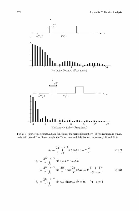
Example 1: Rectangular Waveform. As discussed in Sect. 7.2, the rectangularwaveform is defined by its period T , the duty factor δ and the amplitude Vo. To findits spectral diagram, it is convenient to choose the origin of time (t = 0) in such away that the time function is even (see Fig.C.1).

For even functions, the coefficients bn are all zero, and the values of a0 and an

can be computed using the relations (C.4). Defining τ = δT , we get

ao = 2Voδ

an = 2Vo

T

∫ +τ/2

−τ/2cos nω1t dt = 2Vo

πnsin

nω1τ

2= 2V0

πnsin nπδ

Finally, we get:

s(t) = Voδ

[1 + 2

∞∑n=1

sin nπδ

nπδcos nω1t

]ω1 = 2π

T(C.6)

As an example, Fig.C.1 shows two rectangular waveforms with duty-factor of 10and 30% respectively, and their spectral amplitude diagram for the first 30 harmonics.

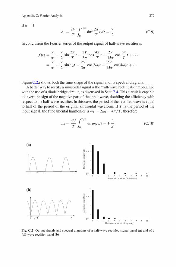
It is worth to note that the shorter pulse has greater amplitude of high frequencycomponents than the longer pulse.Example 2: Rectified Sinusoidal waveform. We calculate now the spectrum of asinusoidal signal after “cutting” its negative part. This waveform is obtained with asimple (nonlinear) circuit made by a diode and a resistor (see Sect. 7.4). The study ofthe rectified waveform is not purely academic as these signals are present as noise inlaboratories when a large amount of direct-current power is required (up to severalhundred kilowatts). The presence of multiple harmonics of the mains frequency (50or 60Hz corresponding respectively to angular frequency ω = 314 s−1 or 377 s−1)increases the probability to have electrical noise6 in the circuits downgrading thequality of the power distribution.

Let us start computing the Fourier series of the output of the half-wave rectifier(see Fig. 7.7a in Chap.7) when the input signal is v(t) = V sinωot . The output signalis the positive part of the input signal as shown in Fig.C.2a. During one wave periodT = 2π/ω the output signal is given by

f (t) ={

V sin(ωot) if 0 < t < T/2

0 if T/2 < t < T

Choosing the form (C.1) to represent the Fourier series, with ω1 = ωo = 2π/T , thecoefficients an and bn are

6 Electrical noise can be defined as all the components of the signals in the circuit not caused bythe input.

http://dx.doi.org/10.1007/978-3-319-31102-9_7

http://dx.doi.org/10.1007/978-3-319-31102-9_7

http://dx.doi.org/10.1007/978-3-319-31102-9_7


0 5 10 15 20 25 30

0 5 10 15 20 25 30

t−T/2 T/2

δT

t−T/2 T/2

Harmonic Number (Frequency)

Harmonic Number (Frequency)

δT

Fig. C.1 Fourier spectrum (|An | as a function of the harmonic number n) of two rectangular waves,both with period T =10 a.u., amplitude V0 = 1 a.u. and duty-factor, respectively, 10 and 30%

a0 = 2V

T

∫ T/2

0sinωot dt = V

2

π(C.7)

an = 2V

T

∫ T/2

0sinωot cos nωot dt

= 2V

T

∫ T/2

0sin

2π

Tt cos

2π

Tnt dt = V

1 + (−1)n

π(1 − n2)(C.8)

bn = 2V

T

∫ T/2

0sinωot sin nωot dt = 0, for n �= 1


If n = 1

b1 = 2V

T

∫ T/2

0sin2

2π

Tt dt = V

2(C.9)

In conclusion the Fourier series of the output signal of half-wave rectifier is

f (t) = V

π+ V

2sin

2π

Tt − 2V

3πcos

4π

Tt − 2V

15πcos

8π

Tt + · · ·

= V

π+ V

2sinωot − 2V

3πcos 2ωot − 2V

15πcos 4ωot + · · ·

FigureC.2a shows both the time shape of the signal and its spectral diagram.A better way to rectify a sinusoidal signal is the “full-wave rectification,” obtained

with the use of a diode bridge circuit, as discussed in Sect. 7.4. This circuit is capableto invert the sign of the negative part of the input wave, doubling the efficiency withrespect to the half-wave rectifier. In this case, the period of the rectified wave is equalto half of the period of the original sinusoidal waveform. If T is the period of theinput signal, the fundamental harmonics is ω1 = 2ω0 = 4π/T , therefore,

a0 = 4V

T

∫ T/2

0sinω0t dt = V

4

π(C.10)

0 1 82 3 4 5 6 7 9 100.0

0.5

0 1 82 3 4 5 6 7 9 100.0

1.0

t

t

T

T/2

Harmonic number (frequency)

Harmonic number (frequency)

Har

mon

ic a

mpl

itud

eH

arm

onic

am

plit

ude

(a)

(b)

Fig. C.2 Output signals and spectral diagrams of a half-wave rectified signal panel (a) and of afull-wave rectifier panel (b)

http://dx.doi.org/10.1007/978-3-319-31102-9_7


an = 4V

T

∫ T/2

0sinω0t cos nω1t dt

= 4V

T

∫ T/2

0sin

(2π

Tt

)cos

(4πn

Tt

)dt = 4V

π(1 − 4n2)(C.11)

bn = 4V

T

∫ T/2

0sinω0t sin nω1t dt = 4V

T

∫ T/2

0sin

(2π

Tt

)sin

(4πn

Tt

)dt = 0

(C.12)In conclusion the Fourier series of the output signal of full-wave rectifier is

f (t) = 4V

π

(1 − 1

3cos

4π

Tt − 1

15cos

8π

Tt − 1

35cos

12π

Tt + · · ·

)

Note that the mean value of the output signal of full-wave rectifier is 4V/π , twotimes greater than the half-wave rectifier. FigureC.2b shows time shape and spec-tral diagram of a full rectified-wave. As can be seen from the figure, the full-waverectification doubles the continous level component of the output, while it decreasesconsiderably the amplitude of the AC components with respect to the half-waverectifier.

C.1.2 The Fourier Transform

It is possible to obtain the spectral characteristic of nonperiodic signals using theFourier Transform or Fourier Integral. A heuristic method to understand the Fouriertransform takes into account the Fourier series in the form (C.3). Assumewe computethe Fourier series for a signal in the time interval −T,+T . Now, leaving the signalunchanged, increase the time interval in which the signal is defined to infinite T →∞; in this limit the discrete variable ω1n becomes a continuous variable ω1n → ω

and the sums become integrals in time.The formal definition of theFourier Transform (orFourier Integral) of the function

s(t) is

S(ω) =∫ +∞

−∞s(t) e− jωt dt (C.13)

The function S(ω) is called the spectrum of the signal s(t).The function s(t) can be obtained from the function S(ω) using the inverse trans-

form

s(t) = 1

2π

∫ +∞

−∞S(ω) e jωt dω (C.14)


−20

0

−10

1

0

2

10

3

20

4

0.0

0.2

0.4

0.6

0.8

0.0

1.0

1.0

t/T

ωT

(a)

(b)

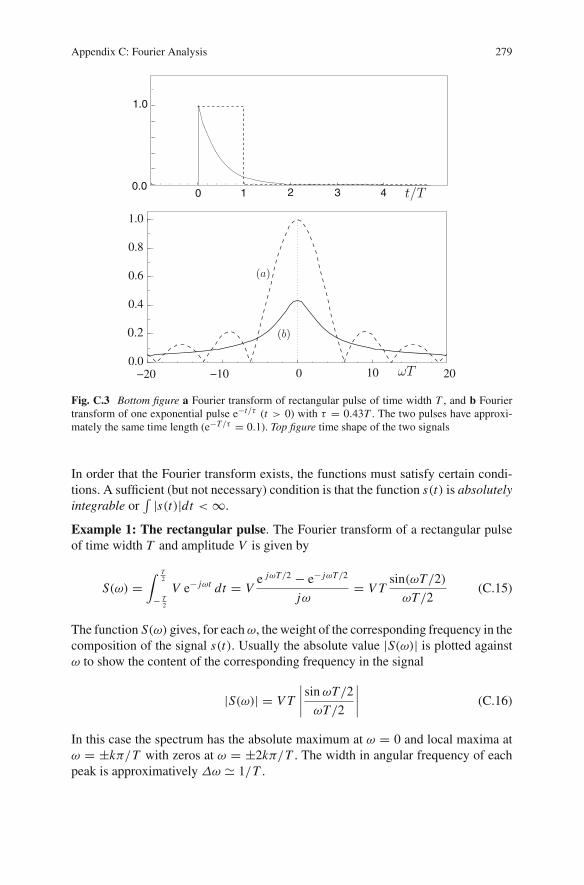
Fig. C.3 Bottom figure a Fourier transform of rectangular pulse of time width T , and b Fouriertransform of one exponential pulse e−t/τ (t > 0) with τ = 0.43T . The two pulses have approxi-mately the same time length (e−T/τ = 0.1). Top figure time shape of the two signals

In order that the Fourier transform exists, the functions must satisfy certain condi-tions. A sufficient (but not necessary) condition is that the function s(t) is absolutelyintegrable or

∫ |s(t)|dt < ∞.

Example 1: The rectangular pulse. The Fourier transform of a rectangular pulseof time width T and amplitude V is given by

S(ω) =∫ T

2

− T2

V e− jωt dt = Ve jωT/2 − e− jωT/2

jω= V T

sin(ωT/2)

ωT/2(C.15)

The function S(ω) gives, for eachω, the weight of the corresponding frequency in thecomposition of the signal s(t). Usually the absolute value |S(ω)| is plotted againstω to show the content of the corresponding frequency in the signal

|S(ω)| = V T

∣∣∣∣sinωT/2

ωT/2

∣∣∣∣ (C.16)

In this case the spectrum has the absolute maximum at ω = 0 and local maxima atω = ±kπ/T with zeros at ω = ±2kπ/T . The width in angular frequency of eachpeak is approximatively Δω � 1/T .


Example 2: The exponential pulse. As a second example, the Fourier transform ofan exponential pulse s(t) = s0e−t/τ (t > 0) is computed as

S(ω) =∫ ∞

0s0e

−t/τ e jωt dt = s0τ

1 + jωτ(C.17)

The modulus and the phase of S(ω) are respectively:

|S(ω)| = V0τ√1 + (ωτ)2

φ = arctanωτ (C.18)

In Fig.C.3 we show the Fourier transform of a rectangular pulse and an exponentialpulse of about the same time length.

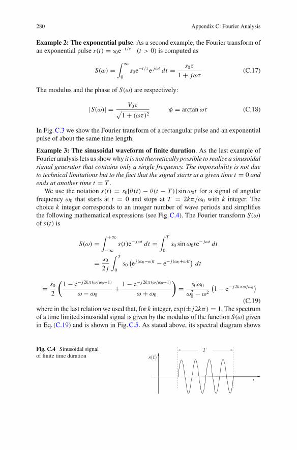
Example 3: The sinusoidal waveform of finite duration. As the last example ofFourier analysis lets us showwhy it is not theoretically possible to realize a sinusoidalsignal generator that contains only a single frequency. The impossibility is not dueto technical limitations but to the fact that the signal starts at a given time t = 0 andends at another time t = T .

We use the notation s(t) = s0[θ(t) − θ(t − T )] sinω0t for a signal of angularfrequency ω0 that starts at t = 0 and stops at T = 2kπ/ω0 with k integer. Thechoice k integer corresponds to an integer number of wave periods and simplifiesthe following mathematical expressions (see Fig.C.4). The Fourier transform S(ω)

of s(t) is

S(ω) =∫ +∞

−∞s(t)e− jωt dt =

∫ T

0s0 sinω0te− jωt dt

= s02 j

∫ T

0s0

(e j (ω0−ω)t − e− j (ω0+ω)t

)dt

= s02

(1 − e− j2kπ(ω/ω0−1)

ω − ω0+ 1 − e− j2kπ(ω/ω0+1)

ω + ω0

)= s0ω0

ω20 − ω2

(1 − e− j2kπω/ω0

)

(C.19)where in the last relation we used that, for k integer, exp(± j2kπ) = 1. The spectrumof a time limited sinusoidal signal is given by the modulus of the function S(ω) givenin Eq. (C.19) and is shown in Fig.C.5. As stated above, its spectral diagram shows

Fig. C.4 Sinusoidal signalof finite time duration

t

s(t)T


0.0 0.5 1.0 1.5 2.00

5

10

15

20

25

30

35ωoS(ω)

ω/ωo

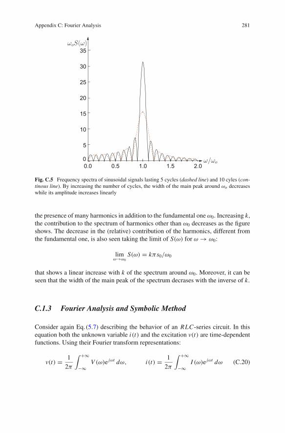
Fig. C.5 Frequency spectra of sinusoidal signals lasting 5 cycles (dashed line) and 10 cyles (con-tinous line). By increasing the number of cycles, the width of the main peak around ωo decreaseswhile its amplitude increases linearly

the presence of many harmonics in addition to the fundamental one ω0. Increasing k,the contribution to the spectrum of harmonics other than ω0 decreases as the figureshows. The decrease in the (relative) contribution of the harmonics, different fromthe fundamental one, is also seen taking the limit of S(ω) for ω → ω0:

limω→ω0

S(ω) = kπs0/ω0

that shows a linear increase with k of the spectrum around ω0. Moreover, it can beseen that the width of the main peak of the spectrum decrases with the inverse of k.

C.1.3 Fourier Analysis and Symbolic Method

Consider again Eq. (5.7) describing the behavior of an RLC-series circuit. In thisequation both the unknown variable i(t) and the excitation v(t) are time-dependentfunctions. Using their Fourier transform representations:

v(t) = 1

2π

∫ +∞

−∞V (ω)e jωt dω, i(t) = 1

2π

∫ +∞

−∞I (ω)e jωt dω (C.20)

http://dx.doi.org/10.1007/978-3-319-31102-9_5


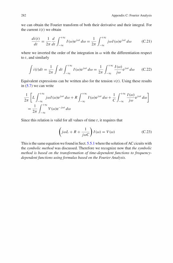
we can obtain the Fourier transform of both their derivative and their integral. Forthe current i(t) we obtain

di(t)

dt= 1

2π

d

dt

∫ +∞

−∞I (ω)e jωt dω = 1

2π

∫ +∞

−∞jωI (ω)e jωt dω (C.21)

where we inverted the order of the integration in ω with the differentiation respectto t , and similarly

∫i(t)dt = 1

2π

∫dt

∫ +∞

−∞I (ω)e jωt dω = 1

2π

∫ +∞

−∞I (ω)

jωe jωt dω (C.22)

Equivalent expressions can be written also for the tension v(t). Using these resultsin (5.7) we can write

1

2π

[L

∫ +∞

−∞jωI (ω)e jωt dω + R

∫ +∞

−∞I (ω)e jωt dω + 1

C

∫ +∞

−∞I (ω)

jωe jωt dω

]

= 1

2π

∫ +∞

−∞V (ω)e− jωt dω

Since this relation is valid for all values of time t , it requires that

(jωL + R + 1

jωC

)I (ω) = V (ω) (C.23)

This is the same equationwe found in Sect. 5.5.1where the solution ofACcicuitswiththe symbolic method was discussed. Therefore we recognize now that the symbolicmethod is based on the transformation of time-dependent functions to frequency-dependent functions using formulas based on the Fourier Analysis.

http://dx.doi.org/10.1007/978-3-319-31102-9_5

http://dx.doi.org/10.1007/978-3-319-31102-9_5

Index

AAC bridge circuits, 137AC coupling, 168, 170, 185Accuracy, 67, 80, 81ADC, 94, 174, 188Admittance, 4Aliasing, 188, 189Alternating signal

rectangular, 167sawtooth, 169sinusoidal, 166triangular, 166

AmmeterD’Arsonval, 84digital, 83full-scale, 82internal resistance, 82moving coil, 83perturbation introduced by, 82promptness, 89sensitivity, 85

Analog ohmmeter, evaluation of uncertainty,101

Analog oscilloscope, 182, 185Analog-to-digital converter, see ADCAND circuit, 94Attenuation, 141, 219Attenuation coefficient, 245Attenuation constant, 213Attenuation in decibel, 142Attenuator, compensated, 219Average power, 122

BBalanced, bridge, 35Bandwidth, 186, 219Bode’s diagrams, 141Bridge

Heaviside’s, 158Wheatstone’s, 34, 45, 137Wien’s, 139

CCapacitance, 14, 110, 120Capacitor

electrolytic, 19in parallel, 8in series, 8real, 15, 17

Cathode ray tube (CRT), 185Characteristic impedance, 235, 236

typical values, 239Class of the ammeter, 101Coaxial cable, 232, 238

capacity per unit length, 238inductance per unit length, 238

Coefficient of self-inductance, 8Compensated attenuator, 219Components

active, 4in alternating current, 110linear, 4nonlinear, 4passive, 4


283

284 Index

Conductance, 6Conductivity, 14Converter AC/DC, 174Correlated quantities, 72Correlation, 60Correlation coefficient, 61, 73Co-tree, 29Covariance, 60, 61Covariance matrix, 60Coverage factor, 63, 69Critical motion, 88

DDAC circuit, 94D’Arsonval, ammeter, 84Decibel, 141Differentiator, 205Digital sampling, 178Diode, 4, 37Displacement current, 111Distributed parameters, 110Drude, model of, 6

EEffective amplitude, see rmsElastance, 8Electrical permittivity, 14Error, 54

random, 55systematic, 55

Exponential pulse, 216Exponential signal, 204

FFourier transform, 235

GGeneralized Ohm’s law, 120Generator

controlled, 12current, 12real, 12voltage, 11

Graph, 29

HHeaviside θ function, 196Heaviside’s bridge, 158High-pass RC, 197

rectangular wave response, 200sinusoidal signal, 144voltage pulse response, 199voltage ramp response, 203voltage step response, 198

IIdeal line, 237Ideal transformer, 152Impedance, 4

input, 140output, 140

Impedance matching, 153, 154, 157Independent loops, 34Inductance, 8, 110, 119, 211, 218Inductors

in parallel, 10in series, 10

Input variables, 59, 66Instantaneous power, 122Integrator, 210

KKirchhoff’s laws, 27

for alternating current and voltage, 111for complex current and voltage, 120

LLinear circuits, 38Loop method, 37Lossless line, 237Low-pass RC, 206, 207

integrator, 210rectangular waveform response, 207voltage pulse response, 207voltage ramp response, 209voltage step, 206

Lumped parameters, 3, 110, 141

MMagnetic permeability, 14Mathematical model, 66Maximum power transfer, 153Maximum power transfer theorem, 46Measurement

of impedance, 178of phase, 178, 191, 192of reactive components, 138of resistance, 97, 98

Measurement error, 54

Index 285

Method of loops, 121Method of meshes, 32, 34Method of nodes, 30, 121Multiple reflections, 242Mutual induction, 9Mutual induction coefficient, 10, 148

NNode, 27, 29Norton’s theorem, 42, 125, 131Nuclear magnetic resonance, 157Nyquist frequency, 188

OOhmmeter, 98

sensitivity of, 99Open-circuit, 12Operational amplifier, 20, 95, 175, 176Oscilloscope synchronization, 185Output impedance, 42

PParasitic capacitance, 212Parasitic inductance, 218, 219Passband, 164, 176Phase, measure of, 191Phase, measurement of, 178, 192Phasors, 116Power, 22, 44Power balance, 43

in transformer, 153Power factor, 123Precision, 80, 81Probe, 186Promptness, 81, 89Propagation constant, 236Propagation of uncertainties, 61Pulse, 199, 207

QQ factor, 128Quality factor, 128

RLC parallel, 131RLC series, 129

RR-2R ladder, 105Random error, 55Range, 81

RC high-pass, 144, 145, 199, 205differentiator, 147

RC low-pass, 142, 144, 207, 209, 210integrator, 147sinusoidal signal, 142

Reactance, 121Real inductor, 15Reciprocity theorem, 43, 106, 124Reflection coefficient, 240, 242Resistance, 6, 14Resistor, 6

carbon composition, 16color code, 16real, 15SMD, 16thin film, 16wire wound, 16

Resonance, 128, 132Resonant circuits, 128Rise time, 207RL circuits, 146, 147, 211RLC parallel, 131, 212RLC series, 115, 128, 215, 216Rms, 108

SSelf induction coefficient, 110Sensitivity, 80, 85

of ohmmeter, 99of voltmeter, 91

Sensitivity coefficients, 60, 66, 69Series-parallel transformation, 135Short-circuit, 12Shunt, 83Signal frequency, 108Signal period, 108Skin depth, 21Skin effect, 20, 245Special generators

open-circuit, 12short-circuit, 12

Static transformer, 148, see also transformerStep signal, 196Stray capacitance, 219Stray inductance, 218Superposition theorem, 38, 124Systematic error, 55

TTelegrapher equation, 234Temperature coefficient, 16, 17, 69

286 Index

Thévenin’s theorem, 39, 105, 125proof, 40

Theorem ofmaximum power transfer, 46Norton, 42, 125open circuit and short circuit, 42reciprocity, 43, 124superposition, 124Thévenin, 39, 105, 125

Thermal AC/DC converter, 176Thermal expansion coefficient, 17Time domain

analysis, 195Transfer function, 140, 141, 143Transformer, 148, 149

coupling coefficent, 148ideal, 153power balance, 153real, 149transformation ratio, 153

Transient, 107, 113, 164Transmission line

attenuation length measurement, 245characteristic impedance, 236ideal, 237input impedance, 246multiple reflections, 242propagation constant, 236propagation speed, 234propagation velocity, 237reflection coefficient, 240sinusoidal regime, 246

Tree, 29, 34Trigger oscilloscope, 185

True value, 54TTL, 94

UUncertainty, 56

analog ohmmeter, 101correlated measurements, 71coverage factor, 63propagation, 61type A and type B, 57

Uncertainty for monomial functions, 62

VValue, 54Vectorial instrument, 178Voltage comparator, 92Voltage divider, 219Voltage ramp, 203, 209Voltmeter, 90

digital, 91electrostatic, 95perturbation introduced by, 90“sensitivity”, 91

WWave speed, 234Wheatstone’s bridge, 34, 45, 137

balanced, 35Wien’s bridge, 139Working range or range, 81

laboratory experiments

Documents