structural connectivity to reconstruct brain activation ... - hal-inria

HAL Id: hal-02945585https://hal.inria.fr/hal-02945585

Submitted on 17 Feb 2021

HAL is a multi-disciplinary open accessarchive for the deposit and dissemination of sci-entific research documents, whether they are pub-lished or not. The documents may come fromteaching and research institutions in France orabroad, or from public or private research centers.

L’archive ouverte pluridisciplinaire HAL, estdestinée au dépôt et à la diffusion de documentsscientifiques de niveau recherche, publiés ou non,émanant des établissements d’enseignement et derecherche français ou étrangers, des laboratoirespublics ou privés.

Structural connectivity to reconstruct brain activationand effective connectivity between brain regions

Brahim Belaoucha, Théodore Papadopoulo

To cite this version:Brahim Belaoucha, Théodore Papadopoulo. Structural connectivity to reconstruct brain activationand effective connectivity between brain regions. Journal of Neural Engineering, IOP Publishing,2020, 17 (3), pp.035006. �10.1088/1741-2552/ab8b2b�. �hal-02945585�

https://hal.inria.fr/hal-02945585

https://hal.archives-ouvertes.fr

Submitted to non-invasive brain imaging special issue

Structural connectivity to reconstruct brain activation andeffective connectivity between brain regions

Brahim Belaoucha*, Théodore Papadopoulo

Inria, Université Côte d’Azur

ABSTRACTUnderstanding how brain regions interact to perform a specific task is very challenging. EEG and MEG are twonon-invasive imaging modalities that allow the measurement of brain activation with high temporal resolution.Several works in EEG/MEG source reconstruction show that estimating brain activation can be improved by con-sidering spatio-temporal constraints but only few of them use structural information to do so. In this work, wepresent a source reconstruction algorithm that uses brain structural connectivity, estimated from diffusion MRI(dMRI), to constrain the EEG/MEG source reconstruction. Contrarily to most source reconstruction methodswhich reconstruct activation for each time instant, the proposed method estimates an initial reconstruction for thefirst time instants and a multivariate autoregressive model that explains the data in further time instants. This au-toregressive model can be thought as an estimation of the effective connectivity between brain regions. We calledthis algorithm iterative Source and Dynamics reconstruction (iSDR). This paper presents the overall iSDR ap-proach and how the proposed model is optimized to obtain both brain activation and brain region interactions.The accuracy of our method is demonstrated using synthetic data in which it shows a good capability to recon-struct both activation and connectivity. iSDR is also tested with real data obtained from [dataset] (face recogni-tion task). The results are in phase with other works published with the same data and others that used differentimaging modalities with the same task showing that the choice of using an autoregressive model gives relevant re-sults.

Keywords: Autoregressive model, EEG/MEG source reconstruction, diffusion MRI, effective connectivity.

1 INTRODUCTIONThere are three main techniques to reconstruct brain activity from EEG/MEG measurements. Dipole fitting as-sumes that the measurements are generated from a fixed number of sources (a few active regions). Its optimizationis nonlinear and non-convex and computationally expensive even when considering a relatively small number ofpossible active regions. Scanning techniques avoid this complexity issue by scanning through regions of interests(ROIs) [beamformer, music, Roninson-etal:99, Gross-etal:01, Mosher-etal:99]. Most scanning techniquesassume some statistical properties on sources and noise (asynchronous, uncorrelated). These properties are usedto derive an optimization criterion that aims at identifying the activated sources. They are also sometimes used toestimate the "dimension" of the signal space in order to achieve a separation between the sources and noise spaces.Finally, distributed models use a significantly large number of sources distributed over the brain substrate or vol-ume and estimate a kind of activation probability. Because the size of the sensor array of EEG/MEG is muchsmaller than the usual dimension of the source space, the distributed model is ill-posed and a prior has to be usedto obtain a unique solution. Many priors lead to convex (and sometimes even linear) problems, which makes dis-tributed models attractive. Distributed models were originally designed to work for reconstructing sources for asingle time instant but were generalized to deal with reconstructing sources in a time window allowing to con-straint sources not only spatially but also temporally [hamalainen-sarvas:89, pascual-marqui-michel-etal:94,gramfort:hal-00690774].


We denote the number of sensors by Nc, the number of sources by Ns and the number of time samples by T . Thegain matrix (lead-field) G is a real matrix of size Nc×Ns, obtained by solving the forward problem [meijs-peters:87,Meijs1988, hamalainen-sarvas:89, yvert-bertrand-etal:95, dassios-kariotou:03]. It allows us to relate cor-tical activation J ∈ RNs×T and the MEG/EEG measurements M ∈ RNc×T with:

M = GJ + E Equation 1.

where E ∈ RNc×T is the measurement noise.

Setting a prior on the source space consists of assuming that the prior term P (J) is small for a given source esti-mate J. A good source estimate is obtained according to the following minimization:

J∗ = argminJ,λ

U(J) = D(M,J) + λP (J) . Equation 2.

where λ is a positive number that controls the trade-off between the data fit term D(M,J) which quantifies howwell the source estimates explains the measured signal and the regularity of the estimate. Although such methodscan deal with temporal or spatio-temporal priors, very often only spatial priors are used because it is easier to con-sider independent time sample reconstruction as it makes the reconstruction faster. Very often also, it is assumedthat sources are centered and follow a Gaussian distribution. In that case, an optimal source reconstruction can beestimated linearly source by minimizing the following cost function:

U(J) = ‖M−GJ‖2F + λ ‖WJ‖2F Equation 3.

where λ is a positive number used to balance D and P . This method is also known as Tikhonov regularization(Ridge Regression) [Tikhonov]. Several methods can be found in the literature that use this formulation, theydiffer mostly by the choice of the weighting matrix W.

The minimum norm estimate (MNE) sets W to the identity matrix in Equation 3 [hamalainen1984interpreting].It is known that MNE overestimates the extent of the activity regions due to underestimating the magnitude of ac-tive sources resulting from the use of l2 norm. Due to its simple linear solution, this approach remains attractive.In the low resolution brain electromagnetic tomography (LORETA) reconstruction [pascual-marqui-michel-etal:94],W is set to LTL where L is the 3D-discretized Laplacian matrix of the source space. The ith row of L acts like adiscrete differentiating operator by computing differences between the ith node of the source space and its directneighbors. This method provides the solution with the maximum spatial smoothness. In the general case, whenW is different from the identity matrix, we need to invert a big matrix of size Ns × Ns which is computationallyexpensive.

Some nonlinear approaches favor specific source configurations. In Minimum Current Estimate – MCE or LASSO– ([MatsuuraMCE]), few sources are active at each time sample. The solution is obtained by solving the follow-ing functional for each time instant independently [MatsuuraMCE, phdGramfort]:

Jλ = argminJ

1

2‖M−GJ‖22 + λ ‖J‖1 , λ > 0.

This results in non-continuous source activation in both time and space, as it can be seen as promoting spatialsparsity independently at each time instant. It thus fails to recover smooth time courses of cortical sources. Toovercome this limitation, structured sparsity can be used. In the Mixed Norm Estimate (MxNE) [gramfort:hal-00690774],the regularization term induces both spatial sparsity and temporal smoothness of sources by using a mixed norm


l21 instead of l1 norm. l21−norm is defined as:

‖J‖21 =∑i

√∑j

Ji(j)2 , Equation 4.

where the sum over i is over sources (spatial position) and the sum over j is the sum over time samples i.e. thel21-norm corresponds to the sum of the l2-norm of individual source time courses. The solution for such a criterioncan be found in [phdGramfort, gramfort:hal-00690774]. MxNE results in few active sources in a given timewindow. Like MNE, it underestimates the source activity due to the use of the l2 norm and soft-threshold, whichis used to solve the minimization, over the time courses [irMxNE].

All of the above methods do not use any structural information to constrain the source space. In [passingham-stephan-etal:02,Sporns2004418, tomassini-jbabdi-etal:07, finger-etal:16, osher-etal:16], authors show that structural con-nectivity (connections between neurons through the white matter) can be an indicator of functional homogeneityof cortical regions. Diffusion magnetic resonance imaging (dMRI) is a non-invasive modality that allows the accessto brain structural connectivity [einstein:05, einstein:56, stejskal-tanner:65, basser-mattiello-etal:94a, fdt].As it is known that EEG/MEG can only "see" activations corresponding to coherent sources spreading across afew cm2 of cortex, it seems interesting and justified – to some extent – to integrate the knowledge of the functionalregions as provided by dMRI in the EEG/MEG reconstruction problem.

As stated above, only few works use diffusion MRI in conjunction with EEG/MEG measurements to reconstructthe brain activity. dMRI was first used as a pure spatial prior in the MEG/EEG inverse problem. In [Hammond-etal:12,hammond-etal:13], dMRI is used to create a network of connected brain regions. Assuming that connected re-gions should have similar activities, they look for a solution of the EEG source reconstruction problem that issmooth across this network. In [philippe:13], dMRI is used again to parcellate the cortex into functional regions.These regions are then used to spatially constrain the source reconstructions to promote solutions that are eitherconstant or smooth in functional regions. In [Knosche20137], the authors use regions defined by dMRI to defineLORETA patch-based algorithm i.e. smooth sources inside patches. The structural connectivity between brain re-gions was also used to reconstruct brain activity by imposing a stronger penalty for regions with weak anatomicalconnections [PinedaPardo2014765]. More elaborate time models have also been designed. In [galka-okito-etal:04],the authors modeled the brain activity at each source location i by:

Jt(i) = aiJt−1(i) + bi∑j 6=i

Jt−1(j) + εt

where εi is noise at the source location i and the sum is over the direct neighbors of i. In their method, there areonly two parameters per source (ai, bi) to be estimated which reduces the dynamics that their model can explain.In this model, for a given time window, only 3 × Ns parameters (J0(i),ai, bi), i = 1..Ns need to be estimated in-stead of the T × Ns parameters that would be estimated with standard spatio-temporal models. This model wassimplified in [long-purdon-etal:06], by simply assuming ai = 1 and bi = 1

ni, where ni the number of neighbors

of node i, so the solution for a given time window only requires estimating Ns parameters (as in the purely spa-tial problem for one time instant). In [lamus-etal:12], the same 3 × Ns need to be estimated but the activities ofneighboring sources are weighted by their distances to source i.

Another nonlinear model is considered in [giralso-dendekker-etal:10]. They modeled the brain activity as fol-lows:

Jt = (a1I + b1L)Jt−1 + a2J2t−1 + a3J

3t−1 + a4Jt−2 + εt

where L is a Laplacian operator applied to neighboring sources. Although this nonlinear model could explain morecomplex dynamics compared to the previous mentioned work, it uses only 5+2×Ns parameters (J0, J1 and a1, b1,a2, a3, a4) to explain source dynamics.


Finally, only few works use MAR models combined with dMRI information to constrain sources’ dynamics. [fukushima-yamashita-etal:12,fukushima-yamashita-etal:13, Fukushima2015408] also start by extracting a network of connected brain re-gions, but in addition to the spatial constraints, the authors use this network to temporally constrain the sources’dynamics by assuming a multivariate autoregressive model (MAR) whose elements are constrained by anatomicalconnections obtained from dMRI. The MAR model is defined by:

Jt =

K∑k=1

AkJt−∆k+ εt ,

where ∆1:K contains all the considered time lags. The only possible nonzero elements of the MAR matrices Ak, k =

1..K are the elements corresponding to anatomical connections between a pair of sources/regions extracted fromdMRI. The time-lag, in their method, for each pair of sources/regions is fixed by the length of the pathways be-tween them. Consequently, nonzero MAR coefficients never overlap between matrices, which reduces the degree offreedom of the model [Fukushima2015408]. A dynamic hierarchical variational Bayesian (dhVB) method is usedto estimate both the sources magnitudes and their interactions. Their method is time-consuming (days for realistichead models) and has several parameters to tune. Unfortunately, the code of dhVB is not published and cannot beused to compare iSDR to dhVB.

Our approach (presented in the next section), follows a similar model. The model has thus more degrees of free-dom compared to [long-purdon-etal:06, giralso-dendekker-etal:10, lamus-etal:12], which allows us to ex-press more complex source configurations. Furthermore, in addition to anatomical connections obtained from dMRI(like in the work of [fukushima-yamashita-etal:13]), we also assume that neighboring cortical regions are con-nected. Part of this work was presented in [belaoucha-etal-embs:16, belaoucha:tel-01534876].

2 METHODS AND PROCEDURES2.1 The iSDR method

In our method, we assume that sources’ dynamics follow a stable MAR model in the time window of interest [1, T ]

whose elements are constrained by neighboring and anatomical connected regions.

Jt =

p∑i=1

AiJt−i + εt ,

where the matrices Ai, i ∈ [1, p] contain non-zero elements only for neighbor sources or sources connected throughwhite matter.

This formulation provides more degree of freedom in the model compared to [Fukushima2015408] as it allowstwo brain regions/sources to interact at p different time lags which allows us to explain complex brain activations.

The T time samples in the window of interest are numbered in the range [1, T ]. We rewrite the MxNE functionalby considering only the EEG/MEG samples in the range [p+1, T ] (as the ones in the range [1, p] depend – throughthe MAR model – on samples that are outside the window of interest) and relate them to sources magnitudes inthe range [1, T − 1]. The rewritten functional takes the form:

U(J) = ‖Mv −GdJv‖22 + λ ‖J‖21 Equation 5.

where

• Mv = vec(M), M ∈ RNc×(T−p), represents the measurements between p+ 1 and T .

• Jv = vec(J), J ∈ RNs×(T−1) contains the sources’ activity between the first time sample and T − 1.


• Gd ∈ RNc(T−p)×Ns(T−1) is a spatio-temporal lead-field that will be further described below.

vec(.) is the vectorization operator that transforms a matrix into a vector by stacking all it columns. It is worthmentioning that while the first p measurements are not part of the criterion 5, the first p source values are not ne-glected as they are predicted from the future MEG/EEG measurement t > p. The matrix Gd is a block matrix ofthe form:

Gd =

Gp Gp−1 · · · G2 G1

Gp Gp−1 · · · G2 G1

. . . . . . . . . . . .Gp Gp−1 · · · G2 G1

, Equation 6.

where Gi = GAi, i ∈ [1, p], with G being the standard lead-field matrix. Our approach can be seen as an exten-sion to the work of [gramfort:hal-00690774] in which, in addition to spatial sparsity, we constrain the dynamicsof sources interactions. Thus activated regions are constrained to be spatially sparse in a time window of T sam-ples.

The data fidelity term in Equation 5 includes errors coming both from the MAR model and source reconstruction.This functional can be seen as an extension to MxNE [gramfort:hal-00690774, irMxNE]. The major improve-ment of our method with compared to MxNE and irMxNE [irMxNE] is that the interactions between sources areincluded in the functional. In our work, the weights are not only in the diagonals of Ai matrices like in irMxNEbut also contains nonzero elements that correspond to the neighbors or anatomical connections. These weights areestimated from the following functional:

V (A) = ‖J∗v −Q′A′v‖22 Equation 7.

where Av = vec(A) is the vectorial form of A =[A1, · · · ,Ap

]. Av is a vector of size pN2

s . A′v is the sub-vector ofthe non-zero components of Av and can be written A′v = SAAv. SA is a selection matrix of size KA × pN2

s , whereKA is the total number of the non-zero coefficients in the various Ai i ∈ [1, p]. SA is a rectangular matrix whereeach row contains exactly one single non-zero coefficient equal to 1. J∗v is the vectorial form of sources’ magnitudesin the range [p+ 1, T ]. Q is a Ns(T − p)× pN2

s matrix:

Q =

D(Jp) D(Jp−1) · · · D(J1)

D(Jp+1) D(Jp) · · · D(J2)...

.... . .

...D(JT−1) D(JT−2) · · · D(JT−p)

Equation 8.

where D(Jk) is the Ns ×N2s matrix:

D(Jk) =

JTk 0 · · · 0

0 JTk · · · 0...

.... . .

...0 0 · · · JTk

Q′ = QSA

T is the submatrix of Q of size Ns(T − p) ×KA, which contains only the columns corresponding to thenon-zero entries of Av.


The Maximum Likelihood (ML) solution minimizing V (A) for the MAR coefficients A is [Weisberg-etall:05](Ordinary Least Square solution):

Av = SATA′v = SA

T (Q′TQ′)−1Q′TJ∗v Equation 9.

The full optimization problem of simultaneously minimizing U(J) and V (A) over Jv and A is non-convex, butcan be solved by solving a sequence of weighted convex optimization problem (MxNE) with weights being definedbased on the previous sources’ estimates by minimizing the functional V .U(Jk) =

∥∥∥Mv −Gdk−1Jkv

∥∥∥2

2+ λ

∥∥Jk∥∥21

V (Ak) =∥∥J∗kv −Q′kA′kv

∥∥2

2

Equation 10.

where Gkd is Gd (Equation 6) obtained from the kth estimate of the MAR model elements and Q′k is obtained

from the kth iteration of the sources magnitudes using Equation 8. iSDR consists in iterating between two steps.We call S-step (MxNE) the part of iSDR that consists in optimizing U . The A-step consists in estimating theMAR elements by minimizing V from the result of the S-step (i.e. with J∗v and Q′ fixed).

S-step:

It estimates the source activation for a given MAR model i.e solving the modified MxNE problem. Block coordi-nate descent is used to find the solution [gramfort:hal-00690774, belaoucha-etal-embs:16, belaoucha:tel-01534876].

A-step:

It consists first in constructing the matrix Q′ and the vector J∗v from the output of the S-step i.e. Jk. Then, it es-timates the MAR elements using Equation 9 and each MAR elements of a source is normalized by its maximumabsolute value (this allows to avoid the scale ambiguity between Ai and J). The MAR elements are saved in thevector Ak

v . There is no need to re-scale the sources correspondingly as those will be re-estimated during the nextS-step, which will take account of the re-scaling.

Improving the convergence speed

If a source s, at a given iteration k, is found to be inactive, there exists no causality between this source and theremaining sources. To reduce the computation time, the A-step removes the corresponding MAR weights of thissource and consequently the corresponding columns of Q′. We also remove the contribution of inactive sourcesinto the measurement i.e. the rows of Q′ and J∗v that correspond to inactive sources1. Consequently, if source sis inactivated at a given iteration k, it will remain inactive for all subsequent iterations. This also means that thesparsity of sources promoted by the regularization term of MxNE also promotes sparsity in A.

Initialization

The algorithm starts with an S-step. Thus the first source estimation depends on the initialization of the MARmodel. The effect of different initialization of Ai is outside the scope of this paper2. In this work, we initialize theMAR model in such a way to obtain an initial S-step solution close to the MxNE estimate. This is done by initial-izing A1 to the identity matrix and the remaining Ai, i ∈ [2, p] to zero matrix.

Stopping criteria1While this can be seen as updating the matrix SA and introducing another selection matrix on sources, it is better achieved by

simply removing rows and columns in the matrices2The interested reader is referred to [belaoucha:tel-01534876]


iSDR includes three stopping criteria. The first is when a maximum number of iterations is reached. The secondtests if there is no significant change in the iSDR estimates between two successive iterations. The last stoppingcriterion compares the size of active sources obtained in iteration k and k − 1. If they are the same, the algorithmstops.

2.2 Experimental data

We used the real dataset described in Wakeman et al. [dataset]. MEG/EEG data were simultaneously recordedduring a face recognition task where a subject is shown famous, unknown or scrambled faces. The dataset alsocontains dMRI and T1 images. The stimuli (photos) were projected onto a screen (black background with a whitefixation cross in the center) approximately 1.3 m in front of the participants. The start of the trial was indicatedby the appearance of the fixation cross for a random duration. A gray-scale photograph was then projected ontothe screen for a random duration between 800 and 1000 ms. The interval between two successive face projectionsis 1700 ms [dataset]. Both MEG (Elekta Neuromag Vectorview 306 system, 102 magnetometers, and 204 gra-diometers) and EEG (70 electrodes conforming to the extended 10-10 system) were measured in a light magnet-ically shielded room. The data was presented to the subjects in six runs of 7.5 min each. In this work, we haveused the data of the eleven subjects that have T1 and dMRI images.

2.3 Data pre-processing

Environmental noise was removed using Signal Space Separation (SSS) [Taulu-etal:05]. The EEG and MEG datawere filtered using a low-pass filter with a cutoff frequency of 35 Hz. This frequency was chosen because somestudies reported the presence of gamma-band in complex visual stimuli [Lachaux2005491]. We averaged the dataof each condition (Familiar, Unfamiliar, Scrambled). We focus on the brain regions responsible for face percep-tion and recognition. To do so, we subtracted the average measurement with famous pictures to that of scrambledfaces.

Down-sampling

In [Horowitz2015], the authors show a correlation between the axon diameter and conduction velocity in the hu-man brain. They have found the ratio between axon diameter and the axon conduction velocity to be 8.75 m/sfor each µm, which coincide with what was obtained before in [Aboitiz1992143]. This results in speeds between10 and 40 m/s for the majority of fibers. The average in this case is 25 m/s. The length of bundles can range be-tween 50mm for U-shape connections to 100 mm for long connections. Thus the time needed to travel from thesource to the target region is between 2 to 4 ms. This is why we decided to down-sample the measurements to 367Hz (1 sample every 3ms).

MEG/EEG forward model

The T1 MRI images were processed with BrainStorm [brainstorm] to extract the geometrical model of the head.The forward EEG/MEG model was obtained using OpenMEEG [Gramfort2010] from BrainStorm consideringfive surfaces: scalp, inner and outer skull and white and grey cortical surfaces.

Cortical surface parcellation

The cortical surfaces of all participants were parcellated into regions using the MNN approach and Tanimoto simi-larity measure with parameter T = 800 [belaoucha-clerc-etal:16] using structural connectivity obtained by fibertracking. It results in cortical regions of around 100mm2 [belaoucha:tel-01534876], which is about the mini-mum size of detectable activations [RevModPhys_65_413]. The parcellation algorithm resulted in an averageof 592.36 regions with a standard deviation (SD) equal to 19.75. In this work, we assume a constant activation percortical region. This allows us to greatly reduce the dimension of the source space from the number of nodes of the


cortical mesh (1̃0k typically used in the distributed sources model) to the number of cortical regions.

Fiber tracking

In the literature, two types of local fiber tracking can be found. Deterministic tracking follows the direction offibers at each image voxel [basser-pajevic-etal:00]. In this model the tracking error is cumulative. Probabilistictracking thus introduces a stochastic dimension in the estimation of fiber direction at each image voxel [Smith-Jenkinson-etal:04,behrens-johansen-berg-etal:07]. Consequently, it is less affected by error in the local fiber direction. This iswhy we used the latter method as implemented in FSL [Smith-Jenkinson-etal:04] to estimate the structuralconnectivity between brain regions.

2.4 Choice of regularization parameter value

In [belaoucha:tel-01534876, belaoucha-etal-embs:16], λ is obtained using a cross-validation technique [arlot2010].But because this is very time consuming when using the MxNE based solver, we decided to use the following ap-proach, which gives similar results.

We want to consider the complexity of the obtained MAR model as measured by p. For low values of p, more sourcesare detected to be active which yields a high number of effective connections to be estimated. For bigger values ofp, fewer regions are detected to be active hence fewer parameters need to be estimated, which results in higher er-ror in explaining the EEG/MEG measurements. We thus need to find a middle ground between explaining wellthe measurements and minimizing the complexity of MAR model. To do so, we consider the following criterion:

CR =‖M−Me‖2‖M‖2

+√pNAKA

Equation 11.

where Me is the reconstructed measurement, NA is the number of estimated non-zero MAR elements and KA isthe total number of allowed connections. The first term is increases with λ whereas the second term is negativelycorrelated to λ. The optimal λ for each EEG/MEG measurements is the value that corresponds to smallest CR.

3 RESULTS AND DISCUSSIONWe start testing iSDR by using synthetic data and compare its results to the ones obtained from 2 other EEG/MEGsource reconstruction methods (MxNE and Lasso). In the second part, we use the real data obtained from [dataset].The iSDR reconstruction is compared to the results obtained by other works using the same dataset and to otherresults based on different datasets but using the same task i.e. face recognition.

3.1 Synthetic data

In this section, we use synthetic data to investigate the accuracy of iSDR method. We compare its reconstructionaccuracy with those of two other sparse approaches, MxNE and Lasso. It is clear that the comparison is somewhatunfair to those methods as the model used to generate the simulated data is the one used in the iSDR approach.On the other hand, it should be remembered that iSDR explains the data with much less parameters than MxNeor Lasso. Elements of the lead-field matrix (10 × 400) are randomly generated from a zero-mean normal distribu-tion with a unit standard deviation. Each column, contribution of a source to the measurement, is then normalizedto give the same importance to the different sources. For putative connexions, we randomly connect five sources toeach source.

We use the following simple model:{Jt(S1) = 0.9Jt−1(S1)− 0.15Jt−1(S2)

Jt(S2) = 0.25Jt−1(S1) + 0.97Jt−1(S2)


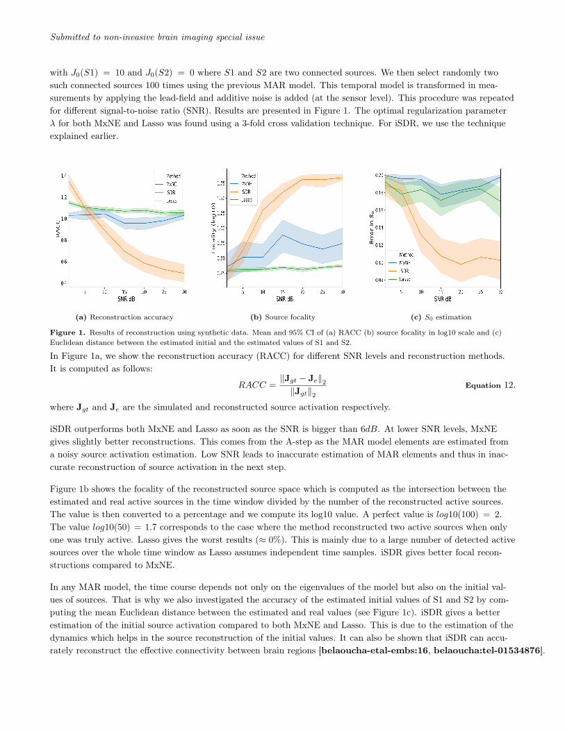
with J0(S1) = 10 and J0(S2) = 0 where S1 and S2 are two connected sources. We then select randomly twosuch connected sources 100 times using the previous MAR model. This temporal model is transformed in mea-surements by applying the lead-field and additive noise is added (at the sensor level). This procedure was repeatedfor different signal-to-noise ratio (SNR). Results are presented in Figure 1. The optimal regularization parameterλ for both MxNE and Lasso was found using a 3-fold cross validation technique. For iSDR, we use the techniqueexplained earlier.

(a) Reconstruction accuracy (b) Source focality (c) S0 estimation

Figure 1. Results of reconstruction using synthetic data. Mean and 95% CI of (a) RACC (b) source focality in log10 scale and (c)Euclidean distance between the estimated initial and the estimated values of S1 and S2.

In Figure 1a, we show the reconstruction accuracy (RACC) for different SNR levels and reconstruction methods.It is computed as follows:

RACC =‖Jgt − Je‖2‖Jgt‖2

Equation 12.

where Jgt and Je are the simulated and reconstructed source activation respectively.

iSDR outperforms both MxNE and Lasso as soon as the SNR is bigger than 6dB. At lower SNR levels, MxNEgives slightly better reconstructions. This comes from the A-step as the MAR model elements are estimated froma noisy source activation estimation. Low SNR leads to inaccurate estimation of MAR elements and thus in inac-curate reconstruction of source activation in the next step.

Figure 1b shows the focality of the reconstructed source space which is computed as the intersection between theestimated and real active sources in the time window divided by the number of the reconstructed active sources.The value is then converted to a percentage and we compute its log10 value. A perfect value is log10(100) = 2.The value log10(50) = 1.7 corresponds to the case where the method reconstructed two active sources when onlyone was truly active. Lasso gives the worst results (≈ 0%). This is mainly due to a large number of detected activesources over the whole time window as Lasso assumes independent time samples. iSDR gives better focal recon-structions compared to MxNE.

In any MAR model, the time course depends not only on the eigenvalues of the model but also on the initial val-ues of sources. That is why we also investigated the accuracy of the estimated initial values of S1 and S2 by com-puting the mean Euclidean distance between the estimated and real values (see Figure 1c). iSDR gives a betterestimation of the initial source activation compared to both MxNE and Lasso. This is due to the estimation of thedynamics which helps in the source reconstruction of the initial values. It can also be shown that iSDR can accu-rately reconstruct the effective connectivity between brain regions [belaoucha-etal-embs:16, belaoucha:tel-01534876].


0 20 40 60 80 100max

%

0

20

40

60

80

100

NR

iSD

RN

RM

xNE %

MAR

p=1p=2p=3p=4

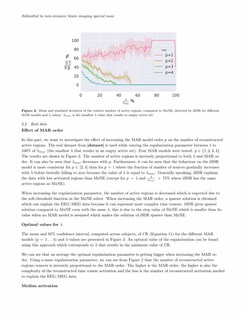
Figure 2. Mean and standard deviation of the relative number of active regions, compared to MxNE, detected by iSDR for differentMAR models and λ values. λmax is the smallest λ value that results to empty active set.

3.2 Real data

Effect of MAR order

In this part, we want to investigate the effect of increasing the MAR model order p on the number of reconstructedactive regions. The real dataset from [dataset] is used while varying the regularization parameter between 1 to100% of λmax (the smallest λ that results in an empty active set). Four MAR models were tested: p ∈ {1, 2, 3, 4}.The results are shown in Figure 2. The number of active regions is inversely proportional to both λ and MAR or-der. It can also be seen that λmax decreases with p. Furthermore, it can be seen that the behaviour on the iSDRmodel is more consistent for p ∈ [2, 4] than for p = 1 where the fraction of number of sources gradually increaseswith λ before brutally falling to zero because the value of λ is equal to λmax. Generally speaking, iSDR explainsthe data with less activated regions than MxNE (except for p = 1 and λ

λmax> 75% where iSDR has the same

active regions as MxNE).

When increasing the regularization parameter, the number of active regions is decreased which is expected due tothe soft-threshold function in the MxNE solver. When increasing the MAR order, a sparser solution is obtainedwhich can explain the EEG/MEG data because it can represent more complex time courses. iSDR gives sparsersolution compared to MxNE even with the same λ, this is due to the step value of MxNE which is smaller than itsvalue when no MAR model is assumed which makes the solution of iSDR sparser than MxNE.

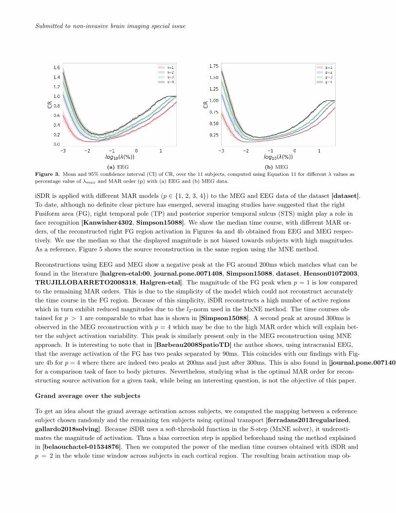
Optimal values for λ

The mean and 95% confidence interval, computed across subjects, of CR (Equation 11) for the different MARmodels (p = 1 . . . 4) and λ values are presented in Figure 3. An optimal value of the regularization can be foundusing this approach which corresponds to λ that results in the minimum value of CR.

We can see that on average the optimal regularization parameter is getting bigger when increasing the MAR or-der. Using a same regularization parameter, we can see from Figure 2 that the number of reconstructed activeregions/sources is inversely proportional to the MAR order. The higher is the MAR order, the higher is also thecomplexity of the reconstructed time course activation and the less is the number of reconstructed activation neededto explain the EEG/MEG data.

Median activation


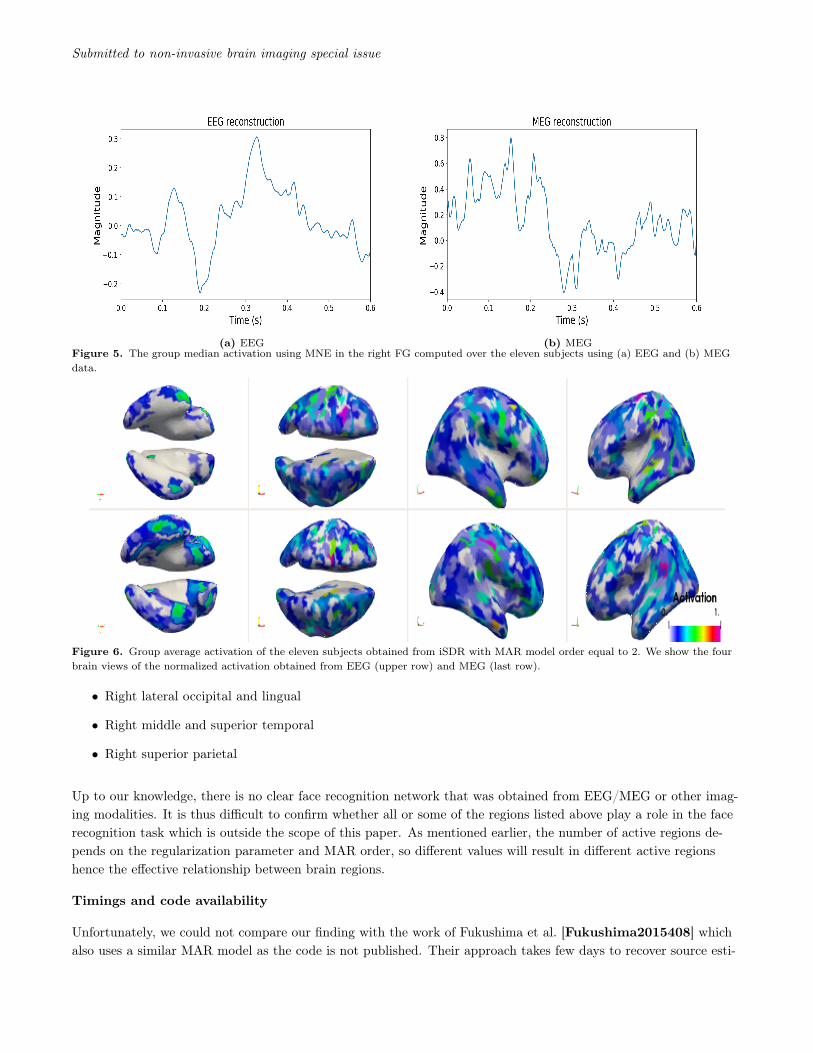
(a) EEG (b) MEGFigure 3. Mean and 95% confidence interval (CI) of CR, over the 11 subjects, computed using Equation 11 for different λ values aspercentage value of λmax and MAR order (p) with (a) EEG and (b) MEG data.

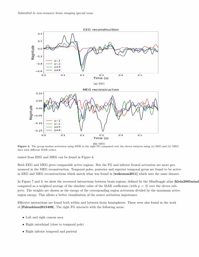
iSDR is applied with different MAR models (p ∈ {1, 2, 3, 4}) to the MEG and EEG data of the dataset [dataset].To date, although no definite clear picture has emerged, several imaging studies have suggested that the rightFusiform area (FG), right temporal pole (TP) and posterior superior temporal sulcus (STS) might play a role inface recognition [Kanwisher4302, Simpson15088]. We show the median time course, with different MAR or-ders, of the reconstructed right FG region activation in Figures 4a and 4b obtained from EEG and MEG respec-tively. We use the median so that the displayed magnitude is not biased towards subjects with high magnitudes.As a reference, Figure 5 shows the source reconstruction in the same region using the MNE method.

Reconstructions using EEG and MEG show a negative peak at the FG around 200ms which matches what can befound in the literature [halgren-etal:00, journal.pone.0071408, Simpson15088, dataset, Henson01072003,TRUJILLOBARRETO2008318, Halgren-etal]. The magnitude of the FG peak when p = 1 is low comparedto the remaining MAR orders. This is due to the simplicity of the model which could not reconstruct accuratelythe time course in the FG region. Because of this simplicity, iSDR reconstructs a high number of active regionswhich in turn exhibit reduced magnitudes due to the l2-norm used in the MxNE method. The time courses ob-tained for p > 1 are comparable to what has is shown in [Simpson15088]. A second peak at around 300ms isobserved in the MEG reconstruction with p = 4 which may be due to the high MAR order which will explain bet-ter the subject activation variability. This peak is similarly present only in the MEG reconstruction using MNEapproach. It is interesting to note that in [Barbeau2008SpatioTD] the author shows, using intracranial EEG,that the average activation of the FG has two peaks separated by 90ms. This coincides with our findings with Fig-ure 4b for p = 4 where there are indeed two peaks at 200ms and just after 300ms. This is also found in [journal.pone.0071408]for a comparison task of face to body pictures. Nevertheless, studying what is the optimal MAR order for recon-structing source activation for a given task, while being an interesting question, is not the objective of this paper.

Grand average over the subjects

To get an idea about the grand average activation across subjects, we computed the mapping between a referencesubject chosen randomly and the remaining ten subjects using optimal transport [ferradans2013regularized,gallardo2018solving]. Because iSDR uses a soft-threshold function in the S-step (MxNE solver), it underesti-mates the magnitude of activation. Thus a bias correction step is applied beforehand using the method explainedin [belaoucha:tel-01534876]. Then we computed the power of the median time courses obtained with iSDR andp = 2 in the whole time window across subjects in each cortical region. The resulting brain activation map ob-


(a) EEG

(b) MEGFigure 4. The group median activation using iSDR in the right FG computed over the eleven subjects using (a) EEG and (b) MEGdata with different MAR orders.

tained from EEG and MEG can be found in Figure 6.

Both EEG and MEG gives comparable active regions. But the FG and inferior frontal activation are more pro-nounced in the MEG reconstruction. Temporal poles, posterior and superior temporal gyrus are found to be activein EEG and MEG reconstructions which match what was found in [wakeman2011] which uses the same dataset.

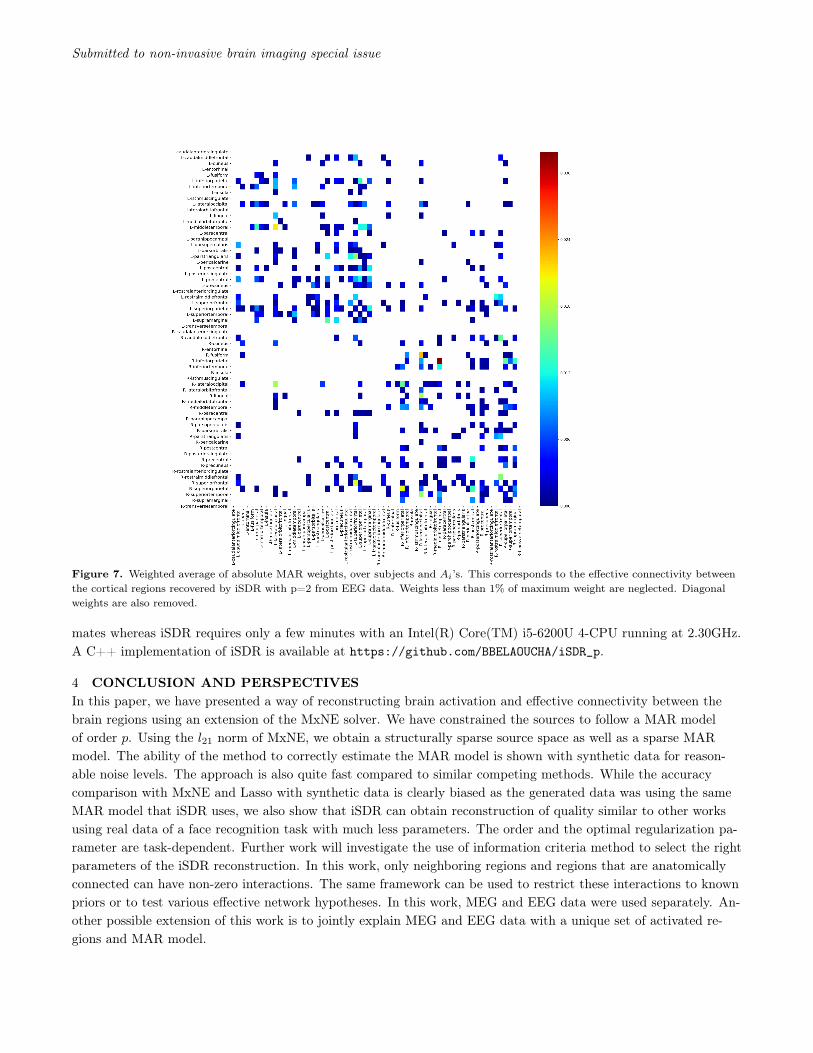
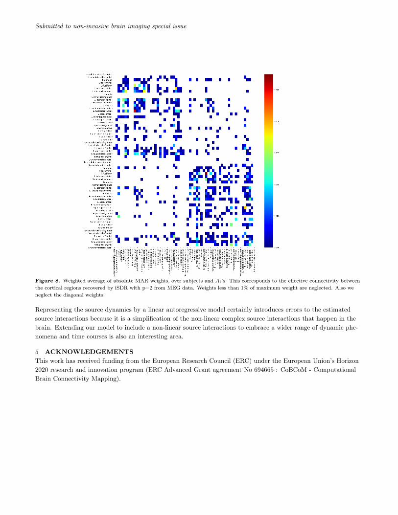
In Figure 7 and 8, we show the recovered interactions between brain regions, defined by the Mindboggle atlas [klein2005mindboggle],computed as a weighted average of the absolute value of the MAR coefficients (with p = 2) over the eleven sub-jects. The weights are chosen as the energy of the corresponding region activation divided by the maximum activeregion energy. This allows a better visualization of the source activation importance.

Effective interactions are found both within and between brain hemispheres. These were also found in the workof [Fukushima2015408]. The right FG interacts with the following areas:

• Left and right cuneus area

• Right entorhinal (close to temporal pole)

• Right inferior temporal and parietal


(a) EEG (b) MEGFigure 5. The group median activation using MNE in the right FG computed over the eleven subjects using (a) EEG and (b) MEGdata.

Figure 6. Group average activation of the eleven subjects obtained from iSDR with MAR model order equal to 2. We show the fourbrain views of the normalized activation obtained from EEG (upper row) and MEG (last row).

• Right lateral occipital and lingual

• Right middle and superior temporal

• Right superior parietal

Up to our knowledge, there is no clear face recognition network that was obtained from EEG/MEG or other imag-ing modalities. It is thus difficult to confirm whether all or some of the regions listed above play a role in the facerecognition task which is outside the scope of this paper. As mentioned earlier, the number of active regions de-pends on the regularization parameter and MAR order, so different values will result in different active regionshence the effective relationship between brain regions.

Timings and code availability

Unfortunately, we could not compare our finding with the work of Fukushima et al. [Fukushima2015408] whichalso uses a similar MAR model as the code is not published. Their approach takes few days to recover source esti-


Figure 7. Weighted average of absolute MAR weights, over subjects and Ai’s. This corresponds to the effective connectivity betweenthe cortical regions recovered by iSDR with p=2 from EEG data. Weights less than 1% of maximum weight are neglected. Diagonalweights are also removed.

mates whereas iSDR requires only a few minutes with an Intel(R) Core(TM) i5-6200U 4-CPU running at 2.30GHz.A C++ implementation of iSDR is available at https://github.com/BBELAOUCHA/iSDR_p.

4 CONCLUSION AND PERSPECTIVESIn this paper, we have presented a way of reconstructing brain activation and effective connectivity between thebrain regions using an extension of the MxNE solver. We have constrained the sources to follow a MAR modelof order p. Using the l21 norm of MxNE, we obtain a structurally sparse source space as well as a sparse MARmodel. The ability of the method to correctly estimate the MAR model is shown with synthetic data for reason-able noise levels. The approach is also quite fast compared to similar competing methods. While the accuracycomparison with MxNE and Lasso with synthetic data is clearly biased as the generated data was using the sameMAR model that iSDR uses, we also show that iSDR can obtain reconstruction of quality similar to other worksusing real data of a face recognition task with much less parameters. The order and the optimal regularization pa-rameter are task-dependent. Further work will investigate the use of information criteria method to select the rightparameters of the iSDR reconstruction. In this work, only neighboring regions and regions that are anatomicallyconnected can have non-zero interactions. The same framework can be used to restrict these interactions to knownpriors or to test various effective network hypotheses. In this work, MEG and EEG data were used separately. An-other possible extension of this work is to jointly explain MEG and EEG data with a unique set of activated re-gions and MAR model.

https://github.com/BBELAOUCHA/iSDR_p


Figure 8. Weighted average of absolute MAR weights, over subjects and Ai’s. This corresponds to the effective connectivity betweenthe cortical regions recovered by iSDR with p=2 from MEG data. Weights less than 1% of maximum weight are neglected. Also weneglect the diagonal weights.

Representing the source dynamics by a linear autoregressive model certainly introduces errors to the estimatedsource interactions because it is a simplification of the non-linear complex source interactions that happen in thebrain. Extending our model to include a non-linear source interactions to embrace a wider range of dynamic phe-nomena and time courses is also an interesting area.

5 ACKNOWLEDGEMENTSThis work has received funding from the European Research Council (ERC) under the European Union’s Horizon2020 research and innovation program (ERC Advanced Grant agreement No 694665 : CoBCoM - ComputationalBrain Connectivity Mapping).

structural connectivity to reconstruct brain activation ... - hal-inria

Documents