structural behavior and modeling of high
TRANSCRIPT
STRUCTURAL BEHAVIOR AND MODELING OF HIGH-PERFORMANCE FIBER-REINFORCED CEMENTITIOUS COMPOSITES FOR EARTHQUAKE-RESISTANT
DESIGN
BY
RAYMOND RICHARD FOLTZ
DISSERTATION
Submitted in partial fulfillment of the requirements
for the degree of Doctor of Philosophy in Civil Engineering in the Graduate College of the
University of Illinois at Urbana-Champaign, 2011
Urbana, Illinois
Doctoral Committee: Associate Professor James M. LaFave, Director of Research and Chair Associate Professor Daniel A. Kuchma Professor Jeffrey R. Roesler Professor Emeritus William L. Gamble
ii
ABSTRACT
For earthquake-resistant design, adequate concrete confinement is vital for a ductile
structural response and for providing a stable energy dissipating mechanism. Since concrete
materials generally exhibit quasi-brittle failure and a low tensile strength, designers of traditional
reinforced concrete often specify extensive transverse reinforcement with thorough detailing to
ensure that appropriate confinement to the concrete and the longitudinal reinforcing bars is
provided. This approach often results in such a large amount of reinforcing steel that
construction of the design can be congested, costly, and even impractical. This effect is
particularly pronounced in critical shear and/or moment regions of structural concrete coupling
beams and pile-wharf connections, as well as in plastic hinge regions of reinforced concrete
beams, columns, and structural walls. To address this problem, the development and modeling
of High Performance Fiber-Reinforced Cementitious Composites (HPFRCC) for use in key shear
and/or moment regions of damage-critical structural concrete elements has been investigated.
An experimental program was conducted to further understand the behavior of HPFRCC
under general multi-axial stress states, such as would be expected at various key locations in a
damage-critical structural component. Concrete plate specimens comprising mixes containing
from one to two percent volume fraction of hooked steel fibers and Spectra (polyethylene) fibers
were tested. After exploration of these different fiber types and volume fractions, a 1.5% volume
fraction of hooked steel fibers was selected as the concrete mix for more comprehensive
examination, based in part on a study to create self-consolidating fiber-reinforced concrete. The
stress-strain behavior of the various HPFRCC mixes was examined, and biaxial failure envelopes
have been developed. The plate specimen tests showed that HPFRCC exhibits a confined
compressive behavior with a significantly increased damage tolerance and deformation capacity.
iii
Using the knowledge and behavioral trends gained from the laboratory tests of HPFRCC
materials, it was possible to create a phenomenological HPFRCC finite element material model,
with a smeared crack representation, that was calibrated to the experimental data. In addition to
small-scale structural / material testing and modeling, the same HPFRCC hooked steel fiber mix
was tested in large-scale coupling beam component tests by project partners at the University of
Michigan. After completion of these large-scale tests, the material model was validated at the
structural component level with their experimental coupling beam results.
Finally, a full-scale structural concrete pile-wharf connection was tested at the University
of Illinois, and the behavior of this damage-critical component was thoroughly analyzed. The
HPFRCC model was then implemented into the pile-wharf connection application. Overall, it
was found that the increase in structural component damage tolerance through a ductile response
obtained by the tensile strain-hardening and confined compressive behavior from the use of
HPFRCC makes it a potentially viable solution as a replacement for some steel confinement
reinforcement and as an additional shear resistance mechanism. With the development of an
HPFRCC modeling tool, insight into the levels of damage experienced by structural elements can
inform performance-based design decisions regarding the use of HPFRCC in critical structural
components.

iv
To the best mother a son could possibly have
Arlene eedle Foltz
1951-2011
v
ACKOWLEDGMETS
The work reported herein was supported in part by the U.S. National Science Foundation
under Grant No. CMS 0530383. The opinions, findings, and conclusions expressed in this
dissertation proposal are those of the author alone and do not necessarily reflect the views of the
sponsor. The author also acknowledges the generous support he has received in the form of an
ACI Charles Pankow Foundation Student Fellowship.
Many people assisted me in the completion of my experimental work. The small-scale
laboratory tests at the Universiy of Illinois at Urbana-Champaign could not have been conducted
without the assistance of Dr. Grezgorz Banas, and many thanks are owed to him for his help and
guidance with conducting experimental research. The construction of the pile-wharf specimen
could not have been completed without the help of my fellow graduate students, namely, Alan
Cubas, Pablo Caiza, Mark Bingham, and Dziugas Reneckis. Also, the continued collaboration
with Remy Lequesne and Prof. Jim Wight, project colleagues at the University of Michigan, was
instrumental in allowing this research to extend to the performance of HPFRCC at the structural
component and structural system level. Without their willing desire to share data and
information, the analytical phase of this research project would not have been possible. I want to
thank my thesis committee for their time and input, and I owe a particular debt of gratitude to my
advisor Prof. Jim LaFave for his continued support, guidance, and immeasurable contributions to
this research and to my overall development as an engineer.
Outside of the laboratory, I owe a great deal of thanks to numerous fellow graduate
students for volunteering their engineering insights and for continuing to remind to enjoy my
time in Champaign-Urbana. Included among these students are Chris Hart, Chris Martin, Josh
Ellis, Ken Marley, Matt Gries, Travis Welt, as well as many others that have shared this

vi
experience with me. Also, I would like to thank my girlfriend, Megan. She has been a
wonderful addition to my life, and easily the most enjoyable part of the last four years of the
Ph.D. process.
Finally, I owe the greatest thanks to my parents for being so supportive of anything that I
have ever decided to undertake. They have always been there to listen patiently and to provide
sagacious advice throughout this seemingly endless graduate school process and my entire life. I
owe everything to them. While my mother is no longer with me physically, I know that she will
be with me forever and proudly watching.
vii
TABLE OF COTETS
CHAPTER 1. ITRODUCTIO.............................................................................................. 1
1.1 Problem ............................................................................................................................. 1
1.2 High-Performance Fiber-Reinforced Cementitious Composite Solution ......................... 2
1.3 Objective and Scope ........................................................................................................ 11
1.4 Chapter Description ........................................................................................................ 13
CHAPTER 2. BACKGROUD IFORMATIO ............................................................... 16
2.1 Previously Conducted Multi-Axial Plain Concrete Results ............................................ 16
2.2 Previously Conducted Fiber-Reinforced Concrete Multi-Axial Results ......................... 25
2.3 Previously Conducted Reinforced Concrete Coupling Beam Tests ................................ 28
2.4 Previously Conducted HPFRCC Coupling Beam Tests .................................................. 40
2.5 HPFRCC Large-Scale Coupled Wall Tests ..................................................................... 46
2.6 Other Previously Investigated Applications of HPFRCC ............................................... 60
2.7 Previously Conducted HPFRCC Analytical Modeling ................................................... 63
CHAPTER 3. MATERIAL TESTIG RESULTS ............................................................... 67
3.1 Preliminary HPFRCC Material Testing ......................................................................... 67
3.2 Materials and Mixture Proportions ................................................................................ 68
3.3 Preliminary Material Property Testing at the University of Michigan ........................... 72
3.4 UIUC Experimental Program Overview ......................................................................... 77
3.5 Specimen Preparation ..................................................................................................... 80
3.6 Testing Procedures .......................................................................................................... 82
3.7 Uniaxial Test Results ....................................................................................................... 85
3.7.1 Uniaxial Compression Failure Mode .................................................................................................... 85
viii
3.7.2 Uniaxial Compression Stress-Strain Behavior ..................................................................................... 87
3.7.3 Uniaxial Tension Failure Mode ............................................................................................................ 92
3.7.4 Uniaxial Tension Stress-Strain Behavior ............................................................................................. 93
3.8 Biaxial Test Results ......................................................................................................... 95
3.8.1 Failure Mode ........................................................................................................................................ 96
3.8.2 Stress-Strain Behavior .......................................................................................................................... 97
3.9 Failure Envelope Results ............................................................................................... 100
3.10 Split Cylinder Test Results ............................................................................................ 105
3.11 Tension Results .............................................................................................................. 108
CHAPTER 4. MATERIAL MODELIG ............................................................................ 110
4.1 ATEA Background ...................................................................................................... 110
4.2 Modeling Parameters .................................................................................................... 112
4.2.1 Material Properties ............................................................................................................................. 113
4.2.2 Element Mesh ..................................................................................................................................... 122
4.2.3 Loading and Boundary Conditions ..................................................................................................... 122
4.3 Material Modeling Validation ....................................................................................... 124
4.3.1 Uniaxial Modeling Results ................................................................................................................. 125
4.3.2 Equal Biaxial Modeling Results ......................................................................................................... 130
4.3.3 Unequal Biaxial Modeling Results ..................................................................................................... 133
4.3.4 Failure Envelope Results .................................................................................................................... 135
CHAPTER 5. COUPLIG BEAM COMPOET TEST RESULTS ............................. 138
5.1 Reinforced Concrete Coupling Beam Tests ................................................................... 138
5.1.1 Galano and Vignoli (2000) ................................................................................................................. 141
5.1.2 Reinforced Concrete Coupling Beam Failure Modes ......................................................................... 146
5.2 HPFRCC Coupling Beam Tests .................................................................................... 151
5.2.1 Lequesne (2011) ................................................................................................................................. 152
ix
5.3 Compiled Coupling Beam Information ......................................................................... 162
CHAPTER 6. COUPLIG BEAM COMPOET MODELIG .................................... 165
6.1 Coupling Beam Modeling Parameters .......................................................................... 165
6.1.1 Constitutive Models ........................................................................................................................... 165
6.1.2 Reinforcement Modeling .................................................................................................................... 168
6.1.3 Finite Element Modeling Parameters ................................................................................................. 170
6.2 RC Coupling Beam Component Modeling .................................................................... 171
6.2.1 RC Coupling Beam Modeling Results ............................................................................................... 172
6.2.2 RC Coupling Beam Parametric Study ................................................................................................ 184
6.3 HPFRCC Coupling Beam Component Modeling .......................................................... 188
6.3.1 HPFRCC Coupling Beam Modeling Results ..................................................................................... 192
6.3.2 HPFRCC Coupling Beam Parametric Study ...................................................................................... 201
6.4 Compiled Coupling Beam Model Performance Assessment ......................................... 203
CHAPTER 7. BACKGROUD AD EXPERIMETAL PLA FOR PILE-WHARF
COECTIO TESTIG ...................................................................................................... 206
7.1 Introduction ................................................................................................................... 206
7.2 Previous Pile-Wharf Connection Research ................................................................... 212
7.2.1 University of Canterbury, New Zealand ............................................................................................. 212
7.2.2 University of California, San Diego ................................................................................................... 214
7.2.3 University of Washington .................................................................................................................. 220
7.2.4 Summary of Past Research ................................................................................................................. 228
7.3 Pile-Wharf Connection Experimental Testing Program ............................................... 229
7.3.1 Experimental Plan .............................................................................................................................. 230
7.3.2 Test Specimen Design ........................................................................................................................ 238
7.3.3 Test Specimen Construction and Installation ..................................................................................... 246
7.3.4 Materials Characterization.................................................................................................................. 258
x
7.3.5 NEES MUST-SIM Facility Overview and Test Setup ....................................................................... 268
7.3.6 Instrumentation ................................................................................................................................... 276
CHAPTER 8. PILE-WHARF COECTIO EXPERIMETAL RESULTS .............. 290
8.1 Overall Global Behavior ............................................................................................... 290
8.1.1 Control Movement ............................................................................................................................. 291
8.1.2 Global Force and Displacement Response ......................................................................................... 297
8.2 Imperial Valley Earthquake .......................................................................................... 301
8.2.1 Imperial Valley - Visual Damage ....................................................................................................... 302
8.2.2 Imperial Valley - Local Behavior ....................................................................................................... 304
8.3 orthridge Earthquake .................................................................................................. 316
8.3.1 Northridge – Visual Damage .............................................................................................................. 317
8.3.2 Northridge – Local Behavior .............................................................................................................. 329
8.4 Kobe Earthquake ........................................................................................................... 337
8.4.1 Kobe – Visual Damage ....................................................................................................................... 339
8.4.2 Kobe – Local Behavior ....................................................................................................................... 344
8.5 Cyclic Loading .............................................................................................................. 353
8.5.1 Cyclic – Visual Damage Progression ................................................................................................. 356
8.5.2 Cyclic – Local Behavior ..................................................................................................................... 379
8.6 Stiffness Degradation Analysis ...................................................................................... 390
8.7 Connection Slip Analysis ............................................................................................... 394
CHAPTER 9. PILE-WHARF COECTIO MODELIG ........................................... 403
9.1 Pile-Wharf Connection Modeling Parameters .............................................................. 403
9.1.1 Constitutive Models ........................................................................................................................... 404
9.1.2 Loading and Boundary Conditions ..................................................................................................... 406
9.1.3 Finite Element Modeling Parameters ................................................................................................. 409
9.2 Pile-Wharf Connection Modeling Results ..................................................................... 411
xi
9.3 Other Modeling Applications ........................................................................................ 420
CHAPTER 10. COCLUSIOS ............................................................................................ 422
10.1 Summary ........................................................................................................................ 422
10.2 HPFRCC Experimental Conclusions ............................................................................ 423
10.3 HPFRCC Modeling Conclusions .................................................................................. 425
10.4 Pile-Wharf Connection Conclusions ............................................................................. 426
10.5 Contributions ................................................................................................................. 427
10.6 Future Work .................................................................................................................. 428
REFERECES ......................................................................................................................... 431
xii
LIST OF FIGURES
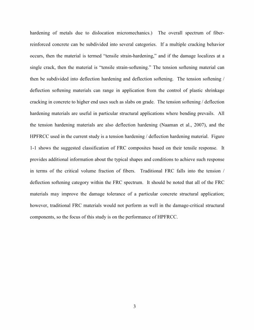
Figure 1-1. Suggested Classification of FRC Composites from Naaman et al. (2007) .................. 4
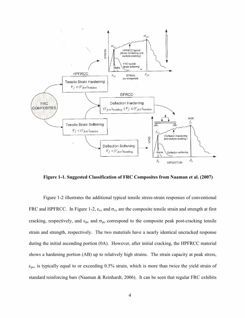
Figure 1-2. Comparison of Typical Stress-Strain Response in Tension of HPFRCC with
Conventional FRCC (Naaman & Reinhardt, 2003) .................................................. 5
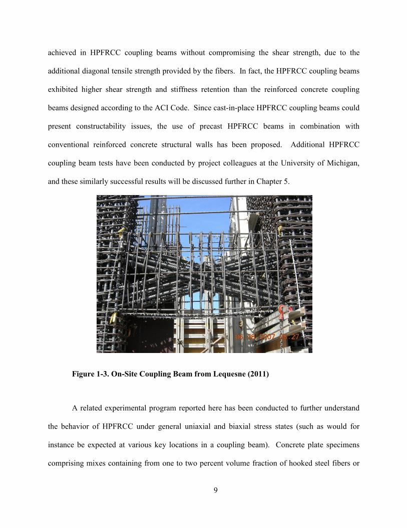
Figure 1-3. On-Site Coupling Beam from Lequesne (2011) .......................................................... 9
Figure 2-1. Brush Bearing Platens (Kupfer et al., 1969) .............................................................. 19
Figure 2-2. Biaxial Strength Envelope of Plain Concrete (Kupfer et al., 1969) ........................... 21
Figure 2-3. Standard Tensile Splitting Failure Modes of Plain Concrete for Different
Stress Ratios (Kupfer et al., 1969) .......................................................................... 23
Figure 2-4. Load Bifurcation Machine used by Yin et al. (1989)................................................. 26
Figure 2-5. Biaxial Strength Envelope for Fiber Reinforced Concrete (Yin et al., 1989) ............ 27
Figure 2-6. Diagonal Tension Failure Mechanism (Paulay, 1971) ............................................... 30
Figure 2-7. Sliding Shear Failure of Conventionally Reinforced Coupling Beam (Paulay,
1977) ........................................................................................................................ 30
Figure 2-8. Reinforcement Layout and Cracks in Large Scale Shear Walls (Paulay and
Santhakumar, 1976) ................................................................................................ 33
Figure 2-9. Investigated Reinforcement Layouts (Tassios et al., 1996) ....................................... 35
Figure 2-10. Coupling Beam Reinforcement Details with Confined Diagonal Bars from
ACI 318-08 (2008) .................................................................................................. 38
Figure 2-11. Coupling Beam Reinforcement without Confined Diagonal Bars and with
Fully Confined Cross-Section from ACI 318-08 (2008) ........................................ 39
Figure 2-12. Force-Drift Relationship for Coupling Beams with Alternate Reinforcement
Layouts (Wallace, 2007) ......................................................................................... 39
xiii
Figure 2-13. Reinforcement Details of Coupling Beam Test Specimens for RC (a) and
HPFRCC (b,c,d) (Canbolat et al., 2005) ................................................................. 42
Figure 2-14. Damage Index versus Shear Distortion Response and the Corresponding
Recommended Performance Levels from Canbolat (2004) .................................... 44
Figure 2-15. Large-scale Experimental Test Setup....................................................................... 48
Figure 2-16. Coupling Beam Reinforcement Layout from Lequesne et al. (2009a) .................... 50
Figure 2-17. Reinforcement Layout for Coupled Wall Specimen 1 from Lequesne et al.
(2010) ...................................................................................................................... 53
Figure 2-18. Reinforcement Layout for Coupled Wall Specimen 2 from Lequesne et al.
(2010) ...................................................................................................................... 54
Figure 2-19. Base Shear versus Drift for Large-Scale Coupled Wall Tests from Lequesne
et al. (2010) ............................................................................................................. 56
Figure 2-20. RC Coupling Beam at 3.3% Drift from Large-Scale Test ....................................... 57
Figure 2-21. HPFRCC Coupling Beam at 3.3% Drift from Large-Scale Test ............................. 58
Figure 2-22. Damage Progression of 4th Story Coupling Beam in CW-2 at Various
Coupling Beam Drifts from Lequesne (2011) ......................................................... 59
Figure 3-1. Spectra Fibers (left) and Hooked Steel Fibers (right) ................................................ 71
Figure 3-2. Triaxial Test Setup (Sirijaroonchai, 2009) ................................................................. 75
Figure 3-3. Average Stress-Strain Responses in Longitudinal Direction under Two Levels
of Confining Pressure from Sirijaroonchai (2009) .................................................. 76
Figure 3-4. Cutting NM6 Loaf into Individual Specimens (Sirijaroonchai, 2009) ...................... 79
Figure 3-5. Biaxial Material Testing Experimental Test Setup .................................................... 83
xiv
Figure 3-6. Krypton LED Layout (left) and Initial LVDT Positioning (right) (adapted
from Sirijaroonchai, 2009) ...................................................................................... 84
Figure 3-7. Typical Failure Surface of Uniaxial Compression Plate Specimen ........................... 86
Figure 3-8. NM6 Uniaxial Compressive Behavior ....................................................................... 89
Figure 3-9. Complete NM6 Cylinder Compressive Stress-Strain Response ................................ 90
Figure 3-10. Cracking Propagation for MM Spectra 1% Direct Tension Test, from
Sirijaroonchai (2009) ............................................................................................... 93
Figure 3-11. Hooked Fiber MM Direct Uniaxial Tension Test Results ....................................... 94
Figure 3-12. Spectra Fiber MM Direct Uniaxial Tension Test Results ........................................ 95
Figure 3-13. Single Shear Failure Mode (left), Multiple Shear Failure Mode (center), and
Tensile Splitting Failure (right) ............................................................................... 97
Figure 3-14. NM6 Average Compressive Response in the Leading Direction ............................ 98
Figure 3-15. NM6 Average Compressive Response in the Trailing Direction............................. 99
Figure 3-16. Biaxial Strength Envelopes from Experimental Test Results ................................ 102
Figure 3-17. Biaxial Strength Envelope Comparison of NM6 Loaf, HPFRCC Individual,
and Plain NM4 Specimens with Historical Tests .................................................. 103
Figure 3-18. Split Cylinder Diametrical Deformation Apparatus and Experimental Test
Setup ...................................................................................................................... 106
Figure 3-19. Split-Cylinder Load versus Deformation for NM6 Cylinders ............................... 108
Figure 4-1. NM6 Compressive Stress-Strain Response in ATENA ........................................... 114
Figure 4-2. NM6 Tensile Stress-Strain Response ....................................................................... 115
Figure 4-3. Plain Concrete Experimental and Model Failure Envelopes ................................... 118
Figure 4-4. Experimental NM6 and Adjusted ATENA Biaxial Failure Surfaces ...................... 119
xv
Figure 4-5. Compressive Strength Reduction due to Cracking .................................................. 120
Figure 4-6. ATENA Uniaxial Material Model Prototype ........................................................... 124
Figure 4-7. Stress Contours (left) and Displacement Contours (right) for HSC Plate
Specimens Subjected to Uniaxial Loads from Hussein and Marzouk (2000b) ..... 125
Figure 4-8. ATENA Uniaxial Y-Stress Distribution in Plain Concrete Specimen ..................... 126
Figure 4-9. ATENA Plain Concrete Uniaxial Compression Stress-Strain Response
Comparison ........................................................................................................... 127
Figure 4-10. ATENA HPFRCC Uniaxial Compression Stress-Strain Response
Comparison ........................................................................................................... 128
Figure 4-11. ATENA HPFRCC Uniaxial Tension Stress-Strain Comparison ........................... 129
Figure 4-12. ATENA HPFRCC Uniaxial Tension Crack Distribution ...................................... 130
Figure 4-13. ATENA Biaxial Model Prototype .......................................................................... 131
Figure 4-14. Equal Biaxial Compression Modeling and Experimental Results ......................... 132
Figure 4-15. 70% Biaxial Compression Modeling and Experimental Results ........................... 133
Figure 4-16. 50% Biaxial Compression Modeling and Experimental Results ........................... 134
Figure 4-17. 30% Biaxial Compression Modeling and Experimental Results ........................... 135
Figure 4-18. Experimental and Modeling Result Biaxial Failure Envelopes ............................. 136
Figure 5-1. Coupling Beam Reinforcement Layouts Modified from Galano and Vignoli
(2000) .................................................................................................................... 140
Figure 5-2. Experimental Test Setup from Galano and Vignoli (2000) ..................................... 142
Figure 5-3. Shear-Rotation Responses of Monotonic Coupling Beams from Galano and
Vignoli (2000) ....................................................................................................... 143
xvi
Figure 5-4. Shear-Rotation Response of Cyclic Conventional RC Coupling Beam from
Galano and Vignoli (2000) .................................................................................... 145
Figure 5-5. Shear-Rotation Response of Cyclic Diagonal RC Coupling Beam from
Galano and Vignoli (2000) .................................................................................... 146
Figure 5-6. Ductile Flexure Failure Modes from Kwan and Zhao (2002) Specimen MCB3
and Galano and Vignoli (2000) Specimen P16 ..................................................... 148
Figure 5-7. Flexure / Diagonal Tension Failure Modes from Tassios et al. (1996)
Specimen CB-1B and Kwan and Zhao (2002) Specimen CCB1 .......................... 149
Figure 5-8. Flexure / Sliding Shear Failure Modes from Paulay (1977) Specimen 315 and
Kwan and Zhao (2002) Specimen CCB12 ............................................................ 149
Figure 5-9. Preemptive Diagonal Tension Failure Modes from Galano and Vignoli (2000)
Specimen P01 and Kwan and Zhao (2002) Specimen MCB1 ............................. 150
Figure 5-10. Diagonal Compression Failure Modes from Galano and Vignoli (2000)
Specimen P12 and Kwan and Zhao (2002) Specimen CCB11 ............................. 150
Figure 5-11. Flexural Compression Failure Modes from Galano and Vignoli (2000)
Specimen P10 and Tassios et al. (1996) Specimen CB-2A .................................. 151
Figure 5-12. Coupling Beam Component Test Setup from Lequesne (2011) ............................ 155
Figure 5-13. Reinforcement Detail of Precast Coupling Beams with a Span-to-Depth
Ratio of 1.75 from Lequesne (2011) ..................................................................... 156
Figure 5-14. Shear Stress versus Drift Response of Specimen CB-2 from Lequesne
(2011) .................................................................................................................... 158
Figure 5-15. CB-2 Damage States at 3.5% Drift (left) and 5.5% Drift (right) from
Lequesne (2011) .................................................................................................... 159
xvii
Figure 5-16. Shear Stress versus Drift for Specimen CB-3 from Lequesne (2011) ................... 160
Figure 5-17. CB-3 Damage States at 3% Drift (left) and 6% Drift (right) from Lequesne
(2011) .................................................................................................................... 161
Figure 6-1. SBETA Equivalent Uniaxial Stress-Strain Relationship from Cervenka et al.
(2010) .................................................................................................................... 166
Figure 6-2. SBETA Compression Softening Displacement Law from Cervenka et al.
(2010) .................................................................................................................... 167
Figure 6-3. CEB-FIP Model Code 1990 Bond-Slip Relationship (left) with Table of
Parameters (right) from Cervenka et al. (2010) .................................................... 169
Figure 6-4. Specimen P01 Model with Loading and Boundary Conditions ............................... 173
Figure 6-5. Shear versus Displacement for Specimen P01 ......................................................... 174
Figure 6-6. Principal Stress and Cracking in P01 near Failure ................................................... 175
Figure 6-7. Specimen P05 Model with Loading and Boundary Conditions ............................... 176
Figure 6-8. Shear versus Displacement for Specimen P05 ......................................................... 177
Figure 6-9. Principal Stress and Cracking in P05 near Failure ................................................... 178
Figure 6-10. Shear versus Displacement for Specimen P02 ....................................................... 179
Figure 6-11. Principal Stress and Cracking in Specimen P02 near Failure ................................ 180
Figure 6-12. Shear versus Displacement for Specimen P07 ....................................................... 182
Figure 6-13. Principal Stress and Cracking in Specimen P07 near Failure ................................ 183
Figure 6-14. Shear versus Displacement for Specimen P01 with HPFRCC .............................. 185
Figure 6-15. Principal Stress in Specimen P01 with HPFRCC Failure Mode............................ 186
Figure 6-16. Shear versus Displacement for Specimen P05 with HPFRCC .............................. 187
Figure 6-17. Specimen P05 with HPFRCC at Peak Load (left) and at Failure (right) ............... 188
xviii
Figure 6-18. Coupling Beam Component Test Setup at U-M from Lequesne (2011) ............... 189
Figure 6-19. Axial Force in HPFRCC Coupling Beams from Lequesne (2011) ........................ 191
Figure 6-20. Specimen CB-2 Model with Loading and Boundary Conditions .......................... 192
Figure 6-21. Shear versus Displacement for Specimen CB-2 .................................................... 194
Figure 6-22. X-Stress (left) and Y-Stress (right) in Specimen CB-2 near Failure ..................... 195
Figure 6-23. Shear Stress in Specimen CB-2 near Failure ......................................................... 196
Figure 6-24. Specimen CB-3 with Loading and Boundary Conditions ...................................... 197
Figure 6-25. Shear versus Displacement for Specimen CB-3 .................................................... 199
Figure 6-26. X-Stress in Specimen at 3% Drift (left) and at Failure (right ) in Specimen
CB-3 ...................................................................................................................... 200
Figure 6-27. Y-Stress (left) and Shear Stress (right) in Specimen CB-3 at Failure.................... 200
Figure 6-28. Shear versus Displacement Response of CB-2 Specimen with RC ....................... 202
Figure 6-29. Shear versus Displacement Response of CB-3 Specimen with RC ....................... 202
Figure 7-1. Typical Pile Support Structure for Seismic Resistance of a Wharf (Roeder et
al., 2001) ................................................................................................................ 207
Figure 7-2. Idealized Port Structure under Seismic Loading (Jellin, 2008) ............................... 208
Figure 7-3. Typical Pile-Wharf Connections (Jellin, 2008) ....................................................... 209
Figure 7-4. Typical Dowel Bar Connection Details (Stringer, 2010) ......................................... 211
Figure 7-5. Pile-Wharf Connection Damage from Loma Prieta (left) and Hanshin (right)
Earthquakes ........................................................................................................... 212
Figure 7-6. Specimen PC6 Connection Details (Joen et al., 1988)............................................. 214
Figure 7-7. Specimen STD1 Connection Details (Silva et al., 1997) ......................................... 215
Figure 7-8. Connection Details from Sritharan and Priestley (1998) ......................................... 216
xix
Figure 7-9. Nonseismic Pile Pile-Deck Connection Detail from Krier (2006) ........................... 218
Figure 7-10. Seismic Pile-Deck Connection Detail from Krier (2006) ...................................... 218
Figure 7-11. Specimen 6 Connection Details from Roeder et al. (2001) ................................... 222
Figure 7-12. Pile-Deck Connection Details from Jellin (2008) .................................................. 225
Figure 7-13. Base Moment versus Drift for Specimen 9 from Jellin (2008) .............................. 226
Figure 7-14. Port of Oakland Berth 55/56 Model Wharf Profile View ...................................... 231
Figure 7-15. Port of Oakland Berth 55/56 Model Wharf Plan View .......................................... 232
Figure 7-16. Georgia Tech OpenSees 2D Translational Model ................................................. 233
Figure 7-17. Selected SAC Ground Motions .............................................................................. 234
Figure 7-18. Imposed Pile Boundary Conditions and Typical Pile Bending Moment
Distribution ............................................................................................................ 236
Figure 7-19. X-Displacement Record Imposed during Earthquake Loading ............................. 237
Figure 7-20. X-Displacement Record Imposed during Cyclic Loading ..................................... 238
Figure 7-21. General Pile-Wharf Connection Test Specimen Dimensions ................................ 240
Figure 7-22. Pile Reinforcement and Other Details .................................................................... 242
Figure 7-23. T-Headed Bar Grouting Details ............................................................................. 243
Figure 7-24. Wharf Deck Reinforcement Details ....................................................................... 244
Figure 7-25. Strong Floor Connection Details ............................................................................ 245
Figure 7-26. Formwork Details................................................................................................... 247
Figure 7-27. Pile Lifting Procedure - Step One .......................................................................... 248
Figure 7-28. Pile Lifting Proecdure - Step Two (left) and Step Three (right) ............................ 248
Figure 7-29. T-Headed Bar Placement ....................................................................................... 250
Figure 7-30. Wharf Deck Reinforcement Placement .................................................................. 251
xx
Figure 7-31. Wharf Deck Casting ............................................................................................... 252
Figure 7-32. Pile-Wharf Connection Repair Scheme ................................................................. 253
Figure 7-33. Longitudinal Repair Bar Placement ....................................................................... 254
Figure 7-34. Specimen Inverting Procedure ............................................................................... 255
Figure 7-35. LBCB Connection Details...................................................................................... 256
Figure 7-36. Moving Specimen into Position ............................................................................. 258
Figure 7-37. Wharf Deck Concrete Strength Development........................................................ 261
Figure 7-38. Deck Deck Concrete Cylinder Compression Results at Specimen Test Date ....... 262
Figure 7-39. T-Headed Reinforcement Stress-Strain Response ................................................. 266
Figure 7-40. Wharf Deck Reinforcement Stress-Strain Response.............................................. 267
Figure 7-41. NEES MUST-SIM Facility at the University of Illinois ........................................ 269
Figure 7-42. Small-Scale MUST-SIM Facility (left) and Small-Scale Specimen Attached
to LBCB (right) ..................................................................................................... 270
Figure 7-43. LBCB with Actuator Labels and Coordinate System ............................................ 271
Figure 7-44. MUST-SIM Overall Software Architecture ........................................................... 273
Figure 7-45. T-Headed Dowel Reinforcement Strain-Gauge Locations .................................... 277
Figure 7-46. Deck Reinforcement Strain-Gauge Locations - Plan View ................................... 278
Figure 7-47. Deck Reinforcement Strain Gauge Locations - Profile View ................................ 279
Figure 7-48. Concrete Strain Gauge Locations– E-W (left) and N-S (right) .............................. 280
Figure 7-49. Inclinometer (left), LVDT (center), and String Pot (right) Examples ................... 283
Figure 7-50. Krypton Coordinate Measurement Machine .......................................................... 284
Figure 7-51. Krypton LED Grid Layout ..................................................................................... 286
Figure 7-52. Overall Instrumentation Layout ............................................................................. 287
xxi
Figure 8-1. Fully Instrumented Pile-Wharf Connection Test Specimen .................................... 291
Figure 8-2. Control Point Lateral Displacement Comparison .................................................... 293
Figure 8-3. Control Point Rotation Comparison before Input Adjustment ................................ 295
Figure 8-4. Control Point Rotation Comparison after Input Adjustment ................................... 296
Figure 8-5. Connection Moment versus Lateral Displacement before and after X1
Actuator Adjustment ............................................................................................. 298
Figure 8-6. Final Connection Moment versus Lateral Displacement ......................................... 300
Figure 8-7. Imperial Valley Earthquake Lateral Displacement Record ..................................... 302
Figure 8-8. North and South Views of the Connection at Peak Displacement During
Imperial Valley ...................................................................................................... 303
Figure 8-9. Front View of the Connection at Peak Displacement during Imperial Valley ........ 304
Figure 8-10. Connection Rotation (left) and Pile Rotation (right) Contributions to Pile-
Wharf Connection Rotation (Jellin, 2008) ............................................................ 305
Figure 8-11. Interface Total Rotation Comparison ..................................................................... 307
Figure 8-12. Comparison of Total Rotation and Pile Flexural Rotation at the Interface ............ 308
Figure 8-13. Total Rotation versus Pile Flexural Rotation Comparison during Imperial
Valley .................................................................................................................... 309
Figure 8-14. Lumped Rotation Comparison from Strain Gauges and Krypton during
Imperial Valley ...................................................................................................... 311
Figure 8-15. Pile Moment-Curvature Response at Interface during Imperial Valley ................. 313
Figure 8-16. Krypton FEM Grid and Strain Gauges at Maximum Displacement during
Imperial Valley ...................................................................................................... 315
Figure 8-17. Northridge Earthquake Lateral Displacement Record ........................................... 317
xxii
Figure 8-18. Initial Cracking of Pile Specimen (Viewed from the Northeast) ........................... 318
Figure 8-19. Front View of Flexural Pile Cracks on North Face at 12" (left) and 24"
(right) ..................................................................................................................... 319
Figure 8-20. Flexural Pile Cracks on North Face at 30" and 42" from Pile-Wharf
Connection (Viewed from the Northwest) ............................................................ 319
Figure 8-21. Initial Spalling at South Face of Pile-Wharf Connection (left) and Wharf
Deck Cracking (right) during Northridge .............................................................. 320
Figure 8-22. North (left) and South (right) Views of Pile-Wharf Connection at First Yield
during Northridge .................................................................................................. 321
Figure 8-23. Cracking at Pile-Wharf Interface during Northridge Maximum Negative
Displacement ......................................................................................................... 322
Figure 8-24. Growth of Pile Flexural Crack at 12" from the Pile-Wharf Interface on the
South Face during Northridge ............................................................................... 322
Figure 8-25. Flexural Crack at 12" from the Pile-Wharf Interface at Maximum Negative
Displacement during Northridge ........................................................................... 323
Figure 8-26. New Flexural Cracks along South Face of Specimen during Northridge
Maximum Negative Displacement ........................................................................ 324
Figure 8-27. North (left) and South (right) Views of the Connection at Maximum
Negative Displacement during Northridge ........................................................... 324
Figure 8-28. Deck Cracking and Spalling at Maximum Displacement during Northridge ........ 325
Figure 8-29. New Flexural Crack at 66" (left) and Widening of Crack at 12" (right)
during Peak Northridge Displacement .................................................................. 326
xxiii
Figure 8-30. Progression of South-Face Pile Spalling during Maximum Northridge
Displacement ......................................................................................................... 327
Figure 8-31. Measurement of Spalled Pile Region after Northridge .......................................... 327
Figure 8-32. North (left) and South (right) Views of the Pile-Wharf Connection after the
Northridge Record ................................................................................................. 328
Figure 8-33. West View of the Pile-Wharf Connection after the Northridge Record ................ 328
Figure 8-34. Northridge Interface Unadjusted Strain Gauge Values (left) and Strain
Gauge Values with Plastic Offset Adjustment (right) ........................................... 330
Figure 8-35. Pile Flexural Rotation and Total Rotation at the Connection during
Northridge ............................................................................................................. 331
Figure 8-36. Lumped Connection Rotation from Krypton during Northridge ........................... 332
Figure 8-37. Pile Rotation versus Total Rotation during Northridge ......................................... 333
Figure 8-38. Base Moment versus Curvature through Northridge ............................................. 334
Figure 8-39. Moment-Curvature Response at 6" (left) and 12" (right) ...................................... 335
Figure 8-40. Krypton and Strain Gauge Strains at First Yield during Northridge ..................... 336
Figure 8-41. Krypton and Strain Gauge Strains at Northridge Peak Displacement ................... 337
Figure 8-42. Kobe Earthquake Lateral Displacement Record .................................................... 338
Figure 8-43. Deck Spalling during Kobe .................................................................................... 340
Figure 8-44. Depth of Deck Spalling and Connection Uplift during Kobe ................................ 340
Figure 8-45. Spalling of the North Pile Face and Wharf during Kobe Peak Negative
Displacement ......................................................................................................... 341
Figure 8-46. Ruler under the South Pile Face at Peak Negative Displacement during Kobe ..... 341
Figure 8-47. Deck Spalling on North Side of Pile during Northridge ........................................ 342
xxiv
Figure 8-48. North and South Views of the Pile-Wharf Connection at Initial Yield of the
South Extreme Dowel Bars during Kobe .............................................................. 343
Figure 8-49. North and South Views of the Pile-Wharf Connection after Kobe Record ........... 343
Figure 8-50. West View of the Pile-Wharf Connection after Earthquake Loading.................... 344
Figure 8-51. Total Rotation and Flexural Pile Rotation at Pile-Wharf Connection during
Kobe ...................................................................................................................... 345
Figure 8-52. Lumped Rotation at Pile-Wharf Interface from Krypton LEDs and Strain
Gauges during Kobe .............................................................................................. 346
Figure 8-53. Pile Rotation versus Total Rotation at the Connection throughout Kobe .............. 347
Figure 8-54. X-Displacement (left) and Y-Rotation (right) versus Connection Rotation
during Kobe ........................................................................................................... 348
Figure 8-55. Adjusted Extreme Dowel Bar Strain Gauges during Kobe .................................... 349
Figure 8-56. Moment-Curvature Response at Pile-Wharf Connection through Earthquake
Loading .................................................................................................................. 350
Figure 8-57. Moment-Curvature Response at 6" and 12" from Interface through
Earthquake Loading .............................................................................................. 351
Figure 8-58. Moment-Curvature Response at 24" from Interface through Earthquake
Loading .................................................................................................................. 352
Figure 8-59. Krypton and Strain Gauge Strains at Peak Negative and Positive
Displacements ....................................................................................................... 353
Figure 8-60. X-Displacement History during Cyclic Loading ................................................... 356
Figure 8-61. North Face of Pile Spalling at -3.5% Drift ............................................................. 357
Figure 8-62. North Wharf Spalling at +3.5% Drift ..................................................................... 359
xxv
Figure 8-63. South Face of Pile at -3.5% Drift during Second Cycle ........................................ 360
Figure 8-64. North Face of Pile at +3.5% Drift during Second Cycle before (left) and
after (right) Wharf Spalling ................................................................................... 360
Figure 8-65. West View of Test Specimen at -5% (left) and +5% (right) Drifts ....................... 362
Figure 8-66. North (left) and South (right) Views of Pile-Wharf Connection at -5% Drift ....... 363
Figure 8-67. North (left) and South (right) Views of Pile-Wharf Connection at +5% Drift ...... 363
Figure 8-68. West View of Pile-Wharf Connection at -5% (left) and +5% (right) Drifts .......... 364
Figure 8-69. Exposed Prestressed Strands and Dowel Bars on South Side of Pile at -6.5%
Drift ....................................................................................................................... 365
Figure 8-70. Extent of Wharf Spalling on South Side of Pile at -6.5% Drift ............................. 366
Figure 8-71. Exposed Reinforcement on North Face of Pile and Extent of Wharf Damage
at +6.5% Drift ........................................................................................................ 367
Figure 8-72. Close View of North Face of Pile at +6.5% Drift .................................................. 367
Figure 8-73. Location of Large Cracks Near Top of Pile ........................................................... 368
Figure 8-74. Close View of Cracks on North (left) and South (right) near Top of Pile ............. 368
Figure 8-75. North (left) and South (right) Views of the Connection at -6.5% Drift ................. 369
Figure 8-76. North (left) and South (right) Views of the Connection at +6.5% Drift ................ 369
Figure 8-77. Cracking on South Side of Pile at -8% Drift .......................................................... 370
Figure 8-78. Wharf Damage and Uplift at North Face of Pile during +8% Drift ....................... 371
Figure 8-79. West View of Specimen at -8% (left) and +8% (right) Drifts ............................... 372
Figure 8-80. West View of Connection at -8% (left) and +8% (right) Drifts ............................. 373
Figure 8-81. North (left) and South (right) Views of the Connection at -8% Drift .................... 373
Figure 8-82. North (left) and South (right) Views of the Connection at +8% Drift ................... 374
xxvi
Figure 8-83. North View of Specimen after Testing .................................................................. 375
Figure 8-84. Close View of North Face of Pile-Wharf Connection after Testing ...................... 375
Figure 8-85. South View of Specimen after Testing .................................................................. 376
Figure 8-86. West View of Specimen after Testing ................................................................... 377
Figure 8-87. Roughened Specimen before Repair ...................................................................... 378
Figure 8-88. Close View of Cleaned Specimen before Repair ................................................... 379
Figure 8-89. Total Rotation and Pile Rotation at the Connection during Cyclic Loading ......... 381
Figure 8-90. Pile Rotation versus Total Rotation through First Five Cycles.............................. 382
Figure 8-91. Comparison of the Lumped Connection Rotation from Krypton and Strain
Gauges during Cyclic Loading .............................................................................. 383
Figure 8-92. X-Displacement (left) and Y-Rotation (right) versus Lumped Connection
Rotation during Cyclic Loading ............................................................................ 384
Figure 8-93. Base Moment versus Lumped Connection Rotation (left) and Base Moment
versus X-Displacement (right) during Cyclic Loading ......................................... 385
Figure 8-94. Pile Curvatures at Varying Locations along Pile Height during Cyclic
Loading .................................................................................................................. 386
Figure 8-95. Base Moment versus Interface Curvature during Cyclic Loading ......................... 387
Figure 8-96. Base Moment versus Curvature at 12 in. (left) and 24 in. (right) from the
Interface during Cyclic Loading ........................................................................... 387
Figure 8-97. Strains from Krypton and Strain Gauges at 3.5% Peak Drifts ............................... 388
Figure 8-98. Strains from Krypton and Strain Gauges at 6.5% Peak Drifts ............................... 389
Figure 8-99. Strains from Krypton and Strain Gauges at 8% Peak Drifts .................................. 389
Figure 8-100. Base Moment versus Displacement Response during Imperial Valley ............... 391
xxvii
Figure 8-101. Base Moment versus Displacement Response during Post-Peak Northridge
(left) and Kobe (right) ........................................................................................... 392
Figure 8-102. Base Moment versus Displacement during Cyclic Loading ................................ 393
Figure 8-103. Extreme Dowel Bar Slip during Earthquake Loading ......................................... 395
Figure 8-104. Extreme Dowel Bar Slip during Imperial Valley Record .................................... 396
Figure 8-105. Extreme Dowel Bar Slip during Northridge Record ............................................ 397
Figure 8-106. Extreme Dowel Bar Slip during Kobe Record ..................................................... 398
Figure 8-107. Measurement of the Interface Slip during Kobe Record ..................................... 399
Figure 8-108. Extreme Dowel Bar Slip during Cyclic Record ................................................... 400
Figure 8-109. Measurement of Interface Slip at +8% Drift ........................................................ 401
Figure 8-110. Bar Stress-Slip Model for #10 Reinforcing Bar Adapted from Zhao and
Sritharan (2007) ..................................................................................................... 402
Figure 9-1. Confined Concrete Constitutive Models for Pile Concrete from Stringer
(2010) .................................................................................................................... 405
Figure 9-2. Cross-Section Simplification for Pile....................................................................... 407
Figure 9-3. Pile-Wharf Model with Loading and Boundary Conditions .................................... 408
Figure 9-4. Finite Element Model Mesh Regions ....................................................................... 410
Figure 9-5. Interface Model Parameters in Shear (left) and Tension (right) from Cervenka
et al. (2010) ........................................................................................................... 411
Figure 9-6. Stress in Prestressing Strands after Application of Prestressing Load Case ............ 412
Figure 9-7. RC Pile-Wharf Connection Cracking Pattern (left) and Minimum Principal
Stress (right) .......................................................................................................... 414
xxviii
Figure 9-8. RC Pile-Wharf Connection Zoomed View of Minimum Principal Stress (left)
and Maximum Principal Strain (right) .................................................................. 415
Figure 9-9. HPFRCC Pile-Wharf Connection Crack Pattern (left) and Maximum
Principal Strain (right) ........................................................................................... 416
Figure 9-10. HPFRCC Pile-Wharf Connection Minimum Principal Stress Global View
(left) and Zoomed View (right) ............................................................................. 417
Figure 9-11. Connection Moment versus Lateral Displacement Comparison of
Experimental and Modeling Results ..................................................................... 419
xxix
LIST OF TABLES
Table 3-1. Mixture Proportions by Weight of Cement ................................................................. 69
Table 3-2. Normalized Mixture Proportions by Weight (Total Weight = 1.00) ........................... 70
Table 3-3. Fiber Property Summary ............................................................................................. 71
Table 3-4. Fiber Weight by Volume Fraction ............................................................................... 71
Table 3-5. Summary of MM Uniaxial Compression Tests from Sirijaroonchai (2009) ............... 73
Table 3-6. Summary of MM Uniaxial Tension Tests from Sirijaroonchai (2009) ....................... 74
Table 3-7. Summary of Triaxial Compression Tests from Sirijaroonchai (2009) ........................ 77
Table 3-8. Specimen Testing Summary ........................................................................................ 80
Table 3-9. Summary of MM and NM6 Uniaxial Compressive Strengths .................................... 92
Table 3-10. Summary of Average Uniaxial and Equal Biaxial Compressive Strength for
Each Specimen Type ............................................................................................. 105
Table 5-1. Coupling Beam Properties ......................................................................................... 163
Table 5-2. Coupling Beam Reinforcement Properties ................................................................ 163
Table 5-3. Coupling Beam Performance .................................................................................... 164
Table 6-1. Model Force and Stiffness Results and Comparisons ............................................... 204
Table 6-2. Model Displacement and Ductility Results and Comparisons .................................. 204
Table 7-1. Roeder et al. (2001) Test Matrix ............................................................................... 221
Table 7-2. Jellin (2008) and Stringer (2010) Test Matrix (Stringer, 2010) ............................... 227
Table 7-3. Deck Concrete Mix Proportions Normalized by Weight (Total Weight = 1.00) ...... 259
Table 7-4. Average Cylinder Compressive Strengths................................................................. 260
Table 7-5. Deck Concrete Property Summary at Specimen Test Date ....................................... 263
Table 7-6. Pile Concrete Compressive Strength Data ................................................................ 263

xxx
Table 7-7. Grout Strength Properties .......................................................................................... 264
Table 7-8. Steel Reinforcement Material Properties................................................................... 265
Table 7-9. LBCB Force and Displacement Capacities ............................................................... 272
Table 8-1. Comparison of Specimen Stiffness during Entire Testing Program ......................... 394
1
CHAPTER 1. ITRODUCTIO
1.1 Problem
Typical concrete materials are characterized by quasi-brittle failures and a low tensile
strength. In practice, reinforcing steel is added to provide a concrete member with the requisite
tensile and confined compression capacities to achieve the desired strength level; however, many
structural applications then require such a large amount of reinforcing steel that physical
construction of the design can be congested, costly, and even impractical. For earthquake-
resistant design, adequate concrete confinement is vital for a ductile structural response and for
providing a stable energy dissipating mechanism. Thus, designers often specify extensive
transverse reinforcement with thorough detailing to ensure that appropriate confinement to the
concrete and the longitudinal bars is provided. This effect is especially pronounced in critical
shear and/or moment regions, such as coupling beams, beam-column connections, and plastic
hinge regions of beams, columns, and structural walls. In fact, in short-span (shear-critical)
coupling beams, densely confined diagonal reinforcement cages are even required by the ACI
code. The construction of such reinforcement layouts is labor intensive, which results in
increased cost. High-performance fiber-reinforced cementitious composites (HPFRCCs) could
potentially alleviate this problem, and others, due to its inherent ability to confine the concrete
and to reduce the amount of transverse reinforcement required, while ensuring a ductile failure
mechanism. Researchers have explored the use of HPFRCC in beam-columns joints, squat
walls, coupling beams, and flexural members subject to high shear stress reversals (Parra-
Montesinos, 2005). All of these efforts have explored the use of HPFRCC with either reduced or
eliminated shear reinforcement. Additionally, Kesner and Billington (2004) explored the use of

2
HPFRCC for the seismic upgrading of deficient framed structures with the use of lightly
reinforced precast HPFRCC infill panels. Further, Chao et al. (2009) investigated the
performance of the bond behavior of reinforcing bars in HPFRCC, and found that HPFRCC can
provide additional benefits to the bond of typical reinforcement. The seismic performance of
structures is of paramount importance to design engineers, and the overall behavior of HPFRCC,
including not only the ultimate strength capacity, but also the deformation capacity and the
resistance to cover spalling of HPFRCC members, should be considered. These studies, as well
as others to be discussed later, have shown the potential of HPFRCC to be a useful material to
enhance the strength, stiffness, ductility, damage tolerance, and energy dissipation of structural
systems, while reducing reinforcement requirements.
1.2 High-Performance Fiber-Reinforced Cementitious Composite Solution
Plain mortar and concrete without the addition of steel reinforcement lose their ability to
carry load almost immediately after the formation of an initial crack. The addition of fibers into
traditional fiber-reinforced concrete (FRC) may make the failures somewhat less brittle, but FRC
typically does not increase the tensile strength or maintain significant residual capacity at strains
beyond initial cracking. Tensile damage to FRC is localized cracking, and the tension softening
deformation behavior after cracking classifies FRC as a quasi-brittle material (Fischer, 2004).
As such, FRC is typically used in crack control applications, such as the control of plastic
shrinkage cracking of concrete floors and thinning the design thickness of slabs on grade. A
“high-performance fiber-reinforced cementitious composite” (HPFRCC) in the engineering
community refers to concrete that experiences a pseudo-strain hardening behavior after initial
cracking, and thus the ultimate strength is higher than the first cracking strength. (The term
pseudo-strain hardening is used to differentiate between this behavior and the actual strain-
3
hardening of metals due to dislocation micromechanics.) The overall spectrum of fiber-
reinforced concrete can be subdivided into several categories. If a multiple cracking behavior
occurs, then the material is termed “tensile strain-hardening,” and if the damage localizes at a
single crack, then the material is “tensile strain-softening.” The tension softening material can
then be subdivided into deflection hardening and deflection softening. The tension softening /
deflection softening materials can range in application from the control of plastic shrinkage
cracking in concrete to higher end uses such as slabs on grade. The tension softening / deflection
hardening materials are useful in particular structural applications where bending prevails. All
the tension hardening materials are also deflection hardening (Naaman et al., 2007), and the
HPFRCC used in the current study is a tension hardening / deflection hardening material. Figure
1-1 shows the suggested classification of FRC composites based on their tensile response. It
provides additional information about the typical shapes and conditions to achieve such response
in terms of the critical volume fraction of fibers. Traditional FRC falls into the tension /
deflection softening category within the FRC spectrum. It should be noted that all of the FRC
materials may improve the damage tolerance of a particular concrete structural application;
however, traditional FRC materials would not perform as well in the damage-critical structural
components, so the focus of this study is on the performance of HPFRCC.
4
Figure 1-1. Suggested Classification of FRC Composites from aaman et al. (2007)
Figure 1-2 illustrates the additional typical tensile stress-strain responses of conventional
FRC and HPFRCC. In Figure 1-2, εcc and σcc are the composite tensile strain and strength at first
cracking, respectively, and εpc and σpc correspond to the composite peak post-cracking tensile
strain and strength, respectively. The two materials have a nearly identical uncracked response
during the initial ascending portion (0A). However, after initial cracking, the HPFRCC material
shows a hardening portion (AB) up to relatively high strains. The strain capacity at peak stress,
εpc, is typically equal to or exceeding 0.5% strain, which is more than twice the yield strain of
standard reinforcing bars (Naaman & Reinhardt, 2006). It can be seen that regular FRC exhibits
5
a rapid strength decay (AB), termed strain-softening. After first cracking, multiple cracks
develop throughout the HPFRCC, rather than a single localized crack in regular FRC. This
portion of the HPFRCC stress-strain response (AB) is the pseudo strain-hardening behavior.
After the peak stress and strain are achieved, the HPFRCC damage localizes at a single crack,
and the strain-softening portions of the stress-strain curves (BC) are similar for both FRC and
HPFRCC.
Figure 1-2. Comparison of Typical Stress-Strain Response in Tension of HPFRCC
with Conventional FRCC (aaman & Reinhardt, 2003)
6
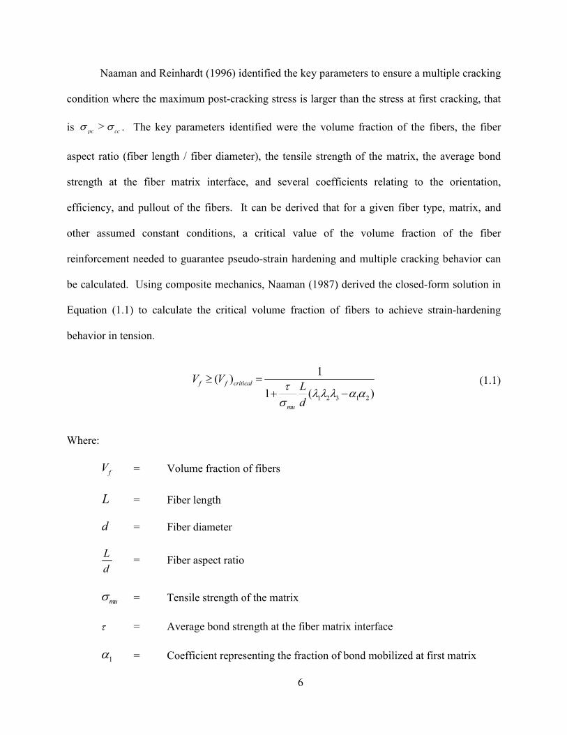
Naaman and Reinhardt (1996) identified the key parameters to ensure a multiple cracking
condition where the maximum post-cracking stress is larger than the stress at first cracking, that
is > pc cc
σ σ . The key parameters identified were the volume fraction of the fibers, the fiber
aspect ratio (fiber length / fiber diameter), the tensile strength of the matrix, the average bond
strength at the fiber matrix interface, and several coefficients relating to the orientation,
efficiency, and pullout of the fibers. It can be derived that for a given fiber type, matrix, and
other assumed constant conditions, a critical value of the volume fraction of the fiber
reinforcement needed to guarantee pseudo-strain hardening and multiple cracking behavior can
be calculated. Using composite mechanics, Naaman (1987) derived the closed-form solution in
Equation (1.1) to calculate the critical volume fraction of fibers to achieve strain-hardening
behavior in tension.
1 2 3 1 2
1( )
1 ( )f f critical
mu
V VL
d
τλ λ λ αα
σ
≥ =
+ − (1.1)
Where:
fV = Volume fraction of fibers
L = Fiber length
d = Fiber diameter
L
d = Fiber aspect ratio
muσ = Tensile strength of the matrix
τ = Average bond strength at the fiber matrix interface
1α = Coefficient representing the fraction of bond mobilized at first matrix

7
cracking
2α = Efficiency factor of fiber orientation in the uncracked state of the
composite
1λ = Expected pull-out length ratio (this is the average fiber length used to
resist the pull out through bond stress and is equal to ¼ from probability
considerations)
2λ = Efficiency factor of orientation in the cracked state
3λ = Group reduction factor associated with the number of fibers pulling-out
per unit area (or density of fiber crossings)
For small values of the fiber volume fraction, 1 1fV− ≈ . Thus, Equation (1.1) can be
rewritten as follows:
1 2 3 1 2
1f
mu
LV
d
τ
σ λλ λ αα≥
− (1.2)
Equation (1.2) is a simple way to demonstrate the direct influence of the independent
variables leading to the development of multiple cracking. Assuming constants for the
coefficients addressing the selected fiber type and orientation (right-hand side of Equation (1.2)),
it can be seen that the aspect ratio of the fiber and the ratio of bond strength to the matrix tensile
strength are at least as influential as the volume fraction of the reinforcement to ensure strain-
hardening behavior (Naaman & Reinhardt, 1996).
In addition to the enhancement of the tensile behavior, the compressive behavior of
concrete is markedly enhanced with the addition of fibers as well, due to the passive confinement
8
afforded by the fibers. Both the compressive strength and deformation capacities of concrete can
be improved with the use of HPFRCC. In the design of reinforced concrete structures subjected
to seismic loading, large displacement reversals may be imposed on the structures. Thus,
detailing of regions that could be subjected to large inelastic deformations is critical. Since
regular reinforced concrete is brittle, extensive reinforcement detailing is required in regions that
are more susceptible to damage, such as column bases, beam ends, hinging regions of structural
walls, and coupling beams in structural wall systems. The use of HPFRCC in these final two
examples is a major focus of this research.
Interest in the development of high-performance fiber-reinforced cementitious
composites as a design alternative to alleviate reinforcement congestion in critical shear and/or
moment regions of reinforced concrete coupled shear walls has been considered. Use of
HPFRCC may allow for simplified reinforcement detailing with adequate damage tolerance
through a ductile response obtained by the tensile strain-hardening and confined compressive
behavior of the material. Thus, use of HPFRCC materials in large-scale structural applications
could significantly reduce the amount of reinforcement required to ensure adequate performance
in areas of inelastic deformation demands, while also potentially reducing labor costs and
construction time delays (Parra-Montesinos, 2005). An example of the typical congestion
present in a diagonally reinforced coupling beam can be seen in Figure 1-3. Due to increased
material costs associated with using HPFRCC, the material has been targeted for critical regions
where substantial reinforcement detailing is currently required for providing adequate behavior
during earthquakes. Canbolat et al. (2005) investigated the use of HPFRCC coupling beams
without diagonal reinforcing bars and with diagonal bars without transverse reinforcement
around the main diagonals. The results indicated that a reduction in such reinforcement may be
9
achieved in HPFRCC coupling beams without compromising the shear strength, due to the
additional diagonal tensile strength provided by the fibers. In fact, the HPFRCC coupling beams
exhibited higher shear strength and stiffness retention than the reinforced concrete coupling
beams designed according to the ACI Code. Since cast-in-place HPFRCC coupling beams could
present constructability issues, the use of precast HPFRCC beams in combination with
conventional reinforced concrete structural walls has been proposed. Additional HPFRCC
coupling beam tests have been conducted by project colleagues at the University of Michigan,
and these similarly successful results will be discussed further in Chapter 5.
Figure 1-3. On-Site Coupling Beam from Lequesne (2011)
A related experimental program reported here has been conducted to further understand
the behavior of HPFRCC under general uniaxial and biaxial stress states (such as would for
instance be expected at various key locations in a coupling beam). Concrete plate specimens
comprising mixes containing from one to two percent volume fraction of hooked steel fibers or
10
Spectra (polyethylene) fibers were tested under uniaxial and biaxial compression, and failure
envelopes were developed for each type of concrete. Previous test results revealed that, across
both fiber types, the residual strength during uniaxial testing exceeded 60 percent of the
maximum stress at as much as 2 percent strain, with the level of residual strength depending on
the fiber volume fraction. Under equal biaxial compression a strength increase of greater than 50
percent over the uniaxial value was observed for both fiber types (Foltz et al., 2008). After the
exploration of these different fiber types and volume fractions, a 1.5 percent volume fraction of
hooked steel fibers was selected as the concrete mix for more comprehensive examination. It has
been found that HPFRCC in compression exhibits about 50 percent residual stress up to a strain
of 3%, as well as a shift in the failure mechanism from tensile splitting to a faulting or shear
failure. Failure envelopes have been developed for each type of composite, and their stress-
strain behaviors as well as failure mechanisms were observed.
Two large one-third scale tests conducted by project colleagues at the University of
Michigan on coupled wall systems were recently conducted. The four-story walls utilized three
HPFRCC precast coupling beams and one reinforced concrete coupling beam. Additionally, the
second wall specimen implemented HPFRCC into the plastic hinge region of the wall. The test
specimens were subjected to reverse cyclic loading, and the results illustrated the ability of
HPFRCC to increase the shear capacity of structural walls while reducing the level of damage
experienced at significant drifts. Further details of the experimental results of the large-scale
tests at the University of Michigan, as well as the multi-axial tests at the University of Illinois at
Urbana-Champaign will be described in Chapters 2 and 3.
From the experimental tests, the material properties were implemented into a nonlinear
finite element program to demonstrate the ability to predict the behavior of HPFRCC under
11
multi-axial loads and in structural components. An effort was undertaken to model the multi-
axial tests at the University of Illinois, and then the HPFRCC material model was extended to
uses of coupling beam component tests.
Another major aspect of this research, although not directly related to HPFRCC use, was
the testing of a full-scale pile-wharf connection. The background and details of the pile-wharf
connection test are outlined in Chapters 7 and 8. The HPFRCC material model that was
developed from the University of Illinois multi-axial tests was then extended to modeling the
pile-wharf connection. While this use of HPFRCC has not been tested in a laboratory, the model
allows one to assess the potential benefits of using HPFRCC on the ductility and capacity of the
pile-wharf connection.
1.3 Objective and Scope
The objective of this study is to achieve the following unique contributions to the
research community:
• The first study to experimentally test the biaxial behavior of a self-consolidating
HPFRCC. The thesis provides failure envelopes and deformation characteristics
that are not available in the literature, and should be useful for calibrating further
finite element models.
• The first study to develop a finite element model for HPFRCC from its own
biaxial experimental results. This thesis outlines the procedure and input
parameters required to utilize commercially available software to model
HPFRCC.
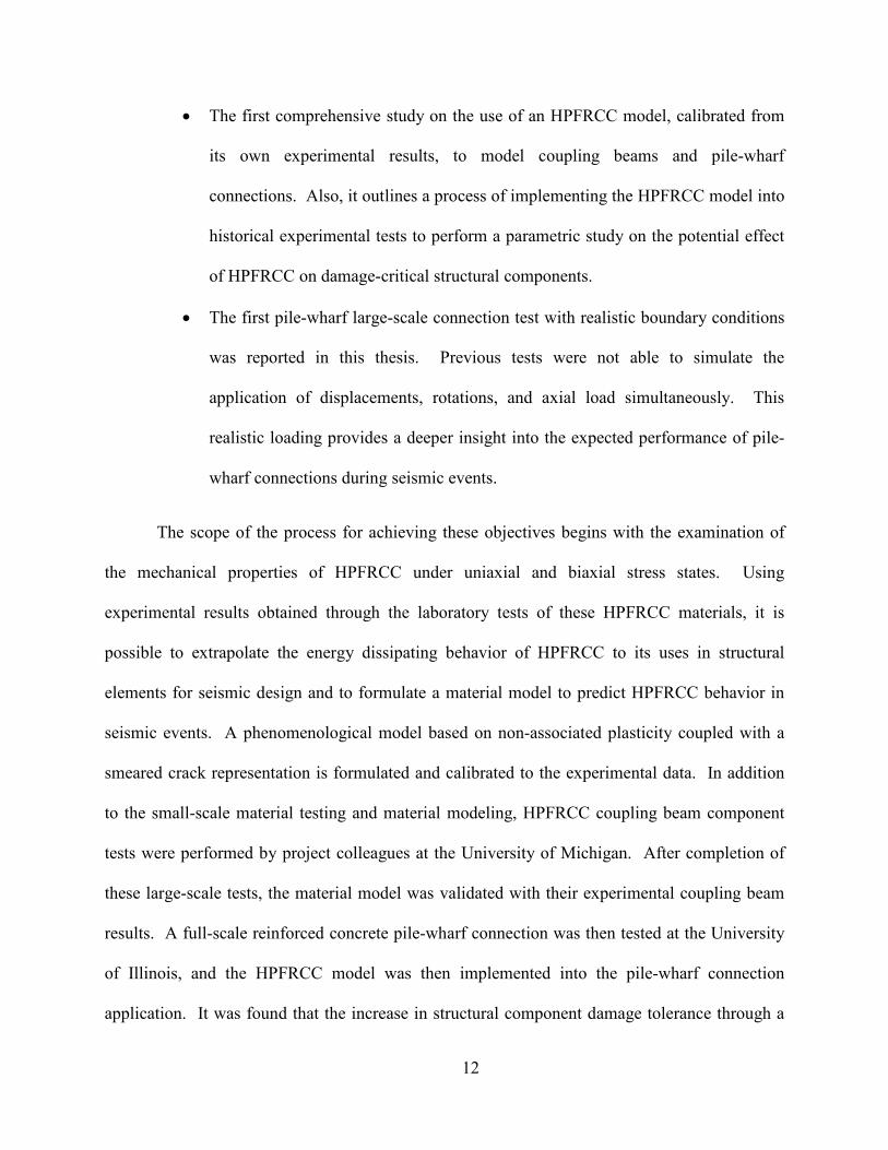
12
• The first comprehensive study on the use of an HPFRCC model, calibrated from
its own experimental results, to model coupling beams and pile-wharf
connections. Also, it outlines a process of implementing the HPFRCC model into
historical experimental tests to perform a parametric study on the potential effect
of HPFRCC on damage-critical structural components.
• The first pile-wharf large-scale connection test with realistic boundary conditions
was reported in this thesis. Previous tests were not able to simulate the
application of displacements, rotations, and axial load simultaneously. This
realistic loading provides a deeper insight into the expected performance of pile-
wharf connections during seismic events.
The scope of the process for achieving these objectives begins with the examination of
the mechanical properties of HPFRCC under uniaxial and biaxial stress states. Using
experimental results obtained through the laboratory tests of these HPFRCC materials, it is
possible to extrapolate the energy dissipating behavior of HPFRCC to its uses in structural
elements for seismic design and to formulate a material model to predict HPFRCC behavior in
seismic events. A phenomenological model based on non-associated plasticity coupled with a
smeared crack representation is formulated and calibrated to the experimental data. In addition
to the small-scale material testing and material modeling, HPFRCC coupling beam component
tests were performed by project colleagues at the University of Michigan. After completion of
these large-scale tests, the material model was validated with their experimental coupling beam
results. A full-scale reinforced concrete pile-wharf connection was then tested at the University
of Illinois, and the HPFRCC model was then implemented into the pile-wharf connection
application. It was found that the increase in structural component damage tolerance through a

13
ductile response obtained by the tensile strain-hardening and confined compressive behavior
from the use of HPFRCC makes it a viable solution as a replacement for some steel confinement
reinforcement and as an additional shear resistance mechanism. With the development of an
HPFRCC modeling tool, insight into the levels of damage experienced by structural elements can
inform performance based design decisions regarding the use of HPFRCC in critical structural
components. Combining the knowledge and behavioral trends gained through laboratory testing
of the HPFRCC materials with the vast experimental information already available in the
literature, it is possible to provide the informed designer with the tools to include HPFRCC in the
seismic design of damage critical structural components.
1.4 Chapter Description
This dissertation proposal is composed of four chapters as follows:
Chapter 1: Introduction – This chapter provides an overview of the research, as well as
the objectives, scope, and layout of the proposed dissertation work.
Chapter 2: Background Information – This chapter provides background about HPFRCC,
as well as a review of previous research pertaining to the use and testing of plain concrete,
HPFRCC, and RC coupling beams. Also, it contains additional previously explored uses of
HPFRCC and prior HPFRCC finite element modeling efforts.
Chapter 3: Material Testing Results – This chapter provides an overview of the
conducted HPFRCC material experimental program. It describes in detail the concrete mixtures
used in the study, testing techniques, and experimental results.
Chapter 4: Material Modeling – This chapter describes the material modeling effort of the
HPFRCC in ATENA, a non-linear continuum finite element program. It outlines the
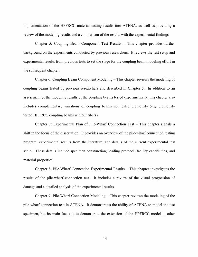
14
implementation of the HPFRCC material testing results into ATENA, as well as providing a
review of the modeling results and a comparison of the results with the experimental findings.
Chapter 5: Coupling Beam Component Test Results – This chapter provides further
background on the experiments conducted by previous researchers. It reviews the test setup and
experimental results from previous tests to set the stage for the coupling beam modeling effort in
the subsequent chapter.
Chapter 6: Coupling Beam Component Modeling – This chapter reviews the modeling of
coupling beams tested by previous researchers and described in Chapter 5. In addition to an
assessment of the modeling results of the coupling beams tested experimentally, this chapter also
includes complementary variations of coupling beams not tested previously (e.g. previously
tested HPFRCC coupling beams without fibers).
Chapter 7: Experimental Plan of Pile-Wharf Connection Test – This chapter signals a
shift in the focus of the dissertation. It provides an overview of the pile-wharf connection testing
program, experimental results from the literature, and details of the current experimental test
setup. These details include specimen construction, loading protocol, facility capabilities, and
material properties.
Chapter 8: Pile-Wharf Connection Experimental Results – This chapter investigates the
results of the pile-wharf connection test. It includes a review of the visual progression of
damage and a detailed analysis of the experimental results.
Chapter 9: Pile-Wharf Connection Modeling – This chapter reviews the modeling of the
pile-wharf connection test in ATENA. It demonstrates the ability of ATENA to model the test
specimen, but its main focus is to demonstrate the extension of the HPFRCC model to other

15
structural components. It reviews the modeling results of the RC pile-wharf connection and
compares the results to the performance of a similar pile-wharf connection with HPFRCC.
Chapter 10: Conclusions – This chapter provides a summary of the findings and
conclusions of this dissertation, as well as an outline of the research contributions and future
work.
16
CHAPTER 2. BACKGROUD IFORMATIO
In this chapter, a review of the literature pertaining to the different aspects of the current
research work is given. There have been previous studies conducted concerning the multi-axial
behavior of plain concrete, as well as some limited tests on the multi-axial behavior of fiber
reinforced concrete. While triaxial concrete tests have been previously completed on concrete,
the focus of the current research is on the biaxial and uniaxial performance of plain concrete and
high-performance fiber-reinforced cementitious composites (HPFRCC). The literature review
begins with a discussion of previous biaxial and uniaxial tests, setting the stage for the testing
program to be discussed in Chapter 3. Testing has also been conducted on both reinforced
concrete coupling beams and HPFRCC coupling beams by previous researchers. A description
of their results is presented, and a discussion of their findings and the implications on the current
proposed use of precast HPFRCC couplings beams and modeling is addressed. Additional
coupling beam component tests have been conducted by research project colleagues at the
University of Michigan, and the details of that testing program and results will be addressed in
Chapter 5. Finally, previous work on the analytical modeling of HPFRCC is discussed.
2.1 Previously Conducted Multi-Axial Plain Concrete Results
Understanding the behavior of concrete under multi-axial stress states is critical to
developing a universal failure criterion for concrete, thus many series of tests have been
conducted on concrete under biaxial stress states over the years. The multi-axial behavior of
concrete is important in design because such forces exist regularly in concrete structures, such as
in shear regions of flexural members, shear walls, slabs, shells, and various containment
structures. Therefore, it is essential in the creation of accurate models that characterize the
17
uniaxial and biaxial behavior of concrete to have an experimental testing regime that imposes the
desired forces and boundary conditions on the specimen. However, a major problem when
conducting the tests occurs when trying to develop a uniform biaxial stress state. Most of the
discrepancies arising in the test results can be traced to unintended differences in the stress states
which have been developed in the test specimen (Kupfer et al., 1969). Early biaxial tests were
conducted on cube concrete specimens of varying dimensions. The initial tests ignored the
biaxial tension condition, as well as the influence on the results produced by the restraining shear
force on the faces of the specimens due to the test setup (Iynegar et al., 1965). This restraint
inevitably results in an increase of the apparent strength in the specimen. Later investigations
employed various surface treatments of the concrete or soft backing between the bearing platens
and the specimen; however, the results widely varied, and the strength obtained for the equal
compression case ranged from 80 percent to 350 percent of the uniaxial compression strength
(Kupfer et al., 1969). A review by Hilsdorf (1965) concluded that square concrete plates
subjected to in-plane loading are suitable for the determination of the biaxial strength of concrete
over the entire range of biaxial stress combinations only once conventional solid bearing plates
are replaced with brush bearing platens. Kupfer et al. (1969) recognized this recommendation to
mitigate the effect of the confining stresses imposed by the loading platens, and replaced the
solid bearing platens. The brush bearing platens consisted of a series of closely spaced steel bars
that were flexible enough to accommodate transverse or lateral deformations of the concrete
specimens without applying any significant restraining force. The brush bearing platens are
shown in Figure 2-1. As such, a similar concept was adopted and used for the present
experimental program, as outlined in Chapter 3.
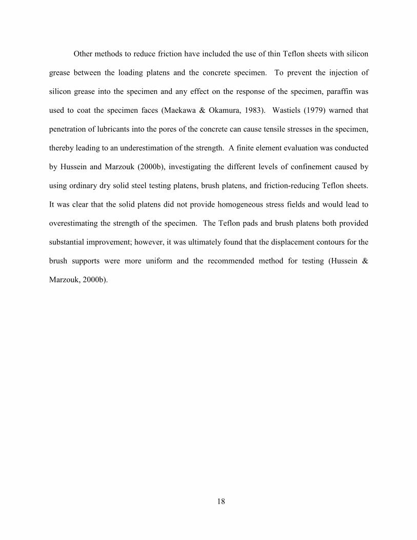
18
Other methods to reduce friction have included the use of thin Teflon sheets with silicon
grease between the loading platens and the concrete specimen. To prevent the injection of
silicon grease into the specimen and any effect on the response of the specimen, paraffin was
used to coat the specimen faces (Maekawa & Okamura, 1983). Wastiels (1979) warned that
penetration of lubricants into the pores of the concrete can cause tensile stresses in the specimen,
thereby leading to an underestimation of the strength. A finite element evaluation was conducted
by Hussein and Marzouk (2000b), investigating the different levels of confinement caused by
using ordinary dry solid steel testing platens, brush platens, and friction-reducing Teflon sheets.
It was clear that the solid platens did not provide homogeneous stress fields and would lead to
overestimating the strength of the specimen. The Teflon pads and brush platens both provided
substantial improvement; however, it was ultimately found that the displacement contours for the
brush supports were more uniform and the recommended method for testing (Hussein &
Marzouk, 2000b).
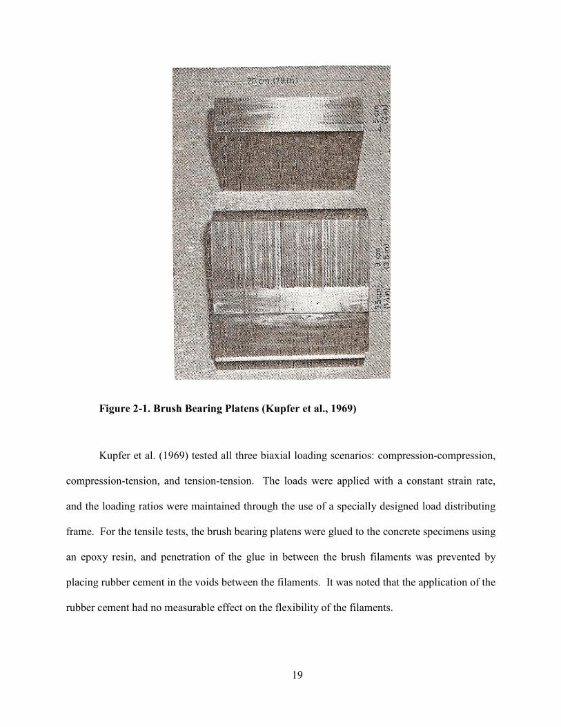
19
Figure 2-1. Brush Bearing Platens (Kupfer et al., 1969)
Kupfer et al. (1969) tested all three biaxial loading scenarios: compression-compression,
compression-tension, and tension-tension. The loads were applied with a constant strain rate,
and the loading ratios were maintained through the use of a specially designed load distributing
frame. For the tensile tests, the brush bearing platens were glued to the concrete specimens using
an epoxy resin, and penetration of the glue in between the brush filaments was prevented by
placing rubber cement in the voids between the filaments. It was noted that the application of the
rubber cement had no measurable effect on the flexibility of the filaments.
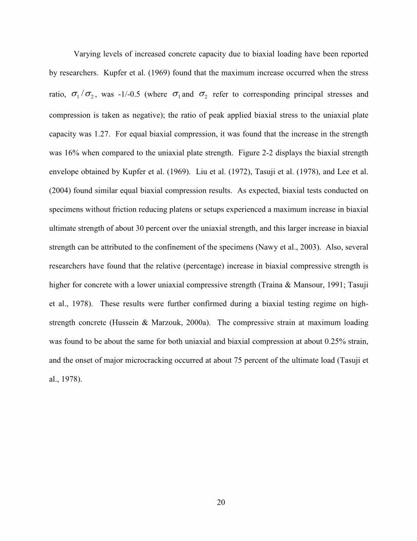
20
Varying levels of increased concrete capacity due to biaxial loading have been reported
by researchers. Kupfer et al. (1969) found that the maximum increase occurred when the stress
ratio, 1 2/σ σ , was -1/-0.5 (where 1σ and 2σ refer to corresponding principal stresses and
compression is taken as negative); the ratio of peak applied biaxial stress to the uniaxial plate
capacity was 1.27. For equal biaxial compression, it was found that the increase in the strength
was 16% when compared to the uniaxial plate strength. Figure 2-2 displays the biaxial strength
envelope obtained by Kupfer et al. (1969). Liu et al. (1972), Tasuji et al. (1978), and Lee et al.
(2004) found similar equal biaxial compression results. As expected, biaxial tests conducted on
specimens without friction reducing platens or setups experienced a maximum increase in biaxial
ultimate strength of about 30 percent over the uniaxial strength, and this larger increase in biaxial
strength can be attributed to the confinement of the specimens (Nawy et al., 2003). Also, several
researchers have found that the relative (percentage) increase in biaxial compressive strength is
higher for concrete with a lower uniaxial compressive strength (Traina & Mansour, 1991; Tasuji
et al., 1978). These results were further confirmed during a biaxial testing regime on high-
strength concrete (Hussein & Marzouk, 2000a). The compressive strain at maximum loading
was found to be about the same for both uniaxial and biaxial compression at about 0.25% strain,
and the onset of major microcracking occurred at about 75 percent of the ultimate load (Tasuji et
al., 1978).
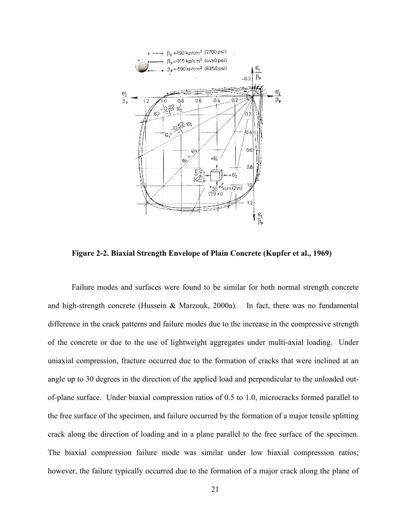
21
Figure 2-2. Biaxial Strength Envelope of Plain Concrete (Kupfer et al., 1969)
Failure modes and surfaces were found to be similar for both normal strength concrete
and high-strength concrete (Hussein & Marzouk, 2000a). In fact, there was no fundamental
difference in the crack patterns and failure modes due to the increase in the compressive strength
of the concrete or due to the use of lightweight aggregates under multi-axial loading. Under
uniaxial compression, fracture occurred due to the formation of cracks that were inclined at an
angle up to 30 degrees in the direction of the applied load and perpendicular to the unloaded out-
of-plane surface. Under biaxial compression ratios of 0.5 to 1.0, microcracks formed parallel to
the free surface of the specimen, and failure occurred by the formation of a major tensile splitting
crack along the direction of loading and in a plane parallel to the free surface of the specimen.
The biaxial compression failure mode was similar under low biaxial compression ratios;
however, the failure typically occurred due to the formation of a major crack along the plane of
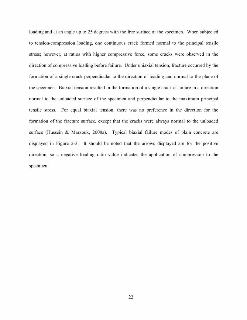
22
loading and at an angle up to 25 degrees with the free surface of the specimen. When subjected
to tension-compression loading, one continuous crack formed normal to the principal tensile
stress; however, at ratios with higher compressive force, some cracks were observed in the
direction of compressive loading before failure. Under uniaxial tension, fracture occurred by the
formation of a single crack perpendicular to the direction of loading and normal to the plane of
the specimen. Biaxial tension resulted in the formation of a single crack at failure in a direction
normal to the unloaded surface of the specimen and perpendicular to the maximum principal
tensile stress. For equal biaxial tension, there was no preference in the direction for the
formation of the fracture surface, except that the cracks were always normal to the unloaded
surface (Hussein & Marzouk, 2000a). Typical biaxial failure modes of plain concrete are
displayed in Figure 2-3. It should be noted that the arrows displayed are for the positive
direction, so a negative loading ratio value indicates the application of compression to the
specimen.
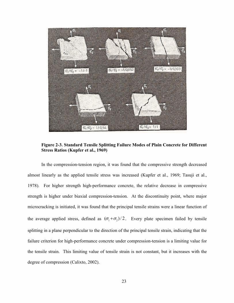
23
Figure 2-3. Standard Tensile Splitting Failure Modes of Plain Concrete for Different
Stress Ratios (Kupfer et al., 1969)
In the compression-tension region, it was found that the compressive strength decreased
almost linearly as the applied tensile stress was increased (Kupfer et al., 1969; Tasuji et al.,
1978). For higher strength high-performance concrete, the relative decrease in compressive
strength is higher under biaxial compression-tension. At the discontinuity point, where major
microcracking is initiated, it was found that the principal tensile strains were a linear function of
the average applied stress, defined as 1 2( ) / 2σ σ+ . Every plate specimen failed by tensile
splitting in a plane perpendicular to the direction of the principal tensile strain, indicating that the
failure criterion for high-performance concrete under compression-tension is a limiting value for
the tensile strain. This limiting value of tensile strain is not constant, but it increases with the
degree of compression (Calixto, 2002).
24
In the tension-tension quadrant, some of the previous researchers observed no increase in
the strength under biaxial tension. They indicated that the biaxial concrete strength was equal to
its uniaxial tensile strength (Kupfer et al., 1969; Nelissen, 1972; Lee et al., 2004). Tasuji et al.
(1978), however, noted a definite increase in the biaxial tensile strength of concrete when
compared to its uniaxial tensile strength, on the order of 10 to 20 percent. The tensile strain at
maximum loading was found to be about the same for both uniaxial and biaxial tension at about
+0.015% strain, and the onset of major microcracking occurred at about 60 percent of the
ultimate load in stress states involving direct tension (Tasuji et al., 1978).
Cho et al. (2004) also investigated the stress-strain relationship of reinforced concrete
subjected to biaxial tension. While these specimens were mostly exploring the biaxial tensile
strength of concrete with varying reinforcement ratios, they did however note that concrete
subjected to biaxial tension experienced lower tensile stresses experimentally than previously
proposed biaxial tension models which were largely based on the results of uniaxial tension tests.
This indicates the importance of understanding the behavior of concrete under biaxial tension,
and the current lack of reliable experimental data.
Lan and Guo (1999) conducted a series of tests on concrete plate specimens that
compared the results of specimens under proportional monotonic compressive biaxial loading to
failure, proportional repeated compressive biaxial loading to failure with complete unloading and
a predetermined strain increment, and proportional repeated compressive biaxial loading to
failure with partial unloading and a predetermined strain increment. For the specimens subjected
to repeated loading, each cycle was loaded to the next predetermined strain increment until
failure occurred in the specimen. The stress ratios investigated were 0.0, 0.25, 0.50, 0.75, and
1.0. It was found that for concrete tested under repeated biaxial loading and unloading cycles,
25
the failure envelope was unaffected when compared to those subjected to monotonic loads.
Also, it was seen that the shape of the envelope of the stress-strain curve under repeated biaxial
loads was independent of the stress ratio and was similar to the uniaxial behavior under repeated
compressive loading when normalized by the failure stress and failure strain. Finally, the effect
of dynamic loads on low-strength concrete cubes was explored by Yan and Lin (2007). They
found that the dynamic strength increases with an increase in strain rate and lateral confinement;
however, the initial tangent stiffness and fracture pattern remain independent of the strain rate.
2.2 Previously Conducted Fiber-Reinforced Concrete Multi-Axial Results
The initial tests on fiber-reinforced concrete subjected to multi-axial loads were
conducted by Yin et al. (1989), and the experiments were performed on both steel fiber
reinforced and plain concrete specimens of dimensions similar in size to those used by Kupfer et
al. (1969). These plate specimens were cut from concrete blocks, similar to the tests that will be
described in Chapter 3. However, testing was conducted on a “load-bifurcation” test machine, as
shown in Figure 2-4, which uses two crescent shaped distribution beams, rather than four
individual actuators. Since the load can only be applied to the distribution beams at three
locations, the test setup limited the variety of compressive stress ratios that were applied to the
specimens to 1.0, 0.5, and 0.2, as well as limiting the tests to being exclusively load-controlled;
all of these specimens were epoxied to the brush platens.
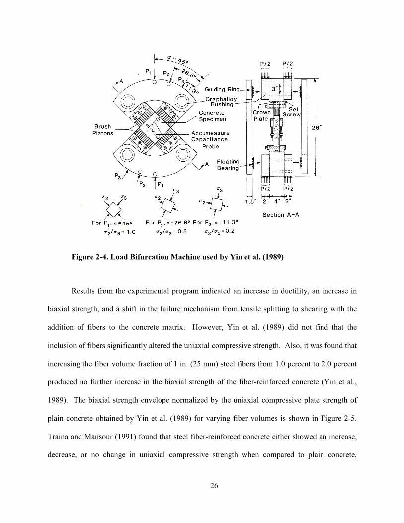
26
Figure 2-4. Load Bifurcation Machine used by Yin et al. (1989)
Results from the experimental program indicated an increase in ductility, an increase in
biaxial strength, and a shift in the failure mechanism from tensile splitting to shearing with the
addition of fibers to the concrete matrix. However, Yin et al. (1989) did not find that the
inclusion of fibers significantly altered the uniaxial compressive strength. Also, it was found that
increasing the fiber volume fraction of 1 in. (25 mm) steel fibers from 1.0 percent to 2.0 percent
produced no further increase in the biaxial strength of the fiber-reinforced concrete (Yin et al.,
1989). The biaxial strength envelope normalized by the uniaxial compressive plate strength of
plain concrete obtained by Yin et al. (1989) for varying fiber volumes is shown in Figure 2-5.
Traina and Mansour (1991) found that steel fiber-reinforced concrete either showed an increase,
decrease, or no change in uniaxial compressive strength when compared to plain concrete,
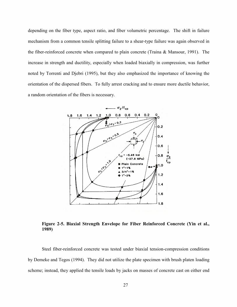
27
depending on the fiber type, aspect ratio, and fiber volumetric percentage. The shift in failure
mechanism from a common tensile splitting failure to a shear-type failure was again observed in
the fiber-reinforced concrete when compared to plain concrete (Traina & Mansour, 1991). The
increase in strength and ductility, especially when loaded biaxially in compression, was further
noted by Torrenti and Djebri (1995), but they also emphasized the importance of knowing the
orientation of the dispersed fibers. To fully arrest cracking and to ensure more ductile behavior,
a random orientation of the fibers is necessary.
Figure 2-5. Biaxial Strength Envelope for Fiber Reinforced Concrete (Yin et al.,
1989)
Steel fiber-reinforced concrete was tested under biaxial tension-compression conditions
by Demeke and Tegos (1994). They did not utilize the plate specimen with brush platen loading
scheme; instead, they applied the tensile loads by jacks on masses of concrete cast on either end

28
of the specimen, and the compressive loads were applied directly, with layers of Teflon and
petroleum jelly to minimize friction. It was found that steel hooked fibers doubled the uniaxial
tensile strength for a 1.5 percent volume fraction, and the strength when compared to plain
concrete was almost three times greater when simultaneously subjected to biaxial compression
and tension for the same volume fraction. For the fiber reinforced specimens, failure occurred
due to fiber pullout, with the extent of the cracked region being a function of the fiber
percentage. All of the plain concrete specimens experienced an abrupt and explosive failure
when one large crack appeared, dividing the specimen into two pieces (Demeke & Tegos, 1994).
The triaxial behavior of steel fiber reinforced concrete was explored by Chern et al. (1992), and
it was found that when compared to cylinders of plain concrete, the steel fiber reinforced
concrete behaved in a more ductile manner, especially when exposed to some tensile loading.
Finally, Yin and Hsu (1995) investigated the performance of steel fiber-reinforced
concrete subjected to cyclic uniaxial and biaxial loading. It was found that fibers could increase
the fatigue strength when the fatigue load was in the low-cycle region because fibers can arrest
the propagation of cracks at higher stress levels; however, in the high-cycle fatigue region, fibers
do not help because they are ineffective at arresting the bond cracks that ultimately dictate the
fatigue life of the specimens. Also, the failure mode of the specimens was unchanged when
compared to monotonic tests (Yin & Hsu, 1995).
2.3 Previously Conducted Reinforced Concrete Coupling Beam Tests
Paulay (1971) reported a series of tests conducted on coupling beams with short span-to-
depth ratios (1.02 and 1.29). At the time, coupling beams were typically constructed using only
top and bottom flexural reinforcement, as well as some transverse reinforcement. Due to the
elongation of the coupling beam caused by damage when subjected to cyclical load reversals, all
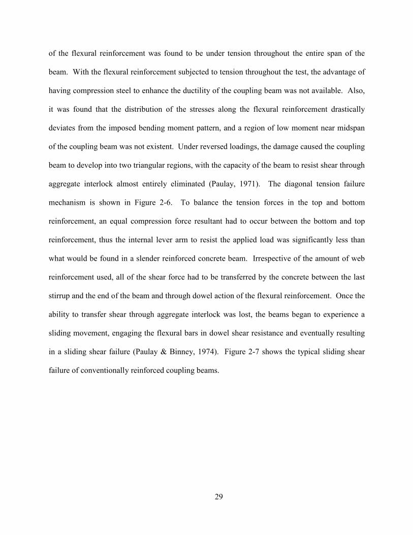
29
of the flexural reinforcement was found to be under tension throughout the entire span of the
beam. With the flexural reinforcement subjected to tension throughout the test, the advantage of
having compression steel to enhance the ductility of the coupling beam was not available. Also,
it was found that the distribution of the stresses along the flexural reinforcement drastically
deviates from the imposed bending moment pattern, and a region of low moment near midspan
of the coupling beam was not existent. Under reversed loadings, the damage caused the coupling
beam to develop into two triangular regions, with the capacity of the beam to resist shear through
aggregate interlock almost entirely eliminated (Paulay, 1971). The diagonal tension failure
mechanism is shown in Figure 2-6. To balance the tension forces in the top and bottom
reinforcement, an equal compression force resultant had to occur between the bottom and top
reinforcement, thus the internal lever arm to resist the applied load was significantly less than
what would be found in a slender reinforced concrete beam. Irrespective of the amount of web
reinforcement used, all of the shear force had to be transferred by the concrete between the last
stirrup and the end of the beam and through dowel action of the flexural reinforcement. Once the
ability to transfer shear through aggregate interlock was lost, the beams began to experience a
sliding movement, engaging the flexural bars in dowel shear resistance and eventually resulting
in a sliding shear failure (Paulay & Binney, 1974). Figure 2-7 shows the typical sliding shear
failure of conventionally reinforced coupling beams.
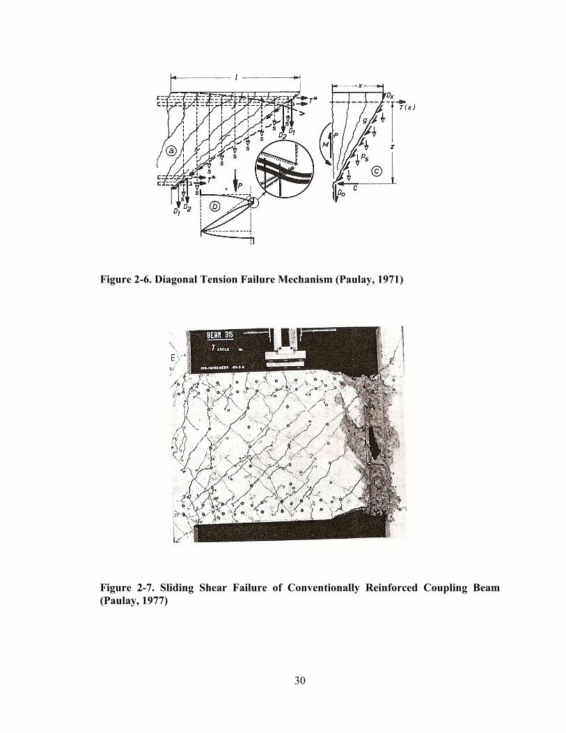
30
Figure 2-6. Diagonal Tension Failure Mechanism (Paulay, 1971)
Figure 2-7. Sliding Shear Failure of Conventionally Reinforced Coupling Beam
(Paulay, 1977)
31
Short coupling beams of aspect ratios 1.02 and 1.29 were then tested by Paulay and
Binney (1974) utilizing diagonal bars to simulate the behavior of “cross-bracing” within the
beam. In these diagonally reinforced beams, the role of the concrete for resisting forces was
relatively minor; instead, the diagonal reinforcement resisted essentially all of the loading, and
the behavior of the beam was governed by the behavior of the diagonal steel reinforcement,
which was equally effective in tension and compression. The coupling beams eventually failed
by buckling of the compression bars after the surrounding concrete had broken away. This
illustrated the importance of confining the concrete within the cage of the diagonally placed
group of bars to preserve the integrity of the section and to provide flexural rigidity (Paulay &
Binney, 1974). Experimental verification of the behavior of diagonally reinforced coupling
beams as part of a whole coupled shear wall structure was then explored by Paulay and
Santhakumar (1976). Two one-quarter full-size seven-story shear walls were tested; one had
conventionally reinforced coupling beams, while the other had diagonally reinforced coupling
beams. The reinforcement in the structural walls of each model was identical, and the walls were
designed such that yielding would occur at the base of the walls only after all of the coupling
beams had yielded. This was done with consideration of the desired sequence of plastification
where a designer would desire to protect the walls against permanent damage. The coupling
beams were designed to have approximately the same shear capacity, and the results of the tests
revealed that the ductility, energy dissipating capacity, level of damage, and overall performance
were superior in the short aspect ratio diagonally reinforced coupling beam structure (Paulay &
Santhakumar, 1976). Results from those tests are shown in Figure 2-8. A major advantage of
the use of the more ductile coupling beams is that the majority of energy to be dissipated during
a large seismic event can be dispersed in the coupling system over the full height of a structure,
32
rather than being concentrated in the plastic hinging region at the base of the walls and perhaps
jeopardizing the gravity load carrying capacity of the wall (Paulay, 1977). Since the
reinforcement in the structural walls of each specimen was the same, the degradation of the
overall stiffness during similar load cycles can be attributed to the performance of the coupling
beams. It was found that in the wall with diagonally reinforced coupling beams, the strength loss
and stiffness degradation at any given displacement was significantly less than in the wall with
conventionally reinforced coupling beams. The reason for the superior performance of the
diagonally reinforced coupled wall was that the critical internal forces were carried by steel
rather than concrete. Thus, the inevitable deterioration of the concrete under severe repeated
reversed loading had little effect, and no significant stiffness degradation was observed in the
diagonally reinforced coupled wall. Comparatively, the conventionally reinforced coupled wall
experienced a sliding shear failure in each coupling beam, followed by the eventual compression
zone failure in the tension wall due to spalling of the concrete coupled with buckling of the
compression reinforcement on the boundary.
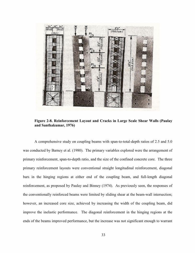
33
Figure 2-8. Reinforcement Layout and Cracks in Large Scale Shear Walls (Paulay
and Santhakumar, 1976)
A comprehensive study on coupling beams with span-to-total-depth ratios of 2.5 and 5.0
was conducted by Barney et al. (1980). The primary variables explored were the arrangement of
primary reinforcement, span-to-depth ratio, and the size of the confined concrete core. The three
primary reinforcement layouts were conventional straight longitudinal reinforcement, diagonal
bars in the hinging regions at either end of the coupling beam, and full-length diagonal
reinforcement, as proposed by Paulay and Binney (1974). As previously seen, the responses of
the conventionally reinforced beams were limited by sliding shear at the beam-wall intersection;
however, an increased core size, achieved by increasing the width of the coupling beam, did
improve the inelastic performance. The diagonal reinforcement in the hinging regions at the
ends of the beams improved performance, but the increase was not significant enough to warrant
34
the additional complexity and cost. The fully developed diagonal reinforcement had the best
strength, ductility, and energy-dissipation of all of the coupling beams tested, but the
improvement was less pronounced in the long-span beams. Therefore, it was concluded that
conventional bars are preferred in coupling beams with span-to-depth ratios greater than 5.0
(Barney et al., 1980).
Other coupling beam reinforcement layouts have also been explored. Tegos and Penelis
(1988) conducted tests on coupling beams with inclined bars forming a rhombic truss. They
found that the rhombic layout, as shown in design 3 of Figure 2-9, was in fact able to
successfully prevent an explosive shear failure, despite having a decreased number of hoops.
Also, there was no appreciable deterioration after reaching the maximum capacity of specimens
with span-to-depth ratios of greater than 1.5 (Tegos & Penelis, 1988). Additional coupling beam
tests were performed by Tassios et al. (1996) on a variety of reinforcement layouts. They
investigated relatively short span-to-depth ratio coupling beams (1.0 and 1.66), and the
reinforcement layouts explored were conventional, diagonal, conventional with inclined bars in
the hinging region, and dowel bars. The details of the reinforcement layout, reinforcement ratio,
and concrete strength of the investigated coupling beams are shown in Figure 2-9. Extreme
pinching was observed in the results of their conventional and dowel coupling beams. The
inclined bars seemed to diminish the pinching effect, and the diagonal bars almost eliminated it.
The benefit of the diagonal reinforcement diminished as the shear span of the coupling beam
increased, and at longer spans, around a 2.67 span-to-depth ratio, conventional reinforcement
was then suggested (Tassios et al., 1996).
Galano and Vignoli (2000) revisited the comparison among conventionally reinforced,
diagonally reinforced, and rhombically reinforced coupling beams in coupled walls. They noted
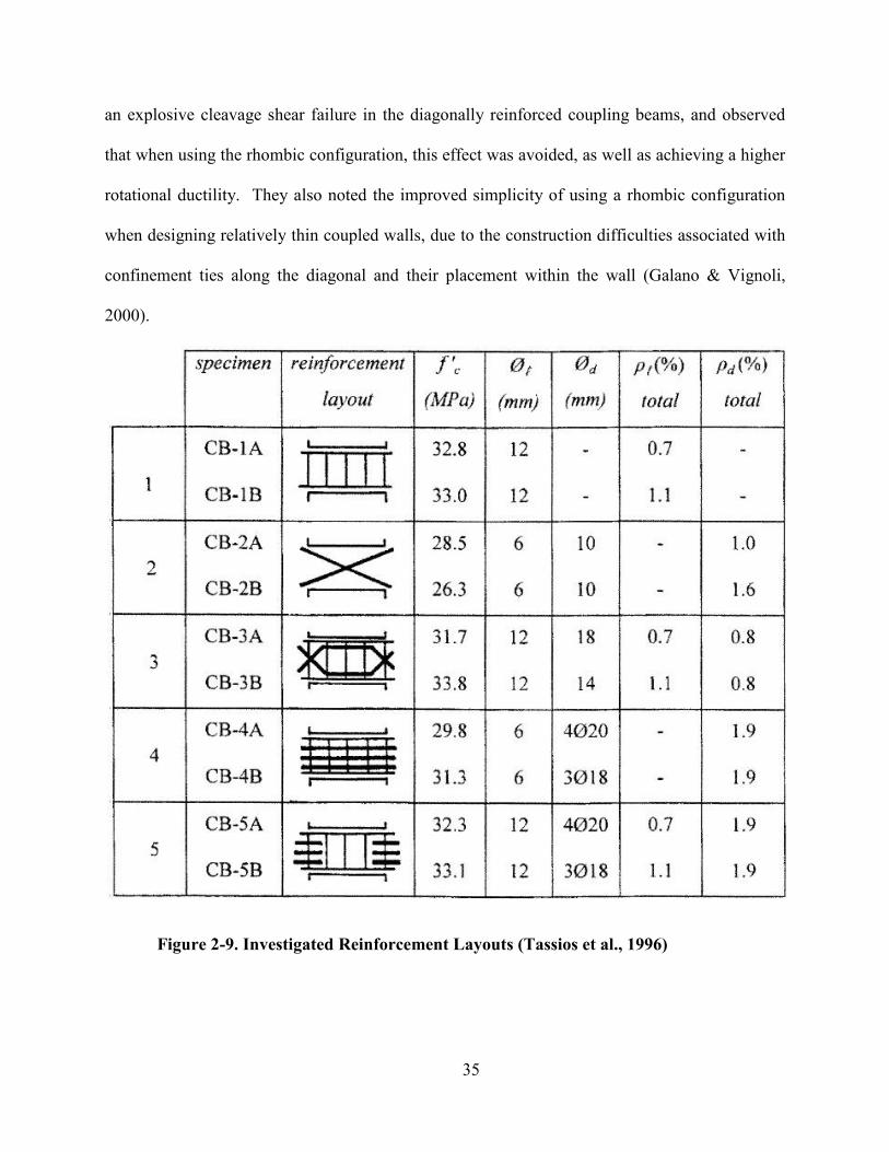
35
an explosive cleavage shear failure in the diagonally reinforced coupling beams, and observed
that when using the rhombic configuration, this effect was avoided, as well as achieving a higher
rotational ductility. They also noted the improved simplicity of using a rhombic configuration
when designing relatively thin coupled walls, due to the construction difficulties associated with
confinement ties along the diagonal and their placement within the wall (Galano & Vignoli,
2000).
Figure 2-9. Investigated Reinforcement Layouts (Tassios et al., 1996)
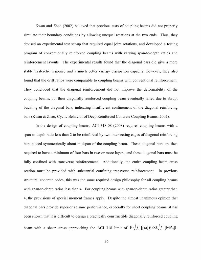
36
Kwan and Zhao (2002) believed that previous tests of coupling beams did not properly
simulate their boundary conditions by allowing unequal rotations at the two ends. Thus, they
devised an experimental test set-up that required equal joint rotations, and developed a testing
program of conventionally reinforced coupling beams with varying span-to-depth ratios and
reinforcement layouts. The experimental results found that the diagonal bars did give a more
stable hysteretic response and a much better energy dissipation capacity; however, they also
found that the drift ratios were comparable to coupling beams with conventional reinforcement.
They concluded that the diagonal reinforcement did not improve the deformability of the
coupling beams, but their diagonally reinforced coupling beam eventually failed due to abrupt
buckling of the diagonal bars, indicating insufficient confinement of the diagonal reinforcing
bars (Kwan & Zhao, Cyclic Behavior of Deep Reinforced Concrete Coupling Beams, 2002).
In the design of coupling beams, ACI 318-08 (2008) requires coupling beams with a
span-to-depth ratio less than 2 to be reinforced by two intersecting cages of diagonal reinforcing
bars placed symmetrically about midspan of the coupling beam. These diagonal bars are then
required to have a minimum of four bars in two or more layers, and these diagonal bars must be
fully confined with transverse reinforcement. Additionally, the entire coupling beam cross
section must be provided with substantial confining transverse reinforcement. In previous
structural concrete codes, this was the same required design philosophy for all coupling beams
with span-to-depth ratios less than 4. For coupling beams with span-to-depth ratios greater than
4, the provisions of special moment frames apply. Despite the almost unanimous opinion that
diagonal bars provide superior seismic performance, especially for short coupling beams, it has
been shown that it is difficult to design a practically constructible diagonally reinforced coupling
beam with a shear stress approaching the ACI 318 limit of ' '10 [psi] (0.83 [MPa])c cf f .

37
Harries et al. (2005) contended that the constraining geometry and confinement requirements of
the individual diagonal elements are unnecessarily restrictive and they proposed the use of
transverse reinforcement to satisfy the code requirements and to confine the entire cross section,
while still providing adequate support and allowing versatility in the design (Harries et al.,
2005). To relieve the difficulty and cost in constructing diagonally reinforced coupling beams,
ACI 318-08 (2008) has a new provision which allows two options when designing coupling
beams with an intermediate span-to-depth ratio between 2 and 4. The first option, shown in
Figure 2-10, is similar to the previous provision and requires transverse reinforcement around the
diagonal bars and modest transverse reinforcement around the entire section. The second option,
displayed in Figure 2-11, does not require transverse reinforcement around the diagonal bars, but
it does require a significantly larger amount of transverse reinforcement to confine the entire
section. Wallace (2007) reported a coupling beam testing program on one-half scale coupling
beams with diagonal reinforcement designed to accommodate maximum shear stresses of
' '10 [psi] (0.83 [MPa])
c cf f and
' '6 [psi] (0.50 [MPa])
c cf f for span-to-depth ratios of 2.4 and
3.33, respectively. Four tests were reported, two at each span-to-depth ratio with each of the
ACI 318-08 (2008) reinforcement layout design provisions explored. The results showed that
very similar force-deformation responses were obtained using the different detailing schemes at
each of the aspect ratios, and these results are shown in Figure 2-12. In Figure 2-12, the plots
labeled “diagonal” refer to the detail shown in Figure 2-10, with confined diagonal reinforcing,
while the plots labeled “full” refer to the detail shown on the right in Figure 2-11, where the
diagonal bars do not have transverse reinforcement, but the coupling beam specimen is confined
with extensive transverse reinforcement. The peak shear stresses achieved the desired design
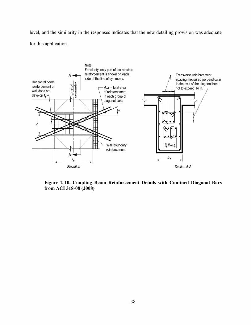
38
level, and the similarity in the responses indicates that the new detailing provision was adequate
for this application.
Figure 2-10. Coupling Beam Reinforcement Details with Confined Diagonal Bars
from ACI 318-08 (2008)
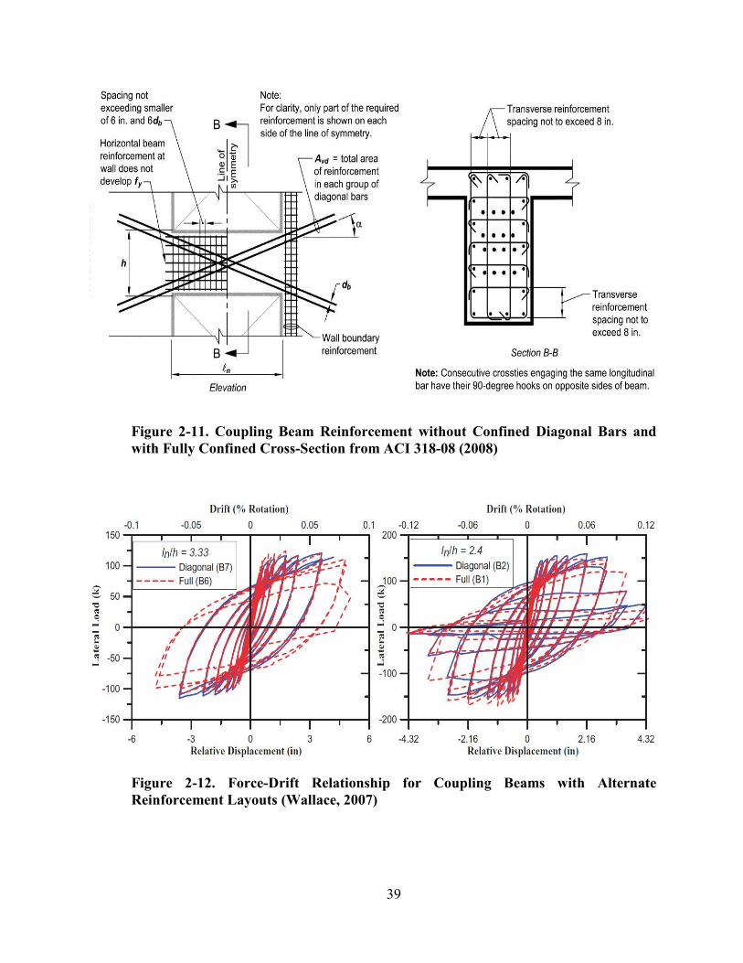
39
Figure 2-11. Coupling Beam Reinforcement without Confined Diagonal Bars and
with Fully Confined Cross-Section from ACI 318-08 (2008)
Figure 2-12. Force-Drift Relationship for Coupling Beams with Alternate
Reinforcement Layouts (Wallace, 2007)
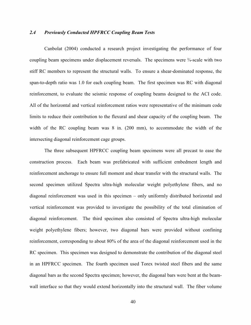
40
2.4 Previously Conducted HPFRCC Coupling Beam Tests
Canbolat (2004) conducted a research project investigating the performance of four
coupling beam specimens under displacement reversals. The specimens were ¾-scale with two
stiff RC members to represent the structural walls. To ensure a shear-dominated response, the
span-to-depth ratio was 1.0 for each coupling beam. The first specimen was RC with diagonal
reinforcement, to evaluate the seismic response of coupling beams designed to the ACI code.
All of the horizontal and vertical reinforcement ratios were representative of the minimum code
limits to reduce their contribution to the flexural and shear capacity of the coupling beam. The
width of the RC coupling beam was 8 in. (200 mm), to accommodate the width of the
intersecting diagonal reinforcement cage groups.
The three subsequent HPFRCC coupling beam specimens were all precast to ease the
construction process. Each beam was prefabricated with sufficient embedment length and
reinforcement anchorage to ensure full moment and shear transfer with the structural walls. The
second specimen utilized Spectra ultra-high molecular weight polyethylene fibers, and no
diagonal reinforcement was used in this specimen – only uniformly distributed horizontal and
vertical reinforcement was provided to investigate the possibility of the total elimination of
diagonal reinforcement. The third specimen also consisted of Spectra ultra-high molecular
weight polyethylene fibers; however, two diagonal bars were provided without confining
reinforcement, corresponding to about 80% of the area of the diagonal reinforcement used in the
RC specimen. This specimen was designed to demonstrate the contribution of the diagonal steel
in an HPFRCC specimen. The fourth specimen used Torex twisted steel fibers and the same
diagonal bars as the second Spectra specimen; however, the diagonal bars were bent at the beam-
wall interface so that they would extend horizontally into the structural wall. The fiber volume
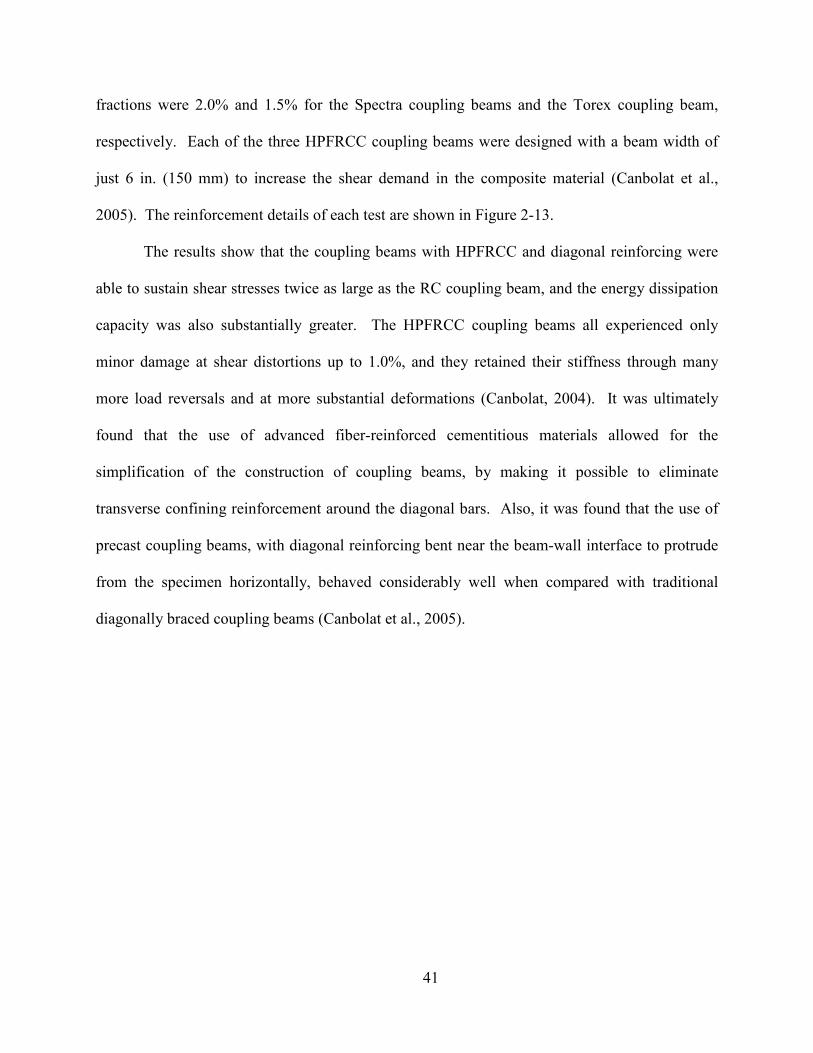
41
fractions were 2.0% and 1.5% for the Spectra coupling beams and the Torex coupling beam,
respectively. Each of the three HPFRCC coupling beams were designed with a beam width of
just 6 in. (150 mm) to increase the shear demand in the composite material (Canbolat et al.,
2005). The reinforcement details of each test are shown in Figure 2-13.
The results show that the coupling beams with HPFRCC and diagonal reinforcing were
able to sustain shear stresses twice as large as the RC coupling beam, and the energy dissipation
capacity was also substantially greater. The HPFRCC coupling beams all experienced only
minor damage at shear distortions up to 1.0%, and they retained their stiffness through many
more load reversals and at more substantial deformations (Canbolat, 2004). It was ultimately
found that the use of advanced fiber-reinforced cementitious materials allowed for the
simplification of the construction of coupling beams, by making it possible to eliminate
transverse confining reinforcement around the diagonal bars. Also, it was found that the use of
precast coupling beams, with diagonal reinforcing bent near the beam-wall interface to protrude
from the specimen horizontally, behaved considerably well when compared with traditional
diagonally braced coupling beams (Canbolat et al., 2005).
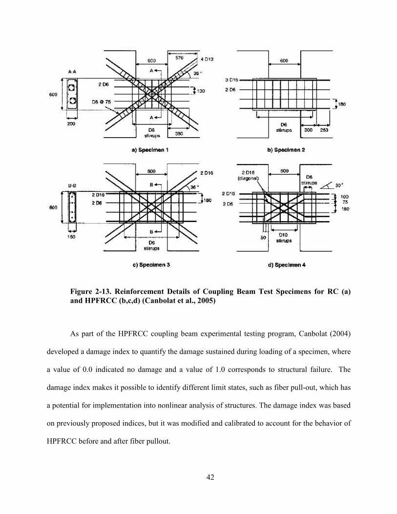
42
Figure 2-13. Reinforcement Details of Coupling Beam Test Specimens for RC (a)
and HPFRCC (b,c,d) (Canbolat et al., 2005)
As part of the HPFRCC coupling beam experimental testing program, Canbolat (2004)
developed a damage index to quantify the damage sustained during loading of a specimen, where
a value of 0.0 indicated no damage and a value of 1.0 corresponds to structural failure. The
damage index makes it possible to identify different limit states, such as fiber pull-out, which has
a potential for implementation into nonlinear analysis of structures. The damage index was based
on previously proposed indices, but it was modified and calibrated to account for the behavior of
HPFRCC before and after fiber pullout.
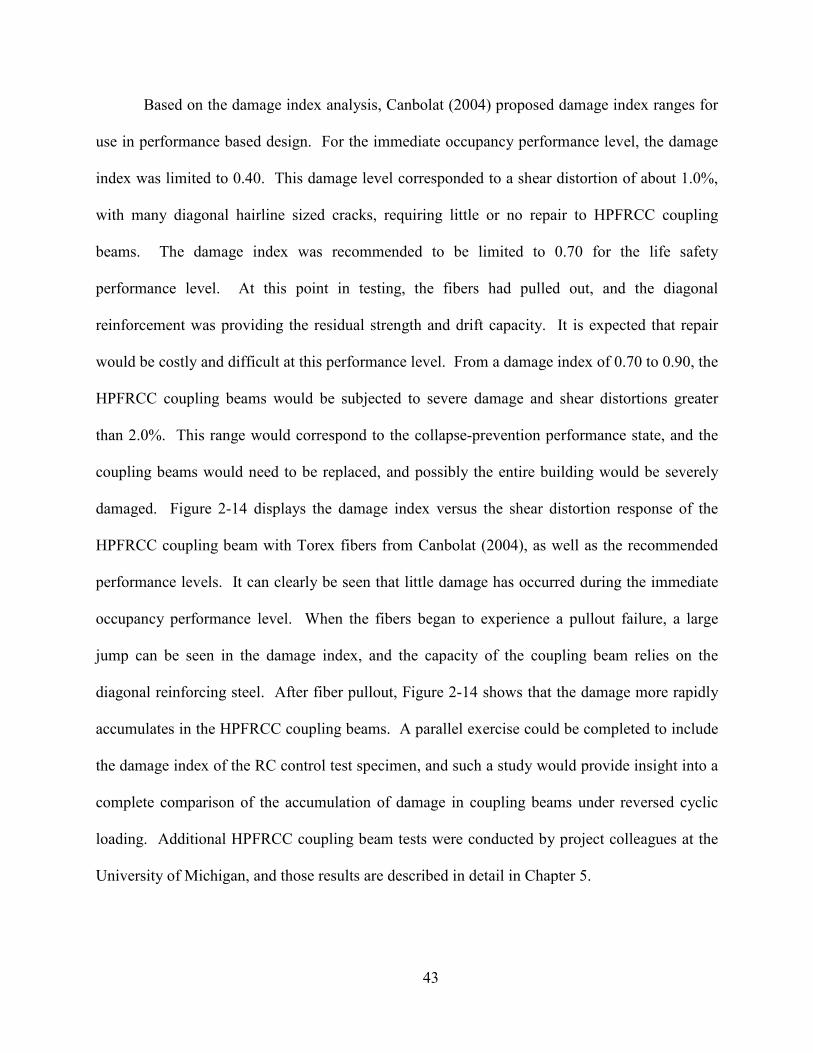
43
Based on the damage index analysis, Canbolat (2004) proposed damage index ranges for
use in performance based design. For the immediate occupancy performance level, the damage
index was limited to 0.40. This damage level corresponded to a shear distortion of about 1.0%,
with many diagonal hairline sized cracks, requiring little or no repair to HPFRCC coupling
beams. The damage index was recommended to be limited to 0.70 for the life safety
performance level. At this point in testing, the fibers had pulled out, and the diagonal
reinforcement was providing the residual strength and drift capacity. It is expected that repair
would be costly and difficult at this performance level. From a damage index of 0.70 to 0.90, the
HPFRCC coupling beams would be subjected to severe damage and shear distortions greater
than 2.0%. This range would correspond to the collapse-prevention performance state, and the
coupling beams would need to be replaced, and possibly the entire building would be severely
damaged. Figure 2-14 displays the damage index versus the shear distortion response of the
HPFRCC coupling beam with Torex fibers from Canbolat (2004), as well as the recommended
performance levels. It can clearly be seen that little damage has occurred during the immediate
occupancy performance level. When the fibers began to experience a pullout failure, a large
jump can be seen in the damage index, and the capacity of the coupling beam relies on the
diagonal reinforcing steel. After fiber pullout, Figure 2-14 shows that the damage more rapidly
accumulates in the HPFRCC coupling beams. A parallel exercise could be completed to include
the damage index of the RC control test specimen, and such a study would provide insight into a
complete comparison of the accumulation of damage in coupling beams under reversed cyclic
loading. Additional HPFRCC coupling beam tests were conducted by project colleagues at the
University of Michigan, and those results are described in detail in Chapter 5.
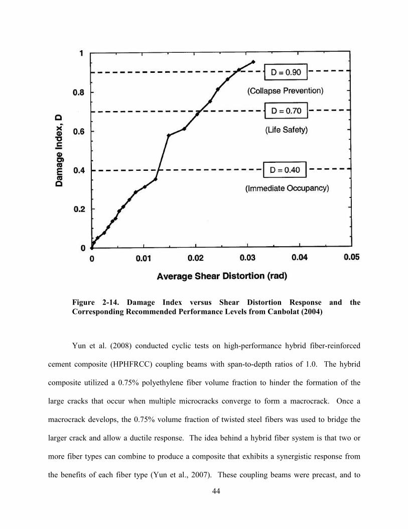
44
Figure 2-14. Damage Index versus Shear Distortion Response and the
Corresponding Recommended Performance Levels from Canbolat (2004)
Yun et al. (2008) conducted cyclic tests on high-performance hybrid fiber-reinforced
cement composite (HPHFRCC) coupling beams with span-to-depth ratios of 1.0. The hybrid
composite utilized a 0.75% polyethylene fiber volume fraction to hinder the formation of the
large cracks that occur when multiple microcracks converge to form a macrocrack. Once a
macrocrack develops, the 0.75% volume fraction of twisted steel fibers was used to bridge the
larger crack and allow a ductile response. The idea behind a hybrid fiber system is that two or
more fiber types can combine to produce a composite that exhibits a synergistic response from
the benefits of each fiber type (Yun et al., 2007). These coupling beams were precast, and to
45
provide material continuity and proper shear and moment transfer, the coupling beams extended
into each wall half of the span length and the reinforcement was fully developed. Also, of the
three specimens constructed, one RC coupling beam had diagonal reinforcing, one HPHFRCC
had diagonal reinforcing, and one HPHFRCC had only conventional longitudinal and transverse
reinforcing. It was found that the diagonally reinforced coupling beam with HPHFRCC could
sustain significantly higher loads and higher drift levels than the reinforced concrete coupling
beam, as well as further confirming that HPHFRCC provides sufficient lateral confinement
around the diagonal reinforcing. Further, the HPHFRCC coupling beam with only conventional
reinforcement also outperformed the reinforced concrete coupling beam with diagonal
reinforcement in terms of maximum load, displacement ductility, and energy absorption (Yun et
al., 2008).
Kuang and Baczkowski (2009) performed an experimental program on five steel fiber-
reinforced concrete coupling beams to investigate the effect of span-to-depth ratio, steel fiber
content, and shear reinforcement ratio on the monotonic response of the specimens. Longer
Dramix fibers, similar to those presented later in this study, were used in these specimens, and
the coupling beams were cast continuously with base blocks, which were used to simulate stiff
structural walls. All of the coupling beams were conventionally reinforced, and the observed
experimental strengths were compared with the strengths predicted by both the British standard
BS 8110 and the Eurocode 2. It was found that the steel fiber-reinforced coupling beams without
any web shear reinforcement achieved three to four times the shear strength predicted by the
codes of practice, thus illustrating the ability of steel fibers to effectively act as shear
reinforcement beyond the code expectations. For coupling beams with transverse reinforcement,
the higher transverse steel ratios resulted in higher coupling beam shear strengths; however, the
46
post-peak load performance for each specimen was very similar, indication that the shear
reinforcement did not have an effect on the post-peak load behavior of HPFRCC coupling
beams. Finally, the study again confirmed that steel fibers increase the post-cracking tensile
strength and ductility of concrete (Kuang & Baczkowski, 2009).
2.5 HPFRCC Large-Scale Coupled Wall Tests
To study the effect of HPFRCC coupling beams on overall system performance two one-
third scale coupled structural wall systems were tested at the University of Michigan by
Lequesne et al. (2010). Each wall was 4-stories tall, composed of a pair of T-shaped walls,
coupling beams, and slabs (at the second and fourth story levels). Within each wall, three of the
four coupling beams used HPFRCC, while the fourth coupling beam was made of regular
reinforced concrete. Each coupling beam was designed with the intent of achieving a similar
capacity; however, slight reinforcement detailing differences were employed to further explore
the effect of reinforcement layout on overall ductility. Also, the first two stories of the second
coupled wall specimen used HPFRCC within the structural walls themselves. This was done to
compare the effect of HPFRCC in the plastic hinging region between the two wall specimens.
The HPFRCC used in each specimen was the same NEES Mix #6 that was previously described
in Chapter 3. The coupling beams were precast with reinforcing bars extending only
horizontally from the precast specimen. It was found throughout construction of the specimen
that given sufficient development of the reinforcing bars, the precast coupling beams could be
easily integrated into the construction sequence of cast-in-place structural walls.
Since coupled walls are typically located near the center of a structure for use as a
structural core, the walls were selected to be T-shaped. It was thought that this would provide a
more accurate representation of typically constructed systems. Thus, the flanges of the T-shaped
47
walls were oriented toward the outer edges of the specimen, with the coupling beams connecting
the narrower stem. The base of the specimen was assumed fixed during design, and this was
addressed through the use of thick concrete base blocks which were then post-tensioned to the
laboratory strong floor. Longitudinal reinforcement was anchored in the foundation and at the
top of the wall system by ACI Code compliant screw-on mechanical anchors, and mechanical
splices were used near mid-height of the wall system to reduce reinforcement congestion
(Lequesne et al., 2010).
At the second and fourth stories of the specimen, a width of slab was poured to create a
means through which to apply the lateral forces, as well as to observe the interaction between the
slab and coupling beam interface. Since the proposal is for precast coupling beams, no special
detail was designed to encourage interaction between the coupling beam and the adjacent slab.
Therefore, the slab reinforcement perpendicular to the direction of loading was continuous
through the structural walls but not through the coupling beams. Gravity loading was simulated
through a vertical force applied to both walls by external prestressing tendons, which were
anchored at the second story slab and in the base block foundation. The strands were prestressed
to achieve an axial stress of 7% f’c based on the gross area of the structural walls, and the force
was constant throughout the test. This level of gravity load is consistent with current design
practice for structural walls and was sufficient to offset a majority of the uplift force resulting
from the coupling of the walls (Lequesne et al., 2010). The loading protocol was such that the
actuator at the fourth story applied a predetermined sequence of lateral displacements, generally
increasing the displacement with each reversed cycle by 0.25% drift. The actuator mounted at
the second story then simultaneously applied a force equal to 60% of the force applied by the top
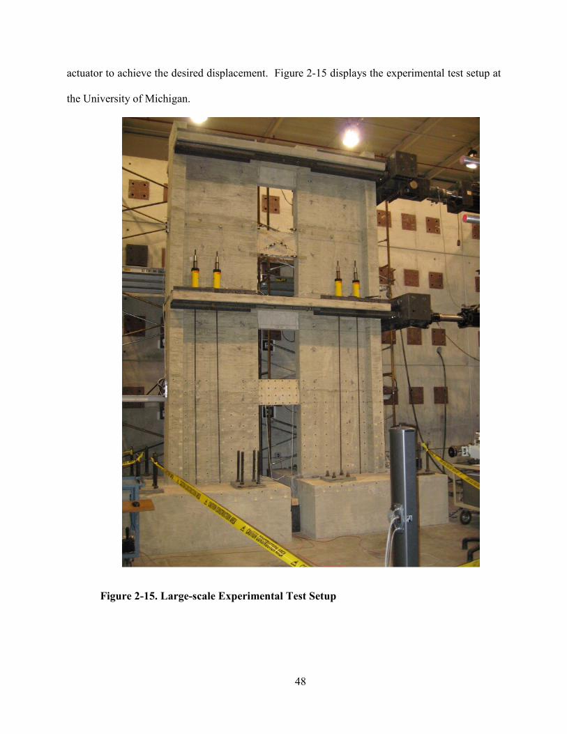
48
actuator to achieve the desired displacement. Figure 2-15 displays the experimental test setup at
the University of Michigan.
Figure 2-15. Large-scale Experimental Test Setup
49
The coupling beam details and dimensions were a main focus of this portion of the
research project, so they were the first component designed for the coupled wall system. Three
different coupling beam designs, shown in Figure 2-16 and described by Lequesne et al. (2009a),
were explored: Bonded FRC, Debonded FRC, and RC. The bonded FRC coupling beams were
different from traditional coupling beams for a number of reasons. The diagonal bars did not
have any special transverse reinforcement to prevent buckling of the bars because it had been
shown previously that HPFRCC can adequately confine diagonal reinforcement (Canbolat et al.,
2005). Also, dowel bars were provided at the interface of the beam and wall to strengthen the
connection. The dowel bars were terminated only 4 in. (100 mm) into the beam due to the high
bond stress that develops between the HPFRCC and the reinforcing bars. The transverse
reinforcement was distributed to provide column-type confinement to the ends of the coupling
beam, extending approximately 2h away from the face of the walls, where h is the coupling
beam height. No special confinement reinforcement was required for the remaining portion of
the span, due to the confinement afforded by the HPFRCC. Throughout the rest of the beam,
stirrups were provided to assist in about 60% of the shear resistance for the first wall and 35%
for the second wall. The Debonded FRC had one change; the dowel bars were extended an
additional 3 in. (75 mm) into the coupling beam, but the additional length was wrapped in plastic
sheeting and taped to prevent the HPFRCC from bonding with the bar. This was done with the
intention to distribute the flexural yielding and to prevent or delay the formation of a single
failure plane due to localized rotations. The RC coupling beams were precast and had the same
general design changes, except the dowel bars were extended 7.5 in. (188 mm), and the
transverse reinforcement was essentially doubled in both the plastic hinging region and the
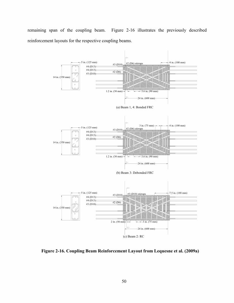
50
remaining span of the coupling beam. Figure 2-16 illustrates the previously described
reinforcement layouts for the respective coupling beams.
Figure 2-16. Coupling Beam Reinforcement Layout from Lequesne et al. (2009a)
(c) Beam 2: RC
(b) Beam 3: Debonded FRC
(a) Beam 1, 4: Bonded FRC
1.2 in. (30 mm) 3.6 in. (90 mm)
24 in. (600 mm)
4 in. (100 mm)
14 in. (350 mm)
5 in. (125 mm)
2 in. (50 mm) 3 in. (75 mm)
7.5 in. (188 mm)
3 in. (75 mm)
#4 (D13)
#2 (D6) stirrups#3 (D10)
#2 (D6)#4 (D13)
#3 (D10)
1.2 in. (30 mm) 3.6 in. (90 mm)
24 in. (600 mm)
4 in. (100 mm)
14 in. (350 mm)
5 in. (125 mm)
#4 (D13)
#2 (D6) stirrups#3 (D10)
#2 (D6)#4 (D13)
#3 (D10)
24 in. (600 mm)
14 in. (350 mm)
5 in. (125 mm)
#4 (D13)
#3 (D10) stirrups#3 (D10)
#2 (D6)#4 (D13)
#3 (D10)
51
Each of the coupling beams were designed with similar initial stiffnesses and flexural
capacities to prevent a single beam from attracting a disproportionate amount of the loading. For
sizing the diagonal, longitudinal, and transverse reinforcement, the design philosophy outlined in
Chapter 5 and Lequesne et al. (2010) was employed. The flexural and diagonal reinforcement
were identical for the HPFRCC and RC coupling beams to provide similar stiffnesses and
flexural capacities. However, the transverse reinforcement ratio was increased from 0.55% for
the HPFRCC coupling beams to 1.5% to provide additional shear resistance and confinement to
the RC beam.
A reinforcement detailing difference arose between the two coupled wall specimens. In
the first test specimen, the coupling beam longitudinal reinforcement was terminated about 3 in.
(75 mm) into the structural wall from the coupling beam-wall interface. This was done to
emulate design practice, but the resulting maximum shear stress calculated from the flexural
capacity of the beams was approximately ' '
5 [psi] (0.42 [MPa])c c
f f , and it resulted in an
undesirable localization of damage along the interface between the structural wall and precast
coupling beam section. All of the coupling beam reinforcement was fully developed in the
second coupled-wall system, which resulted in damage occurring within the precast section and
full development of the coupling beam capacity, and the corresponding peak shear stress was
approximately ' '
9 [psi] (0.75 [MPa])c c
f f (Lequesne et al., 2010)
The structural walls for the first specimen were designed according the ACI Building
Code (ACI Committee 318, 2008), and the second specimen used HPFRCC in the first two
stories, so the transverse reinforcement was reduced due to the assumed higher contribution of
the concrete to the shear strength of the system. During the design of the structural walls, the
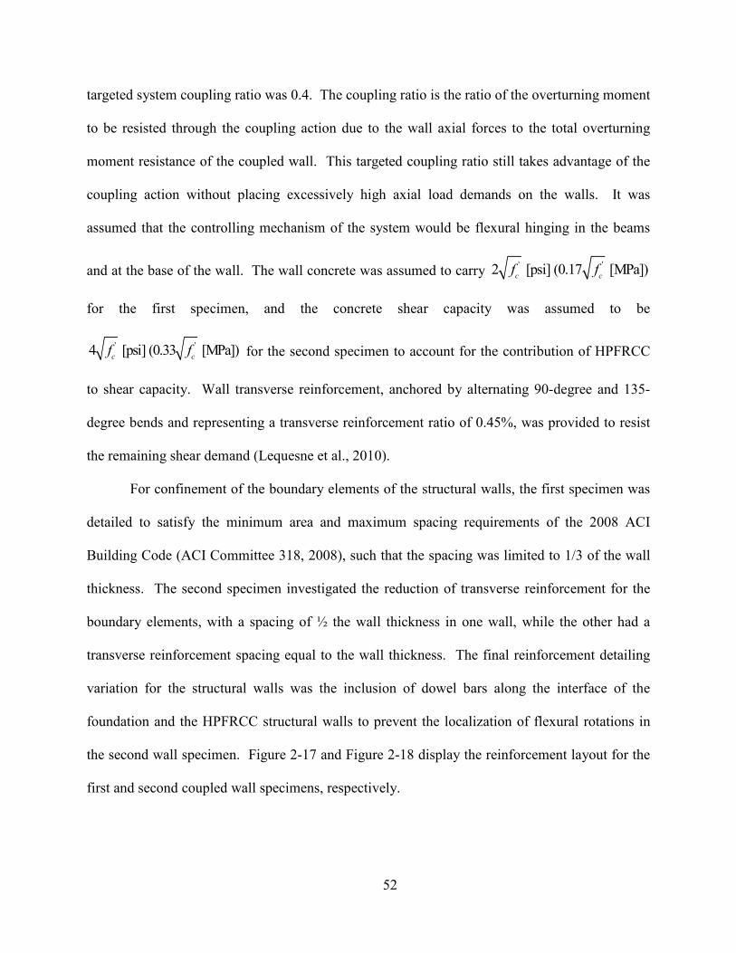
52
targeted system coupling ratio was 0.4. The coupling ratio is the ratio of the overturning moment
to be resisted through the coupling action due to the wall axial forces to the total overturning
moment resistance of the coupled wall. This targeted coupling ratio still takes advantage of the
coupling action without placing excessively high axial load demands on the walls. It was
assumed that the controlling mechanism of the system would be flexural hinging in the beams
and at the base of the wall. The wall concrete was assumed to carry ' '
2 [psi] (0.17 [MPa])c c
f f
for the first specimen, and the concrete shear capacity was assumed to be
' '4 [psi] (0.33 [MPa])
c cf f
for the second specimen to account for the contribution of HPFRCC
to shear capacity. Wall transverse reinforcement, anchored by alternating 90-degree and 135-
degree bends and representing a transverse reinforcement ratio of 0.45%, was provided to resist
the remaining shear demand (Lequesne et al., 2010).
For confinement of the boundary elements of the structural walls, the first specimen was
detailed to satisfy the minimum area and maximum spacing requirements of the 2008 ACI
Building Code (ACI Committee 318, 2008), such that the spacing was limited to 1/3 of the wall
thickness. The second specimen investigated the reduction of transverse reinforcement for the
boundary elements, with a spacing of ½ the wall thickness in one wall, while the other had a
transverse reinforcement spacing equal to the wall thickness. The final reinforcement detailing
variation for the structural walls was the inclusion of dowel bars along the interface of the
foundation and the HPFRCC structural walls to prevent the localization of flexural rotations in
the second wall specimen. Figure 2-17 and Figure 2-18 display the reinforcement layout for the
first and second coupled wall specimens, respectively.
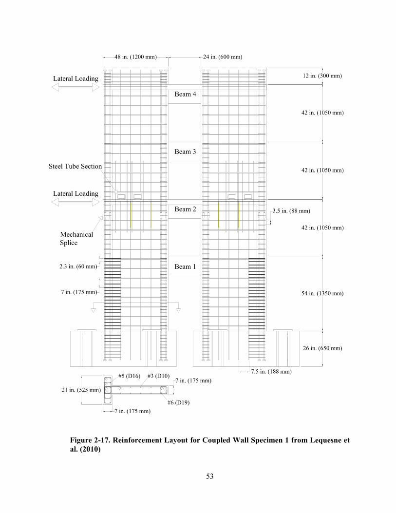
53
Figure 2-17. Reinforcement Layout for Coupled Wall Specimen 1 from Lequesne et
al. (2010)
Beam 1
Beam 2
Beam 3
Beam 4
48 in. (1200 mm) 24 in. (600 mm)
26 in. (650 mm)
54 in. (1350 mm)
42 in. (1050 mm)
42 in. (1050 mm)
42 in. (1050 mm)
12 in. (300 mm)
Mechanical
Splice
Steel Tube Section
#5 (D16)
#6 (D19)
#3 (D10)
7 in. (175 mm)
7 in. (175 mm)
21 in. (525 mm)
7 in. (175 mm)
Lateral Loading
Lateral Loading
2.3 in. (60 mm)
3.5 in. (88 mm)
7.5 in. (188 mm)
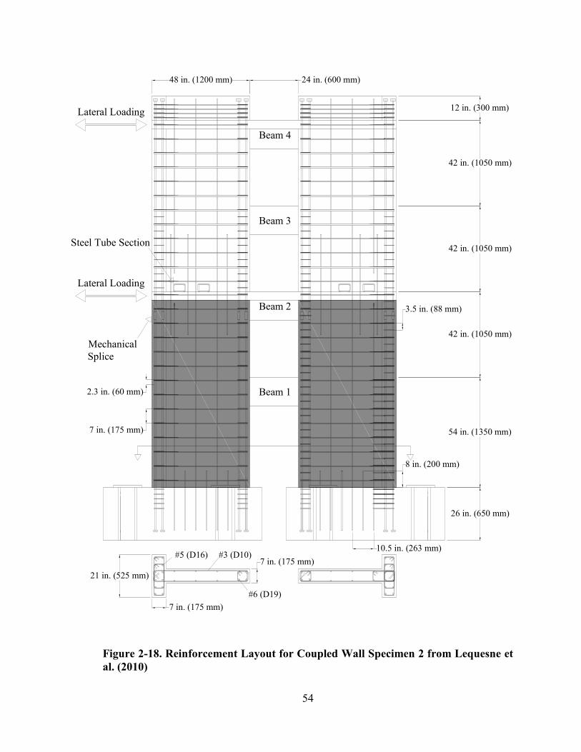
54
Figure 2-18. Reinforcement Layout for Coupled Wall Specimen 2 from Lequesne et
al. (2010)
Beam 1
Beam 2
Beam 3
Beam 4
48 in. (1200 mm) 24 in. (600 mm)
26 in. (650 mm)
54 in. (1350 mm)
42 in. (1050 mm)
42 in. (1050 mm)
42 in. (1050 mm)
12 in. (300 mm)
Mechanical
Splice
Steel Tube Section
#5 (D16)
#6 (D19)
#3 (D10)
7 in. (175 mm)
7 in. (175 mm)
21 in. (525 mm)
7 in. (175 mm)
Lateral Loading
Lateral Loading
2.3 in. (60 mm)
3.5 in. (88 mm)
10.5 in. (263 mm)
8 in. (200 mm)
55
Since the use of HPFRCC is a departure from typical design and construction practice,
efforts were made to be realistic with respect to construction methods and sequencing to truly
gauge the possible construction scheduling advantages recognized with the use of precast
coupling beams. The construction process began with the precasting of the coupling beams, and
then storing them until the rest of the wall was ready for their placement. Construction of the
coupled wall began with the wooden formwork for the walls and the reinforcement cages for the
foundation. The vertical reinforcement was placed into the foundation when the concrete was
poured. Each floor of the wall was then constructed, and as the wall reinforcement reached the
level of the coupling beam, the precast beam was put into place with an overhead crane. The
beam was then supported on the formwork until the wall concrete was placed. After each level
was poured, the formwork was removed and shifted up to the next level. This process was
repeated for each level.
The base shear versus top story drift for each coupled wall is displayed in Figure 2-19. It
can be seen that both of the coupled walls were able to achieve significant drift without
appreciable strength degradation. The base shear capacity of the second wall was greater than
the first, and that can be largely attributed to the full development of the coupling beam
reinforcement and the presence of HPFRCC in the lower two stories of the wall. The first
specimen did very well and was able to maintain about 80% of the peak overturning moment
capacity to beyond 2.5% drift in both directions. However, the second specimen had an even
superior behavior and was able to retain more than 80% of the peak capacity to beyond 3% drift.
Also, the hysteresis loops show essentially no pinching in both experiments, and this may be
attributed to the responses being governed by flexural hinging in the bases of the walls and at the
ends of the coupling beams. The ability of the coupled concrete walls to achieve an overall drift
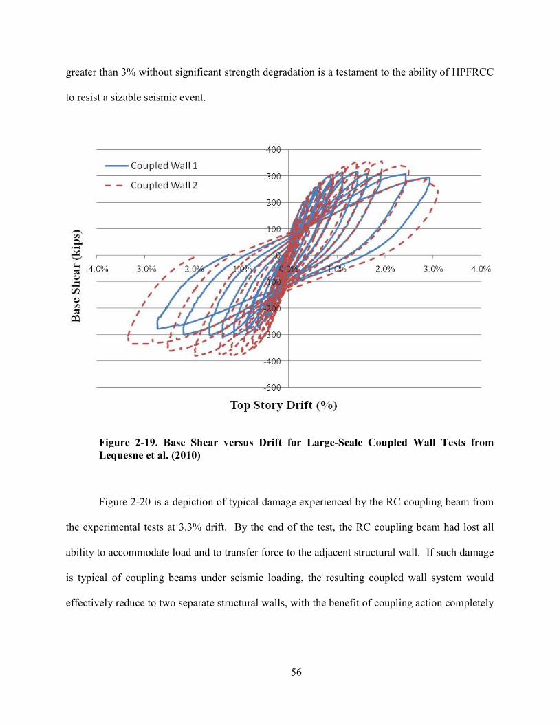
56
greater than 3% without significant strength degradation is a testament to the ability of HPFRCC
to resist a sizable seismic event.
Figure 2-19. Base Shear versus Drift for Large-Scale Coupled Wall Tests from
Lequesne et al. (2010)
Figure 2-20 is a depiction of typical damage experienced by the RC coupling beam from
the experimental tests at 3.3% drift. By the end of the test, the RC coupling beam had lost all
ability to accommodate load and to transfer force to the adjacent structural wall. If such damage
is typical of coupling beams under seismic loading, the resulting coupled wall system would
effectively reduce to two separate structural walls, with the benefit of coupling action completely
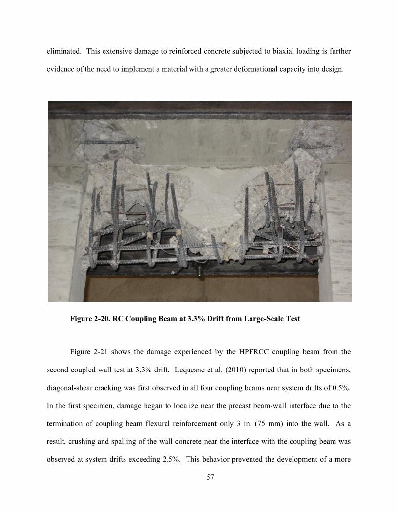
57
eliminated. This extensive damage to reinforced concrete subjected to biaxial loading is further
evidence of the need to implement a material with a greater deformational capacity into design.
Figure 2-20. RC Coupling Beam at 3.3% Drift from Large-Scale Test
Figure 2-21 shows the damage experienced by the HPFRCC coupling beam from the
second coupled wall test at 3.3% drift. Lequesne et al. (2010) reported that in both specimens,
diagonal-shear cracking was first observed in all four coupling beams near system drifts of 0.5%.
In the first specimen, damage began to localize near the precast beam-wall interface due to the
termination of coupling beam flexural reinforcement only 3 in. (75 mm) into the wall. As a
result, crushing and spalling of the wall concrete near the interface with the coupling beam was
observed at system drifts exceeding 2.5%. This behavior prevented the development of a more
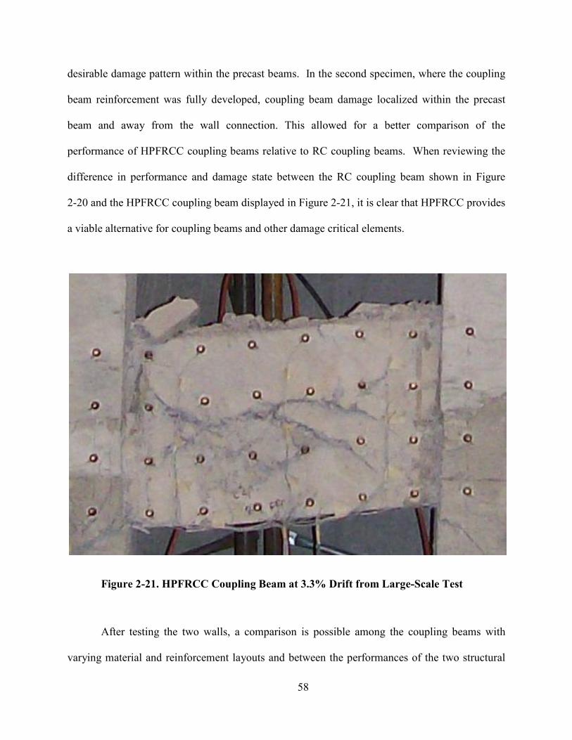
58
desirable damage pattern within the precast beams. In the second specimen, where the coupling
beam reinforcement was fully developed, coupling beam damage localized within the precast
beam and away from the wall connection. This allowed for a better comparison of the
performance of HPFRCC coupling beams relative to RC coupling beams. When reviewing the
difference in performance and damage state between the RC coupling beam shown in Figure
2-20 and the HPFRCC coupling beam displayed in Figure 2-21, it is clear that HPFRCC provides
a viable alternative for coupling beams and other damage critical elements.
Figure 2-21. HPFRCC Coupling Beam at 3.3% Drift from Large-Scale Test
After testing the two walls, a comparison is possible among the coupling beams with
varying material and reinforcement layouts and between the performances of the two structural
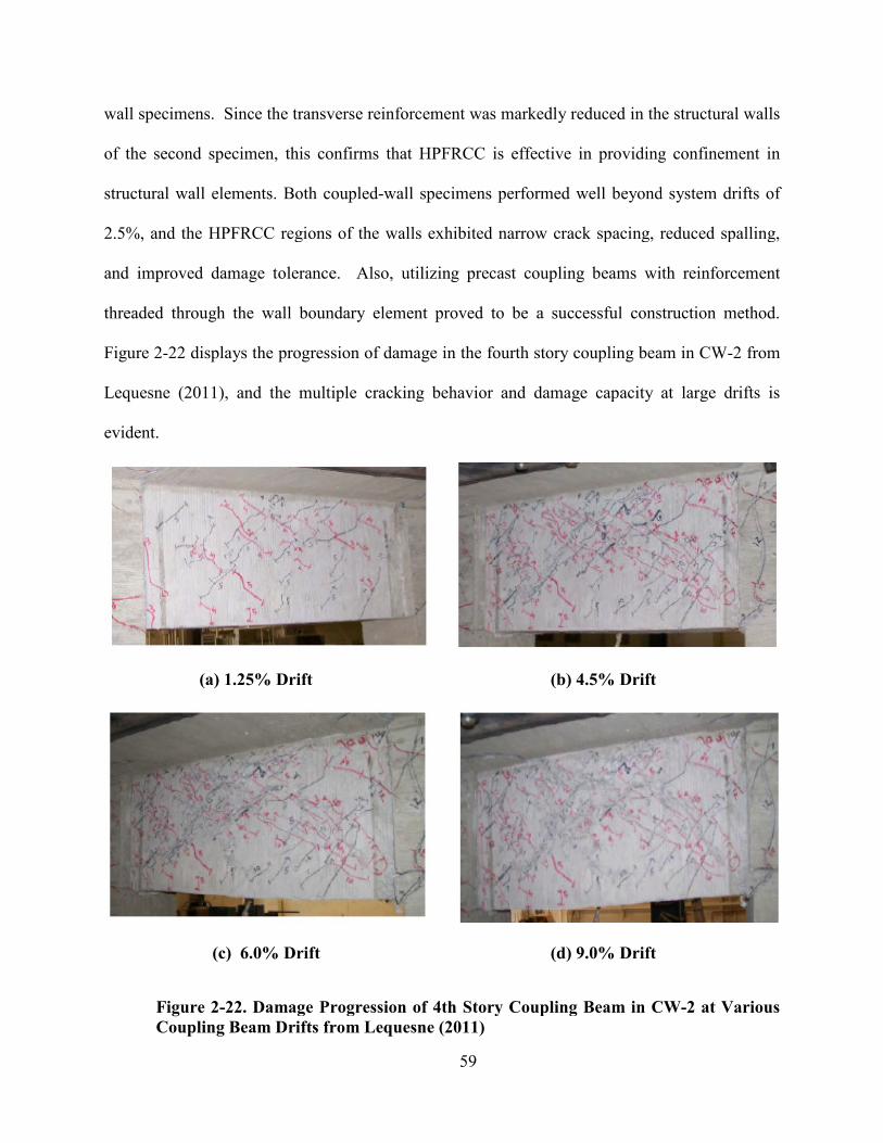
wall specimens. Since the transverse reinforcement was markedly reduced in the structural walls
of the second specimen, this confirms that HPFRCC is effective in providing confinement in
structural wall elements. Both coupled
2.5%, and the HPFRCC regions of the walls exhibited narrow crack spacing, reduced spalling,
and improved damage tolerance. Also, utilizing precast coupling beams with reinforcement
threaded through the wall boundary element proved to be a s
Figure 2-22 displays the progression of damage in the fourth story coupling beam in CW
Lequesne (2011), and the multip
evident.
(a) 1.25% Drift
(c) 6.0% Drift
Figure 2-22. Damage Progres
Coupling Beam Drifts from Lequesne
59
. Since the transverse reinforcement was markedly reduced in the structural walls
of the second specimen, this confirms that HPFRCC is effective in providing confinement in
Both coupled-wall specimens performed well beyond system drifts of
2.5%, and the HPFRCC regions of the walls exhibited narrow crack spacing, reduced spalling,
and improved damage tolerance. Also, utilizing precast coupling beams with reinforcement
boundary element proved to be a successful construction method.
displays the progression of damage in the fourth story coupling beam in CW
, and the multiple cracking behavior and damage capacity at large drifts is
(b) 4.5% Drift
(d) 9.0% Drift
. Damage Progression of 4th Story Coupling Beam in CW
from Lequesne (2011)
. Since the transverse reinforcement was markedly reduced in the structural walls
of the second specimen, this confirms that HPFRCC is effective in providing confinement in
performed well beyond system drifts of
2.5%, and the HPFRCC regions of the walls exhibited narrow crack spacing, reduced spalling,
and improved damage tolerance. Also, utilizing precast coupling beams with reinforcement
uccessful construction method.
displays the progression of damage in the fourth story coupling beam in CW-2 from
le cracking behavior and damage capacity at large drifts is
sion of 4th Story Coupling Beam in CW-2 at Various
60
Additional experimental data has been provided by project colleagues at the University of
Michigan, including coupling beam chord rotations, coupling beam axial deformations,
overturning moments, and interstory drifts from the two coupled wall tests. Using this data,
future analyses may be able to capture the behavior of the coupled wall specimens, both globally
and locally.
2.6 Other Previously Investigated Applications of HPFRCC
Beyond just coupling beams, additional HPFRCC studies have been conducted on
various other shear-dominated members or flexural members subjected to shear reversals.
Several applications have found that using HPFRCC as a design alternative can increase
distortion capacity, shear strength, and damage tolerance in shear critical members. Parra-
Montesinos (2005) outlined several research projects that have demonstrated the versatility and
applicability of HPFRCC. Parra-Montesinos et al. (2005) described a testing program using
HPFRCC in reinforced concrete beam-column connections in which confinement reinforcement
was fully eliminated by using Spectra fibers in a 1.5% volume fraction. Also, Parra-Montesinos
(2005) described the use of HPFRCC to reduce the connection confinement reinforcement of
hybrid reinforced concrete column-steel beam (RCS) connections. In RCS connections, the steel
beam passes continuously through the RC column, and the connection confinement is commonly
provided through overlapping U-shaped stirrups passing through holes drilled in the web of the
steel beam, as well as closely spaced stirrups above and below the steel beam flanges to increase
concrete bearing strength and to transfer shear in the connection. In both cases, the HPFRCC
specimen with reduced connection confinement reinforcement exhibited superior performance
during the test with only minor damage. Additionally, the HPFRCC materials were found to be
effective in reducing slip of the reinforcing bars passing through the beam-column connections
61
(Parra-Montesinos, 2005). Kim and Parra-Montesinos (2003) investigated the use of HPFRCC
in lightly reinforced low-rise walls to increase the displacement capacity when subjected to large
displacement reversals. Two wall specimens were tested; one with Spectra fibers in a 1.5%
volume fraction, and one with a 2.0% volume fraction of hooked steel fibers. In both specimens
the reinforcement in the walls was reduced below the minimum specified standard. While
typical reinforced concrete squat walls exhibit drift capacities below 1%, Kim and Parra-
Montesinos (2003) reported drifts of about 2.5%, with only moderate damage up to 2.0% drift. It
was estimated that the addition of fibers to the concrete matrix contributed to about 80% of the
wall shear strength. Tests were also conducted by Chompreda and Parra-Montesinos (2005) on
the use of HPFRCC in the plastic hinge region at the end of flexural members. The study
relaxed the transverse reinforcement in the plastic hinge region of flexural members and
subjected the specimens to large shear reversals. It was concluded that HPFRCC represents a
viable alternative to reduce or even eliminate the transverse reinforcement in plastic hinge
regions of beams.
Parra-Montesinos et al. (2006) explored the ability of HPFRCC to alleviate confinement
reinforcement in the boundary regions of slender structural walls. Four wall specimens with
shear span-to-wall length ratios of 3.7 were tested under large displacement reversals. One wall
was constructed with regular concrete and detailed according to the 2002 ACI Building Code,
while the other three specimens contained steel fibers, twisted or hooked, in the plastic hinge
region of the specimen. It was found that a 2.0% fiber volume fraction allowed the elimination
of boundary confinement reinforcement without any adverse effects on performance, and a
denser array of smaller width cracks were observed, indicating flexure dominated behavior with
no major shear-related damage. Although the reinforced concrete control wall did not fail,
62
significant signs of distress were evident at the final drift level. Additionally, further reverse-
cyclic experiments were conducted on flexural members with HPFRCC by Parra-Montesinos
and Chompredain (2007), and it was found that HPFRCC behaved adequately. All HPFRCC test
specimens, with or without transverse steel reinforcement, exhibited drift capacities equal to or
greater than 4.0%, and HPFRCC was able to prevent buckling of the longitudinal reinforcement
without web reinforcement until a 4.0% plastic hinge rotation.
Chao et al. (2009) undertook a testing program to evaluate the bond between reinforcing
bars and FRC composites. Pullout specimens were constructed consisting of No. 5 and No. 8
(No. 16M and No. 25M) reinforcing bars embedded 4 in. (102 mm) into control plain concrete or
FRC prisms having the dimensions of 6 x 6 x 4 in. (150 x 150 x 102 mm). The test parameters
were fiber type, fiber volume fraction, fiber length, and loading type. Typically, bearing forces
induced by mechanical interlocking between a deformed reinforcing bar and the surrounding
concrete lead to inclined cracks in the concrete. These internal inclined cracks grow wider upon
further tension loading, and lead to a large residual slip. Without transverse reinforcement,
circumferential tensile stresses lead to the formation of splitting cracks in the concrete and
ultimately to a bond failure. If significant transverse reinforcement is present, the propagation of
the inclined cracks can be controlled, and the degradation of bond strength is mainly caused by
concrete crushing at the toe of the reinforcing bar ribs and shearing of the concrete between the
ribs. With the addition of HPFRCC, it was found that the fiber bridging effect helps to control
the crack opening and propagation, thus increasing the bond strength. The bond strength in
HPFRCC specimens subjected to monotonic loading was as high as 1.5 times that of the spirally
reinforced specimens with a volumetric steel reinforcing ratio of 2%; therefore, fibers in
HPFRCC were found to be more effective than conventional transverse reinforcement for
63
enhancing bond strength, as well as for crack control. Further, the conventional spiral
reinforcement was inferior to the HPFRCC specimens under both unidirectional cyclic loading
and fully reversed cyclic loading. The cumulative energy dissipated by the HPFRCC specimen
was approximately 22 times that of the plain concrete specimen and 2.5 times that of the spirally
reinforced specimen. Thus, test results suggest that the application of HPFRCC can largely
reduce the development length of deformed bars in reinforced concrete members (Chao et al.,
2009).
A recent study by Dinh et al. (2010) explored the performance of three different hooked
steel fiber types at varying volume fractions in concrete beams without shear reinforcement.
Control reinforced concrete beams without shear reinforcement were tested for comparison, and
an additional reinforced concrete beam was tested with minimum shear reinforcing per the ACI
code. It was found that the addition of a 0.75% fiber volume fraction improved the shear
strength of beams without shear reinforcement by at least ' '4.0 [ksi] (0.33 [MPa])c cf f . Also,
the test results showed that when compared with the reinforced concrete beam with shear stirrup
reinforcement satisfying the 2008 ACI Code, all three fiber types, when used in a volume
fraction of 0.75% or greater, could be used instead of the minimum required stirrup
reinforcement per the ACI Code. Overall, the potential for HPFRCC can clearly extend to uses
where damage tolerance is required or reinforcement congestion is troublesome for earthquake-
resistant design (Parra-Montesinos, 2005).
2.7 Previously Conducted HPFRCC Analytical Modeling
Murugappan et al. (1993) presented an analytical biaxial failure envelope model for steel-
fiber-reinforced concrete based on a four-parametric model proposed by Ottosen (1977) for plain
64
concrete. It was proposed that the steel fibers provided a confining pressure in the direction
perpendicular to the stress plane, with the confining pressure being taken as the post-cracking
tensile strength of the fiber-reinforced concrete. However, there were some discrepancies
between the analytical model and their experimental results, and the model was limited to the
compression-compression region of behavior. Hu et al. (2003) suggested a new biaxial failure
model for steel fiber-reinforced concrete based on stretching and distorting an inclined ellipse,
while ensuring that the biaxial failure envelope maintains convexity; the curve avoids any
inflection points to limit numerical difficulties associated with the corner effects. An isotropic
hardening rule was adopted, and the yield and loading envelopes were obtained by scaling the
failure envelope. The stress-strain relationship was assumed to behave in an elastoplastic
manner after initial yielding, as had been observed by previous researchers. The results showed
reasonable agreement with previous experiments; however, the model was calibrated without any
experimental data in the tension-compression and tension-tension regions, and the model is not
applicable for high-performance fiber-reinforced concrete because it does not account for
pseudo-strain hardening after initial yielding.
Seow and Swaddiwudhipong (2005) proposed a unified closed-form approach to define a
failure criterion for both normal strength concrete and steel-fiber-reinforced concrete, without
curve-fitting to experimental data. The model was designed for regular steel fiber-reinforced
concrete, and the main parameters were the fiber volume fraction, the fiber aspect ratio, the
uniaxial concrete compressive strength, the fiber yield stress, and the fiber bond strength. The
main shortcoming of the model is that it cannot capture the significant post-peak strain and
pseudo-strain hardening of HPFRCC. Swaddiwudhipong and Seow (2006) reported an
experimental program to validate the relative accuracy of the previously proposed failure
65
surface. A series of plate specimens with fiber volume fractions varying from 0.5% to 1.5%
were constructed and tested under biaxial loading. The model was implemented into a user
subroutine in ABAQUS and was found to reasonably predict the biaxial stress-strain behavior of
plate specimens. Further parametric studies were conducted on previously tested beam
specimens, and the model was able to predict the failure loads of the beams within 15%, but due
to the neglect of bond-slip and other parameters, there was a sizable discrepancy between the
analytical and experimental strains and displacements (Swaddiwudhipong & Seow, 2006).
A cyclic analytical model for HPFRCC has recently been developed by project
colleagues at the University of Michigan. Hung and El-Tawil (2009) developed a material
model for HPFRCC where the material is considered homogenous during the initial stages, and
crack localization is determined by a strain criterion. The uniaxial stress-strain curves are largely
a curve fit from previous experimental results conducted by Liao et al. (2006) at the University
of Michigan. The cyclic loading stress-strain functions from Han et al. (2003) were adopted,
with the modification of using Hognestad’s parabolic function to describe the hardening behavior
before the peak compressive load. Shear stiffness retention was linearly decreased as a function
of the normal strain on the crack plane, and LS-DYNA was used to perform the analyses. The
proposed model was investigated with a comparison to experimental data from shear walls tested
under reversed cyclic loading with HPFRCC and a 1.5% volume fraction of steel twisted fibers
(from Parra-Montesinos et al. (2006)). Other efforts by Hung include the modeling of two 18-
story coupled wall systems. In these models, one system utilized HPFRCC in the coupling
beams and the plastic hinging region of the walls, while the other model implemented traditional
RC coupled walls and coupling beams. The coupling beams using HPFRCC had a reduced and
simplified reinforcement layout, and when subjected to a seismic analysis it was shown that the
66
buildings performed comparably with respect to drift and rotation. Also, the crack patterns in the
coupling beams significantly differed between the two models. The HPFRCC coupling beams
were only slightly cracked, while the RC coupling beams had clearly experienced more damage,
thus requiring more thorough and costly repairs. Since the material model developed by Hung
and El-Tawil (2009) was not based upon a suite of experimental data, a model calibrated to the
results of the multi-axial tests conducted at the University of Illinois could potentially provide a
more reliable finite element result with respect to the HPFRCC material behavior and the
damage evolution of HPFRCC in structural components.
67
CHAPTER 3. MATERIAL TESTIG RESULTS
This chapter provides an overview of the experimental program (and results obtained to
date) performed on plain concrete and HPFRCC material specimens under various loading states,
such as uniaxial compression, biaxial compression, and indirect tension, as well as an overview
of related tests performed by project colleagues at the University of Michigan on similar
materials. The plain and HPFRCC specimens tested at the University of Illinois were plate
specimens under multi-axial loading for material characterization, while the University of
Michigan tests included preliminary HPFRCC material testing, as well as coupled wall systems
with both HPFRCC and plain reinforced concrete coupling beams. Results from these tests will
be used to construct failure surfaces and to inform other modeling parameters to be used later in
finite element modeling.
3.1 Preliminary HPFRCC Material Testing
As part of the NEES research project titled “Innovative Applications of Damage Tolerant
Fiber-Reinforced Cementitious Materials for New Earthquake-Resistant Structural Systems and
Retrofit of Existing Structures,” Liao et al. (2006) initially explored and established the
mechanical properties of six different high-performance fiber-reinforced concrete mixes. Each
of these mixes had at least some differences from one another with respect to the mixture
proportions (including the quantity of admixtures) or in the type and volume fraction of fibers.
Of the six mixes, two specific ones were further explored, called as NEES Mix #4 (NM4) and
NEES Mix #6 (NM6). The main objective in developing these mixes was to obtain a strain-
hardening, self-consolidating concrete mix with 28-day strength of between 5 ksi (34.5 MPa) and
9 ksi (62.1 MPa). Another series of tests was conducted on specimens as described by
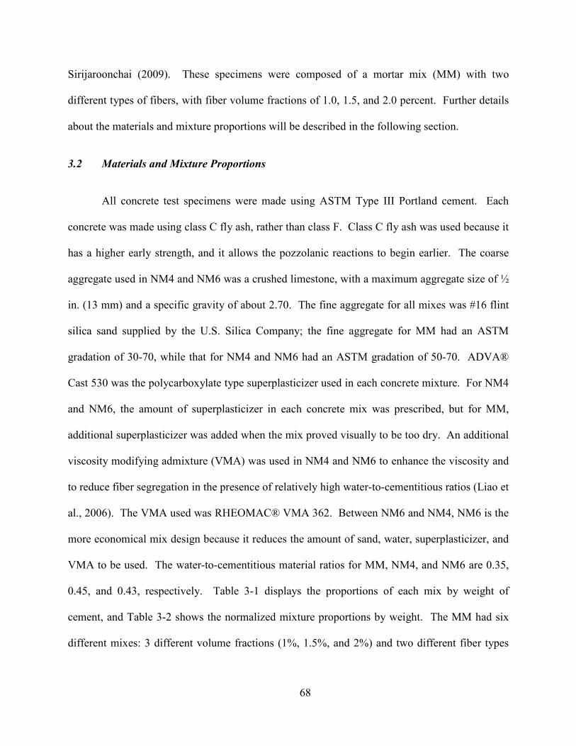
68
Sirijaroonchai (2009). These specimens were composed of a mortar mix (MM) with two
different types of fibers, with fiber volume fractions of 1.0, 1.5, and 2.0 percent. Further details
about the materials and mixture proportions will be described in the following section.
3.2 Materials and Mixture Proportions
All concrete test specimens were made using ASTM Type III Portland cement. Each
concrete was made using class C fly ash, rather than class F. Class C fly ash was used because it
has a higher early strength, and it allows the pozzolanic reactions to begin earlier. The coarse
aggregate used in NM4 and NM6 was a crushed limestone, with a maximum aggregate size of ½
in. (13 mm) and a specific gravity of about 2.70. The fine aggregate for all mixes was #16 flint
silica sand supplied by the U.S. Silica Company; the fine aggregate for MM had an ASTM
gradation of 30-70, while that for NM4 and NM6 had an ASTM gradation of 50-70. ADVA®
Cast 530 was the polycarboxylate type superplasticizer used in each concrete mixture. For NM4
and NM6, the amount of superplasticizer in each concrete mix was prescribed, but for MM,
additional superplasticizer was added when the mix proved visually to be too dry. An additional
viscosity modifying admixture (VMA) was used in NM4 and NM6 to enhance the viscosity and
to reduce fiber segregation in the presence of relatively high water-to-cementitious ratios (Liao et
al., 2006). The VMA used was RHEOMAC® VMA 362. Between NM6 and NM4, NM6 is the
more economical mix design because it reduces the amount of sand, water, superplasticizer, and
VMA to be used. The water-to-cementitious material ratios for MM, NM4, and NM6 are 0.35,
0.45, and 0.43, respectively. Table 3-1 displays the proportions of each mix by weight of
cement, and Table 3-2 shows the normalized mixture proportions by weight. The MM had six
different mixes: 3 different volume fractions (1%, 1.5%, and 2%) and two different fiber types
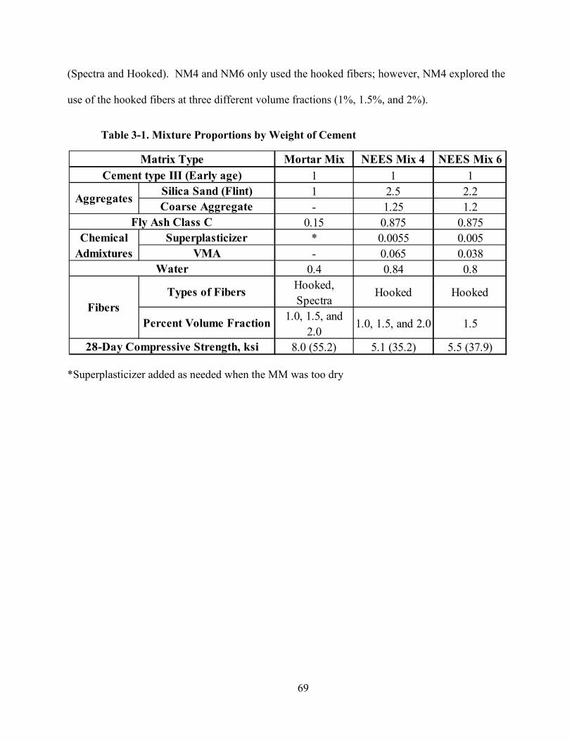
69
(Spectra and Hooked). NM4 and NM6 only used the hooked fibers; however, NM4 explored the
use of the hooked fibers at three different volume fractions (1%, 1.5%, and 2%).
Table 3-1. Mixture Proportions by Weight of Cement
*Superplasticizer added as needed when the MM was too dry
Mortar Mix EES Mix 4 EES Mix 6
1 1 1
1 2.5 2.2
- 1.25 1.2
0.15 0.875 0.875
* 0.0055 0.005
- 0.065 0.038
0.4 0.84 0.8
Hooked,
SpectraHooked Hooked
1.0, 1.5, and
2.01.0, 1.5, and 2.0 1.5
8.0 (55.2) 5.1 (35.2) 5.5 (37.9)
Matrix Type
Cement type III (Early age)
AggregatesSilica Sand (Flint)
Coarse Aggregate
Fly Ash Class C
Chemical
Admixtures
Superplasticizer
VMA
28-Day Compressive Strength, ksi
Water
Fibers
Types of Fibers
Percent Volume Fraction
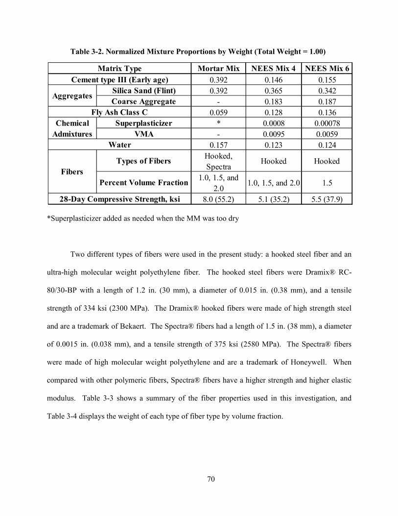
70
Table 3-2. ormalized Mixture Proportions by Weight (Total Weight = 1.00)
*Superplasticizer added as needed when the MM was too dry
Two different types of fibers were used in the present study: a hooked steel fiber and an
ultra-high molecular weight polyethylene fiber. The hooked steel fibers were Dramix® RC-
80/30-BP with a length of 1.2 in. (30 mm), a diameter of 0.015 in. (0.38 mm), and a tensile
strength of 334 ksi (2300 MPa). The Dramix® hooked fibers were made of high strength steel
and are a trademark of Bekaert. The Spectra® fibers had a length of 1.5 in. (38 mm), a diameter
of 0.0015 in. (0.038 mm), and a tensile strength of 375 ksi (2580 MPa). The Spectra® fibers
were made of high molecular weight polyethylene and are a trademark of Honeywell. When
compared with other polymeric fibers, Spectra® fibers have a higher strength and higher elastic
modulus. Table 3-3 shows a summary of the fiber properties used in this investigation, and
Table 3-4 displays the weight of each type of fiber type by volume fraction.
Mortar Mix EES Mix 4 EES Mix 6
0.392 0.146 0.155
0.392 0.365 0.342
- 0.183 0.187
0.059 0.128 0.136
* 0.0008 0.00078
- 0.0095 0.0059
0.157 0.123 0.124
Hooked,
SpectraHooked Hooked
1.0, 1.5, and
2.01.0, 1.5, and 2.0 1.5
8.0 (55.2) 5.1 (35.2) 5.5 (37.9)28-Day Compressive Strength, ksi
Chemical
Admixtures
Superplasticizer
VMA
Water
Fibers
Types of Fibers
Percent Volume Fraction
Matrix Type
Cement type III (Early age)
AggregatesSilica Sand (Flint)
Coarse Aggregate
Fly Ash Class C
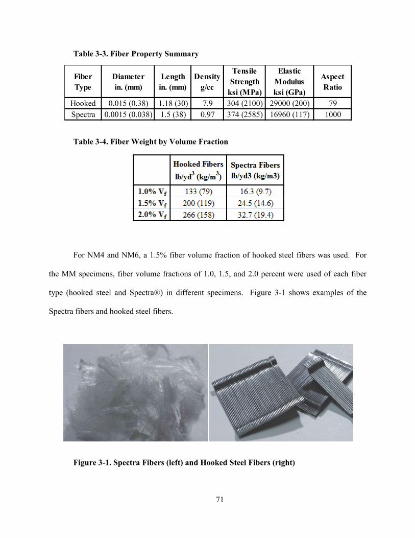
71
Table 3-3. Fiber Property Summary
Table 3-4. Fiber Weight by Volume Fraction
For NM4 and NM6, a 1.5% fiber volume fraction of hooked steel fibers was used. For
the MM specimens, fiber volume fractions of 1.0, 1.5, and 2.0 percent were used of each fiber
type (hooked steel and Spectra®) in different specimens. Figure 3-1 shows examples of the
Spectra fibers and hooked steel fibers.
Figure 3-1. Spectra Fibers (left) and Hooked Steel Fibers (right)
Fiber
Type
Diameter
in. (mm)
Length
in. (mm)
Density
g/cc
Tensile
Strength
ksi (MPa)
Elastic
Modulus
ksi (GPa)
Aspect
Ratio
Hooked 0.015 (0.38) 1.18 (30) 7.9 304 (2100) 29000 (200) 79
Spectra 0.0015 (0.038) 1.5 (38) 0.97 374 (2585) 16960 (117) 1000
72
3.3 Preliminary Material Property Testing at the University of Michigan
Liao et al. (2006) conducted uniaxial compression and uniaxial tension tests on NM4 and
NM6 at the University of Michigan. The uniaxial compression tests on 4 in. (102 mm) diameter
by 8 in. (203 mm) tall cylinders were done according to ASTM C39. Three linear variable
differential transformers (LVDTs) were used to measure the strains in the specimen, and they
were removed to capture post-peak response. NM4 was found to have an average 28-day
compressive strength of 5.1 ksi (35.2 MPa). Direct tension tests were conducted on dog-bone
shaped tensile specimens. The total length of each dog-bone specimen was 21 in. (533 mm), and
the cross-section of the middle portion of the specimen, where the failure occurs, was 1 in. (25
mm) by 2 in. (51 mm). Displacement was applied to the specimen at a rate of 0.05 in./min. (1.27
mm/min.), and the elongation was measured by two LVDTs over a gauge length of 7 in. (178
mm). For NM4, the average post-cracking tensile strength was found to be 502 psi (3.5 MPa) at
a 0.25% strain from direct tension tests. For NM6, the 28-day cylinder compressive strength was
5.5 ksi (37.9 MPa), and the average post-cracking tensile strength was 503 psi (3.5 MPa) at a
strain of 0.45% from direct tension tests (Liao et al., 2006). More detailed information
(including stress-strain plots) for this tensile behavior is presented later in Sections 3.7.3 and
3.7.4.
To explore the effect of different types of fibers and varying volume fractions,
Sirijaroonchai (2009) tested 1.0, 1.5, and 2.0 percent volume fractions of both Dramix® hooked
steel fibers and Spectra® ultra-high molecular weight polyethylene fibers. These fiber volume
fractions were placed into the mortar mix, whose proportions are given in Table 3-1 and Table
3-2. The MM specimens were subjected to uniaxial compression, uniaxial tension, and triaxial
compression. The uniaxial compression tests were conducted as previously described per ASTM
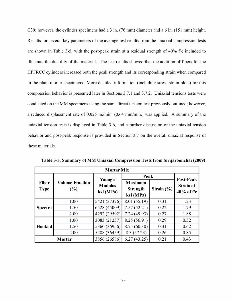
73
C39; however, the cylinder specimens had a 3 in. (76 mm) diameter and a 6 in. (151 mm) height.
Results for several key parameters of the average test results from the uniaxial compression tests
are shown in Table 3-5, with the post-peak strain at a residual strength of 40% f’c included to
illustrate the ductility of the material. The test results showed that the addition of fibers for the
HPFRCC cylinders increased both the peak strength and its corresponding strain when compared
to the plain mortar specimens. More detailed information (including stress-strain plots) for this
compression behavior is presented later in Sections 3.7.1 and 3.7.2. Uniaxial tensions tests were
conducted on the MM specimens using the same direct tension test previously outlined; however,
a reduced displacement rate of 0.025 in./min. (0.64 mm/min.) was applied. A summary of the
uniaxial tension tests is displayed in Table 3-6, and a further discussion of the uniaxial tension
behavior and post-peak response is provided in Section 3.7 on the overall uniaxial response of
these materials.
Table 3-5. Summary of MM Uniaxial Compression Tests from Sirijaroonchai (2009)
Maximum
Strength
ksi (MPa)
Strain (%)
1.00 5421 (37376) 8.01 (55.19) 0.31 1.23
1.50 6528 (45009) 7.57 (52.21) 0.22 1.79
2.00 4292 (29592) 7.24 (49.93) 0.27 1.88
1.00 3083 (21257) 8.25 (56.91) 0.29 0.52
1.50 5360 (36956) 8.75 (60.30) 0.31 0.62
2.00 5288 (36459) 8.3 (57.23) 0.26 0.85
3856 (26586) 6.27 (43.25) 0.21 0.43
Mortar Mix
Volume Fraction
(%)
Fiber
Type
Mortar
Hooked
Spectra
PeakPost-Peak
Strain at
40% of f'c
Young's
Modulus
ksi (MPa)
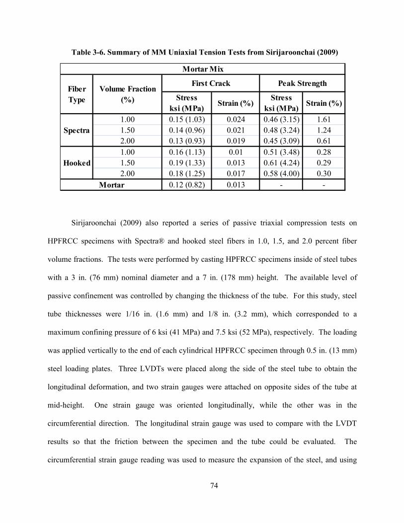
74
Table 3-6. Summary of MM Uniaxial Tension Tests from Sirijaroonchai (2009)
Sirijaroonchai (2009) also reported a series of passive triaxial compression tests on
HPFRCC specimens with Spectra® and hooked steel fibers in 1.0, 1.5, and 2.0 percent fiber
volume fractions. The tests were performed by casting HPFRCC specimens inside of steel tubes
with a 3 in. (76 mm) nominal diameter and a 7 in. (178 mm) height. The available level of
passive confinement was controlled by changing the thickness of the tube. For this study, steel
tube thicknesses were 1/16 in. (1.6 mm) and 1/8 in. (3.2 mm), which corresponded to a
maximum confining pressure of 6 ksi (41 MPa) and 7.5 ksi (52 MPa), respectively. The loading
was applied vertically to the end of each cylindrical HPFRCC specimen through 0.5 in. (13 mm)
steel loading plates. Three LVDTs were placed along the side of the steel tube to obtain the
longitudinal deformation, and two strain gauges were attached on opposite sides of the tube at
mid-height. One strain gauge was oriented longitudinally, while the other was in the
circumferential direction. The longitudinal strain gauge was used to compare with the LVDT
results so that the friction between the specimen and the tube could be evaluated. The
circumferential strain gauge reading was used to measure the expansion of the steel, and using
Stress
ksi (MPa)Strain (%)
Stress
ksi (MPa)Strain (%)
1.00 0.15 (1.03) 0.024 0.46 (3.15) 1.61
1.50 0.14 (0.96) 0.021 0.48 (3.24) 1.24
2.00 0.13 (0.93) 0.019 0.45 (3.09) 0.61
1.00 0.16 (1.13) 0.01 0.51 (3.48) 0.28
1.50 0.19 (1.33) 0.013 0.61 (4.24) 0.29
2.00 0.18 (1.25) 0.017 0.58 (4.00) 0.30
0.12 (0.82) 0.013 - -
Mortar Mix
Mortar
First Crack Peak StrengthFiber
Type
Volume Fraction
(%)
Spectra
Hooked
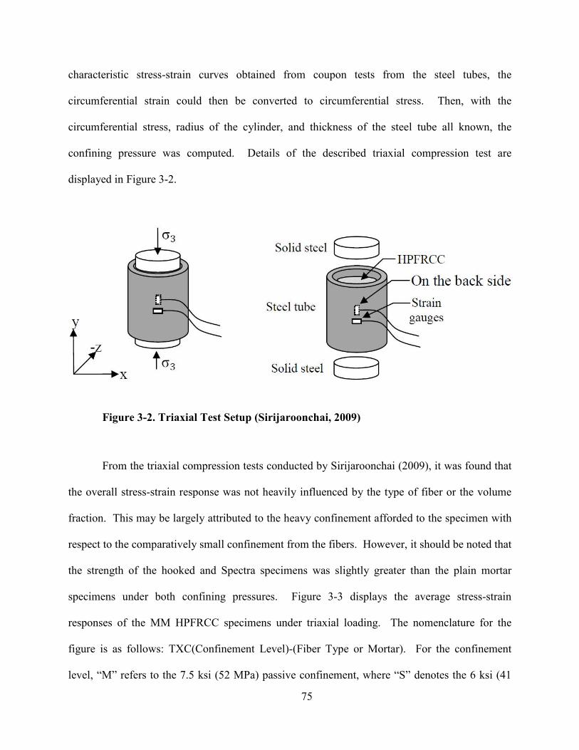
75
characteristic stress-strain curves obtained from coupon tests from the steel tubes, the
circumferential strain could then be converted to circumferential stress. Then, with the
circumferential stress, radius of the cylinder, and thickness of the steel tube all known, the
confining pressure was computed. Details of the described triaxial compression test are
displayed in Figure 3-2.
Figure 3-2. Triaxial Test Setup (Sirijaroonchai, 2009)
From the triaxial compression tests conducted by Sirijaroonchai (2009), it was found that
the overall stress-strain response was not heavily influenced by the type of fiber or the volume
fraction. This may be largely attributed to the heavy confinement afforded to the specimen with
respect to the comparatively small confinement from the fibers. However, it should be noted that
the strength of the hooked and Spectra specimens was slightly greater than the plain mortar
specimens under both confining pressures. Figure 3-3 displays the average stress-strain
responses of the MM HPFRCC specimens under triaxial loading. The nomenclature for the
figure is as follows: TXC(Confinement Level)-(Fiber Type or Mortar). For the confinement
level, “M” refers to the 7.5 ksi (52 MPa) passive confinement, where “S” denotes the 6 ksi (41
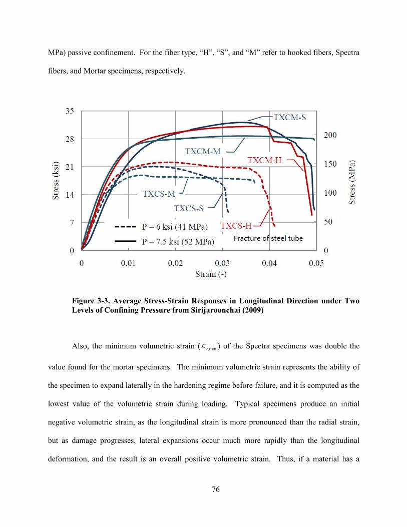
76
MPa) passive confinement. For the fiber type, “H”, “S”, and “M” refer to hooked fibers, Spectra
fibers, and Mortar specimens, respectively.
Figure 3-3. Average Stress-Strain Responses in Longitudinal Direction under Two
Levels of Confining Pressure from Sirijaroonchai (2009)
Also, the minimum volumetric strain ( ,minvε ) of the Spectra specimens was double the
value found for the mortar specimens. The minimum volumetric strain represents the ability of
the specimen to expand laterally in the hardening regime before failure, and it is computed as the
lowest value of the volumetric strain during loading. Typical specimens produce an initial
negative volumetric strain, as the longitudinal strain is more pronounced than the radial strain,
but as damage progresses, lateral expansions occur much more rapidly than the longitudinal
deformation, and the result is an overall positive volumetric strain. Thus, if a material has a
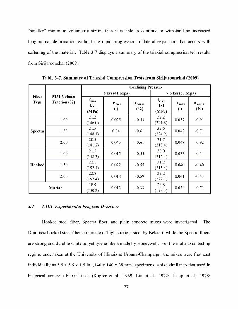
77
“smaller” minimum volumetric strain, then it is able to continue to withstand an increased
longitudinal deformation without the rapid progression of lateral expansion that occurs with
softening of the material. Table 3-7 displays a summary of the triaxial compression test results
from Sirijaroonchai (2009).
Table 3-7. Summary of Triaxial Compression Tests from Sirijaroonchai (2009)
3.4 UIUC Experimental Program Overview
Hooked steel fiber, Spectra fiber, and plain concrete mixes were investigated. The
Dramix® hooked steel fibers are made of high strength steel by Bekaert, while the Spectra fibers
are strong and durable white polyethylene fibers made by Honeywell. For the multi-axial testing
regime undertaken at the University of Illinois at Urbana-Champaign, the mixes were first cast
individually as 5.5 x 5.5 x 1.5 in. (140 x 140 x 38 mm) specimens, a size similar to that used in
historical concrete biaxial tests (Kupfer et al., 1969; Liu et al., 1972; Tasuji et al., 1978;
fmax
ksi
(MPa)
εεεεmax
(-)
εεεε v,min
(%)
fmax
ksi
(MPa)
εεεεmax
(-)
εεεε v,min
(%)
1.0021.2
(146.0)0.025 -0.53
32.2
(221.8)0.037 -0.91
1.5021.5
(148.1)0.04 -0.61
32.6
(224.9)0.042 -0.71
2.0020.5
(141.2)0.045 -0.61
31.7
(218.4)0.048 -0.92
1.0021.5
(148.3)0.015 -0.55
30.0
(215.4)0.033 -0.54
1.5022.1
(152.4)0.022 -0.55
31.2
(215.4)0.040 -0.40
2.0022.8
(157.4)0.018 -0.59
32.2
(222.1)0.041 -0.43
18.9
(130.3)0.013 -0.33
28.8
(198.3)0.034 -0.71
7.5 ksi (52 Mpa)
Spectra
Hooked
Mortar
Confining Pressure
Fiber
Type
MM Volume
Fraction (%)
6 ksi (41 Mpa)
78
Maekawa & Okamura, 1983; Yin et al., 1989; Lan & Guo, 1999; Hussein & Marzouk, 2000a;
Lee et al., 2004). Three concrete mixtures were explored: the Mortar Mix (MM), NEES Mix #4
(NM4), and NEES Mix #6 (NM6). The details of each mix were previously described in Section
3.2. Specimens were cast with Spectra fibers, hooked steel fibers, or without fibers for the MM,
while only hooked steel fiber and plain concrete mixes were batched for NM4 and NM6.
To explore the influence of specimen type on orientation of the fibers at casting (and
therefore on eventual biaxial behavior), large 6.5 x 6.5 x 18 in. (165 x 165 x 457 mm) “loaves”
of the MM were also cast, to ensure a random orientation of the fibers. These loaves were then
cut and trimmed to the aforementioned 5.5 x 5.5 x 1.5 in. (140 x 140 x 38 mm) specimen size
using a diamond precision saw. Upon visual inspection, it was clear that the fibers were well-
dispersed and randomly oriented in the loaf specimens. The first generation of tests utilized the
MM and NM4 designs, but after those individually cast specimen results were compared to the
loaf specimens, the decision was made to explore only casting in loaves for the eventual NM6
design (Foltz et al., 2008). Figure 3-4 illustrates how the larger loaf specimens were cut and
trimmed to the smaller individually sized specimens. For the MM specimens, 1.0, 1.5, and 2.0
percent fiber volume fractions were used for both fiber types, while only a 1.5 percent hooked
steel fiber volume fraction was used for the NM4 and NM6 specimens.
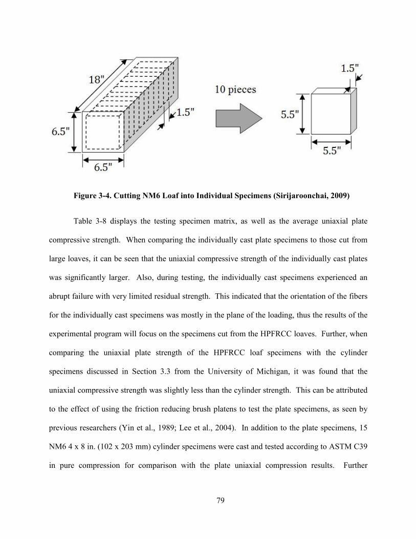
79
Figure 3-4. Cutting M6 Loaf into Individual Specimens (Sirijaroonchai, 2009)
Table 3-8 displays the testing specimen matrix, as well as the average uniaxial plate
compressive strength. When comparing the individually cast plate specimens to those cut from
large loaves, it can be seen that the uniaxial compressive strength of the individually cast plates
was significantly larger. Also, during testing, the individually cast specimens experienced an
abrupt failure with very limited residual strength. This indicated that the orientation of the fibers
for the individually cast specimens was mostly in the plane of the loading, thus the results of the
experimental program will focus on the specimens cut from the HPFRCC loaves. Further, when
comparing the uniaxial plate strength of the HPFRCC loaf specimens with the cylinder
specimens discussed in Section 3.3 from the University of Michigan, it was found that the
uniaxial compressive strength was slightly less than the cylinder strength. This can be attributed
to the effect of using the friction reducing brush platens to test the plate specimens, as seen by
previous researchers (Yin et al., 1989; Lee et al., 2004). In addition to the plate specimens, 15
NM6 4 x 8 in. (102 x 203 mm) cylinder specimens were cast and tested according to ASTM C39
in pure compression for comparison with the plate uniaxial compression results. Further
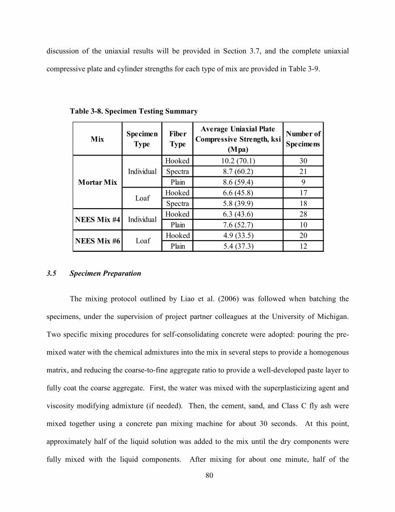
80
discussion of the uniaxial results will be provided in Section 3.7, and the complete uniaxial
compressive plate and cylinder strengths for each type of mix are provided in Table 3-9.
Table 3-8. Specimen Testing Summary
3.5 Specimen Preparation
The mixing protocol outlined by Liao et al. (2006) was followed when batching the
specimens, under the supervision of project partner colleagues at the University of Michigan.
Two specific mixing procedures for self-consolidating concrete were adopted: pouring the pre-
mixed water with the chemical admixtures into the mix in several steps to provide a homogenous
matrix, and reducing the coarse-to-fine aggregate ratio to provide a well-developed paste layer to
fully coat the coarse aggregate. First, the water was mixed with the superplasticizing agent and
viscosity modifying admixture (if needed). Then, the cement, sand, and Class C fly ash were
mixed together using a concrete pan mixing machine for about 30 seconds. At this point,
approximately half of the liquid solution was added to the mix until the dry components were
fully mixed with the liquid components. After mixing for about one minute, half of the
MixSpecimen
Type
Fiber
Type
Average Uniaxial Plate
Compressive Strength, ksi
(Mpa)
umber of
Specimens
Hooked 10.2 (70.1) 30
Spectra 8.7 (60.2) 21
Plain 8.6 (59.4) 9
Hooked 6.6 (45.8) 17
Spectra 5.8 (39.9) 18
Hooked 6.3 (43.6) 28
Plain 7.6 (52.7) 10
Hooked 4.9 (33.5) 20
Plain 5.4 (37.3) 12LoafEES Mix #6
EES Mix #4
Mortar Mix
Individual
Loaf
Individual
81
remaining liquid was poured into the mix. After another minute of mixing, half of the remaining
liquid was again poured into the concrete mixture. Then, after still another minute of mixing, the
remainder of the liquid solution was poured into the mix. Next, all of the coarse aggregate (if
needed) was added and mixed for about two minutes. Finally, fibers were slowly added
incrementally to the mix. During the addition of fibers, special care was made to ensure that
they did not clump, especially for the Spectra fibers. After mixing for about three additional
minutes, the HPFRCC was ready to be poured. Before pouring the specimens, the slump flow
test (EFNARC, 2002) was performed on the HPFRCC batch. Rather than measuring the loss of
height, as in the standard ASTM slump test, the slump flow test measures the average diameter
of the concrete spread in two perpendicular directions. In general, higher slump flow
corresponds to an increased ability to fill formwork. The slump flows for NM4 and NM6 were
22.6 in. (575 mm) and 22.2 in. (565 mm), respectively. Although these slump flow values are in
the EFNARC (2002) SF1 slump flow class, the least flowable of recommended SCC mixes, they
do indicate remarkable slump-flow for a fiber reinforced concrete mix. Also, when compared to
other fiber reinforced mixes with similar fiber volume fractions, the slump-flow is comparable
(Liao et al., 2006). Once the HPFRCC was deemed adequate, the concrete was cast into plastic
molds and placed on a vibrating table to achieve sufficient compaction. After each concrete
pour, specimens were kept in their molds and covered with plastic sheets for about 24 hours.
They were removed from the molds and placed into a water curing tank for at least another 28
days. All specimens were allowed to dry for at least 48 hours prior to testing. As previously
noted, specimens cast as loaves were cut with a diamond precision saw to 5.5 x 5.5 x 1.5 in. (140
x 140 x 38 mm). To ensure uniform biaxial stress and strain fields, the four sides of each
specimen were then ground to achieve flat edges and right-angle corners. A problem reported
82
during some previous testing by Maekawa and Okamura (1983) was that local damage would
occur at the interface between the specimen and the platen as the result of a lower local strength
due to bleeding of the concrete; however, trimming the edges of the specimens to avoid these
areas proved to be effective in preventing the damage localization at the edges in this study.
3.6 Testing Procedures
The plate specimen experiments were displacement-controlled, with the ratio of principal
strains varied in an effort to obtain a comprehensive understanding of the materials’ biaxial
behavior. Testing was conducted using a 112 kip (500 kN) INSTRON biaxial servo-controlled
hydraulic frame. A closed-loop system in displacement control was used to capture the post-
peak response of the specimens, with all of the biaxial compressive loads applied
simultaneously. Displacement control was provided by AC linear variable differential
transformers (LVDTs) attached to each hydraulic actuator. Each axis of loading had one
actuator slaved to the other (master) actuator through digital line connections. The closed-loop
control of the actuators was executed using INSTRON 8500 and INSTRON 8800 controllers.
Similar to what was done by previous researchers (Kupfer et al., 1969; Nelissen, 1972), frictional
confinement at the edges of the test specimens by the loading platens was minimized by using
brush-type loading platens. The brush platens were pin-connected to testing fixtures (including
simple guide-ways to ensure planar loading), which were then in turn mounted to the load cell of
each actuator. For compression (and equal biaxial compression) loading, the standard applied
strain rate used was 0.01 in./min (0.25 mm/min). For intermediate targeted stress ratios, σ 1/σ 2,
the standard applied strain rate was simply reduced in the horizontal direction to try and achieve
the desired stress ratio. Figure 3-5 shows both a line drawing and a picture of the typical test
setup.
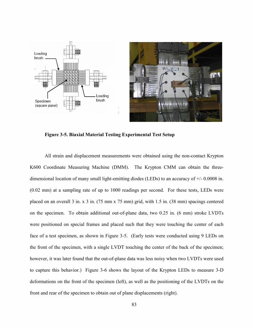
83
Figure 3-5. Biaxial Material Testing Experimental Test Setup
All strain and displacement measurements were obtained using the non-contact Krypton
K600 Coordinate Measuring Machine (DMM). The Krypton CMM can obtain the three-
dimensional location of many small light-emitting diodes (LEDs) to an accuracy of +/- 0.0008 in.
(0.02 mm) at a sampling rate of up to 1000 readings per second. For these tests, LEDs were
placed on an overall 3 in. x 3 in. (75 mm x 75 mm) grid, with 1.5 in. (38 mm) spacings centered
on the specimen. To obtain additional out-of-plane data, two 0.25 in. (6 mm) stroke LVDTs
were positioned on special frames and placed such that they were touching the center of each
face of a test specimen, as shown in Figure 3-5. (Early tests were conducted using 9 LEDs on
the front of the specimen, with a single LVDT touching the center of the back of the specimen;
however, it was later found that the out-of-plane data was less noisy when two LVDTs were used
to capture this behavior.) Figure 3-6 shows the layout of the Krypton LEDs to measure 3-D
deformations on the front of the specimen (left), as well as the positioning of the LVDTs on the
front and rear of the specimen to obtain out of plane displacements (right).
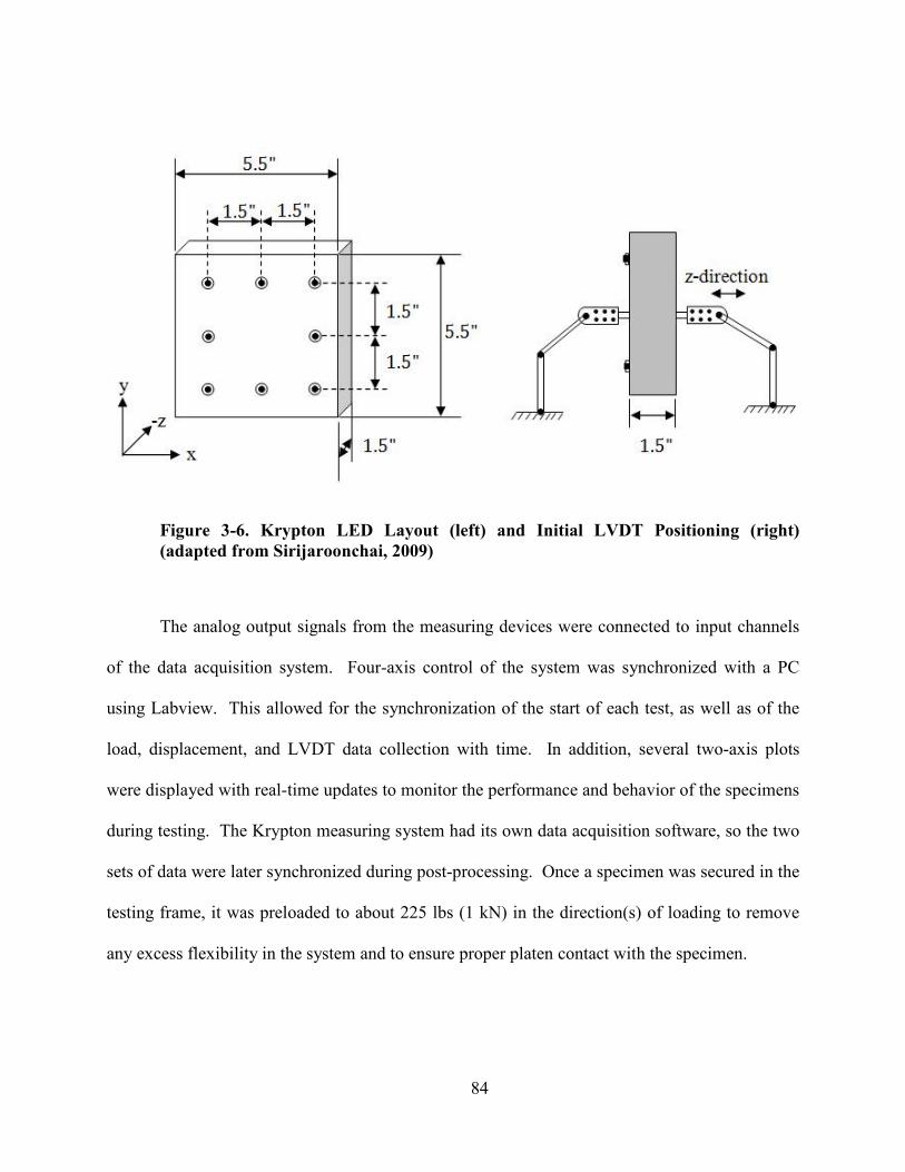
84
Figure 3-6. Krypton LED Layout (left) and Initial LVDT Positioning (right)
(adapted from Sirijaroonchai, 2009)
The analog output signals from the measuring devices were connected to input channels
of the data acquisition system. Four-axis control of the system was synchronized with a PC
using Labview. This allowed for the synchronization of the start of each test, as well as of the
load, displacement, and LVDT data collection with time. In addition, several two-axis plots
were displayed with real-time updates to monitor the performance and behavior of the specimens
during testing. The Krypton measuring system had its own data acquisition software, so the two
sets of data were later synchronized during post-processing. Once a specimen was secured in the
testing frame, it was preloaded to about 225 lbs (1 kN) in the direction(s) of loading to remove
any excess flexibility in the system and to ensure proper platen contact with the specimen.

85
3.7 Uniaxial Test Results
This section will describe the behavior of HPFRCC and plain concrete specimens
subjected to both compressive and tensile uniaxial loading. The failure modes under uniaxial
compression, and the typical compressive stress-strain behavior observed during experimental
tests for both plates and cylinders will be reviewed. Also, the progression of damage in
HPFRCC specimens subjected to uniaxial tension will be examined, and the uniaxial tensile
stress-strain behavior will be explored.
3.7.1 Uniaxial Compression Failure Mode
To eventually better understand the response of plate specimens under more complex
biaxial stress states, the uniaxial failure mode and stress-strain response are first explored. Under
uniaxial compression the failure modes exhibited by the plate specimens were similar to classical
uniaxial plain concrete plate tests, with crack formation at an angle of 20 to 40 degrees with the
axis of loading and perpendicular to the larger unloaded out-of-plane surface. Figure 3-7 shows
a failure surface of a loaf NM6 plate specimen subjected to uniaxial compression, which was
typical of loaf HPFRCC specimens under similar loading.

86
Figure 3-7. Typical Failure Surface of Uniaxial Compression Plate Specimen
Since NM4 and NM6 were deliberately designed not to be high strength concrete mixes,
crack formation and propagation occurred in the cementitious mortar (around the coarse
aggregate). For plain concrete, when the material is loaded in one direction without any
confinement, the largest macrocracks develop in the direction of the loading. Thus for the
uniaxial compression case, crack formation was characterized by a series of vertical tensile
splitting cracks, resulting in a dramatic loss of capacity for the plain concrete specimens.
However, with the addition of fibers, the growth of the macrocracks are retarded, and the
material ultimately fails by the interconnecting of a multitude of small microcracks along a
faulting zone inclining at an angle to the direction of the applied load. This type of failure is
characterized as a faulting failure (Yin et al., 1989). Since the fibers are able to arrest the
propagation of macrocracks, the fiber-reinforced specimens still exhibited significant ductility
beyond peak loading.
87
3.7.2 Uniaxial Compression Stress-Strain Behavior
Due to the displacement-controlled nature of the experiments, loading was stable beyond
the maximum load on the plate specimens, and the descending branch of the stress-strain curve
as obtained out to fairly large deformations. Figure 3-8 shows a comparison of the average
stress-strain response from NM6 HPFRCC and plain concrete results for both plate and cylinder
specimens. It can be seen that the plain specimens failed abruptly, without any significant post-
peak response; however, the HPFRCC exhibited a gradual descending branch and a sustained
capacity of approximately 50% of the maximum applied load out to 3% strain. This significant
deformation capacity is further evidence of the energy-dissipating capability of the material.
These average stress-strain curves were found by averaging the applied stress across a group of
specimens for a given strain obtained from the Krypton LEDs. When processing the data, the
flexibility of the experimental test setup was obtained by comparing the relationship between the
stiffness found using data from the loading platens and that obtained from the Krypton targets.
Since it is possible for local strain accumulation to adversely influence the data collected at
individual LEDs on the surface of a specimen, once the flexibility in the test setup was corrected
for in the experimental data, reliable post-peak behavior for the fiber-reinforced specimens was
then also able to be obtained from the actuators.
Figure 3-8 also shows that the HPFRCC cylinder specimens were slightly stiffer than the
plain concrete specimens as the loading increased, but the stiffnesses were almost identical up to
about 2 ksi (13.8 MPa). The higher HPFRCC stiffness can be attributed to the hooked steel
fibers arresting the propagation and development of early cracking. The plate specimens,
however, had a nearly identical stiffness with or without fibers. It is expected that the addition of
fibers will not affect the stiffness in the linear range, but while plain concrete may begin to
88
undergo damage, the HPFRCC specimens are restrained by the fibers. For the plain plate
specimens, each uniaxial test failed abruptly due to concrete crushing, so the initial damage and
softening is not evident as in the plain cylinders. Also, it can be seen that the average uniaxial
strengths of the similar type of plain and HPFRCC specimens only slightly differed, which is
consistent with the literature (Yin et al., 1989). The average uniaxial compressive strengths of
the concrete and HPFRCC plate specimens were 5.4 ksi (37.3 MPa) and 4.9 ksi (33.5 MPa),
respectively. The average uniaxial compressive strengths of the concrete and HPFRCC cylinder
specimens were 7.2 ksi (49.7 MPa) and 6.8 ksi (46.9 MPa), respectively. The magnitude of the
compressive strength of the plates can be seen to be lower than for the cylinders, which is
consistent with the literature (Yin et al., 1989; Lee et al., 2004). Lee et al. (2004) attributed this
to the difference in geometric shapes and sizes, the effect of a more confined end condition for
the cylinder specimens, and a lower absorption capacity of failure energy in the plate specimens
due to the fact that they have four edges in the axial direction.
With regard to varying the fiber volume fraction, previous test results on MM specimens
showed the general trend that, as fiber volume fraction increased from 1 to 2 percent, the
unconfined uniaxial compressive strength from cylinder tests slightly decreased (Foltz et al.,
2008). Further, the maximum stress was achieved in both the cylinders and plate specimens
under uniaxial compression at a strain of approximately 0.003 for both the plain and HPFRCC
specimens.
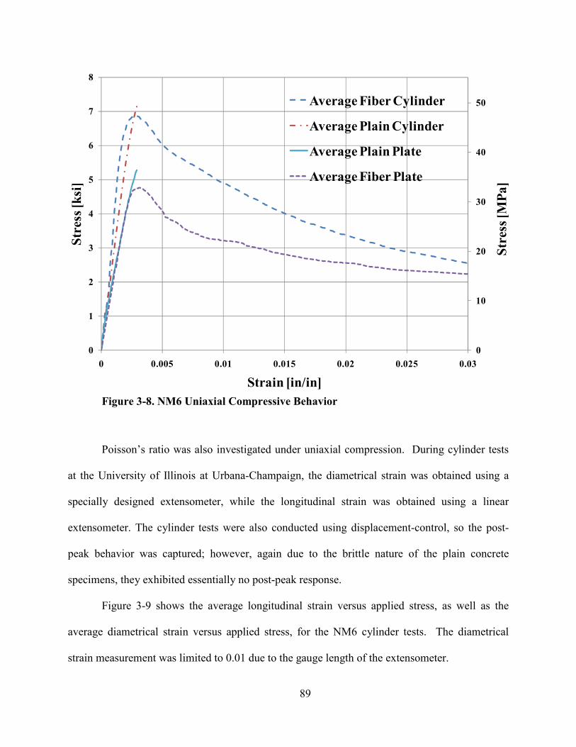
89
Figure 3-8. M6 Uniaxial Compressive Behavior
Poisson’s ratio was also investigated under uniaxial compression. During cylinder tests
at the University of Illinois at Urbana-Champaign, the diametrical strain was obtained using a
specially designed extensometer, while the longitudinal strain was obtained using a linear
extensometer. The cylinder tests were also conducted using displacement-control, so the post-
peak behavior was captured; however, again due to the brittle nature of the plain concrete
specimens, they exhibited essentially no post-peak response.
Figure 3-9 shows the average longitudinal strain versus applied stress, as well as the
average diametrical strain versus applied stress, for the NM6 cylinder tests. The diametrical
strain measurement was limited to 0.01 due to the gauge length of the extensometer.
0
10
20
30
40
50
0
1
2
3
4
5
6
7
8
0 0.005 0.01 0.015 0.02 0.025 0.03
Str
ess
[MP
a]
Str
ess
[ksi
]
Strain [in/in]
Average Fiber Cylinder
Average Plain Cylinder
Average Plain Plate
Average Fiber Plate
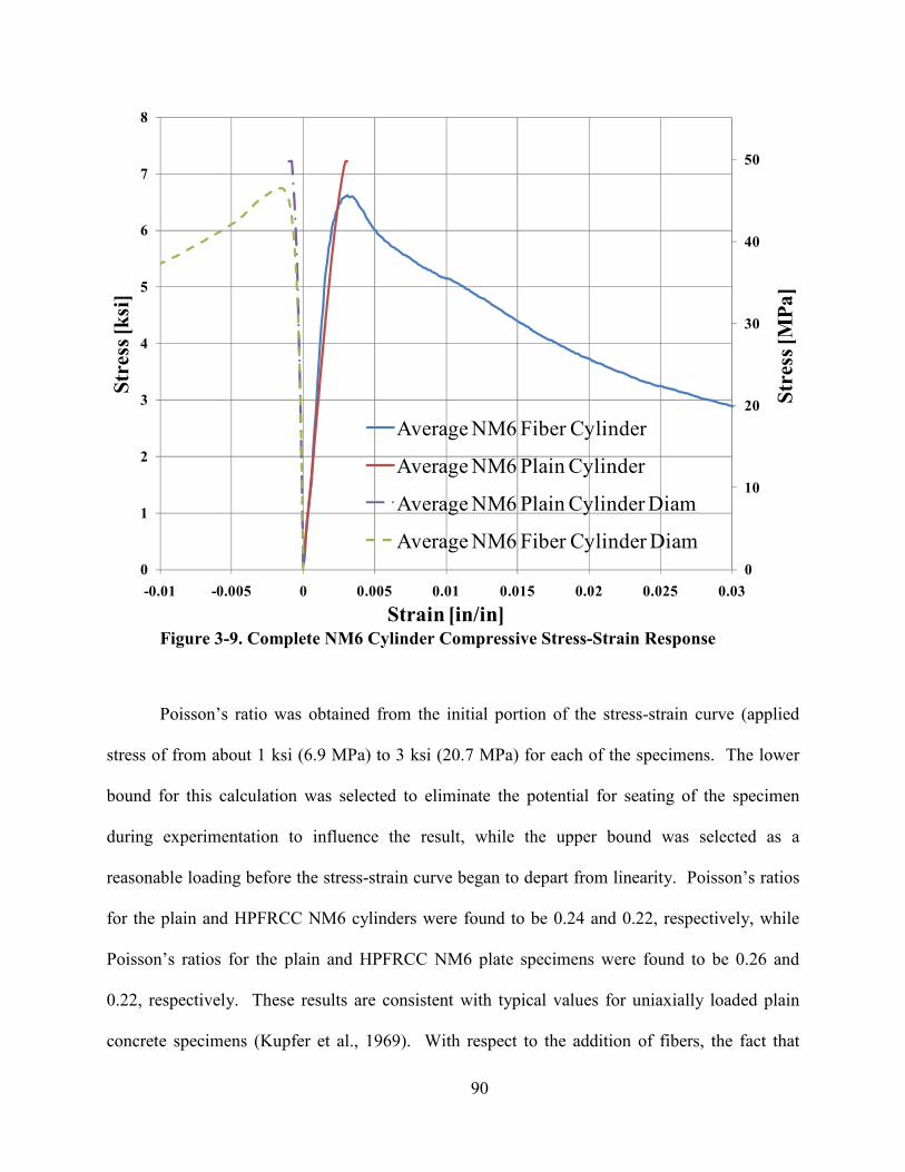
90
Figure 3-9. Complete M6 Cylinder Compressive Stress-Strain Response
Poisson’s ratio was obtained from the initial portion of the stress-strain curve (applied
stress of from about 1 ksi (6.9 MPa) to 3 ksi (20.7 MPa) for each of the specimens. The lower
bound for this calculation was selected to eliminate the potential for seating of the specimen
during experimentation to influence the result, while the upper bound was selected as a
reasonable loading before the stress-strain curve began to depart from linearity. Poisson’s ratios
for the plain and HPFRCC NM6 cylinders were found to be 0.24 and 0.22, respectively, while
Poisson’s ratios for the plain and HPFRCC NM6 plate specimens were found to be 0.26 and
0.22, respectively. These results are consistent with typical values for uniaxially loaded plain
concrete specimens (Kupfer et al., 1969). With respect to the addition of fibers, the fact that
0
10
20
30
40
50
0
1
2
3
4
5
6
7
8
-0.01 -0.005 0 0.005 0.01 0.015 0.02 0.025 0.03
Str
ess
[MP
a]
Str
ess
[k
si]
Strain [in/in]
Average NM6 Fiber Cylinder
Average NM6 Plain Cylinder
Average NM6 Plain Cylinder Diam
Average NM6 Fiber Cylinder Diam
91
Poisson’s ratio remained practically unchanged after adding fiber was also observed in previous
research (Yin et al., 1989). One observation that can be made about the different behavior due to
the effect of fibers on the Poisson’s ratio is that the percent of peak loading at which the rapid
increase in volume of the concrete occurs is much larger. In typical plain concrete, microcracks
begin to form due to the lateral tensile strains, and these cracks continue to grow and coalesce
until failure. This same process of microcracking eventually occurrs in the HPFRCC specimens;
however, it happens at larger strains, and it is accompanied by a significant post-peak
deformation capacity. From Figure 3-9, a comparison between the lateral growth of the NM6
hooked fiber specimens and the NM6 plain specimens shows the ductility of HPFRCC in all
directions. Both fiber and plain cylinders behaved almost identically to about 80% of the
maximum loading. As damage progressed in the specimens, the fiber reinforced concrete
cylinders began to deform vertically and laterally. Once the capacity of the cylinder was
reached, the HPFRCC cylinders showed significant ductility in each direction, while the plain
cylinder specimens failed with essentially no post-peak behavior.
Table 3-8 displays a summary of the average uniaxial compressive strengths of all of the
specimen types tested in this study. Since all of the individually cast plate specimens had
anomalously high compressive strengths, only the plate specimens cast as loaves were included
in the summary. For comparison, Table 3-9 includes uniaxial compressive cylinder tests
conducted at the University of Michigan, as well as the results of the uniaxial compressive plate
and cylinder tests performed at the University of Illinois.
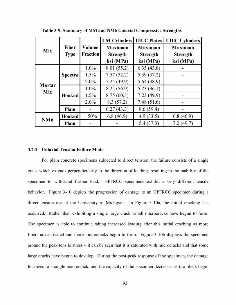
92
Table 3-9. Summary of MM and M6 Uniaxial Compressive Strengths
3.7.3 Uniaxial Tension Failure Mode
For plain concrete specimens subjected to direct tension, the failure consists of a single
crack which extends perpendicularly to the direction of loading, resulting in the inability of the
specimen to withstand further load. HPFRCC specimens exhibit a very different tensile
behavior. Figure 3-10 depicts the progression of damage to an HPFRCC specimen during a
direct tension test at the University of Michigan. In Figure 3-10a, the initial cracking has
occurred. Rather than exhibiting a single large crack, small microcracks have begun to form.
The specimen is able to continue taking increased loading after this initial cracking as more
fibers are activated and more microcracks begin to form. Figure 3-10b displays the specimen
around the peak tensile stress – it can be seen that it is saturated with microcracks and that some
large cracks have begun to develop. During the post-peak response of the specimen, the damage
localizes to a single macrocrack, and the capacity of the specimen decreases as the fibers begin
UM Cylinders UIUC Plates UIUC Cylinders
Maximum
Strength
ksi (MPa)
Maximum
Strength
ksi (MPa)
Maximum
Strength
ksi (MPa)
1.0% 8.01 (55.2) 6.35 (43.8) -
1.5% 7.57 (52.2) 5.39 (37.2) -
2.0% 7.24 (49.9) 5.64 (38.9) -
1.0% 8.25 (56.9) 5.23 (36.1) -
1.5% 8.75 (60.3) 7.23 (49.9) -
2.0% 8.3 (57.2) 7.48 (51.6) -
Plain - 6.27 (43.3) 8.6 (59.4) -
Hooked 1.50% 6.8 (46.9) 4.9 (33.5) 6.8 (46.9)
Plain - - 5.4 (37.3) 7.2 (49.7)
Spectra
Hooked
Mortar
Mix
M6
Volume
Fraction
Fiber
TypeMix
93
to pull out of the specimen. The crack localization stage is displayed in Figure 3-10c. The
comparison between the failure mode of plain concrete and HPFRCC illustrates the benefit that
the addition of fibers has on the deformation capacity and energy absorption of concrete.
Figure 3-10. Cracking Propagation for MM Spectra 1% Direct Tension Test, from
Sirijaroonchai (2009)
3.7.4 Uniaxial Tension Stress-Strain Behavior
The response of the HPFRCC specimens is linear until first cracking. As multiple
cracking develops, the stiffness of the HPFRCC specimens reduces, but they are still able to
accommodate increased loading. This ability to withstand additional stress beyond cracking has
been coined pseudo-strain hardening. After the specimen is saturated with microcracks, the
Fiber Pullout
Initial Cracking
Multiple
Cracking
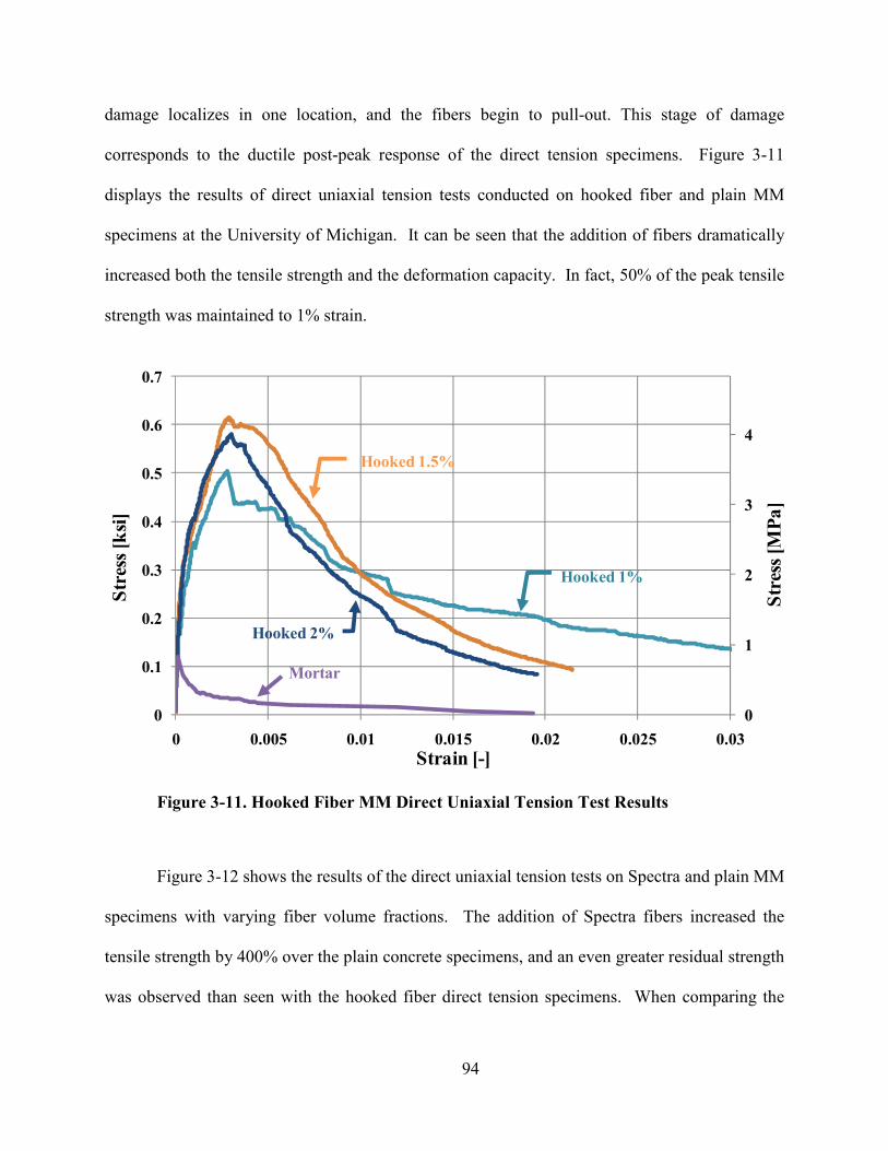
94
damage localizes in one location, and the fibers begin to pull-out. This stage of damage
corresponds to the ductile post-peak response of the direct tension specimens. Figure 3-11
displays the results of direct uniaxial tension tests conducted on hooked fiber and plain MM
specimens at the University of Michigan. It can be seen that the addition of fibers dramatically
increased both the tensile strength and the deformation capacity. In fact, 50% of the peak tensile
strength was maintained to 1% strain.
Figure 3-11. Hooked Fiber MM Direct Uniaxial Tension Test Results
Figure 3-12 shows the results of the direct uniaxial tension tests on Spectra and plain MM
specimens with varying fiber volume fractions. The addition of Spectra fibers increased the
tensile strength by 400% over the plain concrete specimens, and an even greater residual strength
was observed than seen with the hooked fiber direct tension specimens. When comparing the
0
1
2
3
4
0
0.1
0.2
0.3
0.4
0.5
0.6
0.7
0 0.005 0.01 0.015 0.02 0.025 0.03
Str
ess
[MP
a]
Str
ess
[ksi
]
Strain [-]
Hooked 1%
Hooked 1.5%
Hooked 2%
Mortar
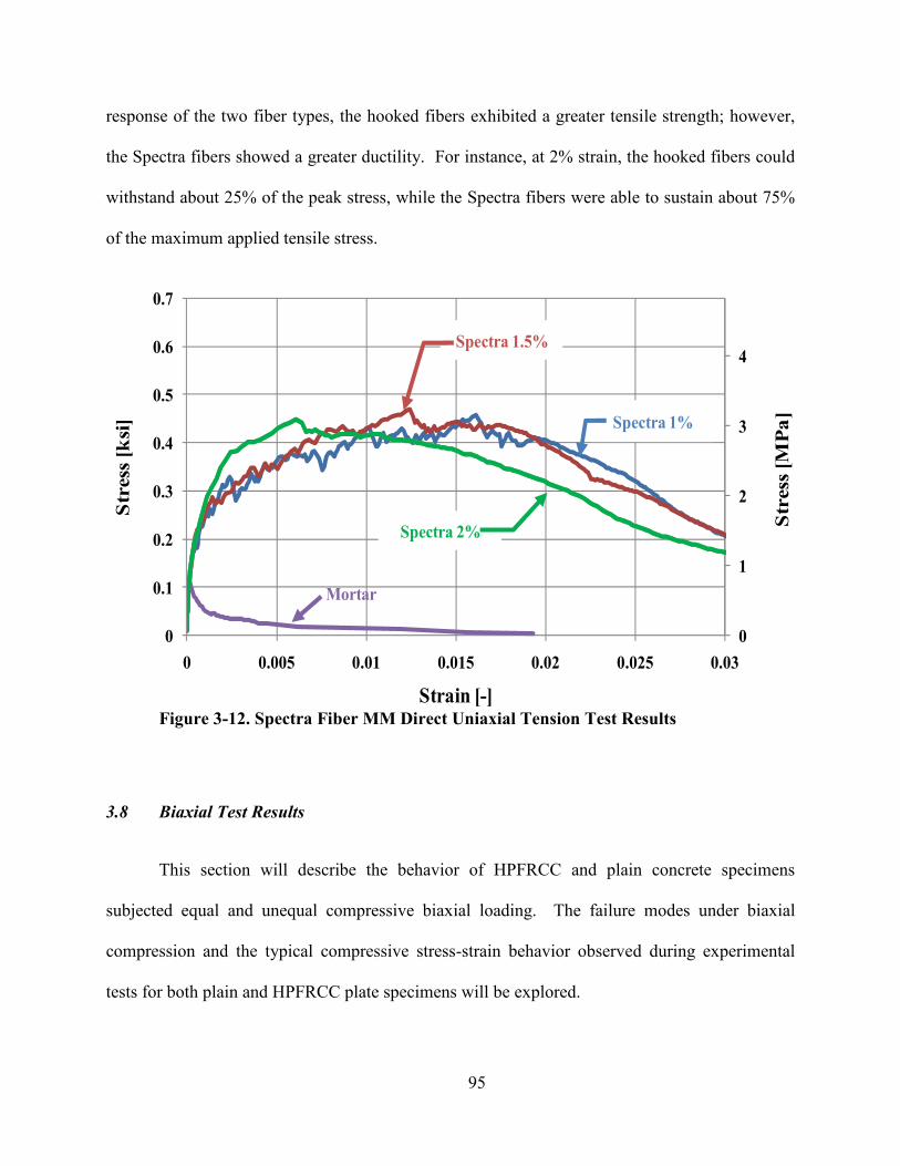
95
response of the two fiber types, the hooked fibers exhibited a greater tensile strength; however,
the Spectra fibers showed a greater ductility. For instance, at 2% strain, the hooked fibers could
withstand about 25% of the peak stress, while the Spectra fibers were able to sustain about 75%
of the maximum applied tensile stress.
Figure 3-12. Spectra Fiber MM Direct Uniaxial Tension Test Results
3.8 Biaxial Test Results
This section will describe the behavior of HPFRCC and plain concrete specimens
subjected equal and unequal compressive biaxial loading. The failure modes under biaxial
compression and the typical compressive stress-strain behavior observed during experimental
tests for both plain and HPFRCC plate specimens will be explored.
0
1
2
3
4
0
0.1
0.2
0.3
0.4
0.5
0.6
0.7
0 0.005 0.01 0.015 0.02 0.025 0.03
Str
ess
[M
Pa
]
Str
ess
[k
si]
Strain [-]
Spectra 1.5%
Spectra 1%
Spectra 2%
Mortar
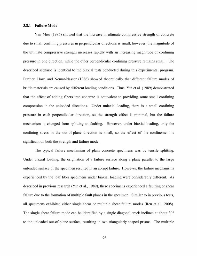
96
3.8.1 Failure Mode
Van Mier (1986) showed that the increase in ultimate compressive strength of concrete
due to small confining pressures in perpendicular directions is small; however, the magnitude of
the ultimate compressive strength increases rapidly with an increasing magnitude of confining
pressure in one direction, while the other perpendicular confining pressure remains small. The
described scenario is identical to the biaxial tests conducted during this experimental program.
Further, Horri and Nemat-Nasser (1986) showed theoretically that different failure modes of
brittle materials are caused by different loading conditions. Thus, Yin et al. (1989) demonstrated
that the effect of adding fibers into concrete is equivalent to providing some small confining
compression in the unloaded directions. Under uniaxial loading, there is a small confining
pressure in each perpendicular direction, so the strength effect is minimal, but the failure
mechanism is changed from splitting to faulting. However, under biaxial loading, only the
confining stress in the out-of-plane direction is small, so the effect of the confinement is
significant on both the strength and failure mode.
The typical failure mechanism of plain concrete specimens was by tensile splitting.
Under biaxial loading, the origination of a failure surface along a plane parallel to the large
unloaded surface of the specimen resulted in an abrupt failure. However, the failure mechanisms
experienced by the loaf fiber specimens under biaxial loading were considerably different. As
described in previous research (Yin et al., 1989), these specimens experienced a faulting or shear
failure due to the formation of multiple fault planes in the specimen. Similar to in previous tests,
all specimens exhibited either single shear or multiple shear failure modes (Ren et al., 2008).
The single shear failure mode can be identified by a single diagonal crack inclined at about 30°
to the unloaded out-of-plane surface, resulting in two triangularly shaped prisms. The multiple
97
shear failure mode is similar to single shear, except the specimen fails along several inclined
diagonal cracks, resulting in it being divided into a few triangular pyramids. Figure 3-13 shows
examples of both the single shear and multiple shear failure modes for HPFRCC, as well as the
tensile splitting failure that was common in plain concrete specimens. The individually cast
specimens had relatively more fibers oriented in the plane of the specimen than in the 1.5” (38
mm) out-of-plane direction. As a result, when the individually cast specimens failed brittlely,
concrete exploded in the out-of-plane dimension of the specimen. This demonstrated that the
fibers were not oriented to properly provide passive confinement.
Figure 3-13. Single Shear Failure Mode (left), Multiple Shear Failure Mode (center),
and Tensile Splitting Failure (right)
3.8.2 Stress-Strain Behavior
The biaxial stress-strain behavior is largely dependent upon the ratio of applied axial
loads. As previously described, the loading ratio was varied by altering the horizontal strain rate
in the biaxial testing machine. Figure 3-14 shows the average compressive response of the
leading direction of the biaxially loaded NM6 specimens, and the average uniaxial compressive
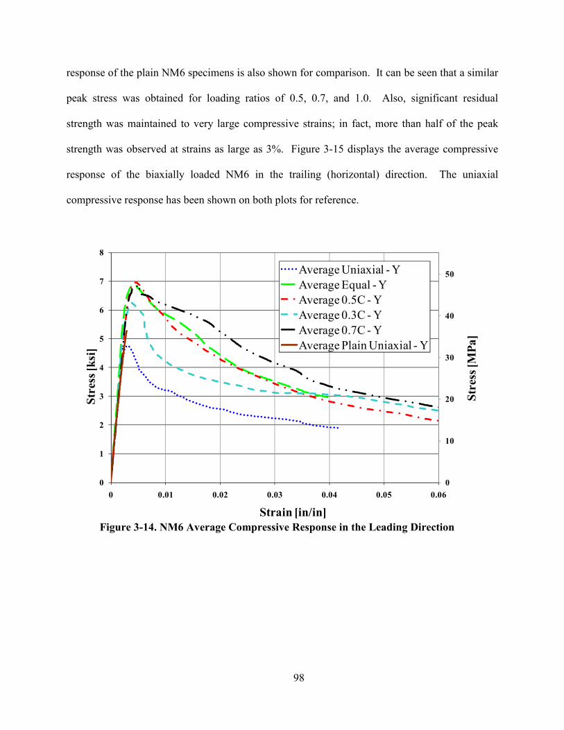
98
response of the plain NM6 specimens is also shown for comparison. It can be seen that a similar
peak stress was obtained for loading ratios of 0.5, 0.7, and 1.0. Also, significant residual
strength was maintained to very large compressive strains; in fact, more than half of the peak
strength was observed at strains as large as 3%. Figure 3-15 displays the average compressive
response of the biaxially loaded NM6 in the trailing (horizontal) direction. The uniaxial
compressive response has been shown on both plots for reference.
Figure 3-14. M6 Average Compressive Response in the Leading Direction
0
10
20
30
40
50
0
1
2
3
4
5
6
7
8
0 0.01 0.02 0.03 0.04 0.05 0.06
Str
ess
[M
Pa
]
Str
ess
[k
si]
Strain [in/in]
Average Uniaxial - Y
Average Equal - Y
Average 0.5C - Y
Average 0.3C - Y
Average 0.7C - Y
Average Plain Uniaxial - Y
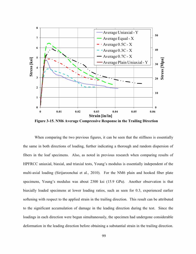
99
Figure 3-15. M6 Average Compressive Response in the Trailing Direction
When comparing the two previous figures, it can be seen that the stiffness is essentially
the same in both directions of loading, further indicating a thorough and random dispersion of
fibers in the loaf specimens. Also, as noted in previous research when comparing results of
HPFRCC uniaxial, biaxial, and triaxial tests, Young’s modulus is essentially independent of the
multi-axial loading (Sirijaroonchai et al., 2010). For the NM6 plain and hooked fiber plate
specimens, Young’s modulus was about 2300 ksi (15.9 GPa). Another observation is that
biaxially loaded specimens at lower loading ratios, such as seen for 0.3, experienced earlier
softening with respect to the applied strain in the trailing direction. This result can be attributed
to the significant accumulation of damage in the leading direction during the test. Since the
loadings in each direction were begun simultaneously, the specimen had undergone considerable
deformation in the leading direction before obtaining a substantial strain in the trailing direction.
0
10
20
30
40
50
0
1
2
3
4
5
6
7
8
0 0.01 0.02 0.03 0.04 0.05 0.06
Str
ess
[Mp
a]
Str
ess
[ksi
]
Strain [in/in]
Average Uniaxial - Y
Average Equal - X
Average 0.5C - X
Average 0.3C - X
Average 0.7C - X
Average Plain Uniaxial - Y
100
Also, the strain at maximum applied stress shifted to about 0.4% for specimens subjected to a
biaxial loading ratio of 0.5 or greater, while the strain at maximum stress was approximately
0.3% for the uniaxial specimens. Previous research shows the strain at the onset of significant
spalling for short RC columns (analogous to coupling beams) occurs at about 0.5% (Berry &
Eberhard, 2003). Since HPFRCC specimens exhibit residual strengths of about 70% of the peak
strength at a strain of 1% and about 50% of the peak strength at a strain of 2%, the deformation
capacity of HPFRCC can dramatically improve the seismic performance of such structural
elements. For structural designers, the performance of structural elements is a critical
consideration; therefore, it is important that both the core and the cover of the coupling beams
can withstand design basis earthquakes without undergoing significant damage or jeopardizing
the load carrying capacity of the structural component. Thus, the demonstrated deformation
capacity and residual strength of HPFRCC is evidence of its potential as a material to withstand
seismic events while maintaining the integrity of structural elements.
3.9 Failure Envelope Results
Non-dimensionalized ultimate strength data are shown as biaxial stress envelopes,
depicted in Figure 3-16 and Figure 3-17. Stresses are reported as fractions of the average
unconfined uniaxial compressive plate strength of the specimens for the particular concrete
mixture and fiber volume fraction, σco. (Average uniaxial compressive plate strengths are given
in Table 3-8.) Figure 3-16 shows the biaxial failure envelopes obtained from this testing
program. This figure illustrates the effect of a more random fiber orientation by plotting the
average result for each tested type of fiber, concrete mixture, and specimen (loaf vs. individually
cast). The averaged curves were obtained by first normalizing each specific concrete batch by its
average uniaxial value, and then the data points that had a similar failure stress ratio for a
101
particular specimen, mix, and fiber type were averaged to create the data points for the curve.
For example, the average loaf Spectra curve was made by first normalizing the 1.0, 1.5, and 2.0
percent fiber volume fraction results by their respective average uniaxial values, and then data
points with similar failure stress ratios were averaged together. Each averaged data point used to
generate the failure envelope represents the results of 3 to 7 experimental tests, depending on the
quantity of specimens available for the particular mix. Each plot has been normalized by its
average uniaxial compressive performance, so the individual specimens were not actually weaker
than the loaf specimens; they just did not benefit as much from the addition of a second principal
confining stress. This is consistent with the results of Tasuji et al. (1978), which indicated that
the increase in biaxial compressive strength for concrete is higher for concrete with a lower
uniaxial compressive strength. Additionally, Figure 3-16 displays the plain MM and plain NM4
biaxial failure envelopes, and it can be seen that the results from the plain concrete mixes even
experienced a greater biaxial strength increase than the individually cast HPFRCC specimens,
reconfirming the reduced effect of fibers without a random dispersion throughout the concrete.
A post-experiment “autopsy” of the individually cast specimens continued to confirm that the
fibers were indeed aligned in the plane of the specimen.

102
Figure 3-16. Biaxial Strength Envelopes from Experimental Test Results
In Figure 3-17, a comparison of various biaxial failure envelopes from the experimental
test program with those obtained by other experiments from the literature on plain concrete is
shown (Kupfer et al., 1969; Hussein & Marzouk, 2000a; Nelissen, 1972; Tasuji et al., 1978). It
can be seen that the benefit of a biaxial stress state on the strength of the concrete is markedly
increased with the addition of fibers in the HPFRCC specimens when comparing the average
0
0.2
0.4
0.6
0.8
1
1.2
1.4
1.6
1.8
2
0 0.2 0.4 0.6 0.8 1 1.2 1.4 1.6 1.8 2
σσ σσ2/ σσ σσco
σσσσ1 / σσσσco
NM4 Avg. Ind.
Hooked Avg. Ind.
Spectra Avg. Ind.
Hooked Avg. Loaf
Spectra Avg. Loaf
NM6 Avg. Loaf
MM Plain
NM4 Plain
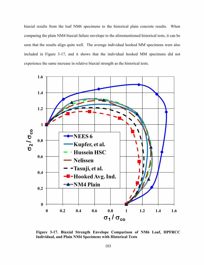
103
biaxial results from the loaf NM6 specimens to the historical plain concrete results. When
comparing the plain NM4 biaxial failure envelope to the aforementioned historical tests, it can be
seen that the results align quite well. The average individual hooked MM specimens were also
included in Figure 3-17, and it shows that the individual hooked MM specimens did not
experience the same increase in relative biaxial strength as the historical tests.
Figure 3-17. Biaxial Strength Envelope Comparison of M6 Loaf, HPFRCC
Individual, and Plain M4 Specimens with Historical Tests
0
0.2
0.4
0.6
0.8
1
1.2
1.4
1.6
0 0.2 0.4 0.6 0.8 1 1.2 1.4 1.6
σσ σσ2/ σσ σσco
σσσσ1 / σσσσco
EES 6
Kupfer, et al.
Hussein HSC
elissen
Tasuji, et al.
Hooked Avg. Ind.
M4 Plain
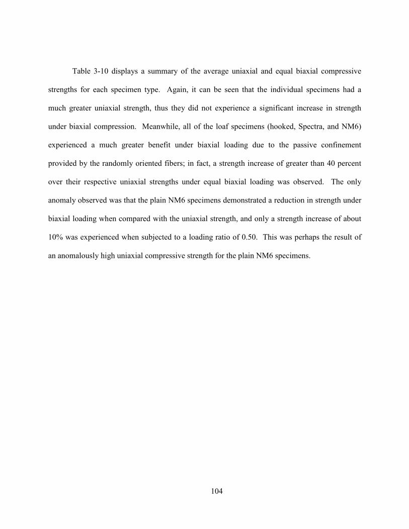
104
Table 3-10 displays a summary of the average uniaxial and equal biaxial compressive
strengths for each specimen type. Again, it can be seen that the individual specimens had a
much greater uniaxial strength, thus they did not experience a significant increase in strength
under biaxial compression. Meanwhile, all of the loaf specimens (hooked, Spectra, and NM6)
experienced a much greater benefit under biaxial loading due to the passive confinement
provided by the randomly oriented fibers; in fact, a strength increase of greater than 40 percent
over their respective uniaxial strengths under equal biaxial loading was observed. The only
anomaly observed was that the plain NM6 specimens demonstrated a reduction in strength under
biaxial loading when compared with the uniaxial strength, and only a strength increase of about
10% was experienced when subjected to a loading ratio of 0.50. This was perhaps the result of
an anomalously high uniaxial compressive strength for the plain NM6 specimens.
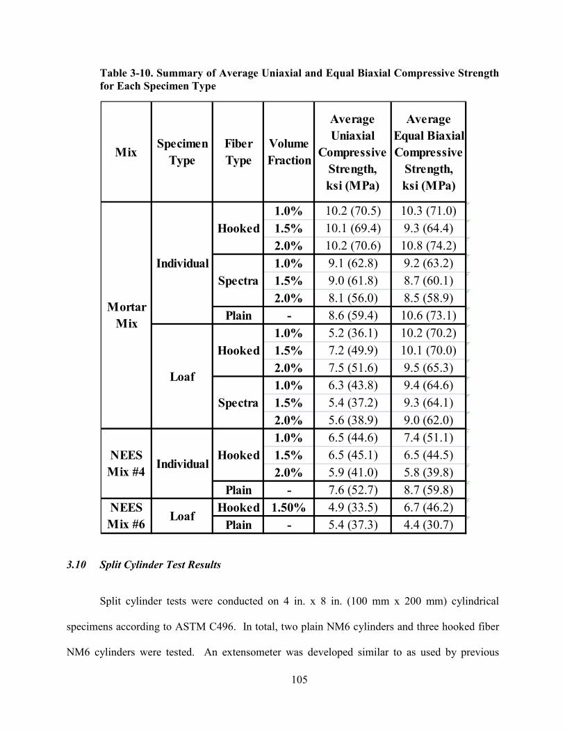
105
Table 3-10. Summary of Average Uniaxial and Equal Biaxial Compressive Strength
for Each Specimen Type
3.10 Split Cylinder Test Results
Split cylinder tests were conducted on 4 in. x 8 in. (100 mm x 200 mm) cylindrical
specimens according to ASTM C496. In total, two plain NM6 cylinders and three hooked fiber
NM6 cylinders were tested. An extensometer was developed similar to as used by previous
MixSpecimen
Type
Fiber
Type
Volume
Fraction
Average
Uniaxial
Compressive
Strength,
ksi (MPa)
Average
Equal Biaxial
Compressive
Strength,
ksi (MPa)
1.0% 10.2 (70.5) 10.3 (71.0)
1.5% 10.1 (69.4) 9.3 (64.4)
2.0% 10.2 (70.6) 10.8 (74.2)
1.0% 9.1 (62.8) 9.2 (63.2)
1.5% 9.0 (61.8) 8.7 (60.1)
2.0% 8.1 (56.0) 8.5 (58.9)
Plain - 8.6 (59.4) 10.6 (73.1)
1.0% 5.2 (36.1) 10.2 (70.2)
1.5% 7.2 (49.9) 10.1 (70.0)
2.0% 7.5 (51.6) 9.5 (65.3)
1.0% 6.3 (43.8) 9.4 (64.6)
1.5% 5.4 (37.2) 9.3 (64.1)
2.0% 5.6 (38.9) 9.0 (62.0)
1.0% 6.5 (44.6) 7.4 (51.1)
1.5% 6.5 (45.1) 6.5 (44.5)
2.0% 5.9 (41.0) 5.8 (39.8)
Plain - 7.6 (52.7) 8.7 (59.8)
Hooked 1.50% 4.9 (33.5) 6.7 (46.2)
Plain - 5.4 (37.3) 4.4 (30.7)
IndividualHooked
Mortar
Mix
EES
Mix #4
EES
Mix #6Loaf
Individual
Hooked
Spectra
Loaf
Hooked
Spectra
106
researchers to obtain a measure of the transverse deformation under loading (Nanni, 1988;
Graybeal, 2006). This diametrical deformation measuring apparatus was spring-loaded to ensure
constant contact with the cylinder, and two linear variable differential transformers (LVDTs)
were used to measure the lateral deformation during loading; also, the load data was
continuously collected and monitored using Labview. With this particular test setup, it was
possible to visually monitor the load versus lateral expansion plot during testing. Figure 3-18
displays the extensometer used for the testing of the split-cylinders. It was essential that the
LVDTs were sufficiently sensitive to measure the smaller diametrical strains that occur even
before the initial cracking of the specimen.
Figure 3-18. Split Cylinder Diametrical Deformation Apparatus and Experimental
Test Setup
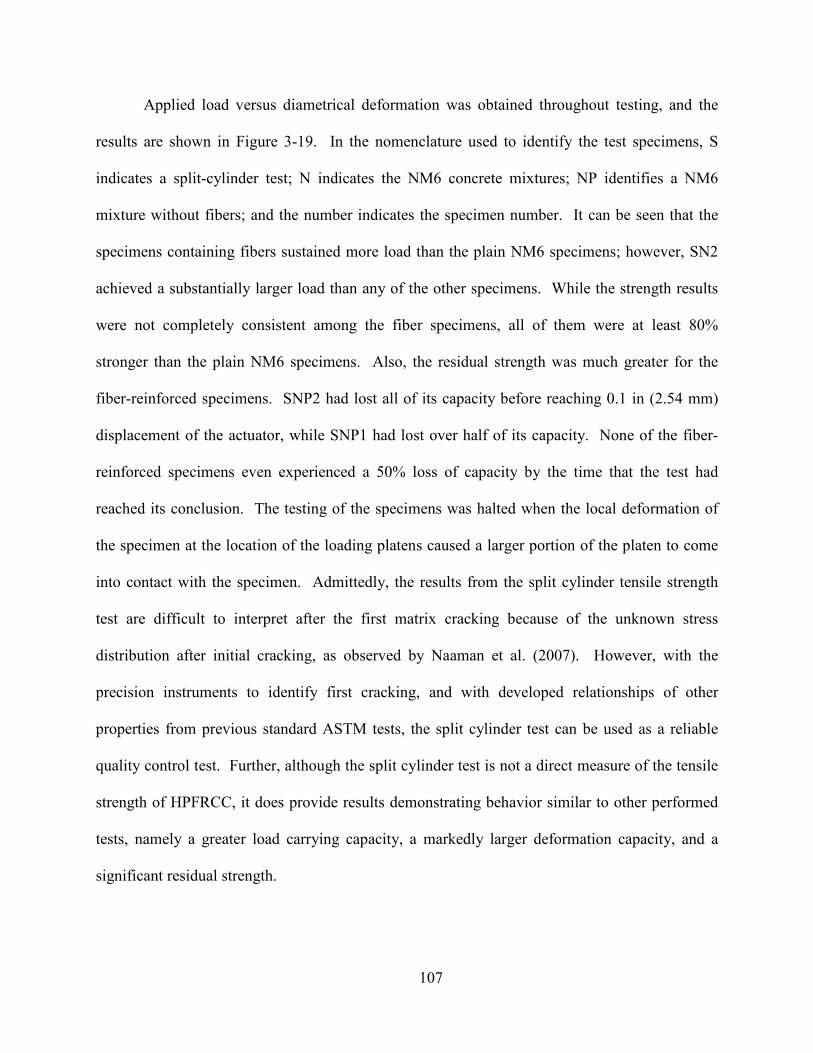
107
Applied load versus diametrical deformation was obtained throughout testing, and the
results are shown in Figure 3-19. In the nomenclature used to identify the test specimens, S
indicates a split-cylinder test; N indicates the NM6 concrete mixtures; NP identifies a NM6
mixture without fibers; and the number indicates the specimen number. It can be seen that the
specimens containing fibers sustained more load than the plain NM6 specimens; however, SN2
achieved a substantially larger load than any of the other specimens. While the strength results
were not completely consistent among the fiber specimens, all of them were at least 80%
stronger than the plain NM6 specimens. Also, the residual strength was much greater for the
fiber-reinforced specimens. SNP2 had lost all of its capacity before reaching 0.1 in (2.54 mm)
displacement of the actuator, while SNP1 had lost over half of its capacity. None of the fiber-
reinforced specimens even experienced a 50% loss of capacity by the time that the test had
reached its conclusion. The testing of the specimens was halted when the local deformation of
the specimen at the location of the loading platens caused a larger portion of the platen to come
into contact with the specimen. Admittedly, the results from the split cylinder tensile strength
test are difficult to interpret after the first matrix cracking because of the unknown stress
distribution after initial cracking, as observed by Naaman et al. (2007). However, with the
precision instruments to identify first cracking, and with developed relationships of other
properties from previous standard ASTM tests, the split cylinder test can be used as a reliable
quality control test. Further, although the split cylinder test is not a direct measure of the tensile
strength of HPFRCC, it does provide results demonstrating behavior similar to other performed
tests, namely a greater load carrying capacity, a markedly larger deformation capacity, and a
significant residual strength.
Figure 3-19. Split-Cylinder
3.11 Tension Results
A suite of uniaxial and biaxial compressive experiments
experimental program intended to test the
and tension-tension) to complete the failure envelope.
tests, and they were to be performed using
epoxied to the brush platens, as done in previous historical tests
al., 1978; Maekawa & Okamura, 1983; Hussein & Marzouk, 2000a; Calixto, 2002; Lee et al.,
2004; Ren et al., 2008). Unfortuantely, due to general experimental obstacles, ranging from
108
Cylinder Load versus Deformation for M6 Cylinders
suite of uniaxial and biaxial compressive experiments were conducted,
experimental program intended to test the remaining two loading scenarios (tension
tension) to complete the failure envelope. The experiments were to be direct tension
performed using the biaxial testing machine with the plate specimens
epoxied to the brush platens, as done in previous historical tests (Kupfer et al.
a, 1983; Hussein & Marzouk, 2000a; Calixto, 2002; Lee et al.,
Unfortuantely, due to general experimental obstacles, ranging from
Load versus Deformation for M6 Cylinders
conducted, and this
remaining two loading scenarios (tension-compression
riments were to be direct tension
the biaxial testing machine with the plate specimens
et al., 1969; Tasuji et
a, 1983; Hussein & Marzouk, 2000a; Calixto, 2002; Lee et al.,
Unfortuantely, due to general experimental obstacles, ranging from

109
testing machine mechanical problems to controller availability to the veteran lab technician
retiring, the tensile panel tension tests were unable to be completed. Therefore, the dogbone
results provided by project colleagues at the University of Michigan will be used as the HPFRCC
uniaxial tensile property for material modeling purposes.
110
CHAPTER 4. MATERIAL MODELIG
The analytical phase of the research program focuses on the creation of finite element
models using the ATENA software from Cervenka Consulting, which has a main strength in the
nonlinear finite element modeling of structural concrete. This chapter will provide a background
of the ATENA software, and an overview of the modeling of the HPFRCC material tests. The
intent is to first validate the material parameters within ATENA by modeling the material tests
described in Chapter 3, then the HPFRCC model can be extended to more complex structural
components, such as coupling beams and pile-wharf connections, as described in Chapter 6 and
Chapter 9, respectively.
4.1 ATE6A Background
Since the conducted material tests were planar, the ATENA 2D software was used for the
HPFRCC modeling parameter validation portion of the current research. The ATENA program
is specially designed for the nonlinear finite element analysis of concrete and reinforced concrete
structural behavior. The program consists of the solution core and the user interface. The
solution core has the capability to analyze 2-dimensional and 3-dimensional continuum
structures, and it consists of libraries of finite elements, material models, and solution methods.
The User Graphic Interface enables access to the ATENA solution core, and it provides the user
with the ability to graphically model a structure and to explore a visualization of the analytical
results.
While many structures may be sufficiently modeled using a linear formulation, the focus
of the current research is to capture the softening and post-peak behavior of HPFRCC, thus an
iterative non-linear solution scheme must be used. ATENA is suited for both the modeling of
111
the material nonlinear behavior and the geometric nonlinear behavior. The geometric nonlinear
behavior results when the deformations of the structure are large enough to require equilibrium
equations to be used on the displaced shape. To capture the behavior of the displaced shape,
ATENA uses the Updated Lagrangian formulation, so the governing equations are with respect
to the most recent deformed configuration.
The SBETA model is the standard concrete material model used within ATENA. The
concept of the SBETA material model includes the nonlinear behavior of concrete in
compression (hardening and softening), fracture of concrete in tension, biaxial failure criterion,
reduction of compressive strength after cracking, tension stiffening, reduction of the shear
stiffness after cracking, and both fixed and rotating crack models. Since the SBETA material
model has been designed to model regular reinforced concrete and since the user defined options
are limited, it will be used for the modeling of reinforced concrete structural components where
further details about the concrete properties are not known. Since detailed material tests were
conducted on the HPFRCC material, another material model will be used that allows the user to
input specific material properties and constitutive relationships.
HPFRCC was modeled using a fracture-plastic constitutive model. Specifically, the
CC3DNonLinCementitious2User model was implemented for HPFRCC. As described in detail
by Cervenka et al. (2010), the fracture-plastic model combines constitutive models for tensile
(fracturing) and compressive (plastic) behavior. The fracture model considers a classical
orthotropic smeared crack formulation and crack band model. It uses the Rankine failure
criterion with exponential softening. The plasticity model is based on the Menetrey-William
failure surface, with a return mapping algorithm for the integration of constitutive equations.
The model is unique in its combination of both fracture and plasticity. A combined algorithm is
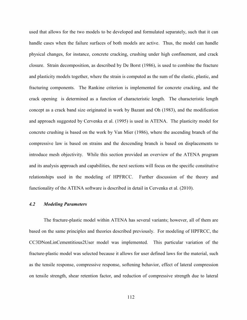
112
used that allows for the two models to be developed and formulated separately, such that it can
handle cases when the failure surfaces of both models are active. Thus, the model can handle
physical changes, for instance, concrete cracking, crushing under high confinement, and crack
closure. Strain decomposition, as described by De Borst (1986), is used to combine the fracture
and plasticity models together, where the strain is computed as the sum of the elastic, plastic, and
fracturing components. The Rankine criterion is implemented for concrete cracking, and the
crack opening is determined as a function of characteristic length. The characteristic length
concept as a crack band size originated in work by Bazant and Oh (1983), and the modification
and approach suggested by Cervenka et al. (1995) is used in ATENA. The plasticity model for
concrete crushing is based on the work by Van Mier (1986), where the ascending branch of the
compressive law is based on strains and the descending branch is based on displacements to
introduce mesh objectivity. While this section provided an overview of the ATENA program
and its analysis approach and capabilities, the next sections will focus on the specific constitutive
relationships used in the modeling of HPFRCC. Further discussion of the theory and
functionality of the ATENA software is described in detail in Cervenka et al. (2010).
4.2 Modeling Parameters
The fracture-plastic model within ATENA has several variants; however, all of them are
based on the same principles and theories described previously. For modeling of HPFRCC, the
CC3DNonLinCementitious2User model was implemented. This particular variation of the
fracture-plastic model was selected because it allows for user defined laws for the material, such
as the tensile response, compressive response, softening behavior, effect of lateral compression
on tensile strength, shear retention factor, and reduction of compressive strength due to lateral
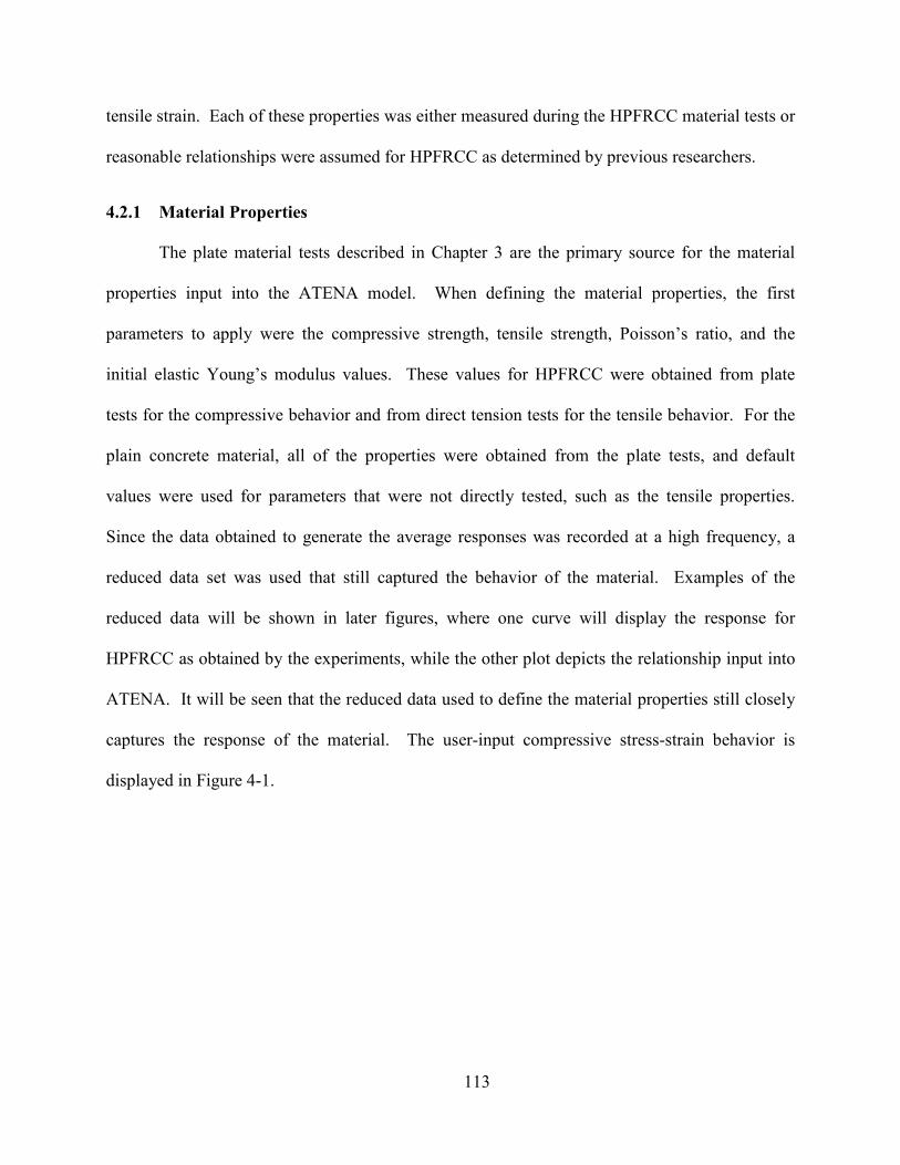
113
tensile strain. Each of these properties was either measured during the HPFRCC material tests or
reasonable relationships were assumed for HPFRCC as determined by previous researchers.
4.2.1 Material Properties
The plate material tests described in Chapter 3 are the primary source for the material
properties input into the ATENA model. When defining the material properties, the first
parameters to apply were the compressive strength, tensile strength, Poisson’s ratio, and the
initial elastic Young’s modulus values. These values for HPFRCC were obtained from plate
tests for the compressive behavior and from direct tension tests for the tensile behavior. For the
plain concrete material, all of the properties were obtained from the plate tests, and default
values were used for parameters that were not directly tested, such as the tensile properties.
Since the data obtained to generate the average responses was recorded at a high frequency, a
reduced data set was used that still captured the behavior of the material. Examples of the
reduced data will be shown in later figures, where one curve will display the response for
HPFRCC as obtained by the experiments, while the other plot depicts the relationship input into
ATENA. It will be seen that the reduced data used to define the material properties still closely
captures the response of the material. The user-input compressive stress-strain behavior is
displayed in Figure 4-1.
114
Figure 4-1. M6 Compressive Stress-Strain Response in ATEA
These user defined stress-strain curves were input for both the compressive and tensile
properties of the material. The compressive strength implemented into ATENA was from the
plate tests. This compressive strength was used instead of the cylinder compressive strength in
accordance with the guidance of the finite element program. Again, the tensile properties of the
NM6 HPFRCC material were obtained from direct tension dogbone tests. These tests were
conducted by project colleagues at the University of Michigan, and the full results are reported
by Liao et al. (2006). Figure 4-2 displays the NM6 uniaxial tension response, as well as the
tensile stress-strain characteristic behavior input into ATENA with the reduced data set.
0
1
2
3
4
5
0 0.005 0.01 0.015 0.02 0.025 0.03
Str
ess
(ksi
)
Plastic Strain (in/in)
115
Figure 4-2. M6 Tensile Stress-Strain Response
Several additional properties are required for input into ATENA, and they include the
characteristic size, chL , and the localized strain value, locε . In ATENA, the characteristic size
represents the size for which the tensile and compression diagrams were valid. Since the
compressive result is the average response obtained on 5.5 in. (140 mm) wide specimens, that
dimension was considered the compressive characteristic size. Similarly, the width of the
dogbone specimens was 2 in. (50 mm), so that dimension was considered the corresponding
tensile characteristic size. The characteristic size approach is implemented to reduce the
dependency of the results on the finite element mesh. The localized strain values were also
obtained from the experiments. For both the compressive and tensile tests, the strain began to
localize at the peak strength, and then softening ensued through the slow pullout of the fibers
under continued deformations. The localized strain values were 0.0031 and 0.0046 in
0.0
0.1
0.2
0.3
0.4
0.5
0.6
0.000 0.005 0.010 0.015
Str
ess
(ksi
)
Strain (in/in)
Ten. HPFRCC Full Data
Ten. HPFRCC Reduced Data

116
compression and tension, respectively. The strain value that is used to determine the strength is
calculated using the following equations, where the tensile strain value is used as an example:
If 1
f f
locε ε<
1 1
f fε ε=ɶ
else
( )1 1
f f f f tloc loc
ch
LL
ε ε ε ε= + −ɶ (4.1)
The calculation of the strain values for the compressive case and for the shear strength retention
function are based on a similar strain calculation; however, the appropriate values for the
characteristic size and localized strain value should be used in each case. It is important to note
that 1
fε is the tensile strain calculated from the strain tensor at the finite element integration
points, while the strain 1
fεɶ is used to determine the current tensile strength from the provided
stress-strain diagrams, as seen in Figure 4-1 and Figure 4-2. The use of the characteristic length
represents a scaling that takes into account the difference between the experimental size and the
size of the finite element. This approach ensures that the same amount of energy is dissipated
when using large and small finite elements.
For the biaxial failure criterion, the failure surface reported by Menetrey and William
(1995) is used within ATENA. The failure criterion is characterized by three parameters: f’c, f’t,
and e, where e is an eccentricity parameter that influences the size and shape of the failure
surface. The default parameter is for an e value of 0.52. This should correspond to a failure
surface which matches closely to the biaxial failure surface observed by Kupfer et al. (1969).
Figure 4-3 shows a comparison of the failure envelope obtained by Kupfer et al. (1969) to three
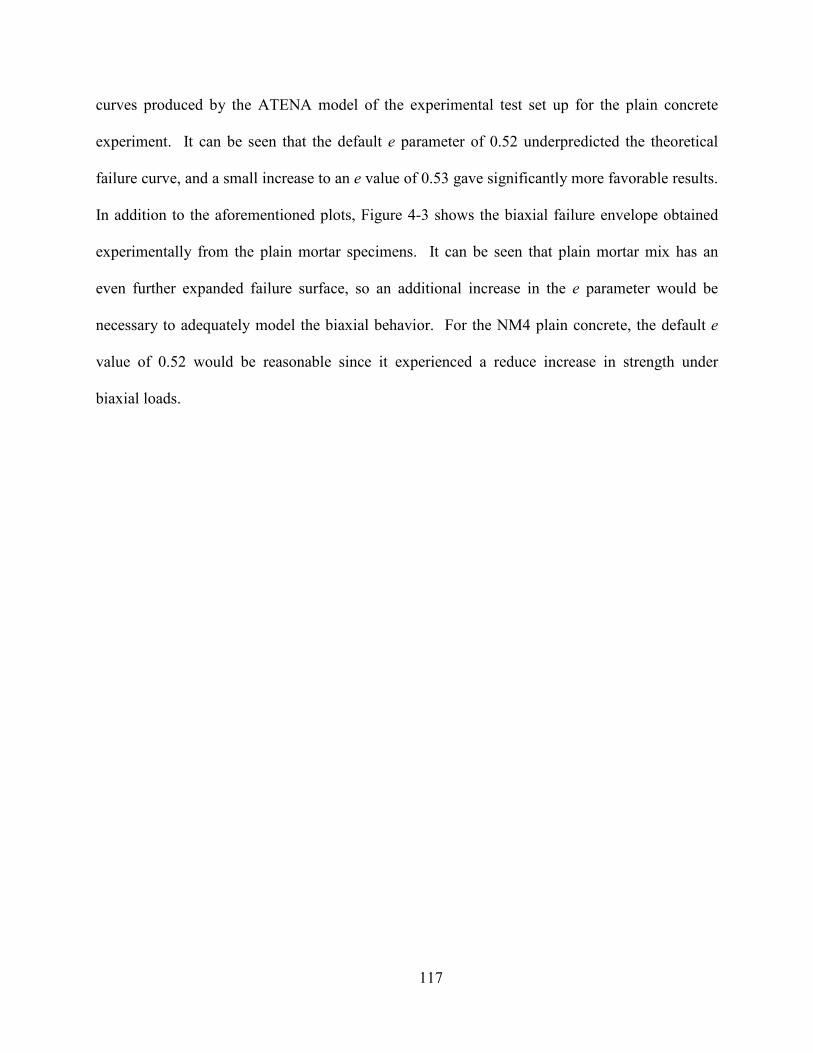
117
curves produced by the ATENA model of the experimental test set up for the plain concrete
experiment. It can be seen that the default e parameter of 0.52 underpredicted the theoretical
failure curve, and a small increase to an e value of 0.53 gave significantly more favorable results.
In addition to the aforementioned plots, Figure 4-3 shows the biaxial failure envelope obtained
experimentally from the plain mortar specimens. It can be seen that plain mortar mix has an
even further expanded failure surface, so an additional increase in the e parameter would be
necessary to adequately model the biaxial behavior. For the NM4 plain concrete, the default e
value of 0.52 would be reasonable since it experienced a reduce increase in strength under
biaxial loads.
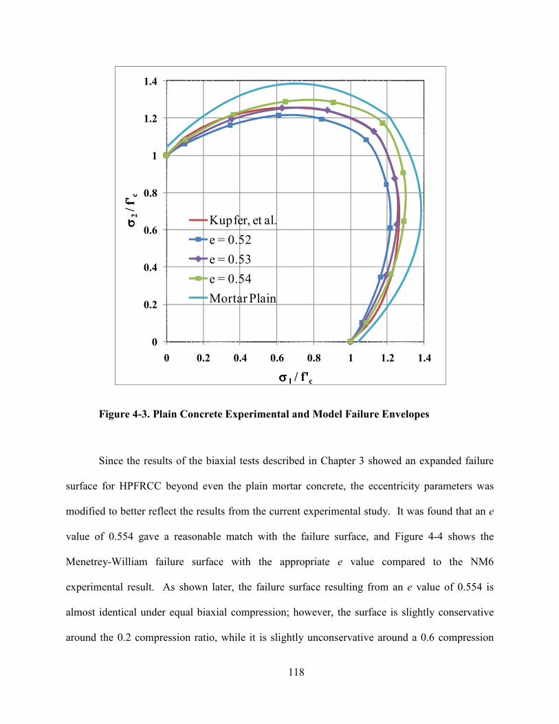
118
Figure 4-3. Plain Concrete Experimental and Model Failure Envelopes
Since the results of the biaxial tests described in Chapter 3 showed an expanded failure
surface for HPFRCC beyond even the plain mortar concrete, the eccentricity parameters was
modified to better reflect the results from the current experimental study. It was found that an e
value of 0.554 gave a reasonable match with the failure surface, and Figure 4-4 shows the
Menetrey-William failure surface with the appropriate e value compared to the NM6
experimental result. As shown later, the failure surface resulting from an e value of 0.554 is
almost identical under equal biaxial compression; however, the surface is slightly conservative
around the 0.2 compression ratio, while it is slightly unconservative around a 0.6 compression
0
0.2
0.4
0.6
0.8
1
1.2
1.4
0 0.2 0.4 0.6 0.8 1 1.2 1.4
σσ σσ2/ f'
c
σσσσ1 / f'c
Kupfer, et al.
e = 0.52
e = 0.53
e = 0.54
Mortar Plain
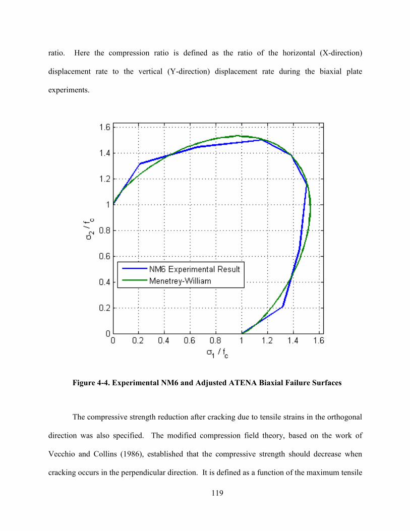
119
ratio. Here the compression ratio is defined as the ratio of the horizontal (X-direction)
displacement rate to the vertical (Y-direction) displacement rate during the biaxial plate
experiments.
Figure 4-4. Experimental M6 and Adjusted ATEA Biaxial Failure Surfaces
The compressive strength reduction after cracking due to tensile strains in the orthogonal
direction was also specified. The modified compression field theory, based on the work of
Vecchio and Collins (1986), established that the compressive strength should decrease when
cracking occurs in the perpendicular direction. It is defined as a function of the maximum tensile
120
strain and specifies a reduction of the maximum uniaxial compressive strength, f’c. For modeling
of HPFRCC, the results of the uniaxial compressive tests were used to get relationship between
the lateral strain in the specimen and the reduction of the compressive strength with respect to
the maximum strength. The resulting relationship implemented into ATENA is shown in Figure
4-5.
Figure 4-5. Compressive Strength Reduction due to Cracking
In addition to the previously described material parameters, multiple cracking during the
hardening phase, as well as localized cracking during softening of the HPFRCC material, can be
modeled. ATENA assumes that a set of parallel planar multiple cracks will form perpendicular
to the maximum principal stress when the applied stress exceeds the first cracking strength, as
described by Kabele (2007). As the loading increases, additional cracks may form within the
0
0.2
0.4
0.6
0.8
1
1.2
0 0.01 0.02 0.03 0.04
σσ σσ2/ f'
c
εεεε1, Lateral Strain (in/in)
NM6 fc-et Full Data
NM6 fc-et Reduced Data
121
finite element, but the direction of the initial set of cracks is fixed to be perpendicular to the
principal stress direction. Cracks will then be allowed to slide if the direction of principal stress
changes; however, crack opening and sliding is resisted by fiber bridging. The crack sliding
phenomena is implemented using a variable shear retention factor, β . The shear retention factor
is defined as a ratio of the material post-cracking shear stiffness cG to its elastic shear stiffness
G . The value of the shear retention is affected by the fiber volume fraction, fiber shear
modulus, fiber Young’s modulus, fiber diameter, and fiber cross-section shape. Within the finite
element, a secondary set of cracks may form in a direction perpendicular to the primary set of
cracks if the maximum normal stress in the secondary crack-normal direction also exceeds the
first cracking stress. No interaction is assumed between the two sets of cracks. Once the normal
cracking strain in a set of multiple cracks exceeds the level of the cracking strain capacity, a
localized crack will form, and the material softening will occur. The overall strain of the
representative volume of the material is then obtained as the sum of the strain in the material
between the cracks, cracking strains due to multiple cracking, and cracking strains due to
localized cracks.
Of the material parameters input for the HPFRCC material modeling tests, all of the
properties were obtained experimentally as a part of this project except for the shear retention
behavior. Since no tests were done to measure the shear retention as a function of crack opening,
the model by Kabele (2007) was used, and the pertinent fiber hooked steel fiber properties were
input into the model. While this may not have a large effect on the material tests, it should help
to more accurately capture the pre-cracking and post-cracking behavior of HPFRCC when
located in larger shear critical structural components, such as coupling beams.
122
4.2.2 Element Mesh
A brief mesh sensitivity study was conducted on the uniaxial specimens. Since the NM6
concrete mix had aggregate as large as 3/8 in. (9.5 mm), the minimum reasonable mesh size was
considered to be 0.4 in. (10 mm). Models were run using increasingly larger mesh sizes, and it
was found that for the material modeling tests, a mesh size of 0.6875 in. (17.5 mm) was adequate
for convergence to a solution.
4.2.3 Loading and Boundary Conditions
For the modeling of the material tests, displacements were imposed on the specimens
through elastic steel elements, and the forces were then transferred to the HPFRCC through
interface elements. The interface material model was used to simulate the contact between the
concrete and the brush platens. Since the main purpose of the brush platens was to reduce the
confinement of the specimen to obtain the true stress-strain response, it was important to
appropriately model the interface elements. The elastic normal and shear stiffness of the element
were selected as small enough values to allow for the transmission of force while not restraining
the edge of the specimen, and the cohesion was set to zero. This was validated during post-
processing upon review of the vertical and lateral stresses and strains. For the modeling of the
tension experiment, the tensile strength of the interface element was specified as being
significantly larger than the tensile strength of the concrete to ensure that the failure would
localize in the HPFRCC material.
For the uniaxial tests, the displacements were applied to the top brush platen, while the
bottom brush platen was fixed against vertical displacement along its entire length, and the left
most node of the bottom brush platen was fixed against lateral displacement. For the biaxial
tests, the displacements were applied to the top, left, and right brush platens, while the bottom
123
platen was fixed against vertical and horizontal displacements. Figure 4-6 shows a screen shot of
the uniaxial plate tests from the ATENA program. The support conditions can be seen along the
bottom brush platen, and the monitoring points, which report forces, displacements, stresses, and
strains at desired locations, can also be seen at various points in the model. The monitoring
points are used to streamline the extraction of specific numerical values after the analysis. For
these models, the stresses and strains at the middle of the specimen were of particular interest to
make a comparison with the experimental results. Additionally, the reaction force required to
achieve the imposed displacements, as well as the imposed deformation on the specimen were
monitored. These results give a better representation of the material properties obtained during
the experimental research because they can be used to calculate an average stress-strain response,
as done for the experimental specimens.
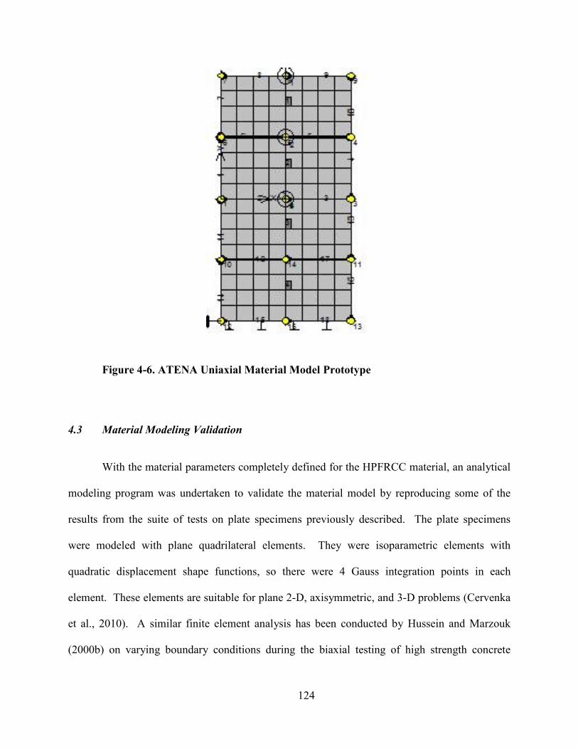
124
Figure 4-6. ATEA Uniaxial Material Model Prototype
4.3 Material Modeling Validation
With the material parameters completely defined for the HPFRCC material, an analytical
modeling program was undertaken to validate the material model by reproducing some of the
results from the suite of tests on plate specimens previously described. The plate specimens
were modeled with plane quadrilateral elements. They were isoparametric elements with
quadratic displacement shape functions, so there were 4 Gauss integration points in each
element. These elements are suitable for plane 2-D, axisymmetric, and 3-D problems (Cervenka
et al., 2010). A similar finite element analysis has been conducted by Hussein and Marzouk
(2000b) on varying boundary conditions during the biaxial testing of high strength concrete
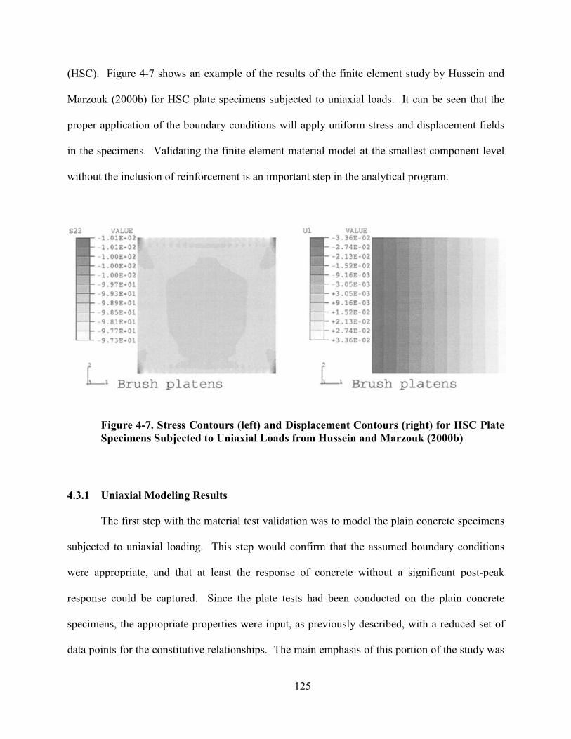
125
(HSC). Figure 4-7 shows an example of the results of the finite element study by Hussein and
Marzouk (2000b) for HSC plate specimens subjected to uniaxial loads. It can be seen that the
proper application of the boundary conditions will apply uniform stress and displacement fields
in the specimens. Validating the finite element material model at the smallest component level
without the inclusion of reinforcement is an important step in the analytical program.
Figure 4-7. Stress Contours (left) and Displacement Contours (right) for HSC Plate
Specimens Subjected to Uniaxial Loads from Hussein and Marzouk (2000b)
4.3.1 Uniaxial Modeling Results
The first step with the material test validation was to model the plain concrete specimens
subjected to uniaxial loading. This step would confirm that the assumed boundary conditions
were appropriate, and that at least the response of concrete without a significant post-peak
response could be captured. Since the plate tests had been conducted on the plain concrete
specimens, the appropriate properties were input, as previously described, with a reduced set of
data points for the constitutive relationships. The main emphasis of this portion of the study was
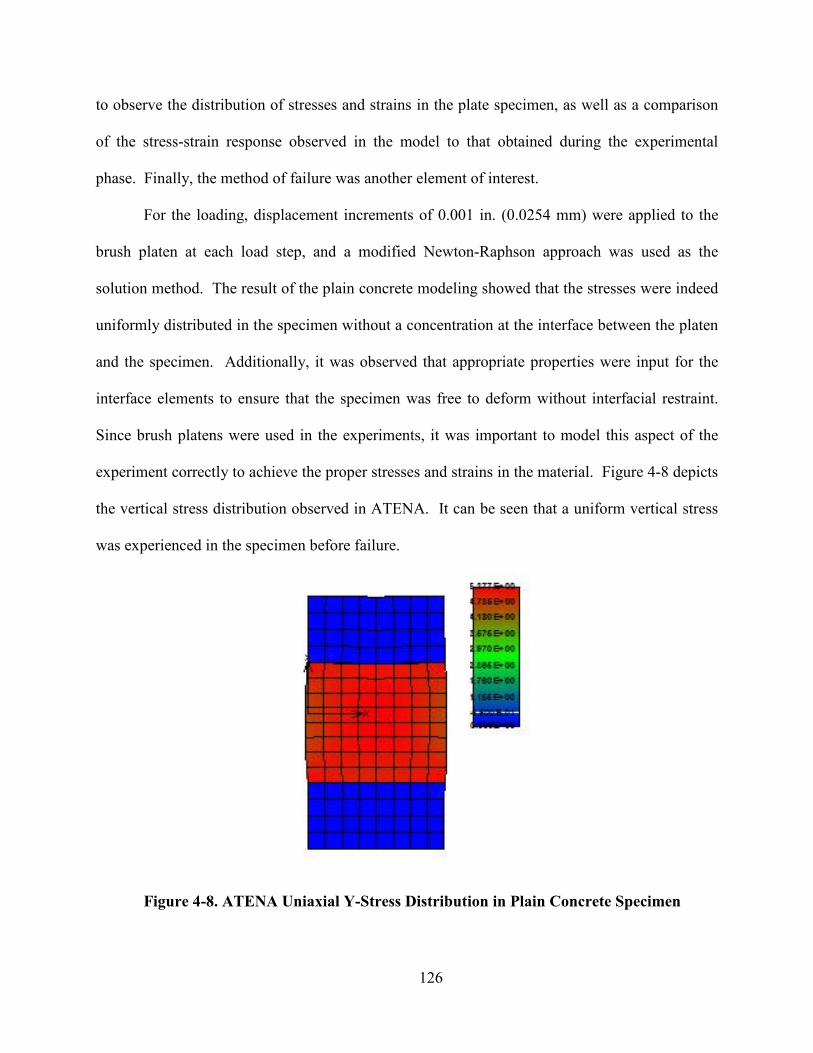
126
to observe the distribution of stresses and strains in the plate specimen, as well as a comparison
of the stress-strain response observed in the model to that obtained during the experimental
phase. Finally, the method of failure was another element of interest.
For the loading, displacement increments of 0.001 in. (0.0254 mm) were applied to the
brush platen at each load step, and a modified Newton-Raphson approach was used as the
solution method. The result of the plain concrete modeling showed that the stresses were indeed
uniformly distributed in the specimen without a concentration at the interface between the platen
and the specimen. Additionally, it was observed that appropriate properties were input for the
interface elements to ensure that the specimen was free to deform without interfacial restraint.
Since brush platens were used in the experiments, it was important to model this aspect of the
experiment correctly to achieve the proper stresses and strains in the material. Figure 4-8 depicts
the vertical stress distribution observed in ATENA. It can be seen that a uniform vertical stress
was experienced in the specimen before failure.
Figure 4-8. ATEA Uniaxial Y-Stress Distribution in Plain Concrete Specimen
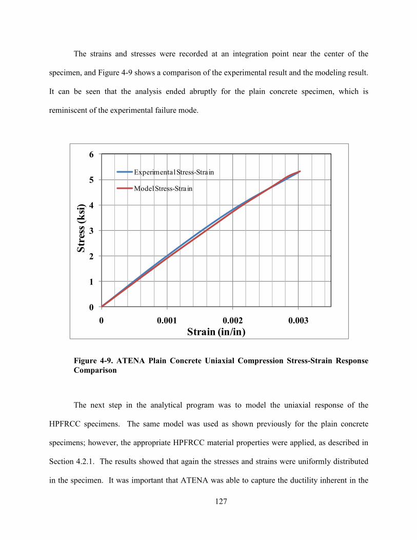
127
The strains and stresses were recorded at an integration point near the center of the
specimen, and Figure 4-9 shows a comparison of the experimental result and the modeling result.
It can be seen that the analysis ended abruptly for the plain concrete specimen, which is
reminiscent of the experimental failure mode.
Figure 4-9. ATEA Plain Concrete Uniaxial Compression Stress-Strain Response
Comparison
The next step in the analytical program was to model the uniaxial response of the
HPFRCC specimens. The same model was used as shown previously for the plain concrete
specimens; however, the appropriate HPFRCC material properties were applied, as described in
Section 4.2.1. The results showed that again the stresses and strains were uniformly distributed
in the specimen. It was important that ATENA was able to capture the ductility inherent in the
0
1
2
3
4
5
6
0 0.001 0.002 0.003
Str
ess
(ksi
)
Strain (in/in)
Experimental Stress-Strain
Model Stress-Stra in
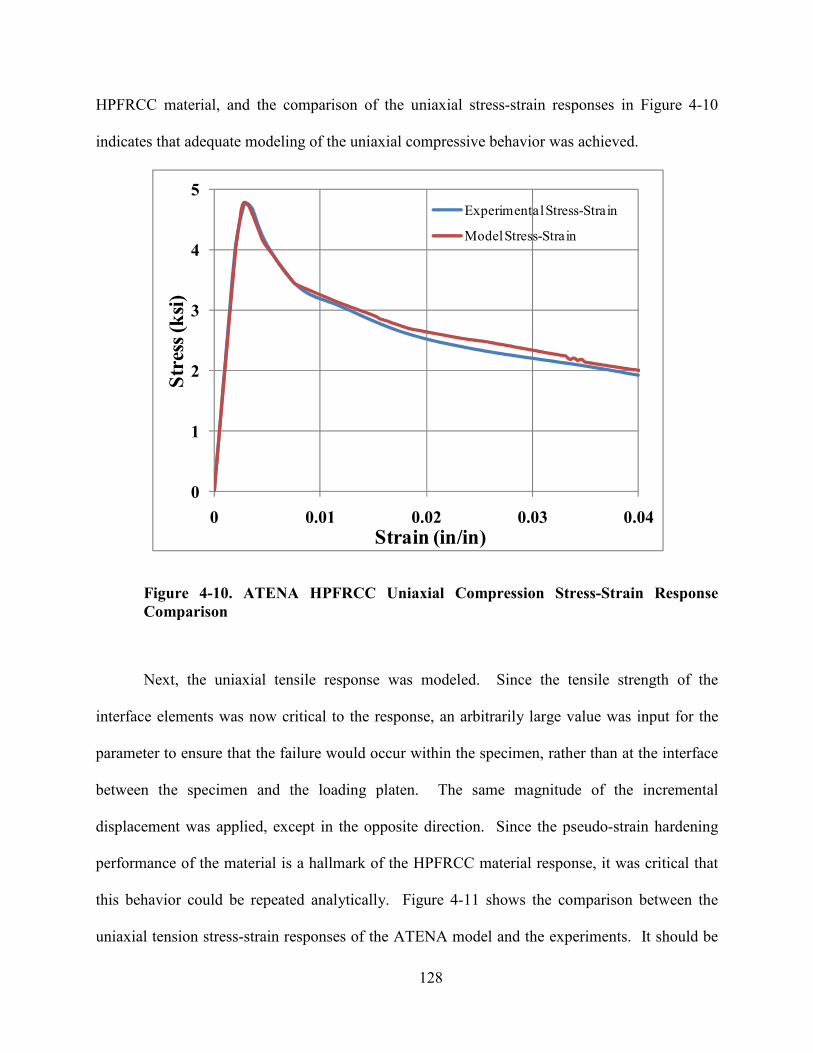
128
HPFRCC material, and the comparison of the uniaxial stress-strain responses in Figure 4-10
indicates that adequate modeling of the uniaxial compressive behavior was achieved.
Figure 4-10. ATEA HPFRCC Uniaxial Compression Stress-Strain Response
Comparison
Next, the uniaxial tensile response was modeled. Since the tensile strength of the
interface elements was now critical to the response, an arbitrarily large value was input for the
parameter to ensure that the failure would occur within the specimen, rather than at the interface
between the specimen and the loading platen. The same magnitude of the incremental
displacement was applied, except in the opposite direction. Since the pseudo-strain hardening
performance of the material is a hallmark of the HPFRCC material response, it was critical that
this behavior could be repeated analytically. Figure 4-11 shows the comparison between the
uniaxial tension stress-strain responses of the ATENA model and the experiments. It should be
0
1
2
3
4
5
0 0.01 0.02 0.03 0.04
Str
ess
(ksi
)
Strain (in/in)
Experimental Stress-Strain
Model Stress-Strain
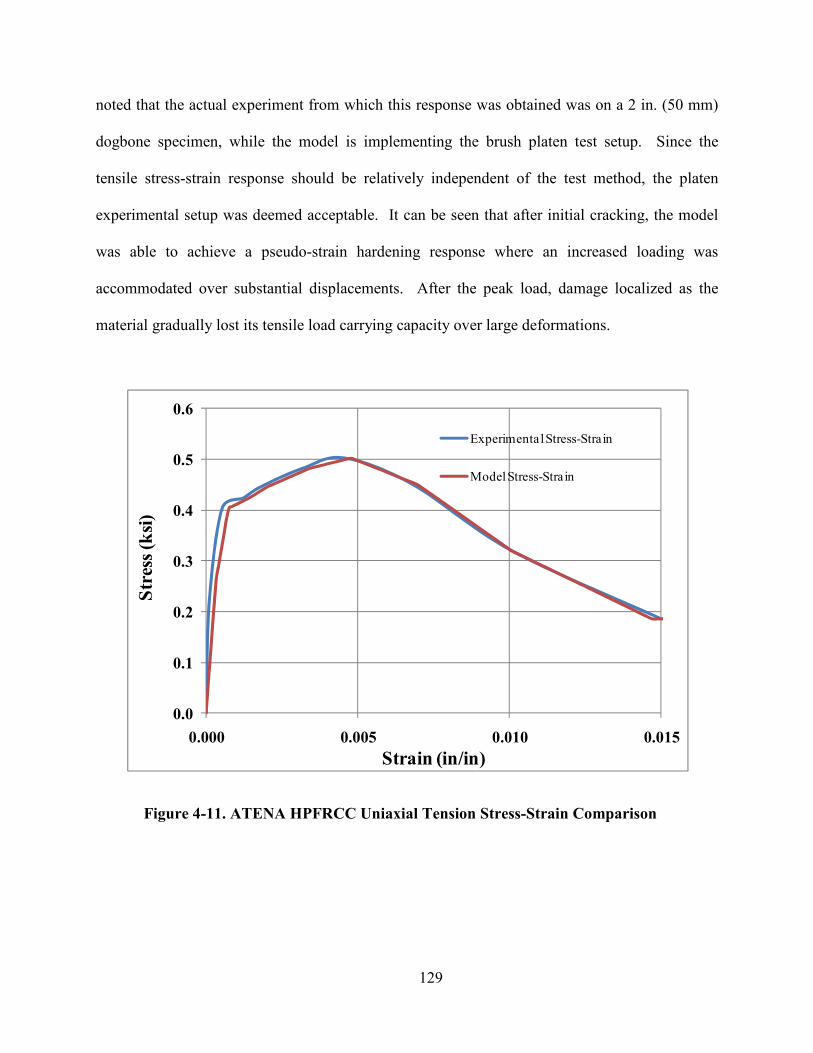
129
noted that the actual experiment from which this response was obtained was on a 2 in. (50 mm)
dogbone specimen, while the model is implementing the brush platen test setup. Since the
tensile stress-strain response should be relatively independent of the test method, the platen
experimental setup was deemed acceptable. It can be seen that after initial cracking, the model
was able to achieve a pseudo-strain hardening response where an increased loading was
accommodated over substantial displacements. After the peak load, damage localized as the
material gradually lost its tensile load carrying capacity over large deformations.
Figure 4-11. ATEA HPFRCC Uniaxial Tension Stress-Strain Comparison
0.0
0.1
0.2
0.3
0.4
0.5
0.6
0.000 0.005 0.010 0.015
Str
ess
(ksi
)
Strain (in/in)
Experimental Stress-Strain
Model Stress-Strain
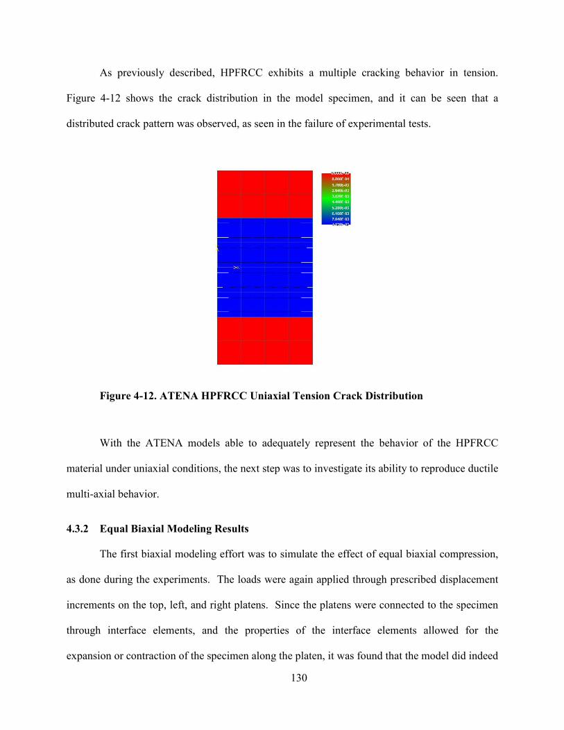
130
As previously described, HPFRCC exhibits a multiple cracking behavior in tension.
Figure 4-12 shows the crack distribution in the model specimen, and it can be seen that a
distributed crack pattern was observed, as seen in the failure of experimental tests.
Figure 4-12. ATEA HPFRCC Uniaxial Tension Crack Distribution
With the ATENA models able to adequately represent the behavior of the HPFRCC
material under uniaxial conditions, the next step was to investigate its ability to reproduce ductile
multi-axial behavior.
4.3.2 Equal Biaxial Modeling Results
The first biaxial modeling effort was to simulate the effect of equal biaxial compression,
as done during the experiments. The loads were again applied through prescribed displacement
increments on the top, left, and right platens. Since the platens were connected to the specimen
through interface elements, and the properties of the interface elements allowed for the
expansion or contraction of the specimen along the platen, it was found that the model did indeed
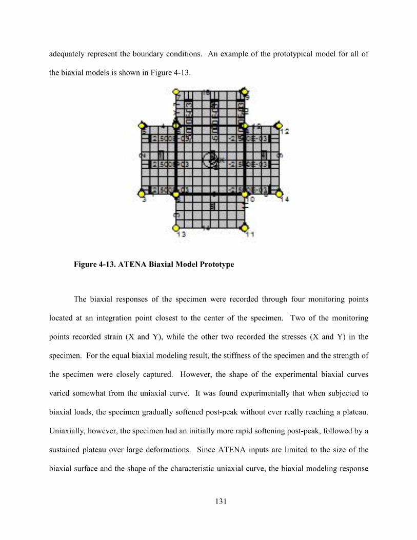
131
adequately represent the boundary conditions. An example of the prototypical model for all of
the biaxial models is shown in Figure 4-13.
Figure 4-13. ATEA Biaxial Model Prototype
The biaxial responses of the specimen were recorded through four monitoring points
located at an integration point closest to the center of the specimen. Two of the monitoring
points recorded strain (X and Y), while the other two recorded the stresses (X and Y) in the
specimen. For the equal biaxial modeling result, the stiffness of the specimen and the strength of
the specimen were closely captured. However, the shape of the experimental biaxial curves
varied somewhat from the uniaxial curve. It was found experimentally that when subjected to
biaxial loads, the specimen gradually softened post-peak without ever really reaching a plateau.
Uniaxially, however, the specimen had an initially more rapid softening post-peak, followed by a
sustained plateau over large deformations. Since ATENA inputs are limited to the size of the
biaxial surface and the shape of the characteristic uniaxial curve, the biaxial modeling response
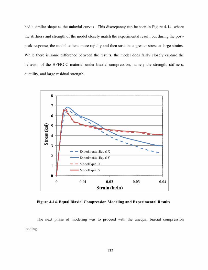
132
had a similar shape as the uniaxial curves. This discrepancy can be seen in Figure 4-14, where
the stiffness and strength of the model closely match the experimental result, but during the post-
peak response, the model softens more rapidly and then sustains a greater stress at large strains.
While there is some difference between the results, the model does fairly closely capture the
behavior of the HPFRCC material under biaxial compression, namely the strength, stiffness,
ductility, and large residual strength.
Figure 4-14. Equal Biaxial Compression Modeling and Experimental Results
The next phase of modeling was to proceed with the unequal biaxial compression
loading.
0
1
2
3
4
5
6
7
8
0 0.01 0.02 0.03 0.04
Str
ess
(ksi
)
Strain (in/in)
Experimental Equal X
Experimental Equal Y
Model Equal X
Model Equal Y
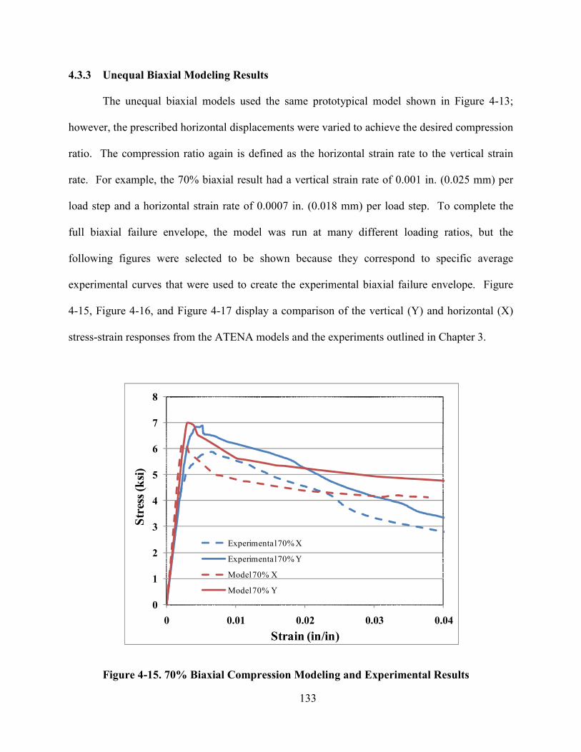
133
4.3.3 Unequal Biaxial Modeling Results
The unequal biaxial models used the same prototypical model shown in Figure 4-13;
however, the prescribed horizontal displacements were varied to achieve the desired compression
ratio. The compression ratio again is defined as the horizontal strain rate to the vertical strain
rate. For example, the 70% biaxial result had a vertical strain rate of 0.001 in. (0.025 mm) per
load step and a horizontal strain rate of 0.0007 in. (0.018 mm) per load step. To complete the
full biaxial failure envelope, the model was run at many different loading ratios, but the
following figures were selected to be shown because they correspond to specific average
experimental curves that were used to create the experimental biaxial failure envelope. Figure
4-15, Figure 4-16, and Figure 4-17 display a comparison of the vertical (Y) and horizontal (X)
stress-strain responses from the ATENA models and the experiments outlined in Chapter 3.
Figure 4-15. 70% Biaxial Compression Modeling and Experimental Results
0
1
2
3
4
5
6
7
8
0 0.01 0.02 0.03 0.04
Str
ess
(ksi
)
Strain (in/in)
Experimental 70% X
Experimental 70% Y
Model 70% X
Model 70% Y
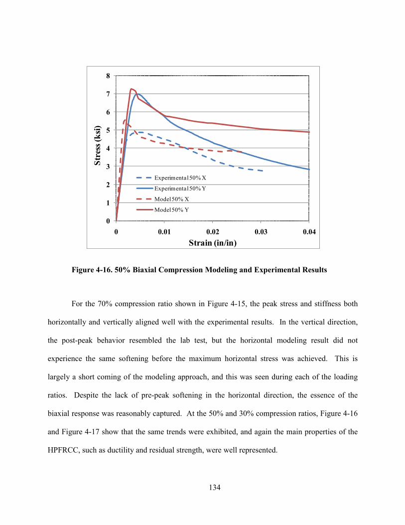
134
Figure 4-16. 50% Biaxial Compression Modeling and Experimental Results
For the 70% compression ratio shown in Figure 4-15, the peak stress and stiffness both
horizontally and vertically aligned well with the experimental results. In the vertical direction,
the post-peak behavior resembled the lab test, but the horizontal modeling result did not
experience the same softening before the maximum horizontal stress was achieved. This is
largely a short coming of the modeling approach, and this was seen during each of the loading
ratios. Despite the lack of pre-peak softening in the horizontal direction, the essence of the
biaxial response was reasonably captured. At the 50% and 30% compression ratios, Figure 4-16
and Figure 4-17 show that the same trends were exhibited, and again the main properties of the
HPFRCC, such as ductility and residual strength, were well represented.
0
1
2
3
4
5
6
7
8
0 0.01 0.02 0.03 0.04
Str
ess
(ksi
)
Strain (in/in)
Experimental 50% X
Experimental 50% Y
Model 50% X
Model 50% Y
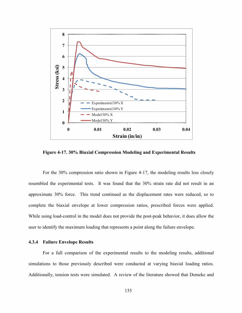
135
Figure 4-17. 30% Biaxial Compression Modeling and Experimental Results
For the 30% compression ratio shown in Figure 4-17, the modeling results less closely
resembled the experimental tests. It was found that the 30% strain rate did not result in an
approximate 30% force. This trend continued as the displacement rates were reduced, so to
complete the biaxial envelope at lower compression ratios, prescribed forces were applied.
While using load-control in the model does not provide the post-peak behavior, it does allow the
user to identify the maximum loading that represents a point along the failure envelope.
4.3.4 Failure Envelope Results
For a full comparison of the experimental results to the modeling results, additional
simulations to those previously described were conducted at varying biaxial loading ratios.
Additionally, tension tests were simulated. A review of the literature showed that Demeke and
0
1
2
3
4
5
6
7
8
0 0.01 0.02 0.03 0.04
Str
ess
(ksi
)
Strain (in/in)
Experimental 30% X
Experimental 30% Y
Model 30% X
Model 30% Y
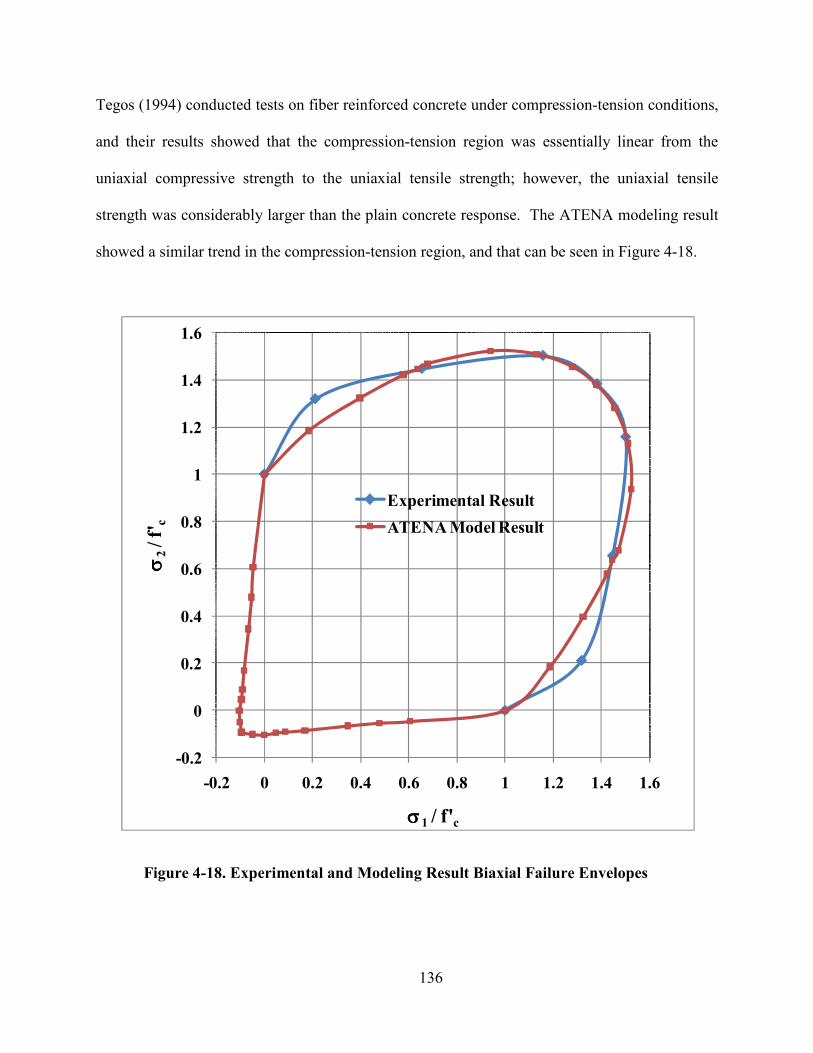
136
Tegos (1994) conducted tests on fiber reinforced concrete under compression-tension conditions,
and their results showed that the compression-tension region was essentially linear from the
uniaxial compressive strength to the uniaxial tensile strength; however, the uniaxial tensile
strength was considerably larger than the plain concrete response. The ATENA modeling result
showed a similar trend in the compression-tension region, and that can be seen in Figure 4-18.
Figure 4-18. Experimental and Modeling Result Biaxial Failure Envelopes
-0.2
0
0.2
0.4
0.6
0.8
1
1.2
1.4
1.6
-0.2 0 0.2 0.4 0.6 0.8 1 1.2 1.4 1.6
σσ σσ2/ f'
c
σσσσ1 / f'c
Experimental Result
ATEA Model Result
137
Figure 4-18 displays a comparison between the experimental failure envelope and the
failure envelope obtained from the modeling effort. It shows that under biaxial compression, the
results align well from compression ratios of 50% to equal compression. However, the model
was conservative and underpredicts the biaxial strength at lower loading ratios. For the tension
results, while specific experimental data was not available to validate the model under
compression-tension and tension-tension, a review of the literature shows the results to be
reasonable. Overall, the model has shown that it is able to capture the strength, deformation,
stiffness, and ductility of HPFRCC under both uniaxial and biaxial loading. The next phase of
the analytical program is to extend the use of HPFRCC to the modeling of structural
components. The modeling of coupling beams and pile-wharf connections will be described in
the Chapter 6 and Chapter 9, respectively.

138
CHAPTER 5. COUPLIG BEAM COMPOET TEST RESULTS
Coupling beam component tests have been conducted by many researchers since the
1970s. Chapter 2 highlighted some of the previously conducted tests, and it discussed briefly
some of the differences. While the focus of Chapter 2 was to introduce some of the research that
have been completed, this chapter is intended to more thoroughly review the results of some of
the previous coupling beam component test research. These results will become particularly
important during the analytical phase of the research, where reinforced concrete coupling beam
components are modeled and the HPFRCC model is implemented to observe the change in
behavior, and vice versa.
5.1 Reinforced Concrete Coupling Beam Tests
As outlined in Chapter 2, coupling beam component tests have been conducted on
specimens with three basic reinforcement layouts: conventional reinforcement, diagonal
reinforcement, and rhombic reinforcement. Examples of each reinforcement pattern from
Galano and Vignoli (2000) is shown in Figure 5-1. The conventionally reinforced coupling
beams typically have top and bottom longitudinal bars to resist the flexural demand, and stirrups
are provided for shear resistance. They are generally designed as well confined beams, and ACI
318 (2008) restricts the reinforcement layout to shear stress demands less than '4 c wf b d and
/ 4nl h > , where wb is the width of the coupling beam; d is the depth of the coupling beam; h is
the height of the coupling beam; and nl is the clear span. Diagonally reinforced coupling beams
have two intersecting groups of diagonally placed bars symmetrical about the midspan. The
diagonal bars are confined with closely spaced ties to prevent buckling of the bars, and additional
139
longitudinal reinforcement and stirrups are included. These beams are required in coupling
beams with a shear demand exceeding '4 c wf b d and / 2nl h < . In the intermediate aspect ratio
range of 2 to 4, coupling beams are reinforced with diagonal bars; however, two confinement
options exist: each diagonal can be individually confined, in addition to the perimeter of the
cross-section, or the entire beam cross-section may be heavily confined, and the diagonal bars
need not have confinement (ACI Committee 318, 2008). Examples of the two intermediate
reinforcement layouts were shown previously in Figure 2-10 and Figure 2-11. For coupling
beams with / 4nl h ≥ , the design must satisfy the requirements for flexural members of special
moment frames. The rhombic reinforcement pattern shown in Figure 5-1 has been tested
experimentally, but is not used in practice. It consists of two sets of diagonal bars that cross at
each end of the coupling beam, and the idea is that the inclined orientation of the reinforcement
would improve the shear resistance at the hinge location.
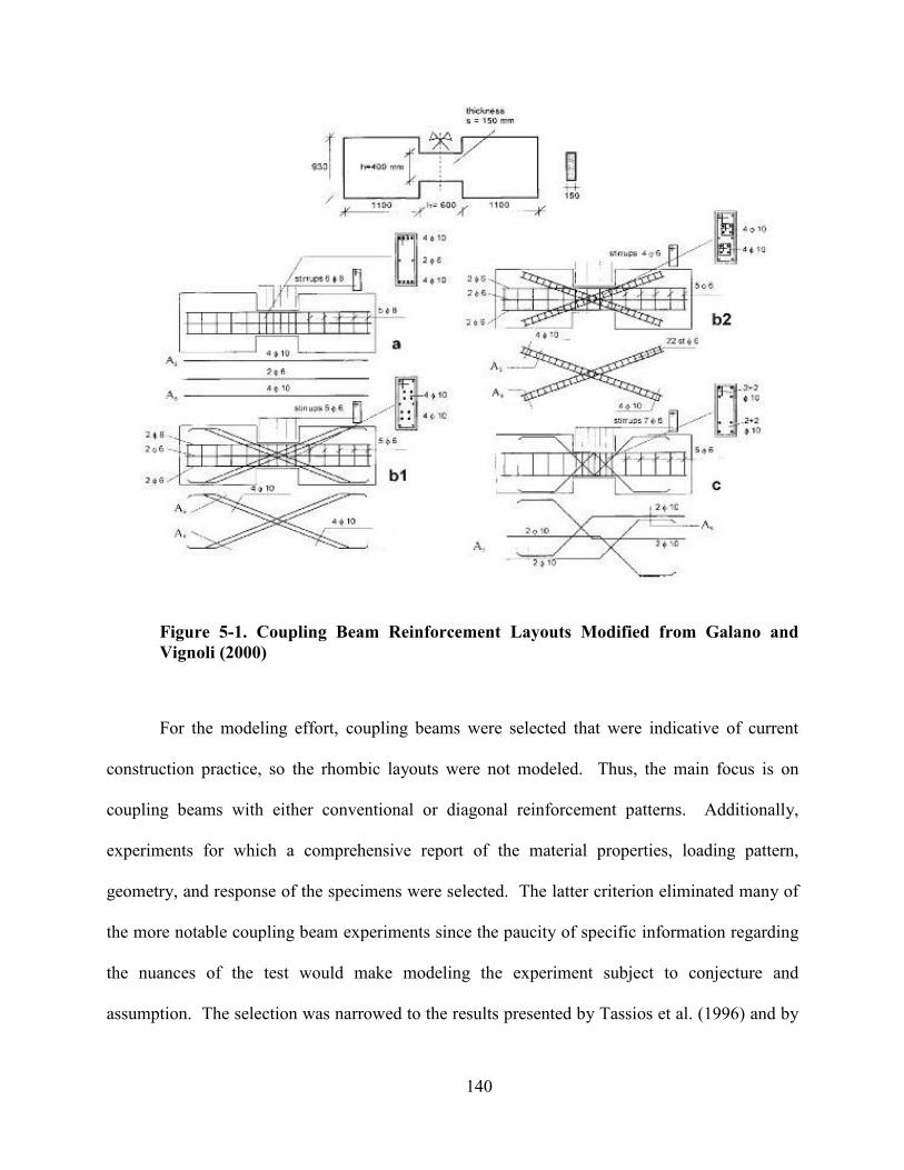
140
Figure 5-1. Coupling Beam Reinforcement Layouts Modified from Galano and
Vignoli (2000)
For the modeling effort, coupling beams were selected that were indicative of current
construction practice, so the rhombic layouts were not modeled. Thus, the main focus is on
coupling beams with either conventional or diagonal reinforcement patterns. Additionally,
experiments for which a comprehensive report of the material properties, loading pattern,
geometry, and response of the specimens were selected. The latter criterion eliminated many of
the more notable coupling beam experiments since the paucity of specific information regarding
the nuances of the test would make modeling the experiment subject to conjecture and
assumption. The selection was narrowed to the results presented by Tassios et al. (1996) and by
141
Galano and Vignoli (2000). While a more thorough modeling effort of all of the coupling beams
presented in the literature may have been preferred, only the coupling beams from Galano and
Vignoli (2000) were investigated for this research. The following sections will outline the
specific coupling beam component experiments that were selected for the modeling effort to be
described in Chapter 6.
5.1.1 Galano and Vignoli (2000)
This experimental study investigated the effect of reinforcement layout and loading
history through testing fifteen short coupling beams with four different reinforcement
arrangements. Each reinforcement layout had specimens subjected to monotonic and cyclic
loading, and the length-to-depth ratio of each specimen was 1.50. The reinforcement layouts
investigated are displayed in Figure 5-1. They include conventional reinforcement, diagonal
reinforcement without ties, diagonal reinforcement with confining ties, and rhombic
reinforcement.
The specimens had two lateral stiff blocks to simulate the surrounding walls and to apply
the loading histories. The coupling beams were tested in the vertical position under asymmetric
bending and constant shear. Six steel rollers were used to constrain the specimen. Two rollers
were placed laterally to prevent horizontal movements of the specimens, and the other four
rollers were positioned to produce the desired loading histories. Two hydraulic actuators were
attached to the specimen to impose equal and opposite rotations on the specimen. The described
test setup is shown in Figure 5-2. The specimens were loaded either monotonically or cyclically
to failure.
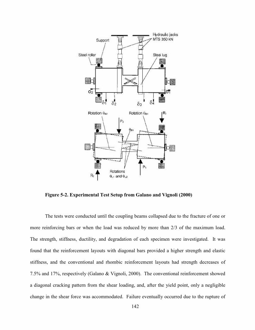
142
Figure 5-2. Experimental Test Setup from Galano and Vignoli (2000)
The tests were conducted until the coupling beams collapsed due to the fracture of one or
more reinforcing bars or when the load was reduced by more than 2/3 of the maximum load.
The strength, stiffness, ductility, and degradation of each specimen were investigated. It was
found that the reinforcement layouts with diagonal bars provided a higher strength and elastic
stiffness, and the conventional and rhombic reinforcement layouts had strength decreases of
7.5% and 17%, respectively (Galano & Vignoli, 2000). The conventional reinforcement showed
a diagonal cracking pattern from the shear loading, and, after the yield point, only a negligible
change in the shear force was accommodated. Failure eventually occurred due to the rupture of
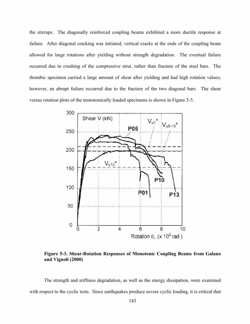
143
the stirrups. The diagonally reinforced coupling beams exhibited a more ductile response at
failure. After diagonal cracking was initiated, vertical cracks at the ends of the coupling beam
allowed for large rotations after yielding without strength degradation. The eventual failure
occurred due to crushing of the compressive strut, rather than fracture of the steel bars. The
rhombic specimen carried a large amount of shear after yielding and had high rotation values;
however, an abrupt failure occurred due to the fracture of the two diagonal bars. The shear
versus rotation plots of the monotonically loaded specimens is shown in Figure 5-3.
Figure 5-3. Shear-Rotation Responses of Monotonic Coupling Beams from Galano
and Vignoli (2000)
The strength and stiffness degradation, as well as the energy dissipation, were examined
with respect to the cyclic tests. Since earthquakes produce severe cyclic loading, it is critical that
144
coupling beams with significant strength and stiffness degradation be avoided, while energy
dissipating designs are favored. When reviewing the cyclic performance of the coupling beams,
it was found that the conventionally reinforced coupling beams demonstrated a lower energy
dissipating capacity due to the pinching of the hysteresis loops. The conventionally reinforced
coupling beam did exhibit comparable strength retention characteristics initially, but at larger
displacements, the strength dropped considerably. Also, the test results showed that the beams
with diagonal or rhombic reinforcement exhibited a higher rotational ductility than
conventionally reinforced coupling beams. Between the diagonal and rhombic layouts, the
difference in energy dissipation was found to be negligible, and it was the opinion of the authors
that the rhombic arrangement performed better than the diagonal reinforcement with respect to
rotational capacity and the degradation in both strength and stiffness. The shear-rotation
responses of the cyclic conventionally reinforced and diagonally reinforced coupling beams are
shown in Figure 5-4 and Figure 5-5, respectively.
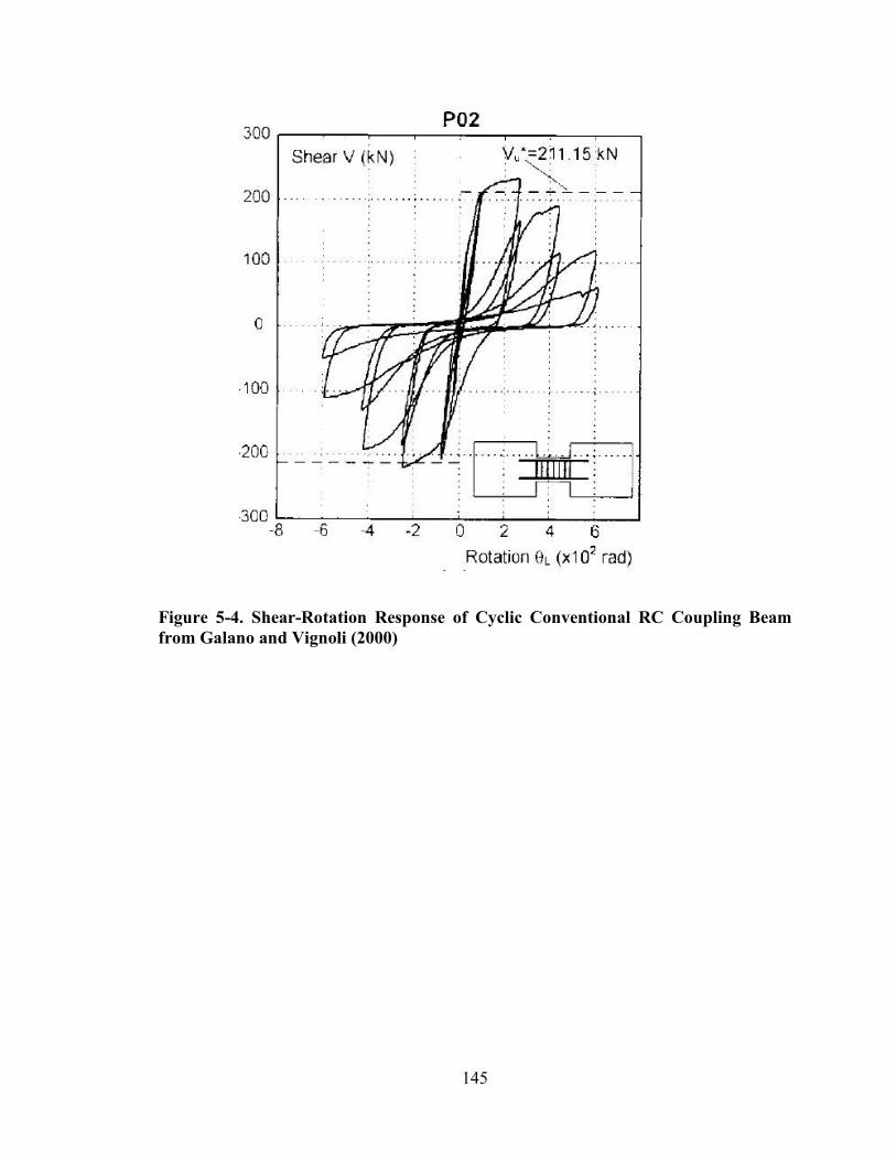
145
Figure 5-4. Shear-Rotation Response of Cyclic Conventional RC Coupling Beam
from Galano and Vignoli (2000)
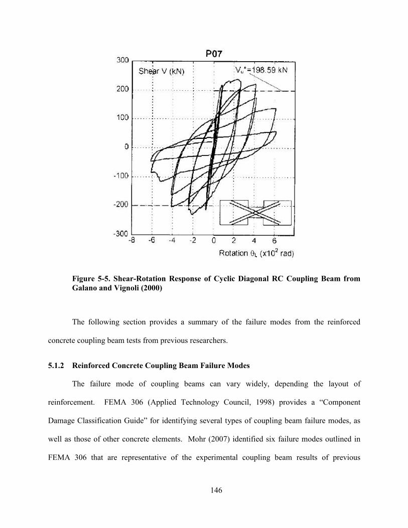
146
Figure 5-5. Shear-Rotation Response of Cyclic Diagonal RC Coupling Beam from
Galano and Vignoli (2000)
The following section provides a summary of the failure modes from the reinforced
concrete coupling beam tests from previous researchers.
5.1.2 Reinforced Concrete Coupling Beam Failure Modes
The failure mode of coupling beams can vary widely, depending the layout of
reinforcement. FEMA 306 (Applied Technology Council, 1998) provides a “Component
Damage Classification Guide” for identifying several types of coupling beam failure modes, as
well as those of other concrete elements. Mohr (2007) identified six failure modes outlined in
FEMA 306 that are representative of the experimental coupling beam results of previous
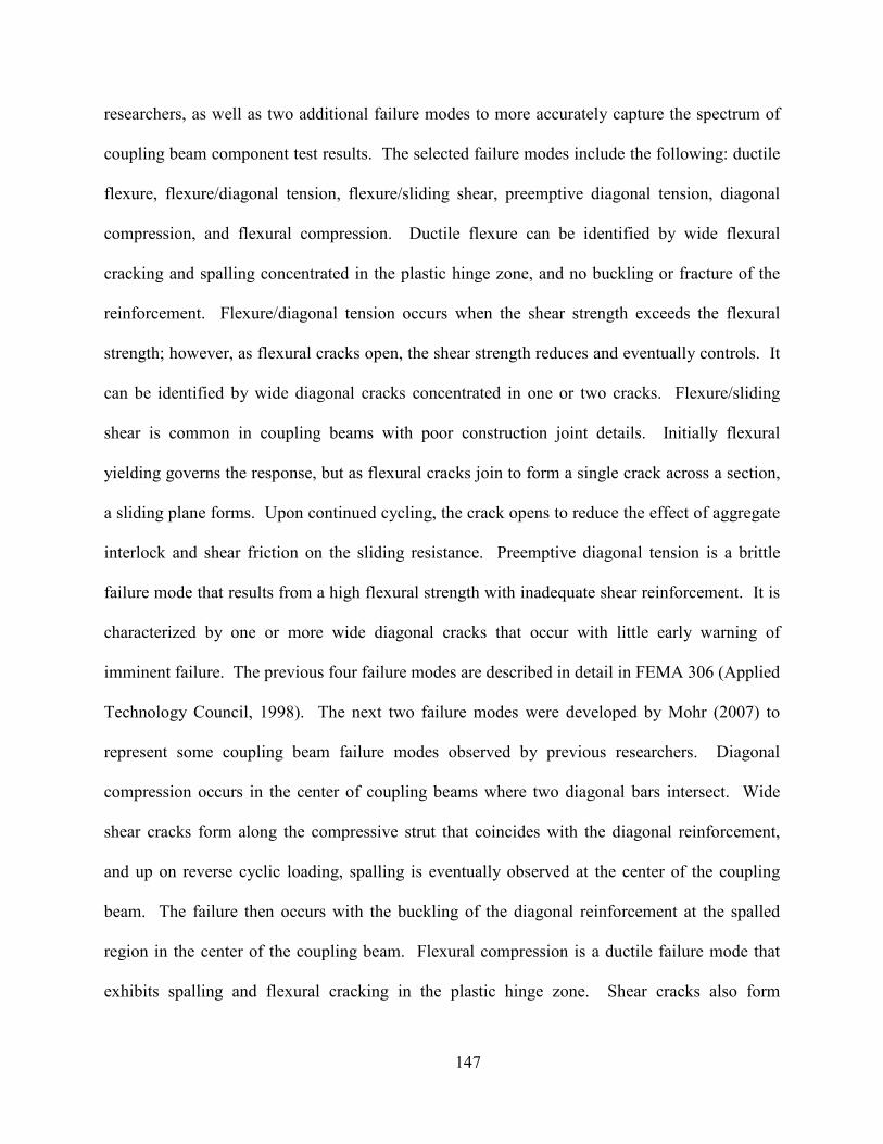
147
researchers, as well as two additional failure modes to more accurately capture the spectrum of
coupling beam component test results. The selected failure modes include the following: ductile
flexure, flexure/diagonal tension, flexure/sliding shear, preemptive diagonal tension, diagonal
compression, and flexural compression. Ductile flexure can be identified by wide flexural
cracking and spalling concentrated in the plastic hinge zone, and no buckling or fracture of the
reinforcement. Flexure/diagonal tension occurs when the shear strength exceeds the flexural
strength; however, as flexural cracks open, the shear strength reduces and eventually controls. It
can be identified by wide diagonal cracks concentrated in one or two cracks. Flexure/sliding
shear is common in coupling beams with poor construction joint details. Initially flexural
yielding governs the response, but as flexural cracks join to form a single crack across a section,
a sliding plane forms. Upon continued cycling, the crack opens to reduce the effect of aggregate
interlock and shear friction on the sliding resistance. Preemptive diagonal tension is a brittle
failure mode that results from a high flexural strength with inadequate shear reinforcement. It is
characterized by one or more wide diagonal cracks that occur with little early warning of
imminent failure. The previous four failure modes are described in detail in FEMA 306 (Applied
Technology Council, 1998). The next two failure modes were developed by Mohr (2007) to
represent some coupling beam failure modes observed by previous researchers. Diagonal
compression occurs in the center of coupling beams where two diagonal bars intersect. Wide
shear cracks form along the compressive strut that coincides with the diagonal reinforcement,
and up on reverse cyclic loading, spalling is eventually observed at the center of the coupling
beam. The failure then occurs with the buckling of the diagonal reinforcement at the spalled
region in the center of the coupling beam. Flexural compression is a ductile failure mode that
exhibits spalling and flexural cracking in the plastic hinge zone. Shear cracks also form
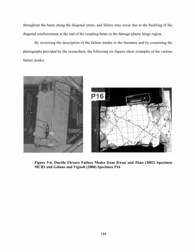
throughout the beam along the diagonal struts
diagonal reinforcement at the end of the coupling beam in the damage plastic hinge region.
By reviewing the description of the failure modes in the literature and by examining
photographs provided by the researchers, the following
failure modes.
Figure 5-6. Ductile Flexure Failure Modes from Kwan and Zhao
MCB3 and Galano and Vignoli
148
eam along the diagonal struts, and failure may occur due to the buckling of the
diagonal reinforcement at the end of the coupling beam in the damage plastic hinge region.
By reviewing the description of the failure modes in the literature and by examining
photographs provided by the researchers, the following six figures show examples of the various
. Ductile Flexure Failure Modes from Kwan and Zhao (2002)
MCB3 and Galano and Vignoli (2000) Specimen P16
, and failure may occur due to the buckling of the
diagonal reinforcement at the end of the coupling beam in the damage plastic hinge region.
By reviewing the description of the failure modes in the literature and by examining the
figures show examples of the various
(2002) Specimen
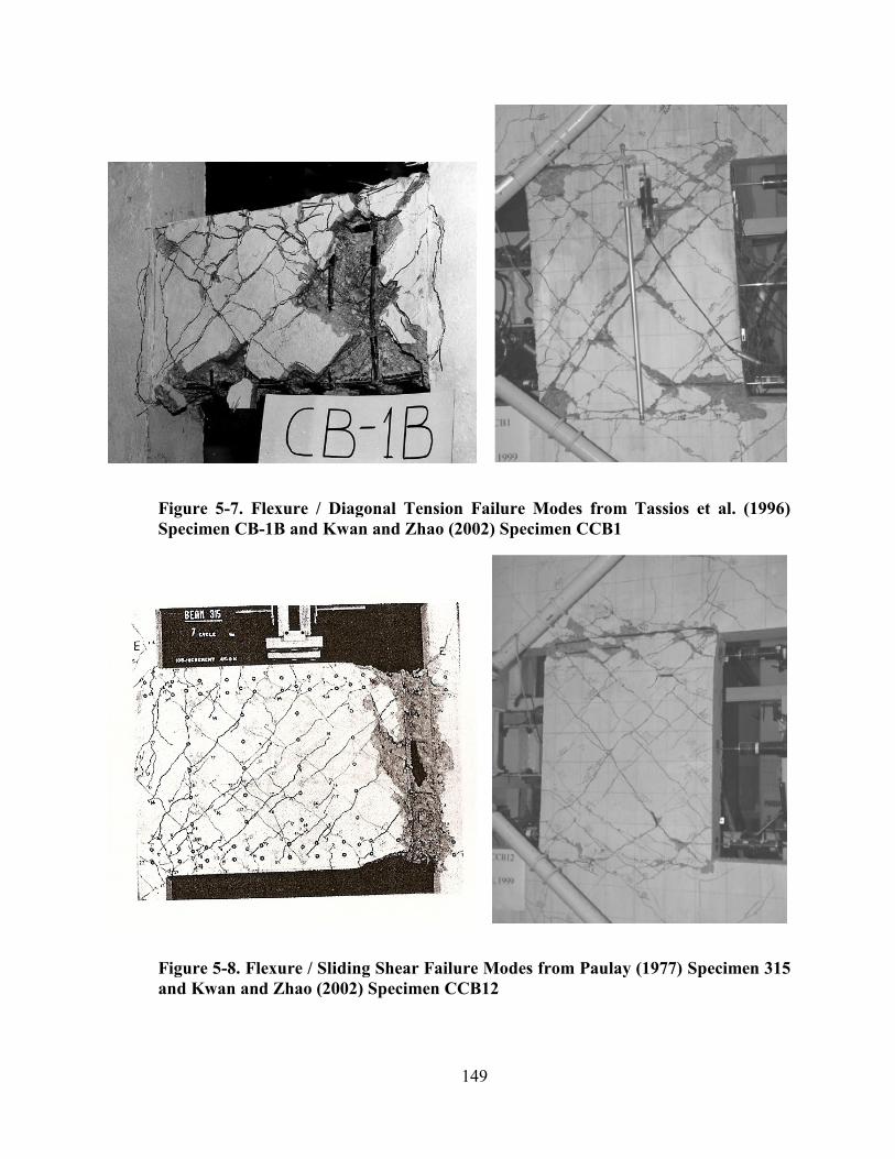
Figure 5-7. Flexure / Diagonal Tension Failure Modes from Tassios et al
Specimen CB-1B and Kwan and Zhao
Figure 5-8. Flexure / Sliding Shear Failure Modes from Paulay
and Kwan and Zhao (2002)
149
. Flexure / Diagonal Tension Failure Modes from Tassios et al
1B and Kwan and Zhao (2002) Specimen CCB1
. Flexure / Sliding Shear Failure Modes from Paulay (1977)
(2002) Specimen CCB12
. Flexure / Diagonal Tension Failure Modes from Tassios et al. (1996)
(1977) Specimen 315
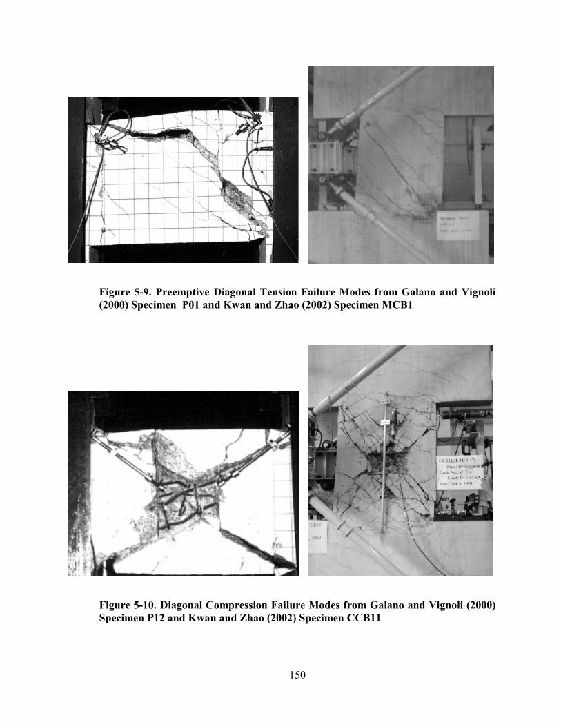
Figure 5-9. Preemptive Diagonal Tension Failure Modes from Galano
(2000) Specimen P01 and Kwan and Zhao
Figure 5-10. Diagonal Compression Failure Modes from
Specimen P12 and Kwan and Zhao
150
. Preemptive Diagonal Tension Failure Modes from Galano
P01 and Kwan and Zhao (2002) Specimen MCB1
. Diagonal Compression Failure Modes from Galano and Vignoli
Specimen P12 and Kwan and Zhao (2002) Specimen CCB11
. Preemptive Diagonal Tension Failure Modes from Galano and Vignoli
Galano and Vignoli (2000)
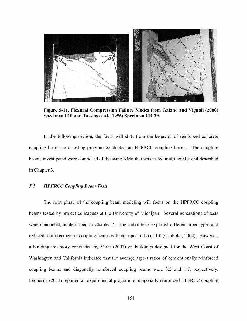
151
Figure 5-11. Flexural Compression Failure Modes from Galano and Vignoli (2000)
Specimen P10 and Tassios et al. (1996) Specimen CB-2A
In the following section, the focus will shift from the behavior of reinforced concrete
coupling beams to a testing program conducted on HPFRCC coupling beams. The coupling
beams investigated were composed of the same NM6 that was tested multi-axially and described
in Chapter 3.
5.2 HPFRCC Coupling Beam Tests
The next phase of the coupling beam modeling will focus on the HPFRCC coupling
beams tested by project colleagues at the University of Michigan. Several generations of tests
were conducted, as described in Chapter 2. The initial tests explored different fiber types and
reduced reinforcement in coupling beams with an aspect ratio of 1.0 (Canbolat, 2004). However,
a building inventory conducted by Mohr (2007) on buildings designed for the West Coast of
Washington and California indicated that the average aspect ratios of conventionally reinforced
coupling beams and diagonally reinforced coupling beams were 3.2 and 1.7, respectively.
Lequesne (2011) reported an experimental program on diagonally reinforced HPFRCC coupling
152
beams with an aspect ratio of 1.75, and since this was more representative of the current state of
practice, these coupling beams were selected for the modeling effort in this research.
5.2.1 Lequesne (2011)
Coupling beam tests were conducted by Lequesne (2011) on specimens with span length-
to-depth ratio of 1.75 to investigate the response of less shear critical members than previous
coupling beam tests. The tests were designed to show that HPFRCC can improve the shear
resistance of coupling beams in three ways: 1.) preventing buckling in the diagonal
reinforcement, allowing for both the tension and compression diagonal steel to resist shear, 2.)
limiting damage in the coupling beam, thus maintaining the integrity of the specimen, and 3.)
enhancing aggregate interlock by the fibers bridging cracks and transferring tensile stresses
across cracks.
The coupling beams were precast and the same NEES Mix #6 that was described in
Chapter 3 and used in this dissertation was implemented in the concrete mixture for their design
and construction. These coupling beams used the same hooked steel Dramix fibers in the
HPFRCC, and the properties are described in Table 3-3. The hooked steel fibers were selected
over the Spectra fibers because they provide better pullout resistance. In the design of these
coupling beams, a departure from the typical assumption that the behavior is controlled by the
diagonal reinforcing steel was employed. Instead, the diagonal reinforcement was assumed to
provide one-third of the ultimate shear capacity, with the remaining shear demand resisted by the
transverse reinforcement and the HPFRCC. Basing the design approach on this assumption
reduces the reliance on diagonal steel reinforcement and accounts for the improved damage
tolerance of HPFRCC.
153
The design process of the coupling beam specimens is outlined by Lequesne (2011). The
process began with the selection of the diagonal bar area and orientation. The diagonal bars
were selected to resist 30-40% of the expected shear demand, and the design shear force of
' '10 A [lb] (0.83 A [kN])c cw c cwf f , where cwA is the gross cross-sectional area of the coupling
beam, was assumed. This was selected because it is the upper limit for the shear capacity
permitted by the ACI 318 (ACI Committee 318, 2008). To relieve constructability issues with
the precast coupling beams, the diagonal bars were bent to exit the precast coupling beam
horizontally. This was intended to ease the process of threading the coupling beam
reinforcement into the dense reinforcing cage in the boundary elements of the structural walls.
Additionally, bending the diagonal bars within the clear span of the coupling beam allowed for a
slight increase of the inclination of the diagonal bars from 22° to 24°. No confinement steel was
provided around the diagonal bars, since it was found previously that the HPFRCC adequately
confined the diagonals because no reinforcement instability was observed (2004).
The next step in the design was the selection of the longitudinal reinforcement. Since the
behavior of the HPFRCC coupling beams is expected to be dominated by the formation of the
plastic hinges at each end, the capacity of the coupling beam will be governed by the selection of
the longitudinal reinforcement. The moment capacity was assumed to be that produced by the
expected shear demand described previously ( / 2)u u nM V l= . The contribution of the diagonal
reinforcement to the flexural strength was considered, and the remaining area of longitudinal
steel was calculated. It should be noted that all of the longitudinal and diagonal reinforcement
was fully developed into the wall to all for the reinforcement to yield at the beam-wall interface.
The remaining reinforcement to select was the transverse reinforcement. The goal of the
transverse reinforcement is to transfer tension stresses, resist the opening of diagonal cracks, and
154
to provide confinement of the concrete core and reinforcement (2011). The specimen was
divided into two distinct regions: midspan region and end region. In the midspan region, the
transverse reinforcement was selected resist approximately 40% of the shear demand. Since the
diagonal reinforcement was designed to resist 30-40% of the shear, this leaves 30-40% of the
shear to be resisted by the HPFRCC. In the first two specimens, CB-1 and CB-2, #3 (D10)
hoops were spaced at 6 in. (152 mm), corresponding to a volumetric ratio of 0.89%. The third
specimen, CB-3, also used #3 (D10) hoops, but at a spacing of 8 in. (203 mm), which
corresponded to a reduced volumetric ratio of 0.67%. In the third specimen, the HPFRCC was
expected to carry an increased 40-50% of the shear force. In the end region, additional
transverse reinforcement was required to stabilize the bend in the diagonal reinforcement. The
end region was considered to extend a distance h/2 into the coupling beam from the face of the
wall. In Specimen CB-1, an inadequate amount of the transverse reinforcement was provided in
this region, and a premature failure occurred. The design methodology was revised for
Specimens CB-2 and CB-3, and the end region in these specimens was confined with #3 (D10)
hoops at 2.75 in. (70 mm). This resulted in a volumetric reinforcement ratio of 2.9%, and it
essentially satisfied the ACI 318 (ACI Committee 318, 2008) requirements for special column
confinement.
The final design step was to address the transfer of forces from the precast coupling beam
element to the structural wall. Two connection details were investigated: U-shaped dowel bars
and straight dowel bars. The dowel bars were intended to increase the capacity of the coupling
beam at the beam-wall interface and to shift the localization of damage in the coupling beam into
the well confined end region of the beam. To prevent sliding shear, shear friction adopted by
ACI 318 (2008) was used to calculate the area of the dowel reinforcement required across the
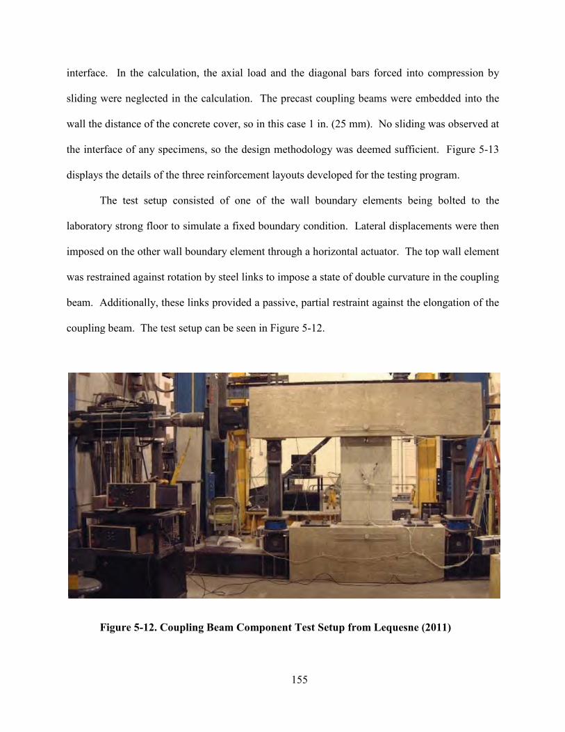
interface. In the calculation, th
sliding were neglected in the calculation.
wall the distance of the concrete cover, so in this case 1 in. (25 mm).
the interface of any specimens, so the design methodology was deemed sufficient.
displays the details of the three reinforcement layouts
The test setup consisted of one of the wall
laboratory strong floor to simulate a fixed boundary condition. Lateral displacements were then
imposed on the other wall boundary element through a horizontal actuator. The top wall element
was restrained against rotation by steel links to impose a state of double curvature in the coupling
beam. Additionally, these links provided a passive, partial restraint against the elongation of the
coupling beam. The test setup can be seen in
Figure 5-12. Coupling Beam Component Test Setup from Lequesne
155
interface. In the calculation, the axial load and the diagonal bars forced into compression by
sliding were neglected in the calculation. The precast coupling beams were embedded into the
wall the distance of the concrete cover, so in this case 1 in. (25 mm). No sliding was observed at
the interface of any specimens, so the design methodology was deemed sufficient.
three reinforcement layouts developed for the testing program
The test setup consisted of one of the wall boundary elements being bolted to the
laboratory strong floor to simulate a fixed boundary condition. Lateral displacements were then
imposed on the other wall boundary element through a horizontal actuator. The top wall element
tation by steel links to impose a state of double curvature in the coupling
beam. Additionally, these links provided a passive, partial restraint against the elongation of the
coupling beam. The test setup can be seen in Figure 5-12.
. Coupling Beam Component Test Setup from Lequesne (2011)
e axial load and the diagonal bars forced into compression by
The precast coupling beams were embedded into the
No sliding was observed at
the interface of any specimens, so the design methodology was deemed sufficient. Figure 5-13
developed for the testing program.
boundary elements being bolted to the
laboratory strong floor to simulate a fixed boundary condition. Lateral displacements were then
imposed on the other wall boundary element through a horizontal actuator. The top wall element
tation by steel links to impose a state of double curvature in the coupling
beam. Additionally, these links provided a passive, partial restraint against the elongation of the
(2011)
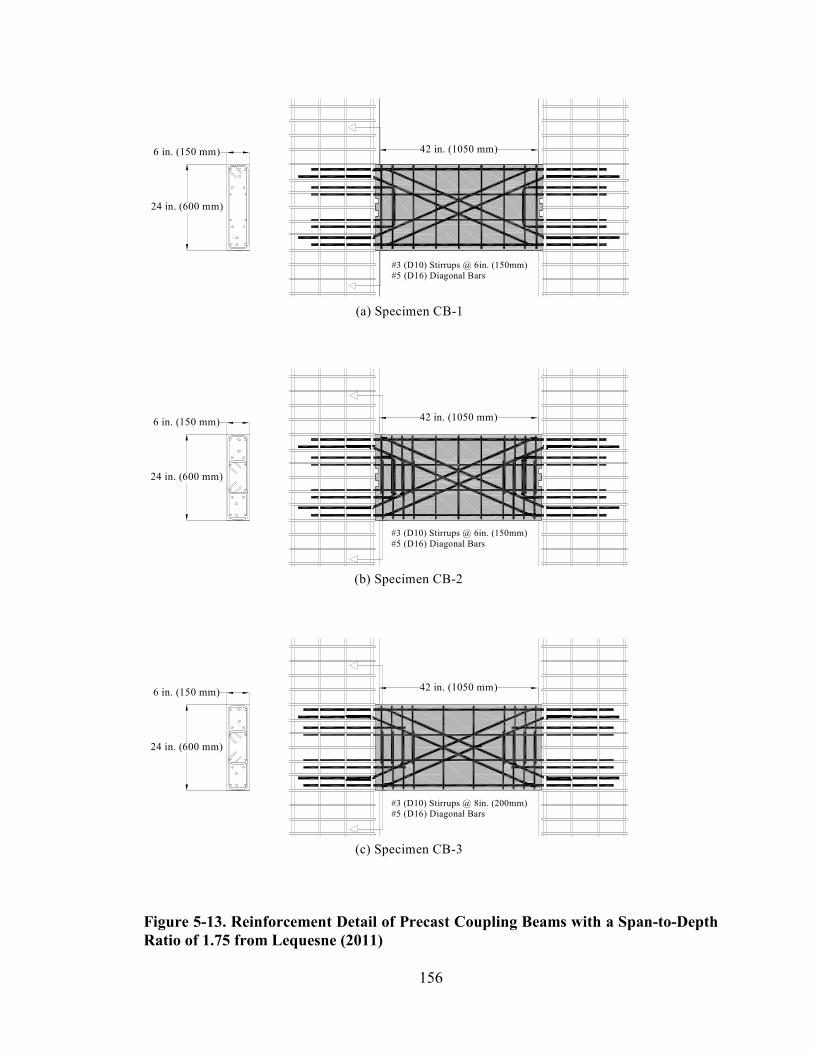
156
Figure 5-13. Reinforcement Detail of Precast Coupling Beams with a Span-to-Depth
Ratio of 1.75 from Lequesne (2011)
42 in. (1050 mm)
24 in. (600 mm)
6 in. (150 mm)
#3 (D10) Stirrups @ 6in. (150mm)#5 (D16) Diagonal Bars
(a) Specimen CB-1
42 in. (1050 mm)
24 in. (600 mm)
6 in. (150 mm)
#3 (D10) Stirrups @ 6in. (150mm)#5 (D16) Diagonal Bars
(b) Specimen CB-2
42 in. (1050 mm)
24 in. (600 mm)
6 in. (150 mm)
#3 (D10) Stirrups @ 8in. (200mm)#5 (D16) Diagonal Bars
(c) Specimen CB-3
157
The load-displacement behavior of the coupling beam is presented as average shear stress
versus drift. The drift is defined with the same equation that ASCE/SEI 41 (ASCE, 2007), as
shown below.
. 2
DriftL
θ∆= −
. (5.1)
Where ∆ is the relative displacement of the coupling beam, L is the length of the
coupling beam, and θ is the rotation of the end of the coupling beam. Since the two ends of the
coupling beam were assumed not to rotate, θ was zero throughout the tests.
Specimen CB-1 displayed good energy dissipation in the early cycles, with the maximum
stress achieved around 2% drift; however, the transverse reinforcement in the end region was not
sufficient to resist the bursting force from the bent diagonal bar while still effectively confining
the plastic hinge. The result was a failure in the plastic hinge region at about 2.2% drift. As
discussed previously, this design deficiency was addressed in subsequent specimens, and the
transverse reinforcement in the end regions was increased. Specimen CB-2 displayed a much
more stable hysteresis behavior. The maximum shear stress achieved during testing exceeded
' '11.5 [psi] (0.87 [MPa])c cf f , and the specimen still performed in a stable minor with minor
pinching. A capacity retention of about 80% of the peak shear force was maintained to drifts of
about 5% in each direction. The shear stress versus drift response of the Specimen CB-2 can is
shown in Figure 5-14.
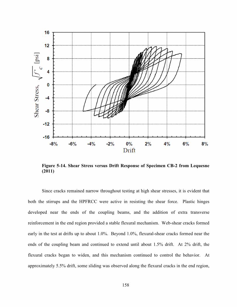
Figure 5-14. Shear Stress versus Drift
(2011)
Since cracks remained narrow throughout testing at high shear stresses, it is evident that
both the stirrups and the HPFRCC were active in resisting the shear force. Pl
developed near the ends of the coupling beams, and the addition of extra transverse
reinforcement in the end region provided a stable flexural mechanism. Web
early in the test at drifts up to about 1.0%. Beyond 1.0%, flex
ends of the coupling beam and continued to extend until about 1.5% drift. At 2% drift, the
flexural cracks began to widen, and this mechanism continued to control the behavior. At
approximately 5.5% drift, some sliding w
158
. Shear Stress versus Drift Response of Specimen CB-2 from Lequesne
Since cracks remained narrow throughout testing at high shear stresses, it is evident that
both the stirrups and the HPFRCC were active in resisting the shear force. Pl
developed near the ends of the coupling beams, and the addition of extra transverse
reinforcement in the end region provided a stable flexural mechanism. Web-shear cracks formed
early in the test at drifts up to about 1.0%. Beyond 1.0%, flexural-shear cracks formed near the
ends of the coupling beam and continued to extend until about 1.5% drift. At 2% drift, the
flexural cracks began to widen, and this mechanism continued to control the behavior. At
approximately 5.5% drift, some sliding was observed along the flexural cracks in the end region,
2 from Lequesne
Since cracks remained narrow throughout testing at high shear stresses, it is evident that
both the stirrups and the HPFRCC were active in resisting the shear force. Plastic hinges
developed near the ends of the coupling beams, and the addition of extra transverse
shear cracks formed
shear cracks formed near the
ends of the coupling beam and continued to extend until about 1.5% drift. At 2% drift, the
flexural cracks began to widen, and this mechanism continued to control the behavior. At
as observed along the flexural cracks in the end region,
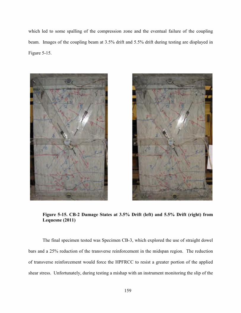
which led to some spalling of the compression zone and the eventual failure of the coupling
beam. Images of the coupling beam at 3.5% drift and 5.5% drift during testing are displayed in
Figure 5-15.
Figure 5-15. CB-2 Damage States at 3.5% Drift (left) and 5.5% Drift (right) from
Lequesne (2011)
The final specimen tested was
bars and a 25% reduction of the transverse reinforcement in the midspan region. The reduction
of transverse reinforcement would force the HPFRCC to resist a greater portion of the applied
shear stress. Unfortunately, during testing a mishap with an instrument monitoring the slip of the
159
which led to some spalling of the compression zone and the eventual failure of the coupling
beam. Images of the coupling beam at 3.5% drift and 5.5% drift during testing are displayed in
2 Damage States at 3.5% Drift (left) and 5.5% Drift (right) from
The final specimen tested was Specimen CB-3, which explored the use of straight dowel
bars and a 25% reduction of the transverse reinforcement in the midspan region. The reduction
of transverse reinforcement would force the HPFRCC to resist a greater portion of the applied
nately, during testing a mishap with an instrument monitoring the slip of the
which led to some spalling of the compression zone and the eventual failure of the coupling
beam. Images of the coupling beam at 3.5% drift and 5.5% drift during testing are displayed in
2 Damage States at 3.5% Drift (left) and 5.5% Drift (right) from
3, which explored the use of straight dowel
bars and a 25% reduction of the transverse reinforcement in the midspan region. The reduction
of transverse reinforcement would force the HPFRCC to resist a greater portion of the applied
nately, during testing a mishap with an instrument monitoring the slip of the
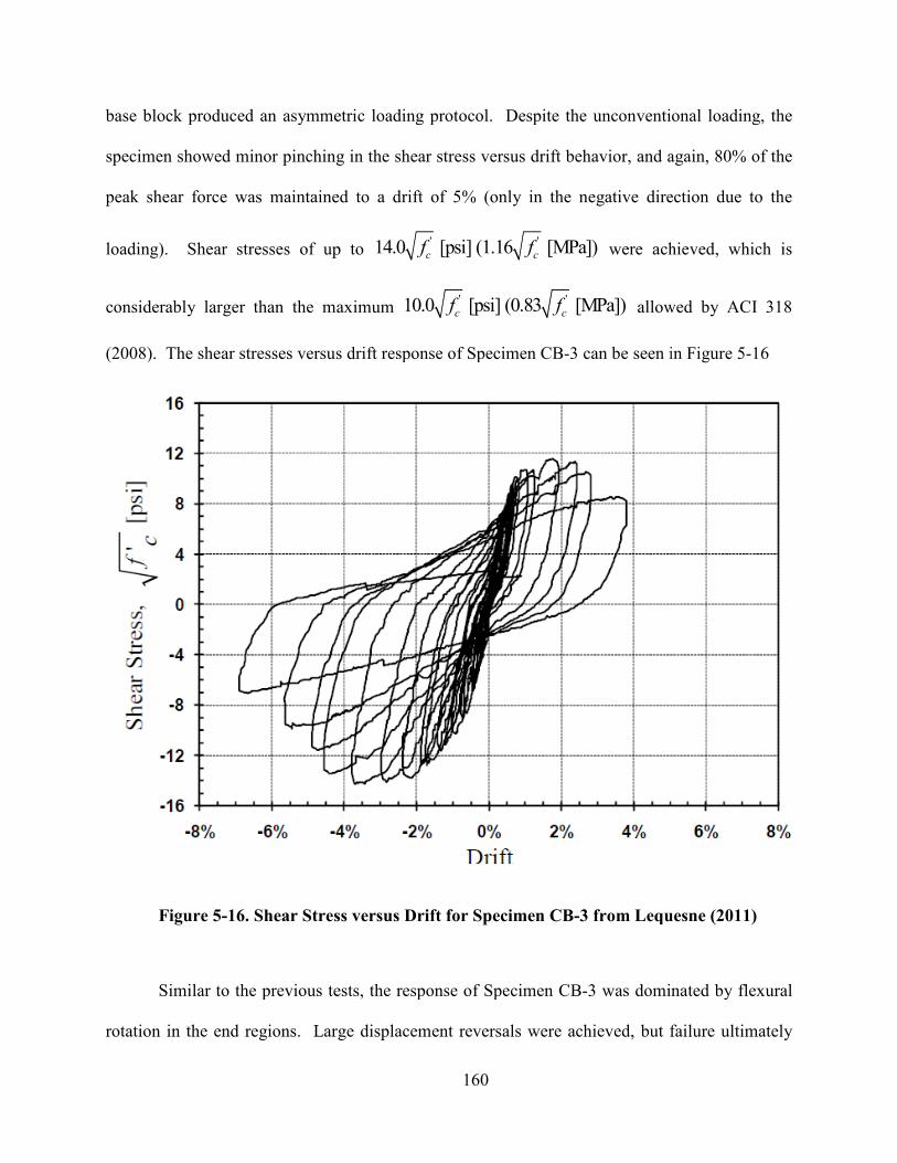
base block produced an asymmetric loading protocol. Despite the unconventional loading, the
specimen showed minor pinching in the shear stress versus drift behavior, and again,
peak shear force was maintained to a drift of 5% (only in the negative direction due to the
loading). Shear stresses of up to
considerably larger than the maximum
(2008). The shear stresses versus drift response of Specimen CB
Figure 5-16. Shear Stress versus
Similar to the previous tests, the response of Specimen CB
rotation in the end regions. Large displacement reversals were achieved, but failur
160
base block produced an asymmetric loading protocol. Despite the unconventional loading, the
specimen showed minor pinching in the shear stress versus drift behavior, and again,
peak shear force was maintained to a drift of 5% (only in the negative direction due to the
loading). Shear stresses of up to ' '14.0 [psi] (1.16 [MPa])c cf f were achieved, which is
larger than the maximum ' '10.0 [psi] (0.83 [MPa])c cf f
allowed by ACI 318
. The shear stresses versus drift response of Specimen CB-3 can be seen in
. Shear Stress versus Drift for Specimen CB-3 from Lequesne
Similar to the previous tests, the response of Specimen CB-3 was dominated by flexural
rotation in the end regions. Large displacement reversals were achieved, but failur
base block produced an asymmetric loading protocol. Despite the unconventional loading, the
specimen showed minor pinching in the shear stress versus drift behavior, and again, 80% of the
peak shear force was maintained to a drift of 5% (only in the negative direction due to the
were achieved, which is
owed by ACI 318
3 can be seen in Figure 5-16
3 from Lequesne (2011)
3 was dominated by flexural
rotation in the end regions. Large displacement reversals were achieved, but failure ultimately
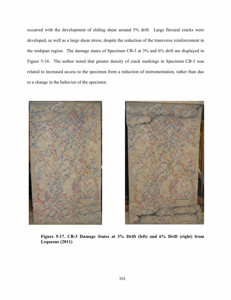
occurred with the development of sliding shear around 5% drift. Large flexural cracks were
developed, as well as a large shear stress, despite the reduction of the transverse reinforcement in
the midspan region. The damage states of Specimen
Figure 5-16. The author noted that greater density of crack markings in Specimen CB
related to increased access to the specimen from a reduction of instrumentation, rather than due
to a change in the behavior of the specimen.
Figure 5-17. CB-3 Damage States at 3% Drift (left) and 6% Drift (right) from
Lequesne (2011)
161
occurred with the development of sliding shear around 5% drift. Large flexural cracks were
developed, as well as a large shear stress, despite the reduction of the transverse reinforcement in
the midspan region. The damage states of Specimen CB-3 at 3% and 6% drift are displayed in
. The author noted that greater density of crack markings in Specimen CB
related to increased access to the specimen from a reduction of instrumentation, rather than due
to a change in the behavior of the specimen.
3 Damage States at 3% Drift (left) and 6% Drift (right) from
occurred with the development of sliding shear around 5% drift. Large flexural cracks were
developed, as well as a large shear stress, despite the reduction of the transverse reinforcement in
3 at 3% and 6% drift are displayed in
. The author noted that greater density of crack markings in Specimen CB-3 was
related to increased access to the specimen from a reduction of instrumentation, rather than due
3 Damage States at 3% Drift (left) and 6% Drift (right) from
162
In each of the coupling beams, flexural hinging at the ends of the coupling beams
dominated the behavior. Shear stresses exceeded ' '10.0 [psi] (0.83 [MPa])c cf f
, and with
proper confinement of the end region, the coupling beams were able to resist more than 80% of
the peak shear force beyond 5% drift. It was found that precasting the HPFRCC coupling beam
and embedding the reinforcement in the boundary element of the shear wall was an effective
design. For the shear resistance, the diagonal reinforcement provided 20-30% of the applied
shear, and it was found that assuming that HPFRCC could resist ' '
5.0 [psi] (0.42 [MPa])c c
f f was
a conservative estimate of the HPFRCC contribution to the shear capacity. Sliding shear
deformations initiated along flexural cracks at about 2% drift, but the failure mechanism was
resisted until rather large drifts were achieved. A final finding from the tests was that the
HPFRCC coupling beams exhibited a shear stiffness of approximately 0.04 c gE A at drifts greater
than 1%. This value is only 10% of the recommended 0.4 c gE A proposed by ASCE/SEI 41
(2007) for modeling coupling beams. The author attributes this large discrepancy to ASCE/SEI
41 not accounting for the reduction of shear stiffness due to diagonal and flexural cracking, so
the reduced value is recommended (2011).
5.3 Compiled Coupling Beam Information
Since the next portion of this research program involves modeling of the coupling beams
previously discussed in this chapter, the geometery, reinforcement details, and material
properties are included in the following tables. These tables contain the relevant properties for
creating the coupling beam models and for evaluating the model. Table 5-1 outlines the coupling
beam geometry and general material properties. Table 5-2 displays more specifics about the
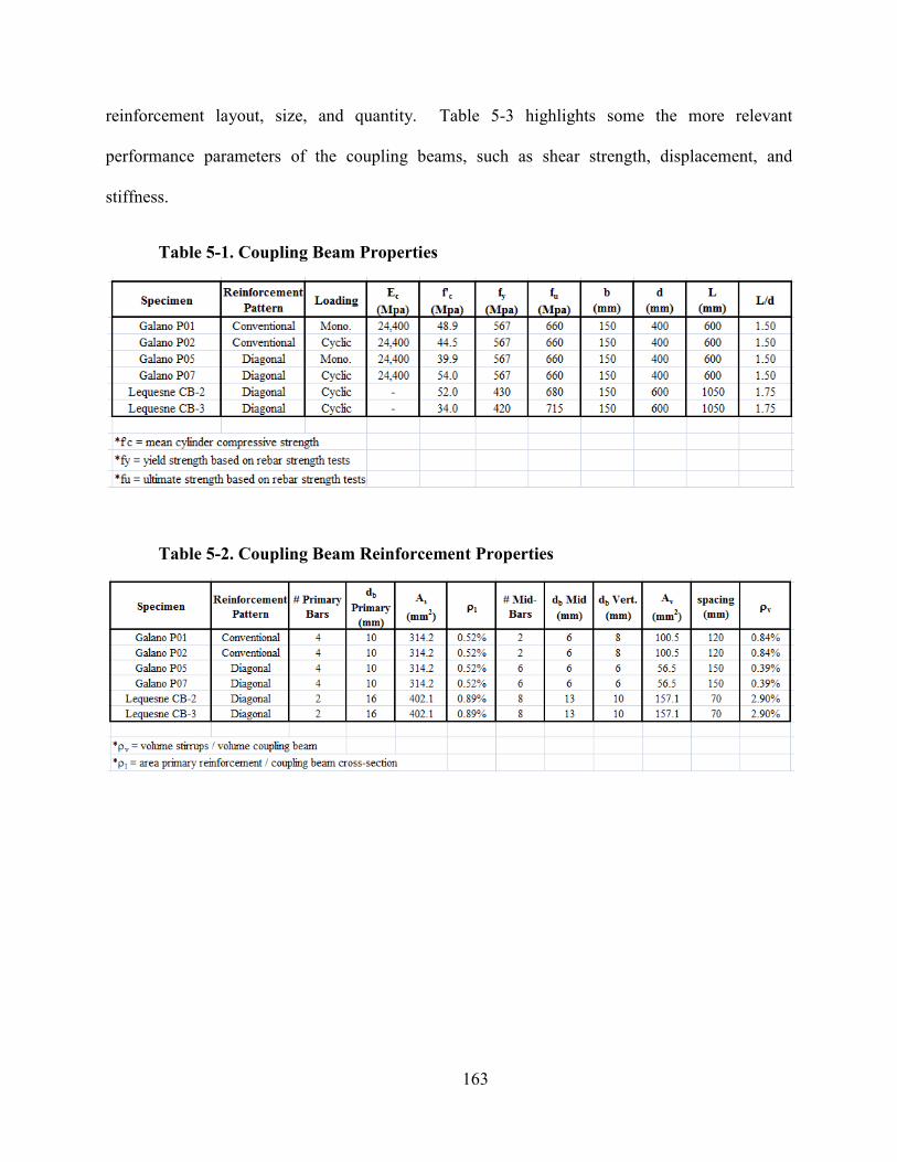
163
reinforcement layout, size, and quantity. Table 5-3 highlights some the more relevant
performance parameters of the coupling beams, such as shear strength, displacement, and
stiffness.
Table 5-1. Coupling Beam Properties
Table 5-2. Coupling Beam Reinforcement Properties
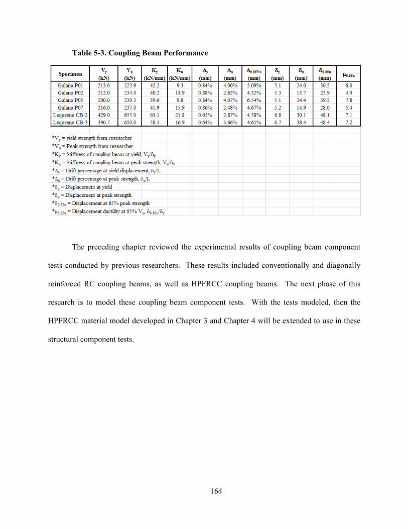
164
Table 5-3. Coupling Beam Performance
The preceding chapter reviewed the experimental results of coupling beam component
tests conducted by previous researchers. These results included conventionally and diagonally
reinforced RC coupling beams, as well as HPFRCC coupling beams. The next phase of this
research is to model these coupling beam component tests. With the tests modeled, then the
HPFRCC material model developed in Chapter 3 and Chapter 4 will be extended to use in these
structural component tests.
165
CHAPTER 6. COUPLIG BEAM COMPOET MODELIG
As seen in the previous chapters, coupling beam component tests have been conducted by
many researchers over the years; however, most of the results focused on the testing of RC
coupling beams. Given the extensive testing on the HPFRCC material presented in Chapter 3, as
well as the material model validation presented in Chapter 4, this chapter will focus on the
results of implementing the HPFRCC material model into a structural component. The goal of
this chapter is to model coupling beams tested by previous researchers with RC, while observing
the behavior and response of the specimen. Then the same coupling beams will be modeled with
the validated HPFRCC material, and the effect of adding HPFRCC to the coupling beams can be
seen from the results of the parametric study. Additionally, coupling beams tested with
HPFRCC will be modeled. This portion of the modeling effort will demonstrate the ability of
the model to effectively represent the behavior of HPFRCC in a structural component. Finally,
since the HPFRCC coupling beams did not have a control RC coupling beam, the same
reinforcement layout of the HPFRCC coupling beams will be used; however, a reinforced
concrete will be implemented as the material to provide the results of a control RC specimen.
6.1 Coupling Beam Modeling Parameters
The next sections will outline the modeling parameters implemented into the coupling
beam models. The parameters include constitutive models, reinforcement modeling, finite
element parameters, and loading and boundary conditions.
6.1.1 Constitutive Models
For the modeling of the concrete within the RC coupling beams, the default parameters
for SBETA concrete within ATENA was used, given the reported compressive strength for the
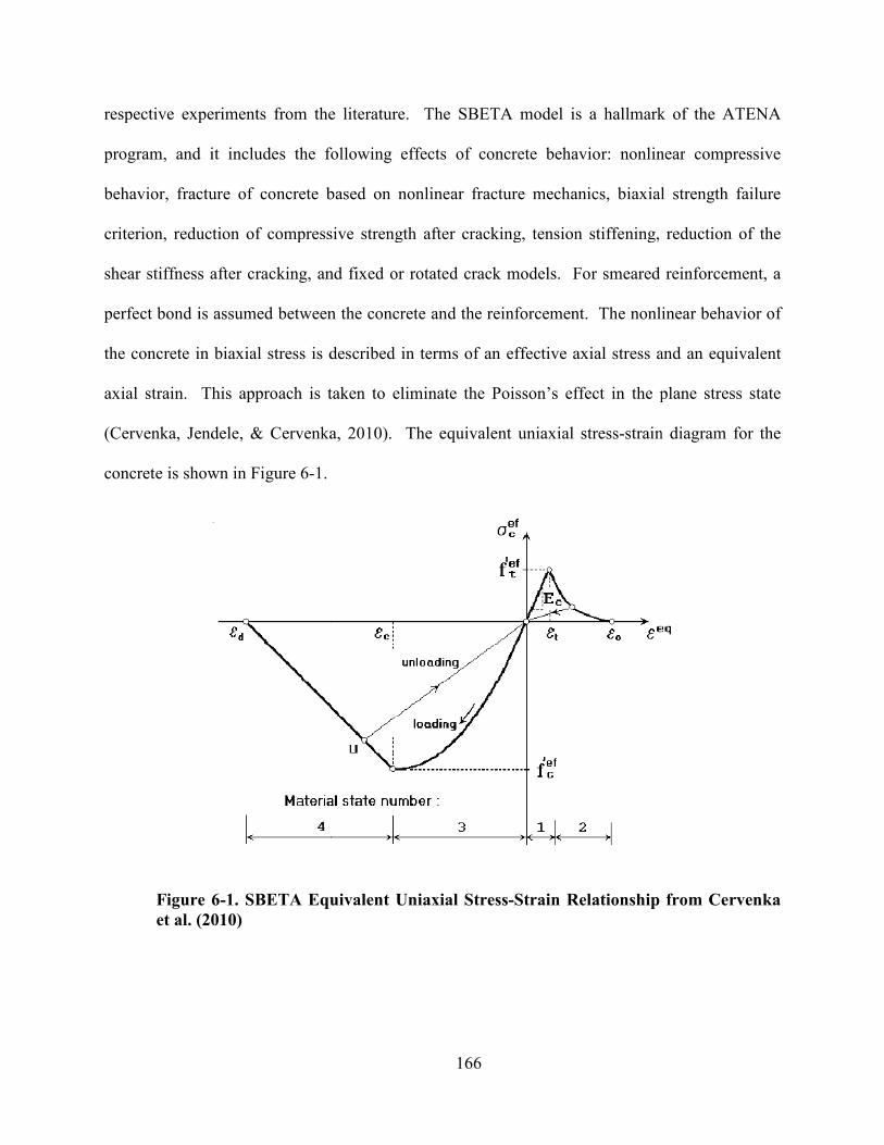
respective experiments from the literature.
program, and it includes the following effects of concrete behavior: nonlinear
behavior, fracture of concrete based on nonlinear fracture mechanics, biaxial strength failure
criterion, reduction of compressive strength after cracking, tension stiffening, reduction of the
shear stiffness after cracking, and fixed or rotat
perfect bond is assumed between the concrete and the reinforcement.
the concrete in biaxial stress is described in terms of an effective axial stress and an equivalent
axial strain. This approach is taken to eliminate the Poisson’s effect in the plane stress state
(Cervenka, Jendele, & Cervenka, 2010)
concrete is shown in Figure 6-1.
Figure 6-1. SBETA Equivalent Uniaxial Stress
et al. (2010)
166
respective experiments from the literature. The SBETA model is a hallmark of the ATENA
program, and it includes the following effects of concrete behavior: nonlinear
behavior, fracture of concrete based on nonlinear fracture mechanics, biaxial strength failure
criterion, reduction of compressive strength after cracking, tension stiffening, reduction of the
shear stiffness after cracking, and fixed or rotated crack models. For smeared reinforcement, a
perfect bond is assumed between the concrete and the reinforcement. The nonlinear behavior of
the concrete in biaxial stress is described in terms of an effective axial stress and an equivalent
This approach is taken to eliminate the Poisson’s effect in the plane stress state
(Cervenka, Jendele, & Cervenka, 2010). The equivalent uniaxial stress-strain diagram for the
. SBETA Equivalent Uniaxial Stress-Strain Relationship from Cervenka
The SBETA model is a hallmark of the ATENA
program, and it includes the following effects of concrete behavior: nonlinear compressive
behavior, fracture of concrete based on nonlinear fracture mechanics, biaxial strength failure
criterion, reduction of compressive strength after cracking, tension stiffening, reduction of the
ed crack models. For smeared reinforcement, a
The nonlinear behavior of
the concrete in biaxial stress is described in terms of an effective axial stress and an equivalent
This approach is taken to eliminate the Poisson’s effect in the plane stress state
strain diagram for the
Strain Relationship from Cervenka
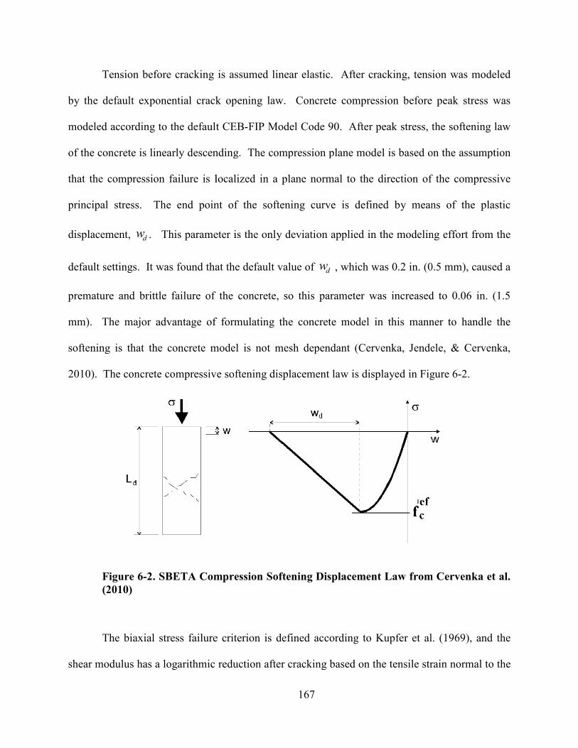
Tension before cracking is assumed linear elastic. After cracki
by the default exponential crack opening law. Concrete compression before peak stress was
modeled according to the default CEB
of the concrete is linearly descending. The co
that the compression failure is localized in a plane normal to the direction of the compressive
principal stress. The end point of the softening curve is defined by means of the plastic
displacement, dw . This parameter is the only deviation applied in the modeling effort from the
default settings. It was found that the default value of
premature and brittle failure of the concrete, so this parameter was increased to 0.06 in. (1.5
mm). The major advantage of formulating the concrete model in this manner to handle the
softening is that the concrete model is not mesh dependant
2010). The concrete compressive softening displacement law is displayed in
Figure 6-2. SBETA Compression Softening Displacemen
(2010)
The biaxial stress failure criterion is defined according to Kupfer et al.
shear modulus has a logarithmic reduction after cracki
167
Tension before cracking is assumed linear elastic. After cracking, tension was modeled
by the default exponential crack opening law. Concrete compression before peak stress was
modeled according to the default CEB-FIP Model Code 90. After peak stress, the softening law
of the concrete is linearly descending. The compression plane model is based on the assumption
that the compression failure is localized in a plane normal to the direction of the compressive
principal stress. The end point of the softening curve is defined by means of the plastic
This parameter is the only deviation applied in the modeling effort from the
default settings. It was found that the default value of dw , which was 0.2 in. (0.5 mm),
e and brittle failure of the concrete, so this parameter was increased to 0.06 in. (1.5
mm). The major advantage of formulating the concrete model in this manner to handle the
softening is that the concrete model is not mesh dependant (Cervenka, Jendele, & Cervenka,
. The concrete compressive softening displacement law is displayed in Figure
. SBETA Compression Softening Displacement Law from Cervenka et al.
The biaxial stress failure criterion is defined according to Kupfer et al.
shear modulus has a logarithmic reduction after cracking based on the tensile strain normal to the
ng, tension was modeled
by the default exponential crack opening law. Concrete compression before peak stress was
After peak stress, the softening law
mpression plane model is based on the assumption
that the compression failure is localized in a plane normal to the direction of the compressive
principal stress. The end point of the softening curve is defined by means of the plastic
This parameter is the only deviation applied in the modeling effort from the
, which was 0.2 in. (0.5 mm), caused a
e and brittle failure of the concrete, so this parameter was increased to 0.06 in. (1.5
mm). The major advantage of formulating the concrete model in this manner to handle the
(Cervenka, Jendele, & Cervenka,
Figure 6-2.
from Cervenka et al.
The biaxial stress failure criterion is defined according to Kupfer et al. (1969), and the
ng based on the tensile strain normal to the
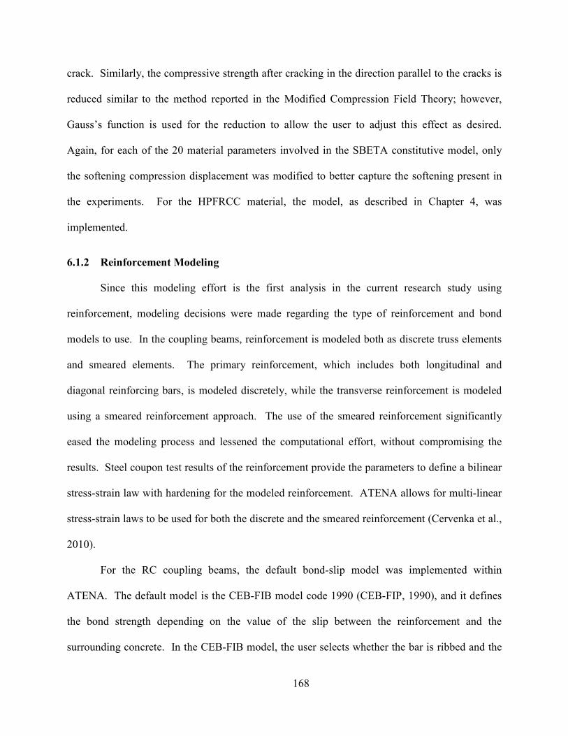
168
crack. Similarly, the compressive strength after cracking in the direction parallel to the cracks is
reduced similar to the method reported in the Modified Compression Field Theory; however,
Gauss’s function is used for the reduction to allow the user to adjust this effect as desired.
Again, for each of the 20 material parameters involved in the SBETA constitutive model, only
the softening compression displacement was modified to better capture the softening present in
the experiments. For the HPFRCC material, the model, as described in Chapter 4, was
implemented.
6.1.2 Reinforcement Modeling
Since this modeling effort is the first analysis in the current research study using
reinforcement, modeling decisions were made regarding the type of reinforcement and bond
models to use. In the coupling beams, reinforcement is modeled both as discrete truss elements
and smeared elements. The primary reinforcement, which includes both longitudinal and
diagonal reinforcing bars, is modeled discretely, while the transverse reinforcement is modeled
using a smeared reinforcement approach. The use of the smeared reinforcement significantly
eased the modeling process and lessened the computational effort, without compromising the
results. Steel coupon test results of the reinforcement provide the parameters to define a bilinear
stress-strain law with hardening for the modeled reinforcement. ATENA allows for multi-linear
stress-strain laws to be used for both the discrete and the smeared reinforcement (Cervenka et al.,
2010).
For the RC coupling beams, the default bond-slip model was implemented within
ATENA. The default model is the CEB-FIB model code 1990 (CEB-FIP, 1990), and it defines
the bond strength depending on the value of the slip between the reinforcement and the
surrounding concrete. In the CEB-FIB model, the user selects whether the bar is ribbed and the
confinement conditions. Since all of the primary reinforcement in the coupling beams we
within a densely confined concrete core, the bond condition was selected as “good.” This model
then assumes that a slip failure occurs due to shearing of the concrete between the ribs of the
deformed bar (Cervenka, Jendele, &
associated parameters values are shown in
Figure 6-3. CEB-FIP Model Code 1990 Bond
Parameters (right) from Cervenka et al.
Since prior research has been conducted on the bond performance of HPFRCC with
reinforcing steel, the bond-slip experiments
found that the research did not explicitly provide a bond
plotted the experimental results of several different types of fibers in varying volume fractions
relative to the conventionally reinforced concrete. The research reported that the bond strength of
HPFRCC was about 1.5 times that of spirally reinforced specimens subjected to monotonic
loading, and about 33% greater than the bond performance when subjected to u
cyclic loading (Chao et al., 2009). Provided that information, the default bond model was used
with an increase in the maximum bond stress and an increase in the
169
confinement conditions. Since all of the primary reinforcement in the coupling beams we
within a densely confined concrete core, the bond condition was selected as “good.” This model
then assumes that a slip failure occurs due to shearing of the concrete between the ribs of the
(Cervenka, Jendele, & Cervenka, 2010). The bond-slip relationship and the
associated parameters values are shown in Figure 6-3.
FIP Model Code 1990 Bond-Slip Relationship (left) w
from Cervenka et al. (2010)
Since prior research has been conducted on the bond performance of HPFRCC with
experiments reported by Chao et al. (2009) were reviewed. It was
found that the research did not explicitly provide a bond-slip model for HPFRCC, rather it
plotted the experimental results of several different types of fibers in varying volume fractions
to the conventionally reinforced concrete. The research reported that the bond strength of
HPFRCC was about 1.5 times that of spirally reinforced specimens subjected to monotonic
loading, and about 33% greater than the bond performance when subjected to u
(Chao et al., 2009). Provided that information, the default bond model was used
with an increase in the maximum bond stress and an increase in the permitted slip.
confinement conditions. Since all of the primary reinforcement in the coupling beams were
within a densely confined concrete core, the bond condition was selected as “good.” This model
then assumes that a slip failure occurs due to shearing of the concrete between the ribs of the
slip relationship and the
Slip Relationship (left) with Table of
Since prior research has been conducted on the bond performance of HPFRCC with
ere reviewed. It was
slip model for HPFRCC, rather it
plotted the experimental results of several different types of fibers in varying volume fractions
to the conventionally reinforced concrete. The research reported that the bond strength of
HPFRCC was about 1.5 times that of spirally reinforced specimens subjected to monotonic
loading, and about 33% greater than the bond performance when subjected to unidirectional
(Chao et al., 2009). Provided that information, the default bond model was used
slip.
170
6.1.3 Finite Element Modeling Parameters
ATENA provides a finite element mesh tool to define the parameter of mesh generation.
For reinforced concrete, with discrete truss elements for the reinforcing steel, the mesh is
generated in two phases. First, a mesh of 3-D elements is produced within the pre-processor. In
the pre-processor the bars are still maintained as geometrical objects without mesh. When the
control is passed to the analysis program, the bar finite elements are generated as embedded
elements within the existing mesh of 3-D finite elements. Thus, the user cannot affect the
meshing of bars, since it is governed by the overall mesh of the finite elements (Cervenka et al.,
2010). The use of embedded reinforcing bars is beneficial when modeling reinforced concrete
because the nodes of the discrete reinforcing bar do not have to align with the nodes of the mesh.
The elements used will be plane stress elements, and a smeared approach will be used to model
and to apply the material properties.
For the boundary conditions of the coupling beam components, an effort was made for
each coupling beam to be model the boundary conditions of the experiment. In general, the
coupling beams were modeled with large loading blocks on the either side of the beam. The left
coupling beam block was restrained on the top and bottom against vertical displacements, while
the right edge of the right loading block was fixed against horizontal displacements. The
deformations were then imposed by specifying a prescribed displacement along the bottom edge
of the loading block through a steel plate. This configuration adequately represent the boundary
conditions of the experiments by imposing equal and opposite rotations on each end of the
coupling beam, while allowing the coupling beam to expand axially as damage progressed. For
the coupling beams with axial restraint (Lequesne, 2011), completely restraining the blocks from
axial expansion was found to unconservatively generate a large axial load. Thus, where the axial
171
loading was provided in the literature, a corresponding axial load was applied in the model. This
approach proved to be sufficient in capturing the appropriate stress and strain state in the
specimen.
The coupling beam specimens were modeled with plane quadrilateral elements. They are
isoparametric elements with quadratic displacement shape functions, so there are 9 Gauss
integration points in each element. These elements are suitable for plane 2-D, axisymmetric, and
3-D problems (Cervenka et al., 2010). The automatic meshing feature employed by the ATENA
software was implemented for each model. For the element size, since the HPFRCC had
aggregate as large as 0.375 in. (9.525 mm), 0.4 in. (10.2 mm) was determined to be the minimum
mesh size. A brief sensitivity study was conducted with increasing element size, and it was
found that an element mesh size of 1 in. (25 mm) was found to accurately capture the results
while decreasing the required computational time.
The solution parameters for ATENA implements the full Newton-Raphson solution of
nonlinear equations. The main feature of the full Newton-Raphson procedure is that it continues
to update the stiffness matrix with each step, while the Modified Newton-Raphson procedure
continues to use the initial stiffness obtained in the first step. While it may take more
computational time to update the stiffness matrix, it is believed that the convergence to the
solution is superior with the full Newton-Raphson technique. The node numbers were optimized
with the Sloan method, and iteration limit for each step was set to 50. The default displacement,
residual, absolute residual, and energy error tolerances were used.
6.2 RC Coupling Beam Component Modeling
The first modeling effort was of the conventionally reinforced and diagonally reinforced
coupling beams tested by Galano and Vignoli (2000). Many of the details of the testing program
172
were presented previously in Chapter 5; however, the modeling portion of this research only
focused on modeling four of the coupling beams from the experimental program: conventionally
reinforced with monotonic loading, conventionally reinforced with cyclic loading, diagonally
reinforced with monotonic loading, and diagonally reinforced with cyclic loading. The results of
the RC coupling beam models will be reviewed in the next sections, as well as the results of the
coupling beams implementing the HPFRCC material model described in Chapter 4.
6.2.1 RC Coupling Beam Modeling Results
The coupling beams tested by Galano and Vignoli (2000) were modeled with the same
geometry reported by the researchers. The left block was restrained on the top and bottom
against vertical movement, while the right block was restrained from lateral movement. In the
experiment, no comment was made about the ability of the coupling beam to expand axially or
about the axial force generated during loading. The authors only mention that undesirable
movements were prevented. A model was conducted with axial expansion prevented by fixing
the left block from horizontal movement, and the result was a very large axial force and
premature failure of the coupling beam. Since this was not what was reported by the researchers,
the subsequent models were conducted without the axial restraint, and the modeling loading and
boundary conditions for Specimen P01 may be seen in Figure 6-4.
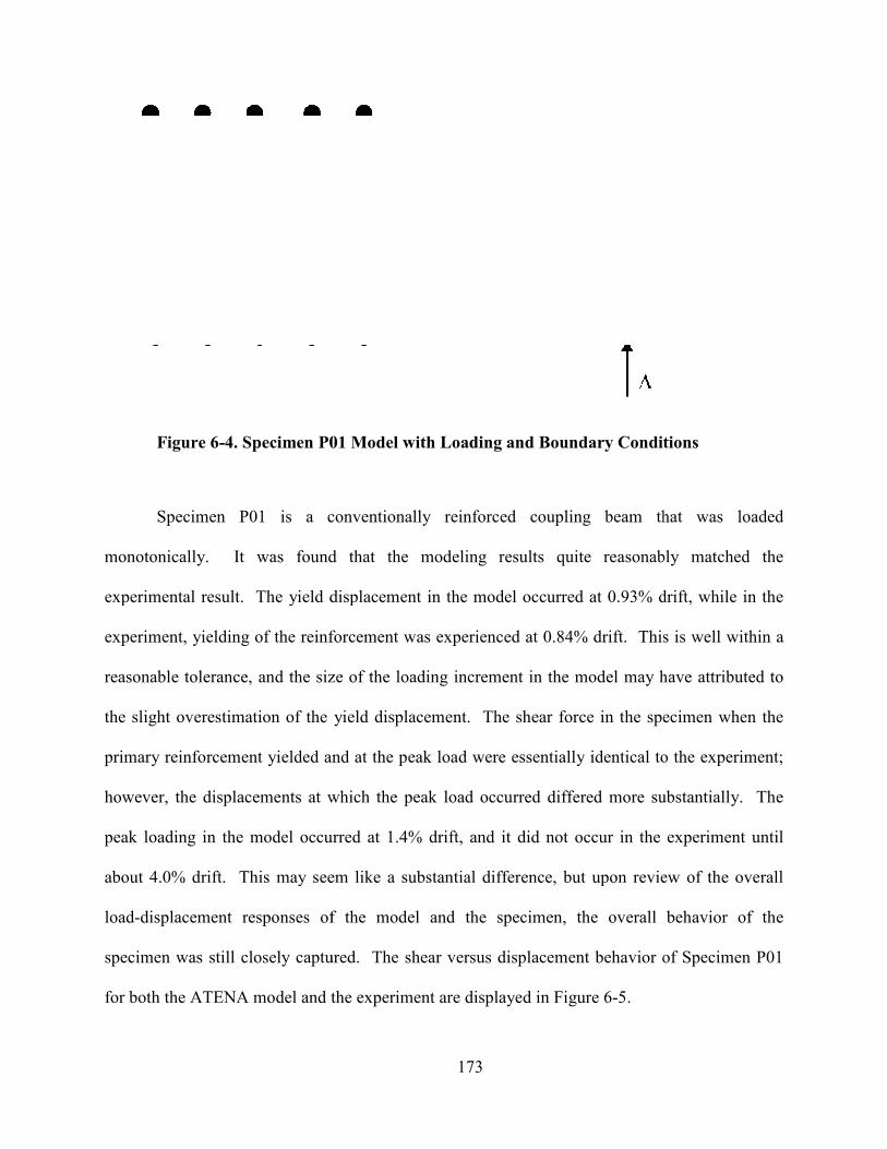
Figure 6-4. Specimen P01 Model with Loading and Boundary Conditions
Specimen P01 is a conventionally rei
monotonically. It was found that the modeling results quite reasonably matched the
experimental result. The yield displacement in the model occurred at 0.93% drift, while in the
experiment, yielding of the reinforcem
reasonable tolerance, and the size of the loading increment in the model may have attributed to
the slight overestimation of the yield displacement. The shear force in the specimen when the
primary reinforcement yielded and at the peak load were essentially identical to the experiment;
however, the displacements at which the peak load occurred differed more substantially. The
peak loading in the model occurred at 1.4% drift, and it did not occur i
about 4.0% drift. This may seem like a substantial difference, but upon review of the overall
load-displacement responses of the model and the specimen, the overall behavior of the
specimen was still closely captured.
for both the ATENA model and the experiment are displayed in
173
. Specimen P01 Model with Loading and Boundary Conditions
Specimen P01 is a conventionally reinforced coupling beam that was loaded
monotonically. It was found that the modeling results quite reasonably matched the
experimental result. The yield displacement in the model occurred at 0.93% drift, while in the
experiment, yielding of the reinforcement was experienced at 0.84% drift. This is well within a
reasonable tolerance, and the size of the loading increment in the model may have attributed to
the slight overestimation of the yield displacement. The shear force in the specimen when the
y reinforcement yielded and at the peak load were essentially identical to the experiment;
however, the displacements at which the peak load occurred differed more substantially. The
peak loading in the model occurred at 1.4% drift, and it did not occur in the experiment until
about 4.0% drift. This may seem like a substantial difference, but upon review of the overall
displacement responses of the model and the specimen, the overall behavior of the
specimen was still closely captured. The shear versus displacement behavior of Specimen P01
for both the ATENA model and the experiment are displayed in Figure 6-5.
. Specimen P01 Model with Loading and Boundary Conditions
nforced coupling beam that was loaded
monotonically. It was found that the modeling results quite reasonably matched the
experimental result. The yield displacement in the model occurred at 0.93% drift, while in the
ent was experienced at 0.84% drift. This is well within a
reasonable tolerance, and the size of the loading increment in the model may have attributed to
the slight overestimation of the yield displacement. The shear force in the specimen when the
y reinforcement yielded and at the peak load were essentially identical to the experiment;
however, the displacements at which the peak load occurred differed more substantially. The
n the experiment until
about 4.0% drift. This may seem like a substantial difference, but upon review of the overall
displacement responses of the model and the specimen, the overall behavior of the
sus displacement behavior of Specimen P01
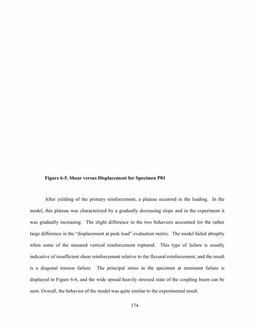
Figure 6-5. Shear versus Displacement for Specimen P01
After yielding of the primary reinforcement, a plateau occurred in the loading. In the
model, this plateau was characterized by a gradually decreasing slope and in the experiment it
was gradually increasing. The slight difference in the two behaviors accounted
large difference in the “displacement at peak load” evaluation metric.
when some of the smeared vertical reinforcement ruptured. This type of failure is usually
indicative of insufficient shear reinforcement rela
is a diagonal tension failure. The principal stress in the specimen at imminent failure is
displayed in Figure 6-6, and the wide spread heavily stressed state of the coupling bea
seen. Overall, the behavior of the model was quite similar to the experimental result
174
. Shear versus Displacement for Specimen P01
yielding of the primary reinforcement, a plateau occurred in the loading. In the
model, this plateau was characterized by a gradually decreasing slope and in the experiment it
was gradually increasing. The slight difference in the two behaviors accounted
large difference in the “displacement at peak load” evaluation metric. The model failed abruptly
when some of the smeared vertical reinforcement ruptured. This type of failure is usually
indicative of insufficient shear reinforcement relative to the flexural reinforcement, and the result
is a diagonal tension failure. The principal stress in the specimen at imminent failure is
, and the wide spread heavily stressed state of the coupling bea
seen. Overall, the behavior of the model was quite similar to the experimental result
yielding of the primary reinforcement, a plateau occurred in the loading. In the
model, this plateau was characterized by a gradually decreasing slope and in the experiment it
was gradually increasing. The slight difference in the two behaviors accounted for the rather
The model failed abruptly
when some of the smeared vertical reinforcement ruptured. This type of failure is usually
tive to the flexural reinforcement, and the result
is a diagonal tension failure. The principal stress in the specimen at imminent failure is
, and the wide spread heavily stressed state of the coupling beam can be
seen. Overall, the behavior of the model was quite similar to the experimental result.
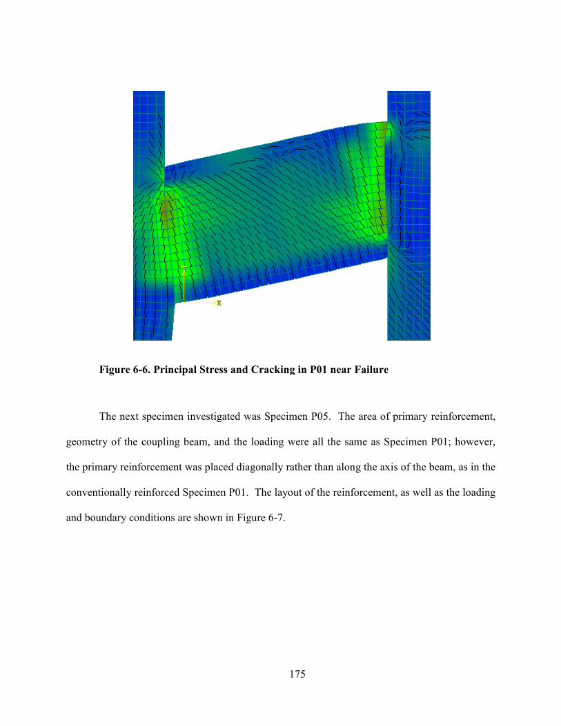
Figure 6-6. Principal Stress and Cracking in P01 near
The next specimen investigated was Specimen P0
geometry of the coupling beam, and the loading were all the same as Specimen P01; however,
the primary reinforcement was placed diagonally rather than along the axis of the beam, as in the
conventionally reinforced Specimen P01. The layout of the reinforcement, as well as the loading
and boundary conditions are shown in
175
al Stress and Cracking in P01 near Failure
The next specimen investigated was Specimen P05. The area of primary reinforcement,
geometry of the coupling beam, and the loading were all the same as Specimen P01; however,
the primary reinforcement was placed diagonally rather than along the axis of the beam, as in the
ecimen P01. The layout of the reinforcement, as well as the loading
and boundary conditions are shown in Figure 6-7.
5. The area of primary reinforcement,
geometry of the coupling beam, and the loading were all the same as Specimen P01; however,
the primary reinforcement was placed diagonally rather than along the axis of the beam, as in the
ecimen P01. The layout of the reinforcement, as well as the loading
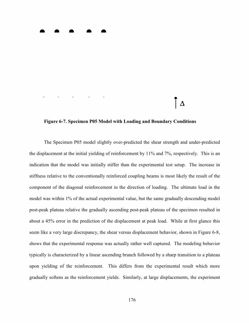
Figure 6-7. Specimen P05 Model with Loading and Boundary Cond
The Specimen P05 model slightly over
the displacement at the initial yielding of reinforcement by 11% and 7%, respectively. This is an
indication that the model was initially
stiffness relative to the conventionally reinforced coupling beams is most likely the result of the
component of the diagonal reinforcement in the direction of loading. The ultimate load in the
model was within 1% of the actual experimental value, but the same gradually descending model
post-peak plateau relative the gradually ascending post
about a 45% error in the prediction of the displacement at peak load. While
seem like a very large discrepancy, the shear versus displacement behavior, shown in
shows that the experimental response was actually rather well captured. The modeling behavior
typically is characterized by a linear ascending branch followed by a sharp transition to a plateau
upon yielding of the reinforcement. This differs from the experimental result which more
gradually softens as the reinforcement yields. Similarly, at large displacements, the experimen
176
. Specimen P05 Model with Loading and Boundary Conditions
The Specimen P05 model slightly over-predicted the shear strength and under
the displacement at the initial yielding of reinforcement by 11% and 7%, respectively. This is an
indication that the model was initially stiffer than the experimental test setup.
stiffness relative to the conventionally reinforced coupling beams is most likely the result of the
component of the diagonal reinforcement in the direction of loading. The ultimate load in the
e actual experimental value, but the same gradually descending model
peak plateau relative the gradually ascending post-peak plateau of the specimen resulted in
about a 45% error in the prediction of the displacement at peak load. While at first glan
seem like a very large discrepancy, the shear versus displacement behavior, shown in
shows that the experimental response was actually rather well captured. The modeling behavior
a linear ascending branch followed by a sharp transition to a plateau
upon yielding of the reinforcement. This differs from the experimental result which more
gradually softens as the reinforcement yields. Similarly, at large displacements, the experimen
itions
predicted the shear strength and under-predicted
the displacement at the initial yielding of reinforcement by 11% and 7%, respectively. This is an
mental test setup. The increase in
stiffness relative to the conventionally reinforced coupling beams is most likely the result of the
component of the diagonal reinforcement in the direction of loading. The ultimate load in the
e actual experimental value, but the same gradually descending model
peak plateau of the specimen resulted in
at first glance this
seem like a very large discrepancy, the shear versus displacement behavior, shown in Figure 6-8,
shows that the experimental response was actually rather well captured. The modeling behavior
a linear ascending branch followed by a sharp transition to a plateau
upon yielding of the reinforcement. This differs from the experimental result which more
gradually softens as the reinforcement yields. Similarly, at large displacements, the experiment
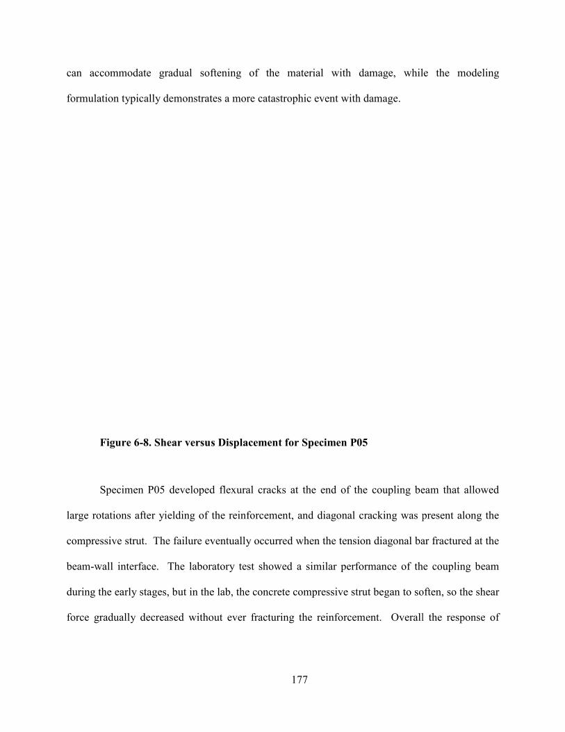
can accommodate gradual softening of the material with damage, while the modeling
formulation typically demonstrates a more catastrophic event with damage.
Figure 6-8. Shear versus Displacement for Specim
Specimen P05 developed flexural cracks at the end of the coupling beam that allowed
large rotations after yielding of the reinforcement, and diagonal cracking was present along the
compressive strut. The failure eventually occurred when the tensio
beam-wall interface. The laboratory test showed a similar performance of the coupling beam
during the early stages, but in the lab, the concrete compressive strut began to soften, so the shear
force gradually decreased without ever fracturing the reinforcement. Overall the respons
177
can accommodate gradual softening of the material with damage, while the modeling
formulation typically demonstrates a more catastrophic event with damage.
. Shear versus Displacement for Specimen P05
Specimen P05 developed flexural cracks at the end of the coupling beam that allowed
large rotations after yielding of the reinforcement, and diagonal cracking was present along the
The failure eventually occurred when the tension diagonal bar fractured at the
wall interface. The laboratory test showed a similar performance of the coupling beam
during the early stages, but in the lab, the concrete compressive strut began to soften, so the shear
out ever fracturing the reinforcement. Overall the respons
can accommodate gradual softening of the material with damage, while the modeling
Specimen P05 developed flexural cracks at the end of the coupling beam that allowed
large rotations after yielding of the reinforcement, and diagonal cracking was present along the
n diagonal bar fractured at the
wall interface. The laboratory test showed a similar performance of the coupling beam
during the early stages, but in the lab, the concrete compressive strut began to soften, so the shear
out ever fracturing the reinforcement. Overall the response of
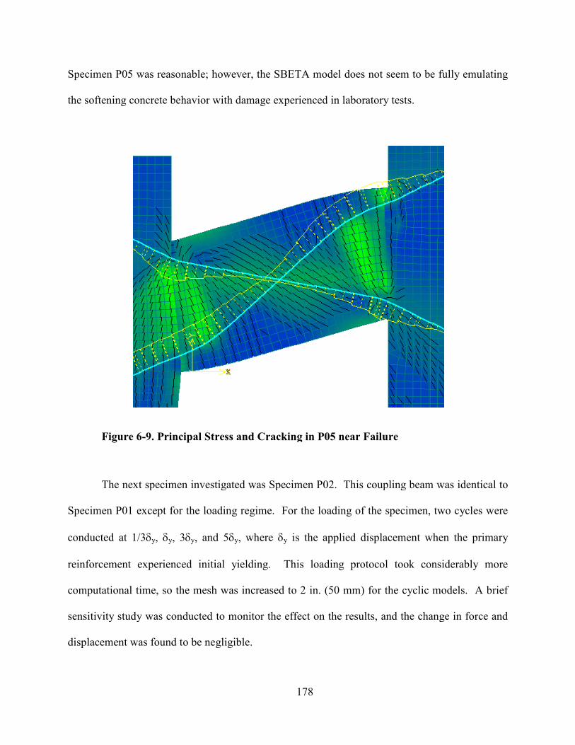
Specimen P05 was reasonable; however, the SBETA model does not seem to be fully emulating
the softening concrete behavior with damage experienced in laboratory tests.
Figure 6-9. Principal Stress and Cracking in P05 near
The next specimen investigated was Specimen P02. This coupling beam was identical to
Specimen P01 except for the loading regime. For the loading of the specimen, two
conducted at 1/3δy, δy, 3δy, and 5
reinforcement experienced initial yielding. This loading protocol took considerably more
computational time, so the mesh was increased to
sensitivity study was conducted to monitor the effect on the results, and the change in force and
displacement was found to be negligible.
178
; however, the SBETA model does not seem to be fully emulating
the softening concrete behavior with damage experienced in laboratory tests.
al Stress and Cracking in P05 near Failure
The next specimen investigated was Specimen P02. This coupling beam was identical to
Specimen P01 except for the loading regime. For the loading of the specimen, two
, and 5δy, where δy is the applied displacement when the primary
reinforcement experienced initial yielding. This loading protocol took considerably more
computational time, so the mesh was increased to 2 in. (50 mm) for the cyclic models. A brief
sensitivity study was conducted to monitor the effect on the results, and the change in force and
displacement was found to be negligible.
; however, the SBETA model does not seem to be fully emulating
The next specimen investigated was Specimen P02. This coupling beam was identical to
Specimen P01 except for the loading regime. For the loading of the specimen, two cycles were
is the applied displacement when the primary
reinforcement experienced initial yielding. This loading protocol took considerably more
) for the cyclic models. A brief
sensitivity study was conducted to monitor the effect on the results, and the change in force and
In the experiment it was found that at low drift ratios that the conventionally r
coupling beams performed similarly to the diagonally reinforced coupling beams, but at large
displacement, the strength began to decay rather rapidly. A similar behavior was seen with the
ATENA model of the specimen; however, the model was not a
large as in the experiment. For the model, the shear and displacement at initial yielding of the
reinforcement were within 6% and 9
shear load was essentially identical to that experiment; however, when the experiment began to
experience damage and lose capacity, the model lost capacity rapidly. The envelope of the
experimental shear-displacement response and the ATENA result are compared in
Figure 6-10. Shear versus Displacement for Specimen P02
179
In the experiment it was found that at low drift ratios that the conventionally r
coupling beams performed similarly to the diagonally reinforced coupling beams, but at large
displacement, the strength began to decay rather rapidly. A similar behavior was seen with the
ATENA model of the specimen; however, the model was not able to achieve displacements as
large as in the experiment. For the model, the shear and displacement at initial yielding of the
6% and 9% of the experimental result, respectively. Also, the peak
ical to that experiment; however, when the experiment began to
experience damage and lose capacity, the model lost capacity rapidly. The envelope of the
displacement response and the ATENA result are compared in
. Shear versus Displacement for Specimen P02
In the experiment it was found that at low drift ratios that the conventionally reinforced
coupling beams performed similarly to the diagonally reinforced coupling beams, but at large
displacement, the strength began to decay rather rapidly. A similar behavior was seen with the
ble to achieve displacements as
large as in the experiment. For the model, the shear and displacement at initial yielding of the
% of the experimental result, respectively. Also, the peak
ical to that experiment; however, when the experiment began to
experience damage and lose capacity, the model lost capacity rapidly. The envelope of the
displacement response and the ATENA result are compared in Figure 6-10.
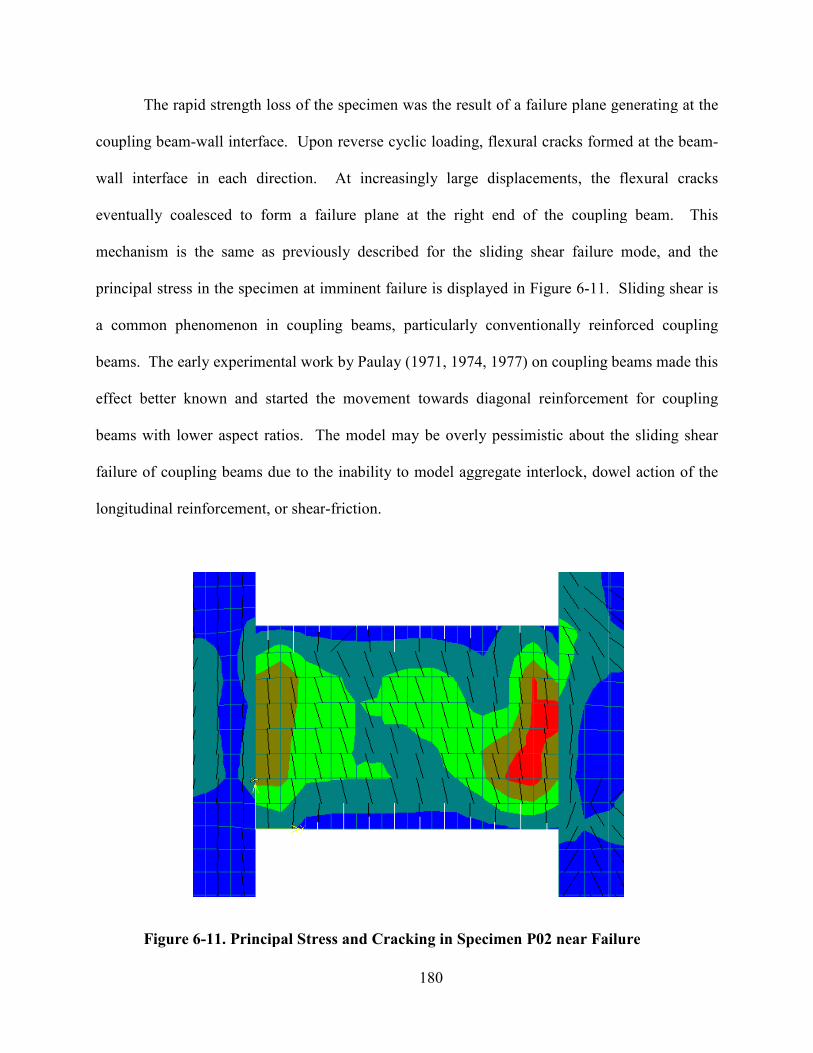
The rapid strength loss of the specimen was the result of a failure plane generating at the
coupling beam-wall interface. Upon rever
wall interface in each direction. At increasingly large displacements, the flexural cracks
eventually coalesced to form a failure plane at the right end of the coupling beam. This
mechanism is the same as previously
principal stress in the specimen at imminent failure is displayed in
a common phenomenon in coupling beams, particularly conventi
beams. The early experimental work by Paulay
effect better known and started the
beams with lower aspect ratios.
failure of coupling beams due to the inability to model aggregate interlock, dowel action of the
longitudinal reinforcement, or shear
Figure 6-11. Principal Stres
180
The rapid strength loss of the specimen was the result of a failure plane generating at the
wall interface. Upon reverse cyclic loading, flexural cracks formed at the beam
wall interface in each direction. At increasingly large displacements, the flexural cracks
form a failure plane at the right end of the coupling beam. This
previously described for the sliding shear failure mode, and the
principal stress in the specimen at imminent failure is displayed in Figure 6-11.
a common phenomenon in coupling beams, particularly conventionally reinforced coupling
beams. The early experimental work by Paulay (1971, 1974, 1977) on coupling beams made this
known and started the movement towards diagonal reinforcement for coupling
The model may be overly pessimistic about the sliding shear
failure of coupling beams due to the inability to model aggregate interlock, dowel action of the
longitudinal reinforcement, or shear-friction.
incipal Stress and Cracking in Specimen P02 near Failure
The rapid strength loss of the specimen was the result of a failure plane generating at the
se cyclic loading, flexural cracks formed at the beam-
wall interface in each direction. At increasingly large displacements, the flexural cracks
form a failure plane at the right end of the coupling beam. This
described for the sliding shear failure mode, and the
. Sliding shear is
onally reinforced coupling
on coupling beams made this
diagonal reinforcement for coupling
be overly pessimistic about the sliding shear
failure of coupling beams due to the inability to model aggregate interlock, dowel action of the
Failure
181
The final coupling beam modeled in this portion of the study that was tested by Galano
and Vignoli (2000) is Specimen P07. This specimen is identical to the diagonally reinforced
Specimen P05; however, reverse cyclic displacement were imposed on the specimen. The cyclic
loading applied to this specimen followed the same displacement protocol as in the
conventionally reinforced Specimen P02. The displacement and shear force at the initial
yielding of the primary reinforcement were within 6% and 8% of the experimental values,
respectively. Also, peak strength was predicted to within 1% of the experimental value;
however, the peak value occurred at a drift of 20% less than experienced in the laboratory. The
trend of the model accurately capturing the strength and performing well at the early stages of
the experiment continued, but as the displacements increased, the model typically lost its
capacity more rapidly than the experiment. At the 2δy displacement level, the model began to
soften relative to the laboratory test. The experiment maintained about 94% of its peak capacity,
and the model only maintained 68%. At the 3δy displacement level, the experiment had reduced
to 58% of its peak capacity, and the model had reduced to 38%. While this is still less than the
experimental value, the model did more accurately capture the later cycles. The applied shear
force versus displacement response of the experiment and ATENA model are plotted in Figure
6-12.
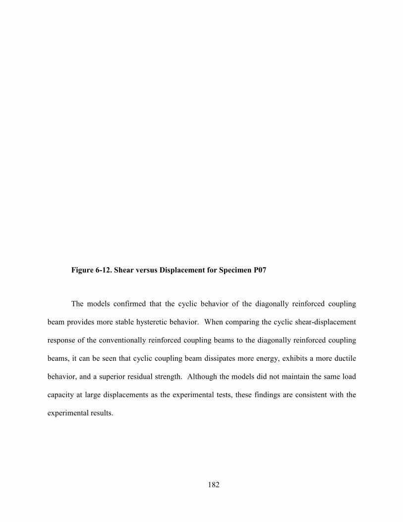
Figure 6-12. Shear versus Displacement for Specimen P07
The models confirmed that the cyclic behavior of the diagonally reinforced coupling
beam provides more stable hysteretic behavior. When comparing the cyclic shear
response of the conventionally reinforced coupling beams to the diagonally reinforced coupling
beams, it can be seen that cyclic coupling beam dissipates more energy, exhibits a more ductil
behavior, and a superior residual strength. Although the models did not maintain the same load
capacity at large displacements as the experimental tests, these findings are consistent with the
experimental results.
182
. Shear versus Displacement for Specimen P07
The models confirmed that the cyclic behavior of the diagonally reinforced coupling
hysteretic behavior. When comparing the cyclic shear
response of the conventionally reinforced coupling beams to the diagonally reinforced coupling
beams, it can be seen that cyclic coupling beam dissipates more energy, exhibits a more ductil
behavior, and a superior residual strength. Although the models did not maintain the same load
capacity at large displacements as the experimental tests, these findings are consistent with the
The models confirmed that the cyclic behavior of the diagonally reinforced coupling
hysteretic behavior. When comparing the cyclic shear-displacement
response of the conventionally reinforced coupling beams to the diagonally reinforced coupling
beams, it can be seen that cyclic coupling beam dissipates more energy, exhibits a more ductile
behavior, and a superior residual strength. Although the models did not maintain the same load
capacity at large displacements as the experimental tests, these findings are consistent with the
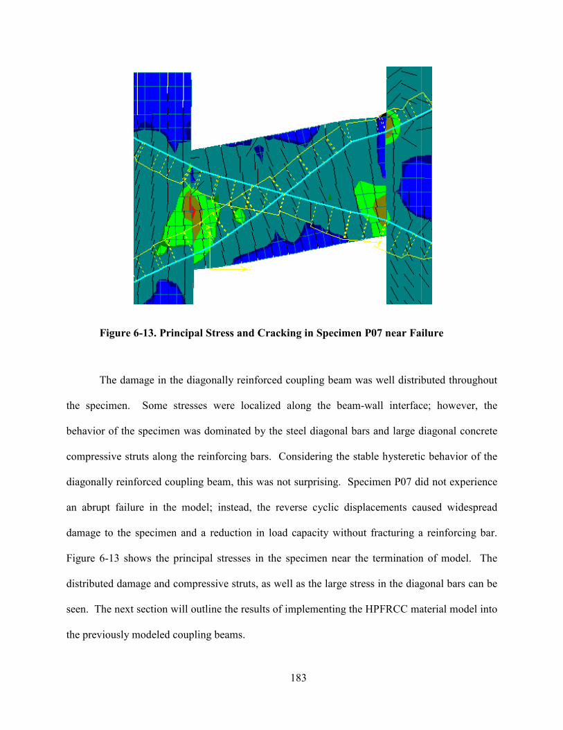
Figure 6-13. Principal Stress and Cracking in Specimen P07 near Failure
The damage in the diagonally reinforced coupling beam was well distributed throughout
the specimen. Some stresses were localized along the beam
behavior of the specimen was dominated by the steel diagonal bars and large diagonal concrete
compressive struts along the reinforcing bars. Considering the stable hysteretic behavior of the
diagonally reinforced coupling beam, this was not surprising.
an abrupt failure in the model; instead, the reverse cyclic displacements caused widespread
damage to the specimen and a reduction in load capacity without fracturing a reinforcing bar.
Figure 6-13 shows the principal stresses in the specimen near the termination of model. The
distributed damage and compressive struts, as well as the large stress in the diagonal bars can be
seen. The next section will outline the results of implementing the HPFR
the previously modeled coupling beams.
183
. Principal Stress and Cracking in Specimen P07 near Failure
The damage in the diagonally reinforced coupling beam was well distributed throughout
the specimen. Some stresses were localized along the beam-wall interface; however, t
behavior of the specimen was dominated by the steel diagonal bars and large diagonal concrete
compressive struts along the reinforcing bars. Considering the stable hysteretic behavior of the
diagonally reinforced coupling beam, this was not surprising. Specimen P07 did not experience
an abrupt failure in the model; instead, the reverse cyclic displacements caused widespread
damage to the specimen and a reduction in load capacity without fracturing a reinforcing bar.
shows the principal stresses in the specimen near the termination of model. The
distributed damage and compressive struts, as well as the large stress in the diagonal bars can be
The next section will outline the results of implementing the HPFRCC material model into
the previously modeled coupling beams.
. Principal Stress and Cracking in Specimen P07 near Failure
The damage in the diagonally reinforced coupling beam was well distributed throughout
wall interface; however, the
behavior of the specimen was dominated by the steel diagonal bars and large diagonal concrete
compressive struts along the reinforcing bars. Considering the stable hysteretic behavior of the
Specimen P07 did not experience
an abrupt failure in the model; instead, the reverse cyclic displacements caused widespread
damage to the specimen and a reduction in load capacity without fracturing a reinforcing bar.
shows the principal stresses in the specimen near the termination of model. The
distributed damage and compressive struts, as well as the large stress in the diagonal bars can be
CC material model into
184
6.2.2 RC Coupling Beam Parametric Study
The RC coupling beams by Galano and Vignoli (2000) modeled in the preceding section
were next modeled with HPFRCC. Since the cyclic behavior of HPFRCC has not yet been
evaluated and this is the first effort to implement the HPFRCC model into a structural
component, only the monotonically loaded specimens, P01 and P05, were explored for this
parametric study. The compressive strength of the concrete in P01 and P05 was 7.09 ksi (48.9
MPa) and 5.78 ksi (39.9 MPa). Both of these compressive strengths exceed the compressive
strength of NM6, which was 4.76 ksi (32.8 MPa), but the modeling approach for this portion of
the research was to investigate the effect of implementing the exact NM6 model developed in
Chapter 4 into the RC coupling beams. The cyclic properties of the HPFRCC would be
evaluated in the next phase of the modeling program when the HPFRCC coupling beams by
Lequesne (2011) were investigated.
First, Specimen P01 was modeled. The NM6 HPFRCC model was applied only to the
coupling beam elements, and the adjacent wall blocks maintained their original properties. The
same boundary conditions, solution parameters, and loading were implemented. The evaluation
of the research by Chao et al. (2009) led to the enhancement of the maximum permissible bond
strength, and the remainder of the configuration of the model was identical to the version with an
RC coupling beam.
The shear versus displacement response of the HPFRCC coupling beam relative to the
RC coupling beam results is displayed in Figure 6-14. The marked difference in the behavior is
immediately apparent. The HPFRCC coupling beam experienced a much larger load before
cracking initiated in the specimen. Additionally, the capacity was increased by about 40%, while
the deformation capacity of the coupling beam was increased by about 50%. These considerable
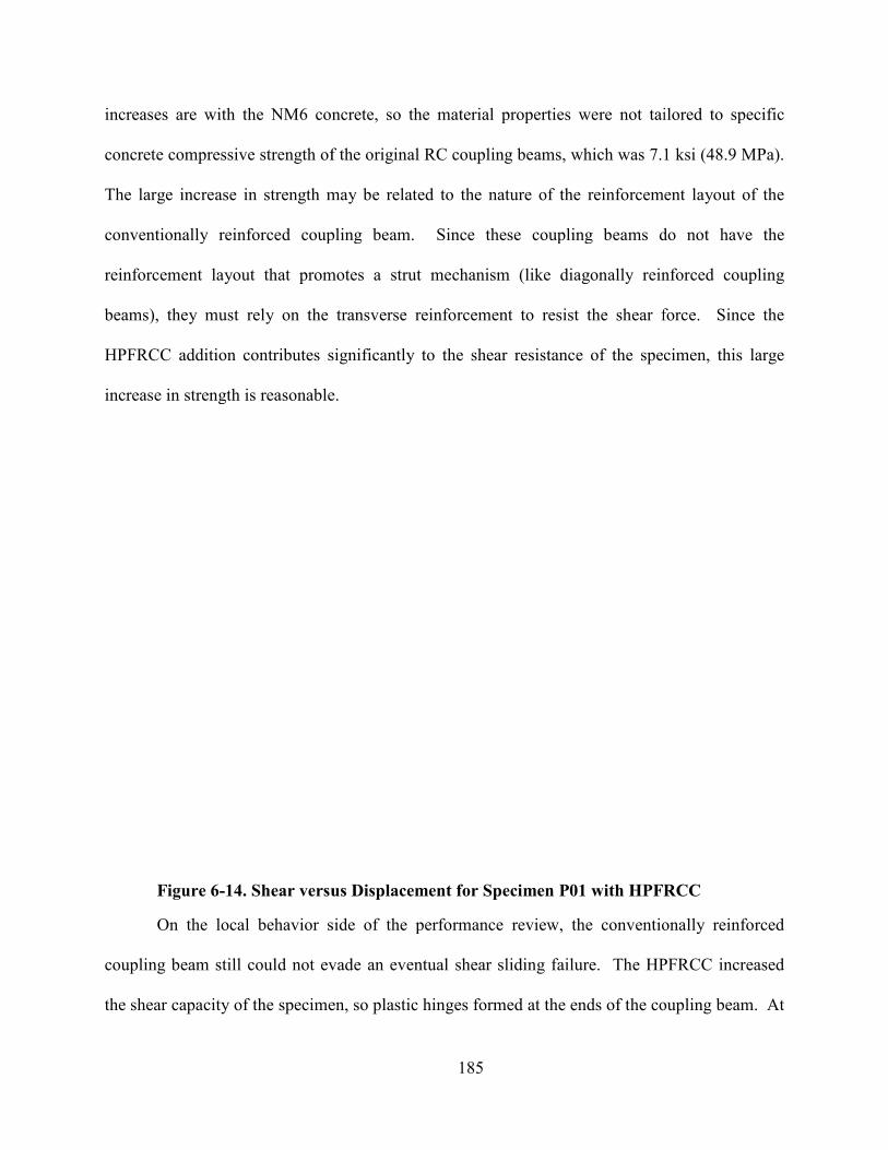
increases are with the NM6 concrete, so the material properties were not tailored to specific
concrete compressive strength of the original RC coupling beams, which was 7.1 ksi (48.9 MPa).
The large increase in strength may be related to the nature of the reinforcement layout of the
conventionally reinforced coupling beam. Since these coupling beams do not have the
reinforcement layout that promotes a strut mechanism (like diagonally reinforced coupling
beams), they must rely on the transverse reinforcement to resist the shear force. Since the
HPFRCC addition contributes significantly
increase in strength is reasonable.
Figure 6-14. Shear versus Displacement for Specimen P01 with HPFRCC
On the local behavior side of the performance review, the conventionally reinforced
coupling beam still could not evade an eventual shear sliding failure. The HPFRCC increased
the shear capacity of the specimen, so plastic hinges formed at the ends of the coupling beam. At
185
increases are with the NM6 concrete, so the material properties were not tailored to specific
concrete compressive strength of the original RC coupling beams, which was 7.1 ksi (48.9 MPa).
strength may be related to the nature of the reinforcement layout of the
conventionally reinforced coupling beam. Since these coupling beams do not have the
reinforcement layout that promotes a strut mechanism (like diagonally reinforced coupling
they must rely on the transverse reinforcement to resist the shear force. Since the
significantly to the shear resistance of the specimen, this large
increase in strength is reasonable.
. Shear versus Displacement for Specimen P01 with HPFRCC
On the local behavior side of the performance review, the conventionally reinforced
coupling beam still could not evade an eventual shear sliding failure. The HPFRCC increased
e shear capacity of the specimen, so plastic hinges formed at the ends of the coupling beam. At
increases are with the NM6 concrete, so the material properties were not tailored to specific
concrete compressive strength of the original RC coupling beams, which was 7.1 ksi (48.9 MPa).
strength may be related to the nature of the reinforcement layout of the
conventionally reinforced coupling beam. Since these coupling beams do not have the
reinforcement layout that promotes a strut mechanism (like diagonally reinforced coupling
they must rely on the transverse reinforcement to resist the shear force. Since the
to the shear resistance of the specimen, this large
. Shear versus Displacement for Specimen P01 with HPFRCC
On the local behavior side of the performance review, the conventionally reinforced
coupling beam still could not evade an eventual shear sliding failure. The HPFRCC increased
e shear capacity of the specimen, so plastic hinges formed at the ends of the coupling beam. At
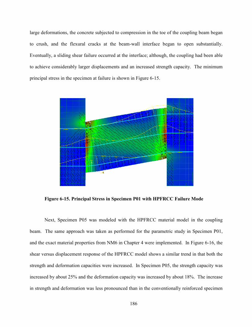
large deformations, the concrete subjected to compression in the toe of the coupling beam began
to crush, and the flexural cracks at the beam
Eventually, a sliding shear failure occurred at the interface; although, the coupling had been able
to achieve considerably larger displacements and an increased strength capacity. The minimum
principal stress in the specimen a
Figure 6-15. Principal Stress in
Next, Specimen P05 was modeled with the HPFRCC material model in the cou
beam. The same approach was taken as performed for the parametric study in Specimen P01,
and the exact material properties from NM6 in Chapter 4 were implemented. In
shear versus displacement response of t
strength and deformation capacities were increased. In Specimen P05, the strength capacity was
increased by about 25% and the deformation capacity was increased by about 18%.
in strength and deformation was less pronounced than in the conventionally reinforced specimen
186
large deformations, the concrete subjected to compression in the toe of the coupling beam began
to crush, and the flexural cracks at the beam-wall interface began to open substantially.
Eventually, a sliding shear failure occurred at the interface; although, the coupling had been able
to achieve considerably larger displacements and an increased strength capacity. The minimum
principal stress in the specimen at failure is shown in Figure 6-15.
Principal Stress in Specimen P01 with HPFRCC Failure Mode
Next, Specimen P05 was modeled with the HPFRCC material model in the cou
beam. The same approach was taken as performed for the parametric study in Specimen P01,
and the exact material properties from NM6 in Chapter 4 were implemented. In
shear versus displacement response of the HPFRCC model shows a similar trend in that both the
strength and deformation capacities were increased. In Specimen P05, the strength capacity was
increased by about 25% and the deformation capacity was increased by about 18%.
and deformation was less pronounced than in the conventionally reinforced specimen
large deformations, the concrete subjected to compression in the toe of the coupling beam began
gan to open substantially.
Eventually, a sliding shear failure occurred at the interface; although, the coupling had been able
to achieve considerably larger displacements and an increased strength capacity. The minimum
Specimen P01 with HPFRCC Failure Mode
Next, Specimen P05 was modeled with the HPFRCC material model in the coupling
beam. The same approach was taken as performed for the parametric study in Specimen P01,
and the exact material properties from NM6 in Chapter 4 were implemented. In Figure 6-16, the
he HPFRCC model shows a similar trend in that both the
strength and deformation capacities were increased. In Specimen P05, the strength capacity was
increased by about 25% and the deformation capacity was increased by about 18%. The increase
and deformation was less pronounced than in the conventionally reinforced specimen
most likely as a result of the reinforcement layout. In diagonally reinforced coupling beams, the
behavior is largely controlled by the diagonal reinforcing bars. While t
did increase the shear capacity, the mechanism by which the majority of the force was resisted
was still through a compressive strut aligned along the length of the reinforcement.
Figure 6-16. Shear versus Displacement for Specimen P05 with HPFRCC
The diagonal compressive strut at peak load can be seen in the image on the left in
6-17. It shows a clear diagonal compression, with some flexural crack
wall interface. However, as before, Specimen P05 with HPFRCC experienced the same sliding
shear failure once the damage accumulated at the beam
was also the eventual failure mode of the H
187
most likely as a result of the reinforcement layout. In diagonally reinforced coupling beams, the
behavior is largely controlled by the diagonal reinforcing bars. While the addition of the fibers
did increase the shear capacity, the mechanism by which the majority of the force was resisted
was still through a compressive strut aligned along the length of the reinforcement.
. Shear versus Displacement for Specimen P05 with HPFRCC
The diagonal compressive strut at peak load can be seen in the image on the left in
. It shows a clear diagonal compression, with some flexural cracks developing at the beam
wall interface. However, as before, Specimen P05 with HPFRCC experienced the same sliding
shear failure once the damage accumulated at the beam-wall interface. The sliding shear failure
was also the eventual failure mode of the HPFRCC coupling beams tested by Lequesne
most likely as a result of the reinforcement layout. In diagonally reinforced coupling beams, the
he addition of the fibers
did increase the shear capacity, the mechanism by which the majority of the force was resisted
was still through a compressive strut aligned along the length of the reinforcement.
. Shear versus Displacement for Specimen P05 with HPFRCC
The diagonal compressive strut at peak load can be seen in the image on the left in Figure
s developing at the beam-
wall interface. However, as before, Specimen P05 with HPFRCC experienced the same sliding
wall interface. The sliding shear failure
PFRCC coupling beams tested by Lequesne (2011),
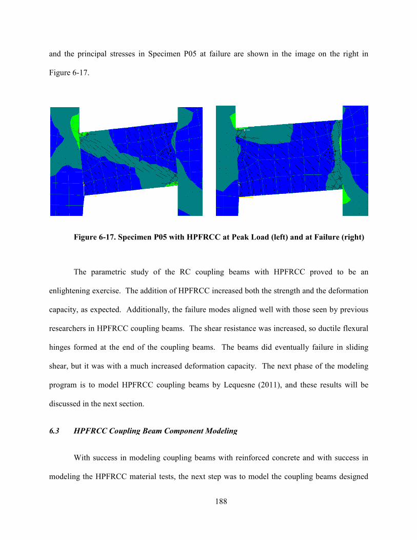
and the principal stresses in Specimen P05 at failure are shown in the image on the right in
Figure 6-17.
Figure 6-17. Specimen P05 with HPFRCC at Peak Load (left) and at Failure (right)
The parametric study of the RC coupling beams with HPFRCC proved to be an
enlightening exercise. The addition of HPFRCC increased both the strength and t
capacity, as expected. Additionally, the failure modes aligned well with those seen by previous
researchers in HPFRCC coupling beams. The shear resistance was increased, so ductile flexural
hinges formed at the end of the coupling beams.
shear, but it was with a much increased
program is to model HPFRCC coupling beams by Lequesne
discussed in the next section.
6.3 HPFRCC Coupling Beam Component Modeling
With success in modeling coupling beams with reinforced concrete and with success in
modeling the HPFRCC material tests, the next step
188
and the principal stresses in Specimen P05 at failure are shown in the image on the right in
. Specimen P05 with HPFRCC at Peak Load (left) and at Failure (right)
The parametric study of the RC coupling beams with HPFRCC proved to be an
enlightening exercise. The addition of HPFRCC increased both the strength and t
capacity, as expected. Additionally, the failure modes aligned well with those seen by previous
researchers in HPFRCC coupling beams. The shear resistance was increased, so ductile flexural
hinges formed at the end of the coupling beams. The beams did eventually failure in sliding
shear, but it was with a much increased deformation capacity. The next phase of the modeling
program is to model HPFRCC coupling beams by Lequesne (2011), and these results
C Coupling Beam Component Modeling
With success in modeling coupling beams with reinforced concrete and with success in
C material tests, the next step was to model the coupling beams designed
and the principal stresses in Specimen P05 at failure are shown in the image on the right in
. Specimen P05 with HPFRCC at Peak Load (left) and at Failure (right)
The parametric study of the RC coupling beams with HPFRCC proved to be an
enlightening exercise. The addition of HPFRCC increased both the strength and the deformation
capacity, as expected. Additionally, the failure modes aligned well with those seen by previous
researchers in HPFRCC coupling beams. The shear resistance was increased, so ductile flexural
The beams did eventually failure in sliding
deformation capacity. The next phase of the modeling
, and these results will be
With success in modeling coupling beams with reinforced concrete and with success in
was to model the coupling beams designed
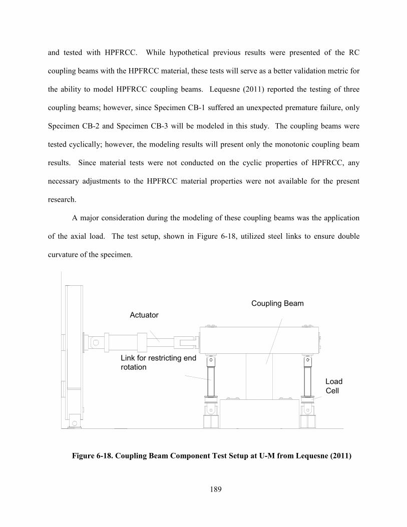
189
and tested with HPFRCC. While hypothetical previous results were presented of the RC
coupling beams with the HPFRCC material, these tests will serve as a better validation metric for
the ability to model HPFRCC coupling beams. Lequesne (2011) reported the testing of three
coupling beams; however, since Specimen CB-1 suffered an unexpected premature failure, only
Specimen CB-2 and Specimen CB-3 will be modeled in this study. The coupling beams were
tested cyclically; however, the modeling results will present only the monotonic coupling beam
results. Since material tests were not conducted on the cyclic properties of HPFRCC, any
necessary adjustments to the HPFRCC material properties were not available for the present
research.
A major consideration during the modeling of these coupling beams was the application
of the axial load. The test setup, shown in Figure 6-18, utilized steel links to ensure double
curvature of the specimen.
Figure 6-18. Coupling Beam Component Test Setup at U-M from Lequesne (2011)
Coupling Beam
Load Cell
Link for restricting end rotation
Actuator
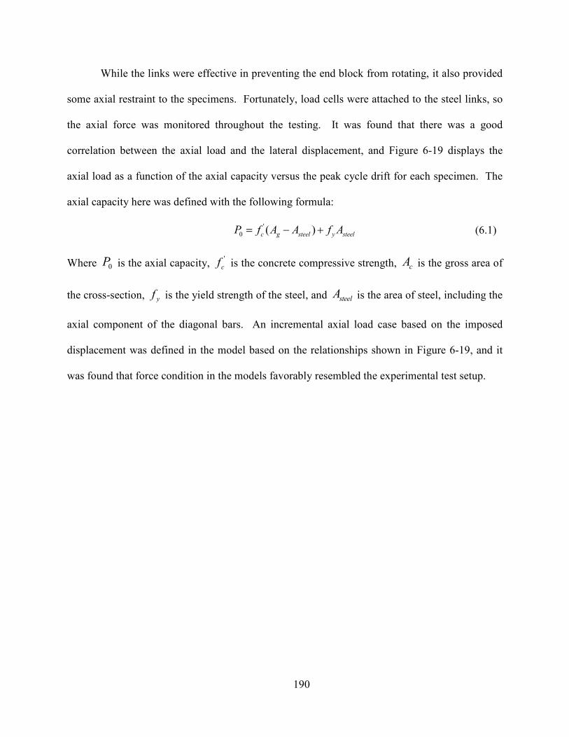
190
While the links were effective in preventing the end block from rotating, it also provided
some axial restraint to the specimens. Fortunately, load cells were attached to the steel links, so
the axial force was monitored throughout the testing. It was found that there was a good
correlation between the axial load and the lateral displacement, and Figure 6-19 displays the
axial load as a function of the axial capacity versus the peak cycle drift for each specimen. The
axial capacity here was defined with the following formula:
'
0 ( )c g steel y steel
P f A A f A= − + (6.1)
Where 0P is the axial capacity, '
cf is the concrete compressive strength, cA is the gross area of
the cross-section, yf is the yield strength of the steel, and steelA is the area of steel, including the
axial component of the diagonal bars. An incremental axial load case based on the imposed
displacement was defined in the model based on the relationships shown in Figure 6-19, and it
was found that force condition in the models favorably resembled the experimental test setup.
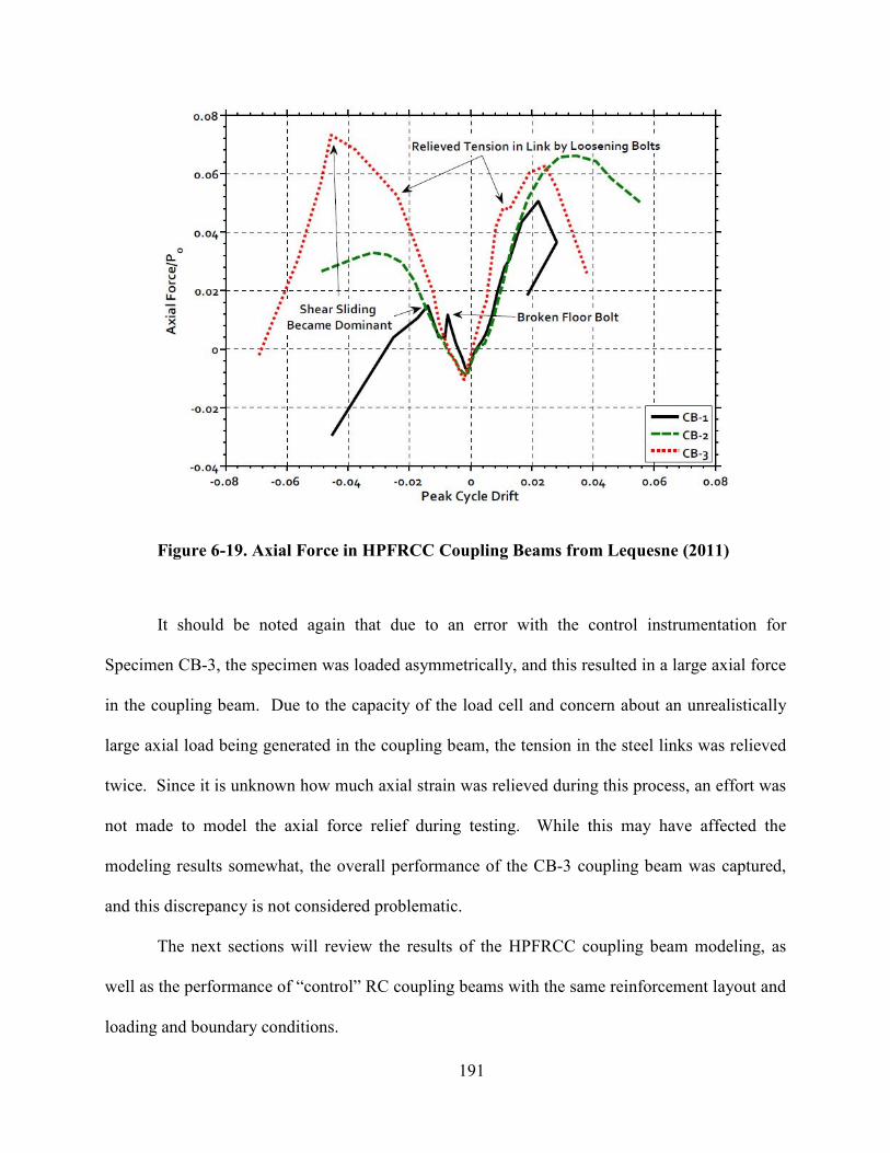
191
Figure 6-19. Axial Force in HPFRCC Coupling Beams from Lequesne (2011)
It should be noted again that due to an error with the control instrumentation for
Specimen CB-3, the specimen was loaded asymmetrically, and this resulted in a large axial force
in the coupling beam. Due to the capacity of the load cell and concern about an unrealistically
large axial load being generated in the coupling beam, the tension in the steel links was relieved
twice. Since it is unknown how much axial strain was relieved during this process, an effort was
not made to model the axial force relief during testing. While this may have affected the
modeling results somewhat, the overall performance of the CB-3 coupling beam was captured,
and this discrepancy is not considered problematic.
The next sections will review the results of the HPFRCC coupling beam modeling, as
well as the performance of “control” RC coupling beams with the same reinforcement layout and
loading and boundary conditions.
6.3.1 HPFRCC Coupling Beam Modeling Results
The HPFRCC coupling beam models had a similar boundary condition
RC coupling beam models: the left wall block was restrained on the top and bottom against
vertical movement, the right wall block was restrained against lateral movement, and a vertical
incremental displacement was applied to the right wal
loading regime was the application of the axial load. The incremental axial load relationship was
developed as a function of the vertical displacement of the specimen.
function was developed based on the axial force
6-19. This function was developed such that at the appropriate axial force was applied to the
specimen for the given vertical displacement. The finite element
boundary conditions is depicted in
Figure 6-20. Specimen CB
192
HPFRCC Coupling Beam Modeling Results
The HPFRCC coupling beam models had a similar boundary condition
RC coupling beam models: the left wall block was restrained on the top and bottom against
vertical movement, the right wall block was restrained against lateral movement, and a vertical
incremental displacement was applied to the right wall block. The only real difference to the
loading regime was the application of the axial load. The incremental axial load relationship was
developed as a function of the vertical displacement of the specimen. A piecewise linear
sed on the axial force-peak cycle drift relationship shown in
. This function was developed such that at the appropriate axial force was applied to the
specimen for the given vertical displacement. The finite element model with the loading and
boundary conditions is depicted in Figure 6-20.
. Specimen CB-2 Model with Loading and Boundary Conditions
The HPFRCC coupling beam models had a similar boundary condition as the previous
RC coupling beam models: the left wall block was restrained on the top and bottom against
vertical movement, the right wall block was restrained against lateral movement, and a vertical
l block. The only real difference to the
loading regime was the application of the axial load. The incremental axial load relationship was
A piecewise linear
peak cycle drift relationship shown in Figure
. This function was developed such that at the appropriate axial force was applied to the
model with the loading and
2 Model with Loading and Boundary Conditions
193
For the modeling results, the specimens were loaded monotonically since the cyclic
properties of the HPFRCC were unknown. An envelope of the cyclic response of the laboratory
tests was generated, and the monotonic results were compared to the envelope. Although the
HPFRCC material implemented into the experimental tests was the same NM6 described in
Chapter 4, the compressive strength of the concrete in Specimen CB-2 was 7.5 ksi (52 MPa) at
the time of testing. Since the compressive strength in the material model is a function of the
percentage of the peak compressive strength versus strain, the compressive relationship was only
modified by increasing the peak compressive strength of the HPFRCC material to match the
experiment. Since the tensile strength is more a function of the fibers and the volume fraction,
the tensile properties remained unchanged. The initial stiffness of the model aligned will with
the laboratory test; however, the onset of damage was delayed in the model relative to the
experiment. This delay in the onset of damage in the model may be related to softening of the
experiment due to the cyclic loading, while the model was only loaded monotonically. The
experiment began to soften, and initial yielding of the primary reinforcement occurred at a shear
force of 96.4 kips (429 kN ). In the model, the response of the specimen did not begin to soften
until reinforcement yielded at 112 kips (499 kN). Thus, the shear force at first yielding was over
predicted by about 16%, while the displacement at first yielding was under predicted by about
13%. The peak strength and displacement were much more closely predicted; the peak strength
was within 3% of the laboratory test and the displacement at the peak strength was within 1% of
the experiment. Finally, the displacement and strength at failure were quite close to the
experimental test. The shear versus displacement response of the model relative to the envelope
of the experiment is displayed in Figure 6-21.
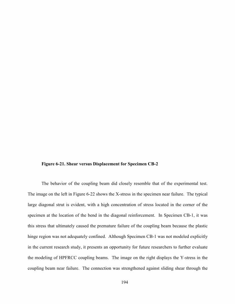
Figure 6-21. Shear versus Displacement for Specimen CB
The behavior of the coupling beam did closely resemble that of the experimental test.
The image on the left in Figure 6
large diagonal strut is evident, with a high concentration of stress located in the corner of the
specimen at the location of the bend in the diagonal reinforcement. In Specimen CB
this stress that ultimately caused the pr
hinge region was not adequately confined.
in the current research study, it presents an opportunity for future researchers to further evaluate
the modeling of HPFRCC coupling beams.
coupling beam near failure. The connection was strengthened against sliding shear through the
194
. Shear versus Displacement for Specimen CB-2
The behavior of the coupling beam did closely resemble that of the experimental test.
6-22 shows the X-stress in the specimen near failure. The typical
large diagonal strut is evident, with a high concentration of stress located in the corner of the
specimen at the location of the bend in the diagonal reinforcement. In Specimen CB
this stress that ultimately caused the premature failure of the coupling beam because the plastic
hinge region was not adequately confined. Although Specimen CB-1 was not modeled explicitly
in the current research study, it presents an opportunity for future researchers to further evaluate
odeling of HPFRCC coupling beams. The image on the right displays the
coupling beam near failure. The connection was strengthened against sliding shear through the
The behavior of the coupling beam did closely resemble that of the experimental test.
failure. The typical
large diagonal strut is evident, with a high concentration of stress located in the corner of the
specimen at the location of the bend in the diagonal reinforcement. In Specimen CB-1, it was
emature failure of the coupling beam because the plastic
1 was not modeled explicitly
in the current research study, it presents an opportunity for future researchers to further evaluate
The image on the right displays the Y-stress in the
coupling beam near failure. The connection was strengthened against sliding shear through the

addition of U-shaped dowel bars at the beam
(152 mm) into the coupling beam, and this localization of stress can be seen on the right in
Figure 6-22. The subsequent beam utilized straight dowel bars in an effort to prevent this
immediate drop in capacity. In any event, this Specimen CB
mode due to the localized damage at the interface, which resembles the eventual failure in the
experimental test.
Figure 6-22. X-Stress (left) and Y
Figure 6-23 shows the shear stress in the specimen near failure. The shear stress shows a
clear compressive strut along the diagonal in the coupling beam, as well as
cracks in the beam with the shear stress.
195
shaped dowel bars at the beam-wall interface. The U-shaped bar terminated 6 in.
(152 mm) into the coupling beam, and this localization of stress can be seen on the right in
The subsequent beam utilized straight dowel bars in an effort to prevent this
ty. In any event, this Specimen CB-2 experienced the same failure
mode due to the localized damage at the interface, which resembles the eventual failure in the
ess (left) and Y-Stress (right) in Specimen CB-2 near Failure
shows the shear stress in the specimen near failure. The shear stress shows a
clear compressive strut along the diagonal in the coupling beam, as well as the alignment of the
cracks in the beam with the shear stress.
bar terminated 6 in.
(152 mm) into the coupling beam, and this localization of stress can be seen on the right in
The subsequent beam utilized straight dowel bars in an effort to prevent this
2 experienced the same failure
mode due to the localized damage at the interface, which resembles the eventual failure in the
2 near Failure
shows the shear stress in the specimen near failure. The shear stress shows a
the alignment of the
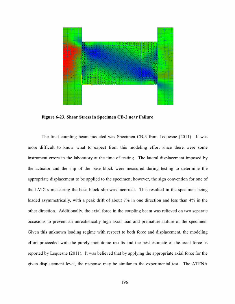
Figure 6-23. Shear Stress in Specimen CB
The final coupling beam modeled was Specimen CB
more difficult to know what to expect from this modeling effort since there were some
instrument errors in the laboratory at the time of testing. The lateral displacement imposed by
the actuator and the slip of the base bl
appropriate displacement to be applied to the specimen; however, the sign convention for one of
the LVDTs measuring the base block slip was incorrect. This resulted in the specimen being
loaded asymmetrically, with a peak drift of about 7% in one direction and less than 4% in the
other direction. Additionally, the axial force in the coupling beam was relieved on two separate
occasions to prevent an unrealistically high axial load and premature failure of t
Given this unknown loading regime
effort proceeded with the purely monotonic results
reported by Lequesne (2011). It was believed that by applying the appropriate axial force for the
given displacement level, the response may be similar to the experimental test. The ATENA
196
. Shear Stress in Specimen CB-2 near Failure
The final coupling beam modeled was Specimen CB-3 from Lequesne
more difficult to know what to expect from this modeling effort since there were some
instrument errors in the laboratory at the time of testing. The lateral displacement imposed by
the actuator and the slip of the base block were measured during testing to determine the
appropriate displacement to be applied to the specimen; however, the sign convention for one of
the LVDTs measuring the base block slip was incorrect. This resulted in the specimen being
lly, with a peak drift of about 7% in one direction and less than 4% in the
Additionally, the axial force in the coupling beam was relieved on two separate
occasions to prevent an unrealistically high axial load and premature failure of t
Given this unknown loading regime with respect to both force and displacement
effort proceeded with the purely monotonic results and the best estimate of the axial force as
. It was believed that by applying the appropriate axial force for the
given displacement level, the response may be similar to the experimental test. The ATENA
3 from Lequesne (2011). It was
more difficult to know what to expect from this modeling effort since there were some
instrument errors in the laboratory at the time of testing. The lateral displacement imposed by
ock were measured during testing to determine the
appropriate displacement to be applied to the specimen; however, the sign convention for one of
the LVDTs measuring the base block slip was incorrect. This resulted in the specimen being
lly, with a peak drift of about 7% in one direction and less than 4% in the
Additionally, the axial force in the coupling beam was relieved on two separate
occasions to prevent an unrealistically high axial load and premature failure of the specimen.
with respect to both force and displacement, the modeling
and the best estimate of the axial force as
. It was believed that by applying the appropriate axial force for the
given displacement level, the response may be similar to the experimental test. The ATENA
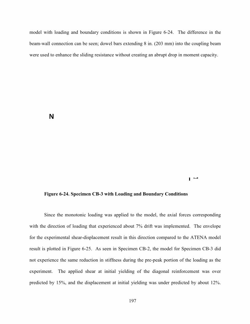
model with loading and boundary conditions is shown in
beam-wall connection can be seen; dowel bars extending 8 in. (203 mm) into the coupling beam
were used to enhance the sliding resistance without creating a
Figure 6-24. Specimen CB
Since the monotonic loading was applied to the model, the axial forces corresponding
with the direction of loading that experienced about 7% drift was implemented. The envel
for the experimental shear-displacement result in this direction compared to the ATENA model
result is plotted in Figure 6-25.
not experience the same reduction in sti
experiment. The applied shear at initial yielding of the diagonal reinforcement was
predicted by 15%, and the displacement at initial yielding was
197
model with loading and boundary conditions is shown in Figure 6-24. The difference in the
wall connection can be seen; dowel bars extending 8 in. (203 mm) into the coupling beam
were used to enhance the sliding resistance without creating an abrupt drop in moment capacity.
. Specimen CB-3 with Loading and Boundary Conditions
Since the monotonic loading was applied to the model, the axial forces corresponding
with the direction of loading that experienced about 7% drift was implemented. The envel
displacement result in this direction compared to the ATENA model
. As seen in Specimen CB-2, the model for Specimen CB
t experience the same reduction in stiffness during the pre-peak portion of the loading as the
experiment. The applied shear at initial yielding of the diagonal reinforcement was
by 15%, and the displacement at initial yielding was under predicted
. The difference in the
wall connection can be seen; dowel bars extending 8 in. (203 mm) into the coupling beam
n abrupt drop in moment capacity.
3 with Loading and Boundary Conditions
Since the monotonic loading was applied to the model, the axial forces corresponding
with the direction of loading that experienced about 7% drift was implemented. The envelope
displacement result in this direction compared to the ATENA model
Specimen CB-3 did
peak portion of the loading as the
experiment. The applied shear at initial yielding of the diagonal reinforcement was over
under predicted by about 12%.
198
This may be due to a shortcoming in the model and/or the experimental effects of both the
asymmetric loading and the unrecorded large axial force in the experiment. Also, the early
softening of the experiment may have been related to the cyclic loading of the experiment
compared to the monotonic loading of the model. The peak load of the model did closely
capture that observed in the experiment, and it was within 4%; however, the corresponding drift
at the peak load was under predicted by 25% in the model. The nature of the unknown loading
in the experiment makes it difficult to more closely model the experimental response. The initial
softening of the specimen could be the result of the large axial force generated, and the
subsequent release of axial strain and relaxation of the specimen may have allowed the large
displacement. The displacement at which a 15% reduction in the peak load occurred was
predicted within about 7% by the model. Near failure, the model experienced an explosive
event, and the capacity dropped rather rapidly, while the experiment demonstrated a more
gradual decrease in capacity.
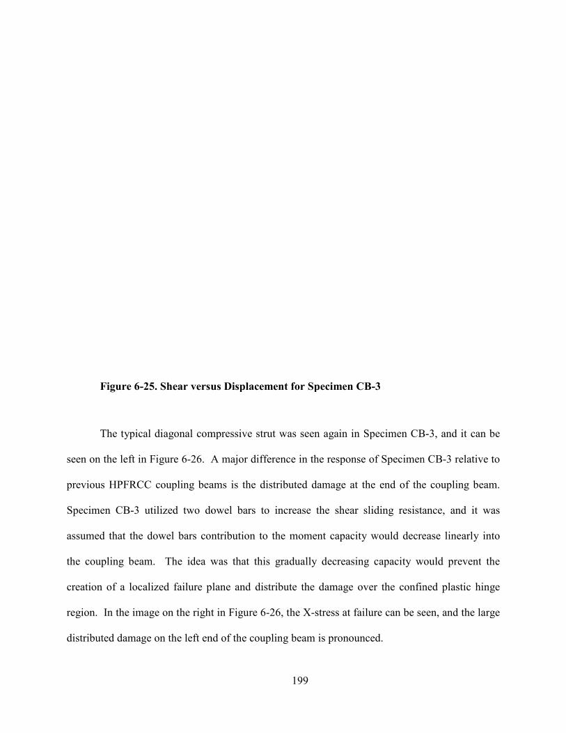
Figure 6-25. Shear versus Displacement for Specimen CB
The typical diagonal compressive strut was seen again in Sp
seen on the left in Figure 6-26. A major difference in the response of Specimen CB
previous HPFRCC coupling beams is the distributed damage at the end of the coupling beam.
Specimen CB-3 utilized two dowel bars to increase the shear sliding resistance, and it was
assumed that the dowel bars contribution to the moment capacity would decrease linearly into
the coupling beam. The idea was that this gradually decreasing capacity would prevent
creation of a localized failure plane and distribute the damage over the confined plastic hinge
region. In the image on the right in
distributed damage on the left end of the coupling beam is pronounced.
199
. Shear versus Displacement for Specimen CB-3
The typical diagonal compressive strut was seen again in Specimen CB
. A major difference in the response of Specimen CB
previous HPFRCC coupling beams is the distributed damage at the end of the coupling beam.
utilized two dowel bars to increase the shear sliding resistance, and it was
assumed that the dowel bars contribution to the moment capacity would decrease linearly into
the coupling beam. The idea was that this gradually decreasing capacity would prevent
creation of a localized failure plane and distribute the damage over the confined plastic hinge
region. In the image on the right in Figure 6-26, the X-stress at failure can be seen, and the large
eft end of the coupling beam is pronounced.
ecimen CB-3, and it can be
. A major difference in the response of Specimen CB-3 relative to
previous HPFRCC coupling beams is the distributed damage at the end of the coupling beam.
utilized two dowel bars to increase the shear sliding resistance, and it was
assumed that the dowel bars contribution to the moment capacity would decrease linearly into
the coupling beam. The idea was that this gradually decreasing capacity would prevent the
creation of a localized failure plane and distribute the damage over the confined plastic hinge
stress at failure can be seen, and the large
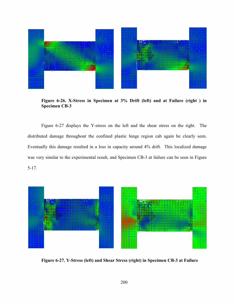
Figure 6-26. X-Stress in Specimen at 3% Drift (left) and at Failure (right ) in
Specimen CB-3
Figure 6-27 displays the Y
distributed damage throughout the confined plastic hinge region cab again be clearly seen.
Eventually this damage resulted in a loss in capacity around 4% drift. This localized damage
was very similar to the experimental result, and Specimen CB
5-17.
Figure 6-27. Y-Stress (left) and Shear Stress (right) in Specimen CB
200
Stress in Specimen at 3% Drift (left) and at Failure (right ) in
displays the Y-stress on the left and the shear stress on the right. The
distributed damage throughout the confined plastic hinge region cab again be clearly seen.
Eventually this damage resulted in a loss in capacity around 4% drift. This localized damage
o the experimental result, and Specimen CB-3 at failure can be seen in
Stress (left) and Shear Stress (right) in Specimen CB-
Stress in Specimen at 3% Drift (left) and at Failure (right ) in
on the left and the shear stress on the right. The
distributed damage throughout the confined plastic hinge region cab again be clearly seen.
Eventually this damage resulted in a loss in capacity around 4% drift. This localized damage
3 at failure can be seen in Figure
-3 at Failure
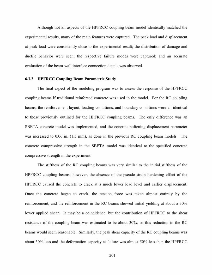
201
Although not all aspects of the HPFRCC coupling beam model identically matched the
experimental results, many of the main features were captured. The peak load and displacement
at peak load were consistently close to the experimental result; the distribution of damage and
ductile behavior were seen; the respective failure modes were captured; and an accurate
evaluation of the beam-wall interface connection details was observed.
6.3.2 HPFRCC Coupling Beam Parametric Study
The final aspect of the modeling program was to assess the response of the HPFRCC
coupling beams if traditional reinforced concrete was used in the model. For the RC coupling
beams, the reinforcement layout, loading conditions, and boundary conditions were all identical
to those previously outlined for the HPFRCC coupling beams. The only difference was an
SBETA concrete model was implemented, and the concrete softening displacement parameter
was increased to 0.06 in. (1.5 mm), as done in the previous RC coupling beam models. The
concrete compressive strength in the SBETA model was identical to the specified concrete
compressive strength in the experiment.
The stiffness of the RC coupling beams was very similar to the initial stiffness of the
HPFRCC coupling beams; however, the absence of the pseudo-strain hardening effect of the
HPFRCC caused the concrete to crack at a much lower load level and earlier displacement.
Once the concrete began to crack, the tension force was taken almost entirely by the
reinforcement, and the reinforcement in the RC beams showed initial yielding at about a 30%
lower applied shear. It may be a coincidence, but the contribution of HPFRCC to the shear
resistance of the coupling beam was estimated to be about 30%, so this reduction in the RC
beams would seem reasonable. Similarly, the peak shear capacity of the RC coupling beams was
about 30% less and the deformation capacity at failure was almost 50% less than the HPFRCC

coupling beams. The shear versus displacement result of Specimen CB
are shown in Figure 6-28 and Figure
Figure 6-28. Shear versus Displacement Response of CB
Figure 6-29. Shear versus Displacement Response of CB
202
coupling beams. The shear versus displacement result of Specimen CB-2 and Specimen CB
Figure 6-29, respectively.
. Shear versus Displacement Response of CB-2 Specimen with RC
. Shear versus Displacement Response of CB-3 Specimen with RC
2 and Specimen CB-3
2 Specimen with RC
3 Specimen with RC
203
The parametric study involving the application of RC to the HPFRCC coupling beams
demonstrates several benefits of HPFRCC in the design of coupling beams. The increased shear
strength from the use of HPFRCC may allow a designer to permit a larger maximum coupling
beam shear stress, to reduce the reinforcement required, or to reduce the size of the coupling
beam. Also, the increased deformation capacity may allow a ductile structural system
performance in the event of an earthquake. A focus of this research was to provide a method to
assess the performance-based design implications of adding HPFRCC to a damage-critical
member, and both the laboratory tests and the subsequent modeling effort illustrate clear
application of HPFRCC and the resulting enhancement in the component response. The
performance of the models relative to the experimental tests is provided in a tabular format in the
next section.
6.4 Compiled Coupling Beam Model Performance Assessment
The models were evaluated through several global parameters: displacement capacity,
strength capacity, stiffness, and ductility. The experimental response for each of these evaluation
parameters was provided previously for each coupling beam modeled in Table 5-3. Table 6-1
and Table 6-2 provide the results discussed in this chapter for each of the evaluation parameters
obtained from the modeling research program, and comparisons of the ATENA results to the
experimental results were also included. Table 6-1 displays the results relating to strength and
stiffness, and Table 6-2 includes the results pertaining to displacement and ductility. In the
tables, the subscript “e” indicates an experimental result. The same definitions of the parameters
defined for Table 5-3 apply in the following two tables.
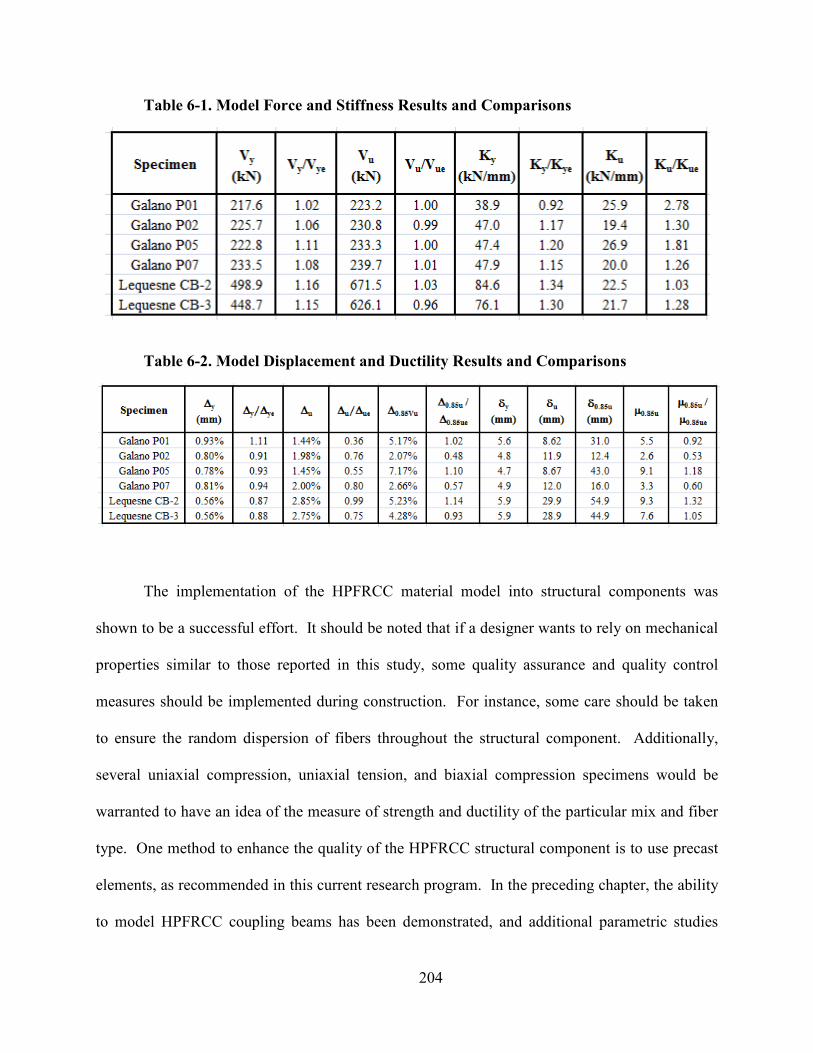
204
Table 6-1. Model Force and Stiffness Results and Comparisons
Table 6-2. Model Displacement and Ductility Results and Comparisons
The implementation of the HPFRCC material model into structural components was
shown to be a successful effort. It should be noted that if a designer wants to rely on mechanical
properties similar to those reported in this study, some quality assurance and quality control
measures should be implemented during construction. For instance, some care should be taken
to ensure the random dispersion of fibers throughout the structural component. Additionally,
several uniaxial compression, uniaxial tension, and biaxial compression specimens would be
warranted to have an idea of the measure of strength and ductility of the particular mix and fiber
type. One method to enhance the quality of the HPFRCC structural component is to use precast
elements, as recommended in this current research program. In the preceding chapter, the ability
to model HPFRCC coupling beams has been demonstrated, and additional parametric studies

205
were shown to illustrate the potential effect of including HPFRCC in regular RC coupling
beams. Similar parametric studies could be performed with varying levels of HPFRCC strength
and ductility for designers developing a unique mix. This overall modeling program is further
significant because if HPFRCC is to be embraced by the design community, an HPFRCC model
must be available that can be readily integrated into commercially available software. While
some open-source nonlinear platforms have received considerable research attention, it will most
likely be through commercially available software where the design community can conduct its
own parametric studies on the effects of HPFRCC when considering it as a viable alternative to
the design of damage-critical structural components.
206
CHAPTER 7. BACKGROUD AD EXPERIMETAL PLA FOR PILE-
WHARF COECTIO TESTIG
Another aspect of this research focused on laboratory testing of pile-wharf connections.
Admittedly, this is a rather abrupt change in focus from the previous chapters, but this aspect of
the research will be linked with the HPFRCC topic in Chapter 9 where the pile-wharf connection
is modeled with HPFRCC.
This chapter provides an overview of the current concerns about existing connection
designs, as well as a description of previous research on the topic. Additionally, a large-scale
specimen was tested in the NEES MUST-SIM facility at the University of Illinois at Urbana-
Champaign, and this chapter will discuss in detail the experimental setup, testing plan, and
specimen instrumentation.
7.1 Introduction
Ports are a critical infrastructure component to the economy. They are the beginning and
ending points for the exporting and importing of goods, and ports employ millions of workers
worldwide. However, in the United States many container ports are located in regions of high
seismicity, so they are vulnerable to potentially devastating physical and economic damage.
This economic damage has both short-term and long-term implications. As an example, in 1995
the Port of Kobe was the 6th busiest container port in the world when the Great Hanshin
earthquake struck and caused an estimated $10 billion of damage. During the time needed for
repairs, many clients had to move their business to neighboring ports, and often that business
never returned. In the case of Kobe, the once flourishing port had dropped to the 17th busiest
port in the world by 1997, and by 2005 it had dropped to 39th (Chang, 2000). This serves to
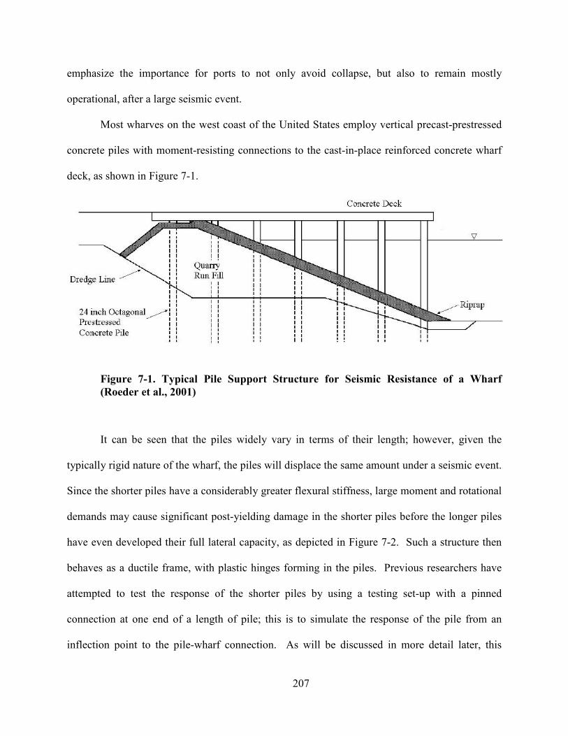
207
emphasize the importance for ports to not only avoid collapse, but also to remain mostly
operational, after a large seismic event.
Most wharves on the west coast of the United States employ vertical precast-prestressed
concrete piles with moment-resisting connections to the cast-in-place reinforced concrete wharf
deck, as shown in Figure 7-1.
Figure 7-1. Typical Pile Support Structure for Seismic Resistance of a Wharf
(Roeder et al., 2001)
It can be seen that the piles widely vary in terms of their length; however, given the
typically rigid nature of the wharf, the piles will displace the same amount under a seismic event.
Since the shorter piles have a considerably greater flexural stiffness, large moment and rotational
demands may cause significant post-yielding damage in the shorter piles before the longer piles
have even developed their full lateral capacity, as depicted in Figure 7-2. Such a structure then
behaves as a ductile frame, with plastic hinges forming in the piles. Previous researchers have
attempted to test the response of the shorter piles by using a testing set-up with a pinned
connection at one end of a length of pile; this is to simulate the response of the pile from an
inflection point to the pile-wharf connection. As will be discussed in more detail later, this
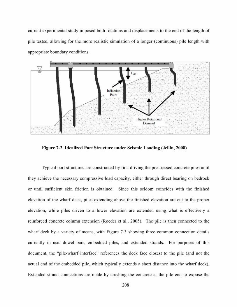
208
current experimental study imposed both rotations and displacements to the end of the length of
pile tested, allowing for the more realistic simulation of a longer (continuous) pile length with
appropriate boundary conditions.
Figure 7-2. Idealized Port Structure under Seismic Loading (Jellin, 2008)
Typical port structures are constructed by first driving the prestressed concrete piles until
they achieve the necessary compressive load capacity, either through direct bearing on bedrock
or until sufficient skin friction is obtained. Since this seldom coincides with the finished
elevation of the wharf deck, piles extending above the finished elevation are cut to the proper
elevation, while piles driven to a lower elevation are extended using what is effectively a
reinforced concrete column extension (Roeder et al., 2005). The pile is then connected to the
wharf deck by a variety of means, with Figure 7-3 showing three common connection details
currently in use: dowel bars, embedded piles, and extended strands. For purposes of this
document, the “pile-wharf interface” references the deck face closest to the pile (and not the
actual end of the embedded pile, which typically extends a short distance into the wharf deck).
Extended strand connections are made by crushing the concrete at the pile end to expose the
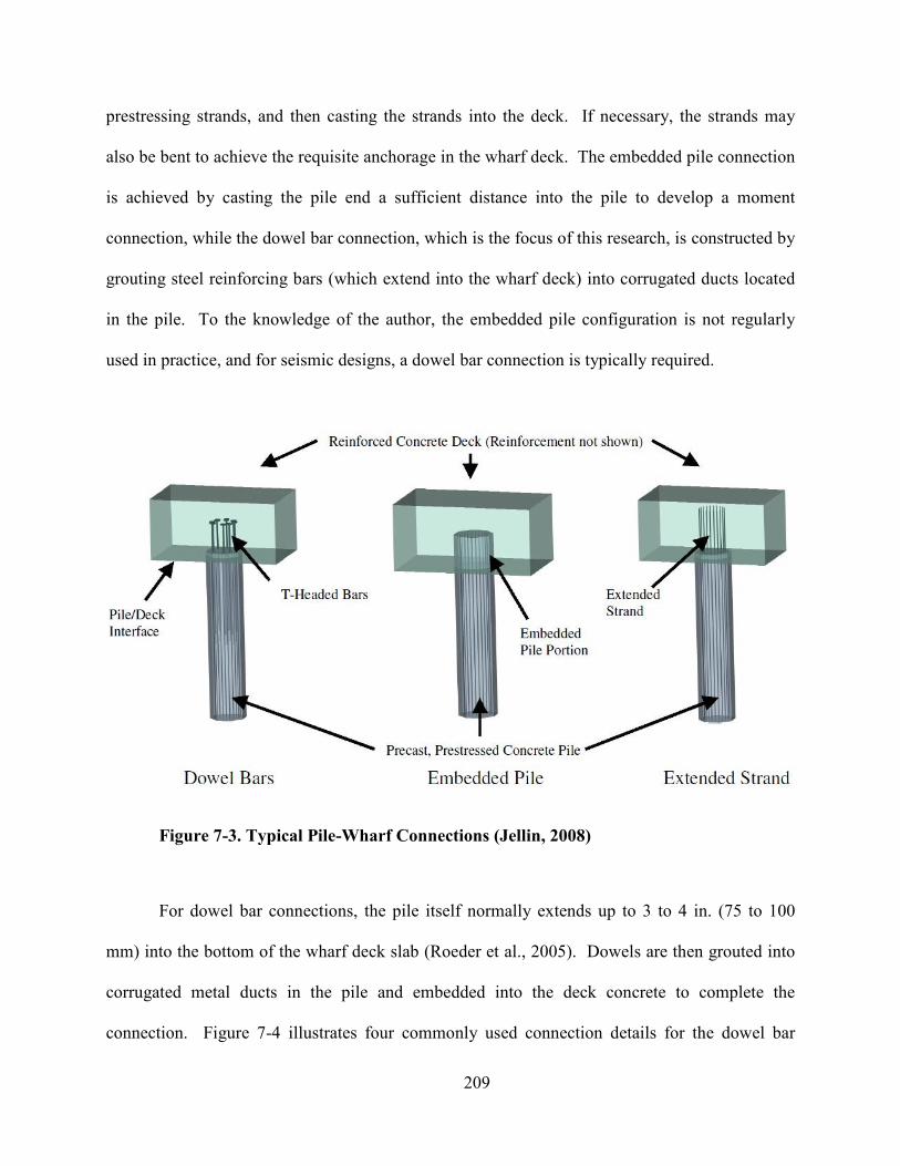
209
prestressing strands, and then casting the strands into the deck. If necessary, the strands may
also be bent to achieve the requisite anchorage in the wharf deck. The embedded pile connection
is achieved by casting the pile end a sufficient distance into the pile to develop a moment
connection, while the dowel bar connection, which is the focus of this research, is constructed by
grouting steel reinforcing bars (which extend into the wharf deck) into corrugated ducts located
in the pile. To the knowledge of the author, the embedded pile configuration is not regularly
used in practice, and for seismic designs, a dowel bar connection is typically required.
Figure 7-3. Typical Pile-Wharf Connections (Jellin, 2008)
For dowel bar connections, the pile itself normally extends up to 3 to 4 in. (75 to 100
mm) into the bottom of the wharf deck slab (Roeder et al., 2005). Dowels are then grouted into
corrugated metal ducts in the pile and embedded into the deck concrete to complete the
connection. Figure 7-4 illustrates four commonly used connection details for the dowel bar

210
connection. Inward and outward bent bars use hooked dowel bars bent in an L-shape into the top
of the wharf deck, placed in a radial or orthogonal pattern. Both of these designs can interfere
with the placement of the deck reinforcement and cause difficulty in concrete placement. To
ease congestion problems, the T-headed dowel bar connection and the bond bar connections are
often used. The T-headed dowel bar uses straight dowels with a circular or square steel plate
welded on one end of the bar to achieve mechanical development. The bond bar connection uses
straight dowels with a bulbous end grouted into the pile and a T-headed bar with a bulbous end
cast into the deck directly adjacent to the dowel bar – the idea is that the bulbous ends will serve
as a lap splice to develop the necessary connection continuity (Stringer, 2010). The most
common connection on the west coast of the United States is the T-headed dowel bar
construction, and this is the type of connection explored in the current laboratory testing
program. Once the connection detail is implemented, the reinforced concrete cast-in-place deck
is formed and cast. An alternative deck detail can sometimes be to use precast, prestressed
concrete panels spanning between cast-in-place reinforced concrete pile caps, with such a precast
deck system then covered with a reinforced concrete topping slab.
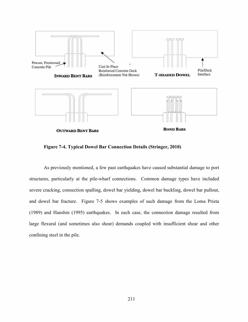
211
Figure 7-4. Typical Dowel Bar Connection Details (Stringer, 2010)
As previously mentioned, a few past earthquakes have caused substantial damage to port
structures, particularly at the pile-wharf connections. Common damage types have included
severe cracking, connection spalling, dowel bar yielding, dowel bar buckling, dowel bar pullout,
and dowel bar fracture. Figure 7-5 shows examples of such damage from the Loma Prieta
(1989) and Hanshin (1995) earthquakes. In each case, the connection damage resulted from
large flexural (and sometimes also shear) demands coupled with insufficient shear and other
confining steel in the pile.
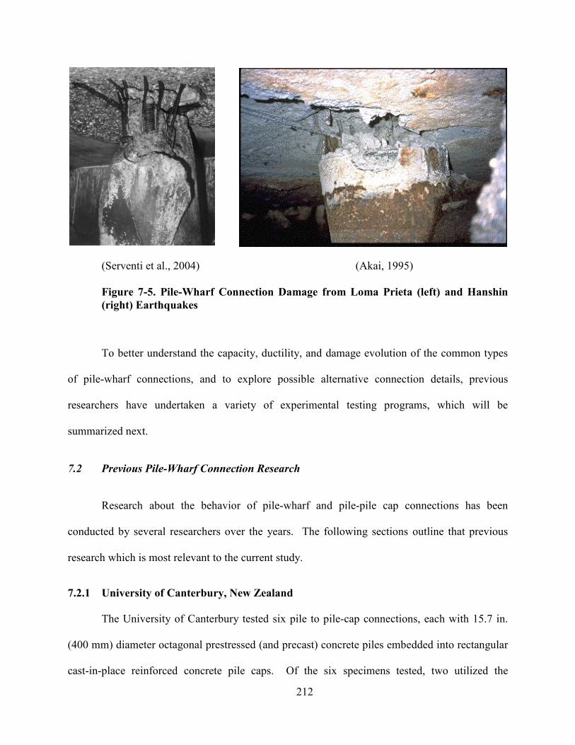
212
(Serventi et al., 2004) (Akai, 1995)
Figure 7-5. Pile-Wharf Connection Damage from Loma Prieta (left) and Hanshin
(right) Earthquakes
To better understand the capacity, ductility, and damage evolution of the common types
of pile-wharf connections, and to explore possible alternative connection details, previous
researchers have undertaken a variety of experimental testing programs, which will be
summarized next.
7.2 Previous Pile-Wharf Connection Research
Research about the behavior of pile-wharf and pile-pile cap connections has been
conducted by several researchers over the years. The following sections outline that previous
research which is most relevant to the current study.
7.2.1 University of Canterbury, ew Zealand
The University of Canterbury tested six pile to pile-cap connections, each with 15.7 in.
(400 mm) diameter octagonal prestressed (and precast) concrete piles embedded into rectangular
cast-in-place reinforced concrete pile caps. Of the six specimens tested, two utilized the
213
embedded pile connection, three implemented the extended strand connection method, and only
Specimen PC6 utilized the dowel bar method similar to that investigated in this study. That
connection was achieved by epoxying four #6 diameter (D19) dowel bars into 21 in. (530 mm)
long, 1.57 in. (40 mm) diameter drilled holes. Those bars were then anchored into the pile cap
with a standard 90 degree inward bar bend, with the pile itself embedded 2 in. (50 mm) into the
pile cap. Figure 7-6 shows an illustration of the Specimen PC6 connection details. Of the six
specimens, PC6 performed the worst; it was the only specimen to not exceed the theoretical
moment capacity, and it suffered the worst deterioration in capacity due to severe spalling of the
pile. The relative superior performance of the embedded pile and extended strand connections
may be attributed to their use of either ten prestressed tendons or ten prestressed tendons and ten
reinforcing bars to develop the connection in the embedded pile and extended strand
connections, while the dowel connection only had four dowel bars extending into the wharf deck.
In fact, it was noted by the authors that the inclusion of more dowel bars would have likely
increased the strength and stiffness of the connection (Joen et al., 1988).
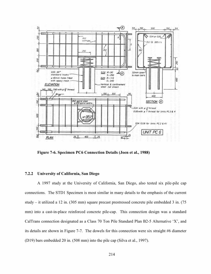
214
Figure 7-6. Specimen PC6 Connection Details (Joen et al., 1988)
7.2.2 University of California, San Diego
A 1997 study at the University of California, San Diego, also tested six pile-pile cap
connections. The STD1 Specimen is most similar in many details to the emphasis of the current
study – it utilized a 12 in. (305 mm) square precast prestressed concrete pile embedded 3 in. (75
mm) into a cast-in-place reinforced concrete pile-cap. This connection design was a standard
CalTrans connection designated as a Class 70 Ton Pile Standard Plan B2-5 Alternative ‘X’, and
its details are shown in Figure 7-7. The dowels for this connection were six straight #6 diameter
(D19) bars embedded 20 in. (508 mm) into the pile cap (Silva et al., 1997).
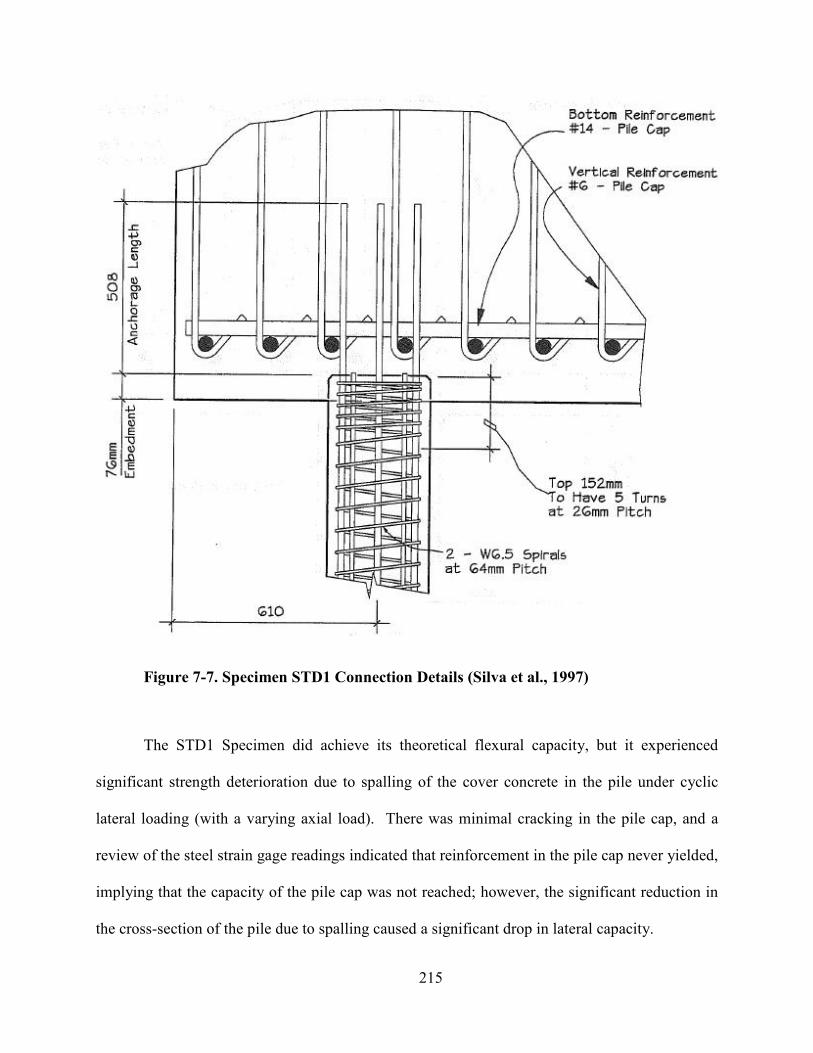
215
Figure 7-7. Specimen STD1 Connection Details (Silva et al., 1997)
The STD1 Specimen did achieve its theoretical flexural capacity, but it experienced
significant strength deterioration due to spalling of the cover concrete in the pile under cyclic
lateral loading (with a varying axial load). There was minimal cracking in the pile cap, and a
review of the steel strain gage readings indicated that reinforcement in the pile cap never yielded,
implying that the capacity of the pile cap was not reached; however, the significant reduction in
the cross-section of the pile due to spalling caused a significant drop in lateral capacity.

216
Sritharan and Priestley (1998) tested one large-scale “pile-deck” connection specimen for
the Port of Los Angeles, to examine the performance of an embedded dowel connection with T-
headed bars. The connection used eight #10 diameter (D32) dowel bars with bulb ends cast into
the end of the pile, with 29 in. (735 mm) embedment into the deck. Eight 26 in. (660 mm) long
#9 diameter (D25) T-headed bond bars were cast next to the dowel bars, with a #5 (D16) spiral at
3 in. (75 mm) on center surrounding the entire connection reinforcement in the deck. Details of
the connection are shown in Figure 7-8.
Figure 7-8. Connection Details from Sritharan and Priestley (1998)
The specimen was constructed monolithically for the pile and the deck, so the resulting
structural behavior more closely resembled an extended pile connection. The loading protocol
called for an increasing reversed-cyclic loading (with no axial pile load), and it was seen that the
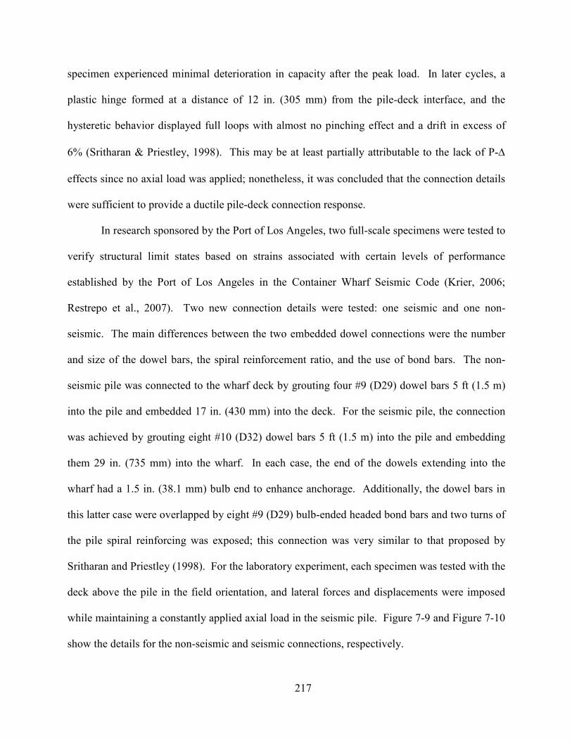
217
specimen experienced minimal deterioration in capacity after the peak load. In later cycles, a
plastic hinge formed at a distance of 12 in. (305 mm) from the pile-deck interface, and the
hysteretic behavior displayed full loops with almost no pinching effect and a drift in excess of
6% (Sritharan & Priestley, 1998). This may be at least partially attributable to the lack of P-∆
effects since no axial load was applied; nonetheless, it was concluded that the connection details
were sufficient to provide a ductile pile-deck connection response.
In research sponsored by the Port of Los Angeles, two full-scale specimens were tested to
verify structural limit states based on strains associated with certain levels of performance
established by the Port of Los Angeles in the Container Wharf Seismic Code (Krier, 2006;
Restrepo et al., 2007). Two new connection details were tested: one seismic and one non-
seismic. The main differences between the two embedded dowel connections were the number
and size of the dowel bars, the spiral reinforcement ratio, and the use of bond bars. The non-
seismic pile was connected to the wharf deck by grouting four #9 (D29) dowel bars 5 ft (1.5 m)
into the pile and embedded 17 in. (430 mm) into the deck. For the seismic pile, the connection
was achieved by grouting eight #10 (D32) dowel bars 5 ft (1.5 m) into the pile and embedding
them 29 in. (735 mm) into the wharf. In each case, the end of the dowels extending into the
wharf had a 1.5 in. (38.1 mm) bulb end to enhance anchorage. Additionally, the dowel bars in
this latter case were overlapped by eight #9 (D29) bulb-ended headed bond bars and two turns of
the pile spiral reinforcing was exposed; this connection was very similar to that proposed by
Sritharan and Priestley (1998). For the laboratory experiment, each specimen was tested with the
deck above the pile in the field orientation, and lateral forces and displacements were imposed
while maintaining a constantly applied axial load in the seismic pile. Figure 7-9 and Figure 7-10
show the details for the non-seismic and seismic connections, respectively.
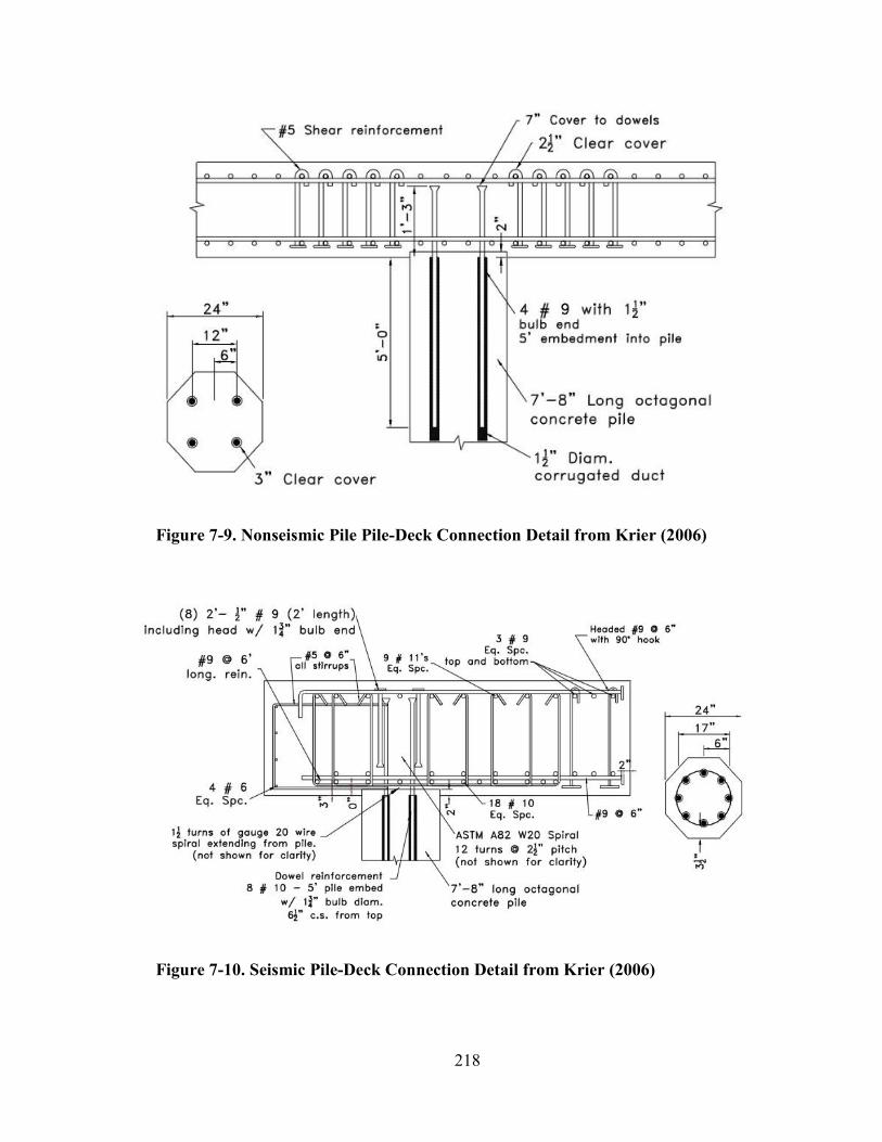
218
Figure 7-9. onseismic Pile Pile-Deck Connection Detail from Krier (2006)
Figure 7-10. Seismic Pile-Deck Connection Detail from Krier (2006)
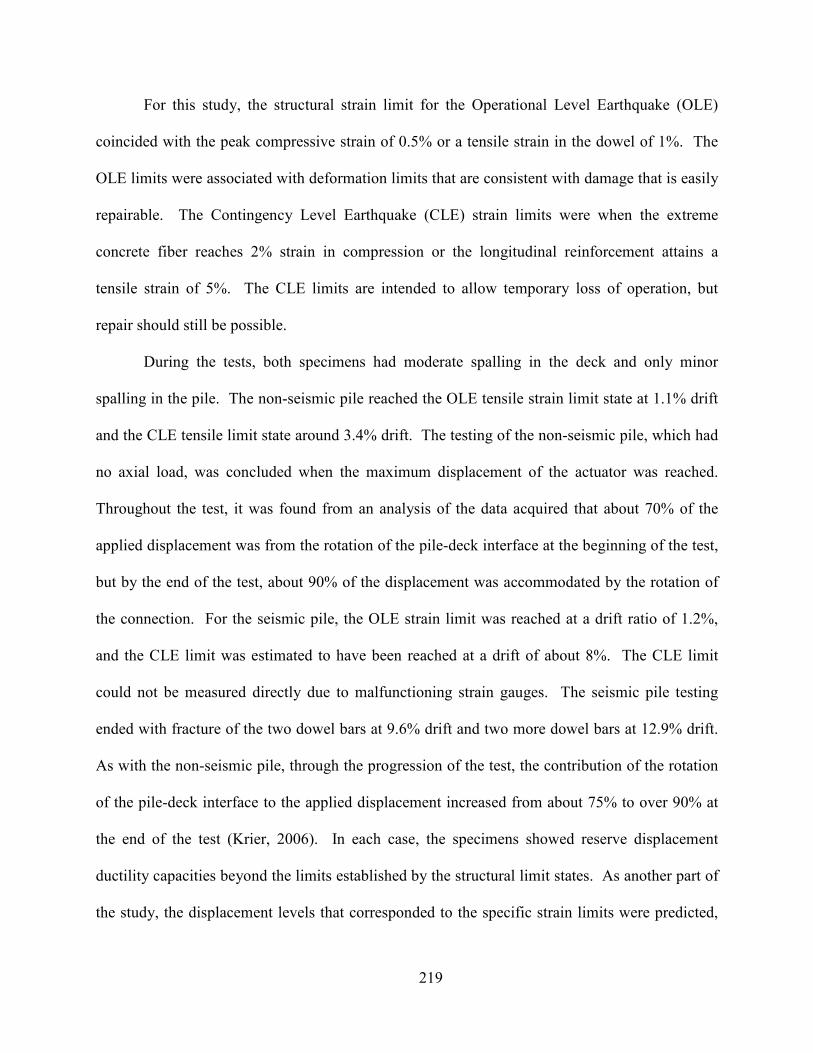
219
For this study, the structural strain limit for the Operational Level Earthquake (OLE)
coincided with the peak compressive strain of 0.5% or a tensile strain in the dowel of 1%. The
OLE limits were associated with deformation limits that are consistent with damage that is easily
repairable. The Contingency Level Earthquake (CLE) strain limits were when the extreme
concrete fiber reaches 2% strain in compression or the longitudinal reinforcement attains a
tensile strain of 5%. The CLE limits are intended to allow temporary loss of operation, but
repair should still be possible.
During the tests, both specimens had moderate spalling in the deck and only minor
spalling in the pile. The non-seismic pile reached the OLE tensile strain limit state at 1.1% drift
and the CLE tensile limit state around 3.4% drift. The testing of the non-seismic pile, which had
no axial load, was concluded when the maximum displacement of the actuator was reached.
Throughout the test, it was found from an analysis of the data acquired that about 70% of the
applied displacement was from the rotation of the pile-deck interface at the beginning of the test,
but by the end of the test, about 90% of the displacement was accommodated by the rotation of
the connection. For the seismic pile, the OLE strain limit was reached at a drift ratio of 1.2%,
and the CLE limit was estimated to have been reached at a drift of about 8%. The CLE limit
could not be measured directly due to malfunctioning strain gauges. The seismic pile testing
ended with fracture of the two dowel bars at 9.6% drift and two more dowel bars at 12.9% drift.
As with the non-seismic pile, through the progression of the test, the contribution of the rotation
of the pile-deck interface to the applied displacement increased from about 75% to over 90% at
the end of the test (Krier, 2006). In each case, the specimens showed reserve displacement
ductility capacities beyond the limits established by the structural limit states. As another part of
the study, the displacement levels that corresponded to the specific strain limits were predicted,
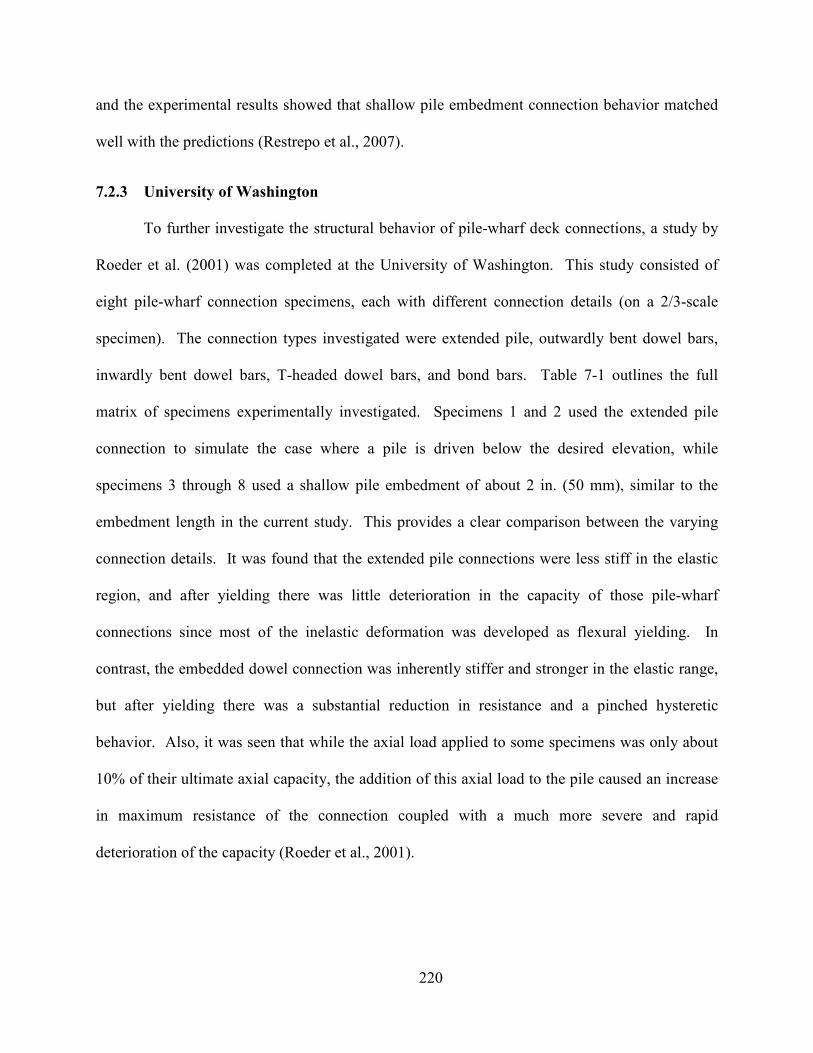
220
and the experimental results showed that shallow pile embedment connection behavior matched
well with the predictions (Restrepo et al., 2007).
7.2.3 University of Washington
To further investigate the structural behavior of pile-wharf deck connections, a study by
Roeder et al. (2001) was completed at the University of Washington. This study consisted of
eight pile-wharf connection specimens, each with different connection details (on a 2/3-scale
specimen). The connection types investigated were extended pile, outwardly bent dowel bars,
inwardly bent dowel bars, T-headed dowel bars, and bond bars. Table 7-1 outlines the full
matrix of specimens experimentally investigated. Specimens 1 and 2 used the extended pile
connection to simulate the case where a pile is driven below the desired elevation, while
specimens 3 through 8 used a shallow pile embedment of about 2 in. (50 mm), similar to the
embedment length in the current study. This provides a clear comparison between the varying
connection details. It was found that the extended pile connections were less stiff in the elastic
region, and after yielding there was little deterioration in the capacity of those pile-wharf
connections since most of the inelastic deformation was developed as flexural yielding. In
contrast, the embedded dowel connection was inherently stiffer and stronger in the elastic range,
but after yielding there was a substantial reduction in resistance and a pinched hysteretic
behavior. Also, it was seen that while the axial load applied to some specimens was only about
10% of their ultimate axial capacity, the addition of this axial load to the pile caused an increase
in maximum resistance of the connection coupled with a much more severe and rapid
deterioration of the capacity (Roeder et al., 2001).
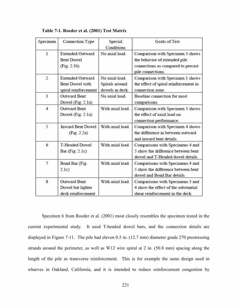
221
Table 7-1. Roeder et al. (2001) Test Matrix
Specimen 6 from Roeder et al. (2001) most closely resembles the specimen tested in the
current experimental study. It used T-headed dowel bars, and the connection details are
displayed in Figure 7-11. The pile had eleven 0.5 in. (12.7 mm) diameter grade 270 prestressing
strands around the perimeter, as well as W12 wire spiral at 2 in. (50.8 mm) spacing along the
length of the pile as transverse reinforcement. This is for example the same design used in
wharves in Oakland, California, and it is intended to reduce reinforcement congestion by
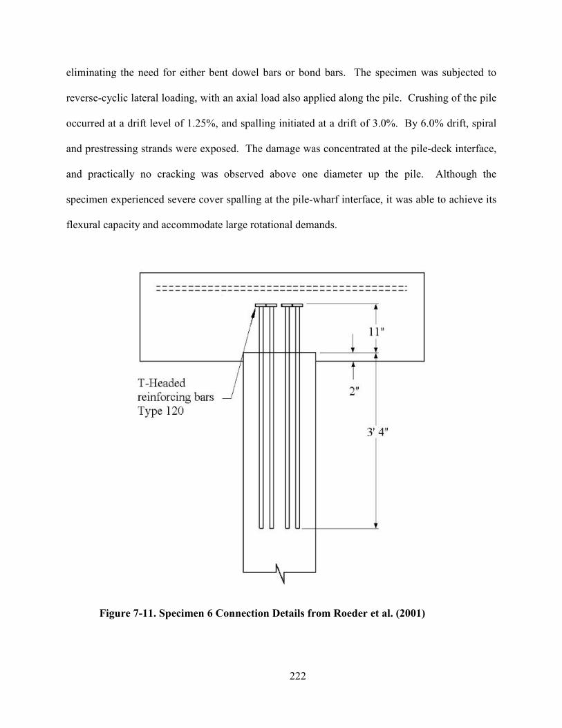
222
eliminating the need for either bent dowel bars or bond bars. The specimen was subjected to
reverse-cyclic lateral loading, with an axial load also applied along the pile. Crushing of the pile
occurred at a drift level of 1.25%, and spalling initiated at a drift of 3.0%. By 6.0% drift, spiral
and prestressing strands were exposed. The damage was concentrated at the pile-deck interface,
and practically no cracking was observed above one diameter up the pile. Although the
specimen experienced severe cover spalling at the pile-wharf interface, it was able to achieve its
flexural capacity and accommodate large rotational demands.
Figure 7-11. Specimen 6 Connection Details from Roeder et al. (2001)
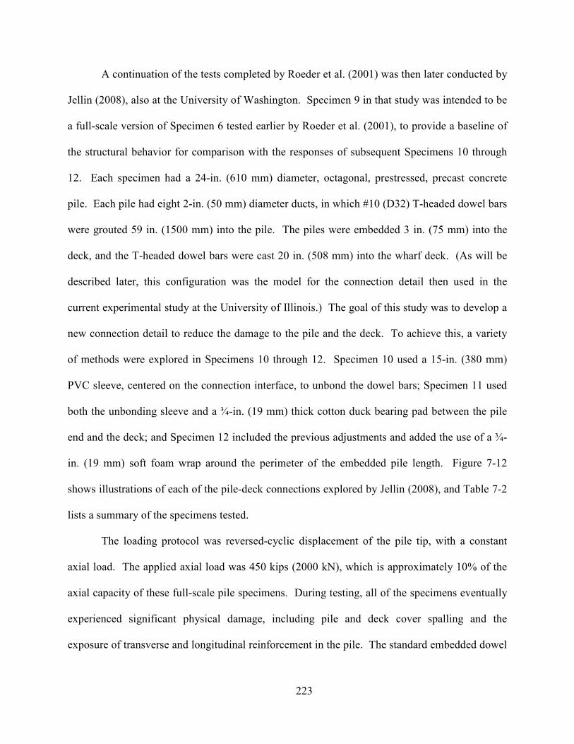
223
A continuation of the tests completed by Roeder et al. (2001) was then later conducted by
Jellin (2008), also at the University of Washington. Specimen 9 in that study was intended to be
a full-scale version of Specimen 6 tested earlier by Roeder et al. (2001), to provide a baseline of
the structural behavior for comparison with the responses of subsequent Specimens 10 through
12. Each specimen had a 24-in. (610 mm) diameter, octagonal, prestressed, precast concrete
pile. Each pile had eight 2-in. (50 mm) diameter ducts, in which #10 (D32) T-headed dowel bars
were grouted 59 in. (1500 mm) into the pile. The piles were embedded 3 in. (75 mm) into the
deck, and the T-headed dowel bars were cast 20 in. (508 mm) into the wharf deck. (As will be
described later, this configuration was the model for the connection detail then used in the
current experimental study at the University of Illinois.) The goal of this study was to develop a
new connection detail to reduce the damage to the pile and the deck. To achieve this, a variety
of methods were explored in Specimens 10 through 12. Specimen 10 used a 15-in. (380 mm)
PVC sleeve, centered on the connection interface, to unbond the dowel bars; Specimen 11 used
both the unbonding sleeve and a ¾-in. (19 mm) thick cotton duck bearing pad between the pile
end and the deck; and Specimen 12 included the previous adjustments and added the use of a ¾-
in. (19 mm) soft foam wrap around the perimeter of the embedded pile length. Figure 7-12
shows illustrations of each of the pile-deck connections explored by Jellin (2008), and Table 7-2
lists a summary of the specimens tested.
The loading protocol was reversed-cyclic displacement of the pile tip, with a constant
axial load. The applied axial load was 450 kips (2000 kN), which is approximately 10% of the
axial capacity of these full-scale pile specimens. During testing, all of the specimens eventually
experienced significant physical damage, including pile and deck cover spalling and the
exposure of transverse and longitudinal reinforcement in the pile. The standard embedded dowel

224
and sleeved embedded dowel connections had significant pile and deck spalling, but the addition
of the bearing pad between the embedded end of the pile and the deck both reduced and delayed
the onset of spalling in the pile. It was also seen that the use of the soft foam wrap essentially
eliminated spalling of the wharf deck. When comparing the measured responses, specimens with
bearing pads had a slightly reduced peak moment capacity, reduced stiffness, and the maximum
moment was reached at higher drifts levels. Also, specimens with a bearing pad experienced
substantially less degradation of their moment resistance (Jellin, 2008).
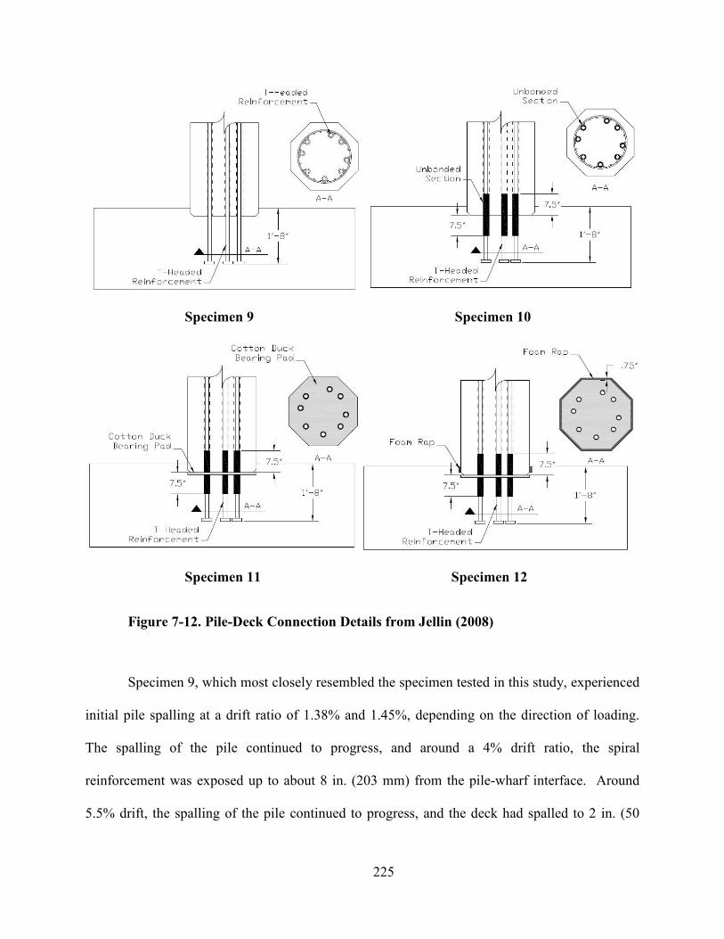
225
Specimen 9 Specimen 10
Specimen 11 Specimen 12
Figure 7-12. Pile-Deck Connection Details from Jellin (2008)
Specimen 9, which most closely resembled the specimen tested in this study, experienced
initial pile spalling at a drift ratio of 1.38% and 1.45%, depending on the direction of loading.
The spalling of the pile continued to progress, and around a 4% drift ratio, the spiral
reinforcement was exposed up to about 8 in. (203 mm) from the pile-wharf interface. Around
5.5% drift, the spalling of the pile continued to progress, and the deck had spalled to 2 in. (50
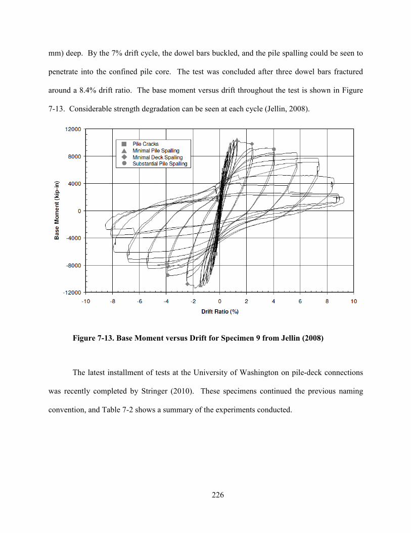
mm) deep. By the 7% drift cycle, the dowel bars buckled, and the pile spalling could be seen to
penetrate into the confined pile core. The test was concluded after three dowel bars fractured
around a 8.4% drift ratio. The base moment versus drift throughout the test is shown in
7-13. Considerable strength degradation can be seen at each cycle
Figure 7-13. Base Moment versus Drift for Specimen 9 from Jellin
The latest installment of tests at the University of
was recently completed by Stringer
convention, and Table 7-2 shows a summary of the experiments cond
226
mm) deep. By the 7% drift cycle, the dowel bars buckled, and the pile spalling could be seen to
e core. The test was concluded after three dowel bars fractured
The base moment versus drift throughout the test is shown in
. Considerable strength degradation can be seen at each cycle (Jellin, 2008)
. Base Moment versus Drift for Specimen 9 from Jellin (2008)
The latest installment of tests at the University of Washington on pile-deck connections
was recently completed by Stringer (2010). These specimens continued the previous naming
shows a summary of the experiments conducted.
mm) deep. By the 7% drift cycle, the dowel bars buckled, and the pile spalling could be seen to
e core. The test was concluded after three dowel bars fractured
The base moment versus drift throughout the test is shown in Figure
(Jellin, 2008).
(2008)
deck connections
. These specimens continued the previous naming
227
Table 7-2. Jellin (2008) and Stringer (2010) Test Matrix (Stringer, 2010)
Specimen 13 and Specimen 14 were intentionally identical to Specimen 12, to provide a
baseline for comparison of the results and to explore the variability in performance of the same
connection detail. Also, Specimen 14 was tested with twice the axial load of the other
specimens. Specimen 15 and Specimen 16 investigated the use of an annular ¾ in. (19 mm)
cotton duck bearing pad and an annular ½ in. (13 mm) random oriented fiber reinforced
elastomeric bearing pad, respectively. The annular pads were cut to a 24 in. (610 mm) octagon
228
to fit the cross-section of the pile, and an 18 in. (460 mm) diameter hole was cut in the center to
accommodate the dowel bars. Results of these tests showed that in Specimen 14, the higher axial
load caused an earlier onset of pile spalling and rapid strength degradation. The specimens with
annular pads had essentially the same response, and it was seen that the annular pad delayed pile
spalling, but after spalling occurred, a rapid strength loss was observed. In each specimen, it was
again seen that the use of the soft foam wrap around the end of the pile eliminated deck spalling.
Comparing the performance with and without bearing pads, it was found that standard embedded
dowels achieved a given pile tip displacement (at the load application point, nearly 10 ft from the
connection interface) through about 30% pile end rotation and 70% pile elastic and inelastic
flexural action, while specimens with bearing pads achieved the same displacement through 80%
to 90% end rotation of the pile (Stringer, 2010). This effect results in delayed damage of the pile
and an increased resistance to strength degradation. Each of the above investigated adjustments
to the standard pile-wharf connection design improve the damage resistance of the pile-wharf
connection, but the increase in flexibility of the seismically designed piles may have some design
implications on the system-level. In a full port structure, if the shorter seismic piles undergo
larger displacements for a given load, then the longer non-seismic piles may be required to
participate in the lateral resistance of the port structure in a more meaningful way.
7.2.4 Summary of Past Research
As outlined above, several researchers have investigated pile-deck connections and
attempted various approaches to achieve an enhanced structural performance. It has been found
that pile-deck connections exhibit essentially plastic behavior under no axial load, with a plastic
hinge forming near the pile-deck interface. As an increasing axial load is applied, significant
strength degradation is seen due to spalling of the thick concrete cover. This is exacerbated by
229
the fact that piles have more stringent (thicker) cover requirements due to the corrosive marine
environment. Embedded dowel connections are preferred both due to their structural
performance and also to the ease of construction in the field. While the current study will focus
on a traditional embedded dowel connection with T-headed bars, previous researchers have
explored the impact of including bearing pads, unbonded dowel bars at the pile-deck interface,
and a foam wrap around the embedded pile length, all with favorable results. The remainder of
this chapter focuses on the construction and testing of a pile with more realistic boundary
conditions at the University of Illinois at Urbana-Champaign, as well as a discussion of a
proposal to repair that embedded dowel pile-deck connection once damaged.
7.3 Pile-Wharf Connection Experimental Testing Program
A “grand challenge” research effort addressing seismic risk management for port
systems, supported through the George E. Brown, Jr. Network for Earthquake Engineering
Simulation (NEES), is currently underway. The project that in part funded this research is titled
“Seismic Risk Management for Port Systems,” with its main objectives focused on predicting the
seismic response and damage states of key port components, estimating the effect of damage to
these components on overall port capacity and revenues, and developing strategies for mitigation
of possible losses through engineering design and retrofit options. More information related to
all the specific tasks and the institutions involved can be found on the project website
(http://www.neesgc.gatech.edu).
As part of that NEES project, the seismic performance of precast/prestressed concrete
pile-wharf connections is being investigated at the University of Illinois using the Multi-Axial
Full-Scale Sub-Structured Testing and Simulations Facility (MUST-SIM). While the previously
discussed experimental studies by project colleagues at the University of Washington (some also
230
partly supported by this NEES project) have focused on developing alternative connection
concepts and construction practices to better resist damage during earthquakes, the objectives of
the research at the University of Illinois are instead to understand the structural performance of
typical designs of vertical pile moment-resisting connections to a wharf deck (of the type that
commonly have been and are being constructed), and to test a repair technique for restoring
structural integrity after an earthquake. Previous tests utilized a simplified testing set-up;
however, this investigation uses a unique “Loading and Boundary Condition Box” (LBCB),
which utilizes six actuators in an arrangement enabling complete six degree-of-freedom control
at the (non-connection) end of the pile. The LBCB loading unit allows for precise control of
both forces and displacements in each degree of freedom, thereby permitting the application of
equivalent loads from a computational model of a full-scale port structure (further details about
the LBCB will be discussed in Section 7.3.5). Overall, the objectives of this portion of the
research are to utilize the MUST-SIM small-scale facility to develop a mixed-mode loading
protocol, to test a large-scale specimen to significant damage, and to repair and retest the large-
scale specimen. While the last objective is not necessarily within the scope of this document,
further information about the progress and results of the repaired specimen can be found at the
MUST-SIM website (http://nees.uiuc.edu).
7.3.1 Experimental Plan
The experimental plan is composed of three phases: small-scale testing of a 1/5-scale
rubber specimen (to validate key aspects of test control), large-scale testing of a full-scale pile-
wharf connection, and large-scale re-testing of the repaired full-scale pile-wharf connection.
One objective of the testing is to simulate the realistic boundary conditions that a pile may
experience during a seismic event. Previous tests were able to apply an axial load while
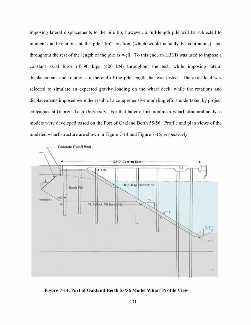
231
imposing lateral displacements to the pile tip; however, a full-length pile will be subjected to
moments and rotations at the pile “tip” location (which would actually be continuous), and
throughout the rest of the length of the pile as well. To this end, an LBCB was used to impose a
constant axial force of 90 kips (400 kN) throughout the test, while imposing lateral
displacements and rotations to the end of the pile length that was tested. The axial load was
selected to simulate an expected gravity loading on the wharf deck, while the rotations and
displacements imposed were the result of a comprehensive modeling effort undertaken by project
colleagues at Georgia Tech University. For that latter effort, nonlinear wharf structural analysis
models were developed based on the Port of Oakland Berth 55/56. Profile and plan views of the
modeled wharf structure are shown in Figure 7-14 and Figure 7-15, respectively.
Figure 7-14. Port of Oakland Berth 55/56 Model Wharf Profile View
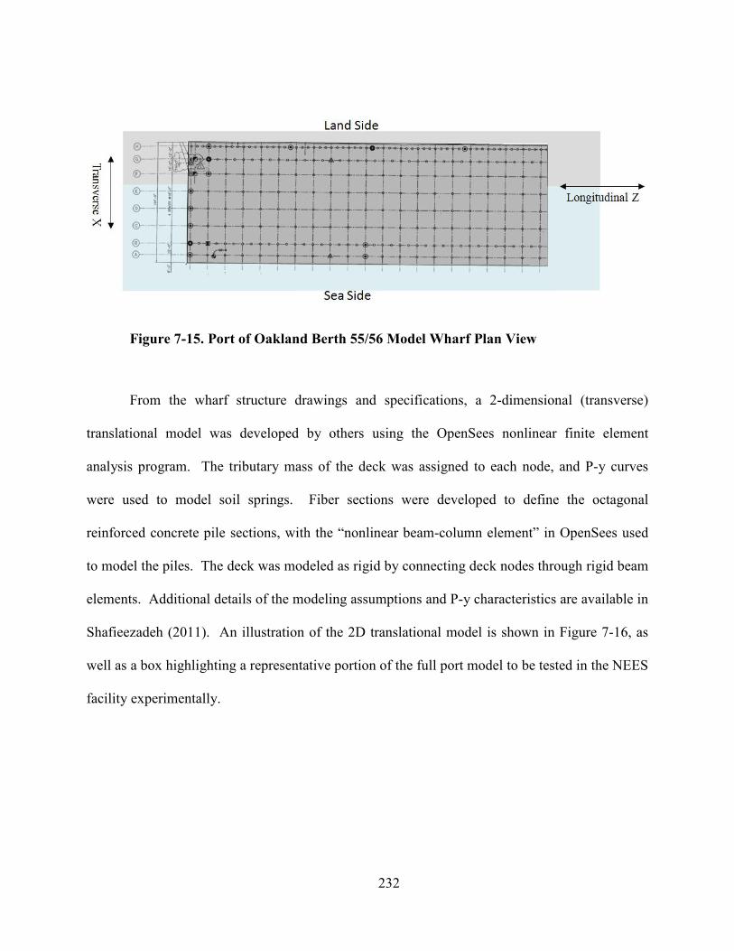
232
Figure 7-15. Port of Oakland Berth 55/56 Model Wharf Plan View
From the wharf structure drawings and specifications, a 2-dimensional (transverse)
translational model was developed by others using the OpenSees nonlinear finite element
analysis program. The tributary mass of the deck was assigned to each node, and P-y curves
were used to model soil springs. Fiber sections were developed to define the octagonal
reinforced concrete pile sections, with the “nonlinear beam-column element” in OpenSees used
to model the piles. The deck was modeled as rigid by connecting deck nodes through rigid beam
elements. Additional details of the modeling assumptions and P-y characteristics are available in
Shafieezadeh (2011). An illustration of the 2D translational model is shown in Figure 7-16, as
well as a box highlighting a representative portion of the full port model to be tested in the NEES
facility experimentally.
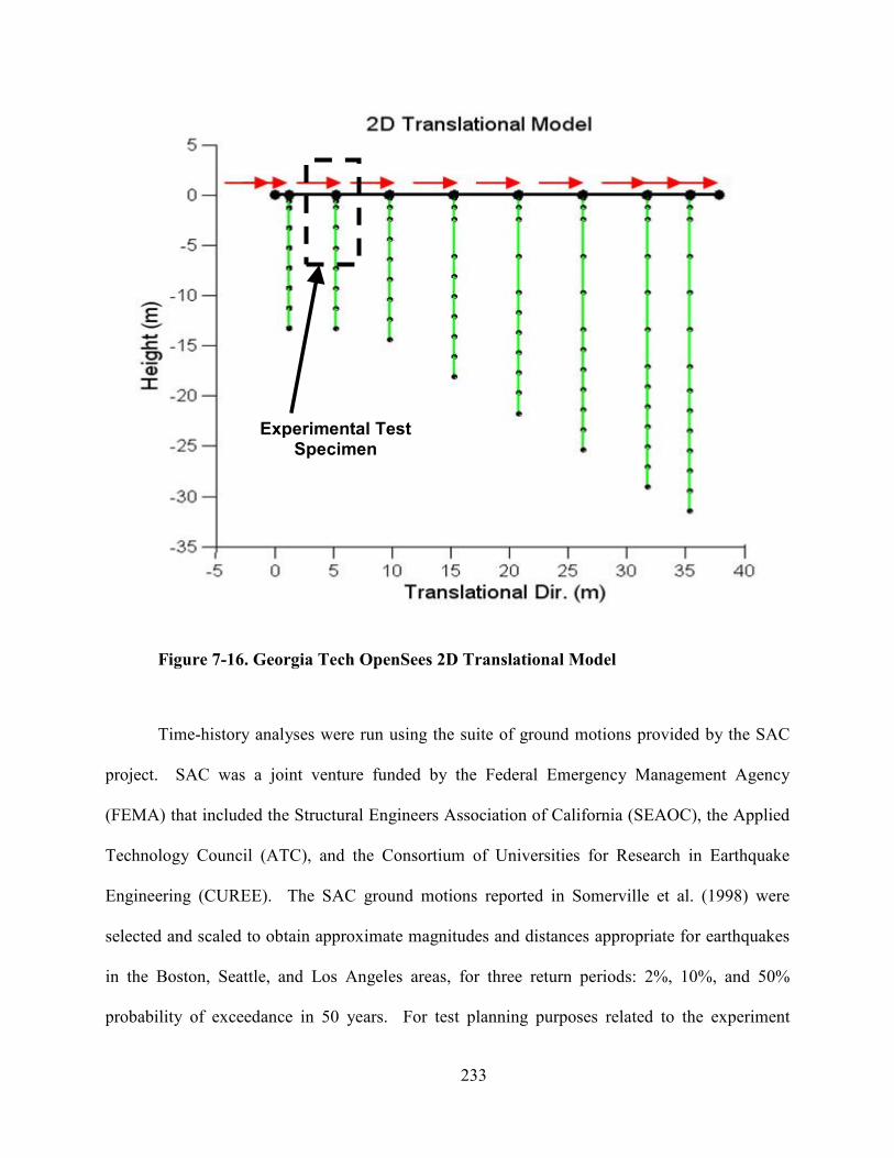
233
Figure 7-16. Georgia Tech OpenSees 2D Translational Model
Time-history analyses were run using the suite of ground motions provided by the SAC
project. SAC was a joint venture funded by the Federal Emergency Management Agency
(FEMA) that included the Structural Engineers Association of California (SEAOC), the Applied
Technology Council (ATC), and the Consortium of Universities for Research in Earthquake
Engineering (CUREE). The SAC ground motions reported in Somerville et al. (1998) were
selected and scaled to obtain approximate magnitudes and distances appropriate for earthquakes
in the Boston, Seattle, and Los Angeles areas, for three return periods: 2%, 10%, and 50%
probability of exceedance in 50 years. For test planning purposes related to the experiment
Experimental Test
Specimen
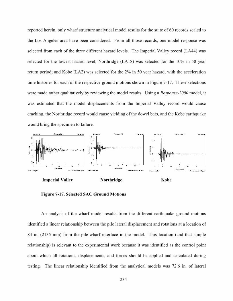
234
reported herein, only wharf structure analytical model results for the suite of 60 records scaled to
the Los Angeles area have been considered. From all those records, one model response was
selected from each of the three different hazard levels. The Imperial Valley record (LA44) was
selected for the lowest hazard level; Northridge (LA18) was selected for the 10% in 50 year
return period; and Kobe (LA2) was selected for the 2% in 50 year hazard, with the acceleration
time histories for each of the respective ground motions shown in Figure 7-17. These selections
were made rather qualitatively by reviewing the model results. Using a Response-2000 model, it
was estimated that the model displacements from the Imperial Valley record would cause
cracking, the Northridge record would cause yielding of the dowel bars, and the Kobe earthquake
would bring the specimen to failure.
Imperial Valley orthridge Kobe
Figure 7-17. Selected SAC Ground Motions
An analysis of the wharf model results from the different earthquake ground motions
identified a linear relationship between the pile lateral displacement and rotations at a location of
84 in. (2135 mm) from the pile-wharf interface in the model. This location (and that simple
relationship) is relevant to the experimental work because it was identified as the control point
about which all rotations, displacements, and forces should be applied and calculated during
testing. The linear relationship identified from the analytical models was 72.6 in. of lateral
235
displacement per radian of rotation. In addition to the imposed displacement and rotation on the
top of the pile, a constant axial load of 90 kips (400 kN) was also applied. These imposed
boundary conditions with the appropriate sign convention are displayed in Figure 7-18, as well
as the typical bending moment distribution along the height of the pile. An applied shear force
and moment correspond to the imposed displacement and rotation at the end of the pile. Since
the magnitude of the imposed rotation was less than the free rotation of a cantilever, the result
was an applied moment with the opposite sign of the moment at the pile-wharf connection, as
shown Figure 7-18.
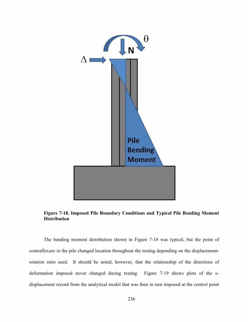
236
Figure 7-18. Imposed Pile Boundary Conditions and Typical Pile Bending Moment
Distribution
The bending moment distribution shown in Figure 7-18 was typical, but the point of
contraflexure in the pile changed location throughout the testing depending on the displacement-
rotation ratio used. It should be noted, however, that the relationship of the directions of
deformation imposed never changed during testing. Figure 7-19 shows plots of the x-
displacement record from the analytical model that was then in turn imposed at the control point
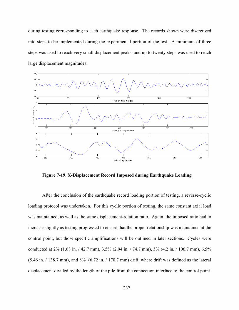
237
during testing corresponding to each earthquake response. The records shown were discretized
into steps to be implemented during the experimental portion of the test. A minimum of three
steps was used to reach very small displacement peaks, and up to twenty steps was used to reach
large displacement magnitudes.
Figure 7-19. X-Displacement Record Imposed during Earthquake Loading
After the conclusion of the earthquake record loading portion of testing, a reverse-cyclic
loading protocol was undertaken. For this cyclic portion of testing, the same constant axial load
was maintained, as well as the same displacement-rotation ratio. Again, the imposed ratio had to
increase slightly as testing progressed to ensure that the proper relationship was maintained at the
control point, but those specific amplifications will be outlined in later sections. Cycles were
conducted at 2% (1.68 in. / 42.7 mm), 3.5% (2.94 in. / 74.7 mm), 5% (4.2 in. / 106.7 mm), 6.5%
(5.46 in. / 138.7 mm), and 8% (6.72 in. / 170.7 mm) drift, where drift was defined as the lateral
displacement divided by the length of the pile from the connection interface to the control point.
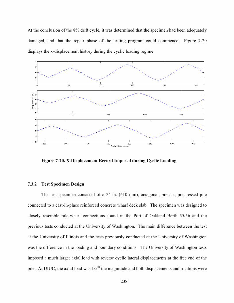
238
At the conclusion of the 8% drift cycle, it was determined that the specimen had been adequately
damaged, and that the repair phase of the testing program could commence. Figure 7-20
displays the x-displacement history during the cyclic loading regime.
Figure 7-20. X-Displacement Record Imposed during Cyclic Loading
7.3.2 Test Specimen Design
The test specimen consisted of a 24-in. (610 mm), octagonal, precast, prestressed pile
connected to a cast-in-place reinforced concrete wharf deck slab. The specimen was designed to
closely resemble pile-wharf connections found in the Port of Oakland Berth 55/56 and the
previous tests conducted at the University of Washington. The main difference between the test
at the University of Illinois and the tests previously conducted at the University of Washington
was the difference in the loading and boundary conditions. The University of Washington tests
imposed a much larger axial load with reverse cyclic lateral displacements at the free end of the
pile. At UIUC, the axial load was 1/5th the magnitude and both displacements and rotations were
239
imposed at the free end of the pile. Additionally, the imposed displacements and rotations were
the result of a system level modeling effort with imposed ground motions. The specimen was
cast upright to simulate actual field construction; however, testing was done with the pile
specimen inverted, as shown in Figure 7-21. The concrete pile was embedded 2 in. (50 mm) into
the cast-in-place deck, and the connection was achieved by using eight #10 (D32) T-headed
dowel bars grouted into the pile. As shown in Figure 7-21, the control point for testing was
specified at the center of the pile cross-section at a distance of 7 ft (2.1 m) from the pile-deck
interface. Through the use of the LBCB and externally-mounted string potentiometers, all
control “displacements” and “forces” imposed during testing and described hereafter are in
reference to the control point, not the end of the pile. The term “displacements” is used to
reference both the lateral displacement and the rotation at the end of the pile, while the term
“forces” refers to the axial force, lateral force, and moment on the pile.
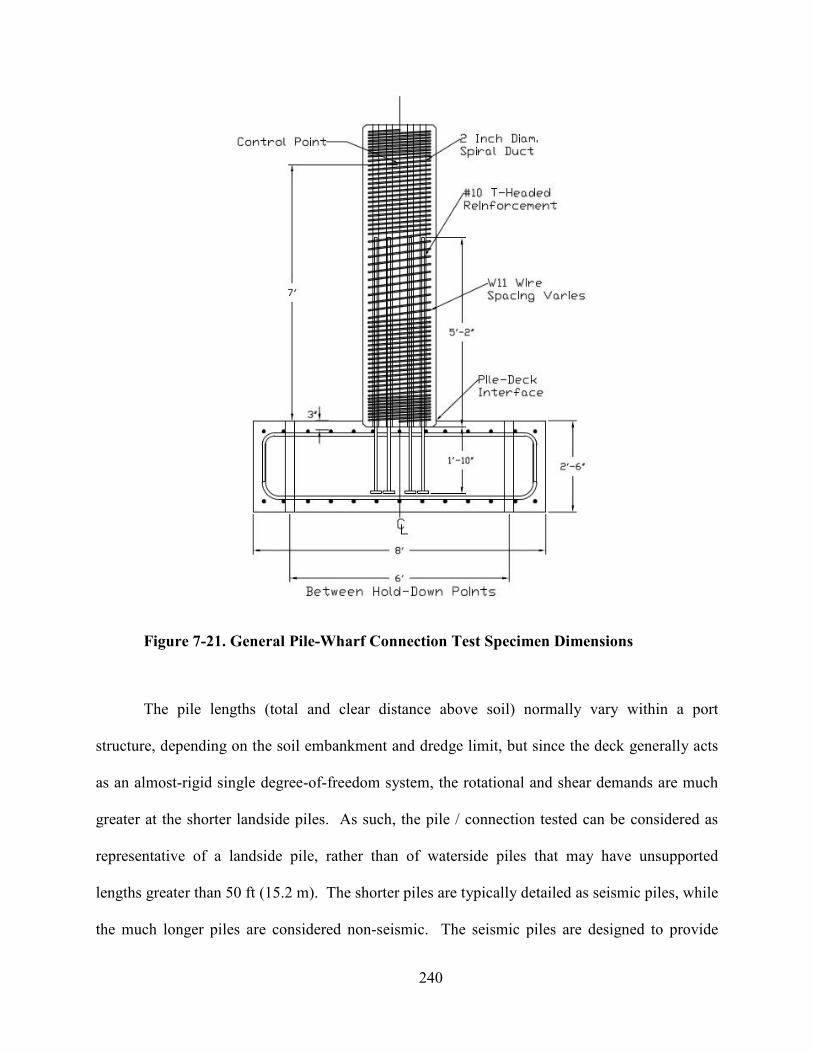
240
Figure 7-21. General Pile-Wharf Connection Test Specimen Dimensions
The pile lengths (total and clear distance above soil) normally vary within a port
structure, depending on the soil embankment and dredge limit, but since the deck generally acts
as an almost-rigid single degree-of-freedom system, the rotational and shear demands are much
greater at the shorter landside piles. As such, the pile / connection tested can be considered as
representative of a landside pile, rather than of waterside piles that may have unsupported
lengths greater than 50 ft (15.2 m). The shorter piles are typically detailed as seismic piles, while
the much longer piles are considered non-seismic. The seismic piles are designed to provide

241
strength, ductility, and gravity loading capacity, while the non-seismic piles are designed
primarily for gravity loading and are only detailed for limited ductility (Krier, 2006).
Details of the prestressed, precast pile used in this study are given in Figure 7-22. The
pile was donated by Concrete Technology Corporation of Tacoma, WA. Specimen dimensions
for the pile were 99 in. (2.5 m) in length and 24-in. (610 mm) in diameter (octagonal), and it
contained eight 2-in. (50 mm) diameter corrugated metal ducts. The pile was reinforced with
twenty-two 0.5 in. (12.5 mm) diameter, 270 ksi (1860 MPa) low-relaxation strands, with each
strand prestressed to 31 kips (138 kN). Spiral reinforcement was W11 (0.374 in. / 9.5 mm
diameter) smooth wire. Spiral pitch varied from 1 in. (25 mm) at the end of the pile to 3 in. (75
mm) along the middle of the pile, as shown in Figure 7-22.
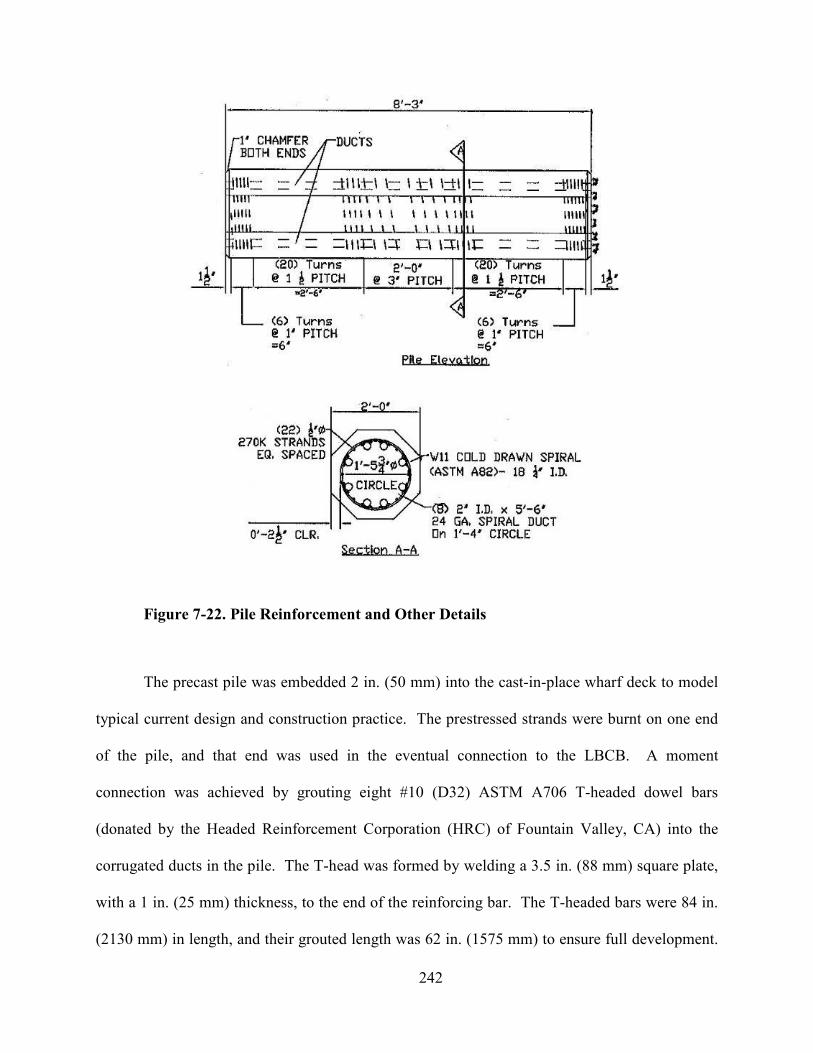
242
Figure 7-22. Pile Reinforcement and Other Details
The precast pile was embedded 2 in. (50 mm) into the cast-in-place wharf deck to model
typical current design and construction practice. The prestressed strands were burnt on one end
of the pile, and that end was used in the eventual connection to the LBCB. A moment
connection was achieved by grouting eight #10 (D32) ASTM A706 T-headed dowel bars
(donated by the Headed Reinforcement Corporation (HRC) of Fountain Valley, CA) into the
corrugated ducts in the pile. The T-head was formed by welding a 3.5 in. (88 mm) square plate,
with a 1 in. (25 mm) thickness, to the end of the reinforcing bar. The T-headed bars were 84 in.
(2130 mm) in length, and their grouted length was 62 in. (1575 mm) to ensure full development.
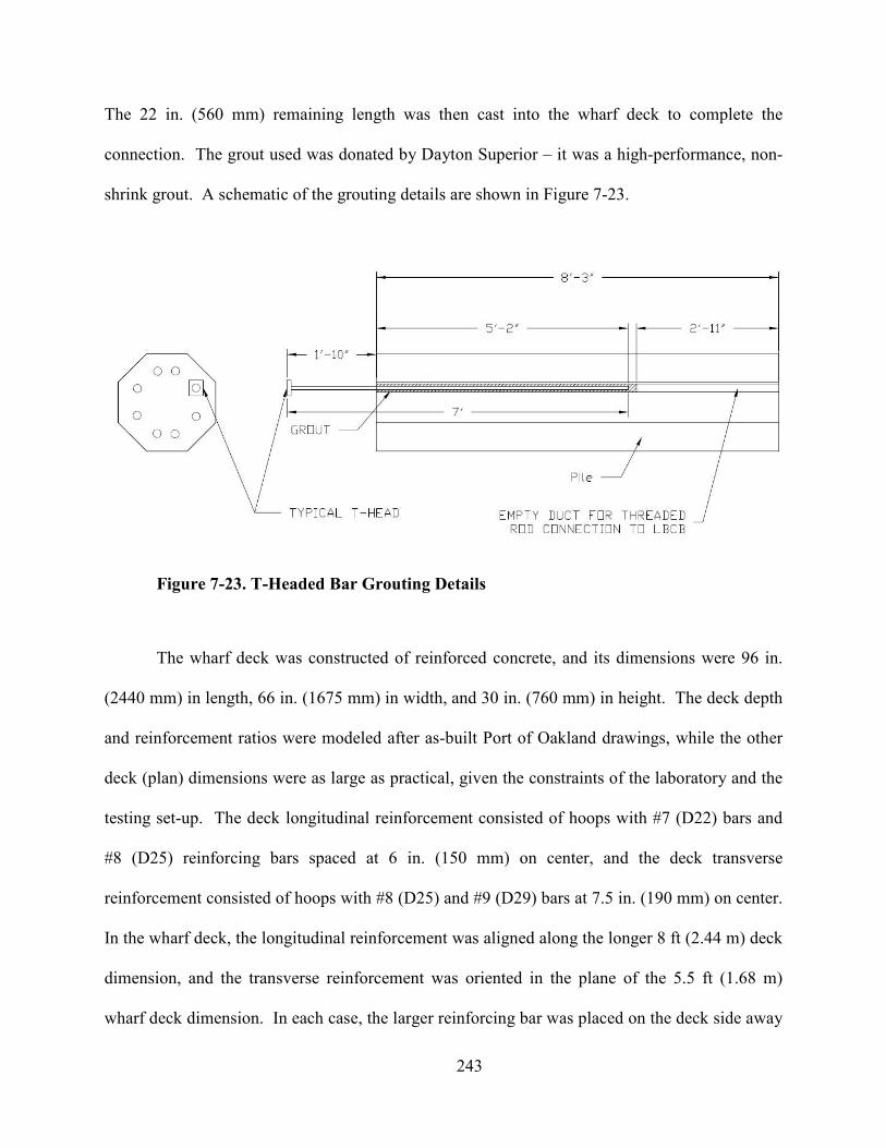
243
The 22 in. (560 mm) remaining length was then cast into the wharf deck to complete the
connection. The grout used was donated by Dayton Superior – it was a high-performance, non-
shrink grout. A schematic of the grouting details are shown in Figure 7-23.
Figure 7-23. T-Headed Bar Grouting Details
The wharf deck was constructed of reinforced concrete, and its dimensions were 96 in.
(2440 mm) in length, 66 in. (1675 mm) in width, and 30 in. (760 mm) in height. The deck depth
and reinforcement ratios were modeled after as-built Port of Oakland drawings, while the other
deck (plan) dimensions were as large as practical, given the constraints of the laboratory and the
testing set-up. The deck longitudinal reinforcement consisted of hoops with #7 (D22) bars and
#8 (D25) reinforcing bars spaced at 6 in. (150 mm) on center, and the deck transverse
reinforcement consisted of hoops with #8 (D25) and #9 (D29) bars at 7.5 in. (190 mm) on center.
In the wharf deck, the longitudinal reinforcement was aligned along the longer 8 ft (2.44 m) deck
dimension, and the transverse reinforcement was oriented in the plane of the 5.5 ft (1.68 m)
wharf deck dimension. In each case, the larger reinforcing bar was placed on the deck side away
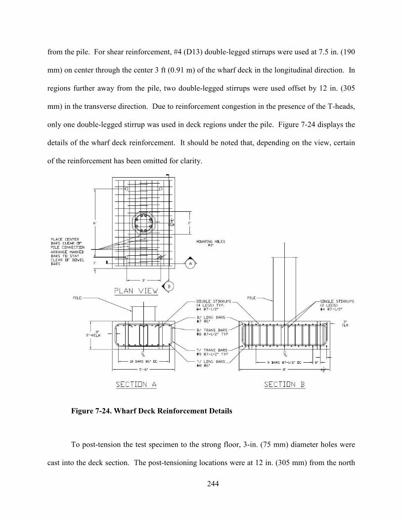
244
from the pile. For shear reinforcement, #4 (D13) double-legged stirrups were used at 7.5 in. (190
mm) on center through the center 3 ft (0.91 m) of the wharf deck in the longitudinal direction. In
regions further away from the pile, two double-legged stirrups were used offset by 12 in. (305
mm) in the transverse direction. Due to reinforcement congestion in the presence of the T-heads,
only one double-legged stirrup was used in deck regions under the pile. Figure 7-24 displays the
details of the wharf deck reinforcement. It should be noted that, depending on the view, certain
of the reinforcement has been omitted for clarity.
Figure 7-24. Wharf Deck Reinforcement Details
To post-tension the test specimen to the strong floor, 3-in. (75 mm) diameter holes were
cast into the deck section. The post-tensioning locations were at 12 in. (305 mm) from the north
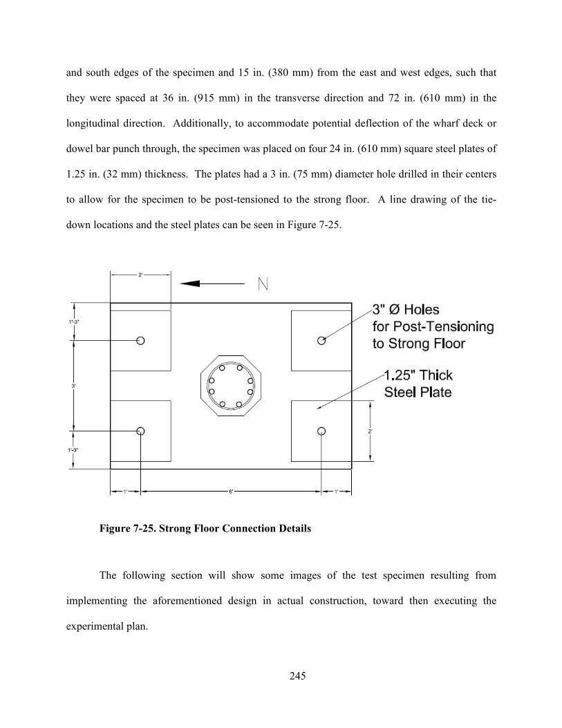
245
and south edges of the specimen and 15 in. (380 mm) from the east and west edges, such that
they were spaced at 36 in. (915 mm) in the transverse direction and 72 in. (610 mm) in the
longitudinal direction. Additionally, to accommodate potential deflection of the wharf deck or
dowel bar punch through, the specimen was placed on four 24 in. (610 mm) square steel plates of
1.25 in. (32 mm) thickness. The plates had a 3 in. (75 mm) diameter hole drilled in their centers
to allow for the specimen to be post-tensioned to the strong floor. A line drawing of the tie-
down locations and the steel plates can be seen in Figure 7-25.
Figure 7-25. Strong Floor Connection Details
The following section will show some images of the test specimen resulting from
implementing the aforementioned design in actual construction, toward then executing the
experimental plan.
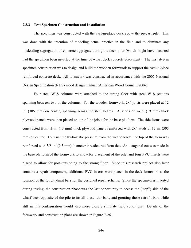
246
7.3.3 Test Specimen Construction and Installation
The specimen was constructed with the cast-in-place deck above the precast pile. This
was done with the intention of modeling actual practice in the field and to eliminate any
misleading segregation of concrete aggregate during the deck pour (which might have occurred
had the specimen been inverted at the time of wharf deck concrete placement). The first step in
specimen construction was to design and build the wooden formwork to support the cast-in-place
reinforced concrete deck. All formwork was constructed in accordance with the 2005 National
Design Specification (NDS) wood design manual (American Wood Council, 2006).
Four steel W18 columns were attached to the strong floor with steel W18 sections
spanning between two of the columns. For the wooden formwork, 2x4 joists were placed at 12
in. (305 mm) on center, spanning across the steel beams. A series of ¾-in. (19 mm) thick
plywood panels were then placed on top of the joists for the base platform. The side forms were
constructed from ½-in. (13 mm) thick plywood panels reinforced with 2x4 studs at 12 in. (305
mm) on center. To resist the hydrostatic pressure from the wet concrete, the top of the form was
reinforced with 3/8-in. (9.5 mm) diameter threaded rod form ties. An octagonal cut was made in
the base platform of the formwork to allow for placement of the pile, and four PVC inserts were
placed to allow for post-tensioning to the strong floor. Since this research project also later
contains a repair component, additional PVC inserts were placed in the deck formwork at the
location of the longitudinal bars for the designed repair scheme. Since the specimen is inverted
during testing, the construction phase was the last opportunity to access the (“top”) side of the
wharf deck opposite of the pile to install these four bars, and grouting those retrofit bars while
still in this configuration would also more closely simulate field conditions. Details of the
formwork and construction plans are shown in Figure 7-26.
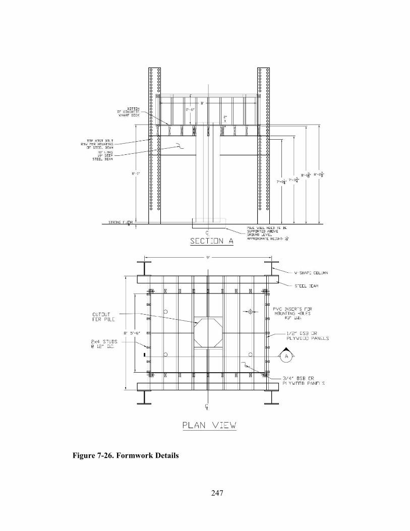
247
Figure 7-26. Formwork Details
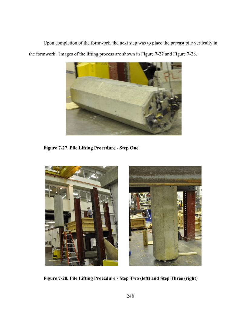
248
Upon completion of the formwork, the next step was to place the precast pile vertically in
the formwork. Images of the lifting process are shown in Figure 7-27 and Figure 7-28.
Figure 7-27. Pile Lifting Procedure - Step One
Figure 7-28. Pile Lifting Proecdure - Step Two (left) and Step Three (right)
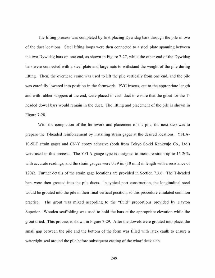
249
The lifting process was completed by first placing Dywidag bars through the pile in two
of the duct locations. Steel lifting loops were then connected to a steel plate spanning between
the two Dywidag bars on one end, as shown in Figure 7-27, while the other end of the Dywidag
bars were connected with a steel plate and large nuts to withstand the weight of the pile during
lifting. Then, the overhead crane was used to lift the pile vertically from one end, and the pile
was carefully lowered into position in the formwork. PVC inserts, cut to the appropriate length
and with rubber stoppers at the end, were placed in each duct to ensure that the grout for the T-
headed dowel bars would remain in the duct. The lifting and placement of the pile is shown in
Figure 7-28.
With the completion of the formwork and placement of the pile, the next step was to
prepare the T-headed reinforcement by installing strain gages at the desired locations. YFLA-
10-5LT strain gages and CN-Y epoxy adhesive (both from Tokyo Sokki Kenkyujo Co., Ltd.)
were used in this process. The YFLA gauge type is designed to measure strain up to 15-20%
with accurate readings, and the strain gauges were 0.39 in. (10 mm) in length with a resistance of
120Ω. Further details of the strain gage locations are provided in Section 7.3.6. The T-headed
bars were then grouted into the pile ducts. In typical port construction, the longitudinal steel
would be grouted into the pile in their final vertical position, so this procedure emulated common
practice. The grout was mixed according to the “fluid” proportions provided by Dayton
Superior. Wooden scaffolding was used to hold the bars at the appropriate elevation while the
grout dried. This process is shown in Figure 7-29. After the dowels were grouted into place, the
small gap between the pile and the bottom of the form was filled with latex caulk to ensure a
watertight seal around the pile before subsequent casting of the wharf deck slab.
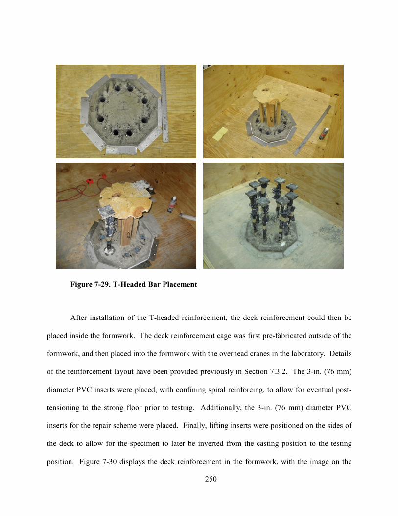
250
Figure 7-29. T-Headed Bar Placement
After installation of the T-headed reinforcement, the deck reinforcement could then be
placed inside the formwork. The deck reinforcement cage was first pre-fabricated outside of the
formwork, and then placed into the formwork with the overhead cranes in the laboratory. Details
of the reinforcement layout have been provided previously in Section 7.3.2. The 3-in. (76 mm)
diameter PVC inserts were placed, with confining spiral reinforcing, to allow for eventual post-
tensioning to the strong floor prior to testing. Additionally, the 3-in. (76 mm) diameter PVC
inserts for the repair scheme were placed. Finally, lifting inserts were positioned on the sides of
the deck to allow for the specimen to later be inverted from the casting position to the testing
position. Figure 7-30 displays the deck reinforcement in the formwork, with the image on the
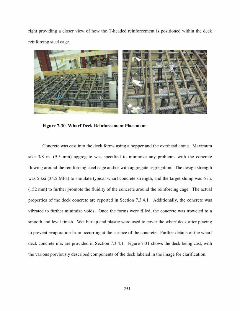
251
right providing a closer view of how the T-headed reinforcement is positioned within the deck
reinforcing steel cage.
Figure 7-30. Wharf Deck Reinforcement Placement
Concrete was cast into the deck forms using a hopper and the overhead crane. Maximum
size 3/8 in. (9.5 mm) aggregate was specified to minimize any problems with the concrete
flowing around the reinforcing steel cage and/or with aggregate segregation. The design strength
was 5 ksi (34.5 MPa) to simulate typical wharf concrete strength, and the target slump was 6 in.
(152 mm) to further promote the fluidity of the concrete around the reinforcing cage. The actual
properties of the deck concrete are reported in Section 7.3.4.1. Additionally, the concrete was
vibrated to further minimize voids. Once the forms were filled, the concrete was troweled to a
smooth and level finish. Wet burlap and plastic were used to cover the wharf deck after placing
to prevent evaporation from occurring at the surface of the concrete. Further details of the wharf
deck concrete mix are provided in Section 7.3.4.1. Figure 7-31 shows the deck being cast, with
the various previously described components of the deck labeled in the image for clarification.
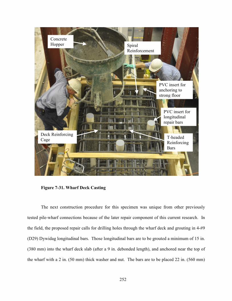
252
Figure 7-31. Wharf Deck Casting
The next construction procedure for this specimen was unique from other previously
tested pile-wharf connections because of the later repair component of this current research. In
the field, the proposed repair calls for drilling holes through the wharf deck and grouting in 4-#9
(D29) Dywidag longitudinal bars. Those longitudinal bars are to be grouted a minimum of 15 in.
(380 mm) into the wharf deck slab (after a 9 in. debonded length), and anchored near the top of
the wharf with a 2 in. (50 mm) thick washer and nut. The bars are to be placed 22 in. (560 mm)
PVC insert for anchoring to
strong floor
PVC insert for longitudinal
repair bars
Spiral
Reinforcement
Concrete
Hopper
Deck Reinforcing
Cage T-headed Reinforcing
Bars
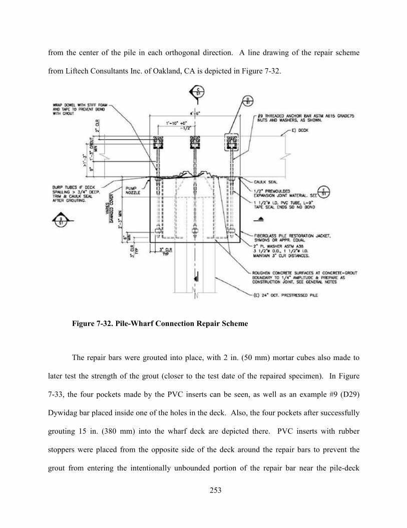
253
from the center of the pile in each orthogonal direction. A line drawing of the repair scheme
from Liftech Consultants Inc. of Oakland, CA is depicted in Figure 7-32.
Figure 7-32. Pile-Wharf Connection Repair Scheme
The repair bars were grouted into place, with 2 in. (50 mm) mortar cubes also made to
later test the strength of the grout (closer to the test date of the repaired specimen). In Figure
7-33, the four pockets made by the PVC inserts can be seen, as well as an example #9 (D29)
Dywidag bar placed inside one of the holes in the deck. Also, the four pockets after successfully
grouting 15 in. (380 mm) into the wharf deck are depicted there. PVC inserts with rubber
stoppers were placed from the opposite side of the deck around the repair bars to prevent the
grout from entering the intentionally unbounded portion of the repair bar near the pile-deck
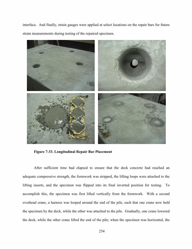
254
interface. And finally, strain gauges were applied at select locations on the repair bars for future
strain measurements during testing of the repaired specimen.
Figure 7-33. Longitudinal Repair Bar Placement
After sufficient time had elapsed to ensure that the deck concrete had reached an
adequate compressive strength, the formwork was stripped, the lifting loops were attached to the
lifting inserts, and the specimen was flipped into its final inverted position for testing. To
accomplish this, the specimen was first lifted vertically from the formwork. With a second
overhead crane, a harness was looped around the end of the pile, such that one crane now held
the specimen by the deck, while the other was attached to the pile. Gradually, one crane lowered
the deck, while the other crane lifted the end of the pile; when the specimen was horizontal, the
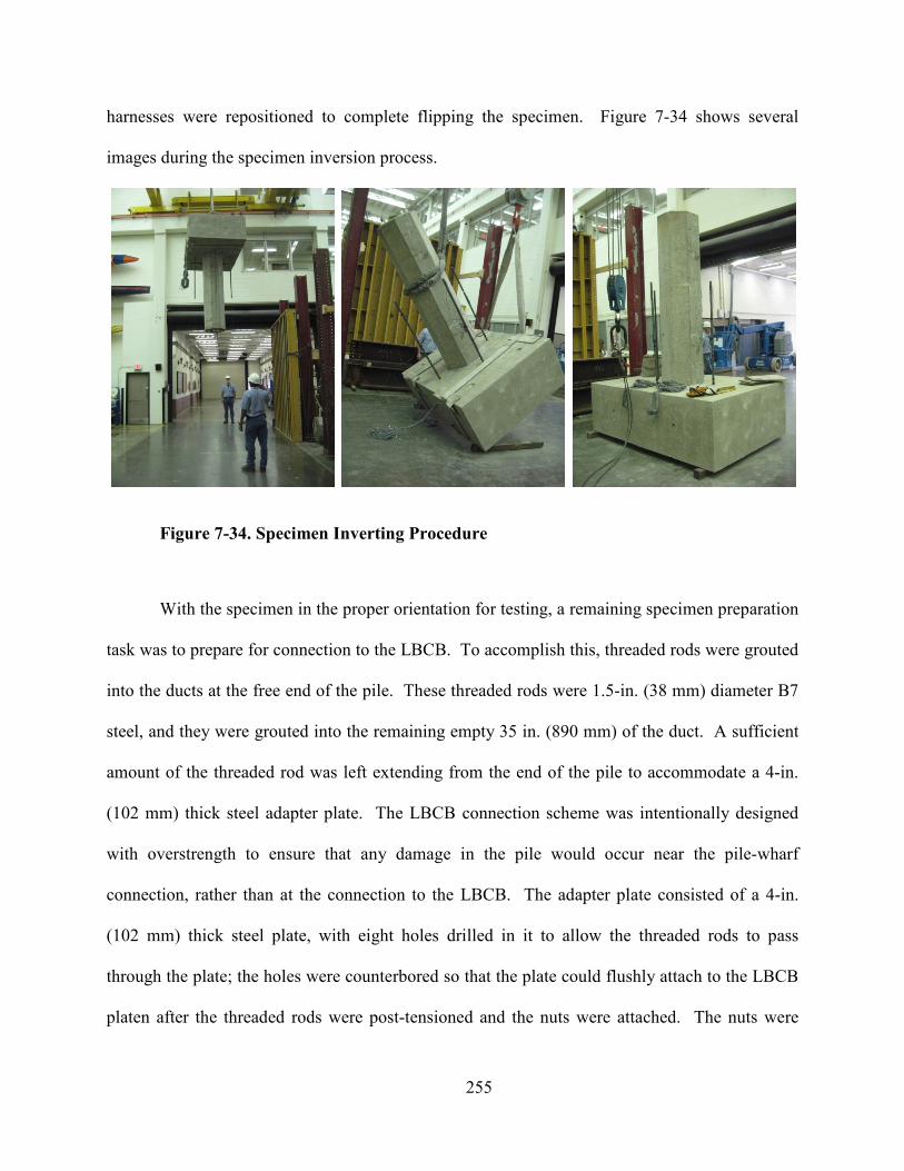
255
harnesses were repositioned to complete flipping the specimen. Figure 7-34 shows several
images during the specimen inversion process.
Figure 7-34. Specimen Inverting Procedure
With the specimen in the proper orientation for testing, a remaining specimen preparation
task was to prepare for connection to the LBCB. To accomplish this, threaded rods were grouted
into the ducts at the free end of the pile. These threaded rods were 1.5-in. (38 mm) diameter B7
steel, and they were grouted into the remaining empty 35 in. (890 mm) of the duct. A sufficient
amount of the threaded rod was left extending from the end of the pile to accommodate a 4-in.
(102 mm) thick steel adapter plate. The LBCB connection scheme was intentionally designed
with overstrength to ensure that any damage in the pile would occur near the pile-wharf
connection, rather than at the connection to the LBCB. The adapter plate consisted of a 4-in.
(102 mm) thick steel plate, with eight holes drilled in it to allow the threaded rods to pass
through the plate; the holes were counterbored so that the plate could flushly attach to the LBCB
platen after the threaded rods were post-tensioned and the nuts were attached. The nuts were
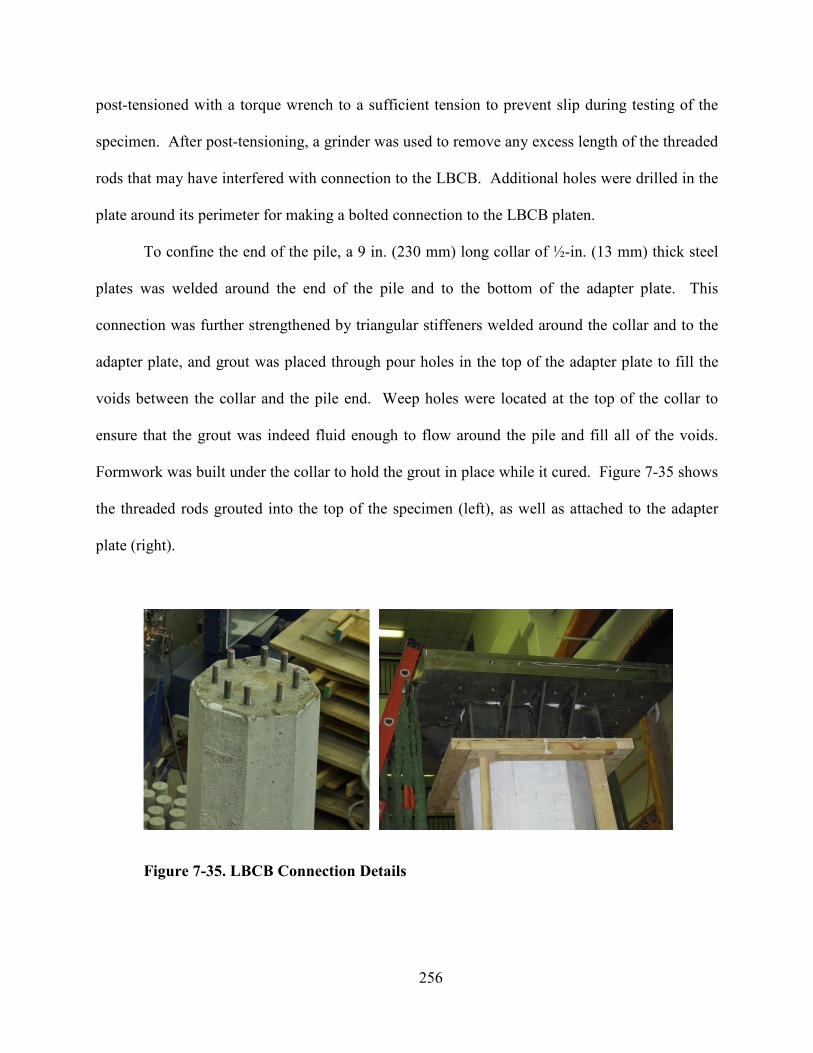
256
post-tensioned with a torque wrench to a sufficient tension to prevent slip during testing of the
specimen. After post-tensioning, a grinder was used to remove any excess length of the threaded
rods that may have interfered with connection to the LBCB. Additional holes were drilled in the
plate around its perimeter for making a bolted connection to the LBCB platen.
To confine the end of the pile, a 9 in. (230 mm) long collar of ½-in. (13 mm) thick steel
plates was welded around the end of the pile and to the bottom of the adapter plate. This
connection was further strengthened by triangular stiffeners welded around the collar and to the
adapter plate, and grout was placed through pour holes in the top of the adapter plate to fill the
voids between the collar and the pile end. Weep holes were located at the top of the collar to
ensure that the grout was indeed fluid enough to flow around the pile and fill all of the voids.
Formwork was built under the collar to hold the grout in place while it cured. Figure 7-35 shows
the threaded rods grouted into the top of the specimen (left), as well as attached to the adapter
plate (right).
Figure 7-35. LBCB Connection Details
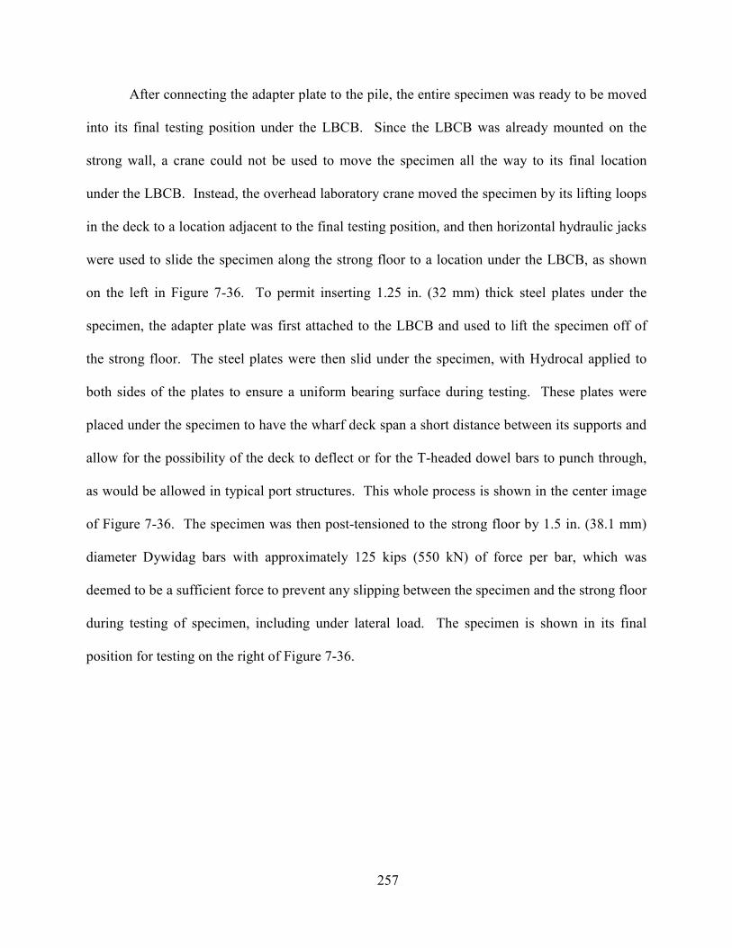
257
After connecting the adapter plate to the pile, the entire specimen was ready to be moved
into its final testing position under the LBCB. Since the LBCB was already mounted on the
strong wall, a crane could not be used to move the specimen all the way to its final location
under the LBCB. Instead, the overhead laboratory crane moved the specimen by its lifting loops
in the deck to a location adjacent to the final testing position, and then horizontal hydraulic jacks
were used to slide the specimen along the strong floor to a location under the LBCB, as shown
on the left in Figure 7-36. To permit inserting 1.25 in. (32 mm) thick steel plates under the
specimen, the adapter plate was first attached to the LBCB and used to lift the specimen off of
the strong floor. The steel plates were then slid under the specimen, with Hydrocal applied to
both sides of the plates to ensure a uniform bearing surface during testing. These plates were
placed under the specimen to have the wharf deck span a short distance between its supports and
allow for the possibility of the deck to deflect or for the T-headed dowel bars to punch through,
as would be allowed in typical port structures. This whole process is shown in the center image
of Figure 7-36. The specimen was then post-tensioned to the strong floor by 1.5 in. (38.1 mm)
diameter Dywidag bars with approximately 125 kips (550 kN) of force per bar, which was
deemed to be a sufficient force to prevent any slipping between the specimen and the strong floor
during testing of specimen, including under lateral load. The specimen is shown in its final
position for testing on the right of Figure 7-36.
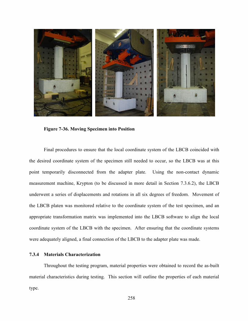
258
Figure 7-36. Moving Specimen into Position
Final procedures to ensure that the local coordinate system of the LBCB coincided with
the desired coordinate system of the specimen still needed to occur, so the LBCB was at this
point temporarily disconnected from the adapter plate. Using the non-contact dynamic
measurement machine, Krypton (to be discussed in more detail in Section 7.3.6.2), the LBCB
underwent a series of displacements and rotations in all six degrees of freedom. Movement of
the LBCB platen was monitored relative to the coordinate system of the test specimen, and an
appropriate transformation matrix was implemented into the LBCB software to align the local
coordinate system of the LBCB with the specimen. After ensuring that the coordinate systems
were adequately aligned, a final connection of the LBCB to the adapter plate was made.
7.3.4 Materials Characterization
Throughout the testing program, material properties were obtained to record the as-built
material characteristics during testing. This section will outline the properties of each material
type.
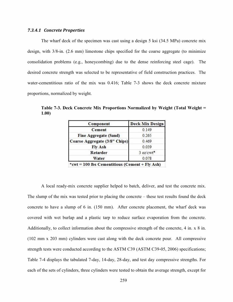
259
7.3.4.1 Concrete Properties
The wharf deck of the specimen was cast using a design 5 ksi (34.5 MPa) concrete mix
design, with 3/8-in. (2.6 mm) limestone chips specified for the coarse aggregate (to minimize
consolidation problems (e.g., honeycombing) due to the dense reinforcing steel cage). The
desired concrete strength was selected to be representative of field construction practices. The
water-cementitious ratio of the mix was 0.416; Table 7-3 shows the deck concrete mixture
proportions, normalized by weight.
Table 7-3. Deck Concrete Mix Proportions ormalized by Weight (Total Weight =
1.00)
A local ready-mix concrete supplier helped to batch, deliver, and test the concrete mix.
The slump of the mix was tested prior to placing the concrete – these test results found the deck
concrete to have a slump of 6 in. (150 mm). After concrete placement, the wharf deck was
covered with wet burlap and a plastic tarp to reduce surface evaporation from the concrete.
Additionally, to collect information about the compressive strength of the concrete, 4 in. x 8 in.
(102 mm x 203 mm) cylinders were cast along with the deck concrete pour. All compressive
strength tests were conducted according to the ASTM C39 (ASTM C39-05, 2006) specifications;
Table 7-4 displays the tabulated 7-day, 14-day, 28-day, and test day compressive strengths. For
each of the sets of cylinders, three cylinders were tested to obtain the average strength, except for

260
the test day cylinders, where five cylinders were tested. Also, due to the disappearance of
cylinders from the moist curing room, only 28-day moist cured strengths were obtained; the
remainder of the cylinders were dry cured in the laboratory.
Table 7-4. Average Cylinder Compressive Strengths
The strength gain with respect to time is shown in Figure 7-37. It can be seen that the
majority of the compressive strength for testing was achieved by 28 days after pouring the wharf
deck slab concrete.
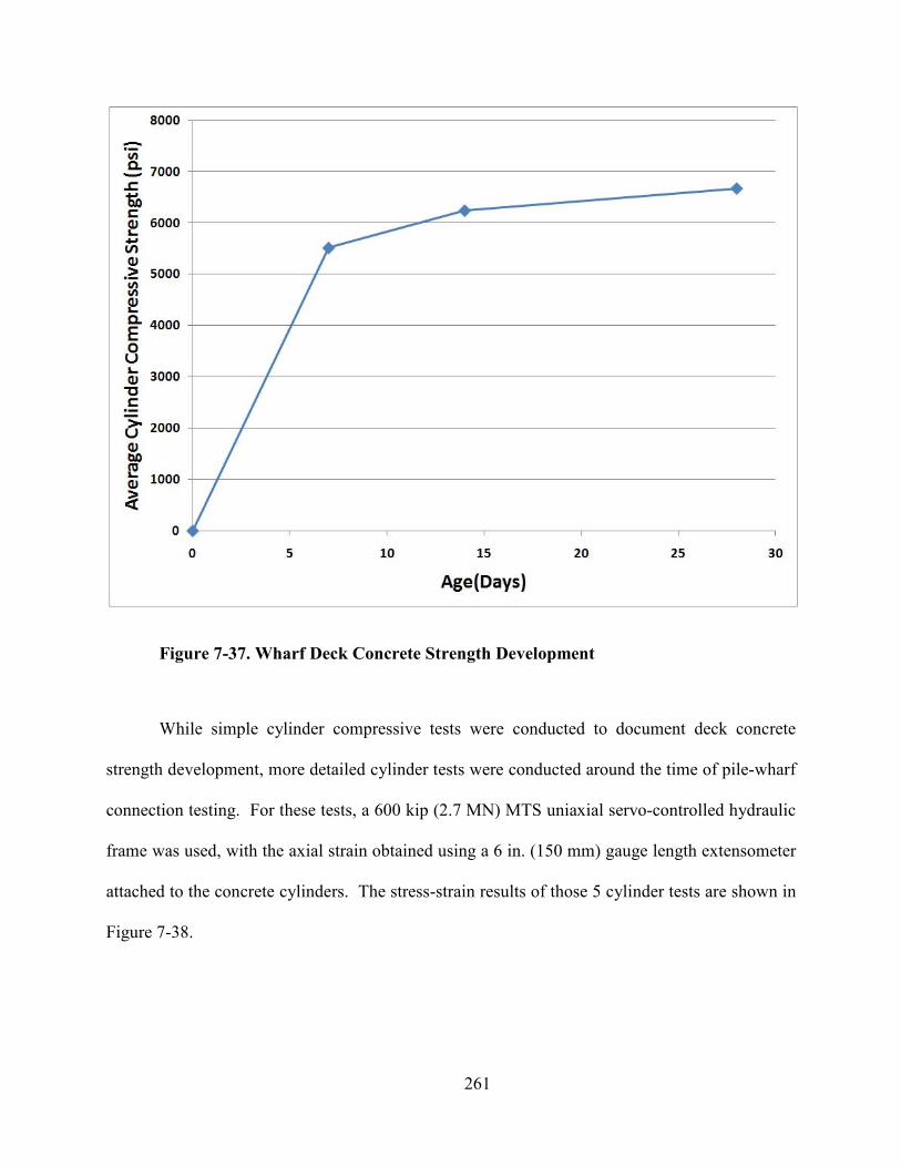
261
Figure 7-37. Wharf Deck Concrete Strength Development
While simple cylinder compressive tests were conducted to document deck concrete
strength development, more detailed cylinder tests were conducted around the time of pile-wharf
connection testing. For these tests, a 600 kip (2.7 MN) MTS uniaxial servo-controlled hydraulic
frame was used, with the axial strain obtained using a 6 in. (150 mm) gauge length extensometer
attached to the concrete cylinders. The stress-strain results of those 5 cylinder tests are shown in
Figure 7-38.
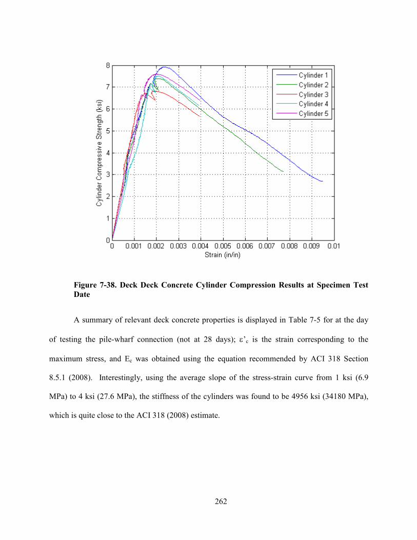
262
Figure 7-38. Deck Deck Concrete Cylinder Compression Results at Specimen Test
Date
A summary of relevant deck concrete properties is displayed in Table 7-5 for at the day
of testing the pile-wharf connection (not at 28 days); ε’c is the strain corresponding to the
maximum stress, and Ec was obtained using the equation recommended by ACI 318 Section
8.5.1 (2008). Interestingly, using the average slope of the stress-strain curve from 1 ksi (6.9
MPa) to 4 ksi (27.6 MPa), the stiffness of the cylinders was found to be 4956 ksi (34180 MPa),
which is quite close to the ACI 318 (2008) estimate.
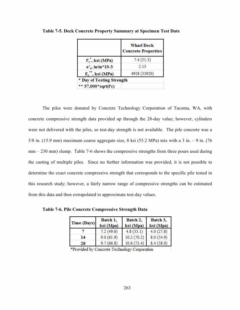
263
Table 7-5. Deck Concrete Property Summary at Specimen Test Date
The piles were donated by Concrete Technology Corporation of Tacoma, WA, with
concrete compressive strength data provided up through the 28-day value; however, cylinders
were not delivered with the piles, so test-day strength is not available. The pile concrete was a
5/8 in. (15.9 mm) maximum coarse aggregate size, 8 ksi (55.2 MPa) mix with a 3 in. – 9 in. (76
mm – 230 mm) slump. Table 7-6 shows the compressive strengths from three pours used during
the casting of multiple piles. Since no further information was provided, it is not possible to
determine the exact concrete compressive strength that corresponds to the specific pile tested in
this research study; however, a fairly narrow range of compressive strengths can be estimated
from this data and then extrapolated to approximate test-day values.
Table 7-6. Pile Concrete Compressive Strength Data
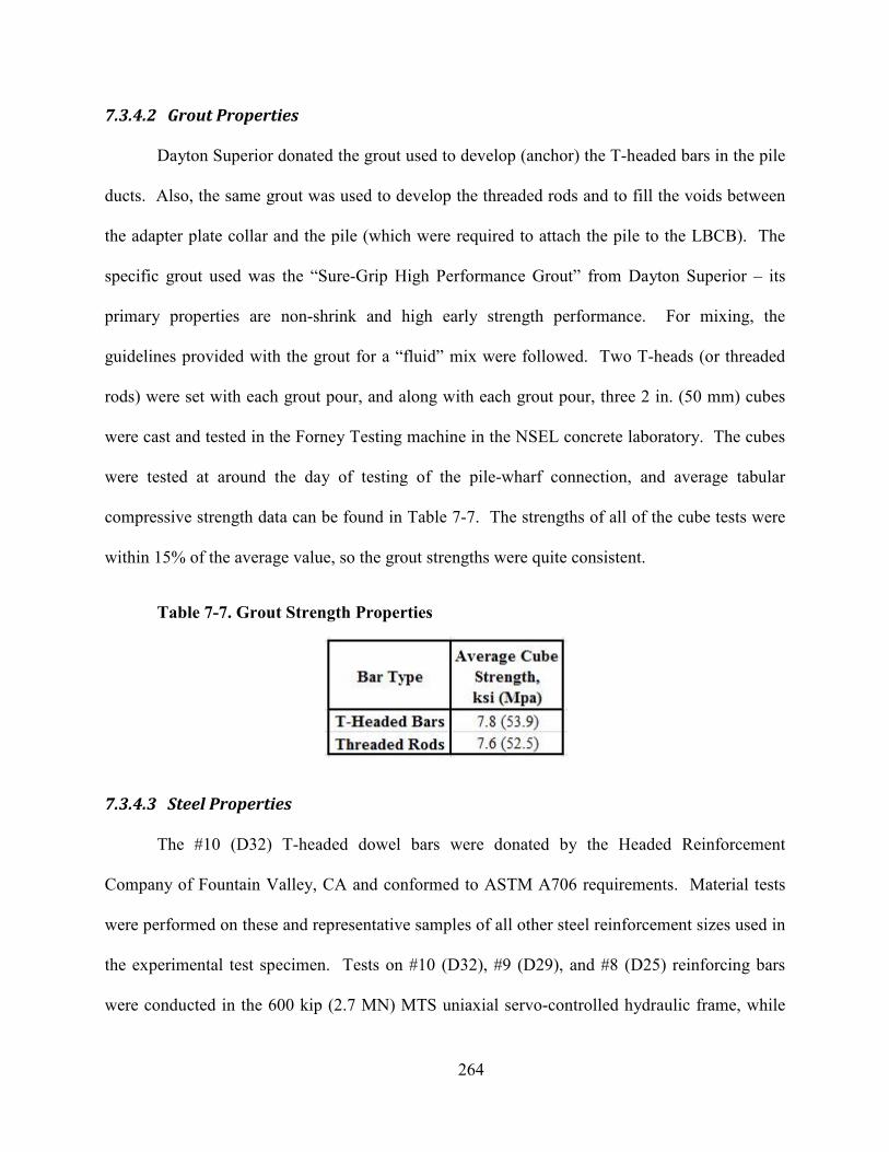
264
7.3.4.2 Grout Properties
Dayton Superior donated the grout used to develop (anchor) the T-headed bars in the pile
ducts. Also, the same grout was used to develop the threaded rods and to fill the voids between
the adapter plate collar and the pile (which were required to attach the pile to the LBCB). The
specific grout used was the “Sure-Grip High Performance Grout” from Dayton Superior – its
primary properties are non-shrink and high early strength performance. For mixing, the
guidelines provided with the grout for a “fluid” mix were followed. Two T-heads (or threaded
rods) were set with each grout pour, and along with each grout pour, three 2 in. (50 mm) cubes
were cast and tested in the Forney Testing machine in the NSEL concrete laboratory. The cubes
were tested at around the day of testing of the pile-wharf connection, and average tabular
compressive strength data can be found in Table 7-7. The strengths of all of the cube tests were
within 15% of the average value, so the grout strengths were quite consistent.
Table 7-7. Grout Strength Properties
7.3.4.3 Steel Properties
The #10 (D32) T-headed dowel bars were donated by the Headed Reinforcement
Company of Fountain Valley, CA and conformed to ASTM A706 requirements. Material tests
were performed on these and representative samples of all other steel reinforcement sizes used in
the experimental test specimen. Tests on #10 (D32), #9 (D29), and #8 (D25) reinforcing bars
were conducted in the 600 kip (2.7 MN) MTS uniaxial servo-controlled hydraulic frame, while
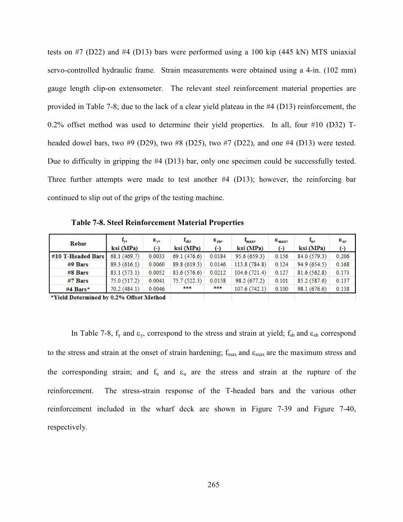
265
tests on #7 (D22) and #4 (D13) bars were performed using a 100 kip (445 kN) MTS uniaxial
servo-controlled hydraulic frame. Strain measurements were obtained using a 4-in. (102 mm)
gauge length clip-on extensometer. The relevant steel reinforcement material properties are
provided in Table 7-8; due to the lack of a clear yield plateau in the #4 (D13) reinforcement, the
0.2% offset method was used to determine their yield properties. In all, four #10 (D32) T-
headed dowel bars, two #9 (D29), two #8 (D25), two #7 (D22), and one #4 (D13) were tested.
Due to difficulty in gripping the #4 (D13) bar, only one specimen could be successfully tested.
Three further attempts were made to test another #4 (D13); however, the reinforcing bar
continued to slip out of the grips of the testing machine.
Table 7-8. Steel Reinforcement Material Properties
In Table 7-8, fy and εy, correspond to the stress and strain at yield; fsh and εsh correspond
to the stress and strain at the onset of strain hardening; fmax and εmax are the maximum stress and
the corresponding strain; and fu and εu are the stress and strain at the rupture of the
reinforcement. The stress-strain response of the T-headed bars and the various other
reinforcement included in the wharf deck are shown in Figure 7-39 and Figure 7-40,
respectively.
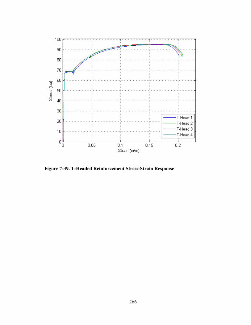
266
Figure 7-39. T-Headed Reinforcement Stress-Strain Response
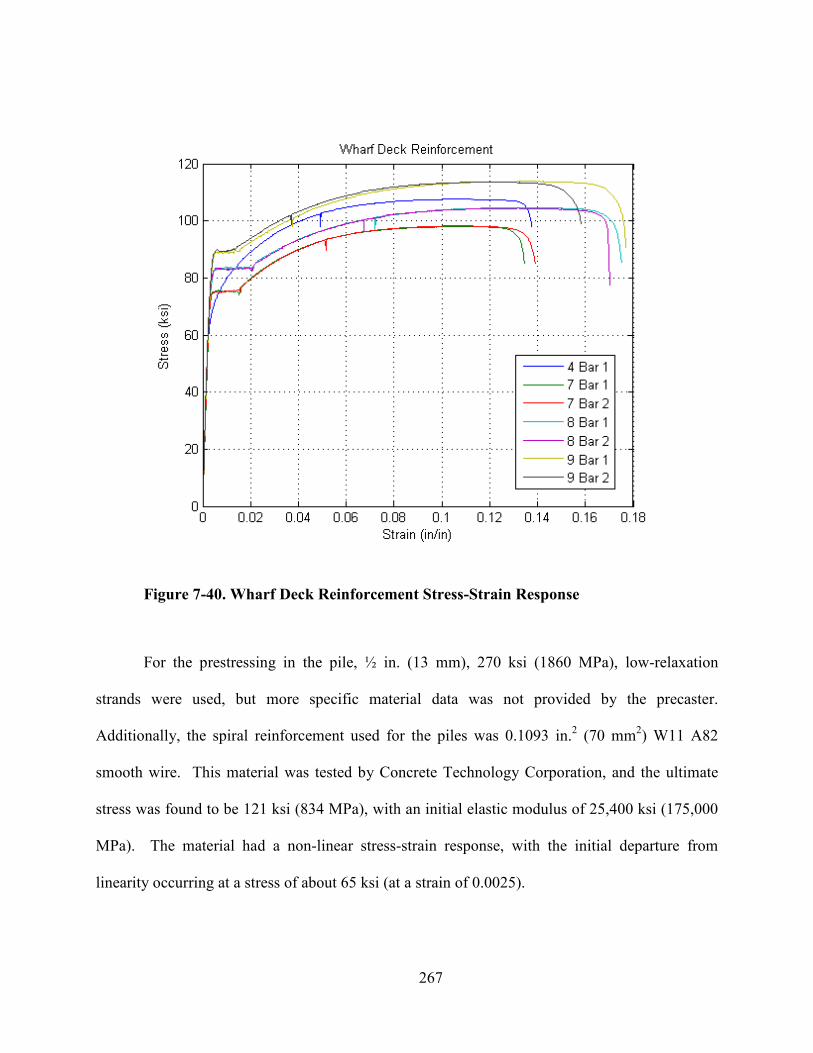
267
Figure 7-40. Wharf Deck Reinforcement Stress-Strain Response
For the prestressing in the pile, ½ in. (13 mm), 270 ksi (1860 MPa), low-relaxation
strands were used, but more specific material data was not provided by the precaster.
Additionally, the spiral reinforcement used for the piles was 0.1093 in.2 (70 mm2) W11 A82
smooth wire. This material was tested by Concrete Technology Corporation, and the ultimate
stress was found to be 121 ksi (834 MPa), with an initial elastic modulus of 25,400 ksi (175,000
MPa). The material had a non-linear stress-strain response, with the initial departure from
linearity occurring at a stress of about 65 ksi (at a strain of 0.0025).
268
7.3.5 EES MUST-SIM Facility Overview and Test Setup
The primary way in which the current structural concrete pile-wharf connection test
differs from other previous tests is the manner in which the loads and displacements are applied.
The University of Illinois Multi-Axial Full-Scale Sub-Structured Testing and Simulation
(MUST-SIM) Facility is one of the 15 equipment sites that form the George E. Brown Network
for Earthquake Engineering Simulation (NEES). The facility possesses six Loading and
Boundary Condition Boxes (LBCBs), which allow for loads and/or displacements to be applied
in all six degrees of freedom. Three of the boxes are in the NSEL, and these full-scale LBCBs
are used to test large-scale specimens. The LBCBs can be oriented in any configuration
necessary for testing, and they may be mounted on either the strong floor or the reaction wall, as
needed. The reaction wall is an L-shaped post-tensioned concrete wall, with legs measuring 50
ft (15.2 m) and 30 ft (9.1 m). Also, the wall is 28 ft (8.5 m) tall, 5 ft (1.5 m) thick, and post-
tensioned to the strong floor, which is a 17 ft (5.2 m) deep box-girder on grade. The full-scale
LBCBs, reaction wall, and strong floor can all be seen in Figure 7-41.
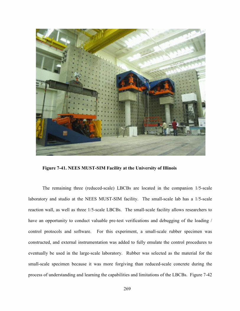
269
Figure 7-41. EES MUST-SIM Facility at the University of Illinois
The remaining three (reduced-scale) LBCBs are located in the companion 1/5-scale
laboratory and studio at the NEES MUST-SIM facility. The small-scale lab has a 1/5-scale
reaction wall, as well as three 1/5-scale LBCBs. The small-scale facility allows researchers to
have an opportunity to conduct valuable pre-test verifications and debugging of the loading /
control protocols and software. For this experiment, a small-scale rubber specimen was
constructed, and external instrumentation was added to fully emulate the control procedures to
eventually be used in the large-scale laboratory. Rubber was selected as the material for the
small-scale specimen because it was more forgiving than reduced-scale concrete during the
process of understanding and learning the capabilities and limitations of the LBCBs. Figure 7-42
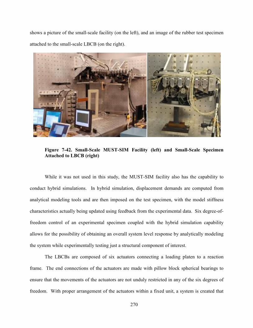
270
shows a picture of the small-scale facility (on the left), and an image of the rubber test specimen
attached to the small-scale LBCB (on the right).
Figure 7-42. Small-Scale MUST-SIM Facility (left) and Small-Scale Specimen
Attached to LBCB (right)
While it was not used in this study, the MUST-SIM facility also has the capability to
conduct hybrid simulations. In hybrid simulation, displacement demands are computed from
analytical modeling tools and are then imposed on the test specimen, with the model stiffness
characteristics actually being updated using feedback from the experimental data. Six degree-of-
freedom control of an experimental specimen coupled with the hybrid simulation capability
allows for the possibility of obtaining an overall system level response by analytically modeling
the system while experimentally testing just a structural component of interest.
The LBCBs are composed of six actuators connecting a loading platen to a reaction
frame. The end connections of the actuators are made with pillow block spherical bearings to
ensure that the movements of the actuators are not unduly restricted in any of the six degrees of
freedom. With proper arrangement of the actuators within a fixed unit, a system is created that
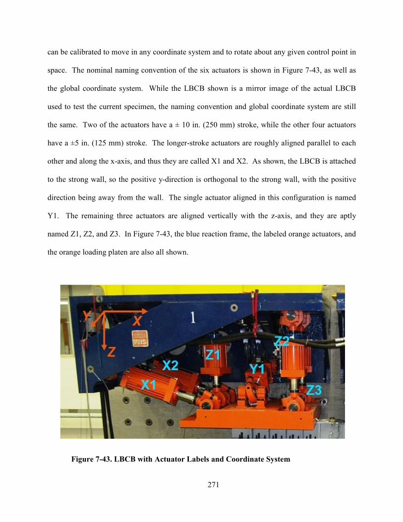
271
can be calibrated to move in any coordinate system and to rotate about any given control point in
space. The nominal naming convention of the six actuators is shown in Figure 7-43, as well as
the global coordinate system. While the LBCB shown is a mirror image of the actual LBCB
used to test the current specimen, the naming convention and global coordinate system are still
the same. Two of the actuators have a ± 10 in. (250 mm) stroke, while the other four actuators
have a ±5 in. (125 mm) stroke. The longer-stroke actuators are roughly aligned parallel to each
other and along the x-axis, and thus they are called X1 and X2. As shown, the LBCB is attached
to the strong wall, so the positive y-direction is orthogonal to the strong wall, with the positive
direction being away from the wall. The single actuator aligned in this configuration is named
Y1. The remaining three actuators are aligned vertically with the z-axis, and they are aptly
named Z1, Z2, and Z3. In Figure 7-43, the blue reaction frame, the labeled orange actuators, and
the orange loading platen are also all shown.
Figure 7-43. LBCB with Actuator Labels and Coordinate System
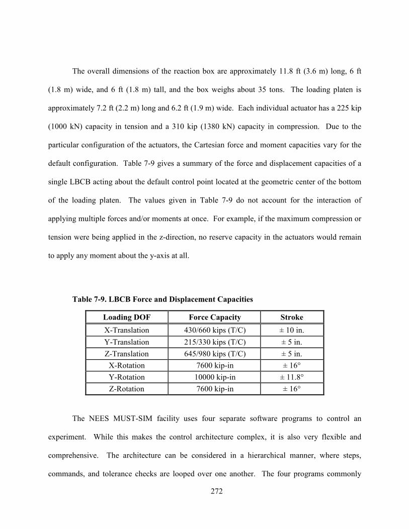
272
The overall dimensions of the reaction box are approximately 11.8 ft (3.6 m) long, 6 ft
(1.8 m) wide, and 6 ft (1.8 m) tall, and the box weighs about 35 tons. The loading platen is
approximately 7.2 ft (2.2 m) long and 6.2 ft (1.9 m) wide. Each individual actuator has a 225 kip
(1000 kN) capacity in tension and a 310 kip (1380 kN) capacity in compression. Due to the
particular configuration of the actuators, the Cartesian force and moment capacities vary for the
default configuration. Table 7-9 gives a summary of the force and displacement capacities of a
single LBCB acting about the default control point located at the geometric center of the bottom
of the loading platen. The values given in Table 7-9 do not account for the interaction of
applying multiple forces and/or moments at once. For example, if the maximum compression or
tension were being applied in the z-direction, no reserve capacity in the actuators would remain
to apply any moment about the y-axis at all.
Table 7-9. LBCB Force and Displacement Capacities
Loading DOF Force Capacity Stroke
X-Translation 430/660 kips (T/C) ± 10 in.
Y-Translation 215/330 kips (T/C) ± 5 in.
Z-Translation 645/980 kips (T/C) ± 5 in.
X-Rotation 7600 kip-in ± 16°
Y-Rotation 10000 kip-in ± 11.8°
Z-Rotation 7600 kip-in ± 16°
The NEES MUST-SIM facility uses four separate software programs to control an
experiment. While this makes the control architecture complex, it is also very flexible and
comprehensive. The architecture can be considered in a hierarchical manner, where steps,
commands, and tolerance checks are looped over one another. The four programs commonly
273
used at the MUST-SIM facility have been termed as the Simulation Coordinator (SimCor), the
LBCB Plugin, the Operation Manager (OM), and the Shore Western control software. This
software is exclusively used to control the LBCB, while an entirely different system of
computers is then used for data acquisition, for taking photographs, and for sharing real-time
data and images with off-site collaborators. The other programs used are the data and acquisition
software (NEESdaq), camera plugin, Krypton plugin, Data Turbine, Remote Data Viewer
(RDV), and NEES Central. The overall software architecture is shown in Figure 7-44.
Figure 7-44. MUST-SIM Overall Software Architecture
The LBCBs are servo-controlled units produced by Shore Western Manufacturing of
Monrovia, CA. The Shore Western controller is used to drive and to maintain the actuators at a
given command length, but it is not capable of calculating the required sets of displacements of
274
the six individual actuators necessary to achieve a desired overall Cartesian LBCB position.
Since the only data available are the actuator lengths and connection points of the actuator ends,
the Operation Manager (OM) is used to make the transformation from actuator space to
Cartesian space. A closed form solution can be obtained to determine the actuator lengths from a
given Cartesian position; however, an iterative solution is required to compute the Cartesian
location for given actuator lengths. Nakata et al. (2007) discusses the method used by the OM to
calculate the Cartesian position using a Newton-Raphson iterative solution with a kinematic
Jabcobian. To successfully move the LBCB platforms smoothly in Cartesian space, the actuator
commands and the corresponding feedback must be rapidly processed by the OM. The decision
to use a separate computer for the OM to generate and measure the commands is due to the
computational expense of the previously described procedure. The OM receives the servo error,
LVDT readings, and load cell readings from each actuator, and the individual actuator readings
are used to calculate the current Cartesian position of the loading platen. With the position of the
loading platen known and the load cell readings, the individual actuator vectors can then be used
to calculate the Cartesian forces and moments about the control point.
User input to the OM is required for all six degrees of freedom, and the OM is capable of
handling both force-controlled and displacement-controlled loading schemes. While a
displacement-controlled degree of freedom is straight forward, a force-controlled degree of
freedom requires another iterative loop within the OM. The specimen stiffness is stored and
continually updated in the OM, based on the change in force obtained for a given change in
displacement command. Thus, the OM calculates the estimated change in displacement required
to achieve the desired force. Iterations of the force-controlled DOFs are conducted one DOF at a
time, in order to ensure that the effect of changing a single DOF is properly represented in the
275
specimen stiffness matrix. This procedure continues until all of the force-controlled degrees of
freedom are brought within the user-defined tolerance.
While the OM is able to enforce mixed-mode commands using the LBCB throughout
testing, the Cartesian displacements calculated by the OM do not necessarily reflect the
displacements realized by the specimen control point. Since an equal and opposite force occurs
in the LBCB any time a load is applied to a specimen, the LBCBs are susceptible to elastic
deformations that must be accounted for if the desired specimen displacements are to be
achieved. Since the OM is unaware of these errors or their magnitude, an additional software
package is used to augment the Cartesian commands created by the OM – this software is the
LBCB Plugin. Obtaining the actual specimen displacement requires a set of external sensors
mounted to the specimen control point. The connection locations of these sensors in Cartesian
space are input into the LBCB Plugin. The LBCB Plugin then uses the changes in the external
sensor readings and the desired input displacements to compute a kinematic Jacobian defining
the relationship between a change in specimen location vs. the change in external sensor
readings, similar to the procedure described to compute the actuator-to-Cartesian calculations in
the OM. If the measured specimen displacement(s) differ from the desired input displacement(s)
by more than the user-defined tolerance, the necessary adjustment to the input displacement is
computed and sent to the OM for another iteration. This process continues until all of the
displacement DOFs have converged within their tolerances.
Once all of the mixed-mode criteria for a particular step have been satisfied, the LBCB
Plugin then sends triggers to the data acquisition software, camera plugin, and Krypton plugin to
collect what has been colloquially termed “step data.” The step data provides synchronized data
from a given step collected from each instrument, as well as the LBCB command, displacement,
276
and force data. Previous versions of the control software used UI-SimCor for data
synchronization, but with recent updates to the software packages and given that this test was not
a hybrid simulation, the use of UI-SimCor was not required. An additional feature of the
software packages is that the data samples collected can be simultaneously shared across the
internet to the NEES Realtime Data View (RDV) for remote viewing by project colleagues and
to NEES Central for additional data archiving. The previously described procedure is repeated
for each individual load step until all of the steps are completed.
7.3.6 Instrumentation
One of the characteristics of a NEESR project at the MUST-SIM facility is the quantity
and variety of instrumentation applied to each test specimen. Such dense data collection is
critical toward making any future comprehensive modeling endeavors as robust as possible. The
current test specimen was heavily instrumented with traditional instrumentation, such as strain
gauges, linear variable displacement transducers (LVDTs), string potentiometers, and
inclinometers. Additionally, the Krypton system, introduced previously in Section 3.6, was used
as a non-contact measurement machine to obtain a dense specimen displacement field during
testing. In total, 137 channels of data were logged by the DAQ system, and an additional 132
LED positions were recorded by the Krypton system throughout testing. Further specifics about
types of instrumentation, DAQ setup, and application to the test specimen will be discussed in
this section.
7.3.6.1 Traditional Instrumentation
Quarter-bridge strain gauges were applied densely on the #10 (D32) T-headed dowel bars
and more lightly throughout the reinforcement in the deck and on the pile concrete surface. The
strain gauges applied to the steel reinforcement were high-elongation, with a 0.4 in. (10 mm)
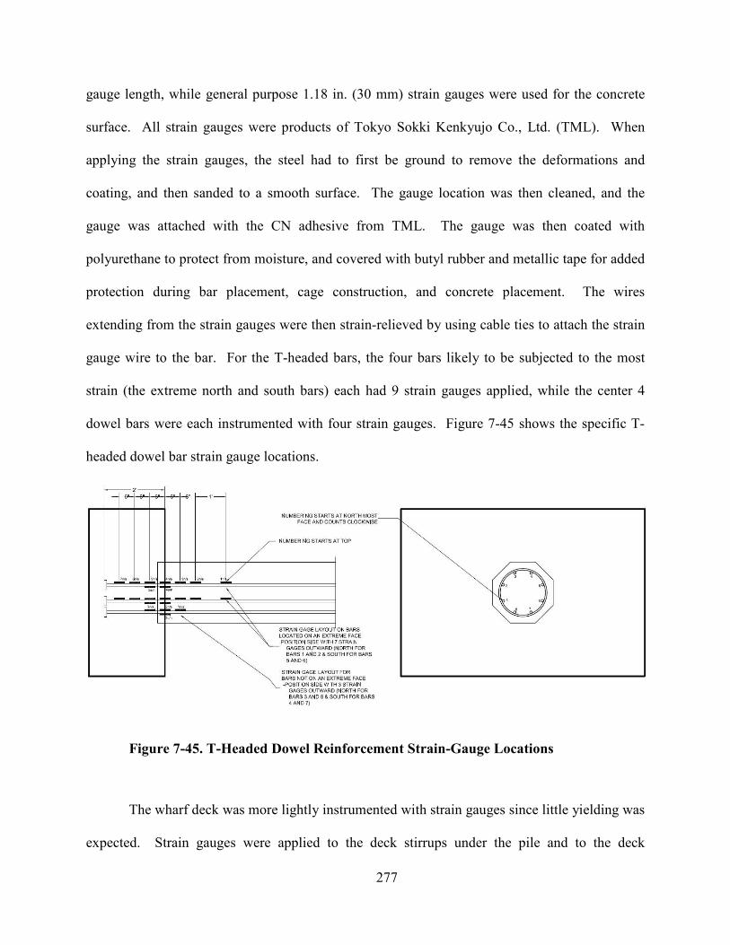
277
gauge length, while general purpose 1.18 in. (30 mm) strain gauges were used for the concrete
surface. All strain gauges were products of Tokyo Sokki Kenkyujo Co., Ltd. (TML). When
applying the strain gauges, the steel had to first be ground to remove the deformations and
coating, and then sanded to a smooth surface. The gauge location was then cleaned, and the
gauge was attached with the CN adhesive from TML. The gauge was then coated with
polyurethane to protect from moisture, and covered with butyl rubber and metallic tape for added
protection during bar placement, cage construction, and concrete placement. The wires
extending from the strain gauges were then strain-relieved by using cable ties to attach the strain
gauge wire to the bar. For the T-headed bars, the four bars likely to be subjected to the most
strain (the extreme north and south bars) each had 9 strain gauges applied, while the center 4
dowel bars were each instrumented with four strain gauges. Figure 7-45 shows the specific T-
headed dowel bar strain gauge locations.
Figure 7-45. T-Headed Dowel Reinforcement Strain-Gauge Locations
The wharf deck was more lightly instrumented with strain gauges since little yielding was
expected. Strain gauges were applied to the deck stirrups under the pile and to the deck
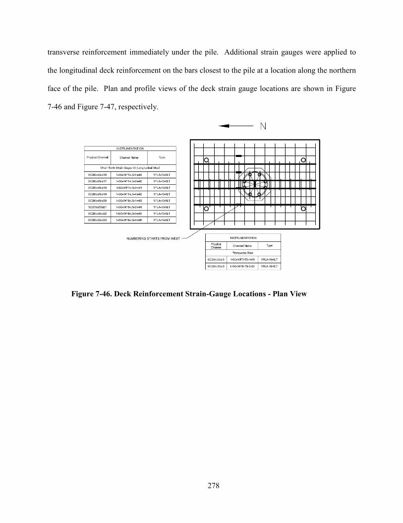
278
transverse reinforcement immediately under the pile. Additional strain gauges were applied to
the longitudinal deck reinforcement on the bars closest to the pile at a location along the northern
face of the pile. Plan and profile views of the deck strain gauge locations are shown in Figure
7-46 and Figure 7-47, respectively.
Figure 7-46. Deck Reinforcement Strain-Gauge Locations - Plan View
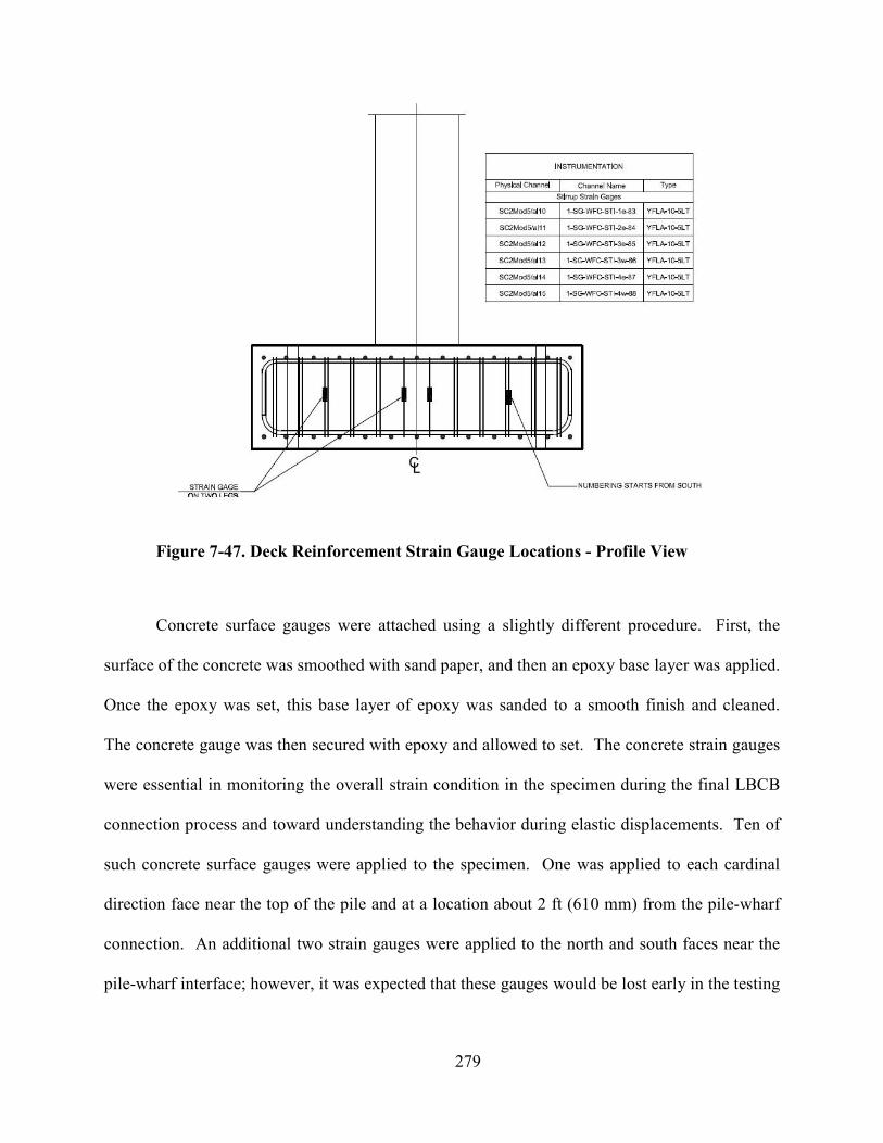
279
Figure 7-47. Deck Reinforcement Strain Gauge Locations - Profile View
Concrete surface gauges were attached using a slightly different procedure. First, the
surface of the concrete was smoothed with sand paper, and then an epoxy base layer was applied.
Once the epoxy was set, this base layer of epoxy was sanded to a smooth finish and cleaned.
The concrete gauge was then secured with epoxy and allowed to set. The concrete strain gauges
were essential in monitoring the overall strain condition in the specimen during the final LBCB
connection process and toward understanding the behavior during elastic displacements. Ten of
such concrete surface gauges were applied to the specimen. One was applied to each cardinal
direction face near the top of the pile and at a location about 2 ft (610 mm) from the pile-wharf
connection. An additional two strain gauges were applied to the north and south faces near the
pile-wharf interface; however, it was expected that these gauges would be lost early in the testing
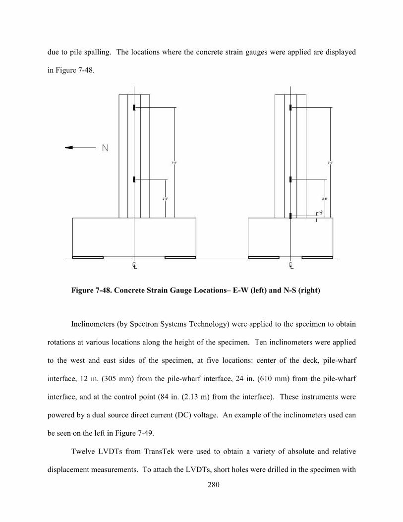
280
due to pile spalling. The locations where the concrete strain gauges were applied are displayed
in Figure 7-48.
Figure 7-48. Concrete Strain Gauge Locations– E-W (left) and -S (right)
Inclinometers (by Spectron Systems Technology) were applied to the specimen to obtain
rotations at various locations along the height of the specimen. Ten inclinometers were applied
to the west and east sides of the specimen, at five locations: center of the deck, pile-wharf
interface, 12 in. (305 mm) from the pile-wharf interface, 24 in. (610 mm) from the pile-wharf
interface, and at the control point (84 in. (2.13 m) from the interface). These instruments were
powered by a dual source direct current (DC) voltage. An example of the inclinometers used can
be seen on the left in Figure 7-49.
Twelve LVDTs from TransTek were used to obtain a variety of absolute and relative
displacement measurements. To attach the LVDTs, short holes were drilled in the specimen with
281
an impact drill, epoxy was injected into the holes, and ¼ in. (6 mm) diameter threaded rods were
inserted. The LVDTs were then connected using specially constructed LVDT holders attached to
the threaded rods. Four LVDTs were used to monitor any uplift, rotation, or slip of the wharf
deck. Uplift of the deck was monitored using two vertically aligned LVDTs attached to the
north and south faces of the wharf deck. Rotation and slip of the deck were monitored through
two horizontally aligned LVDTs attached to the strong floor and monitoring locations on the
west and east corners of the south deck face.
Uplift of the pile was monitored by using four spring-loaded LVDTs, where two were
attached to each of the west and east faces of the pile near the pile-wharf interface. These
LVDTs provided a relative measurement between the pile and wharf deck; however, due to deck
spalling over the course of testing, some of the later LVDT uplift measurements became
unreliable. The remaining LVDTs were used to measure the curvature of the pile at 12 in. (305
mm) and 24 in. (610 mm) from the pile-deck interface. These LVDTs were attached to the pile,
with their measurements taken relative to a steel angle supported slightly above the deck. The
steel angle was used to prevent deck spalling near the North and South faces of the pile from
affecting these LVDT readings. The deck LVDTs were powered by a DC voltage, while the
LVDTs attached to the pile all used an alternating current (AC) power supply. An example of an
LVDT used for the pile curvature measurements is shown in the center of Figure 7-49.
The final type of traditional instrumentation used was string potentiometers from
Celesco. In total, nine string potentiometers were used to obtain absolute measurements of the
displacement of the pile at several locations. Depending on the expected range of motion, string
potentiometers of different length strokes were used. To monitor any slip of the pile relative to
the wharf deck, two string potentiometer bases were secured to the north end of the wharf deck
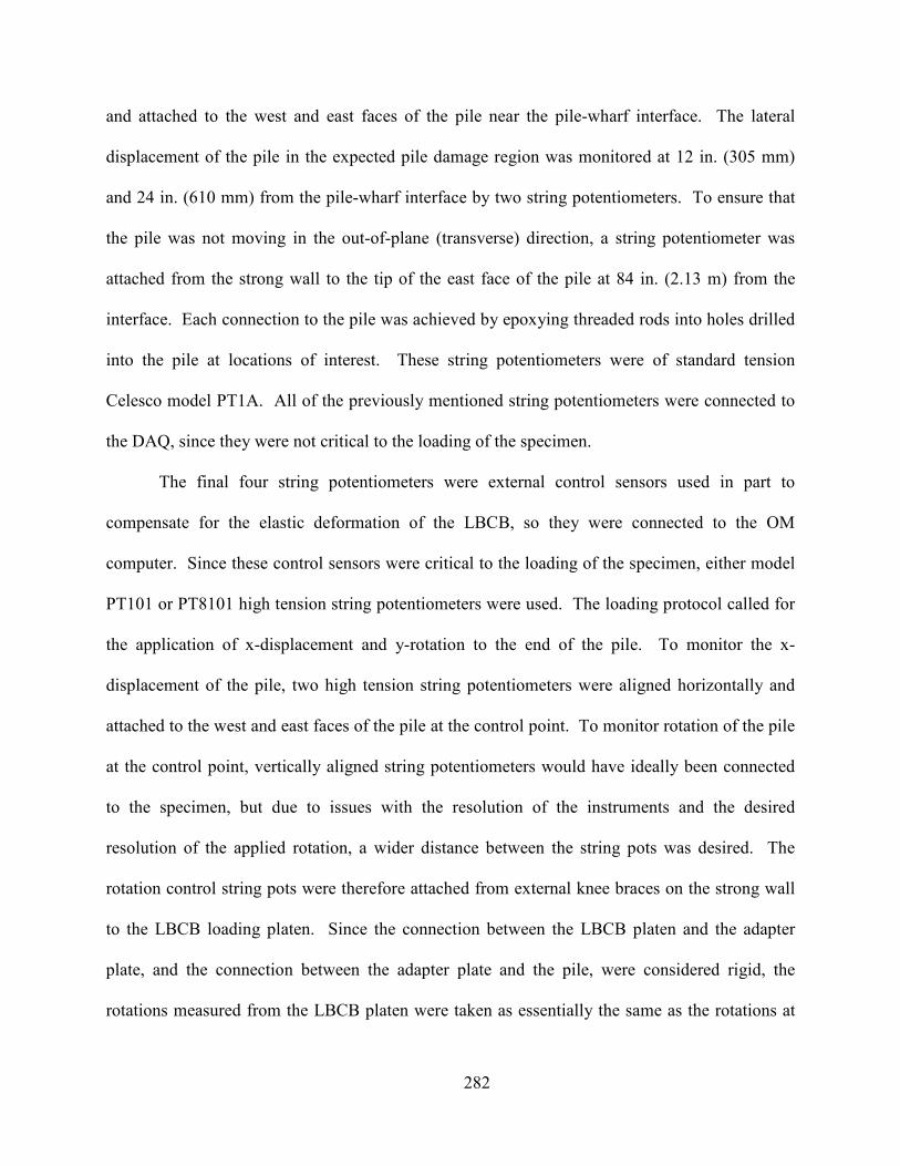
282
and attached to the west and east faces of the pile near the pile-wharf interface. The lateral
displacement of the pile in the expected pile damage region was monitored at 12 in. (305 mm)
and 24 in. (610 mm) from the pile-wharf interface by two string potentiometers. To ensure that
the pile was not moving in the out-of-plane (transverse) direction, a string potentiometer was
attached from the strong wall to the tip of the east face of the pile at 84 in. (2.13 m) from the
interface. Each connection to the pile was achieved by epoxying threaded rods into holes drilled
into the pile at locations of interest. These string potentiometers were of standard tension
Celesco model PT1A. All of the previously mentioned string potentiometers were connected to
the DAQ, since they were not critical to the loading of the specimen.
The final four string potentiometers were external control sensors used in part to
compensate for the elastic deformation of the LBCB, so they were connected to the OM
computer. Since these control sensors were critical to the loading of the specimen, either model
PT101 or PT8101 high tension string potentiometers were used. The loading protocol called for
the application of x-displacement and y-rotation to the end of the pile. To monitor the x-
displacement of the pile, two high tension string potentiometers were aligned horizontally and
attached to the west and east faces of the pile at the control point. To monitor rotation of the pile
at the control point, vertically aligned string potentiometers would have ideally been connected
to the specimen, but due to issues with the resolution of the instruments and the desired
resolution of the applied rotation, a wider distance between the string pots was desired. The
rotation control string pots were therefore attached from external knee braces on the strong wall
to the LBCB loading platen. Since the connection between the LBCB platen and the adapter
plate, and the connection between the adapter plate and the pile, were considered rigid, the
rotations measured from the LBCB platen were taken as essentially the same as the rotations at
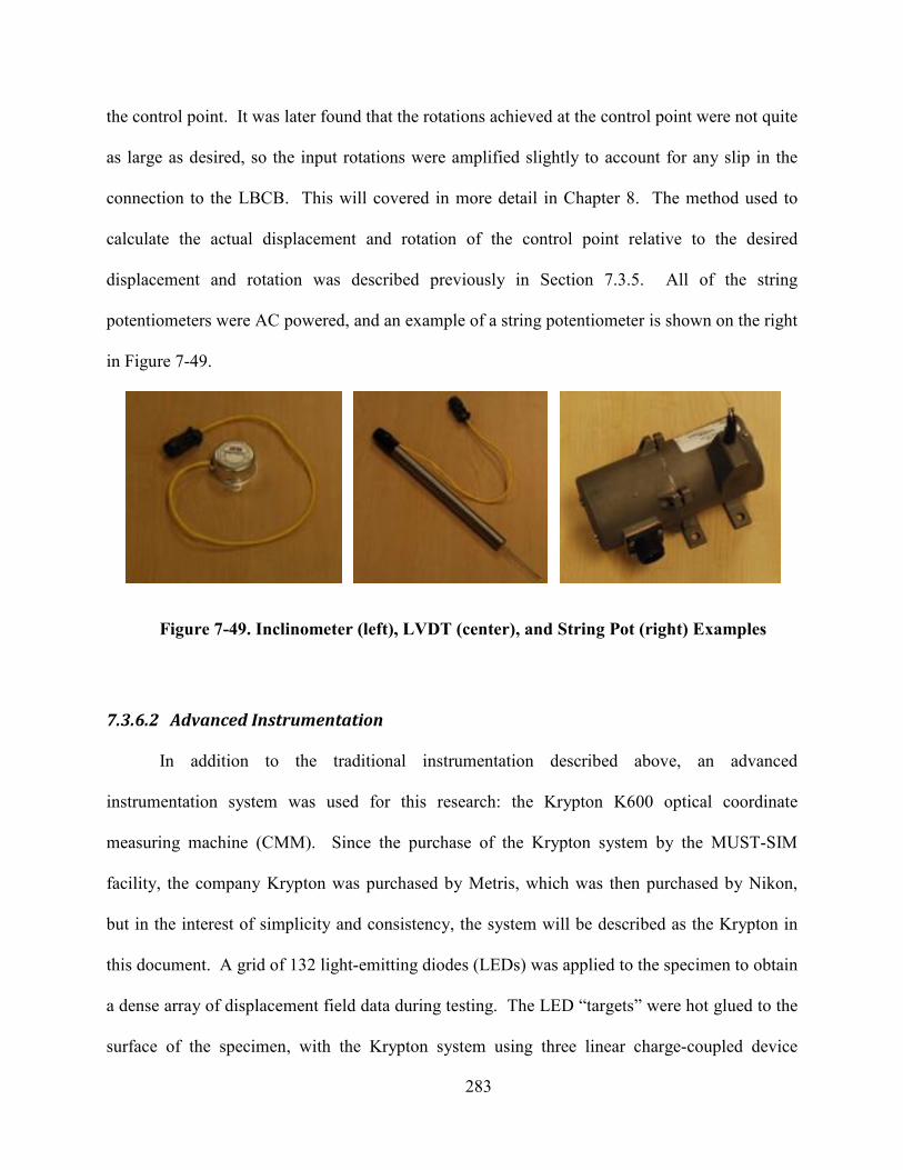
283
the control point. It was later found that the rotations achieved at the control point were not quite
as large as desired, so the input rotations were amplified slightly to account for any slip in the
connection to the LBCB. This will covered in more detail in Chapter 8. The method used to
calculate the actual displacement and rotation of the control point relative to the desired
displacement and rotation was described previously in Section 7.3.5. All of the string
potentiometers were AC powered, and an example of a string potentiometer is shown on the right
in Figure 7-49.
Figure 7-49. Inclinometer (left), LVDT (center), and String Pot (right) Examples
7.3.6.2 Advanced Instrumentation
In addition to the traditional instrumentation described above, an advanced
instrumentation system was used for this research: the Krypton K600 optical coordinate
measuring machine (CMM). Since the purchase of the Krypton system by the MUST-SIM
facility, the company Krypton was purchased by Metris, which was then purchased by Nikon,
but in the interest of simplicity and consistency, the system will be described as the Krypton in
this document. A grid of 132 light-emitting diodes (LEDs) was applied to the specimen to obtain
a dense array of displacement field data during testing. The LED “targets” were hot glued to the
surface of the specimen, with the Krypton system using three linear charge-coupled device
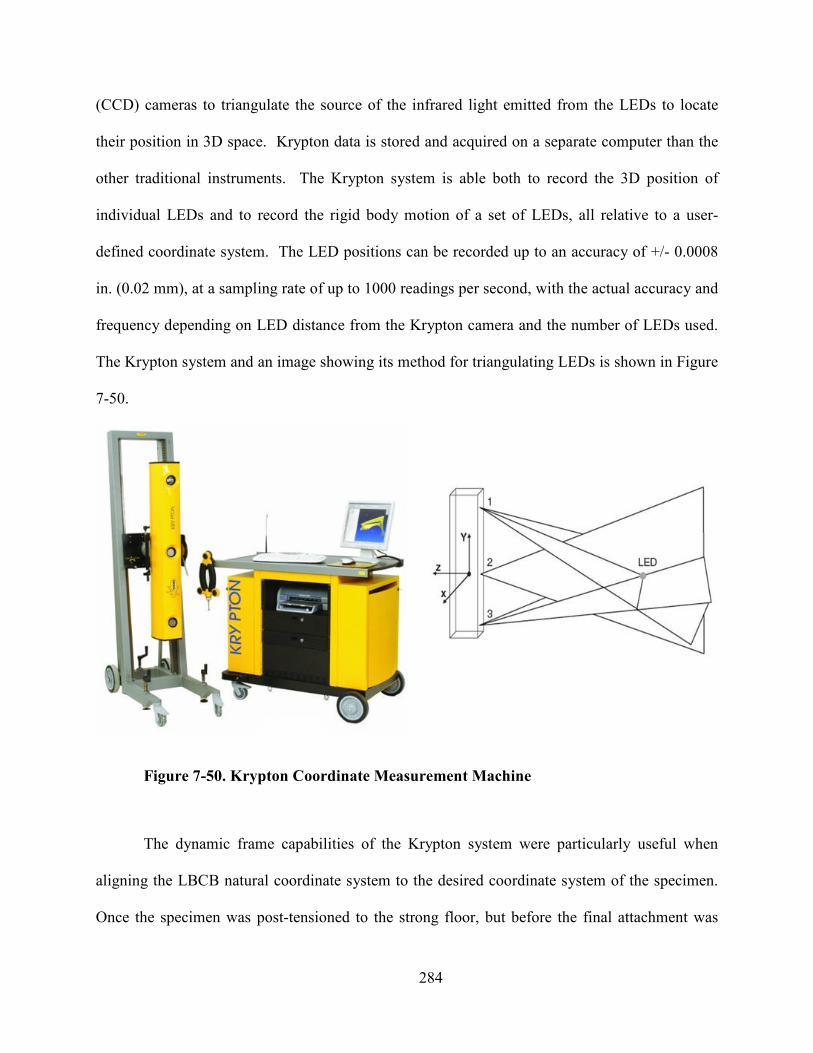
284
(CCD) cameras to triangulate the source of the infrared light emitted from the LEDs to locate
their position in 3D space. Krypton data is stored and acquired on a separate computer than the
other traditional instruments. The Krypton system is able both to record the 3D position of
individual LEDs and to record the rigid body motion of a set of LEDs, all relative to a user-
defined coordinate system. The LED positions can be recorded up to an accuracy of +/- 0.0008
in. (0.02 mm), at a sampling rate of up to 1000 readings per second, with the actual accuracy and
frequency depending on LED distance from the Krypton camera and the number of LEDs used.
The Krypton system and an image showing its method for triangulating LEDs is shown in Figure
7-50.
Figure 7-50. Krypton Coordinate Measurement Machine
The dynamic frame capabilities of the Krypton system were particularly useful when
aligning the LBCB natural coordinate system to the desired coordinate system of the specimen.
Once the specimen was post-tensioned to the strong floor, but before the final attachment was
285
made between the adapter plate and the LBCB, the LBCB coordinate system had to be
transformed to a coordinate system in “specimen space”. To accomplish this, a dynamic frame
was created with LEDs attached to the LBCB platen, while a measurement coordinate system
was defined relative to the test specimen. Then, the LBCB underwent a series of displacements
and rotations, one degree of freedom at a time, while the movement was monitored with the
Krypton. Using these results, a transformation matrix was produced to adjust the LBCB motion
to align with the specimen coordinate system. This procedure was then repeated, and the
alignment of rotations and displacements was verified. In a similar manner, the control point of
the LBCB was monitored and translated to the appropriate location within the specimen. A
useful capability of the Krypton data is that each node can be considered a node of a finite
element model, and thus the displacement field can be input and operated on in a similar fashion
as a finite element post-processor to provide strains in quadrilateral elements. This will be
further demonstrated in Chapter 8, and an image of the dense LED grid pattern is shown in
Figure 7-51.

286
Figure 7-51. Krypton LED Grid Layout
An overall line drawing showing the location of all the aforementioned instrumentation,
traditional and advanced, is displayed in Figure 7-52.
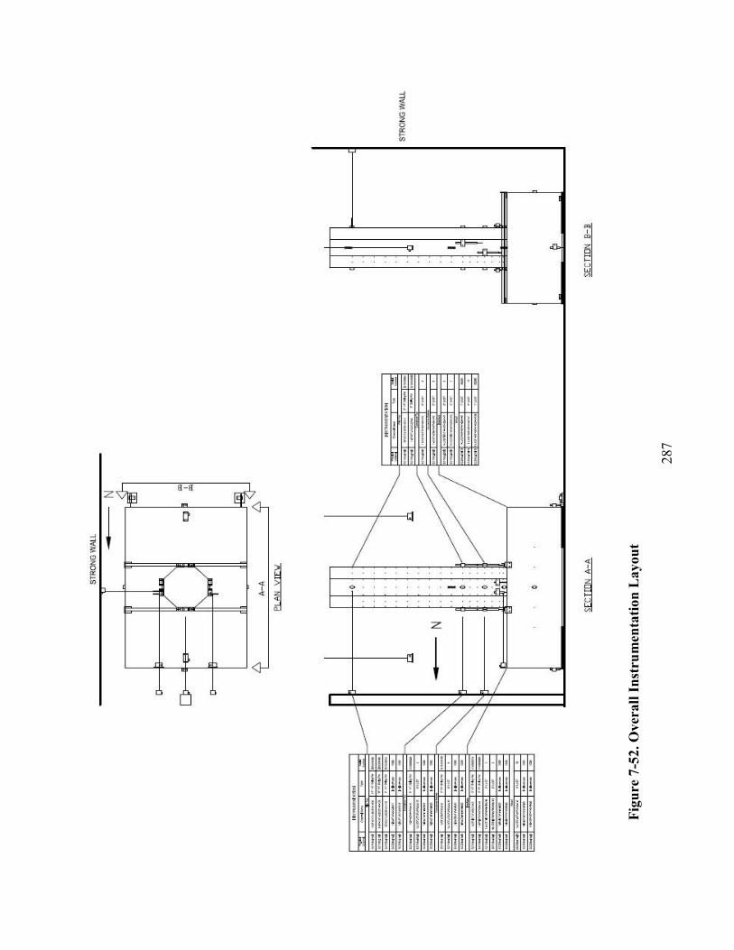
287
Fig
ure
7-5
2. O
ver
all
In
stru
men
tati
on
Layou
t
288
7.3.6.3 NEES Data Acquisition System
As can be seen from the previous sections, the instruments used to obtain data from the
port specimen were extensive, and collecting the data in a meaningful way is critical to the
understanding and analysis conducted after the experiment. The data during testing was
collected both discretely and continuously. The discrete data was collected at the conclusion of
each step, which provides a manageable amount of data to analyze the response of the specimen
during testing. To capture any events between converged loading steps, continuous data was
also collected. The continuous data collection is more traditional; however, synchronizing the
data collected on multiple computers can become burdensome during post-processing.
In total, the (non-Krypton) DAQ system logged 137 channels with the following
breakdown: 24 LBCB channels (load and displacement in Cartesian and actuator space), 12
LVDT channels, 9 string potentiometer channels, 10 inclinometer channels, 68 steel strain gauge
channels, 10 concrete strain gauge channels, and 4 excitation voltage channels. The DAQ unit
used National Instruments (NI) hardware. Two SCXI-1001 chassis were connected in series,
with signal conditioning completed by the modules and terminals connected into each chassis.
The modules used were SCXI-1540, SCXI-1521b, and SCXI-1104c. These modules were
connected to the SCXI-1513, SCXI-1317, and BNC-2095 terminal blocks, respectively. The
chassis were connected to the DAQ computer with an NI PCI-6289 card, and the signals were
monitored using the NEESdaq program built with LabView. The NEESdaq program was written
such that each instrument could be input into a spreadsheet, with relevant calibration and channel
name parameters provided. Then, a script automatically generates each channel within the
NEESdaq program, eliminating the tedious task of inputting each individual channel by the
researcher. All of the data collected is recorded locally, and will be uploaded to the NEEShub

289
data repository for use by collaborators. Additionally, data from this current experimental
program and the subsequent repaired pile test has been archived locally at the NEES MUST-SIM
facility for future researchers.
290
CHAPTER 8. PILE-WHARF COECTIO EXPERIMETAL RESULTS
One of the major objectives of this current study is to understand the structural behavior
of pile-wharf connections; thus it is critical to examine in detail the onset and progression of
damage during testing, as well as to understand the global and local responses of the test
specimen. The data investigated in this analysis is available for future researchers both at the
NEEShub data repository and at the MUST-SIM facility at the University of Illinois.
8.1 Overall Global Behavior
The overall global behavior of the pile-wharf connection specimen was monitored
throughout testing. The global behavior here is described as the applied and resulting
displacements, as well as the reaction (resulting) forces and moments. As previously noted, the
forces applied to the specimen were monitored by measuring the forces in the load cells located
on each of the six actuators, and then the actuator forces were converted into specimen space
through transformation matrices. The displacements imposed on the specimen were controlled
through an iterative feedback loop between externally mounted string potentiometers and the
LVDTs located on each actuator. Additional verification of these displacements will be shown
in this section, where the intended displacements and rotations are compared to the actual
measured values from other data acquisition instruments. The fully instrumented pile-wharf
connection specimen is shown in Figure 8-1 right before testing. Many of the instruments can be
seen, including the dense Krypton LED grid and the rotation control string potentiometers. The
vertical reinforcing bars protruding from the wharf deck are partially pre-installed for later use in
the repair during the next phase of the experimental program (after the testing described below).
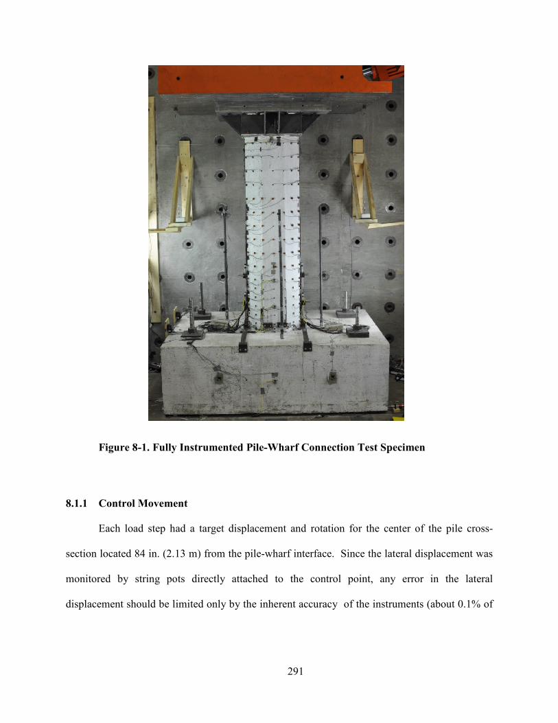
291
Figure 8-1. Fully Instrumented Pile-Wharf Connection Test Specimen
8.1.1 Control Movement
Each load step had a target displacement and rotation for the center of the pile cross-
section located 84 in. (2.13 m) from the pile-wharf interface. Since the lateral displacement was
monitored by string pots directly attached to the control point, any error in the lateral
displacement should be limited only by the inherent accuracy of the instruments (about 0.1% of
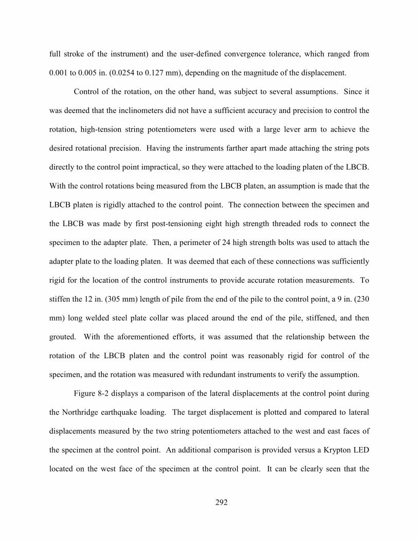
292
full stroke of the instrument) and the user-defined convergence tolerance, which ranged from
0.001 to 0.005 in. (0.0254 to 0.127 mm), depending on the magnitude of the displacement.
Control of the rotation, on the other hand, was subject to several assumptions. Since it
was deemed that the inclinometers did not have a sufficient accuracy and precision to control the
rotation, high-tension string potentiometers were used with a large lever arm to achieve the
desired rotational precision. Having the instruments farther apart made attaching the string pots
directly to the control point impractical, so they were attached to the loading platen of the LBCB.
With the control rotations being measured from the LBCB platen, an assumption is made that the
LBCB platen is rigidly attached to the control point. The connection between the specimen and
the LBCB was made by first post-tensioning eight high strength threaded rods to connect the
specimen to the adapter plate. Then, a perimeter of 24 high strength bolts was used to attach the
adapter plate to the loading platen. It was deemed that each of these connections was sufficiently
rigid for the location of the control instruments to provide accurate rotation measurements. To
stiffen the 12 in. (305 mm) length of pile from the end of the pile to the control point, a 9 in. (230
mm) long welded steel plate collar was placed around the end of the pile, stiffened, and then
grouted. With the aforementioned efforts, it was assumed that the relationship between the
rotation of the LBCB platen and the control point was reasonably rigid for control of the
specimen, and the rotation was measured with redundant instruments to verify the assumption.
Figure 8-2 displays a comparison of the lateral displacements at the control point during
the Northridge earthquake loading. The target displacement is plotted and compared to lateral
displacements measured by the two string potentiometers attached to the west and east faces of
the specimen at the control point. An additional comparison is provided versus a Krypton LED
located on the west face of the specimen at the control point. It can be clearly seen that the

293
external sensors all closely match the desired inputs to within 0.02 in. (0.5 mm) throughout the
loading, even at small target displacements. The result shown in Figure 8-2 (from the Northridge
loading) was typical of that seen throughout the entire testing program.
Figure 8-2. Control Point Lateral Displacement Comparison
The measured rotation at the control point did not as closely match the intended “input”
value as the displacements did; however, they were reasonably close, and with some adjustment
they were almost identical to the desired rotation. For the Imperial Valley and Northridge
earthquake loadings, the input files endeavored to directly obtain a target ratio of 72.6 in. (1.84
-0.80
-0.60
-0.40
-0.20
0.00
0.20
0.40
0.60
0.80
1.00
395 445 495 545 595
La
tera
l Dis
pla
cem
ent (i
n.)
Step umber
Target Displacement
Krypton Displacement
SP East
SP West
294
m) of displacement per radian of rotation. It was found during post-processing after completion
of the initial portion of the testing program that actual rotations at the control point were about
12% less than the desired input. This effect can be seen in Figure 8-3, which compares various
rotations measured at and near the control point during the Northridge loading. The outer two
curves represent the target input rotation and the corresponding rotation measured by the control
string pots. As expected, these two curves align quite well; however, the other curves represent
rotations nearer the control point. Those rotations are measured by three LEDs on the steel
connection collar and from an inclinometer located right at the control point. It can be seen that
each of these instruments showed the rotation near the control point to be slightly less than the
target rotation, so an amplification of 15% was applied to the rotations in the input file of
subsequent testing days.
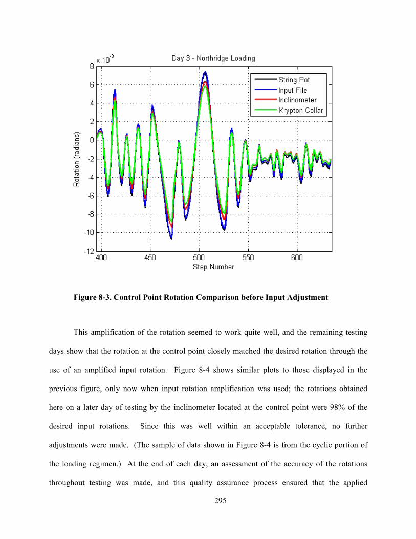
295
Figure 8-3. Control Point Rotation Comparison before Input Adjustment
This amplification of the rotation seemed to work quite well, and the remaining testing
days show that the rotation at the control point closely matched the desired rotation through the
use of an amplified input rotation. Figure 8-4 shows similar plots to those displayed in the
previous figure, only now when input rotation amplification was used; the rotations obtained
here on a later day of testing by the inclinometer located at the control point were 98% of the
desired input rotations. Since this was well within an acceptable tolerance, no further
adjustments were made. (The sample of data shown in Figure 8-4 is from the cyclic portion of
the loading regimen.) At the end of each day, an assessment of the accuracy of the rotations
throughout testing was made, and this quality assurance process ensured that the applied
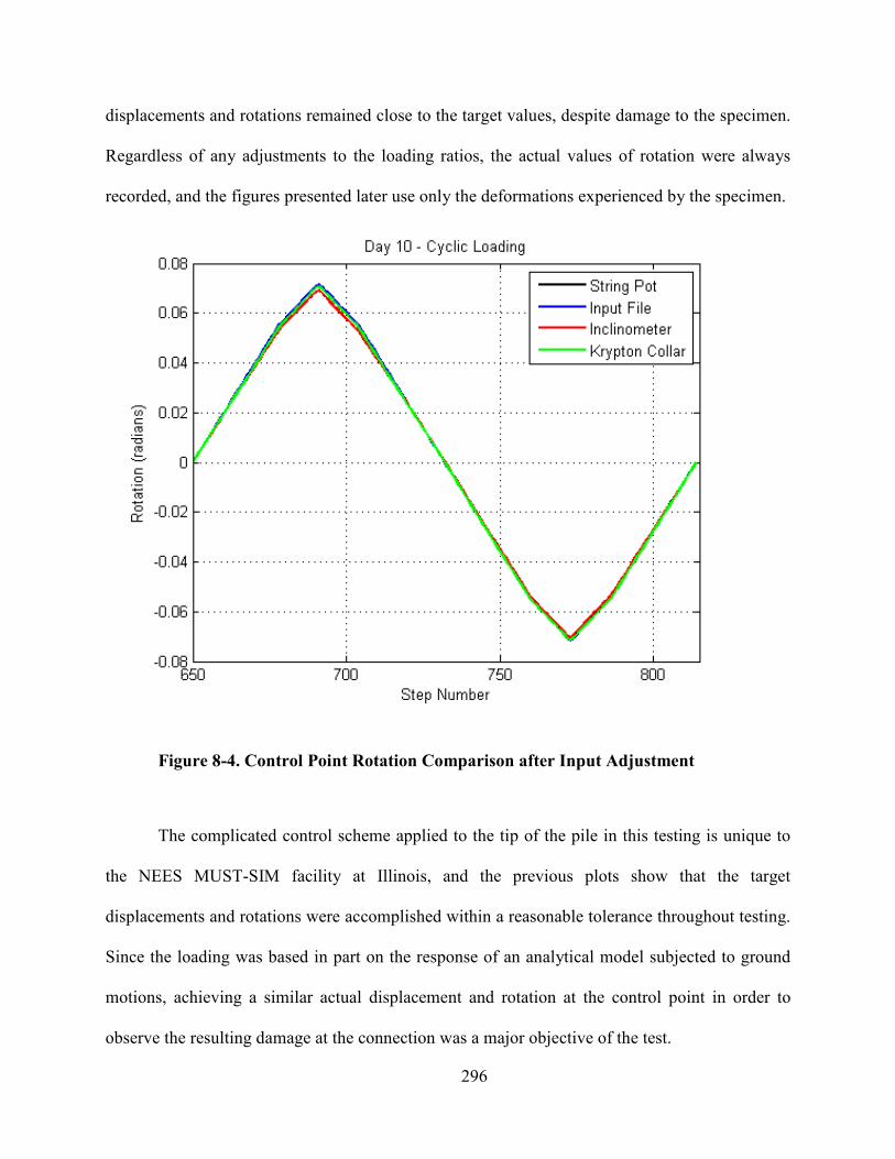
296
displacements and rotations remained close to the target values, despite damage to the specimen.
Regardless of any adjustments to the loading ratios, the actual values of rotation were always
recorded, and the figures presented later use only the deformations experienced by the specimen.
Figure 8-4. Control Point Rotation Comparison after Input Adjustment
The complicated control scheme applied to the tip of the pile in this testing is unique to
the NEES MUST-SIM facility at Illinois, and the previous plots show that the target
displacements and rotations were accomplished within a reasonable tolerance throughout testing.
Since the loading was based in part on the response of an analytical model subjected to ground
motions, achieving a similar actual displacement and rotation at the control point in order to
observe the resulting damage at the connection was a major objective of the test.
297
8.1.2 Global Force and Displacement Response
The force and moment response of the pile-wharf connection was a major point of
interest for the test. Understanding the moment capacity at the connection for typical pile-wharf
connection designs is critical to the design and construction of port structures in the field and to
fully understanding the behavior of the experimental specimen.
During testing, the moment at the connection was computed from three separate
contributions: moment applied to the tip of the pile, shear applied at the tip of the pile at a known
lever arm, and the axial force applied at the tip of the pile at a known LBCB displacement (P-∆).
Throughout the test these individual terms were monitored, as well as the total computed
connection moment. While the moment during the initial earthquake records seemed reasonable
for the cross-section of the pile-wharf specimen, it was discovered between the earthquake
loading and the cyclic loading regimes that some of the internal electronics associated with the
X1 actuator load cell had not been working properly. Since the specimen was offset on the
LBCB platen toward the X2 actuator, it was logical that the X2 actuator would contribute more
to the lateral force; however, a close examination of the data revealed that the X1 actuator load
cell was never reporting forces above one kip. This issue was later resolved, and the data
reported from the cyclic portion of testing was without incident. The force in the X1 actuator
during earthquake loading was solved for through equilibrium equations during post-processing.
Since the LVDTs in each actuator were working properly, it was possible to know the position of
each actuator throughout the test. With the positions of each actuator known, as well as the
forces in five of the six actuators, the final X1 actuator force was computed through an
equilibrium calculation by setting the Z-moment to a zero value. With all of the actuator loads
and positions known, it was then possible to perform the same transformation as the Operations
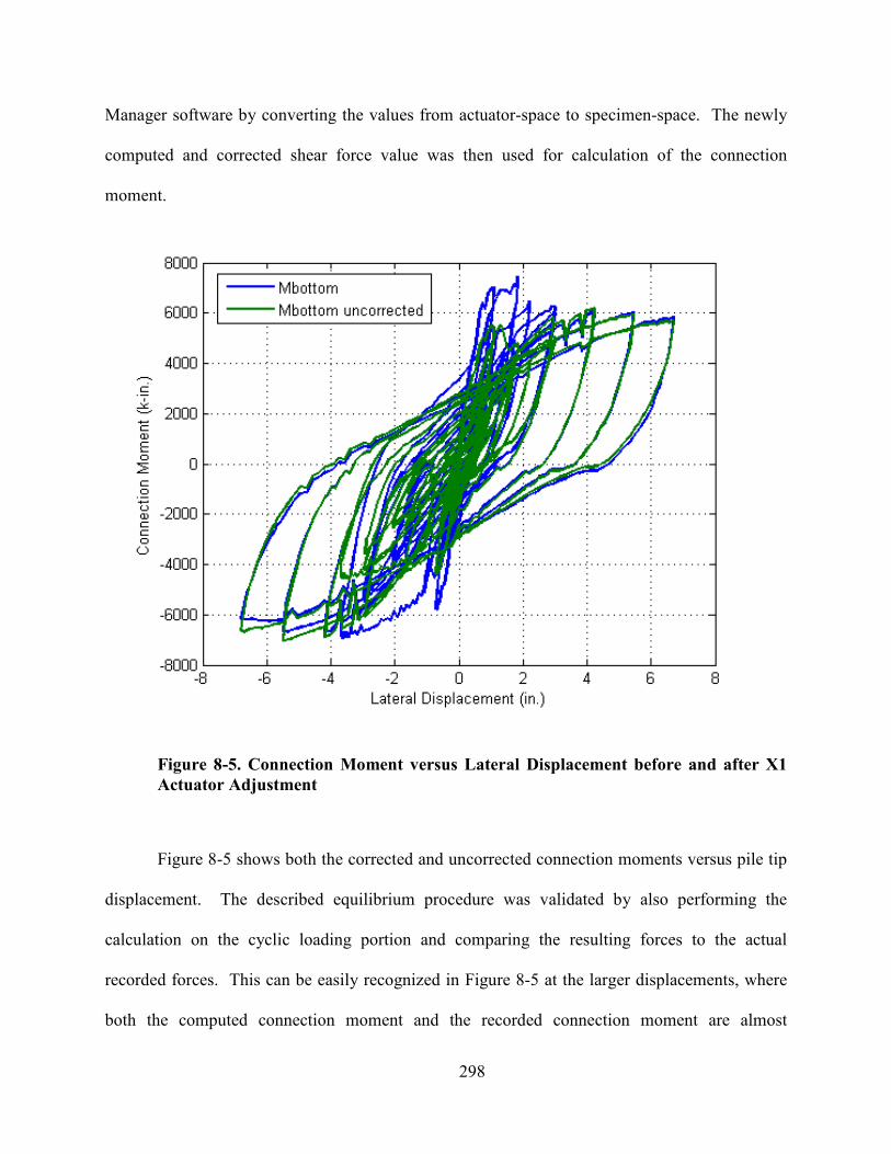
298
Manager software by converting the values from actuator-space to specimen-space. The newly
computed and corrected shear force value was then used for calculation of the connection
moment.
Figure 8-5. Connection Moment versus Lateral Displacement before and after X1
Actuator Adjustment
Figure 8-5 shows both the corrected and uncorrected connection moments versus pile tip
displacement. The described equilibrium procedure was validated by also performing the
calculation on the cyclic loading portion and comparing the resulting forces to the actual
recorded forces. This can be easily recognized in Figure 8-5 at the larger displacements, where
both the computed connection moment and the recorded connection moment are almost
299
identical. With this method proven to be reliable, the data recorded during the earthquake
loading was adjusted, and the X1 actuator force was back-solved. Figure 8-6 shows the final
connection moment versus displacement plot where the connection moment from the earthquake
portion of the loading is from the actuator forces with an adjusted X1 value, and the connection
moment from the cyclic loading is from the actual recorded actuator load cell values.
From the connection moment versus lateral tip displacement shown in Figure 8-6, it can
be seen that the moment capacity of the connection never experienced a significant degradation.
The peak moment of 7,451 kip-in. was experienced in the positive displacement direction during
the Northridge loading, while a maximum moment of 7,038 kip-in. in the negative displacement
direction occurred during the cyclic loading. The moment capacity of the connection
experienced only minor degradation over the duration of the test, with final moments at peak
displacements achieving 5,707 kip-in. and 6,599 kip-in. in the positive and negative directions,
respectively. This corresponds to about a 25% drop in moment capacity in the positive direction
and only a 12% drop in the negative direction, relative to the maximum achieved connection
moment. The smaller strength reduction in the negative direction may be due in part to the fact
that the negative direction never reached its possible peak moment due to pre-existing damage in
the opposite direction. The Response-2000 sectional model presented in more detail later
predicted a maximum moment capacity at the connection of 7190 kip-in., which is in good
agreement with the experimental results. The asymmetry in the response is due to the
unsymmetrical nature of the earthquake loading during early damage. While this is less common
to see in a laboratory testing environment, the realistic loading and boundary conditions of the
test setup should be more similar to the connection response that may be seen during an
earthquake. The progressively larger cyclic load steps were ceased when the X-actuators began
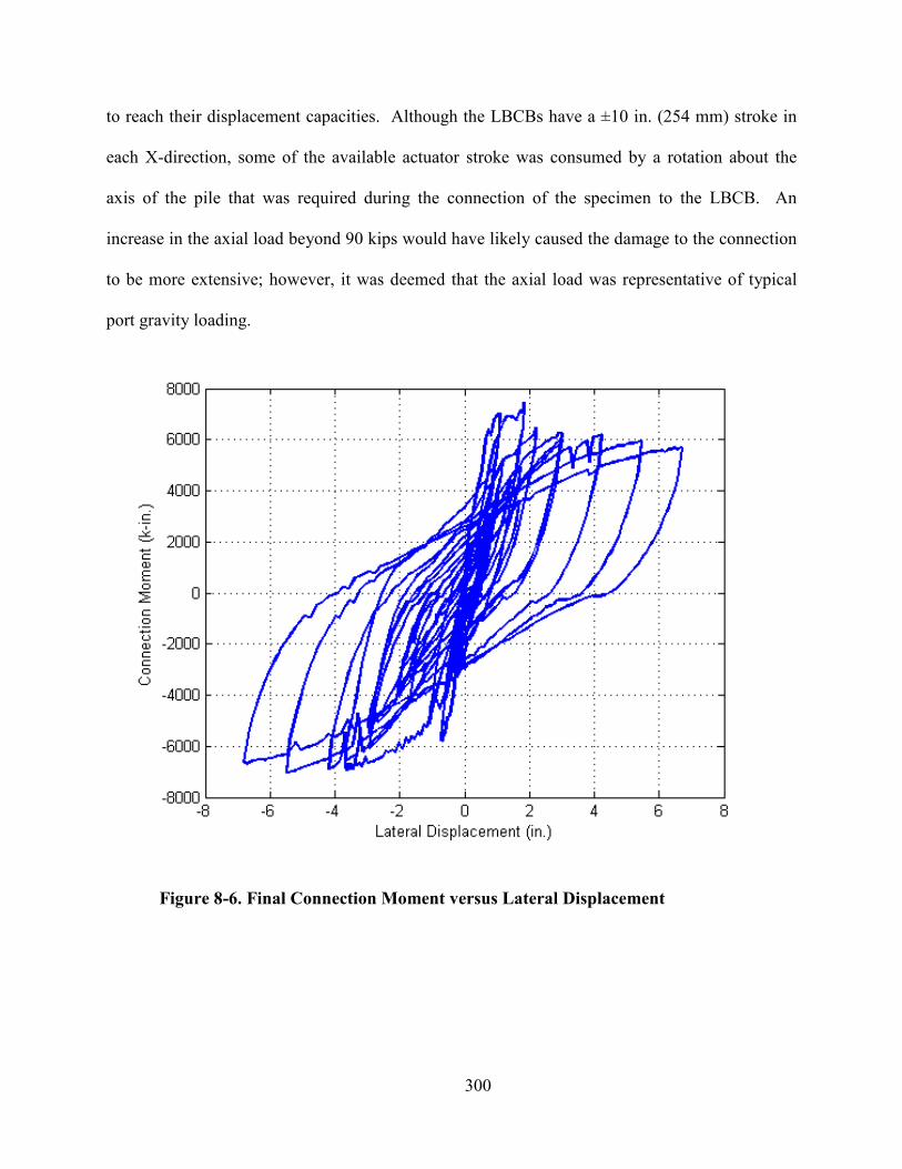
300
to reach their displacement capacities. Although the LBCBs have a ±10 in. (254 mm) stroke in
each X-direction, some of the available actuator stroke was consumed by a rotation about the
axis of the pile that was required during the connection of the specimen to the LBCB. An
increase in the axial load beyond 90 kips would have likely caused the damage to the connection
to be more extensive; however, it was deemed that the axial load was representative of typical
port gravity loading.
Figure 8-6. Final Connection Moment versus Lateral Displacement
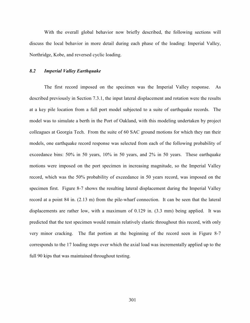
301
With the overall global behavior now briefly described, the following sections will
discuss the local behavior in more detail during each phase of the loading: Imperial Valley,
Northridge, Kobe, and reversed cyclic loading.
8.2 Imperial Valley Earthquake
The first record imposed on the specimen was the Imperial Valley response. As
described previously in Section 7.3.1, the input lateral displacement and rotation were the results
at a key pile location from a full port model subjected to a suite of earthquake records. The
model was to simulate a berth in the Port of Oakland, with this modeling undertaken by project
colleagues at Georgia Tech. From the suite of 60 SAC ground motions for which they ran their
models, one earthquake record response was selected from each of the following probability of
exceedance bins: 50% in 50 years, 10% in 50 years, and 2% in 50 years. These earthquake
motions were imposed on the port specimen in increasing magnitude, so the Imperial Valley
record, which was the 50% probability of exceedance in 50 years record, was imposed on the
specimen first. Figure 8-7 shows the resulting lateral displacement during the Imperial Valley
record at a point 84 in. (2.13 m) from the pile-wharf connection. It can be seen that the lateral
displacements are rather low, with a maximum of 0.129 in. (3.3 mm) being applied. It was
predicted that the test specimen would remain relatively elastic throughout this record, with only
very minor cracking. The flat portion at the beginning of the record seen in Figure 8-7
corresponds to the 17 loading steps over which the axial load was incrementally applied up to the
full 90 kips that was maintained throughout testing.
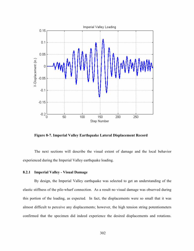
302
Figure 8-7. Imperial Valley Earthquake Lateral Displacement Record
The next sections will describe the visual extent of damage and the local behavior
experienced during the Imperial Valley earthquake loading.
8.2.1 Imperial Valley - Visual Damage
By design, the Imperial Valley earthquake was selected to get an understanding of the
elastic stiffness of the pile-wharf connection. As a result no visual damage was observed during
this portion of the loading, as expected. In fact, the displacements were so small that it was
almost difficult to perceive any displacements; however, the high tension string potentiometers
confirmed that the specimen did indeed experience the desired displacements and rotations.
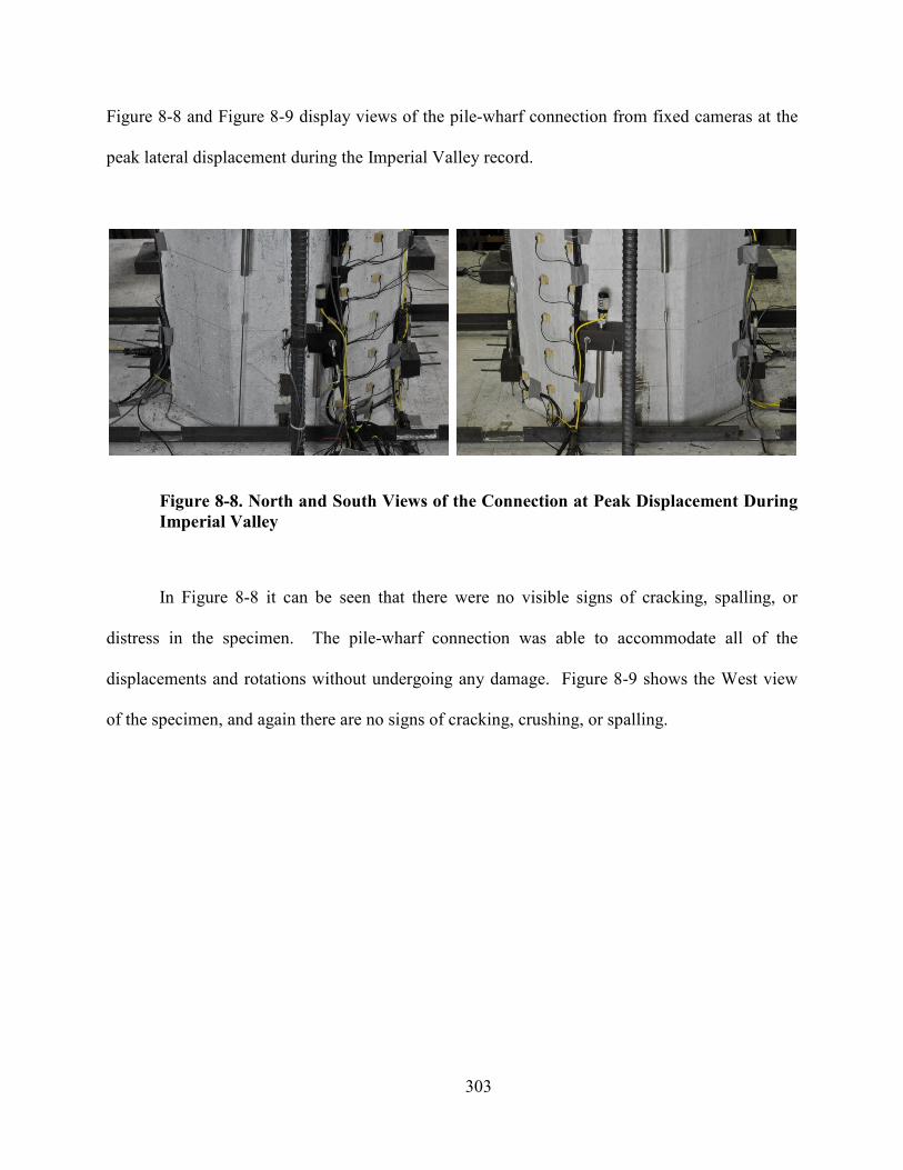
303
Figure 8-8 and Figure 8-9 display views of the pile-wharf connection from fixed cameras at the
peak lateral displacement during the Imperial Valley record.
Figure 8-8. orth and South Views of the Connection at Peak Displacement During
Imperial Valley
In Figure 8-8 it can be seen that there were no visible signs of cracking, spalling, or
distress in the specimen. The pile-wharf connection was able to accommodate all of the
displacements and rotations without undergoing any damage. Figure 8-9 shows the West view
of the specimen, and again there are no signs of cracking, crushing, or spalling.
304
Figure 8-9. Front View of the Connection at Peak Displacement during Imperial
Valley
While there was no visual change in the specimen throughout the Imperial Valley
loading, the dense instrumentation seen in the previous two figures did provide significant
detailed data about the nature of the structural response of the pile-wharf connection to this
earthquake record.
8.2.2 Imperial Valley - Local Behavior
Characterizing the local structural behavior requires a thorough analysis of data from the
various instruments mounted on the specimen. Throughout testing, the specimen seemed to be
rotating about the connection at the wharf deck through two mechanisms: flexural behavior of
the pile and concentrated connection rotation. The contribution of the pile comes in the form of
elastic flexural bending (including cracking and spalling of the prestressed, precast concrete
pile), and connection rotation is the term that will be used to describe the behavior below the
pile-deck interface, including elongation and slip of the T-headed bars, as well as crushing of the
pile at the compression toe. Therefore, to properly calculate the demand on and curvature of the
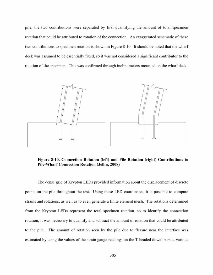
305
pile, the two contributions were separated by first quantifying the amount of total specimen
rotation that could be attributed to rotation of the connection. An exaggerated schematic of these
two contributions to specimen rotation is shown in Figure 8-10. It should be noted that the wharf
deck was assumed to be essentially fixed, so it was not considered a significant contributor to the
rotation of the specimen. This was confirmed through inclinometers mounted on the wharf deck.
Figure 8-10. Connection Rotation (left) and Pile Rotation (right) Contributions to
Pile-Wharf Connection Rotation (Jellin, 2008)
The dense grid of Krypton LEDs provided information about the displacement of discrete
points on the pile throughout the test. Using these LED coordinates, it is possible to compute
strains and rotations, as well as to even generate a finite element mesh. The rotations determined
from the Krypton LEDs represent the total specimen rotation, so to identify the connection
rotation, it was necessary to quantify and subtract the amount of rotation that could be attributed
to the pile. The amount of rotation seen by the pile due to flexure near the interface was
estimated by using the values of the strain gauge readings on the T-headed dowel bars at various
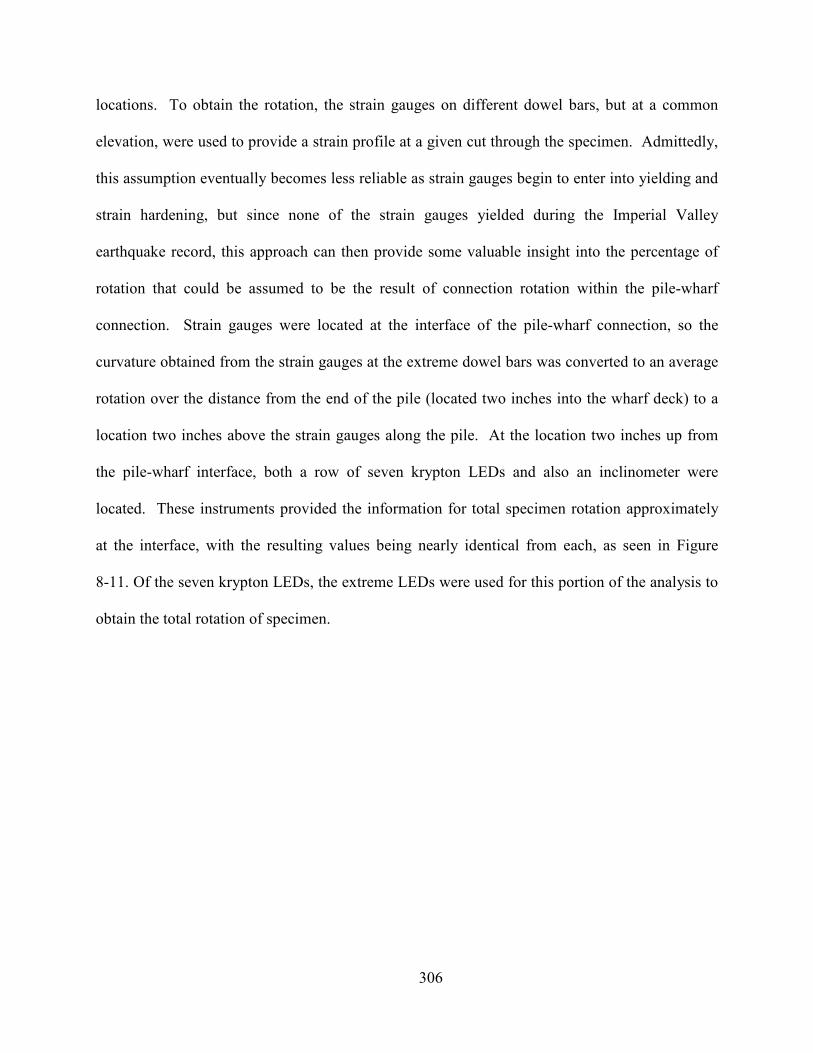
306
locations. To obtain the rotation, the strain gauges on different dowel bars, but at a common
elevation, were used to provide a strain profile at a given cut through the specimen. Admittedly,
this assumption eventually becomes less reliable as strain gauges begin to enter into yielding and
strain hardening, but since none of the strain gauges yielded during the Imperial Valley
earthquake record, this approach can then provide some valuable insight into the percentage of
rotation that could be assumed to be the result of connection rotation within the pile-wharf
connection. Strain gauges were located at the interface of the pile-wharf connection, so the
curvature obtained from the strain gauges at the extreme dowel bars was converted to an average
rotation over the distance from the end of the pile (located two inches into the wharf deck) to a
location two inches above the strain gauges along the pile. At the location two inches up from
the pile-wharf interface, both a row of seven krypton LEDs and also an inclinometer were
located. These instruments provided the information for total specimen rotation approximately
at the interface, with the resulting values being nearly identical from each, as seen in Figure
8-11. Of the seven krypton LEDs, the extreme LEDs were used for this portion of the analysis to
obtain the total rotation of specimen.
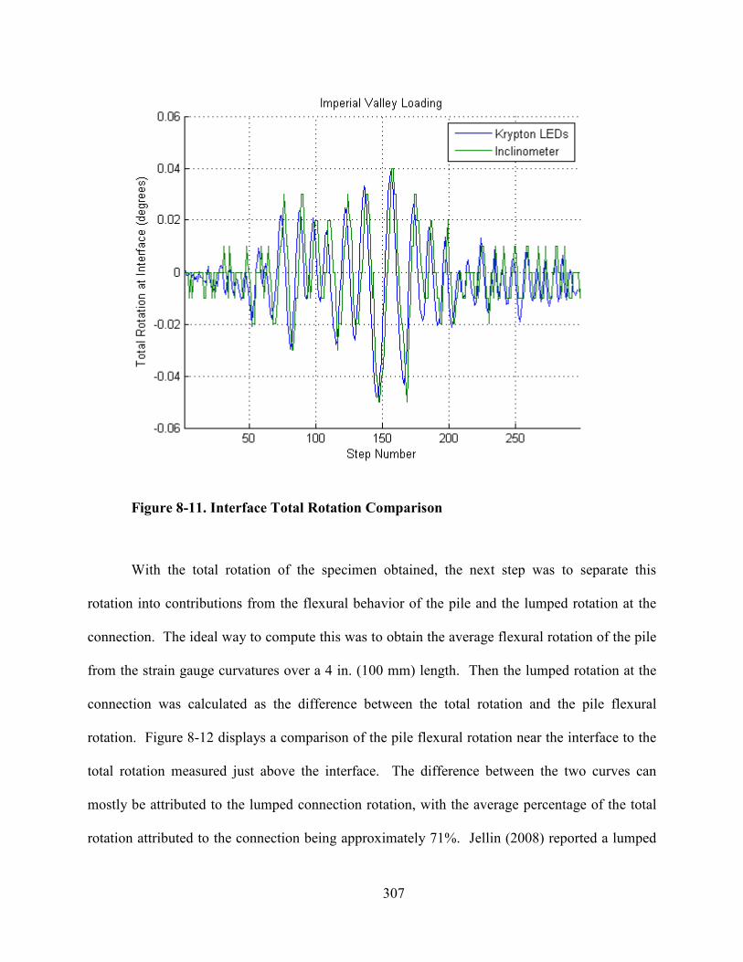
307
Figure 8-11. Interface Total Rotation Comparison
With the total rotation of the specimen obtained, the next step was to separate this
rotation into contributions from the flexural behavior of the pile and the lumped rotation at the
connection. The ideal way to compute this was to obtain the average flexural rotation of the pile
from the strain gauge curvatures over a 4 in. (100 mm) length. Then the lumped rotation at the
connection was calculated as the difference between the total rotation and the pile flexural
rotation. Figure 8-12 displays a comparison of the pile flexural rotation near the interface to the
total rotation measured just above the interface. The difference between the two curves can
mostly be attributed to the lumped connection rotation, with the average percentage of the total
rotation attributed to the connection being approximately 71%. Jellin (2008) reported a lumped
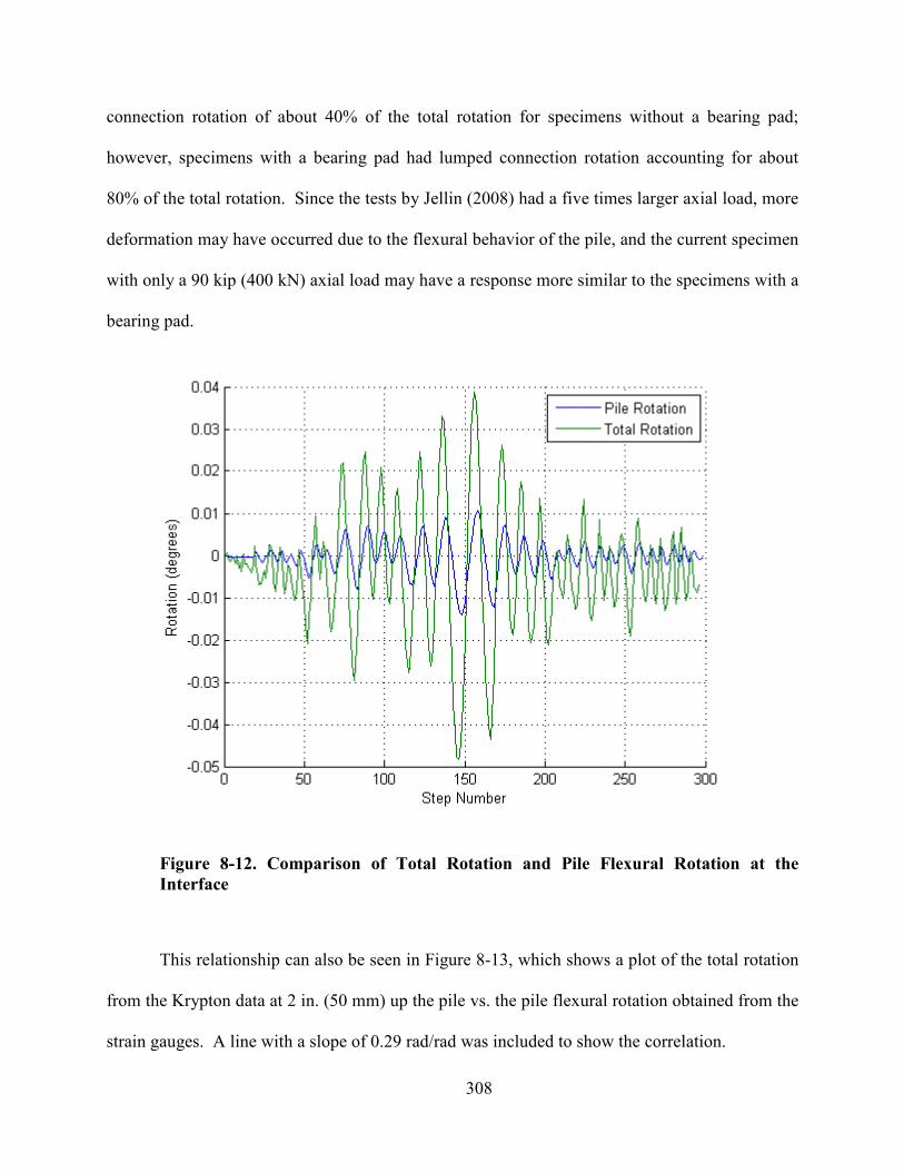
308
connection rotation of about 40% of the total rotation for specimens without a bearing pad;
however, specimens with a bearing pad had lumped connection rotation accounting for about
80% of the total rotation. Since the tests by Jellin (2008) had a five times larger axial load, more
deformation may have occurred due to the flexural behavior of the pile, and the current specimen
with only a 90 kip (400 kN) axial load may have a response more similar to the specimens with a
bearing pad.
Figure 8-12. Comparison of Total Rotation and Pile Flexural Rotation at the
Interface
This relationship can also be seen in Figure 8-13, which shows a plot of the total rotation
from the Krypton data at 2 in. (50 mm) up the pile vs. the pile flexural rotation obtained from the
strain gauges. A line with a slope of 0.29 rad/rad was included to show the correlation.
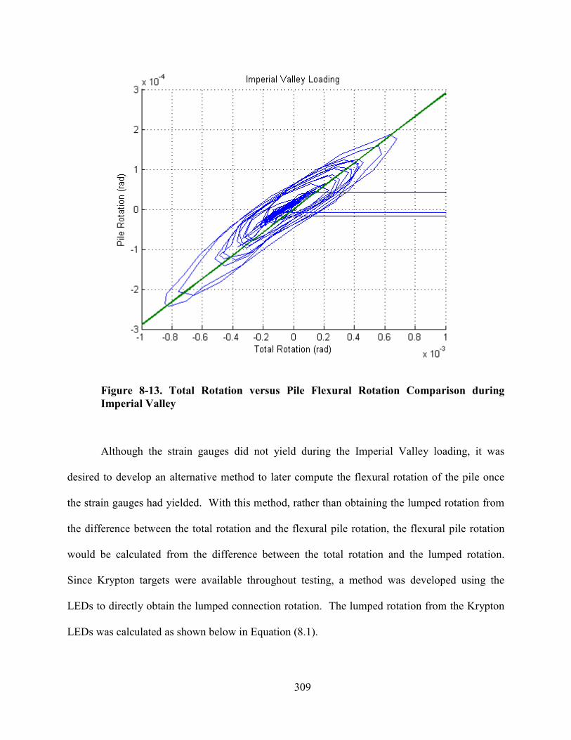
309
Figure 8-13. Total Rotation versus Pile Flexural Rotation Comparison during
Imperial Valley
Although the strain gauges did not yield during the Imperial Valley loading, it was
desired to develop an alternative method to later compute the flexural rotation of the pile once
the strain gauges had yielded. With this method, rather than obtaining the lumped rotation from
the difference between the total rotation and the flexural pile rotation, the flexural pile rotation
would be calculated from the difference between the total rotation and the lumped rotation.
Since Krypton targets were available throughout testing, a method was developed using the
LEDs to directly obtain the lumped connection rotation. The lumped rotation from the Krypton
LEDs was calculated as shown below in Equation (8.1).
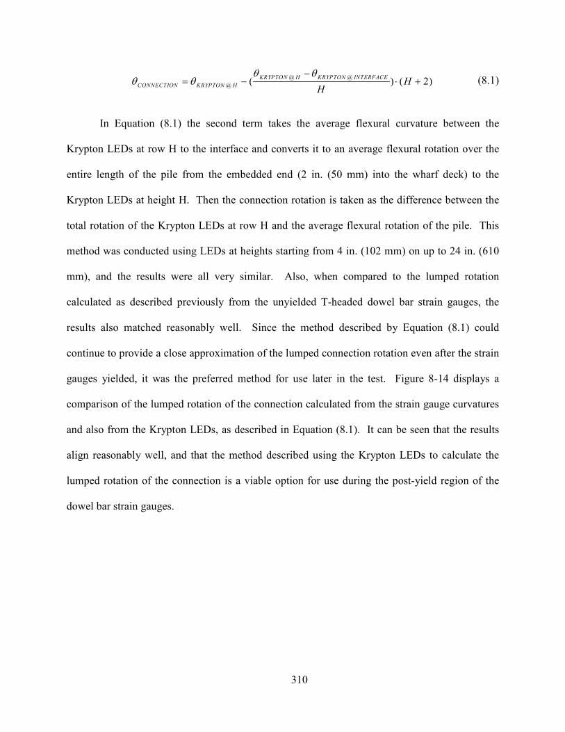
310
@ @
@ ( ) ( 2)KRYPTO H KRYPTO ITERFACE
COECTIO KRYPTO H HH
θ θθ θ
−= − ⋅ + (8.1)
In Equation (8.1) the second term takes the average flexural curvature between the
Krypton LEDs at row H to the interface and converts it to an average flexural rotation over the
entire length of the pile from the embedded end (2 in. (50 mm) into the wharf deck) to the
Krypton LEDs at height H. Then the connection rotation is taken as the difference between the
total rotation of the Krypton LEDs at row H and the average flexural rotation of the pile. This
method was conducted using LEDs at heights starting from 4 in. (102 mm) on up to 24 in. (610
mm), and the results were all very similar. Also, when compared to the lumped rotation
calculated as described previously from the unyielded T-headed dowel bar strain gauges, the
results also matched reasonably well. Since the method described by Equation (8.1) could
continue to provide a close approximation of the lumped connection rotation even after the strain
gauges yielded, it was the preferred method for use later in the test. Figure 8-14 displays a
comparison of the lumped rotation of the connection calculated from the strain gauge curvatures
and also from the Krypton LEDs, as described in Equation (8.1). It can be seen that the results
align reasonably well, and that the method described using the Krypton LEDs to calculate the
lumped rotation of the connection is a viable option for use during the post-yield region of the
dowel bar strain gauges.
311
Figure 8-14. Lumped Rotation Comparison from Strain Gauges and Krypton
during Imperial Valley
With the various contributions to specimen rotation near the connection interface now
separated, the curvature response can be calculated. The general flexural curvature response of
the pile was determined from stain gauges located throughout its height. While it was not an
issue during the Imperial Valley loading, in later earthquakes when the strain-gauged dowel bars
had yielded an effort was still made to continue using the strain gauges to calculate the curvature,
by removing the plastic strain from the readings. Since the earthquake records each possessed
small cyclic displacements over a portion of the record, the stain gauges were offset by the strain
about which the gauges cycled in the post-yield regions. This will be discussed further in the
next sections.
312
Using the material properties of the pile and the reinforcement described in detail in
Section 7.3.4, a model of the pile cross-section was made in the sectional analysis program
Response-2000. Figure 8-15 shows the moment-curvature behavior of the pile at the interface
during testing compared to the predicted sectional response from Response-2000. Only the
dowel reinforcing bars were included in the Response-2000 model to represent conditions at the
pile-wharf interface. It should be noted that the inclusion of the effect of the prestressing strands
away from the interface would improve the capacity of the pile. Reviewing the figure, it is not
surprising that the specimen was still linear elastic and relatively undamaged throughout the
duration of the Imperial Valley loading since the maximum moment achieved during this portion
of the loading was such a small percentage of the moment capacity.
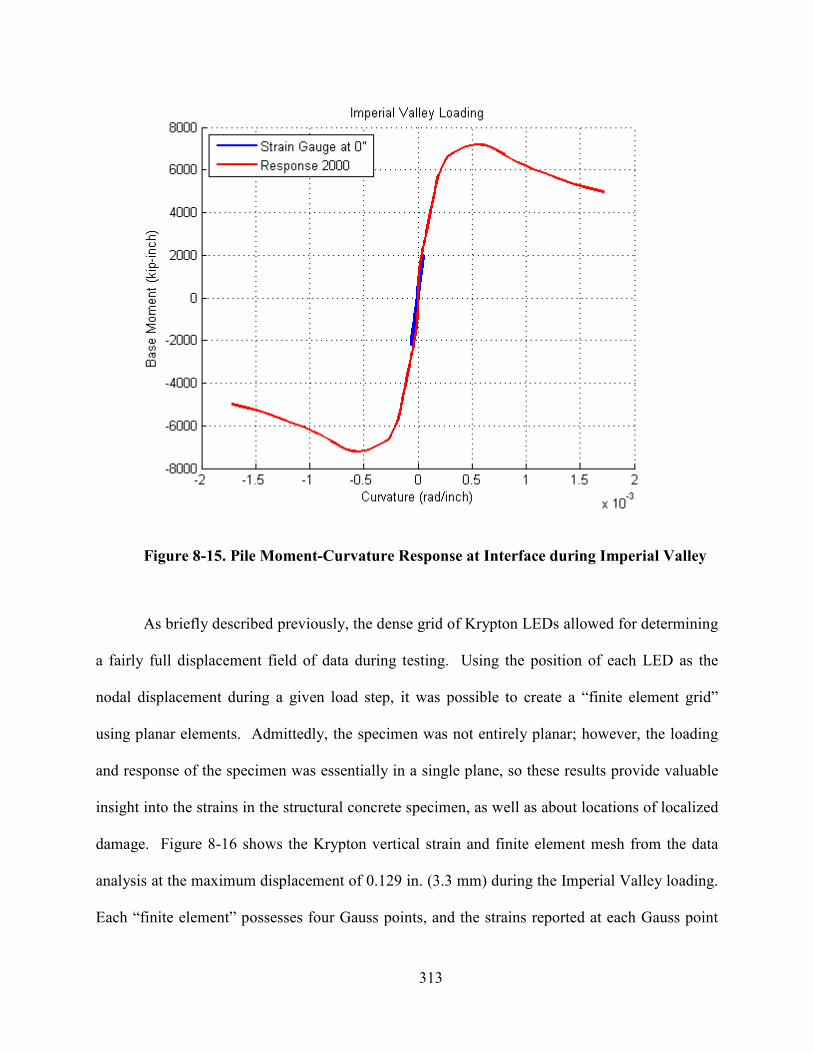
313
Figure 8-15. Pile Moment-Curvature Response at Interface during Imperial Valley
As briefly described previously, the dense grid of Krypton LEDs allowed for determining
a fairly full displacement field of data during testing. Using the position of each LED as the
nodal displacement during a given load step, it was possible to create a “finite element grid”
using planar elements. Admittedly, the specimen was not entirely planar; however, the loading
and response of the specimen was essentially in a single plane, so these results provide valuable
insight into the strains in the structural concrete specimen, as well as about locations of localized
damage. Figure 8-16 shows the Krypton vertical strain and finite element mesh from the data
analysis at the maximum displacement of 0.129 in. (3.3 mm) during the Imperial Valley loading.
Each “finite element” possesses four Gauss points, and the strains reported at each Gauss point
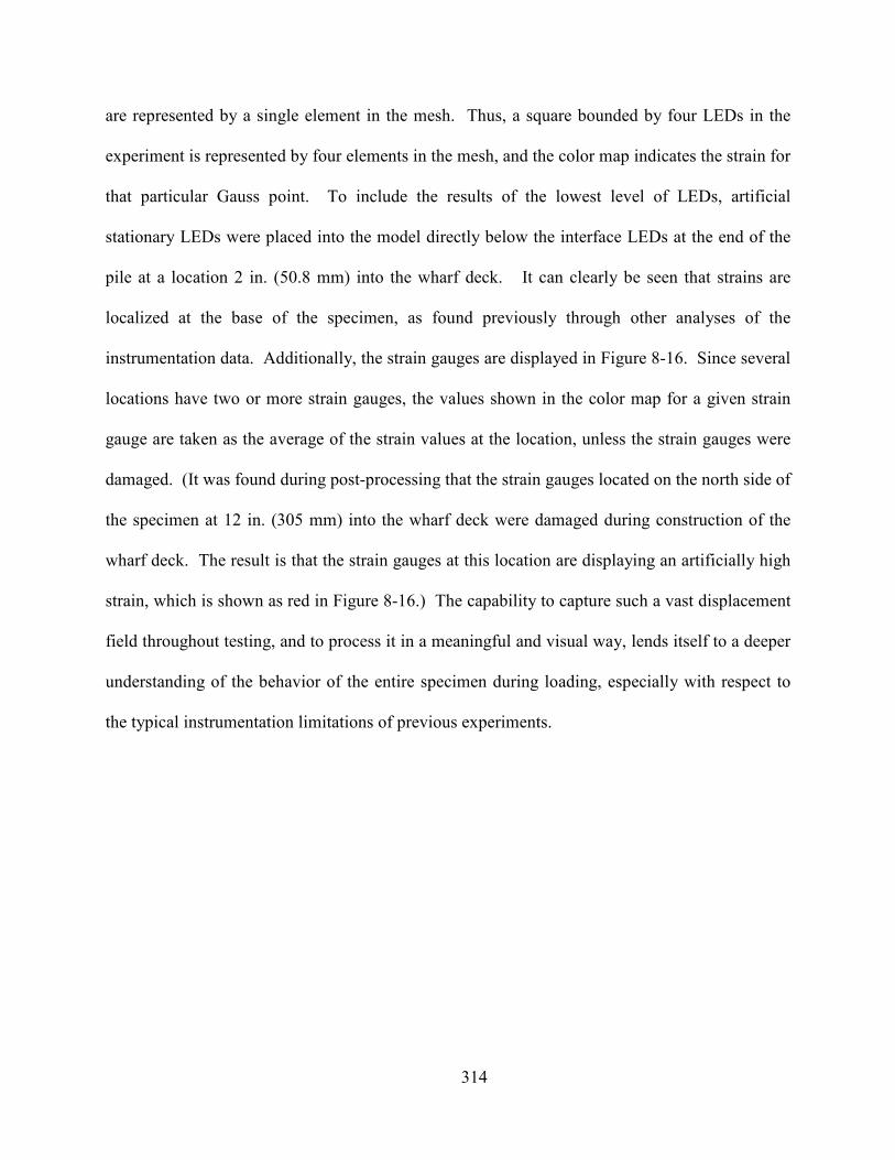
314
are represented by a single element in the mesh. Thus, a square bounded by four LEDs in the
experiment is represented by four elements in the mesh, and the color map indicates the strain for
that particular Gauss point. To include the results of the lowest level of LEDs, artificial
stationary LEDs were placed into the model directly below the interface LEDs at the end of the
pile at a location 2 in. (50.8 mm) into the wharf deck. It can clearly be seen that strains are
localized at the base of the specimen, as found previously through other analyses of the
instrumentation data. Additionally, the strain gauges are displayed in Figure 8-16. Since several
locations have two or more strain gauges, the values shown in the color map for a given strain
gauge are taken as the average of the strain values at the location, unless the strain gauges were
damaged. (It was found during post-processing that the strain gauges located on the north side of
the specimen at 12 in. (305 mm) into the wharf deck were damaged during construction of the
wharf deck. The result is that the strain gauges at this location are displaying an artificially high
strain, which is shown as red in Figure 8-16.) The capability to capture such a vast displacement
field throughout testing, and to process it in a meaningful and visual way, lends itself to a deeper
understanding of the behavior of the entire specimen during loading, especially with respect to
the typical instrumentation limitations of previous experiments.
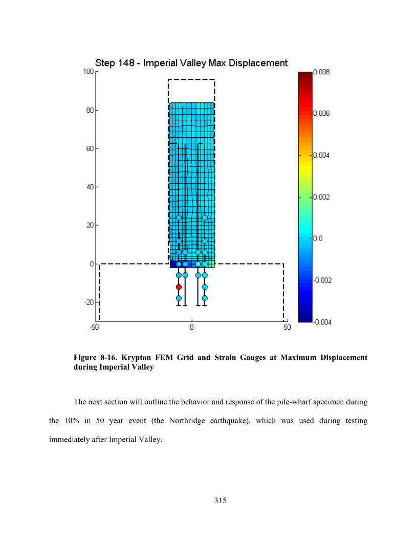
315
Figure 8-16. Krypton FEM Grid and Strain Gauges at Maximum Displacement
during Imperial Valley
The next section will outline the behavior and response of the pile-wharf specimen during
the 10% in 50 year event (the Northridge earthquake), which was used during testing
immediately after Imperial Valley.
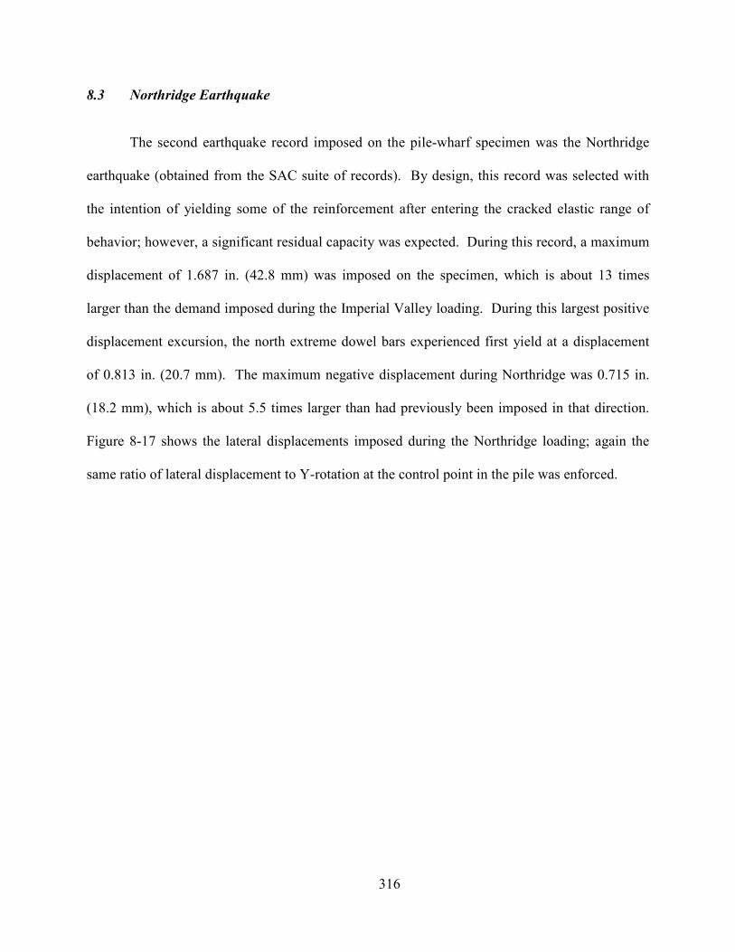
316
8.3 6orthridge Earthquake
The second earthquake record imposed on the pile-wharf specimen was the Northridge
earthquake (obtained from the SAC suite of records). By design, this record was selected with
the intention of yielding some of the reinforcement after entering the cracked elastic range of
behavior; however, a significant residual capacity was expected. During this record, a maximum
displacement of 1.687 in. (42.8 mm) was imposed on the specimen, which is about 13 times
larger than the demand imposed during the Imperial Valley loading. During this largest positive
displacement excursion, the north extreme dowel bars experienced first yield at a displacement
of 0.813 in. (20.7 mm). The maximum negative displacement during Northridge was 0.715 in.
(18.2 mm), which is about 5.5 times larger than had previously been imposed in that direction.
Figure 8-17 shows the lateral displacements imposed during the Northridge loading; again the
same ratio of lateral displacement to Y-rotation at the control point in the pile was enforced.
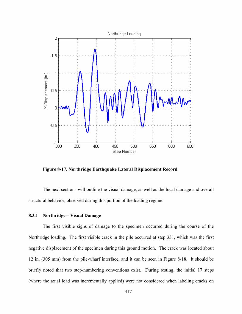
317
Figure 8-17. orthridge Earthquake Lateral Displacement Record
The next sections will outline the visual damage, as well as the local damage and overall
structural behavior, observed during this portion of the loading regime.
8.3.1 orthridge – Visual Damage
The first visible signs of damage to the specimen occurred during the course of the
Northridge loading. The first visible crack in the pile occurred at step 331, which was the first
negative displacement of the specimen during this ground motion. The crack was located about
12 in. (305 mm) from the pile-wharf interface, and it can be seen in Figure 8-18. It should be
briefly noted that two step-numbering conventions exist. During testing, the initial 17 steps
(where the axial load was incrementally applied) were not considered when labeling cracks on
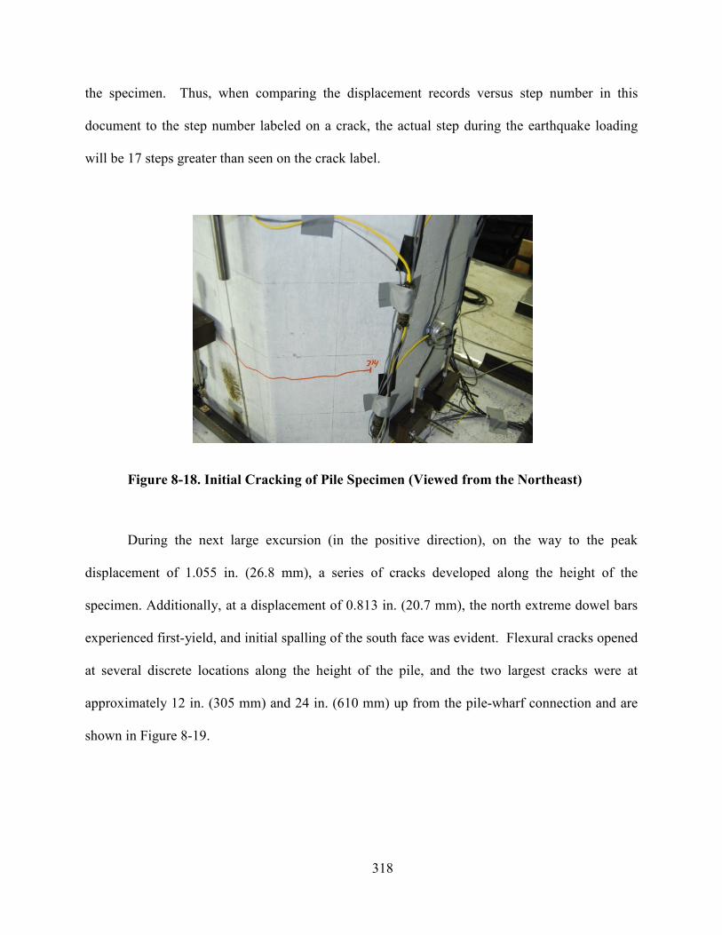
318
the specimen. Thus, when comparing the displacement records versus step number in this
document to the step number labeled on a crack, the actual step during the earthquake loading
will be 17 steps greater than seen on the crack label.
Figure 8-18. Initial Cracking of Pile Specimen (Viewed from the ortheast)
During the next large excursion (in the positive direction), on the way to the peak
displacement of 1.055 in. (26.8 mm), a series of cracks developed along the height of the
specimen. Additionally, at a displacement of 0.813 in. (20.7 mm), the north extreme dowel bars
experienced first-yield, and initial spalling of the south face was evident. Flexural cracks opened
at several discrete locations along the height of the pile, and the two largest cracks were at
approximately 12 in. (305 mm) and 24 in. (610 mm) up from the pile-wharf connection and are
shown in Figure 8-19.
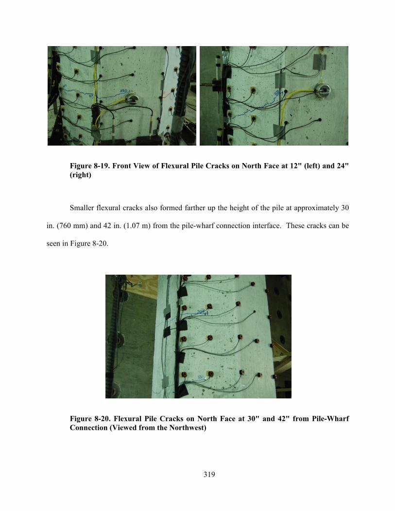
319
Figure 8-19. Front View of Flexural Pile Cracks on orth Face at 12" (left) and 24"
(right)
Smaller flexural cracks also formed farther up the height of the pile at approximately 30
in. (760 mm) and 42 in. (1.07 m) from the pile-wharf connection interface. These cracks can be
seen in Figure 8-20.
Figure 8-20. Flexural Pile Cracks on orth Face at 30" and 42" from Pile-Wharf
Connection (Viewed from the orthwest)
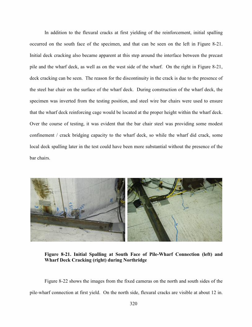
320
In addition to the flexural cracks at first yielding of the reinforcement, initial spalling
occurred on the south face of the specimen, and that can be seen on the left in Figure 8-21.
Initial deck cracking also became apparent at this step around the interface between the precast
pile and the wharf deck, as well as on the west side of the wharf. On the right in Figure 8-21,
deck cracking can be seen. The reason for the discontinuity in the crack is due to the presence of
the steel bar chair on the surface of the wharf deck. During construction of the wharf deck, the
specimen was inverted from the testing position, and steel wire bar chairs were used to ensure
that the wharf deck reinforcing cage would be located at the proper height within the wharf deck.
Over the course of testing, it was evident that the bar chair steel was providing some modest
confinement / crack bridging capacity to the wharf deck, so while the wharf did crack, some
local deck spalling later in the test could have been more substantial without the presence of the
bar chairs.
Figure 8-21. Initial Spalling at South Face of Pile-Wharf Connection (left) and
Wharf Deck Cracking (right) during orthridge
Figure 8-22 shows the images from the fixed cameras on the north and south sides of the
pile-wharf connection at first yield. On the north side, flexural cracks are visible at about 12 in.
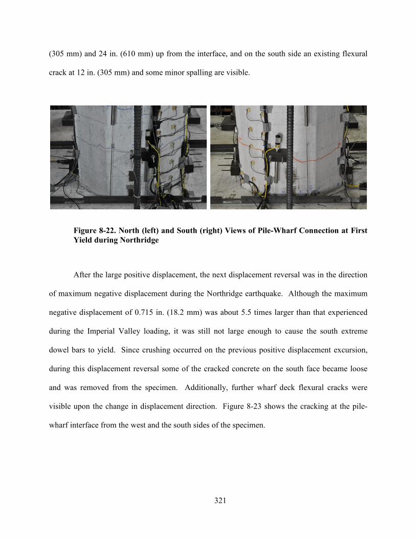
321
(305 mm) and 24 in. (610 mm) up from the interface, and on the south side an existing flexural
crack at 12 in. (305 mm) and some minor spalling are visible.
Figure 8-22. orth (left) and South (right) Views of Pile-Wharf Connection at First
Yield during orthridge
After the large positive displacement, the next displacement reversal was in the direction
of maximum negative displacement during the Northridge earthquake. Although the maximum
negative displacement of 0.715 in. (18.2 mm) was about 5.5 times larger than that experienced
during the Imperial Valley loading, it was still not large enough to cause the south extreme
dowel bars to yield. Since crushing occurred on the previous positive displacement excursion,
during this displacement reversal some of the cracked concrete on the south face became loose
and was removed from the specimen. Additionally, further wharf deck flexural cracks were
visible upon the change in displacement direction. Figure 8-23 shows the cracking at the pile-
wharf interface from the west and the south sides of the specimen.
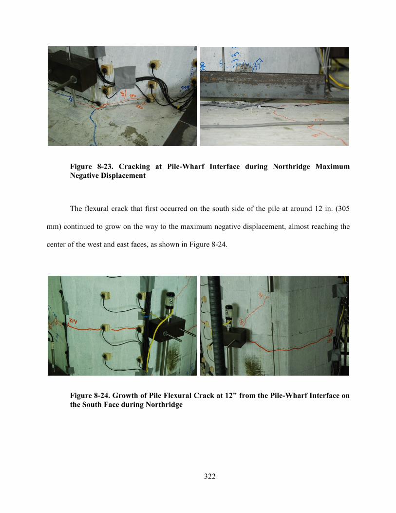
322
Figure 8-23. Cracking at Pile-Wharf Interface during orthridge Maximum
egative Displacement
The flexural crack that first occurred on the south side of the pile at around 12 in. (305
mm) continued to grow on the way to the maximum negative displacement, almost reaching the
center of the west and east faces, as shown in Figure 8-24.
Figure 8-24. Growth of Pile Flexural Crack at 12" from the Pile-Wharf Interface on
the South Face during orthridge
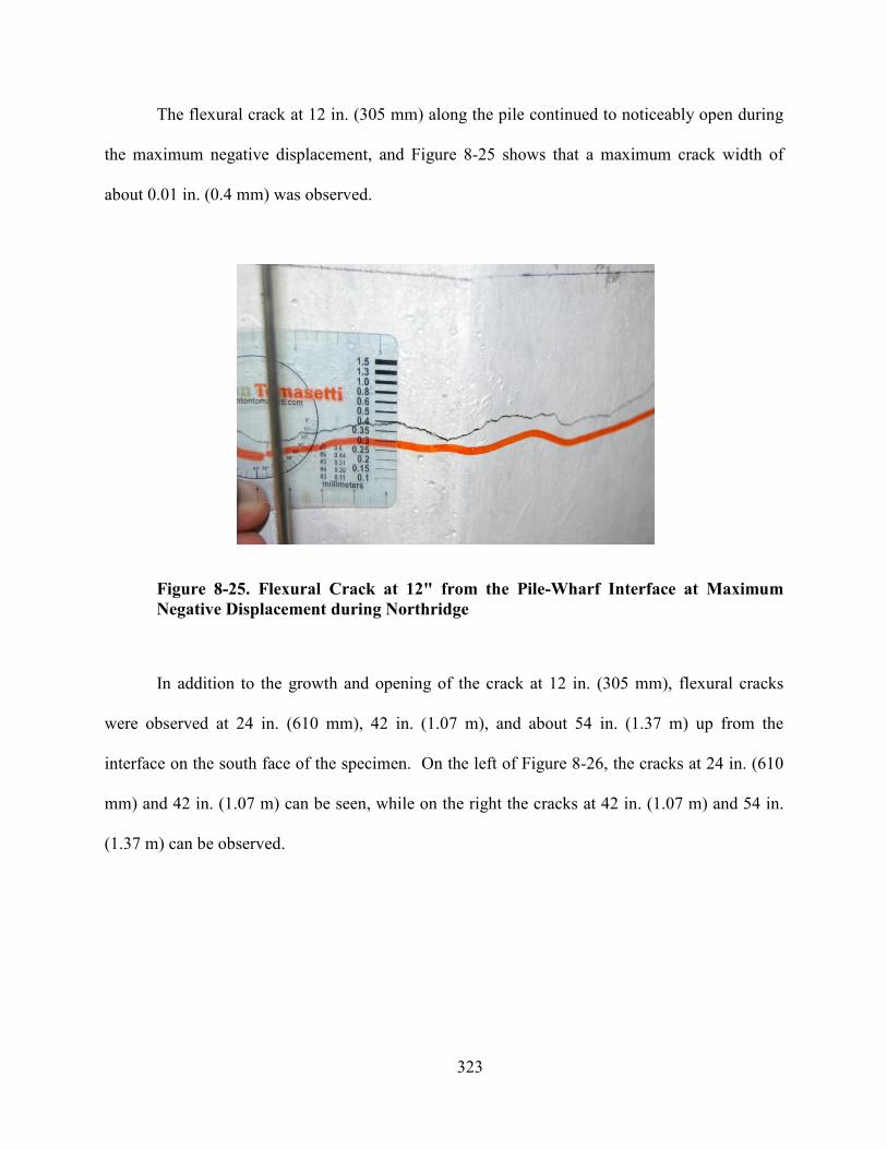
323
The flexural crack at 12 in. (305 mm) along the pile continued to noticeably open during
the maximum negative displacement, and Figure 8-25 shows that a maximum crack width of
about 0.01 in. (0.4 mm) was observed.
Figure 8-25. Flexural Crack at 12" from the Pile-Wharf Interface at Maximum
egative Displacement during orthridge
In addition to the growth and opening of the crack at 12 in. (305 mm), flexural cracks
were observed at 24 in. (610 mm), 42 in. (1.07 m), and about 54 in. (1.37 m) up from the
interface on the south face of the specimen. On the left of Figure 8-26, the cracks at 24 in. (610
mm) and 42 in. (1.07 m) can be seen, while on the right the cracks at 42 in. (1.07 m) and 54 in.
(1.37 m) can be observed.
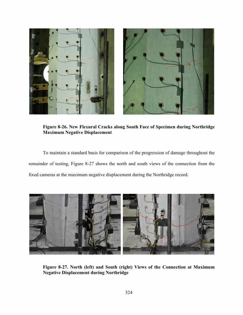
324
Figure 8-26. ew Flexural Cracks along South Face of Specimen during orthridge
Maximum egative Displacement
To maintain a standard basis for comparison of the progression of damage throughout the
remainder of testing, Figure 8-27 shows the north and south views of the connection from the
fixed cameras at the maximum negative displacement during the Northridge record.
Figure 8-27. orth (left) and South (right) Views of the Connection at Maximum
egative Displacement during orthridge
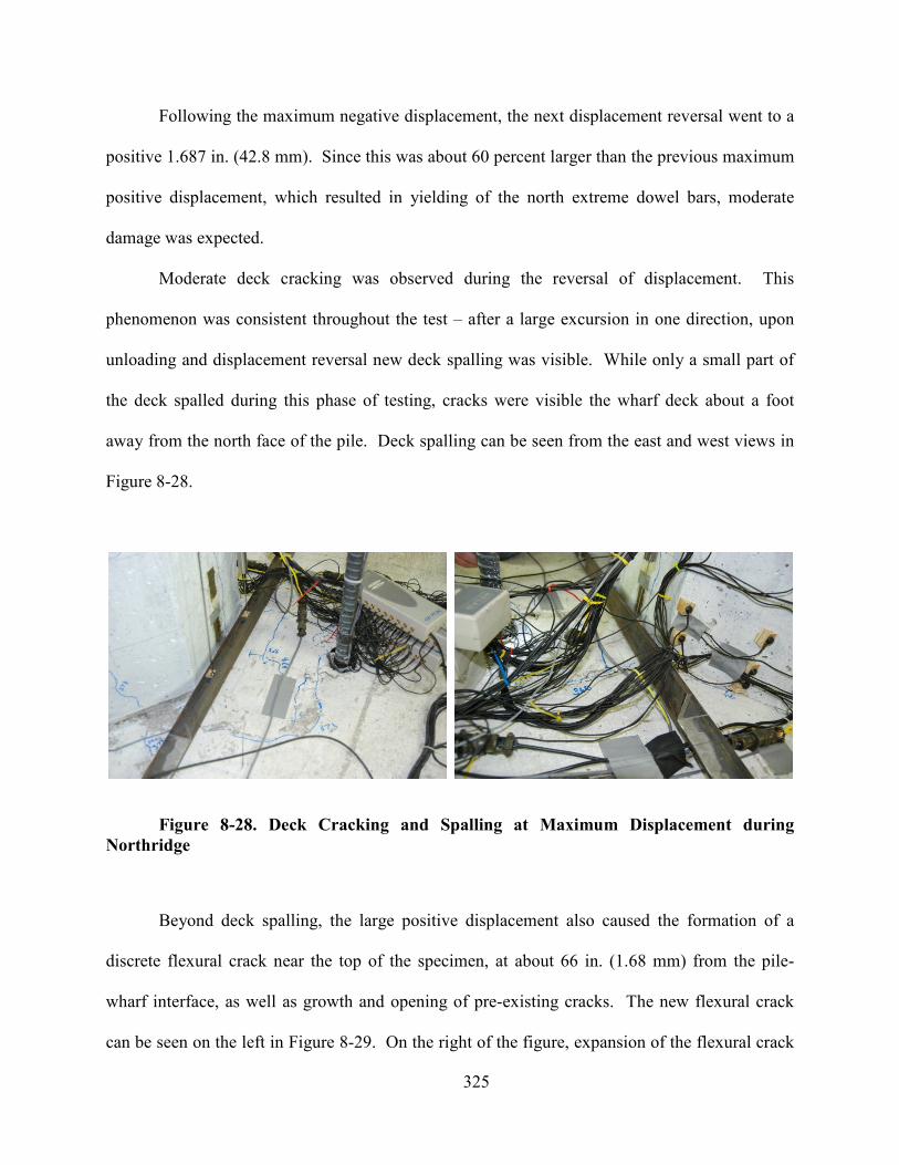
325
Following the maximum negative displacement, the next displacement reversal went to a
positive 1.687 in. (42.8 mm). Since this was about 60 percent larger than the previous maximum
positive displacement, which resulted in yielding of the north extreme dowel bars, moderate
damage was expected.
Moderate deck cracking was observed during the reversal of displacement. This
phenomenon was consistent throughout the test – after a large excursion in one direction, upon
unloading and displacement reversal new deck spalling was visible. While only a small part of
the deck spalled during this phase of testing, cracks were visible the wharf deck about a foot
away from the north face of the pile. Deck spalling can be seen from the east and west views in
Figure 8-28.
Figure 8-28. Deck Cracking and Spalling at Maximum Displacement during
orthridge
Beyond deck spalling, the large positive displacement also caused the formation of a
discrete flexural crack near the top of the specimen, at about 66 in. (1.68 mm) from the pile-
wharf interface, as well as growth and opening of pre-existing cracks. The new flexural crack
can be seen on the left in Figure 8-29. On the right of the figure, expansion of the flexural crack
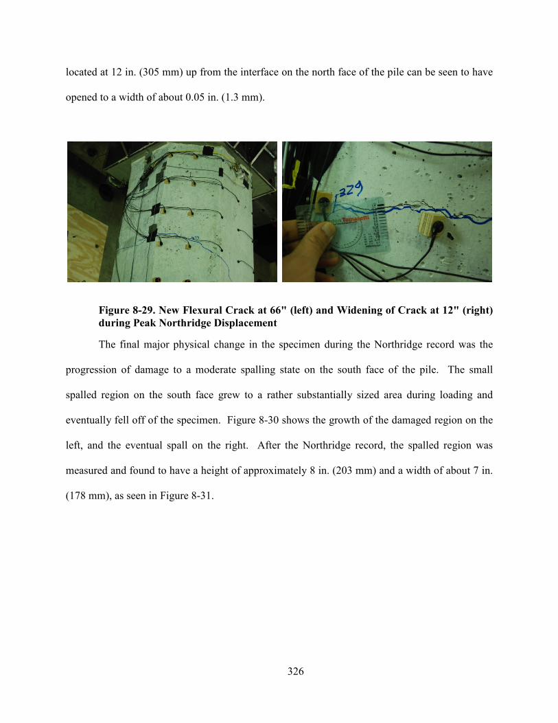
326
located at 12 in. (305 mm) up from the interface on the north face of the pile can be seen to have
opened to a width of about 0.05 in. (1.3 mm).
Figure 8-29. ew Flexural Crack at 66" (left) and Widening of Crack at 12" (right)
during Peak orthridge Displacement
The final major physical change in the specimen during the Northridge record was the
progression of damage to a moderate spalling state on the south face of the pile. The small
spalled region on the south face grew to a rather substantially sized area during loading and
eventually fell off of the specimen. Figure 8-30 shows the growth of the damaged region on the
left, and the eventual spall on the right. After the Northridge record, the spalled region was
measured and found to have a height of approximately 8 in. (203 mm) and a width of about 7 in.
(178 mm), as seen in Figure 8-31.
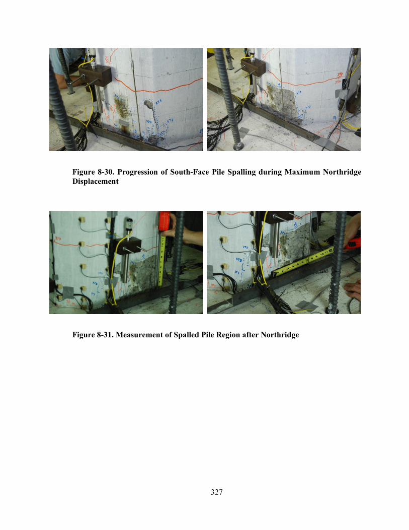
327
Figure 8-30. Progression of South-Face Pile Spalling during Maximum orthridge
Displacement
Figure 8-31. Measurement of Spalled Pile Region after orthridge
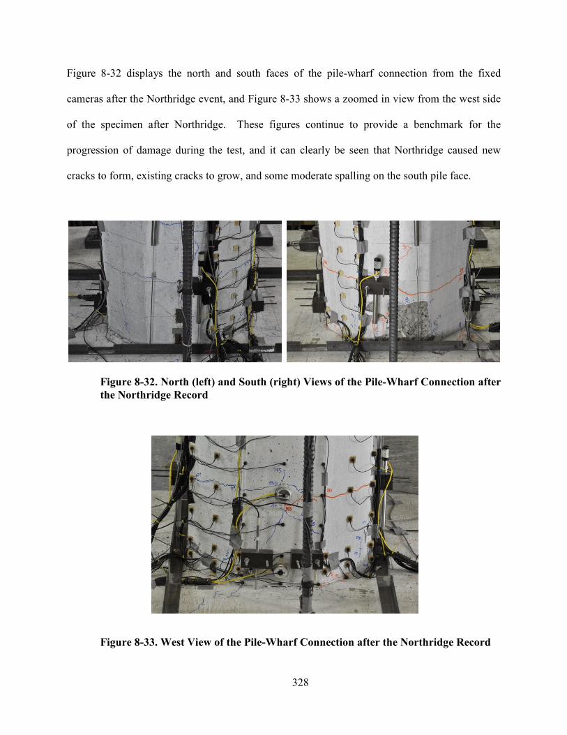
328
Figure 8-32 displays the north and south faces of the pile-wharf connection from the fixed
cameras after the Northridge event, and Figure 8-33 shows a zoomed in view from the west side
of the specimen after Northridge. These figures continue to provide a benchmark for the
progression of damage during the test, and it can clearly be seen that Northridge caused new
cracks to form, existing cracks to grow, and some moderate spalling on the south pile face.
Figure 8-32. orth (left) and South (right) Views of the Pile-Wharf Connection after
the orthridge Record
Figure 8-33. West View of the Pile-Wharf Connection after the orthridge Record

329
The Northridge event clearly caused some visible physical damage to the specimen, and
the next section will investigate in more detail the local behavior of the specimen as measured by
the dense array of instrumentation.
8.3.2 orthridge – Local Behavior
An analysis of the behavior of the test specimen through the Northridge record shows that
there was indeed some overall softening and damage, but a majority of the rotation continued to
occur at the pile-wharf connection.
Since the north strain gauges began to yield during the Northridge record, an effort was
made to adjust the strain gauge values (for purposes of estimating relative rotation, actual stress,
etc.) by the estimated plastic strain. This was obtained by reviewing the strain gauge values
during the small displacement reversals in the latter part of the Northridge record, and obtaining
the plastic offset value. The unadjusted strain gauge readings of the north and south extreme
dowel bars at the interface are shown on the left in Figure 8-34, and the strain gauge values with
the plastic offset are displayed on the right. It can be seen that, with the adjustment, the strain
values cycle around zero strain when the loading is at zero.
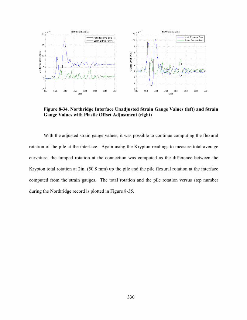
330
Figure 8-34. orthridge Interface Unadjusted Strain Gauge Values (left) and Strain
Gauge Values with Plastic Offset Adjustment (right)
With the adjusted strain gauge values, it was possible to continue computing the flexural
rotation of the pile at the interface. Again using the Krypton readings to measure total average
curvature, the lumped rotation at the connection was computed as the difference between the
Krypton total rotation at 2in. (50.8 mm) up the pile and the pile flexural rotation at the interface
computed from the strain gauges. The total rotation and the pile rotation versus step number
during the Northridge record is plotted in Figure 8-35.
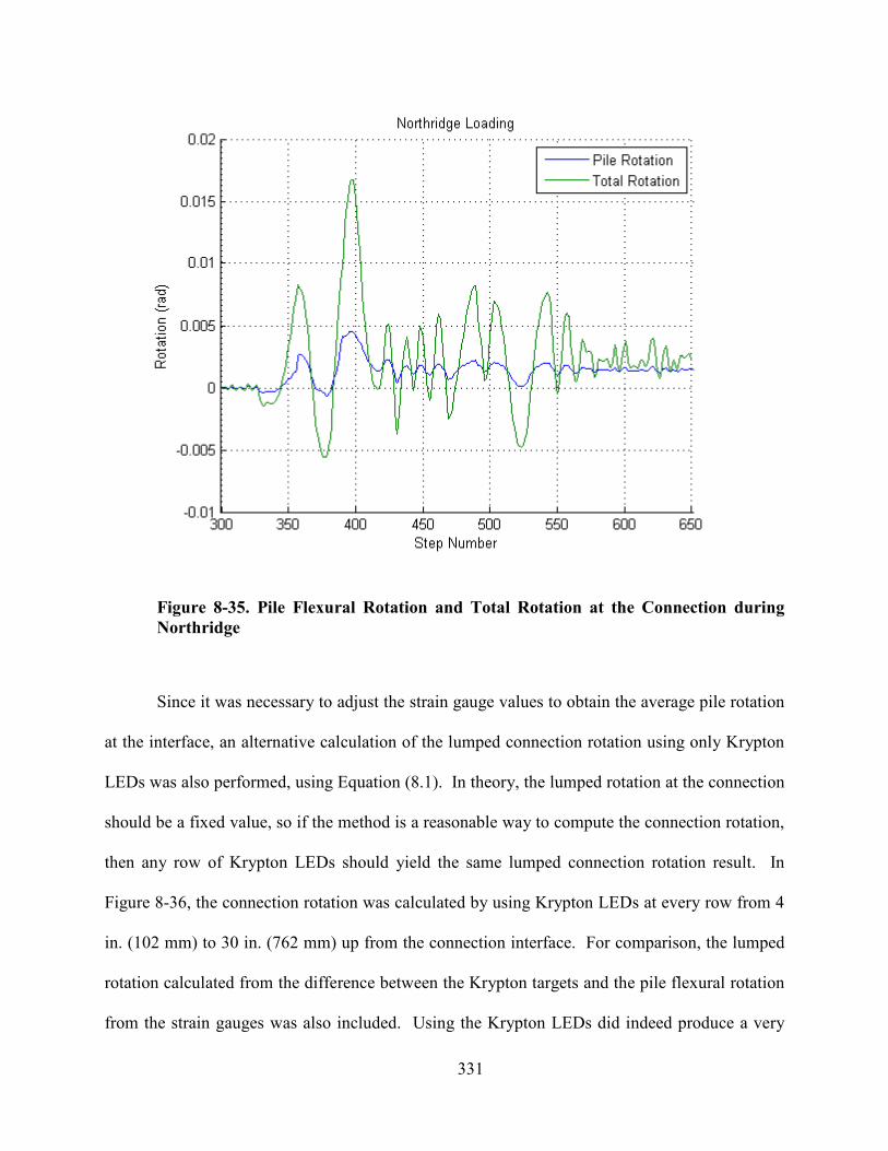
331
Figure 8-35. Pile Flexural Rotation and Total Rotation at the Connection during
orthridge
Since it was necessary to adjust the strain gauge values to obtain the average pile rotation
at the interface, an alternative calculation of the lumped connection rotation using only Krypton
LEDs was also performed, using Equation (8.1). In theory, the lumped rotation at the connection
should be a fixed value, so if the method is a reasonable way to compute the connection rotation,
then any row of Krypton LEDs should yield the same lumped connection rotation result. In
Figure 8-36, the connection rotation was calculated by using Krypton LEDs at every row from 4
in. (102 mm) to 30 in. (762 mm) up from the connection interface. For comparison, the lumped
rotation calculated from the difference between the Krypton targets and the pile flexural rotation
from the strain gauges was also included. Using the Krypton LEDs did indeed produce a very
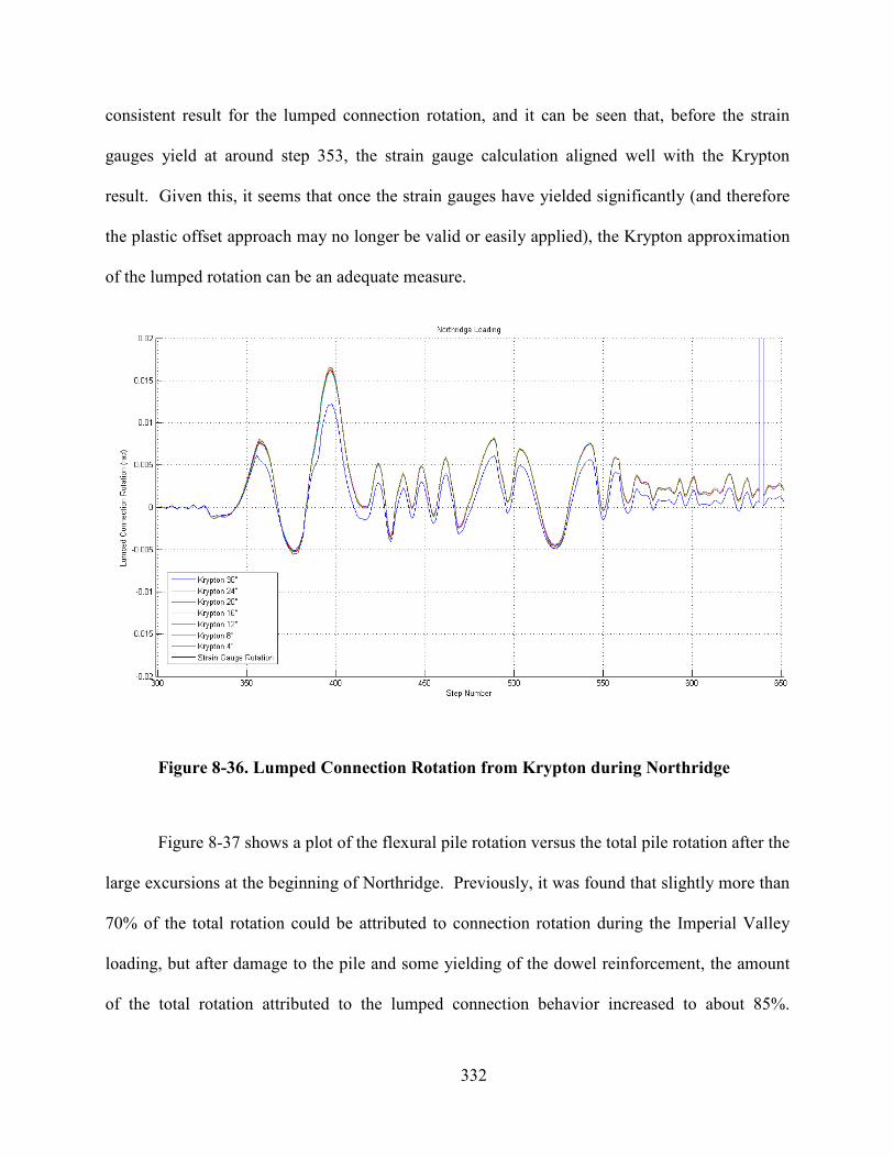
332
consistent result for the lumped connection rotation, and it can be seen that, before the strain
gauges yield at around step 353, the strain gauge calculation aligned well with the Krypton
result. Given this, it seems that once the strain gauges have yielded significantly (and therefore
the plastic offset approach may no longer be valid or easily applied), the Krypton approximation
of the lumped rotation can be an adequate measure.
Figure 8-36. Lumped Connection Rotation from Krypton during orthridge
Figure 8-37 shows a plot of the flexural pile rotation versus the total pile rotation after the
large excursions at the beginning of Northridge. Previously, it was found that slightly more than
70% of the total rotation could be attributed to connection rotation during the Imperial Valley
loading, but after damage to the pile and some yielding of the dowel reinforcement, the amount
of the total rotation attributed to the lumped connection behavior increased to about 85%.
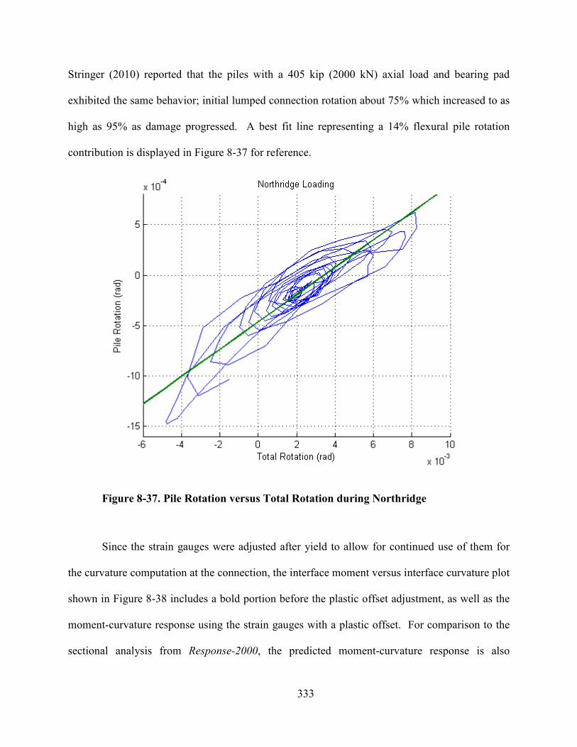
333
Stringer (2010) reported that the piles with a 405 kip (2000 kN) axial load and bearing pad
exhibited the same behavior; initial lumped connection rotation about 75% which increased to as
high as 95% as damage progressed. A best fit line representing a 14% flexural pile rotation
contribution is displayed in Figure 8-37 for reference.
Figure 8-37. Pile Rotation versus Total Rotation during orthridge
Since the strain gauges were adjusted after yield to allow for continued use of them for
the curvature computation at the connection, the interface moment versus interface curvature plot
shown in Figure 8-38 includes a bold portion before the plastic offset adjustment, as well as the
moment-curvature response using the strain gauges with a plastic offset. For comparison to the
sectional analysis from Response-2000, the predicted moment-curvature response is also
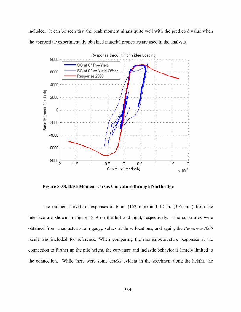
334
included. It can be seen that the peak moment aligns quite well with the predicted value when
the appropriate experimentally obtained material properties are used in the analysis.
Figure 8-38. Base Moment versus Curvature through orthridge
The moment-curvature responses at 6 in. (152 mm) and 12 in. (305 mm) from the
interface are shown in Figure 8-39 on the left and right, respectively. The curvatures were
obtained from unadjusted strain gauge values at those locations, and again, the Response-2000
result was included for reference. When comparing the moment-curvature responses at the
connection to further up the pile height, the curvature and inelastic behavior is largely limited to
the connection. While there were some cracks evident in the specimen along the height, the
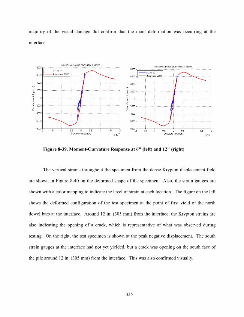
335
majority of the visual damage did confirm that the main deformation was occurring at the
interface.
Figure 8-39. Moment-Curvature Response at 6" (left) and 12" (right)
The vertical strains throughout the specimen from the dense Krypton displacement field
are shown in Figure 8-40 on the deformed shape of the specimen. Also, the strain gauges are
shown with a color mapping to indicate the level of strain at each location. The figure on the left
shows the deformed configuration of the test specimen at the point of first yield of the north
dowel bars at the interface. Around 12 in. (305 mm) from the interface, the Krypton strains are
also indicating the opening of a crack, which is representative of what was observed during
testing. On the right, the test specimen is shown at the peak negative displacement. The south
strain gauges at the interface had not yet yielded, but a crack was opening on the south face of
the pile around 12 in. (305 mm) from the interface. This was also confirmed visually.
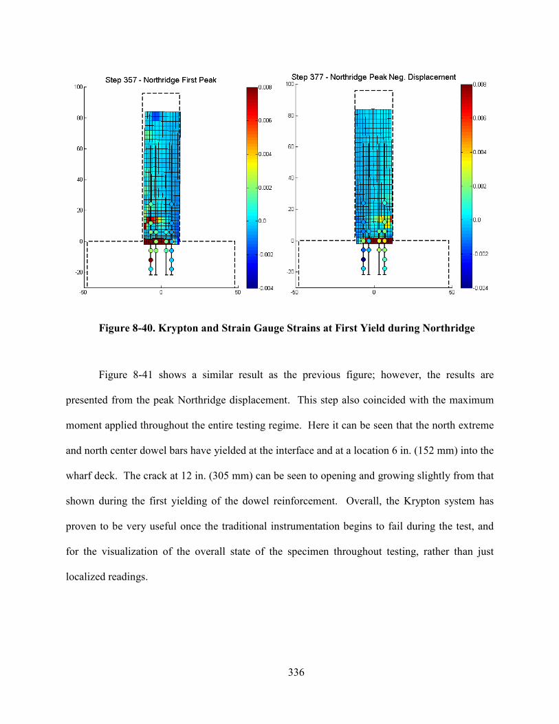
336
Figure 8-40. Krypton and Strain Gauge Strains at First Yield during orthridge
Figure 8-41 shows a similar result as the previous figure; however, the results are
presented from the peak Northridge displacement. This step also coincided with the maximum
moment applied throughout the entire testing regime. Here it can be seen that the north extreme
and north center dowel bars have yielded at the interface and at a location 6 in. (152 mm) into the
wharf deck. The crack at 12 in. (305 mm) can be seen to opening and growing slightly from that
shown during the first yielding of the dowel reinforcement. Overall, the Krypton system has
proven to be very useful once the traditional instrumentation begins to fail during the test, and
for the visualization of the overall state of the specimen throughout testing, rather than just
localized readings.
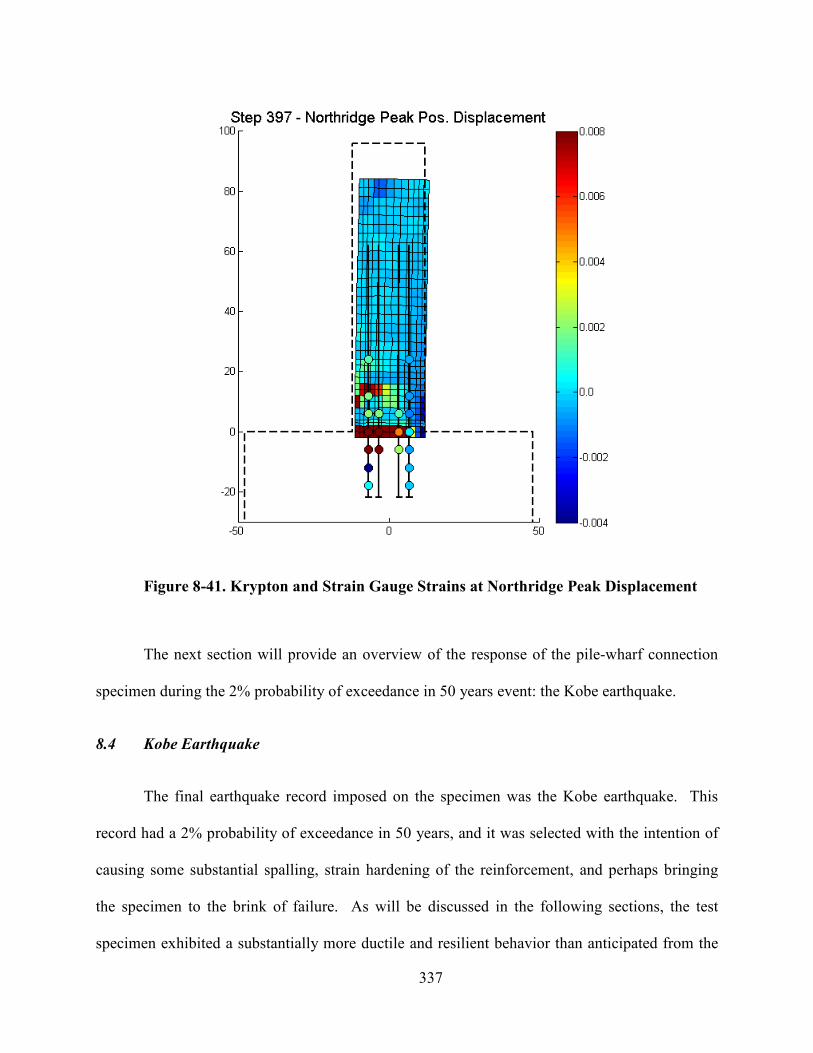
337
Figure 8-41. Krypton and Strain Gauge Strains at orthridge Peak Displacement
The next section will provide an overview of the response of the pile-wharf connection
specimen during the 2% probability of exceedance in 50 years event: the Kobe earthquake.
8.4 Kobe Earthquake
The final earthquake record imposed on the specimen was the Kobe earthquake. This
record had a 2% probability of exceedance in 50 years, and it was selected with the intention of
causing some substantial spalling, strain hardening of the reinforcement, and perhaps bringing
the specimen to the brink of failure. As will be discussed in the following sections, the test
specimen exhibited a substantially more ductile and resilient behavior than anticipated from the
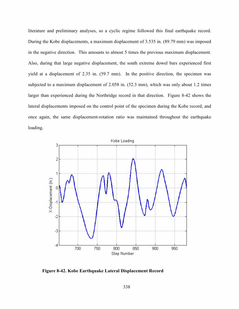
338
literature and preliminary analyses, so a cyclic regime followed this final earthquake record.
During the Kobe displacements, a maximum displacement of 3.535 in. (89.79 mm) was imposed
in the negative direction. This amounts to almost 5 times the previous maximum displacement.
Also, during that large negative displacement, the south extreme dowel bars experienced first
yield at a displacement of 2.35 in. (59.7 mm). In the positive direction, the specimen was
subjected to a maximum displacement of 2.058 in. (52.3 mm), which was only about 1.2 times
larger than experienced during the Northridge record in that direction. Figure 8-42 shows the
lateral displacements imposed on the control point of the specimen during the Kobe record, and
once again, the same displacement-rotation ratio was maintained throughout the earthquake
loading.
Figure 8-42. Kobe Earthquake Lateral Displacement Record
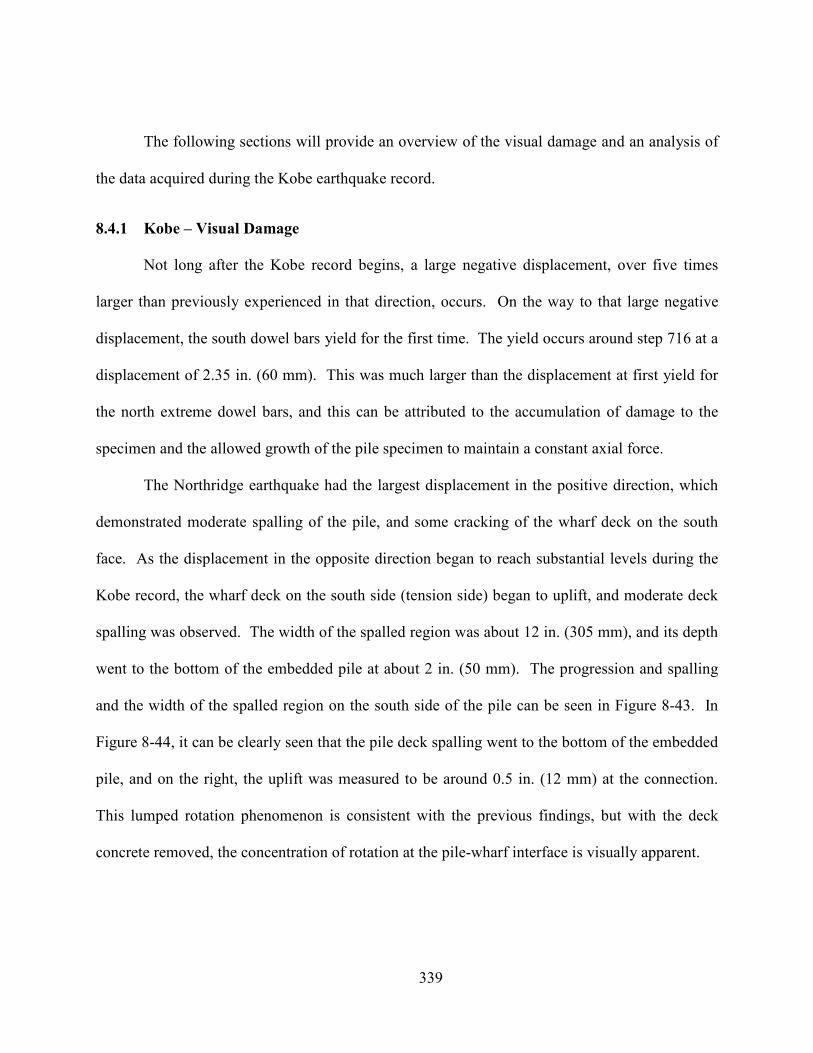
339
The following sections will provide an overview of the visual damage and an analysis of
the data acquired during the Kobe earthquake record.
8.4.1 Kobe – Visual Damage
Not long after the Kobe record begins, a large negative displacement, over five times
larger than previously experienced in that direction, occurs. On the way to that large negative
displacement, the south dowel bars yield for the first time. The yield occurs around step 716 at a
displacement of 2.35 in. (60 mm). This was much larger than the displacement at first yield for
the north extreme dowel bars, and this can be attributed to the accumulation of damage to the
specimen and the allowed growth of the pile specimen to maintain a constant axial force.
The Northridge earthquake had the largest displacement in the positive direction, which
demonstrated moderate spalling of the pile, and some cracking of the wharf deck on the south
face. As the displacement in the opposite direction began to reach substantial levels during the
Kobe record, the wharf deck on the south side (tension side) began to uplift, and moderate deck
spalling was observed. The width of the spalled region was about 12 in. (305 mm), and its depth
went to the bottom of the embedded pile at about 2 in. (50 mm). The progression and spalling
and the width of the spalled region on the south side of the pile can be seen in Figure 8-43. In
Figure 8-44, it can be clearly seen that the pile deck spalling went to the bottom of the embedded
pile, and on the right, the uplift was measured to be around 0.5 in. (12 mm) at the connection.
This lumped rotation phenomenon is consistent with the previous findings, but with the deck
concrete removed, the concentration of rotation at the pile-wharf interface is visually apparent.
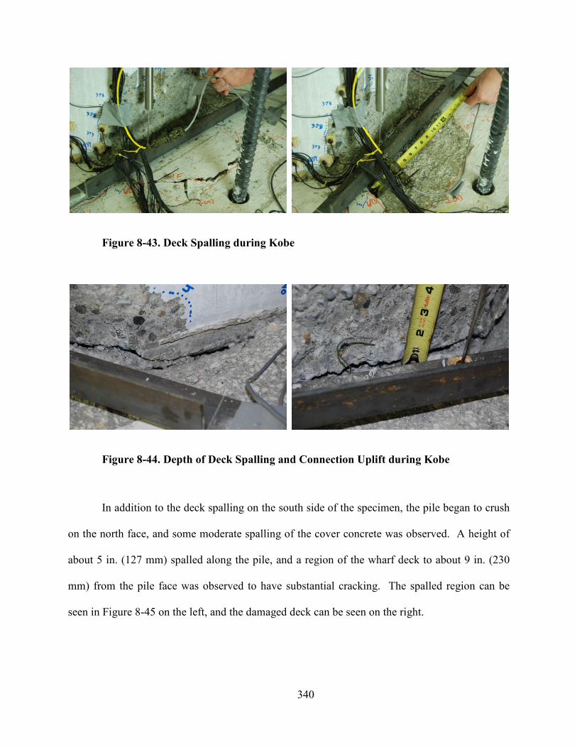
340
Figure 8-43. Deck Spalling during Kobe
Figure 8-44. Depth of Deck Spalling and Connection Uplift during Kobe
In addition to the deck spalling on the south side of the specimen, the pile began to crush
on the north face, and some moderate spalling of the cover concrete was observed. A height of
about 5 in. (127 mm) spalled along the pile, and a region of the wharf deck to about 9 in. (230
mm) from the pile face was observed to have substantial cracking. The spalled region can be
seen in Figure 8-45 on the left, and the damaged deck can be seen on the right.
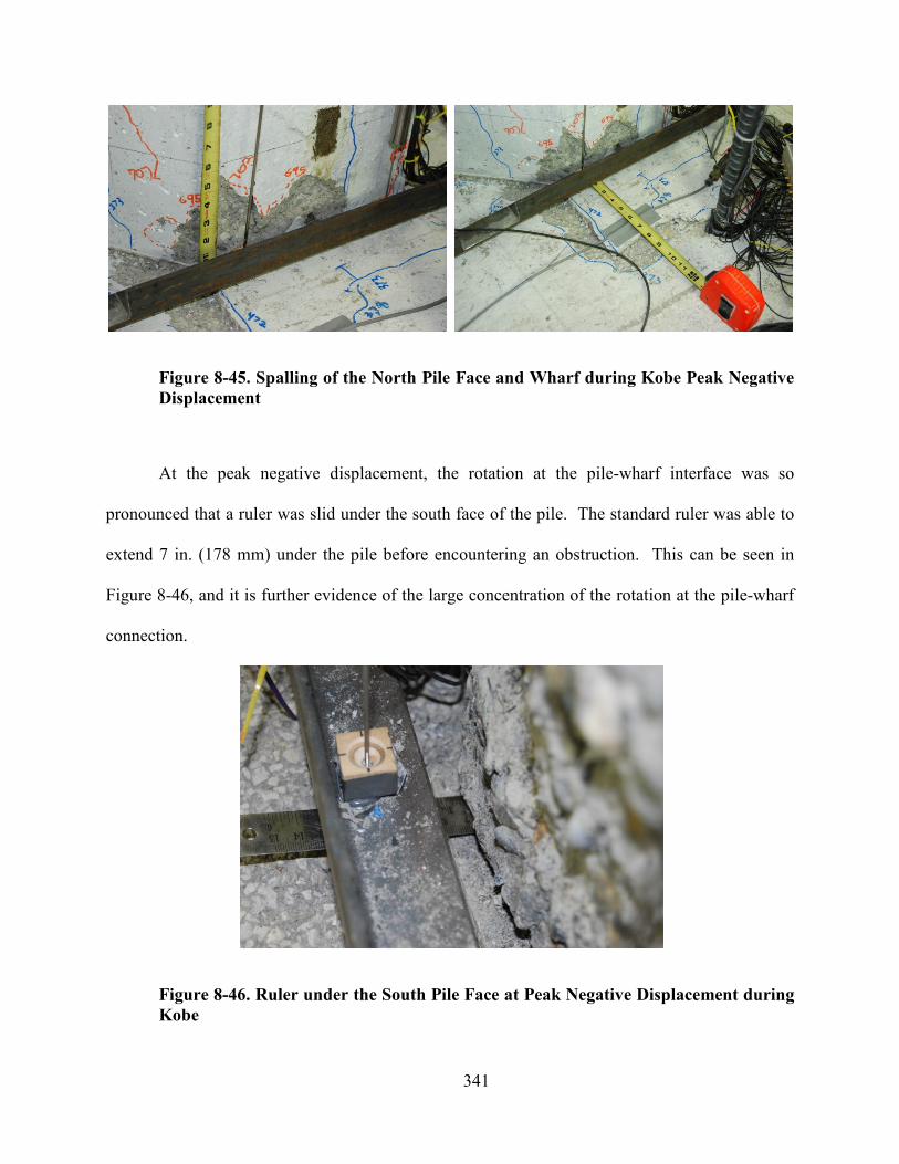
341
Figure 8-45. Spalling of the orth Pile Face and Wharf during Kobe Peak egative
Displacement
At the peak negative displacement, the rotation at the pile-wharf interface was so
pronounced that a ruler was slid under the south face of the pile. The standard ruler was able to
extend 7 in. (178 mm) under the pile before encountering an obstruction. This can be seen in
Figure 8-46, and it is further evidence of the large concentration of the rotation at the pile-wharf
connection.
Figure 8-46. Ruler under the South Pile Face at Peak egative Displacement during
Kobe
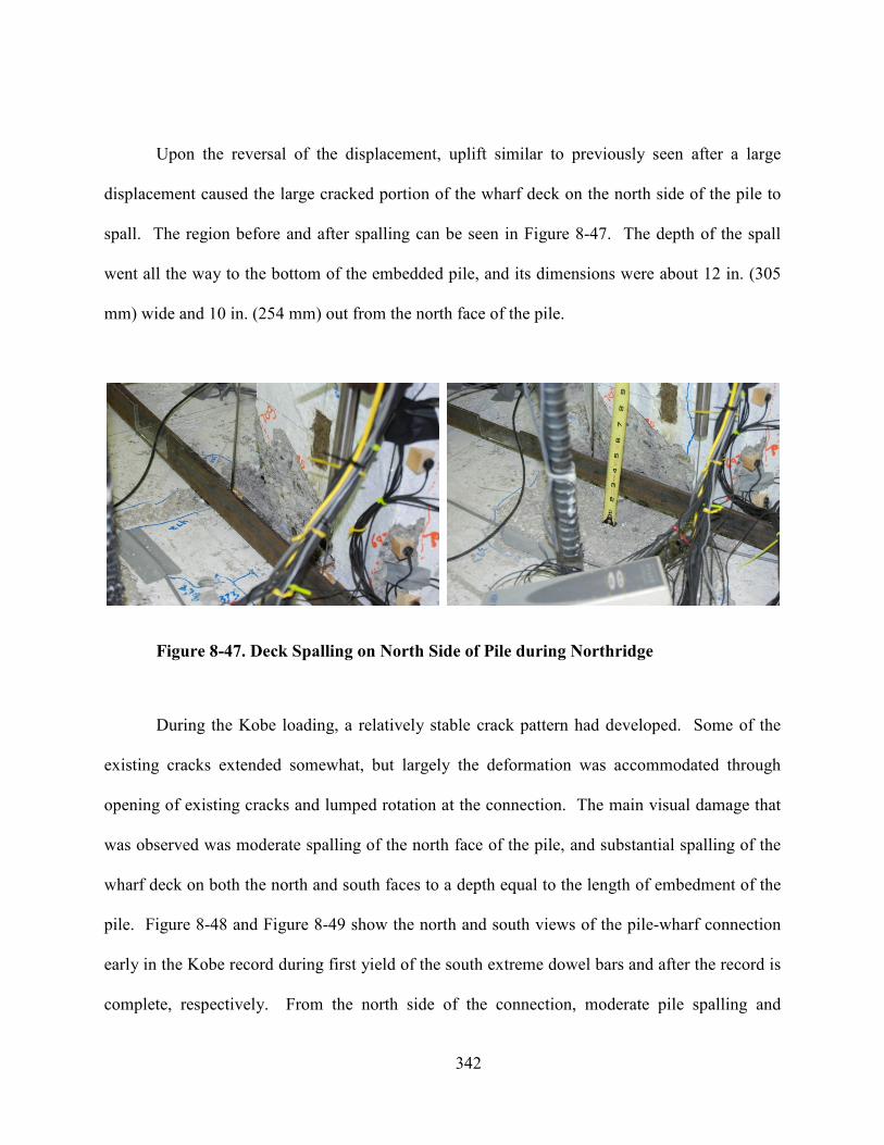
342
Upon the reversal of the displacement, uplift similar to previously seen after a large
displacement caused the large cracked portion of the wharf deck on the north side of the pile to
spall. The region before and after spalling can be seen in Figure 8-47. The depth of the spall
went all the way to the bottom of the embedded pile, and its dimensions were about 12 in. (305
mm) wide and 10 in. (254 mm) out from the north face of the pile.
Figure 8-47. Deck Spalling on orth Side of Pile during orthridge
During the Kobe loading, a relatively stable crack pattern had developed. Some of the
existing cracks extended somewhat, but largely the deformation was accommodated through
opening of existing cracks and lumped rotation at the connection. The main visual damage that
was observed was moderate spalling of the north face of the pile, and substantial spalling of the
wharf deck on both the north and south faces to a depth equal to the length of embedment of the
pile. Figure 8-48 and Figure 8-49 show the north and south views of the pile-wharf connection
early in the Kobe record during first yield of the south extreme dowel bars and after the record is
complete, respectively. From the north side of the connection, moderate pile spalling and
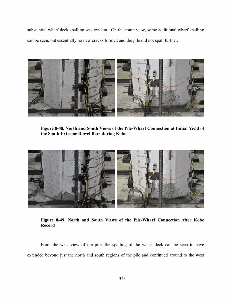
343
substantial wharf deck spalling was evident. On the south view, some additional wharf spalling
can be seen, but essentially no new cracks formed and the pile did not spall further.
Figure 8-48. orth and South Views of the Pile-Wharf Connection at Initial Yield of
the South Extreme Dowel Bars during Kobe
Figure 8-49. orth and South Views of the Pile-Wharf Connection after Kobe
Record
From the west view of the pile, the spalling of the wharf deck can be seen to have
extended beyond just the north and south regions of the pile and continued around to the west
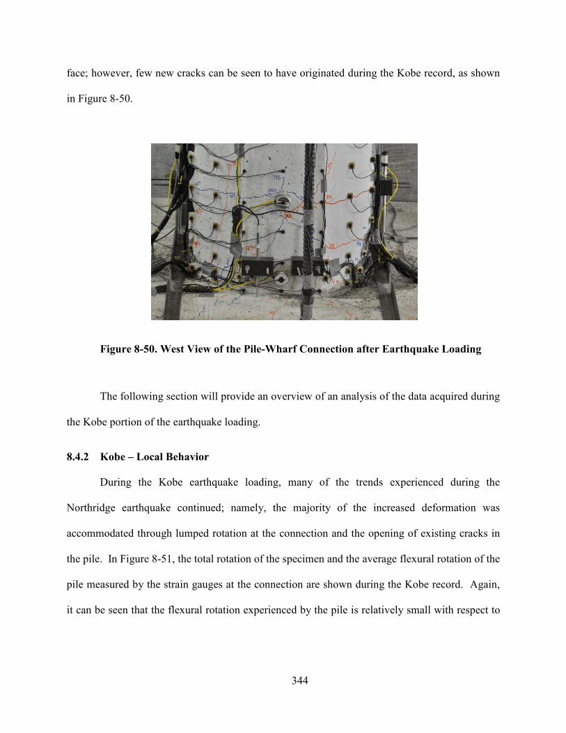
344
face; however, few new cracks can be seen to have originated during the Kobe record, as shown
in Figure 8-50.
Figure 8-50. West View of the Pile-Wharf Connection after Earthquake Loading
The following section will provide an overview of an analysis of the data acquired during
the Kobe portion of the earthquake loading.
8.4.2 Kobe – Local Behavior
During the Kobe earthquake loading, many of the trends experienced during the
Northridge earthquake continued; namely, the majority of the increased deformation was
accommodated through lumped rotation at the connection and the opening of existing cracks in
the pile. In Figure 8-51, the total rotation of the specimen and the average flexural rotation of the
pile measured by the strain gauges at the connection are shown during the Kobe record. Again,
it can be seen that the flexural rotation experienced by the pile is relatively small with respect to
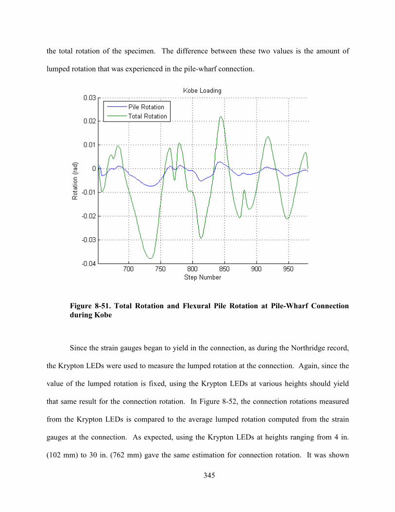
345
the total rotation of the specimen. The difference between these two values is the amount of
lumped rotation that was experienced in the pile-wharf connection.
Figure 8-51. Total Rotation and Flexural Pile Rotation at Pile-Wharf Connection
during Kobe
Since the strain gauges began to yield in the connection, as during the Northridge record,
the Krypton LEDs were used to measure the lumped rotation at the connection. Again, since the
value of the lumped rotation is fixed, using the Krypton LEDs at various heights should yield
that same result for the connection rotation. In Figure 8-52, the connection rotations measured
from the Krypton LEDs is compared to the average lumped rotation computed from the strain
gauges at the connection. As expected, using the Krypton LEDs at heights ranging from 4 in.
(102 mm) to 30 in. (762 mm) gave the same estimation for connection rotation. It was shown
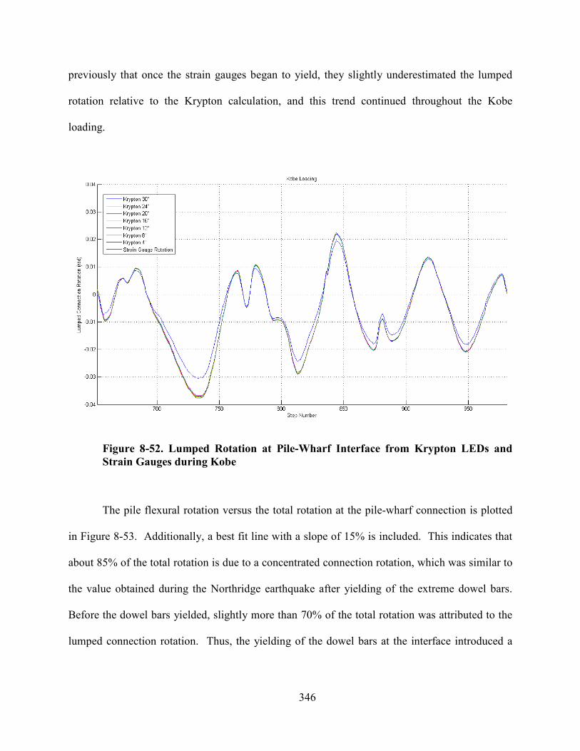
346
previously that once the strain gauges began to yield, they slightly underestimated the lumped
rotation relative to the Krypton calculation, and this trend continued throughout the Kobe
loading.
Figure 8-52. Lumped Rotation at Pile-Wharf Interface from Krypton LEDs and
Strain Gauges during Kobe
The pile flexural rotation versus the total rotation at the pile-wharf connection is plotted
in Figure 8-53. Additionally, a best fit line with a slope of 15% is included. This indicates that
about 85% of the total rotation is due to a concentrated connection rotation, which was similar to
the value obtained during the Northridge earthquake after yielding of the extreme dowel bars.
Before the dowel bars yielded, slightly more than 70% of the total rotation was attributed to the
lumped connection rotation. Thus, the yielding of the dowel bars at the interface introduced a
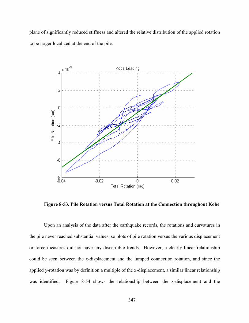
347
plane of significantly reduced stiffness and altered the relative distribution of the applied rotation
to be larger localized at the end of the pile.
Figure 8-53. Pile Rotation versus Total Rotation at the Connection throughout Kobe
Upon an analysis of the data after the earthquake records, the rotations and curvatures in
the pile never reached substantial values, so plots of pile rotation versus the various displacement
or force measures did not have any discernible trends. However, a clearly linear relationship
could be seen between the x-displacement and the lumped connection rotation, and since the
applied y-rotation was by definition a multiple of the x-displacement, a similar linear relationship
was identified. Figure 8-54 shows the relationship between the x-displacement and the
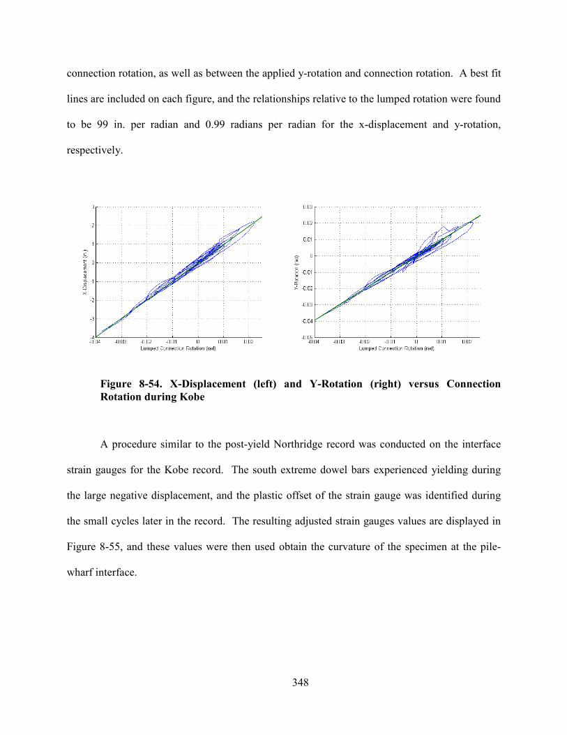
348
connection rotation, as well as between the applied y-rotation and connection rotation. A best fit
lines are included on each figure, and the relationships relative to the lumped rotation were found
to be 99 in. per radian and 0.99 radians per radian for the x-displacement and y-rotation,
respectively.
Figure 8-54. X-Displacement (left) and Y-Rotation (right) versus Connection
Rotation during Kobe
A procedure similar to the post-yield Northridge record was conducted on the interface
strain gauges for the Kobe record. The south extreme dowel bars experienced yielding during
the large negative displacement, and the plastic offset of the strain gauge was identified during
the small cycles later in the record. The resulting adjusted strain gauges values are displayed in
Figure 8-55, and these values were then used obtain the curvature of the specimen at the pile-
wharf interface.
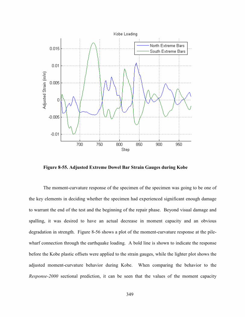
349
Figure 8-55. Adjusted Extreme Dowel Bar Strain Gauges during Kobe
The moment-curvature response of the specimen of the specimen was going to be one of
the key elements in deciding whether the specimen had experienced significant enough damage
to warrant the end of the test and the beginning of the repair phase. Beyond visual damage and
spalling, it was desired to have an actual decrease in moment capacity and an obvious
degradation in strength. Figure 8-56 shows a plot of the moment-curvature response at the pile-
wharf connection through the earthquake loading. A bold line is shown to indicate the response
before the Kobe plastic offsets were applied to the strain gauges, while the lighter plot shows the
adjusted moment-curvature behavior during Kobe. When comparing the behavior to the
Response-2000 sectional prediction, it can be seen that the values of the moment capacity
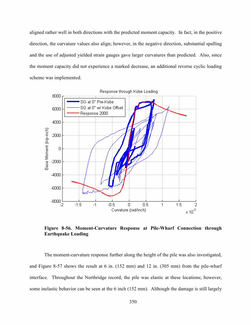
350
aligned rather well in both directions with the predicted moment capacity. In fact, in the positive
direction, the curvature values also align; however, in the negative direction, substantial spalling
and the use of adjusted yielded strain gauges gave larger curvatures than predicted. Also, since
the moment capacity did not experience a marked decrease, an additional reverse cyclic loading
scheme was implemented.
Figure 8-56. Moment-Curvature Response at Pile-Wharf Connection through
Earthquake Loading
The moment-curvature response further along the height of the pile was also investigated,
and Figure 8-57 shows the result at 6 in. (152 mm) and 12 in. (305 mm) from the pile-wharf
interface. Throughout the Northridge record, the pile was elastic at these locations; however,
some inelastic behavior can be seen at the 6 inch (152 mm). Although the damage is still largely
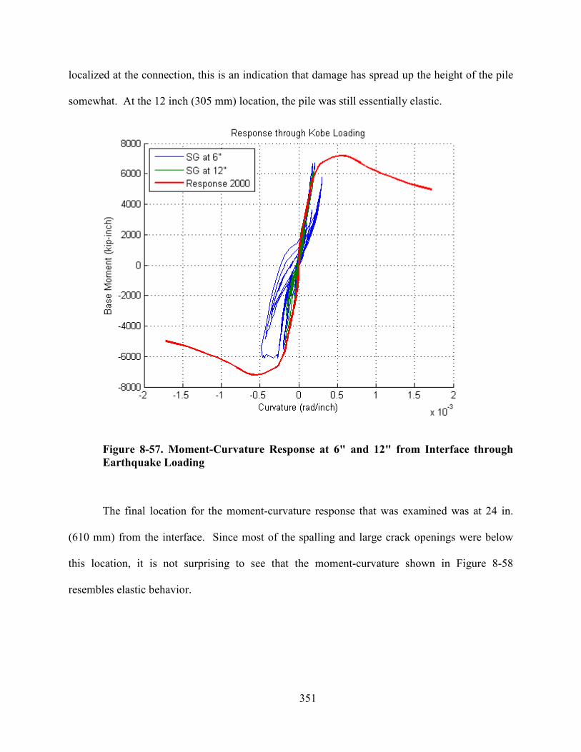
351
localized at the connection, this is an indication that damage has spread up the height of the pile
somewhat. At the 12 inch (305 mm) location, the pile was still essentially elastic.
Figure 8-57. Moment-Curvature Response at 6" and 12" from Interface through
Earthquake Loading
The final location for the moment-curvature response that was examined was at 24 in.
(610 mm) from the interface. Since most of the spalling and large crack openings were below
this location, it is not surprising to see that the moment-curvature shown in Figure 8-58
resembles elastic behavior.
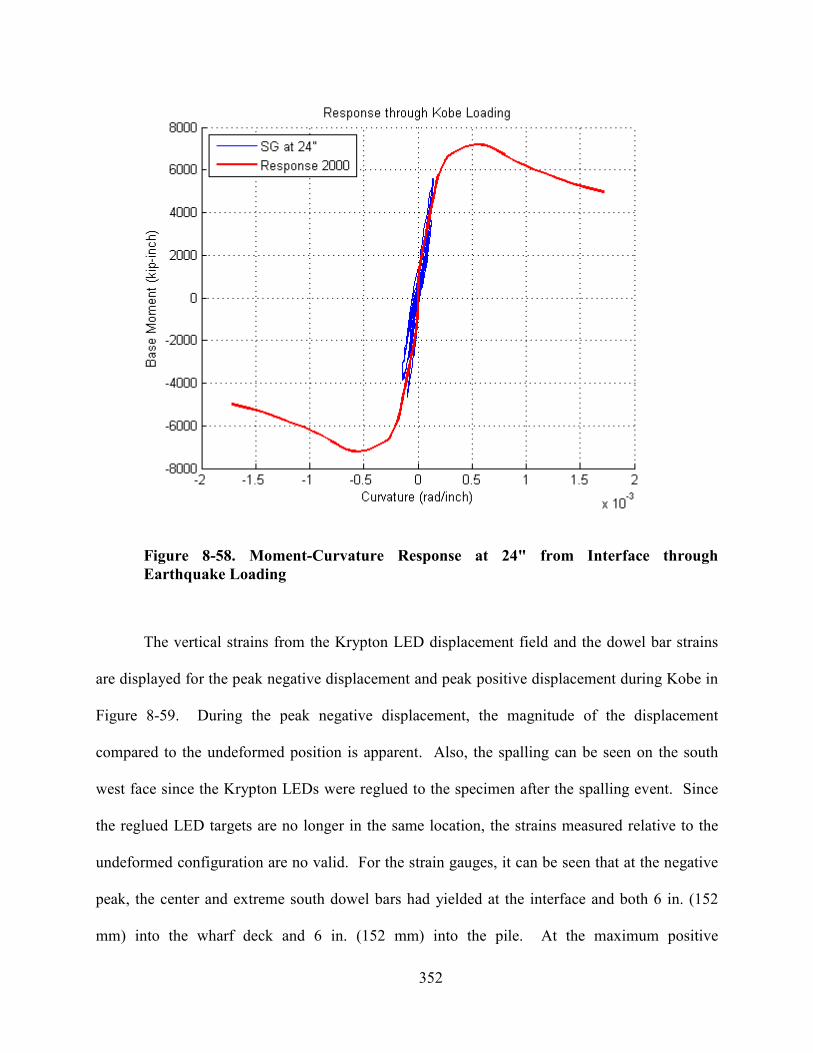
352
Figure 8-58. Moment-Curvature Response at 24" from Interface through
Earthquake Loading
The vertical strains from the Krypton LED displacement field and the dowel bar strains
are displayed for the peak negative displacement and peak positive displacement during Kobe in
Figure 8-59. During the peak negative displacement, the magnitude of the displacement
compared to the undeformed position is apparent. Also, the spalling can be seen on the south
west face since the Krypton LEDs were reglued to the specimen after the spalling event. Since
the reglued LED targets are no longer in the same location, the strains measured relative to the
undeformed configuration are no valid. For the strain gauges, it can be seen that at the negative
peak, the center and extreme south dowel bars had yielded at the interface and both 6 in. (152
mm) into the wharf deck and 6 in. (152 mm) into the pile. At the maximum positive
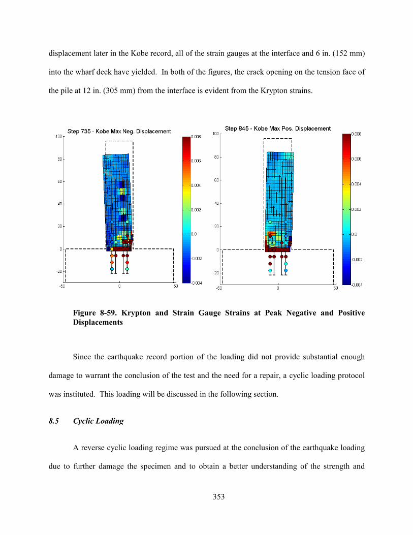
353
displacement later in the Kobe record, all of the strain gauges at the interface and 6 in. (152 mm)
into the wharf deck have yielded. In both of the figures, the crack opening on the tension face of
the pile at 12 in. (305 mm) from the interface is evident from the Krypton strains.
Figure 8-59. Krypton and Strain Gauge Strains at Peak egative and Positive
Displacements
Since the earthquake record portion of the loading did not provide substantial enough
damage to warrant the conclusion of the test and the need for a repair, a cyclic loading protocol
was instituted. This loading will be discussed in the following section.
8.5 Cyclic Loading
A reverse cyclic loading regime was pursued at the conclusion of the earthquake loading
due to further damage the specimen and to obtain a better understanding of the strength and
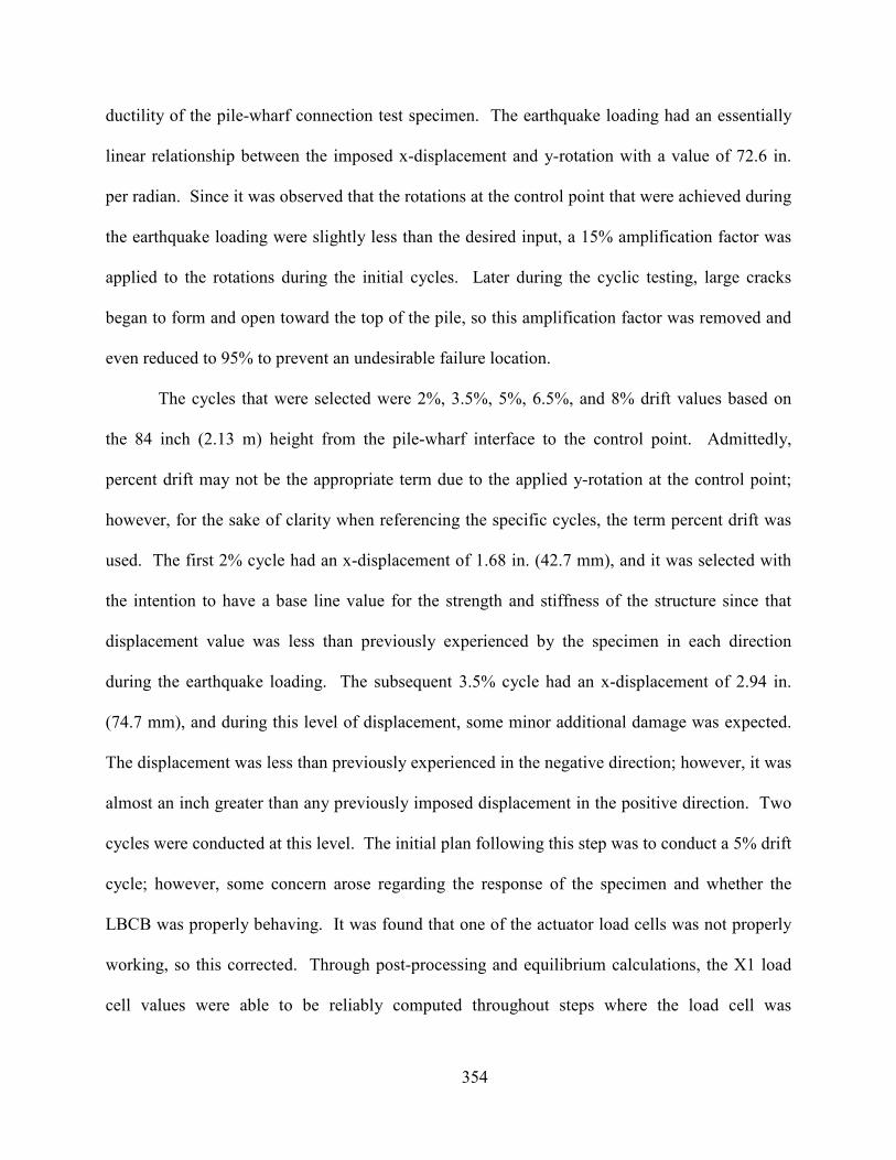
354
ductility of the pile-wharf connection test specimen. The earthquake loading had an essentially
linear relationship between the imposed x-displacement and y-rotation with a value of 72.6 in.
per radian. Since it was observed that the rotations at the control point that were achieved during
the earthquake loading were slightly less than the desired input, a 15% amplification factor was
applied to the rotations during the initial cycles. Later during the cyclic testing, large cracks
began to form and open toward the top of the pile, so this amplification factor was removed and
even reduced to 95% to prevent an undesirable failure location.
The cycles that were selected were 2%, 3.5%, 5%, 6.5%, and 8% drift values based on
the 84 inch (2.13 m) height from the pile-wharf interface to the control point. Admittedly,
percent drift may not be the appropriate term due to the applied y-rotation at the control point;
however, for the sake of clarity when referencing the specific cycles, the term percent drift was
used. The first 2% cycle had an x-displacement of 1.68 in. (42.7 mm), and it was selected with
the intention to have a base line value for the strength and stiffness of the structure since that
displacement value was less than previously experienced by the specimen in each direction
during the earthquake loading. The subsequent 3.5% cycle had an x-displacement of 2.94 in.
(74.7 mm), and during this level of displacement, some minor additional damage was expected.
The displacement was less than previously experienced in the negative direction; however, it was
almost an inch greater than any previously imposed displacement in the positive direction. Two
cycles were conducted at this level. The initial plan following this step was to conduct a 5% drift
cycle; however, some concern arose regarding the response of the specimen and whether the
LBCB was properly behaving. It was found that one of the actuator load cells was not properly
working, so this corrected. Through post-processing and equilibrium calculations, the X1 load
cell values were able to be reliably computed throughout steps where the load cell was
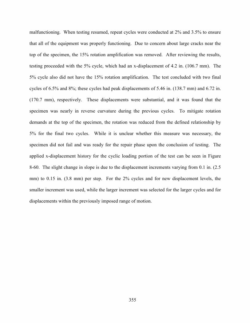
355
malfunctioning. When testing resumed, repeat cycles were conducted at 2% and 3.5% to ensure
that all of the equipment was properly functioning. Due to concern about large cracks near the
top of the specimen, the 15% rotation amplification was removed. After reviewing the results,
testing proceeded with the 5% cycle, which had an x-displacement of 4.2 in. (106.7 mm). The
5% cycle also did not have the 15% rotation amplification. The test concluded with two final
cycles of 6.5% and 8%; these cycles had peak displacements of 5.46 in. (138.7 mm) and 6.72 in.
(170.7 mm), respectively. These displacements were substantial, and it was found that the
specimen was nearly in reverse curvature during the previous cycles. To mitigate rotation
demands at the top of the specimen, the rotation was reduced from the defined relationship by
5% for the final two cycles. While it is unclear whether this measure was necessary, the
specimen did not fail and was ready for the repair phase upon the conclusion of testing. The
applied x-displacement history for the cyclic loading portion of the test can be seen in Figure
8-60. The slight change in slope is due to the displacement increments varying from 0.1 in. (2.5
mm) to 0.15 in. (3.8 mm) per step. For the 2% cycles and for new displacement levels, the
smaller increment was used, while the larger increment was selected for the larger cycles and for
displacements within the previously imposed range of motion.
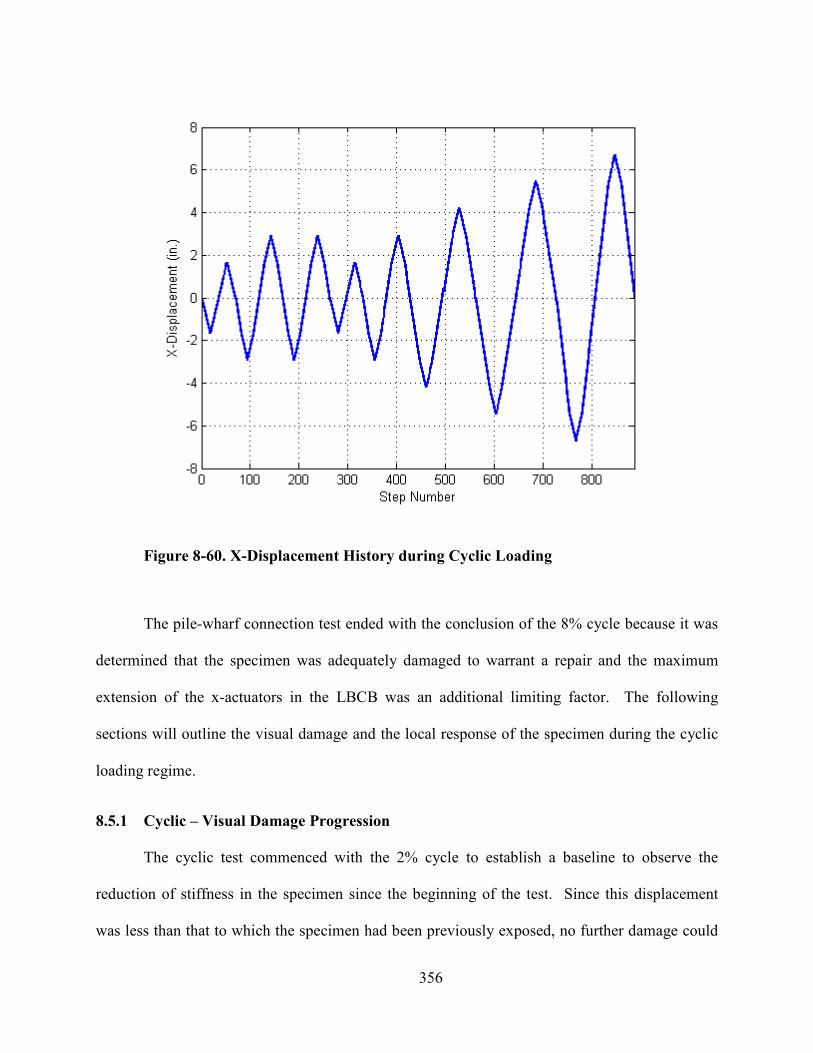
356
Figure 8-60. X-Displacement History during Cyclic Loading
The pile-wharf connection test ended with the conclusion of the 8% cycle because it was
determined that the specimen was adequately damaged to warrant a repair and the maximum
extension of the x-actuators in the LBCB was an additional limiting factor. The following
sections will outline the visual damage and the local response of the specimen during the cyclic
loading regime.
8.5.1 Cyclic – Visual Damage Progression
The cyclic test commenced with the 2% cycle to establish a baseline to observe the
reduction of stiffness in the specimen since the beginning of the test. Since this displacement
was less than that to which the specimen had been previously exposed, no further damage could
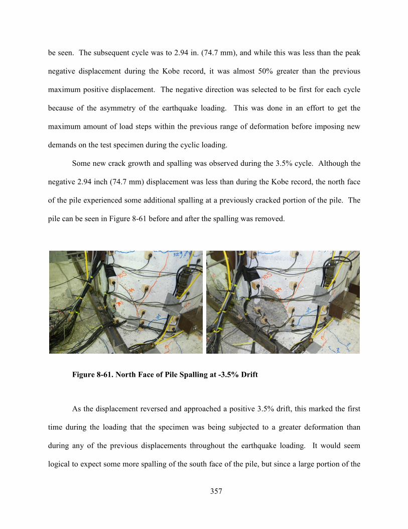
357
be seen. The subsequent cycle was to 2.94 in. (74.7 mm), and while this was less than the peak
negative displacement during the Kobe record, it was almost 50% greater than the previous
maximum positive displacement. The negative direction was selected to be first for each cycle
because of the asymmetry of the earthquake loading. This was done in an effort to get the
maximum amount of load steps within the previous range of deformation before imposing new
demands on the test specimen during the cyclic loading.
Some new crack growth and spalling was observed during the 3.5% cycle. Although the
negative 2.94 inch (74.7 mm) displacement was less than during the Kobe record, the north face
of the pile experienced some additional spalling at a previously cracked portion of the pile. The
pile can be seen in Figure 8-61 before and after the spalling was removed.
Figure 8-61. orth Face of Pile Spalling at -3.5% Drift
As the displacement reversed and approached a positive 3.5% drift, this marked the first
time during the loading that the specimen was being subjected to a greater deformation than
during any of the previous displacements throughout the earthquake loading. It would seem
logical to expect some more spalling of the south face of the pile, but since a large portion of the
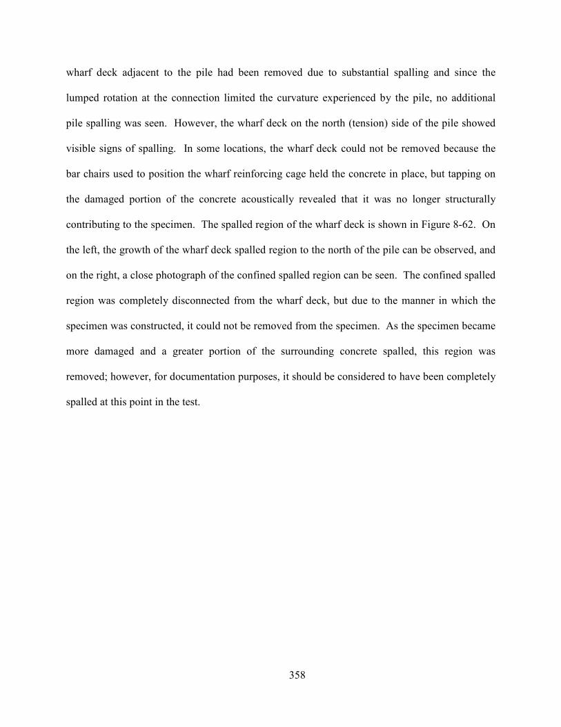
358
wharf deck adjacent to the pile had been removed due to substantial spalling and since the
lumped rotation at the connection limited the curvature experienced by the pile, no additional
pile spalling was seen. However, the wharf deck on the north (tension) side of the pile showed
visible signs of spalling. In some locations, the wharf deck could not be removed because the
bar chairs used to position the wharf reinforcing cage held the concrete in place, but tapping on
the damaged portion of the concrete acoustically revealed that it was no longer structurally
contributing to the specimen. The spalled region of the wharf deck is shown in Figure 8-62. On
the left, the growth of the wharf deck spalled region to the north of the pile can be observed, and
on the right, a close photograph of the confined spalled region can be seen. The confined spalled
region was completely disconnected from the wharf deck, but due to the manner in which the
specimen was constructed, it could not be removed from the specimen. As the specimen became
more damaged and a greater portion of the surrounding concrete spalled, this region was
removed; however, for documentation purposes, it should be considered to have been completely
spalled at this point in the test.
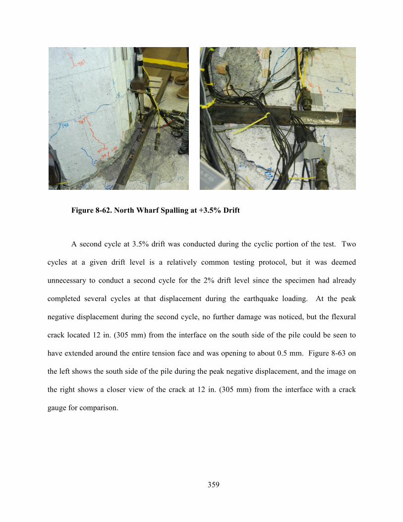
359
Figure 8-62. orth Wharf Spalling at +3.5% Drift
A second cycle at 3.5% drift was conducted during the cyclic portion of the test. Two
cycles at a given drift level is a relatively common testing protocol, but it was deemed
unnecessary to conduct a second cycle for the 2% drift level since the specimen had already
completed several cycles at that displacement during the earthquake loading. At the peak
negative displacement during the second cycle, no further damage was noticed, but the flexural
crack located 12 in. (305 mm) from the interface on the south side of the pile could be seen to
have extended around the entire tension face and was opening to about 0.5 mm. Figure 8-63 on
the left shows the south side of the pile during the peak negative displacement, and the image on
the right shows a closer view of the crack at 12 in. (305 mm) from the interface with a crack
gauge for comparison.
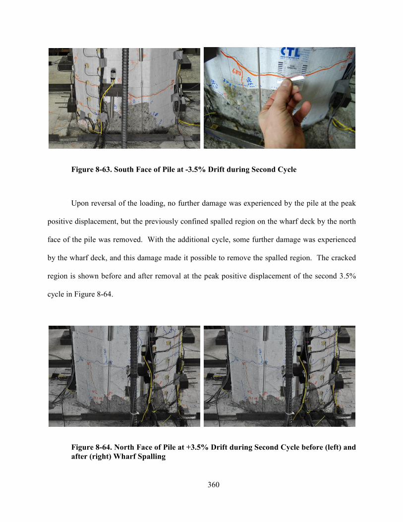
360
Figure 8-63. South Face of Pile at -3.5% Drift during Second Cycle
Upon reversal of the loading, no further damage was experienced by the pile at the peak
positive displacement, but the previously confined spalled region on the wharf deck by the north
face of the pile was removed. With the additional cycle, some further damage was experienced
by the wharf deck, and this damage made it possible to remove the spalled region. The cracked
region is shown before and after removal at the peak positive displacement of the second 3.5%
cycle in Figure 8-64.
Figure 8-64. orth Face of Pile at +3.5% Drift during Second Cycle before (left) and
after (right) Wharf Spalling
361
At the conclusion of the two 3.5% drift cycles, the next planned level of deformation was
to be two 5% cycles. Several days elapsed before the 5% cycles commenced, and when the
cycles started, some anomalous behavior was observed. It could be seen that localized cracks
were opening near the top of the pile, and it was noticed that the X1 actuator load cell was not
reading properly. At this point, testing came to a halt and troubleshooting began. The problem
with the X1 load cell was remedied, and through post-processing and equilibrium calculations, it
was found that the proper X1 load cell value could be computed. When testing resumed, the
cyclic loading was adjusted, and it was desired to conduct a single cycle at both 2% and 3.5% to
ensure that specimen and LBCB were behaving as expected. Additionally, the previous cyclic
loading used a 15% amplification on the rotation to ensure that the proper rotation was being
achieved at the control point. Upon post-processing the data obtained during troubleshooting, it
was found that the 15% amplification was no longer needed to obtain the desired rotation at the
control point, so in the interest of not inducing a failure at the top of the specimen, the 15%
amplification factor was removed for all subsequent rotations. Thus, the applied displacement-
rotation ratio was 72.6 in. per radian. The 2% and 3.5% cycles were conducted and the damage
and crack growth was monitored; however, no new significant visual damage was observed
during these cycles, as expected.
With the instrument issues resolved, and the 2% and 3.5% levels of displacement
repeated to satisfaction, the next cycle conducted was the 5% drift. The 5% drift corresponded to
4.2 in. (107 mm), and this distance was substantially larger than previously imposed on the
specimen in either direction. Given the large increase in displacement, it was expected that
damage would propagate throughout the specimen; however, additional spalling of the pile was
not apparent and only slight growth of existing cracks occurred. It seems that the additional
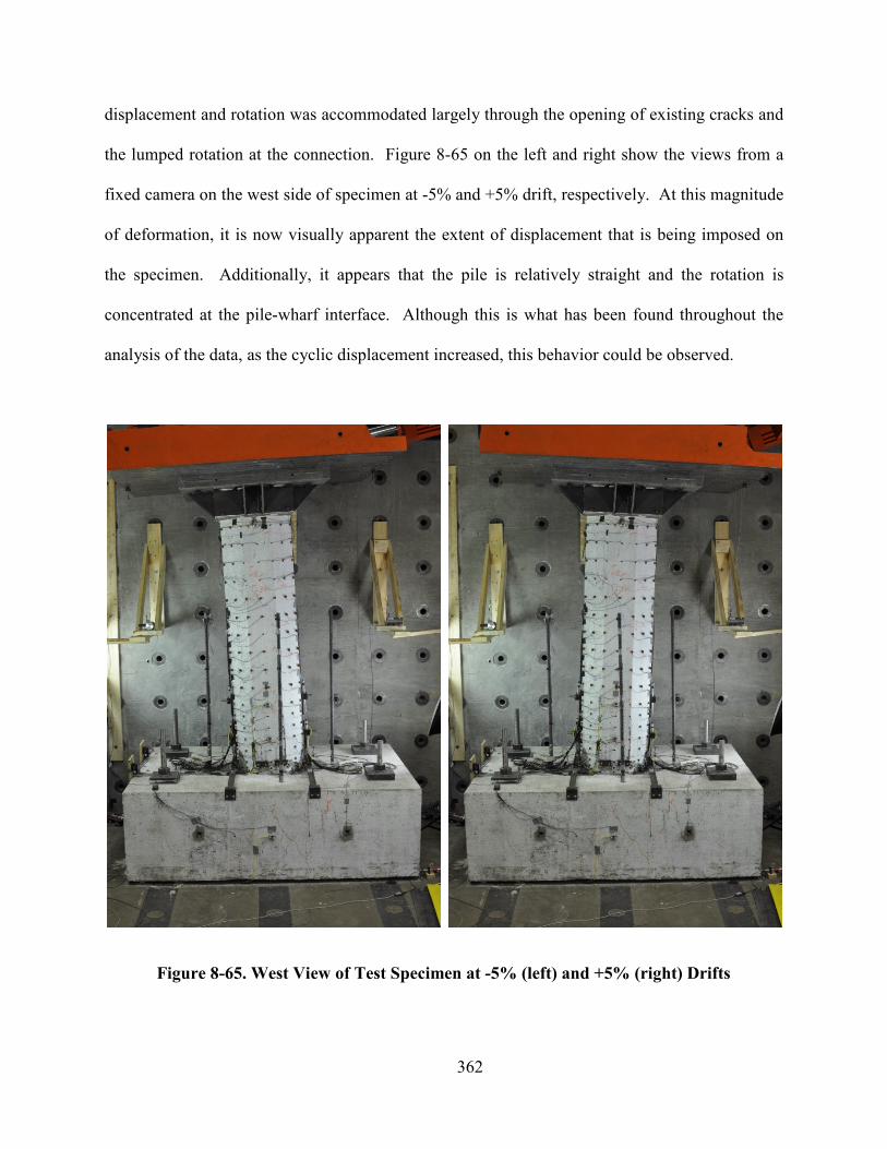
362
displacement and rotation was accommodated largely through the opening of existing cracks and
the lumped rotation at the connection. Figure 8-65 on the left and right show the views from a
fixed camera on the west side of specimen at -5% and +5% drift, respectively. At this magnitude
of deformation, it is now visually apparent the extent of displacement that is being imposed on
the specimen. Additionally, it appears that the pile is relatively straight and the rotation is
concentrated at the pile-wharf interface. Although this is what has been found throughout the
analysis of the data, as the cyclic displacement increased, this behavior could be observed.
Figure 8-65. West View of Test Specimen at -5% (left) and +5% (right) Drifts
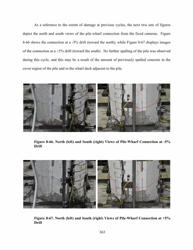
363
As a reference to the extent of damage at previous cycles, the next two sets of figures
depict the north and south views of the pile-wharf connection from the fixed cameras. Figure
8-66 shows the connection at a -5% drift (toward the north), while Figure 8-67 displays images
of the connection at a +5% drift (toward the south). No further spalling of the pile was observed
during this cycle, and this may be a result of the amount of previously spalled concrete in the
cover region of the pile and in the wharf deck adjacent to the pile.
Figure 8-66. orth (left) and South (right) Views of Pile-Wharf Connection at -5%
Drift
Figure 8-67. orth (left) and South (right) Views of Pile-Wharf Connection at +5%
Drift
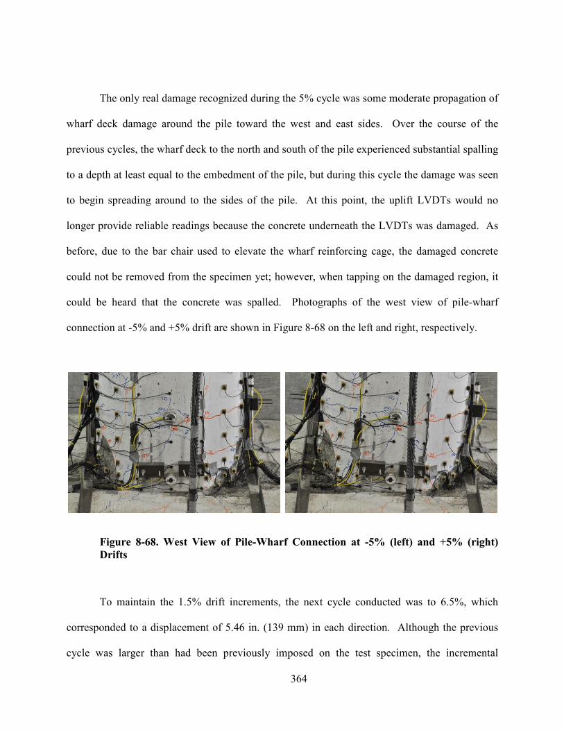
364
The only real damage recognized during the 5% cycle was some moderate propagation of
wharf deck damage around the pile toward the west and east sides. Over the course of the
previous cycles, the wharf deck to the north and south of the pile experienced substantial spalling
to a depth at least equal to the embedment of the pile, but during this cycle the damage was seen
to begin spreading around to the sides of the pile. At this point, the uplift LVDTs would no
longer provide reliable readings because the concrete underneath the LVDTs was damaged. As
before, due to the bar chair used to elevate the wharf reinforcing cage, the damaged concrete
could not be removed from the specimen yet; however, when tapping on the damaged region, it
could be heard that the concrete was spalled. Photographs of the west view of pile-wharf
connection at -5% and +5% drift are shown in Figure 8-68 on the left and right, respectively.
Figure 8-68. West View of Pile-Wharf Connection at -5% (left) and +5% (right)
Drifts
To maintain the 1.5% drift increments, the next cycle conducted was to 6.5%, which
corresponded to a displacement of 5.46 in. (139 mm) in each direction. Although the previous
cycle was larger than had been previously imposed on the test specimen, the incremental
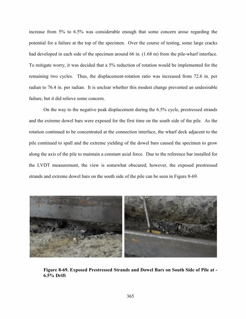
365
increase from 5% to 6.5% was considerable enough that some concern arose regarding the
potential for a failure at the top of the specimen. Over the course of testing, some large cracks
had developed in each side of the specimen around 66 in. (1.68 m) from the pile-wharf interface.
To mitigate worry, it was decided that a 5% reduction of rotation would be implemented for the
remaining two cycles. Thus, the displacement-rotation ratio was increased from 72.6 in. per
radian to 76.4 in. per radian. It is unclear whether this modest change prevented an undesirable
failure, but it did relieve some concern.
On the way to the negative peak displacement during the 6.5% cycle, prestressed strands
and the extreme dowel bars were exposed for the first time on the south side of the pile. As the
rotation continued to be concentrated at the connection interface, the wharf deck adjacent to the
pile continued to spall and the extreme yielding of the dowel bars caused the specimen to grow
along the axis of the pile to maintain a constant axial force. Due to the reference bar installed for
the LVDT measurement, the view is somewhat obscured; however, the exposed prestressed
strands and extreme dowel bars on the south side of the pile can be seen in Figure 8-69.
Figure 8-69. Exposed Prestressed Strands and Dowel Bars on South Side of Pile at -
6.5% Drift
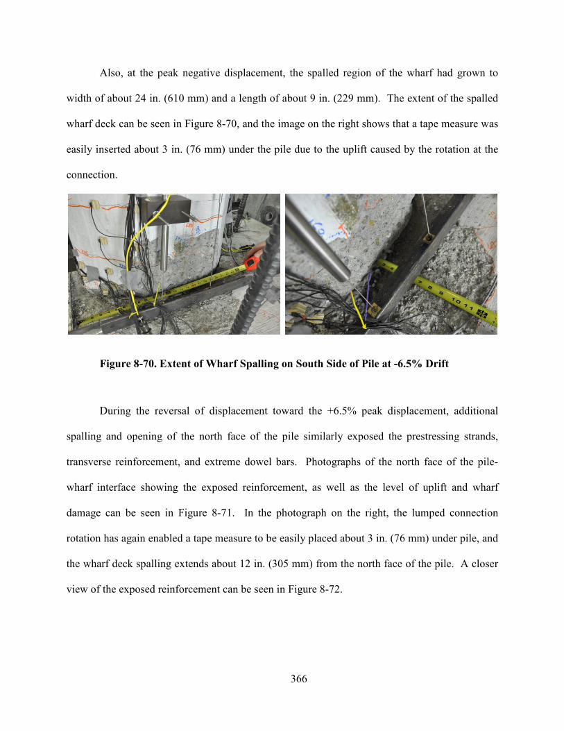
366
Also, at the peak negative displacement, the spalled region of the wharf had grown to
width of about 24 in. (610 mm) and a length of about 9 in. (229 mm). The extent of the spalled
wharf deck can be seen in Figure 8-70, and the image on the right shows that a tape measure was
easily inserted about 3 in. (76 mm) under the pile due to the uplift caused by the rotation at the
connection.
Figure 8-70. Extent of Wharf Spalling on South Side of Pile at -6.5% Drift
During the reversal of displacement toward the +6.5% peak displacement, additional
spalling and opening of the north face of the pile similarly exposed the prestressing strands,
transverse reinforcement, and extreme dowel bars. Photographs of the north face of the pile-
wharf interface showing the exposed reinforcement, as well as the level of uplift and wharf
damage can be seen in Figure 8-71. In the photograph on the right, the lumped connection
rotation has again enabled a tape measure to be easily placed about 3 in. (76 mm) under pile, and
the wharf deck spalling extends about 12 in. (305 mm) from the north face of the pile. A closer
view of the exposed reinforcement can be seen in Figure 8-72.
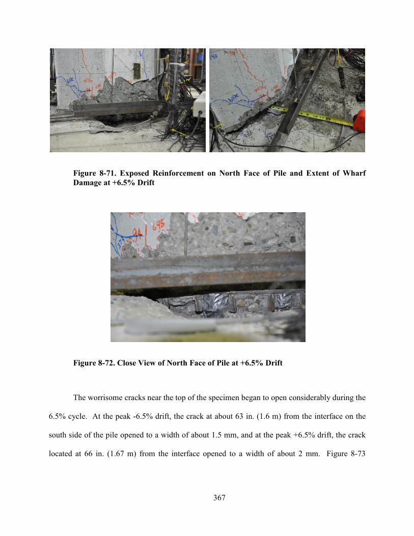
367
Figure 8-71. Exposed Reinforcement on orth Face of Pile and Extent of Wharf
Damage at +6.5% Drift
Figure 8-72. Close View of orth Face of Pile at +6.5% Drift
The worrisome cracks near the top of the specimen began to open considerably during the
6.5% cycle. At the peak -6.5% drift, the crack at about 63 in. (1.6 m) from the interface on the
south side of the pile opened to a width of about 1.5 mm, and at the peak +6.5% drift, the crack
located at 66 in. (1.67 m) from the interface opened to a width of about 2 mm. Figure 8-73
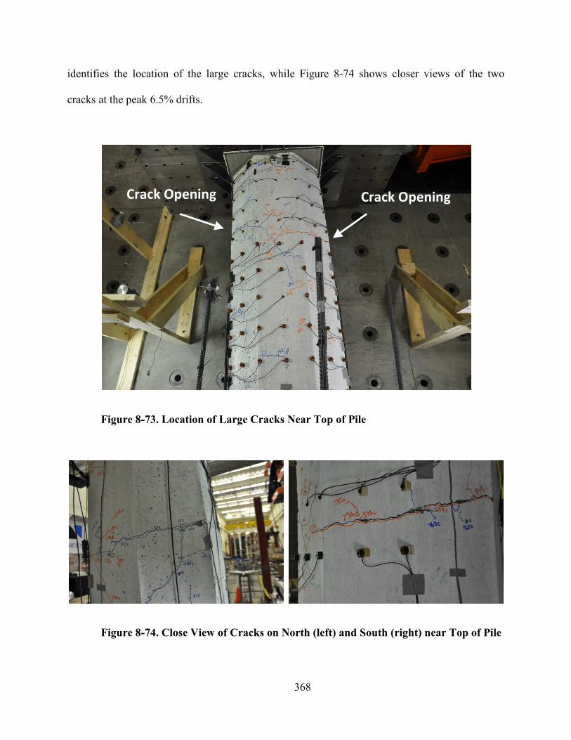
368
identifies the location of the large cracks, while Figure 8-74 shows closer views of the two
cracks at the peak 6.5% drifts.
Figure 8-73. Location of Large Cracks ear Top of Pile
Figure 8-74. Close View of Cracks on orth (left) and South (right) near Top of Pile
Crack Opening Crack Opening
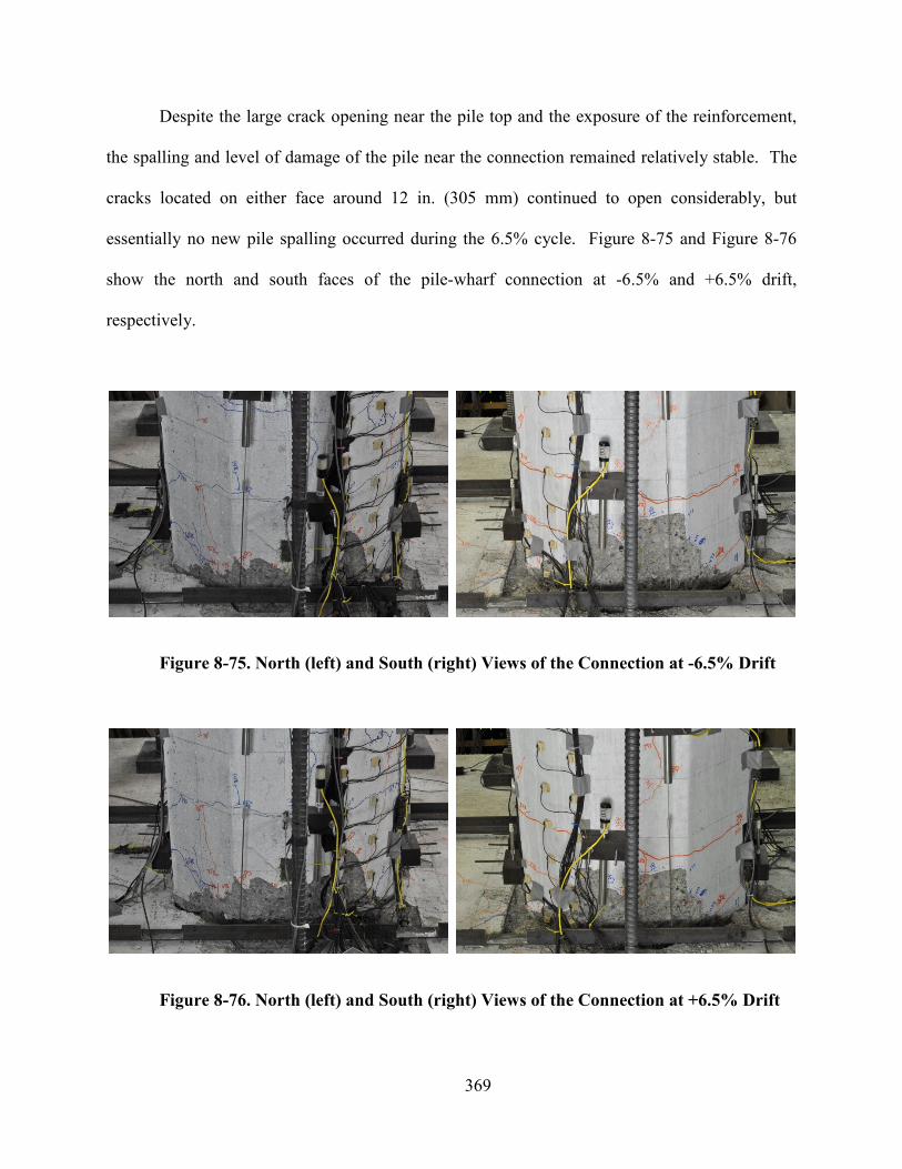
369
Despite the large crack opening near the pile top and the exposure of the reinforcement,
the spalling and level of damage of the pile near the connection remained relatively stable. The
cracks located on either face around 12 in. (305 mm) continued to open considerably, but
essentially no new pile spalling occurred during the 6.5% cycle. Figure 8-75 and Figure 8-76
show the north and south faces of the pile-wharf connection at -6.5% and +6.5% drift,
respectively.
Figure 8-75. orth (left) and South (right) Views of the Connection at -6.5% Drift
Figure 8-76. orth (left) and South (right) Views of the Connection at +6.5% Drift
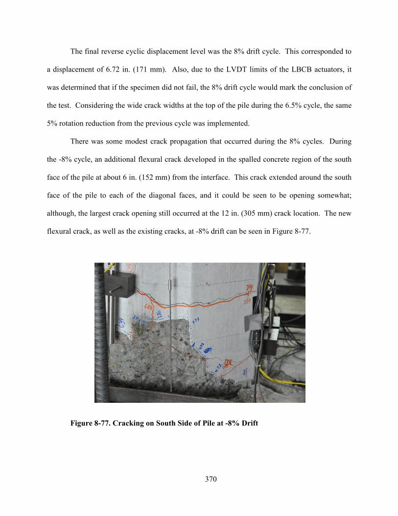
370
The final reverse cyclic displacement level was the 8% drift cycle. This corresponded to
a displacement of 6.72 in. (171 mm). Also, due to the LVDT limits of the LBCB actuators, it
was determined that if the specimen did not fail, the 8% drift cycle would mark the conclusion of
the test. Considering the wide crack widths at the top of the pile during the 6.5% cycle, the same
5% rotation reduction from the previous cycle was implemented.
There was some modest crack propagation that occurred during the 8% cycles. During
the -8% cycle, an additional flexural crack developed in the spalled concrete region of the south
face of the pile at about 6 in. (152 mm) from the interface. This crack extended around the south
face of the pile to each of the diagonal faces, and it could be seen to be opening somewhat;
although, the largest crack opening still occurred at the 12 in. (305 mm) crack location. The new
flexural crack, as well as the existing cracks, at -8% drift can be seen in Figure 8-77.
Figure 8-77. Cracking on South Side of Pile at -8% Drift

371
During the +8% drift cycle, there were not considerably more cracks, but there was some
crack growth at the location near the top of the pile. Starting during the Kobe record where large
negative displacements occurred, the north side of the pile continued to be more damaged
visually than the south side of the specimen. This continued throughout the test, so the +8% drift
cycle presented the best opportunity to see the extent of damage under the pile and to observe the
maximum uplift that occurred at the interface during the concentrated rotation at the connection.
Figure 8-78. Wharf Damage and Uplift at orth Face of Pile during +8% Drift
The next figures will show the photographs of the specimen at the peak 8% drift positions
as seen from the various fixed cameras. These figures will provide a visual reference for the
magnitude of deformation imposed on the test specimen, as well as the extent of damage, when
compared to previous figures from the same perspective. Figure 8-79 shows the west view of the
entire test specimen at -8% and +8% drift. Since some initial stroke of the LBCB actuators was
used through z-rotation to make the connection to the test specimen, the magnitude of these
displacements and rotations shown correspond to the 95% of LBCB displacement capacity. As
before, other than large localized cracks in the specimen, the majority of the deformation was
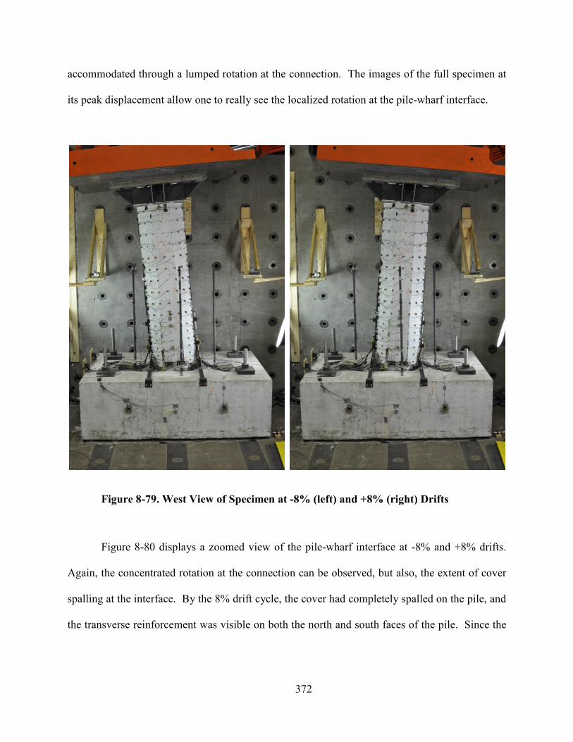
372
accommodated through a lumped rotation at the connection. The images of the full specimen at
its peak displacement allow one to really see the localized rotation at the pile-wharf interface.
Figure 8-79. West View of Specimen at -8% (left) and +8% (right) Drifts
Figure 8-80 displays a zoomed view of the pile-wharf interface at -8% and +8% drifts.
Again, the concentrated rotation at the connection can be observed, but also, the extent of cover
spalling at the interface. By the 8% drift cycle, the cover had completely spalled on the pile, and
the transverse reinforcement was visible on both the north and south faces of the pile. Since the
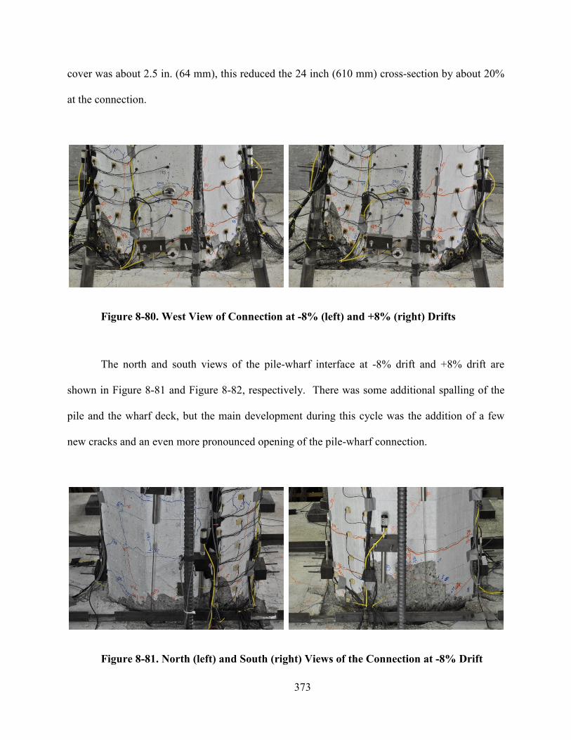
373
cover was about 2.5 in. (64 mm), this reduced the 24 inch (610 mm) cross-section by about 20%
at the connection.
Figure 8-80. West View of Connection at -8% (left) and +8% (right) Drifts
The north and south views of the pile-wharf interface at -8% drift and +8% drift are
shown in Figure 8-81 and Figure 8-82, respectively. There was some additional spalling of the
pile and the wharf deck, but the main development during this cycle was the addition of a few
new cracks and an even more pronounced opening of the pile-wharf connection.
Figure 8-81. orth (left) and South (right) Views of the Connection at -8% Drift
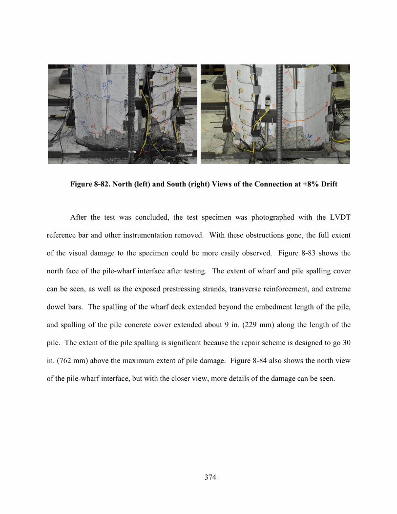
374
Figure 8-82. orth (left) and South (right) Views of the Connection at +8% Drift
After the test was concluded, the test specimen was photographed with the LVDT
reference bar and other instrumentation removed. With these obstructions gone, the full extent
of the visual damage to the specimen could be more easily observed. Figure 8-83 shows the
north face of the pile-wharf interface after testing. The extent of wharf and pile spalling cover
can be seen, as well as the exposed prestressing strands, transverse reinforcement, and extreme
dowel bars. The spalling of the wharf deck extended beyond the embedment length of the pile,
and spalling of the pile concrete cover extended about 9 in. (229 mm) along the length of the
pile. The extent of the pile spalling is significant because the repair scheme is designed to go 30
in. (762 mm) above the maximum extent of pile damage. Figure 8-84 also shows the north view
of the pile-wharf interface, but with the closer view, more details of the damage can be seen.
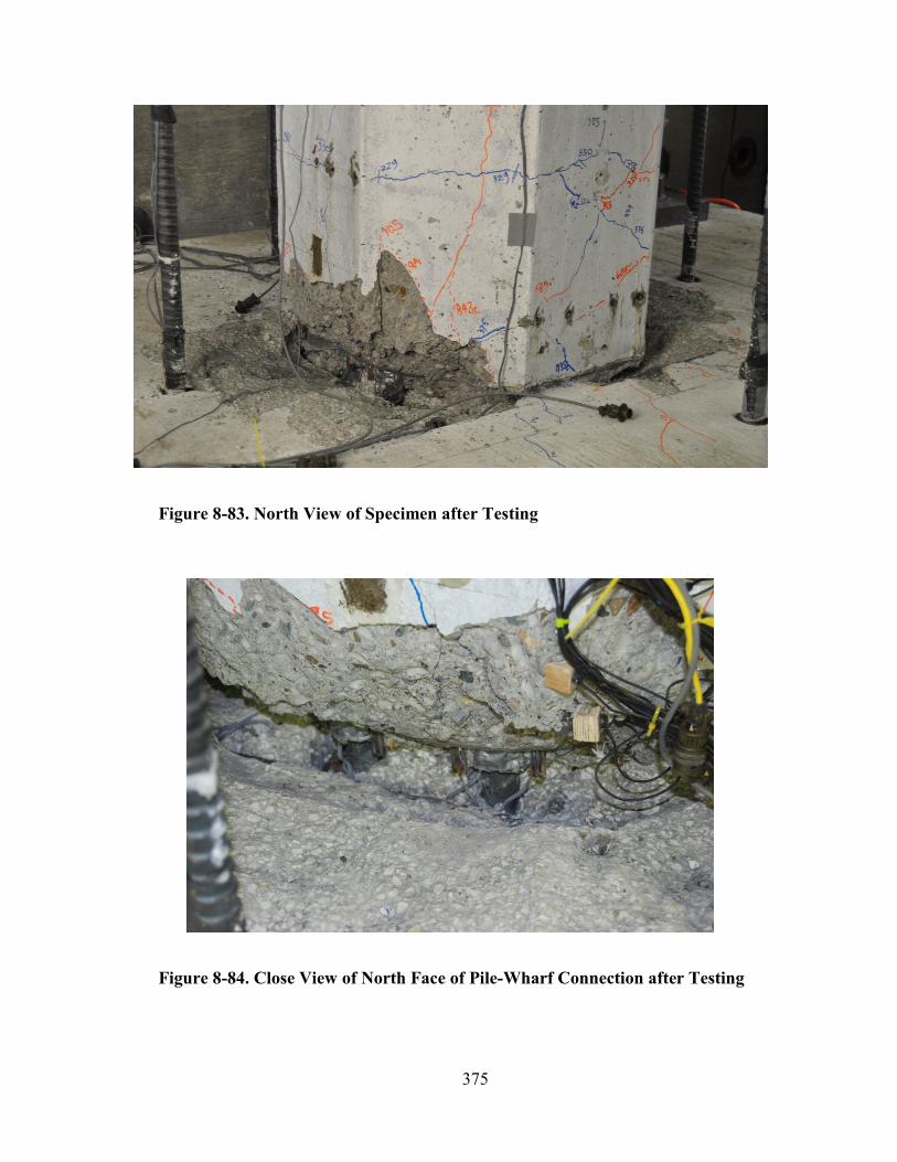
375
Figure 8-83. orth View of Specimen after Testing
Figure 8-84. Close View of orth Face of Pile-Wharf Connection after Testing
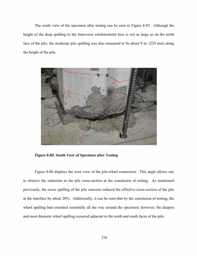
376
The south view of the specimen after testing can be seen in Figure 8-85. Although the
height of the deep spalling to the transverse reinforcement here is not as large as on the north
face of the pile, the moderate pile spalling was also measured to be about 9 in. (229 mm) along
the height of the pile.
Figure 8-85. South View of Specimen after Testing
Figure 8-86 displays the west view of the pile-wharf connection. This angle allows one
to observe the reduction in the pile cross-section at the conclusion of testing. As mentioned
previously, the cover spalling of the pile concrete reduced the effective cross-section of the pile
at the interface by about 20%. Additionally, it can be seen that by the conclusion of testing, the
wharf spalling had extended essentially all the way around the specimen; however, the deepest
and most dramatic wharf spalling occurred adjacent to the north and south faces of the pile.
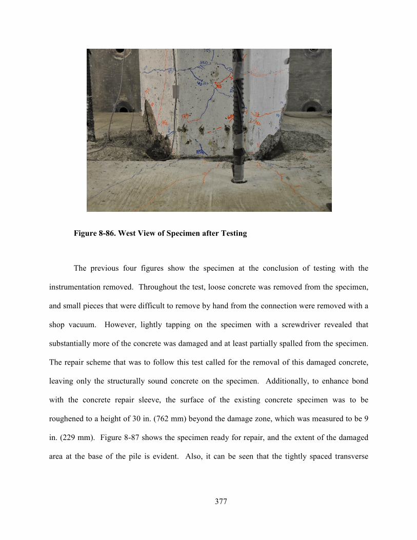
377
Figure 8-86. West View of Specimen after Testing
The previous four figures show the specimen at the conclusion of testing with the
instrumentation removed. Throughout the test, loose concrete was removed from the specimen,
and small pieces that were difficult to remove by hand from the connection were removed with a
shop vacuum. However, lightly tapping on the specimen with a screwdriver revealed that
substantially more of the concrete was damaged and at least partially spalled from the specimen.
The repair scheme that was to follow this test called for the removal of this damaged concrete,
leaving only the structurally sound concrete on the specimen. Additionally, to enhance bond
with the concrete repair sleeve, the surface of the existing concrete specimen was to be
roughened to a height of 30 in. (762 mm) beyond the damage zone, which was measured to be 9
in. (229 mm). Figure 8-87 shows the specimen ready for repair, and the extent of the damaged
area at the base of the pile is evident. Also, it can be seen that the tightly spaced transverse
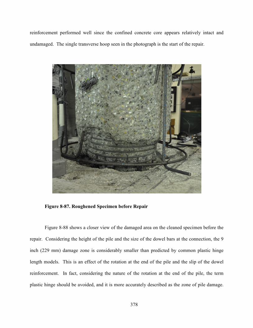
378
reinforcement performed well since the confined concrete core appears relatively intact and
undamaged. The single transverse hoop seen in the photograph is the start of the repair.
Figure 8-87. Roughened Specimen before Repair
Figure 8-88 shows a closer view of the damaged area on the cleaned specimen before the
repair. Considering the height of the pile and the size of the dowel bars at the connection, the 9
inch (229 mm) damage zone is considerably smaller than predicted by common plastic hinge
length models. This is an effect of the rotation at the end of the pile and the slip of the dowel
reinforcement. In fact, considering the nature of the rotation at the end of the pile, the term
plastic hinge should be avoided, and it is more accurately described as the zone of pile damage.
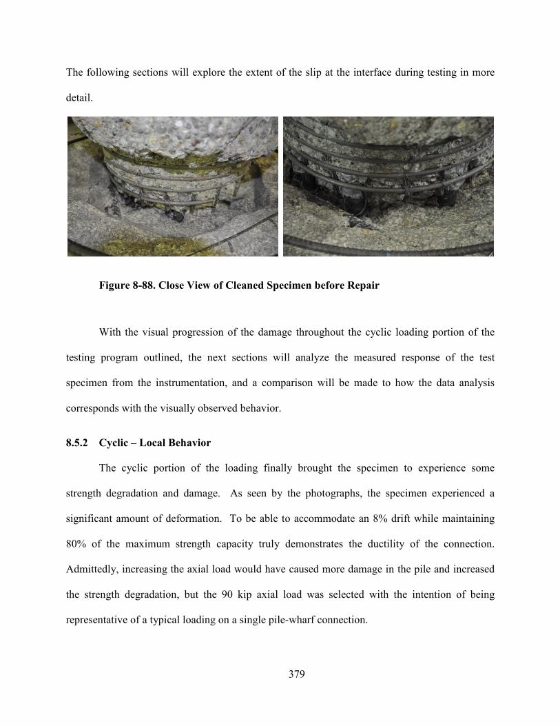
379
The following sections will explore the extent of the slip at the interface during testing in more
detail.
Figure 8-88. Close View of Cleaned Specimen before Repair
With the visual progression of the damage throughout the cyclic loading portion of the
testing program outlined, the next sections will analyze the measured response of the test
specimen from the instrumentation, and a comparison will be made to how the data analysis
corresponds with the visually observed behavior.
8.5.2 Cyclic – Local Behavior
The cyclic portion of the loading finally brought the specimen to experience some
strength degradation and damage. As seen by the photographs, the specimen experienced a
significant amount of deformation. To be able to accommodate an 8% drift while maintaining
80% of the maximum strength capacity truly demonstrates the ductility of the connection.
Admittedly, increasing the axial load would have caused more damage in the pile and increased
the strength degradation, but the 90 kip axial load was selected with the intention of being
representative of a typical loading on a single pile-wharf connection.
380
When reviewing the data from the cyclic loading portion of the test, it was realized that
the Krypton malfunctioned during the 5% drift cycle, so this cycle has been omitted during the
post-processing. Thus, the cycles that will be displayed are, in order: 2%, 3.5%, 3.5%, 2%,
3.5%, 6.5%, and 8%. Due to the nature of the Krypton data acquisition, the data could not be
seen in real time, so it was only through a post-processing effort that the LEDs could be realized
as “invisible” to the camera. Through troubleshooting, it was determined that one of the
extension wires from the Krypton controller to the strober units, into which the LEDs plug, went
bad during the test. The extension cable was replaced, and the testing resumed. A
recommendation was placed to the MUST-SIM site to create a method enabling the visualization
of the LEDs after each converged load step to ensure future tests did not experience a similar
problem. As seen through the data analysis, the Krypton data has proven to be very valuable in
characterizing the behavior of the specimen.
The review of the data from the cyclic loading begins with an assessment of the state of
the strain gauges throughout the cyclic loading. The strain gauges had been previously used
through the processing to provide a measure of the curvature or average rotation experienced by
the pile. Since it was anticipated that the strain gauges would yield considerably and eventually
even fail, a method was developed to use the Krypton readings to quantify the lumped rotation at
the connection. With the lumped rotation computed, the difference between the total rotation
obtained by the Krypton LEDs and the lumped connection rotation would provide the flexural
rotation of the pile at various locations of interest. By comparing this method to the pile flexural
rotation obtained from strain gauges that were properly functioning, it was concluded that it was
viable procedure, and it will be used for the pile curvatures reported in this section. Figure 8-89
shows the total rotation from the Krypton LEDs at the interface and the computed average
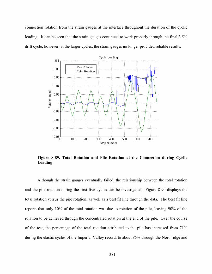
381
connection rotation from the strain gauges at the interface throughout the duration of the cyclic
loading. It can be seen that the strain gauges continued to work properly through the final 3.5%
drift cycle; however, at the larger cycles, the strain gauges no longer provided reliable results.
Figure 8-89. Total Rotation and Pile Rotation at the Connection during Cyclic
Loading
Although the strain gauges eventually failed, the relationship between the total rotation
and the pile rotation during the first five cycles can be investigated. Figure 8-90 displays the
total rotation versus the pile rotation, as well as a best fit line through the data. The best fit line
reports that only 10% of the total rotation was due to rotation of the pile, leaving 90% of the
rotation to be achieved through the concentrated rotation at the end of the pile. Over the course
of the test, the percentage of the total rotation attributed to the pile has increased from 71%
during the elastic cycles of the Imperial Valley record, to about 85% through the Northridge and
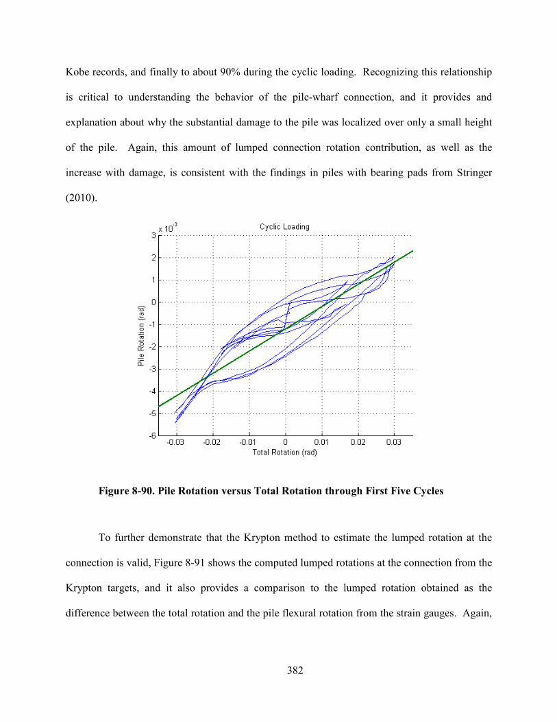
382
Kobe records, and finally to about 90% during the cyclic loading. Recognizing this relationship
is critical to understanding the behavior of the pile-wharf connection, and it provides and
explanation about why the substantial damage to the pile was localized over only a small height
of the pile. Again, this amount of lumped connection rotation contribution, as well as the
increase with damage, is consistent with the findings in piles with bearing pads from Stringer
(2010).
Figure 8-90. Pile Rotation versus Total Rotation through First Five Cycles
To further demonstrate that the Krypton method to estimate the lumped rotation at the
connection is valid, Figure 8-91 shows the computed lumped rotations at the connection from the
Krypton targets, and it also provides a comparison to the lumped rotation obtained as the
difference between the total rotation and the pile flexural rotation from the strain gauges. Again,
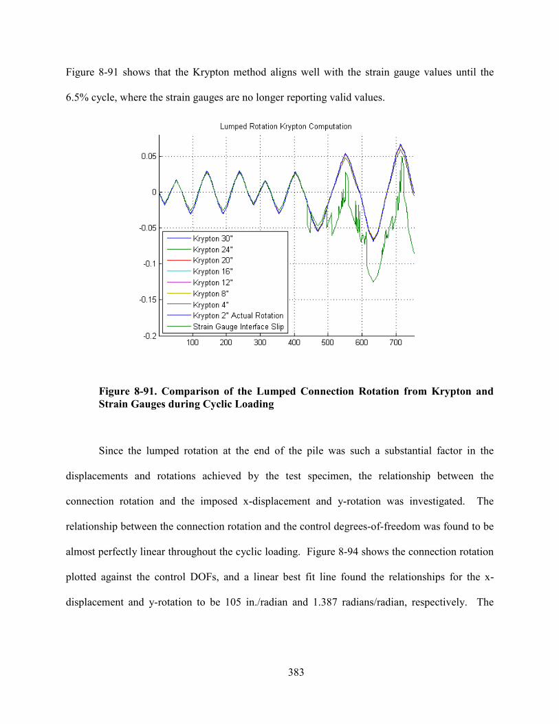
383
Figure 8-91 shows that the Krypton method aligns well with the strain gauge values until the
6.5% cycle, where the strain gauges are no longer reporting valid values.
Figure 8-91. Comparison of the Lumped Connection Rotation from Krypton and
Strain Gauges during Cyclic Loading
Since the lumped rotation at the end of the pile was such a substantial factor in the
displacements and rotations achieved by the test specimen, the relationship between the
connection rotation and the imposed x-displacement and y-rotation was investigated. The
relationship between the connection rotation and the control degrees-of-freedom was found to be
almost perfectly linear throughout the cyclic loading. Figure 8-94 shows the connection rotation
plotted against the control DOFs, and a linear best fit line found the relationships for the x-
displacement and y-rotation to be 105 in./radian and 1.387 radians/radian, respectively. The
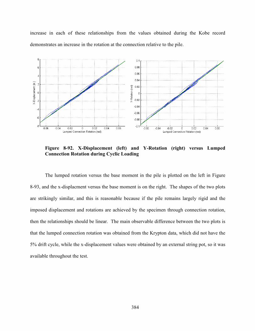
384
increase in each of these relationships from the values obtained during the Kobe record
demonstrates an increase in the rotation at the connection relative to the pile.
Figure 8-92. X-Displacement (left) and Y-Rotation (right) versus Lumped
Connection Rotation during Cyclic Loading
The lumped rotation versus the base moment in the pile is plotted on the left in Figure
8-93, and the x-displacment versus the base moment is on the right. The shapes of the two plots
are strikingly similar, and this is reasonable because if the pile remains largely rigid and the
imposed displacement and rotations are achieved by the specimen through connection rotation,
then the relationships should be linear. The main observable difference between the two plots is
that the lumped connection rotation was obtained from the Krypton data, which did not have the
5% drift cycle, while the x-displacement values were obtained by an external string pot, so it was
available throughout the test.
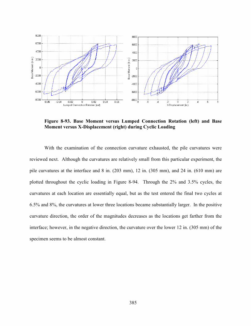
385
Figure 8-93. Base Moment versus Lumped Connection Rotation (left) and Base
Moment versus X-Displacement (right) during Cyclic Loading
With the examination of the connection curvature exhausted, the pile curvatures were
reviewed next. Although the curvatures are relatively small from this particular experiment, the
pile curvatures at the interface and 8 in. (203 mm), 12 in. (305 mm), and 24 in. (610 mm) are
plotted throughout the cyclic loading in Figure 8-94. Through the 2% and 3.5% cycles, the
curvatures at each location are essentially equal, but as the test entered the final two cycles at
6.5% and 8%, the curvatures at lower three locations became substantially larger. In the positive
curvature direction, the order of the magnitudes decreases as the locations get farther from the
interface; however, in the negative direction, the curvature over the lower 12 in. (305 mm) of the
specimen seems to be almost constant.
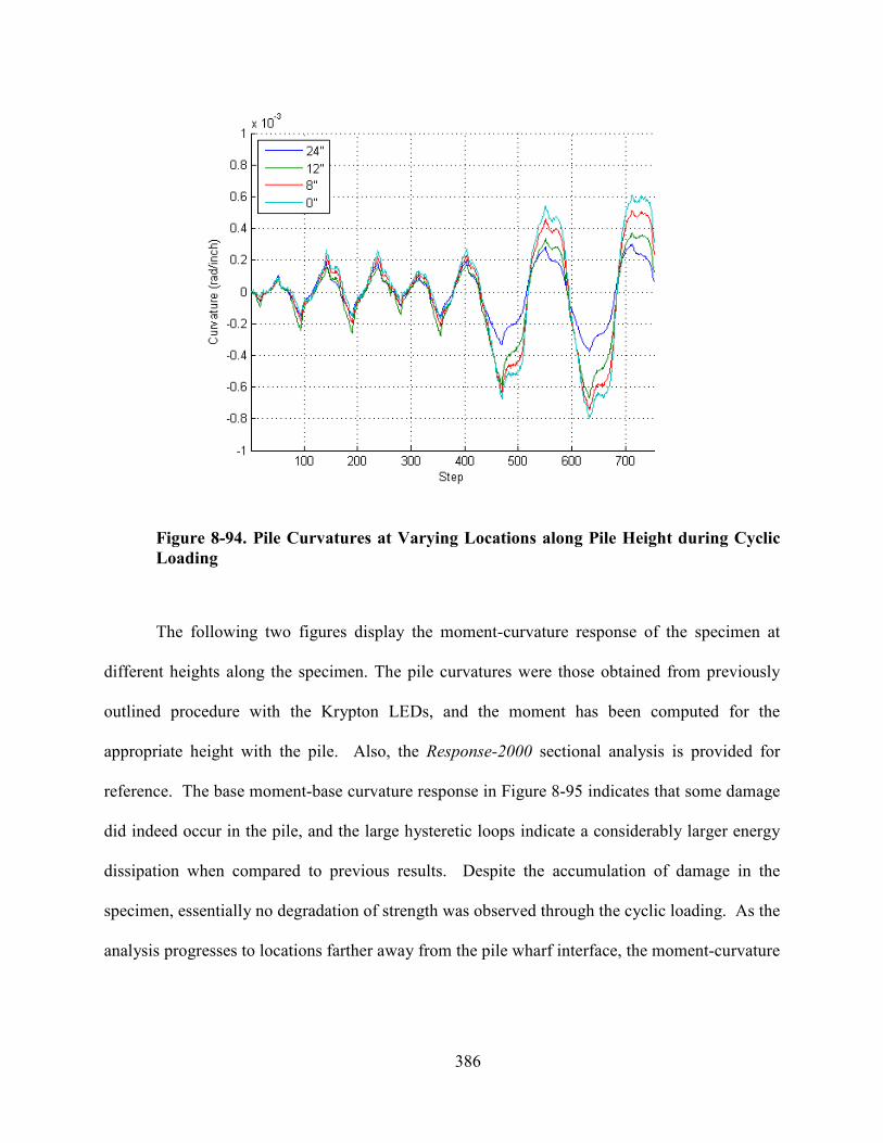
386
Figure 8-94. Pile Curvatures at Varying Locations along Pile Height during Cyclic
Loading
The following two figures display the moment-curvature response of the specimen at
different heights along the specimen. The pile curvatures were those obtained from previously
outlined procedure with the Krypton LEDs, and the moment has been computed for the
appropriate height with the pile. Also, the Response-2000 sectional analysis is provided for
reference. The base moment-base curvature response in Figure 8-95 indicates that some damage
did indeed occur in the pile, and the large hysteretic loops indicate a considerably larger energy
dissipation when compared to previous results. Despite the accumulation of damage in the
specimen, essentially no degradation of strength was observed through the cyclic loading. As the
analysis progresses to locations farther away from the pile wharf interface, the moment-curvature
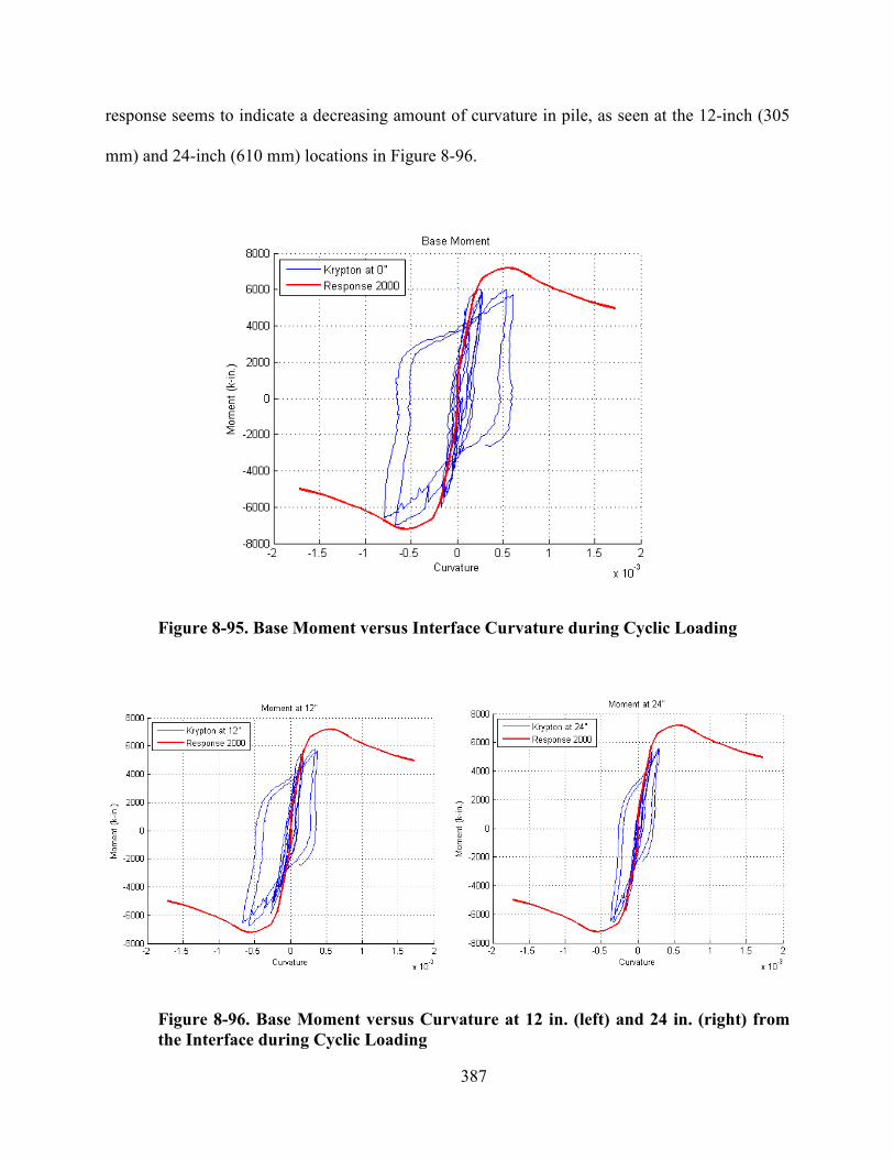
387
response seems to indicate a decreasing amount of curvature in pile, as seen at the 12-inch (305
mm) and 24-inch (610 mm) locations in Figure 8-96.
Figure 8-95. Base Moment versus Interface Curvature during Cyclic Loading
Figure 8-96. Base Moment versus Curvature at 12 in. (left) and 24 in. (right) from
the Interface during Cyclic Loading
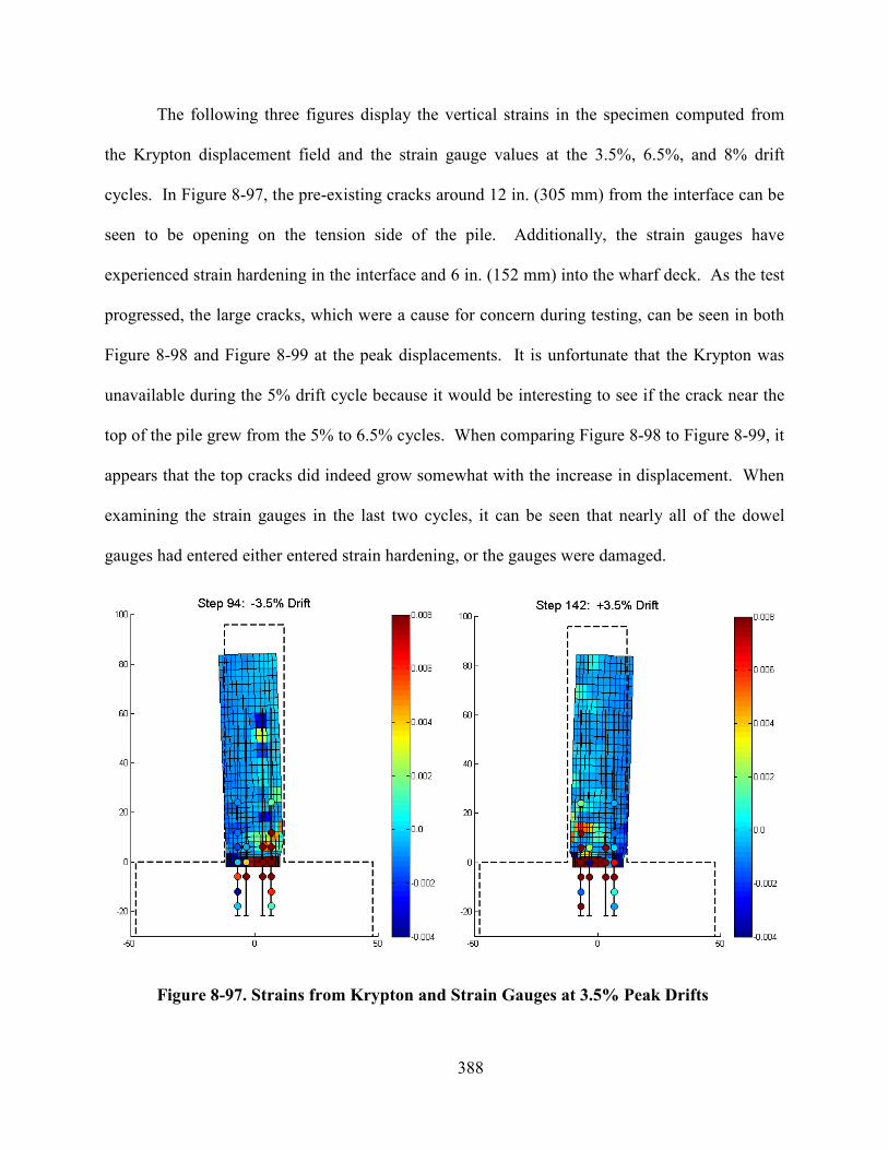
388
The following three figures display the vertical strains in the specimen computed from
the Krypton displacement field and the strain gauge values at the 3.5%, 6.5%, and 8% drift
cycles. In Figure 8-97, the pre-existing cracks around 12 in. (305 mm) from the interface can be
seen to be opening on the tension side of the pile. Additionally, the strain gauges have
experienced strain hardening in the interface and 6 in. (152 mm) into the wharf deck. As the test
progressed, the large cracks, which were a cause for concern during testing, can be seen in both
Figure 8-98 and Figure 8-99 at the peak displacements. It is unfortunate that the Krypton was
unavailable during the 5% drift cycle because it would be interesting to see if the crack near the
top of the pile grew from the 5% to 6.5% cycles. When comparing Figure 8-98 to Figure 8-99, it
appears that the top cracks did indeed grow somewhat with the increase in displacement. When
examining the strain gauges in the last two cycles, it can be seen that nearly all of the dowel
gauges had entered either entered strain hardening, or the gauges were damaged.
Figure 8-97. Strains from Krypton and Strain Gauges at 3.5% Peak Drifts
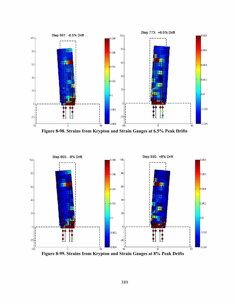
389
Figure 8-98. Strains from Krypton and Strain Gauges at 6.5% Peak Drifts
Figure 8-99. Strains from Krypton and Strain Gauges at 8% Peak Drifts
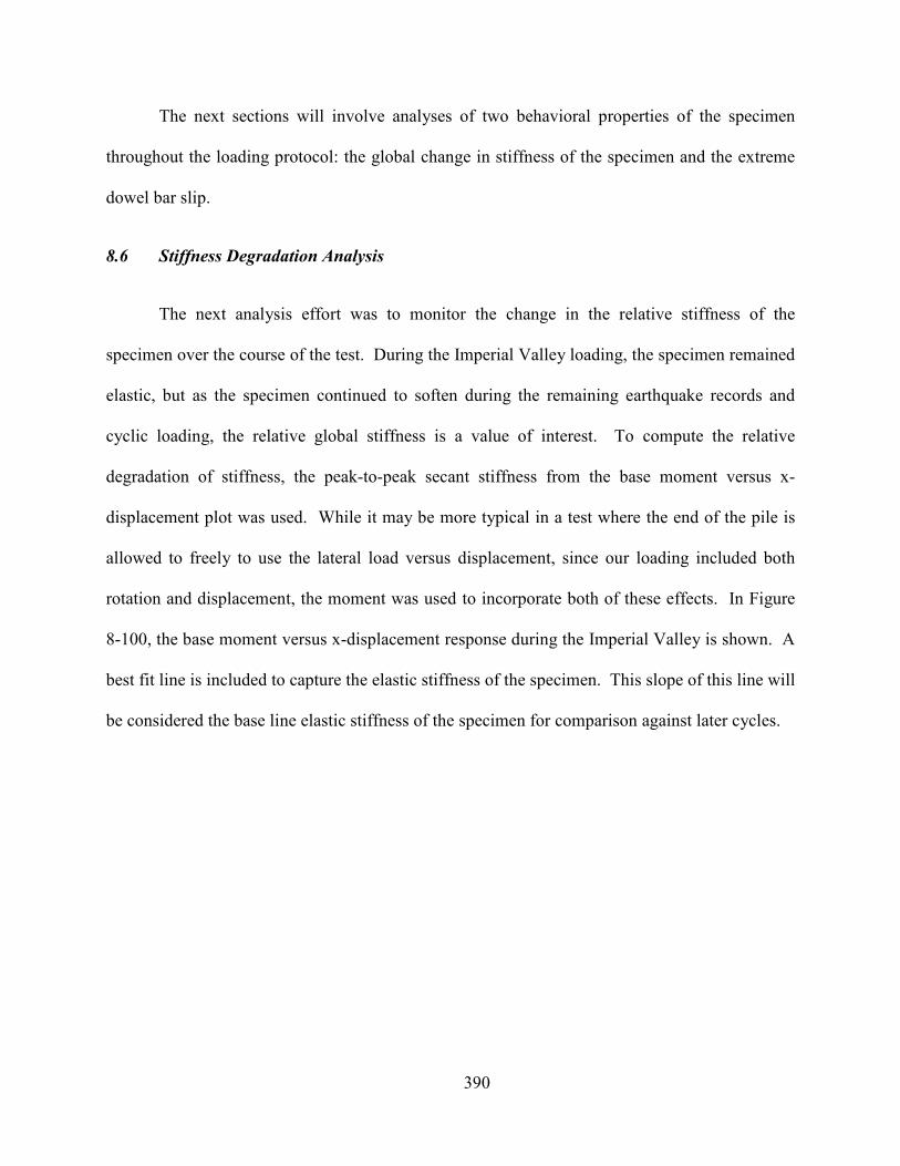
390
The next sections will involve analyses of two behavioral properties of the specimen
throughout the loading protocol: the global change in stiffness of the specimen and the extreme
dowel bar slip.
8.6 Stiffness Degradation Analysis
The next analysis effort was to monitor the change in the relative stiffness of the
specimen over the course of the test. During the Imperial Valley loading, the specimen remained
elastic, but as the specimen continued to soften during the remaining earthquake records and
cyclic loading, the relative global stiffness is a value of interest. To compute the relative
degradation of stiffness, the peak-to-peak secant stiffness from the base moment versus x-
displacement plot was used. While it may be more typical in a test where the end of the pile is
allowed to freely to use the lateral load versus displacement, since our loading included both
rotation and displacement, the moment was used to incorporate both of these effects. In Figure
8-100, the base moment versus x-displacement response during the Imperial Valley is shown. A
best fit line is included to capture the elastic stiffness of the specimen. This slope of this line will
be considered the base line elastic stiffness of the specimen for comparison against later cycles.
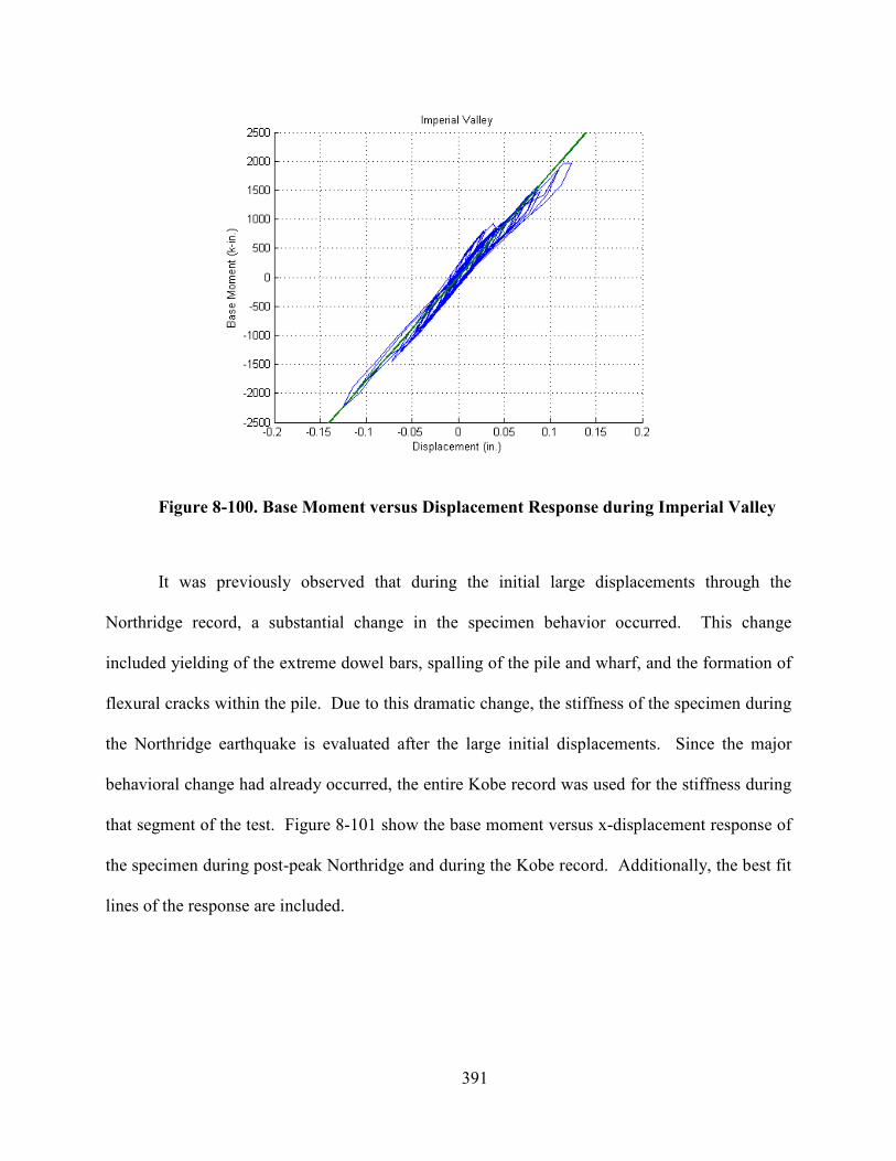
391
Figure 8-100. Base Moment versus Displacement Response during Imperial Valley
It was previously observed that during the initial large displacements through the
Northridge record, a substantial change in the specimen behavior occurred. This change
included yielding of the extreme dowel bars, spalling of the pile and wharf, and the formation of
flexural cracks within the pile. Due to this dramatic change, the stiffness of the specimen during
the Northridge earthquake is evaluated after the large initial displacements. Since the major
behavioral change had already occurred, the entire Kobe record was used for the stiffness during
that segment of the test. Figure 8-101 show the base moment versus x-displacement response of
the specimen during post-peak Northridge and during the Kobe record. Additionally, the best fit
lines of the response are included.
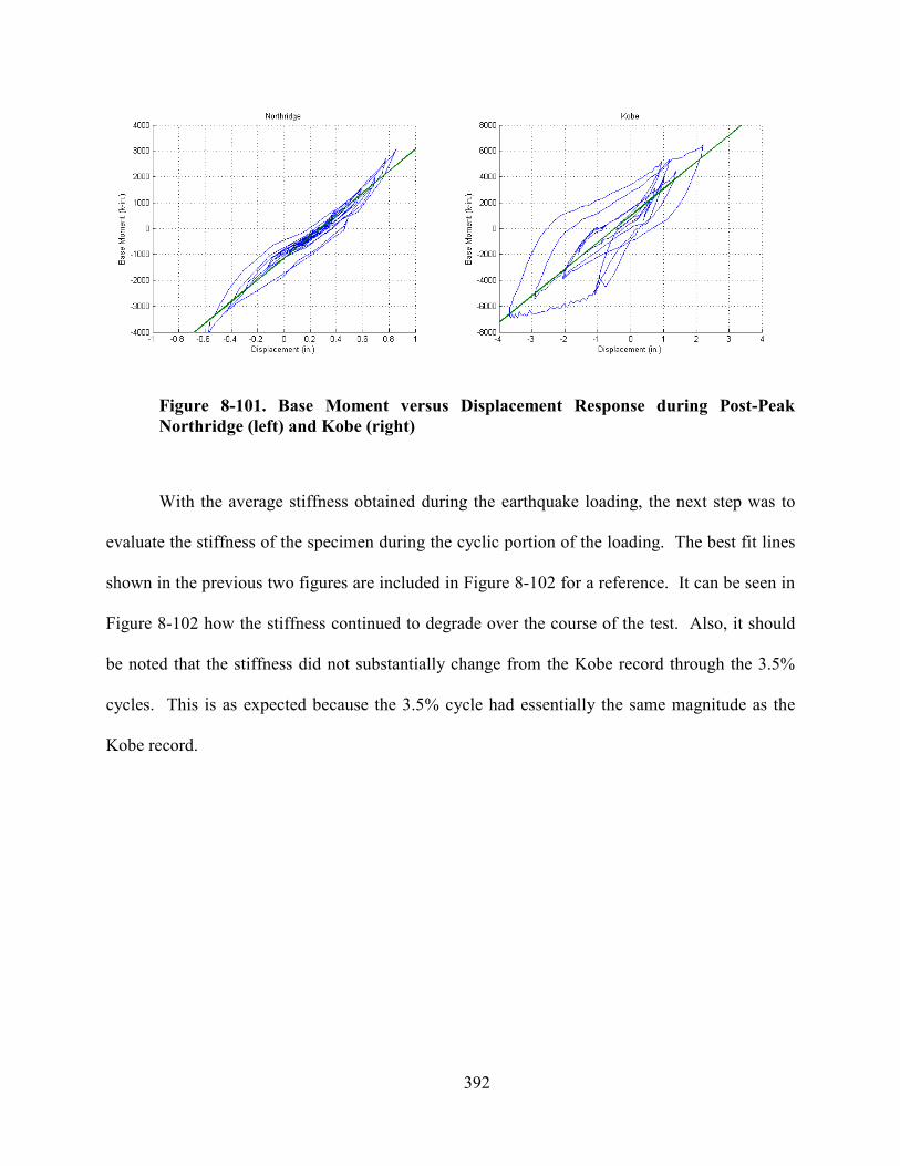
392
Figure 8-101. Base Moment versus Displacement Response during Post-Peak
orthridge (left) and Kobe (right)
With the average stiffness obtained during the earthquake loading, the next step was to
evaluate the stiffness of the specimen during the cyclic portion of the loading. The best fit lines
shown in the previous two figures are included in Figure 8-102 for a reference. It can be seen in
Figure 8-102 how the stiffness continued to degrade over the course of the test. Also, it should
be noted that the stiffness did not substantially change from the Kobe record through the 3.5%
cycles. This is as expected because the 3.5% cycle had essentially the same magnitude as the
Kobe record.
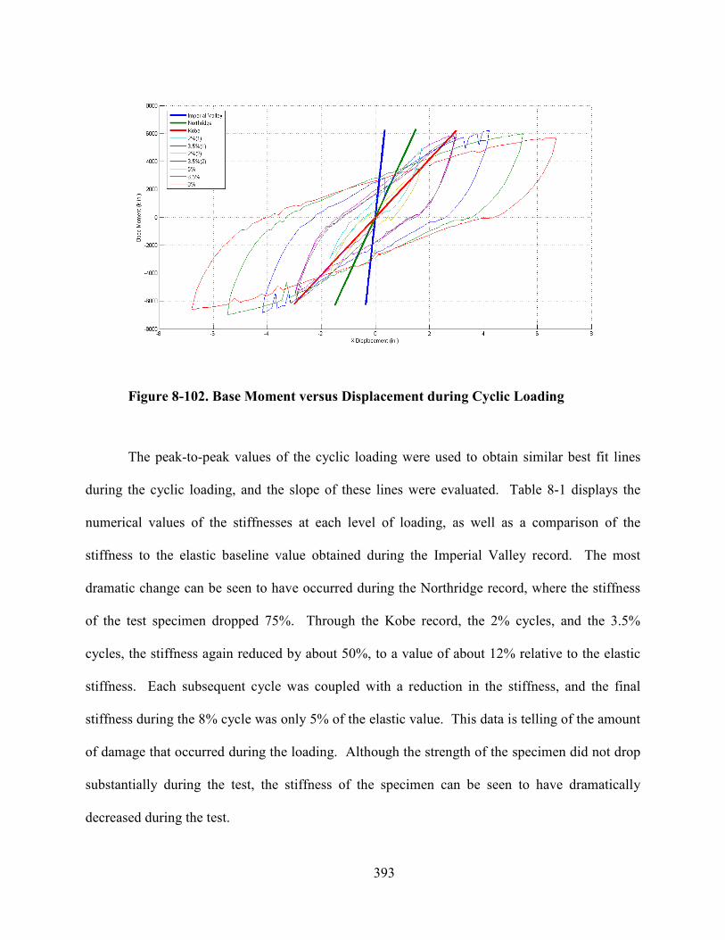
393
Figure 8-102. Base Moment versus Displacement during Cyclic Loading
The peak-to-peak values of the cyclic loading were used to obtain similar best fit lines
during the cyclic loading, and the slope of these lines were evaluated. Table 8-1 displays the
numerical values of the stiffnesses at each level of loading, as well as a comparison of the
stiffness to the elastic baseline value obtained during the Imperial Valley record. The most
dramatic change can be seen to have occurred during the Northridge record, where the stiffness
of the test specimen dropped 75%. Through the Kobe record, the 2% cycles, and the 3.5%
cycles, the stiffness again reduced by about 50%, to a value of about 12% relative to the elastic
stiffness. Each subsequent cycle was coupled with a reduction in the stiffness, and the final
stiffness during the 8% cycle was only 5% of the elastic value. This data is telling of the amount
of damage that occurred during the loading. Although the strength of the specimen did not drop
substantially during the test, the stiffness of the specimen can be seen to have dramatically
decreased during the test.
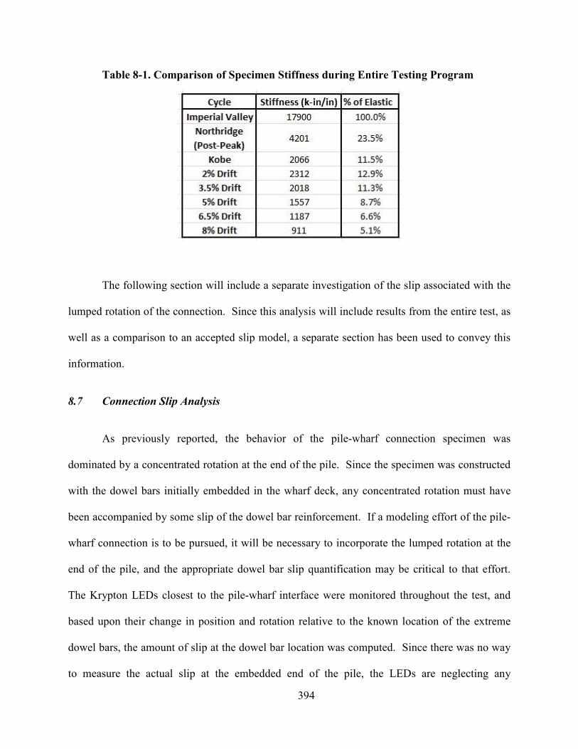
394
Table 8-1. Comparison of Specimen Stiffness during Entire Testing Program
The following section will include a separate investigation of the slip associated with the
lumped rotation of the connection. Since this analysis will include results from the entire test, as
well as a comparison to an accepted slip model, a separate section has been used to convey this
information.
8.7 Connection Slip Analysis
As previously reported, the behavior of the pile-wharf connection specimen was
dominated by a concentrated rotation at the end of the pile. Since the specimen was constructed
with the dowel bars initially embedded in the wharf deck, any concentrated rotation must have
been accompanied by some slip of the dowel bar reinforcement. If a modeling effort of the pile-
wharf connection is to be pursued, it will be necessary to incorporate the lumped rotation at the
end of the pile, and the appropriate dowel bar slip quantification may be critical to that effort.
The Krypton LEDs closest to the pile-wharf interface were monitored throughout the test, and
based upon their change in position and rotation relative to the known location of the extreme
dowel bars, the amount of slip at the dowel bar location was computed. Since there was no way
to measure the actual slip at the embedded end of the pile, the LEDs are neglecting any
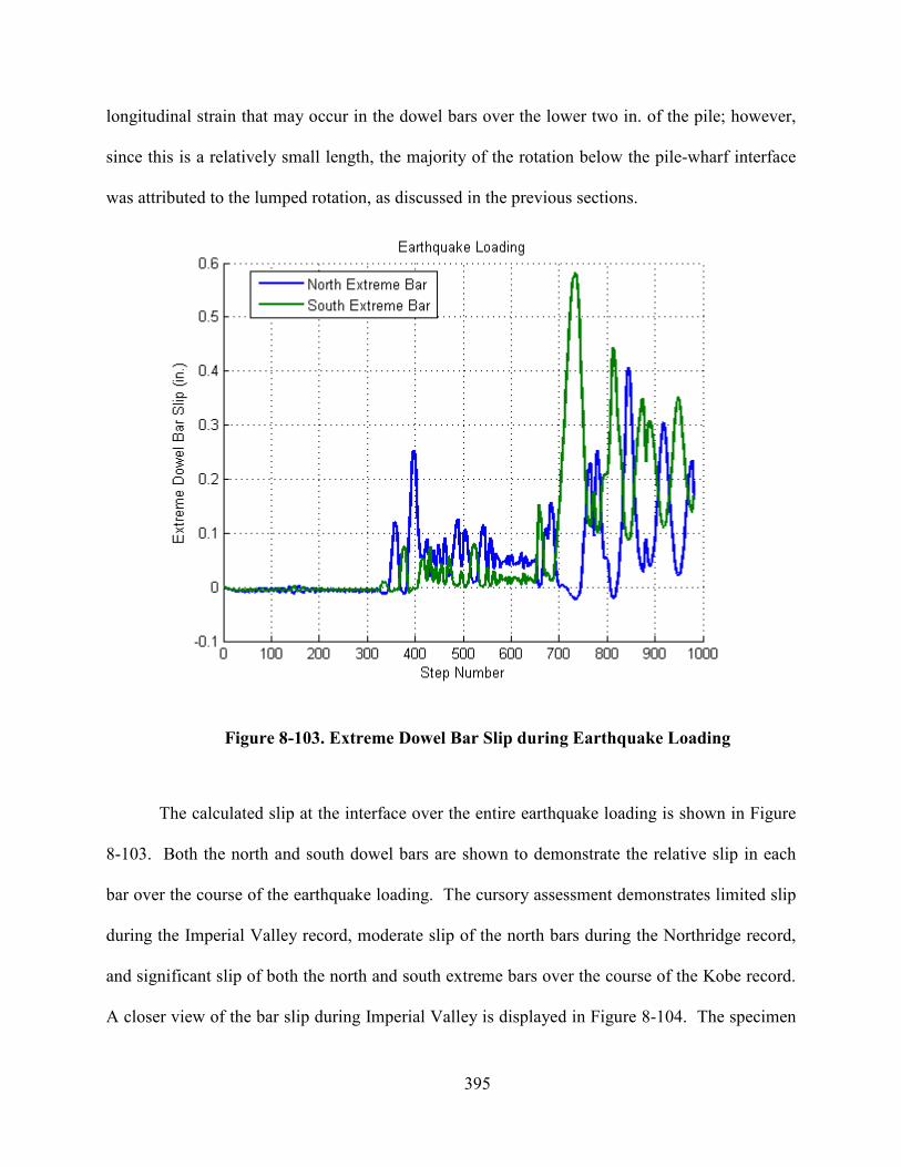
395
longitudinal strain that may occur in the dowel bars over the lower two in. of the pile; however,
since this is a relatively small length, the majority of the rotation below the pile-wharf interface
was attributed to the lumped rotation, as discussed in the previous sections.
Figure 8-103. Extreme Dowel Bar Slip during Earthquake Loading
The calculated slip at the interface over the entire earthquake loading is shown in Figure
8-103. Both the north and south dowel bars are shown to demonstrate the relative slip in each
bar over the course of the earthquake loading. The cursory assessment demonstrates limited slip
during the Imperial Valley record, moderate slip of the north bars during the Northridge record,
and significant slip of both the north and south extreme bars over the course of the Kobe record.
A closer view of the bar slip during Imperial Valley is displayed in Figure 8-104. The specimen
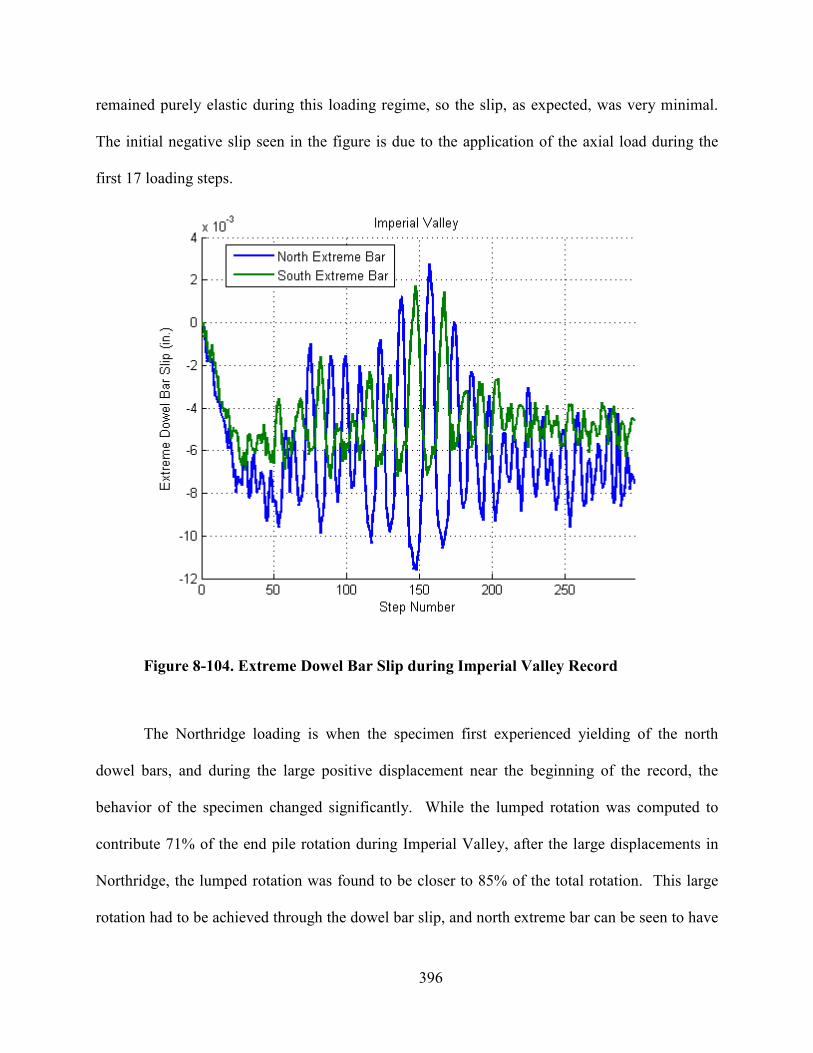
396
remained purely elastic during this loading regime, so the slip, as expected, was very minimal.
The initial negative slip seen in the figure is due to the application of the axial load during the
first 17 loading steps.
Figure 8-104. Extreme Dowel Bar Slip during Imperial Valley Record
The Northridge loading is when the specimen first experienced yielding of the north
dowel bars, and during the large positive displacement near the beginning of the record, the
behavior of the specimen changed significantly. While the lumped rotation was computed to
contribute 71% of the end pile rotation during Imperial Valley, after the large displacements in
Northridge, the lumped rotation was found to be closer to 85% of the total rotation. This large
rotation had to be achieved through the dowel bar slip, and north extreme bar can be seen to have
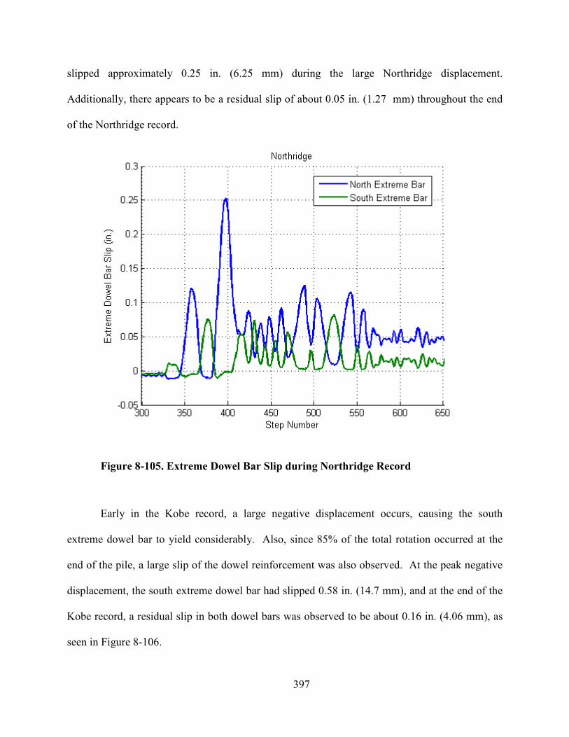
397
slipped approximately 0.25 in. (6.25 mm) during the large Northridge displacement.
Additionally, there appears to be a residual slip of about 0.05 in. (1.27 mm) throughout the end
of the Northridge record.
Figure 8-105. Extreme Dowel Bar Slip during orthridge Record
Early in the Kobe record, a large negative displacement occurs, causing the south
extreme dowel bar to yield considerably. Also, since 85% of the total rotation occurred at the
end of the pile, a large slip of the dowel reinforcement was also observed. At the peak negative
displacement, the south extreme dowel bar had slipped 0.58 in. (14.7 mm), and at the end of the
Kobe record, a residual slip in both dowel bars was observed to be about 0.16 in. (4.06 mm), as
seen in Figure 8-106.
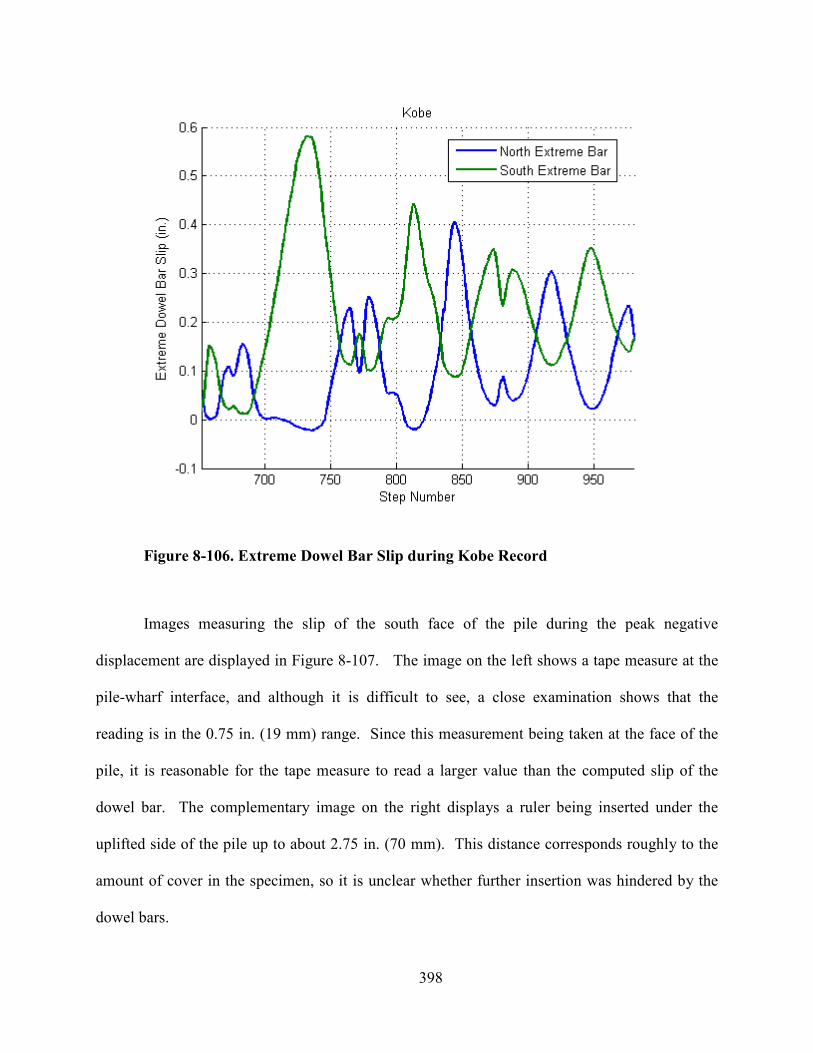
398
Figure 8-106. Extreme Dowel Bar Slip during Kobe Record
Images measuring the slip of the south face of the pile during the peak negative
displacement are displayed in Figure 8-107. The image on the left shows a tape measure at the
pile-wharf interface, and although it is difficult to see, a close examination shows that the
reading is in the 0.75 in. (19 mm) range. Since this measurement being taken at the face of the
pile, it is reasonable for the tape measure to read a larger value than the computed slip of the
dowel bar. The complementary image on the right displays a ruler being inserted under the
uplifted side of the pile up to about 2.75 in. (70 mm). This distance corresponds roughly to the
amount of cover in the specimen, so it is unclear whether further insertion was hindered by the
dowel bars.
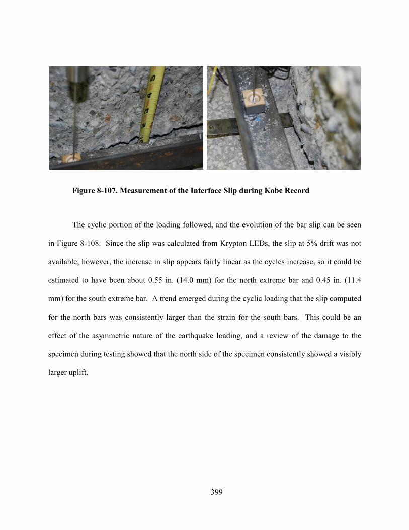
399
Figure 8-107. Measurement of the Interface Slip during Kobe Record
The cyclic portion of the loading followed, and the evolution of the bar slip can be seen
in Figure 8-108. Since the slip was calculated from Krypton LEDs, the slip at 5% drift was not
available; however, the increase in slip appears fairly linear as the cycles increase, so it could be
estimated to have been about 0.55 in. (14.0 mm) for the north extreme bar and 0.45 in. (11.4
mm) for the south extreme bar. A trend emerged during the cyclic loading that the slip computed
for the north bars was consistently larger than the strain for the south bars. This could be an
effect of the asymmetric nature of the earthquake loading, and a review of the damage to the
specimen during testing showed that the north side of the specimen consistently showed a visibly
larger uplift.
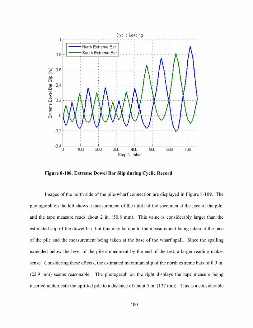
400
Figure 8-108. Extreme Dowel Bar Slip during Cyclic Record
Images of the north side of the pile-wharf connection are displayed in Figure 8-109. The
photograph on the left shows a measurement of the uplift of the specimen at the face of the pile,
and the tape measure reads about 2 in. (50.8 mm). This value is considerably larger than the
estimated slip of the dowel bar, but this may be due to the measurement being taken at the face
of the pile and the measurement being taken at the base of the wharf spall. Since the spalling
extended below the level of the pile embedment by the end of the test, a larger reading makes
sense. Considering these effects, the estimated maximum slip of the north extreme bars of 0.9 in.
(22.9 mm) seems reasonable. The photograph on the right displays the tape measure being
inserted underneath the uplifted pile to a distance of about 5 in. (127 mm). This is a considerable
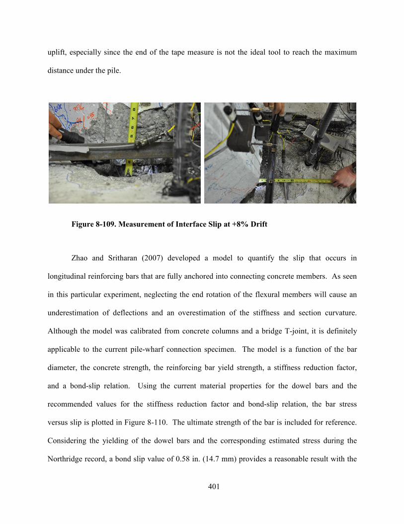
401
uplift, especially since the end of the tape measure is not the ideal tool to reach the maximum
distance under the pile.
Figure 8-109. Measurement of Interface Slip at +8% Drift
Zhao and Sritharan (2007) developed a model to quantify the slip that occurs in
longitudinal reinforcing bars that are fully anchored into connecting concrete members. As seen
in this particular experiment, neglecting the end rotation of the flexural members will cause an
underestimation of deflections and an overestimation of the stiffness and section curvature.
Although the model was calibrated from concrete columns and a bridge T-joint, it is definitely
applicable to the current pile-wharf connection specimen. The model is a function of the bar
diameter, the concrete strength, the reinforcing bar yield strength, a stiffness reduction factor,
and a bond-slip relation. Using the current material properties for the dowel bars and the
recommended values for the stiffness reduction factor and bond-slip relation, the bar stress
versus slip is plotted in Figure 8-110. The ultimate strength of the bar is included for reference.
Considering the yielding of the dowel bars and the corresponding estimated stress during the
Northridge record, a bond slip value of 0.58 in. (14.7 mm) provides a reasonable result with the
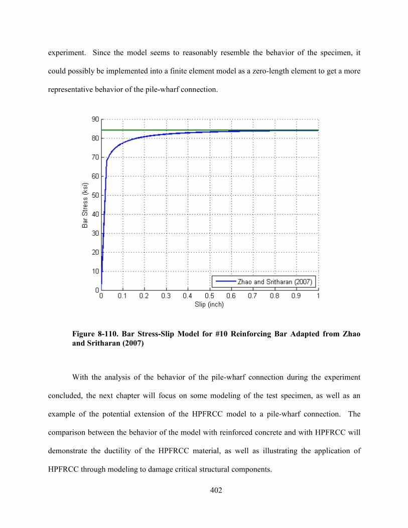
402
experiment. Since the model seems to reasonably resemble the behavior of the specimen, it
could possibly be implemented into a finite element model as a zero-length element to get a more
representative behavior of the pile-wharf connection.
Figure 8-110. Bar Stress-Slip Model for #10 Reinforcing Bar Adapted from Zhao
and Sritharan (2007)
With the analysis of the behavior of the pile-wharf connection during the experiment
concluded, the next chapter will focus on some modeling of the test specimen, as well as an
example of the potential extension of the HPFRCC model to a pile-wharf connection. The
comparison between the behavior of the model with reinforced concrete and with HPFRCC will
demonstrate the ductility of the HPFRCC material, as well as illustrating the application of
HPFRCC through modeling to damage critical structural components.
403
CHAPTER 9. PILE-WHARF COECTIO MODELIG
With the ATENA model having proven its ability to reasonably emulate the laboratory
response of HPFRCC at the material level and the structural component level, the extension of
HPFRCC to other damage-critical structural components is the final phase of the current
research. The purpose of this chapter is twofold: to further demonstrate the extension of
HPFRCC to the modeling of structural components and to bridge the two major experimental
thrusts of this research.
9.1 Pile-Wharf Connection Modeling Parameters
The major objective of the pile-wharf connection research was to explore the structural
connection behavior by constructing, testing, analyzing, repairing, and re-testing a full-scale pile-
wharf connection specimen in an experimental set-up having realistic structural boundary
conditions. The test specimen consisted of a 24-inch diameter, octagonal, precast, prestressed
pile connected to a cast-in-place reinforced concrete wharf deck slab. The connection was made
by embedding the pile two in. into the deck and then grouting T-headed bars into ducts within
the pile; wharf reinforcement was placed around the connection, with the T-heads developed into
the wharf. The details of this test and the experimental results were described previously in
Chapter 7 and Chapter 8. It was observed that after a seismic event, the damage in port
structures was often concentrated at the pile-wharf connection, and given that HPFRCC has
exhibited a superior ability to withstand damage and to prevent diagonal bars in coupling beams
from buckling, it was thought to be interesting to see how the implementation of the HPFRCC
model into the pile-wharf connection region would affect the performance of the specimen.
Since experimental data is available from the completed laboratory test, a comparison of the
404
response of typically constructed pile-wharf connections with those utilizing HPFRCC may be a
very viable way to extend the use of HPFRCC to other damage critical structural elements.
While implementing HPFRCC into the end of precast piles may pose some constructability
issues that would need to be practically resolved, the parametric study could provide insight into
the damage tolerance and performance improvement that HPFRCC could afford to such a
structure.
9.1.1 Constitutive Models
The first step in developing the finite element model was to determine the appropriate
material models to be used in the modeling effort. The precast, prestressed pile represents a
significant departure from the concrete elements previously modeled in this study. Compressive
concrete behavior of the concrete core is highly confined by the transverse reinforcement, so a
modification of the concrete model is necessary. Previous research by Mander et al. (1988)
provides a reinforced concrete model for confined concrete. The model uses the Popovics curve
to represent the stress-strain relationship of both confined and unconfined concrete, and it has
been verified to provide accurate results in nonlinear analysis. Stringer (2010) provided general
guidelines for the modeling of pile-wharf connections and generated two stress-strain curves for
the confined pile concrete using models by Leslie (1974) and Mander et al. (1988), as shown in
Figure 9-1. It can be seen that each model provides similar results, and in this study, the Mander
model was used for the pile concrete.
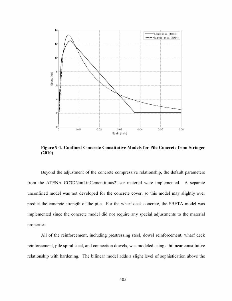
Figure 9-1. Confined Concrete
(2010)
Beyond the adjustment of the concrete compressive relationship, the default parameters
from the ATENA CC3DNonLinCementitious2User
unconfined model was not developed for the concrete cover, so this model may slightly over
predict the concrete strength of the pile.
implemented since the concrete model did not require any spec
properties.
All of the reinforcement, including prestressing steel, dowel reinforcement, wharf deck
reinforcement, pile spiral steel, and connection dowels
relationship with hardening. The bilinear model adds a slight level of sophistication above the
405
. Confined Concrete Constitutive Models for Pile Concrete from Stringer
Beyond the adjustment of the concrete compressive relationship, the default parameters
ATENA CC3DNonLinCementitious2User material were implemented.
unconfined model was not developed for the concrete cover, so this model may slightly over
predict the concrete strength of the pile. For the wharf deck concrete, the SBETA model was
implemented since the concrete model did not require any special adjustments to the material
All of the reinforcement, including prestressing steel, dowel reinforcement, wharf deck
, and connection dowels, was modeled using a bilinear constitutive
ning. The bilinear model adds a slight level of sophistication above the
Constitutive Models for Pile Concrete from Stringer
Beyond the adjustment of the concrete compressive relationship, the default parameters
were implemented. A separate
unconfined model was not developed for the concrete cover, so this model may slightly over
For the wharf deck concrete, the SBETA model was
ial adjustments to the material
All of the reinforcement, including prestressing steel, dowel reinforcement, wharf deck
, was modeled using a bilinear constitutive
ning. The bilinear model adds a slight level of sophistication above the
406
elastic-perfectly plastic model, and since the material properties were known for all of the
reinforcement, the bilinear model was easily implemented.
For the reinforcement, the default bond-slip model was implemented within ATENA.
The default model is the CEB-FIB model code 1990, and it defines the bond strength depending
on the value of the slip between the reinforcement and the surrounding concrete. In the CEB-
FIB model, the user selects whether the bar is ribbed and the confinement conditions. Since all
of the reinforcement was in a relatively well confined region, the bond condition was selected as
“good.” For the prestressing steel, “cold-drawn wire” was selected for the type of reinforcement,
while the dowels were selected as “ribbed” reinforcement. These parameters affect the values of
the bond slip relationship (Cervenka, Jendele, & Cervenka, 2010). Since the prestressing should
have almost no effect at the end of the pile, and the stress in the strand develops over a transfer
length, the slip model for the prestressing steel was important to simulate the lab conditions. A
slip model was not required for the wharf deck reinforcement or the pile spiral reinforcement
because they were modeled as smeared reinforcement. The dowel bars used to connect the
specimen to the LBCB were included in the model to prevent a weakness at the top of the pile.
These bars were modeled to remain elastic, and a perfect bond model was used. The following
section will outline the finite element modeling parameters implemented in the model.
9.1.2 Loading and Boundary Conditions
The geometry of the model was identical to the experimental specimen in an effort to
most closely model the experimental test. In the laboratory, the specimen was connected to the
floor through four post-tensioned threaded rods through the wharf deck. The wharf deck was
designed to be large enough that the post-tensioning stress in the wharf deck would not affect the
behavior of the pile-wharf connection. Thus, it was reasonable to apply the supports in the
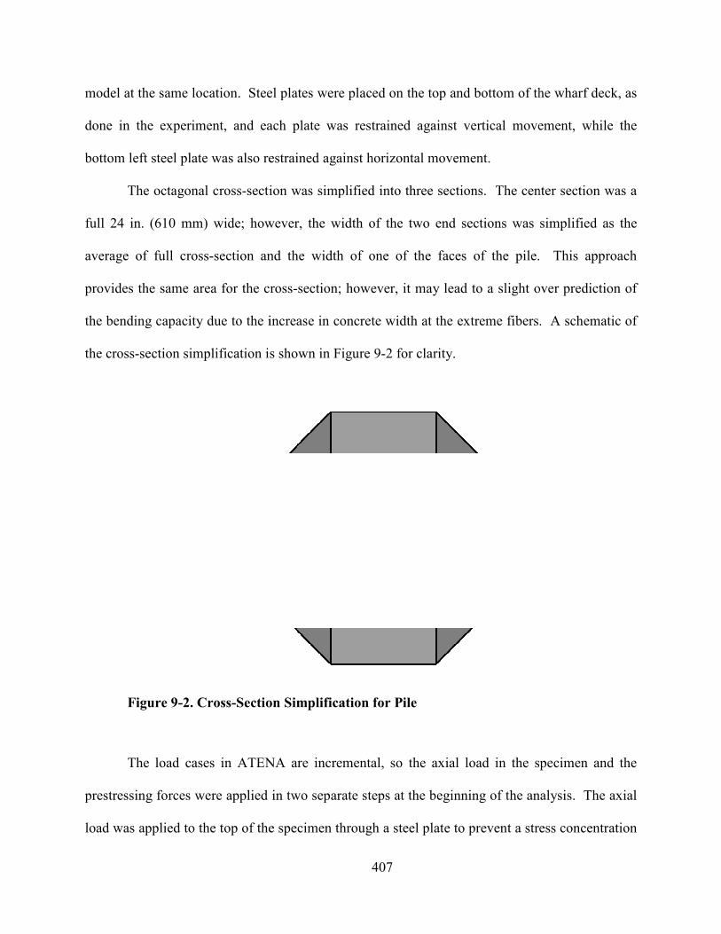
model at the same location. Steel plates were placed on the top and bottom of the wharf deck, as
done in the experiment, and each plate was
bottom left steel plate was also restrained against horizontal movement.
The octagonal cross-section was simplified into three sections.
full 24 in. (610 mm) wide; however, the wi
average of full cross-section and the width of one of the faces of the pile. This approach
provides the same area for the cross
the bending capacity due to the increase in concrete width at the extreme fibers. A schematic of
the cross-section simplification is shown in
Figure 9-2. Cross-Section S
The load cases in ATENA are incremental, so the axial load in the specimen and the
prestressing forces were applied in two separate steps at the beginning of the analysis.
load was applied to the top of the specimen throu
407
model at the same location. Steel plates were placed on the top and bottom of the wharf deck, as
done in the experiment, and each plate was restrained against vertical movement, while the
bottom left steel plate was also restrained against horizontal movement.
section was simplified into three sections. The center section was a
610 mm) wide; however, the width of the two end sections was simplified as the
section and the width of one of the faces of the pile. This approach
provides the same area for the cross-section; however, it may lead to a slight over prediction of
city due to the increase in concrete width at the extreme fibers. A schematic of
section simplification is shown in Figure 9-2 for clarity.
Section Simplification for Pile
The load cases in ATENA are incremental, so the axial load in the specimen and the
prestressing forces were applied in two separate steps at the beginning of the analysis.
load was applied to the top of the specimen through a steel plate to prevent a stress concentration
model at the same location. Steel plates were placed on the top and bottom of the wharf deck, as
restrained against vertical movement, while the
enter section was a
dth of the two end sections was simplified as the
section and the width of one of the faces of the pile. This approach
section; however, it may lead to a slight over prediction of
city due to the increase in concrete width at the extreme fibers. A schematic of
The load cases in ATENA are incremental, so the axial load in the specimen and the
prestressing forces were applied in two separate steps at the beginning of the analysis. The axial
gh a steel plate to prevent a stress concentration
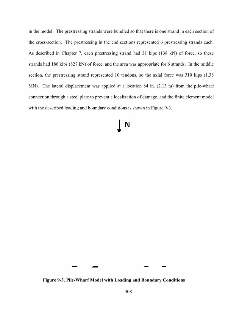
in the model. The prestressing strands
the cross-section. The prestressing in the end sections represented 6 prestressing strands each.
As described in Chapter 7, each prestressing strand had 31 kips (138 kN) of force, so these
strands had 186 kips (827 kN) of force, and the area was appropriate for 6 strands. In the middle
section, the prestressing strand represented 10 tendons, so the axial f
MN). The lateral displacement was applied at a location 84 in. (2.13 m) from the pile
connection through a steel plate to prevent a localization of damage, and the finite element model
with the described loading and boundary
Figure 9-3. Pile-Wharf Model with Loading and Boundary Conditions
408
in the model. The prestressing strands were bundled so that there is one strand in each section of
section. The prestressing in the end sections represented 6 prestressing strands each.
cribed in Chapter 7, each prestressing strand had 31 kips (138 kN) of force, so these
strands had 186 kips (827 kN) of force, and the area was appropriate for 6 strands. In the middle
section, the prestressing strand represented 10 tendons, so the axial force was 310 kips (1.38
MN). The lateral displacement was applied at a location 84 in. (2.13 m) from the pile
connection through a steel plate to prevent a localization of damage, and the finite element model
with the described loading and boundary conditions is shown in Figure 9-3.
Wharf Model with Loading and Boundary Conditions
were bundled so that there is one strand in each section of
section. The prestressing in the end sections represented 6 prestressing strands each.
cribed in Chapter 7, each prestressing strand had 31 kips (138 kN) of force, so these
strands had 186 kips (827 kN) of force, and the area was appropriate for 6 strands. In the middle
orce was 310 kips (1.38
MN). The lateral displacement was applied at a location 84 in. (2.13 m) from the pile-wharf
connection through a steel plate to prevent a localization of damage, and the finite element model
Wharf Model with Loading and Boundary Conditions
409
The models were run with a monotonic loading; although, the experimental tests were
performed cyclically. Also, a rotation was not applied to the top of the specimen as done in the
laboratory tests. This approach was taken because the goal of this modeling effort was not to
exactly reproduce the experiment, but rather to explore the modeling of the pile-wharf
connection without and with HPFRCC. A general effort was made to mimic that experimental
specimen, but again perfect duplication was not the focus of this study. A comprehensive
modeling effort to capture all of the nuances and complexities of the pile-wharf connection is
currently being reviewed by colleagues at the University of Illinois (Caiza et al., 2010).
9.1.3 Finite Element Modeling Parameters
The finite element model mesh was varied to better capture areas of interest. In the
connection region, a 1 in. (25 mm) mesh was implemented. Since the area experienced the
greatest amount of deformation, a finer mesh was required to better capture the response. The
two regions adjacent to the pile-wharf interface region had a 2 in. (50.8 mm) mesh. These
regions included one in the wharf deck and one in the lower portion of the pile. These two areas
were expected to have some damage, so a slightly finer mesh was implemented. The final three
regions had a 4 in. (102 mm) mesh. These areas were expected to remain relatively undamaged,
so a closely spaced mesh was unnecessary. Figure 9-4 depicts the finite element mesh for the
model, as well as boxes to illustrate the different meshing regions previously described.
Figure 9-4. Finite Element Model Mesh Regions
To be able to truly capture the response of the pile
the connection to rotate. In a discrete finite element
could be implemented in the connection to accommodate this rotation. Since ATENA is a
continuum finite element program, interface elements were used at the pile
an effort to capture the behavior
between the pile and the wharf deck.
separating from the wharf deck at the cold joint, so the tensile strength of the interface elements
was set to zero. This parameter should allow the pile to freely rotate from the wharf deck. For
the shear parameter of the interface element, the coefficient of friction was set as 0.2, and the
410
. Finite Element Model Mesh Regions
To be able to truly capture the response of the pile-wharf connection, it is critical to allow
the connection to rotate. In a discrete finite element package, a zero-length rotational spring
could be implemented in the connection to accommodate this rotation. Since ATENA is a
continuum finite element program, interface elements were used at the pile-wharf connection in
an effort to capture the behavior. The interface model was intended to simulate the contact
between the pile and the wharf deck. In the experiment, the pile was observed lifting and
separating from the wharf deck at the cold joint, so the tensile strength of the interface elements
et to zero. This parameter should allow the pile to freely rotate from the wharf deck. For
the shear parameter of the interface element, the coefficient of friction was set as 0.2, and the
wharf connection, it is critical to allow
length rotational spring
could be implemented in the connection to accommodate this rotation. Since ATENA is a
wharf connection in
. The interface model was intended to simulate the contact
In the experiment, the pile was observed lifting and
separating from the wharf deck at the cold joint, so the tensile strength of the interface elements
et to zero. This parameter should allow the pile to freely rotate from the wharf deck. For
the shear parameter of the interface element, the coefficient of friction was set as 0.2, and the
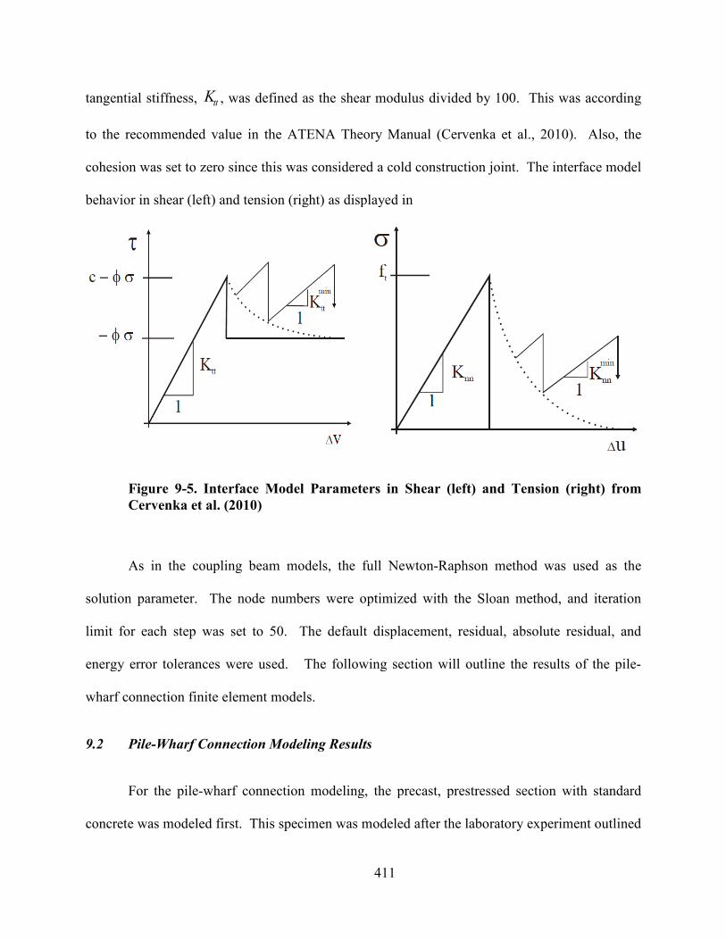
tangential stiffness, ttK , was defined as
to the recommended value in the ATENA Theory Manual
cohesion was set to zero since this was considered a cold construction joint.
behavior in shear (left) and tension (right) as displayed in
Figure 9-5. Interface Model Parameters in Shear (left) and Tension (right) from
Cervenka et al. (2010)
As in the coupling beam models, the full Newton
solution parameter. The node numbers were optimized with the Sloan method, and iteration
limit for each step was set to 50. The default displacement, residual, absolute residual, and
energy error tolerances were used.
wharf connection finite element models.
9.2 Pile-Wharf Connection Modeling Results
For the pile-wharf connection modeling, the precast, prestressed section with standa
concrete was modeled first. This specimen was modeled after the laboratory experiment
411
, was defined as the shear modulus divided by 100. This was according
to the recommended value in the ATENA Theory Manual (Cervenka et al., 2010).
cohesion was set to zero since this was considered a cold construction joint. The interface model
ar (left) and tension (right) as displayed in
. Interface Model Parameters in Shear (left) and Tension (right) from
oupling beam models, the full Newton-Raphson method was used as the
solution parameter. The node numbers were optimized with the Sloan method, and iteration
limit for each step was set to 50. The default displacement, residual, absolute residual, and
rgy error tolerances were used. The following section will outline the results of the pile
wharf connection finite element models.
Wharf Connection Modeling Results
wharf connection modeling, the precast, prestressed section with standa
concrete was modeled first. This specimen was modeled after the laboratory experiment
the shear modulus divided by 100. This was according
(Cervenka et al., 2010). Also, the
The interface model
. Interface Model Parameters in Shear (left) and Tension (right) from
Raphson method was used as the
solution parameter. The node numbers were optimized with the Sloan method, and iteration
limit for each step was set to 50. The default displacement, residual, absolute residual, and
The following section will outline the results of the pile-
wharf connection modeling, the precast, prestressed section with standard
concrete was modeled first. This specimen was modeled after the laboratory experiment outlined
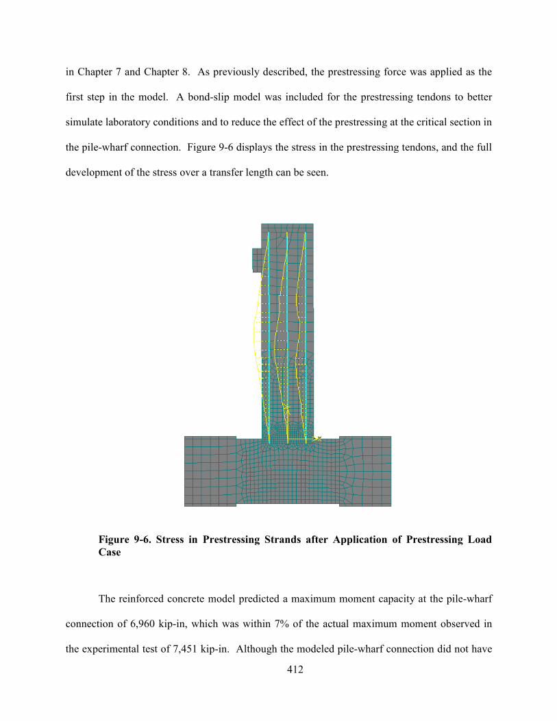
in Chapter 7 and Chapter 8. As previously described, the prestressing force was applied as the
first step in the model. A bond
simulate laboratory conditions and to
the pile-wharf connection. Figure
development of the stress over a transfer length can be seen.
Figure 9-6. Stress in Prestressing
Case
The reinforced concrete model predicted a maxi
connection of 6,960 kip-in, which was within 7% of the actual maximum moment observed in
the experimental test of 7,451 kip
412
in Chapter 7 and Chapter 8. As previously described, the prestressing force was applied as the
step in the model. A bond-slip model was included for the prestressing tendons to
simulate laboratory conditions and to reduce the effect of the prestressing at the critical section in
Figure 9-6 displays the stress in the prestressing tendons, and
development of the stress over a transfer length can be seen.
. Stress in Prestressing Strands after Application of Prestressing Load
The reinforced concrete model predicted a maximum moment capacity at the pile
in, which was within 7% of the actual maximum moment observed in
the experimental test of 7,451 kip-in. Although the modeled pile-wharf connection did not have
in Chapter 7 and Chapter 8. As previously described, the prestressing force was applied as the
the prestressing tendons to better
reduce the effect of the prestressing at the critical section in
displays the stress in the prestressing tendons, and the full
Strands after Application of Prestressing Load
mum moment capacity at the pile-wharf
in, which was within 7% of the actual maximum moment observed in
wharf connection did not have
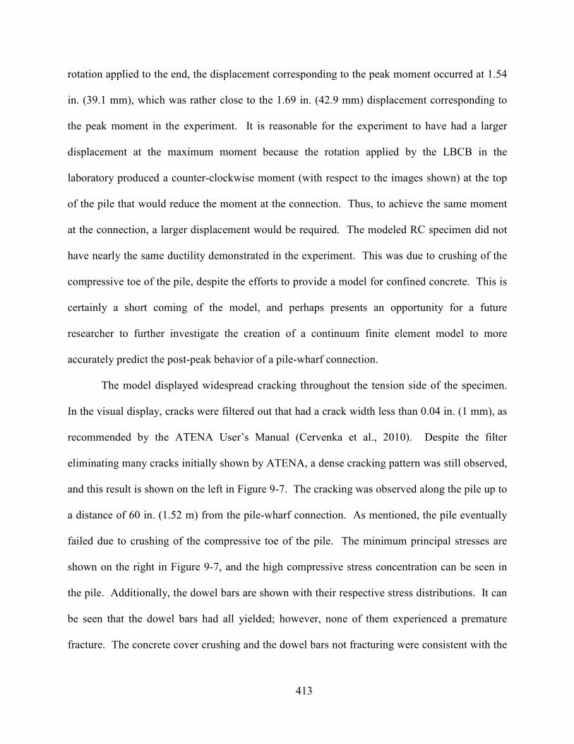
413
rotation applied to the end, the displacement corresponding to the peak moment occurred at 1.54
in. (39.1 mm), which was rather close to the 1.69 in. (42.9 mm) displacement corresponding to
the peak moment in the experiment. It is reasonable for the experiment to have had a larger
displacement at the maximum moment because the rotation applied by the LBCB in the
laboratory produced a counter-clockwise moment (with respect to the images shown) at the top
of the pile that would reduce the moment at the connection. Thus, to achieve the same moment
at the connection, a larger displacement would be required. The modeled RC specimen did not
have nearly the same ductility demonstrated in the experiment. This was due to crushing of the
compressive toe of the pile, despite the efforts to provide a model for confined concrete. This is
certainly a short coming of the model, and perhaps presents an opportunity for a future
researcher to further investigate the creation of a continuum finite element model to more
accurately predict the post-peak behavior of a pile-wharf connection.
The model displayed widespread cracking throughout the tension side of the specimen.
In the visual display, cracks were filtered out that had a crack width less than 0.04 in. (1 mm), as
recommended by the ATENA User’s Manual (Cervenka et al., 2010). Despite the filter
eliminating many cracks initially shown by ATENA, a dense cracking pattern was still observed,
and this result is shown on the left in Figure 9-7. The cracking was observed along the pile up to
a distance of 60 in. (1.52 m) from the pile-wharf connection. As mentioned, the pile eventually
failed due to crushing of the compressive toe of the pile. The minimum principal stresses are
shown on the right in Figure 9-7, and the high compressive stress concentration can be seen in
the pile. Additionally, the dowel bars are shown with their respective stress distributions. It can
be seen that the dowel bars had all yielded; however, none of them experienced a premature
fracture. The concrete cover crushing and the dowel bars not fracturing were consistent with the
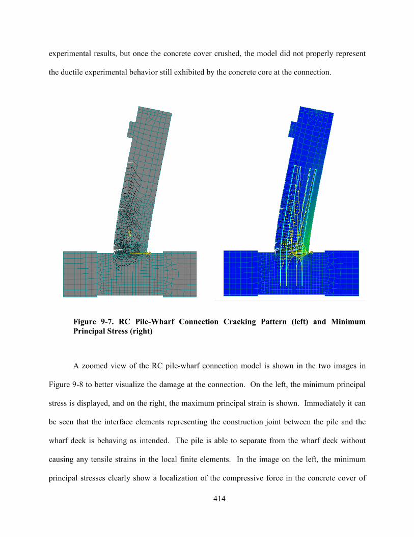
experimental results, but once the concrete cover crushed, the model did not properly represent
the ductile experimental behavior still exhibited by
Figure 9-7. RC Pile-Wharf Connection Cracking Pattern (left) and Minimum
Principal Stress (right)
A zoomed view of the RC pile
Figure 9-8 to better visualize the damage at the connection. On the left, the minimum principal
stress is displayed, and on the right, the maximum principal strain is shown. Immediately it can
be seen that the interface elements representing the construction joint between the pile and the
wharf deck is behaving as intended. The pile is able to separate from the wharf deck without
causing any tensile strains in the local finite elements.
principal stresses clearly show a localization of the compressive force in the concrete cover of
414
experimental results, but once the concrete cover crushed, the model did not properly represent
the ductile experimental behavior still exhibited by the concrete core at the connection.
Wharf Connection Cracking Pattern (left) and Minimum
A zoomed view of the RC pile-wharf connection model is shown in the two images in
to better visualize the damage at the connection. On the left, the minimum principal
stress is displayed, and on the right, the maximum principal strain is shown. Immediately it can
at the interface elements representing the construction joint between the pile and the
wharf deck is behaving as intended. The pile is able to separate from the wharf deck without
causing any tensile strains in the local finite elements. In the image on the left, the minimum
principal stresses clearly show a localization of the compressive force in the concrete cover of
experimental results, but once the concrete cover crushed, the model did not properly represent
the concrete core at the connection.
Wharf Connection Cracking Pattern (left) and Minimum
own in the two images in
to better visualize the damage at the connection. On the left, the minimum principal
stress is displayed, and on the right, the maximum principal strain is shown. Immediately it can
at the interface elements representing the construction joint between the pile and the
wharf deck is behaving as intended. The pile is able to separate from the wharf deck without
the left, the minimum
principal stresses clearly show a localization of the compressive force in the concrete cover of
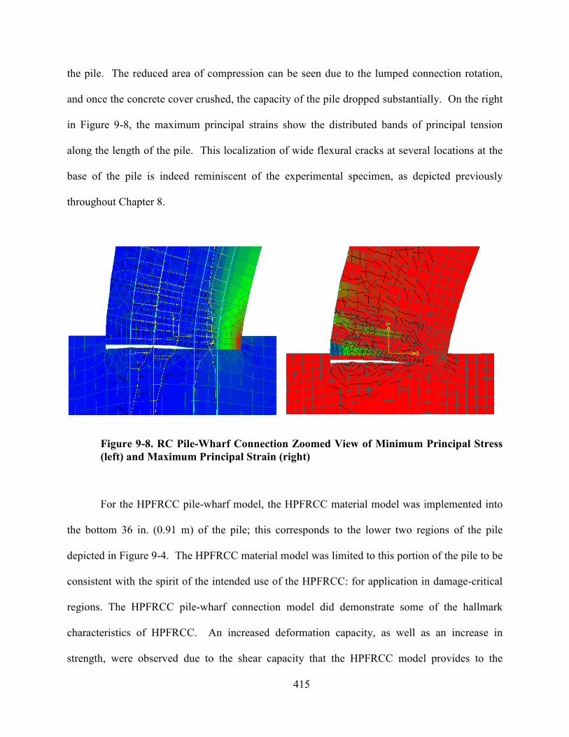
the pile. The reduced area of compression can be seen due to the lumped connection rotation,
and once the concrete cover crushed, the ca
in Figure 9-8, the maximum principal strains show the distributed bands of principal tension
along the length of the pile. This localization of wide flexural cracks at sever
base of the pile is indeed reminiscent of the experimental specimen, as depicted previously
throughout Chapter 8.
Figure 9-8. RC Pile-Wharf Connection Zoomed View of Minimum Princ
(left) and Maximum Principal Strain (right)
For the HPFRCC pile-wharf model, the HPFRCC material model was implemented into
the bottom 36 in. (0.91 m) of the pile; this corresponds to the lower two regions of the pile
depicted in Figure 9-4. The HPFRCC
consistent with the spirit of the intended use of the HPFRCC: for application in damage
regions. The HPFRCC pile-wharf connection model did demonstra
characteristics of HPFRCC. An increased deformation capacity, as well as an increase in
strength, were observed due to the shear capacity that the HPFRCC model provides to the
415
the pile. The reduced area of compression can be seen due to the lumped connection rotation,
and once the concrete cover crushed, the capacity of the pile dropped substantially. On the right
, the maximum principal strains show the distributed bands of principal tension
along the length of the pile. This localization of wide flexural cracks at several locations at the
base of the pile is indeed reminiscent of the experimental specimen, as depicted previously
Wharf Connection Zoomed View of Minimum Princ
(left) and Maximum Principal Strain (right)
wharf model, the HPFRCC material model was implemented into
the bottom 36 in. (0.91 m) of the pile; this corresponds to the lower two regions of the pile
The HPFRCC material model was limited to this portion of the pile
consistent with the spirit of the intended use of the HPFRCC: for application in damage
wharf connection model did demonstrate some of the hallmark
An increased deformation capacity, as well as an increase in
observed due to the shear capacity that the HPFRCC model provides to the
the pile. The reduced area of compression can be seen due to the lumped connection rotation,
pacity of the pile dropped substantially. On the right
, the maximum principal strains show the distributed bands of principal tension
al locations at the
base of the pile is indeed reminiscent of the experimental specimen, as depicted previously
Wharf Connection Zoomed View of Minimum Principal Stress
wharf model, the HPFRCC material model was implemented into
the bottom 36 in. (0.91 m) of the pile; this corresponds to the lower two regions of the pile
material model was limited to this portion of the pile to be
consistent with the spirit of the intended use of the HPFRCC: for application in damage-critical
te some of the hallmark
An increased deformation capacity, as well as an increase in
observed due to the shear capacity that the HPFRCC model provides to the
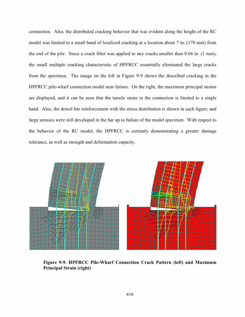
connection. Also, the distributed cracking behavior th
model was limited to a small band of localized cracking a
the end of the pile. Since a crack filter was applied to any cracks smaller than 0.04 in. (1 mm),
the small multiple cracking characteristic
from the specimen. The image on the left in
HPFRCC pile-wharf connection model near failure. On the right,
are displayed, and it can be seen that the tensile strain in the connection is limited to a single
band. Also, the dowel bar reinforcement with the stress distribution is shown in each figure, and
large stresses were still developed in the bar up to failure
the behavior of the RC model, the HPFRCC is certainly demonstrating a greater damage
tolerance, as well as strength and deformation capacity.
Figure 9-9. HPFRCC Pile
Principal Strain (right)
416
connection. Also, the distributed cracking behavior that was evident along the height of the RC
model was limited to a small band of localized cracking at a location about 7 in. (178 mm) from
the end of the pile. Since a crack filter was applied to any cracks smaller than 0.04 in. (1 mm),
cracking characteristic of HPFRCC essentially eliminated the
from the specimen. The image on the left in Figure 9-9 shows the described
wharf connection model near failure. On the right, the maximum principal strains
are displayed, and it can be seen that the tensile strain in the connection is limited to a single
Also, the dowel bar reinforcement with the stress distribution is shown in each figure, and
veloped in the bar up to failure of the model specimen
the behavior of the RC model, the HPFRCC is certainly demonstrating a greater damage
tolerance, as well as strength and deformation capacity.
. HPFRCC Pile-Wharf Connection Crack Pattern (left) and Maximum
at was evident along the height of the RC
bout 7 in. (178 mm) from
the end of the pile. Since a crack filter was applied to any cracks smaller than 0.04 in. (1 mm),
of HPFRCC essentially eliminated the large cracks
described cracking in the
the maximum principal strains
are displayed, and it can be seen that the tensile strain in the connection is limited to a single
Also, the dowel bar reinforcement with the stress distribution is shown in each figure, and
of the model specimen. With respect to
the behavior of the RC model, the HPFRCC is certainly demonstrating a greater damage
Wharf Connection Crack Pattern (left) and Maximum
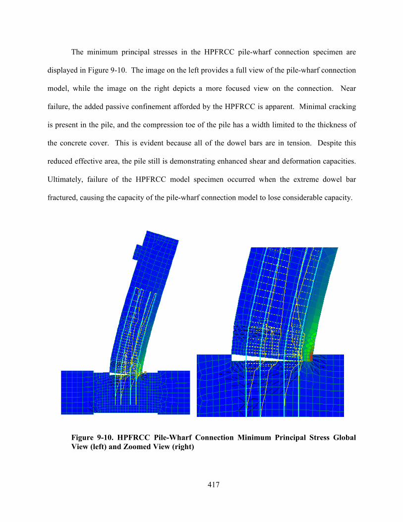
The minimum principal stresses in the HPFRCC pile
displayed in Figure 9-10. The image on the left provides a full view of the pile
model, while the image on the right depicts a more focused view on the connection. Near
failure, the added passive confinement afforded by the HPFRCC is apparent.
is present in the pile, and the compression toe of the pile has a width limited to the thickness of
the concrete cover. This is evident because all of the dowel bars are in tension. Despite this
reduced effective area, the pile still is demonstrating enhanced
Ultimately, failure of the HPFRCC model specimen occurred when the extreme dowel bar
fractured, causing the capacity of the pile
Figure 9-10. HPFRCC Pile
View (left) and Zoomed View (right)
417
The minimum principal stresses in the HPFRCC pile-wharf connection specimen are
image on the left provides a full view of the pile-wharf connection
model, while the image on the right depicts a more focused view on the connection. Near
failure, the added passive confinement afforded by the HPFRCC is apparent. Minimal
sent in the pile, and the compression toe of the pile has a width limited to the thickness of
the concrete cover. This is evident because all of the dowel bars are in tension. Despite this
reduced effective area, the pile still is demonstrating enhanced shear and deformation capacities.
he HPFRCC model specimen occurred when the extreme dowel bar
fractured, causing the capacity of the pile-wharf connection model to lose considerable capacity.
. HPFRCC Pile-Wharf Connection Minimum Principal Stress Global
View (left) and Zoomed View (right)
wharf connection specimen are
wharf connection
model, while the image on the right depicts a more focused view on the connection. Near
Minimal cracking
sent in the pile, and the compression toe of the pile has a width limited to the thickness of
the concrete cover. This is evident because all of the dowel bars are in tension. Despite this
shear and deformation capacities.
he HPFRCC model specimen occurred when the extreme dowel bar
wharf connection model to lose considerable capacity.
Wharf Connection Minimum Principal Stress Global
418
The connection moment versus lateral displacement response of the RC model and the
HPFRCC model are presented and compared to the experimental result in Figure 9-11.
Admittedly, a comparison of the model displacement response to the experimental displacement
response is not completely valid because of the different boundary conditions present in the
experimental test due to the applied rotation; however, it does provide a general qualitative frame
of reference for the modeling result. For a given displacement, the experiment applied a rotation
at the top of the pile to reduce the moment at the pile-wharf connection, so it sensible for the
displacements of the experiment to be slightly larger than those demonstrated by the model.
Even with that consideration, the model was not able to capture the same level of ductility
displayed by the experiment. Figure 9-11 illustrates the added shear capacity that the HPFRCC
provided to the damage-critical region of the pile-wharf connection model. The HPFRCC model
had a peak moment capacity of about 9,400 kip-in., approximately 33% larger than the
connection moment in the RC model. Also, the HPFRCC model was able to accommodate
larger lumped connection rotation before the eventual failure of the model specimen. This was
achieved largely due to the enhancement of the compressive strength afforded by the passive
confinement of the fiber reinforcement.
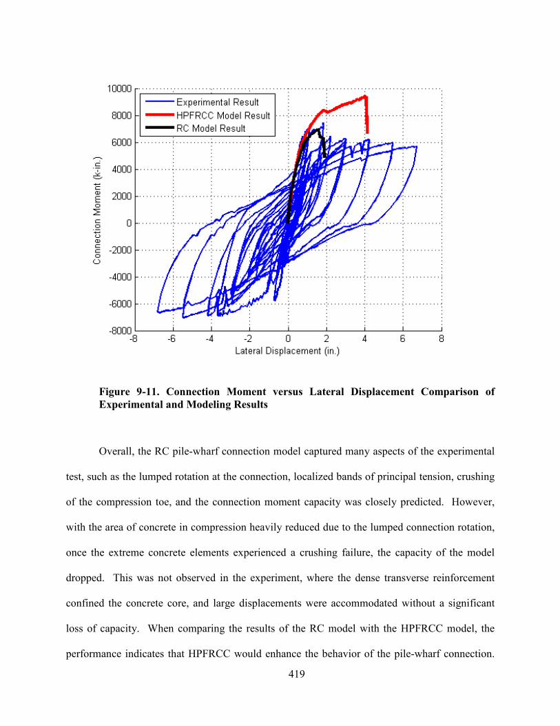
419
Figure 9-11. Connection Moment versus Lateral Displacement Comparison of
Experimental and Modeling Results
Overall, the RC pile-wharf connection model captured many aspects of the experimental
test, such as the lumped rotation at the connection, localized bands of principal tension, crushing
of the compression toe, and the connection moment capacity was closely predicted. However,
with the area of concrete in compression heavily reduced due to the lumped connection rotation,
once the extreme concrete elements experienced a crushing failure, the capacity of the model
dropped. This was not observed in the experiment, where the dense transverse reinforcement
confined the concrete core, and large displacements were accommodated without a significant
loss of capacity. When comparing the results of the RC model with the HPFRCC model, the
performance indicates that HPFRCC would enhance the behavior of the pile-wharf connection.

420
While this may introduce some complications logistically to actually construct a precast pile
where a portion of the pile is HPFRCC, the exercise of implementing the HPFRCC model into a
damage-critical structural component and assessing the effect of HPFRCC on the performance of
that component was the primary thrust of this portion of the research.
9.3 Other Modeling Applications
With the extension of the HPFRCC model to coupling beam components and pile-wharf
connections, its use could be reasonably extended to other, potentially larger, structural
applications. For example, the large-scale coupled wall specimen tested by project colleagues at
the University of Michigan integrated HPFRCC coupling beams into an RC coupled wall system.
That same testing program also explored the use of HPFRCC in the plastic hinging region of the
wall. These two large-scale tests provide excellent opportunities to integrate the HPFRCC model
into larger structural systems, with the possibility of validating the model through the available
experimental results. Another possibility could include a prototype reinforced concrete dual
structural system consisting of a coupled wall and a moment resisting frame. Then, critical areas
where inelastic activity is expected to occur, such as at the base of the wall regions, the coupling
beams, the beam ends, and the column bases, could be modeled using the HPFRCC material
model. This parametric study could show the effect of incorporating the HPFRCC on the
stiffness, strength, and ductility of the structure. Also, another study could be conducted
exploring the influence of including HPFRCC into only some of the damage critical members.
Such a parametric study could provide significant insight into the use of HPFRCC in structures
by demonstrating its ability to enhance various aspects of structural performance. Whatever the
case, the development of an HPFRCC model that can be implemented into commercially
available software presents essentially unlimited possibilities for a designer to explore the impact

421
of HPFRCC on a structural design, whether it is the reduction of the required reinforcement or an
impact on the global ductility of the structure.
422
CHAPTER 10. COCLUSIOS
This chapter provides a summary of the findings and conclusions of this research study,
as well as provides recommendations for future work.
10.1 Summary
In the current research program, the behavior of high-performance fiber-reinforced
cementitious composites (HPFRCC) under multi-axial loads was studied thoroughly. An
experimental program was performed on small-scale HPFRCC specimens under multi-axial
loads on two different concrete mixes. Each concrete mix explored the use of two different
fibers types, hooked steel fibers and Spectra fibers, as well as the effect of varying volume
fractions. A final HPFRCC mix was selected, and an even more thorough investigation of the
multi-axial behavior of this concrete mix was performed. Failure envelopes and constitutive
relationships were developed from the small-scale experimental tests. These properties were
then implemented into ATENA, a nonlinear finite element program, and modeling of the small-
scale program was conducted. The modeling effort showed that the ATENA model could
appropriately represent the performance of the HPFRCC material under multi-axial loads. Then,
the HPFRCC material model was extended into use in structural components. Coupling beam
component tests had been conducted by previous researchers on RC coupling beams and
HPFRCC coupling beams. The RC coupling beams were modeled to ensure that the modeling
approach was appropriately representing the experimental results, and the HPFRCC material
model was implemented into the historical RC coupling beam models to perform a parametric
study on the effect of HPFRCC on the coupling beam performance. Next, HPFRCC coupling
beam component tests performed by project colleagues at the University of Michigan were
423
modeled. These coupling beams were modeled with the HPFRCC material model formulated
from the material tests, and it was found to accurately capture the response of the experiments.
Control RC coupling beams were also modeled with the same layout and loading as the
HPFRCC coupling beams to perform another study on the effect of HPFRCC on coupling beam
performance.
A separate research project was also conducted that was not directly related to the multi-
axial behavior of HPFRCC. This research project involved the large-scale testing of a pile-wharf
connection at the NEES MUST-SIM facility at the University of Illinois. This experiment
explored the behavior of a pile-wharf connection with realistic boundary conditions. The loading
protocol was developed from the results of a nonlinear port system model developed by project
colleagues at Georgia Tech. The test specimen was tested with mixed mode control;
displacements and rotations were applied to the end of the specimen while a constant axial load
was maintained. In an effort to link the two research projects, a pile-wharf connection modeling
effort was pursued. A traditional RC pile-wharf connection was modeled, and then the pile-
wharf connection was modeled with the addition of HPFRCC. This effort showed the effect of
HPFRCC on the pile-wharf connection, as well as the versatility of implementing the HPFRCC
model into damage-critical structural components.
10.2 HPFRCC Experimental Conclusions
Several HPFRCC concrete mixes were tested in this study; however, the main findings of
the small-scale experimental program can be briefly summarized as follows:
• HPFRCC specimens demonstrate a pseudo-strain hardening and multi-cracking
behavior in tension after initial cracking. This is contrasted with plain concrete
424
and other conventional FRC, which would not perform with the same beneficial
mechanical behavior.
• Under biaxial compression, the ultimate strength of HPFRCC relative to its
uniaxial compressive strength is higher than for plain concrete.
• Under equal biaxial stresses, the HPFRCC specimens experience between 40%
and 55% increase in strength over uniaxial compression.
• The maximum biaxial strength occurs at an intermediate compression-
compression ratio. Depending on the properties of the mix, this strength increase
may vary from 50% - 80% greater than the uniaxial compressive strength.
• The increase in multi-axial compressive strength relative to the uniaxial
compressive strength is more pronounced for lower strength HPFRCC mixes.
• HPFRCC exhibits an enhanced deformation capacity and significant residual
strength at large strains. The residual compressive strength of HPFRCC is
regularly 70% of the peak compressive strength at 1% strain and 50% of the peak
compressive strength at 2% strain.
• The addition of fibers did not affect the elastic modulus of the concrete mix or
Poisson’s ratio.
• The addition of fibers alters the failure mechanism of the plate specimens from a
splitting tension failure to a shear faulting failure.
425
10.3 HPFRCC Modeling Conclusions
HPFRCC material tests, RC coupling beams, HPFRCC coupling beams, and pile-wharf
connections were all modeled as part of this research. The main findings of the modeling
program can be summarized as follows:
• RC coupling beams from the literature can be accurately modeled with
commercial nonlinear finite element programs, provided appropriate information
is provided regarding the test setup, loading, boundary conditions, and material
properties.
• An increase of the SBETA softening parameter was the only change from the
default concrete model for the RC coupling beams.
• The cyclic models for the RC coupling beams experienced a rapid strength loss
and premature sliding shear failure due to the inability of the model to capture
aggregate interlock, dowel action, and other elements contributing to the shear
friction mechanism.
• The parametric study of the RC coupling beams with HPFRCC showed that
HPFRCC can effectively increase the shear capacity of the coupling beams by
about 30% while also increasing the displacement at failure by at least 20%,
depending on the reinforcement layout of the coupling beam.
• The HPFRCC coupling beam models were loaded monotonically, so the models
were stiffer at low displacements than the experimental tests. This resulted in an
over prediction of the force at initial yielding of the reinforcement (15%) and an
under prediction of the displacement (12%) at initial yielding of the
reinforcement.
426
• In all of the coupling beam models, the peak strength is predicted to within 4% of
the experimental result. In the RC coupling beams, the shear force at initial
yielding of the reinforcement was within 10%.
• The displacement at yielding of the reinforcement and at the ultimate load is
under predicted by the model on average of 6% and 30%, respectively.
• Failure modes of the experimental coupling beams are predicted accurately by the
model.
• The parametric study of the HPFRCC coupling beam with RC shows again that
the addition of HPFRCC can increase the shear capacity of the coupling beam by
about 30%.
• The application of HPFRCC to the pile-wharf connection further demonstrates the
ability to implement the HPFRCC model into other structural components to
evaluate its effect on the performance of a damage-critical member.
10.4 Pile-Wharf Connection Conclusions
After an examination of the behavior of the pile-wharf connection specimen, the
following conclusions can be made:
• The primary mechanism through which pile displacements are accommodated
was through lumped rotation at the pile-wharf connection and not through flexural
action of the pile.
• At lower loads, flexural rotation of the pile accounts for about 30% of the total
rotation of the pile, with 70% being attributed to a lumped connection rotation.
427
• As damage progresses, the flexural rotation of the pile accounts for less of the
total rotation. In fact, the lumped connection rotation accounts for as much as
90% of the total rotation after significant damage occurs in the pile-wharf
connection.
• Pile spalling and deck spalling lead to a decrease in the capacity of the pile-wharf
connection; however, if the confined concrete core remains intact, the pile-wharf
connection can accommodate large lateral deformations with only a modest
reduction of capacity.
• A reduced axial load '(0.02 )
c gf A relative to other experimental tests causes the
pile-wharf connection to behave similar to tests performed by previous
researchers with bearing pads located at the end of the pile, with deformation
localizing in the connection.
• A dense Krypton LED grid allows for the creation of unique visualization tools to
review the behavior and strains throughout the specimen during testing.
10.5 Contributions
To the author’s knowledge, this research provides the following unique research
contributions:
• The first study to experimentally test the biaxial behavior of a self-consolidating
HPFRCC. The thesis provides failure envelopes and deformation characteristics
that are not available in the literature, and should be useful for calibrating further
finite element models.
428
• The first study to develop a finite element model for HPFRCC from its own
biaxial experimental results. This thesis outlines the procedure and input
parameters required to utilize commercially available software to model
HPFRCC.
• This thesis contains the first comprehensive study on the use of an HPFRCC
model, calibrated from its own experimental results, to model coupling beams and
pile-wharf connections. Also, it outlines a process of implementing the HPFRCC
model into historical experimental tests to perform a parametric study on the
potential effect of HPFRCC on damage-critical structural components.
• The first pile-wharf large-scale connection test with realistic boundary conditions
was reported in this thesis. Previous tests were not able to simulate the
application of displacements, rotations, and axial load simultaneously. This
realistic loading provides a deeper insight into the expected performance of pile-
wharf connections during seismic events.
10.6 Future Work
This research program has provided a review of the multi-axial behavior of HPFRCC, as
well as the performance of pile-wharf connection. In light of this research program, several
topics exist that the author believes warrant further exploration. Recommendations for future
work include the following:
• Biaxial tests on HPFRCC subjected to compression-tension and tension-tension
have yet to be completed. This testing program would complete the biaxial
failure envelope and provide further insight into the performance of HPFRCC
429
under complex loading, as would be expected in a damage-critical structural
component.
• The cyclic properties of HPFRCC should be investigated experimentally, as well
as the implementation of the cyclic properties into the nonlinear finite element
model. Since seismic events cause considerable cyclic deformations, the
HPFRCC model should be validated to properly model such events.
• The development of definitions of performance levels for HPFRCC associated
with specific engineering demand parameters. Since HPFRCC is targeted for
damage-critical components, it is important to be able to map the deformation or
damage of the structural element to a specific performance level for the
assessment of the HPFRCC properties. This capability could greatly further the
ability of designers to make performance-based design decisions regarding the use
of HPFRCC.
• Additional pile-wharf connection specimens could be tested with varying loading
parameters, such as an increased axial load or a different applied displacement-
rotation ratio. Also, a larger-scale model, as originally planned at the NEES
MUST-SIM facility, including multiple pile-wharf specimens attached to a single
wharf deck could provide valuable insight into the effect that the interaction
between adjacent piles has on the global seismic response of a port structure.
• A more detailed pile-wharf connection model could be developed characterizing
the behavior of the lumped connection rotation. This model could then be
verified under reverse cyclic and/or earthquake loading. Additionally, the

430
implementation of the model into a full port structure could provide a valuable
tool for the seismic assessment of existing port systems.
431
REFERECES
ACI Committee 318. (2008). Building Code Requirements for Structural Concrete (ACI 318-08)
and Commentary. Farmington Hills, MI, MI: American Concrete Institute.
Akai, K. (1995). Geotechnical Reconnaissance of the Effects of the January 17, 1995,
Hyogoken-Nanbu Earthquake, Japan. Report o. UCB/EERC-95/01 . Berkeley, CA:
Earthquake Engineering Research Center.
American Wood Council. (2006). ational Design Specification for Wood Construction
ASD/LRFD, 2005 Edition. American Forest & Paper Association, Inc.
Applied Technology Council. (1998). FEMA 306. Evaluation of Earthquake Damaged Concrete
and Masonry Wall Buildings .
ASCE. (2007). ASCE/SEI 41/06. Seismic Rehabilitation of Existing Buildings . Reston, VA:
ASCE.
ASTM C39-05. (2006). Standard Test Method for Compressive Strength of Cylindrical Concrete
Specimens. West Conshohocken, PA.
ASTM C496-04. (2006). Standard Test Method for Splitting Tensile Strength of Cylindrical
Concrete Specimens. West Conshohocken, PA.
Barney, G., Shiu, K., Rabbat, B., Fioratio, A., Russell, H., & Corley, W. (1980). Behavior of
Coupling Beams under Load Reversals. Skokie, IL: Portland Cement Association.
Bazant, Z., & Oh, B. (1983). Crack Band Theory for Fracture of Concrete. Materials and
Structures , 16, 155-177.
432
Berry, M., & Eberhard, M. (2003). Performance Models for Flexural Damage in Reinforced
Concrete Columns. Pacific Earthquake Engineering Research Center.
Caiza, P., Andrawes, B., & LaFave, J. (2010). Structural Concrete Pile-Wharf Connections under
Cyclic Lateral Loading. 9 US 10 Canadian Conference on Structural Engineering.
Toronto, CA.
Calixto, J. (2002). Behavior of High-Performance Concrete Subjected to Biaxial Tension-
Compression Stresses. ACI Special Publication , 207 , 1-14. Detroit, MI: American
Concrete Institute.
Canbolat, B. (2004). Seismic Behavior of High-Performance Fiber Reinforced Cementitious
Composite Coupling Beams. Ph.D. Thesis . Ann Arbor, MI: The University of Michigan.
Canbolat, B., Parra-Montesinos, G., & Wight, J. (2005). Experimental Study on Seismic
Behavior of High-Performance Fiber-Reinforced Cement Composite Coupling Beams.
ACI Structural Journal , 102 (1), 159-166.
CEB-FIP. (1990). CEB-FIP Model Code 1990. Bulletin d'information o. 195,196 . Comitte
Euro-International du Beton.
Cervenka, V., Jendele, L., & Cervenka, J. (2010, March 22). ATEA Program Documentation -
Part 1 - Theory . Prague, Czech Republic: Cervenka Consulting.
Cervenka, V., Pukl, R., Ozbolt, J., & Eligehausen, R. (1995). Mesh Sensitivity Effects in
Smeared Finite Element Analysis of Concrete Fracture. Proceedings of FRAMCOS2.
Zurich, Switzerland.
433
Chang, S. E. (2000). Disasters and Transport Systems: Loss, Recovery, and Competition at the
Port of Kobe after the 1995 Earthquake. Journal of Transport Geograpy , 8 (1), 53-65.
Chao, S.-H., Naaman, A., & Parra-Montesinos, G. (2009). Bond Behavior of Reinforcing Bars in
Tensile Strain-Hardening Fiber-Reinforced Cement Composites. ACI Structural Journal ,
106 (6), 897-906.
Chern, J., Yang, H., & Chen, H. (1992). Behavior of Steel Fiber Reinforced Concrete in
Multiaxial Loading. ACI Materials Journal , 89 (1), 32-40.
Cho, J., Kim, N., Cho, N., & Choun, Y. (2004). Stress-Strain Relationship of Reinforced
Concrete Subjected to Biaxial Tension. ACI Structural Journal , 101 (2), 202-208.
Chompreda, P., & Parra-Montesinos, G. (2005). Deformation Capacity and Shear Strength of
Fiber Reinforced Cement Composite Flexural Members Subjected to Displacement
Reversals. Report o. UMCEE 05-03 . Ann Arbor, MI: Dept. of Civil and Environmental
Engineering, University of Michigan.
De Borst, R. (1986). onlinear Analysis of Frictional Materials. Ph.D. Thesis, Delft University
of Technology.
Demeke, A., & Tegos, I. (1994). Steel Fiber Reinforced Concrete in Biaxial Stress Tension-
Compression Conditions. ACI Structural Journal , 91 (5), 579-584.
Dinh, H., Parra-Montesinos, G., & Wight, J. (2010). Shear Behavior of Steel Fiber-Reinforced
Concrete Beams without Shear Reinforcement. ACI Structural Journal , 107 (5), 597-
606.
434
EFNARC. (2002). Specification and Guidelines for Self-Consolidating Concrete. Retrieved from
http://www.efnarc.org
Fischer, G. (2004). Characterization of Fiber-Reinforced Cement Composites by their Tensile
Stress-Strain Behavior and Quantification of Crack Formation. 6th RILEM Symposium on
Fiber-Reinforced Concretes (FRC), (pp. 331-338). Varenna, Italy.
Foltz, R., Guerra, J., & LaFave, J. (2008). Behavior of High-Performance Fiber-Reinforced
Cementitious Composites for RC Coupling Beams in Earthquake-Resistant Structural
Wall Systems. 14th World Conference on Earthquake Engineering. Beijing, China.
Galano, L., & Vignoli, A. (2000). Seismic Behavior of Short Coupling Beams with Different
Reinforcement Layouts. ACI Structural Journal , 97 (6), 876-885.
Graybeal, B. A. (2006). Practical Means for Determination of the Tensile Behavior of Ultra-High
Performance Concrete. Journal of ASTM International , 3 (8).
Han, T., Feenstra, P., & Billington, S. (2003). Simulation of Highly Ductile Fiber-Reinforced
Cement-Based Composite Components under Cyclic Loading. ACI Structural Journal ,
100 (6), 749-757.
Harries, K., Fortney, P., Shahrooz, B., & Brienen, P. (2005). Practical Design of Diagonally
Reinforced Concrete Coupling Beams -- Critical Review of ACI 318 Requirements. ACI
Structural Journal , 102 (6), 876-882.
Hilsdorf, H. (1965). The Experimental Determination of the Biaxial Strength of Concrete.
Deutscher Ausschuss fur Stahlbeton. Berlin.
435
Horri, H., & Nemat-Nasser, S. (1986). Brittle Failure in Compression: Splitting, Faulting and
Brittle-Ductile Transition. Philosophical Transactions , 319, 337-374.
Hu, X., Day, R., & Dux, P. (2003). Biaxial Failure Model for Fiber Reinforced Concrete.
Journal of Materials in Civil Engineering , 15 (6), 609-615.
Hung, C.-C., & El-Tawil, S. (2009). Cyclic Model for High Performance Fiber Reinforced
Cementitious Composite Structures. ATC & SEI Conference on Improving the Seismic
Performance of Existing Buildings and Other Structures. San Francisco, California.
Hussein, A., & Marzouk, H. (2000a). Behavior of High Strength Concrete under Biaxial
Stresses. ACI Materials Journal , 97 (1), 27-36.
Hussein, A., & Marzouk, H. (2000b). Finite Element Evaluation of the Boundary Conditions for
Biaxial Testing of High Strength Concrete. Materials and Structures , 33, 299-308.
Iynegar, K., Chandrashekhara, K., & Krishnaswamy, K. (1965). Strength of Concrete Under
Biaxial Compression. Journal of the American Concrete Institute , 62 (14), 239-250.
Jellin, A. (2008). Improved Seismic Connections for Pile-Wharf Construction. Master's Thesis,
University of Washington.
Joen, P., Park, R., & Priestley, M. (1988). Seismic Performance of Prestressed Concrete Piles
and Pile-Pile Cap Connections. Research Report 88-3 . New Zealand: University of
Canterbury.
Kabele, P. (2007). Multiscale Framework for Modeling of Fracture in High Performance Fiber
Reinforced Cementitious Composites. Engineering Fracture Mechanics , 74, 194-209.
436
Kesner, K., & Billington, S. (2004). Tension, Compression, and Cyclic Testing of Engineered
Cementitious Composite Materials. State University of New York at Buffalo: Multi-
disciplinary Center for Earthquake Engineering Research.
Kim, K., & Parra-Montesinos, G. (2003). Behavior of HPFRCC Low-Rise Walls Sujected to
Displacement Reversals. High Performance Fiber Reinforced Cement Composites
(HPFRCC 4), Proceedings of the Fourth International RILEM Workshop (pp. 505-515).
Cachan Cedex, France: RILEM Publications.
Krier, C. (2006). Seismic Testing of Full-Scale Precast Prestressed Pile to Deck Connections.
Master's Thesis, University of California, San Diego.
Kuang, J., & Baczkowski, B. (2009). Steel-Fiber-Reinforced Concrete Coupling Beams
Subjected to Monotonic Loading. Magazine of Concrete Research , 61 (1), 35-41.
Kupfer, H., Hilsdorf, H., & Rusch, H. (1969). Behavior of Concrete under Biaxial Stresses. ACI
Journal Proceedings , 66 (8), 656-666.
Kwan, A., & Zhao, Z. (2002). Testing of Coupling Beams with Equal End Rotations Maintained
and Local Joint Deformation Allowed. Structures & Buildings , 152 (1), 67-78.
Kwan, A., & Zhao, Z.-Z. (2002). Cyclic Behavior of Deep Reinforced Concrete Coupling
Beams. Structures & Buildings , 152 (3), 283-293.
Lan, S., & Guo, Z. (1999). Biaxial Compression Behavior of Concrette under Repeated Loading.
Journal of Materials in Civil Engineering , 11 (2), 105-115.
Lee, S., Song, Y., & Han, S. (2004). Biaxial Behavior of Plain Concrete of Nuclear Containment
Building. uclear Engineering and Design , 227, 143-153.
437
Lequesne, R. (2011). Behavior and Design of High-Performance Fiber-Reinforced Concrete
Coupling Beams and Coupled-Wall Systems. Ph.D. Thesis . University of Michigan.
Lequesne, R., Parra-Montesinos, G., & Wight, J. (2009a). Test of a Coupled Wall with High-
Performance Fiber-Reinforced Concrete Coupling Beams. ACI Special Publication, SP-
265 . American Concrete Institute.
Lequesne, R., Setkit, M., Parra-Montesinos, G., & Wight, J. (2009b). Seismic Detailing and
Behavior of Coupling Beams with High-Performance Fiber Reinforced Concrete. Antoine
E. aaman Symposium – Four Decades of Progress in Prestressed Concrete, Fiber
Reinforced Concrete, and Thin Laminate Composites, SP-In Press , 14. Farmington Hills,
MI: American Concrete Institute.
Lequesne, R., Wight, J., & Parra-Montesinos, G. (2010). Seismic Detailing and Behavior of
Coupled-Wall Systems with High-Performance Fiber-Reinforced Concrete. Joint 9US /
10CCEE Conference Proceedings, (p. 10). Toronto, Canada.
Leslie, P. (1974). Ductility of Reinforced Concrete Bridge Piers. Master's Thesis . University of
Canterbury.
Liao, W., Chao, S., Park, S., & Naaman, A. (2006). Self-Consolidating High-Performance Fiber-
Reinforced Concrete (SCHPFRC) - Preliminary Investigation. UMCEE 06-02.
Liu, T., Nilson, A., & Slate, F. (1972). Stress-Strain Response and Fracture of Concrete in
Uniaxial and Biaxial Compression. ACI Journal Proceedings , 69 (5), 291-295.

438
Maekawa, K., & Okamura, H. (1983). The Deformational Behavior and Constitutive Equation of
Concrete Using the Elasto-Plastic and Fracture Model. Journal of the Faculty of
Engineering, The University of Tokyo , 37 (2), 253-272.
Mander, J., Priestly, M., & Park, R. (1988). Theoretical Stress-Strain Model for Confined
Concrete. Journal of Structural Engineering , 114 (8), 1804-1826.
Menetrey, P., & William, K. (1995). Triaxial Failure Criterion for Concrete and Its
Generalization. ACI Structural Journal , 92 (3), 311-318.
Mohr, D. (2007). Nonlinear Analysis and Performance Based Design Methods for Reinforced
Concrete Coupled Shear Walls. Master's Thesis . University of Washington.
Murugappan, K., Paramasivam, P., & Tan, K. (1993). Failure Envelope for Steel-Fiber Concrete
under Biaxial Compression. Journal of Materials in Civil Engineering , 5 (4), 436-446.
Naaman, A. (1987). High Performance Fiber Reinforced Cement Composites. Proceedings of the
IABSE Symposium on Concrete Structures for the Future, (pp. 371-376). Paris, France.
Naaman, A., & Reinhardt, H. (1996). Characterization of High Performance Fiber Reinforced
Cement Composites -- HPFRCC. In A. E. Naaman, & H. W. Reinhardt (Ed.), High
Performance Fiber Reinforced Cement Composites 2 (HPFRCC 2) (pp. 1-24). Ann
Arbor, USA: E&FN Spon.
Naaman, A., & Reinhardt, H. (2006). Proposed Classification of HPFRC Composites based on
their Tensile Response. Materials and Structures , 39, 547-555.
Naaman, A., & Reinhardt, H. (2003). Setting the Stage: Toward Performance Based
Classification of FRC Composites. In A. E. Naaman, & H. W. Reinhardt (Ed.), High
439
Performance Fiber Reinforced Cement Composites (HPFRCC4), Proceedings of the
Fourth International RILEM Workshop (pp. 1-4). Ann Arbor, USA: RILEM Publications.
Naaman, A., Fischer, G., & Krstulovic-Opara, N. (2007). Measurement of Tensile Properties of
Fiber Reinforced Concrete: Draft Submitted to ACI Committee 544. In H. W. Reinhardt,
& A. E. Naaman (Ed.), High Performance Fiber Reinforced Cement Composites
(HPFRCC5), Proceeding of the Fifth International RILEM Workshop (pp. 3-9). Mainz,
Germany: RILEM Publications.
Nakata, N., Spencer, B., & Elnashai, A. (2007). Multi-Dimensional Mixed-Mode Hybrid
Simulation Control and Applications. NSEL-005, Newmark Structural Engineering
Laboratory Report Series.
Nanni, A. (1988). Splitting-Tension Test for Fiber Reinforced Concrete. ACI Materials Journal ,
85 (4), 229-233.
Nawy, E., Lim, D., & McPherson, K. (2003). Compressive Behavior of High-Strength High-
Performance Concrete under Biaxial Loading. ACI Special Publication , 213, 43-60.
Nelissen, L. (1972). Biaxial Testing of Normal Concrete. Heron , 18 (1), 90.
Ottosen, N. (1977). A Failure Criterion for Concrete. Journal of Engineering Mech. Division ,
103 (4), 527-535.
Parra-Montesinos, G. (2005). High-Performance Fiber-Reinforced Cement Composites: An
Alternative for Seismic Design of Structures. ACI Structural Journal , 102 (5), 668-675.
440
Parra-Montesinos, G., & Chompreda, P. (2007). Deformation Capacity and Shear Strength of
Fiber-Reinforced Cement Composite Flexural Members Subjected to Displacement
Reversals. Journal of Structural Engineering , 133 (3), 421-431.
Parra-Montesinos, G., Canbolat, B., & Jeyaraman, G. (2006). Relation of Confinement
Reinforcement Requirements in Structural Walls through the Use of Fiber Reinforced
Cement Composites. 8th U.S. ational Conference on Earthquake Engineering. San
Francisco, CA.
Parra-Montesinos, G., Peterfreund, S., & Chao, S.-H. (2005). Highly Damage-Tolerant Beam-
Column Joints through Use of High-Performance Fiber-Reinforced Cement Composites.
ACI Structural Journal , 102 (3), 487-495.
Parra-Montesinos, G., Wight, J., & Canbolat, B. (2005). Development of Precast High-
Performance Fiber Reinforced Cement Composite Coupling Beams for Earthquake-
Resistant Wall Systems. ACI Special Publication 228 . Detroit, MI: American Concrete
Institute.
Paulay, T. (1971). Coupling Beams of Reinforced Concrete Shear Walls. Proceedings of the
American Society of Civil Engineers Structural Division , 97 (ST3), 843-862.
Paulay, T. (1977). Ductility of Reinforced Concrete Shearwalls for Seismic Areas. ACI Special
Publication 53 , 127-147. Detroit, Michigan: American Concrete Institute.
Paulay, T., & Binney, J. (1974). Diagonally Reinforced Coupling Beams of Shear Walls. ACI
Special Publication 42 , 579-598. Detroit, MI: American Concrete Institute.
441
Paulay, T., & Santhakumar, A. (1976). Ductile Behavior of Coupled Shear Walls. ASCE Journal
of the Structural Division , 102 (1), 93-108.
Ren, X., Yang, W., Zhou, Y., & Li, J. (2008). Behavior of High-Performance Concrete Under
Uniaxial and Biaxial Loading. ACI Materials Journal , 105 (6), 548-557.
Restrepo, J., Yin, P., Jaradat, O., & Weismair, M. (2007). Performance of New Pile-Deck
Connections under Earthquakes. Ports 2007: 30 Years of Sharing Ideas 1977-2007, (pp.
104-113). San Diego, CA.
Roeder, C., Graff, R., Soderstrom, J., & Yoo, J. (2001). Seismic Performance of Pile-Wharf
Connections. PEER Report 2002/07 . Berkeley, CA: Pacific Earthquake Engineering
Research Center, University of California.
Roeder, C., Graff, R., Soderstrom, J., & Yoo, J. (2005). Seismic Performance of Pile-Wharf
Connections. ASCE Journal of Structural Engineering , 131 (3), 428-437.
Seow, P., & Swaddiwudhipong, S. (2005). Failure Surface for Concrete under Multiaxial Load -
a Unified Approach. Journal of Materials in Civil Engineering , 17 (2), 219-228.
Serventi, G., Jordan, M., Fotinos, G., & Soderberg, E. (2004). The Design of Earthquake
Damage Repairs to Wharves before the Earthquake Occurs. Port Development in the
Changing World, PORTS 2004, (pp. 297-306).
Shafieezadeh, A. (2011). Seismic Vulnerability Assessment of Wharf Structures. Ph.D. Thesis .
Georgia Institute of Technology.
442
Silva, P., Seible, F., & Priestley, M. (1997). Response of Standard Caltrans Pile-to-Pile Cap
Connections under Simulated Seismic Loads. Report o. SSRP-97/09 . UC San Diego:
Division of Structural Engineering.
Sirijaroonchai, K. (2009). A Macro-Scale Plasticity Model for High Performance Fiber
Reinforced Cement Composites. Ph.D. Thesis, University of Michigan, Ann Arbor, MI.
Sirijaroonchai, K., El-Tawil, S., & Parra-Montesinos, G. (2010). Behavior of High Performance
Fiber Reinforced Cement Composites under Multi-Axial Compressive Loading. Cement
& Concrete Composites , 32, 62-72.
Somerville, P., Smith, N., Punyamurthula, S., & Sun, J. (1998). Development of Ground Motion
Time Histories for Phase 2 of the FEMA/SAC Steel Project , SAC/BD-07/04. Sacramento,
CA: SAC Joint Venture.
Sritharan, S., & Priestley, M. (1998). Seismic testing of a Full-Scale Pile-Deck Connection
Utilizing Headed Reinforcement. Report TR98/14 . University of California, San Diego.
Stringer, S. (2010). Seismic Performance of Improved Damage Resistant Pile to Wharf Deck
Connections. Master's Thesis, University of Washington.
Swaddiwudhipong, S., & Seow, P. (2006). Modelling of Steel Fiber-Reinforced Concrete under
Multi-Axial Loads. Cement and Concrete Research , 36, 1354-1361.
Tassios, T., Moretti, M., & Bezas, A. (1996). On the Behavior and Ductility of Reinforced
Concrete Coupling Beams of Shear Walls. ACI Structural Journal , 93 (6), 711-720.
Tasuji, M., Slate, F., & Nilsson, A. (1978). Stress-Strain Response and Fracture of Concrete in
Biaxial Loading. ACI Journal Proceedings , 75 (7), 306-312.
443
Tegos, I., & Penelis, G. (1988). Seismic Resistance of Short Columns and Coupling Beams
Reinforced with Inclined Bars. ACI Structural Journal , 85 (1), 82-88.
Torrenti, J., & Djebri, B. (1995). Behaviour of Steel-Fibre-Reinforced Concretes under Biaxial
Compression Loads. Cement & Concrete Composites , 17 (4), 261-266.
Traina, L., & Mansour, S. (1991). Biaxial Strength and Deformational Behavior of Plain and
Steel Fiber Concrete. ACI Materials Journal , 88 (4), 354-362.
van Mier, J. (1986). Fracture of Concrete under Complex Stress. Heron , 31 (3), 89.
van Mier, J. (1986). Multi-Axial Strain-Softening of Concrete, Part I. Materials and Structures ,
19 (111).
Vecchio, F., & Collins, M. (1986). Modified Compression-Field Theory for Reinforced Concrete
Beams Subjected to Shear. ACI Journal , 83 (2), 219-231.
Wallace, J. (2007). Modelling Issues for Tall Reinforced Concrete Core Wall Buildings. The
Structural Design of Tall and Special Buildings , 16, 615-632.
Wastiels, J. (1979). Behaviour of Concrete under Multiaxial Stresses - A Review. Cement and
Concrete Research , 9, 35-44.
Yan, D., & Lin, G. (2007). Dynamic Behaviour of Concrete in Biaxial Compression. Magazine
of Concrete Research , 59 (1), 45-52.
Yin, W., & Hsu, T. (1995). Fatigue Behavior of Steel Fiber Reinforced Concrete in Uniaxial and
Biaxial Compression. ACI Materials Journal , 92 (1), 1-11.
444
Yin, W., Su, E., Mansour, M., & Hsu, T. (1989). Biaxial Tests of Plain and Fiber Concrete. ACI
Materials Journal , 86 (3), 236-243.
Yun, H., Kim, S., Jeon, E., Park, W., & Lee, Y. (2008). Effects of Fiber-Reinforced Cement
Composites' Ductility on the Seismic Performance of Short Coupling Beams. Magazine
of Concrete Research , 60 (3), 223-233.
Yun, H., Yang, I., Kim, S., Jeon, E., Choi, C., & Fukuyama, H. (2007). Mechanical Properties of
High-Performance Hybrid-Fiber-Reinforced Cementitious Composites (HPHFRCCs).
Magazine of Concrete Research , 59 (4), 257-271.
Zhao, J., & Sritharan, S. (2007). Modeling of Strain Penetration Effects in Fiber-Based Analysis
of Reinforced Concrete Structures. ACI Structural Journal , 104 (2), 133-141.