modeling user-perceived reliability based on user behavior graphs
TRANSCRIPT
April 19, 2009 23:38 WSPC/INSTRUCTION FILE service˙reliability
Modeling User-Perceived Reliability Based on User Behavior Graphs ∗
Dazhi Wang
Department of Computer Science, Duke University
Durham, NC 27708
Kishor S. Trivedi, Fellow IEEE
Department of Electrical and Computer Engineering, Duke University
Durham, NC 27708
Service Reliability is an important consideration for new service deployment. Traditionalsystem-oriented measures are no longer adequate to describe the reliability perceived bythe user. In this paper we propose a general service reliability analysis approach basedon user behavior, and derive formulas to compute service reliability from the user model
and service models. The derived user-perceived service reliability incorporates the usertask reliabilities, the dependencies of different user tasks, and various types of userbehavior besides failure and recovery of system hardware and software components.This approach is applied to the service reliability computation for an example faulttolerant cluster hosing two services. Factors from both the system side and the user sideare analyzed for the user-perceived service reliability of the cluster, and the results arecompared with the system availability and service reliability lower bound.
Keywords: Service reliability, user behavior graph, Markov chain, service continuity,service accessibility
1. Introduction
Today the fast development of new technologies have enabled a variety of new ser-
vices for voice, data and multimedia. Ensuring high service reliability is important
as users become more dependent on these services to conduct their everyday activ-
ities. For this purpose, systems that provide these services are often designed to be
fault tolerant. When a fault occurs, the system may enter degraded states in which
it cannot operate in full capacity, or partial failure states in which some services
are available while some other services are not. The existence of degraded states
and partial-failure states causes two difficulties for service reliability analysis: 1)
due to the degraded states, the computation for service completion probability and
service completion time becomes more difficult because the service rate is no longer
constant; 2) due to the partial failure states, it is not possible to statically define
∗This research was supported in part by the US National Science Foundation under grant NSF-CNS-08-31325
1
April 19, 2009 23:38 WSPC/INSTRUCTION FILE service˙reliability
2
up and down states (which is required for dependability analysis) from the system’s
perspective because the user may require different services at different times. This
creates a dynamic view of system up and down states.
Because of the degraded or partial failure states that impact the normal ex-
ecution of services, traditional dependability measures such as system reliabil-
ity/availability, mean time to failure, etc. (whose definitions can be found in 2 16 21)
cannot be directly applied to service reliability quantification since they are primar-
ily from the system’s point of view. In contrast to the system dependability mea-
sures, the service dependability should be a function of not only system resource
availabilities (both hardware and software), but also the characteristics of trans-
actions being served (e.g., resource requirement of the transaction), and the user
behavior (e.g., access sequence & usage pattern of different services). To correctly
evaluate the service quality, we propose the quantification of service reliability from
the user’s perspective.
During the user interaction with the system, the user often submits a sequence of
requests to achieve certain goals, each of the requests may require a different set of
resources in the system. The characteristics for the interaction can be summarized
as follows:
• Not all system resources are required to be up over the entire user
interaction with the system. Thus, because of the largeness of net-
worked/distributed systems that host multiple services, and only a subset
of the system resources are needed to process a user task, we are motivated
to focus on service reliability instead of the system reliability/availability.
• A resource is required to be up only during the time periods when the user
requests this resource. The resource unavailability will not affect the user-
perceived service reliability when the resource is not needed. This charac-
teristic determines that our service reliability analysis must be user-centric
as opposed to commonly carried out system-centric analysis.
• A resource may be requested multiple times during the user-system inter-
action. Due to this requirement, traditional point availability measures can
not be applied in service reliability analysis. Instead, joint availability 2 or
interval reliability 1 may be used as a basis to further develop the notion
of service reliability.
Based on these observations, the service reliability analysis needs to take into
account the details of user behavior, and it should adopt a dynamic view of system
up/down states (when needed, as long as needed, as many times as needed). We
interpret the user-perceived service reliability as follows:
During the user interaction (session) with the system, the user issues multiple
tasks (or requests) at different time points for different services in the system. The
user-perceived service reliability is the probability that all tasks in the user session
are successfully completed.
April 19, 2009 23:38 WSPC/INSTRUCTION FILE service˙reliability
3
Service Models
User ModelS1(T1) S2(T2) S3(T3)
R1 R2 R1 R3 R4 R3
System ModelR1 R2 R3
... Rn
... ... ...
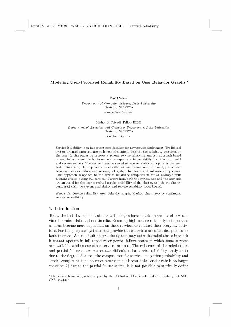
Fig. 1. User-based service reliability modeling
Figure 1 shows a high level view of service reliability from the user’s perspective.
It contains three levels: user model, a set of service models, and the system model.
The user model contains user behavior in a user session, such as issuing different
tasks/requests, thinking, or retrying after a failed task. The system model includes
the failure/recovery behavior of its resources. The service models are derived from
the system model and requirement of tasks (such as system resources needed by
the task, and the work requirement of the task). Task execution in the system
is captured by the service models. Using this approach, we not only model the
service reliability for individual tasks, but also take into consideration dependencies
between different user tasks, and the user interactions with the system.
Some research related to service reliability modeling has been conducted. One
class of such research is on the concepts and quantitative statements for service re-
liability engineering. In 29 the service reliability theory as well as the failure modes
and failure mechanisms for services are presented. In 13 the customer-oriented defi-
nitions of availability and reliability are developed for switched telecommunication
services. The second class of service reliability research is on the service availability
of various networks or computer systems, such as 9 17 30. The basic approach is
to map service availability to the availability of some system resources or certain
system configurations. In the context of the literature above, service availability
corresponds to the concept of ‘service accessibility’ described in 29, and the ser-
vice continuity for the transactions/tasks is not addressed. The third class focuses
on the modeling of service continuity. It is normally from the task’s perspective,
evaluating the reliability of the task or related measures such as task completion
time. Based on whether or not the system has degradable performance, it can be
further divided into task reliability evaluation without degraded system states such
as 10 11, and evaluation with degraded system states such as 19 27 28 3. The latter
is closely related to the distribution of performability 18 25, which characterizes
the system performance under failures. The last class studies the service reliabil-
April 19, 2009 23:38 WSPC/INSTRUCTION FILE service˙reliability
4
ity by incorporating the user’s behavior. In 15 the user-perceived availability of a
web-based travel agency is evaluated where the user sends multiple requests during
the user session. In 31 the user think state is addressed when modeling the user-
perceived web-server availability. In 20 the various joint availabilities for multiple
user requests are considered.
The research work above focus on various aspects of the service reliability mod-
eling, however, it lacks a methodology to put all parts together to get the overall
service reliability from the user’s perspective. The main contribution of this paper
is summarized as follows:
• propose a general modeling framework for the user perceived service relia-
bility, which integrates both service accessibility and service continuity as
well as user behavior. In the framework, we take into consideration 1) task
execution under degradable systems, 2) dependencies between a sequence
of user tasks, 3) impact of user behavior on service reliability.
• derive equations to compute the service reliability for single task with de-
terministic work requirement, and develop efficient computation method
for user-perceived service reliability for a sequence of user tasks by incor-
porating the user behavior model and service models.
• apply the user-perceived service reliability modeling approach to an ex-
ample cluster system hosting two services. Various factors from both the
system side and the user side that impact the user-perceived service relia-
bility are analyzed.
The rest of the paper is organized as follows: In Section 2 we first present a simple
example to illustrate the basic idea of the service reliability quantification, then in
Section 2.2 we use the technique in 4 to derive the service reliability for single user
task in degradable systems with deterministic work requirement, in Section 2.3 the
approach in Section 2.2 is extended to model the user-perceived service reliability
with multiple user requests, in Section 2.5 the possible extension of the user model is
discussed to allow the modeling of more types of user behavior. Section 3 applies our
service reliability modeling technique to a fault tolerant computer cluster that hosts
two services, and gives the numerical results of the user-perceived service reliability
for the example system. Various factors that influence the user-perceived service
reliability are also analyzed. Section 4 presents the summary and conclusions.
2. Service Reliability Modeling
In this paper we study the following aspects of the user-perceived service relia-
bility: 1) service accessibility – the ability to initiate a transaction in the service
when desired; 2) service continuity – the ability to successfully serve an initiated
transaction till its completion; 3) service re-accessibility – the ability to re-access
the service multiple times after the first access. The concepts of 1) and 2) have
been introduced in 29, and concept 3) has been implied in 20. A service can be in-
April 19, 2009 23:38 WSPC/INSTRUCTION FILE service˙reliability
5
terpreted as requiring certain hardware/software resources in the system to be up.
Given a CTMC model of the system in which the states characterize availabilities of
system resources, a service defines a set of up states of the system in which the ser-
vice is operational. The service accessibility can be captured by the instantaneous
availability defined on the CTMC, which is the probability that the system is in
one of the up states at time t (i.e., the time epoch when the service is accessed).
For systems without degraded states, the service continuity can be captured by the
system reliability, which is the probability that the system stays in up states during
[t, t + x] for a task requiring x units of service time. And the service re-accessibility
is analogous to the joint-availability which is the probability that the system is in
up states at times t1 and t2. However, for systems with degraded states and user
sessions containing multiple tasks or requests, the user-perceived service reliability
is not straight-forward any more to compute.
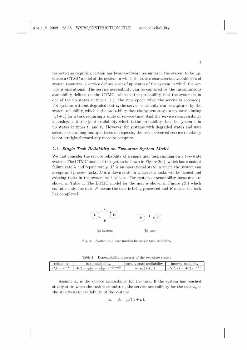
2.1. Single Task Reliability on Two-state System Model
We first consider the service reliability of a single user task running on a two-state
system. The CTMC model of the system is shown in Figure 2(a), which has constant
failure rate λ and repair rate µ. U is an operational state in which the system can
accept and process tasks, D is a down state in which new tasks will be denied and
existing tasks in the system will be lost. The system dependability measures are
shown in Table 1. The DTMC model for the user is shown in Figure 2(b) which
contains only one task. P means the task is being processed and E means the task
has completed.
U Dλ
µ
(a) system
EP 1
(b) user
Fig. 2. System and user models for single task reliability
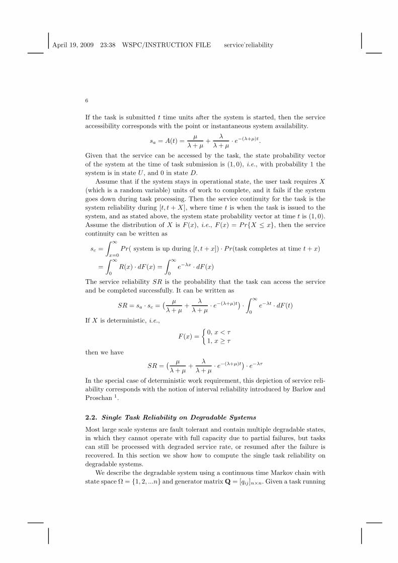
Table 1. Dependability measures of the two-state system
reliability inst. availability. steady-state availability interval reliability
R(t) = e−λt A(t) = µ
λ+µ+ λ
λ+µ· e−(λ+µ)t A=µ/(λ + µ) RI(t, τ) = A(t) · e−λτ
Assume sa is the service accessibility for the task. If the system has reached
steady-state when the task is submitted, the service accessibility for the task sa is
the steady-state availability of the system:
sa = A = µ/(λ + µ).
April 19, 2009 23:38 WSPC/INSTRUCTION FILE service˙reliability
6
If the task is submitted t time units after the system is started, then the service
accessibility corresponds with the point or instantaneous system availability.
sa = A(t) =µ
λ + µ+
λ
λ + µ· e−(λ+µ)t.
Given that the service can be accessed by the task, the state probability vector
of the system at the time of task submission is (1, 0), i.e., with probability 1 the
system is in state U , and 0 in state D.
Assume that if the system stays in operational state, the user task requires X
(which is a random variable) units of work to complete, and it fails if the system
goes down during task processing. Then the service continuity for the task is the
system reliability during [t, t + X ], where time t is when the task is issued to the
system, and as stated above, the system state probability vector at time t is (1, 0).
Assume the distribution of X is F (x), i.e., F (x) = PrX ≤ x, then the service
continuity can be written as
sc =
∫ ∞
x=0
Pr( system is up during [t, t + x]) · Pr(task completes at time t + x)
=
∫ ∞
0
R(x) · dF (x) =
∫ ∞
0
e−λx · dF (x)
The service reliability SR is the probability that the task can access the service
and be completed successfully. It can be written as
SR = sa · sc =( µ
λ + µ+
λ
λ + µ· e−(λ+µ)t
)
·
∫ ∞
0
e−λt · dF (t)
If X is deterministic, i.e.,
F (x) =
0, x < τ
1, x ≥ τ
then we have
SR =( µ
λ + µ+
λ
λ + µ· e−(λ+µ)t
)
· e−λτ
In the special case of deterministic work requirement, this depiction of service reli-
ability corresponds with the notion of interval reliability introduced by Barlow and
Proschan 1.
2.2. Single Task Reliability on Degradable Systems
Most large scale systems are fault tolerant and contain multiple degradable states,
in which they cannot operate with full capacity due to partial failures, but tasks
can still be processed with degraded service rate, or resumed after the failure is
recovered. In this section we show how to compute the single task reliability on
degradable systems.
We describe the degradable system using a continuous time Markov chain with
state space Ω = 1, 2, ...n and generator matrix Q = [qij ]n×n. Given a task running
April 19, 2009 23:38 WSPC/INSTRUCTION FILE service˙reliability
7
on the system, Ω is divided into three sets: fully operational states U , in which the
task is processed by the system with full capacity; degraded states O, in which the
task is processed with less service rate but the work done so far will not be lost;
down states D, in which the work is lost and the task is considered failed. Note that
the task execution policy we considered in this paper is prs (preemptive resume) 7,
while the pri (preemptive repeat identical) and prd (preemptive repeat different)
policies 7 are beyond the scope of this paper. Assume there are totally m states in
either U or O, and therefore n−m states in D. Each state i is assigned a reward rate
ri denoting the production capacity in that state, i.e., if the system stays in state
i for t time units, then the amount of work done in that state is rit. For simplicity,
we assume ri = 1 for i ∈ U , then 0 ≤ ri < 1 for i ∈ O, and ri = 0 for i ∈ D. Let π0
be the state probability vector of the system when the task is initially submitted.
Assume the task requires a fixed τ units of work (which means it will be com-
pleted in τ time units if the system stays in fully operational states), then the task
reliability is the probability that the accumulated reward is greater than or equal to
τ before the system enters one of the down states 18, and it can be quantified using
exact solution methods such as 22 24 27. However these methods are complicated
and in most cases do not scale to large systems.
In this paper we adopt a different approach which uses Erlang distribution to
approximate deterministic distribution to compute the task reliability. As shown
in 23 and 26, a deterministic distribution with parameter τ can be approximated
using a k-stage Erlang distribution with pdf f(t; k, λ) = λktk−1e−λt/(k− 1)! where
λ = k/τ is the rate parameter. It approaches the deterministic distribution as
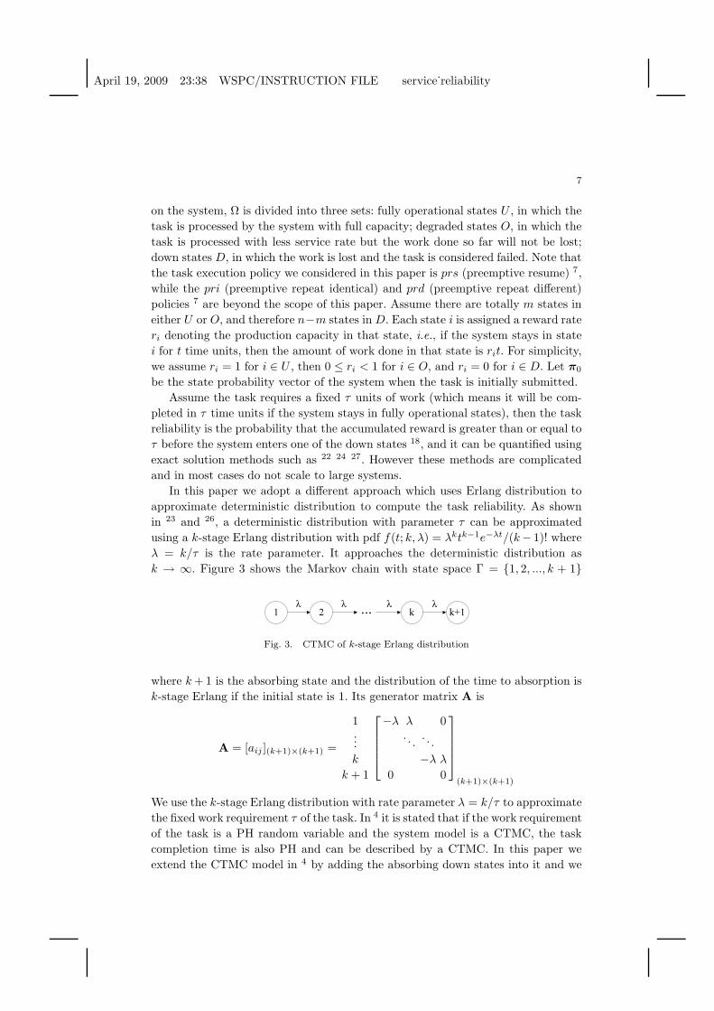
k → ∞. Figure 3 shows the Markov chain with state space Γ = 1, 2, ..., k + 1
1 2 k... k+1λ λ λ λ
Fig. 3. CTMC of k-stage Erlang distribution
where k + 1 is the absorbing state and the distribution of the time to absorption is
k-stage Erlang if the initial state is 1. Its generator matrix A is
A = [aij ](k+1)×(k+1) =
1...
k
k + 1
−λ λ 0. . .
. . .
−λ λ
0 0
(k+1)×(k+1)
We use the k-stage Erlang distribution with rate parameter λ = k/τ to approximate
the fixed work requirement τ of the task. In 4 it is stated that if the work requirement
of the task is a PH random variable and the system model is a CTMC, the task
completion time is also PH and can be described by a CTMC. In this paper we
extend the CTMC model in 4 by adding the absorbing down states into it and we
April 19, 2009 23:38 WSPC/INSTRUCTION FILE service˙reliability
8
call it service model from now on. For better presentation of the service model, we
first reorder the states in Ω of the system model by moving the m states in U ∪O to
the front. Assume the new ordered state space is Ω = s1, s2, ..., sm, sm+1, ..., sn,
where the first m states are either fully operational states or degraded states, and
the last n−m states are down states. (s1, s2, ..., sn) is a permutation of (1, 2, ..., n).
Assume the permutation matrix is E, then
(1, 2, ..., n) = (s1, s2, ..., sn)E, and (s1, s2, ..., sn) = (1, 2, ..., n)ET
where ET is the transpose of E. After reordering the states in Ω, the generator
matrix of the system model is
Q = E · Q · ET =
[
Q1 Q2
Q3 Q4
]
n×n
where Q1 is a m × m sub-matrix that contains transition rates within states in
U ∪ O, and Q2 is a m × (n − m) sub-matrix that contains transition rates from
U ∪ O to D. Define the diagonal matrix R = diag[rs1, rs2
, ..., rsm] where rsi
is the
reward rate assigned to state si.
Based on the results in 4, the service model can be constructed from A and Q
as follows: each not-down state si(1 ≤ i ≤ m) in the system model is expanded
into a cluster of k + 1 states (si, j)|1 ≤ j ≤ k + 1, where (si, j) means the
system is in state si and the task has reached the jth stage. The service model also
contains n−m down states sm+1, ..., sn, thus having mk+n states in total. Of the
mk + n states, (si, j)|1 ≤ i ≤ m, 1 ≤ j ≤ k are transient states, (si, k + 1)|1 ≤
i ≤ m are absorbing states representing task completion, and sm+1, ..., sn are
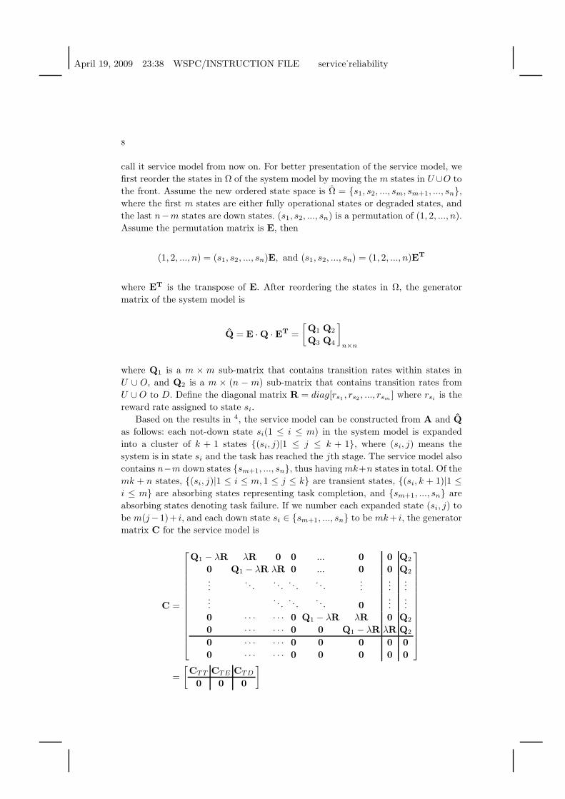
absorbing states denoting task failure. If we number each expanded state (si, j) to
be m(j−1)+ i, and each down state si ∈ sm+1, ..., sn to be mk+ i, the generator
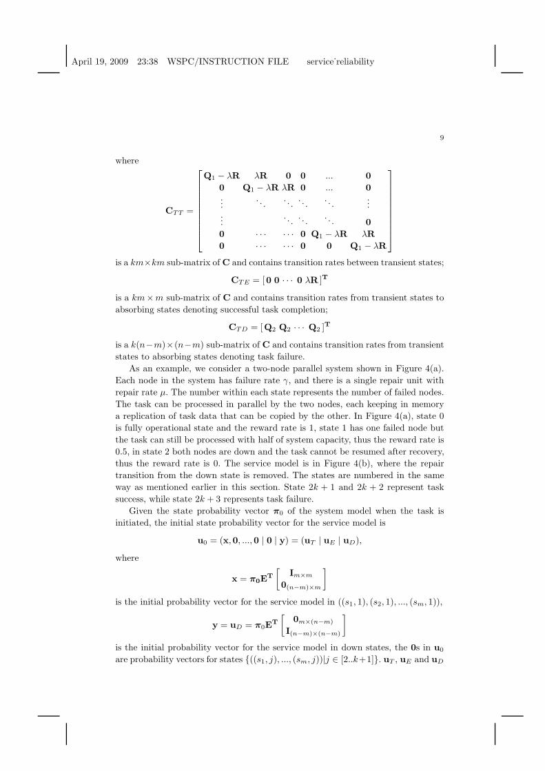
matrix C for the service model is
C =
Q1 − λR λR 0 0 ... 0 0 Q2
0 Q1 − λR λR 0 ... 0 0 Q2
.... . .
. . .. . .
. . ....
......
.... . .
. . .. . . 0
......
0 · · · · · · 0 Q1 − λR λR 0 Q2
0 · · · · · · 0 0 Q1 − λR λR Q2
0 · · · · · · 0 0 0 0 0
0 · · · · · · 0 0 0 0 0
=
[
CTT CTE CTD
0 0 0
]
April 19, 2009 23:38 WSPC/INSTRUCTION FILE service˙reliability
9
where
CTT =
Q1 − λR λR 0 0 ... 0
0 Q1 − λR λR 0 ... 0...
. . .. . .
. . .. . .
......
. . .. . .
. . . 0
0 · · · · · · 0 Q1 − λR λR
0 · · · · · · 0 0 Q1 − λR
is a km×km sub-matrix of C and contains transition rates between transient states;
CTE = [0 0 · · · 0 λR ]T
is a km×m sub-matrix of C and contains transition rates from transient states to
absorbing states denoting successful task completion;
CTD = [Q2 Q2 · · · Q2 ]T
is a k(n−m)×(n−m) sub-matrix of C and contains transition rates from transient
states to absorbing states denoting task failure.
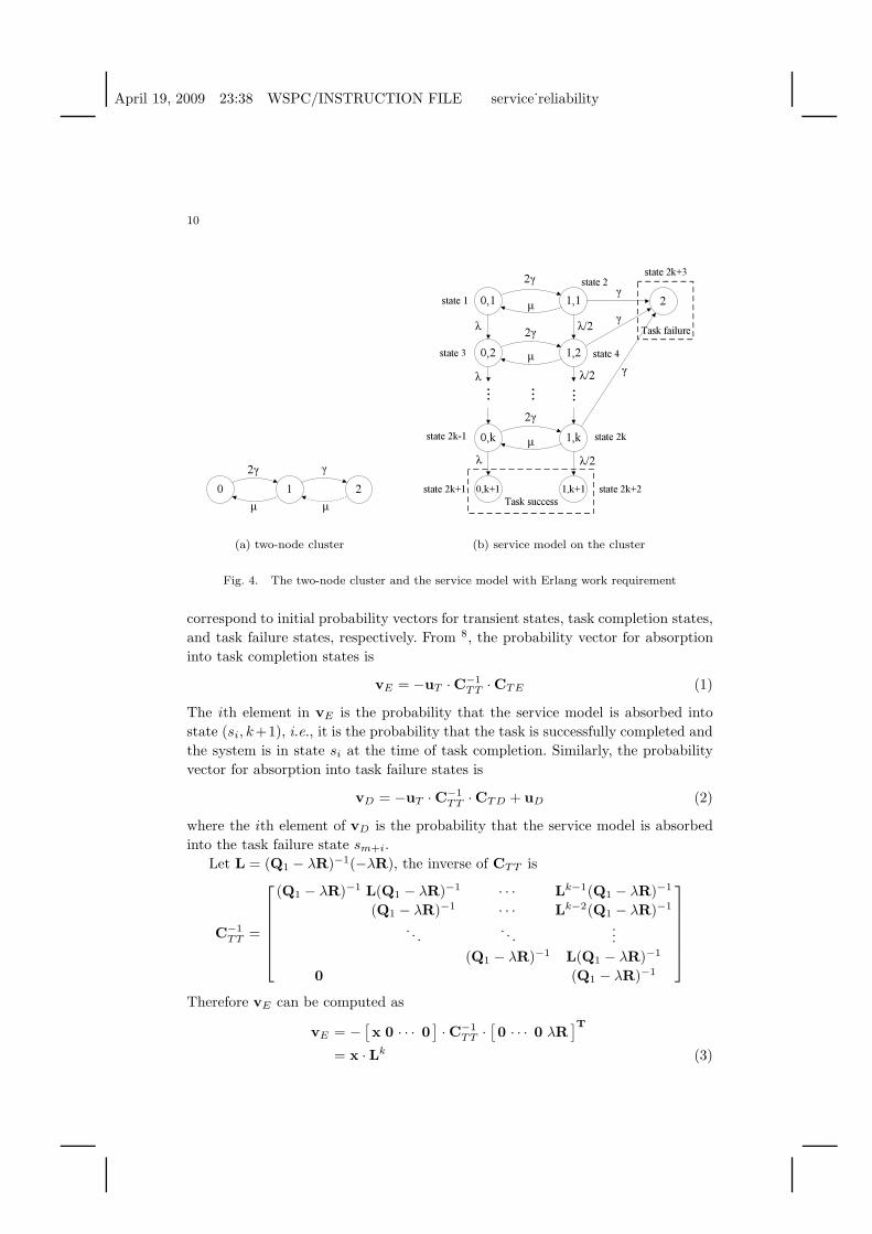
As an example, we consider a two-node parallel system shown in Figure 4(a).
Each node in the system has failure rate γ, and there is a single repair unit with
repair rate µ. The number within each state represents the number of failed nodes.
The task can be processed in parallel by the two nodes, each keeping in memory
a replication of task data that can be copied by the other. In Figure 4(a), state 0
is fully operational state and the reward rate is 1, state 1 has one failed node but
the task can still be processed with half of system capacity, thus the reward rate is
0.5, in state 2 both nodes are down and the task cannot be resumed after recovery,
thus the reward rate is 0. The service model is in Figure 4(b), where the repair
transition from the down state is removed. The states are numbered in the same
way as mentioned earlier in this section. State 2k + 1 and 2k + 2 represent task
success, while state 2k + 3 represents task failure.
Given the state probability vector π0 of the system model when the task is
initiated, the initial state probability vector for the service model is
u0 = (x,0, ...,0 | 0 | y) = (uT | uE | uD),
where
x = π0ET
[
Im×m
0(n−m)×m
]
is the initial probability vector for the service model in ((s1, 1), (s2, 1), ..., (sm, 1)),
y = uD = π0ET
[
0m×(n−m)
I(n−m)×(n−m)
]
is the initial probability vector for the service model in down states, the 0s in u0
are probability vectors for states ((s1, j), ..., (sm, j))|j ∈ [2..k+1]. uT , uE and uD
April 19, 2009 23:38 WSPC/INSTRUCTION FILE service˙reliability
10
0 1 22γ γ
µ µ
(a) two-node cluster
0,1 1,1 2
0,2 1,2
0,k 1,k
...
...
...
0,k+1 1,k+1Task success
Task failure
state 1state 2
state 3
state 2k-1
state 4
state 2k
state 2k+1 state 2k+2
state 2k+32γ
2γ
2γ
µ
µ
µ
λ
λ
λ
λ/2
λ/2
λ/2
γγ
γ
(b) service model on the cluster
Fig. 4. The two-node cluster and the service model with Erlang work requirement
correspond to initial probability vectors for transient states, task completion states,
and task failure states, respectively. From 8, the probability vector for absorption
into task completion states is
vE = −uT ·C−1TT ·CTE (1)
The ith element in vE is the probability that the service model is absorbed into
state (si, k+1), i.e., it is the probability that the task is successfully completed and
the system is in state si at the time of task completion. Similarly, the probability
vector for absorption into task failure states is
vD = −uT · C−1TT ·CTD + uD (2)
where the ith element of vD is the probability that the service model is absorbed
into the task failure state sm+i.
Let L = (Q1 − λR)−1(−λR), the inverse of CTT is
C−1TT =
(Q1 − λR)−1 L(Q1 − λR)−1 · · · Lk−1(Q1 − λR)−1
(Q1 − λR)−1 · · · Lk−2(Q1 − λR)−1
. . .. . .
...
(Q1 − λR)−1 L(Q1 − λR)−1
0 (Q1 − λR)−1
Therefore vE can be computed as
vE = −[
x 0 · · · 0]
· C−1TT ·
[
0 · · · 0 λR]T
= x · Lk (3)
April 19, 2009 23:38 WSPC/INSTRUCTION FILE service˙reliability
11
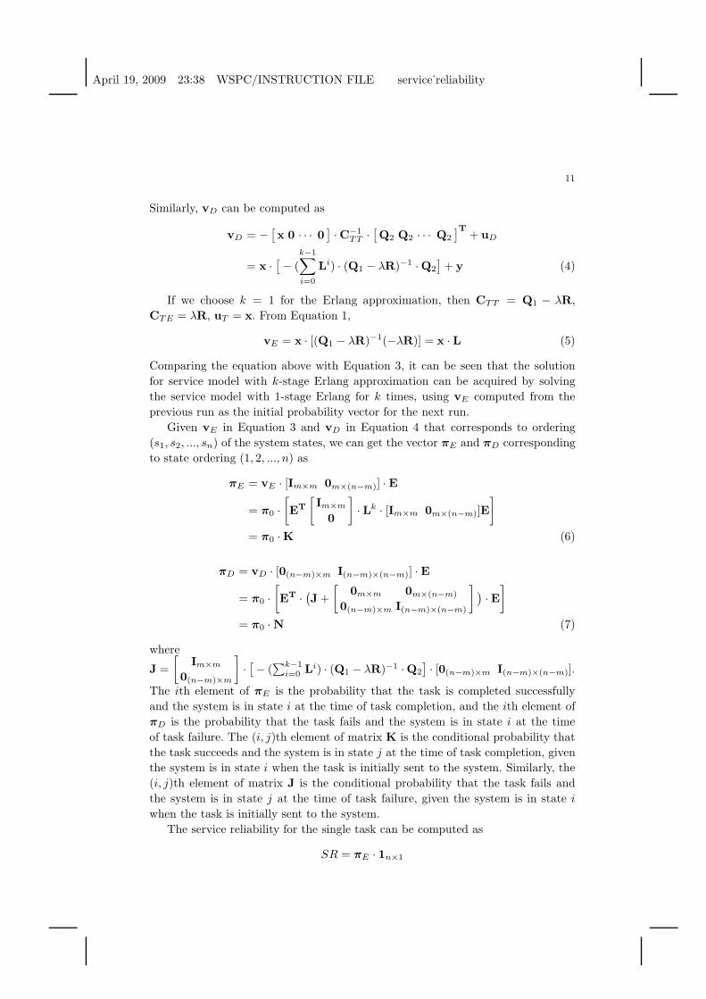
Similarly, vD can be computed as
vD = −[
x 0 · · · 0]
·C−1TT ·
[
Q2 Q2 · · · Q2
]T+ uD
= x ·[
− (
k−1∑
i=0
Li) · (Q1 − λR)−1 ·Q2
]
+ y (4)
If we choose k = 1 for the Erlang approximation, then CTT = Q1 − λR,
CTE = λR, uT = x. From Equation 1,
vE = x · [(Q1 − λR)−1(−λR)] = x · L (5)
Comparing the equation above with Equation 3, it can be seen that the solution
for service model with k-stage Erlang approximation can be acquired by solving
the service model with 1-stage Erlang for k times, using vE computed from the
previous run as the initial probability vector for the next run.
Given vE in Equation 3 and vD in Equation 4 that corresponds to ordering
(s1, s2, ..., sn) of the system states, we can get the vector πE and πD corresponding
to state ordering (1, 2, ..., n) as
πE = vE · [Im×m 0m×(n−m)] · E
= π0 ·
[
ET
[
Im×m
0
]
· Lk · [Im×m 0m×(n−m)]E
]
= π0 ·K (6)
πD = vD · [0(n−m)×m I(n−m)×(n−m)] · E
= π0 ·
[
ET ·(
J +
[
0m×m 0m×(n−m)
0(n−m)×m I(n−m)×(n−m)
]
)
·E
]
= π0 · N (7)
where
J =
[
Im×m
0(n−m)×m
]
·[
− (∑k−1
i=0 Li) · (Q1 − λR)−1 ·Q2
]
· [0(n−m)×m I(n−m)×(n−m)].
The ith element of πE is the probability that the task is completed successfully
and the system is in state i at the time of task completion, and the ith element of
πD is the probability that the task fails and the system is in state i at the time
of task failure. The (i, j)th element of matrix K is the conditional probability that
the task succeeds and the system is in state j at the time of task completion, given
the system is in state i when the task is initially sent to the system. Similarly, the
(i, j)th element of matrix J is the conditional probability that the task fails and
the system is in state j at the time of task failure, given the system is in state i
when the task is initially sent to the system.
The service reliability for the single task can be computed as
SR = πE · 1n×1
April 19, 2009 23:38 WSPC/INSTRUCTION FILE service˙reliability
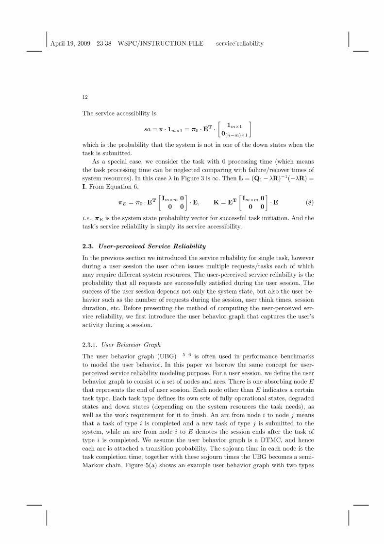
12
The service accessibility is
sa = x · 1m×1 = π0 · ET ·
[
1m×1
0(n−m)×1
]
which is the probability that the system is not in one of the down states when the
task is submitted.
As a special case, we consider the task with 0 processing time (which means
the task processing time can be neglected comparing with failure/recover times of
system resources). In this case λ in Figure 3 is ∞. Then L = (Q1−λR)−1(−λR) =
I. From Equation 6,
πE = π0 ·ET
[
Im×m 0
0 0
]
·E, K = ET
[
Im×m 0
0 0
]
· E (8)
i.e., πE is the system state probability vector for successful task initiation. And the
task’s service reliability is simply its service accessibility.
2.3. User-perceived Service Reliability
In the previous section we introduced the service reliability for single task, however
during a user session the user often issues multiple requests/tasks each of which
may require different system resources. The user-perceived service reliability is the
probability that all requests are successfully satisfied during the user session. The
success of the user session depends not only the system state, but also the user be-
havior such as the number of requests during the session, user think times, session
duration, etc. Before presenting the method of computing the user-perceived ser-
vice reliability, we first introduce the user behavior graph that captures the user’s
activity during a session.
2.3.1. User Behavior Graph
The user behavior graph (UBG) 5 6 is often used in performance benchmarks
to model the user behavior. In this paper we borrow the same concept for user-
perceived service reliability modeling purpose. For a user session, we define the user
behavior graph to consist of a set of nodes and arcs. There is one absorbing node E
that represents the end of user session. Each node other than E indicates a certain
task type. Each task type defines its own sets of fully operational states, degraded
states and down states (depending on the system resources the task needs), as
well as the work requirement for it to finish. An arc from node i to node j means
that a task of type i is completed and a new task of type j is submitted to the
system, while an arc from node i to E denotes the session ends after the task of
type i is completed. We assume the user behavior graph is a DTMC, and hence
each arc is attached a transition probability. The sojourn time in each node is the
task completion time, together with these sojourn times the UBG becomes a semi-
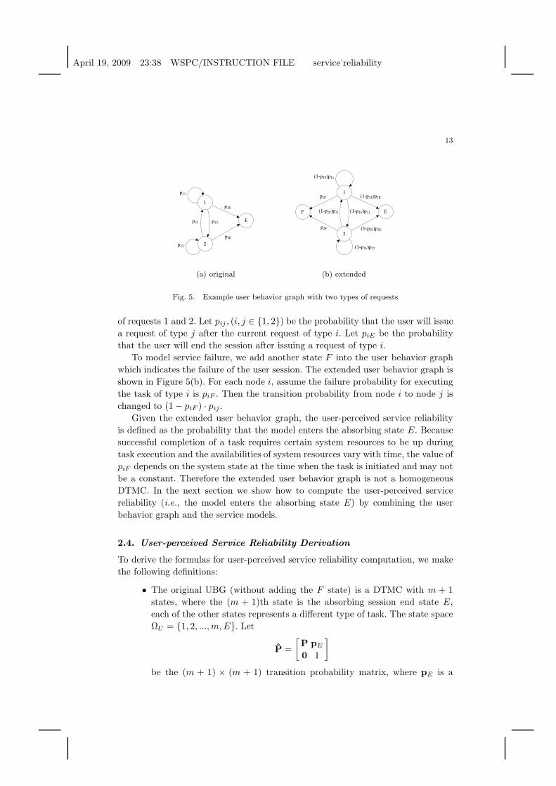
Markov chain. Figure 5(a) shows an example user behavior graph with two types
April 19, 2009 23:38 WSPC/INSTRUCTION FILE service˙reliability
13
1
2
p11
Ep12
p1E
p22
p21
p2E
(a) original
1
2
(1-p1F)p11
E(1-p1F)p12
(1-p1F)p1E
(1-p2F)p22
(1-p2F)p21
(1-p2F)p2E
F
p1F
p2F
(b) extended
Fig. 5. Example user behavior graph with two types of requests
of requests 1 and 2. Let pij , (i, j ∈ 1, 2) be the probability that the user will issue
a request of type j after the current request of type i. Let piE be the probability
that the user will end the session after issuing a request of type i.
To model service failure, we add another state F into the user behavior graph
which indicates the failure of the user session. The extended user behavior graph is
shown in Figure 5(b). For each node i, assume the failure probability for executing
the task of type i is piF . Then the transition probability from node i to node j is
changed to (1 − piF ) · pij .
Given the extended user behavior graph, the user-perceived service reliability
is defined as the probability that the model enters the absorbing state E. Because
successful completion of a task requires certain system resources to be up during
task execution and the availabilities of system resources vary with time, the value of
piF depends on the system state at the time when the task is initiated and may not
be a constant. Therefore the extended user behavior graph is not a homogeneous
DTMC. In the next section we show how to compute the user-perceived service
reliability (i.e., the model enters the absorbing state E) by combining the user
behavior graph and the service models.
2.4. User-perceived Service Reliability Derivation
To derive the formulas for user-perceived service reliability computation, we make
the following definitions:
• The original UBG (without adding the F state) is a DTMC with m + 1
states, where the (m + 1)th state is the absorbing session end state E,
each of the other states represents a different type of task. The state space
ΩU = 1, 2, ..., m, E. Let
P =
[
P pE
0 1
]
be the (m + 1) × (m + 1) transition probability matrix, where pE is a
April 19, 2009 23:38 WSPC/INSTRUCTION FILE service˙reliability
14
column vector whose ith element is piE . P = (p1,p2, ...,pm) is m × m
transition probability sub-matrix for the first m states, and pi, i ∈ [1..m]
are column vectors. The initial probability vector when the session begins
is v0 = (v1, v2, ..., vm, vE).
• The system model is a CTMC with state space ΩS = 1, 2, ..., n and
generator matrix Q. The initial probability vector at the beginning of the
session is π0 = (π1, π2, ..., πn).
As defined in Section 2.2, Each task type i in the user model has its own sets of fully
operational states Ui, degraded states Oi and down states Di in the system model,
as well as the reward rates for each system state. Therefore as shown in Equation
6, each state i of the user model corresponds to a matrix Ki, in which the (j, k)th
element of Ki is the probability that the task of type i completes successfully and
the system is in state k at the time the task ends, given that the system is in state
j when the task is initiated.
Given the user behavior graph and matrices Ki (i ∈ [1..m]) for each user state,
we build the DTMC that can be used to compute the user-perceived service relia-
bility. The DTMC has one absorbing state E that represents user session success,
and one absorbing state F representing user session failure. For any other state, we
label it using a 2-tuple (i, j) which means the system is in state j ∈ [1..n] when a
task of type i ∈ [1..m] is initiated in the system. Then we have the following state
transition probabilities:
(i, j) → (x, y) : k(i)jy · pix
(i, j) → E :n
∑
y=1
k(i)jy · piE
(i, j) → F : 1 −n
∑
y=1
k(i)jy
And the initial probability for state (i, j) is vi · πj . If we number state (i, j) as
(i−1)∗n+ j, E as mn+1 and F as mn+2, then the transition probability matrix
is
M =
p11K1 p12K1 · · · p1mK1 p1EK1 · 1 1 − K1 · 1
p21K2 p22K2 · · · p2mK2 p2EK2 · 1 1 − K2 · 1... · · · · · ·
...
pm1Km pm2Km · · · pmmKm pmEKm · 1 1 − Km · 1
01×mn 1 0
01×mn 0 1
=
Smn×mn αmn×1 βmn×1
01×mn 1 0
01×mn 0 1
April 19, 2009 23:38 WSPC/INSTRUCTION FILE service˙reliability
15
and the initial probability vector is
u(0) = (uT (0), uE(0), uF (0)) = (uT (0), 0, 0)
where uT (0) = (u1(0),u2(0), · · · ,um(0)) and uj(0) = (vjπ1, vjπ2, ..., vjπn) is the
initial probability vector for states (j, 1), (j, 2), · · · , (j, n).
If we use u(k) to represent the state probability vector after the kth transition,
we have
u(k) = u(k − 1) ·M (9)
Therefore
uT (k) = uT (k − 1) · S, and uj(k) =
m∑
i=1
pij · ui(k − 1)Ki
We can rewrite uT (k) in matrix form as follows:
uT (k) =
u1(k)
u2(k)...
um(k)
= PT ·
u1(k − 1) ·K1
u2(k − 1) ·K2
...
um(k − 1) ·Km
(10)
The equation above takes O(m2n + mn2) time to compute.
From Equation 9, uE(k) = uE(k − 1) + uT (k − 1) · α, and the user-perceived
service reliability is
SR = uE(∞) =∞∑
k=0
uT (k) · α (11)
2.5. Modeling More General User Behavior
In Section 2.4 we derived the user-perceived service reliability by assuming the
work requirement of each task is deterministic and each state in the user model
corresponds to a task type. In this section we discuss some extensions of the models
used in the derivation to allow the modeling of more general user behavior.
First, the work requirement of each task does not need to be deterministic, it
can be of any PH-type distribution such that the techniques in 4 can be applied
to construct the service model, and Equation 1 can still be used to compute the
transition probability matrix K. The difference between Equation 1 and Equation
6 (which is for the case of Erlang distribution) is that the former needs to solve a
larger service model thus manipulating a larger matrix.
Second, in Section 2, for simplicity we assumed that each state i of the UBG
represents user sending a task of type i, however it can also represent other user
behavior as long as we can get the transition probability matrix Ki, in which the
(j, k)th element is the probability that the system is in state k when the UBG leaves
state i, given the system is in state j when the UBG enters state i.
April 19, 2009 23:38 WSPC/INSTRUCTION FILE service˙reliability
16
As an example, a UBG state i can represent a user think state, in which all
states in the system model are fully operational states. Assume the thinking time
distribution is Θ(t), the transition probability matrix Ki is
Ki =
∫ ∞
t=0
eQtdΘ(t)
where Q is the generator matrix of the system model. Specifically, if the user think
time is deterministic with parameter θ, then
Ki = eQθ (12)
If Θ(t) is a PH distribution, the method in Section 2.2 can be used to compute Ki.
Especially if Θ(t) is exponentially distributed with rate λ, then
Ki =
∫ ∞
t=0
eQtd(1 − e−λt) = (I −Q
λ)−1 (13)
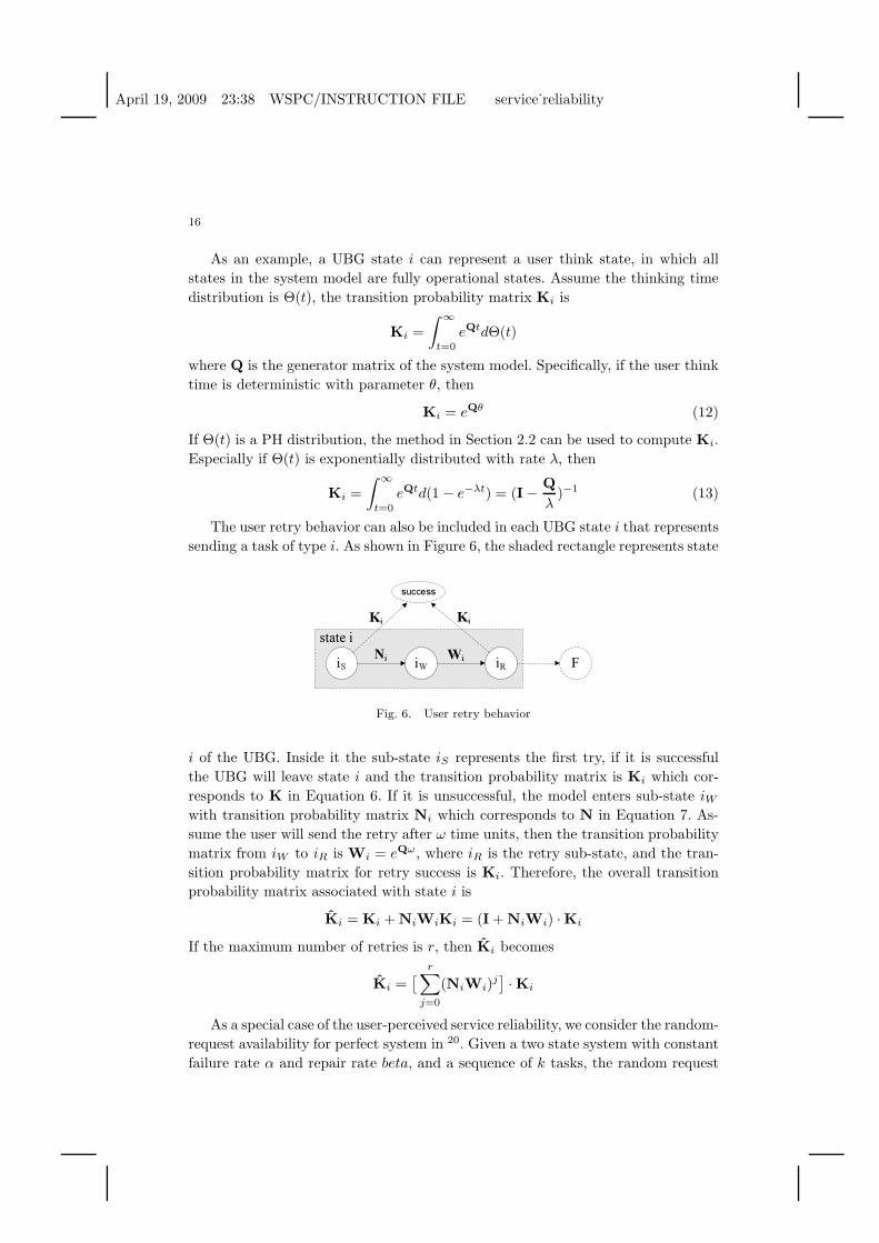
The user retry behavior can also be included in each UBG state i that represents
sending a task of type i. As shown in Figure 6, the shaded rectangle represents state
iS iW iR
success
F
Ki
Ni Wi
Ki
state i
Fig. 6. User retry behavior
i of the UBG. Inside it the sub-state iS represents the first try, if it is successful
the UBG will leave state i and the transition probability matrix is Ki which cor-
responds to K in Equation 6. If it is unsuccessful, the model enters sub-state iWwith transition probability matrix Ni which corresponds to N in Equation 7. As-
sume the user will send the retry after ω time units, then the transition probability
matrix from iW to iR is Wi = eQω, where iR is the retry sub-state, and the tran-
sition probability matrix for retry success is Ki. Therefore, the overall transition
probability matrix associated with state i is
Ki = Ki + NiWiKi = (I + NiWi) ·Ki
If the maximum number of retries is r, then Ki becomes
Ki =[
r∑
j=0
(NiWi)j]
· Ki
As a special case of the user-perceived service reliability, we consider the random-
request availability for perfect system in 20. Given a two state system with constant
failure rate α and repair rate beta, and a sequence of k tasks, the random request
April 19, 2009 23:38 WSPC/INSTRUCTION FILE service˙reliability
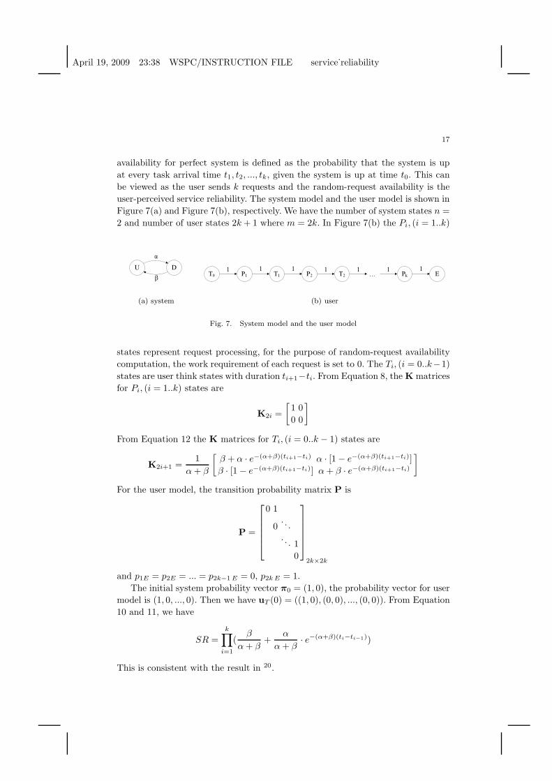
17
availability for perfect system is defined as the probability that the system is up
at every task arrival time t1, t2, ..., tk, given the system is up at time t0. This can
be viewed as the user sends k requests and the random-request availability is the
user-perceived service reliability. The system model and the user model is shown in
Figure 7(a) and Figure 7(b), respectively. We have the number of system states n =
2 and number of user states 2k + 1 where m = 2k. In Figure 7(b) the Pi, (i = 1..k)
U Dα
β
(a) system
P1 T1 P2 T2 ... Pk E1 1 1 1 1 1
T01
(b) user
Fig. 7. System model and the user model
states represent request processing, for the purpose of random-request availability
computation, the work requirement of each request is set to 0. The Ti, (i = 0..k−1)
states are user think states with duration ti+1−ti. From Equation 8, the K matrices
for Pi, (i = 1..k) states are
K2i =
[
1 0
0 0
]
From Equation 12 the K matrices for Ti, (i = 0..k − 1) states are
K2i+1 =1
α + β
[
β + α · e−(α+β)(ti+1−ti) α · [1 − e−(α+β)(ti+1−ti)]
β · [1 − e−(α+β)(ti+1−ti)] α + β · e−(α+β)(ti+1−ti)
]
For the user model, the transition probability matrix P is
P =
0 1
0. . .
. . . 1
0
2k×2k
and p1E = p2E = ... = p2k−1 E = 0, p2k E = 1.
The initial system probability vector π0 = (1, 0), the probability vector for user
model is (1, 0, ..., 0). Then we have uT (0) = ((1, 0), (0, 0), ..., (0, 0)). From Equation
10 and 11, we have
SR =
k∏
i=1
(β
α + β+
α
α + β· e−(α+β)(ti−ti−1))
This is consistent with the result in 20.
April 19, 2009 23:38 WSPC/INSTRUCTION FILE service˙reliability
18
3. A Numerical Example
In this section we apply the service reliability modeling technique to a cluster
hosting two stateless services, which could be web services, SOA services, database
services, etc.
3.1. System and User models
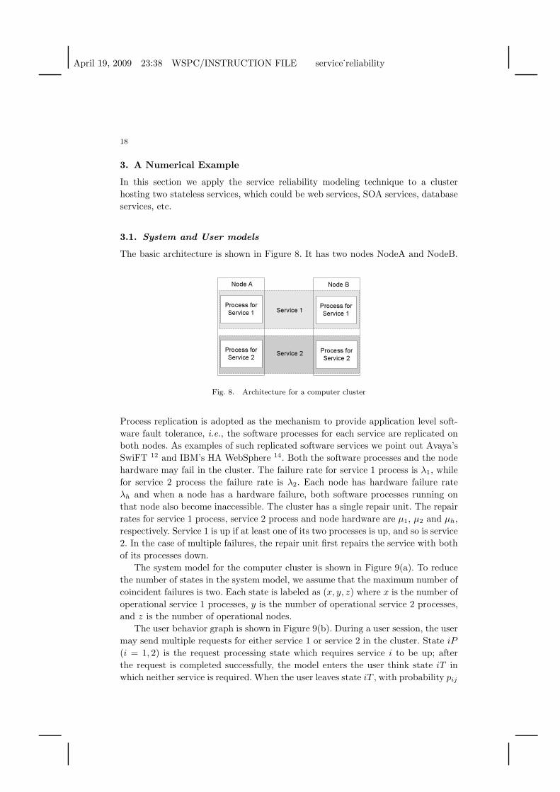
The basic architecture is shown in Figure 8. It has two nodes NodeA and NodeB.
Process for Service 1
Node A Node B
Process for Service 1Service 1
Service 2Process for Service 2
Process for Service 2
Fig. 8. Architecture for a computer cluster
Process replication is adopted as the mechanism to provide application level soft-
ware fault tolerance, i.e., the software processes for each service are replicated on
both nodes. As examples of such replicated software services we point out Avaya’s
SwiFT 12 and IBM’s HA WebSphere 14. Both the software processes and the node
hardware may fail in the cluster. The failure rate for service 1 process is λ1, while
for service 2 process the failure rate is λ2. Each node has hardware failure rate
λh and when a node has a hardware failure, both software processes running on
that node also become inaccessible. The cluster has a single repair unit. The repair
rates for service 1 process, service 2 process and node hardware are µ1, µ2 and µh,
respectively. Service 1 is up if at least one of its two processes is up, and so is service
2. In the case of multiple failures, the repair unit first repairs the service with both
of its processes down.
The system model for the computer cluster is shown in Figure 9(a). To reduce
the number of states in the system model, we assume that the maximum number of
coincident failures is two. Each state is labeled as (x, y, z) where x is the number of
operational service 1 processes, y is the number of operational service 2 processes,
and z is the number of operational nodes.
The user behavior graph is shown in Figure 9(b). During a user session, the user
may send multiple requests for either service 1 or service 2 in the cluster. State iP
(i = 1, 2) is the request processing state which requires service i to be up; after
the request is completed successfully, the model enters the user think state iT in
which neither service is required. When the user leaves state iT , with probability pij
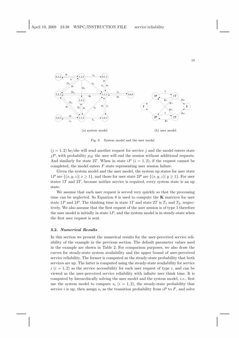
April 19, 2009 23:38 WSPC/INSTRUCTION FILE service˙reliability
19
2,2,2
1,2,2
2,1,2
1,1,1
0,2,2
1,1,2
0,1,1
2,0,2 1,0,1
0,0,0
µ1λ1
2λ1 µ12λh
2λ2µ2
µh
λ2µ2
λh
λh2λ2
2λ1 µ1
λh
λh
λ1
λ2
µ1
µ2
λhµh
(a) system model
1P 1T
2P 2T
EF
p1E
p2E
p11p12
p22
p21
1
1
(b) user model
Fig. 9. System model and the user model
(j = 1, 2) he/she will send another request for service j and the model enters state
jP , with probability piE the user will end the session without additional requests.
And similarly for state 2T . When in state iP (i = 1, 2), if the request cannot be
completed, the model enters F state representing user session failure.
Given the system model and the user model, the system up states for user state
1P are (x, y, z)| x ≥ 1, and those for user state 2P are (x, y, z)| y ≥ 1. For user
states 1T and 2T , because neither service is required, every system state is an up
state.
We assume that each user request is served very quickly so that the processing
time can be neglected. So Equation 8 is used to compute the K matrices for user
state 1P and 2P . The thinking time in state 1T and state 2T is T1 and T2, respec-
tively. We also assume that the first request of the user session is of type 1 therefore
the user model is initially in state 1P , and the system model is in steady-state when
the first user request is sent.
3.2. Numerical Results
In this section we present the numerical results for the user-perceived service reli-
ability of the example in the previous section. The default parameter values used
in the example are shown in Table 2. For comparison purposes, we also draw the
curves for steady-state system availability and the upper bound of user-perceived
service reliability. The former is computed as the steady-state probability that both
services are up. The latter is computed using the steady-state availability for service
i (i = 1, 2) as the service accessibility for each user request of type i, and can be
viewed as the user-perceived service reliability with infinite user think time. It is
computed by hierarchically solving the user model and the system model, i.e., first
use the system model to compute si (i = 1, 2), the steady-state probability that
service i is up, then assign si as the transition probability from iP to F , and solve
April 19, 2009 23:38 WSPC/INSTRUCTION FILE service˙reliability
20
the user model in Figure 9(b) to get the absorption probability in state E.
Table 2. Default parameters used in the example
Parameter Default value Description
1/λ1 168 hours mean time to failure for service 1 process1/λ2 168 hours mean time to failure for service 2 process1/λh 200 hours mean time to failure for node hardware1/µ1 30 minutes mean time to repair service 1 process failure1/µ2 30 minutes mean time to repair service 2 process failure1/µh 1 hour mean time to repair node hardware failureT1 5 minutes user think time in state 1TT2 5 minutes user think time in state 2Tp11 0.4 transition probability from 1T to 1Pp12 0.3 transition probability from 1T to 2Pp1E 0.3 transition probability from 1T to Ep21 0.4 transition probability from 2T to 1P
p22 0.3 transition probability from 2T to 2Pp2E 0.3 transition probability from 2T to E
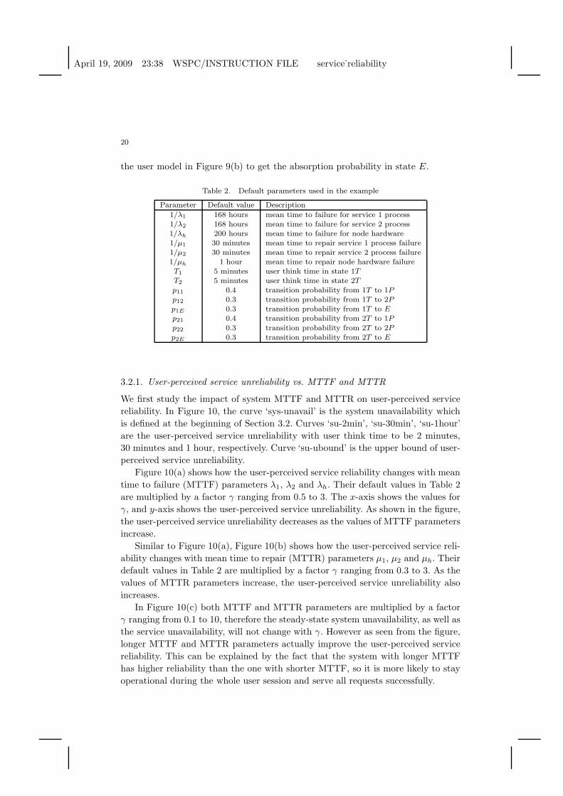
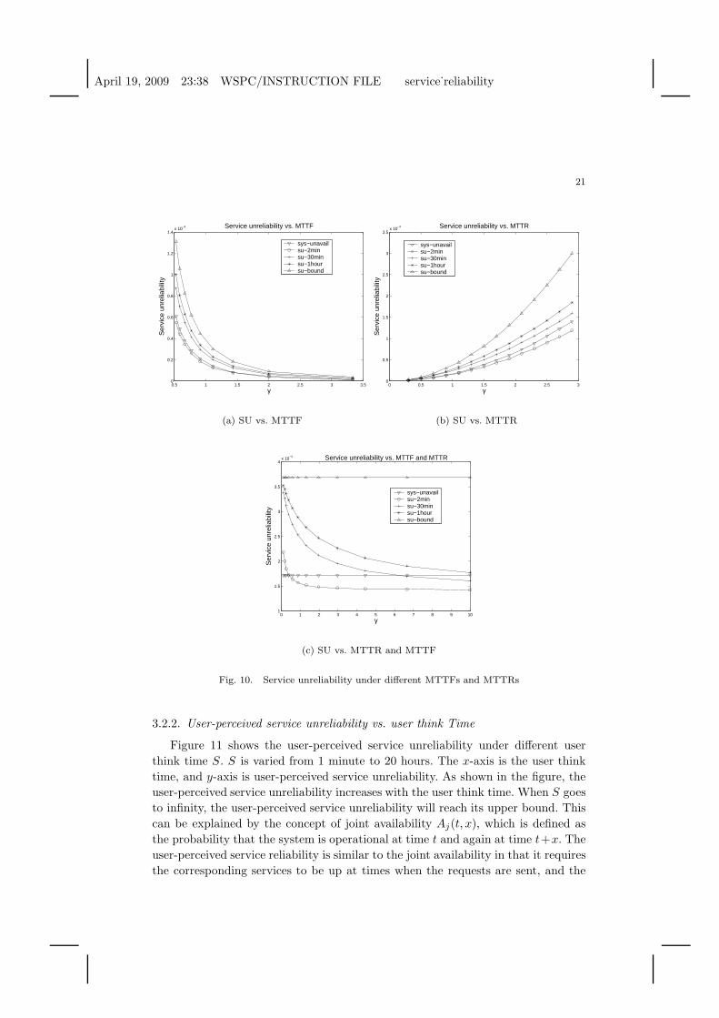
3.2.1. User-perceived service unreliability vs. MTTF and MTTR
We first study the impact of system MTTF and MTTR on user-perceived service
reliability. In Figure 10, the curve ‘sys-unavail’ is the system unavailability which
is defined at the beginning of Section 3.2. Curves ‘su-2min’, ‘su-30min’, ‘su-1hour’
are the user-perceived service unreliability with user think time to be 2 minutes,
30 minutes and 1 hour, respectively. Curve ‘su-ubound’ is the upper bound of user-
perceived service unreliability.
Figure 10(a) shows how the user-perceived service reliability changes with mean
time to failure (MTTF) parameters λ1, λ2 and λh. Their default values in Table 2
are multiplied by a factor γ ranging from 0.5 to 3. The x-axis shows the values for
γ, and y-axis shows the user-perceived service unreliability. As shown in the figure,
the user-perceived service unreliability decreases as the values of MTTF parameters
increase.
Similar to Figure 10(a), Figure 10(b) shows how the user-perceived service reli-
ability changes with mean time to repair (MTTR) parameters µ1, µ2 and µh. Their
default values in Table 2 are multiplied by a factor γ ranging from 0.3 to 3. As the
values of MTTR parameters increase, the user-perceived service unreliability also
increases.
In Figure 10(c) both MTTF and MTTR parameters are multiplied by a factor
γ ranging from 0.1 to 10, therefore the steady-state system unavailability, as well as
the service unavailability, will not change with γ. However as seen from the figure,
longer MTTF and MTTR parameters actually improve the user-perceived service
reliability. This can be explained by the fact that the system with longer MTTF
has higher reliability than the one with shorter MTTF, so it is more likely to stay
operational during the whole user session and serve all requests successfully.
April 19, 2009 23:38 WSPC/INSTRUCTION FILE service˙reliability
21
0.5 1 1.5 2 2.5 3 3.50
0.2
0.4
0.6
0.8
1
1.2
1.4x 10
−3 Service unreliability vs. MTTF
γ
Ser
vice
unr
elia
bilit
y
sys−unavailsu−2minsu−30minsu−1hoursu−bound
(a) SU vs. MTTF
0 0.5 1 1.5 2 2.5 30
0.5
1
1.5
2
2.5
3
3.5x 10
−3 Service unreliability vs. MTTR
γ
Ser
vice
unr
elia
bilit
y
sys−unavailsu−2minsu−30minsu−1hoursu−bound
(b) SU vs. MTTR
0 1 2 3 4 5 6 7 8 9 101
1.5
2
2.5
3
3.5
4x 10
−4 Service unreliability vs. MTTF and MTTR
γ
Ser
vice
unr
elia
bilit
y
sys−unavailsu−2minsu−30minsu−1hoursu−bound
(c) SU vs. MTTR and MTTF
Fig. 10. Service unreliability under different MTTFs and MTTRs
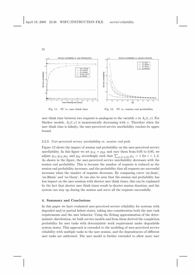
3.2.2. User-perceived service unreliability vs. user think Time
Figure 11 shows the user-perceived service unreliability under different user
think time S. S is varied from 1 minute to 20 hours. The x-axis is the user think
time, and y-axis is user-perceived service unreliability. As shown in the figure, the
user-perceived service unreliability increases with the user think time. When S goes
to infinity, the user-perceived service unreliability will reach its upper bound. This
can be explained by the concept of joint availability Aj(t, x), which is defined as
the probability that the system is operational at time t and again at time t+x. The
user-perceived service reliability is similar to the joint availability in that it requires
the corresponding services to be up at times when the requests are sent, and the
April 19, 2009 23:38 WSPC/INSTRUCTION FILE service˙reliability
22
0 2 4 6 8 10 12 14 16 18 201
1.5
2
2.5
3
3.5
4x 10
−4 Service unreliability vs. user thinking time
User thinking time (hour)
Ser
vice
unr
elia
bilit
y
sys−unavails1−unavails2−unavailservice unrelsu−bound
Fig. 11. SU vs. user think time
0 0.1 0.2 0.3 0.4 0.5 0.6 0.7 0.8 0.9 10
0.5
1
1.5
2
2.5x 10
−3 Service unreliability vs. session end prob.
pES
ervi
ce u
nrel
iabi
lity
su−2minsu−30minsu−1hoursu−bound
Fig. 12. SU vs. session end probability
user think time between two requests is analogous to the variable x in Aj(t, x). For
Markov models, Aj(t, x) is monotonically decreasing with x. Therefore when the
user think time is infinity, the user-perceived service unreliability reaches its upper
bound.
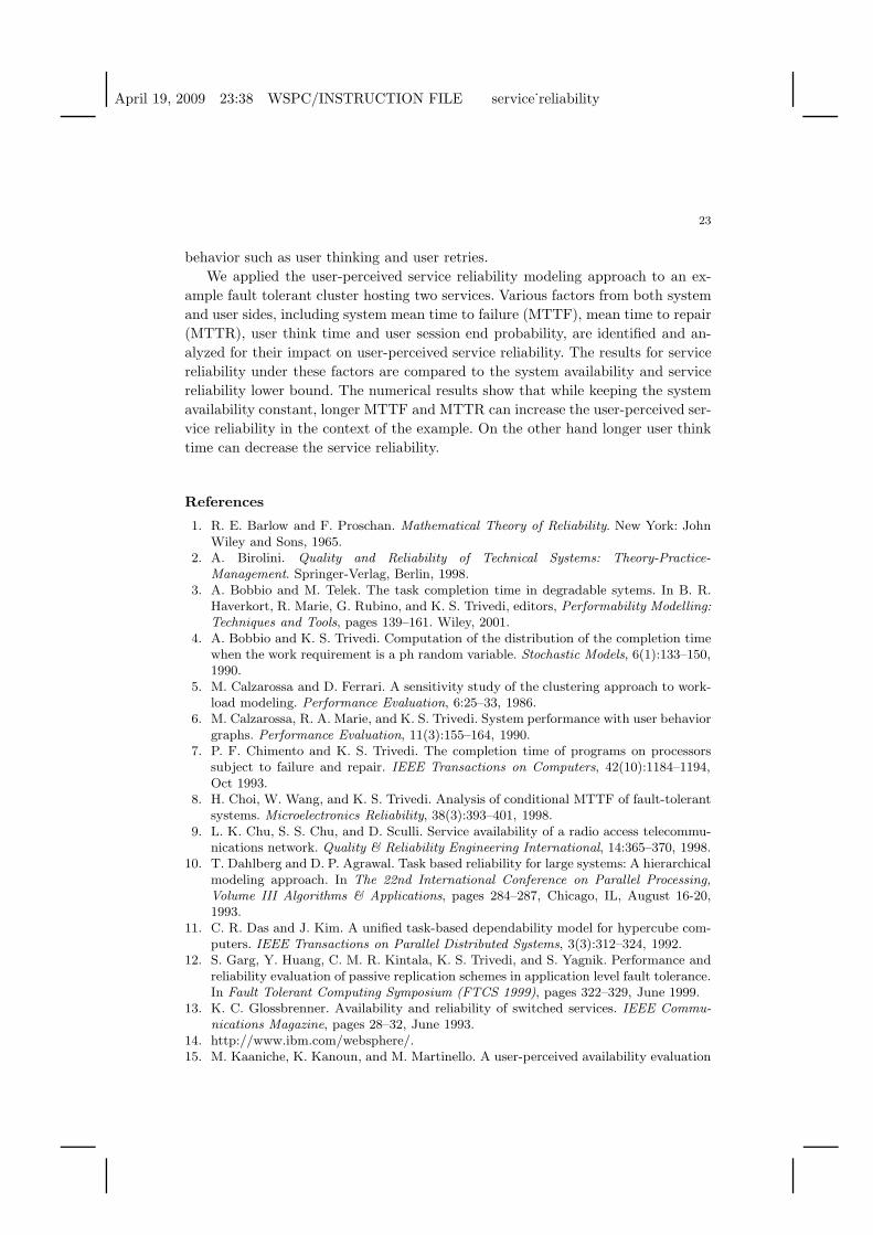
3.2.3. User-perceived service unreliability vs. session end prob.
Figure 12 shows the impact of session end probability on the user-perceived service
unreliability. In this figure we set p1E = p2E and vary them from 0.05 to 0.95, we
adjust p11, p12, p21 and p22 accordingly such that∑
j∈1,2,E pij = 1 for i = 1, 2.
As shown in the figure, the user-perceived service unreliability decreases with the
session end probability. This is because the number of requests is reduced as the
session end probability increases, and the probability that all requests are successful
increases when the number of requests decreases. By comparing curve ‘su-2min’,
‘su-30min’ and ‘su-1hour’, It can also be seen that the session end probability has
less impact on the user sessions with shorter user think times, this can be explained
by the fact that shorter user think times result in shorter session duration, and the
system can stay up during the session and serve all the requests successfully.
4. Summary and Conclusions
In this paper we have evaluated user-perceived service reliability for systems with
degraded and/or partial failure states, taking into consideration both the user task
requirements and the user behavior. Using the Erlang approximation of the deter-
ministic distribution, we built service models and from them derived the completion
probability for user tasks with deterministic work requirement under degradable
system states. This approach is extended to the modeling of user-perceived service
reliability with multiple tasks in the user session, and the dependencies of different
user tasks are addressed. The user model is further extended to allow more user
April 19, 2009 23:38 WSPC/INSTRUCTION FILE service˙reliability
23
behavior such as user thinking and user retries.
We applied the user-perceived service reliability modeling approach to an ex-
ample fault tolerant cluster hosting two services. Various factors from both system
and user sides, including system mean time to failure (MTTF), mean time to repair
(MTTR), user think time and user session end probability, are identified and an-
alyzed for their impact on user-perceived service reliability. The results for service
reliability under these factors are compared to the system availability and service
reliability lower bound. The numerical results show that while keeping the system
availability constant, longer MTTF and MTTR can increase the user-perceived ser-
vice reliability in the context of the example. On the other hand longer user think
time can decrease the service reliability.
References
1. R. E. Barlow and F. Proschan. Mathematical Theory of Reliability. New York: JohnWiley and Sons, 1965.
2. A. Birolini. Quality and Reliability of Technical Systems: Theory-Practice-Management. Springer-Verlag, Berlin, 1998.
3. A. Bobbio and M. Telek. The task completion time in degradable sytems. In B. R.Haverkort, R. Marie, G. Rubino, and K. S. Trivedi, editors, Performability Modelling:Techniques and Tools, pages 139–161. Wiley, 2001.
4. A. Bobbio and K. S. Trivedi. Computation of the distribution of the completion timewhen the work requirement is a ph random variable. Stochastic Models, 6(1):133–150,1990.
5. M. Calzarossa and D. Ferrari. A sensitivity study of the clustering approach to work-load modeling. Performance Evaluation, 6:25–33, 1986.
6. M. Calzarossa, R. A. Marie, and K. S. Trivedi. System performance with user behaviorgraphs. Performance Evaluation, 11(3):155–164, 1990.
7. P. F. Chimento and K. S. Trivedi. The completion time of programs on processorssubject to failure and repair. IEEE Transactions on Computers, 42(10):1184–1194,Oct 1993.
8. H. Choi, W. Wang, and K. S. Trivedi. Analysis of conditional MTTF of fault-tolerantsystems. Microelectronics Reliability, 38(3):393–401, 1998.
9. L. K. Chu, S. S. Chu, and D. Sculli. Service availability of a radio access telecommu-nications network. Quality & Reliability Engineering International, 14:365–370, 1998.
10. T. Dahlberg and D. P. Agrawal. Task based reliability for large systems: A hierarchicalmodeling approach. In The 22nd International Conference on Parallel Processing,Volume III Algorithms & Applications, pages 284–287, Chicago, IL, August 16-20,1993.
11. C. R. Das and J. Kim. A unified task-based dependability model for hypercube com-puters. IEEE Transactions on Parallel Distributed Systems, 3(3):312–324, 1992.
12. S. Garg, Y. Huang, C. M. R. Kintala, K. S. Trivedi, and S. Yagnik. Performance andreliability evaluation of passive replication schemes in application level fault tolerance.In Fault Tolerant Computing Symposium (FTCS 1999), pages 322–329, June 1999.
13. K. C. Glossbrenner. Availability and reliability of switched services. IEEE Commu-nications Magazine, pages 28–32, June 1993.
14. http://www.ibm.com/websphere/.15. M. Kaaniche, K. Kanoun, and M. Martinello. A user-perceived availability evaluation
April 19, 2009 23:38 WSPC/INSTRUCTION FILE service˙reliability
24
of a web based travel agency. In International Conference on Dependable Systems andNetworks (DSN’03), pages 709–718, San Francisco, California, June, 2003.
16. K. C. Kapur and L. R. Lamberson. Reliability in Engineering Design. John Wiley &Sons, New York, 1977.
17. R. Keralapura, C.-N. Chuah, G. Iannaccone, and S. Bhattacharyya. Service availabil-ity: a new approach to characterize ip backbone topologies. In The Twelfth IEEEInternational Workshop on Quality of Service, pages 232–241, June 2004.
18. V. Kulkarni, V. Nicola, R. Smith, and K. S. Trivedi. Numerical evaluation of per-formability measures and job completion time in a repairable fault-tolerant system.In Sixteenth International Symposium on Fault-Tolerant Computing, Vienna, Austria,July 1986.
19. V. Kulkarni, V. Nicola, and K. S. Trivedi. The completion time of a job on multi-modesystems. Advances in Applied Probability, 19(4):932–954, December 1987.
20. K. W. Lee. Stochastic models for random-request availability. IEEE Transactions onReliability, 49(1):80–84, March 2000.
21. E. E. Lewis. Introduction to Reliability Engineering. John Wiley & Sons, New York,1987.
22. C. Lindemann. An improved numerical algorithm for calculating steady-state so-lutions of deterministic and stochastic petri net models. Performance Evaluation,8(1):79–95, 1993.
23. M. Malhotra and A. L. Reibman. Selecting and implementing phase approximationsfor semi-Markov models. Stochastic Models, 9(4):473–506, 1993.
24. M. A. Marsan and G. Chiola. On petri nets with deterministic and exponentiallydistributed firing times. In Advances in Petri Nets 1987, Lecture Notes in ComputerScience, volume 266, pages 132–145. Springer Verlag, London, 1986.
25. J. F. Meyer. On evaluating the performability of degradable computing systems. IEEETransactions on Computers, 22:720–731, Aug 1980.
26. M. F. Neuts. Renewal process of phase type. Naval Research Logistics Quartely,25(3):445–454, 1978.
27. E. De Souza E Silva and H. R. Gail. Calculating availability and performability mea-sures of repairable computer systems using randomization. Journal of the Associationfor Computing Machinery, 36(1):171–193, January 1989.
28. E. De Souza E Silva, H. R. Gail, and R. V. Campos. Calculating transient distributionsof cumulative reward. In Performance’95 and 1995 ACM SIGMETRICS Conference,pages 231–240, 1995.
29. M. Tortorella. Service reliability theory and engineering, i: Foundations. Quality Tech-nology and Quantitative Management, 2(1):1–16, 2005.
30. M. R. Wilson. The quantitative impact of survivable network architectures on serviceavailability. IEEE Communications Magazine, pages 122–126, May 1998.
31. W. Xie, H. Sun, Y. Cao, and K. S. Trivedi. Modeling of user perceived webserveravailability. In IEEE International Conference on Communications (ICC 2003), An-chorage, Alaska, May 11-15, 2003.