Structural Equation Modeling (“Hybrid Models”)

• What is it?

– General method for modeling Σ = Σ(Θ) i.e. for modeling covariancestructure

– Intuitively can be thought of as the combination of confirmatory factoranalysis (CFA) with path analysis.∗ CFA and path analysis are each special cases of structural equation

modeling

• What is it good for?

– To account for measurement error in modeling relationships betweenvariables measured with error (i.e. latent variables)

– As it uses the graphical notation of path analysis, it provides a methodfor describing the assumed causal relationships between observed vari-ables, between observed and latent, and between latent and latent.

– To take advantage of multicollinearity in a set of predictors rather thanseeing it as a hinderance.

1

SEM - becoming ubiquitousSTRUCTURAL EQUATION MODELING, 10(1), 35–46Copyright © 2003, Lawrence Erlbaum Associates, Inc.

The Growth of Structural EquationModeling: 1994–2001

Scott L. HershbergerDepartment of Psychology

California State University, Long Beach

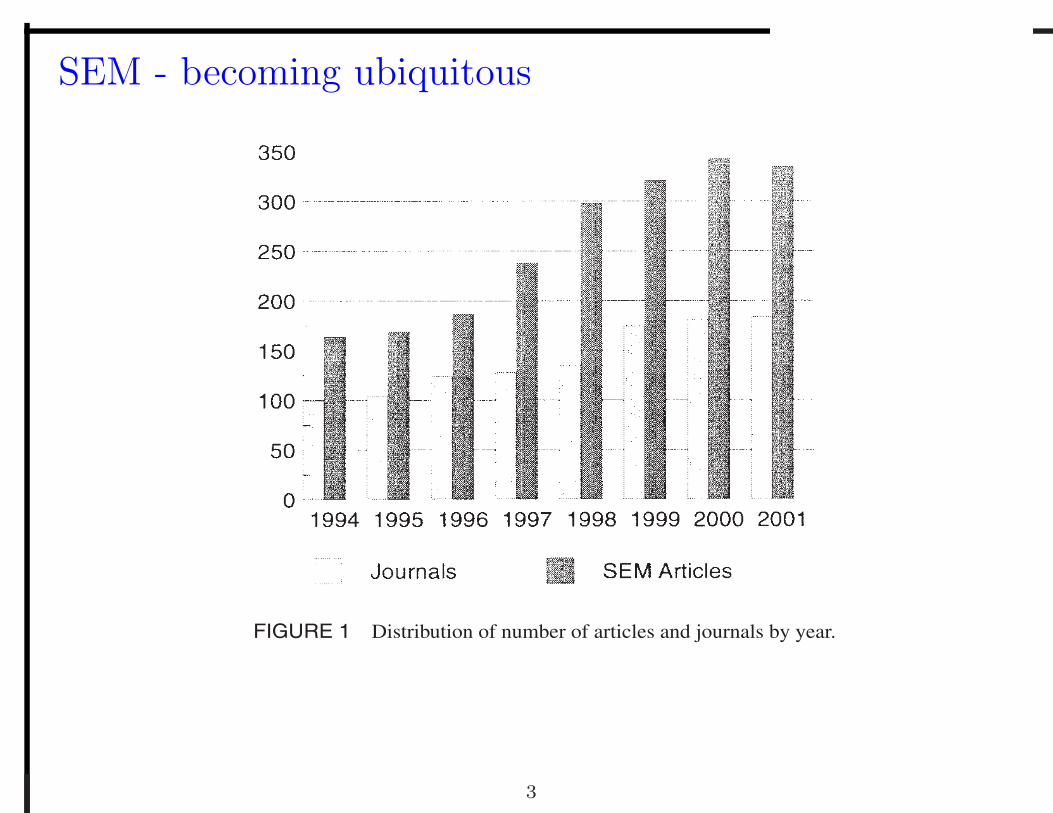
This study examines the growth and development of structural equation modeling(SEM) from the years 1994 to 2001. The synchronous development and growth ofthe Structural Equation Modeling journal was also examined. Abstracts located onPsycINFO were used as the primary source of data. The major results of this investi-gation were clear: (a) The number of journal articles concerned with SEM increased;(b) the number of journals publishing these articles increased; (c) SEM acquired he-gemony among multivariate techniques; and (d) Structural Equation Modeling be-came the primary source of publication for technical developments in SEM.

2

SEM - becoming ubiquitous

FIGURE 1 Distribution of number of articles and journals by year.

3

SEM - becoming ubiquitous

Over 1100 Selected Publications that Cite Amos for Structural Equation Mod-eling March, 2004, http://www.amosdevelopment.com/

4

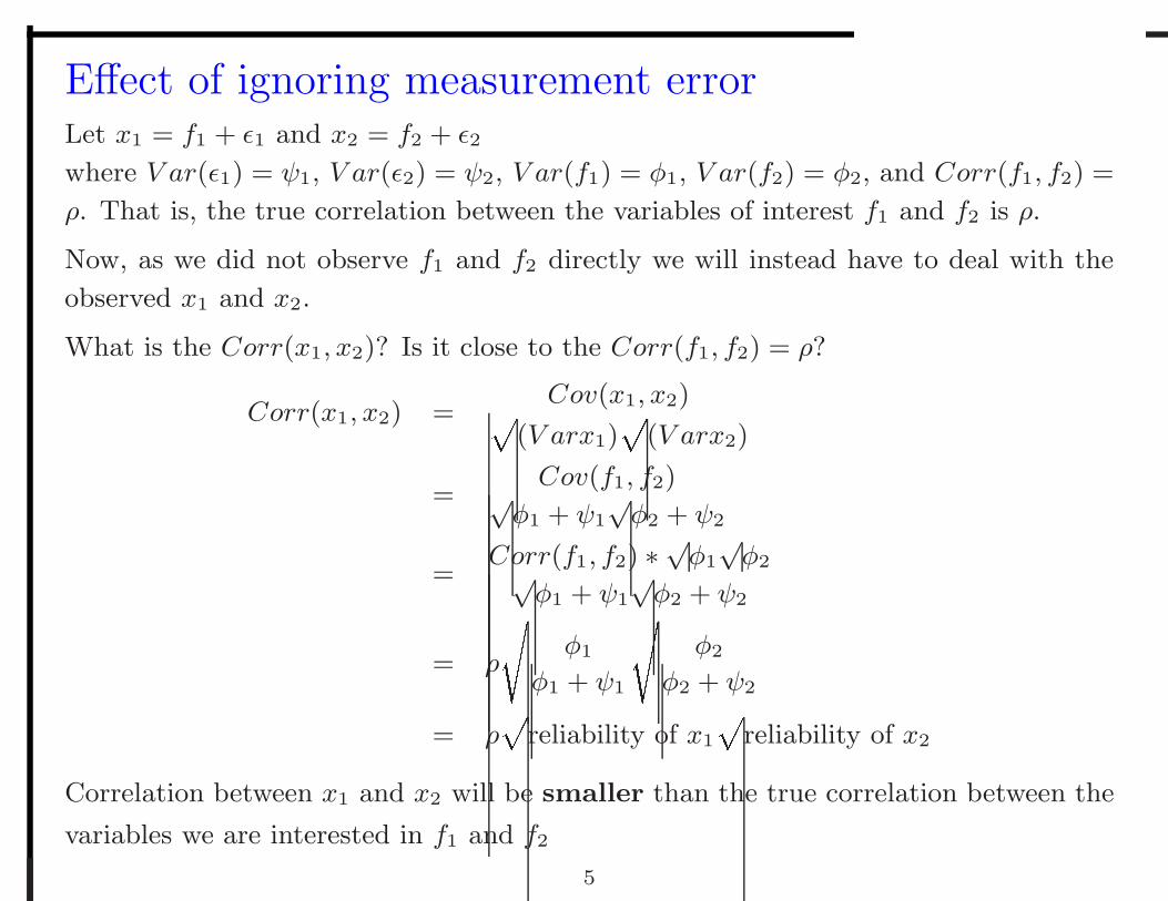
Effect of ignoring measurement errorLet x1 = f1 + ε1 and x2 = f2 + ε2

where V ar(ε1) = ψ1, V ar(ε2) = ψ2, V ar(f1) = φ1, V ar(f2) = φ2, and Corr(f1, f2) =

ρ. That is, the true correlation between the variables of interest f1 and f2 is ρ.

Now, as we did not observe f1 and f2 directly we will instead have to deal with the

observed x1 and x2.

What is the Corr(x1, x2)? Is it close to the Corr(f1, f2) = ρ?

Corr(x1, x2) =Cov(x1, x2)�

(V arx1)

�

(V arx2)

=Cov(f1, f2)√

φ1 + ψ1

√φ2 + ψ2

=Corr(f1, f2) ∗ √φ1

√φ2√

φ1 + ψ1

√φ2 + ψ2

= ρ

�

φ1

φ1 + ψ1

�φ2

φ2 + ψ2

= ρ

�

reliability of x1

�reliability of x2

Correlation between x1 and x2 will be smaller than the true correlation between the

variables we are interested in f1 and f2

5

SEM takes the measurement error into account

Rather than taking scales with less than perfect reliability and using them as ifthey are perfect measurements of the latent variable, SEM models incorporatesthe measurement error and thus “adjusts” the correlations and path coefficientsappropriately. Assuming the model specification is correct (as usual).

Two nice papers discussing this:

• Charles EP (2005) The Correction for Attenuation Due to MeasurementError: Clarifying Concepts and Creating Confidence Sets, PsychologicalMethods 10(2) 206-226.

• DeShon, R. P. (1998). A cautionary note on measurement error correctionsin structural equation models. Psychological M ethods, 3(4), 412-423.

6

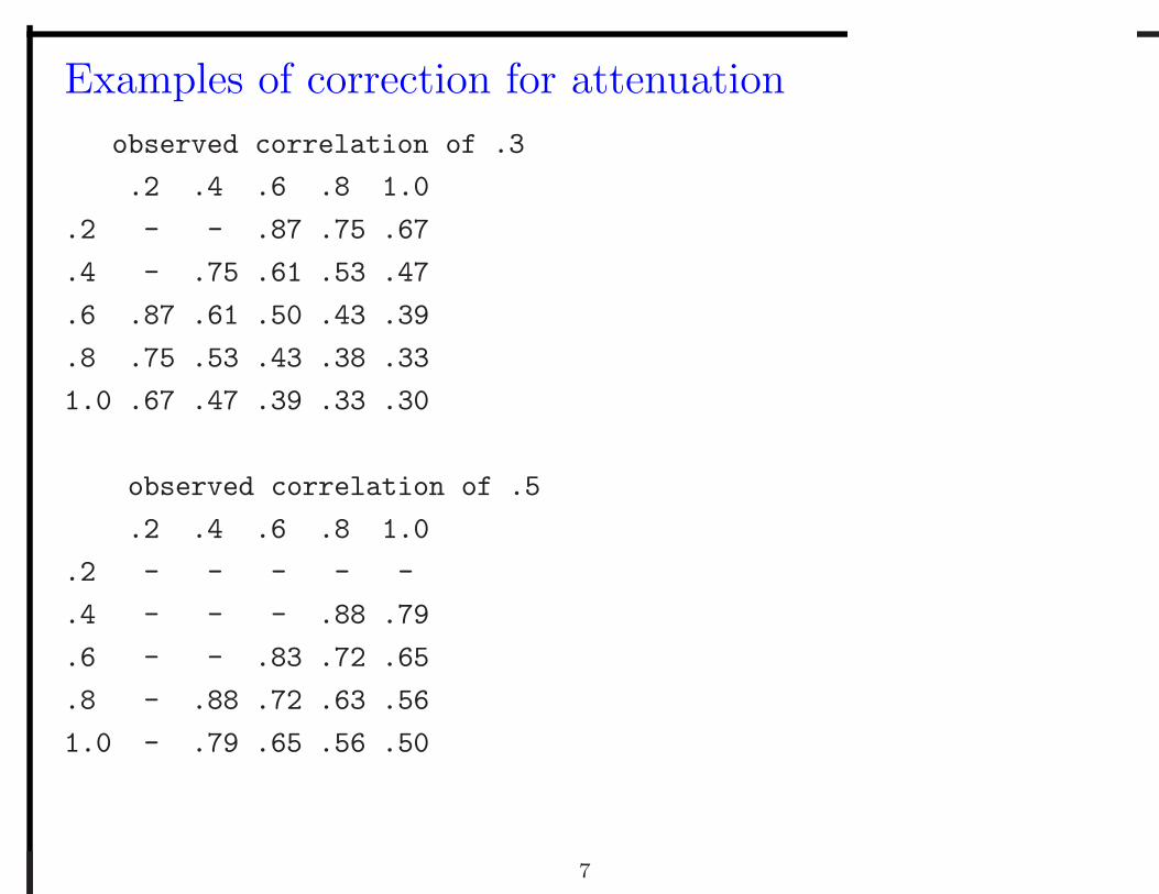
Examples of correction for attenuation

observed correlation of .3

.2 .4 .6 .8 1.0

.2 - - .87 .75 .67

.4 - .75 .61 .53 .47

.6 .87 .61 .50 .43 .39

.8 .75 .53 .43 .38 .33

1.0 .67 .47 .39 .33 .30

observed correlation of .5

.2 .4 .6 .8 1.0

.2 - - - - -

.4 - - - .88 .79

.6 - - .83 .72 .65

.8 - .88 .72 .63 .56

1.0 - .79 .65 .56 .50

7

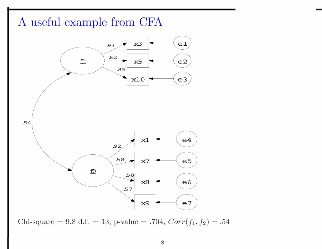
A useful example from CFA

f1

x3 e1.93

x5 e2.62

x10 e3

.85

f2

x1 e4.92

x7 e5.58

x8 e6.58

x9 e7

.57

.54

Chi-square = 9.8 d.f. = 13, p-value = .704, Corr(f1, f2) = .54

8

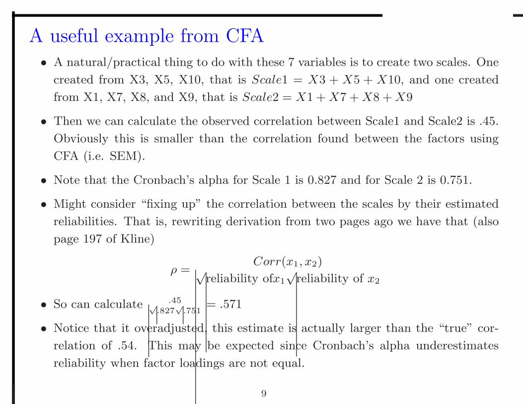
A useful example from CFA• A natural/practical thing to do with these 7 variables is to create two scales. One

created from X3, X5, X10, that is Scale1 = X3 + X5 + X10, and one created

from X1, X7, X8, and X9, that is Scale2 = X1 +X7 +X8 +X9

• Then we can calculate the observed correlation between Scale1 and Scale2 is .45.

Obviously this is smaller than the correlation found between the factors using

CFA (i.e. SEM).

• Note that the Cronbach’s alpha for Scale 1 is 0.827 and for Scale 2 is 0.751.

• Might consider “fixing up” the correlation between the scales by their estimated

reliabilities. That is, rewriting derivation from two pages ago we have that (also

page 197 of Kline)

ρ =Corr(x1, x2)√

reliability ofx1

√reliability of x2

• So can calculate .45√.827

√.751

= .571

• Notice that it overadjusted, this estimate is actually larger than the “true” cor-

relation of .54. This may be expected since Cronbach’s alpha underestimates

reliability when factor loadings are not equal.

9

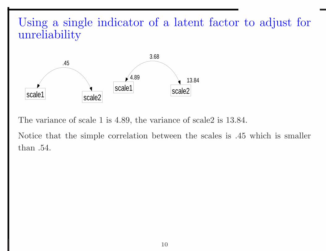
Using a single indicator of a latent factor to adjust forunreliability

scale1 scale2

.45

4.89

scale113.84

scale2

3.68

The variance of scale 1 is 4.89, the variance of scale2 is 13.84.

Notice that the simple correlation between the scales is .45 which is smallerthan .54.

10

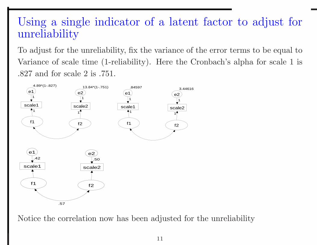
Using a single indicator of a latent factor to adjust forunreliability

To adjust for the unreliability, fix the variance of the error terms to be equal toVariance of scale time (1-reliability). Here the Cronbach’s alpha for scale 1 is.827 and for scale 2 is .751.

f1 f2

scale1

4.89*(1-.827)

e1

1

1

scale2

13.84*(1-.751)

e2

1

1

f1 f2

scale1

.84597

e1

1

1

scale2

3.44616

e2

1

1

f1 f2

scale1

e1.42

scale2

e2.50

.57

Notice the correlation now has been adjusted for the unreliability

11

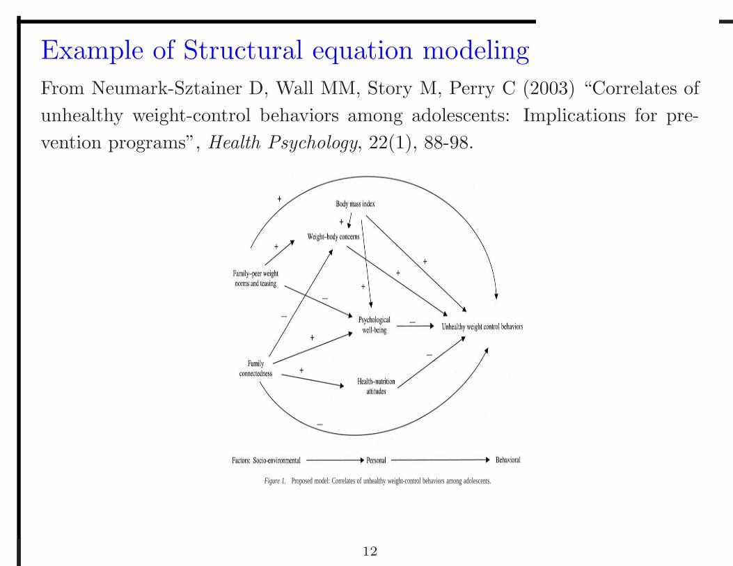
Example of Structural equation modeling

From Neumark-Sztainer D, Wall MM, Story M, Perry C (2003) “Correlates ofunhealthy weight-control behaviors among adolescents: Implications for pre-vention programs”, Health Psychology, 22(1), 88-98.

Figure 1. Proposed model: Correlates of unhealthy weight-control behaviors among adolescents.

12

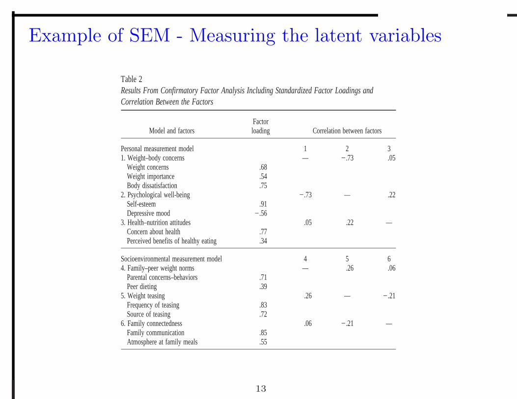
Example of SEM - Measuring the latent variables

Table 2Results From Confirmatory Factor Analysis Including Standardized Factor Loadings andCorrelation Between the Factors

Model and factorsFactorloading Correlation between factors

Personal measurement model 1 2 31. Weight–body concerns — �.73 .05

Weight concerns .68Weight importance .54Body dissatisfaction .75

2. Psychological well-being �.73 — .22Self-esteem .91Depressive mood �.56

3. Health–nutrition attitudes .05 .22 —Concern about health .77Perceived benefits of healthy eating .34

Socioenvironmental measurement model 4 5 64. Family–peer weight norms — .26 .06

Parental concerns–behaviors .71Peer dieting .39

5. Weight teasing .26 — �.21Frequency of teasing .83Source of teasing .72

6. Family connectedness .06 �.21 —Family communication .85Atmosphere at family meals .55

13

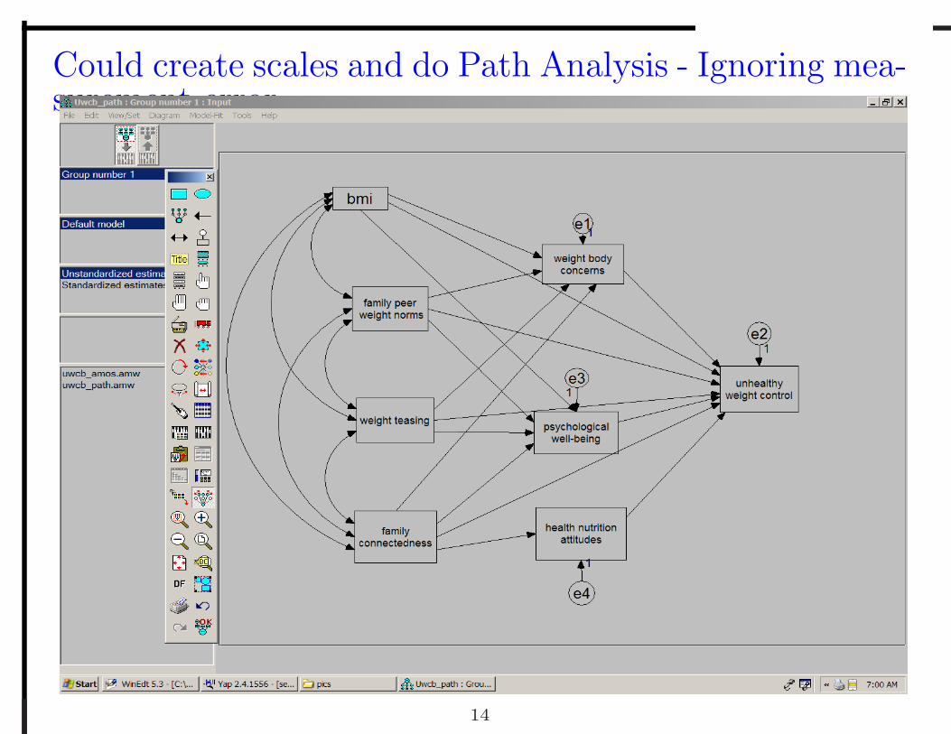
Could create scales and do Path Analysis - Ignoring mea-surement error

14

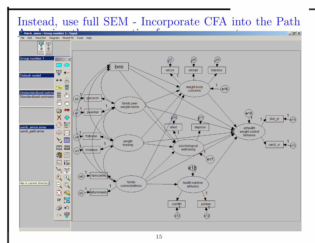
Instead, use full SEM - Incorporate CFA into the PathAnalysis - thus accounting for measurement error

15

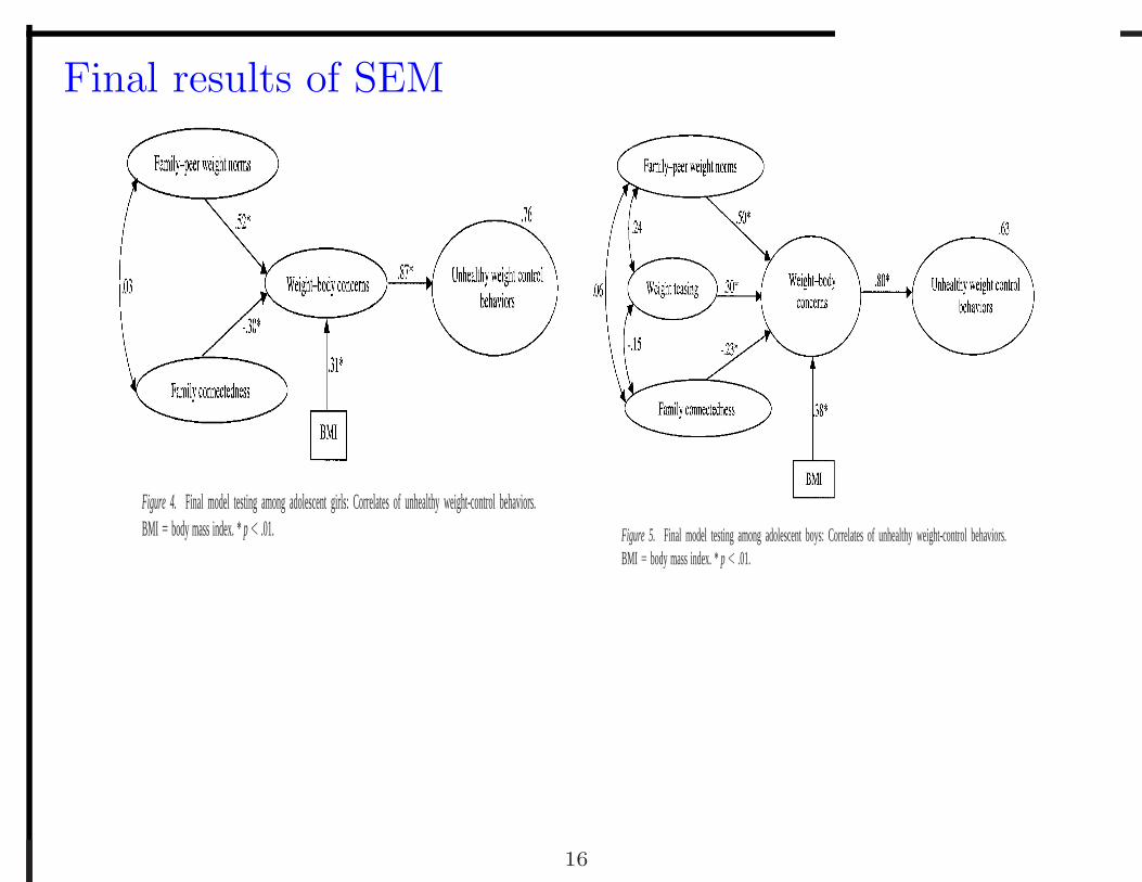
Final results of SEM

Figure 4. Final model testing among adolescent girls: Correlates of unhealthy weight-control behaviors.BMI � body mass index. * p � .01. Figure 5. Final model testing among adolescent boys: Correlates of unhealthy weight-control behaviors.

BMI � body mass index. * p � .01.

16

Common to use 2-step approach to SEM

1. Develop measurement model (CFA) relating observed variables to latentvariables. Examine goodness of fit of this model on its own. Examinecorrelations between all variables (usually latent variables) of interest bylooking at correlations between factors from CFA.

2. Develop full structural equation model. That is, change the “spuriouslycorrelated” relationships in the CFA to impose theoretical causal directeffects between variables and drop relationships not assumed by theory.Examine goodness of fit of this model as a whole.

Common reference advocating this approach isAnderson, J.C. and Gerbing, D.W. (1988) Psychological Bulletin

17

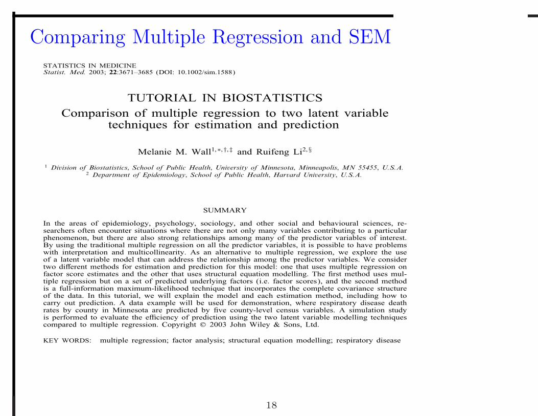
Comparing Multiple Regression and SEMSTATISTICS IN MEDICINEStatist. Med. 2003; 22:3671–3685 (DOI: 10.1002/sim.1588)

TUTORIAL IN BIOSTATISTICSComparison of multiple regression to two latent variable

techniques for estimation and prediction

Melanie M. Wall1;∗;†;‡ and Ruifeng Li2;§

1 Division of Biostatistics; School of Public Health; University of Minnesota; Minneapolis; MN 55455; U.S.A.2 Department of Epidemiology; School of Public Health; Harvard University; U.S.A.

SUMMARY

In the areas of epidemiology, psychology, sociology, and other social and behavioural sciences, re-searchers often encounter situations where there are not only many variables contributing to a particularphenomenon, but there are also strong relationships among many of the predictor variables of interest.By using the traditional multiple regression on all the predictor variables, it is possible to have problemswith interpretation and multicollinearity. As an alternative to multiple regression, we explore the useof a latent variable model that can address the relationship among the predictor variables. We considertwo di�erent methods for estimation and prediction for this model: one that uses multiple regression onfactor score estimates and the other that uses structural equation modelling. The �rst method uses mul-tiple regression but on a set of predicted underlying factors (i.e. factor scores), and the second methodis a full-information maximum-likelihood technique that incorporates the complete covariance structureof the data. In this tutorial, we will explain the model and each estimation method, including how tocarry out prediction. A data example will be used for demonstration, where respiratory disease deathrates by county in Minnesota are predicted by �ve county-level census variables. A simulation studyis performed to evaluate the e�ciency of prediction using the two latent variable modelling techniquescompared to multiple regression. Copyright ? 2003 John Wiley & Sons, Ltd.

KEY WORDS: multiple regression; factor analysis; structural equation modelling; respiratory disease

18

Data Source - MN county example

• Minnesota county-level census death record data from 1990 to 1998

• Outcome: Log of age-adjusted respiratory disease death rate

• Observed Predictors: Five census variables on the county-level

• Goal: establish the relation of predictors with outcome for interpretationand prediction

19

FIVE PREDICTORS (all on the county-level)- MN countyexample

• eduhs: percent with high school education

• medhhin: median households income (in dollars)

• percapit: per capita income (in dollars)

• pubwater: percent of households with access to public water

• wood: percent of households using wood to heat the home

20

Multiple Regression -MN county example

.00

educhs

.33

m edhhinc

.04

percapin

.04

pubwater

.01

wood

respm ort

1.29

.11

-.02

.07

.53.03

e11

.03

.01

.00

.00

.11

.05

-.02.02

-.01

-.02

resp = β0 + β1eduhs + β2medhhin + β3percapit + β4pubwater + β5wood + ε

21

Tool in AMOS to draw many covariance arrows

• Click on each variable in the set which will be correlated with each other

• Click on Tools then Macros then Draw Covariance

• This will then draw all the desired double headed arrows.

22

Multiple Regression-MN county example

Examining unstandardized estimates. The coefficients are scaled up by 10 (forthe percents) and 1000 for the dollar amounts compared to numbers in theoriginal paper because units of raw data are scaled down.

Regression W eights Estimate S.E. C.R. P respmort <-- wood 1.294362 0.452701 2.859198 0.004247 respmort <-- pubwater 0.108254 0.228837 0.473061 0.636170 respmort <-- percapin -0.017170 0.321008 -0.053488 0.957343 respmort <-- medhhinc 0.072829 0.098331 0.740651 0.458905 respmort <-- educhs 0.528606 0.718153 0.736064 0.461692

Only WOOD is significant.

23

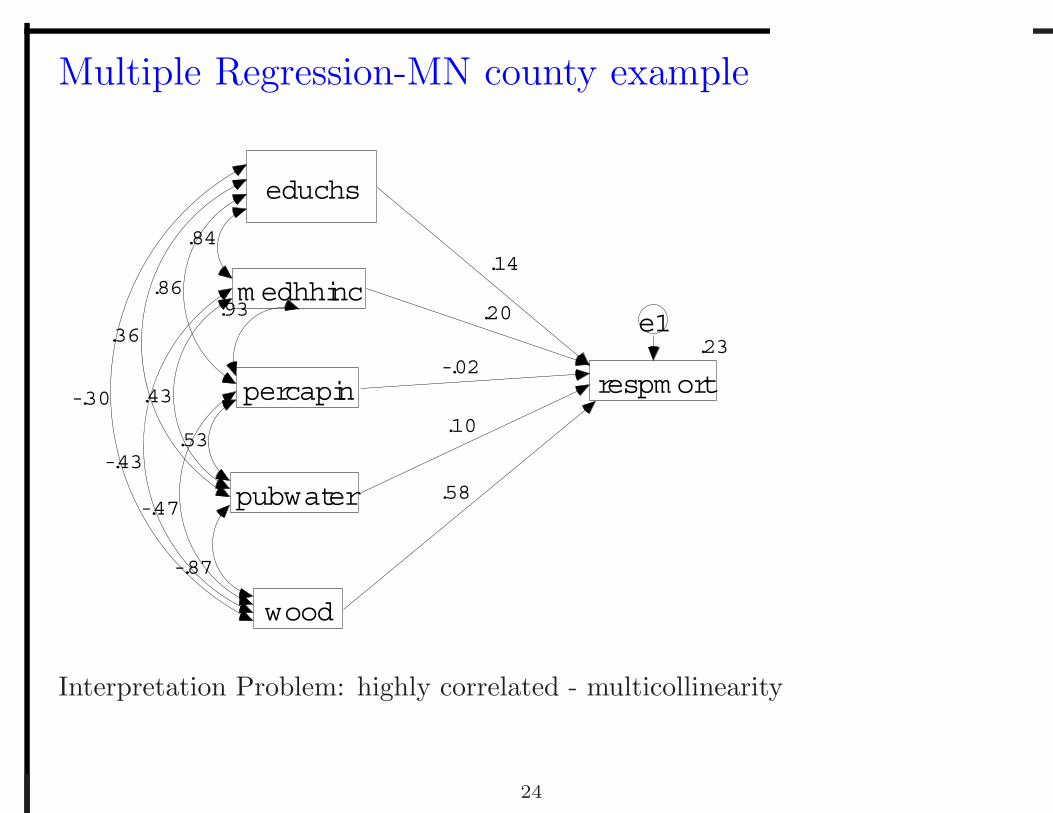
Multiple Regression-MN county example

educhs

m edhhinc

percapin

pubwater

wood

.23

respm ort

.58

.10

-.02

.20

.14

e1

.84

.86

.36

-.30

.93

.43

-.43.53

-.47

-.87

Interpretation Problem: highly correlated - multicollinearity

24

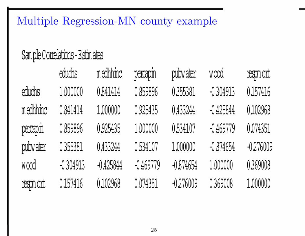
Multiple Regression-MN county example

Sample Correlations - Estimates educhs medhhinc percapin pubwater wood respmort educhs 1.000000 0.841414 0.859896 0.355381 -0.304913 0.157416 medhhinc 0.841414 1.000000 0.925435 0.433244 -0.425844 0.102968 percapin 0.859896 0.925435 1.000000 0.534107 -0.469779 0.074351 pubwater 0.355381 0.433244 0.534107 1.000000 -0.874654 -0.276009 wood -0.304913 -0.425844 -0.469779 -0.874654 1.000000 0.369008 respmort 0.157416 0.102968 0.074351 -0.276009 0.369008 1.000000

25

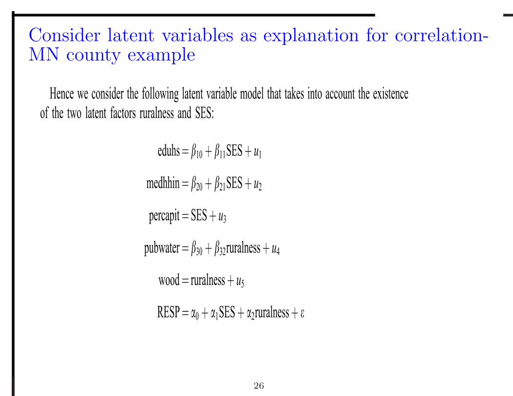
Consider latent variables as explanation for correlation-MN county example

Hence we consider the following latent variable model that takes into account the existenceof the two latent factors ruralness and SES:

eduhs = �10 + �11SES + u1

medhhin = �20 + �21SES + u2

percapit = SES + u3

pubwater = �30 + �32ruralness + u4

wood = ruralness + u5

RESP= �0 + �1SES + �2ruralness + �

26

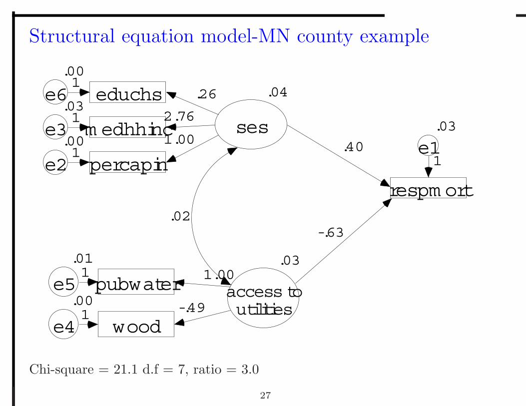
Structural equation model-MN county example

respm ort

.03

e11

.04

ses

percapin.00

e2

1.001

m edhhinc.03

e32.761

.03

access toutilities

wood

.00

e4-.491

pubwater

.01

e51.001

educhs.00

e6 .261

.02-.63

.40

Chi-square = 21.1 d.f = 7, ratio = 3.0

27

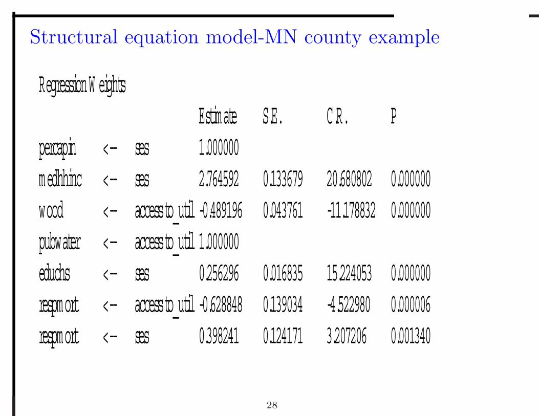
Structural equation model-MN county example

Regression W eights Estimate S.E. C.R. P percapin <-- ses 1.000000 medhhinc <-- ses 2.764592 0.133679 20.680802 0.000000 wood <-- access to_util -0.489196 0.043761 -11.178832 0.000000 pubwater <-- access to_util 1.000000 educhs <-- ses 0.256296 0.016835 15.224053 0.000000 respmort <-- access to_util -0.628848 0.139034 -4.522980 0.000006 respmort <-- ses 0.398241 0.124171 3.207206 0.001340

28

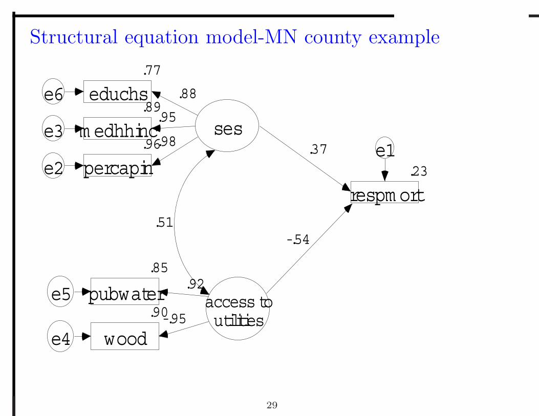
Structural equation model-MN county example

.23

respm ort

e1ses

.96

percapine2

.98

.89

m edhhince3.95

access toutilities.90

woode4-.95

.85

pubwatere5.92

.77

educhse6 .88

.51-.54

.37

29

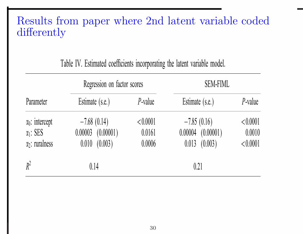
Results from paper where 2nd latent variable codeddifferently

Table IV. Estimated coe�cients incorporating the latent variable model.

Regression on factor scores SEM-FIML

Parameter Estimate (s.e.) P-value Estimate (s.e.) P-value

�0: intercept −7:68 (0.14) ¡0:0001 −7:85 (0.16) ¡0:0001�1: SES 0.00003 (0.00001) 0.0161 0.00004 (0.00001) 0.0010�2: ruralness 0.010 (0.003) 0.0006 0.013 (0.003) ¡0.0001

R2 0.14 0.21

30

Explanation of how SEM might predict better than Mul-tiple regression

How is it possible for the SEM-FIML technique to beat ordinary least squares in terms ofprediction? It is well known that E(Y |X) is the best mean square predictor of Y .Although in general the form of E(Y |X) is unknown, when (Y;X) is jointly normal, withE(Y;X)= (�Y ; \X ), Var(X)=�XX and Cov(Y;X)=�YX, then E(Y |X)=�Y+�YX�−1

XX(X−\X ).The best predictor given a particular data set is then equal to E(Y |X), with the maximum-likelihood estimates plugged in for \Y , \X , �YX and �XX. When nothing is assumed aboutthe p(p+ 1)=2 unique elements of the symmetric matrix �XX, the maximum-likelihood esti-mator for �XX is simply the sample covariance matrix of X, i.e. every element is estimatedindependently, and the E(Y |X) with maximum-likelihood estimators plugged in yields theOLS predictor. However, if we have some model for the elements of �XX as is the casein the latent variable model where �XX is a function of fewer parameters than p(p + 1)=2,and these parameters also appear in �YX, then maximum-likelihood estimators based on themodelled �XX and �YX plugged into E(Y |X) such as (11) should be best with respect tomean squared prediction error. Simply put, if the SEM model �(�) is a good model for �,then �YX(�̂)�

−1XX(�̂) is more e�cient than the OLS estimator SxyS−1xx for estimating �YX�

−1XX.

Furthermore, we point out that like the ordinary least-squares regression predictor, thepredictor using factor score estimates (9) is also a linear predictor (i.e. a linear functionof Y ). On the other hand, the SEM-FIML predictor (11) is not linear since the parameterestimators are non-linear functions of both the Y and X variables. This may help to furtherexplain how it performs more e�ciently than the other methods.

31

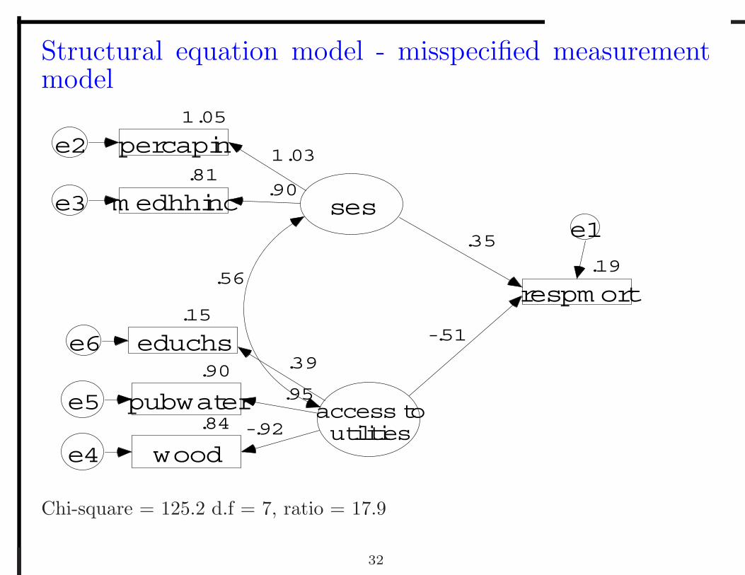
Structural equation model - misspecified measurementmodel

.19

respm ort

e1ses

1.05

percapine2 1.03.81

m edhhince3.90

access toutilities.84

woode4-.92

.90

pubwatere5 .95

.15

educhse6

.56

-.51

.35

.39

Chi-square = 125.2 d.f = 7, ratio = 17.9

32

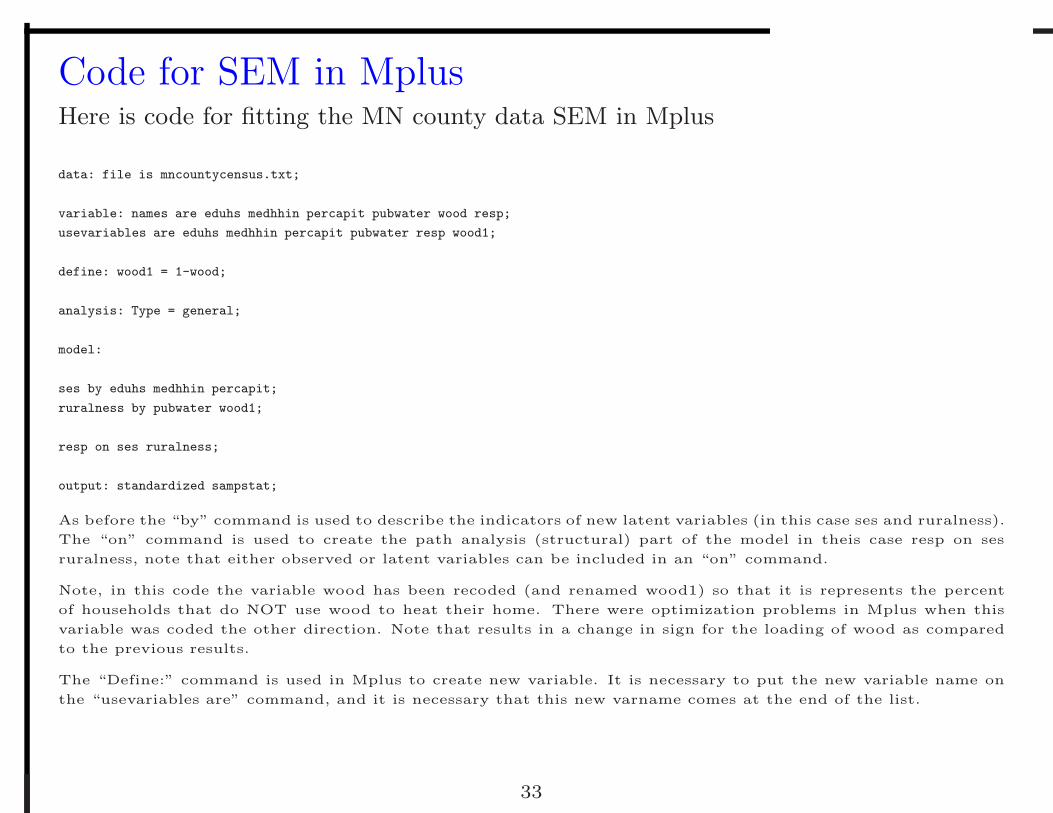
Code for SEM in MplusHere is code for fitting the MN county data SEM in Mplus

data: file is mncountycensus.txt;

variable: names are eduhs medhhin percapit pubwater wood resp;

usevariables are eduhs medhhin percapit pubwater resp wood1;

define: wood1 = 1-wood;

analysis: Type = general;

model:

ses by eduhs medhhin percapit;

ruralness by pubwater wood1;

resp on ses ruralness;

output: standardized sampstat;

As before the “by” command is used to describe the indicators of new latent variables (in this case ses and ruralness).The “on” command is used to create the path analysis (structural) part of the model in theis case resp on sesruralness, note that either observed or latent variables can be included in an “on” command.

Note, in this code the variable wood has been recoded (and renamed wood1) so that it is represents the percentof households that do NOT use wood to heat their home. There were optimization problems in Mplus when thisvariable was coded the other direction. Note that results in a change in sign for the loading of wood as comparedto the previous results.

The “Define:” command is used in Mplus to create new variable. It is necessary to put the new variable name onthe “usevariables are” command, and it is necessary that this new varname comes at the end of the list.

33

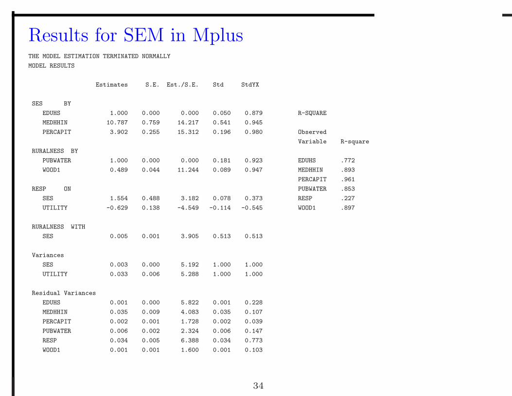
Results for SEM in MplusTHE MODEL ESTIMATION TERMINATED NORMALLY

MODEL RESULTS

Estimates S.E. Est./S.E. Std StdYX

SES BY

EDUHS 1.000 0.000 0.000 0.050 0.879 R-SQUARE

MEDHHIN 10.787 0.759 14.217 0.541 0.945

PERCAPIT 3.902 0.255 15.312 0.196 0.980 Observed

Variable R-square

RURALNESS BY

PUBWATER 1.000 0.000 0.000 0.181 0.923 EDUHS .772

WOOD1 0.489 0.044 11.244 0.089 0.947 MEDHHIN .893

PERCAPIT .961

RESP ON PUBWATER .853

SES 1.554 0.488 3.182 0.078 0.373 RESP .227

UTILITY -0.629 0.138 -4.549 -0.114 -0.545 WOOD1 .897

RURALNESS WITH

SES 0.005 0.001 3.905 0.513 0.513

Variances

SES 0.003 0.000 5.192 1.000 1.000

UTILITY 0.033 0.006 5.288 1.000 1.000

Residual Variances

EDUHS 0.001 0.000 5.822 0.001 0.228

MEDHHIN 0.035 0.009 4.083 0.035 0.107

PERCAPIT 0.002 0.001 1.728 0.002 0.039

PUBWATER 0.006 0.002 2.324 0.006 0.147

RESP 0.034 0.005 6.388 0.034 0.773

WOOD1 0.001 0.001 1.600 0.001 0.103

34

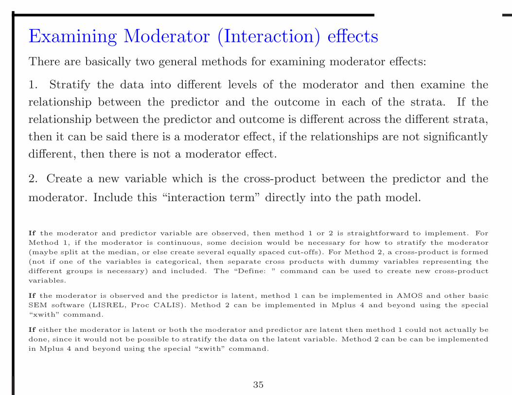
Examining Moderator (Interaction) effectsThere are basically two general methods for examining moderator effects:

1. Stratify the data into different levels of the moderator and then examine the

relationship between the predictor and the outcome in each of the strata. If the

relationship between the predictor and outcome is different across the different strata,

then it can be said there is a moderator effect, if the relationships are not significantly

different, then there is not a moderator effect.

2. Create a new variable which is the cross-product between the predictor and the

moderator. Include this “interaction term” directly into the path model.

If the moderator and predictor variable are observed, then method 1 or 2 is straightforward to implement. ForMethod 1, if the moderator is continuous, some decision would be necessary for how to stratify the moderator(maybe split at the median, or else create several equally spaced cut-offs). For Method 2, a cross-product is formed(not if one of the variables is categorical, then separate cross products with dummy variables representing thedifferent groups is necessary) and included. The “Define: ” command can be used to create new cross-productvariables.

If the moderator is observed and the predictor is latent, method 1 can be implemented in AMOS and other basicSEM software (LISREL, Proc CALIS). Method 2 can be implemented in Mplus 4 and beyond using the special“xwith” command.

If either the moderator is latent or both the moderator and predictor are latent then method 1 could not actually bedone, since it would not be possible to stratify the data on the latent variable. Method 2 can be can be implementedin Mplus 4 and beyond using the special “xwith” command.

35

Examining Moderator (Interaction) effects

NOTE: When considering a moderator of the relationship between a predictorand an outcome, it is the case that the predictor also moderates the relationshipbetween the moderator and the outcome. The two variables moderate eachothers’ relationships with the outcome.

For more on conceptualizing moderators (and mediators), see e.g., Petrosino(2000) Mediators and moderators in the evaluation of programs for children.Current Practice and Agenda for Improvement. Evaluation Review, 24(1) 47-72.

36

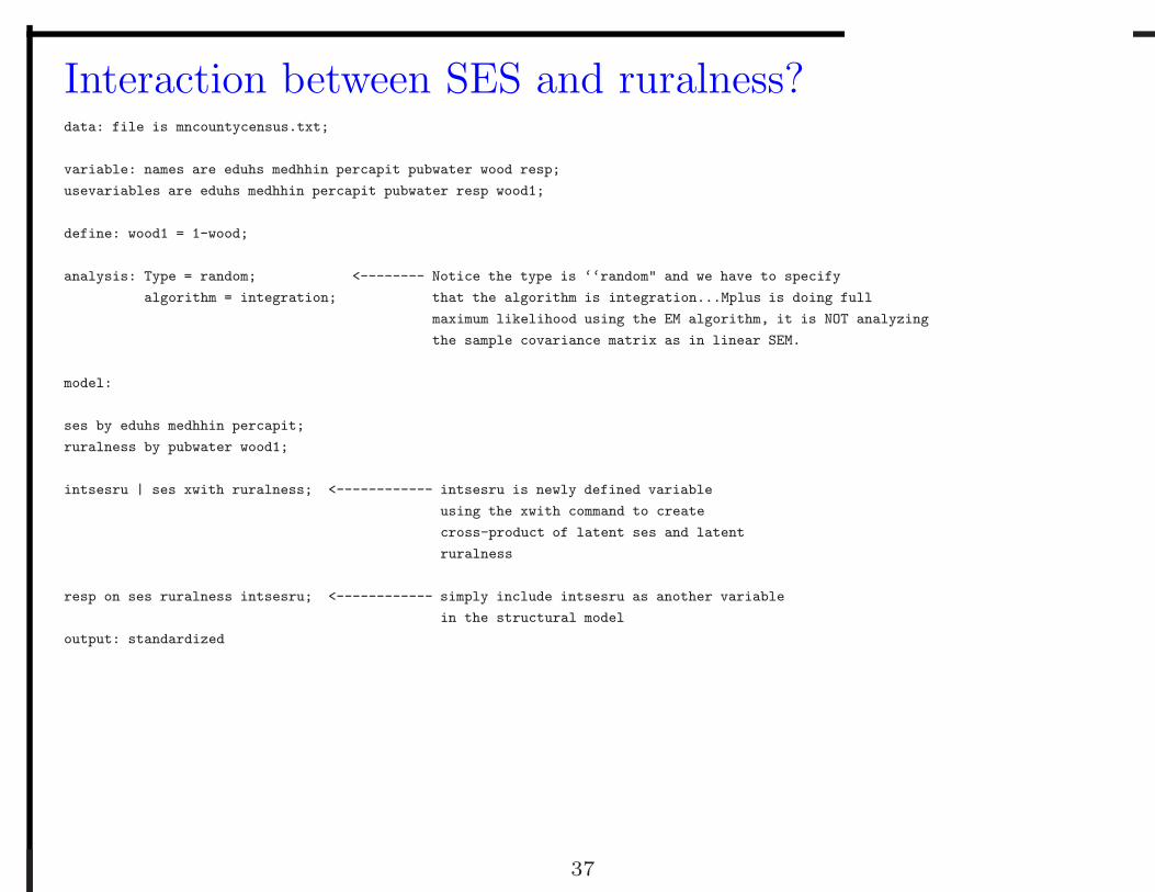
Interaction between SES and ruralness?data: file is mncountycensus.txt;

variable: names are eduhs medhhin percapit pubwater wood resp;

usevariables are eduhs medhhin percapit pubwater resp wood1;

define: wood1 = 1-wood;

analysis: Type = random; <-------- Notice the type is ‘‘random" and we have to specify

algorithm = integration; that the algorithm is integration...Mplus is doing full

maximum likelihood using the EM algorithm, it is NOT analyzing

the sample covariance matrix as in linear SEM.

model:

ses by eduhs medhhin percapit;

ruralness by pubwater wood1;

intsesru | ses xwith ruralness; <------------ intsesru is newly defined variable

using the xwith command to create

cross-product of latent ses and latent

ruralness

resp on ses ruralness intsesru; <------------ simply include intsesru as another variable

in the structural model

output: standardized

37

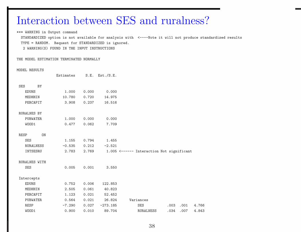
Interaction between SES and ruralness?*** WARNING in Output command

STANDARDIZED option is not available for analysis with <----Note it will not produce standardized results

TYPE = RANDOM. Request for STANDARDIZED is ignored.

2 WARNING(S) FOUND IN THE INPUT INSTRUCTIONS

THE MODEL ESTIMATION TERMINATED NORMALLY

MODEL RESULTS

Estimates S.E. Est./S.E.

SES BY

EDUHS 1.000 0.000 0.000

MEDHHIN 10.780 0.720 14.975

PERCAPIT 3.908 0.237 16.516

RURALNES BY

PUBWATER 1.000 0.000 0.000

WOOD1 0.477 0.062 7.709

RESP ON

SES 1.155 0.794 1.455

RURALNESS -0.535 0.212 -2.521

INTSESRU 2.783 2.769 1.005 <------ Interaction Not significant

RURALNES WITH

SES 0.005 0.001 3.550

Intercepts

EDUHS 0.752 0.006 122.853

MEDHHIN 2.505 0.061 40.823

PERCAPIT 1.123 0.021 52.452

PUBWATER 0.564 0.021 26.824 Variances

RESP -7.290 0.027 -273.185 SES .003 .001 4.766

WOOD1 0.900 0.010 89.704 RURALNESS .034 .007 4.843

38

Latent interaction models - nonlinear latent variablesOnce the model includes a nonlinear function of a latent variables, the traditional

methods for estimating SEM (which are based on modeling the observed covariance

matrix S) are not useful. The traditional methods only apply to linear structural

models, NOTE, the well-known term LISREL stands for “Linear structural relations”.

During the past decade, much work has been done to develop methods for estimating

nonlinear structural relations. Mplus implements one such method which allows the

direct fitting of products of latent variables in the structural part of the model. Note,

quadratic terms can also be created by taking a latent variable “xwith”ed with itself,

e.g. sesquad | ses xwith ses; would create a latent quadratic ses term.

In Mplus, the estimation method is directly fitting the latent interaction using full

maximum likelihood (via the EM algorithm) with the nonlinear structural model di-

rectly included. Full maximum likelihood can also now be done using SAS PROC

NLMIXED and can similarly be implemented in Winbugs (within a Bayesian frame-

work).

See Wall M.M. Maximum likelihood and Bayesian estimation for nonlinear structural

equation models using SAS, Mplus, and Winbugs Research Report 2007-021, Division

of Biostatistics, University of Minnesota, 2007.

39

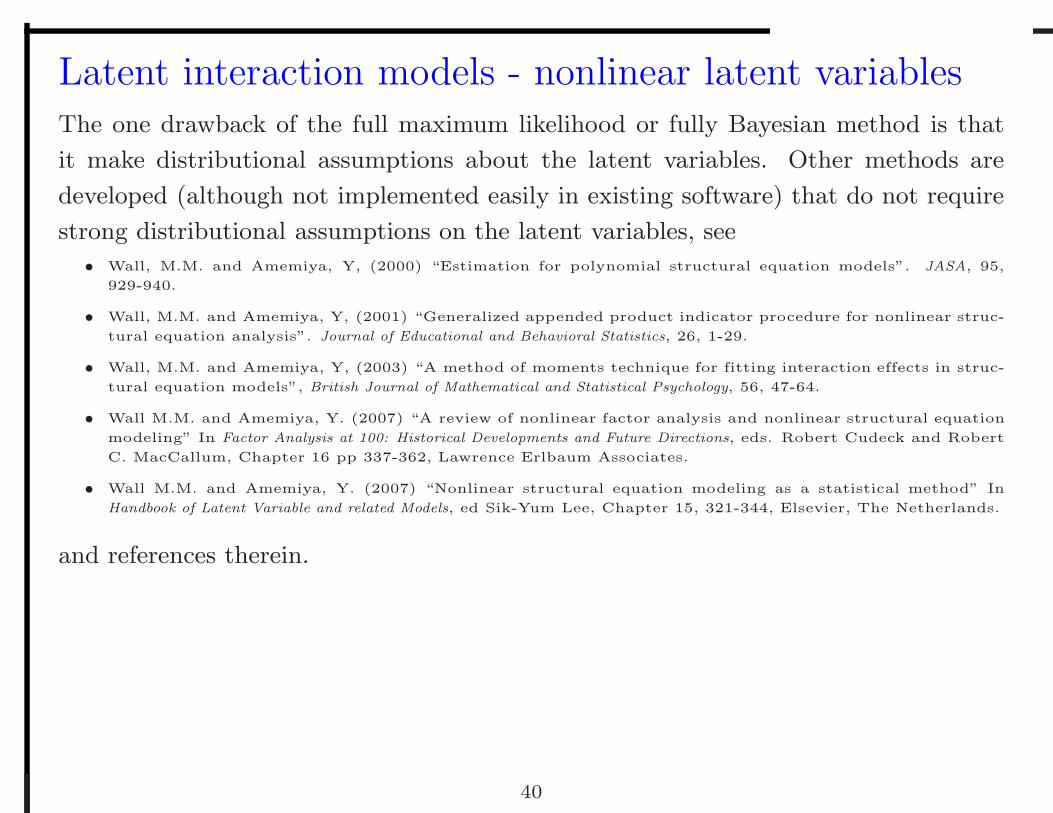
Latent interaction models - nonlinear latent variablesThe one drawback of the full maximum likelihood or fully Bayesian method is that

it make distributional assumptions about the latent variables. Other methods are

developed (although not implemented easily in existing software) that do not require

strong distributional assumptions on the latent variables, see

• Wall, M.M. and Amemiya, Y, (2000) “Estimation for polynomial structural equation models”. JASA, 95,929-940.

• Wall, M.M. and Amemiya, Y, (2001) “Generalized appended product indicator procedure for nonlinear struc-tural equation analysis”. Journal of Educational and Behavioral Statistics, 26, 1-29.

• Wall, M.M. and Amemiya, Y, (2003) “A method of moments technique for fitting interaction effects in struc-tural equation models”, British Journal of Mathematical and Statistical Psychology, 56, 47-64.

• Wall M.M. and Amemiya, Y. (2007) “A review of nonlinear factor analysis and nonlinear structural equationmodeling” In Factor Analysis at 100: Historical Developments and Future Directions, eds. Robert Cudeck and RobertC. MacCallum, Chapter 16 pp 337-362, Lawrence Erlbaum Associates.

• Wall M.M. and Amemiya, Y. (2007) “Nonlinear structural equation modeling as a statistical method” InHandbook of Latent Variable and related Models, ed Sik-Yum Lee, Chapter 15, 321-344, Elsevier, The Netherlands.

and references therein.

40

Multilevel modeling

Data collection involves: patients within clinics, students within classrooms,employees within units, repeated measures within patient (i.e. longitudinaldata). In each case the grouping or clustering variable is: clinics, classrooms,units, patient.from Heck (2001) Multilevel Modeling in SEM, Chapter 4, New Developments and Techniques in SEM, eds Marcoulidesand Schumacker, 89-127

Ignoring the presence of substantial similarities among individuals within groupscan result in substantially biased estimates of the model’s parameters, standarderrors, and fit indexes.

41

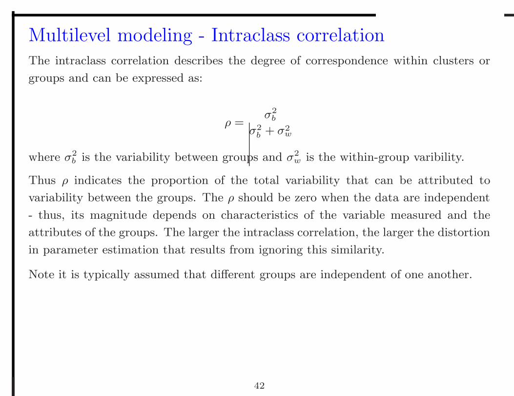
Multilevel modeling - Intraclass correlationThe intraclass correlation describes the degree of correspondence within clusters or

groups and can be expressed as:

ρ =σ2

b

σ2b + σ2

w

where σ2b is the variability between groups and σ2

w is the within-group varibility.

Thus ρ indicates the proportion of the total variability that can be attributed to

variability between the groups. The ρ should be zero when the data are independent

- thus, its magnitude depends on characteristics of the variable measured and the

attributes of the groups. The larger the intraclass correlation, the larger the distortion

in parameter estimation that results from ignoring this similarity.

Note it is typically assumed that different groups are independent of one another.

42