th 202

Strengthening Reinforced Concrete Column-beam Joints with Modular Shape Memory Alloy Plate Optimized through

Probabilistic Damage Prediction

Author: Mohammad Amin Molod

the degree of Doctor of Engineering at the Faculty of Architecture and Civil

TU Dortmund UniversityFaculty of Architecture and Civil EngineeringInstitute of Structural Analysis August-Schmidt-Str. 8D-44227 DortmundGermany

Reviewers:Professor Dr.-Ing. habil. Franz-Joseph BartholdProfessor Dr.-Ing. Panagiotis Spyridis

"Printed and/or published with the support of the German Academic Exchange Service"

MOLOD I

Abstract

Column-beam joints are one of the most critical zones of concrete structures, especially under

unpredicted heavy loads and lateral loads such as seismic. Failure of the joints can even lead

to failure of structures in their entirety. The low strength capacity of concrete is a reason of

sensitivity of the region. Shape memory alloy (SMA) plates can be employed in order to

overcome this weakness and increase the stiffness of joints in existing structures. SMA is a

smart material whose functionality, workability and its self-healing feature are under

investigation by scientists in the field of structural engineering. In fact, there are two types

of alloy: i) superelastic shape memory alloy and ii) shape memory effect that is sensitive to

temperature, but it is out of the topic of the research. However, a superelastic form is the

most common type of alloy in the field of structural engineering that can be used not only as

external reinforcement bolted to the concrete surface but also as internal reinforcement

embedded within the concrete elements. The author of this numerical research attempted to

implement a plate form of the alloy as external reinforcement to increase stiffness and

ductility of the joint. To do so, an experimentally investigated concrete column-beam joint

has been modelled in Ansys, and it was loaded under a large number of randomly selected

load combinations. The plate initially was designed with a uniform thickness and length in

the plastic hinge region of the joint under the critical load combination. Then, probabilistic

analysis was carried out to optimize the plate’s thickness. To that end, the stress values of

thirty-five predefined nodes on the plate surface were recorded under each load

combinations. Results were imported into MATLAB software to run the probabilistic

analysis and specifying 0.95 quantile of the stored stresses of the nodes. Design optimization

was also carried out based on the probabilistic results in order to design the thickness of the

plate at different control nodes. During the course of the research, a set of necessary

additional trials have been carried out, as for example with regards to the proper Ansys

element type selection for reinforced concrete, determination of limit state functions, and to

assess the most suitable parallel processing setup. A fastening technique was also employed

to connect the optimized SMA plate to the surface of the concrete joint. Finally, some

numerical examples have been run in order to check to what extend the utilized method

worked properly. The procedure was applied twice; i) when the load combinations were

applied in cyclic form and ii) when the load combinations were exerted in reverse cyclic

form. Therefore, two optimized SMA have been designed and examined. The results of the

analyses showed that the employed technique enhanced the strength of the joint considerably

so that the cracking load of the system reinforced with optimized SMA plate under cyclic

loading was 1.4 times greater than the benchmark. The load-carrying capacity of the

reinforced system in the elastic regime was higher than the unreinforced structure, and the

capability in the plastic regime was even higher. Indicatively, the load-carrying capacity of

the reference system at a displacement of 32 mm was approximately 98 kN, whereas the

respective resistance value was approximately 66 kN in the system without the plate. Besides,

the existence of the plate led to transition of the failure zone from the joint to the beam span,

which leads to a lower risk of failure of the entire structure. As a result, the main focus of the

research was to describe a novel method that allows for a probability-based prediction of

damage in concrete structures that can facilitate the assessment and design of degraded

structures under risk of failure.

Keywords: Shape memory alloys (SMA), reinforced concrete, column-beam joints,

probabilistic analysis, optimization, Ansys

MOLOD II

Table of Contents

ABSTRACT ....................................................................................................... I

LIST OF FIGURES .......................................................................................... IV

LIST OF TABLES ........................................................................................ VIII

CHAPTER 1. INTRODUCTION ...................................................................... 1

1.1. Motivation ................................................................................................................... 1

1.2. Shape memory alloy materials .................................................................................... 4 1.2.1. History of SMAs ..................................................................................... 4 1.2.2. SMAs forms and properties .................................................................... 5

1.3. Aim and objectives ..................................................................................................... 7

1.3.1. Aim .......................................................................................................... 7 1.3.2. Objectives ................................................................................................ 7

1.4. Outline of the research/ ............................................................................................... 8

CHAPTER 2. LITERATURE REVIEW ........................................................... 9

CHAPTER 3. METHODOLOGY OF MODELING ....................................... 17

3.1. Introduction and algorithm of the project ................................................................. 17 3.2. Introduction to the model .......................................................................................... 20

3.3. Model set up .............................................................................................................. 21 3.4. Mesh size convergence ............................................................................................. 25 3.5. Verification ............................................................................................................... 26

3.5.1. Reaction forces ...................................................................................... 26

3.5.2. Influence of link and beam elements on results .................................... 28 3.6. Element selection and validation .............................................................................. 30 3.7. Plastic hinge region determination ........................................................................... 37

3.8. Limit state functions determination .......................................................................... 38 3.9. Selection of load combinations ................................................................................. 44

CHAPTER 4. PARALLEL COMPUTING ..................................................... 46

4.1. Introduction ............................................................................................................... 46 4.2. Supercomputer of TU Dortmund .............................................................................. 46 4.3. Methods of parallel computing with Ansys .............................................................. 48

CHAPTER 5. PROBABILISTIC FINITE ELEMENT ANALYSIS .............. 51

5.1. Probabilistic study and design optimization ............................................................. 51 5.2. Fastening technique .................................................................................................. 52

5.3. Numerical examples ................................................................................................. 55

CHAPTER 6. RESULT AND DISCUSSION ................................................. 56

6.1. Introduction ............................................................................................................... 56 6.1.1. Determination of the critical case ......................................................... 56 6.1.2. Estimation of initial SMA plate’s geometry ......................................... 58

6.2. Probabilistic analysis ................................................................................................ 64

MOLOD III

6.2.1. Reinforced System with SMA plate under cyclic load ......................... 64 6.2.2. Reinforced System with SMA plate under reverse cyclic load............. 67

6.3. Optimization ............................................................................................................. 70 6.3.1. Optimized plate for the system under cyclic load ................................. 70 6.3.2. Optimized plate for the system under reverse cyclic load .................... 72

6.4. Numerical examples ................................................................................................. 74 6.5. Fastening technique and its numerical examples ...................................................... 80

CHAPTER 7. CONCLUSION AND FUTURE WORK ................................. 85

7.1. Conclusion ................................................................................................................ 85 List of outcomes .............................................................................................. 85

7.2. Future works ............................................................................................................. 87

NOTATIONS ................................................................................................... 89

REFERENCES ................................................................................................. 91

APPENDIXES ................................................................................................. 95

Appendix 1: pdf and cdf diagrams of all nodes of the system under cyclic loading

explained in section 6.2.1 ......................................................................................... 95

Appendix 2: pdf and cdf diagrams of all nodes of the system under reverse cyclic

loading explained in section 6.2.2 .......................................................................... 105

Appendix 3: cross-sections of the plate for the system under cyclic load explained in

section 6.3.1 ............................................................................................................ 115

Appendix 4: cross-sections of the plate for the system under cyclic load explained in

section 6.3.2 ............................................................................................................ 118

MOLOD IV

List of Figures

FIG 1. PROGRESS OF PUBLISHED PAPERS REGARDING SELF-HEALING MATERIALS BY YEARS .... 3

FIG 2. SHAPE MEMORY EFFECT FORM ...................................................................................... 5

FIG 3. SUPER ELASTIC SHAPE MEMORY ALLOY FORM ............................................................... 5

FIG 4. A)REINFORCED CONCRETE COLUMN-BEAM JOINT USING SMA-FRP COMPOSITE BARS 10

FIG 5. REINFORCED CONCRETE SHEAR WALL REINFORCED WITH SMA BARS IN ITS PLASTIC

HINGE REGIONS .............................................................................................................. 11

FIG 6. SMA AS A FASTENING TOOL TO LINK CONCRETE COLUMN AND FOOTING .................... 11

FIG 7. NEAR SURFACE MOUNTED SMA STRIPS IN REINFORCED CONCRETE BEAM .................. 12

FIG 8. NEAR SURFACE MOUNTED SMA BAR IN REINFORCED CONCRETE BEAM ...................... 12

FIG 9. COLUMN REINFORCED WITH FRP AND SMA WIRE ...................................................... 13

FIG 10. CONCRETE COLUMN-BEAM JOINT REPAIRED WITH SME WIRES ................................. 13

FIG 11. CONCRETE COLUMN-BEAM REHABILITATION TECHNIQUE PROPOSED BY YURDAKUL ET

AL. (2018) ..................................................................................................................... 14

FIG 12. CONCRETE COLUMN-BEAM REHABILITATION TECHNIQUE PROPOSED BY ELBAHY ET

AL. (2019) ..................................................................................................................... 14

FIG 13. REINFORCED CONCRETE BEAM REINFORCED WITH EXTERNALLY BONDED FE-SMA

STRIP.............................................................................................................................. 14

FIG 14. R. C. BEAM REINFORCED WITH NEAR SURFACE FE-SMA STRIPS ................................ 14

FIG 15. SCHEMATIC VIEW OF R.C. JOINT REINFORCED WITH NITI SMA BAR IN THE PLASTIC

HINGE REGION ................................................................................................................ 15

FIG 16. EXPERIMENTALLY INVESTIGATED R.C. BEAM-COLUMN STRENGTHENED WITH SMA

BARS .............................................................................................................................. 15

FIG 17. STEEL COLUMN-BEAM SUPPORTING R.C. SLAB CONNECTED TOGETHER BY SMA

BOLTS ............................................................................................................................ 16

FIG 18. SMA-FRP COMPOSITE USED IN PLASTIC HINGE REGION OF CONCRETE COLUMN-BEAM

JOINT ............................................................................................................................. 16

FIG 19. SCHEMATIC VIEW OF A STRUCTURE WITH DIFFERENT JOINTS’ SIZE AND POSITION

UNDER DIFFERENT LOAD TYPES ..................................................................................... 18

FIG 20. ALGORITHM TO CARRY OUT THE RESEARCH .............................................................. 19

FIG 21. UNDER INVESTIGATED CONCRETE COLUMN-BEAM JOINT IN DETAILS ........................ 20

FIG 22. SCHEMATIC VIEW OF THE CONCRETE COLUMN-BEAM JOINT MODELED IN ANSYS ...... 22

FIG 23. LINEAR AND NON-LINEAR BEHAVIOR OF THE CONCRETE MATERIAL .......................... 23

FIG 24. A) BEHAVIOR OF MAIN STEEL BARS AND B) BEHAVIOR OF STIRRUPS .......................... 24

FIG 25. CONSTITUTIVE LAW OF SMA FOR STRUCTURAL APPLICATION .................................. 24

MOLOD V

FIG 26. A) SIMPLIFIED MATERIAL MODEL OF SMA IN ANSYS AND B) INPUT DATA ................. 25

FIG 27. MESH SIZE CONVERGENCE STUDY TO SPECIFY ELEMENT SIZE FOR THE SYSTEM ......... 26

FIG 28. FREE BODY DIAGRAM OF THE COLUMN-BEAM JOINT .................................................. 28

FIG 29. BEAM AND LINK ELEMENTS WITHIN CONCRETE SOLID ELEMENTS ............................. 29

FIG 30. COUPLED DAMAGE-PLASTICITY MICROPLANE MODEL ............................................... 30

FIG 31. ELASTIC MICROPLANE MATERIAL MODEL .................................................................. 31

FIG 32. CONCRETE BEHAVIOR DEFINED FOR SOLID 65 ........................................................... 31

FIG 33. A) SOLID ELEMENT CPT 215 AND B) SOLID ELEMENT 65 .......................................... 33

FIG 34. A) REINF264, B) BEAM 188 AND C) LINK180 ............................................................. 34

FIG 35. BILINEAR ISOTROPIC HARDENING MATERIAL MODEL OF STEEL FIBERS ...................... 34

FIG 36. LOAD-DISPLACEMENT BEHAVIOR OF THE SYSTEM MODELED WITH DIFFERENT

COMBINATION OF ELEMENTS ......................................................................................... 35

FIG 37. LOAD-DISPLACEMENT BEHAVIOR OF THE JOINT SIMULATED WITH THREE DIFFERENT

SOLID ELEMENTS............................................................................................................ 36

FIG 38. SCHEMATIC VIEW OF SMA PLATE GEOMETRY SELECTED FOR PROBABILISTIC AND

OPTIMIZATION STUDY .................................................................................................... 38

FIG 39. REQUIRED POINTS TO DRAW RELATIONSHIP BETWEEN R1 AND R2 ............................. 39

FIG 40. A) R1-R2 RELATIONSHIP AND B) R1-R3 RELATIONSHIP ............................................. 43

FIG 41. A) REQUIRED STEPS TO SPECIFY SAFE AND UNSAFE ZONE OF THE SYSTEM UNDER R1,

R2 AND R3 ...................................................................................................................... 44

FIG 42. ALL THREE LIMIT STATE FUNCTIONS AVAILABLE IN THE SYSTEM .............................. 44

FIG 43. SCHEMATIC VIEW ARCHITECTURE OF LIDO3 SYSTEM OF TU DORTMUND ................ 47

FIG 44. SCHEMATIC VIEW REPRESENTATION OF ANSYS PROCEDURE TO RUN A SIMULATION

WITH PARALLEL COMPUTING ......................................................................................... 48

FIG 45. A) SHARED MEMORY AND B) GPU PARALLEL PROCESSING ...................................... 49

FIG 46. SHARED MEMORY PARALLEL WITH DIFFERENT NUMBER OF CPUS FOR A SINGLE

SIMULATION .................................................................................................................. 50

FIG 47. DISTRIBUTED MEMORY PARALLEL WITH DIFFERENT NUMBER OF CPUS FOR A SINGLE

SIMULATION .................................................................................................................. 50

FIG 48. SOLUTION TIME FOR 15 SIMULATIONS WITH DIFFERENT METHODS OF PARALLEL

PROCESSING ................................................................................................................... 50

FIG 49. LOCATION OF THE BOLTS INSTALLATION ................................................................... 53

FIG 50. GEOMETRY AND SIZE OF THE BOLT ............................................................................ 54

FIG 51. MECHANICAL PROPERTIES OF THE BOLT .................................................................... 54

FIG 52. GEOMETRY OF A) CONTACT ELEMENT 174 AND B) TARGET 170 ............................... 54

MOLOD VI

FIG 53. TARGET170 GEOMETRY ............................................................................................. 54

FIG 54. DISPLACEMENT OF THE SYSTEM UNDER THE CRITICAL LOAD COMBO, COMBO NUMBER

630 ................................................................................................................................ 57

FIG 55. AXIAL STRESS OF THE SYSTEM REINFORCEMENTS UNDER CRITICAL COMBO .............. 58

FIG 56. STRESS DISTRIBUTION OF THE PLATE WITH ITS INITIAL GEOMETRY UNDER THE

CRITICAL COMBO ........................................................................................................... 59

FIG 57. A) AXIAL STRESS OF STEEL BAR AND B) DISPLACEMENT OF THE SYSTEM UNDER

CRITICAL COMBO ........................................................................................................... 59

FIG 58. A) STRESS DISTRIBUTION ON THE PLATE AND AXIAL STRESS OF STEEL BARS FOR PLATE

WITH 50 MM OFFSETS ..................................................................................................... 60

FIG 59. A) AXIAL STRESS IN SYSTEM WITH 1MM THICK PLATE B) 3MM THICK PLATE............. 63

FIG 60. ALL 35 SELECTED CONTROL NODES ON SURFACE OF THE SMA PLATE ...................... 64

FIG 61. A) PDF DIAGRAM AND B) CDF DIAGRAM OF NODE POSSESS MAXIMUM STRESS......... 65

FIG 62. A) PDF DIAGRAM AND B) CDF DIAGRAM OF NODE NUMBER 1 .................................. 66

FIG 63. A) PDF DIAGRAM AND B) CDF DIAGRAM OF NODE NUMBER 8 .................................. 66

FIG 64. A) PDF DIAGRAM AND B) CDF DIAGRAM OF NODE NUMBER 27 ................................ 67

FIG 65. A) PDF DIAGRAM AND B) CDF DIAGRAM OF NODE POSSESS MAXIMUM STRESS......... 68

FIG 66. A) PDF DIAGRAM AND B) CDF DIAGRAM OF NODE 1 ................................................. 68

FIG 67. A) PDF DIAGRAM AND B) CDF DIAGRAM OF NODE 8 ................................................. 69

FIG 68. A) PDF DIAGRAM AND B) CDF DIAGRAM OF NODE 18 ............................................... 69

FIG 69. OPTIMIZED SMA PLATE FOR THE SYSTEM UNDER CYCLIC LOADING. ......................... 71

FIG 70. CROSS-SECTION 2-2 AND E-E OF THE OPTIMIZED PLATE OF THE SYSTEM UNDER

CYCLIC LOADING. .......................................................................................................... 72

FIG 71. OPTIMIZED SMA PLATE FOR THE SYSTEM UNDER REVERSE CYCLIC LOADING. .......... 73

FIG 72. CROSS-SECTION 2-2 AND E-E OF THE OPTIMIZED PLATE OF THE SYSTEM UNDER

CYCLIC LOADING. .......................................................................................................... 74

FIG 73. STRESS DISTRIBUTION OF THE SMA PLATE OF THE SYSTEM UNDER 0.95 QUANTILE OF

ALL R2 (CYCLIC) ............................................................................................................ 75

FIG 74. A) DISPLACED STRUCTURE AND B) AXIAL STRESS OF THE STEEL BARS UNDER 95% OF

R2 ................................................................................................................................. 76

FIG 75. STRESS DISTRIBUTION OF THE SMA PLATE OF THE SYSTEM UNDER SAME LOAD

VALUES AS EXPERIMENT ................................................................................................ 77

FIG 76. A) DISPLACED STRUCTURE AND B) AXIAL STRESS OF THE REBAR UNDER SAME LOAD AS

EXPERIMENT .................................................................................................................. 77

FIG 77. LOAD-DISPLACEMENT BEHAVIOR OF SYSTEMS WITH AND WITHOUT THE SMA PLATE78

MOLOD VII

FIG 78. STRESS DISTRIBUTION OF THE SMA PLATE OF THE SYSTEM UNDER 0.95 QUANTILE OF

ALL R2 (REVERSE CYCLIC) ............................................................................................ 79

FIG 79. A) DISPLACED STRUCTURE AND B) AXIAL STRESS OF THE STEEL BARS UNDER 95% OF

R2 ................................................................................................................................. 80

FIG 80. LOCATION AND SHAPE OF BOLTS USED TO CONNECT SMA PLATE TO THE CONCRETE

JOINT ............................................................................................................................. 80

FIG 81. A) STRESS OF THE PLATE AFTER FIRST LOAD STEP AND B) AFTER SECOND LOAD STEP 81

FIG 82. AXIAL STRESS OF STEEL BARS OF THE SYSTEM WITH BOLTED SMA PLATE UNDER

CYCLIC LOAD ................................................................................................................. 82

FIG 83. A) STRESS OF THE PLATE AFTER FIRST LOAD STEP AND B) AFTER SECOND LOAD STEP 83

FIG 84. AXIAL STRESS OF STEEL BARS OF THE SYSTEM WITH BOLTED SMA PLATE UNDER

REVERSE CYCLIC LOAD .................................................................................................. 84

MOLOD VIII

List of Tables

TABLE 1. PROPERTIES OF SMA VS STEEL ................................................................................ 6

TABLE 2. REACTION FORCES COMPUTED BY ANSYS .............................................................. 28

TABLE 3. INFLUENCE OF PRESENCE OF LINK 180 IN THE SYSTEM ON RESULTS ....................... 29

TABLE 4. REQUIRED PARAMETERS TO DEFINE COUPLED DAMAGE-PLASTICITY MICROPLANE

MODEL ........................................................................................................................... 32

TABLE 5. REQUIRED PARAMETERS TO DEFINE MENETREY-WILLIAM CONSTITUTIVE MODEL . 33

TABLE 6. REQUIRED PARAMETERS TO DEFINE ELASTIC MICROPLANE MATERIAL MODEL ....... 33

MOLOD 1

Chapter 1. Introduction

1.1. Motivation

One of the most common construction materials that have been used for numerous

decades is concrete. A large portion of buildings, bridges, and roads around the world is made

of concrete reinforced with conventional steel bars. The first usage of concrete as bulk

construction materials dates back to ancient times, and it is attributed to Roman engineers

(Van Oss, 2005). McLeod (2005) reported that annual use of concrete after two centuries

since its discovery is twice as all other construction materials. Besides, according to the

International Energy Agency (2009), concrete is in the second position concerning annual

material consumption bye society after water.

Although concrete has a high and reliable compressive strength, good workability and

versatility, there are some drawbacks in its application as a construction material. One

of those drawbacks is related to its durability that may stem from the cracking of

concrete structural members during their service life. This phenomenon is inevitable,

especially when a tensile load is applied to the reinforced concrete members. Once stress

reaches the tensile strength value, fct, the cracking phenomenon happens (Ghali et al.,

2006). Cracks may result from numerous causes in special, but in general, the formation of

all concrete cracks is due to its brittle nature and its low resistance under tensile loads.

The concrete’s tendency for cracking can imperil its mechanical and structural

properties, such as stiffness, strength, service life and durability (Van Breugel, 2007). As

a result, crack initiation and propagation in the concrete structural members can lead to

certain infrastructure life-cycle concerns such as aesthetics, sustainability, retrofitting cost

and even durability due to steel reinforcement corrosion.

Generally, the formation of crack started first through micro-cracks status; then, that

may be developed into macro-cracks. Formation of cracks will let harmful chemical particles

and moisture penetrate into the concrete; consequently, it will lead to corrosion of steel bar

reinforcements and other issues like freeze-thaw damage. Hence, the tendency of cracks to

grow and propagate within concrete elements may not only damage the structures’ aesthetics,

but it may also jeopardize their mechanical resistance and durability. Growing crack width

allows that steel reinforcement to expose to the environment and subsequently to be oxidized.

Consequently, corrosion of steel bars can reduce their area; hence, their capability and

resistance as tension members will deteriorate that potentially results in the complete

structural failure. In this regards, numerous researches have been carried out by

(Abdulrahman et al., 2011, Shanmugam et al., 2013). Retrofitting and rehabilitation of civil

infrastructures due to this kind of deterioration have been unprecedentedly increased and

become a significant target even in developed countries; annual outlay of retrofitting is even

more than of construction of new infrastructure (Li and Herbert, 2012). Van Breugel (2009)

reported that the United Kingdom and Netherland spent 38% and 33%, respectively, of their

annum construction cost for inspection, renovation and maintenance of the existing

structures.

Because crack formation in reinforced concrete is inevitable and seismic resistance of

the concrete structures, which largely depends on their tensile reinforcement has not been

MOLOD 2

sufficiently considered in design codes, the design codes have been regularly updating to

limit the cracks rather than prevention. Euro-Code2 (2004) specified the maximum concrete

crack width depending on the application of the concrete structures. Although recommended

criteria by design codes might limit the cracking width, still durability matter arising from

concrete cracking is normal (Richardson, 2003). The design must effectively estimate

demands and also takes energy dissipation into account without a negative impact on the

structures’ strength. These objectives can be achieved by applying suitable concrete

confinement and proper transverse and longitudinal reinforcements. Mosley et al. (2012)

stated that concrete crack width can be decreased with three basic ways: 1) using thinner steel

bars which leads to decreasing the spacing of the bars, 2) increasing effective reinforcement

ratio, and 3) decreasing steel reinforcement stress.

Owing to unsuitable reinforcement layouts, large portion of reinforced concrete

structures during recent earthquakes or due to unexpected heavy loads have been partially or

completely failed. Hence, taking seismic and other stability-critical loads into account during

the design process to avoid structures’ failure risks has considerably become important in the

current researches. Numerous ideas have been proposed to solve this issue by researchers,

but few of them are applicable due to difficulty in applying them in real size structures. In

addition, many ideas have been proposed to cracks’ prevention and reducing crack width in

reinforced concrete structures. Although pre-stressed concrete was proposed as a crack

prevention method, the design method could only reduce and restrict the crack width

normally to 0.3 mm width (Euro-Code, 2004). Therefore, durability issues resulting from

cracking are still a problem and proposed ideas could not still successfully prevent the

durability damage since cracking still not only exceed their defined limit in the normal

reinforced concrete, but also appears in the proposed ideas, such as the pre-stressed concrete

structures. Therefore, regular inspection and maintenance have been the only solution to

manage these durability issues so far although the controllers might be jeopardized during

the work.

One of the solutions can be to use smart materials for self-repairing concrete cracks

created at the beginning of the service life of the structures. Focus on using smart and self-

healing materials in reinforced concrete elements has increased in the recent investigations.

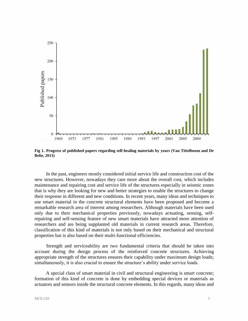
Van Tittelboom and De Belie (2013) reported a progress of published papers regarding self-

healing materials by years as shown in Fig 1. The ability of this class of materials to react to

the damages at the initial of the appearance of cracks and to repair themselves (passively or

actively) resulted to the achievement of durability through their management rather than their

prevention (Zwaag, 2008). Therefore, it may not only increase the service life of the structure,

but it can also reduce demands for new structures to its minimal level. Indeed, through using

this technique, it should be considered that the self-repaired structures might be re-subjected

to new critical conditions and forces; hence, the repaired structures should have ability to

endure new applied load with the least damage. In addition, this technique should lead to an

economic environmental solution.

MOLOD 3

In the past, engineers mostly considered initial service life and construction cost of the

new structures. However, nowadays they care more about the overall cost, which includes

maintenance and repairing cost and service life of the structures especially in seismic zones

that is why they are looking for new and better strategies to enable the structures to change

their response in different and new conditions. In recent years, many ideas and techniques to

use smart material in the concrete structural elements have been proposed and become a

remarkable research area of interest among researchers. Although materials have been used

only due to their mechanical properties previously, nowadays actuating, sensing, self-

repairing and self-sensing feature of new smart materials have attracted more attention of

researchers and are being supplanted old materials in current research areas. Therefore,

classification of this kind of materials is not only based on their mechanical and structural

properties but is also based on their multi-functional efficiencies.

Strength and serviceability are two fundamental criteria that should be taken into

account during the design process of the reinforced concrete structures. Achieving

appropriate strength of the structures ensures their capability under maximum design loads;

simultaneously, it is also crucial to ensure the structure’s ability under service loads.

A special class of smart material in civil and structural engineering is smart concrete;

formation of this kind of concrete is done by embedding special devices or materials as

actuators and sensors inside the structural concrete elements. In this regards, many ideas and

Fig 1. Progress of published papers regarding self-healing materials by years (Van Tittelboom and De

Belie, 2013)

MOLOD 4

techniques have been proposed and applied that are explained in the next section; however,

smart concrete formed by adding shape memory alloys has attracted special attention of

researches currently. For instance, this kind of smart concrete has been used to generate

active columns confinement, enabling self-repairing of the concrete structural members and

controlling mechanical and structural properties of pre-stressed structural elements by Deng

et al. (2006), Daghia et al. (2011) and Kuang and Ou (2008), respectively.

Nevertheless, there are not only durability issues arising from concrete cracks, but also

sustainability matters. In the following those sustainability issues are discussed, which are

linked to the durability issue. In case of concrete durability improvement, some sustainability

issues, including regular inspection demands, renovation, maintenance and even new

structure replacement can be reduced. One of the sustainability issues of using reinforced

concrete is environmental pollution. Davidovits (1994) stated that releasing levels of CO2

into the atmosphere lie at about 1 tone for every tone of Ordinary Portland Cement.

Considering this statistic and knowing that annual world requirement to cement which is

around 4×109 tones, the environment matter due to concrete is obvious (European Cement

Association, 2013). Pearce (1997) reported that global cement production is in the third

position, after energy and transportation departments in releasing CO2 into the atmosphere.

McLeod (2005) updated that 7 to 10% of the total CO2 emissions around the world is due to

the global production of cement. Therefore, attempts to reduce the amount of concrete used

in the construction should be increased. Another sustainability issue with reinforced concrete

comes from an economic point of view. Whole-life costs of reinforced concrete structures

are evaluated from the budget spends for the construction regular inspection, renovation and

maintenance of the structures.

1.2. Shape memory alloy materials

1.2.1. History of SMAs

The history of SMA backs to 1932 once for the first time SMA transformation

properties were observed and recorded in Gold-Cadmium (Au Cd) by Chang and Read. Later

on, Buechler and his colleagues in 1962 found out Nickel-Titanium (NiTi) type of shape

memory effect. Among all numerous types of SMA, NiTi SMAs have been most used in civil

engineering due to their perfect thermomechanical and thermo-electrical properties

(Miyazaki et al., 1990). In general, SMAs and in specific NiTi-SMAs are the most attractive

for seismic application due to their capability to dissipate considerable energy and regain

large deformation and give more ductility to the structure. NiTi SMAs are also known as

Nitinol, which is extracted from ‘Ni’ for Nickel, ‘ti’ for Titanium and ‘nol’ is the abbreviation

of Naval Ordinance Laboratory, where Ni-Ti SME was firstly discovered.

In the beginning, this kind of materials has been utilized in a few fields, such as

aerospace engineering (airplane wings) and in robotic and automotive industries as artificial

limbs. Nowadays, the applicability of SMA materials can be observed in more engineering

fields due to their special characteristics, including good corrosion resistance, great

MOLOD 5

durability, high power density, fair fatigue resistance, good damping capacity and being

actuator in their solid phase (Song et al., 2006).

1.2.2. SMAs forms and properties

SMAs have two different crystal forms: 1) Austenite form which is stable in high

temperature and has comparatively powerful resistance to any externally applied stress; this

phase is stronger and body-centered cubic structure and 2) Maternsite form which is stable

in low temperature and has a weak resistance to external stress due to its parallelogram

structure. These two phases can be transferred to each other if an external force obtained

from the difference between free Gibbs energy of these two phases applied on the body.

These loads can be applied due to either different temperature or mechanical loads. In overall,

both Martensite and Austenite phase depend on two thermos-mechanical parameters: 1)

amount of mechanical applied forces and 2) existing composite temperature.

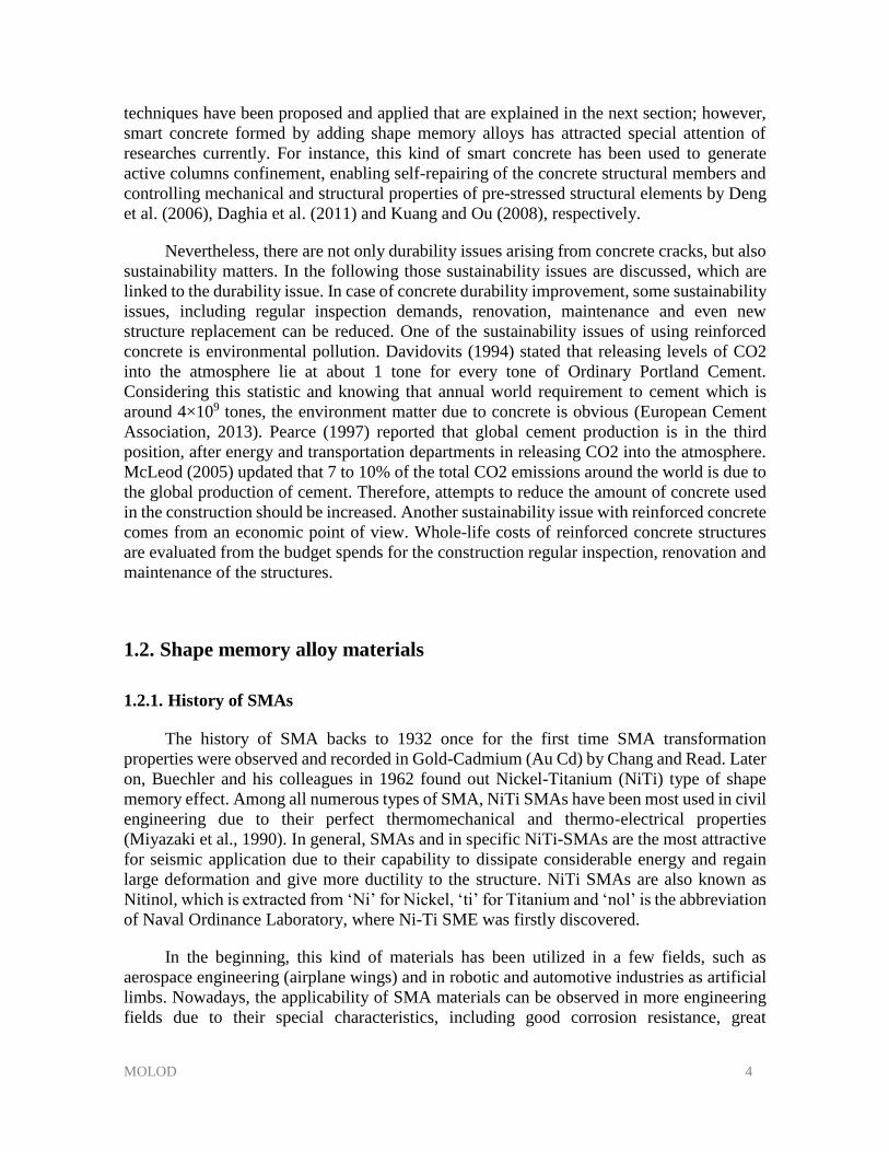
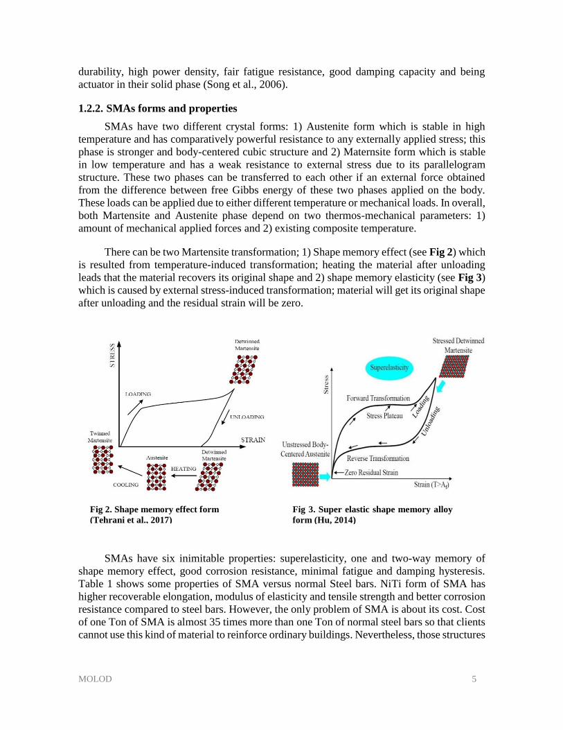
There can be two Martensite transformation; 1) Shape memory effect (see Fig 2) which

is resulted from temperature-induced transformation; heating the material after unloading

leads that the material recovers its original shape and 2) shape memory elasticity (see Fig 3)

which is caused by external stress-induced transformation; material will get its original shape

after unloading and the residual strain will be zero.

SMAs have six inimitable properties: superelasticity, one and two-way memory of

shape memory effect, good corrosion resistance, minimal fatigue and damping hysteresis.

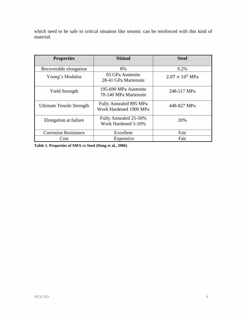
Table 1 shows some properties of SMA versus normal Steel bars. NiTi form of SMA has

higher recoverable elongation, modulus of elasticity and tensile strength and better corrosion

resistance compared to steel bars. However, the only problem of SMA is about its cost. Cost

of one Ton of SMA is almost 35 times more than one Ton of normal steel bars so that clients

cannot use this kind of material to reinforce ordinary buildings. Nevertheless, those structures

Fig 2. Shape memory effect form

(Tehrani et al., 2017) Fig 3. Super elastic shape memory alloy

form (Hu, 2014)

MOLOD 6

which need to be safe in critical situation like seismic can be reinforced with this kind of

material.

Properties Nitinol Steel

Recoverable elongation 8% 0.2%

Young’s Modulus 83 GPa Austenite

28-41 GPa Martensite2.07 × 105 MPa

Yield Strength 195-690 MPa Austenite

70-140 MPa Martensite248-517 MPa

Ultimate Tensile Strength Fully Annealed 895 MPa

Work Hardened 1900 MPa 448-827 MPa

Elongation at failure Fully Annealed 25-50%

Work Hardened 5-10% 20%

Corrosion Resistance Excellent Fair

Cost Expensive Fair

Table 1. Properties of SMA vs Steel (Deng et al., 2006)

MOLOD 7

1.3. Aim and objectives

1.3.1. Aim

The main aim of the research is to describe a novel method that allows for a probability-

based prediction of damage in concrete structures that can facilitate the assessment and

design degraded structures under risk of failure. It can also develop probabilistic strength

domains and relative statistics (e.g. 0.95 quantile of stress) to be employed as simplified

design tools to optimize the dimensions and assemblage configuration of SMA plates at a

concrete column-beam joint to enhance strength and ductility of the joint.

1.3.2. Objectives

To achieve the main aim of the research, several goals and objectives are required to be

investigated as below:

1. Better understanding SMA material properties and its application in the civil and

structural engineering field.

2. Modeling reinforced concrete column-beam joint in advanced non-linear FE software

properly and selecting the most appropriate elements and material models to simulate

concrete, steel and SMA.

3. Identifying all types of parallel processing with advanced non-linear FE software and

recognizing the fastest method to simulate with a large number of repetitions.

4. Specifying limit state functions of a concrete column-beam joint under three

combined loads: i) axial column force (R1); ii) bending force of beam (R2); and iii)

axial beam force (R3) and generating random load combinations in an innovative way.

5. Identifying all sources of uncertainty in strength domains of concrete column-beam

joint (e.g. load type, form and values, material properties of concrete, constitutive law

of SMA).

6. Carrying out a probabilistic analysis in MATLAB software based on achieved data

from a large number of simulations in Ansys.

7. Designing and optimizing the geometry of the SMA plate based on the obtained

results from the probabilistic study.

8. Employing fastening technique to connect optimized SMA plate with the external

surface of concrete column-beam joint.

9. Discussing results and findings, and providing recommendations to improve the

introduced innovative concept in the future.

MOLOD 8

1.4. Outline of the research

This research is divided into five main chapters. In the first chapter, an introduction

about concrete and SMA materials is given. History and main properties of SMAs and

reasons to use this kind of material as a strengthening element for concrete are discussed. In

addition, the main aim and objectives of the study shall be explained. The second chapter is

dedicated to reviewing existing literature and research performed concerning the application

of SMA in the civil and structural engineering field in general and in reinforced concrete

members in particular. Most proposed techniques to reinforce concrete beams and column-

beam joints with both types of SMAs, stress-induced and temperature-induced

transformation, will be discussed and the outcomes will be shown. The third chapter deals

with a methodology to carry out this investigation numerically. This chapter presents not

only the methodology that is going to be used in the research, but also the most appropriate

available elements and material models to model reinforced concrete in Ansys and the fastest

parallel processing method of Ansys. Furthermore, the way of specifying of limit state

functions and generating random load combinations are going to be demonstrated. The

investigation is developed in three different steps. In the first step, an experimentally

investigated concrete column-beam joint is simulated in Ansys, and verification and

validation of the numerical model are carried out. Then, a probabilistic study is based on the

achieved results of a large number of repetitions of a simulated model under different loading

forms is reported. Finally, an optimization study is run in order to reduce the amount of SMA

material. Obtained results and findings are presented in the fourth chapter. Furthermore, a

discussion to evaluate the achievements and a further detailed discussion about accuracy and

reliability of the results are held. Beside, the applicability of the proposed technique in large-

scale structure size is investigated. Finally, key-points of chapters 3-5 are collated as

conclusion, while a certain number of suggestions and recommendations for future associated

research and for further improvement of the proposed technique is offered.

MOLOD 9

Chapter 2. Literature review

Application of SMA in civil engineering can be reviewed in two different time periods.

During early years of 2000 due to high cost of SMA materials, researchers tried to use this

kind of material as less as possible in their investigations; hence, less researches had been

done in general and in specific in civil engineering field. With increasing applicability of

SMA in numerous fields of engineering, production of this kind of material has been

enhanced. Subsequently, its cost has been gradually and significantly reducing so that

nowadays more researchers have been investigating performance of this kind of material in

structural concrete elements. On the other hand, the material was used as external

strengthening element for steel structures at the beginning, and researchers have applied the

material in different sections of structures for different purposes. For instance, Han et al.

(2003) studied experimentally and numerically advantage of using hybrid SMA and steel

wires as damper device and diagonal braces for a steel frame structure. Tamai and Kitagawa

(2002) used diagonal braces, lower part made of Super-elastic SMA and upper part made of

steel, as devices for earthquake resistance. Sun and Rajapakse (2003) numerically

investigated performance of pre-strained SMA wire as diagonal tendon braces installed for a

simple frame in order to analyze dynamic and transient reaction of the structure. Khan and

Lagoudas (2002) numerically and Mayes et al. (2001) experimentally examined performance

of SMA springs as single degree of freedom vibration isolation system to filter ground motion

modeled using a shake table. Dolce et al. (2001) perused experimentally and numerically

performance of super-elastic NiTi-SMA as two full-scale vibration isolation system installed

between a super structure and ground. Song et al. (2006) stated that both forms of SMA,

pseudo-elastic and shape memory effect, can be utilized as bridge damper elements. Li et al.

(2004) used hybrid super-elastic SMA and cable as damper system in a stay-cable bridge

analytically in order to mitigate vibration of the cable. DesRoches and Delemont (2002)

analytically investigated capability of pseudo-elastic SMA restrainer bars in reducing the

earthquake vulnerability of simply supported bridge. Ozbulut and Hurlebaus (2010)

numerically studied efficiency of the hybrid laminated rubber bearing and auxiliary device

made of SMA wires as the base isolation system for an elevated bridge. Tamai et al. (2003)

experimentally and numerically studied effectiveness of anchorage made of SMA in

exposed-type column for building structures as passive damper and seismic resistance

member.

As it was mentioned, with increasing applicability of SMA in numerous field of

engineering, its production has been enhancing; hence, its cost significantly has been

reducing. As a result, number of researches regarding this material in all fields, especially in

civil and structural members have been enhanced. This reduction in cost allows civil and

structural engineering scientists to examine efficiency of SMAs as reinforcement of concrete

structural elements. Alam et al. (2008) numerically investigated performance of NiTi (55%

Ni to 45%Ti) super-elastic shape memory alloy in beam-column joint and column-footing

joint under seismic load. Results showed that SMA beam-column joint and column-footing

joint had less residual displacements in the joint and lower energy dissipation compared to

steel beam-column joint. Therefore, since the main cause of buildings’ and bridges’ failure

during seismic is residual and lateral displacement, SMA beam-column joint and column-

footing act better that of conventional ones. Shahverdi et al. (2015) used iron-based shape

memory alloy, so called Fe-SMA, as strip to reinforce four beam specimens, one not activated

MOLOD 10

and three activated strips. It was shown that using pre-stressed Fe-SMA resulted in increasing

strength of the beams approximately two times. In addition, cracking load of beams

reinforced with pre-stressed Fe-SMA was about 80% higher than that one reinforced with

not pre-stressed Fe-SMA. Therefore, using pre-stressed Fe-SMA can reduce deflection,

width of cracks, Stress in internal steel and consequently improve durability and

serviceability of concrete structures. Shahverdi et al. (2016) examined application of iron-

based SMA bars embedded in a shotcrete layer in bottom surface of two simply supported

beams. Results demonstrated that and this new reinforcing technique worked well and using

pre-stressed Fe-SMA bars could enhance cracking load. It was also shown that pre-stressing

Fe-SMA bars was easier than conventional steel bars since it did not need anchor heads and

mechanical jacks. Mas et al. (2017) investigated performance of NiTi shape memory alloy

cables as longitudinal reinforcement of concrete beam experimentally. Results showed that

the NiTi-SMA cables were considerably robust and durable if they are used as tension

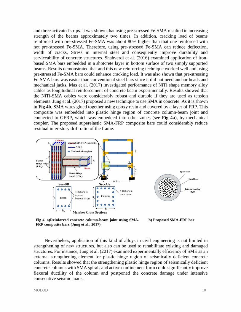
elements. Jung et al. (2017) proposed a new technique to use SMA in concrete. As it is shown

in Fig 4b, SMA wires glued together using epoxy resin and covered by a layer of FRP. This

composite was embedded into plastic hinge region of concrete column-beam joint and

connected to GFRP, which was embedded into other zones (see Fig 4a), by mechanical

coupler. The proposed superelastic SMA-FRP composite bars could considerably reduce

residual inter-story drift ratio of the frame.

Fig 4. a)Reinforced concrete column-beam joint using SMA-

FRP composite bars (Jung et al., 2017)

b) Proposed SMA-FRP bar

Nevertheless, application of this kind of alloys in civil engineering is not limited in

strengthening of new structures, but also can be used to rehabilitate existing and damaged

structures. For instance, Jung et al. (2017) examined experimentally efficiency of SME as an

external strengthening element for plastic hinge region of seismically deficient concrete

columns. Results showed that the strengthening plastic hinge region of seismically deficient

concrete columns with SMA spirals and active confinement form could significantly improve

flexural ductility of the column and postponed the concrete damage under intensive

consecutive seismic loads.

MOLOD 11

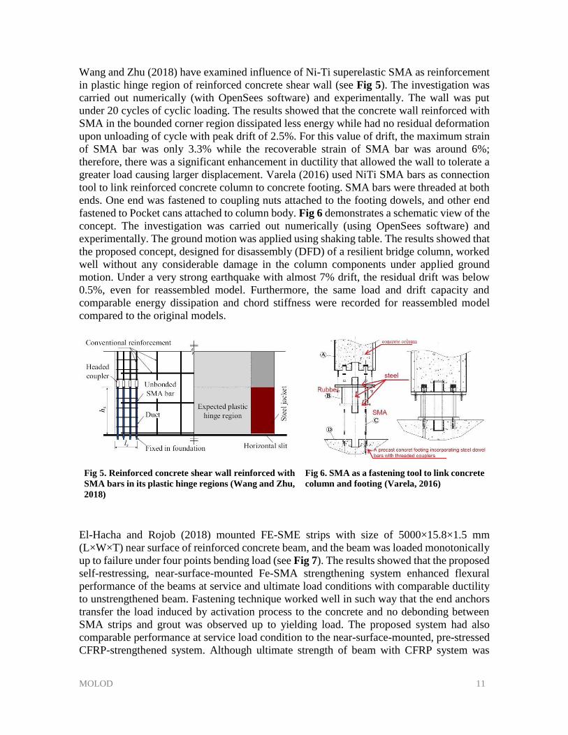
Wang and Zhu (2018) have examined influence of Ni-Ti superelastic SMA as reinforcement

in plastic hinge region of reinforced concrete shear wall (see Fig 5). The investigation was

carried out numerically (with OpenSees software) and experimentally. The wall was put

under 20 cycles of cyclic loading. The results showed that the concrete wall reinforced with

SMA in the bounded corner region dissipated less energy while had no residual deformation

upon unloading of cycle with peak drift of 2.5%. For this value of drift, the maximum strain

of SMA bar was only 3.3% while the recoverable strain of SMA bar was around 6%;

therefore, there was a significant enhancement in ductility that allowed the wall to tolerate a

greater load causing larger displacement. Varela (2016) used NiTi SMA bars as connection

tool to link reinforced concrete column to concrete footing. SMA bars were threaded at both

ends. One end was fastened to coupling nuts attached to the footing dowels, and other end

fastened to Pocket cans attached to column body. Fig 6 demonstrates a schematic view of the

concept. The investigation was carried out numerically (using OpenSees software) and

experimentally. The ground motion was applied using shaking table. The results showed that

the proposed concept, designed for disassembly (DFD) of a resilient bridge column, worked

well without any considerable damage in the column components under applied ground

motion. Under a very strong earthquake with almost 7% drift, the residual drift was below

0.5%, even for reassembled model. Furthermore, the same load and drift capacity and

comparable energy dissipation and chord stiffness were recorded for reassembled model

compared to the original models.

Fig 5. Reinforced concrete shear wall reinforced with

SMA bars in its plastic hinge regions (Wang and Zhu,

2018)

Fig 6. SMA as a fastening tool to link concrete

column and footing (Varela, 2016)

El-Hacha and Rojob (2018) mounted FE-SME strips with size of 5000×15.8×1.5 mm

(L×W×T) near surface of reinforced concrete beam, and the beam was loaded monotonically

up to failure under four points bending load (see Fig 7). The results showed that the proposed

self-restressing, near-surface-mounted Fe-SMA strengthening system enhanced flexural

performance of the beams at service and ultimate load conditions with comparable ductility

to unstrengthened beam. Fastening technique worked well in such way that the end anchors

transfer the load induced by activation process to the concrete and no debonding between

SMA strips and grout was observed up to yielding load. The proposed system had also

comparable performance at service load condition to the near-surface-mounted, pre-stressed

CFRP-strengthened system. Although ultimate strength of beam with CFRP system was

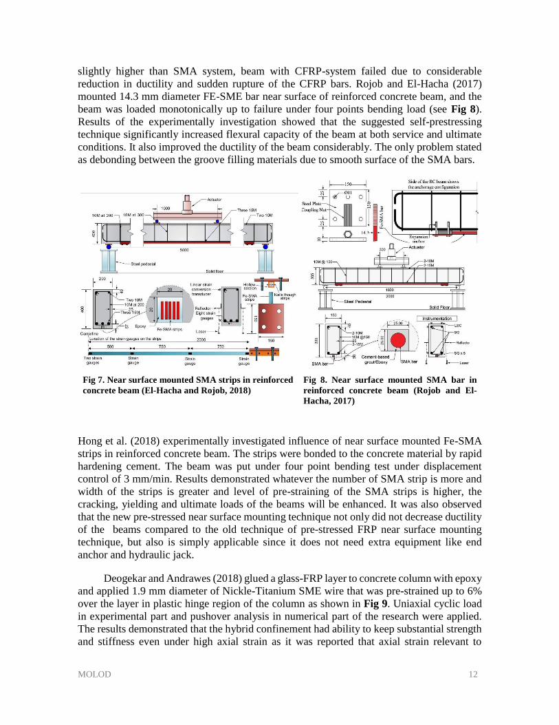
MOLOD 12

slightly higher than SMA system, beam with CFRP-system failed due to considerable

reduction in ductility and sudden rupture of the CFRP bars. Rojob and El-Hacha (2017)

mounted 14.3 mm diameter FE-SME bar near surface of reinforced concrete beam, and the

beam was loaded monotonically up to failure under four points bending load (see Fig 8).

Results of the experimentally investigation showed that the suggested self-prestressing

technique significantly increased flexural capacity of the beam at both service and ultimate

conditions. It also improved the ductility of the beam considerably. The only problem stated

as debonding between the groove filling materials due to smooth surface of the SMA bars.

Fig 7. Near surface mounted SMA strips in reinforced

concrete beam (El-Hacha and Rojob, 2018)

Fig 8. Near surface mounted SMA bar in

reinforced concrete beam (Rojob and El-

Hacha, 2017)

Hong et al. (2018) experimentally investigated influence of near surface mounted Fe-SMA

strips in reinforced concrete beam. The strips were bonded to the concrete material by rapid

hardening cement. The beam was put under four point bending test under displacement

control of 3 mm/min. Results demonstrated whatever the number of SMA strip is more and

width of the strips is greater and level of pre-straining of the SMA strips is higher, the

cracking, yielding and ultimate loads of the beams will be enhanced. It was also observed

that the new pre-stressed near surface mounting technique not only did not decrease ductility

of the beams compared to the old technique of pre-stressed FRP near surface mounting

technique, but also is simply applicable since it does not need extra equipment like end

anchor and hydraulic jack.

Deogekar and Andrawes (2018) glued a glass-FRP layer to concrete column with epoxy

and applied 1.9 mm diameter of Nickle-Titanium SME wire that was pre-strained up to 6%

over the layer in plastic hinge region of the column as shown in Fig 9. Uniaxial cyclic load

in experimental part and pushover analysis in numerical part of the research were applied.

The results demonstrated that the hybrid confinement had ability to keep substantial strength

and stiffness even under high axial strain as it was reported that axial strain relevant to

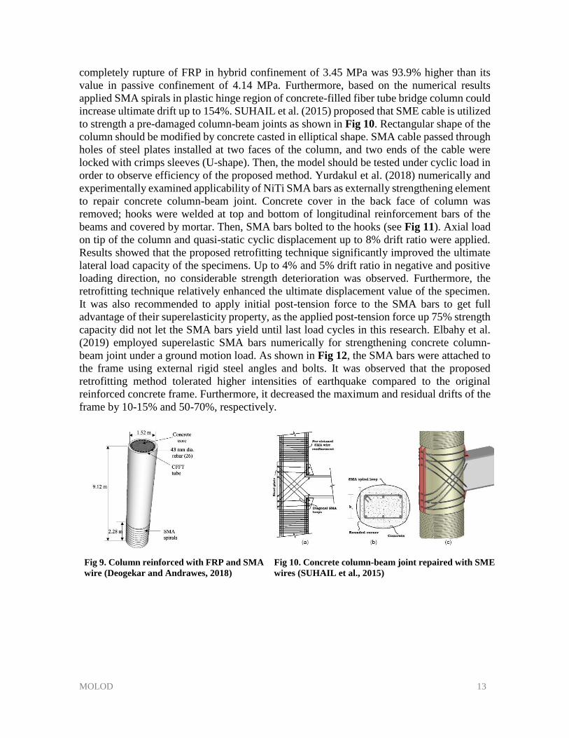
MOLOD 13

completely rupture of FRP in hybrid confinement of 3.45 MPa was 93.9% higher than its

value in passive confinement of 4.14 MPa. Furthermore, based on the numerical results

applied SMA spirals in plastic hinge region of concrete-filled fiber tube bridge column could

increase ultimate drift up to 154%. SUHAIL et al. (2015) proposed that SME cable is utilized

to strength a pre-damaged column-beam joints as shown in Fig 10. Rectangular shape of the

column should be modified by concrete casted in elliptical shape. SMA cable passed through

holes of steel plates installed at two faces of the column, and two ends of the cable were

locked with crimps sleeves (U-shape). Then, the model should be tested under cyclic load in

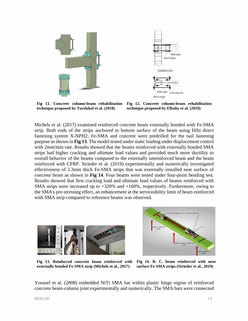
order to observe efficiency of the proposed method. Yurdakul et al. (2018) numerically and

experimentally examined applicability of NiTi SMA bars as externally strengthening element

to repair concrete column-beam joint. Concrete cover in the back face of column was

removed; hooks were welded at top and bottom of longitudinal reinforcement bars of the

beams and covered by mortar. Then, SMA bars bolted to the hooks (see Fig 11). Axial load

on tip of the column and quasi-static cyclic displacement up to 8% drift ratio were applied.

Results showed that the proposed retrofitting technique significantly improved the ultimate

lateral load capacity of the specimens. Up to 4% and 5% drift ratio in negative and positive

loading direction, no considerable strength deterioration was observed. Furthermore, the

retrofitting technique relatively enhanced the ultimate displacement value of the specimen.

It was also recommended to apply initial post-tension force to the SMA bars to get full

advantage of their superelasticity property, as the applied post-tension force up 75% strength

capacity did not let the SMA bars yield until last load cycles in this research. Elbahy et al.

(2019) employed superelastic SMA bars numerically for strengthening concrete column-

beam joint under a ground motion load. As shown in Fig 12, the SMA bars were attached to

the frame using external rigid steel angles and bolts. It was observed that the proposed

retrofitting method tolerated higher intensities of earthquake compared to the original

reinforced concrete frame. Furthermore, it decreased the maximum and residual drifts of the

frame by 10-15% and 50-70%, respectively.

Fig 9. Column reinforced with FRP and SMA

wire (Deogekar and Andrawes, 2018)

Fig 10. Concrete column-beam joint repaired with SME

wires (SUHAIL et al., 2015)

MOLOD 14

Fig 11. Concrete column-beam rehabilitation

technique proposed by Yurdakul et al. (2018)

Fig 12. Concrete column-beam rehabilitation

technique proposed by Elbahy et al. (2019)

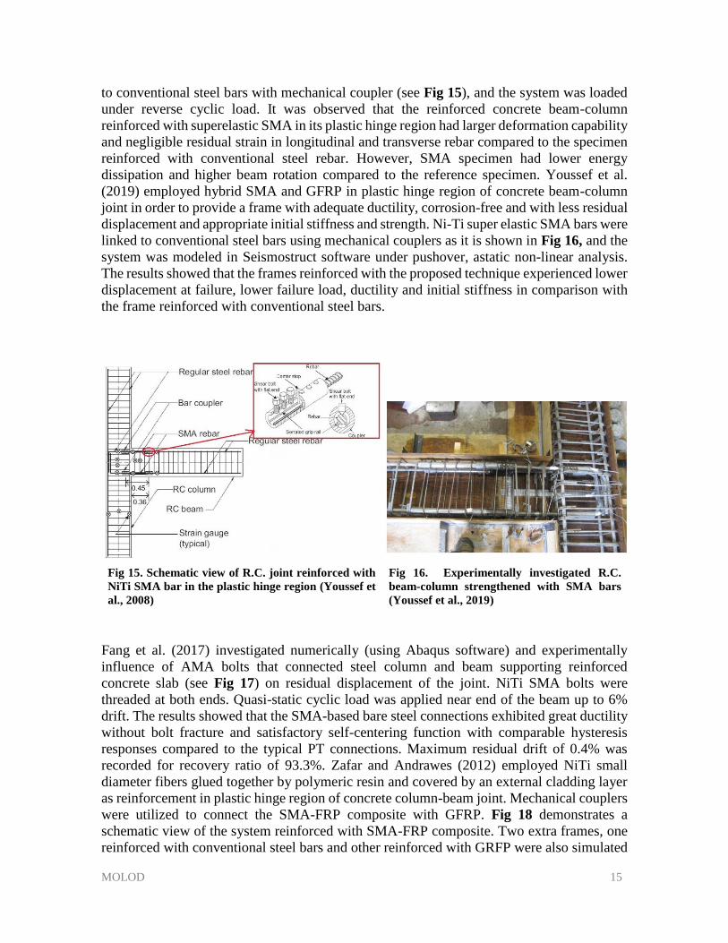
Michels et al. (2017) examined reinforced concrete beam externally bonded with Fe-SMA

strip. Both ends of the strips anchored to bottom surface of the beam using Hilti direct

fastening system X-NPH2; Fe-SMA and concrete were predrilled for the nail fastening

purpose as shown in Fig 13. The model tested under static loading under displacement control

with 2mm/min rate. Results showed that the beams reinforced with externally bonded SMA

strips had higher cracking and ultimate load values and provided much more ductility to

overall behavior of the beams compared to the externally unreinforced beam and the beam

reinforced with CFRP. Strieder et al. (2019) experimentally and numerically investigated

effectiveness of 2.3mm thick Fe-SMA strips that was externally installed near surface of

concrete beam as shown in Fig 14. Four beams were tested under four-point bending test.

Results showed that first cracking load and ultimate load values of beams reinforced with

SMA strips were increased up to +320% and +160%, respectively. Furthermore, owing to

the SMA's pre-stressing effect, an enhancement at the serviceability limit of beam reinforced

with SMA strip compared to reference beams was observed.

Fig 13. Reinforced concrete beam reinforced with

externally bonded Fe-SMA strip (Michels et al., 2017)

Fig 14. R. C. beam reinforced with near

surface Fe-SMA strips (Strieder et al., 2019)

Youssef et al. (2008) embedded NiTi SMA bar within plastic hinge region of reinforced

concrete beam-column joint experimentally and numerically. The SMA bars were connected

MOLOD 15

to conventional steel bars with mechanical coupler (see Fig 15), and the system was loaded

under reverse cyclic load. It was observed that the reinforced concrete beam-column

reinforced with superelastic SMA in its plastic hinge region had larger deformation capability

and negligible residual strain in longitudinal and transverse rebar compared to the specimen

reinforced with conventional steel rebar. However, SMA specimen had lower energy

dissipation and higher beam rotation compared to the reference specimen. Youssef et al.

(2019) employed hybrid SMA and GFRP in plastic hinge region of concrete beam-column

joint in order to provide a frame with adequate ductility, corrosion-free and with less residual

displacement and appropriate initial stiffness and strength. Ni-Ti super elastic SMA bars were

linked to conventional steel bars using mechanical couplers as it is shown in Fig 16, and the

system was modeled in Seismostruct software under pushover, astatic non-linear analysis.

The results showed that the frames reinforced with the proposed technique experienced lower

displacement at failure, lower failure load, ductility and initial stiffness in comparison with

the frame reinforced with conventional steel bars.

Fig 15. Schematic view of R.C. joint reinforced with

NiTi SMA bar in the plastic hinge region (Youssef et

al., 2008)

Fig 16. Experimentally investigated R.C.

beam-column strengthened with SMA bars

(Youssef et al., 2019)

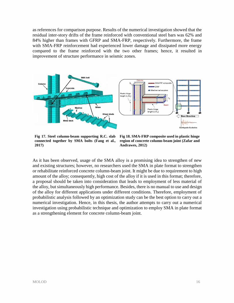
Fang et al. (2017) investigated numerically (using Abaqus software) and experimentally

influence of AMA bolts that connected steel column and beam supporting reinforced

concrete slab (see Fig 17) on residual displacement of the joint. NiTi SMA bolts were

threaded at both ends. Quasi-static cyclic load was applied near end of the beam up to 6%

drift. The results showed that the SMA-based bare steel connections exhibited great ductility

without bolt fracture and satisfactory self-centering function with comparable hysteresis

responses compared to the typical PT connections. Maximum residual drift of 0.4% was

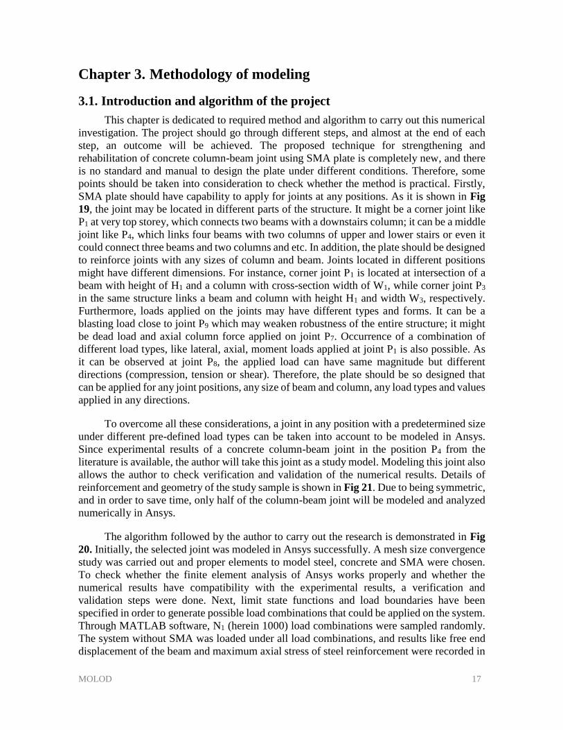
recorded for recovery ratio of 93.3%. Zafar and Andrawes (2012) employed NiTi small

diameter fibers glued together by polymeric resin and covered by an external cladding layer

as reinforcement in plastic hinge region of concrete column-beam joint. Mechanical couplers

were utilized to connect the SMA-FRP composite with GFRP. Fig 18 demonstrates a

schematic view of the system reinforced with SMA-FRP composite. Two extra frames, one

reinforced with conventional steel bars and other reinforced with GRFP were also simulated

MOLOD 16

as references for comparison purpose. Results of the numerical investigation showed that the

residual inter-story drifts of the frame reinforced with conventional steel bars was 62% and

84% higher than frames with GFRP and SMA-FRP, respectively. Furthermore, the frame

with SMA-FRP reinforcement had experienced lower damage and dissipated more energy

compared to the frame reinforced with the two other frames; hence, it resulted in

improvement of structure performance in seismic zones.

Fig 17. Steel column-beam supporting R.C. slab

connected together by SMA bolts (Fang et al.,

2017)

Fig 18. SMA-FRP composite used in plastic hinge

region of concrete column-beam joint (Zafar and

Andrawes, 2012)

As it has been observed, usage of the SMA alloy is a promising idea to strengthen of new

and existing structures; however, no researchers used the SMA in plate format to strengthen

or rehabilitate reinforced concrete column-beam joint. It might be due to requirement to high

amount of the alloy; consequently, high cost of the alloy if it is used in this format; therefore,

a proposal should be taken into consideration that leads to employment of less material of

the alloy, but simultaneously high performance. Besides, there is no manual to use and design

of the alloy for different applications under different conditions. Therefore, employment of

probabilistic analysis followed by an optimization study can be the best option to carry out a

numerical investigation. Hence, in this thesis, the author attempts to carry out a numerical

investigation using probabilistic technique and optimization to employ SMA in plate format

as a strengthening element for concrete column-beam joint.

MOLOD 17

Chapter 3. Methodology of modeling

3.1. Introduction and algorithm of the project

This chapter is dedicated to required method and algorithm to carry out this numerical

investigation. The project should go through different steps, and almost at the end of each

step, an outcome will be achieved. The proposed technique for strengthening and

rehabilitation of concrete column-beam joint using SMA plate is completely new, and there

is no standard and manual to design the plate under different conditions. Therefore, some

points should be taken into consideration to check whether the method is practical. Firstly,

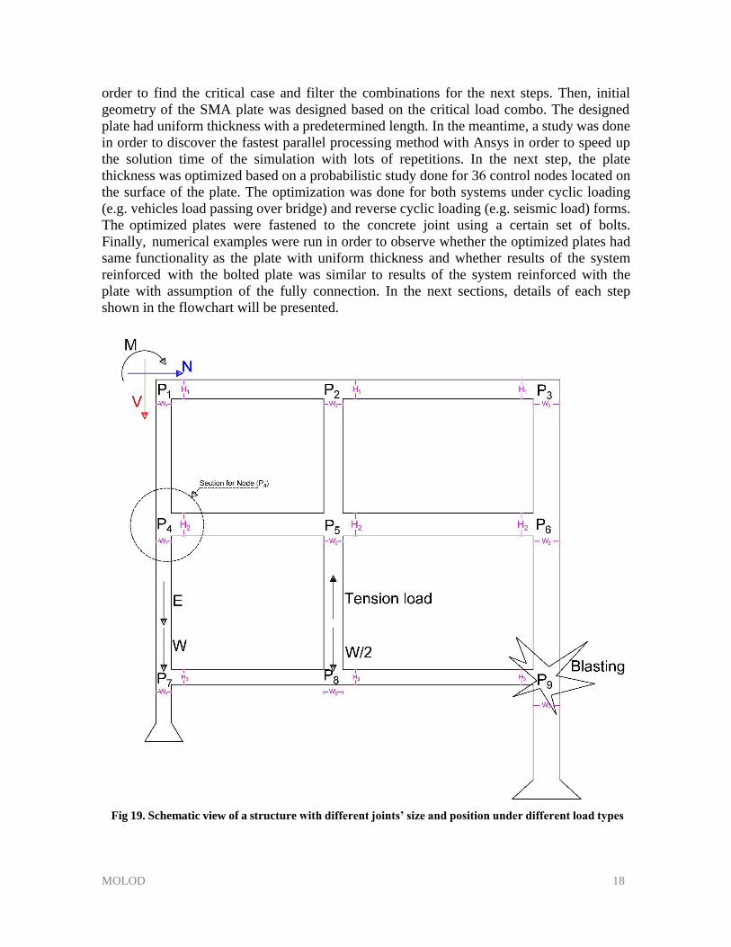
SMA plate should have capability to apply for joints at any positions. As it is shown in Fig

19, the joint may be located in different parts of the structure. It might be a corner joint like

P1 at very top storey, which connects two beams with a downstairs column; it can be a middle

joint like P4, which links four beams with two columns of upper and lower stairs or even it

could connect three beams and two columns and etc. In addition, the plate should be designed

to reinforce joints with any sizes of column and beam. Joints located in different positions

might have different dimensions. For instance, corner joint P1 is located at intersection of a

beam with height of H1 and a column with cross-section width of W1, while corner joint P3

in the same structure links a beam and column with height H1 and width W3, respectively.

Furthermore, loads applied on the joints may have different types and forms. It can be a

blasting load close to joint P9 which may weaken robustness of the entire structure; it might

be dead load and axial column force applied on joint P7. Occurrence of a combination of

different load types, like lateral, axial, moment loads applied at joint P1 is also possible. As

it can be observed at joint P8, the applied load can have same magnitude but different

directions (compression, tension or shear). Therefore, the plate should be so designed that

can be applied for any joint positions, any size of beam and column, any load types and values

applied in any directions.

To overcome all these considerations, a joint in any position with a predetermined size

under different pre-defined load types can be taken into account to be modeled in Ansys.

Since experimental results of a concrete column-beam joint in the position P4 from the

literature is available, the author will take this joint as a study model. Modeling this joint also

allows the author to check verification and validation of the numerical results. Details of

reinforcement and geometry of the study sample is shown in Fig 21. Due to being symmetric,

and in order to save time, only half of the column-beam joint will be modeled and analyzed

numerically in Ansys.

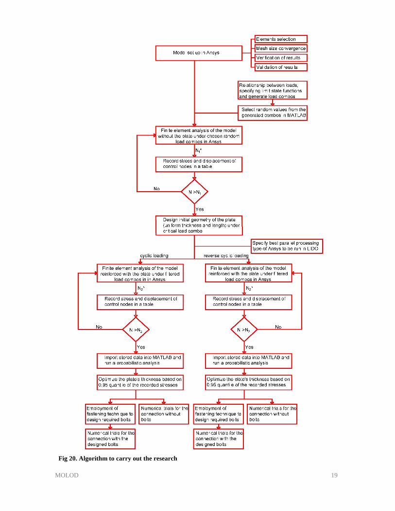
The algorithm followed by the author to carry out the research is demonstrated in Fig

20. Initially, the selected joint was modeled in Ansys successfully. A mesh size convergence

study was carried out and proper elements to model steel, concrete and SMA were chosen.

To check whether the finite element analysis of Ansys works properly and whether the

numerical results have compatibility with the experimental results, a verification and

validation steps were done. Next, limit state functions and load boundaries have been

specified in order to generate possible load combinations that could be applied on the system.

Through MATLAB software, N1 (herein 1000) load combinations were sampled randomly.

The system without SMA was loaded under all load combinations, and results like free end

displacement of the beam and maximum axial stress of steel reinforcement were recorded in

MOLOD 18

order to find the critical case and filter the combinations for the next steps. Then, initial

geometry of the SMA plate was designed based on the critical load combo. The designed

plate had uniform thickness with a predetermined length. In the meantime, a study was done

in order to discover the fastest parallel processing method with Ansys in order to speed up

the solution time of the simulation with lots of repetitions. In the next step, the plate

thickness was optimized based on a probabilistic study done for 36 control nodes located on

the surface of the plate. The optimization was done for both systems under cyclic loading

(e.g. vehicles load passing over bridge) and reverse cyclic loading (e.g. seismic load) forms.

The optimized plates were fastened to the concrete joint using a certain set of bolts.

Finally, numerical examples were run in order to observe whether the optimized plates had

same functionality as the plate with uniform thickness and whether results of the system

reinforced with the bolted plate was similar to results of the system reinforced with the

plate with assumption of the fully connection. In the next sections, details of each step

shown in the flowchart will be presented.

Fig 19. Schematic view of a structure with different joints’ size and position under different load types

MOLOD 19

Fig 20. Algorithm to carry out the research

MOLOD 20

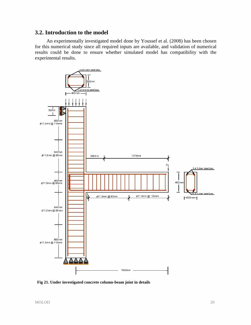
3.2. Introduction to the model

An experimentally investigated model done by Youssef et al. (2008) has been chosen

for this numerical study since all required inputs are available, and validation of numerical

results could be done to ensure whether simulated model has compatibility with the

experimental results.

Fig 21. Under investigated concrete column-beam joint in details

MOLOD 21

The experiment was done at structures laboratory of the university of Western Ontario

based on Canadian standards. The concrete column-beam joint was taken from fifth-sixth

floor of an eight-story building. For simplification and due to limitation of the laboratory

space and facilities, size of the joint has been scaled down to ¾ of its original size.

Furthermore, applied loads were scaled down with a factor of (¾)2. Design of the system was

done based on CSA A23.3-0.4. The column was designed for axial force equals 620 kN, but

was scaled down to only 350 kN so that four bars with diameter 19.5 mm were installed as

main reinforcement of the column. Eleven shear reinforcements with diameter 11.3 mm

started at distance ±640 mm far from the column face with space 80 mm center to center and

column stirrups at other parts arranged with 115 mm center to center. Same longitudinal

reinforcements have been placed within concrete beams; however, 11 stirrups started at space

50 mm far from face of the beam with center to center space of 80 mm, and rest of shear bars

lied along the beam with center to center 150 mm. More details about geometry and

reinforcements of the system can be found in Fig 21.

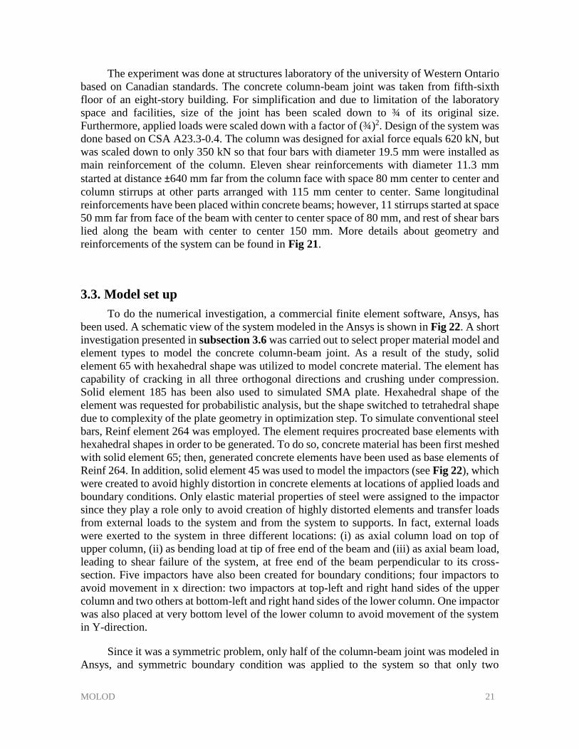
3.3. Model set up

To do the numerical investigation, a commercial finite element software, Ansys, has

been used. A schematic view of the system modeled in the Ansys is shown in Fig 22. A short

investigation presented in subsection 3.6 was carried out to select proper material model and

element types to model the concrete column-beam joint. As a result of the study, solid

element 65 with hexahedral shape was utilized to model concrete material. The element has

capability of cracking in all three orthogonal directions and crushing under compression.

Solid element 185 has been also used to simulated SMA plate. Hexahedral shape of the

element was requested for probabilistic analysis, but the shape switched to tetrahedral shape

due to complexity of the plate geometry in optimization step. To simulate conventional steel

bars, Reinf element 264 was employed. The element requires procreated base elements with

hexahedral shapes in order to be generated. To do so, concrete material has been first meshed

with solid element 65; then, generated concrete elements have been used as base elements of

Reinf 264. In addition, solid element 45 was used to model the impactors (see Fig 22), which

were created to avoid highly distortion in concrete elements at locations of applied loads and

boundary conditions. Only elastic material properties of steel were assigned to the impactor

since they play a role only to avoid creation of highly distorted elements and transfer loads

from external loads to the system and from the system to supports. In fact, external loads

were exerted to the system in three different locations: (i) as axial column load on top of

upper column, (ii) as bending load at tip of free end of the beam and (iii) as axial beam load,

leading to shear failure of the system, at free end of the beam perpendicular to its cross-

section. Five impactors have also been created for boundary conditions; four impactors to

avoid movement in x direction: two impactors at top-left and right hand sides of the upper

column and two others at bottom-left and right hand sides of the lower column. One impactor

was also placed at very bottom level of the lower column to avoid movement of the system

in Y-direction.

Since it was a symmetric problem, only half of the column-beam joint was modeled in

Ansys, and symmetric boundary condition was applied to the system so that only two

MOLOD 22

longitudinal bars in each column and beam was simulated, and stirrups was modeled like half

of a rectangle. As symmetric boundary condition, movement of those nodes located at half

depth of the system (Z =125 mm) was closed in Z-direction.

Fig 22. Schematic view of the concrete column-beam joint modeled in Ansys

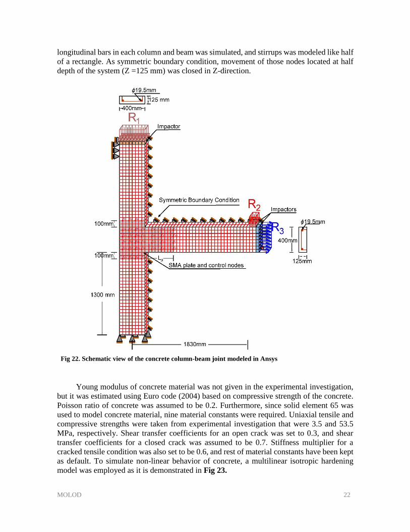
Young modulus of concrete material was not given in the experimental investigation,

but it was estimated using Euro code (2004) based on compressive strength of the concrete.

Poisson ratio of concrete was assumed to be 0.2. Furthermore, since solid element 65 was

used to model concrete material, nine material constants were required. Uniaxial tensile and

compressive strengths were taken from experimental investigation that were 3.5 and 53.5

MPa, respectively. Shear transfer coefficients for an open crack was set to 0.3, and shear

transfer coefficients for a closed crack was assumed to be 0.7. Stiffness multiplier for a

cracked tensile condition was also set to be 0.6, and rest of material constants have been kept

as default. To simulate non-linear behavior of concrete, a multilinear isotropic hardening

model was employed as it is demonstrated in Fig 23.

MOLOD 23

Fig 23. Linear and non-linear behavior of the concrete material

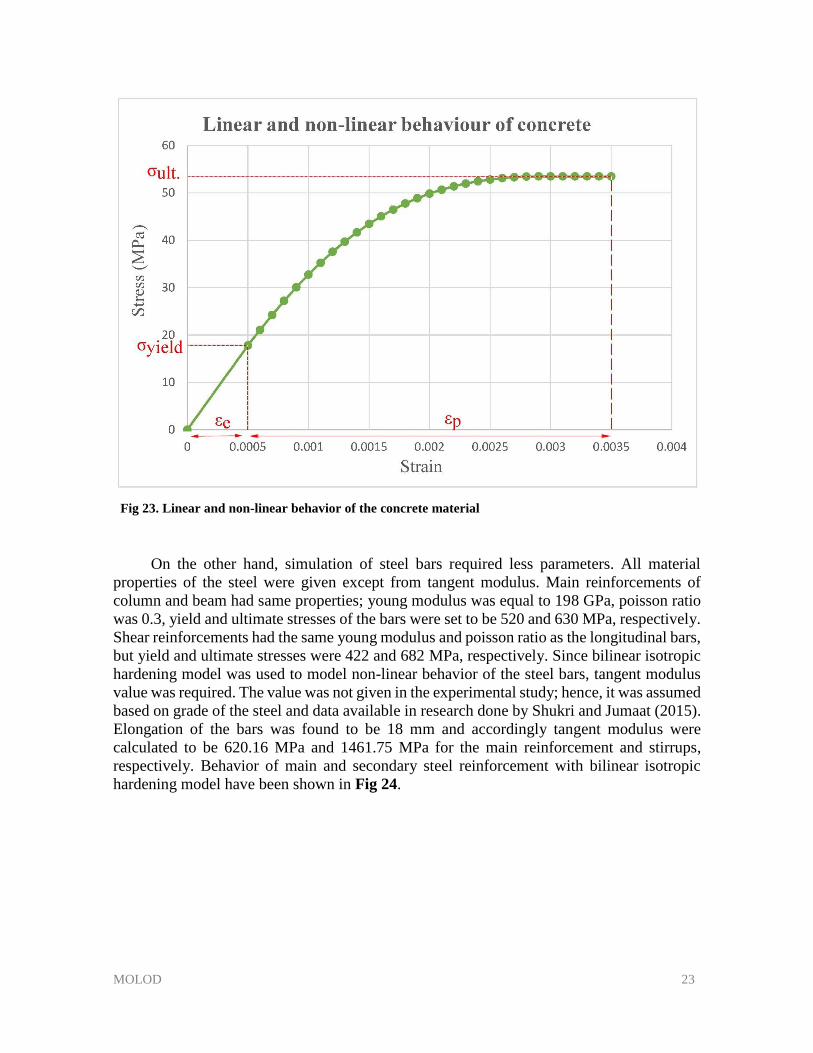
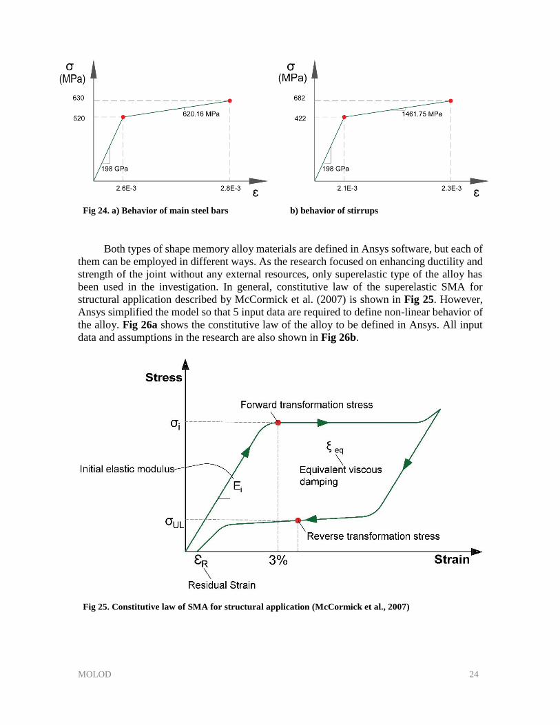
On the other hand, simulation of steel bars required less parameters. All material

properties of the steel were given except from tangent modulus. Main reinforcements of

column and beam had same properties; young modulus was equal to 198 GPa, poisson ratio

was 0.3, yield and ultimate stresses of the bars were set to be 520 and 630 MPa, respectively.

Shear reinforcements had the same young modulus and poisson ratio as the longitudinal bars,

but yield and ultimate stresses were 422 and 682 MPa, respectively. Since bilinear isotropic

hardening model was used to model non-linear behavior of the steel bars, tangent modulus

value was required. The value was not given in the experimental study; hence, it was assumed

based on grade of the steel and data available in research done by Shukri and Jumaat (2015).

Elongation of the bars was found to be 18 mm and accordingly tangent modulus were

calculated to be 620.16 MPa and 1461.75 MPa for the main reinforcement and stirrups,

respectively. Behavior of main and secondary steel reinforcement with bilinear isotropic

hardening model have been shown in Fig 24.

MOLOD 24

Fig 24. a) Behavior of main steel bars b) behavior of stirrups

Both types of shape memory alloy materials are defined in Ansys software, but each of

them can be employed in different ways. As the research focused on enhancing ductility and

strength of the joint without any external resources, only superelastic type of the alloy has

been used in the investigation. In general, constitutive law of the superelastic SMA for

structural application described by McCormick et al. (2007) is shown in Fig 25. However,

Ansys simplified the model so that 5 input data are required to define non-linear behavior of

the alloy. Fig 26a shows the constitutive law of the alloy to be defined in Ansys. All input

data and assumptions in the research are also shown in Fig 26b.

Fig 25. Constitutive law of SMA for structural application (McCormick et al., 2007)

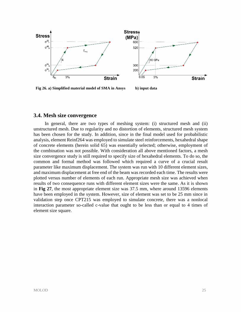
MOLOD 25

Fig 26. a) Simplified material model of SMA in Ansys b) input data

3.4. Mesh size convergence

In general, there are two types of meshing system: (i) structured mesh and (ii)

unstructured mesh. Due to regularity and no distortion of elements, structured mesh system

has been chosen for the study. In addition, since in the final model used for probabilistic

analysis, element Reinf264 was employed to simulate steel reinforcements, hexahedral shape

of concrete elements (herein solid 65) was essentially selected; otherwise, employment of

the combination was not possible. With consideration all above mentioned factors, a mesh

size convergence study is still required to specify size of hexahedral elements. To do so, the

common and formal method was followed which required a curve of a crucial result

parameter like maximum displacement. The system was run with 10 different element sizes,

and maximum displacement at free end of the beam was recorded each time. The results were

plotted versus number of elements of each run. Appropriate mesh size was achieved when

results of two consequence runs with different element sizes were the same. As it is shown

in Fig 27, the most appropriate element size was 37.5 mm, where around 13596 elements

have been employed in the system. However, size of element was set to be 25 mm since in

validation step once CPT215 was employed to simulate concrete, there was a nonlocal

interaction parameter so-called c-value that ought to be less than or equal to 4 times of

element size square.

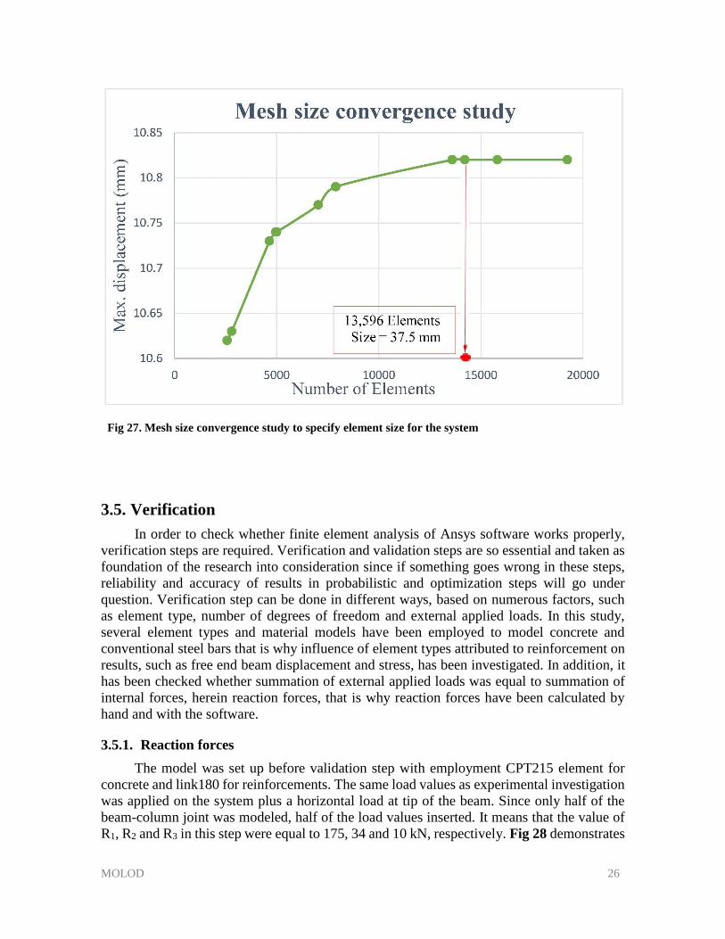
MOLOD 26

Fig 27. Mesh size convergence study to specify element size for the system

3.5. Verification

In order to check whether finite element analysis of Ansys software works properly,

verification steps are required. Verification and validation steps are so essential and taken as

foundation of the research into consideration since if something goes wrong in these steps,

reliability and accuracy of results in probabilistic and optimization steps will go under

question. Verification step can be done in different ways, based on numerous factors, such

as element type, number of degrees of freedom and external applied loads. In this study,

several element types and material models have been employed to model concrete and

conventional steel bars that is why influence of element types attributed to reinforcement on

results, such as free end beam displacement and stress, has been investigated. In addition, it

has been checked whether summation of external applied loads was equal to summation of

internal forces, herein reaction forces, that is why reaction forces have been calculated by

hand and with the software.

3.5.1. Reaction forces

The model was set up before validation step with employment CPT215 element for

concrete and link180 for reinforcements. The same load values as experimental investigation

was applied on the system plus a horizontal load at tip of the beam. Since only half of the

beam-column joint was modeled, half of the load values inserted. It means that the value of

R1, R2 and R3 in this step were equal to 175, 34 and 10 kN, respectively. Fig 28 demonstrates

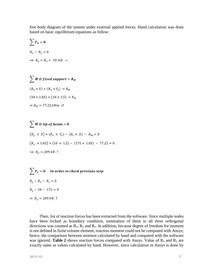
MOLOD 27

free body diagram of the system under external applied forces. Hand calculation was done

based on basic equilibrium equations as follow:

∑ 𝑭𝑿 = 𝟎

𝑅𝑥 − 𝑅3 = 0

⟹ 𝑅𝑥 = 𝑅3 = 10 𝑘𝑁 ←

∑ 𝑴 @ 𝒇𝒊𝒙𝒆𝒅 𝒔𝒖𝒑𝒑𝒐𝒓𝒕 = 𝑹𝑴

(𝑅2 × 𝑋) + (𝑅3 × 𝑌2) = 𝑅𝑀

(34 × 1.83) + (10 × 1.5) = 𝑅𝑀

⇒ 𝑅𝑀 = 77.22 𝑘𝑁𝑚 ↺

∑ 𝑴 @ 𝒕𝒊𝒑 𝒐𝒇 𝒃𝒆𝒂𝒎 = 𝟎

(𝑅𝑦 × 𝑋) + (𝑅𝑥 × 𝑌2) − (𝑅1 × 𝑋) − 𝑅𝑀 = 0

(𝑅𝑦 × 1.83) + (10 × 1.5) − (175 × 1.83) − 77.22 = 0

⟹ 𝑅𝑦 = 209 𝑘𝑁 ↑

∑ 𝑭𝒀 = 𝟎 𝑰𝒏 𝒐𝒓𝒅𝒆𝒓 𝒕𝒐 𝒄𝒉𝒆𝒄𝒌 𝒑𝒓𝒆𝒗𝒊𝒐𝒖𝒔 𝒔𝒕𝒆𝒑

𝑅𝑦 − 𝑅2 − 𝑅1 = 0

𝑅𝑦 − 34 − 175 = 0

⇒ 𝑅𝑦 = 209 𝑘𝑁 ↑

Then, list of reaction forces has been extracted from the software. Since multiple nodes

have been locked as boundary condition, summation of them in all three orthogonal

directions was counted as Rx, Ry and Rz. In addition, because degree of freedom for moment

is not defined in finite volume element, reaction moment could not be computed with Ansys;

hence, the comparison between moment calculated by hand and computed with the software

was ignored. Table 2 shows reaction forces computed with Ansys. Value of Rx and Ry are

exactly same as values calculated by hand. However, since calculation in Ansys is done by

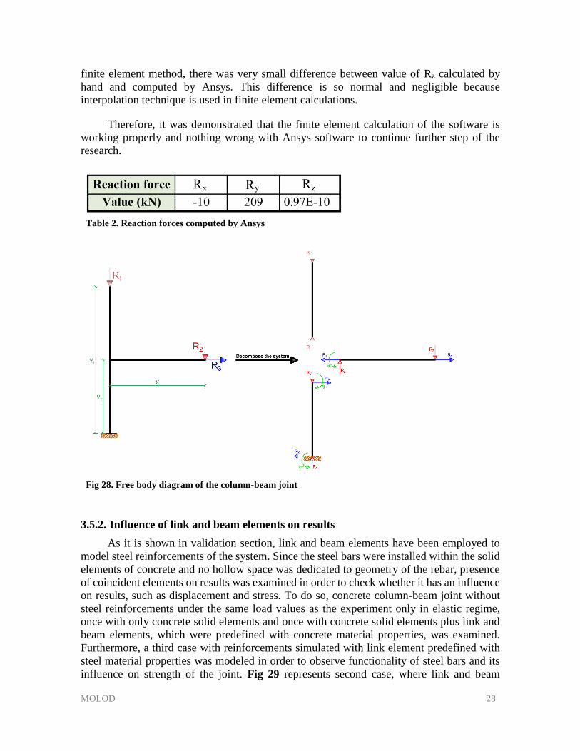
MOLOD 28

finite element method, there was very small difference between value of Rz calculated by

hand and computed by Ansys. This difference is so normal and negligible because

interpolation technique is used in finite element calculations.

Therefore, it was demonstrated that the finite element calculation of the software is

working properly and nothing wrong with Ansys software to continue further step of the

research.

Table 2. Reaction forces computed by Ansys

Fig 28. Free body diagram of the column-beam joint

3.5.2. Influence of link and beam elements on results

As it is shown in validation section, link and beam elements have been employed to

model steel reinforcements of the system. Since the steel bars were installed within the solid

elements of concrete and no hollow space was dedicated to geometry of the rebar, presence

of coincident elements on results was examined in order to check whether it has an influence

on results, such as displacement and stress. To do so, concrete column-beam joint without

steel reinforcements under the same load values as the experiment only in elastic regime,

once with only concrete solid elements and once with concrete solid elements plus link and

beam elements, which were predefined with concrete material properties, was examined.

Furthermore, a third case with reinforcements simulated with link element predefined with

steel material properties was modeled in order to observe functionality of steel bars and its

influence on strength of the joint. Fig 29 represents second case, where link and beam

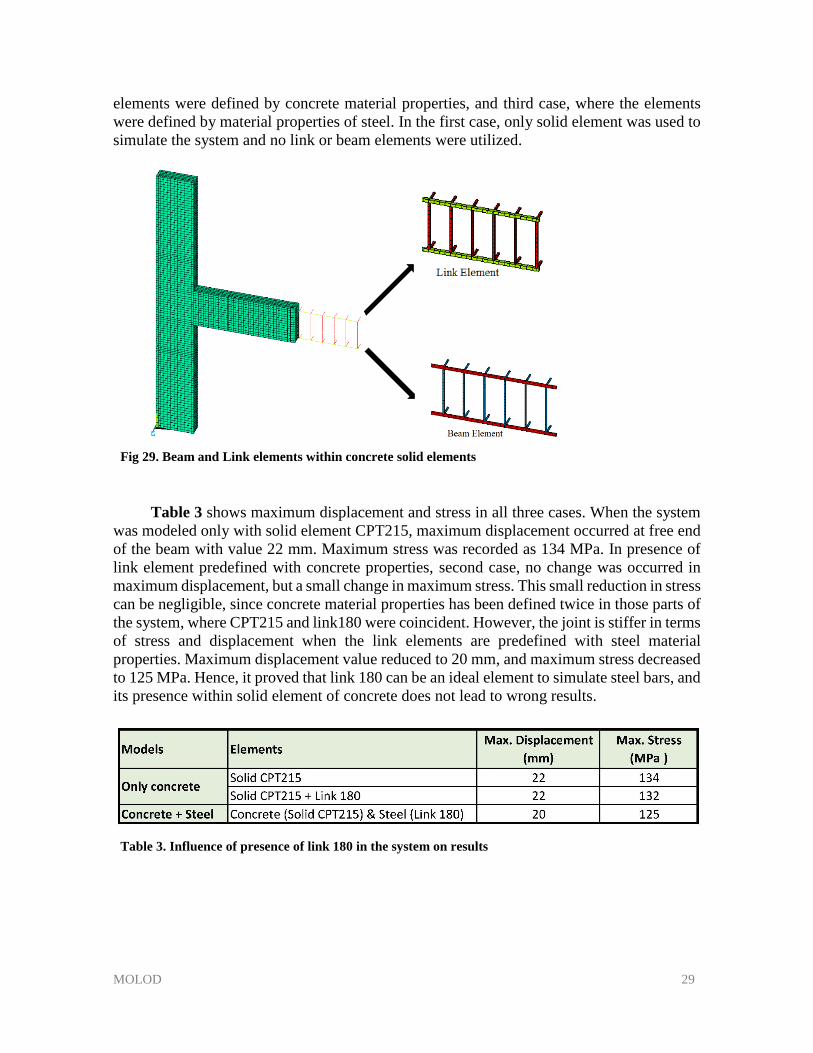
MOLOD 29

elements were defined by concrete material properties, and third case, where the elements

were defined by material properties of steel. In the first case, only solid element was used to

simulate the system and no link or beam elements were utilized.

Fig 29. Beam and Link elements within concrete solid elements

Table 3 shows maximum displacement and stress in all three cases. When the system

was modeled only with solid element CPT215, maximum displacement occurred at free end

of the beam with value 22 mm. Maximum stress was recorded as 134 MPa. In presence of

link element predefined with concrete properties, second case, no change was occurred in

maximum displacement, but a small change in maximum stress. This small reduction in stress

can be negligible, since concrete material properties has been defined twice in those parts of

the system, where CPT215 and link180 were coincident. However, the joint is stiffer in terms

of stress and displacement when the link elements are predefined with steel material

properties. Maximum displacement value reduced to 20 mm, and maximum stress decreased

to 125 MPa. Hence, it proved that link 180 can be an ideal element to simulate steel bars, and

its presence within solid element of concrete does not lead to wrong results.

Table 3. Influence of presence of link 180 in the system on results

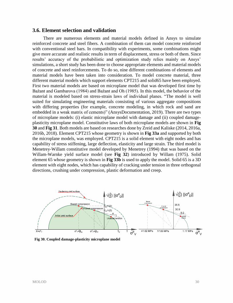
MOLOD 30

3.6. Element selection and validation

There are numerous elements and material models defined in Ansys to simulate

reinforced concrete and steel fibers. A combination of them can model concrete reinforced

with conventional steel bars. In compatibility with experiments, some combinations might

give more accurate and realistic results in term of displacement, stress or both of them. Since

results’ accuracy of the probabilistic and optimization study relies mainly on Ansys’

simulations, a short study has been done to choose appropriate elements and material models

of concrete and steel reinforcements. To do so, nine different combinations of elements and

material models have been taken into consideration. To model concrete material, three

different material models which support elements CPT215 and solid65 have been employed.

First two material models are based on microplane model that was developed first time by

Bažant and Gambarova (1984) and Bažant and Oh (1985). In this model, the behavior of the

material is modeled based on stress-strain laws of individual planes. “The model is well

suited for simulating engineering materials consisting of various aggregate compositions

with differing properties (for example, concrete modeling, in which rock and sand are

embedded in a weak matrix of cements)” (AnsysDocumentation, 2019). There are two types

of microplane models: (i) elastic microplane model with damage and (ii) coupled damage-

plasticity microplane model. Constitutive laws of both microplane models are shown in Fig

30 and Fig 31. Both models are based on researches done by Zreid and Kaliske (2014, 2016a,

2016b, 2018). Element CPT215 whose geometry is shown in Fig 33a and supported by both

the microplane models, was employed. CPT215 is a solid element with eight nodes and has

capability of stress stiffening, large deflection, elasticity and large strain. The third model is

Menetrey-Willam constitutive model developed by Menetrey (1994) that was based on the

Willam-Warnke yield surface model (see Fig 32) introduced by Willam (1975). Solid

element 65 whose geometry is shown in Fig 33b is used to apply the model. Solid 65 is a 3D

element with eight nodes, which has capability of cracking under tension in three orthogonal

directions, crushing under compression, plastic deformation and creep.

Fig 30. Coupled damage-plasticity microplane model

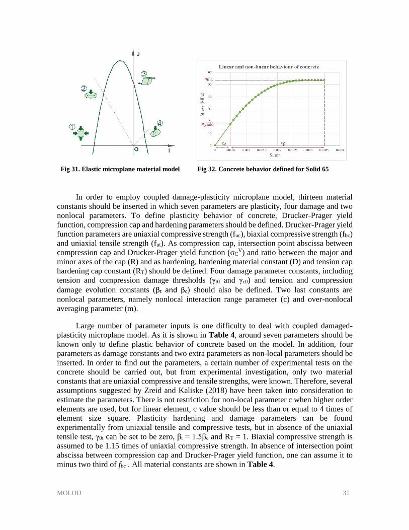
MOLOD 31

Fig 31. Elastic microplane material model Fig 32. Concrete behavior defined for Solid 65

In order to employ coupled damage-plasticity microplane model, thirteen material

constants should be inserted in which seven parameters are plasticity, four damage and two

nonlocal parameters. To define plasticity behavior of concrete, Drucker-Prager yield

function, compression cap and hardening parameters should be defined. Drucker-Prager yield

function parameters are uniaxial compressive strength (fuc), biaxial compressive strength (fbc)

and uniaxial tensile strength (fut). As compression cap, intersection point abscissa between

compression cap and Drucker-Prager yield function (σCV) and ratio between the major and

minor axes of the cap (R) and as hardening, hardening material constant (D) and tension cap

hardening cap constant (RT) should be defined. Four damage parameter constants, including

tension and compression damage thresholds (γt0 and γc0) and tension and compression

damage evolution constants (βt and βc) should also be defined. Two last constants are

nonlocal parameters, namely nonlocal interaction range parameter (c) and over-nonlocal

averaging parameter (m).

Large number of parameter inputs is one difficulty to deal with coupled damaged-

plasticity microplane model. As it is shown in Table 4, around seven parameters should be

known only to define plastic behavior of concrete based on the model. In addition, four

parameters as damage constants and two extra parameters as non-local parameters should be

inserted. In order to find out the parameters, a certain number of experimental tests on the

concrete should be carried out, but from experimental investigation, only two material

constants that are uniaxial compressive and tensile strengths, were known. Therefore, several

assumptions suggested by Zreid and Kaliske (2018) have been taken into consideration to

estimate the parameters. There is not restriction for non-local parameter c when higher order

elements are used, but for linear element, c value should be less than or equal to 4 times of

element size square. Plasticity hardening and damage parameters can be found

experimentally from uniaxial tensile and compressive tests, but in absence of the uniaxial

tensile test, γ0t can be set to be zero, βt = 1.5βc and RT = 1. Biaxial compressive strength is

assumed to be 1.15 times of uniaxial compressive strength. In absence of intersection point

abscissa between compression cap and Drucker-Prager yield function, one can assume it to

minus two third of fbc . All material constants are shown in Table 4.

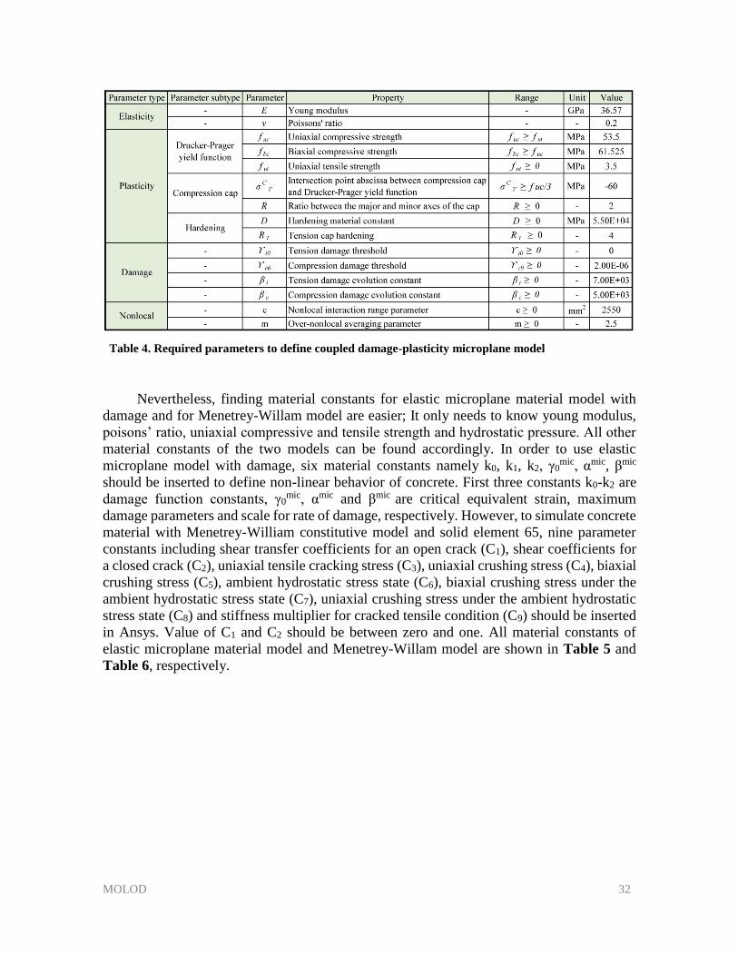
MOLOD 32

Table 4. Required parameters to define coupled damage-plasticity microplane model

Nevertheless, finding material constants for elastic microplane material model with

damage and for Menetrey-Willam model are easier; It only needs to know young modulus,

poisons’ ratio, uniaxial compressive and tensile strength and hydrostatic pressure. All other

material constants of the two models can be found accordingly. In order to use elastic

microplane model with damage, six material constants namely k0, k1, k2, γ0mic, αmic, βmic

should be inserted to define non-linear behavior of concrete. First three constants k0-k2 are

damage function constants, γ0mic, αmic and βmic are critical equivalent strain, maximum

damage parameters and scale for rate of damage, respectively. However, to simulate concrete

material with Menetrey-William constitutive model and solid element 65, nine parameter

constants including shear transfer coefficients for an open crack (C1), shear coefficients for

a closed crack (C2), uniaxial tensile cracking stress (C3), uniaxial crushing stress (C4), biaxial

crushing stress (C5), ambient hydrostatic stress state (C6), biaxial crushing stress under the

ambient hydrostatic stress state (C7), uniaxial crushing stress under the ambient hydrostatic

stress state (C8) and stiffness multiplier for cracked tensile condition (C9) should be inserted

in Ansys. Value of C1 and C2 should be between zero and one. All material constants of

elastic microplane material model and Menetrey-Willam model are shown in Table 5 and

Table 6, respectively.

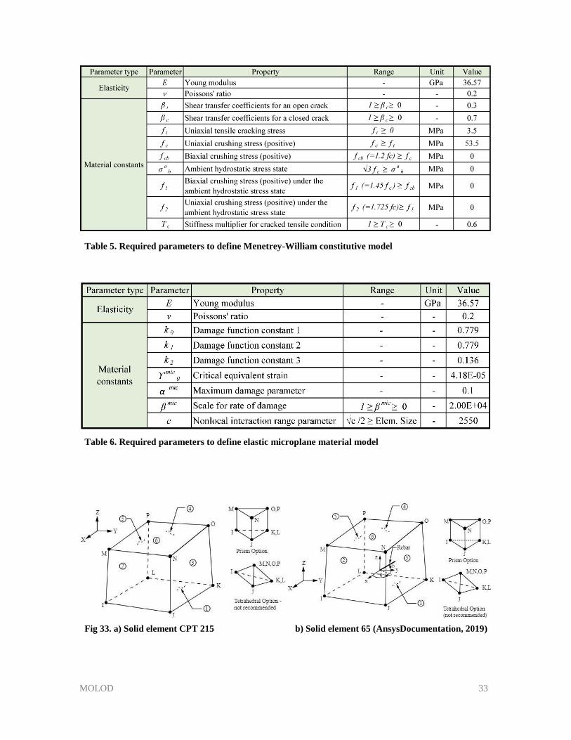
MOLOD 33

Table 5. Required parameters to define Menetrey-William constitutive model

Table 6. Required parameters to define elastic microplane material model

Fig 33. a) Solid element CPT 215 b) Solid element 65 (AnsysDocumentation, 2019)

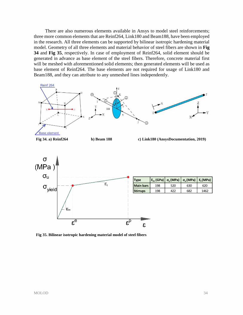
MOLOD 34

There are also numerous elements available in Ansys to model steel reinforcements;

three more common elements that are Reinf264, Link180 and Beam188, have been employed

in the research. All three elements can be supported by bilinear isotropic hardening material

model. Geometry of all three elements and material behavior of steel fibers are shown in Fig

34 and Fig 35, respectively. In case of employment of Reinf264, solid element should be

generated in advance as base element of the steel fibers. Therefore, concrete material first

will be meshed with aforementioned solid elements; then generated elements will be used as

base element of Reinf264. The base elements are not required for usage of Link180 and

Beam188, and they can attribute to any unmeshed lines independently.

Fig 34. a) Reinf264 b) Beam 188 c) Link180 (AnsysDocumentation, 2019)

Fig 35. Bilinear isotropic hardening material model of steel fibers

Type Em (GPa) σy (MPa) σu (MPa) Et (MPa)

Main bars 198 520 630 620

Stirrups 198 422 682 1462

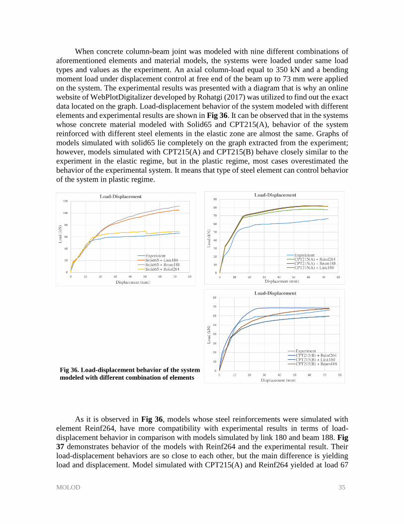
MOLOD 35

When concrete column-beam joint was modeled with nine different combinations of

aforementioned elements and material models, the systems were loaded under same load

types and values as the experiment. An axial column-load equal to 350 kN and a bending

moment load under displacement control at free end of the beam up to 73 mm were applied

on the system. The experimental results was presented with a diagram that is why an online

website of WebPlotDigitalizer developed by Rohatgi (2017) was utilized to find out the exact

data located on the graph. Load-displacement behavior of the system modeled with different

elements and experimental results are shown in Fig 36. It can be observed that in the systems

whose concrete material modeled with Solid65 and CPT215(A), behavior of the system

reinforced with different steel elements in the elastic zone are almost the same. Graphs of

models simulated with solid65 lie completely on the graph extracted from the experiment;

however, models simulated with CPT215(A) and CPT215(B) behave closely similar to the

experiment in the elastic regime, but in the plastic regime, most cases overestimated the

behavior of the experimental system. It means that type of steel element can control behavior

of the system in plastic regime.

Fig 36. Load-displacement behavior of the system

modeled with different combination of elements

As it is observed in Fig 36, models whose steel reinforcements were simulated with

element Reinf264, have more compatibility with experimental results in terms of load-

displacement behavior in comparison with models simulated by link 180 and beam 188. Fig

37 demonstrates behavior of the models with Reinf264 and the experimental result. Their

load-displacement behaviors are so close to each other, but the main difference is yielding

load and displacement. Model simulated with CPT215(A) and Reinf264 yielded at load 67

MOLOD 36

kN and displacement 16 mm; however, the experimental values were 51.3 kN and 12 mm,

respectively. Yielding displacement reached 26mm at failure load 68 kN when combination

of CPT215(B) and Reinf264 was employed. These yielding values are not close to the

experimental results. Therefore, the combinations do not have good compatibility with the

experiment when yielding load and displacement are aimed. On the other hand, concrete

column-beam joint modeled with Solid65 and Reinf64 demonstrated a very good

compatibility with the experimental results in terms of load-displacement behavior as well

as yielding load and displacement, where yielding load and displacement were 58 kN and 15

mm, respectively. Elastic behavior of the model lies almost on the graph of the experimental

result, and only after cracking the behavior has been to somehow overestimated. In addition,

at displacement equal to 51 mm, a warning message appeared to warn about a large

displacement at one node, but the message was suppressed that is why a fluctuation is

observed in the graph. Moreover, since limit state function (see section 3.8) gives failure

restriction for a range of ±10% of cracking load, and the displacement in none of 1000

simulations would reach 50 mm, one can rely on results of the numerical model simulated

with Solid65 and Reinf264.

Fig 37. Load-displacement behavior of the joint simulated with three different solid elements

0

10

20

30

40

50

60

70

80

90

0 10 20 30 40 50 60 70 80

Lo

ad

(k

N)

Displacement (mm)

Load-Displacement

Experiment

Solid65 + Reinf264

CPT215(B) + Reinf264

CPT215(A) + Reinf264

16 2612

58 kN

15

67 kN

68 kN

51.3 kN

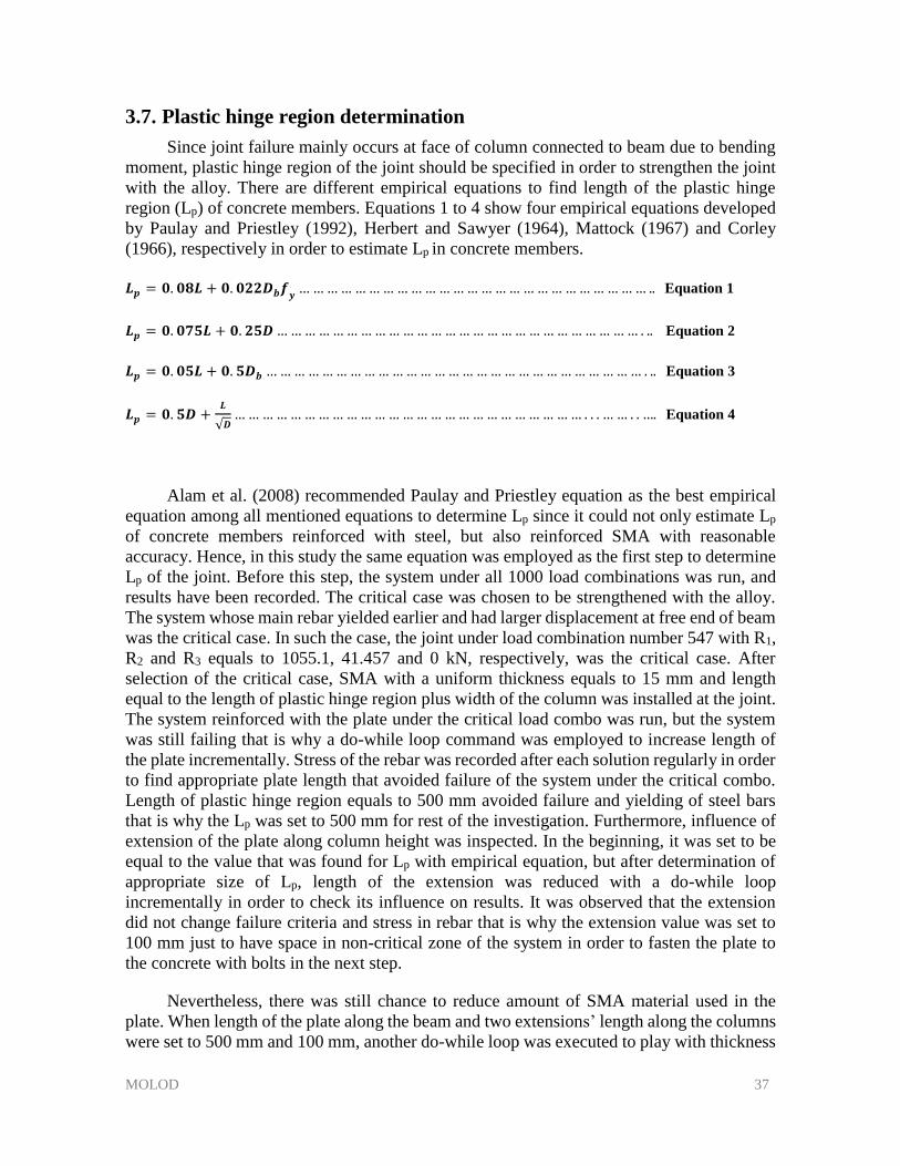
MOLOD 37

3.7. Plastic hinge region determination

Since joint failure mainly occurs at face of column connected to beam due to bending

moment, plastic hinge region of the joint should be specified in order to strengthen the joint

with the alloy. There are different empirical equations to find length of the plastic hinge

region (Lp) of concrete members. Equations 1 to 4 show four empirical equations developed

by Paulay and Priestley (1992), Herbert and Sawyer (1964), Mattock (1967) and Corley

(1966), respectively in order to estimate Lp in concrete members.

𝑳𝒑 = 𝟎. 𝟎𝟖𝑳 + 𝟎. 𝟎𝟐𝟐𝑫𝒃𝒇𝒚

… … … … … … … … … … … … … … … … … … … … … … … … … .. Equation 1

𝑳𝒑 = 𝟎. 𝟎𝟕𝟓𝑳 + 𝟎. 𝟐𝟓𝑫 … … … … … … … … … … … … … … … … … … … … … … … … … … . .. Equation 2

𝑳𝒑 = 𝟎. 𝟎𝟓𝑳 + 𝟎. 𝟓𝑫𝒃 … … … … … … … … … … … … … … … … … … … … … … … … … … … . .. Equation 3

𝑳𝒑 = 𝟎. 𝟓𝑫 +𝑳

√𝑫… … … … … … … … … … … … … … … … … … … … … … … … … . . . … … . . …. Equation 4

Alam et al. (2008) recommended Paulay and Priestley equation as the best empirical

equation among all mentioned equations to determine Lp since it could not only estimate Lp

of concrete members reinforced with steel, but also reinforced SMA with reasonable

accuracy. Hence, in this study the same equation was employed as the first step to determine

Lp of the joint. Before this step, the system under all 1000 load combinations was run, and

results have been recorded. The critical case was chosen to be strengthened with the alloy.

The system whose main rebar yielded earlier and had larger displacement at free end of beam

was the critical case. In such the case, the joint under load combination number 547 with R1,

R2 and R3 equals to 1055.1, 41.457 and 0 kN, respectively, was the critical case. After

selection of the critical case, SMA with a uniform thickness equals to 15 mm and length

equal to the length of plastic hinge region plus width of the column was installed at the joint.

The system reinforced with the plate under the critical load combo was run, but the system

was still failing that is why a do-while loop command was employed to increase length of

the plate incrementally. Stress of the rebar was recorded after each solution regularly in order

to find appropriate plate length that avoided failure of the system under the critical combo.

Length of plastic hinge region equals to 500 mm avoided failure and yielding of steel bars

that is why the Lp was set to 500 mm for rest of the investigation. Furthermore, influence of

extension of the plate along column height was inspected. In the beginning, it was set to be

equal to the value that was found for Lp with empirical equation, but after determination of

appropriate size of Lp, length of the extension was reduced with a do-while loop

incrementally in order to check its influence on results. It was observed that the extension

did not change failure criteria and stress in rebar that is why the extension value was set to

100 mm just to have space in non-critical zone of the system in order to fasten the plate to

the concrete with bolts in the next step.

Nevertheless, there was still chance to reduce amount of SMA material used in the

plate. When length of the plate along the beam and two extensions’ length along the columns

were set to 500 mm and 100 mm, another do-while loop was executed to play with thickness

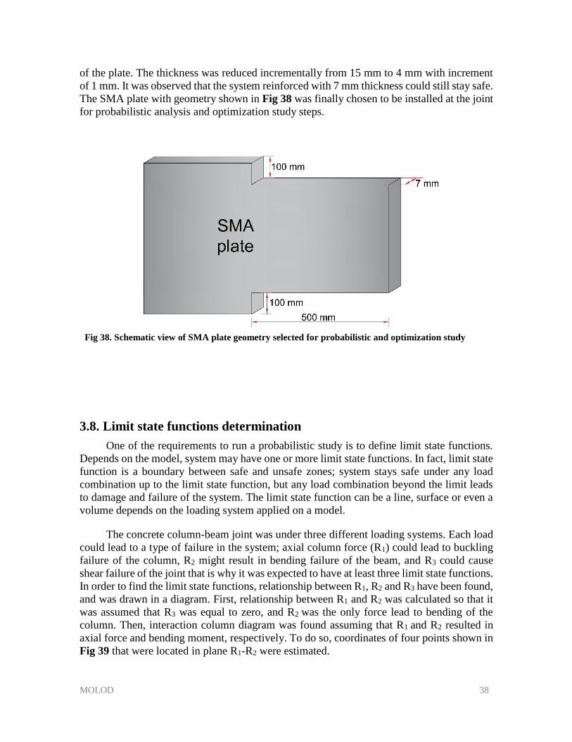
MOLOD 38

of the plate. The thickness was reduced incrementally from 15 mm to 4 mm with increment

of 1 mm. It was observed that the system reinforced with 7 mm thickness could still stay safe.

The SMA plate with geometry shown in Fig 38 was finally chosen to be installed at the joint

for probabilistic analysis and optimization study steps.

Fig 38. Schematic view of SMA plate geometry selected for probabilistic and optimization study

3.8. Limit state functions determination

One of the requirements to run a probabilistic study is to define limit state functions.

Depends on the model, system may have one or more limit state functions. In fact, limit state

function is a boundary between safe and unsafe zones; system stays safe under any load

combination up to the limit state function, but any load combination beyond the limit leads

to damage and failure of the system. The limit state function can be a line, surface or even a

volume depends on the loading system applied on a model.

The concrete column-beam joint was under three different loading systems. Each load

could lead to a type of failure in the system; axial column force (R1) could lead to buckling

failure of the column, R2 might result in bending failure of the beam, and R3 could cause

shear failure of the joint that is why it was expected to have at least three limit state functions.

In order to find the limit state functions, relationship between R1, R2 and R3 have been found,

and was drawn in a diagram. First, relationship between R1 and R2 was calculated so that it

was assumed that R3 was equal to zero, and R2 was the only force lead to bending of the

column. Then, interaction column diagram was found assuming that R1 and R2 resulted in

axial force and bending moment, respectively. To do so, coordinates of four points shown in

Fig 39 that were located in plane R1-R2 were estimated.

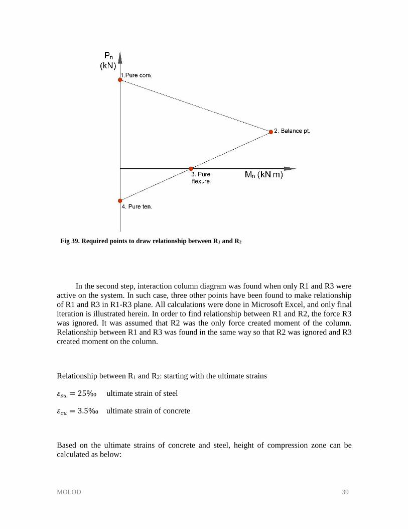
MOLOD 39

Fig 39. Required points to draw relationship between R1 and R2

In the second step, interaction column diagram was found when only R1 and R3 were

active on the system. In such case, three other points have been found to make relationship

of R1 and R3 in R1-R3 plane. All calculations were done in Microsoft Excel, and only final

iteration is illustrated herein. In order to find relationship between R1 and R2, the force R3

was ignored. It was assumed that R2 was the only force created moment of the column.

Relationship between R1 and R3 was found in the same way so that R2 was ignored and R3

created moment on the column.

Relationship between R1 and R2: starting with the ultimate strains

𝜀𝑠𝑢 = 25‰ ultimate strain of steel

𝜀𝑐𝑢 = 3.5‰ ultimate strain of concrete

Based on the ultimate strains of concrete and steel, height of compression zone can be

calculated as below:

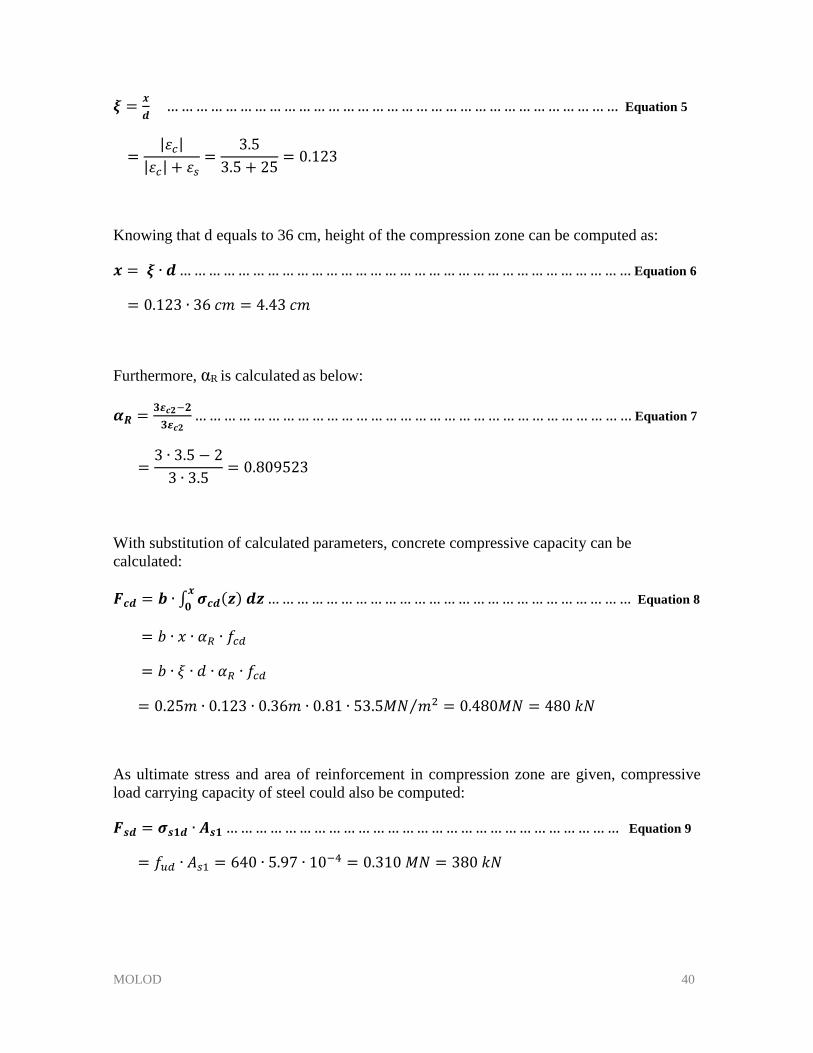
MOLOD 40

𝝃 =𝒙

𝒅 … … … … … … … … … … … … … … … … … … … … … … … … … … … … … … … Equation 5

=|𝜀𝑐|

|𝜀𝑐| + 𝜀𝑠=

3.5

3.5 + 25= 0.123

Knowing that d equals to 36 cm, height of the compression zone can be computed as:

𝒙 = 𝝃 ∙ 𝒅 … … … … … … … … … … … … … … … … … … … … … … … … … … … … … … … Equation 6

= 0.123 ∙ 36 𝑐𝑚 = 4.43 𝑐𝑚

Furthermore, αR is calculated as below:

𝜶𝑹 =𝟑𝜺𝒄𝟐−𝟐

𝟑𝜺𝒄𝟐… … … … … … … … … … … … … … … … … … … … … … … … … … … … … … Equation 7

=3 ∙ 3.5 − 2

3 ∙ 3.5= 0.809523

With substitution of calculated parameters, concrete compressive capacity can be

calculated:

𝑭𝒄𝒅 = 𝒃 ∙ ∫ 𝝈𝒄𝒅(𝒛) 𝒅𝒛𝒙

𝟎… … … … … … … … … … … … … … … … … … … … … … … … … Equation 8

= 𝑏 ∙ 𝑥 ∙ 𝛼𝑅 ∙ 𝑓𝑐𝑑

= 𝑏 ∙ 𝜉 ∙ 𝑑 ∙ 𝛼𝑅 ∙ 𝑓𝑐𝑑

= 0.25𝑚 ∙ 0.123 ∙ 0.36𝑚 ∙ 0.81 ∙ 53.5𝑀𝑁 𝑚2⁄ = 0.480𝑀𝑁 = 480 𝑘𝑁

As ultimate stress and area of reinforcement in compression zone are given, compressive

load carrying capacity of steel could also be computed:

𝑭𝒔𝒅 = 𝝈𝒔𝟏𝒅 ∙ 𝑨𝒔𝟏 … … … … … … … … … … … … … … … … … … … … … … … … … … … Equation 9

= 𝑓𝑢𝑑 ∙ 𝐴𝑠1 = 640 ∙ 5.97 ∙ 10−4 = 0.310 𝑀𝑁 = 380 𝑘𝑁

MOLOD 41

Check:

∑ 𝐻 = 0 → 𝐹𝑠𝑑 − 𝐹𝑐𝑑 = 0.480 − 0.380 → 0.10 ≠ 0

Since the concrete compressive capacity is greater than steel, steel fails.

The same procedure has been followed for relationship between R1 and R3. In this iteration,

it was assumed that there is variation in concrete strain, but steel strain remains constant.

Therefore:

𝜀𝑐 = 2.88 ‰

𝜀𝑠 = 25‰

Calculation of compression zone height of concrete:

𝜉 =|𝜀𝑐|

|𝜀𝑐| + 𝜀𝑠

=2.88

2.88 + 25= 0.10

𝑥 = 𝜉 ∙ 𝑑 = 0.10 ∙ 36𝑐𝑚 = 3.60 𝑐𝑚

Beside:

𝛼𝑅 =3𝜀𝑐2 − 2

3𝜀𝑐2=

3 ∙ 2.88 − 2

3 ∙ 2.88= 0.77

Therefore, compressive carrying load capacity of concrete and steel are:

𝐹𝑐𝑑 = 𝑏 ∙ 𝜉 ∙ 𝑑 ∙ 𝛼𝑅 ∙ 𝑓𝑐𝑑 = 0.25 ∙ 0.10 ∙ 0.36 ∙ 0.77 ∙ 53.5 = 0.37𝑀𝑁 = 370 𝑘𝑁

𝐹𝑠𝑑 = 𝜎𝑠1𝑑 ∙ 𝐴𝑠1 = 𝑓𝑢𝑑 ∙ 𝐴𝑠1 = 640 ∙ 5.97 ∙ 10−4 = 0.380 𝑀𝑁 = 380 𝑘𝑁

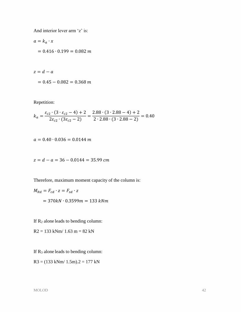
MOLOD 42

And interior lever arm ‘z’ is:

𝑎 = 𝑘𝑎 ∙ 𝑥

= 0.416 ∙ 0.199 = 0.082 𝑚

𝑧 = 𝑑 − 𝑎

= 0.45 − 0.082 = 0.368 𝑚

Repetition:

𝑘𝑎 =𝜀𝑐2 ∙ (3 ∙ 𝜀𝑐2 − 4) + 2

2𝜀𝑐2 ∙ (3𝜀𝑐2 − 2)=

2.88 ∙ (3 ∙ 2.88 − 4) + 2

2 ∙ 2.88 ∙ (3 ∙ 2.88 − 2)= 0.40

𝑎 = 0.40 ∙ 0.036 = 0.0144 𝑚

𝑧 = 𝑑 − 𝑎 = 36 − 0.0144 = 35.99 𝑐𝑚

Therefore, maximum moment capacity of the column is:

𝑀𝑅𝑑 = 𝐹𝑐𝑑 ∙ 𝑧 = 𝐹𝑠𝑑 ∙ 𝑧

= 370𝑘𝑁 ∙ 0.3599𝑚 = 133 𝑘𝑁𝑚

If R2 alone leads to bending column:

R2 = 133 kNm/ 1.63 m = 82 kN

If R3 alone leads to bending column:

R3 = (133 kNm/ 1.5m).2 = 177 kN

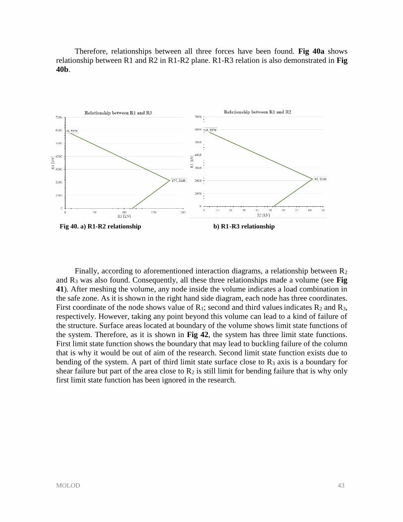
MOLOD 43

Therefore, relationships between all three forces have been found. Fig 40a shows

relationship between R1 and R2 in R1-R2 plane. R1-R3 relation is also demonstrated in Fig

40b.

Fig 40. a) R1-R2 relationship b) R1-R3 relationship

Finally, according to aforementioned interaction diagrams, a relationship between R2

and R3 was also found. Consequently, all these three relationships made a volume (see Fig

41). After meshing the volume, any node inside the volume indicates a load combination in

the safe zone. As it is shown in the right hand side diagram, each node has three coordinates.

First coordinate of the node shows value of R1; second and third values indicates R2 and R3,

respectively. However, taking any point beyond this volume can lead to a kind of failure of

the structure. Surface areas located at boundary of the volume shows limit state functions of

the system. Therefore, as it is shown in Fig 42, the system has three limit state functions.

First limit state function shows the boundary that may lead to buckling failure of the column

that is why it would be out of aim of the research. Second limit state function exists due to

bending of the system. A part of third limit state surface close to R3 axis is a boundary for

shear failure but part of the area close to R2 is still limit for bending failure that is why only

first limit state function has been ignored in the research.

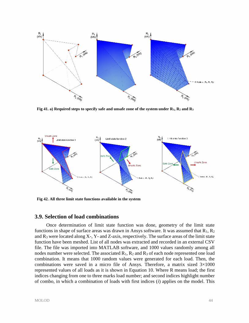
MOLOD 44

Fig 41. a) Required steps to specify safe and unsafe zone of the system under R1, R2 and R3

.

Fig 42. All three limit state functions available in the system

3.9. Selection of load combinations

Once determination of limit state function was done, geometry of the limit state

functions in shape of surface areas was drawn in Ansys software. It was assumed that R1, R2

and R3 were located along X-, Y- and Z-axis, respectively. The surface areas of the limit state

function have been meshed. List of all nodes was extracted and recorded in an external CSV

file. The file was imported into MATLAB software, and 1000 values randomly among all

nodes number were selected. The associated R1, R2 and R3 of each node represented one load

combination. It means that 1000 random values were generated for each load. Then, the

combinations were saved in a micro file of Ansys. Therefore, a matrix sized 3×1000

represented values of all loads as it is shown in Equation 10. Where R means load; the first

indices changing from one to three marks load number; and second indices highlight number

of combo, in which a combination of loads with first indices (i) applies on the model. This

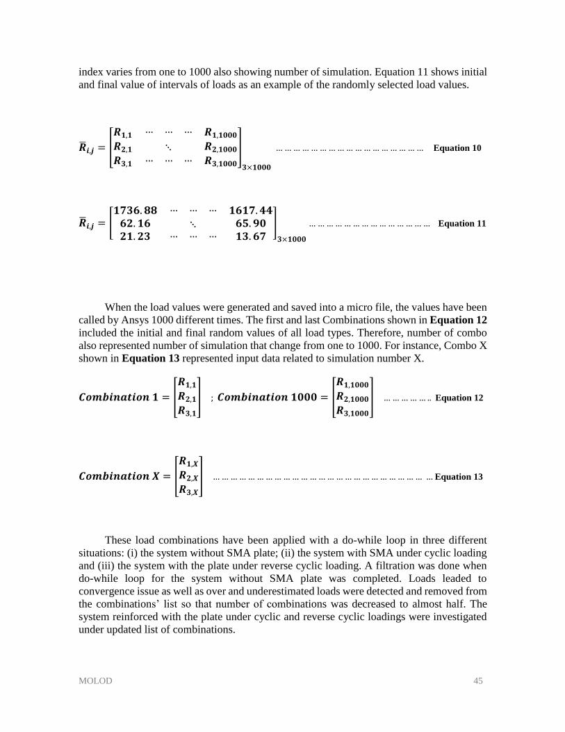
MOLOD 45

index varies from one to 1000 also showing number of simulation. Equation 11 shows initial

and final value of intervals of loads as an example of the randomly selected load values.

�̅�𝒊,𝒋 = [

𝑹𝟏,𝟏… … … 𝑹𝟏,𝟏𝟎𝟎𝟎

𝑹𝟐,𝟏 ⋱ 𝑹𝟐,𝟏𝟎𝟎𝟎

𝑹𝟑,𝟏… … … 𝑹𝟑,𝟏𝟎𝟎𝟎

]

𝟑×𝟏𝟎𝟎𝟎

… … … … … … … … … … … … … … … … … Equation 10

�̅�𝒊,𝒋 = [𝟏𝟕𝟑𝟔. 𝟖𝟖 … … … 𝟏𝟔𝟏𝟕. 𝟒𝟒

𝟔𝟐. 𝟏𝟔 ⋱ 𝟔𝟓. 𝟗𝟎𝟐𝟏. 𝟐𝟑 … … … 𝟏𝟑. 𝟔𝟕

]

𝟑×𝟏𝟎𝟎𝟎

… … … … … … … … … … … … … … Equation 11

When the load values were generated and saved into a micro file, the values have been

called by Ansys 1000 different times. The first and last Combinations shown in Equation 12

included the initial and final random values of all load types. Therefore, number of combo

also represented number of simulation that change from one to 1000. For instance, Combo X

shown in Equation 13 represented input data related to simulation number X.

𝑪𝒐𝒎𝒃𝒊𝒏𝒂𝒕𝒊𝒐𝒏 𝟏 = [

𝑹𝟏,𝟏

𝑹𝟐,𝟏

𝑹𝟑,𝟏

] ; 𝑪𝒐𝒎𝒃𝒊𝒏𝒂𝒕𝒊𝒐𝒏 𝟏𝟎𝟎𝟎 = [

𝑹𝟏,𝟏𝟎𝟎𝟎

𝑹𝟐,𝟏𝟎𝟎𝟎

𝑹𝟑,𝟏𝟎𝟎𝟎

] … … … … … .. Equation 12

𝑪𝒐𝒎𝒃𝒊𝒏𝒂𝒕𝒊𝒐𝒏 𝑿 = [

𝑹𝟏,𝑿

𝑹𝟐,𝑿

𝑹𝟑,𝑿

] … … … … … … … … … … … … … … … … … … … … … … … … … Equation 13

These load combinations have been applied with a do-while loop in three different

situations: (i) the system without SMA plate; (ii) the system with SMA under cyclic loading

and (iii) the system with the plate under reverse cyclic loading. A filtration was done when

do-while loop for the system without SMA plate was completed. Loads leaded to

convergence issue as well as over and underestimated loads were detected and removed from

the combinations’ list so that number of combinations was decreased to almost half. The

system reinforced with the plate under cyclic and reverse cyclic loadings were investigated

under updated list of combinations.

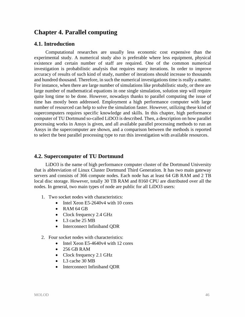
MOLOD 46

Chapter 4. Parallel computing

4.1. Introduction

Computational researches are usually less economic cost expensive than the

experimental study. A numerical study also is preferable where less equipment, physical

existence and certain number of staff are required. One of the common numerical

investigation is probabilistic analysis that requires many iterations. In order to improve

accuracy of results of such kind of study, number of iterations should increase to thousands

and hundred thousand. Therefore, in such the numerical investigations time is really a matter.

For instance, when there are large number of simulations like probabilistic study, or there are

large number of mathematical equations in one single simulation, solution step will require

quite long time to be done. However, nowadays thanks to parallel computing the issue of

time has mostly been addressed. Employment a high performance computer with large

number of resourced can help to solve the simulation faster. However, utilizing these kind of

supercomputers requires specific knowledge and skills. In this chapter, high performance

computer of TU Dortmund so-called LiDO3 is described. Then, a description on how parallel

processing works in Ansys is given, and all available parallel processing methods to run an

Ansys in the supercomputer are shown, and a comparison between the methods is reported

to select the best parallel processing type to run this investigation with available resources.

4.2. Supercomputer of TU Dortmund

LiDO3 is the name of high performance computer cluster of the Dortmund University

that is abbreviation of Linux Cluster Dortmund Third Generation. It has two main gateway

servers and consists of 366 compute nodes. Each node has at least 64 GB RAM and 2 TB

local disc storage. However, totally 30 TB RAM and 8160 CPU are distributed over all the

nodes. In general, two main types of node are public for all LiDO3 users:

1. Two socket nodes with characteristics:

Intel Xeon E5-2640v4 with 10 cores

RAM 64 GB

Clock frequency 2.4 GHz

L3 cache 25 MB

Interconnect Infiniband QDR

2. Four socket nodes with characteristics:

Intel Xeon E5-4640v4 with 12 cores

256 GB RAM

Clock frequency 2.1 GHz

L3 cache 30 MB

Interconnect Infiniband QDR

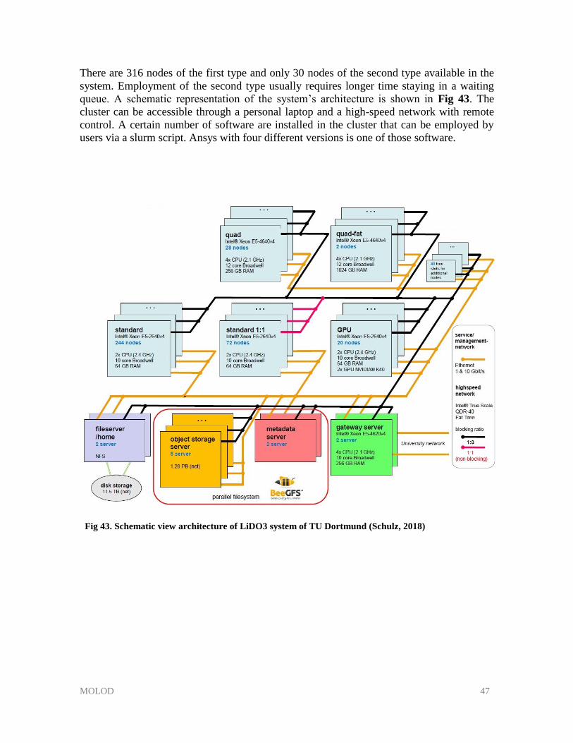
MOLOD 47

There are 316 nodes of the first type and only 30 nodes of the second type available in the

system. Employment of the second type usually requires longer time staying in a waiting

queue. A schematic representation of the system’s architecture is shown in Fig 43. The

cluster can be accessible through a personal laptop and a high-speed network with remote

control. A certain number of software are installed in the cluster that can be employed by

users via a slurm script. Ansys with four different versions is one of those software.

Fig 43. Schematic view architecture of LiDO3 system of TU Dortmund (Schulz, 2018)

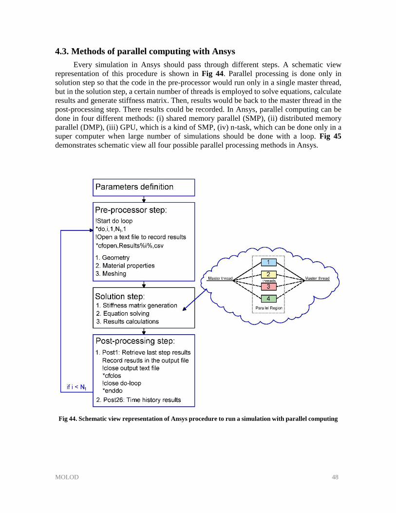
MOLOD 48

4.3. Methods of parallel computing with Ansys

Every simulation in Ansys should pass through different steps. A schematic view

representation of this procedure is shown in Fig 44. Parallel processing is done only in

solution step so that the code in the pre-processor would run only in a single master thread,

but in the solution step, a certain number of threads is employed to solve equations, calculate

results and generate stiffness matrix. Then, results would be back to the master thread in the

post-processing step. There results could be recorded. In Ansys, parallel computing can be

done in four different methods: (i) shared memory parallel (SMP), (ii) distributed memory

parallel (DMP), (iii) GPU, which is a kind of SMP, (iv) n-task, which can be done only in a

super computer when large number of simulations should be done with a loop. Fig 45

demonstrates schematic view all four possible parallel processing methods in Ansys.

Fig 44. Schematic view representation of Ansys procedure to run a simulation with parallel computing

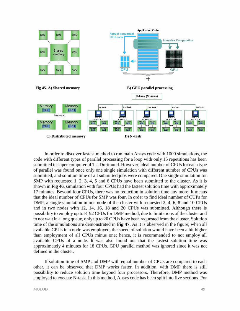
MOLOD 49

Fig 45. A) Shared memory B) GPU parallel processing

C) Distributed memory D) N-task

In order to discover fastest method to run main Ansys code with 1000 simulations, the

code with different types of parallel processing for a loop with only 15 repetitions has been

submitted in super computer of TU Dortmund. However, ideal number of CPUs for each type

of parallel was found once only one single simulation with different number of CPUs was

submitted, and solution time of all submitted jobs were compared. One single simulation for

SMP with requested 1, 2, 3, 4, 5 and 6 CPUs have been submitted to the cluster. As it is

shown in Fig 46, simulation with four CPUs had the fastest solution time with approximately

17 minutes. Beyond four CPUs, there was no reduction in solution time any more. It means

that the ideal number of CPUs for SMP was four. In order to find ideal number of CUPs for

DMP, a single simulation in one node of the cluster with requested 2, 4, 6, 8 and 10 CPUs

and in two nodes with 12, 14, 16, 18 and 20 CPUs was submitted. Although there is

possibility to employ up to 8192 CPUs for DMP method, due to limitations of the cluster and

to not wait in a long queue, only up to 20 CPUs have been requested from the cluster. Solution

time of the simulations are demonstrated in Fig 47. As it is observed in the figure, when all

available CPUs in a node was employed, the speed of solution would have been a bit higher

than employment of all CPUs minus one; hence, it is recommended to not employ all

available CPUs of a node. It was also found out that the fastest solution time was

approximately 4 minutes for 18 CPUs. GPU parallel method was ignored since it was not

defined in the cluster.

If solution time of SMP and DMP with equal number of CPUs are compared to each

other, it can be observed that DMP works faster. In addition, with DMP there is still

possibility to reduce solution time beyond four processors. Therefore, DMP method was

employed to execute N-task. In this method, Ansys code has been split into five sections. For

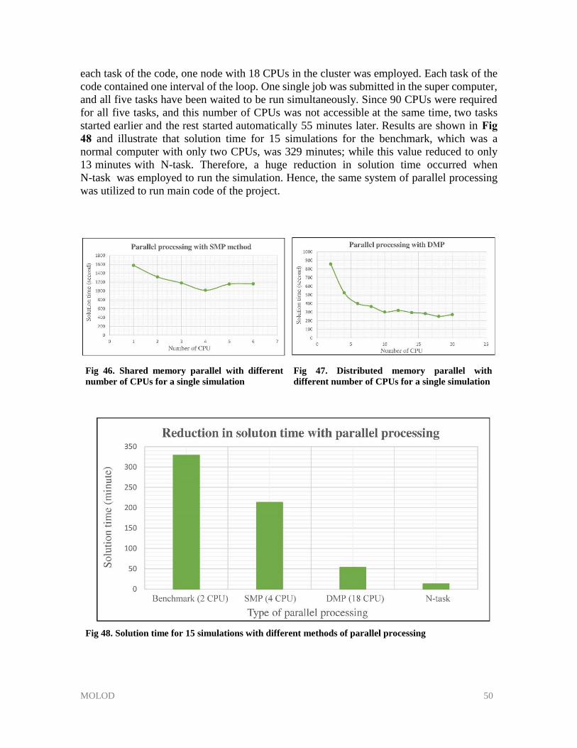
MOLOD 50

each task of the code, one node with 18 CPUs in the cluster was employed. Each task of the

code contained one interval of the loop. One single job was submitted in the super computer,

and all five tasks have been waited to be run simultaneously. Since 90 CPUs were required

for all five tasks, and this number of CPUs was not accessible at the same time, two tasks

started earlier and the rest started automatically 55 minutes later. Results are shown in Fig

48 and illustrate that solution time for 15 simulations for the benchmark, which was a

normal computer with only two CPUs, was 329 minutes; while this value reduced to only

13 minutes with N-task. Therefore, a huge reduction in solution time occurred when

N-task was employed to run the simulation. Hence, the same system of parallel processing

was utilized to run main code of the project.

Fig 46. Shared memory parallel with different

number of CPUs for a single simulation

Fig 47. Distributed memory parallel with

different number of CPUs for a single simulation

Fig 48. Solution time for 15 simulations with different methods of parallel processing

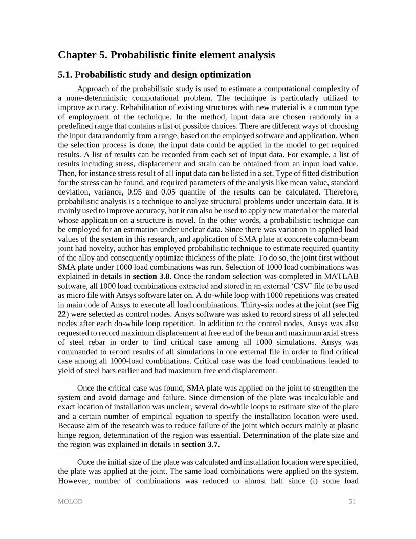
MOLOD 51

Chapter 5. Probabilistic finite element analysis

5.1. Probabilistic study and design optimization

Approach of the probabilistic study is used to estimate a computational complexity of

a none-deterministic computational problem. The technique is particularly utilized to

improve accuracy. Rehabilitation of existing structures with new material is a common type

of employment of the technique. In the method, input data are chosen randomly in a

predefined range that contains a list of possible choices. There are different ways of choosing

the input data randomly from a range, based on the employed software and application. When

the selection process is done, the input data could be applied in the model to get required

results. A list of results can be recorded from each set of input data. For example, a list of

results including stress, displacement and strain can be obtained from an input load value.

Then, for instance stress result of all input data can be listed in a set. Type of fitted distribution

for the stress can be found, and required parameters of the analysis like mean value, standard

deviation, variance, 0.95 and 0.05 quantile of the results can be calculated. Therefore,

probabilistic analysis is a technique to analyze structural problems under uncertain data. It is

mainly used to improve accuracy, but it can also be used to apply new material or the material

whose application on a structure is novel. In the other words, a probabilistic technique can

be employed for an estimation under unclear data. Since there was variation in applied load

values of the system in this research, and application of SMA plate at concrete column-beam

joint had novelty, author has employed probabilistic technique to estimate required quantity

of the alloy and consequently optimize thickness of the plate. To do so, the joint first without

SMA plate under 1000 load combinations was run. Selection of 1000 load combinations was

explained in details in section 3.8. Once the random selection was completed in MATLAB

software, all 1000 load combinations extracted and stored in an external ‘CSV’ file to be used

as micro file with Ansys software later on. A do-while loop with 1000 repetitions was created

in main code of Ansys to execute all load combinations. Thirty-six nodes at the joint (see Fig

22) were selected as control nodes. Ansys software was asked to record stress of all selected

nodes after each do-while loop repetition. In addition to the control nodes, Ansys was also

requested to record maximum displacement at free end of the beam and maximum axial stress

of steel rebar in order to find critical case among all 1000 simulations. Ansys was

commanded to record results of all simulations in one external file in order to find critical

case among all 1000-load combinations. Critical case was the load combinations leaded to

yield of steel bars earlier and had maximum free end displacement.

Once the critical case was found, SMA plate was applied on the joint to strengthen the

system and avoid damage and failure. Since dimension of the plate was incalculable and

exact location of installation was unclear, several do-while loops to estimate size of the plate

and a certain number of empirical equation to specify the installation location were used.

Because aim of the research was to reduce failure of the joint which occurs mainly at plastic

hinge region, determination of the region was essential. Determination of the plate size and

the region was explained in details in section 3.7.

Once the initial size of the plate was calculated and installation location were specified,

the plate was applied at the joint. The same load combinations were applied on the system.

However, number of combinations was reduced to almost half since (i) some load

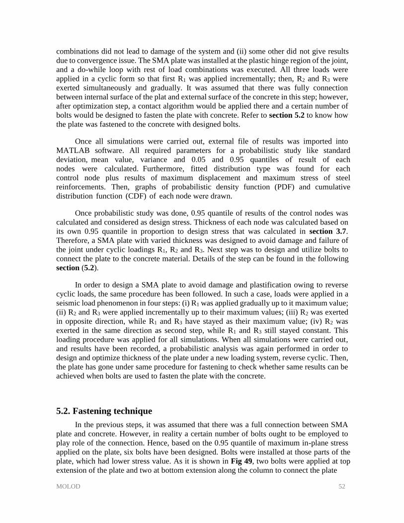
MOLOD 52

combinations did not lead to damage of the system and (ii) some other did not give results

due to convergence issue. The SMA plate was installed at the plastic hinge region of the joint,

and a do-while loop with rest of load combinations was executed. All three loads were

applied in a cyclic form so that first R1 was applied incrementally; then, R2 and R3 were

exerted simultaneously and gradually. It was assumed that there was fully connection

between internal surface of the plat and external surface of the concrete in this step; however,

after optimization step, a contact algorithm would be applied there and a certain number of

bolts would be designed to fasten the plate with concrete. Refer to section 5.2 to know how

the plate was fastened to the concrete with designed bolts.

Once all simulations were carried out, external file of results was imported into

MATLAB software. All required parameters for a probabilistic study like standard

deviation, mean value, variance and 0.05 and 0.95 quantiles of result of each

nodes were calculated. Furthermore, fitted distribution type was found for each

control node plus results of maximum displacement and maximum stress of steel

reinforcements. Then, graphs of probabilistic density function (PDF) and cumulative

distribution function (CDF) of each node were drawn.

Once probabilistic study was done, 0.95 quantile of results of the control nodes was

calculated and considered as design stress. Thickness of each node was calculated based on

its own 0.95 quantile in proportion to design stress that was calculated in section 3.7.

Therefore, a SMA plate with varied thickness was designed to avoid damage and failure of

the joint under cyclic loadings R1, R2 and R3. Next step was to design and utilize bolts to

connect the plate to the concrete material. Details of the step can be found in the following

section (5.2).

In order to design a SMA plate to avoid damage and plastification owing to reverse

cyclic loads, the same procedure has been followed. In such a case, loads were applied in a

seismic load phenomenon in four steps: (i) R1 was applied gradually up to it maximum value;

(ii) R2 and R3 were applied incrementally up to their maximum values; (iii) R2 was exerted in opposite direction, while R1 and R3 have stayed as their maximum value; (iv) R2 was exerted in the same direction as second step, while R1 and R3 still stayed constant. This loading procedure was applied for all simulations. When all simulations were carried out, and results have been recorded, a probabilistic analysis was again performed in order to design and optimize thickness of the plate under a new loading system, reverse cyclic. Then, the plate has gone under same procedure for fastening to check whether same results can be achieved when bolts are used to fasten the plate with the concrete.

5.2. Fastening technique

In the previous steps, it was assumed that there was a full connection between SMA

plate and concrete. However, in reality a certain number of bolts ought to be employed to

play role of the connection. Hence, based on the 0.95 quantile of maximum in-plane stress

applied on the plate, six bolts have been designed. Bolts were installed at those parts of the

plate, which had lower stress value. As it is shown in Fig 49, two bolts were applied at top

extension of the plate and two at bottom extension along the column to connect the plate

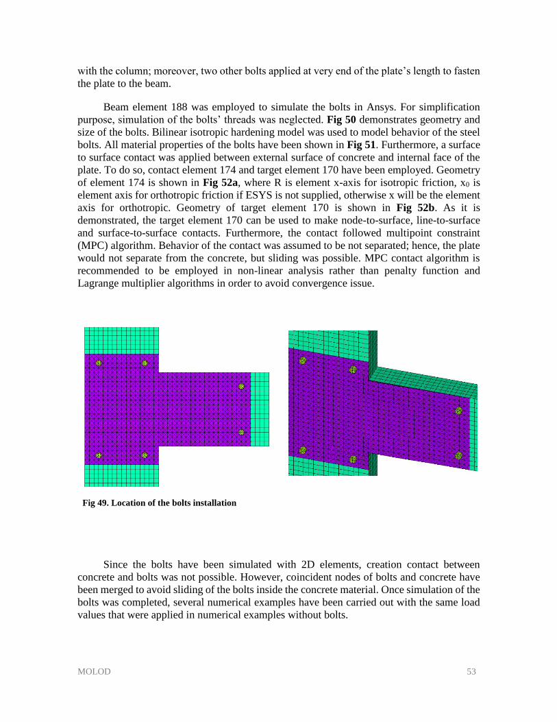
MOLOD 53

with the column; moreover, two other bolts applied at very end of the plate’s length to fasten

the plate to the beam.

Beam element 188 was employed to simulate the bolts in Ansys. For simplification

purpose, simulation of the bolts’ threads was neglected. Fig 50 demonstrates geometry and

size of the bolts. Bilinear isotropic hardening model was used to model behavior of the steel

bolts. All material properties of the bolts have been shown in Fig 51. Furthermore, a surface

to surface contact was applied between external surface of concrete and internal face of the

plate. To do so, contact element 174 and target element 170 have been employed. Geometry

of element 174 is shown in Fig 52a, where R is element x-axis for isotropic friction, x0 is

element axis for orthotropic friction if ESYS is not supplied, otherwise x will be the element

axis for orthotropic. Geometry of target element 170 is shown in Fig 52b. As it is

demonstrated, the target element 170 can be used to make node-to-surface, line-to-surface

and surface-to-surface contacts. Furthermore, the contact followed multipoint constraint

(MPC) algorithm. Behavior of the contact was assumed to be not separated; hence, the plate

would not separate from the concrete, but sliding was possible. MPC contact algorithm is

recommended to be employed in non-linear analysis rather than penalty function and

Lagrange multiplier algorithms in order to avoid convergence issue.

Fig 49. Location of the bolts installation

Since the bolts have been simulated with 2D elements, creation contact between

concrete and bolts was not possible. However, coincident nodes of bolts and concrete have

been merged to avoid sliding of the bolts inside the concrete material. Once simulation of the

bolts was completed, several numerical examples have been carried out with the same load

values that were applied in numerical examples without bolts.

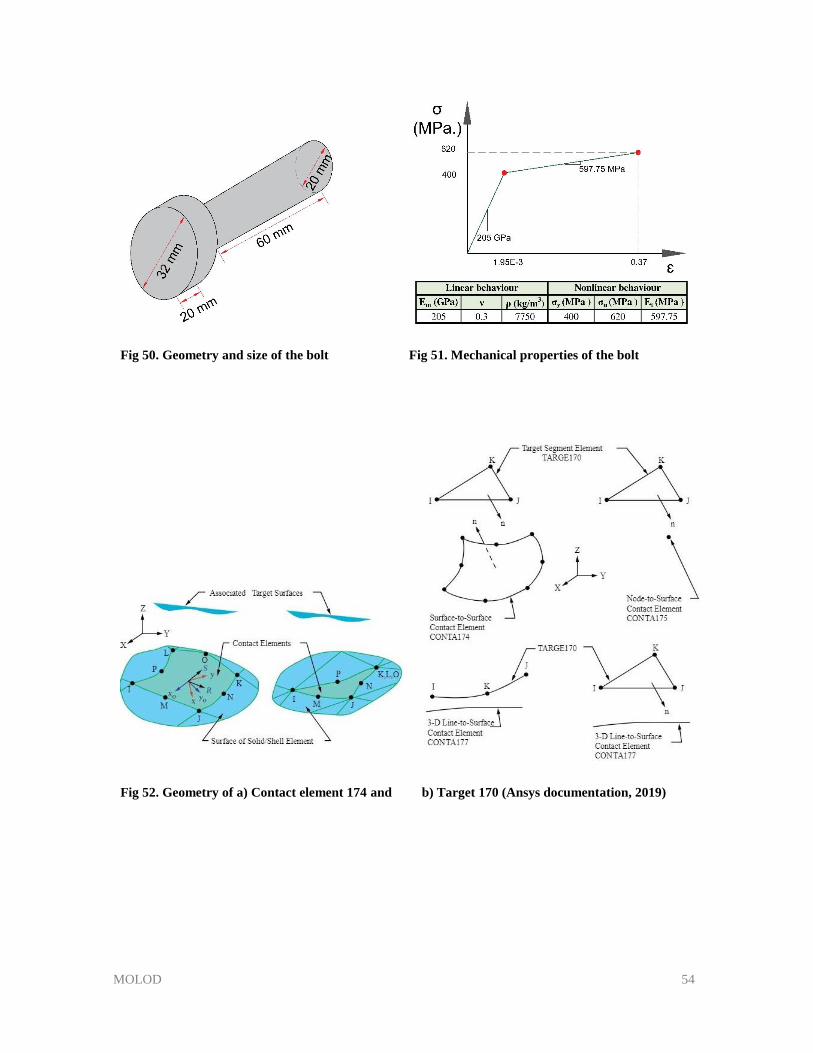
MOLOD 54

Fig 50. Geometry and size of the bolt Fig 51. Mechanical properties of the bolt

Fig 52. Geometry of a) Contact element 174 and b) Target 170 (Ansys documentation, 2019)

Fig 53. Target170 geometry (Ansys documentation, 2019)

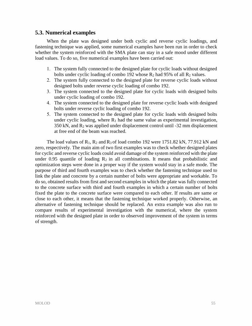
MOLOD 55

5.3. Numerical examples

When the plate was designed under both cyclic and reverse cyclic loadings, and

fastening technique was applied, some numerical examples have been run in order to check

whether the system reinforced with the SMA plate can stay in a safe mood under different

load values. To do so, five numerical examples have been carried out:

1. The system fully connected to the designed plate for cyclic loads without designed bolts under cyclic loading of combo 192 whose R2 had 95% of all R2 values.

2. The system fully connected to the designed plate for reverse cyclic loads without designed bolts under reverse cyclic loading of combo 192.

3. The system connected to the designed plate for cyclic loads with designed bolts under cyclic loading of combo 192.

4. The system connected to the designed plate for reverse cyclic loads with designed bolts under reverse cyclic loading of combo 192.

5. The system connected to the designed plate for cyclic loads with designed bolts under cyclic loading, where R1 had the same value as experimental investigation, 350 kN, and R2 was applied under displacement control until -32 mm displacement at free end of the beam was reached.

The load values of R1, R2 and R3 of load combo 192 were 1751.82 kN, 77.912 kN and

zero, respectively. The main aim of two first examples was to check whether designed plates

for cyclic and reverse cyclic loads could avoid damage of the system reinforced with the plate

under 0.95 quantile of loading R2 in all combinations. It means that probabilistic and

optimization steps were done in a proper way if the system would stay in a safe mode. The

purpose of third and fourth examples was to check whether the fastening technique used to

link the plate and concrete by a certain number of bolts were appropriate and workable. To

do so, obtained results from first and second examples in which the plate was fully connected

to the concrete surface with third and fourth examples in which a certain number of bolts

fixed the plate to the concrete surface were compared to each other. If results are same or close to each other, it means that the fastening technique worked properly. Otherwise, an

alternative of fastening technique should be replaced. An extra example was also run to

compare results of experimental investigation with the numerical, where the system

reinforced with the designed plate in order to observed improvement of the system in terms

of strength.

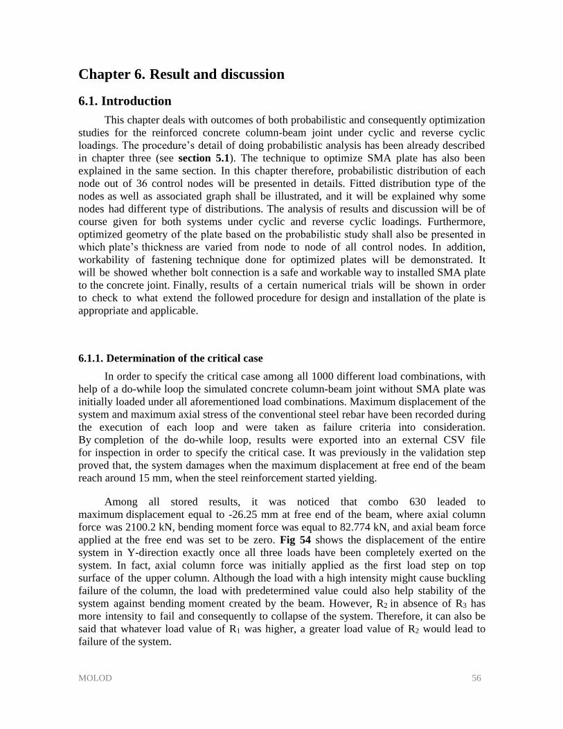
MOLOD 56

Chapter 6. Result and discussion

6.1. Introduction

This chapter deals with outcomes of both probabilistic and consequently optimization

studies for the reinforced concrete column-beam joint under cyclic and reverse cyclic

loadings. The procedure’s detail of doing probabilistic analysis has been already described

in chapter three (see section 5.1). The technique to optimize SMA plate has also been

explained in the same section. In this chapter therefore, probabilistic distribution of each

node out of 36 control nodes will be presented in details. Fitted distribution type of the

nodes as well as associated graph shall be illustrated, and it will be explained why some

nodes had different type of distributions. The analysis of results and discussion will be of

course given for both systems under cyclic and reverse cyclic loadings. Furthermore,

optimized geometry of the plate based on the probabilistic study shall also be presented in

which plate’s thickness are varied from node to node of all control nodes. In addition,

workability of fastening technique done for optimized plates will be demonstrated. It

will be showed whether bolt connection is a safe and workable way to installed SMA plate

to the concrete joint. Finally, results of a certain numerical trials will be shown in order

to check to what extend the followed procedure for design and installation of the plate is

appropriate and applicable.

6.1.1. Determination of the critical case

In order to specify the critical case among all 1000 different load combinations, with

help of a do-while loop the simulated concrete column-beam joint without SMA plate was

initially loaded under all aforementioned load combinations. Maximum displacement of the

system and maximum axial stress of the conventional steel rebar have been recorded during

the execution of each loop and were taken as failure criteria into consideration.

By completion of the do-while loop, results were exported into an external CSV file

for inspection in order to specify the critical case. It was previously in the validation step

proved that, the system damages when the maximum displacement at free end of the beam

reach around 15 mm, when the steel reinforcement started yielding.

Among all stored results, it was noticed that combo 630 leaded to

maximum displacement equal to -26.25 mm at free end of the beam, where axial column

force was 2100.2 kN, bending moment force was equal to 82.774 kN, and axial beam force

applied at the free end was set to be zero. Fig 54 shows the displacement of the entire

system in Y-direction exactly once all three loads have been completely exerted on the

system. In fact, axial column force was initially applied as the first load step on top

surface of the upper column. Although the load with a high intensity might cause buckling

failure of the column, the load with predetermined value could also help stability of the

system against bending moment created by the beam. However, R2 in absence of R3 has

more intensity to fail and consequently to collapse of the system. Therefore, it can also be

said that whatever load value of R1 was higher, a greater load value of R2 would lead to

failure of the system.

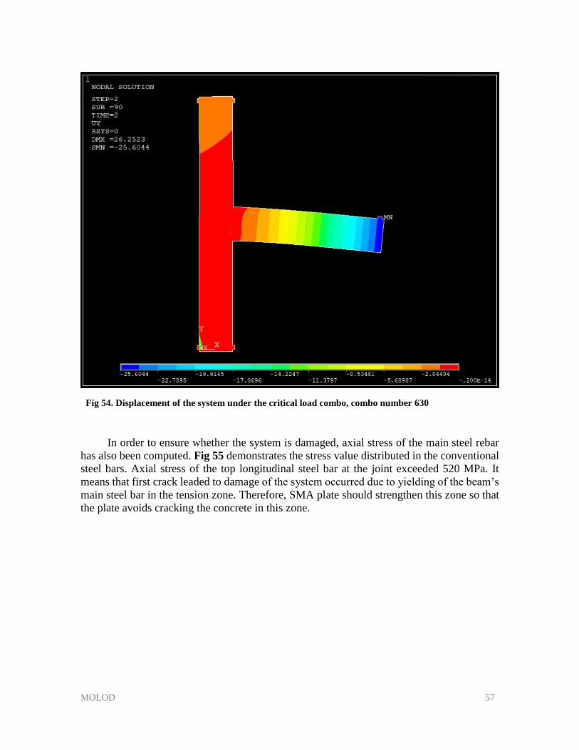
MOLOD 57

Fig 54. Displacement of the system under the critical load combo, combo number 630

In order to ensure whether the system is damaged, axial stress of the main steel rebar

has also been computed. Fig 55 demonstrates the stress value distributed in the conventional

steel bars. Axial stress of the top longitudinal steel bar at the joint exceeded 520 MPa. It

means that first crack leaded to damage of the system occurred due to yielding of the beam’s

main steel bar in the tension zone. Therefore, SMA plate should strengthen this zone so that

the plate avoids cracking the concrete in this zone.

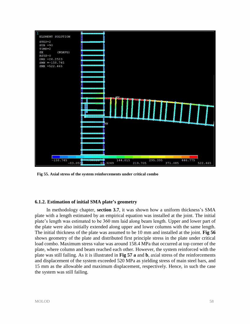
MOLOD 58

Fig 55. Axial stress of the system reinforcements under critical combo

6.1.2. Estimation of initial SMA plate’s geometry

In methodology chapter, section 3.7, it was shown how a uniform thickness’s SMA

plate with a length estimated by an empirical equation was installed at the joint. The initial

plate’s length was estimated to be 360 mm laid along beam length. Upper and lower part of

the plate were also initially extended along upper and lower columns with the same length.

The initial thickness of the plate was assumed to be 10 mm and installed at the joint. Fig 56

shows geometry of the plate and distributed first principle stress in the plate under critical

load combo. Maximum stress value was around 158.4 MPa that occurred at top corner of the

plate, where column and beam reached each other. However, the system reinforced with the

plate was still failing. As it is illustrated in Fig 57 a and b, axial stress of the reinforcements

and displacement of the system exceeded 520 MPa as yielding stress of main steel bars, and

15 mm as the allowable and maximum displacement, respectively. Hence, in such the case

the system was still failing.

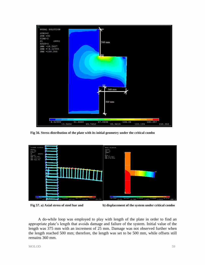
MOLOD 59

Fig 56. Stress distribution of the plate with its initial geometry under the critical combo

Fig 57. a) Axial stress of steel bar and b) displacement of the system under critical combo

A do-while loop was employed to play with length of the plate in order to find an

appropriate plate’s length that avoids damage and failure of the system. Initial value of the

length was 375 mm with an increment of 25 mm. Damage was not observed further when

the length reached 500 mm; therefore, the length was set to be 500 mm, while offsets still

remains 360 mm.

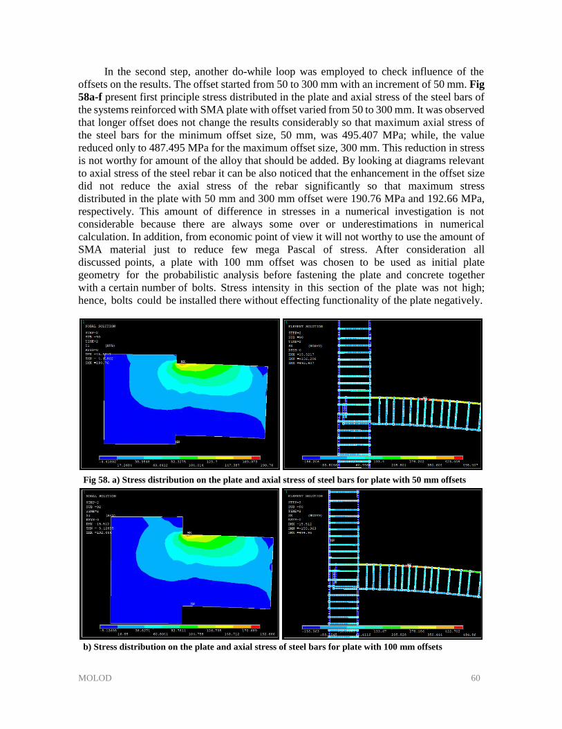
MOLOD 60

In the second step, another do-while loop was employed to check influence of the

offsets on the results. The offset started from 50 to 300 mm with an increment of 50 mm. Fig

58a-f present first principle stress distributed in the plate and axial stress of the steel bars of

the systems reinforced with SMA plate with offset varied from 50 to 300 mm. It was observed

that longer offset does not change the results considerably so that maximum axial stress of

the steel bars for the minimum offset size, 50 mm, was 495.407 MPa; while, the value

reduced only to 487.495 MPa for the maximum offset size, 300 mm. This reduction in stress

is not worthy for amount of the alloy that should be added. By looking at diagrams relevant

to axial stress of the steel rebar it can be also noticed that the enhancement in the offset size

did not reduce the axial stress of the rebar significantly so that maximum stress

distributed in the plate with 50 mm and 300 mm offset were 190.76 MPa and 192.66 MPa,

respectively. This amount of difference in stresses in a numerical investigation is not

considerable because there are always some over or underestimations in numerical

calculation. In addition, from economic point of view it will not worthy to use the amount of

SMA material just to reduce few mega Pascal of stress. After consideration all

discussed points, a plate with 100 mm offset was chosen to be used as initial plate

geometry for the probabilistic analysis before fastening the plate and concrete together

with a certain number of bolts. Stress intensity in this section of the plate was not high;

hence, bolts could be installed there without effecting functionality of the plate negatively.

Fig 58. a) Stress distribution on the plate and axial stress of steel bars for plate with 50 mm offsets

b) Stress distribution on the plate and axial stress of steel bars for plate with 100 mm offsets

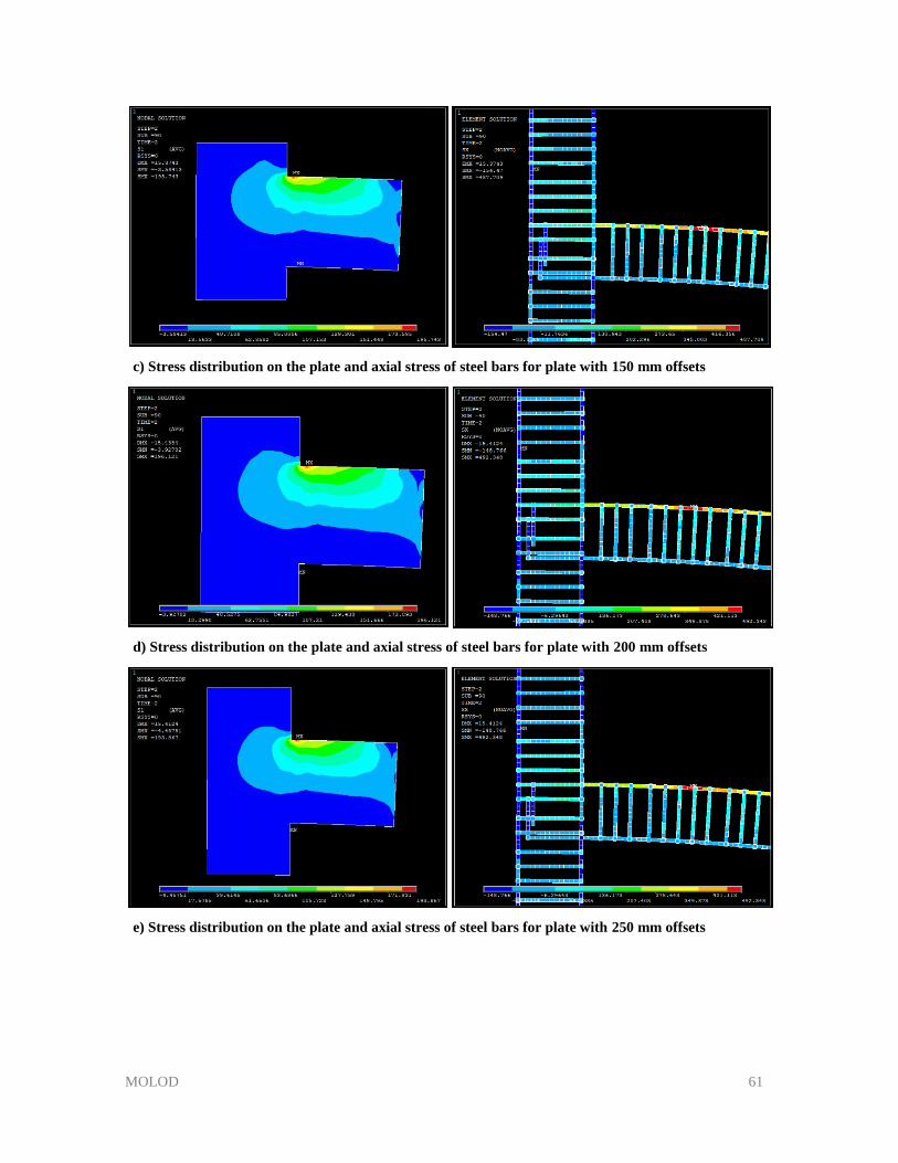
MOLOD 61

c) Stress distribution on the plate and axial stress of steel bars for plate with 150 mm offsets

d) Stress distribution on the plate and axial stress of steel bars for plate with 200 mm offsets

e) Stress distribution on the plate and axial stress of steel bars for plate with 250 mm offsets

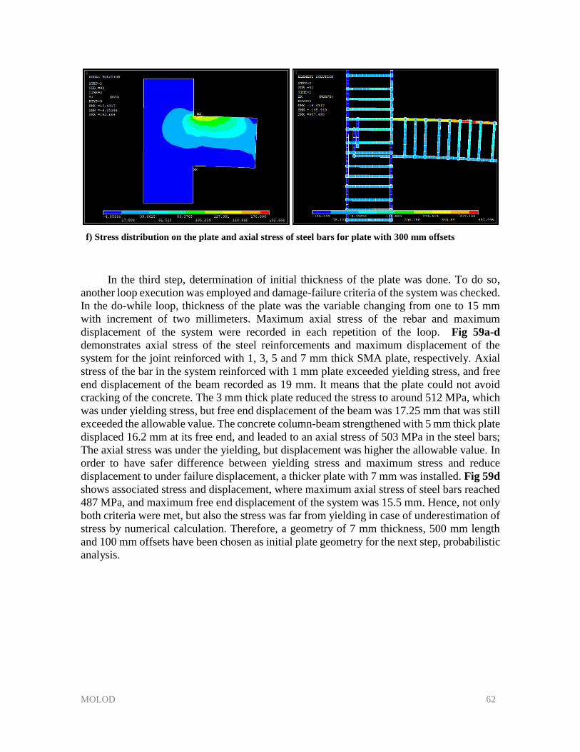
MOLOD 62

f) Stress distribution on the plate and axial stress of steel bars for plate with 300 mm offsets

In the third step, determination of initial thickness of the plate was done. To do so,

another loop execution was employed and damage-failure criteria of the system was checked.

In the do-while loop, thickness of the plate was the variable changing from one to 15 mm

with increment of two millimeters. Maximum axial stress of the rebar and maximum

displacement of the system were recorded in each repetition of the loop. Fig 59a-d

demonstrates axial stress of the steel reinforcements and maximum displacement of the

system for the joint reinforced with 1, 3, 5 and 7 mm thick SMA plate, respectively. Axial

stress of the bar in the system reinforced with 1 mm plate exceeded yielding stress, and free

end displacement of the beam recorded as 19 mm. It means that the plate could not avoid

cracking of the concrete. The 3 mm thick plate reduced the stress to around 512 MPa, which

was under yielding stress, but free end displacement of the beam was 17.25 mm that was still

exceeded the allowable value. The concrete column-beam strengthened with 5 mm thick plate

displaced 16.2 mm at its free end, and leaded to an axial stress of 503 MPa in the steel bars;

The axial stress was under the yielding, but displacement was higher the allowable value. In

order to have safer difference between yielding stress and maximum stress and reduce

displacement to under failure displacement, a thicker plate with 7 mm was installed. Fig 59d

shows associated stress and displacement, where maximum axial stress of steel bars reached

487 MPa, and maximum free end displacement of the system was 15.5 mm. Hence, not only

both criteria were met, but also the stress was far from yielding in case of underestimation of

stress by numerical calculation. Therefore, a geometry of 7 mm thickness, 500 mm length

and 100 mm offsets have been chosen as initial plate geometry for the next step, probabilistic

analysis.

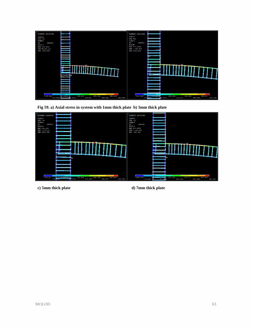
MOLOD 63

Fig 59. a) Axial stress in system with 1mm thick plate b) 3mm thick plate

3

c) 5mm thick plate d) 7mm thick plate

7

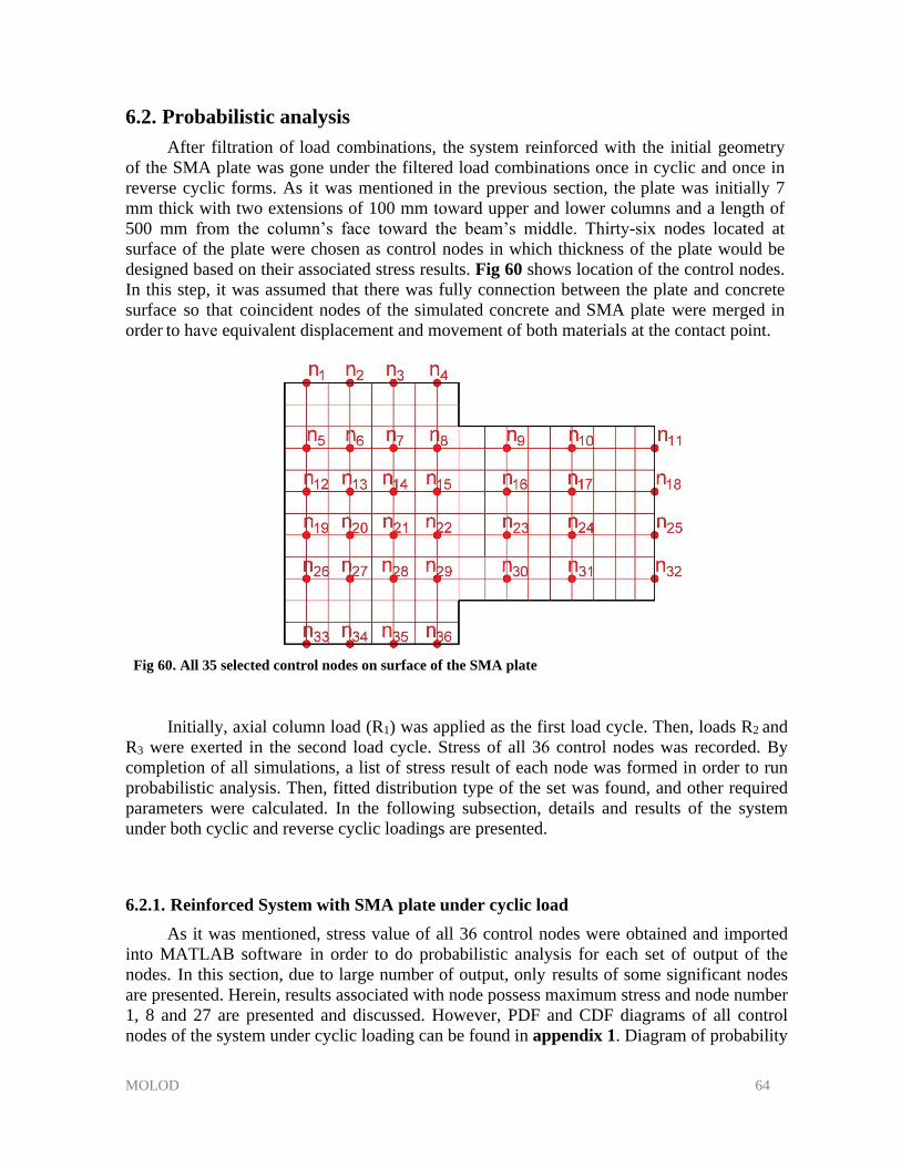
MOLOD 64

6.2. Probabilistic analysis

After filtration of load combinations, the system reinforced with the initial geometry

of the SMA plate was gone under the filtered load combinations once in cyclic and once in

reverse cyclic forms. As it was mentioned in the previous section, the plate was initially 7

mm thick with two extensions of 100 mm toward upper and lower columns and a length of

500 mm from the column’s face toward the beam’s middle. Thirty-six nodes located at

surface of the plate were chosen as control nodes in which thickness of the plate would be

designed based on their associated stress results. Fig 60 shows location of the control nodes.

In this step, it was assumed that there was fully connection between the plate and concrete

surface so that coincident nodes of the simulated concrete and SMA plate were merged in

order to have equivalent displacement and movement of both materials at the contact point.

Fig 60. All 35 selected control nodes on surface of the SMA plate

Initially, axial column load (R1) was applied as the first load cycle. Then, loads R2 and

R3 were exerted in the second load cycle. Stress of all 36 control nodes was recorded. By

completion of all simulations, a list of stress result of each node was formed in order to run

probabilistic analysis. Then, fitted distribution type of the set was found, and other required

parameters were calculated. In the following subsection, details and results of the system

under both cyclic and reverse cyclic loadings are presented.

6.2.1. Reinforced System with SMA plate under cyclic load

As it was mentioned, stress value of all 36 control nodes were obtained and imported

into MATLAB software in order to do probabilistic analysis for each set of output of the

nodes. In this section, due to large number of output, only results of some significant nodes

are presented. Herein, results associated with node possess maximum stress and node number

1, 8 and 27 are presented and discussed. However, PDF and CDF diagrams of all control

nodes of the system under cyclic loading can be found in appendix 1. Diagram of probability

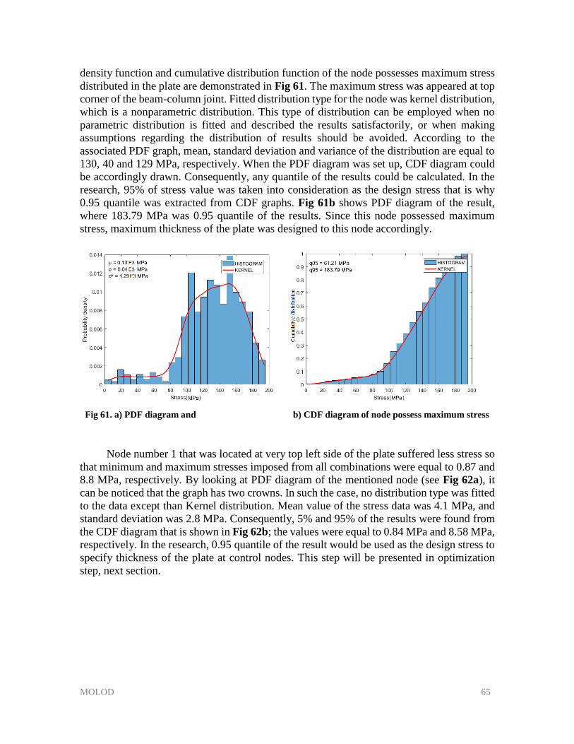
MOLOD 65

density function and cumulative distribution function of the node possesses maximum stress

distributed in the plate are demonstrated in Fig 61. The maximum stress was appeared at top

corner of the beam-column joint. Fitted distribution type for the node was kernel distribution,

which is a nonparametric distribution. This type of distribution can be employed when no

parametric distribution is fitted and described the results satisfactorily, or when making

assumptions regarding the distribution of results should be avoided. According to the

associated PDF graph, mean, standard deviation and variance of the distribution are equal to

130, 40 and 129 MPa, respectively. When the PDF diagram was set up, CDF diagram could

be accordingly drawn. Consequently, any quantile of the results could be calculated. In the

research, 95% of stress value was taken into consideration as the design stress that is why

0.95 quantile was extracted from CDF graphs. Fig 61b shows PDF diagram of the result,

where 183.79 MPa was 0.95 quantile of the results. Since this node possessed maximum

stress, maximum thickness of the plate was designed to this node accordingly.

Fig 61. a) PDF diagram and b) CDF diagram of node possess maximum stress

Node number 1 that was located at very top left side of the plate suffered less stress so

that minimum and maximum stresses imposed from all combinations were equal to 0.87 and

8.8 MPa, respectively. By looking at PDF diagram of the mentioned node (see Fig 62a), it

can be noticed that the graph has two crowns. In such the case, no distribution type was fitted

to the data except than Kernel distribution. Mean value of the stress data was 4.1 MPa, and

standard deviation was 2.8 MPa. Consequently, 5% and 95% of the results were found from

the CDF diagram that is shown in Fig 62b; the values were equal to 0.84 MPa and 8.58 MPa,

respectively. In the research, 0.95 quantile of the result would be used as the design stress to

specify thickness of the plate at control nodes. This step will be presented in optimization

step, next section.

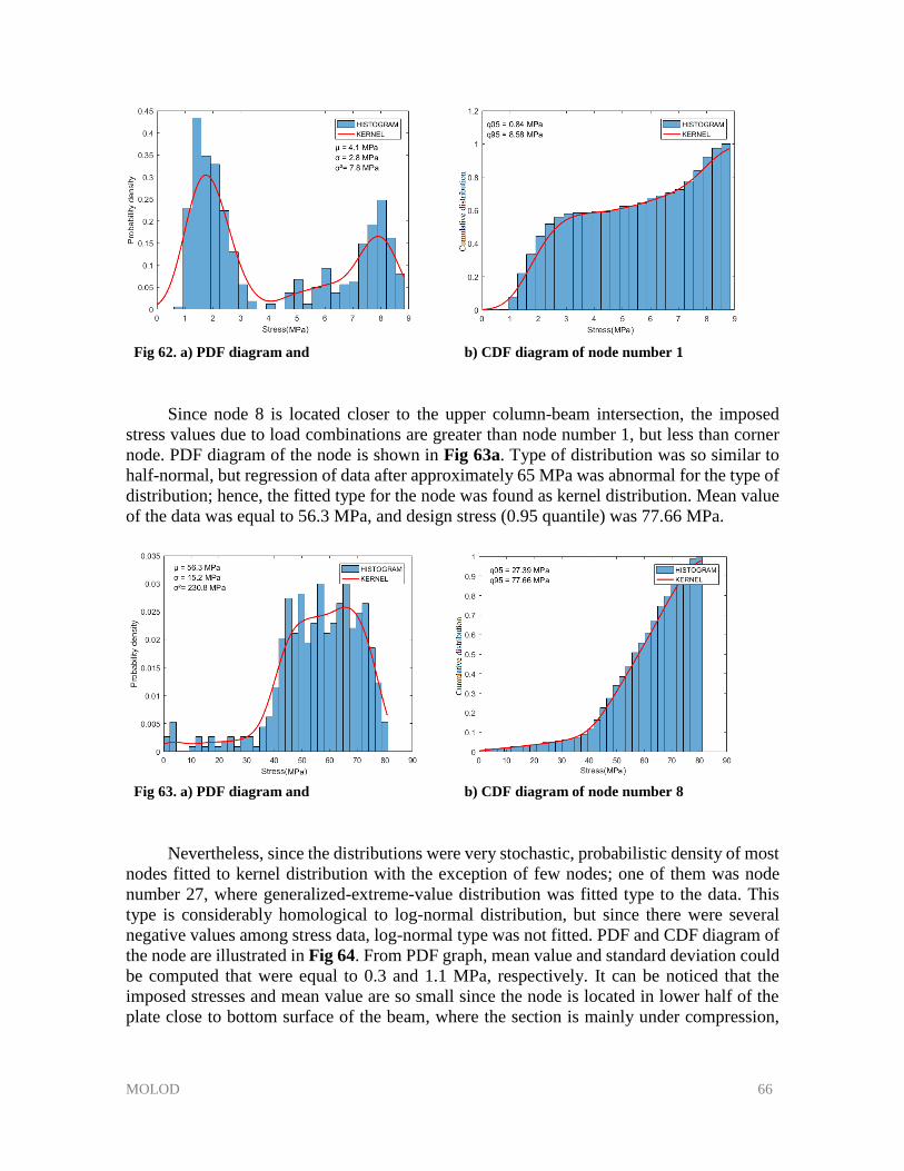
MOLOD 66

Fig 62. a) PDF diagram and b) CDF diagram of node number 1

Since node 8 is located closer to the upper column-beam intersection, the imposed

stress values due to load combinations are greater than node number 1, but less than corner

node. PDF diagram of the node is shown in Fig 63a. Type of distribution was so similar to

half-normal, but regression of data after approximately 65 MPa was abnormal for the type of

distribution; hence, the fitted type for the node was found as kernel distribution. Mean value

of the data was equal to 56.3 MPa, and design stress (0.95 quantile) was 77.66 MPa.

Fig 63. a) PDF diagram and b) CDF diagram of node number 8

Nevertheless, since the distributions were very stochastic, probabilistic density of most

nodes fitted to kernel distribution with the exception of few nodes; one of them was node

number 27, where generalized-extreme-value distribution was fitted type to the data. This

type is considerably homological to log-normal distribution, but since there were several

negative values among stress data, log-normal type was not fitted. PDF and CDF diagram of

the node are illustrated in Fig 64. From PDF graph, mean value and standard deviation could

be computed that were equal to 0.3 and 1.1 MPa, respectively. It can be noticed that the

imposed stresses and mean value are so small since the node is located in lower half of the

plate close to bottom surface of the beam, where the section is mainly under compression,

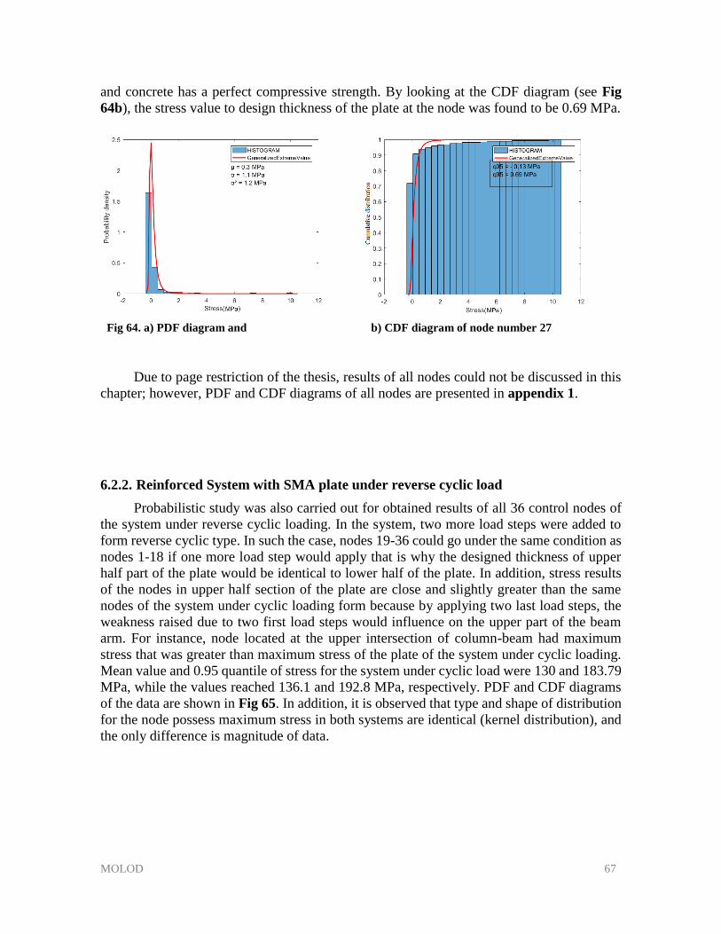
MOLOD 67

and concrete has a perfect compressive strength. By looking at the CDF diagram (see Fig

64b), the stress value to design thickness of the plate at the node was found to be 0.69 MPa.

Fig 64. a) PDF diagram and b) CDF diagram of node number 27

Due to page restriction of the thesis, results of all nodes could not be discussed in this

chapter; however, PDF and CDF diagrams of all nodes are presented in appendix 1.

6.2.2. Reinforced System with SMA plate under reverse cyclic load

Probabilistic study was also carried out for obtained results of all 36 control nodes of

the system under reverse cyclic loading. In the system, two more load steps were added to

form reverse cyclic type. In such the case, nodes 19-36 could go under the same condition as

nodes 1-18 if one more load step would apply that is why the designed thickness of upper

half part of the plate would be identical to lower half of the plate. In addition, stress results

of the nodes in upper half section of the plate are close and slightly greater than the same

nodes of the system under cyclic loading form because by applying two last load steps, the

weakness raised due to two first load steps would influence on the upper part of the beam

arm. For instance, node located at the upper intersection of column-beam had maximum

stress that was greater than maximum stress of the plate of the system under cyclic loading.

Mean value and 0.95 quantile of stress for the system under cyclic load were 130 and 183.79

MPa, while the values reached 136.1 and 192.8 MPa, respectively. PDF and CDF diagrams

of the data are shown in Fig 65. In addition, it is observed that type and shape of distribution

for the node possess maximum stress in both systems are identical (kernel distribution), and

the only difference is magnitude of data.

Cum

ula

tive

dis

trib

uti

on

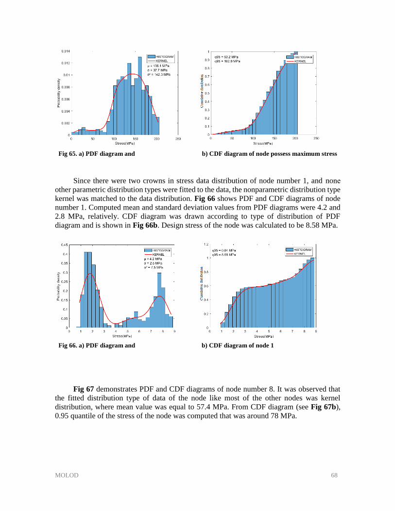
MOLOD 68

Fig 65. a) PDF diagram and b) CDF diagram of node possess maximum stress

Since there were two crowns in stress data distribution of node number 1, and none other parametric distribution types were fitted to the data, the nonparametric distribution type

kernel was matched to the data distribution. Fig 66 shows PDF and CDF diagrams of node

number 1. Computed mean and standard deviation values from PDF diagrams were 4.2 and

2.8 MPa, relatively. CDF diagram was drawn according to type of distribution of PDF

diagram and is shown in Fig 66b. Design stress of the node was calculated to be 8.58 MPa.

Fig 66. a) PDF diagram and b) CDF diagram of node 1

Fig 67 demonstrates PDF and CDF diagrams of node number 8. It was observed that

the fitted distribution type of data of the node like most of the other nodes was kernel

distribution, where mean value was equal to 57.4 MPa. From CDF diagram (see Fig 67b),

0.95 quantile of the stress of the node was computed that was around 78 MPa.

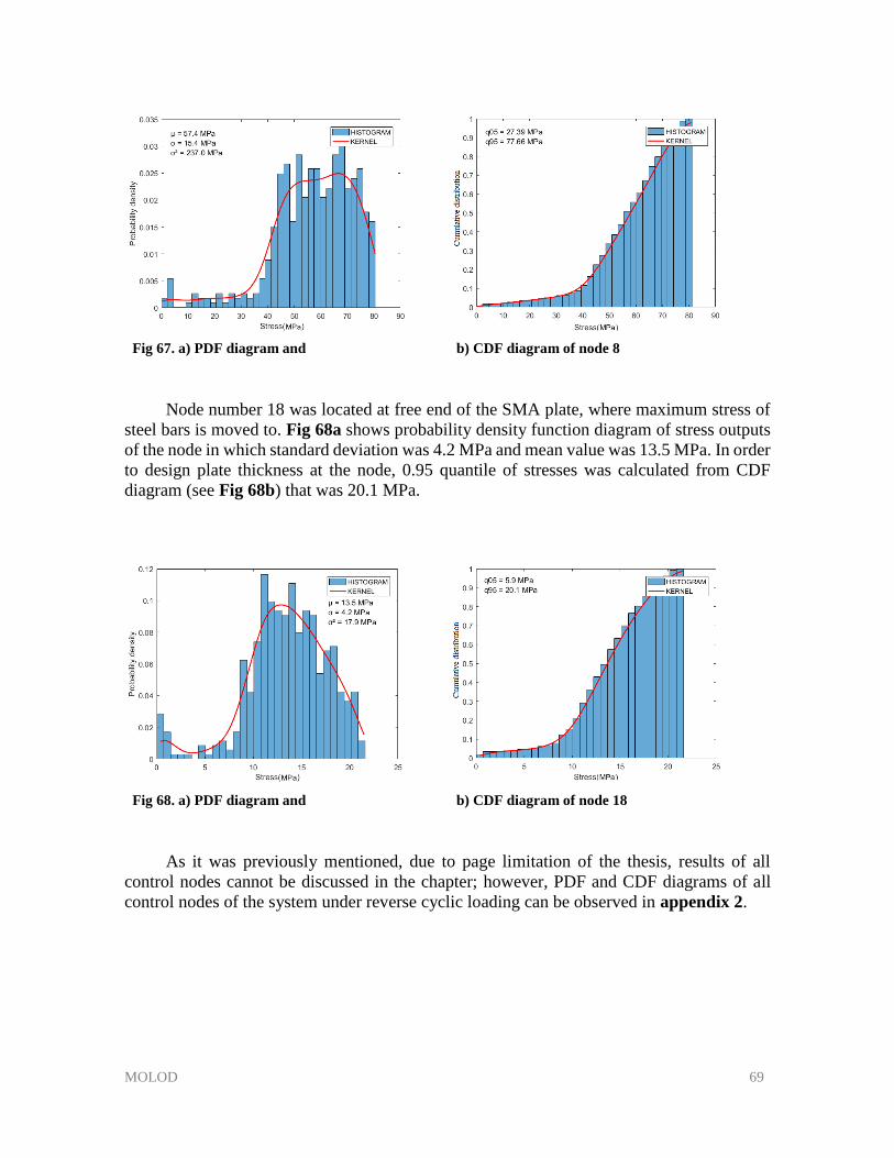
MOLOD 69

Fig 67. a) PDF diagram and b) CDF diagram of node 8

Node number 18 was located at free end of the SMA plate, where maximum stress of

steel bars is moved to. Fig 68a shows probability density function diagram of stress outputs

of the node in which standard deviation was 4.2 MPa and mean value was 13.5 MPa. In order

to design plate thickness at the node, 0.95 quantile of stresses was calculated from CDF

diagram (see Fig 68b) that was 20.1 MPa.

Fig 68. a) PDF diagram and b) CDF diagram of node 18

As it was previously mentioned, due to page limitation of the thesis, results of all

control nodes cannot be discussed in the chapter; however, PDF and CDF diagrams of all

control nodes of the system under reverse cyclic loading can be observed in appendix 2.

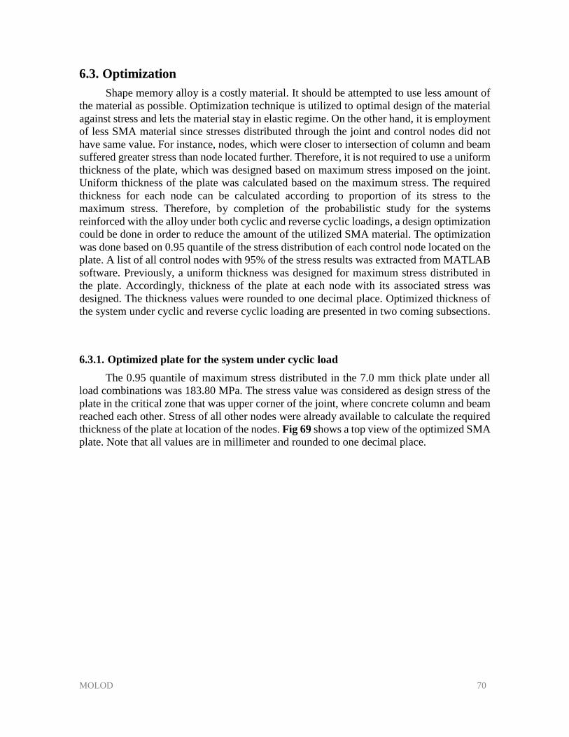
MOLOD 70

6.3. Optimization

Shape memory alloy is a costly material. It should be attempted to use less amount of

the material as possible. Optimization technique is utilized to optimal design of the material

against stress and lets the material stay in elastic regime. On the other hand, it is employment

of less SMA material since stresses distributed through the joint and control nodes did not

have same value. For instance, nodes, which were closer to intersection of column and beam

suffered greater stress than node located further. Therefore, it is not required to use a uniform

thickness of the plate, which was designed based on maximum stress imposed on the joint.

Uniform thickness of the plate was calculated based on the maximum stress. The required

thickness for each node can be calculated according to proportion of its stress to the

maximum stress. Therefore, by completion of the probabilistic study for the systems

reinforced with the alloy under both cyclic and reverse cyclic loadings, a design optimization

could be done in order to reduce the amount of the utilized SMA material. The optimization

was done based on 0.95 quantile of the stress distribution of each control node located on the

plate. A list of all control nodes with 95% of the stress results was extracted from MATLAB

software. Previously, a uniform thickness was designed for maximum stress distributed in

the plate. Accordingly, thickness of the plate at each node with its associated stress was

designed. The thickness values were rounded to one decimal place. Optimized thickness of

the system under cyclic and reverse cyclic loading are presented in two coming subsections.

6.3.1. Optimized plate for the system under cyclic load

The 0.95 quantile of maximum stress distributed in the 7.0 mm thick plate under all

load combinations was 183.80 MPa. The stress value was considered as design stress of the

plate in the critical zone that was upper corner of the joint, where concrete column and beam

reached each other. Stress of all other nodes were already available to calculate the required

thickness of the plate at location of the nodes. Fig 69 shows a top view of the optimized SMA

plate. Note that all values are in millimeter and rounded to one decimal place.

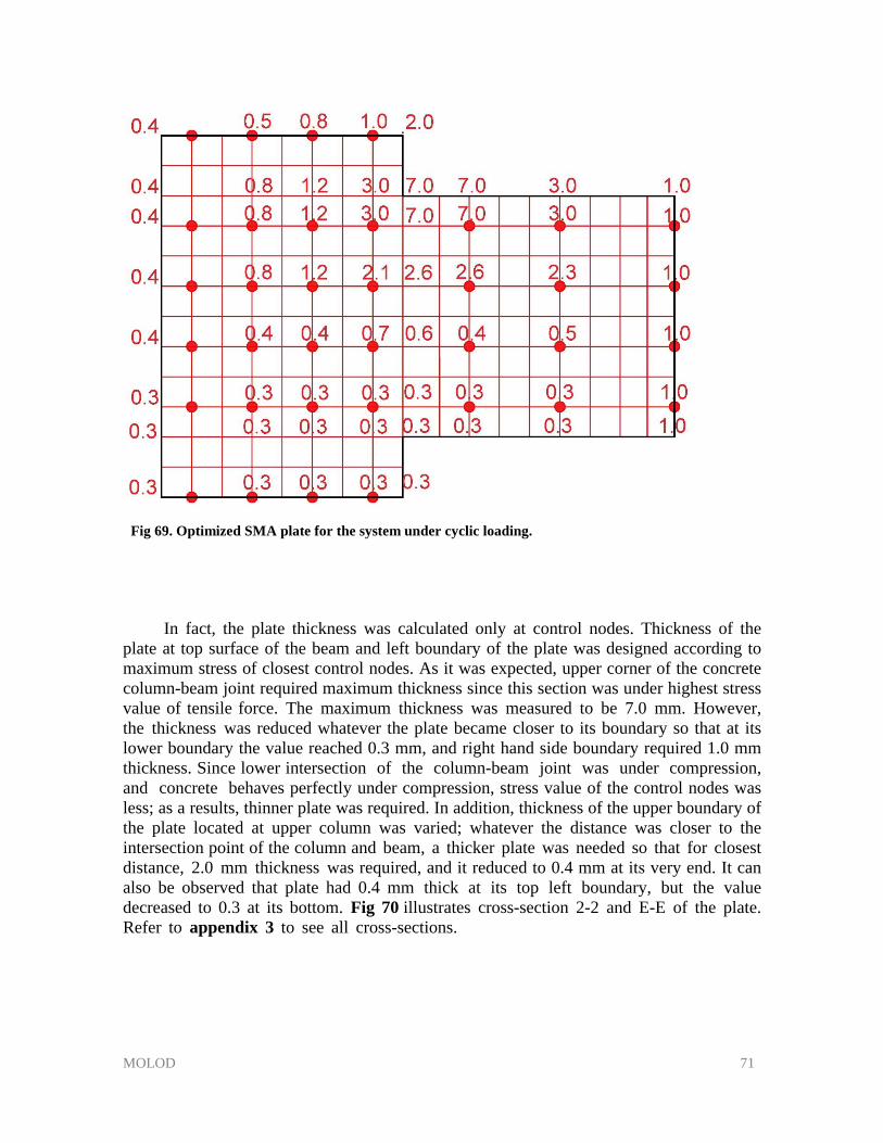
MOLOD 71

Fig 69. Optimized SMA plate for the system under cyclic loading.

In fact, the plate thickness was calculated only at control nodes. Thickness of the

plate at top surface of the beam and left boundary of the plate was designed according to

maximum stress of closest control nodes. As it was expected, upper corner of the concrete

column-beam joint required maximum thickness since this section was under highest stress

value of tensile force. The maximum thickness was measured to be 7.0 mm. However,

the thickness was reduced whatever the plate became closer to its boundary so that at its

lower boundary the value reached 0.3 mm, and right hand side boundary required 1.0 mm

thickness. Since lower intersection of the column-beam joint was under compression,

and concrete behaves perfectly under compression, stress value of the control nodes was

less; as a results, thinner plate was required. In addition, thickness of the upper boundary of

the plate located at upper column was varied; whatever the distance was closer to the

intersection point of the column and beam, a thicker plate was needed so that for closest

distance, 2.0 mm thickness was required, and it reduced to 0.4 mm at its very end. It can

also be observed that plate had 0.4 mm thick at its top left boundary, but the value

decreased to 0.3 at its bottom. Fig 70 illustrates cross-section 2-2 and E-E of the plate.

Refer to appendix 3 to see all cross-sections.

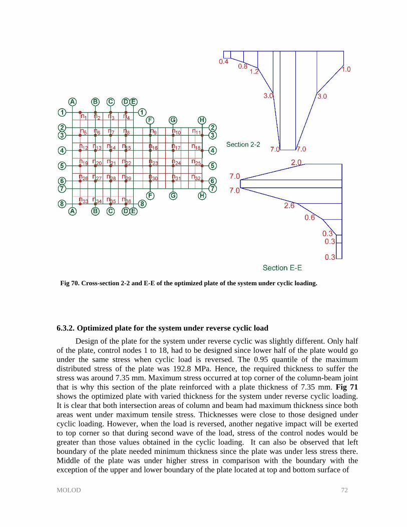
MOLOD 72

Fig 70. Cross-section 2-2 and E-E of the optimized plate of the system under cyclic loading.

6.3.2. Optimized plate for the system under reverse cyclic load

Design of the plate for the system under reverse cyclic was slightly different. Only half

of the plate, control nodes 1 to 18, had to be designed since lower half of the plate would go

under the same stress when cyclic load is reversed. The 0.95 quantile of the maximum

distributed stress of the plate was 192.8 MPa. Hence, the required thickness to suffer the

stress was around 7.35 mm. Maximum stress occurred at top corner of the column-beam joint

that is why this section of the plate reinforced with a plate thickness of 7.35 mm. Fig 71

shows the optimized plate with varied thickness for the system under reverse cyclic loading.

It is clear that both intersection areas of column and beam had maximum thickness since both

areas went under maximum tensile stress. Thicknesses were close to those designed under

cyclic loading. However, when the load is reversed, another negative impact will be exerted

to top corner so that during second wave of the load, stress of the control nodes would be

greater than those values obtained in the cyclic loading. It can also be observed that left

boundary of the plate needed minimum thickness since the plate was under less stress there.

Middle of the plate was under higher stress in comparison with the boundary with the

exception of the upper and lower boundary of the plate located at top and bottom surface of

MOLOD 73

the beam. Fig 72 illustrates cross-sections 2-2, 7-7 and E-E of the plate. Refer to appendix

4 to see all cross-sections.

Fig 71. Optimized SMA plate for the system under reverse cyclic loading.

MOLOD 74

Fig 72. Cross-section 2-2 and E-E of the optimized plate of the system under cyclic loading.

6.4. Numerical examples

In order to check whether optimized SMA plates can still avoid damage and failure of

the structure, several numerical examples have been carried out. Since designed plate for

cyclic loading up to end of loading step can construe the same situation of the experiment,

three examples with the plate have been run, but one example for the system reinforced

optimized plate for reverse cyclic loading. For cyclic loading the following examples have

been done:

1. In order to check whether the SMA plate designed based on the 95% of stress can

avoid the system’s failure, the system under 0.95 quantile of bending moment load

with its associated R1 and R3 was analyzed.

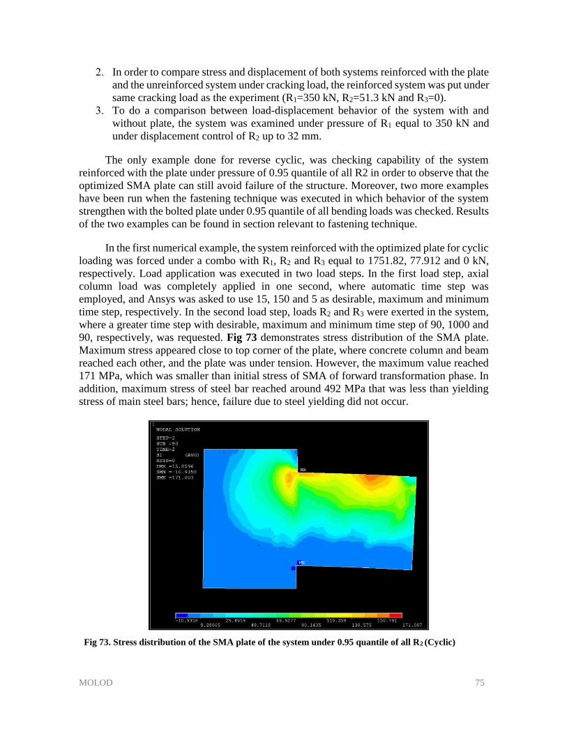
MOLOD 75

2. In order to compare stress and displacement of both systems reinforced with the plate and the unreinforced system under cracking load, the reinforced system was put under same cracking load as the experiment (R1=350 kN, R2=51.3 kN and R3=0).

3. To do a comparison between load-displacement behavior of the system with and without plate, the system was examined under pressure of R1 equal to 350 kN and under displacement control of R2 up to 32 mm.

The only example done for reverse cyclic, was checking capability of the system

reinforced with the plate under pressure of 0.95 quantile of all R2 in order to observe that the

optimized SMA plate can still avoid failure of the structure. Moreover, two more examples

have been run when the fastening technique was executed in which behavior of the system

strengthen with the bolted plate under 0.95 quantile of all bending loads was checked. Results

of the two examples can be found in section relevant to fastening technique.

In the first numerical example, the system reinforced with the optimized plate for cyclic

loading was forced under a combo with R1, R2 and R3 equal to 1751.82, 77.912 and 0 kN,

respectively. Load application was executed in two load steps. In the first load step, axial

column load was completely applied in one second, where automatic time step was

employed, and Ansys was asked to use 15, 150 and 5 as desirable, maximum and minimum

time step, respectively. In the second load step, loads R2 and R3 were exerted in the system,

where a greater time step with desirable, maximum and minimum time step of 90, 1000 and

90, respectively, was requested. Fig 73 demonstrates stress distribution of the SMA plate.

Maximum stress appeared close to top corner of the plate, where concrete column and beam

reached each other, and the plate was under tension. However, the maximum value reached

171 MPa, which was smaller than initial stress of SMA of forward transformation phase. In

addition, maximum stress of steel bar reached around 492 MPa that was less than yielding

stress of main steel bars; hence, failure due to steel yielding did not occur.

Fig 73. Stress distribution of the SMA plate of the system under 0.95 quantile of all R2 (Cyclic)

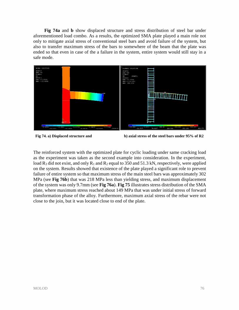
MOLOD 76

Fig 74a and b show displaced structure and stress distribution of steel bar under

aforementioned load combo. As a results, the optimized SMA plate played a main role not

only to mitigate axial stress of conventional steel bars and avoid failure of the system, but

also to transfer maximum stress of the bars to somewhere of the beam that the plate was

ended so that even in case of the a failure in the system, entire system would still stay in a

safe mode.

Fig 74. a) Displaced structure and b) axial stress of the steel bars under 95% of R2

The reinforced system with the optimized plate for cyclic loading under same cracking load

as the experiment was taken as the second example into consideration. In the experiment,

load R3 did not exist, and only R1 and R2 equal to 350 and 51.3 kN, respectively, were applied

on the system. Results showed that existence of the plate played a significant role to prevent

failure of entire system so that maximum stress of the main steel bars was approximately 302

MPa (see Fig 76b) that was 218 MPa less than yielding stress, and maximum displacement

of the system was only 9.7mm (see Fig 76a). Fig 75 illustrates stress distribution of the SMA

plate, where maximum stress reached about 149 MPa that was under initial stress of forward

transformation phase of the alloy. Furthermore, maximum axial stress of the rebar were not

close to the join, but it was located close to end of the plate.

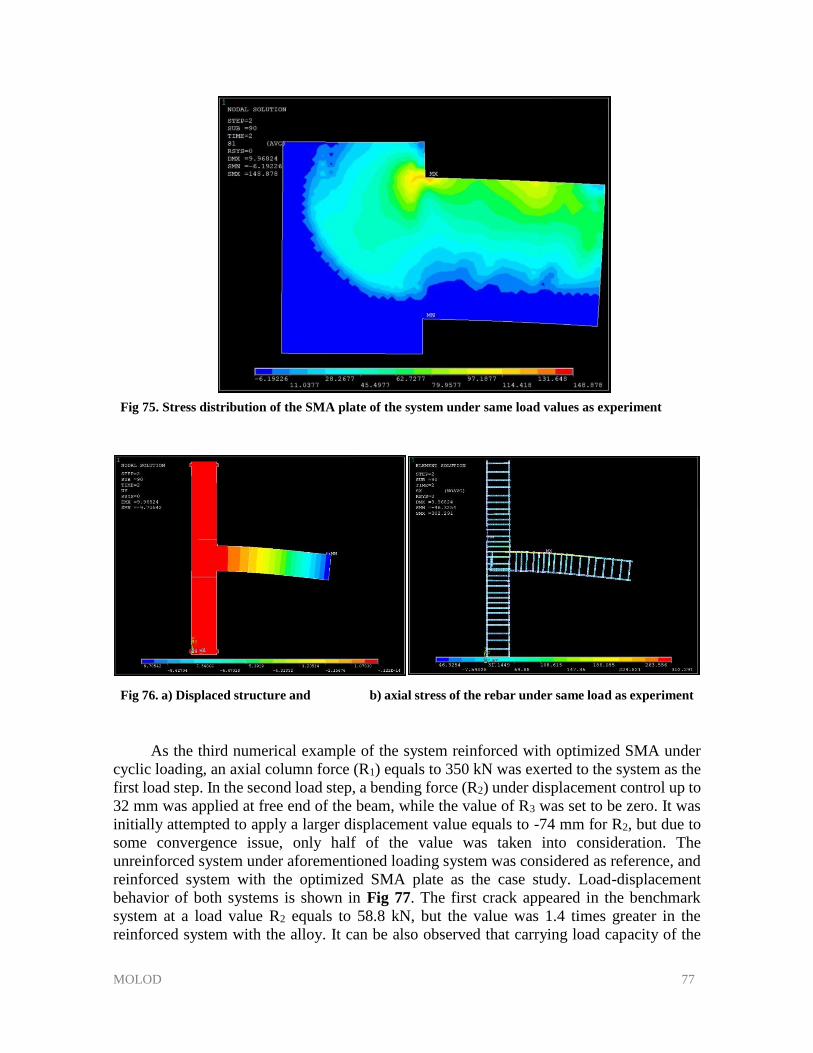
MOLOD 77

Fig 75. Stress distribution of the SMA plate of the system under same load values as experiment

Fig 76. a) Displaced structure and b) axial stress of the rebar under same load as experiment

As the third numerical example of the system reinforced with optimized SMA under

cyclic loading, an axial column force (R1) equals to 350 kN was exerted to the system as the

first load step. In the second load step, a bending force (R2) under displacement control up to

32 mm was applied at free end of the beam, while the value of R3 was set to be zero. It was

initially attempted to apply a larger displacement value equals to -74 mm for R2, but due to

some convergence issue, only half of the value was taken into consideration. The

unreinforced system under aforementioned loading system was considered as reference, and

reinforced system with the optimized SMA plate as the case study. Load-displacement

behavior of both systems is shown in Fig 77. The first crack appeared in the benchmark

system at a load value R2 equals to 58.8 kN, but the value was 1.4 times greater in the

reinforced system with the alloy. It can be also observed that carrying load capacity of the

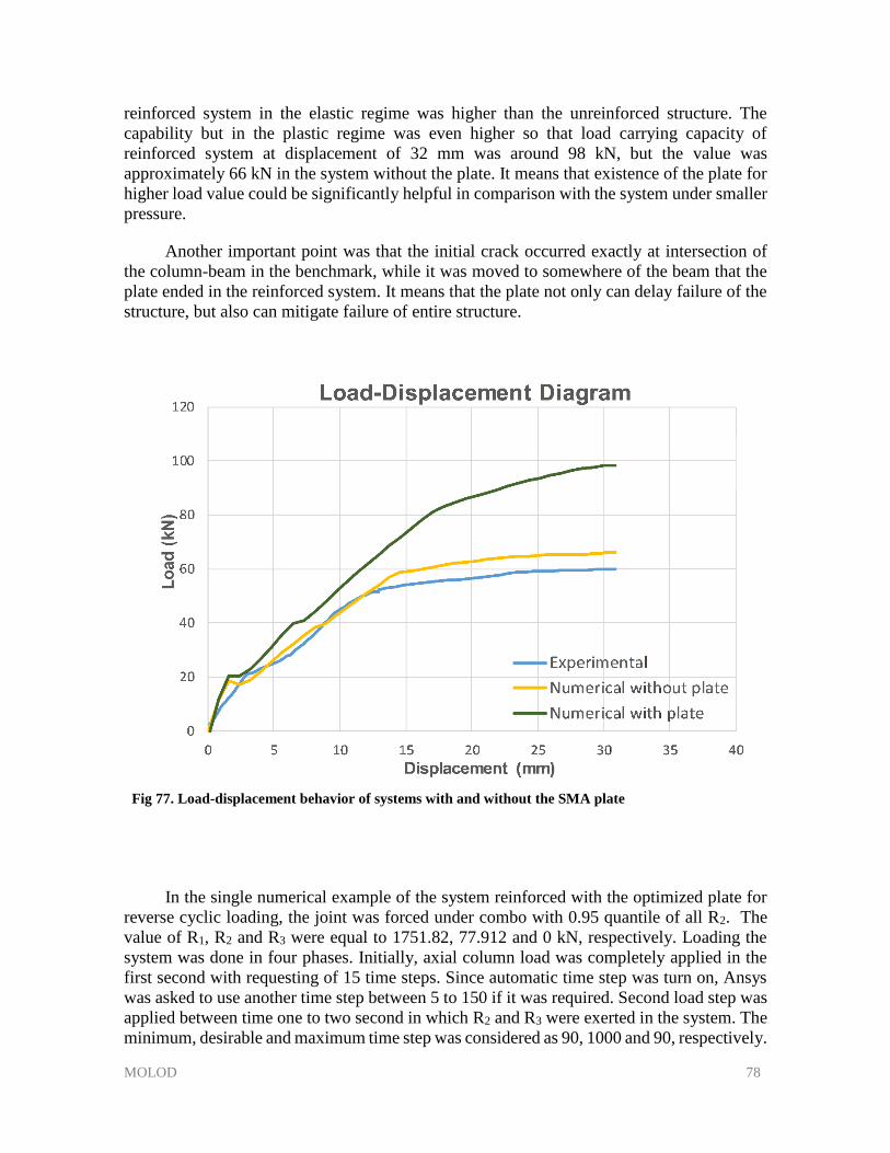
MOLOD 78

reinforced system in the elastic regime was higher than the unreinforced structure. The

capability but in the plastic regime was even higher so that load carrying capacity of

reinforced system at displacement of 32 mm was around 98 kN, but the value was

approximately 66 kN in the system without the plate. It means that existence of the plate for

higher load value could be significantly helpful in comparison with the system under smaller

pressure.

Another important point was that the initial crack occurred exactly at intersection of

the column-beam in the benchmark, while it was moved to somewhere of the beam that the

plate ended in the reinforced system. It means that the plate not only can delay failure of the

structure, but also can mitigate failure of entire structure.

Fig 77. Load-displacement behavior of systems with and without the SMA plate

In the single numerical example of the system reinforced with the optimized plate for

reverse cyclic loading, the joint was forced under combo with 0.95 quantile of all R2. The

value of R1, R2 and R3 were equal to 1751.82, 77.912 and 0 kN, respectively. Loading the

system was done in four phases. Initially, axial column load was completely applied in the

first second with requesting of 15 time steps. Since automatic time step was turn on, Ansys

was asked to use another time step between 5 to 150 if it was required. Second load step was

applied between time one to two second in which R2 and R3 were exerted in the system. The

minimum, desirable and maximum time step was considered as 90, 1000 and 90, respectively.

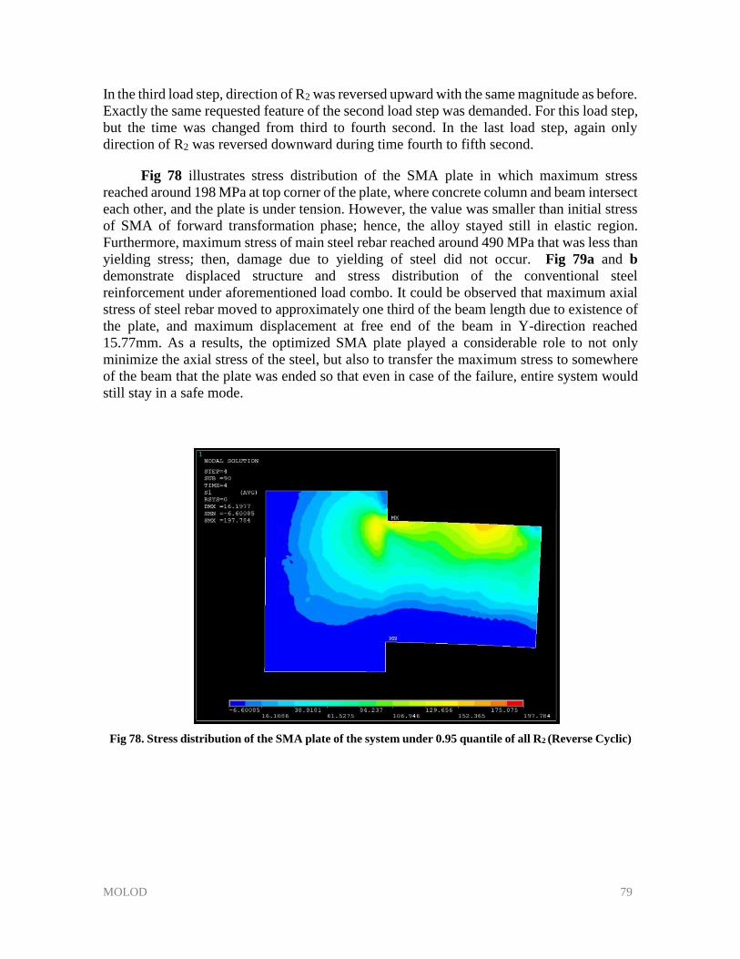
MOLOD 79

In the third load step, direction of R2 was reversed upward with the same magnitude as before.

Exactly the same requested feature of the second load step was demanded. For this load step,

but the time was changed from third to fourth second. In the last load step, again only

direction of R2 was reversed downward during time fourth to fifth second.

Fig 78 illustrates stress distribution of the SMA plate in which maximum stress

reached around 198 MPa at top corner of the plate, where concrete column and beam intersect

each other, and the plate is under tension. However, the value was smaller than initial stress

of SMA of forward transformation phase; hence, the alloy stayed still in elastic region.

Furthermore, maximum stress of main steel rebar reached around 490 MPa that was less than

yielding stress; then, damage due to yielding of steel did not occur. Fig 79a and b

demonstrate displaced structure and stress distribution of the conventional steel

reinforcement under aforementioned load combo. It could be observed that maximum axial

stress of steel rebar moved to approximately one third of the beam length due to existence of

the plate, and maximum displacement at free end of the beam in Y-direction reached

15.77mm. As a results, the optimized SMA plate played a considerable role to not only

minimize the axial stress of the steel, but also to transfer the maximum stress to somewhere

of the beam that the plate was ended so that even in case of the failure, entire system would

still stay in a safe mode.

Fig 78. Stress distribution of the SMA plate of the system under 0.95 quantile of all R2 (Reverse Cyclic)

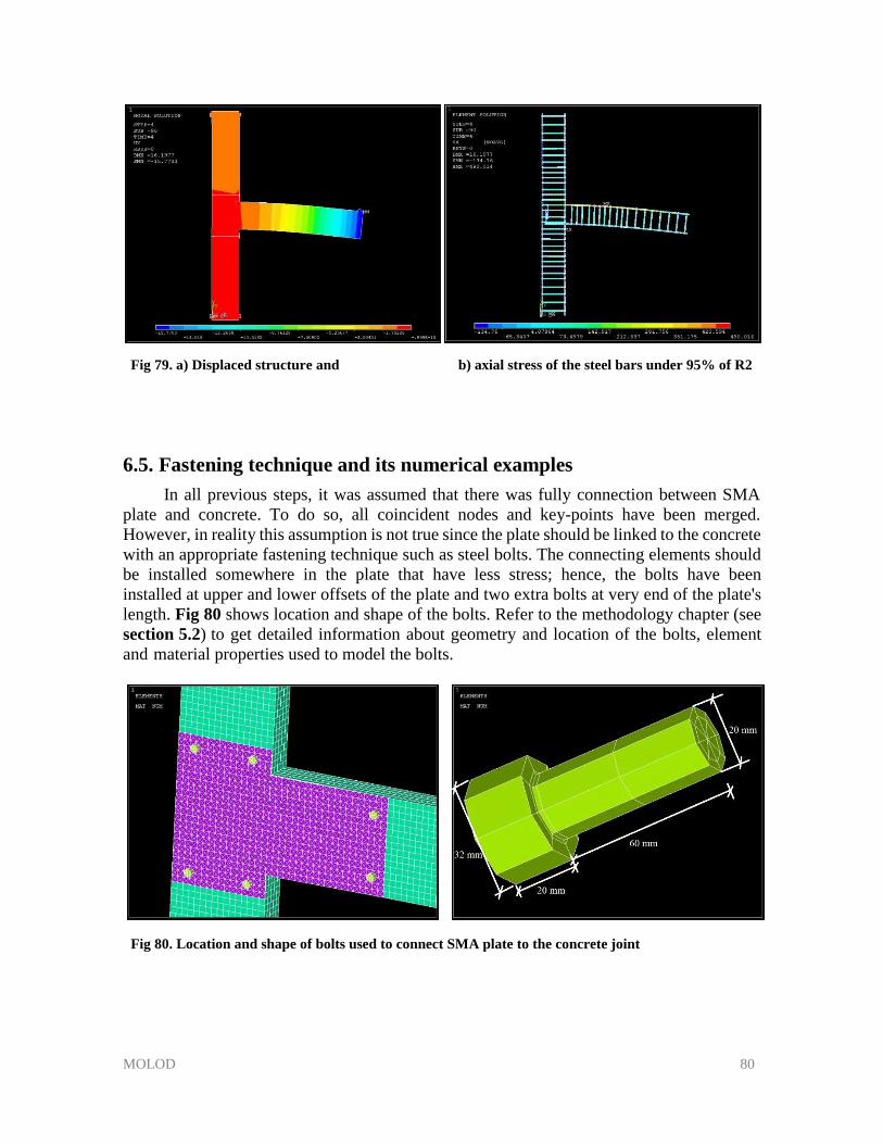
MOLOD 80

Fig 79. a) Displaced structure and b) axial stress of the steel bars under 95% of R2

6.5. Fastening technique and its numerical examples

In all previous steps, it was assumed that there was fully connection between SMA

plate and concrete. To do so, all coincident nodes and key-points have been merged.

However, in reality this assumption is not true since the plate should be linked to the concrete

with an appropriate fastening technique such as steel bolts. The connecting elements should

be installed somewhere in the plate that have less stress; hence, the bolts have been

installed at upper and lower offsets of the plate and two extra bolts at very end of the plate's length. Fig 80 shows location and shape of the bolts. Refer to the methodology chapter (see

section 5.2) to get detailed information about geometry and location of the bolts, element

and material properties used to model the bolts.

Fig 80. Location and shape of bolts used to connect SMA plate to the concrete joint

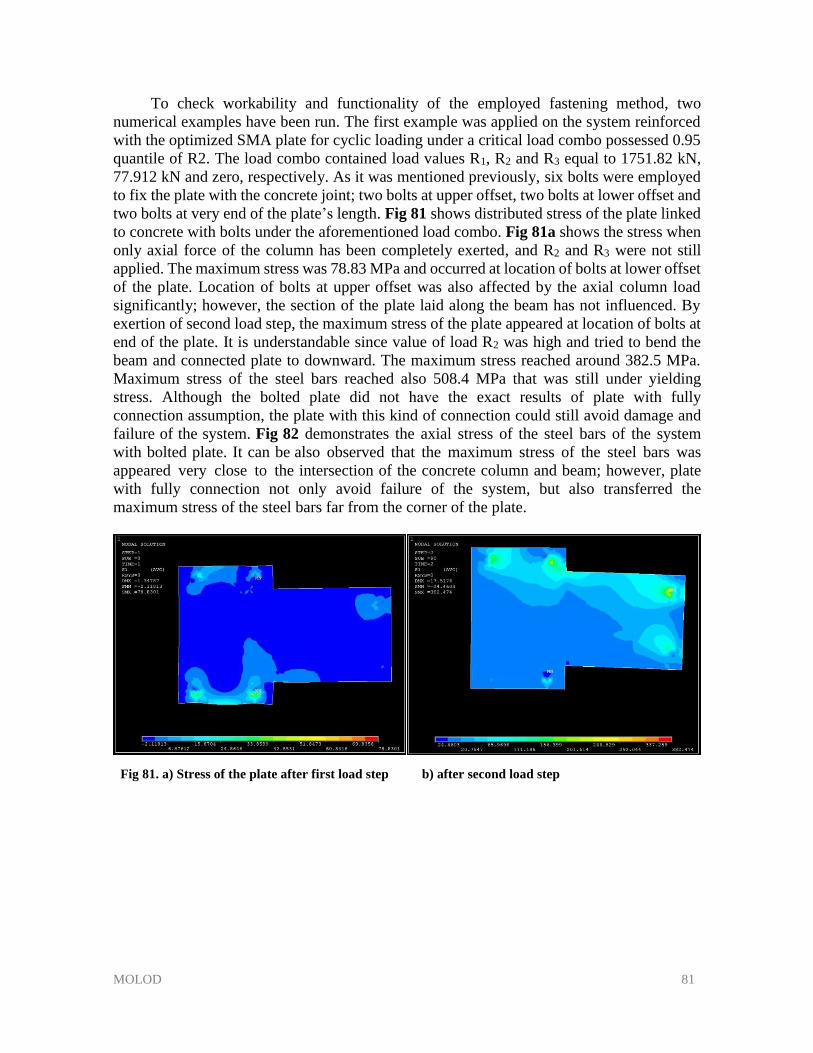
MOLOD 81

To check workability and functionality of the employed fastening method, two

numerical examples have been run. The first example was applied on the system reinforced

with the optimized SMA plate for cyclic loading under a critical load combo possessed 0.95

quantile of R2. The load combo contained load values R1, R2 and R3 equal to 1751.82 kN,

77.912 kN and zero, respectively. As it was mentioned previously, six bolts were employed

to fix the plate with the concrete joint; two bolts at upper offset, two bolts at lower offset and

two bolts at very end of the plate’s length. Fig 81 shows distributed stress of the plate linked

to concrete with bolts under the aforementioned load combo. Fig 81a shows the stress when

only axial force of the column has been completely exerted, and R2 and R3 were not still

applied. The maximum stress was 78.83 MPa and occurred at location of bolts at lower offset

of the plate. Location of bolts at upper offset was also affected by the axial column load

significantly; however, the section of the plate laid along the beam has not influenced. By

exertion of second load step, the maximum stress of the plate appeared at location of bolts at

end of the plate. It is understandable since value of load R2 was high and tried to bend the

beam and connected plate to downward. The maximum stress reached around 382.5 MPa.

Maximum stress of the steel bars reached also 508.4 MPa that was still under yielding

stress. Although the bolted plate did not have the exact results of plate with fully

connection assumption, the plate with this kind of connection could still avoid damage and

failure of the system. Fig 82 demonstrates the axial stress of the steel bars of the system

with bolted plate. It can be also observed that the maximum stress of the steel bars was

appeared very close to the intersection of the concrete column and beam; however, plate

with fully connection not only avoid failure of the system, but also transferred the

maximum stress of the steel bars far from the corner of the plate.

Fig 81. a) Stress of the plate after first load step b) after second load step

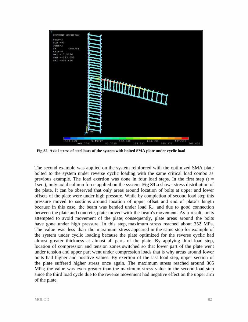
MOLOD 82

Fig 82. Axial stress of steel bars of the system with bolted SMA plate under cyclic load

The second example was applied on the system reinforced with the optimized SMA plate

bolted to the system under reverse cyclic loading with the same critical load combo as

previous example. The load exertion was done in four load steps. In the first step (t =

1sec.), only axial column force applied on the system. Fig 83 a shows stress distribution of

the plate. It can be observed that only areas around location of bolts at upper and lower

offsets of the plate were under high pressure. While by completion of second load step this

pressure moved to sections around location of upper offset and end of plate’s length

because in this case, the beam was bended under load R2, and due to good connection

between the plate and concrete, plate moved with the beam's movement. As a result, bolts

attempted to avoid movement of the plate; consequently, plate areas around the bolts

have gone under high pressure. In this step, maximum stress reached about 352 MPa.

The value was less than the maximum stress appeared in the same step for example of

the system under cyclic loading because the plate optimized for the reverse cyclic had

almost greater thickness at almost all parts of the plate. By applying third load step,

location of compression and tension zones switched so that lower part of the plate went

under tension and upper part went under compression loads that is why areas around lower

bolts had higher and positive values. By exertion of the last load step, upper section of

the plate suffered higher stress once again. The maximum stress reached around 365

MPa; the value was even greater than the maximum stress value in the second load step

since the third load cycle due to the reverse movement had negative effect on the upper arm

of the plate.

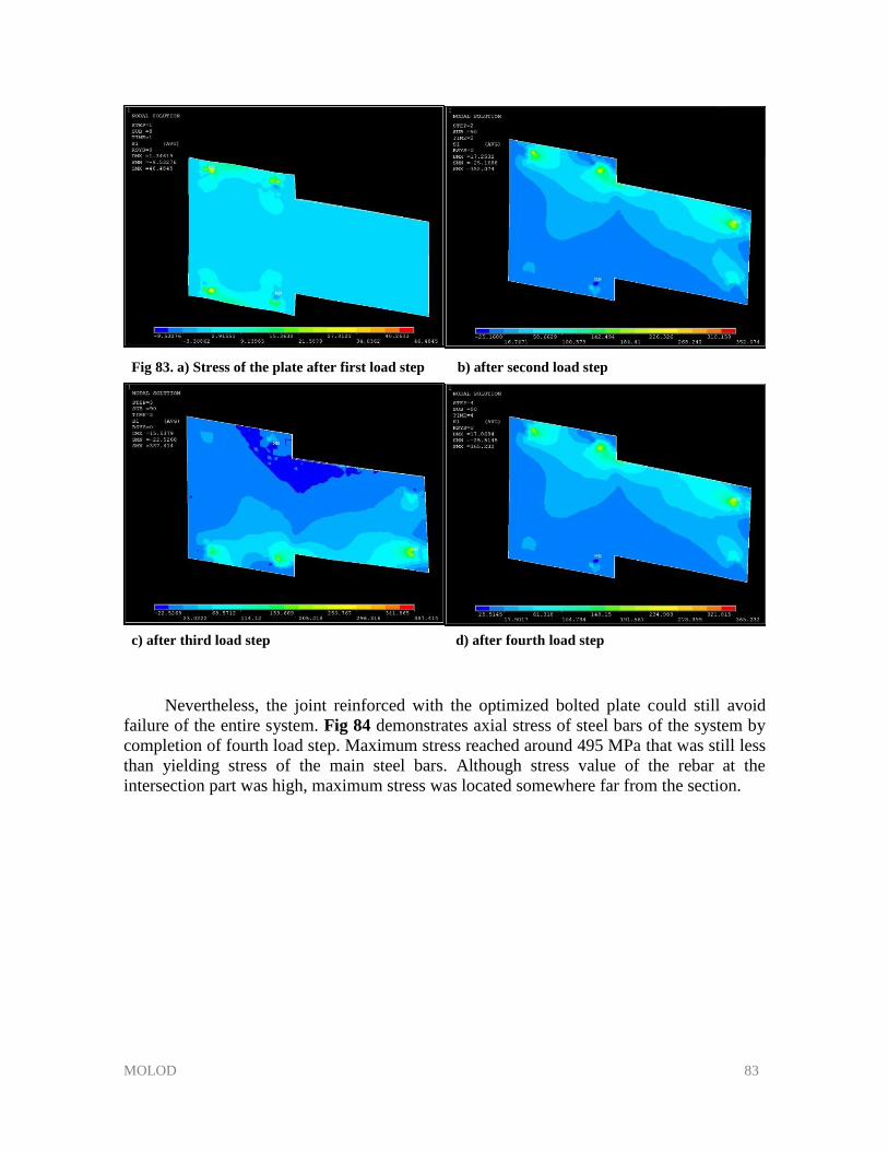
MOLOD 83

Fig 83. a) Stress of the plate after first load step b) after second load step

c) after third load step d) after fourth load step

Nevertheless, the joint reinforced with the optimized bolted plate could still avoid

failure of the entire system. Fig 84 demonstrates axial stress of steel bars of the system by

completion of fourth load step. Maximum stress reached around 495 MPa that was still less

than yielding stress of the main steel bars. Although stress value of the rebar at the

intersection part was high, maximum stress was located somewhere far from the section.

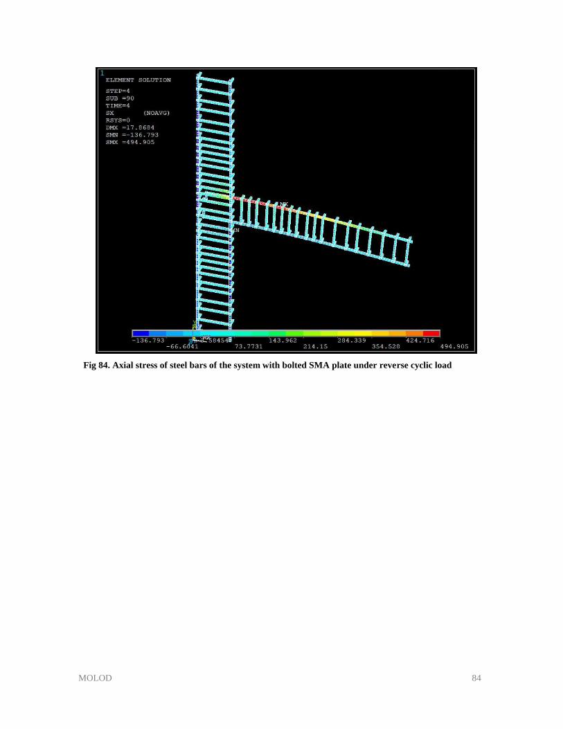
MOLOD 84

Fig 84. Axial stress of steel bars of the system with bolted SMA plate under reverse cyclic load

MOLOD 85

Chapter 7. Conclusion and future work

7.1. Conclusion

This numerical investigation has been carried out in order to assess influence of SMA

plates installed at a concrete column-beam joint on strength and ductility of the system. To

do so, an experimentally investigated concrete joint has been simulated in Ansys software.

The system was loaded under three loading types namely axial column load (R1), bending

moment load applied at free end of the beam (R2) and axial load applied at free end of the

beam (R3). When a mesh size convergence was run and appropriate element size was chosen,

verification of numerical model was certified. A validation was also carried out, and

compatibility of the numerical outcomes with experimental results has been approved. In this

step, different combinations of elements were gone under examination in order to find out

the proper and appropriate element combination to model concrete and streel reinforcement

material in Ansys. Simultaneously, three limit state functions for the system under

aforementioned loads R1, R2 and R3 were estimated. Then, 1000 load combinations each

included a value for R1, R2 and R3, were randomly selected from surface areas of the limit

state functions. A do-while loop with all 1000 load combinations were executed on the

system without SMA plate in order to filter load combinations and find out the critical case.

With help of an empirical equation and several do-while loops, initial size and thickness of

the plate was estimated. In the second step, a probabilistic study was carried out, where the

system reinforced with a uniform thickness of SMA plate was gone under aforementioned

load combinations; the system was once under cyclic loading and once under reverse cyclic

loading forms. Thirty-six nodes located at external surface of the plate were chosen as

control nodes. For each do-while loop, stress of the nodes and maximum stress of steel bars

and maximum displacement at free end of the beam were recorded. Consequently, a list of

stored results was imported into MATLAB software. Then, 0.95 quantile of the results was

computed and chosen as stress design to optimize the plate thickness. When the optimization

step was done, and the plate had been installed at the joint, using fastening technique, a

certain number of bolts were designed to connect the plate to the concrete. Finally, some

numerical examples were carried out in order to compare numerical results with the

experimental one, and to check whether designed plate and bolts work properly.

List of outcomes

By achieving the main aim of the research, certain outcomes have been achieved. A list of

all results are presented below:

1. A comparison between several common element combinations to model reinforced

concrete in Ansys software demonstrated that combination of solid element 65 and reinf264 was the best combination in terms of prediction of concrete

displacement and yielding stress of steel bars. Solid element 65 was used to

model concrete and reinf264 utilized to simulate steel reinforcement. It is also

strongly recommended to use cubic shape of element and small increment of

time step by employment of solid element 65 in order to avoid convergence issue.

MOLOD 86

2. Verification and validation steps illustrated that the numerical model worked properly and had fully compatibility with the experimental results. Yielding load in experimental occurred at value of 51.3 kN with displacement equal to 12 mm, while in numerical investigation the yielding load was 58 kN at displacement 15 mm.

3. Four methods of parallel computing to reduce solution time in Ansys were presented in the research. Although, all four methods reduced the time, n-task decreased the execution time considerably and showed the best performance among all other methods, where its execution time was around 25 times faster than the solution time run by a normal computer with 2 CPUs.

4. Although plastic hinge region of the concrete column-beam joint could be initially estimated by some empirical equations, the exact length of the region was found with several do-while loops playing with length of the plate under the critical load combo. It was found out that 500 mm length of the plate with a uniform thickness of 7 mm could avoid damage and failure of the system under the critical load combo. It was also observed that extension of the plate along lower and upper columns did not change the results significantly that is why only 100 mm extensions toward lower and upper columns was added in order to be used

during bolt installation to connect the plate to the concrete system.

5. In the probabilistic analysis step, the most fitted distribution type for control nodes

26-28 was Generalized-Extreme-Value type, while for the rest it was Kernel distribution type. It meant that all parametric distributions of the data could not satisfactorily characterized, and there was always variation in the data distributions.

6. By completion of probabilistic study and design optimization steps, a SMA plate with varied thicknesses was designed to avoid system failure under cyclic loading. Maximum thickness was 7 mm located at upper intersection of the column and beam. The plate became gradually thinner whatever it reached its two ends so that thickness at the right end of the plate reached 1 mm. The same incremental reduction occurred from top to bottom of the plate. With assumption of fully connection between the plate and concrete, the system was put under load combo192, which possessed 0.95 quantile of all R2 values of all combinations. It was demonstrated that designed plate for cyclic loading could not only avoid failure of the system, but also transferred maximum stress of the steel bar from intersection part of column-beam to somewhere close to end of the plate and one fourth of the

beam length. This achieves a capacity design to prohibit catastrophic collapse situations.

7. A SMA plate with varied thicknesses was also designed to avoid system damage and failure under reverse cyclic loading. Maximum thickness of the designed plate was 7.35 mm located at bottom and top column-beam intersection segments of the system. The plate became gradually thinner whatever two ends of the plate were reached so that ends the plate reached a thickness of 1 mm. Furthermore, top and bottom parts of the plate were thicker than its middle part. Under the combinations possessed 95% of all R2 values, it was shown that designed plate under reverse

MOLOD 87

cyclic loading could avoid failure of the system and transferred maximum stress

of the steel bar from top intersection part to somewhere close to end of plate.

8. Based on the employed fastening method, connection between the plate and concrete changed from an assumption of fully connection to a connection with six bolts and definition of sliding contact between two materials. The plate with new installation type could still avoid failure of whole the system. The maximum stress of the steel bars was only slightly greater than the system with the previous

connection type. It meant that the utilized fastening technique worked properly

and had workability. However, maximum stress of the SMA plate appeared at

location of bolts around the holes. A thicker plate around the holes can still

help the plate to make the structure more stable.

9. The system reinforced with the SMA plate designed for cyclic load under same loading condition as the experiment showed a significant improvement in terms of cracking load and total displacement in comparison with the system without the plate so that R2 value was 58.8 kN once cracking started, while the value reached 81.2 kN for the reinforced system. In addition, cracks occurred exactly at upper intersection of column and beam in unreinforced system, but the plate could transfer the maximum stress of the steel bars from intersection segment to end of the plate, where it was ended toward the beam length; hence, risk of failure of entire of the structure was reduced.

7.2. Future works

In this research, a probabilistic and optimization study have been carried out to design

a SMA plate to strengthen concrete column-beam joint. However, the investigated research

can be still further extended as below:

1. Due to current state of computer technology, the probabilistic analysis with only 1000 simulations was carried out. In order to get more accurate results, the numerical investigation with hundred thousand or even millions iterations can be examined.

2. An experimental research can be carried out in which the same concrete column-beam joint reinforced with the designed SMA goes under cyclic load up to failure in order to validate load-displacement behavior of the numerical model.

3. In this research, load combinations were set to be design variable. However, a parametric study can be also done on the same concrete column-beam joint reinforced with the designed plate once under cyclic and once under reverse cyclic loadings,

but this time, material properties of concrete and constitutive law of the alloy set

to be main examined variables.

4. This project offered a clear novel procedure to design and optimize a SMA plate to strengthen concrete column-beam joint. A comprehensive probabilistic study can be also run to make a manual to design SMA plate for concrete joints without further

MOLOD 88

calculations. To do so, the same system with numerous variation in dimension under

aforementioned loads can be examined. Dimension of the designed plate for

different joint's geometry will be recorded after completion of the simulations. It

means that width of the column for example will be changed several times

with an increment; consequently, dimension of a designed plate will be recorded.

At the end, there will be a comprehensive data regarding thickness of the plate at

different locations of the joints, which have different geometries. A graph

representing thickness of the plate at different locations for varied join geometry

can be finally achieved to estimate thickness of the plate for other geometry of the

plate.

5. The same procedure as done in the research can be applied on concrete column-beam

joints located at other areas of a building, such as a joint located at top-corner of a

building where there is only one column intersecting two beams that are

perpendicular to each other. A joint located at middle plan of a building, where four

columns and two beams are intersecting each other can be stated as another example.

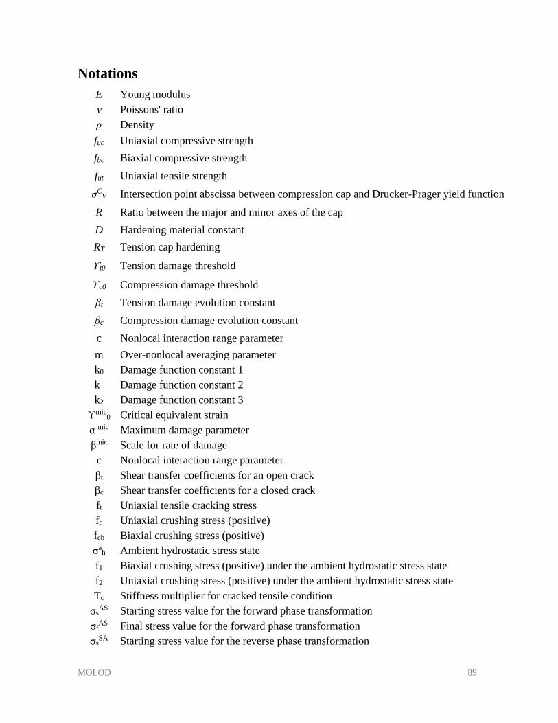
MOLOD 89

Notations

E Young modulus

ν Poissons' ratio

ρ Density

fuc Uniaxial compressive strength

fbc Biaxial compressive strength

fut Uniaxial tensile strength

σCV Intersection point abscissa between compression cap and Drucker-Prager yield function

R Ratio between the major and minor axes of the cap

D Hardening material constant

RT Tension cap hardening

ϒt0 Tension damage threshold

ϒc0 Compression damage threshold

βt Tension damage evolution constant

βc Compression damage evolution constant

c Nonlocal interaction range parameter

m Over-nonlocal averaging parameter

k0 Damage function constant 1

k1 Damage function constant 2

k2 Damage function constant 3

ϒmic0 Critical equivalent strain

α mic Maximum damage parameter

βmic Scale for rate of damage

c Nonlocal interaction range parameter

βt Shear transfer coefficients for an open crack

βc Shear transfer coefficients for a closed crack

ft Uniaxial tensile cracking stress

fc Uniaxial crushing stress (positive)

fcb Biaxial crushing stress (positive)

σah Ambient hydrostatic stress state

f1 Biaxial crushing stress (positive) under the ambient hydrostatic stress state

f2 Uniaxial crushing stress (positive) under the ambient hydrostatic stress state

Tc Stiffness multiplier for cracked tensile condition

σsAS Starting stress value for the forward phase transformation

σfAS Final stress value for the forward phase transformation

σsSA Starting stress value for the reverse phase transformation

MOLOD 90

σfSA Final stress value for the reverse phase transformation

eL Maximum residual strain

α Parameter measuring the difference between material responses in tension and compression

σy Yield stress

σu Ultimate stress

εsu Ultimate strain of steel

εcu Ultimate strain of concrete

εs Strain of steel

εc Strain of concrete

ξ Factor defining the effective height of the compression zone

x distance of the neutral axis from the extreme compression fiber

d Distance between top surface of a beam and middle of bottom reinforcement

a Distance between top surface of a beam and middle of top reinforcement

z Depth of beam

b Width of beam cross-section

αR Factor defining the effective strength of concrete

Fcd Compressive carrying load capacity of concrete

Fsd Compressive carrying load capacity of steel

σcd Design stress of concrete

σsd Design stress of steel

As1 Area of top steel reinforcement (compression rebar)

As2 Area of bottom steel reinforcement (tensile rebar)

Fud Ultimate design load

Ka Coefficient

MRd Moment capacity of the section

R1 Axial column force

R2 Bending moment force

R3 Axial beam force

MOLOD 91

References

Abdulrahman, A., Ismail, M. and Hussain, M. S. (2011) 'Corrosion inhibitors for steel

reinforcement in concrete: A review', Scientific Research and Essays, 6(20), pp.

4152-4162.

Alam, M., Youssef, M. and Nehdi, M. (2008) 'Analytical prediction of the seismic behaviour

of superelastic shape memory alloy reinforced concrete elements', Engineering

Structures, 30(12), pp. 3399-3411.

AnsysDocumentation (2019) 'Ansys®ANSYS Mechanical APDL, 2019.1, help system,

Ansys documentation, ANSYS, Inc. '.

Association, E. C. ( 2013) Activity Report 2013, Brussels: : CEMBUREAU.

Bažant, Z. P. and Gambarova, P. G. (1984) 'Crack shear in concrete: Crack band microflane

model', Journal of Structural Engineering, 110(9), pp. 2015-2035.

Bažant, Z. P. and Oh, B. H. (1985) 'Microplane model for progressive fracture of concrete

and rock', Journal of Engineering Mechanics, 111(4), pp. 559-582.

Corley, W. (1966) 'Rotational capacity of reinforced concrete beams', Journal of the

Structural Division, 92(5), pp. 121-146.

Daghia, F., Giammarruto, A. and Pascale, G. (2011) 'Combined use of FBG sensors and SMA

actuators for concrete beams repair', Structural Control and Health Monitoring,

18(8), pp. 908-921.

Davidovits, J. (1994) 'Global warming impact on the cement and aggregates industries',

World Resource Review, 6(2), pp. 263-278.

Deng, Z., Li, Q. and Sun, H. (2006) 'Behavior of concrete beam with embedded shape

memory alloy wires', Engineering structures, 28(12), pp. 1691-1697.

Deogekar, P. S. and Andrawes, B. (2018) 'Hybrid confinement of high strength concrete

using shape memory alloys and fiber-reinforced polymers', Journal of Structural

Integrity and Maintenance, 3(1), pp. 22-32.

DesRoches, R. and Delemont, M. (2002) 'Seismic retrofit of simply supported bridges using

shape memory alloys', Engineering Structures, 24(3), pp. 325-332.

Dolce, M., Cardone, D. and Marnetto, R. 'SMA re-centering devices for seismic isolation of

civil structures'. Proceedings of SPIE, 238-249.

El-Hacha, R. and Rojob, H. (2018) 'Flexural strengthening of large-scale reinforced concrete

beams using near-surface-mounted self-prestressed iron-based shape-memory alloy

strips', PCI Journal, 63(6).

Elbahy, Y., Youssef, M. and Meshaly, M. (2019) 'Seismic performance of reinforced

concrete frames retrofitted using external superelastic shape memory alloy bars',

Bulletin of Earthquake Engineering, 17(2), pp. 781-802.

EN, B. (2004) '1-1. Eurocode 2: Design of concrete structures–Part 1-1: General rules and

rules for buildings', European Committee for Standardization (CEN).

Fang, C., Wang, W., He, C. and Chen, Y. (2017) 'Self-centring behaviour of steel and steel-

concrete composite connections equipped with NiTi SMA bolts', Engineering

Structures, 150, pp. 390-408.

Ghali, A., Favre, R. and Elbadry, M. (2006) Concrete structures: Stresses and deformations:

Analysis and design for serviceability. CRC Press.

Han, Y. L., Li, Q., Li, A. Q., Leung, A. and Lin, P. H. (2003) 'Structural vibration control by

shape memory alloy damper', Earthquake engineering & structural dynamics, 32(3),

pp. 483-494.

MOLOD 92

Herbert, A. and Sawyer, J. (1964) 'Design of concrete frames for two failure stages', ACI

Structural Journal, pp. 405-437.

Hong, K., Lee, S., Yeon, Y. and Jung, K. (2018) 'Flexural response of reinforced concrete

beams strengthened with near-surface-mounted Fe-based shape-memory alloy strips',

International Journal of Concrete Structures and Materials, 12(1), pp. 1-13.

Hu, J. W. (2014) 'Investigation on the cyclic response of superelastic shape memory alloy

(SMA) slit damper devices simulated by quasi-static finite element (FE) analyses',

Materials, 7(2), pp. 1122-1141.

Institution, B. S. (2004) Eurocode 2: Design of Concrete Structures: Part 1-1: General Rules

and Rules for Buildings. British Standards Institution.

International Energy Agency, W. B. C. f. S. D., and Organisation for Economic Co-operation

and Development 2009. Cement Technology Roadmap 2009 Carbon Emissions

Reductions up to 2050. Paris, France; Conches-Geneva, Switzerland: OECD, IEA,

WBCSD.

Jung, D., Zafar, A. and Andrawes, B. (2017) 'Sustainability of civil infrastructure using shape

memory technology', Innovative Infrastructure Solutions, 2(1), pp. 28.

Khan, M. M. and Lagoudas, D. C. 'Modeling of shape memory alloy pseudoelastic spring

elements using Preisach model for passive vibration isolation'. Proceedings of SPIE,

336-347.

Kuang, Y. and Ou, J. (2008) 'Self-repairing performance of concrete beams strengthened

using superelastic SMA wires in combination with adhesives released from hollow

fibers', Smart Materials and Structures, 17(2), pp. 025020.

Li, H., Liu, M. and Ou, J. (2004) 'Vibration mitigation of a stay cable with one shape memory

alloy damper', Structural Control and Health Monitoring, 11(1), pp. 21-36.

Li, V. C. and Herbert, E. (2012) 'Robust self-healing concrete for sustainable infrastructure',

Journal of Advanced Concrete Technology, 10(6), pp. 207-218.

Mas, B., Biggs, D., Vieito, I., Cladera, A., Shaw, J. and Martínez-Abella, F. (2017)

'Superelastic shape memory alloy cables for reinforced concrete applications',

Construction and Building Materials, 148, pp. 307-320.

Mattock, A. H. (1967) 'Discussion of" Rotation Capacity of Reinforced Concrete Beams" by

WG Corley', Journal of Structual Division ASCE, 93, pp. 519-522.

Mayes, J. J., Lagoudas, D. C. and Henderson, B. K. 'An experimental investigation of shape

memory alloy springs for passive vibration isolation'. Proc. Conf. AIAA Space 2001

Conference and Exposition.

McCormick, J., DesRoches, R., Fugazza, D. and Auricchio, F. (2007) 'Seismic assessment

of concentrically braced steel frames with shape memory alloy braces', Journal of

Structural Engineering, 133(6), pp. 862-870.

McLeod, R. S. (2005) 'Ordinary portland cement', BFF Autumn, 30, pp. 33.

Menetrey, P. (1994) Numerical analysis of punching failure in reinforced concrete

structures: EPFL.

Michels, J., Shahverdi, M., Czaderski, C., Schranz, B. and Motavalli, M. (2017) 'Iron based

shape memory alloy strips, part 2: Flexural strengthening of RC beams', Proceedings

of the SMAR.

Miyazaki, S., Duerig, T. and Melton, K. 1990. Engineering aspects of shape memory alloys.

Butterworth-Heinemann, London.

Mosley, W. H., Hulse, R. and Bungey, J. H. (2012) Reinforced concrete design: to Eurocode

2. Palgrave macmillan.

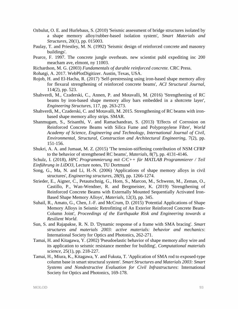
MOLOD 93

Ozbulut, O. E. and Hurlebaus, S. (2010) 'Seismic assessment of bridge structures isolated by

a shape memory alloy/rubber-based isolation system', Smart Materials and

Structures, 20(1), pp. 015003.

Paulay, T. and Priestley, M. N. (1992) 'Seismic design of reinforced concrete and masonry

buildings'.

Pearce, F. 1997. The concrete jungle overheats. new scientist publ expediting inc 200

meacham ave, elmont, ny 11003.

Richardson, M. G. (2003) Fundamentals of durable reinforced concrete. CRC Press.

Rohatgi, A. 2017. WebPlotDigitizer. Austin, Texas, USA.

Rojob, H. and El-Hacha, R. (2017) 'Self-prestressing using iron-based shape memory alloy

for flexural strengthening of reinforced concrete beams', ACI Structural Journal,

114(2), pp. 523.

Shahverdi, M., Czaderski, C., Annen, P. and Motavalli, M. (2016) 'Strengthening of RC

beams by iron-based shape memory alloy bars embedded in a shotcrete layer',

Engineering Structures, 117, pp. 263-273.

Shahverdi, M., Czaderski, C. and Motavalli, M. 2015. Strengthening of RC beams with iron-

based shape memory alloy strips. SMAR.

Shanmugam, S., Srisanthi, V. and Ramachandran, S. (2013) 'Effects of Corrosion on

Reinforced Concrete Beams with Silica Fume and Polypropylene Fibre', World

Academy of Science, Engineering and Technology, International Journal of Civil,

Environmental, Structural, Construction and Architectural Engineering, 7(2), pp.

151-156.

Shukri, A. A. and Jumaat, M. Z. (2015) 'The tension-stiffening contribution of NSM CFRP

to the behavior of strengthened RC beams', Materials, 8(7), pp. 4131-4146.

Schulz, I. (2018), HPC Programmierung mit C/C++ für MATLAB Programmierer / Teil

Einführung in LiDO3, Lecture notes, TU Dortmund

Song, G., Ma, N. and Li, H.-N. (2006) 'Applications of shape memory alloys in civil

structures', Engineering structures, 28(9), pp. 1266-1274.

Strieder, E., Aigner, C., Petautschnig, G., Horn, S., Marcon, M., Schwenn, M., Zeman, O.,

Castillo, P., Wan-Wendner, R. and Bergmeister, K. (2019) 'Strengthening of

Reinforced Concrete Beams with Externally Mounted Sequentially Activated Iron-

Based Shape Memory Alloys', Materials, 12(3), pp. 345.

Suhail, R., Amato, G., Chen, J.-F. and McCrum, D. (2015) 'Potential Applications of Shape

Memory Alloys in Seismic Retrofitting of An Exterior Reinforced Concrete Beam-

Column Joint', Proceedings of the Earthquake Risk and Engineering towards a

Resilient World.

Sun, S. and Rajapakse, R. N. D. 'Dynamic response of a frame with SMA bracing'. Smart

structures and materials 2003: active materials: behavior and mechanics:

International Society for Optics and Photonics, 262-271.

Tamai, H. and Kitagawa, Y. (2002) 'Pseudoelastic behavior of shape memory alloy wire and

its application to seismic resistance member for building', Computational materials

science, 25(1), pp. 218-227.

Tamai, H., Miura, K., Kitagawa, Y. and Fukuta, T. 'Application of SMA rod to exposed-type

column base in smart structural system'. Smart Structures and Materials 2003: Smart

Systems and Nondestructive Evaluation for Civil Infrastructures: International

Society for Optics and Photonics, 169-178.

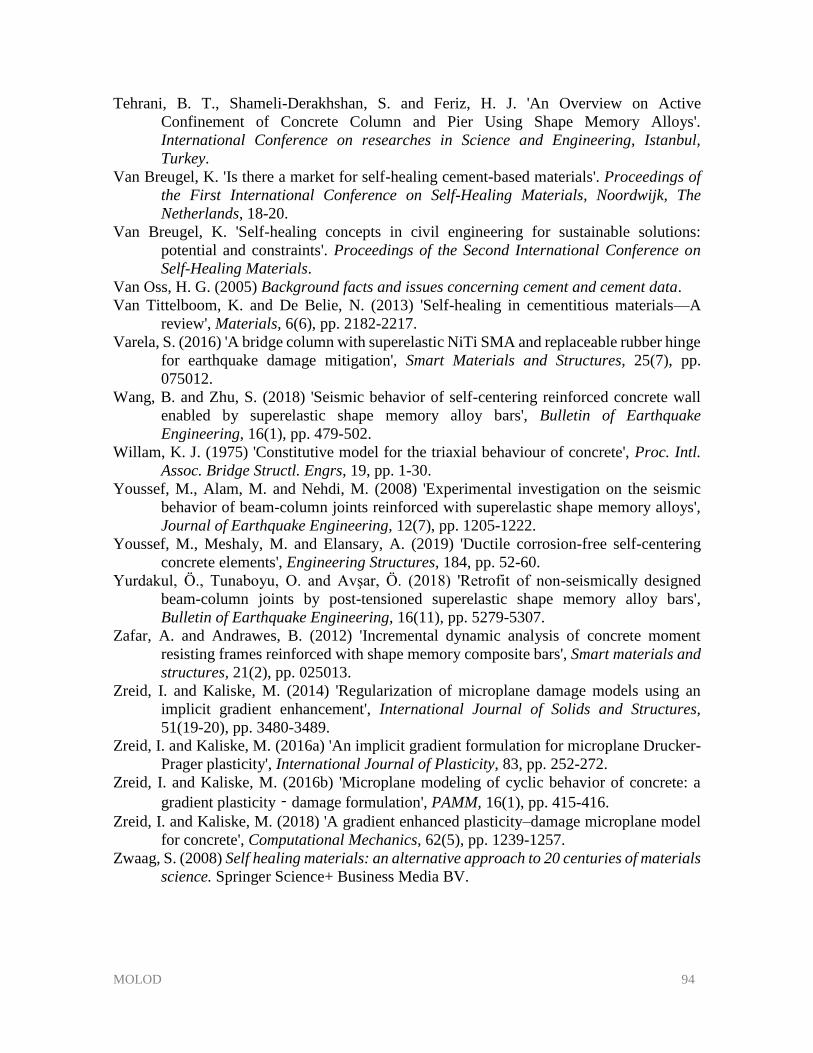
MOLOD 94

Tehrani, B. T., Shameli-Derakhshan, S. and Feriz, H. J. 'An Overview on Active

Confinement of Concrete Column and Pier Using Shape Memory Alloys'.

International Conference on researches in Science and Engineering, Istanbul,

Turkey.

Van Breugel, K. 'Is there a market for self-healing cement-based materials'. Proceedings of

the First International Conference on Self-Healing Materials, Noordwijk, The

Netherlands, 18-20.

Van Breugel, K. 'Self-healing concepts in civil engineering for sustainable solutions:

potential and constraints'. Proceedings of the Second International Conference on

Self-Healing Materials.

Van Oss, H. G. (2005) Background facts and issues concerning cement and cement data.

Van Tittelboom, K. and De Belie, N. (2013) 'Self-healing in cementitious materials—A

review', Materials, 6(6), pp. 2182-2217.

Varela, S. (2016) 'A bridge column with superelastic NiTi SMA and replaceable rubber hinge

for earthquake damage mitigation', Smart Materials and Structures, 25(7), pp.

075012.

Wang, B. and Zhu, S. (2018) 'Seismic behavior of self-centering reinforced concrete wall

enabled by superelastic shape memory alloy bars', Bulletin of Earthquake

Engineering, 16(1), pp. 479-502.

Willam, K. J. (1975) 'Constitutive model for the triaxial behaviour of concrete', Proc. Intl.

Assoc. Bridge Structl. Engrs, 19, pp. 1-30.

Youssef, M., Alam, M. and Nehdi, M. (2008) 'Experimental investigation on the seismic

behavior of beam-column joints reinforced with superelastic shape memory alloys',

Journal of Earthquake Engineering, 12(7), pp. 1205-1222.

Youssef, M., Meshaly, M. and Elansary, A. (2019) 'Ductile corrosion-free self-centering

concrete elements', Engineering Structures, 184, pp. 52-60.

Yurdakul, Ö., Tunaboyu, O. and Avşar, Ö. (2018) 'Retrofit of non-seismically designed

beam-column joints by post-tensioned superelastic shape memory alloy bars',

Bulletin of Earthquake Engineering, 16(11), pp. 5279-5307.

Zafar, A. and Andrawes, B. (2012) 'Incremental dynamic analysis of concrete moment

resisting frames reinforced with shape memory composite bars', Smart materials and

structures, 21(2), pp. 025013.

Zreid, I. and Kaliske, M. (2014) 'Regularization of microplane damage models using an

implicit gradient enhancement', International Journal of Solids and Structures,

51(19-20), pp. 3480-3489.

Zreid, I. and Kaliske, M. (2016a) 'An implicit gradient formulation for microplane Drucker-

Prager plasticity', International Journal of Plasticity, 83, pp. 252-272.

Zreid, I. and Kaliske, M. (2016b) 'Microplane modeling of cyclic behavior of concrete: a

gradient plasticity‐damage formulation', PAMM, 16(1), pp. 415-416.

Zreid, I. and Kaliske, M. (2018) 'A gradient enhanced plasticity–damage microplane model

for concrete', Computational Mechanics, 62(5), pp. 1239-1257.

Zwaag, S. (2008) Self healing materials: an alternative approach to 20 centuries of materials

science. Springer Science+ Business Media BV.

MOLOD 95

Appendixes

Appendix 1: PDF and CDF diagrams of all nodes of the system

under cyclic loading explained in section 6.2.1

Node 1: a) PDF diagram b) CDF diagram

Node 2: a) PDF diagram b) CDF diagram

Node 3: a) PDF diagram b) CDF diagram

MOLOD 96

Node 4: a) PDF diagram b) CDF diagram

Node 5: a) PDF diagram b) CDF diagram

Node 6: a) PDF diagram b) CDF diagram

Node 7: a) PDF diagram b) CDF diagram

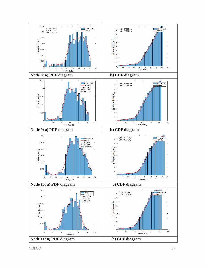
MOLOD 97

Node 8: a) PDF diagram b) CDF diagram

Node 9: a) PDF diagram b) CDF diagram

Node 10: a) PDF diagram b) CDF diagram

Node 11: a) PDF diagram b) CDF diagram

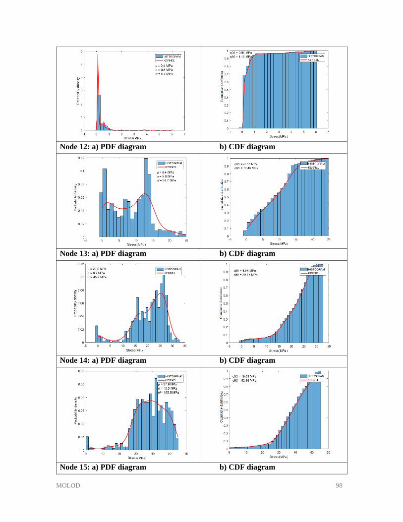
MOLOD 98

Node 12: a) PDF diagram b) CDF diagram

Node 13: a) PDF diagram b) CDF diagram

Node 14: a) PDF diagram b) CDF diagram

Node 15: a) PDF diagram b) CDF diagram

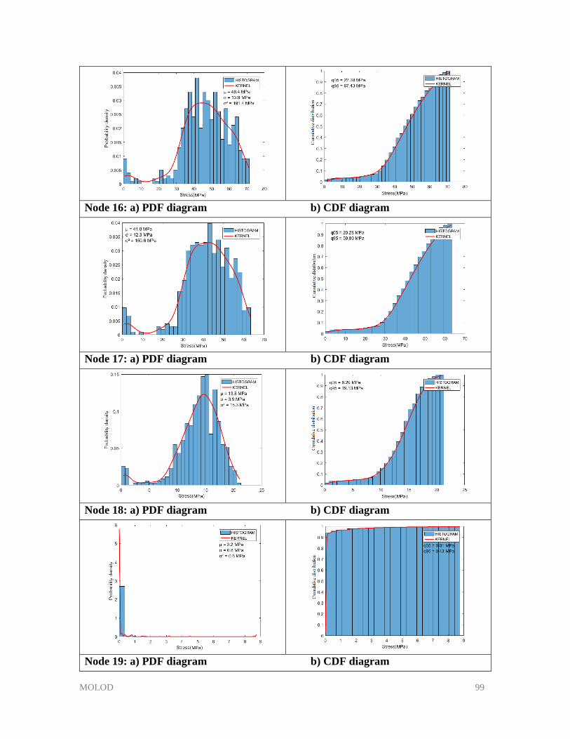
MOLOD 99

Node 16: a) PDF diagram b) CDF diagram

Node 17: a) PDF diagram b) CDF diagram

Node 18: a) PDF diagram b) CDF diagram

Node 19: a) PDF diagram b) CDF diagram

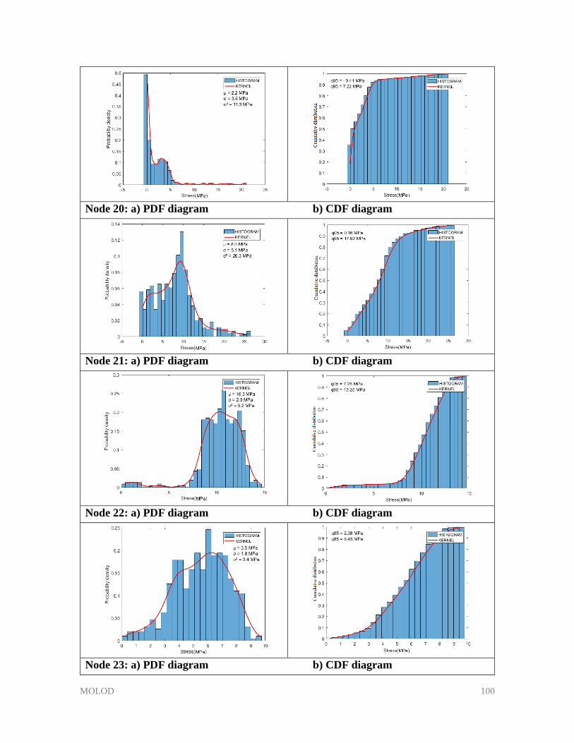
MOLOD 100

Node 20: a) PDF diagram b) CDF diagram

Node 21: a) PDF diagram b) CDF diagram

Node 22: a) PDF diagram b) CDF diagram

Node 23: a) PDF diagram b) CDF diagram

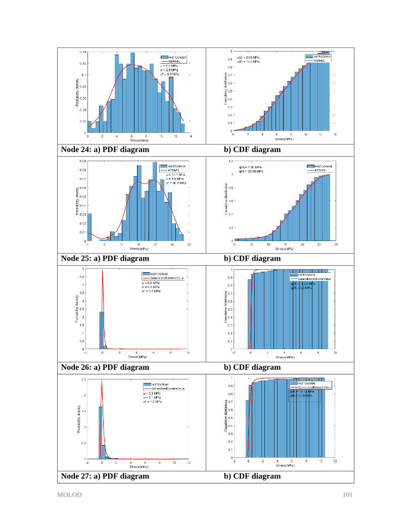
MOLOD 101

Node 24: a) PDF diagram b) CDF diagram

Node 25: a) PDF diagram b) CDF diagram

Node 26: a) PDF diagram b) CDF diagram

Node 27: a) PDF diagram b) CDF diagram

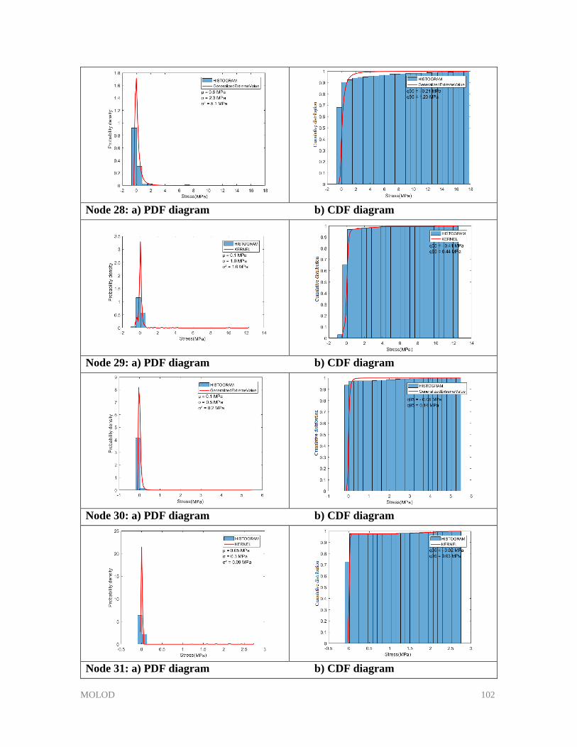
MOLOD 102

Node 28: a) PDF diagram b) CDF diagram

Node 29: a) PDF diagram b) CDF diagram

Node 30: a) PDF diagram b) CDF diagram

Node 31: a) PDF diagram b) CDF diagram

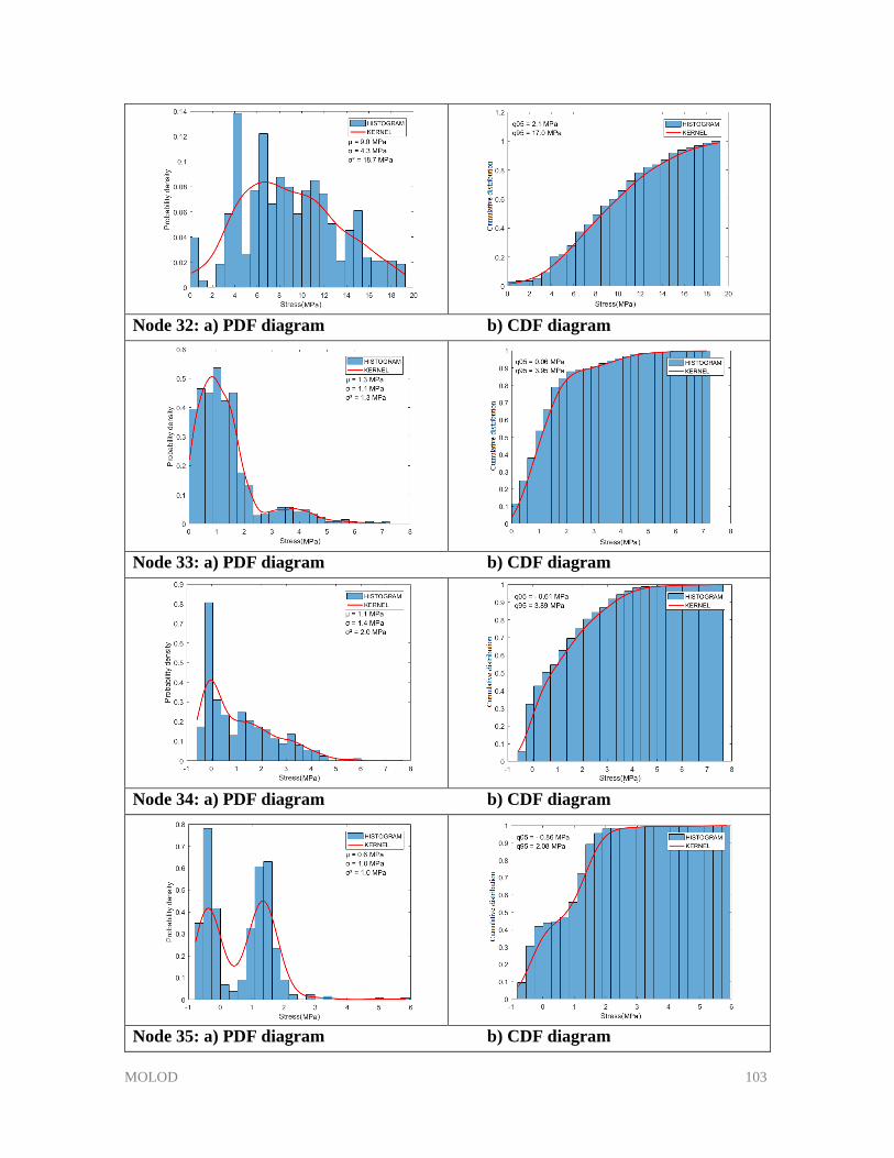
MOLOD 103

Node 32: a) PDF diagram b) CDF diagram

Node 33: a) PDF diagram b) CDF diagram

Node 34: a) PDF diagram b) CDF diagram

Node 35: a) PDF diagram b) CDF diagram

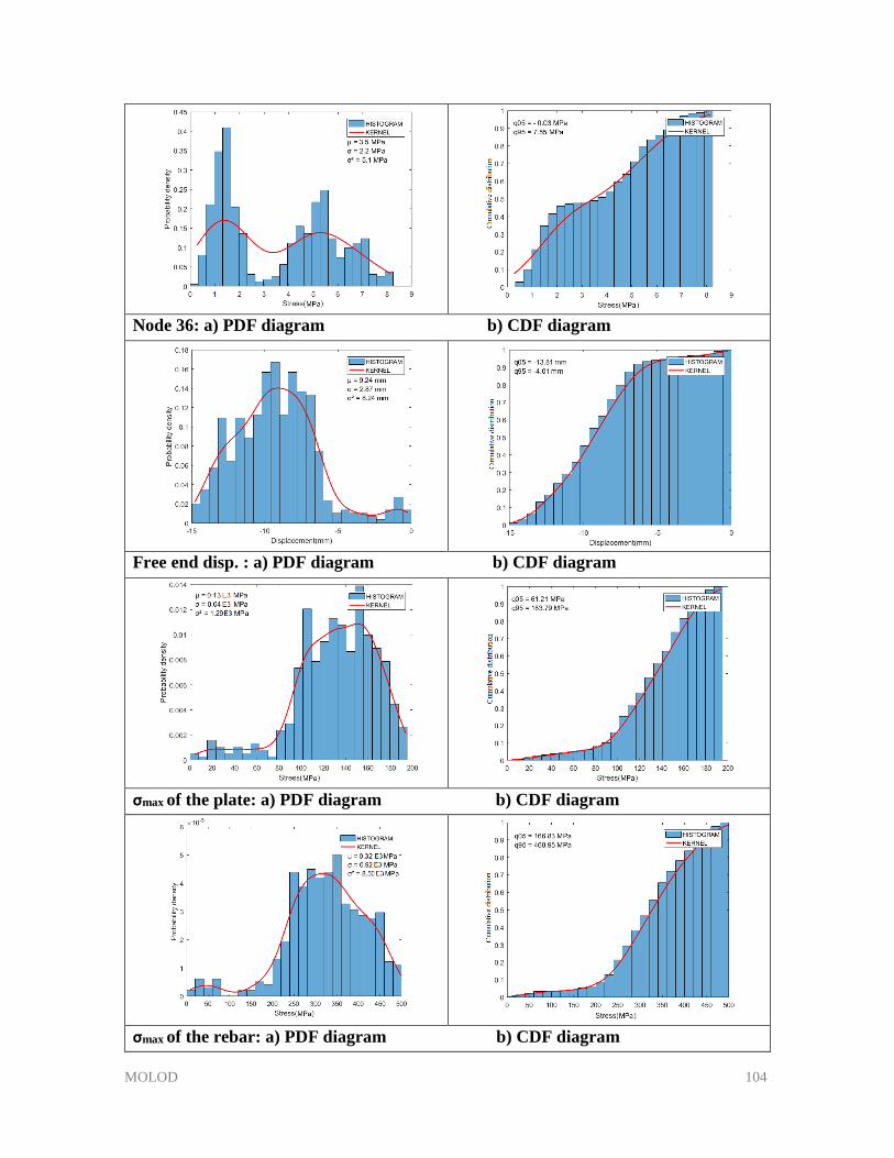
MOLOD 104

Node 36: a) PDF diagram b) CDF diagram

Free end disp. : a) PDF diagram b) CDF diagram

σmax of the plate: a) PDF diagram b) CDF diagram

σmax of the rebar: a) PDF diagram b) CDF diagram

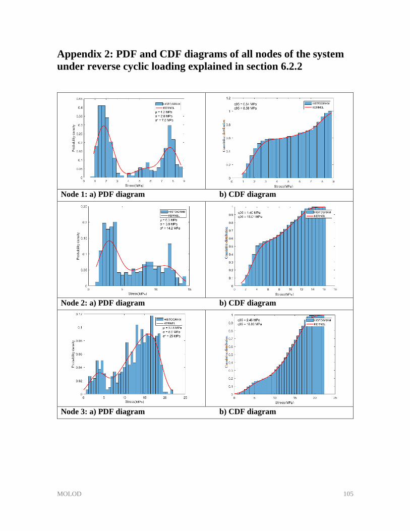
MOLOD 105

Appendix 2: PDF and CDF diagrams of all nodes of the system

under reverse cyclic loading explained in section 6.2.2

Node 1: a) PDF diagram b) CDF diagram

Node 2: a) PDF diagram b) CDF diagram

Node 3: a) PDF diagram b) CDF diagram

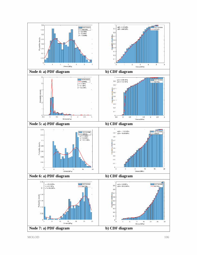
MOLOD 106

Node 4: a) PDF diagram b) CDF diagram

Node 5: a) PDF diagram b) CDF diagram

Node 6: a) PDF diagram b) CDF diagram

Node 7: a) PDF diagram b) CDF diagram

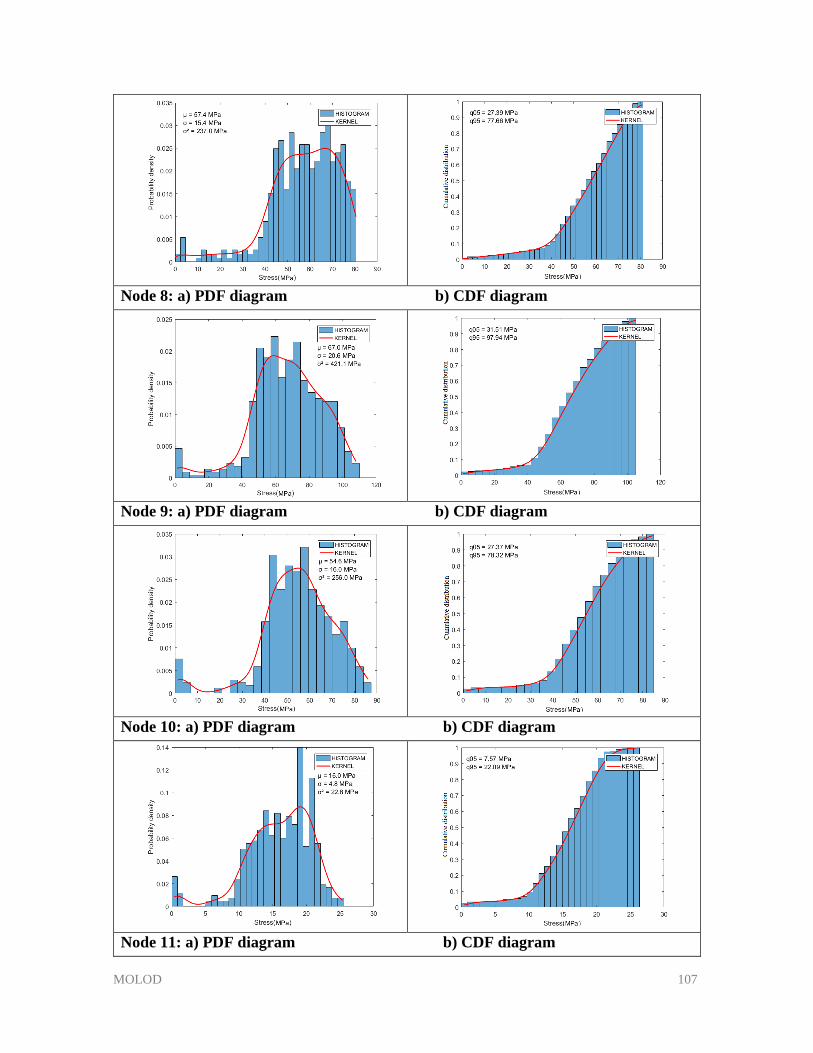
MOLOD 107

Node 8: a) PDF diagram b) CDF diagram

Node 9: a) PDF diagram b) CDF diagram

Node 10: a) PDF diagram b) CDF diagram

Node 11: a) PDF diagram b) CDF diagram

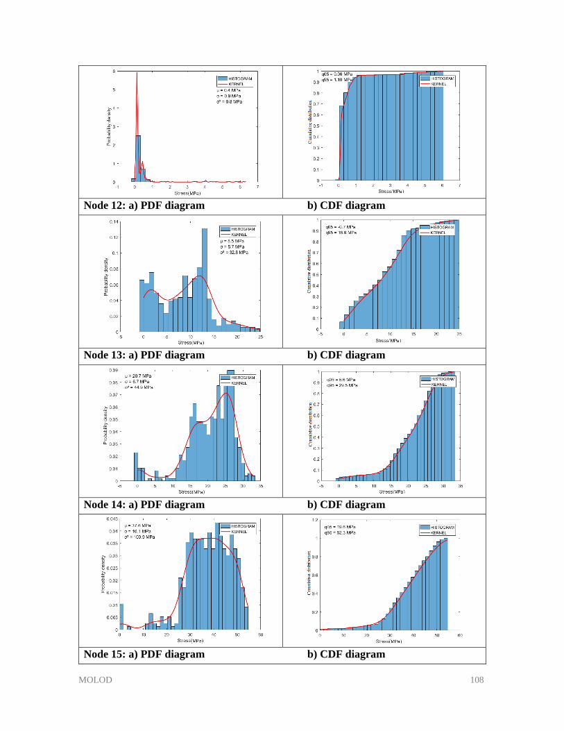
MOLOD 108

Node 12: a) PDF diagram b) CDF diagram

Node 13: a) PDF diagram b) CDF diagram

Node 14: a) PDF diagram b) CDF diagram

Node 15: a) PDF diagram b) CDF diagram

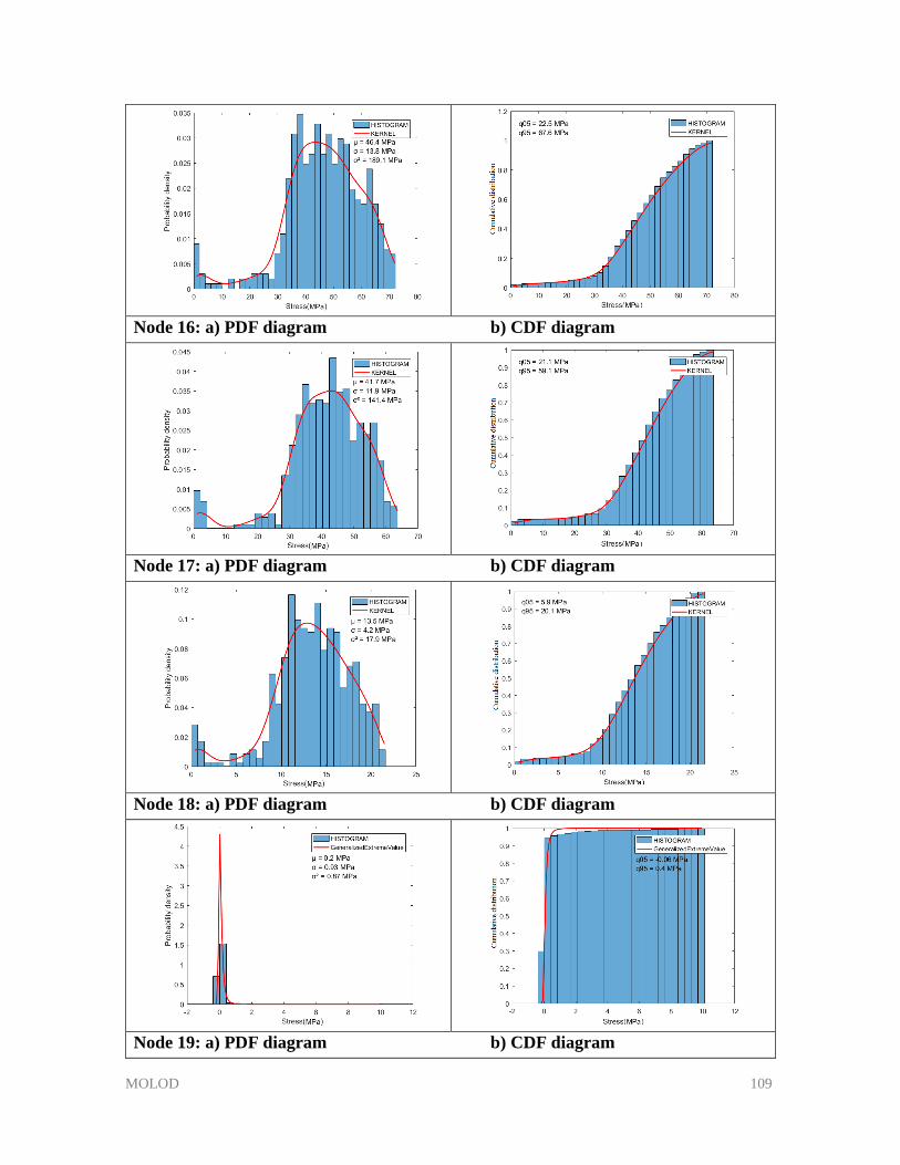
MOLOD 109

Node 16: a) PDF diagram b) CDF diagram

Node 17: a) PDF diagram b) CDF diagram

Node 18: a) PDF diagram b) CDF diagram

Node 19: a) PDF diagram b) CDF diagram

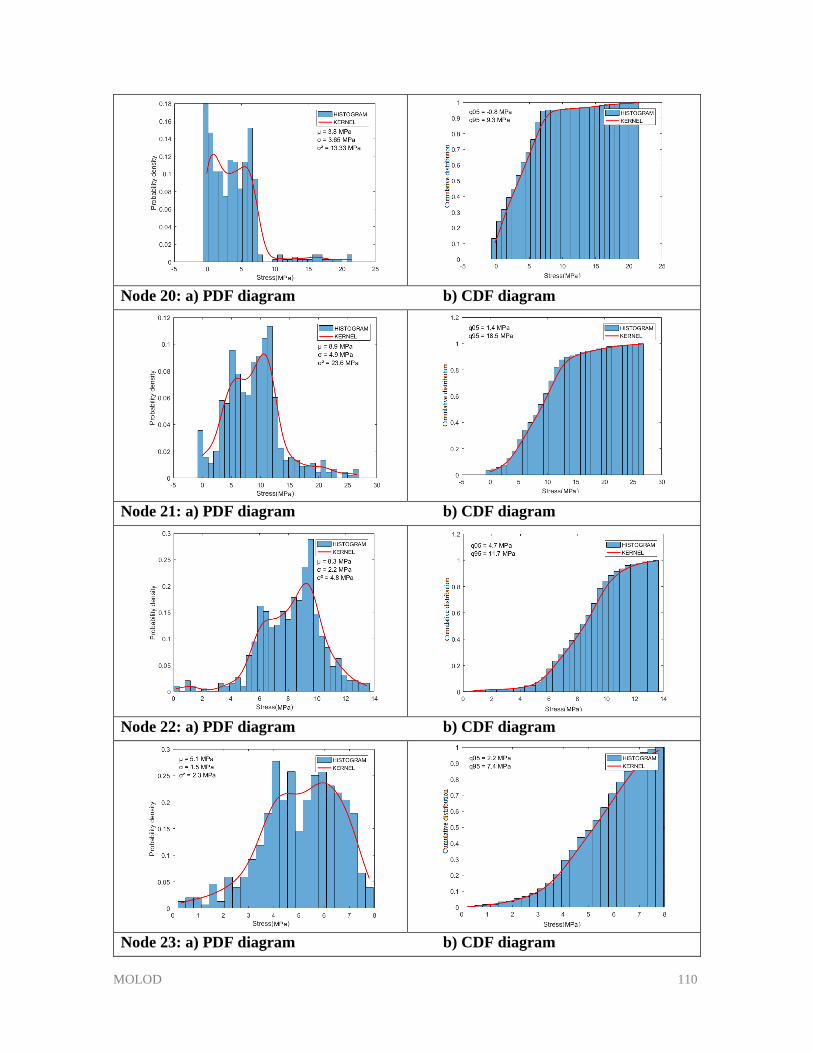
MOLOD 110

Node 20: a) PDF diagram b) CDF diagram

Node 21: a) PDF diagram b) CDF diagram

Node 22: a) PDF diagram b) CDF diagram

Node 23: a) PDF diagram b) CDF diagram

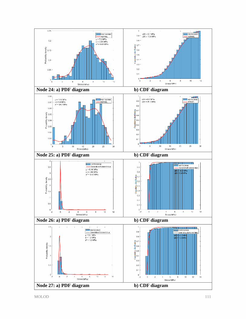
MOLOD 111

Node 24: a) PDF diagram b) CDF diagram

Node 25: a) PDF diagram b) CDF diagram

Node 26: a) PDF diagram b) CDF diagram

Node 27: a) PDF diagram b) CDF diagram

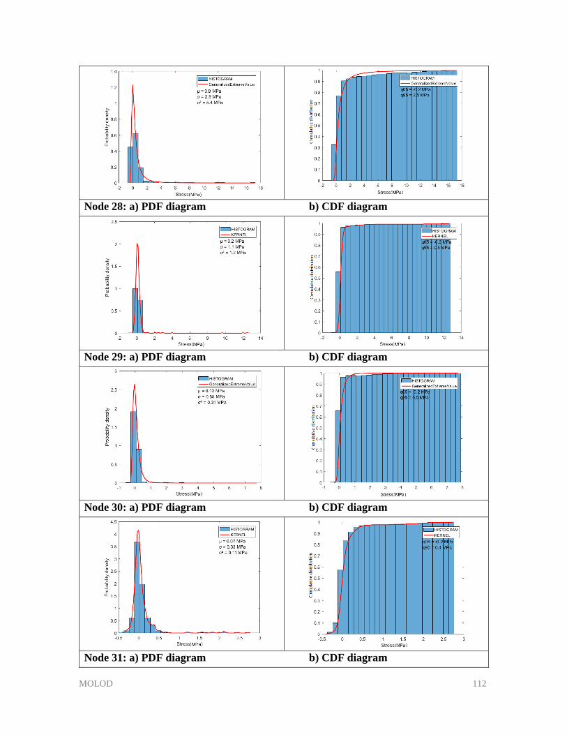
MOLOD 112

Node 28: a) PDF diagram b) CDF diagram

Node 29: a) PDF diagram b) CDF diagram

Node 30: a) PDF diagram b) CDF diagram

Node 31: a) PDF diagram b) CDF diagram

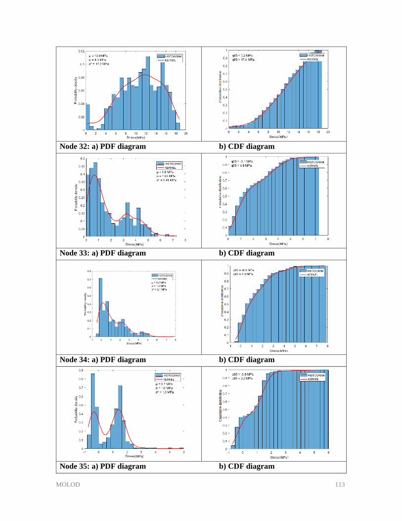
MOLOD 113

Node 32: a) PDF diagram b) CDF diagram

Node 33: a) PDF diagram b) CDF diagram

Node 34: a) PDF diagram b) CDF diagram

Node 35: a) PDF diagram b) CDF diagram

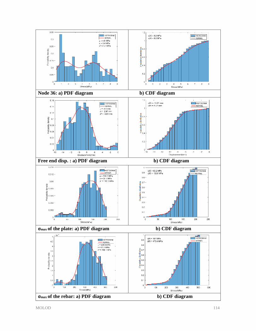
MOLOD 114

Node 36: a) PDF diagram b) CDF diagram

Free end disp. : a) PDF diagram b) CDF diagram

σmax of the plate: a) PDF diagram b) CDF diagram

σmax of the rebar: a) PDF diagram b) CDF diagram

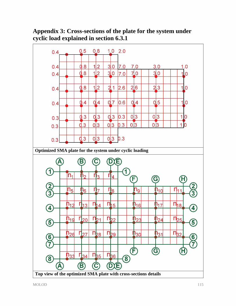
MOLOD 115

Appendix 3: Cross-sections of the plate for the system under

cyclic load explained in section 6.3.1

Optimized SMA plate for the system under cyclic loading

Top view of the optimized SMA plate with cross-sections details

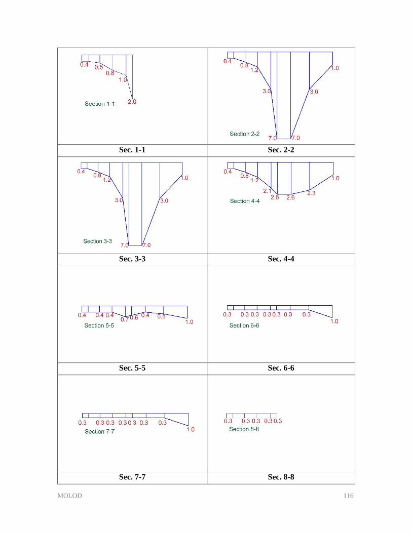
MOLOD 116

Sec. 1-1 Sec. 2-2

Sec. 3-3 Sec. 4-4

Sec. 5-5 Sec. 6-6

Sec. 7-7 Sec. 8-8

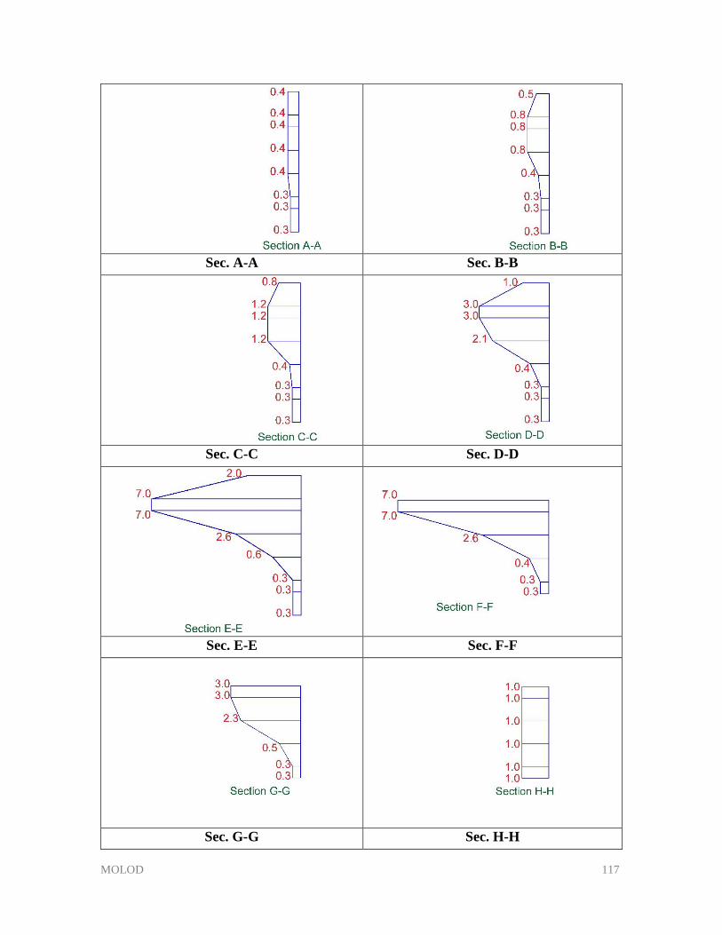
MOLOD 117

Sec. A-A Sec. B-B

Sec. C-C Sec. D-D

Sec. E-E Sec. F-F

Sec. G-G Sec. H-H

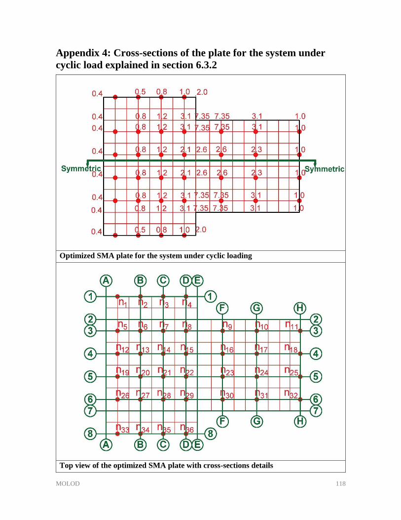
MOLOD 118

Appendix 4: Cross-sections of the plate for the system under

cyclic load explained in section 6.3.2

Optimized SMA plate for the system under cyclic loading

Top view of the optimized SMA plate with cross-sections details

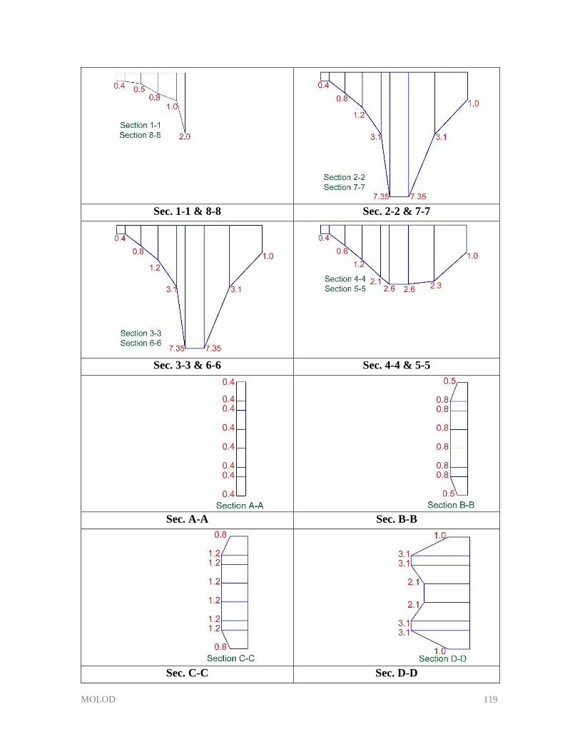
MOLOD 119

Sec. 1-1 & 8-8 Sec. 2-2 & 7-7

Sec. 3-3 & 6-6 Sec. 4-4 & 5-5

Sec. A-A Sec. B-B

Sec. C-C Sec. D-D

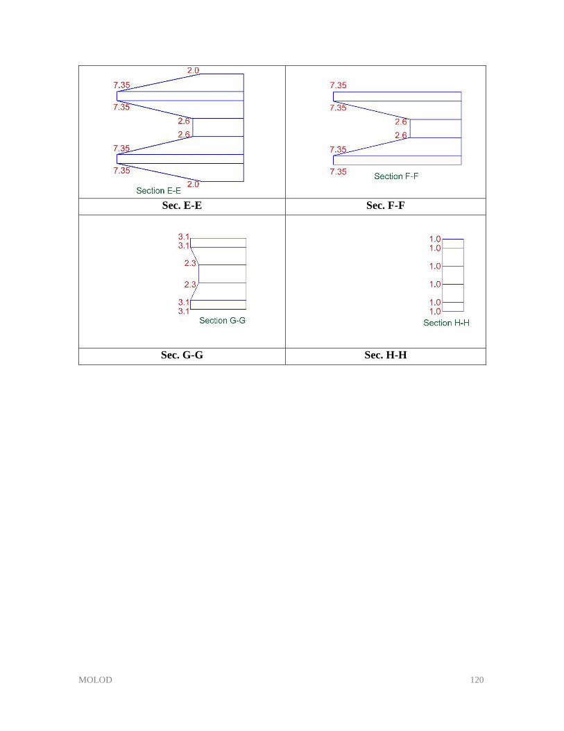
MOLOD 120

Sec. E-E Sec. F-F

Sec. G-G Sec. H-H