Stochastic Approximations and Differential

Inclusions.

Part II: Applications ∗

Michel Benaım

Institut de Mathematiques, Universite de NeuchatelRue Emile-Argand 11, Neuchatel, Suisse

michel.benaim@unine.ch

Josef HofbauerDepartment of Mathematics, University College London

London WC1E 6BT, U.K.j.hofbauer@ucl.ac.uk

Sylvain SorinEquipe Combinatoire et Optimisation, UFR 921,

Universite P. et M. Curie - Paris 6,175 Rue du Chevaleret, 75013 Paris

and Laboratoire d’Econometrie, Ecole Polytechnique,1 rue Descartes, 75005 Paris, France

sorin@math.jussieu.fr

revised December 2005

∗We acknowledge financial support from the Swiss National Science Foundation, grant200021-1036251/1 and from UCL’s Centre for Economic Learning and Social Evolution(ELSE).

1

Abstract

We apply the theoretical results on “stochastic approximations anddifferential inclusions” developed in Benaım, Hofbauer and Sorin (2005)to several adaptive processes used in game theory including: classicaland generalized approachability, no-regret potential procedures (Hartand Mas-Colell), smooth fictitious play (Fudenberg and Levine).

Keywords: Stochastic approximation, differential inclusions, set valued dynamical

systems, approachability, no regret, consistency, smooth fictitious play.

1 Introduction

The first paper of this series (Benaım, Hofbauer and Sorin, 2005), henceforthreferred to as BHS, was devoted to the analysis of the long term behavior of aclass of continuous paths called perturbed solution that are obtained as certainperturbations of trajectories solutions to a differential inclusion in R

m

x ∈M(x). (1)

A fundamental and motivating example is given by (continuous time linearinterpolation of) discrete stochastic approximations of the form

Xn+1 −Xn = an+1Yn+1 (2)

withE(Yn+1 | Fn) ∈M(Xn)

where n ∈ N, an ≥ 0,∑

n an = +∞ and Fn is the σ-algebra generated by(X0, . . . , Xn), under conditions on the increments Yn and the coefficients an.For example if:

(i) supn | Yn+1 − E(Yn+1 | Fn) |<∞, and

(ii) an = o( 1log(n)

)

the interpolation of a process Xn satisfying (2) is almost surely a perturbedsolution of (1).Following the dynamical system approach to stochastic approximations initiatedby Benaım and Hirsch (Benaım (1996, 1999); Benaım and Hirsch (1996, 1999))it was shown in BHS that the set of limit points of a perturbed solution is acompact invariant attractor free set for the set-valued dynamical system inducedby (1).

2

From a mathematical viewpoint, this type of property is a natural generalizationof Benaım and Hirsch’s previous results.1 In view of applications, it is stronglymotivated by a large class of problems, especially in game theory, where the useof differential inclusions is unavoidable since one deals with unilateral dynamicswhere the strategies chosen by a player’s opponents (or nature) are unknownto this player.In BHS a few applications where given: 1) in the framework of approachabilitytheory (where one player aims at controlling the asymptotic behavior of theCesaro mean of a sequence of vector payoffs corresponding to the outcomes of arepeated game) and 2) for the study of fictitious play (where each player uses,at each stage of a repeated game, a move which is a best reply to the pastfrequencies of moves of the opponent).

The purpose of the current paper is to explore much further the range ofpossible applications of the theory and to convince the reader that it providesa unified and powerful approach to several questions such as approachability orconsistency (no regret). The price to pay is a bit of theory, but as a reward weobtain neat and simpler (sometime much simpler...) proofs of numerous resultsarising in different contexts.

The general structure for the analysis of such discrete time dynamics relieson the identification of a state variable for which the increments satisfies anequation like (2). This requires in particular vanishing step size (for examplethe state variable will be a time average—of payoffs or moves—) and a Markovproperty for the conditional law of the increments (the behavioral strategy willbe a function of the state variable).

The organization of the paper is as follows. Section 2 summarizes the re-sults of BHS that will be needed here. In section 3 we first consider generalizedapproachability, where the parameters are a correspondence N and a potentialfunction Q adapted to a set C and extend results obtained by Hart and Mas-Colell (2001a). In Section 4 we deal with (external) consistency (or no regret):the previous set C is now the negative orthant and an approachability strat-egy is constructed explicitely through a potential function P , following Hartand Mas-Colell (2001a). A similar approach (Section 5) allows also to recoverconditional (or internal) consistency properties via generalized approachability.The next section 6 shows analogous results for an alternative dynamics: smoothfictitious play. This allows to retrieve and extend certain properties obtained byFudenberg and Levine (1995, 1999) on consistency and conditional consistency.Section 7 deals with several extensions of the previous to the case where the

1Benaım and Hirsch’s analysis was restricted to asymptotic pseudo trajectories (perturbedsolutions) of differential equations and flows.

3

information available to a player is reduced, and section 8 applies to resultsrecently obtained by Benaım and BenArous (2003).

2 General framework and previous results

Consider the differential inclusion (1). All the analysis will be done under thefollowing condition, which corresponds to Hypothesis 1.1 in BHS:

Hypothesis 2.1 (Standing assumptions) M is an upper semi continuouscorrespondence from R

m to itself, with compact convex non–empty values andwhich satisfies the following growth condition. There exists c > 0 such that forall x ∈ R

m

supz∈M(x)

‖z‖ ≤ c (1 + ‖x‖).

Here ‖ · ‖ denotes any norm on Rm.

Remark These conditions are quite standard and such correspondences are some-

times called Marchaud maps (see Aubin (1991), p. 62). Note also that in most of our

applications one has M(x)⊂K0 where K0 is a given compact set, so that the growth

condition is automatically satisfied.

In order to state the main results of BHS that will be used here, we firstrecall some definitions and notation.The set–valued dynamical system Φtt∈R induced by (1) is defined by

Φt(x) = x(t) : x is a solution to (1) with x(0) = x

where a solution to the differential inclusion (1) is an absolutely continuousmapping x : R → R

m satisfying

dx(t)

dt∈M(x(t))

for almost every t ∈ R.Given a set of times T ⊂ R and a set of positions V ⊂ R

m

ΦT (V ) =⋃

t∈T

⋃

v∈V

Φt(v)

denote the set of possible values, at some time in T , of trajectories being in Vat time 0.

4

Given a point x ∈ Rm we let

ωΦ(x) =⋂

t≥0

Φ[t,∞)(x)

denote its ω–limit set (where as usual the bar stands for the closure operator).The corresponding notion for a set Y, denoted ωΦ(Y ), is defined similarly withΦ[t,∞)(Y ) instead of Φ[t,∞)(x).A set A is said invariant if, for all x ∈ A there exists a solution x with x(0) = xsuch that x(R) ⊂ A, and strongly positively invariant if Φt(A) ⊂ A for all t > 0.A non–empty compact set A is called an attracting set if there exists a neigh-borhood U of A and a function t from (0, ε0) to R

+ with ε0 > 0 such that

Φt(U) ⊂ Aε

for all ε < ε0 and t ≥ t(ε), where Aε stands for the ε−neighborhood of A. Thiscorresponds to a strong notion of attraction, uniform with respect to the initialconditions and the feasible trajectories.If additionally A is invariant, then A is called an attractor.Given an attracting set (resp. attractor) A, its basin of attraction is the set

B(A) = x ∈ Rm : ωΦ(x) ⊂ A.

When B(A) = Rm, we call A a globally attracting set (resp. a global attractor).

Remark The following terminology is sometimes used in the literature. A set Ais said asymptotically stable if it is

(i) invariant,

(ii) Lyapounov stable, i.e., for every neighborhood U of A there exists a neighborhoodV of A such that its forward image Φ[0,∞)(V ) satisfies Φ[0,∞)(V ) ⊂ U , and

(iii) attractive, i.e., its basin of attraction B(A) is a neighborhood of A.

However, as shown in (BHS, Corollary 3.18) attractors and compact asymptotically

stable sets coincide.

Given a closed invariant set L, the induced dynamical system ΦL is definedon L by

ΦLt (x) = x(t) : x is a solution to (1) with x(0) = x and x(R) ⊂ L.

5

A set L is said attractor free if there exists no proper subset A of L which is anattractor for ΦL.

We now turn to the discrete random perturbations of (1) and consider, ona probability space (Ω,F , P ), random variables Xn, n ∈ N, with values in R

m,satisfying the difference inclusion

Xn+1 −Xn ∈ an+1[M(Xn) + Un+1] (3)

where the coefficients an are nonnegative numbers with

∑

n

an = +∞.

Such a process Xn is a Discrete Stochastic Approximation (DSA) of the dif-ferential inclusion (1) if the following conditions on the perturbations Un andthe coefficients an hold:

(i) E(Un+1 | Fn) = 0 where Fn is the σ-algebra generated by (X1, · · · , Xn),

(ii) (a) supn E(‖Un+1‖2) <∞ and

∑

n a2n < +∞ or

(b) supn ‖Un+1‖ < K and an = o( 1log(n)

).

Remark More general conditions on the characteristics (an, Un) can be found in

(BHS, Proposition 1.4).

A typical example is given by equations of the form (2) by letting

Un+1 = Yn+1 − E(Yn+1 | Fn).

Given a trajectory Xn(ω)n≥1, its set of accumulation points is denotedby L(ω) = L(Xn(ω)). The limit set of the process Xn is the random setL = L(Xn).

The principal properties established in BHS express relations between limitsets of DSA and attracting sets through the following results involving internallychain transitive (ICT) sets. (We do not define ICT sets here, see BHS Section3.3, since we only use the fact that they satisfy Properties 2 and 4 below).

Property 1 The limit set L of a bounded DSA is almost surely an ICT set.

6

This result is in fact stated in BHS for the limit set of the continuous timeinterpolated process but under our conditions both sets coıncide.

Properties of the limit set L will then be obtained through the next result(BHS, Lemma 3.5, Proposition 3.20 and Theorem 3.23):

Property 2 (i) ICT sets are non–empty, compact, invariant and attractorfree.

(ii) If A is an attracting set with B(A) ∩ L 6= ∅ and L is ICT, then L ⊂ A.

Some useful properties of attracting sets or attractors are the two following(BHS, Propositions 3.25 and 3.27).

Property 3 (Strong Lyapounov) Let Λ ⊂ Rm be compact with a bounded

open neighborhood Uand V : U → [0,∞[. Assume the following conditions:

(i) U is strongly positively invariant,

(ii) V −1(0) = Λ,

(iii) V is continuous and for all x ∈ U \ Λ, y ∈ Φt(x) and t > 0, V (y) < V (x).

Then Λ contains an attractor whose basin contains U.The map V is called a strong Lyapounov function associated to Λ.

Let Λ ⊂ Rm be a set and U ⊂ R

m an open neighborhood of Λ. A continuousfunction V : U → R is called a Lyapunov function for Λ ⊂ R

m if V (y) < V (x)for all x ∈ U \ Λ, y ∈ Φt(x), t > 0; and V (y) ≤ V (x) for all x ∈ Λ, y ∈ Φt(x)and t ≥ 0.

Property 4 (Lyapounov) Suppose V is a Lyapunov function for Λ. Assumethat V (Λ) has an empty interior. Then every internally chain transitive setL ⊂ U is contained in Λ and V |L is constant.

3 Generalized approachability: a potential ap-

proach

We follow here the approach of Hart and Mas-Colell (2001a, 2003). Throughoutthis section C is a closed subset of R

m andQ is a ‘potential function’ that attainsits minimum on C. Given a correspondence N we consider a dynamical systemdefined by

w ∈ N(w) − w. (4)

7

We provide two sets of conditions on N and Q that imply convergence of thesolutions to (4) and of the corresponding DSA to the set C. When appliedin the approachability framework (Blackwell, 1956) this will extend Blackwell’sproperty.

Hypothesis 3.1 Q is a C1 function from Rm to R such that

Q ≥ 0 and C = Q = 0

and N is a correspondence satisfying the standard hypothesis 2.1.

3.1 Exponential convergence

Hypothesis 3.2 There exists some positive constant B such that for w ∈Rm \ C

〈∇Q(w), N(w) − w〉 ≤ −B Q(w),

meaning 〈∇Q(w), w′ − w〉 ≤ −B Q(w) for all w′ ∈ N(w).

Theorem 3.3 Let w(t) be a solution of (4). Under hypotheses 3.1 and 3.2,Q(w(t)) goes to zero at exponential rate and the set C is a globally attractingset.

Proof: If w(t) /∈ C

d

dtQ(w(t)) = 〈∇Q(w(t)), w(t)〉,

henced

dtQ(w(t)) ≤ −B Q(w(t)),

so thatQ(w(t)) ≤ Q(w(0))e−Bt.

This implies that, for any ε > 0, any bounded neighborhood V of C satisfiesΦt(V ) ⊂ Cε, for t large enough.Alternatively, Property 3 applies to the forward image W = Φ[0,∞)(V ).

Corollary 3.4 Any bounded DSA of (4) converges a.s. to C.

Proof: Being a DSA implies Property 1. C is a global attracting set, thusProperty 2 applies. Hence the limit set of any DSA is a.s. included in C.

8

3.2 Application: approachability

Following again Hart and Mas-Colell (2001a) and (2003) and assuming hypoth-esis 3.2, we show here that the above property extends Blackwell’s approacha-bility theory (Blackwell, 1956; Sorin, 2002) in the convex case. (A first approachcan be found in BHS, §5.)

Let I and L be two finite sets of moves. Consider a two-person game withvector payoffs described by an I×L matrix A with entries in R

m. At each stagen + 1, knowing the previous sequence of moves hn = (i1, `1, ..., in, `n) player 1(resp. 2) chooses in+1 in I (resp. `n+1 in L). The corresponding stage payoff isgn+1 = Ain+1,`n+1

and gn = 1n

∑nm=1gm denotes the average of the payoffs until

stage n. Let X = ∆(I) denote the simplex of mixed moves (probabilities onI) and similarly Y = ∆(L). Hn = (I × L)n denotes the space of all possiblesequences of moves up to time n. A strategy for player 1 is a map

σ :⋃

n

Hn → X, hn ∈ Hn → σ(hn) = (σi(hn))i∈I

and similarly τ :⋃

nHn → Y for player 2. A pair of strategies (σ, τ) for theplayers specifies at each stage n+ 1 the distribution of the current moves giventhe past according to the formulae:

P (in+1 = i, `n+1 = ` | Fn)(hn) = σi(hn)τ`(hn),

where Fn is the σ-algebra generated by hn. It then induces a probability on thespace of sequences of moves (I × L)N denoted Pσ,τ .For x in X we let xA denote the convex hull of the family xA` =

∑

i∈I xiAi`; ` ∈L. Finally d(., C) stands for the distance to the closed set C: d(x, C) =infy∈C d(x, y).

Definition 3.5 Let N be a correspondence from Rm to itself. A function x

from Rm to X is N-adapted if

x(w)A ⊂ N(w), ∀w /∈ C.

Theorem 3.6 Assume hypotheses 3.1, 3.2 and that x is N-adapted. Then anystrategy σ of player 1 that satisfies σ(hn) = x(gn) at each stage n, whenevergn /∈ C, approaches C: explicitly, for any strategy τ of player 2,

d(gn, C)→0 Pσ,τ a.s.

9

Proof: The proof proceeds in 2 steps.First we show that the discrete dynamics associated to the approachabilityprocess is a DSA of (4), like in BHS §2 and §5. Then we apply the previousCorollary 3.4. Explicitly, the sequence of outcomes satisfy:

gn+1 − gn =1

n + 1(gn+1 − gn).

By the choice of player 1’s strategy Eσ,τ (gn+1 | Fn) = γn belongs to x(gn)A ⊂N(gn), for any strategy τ of player 2. Hence one writes

gn+1 − gn =1

n+ 1(γn − gn + (gn+1 − γn))

which shows that gn is a DSA of (4) (with an = 1/n and Yn+1 = gn+1 − gn,so that E(Yn+1 | Fn) ∈ N(gn) − gn). Then Corollary 3.4 applies.

Remark The fact that x is N -adapted implies that the trajectories of the deter-

ministic continuous time process when player 1 follows x are always feasible under N

— while N might be much more regular and easier to study.

Convex case

Assume C convex. Let us show that the above analysis covers Blackwell (1956)’soriginal framework . Recall that Blackwell’s sufficient condition for approacha-bility states that, for any w /∈ C, there exists x(w) ∈ X with:

〈w − ΠC(w), x(w)A− ΠC(w)〉 ≤ 0 (5)

where ΠC(w) denotes the projection of w on C.Convexity of C implies the following property:

Lemma 3.7 Let Q(w) = ‖w − ΠC(w)‖22, then Q is C1 with ∇Q(w) = 2(w −

ΠC(w)).

Proof: We simply write ‖w‖2 for the square of the L2 norm.

Q(w + w′) −Q(w) = ‖w + w′ − ΠC(w + w′)‖2 − ‖w − ΠC(w)‖2

≤ ‖w + w′ − ΠC(w)‖2 − ‖w − ΠC(w)‖2

= 2〈w′, w − ΠC(w)〉 + ‖w′‖2.

10

Similarly

Q(w + w′) −Q(w) ≥ ‖w + w′ − ΠC(w + w′)‖2 − ‖w − ΠC(w + w′)‖2

= 2〈w′, w − ΠC(w + w′)〉 + ‖w′‖2.

C being convex, ΠC is continuous (1 Lipschitz), hence there exists two constantsc1 and c2 such that

c1‖w′‖2 ≤ Q(w + w′) −Q(w) − 2〈w′, w − ΠC(w)〉 ≤ c2‖w

′‖2.

Thus Q is C1 and ∇Q(w) = 2(w − ΠC(w)).

Proposition 3.8 If player 1 uses a strategy σ which, at each position gn = w,induces a mixed move x(w) satisfying Blackwell’s condition (5), then approach-ability holds: for any strategy τ of player 2,

d(gn, C)→0 Pσ,τ a.s.

Proof: Let N(w) be the intersection of A, the convex hull of the family Ai`; i ∈I, ` ∈ L, with the closed half space θ ∈ R

m; 〈w − ΠC(w), θ − ΠC(w)〉 ≤ 0.Then N is u.s.c. by continuity of ΠC , and (5) makes x N -adapted. Furthermore,the condition

〈w − ΠC(w), N(w) − ΠC(w)〉 ≤ 0

can be rewritten as

〈w − ΠC(w), N(w) − w〉 ≤ −‖w − ΠC(w)‖2

which is

〈1

2∇Q(w), N(w) − w〉 ≤ −Q(w)

with Q(w) = ‖w−ΠC(w)‖2, by the previous Lemma 3.7. Hence hypotheses 3.1and 3.2 hold and Theorem 3.6 applies.

Remark

(i) The convexity of C was used to get the property of ΠC , hence of Q (C1) and ofN (u.s.c.).Define the support function of C on R

m by:

wC(u) = supc∈C

〈u, c〉.

11

The previous condition of hypothesis 3.2 holds in particular if Q satisfies:

〈∇Q(w), w〉 − wC(∇Q(w)) ≥ B.Q(w), (6)

and N fulfills the following inequality:

〈∇Q(w), N(w)〉 ≤ wC(∇Q(w)) ∀w ∈ Rm \ C (7)

which are the original conditions of Hart and Mas-Colell (2001a, p. 34).

(ii) Blackwell (1956) obtains also a speed of convergence of n−1/2 for the expectationof the distance: ρn = E(d(gn, C)). This corresponds to the exponential decreaseρ2t = Q(x(t)) ≤ Le−t since in the DSA, stage n ends at time tn =

∑

m≤n 1/m ∼log(n).

(iii) BHS proves results very similar to Proposition 3.8 (Corollaries 5.1 and 5.2 inBHS) for arbitrary (i.e non necessarily convex) compact sets C but under astronger separability assumption.

3.3 Slow convergence

We follow again Hart and Mas-Colell (2001a) in considering a hypothesis weakerthan 3.2.

Hypothesis 3.9 Q and N satisfy, for w∈Rm \ C:

〈∇Q(w), N(w) − w〉 < 0.

Remark This is in particular the case if C is convex, inequality (7) holds, andwhenever w /∈ C:

〈∇Q(w), w〉 > wC(∇Q(w)) (8)

(A closed half space with exterior normal vector ∇Q(w) contains C and N(w) but

not w, see Hart and Mas-Colell (2001a) p.31).

Theorem 3.10 Under hypotheses 3.1 and 3.9, Q is a strong Lyapounov func-tion for (4).

Proof: Using hypothesis 3.9, one obtains if w(t)/∈C:

d

dtQ(w(t)) = 〈∇Q(w(t)), w(t)〉 = 〈∇Q(w(t)), N(w(t)) − w(t)〉 < 0.

12

Corollary 3.11 Assume hypotheses 3.1 and 3.9. Then any bounded DSA of(4) converges a.s. to C.Furthermore, theorem 3.6 applies when hypothesis 3.2 is replaced by hypothesis3.9.

Proof: Follows from Properties 1, 2 and 3. The set C contains a global attrac-tor, hence the limit set of a bounded DSA is included in C.

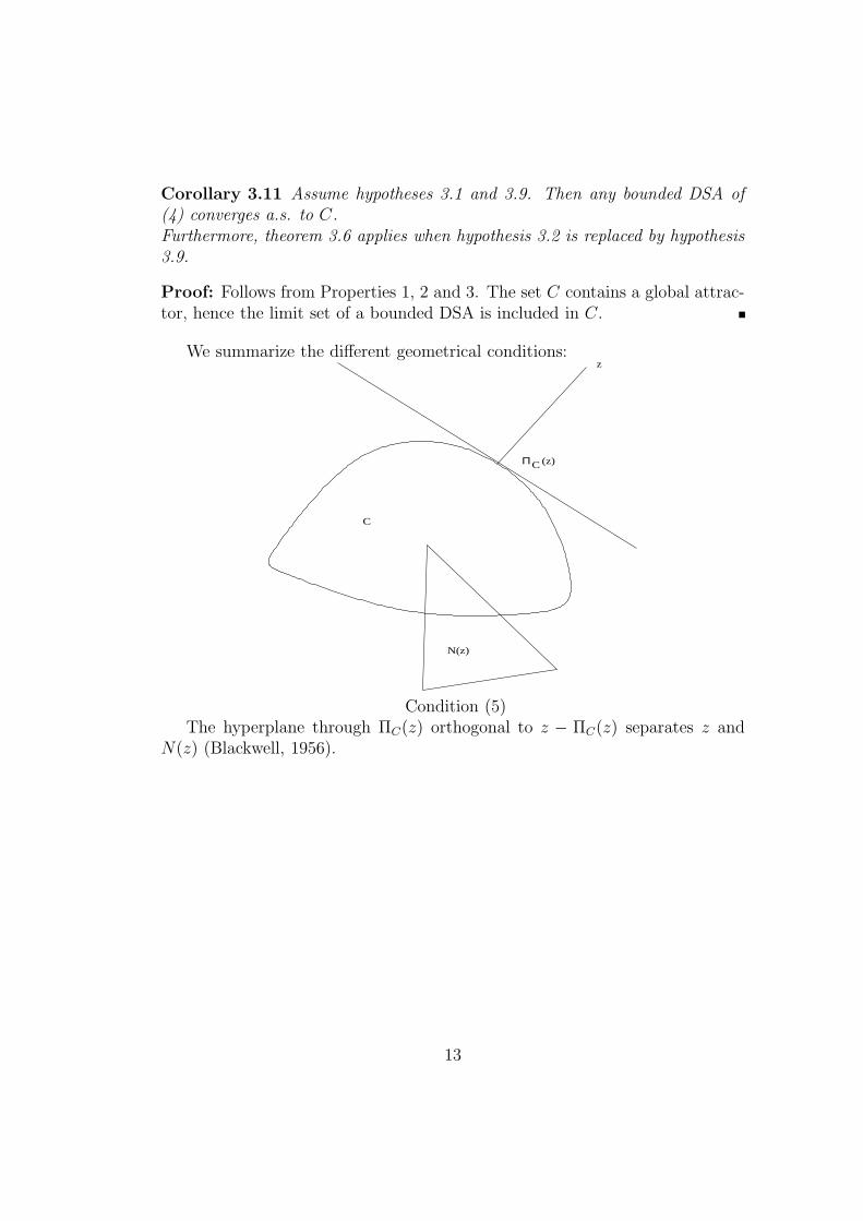
We summarize the different geometrical conditions:

(z)

z

C

N(z)

ΠC

Condition (5)The hyperplane through ΠC(z) orthogonal to z − ΠC(z) separates z and

N(z) (Blackwell, 1956).

13

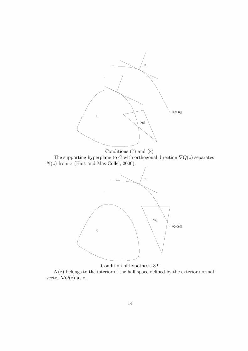
Q=Q(z)

z

C

N(z)

Conditions (7) and (8)The supporting hyperplane to C with orthogonal direction ∇Q(z) separates

N(z) from z (Hart and Mas-Collel, 2000).

N(z)

z

CQ=Q(z)

Condition of hypothesis 3.9N(z) belongs to the interior of the half space defined by the exterior normal

vector ∇Q(z) at z.

14

4 Approachability and consistency

We consider here a framework where the previous set C is the negative orthantand the vector of payoffs describes the vector of regrets in a strategic game,see Hart and Mas-Colell (2001a), (2003). The consistency condition amountsto the convergence of the average regrets to C. The interest of the approach isthat the same function P will be used to play the role of the function Q on onehand and to define the strategy and hence the correspondence N on the otherhand. Also the procedure can be defined on the payoff space as well as on theset of correlated moves.

4.1 No regret and correlated moves

Consider a finite game in strategic form. There are finitely many players labeleda = 1, 2, . . . , A. We let Sa denote the finite moves set of player a, S =

∏

a Sa,

and Z = ∆(S) the set of probabilities on S (correlated moves).Since we will consider everything from the view point of player 1 it is conve-nient to set S1 = I,X = ∆(I) (mixed moves of player 1), L =

∏

a6=1 Sa, and

Y = ∆(L) (correlated mixed moves of player 1’s opponents) hence Z = ∆(I×L).Throughout, X×Y is identified with a subset of Z through the natural embed-ding (x, y) → x × y, where x × y stands for the product probability of x andy. As usual, I (L, S) is also identified with a subset of X (Y, Z) through theembedding k → δk. We let U : S → R denote the payoff function of player 1and we still denote by U its linear extension to Z, and its bilinear extension toX × Y.Let m be the cardinality of I and R(z) denote the m-dimensional vector ofregrets for player 1 at z in Z, defined by

R(z) = U(i, z−1) − U(z)i∈I

where z−1 stands for the marginal of z on L. (Player 1 compares his payoffusing a given move i to his actual payoff, assuming the other players’ behavior,z−1, given.)Let D = R

m− be the closed negative orthant associated to the set of moves of

player 1.

Definition 4.1 H (for Hannan’s set) is the set of probabilities in Z satisfyingthe no-regret condition for player 1. Formally:

H = z ∈ Z : U(i, z−1) ≤ U(z), ∀i ∈ I = z∈Z : R(z) ∈ D.

15

Definition 4.2 P is a potential function for D if it satisfies the following setof conditions:

(i) P is a C1 nonnegative function from Rm to R,

(ii) P (w) = 0 iff w ∈ D,

(iii) ∇P (w) ≥ 0,

(iv) 〈∇P (w), w〉 > 0, ∀w /∈ D.

Definition 4.3 Given a potential P for D, the P -regret-based dynamics forplayer 1 is defined on Z by

z ∈ N(z) − z (9)

where

(i) N(z) = ϕ(R(z)) × Y ⊂ Z, with

(ii) ϕ(w) = ∇P (w)|∇P (w)|

∈ X whenever w /∈ D and ϕ(w) = X otherwise.

Here |∇P (w)| stands for the L1 norm of ∇P (w).

Remark This corresponds to a process where only the behavior of player 1, out-

side of H, is specified. Note that even the dynamics is truly independent among the

players (”uncoupled” according to Hart and Mas Collel, see Hart (2005)) the natural

state space is the set of correlated moves (and not the product of the sets of mixed

moves) since the criteria involves the actual payoffs and not only the marginal em-

pirical frequencies.

The associated discrete process is as follows. Let sn ∈ S be the randomvariable of profile of actions at stage n, and Fn the σ-algebra generated by thehistory hn = (s1, . . . , sn). The average zn = 1

n

∑nm=1sm satisfies:

zn+1 − zn =1

n+ 1[sn+1 − zn]. (10)

Definition 4.4 A P -regret-based strategy for player 1 is specified by the condi-tions:

(i) For all (i, `) ∈ I × L

P(in+1 = i, `n+1 = `|Fn) = P(in+1 = i|Fn)P(`n+1 = `|Fn),

16

(ii) P(in+1 = i|Fn) = ϕi(R(zn)) whenever R(zn) /∈ D, where ϕ(·) = ϕi(·)i∈Iis like in definition 4.3.

The corresponding discrete time process (10) is called a P -regret-based discretedynamics.

Clearly, one has

Proposition 4.5 The P -regret-based discrete dynamics (10) is a DSA of (9).

The next result is obvious but crucial.

Lemma 4.6 Let z = x× y ∈ X×Y ⊂ Z, then

〈x,R(z)〉 = 0.

Proof:One has

∑

i∈I

xi[U(i, y) − U(x× y)] = 0.

4.2 Blackwell’s framework

Given w ∈ Rm, let w+ be the vector with components w+

k = max(wk, 0). DefineQ(w) =

∑

k(w+k )2. Note that ∇Q(w) = 2w+, hence Q satisfies the condi-

tions (i) − (iv) of definition 4.2. If Π denotes the projection on D one hasw − Π(w) = w+ and 〈w+,Π(w)〉 = 0.In the game with vector payoff given by the regret of player 1, the set of fea-sible expected payoffs corresponding to xA (cf. §3.2), when player 1 uses θ, isR(z); z = θ×z−1. Assume that player 1 uses a Q-regret-based strategy. Sinceat w = gn, θ(w) is proportional to ∇Q(w), hence to w+, Lemma 4.6 impliesthat condition (5): 〈w − Πw, xA − Πw〉 ≤ 0 is satisfied; in fact, this quantityreduces to: 〈w+, R(y)− Πw〉 which equals 0.Hence a Q-regret-based strategy approaches the orthant D.

4.3 Convergence of P -regret-based dynamics

The previous dynamics in Section 3 were defined on the payoff space. Here, wetake the image by R (which is linear), of the dynamical system (9) and obtainthe following differential inclusion in R

m:

w ∈ N(w) − w (11)

17

whereN(w) = R(ϕ(w) × Y ).

The associated discrete dynamics to (10) is given as

wn+1 − wn =1

n+ 1(wn+1 − wn) (12)

with wn = R(zn).

Theorem 4.7 The potential P is a strong Lyapounov function associated tothe set D for (11), and similarly P R to the set H for (9). Hence, D containsan attractor for (11) and H contains an attractor for (9).

Proof: Remark that 〈∇P (w), N(w)〉 = 0: in fact ∇P (w) = 0 for w ∈ D, andfor w 6∈ D use Lemma 4.6. Hence for any w(t) solution to (11)

d

dtP (w(t)) = 〈∇P (w(t)), w(t)〉 = −〈∇P (w(t)),w(t)〉 < 0

and P is a strong Lyapounov function associated to D, in view of conditions(i) − (iv) of definition 4.2. The last assertion follows from Property 3.

Corollary 4.8 Any P -regret-based discrete dynamics (10) approaches D in thepayoff space, hence H in the action space.

Proof: D (resp. H) contains an attractor for (11) whose basin of attractioncontains R(Z) (resp. Z) and the process (12) (resp. (10)) is a bounded DSA,hence Properties 1, 2 and 3 apply.

Remark A direct proof is available as follows :Let R the range of R and define, for w /∈ D,

N(w) = w′∈Rm; 〈w′,∇P (w)〉 = 0∩?R.

Hypotheses (3.1) and 3.9 are satisfied and Corollary 3.11 applies.

18

5 Approachability and conditional consistency

We keep the framework of Section 4 and the notation introduced in 4.1, andfollow Hart and Mas-Colell (2000), (2001a), (2003) in studying conditional (orinternal) regrets. One constructs again an approachability strategy from anassociate potential function P . Like in the previous Section 4 the dynamics canbe defined either in the payoff space or in the space of correlated moves.

We still consider only player 1 and denote by U his payoff.Given z = (zs)s∈S ∈ Z, introduce the family of m comparison vectors of dimen-sion m (testing k against j with (j, k) ∈ I2)

C(j, k)(z) =∑

`∈L

[U(k, `) − U(j, `)]z(j,`).

(This corresponds to the change in the expected gain of Player 1 at z whenreplacing move j by k.) Remark that if one let (z | j) denote the conditionalprobability on L induced by z given j ∈ I and z1 the marginal on I, then

C(j, k)(z)k∈I = z1jR((z | j))

where we recall that R((z | j)) is the vector of regrets for player 1 at (z | j).

Definition 5.1 The set of no conditional regret (for player 1) is

C1 = z;C(j, k)(z) ≤ 0, ∀j, k ∈ I.

It is obviously a subset of H since

∑

j

C(j, k)(z)k∈I = R(z).

Property The intersection over all players a of the sets Ca is the set of cor-related equilibria of the game.

5.1 Discrete standard case

Here we will use approachability theory to retrieve the well known fact (seeHart and Mas-Colell (2000)) that player 1 has a strategy such that the vectorC(zn) converges to the negative orthant of R

m2

, where zn ∈ Z is the average(correlated) distribution on S.Given s ∈ S define the auxiliary “vector payoff” B(s) to be the m × m realvalued matrix where, if s = (j, `) ∈ I × L, hence j is the move of player 1, the

19

only non-zero line is line j with entry on column k being U(k, `)−U(j, `). Theaverage payoff at stage n is thus a matrix Bn with coefficient

Bn(j, k) =1

n

∑

r,ir=j

(U(k, `r) − U(j, `r)) = C(j, k)(zn)

which is the test of k versus j on the dates, up to stage n, where j was played.Consider the Markov chain on I with transition matrix

Mn(j, k) =Bn(j, k)

+

bn,

for j 6= k where bn > maxj∑

kBn(j, k)+. By standard results on finite Markov

chains, Mn admits (at least) one invariant probability measure. Let µn = µ(Bn)be such a measure. Then (dropping the subscript n)

µj =∑

k

µkM(k, j) =∑

k 6=j

µkB(k, j)+

b+ µj(1 −

∑

k 6=j

B(j, k)+

b).

Thus b disappears and the condition writes∑

k 6=j

µkB(k, j)+ = µj∑

k 6=j

B(j, k)+.

Theorem 5.2 Any strategy of player 1 satisfying σ(hn) = µn is an approacha-bility strategy for the negative orthant of R

m2

. Namely

∀j, k limn→∞

Bn(j, k)+ = 0 a.s.

Equivalently, (zn) approaches the set of no conditional regret for player 1 :

limn→∞

d(zn, C1) = 0.

Proof: Let Ω denote the closed negative orthant of Rm2

. In view of proposition3.8 it is enough to prove that inequality (5)

〈b− ΠΩ(b), b′ − ΠΩ(b)〉 ≤ 0, ∀b /∈ Ω

holds for every regret matrix b′, feasible under µ = µ(b).As usual, since the projection is on the negative orthant Ω, b−ΠΩ(b) = b+ and〈b− ΠΩ(b),ΠΩ(b)〉 = 0. Hence it remains to evaluate

∑

j,k

B(j, k)+µj[U(k, `) − U(j, `)]

but the coefficient of U(j, `) is precisely∑

k

B+(k, j)µk − µj∑

k

B+(j, k) = 0

by the choice of µ = µ(b).

20

5.2 Continuous general case

We first state a general property (compare Lemma 4.6):

Lemma 5.3 Given a ∈ Rm2

, let µ∈X satisfy :

∑

k: k 6=j

µka(k, j) = µj∑

k: k 6=j

a(j, k), ∀j ∈ I

then〈a, C(µ× y)〉 = 0, ∀y∈Y.

Proof: As above one computes:

∑

j

∑

k

a(j, k)µj[U(k, y) − U(j, y)]

but the coefficient of U(j, y) is precisely

∑

k

a(k, j)µk − µj∑

k

a(j, k) = 0.

Let P be a potential function for Ω the negative orthant of Rm2

, for exampleP (w) =

∑

ij(w+ij)

2, as in the standard case above.

Definition 5.4 The P -conditional regret dynamics in continuous time is de-fined on Z by:

z ∈ µ(z)×Y − z (13)

where µ(z) is the set of µ ∈ X that are solution to:

∑

k∈Sµk∇Pkj(C(z)) = µj

∑

k∇Pjk(C(z))

whenever C(z) /∈ Ω (∇Pjk denotes the jk component of the gradient of P ). Inparticular µ(z) = X whenever C(z) ∈ Ω.

The associated process in Rm2

is the image under C:

w ∈ C(ν(w) × Y ) − w (14)

where ν(w) is the set of ν ∈ X with

∑

k∈Sνk∇Pkj(w) = νj

∑

k∇Pjk(w).

21

Theorem 5.5 The processes (13) and (14) satisfy:

C+(j, k)(z(t)) = w+jk(t)→t→∞0.

Proof: Apply Theorem 3.10 with:

N(w) = w′∈(Rm)2 : 〈∇P (w), w′〉 = 0 ∩ C

where C is the range C(Z) of C. Since w(t) = C(z(t)) the previous lemma 5.3implies that w(t) ∈ N(w(t)) − w(t).

The discrete processes corresponding to (13) and (14) are respectively in Z

zn+1 − zn =1

n+ 1[µn+1 × z−1

n+1 − zn + (zn+1 − µn+1 × z−1n+1)] (15)

where µn+1 satisfies:

∑

k∈Sµkn+1∇Pkj(C(zn)) = µjn+1

∑

k∇Pjk(C(zn))

and in Rm2

wn+1 − wn =1

n+ 1[C(µn+1 × z−1

n+1) − wn + (wn+1 − C(µn+1 × z−1n+1)]. (16)

Corollary 5.6 The discrete processes (15) and (16) satisfy:

C+(j, k)(zn) = wjk,+n →t→∞0 a.s.

Proof: (15) and (16) are bounded DSA of (13) and (14) and Properties 1, 2,and 3 apply.

Corollary 5.7 If all players follow the above procedure, the empirical distribu-tion of moves converges a.s. to the set of correlated equilibria.

6 Smooth fictitious play and consistency

We follow the approach of Fudenberg and Levine concerning consistency (1995)and conditional consistency (1999) and deduce some of their main results (seeTheorems 6.6, 6.12 below) as corollaries of dynamical properties. Basically thecriteria are similar to the ones studied in Section 4 and 5 but the procedureis different and based only on the previous behavior of the opponents. Like insections 4 and 5 we continue to adopt the point of view of player 1.

22

6.1 Consistency

LetV (y) = max

x∈XU(x, y).

The average regret evaluation along hn ∈ Hn is

e(hn) = en = V (yn) −1

n

∑n

m=1U(im, `m).

where as usual yn stands for the time average of (`m) up to time n. (Thiscorresponds to the maximal component of the regret vector R(zn)).

Definition 6.1 (Fudenberg and Levine, 1995) Let η > 0. A strategy σ forplayer 1 is said η-consistent if for any opponents strategy τ

lim supn→∞

en ≤ η Pσ,τ a.s.

6.2 Smooth fictitious play

A smooth perturbation of the payoff U is a map

U ε(x, y) = U(x, y) + ερ(x), 0 < ε < ε0

such that:

(i) ρ : X → R is a C1 function with ‖ρ‖ ≤ 1,

(ii) argmaxx∈XUε(., y) reduces to one point and defines a continuous map

brε : Y → X

called a smooth best reply function,

(iii) D1Uε(brε(y), y).Dbrε(y) = 0 (for example D1U

ε(., y) is 0 at brε(y). Thisoccurs in particular if brε(y) belongs to the interior of X).

Remark A typical example is

ρ(x) = −∑

k

xk log xk. (17)

which leads to

brεi (y) =exp(U(i, y)/ε)

∑

k∈I exp(U(k, y)/ε)(18)

23

as shown by Fudenberg and Levine (1995, 1999).

LetV ε(y) = max

xU ε(x, y) = U ε(brε(y), y).

Lemma 6.2 (Fudenberg and Levine (1999))

DV ε(y)(h) = U(brε(y), h).

Proof: One has

DV ε(y) = D1Uε(brε(y), y).Dbrε(y) +D2U

ε(brε(y), y)

The first term is zero by condition (iii) above. For the second term one has

D2Uε(brε(y), y) = D2U(brε(y), y)

which, by linearity of U(x, .) gives the result.

Definition 6.3 A smooth fictitious play strategy for player 1 associated to thesmooth best response function brε (in short a SFP(ε) strategy) is a strategy σε

such thatEσε ,τ(in+1 | Fn) = brε(yn)

for any τ.

There are two classical interpretations of SFP(ε) strategies. One is that player1 chooses to randomize his moves. Another one called stochastic fictitious play(Fudenberg and Levine (1998), Benaım and Hirsch (1999)) is that payoffs areperturbed in each period by random shocks and that player 1 plays the bestreply to the empirical mixed strategy of its opponents. Under mild assumptionson the distribution of the shocks it was shown by Hofbauer and Sandholm (2002)(Theorem 2.1) that this can always be seen as a SFP(ε) strategy for a suitableρ.

6.3 SFP and consistency

Fictitious play was initially used as a global dynamics (i.e. the behavior of eachplayer is specified) to prove convergence of the empirical strategies to optimalstrategies (see Brown (1951) and Robinson (1951) and for recent results BHSSection 5.3 and Hofbauer and Sorin (2006)).Here we deal with unilateral dynamics and consider the consistency property.Hence the state space cannot be reduced to the product of the sets of mixed

24

moves but has to incorporate the payoffs.Explicitly, the discrete dynamics of averaged moves is

xn+1 − xn =1

n+ 1[in+1 − xn], yn+1 − yn =

1

n+ 1[`n+1 − yn]. (19)

Let un = U(in, `n) be the payoff at stage n and un be the average payoff up tostage n so that

un+1 − un =1

n + 1[un+1 − un]. (20)

Lemma 6.4 Assume that player 1 plays a SFP(ε) strategy. Then the process(xn, yn, un) is a DSA of the differential inclusion

ω ∈ N(ω) − ω (21)

where ω = (x, y, u) ∈ X×Y×R and

N(x, y, u) = (brε(y), β, U(brε(y), β)) : β∈Y .

Proof: To shorten notation we write E(. | Fn) for Eσε,τ (. | Fn) where τ is anyopponents strategy. By assumption E(in+1 | Fn) = brε(yn). Set E(`n+1 | Fn) =βn ∈ Y. Then, by conditional independence of in+1 and `n+1, one gets thatE(un+1 | Fn) = U(brε(yn), βn). Hence E((in+1, `n+1, un+1) | Fn) ∈ N(xn, yn, un).

Theorem 6.5 The set (x, y, u) ∈ X × Y × R : V ε(y) − u ≤ ε is a globalattracting set for (21). In particular, for any η > 0, there exists ε such thatfor ε ≤ ε, lim supt→∞ V ε(y(t)) − u(t) ≤ η (i.e. continuous SFP(ε) satisfiesη-consistency.)

Proof: Let wε(t) = V ε(y(t))− u(t). Taking time derivative one obtains, usingLemma 6.2 and (21):

wε(t) = DV ε(y(t)).y(t) − u(t)

= U(brε(y(t)), β(t)) − U(brε(y(t)),y(t)) − U(brε(y(t)), β(t)) + u(t)

= u(t) − U(brε(y(t)),y(t))

= −wε(t) + ερ(σε(y(t))).

Hencewε(t) + wε(t) ≤ ε

so that wε(t) ≤ ε? +Ke−t for some constant K and the result follows.

25

Theorem 6.6 For any η > 0, there exists ε such that for ε ≤ ε, SFP(ε) is η-consistent.

Proof: The assertion follows from lemma 6.4, Property 1, Property 2 (ii) andTheorem 6.5.

6.4 Remarks and Generalizations

The definition given here of a SFP(ε) strategy can be extended in some inter-esting directions. Rather than developing a general theory we focus on twoparticular examples.

1. Strategies based on pairwise comparison of payoffs: Suppose thatρ is given by (17). Then, playing a SFP(ε) strategy requires for player 1 thecomputation of brε(yn) given by (18) at each stage. In case where the cardinalityof S1 is very large (say 2N with N ≥ 10) this computation is not feasible! Analternative feasible strategy is the following:Assume that I is the set of vertices of a graph. Write i ∼ j when i and j areneigbhours in this graph. Assume furthermore that the graph is symmetric (∼is a symmetric relation) and connected (given any two points i, j ∈ I there existsa finite sequence i1 = i, i2, . . . , im = j such that il ∼ il+1 for l = 1, . . . , m− 1).Let N(i) = j ∈ I \ i : i ∼ j. The strategy is as follows: Let i be the actionchosen at time n (i.e. in = i). At time n + 1, player 1 picks an action j atrandom in N(i). He then switches to j (i.e. in+1 = j) with probability

R(i, j, yn) = min

[

1,|N(i)|

|N(j)|exp

(

1

ε(U(j, yn) − U(i, yn))

)]

and keeps i (i.e in+1 = i) with the complementary probability 1 − R(i, j, yn).Here |N(i)| stands for the cardinal of N(i).Note that this strategy only involves at each step the computation of the payoffsdifference (U(j, yn) − U(i, yn)) . While this strategy is not an SFP(ε) strategy,one still has:

Theorem 6.7 For any η > 0, there exists ε such that, for ε ≤ ε, the strategydescribed above is η-consistent.

Proof: For fixed y ∈ Y, let Q(y) be the Markov transition matrix given byQ(i, j, y) = 1

|N(i)|R(i, j, y) for j ∈ N(i), Q(i, j, y) = 0 for j 6∈ N(i) ∪ i, and

Q(i, i, y)) = 1 −∑

j 6=iQ(i, j, y). Then Q(y) is an irreducible Markov matrix

26

having brε(y) as unique invariant probability: this is easily seen by check-ing that Q(y) is reversible with respect to brε(y). That is brεi (y)Q(i, j, y) =brεj(y)Q(j, i, y).The discrete time process (19), (20) is not a DSA (as defined here) to (21) be-cause E(in+1 | Fn) 6= brε(yn). However, the conditional law of in+1 given Fn isQ(xn, ·, yn) and using the techniques introduced by Metivier and Priouret (1992)to deal with Markovian perturbations (see e.g. Duflo 1996, Chapter 3.IV) it canstill be proved that the assumptions of Proposition 1.3 in BHS are fulfilled, fromwhich it follows that the interpolated affine process associated to (19), (20) is aperturbed solution (see BHS, for a precise definition) to (21). Hence Property1 applies and the end of the proof is similar to the proof of Theorem 6.6.

2. Convex sets of actions: Suppose that X and Y are two convex compactsubsets of finite dimensional Euclidean spaces. U is a bounded function withU(x, .) linear on Y . The discrete dynamics of averaged moves is

xn+1 − xn =1

n+ 1[xn+1 − xn], yn+1 − yn =

1

n+ 1[yn+1 − yn]. (22)

with xn+1 = brε(yn). Let un = U(xn, yn) be the payoff at stage n and un bethe average payoff up to stage n so that

un+1 − un =1

n + 1[un+1 − un]. (23)

Then the results of the previous section 6.3 still hold.

6.5 SFP and conditional consistency

We keep here the framework of Section 4 but extend the analysis from consis-tency to conditional consistency (which is like studying external regrets (Section4) and then internal regrets (Section 5)). Given z ∈ Z, recall that we let z1 ∈ Xdenote the marginal of z on I. That is

z1 = (z1i )i∈I with z1

i =∑

`∈L

zi`.

Let z[i] ∈ RL be the vector with components z[i]` = zi`. Note that z[i] belongs

to tY for some 0 ≤ t ≤ 1. A conditional probability on L induced by z giveni ∈ I satisfies

z | i = (z | i)`∈L with (z | i)`z1i = zi` = z[i]`.

27

Let [0, 1].Y = ty : 0 ≤ t ≤ 1, y ∈ Y . Extend U to X × ([0, 1] × Y ) byU(x, ty) = tU(x, y) and similarly for V . The conditional evaluation function atz ∈ Z is

ce(z) =∑

i∈I

V (z[i])−U(i, z[i]) =∑

i∈I

z1i [V (z | i)−U(i, z | i)] =

∑

i∈Iz1i V (z|i)−U(z).

with the convention that z1i V (z | i) = z1

i U(i, z | i) = 0 when z1i = 0.

Like in Section 5, conditional consistency means consistency with respect tothe conditional distribution given each event of the form “i was played”. In adiscrete framework the conditional evaluation is thus

cen = ce(zn)

where as usual zn stands for the empirical correlated distribution of moves upto stage n.Conditional consistency is defined like consistency but with respect to (cen).More precisely:

Definition 6.8 A strategy σ for player 1 is said η-conditionally consistent iffor any opponents strategy τ

lim supn→∞

cen ≤ η Pσ,τ a.s.

Given a smooth best reply function brε : Y → X, let us introduce a corre-spondence Brε defined on [0, 1] × Y by Brε(ty)= brε(y) for 0 < t ≤ 1 andBrε(0) = X. For z ∈ Z, let µε(z) ⊂ X denote the set of all µ ∈ X that aresolution to the equation

∑

i∈Iµib

i = µ (24)

for some vectors family bii∈I such that bi ∈ Brε(z[i]).

Lemma 6.9 µε is an u.s.c correspondence with compact convex non–empty val-ues.

Proof: For any vectors family bii∈I with bi ∈ X the function µ →∑

i∈I µibi

maps continuously X into itself. It then has fixed points by Brouwer’s fixedpoint theorem, showing that µε(z) 6= ∅. Let µ, ν ∈ µε(z). That is µ =

∑

i µibi

and ν =∑

i νici with bi, ci ∈ Brε(z[i]). Then for any 0 ≤ t ≤ 1 tµ+ (1 − t)ν =

∑

i(tµi + (1 − t)νi)di with di = tµib

i+(1−t)νici

(tµi+(1−t)νi). By convexity of Brε(z[i]), di ∈

Brε(z[i]). Thus tµ+ (1 − t)ν ∈ µε(z) proving convexity of µε(z).Using the factthat Brε has a closed graph, it is easy to show that µε has a closed graph, fromwhich it will follow that it is u.s.c with compact values. Details are left to thereader.

28

Definition 6.10 A conditional smooth fictitious play strategy for player 1 as-sociated to the smooth best response function brε (in short a CSFP(ε) strategy)is a strategy σε such that σε(hn) ∈ µε(zn).

The random discrete process associated to CSFP(ε) is thus defined by:

zn+1 − zn =1

n+ 1[zn+1 − zn] (25)

where the conditional law of zn+1 = (in+1, `n+1) given the past up to time n isa product law σε(hn) × τ(hn). The associated differential inclusion is

z ∈ µε(z) × Y − z. (26)

Extend brε to a map, still denoted brε, on [0, 1]× Y by choosing a non–emptyselection of Brε and define

V ε(z[i]) = U(brε(z[i]), z[i]) − εz1i ρ(brε(z[i]))

(so that if z1i > 0 V ε(z[i]) = z1

i Vε(z | i) and V ε(0) = 0). Let

ceε(z) =∑

i

(V ε(z[i]) − U(z[i])) =∑

i

V ε(z[i]) − U(z).

The evaluation along a solution t→ z(t) to (26) is

Wε(t) = ceε(z(t)).

The next proof is in spirit similar to Section 6.3 but technically heavier.Since we are dealing with smooth best reply to conditional events there is adiscontinuity at the boundary and the analysis has to take care of this aspect.

Theorem 6.11 The set z ∈ Z : ceε(z) ≤ ε is an attracting set for (26)whose basin is Z. In particular, conditional consistency holds for continuousCSFP(ε).

Proof: We shall compute

Wε(t) =d

dt

∑

iV ε(z[i](t)) −

d

dtU(z(t)).

The last term isd

dtU(z(t)) = U(µε(t), β(t)) − U(z(t))

29

by linearity, with β(t) ∈ Y and µε(t) ∈ µε(z(t)). We now pass to the first term.First observe that

d

dtz1i ∈ µεi (z) − z1

i ≥ −z1i .

Hence z1i (t) > 0 implies z1

i (s) > 0 for all s ≥ t. It then exists τi ∈ [0,∞] suchthat z1

i (s) = 0 for s ≤ τi and z1i (s) > 0 for s > τi. Consequently the map

t → V ε(z[i](t)) is differentiable everywhere but possibly at t = τi and is zerofor t ≤ τi. If t > τi, then

d

dtV ε(z[i](t)) =

d

dtU ε(brε(z[i](t)), z[i](t)) − εz1

i (t)ρ(brε(z[i](t)))

= U ε(brε(z[i](t)), z[i](t)) − z1i (t)ερ(brε(z[i](t))) (27)

by Lemma 6.2. If now t < τi, both z[i](t) and ddtV ε(z[i](t)) are zero, so that

equality (27) is still valid.Finally, using d

dtzij(t) = µεi(t)βj(t) − zij(t), we get that

Wε(t) =∑

i

U ε(brε(z[i](t)), µεi (t)β(t) − z[i](t))

+∑

i

(µεi (t) − z1i (t))ερ(brε(z[i](t))) − U(µε(t), β(t)) + U(z(t))

for all (but possibly finitely many) t ≥ 0. Replacing gives

Wε(t) = −Wε(t) + A(t)

whereA(t) = −U(µε(t), β(t))

+∑

i

U ε(brε(z[i]((t)), µεi (t)β(t)) +∑

i

µεi (t)ερ(brε(z[i](t))).

Thus one obtains:

A(t) = −U(µε(t), β(t)) +∑

iµεi (t) [U(brε(z[i](t)), β(t)) + ερ(brε(z[i](t)))] .

Now equation (24) and linearity of U(., y) implies

U(µε(t), β(t)) =∑

iµεi (t)U(brε(z[i](t)), β(t))).

ThusA(t) = ε

∑

i

µεi (t)ρ(brε(z[i](t)))

30

so thatWε(t) ≤ −Wε(t) + ε

for all (but possibly finitely many) t ≥ 0. Hence

Wε(t) ≤ e−t(Wε(0) − ε) + ε

for all t ≥ 0.

Theorem 6.12 For any η > 0, there exists ε > 0 such that, for ε ≤ ε, aCSFP(ε) strategy is η-consistent.

Proof: Let L = L(zn) be the limit set of (zn) defined by (25). Since (zn) is aDSA to (26) and z ∈ Z : ceε(z) ≤ ε is an attracting set for (26) whose basinis Z (Theorem 6.11), it suffices to apply Property 2 (ii).

7 Extensions

We study in this section extensions of the previous dynamics in the case wherethe information of player 1 is reduced: either he does not recall his past moves,or he does not know the other players moves sets, or he is not told their moves.

7.1 Procedure in law

We consider here procedures where player 1 is uninformed of his previous se-quences of moves, but know only its law (team problem).

The general framework is as follows. A discrete time process wn is definedthrough a recursive equation by:

wn+1 − wn = an+1V (wn, in+1, `n+1) (28)

where (in+1, `n+1) ∈ I × L are the moves2 of the players at stage n + 1 andV : R

m × I × L→ Rm is some bounded measurable map.

A typical example is given, in the framework of approachability (see section3.2), by

V (w, i, `) = −w + Ai` (29)

where Ai` is the vector valued payoff corresponding to (i, `) and an = 1/n. Insuch case wn = gn is the average payoff.

2For convenience, we keep the notation used for finite games but it is unnecessary toassume here that the move spaces are finite.

31

Assume that player 1 uses a strategy (as defined in section 3.2) of the form

σ(hn) = ψ(wn)

where for each w, ψ(w) is some probability over I. Hence w plays the role of astate variable for player 1 and we call such σ a ψ−strategy. Let Vψ(w) be therange of V under σ at w, namely the convex hull of

∫

I

V (w, i, `)ψ(w)(di); ` ∈ L.

Then the associated continuous time process associated to (28) is

w ∈ Vψ(w). (30)

We consider now another discrete time process where, after each stage n, player1 is not informed upon his realized move in but only upon `n. Define by induc-tion the new input at stage n+ 1:

w∗n+1 − w∗

n = an+1

∫

I

V (w∗n, i, `n+1)ψ(w∗

n)(di). (31)

Remark that the range of V under ψ(w∗) at w∗ is Vψ(w∗) so that the continuoustime process associated to (31) is again (30). Explicitely (28) and (31) are DSAof the same differential inclusion (30).

Definition 7.1 A ψ-procedure in law is a strategy σ of the form σ(hn) = ψ(w∗n)

where for each w, ψ(w) is some probability over I and w∗n is given by (31).

The key observation is that a procedure in law for player 1 is independenton the moves of player 1 and only requires the knowledge of the map V andthe observation of the opponents moves. The interesting result is that sucha procedure will in fact induce, under certain assumptions (see hypothesis 7.2below), the same asymptotic behavior in the original discrete process.

Suppose that player 1 uses a ψ-procedure in law. Then the coupled system(28, 31) is a DSA to the differential inclusion

(w, w∗) ∈ V 2ψ (w,w∗) (32)

where V 2ψ (w,w∗) is the convex hull of

(

∫

I

V (w, i, `)ψ(w∗)(di),

∫

I

V (w∗, i, `)ψ(w∗)(di)); ` ∈ L.

We shall assume, from now on, that (32) meets the standing hypothesis 2.1.We furthermore assume that

32

Hypothesis 7.2 The map V satisfies one of the two following conditions:

(i) There exists a norm || · || such that w → w + V (w, i, `) is contractinguniformly in s = (i, `). That is

||w + V (w, s) − (u+ V (u, s))|| ≤ ρ||w − u||

for some ρ < 1.

(ii) V is C1 in w and there exists α > 0 such that all eigenvalues of thesymmetric matrix

∂V

∂w(w, s) +

t∂V

∂w(w, s)

are bounded by −α.

(t stands for the transpose). Remark that hypothesis 7.2 holds trivially for (29).Under this later hypothesis one has the following result.

Theorem 7.3 Assume that wn, w∗n is a bounded sequence. Under a ψ−procedure

in law the limit sets of wn and w∗n coincide, and this limit set is an ICT

set of the differential inclusion (30). Under a ψ−strategy the limit set of wnis also an ICT set of the same differential inclusion.

Proof: Let L be the limit set of wn, w∗n. By properties 1 and 2, L is compact

and invariant. Choose (w,w∗) ∈ L and let t → (w(t),w∗(t)) denote a solutionto (32) that lies in L (by invariance) with initial condition (w,w∗). Let u(t) =w(t) − w∗(t).

Assume condition (i) in hypothesis 7.2. Let Q(t) = ||u(t)||. Then for all0 ≤ s ≤ 1

Q(t + s) = ||u(t) + u(t)s+ o(s)|| = ||(1 − s)u(t) + (u(t) + u(t))s + o(s)||

≤ (1 − s)Q(t) + s||u(t) + u(t)|| + o(s).

Now u(t) + u(t) can be written as

w(t) − w∗(t) +

∫

I×L

[V (w(t), i, `) − V (w∗(t), i, `)]ψ(w∗(t))(di)dν(`)

for some probability measure ν over L. Thus by condition (i)

Q(t+ s) ≤ (1 − s)Q(t) + sρQ(t) + o(s),

33

from which it follows that

Q(t) ≤ (ρ− 1)Q(t)

for almost every t. Hence, for all t ≥ 0 :

Q(0) ≤ e(ρ−1)tQ(−t) ≤ e(ρ−1)tK

for some constant K. Letting t→ +∞ shows that Q(0) = 0. That is w = w∗.

Assume now condition (ii). Let || · || denote the Euclidean norm on Rm and

〈·, ·〉 the associated scalar product. Then

〈V (w, s)−V (w∗, s), w−w∗〉 =

∫ 1

0

〈∂wV (w∗ +u(w−w∗), s).(w−w∗), w−w∗〉du

≤ −α

2||w − w∗||2.

Therefore

d

dtQ2(t) = 2〈w(t) − w∗(t), w(t) − w∗(t)〉 ≤ −αQ2(t)

from which it follows (like previously) that Q(0) = 0.We then have proved that given hypothesis 7.2, wn and w∗

n have the samelimit set under a ψ−procedure in law. Since w∗

n is a DSA to (30), this limitset is ICT for (30) by Property 1. The same property holds for wn under aψ−strategy.

Remark Let R denote the set of chain-recurrent points for (28). Hypothesis 7.2

can be weakened to the assumption that conditions (i) or (ii) are satisfied for V

restricted to R× I × L.

The previous result applies to the framework of Sections 4 and 5 and showthat the discrete regret dynamics will have the same properties when based onthe (conditional) expected stage regret ExR(s) or ExC(s).

7.2 Best prediction algorithm

Consider a situation where at each stage n an unknown vector Un (∈ [−1,+1]I)is selected and a player chooses a component in ∈ I. Let ωn = U in

n . Assume

34

that Un is announced after stage n.Consistency is defined trough the evaluation vector Vn with V i

n = U in− ωn, i ∈ I,

where, as usual, Un is the average vector and ωn the average realization.Conditional consistency is defined through the evaluation matrixWn withW jk

n =(1/n)(

∑

m,im=j Ukm − ωm).

This formulation is related to on line algorithms, see Foster and Vohra (1999)for a general presentation. In the previous framework, the vector Un is U(., `n)where `n is the choice of players other than 1 at stage n. The claim is thatall previous results go through (Vn or Wn converges to the negative orthant)when dealing with the dynamics expressed on the payoffs space. This meansthat player 1 does not need to know the payoff matrix, nor the set of moves ofthe other players; only a compact range for the payoffs is requested. A sketchof proofs is as follow.

7.2.1 Approachability: consistency

We consider the dynamics of section 4. The regret vector R∗ if i is played, isR∗(i) = U j − U ij∈I . Lemma 4.6 is now for θ ∈ ∆(I)

〈θ, R∗(θ)〉 = 0

since R∗(θ), the expectation of R∗ under θ is

R∗(θ) =∑

i∈I

θ(i)R∗(i) = U j − 〈θ, U〉j

hence the properties of the P -regret based dynamics on the payoff space Rm

still hold (Theorem 4.7 and Corollary 4.8).

7.2.2 Approachability: conditional consistency

The content of Section 5 extends as well. The I × I regret matrix is defined, atstage n, given the move in, by all lines being 0 except line in which is the vectorU j

n − U inj∈J . Then the analysis is identical and the convergence of the regret

to the negative orthant holds for P -conditional regret dynamics as in Theorem5.5 and Corollary 5.6.

7.2.3 SFP: consistency

In the framework of Section 6, the only hypothesis used on the set Y was thatit was convex compact, hence one can take L = [−1,+1]I and U(x, `) = 〈x, `〉.Then all computations go through.

35

7.2.4 SFP: conditional consistency

For the analog of Section 6.5 let us define the I × I evaluation matrix Mn atstage n and given the move in, by all lines equal to 0 except line in being thevector Un. Its average at stage n is Mn. µn is an invariant measure for theMarkov matrix defined by the family BRε(M i

n), where (M in) denotes the i-line

of (Mn).

7.3 Partial information

We consider here the framework of section 7.2 but where only ωn is observed byplayer 1, not the vector Un. In a game theoretical framework, this means thatthe move of the opponent at stage n is not observed by player 1 but only thecorresponding payoff U(in, `n) is known.This problem has been studied in Auer and alii (1995), Foster and Vohra (1997),Fudenberg and Levine (1999), Hart and Mas-Colell (2001b) and in a gametheoretical framework by Banos (1968) and Megiddo (1980) (note that workingin the framework of 7.2 is more demanding than finding an optimal strategy ina game, since the payoffs can actually vary stage after stage).The basic idea is to generate, from the actual history of payoffs and movesωn, in and the knowledge of the strategy σ a sequence of pseudo-vectors Un ∈RS to which the previous procedures applies.

7.3.1 Consistency

We follow Auer and alii (1995) and define Un by

U in =

ωnσin

1i=in

where as usual in is the component chosen at stage n and σin stands for σ(hn−1)(i).The associated pseudo-regret vector is Ri

n = U in − ωni∈I . Notice that

E(Rin|hn−1) = U i

n − 〈σn, Un〉

hence, in particular〈σn, E(Rn|hn−1)〉 = 0.

To keep Un bounded one defines first τn adapted to the vector Un as in Section7.2, namely proportional to ∇P ( 1

n−1

∑n−1m=1 Rm), see section 4, then σ is specified

byσin = (1 − δ)τ in + δ/K

36

for δ > 0 small enough and K being the cardinality of the set I.The discrete dynamics is thus

¯Rn −¯Rn+1 =

1

n(Rn+1 −

¯Rn).

The corresponding dynamics in continuous time satisfies:

w(t) = α(t) − w(t)

with α(t) = Ut−〈p(t), Ut〉 for some measurable process Ut with values in [−1, 1]and p(t) = (1 − δ)q(t) + δ/K with

∇P (w(t)) = ‖∇P (w(t))‖q(t).

Define the condition

〈∇P (w), w〉 ≥ B‖∇P (w)‖‖w+‖ (33)

on RS \ D for some positive constant B (satisfied for example by P (w) =

∑

s(w+s )2).

Proposition 7.4 Assume that the potential satisfies in addition (33). Thenconsistency holds for the continuous process Rt and both discrete processes Rn

and Rn.

Proof: One has

d

dtP (w(t)) = 〈∇P (w(t)), w(t)〉

= 〈∇P (w(t)), α(t)− w(t)〉.

Now

〈∇P (w(t)), α(t)〉 = ‖∇P (w(t))‖〈q(t), α(t)〉

= ‖∇P (w(t))‖〈1

1− δpt −

δ

(1 − δ)K,α(t)〉

≤ ‖∇P (w(t))‖δ

(1 − δ)KR

for some constant R since 〈p(t), α(t)〉 = 0 and the range of α is bounded. Itfollows, using (33), that given ε > 0, δ > 0 small enough and ‖w+(t)‖ ≥ εimplies

d

dtP (w(t)) ≤ ‖∇P (w(t))‖(

δ

(1− δ)KR −B‖w+(t)‖)

≤ −‖∇P (w(t))‖Bε/2.

37

Now 〈∇P (w), w〉 > 0 for w /∈ D implies ‖∇P (w)‖ ≥ a > 0 on ‖w+‖ ≥ ε.Let β > 0, A = P ≤ β and choose ε > 0 such that ‖w+‖ ≤ ε is includedA. Then the complement of A is an attracting set and consistency holds forthe process Rt, hence as in section 4, for the discrete time process Rn. Theresult concerning the actual process Rn with Rk

n = Ukn − ωn finally follows from

another application of Theorem 7.3 since both processes have same conditionalexpectation.

7.3.2 Conditional consistency

A similar analysis holds in this framework. The pseudo regret matrix is nowdefined by

Cn(i, j) =σinσjnU jn1j=in − U i

n1i=in

henceE(Cn(i, j)|hn−1) = σin(U

jn − U i

n)

and this relation allows to invoke ultimately Theorem 7.3, hence to work withthe pseudo process. The construction is similar to subsection 5.2, in particularequation (A6). µ(w) is a solution of

∑

k

µk(w)∇kjP (w) = µj(w)∑

k

∇jkP (w)

and player 1 uses a perturbation ν(t) = (1− δ)µ(w(t))+ δu where u is uniform.Then the analysis is as above and leads to

Proposition 7.5 Assume that the potential satisfies in addition (33). Thenconsistency holds for the continuous process Ct and both discrete processes Cnand Cn.

8 A learning example

We consider here a process analyzed by Benaım and Ben Arous (2003). LetS = 0, . . . , K,

X = ∆(S) = x ∈ RK+1 : xk ≥ 0,

K∑

k=0

xk = 1

38

be the K dimensional simplex, and f = fk, k ∈ S a family of bounded realvalued functions on X. Suppose that a “player” has to choose an infinite se-quence x1, x2, . . . ∈ S (identified with the extreme points of X) and is rewardedat time n + 1 by

yn+1 = fxn+1(xn)

where

xn =1

n

∑

1≤m≤n

xm.

Let

yn =1

n

∑

1≤m≤n

ym

denote the average payoff at time n. The goal of the player is thus to maximizeits long term average payoff lim inf yn. In order to analyze this system note thatthe average discrete process satisfies

xn+1 − xn =1

n(xn+1 − xn),

yn+1 − yn =1

n(fxn+1

(xn) − yn).

Therefore, it is easily seen to be a DSA of the following differential inclusion

(x, y) ∈ −(x,y) +N(x,y) (34)

where (x, y) ∈ X × [α−, α+], α− = infS,X fk(x), α+ = supS,X fk(x) and N isdefined as

N(x, y) = (θ, 〈θ, f(x)〉) : θ ∈ X.

Definition 8.1 f has a gradient structure if, letting

gk(x1, . . . , xK) = f0(1 −K

∑

k=1

xk, x1, . . . , xK) − fk(1 −K

∑

k=1

xk, x1, . . . , xK)

there exists a C1 function V , defined in a neighborhood of

Z = z ∈ RK , z = zk, k = 1, . . . , K, with (x0, z) ∈ X for some x0 ∈ [0, 1],

satisfying∇V (z) = g(z).

39

Theorem 8.2 Assume that f has a gradient structure. Then every compactinvariant set of (34) meets the graph

S = (x, y) ∈ X × [α−, α+] : y = 〈f(x), x〉.

Proof: We follow the computation in Benaım and Ben Arous (2003). Notethat (34) can be rewritten as

x+ x ∈ X

y = 〈x+ x, f(x)〉 − y.

Hence

y(s+ t) − y(s)

t=

1

t

∫ s+t

s

y(u)du

=1

t[

∫ s+t

s

?〈f(x(u)), x(u)〉 − y(u)du+

∫ s+t

s

?〈f(x(u)), x(u)〉du]

but x(u) ∈ X implies

〈f(x(u)), x(u)〉 =∑K

k=0fk(x(u))xk(u)

=∑K

k=1[ − f0(x(u)) + fk(x(u))]xk(u)

= −∑K

k=1gk(z(u))zk(u)

= −d

dtV (z(u))

where z(u) ∈ Rm is defined by zk(u) = xk(u). So that

1

t

∫ s+t

s

(〈f(x(u)), x(u)〉 − y(u))du =(y(s+ t) + V (z(s + t)) − (y(s) + V (z(s))

t

and the right hand term goes to zero uniformly (in s, y, z) as t→∞. Let now L bea compact invariant set. Replacing L by one of its connected components we canalways assume that L is connected. Suppose that L∩S = ∅. Then (〈f(x), x〉−y)has constant sign on L (say > 0) and, by compactness, is bounded below by apositive number δ. Thus for any trajectory t→ (x(t), y(t)) contained in L

1

t

∫ s+t

s

(〈f(x(u)), x(u)〉 − y(u))du ≥ δ.

A contradiction.

40

Corollary 8.3 The limit set of (xn, yn)n meets S. In particular

lim inf yn ≤ supx∈X

〈x, f(x)〉.

If, furthermore (xn) is such that limn→∞ xn = x∗ then

limn→∞

yn = supx∈X

〈x∗, f(x∗)〉.

Proof : One uses the fact that the discrete process is a DSA hence the limit setis invariant, being ICT by Property 2. The second part of the corollary followsfrom the proof part (a) of Theorem 4 in Benaım and Ben Arous (2003).

9 Concluding remarks

The main purpose of the paper was to show that stochastic approximation toolsare extremely effective for analyzing several game dynamics and that the useof differential inclusions is needed. Note that certain discrete dynamics do notenter this framework: one example is the procedure of Hart and Mas-Colell(2001a) which depends both on the average regret and on the last move. Thecorresponding continuous process generates in fact a differential equation oforder 2. Moreover, as shown in Hart and Mas-Colell (2003), see also Cahn(2004), this continuous process has regularity properties not shared by the dis-crete counterpart.Among the open problems not touched upon in the present work are the ques-tions related to the speed of convergence and to the convergence to a subset ofthe approachable set.

References

[1] Aubin J.-P., (1991) Viability Theory, Birkhauser.

[2] Auer P., Cesa-Bianchi N., Freund Y. and R.E. Shapire, (1995) Gambling ina rigged casino: the adversarial multi-armed bandit problem, Proceedingsof the 36 th Annual IEEE Symposium on Foundations of Computer Science,322-331.

[3] Auer P., Cesa-Bianchi N., Freund Y. and R.E. Shapire, (2002) The non-stochastic multiarmed bandit problem, SIAM J. Comput., 32, 48-77.

41

[4] Banos A., (1968) On pseudo-games, Annals of Mathematical Statistics, 39,1932-1945.

[5] Benaım M., (1996) A dynamical system approach to stochastic approxi-mation, SIAM Journal on Control and Optimization, 34, 437-472.

[6] Benaım M., (1999) Dynamics of stochastic approximation algorithms,Seminaire de Probabilites XXXIII, Lecture Notes in Math. 1709, 1–68,Springer.

[7] Benaım M. and G. Ben Arous, (2003) A two armed bandit type problem,International Journal of Game Theory, 32, 3-16.

[8] Benaım M. and M.W. Hirsch, (1996) Asymptotic pseudotrajectories andchain recurrent flows, with applications, J. Dynam. Differential Equations,8, 141-176.

[9] Benaım M. and M.W. Hirsch, (1999) Mixed equilibria and dynamical sys-tems arising from fictitious play in perturbed games, Games and EconomicBehavior, 29, 36-72.

[10] Benaım M., J. Hofbauer and S. Sorin, (2005) Stochastic approximationsand differential inclusions, SIAM Journal on Control and Optimization,44, 328-348.

[11] Blackwell D., (1956) An analog of the minmax theorem for vector payoffs,Pacific Journal of Mathematics, 6, 1-8.

[12] Brown G., (1951) Iterative solution of games by fictitious play, in Koop-mans T.C. (ed.) Activity Analysis of Production and Allocation , Wiley,374-376.

[13] Cahn A., (2004) General procedures leading to correlated equilibria, Inter-national Journal of Game Theory, 33, 21-40.

[14] Duflo M., (1996) Algorithmes Stochastiques, Springer.

[15] Foster D. and R. Vohra, (1997) Calibrated learning and correlated equilib-ria, Games and Economic Behavior, 21, 40-55.

[16] Foster D. and R. Vohra, (1998) Asymptotic calibration, Biometrika, 85,379-390.

42

[17] Foster D. and R. Vohra, (1999) Regret in the on-line decision problem,Games and Economic Behavior, 29, 7-35.

[18] Freund Y. and R.E. Shapire, (1999) Adaptive game playing using multi-plicative weights, Games and Economic Behavior, 29, 79-103.

[19] Fudenberg D. and D. K. Levine, (1995) Consistency and cautious fictitiousplay, Journal of Economic Dynamics and Control, 19, 1065-1089.

[20] Fudenberg D. and D. K. Levine, (1998) The Theory of Learning in Games,MIT Press.

[21] Fudenberg D. and D. K. Levine, (1999) Conditional universal consistency,Games and Economic Behavior, 29, 104-130.

[22] Hannan J., (1957) Approximation to Bayes risk in repeated plays, Con-tributions to the Theory of Games, III, Dresher M., A.W. Tucker and P.Wolfe Eds., 97-139, Princeton U.P.

[23] Hart S., (2005) Adaptive heuristics, Econometrica, 73, 1401-1430.

[24] Hart S. and A. Mas-Colell, (2000) A simple adaptive procedure leading tocorrelated equilibria, Econometrica, 68, 1127-1150.

[25] Hart S. and A. Mas-Colell, (2001a) A general class of adaptive strategies,Journal of Economic Theory, 98, 26-54.

[26] Hart S. and A. Mas-Colell, (2001b) A reinforcement procedure leading tocorrelated equilibria, in Economic Essays: A Festschrift for Wener Hilden-brandt, Debreu G., W. Neuefeind and W. Trockel Eds., Springer, 181-200.

[27] Hart S. and A. Mas-Colell, (2003) Regret-based continuous time dynamics,Games and Economic Behavior, 45, 375-394.

[28] Hofbauer J. and W.H. Sandholm, (2002) On the global convergence ofstochastic fictitious play, Econometrica, 70, 2265-2294.

[29] Hofbauer J. and S. Sorin, (2006) Best response dynamics for continuouszero–sum games, Discrete and Continuous Dynamical Systems, B, 6, 215-224.

[30] Megiddo N., (1980) On repeated games with incomplete information playedby non-Bayesian players, International Journal of Game Theory, 9, 157-167.

43

[31] Metivier, M. and P. Priouret, (1992) Theoremes de convergence preque-sure pour une classe d’algorithmes stochastiques a pas decroissants, Prob.Theor. Relat. Fields, 74, 403-438.

[32] Robinson J., (1951) An iterative method of solving a game, Annals ofMathematics, 54, 296-301.

[33] Sorin S., (2002) A First Course on Zero-Sum Repeated Games, Springer.

44