stigma: the psychology and economics of superfund
TRANSCRIPT

1
STIGMA: THE PSYCHOLOGY AND ECONOMICS OF SUPERFUND*
Prepared by:
William Schulze, Project Director
Kent Messer, Katherine Hackett
Department of Applied Economics and Management Cornell University
Ithaca, New York 14853
Trudy Cameron, Graham Crawford University of Oregon
Eugene, Oregon 97403
Gary McClelland University of Colorado
Boulder, Colorado 80309
Prepared for: U.S. ENVIRONMENTAL PROTECTION AGENCY
CR 824393-01-0
July 2004
Project Officer Dr. Alan Carlin
National Center for Environmental Economics Office of Policy, Economics and Innovation
U.S. Environmental Protection Agency Washington, DC 20460
* This research was supported by the USEPA under cooperative agreement CR 824393-01-0. We do wish to thank Alan Carlin for his patience and support and Kip Viscusi for his thoughtful comments. We also would like to thank Christian Coerds, Rachel Deming, Brian Hurd, Eleanor Smith, and Matt Todaro for their support on this project and the participants of the Risk Perception, Valuation and Policy conference at the University of Central Florida and the 2004 AERE Workshop in Estes Park, Colorado for their helpful feedback.
2
DISCLAIMER Although prepared with partial EPA funding, this report has neither been reviewed nor
approved by the U.S. Environmental Protection Agency for publication as an EPA report. The
contents do not necessarily reflect the views or policies of the U.S. Environmental Protection
Agency, nor does mention of trade names or commercial products constitute endorsement or
recommendation for use.
3
TABLE OF CONTENTS ABSTRACT ..................................................................................................................7 CHAPTER 1 OVERVIEW AND EXECUTIVE SUMMARY ...........................................8
1.1 Introduction..................................................................................................................... 8 1.2 Case Studies .................................................................................................................... 9 1.3 Expert Error .................................................................................................................. 18 1.4 Events, Perceptual Cues, Risk Perception, and Stigma ................................................ 21 1.5 Stigma and Property Values.......................................................................................... 24 1.6 Policy Implications ....................................................................................................... 40
CHAPTER 2 HISTORY OF CURRENT SUPERFUND LEGISLATION ........................44 2.1 Overview of Superfund Legislation.............................................................................. 44 2.2 Legislative Background ................................................................................................ 45 2.3 Comprehensive Environmental Response, Compensation, and Liability Act.............. 47 2.4 Implementation of Superfund: 1980-1985.................................................................... 48 2.5 1985: The Expiration of Superfund .............................................................................. 50 2.6 Superfund Amendments and Reauthorizations............................................................. 51 2.7 Superfund Reforms and Successes ............................................................................... 53 2.8 Conclusion .................................................................................................................... 55
CHAPTER 3 OPERATING INDUSTRIES, INC. LANDFILL.......................................56 3.1 Overview....................................................................................................................... 56 3.2 History of the Landfill .................................................................................................. 59
CHAPTER 4 WOBURN, MASSACHUSETTS............................................................69 4.1 Overview....................................................................................................................... 69 4.2 History of Woburn and its Superfund Sites .................................................................. 72
CHAPTER 5 MONTCLAIR, NEW JERSEY..............................................................91 5.1 Overview....................................................................................................................... 91 5.2 Timeline and History .................................................................................................... 92
CHAPTER 6 EAGLE MINE, COLORADO.............................................................105 6.1 Overview..................................................................................................................... 105 6.2 History and Timeline .................................................................................................. 107
CHAPTER 7 EXPERT ERROR AND THE PSYCHOLOGY OF RISK AND STIGMA...120 7.1 Expert Error ................................................................................................................ 120
7.1.1 Love Canal, Niagara, New York......................................................................... 121 7.1.2 Times Beach, Missouri ....................................................................................... 125 7.1.3 The Defective Dalkon Shield.............................................................................. 128 7.1.4 The Discovery of Cold Fusion............................................................................ 131 7.1.5 The Failure of Biosphere 2 ................................................................................. 132 7.1.6 The Three Mile Island Accident ......................................................................... 134 7.1.7 Union Carbide Accident in Bhopal, India........................................................... 137
7.2 Contradictory Information in the News ...................................................................... 140 7.3 Events, Perceptual Cues, Risk Perception, and Stigma .............................................. 142

4
CHAPTER 8 PROPERTY VALUE, APPROACH, AND DATA ..................................145 8.1 Introduction................................................................................................................. 145
8.1.1 Objective versus Subjective Risk........................................................................ 147 8.1.2 Distance Effects over Time................................................................................. 147 8.1.3 Endogenous Socio-demographics....................................................................... 149 8.1.4 Endogenous Housing Stock Attributes ............................................................... 150 8.1.5 Environmental Justice/Equity ............................................................................. 151
8.2 The Sample ................................................................................................................. 152 8.2.1 Descriptive Statistics, Exclusions ....................................................................... 154 8.2.2 Extent of the Market ........................................................................................... 155
8.3 Hedonic Property Value Models................................................................................. 156 8.4 Control Variables ........................................................................................................ 158
8.4.1 Annual Dummy Variables .................................................................................. 158 8.4.2 Distance to the Superfund Site............................................................................ 159 8.4.3 Housing Characteristics ...................................................................................... 160 8.4.4 Neighborhood Characteristics............................................................................. 163 8.4.5 Other Local Amenities and Disamenities ........................................................... 166
CHAPTER 9 PROPERTY VALUE RESULTS .........................................................173 9.1 Classes of Hedonic Property Value Models ............................................................... 173 9.2 Auxiliary Models Time-Varying Demographic Patterns............................................ 174
9.2.1 Montclair............................................................................................................. 180 9.2.2 OII ....................................................................................................................... 182 9.2.3 Woburn ............................................................................................................... 183 9.2.4 Eagle Mine .......................................................................................................... 184 9.2.5 Synthesis ............................................................................................................. 184
9.3 Auxiliary Models: Time-Varying Housing Attributes................................................ 185 9.3.1 Montclair............................................................................................................. 186 9.3.2 OII ....................................................................................................................... 187 9.3.3 Woburn ............................................................................................................... 188 9.3.4 Eagle Mine .......................................................................................................... 188 9.3.5 Synthesis ............................................................................................................. 189
9.4 Hedonic Property Value Models with Time-Varying Proximity Effects ................... 189 9.4.1 Montclair............................................................................................................. 190 9.4.2 OII ....................................................................................................................... 196 9.4.3 Woburn ............................................................................................................... 201 9.4.4 Eagle Mine .......................................................................................................... 208
9.5 Synthesis and Conclusions.......................................................................................... 212 CHAPTER 10 CONCLUSION: STIGMA AND PROPERTY VALUES..........................214 CHAPTER 11 REFERENCES …..................................................................231 APPENDIX A – MONTCLAIR...................................................................................242 APPENDIX B – OII LANDFILL................................................................................284 APPENDIX C – WOBURN ........................................................................................327 APPENDIX D – EAGLE MINE..................................................................................365
5
TABLES
Table 1.1 Key Dates and Statistics ............................................................................................... 11 Table 1.2 Coefficient Determinants.............................................................................................. 31 Table 1.3 Number and Description of Events............................................................................... 35
Table 1.4 Psychological Model, Dependent Variable 1−− tt RR .................................................. 37 Table 1.5 Cleanup Scenarios......................................................................................................... 41 Table 8.1 Montclair Housing Characteristics ............................................................................. 161 Table 8.2 OII Housing Characteristics........................................................................................ 162 Table 8.3 Woburn Housing Characteristics ................................................................................ 162 Table 8.4 Eagle Mine Housing Characteristics........................................................................... 163 Table 8.5 Neighborhood Characteristic Variables...................................................................... 164 Table 9.1 Montclair Census Tract Proportion Coefficient.......................................................... 180 Table 9.2 OII Census Tract Proportion Coefficients .................................................................. 182 Table 9.3 Woburn Census Tract Proportion Coefficients........................................................... 183 Table 9.4 Montclair Housing Attribute Coefficient.................................................................... 186 Table 9.5 OII Housing Attribute Coefficient.............................................................................. 187 Table 9.6 Woburn Housing Attribute Coefficients..................................................................... 188 Table 9.7 Montclair..................................................................................................................... 191 Table 9.8 Montclair (with lot size interactions).......................................................................... 194 Table 9.9 OII Landfill ................................................................................................................. 197 Table 9.10 OII Landfill (with lot size interactions) .................................................................... 199 Table 9.11 Woburn ..................................................................................................................... 202 Table 9.12 Eagle Mine................................................................................................................ 211 Table 10.1 Distance Coefficients................................................................................................ 220 Table 10.2 Number and Description of Events........................................................................... 223
Table 10.3 Psychological Model, Dependent Variable 1−− tt RR .............................................. 225 Table 10.4 Cleanup Scenarios..................................................................................................... 229

6
FIGURES Figure 1.1 The Effect of Stigma on Equilibrium Housing Prices................................................. 26 Figure 1.2 Discriminative Auction Market................................................................................... 27 Figure 1.3 Relative Property Value over Time for Woburn, Massachusetts ................................ 34 Figure 1.4 Relative Property Value over Time for OII Landfill, California................................. 34 Figure 1.5 Relative Property Value over Time for Montclair, New Jersey (outside of area)....... 34 Figure 1.6 Relative Property Value over Time for Eagle Mine, Colorado................................... 38 Figure 1.7 Relative Property Value over Time for Montclair, New Jersey (inside of area)......... 39 Figure 1.8 Relative Property Value over Time for Woburn, Massachusetts with and without
socio-demographic variables. ............................................................................................... 40 Figure 1.9 Policy Simulations Using the OII Landfill History..................................................... 42 Figure 2.1 Superfund Budget (1981-2004)................................................................................... 45 Figure 3.1 OII Landfill Vicinity.................................................................................................... 56 Figure 3.2 OII Landfill.................................................................................................................. 57 Figure 4.1 Woburn Vicinity.......................................................................................................... 69 Figure 4.2 Industri-Plex and Wells G&H Sites ............................................................................ 70 Figure 5.1 West Orange, Montclair, Glen Ridge Sites ................................................................. 92 Figure 6.1 Eagle Mine Site ......................................................................................................... 106 Figure 9.1 Changes in Socio-demographics near Superfund site over time ............................... 178 Figure 9.2 Woburn Model 4........................................................................................................ 206 Figure 10.1 The Effect of Stigma on Equilibrium Housing Prices............................................. 215 Figure 10.2 Discriminative Auction Market............................................................................... 217 Figure 10.3 Relative Property Value over Time for OII Landfill, California............................. 221 Figure 10.4 Relative Property Value over Time for Montclair, New Jersey (outside of area)... 221 Figure 10.5 Relative Property Value over Time for Woburn, Massachusetts ............................ 221 Figure 10.6 Relative Property Value over Time for Montclair, New Jersey (inside of area)..... 227 Figure 10.7 Relative Property Value over Time for Eagle Mine, Colorado............................... 227 Figure 10.8 Relative Property Value over Time for Woburn, Massachusetts with and without
socio-demographic variables .............................................................................................. 227 Figure 10.9 Policy Simulations using the OII Landfill History.................................................. 228

7
Abstract
This study documents the long-term impacts of Superfund cleanup on property values in
communities neighboring prominent Superfund sites. To understand the impacts, one must
integrate the psychology of risk perceptions and stigma with the economics of property values
that capture those perceptions. The research specifically examines the sale prices of nearly
35,000 homes for up to a thirty-year period near six very large Superfund sites. To our
knowledge, no property value studies have examined sites in multiple areas with large property
value losses over the length of time used here. The results we obtain for these very large sites are
both surprising and inconsistent with most prior work. The principal result is it that, when
cleanup is delayed for ten, fifteen, and even up to twenty years, the discounted present value of
the cleanup is mostly lost, most likely because sites are stigmatized and the homes in the
surrounding communities are shunned. The psychological model developed suggests that, for
very large sites, expedited cleanup and simplifying the process to reduce the number of
stigmatizing events that attract attention to sites would reduce property losses.

8
Chapter 1
Overview and Executive Summary
1.1 Introduction
This study attempts to evaluate the benefits (as captured in residential property values) of
hazardous waste cleanup conducted under the Comprehensive Environmental Response,
Compensation, and Liability Act (CERCLA), commonly known as Superfund. When this
legislation was passed in 1983, following Love Canal, the public imagined that the
Environmental Protection Agency (EPA) would begin immediate cleanup of sites deemed
hazardous to human and environmental health, using tax money collected from the petroleum
and chemical industries. However, CERCLA’s provision of joint and several liability requires
that all previous and current owners could be responsible for cleanup cost, regardless of the
amount of hazardous waste deposited at the site. Thus the legal complexity of CERCLA in
establishing fair and just responsibility substantially delayed cleanup at many listed Superfund
sites (as described in detail in Chapter 2, which provides a brief history of Superfund).
This research documents the consequences of that delay on property values in
communities neighboring prominent Superfund sites. To understand those consequences, one
must integrate the psychology of risk perceptions and stigma with the economics of property
values that capture those perceptions. To explore the possibility that stigma can help explain
public reaction to potentially hazardous sites, six Superfund sites in four geographic areas are
examined: the Operating Industries, Inc. landfill site near the communities of Monterey Park and
Montebello, California; the radium pollution in Montclair, Glen Ridge, and East/West Orange
Townships in northern New Jersey; the Industri-Plex and water Wells G & H in Woburn,
Massachusetts, and the Eagle Mine outside Vail, Colorado. The research specifically examines
the sale prices of nearly 35,000 homes for up to a thirty-year period, and describes the history of
each site. It should be noted that many Superfund sites have shown no or small property value
losses in surrounding communities. The sites selected for this study all have shown large losses
at some point in time. Furthermore, to our knowledge, no prior property value study has
examined sites in multiple areas with large property value losses over the length of time used

9
here. The results we obtain are both surprising and inconsistent with most prior work that looks
at shorter time periods (e.g., McClelland, Schulze and Hurd 1990; Gayer, Hamilton, and Viscusi,
2000; Gayer and Viscusi, 2002). For our prominent sites, one can draw a variety of conclusions
depending on what part of the history of property values are examined. Our results are more
consistent with studies that look beyond the complete cleanup which suggest property values
may only recover after cleanup is complete (Kohlhase, 1991; Dale et al., 1999).
In summary, the principal result is it that over the long term, when cleanup is delayed for
ten, fifteen, and even up to twenty years, the discounted present value of benefits of cleanup are
mostly lost because sites are stigmatized and the homes in the surrounding communities are
shunned. Additionally, the research documents how trends in the socio-demographic
composition of the communities near the sites differed from the trends in communities farther
from the site.
This chapter summarizes the key findings of the study and is organized as follows. The
second section briefly describes the six Superfund sites in four geographic areas throughout the
U.S. The third section discusses why residents of communities neighboring Superfund sites may
not completely believe the opinion of scientific experts regarding the health risks associated with
the sites. The fourth section outlines what is known about the psychology of risk perceptions and
stigma. The fifth section integrates the psychology of stigma with economic hedonic property
value approach which, as noted by Adams and Cantor (2001), is a nontrivial task. Finally, the
sixth section presents our conclusions.
1.2 Case Studies
Operating Industries, Inc. Landfill: The OII Landfill covers 190 acres and is located 10 miles (16
kilometers) east of Los Angeles between the communities of Monterey Park and Montebello,
California. The Pomona Freeway (Route 60) divides the site into two parcels; one 45-acre area
lies north of the freeway and the other 145-acre parcel lies south of the freeway. The landfill is in
the city of Monterey and the city of Montebello borders the southern end and portions of the
northern section of the landfill. Throughout its operating life, from 1948 to 1984, the landfill
received 30 million cubic yards of residential and commercial refuse, industrial wastes, liquid
wastes, and a variety of hazardous wastes. The EPA determined that approximately 4,000

10
different parties sent waste to the landfill at one point or another. In October 1984, the landfill
was closed and proposed for listing on the National Priority List (NPL). In June 1986, the landfill
was officially listed as a NPL Superfund site, and experts estimated that the cleanup could take
as long as 45 years, and more than $600 million to complete. As of 2002, the EPA had reached
settlements with almost 4,000 parties to pay for the cleanup work, with the total settlements
reaching over $600 million (Table 1.1).
OII Landfill and Neighboring Community
In the early 1980’s, residents near the landfill formed Homeowners to Eliminate Landfill
Problems (HELP) to address increasing odor and potential health problems at the site, as well as
specific issues such as leachate seepage, methane gas buildup, declining property values, and
land use after closure of the site. This organization, comprised of 460 dues-paying families, was
an essential force in the eventual closing of the landfill. Community council meetings became
volatile as residents protested the “assaulting stench” of the air. “We could never open the
[house] windows,” said Montebello resident Phyllis Lee. As another resident stated, “Some
nights I wake up coughing at two, three, four o’clock in the morning. The methane gas is so
strong that I have a hard time breathing.”

11
Table 1.1 Key Dates and Statistics
Site Name DiscoveryNPL
ListingDates & Descriptions of Major Clean-up Phases
Homes in
Sample
Clean-up
Cost
Total Property
Value Loss Operating Industries, Inc. Landfill Los Angeles, California
1978
1985
1988 Drilling of wells
and groundwater treatment
1997 Construction of
cap on landfill
9,200
$600m
39.5%
Montclair, West Orange, & Glen Ridge New Jersey
1983
1985
1991 Phase 1 1993-1995 Phase 2 & 3 1996 Phase 4 & 5
12,444
$200m
8.9%
Industriplex and Water Wells G & H Woburn, Massachusetts
1979
1983
1992-1993 Main cleanup on
both sites
11,940
. $80m
14%
Eagle Mine Colorado
1984
1986
1989-1991 Problematic
State-led cleanup 1996 Removal of
contaminated soils 1997 Tailing piles capped
1,087
$70m +
$0.7m/yr
15.3%
According to Katherine Shrine, assistant regional counsel for the EPA Region 9, “This
site is basically a 300-foot-tall, 190-acre mountain of every kind of disposable item in the
world.” Residents say the landfill is so large that it interferes with television reception.
Approximately 53,000 people live within three miles of the sites, 23,000 within one mile of the
site, and 2,150 within 1000 feet of the landfill. Three schools are located within 1 mile of the
landfill. The area consists of heavy residential development and mostly middle income and
multi-racial neighborhoods.
For the Operating Industries, Inc. (OII) Landfill case study, we were able to obtain data
on selling prices, housing characteristics, and Census information for nearly three decades (1970
to 1999). The length of this sample enables an examination of how proximity to the landfill
affected housing prices well before the problems began to arise in the late 1970’s. A relatively
large footprint was selected in this study. The broader neighborhood surrounding the OII Landfill
site includes 9,279 dwellings between 60 meters and about 8.5 kilometers (5.3 miles) from the
boundary of the site. Chapter 3 presents a more detailed history of the OII Landfill site.

12
Montclair, West Orange, and Glen Ridge, New Jersey: Montclair, Glen Ridge, and East and
West Orange Townships are located about eight miles from Newark Airport in northern New
Jersey. These towns are densely populated, and are located in one of the most densely populated
regions of the United States. Approximately 50,000 people live within one mile of the Superfund
sites. The Montclair/West Orange Radium Superfund site consists of 366 residential properties
on 120 acres in Montclair and West Orange. The Glen Ridge Radium Superfund site is
comprised of 306 properties on 90 acres of residential land in Glen Ridge and East Orange. The
soil at both sites is contaminated with radium, a naturally occurring element that can result in
high levels of radon gas and gamma radiation in nearby homes. Several plants occupied the area,
the largest of which was the U.S. Radium Corporation (formerly the Radium Luminous
Materials Corporation) which operated between 1915 and 1926. Because of its luminescent
properties, radium was added to the paint that was used for numbers on watch dials and
instruments, which became especially popular during World War I. The Center for Disease
Control and the New Jersey Department of Health declared these sites to be a public health
hazard due to concerns about lung cancer. Montclair/West Orange and Glen Ridge were listed on
the NPL for Superfund sites in 1985 because of their proximity to radium waste generated by
radium processing. These plants had operated in the area after the turn of the 20th century and an
estimated 200,000 cubic yards of contaminated material were placed on private and public areas
in the communities. A USEPA contractor takes gamma radiation measurements in Montclair.
New Jersey Department of Environmental Protection officials were planning to notify
local government officials and residents of their findings in early December 1983. However,

13
despite a request by officials to hold the story until official notification had been made, a
November 30th television news report broke the story early. According to the New York Times
(October 16, 1984) article published one year later, “[Many] residents of the three communities –
Montclair, West Orange and Glen Ridge – were not told about the problem until…technicians,
wearing protective gear began taking soil and air samples in and around their homes.” A couple
of news reports, referred to the radium contamination in New Jersey as “another Love Canal,”
since both residential areas were built on contaminated soil.
Initial attempts to remove the contaminated soil were hampered by the lack of a suitable
waste depository, resulting in 4,902 drums and 33 containers of soil being stored for nearly two
years on the yards of partially excavated properties in Montclair. In 1999, nearly 20 years after
the initial identification of the problem and 12 years after being put on the NPL, cleanup
activities continued to occur as the streets were replaced and the EPA continued to investigate
the possibility of additional groundwater contamination. By 1998, a total of $175 million had
been spent to remediate over 300 houses and remove 80,000 cubic yards (or 5,000 large truck
loads) of contaminated soil. In 2004, estimates of total cleanup exceeded $200 million (Table
1.1).
For this case study of the radium contamination in the communities of Montclair, Glen
Ridge, and East and West Orange in northern New Jersey, we were able to obtain good data on
selling prices, housing characteristics, and Census information for one decade (1987 to 1997),
which started just two years after the sites were listed on the NPL. This data enabled us to
examine the change over time of housing prices during the lengthy multi-phase cleanup process.
The data for this case study showed two different patterns of affects on housing prices.
For homes that neighbored the affected communities, but did not experience the contamination
themselves, there was a general decrease in property values as described below. For the homes
that were within the affected communities, the swings in property value changes were greater,
and the initial remediation efforts appear to have caused a temporary recovery in property value,
however, this recovery does not appear permanent. One possible explanation for this recovery in
property values is that the process of remediation often involved some remodeling of the homes
directly, such as a new garage and/or landscape. Therefore, the cleanup not only removed

14
potential hazards, but directly improved affected homes. Chapter 4 provides a more detailed
description of these sites.
Industri-Plex and Water Wells G & H, Woburn, Massachusetts: Woburn is a historic city
(founded in 1640) of about 35,000 people located 12 miles northwest of Boston. The community
is predominantly blue-collar because of its industrial heritage. In the mid-1800s, Woburn became
known for shoe manufacturing. Local manufacturing activity later shifted from shoes to leather
production, and Woburn became a leader in the U.S. tanning industry by 1865. By 1884, Woburn
was home to 26 large tanneries that employed approximately 1,500 employees and produced
$4.5 million worth of leather. At the peak of Woburn’s tanning industry, from 1900 to 1934, an
estimated 2,000 to 4,000 tons of chromium was dumped directly into Woburn’s water resources,
as well as 65 to 140 tons of copper, 85 to 175 tons of lead, and 40 to 75 tons of zinc.
Abandoned 55-gallon Drum with the Entire Side Corroded; Found Near Wells G & H.
Woburn is also the location of two large Superfund sites: Wells G & H and Industri-Plex.
Together the sites cover almost 600 acres of land in the 14 square mile community. Both sites are
located in the section of Woburn east of Main Street, a low, swampy area that includes many
streams and the Aberjona River. This section of Woburn, referred to as East Woburn, is a mix of
industrial and residential areas. Roughly 13,000 households are located within two miles of the
Industri-Plex site, and homes are located within 1,000 feet of the site. Approximately 34,000
people live within three miles of both sites. While the two sites are distinct from each other, the
pollution problems at both sites were discovered within a few months of each other. Both sites
were evaluated by the EPA and added to the NPL in the early 1980s (Table 1.1).

15
Throughout Woburn’s history, more than 100 companies used the Aberjona River, which
flows through the city, for industrial waste disposal. Companies dumped wastes on land, into
lagoons and ponds adjacent to the river, as well as directly into the river itself. From 1853 to
1931, compounds and chemicals such as acetic acid, sulfuric acid, lead, arsenic, chromium,
benzene and toluene were dumped behind buildings, used as fill for low spots, and included in
construction material for dikes and levees. Woburn has a long history of public health problems,
including elevated rates of kidney and liver cancer, colon-rectal cancer, child and adult leukemia,
male breast cancer, melanoma, multiple myeloma, and brain and lung cancer.
The 330-acre Wells G & H site is located near the Aberjona River, about one and a
quarter miles downstream (south) of the Industri-Plex site. It once ranked as the tenth worst site
on the EPA’s NPL list. The site is the location of two drinking water wells for the city of
Woburn, which were built in 1964 (Well G) and 1967 (Well H). These wells were located near
an automobile graveyard, an industrial barrel cleaning and reclamation company, a waste oil
refinery, a tannery, a dry cleaner, and a machinery manufacturer. Despite public complaints
about the water from these wells, Woburn continued to use the wells, especially during the
summer. Both wells were finally closed in 1979 after testing showed that the water was
contaminated. Soil and groundwater at the site are contaminated with volatile organic
compounds (VOCs), such as trichlorethylene (TCE) and tetrachloroethylene (also called
perchlorethylne, PCE, or ‘perc’). Land in this area is zoned for industrial and commercial use,
with some areas for residential and recreational use.
The Industri-Plex site, the location of Woburn’s most intensive industrial activity since
the 1850s, consists of 245 acres in an industrial park and once ranked as the fifth worst site on
the NPL. This area is located one mile northwest of the intersection of Interstate 93 and Route
128 and is bordered by the communities of Wilmington and Reading. Two tributaries of the
Aberjona River flow through the Industri-Plex site. Of the 245 acres at the site, one-third was
contaminated and 60 acres were used for commercial purposes throughout the remediation of the
site. Contamination at the Industri-Plex site includes heavy metals and hydrocarbons. In the soil,
the contamination was primarily arsenic, lead, and chromium and in the water the contamination
was primarily benzene, toluene, arsenic, and chromium. Additionally, hydrogen sulfide gas
emanating from wastes and buried animal hides from the tanneries, once permeated the air.

16
The discovery of two major hazardous waste problems in one town prompted strong
media interest as well as the active response and involvement of Woburn’s residents. Area
newspapers and TV stations ran multi-part stories about Woburn, alluding to it as a “toxic
wasteland.” Millions of dollars and several years were devoted to the Woburn court case which
commanded front-page national media attention. The book describing the lawsuit, A Civil Action,
was published in 1996 and became a bestseller. In 1999, the book was made into a movie
starring John Travolta.
For Woburn, Massachusetts, we were able to obtain data on selling prices, housing
characteristics, and Census information from 1978 to 1997 on 12,444 homes. Therefore, the
sample begins one year before the discovery of contamination at Industri-Plex and Wells G & H
and extends throughout the lengthy litigation and cleanup activities. The Woburn case most
clearly demonstrates the importance of accounting for socio-demographic change when
conducting economic studies on the value of neighboring homes. When these factors are
included, it becomes evident that part of the decline in relative values for homes near the two
sites is related to a general deterioration of the neighborhoods. If these factors are not controlled
for in the analysis, the property affects of proximity to the sites may be overstated. However, the
sites themselves are the likely cause of neighborhood deterioration. Chapter 5 provides a detailed
history of these sites.
Eagle Mine, Colorado: Eagle Mine is centrally located between Vail and Beaver Creek ski areas,
approximately 100 miles west of Denver, Colorado. Eagle Mine lies between the small towns of
Minturn and Red Cliff, just off U.S. Highway 24 and was once one of the nation’s top producers
of zinc. The property consists of approximately 6,000 acres, 340 of which are contaminated with
toxic waste. Most of the contamination originates from areas located along the Eagle River, and
includes: the abandoned mining town of Gilman located on a cliff just above the mine, the old
Eagle Mine processing plant in Belden, two ponds containing wastes from the smelting of ore,
Maloit Park, Rex Flats, various waste rock and roaster piles, and an elevated pipeline. The Eagle
River (a major tributary of the Colorado River), Cross Creek, and several other tributaries run
through the site.

17
Warning sign at the entrance to Rex Flats & OTP.
The Eagle Mine site is contaminated with eight to ten million tons of hazardous
substances including arsenic, nickel, chromium, zinc, manganese, cadmium, copper, and lead.
The main cause of Eagle River contamination came from acid mine drainage, which occurs when
sulfide minerals, such as pyrite, are exposed to oxygen and water and then oxidize. This process
creates sulfuric acid, which contaminated soil, groundwater, and surface water surrounding Eagle
Mine, producing water with low pH levels. Acid drainage at Eagle Mine resulted from
precipitation flowing through the waste piles that accumulated from nearly 100 years of mining.
As Eagle Mine acid drainage seeped into ground and surface water, it killed aquatic life and
vegetation growing along the water's edge and contaminated the river with zinc, lead,
manganese, and cadmium. Not only did this contamination threaten brown trout, the most
populous fish in this segment of the river, but it also permanently stained the rocks in and along
the river bright orange, providing Minturn and Red Cliff residents with a constant reminder of
the contamination at Eagle River.
State studies conducted in 1984 revealed dangerously high levels of cadmium, copper,
lead, and zinc in local water resources. Minturn, with a population of 1,500, is the closest town
and draws drinking water from Cross Creek and two wells located within 2,000 feet of the mine
tailings. While Eagle Mine had a history of environmental problems dating back to 1957, the
majority of the problems arose after the mine closed in 1984. In March 1985, Ray Merry, the
Eagle Mine Environmental Health Officer, ordered the 14 families remaining in Gilman to leave
the site because of potential human health hazards. By July, all families had left the area and

18
Gilman became a ghost town. A gate prohibiting entrance to the town read “Town for Sale.”
Eagle Mine was placed on the NPL in June 1986.
As the cleanup began, public concern about the possibility of adverse human health
effects intensified. Although the EPA chose not to endorse the State of Colorado’s cleanup plan
because it was skeptical of the plan’s long-term effectiveness, the State forged ahead with the
cleanup of the Eagle River site fearing the worsening of public health and environmental
damages that might result from continued acid mine drainage. However, the State’s decision to
pump tailings pond water back into the mine, using the mine as a holding tank, proved to be
disastrous and caused even more pollution to infiltrate the Eagle River. A dry winter caused mine
seepage to make up most of river water, and the river turned orange. As a result, fish populations
declined dramatically. Samples taken from the river that fall revealed zinc levels were 255 times
higher than fish tolerance thresholds. No fish lived in the river, and contamination was turning
the Eagle River various colors.
For the Eagle Mine, near Vail, Colorado, we were able to obtain data from 1,087 owner
occupied properties downstream of the Eagle Mine over a 24-year period (1976 to 1999).
Unfortunately, the data available from the Eagle County Assessor’s office does not span enough
distinct Census tracts for the differences in socio-demographic characteristics across these tracts
to be useful in explaining the variation in housing prices. A challenge with this area is that,
unlike the other three cases, a high percent of the homes are recreational and not owner occupied.
There is substantial evidence that areas most effected by the pollution from Eagle Mine, such as
Minturn, did not experience rapid development growth that occurred in other areas of the Vail
area, even though they were in closer proximity to Vail resort. Due to the lack of socio-
demographic data and the fact that Eagle Mine affected a mountain community where the main
pollution was observed in a river, not just the original point source, the data from Eagle Mine
was not included in the psychological model and analysis described below. Chapter 6 describes
the Eagle mine site and history in more detail.
1.3 Expert Error
Gayer, Hamilton and Viscusi (2000) argue that residents living near Superfund sites judge
risks to be of a magnitude consistent with EPA expert opinions and that these judgments are

19
reflected in property values. The research presented here suggests quite the opposite. However,
the sites studied here are much larger and likely to attract more attention. This section documents
many cases of expert error to help explain why expert opinion plays a limited role in explaining
residents' risk beliefs. Thus, the judgments of experts are only one component of the mix of news
media stories and perceptual cues received by the typical citizen. Even if statements by scientific
experts were accepted as credible, they would compete with a mix of the other signals and
perceptual cues. As simply one component, such statements are unlikely to be the primary
determinant of individual risk beliefs. Thus, risk beliefs determined largely by media stories and
other perceptual cues are unlikely to be easily changed by the pronouncements of a few scientists
(Fischhoff, 1989).
Furthermore, it is unlikely that statements by scientific experts will be accepted as
completely credible. Even when different experts are in essential agreement, the news media
often focuses on those aspects where experts disagree (Wilkins and Patterson, 1990), thus
lowering the perceived credibility of experts. In a study examining news coverage of Three Mile
Island and Chernobyl, Rubin (1987) found that news stories tended to dichotomize events rather
than blend a continuum of information to recipients. The result is that the public discredits
information it receives from experts because it appears that experts cannot agree among
themselves and, therefore, do not really know the risk that a site presents.
Despite the ideal that science discovers absolute truths, for every health or environment
related article there appears to be a corresponding article that rejects the tenets of the previously
publicized claim. Numerous famous examples exist where experts from academia, government,
and industry have made errors and misestimates:
• Soil contamination at Love Canal, Niagara, New York
• Dioxin contamination in Times Beach, Missouri
• The defective Dalkon Shield for birth control
• The false discovery of Cold Fusion
• The failures at Biosphere 2
• The near nuclear meltdown at Three Mile Island
• The Union Carbide Accident in Bhopal, India

20
These examples, which are described in detail in Chapter 7, are not just relegated to the
past, as the costly search for weapons of mass destruction in Iraq, to date, has yet to support early
claims by intelligence experts.
News about human and environmental health is omnipresent, yet much of this
information is contradictory. Nearly every day newspapers, magazines, and television shows
report new information that tends to further obscure issues rather than clarify them. A cursory
survey of two major national newspapers conducted between September 1, 1999, and November
1, 1999, yielded several articles that contested previously reported claims or presented evidence
of scientific or expert misjudgment and error. These articles reported the following:
• “Studies Bolster Link between Diet Drugs, Heart-Valve Leaks.” Contrary to the previous
claims of the manufacturer, the diet drugs Redux and fen-phen can cause permanent heart
damage (Wall Street Journal, September 10, 1999).
• “Questions for Drug Maker on Honesty of Test Results: FBI Asks About Diet Product’s
Approval.” A drug manufacturer did not report to the Federal Drug Administration all
relevant test results prior to petitioning for approval of a drug (New York Times,
September 10, 1999).
• “Tobacco Industry Accused of Fraud” For more than forty years, the tobacco industry
suppressed evidence that tobacco use causes cancer (New York Times, September 23,
1999).
• “Japanese Fuel Plant Spews Radiation after Accident.” Trained operators of a nuclear
power plant in Japan poured more than six times the required amount of uranium into a
tank, resulting in a nuclear chain reaction (New York Times, October 1, 1999).
• “Two Teams, Two Measures Equaled One Lost Spacecraft.” The Mars Orbiter burned in
space because the spacecraft’s creator used imperial measurements when the spacecraft’s
navigational team used metric measurements (New York Times, October 1, 1999).
• “Drug May Be Cause of Veterans’ Illness: Pentagon Survey Links Gulf War Syndrome
to Nerve-Gas Antidote.” Persian Gulf War soldiers who were given a drug to protect
them from nerve gas attacks suffer from damage to areas of the brain that control
reflexes, movement, memory, and emotion (New York Times, October 19, 1999).

21
• “Testing in Nevada Desert is Tied to Cancers.” Soldiers who participated in nuclear tests
for the military in the 1950s have higher than normal death rates and an increased
likelihood of developing leukemia and prostrate and nasal cancer (New York Times,
October 26, 1999).
Due to this steady flow of events and news stories that present contradictory, inaccurate,
or incomplete expert evidence, the public is unlikely to accept expert evidence as absolutely
accurate all the time. The frequency of events as well as the ambiguity and uncertainty of
experts, government officials, and the media, as demonstrated by these examples, leads to doubt
and skepticism on behalf of the public. The implication is that residents living near Superfund
sites are forced to construct their own risk beliefs based on perceptual cues and media coverage.
McClelland et al. (1990) surveyed residents near OII about their risk beliefs and found a bimodal
response with more than half believing that living near the site was as dangerous as smoking
more than one pack of cigarettes per day, with an incremental annual risk of death of
approximately 1/100. Most of the remaining residents viewed the risk as trivial. Assuming
typical values for statistical life and assuming three people per home, the discounted present
value of the risk for the residents that assessed the risk as similar to smoking exceeds the price
paid by these residents for their homes! Residents who responded this way did report that they
were desperate to sell and sought immediate cleanup.
1.4 Events, Perceptual Cues, Risk Perception, and Stigma
Given the doubts that people will inevitably have with respect to the credibility of expert
risk assessment, perceived risks will be based on personal and community judgments derived
from other sources of information. Events that are associated with a Superfund site will lead to
perceptual cues and media attention that will most likely elevate perceived risk and stigmatize
the site for reasons documented below. Some of the most important determinants of risk beliefs
are perceptual cues. Perceptual cues are physical aspects of a site that are perceived by local
residents, and are suggestive of risk. Examples of perceptual cues include odors emanating from
landfills, unusual odors or flavors in well water, unusual soil or water coloration at the site, and a
heavy volume of truck traffic going in and out of the site. Ironically, some actions taken by
authorities to minimize public health and safety risks tend to exacerbate risk beliefs by providing

22
clear cues that some risk is present. Erecting chain link fences, posting 24-hour guards, placing
warning signs, conducting on-site tests (especially by workers wearing protective clothing) are
all cues to residents that risk levels may be higher than they thought. Such actions, which may be
necessary, almost never lower risk beliefs. Proximity to a site increases the frequency and
duration of contact with, or observation of, perceptual cues, which contributes directly to the
intensity of risk beliefs.
The effects of strong perceptual cues are well illustrated by the OII Landfill. Initially,
concern about high volumes of truck traffic and odors (produced by decomposition in the
landfill) prompted local residents to organize and confront problems associated with the site.
McClelland et al. (1990) found a significant correlation between recognition of these perceptual
cues and the high risk beliefs of many residents living near the site. Several of the perceptual
cues were removed or reduced by (a) installing wells to extract the methane gas for commercial
use and (b) closing the site, which eliminated most of the truck traffic. Even though these actions
did not address risks that hazardous substances would migrate into local neighborhoods, the risk
estimates of many residents dropped dramatically after the principal perceptual cues were
removed. McClelland et al. also demonstrated that there were significant property value losses
associated with these risk beliefs.
Attention given to a site in the media, apart from the actual content of news stories, is
itself a perceptual cue that risks may be high. Many studies have shown that frequent exposure to
media reports about a site increases the likelihood that residents will believe the site is very
risky. The specific risk at a site and perhaps the site itself will usually be unfamiliar to residents.
That in itself increases risk beliefs (Wilkins and Patterson, 1987). But more importantly, it means
that residents are almost totally dependent on the news media for information about the risk.
Reflecting the concerns of their consumers, the news media often focus on aspects that
accentuate dread, such as the uncontrollability of the risk and the frightful worst outcome (e.g.,
dying of cancer), rather than on information about the low probabilities of the risk and how those
probabilities compare to other risks that residents accept.
The signals that the media sends to the public regarding risks from hazardous waste sites
are important, but the way in which the public interprets this information is equally important. A
key feature of how news coverage is interpreted by residents is whether there is an easily

23
identifiable "villain" responsible for the hazardous waste problems at the site. For example, if the
responsible party is a corporation whose primary business activity is outside the community, then
it is more easily portrayed as a villain than a local business which has strong affiliations to the
community. Russell et al. (1991) found that the more important a site's potentially responsible
parties (PRPs) were to the local economy, the more skeptical residents living near the site were
that it needed to be cleaned up. Personal familiarity with a site also influences how news reports
are interpreted. The greater the prior familiarity, the less risk beliefs are likely to be elevated by
news stories.
The largest PRP for the OII Landfill was an outside corporation that had not provided
significant employment or other economic benefits for the residents who lived nearby. Most of
the waste, especially hazardous waste, was generated and brought to OII from outside the
community. OII was primarily a commercial landfill serving many interests outside of the
community. In short, conditions were ripe for news stories to elevate risk concerns significantly.
How a risk affects the community, society, and the economy will depend on individual
and group perceptions of the risk (Slovic et al., 1991; Kunreuther and Slovic, 2001). There can
be a compounding or "rippling" effect as more and more individuals respond to the risk
(Kasperson et al., 1988). Or, as Dr. Paul Slovic describes it, interactions among individuals can
produce a "social amplification of the original risk concern." The greater the population living
near a site, the greater the potential for compounding or social amplification.
When residents or potential buyers are extraordinarily fearful of a site, they may respond
by shunning the site. This behavioral response has been labeled stigmatization and has been
explored in a number of experiments that suggest that if risks are perceived as being excessive,
people replace calculations of risk versus benefit with a simple heuristic of shunning, the
avoidance of the stigmatized object.
Stigma has been shown to have a number of key properties. Laboratory experiments
testing these properties have involved dipping a medically sterilized cockroach into glasses of
juice and gauging subjects’ willingness to drink the juice after the cockroach has been removed
(Rozin, 2001). First, stigma shares many of the psychological characteristics of contagion, where
contagion is associated with touch or physical contact. For example, while subjects refused to
drink the juice if the sterilized cockroach was dipped into the glass, they would drink the juice if

24
the cockroach was just placed near it. Second, stigma appears to be permanent. Subjects refused
to drink the juice even if it had been in the freezer for one year. Third, stigma appeared to be
insensitive to dose. Reductions in the duration of contact between juice and cockroach had little
effect. Any contact was sufficient for subjects to shun the juice. Fourth, the source of contagion
is usually unknown. Thus, while shunning may have evolved from an adaptive response to avoid
contaminated food, it can be triggered in inappropriate circumstances. For example, subjects who
saw sugar water placed in a clean empty jar and then saw a cyanide label placed on the jar still
tended to refuse to drink the sugar water. Finally, subjects tend to medicalize the risk, arguing
that the stigmatization was the result of a fear of health effects.
The possibility that Superfund sites might be stigmatized could have a major impact on
the prospects for successful cleanup of contaminated sites. If such sites are permanently shunned
because, like the "cockroached" juice, they are viewed as permanently stigmatized, property
values may not recover immediately once cleanup is in progress (since future improvements
should be capitalized into home values) or even when cleanup is completed.
1.5 Stigma and Property Values
The possibility that stigma may cause large losses in property values has been noted by
other researchers (e.g., Dale et al., 1999; Adams and Cantor, 2001) and the EPA (Harris, 2004).
In contrast to the hedonic approach (Rosen, 1974; and for application to hazardous sites see
Bartik, 1998; Harris, 2004; Harrison and Stock, 1984; Ketkar, 1992; Kolhase, 1991;
Mendelsohn, et al., 1992; Michaels and Smith, 1990; etc.) where risk is treated as one of many
attributes that contribute to a determination of sale price, stigma is likely to effect property
values in a rather different and more direct manner. Upon learning of the contamination
potentially affecting their community, some current home owners may simply be unwilling to
continue to live in their home, and likewise, potential buyers will be unwilling to consider
buying a home in that community. If some owners and buyers have lexicographic preferences,
the standard hedonic model fails since it relies on a tradeoff between risk and home prices.
Rather, shunning by both current owners and potential home buyers will reduce the total demand
for housing for a neighborhood near a site as shown in Figure 1.1. Imagine that the total demand

25
for homes in a particular fully built-out neighborhood with H existing homes is Q(P) where Q is
the number of desired homes, P is the sale price, and quantity demanded falls with price, Q'< 0.
If, for example, homes were sold in a competitive uniform price auction, the equilibrium price,
Pe, is obtained by solving H=Q(P), so Pe=Q-1(H). Now consider the case where a fraction f of
home buyers and owners shun a neighborhood because of a nearby Superfund site. The usual
hedonic model cannot handle this phenomenon because the hedonic price adjustment for these
individuals, either through very high subjective risk beliefs (assuming conventional values of
statistical life) or shunning would give homes a risk deficit greater than or equal to the value of
the home. In other words, in either case the perceived costs of staying in the home are greater
than the entire value of the home and the observed behavior would be identical. This implies that
fraction f of current owners will sell and that the number of potential buyers will be reduced by
fraction f as well. As shown in Figure 1.1, since we have defined total demand for the
neighborhood to include current owners, the equilibrium price will now be determined by the
solving H=(1-f)Q(P), so Pe*=Q-1(H/(1-f)) and Pe* < Pe for f > 0. If f falls with distance from the
site, as is likely since perceptual cues decline with distance, then property values will rise with
distance, ceteris paribus. Of course, relative demand for housing that is more distant from the
site will increase, but presumably this increase in demand will fall on a much larger group of
homes, resulting in a negligible increase in prices of homes farther from the site.
The next question is, since a hedonic analysis is used to incorporate normal attributes for
predicting property prices, how can downward sloping demand be incorporated into the analysis?
The answer proposed here is that hedonic models predict an average price based on home and
community attributes, but do not take into account individual buyer characteristics, including
bidding errors, which will affect the willingness to pay for homes in a particular area. So, for
example, relative to a predicted hedonic price, Ph, one particular individual will be willing to pay
more because grandmother happens to live in the neighborhood and another particular individual
will be willing to pay less because of a random error in bidding strategy. Clearly no hedonic
market can exist for such attributes since they are buyer specific, and these sale price deviations
will appear as part of the error term in the estimated hedonic equation. Thus, for homes with a
particular set of hedonic attributes in a homogenous neighborhood with a mean sale price of Ph,
there exists an array of values for homes among potential buyers, V, with a cumulative

26
distribution function of Q(V). Presumably, the H buyers with the highest individual values will
own homes in the area.
Figure 1.1 The Effect of Stigma on Equilibrium Housing Prices
f * Q(1 - f) * Q
HQ
P
H
Pe
Pe*
(1-f) * Q
To further understand the property value market, we model the market itself as a
discriminative auction to account for the fact that identical homes in the same neighborhood can,
in fact, sell for different prices depending on unobserved individual buyer errors and other
attributes (see Cox et al, 1984, for a discussion of the relevant theory and an experimental test of
this auction). Approximating the property value market with an appropriate auction where
multiple buyers compete for available homes solves the potential problem associated with
modeling real estate sales as bilateral negotiations where some sellers potentially have no value.
Rather, in a discriminative auction other potential buyers provide competition that maintains the
price at a higher level than that which would be predicted by bilateral negotiation. The properties
of a discriminative auction are well understood, and this auction provides a reasonable

27
approximation of the real estate market under the special circumstances where homes near a site
are stigmatized.
As previously discussed, sellers in our model have essentially no value for the homes
they are selling since they shun the site. Thus, any price they can get for the home is acceptable.
This corresponds to an auction situation where buyers bid on H homes put up for sale, and the H
bidders with highest bids obtain the homes for the prices bid. Figure 1.2 shows this market in the
context of total demand where all homes in a neighborhood are potentially up for sale. Note that
the bids in a discriminative auction (shown as the lower step function) fall below the true values
(upper step function). Note also, that compared to the price that would be obtained in a uniform
price auction giving a price, Pe, in a discriminative auction there is a distribution of bids and sale
prices around the equilibrium price, since buyers pay accepted bid prices. In a discriminative
auction, it is well known that if buyers are risk neutral, the average of the accepted bids will
equal the uniform price, so revenue neutrality exists in theory between uniform price and
discriminative auctions. Note also that risk aversion will increase bids in a discriminative auction
and bring them closer to true values because buyers trade off the gain in consumer surplus of a
lower accepted bid against the reduced probability of having their lower bid accepted. The lower
bid curve shown in Figure 1.2 assumes risk neutrality and plausibly provides a lower bound for
bids in a real estate market.
Figure 1.2 Discriminative Auction Market
QV a lu e B id
P
P e
H

28
itiTiteiTt eeeeDISTPSPRICE DbSbAbbittit
ε421=
itiTtittiTtitttit DbSbAbLDISTbPLSPRICE ε+++++= 4321ln
With these concepts in mind, we can then turn to the hedonic model used to estimate
property values at each of our study sites. The hedonic model estimated to explain property
values uses a logarithmic specification and takes the form:
(1.1)
Here, Pt is an area-wide price index for owner-occupied housing in year t, DISTit is the distance
of each dwelling from the Superfund site in question. The coefficient associated with this
variable will be allowed to differ across years by interacting the constant distance measure with
yearly dummy variables. The vector AiT is property attributes and Sit is a vector of (interpolated)
time-varying characteristics of the Census tract in which the dwelling is located, and DiT is a
vector of the logarithms of the distances from the dwelling to a potentially relevant set of other
spatially differentiated local amenities or disamenities, calculated at time T, the end of the
sample period, rather than contemporaneously.
Taking the logarithms of both sides of the equation yields a version of this model that is
appropriate for estimation:
(1.2)
where LSPRICEit denotes the logarithm of the observed selling price, lnPt will be captured as an
intercept for the first year in the sample and a set of intercept shifters activated by year dummy
variables. The variables of key interest are the LDISTit, which consist of a vector of logged
distances from the dwelling to the Superfund site interacted with yearly dummies in order to
permit year-varying elasticities of housing prices with respect to distance to the site. Geographic
Information Systems (GIS) techniques were used to measure distances from the homes to the
closest Superfund site in the specific year, t, that the sales price was observed and the distance to
other local amenities or disamenities as they existed in year T.
An ideal sample of data would consist of transactions data and housing structural
characteristics, neighborhood characteristics, distances to all relevant amenities and disamenities,
all collected contemporaneously with the time of sale. This ideal data would also include

29
analogous information (except for selling price) about houses that did not sell in these periods,
either because they were not for sale, or they did not find a buyer. This would allow the
researcher to control for non-random selection into the pool of dwellings actually observed to be
transacted.
When a researcher has data like these data over a number of years, it is possible to control
for many unobserved housing and neighborhood characteristics that do not vary across time by
using the so-called “repeat sales” method. When a house has sold more than once in the observed
time period, the difference in the selling price can be explained in terms of differences in any
explanatory variables that have also changed over time. This method for eliminating all the time-
invariant characteristics from the analysis was first proposed by Bailey, et al. (1963), and has
recently been used to analyze the influence of news stories about Superfund sites on housing
prices (Gayer and Viscusi, 2002). One disadvantage of this method is that the sample of repeat-
sales dwellings over-represents houses with greater turnover and excludes dwellings that have
been sold only once during the window of time for which data are available. There is also a
problem that any remodeling or updating of the property that is not captured by the quantity
variables typically recorded in multiple listing service data will go unacknowledged in the
process of dropping all structural characteristics by differencing over time.
In this study, we use a source of data that over-samples houses that have been sold only
once over the time period in question. Our data roughly reflect the current status of dwellings.
The data are provided, for the most part, by Experian, a company which provides information to
direct mail marketers and others. These data are updated at fairly regular intervals, although not
simultaneously. Anyone buying these records gets the most recent information available. For
each street address in the sample, most records include information on the date when the house
was purchased and the price that was paid at that time. For different localities, there are different
quantities of structural information in the data set. From the same data supplier, all fields will be
available for all localities, but for any given locality, blocks of fields will be blank. Blank fields
differ across localities, possibly reflecting different public recording requirements.
In some cases, notably the Eagle County files sought for the Eagle Mine site near Vail,
Colorado, the missing data problem was so severe that, despite the appearance of over 5,000
house transactions in the data, there were less than 50 with sufficient data for estimation of a

30
basic hedonic property value model. Part of the problem is that a large share of dwellings is not
owner-occupied. In that case, we sought and received data from the Eagle County Assessors
office. There were roughly 1,400 observations for owner-occupied units, lying between 2.6 and
19.3 kilometers of the nearest part of the Eagle Mine site. About 57% were owner-occupied but
were not single-family dwellings. Other problems existed with this data. For example, the data
indicates that there are no current owner-occupied units in the vicinity of the middle school
which is only 1,500 feet from a tailings pile. It would have been vastly preferable to have
acquired the same assessor’s office information for each year during the time span of interest (in
this case, from 1976 to 1999). However, data that are “obsolete” from the point of view of the
assessor’s office are apparently not retained merely for the convenience of researchers who wish
to understand time patterns in property values.
An obvious disadvantage of our sample is that in all of our data sets we only observe
selling prices for the most recent sale of a house. If a house is in an area where turnover is high,
there will be more recent sales and fewer earlier sales. For analytical purposes, it would be
preferable to have data on all sales in all years and selling price in those years, but such data do
not exist. Data could be purchased from Experian every year, if a future study could be
anticipated, but retrospectively, the data are not available. The data are collected primarily for
current marketing purposes and records are updated without saving their previous values.
Historical modeling is not a use anticipated by the providers of the data. Consequently, there
may be some systematic sampling. We observe earlier transactions prices only for houses which
are still occupied by the owners who purchased them at that earlier date. We do not observe
many early transactions prices for houses in neighborhoods where there has been a lot of
turnover. It must be a maintained hypothesis that rates of turnover are uncorrelated with
identification and cleanup of Superfund sites. This may be a strenuous assumption, but there are
few alternatives. So it will be necessary to speculate upon the types of biases this non-random
selection is likely to produce in the effects of distance from a Superfund site on housing
transactions prices. Chapter 8 presents a description of the property value approach and data used
in the study, while Chapter 9 presents the property value results.
However, a distinct advantage exists of only having one observation for each home in the
sample. By only having one observation per house and controlling for area-wide price index with

31
101
max
min
bb
t
t
DISTDISTR
−
⎟⎟⎠
⎞⎜⎜⎝
⎛=
dummy variables, we ensure that each observation is independent. Therefore, the coefficient b1t
(the effect of distance from the Superfund site on property values) can be observed over time by
looking at the hedonic estimates for each year over the 20-30 years of observations that have
been obtained for each of the sites. To dampen noise, we average b1t the coefficients over three-
year intervals. To get time trends in property values as affected by the site, we normalize both by
the initial three-year period property value effect, t=0, and by distance. Thus, we ask the
question, at a minimum distance from the site, DISTmin, how do property values compare to price
at distance DISTmax (the boundary of the available data), which was chosen to be sufficiently far
away such that no effects of the site should be present, and to the magnitude of this effect in the
initial period. The relative property value effect, normalized by base period and by property
values at a large distance is defined as
(1.3)
Thus, the index for each site starts at 1.0 (or 100% in the figures below) and either decreases or
increases in successive three-year periods from this value. Table 1.2 presents the results for each
of the case studies.
Table 1.2 Coefficient Determinants
Time
Period
Average Distance
Coefficient Normalized
Value OII 1970-1972 -0.133 100.00%
1973-1975 -0.136 100.79% 1976-1978 -0.086 86.25% 1979-1981 -0.099 89.65% 1982-1984 -0.015 68.94% 1985-1987 -0.039 74.28% 1988-1990 0.013 63.03% 1991-1993 0.015 62.65% 1994-1996 0.015 62.65% 1997-1999 0.027 60.46%
Montclair 1987-1989 -0.022 100.00% (Outside) 1990-1992 0.009 90.65%
1993-1995 0.031 84.81% 1996-1997 0.064 76.51%
Montclair 1987-1989 0.102 100.0% (Inside) 1990-1992 0.174 92.9%
1993-1995 0.094 100.8%

32
∑ −− +=−j
tjjtt Eff 1,1 βα
1996-1997 0.191 91.1% Woburn 1978-1979 -0.166 100.00%
1980-1982 -0.115 87.96% 1983-1985 -0.154 97.01% 1986-1988 -0.157 97.85% 1989-1991 -0.134 92.35% 1992-1994 -0.111 87.12% 1995-1997 -0.106 86.04%
Eagle 1976-1982 -0.814 100.00% 1983-1988 2.134 83.88% 1989-1994 4.815 71.48% 1995-1999 1.966 84.72%
As can be seen in Figures 1.4, 1.5, and 1.6 presented below, relative property values of
the three metropolitan case studies (OII in Los Angeles, Industri-Plex and Wells G&H in
Woburn, and Montclair, New Jersey) tend to follow an overall declining trend consistent with the
notion of progressive stigmatization of the site as suggested by arguments from psychology. This
result is in contrast to a number of earlier studies that examined property values over shorter time
periods (Carroll et al, 1996; Kiel, 1995; Kiel and Zabel, 2001).
Our concluding chapter, Chapter 10, attempts to explain the long term downward trends
observed in relative property values shown in Figures 1.3-1.5 using a psychological model. If the
trend is driven by f, the fraction of home owners and potential buyers who shun homes near the
site, a model of the determination of f over time is needed. From the discussion of the
psychology of risk perception and stigma, the determination of the fraction of shunners will be
driven by media attention and perceptual cues resulting from activity at the site, which are in turn
driven by “events” such as EPA announcements, discovery, NPL-listing, and cleanup. Thus, it is
plausible that the percentage change between periods in the fraction of the population who shun
the site is a linear function of events of type j occurring during the prior interval, characterized
by the discrete dummy variable (or index summarizing a number of dummy variables), Ej, t-1,
thus
(1.4)
So, in a period with no events, Ej, t-1= 0 ∀j, we hypothesize that α is negative and f will decline,
thereby raising home values, because some people who know about the site will leave the area

33
)( 1,1 ∑ −−−
− +−=−j
tjitt ERR βαηη
(perhaps because of job opportunities elsewhere) and some new potential buyers will move into
the area who will have no awareness of the site. Other events, such as cleanup activities, might,
(a) raise awareness and thereby increase the fraction of the population who shun the site, or
alternatively, (b) reduce the fraction of shunners by convincing people who know about the site
that it is now safe. This latter possibility is unlikely in that the notion that, "once contaminated,
always contaminated" is part of the psychology of stigmatization. Note, also, that changes in
perceived risk for those who may not shun the site will likely follow a similar model.
There is no available data on f, so the model specified above cannot be estimated directly.
However, if one assumes a constant elasticity of demand, η<0, and risk neutrality, a simple
transformation exists between ft and Rt as defined above: η−−= tt Rf 1 . Thus, the equation
describing movement in ft can be rewritten as:
(1.5)

34
0%
20%
40%
60%
80%
100%
120%
1978-1979 1980-1982 1983-1985 1986-1988 1989-1991 1992-1994 1995-1997
Perc
ent V
alue
from
Ori
gina
l 3-Y
ear P
erio
d (1
978-
1979
)
1979. Discovery
1983. NPL listing, both sites
1992-1993. Clean-up begins1981. Industriplex - Proposed NPL1982. Wells G & H - Proposed NPL
Figure 1.3 Relative Property Value over Time for Woburn, Massachusetts
Figure 1.4 Relative Property Value over Time for OII Landfill, California
Figure 1.5 Relative Property Value over Time for Montclair, New Jersey (outside of area)
0%
20%
40%
60%
80%
100%
120%
1970-1972
1973-1975
1976-1978
1979-1981
1982-1984
1985-1987
1988-1990
1991-1993
1994-1996
1997-1999
Perc
ent V
alue
from
Ori
gina
l 3-Y
ear P
erio
d (1
970-
1972
)
1978. Discovery
1984. NPL Proposal
1997. Cap Begins
1985. NPL Listing
1988. Monitor Wells1989. Groundw ater Treatment
0%
20%
40%
60%
80%
100%
120%
1987-1989 1990-1992 1993-1995 1996-1997
Perc
ent V
alue
from
Orig
inal
3-Y
ear P
erio
d (1
987-
1989
)
1991. Phase 1 clean-up
1994. Phase 2 clean-up1995. Phase 3. clean-up
1996. Phase 4 & 5

35
To employ this transformation we need to know the relevant elasticities of demand that depend
on the error distribution in bids. Since we do not have this information, we assume that the
elasticities are all -1.0, consistent with a linear approximation of the relationship between f and
the change in R over time.
Table 1.3 Number and Description of Events
Event Type OII Montclair Woburn TOTAL
EPA Action 11 3 14 28
State Government Action 6 1 4 11
Local Government Action
10 1 0 11
Public Action 2 1 9 12
Potentially Responsible Party Action
7 0 0 7
Remediation Action 6 4 3 13
EPA Announcement 12 3 8 23
Site Incident 5 2 12 19
TOTAL 59 15 50 124
Number of Events
Table 1.4 presents a psychological model using the data shown in Figures 1.3, 1.4, and
1.5 of relative property values over time for the three metropolitan sites. Note, as mentioned
earlier, Eagle Mine was excluded from this analysis because the socio-demographic information
for the homes were unavailable. Since all of the home sale observations were independent, a
simple linear regression could be used with 18 observations of changes in relative property value
( ηη −−
− − 1tt RR ) over the three-year periods for the three sites. For Discovery, NPL Listing, and the
Beginning of Major Phases of Cleanup, dummy variables were used. The variable “Events” was

36
derived by summing the number of major announcements and actions described in EPA
published reports for the relevant three-year interval for each of the three case studies (Table
1.3). Events are defined as followed:
• EPA Action – Includes site investigations, orders, notifications/decisions,
remediation, legal actions, and regulations the EPA.
• State Government Action – Includes site investigations, orders, resolutions,
remediation, lawsuits, reports, and regulations by state agencies.
• Local Government Action – Includes site investigations, orders, resolutions,
remediation, lawsuits, reports, and regulations by local cities, county, and school
districts.
• Public Action – Include the creation of public interest groups, major public meetings
and protests, lawsuits by the residents, and the hiring of technical advisors for the
community.
• Potentially Responsible Parties Action – Include site operation and closure, and
committees formed. Lawsuits by PRPs.
• Remediation Action – Includes containment of contaminations, remediation efforts
and site improvements.
• EPA Announcement – Includes official Consent Decrees, Record of Decisions
(RODs), and announcements of settlements with PRPs.
• Site Incident – Includes general site facts, reports and studies regarding the
contaminants and occurrences at the site.
The analysis across the three sites shows that discovery, cleanup itself, and the number of
events all negatively affect property values by drawing attention to the site and possibly
increasing the number of owners and potential buyers who shun the site thereafter (Table 1.4).
Thus, the effect of any event, publicity or site information, good or bad, appears to increase the
fraction of the current home owners and potential buyers that stigmatize and consequently shun
the communities neighboring the sites. In other words, at least within the observed period of the

37
studies, all news is bad news and causes relatively permanent property value losses as an
increasing fraction of original owners leave and more potential buyers shun the site. The only
good news in the study is that property values did significantly recover for a short period after
sites were listed on the NPL. But, it is likely that as soon as it was realized that EPA could not
immediately clean up the sites, the process of stigmatization began with consequent reduction in
property values. All of these coefficients except the constant are significant at better than 1%
level.
Table 1.4 Psychological Model, Dependent Variable 1−− tt RR
Model B t p (Constant)
0.078 3.578 0.003
Discovery
-0.160 -4.493 0.001
NPL – Listing
0.105 4.097 0.001
Clean-up Begins
-0.096 -4.753 0.001
Number of Events
-0.016 -6.156 0.000
N=18 R2 = 0.855
Rather than property losses reversing immediately once cleanup has begun, we see no
permanent recovery in property values within the time period of our data and speculate that
recovery will only occur as the local population gradually moves away, events cease, and
perceptual cues and media attention disappear, so more buyers are uninformed. Note that
McClelland et al. (1990) found that most buyers were uninformed in spite of reporting
requirements. The positive intercept in the psychological model (significant at better than the 5%
level) indicates that property values will increase at a linear rate of about 12% every three-years
if no actions are taken and no news is generated by the site. Thus, at OII one could expect a
complete recovery in about a decade if no news is generated from the site and recovery might
occur in about half that time for the other sites.

38
Figure 1.6 Relative Property Value over Time for Eagle Mine, Colorado
0%
20%
40%
60%
80%
100%
120%
1976-1982 1983-1988 1989-1994 1995-1999
Perc
ent V
alue
from
Orig
inal
6-Y
ear P
erio
d (1
976-
1982
)
1996. Contaminated soils removed.1997. Main tailings pile capped.
1989-1991. Problems with clean-up.
1984. Mine closes.1984. Discovery1986. NPL Listing
1979. Zink mining activity ceases .
The sites excluded from the model are also of some independent interest. First, although
the Eagle Mine (see Figure 1.6) has very different characteristics from the three sites discussed
above, it shows a similar pattern in that relative property values decline for most of the period
analyzed. Given the small amount of data available along the Eagle River, we are forced to use
six-year rather than three-year periods for the analysis but do confirm the general pattern shown
above. Second, the “inside” Montclair property value estimates do not use distance as an
explanatory variable since the homes themselves are within the Superfund site. Yearly dummy
variables averaged over the same three-year intervals used in the outside-Montclair analysis
show that, unsurprisingly, cleanup itself does have a positive impact on property values (Figure
1.7). Third, another interesting result in the property value studies is the effect of including
socio-demographic variables. As shown in Figure 8, these make a large difference in the
magnitude of property losses at the Woburn site. Negative socio-demographic trends, that may

39
be the result of the progressive stigmatization of the site, also take a substantial toll on property
values (that are not included in the psychological model), but possibly should be included in any
damage assessment. These results suggest a different trend than observed by Kiel and Zabel
(2001) which did not account for these socio-demographic affects.
Figure 1.7 Relative Property Value over Time for Montclair, New Jersey (inside of area)
0%
20%
40%
60%
80%
100%
120%
1987-1989 1990-1992 1993-1995 1996-1997
Perc
ent V
alue
from
Orig
inal
3-Y
ear P
erio
d (1
987-
1989
)
v
1991. Phase 1 clean-up
1994. Phase 2 clean-up1995. Phase 3. clean-up
1996. Phase 4 & 5

40
Figure 1.8 Relative Property Value over Time for Woburn, Massachusetts with and without socio-demographic variables.
0%
20%
40%
60%
80%
100%
120%
1978-1979 1980-1982 1983-1985 1986-1988 1989-1991 1992-1994 1995-1997
Perc
ent V
alue
from
Orig
inal
3-Y
ear P
erio
d (1
978-
1979
)
Model 4 with Sociodemographics Model 2 without Sociodemographics
1979. Discovery
1983. NPL listing, both sites
1992-1993. Clean-up begins1981. Industriplex - Proposed NPL1982. Wells G & H - Proposed NPL
1.6 Policy Implications
Since economic benefits are based on discounted present value, the benefits of delayed
cleanup for homes surrounding sites are likely to be negligible where cleanup takes 20 years and
another 5-10 years may be needed after cleanup is complete for property values to recover. The
principal policy conclusion becomes evident from the results of the psychological model, which
suggest that the promise of a prompt cleanup raises property values, while an increase in the
number of events that are the root cause of perceptual cues and media attention decreases

41
property values. Thus, an expedited cleanup should occur as quickly as possible after a site has
been determined to be hazardous and this cleanup should be conducted in a way that does not
arouse excessive attention. Otherwise the neighborhoods surrounding the site will likely be
stigmatized resulting in quasi-permanent economic damages.
Table 1.5 Cleanup Scenarios
Time Horizon
Events Discovery NPL Listing
Cleanup time periods
Recovery time periods
Final % of Original Value
Scenario A 33 years All 1978 1985 1988-1990 & 1997-1999
2002-2005 64.5%
Scenario B 33 years 25% Fewer 1978 1985 1988-1990 & 1997-1999
2002-2005 85.2%
Scenario C 24 years 25% Fewer 1978 1982 1985-1987 & 1988-1990
1990-1995 95.6%
Scenario D
15 years
25% Fewer 1978
1979
1979-1981
1982-1987
100.0%
Using the history of the OII and the corresponding dates and events in a simulation, the
potential benefits of these policies becomes evident (Figure 1.9). As shown in Table 1.5, this
simulation considers four different scenarios and includes an extrapolation of a recovery in
property values after cleanup is complete where there are no further events. Given the legislative
history of Superfund, some of these scenarios are clearly fanciful, but the results are nevertheless
suggestive as to what potential benefits could be obtained by expediting the cleanup process and
reducing the number of events that drive perceptual cues, media attention, and social
amplification. These results support several of the suggestions made by Kunreuther and Slovic
(Chapter 21, 2001) for reducing stigma. In particular, they suggest prevention of the occurrence
of stigmatizing events and the reduction of the number of stigmatizing messages and thus
reducing social amplification.
Note that these results contrast with those of Gayer, Hamilton and Viscusi (2000) and
Gayer and Viscusi (2002) who argue that media attention supports learning that leads to a
lowering of public risk perceptions more consistent with scientific evidence for smaller sites. No
credible evidence supports a significant long-term health risk to residents living near OII
(McClelland et al. 1990). Yet the actual property value losses are enormous. One difference is

42
that this study focuses on prominent sites while the two studies cited above focused on less
prominent sites. Note, however, that most potential benefits from cleanup are likely to come
from prominent sites. Also, both Woburn and Montclair are associated with demonstrable long-
term health risks, yet property losses are much smaller than at OII. Finally, property value losses
seem to be greatest when cleanup finishes, when risks should be at their lowest.
Figure 1.9 Policy Simulations Using the OII Landfill History
0%
20%
40%
60%
80%
100%
120%
1973
-197
5
1976
-197
8
1979
-198
1
1982
-198
4
1985
-198
7
1988
-199
0
1991
-199
3
1994
-199
6
1997
-199
9
2000
-200
2
2003
-200
5
Perc
ent o
f Orig
inal
Pro
pert
y Va
lue
A: Baseline - 33 yearsB: 33 years; 25% fewer eventsC: 24 years; 25% fewer eventsD: 15 years; 25% fewer events
A
B
CD

43
It is interesting to note that Carol Browner did in fact institute reforms to USEPA policy
in 1995 to at least partly attempt to avoid the pattern shown in this study. EPA began to work
with PRPs in an attempt to negotiate sufficient cleanup at potential Superfund sites to avoid
having sites listed on the NPL. These reforms may, in fact, have represented an optimal response
given the difficulty stigma presents for neighborhoods surrounding Superfund sites. It should
also be noted that the enormously costly process of litigation and delayed cleanup that has
occurred under the Superfund program has provided strong incentives for industry to avoid
creating new hazardous waste sites. However, for residents living near very large Superfund
sites, as they have often stated, the program has failed in spite of EPA's best efforts. In this
regard, it should be noted that when CERCLA was passed, little or none of the work in
psychology necessary to understand the phenomena described here had been completed. In fact,
much of the relevant work was motivated by Superfund.
This study raises several questions for future research. First, are smaller sites truly
different as the work by Gayer, Hamilton and Viscusi suggests? Second, although the
psychological model developed here is statistically significant, it is based on data from just three
sites. Additional work to incorporate both larger sites, as well as smaller sites, and additional
explanatory variables would be worthwhile in our judgment. Finally, more research to
understand and prevent stigmatization is warranted.

44
Chapter 2
History of Current Superfund Legislation
2.1 Overview of Superfund Legislation
Superfund is one of the most controversial pieces of legislation ever implemented by the
EPA, and it has been tainted for years by skepticism and uncertainty. Congress approved the
Superfund bill in 1980, despite uncertainty about the number of sites, costs of cleanup, and
availability of appropriate technology. The number of sites in need of cleanup and the costs of
the program skyrocketed beyond the original expectations of Congress or the EPA, due to
underestimates of the extent of the hazardous waste problem. The bill was reauthorized twice,
but in December 1995 it was not renewed. The taxing authority of the fund expired in December
1995, leaving only fines, penalties, and interest as working income for EPA’s Superfund
program.
Since 1995, the Superfund program has been primarily funded by the Trust Fund, and the
General Fund that supplements the Trust Fund. Since 2000, an average total of $1.3 billion is
appropriated to Superfund each year with more money being allocated from the General Fund
than the Trust Fund (Figure 2.1). The Superfund trust is used in cases where responsible
polluting parties cannot or will not pay for cleanup. In some cases where the EPA has tapped the
Superfund trust for cleanup, EPA cleans up the property itself and then sues the responsible
polluting party for triple the damages. The 2004 request is $1.1 billion from the General Fund
and only $290 Million from the Trust Fund. Changes in the way the Superfund program and how
the EPA cleans hazardous areas are underway. On April 12, 2004, the National Advisory
Council for Environmental Policy and Technology released its Final Report on the how the
Superfund program could be improved.
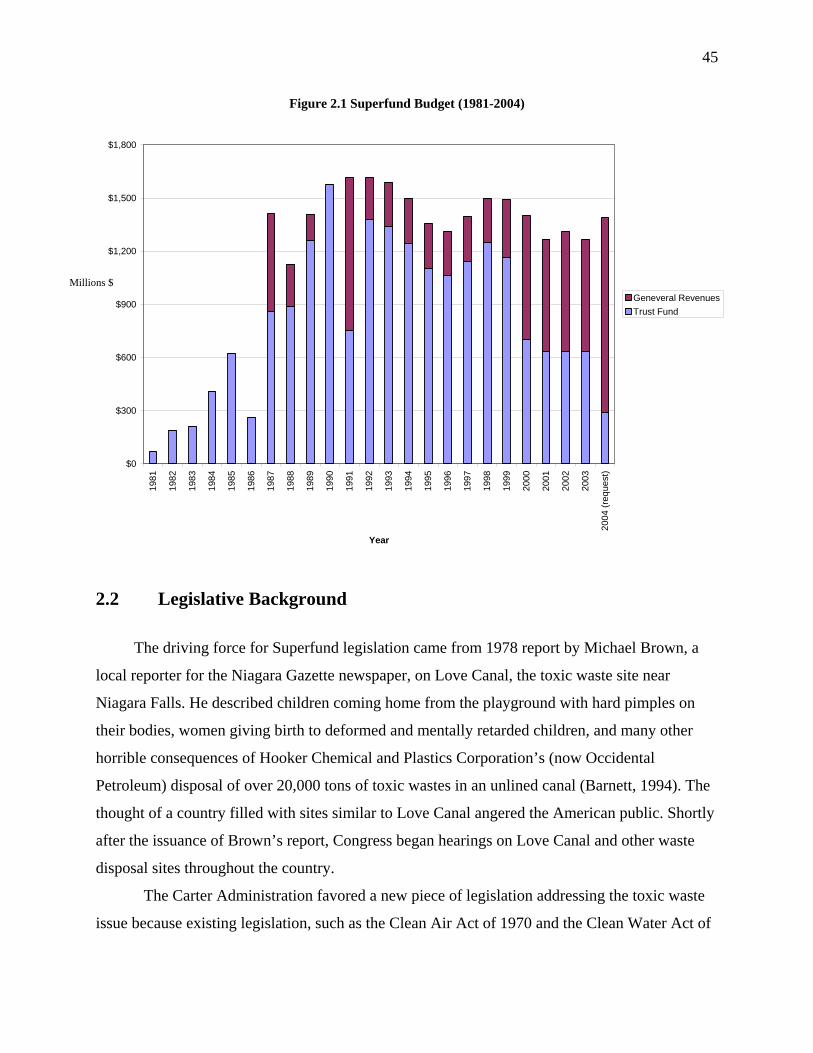
45
Figure 2.1 Superfund Budget (1981-2004)
$0
$300
$600
$900
$1,200
$1,500
$1,80019
81
1982
1983
1984
1985
1986
1987
1988
1989
1990
1991
1992
1993
1994
1995
1996
1997
1998
1999
2000
2001
2002
2003
2004
(req
uest
)
Year
Geneveral RevenuesTrust Fund
2.2 Legislative Background
The driving force for Superfund legislation came from 1978 report by Michael Brown, a
local reporter for the Niagara Gazette newspaper, on Love Canal, the toxic waste site near
Niagara Falls. He described children coming home from the playground with hard pimples on
their bodies, women giving birth to deformed and mentally retarded children, and many other
horrible consequences of Hooker Chemical and Plastics Corporation’s (now Occidental
Petroleum) disposal of over 20,000 tons of toxic wastes in an unlined canal (Barnett, 1994). The
thought of a country filled with sites similar to Love Canal angered the American public. Shortly
after the issuance of Brown’s report, Congress began hearings on Love Canal and other waste
disposal sites throughout the country.
The Carter Administration favored a new piece of legislation addressing the toxic waste
issue because existing legislation, such as the Clean Air Act of 1970 and the Clean Water Act of
Millions $

46
1972, regulated the emission of chemical pollutants, but did not consider the impact of chemical
pollutants and toxic waste on human and ecological health. A key question in the legislative
debate was whether the funds should come from general government revenues or from the
financial contributions of both the offending industry and the government. In mid-1979,
President Carter spoke in favor of a bill with a $1.6 billion fund, financed 80% by industry and
20% by government imposing strict, joint and several liability on responsible polluting parties
(Barnett, 1994). Joint and several liability means that a company, individual, or some
combination thereof, can be held responsible for the entire cleanup of a hazardous waste site
regardless of the amount of pollution contributed to the site. That is, there is no proportionality
with respect to liability. This “deep pockets” principle was highly controversial.
In 1979, several key issues divided the proposed Superfund legislation in the House and
Senate. These included the size of the fund and if the legislation should be limited to abandoned
hazardous waste sites or also include provisions for oil and hazardous substance spills. The
House preferred two separate bills totaling $1.9 billion, while the Senate preferred a $4.1 billion
bill that could be used for both emergency removals and more costly, long lasting projects. Both
the House and Senate, however, agreed the legislation should be financed primarily through
taxes imposed on chemical feed stocks. The chemical industry disputed this overall tax on the
industry and advocated financing the fund through the federal treasury, responsible parties, and
state contributions. The final Superfund bill did not include other House and Senate
recommendations regarding public participation in the siting of hazardous wastes or determining
satisfactory levels of cleanup.
The Comprehensive Environmental Response, Compensation, and Liability Act
(CERCLA) of 1980 (commonly referred to as Superfund) was signed into Public Law 96-510 by
President Carter on December 11, 1980. It passed by wide margins in both the Senate (78 to 9)
and House (274 to 94). The final Superfund bill passed under several unusual circumstances. The
Senate Finance Committee sent the bill forward without a formal recommendation and President
Carter pushed for it to be signed quickly, before Reagan took office. The bill, because it was
rushed, was not based upon an accurate assessment of the problem, and suffered from a lack of
research as well as inaccurate estimates of the potential costs and the number of toxic waste sites.
As noted in a 1985 report funded by the Cato Institute, the law "was based upon

47
misunderstandings and distortions of the situation, and zipped through a lame duck Congress in a
spirit of vengeance against the polluters" (Delong, 1995).
2.3 Comprehensive Environmental Response, Compensation, and
Liability Act
CERCLA created a five-year, $1.6 billion trust fund for the cleanup of active or abandoned
hazardous waste disposal sites that posed an immediate threat to public health and the
environment or when a responsible party would not take action. Superfund called for two
different types of cleanups: (1) Remedial Actions, which ere long-term cleanup for sites on the
National Priority List (NPL), and (2) Removal Actions, which are short-term cleanups of
immediate threats. Removal Actions did not require listing on the NPL.
The trust was funded by the chemical and petroleum industries, which were required to pay
into the fund. The chemical industry ended up paying 85% of the $1.38 billion paid by these two
industries. The States were required to contribute 10% of the total cleanup costs, provide long
term maintenance at sites, and provide disposal capacity for waste removal (Office of
Technological Assessment, 1984). The other component of the Superfund trust included a series
of taxes. Specifically, the bill created a $0.79 per barrel tax on US refineries, crude oil and
petroleum imports, and domestically produced crude oil. Hazardous chemicals and wastes were
taxed at rates varying from $0.22 to $4.87 per ton. After September 30, 1983, there was an
additional excise tax of $2.13 per dry weight ton of hazardous waste received at qualified
hazardous waste disposal sites (Office of Technological Assessment, 1984). The taxing authority
of the CERCLA legislation expired September 30, 1985, though it was reauthorized shortly
thereafter.
Under the CERCLA legislation the EPA was required to assess the nation's hazardous
waste sites according to the hazard ranking system, which is a numerically based screening
system that determines the threat of waste sites to human health. A minimum of 400 of the worst
hazardous waste sites were to be placed on the NPL, and each state was given the opportunity to
place a site on the list as well. The bill also gave the EPA and the Justice Department legal
authority to identify polluting parties, enforce liability, and enlist contributions for cleanup.

48
Superfund imposed strict, joint, and several liability, and the generators of hazardous waste
substances and the owners and operators of waste facilities, past and present, were all liable to
pay for the costs of cleanups. The process for cleanup entailed listing a site on the NPL. Then
scientists conducted a detailed examination of the site called a remedial investigation. This was
followed by a feasibility study, an ascription of the most appropriate cleanup remedies. These
two processes are often referred to as the “remedial investigation/feasibility study” or “RI/FS”.
Once the appropriate remedies were selected, the EPA prepared, or appointed an agency to
prepare specifications and timelines for the cleanup of the site and remediation begins.
2.4 Implementation of Superfund: 1980-1985
The Reagan Administration took office only weeks after the Superfund bill was signed,
and it promoted an ideology that was incompatible with many of Superfund’s legislative
provisions. The objective of the Reagan Program was to promote economic growth by reducing
the size and number of federal spending programs, cutting taxes, and reforming regulatory
agencies (Barnett, 1994). Reagan reduced government spending and emphasized voluntary
compliance with environmental regulations.
Funding Superfund presented an immediate problem. The actual costs of cleanups were
much higher than the original estimates of $7 to $10 million (Barnett, 1994). By 1992, 42 of the
50 states lacked adequate resources to fulfill their obligations to pay 10% of the costs of cleanup
(Office of Technology and Assessment, 1983). During the first three years of the program,
appropriations for Superfund also fell far below those initially authorized by Congress. Of the
$960 million authorized in the first three years, $74.4 million was appropriated in 1981, $26.6
million in 1982, and $210 million in 1983. Most funding for the program was devoted to legal
battles with polluters as well, and the federal government wrote off $270 million because
responsible parties could not be found or were unable to pay (New York Times, 1993). As a
result of these funding setbacks, elements of the Superfund program were cut back in 1981 and
1983. The EPA’s total outlays were cut by one third (Shabecoff, 1983), the abatement and
control staff declined 21%, the enforcement staff decreased 33%, and the research and
development staff declined16% (Crandall and Portney, 1984: 68).

49
While the funding for Superfund was less than originally anticipated, the number of sites
identified for the National Priority List far exceeded expectations. The legislation called for an
identification of at least 400 sites to be added to the NPL. The EPA quickly identified 16,200
potentially hazardous sites and placed 546 sites on the proposed National Priority List. The first
official National Priority List, released in September of 1983, included 406 sites (Environmental
Protection Agency, 1997). The following year, the EPA added 132 more sites to the List bringing
the total up to 538 (Environmental Protection Agency, 1997). While the list continued to grow,
only 119 site removals and two full cleanups were completed by mid-1983 (Davis, 1983).
Various government and private agencies re-estimated the number of sites in need of cleanup.
The new figures were much larger than originally anticipated, and ranged from EPA’s initial
estimate of 2,000 sites to the Office of Technological Assessment's estimate of over 10,000 sites
(Office of Technological Assessment, 1985). As of March 31, 2004, 1,239 sites were listed on
the National Priorities List (NPL).
To further complicate the bill’s implementation, a scandal concerning the manipulation of
hazardous waste programs by some EPA officials erupted in 1982. Top officials were charged
with using political criteria to determine Superfund spending and making "sweetheart" deals with
industry members for partial cleanup, perjury, and the manipulation and destruction of
government files. EPA Administrator Anne Burford and 13 other top EPA officials, including
Rita Lavelle (head of the Superfund program), were forced to resign in March of 1983. This
"Sewergate" scandal dominated the front pages of major newspapers for the first three months of
the year, causing the EPA to lose a considerable amount of legitimacy and some of its own
morale. This scandal, furthermore, undermined the momentum of the already struggling
program.
After the resignation of Administrator Anne Burford, William Ruckelshaus took office in
1983. Ruckelshaus adopted a more aggressive approach to remediation and often used lawsuits
to force industry members into compliance. The EPA financed 102 waste removals within the
first six months of Ruckleshaus’ term and an additional 157 waste removals from 1984 to 1985.
The EPA’s combined outlays in fiscal years 1984 and 1985 totaled over $600 million, a 261%
increase over the $233 million spent between 1981 and 1983 (Barnett, 1994).

50
2.5 1985: The Expiration of Superfund
Superfund legislation expired on September 30, 1985. Debates about reauthorization of the
bill continued for over a year because of uncertainty about how to improve the program's
performance. Reauthorization issues included concerns over health and environmental risks at
waste sites, questions about risk assessment, frustration with lengthy cleanups, and burgeoning
costs. Many cleanup cases were embroiled in legal battles which often expanded into complex
webs of multiple party lawsuits, further compounding Superfund’s problems. The public's
expectations of the program were initially very high, but they found the rate and success of
cleanups disappointing (Office of Technological Assessment, 1984). Changes to the Superfund
legislation were imminent and necessary.
The House and Senate proposed different reauthorization bills in 1985. The House was
overwhelmingly (391 to 33) in favor of a bill creating a five-year, $10.1 billion dollar program.
Revenues would include $3.1 billion from a tax on petroleum companies, $2 billion from a tax
on chemical companies, and $2 billion from a tax on toxic wastes. The Senate proposed a five-
year, $7.5 billion program. General revenues would provide approximately $1 billion with the
remaining $6.5 billion to come from special taxes on manufacturers and processors of raw
materials with annual sales of $5 million or more (Shabecoff, 1985). Environmentalists argued
that the bill would not raise enough money and was described by the Washington representative
of the Sierra Club as "a missed opportunity to build an effective program" (Shabecoff, 1985).
The EPA anticipated that the debate between Congress and the House would continue past
the bill's expiration date and began to halt or slow cleanup at 57 sites in August of 1985 (New
York Times, 1985). As the authorization debate continued through April, the Agency reduced its
response rate to toxic waste emergencies by 80%. Although EPA Administrator Lee Thomas said
that $5 billion was the most EPA was capable of spending over the next five years, the House
and Senate remained firm in their higher requests of $10.1 billion and $7.5 billion respectively
(New York Times, 1985). As a result of the lengthy debates in 1986, appropriations for the
program were reduced from the expected $900 million to $206 million (Shabecoff, 1986).

51
2.6 Superfund Amendments and Reauthorizations
A conference committee finally approved a plan on July 31, 1986 for a five-year, $9 billion
fund. The bill included $500 million for regulating leaky underground storage tanks; created a
new, broad based tax on corporations earning more than $2 million a year; and increased taxes
on oil products (Shabecoff, 1986). Other provisions imposed new regulations throughout all EPA
offices with respect to deadlines and cleanup standards, increased public involvement by
requiring industry to provide local residents with information about chemicals used, and required
the EPA to provide technical assistance grants to communities proximate to NPL sites.
President Reagan signed this bill known as the Superfund Amendments and
Reauthorization Act of 1986 (SARA) on October 17, 1986. After the expiration of Superfund’s
taxing authority, the CERCLA legislation was extended two more times: first for a four-year
period at which time $5.1 billion was authorized for the program and second through December
1995.
The 1986 reauthorization failed to solve many of the Superfund’s problems. The EPA
still lacked adequate financial resources to cleanup many waste sites due to difficulties collecting
money from responsible parties. The liability scheme caused funds to be tied up in legal battles.
The EPA spends approximately 15-18% of the Superfund budget on the legal enforcement of its
cleanup mandates. There were often over 100 PRPs at large sites, creating complex webs of
lawsuits (Barnett, 1994). Responsible parties found it worthwhile to litigate in hopes of
spreading costs among many responsible parties (as opposed to settling) because the average cost
of cleanup at a site was approximately $30 million. A 1993 report funded by the Cato Institute
indicated that, in 1989, insurance companies spent an average of $470 million on costs related to
the Superfund program, $410 million of which went to defending their policy holders (New York
Times, 1992). According to a RAND Corporation survey in 1994, legal fighting over prior
liability was costing a total of $1 billion a year, while fewer than 200 of the most serious 1200
sites had been cleaned up (Quint, 1994).
To help remedy inefficient spending on legal fees, the Congressional Budget Office
(CBO) studied the costs of repealing prior liability, a provision in the Superfund legislation that
holds a company legally responsible for cleanups when the waste was dumped before Superfund

52
was enacted. The CBO found that repealing prior liability would reduce transaction costs and
increase efficiency of the program. It might also, however, reduce the speed of cleanup or require
lowering cleanup standards. Additionally, federal government spending on Superfund would
need to increase by $1.6 billion per year and the government would incur an additional one-time
cost of almost $7.5 billion for PRPs’ ongoing expenses plus $6 billion for past costs (Committee
for the National Institute for the Environment, 1997). Consequently, many government officials
remain opposed to the repeal of prior liability. They believe that the general public should not
have to pay for the costs of hazardous waste cleanup and that tax money should be reserved for
orphan sites and emergency actions.
Other challenges with the Superfund program remain as well. Cleanup times were
criticized as being too slow. According to the General Accounting Office (GAO), the average
time to cleanup a site increased from 3.9 years in 1986 to 10.6 years in 1996 to 11.5 years in
1999. The time it took from discovery of a problem site to its final listing increased from 5.8
years in the 1986-1990 time period to 9.4 years in 1996 (GAO, 1998). The GAO concluded that
these increases are due to the legislation's ambiguous cleanup requirements (GAO, 1998). The
structure of the program was fundamentally flawed because it neither provided contractors with
incentives for cost effective remediation nor encouraged innovation. Responsible parties were
reluctant to try new technology because they feared inadequate results and the possibility of
having to conduct a second costly remediation. The legislation also required copious amounts of
paperwork and authorizations. Critics also were concerned about the EPA’s risk assessment
procedures, claiming that the true risks of most people living near sites are overstated, resulting
in costly remedies and little gain in risk reduction. Polluters and their insurance companies are
dissatisfied with the law's retroactive provisions, requirements to reach "gold plated" cleanups,
and disregard for cost when selecting cleanup remedies (Center for Hazardous Waste
Management, 1997).
In December 1995, Superfund lost the ability to tax, and this taxing authority has not
been renewed. Since taxes on the industry could not finance the Superfund Trust Fund, it began
to rely heavily on appropriations from general revenue. Other income also included fines,
penalties, and cost recoveries. Since 1995, there have been several bills debated in Congress, yet
none have been approved.

53
Reauthorization was a top environmental priority for the 105th and 106th Congresses,
according to Congressional leaders, but action on Superfund legislation never materialized.
President Clinton toured a Superfund site in Wallington, NJ in March 1996 to show his concern
about Superfund’s shortcomings. Reauthorization issues include the size of the fund, broad
liability scheme, high contractor costs, and slow pace of cleanups. Most Republicans, and some
Democrats, continue to support repealing prior liability (Government and Commerce, 1997).
There are also disagreements over who should be required to pay for cleanups, the stringency of
cleanup currently required by the law, whether cleanup results in too few benefits for the costs,
and whether or not to limit the National Priority List. Another issue that has gained more
attention recently is the damage to natural resources, such as rivers, caused by hazardous wastes
(Government and Commerce, 1997). The Senate proposed to allow the addition of only 90 more
sites (30 annually for three years) to the National Priority List. The House proposed to allow 125
sites over an eight-year period, declining from 30 sites in the first year to 10 sites in each of the
last three years.
2.7 Superfund Reforms and Successes
Under the leadership of Carol Browner, in 1995, the EPA implemented three series of
more than 45 administrative reforms designed to strengthen Superfund by targeting its problems
with cleanups and enforcement. The reforms sought the goal of being “faster, fairer, more
efficient” and were similar to provision of the 1994 reauthorization legislation that died in the
previous Congress. These reforms expanded beyond the scope of the reforms in the
reauthorization of 1986 and have been even more successful than originally anticipated
(Nakamura and Church, 2003).
While the federal government maintains control of determining appropriate remedies for
hazardous waste sites, states have recently taken on more responsibility for the cleanup of
Superfund sites. States have developed the capacity and technical expertise necessary for
successful remediation of Superfund sites. Currently, the federal government enters into
cooperative agreements with states, on a site-by-site basis, which authorizes the states to conduct
cleanup activities.

54
In 1995, the EPA also implemented a new "brownfields" economic redevelopment
program. Brownfields are sites contaminated with hazardous waste that are possible candidates
for the National Priority List. These sites often remain abandoned for long periods of time
because they are undesirable to lenders and developers who fear that they will assume liability or
that the land will remain undervalued. To date, the brownfields program has been highly
successful and helps states, communities, and other stakeholders work together to safely and
efficiently cleanup and reuse brownfields (Environmental Protection Agency, 1997).
The Superfund program has been much more successful in recent years as a result of the
aforementioned reforms. As of 2004, more than 82% of the sites on the final Superfund NPL
were either undergoing or had completed cleanup (NACEPT, 2004). Furthermore, the number of
sites added to the National Priority List is currently declining, while the number of sites deleted
is increasing. Only 12 sites were added in 2003, as opposed to 162 additions in 1986. The total
number of sites listed as possible National Priority List sites also decreased over the past years.
In 1988, there were 378 sites on the proposed list. In 2003, 54 sites were on the list. As of 2003,
the total number of sites on the National Priority list is 1,572 while 274 sites have been deleted
from the NPL list. Deletion from the NPL list means that the remedial goals had been achieved
even if operation and maintenance of the site continues (NACEPT, 2004).
Responsible parties were also paying a higher percentage of the cleanup costs than in the
past. Polluters were now contributing more than 75% of long term cleanup costs compared to
37% in 1987 (EPA, 1997). This has saved taxpayers a total of over $12 billion and resulted in the
EPA obtaining over $7.00 in private cleanup commitments for every $1.00 spent in Superfund
enforcement. The EPA also reached settlements with more than 14,000 smaller polluting parties
(such as small businesses and municipal governments) and gave over $457 million in
compensation to responsible parties willing to negotiate long-term cleanup settlements
(Superfund Administrative Reforms, 1996). Moreover, the Justice Department collected $790
million for cleanup activities from responsible parties in 1996. As a result, the EPA was able to
preserve the Superfund budget for sites where responsible parties could not be identified.
In July 2001, the Superfund Subcommittee of the National Advisory Council for
Environmental Policy and Technology was formed to evaluate the Superfund Program. In April
12, 2004, the Final Report was released which recommend improvements to three main areas:

55
what types of sites should be listed on the NPL, how to measure performance, and what to do
about “mega sites” (cleanup costs greater than $50 million).
2.8 Conclusion
Superfund has been controversial since its inception. Many of the problems with the
program, such as high legal costs, inadequate funding, slow pace of cleanups, and high
contractor costs, plagued the program from the outset because it was developed in response to an
emergency situation of uncertain proportions. However, Superfund did have some success in the
1990s. As of 2004, over 82% of the sites on the final Superfund NPL were either undergoing
construction or have completed cleanup. Responsible parties are paying more of the costs of
cleanups, allowing the EPA to conserve its budget for orphaned hazardous waste sites. In the
next chapters, detailed site histories are provided for the six “mega-sites” examined in this study.

56
Chapter 3
Operating Industries, Inc. Landfill
3.1 Overview
The Landfill covers 190 acres and is located 10 miles (16 kilometers) east of Los Angeles
between the communities of Monterey Park and Montebello, California (Figure 3.1). The
Pomona Freeway (Route 60) divides the site into two parcels, one 45-acre area lies north of the
freeway and the other 145-acre parcel lies south of the freeway (Figure 3.2). The landfill is in the
city of Monterey and the city of Montebello borders the southern end and portions of the
northern section of the landfill. Throughout its operating life, from 1948 to 1984, the landfill
received 30 million cubic yards of residential and commercial refuse, industrial wastes, liquid
wastes, and a variety of hazardous wastes. The EPA determined that approximately 4,000
different parties sent waste to the landfill at one point or another. In October 1984, the landfill
was closed and proposed for listing on the National Priority List (NPL). In June 1986, the landfill
was officially listed as a NPL Superfund site, and experts estimated that the cleanup could take
as much as 45 years and more than $600 million to complete. As of 2002, the EPA had reached
settlement with more than 1,250 parties to pay for the cleanup work, with the total settlements
reaching more than $600 million.
Figure 3.1 OII Landfill Vicinity

57
Figure 3.2 OII Landfill

58
The landfill remains a particularly prominent feature of the area, towering more than 300 feet
above the surrounding community.
On the road to completion: OII's final landfill cover along the Pomona Freeway.
According to Katherine Shrine, assistant regional counsel for the EPA Region 9, “This
site is basically a 300-foot-tall, 190-acre mountain of every kind of disposable item in the
world.” Residents say the landfill is so large that it interferes with television reception.
Approximately 53,000 people live within three miles (4.8 kilometers) of the sites, 23,000 within
one mile (1.6 kilometers) of the site, and 2,150 within 1000 feet (0.3 kilometers) of the landfill.
Three schools are located within 1 mile (1.6 kilometers) of the landfill. The area consists of
heavy residential development and mostly middle income and multi-racial neighborhoods.
OII Landfill and Neighboring Community.

59
3.2 History of the Landfill
Before 1970
In 1948, the Monterey Park Disposal Company began municipal dump operations in a
former stone and sand quarry. At this time there was very little development neighboring the site.
Operating Industries, Inc. (OII) purchased the site four years later in January 1952. OII continued
municipal operations, but began accepting industrial wastes at the site as well.
1970-1972
In the early 1970’s, the population of southern California blossomed and development
pressure in areas surrounding Los Angeles increased dramatically. To help alleviate this
pressure, the land surrounding the landfill was approved by Montebello for residential use.
Promised closure of the landfill by the city and proposed development of a golf course on the site
prompted rapid development of the area.
1973-1975
The Pomona Freeway was built in 1974 and intersected the 190-acre landfill. Soon the
middle income communities of Monterey Park and Montebello encircled the OII Landfill.
Landfill activities were restricted to the larger southern area (South Parcel) of the landfill, closest
to Montebello. In compensation for the closure of the North Parcel, the city increased the height
limits on the South Parcel of the landfill.
1976-1978
The increase in the height limit on the South Parcel led to increased erosion, mudslides,
and ultimately exposed refuse. Starting in 1978, leachate seepages were observed periodically on
the slopes of the South Parcel of the OII Landfill. The leachate contained both organic
constituents (such as volatile organic compounds, semi-volatile organic compounds, oil, and
grease) and inorganic constituents (such as metals, ammonia, chloride, and high levels of total
dissolved solids). Large amounts of landfill gas, generated by the natural decomposition of
organic and hazardous wastes, were also reported at the site. Tests of the landfill gas found its
primary components to be methane, nitrogen, carbon dioxide, and volatile organic compounds

60
(approximately 0.05 percent). Threats of contamination at OII stemmed from exposure to toxic
compounds (such as trichloroethane and toluene) and carcinogenic compounds (such as vinyl
chloride, benzene, trichloroethylene, and carbon tetrachloride) via air, groundwater, soil, and
leachate.
Before the EPA’s involvement, numerous state, regional, and local agencies were
involved with the OII site. The earliest government intervention began in March 1978 when the
South Coast Air Quality Management District (SCAQMD) issued an order requiring OII to
follow proper maintenance and disposal procedures. One year later, OII hired Getty Synthetic
Fuels to collect methane gas generated by the landfill. Getty Synthetic Fuels then removed the
methane gas from the site and refined it for commercial purposes but these activities, including
drilling, exacerbated odor problems
1979-1981
In 1980, the Los Angeles County Department of Health Services (LACDOHS) realized
that the original methane gas collection system by itself was insufficient and directed OII to
institute a second gas control system.
Residents near the landfill formed Homeowners to Eliminate Landfill Problems (HELP)
to address increasing odor and potential health problems at the site, as well as specific issues
such as leachate seepage, methane gas buildup, declining property values, and land use after
closure of the site. This organization, comprised of 460 dues-paying families, was an essential
force in the eventual closing of the landfill. According to testimony from Montebello
Councilwoman Norma Lopez-Reid:
“… residents living near the Operating Industries Landfill came home each evening to an
area filled with migrating gases, that made them suffer from headaches, nauseating odors,
and grass-less yards due to the hazardous liquid waste, called leachate, that seeped out of
the ground. These difficult circumstances made the quality of life in this bedroom
community decrease considerably, we couldn't even open our windows on hot summer
nights. Little did our residents know the extent to which companies, large and small, had
been allowed to dump incredible amounts of hazardous waste, including carcinogens,
into the landfill that was only supposed to contain regular trash.”

61
In the early 1980’s, community council meetings became volatile as residents protested
the “assaulting stench” of the air. “We could never open the [house] windows,” said Montebello
resident Phyllis Lee. As another resident stated, “Some nights I wake up coughing at two, three,
four o’clock in the morning. The methane gas is so strong that I have a hard time breathing.”
On March 5, 1981, the Montebello School District passed a resolution objecting to the
landfill odors and ordering an investigation of potential health risks. Later that year, county
health officials cited OII for not controlling the migration of potentially hazardous gasses. The
OII Landfill was ordered to temporarily shut down.
1982-1984
Despite resident complaints, heavy criticism from state health and air quality officials,
possible $1,000 per day operating fines, and the previous temporary order to shutdown, OII
reopened and continued to operate. Finally, in January 1983, OII ceased accepting hazardous
liquid waste. In April, they stopped accepting any liquid waste. Also in April, offsite levels of
vinyl chloride gas (a known carcinogen) were measured at 19 parts per billion (the state
regulated level at that time for vinyl chloride was 10 parts per billion), however, in a random
sample of 12 homes elevated levels of vinyl chloride gas were not detected. In June, a buildup of
methane within the landfill caused several underground fires. Potentially explosive levels of
methane were also discovered underneath city streets adjacent to the landfill. Levels of air-borne
vinyl chloride in excess of EPA and state health standards were also detected around the site.
However, the LA County Department of Health released a 1983 study showing no pattern of
school absence and that there was not excess mortality around the OII Landfill compared to other
areas of Los Angeles.
In January 1984, the State of California placed the OII Landfill on the California
Hazardous Waste Priority List.
In August 1984, the LACDOHS cited OII for allowing landfill gas concentrations which
exceeded the lower explosive limit (5% methane in air) to migrate beyond landfill boundaries.
That same month, California Department of Health Services (CADOH) also issued its first
Remedial Action Order against OII. It required OII to completely phase out the on-site disposal

62
of leachate and to provide plans for implementing leachate collection and treatment systems, site
characterization and groundwater monitoring programs, landfill gas collection and monitoring
programs, and slope stability corrective measures.
In October 1984, after four years of legal battles, public hearings, and tremendous
community public hearings, SCAQMD issued a second order of abatement requiring the landfill
to close permanently, thereby ending the disposal of all solid wastes. This order also instructed
OII to install a landfill gas emission control system, a permanent leachate control system, and
also to perform specified landfill maintenance. Soon after the closure of the landfill, the owner of
OII declared bankruptcy.
Also in October, the EPA proposed OII for the federal Superfund NPL, making it eligible
for federal Superfund money. Likewise, the California Regional Water Quality Control Board
(RWQCB) issued its own abatement order requiring that the on-site disposal of leachate be
phased out.
In December 1984, the EPA dug six wells around the OII site to test for possible
groundwater contamination. The test results showed organics and trace mineral contamination in
three of the wells, but no pesticide contamination. Fortunately, the drinking water used by the
neighboring residents of the landfill came from a number of municipal water companies, which
did not operate any wells located on or near the site. However, based on their initial tests, the
EPA decided to conduct further testing to determine the specific location and potential
movement of the groundwater contamination. The EPA installed an additional 24 wells around
the perimeter of the site, which tested positively for soil and groundwater contamination.
1985-1987
In April 1985, while the OII Landfill awaited its final federal NPL listing, the EPA began
its Remedial Investigation/Feasibility Study (RI/FS) which assessed and prioritized remedial
actions for the site. This did not, however, assuage state concerns about the site. One month later,
the California Waste Management Board (CWMB) joined the CADOHS and filed a joint suit
against OII for not complying with the CADOHS’s first Remedial Action Order issued in August
1984.

63
In June 1986, the EPA placed the landfill on the NPL of Superfund sites and assumed
responsibility for all remedial activities at the site. Shortly after the NPL listing of the site, the
California Department of Health Services conducted an extensive epidemiological investigation
comparing health symptoms of residents near the site with those of control communities (Satin et
al., 1986). The results indicated no significant differences between the health of local residents
and that of control communities.
The EPA began its search for OII’s PRPs concurrent with the NPL listing. Because of the
nature of landfills, the EPA estimated that as many as 4,000 companies were potentially liable
for dumping hazardous waste at the OII Landfill during its operable years. Although not all of
these PRPs contributed to the cleanup of the landfill, the first of several cleanup agreements was
signed in May 1989 between the EPA and over 110 polluting companies. Valued at
approximately $66 million, this First Partial Consent Decree required site control and monitoring
activities and construction of an interim leachate treatment facility. In return for their immediate
cooperation and financial contributions, the Consent Decree released from future liability several
large national corporations including Mobil, Exxon, and General Motors. A group of PRPs then
organized the OII Steering Committee, of which OII was not a part, to handle legal and
environmental issues at the site. This committee eventually formed a corporation called the
Coalition Undertaking Remedial Efforts, Inc. (CURE), which would remediate leachate at the
site according to the established leachate management plan.
The EPA signed its first Record of Decision (ROD) for the OII site in July 1987,
authorizing short-term control and management activities to prevent further contamination and
exposure to potential health risks. One such action included fencing the site and posting a guard
at the entrance to ensure that no trespassers come into contact with the contaminants. Other
emergency measures included gas migration control measures, slope stability, leachate control
measures, erosion control, and runoff and drainage improvements.
Once these emergency measures were in place, the EPA signed the second ROD, in
November, for control and cleanup of leachate at the site. The EPA proposed several alternative
plans and submitted its draft plan for public review. As it often did for area residents, the EPA
extended the 30-day public comment period to allow ample time for all interested parties to
respond. Based on these public comments, the EPA decided to replace the system of off-site

64
leachate treatment with an on-site treatment plant because it found this alternative to be more
acceptable, more cost effective, and more protective of public health and the environment. While
the surrounding communities were supportive of this decision, they were greatly concerned that
the plant might be used to process liquid wastes from other sites as well. The EPA assured local
citizens that only liquids generated from the OII site would be treated at the on-site plant, and
then preceded with its remedial plan. The plant would treat 43,200 gallons of OII leachate per
day, test it for compliance, and then discharge it into the Los Angeles County Sanitation District
sewer system. Natural attenuation and degradation of contaminants would also help reduce
groundwater contaminant levels beyond the site boundary, and the EPA agreed to routinely
monitor groundwater under and near the site.
1988-1990
Landfill gas migration was the second major problem the EPA addressed at the OII
Landfill. The EPA’s third ROD for OII called for special gas migration and treatment studies so
that gas control systems could be improved prior to the final site cleanup. The results of these
studies called for the design and construction of a new gas flare facility (thermal destruction
facility), new gas piping and extraction wells, use of existing extraction wells until they are no
longer functional, discontinuing use of the air dike system, construction of additional gas
monitoring probes, and the installation of gas extraction wells on the North Parcel. Fifty gas
wells were also installed in the South Parcel to help control gas and liquid migration. During this
time, the EPA notified residents that workers wearing protective gear and loud drilling noises
would be present at the site for several months. The EPA estimated that with these improvements
70% more of the landfill gas would be collected, but that the landfill still would not reach the
EPA’s goal for surface emissions until the final landfill cover was put into place.
The cost of the leachate treatment facility was estimated to be $1.6 million, with annual
operation and maintenance cost of $700,000. Although the plant was originally scheduled for
construction in the summer of 1988, it was delayed almost a year because of the lack of
appropriate funding and the long processes of public comment and facility design and
finalization. Likewise, plant operation, scheduled to begin in early 1989, did not begin until
August 1994.

65
In 1989, a Consent Decree was signed by the EPA and more than 100 companies that
disposed wastes during the operation of the landfill. These companies formed a committee to
examine the issues facing the cleanup effort. Also in 1989, over 100 businesses and public
entities filed a lawsuit against other PRP’s to share in the cleanup costs.
As part of the gas control system, the EPA amended the ROD to add a landfill cover that
sought to better control gas emissions and improve surface water management. The existing
cover was highly variable in its thickness and ability to limit surface emissions and odor. A new
landfill cover would make gas control remedies more effective and efficient, reduce the amount
of gas escaping into the atmosphere, and facilitate the cost effectiveness of the final site remedy.
The new landfill cover sought to keep water and oxygen out of the landfill and prevent erosion
and run-off from the landfill’s slopes. The cover also was designed to improve the appearance of
the site. Vegetation has been planted, whenever possible, over the cover. The EPA estimated that
the construction of the landfill cover would cost between $61 million and $116 million dollars.
1991-1993
In 1991, the EPA extended the settlement offer to another 154 PRPs, which resulted in a
Second Partial Consent Decree similar to the first. In August, 63 of the 154 companies signed the
Second Partial Consent Decree worth $8.5 million. Those that did not sign the agreement denied
the charges, asserted that they dumped only non-hazardous materials at the site, or maintained
that their refuse dumping records didn’t exist or were unrecoverable. A third settlement between
the EPA and approximately 178 PRPs was reached in December 1991. It required the
defendants, later organized into a corporation called the New CURE, to implement major
portions of the gas control and landfill cover remedies, improvements worth $130 million.
In addition, the EPA sent letters to more than 50 additional PRPs informing them of their
liability at the site. During this time, several private companies brought suit against nearby
communities to make them liable for contaminants dumped at the landfill. To recoup legal costs
resulting from these accusations, one city raised trash collection rates and several other cities
sued trash haulers.
In November 1991, the EPA installed another 21 wells beyond the perimeter of the site,
which determined that groundwater contamination had not spread beyond the boundaries of the

66
landfill. In total, the EPA constructed 75 wells and conducted six major hydrologic
investigations over the course of 28 years.
In April 1992, Judge Mariana R. Pfaelzer of Montebello, California, enforced the
previous $130 million agreement. The EPA also entered into another Consent Decree with a
variety of contributing companies to begin the initial cleanup activities related to gas control and
landfill cover as designed by the EPA.
Implementation of gas control remedies began in 1992. The construction, operation, and
maintenance of these remedies were estimated to cost $73 million over a 30-year period. From
1993 to March 1994, during the construction of the new gas flare facility, low levels of vinyl
chloride escaped into the atmosphere because the temperature of the old gas flare treatment
system was insufficient to incinerate the gas. Although they had no way of monitoring emissions,
the EPA maintained there was no problem with air quality. However, the EPA still tested 197
Montebello homes for vinyl chlorine. Four percent of the homes tested positively and the EPA
installed gas management systems to aerate the homes and prevent further the contamination
from entering the houses. The EPA is required to monitor these homes for ten years.
1994-1996
In 1994, the leachate treatment facility began operations. A settlement was reached in
1994 that resolved the 1989 lawsuit filed by 137 businesses and public entities that had already
contributed more than $200 million to the cleanup efforts.
In April 1995, a Fourth Partial Consent Decree was reached between the United States,
the State of California, several private companies, 14 cities and municipalities that disposed of
municipal waste at the landfill, and those who transported municipal waste to the landfill. The
agreement provided $51 million for the Final Remedy and construction of a Thermal Destruction
Facility on the North Parcel.
In March 1996, thirty companies signed a final Fifth Partial Consent Decree to pay $18.7
million for interim site costs and the Final Remedy. In total, over $270 million had been
collected from almost 400 different entities for the cleanup of the OII Landfill. This estimate
represents only private money contributed to site cleanup. An additional estimated $165 million
of public dollars will be spent for site remediation.

67
In September 1996, the fourth OII ROD for Final Site Remedy was signed. The EPA
agreed to evaluate and monitor the site and the success of their cleanup efforts every five years
after the remedial action plan is implemented. The EPA also decided to replace the gas flare
disposal system with a new landfill gas thermal destruction facility, which would be used to treat
or destroy landfill gas produced at the site.
1997-1999
In mid-February, 50 new testing wells were installed on the southern and western
perimeter of the former OII Landfill near Montebello. These wells were designed to better
control gas and liquid migration from the landfill. The EPA advised residents to not interpret the
workers protective clothing as an indicator of a “hazard for the neighborhood”. Additionally they
emphasized that during the drilling process “there will be no contamination hazard to nearby
residents during these activities” (emphasis in original).
Additionally, construction of the landfill cover began. The EPA mailed out a special
notice to residents informing them of the upcoming constructions and possible disturbances that
may result. Construction of the cover involved moving six million cubic yards of soil. The old
dirt on the landfill was removed and was replaced with a six-foot-thick “monocover”of clean
soil. A variety of native vegetation including grasses and shrubs was added to the slopes of the
landfill and the flat top of the landfill was covered by a multi-layer “geosynthetic clay liner” (a
system of woven matting and clay). The objective of both covers was to prevent rainwater from
entering the landfill and to stop gas from escaping.
In March 1997, the EPA issued a universal administrative order requiring seven more
companies, which collectively dumped six million gallons of hazardous substance into to the OII
Landfill, to contribute to OII’s remediation. Specifically, these companies are responsible for
maintaining the on-site leachate treatment facility until December 1999, which will cost a total of
approximately three million dollars.
In 1999, the EPA reached a settlement with 327 parties which allegedly disposed small
amounts of waste at OII. These parties contributed between 4,200 and 110,000 gallons of waste.
After 1999

68
In 2000, the landfill cap and the new gas control systems (Thermal Destruction Facility)
were essentially completed, gas flares were replaced and the treatment of groundwater
commenced. Development of a shopping center at the North Parcel of the landfill began. This
North Parcel was not significantly affected by the hazardous waste and is one of the largest
pieces of undeveloped property in the Los Angeles area.
In December 2001, a $340 million settlement was signed with 161 PRP’s. This was the
eighth settlement since 1986. Settlements up to this point had totaled over $600 million.
Also in 2001, the construction of the ground water remedy was completed and the EPA
ended its in-home monitoring and random sampling programs after it found no evidence of a
problem in any of the houses for several years.
The eighth Consent Decree was approved in May 2002, which outlined the final cleanup
remedies.
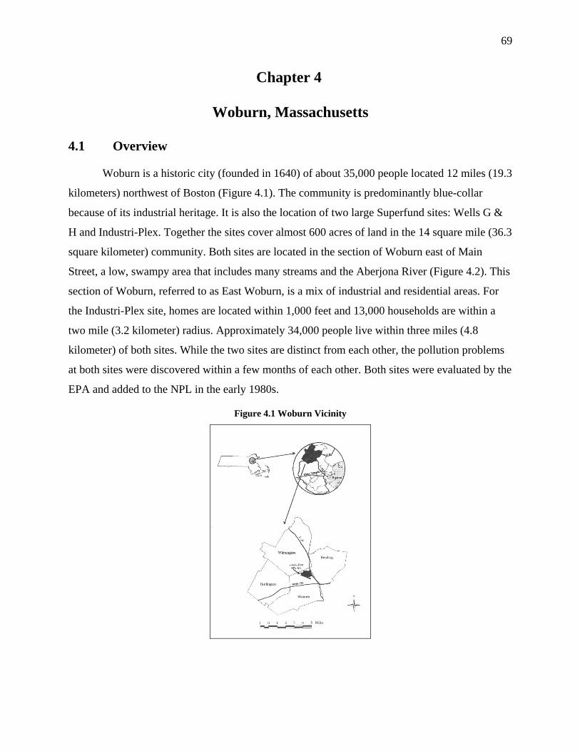
69
Chapter 4
Woburn, Massachusetts
4.1 Overview
Woburn is a historic city (founded in 1640) of about 35,000 people located 12 miles (19.3
kilometers) northwest of Boston (Figure 4.1). The community is predominantly blue-collar
because of its industrial heritage. It is also the location of two large Superfund sites: Wells G &
H and Industri-Plex. Together the sites cover almost 600 acres of land in the 14 square mile (36.3
square kilometer) community. Both sites are located in the section of Woburn east of Main
Street, a low, swampy area that includes many streams and the Aberjona River (Figure 4.2). This
section of Woburn, referred to as East Woburn, is a mix of industrial and residential areas. For
the Industri-Plex site, homes are located within 1,000 feet and 13,000 households are within a
two mile (3.2 kilometer) radius. Approximately 34,000 people live within three miles (4.8
kilometer) of both sites. While the two sites are distinct from each other, the pollution problems
at both sites were discovered within a few months of each other. Both sites were evaluated by the
EPA and added to the NPL in the early 1980s.
Figure 4.1 Woburn Vicinity

70
Figure 4.2 Industri-Plex and Wells G&H Sites

71
Throughout Woburn’s history, more than 100 companies used the Aberjona River, which
flows through the city, for industrial waste disposal. Companies dumped wastes on land, into
lagoons and ponds adjacent to the river, as well as directly into the river itself. From 1853 to
1931, compounds and chemicals such as acetic acid, sulfuric acid, lead, arsenic, chromium,
benzene and toluene were dumped behind buildings, used as fill for low spots, and included in
construction material for dikes and levees. Woburn has a long history of public health problems,
including elevated rates of kidney and liver cancer, colon-rectal cancer, child and adult leukemia,
male breast cancer, melanoma, multiple myeloma, and brain and lung cancer.
The 330-acre Wells G & H site is located near the Aberjona River, about one and a
quarter miles (2 kilometers) downstream (south) of the Industri-Plex site. It once ranked as the
tenth worst site on the EPA’s NPL list. The site is the location of two drinking water wells for
the city of Woburn, which were built in 1964 (Well G) and 1967 (Well H). These wells were
located near an automobile graveyard, an industrial barrel cleaning and reclamation company, a
waste oil refinery, a tannery, a dry cleaner, and a machinery manufacturer. Despite public
complaints about the water from these wells, Woburn continued to use the wells, especially
during the summer. Both wells were finally closed in 1979 after testing showed that the water
was contaminated. Soil and groundwater at the site are contaminated with volatile organic
compounds (VOCs), such as trichlorethylene (TCE) and tetrachloroethylene (also called
perchlorethylne, PCE, or ‘perc’). Land in this area is zoned for industrial and commercial use,
with some areas for residential and recreational use.
The Industri-Plex site, the location of Woburn’s most intensive industrial activity since
the 1850s, consists of 245 acres in an industrial park and once ranked as the fifth worst site on
the EPA’s NPL. This area is located one mile (1.6 kilometers) northwest of the intersection of
Interstate 93 and Route 128 and is bordered by the communities of Wilmington and Reading.
Two tributaries of the Aberjona River flow through the Industri-Plex site. Of the 245 acres at the
site, one-third was contaminated and 60 acres were used for commercial purposes throughout the
remediation of the site. Contamination at the Industri-Plex site includes heavy metals and
hydrocarbons. In the soil, the contamination was primarily arsenic, lead, and chromium and in
the water the contamination was primarily benzene, toluene, arsenic, and chromium.

72
Additionally, hydrogen sulfide gas emanating from buried animal hides from the tanneries and
wastes once permeated the air.
Redevelopment plans are now underway for the Industri-Plex site and consist of a
Regional Transportation Center (train station, park and ride), a recycling center, highway
interchange, an office park, and retail space. This development is expected to yield between
12,000 and 16,000 jobs by 2010, relieve traffic congestion in Woburn, and help the Boston area
come into compliance with EPA air emissions standards by enhancing public transportation in
the area. However, as of 1999, the City of Woburn estimated that the number of permanent jobs
at the redeveloped site was 4,315.
Groundwater remediation and monitoring now constitute the bulk of the remaining work
to be done. As of December 1998, three groundwater treatment plants operating at the site had
pumped and treated more than 150 million gallons of water. In addition, all the contaminated soil
has been removed (approximately 150 tons) and 1,360 pounds of VOCs have been destroyed.
Although major strides in the remediation of the property have taken place, according to EPA
lawyers, complete cleanup of the site will cost approximately $80 million and could take another
20-30 years because of the site’s extensive groundwater contamination.
4.2 History of Woburn and its Superfund Sites
1600-1700’s
Woburn was incorporated as a town in 1640 and shortly thereafter became a center of
manufacturing in New England, because its location was ideal for industry because of its
accessibility to major transportation throughways (roadways and seaports) and proximity to the
consumer market of Boston. In 1648, the first tannery opened in Woburn.
1800’s
In the mid-1800s, Woburn became known for shoe manufacturing. Local manufacturing
activity later shifted from shoes to leather production, and Woburn became a leader in the U.S.
tanning industry by 1865. By 1884, Woburn was home to 26 large tanneries that employed
approximately 1,500 employees and produced $4.5 million worth of leather. At the peak of

73
Woburn’s tanning industry, from 1900 to 1934, an estimated 2,000 to 4,000 tons of chromium
was dumped directly into Woburn’s water resources, as well as 65 to 140 tons of copper, 85 to
175 tons of lead, and 40 to 75 tons of zinc.
Numerous chemical manufacturing firms occupied the Industri-Plex land, which is
upstream from water Wells G & H, for almost 150 years. In the 1800s, several firms operated on
the site, producing chemicals for the local tanning, textile, and paper industries. In 1863,
theMerrimac Chemical Company (Merrimac) became the leading industry on the site.
1900’s
From 1863 to 1931, Merrimac produced lead-arsenic insecticides, TNT and other
explosives, dyes, and organic chemicals such as phenol, benzene, and toluene. Between 1900 and
1914, Merrimac was one of the largest producers of arsenic insecticides in the country. In 1915,
as part of the war effort, industry in Woburn began to diversify to include munitions, chemicals,
and insecticides. (Until the war, Germany had been the major source of these chemicals.) By
1917, Merrimac had grown into the largest chemical manufacturer in New England.
1920’s
The City of Woburn built a sewer due to concerns about pollution of the Aberjona River
and Upper Mystic Lake. Monsanto acquired Merrimac in 1929 and moved the chemical
operations off the Industri-Plex site in 1931.
1930’s
In 1934, Monsanto sold the Industri-Plex land. Between 1934 and 1968, the companies
that occupied the Industri-Plex site manufactured glue and gelatin by extracting collagen from
animal hides and chrome-tanned leather. Wastes generated by these processes included animal
hide residues and metals such as arsenic, lead, and chromium. These wastes were generally
deposited on top of existing waste deposits. Waste piles, including the animal hides, covered tens
of acres and reached heights of 40 to 50 feet above the natural grade.
1950’s

74
In the 1950s, East Woburn began discussing the need for additional water supplies for the
city’s expanding population. In 1958, the city hired an engineering consultant to examine the
possibility of utilizing the Aberjona River water for drinking. Although the consultant concluded
that the water was too heavily contaminated to be safe for drinking, the city began constructing
two new wells, Wells G & H.
1960’s
Water Wells G & H, located on the east side of town, began operating in 1964 and 1967,
respectively, to provide Woburn’s growing population with drinking water. At that time, these
two wells supplied 30% of the city’s drinking water. The 330-acre Wells G & H site contains
five contaminated properties bounded by Route 128 to the south, Interstate 93 to the east, the
Boston and Maine Railroad to the west, and Salem Street to the south. The Aberjona River also
flows through the site, through on-site wetlands found immediately adjacent to both sides of the
river, and into the Mystic Lakes. The Mystic Lakes are a popular recreational destination
including swimming and fishing.
Shortly after the installation of the two wells, residents of East Woburn complained that
the water smelled and tasted funny, corroded their pipes, discolored their dishwashers, and
stained clothing and fixtures. Prompted by citizen complaints, city officials tested the water from
the two wells. Test results only revealed high levels of salts in the water and officials
downplayed citizen’s concerns about the water.
In 1967, the Massachusetts State Department of Health (MSDH) recommended that Well
G & H be closed because of concerns about bacteria and only recommended their use in
conjunction with continuous chlorination. Soon residents reported concerns about their water
tasting like “bleach”. In the spring and summer of 1968, residents complained about their “red
water,” but city officials claimed it was due to the city’s unlined old cast iron pipe. MSDH gave
the city permission to add sodium hexametaphosphate (“Calgon”) to Well G & H to remedy the
problem and to adjust the water’s pH content. In an attempt to find a long term water supply
solution that did not involve the use of Wells G & H, the Woburn City Council authorized the
Mayor to negotiate with the Metropolitan District Commission (MDC) about joining its water
system with the neighboring town of Stoneham. Starting in February 1969, the City of Woburn

75
increased the chlorine feed at Well G by 50%. Due to resident’s complaints, Well G was closed
for the winter starting in October.
At Industri-Plex, Stauffer Chemical Company (Stauffer) bought the last of the glue
manufacturers in the 1960s and ceased operation in 1968. In 1968, Mark Philip Realty Trust (MP
Trust), a real estate developer, bought the Industri-Plex land from Stauffer to develop it as an
industrial park. MP Trust began preparing for construction of a shopping mall and an industrial
park. In 1969, the project started illegally without a permit, though a permit was obtained a year
later. The construction at Industri-Plex involved moving piles of waste accumulated over 130
years and filling in low-lying areas and wetlands.
Early 1970’s
Throughout the early 1970s, despite the repeated reassurances from city and state
officials, the citizens of East Woburn continued to express concerns about the water from Wells
G & H. In response to public pressure, Well G was frequently turned off in the winter when
water was more abundant only to be called into service again during hot, dry summers.
Voluntary water restrictions were put into place in 1972 and 1973 to avoid use of the wells,
while the city continued to work with MDC to provide a long-term water solution. In the summer
of 1974, water shortages forced the city to consider activating both Wells G & H, which caused a
“storm of protest” from residents. In 1975, a fire destroying the MDC pumping state at Spot
Pond in Stoneham interrupted construction of the water main connecting Woburn and MDC.
In 1975, as part of the development of the south end of Industri-Plex, 20 acres of animal
hide piles and animal glue waste were disrupted releasing hydrogen sulfide fumes into the air.
This "rotten egg" smell, extremely potent at times, elicited numerous complaints from citizens of
Woburn and the neighboring Town of Reading, downwind of Industri-Plex. Citizens and the
media referred to the omni-present stench as the “Woburn odor.” This odor at times prevented
children from playing outside during noon recess at school and residents of affected areas
claimed that they could not use their yards. When the odor was strong, citizens working outside
complained of nausea, burning eyes, and difficulty breathing. Residents even mentioned that the
airborne chemicals caused the exterior paint on their houses to peel. Large open-air pits of waste
at the site allowed humans and animals to come into direct contact with the contaminants.

76
According to one Woburn mother, “It was only a five-minute walk and you see the open pits
filled with chemicals. We used to go blueberry picking where they found the arsenic.”
The Massachusetts Department of Environmental Quality Engineering (MDEQE) [now
the Massachusetts Department of Environmental Protection] issued MP Trust numerous violation
notices, orders to halt construction, and requests to cleanup wastes at the Industri-Plex site. In
1977, MDEQE and the Town of Reading filed a lawsuit against MP Trust demanding that MP
Trust be prohibited from disturbing the two parcels where the glue waste was buried. However,
MP Trust continued its construction because it had the permission of Massachusetts Department
of Health (MDOH) (which was responsible for hazardous waste management at that time) to
excavate and dispose of hazardous wastes on the site. “It [remediation] would make the land too
expensive to develop. It [the waste] can stay there as far as I’m concerned,” said William
D’Annolfo, owner of MP Trust.
1978-1979
The major pollution problems at both of Woburn’s Superfund sites were discovered
within six months of each other.
Abandoned 55-gallon Drum with the Entire Side Corroded; Found Near Wells G & H.
Wells G&H. In May 1979, construction workers discovered that 184 55-gallon barrels of waste
had been dumped near the Wells G & H. Immediately after this discovery, the MDEQE tested
the wells for possible contamination. These tests revealed high concentrations of several VOCs,
known carcinogens in animals, but indicated that the barrels were not the source. Officials were
particularly concerned about TCE and perc in the well water because TCE levels tested as high
77
as 267 parts per billion and VOC levels tested as high as 100 parts per billion. (The EPA
considered anything more than 27 parts per billion and 5 parts per billion, respectively, to be
hazardous.) Additionally, river sediments were found to be contaminated with polycyclic
aromatic hydrocarbons (PAHs) and heavy metals such as chromium, zinc, mercury, and arsenic.
Adjacent soils also contained PAHs, poly-chlorinated biphenyls (PCBs), VOCs, and pesticides.
Anyone coming into contact, swallowing, or ingesting this groundwater, soil, or river sediments
would be at risk.
Although the EPA discovered these problems with Wells G & H in July of 1979, Woburn
officials and residents were not notified of the problem by the EPA, COE, or MDEQE until an
enterprising reporter released the information in a local newspaper story. The problems described
in the news story and the lack of notification by the official organizations involved, generated
much outrage and distrust on the part of local citizens. Likewise, contamination at Industri-Plex
was documented in federal and state COE and EPA records in August 1979, but local officials
were notified of the contamination not through official channels but, again, by a local newspaper
article reporting the results of EPA investigations conducted earlier that summer.
Industri-Plex. At Industri-Plex, the Massachusetts Department of Environmental Protection
(MDEP) asked the Army Corps of Engineers (COE) to investigate alleged wetlands violations
and help control the activities of MP Trust. After conducting a preliminary survey of the site, the
COE solicited the help of EPA. In late 1979, based on their discovery of illegal filling of
wetlands, the EPA and the U.S. Attorney’s office (on behalf of the Army Corps of Engineers)
obtained a court order against MP Trust to stop development at the Industri-Plex site.
Additionally, the EPA discovered pits of buried animal hair and barrels of slaughterhouse waste.
In December, regional EPA officials requested funds for the installation of a permanent air
monitoring station for North Woburn.
Groundwater was contaminated with arsenic and VOCs, including benzene and toluene,
and soil was extensively contaminated with arsenic, chromium, and lead. Benzene has been
proven to cause leukemia. In fact, EPA investigations revealed a football field-sized arsenic pit
that rose 40 feet into the air. Arsenic was used in the production of lead-arsenate, an insecticide
that was replaced by DDT in the 1940s. Arsenic is a known human carcinogen and can cause

78
skin tumors when ingested, and lung tumors when inhaled. Arsenic is also linked to
chromosomal damage in humans and animals. Measured arsenic concentrations in this pit
reached as high as 1,100 parts per million (ppm) and debris from the pit was detected on the
slopes of Route 93, a half-mile away (0.8 kilometers). Although EPA officials were uncertain
about when the arsenic was dumped, they believed it dates between 1899 and 1934, meaning that
the arsenic has been in Woburn soil for 85 to 100 years. Other contaminants permeated the site
as well. Recorded levels of chromium reached 3,000 ppm in one place and 78,000 ppm in
another. The concentration of lead was as high as 1,200 ppm. At the time, the standards for both
of these contaminants were 0.05 ppm.
Community Reaction. The discovery of two major hazardous waste problems in one town
prompted strong media interest as well as the active response and involvement of Woburn’s
residents. Area newspapers and TV stations ran multi-part stories about Woburn, alluding to it as
a “toxic wasteland.” Local newspapers and magazines featured articles with headlines such as:
“Lagoon of Arsenic Discovered in North Woburn” (The Daily Times, September 10, 1979),
“Chasing A Radioactive Ghost” (The Daily Times, October 16, 1979), “Deaths From Cancer
Increase in Woburn” (The Daily Times, December 12, 1979). In particular, The Daily Times
published two notorious articles about Woburn’s hazardous waste contamination, which reported
higher rates of adult and childhood leukemia, bone and skin cancer, prostate cancer in men, and
breast cancer. However, the estimates quoted in the article were not confirmed by MDOH until
the following spring. Interestingly, in its final report, the MDOH used the same statistics
reported in The Daily Times months earlier.
One east Woburn resident, Anne Anderson, began to suspect a link between the well
water and her son’s leukemia. “From the time we moved here, the water was bad in the summer.
It had an unpleasant odor and a terrible taste,” she later recalled. “My mother brought jars of
MDC water when she came to visit. The kids used to always ask for ‘Nana water.’ It was like a
mother’s milk, for God’s sake. She still brings it when she visits.” Anderson began recognizing
some of her neighbors at the hospital, who were also there with children suffering from
leukemia. “I just don’t see where all the leukemia cases in our area aren’t correlated,” she said.
“It seems they have to be. The thing that strikes me is there are two neighbors off of Pine Street
79
who have children with leukemia. A year later people on the other side of the street had their
child diagnosed and two people we know personally were diagnosed.” Her husband continued,
“Before, in all of my life, I knew of only one child with leukemia. But these are all in Woburn.”
Anderson had requested that city officials test the water, but she was informed that it was not
standard procedure to perform such tests on the basis of one individual’s request. Unsatisfied
with this response, Anderson, with the help of her minister Reverend Bruce Young, convened a
meeting in September 1979 for parents of children with leukemia. Attendees of that meeting
counted the number of local leukemia cases and mapped the homes of the sick children—eight
leukemia cases were clustered within one square mile (1.6 square kilometers) in East Woburn,
six in a six-block square served by Wells G & H.1 Sparked by these findings, the citizens of
Woburn formed the group For A Cleaner Environment (FACE) in October 1979. Two months
later (December), FACE and the doctor treating Woburn children with leukemia convinced the
Woburn City Council to contact the Centers for Disease Control (CDC). After examining the
situation, the CDC found that Woburn’s childhood leukemia rate was two to three times that of
the national average and four times the average of other communities the size of Woburn. As
CDC described it, Woburn had the most persistent leukemia cluster it had ever seen.
Later that December, MDOH released a preliminary report on the second five-year study2
of the health effects of Woburn’s drinking water, which contradicted the clustering of leukemia
in East Woburn and the pronouncements of CDC. It stated that Woburn had a higher than normal
incidence of many cancers but that there was no “association between environmental hazards and
the incidence of childhood leukemia.” (As later determined, the state had used in its
calculations, a population estimate for Woburn, taken from the 1970 Census, which was much
greater than Woburn’s population at the time the study was conducted.) When MDOH corrected
this inaccuracy, its calculations revealed several statistically significant rates of cancer and
leukemia.
1980-1982
1 Between 1964 and 1997, 28 leukemia cases were diagnosed in Woburn. Of these 28 cases, 16 resulted in death. (The last case of documented childhood leukemia in Woburn was reported in 1986.) 2 Dr. Robert Tuthill and Dr. Leslie Lipworth, of the University of Massachusetts, conducted the first five-year study, which found a slightly elevated but statistically insignificant increase in Woburn’s rates of cancer and leukemia.
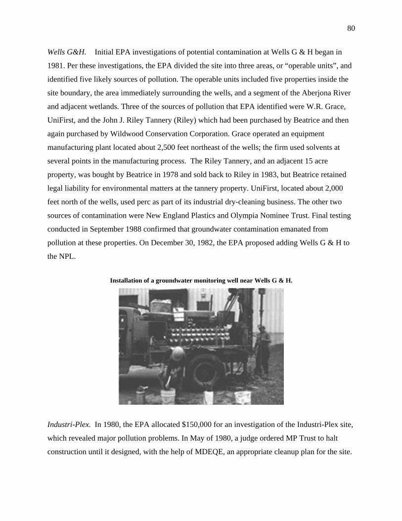
80
Wells G&H. Initial EPA investigations of potential contamination at Wells G & H began in
1981. Per these investigations, the EPA divided the site into three areas, or “operable units”, and
identified five likely sources of pollution. The operable units included five properties inside the
site boundary, the area immediately surrounding the wells, and a segment of the Aberjona River
and adjacent wetlands. Three of the sources of pollution that EPA identified were W.R. Grace,
UniFirst, and the John J. Riley Tannery (Riley) which had been purchased by Beatrice and then
again purchased by Wildwood Conservation Corporation. Grace operated an equipment
manufacturing plant located about 2,500 feet northeast of the wells; the firm used solvents at
several points in the manufacturing process. The Riley Tannery, and an adjacent 15 acre
property, was bought by Beatrice in 1978 and sold back to Riley in 1983, but Beatrice retained
legal liability for environmental matters at the tannery property. UniFirst, located about 2,000
feet north of the wells, used perc as part of its industrial dry-cleaning business. The other two
sources of contamination were New England Plastics and Olympia Nominee Trust. Final testing
conducted in September 1988 confirmed that groundwater contamination emanated from
pollution at these properties. On December 30, 1982, the EPA proposed adding Wells G & H to
the NPL.
Installation of a groundwater monitoring well near Wells G & H.
Industri-Plex. In 1980, the EPA allocated $150,000 for an investigation of the Industri-Plex site,
which revealed major pollution problems. In May of 1980, a judge ordered MP Trust to halt
construction until it designed, with the help of MDEQE, an appropriate cleanup plan for the site.

81
Also in 1980, MDEP placed a latex cover over the inorganic wastes at the site. At that time, the
site contained streams, ponds, remnant manufacturing, buildings, a warehouse, office buildings,
and waste piles.
The EPA began negotiating remediation with the primary polluting parties. On October
23, 1981, the EPA proposed the Industri-Plex site for inclusion on the NPL. The EPA installed
chain link fence. This fence was subsequently damaged by ATVs and was not permanently fixed
until 1986. During this time period, illegal dumping occurred at the Industri-Plex site.
Unlike the lengthy lawsuit with MP Trust over the Industri-Plex site, negotiations with
Stauffer were expeditious. In May 1982, Stauffer signed a Consent Decree with the EPA and
MDEQE to undertake a remedial investigation and feasibility study (RI/FS) for the site.
Community Reaction. In May 1980, the CDC and the National Institute for Occupational Safety
and Health initiated a more detailed study of Woburn’s rates of leukemia, which confirmed the
presence of elevated levels of kidney cancer and childhood leukemia. However, the final report
stated that the results of the study were inconclusive because of the lack of data prior to 1979. It
also failed to attribute elevated levels of leukemia to hazardous wastes, “The information
gathered thus far fails to provide evidence establishing an association between environmental
hazards and the incidence of childhood leukemia…in Woburn.” The public was outraged and
felt betrayed by this persistent stonewalling from governmental agencies. According to local
residents, state and city health officials worked to preserve public health in theory only. The
media continued to document concerns about the sites including “Workers Near Waste Site
Complain of Headaches, Fatigue” (The Daily Times, July 2, 1980), and “Toxic Waste: One Year
Later, Still No Answers” (The Daily Times, August 1, 1980).
The reports fueled community activism and led FACE to question the validity of the
reports. Seven months after their initial meeting, FACE convened a group of state and federal
agency representatives to discuss the plight of Woburn residents. At that meeting, the EPA
agreed to investigate the wells. An EPA report released later that year confirmed what the public
already knew, that high levels of contamination were present in groundwater, particularly in the
areas of Wells G & H. This was the first of FACE’s many victories, as the group was
instrumental in the remediation of both the Wells G & H and the Industri-Plex sites.

82
In 1982, eight Woburn families filed a highly publicized $400 million lawsuit against
several industries alleging that they had contaminated the aquifer for the two wells, and that this
contamination caused the high rate of childhood leukemia and other health problems in Woburn.
While the court case proceeded, FACE continued its grassroots advocacy work and held
numerous public meetings to mobilize community leaders and local residents. Two professors
studying the clustering of disease heard of FACE’s struggles and invited activists Anne
Anderson and Reverend Bruce Young to present the Woburn case at the Harvard School of
Public Health (HSPH). As a result of this presentation, the HSPH and FACE collaborated on a
more detailed study of environmental contaminants at Woburn. The HSPH designed and
administered a public health survey of the area with the help of FACE, which coordinated 235
volunteers to implement the survey. Between April and September, 54% (3,257 households) of
all Woburn residents answered the survey. The results revealed a clear linkage between
leukemia, fetal and newborn deaths, birth defects, and childhood illnesses within the
neighborhoods that received most of their water from Wells G & H. The survey also found that
the well water caused ten times the expected rate of stillborn births. As Reverend Young
described the situation, “For seven years we were told that the burden of proof was upon us as
independent citizens to gather the statistics…. All our work was done independent of the
Commonwealth of Massachusetts. They offered no support, and were in fact one of our
adversaries in this battle to prove that we had a problem.”
Millions of dollars and several years were devoted to the Woburn court case which
commanded front-page national media attention. The book describing the lawsuit, A Civil Action,
was published in 1996 and became a bestseller. In 1999, the book was made into a movie
starring John Travolta.
1983-1985
Wells G & H. On September 8, 1983, Wells G & H were officially listed on the NPL. In 1983,
the EPA issued its first order requiring Grace, Beatrice, and UniFirst to begin initial
investigations on the contamination at their properties affecting Wells G & H. In 1985, the
EPA’s second order mandated that Wildwood Conservation Corporation fence its property and
hire a 24-hour guard to prevent any additional human contact with the contaminants present on
83
that property. An EPA Technical Assistance Grant, awarded to FACE, allowed the community to
hire a consultant who could interpret technical information and reports about the site. FACE
heavily utilized the expertise of their consultant, providing community members the opportunity
to actively participate in the development of the Record of Decision (ROD) and final remediation
guidelines for the site.
Industri-Plex. On September 8, 1983, the EPA placed the Industri-Plex site on the NPL. Stauffer
completed the RI/FS in April 1985 and found that arsenic contamination was even greater than
initially suspected. Stauffer’s investigation also revealed that the northeast section of the
property would require only groundwater monitoring and might be appropriate for future
development. Finally, the report concluded that although Wells G & H and Industri-Plex were
hydraulically connected, contamination present at Wells G & H is the result of pollution dumped
not at the Industri-Plex site, but at a location south of Route 128. The EPA ordered a full-blown
investigation of the entire 330-acre Wells G & H site. Stauffer chemical signed a consent order
with EPA to pay for its apportioned share of the remediation efforts. In May 1985, the parties
approved decrees requiring MP Trust to investigate and cleanup the site, but MP Trust never
undertook these activities citing financial concerns.
1986-1988
Wells G & H. In 1986, after five years, the $400 million lawsuit filed by the eight Woburn
families went to trial. The initial trial lasted only 80 days and none of the surviving plaintiffs
ever took the witness stand to talk about their loss resulting from contamination at Wells G & H.
Woburn residents were embittered by the results of the verdict:
• UniFirst Corporation (UniFirst) settled for $1.05 million prior to the trial without
admitting any wrongdoing.
• Although a jury found Grace & Company (Grace) negligent, a district judge dismissed
the ruling because of inconsistencies in the evidence. Grace eventually settled for $8
million without admitting any wrongdoing. After lawyer’s fees, each family received
approximately $300,000.
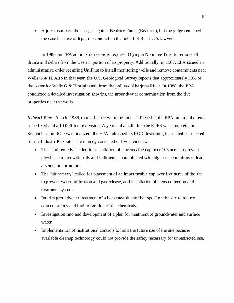
84
• A jury dismissed the charges against Beatrice Foods (Beatrice), but the judge reopened
the case because of legal misconduct on the behalf of Beatrice’s lawyers.
In 1986, an EPA administrative order required Olympia Nominee Trust to remove all
drums and debris from the western portion of its property. Additionally, in 1987, EPA issued an
administrative order requiring UniFirst to install monitoring wells and remove contaminants near
Wells G & H. Also in that year, the U.S. Geological Survey reports that approximately 50% of
the water for Wells G & H originated, from the polluted Aberjona River. In 1988, the EPA
conducted a detailed investigation showing the groundwater contamination from the five
properties near the wells.
Industri-Plex. Also in 1986, to restrict access to the Industri-Plex site, the EPA ordered the fence
to be fixed and a 10,000-foot extension. A year and a half after the RI/FS was complete, in
September the ROD was finalized; the EPA published its ROD describing the remedies selected
for the Industri-Plex site. The remedy consisted of five elements:
• The “soil remedy” called for installation of a permeable cap over 105 acres to prevent
physical contact with soils and sediments contaminated with high concentrations of lead,
arsenic, or chromium.
• The “air remedy” called for placement of an impermeable cap over five acres of the site
to prevent water infiltration and gas release, and installation of a gas collection and
treatment system.
• Interim groundwater treatment of a benzene/toluene “hot spot” on the site to reduce
concentrations and limit migration of the chemicals.
• Investigation into and development of a plan for treatment of groundwater and surface
water.
• Implementation of institutional controls to limit the future use of the site because
available cleanup technology could not provide the safety necessary for unrestricted use.

85
The total cost of site investigations and remedial actions was estimated to be $50 million.
Although cleanup remedies for the Industri-Plex site were identified in 1986, actual cleanup
activities did not begin in until 1993.
The fence around the Industri-Plex site was completed in 1988, but shortly thereafter dirt
bikes and ATV riders again destroyed a section of the fence, and several barrels of waste were
dumped illegally at the site. Three months after the repair, the fence and posted warning signs
were demolished by vandalism.
1989-1991
Wells G & H. In 1989, the EPA granted Woburn a Technical Assistance Grant enabling the
community to hire a technical advisor to help them better understand the technical aspects of the
contamination and remediation efforts and take an active part in decision making processes for
Wells G & H. On September 14, after incorporating issues mentioned in the public comment
phase, the EPA released its final ROD. The ROD addressed the properties contained within the
site, the accompanying groundwater contamination, and the subsequent investigations of the
other two operable units of the site.
In July 1991, after only four months of negotiation, the EPA finalized a “record-
breaking” settlement with four of the five PRPs for the Wells G & H site (Grace, UniFirst,
Beatrice, and North Eastern Plastics). At the time, it was the most expensive Superfund
settlement ever achieved in New England. Although an agreement with the fifth PRP, Olympia
Nominee Trust, was never reached, the comprehensive cleanup of the G & H Wells site began
immediately upon the closing of this multi-million dollar deal. The settlement stipulated that the
companies would:
• Clean up their own properties simultaneously, at a collective cost of approximately $68.4
million,
• Provide funding for EPA’s oversight of cleanup activities, valued at $6.4 million,
• Conduct a risk assessment of the area immediately surrounding Wells G & H, and
• Reimburse the EPA for its investigation studies, which cost approximately $2.65 million.

86
Due to the amount of contamination present at the site, agency officials knew long-term
remedial plans for the site would be critical and remediation of groundwater resources would be
extensive. These plans included excavating and incinerating 2,100 cubic yards of contaminated
soils, extracting toxins from soil vapors (this entailed, literally, suctioning the toxins out of soil),
and pumping groundwater from the underground aquifer and returning it after treatment.
Although the problems at both the Wells G & H and Industri-Plex sites were identified in
1979, local citizens grew increasingly frustrated by the 14 year delay in remediating Industri-
Plex and the 13 year delay in remediating Wells G & H.
Industri-Plex. Trespassing on the Industri-Plex site ceased after the Industri-Plex Site Remedial
Trust (ISRT) established its office on the site in 1989 and posted 24-hour security guards.
After five years of arduous negotiation, MP Trust signed a Consent Decree to investigate
contamination at the site and resolve wetland infilling violations. Unable to comply with terms of
this agreement, MP Trust filed for bankruptcy. A Consent Decree was signed for Industri-Plex
site in April 1989, Monsanto, Stauffer-ICI (ICI Americas, Inc, purchased Stauffer in 1987), and
twenty smaller other PRPs established the Industri-Plex Site Remedial Trust (ISRT) to
implement the agreement. In addition to forming a remedial trust, this Consent Decree allowed
Monsanto and Stauffer-ICI to create a Custodial Trust which would technically own title to
contaminated areas of the Industri-Plex property, protecting Monsanto and Stauffer-ICI from
liability relative to the site, attempt to avoid conflicts among PRPs, and set-up a mechanism to
sell the land after completion of the remediation of site. A key feature of this agreement required
that the recently bankrupt MP Trust sell all of its Industri-Plex holdings to fund its share of
remediation of the toxic contamination and in return to have no additional liability.
1992-1994
Wells G&H. One year after signing their multi-million dollar agreement with the EPA, in
September 1992, UniFirst and Grace began groundwater remediation, and Wildwood and New
England Plastics began soil excavation. This progress was viewed as a mixed blessing.
Government officials applauded the PRPs for ultimately accepting responsibility and then acting
expediently, but residents felt betrayed. According to Gretchen Latowski, director of FACE,

87
“The Woburn experience is the ultimate failure of Superfund. It took 12 years since the problems
at the wells were first identified before anything was done or any responsibility taken.” Excavation of contaminated soil near Wells G & H.
Industri-Plex. Although cleanup remedies for the Industri-Plex site were identified in 1986,
actual cleanup activities did not begin in until 1993 when construction began on the permeable
and impermeable cap for Industri-Plex site. By the summer of 1994, EPA had approved 100% of
the remedial design. Also in the early 1990’s the EPA and the ISRT amended the groundwater
remedies listed in the Industri-Plex ROD (Element 3) because of unanticipated contamination,
advancing technology, and cost efficiency. As a result of this change, groundwater was treated
by a pilot oxygenation and bioremediation process as opposed to the original remedial
prescription to pump groundwater, strip it of contamination, and return it to the aquifer. Industri-Plex during remediation: site with cap on contaminated soils.
1995-1997
Wells G & H. On April 27, 1995, Jeffery Purvis, Chief of the Community Assessment Unit of
the Bureau of Environmental Health Assessment, reported on the status and conditions of Wells

88
G & H. Though not clearly identified, the well field was easily accessible and a No Trespassing
sign was posted. However, the area was not fenced and rolls of fold fencing and piles of concrete
piping lay in the area. The site did not appear to have been accessed recently, though trash,
including clothing, furniture, tires, and other debris, littered the site. In 1995, the UniFirst
Corporation and W.R. Grace and Company installed UV-oxidation systems to treat groundwater
in area bedrock.
The bestselling book, A Civil Action, was published in 1996.
After extensive but fruitless efforts to bring Olympia Nominee Trust to the table, the EPA
in 1997 agreed to remediate that part of the site with money from the Superfund trust. Initial tests
of the Olympia Nominee Trust property began in September 1997.
Industri-Plex. By 1997 the soil and air “remedies” ordered in 1986 for Industri-Plex were in
place (Elements 1 and 2), the groundwater treatment to reduce the benzene/toluene “hot spot”
was only partially implemented (Element 3), and the instructional controls to determine future
use of the site were still not finalized (Element 5).
1998 and later
Wells G & H. In 2000, North Eastern Plastics completed the remediation of the soil and water
contaminants related to Wells G & H. In 2003, six years after reaching agreement with the other
four responsible parties, EPA reached an agreement with Olympia Nominee Trust, the fifth
source of pollution for Wells G & H. The EPA entered into administrative order by consent with
all parties this year to address PAH and PCP contamination.
Phase II investigation of the groundwater contamination, beyond the five sources
continues. As part of Phase III, which focuses on the Aberjona River, the EPA prepared a risk
assessment.
Industri-Plex. At the Industri-Plex site, the gas collection and treatment system were completed
in December 1998. Groundwater remediation and monitoring constitute the bulk of the
remaining work to be done. As of December 1998, the three groundwater treatment plants

89
operating at the site had pumped and treated more than 150 million gallons of water. In addition,
all the contaminated soil was removed (approximately 150 tons) and 1,360 pounds of VOCs had
been destroyed. Although major strides in the remediation of the property have taken place,
according to EPA lawyers, complete cleanup of the site will cost approximately $80 million and
could take another 20-30 years because of the site’s extensive groundwater contamination. An
investigation of groundwater contamination at the Industri-Plex site began in 1999. Initially it
was expected to be completed by early 2000; however, it was not finished until 2003.
State and local governments and EPA officials have been successfully working together
to promote commercial redevelopment of the Industri-Plex site. For example, with the support of
state and local officials, the EPA pursued prospective purchaser agreements which limit the
liability of property purchasers and, in some cases, offered previously contaminated properties at
reduced rates. Plans included having Home Depot and Target serve as anchor stores of the 110
acres of commercial development at the site, with 35 acres being devoted to a regional
transportation center, and 100 acres being preserved as wetlands and open space. As one
development engineer recently observed, foxes and snapping turtles now frequent Industri-Plex
wetlands.
Industri-Plex after remediation: regional transportation center.
Though soil data was collected in 1995 and 1997, additional sediment and surface soil
sampling was conducted in 2000 and 2001 to fill in data gaps of the Human Health and
Ecological Risk Assessments. In 2002, sediment and soil samples were collected along the

90
Aberjona River to evaluate the potential impacts from the river, including on the cranberry bog,
on flood source soil conditions, and on areas the City of Woburn was interested in developing in
the future.
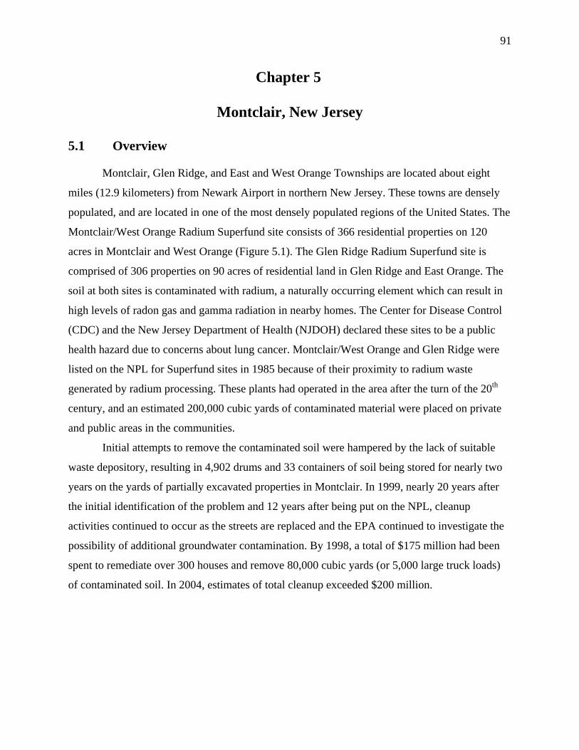
91
Chapter 5
Montclair, New Jersey
5.1 Overview
Montclair, Glen Ridge, and East and West Orange Townships are located about eight
miles (12.9 kilometers) from Newark Airport in northern New Jersey. These towns are densely
populated, and are located in one of the most densely populated regions of the United States. The
Montclair/West Orange Radium Superfund site consists of 366 residential properties on 120
acres in Montclair and West Orange (Figure 5.1). The Glen Ridge Radium Superfund site is
comprised of 306 properties on 90 acres of residential land in Glen Ridge and East Orange. The
soil at both sites is contaminated with radium, a naturally occurring element which can result in
high levels of radon gas and gamma radiation in nearby homes. The Center for Disease Control
(CDC) and the New Jersey Department of Health (NJDOH) declared these sites to be a public
health hazard due to concerns about lung cancer. Montclair/West Orange and Glen Ridge were
listed on the NPL for Superfund sites in 1985 because of their proximity to radium waste
generated by radium processing. These plants had operated in the area after the turn of the 20th
century, and an estimated 200,000 cubic yards of contaminated material were placed on private
and public areas in the communities.
Initial attempts to remove the contaminated soil were hampered by the lack of suitable
waste depository, resulting in 4,902 drums and 33 containers of soil being stored for nearly two
years on the yards of partially excavated properties in Montclair. In 1999, nearly 20 years after
the initial identification of the problem and 12 years after being put on the NPL, cleanup
activities continued to occur as the streets are replaced and the EPA continued to investigate the
possibility of additional groundwater contamination. By 1998, a total of $175 million had been
spent to remediate over 300 houses and remove 80,000 cubic yards (or 5,000 large truck loads)
of contaminated soil. In 2004, estimates of total cleanup exceeded $200 million.

92
Figure 5.1 West Orange, Montclair, Glen Ridge Sites
5.2 Timeline and History
1915-1926
Northern New Jersey was a center for radium processing and the dial-painting industry in
the 1900’s. Several plants occupied the area, the largest of which was the U.S. Radium
Corporation (formerly the Radium Luminous Materials Corporation) which operated between
1915 and 1926. Because of its luminescent properties, radium was added to the paint that was
used for numbers on watch dials and instruments, which became especially popular during
World War I. At various times, U.S. Radium Corporation employed between 100 to 300 young
women as watch dial painters. Corporate supervisors instructed the painters to lick the tips of
their brushes to create the fine point needed for the detailed work. As a result of this process, the

93
dial painters ingested a significant amount of radium. Since clothes were often speckled with this
luminous paint, many of the dial painters glowed in the dark by the time they returned home
from work. Women sometimes painted their fingernails, buttons, or eyelids with the paint for its
special glow-in-the-dark effects. One worker reportedly painted her teeth with the luminous paint
in preparation for a date after work one evening. Because of their exposure to radium, some of
the workers developed bone diseases, such as necrosis of the jaw, anemia, and cancer. Many
factors, including health problems and the discovery of richer uranium ore in the Belgian Congo
led to the closing, and eventual destruction, of New Jersey’s radium plants.
“POISONED! -- as They Chatted Merrily at Their Work
Painting the Luminous Numbers on Watches, the Radium Accumulated in Their Bodies, and Without Warning Began to Bombard and Destroy Teeth, Jaws and Finger Bones. Marking
Fifty Young Factory Girls for Painful, Lingering, But Inevitable Death"3
3 Source: Hearst Sunday supplement American Weekly, February 28, 1926.

94
The U.S. Radium Corporation extracted and purified radium from carnotite ore found in
New Jersey soils. It processed approximately one and a half to two tons of ore each day, and
generated large amounts of radium contaminated waste. This waste was stored temporarily on-
site, and then transported and dumped on nearby rural areas.
1930’s
During the 1930’s, the contaminated soil was used as fill to prepare approximately 200
acres of low-lying areas in Essex County, New Jersey, for residential development.
Contaminated soil was also mixed with cement for foundations and sidewalks. An estimated
200,000 cubic yards of contaminated material is believed to have been disposed of on private and
public lands within the communities before the area was fully developed. This area,
contaminated by radium infill, eventually gave rise to the townships of Montclair, Glen Ridge,
and East & West Orange.
The Montclair site was almost entirely residential with some small businesses and a park
nearby. Within a half-mile (0.8 kilometer) of Montclair were five schools, a hospital, one health
care facility, and a nursing home. West Orange was also predominantly residential with some
businesses located on the north/northeast side of the site. Located within one half-mile of the
West Orange site were two schools and one hospital. The Glen Ridge site was primarily
residential, and encompassed a park and had several small businesses nearby. No hospitals were
located near the Glen Ridge site, but three schools exist within a half-mile.
A USEPA contractor takes gamma radiation measurements in Montclair.

95
Pre-1987
The New Jersey Department of Environmental Protection (NJDEP) discovered radium
contamination in these communities in 1979 during an investigation of the former radium
processing facilities. In 1981, the NJDEP requested EPA funding to perform an aerial gamma
radiation survey of 12 square miles (19.3 kilometers) of Essex County to identify possible
contamination from offsite disposal of radium processing waste. This survey identified three
distinct areas of elevated radiation in the townships of Montclair, Glen Ridge, and West Orange.
The NJDEP conducted additional screening surveys and ground readings in Glen Ridge
in July 1983, and in Montclair and West Orange in October 1983. As part of this screening, 17
homes in Montclair and 10 homes in Glen Ridge underwent additional testing for radiation, 19 of
which were found to exceed federal safety standards for radium (13 in Montclair, 6 in Glen
Ridge).
NJDEP officials were planning to notify local government officials and residents of their
findings in early December 1983. However, despite a request by NJDEP officials to hold the
story until official notification had been made, a November 30th television news report broke the
story early. According to the New York Times (October 16, 1984) article published one year later,
“[Many] residents of the three communities – Montclair, West Orange and Glen Ridge – were
not told about the problem until…technicians, wearing protective gear began taking soil and air
samples in and around their homes.” Within a few days of the television news report, New
Jersey Governor Kean convened a news conference to make an official announcement about the
radium contamination. That month, local newspapers reported extensively on the areas of radium
contamination in their communities. Response to the announcement of radium contamination
was immediate, widespread, and occurred at many levels from local neighborhood residents to
federal agencies. With this heightened public concern, the EPA immediately installed temporary
radon ventilation systems in 38 homes and gamma radiation shielding in 12 homes.
A combined federal and state task force formed in December 1983 to devise a
comprehensive sampling plan that would better define the areas of contamination and provide a
benchmark for remedial action. This plan included an initial screening of “grab” samples which
showed above background radon levels. Long term units for continuous sampling and

96
monitoring were later installed. Technicians in protective suits performed surface gamma
radiation surveys on the properties surrounding affected homes. Soil samples were also collected.
In response to local citizens’ and officials’ concerns, two schools in Montclair were tested but no
contamination was found.
At the local level, community members received different messages from different
agencies about the health risks involved. NJDEP Commissioner Hughey portrayed radon as
strictly an environmental problem. A New Jersey Department of Health (NJDOH) representative
said that the only known health risk was lung cancer, and a NJDOH representative was made
available to meet with affected families for advice. According to the EPA, risks associated with
radon were equivalent to the risks associated with cigarette smoking. A couple of news reports,
however, referred to the radium contamination in New Jersey as “another Love Canal,” since
both residential areas were built on contaminated soil. Even EPA officials expressed great
concern, among themselves, about this case, because it identified the first residences built
directly on contaminated ground. In response to this mixed information, the Montclair Township
Council formed its own task force in December 1983, which held its first organizational meeting
that month. Montclair residents from the contaminated neighborhoods also formed a Radiation
Ad Hoc Committee in December 1983.
Within a month of the November 30, 1983, news report, three bills to aid the affected
communities were introduced into the New Jersey state legislature. One bill requested cleanup
funds, another victim compensation, and the third would require the NJDEP to investigate any
potentially affected homes at the owner’s request and provide a certificate of clearance if the
property was not contaminated. The latter bill was passed in January 1984, and by July 20, 1984,
some residents received certification that their homes had been tested and were clean.
The EPA began field investigations in Glen Ridge and Montclair in January 1984 to
determine the boundary of the contamination and to quantify gamma radiation and radon levels
in the affected areas. Residents were asked for permission to collect samples and were then
provided with the results for their homes. Field investigations continued throughout the fall of
1984. By the end of the year, the EPA had completed all radon source characterization surveys in
the three townships.
97
The NJDOH conducted an epidemiological assessment of the three radium sites and
found a possible, but not statistically significant, increase in lung cancer among white males at
these sites. As a result of this study, the CDC and NJDOH declared these sites to be a public
health hazard. The Centers for Disease Control (CDC) released a Public Health Advisory for
Glen Ridge and Montclair which quantified health risks and recommended appropriate remedial
actions. The CDC divided homes into four categories based on their levels of contamination and
the actions necessary to reduce human exposure contamination:
• Level I homes required remedial action within two days and restricted smoking and time
spent in high radon level areas of the homes.
• Level II homes necessitated remedial action in 1-3 months.
• Level III homes necessitate remedial action within 1-2 years.
• Level IV homes required no action.
Prescribed actions included the installation of remedial systems such as dilution air fans,
air filtration systems, and sealing foundations. The plan also suggested additional studies to
determine the boundaries of the contaminated areas, locate and characterize the source of the
contamination, and assess the potential for groundwater and vegetation contamination.
All this testing and EPA attention prompted local realtors to gather at a Task Force
meeting to discuss the potential impact of radon on the housing market. Reactions were mixed.
Some realtors reported that there was no decrease in the number of homes sold. However, other
realtors reported, anecdotally, a decrease in the selling prices of the homes if the homes were
known to be in affected areas. Fearing lower property values, local residents felt strongly that
they should not have to pay full property taxes on their homes. In response to these concerns, the
Essex County Board of Taxation granted to petitioners in 1984 tax relief on 39 properties in
Montclair: 20% relief if there was soil contamination and 50% relief if radon levels required
installation of ventilation systems. The County also granted tax relief for 22 properties in Glen
Ridge, but the town appealed this in State Court. In West Orange, tax relief was granted for eight
properties – including some adjacent to contaminated properties.
In June, the media agitated already deepening concerns with a spate of negative publicity
which included local newspaper articles and several special news features on major television

98
stations. Residents and officials of Montclair grew more concerned, and decided to hire a private
consultant, David Rosenbaum, a former EPA official. Many of Rosenbaum’s views were
published in the local newspaper, including: 1) levels of radiation are the highest ever
determined in a dwelling in the U.S.; 2) residents in these homes were exposed to “some of the
highest concentrations of any carcinogen ever recorded”; and 3) “Affected residents are in
considerably more danger than the people who once lived in the Love Canal region in NY.”
Rosenbaum concluded that the contaminated soil should be dumped in the ocean and that the
EPA could approve this solution (Montclair Times, October 11, 1984). Residents of Montclair,
Glen Ridge, and West Orange filed suit against the U.S. Radium Corporation. The 7-year legal
battle went to the State Supreme Court and ended in 1991 when 237 residents received a $4.2
million settlement (average $18,000/house) from remnants of the U.S. Radium Corporation.
The entire backyard of this property in Montclair was excavated during cleanup.
A joint EPA/NJDEP task force identified 12 homes in the three communities for a
proposed pilot study involving soil excavation and removal. The EPA decided to postpone the
pilot study until the completion of the requisite feasibility study, scheduled to begin later that
year. The NJDEP, however, planned to proceed with the pilot study on its own. The search for an
acceptable disposal site stalled progress of the pilot program and ultimately generated a great
deal of public anger and distrust of the NJDEP. In August, the NJDEP proposed to temporarily
99
store contaminated soil from the pilot study at the National Guard Armory in West Orange.
Residents of West Orange strongly opposed this plan and the proposal was withdrawn. The
Montclair Township Council was then asked to help locate a disposal site in Montclair for the
radioactive waste. In response, the Council passed a resolution stating that the Township would
under no circumstances comply with the request because: 1) complete cleanup was the only
acceptable alternative; 2) high population density and development pressures excluded the
possibility of local storage sites; and 3) securing a disposal site was a state and federal
responsibility.
As the search for a suitable storage site for the contaminated soil became a major
problem, the NJDEP considered several other options, but significant resistance from people
living in or near the potential sites caused each of these possibilities to be abandoned. For
example, protests and demonstrations were held to prevent storage of contaminated soil at a
dump site on the Montclair State College campus. During this time, questions were raised about
the desirability of a pilot project. Those in favor of the project said that it would shorten the time
it would take the EPA to start cleanup because the project would demonstrate the feasibility of
the cleanup approach.
In the fall of 1984, the NJDEP and federal officials considered simply buying and
fencing-off the contaminated properties. This option deeply concerned the townships, which
soon deemed it the least desirable alternative because it would transform whole neighborhoods
into “radium dumps.” Finally, in September 1984, the Montclair Township Council and
community task forces announced their intention to undertake legal action against the EPA and
the NJDEP to facilitate timely removal of contaminated soil.
The Montclair/West Orange and Glen Ridge sites were added to the proposed NPL in
October 1984, and the EPA began its Remediation Investigation/Feasibility Study (RI/FS) the
following month. Three months later (January 1985), both sites were added to the final NPL. In
April, the EPA finalized its RI/FS and submitted it to the public for final approval.
Also in April, the New Jersey Governor signed a bill appropriating eight million dollars
for the pilot study (this was later increased to $15 million). With this money, the NJDEP was
able to locate a storage site in Beatty, Nevada, and the pilot study began with four homes in Glen
Ridge in June of 1985. In August, five Montclair families were temporarily moved from their
100
homes for an expected two months and excavation of the contaminated soil began. Prior to its
shipment to the permanent storage site, approximately two-thirds of the contaminated soil
excavated for the pilot project (9,500 drums and 51 containers) was stored in Kearny, New
Jersey, and the remainder of the soil (4,902 drums and 33 containers) was stored in the yards of
the partially excavated properties in Montclair.
Immediately preceding the completion of the pilot project and soil shipment, the state of
Nevada revoked the NJDEP’s disposal permit. In October 1985, the U.S. Supreme Court directed
the NJDEP to look for a disposal site within the state. Once again there was no place to store the
contaminated soil from the complete remediation of four homes in Glen Ridge and the partial
remediation of five homes in Montclair. Consequently, almost 5,000 containers of contaminated
soil remained in the yards of the partially excavated Montclair homes.
In July 1986, the NJDEP made plans to ship the excavated soil to an abandoned quarry in
Vernon, New Jersey, where it would be blended with clean dirt to bring radium levels down to
acceptable levels. Thousands of Vernon residents vigorously protested against this plan by
obtaining temporary restraining orders and demonstrating with chants of “Hell no, we won’t
glow.” Several state and federal lawsuits were also filed against the NJDEP, and the NJDEP
dropped the plan in November. As the search for a storage site dragged on, the plight of the
relocated Montclair families continued to be the subject of media attention. Three hundred
people from Montclair and surrounding communities rallied in support of the indefinitely
displaced families.
1987 – 1989
The NJDEP made several offers to buy these five properties from their owners at market
value -- as if the homes were not contaminated -- and to pay relocation costs, but these offers
were refused. The NJDEP also offered to bury the contaminated soil more deeply in the yards
and install filtering systems. This offer was also refused. The Township of Montclair again filed
suit in State Supreme Court to force the NJDEP to remove the barrels. Judgment was passed in
March 1987 requiring the NJDEP to start removing the barrels by May 15, 1987.
Eventually, the EPA negotiated a disposal site, and in December 1987 the NJDEP spent
almost four million dollars to ship the barrels of soil to Oak Ridge, TN where the soil was mixed

101
with radioactive waste from power plants and shipped to a storage site in Washington State.
Likewise, the soil stored at Kearny, NJ was shipped out of state in the summer of 1988.
An excavator removes radium-tainted soil from Barrows Field in Glen Ridge.
In April 1989, the EPA released its draft remediation plan and held public meetings for
discussion and comment. The EPA’s $53 million action plan called for a five-tiered approach to
remediation based on the level of contamination found in the homes. In June, the first Record of
Decision (ROD) was signed. It established five classifications related to the level of
contamination and subsequent required remediation:
Tier A (23 homes): Complete soil removal and replacement of the most contaminated
areas.
Tier B (75 homes): Covering of contaminated soil and installation of radon control
systems in homes with very high radiation levels.
Tier C (65 homes): Installation of anti-radiation devices in less severely contaminated
homes, which would also be subject to deed restrictions and other
controls.
Tier D (296 homes): Monitoring homes with low levels of radon.
Tier E: The homes had no evidence of radium contamination and would
receive no further action.

102
The public staunchly opposed this plan and all proposed remedial efforts short of complete
removal of contaminated soil. In response to public concerns, the EPA installed a fence around
two of the sites to prevent the public from coming into contact with hazardous materials. They
began removing soil at the most contaminated homes and extended the comment period on the
plan, while deferring decisions on the less contaminated homes.
In 1989, Dr. William Kinnard of the Real Estate Counseling Group of Connecticut, Inc.
was retained to conduct a market research study of all single-family residential property sales
within the three radium Superfund site areas. This analysis identified, reported, and measured the
actual market sales behavior of homebuyers and sellers using a total of 1,423 housing sales in
three different locations from July 1, 1980 to June 30, 1989. In one location, Dr. Kinnard found a
statistically significant decrease in property values and volume of housing sales after the public
announcement of contamination discovered at these sites. In the other two locations, the rates of
property value appreciation and housing sales volume increased more slowly than in locations
without Superfund sites. Evidence from Kennard’s study also suggests that the housing market
response to a known Superfund site is a direct function of the speed, proximity, and apparent
effectiveness of any remediation or cleanup efforts.
1990 - 1992
In January 1990, the twice-extended public comment period ended and by June, the
public agreed to a revised $250 million plan and the second ROD was signed. This plan included
removal of the first 15 feet of contaminated soil from approximately 400 homes in the three
towns. Cleanup efforts would be spread out over a maximum of 10 years, and radiation-
ventilating devices would be installed in homes in the interim. As part of this plan, the EPA
would also replace existing radon units with higher efficiency radon units.
In 1991, as discussed above, after seven years of litigation, 237 residents received a $4.2
million settlement (average $18,000/house) from the remnants of U.S. Radium Corporation.
While the pilot study involving a limited number of affected homes started in 1984, the
major cleanup activities of other areas began in 1991. The cleanup was divided into seven phases
based on the severity of contamination, owner access agreements, and location. Radon mitigation
systems were maintained in almost 40 homes throughout each phase of the cleanup and until
103
remediation was complete. Each phase of the remedial plan required access to properties to
perform a design survey, which included gamma radiation surveys, installation of radon and
alpha detectors, and soil sampling and drilling. If the survey found no evidence of contamination,
the property owner was given the results of the test, and a follow-up radon test was conducted
one year later. If the follow-up test confirmed the lack of radium contamination, the property
owner was given a final report summarizing all results. If contamination was present in the initial
or any of the follow-up surveys, the EPA remediated the property. After remediation was
complete, monitoring and sampling were done for one year to evaluate the success of the
cleanup. Once the property was cleared of all contamination, a detailed summary package was
provided to each homeowner, which included details of excavation and results of the testing.
Over the course of cleanup, approximately 100 families were temporarily relocated.
The cleanup process was highly disruptive to the neighborhood as it involved, in some
cases, the installation of building supports and the use of large machinery to remove
contaminated soil. The Pilot Phase and Phase I entailed the cleanup of 56 properties, temporary
relocation of 22 families, and removal of over 15,000 cubic yards of contaminated soil. After the
cleanup was complete, houses, property, driveways, and sidewalks were restored to at least their
original condition and in many cases were improved by enhanced landscaping and sidewalk
and/or garage replacement. Additionally, the amount of radon remaining in the soil at these
locations after remediation was well below the natural level of radon contained in most New
Jersey soils
1993-1995
In 1993, Phase IIA was underway, which included the cleanup of 26 additional
properties. In 1994, Phase IIB started which called for the remediation of 53 properties. During
this time period, EPA had still not made a final decision regarding remediating the three
communities’ streets. Phase III was completed in 1995 and consisted of remediation of 54
homes.
1996-1997
104
Phase IV and Phase V were completed in 1996, and included the partial demolition and
rehabilitation of 55 homes. Phase VII of the cleanup began in the summer of 1997, which
included continuing remediation of properties with post excavation radon levels above normal
and beginning remediation of six additional homes. Remediation at 441 properties complete at
Montclair/West Orange, but 20 additional properties were discovered to need remediation.
After 1997
By 1998, a total of $175 million had been spent to remediate 300 houses and remove
80,000 cubic yards (or 5,000 large truck loads) of contaminated soil. In the fall of 1998, a two-
year remediation plan for the streets finalized and began in 1999, as part of Phase VI. Also, an
additional 30 homes were rehabilitated and 35,000 cubic yards of soil were removed as part of
Phase VI, which was completed in 2001. In 1999, the EPA began testing groundwater for
possible contamination, and a January 2003 Remedial Investigation Report revealed that elevated
levels of radon were found in the groundwater. Phase VIII was completed by the end of 2003.
Three additional properties require remediation and are included in Phase IX, currently
scheduled for completion in January 2005.

105
Chapter 6
Eagle Mine, Colorado
6.1 Overview
Eagle Mine is centrally located between Vail and Beaver Creek ski areas, approximately
100 miles (160 kilometers) west of Denver, Colorado and about 14 miles (22.5 kilometers)
southeast of Vail, Colorado (Figure 6.1). Once one of the nation’s top producers of zinc, the
mine lies between the small towns of Minturn and Red Cliff, just off U.S. Highway 24. The
property consists of approximately 6,000 acres, 340 of which are contaminated with toxic waste.
Most of the contamination originates from areas located along the Eagle River, and includes: the
abandoned mining town of Gilman located on a cliff just above the mine, the old Eagle Mine
processing plant in Belden, two ponds containing wastes from the smelting of ore, Maloit Park,
Rex Flats, various waste rock and roaster piles, and an elevated pipeline. The Eagle River (a
major tributary of the Colorado River), Cross Creek, and several other tributaries run through the
site.
The Eagle Mine site is contaminated with eight to ten million tons of hazardous
substances including arsenic, nickel, chromium, zinc, manganese, cadmium, copper, and lead.
The main cause of Eagle River contamination came from acid mine drainage, which occurs when
sulfide minerals, such as pyrite, are exposed to oxygen and water and then oxidize. This process
creates sulfuric acid, which contaminated soil, groundwater, and surface water surrounding Eagle
Mine, producing water with low pH levels. Acid drainage at Eagle Mine resulted from
precipitation flowing through the waste piles that accumulated from nearly 100 years of mining.
As Eagle Mine acid drainage seeped into ground and surface water, it killed aquatic life and
vegetation growing along the water's edge and contaminated the river with zinc, lead,
manganese, and cadmium. Not only did this contamination threaten brown trout, the most
populous fish in this segment of the river, but it also permanently stained the rocks in and along
the river bright orange, providing Minturn and Red Cliff residents with a constant reminder of
the contamination at Eagle River.
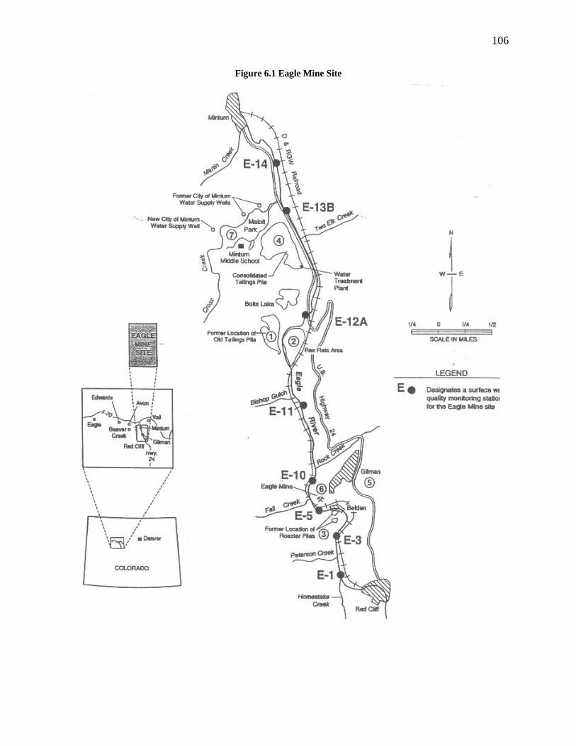
106
Figure 6.1 Eagle Mine Site

107
Eagle River across from CTP, stained rock.
State studies conducted in 1984 revealed dangerously high levels of cadmium, copper,
lead, and zinc in local water resources. Minturn, with a population of 1500, is the closest town
and draws drinking water from Cross Creek and two wells located within 2000 feet of the mine
tailings4. While Eagle Mine had a history of environmental problems dating back to 1957, the
majority of the problems arose after the mine closed in 1984. Eagle Mine was placed on the
national Superfund priorities list (NPL) in June 1986.
6.2 History and Timeline
Mining in Colorado began with the discovery of silver-lead and gold-silver in 1879, and
played an important role in the economic development of many Colorado mountains. In the mid
1890s, a new ore was discovered in Battle Mountain, and the bulk of mine extractions shifted
from gold and silver to zinc. Zinc extracted by independent miners was shipped off site until
1905, when a zinc ore processing plant was built near Belden, approximately a half-mile (0.8
kilometers) southeast of Gilman. The plant heated the ore to extreme temperatures and then
extracted the zinc using magnets, a process called roasting. After the roasting was complete, a
4 Most mine tailings are disposed of in an on-site compound, and are typically comprised of 40-70% effluent liquids used in the mining process and 30-60% solids.
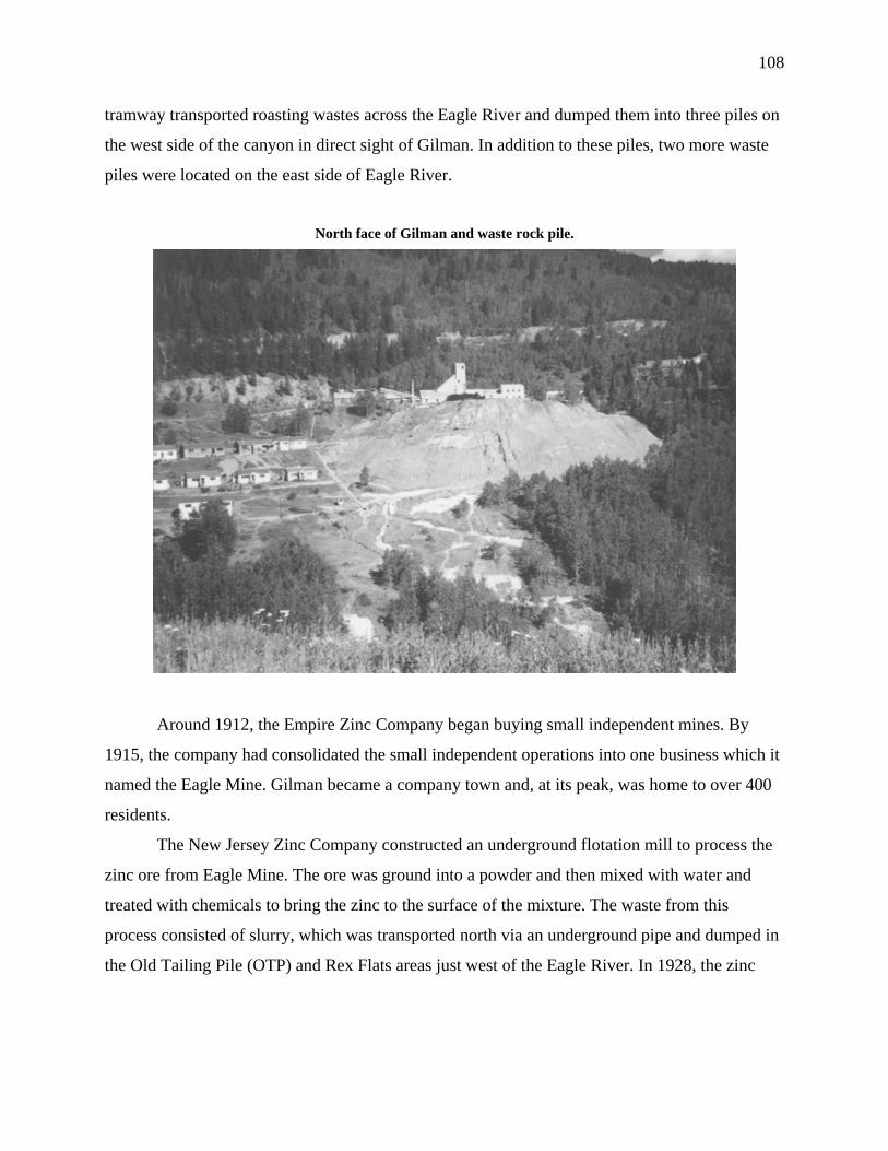
108
tramway transported roasting wastes across the Eagle River and dumped them into three piles on
the west side of the canyon in direct sight of Gilman. In addition to these piles, two more waste
piles were located on the east side of Eagle River.
North face of Gilman and waste rock pile.
Around 1912, the Empire Zinc Company began buying small independent mines. By
1915, the company had consolidated the small independent operations into one business which it
named the Eagle Mine. Gilman became a company town and, at its peak, was home to over 400
residents.
The New Jersey Zinc Company constructed an underground flotation mill to process the
zinc ore from Eagle Mine. The ore was ground into a powder and then mixed with water and
treated with chemicals to bring the zinc to the surface of the mixture. The waste from this
process consisted of slurry, which was transported north via an underground pipe and dumped in
the Old Tailing Pile (OTP) and Rex Flats areas just west of the Eagle River. In 1928, the zinc

109
operation ceased due to falling prices resulting from the Great Depression. Mining of gold and
silver ore continued, but the ores were shipped off-site for processing.
Ownership of the Eagle Mine Superfund site is quite complex. In 1938, Empire Zinc
Company merged with the New Jersey Zinc Company, making it the new owner of Eagle Mine.
Later in 1966, New Jersey Zinc Company merged with Gulf & Western Industries, Inc., which
later changed its name to Gulf+Western, Incorporated.
Because it was used to harden steel, a valuable commodity during the war, zinc
production resumed in the early 1940s. Once again the tailings were deposited at the Old Tailing
Pile (OTP). By 1946, the pile had reached capacity and a New Tailings Pile (NTP) was
established one-half mile (0.8 kilometers) northeast of the OTP, near the confluence of Cross
Creek and the Eagle River, just south of Minturn Middle School and Maloit Park.
Approximately, 75,000 tons of waste, covering 15-20 acres, were dumped at this site.
Long before Eagle Mine was listed on the NPL of Superfund sites, state officials
expressed concern about the amount of hazardous pollution originating at the site. In fact, a
March 17, 1957 Denver Post article reported that a zinc mine in Gilman, CO was asked to pay
$15,000 for 75,000 trout that suffocated in the Eagle River due to an oil fuel spillage. Another
Denver Post article (October 20, 1974) reported that the New Jersey Zinc Company paid “$3,308
for trout and other fish which died July 19 after 12,000 gallons of liquid wastes and 100,000
pounds of mill tailings polluted the Eagle River”.
Peter Seibert and Bob Parker founded Vail ski resort in 1962 less than 14 miles (22.5
kilometers) from Gilman and the Eagle Mine. The resort opened for business on January 10,
1963 and 12 skiers bought lift tickets. Within two years, more than 14,000 skiers visited the
resort. Vail’s reputation blossomed in the mid 1970s when Gerald Ford became president. Ford
had lived part-time in the Vail area since the 1960s, and during his tenure as president, the resort
became known as the “Western White House”. Starting in the 1970s, Vail experienced explosive
growth and building construction. Golf courses, tennis courts, and other sports activities attracted
summer tourists almost as plentiful as Vail’s winter tourists.

110
1976-1982
Zinc production continued until 1977 when, due to falling zinc prices, the operation was
shut down again and more than 150 mineworkers were laid off. Most families moved out of
Gilman at this time.
By 1981, one million tourists visited Vail resort annually.
1983-1988
On September 1, 1983, Glenn Miller, a Colorado businessman, bought the Eagle Mine
property for $17.5 million with the intention of developing it into a ski resort. Unable to finance
this venture, Miller sold to Battle Mountain Corporation (BMC) 1,400 acres of the property
including Rex Flats, the tailings ponds, 70 homes, a bowling alley, and several business offices.
In December 1983, the State of Colorado filed a lawsuit against Gulf+Western and New
Jersey Zinc for contaminating the Eagle River. At this time, the State also initiated a preliminary
risk assessment of the site. As the State and PRPs were unable to come to an out-of-court
agreement, the complaint evolved into a court-ordered negotiation regarding who was
responsible for the $80 million cleanup of the 7.5 million tons of tailings at the site.
In 1984, while the State of Colorado’s lawsuit awaited settlement, the new owner of the
site, Glenn Miller, lost his financial backing and lost the balance of the property due to
nonpayment of taxes. These lands were sold at Eagle County tax sales.
Copper-silver ore mining continued sporadically until 1984 when all mining operations at
the Eagle Mine halted. At that time the mine began to fill with water because of the many
fissures and cracks inside the mine. The Colorado Department of Public Health and Environment
(CDPHE) estimated that approximately 250 gallons of water per minute entered the mine. If the
mine flooded, the water would come in contact with transformers in the mine which contained an
estimated 3,000 pounds of the known-carcinogen polychlorinated biphenyls (PCBs), which could
then potentially seep into local water supplies.
In June, the Public Service Company of Colorado informed the EPA that it was going to
turn off the electric power supplied to the Eagle Mine because Mr. Miller was unable to pay the
mounting electric bill, which was in excess of $90,000. This posed a problem because the mine
was being pumped to prevent it from flooding and coming into contact with PCBs. The EPA
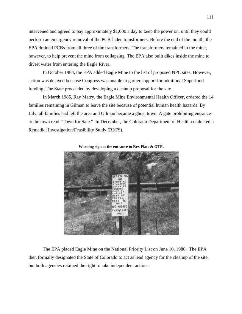
111
intervened and agreed to pay approximately $1,000 a day to keep the power on, until they could
perform an emergency removal of the PCB-laden transformers. Before the end of the month, the
EPA drained PCBs from all three of the transformers. The transformers remained in the mine,
however, to help prevent the mine from collapsing. The EPA also built dikes inside the mine to
divert water from entering the Eagle River.
In October 1984, the EPA added Eagle Mine to the list of proposed NPL sites. However,
action was delayed because Congress was unable to garner support for additional Superfund
funding. The State proceeded by developing a cleanup proposal for the site.
In March 1985, Ray Merry, the Eagle Mine Environmental Health Officer, ordered the 14
families remaining in Gilman to leave the site because of potential human health hazards. By
July, all families had left the area and Gilman became a ghost town. A gate prohibiting entrance
to the town read “Town for Sale.” In December, the Colorado Department of Health conducted a
Remedial Investigation/Feasibility Study (RI/FS).
Warning sign at the entrance to Rex Flats & OTP.
The EPA placed Eagle Mine on the National Priority List on June 10, 1986. The EPA
then formally designated the State of Colorado to act as lead agency for the cleanup of the site,
but both agencies retained the right to take independent actions.
112
In 1986, the State of Colorado filed $50 million lawsuit against Paramount (owner of
Gulf+Western and now Viacom). The lawsuit was resolved in 1988 and the parties entered into a
Consent Decree and Remedial Action Plan (RAP). It was estimated that the cleanup would cost
$150 million and take ten years to complete. The agreement drafted by Colorado State health
officials set acceptable zinc standards and pH levels for the river and relevant soils and required:
1. Plugging the mine portals to stop the production of acid mine drainage;
2. Removal of the roaster piles and reprocessing of the tailings;
3. Collection and treatment of mine water and groundwater;
4. Revegetating the waste removal areas and the Consolidate Tailings Pile (CTP); and
5. Long-term monitoring of the site.
1989 - 1994
As the cleanup began, public concern about the possibility of adverse human health
effects intensified. In March 1989, fearing that no assessment had been conducted, federal EPA
officials conducted their own investigation of potential contamination at Minturn Middle School,
located 400 yards from the mine. A Vail Daily article (July 18, 1989) reported on this
investigation and indicated that “Richard ‘Dick’ Parachini [CDPHE Project Manager] told the
governor that dust levels [from the cleanup] are ‘right on the break point’ of what is generally
considered environmentally safe. Breathing the heavy metals present at the Minturn site, in high
enough levels and over a period of years, is expected to greatly increase cancer risks.” This
news generated alarm among local residents because the school was located less than one mile
(1.6 kilometers) from the 70-acre CTP, which was used for waste dumping until 1977. The EPA
convened a well-attended public meeting regarding the issue. Approximately 1,000 irate citizens
attended this meeting, which EPA officials characterized as a “lynch mob”. At this meeting, the
state agreed to amend its RAP to include the construction of a permanent waste water treatment
plant that would reduce the level of zinc in the river and raise the pH level of the river. This plant
would be operable by July 1, 1990. Additional plugs were installed in the mine to stop water
from pouring directly out of the mine and into the river. Unfortunately, the volume of waste

113
water needing treatment exceeded the capacity of the new plant, allowing contaminated water to
seep into the river. Viacom was forced to begin construction on a second water treatment plant.
In the interim, the local school board hired a private environmental consultant, Leonard
Slosky, to evaluate air quality and dust emanating from the roasting piles. Slosky installed 15 air
monitoring stations in and around the school and enlisted the help of several school teachers as
well. Every day for six weeks, select teachers wore small compact devices that resembled
portable headphone stereos. At the end of each day, a field technician analyzed the filters for
toxic residue. Slosky confirmed the presence of heavy metals in and around the school, but
concluded that the amount of metals present fell far below hazardous levels. For example,
arsenic found at the site presented the greatest potential health risk, but Slosky likened the
children’s chance of developing arsenic-related cancer to that of smoking eight cigarettes in a
lifetime.
Although the EPA chose not to endorse the state’s RAP because it was skeptical of the
plan’s long-term effectiveness, the State forged ahead with the cleanup of the Eagle River site
fearing the worsening of public health and environmental damages that might result from
continued acid mine drainage. However, the State’s decision to pump tailings pond water back
into the mine, using the mine as a holding tank, proved to be disastrous and caused even more
pollution to infiltrate the Eagle River. A dry winter caused mine seepage to make up most of
river water, and the river turned orange. As a result, fish populations declined dramatically.
Samples taken from the river that fall revealed zinc levels were 255 times higher than fish
tolerance thresholds. No fish lived in the river, and contamination was turning the Eagle River
various colors.
Media headlines reinforced the environmental and health related fears of local residents:
“Eagle ‘cleanup’ casts doubt on state” Denver Post April 20, 1990; “Eagle River fish population
smaller than expected” Denver Post April 24, 1990; “Fish fading in river polluted by mine”
Rocky Mountain News April 27, 1990; “Mine cleanup again called inadequate” Denver Post July
13, 1990; “Polluted water flows to Minturn wetlands” Rocky Mountain News July 13, 1990; and
“More problems foul cleanup of zinc mine -- mine’s toxic metals pollute Eagle River” Rocky
Mountain News August 28, 1990. The cleanup was obviously failing, and local citizens felt state
and federal agencies were shirking their responsibilities. In an article published in the Rocky

114
Mountain News on April 18, 1990, a letter from the Minturn town council to Governor Roy
Romer stated, “Our river continues to run from murky green to sickly red…Above the mine the
river is crystal clear. The town of Minturn believes that we are being held hostage to a
bureaucratic nightmare. Minturn is a small town with very limited resources. We find ourselves
unable to get any action from our state officials who are supposed to be acting on our behalf.”
In April, Paramount’s new facility began to treat polluted water. State and PRPs amended
RAP to add a chemical water treatment plant and install additional mine plugs. Colorado
Department of Wildlife began monitoring the fish and macroinvertebrates populations in the
Eagle River on an annual basis. At the start of this process, virtually no fish were found in the
Eagle River.
In September, a newly formed Eagle County Oversight Committee citizens group, joined
by Trout Unlimited, Eagle River White Water, Inc., and the Gore Creek Flyfisher, filed a $300
million class action suit against Paramount Communications, Inc. for water, air, and soil
contamination originating from the Eagle Mine property. The organizations claimed that Eagle
Mine seepage was contaminating the Eagle River as well as the Minturn Middle School. They
added that faulty water treatment plans were causing as much as 40 gallons of contaminated
water per minute to be dumped into Maloit Park wetlands. From Paramount, the plaintiffs sought
damages for potential health risks, compensation of economic harm due to lower property
values, funds for removal of the tailings, and “exemplary damages for wanton and reckless
disregard” of residents’ rights. Cindy Cacioppo, a member of the Committee, said “We decided a
lawsuit was needed for people to recover damages because there’s nothing in Superfund that
allows citizens to recoup.”
In 1991, the EPA became increasingly concerned about the site and notified the State of
Colorado that Paramount was in violation of six different aspects of the Clean Water Act because
of the mine seepage and discharge from the waste piles that had contaminated the river the
previous year. The water treatment plant was replaced and the EPA conducted a risk assessment
for PCBs.
Remediation efforts removed five piles of waste materials from the ore roasting plant
near Belden. This waste was relocated to the CTP, and former waste piles were revegetated.

115
During this time period, Vail Associates started silently acquiring options to buy portions
of Eagle Mine property.
In June 1992, the EPA decided to conduct a Feasibility Study Addendum, which found
that the Eagle River ecosystem continued to suffer severely from heavy metal contamination.
Part of the study included additional risk assessments that resulted in a more comprehensive
investigation of the health of fish and other natural resources. Additional soil studies and risk
assessments of ground water quality were conducted in Maloit Park, Minturn Middle School, and
the town of Gilman. The Feasibility Study Addendum identified the following activities to
supplement the State’s RAP: collect additional seepage from the Rock Creek drainage; monitor
former roaster pile areas and waste rock piles; continue operation of the Water Treatment Plant;
collect additional groundwater from CTP and treat it at the Water Treatment Plant; and cleanup
Maloit Park wetlands area. Risks to human health were also reviewed, but no appreciable threat
to drinking water was found, and heavy metals in soil and dust were found to be well within
acceptable standards.
Regardless of these findings, Viacom later moved Minturn’s drinking wells upstream of
their old location. Finally, the EPA concluded that the potential risk of PCB ingestion from the
15 pounds of PCBs remaining in the transformers was low. The EPA agreed to continue to
monitor for potential PCB contamination, which has never been found. In June of 1992, the EPA
proposed a second and preferred remedial plan for the site, which included an alternative cleanup
for each of the individual areas contributing metals to the Eagle River. Cleanup activities focused
on removing the 150,000 tons of tailings deposited at Rex Flats and the one million tons of
tailings deposited at the Old Tailings Pile (OTP). All of these tailings were relocated to the
consolidated tailing pile (CTP). After the removal of the tailings, revegetation efforts were
undertaken. Restrictions were put into place to restrict the use of groundwater below the OLP.
Efforts were made to control seepage, surface water drainage, and groundwater flow in Rock
Creek Canyon. The seepage and drainage were collected for treatment.
In 1992, recognizing an opportunity for even more expansion, Vail Associates covertly
funded Turkey Creek, LLC’s payment of three years of back taxes on over half of the Eagle
Mine site. Payment of these back taxes guaranteed Turkey Creek LLC and Vail Associates a first
bid option on the Eagle Mine property.
116
In March, 1993, the EPA issued a Record of Decision (ROD) that required additional site
investigations and remedial actions to be implemented. The ROD included modifications of the
established remediation standard, proposed monitoring of additional metals, collection of
additional groundwater seepage, monitoring runoff, accelerating the capping of the CTP,
removal of the contaminated material from the Maloit Park wetlands, development of a
monitoring plan, and implementation of an inspection and maintenance plan.
The 1993 risk assessment determined that soils in Maloit Park Wetlands contained
elevated levels of arsenic, cadmium and lead. In June, the State amended the remedial plan for
the third time. Viacom was to permanently remove pond water from the top of the CTP,
implement a sludge dewatering system, and construct a sludge disposal cell.
In the summer of 1994, the EPA issued a unilateral administrative order that consisted of
additional monitoring and testing of the site, which was amended again in 1995 to add a work
plan for Maloit Park waste removal and restoration.
1995 – 1999
By 1995, more than 2.1 million tourists visit the Vail Valley annually.
In August, 1995, the State of Colorado, US EPA, and Viacom agree to a Three-Party
Consent Decree and Statement of Work to implement the 1993 Record of Decision. The
agreement called for sampling of water quality, along with assessments of the aquatic insect and
fish populations in the Eagle River to determine the effectiveness of the cleanup actions.
Additionally, the three parties agreed to investigate the adaptation of biological-based cleanup
standard for the site.
In addition to the actions taken in 1992, more efforts were made to control seepage,
surface water drainage and groundwater flow in Rock Creek Canyon.
At Rex Flats and OLP, more than 800 cubic yards of zinc concentrates were removed and
moved to the consolidate tailing pile. To prevent ground water contamination, remediation
efforts involve intercepting and diverting 100-200 gallons of clean water per minute from the
Eagle Mine.
In 1996, the contaminated soils in Maloit Park Wetlands were removed. Clean soil was
used to cover the previously contaminated area and revegetation efforts were undertaken.

117
On February 21, 1986, 32 cars of an 82-car train derailed on the Tennessee Pass heading
towards Minturn. Two crew members on the train were killed and another was injured.
According to the EPA, four tank cars ruptured, spilling approximately 54,000 gallons of sulfuric
acid. Five to six acres of nearby trees and vegetation were blackened by the sulfuric acid that
went over an embankment and across the two lane highway. Other contaminates spilled
including Triethylene glycol (antifreeze) and small amounts of diesel fuel. However, the overall
environmental damage appeared to be less than originally feared. Tests of the Eagle River
revealed no significant levels pollution in the river or other water sources.
By 1997, the main tailing pile was capped. Residents reported increasingly better water
quality in the Eagle River. In August, the EPA awarded “Environmental Achievement Awards”
to both the Eagle River Environmental and Business Alliance and Viacom. The Eagle River
Environmental Business Alliance was acknowledge for their efforts in the successful cleanup of
the site by “keeping area residents informed, providing technical input, and discussing with
people their concerns about a hazardous waste cleanup in their neighborhood.” Viacom was
lauded for their cleanup efforts that had “gone beyond legal requirements, furnishing the town of
Minturn with a safe water supply, voluntarily cleaning up large amounts of hazardous materials,
planning to intercept clean water flowing onto its site and keeping a skeptical public informed
about the cleanup.”
In 1998, the EPA issued a final ROD ensuring it would provide ongoing monitoring of
the site. In 1999, state and federal authorities formally sought to change the cleanup agreement to
include pumping of groundwater to keep it from filling the mine and complicating treatment of
contaminated water from the mine.
Although they denied their intentions for years, Vail Associates revealed, under oath in
March, its intention to buy and develop the Gilman property. By April, Vail was already 93%
built out, so it turned its eyes on neighboring communities. While the remediation and
bankruptcy proceedings for the Gilman property progressed, Vail filed suit against Minturn for
its under-utilized water rights, which it would use for its controversial back bowl ski trail
expansion. Much to the dismay of Minturn residents, Vail won the rights to 4.76 cubic feet per
second of running water during the driest months from October to April. The value of these
water rights is estimated to be $14 to $16 million. The enormity of the Vail resort, as well as the
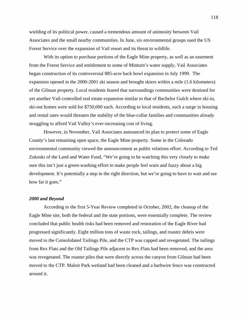
118
wielding of its political power, caused a tremendous amount of animosity between Vail
Associates and the small nearby communities. In June, six environmental groups sued the US
Forest Service over the expansion of Vail resort and its threat to wildlife.
With its option to purchase portions of the Eagle Mine property, as well as an easement
from the Forest Service and entitlement to some of Minturn’s water supply, Vail Associates
began construction of its controversial 885-acre back bowl expansion in July 1999. The
expansion opened in the 2000-2001 ski season and brought skiers within a mile (1.6 kilometers)
of the Gilman property. Local residents feared that surroundings communities were destined for
yet another Vail-controlled real estate expansion similar to that of Bachelor Gulch where ski-in,
ski-out homes were sold for $750,000 each. According to local residents, such a surge in housing
and rental rates would threaten the stability of the blue-collar families and communities already
struggling to afford Vail Valley’s ever-increasing cost of living.
However, in November, Vail Associates announced its plan to protect some of Eagle
County’s last remaining open space, the Eagle Mine property. Some in the Colorado
environmental community viewed the announcement as public relations effort. According to Ted
Zukoski of the Land and Water Fund, “We’re going to be watching this very closely to make
sure this isn’t just a green-washing effort to make people feel warn and fuzzy about a big
development. It’s potentially a step in the right direction, but we’re going to have to wait and see
how far it goes.”
2000 and Beyond
According to the first 5-Year Review completed in October, 2002, the cleanup of the
Eagle Mine site, both the federal and the state portions, were essentially complete. The review
concluded that public health risks had been removed and restoration of the Eagle River had
progressed significantly. Eight million tons of waste rock, tailings, and roaster debris were
moved to the Consolidated Tailings Pile, and the CTP was capped and revegetated. The tailings
from Rex Flats and the Old Tailings Pile adjacent to Rex Flats had been removed, and the area
was revegetated. The roaster piles that were directly across the canyon from Gilman had been
moved to the CTP. Maloit Park wetland had been cleaned and a barbwire fence was constructed
around it.

119
Rock Creek no longer flowed directly into the Eagle River; its water continues to be
treated at the water treatment plant before being released. Also, approximately 250 gallons per
minute (gpm) of water from the mine is being treated before being released into the river. In
total, the water treatment plant treats about 360,000 gpm every day. In October, 2001, The
Denver Post reported that as a result of the 14-year effort and a cost of $70 million that the Eagle
River once again ran clean enough for a healthy fish population. Groundwater remediation
efforts would continue in order to cleanup an estimated 700 million gallons of contaminated
groundwater in the 70 miles (113 kilometers) of tunnels within the mine. The annual cost will be
approximately $750,000.
The only indication of past contamination is permanent oxidized manganese and iron
stains, which give the rocks along the river’s edge a rusty brown “bathtub ring”. The results of
the annual biological assessment of the Eagle Mine site show dramatic improvements in the
Eagle River aquatic community such as higher numbers of fish and macroinvertebrates.

120
Chapter 7
Expert Error and the Psychology of Risk and Stigma
7.1 Expert Error
Gayer, Hamilton and Viscusi (2000) argue that residents living near Superfund sites
judge risks to be of a magnitude consistent with EPA expert opinions and that these judgments
are reflected in property values. The research presented here suggests quite the opposite.
However, the sites studied here are much larger and likely to attract more attention. This section
documents many cases of expert error to help explain why expert opinion plays a limited role in
explaining residents' risk beliefs. Thus, the judgments of experts are only one component of the
mix of news media stories and perceptual cues received by the typical citizen. Even if statements
by scientific experts were accepted as credible, they would compete with a mix of the other
signals and perceptual cues. As simply one component, such statements are unlikely to be the
primary determinant of individual risk beliefs. Thus, risk beliefs determined largely by media
stories and other perceptual cues are unlikely to be easily changed by the pronouncements of a
few scientists (Fischhoff, 1989).
Furthermore, it is unlikely that statements by scientific experts will be accepted as
completely credible. Even when different experts are in essential agreement, the news media
often focuses on those aspects where experts disagree (Wilkins and Patterson, 1990), thus
lowering the perceived credibility of experts. In a study examining news coverage of Three Mile
Island and Chernobyl, Rubin (1987) found that news stories tended to dichotomize events rather
than blend a continuum of information to recipients. The result is that the public discredits
information it receives from experts because it appears that experts cannot agree among
themselves and, therefore, do not really know the risk that a site presents.
Despite the ideal that science discovers absolute truths, for every health or environment
related article there appears to be a corresponding article that rejects the tenets of the previously
publicized claim. Numerous famous examples exist, which are described in detail below, where
experts from academia, government, and industry have made errors and misestimates:
• Soil contamination at Love Canal, Niagara, New York

121
• Dioxin contamination in Times Beach, Missouri
• The defective Dalkon Shield for birth control
• The false discovery of Cold Fusion
• The failures at Biosphere 2
• The near nuclear meltdown at Three Mile Island
• The Union Carbide Accident in Bhopal, India
These examples are not just relegated to the past, as the costly search for weapons of
mass destruction in Iraq, to date, has yet to support early claims by intelligence experts. Each of
the short descriptions below serves to illustrate the characteristics and media attention that such
failures attract.
7.1.1 Love Canal, Niagara, New York
Love Canal is permanently etched in the collective conscious of America, and these
words were synonymous with hazardous waste contamination, cancer, and distrust of authorities.
Love Canal brought about a new understanding of the potential health effects of hazardous waste
as well as Superfund legislation designed to deal with chemical disposal sites.
Located in Niagara Falls, New York, Love Canal is named for William Love who began
digging a canal in 1896 for a proposed hydroelectric power plant. Love abandoned the project
when he declared bankruptcy, and in 1920 the city of Niagara Falls purchased the site for use as
a landfill. In 1942 Hooker Chemicals and Plastics Corporation (now Occidental Chemical
Corporation) purchased the landfill for their own disposal purposes. From 1942 to 1953, Hooker
dumped into Love Canal 21,800 tons of toxic waste including more than 400 different chemicals,
11 known carcinogens, PCBs, dioxins, pesticides such as DDT and lindane (both of which have
been banned in the United States), heavy metals, and multiple solvents. Three years after
Hooker’s dumping began, an internal memo from an engineer foreshadowed the disaster to
come, “[Love Canal is a] quagmire which will be a potential source of lawsuits.”
Once the site reached capacity, Hooker covered the 16-acre toxic waste site with a 40-
acre clay seal to prevent chemical seepage. (A 1981 EPA report confirmed that Hooker’s waste
disposal techniques required only minor adjustments to come into compliance with the hazardous
122
waste disposal standards in place at the time.) Under threats of acquisition by eminent domain
and extreme pressure from the city school board, Hooker reluctantly sold the site to the New
York State Department of Education for $1.00, on the condition that Hooker would be
indemnified from any future liability concerning the site. Because of the potential dangers
associated with the site, Hooker insisted that deed restrictions accompany the property transfer
and repeatedly warned the school board of potential health hazards at the site. Hooker also
stressed that under no circumstances should the land be excavated or the clay cap be jeopardized.
Despite these warnings, the city constructed a school on site and sold the remaining parcels of
land to real estate developers. The community of Love Canal was born.
Love Canal residents first began complaining of chemical odors and residues in the
1960s. By 1976 chemical seepage had infiltrated neighborhood creeks, sewer lines, sump pumps,
and soil – even the air inside several Love Canal homes. That year, the New York Department of
Environmental Conservation initiated the first environmental testing of Love Canal which found
contaminated groundwater, soil, and air. Once the results of that research were released, local
and national media responded quickly: “Vapors from Love Canal Pose Serious Threats” (Courier
Express Niagara, May 15, 1978), “Toxic Exposure at Love Canal Called Chronic” (Courier
Express Niagara, May 25, 1978), “Wider Range of Illnesses Expected” (Courier Express
Niagara, August 4, 1978), “Upstate Waste Site May Endanger Lives” (New York Times, August
2, 1978), and “The Devil’s Brew in Love Canal” (Fortune, November 19, 1979). Heightened
alarm among community members and media attention prompted the New York State
Department of Health to test Love Canal homes close to the disposal site for environmental
contamination. Two years later, the State Department of Health declared a state of emergency,
ordered the school to be closed, and recommended an evacuation of the 239 homes that tested
positive for environmental contamination. This news spread rampantly throughout the
community causing a widespread panic and loss of property values of homes adjacent to and
outside the immediate canal area. Fearing for their health, the lives of their children, and their
futures, the remaining 660 families pressured both New York State Governor Hugh Carey and
President Jimmy Carter to expand the evacuation area.
One year later, in February 1979, Dr. Beverly Paigen, a biologist with Roswell Park
Memorial Institute in Buffalo, conducted a study which revealed that between 1974 and 1978:

123
56% of the children born at Love Canal had birth defects; miscarriages had increased 300%;
urinary tract disorders had increased 300%; and the frequency of asthma, epilepsy, suicide, and
hyperactivty had increased. Dr. Paigen also claimed to have evidence that these conditions
subsided once residents moved away from Love Canal. These findings fueled the Love Canal
panic, even though Dr. Paigen’s research was not a scientific controlled study but, instead, based
on anecdotal evidence from personal interviews with Love Canal residents. Dr. Paigen’s research
was thoroughly discredited at that time by the NY Department of Health. A governor’s panel
charged with reviewing her work found that, “[Dr. Paigen’s research] falls short of the mark as
an exercise of epidemiology. She [Dr. Paigen] believes fervently that her observations prove the
existence of multiple disease states directly attributable to chemical pollution, but her data cannot
be taken as scientific evidence for her conclusions. The study is based largely on anecdotal
information provided by questionnaires submitted to a narrowly selected group of residents.
There are no adequate control groups, the illnesses cited as caused by chemical pollution were
not medically validated…. This panel finds the Paigen report literally impossible to interpret. It
cannot be taken seriously as a piece of sound epidemiological research….”
However, two studies conducted in 1980 by the EPA initially seemed to confirm portions
of Dr. Paigen’s research and found chromosomal irregularities and nerve damage among Love
Canal residents. Upon release of these findings, chaos broke loose at Love Canal and two EPA
officials were involuntarily detained. That evening, Lois Gibbs, a member of the Love Canal
Homeowners Association, phoned the White House to inform them of their hostages. Pressured
by the unfavorable findings of the research and extreme political pressure from local residents,
the President issued orders on May 20, 1980, to permanently relocate all families that wished to
leave. In total, approximately 950 families (2,500 residents) evacuated the area, leaving the
government with $3-5 million in relocation costs. These relocations eventually became
permanent costing the government over $30 million.
The integrity of the two 1980 EPA reports as well as the validity of their findings have
since been questioned by the Center for Disease Control (Morbidity and Mortality Weekly, May
1983), American Medical Association (March 1984), National Research Council, and New York
State Department of Health on the basis of the lack of control group (adjusted for by comparing
Love Canal results with a control group from a previous unpublished experiment), incorrect

124
statistical analysis, small sample sizes, inadequate experimental methodology, report release
prior to peer review, and drawing conclusions that in some cases were not supported by the
evidence. For example, the chromosome study actually found a lower rate of chromosomal
damage among Love Canal residents than the control group. According to a 1981 New York
Times article, “it may well turn out that the public has suffered less from the chemicals [at Love
Canal] than from the hysteria generated by flimsy research irresponsibly handled.”
Research conducted in 1982 by EPA found no unusually high levels of contamination
outside the area immediately surrounding the canal, confirming the results of several previously
conducted reports. This EPA report was considered to be highly controversial and was eventually
dismissed. (However, another EPA study conducted in 1987 confirmed the results of the 1982
study.)
Despite the lack of evidence to support such an action, Love Canal was declared a
national Superfund priority on September 1, 1983. Federal and state remediation activities were
expensive and highly intrusive. Fences were erected around the site and bulldozers demolished
the abandoned homes and school within. Leachate treatment plants, high temperature
incineration, excavation and off-site disposal of contaminants and hydraulic cleaning of sewers
and culverts removed wastes and hazardous toxins from the site. Although twenty thousand tons
of waste currently remains at the site, the area was declared “habitable” in September 1988.
Initial redevelopment of the site was difficult because local banks were hesitant to grant home
mortgages for fear of being held liable for environmental contamination. Although the value of
the homes was approximately 20% lower than comparable markets, 239 of the 240 homes in the
Love Canal neighborhood, now called Black Creek Village, have been successfully rehabilitated
and sold. Approximately 30% of the purchasers are original Love Canal residents.
In 1991, the Committee on Environmental Epidemiology of the National Research
Council thoroughly reviewed all Love Canal research and reports and concluded that there was
no definitive link between the health conditions of Love Canal residents and the chemical
seepage from the canal, with the possible exception of decreased birth weights and heights. Legal
settlements are starting to be resolved as well. In 1998, 2,300 Love Canal families received
between payments ranging from $83 to $400,000 from Occidental Chemical Corporation.
125
Two quotes will serve to summarize public reaction to the site that eventually led to the
Superfund program:
“Love Canal doesn’t end with this generation’s cancer or even with the next
generation’s birth defects. For many residents, the damage is permanent in their
genes and their children’s. The mutated genes will affect all of their descendents,
one generation after another.”
Lois Gibbs, (executive director of the Center for Health, Environment and Justice
and former Love Canal resident) Who’s Poisoning America, p. 270.
“It is not enough for industry and government to act in good faith – their mistakes
are counted in human lives.”
Glamour, November 1980
7.1.2 Times Beach, Missouri
All that remains of Times Beach, Missouri, a small community once located 17 miles
west of St. Louis, is a legacy of an environmental disaster. In 1972 and 1973, the city of Times
Beach hired Russell Bliss to manage air-borne dust from its unpaved roads. During that time,
Northeastern Pharmaceutical and Chemical Corporation also hired Bliss to dispose of their
wastes, including dioxin yielded from the production of a then popular skin cleanser called
hexachlorophene. In an attempt to complete both tasks efficiently, Bliss mixed Northeastern
Pharmaceutical and Chemical Corporation’s wastes with oil and sprayed the mixture on Times
Beach roads. Days later animals started dying, and months later children got sick. After Bliss
sprayed Shenandoah Stables’ roads, several horses died and the proprietor’s daughter became
very ill. In November 1982, the EPA found Bliss’ oil mixture to be contaminated with dioxin, a
known human carcinogen. Dioxin is an unintentional hazardous byproduct of many common
industrial processes such as the bleaching of paper and wood pulp; production of herbicides and
wood preservatives; and incomplete combustion of wood and industrial and municipal wastes.
One month later, the nearby Meramee River flooded. As the water receded, experts predicted
126
that it would redistribute dioxin throughout the city. Consequently, not only would Times Beach
roads be contaminated, but the entire Times Beach community might also be laden with dioxin
contamination.
During this time, several studies emerged supporting the highly carcinogenic nature and
potential dangers associated with dioxin. Based on this research, in 1982, the Centers for Disease
Control and other experts recommended completely evacuating Times Beach. On March 4, 1983,
Times Beach was proposed for Superfund’s NPL. The town was officially closed in April 1985
and six months later, on September 8, 1983, Times Beach was placed on the final NPL. By the
end of 1986, the federal government had spent $33 million to permanently relocate all 2,240
Times Beach residents. The title to the town was conveyed to the State of Missouri, and any
remaining parcels of land were purchased by the Federal Emergency Management Agency
(FEMA). As part of the remediation of the site, almost all buildings in the city were demolished
and the entire area was enclosed by a chain-link fence.
Doubtful of the severity of the adverse health impacts associated with dioxin (such as
cancer and infertility), as well as the proposed pathways of human exposure, many scientists and
experts characterized the Times Beach relocation as an over reaction. An article in the Wall
Street Journal written the week of the evacuation supported this sentiment, “There are two
dangers with toxic wastes. One is the very real threat to health posed by the chemicals
themselves. The second is that a hysterical exaggeration of that threat will needlessly frighten
people and drive them from their homes.” Considering the best available research at that time,
the Times Beach evacuation was indeed an over-reaction because it was based primarily on the
analysis of soil samples, rather than the potential human health risks and exposure pathways of
dioxin.
In 1991, several scientific experts, including Dr. Vernon Houk of the Centers for Disease
Control, reversed their initial conclusions about the toxicity of dioxin and their recommendations
to evacuate Times Beach. This reversal was based on new research, which wholly contradicted
previous conclusions about dioxin. The new research found dioxin to be less harmful to human
health than originally suspected, making the Times Beach evacuation seem that overly drastic
and unwarranted. As Houk stated, “Times Beach was an over-reaction. It was based on the best
available scientific information we had at the time. It turns out that we were in error…. The only

127
thing I would have done differently, I would have said we may be wrong. If we’re going to be
wrong, we’ll be in the wrong side of protecting human health. I don’t think we ever said we may
be wrong.”
Upon learning of the new research, industry representatives complained vociferously
about the over-regulation of dioxin and the exorbitant costs associated with its stringent
regulation. Prompted by these complaints and under the direction of William Reilly, the EPA
Administrator under President Bush, Sr., the EPA undertook an extensive series of highly
technical experiments on the toxicity of dioxin. Three years later, to the surprise and dismay of
industry representatives, these experiments reaffirmed the link between dioxin and cancer even
at very low levels of exposure. These experiments also revealed that dioxin bioaccumulates in
living tissue and can cause stunted fetal development, suppression of the immune system,
interference with regulatory hormones, and increased likelihood of developing endometriosis and
diabetes. However, like the second round of dioxin research, this research also revealed that the
major pathway of dioxin exposure is not environmental but through the ingestion of dairy foods
which contain small amounts of the compound.
Armed with this new knowledge, the EPA devised a plan for the remediation of Times
Beach contamination that included the construction of an on-site thermal destruction plant.
Incineration of the dioxin-contaminated soil began in March 1996. Community action groups,
such as the Times Beach Action Group and Dioxin Incinerator Response Group, strongly
opposed this incinerator fearing that burning the dioxin might spread contamination rather than
reduce it. Research studies conducted on a Jacksonville, Arkansas incinerator -- similar to the
one constructed at Times Beach -- confirmed these fears: blood levels of dioxin among residents
living near the Arkansas incinerator were 22 times higher than before incineration began. The
Arkansas studies further concluded that these elevated levels of dioxin caused increased
incidences of diabetes among residents living near the incineration plant. In 1993, Missouri state
officials confirmed that the Times Beach incinerator was also producing more dioxin than it was
destroying, and the EPA disbanded the plant in 1997. Remediation of the site cost $200 million
and was completed in 1997 with the closing of the incineration plant. The property, now a 40-
acre state park was named Route 66.
128
Although more than two decades have passed since the Times Beach evacuation, many
former residents still speculate about the true effects of dioxin on their families and friends. One
Times Beach resident recalls several now-dead community members that suffered from cancer,
immune deficiencies, miscarriages, and suicides. She laments, “I’m so tired of death. There’s not
a day [that] goes by that I don’t wonder if all this is coincidence – or dioxin.”
7.1.3 The Defective Dalkon Shield
In the 1960s, many women became concerned about the possible adverse health effects,
such as cancer and strokes, associated with oral contraceptives and began seeking alternatives. In
response, several pharmaceutical companies invested heavily in the development of intrauterine
devices (IUDs) as a potentially substitute for birth control pills. A.H. Robins (Robins) decided to
enter the IUD market in 1970 by acquiring Dalkon Corporation, a manufacturer of the Dalkon
Shield. Robins had no experience in the development of contraceptive devices and was best
known for its non-prescriptive remedies such as flea and tick collars and cough medicine.
Because Robins had neither obstetricians nor gynecologists on its staff (nor an appropriate
department at that time), it assigned the production and assembly of its IUD, the Dalkon Shield
(Shield), to its Chap Stick division.
Other than one research study conducted by Dr. Hugh Davis, a co-inventor of the Shield,
Robins had conducted no testing of the Shield in women or animals when it entered the market
in 1971. Yet A.H. Robins positioned the Dalkon Shield as the “Cadillac of contraceptives” and
“the truly superior modern contraceptive”. Dr. Davis’ research boasted, among other things, that
the Shield was five times safer than other IUDs. After its release in January 1971, the popularity
of the Shield blossomed as a total of 4.5 million Dalkon Shields were sold to women worldwide
by 1975. However, as early as the summer of 1972, Robins began receiving reports of the
Shield’s ineffectiveness in preventing pregnancy as well an increased incidence of pelvic
infection among its users. In 1974, Robins was ordered to stop producing the Dalkon Shield and
required to recall the product. By the time most Dalkon Shields had been removed, reports
documented a total of 15 premature Shield-related deaths and an estimated 90,000 Shield-related
injuries including sterility, pelvic inflammatory disease (PID), septic abortions, hemorrhaging,
perforated uteri, and birth defects in children.

129
Even though the shortcomings of the Dalkon Shield were well known to A.H. Robins, the
company continued to produce and distribute its product. Evidence contrary to the purported
comfort, effectiveness, and safety of the Shield was suppressed. For example, research conducted
by Dr. Davis claimed the Shield’s failure rate in preventing pregnancy was 1.1%. Davis did not
reveal, however, that participants in his study used a backup method of birth control for three
months after the Shield was inserted. An independent researcher later found the Shield’s failure
rate to be 3-5%, making it inferior to other IUDs and the pill in preventing pregnancy. Robins
was also forewarned in several memos and conversations of the Shield’s tendency to cause
infection. R.W. Nickless, management coordinator for pharmaceutical products, wrote a memo
to 39 officials at Robins on June 29, 1970, detailing the Shield’s propensity for wicking and
infection. A July 28, 1971 memo written by Wayne Crowder, a quality control supervisor in
Robins’ Chap Stick Department, reinforced these findings as well as the need to address the issue
immediately. Crowder’s memo was ignored and his position later eliminated. Evidence presented
by Crowder was confirmed several months later by Irwin Lerner, the inventor of the Dalkon
Shield, in an October 11, 1971, conversation with Kenneth Moore, Shield project coordinator. In
1972, Dr. Thad Earl, an investor in Dalkon Corporation prior to its acquisition by Robins, also
sent Robins a memo in 1972 warning that women who became pregnant while using the Shield
needed to have it removed immediately to prevent infection. However, Robins warned neither
physicians nor Shield users of the dangers associated with the Shield for another three years,
despite being alerted to the potentially dire consequences of its use.
The Centers for Disease Control (CDC) substantiated the results and warnings contained
in previous memos, correspondence, and conversations. Its study conducted from 1976 to 1978
found that, depending on the length of use, the risk of developing PID among Shield users was
five to ten times higher than for non-Shield IUD users. Two studies conducted in 1985 in Boston
and Seattle yielded similar results.
Researchers found the defective component of the Shield to be the unique design of the
string, or “tail”, which facilitates the removal of IUDs. Previously, a single piece of nylon
formed the tails of IUDs. But the tail of the Shield was comprised of many strands of nylon
encased in a nylon sheath to prevent the spread of bacteria. But the nylon sheath was left open at
both ends of the Shield, allowing bacteria to spread up, or “wick” into, the tail into the uterus.
130
Although Robins had been warned of this wicking tendency numerous times, it was reluctant to
withdraw the Shield from the market because it generated profit margins of 40% in the United
States and 70% internationally.
In 1974, Dr. Howard Tatum, an independent researcher, testified before Congress about
the relationship between Dalkon Shields and PID. Based on this testimony, FDA officials
pressured Robins into halting production of the product. Robins stopped distributing the Shield
in the United States in June 1974, but continued to market the Shield abroad for another 10
months. Finally, in April 1975, Robins stopped international distribution of the Shield. By the
time distribution of the Shield ceased, it had been used by 2.8 million American women and
another 1.7 million women worldwide. Fearing legal repercussions, however, Robins refused to
recall Shields already in use for several more years. In 1983, when FDA officials suspected that
most Shields had already been removed, Robins publicly recalled the Shield and offered to pay
for the removal of any still in use. Over 4,000 women accepted this offer within the first two
months of the announcement.
By 1984, more than 10,000 claims for Shield-related injuries had been filed against
Robins. According to U.S. District Court Judge Miles Lord, who presided over 21 Shield court
cases, “The only conceivable reasons you [Robins] have not recalled this product are that it
would hurt your balance sheet and alert women who have already been harmed that you may be
liable for their injuries. You [E. Claiborne Robins Jr. (President and CEO), William Forest
(General Counsel), and Dr. Carl Lunsford (Director of Research)] have taken the bottom line as
your guiding beacon and the low road as your route.” Robins’ former general attorney, Roger
Tuttle, echoed this sentiment, “Robins entered a therapeutic area with no prior experience, no
trained personnel, and reliance on statistics from an admittedly biased source. Although the
device was based on sound scientific principles, Robins over-promoted it without sufficient
clinical testing in an effort to ride the crest of a marketing wave for financial gain.”
Largely as a result of litigation over the Dalkon Shield, A.H. Robins filed for Chapter 11
bankruptcy in 1985 and established a multi-million dollar trust for unresolved complaints three
years later. Prior to the court trial regarding Robins’ negligence, 12 boxes of correspondence
attributing PID in Dalkon Shield users to the wicking effects of the Shield’s tail disappeared, and
Aetna Life Insurance canceled its contract with Robins.
131
In 1989, American Home Products purchased A.H. Robins. As of July 1992, 115,000 of
the 137,000 claims that have been finalized have received a settlement of $1,000 or less from the
trust. Since the problems with Dalkon Shield, product labeling and package inserts for all IUDs
include extensive and comprehensive information regarding user profiles and potential side-
effects.
7.1.4 The Discovery of Cold Fusion
Imagine a world of equitable nations where resource-poor countries no longer struggle to
survive on dwindling natural resources; where industrialized countries are not tethered to the vast
oil riches of the Middle East; where energy consumption does not necessarily mean
environmental degradation. This is the world promised by cold fusion, the remarkable discovery
of two highly respected University of Utah chemists.
Prior to this discovery, scientists, physicists, and chemists around the world had deemed
cold fusion impossible because the fusion of two atoms required extreme heat temperatures and
expensive heavy metals such as uranium. In March 1989, Stanley Pons and Martin Fleischmann
held a press conference claiming to have had detected bursts of excess heat and the appearance
of neutrons that exceeded background levels in their cold fusion experiments. This
unprecedented discovery astounded the world and promised the world great amounts of energy
generated simply and inexpensively. Cold fusion meant an abundance of energy and the end of
all potential future energy crises.
The day of their announcement, Pons and Fleischmann intimated that their results could
be easily replicated and scaled up for a nuclear reactor, despite the fact that their experiments
substantiated neither claim. A worldwide flurry of media articles, accusations, press conferences,
confirmations, and objections ensued as governmental agencies, scientists, and industrial
representatives raced to replicate the results of Pons’s and Fleischmann’ experiments.
Many experts remained skeptical of cold fusion, because of the inability to replicate their
results. The few experts who claimed to successfully repeat Pons’s and Fleischmann’s
experiments later retracted their results. As was later determined, neuron detectors, used by Pons
and Fleischmann, are very inaccurate and often detect “neutrons” that are actually small
variances in temperature, humidity, or electric power surges. In the end, Pons’s and

132
Fleischmann’s results were rejected because they not only lied about the amount of energy
produced in their experiments, but they also failed to conduct control experiments to establish
accurate baseline data.
Despite the credibility of the scientists who announced cold fusion, the integrity of the
institutions that supported them, and the scientific fervor that surrounded the incidence, cold
fusion’s skeptics prevailed, and Pons’s and Fleischmann’s experiments are now largely
recognized as a scientific hoax. According to one CalTech researcher, “[Cold fusion] has been
cast out by the scientific establishment. Between cold fusion and respectable science there is
[now] virtually no communication at all.”
7.1.5 The Failure of Biosphere 2
On September 26, 1991, eight “biospherians” entered the world’s first self-contained,
human-constructed, completely independent ecosystem. A massive media blitz highlighted the
lofty goals of this experiment, to test the ability of humans to construct and survive
independently in a self-contained environment that would provide everything necessary to
sustain life. The construction of Biosphere 2 took six years and cost $200 million. It contained
five distinct ecosystems (rain forest, ocean and coral reef, fog desert, marsh, and grasslands) and
3,800 different species of animals. Scientists and engineers designed the structure to replicate as
closely as possible the metabolic and biologic functions of the first biosphere, earth. Once they
entered, the biospherians would remain inside the three-acre Biosphere 2 for two years, growing
and harvesting their own food, managing their own wastewater systems, monitoring ecological
systems, etc. According to the project goals, any contact whatsoever with the outside world, be
it importing food or allowing air to escape into the Earth’s atmosphere, would completely
destroy the experiment. Only in the event of a medical emergency would the biospherians be
allowed to leave Biosphere 2.
Discover heralded Biosphere 2 as “the most exciting scientific project to be undertaken in
the United States since President Kennedy launched us toward the moon.” The New York Times
and the Boston Globe followed Discover’s enthusiastic lead. As they reported, hummingbirds
pollinated the flowers within; a colony of termites aided the decomposition of vegetation; and
bugs such as ladybugs, lacewings, and spiders minimized insect damage to Biosphere 2 crops.
133
No outside energy entered the structure. Energy was, instead, provided by an internal solar
power plant. Sensors placed throughout the structure provided 24-hour monitoring of the balance
within Biosphere 2, including the mixture of gasses in the air, emotional and mental stress of the
biospherians, and aerobic rate of microbes in the soil. Lastly, Biosphere 2 was completely sealed
off to prevent any atmospheric exchange between the earth and Biosphere 2.
The purposes of the experiment, as portrayed by the media, varied from developing the
new science of “biospherics” to “develop[ing] the technology necessary to colonize other planets
with biosphere structures” (New Republic). The public later learned that indeed Space Biosphere
Ventures (SBV), the owner of Biosphere 2, intended to develop and sell this type of technology
to NASA and the European Space Agency. SBV also had other intentions, to develop an
extensive 2,500-acre theme park adjacent to Biosphere 2. As the knowledge of these plans
became more common, it strained the credibility of the program among the public as well as
many scientists nationwide.
Within weeks of the biospherians’ entrance, problems arose inside Biosphere 2. One
biospherian, Jane Poynter, cut off the tip of her finger while using the thresher. She left
Biosphere 2 to seek medical attention and returned two days later with a duffel bag purportedly
containing fresh food and new sealant to patch Biosphere 2's air leaks. SBV denied these rumors
for three months until they admitted that Poynter had indeed returned with a duffel bag
containing items such as plastic bags, film, and computer parts. Two months later, Marc Cooper
of the Village Voice confirmed and reported that SBV had installed a carbon dioxide scrubber in
Biosphere 2 just before its closure. Later that month, SBV secretly injected Biopshere 2 with
600,000 cubic feet of outside air to relieve its falling atmospheric pressure. Upon learning of this
injection, Biospherians Linda Leigh and Roy Walford threatened to leave Biopshere 2 unless a
public announcement of the injection was made.
These incidents led SBV to hire a panel of scientists to review how Biosphere 2 science
was being conducted. During this time, the amount of oxygen inside the structure was dropping
from a normal 21% to 14%, approximately the amount of oxygen found at an altitude of 17,500
feet. SBV had no choice but to breach the structure’s seal once again and inject oxygen-enriched
air into the Biosphere 2. Despite the recommendations of the science review panel, business
remained as usual at Biosphere 2 and by the end of April 1993, all of the science panel review

134
members had resigned. As the chair of the science review panel, Thomas Lovejoy of the
Smithsonian Institution indicated, “The Biospherians will soldier on, but their two-year
experiment in self-sufficiency is starting to look less like science and more like a $150 million
stunt.” Two years after their entrance, the biospherians emerged from Biosphere 2 as planned,
but were greeted with much less public and media enthusiasm. Fifteen to thirty percent of
Biosphere 2 species had gone “locally extinct” while other populations exploded. Fruit trees had
produced little to no fruit, and all seven species of frogs disappeared. Despite these problems and
repeatedly breaking Biosphere 2’s atmospheric seal, SBV proclaimed Biosphere 2 a success.
Biosphere 2’s reputation and credibility never recovered from the deliberate public
deceptions of its management and the media ridicule that followed. After remaining dormant for
two years, Columbia University’s Lamont-Doherty Earth Observatory took over Biosphere 2 and
is currently using it as a hands-on research and educational center.
7.1.6 The Three Mile Island Accident
Although it led to no immediate deaths to plant workers or citizens of nearby
communities, the accident at Three Mile Island on March 28, 1979, was the most serious nuclear
power plant accident in the history of the United States. Unbeknownst to the 140,000 residents of
Harrisburg, Pennsylvania ten miles away, a combination of human and system errors caused the
nuclear core of the Three Mile Island nuclear power plant to dangerously overheat and melt.
At about 4:00 a.m., primary water pumps at the plant shut down allowing the cooling
waters circulating through the core of the plant to escape. The emergency backup water coolers
failed because their flow valves had not been reopened after routine testing two days prior.
Pressure immediately began to build in the main nuclear portion of the plant. A safety pressure
release valve opened to relieve the pressure, but later failed to close causing the pressure of the
system to fall below normal. This combination of decreasing pressure and delayed water cooling
produced erroneous readings in the control room. In response to these faulty readings, plant
operators shut off the cooling waters, and the temperature within the reactor core climbed above
4,300 degrees Fahrenheit, 900 degrees below the complete meltdown threshold. This extreme
heat caused fuel to melt through the concrete containment floor of the reactor, and as a result,
radiation leaked into other areas inside the plant as well as into the outside environment. There

135
was great uncertainty about how to properly contain and minimize the exposure to radiation.
However, predicting the next reaction of the core under such stress became a much greater
concern. One possibility was that pressure within the core would continue to increase, causing an
explosion of radioactive gas and debris. According to Walter Cronkite on CBS Evening News,
“The world has never known a day quite like today. It faced the considerable uncertainties and
dangers of the worst nuclear power plant accident of the atomic age. And the horror tonight is
that it could get much worse.”
With these impacts and uncertainties in mind, all non-essential staff were evacuated by
11:00 a.m. that day. Over the next two days, efforts to halt toxic releases to the environment
failed. Two days later on March 30, Pennsylvania Governor Thornburgh called for the
evacuation of all preschool children and pregnant women within a five-mile radius of the plant
and ordered everyone within a ten-mile radius of the plant to remain indoors with their windows
closed. Unlike the April 1986 accident at Chernobyl, the nuclear power plant at Three Mile
Island was fortunately encased in a protective dome that prevented the leakage of large amounts
of radiation. Estimates of immediate exposure to radiation ranged from one millirem of radiation
to 100 millirems of radiation per person. (A standard x-ray exposes an individual to
approximately six millirems.) Phone calls to the Governor’s Three Mile Island hot-line reported
dramatic effects related to radiation exposure, including stillborn and deformed pets and
livestock, unexplainable livestock deaths, radiation poisoning, and mutated vegetation. Two
dentists eight miles northwest of Three Mile Island also found that all dental x-rays of their
patients’ teeth taken within two days of the Three Mile Island accident were fogged or banded.
After the Three Mile Island accident, residents also found dandelion and maple tree mutations
comparable to what was later found in Germany after the Chernobyl accident.
The health affects of the Three Mile Island accident were greatly disputed. After the
accident, several hundred people in the area reported hair loss, eye irritations, skin rashes,
headaches, menstrual irregularities, blistered noses and lips, nausea, vomiting, and a number of
livestock and pet deaths. However, initial studies of the area conducted by the U.S. Nuclear
Regulatory Commission (NRC); U.S. EPA; U.S. Department of Health, Education and Welfare
(now Health and Human Services); National Cancer Institute; Pennsylvania Department of
Energy; and State of Pennsylvania revealed the presence of “very little off-site releases of
136
radioactivity.” These reports further stated that “comprehensive investigations and assessments
by several well-respected organizations [conclude] that in spite of serious damage to the reactor,
most of the radiation was contained and that the actual release had negligible effects on the
physical health of individuals and the environment”. In fact, according to one report, “residents
within 20 miles downwind of the plant had fewer cancer deaths than expected during the five-
year period.” The report of the President’s Commission on the accident at Three Mile Island
found the only adverse health effect of the Three Mile Island accident to be psychological. A
1990 study conducted by the Division of Epidemiology at Columbia University confirmed that
there were no significant adverse health impacts resulting from the Three Mile Island accident.
Finally, Dr. Steve Wing, associate professor of epidemiology at the University of North
Carolina, School of Public Health, led a ten-year study (1975-1985) of residents within ten miles
of Three Mile Island. His study found two to ten times more lung cancer and leukemia among
residents downwind of the plant than among those upwind. Dr. Wing also reanalyzed data from
the 1990 Columbia University study that concluded no significant increase in cancer due to the
Three Mile Island accident. According to Dr. Wing’s analysis of the data and adjustment for pre-
accident cases of cancer, the 1990 Columbia University study does reveal “a striking increase in
cancers downwind from Three Mile Island.” Dr. Wing further stated, “The cancer findings,
along with studies of animal, plant, and chromosomal damage in the Three Mile Island area
residents, all point to much higher radiation levels than were previously reported. If you say that
there was not high radiation, then you are left with higher cancer rates downwind of the plume
than are otherwise unexplainable.”
The cleanup of the nuclear power plant took nearly twelve years and cost approximately
$973 million. As a result of the incident at Three Mile Island, the U.S. Nuclear Regulatory
Commission significantly tightened its regulatory standards and oversight of nuclear power
plants. Yet, the public still perceives that nuclear power poses a significant threat to public
safety. This distrust of nuclear power and scientific estimates is not unwarranted. According to
the Reactor Safety Study conducted in 1975 by Professor Norman Rasmussen of the
Massachusetts Institute of Technology with the financial support of the NRC, the probability of
137
any nuclear power plant accident happening was .000001 accidents per 1,000 reactor years.5
However, five years after the Three Mile Island accident, another NRC-sponsored study
increased this likelihood of a nuclear power plant accident to 1.7 to 4.5 accidents per 1,000
reactor years.
No new nuclear reactors have been built since the accident at Three Mile Island.
Recently, however, as of 2004, two groups of companies have formed with the intentions of
applying for licenses to build new nuclear power plants. Though neither group actually has plans
yet to build the power plant, they intend to work with the U.S. Department of Energy to obtain a
license for an advanced nuclear power reactor.
7.1.7 Union Carbide Accident in Bhopal, India
At approximately 1:00 a.m. on December 3, 1984, hundreds of residents of Bhopal, India,
sought medical attention for persistent coughing, extreme difficulty breathing, fever, eye tearing,
vomiting, difficulty keeping their eyes open, and brief spells of blindness. Because of the number
of complaints and the symptoms described, doctors at Hamidia Hospital immediately suspected
the release of toxic chemicals from the nearby pesticide-producing Union Carbide plant. When
questioned, the Chief Medical Officer for Union Carbide, Dr. L.D. Loya, admitted to an
accidental gas emission of methyl isocyanate (MIC) the night before. Dr. Loya, however, denied
that MIC was toxic and poisonous even though Union Carbide’s plant manual clearly stated that
“MIC is a poison to human beings by inhalation, swallowing, and skin contact.” Dr. Loya
explained that any temporary side effects experienced, such as agitated eyes and strained
breathing, would soon subside. Over the course of the next weeks and months, Union Carbide
maintained this position and claimed that MIC was “nothing more than a potent tear gas.” They
refused to divulge any information regarding the composition or toxicity of the gas. Likewise,
Medical research conducted by the Indian Government regarding the Union Carbide-MIC
accident was also immediately classified as confidential by the government under the Official
Secrets Act. The effects of this “non-poisonous” gas, however, included approximately 3,800
5 Reactor years are the cumulative number of years in which ALL nuclear power plants have been operational. For example, two nuclear power plants operating a total of two years each yields four reactor years.

138
immediate deaths and the hospitalization of 200,000 more people. One thousand animals were
also killed by the accident and another 6,000 harmed.
Studies conducted by the Indian Council of Medical Research (ICMR) revealed that
40,000 new cases of asthma were reported three months after the accident. Five years after the
accident victims continued to display chronic deterioration of the lungs, gastrointestinal
disorders, partial and complete blindness, impaired immune systems, neurological disorders,
menstrual irregularities, reproductive disorders (including stillbirths and deformities), and post
traumatic stress symptoms. Additional ICMR studies also found: three times more people
suffered from MIC-related respiratory disorders in 1991 than in 1987; a three-fold increase in
pulmonary tuberculosis and cataracts among those exposed to MIC (as compared to an
unexposed control group of Bhopal residents); a 300% increase over the national average for
spontaneous abortions; delayed motor and language skills among children conceived or born
after the accident; and the likelihood of permanent damage given the 10-year persistence of
symptoms. The International Medical Commission of Bhopal, comprised of 14 medical
specialists from 11 different countries, confirmed these findings in January 1994, and
additionally reported lung impairment, loss of limb control, neurotoxic injuries, reduced
memory, and 10-15 related deaths per month among those exposed to MIC.
Union Carbide’s accidental 40-ton release of MIC is attributable to human and design
errors as well as to a history of unsafe operations. Inadequate systems and unsafe operations are
not unique to the Union Carbide plant in Bhopal. In 1981, Union Carbide was fined $50,000 for
spilling 25,000 gallons of a cancer-causing chemical into the Kanawha River in West Virginia.
That year, 402 Union Carbide Eveready workers in Indonesia developed kidney disease from
exposure to mercury. Between 1980 and 1984, the EPA detected 61 MIC leaks in the West
Virginia Union Carbide plant. According to the International Confederation of Free Trade Union,
“[B]roken gauges made it hard for the MIC operators to understand what was happening. In
particular, the pressure indicator/control, the temperature indicator, and the pressure level
indicator for the MIC storage tanks had been malfunctioning for more than a year.” Bhopal
operators considered this to be the status quo, “[having broken gauges] was not unusual at the
factory” (New York Times, January 30, 1985). The consequences of this negligence culminated
on December 2, 1984. That night 1,000 to 2,000 gallons of water leaked into an MIC storage

139
tank causing a highly exothermic reaction and the formation of a high-pressure MIC gas bubble.
This increase in pressure went undetected by plant operators. Apparently, the MIC pressure
value gauge was giving abnormally low-pressure readings (i.e. 2 psi instead of 20 psi) prior to
the accident. Two hours before the accident, the gauge indicated an increase in pressure from 3
psi to 10 psi, but plant operators decided that, like many others in the plant, the gauge was faulty.
Thirty minutes after the MIC reaction began, operators suspected a gaseous leak not
because of the plant’s monitoring systems, but because their eyes began to tear. Unable to see or
breath, operators immediately abandoned their control panels. The refrigeration capacity of the
MIC storage tank had been turned off to conserve electricity, and all of the plant’s backup safety
systems failed or were delayed allowing a massive amount of the gas to escape the plant.
Although a safety alarm sounded an hour after the spill, most of the damage had already been
done. Before residents could escape, MIC gas contaminated a 20 square kilometer area. People
within two and a half kilometers of the plant sustained lethal injuries, and people within a four
kilometer radius sustained severe injuries.
Union Carbide officials never notified local authorities of the toxicity of the chemicals
they produced. Consequently, no evacuation or emergency medical procedures were in place,
and no public knowledge of how to deal with the toxic gas cloud existed. Health officials
estimate that hundreds of lives could have been saved had the public been instructed to breathe
through a damp cloth. The catastrophe might also have been avoided if Union Carbide had: 1)
heeded the safety warnings issued after the death of one plant worker in December 1981, the
injury of 28 workers in January 1982, or the October 1982 spill of MIC, hydrochloric acid, and
chloroform and/or 2) repaired the “61 hazards, 30 of them major and 11 in the dangerous
phosgene/MIC units” as reported in a May 1982 safety audit. This outright negligence on the
behalf of Union Carbide affected almost a third of all people living in Bhopal at the time. To
date, approximately 20,000 people have died from MIC exposure.
Victims of the Union Carbide accident filed a $3 billion lawsuit against the corporation,
but Union Carbide adamantly denied liability blaming a fictitious disgruntled worker for the
accident. The Central Bureau of Investigation (CBI), with the help of plant workers, developed a
strong case supporting a connection between the MIC incident and negligent management. On
December 7, 1984, Union Carbide’s Bhopal CEO, Warren Anderson, and 11 other corporate

140
officials were arrested for culpable homicide, grievous hurt, and death and poisoning of animals.
Warren Anderson bailed himself out of jail for $2,000 (US) and has never returned to India.
In private, out-of-court deliberations and fearing the loss of other transnational
corporations, the Indian government settled on a payment of $470 million for the survivors of the
accident (an average payment of $940) as well as a full liability release for Union Carbide. In an
attempt to create goodwill, Union Carbide agreed to set up the Bhopal Hospital Trust, a hospital
to treat the victims of the 1984 accident. Today, Union Carbide’s plant in Bhopal no longer
operates, but the site remains, never cleaned up and still potentially releases dangerous chemicals
into the environment. The Indian government has not been able to extradite Warren Anderson,
and in 2002 the Indian government was prevented by Indian courts from reducing the charges
against Union Carbide officials in an attempt to speed extradition from the United States.
7.2 Contradictory Information in the News
As the examples presented above show, news about human and environmental health is
omnipresent, yet much of this information is contradictory. Nearly everyday, newspapers,
magazines, and television shows report new information that tends to further obscure issues
rather than clarify them. A cursory survey of two major national newspapers conducted between
September 1, 1999, and November 1, 1999, yielded several articles that contested previously
reported claims or presented evidence of scientific or expert misjudgment and error. These
articles reported the following:
• “Studies Bolster Link between Diet Drugs, Heart-Valve Leaks.” Contrary to the previous
claims of the manufacturer, the diet drugs Redux and fen-phen can cause permanent heart
damage (Wall Street Journal, September 10, 1999).
• “Questions for Drug Maker on Honesty of Test Results: FBI Asks About Diet Product’s
Approval.” A drug manufacturer did not report to the Federal Drug Administration all
relevant test results prior to petitioning for approval of a drug (New York Times,
September 10, 1999).
• “Tobacco Industry Accused of Fraud Lawsuit by U.S.” For more than forty years, the
tobacco industry suppressed evidence that tobacco use causes cancer (New York Times,
September 23, 1999).

141
• “Japanese Fuel Plant Spews Radiation after Accident.” Trained operators of a nuclear
power plant in Japan poured more than six times the required amount of uranium into a
tank, resulting in a nuclear chain reaction (New York Times, October 1, 1999).
• “Two Teams, Two Measures Equaled One Lost Spacecraft.” The Mars Orbiter burned in
space because the spacecraft’s creator used imperial measurements when the spacecraft’s
navigational team used metric measurements (New York Times, October 1, 1999).
• “Drug May Be Cause of Veterans’ Illness: Pentagon Survey Links Gulf War Syndrome
to Nerve-Gas Antidote.” Persian Gulf War soldiers who were given a drug to protect
them from nerve gas attacks suffer from damage to areas of the brain that control
reflexes, movement, memory, and emotion (New York Times, October 19, 1999).
• “Testing in Nevada Desert is Tied to Cancers.” Soldiers who participated in nuclear tests
for the military in the 1950s have higher than normal death rates and an increased
likelihood of developing leukemia and prostrate and nasal cancer (New York Times,
October 26, 1999).
Due to this steady flow of events and news stories that present contradictory, inaccurate,
or incomplete expert evidence, the public is unlikely to accept expert evidence as absolutely
accurate all the time. The frequency of events, as well as the ambiguity and uncertainty of
experts, government officials, and the media, as demonstrated by these short case studies, leads
to doubt and skepticism on behalf of the public. The implication is that residents living near
Superfund sites are forced to construct their own risk beliefs based on perceptual cues and media
coverage. McClelland et al. (1990) surveyed residents near OII about their risk beliefs and found
a bimodal response with more than half believing that living near the site was as dangerous as
smoking more than one pack of cigarettes per day, with an incremental annual risk of death of
approximately 1/100. Most of the remaining residents viewed the risk as trivial. Assuming
typical values for statistical life and assuming three people per home, the discounted present
value of the risk for the residents that assessed the risk as similar to smoking exceeds the price
paid by these residents for their homes! Residents who responded this way did report that they
were desperate to sell and sought immediate cleanup.
142
7.3 Events, Perceptual Cues, Risk Perception, and Stigma
Given the doubts that people will inevitably have with respect to the credibility of expert
risk assessment, perceived risks will be based on personal and community judgments derived
from other sources of information. Events that are associated with a Superfund site will lead to
perceptual cues and media attention, that will most likely elevate perceived risk and stigmatize
the site for reasons documented below. Some of the most important determinants of risk beliefs
are perceptual cues. Perceptual cues are physical aspects of a site that are perceived by local
residents, and are suggestive of risk. Examples of perceptual cues include odors emanating from
landfills, unusual odors or flavors in well water, unusual soil or water coloration at the site, and a
heavy volume of truck traffic going in and out of the site. Ironically, the actions taken by
authorities to minimize public health and safety risks tend to exacerbate risk beliefs by providing
clear cues that some risk is present. Erecting chain link fences, posting 24-hour guards, placing
warning signs, conducting on-site tests (especially by workers wearing protective clothing) are
all cues to residents that risk levels may be higher than they thought. Such actions, which may be
necessary, almost never lower risk beliefs. Proximity to a site increases the frequency and
duration of contact with, or observation of, perceptual cues, which contributes directly to the
intensity of risk beliefs.
The effects of strong perceptual cues are well illustrated by the OII Landfill. Initially,
concern about high volumes of truck traffic and odors (produced by decomposition in the
landfill) prompted local residents to organize and confront problems associated with the site.
McClelland et al. (1990) found a significant correlation between recognition of these perceptual
cues and the high risk beliefs of many residents living near the site. Several of the perceptual
cues were removed or reduced by (a) installing wells to extract the methane gas for commercial
use and (b) closing the site, which eliminated most of the truck traffic. Even though these actions
did not address risks that hazardous substances would migrate into local neighborhoods, the risk
estimates of many residents dropped dramatically after the principal perceptual cues were
removed. McClelland et al. also demonstrated that there were significant property value losses
associated with these risk beliefs.

143
Attention given to a site in the media, apart from the actual content of news stories, is
itself a perceptual cue that risks may be high. Many studies have shown that frequent exposure to
media reports about a site increases the likelihood that residents will believe the site is very
risky. The specific risk at a site and perhaps the site itself will usually be unfamiliar to residents.
That in itself increases risk beliefs (Wilkins and Patterson, 1987). But more importantly, it means
that residents are almost totally dependent on the news media for information about the risk.
Reflecting the concerns of their consumers, the news media often focus on aspects that
accentuate dread, such as the uncontrollability of the risk and the frightful worst outcome (e.g.,
dying of cancer), rather than on information about the low probabilities of the risk and how those
probabilities compare to other risks that residents accept.
The signals that the media sends to the public regarding risks from hazardous waste sites
are important, but the way in which the public interprets this information is equally important. A
key feature of how news coverage is interpreted by residents is whether there is an easily
identifiable "villain" responsible for the hazardous waste problems at the site. For example, if the
responsible party is a corporation whose primary business activity is outside the community, then
it is more easily portrayed as a villain than a local business which has strong affiliations to the
community. Russell et al. (1991) found that the more important a site's PRPs were to the local
economy, the more skeptical residents living near the site were that it needed to be cleaned up.
Personal familiarity with a site also influences how news reports are interpreted. The greater the
prior familiarity, the less risk beliefs are likely to be elevated by news stories.
The largest PRP for the OII Landfill was an outside corporation that had not provided
significant employment or other economic benefits for the residents who lived nearby. Most of
the waste, especially hazardous waste, was generated and brought to OII from outside the
community. OII was primarily a commercial landfill serving many interests outside of the
community. In short, conditions were ripe for news stories to elevate risk concerns significantly.
How a risk affects the community, society, and the economy will depend on individual
and group perceptions of the risk (Slovic et al., 1991; Kunreuther and Slovic, 2001). There can
be a compounding or "rippling" effect as more and more individuals respond to the risk
(Kasperson et al., 1988). Or, as Dr. Paul Slovic describes it, interactions among individuals can

144
produce a "social amplification of the original risk concern." The greater the population living
near a site, the greater the potential for compounding or social amplification.
When residents or potential buyers are extraordinarily fearful of a site, they respond by
shunning the site. This behavioral response has been labeled stigmatization and has been
explored in a number of experiments that suggest that if risks are perceived as being excessive,
people replace calculations of risk versus benefit with a simple heuristic of shunning, the
avoidance of the stigmatized object.
Stigma has been shown to have a number of key properties. Laboratory experiments
testing these properties have involved dipping a medically sterilized cockroach into glasses of
juice and gauging subjects’ willingness to drink the juice after the cockroach has been removed
(Rozin, 2001). First, stigma shares many of the psychological characteristics of contagion, where
contagion is associated with touch or physical contact. For example, while subjects refused to
drink the juice if the sterilized cockroach was dipped into the glass, they would drink the juice if
the cockroach was just placed near it. Second, stigma appears to be permanent. Subjects refused
to drink the juice even if it had been in the freezer for one year. Third, stigma appeared to be
insensitive to dose. Reductions in the duration of contact between juice and cockroach had little
effect. Any contact was sufficient for subjects to shun the juice. Fourth, the source of contagion
is usually unknown. Thus, while shunning may have evolved from an adaptive response to avoid
contaminated food, it can be triggered in inappropriate circumstances. For example, subjects who
saw sugar water placed in a clean empty jar and then saw a cyanide label placed on the jar still
tended to refuse to drink the sugar water. Finally, subjects tend to medicalize the risk, arguing
that the stigmatization was the result of a fear of health effects.
The possibility that Superfund sites might be stigmatized could have a major impact on
the prospects for successful cleanup of contaminated sites. If such sites are permanently shunned
because, like the "cockroached" juice, they are viewed as permanently stigmatized, property
values may not recover immediately once cleanup is in progress (since future improvements
should be capitalized into home values) or even when cleanup is completed.
145
Chapter 8
Property Value, Approach, and Data
8.1 Introduction
In this chapter, we undertake a comparison of hedonic property value models across four
different Superfund sites: The Montclair, NJ, area radium sites, the OII landfill in the County of
Los Angeles, CA, the Wells G&H and Industri-Plex sites in Woburn, MA, and the Eagle Mine
site near Vail, CO. Our goal is to clarify whether the effects on property values of distance from
a Superfund site vary over time in a manner that is related to the progress of remediation at that
site. Distance is treated as a proxy for perceived risk. We control for area-wide variations in
housing prices and we also use GIS techniques to measure distances to other local amenities or
disamenities, which can confound the effects of proximity to the Superfund site. Some
provocative results stem from our extensive efforts to control for variations in the socio-
demographic characteristics of the surrounding neighborhood as measured by trends inferred
from tract-level data from multiple decennial Censuses. Neighborhood change occurs and may
be brought about in large part by the episode of “taint” precipitated by the identification and
remediation of the Superfund site. These shifting socio-demographics can easily confound
evidence about the rebound of property values that one would expect to observe following the
cleanup of a Superfund site.
There is considerable public concern about how hazardous waste sites impact property
values in their neighborhoods, both in the short run and in the long run. For a careful review of
empirical studies that assess the negative effects on property values of locally undesirable land
uses (LULUs) such as waste sites, hazardous manufacturing facilities, and electric utility plants,
see Farber (1998). The typical implicit or explicit goal in this literature is to establish a monetary
measure of the loss of welfare experienced by people who live near these sites. This monetary
loss can be interpreted as the amount of money that would be required to compensate these
individuals for this loss, or alternatively as a partial measure of the social benefits that would
ensue from affecting a cleanup.

146
We examine distance and time patterns in property values in the vicinity of four different
sites on the NPL for the Comprehensive Environmental Response, Compensation, and Liability
Act (CERCLA, or “Superfund”) sites in four different states. These include sites in
• Woburn, MA (the Wells G & H site that was the subject of the book and motion picture,
A Civil Action, and the nearby Industri-Plex site);
• Montclair, NJ (three large areas with radium contamination of the soil);
• Monterey Park, CA (the Operating Industries, Inc (OII) landfill site), also featuring some
of the most dramatic demographic changes in Los Angeles County over the time period
in question; and
• Vail, CO (the Eagle Mine site, upstream on the Eagle River from a sizeable fraction of
housing along Interstate 70 west of Vail). Vail is notable as a winter resort area.
The key insights drawn from this work stem from our measurement of trends in both
socio-demographic characteristics and housing stock characteristics at the neighborhood level.
Taking advantage of the large data increment provided by the 2000 U.S. Census, we construct
approximate time-series for the set of conformable Census-tract-level variables in order to span a
31 year time period, based on the 1970, 1980, 1990 and 2000 Censuses. We consider
neighborhood change, both in terms of socio-demographics (ethnicity, age, and household
composition) and the housing stock (owner- versus renter-occupancy and vacancy rates, as well
as shifts over time and with distance from the Superfund site in the characteristics of homes in
our large sample of transactions).
Our findings, borne out across several sites, suggest that endogenous neighborhood
change can be precipitated by the identification and remediation of a Superfund site. While the
objective or subjective risk associated with the site may initially account for decrements in
housing prices around the site, these lower prices also make the neighborhoods more accessible
to lower income groups, younger families, minorities, and non-traditional households. The
increased presence of these groups can replace Superfund site risks as an explanation for
systematically lower property values near the site over time, even after the site has been cleaned
up.
147
A number of threads in the literature on hedonic property values must be acknowledged
explicitly, since each has some bearing on the approach we take here.
8.1.1 Objective versus Subjective Risk
One body of work in this literature emphasizes the effects of objectively measured risk on
property values. In a series of related papers concerning assorted hazardous waste sites and
housing prices in Greater Grand Rapids, Michigan, Gayer (2000), Gayer and Viscusi (2002), and
Gayer, et al. (2002) use detailed calculations of objective risk based partly on distance but also
on assumed transport of pollutants.
An alternative approach typically involves the use of distance from the site as a proxy for
either objective or subjective risk. This research falls into this second category. Even scientists
have difficulty assessing the true levels of risk from a hazardous waste site with any degree of
accuracy. Furthermore, home buyers tend to be less than perfectly well-informed about
environmental risks (see Hite, 1998), and it is the perceptions of home buyers and sellers, rather
than the facts, that will determine the prices observed for housing transactions. However,
McClelland, et al. (1990) explore the distinction between subjective and objective risks to
homeowners and their differential effects in hedonic property value models for the OII landfill.
They find that distance to the site and odor levels are not statistically significant when included
in a model in addition to a neighborhood average of homeowner risk levels.
8.1.2 Distance Effects over Time
In this research, we address some interesting empirical results concerning distance effects
over time in the hedonic property value literature concerning hazardous waste sites. Farber
(1998) reports that the literature suggests that the post-announcement impact of proximity to a
site is roughly $3500 per mile (in 1993 dollars). There is evidence in some cases that property
values that have been temporarily depressed by the announcement of Superfund status rebound
fully after cleanup (see Kohlhase, 1991).
A number of researchers have looked for this rebound effect. In particular, we will refer
to a style of hedonic inquiry represented in work by Kiel (1995) and Kiel and Zabel (2001), in
two papers by Kiel and McClain (1995), one paper by Dale, et al. (1999) and one by Carroll, et

148
al. (1996). In these works, the authors estimate separate hedonic property value functions for
discrete intervals of time separated by mileposts in the process of identifying and remediating a
hazardous site.
Two of the Kiel papers (Kiel, 1995; and Kiel and Zabel, 2001) concentrate on a pair of
Superfund sites in Woburn, MA, Wells G &H (the subject of the book and motion picture
entitled A Civil Action) and the nearby Industri-Plex site. They identify six time periods: 1975-
76, 1977-81, 1982-84, 1985-88, 1989-91 and 1992. (These sites are also one of the cases
examined in our research, albeit for the time period 1978-97, and our data source is different.
Kiel provides a very thorough background for the Woburn sites.) The earlier paper controls for a
variety of structural characteristics of the house itself, and for the logarithm of minimum distance
from the Superfund sites, finding strong evidence of a positive price gradient away from these
sites in the second, fourth and fifth periods. The later paper also controls for two Census tract
variables: the proportion of unemployed workers and median household income in nominal
dollars. The paper does not appear to indicate whether more than one decennial Census was used
to create values for these variables. The variables are billed as being necessary to control for
omitted variables bias, and there is little further discussion of their contribution, since their
coefficients are not statistically significant.
Kiel and McClain (1995) consider the timeline for the siting of an incinerator in North
Andover, MA. These papers seek to discern different distance effects on housing prices in four
different time intervals, 1989-90, 1981-84, 1985-88 and 1989-92.
Dale and his coauthors focus on the RSR lead smelter site in Dallas, Texas, identifying
five time periods: 1979-80, 1981-84, 1985-86, 1987-90, and 1991-95. They use a sample of over
200,000 house sales distributed across these time periods, at an average distance of 11.8 miles
from the smelter. The geographic scope of the sample subsumes 14 school districts. These
authors interpolate between 1980 and 1990 tract-level Census data, and extrapolate based on the
growth rates in variables for 1979 and the years beyond 1990. They control only for the percent
of the Census tract below the poverty line, the percent Hispanic, and the percent black. These
Census variables are the only ones that vary over time, beyond the yearly dummy variables
included in the model. A simple distance variable is the key explanatory variable in these
149
models, and the authors find that house prices increase with distance during the first three time
periods, but fall with distance in the last two.
8.1.3 Endogenous Socio-demographics
Each of these substantial studies that focuses on the time pattern of distance effects on
property values around a locally undesirable land use controls for two or three Census tract level
characteristics, if not in earlier papers from the project, then in later ones. But these earlier
studies were hampered by the absence of the 2000 Census data needed to construct plausible
trends over time in neighborhood characteristics beyond 1990. These researchers have been
limited to extrapolations based on the 1980 and 1990 Census data sets. The present work was
also delayed considerably in its completing while the authors awaited the release of the year
2000 Census results.
None of the earlier papers addressing the time pattern of distance effects reports any
exploration of whether population characteristics near the hazardous waste site also vary
systematically with distance as well as with time. Concerns about omitted variables bias are
acknowledged as justifications for including a few socio-demographic variables, but there are no
reports of scrutiny of the correlations of these Census variables with distances over time.
Why might we expect socio-demographics, potentially, to be correlated with distance in
ways that change over time? Housing prices are expected to be lower, the closer a property lies
to a newly identified Superfund site. These lower prices may result in dwellings being sold to
new owners who differ systematically from the existing population. If neighborhoods with
greater proportions of residents with the characteristics of these new arrivals are typically
associated with lower housing prices, this transition in the neighborhood may result in property
values in this area failing to completely recover their original trajectories over time.
The existing studies which control for time-varying neighborhood demographics when
measuring the effect on property prices of distance from a hazardous waste site may conclude,
from the estimated coefficient on distance that property values have rebounded from an episode
of Superfund designation and cleanup. However, demographics may be endogenously
determined by this process. The evolution of the neighborhood over this time period may leave it
with a different socio-demographic mix than prior to the episode. If these socio-demographic

150
shifts have a negative effect on housing prices, these prices may not fully recover. Most models
attempt to make welfare inferences concerning the losses in capitalized housing values to pre-
existing owners based on the dynamics of the distance coefficient. What matters, however, is the
actual effect on housing prices.
8.1.4 Endogenous Housing Stock Attributes
In addition to localized demographic changes that differ from trends in the broader
community, the housing stock in the area near the hazardous waste site may also be affected
differentially. There may be a shift in tenure from owner occupancy to more rental occupancy,
and there may be changes in vacancy rates. If homeowners are less inclined to remodel houses
nearest the site during the Superfund identification and remediation process, and developers are
less inclined to replace older houses or construct new dwellings for sale in this area, or if new
dwellings here are systematically different from new dwellings in areas beyond the influence of
the hazardous waste site, then these changes in the housing stock in neighborhoods nearer the
site can also contribute to sustained lower housing prices.
It is appropriate to control for demographic and housing stock changes, but all these
hedonic studies implicitly assume that these changes are exogenous, and therefore do not bother
to scrutinize them. We provide evidence that these variables are endogenously determined, and
changes in their levels are correlated with distance from the site and dynamically related to the
identification and remediation process. The full effect on housing prices of “proximity to a
hazardous waste site” over time is captured not just by the simple distance coefficient, but also in
part by the full complement of socio-demographic and housing stock variables whose values are
also affected by the identification and remediation process.
McCluskey and Rausser (2001) utilize a dynamic, discrete-time model to analyze the
evolution of perceived risk around a hazardous waste site and its effect on property values.
Perceived risk enters the model as a state equation that involves a media coverage variable, and
is an unobserved variable whose values are imputed from the model. (Gayer and Viscusi, 2002;
also explore media coverage (newspaper stories) and their effect on property value changes in
the vicinity of Superfund sites.) McCluskey and Rausser’s results suggest that media coverage
and high prior risk perception increase current perceived risk, which in turn lowers property
151
values. However, the pattern of evolution of these imputed perceived risks over time is derived
from a specification that controls for distance from the site, but not for any changes in
demographics, which could also account for systematic shifts in housing prices. Perceived risk is
inferred to remain high if housing prices remain low. But if housing prices remain depressed near
the site because of changes in neighborhood socio-demographics precipitated by the Superfund
identification and remediation, such a model could falsely conclude that perceived risk remains
high.
8.1.5 Environmental Justice/Equity
This research also contributes to the environmental justice literature by explicitly
examining the effects on the socio-demographic mix of neighborhoods over space and time in
response to the identification and cleanup of three different Superfund sites. (The Vail, CO, case
has a settlement pattern that is too localized to allow for enough Census tracts for reliable
analysis.)
The neighborhoods containing hazardous waste sites tend to be lower-income and
possibly more non-white in their racial makeup. Bowen (2002) offers a critical review of the
existing environmental justice literature and concludes, on the basis of studies that he identifies
to be of relatively high quality, that
“…it appears to be that hazardous sites are located in white working-class
neighborhoods with residents heavily concentrated in industrial occupations,
living in somewhat less expensive than average homes.”
He acknowledges the possible presence of other patterns at the subnational level, but that these
vary in their character from region to region.
When a spatial pattern of concentration of hazardous facilities in low-income or minority
communities can be established, the question arises of which came first. Do industries or
governments seeking to locate hazardous facilities disproportionately choose low income or
minority neighborhoods, or does the tendency of these facilities to reduce the prices of nearby
properties attract lower income home-buyers over time, and is ethnicity sufficiently correlated

152
with income to produce this observed spatial pattern. Single cross-sections of data do not afford
an opportunity to discern which came first, the low-income or minority neighborhood, or the
hazardous waste site. It is necessary to determine how neighborhoods change over time, both
close to the hazardous facility and elsewhere. A discussion of the issues is presented in Liu
(1997), and in Been (1994) and Been and Gupta (1997).
Graham, et al. (1999) explore the siting of coke plants and oil refineries. They identify
the year of the siting decision and retrieve historical Census data for the decennial Census
preceding that year (or the earliest adequate Census data, if the siting decision preceded the
advent of sufficiently detailed Census information). They conclude that market and non-market
mechanisms, such as redlining, block-busting and other legal and illegal activities, may dominate
the original coke plant and oil refinery siting decisions as explanations for the 1990 proportion of
non-white residents near these facilities.
Graham, et al. (1999) cite “market dynamics theory” as predicting, over time, that
hazardous or unattractive residential areas will lose high-income residents and attract low-
income residents (due to the relatively depressed property values in these areas.)
8.2 The Sample
An ideal sample of data would consist of transactions data and housing structural
characteristics, neighborhood characteristics, distances to all relevant amenities and disamenities,
all collected contemporaneously with the time of sale. This ideal data would also include
analogous information (except for selling price) about houses that did not sell in these periods,
either because they were not for sale, or they did not find a buyer. This would allow the
researcher to control for non-random selection into the pool of dwellings actually observed to be
transacted.
When a researcher has data like these data over a number of years, it is possible to control
for many unobserved housing and neighborhood characteristics that do not vary across time by
using the so-called “repeat sales” method. When a house has sold more than once in the observed
time period, the difference in the selling price can be explained in terms of differences in any
explanatory variables that have also changed over time. This method for eliminating all the time-
invariant characteristics from the analysis was first proposed by Bailey, et al. (1963), and has
153
recently be used to good effect to analyze the influence of news stories about Superfund sites on
housing prices (Gayer and Viscusi, 2002). One disadvantage of this method is that the sample of
repeat-sales dwellings over-represents houses with greater turnover and excludes dwellings that
have been sold only once during the window of time for which data are available. There is also a
problem that any remodeling or updating of the property that is not captured by the quantity
variables typically recorded in multiple listing service data will go unacknowledged in the
process of dropping all structural characteristics by differencing over time.
We use a source of data that over-samples houses that have been sold only once over the
time period in question. Our data roughly reflect the current status of dwellings. The data are
provided, for the most part, by Experian, a company which provides information to direct mail
marketers and others. These data are updated at fairly regular intervals, although not
simultaneously. Anyone buying these records gets the most recent information available. For
each street address in the sample, most records include information on the date when the house
was purchased and the price that was paid at that time. For different localities, there are different
quantities of structural information in the data set. From the same data supplier, all fields will be
available for all localities, but for any given locality, blocks of fields will be blank. Blank fields
differ across localities, possibly reflecting different public recording requirements.
In some cases, notably the Eagle County files sought for the Eagle Mine site near Vail,
Colorado, the missing data problem was so severe that, despite the appearance of over 5,000
house transactions in the data, there were less than 50 with sufficient data for estimation of a
basic hedonic property value model. It seems that a large share of dwellings are not owner-
occupied. In that case, we sought and received data from the Eagle County Assessors office.
There were roughly 1400 observations for owner-occupied units, lying between 2.6 and 19.3
kilometers of the nearest part of the Eagle Mine site. About 57% were owner-occupied but were
not single-family dwellings. While the site description for the Eagle Mine site indicates that one
of the main deposits of tailings was within 1500 feet of a middle school, there are apparently no
current owner-occupied units in the vicinity. It would have been vastly preferable to have
acquired the same assessor’s office information for each year during the time span of interest (in
this case, from 1976 to 1999). However, data that are “obsolete” from the point of view of the
154
assessor’s office are apparently not retained merely for the convenience of researchers who wish
to understand time patterns in property values.
The feature that has the greatest potential to compromise these data, then, is the fact that,
in all of our data sets, we only observe selling prices for the most recent sale of a house. If a
house is in an area where turnover is high, there will be more recent sales and fewer earlier sales.
For analytical purposes, it would be preferable to have data on all sales in all years and selling
price in those years, but such data do not exist. Data could be purchased from Experian every
year, if a future study could be anticipated, but retrospectively, the data are not available. The
data are collected primarily for current marketing purposes and records are updated without
saving their previous values. Historical modeling is not a use anticipated by the providers of the
data.
Consequently, there may be some systematic sampling. We observe earlier transactions
prices only for houses which are still occupied by the owners who purchased them at that earlier
date. We do not observe many early transactions prices for houses in neighborhoods where there
has been a lot of turnover. It must be a maintained hypothesis that rates of turnover are
uncorrelated with identification and cleanup of Superfund sites. This may be a strenuous
assumption, but there are few alternatives. So it will be necessary to speculate upon the types of
biases this non-random selection is likely to produce in the effects of distance from a Superfund
site on housing transactions prices.
From these difficulties, we can glean an important item for the future research agenda.
8.2.1 Descriptive Statistics, Exclusions
For all of our sites, we exclude dwellings which are not owner-occupied, or if the selling
price or lot size or other key variables are missing. We also omit houses which could not be
successfully geolocated based on address information. For each site, we also limit the sample to
the range of years for which data are sufficiently plentiful. We exclude dwellings with very
unusual characteristics, such as very large values for number of floors, total numbers of rooms,
numbers of bedrooms, numbers of bathrooms, square footage, and lot size, or extraordinarily
high or low selling prices. We are attempting to model housing prices for a generous range of
“typical” dwellings in the geographic areas in question. Very unusual dwellings are therefore
155
excluded. Each of these exclusions accounts for a very small relative number of dwellings, and
these unusual values may, in many places, be simply errors in data entry.
Selection on housing sale prices was conducted as judiciously as possible. Year by year
distributions of house prices, in levels and in log form, were scrutinized for obvious outliers.
Typically there were at most one or two deleted outliers in each year (aggregating across all
Census tracts). Prices are in nominal terms, so it is important not to exclude outliers based on
their identification from a marginal distribution.
Details are presented in the appendix for each site, along with complete descriptive
statistics for each of the classes of variables used in our models.
8.2.2 Extent of the Market
It is at the discretion of the researcher to decide upon the extent of the market that may be
influenced by proximity to a Superfund site. In some cases, if the disamenity is out of the line of
sight, it will have negligible effects. In other cases, where it may contribute to unhealthful air
quality or other obvious externalities, the geographic scope of its effects can be much more far-
reaching. Furthermore, perception of the disamenity can be directional. For example, it can be
influenced by prevailing winds (as in the case of the “Woburn odor”), or by the direction of
water flow in a river (some houses in the Eagle Mine sample are downstream of the mine, others
are not).
We selected a relatively large footprint for our initial models for each sample. For
Montclair, the 11,982 houses in the sample range from zero to about 6.7 kilometers away from
the site and a number of houses are actually located on top of areas of contaminated soil. The
broader neighborhood for the OII landfill site includes 9,279 dwellings between 60 meters and
about 8.5 kilometers from the boundary of the site. In Woburn, we characterize distances in
terms of the distance from the nearer of the two sites, since they are in such close proximity. The
sites are located in a non-residential area, so the range of distances represented among the 12,444
houses in the sample is from about 375 meters to about 8.4 kilometers.
The Eagle Mine site is anomalous. This is the mountainous territory around Vail, and
most settlement is clustered along either the Eagle River or Gore Creek, which runs west through
156
the town of Vail and into the Eagle River at a point downstream of the Eagle Mine site. Our
sample of assessor’s data should be relatively complete, but there is a very high proportion of
non-owner-occupied properties in the region. There are only a handful of houses within six
kilometers of the Superfund site, and we delete these because of their potential to have an
inordinate effect on the price gradient in different years. The 1,087 owner occupied properties in
the Eagle Mine sample lie between 6.09 and about 13 kilometers from the downstream portion of
the site. No houses in the sample are upstream of the site. Furthermore, the numbers of
transactions in each of 1976 through 1999 are sufficiently small that we needed to constrain the
site distance effects to be equal across three-year intervals in order to discern any reliable effects.
The size of the sampling area in a study such as this should be sufficiently large that the
distance premium in housing prices should arguably be zero near the boundary. We expect that
statistically discernible distance premia should emerge only for houses considerably closer to
each site.
8.3 Hedonic Property Value Models
Hedonic property values models have been used widely in literature, so we do not
undertake in this research to explain their theoretical justification or limitations for their use.
Many papers contain clear expositions of the underlying intuition. One recent example is Gayer
and Viscusi (2002).
Most housing attributes are dummy variables or small integer values, with the exception
of square footage and lot size. We retain square footage and lot size in linear form. However, all
key continuous variables, including selling price SPRICE, the value of improvements, IMPVAL,
and all distances, are logged. This allows sufficient flexibility for us to see diminishing marginal
increases in housing prices with distance from a Superfund site, culminating in an essentially flat
distance profiles beyond the radius at which further increases in distance have a negligible effect
on property values.
Our basic model seeks to explain variations over space (i) and time (t) in nominal selling
prices of dwellings, itSPRICE . For some variables, the only available data correspond to the
status of the structure in the last year of the sample, which we will denote as t=T. Our generic
model takes the form:

157
(8.1) 10 11 2 30 31 40 41( ) ( ) ( )t t i iT i it i iT itv A v S v Dit t itSPRICE P DIST e e e eβ β β β β β β ε+ + += ⋅
Here, tP is an area-wide price index for owner-occupied housing in year t, itDIST is the distance
of each dwelling from the Superfund site in question, defined in a manner appropriate to the
case. The coefficient associated with this variable will be allowed to differ across years by
interacting the constant distance measure with yearly dummy variables. The variable iv signifies
lot size. This variable also appears as an element of the vector iTA of property attributes. itS is a
vector of (interpolated) time-varying characteristics of the Census tract in which the dwelling is
located, and iTD is a vector of the logarithms of the distances from the dwelling to a potentially
relevant set of other spatially differentiated local amenities or disamenities, calculated at time T,
the end of the sample period, rather than contemporaneously.
Taking logarithms of both sides of the equation yields a version of this model that is
appropriate for estimation:
(8.2) 10 11 2 30 31 40 41ln( ) ( ) ( ) ( )
it
t t t i it iT i it i iT it
LSPRICEP v LDIST A v S v Dβ β β β β β β ε
=+ + + + + + + +
where itLSPRICE denotes the logarithm of the observed selling price, ln( )tP will be captured as
an intercept for the first year in the sample and a set of intercept shifters activated by year
dummy variables. The variables of key interest are the itLDIST , which consist of a vector of
logged distances from the dwelling to the Superfund site interacted with yearly dummies in order
to permit year-varying elasticities of housing prices with respect to distance to the site. The
control variables include the property attributes iTA , the itS vector of proportions of the number
of persons, households, or dwellings in the Census tract falling into specific categories, and
the iTD set of logged distances to other local features, the identities of which vary according to
the case in question. The effects of these other logged distances are constrained to be constant
over the sample period.

158
The version of the estimating specification in Equation 8.2 highlights the special role of
lot size, iv , in the modeling. Each locational amenity or disamenity should be permitted to affect
not just the price of the property overall, but its price per unit area. In our specifications, lot size
can affect property values outright, but it can also shift the marginal effects of amenities and
disamenities upon house prices. Our primary specifications restrict 11tβ , 31β , and 41β to be zero,
but in the Appendices, we explore the consequences of allowing these parameters to be non-zero.
8.4 Control Variables
The main objective in this study is to determine whether there are statistically detectable
effects on the selling prices of houses due to proximity to a Superfund site, and whether these
effects, if any, vary over time as the site is identified and remediated. Before the incremental
effects of such proximity can be isolated, it is necessary to control for other factors which might
influence these prices. If any of these factors is correlated with distance from the site, or varies
over time, or especially both, then the apparent timewise variations in prices due to proximity to
the site could be distorted by omitted variables bias.
In this study, we use four main classes of covariates to control for systematic variations in
housing prices due to heterogeneity other than the effects of proximity to the Superfund site over
time.
8.4.1 Annual Dummy Variables
The average price of housing in a region will rise and fall over time in response to
regional business cycles that affect area-wide housing demand and other exogenous
macroeconomic factors, such as interest rates. To the extent that housing prices vary over time
independently of the dwelling’s distance from the local Superfund site, we control for all these
implicit time-varying factors with a set of yearly dummy variables in each of our models. Our
dependent variable in all cases is the log of the most recent selling price of the dwelling. The
annual dummy variables associated with all but the earliest period (the omitted category)
therefore bear coefficients that can be interpreted as the area-wide percentage difference in
housing prices, relative to the first year of data, in each year of the sample.

159
Appendices A through D contain descriptive statistics on the frequencies of observations
in each year of the period spanned by each sample. Given the systematic selection on house sale
data for houses still occupied by the same owner since the time of the sale, there are fewer
observations with earlier sale dates and proportionately more observations with recent sale dates.
8.4.2 Distance to the Superfund Site
Montclair: For Montclair, the radium sites spanned three large footprints, and housing had been
built on top of much of the affected areas. Distance is captured by a dummy variable for whether
the house in question was on top of one of these sites (INSIDE) interacted with yearly dummies.
It is also captured by distance from the boundary of the closest site, for houses which are not on
top of a site. Both of these variables—the dummy for being inside or outside a boundary, and
distance from the nearest boundary, if outside—are also interacted with lot size in a set of
auxiliary models. This allows for overall distance effects on selling price to be influenced by lot
size.
OII: In the OII case, there is one well-defined site with all housing external to that site.
Distance from the boundary of that site interacted with yearly dummies. It is also interacted with
lot size in auxiliary models.
Woburn: In the Woburn case, there are two fairly distinct sites, so the distances are calculated to
each of them separately. But there are relatively few housing transactions right near these sites,
since they are not located in residential areas. We went to considerable lengths to attempt to
capture the independent effects on housing prices of proximity to each of these sites: Wells G &
H, and Industri-Plex. However, the two sites are in too-close proximity relative to the
distribution of housing locations, so we were forced, in the end, to consider the distance from
each house to the nearest of the two sites.
The Industri-Plex site is known to have had a distinct olfactory externality downwind that
we have attempted to accommodate. We have included variables measuring the absolute latitude
and absolute longitude position of each dwelling. These variables allow for an underlying spatial
profile in the form of a plane that rises most steeply in any arbitrary direction, whatever the data
160
dictate. On top of this spatial profile can be stacked an additional spatial profile of housing prices
that could rise with distance from the Superfund sites. If the distance premium is not symmetrical
around the site, the combination of these two patterns will allow the level curves of housing
prices relative to the site location to be elliptical and asymmetric around the site, as opposed to
circular and centered on the site.
Preview: If anything, the strategy of using latitude and longitude (separately for each
year of the sample) produced a suggestion that housing prices in many years seem definitely to
rise towards the south and rise towards the east (although possibly at a decreasing rate the further
north one goes). These absolute position effects are strengthened when distance from the nearest
Superfund site is also included in the model.
Eagle Mine: There are four major parts to the Eagle Mine site, each of which we mapped with
our GIS software and included as polygon features. In determining the distance from each house
in the sample to the Eagle Mine site, we used the distance to the boundary of the nearest feature.
In almost all cases, this is the feature that is furthest downstream towards the populated areas
along the Eagle River and Gore Creek, north of their point of confluence.
8.4.3 Housing Characteristics
The dependent variable in all of our models is the logarithm of the selling price of the
house.
All hedonic property value studies include at least some characteristics of the dwelling
itself and the property upon which it is situated. For each of our samples, the available structural
characteristics are as follows:
Montclair: In the Montclair case, the number of non-missing structural characteristics in the
data is unfortunately rather small. We therefore experiment with using the information in the
property tax assessment distinction between land value and the value of improvements. In the
assessment data, the total (most recent) assessed value of most properties is divided into land
value and the value of improvements. In principle, the land value should reflect the value of the
location of the dwelling and the value of the improvements should reflect the quality of the
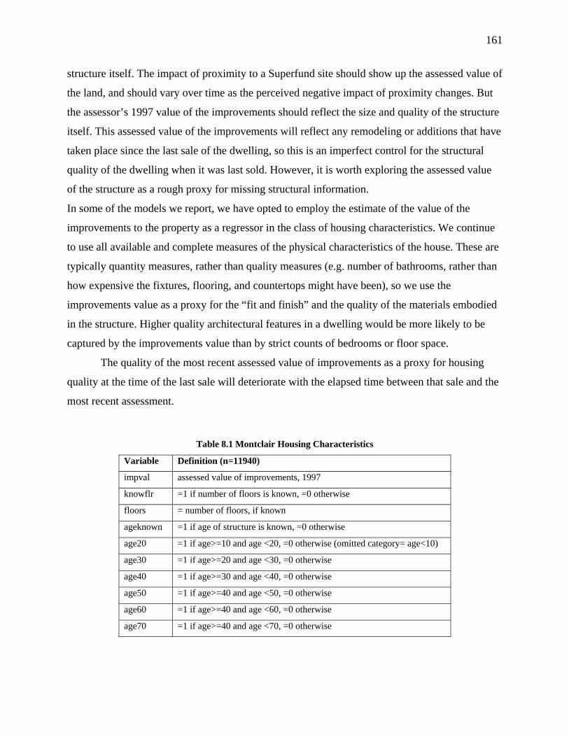
161
structure itself. The impact of proximity to a Superfund site should show up the assessed value of
the land, and should vary over time as the perceived negative impact of proximity changes. But
the assessor’s 1997 value of the improvements should reflect the size and quality of the structure
itself. This assessed value of the improvements will reflect any remodeling or additions that have
taken place since the last sale of the dwelling, so this is an imperfect control for the structural
quality of the dwelling when it was last sold. However, it is worth exploring the assessed value
of the structure as a rough proxy for missing structural information.
In some of the models we report, we have opted to employ the estimate of the value of the
improvements to the property as a regressor in the class of housing characteristics. We continue
to use all available and complete measures of the physical characteristics of the house. These are
typically quantity measures, rather than quality measures (e.g. number of bathrooms, rather than
how expensive the fixtures, flooring, and countertops might have been), so we use the
improvements value as a proxy for the “fit and finish” and the quality of the materials embodied
in the structure. Higher quality architectural features in a dwelling would be more likely to be
captured by the improvements value than by strict counts of bedrooms or floor space.
The quality of the most recent assessed value of improvements as a proxy for housing
quality at the time of the last sale will deteriorate with the elapsed time between that sale and the
most recent assessment.
Table 8.1 Montclair Housing Characteristics
Variable Definition (n=11940)
impval assessed value of improvements, 1997
knowflr =1 if number of floors is known, =0 otherwise
floors = number of floors, if known
ageknown =1 if age of structure is known, =0 otherwise
age20 =1 if age>=10 and age <20, =0 otherwise (omitted category= age<10)
age30 =1 if age>=20 and age <30, =0 otherwise
age40 =1 if age>=30 and age <40, =0 otherwise
age50 =1 if age>=40 and age <50, =0 otherwise
age60 =1 if age>=40 and age <60, =0 otherwise
age70 =1 if age>=40 and age <70, =0 otherwise

162
age70plus =1 if age>=70, =0 otherwise
lot size Size of lot, in ratio to sample average lot size = 9232 sq. ft.
OII: The OII data are drawn from the same Experian source as the Montclair data, but many
more data fields are non-empty in these data. Thus, a wider range of explanatory variables
capturing structural characteristics can be entertained.
Table 8.2 OII Housing Characteristics
Variable Definition (n=9211)
notold =1 if structure was built after 1900, =0 otherwise
age Age of structure if built after 1900
age2 Age of structure, squared
sqft Square feet of floor space, in ‘000s
sqft2 Square feet of floor space, squared
bedrms Number of bedrooms
bthrms Number of bathrooms
sqftbed Interaction term: sqft * bedrms
sqftbth Interaction term: sqft * bthrms
fplace =1 if at least one fireplace, =0 otherwise
knowflr =1 if number of floors is report, =0 otherwise
floors Number of floors, if data not missing
lot size Size of lot, in ratio to sample average lot size = 6199 sq. ft.
Woburn: The explanatory variables available for the Woburn model are the same as those
available for the OII site, although lot size will be normalized on the mean for this different
sample.
Table 8.3 Woburn Housing Characteristics
Variable Definition (n=12444)
notold =1 if structure was built after 1900, =0 otherwise
age Age of structure if built after 1900
age2 Age of structure, squared
sqft Square feet of floor space, in ‘000s
sqft2 Square feet of floor space, squared

163
bedrms Number of bedrooms
bthrms Number of bathrooms
sqftbed Interaction term: sqft * bedrms
sqftbth Interaction term: sqft * bthrms
fplace =1 if at least one fireplace, =0 otherwise
knowflr =1 if number of floors is report, =0 otherwise
floors Number of floors, if data not missing
lot size Size of lot, in ratio to sample average lot size = 15129 sq. ft.
Eagle Mine: Given that the Eagle Mine data are drawn from the Eagle County assessor’s office,
rather than from the Experian data, the available variables are somewhat different.
Table 8.4 Eagle Mine Housing Characteristics
Variable Definition (n=1087)
sfd =1 if single-family dwelling, =0 if condominium
age Age of dwelling
age2 Age of dwelling, squared
bedrms Number of bedrooms
bthrms Number of bathrooms
notwdframe =1 if not wood-frame construction, =0 otherwise
heatelec =1 if electric heating, 0 otherwise
constgood =1 if construction quality rated as “good” or better, =0 otherwise
constfair =1 if construction quality rated as “fair” or worse, =0 otherwise
downstream =1 if nearest to Eagle River, =0 if nearest to Gore Creek
lot size Size of lot, in ratio to sample average lot size = 5154 sq. ft.
8.4.4 Neighborhood Characteristics
We define the neighborhood in which a house is located as synonymous with its Census
tract. Been and Gupta (1997) give a very thorough rationale for the desirability and tractability of
using Census tracts when there is a need to quantify socio-demographic and other very local
characteristics over time. Since neighborhoods change over time, and might be expected to
change as a result of the discovery and remediation of a Superfund site, it is important to
distinguish between changes over time in the effect on housing prices of mere proximity to the
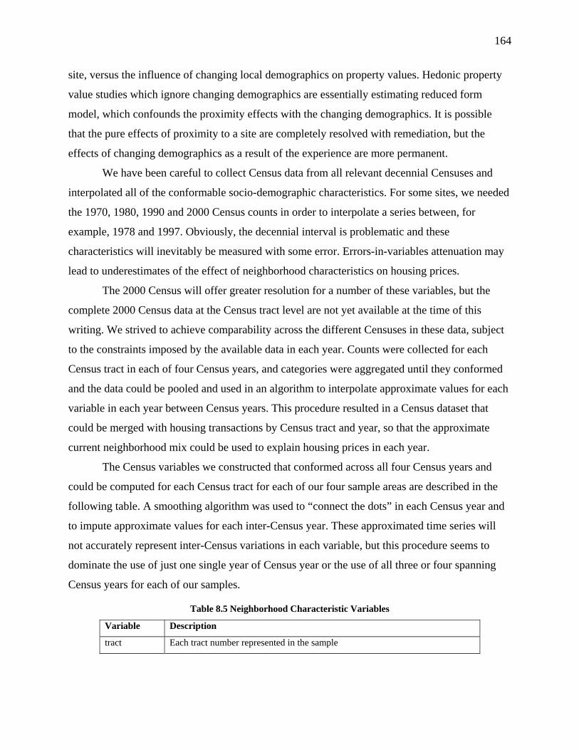
164
site, versus the influence of changing local demographics on property values. Hedonic property
value studies which ignore changing demographics are essentially estimating reduced form
model, which confounds the proximity effects with the changing demographics. It is possible
that the pure effects of proximity to a site are completely resolved with remediation, but the
effects of changing demographics as a result of the experience are more permanent.
We have been careful to collect Census data from all relevant decennial Censuses and
interpolated all of the conformable socio-demographic characteristics. For some sites, we needed
the 1970, 1980, 1990 and 2000 Census counts in order to interpolate a series between, for
example, 1978 and 1997. Obviously, the decennial interval is problematic and these
characteristics will inevitably be measured with some error. Errors-in-variables attenuation may
lead to underestimates of the effect of neighborhood characteristics on housing prices.
The 2000 Census will offer greater resolution for a number of these variables, but the
complete 2000 Census data at the Census tract level are not yet available at the time of this
writing. We strived to achieve comparability across the different Censuses in these data, subject
to the constraints imposed by the available data in each year. Counts were collected for each
Census tract in each of four Census years, and categories were aggregated until they conformed
and the data could be pooled and used in an algorithm to interpolate approximate values for each
variable in each year between Census years. This procedure resulted in a Census dataset that
could be merged with housing transactions by Census tract and year, so that the approximate
current neighborhood mix could be used to explain housing prices in each year.
The Census variables we constructed that conformed across all four Census years and
could be computed for each Census tract for each of our four sample areas are described in the
following table. A smoothing algorithm was used to “connect the dots” in each Census year and
to impute approximate values for each inter-Census year. These approximated time series will
not accurately represent inter-Census variations in each variable, but this procedure seems to
dominate the use of just one single year of Census year or the use of all three or four spanning
Census years for each of our samples.
Table 8.5 Neighborhood Characteristic Variables
Variable Description
tract Each tract number represented in the sample
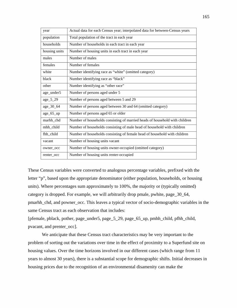
165
year Actual data for each Census year; interpolated data for between-Census years
population Total population of the tract in each year
households Number of households in each tract in each year
housing units Number of housing units in each tract in each year
males Number of males
females Number of females
white Number identifying race as “white” (omitted category)
black Number identifying race as “black”
other Number identifying as “other race”
age_under5 Number of persons aged under 5
age_5_29 Number of persons aged between 5 and 29
age_30_64 Number of persons aged between 30 and 64 (omitted category)
age_65_up Number of persons aged 65 or older
marhh_chd Number of households consisting of married heads of household with children
mhh_child Number of households consisting of male head of household with children
fhh_child Number of households consisting of female head of household with children
vacant Number of housing units vacant
owner_occ Number of housing units owner-occupied (omitted category)
renter_occ Number of housing units renter-occupied
These Census variables were converted to analogous percentage variables, prefixed with the
letter “p”, based upon the appropriate denominator (either population, households, or housing
units). Where percentages sum approximately to 100%, the majority or (typically omitted)
category is dropped. For example, we will arbitrarily drop pmale, pwhite, page_30_64,
pmarhh_chd, and powner_occ. This leaves a typical vector of socio-demographic variables in the
same Census tract as each observation that includes:
[pfemale, pblack, pother, page_under5, page_5_29, page_65_up, pmhh_child, pfhh_child,
pvacant, and prenter_occ].
We anticipate that these Census tract characteristics may be very important to the
problem of sorting out the variations over time in the effect of proximity to a Superfund site on
housing values. Over the time horizons involved in our different cases (which range from 11
years to almost 30 years), there is a substantial scope for demographic shifts. Initial decreases in
housing prices due to the recognition of an environmental disamenity can make the

166
neighborhood accessible to lower-income households, who may be prepared to accept the
disamenity in exchange for more housing at the same price, or cheaper housing, than they can
obtain elsewhere. Neighborhood characteristics are not independent of the “taint” due to a
Superfund site. It is important to ascertain whether the observation that housing price gradients
often tend to rise as one moves away from a Superfund site, even after remediation, may be due
to filtering-down of this housing stock that occurs during the period when taint is maximum.
It is entirely possible that, controlling for neighborhood changes that ensue from an
episode of major environmental taint, the eventual effect of proximity to the site is actually
positive (the price gradient moving away from the site is negative following remediation).
Homeowners may value proximity to a cleaned up site more than they value proximity to other
less-certifiably safe features.
The fact that Census data are available only at ten-year intervals has been an impediment
to addressing this research issue. It was necessary to wait for the availability of the year 2000
Census data to be able to interpolate between the 1990 Census tract information and the 2000
Census information in order to construct usable data for the last seven to nine years of housing
sales in our various data sets.
8.4.5 Other Local Amenities and Disamenities
Many earlier hedonic property value studies have included only one or two other
distances in their models (such as distance to the nearest shopping center, or the central business
district), or even no other distance variables at all. In the last few years, a number of
environmental aspects of spatial data have been examined by researchers who are interested in
determining their potential effects on property values. Acharya and Bennett (2001) use a sample
of about 4000 houses in New Haven county in Connecticut between 1995 and 1997 to explore
whether open space and land-use diversity affect housing prices. Diversity, richness, evenness
and dominance measures are used to quantify the patterns of land use within a fixed radius of
each dwelling. Among the spatial features they include as controls are distances to open space,
lakes, streams, the ocean, parks, and highways. They also use Census block group data for the
percentage of white households, the crime rate, average income, percentage college-bound
students, to quantify neighborhood characteristics. However, they do not attempt to isolate

167
variations over time in the effects of perceived environmental quality on housing prices. The
marginal effects are assumed to be static.
In this research, based on our geo-location of each property using GIS software, we have
measured for each house the distance to a wide variety of other topographic features, land uses,
and institutions. Some of these are common to all four of our samples, such as distance to the
nearest park and distance to the nearest school or shopping center. Others are unique to each site.
Major freeways may be close enough to matter, or they may not, and airports or the flight paths
implied by their runway configurations may be close enough to affect housing prices, or they
may not. Based on a careful examination of the features in the region of each sample, we have
identified and measured distances for a wide variety of things that could plausibly affect housing
sale prices. The “other distance” variables relevant to each Superfund site are discussed in detail
in the appendices devoted to each site, but will be summarized briefly below.
Concerning precedents in the literature for controlling for certain classes of variables, we
can identify the following:
Summits: Benson, et al. (1998) assess the influence on housing prices of a variety of views,
differentiated by both type and quality. They find that depending upon the particular view,
willingness to pay for this type of amenity is quite high. While map proximity to a summit does
not translate into the presence of a view, there may be some correlation.
Schools: “Close to schools” is considered by many home-buyers to be a positive feature of
housing location, but Clauretie and Neill (2000) find that proximity to year-round schools, tends
to decrease housing values.
Roads: Spatiotemporal fluctuations in location premiums associated with a major urban
highway construction project in a study by Vadali and Sohn (2001). Boarnet and Chalermpong
(2001) consider the effect of introducing new toll roads that increase accessibility.

168
Airports: Espey and Lopez (2000) find the airport in their study to be a disamenity. This stands
in contrast to earlier work by Tomkins, et al. (1998), who found proximity to one particular
airport to be a net positive amenity.
Railroads: Strand and Vagnes (2001) study the relationship between the price of residential
properties and proximity to railroads in Oslo. Bowes and Ihlanfeldt (2001) consider the effect of
commuter rail stations on the value of nearby properties.
Parks: Open spaces are not synonymous with parks, but work by Smith, et al. (2002) and by
Geoghegan (2002) considers the impact of open spaces on housing prices, suggesting that urban
parks may play this role to a certain extent in the more heavily settled examples in this research.
Water Bodies: Poor, et al. (2001), Spalatro and Provencher (2001), and Mahan, et al. (2000) all
consider hedonic property models with water features incorporated.
One shortcoming of these data concerning other distances is that they are “snapshot” data
based on the present geographic configuration of the local area. We have no way (at reasonable
cost) to reconstruct the appearance, during our sample periods, of new airports or new parks, for
example. We must rely upon the assumption that each of these features has remained fairly
constant over time (the 11 to 30 years of our samples) so that its effects are independent of time.
Of course, one could interact each of these distances with annual dummy variables to distinguish
year-specific distance effects for each, but the number of regressors would rapidly become even
more unmanageable than it is at present.
It must be acknowledged, however, that the emergence (part-way though our sample
period) of one of the shopping malls present in our sample in 2000 could distort the apparent
effect of distance from a Superfund site in that year. Suppose a shopping mall appears inside the
sample area, close to the Superfund site, half-way through the sample period. Suppose further
that the presence of the shopping mall causes housing values to increase with proximity to the
mall. Prior to the introduction of this mall, the prevailing effect might be the negative effect of
proximity to the Superfund site. Proximity to the yet non-existent mall would have no effect.

169
After the mall appears, however, proximity to the mall will increase prices, but proximity to the
Superfund site will decrease it, and the effects essentially wash out. The coefficient on the
distance from the mall location would be the average over the whole time period of the zero
effects without the mall and the positive effects with the mall, which would be overall positive
but smaller than their “true” effects. The coefficients on proximity to the Superfund site are
allowed to vary by year, however.
In the hedonic property value literature, there is some discussion about whether local
amenities and disamenities should make a fixed difference in the price of a property, regardless
of the size of that property, or whether these factors should in fact affect the per-unit-area price
of the property. We deem it unlikely that either one of these assumptions is entirely credible.
Hence, whenever a local amenity or disamenity enters a model, we explore expanded models
with both the amenity/disamenity distance and this distance interacted with the lot size of the
property in question. The effect of the amenity on house price (the derivative of expected
property price with respect to the amenity or disamenity) is therefore permitted to depend, in a
linear fashion, on the size of the property in question. If no such dependence is present in the
data, the coefficient on the property size interaction term will be indistinguishable from zero.
The “typical” magnitude of a non-constant marginal effect can sometimes be difficult to
appreciate when pondering regression results. Thus we undertake a convenient normalization.
Whatever our estimating sample, we first scale the raw data on lot size by the sample average of
the lot size variable, so that the sample mean of the scaled variable is one. Then, at the mean lot
size in the sample, the marginal effect of an amenity or disamenity that is interacted with lot size
will be given simply by the sum of the coefficient on the level of that amenity and the coefficient
on the interaction term. If these two coefficients are of opposite signs, the coefficient with the
larger absolute value will determine the sign of the effect at the means of the data. This
convention is observed for all of our local amenity and disamenity effects: neighborhood socio-
demographic and housing stock characteristics, distances from other potentially relevant
amenities and disamenities (parks, freeways, etc.), and the effects of distances from the
Superfund site in each year.

170
Montclair We will mention the other distances in the order in which they appear in the
estimating models. By using an additively separate specification in the logarithms of “distance to
the nearest X,” we are of course imposing the strong assumption that the distance gradients
relative to all amenities or disamenities of the same type are identical, and that the effect on
house prices of proximity to one site is not affected by proximity to another. These are strong
assumptions, but given the number of candidate variables, a considerably larger data set would
probably be required to discern the magnitudes of these interactions.
For Montclair, we include distances to the nearest summit of land, to the nearest school
and nearest retail center (shopping mall). We also use distance to the nearest hospital, church,
and cemetery. With respect to surface transportation, we control for distance from a railroad, a
major road, Interstate 280 and the Garden State Parkway. We include distance from parks and
major bodies of water. Among institutions, we have distance to the nearest college or university
and distance to the nearest golf or country club. In addition to controlling for distance from the
nearest airport, we include a separate airport distance unique to Newark International Airport.
The details for each of these amenities or disamenities are included in Appendix A.
OII: For our housing price model for the OII landfill area, we measure and control for
distances from the nearest school, retail center (shopping mall), hospital, church and cemetery.
We also control for distance from the nearest railroad and for distances from a number of
specific Southern California freeways: Interstate 5, Interstate 605, Interstate 10 and State Route
60. The effects for these distances are in addition to those of the distance from the nearest major
road, which may sometimes be one of these freeways, but will often be a large “surface street.”
We control for distance to the nearest “river” (often seasonal in Southern California) and the
nearest major body of water (typically a non-seasonal river constrained within concrete for flood
control). The distance to the nearest park is measured, with additional controls for distance from
the largest regional park, the Whittier Narrows recreation area. There is one college campus that
may be relevant, the California State University at Los Angeles, and we also control for
distances from the nearest country club or golf course.
Full details of the features captured by the “other distance” variables for the OII landfill
site are included in Appendix B.

171
Woburn: For Woburn, we control for distance from the nearest summit of land, as well as
distances from the nearest school, retail center (shopping mall), hospital, church and cemetery.
Along with distance to the nearest railroad, we include a number of different measures of
proximity to roads: the distance to Interstates 93 and 95, the distance to the nearest principal
artery, the distance to the nearest other principal road, the distance to the nearest road including
smaller roads.
Air transportation corridors could also have an effect on housing prices in this area. We
control for distance from each of Boston’s four airports: Logan airport, Beverly Municipal
airport, “Tew-Mac” airport and Hanscom Air Force Base. In addition to the simple distance
measures, we also plotted the potential flight paths over the sample area, based on the trajectories
of runways at each airport. We then computed the distance from each house to the nearest flight
path associated with each airport.
Finally, we include distances to the nearest park, major body of water, and country club.
Details concerning each of these types of “other distances” we have computed for the dwellings
in the Woburn area sample are contained in Appendix C.
Eagle Mine: The universe of available and potentially relevant “other distance” variables
considered in the Eagle mine analysis is displayed below. While we measured distances for
variables in the similar classes as those used for other Superfund sites, the distances to many
features, for the Eagle Mine sample, were great enough that one would not expect them to have
an influence on variations in housing prices within the sample.
Measured distances include distances to the nearest summit (and there are about 20
named summits in the sample area) and to the nearest river, either Eagle River or Gore Creek.
Elevation might plausibly explain housing values, but horizontal distances to the nearest summit
are likely to be a poor proxy for elevation in this terrain. We also collected information about
distances to the nearest school and retail area, hospital, church and cemetery, as usual. Only
schools, however, are contained in the sample area and some of the other distances are extremely
large (up to 50 miles). The effects of distances from the nearest railroad or road will be
confounded by proximity to the nearest river, since the highways and railroad follow either the
172
Eagle River, or Gore Creek, or both, due to the topography of the area. There are no “major
bodies of water” in the area other than the rivers. “Recareas” include three golf clubs, and these
may have independent distance effects. Other points of local interest are too heterogeneous to be
combined (e.g. campgrounds, ranger stations). The one exception is distance to the Vail ski area.
We did measure distances from each site to the nearest town for seven distinct towns
(Avon, Eagle, Eagle-Vail, Leadfille, Minturn, Redcliff, and Vail itself). However, the linear
arrangement of houses and towns along Interstate 70, leaves very little independence in these
distances. The main distance variable we retain in the model is the distance to the Vail ski area.
A full description of these “other distances” for the Eagle Mine sample is included in
Appendix D.

173
Chapter 9
Property Value Results
9.1 Classes of Hedonic Property Value Models
Our most basic specification, called Model 1, explores for time-varying proximity effects
in a generic specification of the following sort:
(9.1) 10 2ln( ) ( )it t t it iT itLSPRICE P LDIST Aβ β ε= + + +
This model is designed to mimic the most rudimentary type of specification that a researcher
might first explore when looking for time-varying distance effects. Distance is interpreted as a
proxy for perceived risk. When we estimate each of our models with time-varying distance
effects, we test the hypothesis that the profile of the distance premium (i.e. the perceive risk
premium) is the same in all years in the sample, since a simpler model yet would not even
distinguish distance effects that may vary over time.
The key argument of this research is that time-varying socio-demographics, both near and
further away from the Superfund site, can have a systematic effect on housing prices. To
determine the effects of demographics when other distances are not controlled, the generic
version of Model 2 is:
(9.2) 10 2 30ln( ) ( ) ( )it t t it iT it itLSPRICE P LDIST A Sβ β β ε= + + + +
However, the question of whether there are any general proximity effects, at all, cannot be
reliably ascertained without controlling for proximity to other amenities and disamenities. The
apparent magnitude of the proximity effects across years may be rendered generally higher or
lower by controlling for time-constant effects of proximity to other features. Model 3 will take
the general form:
(9.3) 10 2 40ln( ) ( ) ( )it t t it iT iT itLSPRICE P LDIST A Dβ β β ε= + + + +

174
This model is similar to the type of model estimated by many previous researchers, although
most models of this form control for a rather limited selection of other distances.
Our most complete general model is Model 4, corresponding to Equation 8.2 above,
which employs all five classes of regressors: the set of year dummies that reveals the area-wide
price index, ln( )tP ; the complete set of interactions between the logarithms of distance from the
Superfund site and annual dummy variables, giving 10( )t itLDISTβ ; the structural characteristics,
iTA ; the other distances, iTD , and the time-varying demographics, itS . In selected cases, we will
include other or different variables, such as potential lot size shifters on the key coefficients, or,
in the case of Woburn, latitude and longitude shifters for the entire price function, or
downstream/non-downstream variables, as in the case of Eagle Mine.
Before we delve into the details of the estimated hedonic property value models,
however, it is important to look at some auxiliary models. These models specifically examine the
trends over time in the socio-demographic characteristics of the populations both near, and
further away from, each Superfund site.
9.2 Auxiliary Models Time-Varying Demographic Patterns
There has been considerable interest in the environmental equity/justice literature about
whether hazardous waste sites are selected because the population in the area is relatively lower
income, has a larger proportion of minorities, or unlikely to organize to resist a siting decision.
The Superfund sites in our sample are not new siting decisions. These sites were in place before
much of the residential development around them began to occur. [See the approximate timelines
listed above.] Much of the population around the site has accumulated during or since the time
the site was in operation. The environmentally relevant “events” in our cases are not decisions to
site a new facility, but the news surrounding each site’s designation as a Superfund site and the
resulting deliberation about cleanup strategies and actual remediation. So in this context, it is not
so much the siting decision that matters, but the consequences over time of the publicity about
the site’s Superfund status, and therefore public awareness of the site and the hazards that it may
represent. Perceived risk is assumed to vary over time, and should also vary over space in a way
that is approximately correlated with possible exposure.
175
It is difficult to reconstruct reliable time-series of neighborhood socio-demographic
characteristics. As Gayer (2000) points out, Census block groups allow a more refined measure
of a dwelling’s neighborhood than the Census tract. However, even Census tracts pose problems
for splicing together data across different Censuses. Tracts tend to be split as density increases,
and it is enough of a challenge to construct a time series at the tract level, since coding categories
change across time. We constructed a set of characteristics that aggregated socio-demographic
groups sufficiently to afford a match across decennial Censuses and aggregated Census tracts to
a common denominator across years. This leads to a loss of some resolution both in detail and
spatially, compared to what is available if one relies solely on the 1990 Census, for example.6
However, we deem it important for us to use a comparable set of variables across the three
samples where this strategy is feasible. We also need to approximate neighborhood
characteristics for years that span the 1970’s, 1980’s and 1990’s, which requires conformation
across four different Censuses.
One of the most significant empirical enquiries into the effects of hazardous waste sites
on local demographics is described in Been and Gupta (1997). These researchers identify 608
commercial hazardous waste treatment, storage, and disposal facilities opened between 1970 and
1990. They collect Census data for the Census prior to the opening, and for 1990 for each of
these tracts. As controls, they draw a random 5% sample of all tracts in the U.S. They analyze
“before” demographics and “after” demographics, but of primary interest in the context of the
present work is their study of the difference-in-differences between the host tracts and all other
tracts, between the Census prior to the facility opening and 1990. As multivariate analyses, these
researchers pooled the host and non-host Census tracts and regressed the 1990 values for each
demographic characteristic (in percentage terms) against the value of this variable in the Census
prior to the siting, along with a dummy variable for whether the tract hosted a site.
Using these empirical techniques, Been and Gupta (1997) conclude that their study “does
not support the argument that market dynamics following a siting of a TSDF change the racial,
ethnic, or socioeconomic characteristics of host neighborhoods. The analysis suggests that the
areas surrounding TSDFs sited in the 1970s and 1980s are growth areas: in host areas, the
6 Only “short-form” 2000 Census statistics are available at the Census tract level as of this writing.

176
number of vacant housing units was lower than in sample areas, and the percentage of housing
built in the prior decade was higher. Such growth suggests that the market for land in the host
areas is active and should respond to any nuisance created by the TSDFs. It also may suggest that
the burdens of the TSDF are being off-set by the benefits, such as increased employment
opportunities.”
As Liu (1997) prescribes, any assessment of market dynamics as a potential explanation
for neighborhood change around a locally undesirable land use requires controlling both for the
characteristics of the neighborhood before a siting decision and for changes in other
neighborhoods. The Been and Gupta (1997) approach uses randomly selected Census tracts
elsewhere in the country as a control for what is happening in “other neighborhoods.” Here, we
control for patterns in other neighborhoods by enlisting the broader area around the host tract as
control tracts. Rather than looking for discrete differences in socio-demographic characteristics
between a host tract and tracts that are greatly displaced in terms of distance, we look for patterns
in demographics over time that differ continuously with distance from our Superfund sites. If the
socio-demographic patterns near the site are indistinguishable from those farther away the
distance gradient relative to the site will be flat. Depending upon conditions at the beginning of
our sample periods, there may be other reasons why we might observe a positive or negative
distance gradient in socio-demographic characteristics. What matters, however, is how this
gradient changes over time. If white residents tend to move out, and non-white residents to move
in, in the wake of publicity about Superfund designation and remediation, then the distance
gradient for whites should be observed to become relatively more positively sloped (or less
negatively sloped) with time. Likewise, the distance gradient for non-whites would be expected
to become less positively sloped (or more negatively sloped) over time.
In the auxiliary models described in this section, we explore the simple trends in
demographics near our four Superfund sites over time. Each observation is a house sale, and for
each observation we know the log of the distance from the site in question. As dependent
variables, we use the Census tract proportions of inhabitants in each class, pX, where X is a
Census category. These are the neighborhood characteristics associated with each house in our
main sample. In future work, we plan to aggregate the analysis to consider each Census tract as a
unit of observation, but for now we preserve houses as observations since this will most clearly
177
highlight the multicollinearities present in our main hedonic property value models. For the
purposes of these main models, we interpolate the information for each Census tract across time
to provide approximate time series for each variable.
We assess the propensity for lower-income families, non-whites, and non-traditional
families to “come to the nuisance,” possibly attracted by lower housing prices brought about by
taint from the Superfund site. The models we examine regress proportions for each socio-
demographic and housing tenure characteristic, across Census tracts and over time, against a
measure of distance, a time trend, and an interaction between distance and time. We use the log
of distance, since this transformation is important in our main hedonic property value models.
The log transformation allows any effect of proximity to the Superfund site to dissipate with
distance until, in the limit, further increases in distance have very little effect on socio-
demographic proportions. This is a reasonable maintained hypothesis, since the “reach” of
influence of any particular Superfund site must be finite.
Our specifications take the following simple form:
(9.4) 0 1 2 3it it it itpX LDIST t t LDISTα α α α ν= + + + ⋅ +
Using the log of distance from the site permits the marginal effect of distance on proportions to
decline with distance, since as distance increases, the same percent change in distance
corresponds to a greater and greater increment of distance. This functional form assumes that the
effect of a percent change in distance is constant.
The effect of the log of distance from the Superfund site on the neighborhood proportion
of a given group is given by 1 3tα α+ . The effect of the passage of time on the neighborhood
proportion of a given group is given by 2 3 itLDISTα α+ . If the distance profile for the proportion
of residents of a particular type is merely shifting upwards or downward everywhere in the
region, we would expect to see 2α nonzero, but 03 =α . In contrast, if the distance profile is
changing systematically over time, we will see 3 0α < if this group is becoming relatively more
numerous near the Superfund site, and 3 0α > if this group is becoming relatively less numerous
near the Superfund site (Figure 9.1).

178
Figure 9.1 Changes in Socio-demographics near Superfund site over time
In the Montclair case, there is not only a distance variable measured from the perimeter
of the nearest site for houses outside the sites, there is also a dummy variable indicating whether
the dwelling in question is inside the site boundaries. In this case, Equation 9.4 will be adapted
to:
(9.5) 0 1 2 3
4 5
it it it
it it it
pX LDIST t t LDISTINSIDE t INSIDE
α α α αα α ν
= + + + ⋅+ + ⋅ +
In reporting these results, we concentrate on the estimated value of 3α (and 5α in the Montclair
case) for each type of Census group, X , for each of the Superfund sites for which we are able to
employ Census tract characteristics (i.e. all sites except Eagle Mine). In the case of groups
becoming relatively more numerous throughout our sample areas, independent of distance from
the Superfund site, any effects of these changes on housing prices will be picked up by the
179
estimated area-wide price index, tP , that is captured by the set of year dummies in the model for
itLSPRICE .
In perusing the estimated values of 3α in the tables that follow, keep in mind that the
dependent variable is constant for all houses in a particular Census tract in a particular year. To
the extent that this variable does not perfectly reflect the “neighborhood” that is relevant to the
house sale in question, there will be a degree of error in this dependent variable. The explanatory
variables, distance and year, are observation-specific.7
It must also be acknowledged that these specifications constrain the time trends to be
monotonic. If they are non-monotonic, perhaps first increasing then decreasing, for example, or
vice versa, this would tend to obscure any trends.
(9.6) 2 20 1 2 3 4 5it it it it itpX LDIST t t LDIST t t LDISTα α α α α α ν= + + + ⋅ + + ⋅ +
This specification yields a distance gradient for Census tract characteristic X in the form of
(9.7)
21 3 5
21 3 5
, orit
it
it
it it
pX t tLDIST
pX t tDIST DIST
α α α
α α α
∂= + +
∂
∂ + +=
∂
This implies that the effect will decrease with distance, and is quadratic in time, if the
5α coefficient is significantly different from zero. The fitted turning point occurs at
*3 5/(2 )t α α= − . If *t lies within the range of the data, the fitted time trend in the Superfund
7 There is an alternative strategy, which we are currently exploring. We find the effective center of gravity for the all the houses in each Census tract across all years by computing the mean latitude and mean longitude of these houses. We then locate these centers of gravity in our GIS software and use ArcMap to measure the distance from each tract centroid to the boundary (or center) of the Superfund site. The number of observations can then be limited to just actual Census years and individual or merged tracts that can be conformed across all Census years. In these more limited data, we lose the resolution on distance for each house, but avoid the spurious estimation precision that accompanies the use of the same Census tract information for all houses in a tract and smoothes the time profile by interpolating. These results are not yet finalized.

180
distance profile of Census characteristic X changes sign. If *t lies beyond the range of the data,
the trend is approximately monotonic.
We have explored the data for evidence of significance in quadratic terms and found
some evidence. But one must bear in mind that the underlying real data consist of only four
decennial snapshots of neighborhood characteristics. The interpolated data are only approximate.
Given the quality of the data, we do not deem it judicious to push too hard on this generalization.
In this research, we report only the key coefficient estimates, and their standard errors,
for the 3α coefficient in Equation 9.4. The rest of the results for each model for each Census
tract attribute are presented in Appendices A through D. The appendices also illustrate the
progression of fitted distance profiles over time, with the heavier line in each graph depicting the
first-year in the sample and the progression being captured by representative intervening years
between then and the end of the sample period.
9.2.1 Montclair
There are significant numbers of observations from each of over 60 different Census
tracts represented in the Montclair sample, so there is considerable variation in tract
characteristics across the sample in any one year, and also in the interpolated time series within
each tract.
The Montclair model for each Census tract characteristic differentiates between distance
effects, implied by 3α , and the effect of being on top of one of the radium sites, 5α . Only these
two coefficients for each model are presented in the following table. The rest of the results for
each model are presented in Appendix A.
Table 9.1 Montclair Census Tract Proportion Coefficient
Census tract
proportion 3α Coefficient
(robust t-test statistic)
5α Coefficient
(robust t-test statistic)
pfemale .0000813 1.33 .00078 2.94***
pwhite .0028637 3.00*** -.0171576 -3.84***
pblack -.0033634 -3.39*** .0184994 4.13***
pother .0003952 1.85* -.0013925 -1.03

181
page_under5 -.000146 -3.98*** -.0000739 -0.38
page_5_29 -.0005365 -3.00*** .0012068 1.68*
page_30_64 -.000451 -3.33*** -.0007805 -1.16
page_65_up .001029 6.10*** -.000403 -0.57
pmarhh_chd -.0005364 -1.79* .0002539 0.18
pmhh_child -2.45e-06 -0.06 .0002933 1.68*
pfhh_child -.0003317 -1.90* .002167 2.54***
powner_occ -.0002585 -0.26 -.0023418 -0.45
pvacant -.0000826 -1.11 -.0002405 -0.50
prenter_occ .0003412 0.36 .0025831 0.53
Over the 1987-1997 time period for which we have data for the Montclair area, we will first
consider changes in the distance profile of relative concentration for different groups. The 3α
coefficient if negative, conveys that the group in question has been becoming more concentrated
closer to the Superfund site. Groups that have become statistically significantly more prevalent
nearer the site include: blacks, children under 5, young people aged 5-29 and people aged 30-64,
as well as (possibly) married heads of household with children and female-headed households
with children. Positive 3α coefficients indicate that a group has become relatively less numerous
closer to the site. These groups include whites and seniors, and possibly other non-white ethnic
groups.
For houses inside the contaminated areas, a positive 5α coefficient implies an increase in
the proportion of that group over time. The relative share of female residents has become
statistically significantly higher over time here, as has the proportion of blacks, female-headed
households with children, and possibly young persons between the ages of 5 and 29 and male
heads of household with children. In contrast, whites have tended to move away from the
contaminated areas.
One notable feature of these results is that there seem to have been no systematic effects
on housing tenure or vacancy rates, either on top of the Montclair sites, or close to them.

182
9.2.2 OII
There are over 50 different Census tracts around the OII landfill. This creates a diversity
of different values for neighborhood effects within any one year, and more variation across years
in the interpolated Census tract data.
In the 1960’s and 1970’s, Asian emigrants began to populate what had been a mostly
white bedroom community. By the 1980s, racial tension between longtime residents and new
immigrants became significant, leading to a controversial law requiring English on business
signs, Chinese books in the public library and attempts to make English the city's official
language. Racial problems have now mostly subsided and Monterey Park has become the only
city in the San Gabriel Valley with an Asian majority.
The pattern in this Southern California community is somewhat different from that in the
Montclair and Woburn cases. Our conformable Census measures do not include a distinct
category for Asian ethnic groups, so these populations are captured by the “pother” category.
Again, only the key 3α coefficient for each model is presented in the following table. The
remainder of the results for each model appear in Appendix B.
Table 9.2 OII Census Tract Proportion Coefficients
Census tract proportion
3α Coefficient (with robust t-test statistic)
pfemale -.0000198 -1.27
pwhite -.0018906 -10.81***
pblack .000019 2.57***
pother .0020202 11.42***
page_under5 .0000226 0.92
page_5_29 .0002393 4.20***
page_30_64 .0003549 6.10***
page_65_up -.0004772 -10.35***
pmarhh_chd .0009305 9.33***
pmhh_child -.0002995 -8.45***
pfhh_child .0000927 2.21***
powner_occ .0009346 4.05***
pvacant .000279 15.02***
prenter_occ -.0012124 -5.54***
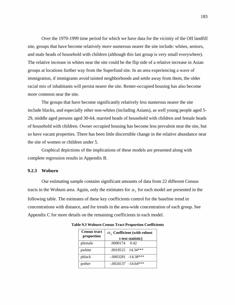
183
Over the 1970-1999 time period for which we have data for the vicinity of the OII landfill
site, groups that have become relatively more numerous nearer the site include: whites, seniors,
and male heads of household with children (although this last group is very small everywhere).
The relative increase in whites near the site could be the flip side of a relative increase in Asian
groups at locations further way from the Superfund site. In an area experiencing a wave of
immigration, if immigrants avoid tainted neighborhoods and settle away from them, the older
racial mix of inhabitants will persist nearer the site. Renter-occupied housing has also become
more common near the site.
The groups that have become significantly relatively less numerous nearer the site
include blacks, and especially other non-whites (including Asians), as well young people aged 5-
29, middle aged persons aged 30-64, married heads of household with children and female heads
of household with children. Owner occupied housing has become less prevalent near the site, but
so have vacant properties. There has been little discernible change in the relative abundance near
the site of women or children under 5.
Graphical depictions of the implications of these models are presented along with
complete regression results in Appendix B.
9.2.3 Woburn
Our estimating sample contains significant amounts of data from 22 different Census
tracts in the Woburn area. Again, only the estimates for 3α for each model are presented in the
following table. The estimates of these key coefficients control for the baseline trend in
concentrations with distance, and for trends in the area-wide concentration of each group. See
Appendix C for more details on the remaining coefficients in each model.
Table 9.3 Woburn Census Tract Proportion Coefficients
Census tract proportion 3α Coefficient (with robust
t-test statistic) pfemale .0000174 0.42
pwhite .0019515 14.34***
pblack -.0003281 -14.38***
pother -.0024137 -14.64***

184
page_under5 .0002072 5.33***
page_5_29 -.0003548 -1.93*
page_30_64 .0001168 0.93
page_65_up -.0000607 -0.41
pmarhh_chd .0016572 6.66***
pmhh_child -.000145 -11.20***
pfhh_child -.0006561 -10.69***
powner_occ -2.66911 -1.54
pvacant -.0003236 -9.13***
prenter_occ -.0033483 -7.69***
Over the 1978-1997 time period for which we have data for the Woburn area, groups that
have become relatively more numerous nearer the site include: blacks, other non-white groups,
the age 5-29 group, male heads of household with children, female headed households with
children, vacant properties, and rental properties. Groups that have become relatively less
numerous near the site include: whites, children under 5, and households with children headed by
married couples. Groups for which there has been little discernible change in the relative
abundance near the site are: females, persons between the ages of 30 and 64, seniors, owner
occupants.
Woburn was incorporated in 1652 and leather, tanning, and boot and shoe production was
the main industry from the mid-1800’s to 1915. Suburban growth began in the mid-1900’s and
has continued. The site has been described extensively by other authors, including Kiel (1995)
and Kiel and Zabel (2001).
9.2.4 Eagle Mine
There are insufficient numbers of Census tracts represented around the Eagle Mine site to
allow an analysis of trends in Census tract attributes associated with house sales over time.
9.2.5 Synthesis
It seems eminently clear that there is a strong tendency for fundamental neighborhood
change in the wake of a Superfund identification and remediation process. The property prices

185
we use from our analysis stem from house sales, and every time there is a house sale, the
occupants of that dwelling typically change. Who moves out and where they choose to go, and
who moves in, determines the change in the composition of the community in the vicinity of a
site. If the negative price shock accompanying a Superfund designation and the cleanup process
make housing in the vicinity of the site more affordable to lower income households,
unconventional households, ethnic minorities, or absentee landlords, a sufficient number of sales
can detectibly alter the makeup of the community.
There is a considerable literature in urban economics concerning the mechanisms of
neighborhood change (invasion-succession, tipping). The precipitating agent for the process, in
our cases, seems likely to have been the identification of the Superfund site.
Empirical models may fail to control for neighborhood change over time as a Superfund
identification and remediation process takes place. This can lead to omitted variables bias that
creates the impression that the Superfund process “taints” a neighborhood long after the site
itself has been cleaned up. In reality, what accounts for the persistent negative price differential
closer to the site could be the gradient in socio-demographic and income classes approaching the
site.
With site-induced neighborhood change, this “income-socio-demographic” gradient will
masquerade as a persistent “Superfund site proximity” gradient. When the site is clean, it may be
that nobody in the neighborhood or beyond is the least worried about any residual hazard. In fact,
having been certifiably cleaned, the site may even appear safer and more environmentally
attractive than competing uncertified areas elsewhere in the region. The true post-cleanup
“environmental gradient” might even display higher property prices near the cleaned site.
However, if one fails to control for the changed “income-socio-demographic gradient,” it is
possible to misidentify the phenomenon as a persistent taint or perceived risk due to the site.
9.3 Auxiliary Models: Time-Varying Housing Attributes
The housing stock in a region can change more slowly than the characteristics of the
population. Many houses are remodeled and updated, sometimes to include additional bathrooms
or perhaps bedrooms, lots are subdivided in order to permit increases in density. In this section,
we examine the trends over time in the average characteristics of houses sold, as a function of
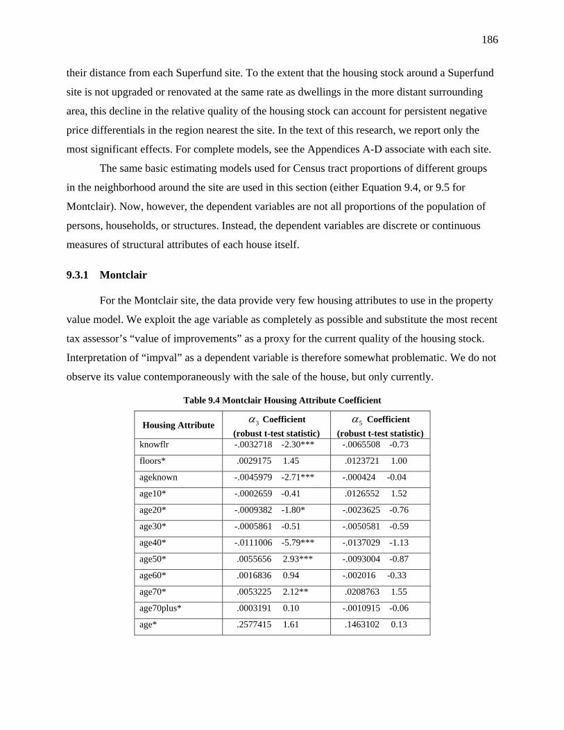
186
their distance from each Superfund site. To the extent that the housing stock around a Superfund
site is not upgraded or renovated at the same rate as dwellings in the more distant surrounding
area, this decline in the relative quality of the housing stock can account for persistent negative
price differentials in the region nearest the site. In the text of this research, we report only the
most significant effects. For complete models, see the Appendices A-D associate with each site.
The same basic estimating models used for Census tract proportions of different groups
in the neighborhood around the site are used in this section (either Equation 9.4, or 9.5 for
Montclair). Now, however, the dependent variables are not all proportions of the population of
persons, households, or structures. Instead, the dependent variables are discrete or continuous
measures of structural attributes of each house itself.
9.3.1 Montclair
For the Montclair site, the data provide very few housing attributes to use in the property
value model. We exploit the age variable as completely as possible and substitute the most recent
tax assessor’s “value of improvements” as a proxy for the current quality of the housing stock.
Interpretation of “impval” as a dependent variable is therefore somewhat problematic. We do not
observe its value contemporaneously with the sale of the house, but only currently.
Table 9.4 Montclair Housing Attribute Coefficient
Housing Attribute 3α Coefficient (robust t-test statistic)
5α Coefficient (robust t-test statistic)
knowflr -.0032718 -2.30*** -.0065508 -0.73
floors* .0029175 1.45 .0123721 1.00
ageknown -.0045979 -2.71*** -.000424 -0.04
age10* -.0002659 -0.41 .0126552 1.52
age20* -.0009382 -1.80* -.0023625 -0.76
age30* -.0005861 -0.51 -.0050581 -0.59
age40* -.0111006 -5.79*** -.0137029 -1.13
age50* .0055656 2.93*** -.0093004 -0.87
age60* .0016836 0.94 -.002016 -0.33
age70* .0053225 2.12** .0208763 1.55
age70plus* .0003191 0.10 -.0010915 -0.06
age* .2577415 1.61 .1463102 0.13
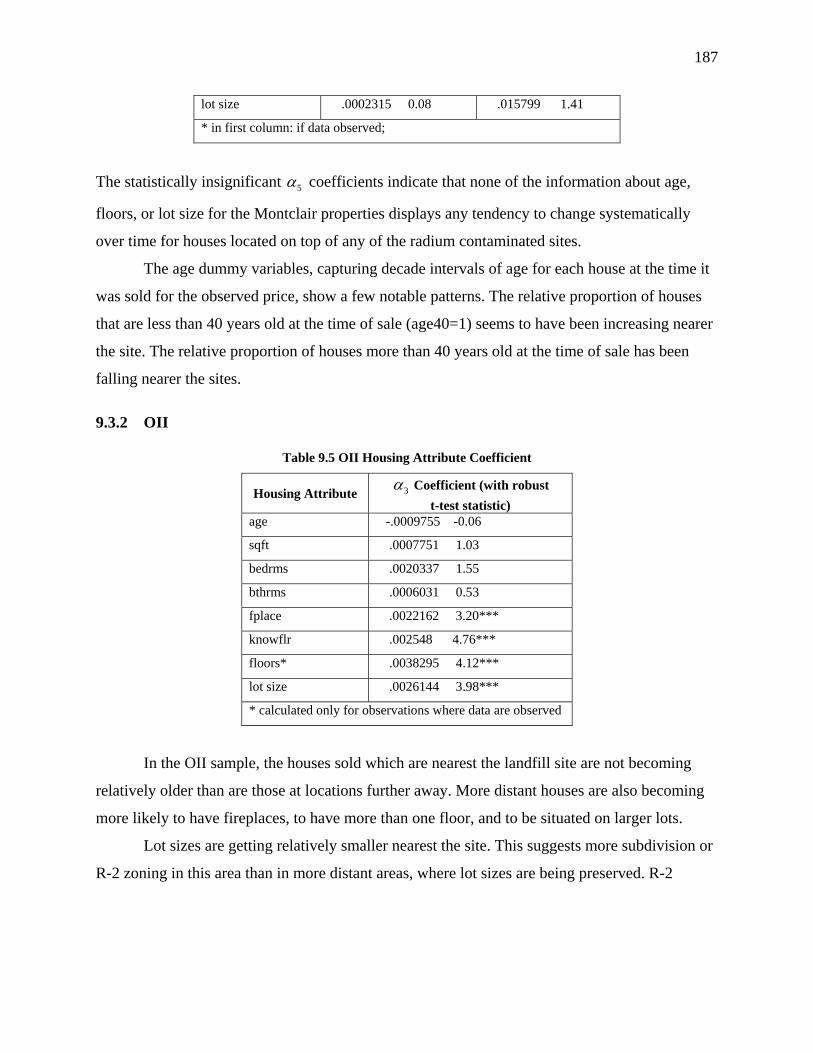
187
lot size .0002315 0.08 .015799 1.41
* in first column: if data observed;
The statistically insignificant 5α coefficients indicate that none of the information about age,
floors, or lot size for the Montclair properties displays any tendency to change systematically
over time for houses located on top of any of the radium contaminated sites.
The age dummy variables, capturing decade intervals of age for each house at the time it
was sold for the observed price, show a few notable patterns. The relative proportion of houses
that are less than 40 years old at the time of sale (age40=1) seems to have been increasing nearer
the site. The relative proportion of houses more than 40 years old at the time of sale has been
falling nearer the sites.
9.3.2 OII
Table 9.5 OII Housing Attribute Coefficient
Housing Attribute 3α Coefficient (with robust t-test statistic)
age -.0009755 -0.06
sqft .0007751 1.03
bedrms .0020337 1.55
bthrms .0006031 0.53
fplace .0022162 3.20***
knowflr .002548 4.76***
floors* .0038295 4.12***
lot size .0026144 3.98***
* calculated only for observations where data are observed
In the OII sample, the houses sold which are nearest the landfill site are not becoming
relatively older than are those at locations further away. More distant houses are also becoming
more likely to have fireplaces, to have more than one floor, and to be situated on larger lots.
Lot sizes are getting relatively smaller nearest the site. This suggests more subdivision or
R-2 zoning in this area than in more distant areas, where lot sizes are being preserved. R-2
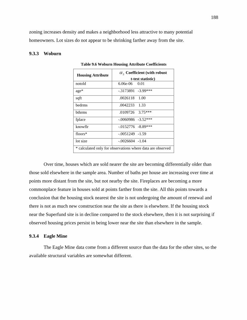
188
zoning increases density and makes a neighborhood less attractive to many potential
homeowners. Lot sizes do not appear to be shrinking farther away from the site.
9.3.3 Woburn
Table 9.6 Woburn Housing Attribute Coefficients
Housing Attribute 3α Coefficient (with robust t-test statistic)
notold 6.06e-06 0.01
age* -.3173891 -3.99***
sqft .0026118 1.00
bedrms .0042233 1.33
bthrms .0109726 3.75***
fplace -.0060986 -3.52***
knowflr -.0152776 -8.89***
floors* -.0051249 -1.59
lot size -.0026604 -1.04
* calculated only for observations where data are observed
Over time, houses which are sold nearer the site are becoming differentially older than
those sold elsewhere in the sample area. Number of baths per house are increasing over time at
points more distant from the site, but not nearby the site. Fireplaces are becoming a more
commonplace feature in houses sold at points farther from the site. All this points towards a
conclusion that the housing stock nearest the site is not undergoing the amount of renewal and
there is not as much new construction near the site as there is elsewhere. If the housing stock
near the Superfund site is in decline compared to the stock elsewhere, then it is not surprising if
observed housing prices persist in being lower near the site than elsewhere in the sample.
9.3.4 Eagle Mine
The Eagle Mine data come from a different source than the data for the other sites, so the
available structural variables are somewhat different.

189
9.3.5 Synthesis
In none of our examples does it appear that the housing stock nearest the Superfund site
is being renewed and upgraded at the same rate as housing at locations further removed from the
site. It may be the case that after a sufficient period of time has passed following a cleanup
project, and the site is designated as “safe” that homeowners in the area will again undertake to
accelerate maintenance of the housing stock to bring it back into line with the typical housing
stock in the surrounding area. However, if lower-income homeowners have moved into the area,
and if rental rates have increased, this may not set the stage for such accelerated renewal of the
stock. Despite cleanup, housing price may remain lower than the surrounding area due to
deferred maintenance and slower remodeling schedules or teardowns and replacements.
As in the case of the “income-socio-demographic” gradient created by earlier price
differentials due to the Superfund identification and cleanup process, we may see a “deferred
maintenance” gradient come into being relative to the location of the Superfund site. To the
extent that degradation of the housing stock accompanies a Superfund experience and the
attendant income and socio-demographic changes, and persists beyond the end of the cleanup
process, this factor may also masquerade as a persistent environmental taint.
9.4 Hedonic Property Value Models with Time-Varying Proximity Effects
Due to the very large number of control variables, and hence estimated coefficients, in
each of the models we estimate, we limit our discussion in the text of this research to the
properties of the key set of year-specific coefficients that describe the elasticity of selling prices
with respect to distance from the Superfund site, by year.
Our key results will be displayed in tables that merely note the presence or absence of the
other types of regressors in the specification. An extensive appendix for each site contains the
full specifications and other supporting statistical results. In the text of this research, we limit our
attention to specifications that constrain the lot size effects to be zero. In some cases, these lot
size effects are individually statistically significant, but including this generalization in the model
does not alter the general weight of the findings in any case, so we do not emphasize those
results.

190
9.4.1 Montclair
The format of the estimating model for the Montclair sample is somewhat different from
the generic specification. Suppressing the 11tβ , 31β , and 41β parameters on the lot size interaction
terms, the Montclair estimating model is:
(9.8) 00 10 2 30 40ln( ) ( ) ( ) ( ) ( )
it
t t it t it iT it iT it
LSPRICEP INSIDE LDIST A S Dβ β β β β ε
=+ + + + + +
Recall that since there are houses being sold that lie inside the boundaries of the radium sites in
the Montclair area, we include year-specific dummy variables, itINSIDE , for these houses. The
coefficients on these variables may also be permitted to vary systematically with lot size, but this
interaction is suppressed in this equation. For houses outside the radium sites, we compute the
distance from the boundary of the site to each house.
If the radium contamination negatively affects housing prices, we expect the
coefficients 00tβ , in some or all years, will be negative. If proximity to the radium contamination
depresses housing prices in some or all years, we expect the coefficients 10tβ to be positive in
those years, reflecting the increase in average selling prices at locations further away from the
boundaries of these sites.
The change in neighborhood characteristics over time, in the vicinity of a Superfund site,
can contribute to the changes in observed property values that have nothing to do with levels of
perceived risk over time.
Table 9.7 presents the portion of the results for the Montclair sample concerning the price
differentials for being on top of the site, as well as the distance coefficients intended to capture
perceived risks. Complete results are presented in Appendix A.
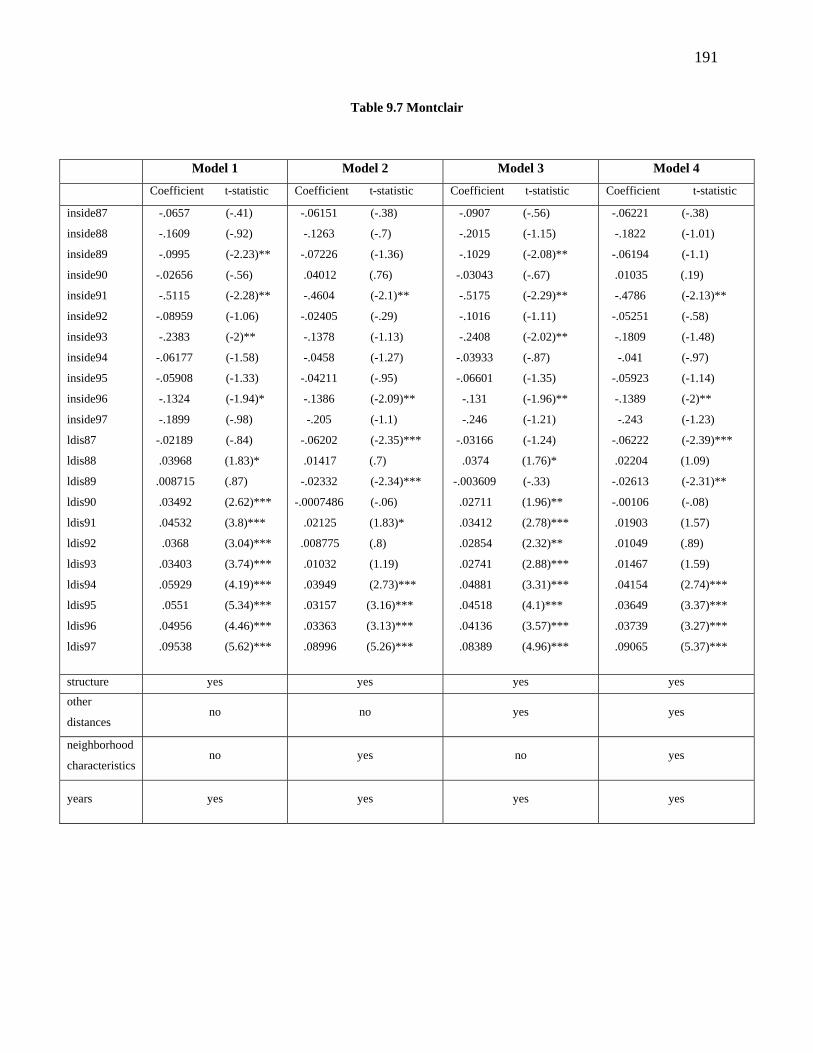
191
Table 9.7 Montclair
Model 1 Model 2 Model 3 Model 4
Coefficient t-statistic Coefficient t-statistic Coefficient t-statistic Coefficient t-statistic
inside87
inside88
inside89
inside90
inside91
inside92
inside93
inside94
inside95
inside96
inside97
ldis87
ldis88
ldis89
ldis90
ldis91
ldis92
ldis93
ldis94
ldis95
ldis96
ldis97
-.0657 (-.41)
-.1609 (-.92)
-.0995 (-2.23)**
-.02656 (-.56)
-.5115 (-2.28)**
-.08959 (-1.06)
-.2383 (-2)**
-.06177 (-1.58)
-.05908 (-1.33)
-.1324 (-1.94)*
-.1899 (-.98)
-.02189 (-.84)
.03968 (1.83)*
.008715 (.87)
.03492 (2.62)***
.04532 (3.8)***
.0368 (3.04)***
.03403 (3.74)***
.05929 (4.19)***
.0551 (5.34)***
.04956 (4.46)***
.09538 (5.62)***
-.06151 (-.38)
-.1263 (-.7)
-.07226 (-1.36)
.04012 (.76)
-.4604 (-2.1)**
-.02405 (-.29)
-.1378 (-1.13)
-.0458 (-1.27)
-.04211 (-.95)
-.1386 (-2.09)**
-.205 (-1.1)
-.06202 (-2.35)***
.01417 (.7)
-.02332 (-2.34)***
-.0007486 (-.06)
.02125 (1.83)*
.008775 (.8)
.01032 (1.19)
.03949 (2.73)***
.03157 (3.16)***
.03363 (3.13)***
.08996 (5.26)***
-.0907 (-.56)
-.2015 (-1.15)
-.1029 (-2.08)**
-.03043 (-.67)
-.5175 (-2.29)**
-.1016 (-1.11)
-.2408 (-2.02)**
-.03933 (-.87)
-.06601 (-1.35)
-.131 (-1.96)**
-.246 (-1.21)
-.03166 (-1.24)
.0374 (1.76)*
-.003609 (-.33)
.02711 (1.96)**
.03412 (2.78)***
.02854 (2.32)**
.02741 (2.88)***
.04881 (3.31)***
.04518 (4.1)***
.04136 (3.57)***
.08389 (4.96)***
-.06221 (-.38)
-.1822 (-1.01)
-.06194 (-1.1)
.01035 (.19)
-.4786 (-2.13)**
-.05251 (-.58)
-.1809 (-1.48)
-.041 (-.97)
-.05923 (-1.14)
-.1389 (-2)**
-.243 (-1.23)
-.06222 (-2.39)***
.02204 (1.09)
-.02613 (-2.31)**
-.00106 (-.08)
.01903 (1.57)
.01049 (.89)
.01467 (1.59)
.04154 (2.74)***
.03649 (3.37)***
.03739 (3.27)***
.09065 (5.37)***
structure yes yes yes yes
other
distances no no yes yes
neighborhood
characteristics no yes no yes
years yes yes yes yes
192
9.4.1.1 Model 1: No Census Variables or Other Distances At the Montclair site, the problem was identified prior to the beginning of our data. The
first Record of Decision was issued in 1989, whereupon remediation could begin. Remediation
was essentially completed by 1997, at the end of our sample period. We are looking for
statistically significant price differentials associated with a house being on top of one of the
radium contaminated areas, and/or positive coefficients on the log distance variables, suggesting
a premium for houses at locations which are exposed to lower risks. We find negative
coefficients on the INSIDE dummies in all years, and statistically significant coefficients in
1989, the year of the first ROD, in 1991, in 1993, and again in 1996. The distance premia in this
model are all positive after 1987 and statistically significantly different from zero in all years
after 1989. These results would suggest significant perceived risks closer to the site.
9.4.1.2 Model 2: Including Census Variables When we control for variations over time in the socio-demographic makeup of the
population near the site, compared to changes elsewhere in the study area, we find that the point
estimates for all of the decrements in house value on top of the site shrink in size up until 1996,
and only the decrements for 1991 and 1996 remain individually significant. The distance effects
actually change sign in the early years, becoming statistically significantly negative in 1987 and
1989, and they lose their statistical significance in 1990 through 1993. If distance captures
perceived risk, this perceived risk is only evident in housing prices during 1994-1997, and its
magnitude is diminished from what was suggested in Model 1.
In the rest of the results for Model 2, reported in Appendix A, it is notable that the
proportion of blacks in the neighborhood makes a very strongly significant positive difference in
housing prices in this context. Appendix A also shows changes in the degree of racial integration
across the different Census tracts over time. There are several predominantly black communities
and several predominantly white communities. Some of these remain strongly segregated
throughout the sample period, but a wide range of other communities in the area has become
considerably more integrated. Blacks, in particular, have moved nearer to the Superfund site in
considerable numbers. It also seems somewhat counter-intuitive that housing prices are highest
193
where there is a higher proportion of vacant dwellings and a higher proportion of renter-occupied
units.
9.4.1.3 Model 3: Including Other Distances When we include only other distances in Model 3, and leave out the Census variables, the
patterns in terms of the Superfund proximity variables exhibited in Model 1 are mostly restored,
although the point estimates of the distance (perceived risk) effects shrink very slightly. The
other distance effects, reported in Appendix A, seem to imply that high points of land (for New
Jersey), retail centers, hospitals, roads, Interstate 280, and especially the Garden State Parkway,
major water bodies (again, this is New Jersey), and Newark International Airport are considered
to be disamenities. Desirable features include: cemeteries, parks, colleges, and airports other
than Newark International. All of these seem to qualify as examples of open space, to some
extent.
9.4.1.4 Model 4: Both Census Data and Other Distances This final model wherein the coefficients on neighborhood characteristics and other
distances do not depend upon lot sizes more or less preserves the same results obtained for the
Superfund site proximity variables attained separately in Models 2 and 3.
9.4.1.5 Models with Lot size Interaction Terms In Table 9.8, we present just the coefficients on the Superfund proximity variables, but in
these four models, we now interact all of the proximity variables, the neighborhood
characteristics variables, and other distances variables with lot size to determine whether the
premium or discount associate with different attributes is independent of lot size or changes with
the size of the parcel in question. Recall that lot sizes are scaled to equal one at the means of the
data, to aid in the interpretation of the estimates. At the means of the data, the effective slope
coefficient will be the sum of the base coefficient and the coefficient on the lot size interaction
term. These models can reveal whether the losses in property values near a Superfund site are
borne disproportionately by homeowners selling smaller properties, or whether they are borne
disproportionately by homeowners selling larger properties.

194
Table 9.8 Montclair (with lot size interactions)
Model 1 Model 2 Model 3 Model 4
Coefficient t-statistic Coefficient t-statistic Coefficient t-statistic Coefficient t-statistic
inside87
inside88
inside89
inside90
inside91
inside92
inside93
inside94
inside95
inside96
inside97
ldis87
ldis88
ldis89
ldis90
ldis91
ldis92
ldis93
ldis94
ldis95
ldis96
ldis97
vinside87
vinside88
vinside89
vinside90
vinside91
vinside92
vinside93
vinside94
vinside95
vinside96
vinside97
vldis87
vldis88
1.204 (1.57)
-.2893 (-1.16)
-.156 (-2.17)**
.03244 (.51)
-.8026 (-2.52)***
.1341 (1.11)
-.4908 (-1.95)*
.08437 (1.05)
-.01186 (-.08)
.02536 (.28)
.1995 (.62)
-2.032 (-1.5)
.2354 (.71)
.08432 (1.63)
-.08558 (-1.2)
.4007 (2.08)**
-.2878 (-1.33)
.2283 (1.65)*
-.2021 (-2.08)**
-.07835 (-.31)
-.1843 (-1.85)*
-.5096 (-.86)
-.04527 (-1.34)
.02927 (1.04)
.04006 (2.54)***
.0554 (2.81)***
.06625 (3.6)***
.05323 (2.85)***
.07795 (4.94)***
.05488 (2.63)***
.0653 (3.54)***
.07897 (4.55)***
.06813 (2.3)**
.02719 (.94)
.01052 (.53)
1.328 (1.74)*
-.314 (-1.23)
-.09118 (-1.09)
.07578 (1.04)
-.7539 (-2.39)***
.1988 (1.65)*
-.4436 (-1.83)*
.1083 (1.37)
-.01322 (-.09)
.04732 (.54)
.1772 (.54)
-2.211 (-1.63)
.3521 (1.02)
.005509 (.08)
-.07026 (-.67)
.409 (2.1)**
-.3188 (-1.47)
.2368 (1.7)*
-.2102 (-2.07)**
-.0282 (-.11)
-.2274 (-2.16)**
-.491 (-.81)
-.06673 (-1.98)**
.001667 (.06)
.01334 (.8)
.02067 (1.15)
.05084 (2.85)***
.02485 (1.44)
.05211 (3.38)***
.04984 (2.36)***
.04575 (2.19)**
.07134 (4.05)***
.08531 (2.76)***
.002705 (.09)
.0135 (.68)
1.312 (1.76)*
-.2724 (-1.09)
-.1442 (-1.79)*
.08889 (1.11)
-.8318 (-2.6)***
.1736 (1.39)
-.4005 (-1.64)
.1253 (1.38)
.03542 (.2)
.0682 (.75)
.235 (.72)
-2.242 (-1.7)*
.1583 (.48)
.06731 (.85)
-.1523 (-1.92)*
.4514 (2.3)**
-.3377 (-1.52)
.1408 (1.07)
-.2235 (-1.92)*
-.14 (-.43)
-.2392 (-2.16)**
-.598 (-1)
-.06854 (-2.06)**
.01633 (.59)
.01808 (1.13)
.01132 (.57)
.03852 (2.16)**
.02719 (1.47)
.04443 (2.76)***
.02964 (1.36)
.02722 (1.37)
.04789 (2.66)***
.05896 (2.05)**
.03459 (1.15)
.02157 (1.04)
1.32 (1.72)*
-.2131 (-.81)
-.05622 (-.54)
.115 (1.41)
-.7885 (-2.45)***
.2425 (1.9)*
-.3638 (-1.5)
.1475 (1.56)
.001388 (.01)
.03598 (.36)
.1947 (.57)
-2.195 (-1.61)
.1111 (.31)
.002244 (.02)
-.1619 (-1.69)*
.4508 (2.24)**
-.3933 (-1.73)*
.1374 (1)
-.2371 (-1.84)*
-.05203 (-.19)
-.1943 (-1.52)
-.5287 (-.84)
-.08702 (-2.61)***
-.007 (-.26)
-.009747 (-.53)
-.02621 (-1.33)
.02363 (1.23)
.00332 (.18)
.03258 (1.97)**
.02317 (1.02)
.01563 (.74)
.04409 (2.26)**
.0669 (2.22)**
.02197 (.75)
.03402 (1.66)*
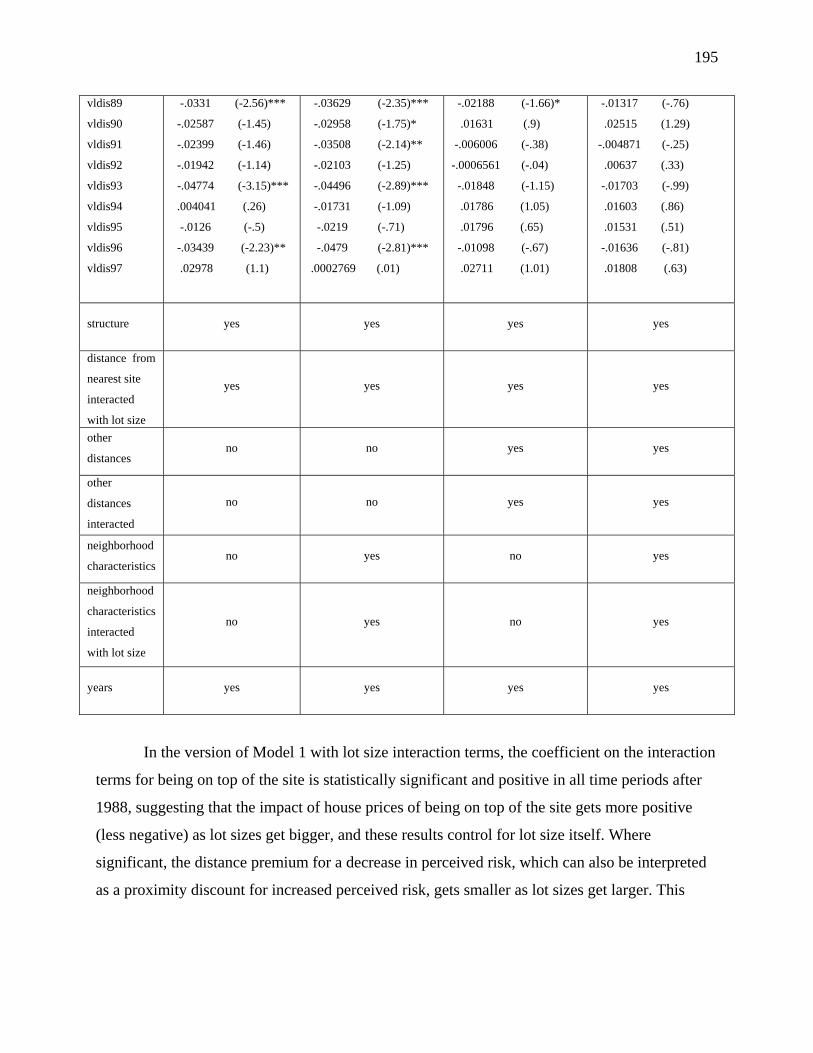
195
vldis89
vldis90
vldis91
vldis92
vldis93
vldis94
vldis95
vldis96
vldis97
-.0331 (-2.56)***
-.02587 (-1.45)
-.02399 (-1.46)
-.01942 (-1.14)
-.04774 (-3.15)***
.004041 (.26)
-.0126 (-.5)
-.03439 (-2.23)**
.02978 (1.1)
-.03629 (-2.35)***
-.02958 (-1.75)*
-.03508 (-2.14)**
-.02103 (-1.25)
-.04496 (-2.89)***
-.01731 (-1.09)
-.0219 (-.71)
-.0479 (-2.81)***
.0002769 (.01)
-.02188 (-1.66)*
.01631 (.9)
-.006006 (-.38)
-.0006561 (-.04)
-.01848 (-1.15)
.01786 (1.05)
.01796 (.65)
-.01098 (-.67)
.02711 (1.01)
-.01317 (-.76)
.02515 (1.29)
-.004871 (-.25)
.00637 (.33)
-.01703 (-.99)
.01603 (.86)
.01531 (.51)
-.01636 (-.81)
.01808 (.63)
structure yes yes yes yes
distance from
nearest site
interacted
with lot size
yes yes yes yes
other
distances no no yes yes
other
distances
interacted
no no yes yes
neighborhood
characteristics no yes no yes
neighborhood
characteristics
interacted
with lot size
no yes no yes
years yes yes yes yes
In the version of Model 1 with lot size interaction terms, the coefficient on the interaction
terms for being on top of the site is statistically significant and positive in all time periods after
1988, suggesting that the impact of house prices of being on top of the site gets more positive
(less negative) as lot sizes get bigger, and these results control for lot size itself. Where
significant, the distance premium for a decrease in perceived risk, which can also be interpreted
as a proximity discount for increased perceived risk, gets smaller as lot sizes get larger. This
196
means that houses on smaller lots at any given distance from the Superfund site experience a
larger relative decrease in value than do houses on large lots.
In the more complete specification in Model 4, however, with both neighborhood and
other distances in the model, lot size effects on the distance premium are much less apparent.
Appendix A also displays the lot size effects on all of the other variables. Over half of the
Census tract variables, and over half of the other distance variables retain statistically significant
lot size effects. In general, the lot size interaction terms have coefficients bearing the opposite
sign to the main effects, indicating that the housing price premiums or discounts associated with
location decrease in absolute magnitude as lot size grows.
9.4.2 OII
For the OII site, the generic estimating formula suffices. There are no special features to these
data. The estimates for the distance effects are contained in Table 9.9.
9.4.2.1 Model 1: No Census Variables or Other Distances In this model, with no controls for socio-demographic change or distances to other
amenities or disamenities, the fitted model creates the impression that the locale of the landfill
was systematically more desirable than the surrounding area until about 1983. In 1984, the
landfill was closed and the site was proposed for the NPL. Following this, there is evidence of a
proximity premium in 1987, 1992, and again in 1999, although a proximity discount is evident at
the 10% level in 1989, 1991 and 1997. A Consent Decree was signed in 1989, and construction
of some of the remediation measures began in 1991. 1996 was the year of the final Record of
Decision and landfill cover work began in 1997, so activity at the site would have been apparent
then.

197
Table 9.9 OII Landfill
Model 1 Model 2 Model 3 Model 4
Coefficient t-statistic Coefficient t-statistic Coefficient t-statistic Coefficient t-statistic
ldis70
ldis71
ldis72
ldis73
ldis74
ldis75
ldis76
ldis77
ldis78
ldis79
ldis80
ldis81
ldis82
ldis83
ldis84
ldis85
ldis86
ldis87
ldis88
ldis89
ldis90
ldis91
ldis92
ldis93
ldis94
ldis95
ldis96
ldis97
ldis98
ldis99
-.09106 (-1.34)
-.1911 (-2.86)***
-.1452 (-3.34)***
-.1446 (-4.15)***
-.1544 (-3.18)***
-.1339 (-5.8)***
-.08965 (-5.91)***
-.09486 (-4.65)***
-.07947 (-4.49)***
-.02105 (-.53)
-.1574 (-3.79)***
-.1389 (-1.05)
.1391 (1.69)*
-.1294 (-3.28)***
-.02547 (-.53)
-.05666 (-1.26)
.001428 (.04)
-.05865 (-2.15)**
-.0136 (-.25)
.08966 (1.7)*
-.03567 (-.96)
.1127 (1.8)*
-.0556 (-2.59)***
-.02067 (-.94)
-.01194 (-.61)
.001991 (.05)
.04686 (1.25)
.0606 (1.75)*
-.004532 (-.34)
.02549 (2.15)**
-.07008 (-.99)
-.153 (-2.28)**
-.129 (-2.96)***
-.1135 (-3.18)***
-.1353 (-2.78)***
-.1044 (-4.47)***
-.0682 (-4.31)***
-.07244 (-3.67)***
-.05892 (-3.35)***
.0009394 (.02)
-.147 (-3.56)***
-.1049 (-.8)
.1327 (1.56)
-.1166 (-2.98)***
-.009132 (-.19)
-.03818 (-.85)
.01342 (.43)
-.04202 (-1.56)
.0005704 (.01)
.1019 (1.98)**
-.0164 (-.45)
.1236 (1.95)*
-.03762 (-1.8)*
-.005524 (-.25)
.01012 (.54)
.01688 (.42)
.06034 (1.67)*
.08704 (2.56)***
.009177 (.72)
.02755 (2.22)**
-.1274 (-1.71)*
-.2088 (-2.98)***
-.1767 (-3.81)***
-.1642 (-4.17)***
-.1842 (-3.5)***
-.1461 (-5.55)***
-.1182 (-6.14)***
-.1215 (-5.12)***
-.09687 (-4.36)***
-.04875 (-1.13)
-.1827 (-4.29)***
-.1629 (-1.22)
.104 (1.16)
-.1617 (-3.81)***
-.05933 (-1.17)
-.08788 (-1.85)*
-.03696 (-1.05)
-.08905 (-2.8)***
-.04601 (-.81)
.05101 (1.03)
-.07362 (-1.91)*
.07644 (1.11)
-.08487 (-3.25)***
-.05289 (-1.94)*
-.04331 (-1.74)*
-.0317 (-.72)
.01493 (.37)
.03561 (.96)
-.03436 (-1.76)*
-.01498 (-.75)
-.08746 (-1.17)
-.1682 (-2.39)***
-.1442 (-3.03)***
-.1307 (-3.27)***
-.1533 (-2.88)***
-.1234 (-4.38)***
-.09191 (-4.42)***
-.09261 (-3.69)***
-.07437 (-3.09)***
-.01745 (-.4)
-.1584 (-3.65)***
-.12 (-.89)
.1175 (1.32)
-.1318 (-3.1)***
-.03113 (-.61)
-.05643 (-1.18)
-.005591 (-.16)
-.05456 (-1.67)*
-.01318 (-.23)
.08643 (1.74)*
-.03331 (-.86)
.111 (1.61)
-.04724 (-1.74)*
-.01805 (-.64)
-.003816 (-.15)
.003596 (.08)
.0459 (1.13)
.0734 (1.98)**
-.004028 (-.2)
.01017 (.48)
structure yes yes yes yes
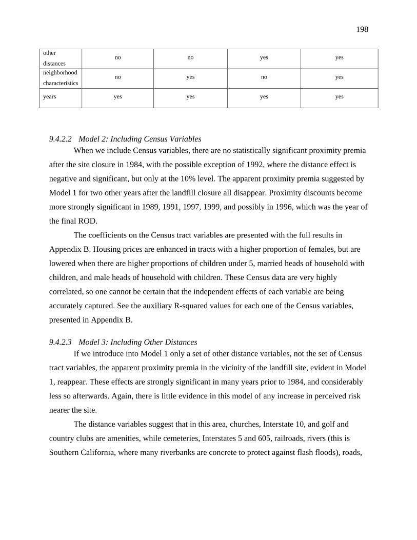
198
other
distances no no yes yes
neighborhood
characteristics no yes no yes
years yes yes yes yes
9.4.2.2 Model 2: Including Census Variables When we include Census variables, there are no statistically significant proximity premia
after the site closure in 1984, with the possible exception of 1992, where the distance effect is
negative and significant, but only at the 10% level. The apparent proximity premia suggested by
Model 1 for two other years after the landfill closure all disappear. Proximity discounts become
more strongly significant in 1989, 1991, 1997, 1999, and possibly in 1996, which was the year of
the final ROD.
The coefficients on the Census tract variables are presented with the full results in
Appendix B. Housing prices are enhanced in tracts with a higher proportion of females, but are
lowered when there are higher proportions of children under 5, married heads of household with
children, and male heads of household with children. These Census data are very highly
correlated, so one cannot be certain that the independent effects of each variable are being
accurately captured. See the auxiliary R-squared values for each one of the Census variables,
presented in Appendix B.
9.4.2.3 Model 3: Including Other Distances If we introduce into Model 1 only a set of other distance variables, not the set of Census
tract variables, the apparent proximity premia in the vicinity of the landfill site, evident in Model
1, reappear. These effects are strongly significant in many years prior to 1984, and considerably
less so afterwards. Again, there is little evidence in this model of any increase in perceived risk
nearer the site.
The distance variables suggest that in this area, churches, Interstate 10, and golf and
country clubs are amenities, while cemeteries, Interstates 5 and 605, railroads, rivers (this is
Southern California, where many riverbanks are concrete to protect against flash floods), roads,
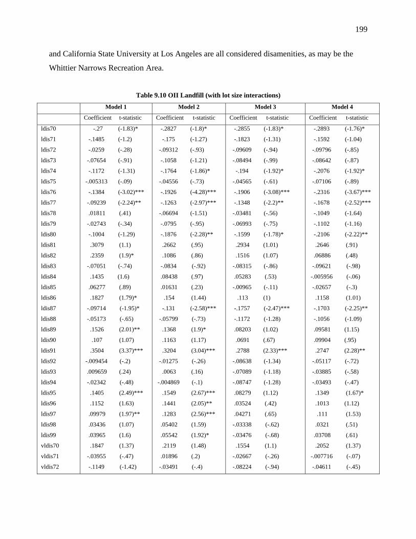
199
and California State University at Los Angeles are all considered disamenities, as may be the
Whittier Narrows Recreation Area.
Table 9.10 OII Landfill (with lot size interactions)
Model 1 Model 2 Model 3 Model 4
Coefficient t-statistic Coefficient t-statistic Coefficient t-statistic Coefficient t-statistic
ldis70
ldis71
ldis72
ldis73
ldis74
ldis75
ldis76
ldis77
ldis78
ldis79
ldis80
ldis81
ldis82
ldis83
ldis84
ldis85
ldis86
ldis87
ldis88
ldis89
ldis90
ldis91
ldis92
ldis93
ldis94
ldis95
ldis96
ldis97
ldis98
ldis99
vldis70
vldis71
vldis72
-.27 (-1.83)*
-.1485 (-1.2)
-.0259 (-.28)
-.07654 (-.91)
-.1172 (-1.31)
-.005313 (-.09)
-.1384 (-3.02)***
-.09239 (-2.24)**
.01811 (.41)
-.02743 (-.34)
-.1004 (-1.29)
.3079 (1.1)
.2359 (1.9)*
-.07051 (-.74)
.1435 (1.6)
.06277 (.89)
.1827 (1.79)*
-.09714 (-1.95)*
-.05173 (-.65)
.1526 (2.01)**
.107 (1.07)
.3504 (3.37)***
-.009454 (-.2)
.009659 (.24)
-.02342 (-.48)
.1405 (2.49)***
.1152 (1.63)
.09979 (1.97)**
.03436 (1.07)
.03965 (1.6)
.1847 (1.37)
-.03955 (-.47)
-.1149 (-1.42)
-.2827 (-1.8)*
-.175 (-1.27)
-.09312 (-.93)
-.1058 (-1.21)
-.1764 (-1.86)*
-.04556 (-.73)
-.1926 (-4.28)***
-.1263 (-2.97)***
-.06694 (-1.51)
-.0795 (-.95)
-.1876 (-2.28)**
.2662 (.95)
.1086 (.86)
-.0834 (-.92)
.08438 (.97)
.01631 (.23)
.154 (1.44)
-.131 (-2.58)***
-.05799 (-.73)
.1368 (1.9)*
.1163 (1.17)
.3204 (3.04)***
-.01275 (-.26)
.0063 (.16)
-.004869 (-.1)
.1549 (2.67)***
.1441 (2.05)**
.1283 (2.56)***
.05402 (1.59)
.05542 (1.92)*
.2119 (1.48)
.01896 (.2)
-.03491 (-.4)
-.2855 (-1.83)*
-.1823 (-1.31)
-.09609 (-.94)
-.08494 (-.99)
-.194 (-1.92)*
-.04565 (-.61)
-.1906 (-3.08)***
-.1348 (-2.2)**
-.03481 (-.56)
-.06993 (-.75)
-.1599 (-1.78)*
.2934 (1.01)
.1516 (1.07)
-.08315 (-.86)
.05283 (.53)
-.00965 (-.11)
.113 (1)
-.1757 (-2.47)***
-.1172 (-1.28)
.08203 (1.02)
.0691 (.67)
.2788 (2.33)***
-.08638 (-1.34)
-.07089 (-1.18)
-.08747 (-1.28)
.08279 (1.12)
.03524 (.42)
.04271 (.65)
-.03338 (-.62)
-.03476 (-.68)
.1554 (1.1)
-.02667 (-.26)
-.08224 (-.94)
-.2893 (-1.76)*
-.1592 (-1.04)
-.09796 (-.85)
-.08642 (-.87)
-.2076 (-1.92)*
-.07106 (-.89)
-.2316 (-3.67)***
-.1678 (-2.52)***
-.1049 (-1.64)
-.1102 (-1.16)
-.2106 (-2.22)**
.2646 (.91)
.06886 (.48)
-.09621 (-.98)
-.005956 (-.06)
-.02657 (-.3)
.1158 (1.01)
-.1703 (-2.25)**
-.1056 (-1.09)
.09581 (1.15)
.09904 (.95)
.2747 (2.28)**
-.05117 (-.72)
-.03885 (-.58)
-.03493 (-.47)
.1349 (1.67)*
.1013 (1.12)
.111 (1.53)
.0321 (.51)
.03708 (.61)
.2052 (1.37)
-.007716 (-.07)
-.04611 (-.45)

200
vldis73
vldis74
vldis75
vldis76
vldis77
vldis78
vldis79
vldis80
vldis81
vldis82
vldis83
vldis84
vldis85
vldis86
vldis87
vldis88
vldis89
vldis90
vldis91
vldis92
vldis93
vldis94
vldis95
vldis96
vldis97
vldis98
vldis99
-.06112 (-.76)
-.0304 (-.44)
-.1062 (-2.25)**
.04763 (1.08)
-.004628 (-.15)
-.089 (-2.05)**
.005398 (.08)
-.05687 (-.81)
-.4912 (-1.56)
-.07137 (-1.17)
-.05983 (-.63)
-.1691 (-2.12)**
-.1112 (-2.57)***
-.1753 (-1.73)*
.03552 (.87)
.03658 (.58)
-.06469 (-1.12)
-.1528 (-1.37)
-.2477 (-2.63)***
-.04449 (-1.18)
-.03445 (-.97)
.01093 (.27)
-.1418 (-2.64)***
-.071 (-1.6)
-.04198 (-1.26)
-.03999 (-1.38)
-.01624 (-.69)
-.008749 (-.11)
.03737 (.49)
-.04743 (-1)
.1328 (2.99)***
.05602 (1.72)*
.009527 (.21)
.07723 (1.13)
.04746 (.65)
-.4108 (-1.29)
.02564 (.39)
-.02607 (-.29)
-.09 (-1.22)
-.04642 (-1.1)
-.1323 (-1.25)
.088 (2.07)**
.05722 (.9)
-.03303 (-.61)
-.1389 (-1.26)
-.2025 (-2.16)**
-.02181 (-.53)
-.01395 (-.43)
.01633 (.36)
-.1395 (-2.55)***
-.08543 (-1.86)*
-.04459 (-1.28)
-.0434 (-1.37)
-.02705 (-1.04)
-.08803 (-1.14)
.01076 (.13)
-.09497 (-1.64)
.07517 (1.23)
.008887 (.17)
-.06312 (-1.08)
.01691 (.21)
-.03085 (-.39)
-.5125 (-1.57)
-.04998 (-.65)
-.08017 (-.87)
-.119 (-1.36)
-.07743 (-1.25)
-.1492 (-1.33)
.08476 (1.36)
.05822 (.77)
-.0361 (-.52)
-.1618 (-1.45)
-.2142 (-2.08)**
-.001723 (-.03)
.01704 (.32)
.03404 (.57)
-.1218 (-1.81)*
-.02421 (-.39)
-.01321 (-.25)
-.007049 (-.14)
.01472 (.32)
-.04798 (-.55)
.05655 (.64)
-.04278 (-.67)
.1502 (2.36)***
.07814 (1.29)
.03014 (.48)
.08485 (1.05)
.05572 (.65)
-.423 (-1.29)
.03959 (.47)
-.0243 (-.25)
-.02818 (-.31)
-.0189 (-.3)
-.1136 (-1.01)
.1174 (1.73)*
.08596 (1.06)
-.00754 (-.1)
-.1448 (-1.28)
-.1698 (-1.65)*
.003867 (.06)
.02118 (.34)
.02696 (.4)
-.1381 (-1.82)*
-.05795 (-.84)
-.04349 (-.7)
-.0393 (-.68)
-.03046 (-.54)
structure yes yes yes yes
distance from
nearest site
interacted
with lot size
yes yes yes yes
other
distances no no yes yes
other
distances
interacted
no no yes yes

201
neighborhood
characteristics no yes no
yesneighborhood
characteristics
interacted
with lot size
no yes no yes
years yes yes yes yes
9.4.2.4 Model 4: Both Census Data and Other Distances When both Census variables and other distances are included in the model, there are no
strongly significant proximity premia after 1983. There is some evidence (at the 10% level) of
proximity premia in 1987 and 1992, and some evidence of a proximity discount in 1989 and
1997, the year a Consent Decree was signed and the year landfill cover work began respectively.
The only strongly significant demographic effects in this model remain the positive
effects of higher percentages of females and the negative effects of children under 5. There may
be a modest decrease in housing values accompanying greater renter-occupancy.
The only remaining apparent disamenities are the I-605 freeway, rivers, roads, and the
Cal State campus. The only remaining significant amenity is the I-10 freeway.
9.4.2.5 Models with Lot Size Interaction Terms Distance effects for models with lot size interaction terms are displayed in Table 9.10. As
was the case for the Montclair models, the inclusion of lot size interaction terms tends to lead to
lot size diminishing the absolute magnitude of the effect. The interaction terms typically have the
opposite sign from the baseline effect of any variable.
9.4.3 Woburn
Very conveniently, Kiel (1995) and Kiel and Zabel (2001) have labeled their six different
phases of the process at the Woburn sites: pre-discovery (1975-76), discovery (1977-81), EPA
announcement of Superfund listing (1982-84), cleanup discussion (1985-88), cleanup
announcement (1989-91), and cleanup (1992). Our results are detailed in Table 9.11.

202
9.4.3.1 Model 1: No Census Variables or Other Distances The most interesting feature of our Woburn results is that our simplest models tend to
confirm the findings of Kiel and Zabel (2001), who find that housing prices increase with
distance from the Woburn sites. In Model 1, we see that the distance elasticities in housing prices
are insignificantly different from zero up through the end of the cleanup discussion. Beginning in
1990, however, there is evidence of a positive distance elasticity. The effect appears to dip in
1994, and again in 1997 (probably because of our smaller sample size covering only part of
1997). Otherwise, the distance elasticity ranges between 0.05 and 0.10.
Table 9.11 Woburn
Model 1 Model 2 Model 3 Model 4
Coefficient t-statistic Coefficient t-statistic Coefficient t-statistic Coefficient t-statistic
ldisw78
ldisw79
ldisw80
ldisw81
ldisw82
ldisw83
ldisw84
ldisw85
ldisw86
ldisw87
ldisw88
ldisw89
ldisw90
ldisw91
ldisw92
ldisw93
ldisw94
ldisw95
ldisw96
ldisw97
-.02852 (-.74)
-.1323 (-1.78)*
-.0005082 (-.01)
-.05335 (-.63)
.007758 (.14)
-.09781 (-1.8)*
.04437 (1.17)
.1042 (2.37)***
-.008799 (-.2)
-.01143 (-.34)
.04308 (1.54)
.03717 (1.36)
.05218 (1.93)*
.05028 (1.76)*
.07371 (2.63)***
.07933 (3.6)***
.04168 (1.67)*
.1095 (4.41)***
.1032 (5.65)***
.04631 (1.28)
-.07515 (-2.01)**
-.1633 (-2.24)**
-.02039 (-.34)
-.1036 (-1.24)
-.04167 (-.77)
-.1412 (-2.74)***
-.1057 (-2.68)***
-.02891 (-.69)
-.101 (-2.39)***
-.1306 (-3.84)***
-.07725 (-2.64)***
-.08354 (-2.89)***
-.07328 (-2.62)***
-.06244 (-2.2)**
-.03901 (-1.32)
-.02932 (-1.26)
-.08882 (-3.48)***
-.01088 (-.43)
-.01269 (-.65)
-.0573 (-1.59)
-.0816 (-1.93)*
-.1858 (-2.47)***
-.05354 (-.84)
-.1366 (-1.58)
-.09406 (-1.66)*
-.1711 (-3.06)***
-.1122 (-2.64)***
-.01804 (-.39)
-.1165 (-2.47)***
-.1179 (-3.11)***
-.08086 (-2.39)***
-.08138 (-2.46)***
-.0873 (-2.66)***
-.08535 (-2.52)***
-.05477 (-1.54)
-.03415 (-1.19)
-.1062 (-3.54)***
-.03558 (-1.19)
-.04663 (-1.83)*
-.1077 (-2.79)***
-.1184 (-2.67)***
-.2127 (-2.75)***
-.07207 (-1.11)
-.1565 (-1.79)*
-.1157 (-1.97)**
-.1991 (-3.56)***
-.1772 (-3.91)***
-.0843 (-1.79)*
-.1607 (-3.35)***
-.1775 (-4.39)***
-.1327 (-3.64)***
-.1365 (-3.84)***
-.1376 (-3.79)***
-.1279 (-3.47)***
-.0982 (-2.55)***
-.08197 (-2.63)***
-.1525 (-4.79)***
-.08104 (-2.48)***
-.0921 (-3.22)***
-.1448 (-3.54)***
structure yes yes yes yes
other
distances no no yes yes

203
neighborhood
characteristics no yes no yes
years yes yes yes yes
9.4.3.2 Model 2: Including Census Variables Model 2, however shows what happens when we introduce our time-varying Census tract
information. What once were insignificant or positive distance elasticities now turn negative and
significant in many cases. The effect is dramatic. This model does not control for distances to
other amenities and disamenities, so we will not yet attempt to interpret individual Census tract
characteristics coefficients. However, only the proportion of black and the proportion of male
heads-of-household fail to make a statistically significant contribution. This is due to the tiny
absolute numbers of these groups in the tracts represented in our sample. In contrast, the only
neighborhood variables that Kiel and Zabel (2001) control for are the proportion of unemployed
in the Census tract and median household income in the Census tract. They find that the
unemployment rate influences housing prices only in the 1982-84 period, and median income
influences housing prices only in the 1989-91 period.
Why does the inclusion of time-varying Census tract information have such a profound
influence on the distance elasticity of housing prices? The answer seems to lie in the different
trends over time in the characteristics of Census tract nearest the site versus farther away.
Appendix C presents a full set of regression models and fitted time-and-distance profiles for the
neighborhood characteristics associated with each house in our sample. Since our main hedonic
price models employ the logarithms of distance, we use the log of distance in these specifications
as well. The most substantial socio-demographic effects we discover include:
• The proportion of whites near the site fell more than it did further away.
• The proportion of blacks, while remaining small, grew much more near the site than
elsewhere in the sample area.
• The proportion of other ethnic groups grew faster near the site than elsewhere.
• About a 30% growth elsewhere in the sample in the proportion of children under 5
whereas the population of young children nearest the site increases hardly at all.
• The proportion of 5-29 year olds shrank more slowly near the site than elsewhere.
204
• The population of prime-aged 30-64 year olds grew more slowly near the site than
elsewhere, as did the population of seniors.
• There was no discernible difference in the rate of decrease over time in the proportion of
married heads of household with children by distance from site.
• The proportion of male heads of household with children, while very small, grew more
quickly near the site than further away.
• Female headed households with children grew, close to the site, but declined as a
proportion of the population further away.
• Owner-occupancy fell near the site, but remained more or less constant further away.
• Renter-occupancy grew over time near the site, but remained relatively constant farther
away.
• There was no discernible difference in the growth in vacancy rates across the sample
area.
It must be noted that the suite of Census variables at our disposal are very highly correlated with
one another. The appendix reports the R-squared values for auxiliary regressions conducted
among the Census variables used in our Models, and these R-squared values are all over 60%
and range as high as almost 96%. As a consequence, it will be difficult to attribute variations in
housing prices to the independent effects of each of these variables. Collectively, however, they
make a considerable difference (for micro-data) to the R-squared value between Model 1 and
Model 2, boosting it from 0.49 to 0.53.
9.4.3.3 Model 3: Including Other Distances Instead of controlling for different and shifting Census tract characteristics, we include
distances to other amenities in Model 3. These distances do not vary over time, but their presence
in the model also causes the previously significant site distance elasticities to change sign and
even become significantly negative. Among the set of other distances, auxiliary R-squared values
reveal that the distances to the nearest d_retail, d_hospital, d_church, and distances to the four
airports (all of which lie outside the sample area) are highly correlated with the rest of the
variables in the model. The coefficients on these particular distance variables are prone to
multicollinearity problems.
205
When we do not control for socio-demographic characteristics, it appears that the housing
prices increase with distance from: hospitals, churches, railroads, “other” primary roads, smaller
roads, Interstate 93, and all four airports. Housing prices appear to decrease with distance from:
schools, retail centers, cemeteries, principal arteries, the flight-path of Tew-Mac airport, parks,
major water bodies, and golf and country clubs. Each of these effects could be argued to be
plausible.
9.4.3.4 Model 4: Both Census Data and Other Distances In Model 4, where we include both time-varying Census tract characteristics and other
distance variables, we find that housing prices seem to vary significantly with a number of
individual Census characteristics, although the resolution on these variables is doubtful because
of the high multicollinearity. Most plausible are the findings that housing prices tend to vary
negatively with the proportion of young people aged 5-29 in the population, and positively with
the proportion of married heads of household with children. Many of the “other distance”
coefficients lose their individual significance, leaving only the results that prices no longer
significantly increase with distance from: churches, and one of the four airports. Prices no longer
significantly decrease with distance from: cemeteries, the flight-path of Tew-Mac airport, or
golf and country clubs, but they now decrease with distances from summits. This seems
plausible, since proximity to a summit is likely to increase the chance of the dwelling having a
view.
The striking effect of including these Census tract attributes and other distances in Model
4 is that the site-distance elasticity of housing prices is now negative and significant at the 10%
level for all but one year in the 1978-1997 interval. It is significant at the 5% level in all but four
years. Next, we need to consider the time profile of these distance elasticities. How do they
change over time?

206
Figure 9.2 Woburn Model 4
Bet
a_1
coef
ficie
nt
Model 4 fitted site-distance elasticities: W oburny ear
beta1 beta1_lc beta1_uc zero
78 80 82 84 86 88 90 92 94 96 98
-.364265
.055484
9.4.3.5 Synthesis In a naïve specification, there do seem to be measurable impacts of proximity to the
nearest of two Woburn Superfund sites. However, when we control for other distances, it is
plausible that the apparent negative effect of proximity to the Superfund sites is just a
manifestation of greater distance from other desirable amenities or greater proximity to other
undesirable disamenities, including physical features as well as neighborhood socio-demographic
effects.
What then of the apparent variations in the effects of proximity to the nearest of the two
Woburn Superfund sites over time? There appears to be a substantial likelihood that the negative
effect of proximity to these sites towards the end of the sample period in a naïve model like
Model 1 may be due to neighborhood transition. Lower housing prices in the vicinity of the
Superfund sites can be explained in part by demographic trends in that areas that differ from
those in the broader sample area.
There is evidence that Superfund site identification and remediation may at first lower
housing prices, but this impact in turn initiates a pattern of in-migration by socio-demographic
groups that previously would have been unable to afford housing in this area. Traditional higher-
income groups will be inclined to buy elsewhere and lower-income groups will have an
opportunity to move in. However, their growing presence may then become the dominant factor

207
keeping downward pressure on housing prices, even though the Superfund remediation takes
place.
9.4.3.6 Models with Latitude and Longitude Variables The Woburn models can differ from the generic model if we allow the absolute location
of each house to systematically affect the sales price. This permits a tilted planar spatial pattern
in housing prices to overlay the systematic effects due to distance from each house to the nearest
of the two Woburn sites; Wells G&H, or the Industri-Plex facility. The rationale for allowing this
generalization is that it may pick up the asymmetric spatial effects due to the “characteristic
Woburn odor” that was apparently carried generally eastward from the area of the sites by the
prevailing winds. The most general model for the Woburn site, short of including lot size effects,
is:
(9.9) 00 10 2 30 40ln( ) ( ) ( ) ( ) ( )
it
t t it t it iT it iT it
LSPRICEP LL LDIST A S Dβ β β β β ε
=+ + + + + +
Here, itLL denotes vectors of interaction terms between year dummies and the latitude and the
longitude of the house location (in decimal degrees, to six decimal places). We also consider
models wherein these latitude and longitude dummies in each year are interacted with the
distance variable. The models reported in the text of this research do not include this
generalization. These results are reported in Appendix C along with other more general models.
Appendix C details models that include latitude and longitude variables by year, and
latitude and longitude by year also interacted with log(distance from site), in addition to Census
variables and other distance variables. Housing prices appear to be significantly increasing to the
east and increasing to the south, overall (or, roughly increasing in the direction of Boston). This
is not surprising, and undoubtedly captures an accessibility effect as well as any directional
gradient in distance effect for the Woburn sites. Adding these variables to Model 4, discussed
above, does not alter its findings concerning the separate effects of the year-specific site-distance
variables.
However, there is a glimmer of something interesting when we also interact the site-
distance variables with the latitude and longitude variables. The coefficient on site distance then
208
becomes a linear function of the absolute location of the house. For these models, the years 1985
and 1988 develop positive and significant main distance effects, negative and marginally
significant latitude*distance effects and longitude*distance effects. The implied formulas for the
elasticity of housing price with respect to distance are as follows in these two years:
1985: 0.25 – 5.4 * latitude -3.2 * longitude
1988: 0.35 - 4.3 * latitude – 2.6 * longitude
Latitude increases to the north and longitude increases to the east. However, mean latitude in the
sample is 42.50474 degrees and mean longitude is -71.13818. Thus, at the means of the data, the
overall effect of distance on house prices is still negative, rather than positive.
9.4.4 Eagle Mine
The Eagle Mine housing sample from the Eagle County Assessor’s office does not span
enough distinct Census tracts for the differences in socio-demographic characteristics across
these tracts to be useful in explaining the variation in housing prices. Only Census tracts 9534,
9535, 9536 and 9537 are represented in the estimating sample, and the total populations for each
of these tracts were only 6162, 2480, 166 and 1134 persons at the time of the 1990 Census. If we
attenuate the footprint of the data to attempt to get a better picture of the more-nearby housing
price effects, we drop to just two Census tracts, which makes of the Census data perfectly
collinear. In the spirit of the models used for the other sites, the richest Eagle mine estimating
model would thus be just:
(9.10) 10 2 40ln( ) ( ) ( )it t t it iT iT itLSPRICE P LDIST A Dβ β β ε= + + + +
However, there is more information that can be brought into play in this case. Eagle River flows
NNW through the mine site. Several kilometers downstream from the mine site, it is joined by
Gore Creek, which flows in from the direction of Vail. The houses in our sample are split
between those lying on the Eagle River, downstream of the Eagle Mine site, and on Gore Creek,
which is not affected by the mine site. Thus, we differentiate between houses in these two

209
groups, using a set of time-specific dummy variables for houses located downstream of the mine
site on Eagle River, rather than Gore Creek, itDOWNSTR . We will also interact these timewise
dummy variables with the distances from the Eagle Mine site, itLDIST to yield a richest model
of the form:
(9.11) 10 1 2
2 2 40
ln( ) ( )it t t it t it t it it
T iT it
LSPRICE P LDIST DOWNSTR DOWNSTR LDISTA D
β γ γβ β ε
= + + + ⋅+ + +
This functional form allows the effect of proximity to the mine to depend on distance in the
following way:
(9.12) 10 2it
t t itit
LSPRICE DOWNSTRLDIST
β γ∂= +
∂
The elasticity of selling prices with respect to distance from the Eagle Mine site will be just 10tβ
in year t for houses on Gore Creek. For houses on the Eagle River, downstream of the mine site,
the elasticity of selling prices will be 10 2t tβ γ+ . If the estimated parameter 2tγ in year t is
insignificantly different from zero, being downstream of the mine does not affect the elasticity of
selling price with respect to distance. If 10tβ is zero and 2tγ is positive, then there is no premium
from being further from the mine site if the house is not downstream from the mine on Eagle
River, but there is a distance effect if the house is downstream.
In the housing data for this site, there are insufficient numbers of observations to permit
entirely separate distance coefficients to be estimated for each individual year. We retain the
yearly dummy variables to control for area-wide increases in housing prices in each year, but we
constrain the distance and downstream effects to be constant across roughly three-year intervals.
To conform with some of the main benchmark years in the site’s history, and to create sufficient
observations while aggregating as little as possible, we hold the downstream and distance effects
constant across the following sets of years: 1976-1979, 1980-1982, 1983-1985, 1986-1988,
1989-1991, 1992-1994, 1995-1997, and 1998-1999.
210
The site was listed on the NPL in 1986 and a remediation plan was approved in 1988, so
there would have been much publicity in the area in the 1986-1988 period. 1996 saw an
agreement between the agencies involved and the responsible party to evaluate and possiblely
construct a groundwater extraction system, although the capping of the main tailings pile was
completed in 1997. This discussion might also have created awareness of the problem in the
1995-1997 period. In 1999, state and federal authorities formally sought to change the cleanup
agreement to include pumping of groundwater to keep it from filling the mine and complicating
treatment of contaminated water from the mine. The lead-up to this re-opening of the agreement
might be expected to influence housing prices in the 1998-99 period.
Empirical results for the distance coefficients are presented in Table 9.12, with complete
results relegated to Appendix D.
9.4.4.1 Model 1: No Control for Other Distances As usual, Model 1 considers distance effects over time, controlling for structural
attributes of the dwelling and general appreciation in housing prices, but not for any other
distances. This model suggests that distance from the mine site mattered little to housing prices
along Gore Creek, but did affect housing prices downstream from the mine along the Eagle River
in some years. House prices increased with distance from the mine along the Eagle River in the
1976-1979 period, and in the 1986-1988 period. In 1992-1994, it seems that there were distance
effects along Gore Creek, but not along the Eagle River. This is difficult to explain. Thus we
consider a richer model, which also controls for other distances that may affect housing prices.
9.4.4.2 Model 2: Controlling for Other Distances We include in Model 2 the logarithms of distance to the Vail ski area, distance to the
nearest recreational area (golf course or country club), distance to the nearest railroad, and
distance to the nearest river. The coefficients on the distances to each of these features bears the
expected sign and all are statistically significant. The Vail ski area is an amenity, with housing
prices decreasing as one moves away from it. Likewise, golf courses and country clubs are
amenities, as are rivers. In contrast, proximity to a railway is a disamenity. Housing prices rise as
one moves away from the railroad.

211
Table 9.12 Eagle Mine
Model 1 Model 3
Coefficient t-statistic Coefficient t-statistic
ldis79
ldis82
ldis85
ldis88
ldis91
ldis94
ldis97
ldis99
downldist79
downldist82
downldist85
downldist88
downldist91
-.181 (-.57)
-.3655 (-1.35)
-.007467 (-.02)
-.1457 (-.7)
.1182 (.7)
.4586 (2.66)***
.05625 (.62)
.1029 (1.2)
6.481 (5.56)***
.9653 (1.22)
-1.42 (-1.73)*
1.716 (2.11)**
-.5503 (-.89)
-.3849 (-.96)
-.4108 (-1.47)
.1481 (.37)
-.216 (-.93)
.002615 (.01)
.3133 (1.5)
-.1811 (-1.06)
-.0487 (-.27)
5.702 (4.57)***
1.172 (1.47)
-1.084 (-1.21)
2.599 (3.01)***
.4107 (.5)
structure yes yes
other
distances no yes
years yes yes
In this model, there are no individually statistically significant distance effects for houses
along Gore Creek, which are not likely to be exposed to any contamination from the Eagle River.
Downstream, however, there are significant positive distance effects in each of four different
time intervals. The largest effect appears to be in the 1976-1979 period, before the site was listed
on the NPL. If we knew more about accessibility of residential areas downstream area in this
period, it might be possible to say more about this observation. This area, further away from
Vail, may have been less accessible in that time period. Significant distance effects appear next
in the 1986-1988 interval, during which the site was proposed for the NPL and the remediation
plan was approved. This would have been a period of high publicity. The next discernible effect
came between 1995-1997. This is when the groundwater flooding problem became apparent and
the government agencies involved began to consider groundwater extraction in order to reduce
212
the amount of contaminated water that had to be treated. A further effect is apparent in 1998-
1999 housing prices. In this period, the EPA formally proposed a change to the prior agreement
concerning remediation plans. It is not surprising that houses downstream of the site might
reflect this concern in their selling prices.
9.4.4.3 Models with Lot size Interaction Terms Appendix D also details a set of models where the context of the dwelling, as opposed to
its attributes, affects not the unit price of the house, but the price per square foot of the land that
it occupies. We include both the usual lot size independent distance effects, and an interaction
term with lot size that allows us to see whether lot size affects the size of the premium for
distance from the site. Our models show that there are no strongly significant effects of lot size
on the “other distances.” If anything, the premium for being closer to the Vail ski area or the
local recreation areas (golf and country clubs) is enhanced when lot sizes are larger. (Lot sizes in
this model are normalized to one to permit evaluation of compound coefficients at mean lot size.)
However, the premium for being further downstream of the Eagle Mine site, now observed for
the 1976-1979, 1986-1988 periods and the 1989-1991 periods, is positive. For the first period it
increases with lot size, but for the two later periods the premium diminishes with lot size.
The positive effects of greater distance observed for the last two periods in Model 2
above disappear when we move to this more complex model. In this model, however, two
downstream simple dummy variables disappear due to multicollinearity and their effects are
absorbed by some of the interaction terms.
9.5 Synthesis and Conclusions
This research contributes four additional case studies to the literature on the time-varying
effects of localized environmental risks on housing prices. Over the relatively long time horizons
involved in Superfund identification and remediation processes, we find that the apparent time
patterns in proximity effects on housing prices seem to be confounded by systematic changes in
neighborhood composition in the vicinity of these sites. There is some evidence that housing
tenure patterns and the housing stock near the site are also altered by the process.
A “reduced form” type specification where individual house selling prices are modeled as
depending only upon structural variables, an area-wide price index for housing, and proximity to
213
a Superfund site interacted with time dummies will indeed document observed patterns in
housing prices during a Superfund identification and remediation process. However, such a
reduced form cannot distinguish between the effect of perceived risk at each distance and the
effects of changing socio-demographic or housing stock variables at each distance. To isolate the
effects of perceived risk, one must control for these other effects, but at the same time, recognize
that these other changes are not exogenous.
The implicit experiment imbedded in an estimated distance effect is a change in the risk
associated with increased distance from the site. At a great enough distance, the risk is presumed
to go to zero, and so should the property value differential. When, over a long time horizon,
property value distance profiles do not return to a zero slope when the risk is reduced essentially
to zero, neighborhood change is a potential explanation for persistent price differentials with
distance. It is not at all possible to conclude that perceived risk does not respond to cleanup.
In some cases, especially the Woburn case, we find that controlling for timewise
variation in neighborhood characteristics such as gender, ethnicity, the age distribution, family
structures and housing tenure reveals very little in the way of a remaining distance profile, so
that any inferences about persistent risk perceptions are difficult to make.

214
Chapter 10
Conclusion: Stigma and Property Values
The possibility that stigma may cause large losses in property values has been noted by
other researchers (e.g., Dale et al., 1999; Adams and Cantor, 2001) and the EPA (Harris, 2004).
In contrast to the hedonic approach (Rosen, 1974; and for application to hazardous sites see
Bartik, 1998; Harris, 2004; Harrison and Stock, 1984; Ketkar, 1992; Kolhase, 1991;
Mendelsohn, et al., 1992; Michaels and Smith, 1990; etc.) where risk is treated as one of many
attributes that contribute to a determination of sale price, stigma is likely to effect property
values in a rather different and more direct manner. Upon learning of the contamination
potentially affecting their community, some current home owners may simply be unwilling to
continue to live in their home, and likewise, potential buyers will be unwilling to consider
buying a home in that community. If some owners and buyers have lexicographic preferences,
the standard hedonic model fails since it relies on a tradeoff between risk and home prices.
Rather, shunning by both current owners and potential home buyers will reduce the total demand
for housing for a neighborhood near a site as shown in Figure 10.1. Imagine that the total
demand for homes in a particular fully built-out neighborhood with H existing homes is Q(P)
where Q is the number of desired homes, P is the sale price, and quantity demanded falls with
price, Q'< 0. If, for example, homes were sold in a competitive uniform price auction, the
equilibrium price, Pe, is obtained by solving H=Q(P), so Pe=Q-1(H). Now consider the case where
a fraction f of home buyers and owners shun a neighborhood because of a nearby Superfund site.
The usual hedonic model cannot handle this phenomenon because the hedonic price adjustment
for these individuals, either through very high subjective risk beliefs (assuming conventional
values of statistical life) or shunning would give homes a risk deficit greater than or equal to the
value of the home. In other words, in either case the perceived costs of staying in the home are
greater than the entire value of the home and the observed behavior would be identical. This
implies that fraction f of current owners will sell and that the number of potential buyers will be
reduced by fraction f as well. As shown in Figure 10.1, since we have defined total demand for
the neighborhood to include current owners, the equilibrium price will now be determined by the
solving H=(1-f)Q(P), so Pe*=Q-1(H/(1-f)) and Pe* < Pe for f > 0. If f falls with distance from the
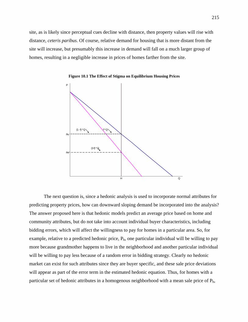
215
site, as is likely since perceptual cues decline with distance, then property values will rise with
distance, ceteris paribus. Of course, relative demand for housing that is more distant from the
site will increase, but presumably this increase in demand will fall on a much larger group of
homes, resulting in a negligible increase in prices of homes farther from the site.
Figure 10.1 The Effect of Stigma on Equilibrium Housing Prices
f * Q(1 - f) * Q
Q
P
H
Pe
Pe*
(1-f) * Q
The next question is, since a hedonic analysis is used to incorporate normal attributes for
predicting property prices, how can downward sloping demand be incorporated into the analysis?
The answer proposed here is that hedonic models predict an average price based on home and
community attributes, but do not take into account individual buyer characteristics, including
bidding errors, which will affect the willingness to pay for homes in a particular area. So, for
example, relative to a predicted hedonic price, Ph, one particular individual will be willing to pay
more because grandmother happens to live in the neighborhood and another particular individual
will be willing to pay less because of a random error in bidding strategy. Clearly no hedonic
market can exist for such attributes since they are buyer specific, and these sale price deviations
will appear as part of the error term in the estimated hedonic equation. Thus, for homes with a
particular set of hedonic attributes in a homogenous neighborhood with a mean sale price of Ph,
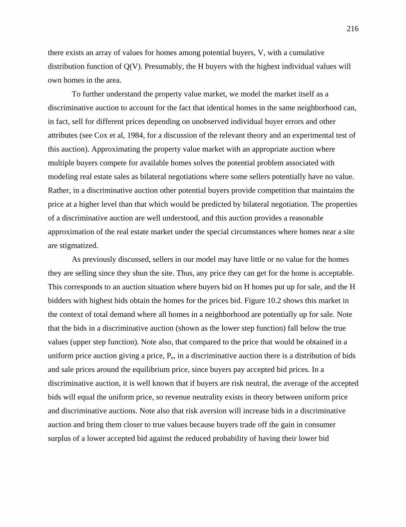
216
there exists an array of values for homes among potential buyers, V, with a cumulative
distribution function of Q(V). Presumably, the H buyers with the highest individual values will
own homes in the area.
To further understand the property value market, we model the market itself as a
discriminative auction to account for the fact that identical homes in the same neighborhood can,
in fact, sell for different prices depending on unobserved individual buyer errors and other
attributes (see Cox et al, 1984, for a discussion of the relevant theory and an experimental test of
this auction). Approximating the property value market with an appropriate auction where
multiple buyers compete for available homes solves the potential problem associated with
modeling real estate sales as bilateral negotiations where some sellers potentially have no value.
Rather, in a discriminative auction other potential buyers provide competition that maintains the
price at a higher level than that which would be predicted by bilateral negotiation. The properties
of a discriminative auction are well understood, and this auction provides a reasonable
approximation of the real estate market under the special circumstances where homes near a site
are stigmatized.
As previously discussed, sellers in our model may have little or no value for the homes
they are selling since they shun the site. Thus, any price they can get for the home is acceptable.
This corresponds to an auction situation where buyers bid on H homes put up for sale, and the H
bidders with highest bids obtain the homes for the prices bid. Figure 10.2 shows this market in
the context of total demand where all homes in a neighborhood are potentially up for sale. Note
that the bids in a discriminative auction (shown as the lower step function) fall below the true
values (upper step function). Note also, that compared to the price that would be obtained in a
uniform price auction giving a price, Pe, in a discriminative auction there is a distribution of bids
and sale prices around the equilibrium price, since buyers pay accepted bid prices. In a
discriminative auction, it is well known that if buyers are risk neutral, the average of the accepted
bids will equal the uniform price, so revenue neutrality exists in theory between uniform price
and discriminative auctions. Note also that risk aversion will increase bids in a discriminative
auction and bring them closer to true values because buyers trade off the gain in consumer
surplus of a lower accepted bid against the reduced probability of having their lower bid
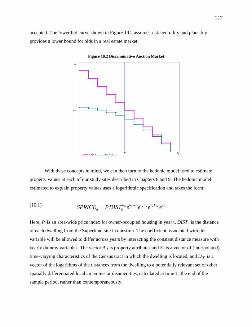
217
itiTiteiTt eeeeDISTPSPRICE DbSbAbbittit
ε421=
accepted. The lower bid curve shown in Figure 10.2 assumes risk neutrality and plausibly
provides a lower bound for bids in a real estate market.
Figure 10.2 Discriminative Auction Market
QV a l u e B i d
P
P e
H
With these concepts in mind, we can then turn to the hedonic model used to estimate
property values at each of our study sites described in Chapters 8 and 9. The hedonic model
estimated to explain property values uses a logarithmic specification and takes the form:
(10.1)
Here, Pt is an area-wide price index for owner-occupied housing in year t, DISTit is the distance
of each dwelling from the Superfund site in question. The coefficient associated with this
variable will be allowed to differ across years by interacting the constant distance measure with
yearly dummy variables. The vector AiT is property attributes and Sit is a vector of (interpolated)
time-varying characteristics of the Census tract in which the dwelling is located, and DiT is a
vector of the logarithms of the distances from the dwelling to a potentially relevant set of other
spatially differentiated local amenities or disamenities, calculated at time T, the end of the
sample period, rather than contemporaneously.

218
itiTtittiTtitttit DbSbAbLDISTbPLSPRICE ε+++++= 4321ln
Taking the logarithms of both sides of the equation yields a version of this model that is
appropriate for estimation:
(10.2)
where LSPRICEit denotes the logarithm of the observed selling price, lnPt will be captured as an
intercept for the first year in the sample and a set of intercept shifters activated by year dummy
variables. The variables of key interest are the LDISTit, which consist of a vector of logged
distances from the dwelling to the Superfund site interacted with yearly dummies in order to
permit year-varying elasticities of housing prices with respect to distance to the site. Geographic
Information Systems techniques were used to measure distances from the homes to the closest
Superfund site in the specific year, t, that the sales price was observed and the distance to other
local amenities or disamenities as they existed in year T.
As discussed previously, n obvious disadvantage of our sample described in previous
chapters is that in all of our data sets we only observe selling prices for the most recent sale of a
house. If a house is in an area where turnover is high, there will be more recent sales and fewer
earlier sales. For analytical purposes, it would be preferable to have data on all sales in all years
and selling price in those years, but such data do not exist. Data could be purchased from
Experian every year, if a future study could be anticipated, but retrospectively, the data are not
available. The data are collected primarily for current marketing purposes and records are
updated without saving their previous values. Historical modeling is not a use anticipated by the
providers of the data. Consequently, there may be some systematic sampling. We observe earlier
transactions prices only for houses which are still occupied by the owners who purchased them at
that earlier date. We do not observe many early transactions prices for houses in neighborhoods
where there has been a lot of turnover. It must be a maintained hypothesis that rates of turnover
are uncorrelated with identification and cleanup of Superfund sites. This may be a strenuous
assumption, but there are few alternatives. So it will be necessary to speculate upon the types of
biases this non-random selection is likely to produce in the effects of distance from a Superfund
site on housing transactions prices.
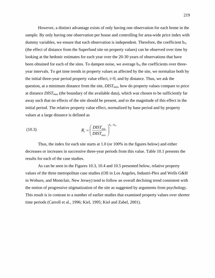
219
101
max
min
bb
t
t
DISTDISTR
−
⎟⎟⎠
⎞⎜⎜⎝
⎛=
However, a distinct advantage exists of only having one observation for each home in the
sample. By only having one observation per house and controlling for area-wide price index with
dummy variables, we ensure that each observation is independent. Therefore, the coefficient b1t
(the effect of distance from the Superfund site on property values) can be observed over time by
looking at the hedonic estimates for each year over the 20-30 years of observations that have
been obtained for each of the sites. To dampen noise, we average b1t the coefficients over three-
year intervals. To get time trends in property values as affected by the site, we normalize both by
the initial three-year period property value effect, t=0, and by distance. Thus, we ask the
question, at a minimum distance from the site, DISTmin, how do property values compare to price
at distance DISTmax (the boundary of the available data), which was chosen to be sufficiently far
away such that no effects of the site should be present, and to the magnitude of this effect in the
initial period. The relative property value effect, normalized by base period and by property
values at a large distance is defined as
(10.3)
Thus, the index for each site starts at 1.0 (or 100% in the figures below) and either
decreases or increases in successive three-year periods from this value. Table 10.1 presents the
results for each of the case studies.
As can be seen in the Figures 10.3, 10.4 and 10.5 presented below, relative property
values of the three metropolitan case studies (OII in Los Angeles, Industri-Plex and Wells G&H
in Woburn, and Montclair, New Jersey) tend to follow an overall declining trend consistent with
the notion of progressive stigmatization of the site as suggested by arguments from psychology.
This result is in contrast to a number of earlier studies that examined property values over shorter
time periods (Carroll et al., 1996; Kiel, 1995; Kiel and Zabel, 2001).
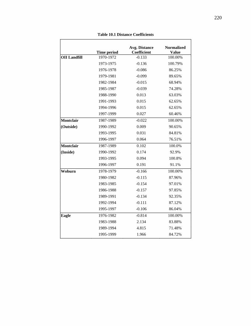
220
Table 10.1 Distance Coefficients
Time period Avg. Distance
Coefficient Normalized
Value OII Landfill 1970-1972 -0.133 100.00%
1973-1975 -0.136 100.79% 1976-1978 -0.086 86.25% 1979-1981 -0.099 89.65% 1982-1984 -0.015 68.94% 1985-1987 -0.039 74.28% 1988-1990 0.013 63.03% 1991-1993 0.015 62.65% 1994-1996 0.015 62.65% 1997-1999 0.027 60.46%
Montclair 1987-1989 -0.022 100.00% (Outside) 1990-1992 0.009 90.65%
1993-1995 0.031 84.81% 1996-1997 0.064 76.51%
Montclair 1987-1989 0.102 100.0% (Inside) 1990-1992 0.174 92.9%
1993-1995 0.094 100.8% 1996-1997 0.191 91.1%
Woburn 1978-1979 -0.166 100.00% 1980-1982 -0.115 87.96% 1983-1985 -0.154 97.01% 1986-1988 -0.157 97.85% 1989-1991 -0.134 92.35% 1992-1994 -0.111 87.12% 1995-1997 -0.106 86.04%
Eagle 1976-1982 -0.814 100.00% 1983-1988 2.134 83.88% 1989-1994 4.815 71.48% 1995-1999 1.966 84.72%

221
0%
20%
40%
60%
80%
100%
120%
1978-1979 1980-1982 1983-1985 1986-1988 1989-1991 1992-1994 1995-1997
Perc
ent V
alue
from
Orig
inal
3-Y
ear P
erio
d (1
978-
1979
)
1979. Discovery
1983. NPL listing, both sites
1992-1993. Clean-up begins1981. Industriplex - Proposed NPL1982. Wells G & H - Proposed NPL
Figure 10.3 Relative Property Value over Time for OII Landfill, California
Figure 10.4 Relative Property Value over Time for Montclair, New Jersey (outside of area)
Figure 10.5 Relative Property Value over Time for Woburn, Massachusetts
0%
20%
40%
60%
80%
100%
120%
1970-1972
1973-1975
1976-1978
1979-1981
1982-1984
1985-1987
1988-1990
1991-1993
1994-1996
1997-1999
Perc
ent V
alue
from
Ori
gina
l 3-Y
ear P
erio
d (1
970-
1972
)
1978. Discovery
1984. NPL Proposal
1997. Cap Begins
1985. NPL Listing
1988. Monitor Wells1989. Groundw ater Treatment
0%
20%
40%
60%
80%
100%
120%
1987-1989 1990-1992 1993-1995 1996-1997
Perc
ent V
alue
from
Orig
inal
3-Y
ear P
erio
d (1
987-
1989
)
1991. Phase 1 clean-up
1994. Phase 2 clean-up1995. Phase 3. clean-up
1996. Phase 4 & 5

222
)( 1,1 ∑ −−−
− +−=−j
tjitt ERR βαηη
∑ −− +=−j
tjjtt Eff 1,1 βα
What explains the long term downward trends observed in relative property values shown
in Figures 10.3-10.5? If the trend is driven by f, the fraction of home owners and potential buyers
who shun homes near the site, a model of the determination of f over time is needed. From the
discussion of the psychology of risk perception and stigma, the determination of the fraction of
shunners will be driven by media attention and perceptual cues resulting from activity at the site,
which are in turn driven by “events” such as EPA announcements, discovery, NPL-listing, and
cleanup. Thus, it is plausible that the percentage change between periods in the fraction of the
population who shun the site is a linear function of events of type j occurring during the prior
interval, characterized by the discrete dummy variable (or index summarizing a number of
dummy variables), Ej, t-1, thus
(10.4)
So, in a period with no events, Ej, t-1= 0 ∀j, we hypothesize that α is negative and f will decline,
thereby raising home values, because some people who know about the site will leave the area
(perhaps because of job opportunities elsewhere) and some new potential buyers will move into
the area who will have no awareness of the site. Other events, such as cleanup activities, might,
(a) raise awareness and thereby increase the fraction of the population who shun the site, or
alternatively, (b) reduce the fraction of shunners by convincing people who know about the site
that it is now safe. This latter possibility is unlikely in that the notion that, "once contaminated,
always contaminated" is part of the psychology of stigmatization. Note, also, that changes in
perceived risk for those who may not shun the site will likely follow a similar model.
There is no available data on f, so the model specified above cannot be estimated directly.
However, if one assumes a constant elasticity of demand, η<0, and risk neutrality, a simple
transformation exists between ft and Rt as defined above: η−−= tt Rf 1 . Thus, the equation
describing movement in ft can be rewritten as:
(10.5)
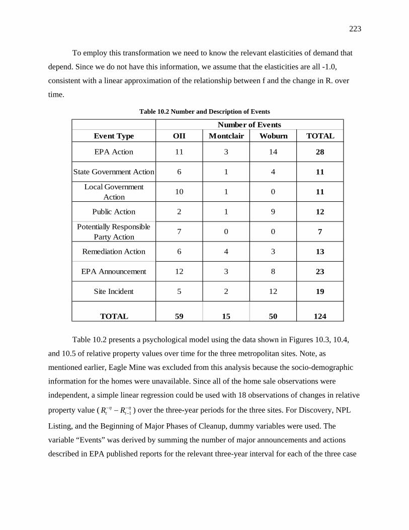
223
To employ this transformation we need to know the relevant elasticities of demand that
depend. Since we do not have this information, we assume that the elasticities are all -1.0,
consistent with a linear approximation of the relationship between f and the change in R. over
time.
Table 10.2 Number and Description of Events
Event Type OII Montclair Woburn TOTAL
EPA Action 11 3 14 28
State Government Action 6 1 4 11
Local Government Action
10 1 0 11
Public Action 2 1 9 12
Potentially Responsible Party Action
7 0 0 7
Remediation Action 6 4 3 13
EPA Announcement 12 3 8 23
Site Incident 5 2 12 19
TOTAL 59 15 50 124
Number of Events
Table 10.2 presents a psychological model using the data shown in Figures 10.3, 10.4,
and 10.5 of relative property values over time for the three metropolitan sites. Note, as
mentioned earlier, Eagle Mine was excluded from this analysis because the socio-demographic
information for the homes were unavailable. Since all of the home sale observations were
independent, a simple linear regression could be used with 18 observations of changes in relative
property value ( ηη −−
− − 1tt RR ) over the three-year periods for the three sites. For Discovery, NPL
Listing, and the Beginning of Major Phases of Cleanup, dummy variables were used. The
variable “Events” was derived by summing the number of major announcements and actions
described in EPA published reports for the relevant three-year interval for each of the three case

224
studies (Table 10.4). Note that such events will be highly correlated with and drive important
perceptual cues defined in Chapter 7 such as noise, odor, truck traffic, visible on site activity, and
media coverage. Events are defined as follows:
• EPA Action – Includes site investigations, orders, notifications/decisions,
remediation, legal actions, and regulations by the EPA.
• State Government Action – Includes site investigations, orders, resolutions,
remediation, lawsuits, reports, and regulations by state agencies.
• Local Government Action – Includes site investigations, orders, resolutions,
remediation, lawsuits, reports, and regulations by local cities, county, and school
districts.
• Public Action – Include the creation of public interest groups, major meetings
and protests, lawsuits by the residents, and the hiring of technical advisors for the
community.
• Potentially Responsible Parties Action – Include site operation and closure,
committees formed, and lawsuits by PRPs.
• Remediation Action – Includes containment of contaminations, remediation
efforts and site improvements.
• EPA Announcement – Includes official Consent Decrees, Record of Decisions
(RODs), and announcements of settlements with PRPs.
• Site Incident – Includes general site facts, reports and studies regarding the
contaminants and occurrences at the site.

225
The analysis across the three sites shows that discovery, cleanup itself, and the number of
events all negatively affect property values by drawing attention to the site and possibly
increasing the number of owners and potential buyers who shun the site thereafter (Table 10.3).
Thus, the effect of any events, publicity or site information, good or bad, appears to increase the
fraction of the current home owners and potential buyers that stigmatize and consequently shun
the communities neighboring the sites. In other words, at least within the observed period of the
studies, all news is bad news and causes relatively permanent property value losses as an
increasing fraction of original owners leave and more potential buyers shun the site. The only
good news in the study is that property values did significantly recover for a short period after
sites were listed on the NPL. But, it is likely that as soon as it was realized that EPA could not
immediately clean up the sites, the process of stigmatization began with consequent reduction in
property values. Given the small sample size, it is remarkable that all of these coefficients are
significant at better than the 1% level.
Table 10.3 Psychological Model, Dependent Variable 1−− tt RR
Model B t p (Constant)
0.078 3.578 0.003
Discovery
-0.160 -4.493 0.001
NPL – Listing
0.105 4.097 0.001
Clean-up Begins
-0.096 -4.753 0.001
Number of Events
-0.016 -6.156 0.000
N=18 R2 = 0.855
Rather than property losses reversing immediately once cleanup begins, we see no
permanent recovery in property values within the time period of our data and speculate that
recovery will only occur as the local population gradually moves away, events cease, and
perceptual cues and media attention disappear, so more buyers are uninformed. Note that
McClelland et al. (1990) found that most buyers were uninformed in spite of reporting
requirements. The positive intercept in the psychological model (significant at the 5% level)
226
indicates that property values will increase at a linear rate of about 12% every three-years if no
actions are taken and no news is generated by the site. Thus, at OII one could expect a complete
recovery in about a decade if no news is generated from the site and recovery might occur in
about half that time for the other sites.
The sites excluded from the model are also of some independent interest. First, although
Eagle Mine (see Figure 10.7) has very different characteristics from the three sites discussed
above, it shows a similar pattern in that relative property values decline for most of the period
analyzed. Given the small amount of data available along the Eagle River, we are forced to use
six-year rather than three-year periods for the analysis but do confirm the general pattern shown
above. Second, the “inside” Montclair property value estimates do not use distance as an
explanatory variable since the homes themselves are within the Superfund site. Yearly dummy
variables averaged over the same three-year intervals used in the outside-Montclair analysis
show that, unsurprisingly, cleanup itself does have a positive impact on property values (Figure
10.6). Third, another interesting result in the property value studies is the effect of including
socio-demographic variables. As shown in Figure 10.8, these make a large difference in the
magnitude of property losses at the Woburn site. Negative socio-demographic trends, that may
be the result of the progressive stigmatization of the site, also take a substantial toll on property
values (that are not included in the psychological model), but possibly should be included in any
damage assessment. These results suggest a different trend than observed by Kiel and Zabel
(2001) which did not account for these socio-demographic affects.
Since economic benefits are based on discounted present value, the benefits of delayed
cleanup for homes surrounding sites are likely to be negligible where cleanup takes 20 years and
another 5-10 years may be needed after cleanup is complete for property values to recover. The
principal policy conclusion becomes evident from the results of the psychological model which
suggest that the promise of a prompt cleanup raises property values, while an increase in the
number of events that are the root causes of perceptual cues and media attention decreases
property values. Thus, an expedited cleanup should occur as quickly as possible after a site has
been determined to be hazardous and this cleanup should be conducted in a way that does not
arouse excessive attention. Otherwise the neighborhoods surrounding the site will likely be
stigmatized resulting in quasi-permanent economic damages.
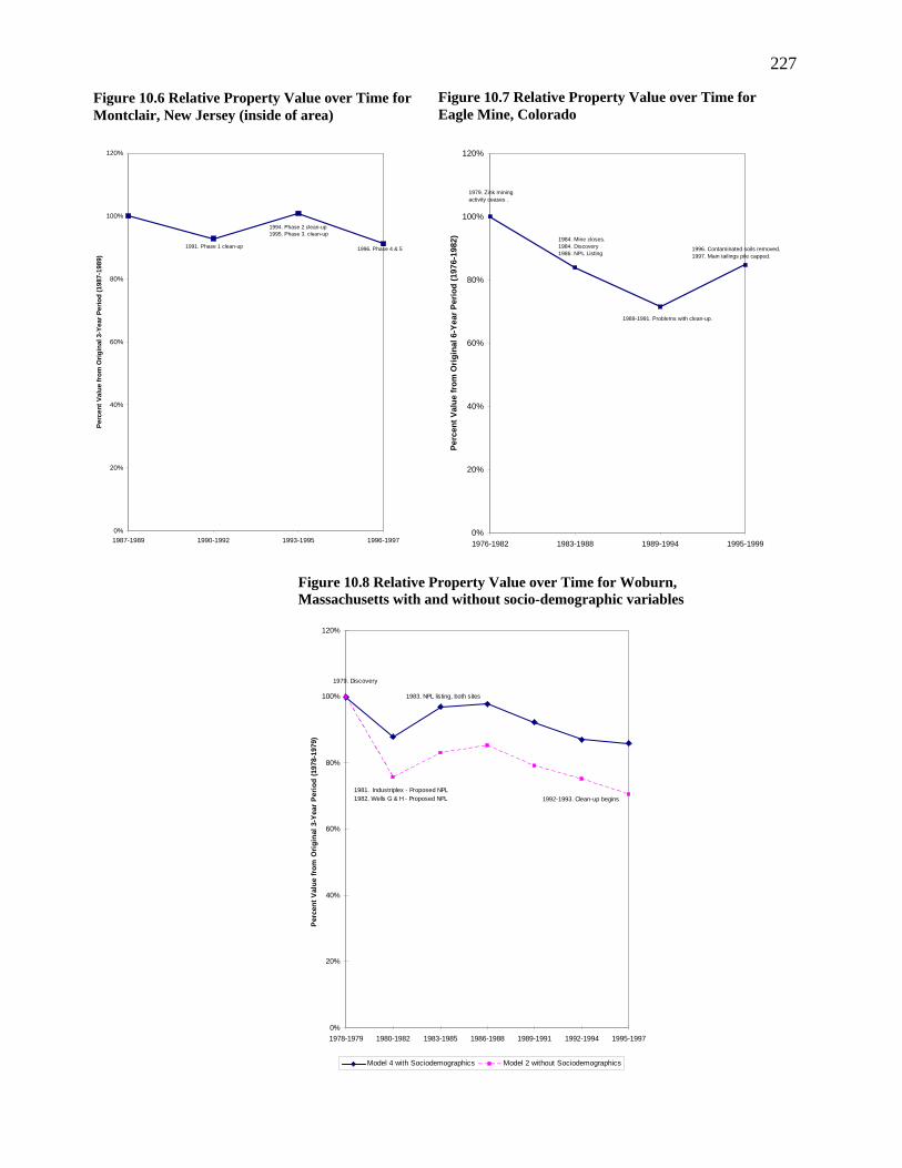
227
0%
20%
40%
60%
80%
100%
120%
1976-1982 1983-1988 1989-1994 1995-1999
Perc
ent V
alue
from
Orig
inal
6-Y
ear P
erio
d (1
976-
1982
)
1996. Contaminated soils removed.1997. Main tailings pile capped.
1989-1991. Problems with clean-up.
1984. Mine closes.1984. Discovery1986. NPL Listing
1979. Zink mining activity ceases .
0%
20%
40%
60%
80%
100%
120%
1978-1979 1980-1982 1983-1985 1986-1988 1989-1991 1992-1994 1995-1997
Per
cent
Val
ue fr
om O
rigi
nal 3
-Yea
r P
erio
d (1
978-
1979
)
Model 4 with Sociodemographics Model 2 without Sociodemographics
1979. Discovery
1983. NPL listing, both sites
1992-1993. Clean-up begins1981. Industriplex - Proposed NPL1982. Wells G & H - Proposed NPL
0%
20%
40%
60%
80%
100%
120%
1987-1989 1990-1992 1993-1995 1996-1997
Perc
ent V
alue
from
Orig
inal
3-Y
ear P
erio
d (1
987-
1989
)
v
1991. Phase 1 clean-up
1994. Phase 2 clean-up1995. Phase 3. clean-up
1996. Phase 4 & 5
Figure 10.6 Relative Property Value over Time for Montclair, New Jersey (inside of area)
Figure 10.7 Relative Property Value over Time for Eagle Mine, Colorado
Figure 10.8 Relative Property Value over Time for Woburn, Massachusetts with and without socio-demographic variables

228
Using the history of the OII and the corresponding events and dates in a simulation, the
potential benefits of these policies becomes evident (Figure 10.9).
Figure 10.9 Policy Simulations using the OII Landfill History
0%
20%
40%
60%
80%
100%
120%
1973
-197
5
1976
-197
8
1979
-198
1
1982
-198
4
1985
-198
7
1988
-199
0
1991
-199
3
1994
-199
6
1997
-199
9
2000
-200
2
2003
-200
5
Perc
ent o
f Orig
inal
Pro
pert
y Va
lue
A: Baseline - 33 yearsB: 33 years; 25% fewer eventsC: 24 years; 25% fewer eventsD: 15 years; 25% fewer events
A
B
CD
As shown in Table 10.4, this simulation considers four different scenarios and includes an
extrapolation of a recovery in property values after cleanup is complete where there are no
further events. Given the legislative history of Superfund, some of these scenarios are clearly
fanciful, but the results are nevertheless suggestive as to what potential benefits could be
obtained by expediting the cleanup process and reducing the number of events that drive
perceptual cues, media attention, and social amplification. These results support several of the
suggestions made by Kunreuther and Slovic (Chapter 21, 2001) for reducing stigma. In

229
particular, they suggest prevention of the occurrence of stigmatizing events and the reduction of
the number of stigmatizing messages and thus reducing social amplification.
Table 10.4 Cleanup Scenarios
Time
Horizon
Events Discovery NPL
Listing
Cleanup
time periods
Recovery
time periods
Final % of
Original Value
Scenario A 33 years All 1978 1985 1988-1990 & 1997-1999
2002-2005 64.5%
Scenario B 33 years 25% Fewer
1978 1985 1988-1990 & 1997-1999
2002-2005 85.2%
Scenario C 24 years 25% Fewer
1978 1982 1985-1987 & 1988-1990
1990-1995 95.6%
Scenario D
15 years
25% Fewer
1978
1979
1979-1981
1982-1987
100.0%
Note that these results directly contrast with those of Gayer, Hamilton and Viscusi (2000)
and Gayer and Viscusi (2002) who argue that media attention supports learning that leads to a
lowering of public risk perceptions more consistent with scientific evidence for smaller sites. No
credible evidence supports a significant long-term health risk to residents living near OII
(McClelland et al. 1990). Yet the actual property value losses are enormous. One difference is
that this study focuses on prominent sites while the two studies cited above focused on less
prominent sites. Note that most potential benefits from cleanup are likely to come from
prominent sites.
It is interesting to note that Carol Browner did in fact institute reforms to USEPA policy
in 1995 to at least partly attempt to avoid the pattern shown in this study. EPA began to work
with PRPs in an attempt to negotiate sufficient cleanup at potential Superfund sites to avoid
having sites listed on the NPL. These reforms may, in fact, have represented an optimal response
given the difficulty stigma presents for neighborhoods surrounding Superfund sites. It should
also be noted that the enormously costly process of litigation and delayed cleanup that has
occurred under the Superfund program has provided strong incentives for industry to avoid
creating new hazardous waste sites. However, for residents living near very large Superfund
sites, as they have often stated, the program has failed in spite of EPA's best efforts. In this
regard, it should be noted that when CERCLA was passed, little or none of the work in
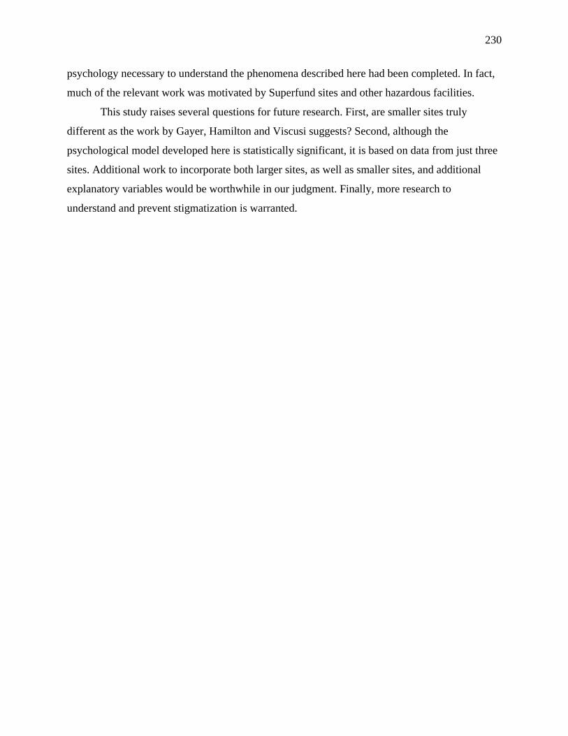
230
psychology necessary to understand the phenomena described here had been completed. In fact,
much of the relevant work was motivated by Superfund sites and other hazardous facilities.
This study raises several questions for future research. First, are smaller sites truly
different as the work by Gayer, Hamilton and Viscusi suggests? Second, although the
psychological model developed here is statistically significant, it is based on data from just three
sites. Additional work to incorporate both larger sites, as well as smaller sites, and additional
explanatory variables would be worthwhile in our judgment. Finally, more research to
understand and prevent stigmatization is warranted.

231
Chapter 11
References …
1. Acharya, G., and L. L. Bennett. “Valuing open space and land-use patterns in urban
watersheds.” Journal of Real Estate Finance and Economics 22: 221-237 (2001).
2. Adams, G. and R. Cantor. “Risk, Stigma, and Property Value-What are People Afraid of?” In Risk, Media and Stigma – Understanding Public Challenges to Modern Science and Technology, by J. Flynn, P. Slovic and H. Kunreuther, London, UK & Sterling, VA: Earthscan Publications Ltd., 2001, 175-185.
3. Allen, John. Biosphere 2: The Human Experiment. New York: Viking Penguin, 1991.
4. Bailey, M. J., R. F. Muth, and H. O. Hourse. “A Regression Method for Real Estate Price
Index Construction.” Journal of the American Statistical Association 58: 933-942 (1963).
5. Barnett, Harold C. Toxic Debts and the Superfund Dilemma. North Carolina: University of North Carolina Press, 1994.
6. Bartik, T.J. “Measuring the Benefits of Amenity Improvements in Hedonic Price
Models.” Land Economics 64 (2): 172-183 (1988).
7. Been, V. “Locally Undesirable Land Uses in Minority Neighborhoods - Disproportionate Siting or Market Dynamics.” Yale Law Journal 103: 1383-1422 (1994).
8. Been, V., and F. Gupta. “Coming to the nuisance or going to the barrios? A longitudinal
analysis of environmental justice claims.” Ecology Law Quarterly 24: 1-56 (1997).
9. Benson, E. D., et al. “Pricing residential amenities: The value of a view.” Journal of Real Estate Finance and Economics 16: 55-73 (1998).
10. Boarnet, M. G., and S. Chalermpong. “New highways, house prices, and urban
development: A case study of toll roads in Orange County, CA.” Housing Policy Debate 12: 575-605 (2001).
11. Bowen, W. “An analytical review of environmental justice research: What do we really
know?” Environmental Management 29: 3-15 (2002).
12. Bowes, D. R., and K. R. Ihlanfeldt. “Identifying the impacts of rail transit stations on residential property values.” Journal of Urban Economics 50: 1-25 (2001).
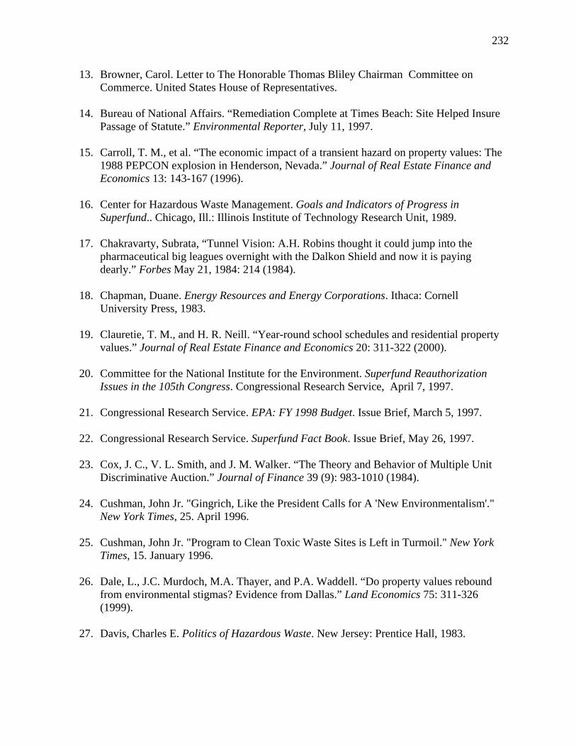
232
13. Browner, Carol. Letter to The Honorable Thomas Bliley Chairman Committee on Commerce. United States House of Representatives.
14. Bureau of National Affairs. “Remediation Complete at Times Beach: Site Helped Insure
Passage of Statute.” Environmental Reporter, July 11, 1997.
15. Carroll, T. M., et al. “The economic impact of a transient hazard on property values: The 1988 PEPCON explosion in Henderson, Nevada.” Journal of Real Estate Finance and Economics 13: 143-167 (1996).
16. Center for Hazardous Waste Management. Goals and Indicators of Progress in
Superfund.. Chicago, Ill.: Illinois Institute of Technology Research Unit, 1989.
17. Chakravarty, Subrata, “Tunnel Vision: A.H. Robins thought it could jump into the pharmaceutical big leagues overnight with the Dalkon Shield and now it is paying dearly.” Forbes May 21, 1984: 214 (1984).
18. Chapman, Duane. Energy Resources and Energy Corporations. Ithaca: Cornell
University Press, 1983.
19. Clauretie, T. M., and H. R. Neill. “Year-round school schedules and residential property values.” Journal of Real Estate Finance and Economics 20: 311-322 (2000).
20. Committee for the National Institute for the Environment. Superfund Reauthorization
Issues in the 105th Congress. Congressional Research Service, April 7, 1997.
21. Congressional Research Service. EPA: FY 1998 Budget. Issue Brief, March 5, 1997.
22. Congressional Research Service. Superfund Fact Book. Issue Brief, May 26, 1997.
23. Cox, J. C., V. L. Smith, and J. M. Walker. “The Theory and Behavior of Multiple Unit Discriminative Auction.” Journal of Finance 39 (9): 983-1010 (1984).
24. Cushman, John Jr. "Gingrich, Like the President Calls for A 'New Environmentalism'."
New York Times, 25. April 1996.
25. Cushman, John Jr. "Program to Clean Toxic Waste Sites is Left in Turmoil." New York Times, 15. January 1996.
26. Dale, L., J.C. Murdoch, M.A. Thayer, and P.A. Waddell. “Do property values rebound
from environmental stigmas? Evidence from Dallas.” Land Economics 75: 311-326 (1999).
27. Davis, Charles E. Politics of Hazardous Waste. New Jersey: Prentice Hall, 1983.

233
28. Delong, James V. Policy Analysis; Privatizing Superfund How to Clean Up Hazardous Waste. Cato Institute, 1995.
29. Dewdney, A.K. Yes, We Have No Neutrons: An Eye-Opening Tour Thought the Twists
and Turns of Bad Science. New York: John Wiley & Sons, Inc. 1997.
30. Downs, Peter. “The EPA Fights Environmentalists.” The Progressive 62 (9): 14 1998.
31. Environmental Protection Agency. 1997 Supplementary Materials: National Priorities List, Proposed Rule and Final Rule. EPA/9320.7-061. U.S Environmental Protection Agency, 1997.
32. Environmental Protection Agency. Superfund Facts: The Program At Work. May 7, 1997.
33. Environmental Protection Agency. Superfund Administrative Reforms Annual Report
Fiscal Year 1996. December 20, 1996.
34. Environmental Protection Agency. The Clinton Administration's Superfund Legislative Reform Principles. May 7, 1997.
35. Environmental Protection Agency. Superfund Reauthorization. EPA Hearings by the
House Transportation and Infrastructure Committee, Subcommittee on Water Resources and Environment. March 12, 1997.
36. Espey, M., and H. Lopez. “The impact of airport noise and proximity on residential
property values.” Growth and Change 31: 408-419 (2000).
37. Farber, S. “Undesirable facilities and property values: A summary of empirical studies.” Ecological Economics 24: 1-14 (1998).
38. Fischhoff, B. “Risk: A Guide to Controversy.” In Appendix to National Research
Council. Improving Risk Communications. Washington, D.C.: National Academy Press, 1989, 211-319.
39. Foster, K., D. Bernstein, and P. Huber. Phantom Risk: Scientific Interference and the
Law. Cambridge, Mass.: MIT Press, 1993.
40. Franklin, Ben. A. "Plan for a 5-Year Toxic Waste Program is Praised." New York Times, 2. August 1986.
41. GAO. Superfund Program: Current Status and Future Fiscal Challenges. GAO-03-850.
31, July 31 2003.
42. GAO. Superfund: Information on EPA'a Administrative Reforms. Washington D.C., May 30, 1997.
234
43. GAO. Superfund: Time to Assess and Cleanup Hazardous Waste Sites Exceed Program
Goals. Washington D.C., February 13, 1997.
44. GAO. Superfund Legal Expenses for Cleanup Related Activities of Major US Corporations. Washington D.C., 1994.
45. Gayer, T. “Neighborhood Demographics and the Distribution of Hazardous Waste Risks:
An Instrumental Variables Estimation.” Journal of Regulatory Economics 17: 131-155 (2000).
46. Gayer, T., J.T. Hamilton, and W.K. Viscusi. “Private Values of Risk Tradeoffs at
Superfund Sites: Housing Market Evidence on Learning about Risk.” The Review of Economics and Statistics 82 (3): 439-451 (2000).
47. Gayer, T., J. T. Hamilton, and W. K. Viscusi. “The Market Value of Reducing Cancer
Risk: Hedonic Housing Prices with Changing Information.” Southern Economic Journal 69: 266-289 (2002).
48. Gayer, T., and W. K. Viscusi. “Housing Price Responses to Newspaper Publicity of
Hazardous Waste Sites.” Resource and Energy Economics 24: 33-51 (2002).
49. Geoghegan, J. “The Value of Open Spaces in Residential Land Use.” Land Use Policy 19: 91-98 (2002).
50. Gibbs, Lois M. Dying from Dioxin: A Citizen’s Guide to Reclaiming Our Health and
Rebuilding Democracy. Boston: South End Press, 1995.
51. Gordon, Meryl. “A Cash Settlement, but No Apology.” New York Times, 20. February 1999.
52. Graham, J. D., et al. “Who lives near coke plants and oil refineries? An exploration of the
environmental inequity hypothesis.” Risk Analysis 19: 171-186 (1999).
53. Hamilton, J.T. and W. Kip Viscusi. Calculating Risks: The Spatial and Political Dimensions of Hazardous Waste Policy. Cambridge, Massachusetts: MIT Press, 1999.
54. Harris, J.D. “Property Values, Stigma, & Superfund.” Working Paper for the US EPA.
http://www.epa.gov/superfund/programs/recycle/property.htm. (2004).
55. Harrison, D. and J. Stock. Hedonic Housing Values, Local Public Goods, and the Benefits of Hazardous Waste Cleanup. Discussion Paper Series. Energy and Environmental Policy Center: Harvard University, 1984.

235
56. Hazarika, Sanjoy. “Gas Leak in India Kills at Least 410 in City of Bhopal.” New York Times, 3. December 1984.
57. Hicks, Karen. Surviving the Dalkon Shield IUD, Women V. The Pharmaceutical Industry.
New York: Teacher’s College Press, 1994.
58. Hite, D. “Information and bargaining in markets for environmental quality.” Land Economics 74: 303-316 (1998).
59. Hogan, Dan. “A new Life for Biosphere 2.” Current Science 82 (12): 8-9 (1997).
60. Howard, Phillip K. The Death of Common Sense How Law is Suffocating America. New
York: Random House, 1994.
61. Howlett, D. and R. Tyson, “Toxicity of Times Beach No Longer in Doubt.” USA Today, 13. September 1994.
62. Kasperson, R., O. Renn, P. Slovic, H. Brown, J. Emel, R. Goble, J. Kasperson, and S.
Ratick. “The Social Amplification of Risk: A Conceptual Framework.” Risk Analysis 8 (2): 177-187 (1988).
63. Ketkar, K. “Hazardous waste sites and property values in the state of New Jersey.”
Applied Economics 24: 647-659 (1992).
64. Kiel, K. A. “Measuring the Impact of the Discovery and Cleaning of Identified Hazardous-Waste Sites On House Values.” Land Economics 71: 428-435 (1995).
65. Kiel, K. A., and K. T. McClain. “House Prices During Siting Decision Stages - the Case
of an Incinerator From Rumor Through Operation.” Journal of Environmental Economics and Management 28: 241-255 (1995).
66. Kiel, K.A., and J. Zabel. “Estimating the economic benefits of cleaning up Superfund
sites: The case of Woburn, Massachusetts.” Journal of Real Estate Finance and Economics 22, 163-184 (2001).
67. Kohlhase, J. “The Impact of Toxic Waste Sites on Housing Values.” Journal of Urban
Economics 30: 1-26 (1991).
68. Kolata, Gina. “Love Canal: False Alarm Cause By Botched Study.” Science, Volume 208, June 30, 1980.
69. Kunreuther, H. and P. Slovic. “Coping with Stigma: Challenges and Opportunities.” In
Risk, Media and Stigma – Understanding Public Challenges to Modern Science and Technology, by J. Flynn, P. Slovic and H. Kunreuther, London, UK & Sterling, VA: Earthscan Publications Ltd., 2001, 331-352.

236
70. Lieberman, Adam. Facts Versus Fears: A Review of the Greatest Unfounded Health
Scares of Recent Times. New York: American Council on Science and Health, September 1997.
71. Liu, F. “Dynamics and causation of environmental equity, locally unwanted land uses,
and neighborhood changes.” Environmental Management 21: 643-656 (1997).
72. Mahan, B. L., S. Polasky, and R. M. Adams. “Valuing urban wetlands: A property price approach.” Land Economics 76: 100-113 (2000).
73. Mazmanian Daniel and Morell, David. Beyond Superfund America's Toxics Policy for the
1990's. Colorado: Westview Press, 1992.
74. McClelland, G., W. Schulze, and B. Hurd. “The Effect of Risk Beliefs on Property Values: A Case Study of a Hazardous Waste Site.” Risk Analysis 10: 485-497 (1990).
75. McCluskey, J. J., and G. C. Rausser. “Estimation of perceived risk and its effect on
property values.” Land Economics 77: 42-55 (2001).
76. Mendelsohn, R., D. Hellerstein, M. Huguenin, R. Unsworth, and R. Brazee. “Measuring Hazardous Waste Damages with Panel Models.” Journal of Environmental Economic and Management 22: 259-271 (1992).
77. Michaels, G. and V. Kerry Smith. “Market Segmentation and Valuing Amenities with
Hedonic Models: The Case of Hazardous Waste Sites.” Journal of Urban Economics 28: 223-242 (1990).
78. Milstein, Michael. “Breaking Up the Biosphere.” Earth 7 (2): 31 (1998).
79. Mintz, Morton. At Any Cost: Corporate Greed, Women, and the Dalkon Shield. New
York: Pantheon Books, 1985.
80. Mitchell, Alison. "Clinton Asks Tax Breaks For Toxic Waste Cleanup." New York Times, 12. March 1996.
81. Morris, Betsy. “Monsanto Unit Stops Marketing Its IUDs in U.S.” The Wall Street
Journal, 3. February 1986.
82. Moss, T. H. and D. L. Sills. The Three Mile Island Nuclear Accident: Lessons and Implications. New York: The New York Academy of Sciences, 1981.
83. Nakamura, R. T. and W. C. Church. Taming Regulation: Superfund and the Challenge of
Regulatory Reform. Washington, D.C.: The Brookings Institution, 2003.
237
84. Napoli, Maryann. “Look Back in Anger: The DES and Dalkon Shield Scandals.” Ms.: 40, May/June 1996.
85. National Advisory Council for Environmental Policy and Technology. Final Report of the
Superfund Subcommittee of NACEPT. April 12, 2004.
86. New York Times. "US Writes Off Cleanup Costs of Toxic Sites." June 21, 1993.
87. New York Times. "Cleanup Gets Little of Superfund Settlements." April 26, 1992.
88. New York Times. "Toxic Site Cleanup Reported Lagging." September 10, 1989.
89. New York Times. "The Superfund: Locked in a Lovefest." July 19, 1986.
90. New York Times. "Senate Refuses to Cut Toxic Waste Cleanup." Sept. 21, 1985.
91. New York Times. "EPA Halts Work On Toxic Cleanups." August 17, 1985.
92. Office of Technological Assessment. Superfund Strategy. Washington, D.C., 1985.
93. Office of Technological Assessment. Background and Issues Relating to the Reauthorization of Superfund : Scheduled for Hearings before the Committee of Finance on September 19 and 25, 1984. Staff of the Joint Committee on Taxation. Washington, D.C., 1984.
94. Quint, Michael. "A Superfund Plan Divides the Insurance Industry." New York Times, 10.
January 1994.
95. Poor, P. J., et al. “Objective versus subjective measures of water clarity in hedonic property value models.” Land Economics 77: 482-493 (2001).
96. Preston, Jennifer. "Showcasing an Issue, Clinton Plans A Visit to A Bergen County
Dumpsite Today." New York Times, 11. March 1996.
97. Probst, K. N. and P. R. Portnoy. Assigning Liability for the Superfund Cleanup: An Analysis of Policy Options. Washington, D.C.: Resources for the Future, 1992.
98. Ramanan, T. “The Bhopal Tragedy Revisited.” Risk Management 39 (10): 62 (1992).
99. Ray, Dixie Lee. Environmental Overkill: Whatever Happened to Common Sense?
Washington, D.C.: Regnery Gateway, 1993. 100. Rosen, S. “Hedonic Prices and Implicit Markets: Product Differentiation in Pure
Competition.” Journal of Political Economy 82: 34-55 (1974).
238
101. Rozin, P. “Technological Stigma: Some Perspectives from the Study of Contagion.” In Risk, Media and Stigma – Understanding Public Challenges to Modern Science and Technology, by J. Flynn, P. Slovic and H. Kunreuther, London, UK & Sterling, VA: Earthscan Publications Ltd., 2001, 31-40.
102. Rubin, D. “How the Media Reported on Three Mile Island and Chernobyl.” Journal of
Communication 37 (3): 42-57 (1987). 103. Russell, M., E. Colglazier, and M. English. Hazardous Waste Remediation: The Task
Ahead. Knoxville, Tennessee: Waste Management and Education Institute, University of Tennessee, 1991.
104. Schneider, Keith. “Times Beach Warning: Regrets a Decade Later.” New York Times, 15.
August 1991. 105. Schneider, Keith. “US Backing Away from Saying Dioxin is a Deadly Peril.” New York
Times, 15. August 1991. 106. Shabecoff, Philip. "Reagan Signs Renewal of Toxic Waste Project." New York Times, 16.
October 1986. 107. Shabecoff, Philip. "Lack of Money Might Halt Toxic Cleanup Soon, U.S. Officials Say."
New York Times, 26. January 1986. 108. Shabecoff, Philip. "House Passes $10 Billion Measure to Bolster Toxic Waste Program."
New York Times, 11. December 1985.
109. Shabecoff, Philip. "Senate Backs Bill For Cleaning Up Hazardous Dumps." New York Times, 27. September 1985.
110. Shabecoff, Philip. "E.P.A. Says It Maps New Top Priority." New York Times, 21.
November 1983. 111. Silverstone, Sally. Eating In: From the Fields to the Kitchen in Biosphere 2. Oracle, AZ:
The Biosphere Press, 1993. 112. Slovic, P., M. Layman, N. Kraus, J. Flynn, J. Chalmers, and G. Gesell. “Perceived Risk,
Stigma, and Potential Economic Impacts of a High-Level Nuclear Waste Repository in Nevada.” Risk Analysis 11 (4): 683-696 (1991).
113. Smith, V. K., C. Poulos, and H. Kim. “Treating open space as an urban amenity.”
Resource and Energy Economics 24: 107-129 (2002). 114. Spalatro, F., and B. Provencher. “An analysis of minimum frontage zoning to preserve
lakefront amenities.” Land Economics 77: 469-481 (2001).
239
115. State Brief: “Love Canal Agency: Our Work Is Done.” Ithaca Journal, December 9,
1999. 116. “Statement of Carol M. Browner Administrator of US Environmental Protection Agency”
before Committee on Environment and Public Works U.S. Senate. March 5, 1997. 117. Strand, J., and M. Vagnes. “The relationship between property values and railroad
proximity: a study based on hedonic prices and real estate brokers' appraisals.” Transportation 28: 137-156 (2001).
118. “Times Beach Toxic Site Cleaned.” Chemical Market Reporter 252 (2): 44 (1997).
119. Tomkins, J., et al. “Noise versus access: The impact of an airport in an urban property
market.” Urban Studies 35: 243-258 (1998). 120. Uzumeri, Mustafa and Charles Snyder. “Information Technology and Accelerated
Science: The Cases of the Pentium Flaw and the Dalkon Shield.” California Management Review 38 (2): 44 (1996).
121. Vadali, S. R., and C. Sohn. "Using a geographic information system to track changes in
spatially segregated location premiums - Alternative method for assessing residential land use impact of transportation projects." In Transportation Research Record, by TRB, National Research Council, Washington, D.C., 2001, 180-192.
122. Whelan, Elizabeth. Toxic Terror: The Truth Behind the Cancer Scares. Buffalo, New
York: Prometheus Books, 1992. 123. White, Jocelyn. "Superfund: Pouring Money Down A Hole." New York Times. 17. April
1992. 124. Wilkins, L. and P. Patterson. “Risk Analysis and the Construction of News.” Journal of
Communication 37 (3): 80-92 (1987). 125. Wilkins, L. and P. Patterson. “Risky Business: Covering Slow-Onset Hazards as Rapidly
Developing News.” Political Communication and Persuasion 7 (2): 11-23 (1990). 126. Zurilla, D. “Reflections of a Dalkon Shield Arbitrator.” Dispute Resolution Journal,
February 1998.
240
Website References: 127. http://caltech.edu/goosstein/fusion.html (September 9, 1999).
128. http://enviroweb.org/Three Mile Islanda/PressP2.html#cont (September 9, 1999).
129. http://research.et.byu.edu/woburn/photos/places/ (March 17, 2000).
130. http://usnews.com/usnews/issue/990329/29Three Mile Island.htm (September 9, 1999).
131. http://yosemite.epa.gov/r9/sfund/sphotos.nsf/57079f1ed19a0334882565cd006099c5/7f22
b96c0346d2eb882568f100010bad?OpenDocument (October 5, 2000). 132. http://www.acsh.org/publications/reports/island_0399.html (September 20, 1999).
133. http://www-bcf.usc.edu/~meshkati/humanfactors.html (1991).
134. http://www.biospherics.org/.
135. http://www.cdc.gov/epo/mmwr/preview/mmwrhtml/00000072.htm (May 06, 1983).
136. http://www.crc.losrios.cc.ca.us/~hodappd/14/wastedoc.html.
137. http://www.crl.com.
138. http://www.consumerlaert.org/fumento/super.htm (September 14, 1999).
139. http://www.coopamerica.org/isf/tobi/tobi-agenda/union-carbise.htm.
140. http://www.corpwatch.org/trac/bhopal/nightmare.htm.
141. http://www.corpwatch.org/trac/feature.india/profiles/bhopal.
142. http://www.earthbase.org/home/timeline/1942/love/ (September 14, 1999).
143. http://www.earthbase.org/home/timeline/1983/times_beach/.
144. http://www.earthbase.org/home/timeline/1984/bhopal/.
145. http://www.envirolink.org/enviroarts/arts_and_activism?loisGibbs.html (September, 14,
1999). 146. http://www.enviroweb.org/issues/dioxin.
241
147. http://www.enviroweb.org/Three Mile Islanda/Mmaple.html (September 9, 1999). 148. http://www.enviroweb.org/Three Mile Islanda/wing4.htm (September 9, 1999).
149. http://www.epa.gov/oerrpage/superfund/sites/npl/nar833.htm.
150. http://www.epa.gov/superfund/pics/.
151. http://www.epa.gov/region01/superfund/sites/wellsgh/photo.html.
152. http://www.epa.gov/region02/superfnd/site_sum/0201290c.htm (September 14, 1999).
153. http://www.epa/gov/region07/programs/nplfacts/TOC.html#missouri.
154. http://www.epaosc.net/site_profile.asp?site_id=0146.
155. http://www.home.stInet.com/~cdstelzer/diox39.html.
156. http://www.msnbc.com/news/150998.asp#BODY (September 14, 1999).
157. http://www.nrc.gov/OPA/gmo/tip/tip9809.htm (September 9, 1999).
158. http://www.nj.gov/dep/srp/publications/site_status/1998/html/98highli2.htm.
159. http://www.nytimes.com/reuters/news/news-utilities-nuclear.html (April 5, 2004).
160. http://www.onlineethics.org/text/cases/l.canal/history.html (September 14, 1999).
161. http://www.opcw.nl/chemhaz/chemacci.htm.
162. http://www.pathfinder.com/time/daily/0,2960,1098,00.html (September 14, 1999).
163. http://www.pathfinder.com/time/daily/0,2960,1740,00.html (September 14, 1999).
164. http://www.prioritiesforhealth.com/1004/lovecanal.html (September 14, 1999).
165. http://www.uwmc.uwc.edu/geography/350/cleanEPA.htm (June 18, 2004).